RANDOM COEFFICIENT PANEL DATA MODELS

CHENG HSIAO M. HASHEM PESARAN

CESIFO WORKING PAPER NO. 1233 CATEGORY 10: EMPIRICAL AND THEORETICAL METHODS

JULY 2004

An electronic version of the paper may be downloaded • from the SSRN website: www.SSRN.com • from the CESifo website: www.CESifo.de

CESifo Working Paper No. 1233

RANDOM COEFFICIENT PANEL DATA MODELS

Abstract

This paper provides a review of linear panel data models with slope heterogeneity, introduces various types of random coefficients models and suggest a common framework for dealing with them. It considers the fundamental issues of statistical inference of a random coefficients formulation using both the sampling and Bayesian approaches. The paper also provides a review of heterogeneous dynamic panels, testing for homogeneity under weak exogeneity, simultaneous equation random coefficient models, and the more recent developments in the area of cross-sectional dependence in panel data models.

Keywords: random coefficient models, dynamic heterogeneous panels, classical and Bayesian approaches, tests of slope heterogeneity, cross section dependence.

JEL Code: C12, C13, C33.

Cheng Hsiao Department of Economics

University of Southern California University Park

Los Angeles, CA 90089-025 USA

hsiao@usc.edu

M. Hashem Pesaran Faculty of Economis and Politics

University of Cambridge Austin Robinson Building

Sidgwick Avenue Cambridge, CB3 9DD

United Kingdom mhp1@econ.cam.ac.uk

We are grateful to G. Bressons and A. Pirotte for their careful reading of an early version and for pointing out many typos. We would also like to thank J. Breitung and Ron Smith for helpful comments.

1 Introduction

Consider a linear regression model of the form

y = β′x+ u, (1)

where y is the dependent variable and x is aK×1 vector of explanatory variables.

The variable u denotes the effects of all other variables that affect the outcome

of y but are not explicitly included as independent variables. The standard

assumption is that u behaves like a random variable and is uncorrelated with

x. However, the emphasis of panel data is often on the individual outcomes.

In explaining human behavior, the list of relevant factors may be extended ad

infinitum. The effect of these factors that have not been explicitly allowed for

may be individual specific and time varying. In fact, one of the crucial issues in

panel data analysis is how the differences in behavior across individuals and/or

through time that are not captured by x should be modeled.

1

The variable intercept and/or error components models attribute the hetero-

geneity across individuals and/or through time to the effects of omitted variables

that are individual time-invariant, like sex, ability and social economic back-

ground variables that stay constant for a given individual but vary across indi-

viduals, and/or period individual-invariant, like prices, interest rates and wide

spread optimism or pessimism that are the same for all cross-sectional units at a

given point in time but vary through time. It does not allow the interaction of the

individual specific and/or time varying differences with the included explanatory

variables, x. A more general formulation would be to let the variable y of the

individual i at time t be denoted as

yit = β′itxit + uit, (2)

= β1itx1it + ...+ βkitxkit + uit,

i = 1, ..., N, and t = 1, ..., T. Expression (2) corresponds to the most general

specification of the panel linear data regression problem. It simply states that

each individual has their own coefficients that are specific to each time period.

However, as pointed out by Balestra (1991) this general formulation is, at most,

descriptive. It lacks any explanatory power and it is useless for prediction. Fur-

thermore, it is not estimable, the number of parameters to be estimated exceeds

the number of observations. For a model to become interesting and to acquire

explanatory and predictive power, it is essential that some structure is imposed

on its parameters.

One way to reduce the number of parameters in (2) is to adopt an analysis of

variance framework by letting

βkit = βk + αki + λkt,N∑

i=1

αki = 0, andT∑

t=1

λkt = 0, k = 1, . . . , K. (3)

This specification treats individual differences as fixed and is computationally

simple. The drawback is that it is not parsimonious, and hence reliable estimates

of αki and λkt are difficult to obtain. Moreover, it is difficult to draw inference

about the population if differences across individuals and/or over time are fixed

and different.

An alternative to the fixed coefficient (or effects) specification of (3) is to let

αki and λkt be random variables and introduce proper stochastic specifications.

2

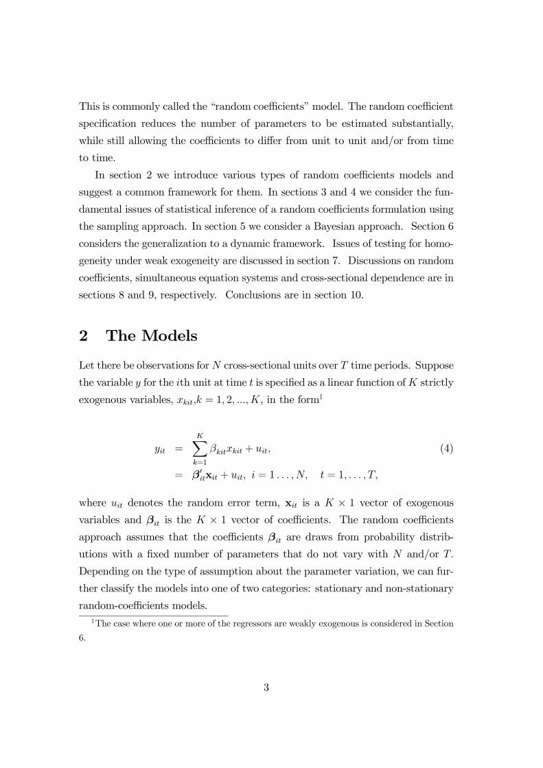
This is commonly called the “random coefficients” model. The random coefficient

specification reduces the number of parameters to be estimated substantially,

while still allowing the coefficients to differ from unit to unit and/or from time

to time.

In section 2 we introduce various types of random coefficients models and

suggest a common framework for them. In sections 3 and 4 we consider the fun-

damental issues of statistical inference of a random coefficients formulation using

the sampling approach. In section 5 we consider a Bayesian approach. Section 6

considers the generalization to a dynamic framework. Issues of testing for homo-

geneity under weak exogeneity are discussed in section 7. Discussions on random

coefficients, simultaneous equation systems and cross-sectional dependence are in

sections 8 and 9, respectively. Conclusions are in section 10.

2 The Models

Let there be observations forN cross-sectional units over T time periods. Suppose

the variable y for the ith unit at time t is specified as a linear function ofK strictly

exogenous variables, xkit,k = 1, 2, ..., K, in the form1

yit =K∑

k=1

βkitxkit + uit, (4)

= β′itxit + uit, i = 1 . . . ,N, t = 1, . . . , T,

where uit denotes the random error term, xit is a K × 1 vector of exogenous

variables and βit is the K × 1 vector of coefficients. The random coefficients

approach assumes that the coefficients βit are draws from probability distrib-

utions with a fixed number of parameters that do not vary with N and/or T.

Depending on the type of assumption about the parameter variation, we can fur-

ther classify the models into one of two categories: stationary and non-stationary

random-coefficients models.

1The case where one or more of the regressors are weakly exogenous is considered in Section

6.

3

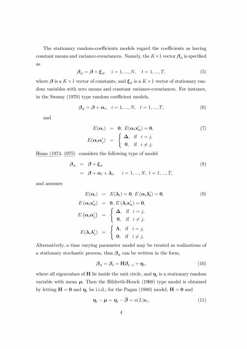
The stationary random-coefficients models regard the coefficients as having

constant means and variance-covariances. Namely, theK×1 vector βit is specifiedas

βit = β + ξit, i = 1, ..., N, t = 1, ..., T, (5)

where β is a K×1 vector of constants, and ξit is a K×1 vector of stationary ran-

dom variables with zero means and constant variance-covariances. For instance,

in the Swamy (1970) type random coefficient models,

βit = β +αi, i = 1, ..., N, t = 1, ..., T, (6)

and

E(αi) = 0, E(αix′

it) = 0, (7)

E(αiα′

j) =

∆, if i = j,

0, if i = j,

Hsiao (1974, 1975) considers the following type of model

βit = β + ξit (8)

= β +αi + λt, i = 1, ...,N, t = 1, ..., T,

and assumes

E(αi) = E(λt) = 0, E (αiλ′

t) = 0, (9)

E (αix′

it) = 0, E (λtx′

it) = 0,

E(αiα

′

j

)=

∆, if i = j,

0, if i = j,

E(λiλ′

j) =

Λ, if i = j,

0, if i = j,

Alternatively, a time varying parameter model may be treated as realizations of

a stationary stochastic process, thus βit can be written in the form,

βit = βt = Hβt−1 + ηt, (10)

where all eigenvalues ofH lie inside the unit circle, and ηt is a stationary random

variable with mean µ. Then the Hildreth-Houck (1968) type model is obtained

by letting H = 0 and ηt be i.i.d.; for the Pagan (1980) model, H = 0 and

ηt − µ = ηt − β = a(L)ǫt, (11)

4

where β is the mean of βt and a(L) is the ratio of polynomials of orders p

and q in the lag operator L(Lǫt = ǫt−1) and ǫt is independent normal. The

Rosenberg (1972, 1973) return-to-normality model assumes the absolute value

of the characteristic roots of H be less than 1 with ηt independently normally

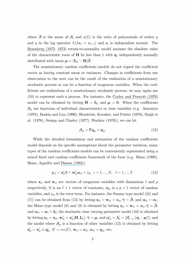
distributed with mean µ = (IK −H)β.The nonstationary random coefficients models do not regard the coefficient

vector as having constant mean or variances. Changes in coefficients from one

observation to the next can be the result of the realization of a nonstationary

stochastic process or can be a function of exogenous variables. When the coef-

ficients are realizations of a nonstationary stochastic process, we may again use

(10) to represent such a process. For instance, the Cooley and Prescott (1976)

model can be obtained by letting H = IK and µ = 0. When the coefficients

βit are functions of individual characteristics or time variables (e.g. Amemiya

(1978), Boskin and Lau (1990), Hendricks, Koenker, and Poirier (1979), Singh et

al. (1976), Swamy and Tinsley (1977), Wachter (1970)), we can let

βit = Γqit + ηit. (12)

While the detailed formulation and estimation of the random coefficients

model depends on the specific assumptions about the parameter variation, many

types of the random coefficients models can be conveniently represented using a

mixed fixed and random coefficients framework of the form (e.g. Hsiao (1990),

Hsiao, Appelbe and Dineen (1992))

yit = z′

itγ +w′

itαit + uit, i = 1, ...,N, t = 1, ..., T, (13)

where zit and wit are vectors of exogenous variables with dimensions ℓ and p

respectively, γ is an ℓ × 1 vector of constants, αit is a p × 1 vector of random

variables, and uit is the error term. For instance, the Swamy type model ((6) and

(7)) can be obtained from (13) by letting zit = wit = xit,γ = β, and αit = αi;

the Hsiao type model (8) and (9) is obtained by letting zit = wit = xit,γ = β,

and αit = αi+λt; the stochastic time varying parameter model (10) is obtained

by letting zit = xit, w′

it = x′

it[H, IK], γ = µ, and α′

it = λ′

t = [β′

t−1, (ηt−µ)′]; andthe model where βit is a function of other variables (12) is obtained by letting

z′it = x′

it ⊗ q′it, γ ′ = vec(Γ), wit = xit, αit = ηit, etc.

5

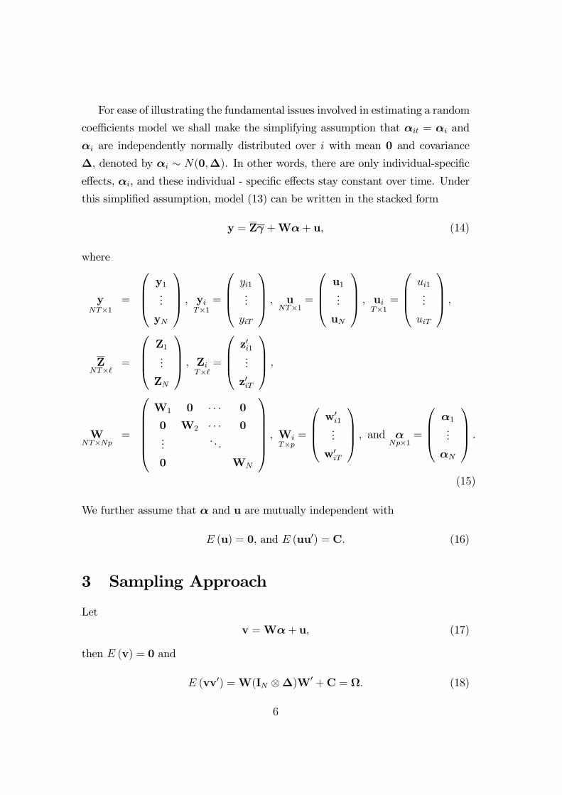
For ease of illustrating the fundamental issues involved in estimating a random

coefficients model we shall make the simplifying assumption that αit = αi and

αi are independently normally distributed over i with mean 0 and covariance

∆, denoted by αi ∼ N(0,∆). In other words, there are only individual-specific

effects, αi, and these individual - specific effects stay constant over time. Under

this simplified assumption, model (13) can be written in the stacked form

y = Zγ +Wα+ u, (14)

where

yNT×1

=

y1...

yN

, yi

T×1=

yi1...

yiT

, u

NT×1=

u1...

uN

, ui

T×1=

ui1...

uiT

,

ZNT×ℓ

=

Z1...

ZN

, Zi

T×ℓ=

z′i1...

z′iT

,

WNT×Np

=

W1 0 · · · 0

0 W2 · · · 0...

. . .

0 WN

, WiT×p

=

w′i1...

w′iT

, and α

Np×1=

α1...

αN

.

(15)

We further assume that α and u are mutually independent with

E (u) = 0, and E (uu′) = C. (16)

3 Sampling Approach

Let

v =Wα+ u, (17)

then E (v) = 0 and

E (vv′) =W(IN ⊗∆)W′ +C = Ω. (18)

6

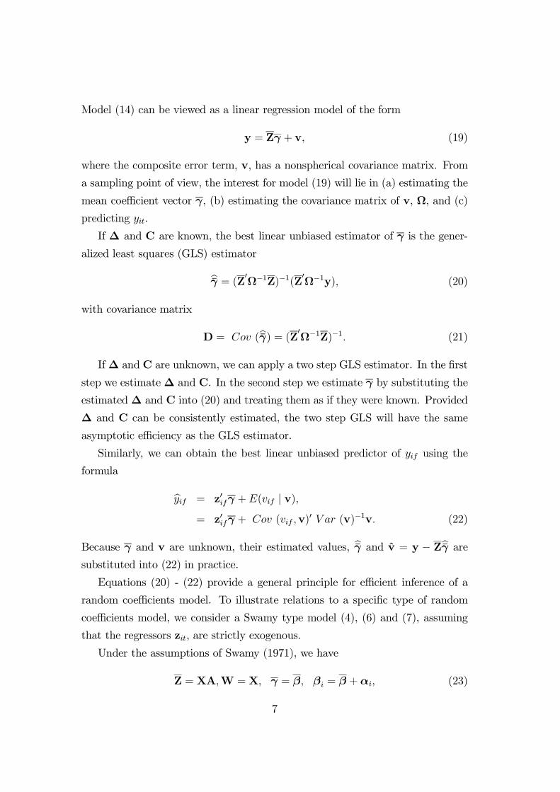
Model (14) can be viewed as a linear regression model of the form

y = Zγ + v, (19)

where the composite error term, v, has a nonspherical covariance matrix. From

a sampling point of view, the interest for model (19) will lie in (a) estimating the

mean coefficient vector γ, (b) estimating the covariance matrix of v, Ω, and (c)

predicting yit.

If ∆ and C are known, the best linear unbiased estimator of γ is the gener-

alized least squares (GLS) estimator

γ = (Z′Ω−1Z)−1(Z′Ω−1y), (20)

with covariance matrix

D = Cov (γ) = (Z′Ω−1Z)−1. (21)

If∆ and C are unknown, we can apply a two step GLS estimator. In the first

step we estimate∆ and C. In the second step we estimate γ by substituting the

estimated∆ and C into (20) and treating them as if they were known. Provided

∆ and C can be consistently estimated, the two step GLS will have the same

asymptotic efficiency as the GLS estimator.

Similarly, we can obtain the best linear unbiased predictor of yif using the

formula

yif = z′ifγ +E(vif | v),= z′ifγ + Cov (vif ,v)

′ V ar (v)−1v. (22)

Because γ and v are unknown, their estimated values, γ and v = y − Zγ are

substituted into (22) in practice.

Equations (20) - (22) provide a general principle for efficient inference of a

random coefficients model. To illustrate relations to a specific type of random

coefficients model, we consider a Swamy type model (4), (6) and (7), assuming

that the regressors zit, are strictly exogenous.

Under the assumptions of Swamy (1971), we have

Z = XA,W = X, γ = β, βi = β +αi, (23)

7

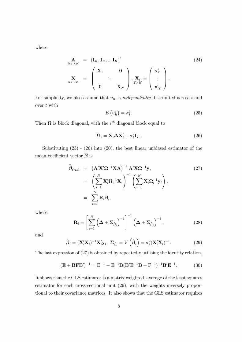
where

ANT×K

= (IK, IK, .., IK)′ (24)

XNT×K

=

X1 0

. . .

0 XN

, Xi

T×K=

x′i1...

x′iT

.

For simplicity, we also assume that uit is independently distributed across i and

over t with

E(u2it)= σ2i . (25)

Then Ω is block diagonal, with the ith diagonal block equal to

Ωi = Xi∆X′

i + σ2i IT . (26)

Substituting (23) - (26) into (20), the best linear unbiased estimator of the

mean coefficient vector β is

βGLS =(A′X′Ω−1XA

)−1A′XΩ−1y, (27)

=

(N∑

i=1

X′iΩ−1i Xi

)−1( N∑

i=1

X′iΩ−1i yi

),

=N∑

i=1

Riβi,

where

Ri =

[N∑

i=1

(∆+Σβ

i

)−1]−1 (

∆+Σβi

)−1

, (28)

and

βi = (X′

iXi)−1X′

iyi, Σβi

= V(βi

)= σ2i (X

′

iXi)−1. (29)

The last expression of (27) is obtained by repeatedly utilising the identity relation,

(E+BFB′)−1 = E−1 −E−1B(B′E−1B+ F−1)−1B′E−1. (30)

It shows that the GLS estimator is a matrix weighted average of the least squares

estimator for each cross-sectional unit (29), with the weights inversely propor-

tional to their covariance matrices. It also shows that the GLS estimator requires

8

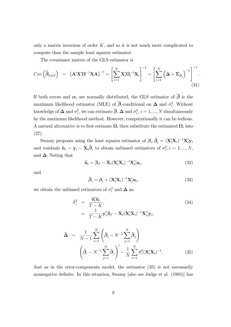
only a matrix inversion of order K, and so it is not much more complicated to

compute than the sample least squares estimator.

The covariance matrix of the GLS estimator is

Cov(βGLS

)=(A′X′Ω−1XA

)−1=

[N∑

i=1

X′

iΩ−1i Xi

]−1=

[N∑

i=1

(∆+Σβ

i

)−1]−1

.

(31)

If both errors and αi are normally distributed, the GLS estimator of β is the

maximum likelihood estimator (MLE) of β conditional on ∆ and σ2i . Without

knowledge of∆ and σ2i , we can estimate β,∆ and σ2i , i = 1, ..., N simultaneously

by the maximum likelihood method. However, computationally it can be tedious.

A natural alternative is to first estimate Ωi then substitute the estimated Ωi into

(27).

Swamy proposes using the least squares estimator of βi, βi = (X′

iXi)−1X′iyi

and residuals ui = yi − Xiβi to obtain unbiased estimators of σ2i , i = 1, ..., N,

and ∆. Noting that

ui = [IT −Xi(X′

iXi)−1X′

i]ui, (32)

and

βi = βi + (X′

iXi)−1X′iui, (33)

we obtain the unbiased estimators of σ2i and ∆ as:

σ2i =u′iui

T −K, (34)

=1

T −Ky′i[IT −Xi(X

′

iXi)−1X′

i]yi,

∆ =1

N − 1

N∑

i=1

(βi −N−1

N∑

j=1

βj

)

(βi −N−1

N∑

j=1

βj

)′− 1

N

N∑

i=1

σ2i (X′

iXi)−1. (35)

Just as in the error-components model, the estimator (35) is not necessarily

nonnegative definite. In this situation, Swamy [also see Judge et al. (1985)] has

9

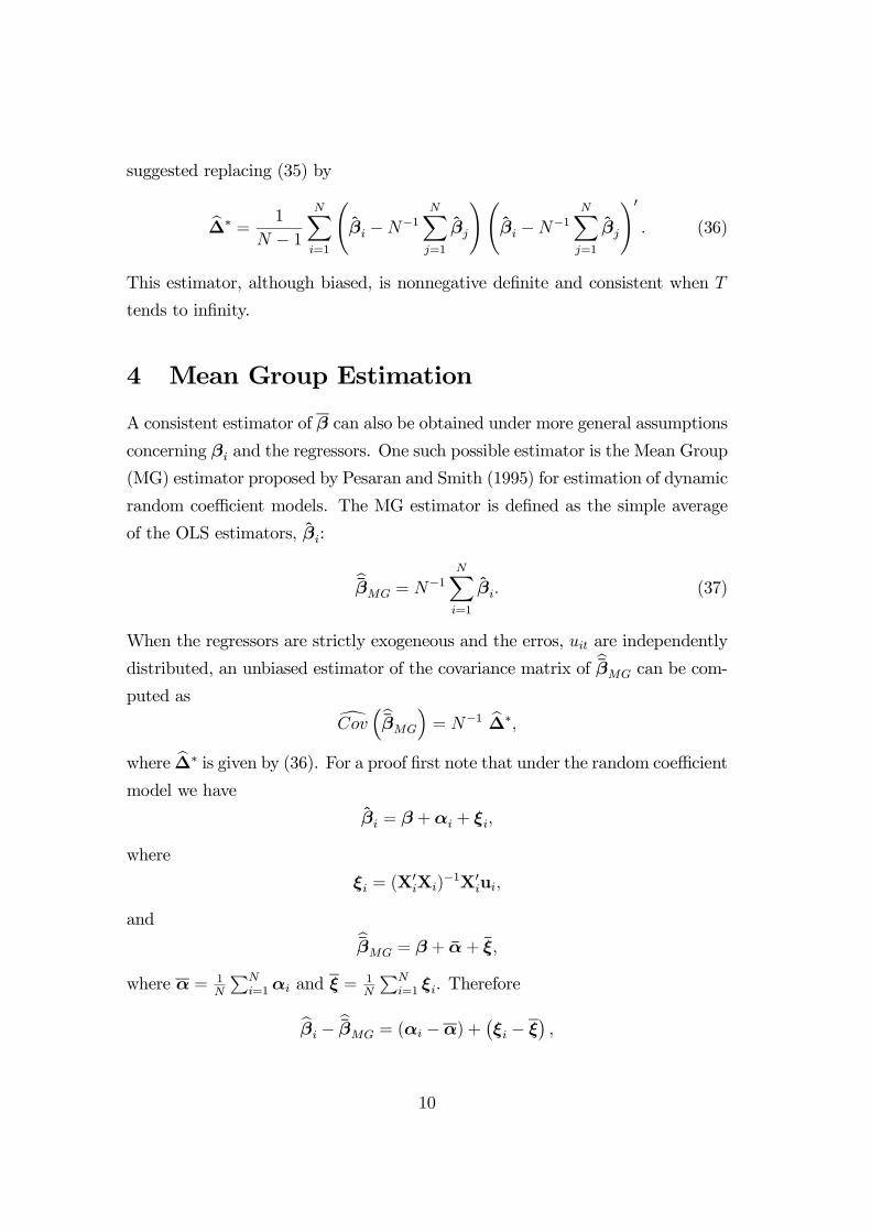
suggested replacing (35) by

∆∗ =1

N − 1

N∑

i=1

(βi −N−1

N∑

j=1

βj

)(βi −N−1

N∑

j=1

βj

)′. (36)

This estimator, although biased, is nonnegative definite and consistent when T

tends to infinity.

4 Mean Group Estimation

A consistent estimator of β can also be obtained under more general assumptions

concerning βi and the regressors. One such possible estimator is the Mean Group

(MG) estimator proposed by Pesaran and Smith (1995) for estimation of dynamic

random coefficient models. The MG estimator is defined as the simple average

of the OLS estimators, βi:

βMG = N−1N∑

i=1

βi. (37)

When the regressors are strictly exogeneous and the erros, uit are independently

distributed, an unbiased estimator of the covariance matrix of βMG can be com-

puted as

Cov(βMG

)= N−1 ∆∗,

where ∆∗ is given by (36). For a proof first note that under the random coefficient

model we have

βi = β +αi + ξi,

where

ξi = (X′

iXi)−1X′

iui,

andβMG = β + α+ ξ,

where α = 1N

∑Ni=1αi and ξ =

1N

∑Ni=1 ξi. Therefore

βi − βMG = (αi −α) +(ξi − ξ

),

10

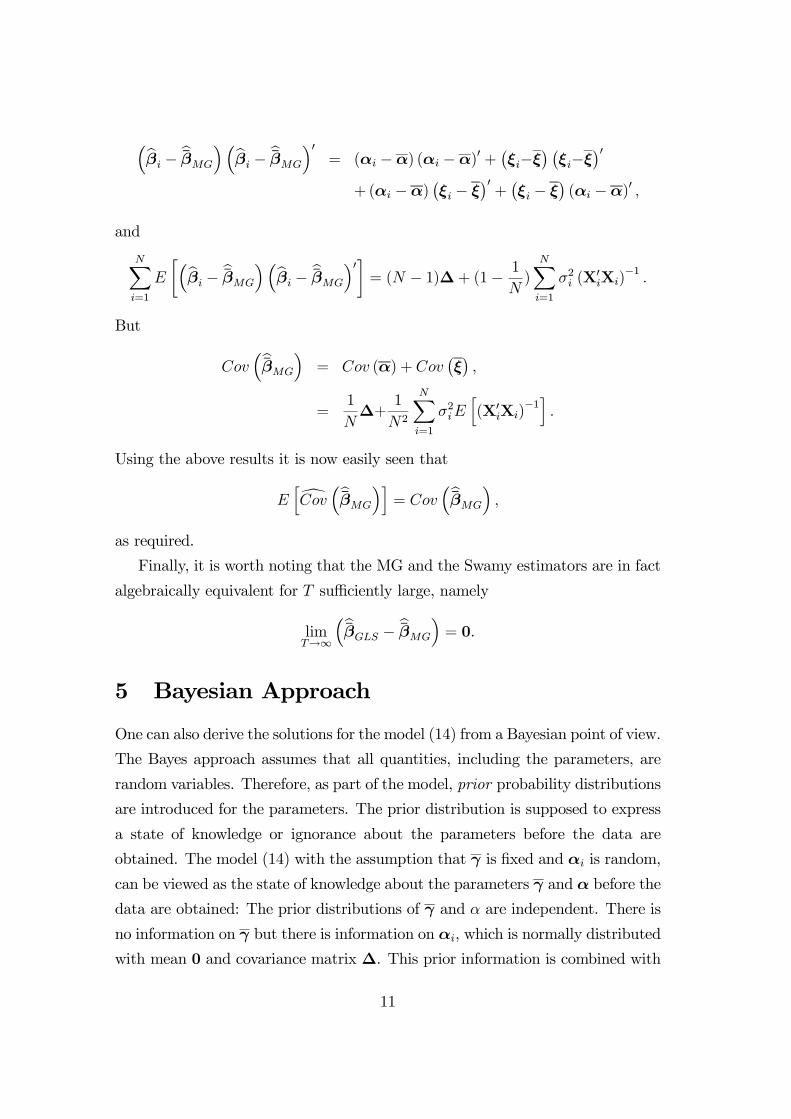
(βi − βMG

)(βi − βMG

)′

= (αi −α) (αi −α)′ +(ξi−ξ

) (ξi−ξ

)′

+(αi −α)(ξi − ξ

)′+(ξi − ξ

)(αi −α)′ ,

and

N∑

i=1

E

[(βi − βMG

)(βi − βMG

)′]= (N − 1)∆+ (1− 1

N)N∑

i=1

σ2i (X′

iXi)−1

.

But

Cov(βMG

)= Cov (α) + Cov

(ξ),

=1

N∆+

1

N2

N∑

i=1

σ2iE[(X′iXi)

−1].

Using the above results it is now easily seen that

E[Cov

(βMG)]= Cov

(βMG),

as required.

Finally, it is worth noting that the MG and the Swamy estimators are in fact

algebraically equivalent for T sufficiently large, namely

limT→∞

(βGLS − βMG)= 0.

5 Bayesian Approach

One can also derive the solutions for the model (14) from a Bayesian point of view.

The Bayes approach assumes that all quantities, including the parameters, are

random variables. Therefore, as part of the model, prior probability distributions

are introduced for the parameters. The prior distribution is supposed to express

a state of knowledge or ignorance about the parameters before the data are

obtained. The model (14) with the assumption that γ is fixed and αi is random,

can be viewed as the state of knowledge about the parameters γ and α before the

data are obtained: The prior distributions of γ and α are independent. There is

no information on γ but there is information on αi, which is normally distributed

with mean 0 and covariance matrix ∆. This prior information is combined with

11

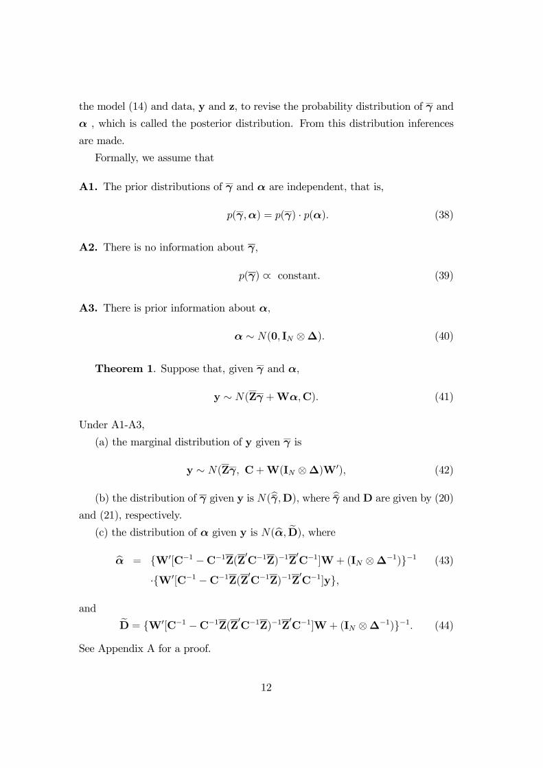
the model (14) and data, y and z, to revise the probability distribution of γ and

α , which is called the posterior distribution. From this distribution inferences

are made.

Formally, we assume that

A1. The prior distributions of γ and α are independent, that is,

p(γ,α) = p(γ) · p(α). (38)

A2. There is no information about γ,

p(γ) ∝ constant. (39)

A3. There is prior information about α,

α ∼ N(0, IN ⊗∆). (40)

Theorem 1. Suppose that, given γ and α,

y ∼ N(Zγ +Wα,C). (41)

Under A1-A3,

(a) the marginal distribution of y given γ is

y ∼ N(Zγ, C+W(IN ⊗∆)W′), (42)

(b) the distribution of γ given y is N(γ,D), where γ and D are given by (20)

and (21), respectively.

(c) the distribution of α given y is N(α, D), where

α = W′[C−1 −C−1Z(Z′C−1Z)−1Z′C−1]W+ (IN ⊗∆−1)−1 (43)

·W′[C−1 −C−1Z(Z′C−1Z)−1Z′C−1]y,

and

D = W′[C−1 −C−1Z(Z′C−1Z)−1Z′C−1]W + (IN ⊗∆−1)−1. (44)

See Appendix A for a proof.

12

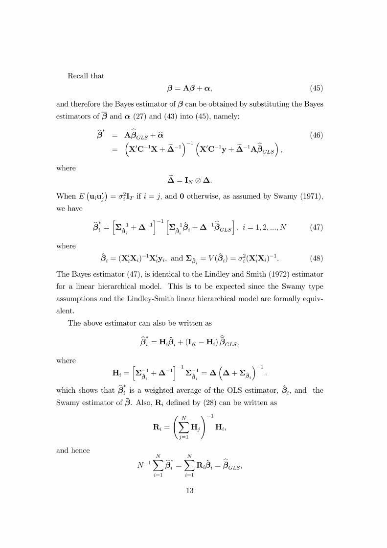
Recall that

β = Aβ +α, (45)

and therefore the Bayes estimator of β can be obtained by substituting the Bayes

estimators of β and α (27) and (43) into (45), namely:

β∗

= AβGLS + α (46)

=(X′C−1X+ ∆−1

)−1 (X′C−1y + ∆−1AβGLS

),

where

∆ = IN ⊗∆.

When E(uiu

′

j

)= σ2i IT if i = j, and 0 otherwise, as assumed by Swamy (1971),

we have

β∗

i =[Σ−1βi

+∆−1]−1 [Σ−1βi

βi +∆−1 βGLS

], i = 1, 2, ..., N (47)

where

βi = (X′

iXi)−1X′

iyi, and Σβi

= V (βi) = σ2i (X′

iXi)−1. (48)

The Bayes estimator (47), is identical to the Lindley and Smith (1972) estimator

for a linear hierarchical model. This is to be expected since the Swamy type

assumptions and the Lindley-Smith linear hierarchical model are formally equiv-

alent.

The above estimator can also be written as

β∗

i = Hiβi + (IK −Hi)βGLS,

where

Hi =[Σ−1βi

+∆−1]−1

Σ−1βi

=∆(∆+Σβ

i

)−1

.

which shows that β∗

i is a weighted average of the OLS estimator, βi, and the

Swamy estimator of β. Also, Ri defined by (28) can be written as

Ri =

(N∑

j=1

Hj

)−1Hi,

and hence

N−1N∑

i=1

β∗

i =N∑

i=1

Riβi =βGLS,

13

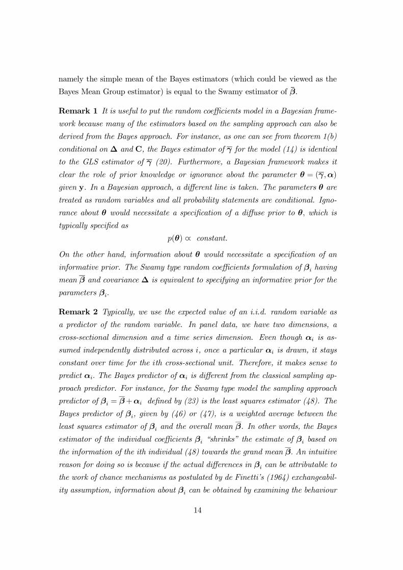
namely the simple mean of the Bayes estimators (which could be viewed as the

Bayes Mean Group estimator) is equal to the Swamy estimator of β.

Remark 1 It is useful to put the random coefficients model in a Bayesian frame-

work because many of the estimators based on the sampling approach can also be

derived from the Bayes approach. For instance, as one can see from theorem 1(b)

conditional on ∆ and C, the Bayes estimator of γ for the model (14) is identical

to the GLS estimator of γ (20). Furthermore, a Bayesian framework makes it

clear the role of prior knowledge or ignorance about the parameter θ = (γ,α)

given y. In a Bayesian approach, a different line is taken. The parameters θ are

treated as random variables and all probability statements are conditional. Igno-

rance about θ would necessitate a specification of a diffuse prior to θ, which is

typically specified as

p(θ) ∝ constant.

On the other hand, information about θ would necessitate a specification of an

informative prior. The Swamy type random coefficients formulation of βi having

mean β and covariance ∆ is equivalent to specifying an informative prior for the

parameters βi.

Remark 2 Typically, we use the expected value of an i.i.d. random variable as

a predictor of the random variable. In panel data, we have two dimensions, a

cross-sectional dimension and a time series dimension. Even though αi is as-

sumed independently distributed across i, once a particular αi is drawn, it stays

constant over time for the ith cross-sectional unit. Therefore, it makes sense to

predict αi. The Bayes predictor of αi is different from the classical sampling ap-

proach predictor. For instance, for the Swamy type model the sampling approach

predictor of βi = β+αi defined by (23) is the least squares estimator (48). The

Bayes predictor of βi, given by (46) or (47), is a weighted average between the

least squares estimator of βi and the overall mean β. In other words, the Bayes

estimator of the individual coefficients βi “shrinks” the estimate of βi based on

the information of the ith individual (48) towards the grand mean β. An intuitive

reason for doing so is because if the actual differences in βi can be attributable to

the work of chance mechanisms as postulated by de Finetti’s (1964) exchangeabil-

ity assumption, information about βi can be obtained by examining the behaviour

14

of others in addition to those of the ith cross-sectional unit because the expected

value of βi is the same as βj. When there are not many observations (i.e. T

is small) with regard to the ith individual, information about βi can be expanded

by considering the responses of others. When T becomes large, more information

about βi becomes available and the weight gradually shifts towards the estimate

based on the ith unit. As T → ∞, the Bayes estimator approaches the least

squares estimator βi.

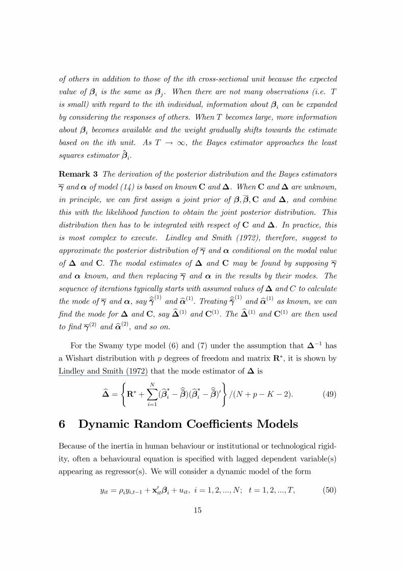
Remark 3 The derivation of the posterior distribution and the Bayes estimators

γ and α of model (14) is based on known C and∆. When C and∆ are unknown,

in principle, we can first assign a joint prior of β,β,C and ∆, and combine

this with the likelihood function to obtain the joint posterior distribution. This

distribution then has to be integrated with respect of C and ∆. In practice, this

is most complex to execute. Lindley and Smith (1972), therefore, suggest to

approximate the posterior distribution of γ and α conditional on the modal value

of ∆ and C. The modal estimates of ∆ and C may be found by supposing γ

and α known, and then replacing γ and α in the results by their modes. The

sequence of iterations typically starts with assumed values of∆ and C to calculate

the mode of γ and α, say γ(1) and α(1). Treating γ(1) and α(1) as known, we can

find the mode for ∆ and C, say ∆(1) and C(1). The ∆(1) and C(1) are then used

to find γ(2) and α(2), and so on.

For the Swamy type model (6) and (7) under the assumption that ∆−1 has

a Wishart distribution with p degrees of freedom and matrix R∗, it is shown by

Lindley and Smith (1972) that the mode estimator of ∆ is

∆ =

R∗ +

N∑

i=1

(β∗

i − β)(β∗

i − β)′/(N + p−K − 2). (49)

6 Dynamic Random Coefficients Models

Because of the inertia in human behaviour or institutional or technological rigid-

ity, often a behavioural equation is specified with lagged dependent variable(s)

appearing as regressor(s). We will consider a dynamic model of the form

yit = ρiyi,t−1 + x′

itβi + uit, i = 1, 2, ..., N ; t = 1, 2, ..., T, (50)

15

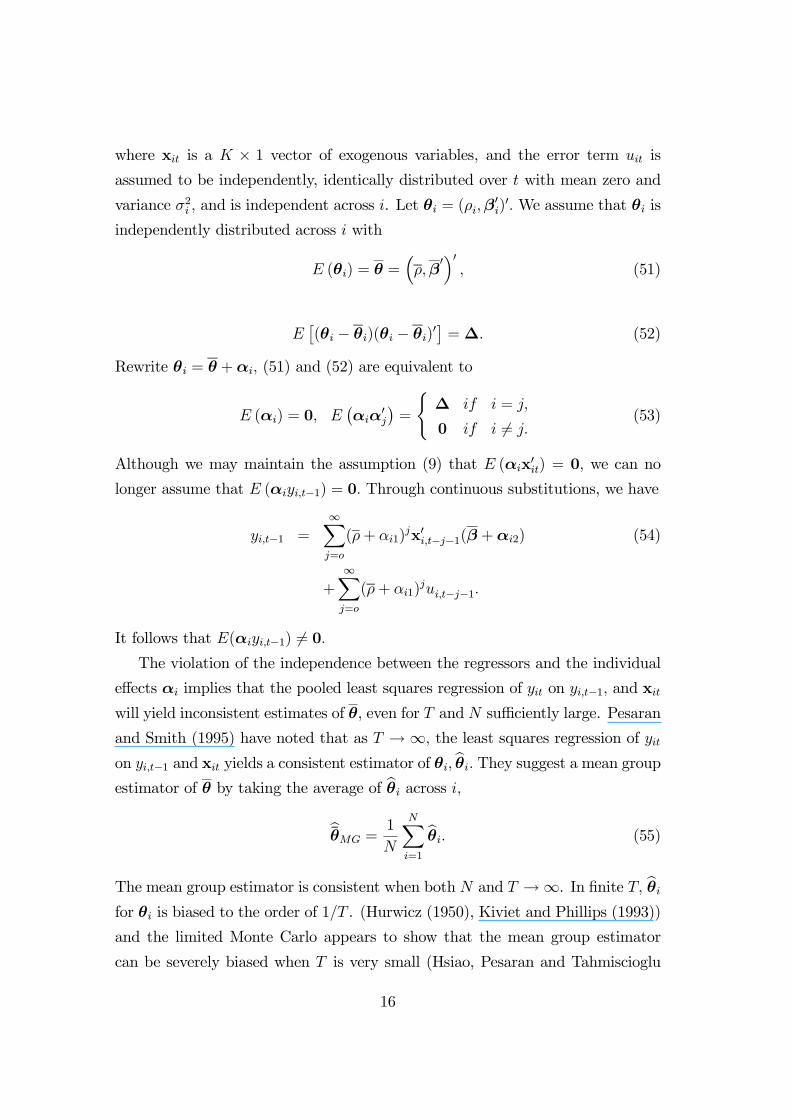
where xit is a K × 1 vector of exogenous variables, and the error term uit is

assumed to be independently, identically distributed over t with mean zero and

variance σ2i , and is independent across i. Let θi = (ρi,β′

i)′. We assume that θi is

independently distributed across i with

E (θi) = θ =(ρ,β

′)′

, (51)

E[(θi − θi)(θi − θi)′

]=∆. (52)

Rewrite θi = θ +αi, (51) and (52) are equivalent to

E (αi) = 0, E(αiα

′

j

)=

∆ if i = j,

0 if i = j.(53)

Although we may maintain the assumption (9) that E (αix′

it) = 0, we can no

longer assume that E (αiyi,t−1) = 0. Through continuous substitutions, we have

yi,t−1 =∞∑

j=o

(ρ+ αi1)jx′i,t−j−1(β +αi2) (54)

+∞∑

j=o

(ρ+ αi1)jui,t−j−1.

It follows that E(αiyi,t−1) = 0.The violation of the independence between the regressors and the individual

effects αi implies that the pooled least squares regression of yit on yi,t−1, and xit

will yield inconsistent estimates of θ, even for T and N sufficiently large. Pesaran

and Smith (1995) have noted that as T →∞, the least squares regression of yit

on yi,t−1 and xit yields a consistent estimator of θi, θi. They suggest a mean group

estimator of θ by taking the average of θi across i,

θMG =1

N

N∑

i=1

θi. (55)

The mean group estimator is consistent when both N and T →∞. In finite T, θi

for θi is biased to the order of 1/T . (Hurwicz (1950), Kiviet and Phillips (1993))

and the limited Monte Carlo appears to show that the mean group estimator

can be severely biased when T is very small (Hsiao, Pesaran and Tahmiscioglu

16

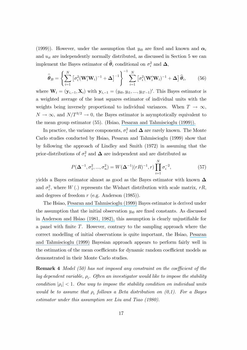
(1999)). However, under the assumption that yi0 are fixed and known and αi

and uit are independently normally distributed, as discussed in Section 5 we can

implement the Bayes estimator of θi conditional on σ2i and ∆,

≏

θB =

N∑

i=1

[σ2i (W

′

iWi)−1 +∆

]−1

−1 N∑

i=1

[σ2i (W

′

iWi)−1 +∆

]θi, (56)

whereWi = (yi,−1,Xi) with yi,−1 = (yi0, yi1, ..., yiT−1)′. This Bayes estimator is

a weighted average of the least squares estimator of individual units with the

weights being inversely proportional to individual variances. When T → ∞,

N → ∞, and N/T 3/2 → 0, the Bayes estimator is asymptotically equivalent to

the mean group estimator (55). (Hsiao, Pesaran and Tahmiscioglu (1999)).

In practice, the variance components, σ2i and∆ are rarely known. The Monte

Carlo studies conducted by Hsiao, Pesaran and Tahmiscioglu (1999) show that

by following the approach of Lindley and Smith (1972) in assuming that the

prior-distributions of σ2i and ∆ are independent and are distributed as

P (∆−1, σ21, ..., σ2n) =W (∆−1|(rR)−1, r)

N∏

i=1

σ−2i , (57)

yields a Bayes estimator almost as good as the Bayes estimator with known ∆

and σ2i , where W (.) represents the Wishart distribution with scale matrix, rR,

and degrees of freedom r (e.g. Anderson (1985)).

The Hsiao, Pesaran and Tahmiscioglu (1999) Bayes estimator is derived under

the assumption that the initial observation yi0 are fixed constants. As discussed

in Anderson and Hsiao (1981, 1982), this assumption is clearly unjustifiable for

a panel with finite T . However, contrary to the sampling approach where the

correct modelling of initial observations is quite important, the Hsiao, Pesaran

and Tahmiscioglu (1999) Bayesian approach appears to perform fairly well in

the estimation of the mean coefficients for dynamic random coefficient models as

demonstrated in their Monte Carlo studies.

Remark 4 Model (50) has not imposed any constraint on the coefficient of the

lag dependent variable, ρi. Often an investigator would like to impose the stability

condition |ρi| < 1. One way to impose the stability condition on individual units

would be to assume that ρi follows a Beta distribution on (0,1). For a Bayes

estimator under this assumption see Liu and Tiao (1980).

17

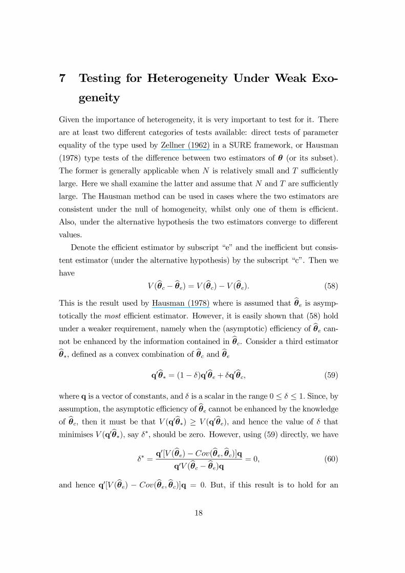
7 Testing for Heterogeneity Under Weak Exo-

geneity

Given the importance of heterogeneity, it is very important to test for it. There

are at least two different categories of tests available: direct tests of parameter

equality of the type used by Zellner (1962) in a SURE framework, or Hausman

(1978) type tests of the difference between two estimators of θ (or its subset).

The former is generally applicable when N is relatively small and T sufficiently

large. Here we shall examine the latter and assume that N and T are sufficiently

large. The Hausman method can be used in cases where the two estimators are

consistent under the null of homogeneity, whilst only one of them is efficient.

Also, under the alternative hypothesis the two estimators converge to different

values.

Denote the efficient estimator by subscript “e” and the inefficient but consis-

tent estimator (under the alternative hypothesis) by the subscript “c”. Then we

have

V (θc − θe) = V (θc)− V (θe). (58)

This is the result used by Hausman (1978) where is assumed that θe is asymp-

totically the most efficient estimator. However, it is easily shown that (58) hold

under a weaker requirement, namely when the (asymptotic) efficiency of θe can-

not be enhanced by the information contained in θc. Consider a third estimator

θ∗, defined as a convex combination of θc and θe

q′θ∗ = (1− δ)q′θe + δq′θc, (59)

where q is a vector of constants, and δ is a scalar in the range 0 ≤ δ ≤ 1. Since, byassumption, the asymptotic efficiency of θe cannot be enhanced by the knowledge

of θc, then it must be that V (q′θ∗) ≥ V (q′θe), and hence the value of δ that

minimises V (q′θ∗), say δ∗, should be zero. However, using (59) directly, we have

δ∗ =q′[V (θe)− Cov(θe, θc)]q

q′V (θc − θe)q= 0, (60)

and hence q′[V (θe) − Cov(θe, θc)]q = 0. But, if this result is to hold for an

18

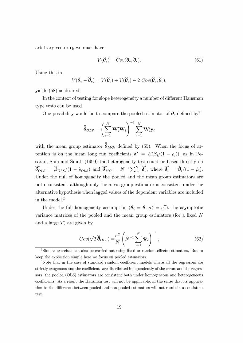
arbitrary vector q, we must have

V (θe) = Cov(θe, θc). (61)

Using this in

V (θc − θe) = V (θc) + V (θe)− 2 Cov(θe, θc),

yields (58) as desired.

In the context of testing for slope heterogeneity a number of different Hausman

type tests can be used.

One possibility would be to compare the pooled estimator of θ, defined by2

θOLS =(

N∑

i=1

W′

iWi

)−1 N∑

i=1

W′

iyi

with the mean group estimator θMG, defined by (55). When the focus of at-

tention is on the mean long run coefficients δ∗ = E(βi/(1 − ρi)), as in Pe-

saran, Shin and Smith (1999) the heterogeneity test could be based directly on

δ∗

OLS = βOLS/(1 − ρOLS) and δ∗

MG = N−1∑N

i=1 δ∗

i , where δ∗

i = βi/(1 − ρi).

Under the null of homogeneity the pooled and the mean group estimators are

both consistent, although only the mean group estimator is consistent under the

alternative hypothesis when lagged values of the dependent variables are included

in the model.3

Under the full homogeneity assumption (θi = θ, σ2i = σ2), the asymptotic

variance matrices of the pooled and the mean group estimators (for a fixed N

and a large T ) are given by

Cov(√T θOLS) =

σ2

N

(N−1

N∑

i=1

Ψi

)−1, (62)

2Similar exercises can also be carried out using fixed or random effects estimators. But to

keep the exposition simple here we focus on pooled estimators.3Note that in the case of standard random coefficient models where all the regressors are

strictly exogenous and the coefficients are distributed independently of the errors and the regres-

sors, the pooled (OLS) estimators are consistent both under homogeneous and heterogeneous

coefficients. As a result the Hausman test will not be applicable, in the sense that its applica-

tion to the difference between pooled and non-pooled estimators will not result in a consistent

test.

19

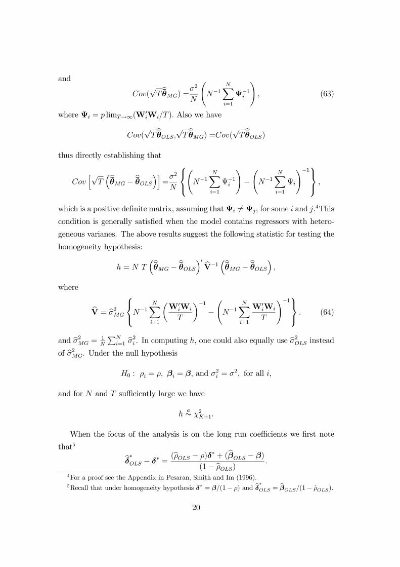
and

Cov(√T θMG) =

σ2

N

(N−1

N∑

i=1

Ψ−1i

), (63)

where Ψi = p limT→∞(W′

iWi/T ). Also we have

Cov(√T θOLS,

√T θMG) =Cov(

√T θOLS)

thus directly establishing that

Cov[√

T(θMG − θOLS

)]=σ2

N

(N−1

N∑

i=1

Ψ−1i

)−(N−1

N∑

i=1

Ψi

)−1 ,

which is a positive definite matrix, assuming thatΨi = Ψj, for some i and j.4This

condition is generally satisfied when the model contains regressors with hetero-

geneous varianes. The above results suggest the following statistic for testing the

homogeneity hypothesis:

h = N T(θMG − θOLS

)′

V−1(θMG − θOLS

),

where

V = σ2MG

N−1

N∑

i=1

(W′

iWi

T

)−1

−(N−1

N∑

i=1

W′

iWi

T

)−1 . (64)

and σ2MG =1N

∑Ni=1 σ

2i . In computing h, one could also equally use σ2OLS instead

of σ2MG. Under the null hypothesis

H0 : ρi = ρ, βi = β, and σ2i = σ2, for all i,

and for N and T sufficiently large we have

ha∼ χ2K+1.

When the focus of the analysis is on the long run coefficients we first note

that5

δ∗

OLS − δ∗ =(ρOLS − ρ)δ∗ + (βOLS − β)

(1− ρOLS).

4For a proof see the Appendix in Pesaran, Smith and Im (1996).5Recall that under homogeneity hypothesis δ∗ = β/(1− ρ) and δ∗OLS = βOLS/(1− ρOLS).

20

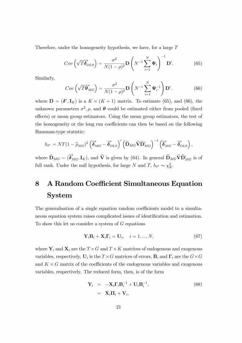
Therefore, under the homogeneity hypothesis, we have, for a large T

Cov(√

T δ∗

OLS

)=

σ2

N(1− ρ)2D

(N−1

N∑

i=1

Ψi

)−1D′. (65)

Similarly,

Cov(√

T θ∗

MG

)=

σ2

N(1− ρ)2D

(N−1

N∑

i=1

Ψ−1i

)D′. (66)

where D = (δ∗, IK) is a K × (K + 1) matrix. To estimate (65), and (66), the

unknown parameters σ2, ρ, and θ could be estimated either from pooled (fixed

effects) or mean group estimators. Using the mean group estimators, the test of

the homogeneity or the long run coefficients can then be based on the following

Hausman-type statistic:

hδ∗ = NT (1− ρMG)2(δ∗

MG − δ∗

OLS

)′(DMGVD

′

MG

)−1 (

δ∗

MG − δ∗

OLS

),

where DMG = (δ∗

MG, IK), and V is given by (64). In general DMGVD′

MG is of

full rank. Under the null hypothesis, for large N and T, hδ∗ ∼ χ2K.

8 ARandomCoefficient Simultaneous Equation

System

The generalisation of a single equation random coefficients model to a simulta-

neous equation system raises complicated issues of identification and estimation.

To show this let us consider a system of G equations

YiBi +XiΓi = Ui, i = 1, ..., N, (67)

whereYi andXi are the T ×G and T ×K matrices of endogenous and exogenous

variables, respectively, Ui is the T×G matrices of errors, Bi and Γi are the G×G

and K ×G matrix of the coefficients of the endogenous variables and exogenous

variables, respectively. The reduced form, then, is of the form

Yi = −XiΓiB−1i +UiB−1i , (68)

= XiΠi +Vi,

21

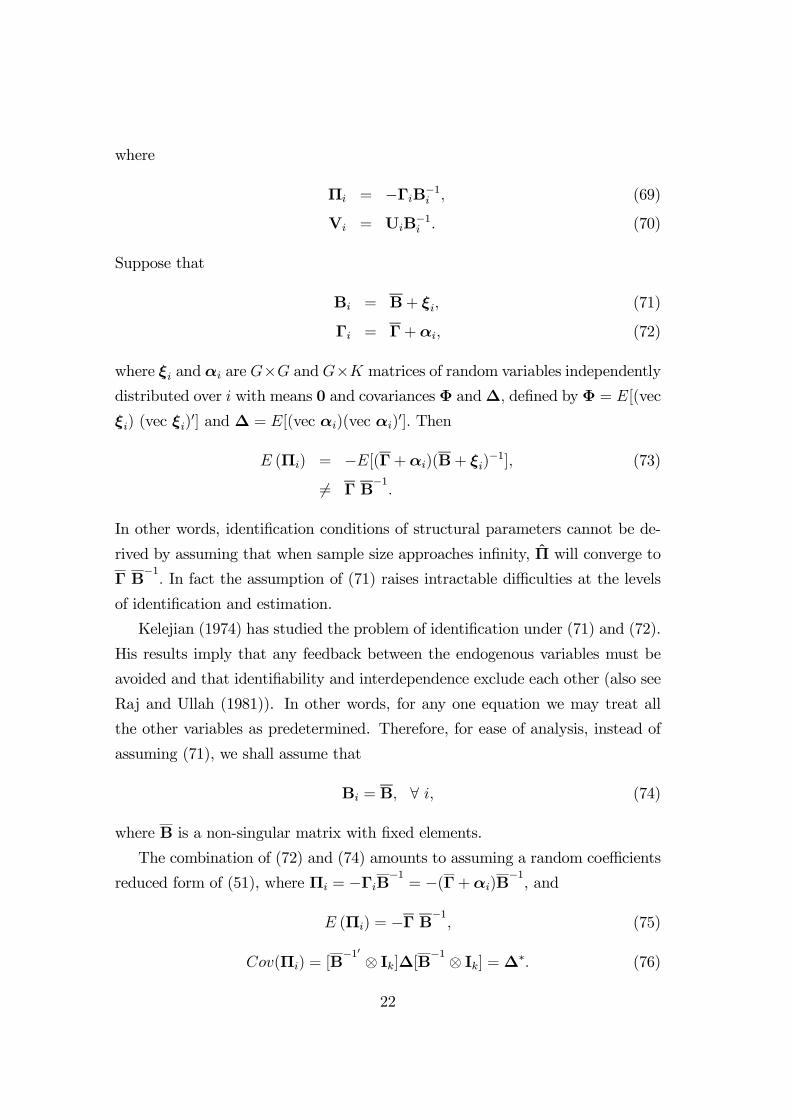
where

Πi = −ΓiB−1i , (69)

Vi = UiB−1i . (70)

Suppose that

Bi = B+ ξi, (71)

Γi = Γ+αi, (72)

where ξi and αi are G×G and G×K matrices of random variables independently

distributed over i with means 0 and covariances Φ and∆, defined by Φ = E[(vec

ξi) (vec ξi)′] and ∆ = E[(vec αi)(vec αi)

′]. Then

E (Πi) = −E[(Γ+αi)(B+ ξi)−1], (73)

= Γ B−1.

In other words, identification conditions of structural parameters cannot be de-

rived by assuming that when sample size approaches infinity, Π will converge to

Γ B−1. In fact the assumption of (71) raises intractable difficulties at the levels

of identification and estimation.

Kelejian (1974) has studied the problem of identification under (71) and (72).

His results imply that any feedback between the endogenous variables must be

avoided and that identifiability and interdependence exclude each other (also see

Raj and Ullah (1981)). In other words, for any one equation we may treat all

the other variables as predetermined. Therefore, for ease of analysis, instead of

assuming (71), we shall assume that

Bi = B, ∀ i, (74)

where B is a non-singular matrix with fixed elements.

The combination of (72) and (74) amounts to assuming a random coefficients

reduced form of (51), where Πi = −ΓiB−1= −(Γ+αi)B

−1, and

E (Πi) = −Γ B−1, (75)

Cov(Πi) = [B−1′ ⊗ Ik]∆[B

−1 ⊗ Ik] =∆∗. (76)

22

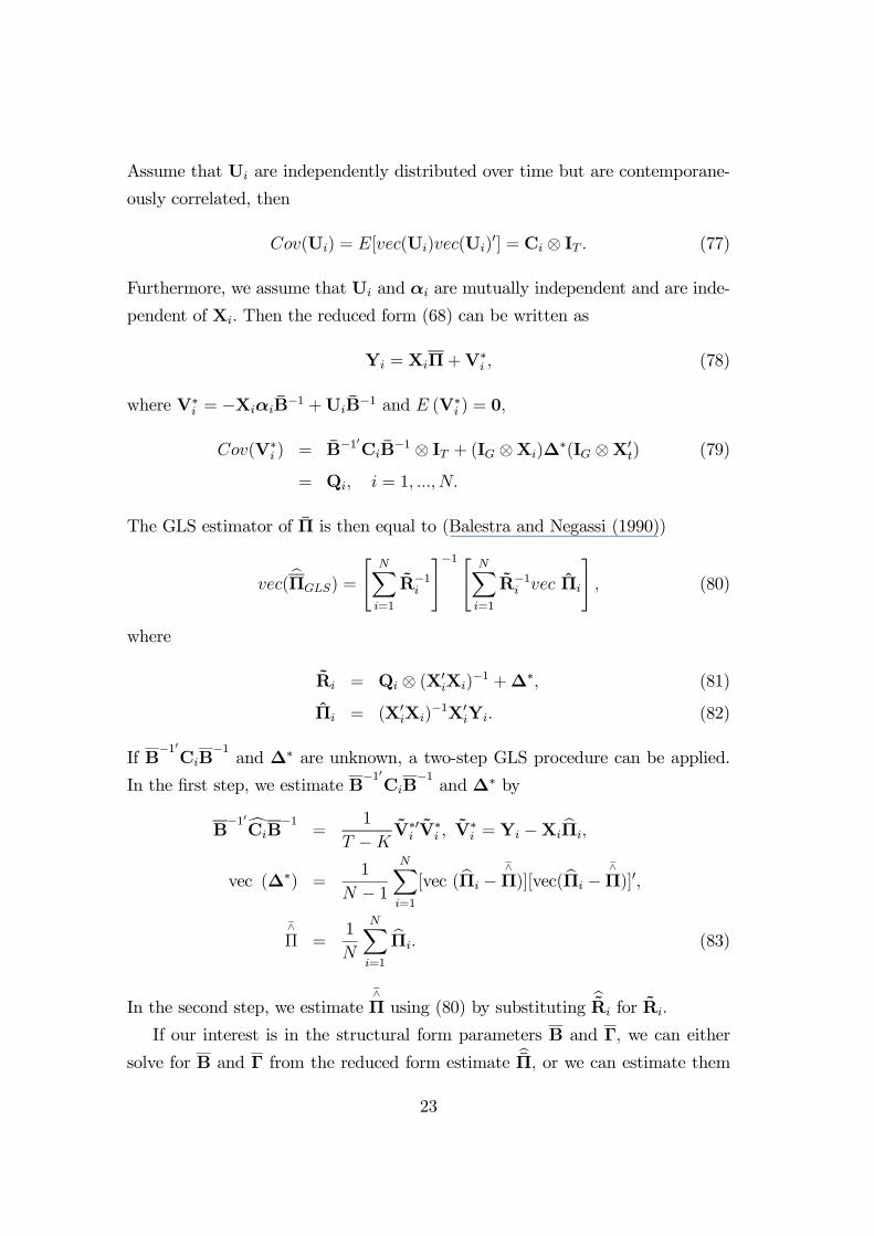
Assume that Ui are independently distributed over time but are contemporane-

ously correlated, then

Cov(Ui) = E[vec(Ui)vec(Ui)′] = Ci ⊗ IT . (77)

Furthermore, we assume that Ui and αi are mutually independent and are inde-

pendent of Xi. Then the reduced form (68) can be written as

Yi = XiΠ+V∗

i , (78)

where V∗

i = −XiαiB−1 +UiB

−1 and E (V∗

i ) = 0,

Cov(V∗

i ) = B−1′

CiB−1 ⊗ IT + (IG ⊗Xi)∆

∗(IG ⊗X′

t) (79)

= Qi, i = 1, ..., N.

The GLS estimator of Π is then equal to (Balestra and Negassi (1990))

vec(ΠGLS) =

[N∑

i=1

R−1i

]−1 [ N∑

i=1

R−1i vec Πi

], (80)

where

Ri = Qi ⊗ (X′iXi)−1 +∆∗, (81)

Πi = (X′

iXi)−1X′

iYi. (82)

If B−1′

CiB−1

and ∆∗ are unknown, a two-step GLS procedure can be applied.

In the first step, we estimate B−1′

CiB−1

and ∆∗ by

B−1′

CiB−1

=1

T −KV∗′

i V∗

i , V∗

i = Yi −XiΠi,

vec (∆∗) =1

N − 1

N∑

i=1

[vec (Πi −⊼

Π)][vec(Πi −⊼

Π)]′,

⊼

Π =1

N

N∑

i=1

Πi. (83)

In the second step, we estimate⊼

Π using (80) by substitutingRi for Ri.

If our interest is in the structural form parameters B and Γ, we can either

solve for B and Γ from the reduced form estimate Π, or we can estimate them

23

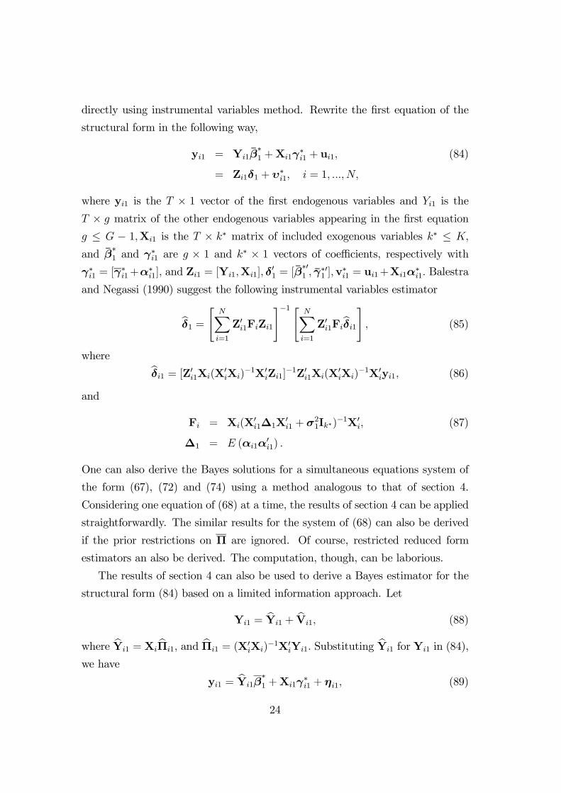
directly using instrumental variables method. Rewrite the first equation of the

structural form in the following way,

yi1 = Yi1β∗

1 +Xi1γ∗

i1 + ui1, (84)

= Zi1δ1 + υ∗

i1, i = 1, ...,N,

where yi1 is the T × 1 vector of the first endogenous variables and Yi1 is the

T × g matrix of the other endogenous variables appearing in the first equation

g ≤ G − 1,Xi1 is the T × k∗ matrix of included exogenous variables k∗ ≤ K,

and β∗

1 and γ∗i1 are g × 1 and k∗ × 1 vectors of coefficients, respectively with

γ∗i1 = [γ∗

i1+α∗

i1], and Zi1 = [Yi1,Xi1], δ′

1 = [β∗′

1 , γ∗′

1 ],v∗

i1 = ui1+Xi1α∗

i1. Balestra

and Negassi (1990) suggest the following instrumental variables estimator

δ1 =

[N∑

i=1

Z′i1FiZi1

]−1 [ N∑

i=1

Z′i1Fiδi1

], (85)

where

δi1 = [Z′

i1Xi(X′

iXi)−1X′

iZi1]−1Z′i1Xi(X

′

iXi)−1X′

iyi1, (86)

and

Fi = Xi(X′

i1∆1X′

i1 + σ21Ik∗)

−1X′

i, (87)

∆1 = E (αi1α′

i1) .

One can also derive the Bayes solutions for a simultaneous equations system of

the form (67), (72) and (74) using a method analogous to that of section 4.

Considering one equation of (68) at a time, the results of section 4 can be applied

straightforwardly. The similar results for the system of (68) can also be derived

if the prior restrictions on Π are ignored. Of course, restricted reduced form

estimators an also be derived. The computation, though, can be laborious.

The results of section 4 can also be used to derive a Bayes estimator for the

structural form (84) based on a limited information approach. Let

Yi1 = Yi1 + Vi1, (88)

where Yi1 = XiΠi1, and Πi1 = (X′

iXi)−1X′

iYi1. Substituting Yi1 for Yi1 in (84),

we have

yi1 = Yi1β∗

1 +Xi1γ∗

i1 + ηi1, (89)

24

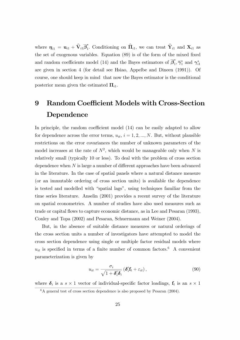
where ηi1 = ui1 + Vi1β∗

1. Conditioning on Πi1, we can treat Yi1 and Xi1 as

the set of exogenous variables. Equation (89) is of the form of the mixed fixed

and random coefficients model (14) and the Bayes estimators of β∗

1,γ∗

1 and γ∗i1

are given in section 4 (for detail see Hsiao, Appelbe and Dineen (1991)). Of

course, one should keep in mind that now the Bayes estimator is the conditional

posterior mean given the estimated Πi1.

9 RandomCoefficientModels with Cross-Section

Dependence

In principle, the random coefficient model (14) can be easily adapted to allow

for dependence across the error terms, uit, i = 1, 2, ..., N . But, without plausible

restrictions on the error covariances the number of unknown parameters of the

model increases at the rate of N2, which would be manageable only when N is

relatively small (typically 10 or less). To deal with the problem of cross section

dependence whenN is large a number of different approaches have been advanced

in the literature. In the case of spatial panels where a natural distance measure

(or an immutable ordering of cross section units) is available the dependence

is tested and modelled with “spatial lags”, using techniques familiar from the

time series literature. Anselin (2001) provides a recent survey of the literature

on spatial econometrics. A number of studies have also used measures such as

trade or capital flows to capture economic distance, as in Lee and Pesaran (1993),

Conley and Topa (2002) and Pesaran, Schuermann and Weiner (2004).

But, in the absence of suitable distance measures or natural orderings of

the cross section units a number of investigators have attempted to model the

cross section dependence using single or multiple factor residual models where

uit is specified in terms of a finite number of common factors.6 A convenient

parameterization is given by

uit =σi√1 + δ′iδi

(δ′ift + εit) , (90)

where δi is a s × 1 vector of individual-specific factor loadings, ft is an s × 16A general test of cross section dependence is also proposed by Pesaran (2004).

25

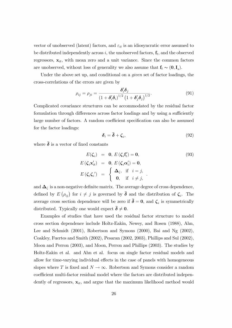
vector of unobserved (latent) factors, and εit is an idiosyncratic error assumed to

be distributed independently across i, the unobserved factors, ft, and the observed

regressors, xit, with mean zero and a unit variance. Since the common factors

are unobserved, without loss of generality we also assume that ft ∼ (0, Is).

Under the above set up, and conditional on a given set of factor loadings, the

cross-correlations of the errors are given by

ρij = ρji =δ′iδj

(1 + δ′iδi)1/2 (

1 + δ′jδj)1/2 . (91)

Complicated covariance structures can be accommodated by the residual factor

formulation through differences across factor loadings and by using a sufficiently

large number of factors. A random coefficient specification can also be assumed

for the factor loadings:

δi = δ + ζi, (92)

where δ is a vector of fixed constants

E(ζi) = 0, E (ζif′

t) = 0, (93)

E (ζix′

it) = 0, E (ζiα′

i) = 0,

E (ζiζi′) =

∆ζ , if i = j,

0, if i = j,.

and∆ζ is a non-negative definite matrix. The average degree of cross dependence,

defined by E(ρij)for i = j is governed by δ and the distribution of ζi. The

average cross section dependence will be zero if δ = 0, and ζi is symmetrically

distributed. Typically one would expect δ = 0.Examples of studies that have used the residual factor structure to model

cross section dependence include Holtz-Eakin, Newey, and Rosen (1988), Ahn,

Lee and Schmidt (2001), Robertson and Symons (2000), Bai and Ng (2002),

Coakley, Fuertes and Smith (2002), Pesaran (2002, 2003), Phillips and Sul (2002),

Moon and Perron (2003), and Moon, Perron and Phillips (2003). The studies by

Holtz-Eakin et al. and Ahn et al. focus on single factor residual models and

allow for time-varying individual effects in the case of panels with homogeneous

slopes where T is fixed and N →∞. Robertson and Symons consider a random

coefficient multi-factor residual model where the factors are distributed indepen-

dently of regressors, xit, and argue that the maximum likelihood method would

26

still be applicable even when N > T . Phillips and Sul (2002) suggest using

SURE-GLS techniques combined with median unbiased estimation in the case of

first order autoregressive panels. Coakley, Fuertes and Smith propose a principal

components approach which is shown by Pesaran (2002) to be consistent only

when the factors and the included regressors are either asymptotically uncorre-

lated or are perfectly correlated. In the more general case Pesaran (2002) shows

that consistent estimation of the random coefficient models with a residual factor

structure can be achieved (under certain regularity conditions) by augmenting

the observed regressors with the cross section averages of the dependent variable

and individual-specific regressors, namely

yt =N∑

j=1

wjyjt, and xit =N∑

j=1

wjxjt, (94)

for any set of weights such that

wi = O

(1

N

),

N∑

i=1

|wi| < K <∞.

An obvious example of such a weighting scheme is wi = 1/N .

Bai and Ng (2002), Phillips and Sul (2002), Moon and Perron (2003), and

Moon, Perron and Phillips (2003), and Pesaran (2003) use residual factor models

to allow for cross section dependence in testing for unit roots in Panels.

10 Concluding Remarks

When the included conditional variables together with the conventional variable

intercept or error components (e.g. Hsiao (2003, ch.3)) cannot completely cap-

tured systematic differences across cross-sectional units and/or over time, and the

possibility of adding additional conditional variables is not an option, either due

to data unavailability or the desire to keep the model simple, there is very little

alternative but to allow the slope coefficients to vary across cross-section units

or over time. If we treat all these coefficients as fixed and different, there is no

particular reason to pool the data, except for some efficiency gain in a Zellner’s

(1962) seemingly unrelated regression framework. Random coefficients models

27

appear to be an attractive middle ground between the implausible assumption

of homogeneity across cross-sectional units or over time and the infeasibility of

treating them all differently, in the sense of being draws from different proba-

bility distributions. Other intermediate formulations could also be considered.

For example, as argued by Pesaran, Shin and Smith (1999), in the context of

dynamic models it would be plausible to impose the homogeneity hypothesis on

the long-run coefficients but let the short-run dynamics to vary freely across the

cross-section units. In this Chapter various formulations are surveyed and their

implications discussed. Our review has been largely confined to linear panel data

models with stationary regressors. The analysis of random coefficient models

with unit roots and cointegration is reviewed in Breitung and Pesaran (2004,

under preparation) in this volume. Parameter heterogeneity in non-linear panel

data models poses fundamentally new problems and needs to be considered on a

case-by-case basis.

28

Appendix A: Proof of Theorem 1To prove part (a) of the theorem, we write (41) in the form of (19) and (17).

Putting u ∼ N(0,C) andα ∼ N(0, IN⊗∆) together with (17), the result follows.

To prove (b), we use Bayes’s theorem, that is

p(γ|y) ∝ p(y|γ)p(γ), (95)

where p(y|γ) follows from (42) and p(γ) is given by (39). The product on the

right hand side of (95) is proportional to exp−12Q, where Q is given by

Q = (y − Zγ)′[C+W(IN ⊗∆)W′]−1(y− Zγ) (96)

= (γ − γ)′D−1(γ − γ) + y′Ω−1 −Ω−1Z[Z′DZ]−1Z′Ω−1y.

The second term on the right hand side of (96) is a constant as far as the distri-

bution of γ is concerned, and the remainder of the expression demonstrates the

truth of (b).

To prove (c), we use the relations

p(α|y) =

∫p(α,γ|y)dγ (97)

=

∫[p(γ|y,α)dγ]p(α|y)

and

p(α,γ|y) ∝ p(y|α,γ)p(α,γ) (98)

= p(y|α,γ)p(α)·p(γ).

Under (38) - (40), the right hand side of (98) is proportional to exp−12Q∗,

where Q∗ is given by

Q∗ = (y − Zγ −Wα)′C−1(y−Zγ −Wα) +α′(IN ⊗∆−1)α

= y′C−1y + γ ′Z′

C−1Zγ +α′W′C−1Wα

−2γ ′Z′C−1y − 2α′W′C−1y + 2γ ′Z′

C−1Wα+α′(IN ⊗∆−1)α

= Q∗

1 +Q∗

2 +Q∗

3, (99)

29

with

Q∗

1 = γ − (Z′C−1Z)−1[Z′C−1(y −Wα)′(Z′C−1Z)·γ − (Z′C−1Z)−1[Z′C−1(y −Wα)], (100)

Q∗

2 = α− DW′[C−1 −C−1Z(Z′C−1Z)−1Z′C−1]y′D−1

·α−DW′[C−1 −C−1Z(Z′C−1Z)−1Z′C−1]y (101)

and

Q∗

3 = y′C−1 −C−1Z(Z′C−1Z)−1Z′C−1 − [C−1 −C−1Z(Z′C−1Z)−1Z′C−1]·WD−1W′[C−1 −C−1Z(Z′C−1Z)−1Z′C−1]y. (102)

As far as the distribution of p(α,γ|y) is concerned, Q∗

3 is a constant. The con-

ditional distribution of γ given y and α is proportional to exp−12Q∗

1, whichintegrates to 1. Therefore, the marginal distribution of α given y is proportional

to exp−12Q∗

2, which demonstrates (c).

Substituting (23) - (26) into (42) we obtain the Bayes solutions for the Swamy

type random coefficients model: (i) the distribution of β given y is N( β,D), and(ii) the distribution of α given y is normal with mean

α = X′[C−1 −C−1XA(A′X′C−1XA)−1A′X′C−1]X+ (IN ⊗∆−1)−1

·X′[C−1 −C−1XA(A′X′C−1XA)−1A′X′C−1]y= DX′[C−1 −C−1XA(A′X′C−1XA)−1A′X′C−1]y, (103)

and covariance

D = X′[C−1 −C−1XA(A′X′C−1XA)−1A′X′C−1]X+ (IN ⊗∆−1)−1. (104)

Letting ∆ = IN ⊗∆ and repeatedly using the identity (30) we can write (104)

in the form

D = [X′C−1X+ ∆−1]−1I−X′C−1XA[A′X′C−1X(X′C−1X+ ∆−1)−1X′C−1XA

−A′X′C−1XA]−1A′X′C−1X[X′C−1X+ ∆−1]−1= [X′C−1X+ ∆−1]−1I+X′C−1XA[A′X′(X∆X′ +C)XA]−1A′(X′C−1X∆−1 − ∆−1)

·[X′C−1X+ ∆−1]−1= [X′C−1X+ ∆−1]−1 + ∆X′(X∆X′ +C)−1XA[A′X′(X∆X′ +C)−1XA]−1

·A′X′(X∆X′ +C)−1X∆. (105)

30

Substituting (105) into (103) we have

α = [X′C−1X+ ∆−1]−1X′C−1y

−(X′C−1X+ ∆−1)−1(X′C−1X+ ∆−1 − ∆−1)A(A′X′C−1XA)−1A′X′C−1y

+∆X′(X∆X′ +C)−1XA[A′X′(X∆X′ +C)−1XA]−1A′X′[C−1 − (X∆X′ +C)−1y

−∆X′(X∆X′ +C)−1XA[A′X′(X∆X′ +C)−1XA]−1

·[I−A′X(X∆X′ +C)−1XA](A′X′C−1XA)−1A′X′C−1y

= (X′C−1X+ ∆−1)−1X′C−1y −A(A′X′C−1XA)−1A′X′C−1y

+(X′C−1 + ∆−1)−1∆−1A(A′X′C−1XA)−1A′X′C−1y

−∆X′(X∆X′ +C)−1XA[A′X′(X∆X′ +C)−1XA]−1A′X′(X∆X′ +C)−1y

+∆X′(X∆X′ +C)−1XA(A′X′C−1XA)−1A′X′C−1y

= (X′C−1X+ ∆−1)−1X′C−1y − ∆X′(X∆X′ +C)−1XAβ. (106)

31

References

[1] Ahn, S.G., Y.H. Lee and P. Schmidt, (2001), GMM Estimation of Linear

Panel Data Models with Time-varying Individual Effects, Journal of Econo-

metrics, 102, 219-255.

[2] Amemiya, T. (1978), “A Note on a Random Coefficients Model”, Interna-

tional Economic Review, 19, 793-796.

[3] Anderson, T.W. (1985), “An Introduction to Multivariate Analysis”, 2nd

edition, Wiley, New York.

[4] Anderson, T.W. and C. Hsiao (1981), “Estimation of Dynamic Models with

Error Components”, Journal of the American Statistical Society, 76, 598-606.

[5] Anderson, T.W. and C. Hsiao (1982),“Formulation and Estimation of Dy-

namic Models Using Panel Data”, Journal of Econometrics, 18, 47-82.

[6] Anselin, L. (2001), “Spatial Econometrics”, in B. Baltagi (ed.), A Compan-

ion to Theoretical Econometrics, Blackwell, Oxford.

[7] Bai, J. and S. Ng (2002), “A Panic Attack on Unit Roots and Cointegration”,

Department of Economics, Boston College, Unpublished Manuscript.

[8] Balestra, P. (1991), “Introduction to Linear Models for Panel Data”, incom-

plete.

[9] Balestra, P. and S. Negassi (1990), “A Random Coefficient Simultaneous

Equation System with an Application to Direct Foreign Investment by

French Firms”, working paper 90-05, Département d’économétrie, Université

de Genève.

[10] Boskin, M.J. and L.J. Lau (1990), “Post-War Economic Growth in the

Group-if-Five Countries: A New Analysis”, CEPR No. 217, Stanford Uni-

versity.

[11] Conley, T.G. and G. Topa (2002), “Socio-economic Distance and Spatial

Patterns in Unemployment”, Journal of Applied Econometrics, 17, 303-327.

32

[12] Cooley, T.F. and E.C. Prescott (1976) “Estimation in the Presence of Sto-

chastic Parameter Variation”, Econometrica, 44, 167-184.

[13] de Finetti, B. (1964), “Foresight: Its Logical Laws. Its Subjective Sources”,

in Studies in Subjective Probability, ed. by J.E. Kyburg, Jr., and H.E. Smok-

ler, New York, Wiley, 93-158.

[14] Friedman, M. (1953), Essays in Positive Economics, Chicago: University of

Chicago Press.

[15] Geisser, S. (1980), “A Predictivistic Primer”, in Bayesian Analysis in Econo-

metrics and Statistics: Essays in Honor of Harold Jeffreys, Amsterdam:

North Holland, 363-382.

[16] Hausman, J.A. (1978), “Specification Tests in Econometrics”, Econometrica,

46, 1251-1271.

[17] Hendricks, W., R. Koenker and D.J. Poirier (1979), “Residential Demand for

Electricity: An Econometric Approach”, Journal of Econometrics, 9, 33-57.

[18] Hildreth, C. and J.P. Houck (1968), “Some Estimators for a Linear Model

with Random Coefficients”, Journal of the American Statistical Association,

63, 584-595.

[19] Holtz-Eakin, D, W.K. Newey and H.Rosen (1988), “Estimating Vector Au-

toregressions with Panel Data”, Econometrica, 56, 1371-1395.

[20] Hsiao, C. (1974), “Statistical Inference for a Model with Both RandomCross-

Sectional and Time Effects”, International Economic Review, 15, 12-30.

[21] Hsiao, C. (1975), “Some Estimation Methods for a Random Coefficients

Model”, Econometrica, 43, 305-325.

[22] Hsiao, C. (1986), Analysis of Panel Data, Econometric Society monographs

No. 11, New York: Cambridge University Press.

[23] Hsiao, C. (1990), “A Mixed Fixed and Random Coefficients Framework for

Pooling Cross-section and Time Series Data”, paper presented at the Third

33

Conference on Telecommunication Demand Analysis with Dynamic Regula-

tion, Hilton, Head, S. Carolina.

[24] Hsiao, C. (2003), Analysis of Panel Data, Economic Society monographs no.

34, 2nd edition, New York: Cambridge University Press.

[25] Hsiao, C. and B.H. Sun (2000), “To Pool or Not to Pool Panel Data”, in

Panel Data Econometrics: Future Directions, Papers in Honour of Profes-

sor Pietro Balestra, ed. by J. Krishnakumar and E. Ronchetti, Amsterdam:

North Holland, 181-198.

[26] Hsiao, C., T.W. Appelbe, and C.R. Dineen (1992), “A General Framework

for Panel Data Models - With an Application to Canadian Customer-Dialed

Long Distance Telephone Service”, Journal of Econometrics (forthcoming).

[27] Hsiao, C., D.C. Mountain, K.Y. Tsui and M.W. Luke Chan (1989), “Model-

ing Ontario Regional Electricity System Demand Using a Mixed Fixed and

Random Coefficients Approach”, Regional Science and Urban Economics 19,

567-587.

[28] Hsiao, C., M.H. Pesaran and A.K. Tahmiscioglu (1999), “Bayes Estimation

of Short-Run Coefficients in Dynamic Panel Data Models”, in Analysis of

Panels and Limited Dependent Variables Models, by C. Hsiao, L.F. Lee, K.

Lahiri and M.H. Pesaran, Cambridge: Cambridge University press, 268-296.

[29] Hurwicz, L. (1950), “Least Squares Bias in Time Series”, in T.C. Koopman,

ed., Statistical Inference in Dynamic Economic Models, New York: Wiley,

365-383.

[30] Jeffreys, H. (1961), Theory of Probability, 3rd ed., Oxford: Clarendon Press.

[31] Judge, G.G., W.E. Griffiths, R.C. Hill, H. Lütkepohl and T.C. Lee (1985),

The Theory and Practice of Econometrics, 2nd ed., New York: Wiley.

[32] Kelejian, H.H. (1974), “Random Parameters in Simultaneous Equation

Framework: Identification and Estimation”, Econometrica, 42, 517-527.

34

[33] Kiviet, J.F. and G.D.A. Phillips (1993), “Alternative Bias Approximation

with Lagged Dependent Variables”, Econometric Theory, 9, 62-80.

[34] Klein, L.R. (1988), “The Statistical Approach to Economics”, Journal of

Econometrics, 37, 7-26.

[35] Lee, K.C., and Pesaran, M.H. (1993), “The Role of Sectoral Interactions

in Wage Determination in the UK Economy”, The Economic Journal, 103,

21-55.

[36] Lindley, D.V. (1961) “The Use of Prior Probability Distributions in Statis-

tical Inference and Decision”, in Proceedings of the Fourth Berkeley Sympo-

sium on Mathematical Statistics and Probability, ed. by J. Neyman, Berkeley:

University of California Press, 453-468.

[37] Lindley, D.V. and A.F.M. Smith (1972), “Bayes Estimates for the Linear

Model”, Journal of the Royal Statistical Society, B. 34, 1-41.

[38] Liu, L.M. and G.C. Tiao (1980), “Random Coefficient First-Order Autore-

gressive Models”, Journal of Econometrics, 13, 305-325.

[39] Min, C.K. and A. Zellner (1993), “Bayesian and Non-Bayesian Methods for

Combining Models and Forecasts with Applications to Forecasting Interna-

tional Growth Rate”, Journal of Econometrics, 56, 89-118.

[40] Moon, H.R. and B. Perron, (2003), “Testing for a Unit Root in Panels with

Dynamic Factors”, Journal of Econometrics (forthcoming).

[41] Moon, H.R., B. Perron and P.C.B. Phillips (2003), “Power Comparisons of

Panel Unit Root Tests under Incidental Trends”, Department of Economics,

University of Southern Califonia, unpublished manuscript.

[42] Pagan, A. (1980), “Some Identification and Estimation Results for Regres-

sion Models with Stochastically Varying Coefficients”, Journal of Economet-

rics, 13, 341-364.

[43] Pesaran, M.H. (2002), “Estimation and Inference in Large Heterogeneous

Panels with Cross Section Dependence”, Cambridge Working Papers in Eco-

nomics No. 0305 and CESIfo Working Paper Series No. 869.

35

[44] Pesaran, M.H. (2003), “A Simple Panel Unit Root Test in the Presence of

Cross Section Dependence”, Cambridge Working Papers in Economics No.

0346, University of Cambridge.

[45] Pesaran, M.H. (2004), “General Diagnostic Tests for Cross Section Depen-

dence in Panels”, Unpublished manuscript, Cambridge University.

[46] Pesaran, M.H. and R. Smith (1995), “Estimation of Long-Run Relationships

from Dynamic Heterogeneous Panels”, Journal of Econometrics, 68, 79-114.

[47] Pesaran, M.H., R. Smith and K.S. Im (1996), “Dynamic Linear Models for

Heterogeneous Panels”, chapter 8 in Màtyàs, L. and P. Sevestre, eds (1996)

The Econometrics of Panel Data: A Handbook of Theory with Applications,

2nd revised edition, Doredrecht: Kluwer Academic Publications.

[48] Pesaran, M.H.,Y. Shin and R.P. Smith, (1999), “PooledMean Group Estima-

tion of Dynamic Heterogeneous Panels”, Journal of the American Statistical

Association, 94, 621-634.

[49] Pesaran, M.H., T. Schuermann and S.M. Weiner (2004), “Modeling Regional

Interdependencies using a Global Error-Correcting Macroeconomic Model”,

Journal of Business Economics and Statistics (with Discussions), forthcom-

ing.

[50] Phillips, P.C.B. and D. Sul (2002), “Dynamic Panel Estimation and Ho-

mogeneity Testing Under Cross Section Dependence”, Cowles Foundation

Discussion Paper No. 1362, Yale University.

[51] Raj, B. and A. Ullah (1981), Econometrics: A Varying Coefficients Ap-

proach, Croom Helm: London.

[52] Rao, C.R. (1970), “Estimation of Heteroscedastic Variances in Linear Mod-

els”, Journal of the American Statistical Association, 65, 161-172.

[53] Rao, C.R. (1972), “Estimation of Variance and Covariance Components in

Linear Models”, Journal of the American Statistical Association, 67, 112-

115.

36

[54] Rao, C.R. (1973), “Linear Statistical Inference and Its Applications, 2nd ed.

New York: Wiley.

[55] Robertson, D. and J. Symons (2000), “Factor Residuals in SUR Regressions:

Estimating Panels Allowing for Cross Sectional Correlation”, Unpublished

manuscript, Faculty of Economics and Politics, University of Cambridge.

[56] Rosenberg, B. (1972), “The Estimation of Stationary Stochastic Regression

Parameters Re-examined”, Journal of the American Statistical Association,

67, 650-654.

[57] Rosenberg, B. (1973), “The Analysis of a Cross-Section of Time Series by

Stochastically Convergent Parameter Regression”, Annals of Economic and

Social Measurement, 2, 399-428.

[58] Schwarz, G. (1978), “Estimating the Dimension of a Model”, Annals of Sta-

tistics, 6, 461-464.

[59] Singh, B., A.L. Nagar, N.K. Choudhry, and B. Raj (1976), “On the Esti-

mation of Structural Changes: A Generalisation of the Random Coefficients

Regression Model”, International Economic Review, 17, 340-361.

[60] Swamy, P.A.V.B. (1970), “Efficient Inference in a Random Coefficient Re-

gression Model”, Econometrica, 38, 311-323.

[61] Swamy, P.A.V.B. and P.A. Tinsley (1977), “Linear Prediction and Estima-

tionMethods for RegressionModels with Stationary Stochastic Coefficients”,

Federal Reserve Board Division of Research and Statistics, Special Studies

Paper No. 78, Washington, D.C.

[62] Wachter, M.L. (1976), “The Changing Cyclical Responsiveness of Wage In-

flation”, Brookings paper on Economic Activity, 1976, 115-168.

[63] Zellner, A. (1962), “An Efficient Method of Estimating Seemingly Unrelated

Regressions and Tests for Aggregation Bias”, Journal of the American Sta-

tistical Association, 57, 348-368.

37

[64] Zellner, A. (1988), “Bayesian Analysis in Econometrics”, Journal of Econo-

metrics, 37, 27-50.

38

CESifo Working Paper Series (for full list see www.cesifo.de)

___________________________________________________________________________ 1168 Horst Raff and Nicolas Schmitt, Exclusive Dealing and Common Agency in

International Markets, April 2004 1169 M. Hashem Pesaran and Allan Timmermann, Real Time Econometrics, April 2004 1170 Sean D. Barrett, Privatisation in Ireland, April 2004 1171 V. Anton Muscatelli, Patrizio Tirelli and Carmine Trecroci, Can Fiscal Policy Help

Macroeconomic Stabilisation? Evidence from a New Keynesian Model with Liquidity Constraints, April 2004

1172 Bernd Huber and Marco Runkel, Tax Competition, Excludable Public Goods and User

Charges, April 2004 1173 John McMillan and Pablo Zoido, How to Subvert Democracy: Montesinos in Peru,

April 2004 1174 Theo Eicher and Jong Woo Kang, Trade, Foreign Direct Investment or Acquisition:

Optimal Entry Modes for Multinationals, April 2004 1175 Chang Woon Nam and Doina Maria Radulescu, Types of Tax Concessions for

Attracting Foreign Direct Investment in Free Economic Zones, April 2004 1176 M. Hashem Pesaran and Andreas Pick, Econometric Issues in the Analysis of

Contagion, April 2004 1177 Steinar Holden and Fredrik Wulfsberg, Downward Nominal Wage Rigidity in Europe,

April 2004 1178 Stefan Lachenmaier and Ludger Woessmann, Does Innovation Cause Exports?

Evidence from Exogenous Innovation Impulses and Obstacles, April 2004 1179 Thiess Buettner and Johannes Rincke, Labor Market Effects of Economic Integration –

The Impact of Re-Unification in German Border Regions, April 2004 1180 Marko Koethenbuerger, Leviathans, Federal Transfers, and the Cartelization

Hypothesis, April 2004 1181 Michael Hoel, Tor Iversen, Tore Nilssen, and Jon Vislie, Genetic Testing and Repulsion

from Chance, April 2004 1182 Paul De Grauwe and Gunther Schnabl, Exchange Rate Regimes and Macroeconomic

Stability in Central and Eastern Europe, April 2004

1183 Arjan M. Lejour and Ruud A. de Mooij, Turkish Delight – Does Turkey’s accession to the EU bring economic benefits?, May 2004

1184 Anzelika Zaiceva, Implications of EU Accession for International Migration: An

Assessment of Potential Migration Pressure, May 2004 1185 Udo Kreickemeier, Fair Wages and Human Capital Accumulation in a Global

Economy, May 2004 1186 Jean-Pierre Ponssard, Rent Dissipation in Repeated Entry Games: Some New Results,

May 2004 1187 Pablo Arocena, Privatisation Policy in Spain: Stuck Between Liberalisation and the

Protection of Nationals’ Interests, May 2004 1188 Günter Knieps, Privatisation of Network Industries in Germany: A Disaggregated

Approach, May 2004 1189 Robert J. Gary-Bobo and Alain Trannoy, Efficient Tuition Fees, Examinations, and

Subsidies, May 2004 1190 Saku Aura and Gregory D. Hess, What’s in a Name?, May 2004 1191 Sjur Didrik Flåm and Yuri Ermoliev, Investment Uncertainty, and Production Games,

May 2004 1192 Yin-Wong Cheung and Jude Yuen, The Suitability of a Greater China Currency Union,

May 2004 1193 Inés Macho-Stadler and David Pérez-Castrillo, Optimal Enforcement Policy and Firms’

Emissions and Compliance with Environmental Taxes, May 2004 1194 Paul De Grauwe and Marianna Grimaldi, Bubbles and Crashes in a Behavioural Finance

Model, May 2004 1195 Michel Berne and Gérard Pogorel, Privatization Experiences in France, May 2004 1196 Andrea Galeotti and José Luis Moraga-González, A Model of Strategic Targeted

Advertising, May 2004 1197 Hans Gersbach and Hans Haller, When Inefficiency Begets Efficiency, May 2004 1198 Saku Aura, Estate and Capital Gains Taxation: Efficiency and Political Economy

Consideration, May 2004 1199 Sandra Waller and Jakob de Haan, Credibility and Transparency of Central Banks: New

Results Based on Ifo’s World Economicy Survey, May 2004 1200 Henk C. Kranendonk, Jan Bonenkamp, and Johan P. Verbruggen, A Leading Indicator

for the Dutch Economy – Methodological and Empirical Revision of the CPB System, May 2004

1201 Michael Ehrmann, Firm Size and Monetary Policy Transmission – Evidence from

German Business Survey Data, May 2004 1202 Thomas A. Knetsch, Evaluating the German Inventory Cycle – Using Data from the Ifo

Business Survey, May 2004 1203 Stefan Mittnik and Peter Zadrozny, Forecasting Quarterly German GDP at Monthly

Intervals Using Monthly IFO Business Conditions Data, May 2004 1204 Elmer Sterken, The Role of the IFO Business Climate Indicator and Asset Prices in

German Monetary Policy, May 2004 1205 Jan Jacobs and Jan-Egbert Sturm, Do Ifo Indicators Help Explain Revisions in German

Industrial Production?, May 2004 1206 Ulrich Woitek, Real Wages and Business Cycle Asymmetries, May 2004 1207 Burkhard Heer and Alfred Maußner, Computation of Business Cycle Models: A

Comparison of Numerical Methods, June 2004 1208 Costas Hadjiyiannis, Panos Hatzipanayotou, and Michael S. Michael, Pollution and

Capital Tax Competition within a Regional Block, June 2004 1209 Stephan Klasen and Thorsten Nestmann, Population, Population Density, and

Technological Change, June 2004 1210 Wolfgang Ochel, Welfare Time Limits in the United States – Experiences with a New

Welfare-to-Work Approach, June 2004 1211 Luis H. R. Alvarez and Erkki Koskela, Taxation and Rotation Age under Stochastic

Forest Stand Value, June 2004 1212 Bernard M. S. van Praag, The Connexion Between Old and New Approaches to

Financial Satisfaction, June 2004 1213 Hendrik Hakenes and Martin Peitz, Selling Reputation When Going out of Business,

June 2004 1214 Heikki Oksanen, Public Pensions in the National Accounts and Public Finance Targets,

June 2004 1215 Ernst Fehr, Alexander Klein, and Klaus M. Schmidt, Contracts, Fairness, and

Incentives, June 2004 1216 Amihai Glazer, Vesa Kanniainen, and Panu Poutvaara, Initial Luck, Status-Seeking and

Snowballs Lead to Corporate Success and Failure, June 2004 1217 Bum J. Kim and Harris Schlesinger, Adverse Selection in an Insurance Market with

Government-Guaranteed Subsistence Levels, June 2004

1218 Armin Falk, Charitable Giving as a Gift Exchange – Evidence from a Field Experiment, June 2004

1219 Rainer Niemann, Asymmetric Taxation and Cross-Border Investment Decisions, June

2004 1220 Christian Holzner, Volker Meier, and Martin Werding, Time Limits on Welfare Use

under Involuntary Unemployment, June 2004 1221 Michiel Evers, Ruud A. de Mooij, and Herman R. J. Vollebergh, Tax Competition

under Minimum Rates: The Case of European Diesel Excises, June 2004 1222 S. Brock Blomberg and Gregory D. Hess, How Much Does Violence Tax Trade?, June

2004 1223 Josse Delfgaauw and Robert Dur, Incentives and Workers’ Motivation in the Public

Sector, June 2004 1224 Paul De Grauwe and Cláudia Costa Storti, The Effects of Monetary Policy: A Meta-

Analysis, June 2004 1225 Volker Grossmann, How to Promote R&D-based Growth? Public Education

Expenditure on Scientists and Engineers versus R&D Subsidies, June 2004 1226 Bart Cockx and Jean Ries, The Exhaustion of Unemployment Benefits in Belgium.

Does it Enhance the Probability of Employment?, June 2004 1227 Bertil Holmlund, Sickness Absence and Search Unemployment, June 2004 1228 Klaas J. Beniers and Robert Dur, Politicians’ Motivation, Political Culture, and

Electoral Competition, June 2004 1229 M. Hashem Pesaran, General Diagnostic Tests for Cross Section Dependence in Panels,

July 2004 1230 Wladimir Raymond, Pierre Mohnen, Franz Palm, and Sybrand Schim van der Loeff, An

Empirically-Based Taxonomy of Dutch Manufacturing: Innovation Policy Implications, July 2004

1231 Stefan Homburg, A New Approach to Optimal Commodity Taxation, July 2004 1232 Lorenzo Cappellari and Stephen P. Jenkins, Modelling Low Pay Transition

Probabilities, Accounting for Panel Attrition, Non-Response, and Initial Conditions, July 2004

1233 Cheng Hsiao and M. Hashem Pesaran, Random Coefficient Panel Data Models, July

2004