Aggregation of Individual Trees and Patches in Forest Succession Models: Capturing Variability with...

Theoretical Population Biology 54, 213�226 (1998)

Aggregation of Individual Trees and Patches inForest Succession Models: Capturing Variabilitywith Height Structured, Random, SpatialDistributions

Heike Lischke,1 Thomas J. Lo� ffler, and Andreas FischlinSystems Ecology, Institute of Terrestrial Ecology, Department of Environmental Sciences,Swiss Federal Institute of Technology Zu� rich (ETHZ), Grabenstrasse 3,CH-8952 Schlieren, Switzerland

Received November 15, 1996

Individual based, stochastic forest patch models have the potential to realistically describeforest dynamics. However, they are mathematically intransparent and need long computingtimes. We simplified such a forest patch model by aggregating the individual trees on manypatches to height-structured tree populations with theoretical random dispersions over thewhole simulated forest area. The resulting distribution-based model produced results similarto those of the patch model under a wide range of conditions. We concluded that the height-structured tree dispersion is an adequate population descriptor to capture the stochasticvariability in a forest and that the new approach is generally applicable to any patch model. Thesimplified model required only 4.10 of the computing time needed by the patch model. Hence,this new model type is well-suited for applications where a large number of dynamic forestsimulations is required. ] 1998 Academic Press

Key Words: forest succession; individual based model; stochastic model; patch model;aggregation; structured population; model simplification; spatial distribution.

INTRODUCTION

The dynamics of populations are determined by birth,death, the change in the state of individuals, and theinteractions between them and also by exogenous eventssuch as disturbances. Individuals differ with respect totheir properties or states, such as size or age, they mayexperience spatially heterogeneous living conditions,such as nutrient supply, and they may also be affecteddifferentially by random events, i.e. by demographic orenvironmental stochasticity (Turelli, 1986). Thesedifferences among indi-viduals lead to a variability in the

population which can strongly influence its overalldynamics (Koehl, 1989; May, 1986).

Individual-based, stochastic models are one approachto account for this variability, since they describeexplicitly the processes and interactions of the indivi-duals and also include random events, e.g. the death ofone particular organism. Thus, they have the potential todescribe the dynamics of entire populations realistically(Grimm et al., 1996; Murdoch et al., 1992), i.e., close towhat can be observed in nature, and to give insight intothe mechanisms of community dynamics (McCook,1994; Shugart, 1984).

In describing the dynamics of forest populations andcommunities, the individual based patch (or gap) modelapproach has a long tradition. It reaches back to thedevelopment of JABOWA (Botkin et al., 1970; Botkin et

Article No. TP981378

213 0040-5809�98 K25.00

Copyright ] 1998 by Academic PressAll rights of reproduction in any form reserved.

1 Corresponding author. Current address: National Forest Inven-tory, Swiss Federal Institute for Forest, Snow and LandscapeResearch, Zu� rcherstrasse 111, CH-8903 Birmensdorf. E-mail:lischke�wsl.ch.

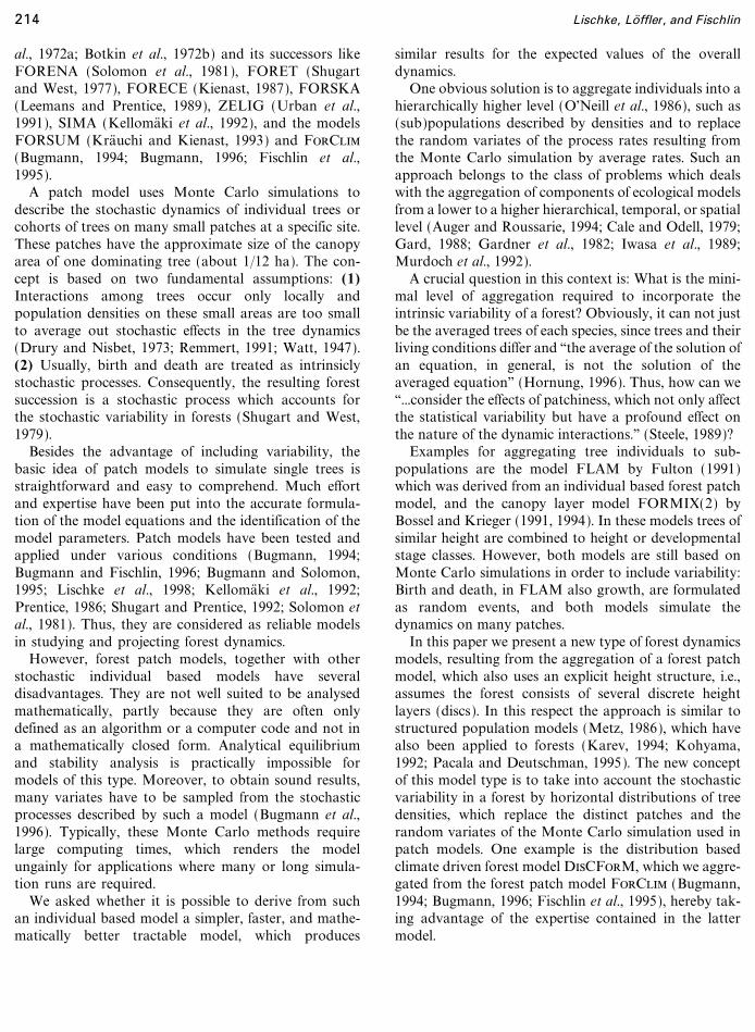
al., 1972a; Botkin et al., 1972b) and its successors likeFORENA (Solomon et al., 1981), FORET (Shugartand West, 1977), FORECE (Kienast, 1987), FORSKA(Leemans and Prentice, 1989), ZELIG (Urban et al.,1991), SIMA (Kelloma� ki et al., 1992), and the modelsFORSUM (Kra� uchi and Kienast, 1993) and ForClim(Bugmann, 1994; Bugmann, 1996; Fischlin et al.,1995).

A patch model uses Monte Carlo simulations todescribe the stochastic dynamics of individual trees orcohorts of trees on many small patches at a specific site.These patches have the approximate size of the canopyarea of one dominating tree (about 1�12 ha). The con-cept is based on two fundamental assumptions: (1)Interactions among trees occur only locally andpopulation densities on these small areas are too smallto average out stochastic effects in the tree dynamics(Drury and Nisbet, 1973; Remmert, 1991; Watt, 1947).(2) Usually, birth and death are treated as intrinsiclystochastic processes. Consequently, the resulting forestsuccession is a stochastic process which accounts forthe stochastic variability in forests (Shugart and West,1979).

Besides the advantage of including variability, thebasic idea of patch models to simulate single trees isstraightforward and easy to comprehend. Much effortand expertise have been put into the accurate formula-tion of the model equations and the identification of themodel parameters. Patch models have been tested andapplied under various conditions (Bugmann, 1994;Bugmann and Fischlin, 1996; Bugmann and Solomon,1995; Lischke et al., 1998; Kelloma� ki et al., 1992;Prentice, 1986; Shugart and Prentice, 1992; Solomon etal., 1981). Thus, they are considered as reliable modelsin studying and projecting forest dynamics.

However, forest patch models, together with otherstochastic individual based models have severaldisadvantages. They are not well suited to be analysedmathematically, partly because they are often onlydefined as an algorithm or a computer code and not ina mathematically closed form. Analytical equilibriumand stability analysis is practically impossible formodels of this type. Moreover, to obtain sound results,many variates have to be sampled from the stochasticprocesses described by such a model (Bugmann et al.,1996). Typically, these Monte Carlo methods requirelarge computing times, which renders the modelungainly for applications where many or long simula-tion runs are required.

We asked whether it is possible to derive from suchan individual based model a simpler, faster, and mathe-matically better tractable model, which produces

similar results for the expected values of the overalldynamics.

One obvious solution is to aggregate individuals into ahierarchically higher level (O'Neill et al., 1986), such as(sub)populations described by densities and to replacethe random variates of the process rates resulting fromthe Monte Carlo simulation by average rates. Such anapproach belongs to the class of problems which dealswith the aggregation of components of ecological modelsfrom a lower to a higher hierarchical, temporal, or spatiallevel (Auger and Roussarie, 1994; Cale and Odell, 1979;Gard, 1988; Gardner et al., 1982; Iwasa et al., 1989;Murdoch et al., 1992).

A crucial question in this context is: What is the mini-mal level of aggregation required to incorporate theintrinsic variability of a forest? Obviously, it can not justbe the averaged trees of each species, since trees and theirliving conditions differ and ``the average of the solution ofan equation, in general, is not the solution of theaveraged equation'' (Hornung, 1996). Thus, how can we``...consider the effects of patchiness, which not only affectthe statistical variability but have a profound effect onthe nature of the dynamic interactions.'' (Steele, 1989)?

Examples for aggregating tree individuals to sub-populations are the model FLAM by Fulton (1991)which was derived from an individual based forest patchmodel, and the canopy layer model FORMIX(2) byBossel and Krieger (1991, 1994). In these models trees ofsimilar height are combined to height or developmentalstage classes. However, both models are still based onMonte Carlo simulations in order to include variability:Birth and death, in FLAM also growth, are formulatedas random events, and both models simulate thedynamics on many patches.

In this paper we present a new type of forest dynamicsmodels, resulting from the aggregation of a forest patchmodel, which also uses an explicit height structure, i.e.,assumes the forest consists of several discrete heightlayers (discs). In this respect the approach is similar tostructured population models (Metz, 1986), which havealso been applied to forests (Karev, 1994; Kohyama,1992; Pacala and Deutschman, 1995). The new conceptof this model type is to take into account the stochasticvariability in a forest by horizontal distributions of treedensities, which replace the distinct patches and therandom variates of the Monte Carlo simulation used inpatch models. One example is the distribution basedclimate driven forest model DisCForM, which we aggre-gated from the forest patch model ForClim (Bugmann,1994; Bugmann, 1996; Fischlin et al., 1995), hereby tak-ing advantage of the expertise contained in the lattermodel.

214 Lischke, Lo� ffler, and Fischlin

MATERIAL AND METHODS

The Patch Model FORCLIM

ForClim is a forest patch model, which can begenerally used where the needed species parameters areavailable. It was developed to study the influences of achanging climate on forests in the northern temperateand boreal zone, and particularly in the European Alps.

We focus on the submodel ForClim-P (version2.4.0.2), which uses as input the expected values ofbioclimatic variables, e.g., drought stress or day-degree-sum, calculated in advance by the submodelForClim-E from inter-annual means, standard devia-tions and correlation coefficients of monthly temperatureand precipitation.

ForClim-P simulates the stochastic dynamics of treecohorts for any number (e.g., 30 for Central Europe; seelegend of Fig. 3) of different species usually on 200patches which are assumed to be independent of eachother. These patches represent different realisations ofthe stochastic process running at a specific site. We inter-pret these realisations in the following as differentpatches of a forest area with spatially homogenous soiland climatic conditions. The model follows the fate, i.e.,establishment, growth, and death, of every single treecohort. All processes depend explicitly on climate and onthe available light intensity at the tree top. Birth anddeath are formulated stochastically, i.e., as probabilitiesfor each cohort, that individual trees are born or die.Since the focus of the model is on the successionaldynamics of forests, population genetics are neglected.Furthermore, establishment occurs from a constant seedpool, which is independent from the parent populationdensity.

Simulation Environment

The new model DisCForM was implemented anddeveloped with the interactive part of the simulationenvironment RAMSES2 (Fischlin, 1991). To improve theperformance of the implementation (Doud, 1993; Lo� ffler,1995), we optimized the code by evaluating time andstate independent expressions in advance, outsidethe integration loop. For comparison, simulations ofDisCForM and ForClim-P were run on a SUNserverMP630 (40 MHz) under RASS (Thoeny et al., 1994), thebatch simulation server of RAMSES.

Sites and Forest Data

The simulations of both models were run for 1200 yearswith a yearly time step. Input included the same constantbioclimatic and edaphic data from seven climatically dif-ferent sites in Switzerland (Table 1).

For the colline, upper montane, and subalpine vegeta-tion belt, represented by the sites Bern, Davos, andSt. Gotthard, respectively, we compared qualitatively thesimulated equilibrium species compositions to data ofspecies compositions (Fig. 3d), compiled from the FirstSwiss National Forest Inventory (WSL, 1997), whichconsists 0.05 ha sample plots on an 1-km grid. InSwitzerland the majority of the forests are managed. Inorder to include only plots in forests as close to naturalas possible and to obtain still a reasonable sample sizewe, therefore, restricted the evaluated sample plots to allthose, where the last management was longer than 25years ago and regeneration was natural. To take intoaccount only plots with similar conditions, plots from 50m below to 50 m above the altitude of the sites fromsurrounding regions (Table 2) were included; the regionshad to be chosen rather large to increase the sample size.The plots were split according to the estimated age of thesurrounding stands, i.e., whether they were likely torepresent rather an early or an intermediate successionalstate (stand age <80 or �80 years). For stands of mixeddevelopmental state stand age was not available; weassumed them to correspond to the mixed age structureof the shifting-mosaic climax (Bormann and Likens,1979; Remmert, 1991). Table 2 shows the numbers ofplots in the three age classes. Wood biovolumen wasestimated (Kaufmann, 1996) from stem diameter atbreast height (DBH) for all trees with DBH>12cm andmultiplied by species specific density factors (Kniggeand Schulz, 1966; Lakida et al., 1995; Niemz, 1993;Trendelenburg and Mayer-Wegelin, 1955) to obtainbiomass in dry weight, same as in the models.

TABLE 1

Characteristics of Sites Used to Test the Forest Models DISCFORM andFORCLIM-P

Elevation Annual mean Annual precipi-Site (m.a.s.l.) temperature (%C) tation sum (cm)

Locarno 379 11.8 184.6Sion 542 9.7 59.7Bern 570 8.4 100.6Huttwil 639 8.1 128.7Davos 1590 3.0 100.7Bever 1712 1.5 84.1St. Gotthard 2090 &0.07 216.2

215Aggregating Individuals in Patch Models

2 RAMSES can be downloaded by anonymous ftp fromftp.ito.umnw.ethz.ch (Internet address: 129.132.80.130). For informa-tion s. homepage at URL http:��www.ito.umnw.ethz.ch�SysEcol.

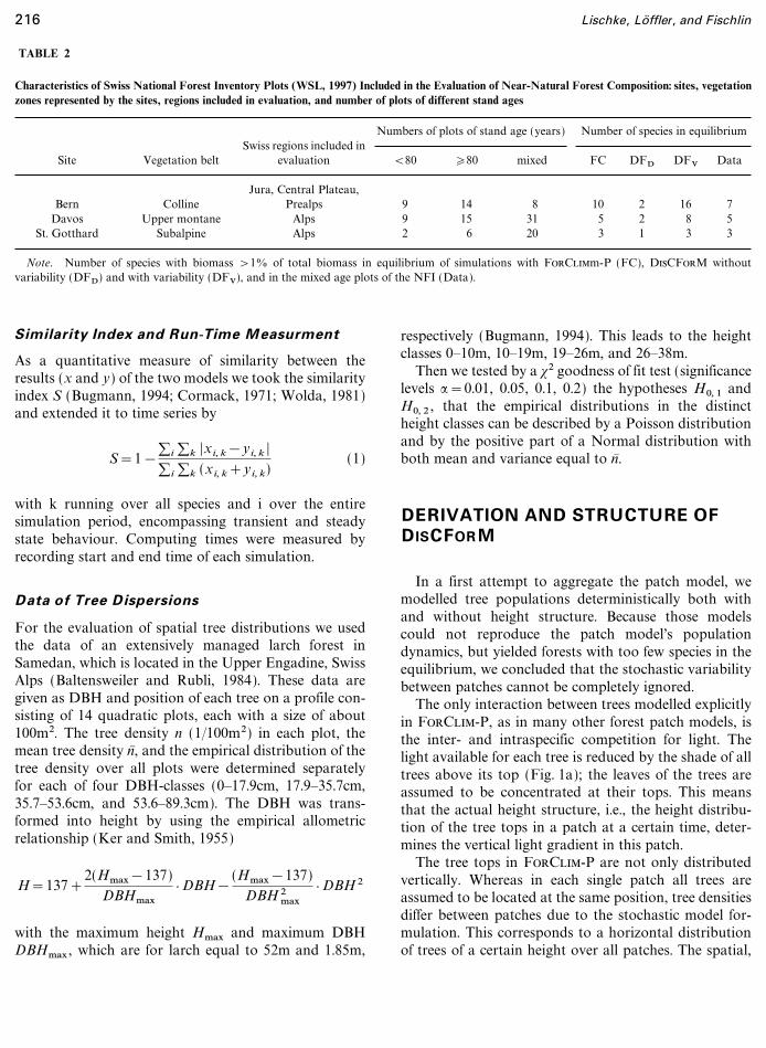
TABLE 2

Characteristics of Swiss National Forest Inventory Plots (WSL, 1997) Included in the Evaluation of Near-Natural Forest Composition: sites, vegetationzones represented by the sites, regions included in evaluation, and number of plots of different stand ages

Numbers of plots of stand age (years) Number of species in equilibriumSwiss regions included in

Site Vegetation belt evaluation <80 �80 mixed FC DFD DFV Data

Bern CollineJura, Central Plateau,

Prealps 9 14 8 10 2 16 7Davos Upper montane Alps 9 15 31 5 2 8 5

St. Gotthard Subalpine Alps 2 6 20 3 1 3 3

Note. Number of species with biomass >10 of total biomass in equilibrium of simulations with ForClimm-P (FC), DisCForM withoutvariability (DFD) and with variability (DFV), and in the mixed age plots of the NFI (Data).

Similarity Index and Run-Time Measurment

As a quantitative measure of similarity between theresults (x and y) of the two models we took the similarityindex S (Bugmann, 1994; Cormack, 1971; Wolda, 1981)and extended it to time series by

S=1&�i �k |x i, k&y i, k |�i �k (x i, k+y i, k)

(1)

with k running over all species and i over the entiresimulation period, encompassing transient and steadystate behaviour. Computing times were measured byrecording start and end time of each simulation.

Data of Tree Dispersions

For the evaluation of spatial tree distributions we usedthe data of an extensively managed larch forest inSamedan, which is located in the Upper Engadine, SwissAlps (Baltensweiler and Rubli, 1984). These data aregiven as DBH and position of each tree on a profile con-sisting of 14 quadratic plots, each with a size of about100m2. The tree density n (1�100m2) in each plot, themean tree density n� , and the empirical distribution of thetree density over all plots were determined separatelyfor each of four DBH-classes (0�17.9cm, 17.9�35.7cm,35.7�53.6cm, and 53.6�89.3cm). The DBH was trans-formed into height by using the empirical allometricrelationship (Ker and Smith, 1955)

H=137+2(Hmax&137)

DBHmax

} DBH&(Hmax&137)

DBH 2max

} DBH 2

with the maximum height Hmax and maximum DBHDBHmax , which are for larch equal to 52m and 1.85m,

respectively (Bugmann, 1994). This leads to the heightclasses 0�10m, 10�19m, 19�26m, and 26�38m.

Then we tested by a /2 goodness of fit test (significancelevels :=0.01, 0.05, 0.1, 0.2) the hypotheses H0, 1 andH0, 2 , that the empirical distributions in the distinctheight classes can be described by a Poisson distributionand by the positive part of a Normal distribution withboth mean and variance equal to n� .

DERIVATION AND STRUCTURE OFDISCFORM

In a first attempt to aggregate the patch model, wemodelled tree populations deterministically both withand without height structure. Because those modelscould not reproduce the patch model's populationdynamics, but yielded forests with too few species in theequilibrium, we concluded that the stochastic variabilitybetween patches cannot be completely ignored.

The only interaction between trees modelled explicitlyin ForClim-P, as in many other forest patch models, isthe inter- and intraspecific competition for light. Thelight available for each tree is reduced by the shade of alltrees above its top (Fig. 1a); the leaves of the trees areassumed to be concentrated at their tops. This meansthat the actual height structure, i.e., the height distribu-tion of the tree tops in a patch at a certain time, deter-mines the vertical light gradient in this patch.

The tree tops in ForClim-P are not only distributedvertically. Whereas in each single patch all trees areassumed to be located at the same position, tree densitiesdiffer between patches due to the stochastic model for-mulation. This corresponds to a horizontal distributionof trees of a certain height over all patches. The spatial,


FIG. 1. Distribution of trees and light in a forest, as simulated by a conventional forest patch model and the new model DisCForM. In bothcases the leaves are assumed to be concentrated at the tree top. The grey areas portray the shading by the canopy: (a) In a conventional forest patchmodel individual tree dynamics produce a continuous vertical distribution of tree heights and light within each distinct patch; (b) In DisCForM thepatches are lumped together to form a forest, which consists of a stack of discrete height classes (``forest discs,'' here three height classes are shown).Within each forest disc, trees and the available light are distributed horizontally; (c) Density functions of tree population densities, (grey columns)and the available light (solid black line), in three forst discs as modelled by DisCForM. Within these discs the tree dispersion is assumed to be randomand is modelled with a Poisson distribution.

i.e., vertical and horizontal, and temporally changing dis-tribution of tree tops determines the spatial distributionof light (Fig. 1a) and influences tree to tree competitionfor light throughout the forest.

The new model DisCForM focuses on the temporaldynamics of these spatial tree and light distributions(Fig. 1b). The spatial distributions are represented by fre-quency distributions (Fig. 1c) of the density of tree topsper unit area and of the light intensity at a certain height.

The main differences between DisCForM and a patchmodel are: (1) The continuous height distribution of thetrees is replaced by a discrete height structure. (2) Theentire forest is simulated at once in each time step. Thespatial distribution of trees per unit area is modelled bythe assumption that in each time step all trees of a certainheight are distributed randomly over the forest, whichresults in a Poisson distribution. Consequently, it is nolonger feasible nor desirable to trace the fate of individualtrees or cohorts.

With these assumptions and the process functions andparameter values of ForClim-P we get the following dis-tribution based, height structured population dynamicsmodel (a summarisation of the symbols is contained inTable 3):

Ns, i is the average population density per patch area oftrees of species s in the height class i in the entire forest.

The rate of change of Ns, i at time t (Eq. (2)) is deter-mined by death Ds, i (Eq. (3)), growth Gs, i (Eq. (4)) andbirth Bs, i (Eq. (5)). Trees grow into height class i fromheight class i&1 (Gs, i&1) and leave height class i by out-growing (Gs, i). Birth (Eq. (5)) is restricted to the lowestheight class (i=0). These processes depend not only onstate but they are also driven by time dependent inputvariables, namely temperature, precipitation andnitrogen. For easier reading we omit all explicit notationof time dependence in the following equations:

dNs, i

dt=&Ds, i

death

+Gs, i&1&Gs, i

growth

+Bs, i

birth

(2)

Ds, i=(+const, s+(1&+const, s) } +� s, i) } Ns, i (3)

Gs, i=#� s, i

hi+1&hi} Ns, i (4)

Bs, i={0,;� s ,

i>0i=0.

(5)

The species specific death, growth, and birth rates+� s, i , #� s, i , and ;� s are the expected values of the lightdependent rates , +s, i (l ), #s, i (l ), and ;s(l ) (for the specificformulation of the rates cf. Appendix 1). Since light


TABLE 3

Symbols Used

Symbol Meaning Unit

t Time yearhi Height of lower boundary of height class i ms Species indexNs, i Average population density of species s in height class i (per unit area) m&2

Ds, i Dying trees of species s in height class i m&2 year&1

Gs, i Trees of species s growing from height class i to height class i+1 m&2 year&1

Bs, 0 New saplings of tree species s m&2 year&1

+� s, i , #� s, i , ;� s Expected values of mortality, growth, and birth rates with respect to light intensity year&1, m year&1, m&2 year&1

+s, const Constant mortality of species s year&1

+s, i (l ) Stress induced mortality of species s at light intensity l in height class i year&1

#s, i (l ) Per tree growth rate of species s at light intensity l in height class i m year&1

#s, i, max Maximal diameter increment of species s in height class i m year&1

|s, i Diameter to height increment conversion factor ��Cs Climate dependence of growth of species s ��g1, s , g2, s , g3, s Species parameters for light dependence ��;S(l ) Birth (establishment) rate of species s at light intensity l m&2 year&1

l;crit, s Critical light intensity for establishment of species s ��;max, s Maximal establishment rate of species s, climate dependent year&1

fY( y) Probability density function of random variable Y ��Li Light in height class i (fraction of full light); random variable ��Xs, j Population density of species s in height class j; random variable m&2

` unit area (set to usual patch size, 833m2=1�12ha) m2

as, j Specific leaf area of trees of species s in height class j m2

LAIi Leave area index in height class i; random variable ��: Extinction coefficient (set to 0.25) ��+LAIi

, _LAIiMean and standard deviation of leaf area index in height class i ��

intensity is a random variable, these expected values arecalculated with the probability density function fLi

oflight intensity Li in height class i by

.� =|�

&�.(l ) } fLi

(l ) dl=|1

0.(l ) } fLi

(l ) dl

with .=+s, i , #s, i , ;s . (6)

In order to be able to use (6) we have to determine thelight density function fLi

.An essential assumption in our approach is that all

trees of each species s in each height class j are randomlydistributed over the patches, which for the tree popula-tion densities Xs, j leads to a Poisson distribution with themean Ns, j . Thus, the tree dispersion in each height classis independent of all other height classes. The Poissondistribution is then approximated by a Normal distribu-tion with the same mean Ns, j and the standard deviation- Ns, j .

Particularly for small means of a Poisson distributionthis seems to be a crude approximation. Yet, tests withrandom numbers drawn from Poisson distributions withvarious parameters and from corresponding normal

approximations which were truncated at zero and scaledto the area of one, indicated that the approximated dis-tributions were satisfactorily similar in position andshape to the original ones. Additionally, the distributionof a linear combination of two Poisson distributedrandom variables was similar to the truncated normaldistribution, which was obtained by first approximatingthe two Poisson distributions by Normal ones, thendetermining the Normal distribution of the linearcombination of the two random variables, and thentruncating and scaling this distribution.

This allows the following transformations:Given a tree density of species s in height hj of Xs, j trees

per unit area ` (size of one patch) and a species andheight specific, constant leaf area as, j per tree, the leafarea index LAIi in height class i is a random variabledefined by

LAIi=� j>i �s Xs, j } as, j

`(7)

Since LAIi in height class i is a linear function of the nor-mally distributed tree densities Xs, j in all height classes


above class i, it is also normally distributed with theparameters

+LAIi=

1`

:j>i

�s

Ns, j } as, j ,

(8)_LAIi

=1` �:

j>i

:s

Ns, j } a2s, j .

With the full light intensity (=1) above the topmostheight class and a the extinction coefficient of leaves, thelight Li which is transmitted down to height class i isdescribed by Li=e&: } LAIi. Thus, a certain light intensityLi in height hi is reached by the leaf area index LAIi ,which fulfils

LAIi=&ln(Li)

:(9)

Using transformation (9), the light density function fLi

can be expressed by the density function of the leaf areaindex fLAIi

which is a normal distribution with theparameters +LAIi

and _LAIi(Eq. (8)).

If fY(y ) is the density function of a random variable Yat a specific realisation y and X is another randomvariable X=h(Y ) with a unique function h and with thedensity function fX , then fY ( y) can be expressed byfY( y)=fX(h( y)) } |dh( y)�dy| (Fisz, 1980). Hence,

fLi(l )= fLAIi \&

ln(l ): + }

1l } :

. (10)

The density function fLiis scaled to 1 by �1

0 fLi(l ) dl =

!1

to partly compensate the errors introduced by replacingthe Poisson by not truncated Normal distributions.

In the implementation light intensity was discretizedinto 10 light classes !, to be able to compute lightdependent rates once in advance for accelerating thecode. In this discrete formulation (6) turns to

.� = :9

!=0

.(l!) } (FLi(l!+1)&FLi

(l!)), (11)

where FLiis the distribution function of the light inten-

sities which we can express by the normal distributionfunction of the leaf area index with the parameters +LAIi

and _LAIi(Eq. (8)) by FLi

(l )=FLAIi(&ln(l )�:). With (11)

the system of ordinary differential equations (2) can besolved.

EMPIRICAL TREE DISPERSIONS

The evaluation of the tree dispersion data fromSamedan (Fig. 2) indicates that the choice of a Poisson

FIG. 2. Empirical and theoretical spatial tree density distribution(dispersion) of larch trees split into four height classes. Data fromBaltensweiler and Rubli (1984) showing the frequencies (bold lines)over a profile of 14 plots of 100m2 size each. Lines show the correspond-ing probability density functions of the Poisson distribution. For threeof four height classes the hypothesis that the data can be described bya Poisson distribution (H0, 1) and its approximation (H0, 2) could notbe rejected for the significance levels (:=0.2, ..., 0.01). The hypotheseswere rejected only for height class 19�26m (at :=0.1 (H0, 1) and:=0.05 (H0, 2), respectively).

distribution (hypothesis H0, 1), and also of its normalapproximation (hypothesis H0, 2) for the theoretical treedispersion, is acceptable. For three of four height classesboth hypotheses could not be rejected (tested levels ofsignificance: :=0.2, 0.1, 0.05, 0.01); only for one heightclass they were rejected (at :=0.1 (H0, 1) and :=0.05(H0, 2)).

BEHAVIOR OF DISCFORM

To compare the results of DisCForM to those of itspredecessor ForClim-P, simulations were carried out for


FIG. 3. Qualitative comparison of forest compositions at three selected sites in the Swiss Alps (see Table 1) representing the colline (Bern), uppermontane (Davos) and subalpine (St. Gotthard) vegetation belt: (a) simulations with the patch model ForClim-P (Bugmann, 1994; Fischlin et al.,1995); (b) simulations with the aggregated model DisCForM without variability; (c) simulations with DisCForM with variability; (d) data of thefirst Swiss National Forest Inventory (WSL, 1997). Please note the different scales of biomass. ``Other species'' are: Pinus silverstris, Taxus baccata,Acer campestre, Acer platanoides, Acer pseudoplatanus, Alnus glutinosa, Alnus incana, Anus viridis, Betula pendula, Carpinus betulus, Castanea sativa,Corylus avellana, Fraxinus excelsior, Populus nigra, Populus tremula, Quercus pubescens, Salix alba, Sorbus aria, Sorbus aucuparia, Tilia cordata, Tiliaplatyphyllos, Ulmus glabra. Simulated biomass comprises woody and leaf biomass of trees higher than 1.37m, biomass in data woody biomass fromtrees with DBH>12cm. All biomass values are given in t dry weight�ha.


seven different sites in Switzerland (Table 1) with thesame bioclimatic variables as inputs for both models. Inall simulations the same 30 tree species (see legend Fig. 3)were used. The continuous time model DisCForM runwith the explicit Euler method with a fixed yearly timestep. The light distribution was discretized into 10classes, the height into 15 classes.

Figure 3 shows the results of both models for threesites. In first simulations with DisCForM we assumed auniform spatial tree distribution, i.e., set the variance ofthe tree distribution to 0. In these simulations (Fig. 3b)less species than in the data (Fig. 3d) and in the patchmodel simulations (Fig. 3a) could coexist in equilibrium(Table 2); e.g. at the subalpine site only one of threespecies present in the ForClim-P simulations and in thedata survived.

Therefore, in the following simulations the treedistribution variance was set to the average populationdensity in each height class, which corresponds to arandom tree dispersion. This leads to results (Fig. 3c)which correspond to the ForClim-P simulation at allthree sites in the overall pattern of the species composi-tion, especially for the dominating species, and yields aslightly higher biodiversity than the ForClim-P simula-tions (table 2). Deviations occur mainly in the totalbiomass and particularly during early succession.

Both models differ from the data (Fig. 3d) of the lessabundant species but reproduce to a same extent the

FIG. 4. Comparison between the overall behaviour of the new model DisCForM and that of the patch model ForClim-P (Bugmann, 1994;Fischlin et al., 1995) in terms of computing time and degree of discretization of the tree heights; similarity indices (rhombi) and computing time(circles) were averaged over six sites in the Swiss Alps (Table 1) and are displayed vs. the number of height classes in DisCForM. Similarity indices(1) were computed from species abundances (t�ha) over the entire simulation period. The computing time DisCForM needed is shown as a fractionof the time needed by ForClim-P (t1000). Error bars: \1 standard deviation.

main characteristics of the observed species composi-tions: the species-rich, Fagus silvatica dominated forest inthe colline zone, the Picea abies dominated needle-leafforest in the upper montane zone, and the Larixdecidua�Pinus cembra�Picea abies forest in the subalpinezone. The transition of the simulated total biomass fromlow values in early succession over a maximum in inter-mediate succession to a lower level in the equilibrium isalso indicated in the data of the colline and subalpinezone. The main deviations are in simulated biomass,which is considerably higher than in the data, and in thesimulated portion of Picea abies, which is too low atBern, and too high at St. Gotthard. Additionally, thenumber of equilibrium species in the data is slightly lowerthan in the simulations with ForClim-P andDisCForM, whereas higher than in the DisCForMsimulations without variability.

A quantitative comparison of similarity and efficiencybetween the two models is shown in Fig. 4. At each siteDisCForM was run with various height discretizations(2, 5, 10, 15, 20, 30, and 60 height classes). Each simula-tion of DisCForM was compared to the correspondingForClim-P simulation by calculating the similarityindex (Eq. (1)) and measuring the relative computingtime. The shown values are averages over all sixsimulated sites.

The quality of the results, as well as the computingtime, depended strongly on the height discretization. The


optimum combination of similarity and efficiency couldbe reached with 15 height classes, with a computing timeof about 4.10 (105 s on a SUNserver MP630) of the timeneeded by ForClim-P and a maximum similarity indexof about 0.76. With respect to the model intrinsicuncertainties of ForClim-P the difference expressed bythis similarity index might still be significant (Bugmann,1994).

DISCUSSION

The presented derivation of a distribution-based,structured population model from an individual-basedmodel is a stochastic, approximate aggregation, combin-ing the concepts of Iwasa et al. (1987; 1989), Gard(1988), Murdoch et al. (1992), and Auger (1994).

The use of approximations was necessary, because aperfect stochastic aggregation (Gard, 1988), where theaggregated model contains exactly the same dynamicinformation about the aggregated variables as theindividual based one, was not possible. Forests can beconceived as systems with only local interactionsbetween sessile individuals and small population sizesin subunits, which is depicted, e.g., by the patchmodel approach. For such models, a direct aggregationof individuals to a population by simply letting theirnumbers go to infinity is difficult, if not impossible (Metzand de Roos, 1992).

The central assumption and approximation usedin this model aggregation were the random spatial dis-tribution of the trees in each height class and theapproximation of the resulting Poisson distribution ofthe tree densities by a matching Normal distribution. Thelatter equivalent is rather crude for small means, butthe evaluation of the empirical spatial tree distribution inthe larch forest at Samedan suggests that this assumptionmight be acceptable in a majority of cases. Also invarious studies of natural and near-natural forests(Abbott, 1984; Stoll et al., 1994; Szwagrzyk andCzerwczak, 1993; Ward and Parker, 1989; Ward et al.,1996; Williamson, 1975) the spatial tree distribution wasclose to random with a tendency to aggregated for youngand to uniform for old trees.

The distribution-based approach produces similarresults as the patch model approach. However, theresults differ in details, particularly in the increase ofbiomass in early succession, accompanied with anovershooting. This is probably due to the height dis-cretization, since in simulations with smaller heightclasses (not shown) the increase was much smoother.

The increased biodiversity produced by DisCForMsimulations might indicate that the random distributionof the trees offers a too wide range of light regimes;reducing the variability will presumably improve theresults.

The comparison of the simulations to the NFI-datawas impeded by the fact that unmanaged and rarelymanaged forests are scarce in Switzerland. Thus, only fewNFI-plots could be evaluated, the considered forests areprobably not completely natural, and the samples had tobe chosen from rather large regions.

Nevertheless, the results can give indications about thevalidity of ForClim-P and DisCForM. Both modelsoverestimate total biomass. This is probably due to theexponential allometric relationship Bstem=0.12 } DBH2.4

used to calculate stem biomass Bstem from DBH. Since inthe models biomass is only an output variable, i.e., doesnot feed back to the dynamics, correcting this formula(e.g., to the sigmoid one proposed and fitted to NFI-databy Perruchoud, 1996) will only affect total biomass, notthe general results.

The major patterns of species composition, such as theforest types and the temporal development of biomassare reproduced by the models. The high portion of Piceaabies in the data of the colline zone might be due toformer management, whereas its high portion in the St.Gotthard simulations has probably to be attributed tothe use of average instead of temporally varying climaticinput (Bugmann, 1997). Simulations with the versionForClim-E�P of the patch-model which allows climateto fluctuate stochastically, e.g., lead to a strong suppres-sion of Picea abies and a forest consisting of Larixdecidua and Pinus cembra. Hence, besides spatialalso temporal variability has the potential to influenceforest dynamics. Such temporally variable input canpresumably be incorporated into the aggregated modelby a temporal aggregation of climate dependencefunctions (Lischke et al., 1997a; Lischke et al., 1997b).

The general form of the aggregated model resemblesa height-discrete, time-continuous version of the con-tinuity equation forest model of Kohyama (1992; 1993;1995); i.e., it is an intermediate between this partialdifferential equation model and a discrete forward one-step transition matrix model (Lefkovitch, 1965; Takadaand Hara, 1994).

However, there are differences. DisCForM takesinto account the spatial dispersion of the trees, whichdetermines through the LAI and light distributions thedistributions and means of the process rates.

Kohyama's first models (e.g., 1991) include variabilityby a diffusion term, where the diffusion constant, whichcorresponds to the variance of the growth rate, is derived


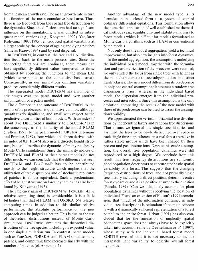
from the mean growth rate. The mean growth rate in turnis a function of the mean cumulative basal area. Thus,there is no feedback from the spatial tree distribution tothe dynamics. Since the diffusion term had no significantinfluence on the simulations, it was omitted in subse-quent model versions (e.g., Kohyama, 1992). Yet, laterKohyama (1993; 1995) reintroduced spatial variability ata larger scale by the concept of ageing and dying patches(same as Karev, 1994) and by seed dispersal.

In DisCForM, in contrast, the tree and LAI distribu-tion feeds back to the mean process rates. Since theconnecting functions are nonlinear, these means canhave significantly different values compared to thoseobtained by applying the functions to the mean LAI(which corresponds to the cumulative basal area).Consequently, in our simulations omitting variabilityproduces considerably different results.

The aggregated model DisCForM has a number ofadvantages over the patch model and over anothersimplification of a patch model.

The difference in the outcome of DisCForM to theresults of its predecessor is qualitatively minor, althoughquantitatively significant, and small with respect to thepredictive uncertainties of both models. With an index ofabout 0.76 DisCForM's similarity to ForClim-P is inthe same range as the similarity of the model FLAM(Fulton, 1991) to the patch model FORSKA (Leemansand Prentice, 1989), from which it had been derived, withan index of 0.8. FLAM also uses a discrete height struc-ture, but still describes the dynamics of many patches byMonte Carlo simulations. Since the similarity indices ofDisCForM and FLAM to their parent models do notdiffer much, we can conclude that the difference betweenDisCForM and ForClim-P has to be contributedmostly to the height structure which implies that theutilization of tree dispersions and of stochastic replicatesof patches is almost equivalent. Such a predominanteffect of height structure on forest dynamics has also beenfound by Kohyama (1993).

The efficiency gain of DisCForM vs. ForClim (4.10relative computing time) is considerable. It is a littlebit higher than that of FLAM vs. FORSKA (50 relativecomputing time). In addition to this similar relativeperformance, the absolute performance of the newapproach can be judged as better. This is due to the useof theoretical distributions instead of Monte Carlosimulations. DisCForM simulates the theoretical dis-tribution of the tree species, including its expected value,in one single simulation run. In contrast, patch modelssuch as ForClim, FORSKA, and FLAM simulate manypatches, and computing time increases linearly with thenumber of patches (cf. Appendix 2).

Another advantage of the new model type is itsformulation in a closed form as a system of coupledordinary differential equations. This formulation allowsthe numerical application of well established mathemati-cal methods (e.g., equilibrium- and stability-analysis) toforest models which is difficult for models formulated asMonte Carlo algorithms such as FLAM or conventionalpatch models.

Not only does the model aggregation yield a technicalimprovement, but also new insights into forest dynamics.

In the model aggregation, the assumptions underlyingthe individual based model, together with the formula-tion and parametrization of the processes were retained;we only shifted the focus from single trees with height asthe main characteristic to tree subpopulations in distinctheight classes. The new model differs from its predecessorin only one central assumption: it assumes a random treedispersion a priori, whereas in the individual basedmodel the dispersion emerges from the individual pro-cesses and interactions. Since this assumption is the onlydeviation, comparing the results of the new model withthose of its predecessor can be used to assess the assump-tion's validity.

We approximated the vertical�horizontal tree distribu-tions by independent layers and random tree dispersions.That means we ignored the single tree histories andassumed the trees to be newly distributed over space ineach single time step, whereas in a real forest trees live inrather stable groups which have been shaped by theirpresent and past interactions. Despite this crude assump-tion, the overall tree population dynamics were stillreproduced to a high degree. We conclude from thisresult that tree frequency distributions are sufficientlygood population descriptors to capture stochastic spatialvariability of a forest. This suggests that the changingfrequency distributions of trees, and not primarily singletree history including its direct position, determine entireforest dynamics and it is a positive answer to the question(Pacala, 1989) ``Can we adequately account for plantpopulation dynamics without specifying the location ofindividuals?'' and an extension of Fulton's (1991) conclu-sion, that ``much of the information contained in indi-vidual tree descriptions is redundant if the main concernis with a dynamically sufficient representation of a forestpatch'' to the entire forest. Urban (1991) has also con-cluded that for the simulation of implicitly spatialphenomena space does not always have to be explicitlytaken into account, same as Deutschman et al. (1997),whose study with the individual based forest modelSORTIE revealed that it is not necessary to includeintrapatch light variability to describe overall forestdynamics.


We hypothesise that frequency distributions are aminimum aggregation level, since other more aggregatedpopulation descriptors which do not take into accountstochastic spatial variability, such as total species meansor means of height classes failed to reproduce the forestdiversity. Although in our model, same as in the patchmodel, seed supply is independent of parent trees,coexistence in this open system can be considered as aprerequisite for coexistence in the closed system, whereseed supply is coupled to parent tree abundance. Ifcoexistence is not possible in the open system, it isunlikely that it will occur in the closed system, since thepositive feedback between parent abundance and recruit-ment will presumably further decrease the number ofspecies which can coexist.

Our finding is supported by the comparison of aspatially explicit forest model with its mean fieldapproximation, where light supply was averaged overspace (Pacala and Deutschman, 1995). The simulationwith the mean field model yielded half the biomass andenhanced the extinction of non dominant species. In amore general frame the hypothesis is consistent with theecological evidence and theory of heterogeneity or distur-bance-mediated coexistence of species (cf. e.g., Denslow,1985; Hutchinson, 1978).

CONCLUSION

By the derivation of the distribution based, structuredpopulation model DisCForM from the individual based,stochastic patch model we reached three goals: The newmodel is faster and its results are similar to the patchmodel simulations, and new insights into forest dynamicswere made possible by the changes.

The stochastic variability in a forest can be depictedby random tree distributions, which implies that treefrequency distributions determine forest dynamics andnot primarily single tree histories or positions. However,distributions seem to be the minimal necessary aggrega-tion level.

The approach of replacing the stochastic distributionsobtained by Monte Carlo simulations with theoreticaldistributions can be applied to all patch models in whichcompetition for light forms the only interaction betweenthe individuals. The idea can also be extended tocompetition for other local resources, e.g., nutrients orwater, if the supply of them is explicitly modelled. Thisapproach is promising even for patch models withcompetition for several independent local resources.

With the good run-time behaviour of the model, manynew applications of forest models are now possible, e.g.,

simulating tree species migration in past and futureclimate changes or forests in large areas on a fine grid.Moreover, this approach can be considered as a potentialcontribution to the development of larger scale dynamicvegetation models because it helps to ``discover the rulesthat permit large-scale ecological models to be derivedfrom fine-scale interactions'' (Pacala and Deutschman,1995).

APPENDIX 1: PROCESS RATES OFDISCFORM

The following process functions of the aggregatedmodel were derived from ForClim-P (Bugmann, 1994,1996) (for explanation of parameters refer to Table 3):

v the growth rate #s, i (l )=#s, i, max } Cs } |s, i } gs(l ),with the light dependence function

gs(l )=g1, s&g2, s } e&1.84 } l&g3, s } e&4.84 } l;

v the light dependent part of the mortality rate

+s, i (l )={0.184,0,

Cs } gs(l )<Max(0.1, 0.0003�#s, i, max)else

;

v and the establishment rate

;s(l )={0,;max, s ,

l<l;crit, s ,l�l;crit, s .

APPENDIX 2: RUNTIMECOMPARISON

On a SUNserver MP630 (40 MHz) FORSKA, e.g.,would need approximately TFk=0.42 min. (Fulton,1991) to simulate np=1 patch over 1200 years. Weassume that applying our distribution based approach toFORSKA (run with np=200 patches) also reduces thecomputing time to about 40. For a hypothetical dis-tribution based FORSKA model this would lead to arun-time of 0.04_200_0.42min=3.44min, regardlessthe number of patches originally used in FORSKA.FLAM needs for np patches 0.05_np_TFk min. Hence,for patch numbers np�3.44�(0.05 } TFk)=164 the dis-tribution based approach is faster than the Monte Carloapproach; it needs 180 less computing time fornp=200, which is considered as the minimum necessarynumber of replicates in patch model simulations to


warrant reliable estimates of the expected values of thespecies biomasses (Bugmann et al., 1996).

ACKNOWLEDGMENTS

This work has been supported by the Swiss Federal Institute ofTechnology (ETH) Zurich and by the Swiss National Science Founda-tion Grants 5001-35172 and 31-31142.91. Thanks to B. Roy for herhelpful comments not only on the English of the manuscript. Thankyou very much also to the reviewers for their comments which helpedto considerably improve the manuscript.

REFERENCES

Abbott, I. 1984. Comparisons of spatial pattern, structure, and treecomposition between virgin and cut-over jarrah forest in westernaustralia, Forest Ecol. Manage. 9, 101�126.

Auger, P. M., and Roussarie, R. 1994. Complex ecological models withsimple dynamics: From individuals to populations, Acta Biotheoret.42, 111�136.

Baltensweiler, W., and Rubli, D. 1984. Forstliche Aspekte derLa� rchenwickler-Massenvermehrungen im Oberengadin, Schweizer-ische Z. Forstwesen 60(1).

Bormann, F. H., and Likens, G. E. 1979. ``Pattern and Process in aForested Ecosystem: Disturbance, Development and the SteadyState: Based on the Hubbard Brook Ecosystem Study,'' Springer-Verlag, New York.

Bossel, H., and Krieger, H.. 1991. Simulation model of natural tropicalforest dynamics, Eco. Modelling 59, 37�71.

Bossel, H., and Krieger, H.. 1994. Simulation of multi-species tropicalforest dynamics using a vertically and horizontally structured model,Forest Ecol. Manage. 69(1�3), 123�144.

Botkin, D. B., Janak, J. F., and Wallis, J. R. 1970. A simulator fornortheastern forest growth, IBM Thomas J. Watson Research Cen-ter, Yorktown Heights, N.Y.

Botkin, D. B., Janak, J. F., and Wallis, J. R. 1972a. Rationale, limita-tions and assumptions of a northeastern forest growth simulator,J. Ecology 16, 101�116.

Botkin, D. B., Janak, J. F., and Wallis, J. R. 1972b. Some ecologicalconsequences of a computer model of forest growth, J. Ecology 60,849�872.

Bugmann, H. 1994. On the ecology of mountainous forests in achanging climate: A simulation study, in `Ènvironmental Sciences,''Swiss Federal Institute of Technology Zurich, Zurich.

Bugmann, H. 1996. A simplified forest model to study species composi-tion alog climate gradients, Ecology 77(7), 2055�2074.

Bugmann, H., Grote, R., Lasch, P., Lindner, M., and Suckow, F. 1997.Simulated impacts of interannual climate variability on past andfuture forest composition, Wengen workshop on past, presentand future climate variability and extremes: The impacts on forests.

Bugmann, H., and Fischlin, A. 1996. Simulating forest dynamics in acomplex topography using gridded climatic data, Climatic Change34, 289�313.

Bugmann, H., Fischlin, A., and Kienast, F. 1996. Model convergenceand state variable update in forest gap models, Ecol. Modelling 89,197�208.

Bugmann, H., and Solomon, A. M. 1995. The use of a European forestmodel in North America: A study of ecosystem response to climategradients, J. Biogeogr. 22, 477�484.

Cale, W. G., and Odell, P. L. 1979. ``Concerning aggregation inecosystem modeling'' (E. Halfon, Ed.), pp. 55�77, Academic Press,New York.

Cormack, R. M. 1971. A review of classification, J. R. Statist. Soc.134(3), 321�353.

Denslow, J. S. 1985. Disturbance-mediated coexistence of species,in ``The Ecology of Natural Disturbance and Patch Dynamics'' (S. T.A. Pickett, and P. S. White, Eds.), pp. 307�323, Academic Press,San Diego.

Deutschman, D. H., Levin, S. A., and Pacala, S. W. 1997. Scaling fromtrees to forest landscapes: The role of fine-scale heterogeneity inlight, Ecol. Monopgraphs, submitted.

Doud, K. 1993. High performance computing - RISC architecture,optimization 6 benchmarks, in `À Nutshell Handbook,'' O'Reilly6 Assoc. Sebastopol, CA.

Drury, W. H., and Nisbet, I. C. T. 1973. Succession, J. Arnold Arbor 54,331�368.

Fischlin, A. 1991. Interactive modeling and simulation of environmen-tal systems on workstations, in `Ànalyse Dynamischer Systeme inMedizin, Biologie und O� kologie'' (D. P. F. Mo� ller and O. Richter,Eds.), Springer-Verlag, Berlin�Heidelberg�Bad-Mu� nster-am-Stein-Ebernburg.

Fischlin, A., Bugmann, H., and Gyalistras, D. 1995. Sensitivity of aforest ecosystem model to climate parametrization schemes, Environ.Pollution 87, 267�282.

Fisz, M. 1980. ``Wahrscheinlichkeitsrechnung und MathematischeStatistik,'' VEB Deutscher Verlag der Wissenschaften, Berlin.

Fulton, M. R. 1991 A computationally efficient forest succession model:Design and initial tests, Forest Ecol. Manage. 42, 23�34.

Gard, T. C. 1988. Aggregation in stochastic ecosystem models, Ecol.Moddeling 44, 153�164.

Gardner, R. H., Cale, W. G., and O'Neill, R. V. 1982. Robust analysisof aggregation errors, Ecology 63(6), 1771�1779.

Grimm, V., Frank, K., Jeltsch, F., Brandl, R., Uchmanski, J., andWissel, C. 1996. Pattern-oriented modelling in population ecology,Sci. Total Environ. 183, 151�166.

Hornung, U. 1996. Mathematical aspects of inverse problems, modelcalibration, and parameter identification, Sci. Total Environ. 183,17�23.

Hutchinson, G. E. 1978. `Àn Introduction to Population Ecology,''Yale Univ. Press, New Haven.

Iwasa, Y., Andreasen, V., and Levin, S. A. 1987. Aggregation in modelecosystems. I. Perfect aggregation, Ecol. Moddeling 47, 287�302.

Iwasa, Y., Levin, S. A., and Andreasen, V. 1989. Aggregation in modelecosystems. II. Approximate aggregation, IMA J. Math. Appl. Med.Biol. 6, 1�23.

Karev, G. P. 1994. Structural models for natural forest dynamics, Dokl.Biol. Sci. Proc. Acad. Sci. USSR 337, 354�356.

Kaufmann, E. 1996. Growth estimation in the Swiss NFI, in `ÌUFROConference on Effects of Environmental Factors on Tree and StandGrowth, Dresden'' (G. Wenk, Ed.), pp. 135�144.

Kelloma� ki, S., Va� isa� nen, H., Ha� nninen, H., Kolstro� m, T., Lauhanen, R.,Mattila, U., and Pajari, B. 1992. SIMA: a model for forest successionbased on the carbon and nitrogen cycles with application to silvicul-tural management of the forest ecosystem: 22, Silva Carelica 22, 1�85.

Ker, J. W., and Smith, J. H. G. 1955. Advantages of the parabolicexpression of height-diameter relationships, For. Chron. 31, 235�246.

Kienast, F. 1987. ``FORECE��A forest succession model for southerncentral Europe,'' Oak Ridge National Laboratories, Oak Ridge, TN.

Knigge, W., and Schulz, H. 1966. ``Grundriss der Forstbenutzung,'' PaulParey, Hamburg�Berlin.


Koehl, M. A. R. 1989. Discussion: From individuals to populations,in ``Perspectives in Ecological Theory'' (J. Roughgarden, R. M. May,and S. A. Levin, Eds.), pp. 39�53, PrincetonUniv. Press, Princeton, NJ.

Kohyama, T. 1991 Simulating stationary size distribution of trees inrain forests, Ann. Botany 68(2), 173�180.

Kohyama, T. 1992. Size-structured multi-species model of rain foresttrees, Funct. Ecol. 6(2), 206�212.

Kohyama, T. 1993. Size-structured tree populations in gap-dynamicforest: The forest architecture hypothesis for the stable coexistence ofspecies, J. Ecol. 84(2), 207�218.

Kohyama, T., and Shigesada, N. 1995. A size-distribution-based modelof forest dynamics along a latitudinal environmental gradient,Vegetatio 121, 117�126.

Kra� uchi, N., and Kienast, F. 1993. Modelling subalpine forestdynamics as influenced by a changing environment, Water, Air,6 Soil Pollution 68, 185�197.

Lakida, P., Nilsson, S., and Shvidenko, A. 1995. Estimation of forestphytomass for selected countries of the former European USSR,IIASA, Laxenburg.

Leemans, R., and Prentice, I. C. 1989. ``FORSKA, A General ForestSuccession Model,'' Institute of Ecological Botany, Uppsala.

Lefkovitch, L. P. 1965. The study of population growth in organismsgrouped by stages, Biometrics 21, 1�18.

Lischke, H., Guisan, A., Fischlin, A., Williams, J., Bugmann, H. 1998.Vegetation responses to climate change in the Alps-Modelingstudies, in `À view from the Alps: Regional perspectives on climatechange'' (P. Cebon, U. Dahinden, H. Davies, D. Imboden, andC. Jaeger, Eds.), MIT Press, Boston.

Lischke, H., Lo� ffler, T. J., and Fischlin, A. 1997a. Calculatingtemperature dependence over long time periods: A comparison andstudy of methods, Agric. For. Meteorol. 86, 169�181.

Lischke, H., Lo� ffler, T. J., and Fischlin, A. 1997b. Calculatingtemperature dependence over long time periods: Derivation ofmethods, Ecol. Model 98(2�3), 105�122.

Lo� ffler, T. J. 1995. How to write fast programs, Report of the groupSystems Ecology, Swiss Federal Institute of Technology, Zu� rich.

May, R. M. 1986. The search for patterns in the balance of nature:Advances and retreats, Ecology 67, 1115�1126.

McCook 1994. Understanding ecological community succession:Causal models and theories, a review, Vegetatio 110, 115�147.

Metz, J. A. J., Diekmann, O. 1986. The dynamics of physiologicallystructured populations, Springer-Verlag, Berlin.

Metz, J. A. J., and de Roos, A. M. 1992. The role of physiologicallystructured population models within a general individual-basedmodeling perspective, in `Ìndividual-Based Models and Approachesin Ecology��Populations, Communities and Ecosystems'' (D. L.DeAngelis, and L. J. Gross, Eds.), pp. 88�111, Chapman 6 Hall,New York�London.

Murdoch, M. M., McCauley, E., Nisbet, R. M., Gurney, W. S. C.,and de Roos, A. M. 1992. Individual-based models: Combiningtestability and generality, in `Ìndividual-Based Models andApproaches in Ecology��Populations, Communities and Eco-systems'' (D. L. DeAngelis, and L. J. Gross, Eds.), pp. 18�35, Chap-man 6 Hall, New York�London.

Niemz, P. 1993. ``Physik des Holzes und der Holzwerkstoffe,'' DRW-Verlag.

O'Neill, R. V., DeAngelis, D. L., Waide, J. B., and Allen, T. F. H. 1986.`À Hierarchical Concept of Ecosystems,'' Princeton Univ. Press,Princeton, NJ.

Pacala, S. W. 1989. Plant population dynamic theory, in `Perspectivesin Ecological Theory'' (J. Roughgarden, R. M. May, and S. A. Levin,Eds.), pp. 54�67, Princeton Univ. Press, Princeton.

Pacala, S. W., and Deutschman, D. H. 1995. Details that matter: Thespatial distribution of individual trees maintains forest ecosystemfunction, OIKOS 74, 357�365.

Perruchoud 1996. Modelling the dynamics of nonliving organic carbonin a changing climate: A case study for temperate forests, Zuerich.

Prentice, I. C. 1986. Vegetation responses to past climatic variation,Vegetatio 67, 131�141.

Remmert, H. 1991. ``The Mosaic-Cycle Concept of Ecosystems,''Springer-Verlag, Berlin.

Shugart, H. H. 1984. `À Theory of Forest Dynamics The EcologicalImplications of Forest Succession Models,'' Springer-Verlag, NewYork.

Shugart, H. H., and Prentice, I. C. 1992. Individual-tree-based modelsof forest dynamics and their application in global change research,in `À Systems Analysis of the Global Boreal Forest'' (H. H. Shugart,R. Leemans, and G. B. Bonan, Eds.), pp. 313�333, Cambridge Univ.Press, Cambridge.

Shugart, H. H., and West, D. C. 1977. Development of an Appalachiandeciduous forest succession model and its application to assessmentof the impact of the chestnut blight, J. Environ. Econ. Manage. 5,161�179.

Shugart, H. H., and West, D. C. 1979. Size and pattern of simulatedforest stands, For. Sci. 25, 120�122.

Solomon, A. M., West, D. C., and Solomon, J. A. 1981. Simulating therole of climate change and species immigration in forest succession,in ``Forest Succession: Concepts and Application'' (D. C. West,H. H. Shugart, and D. B. Botkin, Eds.), pp. 154�177, Springer-Verlag, New York.

Steele, J. H. 1989. Scale and coupling in ecological systems, in ``Perspec-tives in Ecological Theory'' (J. Roughgarden, R. M. May, andS. A. Levin, Eds.), pp. 68�88, Princeton Univ. Press, Princeton.

Stoll, P., Weiner, J., and Schmid, B. 1994. Growth variation in anaturally established population of Pinus sylvestris.

Szwagrzyk, J., and Czerwczak, M. 1993. Spatial patterns of trees innatural forests of East-Central Europe, J. Vegetation Sci. 4, 469�476.

Takada, T., and Hara, T. 1994. The relationship between the transitionmatrix model and the diffusion model, J. Math. Biol. 32, 789�807.

Thoeny, J., Fischlin, A., and Gyalistras, D. 1994. ``RASS: TowardsBridging the Gap between Interactive and Off-Line Simulation''(J. Halin, W. Karplus, and R. Rimane, Eds.), pp. 99�103, TheSociety for Computer Simulation International, San Diego.

Trendelenburg, R., and Mayer-Wegelin, H. 1955. ``Das Holz alsRohstoff,'' Carl Hanser Verlag, Mu� nchen.

Turelli, M. 1986. Stochastic community theory: A partially guided tour,in ``Mathematical Ecology'' (T. G. Hallam, and S. A. Levin, Eds.),Springer-Verlag, Berlin�Heidelberg.

Urban, D. L., Bonan, G. B., Smith, T. M., and Shugart, H. H. 1991.Spatial applications of gap models, For. Ecol. Manage. 42, 95�110.

Ward, J. S., and Parker, G. R. 1989. Spatial dispersion of woodyregeneration in an old-growth forest, Ecology 70(5), 1279�1285.

Ward, J. S., Parker, G. R., and Ferrandino, F. J. 1996. Long-termspatial dynamics in an old-growth deciduous forest, For. Ecol.Manage. 83, 189�202.

Watt, A. S. 1947. Pattern and process in the plant community,J. Ecology 35(1�2), 1�22.

Williamson, G. B. 1975. Pattern and seral composition in anold-growth beech-maple forest, Ecology 56, 727731.

Wolda, H. 1981. Similarity indices, sample size and diversity, Oecologia50, 296�302.

WSL, 1997. Swiss National Forest Inventory, database extract,1.10.1997. Swiss Federal Institute for Forest, Snow, and LandscapeResearch (WSL), Birmensdorf, Switzerland.


Aggregation of Individual Trees and Patches in Forest Succession Models: Capturing Variability with...

Documents

Transcript of Aggregation of Individual Trees and Patches in Forest Succession Models: Capturing Variability with...