�����������������

Citation: Hazar, O.; Tayfur, G.;

Elçi, S.; Singh, V.P. Developing

Predictive Equations for Water

Capturing Performance and

Sediment Release Efficiency for

Coanda Intakes Using Artificial

Intelligence Methods. Water 2022, 14,

972. https://doi.org/10.3390/

w14060972

Academic Editor: Carmen Teodosiu

Received: 18 February 2022

Accepted: 11 March 2022

Published: 19 March 2022

Publisher’s Note: MDPI stays neutral

with regard to jurisdictional claims in

published maps and institutional affil-

iations.

Copyright: © 2022 by the authors.

Licensee MDPI, Basel, Switzerland.

This article is an open access article

distributed under the terms and

conditions of the Creative Commons

Attribution (CC BY) license (https://

creativecommons.org/licenses/by/

4.0/).

water

Article

Developing Predictive Equations for Water CapturingPerformance and Sediment Release Efficiency for CoandaIntakes Using Artificial Intelligence MethodsOguz Hazar 1, Gokmen Tayfur 1,* , Sebnem Elçi 1 and Vijay P. Singh 2

1 Department of Civil Engineering, Izmir Institute of Technology, Izmir 35430, Turkey;oguzhazar@iyte.edu.tr (O.H.); sebnemelci@iyte.edu.tr (S.E.)

2 Department of Biological and Agricultural Engineering, Zachry Department of Civil and EnvironmentalEngineering, Texas A&M University, Bizzell St, College Station, TX 78503-8879, USA;vijay.singh@agnet.tamu.edu

* Correspondence: gokmentayfur@iyte.edu.tr

Abstract: Estimation of withdrawal water and filtered sediment amounts are important to obtainmaximum efficiency from an intake structure. The purpose of this study is to develop empiricalequations to predict Water Capturing Performance (WCP) and Sediment Release Efficiency (SRE) forCoanda type intakes. These equations were developed using 216 sets of experimental data. Intakeswere tested under six different slopes, six screens, and three water discharges. In SRE experiments,sediment concentration was kept constant. Dimensionless parameters were first developed and thensubjected to multicollinearity analysis. Then, nonlinear equations were proposed whose exponentsand coefficients were obtained using the Genetic Algorithm method. The equations were calibratedand validated with 70 and 30% of the data, respectively. The validation results revealed that theempirical equations produced low MAE and RMSE and high R2 values for both the WCP and the SRE.Results showed outperformance of the empirical equations against those of MNLR. Sensitivity analy-sis carried out by the ANNs revealed that the geometric parameters of the intake were comparablymore sensitive than the flow characteristics.

Keywords: Coanda intake; dimensionless parameters; ANN; multicollinearity analysis; empiricalequations; GA; MNLR; calibration; validation

1. Introduction

Intake structures are used to divert water from channels and river systems for variouspurposes, such as energy production, irrigation, and domestic use [1–3]. Tyrolean andCoanda types of water intake structures are the most widely used bottom intake structuresin the world. No matter the type of intake, the expected purpose from any intake structureis to supply required water while filtering most of sediments and other unwanted particlesas much as possible [4,5]. This is because energy production stages are carried out with dif-ferent types of high-value machinery developed for working under clear water conditions.They are sensitive to sediment particles within water. In addition, sediment particles canbecome a shelter for various types of bacteria and protozoa and reduce sanitation efficiency,especially for ultraviolet disinfection operations [6]. In addition, heavy metals can becomeattached to particles, contaminating water in time. Therefore, water that is not purifiedwell from sediment and other particles can cause important health problems.

Withdrawal water and filtered sediment amounts depend on both structural designparameters such as bar spacing of an intake, screen length, screen slope inclination, etc. andincoming flow conditions such as discharge rate and sediment concentration of incomingflow. Therefore, estimation and determination of withdrawal water and excluded sedimentamounts are highly important to obtain maximum efficiency from an intake structure.

Water 2022, 14, 972. https://doi.org/10.3390/w14060972 https://www.mdpi.com/journal/water

Water 2022, 14, 972 2 of 19

Some researchers have tried to find an optimum design to overcome the cloggingproblem by performing experimental studies. A series of experiments were performedby Orth, et al. [7] using Tyrolean type water intakes. They have proposed that a barprofile with a rounded top has high sediment retention and clogging. Rounded shapebars were found to be more susceptible to clogging by Krochin and Sviatoslav [8], whohave recommended that screen bars should be made of iron and their shapes should berectangular or trapezoidal, bar spacing should range between 2 and 6 cm, and screeninclination should be 20. Bouvard [9] worked with Tyrolean type intakes and expressedthat screen slope should be between 10 and 60% to avoid clogging. In the case of screeningfor hydroelectric power plant operations, bar spacing was expressed by Raudkiwi [10] asat least 5 mm and the screen slope as 20% to overcome any possible clogging problem.

There is a structural difference between Tyrolean and Coanda intakes. Tyrolean-typewater intakes have straight screen bars which are oriented parallel to flow direction. Onthe other hand, Coanda-type water intakes have concave screen geometry where screenbars are placed perpendicular to the flow direction. An increment on screen slope reduceswater column height on the intake screen, reducing both the orifice effect and withdrawnwater discharge. Effect of screen inclination on withdrawn water for Tyrolean-type waterintakes was studied by Castillo, et al. [11]. According to their clear water experiments, thebest water capturing performance was obtained at 0% screen inclination and the worstresults were obtained at 30%. On the other hand, in the case of sediment-laden flow,maximum water capture performance was obtained at 30% screen inclination and theworst result was obtained at 0% [11]. The difference is caused by screen clogging due tosediment particles. On the other hand, when Coanda intake is used instead of a Tyroleanintake, even in steeper screen inclinations, the shear mechanism becomes more dominant,keeping withdrawal water discharge relatively high. The self-cleaning ability and high-water withdrawal capacity make Coanda-type water intakes more preferable than Tyroleanones. In addition, the study of Nøvik, et al. [12] indicates that Coanda screens mostly showsatisfactory performance under cold climate conditions. Furthermore, Coanda type waterintakes are environmentally friendly structures since they can allow fish and invertebratesto pass through downstream of a river [13]. Hence, this study has focused on Coanda-typewater intakes.

An important study on Coanda intake structures was done by Wahl [14], who hasproposed empirical equations for offset height of screen bar and orifice effect. He mentionsthat wire tilt angle, which is directly related to offset height, affects the screen capacity. Itincreases the shear effect and withdrawal of water quantity. However, it can cause somedisadvantages to the screen performance such as sediment retention and clogging of thescreen. He also concludes that changing sloth width or wire size directly affects the screenporosity and the screen flow capacity. In another study, Wahl [15] investigated the effect ofchanges in screen parameters, such as wire tilt angle, screen curvature (arc) radius, andscreen length on the withdrawal water discharge. The studies of Wahl [14,15] are importantfor investigating the effect of various screen parameters on the unit withdrawal dischargeunder clear water conditions. A numerical model for clear water conditions to predict waterdischarge through the intake in case of different screen design parameters and variationswas developed by Dzafo and Dzaferovic [16]. Another numeric model to analyze flow in adiversion channel in order to indicate how the numerical (Delft3D-FLOW) and physicalmodels can be used to observe flow patterns nearby a diversion channel, with Coandaintake to estimate design parameters, was developed by Hosseini and Coonrod [17].

In real-life applications, Coanda type intake structures face sediment-laden flow con-ditions as the other intake structures. Some studies have considered sediment-laden flowfor Coanda type intakes. For example, a series of experimental studies were performedby Howarth [18] to investigate Coanda screens. Three Coanda screens that have differentsloth widths (bar opening) were used by Huber [19] who has indicated that the sedimentexclusion efficiency is increasing with decreasing sloth width. On the other hand, a smallersloth width increases the risk of clogging. Some experiments were performed by May [20]

Water 2022, 14, 972 3 of 19

by considering both clear water and sediment-laden flow using three different Coandascreens which had different screen openings. May [20] summarizes that screens havingsmaller wire openings show good performance for sediment exclusion but are more sus-ceptible to clogging. Both studies [19,20] have investigated the effect of different dischargerates and sloth widths. However, constant screen slope and curvature radius were used intheir studies. On the other hand, a series of experiments at Izmir Institute of Technology(IZTECH) Hydraulic Laboratory was performed by Hazar and Elci [21] by using sediment-laden flows using Coanda intakes. Parameters of Water Capturing Performance (WCP) andSediment Release Efficiency (SRE) were defined to explain the screen performances underdifferent conditions. The multi-linear equations for both WCP and SRE of Coanda screenswere developed using the linear regression as a statistical analysis method. However, theseequations were not validated since all the data were employed in their construction.

The relations between WCP and related parameters of water flow, sediment, andintake characteristics are not linear but rather highly nonlinear, which is also true for SRE.This implies that nonlinear empirical equations can represent the actual physical processes.The advantage of developing such empirical equations can be beneficial for designingoptimal intakes and for predicting diverted water amount and corresponding sedimentconcentration in the diverted water. Hence, there is a need for developing nonlinearempirical equations to predict WCP and SRE as a function of Coanda intake structuralcharacteristics, water, fluid, and sediment parameters. This study would be the first one,to the knowledge of the authors, in the literature to develop such empirical equations.To develop the equations, the dimensionless parameters are first to be subjected to themulticollinearity analysis. Empirical nonlinear equations, whose coefficients and exponentswould be determined by applying the method of Genetic Algorithm (GA), would beproposed. The construction of the empirical equations would be carried out by using 70%of the data for the calibration and 30% for the validation.

2. Methods and Methodology2.1. Experimental Setup and Data

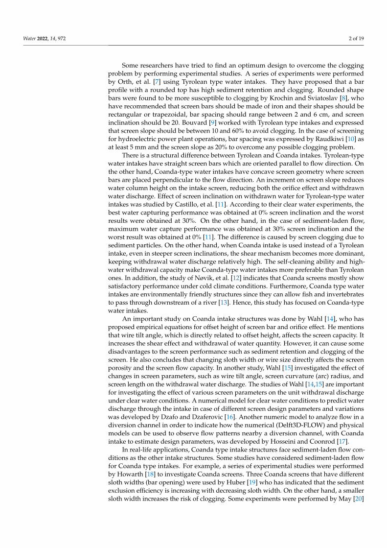
The experimental set-up and results were already presented by Hazar and Elci [21].Experiments were performed at IZTECH Hydraulics Laboratory in Izmir, Turkey (Figure 1).Six different Coanda screens having different properties were designed (Table 1). EachCoanda screen had total screen length of 100 cm, net screen length of 60 cm, and screenwidth of 40 cm.

Water 2022, 14, x FOR PEER REVIEW 4 of 20

Figure 1. Experimental setup utilizing different Coanda-type intakes in the experiments.

Table 1. Screen characteristics.

Screen Type Sloth Width (mm) Curvature Radius (mm) Void Ratio (e/a)

Coanda R800 (1) 1 800 0.046

Coanda R800 (2) 2 800 0.092

Coanda R800 (3) 3 800 0.138

Coanda R1200 (1) 1 1200 0.046

Coanda R1200 (2) 2 1200 0.092

Coanda R1600 (1) 1 1600 0.046

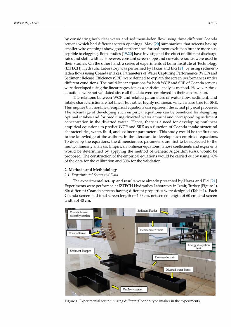
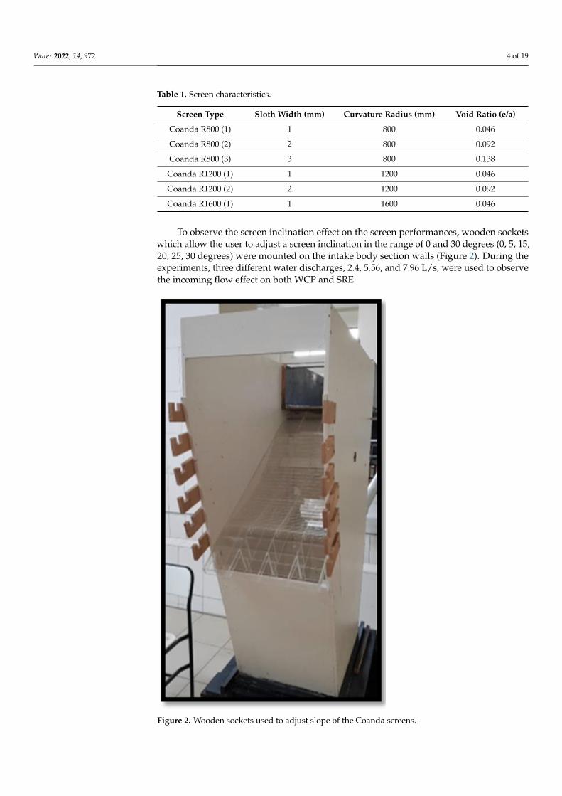
To observe the screen inclination effect on the screen performances, wooden sockets

which allow the user to adjust a screen inclination in the range of 0 and 30 degrees (0, 5,

15, 20, 25, 30 degrees) were mounted on the intake body section walls (Figure 2). During

the experiments, three different water discharges, 2.4, 5.56, and 7.96 l/s, were used to ob-

serve the incoming flow effect on both WCP and SRE.

Figure 1. Experimental setup utilizing different Coanda-type intakes in the experiments.

Water 2022, 14, 972 4 of 19

Table 1. Screen characteristics.

Screen Type Sloth Width (mm) Curvature Radius (mm) Void Ratio (e/a)

Coanda R800 (1) 1 800 0.046

Coanda R800 (2) 2 800 0.092

Coanda R800 (3) 3 800 0.138

Coanda R1200 (1) 1 1200 0.046

Coanda R1200 (2) 2 1200 0.092

Coanda R1600 (1) 1 1600 0.046

To observe the screen inclination effect on the screen performances, wooden socketswhich allow the user to adjust a screen inclination in the range of 0 and 30 degrees (0, 5, 15,20, 25, 30 degrees) were mounted on the intake body section walls (Figure 2). During theexperiments, three different water discharges, 2.4, 5.56, and 7.96 L/s, were used to observethe incoming flow effect on both WCP and SRE.

Water 2022, 14, x FOR PEER REVIEW 5 of 20

Figure 2. Wooden sockets used to adjust slope of the Coanda screens.

In the case of sediment-laden flow, a novel sediment feeder structure was designed

to allow a user to adjust sediment concentration during the experiments (Figure 3). Uni-

form sediment particles that had 0.8 mm diameter were used with 300, 695, and 995 g

amounts for 2.4, 5.56, and 7.96 L/s, respectively, to obtain the same sediment concentration

of 125 g/L for each discharge case.

There were 108 cases (6 different slopes × 6 different screens × 3 different flow dis-

charge) and each experiment was repeated three times, and an average value of WCP was

obtained for each experiment. Thus, in total, 108 × 3 = 324 experiments were carried out

and 108 average WCP values were used in the analysis. The similar procedure was also

applied to the SRE and 108 average SRE values were used in the analysis. Note that the

experiments for the WCP were done in clear water while the experiments for the SRE were

carried out in sediment-laden flows and thus they were totally different experiments. The

statistics of the measured WCP and SRE from all the experiments are summarized in Table

2. Details of the experimental setup and the experiments can be obtained from Hazar and

Elci [21].

Figure 2. Wooden sockets used to adjust slope of the Coanda screens.

Water 2022, 14, 972 5 of 19

In the case of sediment-laden flow, a novel sediment feeder structure was designed toallow a user to adjust sediment concentration during the experiments (Figure 3). Uniformsediment particles that had 0.8 mm diameter were used with 300, 695, and 995 g amountsfor 2.4, 5.56, and 7.96 L/s, respectively, to obtain the same sediment concentration of125 g/L for each discharge case.

Water 2022, 14, x FOR PEER REVIEW 6 of 20

Figure 3. Sediment feeder device.

Table 2. Statistical summary of data sets for WCP and SRE.

Data Sets WCP (Qin/Qdiv) SRE (Sin/Sre)

Maximum 100 90.4

Minimum 38.7 0.3

Range 61.3 90.0

Mean 70.3 52.7

St. Deviation 16.8 26.0

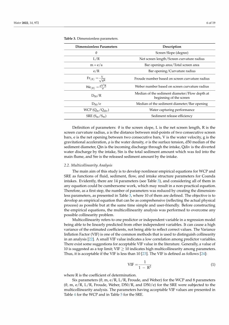
For developing the empirical equations, dimensionless parameters were developed,

as presented in Table 3.

Table 3. Dimensionless parameters.

Dimensionless Parameters Description

ϴ Screen Slope (degree)

L/R Net screen length/Screen curvature radius

m = e/a Bar openings area/Total screen area

e/R Bar opening/Curvature radius

Fr(R) = V

√gR Froude number based on screen curvature radius

We(R)=ρV2R

σ Weber number based on screen curvature radius

D50/R Median of the sediment diameter/Flow depth at beginning

of the screen

D50/e Median of the sediment diameter/Bar opening

WCP (Qin/Qdiv) Water capturing performance

SRE (Sin/Sre) Sediment release efficiency

Definition of parameters: ϴ is the screen slope, L is the net screen length, R is the

screen curvature radius, a is the distance between mid-points of two consecutive screen

Figure 3. Sediment feeder device.

There were 108 cases (6 different slopes × 6 different screens × 3 different flowdischarge) and each experiment was repeated three times, and an average value of WCPwas obtained for each experiment. Thus, in total, 108 × 3 = 324 experiments were carriedout and 108 average WCP values were used in the analysis. The similar procedure wasalso applied to the SRE and 108 average SRE values were used in the analysis. Note thatthe experiments for the WCP were done in clear water while the experiments for the SREwere carried out in sediment-laden flows and thus they were totally different experiments.The statistics of the measured WCP and SRE from all the experiments are summarized inTable 2. Details of the experimental setup and the experiments can be obtained from Hazarand Elci [21].

Table 2. Statistical summary of data sets for WCP and SRE.

Data Sets WCP (Qin/Qdiv) SRE (Sin/Sre)

Maximum 100 90.4

Minimum 38.7 0.3

Range 61.3 90.0

Mean 70.3 52.7

St. Deviation 16.8 26.0

For developing the empirical equations, dimensionless parameters were developed,as presented in Table 3.

Water 2022, 14, 972 6 of 19

Table 3. Dimensionless parameters.

Dimensionless Parameters Description

θ Screen Slope (degree)

L/R Net screen length/Screen curvature radius

m = e/a Bar openings area/Total screen area

e/R Bar opening/Curvature radius

Fr(R) =V√gR Froude number based on screen curvature radius

We(R) =ρV2Rσ

Weber number based on screen curvature radius

D50/R Median of the sediment diameter/Flow depth atbeginning of the screen

D50/e Median of the sediment diameter/Bar opening

WCP (Qin/Qdiv) Water capturing performance

SRE (Sin/Sre) Sediment release efficiency

Definition of parameters: θ is the screen slope, L is the net screen length, R is thescreen curvature radius, a is the distance between mid-points of two consecutive screenbars, e is the net opening between two consecutive bars, V is the water velocity, g is thegravitational acceleration, ρ is the water density, σ is the surface tension, d50 median of thesediment diameter, Qin is the incoming discharge through the intake, Qdiv is the divertedwater discharge by the intake, Sin is the total sediment amount which was fed into themain flume, and Sre is the released sediment amount by the intake.

2.2. Multicollinearity Analysis

The main aim of this study is to develop nonlinear empirical equations for WCP andSRE as functions of fluid, sediment, flow, and intake structure parameters for Coandaintakes. Evidently, there are 14 parameters (see Table 3), and considering all of them inany equation could be cumbersome work, which may result in a non-practical equation.Therefore, as a first step, the number of parameters was reduced by creating the dimension-less parameters, as presented in Table 3, where 10 of them are defined. The objective is todevelop an empirical equation that can be as comprehensive (reflecting the actual physicalprocess) as possible but at the same time simple and user-friendly. Before constructingthe empirical equations, the multicollinearity analysis was performed to overcome anypossible collinearity problem.

Multicollinearity refers to one predictor or independent variable in a regression modelbeing able to be linearly predicted from other independent variables. It can cause a highvariance of the estimated coefficients, not being able to reflect correct values. The VarianceInflation Factor (VIF) is one of the common methods that is used to distinguish collinearityin an analysis [22]. A small VIF value indicates a low correlation among predictor variables.There exist some suggestions for acceptable VIF value in the literature. Generally, a value of10 is suggested as a top limit; VIF ≥ 10 indicates high multicollinearity among parameters.Thus, it is acceptable if the VIF is less than 10 [23]. The VIF is defined as follows [24]:

VIF =1

1 − R2 (1)

where R is the coefficient of determination.Six parameters (θ, m, e/R, L/R, Froude, and Weber) for the WCP and 8 parameters

(θ, m, e/R, L/R, Froude, Weber, D50/R, and D50/e) for the SRE were subjected to themulticollinearity analysis. The parameters having acceptable VIF values are presented inTable 4 for the WCP and in Table 5 for the SRE.

Water 2022, 14, 972 7 of 19

Table 4. Independent parameters and VIF values for WCP.

Independent Parameters VIF Value

θ (Screen Slope) 1.00m = (e/a) 1.18

L/R 6.67Froude 5.56Weber 6.25

Table 5. Independent parameters and VIF values for SRE.

Independent Parameters VIF Value

θ (Screen Slope) 1.00L/R 5.88

Froude 5.88Weber 6.25D50/e 1.11

2.3. Genetic Algorithm (GA)

Genetic Algorithm is a nonlinear search and optimization method, inspired by bio-logical processes of natural selection and survival of the fittest. GA has two main unitsas gene and chromosome. A gene consists of bits and a chromosome consists of genes.The gene represents a model parameter to be optimized and each chromosome stands fora solution candidate. In GA, the search process is initiated with many chromosomes. Ineach iteration, search space is scanned by the chromosomes, while the fitness evaluation,selection, pairing, crossover, and mutation operations are performed. Figure 4 showsthe flowchart summarizing the GA operations. There are innumerous studies (papersand books) available in the literature, including [25], on the details of the GAs and theiroperations, and GA applications in water resources engineering.

Water 2022, 14, x FOR PEER REVIEW 8 of 20

Table 5. Independent parameters and VIF values for SRE.

Independent Parameters VIF Value

ϴ (Screen Slope) 1.00

L/R 5.88

Froude 5.88

Weber 6.25

D50/e 1.11

2.3. Genetic Algorithm (GA)

Genetic Algorithm is a nonlinear search and optimization method, inspired by bio-

logical processes of natural selection and survival of the fittest. GA has two main units as

gene and chromosome. A gene consists of bits and a chromosome consists of genes. The

gene represents a model parameter to be optimized and each chromosome stands for a

solution candidate. In GA, the search process is initiated with many chromosomes. In each

iteration, search space is scanned by the chromosomes, while the fitness evaluation, selec-

tion, pairing, crossover, and mutation operations are performed. Figure 4 shows the

flowchart summarizing the GA operations. There are innumerous studies (papers and

books) available in the literature, including [25], on the details of the GAs and their oper-

ations, and GA applications in water resources engineering.

Figure 4. Flow chart for Genetic Algorithm operations.

2.4. Artificial Neural Networks (ANNs)

Artificial Neural Networks were employed in this study to compare the prediction

performance against the empirical equations. ANNs have been developed as analogies to

the human brain system, consisting of many artificial neurons, with connection links and

Forming initial gene pool

(Randomly generating chromosomes)

Evaluating fitness of each chromosome

(Determining fitness value by inserting each chromosome to objective function)

Selection

(Selecting fit chromosomes and eliminating weak ones)

Cross-over

(Exchanging genes of parent chromosomes to generate new offspring)

Mutation(Generating newer offspring and preventing getting trapped into local minimum)

Figure 4. Flow chart for Genetic Algorithm operations.

Water 2022, 14, 972 8 of 19

2.4. Artificial Neural Networks (ANNs)

Artificial Neural Networks were employed in this study to compare the prediction per-formance against the empirical equations. ANNs have been developed as analogies to thehuman brain system, consisting of many artificial neurons, with connection links and layersthat, as a whole system, can learn from experience and experiments and store information.

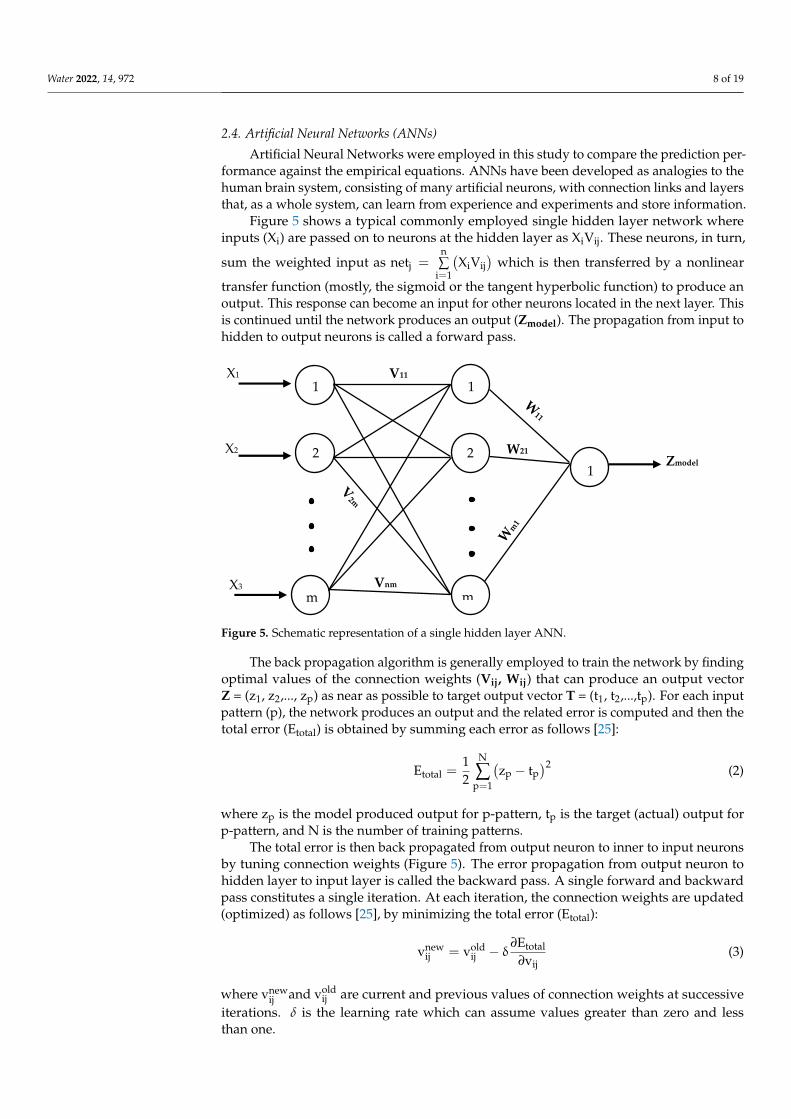
Figure 5 shows a typical commonly employed single hidden layer network whereinputs (Xi) are passed on to neurons at the hidden layer as XiVij. These neurons, in turn,

sum the weighted input as netj =n∑

i=1

(XiVij

)which is then transferred by a nonlinear

transfer function (mostly, the sigmoid or the tangent hyperbolic function) to produce anoutput. This response can become an input for other neurons located in the next layer. Thisis continued until the network produces an output (Zmodel). The propagation from input tohidden to output neurons is called a forward pass.

Water 2022, 14, x FOR PEER REVIEW 9 of 20

layers that, as a whole system, can learn from experience and experiments and store in-

formation.

Figure 5 shows a typical commonly employed single hidden layer network where

inputs (Xi) are passed on to neurons at the hidden layer as XiVij. These neurons, in turn,

sum the weighted input as netj = ∑ (XiVij)ni=1 which is then transferred by a nonlinear

transfer function (mostly, the sigmoid or the tangent hyperbolic function) to produce an

output. This response can become an input for other neurons located in the next layer.

This is continued until the network produces an output (Zmodel). The propagation from

input to hidden to output neurons is called a forward pass.

The back propagation algorithm is generally employed to train the network by find-

ing optimal values of the connection weights (Vij, Wij) that can produce an output vector

Z= (z1, z2,..., zp) as near as possible to target output vector T = (t1, t2,...,tp). For each input

pattern (p), the network produces an output and the related error is computed and then

the total error (Etotal) is obtained by summing each error as follows [25]:

Etotal =1

2∑(zp − tp)

2N

p=1

(2)

where zp is the model produced output for p-pattern, tp is the target (actual) output for p-

pattern, and N is the number of training patterns.

Figure 5. Schematic representation of a single hidden layer ANN.

The total error is then back propagated from output neuron to inner to input neurons

by tuning connection weights (Figure 5). The error propagation from output neuron to

hidden layer to input layer is called the backward pass. A single forward and backward

pass constitutes a single iteration. At each iteration, the connection weights are updated

(optimized) as follows [25], by minimizing the total error (Etotal):

vijnew = vij

old − δ∂Etotal

∂vij (3)

where vijnewand vij

old are current and previous values of connection weights at successive

iterations. δ is the learning rate which can assume values greater than zero and less than

one.

As the iterations are continued, the total error is expected to decrease. There are in-

numerous studies (papers and books) available in the literature, including, [25], on the

1

2

m

1

2

m

1 X1

X2

X3

V11

W21 Zmodel

Vnm

Figure 5. Schematic representation of a single hidden layer ANN.

The back propagation algorithm is generally employed to train the network by findingoptimal values of the connection weights (Vij, Wij) that can produce an output vectorZ = (z1, z2,..., zp) as near as possible to target output vector T = (t1, t2,...,tp). For each inputpattern (p), the network produces an output and the related error is computed and then thetotal error (Etotal) is obtained by summing each error as follows [25]:

Etotal =12

N

∑p=1

(zp − tp

)2 (2)

where zp is the model produced output for p-pattern, tp is the target (actual) output forp-pattern, and N is the number of training patterns.

The total error is then back propagated from output neuron to inner to input neuronsby tuning connection weights (Figure 5). The error propagation from output neuron tohidden layer to input layer is called the backward pass. A single forward and backwardpass constitutes a single iteration. At each iteration, the connection weights are updated(optimized) as follows [25], by minimizing the total error (Etotal):

vnewij = vold

ij − δ∂Etotal

∂vij(3)

where vnewij and vold

ij are current and previous values of connection weights at successiveiterations. δ is the learning rate which can assume values greater than zero and lessthan one.

Water 2022, 14, 972 9 of 19

As the iterations are continued, the total error is expected to decrease. There areinnumerous studies (papers and books) available in the literature, including, [25], on thedetails of the feed forward networks, the back propagation algorithm, the network trainingand testing, and ANN applications in water resources engineering.

2.5. Constructing Empirical Equations

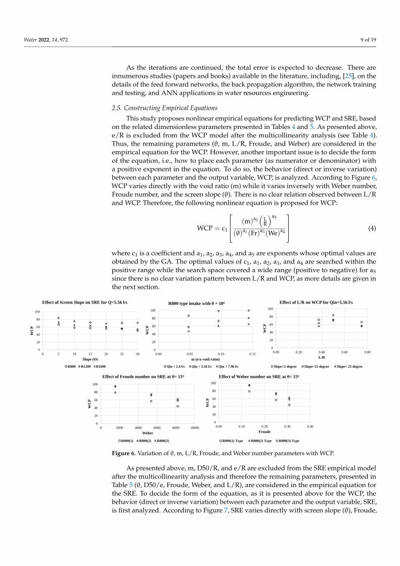
This study proposes nonlinear empirical equations for predicting WCP and SRE, basedon the related dimensionless parameters presented in Tables 4 and 5. As presented above,e/R is excluded from the WCP model after the multicollinearity analysis (see Table 4).Thus, the remaining parameters (θ, m, L/R, Froude, and Weber) are considered in theempirical equation for the WCP. However, another important issue is to decide the formof the equation, i.e., how to place each parameter (as numerator or denominator) witha positive exponent in the equation. To do so, the behavior (direct or inverse variation)between each parameter and the output variable, WCP, is analyzed. According to Figure 6,WCP varies directly with the void ratio (m) while it varies inversely with Weber number,Froude number, and the screen slope (θ). There is no clear relation observed between L/Rand WCP. Therefore, the following nonlinear equation is proposed for WCP:

WCP = c1

(m)a2(

LR

)a5

(θ)a1(Fr)a3(We)a4

(4)

where c1 is a coefficient and a1, a2, a3, a4, and a5 are exponents whose optimal values areobtained by the GA. The optimal values of c1, a1, a2, a3, and a4 are searched within thepositive range while the search space covered a wide range (positive to negative) for a5since there is no clear variation pattern between L/R and WCP, as more details are given inthe next section.

Water 2022, 14, x FOR PEER REVIEW 10 of 20

details of the feed forward networks, the back propagation algorithm, the network train-

ing and testing, and ANN applications in water resources engineering.

2.5. Constructing Empirical Equations

This study proposes nonlinear empirical equations for predicting WCP and SRE,

based on the related dimensionless parameters presented in Tables 4 and 5. As presented

above, e/R is excluded from the WCP model after the multicollinearity analysis (see Table

4). Thus, the remaining parameters (ϴ, m, L/R, Froude, and Weber) are considered in the

empirical equation for the WCP. However, another important issue is to decide the form

of the equation, i.e., how to place each parameter (as numerator or denominator) with a

positive exponent in the equation. To do so, the behavior (direct or inverse variation) be-

tween each parameter and the output variable, WCP, is analyzed. According to Figure 6,

WCP varies directly with the void ratio (m) while it varies inversely with Weber number,

Froude number, and the screen slope (ϴ). There is no clear relation observed between L/R

and WCP. Therefore, the following nonlinear equation is proposed for WCP:

WCP = c1 [(m)a2 (

LR

)a5

(θ)a1(Fr)a3(We)a4] (4)

where c1 is a coefficient and a1, a2, a3, a4, and a5 are exponents whose optimal values are

obtained by the GA. The optimal values of c1, a1, a2, a3, and a4 are searched within the

positive range while the search space covered a wide range (positive to negative) for a5

since there is no clear variation pattern between L/R and WCP, as more details are given

in the next section.

Figure 6. Variation of ϴ, m, L/R, Froude, and Weber number parameters with WCP.

As presented above, m, D50/R, and e/R are excluded from the SRE empirical model

after the multicollinearity analysis and therefore the remaining parameters, presented in

Table 5 (ϴ, D50/e, Froude, Weber, and L/R), are considered in the empirical equation for

the SRE. To decide the form of the equation, as it is presented above for the WCP, the

behavior (direct or inverse variation) between each parameter and the output variable,

SRE, is first analyzed. According to Figure 7, SRE varies directly with screen slope (ϴ),

Froude, and Weber. There is no clear variation behavior observed for L/R and D50/e.

Hence, the following nonlinear empirical equation is proposed for the SRE:

0

20

40

60

80

100

0.00 0.05 0.10 0.15

WC

P

m (e/a void ratio)

R800 type intake with θ = 10o

Qin = 2.4 l/s Qin = 5.56 l/s Qin = 7.96 l/s

0

20

40

60

80

100

0 5 10 15 20 25 30

WC

P

Slope (ϴ)

Effect of Screen Slope on SRE for Q=5.56 l/s

R800 R1200 R1600

0

20

40

60

80

100

0.00 0.10 0.20 0.30 0.40

WC

P

Froude

Effect of Weber number on SRE at θ= 15o

R800(1) Type R800(2) Type R800(3) Type

0

20

40

60

80

100

0.00 0.20 0.40 0.60 0.80

WC

P

L/R

Effect of L/R on WCP for Qin=5.56 l/s

Slope=5 degree Slope=15 degree Slope= 25 degree

0

20

40

60

80

100

0 2000 4000 6000 8000 10000

WC

P

Weber

Effect of Froude number on SRE at θ= 15o

R800(1) R800(2) R800(3)

Figure 6. Variation of θ, m, L/R, Froude, and Weber number parameters with WCP.

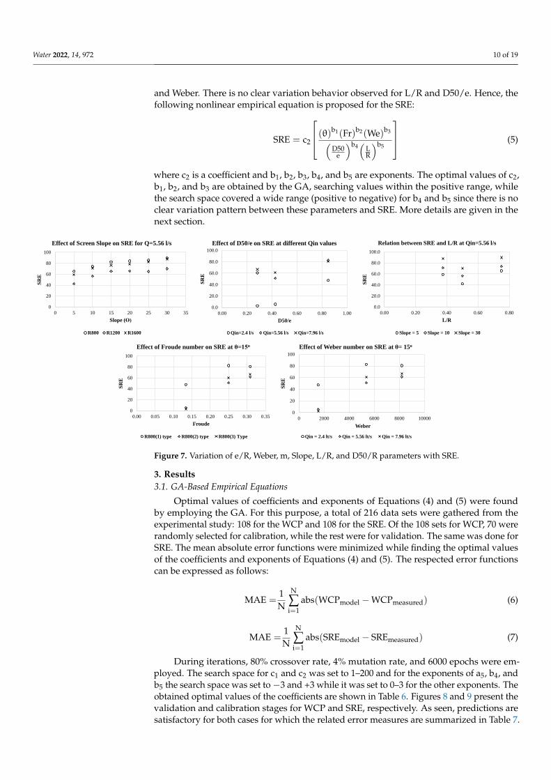
As presented above, m, D50/R, and e/R are excluded from the SRE empirical modelafter the multicollinearity analysis and therefore the remaining parameters, presented inTable 5 (θ, D50/e, Froude, Weber, and L/R), are considered in the empirical equation forthe SRE. To decide the form of the equation, as it is presented above for the WCP, thebehavior (direct or inverse variation) between each parameter and the output variable, SRE,is first analyzed. According to Figure 7, SRE varies directly with screen slope (θ), Froude,

Water 2022, 14, 972 10 of 19

and Weber. There is no clear variation behavior observed for L/R and D50/e. Hence, thefollowing nonlinear empirical equation is proposed for the SRE:

SRE = c2

(θ)b1(Fr)b2(We)b3(D50

e

)b4(

LR

)b5

(5)

where c2 is a coefficient and b1, b2, b3, b4, and b5 are exponents. The optimal values of c2,b1, b2, and b3 are obtained by the GA, searching values within the positive range, whilethe search space covered a wide range (positive to negative) for b4 and b5 since there is noclear variation pattern between these parameters and SRE. More details are given in thenext section.

Water 2022, 14, x FOR PEER REVIEW 11 of 20

SRE = c2 [(θ)b1(Fr)b2(We)b3

(D50

e)

b4

(LR

)b5

] (5)

where c2 is a coefficient and b1, b2, b3, b4, and b5 are exponents. The optimal values of c2,

b1, b2, and b3 are obtained by the GA, searching values within the positive range, while the

search space covered a wide range (positive to negative) for b4 and b5 since there is no

clear variation pattern between these parameters and SRE. More details are given in the

next section.

Figure 7. Variation of e/R, Weber, m, Slope, L/R, and D50/R parameters with SRE.

3. Results

3.1. GA-Based Empirical Equations

Optimal values of coefficients and exponents of Equations (4) and (5) were found by

employing the GA. For this purpose, a total of 216 data sets were gathered from the ex-

perimental study: 108 for the WCP and 108 for the SRE. Of the 108 sets for WCP, 70 were

randomly selected for calibration, while the rest were for validation. The same was done

for SRE. The mean absolute error functions were minimized while finding the optimal

values of the coefficients and exponents of Equations (4) and (5). The respected error func-

tions can be expressed as follows:

MAE =1

N∑ abs(WCPmodel − WCPmeasured)

N

i=1

(6)

MAE =1

N∑ abs(SREmodel − SREmeasured)

N

i=1

(7)

During iterations, 80% crossover rate, 4% mutation rate, and 6000 epochs were em-

ployed. The search space for c1 and c2 was set to 1–200 and for the exponents of a5, b4, and

b5 the search space was set to −3 and +3 while it was set to 0–3 for the other exponents.

The obtained optimal values of the coefficients are shown in Table 6. Figures 8 and 9 pre-

sent the validation and calibration stages for WCP and SRE, respectively. As seen, predic-

tions are satisfactory for both cases for which the related error measures are summarized

in Table 7.

0

20

40

60

80

100

0 2000 4000 6000 8000 10000

SR

E

Weber

Effect of Weber number on SRE at θ= 15o

Qin = 2.4 lt/s Qin = 5.56 lt/s Qin = 7.96 lt/s

0

20

40

60

80

100

0 5 10 15 20 25 30 35

SR

E

Slope (ϴ)

Effect of Screen Slope on SRE for Q=5.56 l/s

R800 R1200 R1600

0.0

20.0

40.0

60.0

80.0

100.0

0.00 0.20 0.40 0.60 0.80

SR

E

L/R

Relation between SRE and L/R at Qin=5.56 l/s

Slope = 5 Slope = 10 Slope = 30

0

20

40

60

80

100

0.00 0.05 0.10 0.15 0.20 0.25 0.30 0.35

SR

E

Froude

Effect of Froude number on SRE at θ=15o

R800(1) type R800(2) type R800(3) Type

0.0

20.0

40.0

60.0

80.0

100.0

0.00 0.20 0.40 0.60 0.80 1.00

SR

E

D50/e

Effect of D50/e on SRE at different Qin values

Qin=2.4 l/s Qin=5.56 l/s Qin=7.96 l/s

Figure 7. Variation of e/R, Weber, m, Slope, L/R, and D50/R parameters with SRE.

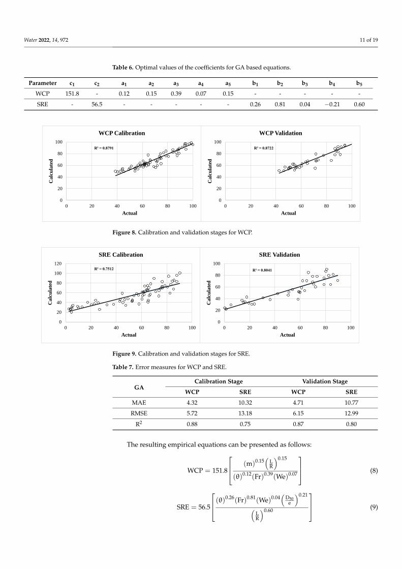
3. Results3.1. GA-Based Empirical Equations

Optimal values of coefficients and exponents of Equations (4) and (5) were foundby employing the GA. For this purpose, a total of 216 data sets were gathered from theexperimental study: 108 for the WCP and 108 for the SRE. Of the 108 sets for WCP, 70 wererandomly selected for calibration, while the rest were for validation. The same was done forSRE. The mean absolute error functions were minimized while finding the optimal valuesof the coefficients and exponents of Equations (4) and (5). The respected error functionscan be expressed as follows:

MAE =1N

N

∑i=1

abs(WCPmodel −WCPmeasured) (6)

MAE =1N

N

∑i=1

abs(SREmodel − SREmeasured) (7)

During iterations, 80% crossover rate, 4% mutation rate, and 6000 epochs were em-ployed. The search space for c1 and c2 was set to 1–200 and for the exponents of a5, b4, andb5 the search space was set to−3 and +3 while it was set to 0–3 for the other exponents. Theobtained optimal values of the coefficients are shown in Table 6. Figures 8 and 9 present thevalidation and calibration stages for WCP and SRE, respectively. As seen, predictions aresatisfactory for both cases for which the related error measures are summarized in Table 7.

Water 2022, 14, 972 11 of 19

Table 6. Optimal values of the coefficients for GA based equations.

Parameter c1 c2 a1 a2 a3 a4 a5 b1 b2 b3 b4 b5

WCP 151.8 - 0.12 0.15 0.39 0.07 0.15 - - - - -

SRE - 56.5 - - - - - 0.26 0.81 0.04 −0.21 0.60

Water 2022, 14, x FOR PEER REVIEW 12 of 20

Table 6. Optimal values of the coefficients for GA based equations.

Parameter c1 c2 a1 a2 a3 a4 a5 b1 b2 b3 b4 b5

WCP 151.8 - 0.12 0.15 0.39 0.07 0.15 - - - - -

SRE - 56.5 - - - - - 0.26 0.81 0.04 −0.21 0.60

Figure 8. Calibration and validation stages for WCP.

Figure 9. Calibration and validation stages for SRE.

Table 7. Error measures for WCP and SRE.

GA Calibration Stage Validation Stage

WCP SRE WCP SRE

MAE 4.32 10.32 4.71 10.77

RMSE 5.72 13.18 6.15 12.99

R2 0.88 0.75 0.87 0.80

The resulting empirical equations can be presented as follows:

WCP = 151.8 [(m)0.15 (

LR

)0.15

(θ)0.12(Fr)0.39(We)0.07] (8)

SRE = 56.5 [(θ)0.26(Fr)0.81(We)0.04 (

D50

e)

0.21

(LR

)0.60 ] (9)

R² = 0.8791

0

20

40

60

80

100

0 20 40 60 80 100

Ca

lcu

late

d

Actual

WCP Calibration

R² = 0.8722

0

20

40

60

80

100

0 20 40 60 80 100C

alc

ula

ted

Actual

WCP Validation

R² = 0.7512

0

20

40

60

80

100

120

0 20 40 60 80 100

Ca

lcu

late

d

Actual

SRE Calibration

R² = 0.8041

0

20

40

60

80

100

0 20 40 60 80 100

Ca

lcu

late

d

Actual

SRE Validation

Figure 8. Calibration and validation stages for WCP.

Water 2022, 14, x FOR PEER REVIEW 12 of 20

Table 6. Optimal values of the coefficients for GA based equations.

Parameter c1 c2 a1 a2 a3 a4 a5 b1 b2 b3 b4 b5

WCP 151.8 - 0.12 0.15 0.39 0.07 0.15 - - - - -

SRE - 56.5 - - - - - 0.26 0.81 0.04 −0.21 0.60

Figure 8. Calibration and validation stages for WCP.

Figure 9. Calibration and validation stages for SRE.

Table 7. Error measures for WCP and SRE.

GA Calibration Stage Validation Stage

WCP SRE WCP SRE

MAE 4.32 10.32 4.71 10.77

RMSE 5.72 13.18 6.15 12.99

R2 0.88 0.75 0.87 0.80

The resulting empirical equations can be presented as follows:

WCP = 151.8 [(m)0.15 (

LR

)0.15

(θ)0.12(Fr)0.39(We)0.07] (8)

SRE = 56.5 [(θ)0.26(Fr)0.81(We)0.04 (

D50

e)

0.21

(LR

)0.60 ] (9)

R² = 0.8791

0

20

40

60

80

100

0 20 40 60 80 100

Ca

lcu

late

d

Actual

WCP Calibration

R² = 0.8722

0

20

40

60

80

100

0 20 40 60 80 100C

alc

ula

ted

Actual

WCP Validation

R² = 0.7512

0

20

40

60

80

100

120

0 20 40 60 80 100

Ca

lcu

late

d

Actual

SRE Calibration

R² = 0.8041

0

20

40

60

80

100

0 20 40 60 80 100

Ca

lcu

late

d

Actual

SRE Validation

Figure 9. Calibration and validation stages for SRE.

Table 7. Error measures for WCP and SRE.

GACalibration Stage Validation Stage

WCP SRE WCP SRE

MAE 4.32 10.32 4.71 10.77

RMSE 5.72 13.18 6.15 12.99

R2 0.88 0.75 0.87 0.80

The resulting empirical equations can be presented as follows:

WCP = 151.8

(m)0.15(

LR

)0.15

(θ)0.12(Fr)0.39(We)0.07

(8)

SRE = 56.5

(θ)0.26(Fr)0.81(We)0.04(

D50e

)0.21

(LR

)0.60

(9)

Water 2022, 14, 972 12 of 19

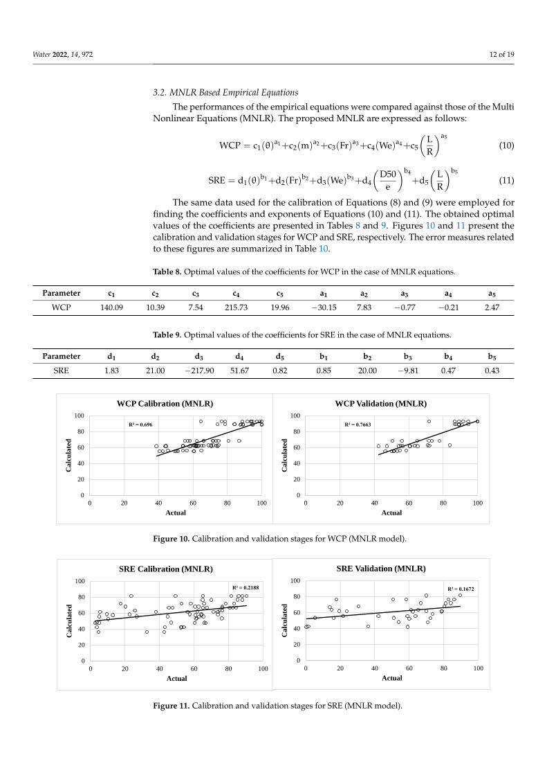
3.2. MNLR Based Empirical Equations

The performances of the empirical equations were compared against those of the MultiNonlinear Equations (MNLR). The proposed MNLR are expressed as follows:

WCP = c1(θ)a1+c2(m)a2+c3(Fr)a3+c4(We)a4+c5

(LR

)a5

(10)

SRE = d1(θ)b1+d2(Fr)b2+d3(We)b3+d4

(D50

e

)b4

+d5

(LR

)b5

(11)

The same data used for the calibration of Equations (8) and (9) were employed forfinding the coefficients and exponents of Equations (10) and (11). The obtained optimalvalues of the coefficients are presented in Tables 8 and 9. Figures 10 and 11 present thecalibration and validation stages for WCP and SRE, respectively. The error measures relatedto these figures are summarized in Table 10.

Table 8. Optimal values of the coefficients for WCP in the case of MNLR equations.

Parameter c1 c2 c3 c4 c5 a1 a2 a3 a4 a5

WCP 140.09 10.39 7.54 215.73 19.96 −30.15 7.83 −0.77 −0.21 2.47

Table 9. Optimal values of the coefficients for SRE in the case of MNLR equations.

Parameter d1 d2 d3 d4 d5 b1 b2 b3 b4 b5

SRE 1.83 21.00 −217.90 51.67 0.82 0.85 20.00 −9.81 0.47 0.43

Water 2022, 14, x FOR PEER REVIEW 13 of 20

3.2. MNLR Based Empirical Equations

The performances of the empirical equations were compared against those of the

Multi Nonlinear Equations (MNLR). The proposed MNLR are expressed as follows:

WCP = c1(θ)a1+ c2(m)a2 + c3(Fr)a3 + c4(We)a4 + c5 (L

R)

a5

(10)

SRE=d1(θ)b1+d2(Fr)b2+d3(We)b3+d4 (D50

e)

b4

+d5 (L

R)

b5

(11)

The same data used for the calibration of Equations (8) and (9) were employed for

finding the coefficients and exponents of Equations (10) and (11). The obtained optimal

values of the coefficients are presented in Tables 8 and 9. Figures 10 and 11 present the

calibration and validation stages for WCP and SRE, respectively. The error measures re-

lated to these figures are summarized in Table 10.

Table 8. Optimal values of the coefficients for WCP in the case of MNLR equations.

Parameter c1 c2 c3 c4 c5 a1 a2 a3 a4 a5

WCP 140.09 10.39 7.54 215.73 19.96 −30.15 7.83 −0.77 −0.21 2.47

Table 9. Optimal values of the coefficients for SRE in the case of MNLR equations.

Parameter d1 d2 d3 d4 d5 b1 b2 b3 b4 b5

SRE 1.83 21.00 −217.90 51.67 0.82 0.85 20.00 −9.81 0.47 0.43

Figure 10. Calibration and validation stages for WCP (MNLR model).

Figure 11. Calibration and validation stages for SRE (MNLR model).

R² = 0.696

0

20

40

60

80

100

0 20 40 60 80 100

Ca

lcu

late

d

Actual

WCP Calibration (MNLR)

R² = 0.7663

0

20

40

60

80

100

0 20 40 60 80 100

Ca

lcu

late

d

Actual

WCP Validation (MNLR)

R² = 0.2188

0

20

40

60

80

100

0 20 40 60 80 100

Ca

lcu

late

d

Actual

SRE Calibration (MNLR)

R² = 0.1672

0

20

40

60

80

100

0 20 40 60 80 100

Ca

lcu

late

d

Actual

SRE Validation (MNLR)

Figure 10. Calibration and validation stages for WCP (MNLR model).

Water 2022, 14, x FOR PEER REVIEW 13 of 20

3.2. MNLR Based Empirical Equations

The performances of the empirical equations were compared against those of the

Multi Nonlinear Equations (MNLR). The proposed MNLR are expressed as follows:

WCP = c1(θ)a1+ c2(m)a2 + c3(Fr)a3 + c4(We)a4 + c5 (L

R)

a5

(10)

SRE=d1(θ)b1+d2(Fr)b2+d3(We)b3+d4 (D50

e)

b4

+d5 (L

R)

b5

(11)

The same data used for the calibration of Equations (8) and (9) were employed for

finding the coefficients and exponents of Equations (10) and (11). The obtained optimal

values of the coefficients are presented in Tables 8 and 9. Figures 10 and 11 present the

calibration and validation stages for WCP and SRE, respectively. The error measures re-

lated to these figures are summarized in Table 10.

Table 8. Optimal values of the coefficients for WCP in the case of MNLR equations.

Parameter c1 c2 c3 c4 c5 a1 a2 a3 a4 a5

WCP 140.09 10.39 7.54 215.73 19.96 −30.15 7.83 −0.77 −0.21 2.47

Table 9. Optimal values of the coefficients for SRE in the case of MNLR equations.

Parameter d1 d2 d3 d4 d5 b1 b2 b3 b4 b5

SRE 1.83 21.00 −217.90 51.67 0.82 0.85 20.00 −9.81 0.47 0.43

Figure 10. Calibration and validation stages for WCP (MNLR model).

Figure 11. Calibration and validation stages for SRE (MNLR model).

R² = 0.696

0

20

40

60

80

100

0 20 40 60 80 100

Ca

lcu

late

d

Actual

WCP Calibration (MNLR)

R² = 0.7663

0

20

40

60

80

100

0 20 40 60 80 100

Ca

lcu

late

d

Actual

WCP Validation (MNLR)

R² = 0.2188

0

20

40

60

80

100

0 20 40 60 80 100

Ca

lcu

late

d

Actual

SRE Calibration (MNLR)

R² = 0.1672

0

20

40

60

80

100

0 20 40 60 80 100

Ca

lcu

late

d

Actual

SRE Validation (MNLR)

Figure 11. Calibration and validation stages for SRE (MNLR model).

Water 2022, 14, 972 13 of 19

Table 10. Error measures for WCP and SRE.

MNLRCalibration Stage Validation Stage

WCP SRE WCP SRE

MAE 6.95 18.04 6.28 20.14

RMSE 9.12 24.00 8.48 25.98

R2 0.70 0.22 0.77 0.17

The obtained MLNR equations can be expressed as follows:

WCP = 140.09(θ)−30.15 +10.39(m)7.83+7.54(Fr)−0.77+215.73(We)−0.21+19.96(

LR

)2.47(12)

SRE = 1.83(θ)0.85+21(Fr)20 − 217.9(We)−9.81+51.67(

D50e

)0.47+0.82

(LR

)0.43(13)

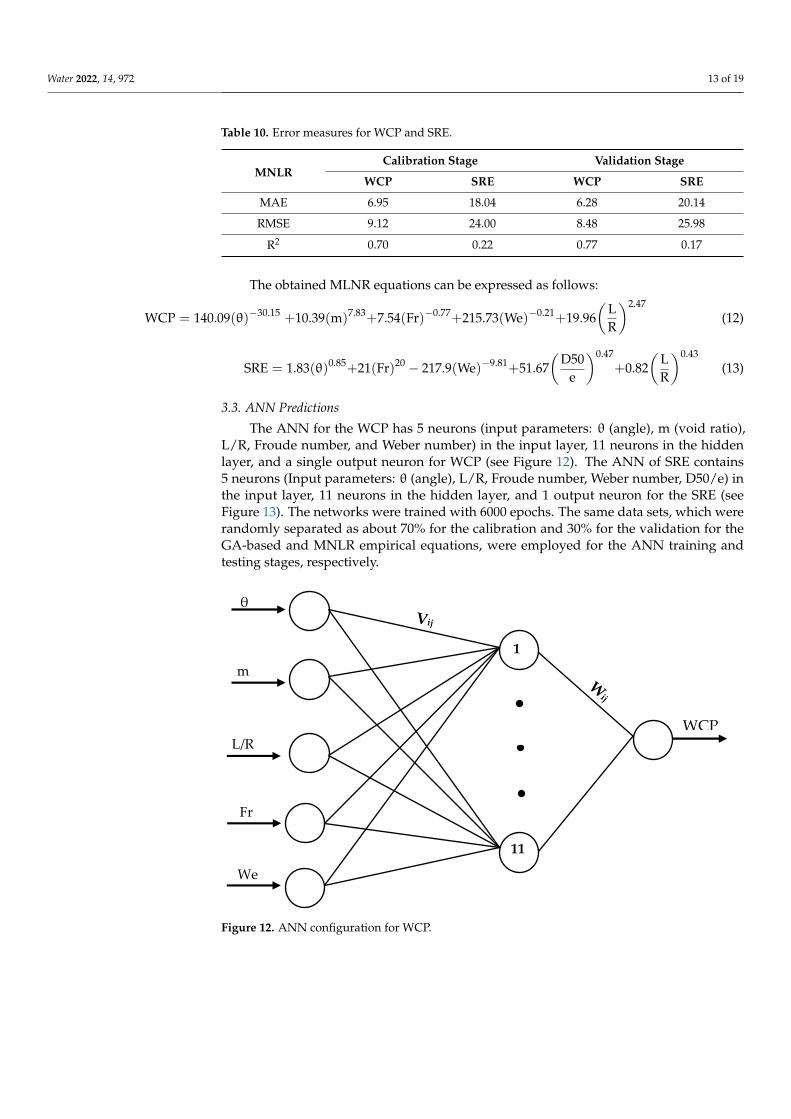
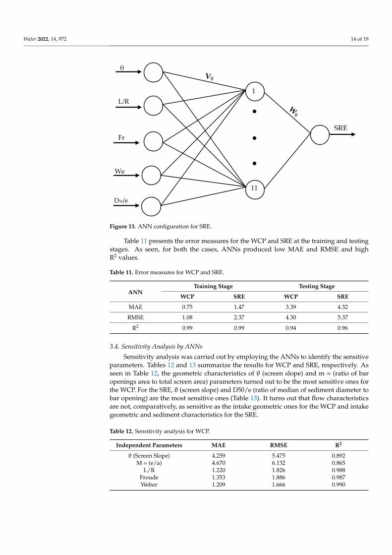
3.3. ANN Predictions

The ANN for the WCP has 5 neurons (input parameters: θ (angle), m (void ratio),L/R, Froude number, and Weber number) in the input layer, 11 neurons in the hiddenlayer, and a single output neuron for WCP (see Figure 12). The ANN of SRE contains5 neurons (Input parameters: θ (angle), L/R, Froude number, Weber number, D50/e) inthe input layer, 11 neurons in the hidden layer, and 1 output neuron for the SRE (seeFigure 13). The networks were trained with 6000 epochs. The same data sets, which wererandomly separated as about 70% for the calibration and 30% for the validation for theGA-based and MNLR empirical equations, were employed for the ANN training andtesting stages, respectively.

Water 2022, 14, x FOR PEER REVIEW 14 of 20

Table 10. Error measures for WCP and SRE.

MNLR Calibration Stage Validation Stage

WCP SRE WCP SRE

MAE 6.95 18.04 6.28 20.14

RMSE 9.12 24.00 8.48 25.98

R2 0.70 0.22 0.77 0.17

The obtained MLNR equations can be expressed as follows:

WCP = 140.09(ϴ)-30.15 + 10.39(m)7.83 + 7.54(Fr)−0.77 + 215.73(We)−0.21 + 19.96 (L

R)

2.47

(12)

SRE = 1.83(θ)0.85 + 21(Fr)20 − 217.9(We)−9.81 + 51.67 (D50

e)

0.47

+ 0.82 (L

R)

0.43

(13)

3.3. ANN Predictions

The ANN for the WCP has 5 neurons (input parameters: ϴ (angle), m (void ratio),

L/R, Froude number, and Weber number) in the input layer, 11 neurons in the hidden

layer, and a single output neuron for WCP (see Figure 12). The ANN of SRE contains 5

neurons (Input parameters: ϴ (angle), L/R, Froude number, Weber number, D50/e) in the

input layer, 11 neurons in the hidden layer, and 1 output neuron for the SRE (see Figure

13). The networks were trained with 6000 epochs. The same data sets, which were ran-

domly separated as about 70% for the calibration and 30% for the validation for the GA-

based and MNLR empirical equations, were employed for the ANN training and testing

stages, respectively.

Figure 12. ANN configuration for WCP.

θ

m

L/R

Fr

We

1

11

WCP

Figure 12. ANN configuration for WCP.

Water 2022, 14, 972 14 of 19Water 2022, 14, x FOR PEER REVIEW 15 of 20

Figure 13. ANN configuration for SRE.

Table 11 presents the error measures for the WCP and SRE at the training and testing

stages. As seen, for both the cases, ANNs produced low MAE and RMSE and high R2

values.

Table 11. Error measures for WCP and SRE.

ANN Training Stage Testing Stage

WCP SRE WCP SRE

MAE 0.75 1.47 3.39 4.32

RMSE 1.08 2.37 4.30 5.37

R2 0.99 0.99 0.94 0.96

3.4. Sensitivity Analysis by ANNs

Sensitivity analysis was carried out by employing the ANNs to identify the sensitive

parameters. Tables 12 and 13 summarize the results for WCP and SRE, respectively. As

seen in Table 12, the geometric characteristics of θ (screen slope) and m = (ratio of bar

openings area to total screen area) parameters turned out to be the most sensitive ones for

the WCP. For the SRE, θ (screen slope) and D50/e (ratio of median of sediment diameter

to bar opening) are the most sensitive ones (Table 13). It turns out that flow characteristics

are not, comparatively, as sensitive as the intake geometric ones for the WCP and intake

geometric and sediment characteristics for the SRE.

Table 12. Sensitivity analysis for WCP.

Independent Parameters MAE RMSE R2

θ (Screen Slope) 4.259 5.475 0.892

M = (e/a) 4.670 6.132 0.865

L/R 1.220 1.826 0.988

Froude 1.353 1.886 0.987

Weber 1.209 1.666 0.990

θ

L/R

Fr

We

1

11

SRE

D50/e

Figure 13. ANN configuration for SRE.

Table 11 presents the error measures for the WCP and SRE at the training and testingstages. As seen, for both the cases, ANNs produced low MAE and RMSE and highR2 values.

Table 11. Error measures for WCP and SRE.

ANNTraining Stage Testing Stage

WCP SRE WCP SRE

MAE 0.75 1.47 3.39 4.32

RMSE 1.08 2.37 4.30 5.37

R2 0.99 0.99 0.94 0.96

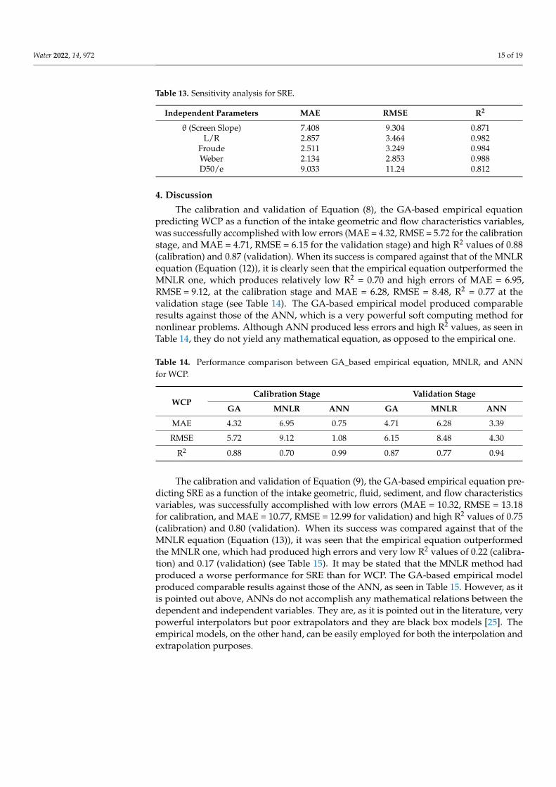
3.4. Sensitivity Analysis by ANNs

Sensitivity analysis was carried out by employing the ANNs to identify the sensitiveparameters. Tables 12 and 13 summarize the results for WCP and SRE, respectively. Asseen in Table 12, the geometric characteristics of θ (screen slope) and m = (ratio of baropenings area to total screen area) parameters turned out to be the most sensitive ones forthe WCP. For the SRE, θ (screen slope) and D50/e (ratio of median of sediment diameter tobar opening) are the most sensitive ones (Table 13). It turns out that flow characteristicsare not, comparatively, as sensitive as the intake geometric ones for the WCP and intakegeometric and sediment characteristics for the SRE.

Table 12. Sensitivity analysis for WCP.

Independent Parameters MAE RMSE R2

θ (Screen Slope) 4.259 5.475 0.892M = (e/a) 4.670 6.132 0.865

L/R 1.220 1.826 0.988Froude 1.353 1.886 0.987Weber 1.209 1.666 0.990

Water 2022, 14, 972 15 of 19

Table 13. Sensitivity analysis for SRE.

Independent Parameters MAE RMSE R2

θ (Screen Slope) 7.408 9.304 0.871L/R 2.857 3.464 0.982

Froude 2.511 3.249 0.984Weber 2.134 2.853 0.988D50/e 9.033 11.24 0.812

4. Discussion

The calibration and validation of Equation (8), the GA-based empirical equationpredicting WCP as a function of the intake geometric and flow characteristics variables,was successfully accomplished with low errors (MAE = 4.32, RMSE = 5.72 for the calibrationstage, and MAE = 4.71, RMSE = 6.15 for the validation stage) and high R2 values of 0.88(calibration) and 0.87 (validation). When its success is compared against that of the MNLRequation (Equation (12)), it is clearly seen that the empirical equation outperformed theMNLR one, which produces relatively low R2 = 0.70 and high errors of MAE = 6.95,RMSE = 9.12, at the calibration stage and MAE = 6.28, RMSE = 8.48, R2 = 0.77 at thevalidation stage (see Table 14). The GA-based empirical model produced comparableresults against those of the ANN, which is a very powerful soft computing method fornonlinear problems. Although ANN produced less errors and high R2 values, as seen inTable 14, they do not yield any mathematical equation, as opposed to the empirical one.

Table 14. Performance comparison between GA_based empirical equation, MNLR, and ANNfor WCP.

WCPCalibration Stage Validation Stage

GA MNLR ANN GA MNLR ANN

MAE 4.32 6.95 0.75 4.71 6.28 3.39

RMSE 5.72 9.12 1.08 6.15 8.48 4.30

R2 0.88 0.70 0.99 0.87 0.77 0.94

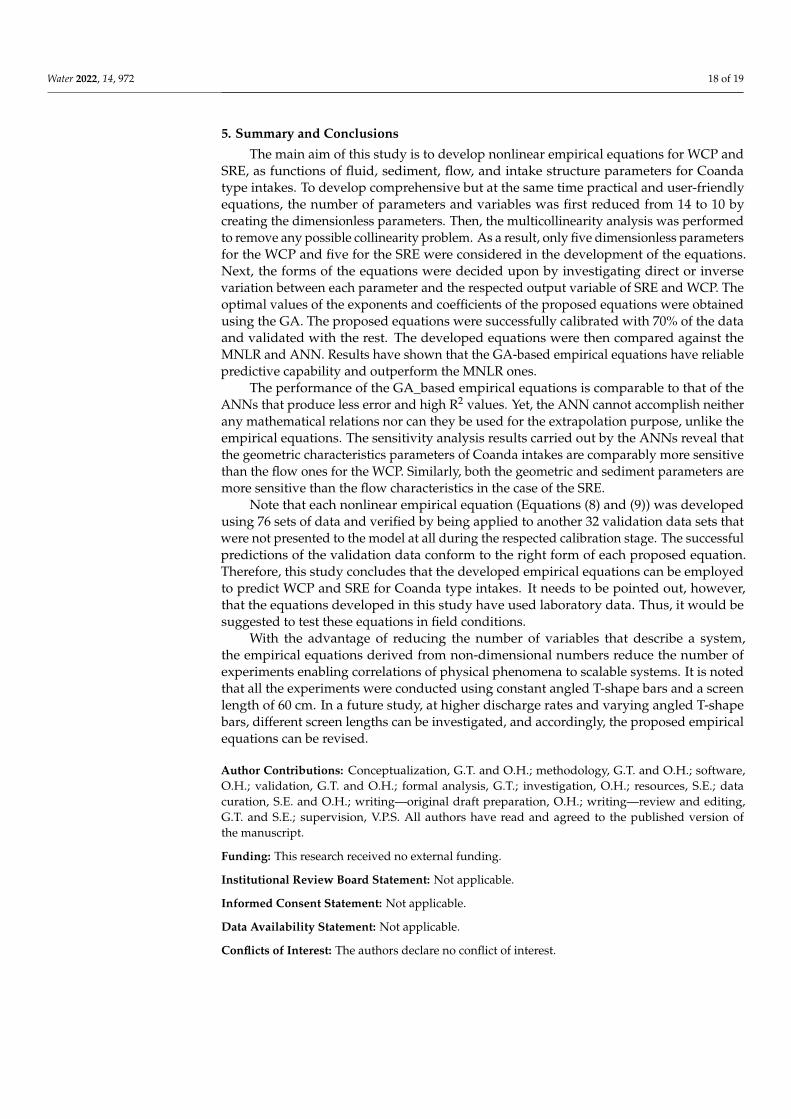
The calibration and validation of Equation (9), the GA-based empirical equation pre-dicting SRE as a function of the intake geometric, fluid, sediment, and flow characteristicsvariables, was successfully accomplished with low errors (MAE = 10.32, RMSE = 13.18for calibration, and MAE = 10.77, RMSE = 12.99 for validation) and high R2 values of 0.75(calibration) and 0.80 (validation). When its success was compared against that of theMNLR equation (Equation (13)), it was seen that the empirical equation outperformedthe MNLR one, which had produced high errors and very low R2 values of 0.22 (calibra-tion) and 0.17 (validation) (see Table 15). It may be stated that the MNLR method hadproduced a worse performance for SRE than for WCP. The GA-based empirical modelproduced comparable results against those of the ANN, as seen in Table 15. However, as itis pointed out above, ANNs do not accomplish any mathematical relations between thedependent and independent variables. They are, as it is pointed out in the literature, verypowerful interpolators but poor extrapolators and they are black box models [25]. Theempirical models, on the other hand, can be easily employed for both the interpolation andextrapolation purposes.

Water 2022, 14, 972 16 of 19

Table 15. Performance comparison between GA_based empirical equation, MNLR, and ANN for SRE.

SRECalibration Stage Validation Stage

GA MNLR ANN GA MNLR ANN

MAE 10.32 18.04 1.47 10.77 20.14 4.32

RMSE 13.18 24.00 2.37 12.99 25.98 5.37

R2 0.75 0.22 0.99 0.80 0.17 0.96

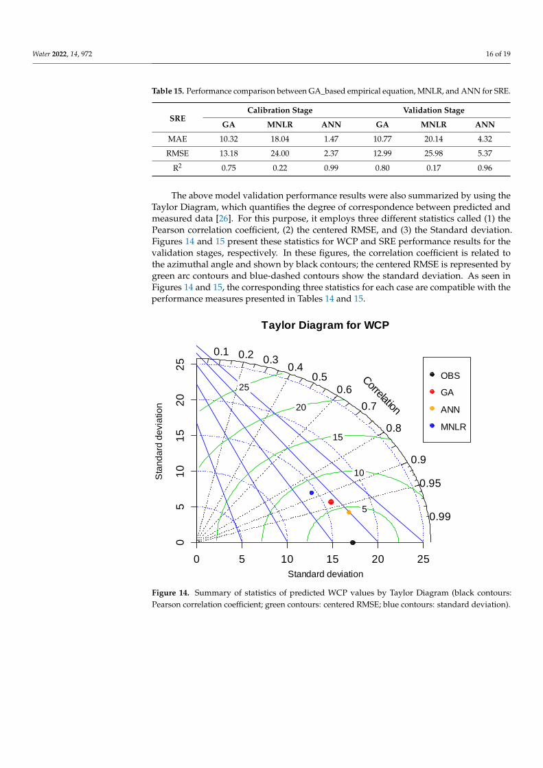
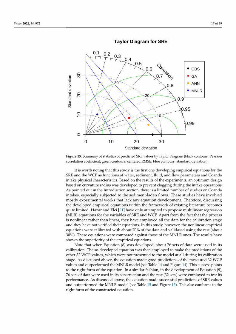
The above model validation performance results were also summarized by using theTaylor Diagram, which quantifies the degree of correspondence between predicted andmeasured data [26]. For this purpose, it employs three different statistics called (1) thePearson correlation coefficient, (2) the centered RMSE, and (3) the Standard deviation.Figures 14 and 15 present these statistics for WCP and SRE performance results for thevalidation stages, respectively. In these figures, the correlation coefficient is related tothe azimuthal angle and shown by black contours; the centered RMSE is represented bygreen arc contours and blue-dashed contours show the standard deviation. As seen inFigures 14 and 15, the corresponding three statistics for each case are compatible with theperformance measures presented in Tables 14 and 15.

Water 2022, 14, x FOR PEER REVIEW 17 of 20

Table 15. Performance comparison between GA_based empirical equation, MNLR, and ANN for

SRE.

SRE Calibration Stage Validation Stage

GA MNLR ANN GA MNLR ANN

MAE 10.32 18.04 1.47 10.77 20.14 4.32

RMSE 13.18 24.00 2.37 12.99 25.98 5.37

R2 0.75 0.22 0.99 0.80 0.17 0.96

The above model validation performance results were also summarized by using the

Taylor Diagram, which quantifies the degree of correspondence between predicted and

measured data [26]. For this purpose, it employs three different statistics called (1) the

Pearson correlation coefficient, (2) the centered RMSE, and (3) the Standard deviation.

Figures 14 and 15 present these statistics for WCP and SRE performance results for the

validation stages, respectively. In these figures, the correlation coefficient is related to the

azimuthal angle and shown by black contours; the centered RMSE is represented by green

arc contours and blue-dashed contours show the standard deviation. As seen in Figures

14 and 15, the corresponding three statistics for each case are compatible with the perfor-

mance measures presented in Tables 14 and 15.

Figure 14. Summary of statistics of predicted WCP values by Taylor Diagram (black contours: Pear-

son correlation coefficient; green contours: centered RMSE; blue contours: standard deviation).

Taylor Diagram for WCP

Sta

nd

ard

de

via

tio

n

Standard deviation

0 5 10 15 20 25

05

10

15

20

25

5

10

15

20

25

0.1 0.20.3

0.40.5

0.6

0.7

0.8

0.9

0.95

0.99

Correlation

OBS

GA

ANN

MNLR

Figure 14. Summary of statistics of predicted WCP values by Taylor Diagram (black contours:Pearson correlation coefficient; green contours: centered RMSE; blue contours: standard deviation).

Water 2022, 14, 972 17 of 19Water 2022, 14, x FOR PEER REVIEW 18 of 20

Figure 15. Summary of statistics of predicted SRE values by Taylor Diagram (black contours: Pear-

son correlation coefficient; green contours: centered RMSE; blue contours: standard deviation).

It is worth noting that this study is the first one developing empirical equations for

the SRE and the WCP as functions of water, sediment, fluid, and flow parameters and

Coanda intake physical characteristics. Based on the results of the experiments, an opti-

mum design based on curvature radius was developed to prevent clogging during the

intake operations. As pointed out in the Introduction section, there is a limited number of

studies on Coanda intakes, especially subjected to the sediment-laden flows. These studies

have involved mostly experimental works that lack any equation development. Therefore,

discussing the developed empirical equations within the framework of existing literature

becomes quite limited. Hazar and Elci [21] have only attempted to propose multilinear

regression (MLR) equations for the variables of SRE and WCP. Apart from the fact that

the process is nonlinear rather than linear, they have employed all the data for the calibra-

tion stage and they have not verified their equations. In this study, however, the nonlinear

empirical equations were calibrated with about 70% of the data and validated using the

rest (about 30%). These equations were compared against those of the MNLR ones. The

results have shown the superiority of the empirical equations.

Note that when Equation (8) was developed, about 76 sets of data were used in its

calibration. The so-developed equation was then employed to make the predictions of the

other 32 WCP values, which were not presented to the model at all during its calibration

stage. As discussed above, the equation made good predictions of the measured 32 WCP

values and outperformed the MNLR model (see Table 14 and Figure 14). This success

points to the right form of the equation. In a similar fashion, in the development of Equa-

tion (9), 76 sets of data were used in its construction and the rest (32 sets) were employed

to test its performance. As discussed above, the equation made successful predictions of

SRE values and outperformed the MNLR model (see Table 15 and Figure 15). This also

conforms to the right form of the constructed equation.

Taylor Diagram for SRE

Sta

nd

ard

de

via

tio

n

Standard deviation

0 10 20 30

01

02

03

0

10

20

30

0.1 0.20.3

0.40.5

0.6

0.7

0.8

0.9

0.95

0.99

Correlation

OBS

GA

ANN

MNLR

Figure 15. Summary of statistics of predicted SRE values by Taylor Diagram (black contours: Pearsoncorrelation coefficient; green contours: centered RMSE; blue contours: standard deviation).

It is worth noting that this study is the first one developing empirical equations for theSRE and the WCP as functions of water, sediment, fluid, and flow parameters and Coandaintake physical characteristics. Based on the results of the experiments, an optimum designbased on curvature radius was developed to prevent clogging during the intake operations.As pointed out in the Introduction section, there is a limited number of studies on Coandaintakes, especially subjected to the sediment-laden flows. These studies have involvedmostly experimental works that lack any equation development. Therefore, discussingthe developed empirical equations within the framework of existing literature becomesquite limited. Hazar and Elci [21] have only attempted to propose multilinear regression(MLR) equations for the variables of SRE and WCP. Apart from the fact that the processis nonlinear rather than linear, they have employed all the data for the calibration stageand they have not verified their equations. In this study, however, the nonlinear empiricalequations were calibrated with about 70% of the data and validated using the rest (about30%). These equations were compared against those of the MNLR ones. The results haveshown the superiority of the empirical equations.

Note that when Equation (8) was developed, about 76 sets of data were used in itscalibration. The so-developed equation was then employed to make the predictions of theother 32 WCP values, which were not presented to the model at all during its calibrationstage. As discussed above, the equation made good predictions of the measured 32 WCPvalues and outperformed the MNLR model (see Table 14 and Figure 14). This success pointsto the right form of the equation. In a similar fashion, in the development of Equation (9),76 sets of data were used in its construction and the rest (32 sets) were employed to test itsperformance. As discussed above, the equation made successful predictions of SRE valuesand outperformed the MNLR model (see Table 15 and Figure 15). This also conforms to theright form of the constructed equation.

Water 2022, 14, 972 18 of 19

5. Summary and Conclusions

The main aim of this study is to develop nonlinear empirical equations for WCP andSRE, as functions of fluid, sediment, flow, and intake structure parameters for Coandatype intakes. To develop comprehensive but at the same time practical and user-friendlyequations, the number of parameters and variables was first reduced from 14 to 10 bycreating the dimensionless parameters. Then, the multicollinearity analysis was performedto remove any possible collinearity problem. As a result, only five dimensionless parametersfor the WCP and five for the SRE were considered in the development of the equations.Next, the forms of the equations were decided upon by investigating direct or inversevariation between each parameter and the respected output variable of SRE and WCP. Theoptimal values of the exponents and coefficients of the proposed equations were obtainedusing the GA. The proposed equations were successfully calibrated with 70% of the dataand validated with the rest. The developed equations were then compared against theMNLR and ANN. Results have shown that the GA-based empirical equations have reliablepredictive capability and outperform the MNLR ones.

The performance of the GA_based empirical equations is comparable to that of theANNs that produce less error and high R2 values. Yet, the ANN cannot accomplish neitherany mathematical relations nor can they be used for the extrapolation purpose, unlike theempirical equations. The sensitivity analysis results carried out by the ANNs reveal thatthe geometric characteristics parameters of Coanda intakes are comparably more sensitivethan the flow ones for the WCP. Similarly, both the geometric and sediment parameters aremore sensitive than the flow characteristics in the case of the SRE.

Note that each nonlinear empirical equation (Equations (8) and (9)) was developedusing 76 sets of data and verified by being applied to another 32 validation data sets thatwere not presented to the model at all during the respected calibration stage. The successfulpredictions of the validation data conform to the right form of each proposed equation.Therefore, this study concludes that the developed empirical equations can be employedto predict WCP and SRE for Coanda type intakes. It needs to be pointed out, however,that the equations developed in this study have used laboratory data. Thus, it would besuggested to test these equations in field conditions.

With the advantage of reducing the number of variables that describe a system,the empirical equations derived from non-dimensional numbers reduce the number ofexperiments enabling correlations of physical phenomena to scalable systems. It is notedthat all the experiments were conducted using constant angled T-shape bars and a screenlength of 60 cm. In a future study, at higher discharge rates and varying angled T-shapebars, different screen lengths can be investigated, and accordingly, the proposed empiricalequations can be revised.

Author Contributions: Conceptualization, G.T. and O.H.; methodology, G.T. and O.H.; software,O.H.; validation, G.T. and O.H.; formal analysis, G.T.; investigation, O.H.; resources, S.E.; datacuration, S.E. and O.H.; writing—original draft preparation, O.H.; writing—review and editing,G.T. and S.E.; supervision, V.P.S. All authors have read and agreed to the published version ofthe manuscript.

Funding: This research received no external funding.

Institutional Review Board Statement: Not applicable.

Informed Consent Statement: Not applicable.

Data Availability Statement: Not applicable.

Conflicts of Interest: The authors declare no conflict of interest.

Water 2022, 14, 972 19 of 19

References1. Lauterjung, H.; Schmidt, G. Planning of water intake structures for irrigation or hydropower. A Publication of GTZ-Postharvest

Project. In Deutsche Gesellschaft für Technische Zusammenarbeit (GTZ); GmbH GTZ: Bonn, Germany, 1989.2. Baltazar, J.; Alves, E.; Bombar, G.; Cardoso, A.H. Effect of a submerged vane-field on the flow pattern of a movable bed channel

with a 90◦ lateral diversion. Water Sui 2021, 13, 828. [CrossRef]3. Rahmani Firozjaei, M.; Behnamtalab, E.; Salehi Neyshabouri, S.A.A. Numerical simulation of the lateral pipe intake: Flow and

sediment field. Water Environ. J. 2021, 34, 291–304. [CrossRef]4. Yılmaz, N.A. Hydraulic Characteristics of Tyrolean Weir. Master’s Thesis, Middle East Technical University, Ankara, Turkey, 2010.5. Zhao, W.; Zhang, J.; He, W.; Shi, L.; Chen, X. Effects of Diversion Wall on the Hydrodynamics and Withdrawal Sediment of a

Lateral Intake. Water Resour. Manag. 2022, 36, 1057–1073. [CrossRef]6. LeChevallier, M.W.; Norton, W.D. Giardia and Cryptosporidium in raw and finished water. J. Am. Water Works Assoc. 1995, 87,

54–68. [CrossRef]7. Orth, J.; Chardonnet, E.; Meynardi, G. Étude de grilles pour prises d’eau du type en-dessous. Houille Blanche 1954, 3, 343–351.

[CrossRef]8. Krochin, S. Diseño Hidráulico; Editorial de la Escuela Politecnica Nacional: Quito, Ecuador, 1978; pp. 97–106.9. Bouvard, M. Mobile Barrages and Intakes on Sediment Transporting Rivers; IAHR: Rotterdam, The Netherlands, 1992.10. Raudkivi, A.J. Hydraulic Structures Design Manual; IAHR: Rotterdam, The Netherlands, 1993; pp. 92–105.11. Castillo, L.; Carillo, J.; Garcia, J.T. Comparison of clear water flow and sediment flow through bottom racks using some lab

measurements and CFD methodology. WIT Trans. Ecol. Environ. 2013, 172, 227–237.12. Nøvik, H.; Lia, L.; Opaker, H. Performance of coanda-effect screens in a cold climate. J. Cold. Reg. Eng. 2014, 28, 04014006.

[CrossRef]13. Strong, J.J.; Ott, R.F. Intake Screens for Small Hydro Plants. Hydro. Rev. 1998, 7, 1–3.14. Wahl, T. Hydraulic performance of coanda-effect screens. J. Hydraul. Eng. 2001, 127, 480–488. [CrossRef]15. Wahl, T. Design Guidance for Coanda-Effect Screens; Research Report R-03-03; U.S. Department of the Interior, Bureau of Reclamation,

Technical Service Center: Denver, CO, USA, 2003.16. Dzafo, H.; Dzaferovic, E. Numerical simulation of air-water two phase flow over coanda-effect screen structure. In Advanced

Technologies, Systems, and Applications. Lecture Notes in Networks and Systems; Hadžikadic, M., Avdakovic, S., Eds.; Springer: Cham,Switzerland, 2017; Volume 3. [CrossRef]

17. Hosseini, S.M.; Coonrod, J. Coupling numerical and physical modeling for analysis of flow in a diversion structure withcoanda-effect screens. Water 2011, 3, 764–786. [CrossRef]

18. Howarth, J. Coanda Hydro Intake Screen Testing and Evaluation; Technical Report Number ETSU-H-06-00053/Rep; Dulas, Ltd.:London, UK, 2001.

19. Huber, D. BEDUIN Project (Better Design of Intakes); Norwegian Water Resources: Oslo, Norway, 2005.20. May, D. Sediment exclusion from water systems using a coanda effect device. Int. J. Hydraul. Eng. 2015, 4, 23–30. [CrossRef]21. Hazar, O.; Elçi, S. Design of coanda intakes for optimum sediment release efficiencies. KSCE J. Civ. Eng. 2021, 25, 492–502.

[CrossRef]22. Rahmati, O.; Haghizadeh, A.; Pourghasemi, H.R.; Noormohamadi, F. Gully erosion susceptibility mapping: The role of GIS-based

bivariate statistical models and their comparison. Nat. Hazards 2016, 82, 1231–1258. [CrossRef]23. Arabameri, A.; Pradhan, B.; Pourghasemi, H.; Rezaei, K.; Kerle, N. Spatial modelling of gully erosion using GIS and R Programing:

A comparison among three data mining algorithms. Appl. Sci. 2018, 8, 1369. [CrossRef]24. Hair, J.F., Jr.; Anderson, R.E.; Tatham, R.L.; Black, W.C. Multivariate Data Analysis, 3rd ed.; Macmillan: New York, NY, USA, 1995.25. Tayfur, G. Soft Computing in Water Resources Engineering: Artificial Neural Network, Fuzzy Logic and Genetic Algorithm; WIT Press:

Southampton, UK, 2012.26. Taylor, K.E. Summarizing multiple aspects of model performance in a single diagram. J. Geophys. Res. 2001, 106, 7183–7192.

[CrossRef]