Nonlinear second order equations with applications to partial differential equations

JOURNAL OF DIFFERENTIAL EQUATIONS 58, 404-427 (1985)

Nonlinear Second Order Equations with Applications to Partial Differential Equations

PATRICIO AVILES* AND JAM= SANDEFUR?

Center for Applied Mathematics, Cornell University, Ithaca, New York 14853

Received March 1, 1983; revised March 23, 1984

1. INTRODUCTION

In this paper we study the Cauchy problem for the abstract second order (in time) semilinear differential equation

u”(t)+Au’(t)+Bu(t)=f(t, u(r)),

where A and B are (usually unbounded) linear operators in a Banach space. These problems arise often in the study of partial differential equations. As is usual we control a nonlinear perturbation (possibly involving spatial derivatives) by the linear terms, which contain higher order spatial derivatives. But contrary to the usual method of reducing the problem to a first order system in some “energy” norm space (as in [9, 5]), we use the factoring method of [lo]. This method allows the equation to be written as an integral equation containing a double integral involving the nonlinearity, reflecting the fact that the equation is second order.

There are several advantages to this approach which will be illustrated fully in the examples. First, we show that the equation is locally well posed if (loosely) the nonlinearity satisfies the local Lipschitz condition

(By absorbing linear terms into f, only the highest order derivatives of the operators A and B need be retained.) For partial differential equations, this gives a good rule of thumb for determining if a certain problem is locally well posed. Energy methods can then be used to show global existence.

Second, this method applies to both hyperbolic and parabolic problems.

* Present address: Department of Mathematics, University of Illinois, Urbana, Illinois 61801.

+ Present address: Department of Mathematics, Georgetown University, Washington, D.C. 20057.

404 0022-0396185 $3.00 Copyright 0 1985 by Academic Press, Inc. All rights of reproduction in any form reserved.

NONLINEAR SECOND ORDER EQUATIONS 405

In the case of hyperbolic problems, we usually obtain results equivalent to results derived using “energy spaces” (as in the wave equation, f must be locally Lipschitz continuous with respect to llVu[l). But for parabolic problems we obtain well posedness for a much larger class of nonlinearities than is usually obtained. This will be illustrated in the examples.

Last, using these techniques, it is quite easy to determine if the semigroups controlling the equation are analytic. This is usually easy to determine using product spaces [12, 141, but in certain cases this may be more difficult to do. One case in point is illustrated in a paper by Holmes and Marsden [S]. In this paper they write the equation of motion for a thin panel as a system in the “energy” space Hz @ L’. In this space it is unclear if the semigroup controlling the equation is analytic and in fact they conjectured that it was not analytic. But in our last example we show using nothing more than L’Hospital’s rule that the semigroup is analytic.

The first example of our abstract theorem is the Klein-Gordon equation

U,,-cxAu,+pu,-Au=pu-b (uIq-lu, a, P, b 2 0, p E R.

It has been shown [2, 9, 13, 141, that if the nonlinearity is locally Lipschitz continuous from the Sobolev space @*(SZ) (0 bounded with smooth boundary dSZ or 52= W3) into L*(Q), then (using Sobolev imbedding theorems and standard energy methods) global solutions exist for 52 E R3 and 1 <q < 3. But we show that for a > 0, the nonlinearity may be locally Lipschitz continuous from H$*(sZ) to L*(Q) which gives us global solutions for q 2 1 and Q z R3. It would be interesting to study the behavior of these solutions as c( JO.

Our examples also include the dynamical version of the von Karman equation and the vibrating beam equation. We use our abstract results to give local strong solutions and then construct energy functions to prove the existence of global strong solutions and to study their stability. Using the Center Manifold Theorem [4], we are also able to study bifurcation. It must be stressed that these methods apply to a much larger class of problems than those considered here. Also note that the coefficients of the differential operators need not be constant, and in fact the operators need not even commute.

The abstract approach we use in Section 2 involves factoring linear operators. The operational calculus for self adjoint operators and perturbation results makes this approach quite general. Because the factored operators may be complicated, we use Lipschitz conditions involving sim- pler operators Bj (often A’, where A is the Laplace operator) which are in some sense dominated by the factored operators.

We suggest that many readers may wish to skip Section 2 temporarily (possibly after skimming over hypothesis (Hl ) and (H2) and Theorem 2.2) and go directly to the examples in Sections 3, 4, and 5.

406 AVILESANDSANDEFUR

We finally mention that G. Ponce [S] has independently studied some classes of nonlinear evolution equations one of which is rather similar to the one considered by us in Example 3. The techniques used by Ponce are totally different.

2. THE ABSTRACT RESULTS

The results we consider in this section are generalizations of work done in [lo]. As such, we assume the reader is familiar with the Spectral Theorem and several function analytic terms such as “Banach space” and “semigroup.” In this section we prove existence and uniqueness results for the abstract Cauchy problem

u”(t) + Au’(t) + h(l) =f(t, u(t)), u(0) = (b, u’(0) = I) (2.1)

in a Banach space 1, where A and B are unbounded linear operators. Although in our examples, A and B commute, this is not a necessary condition.

Problem (2.1) is said to be well-posed locally if there exists a dense set D c x such that if 4, (c/ E D, then there exists a T> 0 and an unique function U: [0, T] + x which satisfies (2.1).

We assume the existence of (linear) operators A,, k = 1,2, such that A, + A, = -A, A,A, = B, and A, generates a (C,)-semigroup Tk, k= 1,2. (Actually we need that closure (A,A,) = B and closure (A, + A,) = -A.) As can be seen from the examples these are reasonable assumptions.

We say that a function u is a mild solution to (2.1) if u is continuous and satisfies

u(t) = T,(t) 4 + j’ T,(t - 7) T,(T)($ - A,d) dT 0

+ j;i; T,(t-z) TJz-s)~(s, u(s))dzds. (2.2)

The motivation for this form of a mild solution came from studying (2.1) in the factored form

and is discussed in Sandefur [lo]. But in that paper, the order of integration in the double integral was reversed and the full advantage of this method was not utilized. Note that in (2.2), the inner integral does not


depend on the nonlinearity. If we formally compute the first integral, we have

We therefore expected (2.2) to be well-posed focally (in the same sense as (2.1)) if f is Lipschitz continuous with respect to (A* -48)“*, or equivalently A or B”*, (whichever has the higher order if they are differential operators). This is essentially what we will prove, although it is somewhat hidden in the technical details. If (6, Ic/ are “nice,” that is, 4, $ E nS,k=ID(AiAk),andf(.,u(.))EC2([W+,X)wheneveru(.)EC2([W+,X),then a mild solution is a strong solution. This is a consequence of the following lemma, which is proved in Kato [6, p. 4861.

LEMMA 2.1. IfgEC’(R+, x) and w(t)==jh T(t-s) g(s)ds, where T(e) is a semigroup generated by a linear operator A on x, then w E C(R + , D(A)) n C’@+, x) and w’(t)= T(t) g(O)+!& T(t-s) g’(s)ds and Aw(t)= w’(t) - g(t).

(Above R + = [0, co) and D(A) is the domain of A). The details of the use of this lemma to show regularity are identical to

those employed by one of the authors in [ 10, Theorem 4.11 to prove a similar result, even though the class of nonlinearitiesf, has been expanded considerably. These techniques can also be used to prove standard regularity theorems when A, and A, are analytic. In Section 3 we shall discuss this matter further.

We solve Eq. (2.2) using successive approximations. Define f,(s) = fk u,(s)) and

uo(t)=T,(t))+jo’T,(WT,(W-A,d)d~, (2.3)

u .+Jt)=~&)+j’j~ T,(t-t) T,(z-s)f,(s)dzds. 0 s

(2.4)

We will show that, under certain conditions on f, the u,(t) converge to some function u(t), uniformly for t E [0, T) for some T > 0.

One advantage of Eq. (2.2) is the double integral. By integrating with respect to z we get, in some sense, (A* - 4B) -‘/* which may “cancel” some

408 AVILES AND SANDEFUR

of the nonlinearityf: Because this operator may be difficult to deal with, we hypothesize the existence of a set of closed linear operators Bj, j = 1,2,..., m with D = fi,“=, D(Bj) dense in x and which satisfy hypotheses (Hl) and (H2). For m = 1 and B, = Z, the identity, these hypotheses are the same as in [lo]. If in (2.1) A and B are differential operators of order p and q, respectively, then normally Bj = A”’ for j= 0, l,..., m, m = max{2p, q}. Here A”=Z and IJA”‘uJJ = -(Au, u) = IIVull, where the last norm is in L2(Q, C”). In other words, the Bj are in some sense dominated by (A2-4B) . ‘I2 Here it is implied that A has certain boundary conditions associated with it. These conditions depend on A and B.

(Hl ) There exists a positive nondecreasing function g: IX! + -+ (0, cc) and an interval [0, T], T>O, such that

0) IIf(t, 01 d g(K) and

(ii) Ilf(t, d)--At, Ic/)II GdK)C~=, llBj(d-Ic/)II when tE WY Tl, 4, $ ED and 11411, lItill, IIB#ll, IlBj$ll <K forj= L..., m.

(H2) Let uk(t), k=O, l,..., be as defined in (2.3) and (2.4) for t E [O, 7’), T> 0. Note that u. is uniformly bounded on [0, T). Then,

(i) u,(t)~D for k=O, l,..., and tc [0, T),

(ii) IIBju/c + 1 (t)ll 6 IlBj~o(t)ll + gW) lb II fA~)ll & and (iii) llBj(U, + I (t)-+(t))11 6 gW)jh llh(~)-f~-,(~)/l 4

where tE[O,T), IIz+(t)]l, I/u,-,(t)ll<K for tE[O,T), j=l,..., m and k = 1, 2,... .

It will be demonstrated in the examples that these hypotheses are easy to apply.

THEOREM 2.2. Suppose A, and A, generate Co-semigroups T, , T2. Also suppose there exists closed linear operators Bj, j= l,..., m with /Jy= J D(Bj) n D(A,)n D(A,) dense in x and such that (Hl) and (H2) are satisfied. Then (2.2) is well-posed locally.

ProoJ: The proof consists in showing that the functions {a,,} defined in (2.3) and (2.4) converge uniformly to a function u for t E [0, T) for some T>O.

First we show, using induction, that for some T> 0 and K> 0 that Iluk(t)ll, IIBjuk(t)ll <K for j= l,..., m, k= 1, 2 ,..., and te [0, T). For simplicity we assume m = 1.

It is easy to show that for some K> 0 and T> 0, that

IIdt)ll> IIB, udt)ll G K/2, tE 10, T) (2.5)

NONLINEARSECONDORDEREQUATIONS 409

for k = 0. Assume (2.5) for k = 0 ,..., n for some n and with K/2 replaced with K. Then

<K/2 + C (’ (t-s) II f,(s)11 ds < K/2 + Cg(K) t2/2 < K 0

for t E [0, (K/Cg(K))‘/‘] for some C > 0. Also

JIB ~un+,(Oll G lIB~uo(t)ll + dK)j; IIfn(~)ll ds

<K/2+g2(K)t<K

for t E [0, K/g’(K)]. So let T= min(K/g2(K), (K/Cg(K))“*}. Thus (2.5) holds (with K/2 replaced with K) for k = 0, l,... .

It is also easy to show that

lb k+ l(t) - dt)ll> llB,(u,+ l(t) - udt))ll G OW%! (2.6)

for t E [0, T) and k = 1. Assume (2.6) holds for k = l,..., n for some n. Then

Il~,+~(~)-~,(~Nl = [rj-‘T~O-,, T2(z-s)(S,(s)--f,-,(s))dzds Ii 0 s II

4gWj’j’ IIB,(u,(s)-u,-,(s))ll dz ds 0 s

<g(K) 1’ 1’ (Ms)“/n! dz ds 0 s

= M”g( K) t” + ‘/(n + 2)! < (Mt)” + ‘/(n + 1 )!

when 442 Tg(K)/Z. Similarly for IIBl(u,+,(t)-u,(t))(l with M>g(K). Therefore, (2.6) holds for all k with M = (1 + T/2) g(K). Thus, U, converges uniformly on [0, T) to a solution u of (2.2).

The uniqueness follows by an application of Gronwall’s inequality as in [lOI. Q.E.D.

We now discuss global continuation of solutions.

COROLLARY 2.3. Let the assumptions of Theorem 2.2 hold and let u be the solution to (2.2) on [0, T). Let Ilull and IlJ3~ull, j= l,..., m, be uniformly

SOS/S8/3-8


bounded on [O, T) and T< co. Then lim,, T u(t) - u(T) exists. Dejine for t> T.

u,(t)= T,(t)d+ j’T,(t-r) TA~)(ti--~l4)dt 0

+ ‘T,(t-z)T+s)f(s,u(s))d~ds.

Assume that for each K > 0 there is a nondecreasing function g, such that (Hl) and (H2) hold with f replaced by fK (defined by fK(t, 4) = f(t + K, 4)) and u. as in (2.7). Then u can be extended to a solution of (2.2) on the interval [O, T-t&) for some E>O.

The proof consists of applying the same techniques as before to functions v,(t) z u,(t + T). See [lo] for more details.

Let B, = Z, B, = A,, and m = 2. Then local existence can also be shown with (H2) replaced by

(H3) Let#jEC’([0,T],X)nC([0,T],D(A,))forj=1,2.Then

!i -$f(t, h(t))ii G g(K)

and

il f (f(t> d,(t))-f(t, h(t))) 6 g(K)&%(t)-4At)ll

/I

+ IIA,(d,(t) - dz(t))ll + II@,(t) - 4Xt)lll

for t E [0, T], g as in (HI ), and where

SUP { II4~i(t)ll, Ilbji’(t)ll, IIAltij(t)ll> G K. IE co,r1

j= 1.2

For the wave equation, Reed [9] has another hypothesis that could also replace (H2). The disadvantage of these alternatives is that they do not take advantage of the strong connection that usually exists between the semigroups and the nonlinearities and especially the fact that the equation is second order.

We also note that f could also be a function of u,. Letting fk(t) = f(t, u,(t), uk,Jt)), (Hl) and (H2) would involve inequalities of the form

IIf(t, 4 u,)-f(t, ‘J, vOII d g(K) f IIBj(U-V)ll + IIu,-vu,II j=l >


and

An example of this is given in our last section. We now give an approximation result

COROLLARY 2.4. Let the hypotheses of Theorem 2.2 hold for the nonlinear perturbations f andf,,, n = 1, 2,..., with the same g in each case. Assume

IIBj(u(t)-un(t))II G g(K) 1: IIf(s, u(s))-fn(s, un(s))II ds (2.8)

when Ilu(t) IIuJt)ll d K, t E [0, T), j= l,..., m, and where u, is the solution of (2.2) with f replaced by f,. Assume that for every E > 0 and K > 0 there is an N>O such that IIf,,(t,cj)-f(t,4)II GE when IIBj(Q))II <Kforj= l,...,m, t E [0, T) and n > N. Then u,(t) + u(t) locally uniformly for t E [0, T,], for some To >O.

Proof. We note that

lb(t) - u,(t)ll = I! 1; j3’ T,(t- 7) TAT -s)(f(s, u(s)) -fn(s, u,(s))) dz dsii

’ GM SI ’ IIf(s, u(s)) -fn(s, M))ll dT ds 0 s

GM ss f ’ llf(h u(s))-f(s, 4z(s))ll 0 s

+ II f(s, u,(s)) -fn(s, u,(s))ll dT ds.

For 0 < To small enough, u and U, are uniformly bounded by K for t E [0, To]. Therefore for any E > 0, there is an N> 0 such that for n > IV,

II’(t)-un(t)II GMj: Js’ g(K) t lIBj(U(S)-U,(s))11 +E dt ds. j=l

BY (2.8)

IIgj(u(t) - u,(t))II G g(K) 1: II f (s, u(s)) - fn(s, un(s))II h

G g2(W Jr f llBj(u(S) - un(S))ll + E ds Oj=l

412 AVILJZS AND SANDEFUR

as above. Let d,(t) = IIu(t) - u,(t)11 +x7=, Ile,(u(t) - u,(t))ll. We have

for some C > 0 and E, --$ 0. By Gronwall’s inequality, u,(t) + u(t) in x as n + 00, uniformly for TV [O, T,], To some positive constant.

3. THE KLEIN-GORDON EQUATION

Here we shall prove existence of global strong solutions and study bifur- cations for the strongly damped Klein-Gordon equation

u,,-2crdu,-du=~u-b Izp-‘)u, (3.1)

with p E R, a > 0, q 2 1 on a bounded domain Sz s R”, n = 1,2,3, with 852 smooth and boundary condition u(t, x) = 0 for x E 852. (Using spectral decomposition instead of eigenfunction expansion we can derive local existence for D = R3. Global existence and energy arguments are identical.)

As is well known, if a =O, p = 0 and 1 <q < 3, then (3.1) has global strong solutions. (This is also what is obtained using the results of Sec- tion 2.) If q > 3, then there are weak global solutions. (See [9].) Our results show that if a > 0, then there are also global strong solutions when q > 3, which leads to the following interesting questions: Fix the initial conditions and q > 3. Denote by z.P the corresponding solution of (3.1) and by u a corresponding weak solution of (3.1) when a = 0.

OPEN PROBLEMS. Does lim,,, ZP exists in some strong sense? What is the relation between ua and v? (For a discussion of these types of problems, see [7].)

We pose (3.1) in the complex Hilbert space L’(Q) and by A we mean the closure of the Laplacian on the set {u E C*(Q): u = 0 on 80) with respect to the L2-norm. -A has eigenvalues ,$, j= 1, 2 ,..., Jj > 0 such that lim, _ m Aj = cc and a corresponding complete set of orthonormal eigenvectors ej (cf. [3, p. 13351).

Let Ak = closure (ad + (- l)“(a*A* + A)‘12) for k = 1, 2. Then, it is seen that A, is the sum of a nonpositive self-adjoint operator and a bounded operator (which corresponds to the finite number of eigenvalues for which (a”A,? -S) is negative). Therefore, Ak generates an analytic semigroup Tk, k= 1, 2.

Now, we let B, = Z, the identity and B, = A. To apply Theorem 2.2 it suffices to show that


0) IIf(u)II GgWh IIfW-fW ~gWWW--~N + 11~--11)9

(ii) Ilk+ 1 II ~W&J + 16 IMdll W, and

(iii) W(U,+~ -4Jl <q:, IIf,(s)-f,-I(sNl ds

when Ilull, Ilull, IlAull, lldoll <K, g is as in (Hl), C is some positive constant independent of n andf,(s) -f(u,(s)) = PU, - b Iu,)(~-‘) u,.

Let ll4l m = who lu(x)l and llullP = (I0 lulp dx)““, p > 1. Then, from the Sobolev imbeddings, ll~ll~ < C lldul\ and IIullP < C lldull for some C > 0. Thus, (i) follows immediately.

Since (ii) and (iii) are similar we shall only verify (iii). Let g(s) =f,,(s) - f,-,(s). Then

lMu,+~ - dll= ASdS:exp((r-t)A,)exp((r-s)A,)g(s)dtds II II

x exp( (z - s)( - aAj + /Ii)) g,(s) dT ds II

by the operational calculus for self-adjoint operators, with flj= (a”$ - 3Lj)l’* and gj(s) = (g(s), ej).

IlA(un+ I P((t-s)(-aJj+fij))

(1

2

- exp((t - SM -alj- Pj))) gjts) ej ds

<C t (T,(t-s)- T,(t-s)) g(s)ds II *

where C = supj lAj/(a2Aj? - Aj)“*l. (We can treat the finite number of eigenvalues for which flj = 0 separately to arrive at the same inequality.) Thus, IlA(un+ I (t) - u,(f))(l 6 C j& (1 g(s)11 ds. Hence, we have the existence of mild local solutions to (3.1).

The existence of global real solutions with b > 0 follows by considering the energies

JW~)=W~~~*+ II~I*-P I1412Y2+b lI~(y+1)‘2112/(q+ 1)

and

k(t)= Ca 11412+ Ibtl12+ IIWl*-CL 11412

+ 2b IIu (q+1)‘2112/(q + 1)]/2a - (U,, Au),


where ( ‘, . ) means inner product. From (3.1) and integration by parts we have

dE,(r) -= -2c? IJVuJ2, dt

which implies that E,(t) is nonincreasing. There is no problem if p < 0, so assume /A is positive. Now, suppose ))uI/’ is unbounded. Then, there exists an increasing sequence t, such that Ilu(t,) I( 2 > n, n = 1, 2,... . Let B, = {xESZ: lu(t,JY-’ > (q+ l)(p+ 1)/2b}. B, has positive measure and se, u2(t,) dx -+ cc as n + co. So

-; lu(t,)12 dx

= s l~(b4*W 14~n)14~‘/(q+ I)-pL)Pdx R

2 s u2( t,)/2 dx - C, &

with C some fixed positive constant. Since Se, u2(t,,) dx + co, E,(t,) + co which is a contradiction and therefore [(u/I is a bounded function in t. From the definition of E, we then see that IjVull, IIu,IJ and I(&+ ‘)“I/ are bounded uniformly in t.

We now consider E2. dE,(t)= ri dt R (Au) a Au, + U,U,,/LY + VU,. VU,

- (Au) u,, + VU. Vu,/a + i 1~1 4 u, sign u + QUU,/U} dt.

Since u,,=c1 Au,+Au-b lulyp’ u+pu, a Aul=ul,-Au+b ~u~~-‘u--pu, and V Iu( = sign u Vu we get

d&(t) _ s dt R - (Au)* + b (u( 4 sign u Au + p Vu. Vu dx

= - 5 (Au)~+(~ Iu14-I-p) IVul’dx. R

Since IlVull is bounded,


for some constant C 2 0. Thus E2( t) < Ct + Ci , with C, some positive constant. Using the inequality

with /I arbitrarily small and since Ilull and J(u,II are bounded, we have from E2 that lldull is bounded on finite intervals. Therefore, from Corollary 2.3 we have global existence of solutions of (3.1) for all q > 1.

To show that solutions are strong solutions it is necessary to prove that 24 117 Au,, and Au are in L2(sZ). We show that Au, is, the others being similar. Using Lemma 2.1 on

u(r)=u,(~)+~~J“T,(t-7) T2(t-s)f(u(s))dzds 0 s

(and assuming the initial data are “nice” enough so that duo, duo,, and uOtr exist) we have after a substitution and a change in the order of integration that

Au,(f)=Auo,+A;~tT,(f-r)j’T,(rs)f(u(s))dsdz 0 0

=u,,+A ‘T,(t-s)f(u(s))ds s 0

+A, j-’ T2(t - T) A j’ T,(z -3) f(u(s)) ds dz. 0 0

Since (i) A2 is bounded (its spectrum is bounded), (ii) Al, A,, A, T1, and T, all commute, (iii) D(A) = D(A ,) by the operational calculus of self- adjoint operators and

(iv) 1: T,(t-s)f(s) dsED(Aj) iffEC(R+, x), j= 1, 2,

we have that each of the above terms is in L2(sZ). We now study bifurcation by letting p be a parameter and using the

Center Manifold Theorem [4]. To do this we need to reduce (3.1) to a first order system

(3.2)

where F(u, V) = (u, f(u))‘, T is the transpose operator. It is easy to see that a strong solution u to (3.1) gives a strong solution to (3.2) with u = u, - A, u. Therefore we have existence of global strong solutions of (3.2).


Note that by the operational calculus for self-adjoint operators [3], and since 2a,lj > a,lj + (a’,lf - Aj)l” > a,lj for large j, we have D(dY) = D(Ai) for O<y<l.

Let F( (4, $)T) = ($, ,ub - b IdI”-’ 4)T. F has a Frechet derivative F from D(A:) $ L’(8) into L2(Q) @ L2(sZ) which is continuous, and F’(0) = (E h). (The norm on D(Ai) is I[4[/{ = I1&12 + llAY4112.) Let p= A1 + 2al,c and rewrite (3.2) as

(3.3)

where A = ($ i, ) and G(Z) = ( -blu&~,). If (4, $)’ = C(ajej, bjej)T = C(aj, bj)T ej, then

- aL, - (aZRf - lj) ‘I2 1

1, -aAj + (a2Af - Aj)‘i2

and a(A)= {/?,* = -aLi+ (a21~-lj+1,)“2;j= l,...}. Note that /I?: =Oand WP;, P,$=2,...l < -8 < 0 for some 6 > 0. The eigenvectors associated with /?I’ are f’ = (1, &co?, + (a2i: - A1)“2)T e,. The eigenvectors associated with /I,*, j= 2 ,..., are orthogonal to f *.

Let P be the projection onto f + along f -, i.e.,

P(a, b)T e, = ((ai, - (a2,1: - R,)“2, l)T, (a, b)T) f +/2al,.

Equation (3.3) can then be rewritten as

s'(t)f + =s(t)~f + +P(O, -b ~uI%)~,

y’(t) = By(t) + (I- P)(O, -b (u14 u)~,

&l=o,

(3.4)

where y is in the space H={f-)@{f+,f-}', with {f+,f-)’ the orthogonal complement off+ andf- in L’(Q). B is a linear operator on H with Re a(B) d -6. By Theorem 6.2.1 of Henry [4], there is a Lipschit- zian local invariant manifold S = { y = h(s, E); IsI, [a( < a,,) for some e0 > 0, tangent to f + at the origin. The flow in S may be represented by the ordinary differential equation

(fff = s&f + + PG(sf + + h(s, E)),

El = 0.


By Corollary 6.2 of Henry [4], I\&, .s)ll = 0(s2 + s2) as (s, E) + (0,O). Therefore PG(sf+ + h(s, E)) = -C JsIQ-’ sf’ + 0(s4+’ + ~9) as (s, E) + (0,O) where C= b jn )ei19- I ei dx/2al, > 0. So the flow on the manifold S may be represented by the solution to

S’=ES-c~(S~9-1S+O(S9+1,ESq)

El = 0. (3.5)

If E < 0, the solution to (3.5) decays exponentially and thus the origin is asymptotically stable in Eq. (3.2). Likewise when E = 0, the origin is stable.

Suppose E > 0 and small. Since (for E small and fixed),

&S-c~s(~-1S+O(S9+‘,&S9)=0 (3.6)

has a positive and negative root (close to zero), the unstable manifold of the origin consists of two stable orbits connecting two fixed points to the origin (see Fig. 1).

We finally remark that analogous bifurcation results for (3.1) were derived by Webb [ 151 when Sz = (0, n).

4. THE DYNAMICAL VON KARMAN EQUATION

Consider

u,, - a AU, +A2u=

A2qS=

for (t, x) E R + x 52, 1 E R, a >/ 0 and with boundary conditions

u=Au=O, (4)~=(4)N=o

Y= h(s,t)

4/./

If+1 ii

FIGURE 1


for XE XJ, and where N denotes the outward normal. Here B z R2 is a bounded region with smooth boundary 80 and

[% VI = ux,,, f-)x2x2 - %xz~x,x2 + ux2x*vxlx,. (4.2)

For the physical relevance of the Von Karman equation, see [ 1, 111. Define

A - !fLd = h2 (3x9 Y) f(x) dx

for f~ CA(B), and where G(x, v) is the Green function of A in Sz with pole at y, i.e., AG(x, y) = 6(x- y) and G(x, y) = 0 if XE 1%2. Then, assuming f$ E I#*(Q), (4.1) is equivalent to

~,,-a Au,+A*u= -+[A-*[u, u], u-J-h,,,,. (4.3)

Here, as in Section 3 (closure of) -A is a positive self-adjoint operator with its first eigenvalue 1, >O. Note also that A-’ is not the inverse of this Laplacian, but an inverse of the Laplacian with Neumann boundary conditions. We again have that if the initial data is sufficiently smooth, say ~(0, .)eZi$*(Q) and u,(O, .)EH~*(Q), then mild solutions are strong solutions. The proof of this fact is exactly as in Section 3.

We shall now show that (4.3) satisfies the conditions for local existence of solutions. For simplicity we denote /Iu[/~ = l/u/l + 11 dull, where 11. II is the usual L,-norm. We now verify (Hi)(i) with B, =I and B,= A. We therefore need to find a nondecreasing function g: R + + (0, co) such that

s I CA -*b, ~1, ~1 - &,I* dx G g(K) (4.4) R

when IIuII, )I AuJI < K. Clearly it suffices to obtain this for the case when I=O.

From (4.2) we have

s Q ICA-*Cu, ~1, ~11 dxQmax(a, b, c> Ib412

with

a = sup IA -‘Cu, ul,,,,I, b = sup 2 IA -*t-u, ulx,x21,

and

c= sup IA -*CK ~lx2xzI,


where sup is taken over 0. From Sobolev imbeddings and the definition of A-‘,

with C denoting several positive constants. Similarly, we get estimates for b and c. Hence (4.4).

We will now verify (Hl)(ii). It is obvious that it suffices to consider

dif(u, u) - (1 [A-*[u, u], u] - [A-*[u, u], o]ll

G IICA-*b, ~1, ~-~I11 + IN-*b-u, ~1, ~111

+ IICA-*CU-Q, ~1, ~111.

Since (1 A$[1 and 11&l 2 are equivalent norms on H$*(SZ), we can use the previous procedure to obtain

Wu, 0) <g(K) lb-412 (4.5)

with g as above. Therefore, (Hl) is satisfied. In this example A,= (a+ (-1)“ /I) A/2 where /I= (a’-4)“* and

therefore it generates a semigroup Tk(t) = exp(A,t) for k = 1,2. Note that these semigroups are analytic with region of analyticity (z: Jarctan(Im z/ Re z)l < (7c/2) - a arctan Ifi/aI}, w h ere a = 1 if /I is imaginary and u = 0 if p is real.

We prove local existence for the cases a > 2, a = 2, and 0 6 a < 2. We use the fact that

A I’ exp(zA) 4 d7 = (exp(tA) - exp(sA)) 4 s

for 4 E L,(Q).

Case 1. a>2.Ifn>Owehave

IlA(u,+ 1 (t) - 4t(t))ll

A consequence of the operational calculus for self-adjoint operators gives us that

llA(u,+ 1 (1) - u,(t))ll

= rexp((a(l-s)-j?(t+s)+2~7)A/2)(.fn(s)-fn~,(s))d7ds Ii


= pCexp((E+B)(t-s)4/2) 111

- w(b - I-W - 8) 42WM -L dd) do //

= p-1 II 1 f [T*(r-s)- T,(t-S)l(fn(S)-fn-1(S))ds 0 II

<2p I ’ Il.L(s) -.L l(s)ll ds.

0

In a similar way we can get bounds on Il~!u,(t)ll thereby establishing (H2).

Case 2. CI = 2. The previous method does not apply because /.I =O. In this case T,(t) = T,(t) and

lIA(u,+ 1 (t) - ~,(t))ll = /I A j’ j’ T,(t - sMW)) -Au,- 1(s))) dz ds . 0 s II

Since Tr is analytic, it is known [6] that

IlA expW-4 AIll G W-4

for some C > 0. So

llA(~n+~ (t)-un(~))ll= A jr@-4 T,(t-s)(f,(s)-f,~,(s))ds 0 II

GC s ; IIf,(s)-fn-1(s)II ds.

Again we can use similar methods to get bounds on IlAu,(t)ll showing that (H2) is satisfied.

Case 3. 0 ,< tl < 2. Here /I is purely imaginary, but the method in Case 1 still works.

Thus for a B 0 we have local existence and uniqueness of solutions of the dynamical Von Karman equation.

To prove the global existence of real-valued solutions we consider the energy function


with y an arbitrarily small number to be chosen later. Then, differentiating and integrating by parts,

dE,(l)ldt = s, ( u,u,,+u,A2u+A-1[u,u]A-1[u,,u]/2

+ yu; + yuu,, - ayu Au,) dx.

Using the self-adjointness of A-’ and the identity

s u[u, w] dx= n f

R [II, u-J w dx

for u, u, w E HZ<*(Q), and letting u = Ae2[u, u], we have

dE,(t)ldf= s, ( u,u,, + u, A*u + [A-2[u, u], u] q/2

2 + yu, + yuutr - ayu Au,) dx.

Using the fact that a,, satisfies (4.3) and integrating by parts, we get

dE,(t)/dt = -a IIW12-~ IIu,II~-Y 11412-Q W’Cu, ~111~

Using the inequality ) (a, u ) I < t( II u II * + 11 u 11 2), the Poincarb inequality (Ilul12,<Ry1 (((Au/(’ for ~EH$*(Q) and where 1, is the first eigenvalue of -A), and choosing y small enough, we get

E,(f) 2 G(ll~,l12 + 11412) 2 C2 dE,(t)ldt (4.6)

for some positive constants C1 and C2. Hence, for some M, C > 0, E,(t) < M exp(Ct). So, using (4.6), we get that IIu,J( * and II dull * are uniformly bounded if t<h4 for any M>O.

The rest of the hypothesis of Corollary 2.3 can be shown to hold as before. Therefore the solution u can be extended to a solution on all of R, .

If 1 <A, (where again R, is the first eigenvalue of -A), we have the asymptotic behavior (stability)

ll4l + 0

To see this define

and ))u,JI +O as f--k co.

E*(t)=/ ~((~,)~+(Au)~+(A~~[~,u])~/4-~u~,-2~uu~-ayuAu)dx n

422 AVILFSANDSANDEFWR

with y arbitrarily small and to be chosen later. Then,

dE,(tW= --a IIW2-Y M2+ (4 u,t)-WC% Au).

From the Poincare inequality, 1/~,/1~ <A;’ llVuJ* and I(u,,/)* 6 2;’ )ldu11* giving us that

dE,(t)/d?6(-a+yA.;‘) IIVu,l/2-y(1 -AA,‘) lldull2.

Choosing A < 1, and y small enough so that dE,/dt < 0 and E2 > 0, we get that lim, _ m E2(t) exists. Therefore lldull is Cauchy since

j’ I~Au(z)~~* dz </’ - (dE,(t)/dr) dz = E,(s) - E,(t). 9 s

Thus sr IlAu(t)l12 dt < 00 and IlAu(t)ll -+O as t + a. Similarly, I(u,(I +O as t-,co.

If CI = 0, we define

E3(t) = E3(0) for all t since dE,(t)/dt ~0. Similarly to the above, we can show that Ildull, llu,ll < C for some positive constant C, independent of t.

Remark. If CI > 0 and 13 I,, we believe that bifurcation results can be obtained in a manner similar to the damped Klein-Gordon equation of Section 3.

5. THE VIBRATING BEAM EQUATION

The object of our final example is the study of the nonlinear equation

u,,+2(crd2+6)u,+d2u=f(u) (5.1)

in a bounded region Q c R” with 8L2 smooth. We assume the boundary conditions u = Au = 0 on &2 although other boundary conditions could be used. For n = 1 this is the equation of a simply supported vibrating beam where CI is viscoelastic structural damping and 6 is aerodynamic damping and f is as in cases 1 and 2 below.

We first show that (5.1) is controlled by an analytic semigroup, contrary to a conjecture formulated by Holmes and Marsden [S]. We then deal with several nonlinearities one of which involves u,. Finally, we discuss global continuation, stability, and bifurcation. In particular, we discuss how Galerkin approximations may be used to analyze this equation.


As in Section 3, we pose (5.1) in the complex Hilbert space L’(Q) and let O<A,< *.., be the set of eigenvalues for -d and let ej be the corresponding complete set of orthonormal eigenvectors. Also, as before, g(d) means the closure of g(d) in L’(Q) using the operational calculus associated with the Spectral Theorem [3, p. 13351. Equation (5.1) is then an ordinary differential equation on L2(Q) with A2 being a positive self- adjoint operator with spectrum o(A2) = (2;; -Aje o(A)), and 6 = 61, Z= identity. This problem is now equivalent to (2.1) and the operators A, and A2 referred to in Theorem 2.2 are

Ak = --ad2 - 6 + (- l)‘(or2A4 + (2~x6 - 1) A2 + 82)1’2 (5.2)

for k = 1,2. These operators have spectrum

for k = 1,2, and where vi = (aLj + 6) and pj = (u’$ + (2~x6 - 1) L,? + h2)l12, j= l,... . Hence A, is a spectral operator in the sense that if 4 = C ujej E D(A,), then Ak~=~aj(-v,j+(-l)kpj)ej, k=l,2.

By 1’Hospital’s rule, it is seen that g(A2) is bounded and therefore A, is a bounded operator. Also -2(c4 + 6) 6 -vi - pj d -a$ - 6 for j large enough. Hence by the operational calculus for self-adjoint operators, D(2aA2 + 26)?D(A,)zD(crA2 + 6) and thus D(A,) = D(A2). Note also that pj is real and -vi- ,uj is negative for all j> J, for some J. Thus A, generates a semigroup Tk, analytic in the right half plane for k = 1,2.

We now consider several relevant perturbations.

Case 1. f(u)=rAu+p.Vu+~~(~,~)Au, where Z,K are constants and p is a constant vector in R”. Z represents in-plane tensile load, p represents dynamical pressure, and K represents nonlinear membrane stiffness.

Remark. More generally, f can be any function satisfying

II f(u)ll G g(K) and IIf(f(u)llGdW ? IlA’(u-u)ll j=O

when liAjo\l, \lAjull 6 K, j= 0, 1, 2, and g is as in Theorem 2.2. Because of the energy methods used, it is difficult to get global bounds for II A’ull, and therefore we tend to consider nonlinearities which satisfy (Hl) and (H2) for Bj = A’, j = 0, 1. Nevertheless we use A2 for our local results and observe that for the specific nonlinearities listed above, A would be suf- ficient.


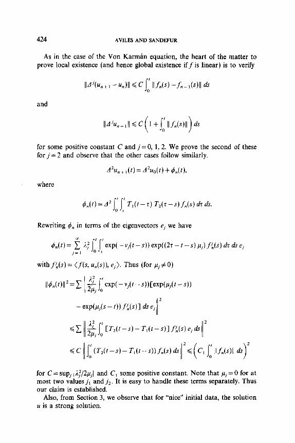
As in the case of the Von Karmdn equation, the heart of the matter to prove local existence (and hence global existence iff is linear) is to verify

II A’(u, + 1 - 4 < C ; IIf,, -fn- l(s)ll ds I

and

for some positive constant C and j = 0, 1,2. We prove the second of these for j = 2 and observe that the other cases follow similarly.

A2u,+ l(f) = A’uo(Q +4,(t),

where

/,(f)=dZJ’ jt T,(t-r) T,(t-s)f,,(s)drds. 0 s

Rewriting 4, in terms of the eigenvectors ej we have

d,,(t)= 2 ~~j’/‘exp(-vj(~-~))exp((2r-t-s)ri)~{(s)drdse, j=l 0 s

with f’,(s) = (f(s, U,(S)), ej). Thus (for pi # 0)

I14&N2=~ f ; /I J exp( -vj(t - s))CeXP(Pj(t -S))

J

II 2

- exP@ji(s - 2)) f’,(S)1 h ej

for C= supj /LJ?/2j.4jjl and C, some positive constant. Note that pj= 0 for at most two values j, and j,. It is easy to handle these terms separately. Thus our claim is established.

Also, from Section 3, we observe that for “nice” initial data, the solution u is a strong solution.


Case 2. f(u, u,) = o(du(t), tit(t)) du, where u is a constant representing nonlinear aerodynamic damping. Here, the local Lipschitz condition on f is

and

IIf(% u,)--f(h u,Nl d d~)(ll~-4l + Il4U-~)ll + II%--v,Il)

when 1141, Ilull, Ildull, Ibll, Ilu,lI, llu,lI <K and g is as in (Hl). (H2) then needs to be phrased as

ll~n(~)ll, Il4(~)ll> ll~,&)ll < C+ g(K) 1; ll.L,(~M ds

and

lb,+ I(l) - %l(~)ll, Il~(%z+ 1(t) - u,(t)ll, lb, + l,,(f) - %l,,(~Nl

where TV CO, Tl, Il~,(~N, Ilu,-r(t)11 <K, n = 1,2,..., and f,(s) =f(s, u,(s), u,,,(s)) as in Section 2.

The above bounds can be shown similarly to case 1 except for those on Il~,,,II and lb, + l,t - u,,J. To see these observe (by Lemma 2.1) that

+o J ; T2(t-s)f,(s)ds.

Using the procedure in Case 1 and the fact that T2 is a bounded operator, we get

IIU ,+Jt)ll G Iluo,t(t)ll + CI; IIfn(s)ll ds

for some positive constant C. Similarly for IIu, + 1,1 - u,,,II. Thus local solutions exist in this case.

As a corollary of Cases 1 and 2, we therefore have the “vibrating beam” equation with f the sum of the nonlinearities in Cases 1 and 2, has local strong solutions controlled by analytic semigroups.


By a straightforward adaptation of the energies defined in Holmes and Marsden [S] we can show global existence of solutions where f is the sum of the perturbations considered in Cases 1 and 2. In addition, if l/p/l2 < 2(6 + &:)(T+ &)I’* with A, the first eigenvalue of -A, we have stability of solutions in the sense that I/dull, IJu,IJ -0. To see this consider

and (for stability)

E(t) = E*(t) + (6 + cd,) E,(t),

where

and

6 IIA 11412+~ llA412+2(4 u,)+; IIVul14 .

With these energies we can prove that E,(t) < CE(t) for some C > 0 and i?, < 0, if ((u(I is sufficiently large which, as in Section 4, imply our claims.

Another approach to this problem which is beneficial in studying bifurcation of this and similar types of equations is Galerkin-like approximations. Here we approximate our solution u with a function a, = P,u, where P, is the projection onto x,, = span{e, ,..., e,} orthogonal to x,’ = span(e, + r ,... }. Therefore u,(t) = C’J= I ui( t) ej. The operators A r , A,, a(Au(t), u,(t)) Au, TAu, and ~(a, u) Au map span{ej} onto itself for each j= l,... . Therefore, if p = 0 and the initial data is contained in x,,, then U=U”, i.e., the vibrating beam equation reduces to a system of second order ordinary differential equations. Using the factoring approach, it can be reduced to a first order system and then the Center Manifold Theorem can be applied as in Section 3.

If p # 0, then we replace the operator p. V with the operator P,p . V. Then our approximate solution u, still satisfies an ordinary differential equation and again the Center Manifold Theorem can be applied. In IF!’ with Q = [0, 1 ] and ei = sin jrrx, j = l,..., these results correspond to those of Holmes and Marsden [S J. The actual calculations in the n-dimensional case are rather messy and lengthy, as expected, but neither illuminating nor surprising. We will content ourselves by saying that under the assumption


that n = a&,, with a a parameter and PO a fixed vector in R”, the bifurcation results associated to (5.1) are quite similar to those obtained by Holmes and Marsden. Note also that by Corollary 2.4, u,(t) converges to u(t) uniformly for t E [0, T] for some T> 0. Since the size of T in the proof of Corollary 2.4 was only used to guarantee that u and u, were uniformly bounded, it is seen that T can be any positive number in this example.

ACKNOWLEDGMENTS

We would like to thank the Center for Applied Mathematics, Cornell University for its sup- port of the authors while doing their research. We would especially like to thank Professors Philip Holmes and Lawrence Payne for their hospitality and encouragement.

REFERENCES

1. M. BERGER, On Von Karman’s equations and the buckling of a thin elastic plate. I. The clamped plate, Comm. Pure Appl. Math. 20 (1967), 687-719.

2. J. CHADAM, Asymptotic for q u=m*u+ C(x, t, u, u,, u,) I, II, Ann. Scuola Norm. Sup. Pisa 26 (1972), 33-63; 65-95.

3. N. DUNFORD AND J. J. SCHWARTZ, “Linear Operators,” Part III, Interscience, New York, 1963.

4. D. HENRY, “Geometric Theory of Semilinear Parabolic Equations,” Lecture Notes in Mathematics Vol. 840, Springer-Verlag, Berlin/Heidelberg/New York, 1981.

5. P. HOLMES AND J. MARSDEN, Bifurcation to divergence and flutter in flow induced oscillations: An infinite dimensional analysis, Automatica 14 (1978), 367-384.

6. T. KATO, “Perturbation Theory for Linear Operators,” Springer-Verlag, New York, 1966. 7. J. L. LIONS AND E. MAGENES, “Problimes aux limites non homogenes et applications,”

Vol. 1, Dunod, Paris, 1968. 8. G. PONCE, “Long Time Stability of Solutions of Nonlinear Evolution Equations,” Ph.D.

thesis, New York University, New York, 1982. 9. M. REED, “Abstract Non-linear Wave Equations,” Lecture Notes in Mathematics,

No. 507, Springer-Verlag, Berlin/Heidelberg/New York, 1975. 10. J. SANDEFUR, Existence and uniqueness of solutions of second order nonlinear differential

equations, SIAM J. Math. Anal. 14 (1983), 477487. ’ 11. D. SCHAEFER AND M. GOLUBITSKY, Boundary conditions and mode jumping in the

buckling of a rectangular plate, to appear. 12. R. SHOWALTER, “Hilbert Space Methods for Partial Differential Equations,” Pitman, San

Francisco, 1977. 13. W. STRAUSS, Decay and asymptotic for q u =f(u), J. Funct. Anal. 2 (1968) 4099457. 14. G. F. WEBB, Existence and asymptotic behavior for a strongly damped nonlinear wave

equation, Canad. J. Math. 32 (1980) 631-643. 15. G. F. WEBB, A bifurcation problem for a nonlinear hyperbolic partial differential

equation, SIAM J. Math. Anal. 10 (1979), 922-932.

Nonlinear second order equations with applications to partial differential equations

Documents

Transcript of Nonlinear second order equations with applications to partial differential equations