COMMUNICATIONS IN NUMERICAL METHODS IN ENGINEERINGCommun. Numer. Meth. Engng 2008; 24:1617–1639Published online 26 October 2007 in Wiley InterScience (www.interscience.wiley.com). DOI: 10.1002/cnm.1055

A new meshless collocation method for partialdifferential equations‡

M. Kamruzzaman1,∗,†, Th. Sonar2, Th. Lutz1 and E. Kramer1

1Institute of Aerodynamics & Gas Dynamics (IAG), Universitat Stuttgart, Pfaffenwaldring 21, D-70550 Germany2Institute of Computational Mathematics, TU Braunschweig, Pockelstrasse 14, D-30106 Germany

SUMMARY

A collocation meshless method is developed for the numerical solution of partial differential equations(PDEs) on the scattered point distribution. The meshless shape functions are constructed on a groupof selected nodes (stencil) arbitrarily distributed in a local support domain by means of a polynomialinterpolation. This shape function formulation possesses the Kronecker delta function property, and hencemany numerical treatments are as simple as those of the finite element method (FEM). The nearestneighbor algorithm is used for the support domain nodes collection, and a search algorithm based onthe Gauss–Jordan pivot method is applied to select a suitable stencil for the construction of the shapefunctions and their derivatives. This search technique is subject to a monitoring procedure which selectsappropriate stencil in order to keep the condition number of the resulting linear systems small. Variousmeshless collocation schemes for the solution of elliptic, parabolic, and hyperbolic PDEs are investigatedfor the proposed method. The proposed method is pure meshless since it only uses scattered sets ofcollocation points and thus no nodes connectivity information is required. Different types of PDEs, i.e.the Poisson equation, the Wave equation, and Burgers’ equation are studied as test cases and all of thecomputational results are examined. Copyright q 2007 John Wiley & Sons, Ltd.

Received 7 December 2006; Revised 17 August 2007; Accepted 29 August 2007

KEY WORDS: meshless collocation method; shape functions; stencil selection; consistency and stability;meshless collocation schemes; scattered data modeling

∗Correspondence to: M. Kamruzzaman, Institute of Aerodynamics & Gas Dynamics (IAG), Universitat Stuttgart,Pfaffenwaldring 21, D-70550, Germany.

†E-mail: kamruzzaman@iag.uni-stuttgart.de‡This work is based on the M.Sc. thesis carried out in TU Braunschweig, Germany to fulfill the M.Sc. degree inComputational Sciences in Engineering (CSE).

Copyright q 2007 John Wiley & Sons, Ltd.

1618 M. KAMRUZZAMAN ET AL.

1. INTRODUCTION

The numerical solution of partial differential equations (PDEs) has been dominated by either finitedifference methods (FDM), finite element methods (FEM), or finite volume methods (FVM). Theseconventional methods can be derived from the assumptions of local interpolation schemes andrequire a mesh to support the localized approximations. The difficulties encountered in conventionalcomputational mesh-based methods are, e.g. meshing complex geometries, mesh distortion dueto large deformation and re-meshing in moving boundary problems. Also the construction of amesh in three or more dimensions is a non-trivial problem. As a result, computational scientistsare seeking alternative approaches for numerical simulations which do not involve the mesh at all.These approaches are known as meshless or meshfree or gridless methods.

Extensive research has been conducted in the area of meshless methods in recent years (see [1, 2]for an overview). The meshless discretization of the PDEs can be categorized into three classes: cellintegration (element-free Galerkin (EFG) method), local point integration (local Petrov–Galerkin(MLPG)), and point collocation [3, 4]. Of these techniques, point collocation is the simplestapproach. However, the robustness of the collocation approach is an issue especially when scatteredand random points are used to discretize the governing equations.

The generation of a point set, good approximation of the meshless shape functions, and thecollocation discretization are the three major steps in efficient meshless methods. Despite thevariety of the meshless methods, the point set generation problem did not warrant sufficientconsideration. Indeed many of the implementations employ mesh generation packages and use thepoint set of a mesh [5]. In this paper, a thinning algorithm for scattered data modeling is applied[6]. This point set generation technique is a modified version of the old version [7]. Least-square-and kernel-based approaches are two techniques that have gained considerable attention for theconstruction of meshless shape functions [8]. However, in least-square-based collocation approach,good approximation of shape functions typically depends on the selection of appropriate stencilfrom the support domain, especially when scattered and random points are used for discretization.Many previous algorithms for this step are complicated since they involve the point set of a mesh,i.e. they are not truly meshless. Positivity conditions are commonly used in the finite differenceliterature on the approximation function and its second-order derivatives. But for a scattered pointset, the positivity conditions are more likely to be violated [9]. Therefore, meshless collocationmethods can be sensitive to the location of the points and the cloud size, especially when thereare less numbers of points and the point distribution is highly irregular [9]. A very promisingapproach is presented by Schonauer in the finite difference element method (FDEM) [10, 11] byan ingenious monitoring procedure which selects appropriate data points in order to keep thecondition number of the resulting linear systems small. But the method described by Schonauerdemands node connectivity information from a finite element mesh. This violates the definitionof true meshless methods. In the present study, this limitation is improved in such a way thatalgorithms can be used for arbitrary data points.

The main aspiration of this study is to present a truly collocation meshless method by under-standing the possible sources of error for improving the robustness on a scattered point distribution.Especially, the errors could arise because of the way the meshless approximation functions andtheir derivatives have been constructed for scattered points or because of the way the discretizationof the governing equations has been performed. Instead of using a straight-forward point collo-cation technique for discretization, it is possible to use more sophisticated collocation methods

Copyright q 2007 John Wiley & Sons, Ltd. Commun. Numer. Meth. Engng 2008; 24:1617–1639DOI: 10.1002/cnm

NEW MESHLESS COLLOCATION METHOD FOR PARTIAL DIFFERENTIAL EQUATIONS 1619

which could minimize solution errors for a scattered set of points [9]. Bearing these facts in mind,to achieve a truly meshless collocation method, the objectives of this paper are to

• develop a polynomial interpolation-based approach to generate meshless shape functions andits derivatives on an appropriate stencil;

• analyze the mesh-based stencil search [11] and improve the limitation in such a way thatalgorithms can be used for arbitrary data points;

• investigate the meshless collocation scheme for different classes of PDEs and its stabilityanalysis;

• validity of the proposed method by examining the consistency conditions;• analyze error analogous to the uniformity of the point distribution and stencil selection;• demonstrate the abilities of the method for the numerical solution of different PDEs;

The rest of the paper is outlined as follows: Section 2 summarizes the domain representationprocedure in meshless method, Sections 3 and 4 give an in-depth description of the different stepssuch as the shape functions approximation, the point collection and appropriate stencil selectionalgorithm and the difference formula. An overview of the discretization techniques, consistencyconditions and error analysis are discussed in Sections 5 and 6. Section 7 contains the meshlesscollocation scheme generation procedures for the different classes of PDEs in the frame work ofthe presented method. Section 8 shows the numerical results of the model test cases. Each of thetest cases is investigated on different data sets (point set of a mesh and scattered data modelingaccording to [6]) and stencil selection algorithm. Also errors corresponding to the threshold valuein search algorithm, support domain definition, and uniformity of the data are observed. Section 9summarizes the achieved goals in this study and explains an outlook of future directions of thepresent work in order to carry the outcome forward.

2. DOMAIN REPRESENTATION

The starting point for the construction of any meshless method is the distribution of nodes in theproblem domain. In a meshless method, the problem domain is represented by a set of arbitrarilydistributed nodes, as schematically illustrated in Figure 2(a) and (b). There is no need to use meshesor elements for field variable interpolation. Hence, there is no need to prescribe the relationshipbetween nodes. However, some meshless methods still require a background mesh of cells for theintegration of the system matrices, e.g. EFG method. These are not true meshless methods [12].The modern concept of scattered data modeling has recently gained much attention in meshlessdiscretization for numerically solving PDEs. In the present purpose, the domain is assumedto be described by the multilevel scattered data modeling techniques based on modified thinningalgorithm according to Reference [6]. A detailed information about these techniques can be foundin [7, 13]. For the sake of comparison, computations have also been performed on the point set ofa mesh generator.

3. REPRESENTATION OF THE LOCAL INTERPOLATION

The domain is assumed to be described by the method mentioned in Section 2. Within thedomain, consider a given set of nodes x1, x2, . . . , xN ∈. To each point xi a set of collocation

Copyright q 2007 John Wiley & Sons, Ltd. Commun. Numer. Meth. Engng 2008; 24:1617–1639DOI: 10.1002/cnm

1620 M. KAMRUZZAMAN ET AL.

points C(i)=i, i1, . . . , im−1 in the neighborhood of xi are assigned, where C(i) is the node indexset, called set of cloud or stencil. The discretized or approximation solution of a unknown functionu at point i is represented by

uhq(x) :=q(x)=∑

j∈C(i)u j ·q, j (x) (1)

The interpolation polynomial q(x) has the form

q(x)=p(x)Ta

in two dimensions which leads to

q(x, y)=a0+a1x+a2y+a3x2+a4xy+a5y

2+·· ·+am−1yq (2)

where q is the degree of the interpolation polynomial, m is the number of basis or number ofunknown coefficients, and in Equation (1) u j denotes the functional or nodal values of u atj =1,2, . . . ,m, j ∈C(i). q, j (x, y) is known as meshless shape function or influence polynomial,which is completely analogue to the finite element shape functions, but used here in a quite differentcontext.

4. SHAPE FUNCTIONS APPROXIMATIONS

The most important feature of the meshless method is the quality approximation of the shapefunctions. Especially in collocation-based methods for scattered data shape function approximationmostly depends on the appropriate stencil or support domain. Evaluation of the discrete derivativesat each node i creates a cloud C(i)=i, i1, . . . , im−1 from its support domain and correspondingC(i) shape functions q, j (x, y) according to Equation (1). To obtain an explicit difference formulathe shape functions are enforced to satisfy the Kronecker delta property:

q, j (xi)=1 if i= j

0 if i = j

It is clear that a polynomial of degree q requires m points in order to find the coefficients of theinterpolation function. For instance, in 2D a polynomial with q=2 needs m=(q+1)(q+2)/2=6and in 3D m=((q+1)(q+2)(q+3))/6=10 points. Consequently, evaluations of the m shapefunctions q, j (x, y) requires m×m coefficients of the interpolation polynomial. For the determina-tion of q, j (x, y) the coordinates x j , y j of selected j ∈C(i) nodes are substituted into Equation (2)which yields a linear system with m right-hand sides. In a compact matrix form this representationcan be expressed as⎡

⎢⎢⎢⎢⎢⎢⎣

1 xi yi .. yqi

1 xi1 yi1 .. yqi1...

......

......

1 xim−1 yim−1 .. yqim−1

⎤⎥⎥⎥⎥⎥⎥⎦

︸ ︷︷ ︸M

⎡⎢⎢⎢⎢⎢⎣

a0,i a0,i1 .. a0,im−1

a1,i a1,i1 .. a1,im−1

......

......

am−1,i am−1,i1 .. am−1,im−1

⎤⎥⎥⎥⎥⎥⎦

︸ ︷︷ ︸A

=

⎡⎢⎢⎢⎢⎢⎣

1 0 · · · 0

0 1 · · · 0

......

......

0 0 · · · 1

⎤⎥⎥⎥⎥⎥⎦

︸ ︷︷ ︸I

Copyright q 2007 John Wiley & Sons, Ltd. Commun. Numer. Meth. Engng 2008; 24:1617–1639DOI: 10.1002/cnm

NEW MESHLESS COLLOCATION METHOD FOR PARTIAL DIFFERENTIAL EQUATIONS 1621

Each solution vector a0, j to am−1, j represents the set of coefficients for the shape functionsq, j (x, y). Therefore, A must be M−1 as the right-hand side is an identity matrix. In the j thcolumn of M−1 there are the coefficients of the j th shape function. With these shape functions,immediately the discrete solution at i can be found from Equation (1). Therefore, it is apparentthat evaluation of the good coefficients from M−1 leads to an efficient approximation of the shapefunctions. Thus, one of the most important concerns is to mark out an appropriate stencil from aproperly defined support domain so that matrix M−1 produces ‘good’ coefficients for the shapefunctions. Because matrix M may be singular or ill conditioned, i.e. if all points are in a straightline they are linearly dependent. This significant issue will be discussed next.

4.1. Stencil selection

The quality of the polynomial approximation in multiple space dimensions on scattered nodesdepends strongly on the locus of the nodes [14]. The stencil search algorithm which is appliedin the present approach begins with m+r nodes from the support domain nodes of the formulanode i and at last selects the appropriate m nodes to create the stencil C(i). The main objective ofthis searching procedure within the support domain is to identify the ‘appropriate’ nodes (nodeshaving more influence on formula point and less effect on the condition number of the matrix M)by avoiding the ‘bad’ nodes (nodes which are responsible for the large condition number of thematrix M). But at the same time sufficient x–y information is essential in order to obtain a properinfluence domain. Thus, two issues are essential at the moment: how to define the support domainfor a node i so that ‘appropriate’ nodes can be search from it or, how far searching algorithm willsearch the ‘appropriate’ nodes, and how can one identify the ‘bad’ nodes from the support domain.The first question indicates the necessity of a proper support domain definition, and the secondargument demands some special search algorithm. In the present study support domain has beendefined by two strategies from which grid points are collected. These are Ring based in whichthe data set is in the form of a triangular mesh [11] and next, newly developed nearest neighborsbased where the data set is randomly distributed.

4.1.1. Ring search. The ring-based points collection requires the connectivity information of thenodes from a mesh generator. The size of the stencil C(i) depends on the polynomial degree. Apolynomial of degree q=2 requires m=6 nodes in C(i) including the formula node i (knownas star node in some literature). Therefore, the definition of the ring is subject to the polynomialdegree q . This ring-based description was introduced by Schonauer and Adolph [11] in FDEM.For the sake of clarity, the definition of a ring is described herein.

Definition 1 (Triangulation)A triangulation of a discrete point set X =x1, . . . , xN is a collection TX =T T∈TX oftriangles in the plane, such that the following conditions hold [7]:1. the vertex set of TX is X ;2. any pair of two distinct triangles in TX intersect at most at one common vertex or along one

common edge;3. the convex hull [X ] of X coincides with the area covered by the union of the triangles in

TX .

Copyright q 2007 John Wiley & Sons, Ltd. Commun. Numer. Meth. Engng 2008; 24:1617–1639DOI: 10.1002/cnm

1622 M. KAMRUZZAMAN ET AL.

Then a collection T=T T∈T of triangles is a triangulation of a connected set ⊂R2, iffproperty 1 holds and is the union of the triangles T.

Definition 2 (Ring)A closer ring of order qc is the point set Xmc =x1, x2, . . . , xmc of at mostmc=(1/d!)∏d

k=1(qc+k)nodes (vertices of the triangles) which are directly connected with the formula node i in a triangularmesh. And an outer ring of order qo is the set of at most mo=(1/d!)∏d

k=1(qo+k) nodes Xmo =x1, x2, . . . , xmo which are connected with the closer ring nodes Xmc such that Xmo ∩Xmc =∅,where d is the dimension.

Definition 3 (Support domain)The support domain of a node i , computed for a polynomial of degree q (in the present study), isthe set of all nodes of the rings that have an order less than or equal to q+dq in a given triangularmesh.

For a given scattered data set (in nearest neighbor-based search) the support domain of node iis the set Xmr =xll=1,...,mr , Xmr ⊆ X =xi i=1,...,N such that

‖(xi −xl)‖2 | hq | ·dq, ∀l=1,2, . . . ,mr, mr N

where hq is a characteristic distance between node i and its m nearest neighbors, and dq denotesthe support of order q .

The representation dq means support for order q . For example, in an approximation withq=2, one may define dq=2 or 4, etc. depending on the problem type and density of the pointdistribution. Thus, it is clear that a large dq value implies that support domain is big (far away fromnode i) and vice versa, see Figure 2(a) and (b). It is found from Reference [11] that even orderpolynomials provide efficient results than preceding odd order polynomials in a monomial basis-based polynomial ansatz. In the present purpose even order polynomials are used for computations,e.g. for q=2 and 4 support is defined as dq=2,4, or 6. Figure 1 demonstrates the rings of differentorders and support domain. For detailed information on rings see Reference [11].

i i

(a) (b)

Figure 1. Rings of different orders: (a) (•) Ring of order qc=2, mc=6 and(b) (•) Support C(i) till q+dq=4.

Copyright q 2007 John Wiley & Sons, Ltd. Commun. Numer. Meth. Engng 2008; 24:1617–1639DOI: 10.1002/cnm

NEW MESHLESS COLLOCATION METHOD FOR PARTIAL DIFFERENTIAL EQUATIONS 1623

i i

(a) (b)

Figure 2. Nearest neighbor-based stencil: (a) (•,,) C(i), for q=2, dq=2and (b) (•,,) C(i), for q=2, dq=4.

4.1.2. Nearest neighbor search. The advantage of the proposed nearest neighbor-based pointcollection procedure is that it does not demand any connectivity information of the nodes. The onlyinformation that is necessary for this method is the characteristic point spacing, i.e. the average|hi |. This can be easily found from the Euclidean norms.

Definition 4 (Nearest neighbors)For a given point set X =xi i=1,...,N in domain , the distance to a point xi from its neighborsxkk=1,...,N−1,k =i is defined as

hik =‖(xi −xk)‖2, k=1,2, . . . ,N−1

Sorting these distances for formula point i gives hik . Then first m−1 nodes of hik are the nearestneighbors of node i denoted as hil , l=1,2, . . . ,m−1. The averaged point spacing is then arithmeticmean of the hil , i.e. defined as |hi |=∑l hil/(m−1).

Once having the nearest m−1 nodes and spacing |hi |, the next r nodes can be easily found byusing the ratio |hi |/maxl(hil ) or the separation distance (sd) and uniformity [13]. The selectionof the spacing and ratio is not trivial. The details of the present implementation can be foundin Algorithm 3 in Reference [6]. Figure 2 shows support domain nodes around point i for apolynomial of order q=2, having support order dq=2 and 4, where (•,,) denote all thesupport domain nodes C(i), are selected nodes for computation, is the formula node i .

4.2. Searching best nodes

For a polynomial of order q instead m nodes, m+r (till the defined support domain (q+dq))nodes will be collected using any of the nodes collection procedures described in the previoussection. The corresponding stencil index sets are C(i)=i, i1, . . . , im−1, im, im+1, . . . , im+r andC(i)⊆ C(i). The important question now is how to identify the ‘bad’ nodes from m+r nodes(stencil C(i)) and create the ‘best’ m as stencil C(i). The approach taken here is checking the pivotelement of the matrixM with a threshold value pivot in each step of Gauss–Jordan pivotingmethodand avoiding the nodes having pivot value smaller than pivot value. This technique was introducedby Schonauer in generalized finite difference algorithms on triangular FEMs [10] and only validfor point set of mesh. In the present study, scattered data are considered, as a result algorithms

Copyright q 2007 John Wiley & Sons, Ltd. Commun. Numer. Meth. Engng 2008; 24:1617–1639DOI: 10.1002/cnm

1624 M. KAMRUZZAMAN ET AL.

have been modified together with new definitions (described in the previous section). It should benoted that, the Gauss–Jordan pivoting method is only used for searching the appropriate nodesindex to create a stencil C(i), not for computing the inverse of M. The matrix inversion has beenmade by singular value decomposition (SVD). Thus, for the present purpose some modificationis necessary to the general Gauss–Jordan algorithm. In C(i) the nodes are arranged according tothe ascending order of the geometrical distance from formula point i , i.e. the first index i is theformula point, the second index i1 is the closest neighbor of i , the third one is second closedneighbor, and so on. Now transform these sets of nodes to a new domain ∈[−1,1]×[−1,1].Definition 5 (Transformation)A given point set Xmr =xi , xi1, . . . , xim+r in domain can be transformed to a new domain∈[−1,1]×[−1,1] having the origin at xi as

x ′k = (xk−xi )

maxk∈C(i)\i

‖ xk−xi ‖∞

where k∈ C(i)\i=i1, . . . , im−1, im, im+1, . . . , im+r .The computational domain may vary from problem to problem; hence, it is important to analyze

the behavior of the points distribution in a general way. Due to this reason the given computationaldomain is transformed to .

Substituting the coordinates (x ′j , y

′j ) at node index j ∈ C(i) reveals the matrix Mr∈Rm+r×m

Mr=

⎡⎢⎢⎢⎢⎢⎢⎢⎢⎢⎢⎢⎢⎢⎢⎢⎢⎢⎣

1 x ′i y′

i x ′2i . . . y′q

i

1 x ′i1 y′

i1 x ′2i1 . . . y′q

i1

......

......

......

1 x ′im−1

y′im−1

x ′2im−1

. . . y′qim−1

1 x ′im y′

im x ′2im . . . y′q

im

......

......

......

1 x ′im+r

y′im+r

x ′2m+r . . . y′q

im+r

⎤⎥⎥⎥⎥⎥⎥⎥⎥⎥⎥⎥⎥⎥⎥⎥⎥⎥⎦

The next step is normalization of the matrix Mr as Mr=Mr/‖Mr‖∞, which means the absoluterow sum of the matrix Mr would be one. It is clear that each row of the matrix Mr is therepresentative to that node, and the equation below in the matrix means that it is far away frompoint i . The objective is to find C(i) from C(i) or m nodes out of m+r . Executing Gauss–Jordanalgorithm by row pivoting with matrix M∈Rm×m ⊆Mr with a threshold value εpivot, the pivotingwould select the row (node) with largest pivot element which is usually an equation far below inthe system that corresponds to a node far away from the formula point, and on each step the pivotvalue is checked with a given pivot value. Thus, if a pivot value becomes too small, dividing anynumber with this pivot value always results in a singular value. Therefore, using the threshold valuepivot, nodes corresponding to the singular values are pointed out and replaced by next nodes of the

Copyright q 2007 John Wiley & Sons, Ltd. Commun. Numer. Meth. Engng 2008; 24:1617–1639DOI: 10.1002/cnm

NEW MESHLESS COLLOCATION METHOD FOR PARTIAL DIFFERENTIAL EQUATIONS 1625

i i

(a) (b)

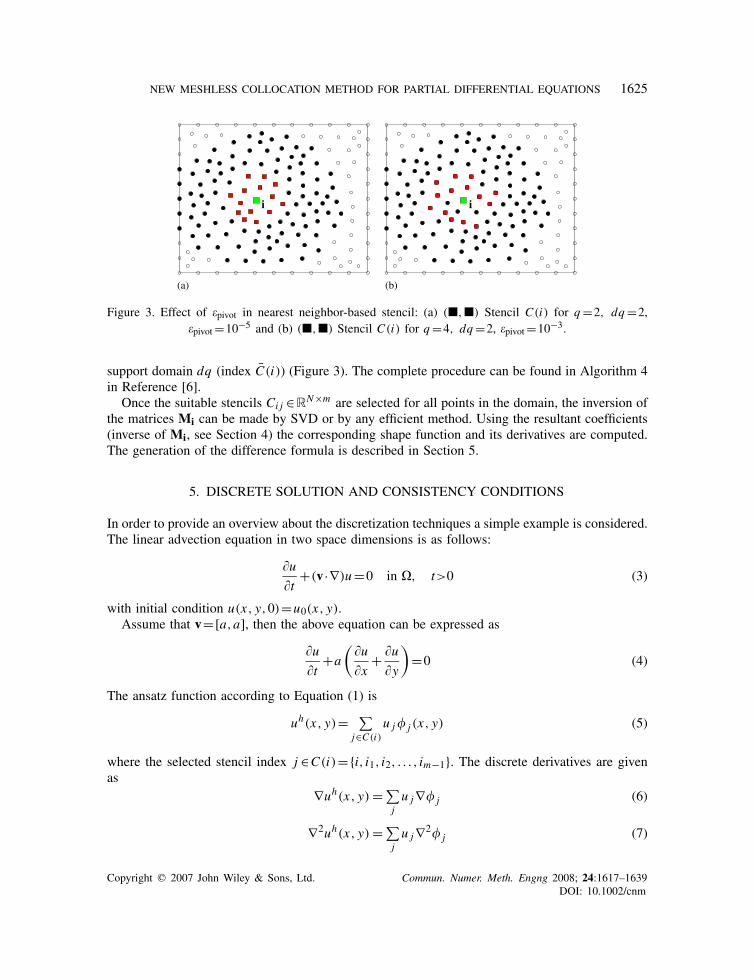
Figure 3. Effect of pivot in nearest neighbor-based stencil: (a) (,) Stencil C(i) for q=2, dq=2,pivot=10−5 and (b) (,) Stencil C(i) for q=4, dq=2, pivot=10−3.

support domain dq (index C(i)) (Figure 3). The complete procedure can be found in Algorithm 4in Reference [6].

Once the suitable stencils Ci j ∈RN×m are selected for all points in the domain, the inversion ofthe matrices Mi can be made by SVD or by any efficient method. Using the resultant coefficients(inverse of Mi, see Section 4) the corresponding shape function and its derivatives are computed.The generation of the difference formula is described in Section 5.

5. DISCRETE SOLUTION AND CONSISTENCY CONDITIONS

In order to provide an overview about the discretization techniques a simple example is considered.The linear advection equation in two space dimensions is as follows:

ut

+(v ·∇)u=0 in , t>0 (3)

with initial condition u(x, y,0)=u0(x, y).Assume that v=[a,a], then the above equation can be expressed as

ut

+a

(ux

+ uy

)=0 (4)

The ansatz function according to Equation (1) is

uh(x, y)= ∑j∈C(i)

u j j (x, y) (5)

where the selected stencil index j ∈C(i)=i, i1, i2, . . . , im−1. The discrete derivatives are givenas

∇uh(x, y) =∑ju j∇ j (6)

∇2uh(x, y) =∑ju j∇2 j (7)

Copyright q 2007 John Wiley & Sons, Ltd. Commun. Numer. Meth. Engng 2008; 24:1617–1639DOI: 10.1002/cnm

1626 M. KAMRUZZAMAN ET AL.

Plugging in the ansatz for spatial part and applying the Euler forward for temporal derivative leadto the following difference equation:

un+1i −uni

t+a

∑j∈C(i)

unj

( j

x+ j

y

)i

≈0 (8)

Solving this scheme with the given initial condition will provide the approximate solution ofthe PDE (4). The details about the discretization procedure of different PDEs and stability analysisof the scheme can be seen in Section 7.

5.1. Consistency conditions

To examine whether a meshless method is consistent for an unstructured grid of nodes is quitedifficult, as compared with checking whether a finite difference scheme on uniform grid is consis-tent. Therefore, it has been chosen to examine the reproducing conditions, i.e. completeness, asdescribed in Reference [1]. The consistency conditions as described below following Reference [2]are investigated for the presented meshless collocation method. In one dimension, the reproducingconditions (partition of unity) can be expressed as follows:∑

j j (x)=1,

∑j

j (x)x j = x,∑j

j (x)x2j = x2, . . .

∑j

j (x)xqj = xq (9)

In two dimensions the derivative reproducing conditions (partition of nullity) for a linear fieldare ∑

j j,x (x) = 0,

∑j

j,y(x)=0

∑j

j,x (x)x j = 1,∑j

j,y(x)x j =0

∑j

j,x (x)y j = 0,∑j

j,y(x)y j =1

(10)

Clearly, the generated shape functions in the present method (as described in Section 4) satisfiedall of these conditions, because

j (xi )=1 if i= j

0 if i = j

e.g. for any point xi the shape function always satisfies Equations (9) and (10). Therefore, themethod is consistent. On the other hand, the stability is also confirmed by means of eigen valueanalysis of the matrix K, i.e. for stability eigen values of K<1, where for elliptic PDEs thematrix K≡LhU (see Equation (20)), and for parabolic and hyperbolic PDEs K≡H−1

f Hm (seeEquation (18)).

6. ERROR ANALYSIS

Errors are caused because of the discretization of the domain. Errors are also developed bytruncation and rounding due to finite precision of the computations. In this section the localdiscretization error of the linear advection equation (4) will be studied.

Copyright q 2007 John Wiley & Sons, Ltd. Commun. Numer. Meth. Engng 2008; 24:1617–1639DOI: 10.1002/cnm

NEW MESHLESS COLLOCATION METHOD FOR PARTIAL DIFFERENTIAL EQUATIONS 1627

For simplicity the difference equation (8) in operator notation can be expressed as

un+1i = uni −a ·t ∑

j∈C(i)unjL j (11)

un+1i =Hi (u

n, i) (12)

where operator L=/x+/y denotes the application on the shape functions j (x).The difference equation (11) is found by direct discretization of the PDE (4). If the approximation

uni is replaced by the exact solution u(xi , yi , tn) at the corresponding point, then the right-handside will not be exactly equal to zero. This remainder of the term is known as local truncationerror, which can be easily found by Taylor series expansion. Therefore, the local truncation errorcan be defined as

Ri= 1

t[u(x, y, t+t)−u(x, y, t)]i +a

∑j∈C(i)

u jL j (13)

Expanding each term on the right-hand side of (13) in a Taylor series about i of the functionu(x, y, t) reveals

u(x, y, t+t)=u(x, y, t)+t ut + t2

2utt +O(t3) (14)

The discrete derivatives of the unknown function u at a point i have been computed with the helpof its neighboring node whose index is j ∈C(i)=i, i1, i2, . . . , im−1. Therefore, the Taylor seriesexpansion about the node i reveals

ui1 = ui +hTi1∇u |i + 12h

Ti1∇2u |i hi1 +·· ·

ui2 = ui +hTi2∇u |i + 12h

Ti2∇2u |i hi2 +·· ·

ui3 = ui +hTi3∇u |i + 12h

Ti3∇2u |i hi3 +·· ·

...

uim−1 = ui +hTim−1∇u |i + 1

2hTim−1

∇2u |i him−1 +·· ·

where hk :=[xk−xi yk− yi ]T=[xk yk]T, k∈C(i)\i . Substituting these in Equation (13) andavoiding the higher order terms give

Ri=ut +a ·ui ∑j∈C(i)

L j +a∑

k∈C(i)\ihTk∇u |i Lk+ a

2

∑k∈C(i)\i

hTk∇2u |i hkLk+ t

2utt

Employing the consistency conditions of (10) produces

∑j∈C(i)

L j =0 as∑j

j

x=0,

∑j

j

y=0

Copyright q 2007 John Wiley & Sons, Ltd. Commun. Numer. Meth. Engng 2008; 24:1617–1639DOI: 10.1002/cnm

1628 M. KAMRUZZAMAN ET AL.

Also

∑kLkhk =

⎡⎢⎢⎢⎣∑k

(k

xxk+ k

yxk

)∑k

(k

xyk+ k

yyk

)⎤⎥⎥⎥⎦=

[1

1

]

where from partition of nullity equation (10)

∑k

k

yxk = 0,

∑k

k

xyk =0

∑k

k

xxk = 1,

∑k

k

yyk =1

Applying consistency conditions and employing the ansatz for operator ∇2 in the summation overk lead to

Ri = a

22uxx |i +2uyy |i + a2t

2(uxx +2uxy+uyy)|i

= au|i + a2t

2u|i +a2tuxy |i

= a∑

j∈C(i)u j j +

a2t

2

∑j∈C(i)

u j j +a2t∑

j∈C(i)u j

2 j

xy

Finally the local truncation error term leads to

Ri=(a+ a2t

2

) ∑j∈C(i)

u j j +a2t∑

j∈C(i)u j

2 j

xy(15)

The local truncation error analysis is very important in order to develop a class of stable numericalschemes. In particular, the numerical solution of advection–diffusion equation, in which manynumerical schemes that attempt to find stable and accurate solutions for advection-dominated cases,have to resort by the vanishing viscosity.

7. MESHLESS COLLOCATION SCHEMES

7.1. Parabolic and hyperbolic PDEs

Parabolic and hyperbolic equations represent time-marching or propagation problems, i.e. problemsthat evolve through time. The discretization procedure of a time-dependent PDE is followed asdiscretization of a radial basis collocation technique, but in the framework of the proposed meshlessmethod. For details the author refers Reference [15]. For demonstration, the advection–diffusion

Copyright q 2007 John Wiley & Sons, Ltd. Commun. Numer. Meth. Engng 2008; 24:1617–1639DOI: 10.1002/cnm

NEW MESHLESS COLLOCATION METHOD FOR PARTIAL DIFFERENTIAL EQUATIONS 1629

equation is considered. The method of line approach is used to discretize the governing operatorequation. The governing equation of the unsteady advection–diffusion problem is given by

u(x, t)t

+Lu(x, t) = f (x, t), ∀x∈⊂Rd , t>0

Bu(x, t) = g(x, t), ∀x∈⊂Rd , t>0

(16)

where operator L=∇2+v ·∇, is the diffusion coefficient, v is a velocity vector, u(x, t) representsa potential function, and B is a boundary operator, which can be a Dirichlet, Neumann, or a mixedtype. The governing equation is parabolic for diffusion-dominated cases and turns hyperbolic foradvection-dominated cases. Equation (16) has to be supplemented with an initial condition of theform u(x, t)=u0(x).

Applying the meshless ansatz for spatial part and class of -method for temporal discretization,the collocation scheme in compact matrix form leads to

Hfun+1=Hmun+Fn+1 (17)

where

Hf=[U+tLhU

BhU

], Hm=

[U−(1−)tLhU

0

], Fn+1=

[tfn+1

gn+1

]

Therefore, by solving for un+1 one can easily obtain the following solution:

un+1=H−1f Hmun+H−1

f Fn+1 (18)

It is very important to note that in the present case matrix U is an identity matrix as shapefunction obeying the Kronecker delta function property. Also the resulting matrix LhU has atmost m non-zero entries in any row, a fact that the stencil size m makes apparent. Different valuesof refer to explicit and implicit schemes. For stability analysis see Reference [15].7.2. Elliptic PDEs

The elliptic-type problem has been discretized according to Reference [16], where meshless approx-imation functions are generated by interpolating moving least-square methods. Poisson’s equationin operator notation can be expressed as

Lu(x) = f (x)|x∈

u(x) = f (x)|x∈D andun

= f (x)|x∈N

(19)

respectively. Here D and N denote the Dirichlet and Neumann boundaries, and u(x)/n=∇u ·nis the directional derivative with respect to the outer normal vector n.

The discrete equation leads to

Lh ·u= f−LhD ·uD −LhN ·uN (20)

Equation (19) is equipped with the functional values, uD = fD and u/n|N = fN at the Dirichletand Neumann boundary.

Copyright q 2007 John Wiley & Sons, Ltd. Commun. Numer. Meth. Engng 2008; 24:1617–1639DOI: 10.1002/cnm

1630 M. KAMRUZZAMAN ET AL.

8. VALIDATIONS AND NUMERICAL RESULTS

To demonstrate the abilities of the proposed meshless collocation method an elliptic PDE, i.e. thePoisson equation, a hyperbolic, e.g. the Wave equation, and a non-linear PDE, e.g. the Burgers’equation, are considered as test problems. Numerical computations have been conducted ondifferent scattered data sets generated according to Reference [6]. The efficiency of the prescribedmethod has been investigated varying the pivot value and support domain definition in the nearestneighbor-based stencil selection algorithm. Also the computational errors due to the uniformity ofthe point distribution are analyzed.

8.1. Elliptic PDEs: the Poisson equation

Poisson’s equation is a second-order PDE which arises in many physical problems such as findingthe electric potential of a given charge distribution, the velocity of an inviscid incompressible fluidflow in a long tube (Poisseuille flow), etc. A Poisson equation in two dimensions is defined as

2ux2

+ 2uy2

=−22 sin(x) ·cos(y), ∀(x, y)∈=(0,1)×(0,1) (21)

with Dirichlet boundary conditions

u(x,0)=u(x,1)=u(0, y)=u(1, y)=0

The exact solution is ue(x, y)=sin(x) ·sin(y). The computational domain is represented byscattered points as shown in Figure 4.

The approximate solution for the given boundary value problem (BVP) according to Section 3 is

uh(x)= ∑j∈C(i)

u j j (x) (22)

The discretization of the given BVP has been done according to the procedure for elliptic BVPsdescribed in Section 7.2, which reveals

LhU ·u= f−LhUD ·uD (23)

where D means the Dirichlet boundary and f =−22 sin(x) ·cos(y)|. The computationalerror has been measured by the L∞ norm in terms of the relative error which is defined as

‖E‖∞ = ‖ue−uh‖∞‖ue‖∞

(24)

where ue and uh denote the exact and approximated solution of the given PDE. For simplicity,in the discussion section the collocation matrix LhU is denoted by L. The parameter valuescorresponding to appropriate stencil selection algorithms and numerical results are presented inTable I.

8.1.1. Numerical results and discussion. Computations are performed varying different parametersas shown in Table I, where XN represents a data set from a triangular mesh (Ring-based stencilselection) and YN is the data set generated by scattered data modeling (nearest neighbors-basedstencil search). Figure 4(b)–(d) shows the domain ∈[0,1]×[0,1] with N =2721,1653,461

Copyright q 2007 John Wiley & Sons, Ltd. Commun. Numer. Meth. Engng 2008; 24:1617–1639DOI: 10.1002/cnm

NEW MESHLESS COLLOCATION METHOD FOR PARTIAL DIFFERENTIAL EQUATIONS 1631

(a) (b)

(d)(c)

Figure 4. Domain by scattered data modeling. (a) Randomly generated data, Y3000;(b) Y2721, =0.25, sd=0.0052, Q=0.02; (c) Y1653, =0.28, sd=0.006, Q=0.024;

and Y461, =0.247, sd=0.012, Q=0.050.

scattered points with respective separation distance sd, radius of the largest inner empty sphereQ, and uniformity (according to Reference [6]). The solutions, pointwise effect of the thresholdvalue pivot on the condition number of M, and error can be viewed in Plate 1. Here, max(Mo)

denotes the maximum condition number of the matrices Mio computed on stencil C(i)o. Subscripto means that the stencil index is closest neighbors of the formula point i . Analogously, max(M)

denotes the maximum condition number of Mi computed on stencil C(i) selected by the proposedstencil search procedure. Figure 5(e) shows an example for a point i in which C(i)=C(i)o dueto a very small pivot value. The effect of the large pivot value can be viewed in Figure 5(f).

The decrease of the condition numbers of the resulting linear system at each point employingthe proposed stencil selection algorithm with a reasonable threshold value pivot is clearly foundin Plate 1(a) and (b). This is due to the fact that in the shape function generation process, badpoints (which have a large effect on the conditioning of the matrix M) are replaced with nextones. Consequently, the condition number of the global matrix L also reduces, see Plate 1(f).The increase in conditioning of L is due to the decrease in the separation distance sd. The smallseparation distance implies that two points in are too close together, this then spoils the conditionnumber. It is clearly visible from Table I and Plate 1(f) that the decrease in sd implies very large

Copyright q 2007 John Wiley & Sons, Ltd. Commun. Numer. Meth. Engng 2008; 24:1617–1639DOI: 10.1002/cnm

1632 M. KAMRUZZAMAN ET AL.

0

0.5

1

0

0.5

10

0.5

1

1.5

2

x 10

0

0.5

1

0

0.5

1

0

2

4

6

8

x 10

0.005 0.007 0.009 0.011 0.013 0.0150.015

105

1010

1015

1020

sd

κ(L

Ω)

εpivot

εpivot

Bad Matrix

0.005 0.007 0.009 0.011 0.013 0.0150.01510

10

10

10

100

sd

|E| ∞

Bad Matrix

Data Y461

Avoided (bad) nodes

Support, dq=4

Selected nodes C(i)\i

Formula node i

i

Data Y461

Avoided(bad) nodes

Support, dq=4

Selected node C(i)\i

Formula node

i

pivot= 1e−5= 1e−4

= 1e−3 to 1e−2 = 1e−3pivot

(a) (b)

(d)(c)

(e) (f)

Figure 5. Poisson’s equation: Cond. No, sd and effect of pivot. (a) ‖E‖∞ surface for Y1653;(b) ‖E‖∞ surface for Y461; (c) (L) for different sd; (d) ‖E‖∞ for different sd; (e) stencilfor node i , pivot=1e−4, (M|C(i))=5.0×1e3, (L)=7.3e16; and (f) Stencil for node i ,

pivot=1e−2, (M|C(i))=1e3, (L)=287.

Copyright q 2007 John Wiley & Sons, Ltd. Commun. Numer. Meth. Engng 2008; 24:1617–1639DOI: 10.1002/cnm

0

0.5

1

0

0.5

10

0.2

0.4

0.6

0.8

1

0 200 400 600 800 1000 1200 1400 1600

104

105

106

107

108

N

κ(M

o)

an

d κ

(M)

κ(Mo)

κ(M)

0 100 200 300 400 470470100

105

1010

1015

1020

1025

N

κ(M

o)

an

d κ

(M)

κ(Mo)

κ(M)

0.0050.1050.2050.30.3

10

10

sd

|E| ∞

pivot

pivot

0.0050.1050.2050.30.310

2

103

104

sd

κ(L

Ω)

pivot= 1e−5

= 1e−3

= 1e−5

= 1e−3pivot

0

0.5

1

0

0.5

10

2

4

6

8

10

x 10

(a) (b)

(d)(c)

(e) (f)

Plate 1. Poisson’s equation: numerical solutions. (a) Pointwise (M) and (Mo) for Y1653; (b) pointwise(M) and (Mo) for Y461; (c) solution for Y2721; (d) ‖E‖∞ surface for Y2721; (e) ‖E‖∞ over separation

distance sd; and (f) pointwise (L) over separation distance sd.

Copyright q 2007 John Wiley & Sons, Ltd. Commun. Numer. Meth. Engng 2008; 24(12)DOI: 10.1002/cnm

NEW MESHLESS COLLOCATION METHOD FOR PARTIAL DIFFERENTIAL EQUATIONS 1633

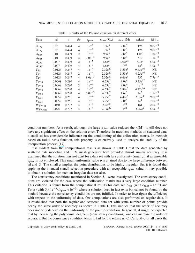
Table I. Results of the Poisson equation on different cases.

Data sd dq pivot max(Mo) max(M) (L) ‖E‖∞

X177 0.26 0.424 4 1e−2 1.9e5 9.8e3 126 9.0e−3

X177 0.26 0.424 4 1e−2 1.9e5 9.8e3 126 9.0e−3

X665 0.01 0.409 2 1e−4 9.9e5 9.8e5 1.0e3 1.8e−3

X665 0.01 0.409 4 7.0e−3 9.9e5 8.8e4 510 1.1e−3

X2577 0.007 0.409 2 1e−5 1.6e21 1.65e21 6.3e3 5.0e−4

X2577 0.007 0.409 4 1e−3 1.6e21 1021 1e3 4.0e−4

Y461 0.0124 0.247 4 1e−4 2.32e20 3.55e6 9.63e16 NEY461 0.0124 0.247 2 1e−4 2.32e20 3.55e6 4.25e16 NEY461 0.0124 0.247 4 8.0e−3 2.32e20 6.66e5 337 7.7e−3

Y1653 0.0068 0.280 4 1e−4 6.53e7 9.0e6 5.35e17 NEY1653 0.0068 0.280 2 1e−4 6.53e7 9.0e6 1e18 NEY1653 0.0068 0.280 4 1e−2 6.53e7 2.88e5 4.22e16 NEY1653 0.0068 0.280 4 5.0e−3 6.53e7 1.6e5 1e3 1.5e−3

Y2721 0.0052 0.251 4 1e−4 5.25e7 4.41e6 6.12e4 9.0e−4

Y2721 0.0052 0.251 4 1e−3 5.25e7 9.0e5 1e4 7.0e−4

Regu441 0.050 0.707 4 1e−4 2.0e20 1e20 161 2.0e−3

Regu1681 0.025 0.707 4 1e−4 2.17e22 1e22 6.47e2 5.0e−4

condition numbers. As a result, although the large pivot value reduces the (M), it still does nothave any significant effect on the solution error. Therefore, in meshless methods on scattered data,a small sd has considerable influence on the conditioning of the collocation matrix. In methodsbased on radial basis function, this property is extensively used to analyze the stability of theinterpolation process [17].

It is evident from the computational results as shown in Table I that the data generated byscattered data modeling and FEM mesh generator both provided almost similar accuracy. It isexamined that the solution may not exist for a data set with less uniformity (small ), if a reasonablepivot is not employed. This small uniformity value is attained due to the large difference betweensd and Q. The small implies the point distributions to be highly irregular. But it is found thatapplying the intended stencil selection procedure with an acceptable pivot value, it may possibleto obtain a solution for such an irregular data set also.

The consistency conditions mentioned in Section 5.1 were investigated. The consistency condi-tions are violated for the case where the collocation matrix has a very large condition number.This criterion is found from the computational results for data set Y461 (with pivot=1e−4) andY1653 (with 5×1e−3pivot<1e−2) where a solution does in fact exist but cannot be found by themethod because the consistency conditions are not fulfilled. In order to investigate the efficiencywith respect to the uniformity of data, few computations are also performed on regular data. Itis established that both the regular and scattered data set with same number of points providenearly the same order of accuracy as shown in Table I. This implies that the order of accuracydoes not only depend on the uniformity of the point distribution. In general, it might be expectedthat by increasing the polynomial degree q (consistency conditions), one can increase the order ofaccuracy. But the consistency condition tends to fail for the setting q>2. Currently, for all cases the

Copyright q 2007 John Wiley & Sons, Ltd. Commun. Numer. Meth. Engng 2008; 24:1617–1639DOI: 10.1002/cnm

1634 M. KAMRUZZAMAN ET AL.

computations are performed with fixed polynomial degree q=2, but as discussed in Section 4.2for each node i it is also possible to use different degrees of polynomials.

8.2. Hyperbolic PDEs: the wave equation

The wave equation is a hyperbolic PDE which models the propagation of sound, light and waterwaves, etc. The two-dimensional wave equation for a wave traveling with speed c is

2ut2

=c2(

2ux2

+ 2uy2

), ∀(x, y)∈, t>0 (25)

with initial conditions

u(x, y,0) = p(x, y)

ut

(x, y,0) = q(x, y)(26)

and Dirichlet boundary conditions

u(lb, y, t) = u(rb, y, t)=0

u(x,bb, t) = u(x,ub, t)=0(27)

where ∈[lb,rb]×[bb,ub] :=[0,1]×[0,1], and the initial conditions are chosen as p(x, y)=x(x−1)y(y−1) and q(x, y)=0. The wave speed is c=1/.

The discretization has been done according to the procedure for time-dependent PDEs describedin Section 7.1 which leads, in matrix form, to

un+1=H−1f Hmun+H−1

f Hbun−1+H−1f Fn+1 (28)

where

Hf=[U−c2t2LhU

U

], Hm=

[2U+(1−)c2t2LhU

0

], Hb=

[U

0

]

and for given boundary conditions (27)

Fn+1=[

t2fn+1

gn+1

]=[0

0

]

solution vectors u∈RN , U =I, U =I are identity matrices of sizes I ∈RN×N and I ∈RN×N . It is important to note that different values of provide different schemes. For the presentpurpose, =0.5, the Crank–Nicolson scheme is considered.

8.2.1. Numerical results and discussion. For the wave equation, computations were performedvarying different parameters similar to the Poisson equation as shown in Table II with scheme (28),=0.5. The time step is selected in such a way that it satisfies the Courant–Friedrichs–Lewy(CFL) condition (c ·thmin). Plate 2(a) shows the computational domain ∈[0,1]×[0,1], wheresd=0.015 and =0.3. A plot of the initial condition is shown in Plate 2(b). The evolution of the

Copyright q 2007 John Wiley & Sons, Ltd. Commun. Numer. Meth. Engng 2008; 24:1617–1639DOI: 10.1002/cnm

NEW MESHLESS COLLOCATION METHOD FOR PARTIAL DIFFERENTIAL EQUATIONS 1635

Table II. Results of the wave equation at t ∈[0,9) for different data sets.

Data sd dq pivot max(Mo) max(M) t ‖E‖∞

X177 0.26 0.424 4 1e−4 1.9e5 1.9e5 0.026 0.0117X177 0.26 0.424 4 1e−2 1.9e5 9.8e3 0.026 7.0e−3

Y273 0.019 0.311 4 1e−4 3.77e20 1.9e18 0.019 NEY273 0.019 0.311 4 1e−2 3.77e20 5.10e4 0.019 0.026Y365 0.015 0.30 4 1e−4 4.89e18 4.57e5 0.015 6.0e−3

Y365 0.015 0.30 4 1e−2 4.89e18 2.27e4 0.015 7.0e−3

X665 0.013 0.459 4 1e−4 9.99e5 9.7e5 0.013 0.010X665 0.013 0.459 4 5.0e−3 9.94e5 6.58e4 0.013 0.010Y743 0.010 0.256 4 1e−4 2.26e20 1.0e20 0.01 NEY743 0.010 0.256 4 1e−2 2.26e20 4.61e4 0.01 0.03Regu441 0.025 0.707 4 1e−4 2.03e20 1.4e4 0.0125 5.0e−3

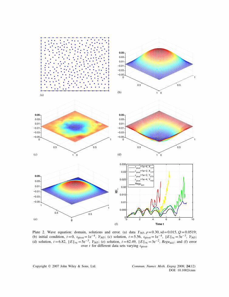
function u at time t=5.56 and 6.82 can be seen in Plate 2(c) and (d). The competence of thestencil selection procedure is clearly visible from Table II. It is evident that for highly irregulardata, the prescribed stencil selection methods seem more effective. The reasonable value of pivotplays a significant role in decreasing the condition number of the local matrix M, which is clearlyfound to be similar to that of Poisson’s equation. It is observed that the solution error grows withincreasing time t . At large t , the solution is not smooth enough for some data sets as demonstratedin Plate 2. For the data sets Y273 and Y743 the solution becomes worse for large t , as indicatedin Plate 3(b) and (d). This may happen if some points (where points tend to pick up) do not getsufficient support from its influence domain. Especially, points near the boundary play a key rolein order to diminish the smoothness of the solution. In order to examine this behavior in a moredetailed manner, computations are conducted on a uniformly distributed data set Regu441 witht ∈(0,62), t=0.0125. It is established from this example, for the uniformly distributed data, thatthis type of behavior does not appear, Plate 2(e). The solutions as visible in Plates 2(f) and 3(f)for the different data sets with large t (above 500 iterations) tend to diverge.

It should be noted that nodes near the boundary may be responsible for a non-smooth solution,since they do not receive proper support from its support domain, i.e. as no points are includedwithin the stencil from one side of the boundary. But for some cases, points inside the domain alsoblow up. This indicates that the definition of the support domain, as well as appropriate stencilinside the shape function generation process, may not be defined properly. Thus, independently itcan be concluded that the non-smooth behavior of the numerical solution at large time t is due tothe inefficient shape functions generation process (lack of proper support domain definition andstencil selection). As a result, the employed collocation scheme shows instable behavior.

8.3. Non-linear problem: the Burgers’ equation

Many physical phenomena in transport processes are described by time-dependent hyperbolicconservation laws. As a last test case, the following Burgers’ equation is considered:

ut

+u

(ux

+ uy

)=0 (29)

Copyright q 2007 John Wiley & Sons, Ltd. Commun. Numer. Meth. Engng 2008; 24:1617–1639DOI: 10.1002/cnm

1636 M. KAMRUZZAMAN ET AL.

This equation is known as inviscid Burgers’ equation. The initial condition for this problem isconsidered as

u(x, y,0)=

⎧⎪⎨⎪⎩exp

( ‖x−c‖2‖x−c‖2−R2

)for ‖x−c‖<R

0 otherwise

where R=0.25,c=[0.3,0.3] on a unit square . In order to be able to model the behavior ofthe numerical solution of this equation with respect to shock formation and shock propagationthere exist approaches that ensure the stability of the employed numerical scheme. One of thepopular approaches, the vanishing viscosity approach, is employed for the present purpose. Thediscretization is conducted by the implicit formulation, as employed by Hon and Mao [18].

un+1+tun(

un+1

x+ un+1

y

)= un

un+1 = gn+1

(30)

Substituting ansatz in Equation (30) and satisfying the condition on each of the interior andboundary collocation points similar to the wave equation case, the scheme follows in matrix form:

un+1=H−1f Hmun+H−1

f Fn+1 (31)

where

Hf =[I+tuL1hU

I

]

Hm =[I+(1−)t (uL1hU)

0

]

and the boundary conditions

Fn+1=[

0

gn+1

]

whereU ∈RN×N , operators L1 :=/x+/y, L2 :=2/x2+2/y applied to the shape func-tions generate the matrix L1h ∈RN×N and L2hU ∈RN×N . The unknown vectors u∈RN andU ∈RN×N ,g∈RN . It is clear that =1 provides the implicit scheme described by Hon andMao [18]. Here u denoted the maximum value of un. This assumption leads one to derive the localtruncation error term for Equation (29) in a similar way as the linear advection case described inSection 6, which reveals

Ri=(u+ u2t

2

) ∑j∈C(i)

u j j + u2t∑

j∈C(i)u j

2 j

x y(32)

Copyright q 2007 John Wiley & Sons, Ltd. Commun. Numer. Meth. Engng 2008; 24:1617–1639DOI: 10.1002/cnm

0

0.5

1 0

0.5

1

0.01

0.03

0.050.05

0

0.5

1 0

0.5

1

0.01

0.03

0.050.05

0

0.5

1 0

0.5

1

0.01

0.03

0.050.05

0

0.5

1

0

0.5

1

0.01

0.03

0.050.05

0 2 4 6 8 100

0.005

0.01

0.015

0.02

0.025

0.03

0.035

Time t

|E| ∞

pivot 177

pivot 177

pivot 273

pivot 743

Regu441

(a)(b)

(d)(c)

(e)

(f)

Plate 2. Wave equation: domain, solutions and error. (a) data Y365,=0.30,sd=0.015,Q=0.0519;(b) initial condition, t=0, pivot=1e−4, Y365; (c) solution, t=5.56, pivot=1e−4, ‖E‖∞ =3e−3, Y365;(d) solution, t=6.82, ‖E‖∞ =5e−3, Y365; (e) solution, t=62.49, ‖E‖∞ =3e−2, Regu441; and (f) error

over t for different data sets varying pivot.

Copyright q 2007 John Wiley & Sons, Ltd. Commun. Numer. Meth. Engng 2008; 24(12)DOI: 10.1002/cnm

0

0.5

1 0

0.5

1

0.01

0.03

0.050.05

0

0.5

1 0

0.5

1

0.01

0.03

0.050.05

0

0.5

1 0

0.5

1

0.01

0.03

0.050.05

0 1 2 3 4 5 6 7 80

0.002

0.004

0.006

0.008

0.01

0.012

Time t

|E| ∞

εpivot 665

εpivot 665

εpivot 365

εpivot 365

(a)(b)

(d)(c)

(f)(e)

Plate 3. Wave equation: domain, solutions and error. (a) data Y273,=0.31,sd=0.02,Q=0.06;(b) solution, t=8.8,pivot=1e−2,‖E‖∞ =0.01,Y273; (c) data Y743,=0.25,sd=0.01,Q=0.04; (d) solu-tion, t=6.49,pivot=1e−2,‖E‖∞ =0.02,Y743; (e) solution, t=5.59,‖E‖∞ =3.0e−3, X665; and (f) error

over t for different data sets varying pivot.

Copyright q 2007 John Wiley & Sons, Ltd. Commun. Numer. Meth. Engng 2008; 24(12)DOI: 10.1002/cnm

0

0.5

1 00.2

0.40.6

0.81

0

0.2

0.4

0.6

0.8

1

1.2

0

0.5

1 00.2

0.40.6

0.81

0

0.2

0.4

0.6

0.8

1

1.2

0

0.5

1 00.2

0.40.6

0.81

0

0.2

0.4

0.6

0.8

1

1.2

0

0.5

1 00.2

0.40.6

0.81

0

0.2

0.4

0.6

0.8

1

1.2

0

0.5

1 00.2

0.40.6

0.81

0

0.2

0.4

0.6

0.8

1

1.2

0

0.5

1 00.2

0.40.6

0.81

0

0.2

0.4

0.6

0.8

1

1.2

(a) (b)

(d)(c)

(e) (f)

Plate 4. Burgers’ equation: stable and unstable solutions. (a) initial condition, t=0; (b) solution at time,t=0.017, X665, scheme 34; (c) solution, t=0.019, X665, without Ri; (d) solution, t=0.052, X665, scheme

34; (e) solution, t=0.026, X665, without Ri; and (f) solution, t=0.85, X665, scheme 34.

Copyright q 2007 John Wiley & Sons, Ltd. Commun. Numer. Meth. Engng 2008; 24(12)DOI: 10.1002/cnm

NEW MESHLESS COLLOCATION METHOD FOR PARTIAL DIFFERENTIAL EQUATIONS 1637

With this artificial dissipation term (local truncation error) the modified equation of the given PDE(29) leads to

un+1+tun(

un+1

x+ un+1

y

)−un ≈Ri (33)

Employing the implicit scheme by Hon and Mao [18] together with Ri reveals

un+1=H−1f Hmun+H−1

f Fn+1 (34)

where

Hf=⎡⎢⎣I+t uL1hU−t

(u+ u2t

2

)L2hU− u2t2LxyU

I

⎤⎥⎦

and

Hm=[I

0

], Fn+1=

[0

gn+1

]

8.3.1. Numerical results and discussion. The initial condition 8.3 is depicted in Plate 4(a), (c) and(e) shows the solution at time t=0.01,0.02 computed with the scheme without the dissipationterm Ri. It is observed that the numerical solution uh for this pure advection problem does notmanage to capture the exact solution u. Consequently, the stability condition is violated. This isconfirmed by the eigen value analysis of Scheme 31, showing that all the eigen values of thematrix K=H−1

f Hm are not less than unity. The solution uh computed by Scheme 34 is also spoileddue to a spurious diffusion term. This scheme is generated by the vanishing viscosity approachwith an explicit error term Ri. However, the eigen value analysis confirmed the stability. Theflow behavior for such a case at time t=0.017,0.05,0.85 is displayed in Plate 4(b), (d) and (f).A viscous Burgers’ equation (a advection–diffusion problem) is also solved (see [6]) which hasparabolic behavior for a diffusion dominated case and turns hyperbolic for a advection-dominatedcases.

It was found that for the diffusive flows (parabolic behavior, =1), the solution agrees wellwith the analytical solution, but for the advection-dominated case (=0.05), the solution is smoothwith a large error. Further decrease in the diffusion coefficient <0.02 shows instability behaviorsuch as inviscid Burgers’ equation as expected.

9. CONCLUSION

Due to the great interest in pure meshless methods, a new collocation-based meshless methodon scattered data for the numerical solution of the PDEs quations is proposed. A brief sketch ofthe methods, its implementation issues, namely domain representation, meshless shape functionsformulation, and collocation discretization are explained elaborately. To demonstrate the truecapabilities of the proposed method different classes of PDEs are considered as test cases. Thecomputational results of each test case were examined by scrutinizing the properties of the data

Copyright q 2007 John Wiley & Sons, Ltd. Commun. Numer. Meth. Engng 2008; 24:1617–1639DOI: 10.1002/cnm

1638 M. KAMRUZZAMAN ET AL.

sets, polynomial degree, the threshold value for stencil search, support domain definition, andmeshless schemes.

It is found that the multilevel scattered data modeling algorithm can be used for the meshlessdiscretization. One can conveniently generate an acceptable uniformed data set with a reasonablecomputational cost, execute the solution process at different levels, and analyze its behavior. Theefficiency of the proposed stencil selection algorithm in decreasing the condition number of thecollocation matrix is clearly established. Especially for a highly irregular data set (less uniformity) the stencil selection algorithm (with an acceptable pivot value) is more efficient (in the sense ofdecreasing error) than well-uniformed data. In particular for a data set with very small separationdistance sd, this stencil selection technique plays an important role in order to decrease the conditionnumber of the collocation matrix. Numerical results of the Poisson equation demonstrate that theproposed support domain definition clearly manages to capture its influence nodes. Consequently,the accuracy order is high. The solutions for some test cases for hyperbolic PDEs deteriorate dueto the instability problem, and employing vanishing viscosity approach ensures stability, but thesolution is spoiled by a spurious diffusion term.

Meshless collocation methods can effectively produce results with a high degree of accuracy. Itsdevelopment is in the nascent stage and further investigations would open up numerous possibilitiesfor the numerical solution of the PDEs. Depending on the characteristics of the respective PDEs thesupport domain definition and stencil selection can be improved for hyperbolic PDEs together witha stable scheme, e.g. a modern approach such as essentially non-oscillatory (ENO) or weightedessentially non-oscillatory (WENO) reconstruction schemes.

REFERENCES

1. Belytschko T, Krongauz Y, Organ D, Fleming M, Krysl P. Meshless methods: an overview and recent developments.Computer Methods in Applied Mechanics and Engineering 1996; 139:3–47.

2. Fries T-P, Matthies H-G. Classification and Overview of Meshfree Methods. Institute of Scientific Computing,Technical University Braunschweig: Brunswick, Germany, 2004.

3. Liszka TJ, Duarte CA, Tworzydlo WW. hp-meshless cloud method. Computer Methods in Applied Mechanicsand Engineering 1996; 139:263–288.

4. Onate E, Idelsohn S, Zienkiewicz OC, Taylor RL. A finite point method in computational mechanics. Applicationsto convective transport and fluid flow. International Journal for Numerical Methods in Engineering 1996; 39:3839–3866.

5. Li X-Y, Teng S-H, Ungor A. Point Placement for Meshless Methods using Sphere Packing and Advancing FrontMethods, Department of Computer Science, University of Illinois at Urbana–Champaign, 2001.

6. Kamruzzaman M. A new meshless collocation method for partial differential equations. M.Sc. Thesis,Computational Sciences in Engineering (CSE), Institute of Computational Mathematics, TU Braunschweig,Germany, 2005.

7. Iske A. Multiresolution Methods in Scattered Data Modelling. Lecture Notes in Computational Science andEngineering, vol. 37. Springer: Germany, 2000.

8. Jin X, Li G, Aluru NR. On the equivalence between least-squares and kernel approximation in meshless methods.CMES. Computer Modelling in Engineering Sciences 2001; 2(4):447–462.

9. Jin X, Li G, Aluru NR. Positivity conditions in meshless collocation methods. Computer Methods in AppliedMechanics and Engineering 2004; 193:1171–1202.

10. Schonauer W. Generation of difference and error formulae of arbitrary consistency order on unstructured grid.Zeitschrift fur Angewandte Mathematik und Mechanik 1998; 78(3):1061–1062.

11. Schonauer W, Adolph T. How we solve PDEs. Journal of Computational and Applied Mathematics 2001;131:473–492.

12. Liu GR. Mesh Free Methods. CRC Press: Boca Raton, 2003.13. Floater MS, Iske A. Multistep scattered data interpolation using compactly supported radial basis functions.

Journal of Computational and Applied Mathematics 2001; 73:65–78.

Copyright q 2007 John Wiley & Sons, Ltd. Commun. Numer. Meth. Engng 2008; 24:1617–1639DOI: 10.1002/cnm

NEW MESHLESS COLLOCATION METHOD FOR PARTIAL DIFFERENTIAL EQUATIONS 1639

14. Furst JJ, Sonar Th. On meshless collocation approximations of conservation laws: preliminary investigations onpositive schemes and dissipation models. Zeitschrift fur Angewandte Mathematik und Mechanik 2001; 81(6):403–415.

15. Djidjeli K, Chinchapatnam PP, Nair PB, Price WG. Global and compact meshless schemes for the unsteadyconvection–diffusion equation. Computational Engineering and Design Group, University of Southampton,Southampton, U.K., 2002.

16. Netuzhylov H. Meshless collocation solution of boundary value problems via interpolating moving least squaresand its application to Navier–Stokes equation. Proceedings of ECCOMAS Thematic Conference on MeshlessMethods, Lisbon, Portugal, 11–14 July 2005.

17. Iske A. Perfect Centre Placement for Radial Basis Function Methods. Zentrum Mathematik, Technische UniversitatMunchen: Germany, 1999.

18. Hon YC, Mao XZ. An efficient numerical scheme for Burgers’ equation. Applied Mathematics and Computation1998; 95:37–50.

Copyright q 2007 John Wiley & Sons, Ltd. Commun. Numer. Meth. Engng 2008; 24:1617–1639DOI: 10.1002/cnm