University of New MexicoUNM Digital Repository

Earth and Planetary Sciences ETDs Electronic Theses and Dissertations

9-9-2010

The partial molar volume of carbon dioxide inperidotite partial melt at high pressureMegan Duncan

Follow this and additional works at: https://digitalrepository.unm.edu/eps_etds

This Thesis is brought to you for free and open access by the Electronic Theses and Dissertations at UNM Digital Repository. It has been accepted forinclusion in Earth and Planetary Sciences ETDs by an authorized administrator of UNM Digital Repository. For more information, please contactdisc@unm.edu.

Recommended CitationDuncan, Megan. "The partial molar volume of carbon dioxide in peridotite partial melt at high pressure." (2010).https://digitalrepository.unm.edu/eps_etds/21

Megan S. Duncanl-analaate

Earth and Planetary SciencesDepanmem

This thesis is approved, and it is acceptable in qualityand form for publication:

Approved by the Thesis Committee:

,

THE PARTIAL MOLAR VOLUME OF CARBON DIOXIDE IN PERIDOTITE PARTIAL MELT AT HIGH PRESSURE

BY

MEGAN S. DUNCAN

BACHELORS GEOLOGY CLEMSON UNIVERSITY 2007

THESIS

Submitted in Partial Fulfillment of the Requirements for the Degree of

Master of Science

Earth and Planetary Sciences

The University of New Mexico Albuquerque, New Mexico

July 2010

iii

ACKNOWLEDGMENTS

I would like to thank Mike Spilde and Ara Kooser for their help with detecting

carbon with the electron microprobe, Dr. Penny King with her help with FTIR, Dr. Carl

Agee for his role as advisor on this project.

THE PARTIAL MOLAR VOLUME OF CARBON DIOXIDE IN PERIDOTITE PARTIAL MELT AT HIGH PRESSURE

BY

MEGAN S. DUNCAN

ABSTRACT OF THESIS

Submitted in Partial Fulfillment of the Requirements for the Degree of

Master of Science

Earth and Planetary Sciences

The University of New Mexico Albuquerque, New Mexico

July 2010

v

The partial molar volume of carbon dioxide in peridotite partial melt at high pressure

Megan S. Duncan

Bachelor of Science, Geology, Clemson University, 2007 Master of Science, Earth and Planetary Sciences, University of New Mexico, 2010

ABSTRACT

The partial molar volume of CO2 ( 2COV ) in silicate melt was determined for a

komatiite composition using high pressure sink/float experiments in a multi-anvil press.

The density of the experimental melt at pressure was determined by observing sinking

and floating of pure forsterite (Fo100) and 90% forsterite (Fo90) buoyancy markers.

Values for 2COV were bracketed at 4.3 GPa (23.71 cm3/mol) and at 5.5 GPa

(22.06 cm3/mol), normalized to 1850°C. Combining the current data with previous work

we now more accurately constrain the compression curve of 2COV over the pressure

range of 1 bar to 20 GPa. These data allow the calculation of density at pressure of

carbonated silicate melts, such as kimberlite and silica undersaturated alkali basalts, and

the determination of their buoyancy and eruptibility.

vi

Table of Contents

List of Figures.................................................................................................................. vii

List of Tables .................................................................................................................. viii

Chapter 1 ........................................................................................................................... 1

Carbon in the Earth.......................................................................................................... 2

Composition..................................................................................................................... 4

Previous Studies .............................................................................................................. 6

Chapter 2 Experimental Procedures ................................................................................ 9

Chapter 3 Analytical Techniques ................................................................................... 16

Electron Microprobe...................................................................................................... 17

Fourier Transform Infrared Spectroscopy ..................................................................... 20

Experimental CO2.......................................................................................................... 22

Chapter 4 Experimental Results..................................................................................... 24

Chapter 5 Error Analysis ................................................................................................ 34

Density........................................................................................................................... 34

Molar Volume................................................................................................................ 39

Chapter 6 Application to the Earth and other Terrestrial Planets................................ 44

Kimberlites .................................................................................................................... 44

Appendices....................................................................................................................... 50

A) Appendix A Experiments .......................................................................................... 51

B) Appendix B Electron Microprobe............................................................................. 58

C) Appendix C FTIR...................................................................................................... 75

References........................................................................................................................ 86

vii

List of Figures

Figure 2-1. BSE images of experimental run products .................................................................................13 Figure 3-1. EPMA for CO2 of Ag-coated experiment...................................................................................18 Figure 4-1. DG-5 experiments and best fit Birch-Murnaghan curve: ρ0 = 2.59 g/cm3; DG-N experiments

and best fit Birch-Murnaghan curve: ρ0 = 2.75 g/cm3 ...............................................................................26 Figure 4-2. DG-5 experiments and best fit Birch-Murnaghan curve: ρ0 = 2.32 g/cm3; DG-N experiments

and best fit Birch-Murnaghan curve: ρ0 = 2.46 g/cm3 ...............................................................................27 Figure 4-3. Compression curves for CO2 fit to ideal data .............................................................................32 Figure 4-4. Vinet EOS compression curves for

2COV and OHV 2................................................................33

Figure 6-1. Kimberlite melt Birch-Murnaghan compression curves.............................................................46 Figure 6-2. Birch-Murnaghan compression curves for a kimberlite melt with only 10.0 wt% CO2.............48 Figure A-1. Cross section of ceramic octahedron with experimental set up .................................................51 Figure A-2. DG-5-9.......................................................................................................................................52 Figure A-3. DG-5-11.....................................................................................................................................52 Figure A-4. DG-5-14.....................................................................................................................................53 Figure A-5. DG-5-16.....................................................................................................................................53 Figure A-6. DG-5-17.....................................................................................................................................53 Figure A-7. DG-5-19.....................................................................................................................................53 Figure A-8. DG-5-21.....................................................................................................................................53 Figure A-9. DG-5-22.....................................................................................................................................53 Figure A-10. DG-5-23...................................................................................................................................54 Figure A-11. DG-N-7....................................................................................................................................55 Figure A-12. DG-N-14..................................................................................................................................55 Figure A-13. DG-N-17..................................................................................................................................55 Figure A-14. DG-N-19..................................................................................................................................55 Figure A-15. DG-N-20..................................................................................................................................55 Figure A-16. DG-N-22..................................................................................................................................55 Figure A-17. DG-N-23..................................................................................................................................56 Figure A-18. DG-N-33..................................................................................................................................56 Figure A-19. And-5-1 ...................................................................................................................................56 Figure C-1. Micro-FTIR analyses of carbonated experiment DG-5-1 using 100 µm spot size ....................76 Figure C-2. Micro-FTIR analyses of carbonated experiment DG-5-1 using 170 µm spot size ....................76 Figure C-3. Spectra of dolomite, calcite crystal and pressed powder of the same crystal ............................77 Figure C-4. Micro-FTIR analyses of non-carbonated experiments DG-N-3 and DG-N-7 ...........................78 Figure C-5. Micro-FTIR analyses of carbonated experiments DG-5-4, DG-5-9, DG-5-11, and DG-5-17 ..79 Figure C-6. Transmission results of powdered and pressed carbonated experiment DG-5-7 .......................79 Figure C-7. Micro-FTIR analyses of carbonated experiment And-5 ............................................................80 Figure C-8. Micro-FTIR analyses of carbonated natural andesites...............................................................81 Figure C-9. Reflected light image of carbonated experiment DG-5-1 ..........................................................82 Figure C-10. Reflected light images of carbonated experiment DG-5-1 FTIR analysis spots......................82 Figure C-11. Reflected light image of carbonated experiment DG-5-4 ........................................................83 Figure C-12. Reflected light images of DG-5-4 FTIR analysis spots ...........................................................83 Figure C-13. Reflected light image of carbonated experiment DG-5-9 ........................................................83 Figure C-14. Reflected light image of DG-5-9 FTIR analysis spot ..............................................................83 Figure C-15. Reflected light image of DG-5-11 FTIR analysis spot ............................................................84 Figure C-16. Reflected light image of DG-5-17 FTIR analysis spot ............................................................84 Figure C-17. Reflected light image of non- carbonated experiment DG-N-3...............................................84 Figure C-18. Reflected light images of DG-N-3 FTIR analysis spots ..........................................................84 Figure C-19. Reflected light image of non- carbonated experiment DG-N-7...............................................85 Figure C-20. Reflected light image of DG-N-7 FTIR analysis spot .............................................................85 Figure C-21. Reflected light images of three And-5 FTIR analysis spots. ...................................................85

viii

List of Tables

Table 1-1. Calculated partial molar volumes of CO2 from previous studies...................................................7 Table 2-1. Composition of peridotite KLB-1, PERC, and our simplified starting compositions..................10 Table 2-2. Elastic parameters for endmember olivines used to calculate density .........................................14 Table 4-1. Carbonated experimental run conditions and results ...................................................................25 Table 4-2. Non-carbonated experimental run conditions and result .............................................................25 Table 4-3. Best fit Birch-Murnaghan EOS parameters used for

2COV calculation ......................................28 Table 4-4. Composition used to calculate

2COV ...........................................................................................29 Table 5-1. Zero pressure density and thermal expansion parameters used to calculate DG-5 and DG-N

compression curves....................................................................................................................................35 Table 5-2. Birch-Murnaghan EOS parameters for different neutral buoyancy results..................................36 Table 5-3. Mineral sphere elastic parameters................................................................................................37 Table 5-4. Neutral buoyancy density values at experimental pressures and 1850°C for DG-5 and DG-N ..38 Table 5-5. Best fit Birch-Murnaghan KT values to different neutral buoyancies for DG-5 and DG-N.........38 Table 5-6. Composition sets used in calculating

2COV . ...............................................................................40 Table 5-7.

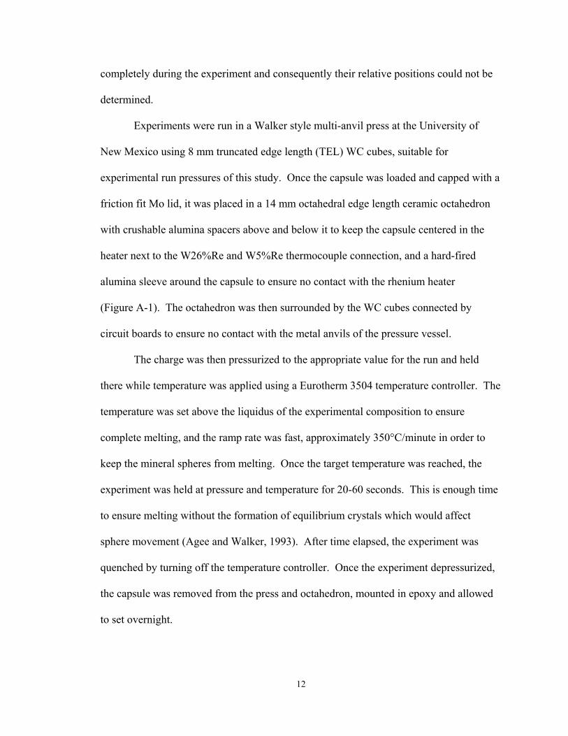
2COV values for each composition and each NB at pressure ......................................................40 Table 5-8.

2COV values for each composition using Mo instead of MoO3...................................................42 Table 5-9.

2COV values for each composition at pressure............................................................................43 Table 6-1. Kimberlite melt compositions ......................................................................................................45 Table 6-2. Birch-Murnaghan EOS elastic parameters for kimberlite melt with only 10.0 wt% CO2 ...........47 Table A-1. Experimental run conditions and results for carbonated experiments. .......................................52 Table A-2. Experimental run conditions and results for non-carbonated experiments. ................................54 Table A-3. Experimental run conditions for “andesite” experiment. ............................................................56 Table B-1. EMPA operating conditions, standards, and experiments analyzed with an Ag-coat .................60 Table B-2. EMPA operating conditions, standards, and experiments analyzed with an Au-coat .................61 Table B-3. Average electron microprobe values for carbonated experiments DG-5-1, 4, 7, 8, 9.................63 Table B-4. Average electron microprobe values for carbonated experiments DG-5-11, 14, 16, 19.............64 Table B-5. Average electron microprobe values for carbonated experiments DG-5-17...............................65 Table B-6. Average electron microprobe values for carbonated experiments DG-5-22, 23.........................66 Table B-7. Average electron microprobe values for non-carbonated experiments DG-N-3, 7, 9, 13, 14.....67 Table B-8. Average electron microprobe values for non-carbonated experiments DG-N-17, 19, 21, 24, 25,

31, 33. ........................................................................................................................................................68 Table B-9. Average electron microprobe values for non-carbonated experiment DG-N-22. .......................69 Table B-10. Average electron microprobe values for non-carbonated experiment DG-N-22. .....................70 Table B-11. Starting composition for carbonated "andesite" mix.................................................................71 Table B-12. Average electron microprobe values for carbonated experiment And-5...................................72 Table B-13. Average electron microprobe oxide values for C-coated carbonated experiments DG-5-9, 14,

16, 19, 21, 22, 23. ......................................................................................................................................74 Table B-14. Average electron microprobe oxide values for C-coated non-carbonated experiments DG-N-7,

14, 20, 22, 23. ............................................................................................................................................74 Table C-1. Micro-FTIR analytical conditions with approximate amount of CO3

2- present in sample. .........75

1

1) Chapter 1

Carbon dioxide is present in the mantle of the Earth and as one of the most

abundant volatile species in the Earth, its effect on melt behavior needs to be well

understood. The presence of carbon dioxide affects the behavior of mantle melts by

lowering their density and solidus and liquidus temperatures; therefore how CO2 interacts

with mantle melts must be studied and understood so that mantle processes can be

quantified. One way to quantify the effect of CO2 on a mantle melt is by determining its

partial molar volume ( 2COV ), and how this value changes with pressure. Using an

average upper mantle composition, derived from a peridotite partial melt, we have

experimentally determined 2COV at upper mantle pressures.

Molar volume cannot be measured directly so we must use a modified version of

Equation (1-1), and simple compositions with known densities to calculate 2COV . In

order to accurately do this, two simple peridotite-derived komatiite compositions were

synthesized with similar major element abundances except that one composition had an

added 5.7 wt% CO2. We experimentally determined the densities of each melt, and were

able to approximate the 2COV from the differences between the densities of the two

compositions.

Molar volume (V ) is an intensive variable that, ideally, is not controlled by the

amount of the component, i.e. the number of moles of the component in the system, but

can be controlled by changes in the system such as in temperature and pressure. When a

melt consists of many liquid oxides, the change in volume that 1 mole of each oxide

2

imparts on the melt is its partial molar volume ( iV ). If the iV s of all components and

their amounts (Xi) are known then the melt density can be calculated using:

∑=i

iiii VXMXρ (1-1)

where ρ is the density of the melt, Xi is the mole fraction of liquid oxide component i, Mi

is its gram formula weight, and iV is its partial molar volume (Bottinga and Weill, 1970).

For example: CO2 is a gas at Standard Temperature and Pressure (STP, 25°C and 1 atm)

and 1 cm3 of this gas contains approximately 2.5x1019 CO2 molecules, whereas 1 cm3 of

SiO2, a solid at STP, consists 2.7x1022 molecules: three orders of magnitude more than

CO2. In order to compare CO2 and SiO2 they are converted to molar volumes (cm3/mol)

using ii

i Vn

V 1= , where ni is the number of moles of component i and Vi is its volume.

At these conditions, the calculated molar volumes are approximately 24,500 cm3/mol for

CO2, and 22.8 cm3/mol for SiO2, which makes sense because CO2 under these conditions

is a gas and 1 mole of a gas has a larger volume than 1 mole of a solid.

Carbon in the Earth

As CO2 is one of the most abundant volatile species in mantle-derived magma

source regions (Anderson, 1975; Canil and Scarfe, 1990), it is vital to understand the

effect it has on melt behavior. Carbon dioxide’s effect on a melt’s density and

eruptibility must be quantified in order to fully detail mantle processes. Carbon dioxide

is found outgassing from volcanoes and is seen as carbon in the form of graphite and

diamonds. Carbon entered the mantle during the accretion of the planet and/or by

meteorite impact on the early Earth’s magma ocean (i. e. late veneer when volatile-rich

bodies impacted the Earth after accretion creating a volatile layer on the Earth’s surface

3

see Kuramoto, 1997; Turekian and Clark, 1975 for discussion), and enters the mantle

today by subduction of ocean slabs in minerals such as magnesite and dolomite. The

actual amount of CO2 in the interior of the Earth is unknown, but estimates can be made

based on element ratios, volcanic gas measurements, recycling models, and through

analysis of mantle rocks (McDonough and Sun, 1995; Taran et al., 1998). Depending on

which mantle rock is analyzed (peridotite, basalt, kimberlite, komatiite) estimates of the

amount of CO2 in the primitive mantle range from 230-550 ppm (Wyllie and

Ryabchikov, 2000; Zhang and Zindler, 1993), and <50 to >500 ppm carbon in the Earth’s

upper mantle today (McDonough and Sun, 1995).

The presence of CO2 in the mantle affects properties such as liquidus and solidus

temperatures, melt density, and the behavior of partial melts in the mantle (Bourgue and

Richet, 2001; Eggler, 1978; Hirose, 1997; Liu and Lange, 2003; Wendlandt and Mysen,

1980). To explore the behavior of CO2 at elevated pressures and temperatures, numerous

studies have been carried out. Many studies have focused on the solubility of CO2 in

various mantle compositions, measuring the amount of CO2 dissolved in different partial

melt compositions (Dobson et al., 1996; Pan et al., 1991; Stolper and Holloway, 1988;

Thibault and Holloway, 1994). The findings from this previous work show that pressure,

temperature, and composition have a significant effect on the solubility of CO2 in silicate

melts (Brooker et al., 2001a; Dasgupta and Hirschmann, 2007; Dixon et al., 1995; Eggler

and Rosenhauer, 1978; Mysen et al., 1976; Taylor, 1990), with pressure increasing

solubility dramatically, temperature decreasing solubility, and melts with non-bridging

oxygen (NBO) to tetrahedral network-forming cation (T, e.g. Si2+ and Al3+) ratios greater

than zero showing the highest CO2 concentrations.

4

Carbon dioxide is most soluble in mafic and ultramafic melts because of the

increased NBO/T ratios most affected by lower amounts of SiO2. The silica tetrahedra

polymerize the melt creating bridging oxygens. In order for CO2 to enter a melt there

must be non-bridging, or “free”, oxygens for the molecule to bond with (Brooker et al.,

2001a). This creates the carbonate anion in the melt, the most common form of carbon in

mantle melts (Mysen et al., 1976). Studies done on the forms of CO2 in basaltic melts

using Raman spectroscopy and Infrared spectroscopy found that while CO32- is most

common, molecular CO2 and CO are also possible in melts with lower NBO/T ratios such

as andesite or rhyolite (Brooker et al., 2001a; Dixon and Pan, 1995; Fine and Stolper,

1985; Lange, 1994) These studies determined that the form of carbon in the melt is

affected by the availability of non-bridging oxygens. Non-bridging oxygens are created

when network modifying cations (e. g. Mg2+, Ca2+) enter the melt and break the bonds of

SiO2 and Al2O3 tetrahedra. Those melts with NBO/T < 0.5 will tend to contain dissolved

CO2, while melts with NBO/T > 0.5 are more likely to contain CO32-, along an

approximately linear relationship. An ultramafic composition, such as komatiite, will

dissolve CO2, as CO32-, and is appropriate as an upper mantle analog, and therefore is our

choice for this study.

Composition

The upper mantle of the Earth is thought to be roughly peridotitic in composition.

Peridotite was first proposed by Bowen (1928) based on mantle seismic velocity and

basaltic magma compositions which are thought to be partial melts of peridotite. Since

that time, peridotite has been further investigated and found to fit the geochemical and

geophysical properties of the mantle (Palme and O'Neill, 2003; Ringwood, 1966). Many

5

peridotite xenoliths exist on or near the Earth’s surface and have been studied thoroughly.

Such xenoliths are present in southern New Mexico at Kilbourne Hole. A sample from

this site, KLB-1, was studied by Takahashi (1986) because it was thought to represent an

undepleted, upper mantle composition and is similar to the pyrolite composition for the

mantle proposed by Ringwood (1966).

A simplified version of a partial melt of this peridotite sample – a komatiite,

containing only major elements, was used for these experiments because of its standing

as a good upper mantle average and its ability to take large (~5 wt%) amounts of

dissolved CO2 into its melt structure. As stated above, CO2 should dissolve in the melt as

CO32- due to the ultramafic nature and the NBO/T value of the experimental composition.

The NBO/T value for our composition is approximately 0.93 and, as shown in Figure 3 of

Brooker et al. (2001a), this NBO/T value indicates that ~6.0 wt% CO2 can dissolve in the

melt at 1.5 GPa for simple, Fe-free compositions. Dixon (1997) modeled CO2 solubility

in Fe-bearing, more Mg-rich compositions and determined a compositional parameter, Π,

to describe CO2 solubility. This parameter is based on melt depolymerization (i. e. the

amount of Si4+ and Al3+ present in the melt) and the potential of cations to react with

carbonate (i. e. network modifying cations that form non-bridging oxygens), where

Π = -6.50(Si4+ + Al3+) + 20.17(Ca2+ 0.8K1+ + 0.7Na1+ + 0.4Mg2+ + 0.4Fe2+), with the

cations in molar proportions. The Π parameter for our experimental composition is

approximately 1.48. This indicates, from Figure 2B of Dixon (1997), that our melt will

dissolve ~4.0 wt% CO2 at 2.0 GPa. Due the pressure affect on CO2 solubility, our

experiments done at pressures above 3.5 GPa, should easily dissolve ≥ 5.0 wt% CO2.

6

Previous Studies

Earlier studies indicated that dissolved CO2 should have a large effect on silicate

liquid density (Bourgue and Richet, 2001; Dasgupta et al., 2007), however there are few

experimental data at high pressure on possible mantle compositions. Here we contribute

to this database by determining the densities of carbonated komatiite melt and the same

melt with no CO2 at high pressure. Using these data, we were able to derive the partial

molar volume of CO2 ( 2COV ) by difference in the silicate melt as a function of pressure

using a modified version of Equation (1-1). Our results bridge the large gap between

1 bar and 19.5 GPa, where 2COV has been measured.

Previous studies have determined the partial molar volumes of other liquid oxides

(e.g. CaO, MgO, H2O) in order to better determine the origin and behavior of magmatic

systems (Agee, 2008a; Lange and Carmichael, 1987). Using a Equation (1-1) and the

molar volumes of melt components, the density of the melt can be determined using

thermal expansivity (∂Vi/∂T) values at a given temperature. By knowing the density and

composition of carbonated and non-carbonated silicate melts of similar major element

abundance, the difference between the melt molar volumes will be 2COV . Determining

2COV values at various pressures will lead to the derivation of a compression curve,

which describes how 2COV changes with pressure. This curve can then be used to explain

the behavior of carbonated silicate melts in the upper mantle.

Studies done on carbonated compositions that measured the density of the melt

can be used to estimate 2COV for those compositions (Table 1-1). Since most of these

studies were done with carbonate compositions rather than silicate, it may not be

appropriate to apply the 2COV values determined to carbonated silicates, such as in the

7

mantle. Also, many of these experiments were performed at 1 bar, and cannot be used to

constrain the 2COV compression curve at high pressure.

Table 1-1. Calculated partial molar volumes of CO2 from previous carbonate and carbonated silicate studies.

Composition 2COV

(cm3/mol)P

(GPa) T

(°C) Reference

CaCO3 25.81 1.0x10-4 827 Liu and Lange (2003) Na2CO3 28.73 1.0x10-4 827 Liu and Lange (2003) K2CO3 32.35 1.0x10-4 827 Liu and Lange (2003) CaCO3 33.36 0.1 1364 Genge et al. (1995) K2Ca(CO3)2 35.20 1.0x10-4 1677 Dobson et al. (1996) K2Ca(CO3)2 31.76 2.5 1677 Dobson et al. (1996) K2Ca(CO3)2 29.92 4.0 1677 Dobson et al. (1996) Tholeiite 23.14 0.1 1200 Pan et al. (1991) MORB 33.00 0.1 1200 Stolper and Holloway (1988) Ca-rich Leucitite 22.03 0.1 1200 Thibault and Holloway (1994)Alkaline silicate melts 19.90 2.0 1400 Liu and Lange (2003) Carbonated MORB 20.98 19.5 2300 Ghosh et al. (2007) A preliminary compression curve for

2COV was determined by Ghosh et al.

(2007). They used sink/float experiments at 19 and 20 GPa with a diamond buoyancy

marker and determined the 2COV for a mid-ocean ridge basalt (MORB) to be

20.98 cm3/mol at 19.5 GPa and 2300°C. In order to calculate an equation of state for

2COV , Ghosh et al. (2007) calculated 1 bar, 2.5 GPa, and 4.0 GPa 2COV values from the

carbonate liquid density studies of Genge et al. (1995) and Dobson et al. (1996),

correcting for temperature using ∂VCO2/∂T = 4.0 x 10-3 cm3/mol-K (Liu and Lange, 2003)

(Table 1-1). They then derived values for the isothermal bulk modulus (KT = 3.7 GPa)

and its pressure derivative (K’ = 9.0) from the Vinet equation of state (EOS).

Since the effect of composition on 2COV is thought to be negligible only for

silicate melts in the range of 40 to 80 mol% SiO2 (Bockris et al., 1956; Bottinga and

Weill, 1970; Shartsis et al., 1952; Tomlinson et al., 1958), carbonate melt compositions

8

with no SiO2 may not accurately describe 2COV for silicate melts. Because the presence of

SiO2 in a melt will alter melt structure from that of a carbonate melt, it follows that the

1 bar, 2.5 GPa, and 4.0 GPa 2COV values, which were calculated from carbonate

compositions and not silicate, may not be accurate to apply to Si-bearing mantle analogs.

Our experiments on carbonated silicate melt now fill in the gap between 1 bar and

19.5 GPa thus removing the need to rely on non-silicate-bearing melt high pressure data.

With an updated 2COV compression curve, based on carbonated silicate melts, the

densities of these melts can be defined more accurately at upper mantle pressures. These

densities are important to know so that the physical properties and behaviors of

carbonated silicate melts, e.g. kimberlite buoyancy and eruption, can be described more

accurately.

9

2) Chapter 2

Experimental Procedures

A simplified komatiite starting composition was chosen for the experimental runs

based on the composition of Dasgupta et al. (2007) (Table 2-1). This composition

(PERC) was a carbonated partial melt derived from peridotite KLB-1. The KLB-1

sample is a good representation of an undepleted, average upper mantle (Takahashi,

1986), and therefore a good analog to determine 2COV in a carbonated silicate melt. The

simplified composition was used to ensure there was no compositional control on 2COV ,

which may be influenced by the form of carbonate present in the melt (CaCO3 rather than

K2CO3, Na2CO3: Liu and Lange, 2003). Two komatiite mixes were made with the same

major element abundances using reagent grade powdered oxides. One mix, DG-5,

contained CaCO3 which translates to approximately 5.7 wt% CO2 (Table 2-1). This

amount is more than is found in partial melts derived from peridotite compositions (~90-

134 ppm in the MORB source region: Shaw et al., 2010), but was chosen because it

should be detected easily by analytical methods. The other mix, DG-N, only contained

CaO so that a non-carbonated baseline density could be determined, which allows for a

more accurate calculation of 2COV .

10

Table 2-1. Composition of peridotite KLB-1, its carbonated experimental partial melt (PERC) at 3 GPa, and our simplified starting compositions based on PERC + 5 wt% CO2.

Starting Material Oxide(wt%)

KLB-1 Takahashi

(1986)

PERC Dasgupta

et al. (2007) DG-5 DG-N SiO2 44.48 43.19 43.36 46.69 TiO2 0.16 0.47 Al2O3 3.59 7.27 6.97 7.30 Cr2O3 0.31 0.33 FeO 8.10 9.64 10.02 10.60 MnO 0.12 0.20 MgO 39.22 25.92 26.63 28.29 CaO 3.44 7.30 7.29 7.13 Na2O 0.30 0.57 K2O 0.02 0.04 NiO 0.25 CO2 5.09 5.72 Total 99.99 100.00 100.0 100.00 NBO/T n/a 0.93 n/a Π n/a 1.48 n/a Mg# 89.62 82.62 82.58 82.64

The sink/float experimental method (Agee and Walker, 1988, 1993) was used in

order to determine the density of the melt in each experiment. This was accomplished by

loading the powdered starting composition into molybdenum (Mo) capsules along with

two mineral spheres. Molybdenum capsules were used because of the oxygen fugacity

(fO2 ~1+ Iron-Wustite oxygen buffer) they impart on the charge and for the lack of

influence that dissolved Mo has on the melt structure (Agee and Walker, 1988). The

capsule, lid, and both mineral spheres were cleaned with ethanol in a sonicator for

50 seconds and allowed to dry before use to ensure no contamination of the experimental

melt composition. Approximately 10 mg of the powered mix was loaded into the capsule

with spheres; the capsule contents were layered: mix-sphere-mix-sphere-mix, so that

there was no contact between the spheres and capsule walls to which the spheres could

adhere during the run which would restrict their movement. This layering was also done

11

to ensure that one sphere was near the bottom of the capsule, while the other was near the

top, to allow for enough space for their movement and making any movement easier to

determine after the run.

Mineral spheres of known density were used to calculate the density of the

experimental melt, which in turn allowed for the calculation of 2COV . These mineral

spheres, or density markers, have well defined density/pressure (compressibility) curves

with constant temperature. Starting with forsterite 100 (Fo100), which was the lowest

density mineral used, the compressibility curves of the two melts was constrained at low

pressure (~4 GPa). San Carlos olivine, approximately forsterite 90 (Fo90), was used to

constrain the compressibility curves of the silicate melts at increasingly higher pressures

(between 4 and 6 GPa) to begin to fill in the gap between 1 bar and 19.5 GPa. Melt

density was determined by relative sphere placement at the end of the run. If the mineral

spheres were denser than the experimental melt, they sank, while if they were less dense

they were located at the top of the capsule at the end of the run. The ideal pressure and

temperature conditions need to be reached where the spheres and melt have the same

density – a neutral buoyancy – where the relative sphere positions remain unchanged

from their initial placement.

A brief note on olivine sphere size – mineral spheres were made using the Bond

air mill technique which uses air pressure to push mineral fragments around a chamber

that is lined with carbide paper thereby grinding them into “spheres” (Bond, 1951). Ideal

size is between 400 and 650 microns determined from these experiments. We found that

spheres bigger than ~700 µm do not have enough space to move in the capsule and yield

false neutral buoyancy results. We also found that spheres smaller than ~350 µm melted

12

completely during the experiment and consequently their relative positions could not be

determined.

Experiments were run in a Walker style multi-anvil press at the University of

New Mexico using 8 mm truncated edge length (TEL) WC cubes, suitable for

experimental run pressures of this study. Once the capsule was loaded and capped with a

friction fit Mo lid, it was placed in a 14 mm octahedral edge length ceramic octahedron

with crushable alumina spacers above and below it to keep the capsule centered in the

heater next to the W26%Re and W5%Re thermocouple connection, and a hard-fired

alumina sleeve around the capsule to ensure no contact with the rhenium heater

(Figure A-1). The octahedron was then surrounded by the WC cubes connected by

circuit boards to ensure no contact with the metal anvils of the pressure vessel.

The charge was then pressurized to the appropriate value for the run and held

there while temperature was applied using a Eurotherm 3504 temperature controller. The

temperature was set above the liquidus of the experimental composition to ensure

complete melting, and the ramp rate was fast, approximately 350°C/minute in order to

keep the mineral spheres from melting. Once the target temperature was reached, the

experiment was held at pressure and temperature for 20-60 seconds. This is enough time

to ensure melting without the formation of equilibrium crystals which would affect

sphere movement (Agee and Walker, 1993). After time elapsed, the experiment was

quenched by turning off the temperature controller. Once the experiment depressurized,

the capsule was removed from the press and octahedron, mounted in epoxy and allowed

to set overnight.

13

Once set, the experimental charge was ground into to expose the inside of the

capsule. This allows for confirmation of melting by the presence of quench crystals

visible under the optical microscope, and the determination of relative sphere position

(Figure 2-1).

Figure 2-1. BSE images of experimental run products with Fo100 spheres. a) Sink DG-5-9, b) Float DG-N-7

For each melt composition and each mineral density marker, a neutral buoyancy,

sink and float are required to ensure the accuracy of the density measurement. The

exception is when the sink and float are within a few tenths of a GPa of each other in

which case a neutral buoyancy is not required. From the neutral buoyancy result, the

density of the melt can be calculated using the density of the mineral spheres. The

density of the melt at neutral buoyancy run conditions was calculated using elastic

properties for the mineral spheres (Table 2-2), assuming linear mixing of the olivine

endmembers, and the third order Birch-Murnaghan EOS:

Fo100

Melt

Fo100

14

( )⎪⎭

⎪⎬

⎫

⎪⎩

⎪⎨

⎧

⎥⎥⎥

⎦

⎤

⎢⎢⎢

⎣

⎡−⎟⎟

⎠

⎞⎜⎜⎝

⎛−−

⎥⎥⎥

⎦

⎤

⎢⎢⎢

⎣

⎡

⎟⎟⎠

⎞⎜⎜⎝

⎛−⎟⎟

⎠

⎞⎜⎜⎝

⎛= 1'4

431

23 3

2

0

35

0

37

0 ρρ

ρρ

ρρ KKP T (2-1)

where P is pressure in GPa, KT is the isothermal bulk modulus of the mineral spheres, K’

is its pressure derivative, ρ is the density of the spheres at experimental pressure, and ρ0

is the zero pressure density at the experimental temperature, which can be written as:

∫=T

T dTTT298

2980, )(exp)( αρρ (2-2)

in which the thermal expansion α is defined as:

2210)( −++= TTT αααα (2-3)

Table 2-2. Elastic parameters for endmember olivines used to calculate density with the 3rd order Birch-Murnaghan EOS.

Mineral KT (GPa) K' dK/dT α0 (x10-5) α1 (x10-9) α2 V0 (cm3/mol)Forsterite 127.5a 4.8a -0.02b 3.034 07.422 -0.5381c 43.68d Fayalite 134.6e 5.2f -0.024e 2.386 11.530 -0.0518g,h,i 46.22i

a (Jacobs and de Jong, 2007), b (Liu and Li, 2006), c (Suzuki, 1975), d (Hushur et al., 2009), e (Graham et al., 1988), f (Isaak et al., 1993), g (Suzuki et al., 1981), h (Smyth, 1975), i (Hazen, 1977)

Once sphere position was determined using the optical microscope, the run

products were analyzed using the JEOL JXA-8200 electron microprobe and Fourier

Transform micro-Infrared Spectroscopy (FTIR). This was done to ensure CO2 was

retained during the run, and acted as a check on the melt composition. (See Chapter 3

and Appendices B and C for complete discussion on analytical techniques.)

After melt density was calculated and composition was confirmed with the

microprobe, the partial molar volume of CO2 ( 2COV ) of the carbonated melt was

determined at the pressure and temperature of the experimental run using a modified

version of the equation of Bottinga and Weill (1970) (see Appendix A for conversion

steps):

15

22222

,,,CO

TPN

iCOCOii

TPCO

iii

TPCO XXMXMXMV

⎪⎭

⎪⎬⎫

⎪⎩

⎪⎨⎧

⎥⎦

⎤⎢⎣

⎡⎟⎠

⎞⎜⎝

⎛−−⎟

⎠

⎞⎜⎝

⎛= ∑∑ ρρ (2-4)

where XCO2 is the mole fraction of CO2 in the melt, MCO2 is the molar mass of CO2, TPCO

,2

ρ

is the density of the carbonated melt (DG-5) at the neutral buoyancy pressure and

temperature, TPN

,ρ is the density of the non-carbonated melt (DG-N) at neutral buoyancy

pressure and temperature. The 2COV was calculated at every neutral buoyancy pressure

and at 1850°C to create the compression curve from 1 bar to 19.5 GPa, using our data

combined with literature data.

16

3) Chapter 3

Analytical Techniques

The run products were analyzed with the electron microprobe (EMPA) for major

elements to verify consistency with starting composition and to quantify Mo ingress. In

previous studies (Dalton and Presnall, 1998; Ghosh et al., 2007) the CO2 content of

quenched melt run products were determined by difference from 100% electron

microprobe totals. Although this method has been widely used previously, it is not an

ideal way to determine volatile content, so in this study we attempted to determine bulk

carbon content using a JEOL JXA 8200 electron microprobe with silver or gold coatings

on the sample and standard surfaces. Overall, our analyses for carbon were broadly

consistent with the starting CO2 content, as well as the CO2 content estimated by

difference from 100% totals, confirming that CO2 loss during the experiments was

negligible or minor.

We also attempted to analyze the run products using Fourier Transform micro-

Infrared Spectroscopy (FTIR) in reflectance and transmission modes, which detects

carbon-bearing species such as CO, CO2 and CO32-. While this technique is proven for

homogeneous glasses, it was not successful for our run products because they contained

heterogeneous quench crystals distributed with glass domains. An added complication is

tiny, highly reflective Mo blebs dispersed in our quenched melts that may induce scatter

or interference of the FTIR beam, masking the C-O signal. Future work may improve this

technique by employing high spatial resolution IR spectral maps which would aid in

characterizing small heterogeneous samples from high pressure solid media devices.

17

We note that earlier work by Dixon (1997) predicts that our melt composition

should readily take 5.7 wt% CO2 (most likely as CO32-: Mysen et al., 1976) into solution

at the high pressures of our experiments (see Chapter 1-Composition). Supporting

evidence for complete solubility of CO2 comes from lack of bubbles or supercritical fluid

phases in our run products. To test this we ran some experiments with 5.7 wt% CO2 at

low pressure (1 GPa) and observed fluid phase bubbles in our quench melt, consistent

with the expectation of lower CO2 solubility at modest pressures.

Electron Microprobe

The convention for determining the amount of CO2 in carbonated samples with

the electron microprobe is to calculate it by difference. In this procedure, a sample is

analyzed for all oxides except CO2 and it is assumed that the deficit from a total of 100%

is due to CO2. Carbon is usually analyzed directly by some other means (e. g. FTIR,

Raman spectroscopy) thereby confirming that the microprobe deficit is due to CO2. This

method has been used repeatedly with some success, but is not ideal. However, the

samples analyzed are typically natural or experimentally quenched glasses. In these

experiments the quench product is quench crystals containing small areas of glass, not a

clear glass, which is typical for ultramafic compositions. Because the quench crystals

cause the sample to be extremely heterogeneous, and can become large (~10-50 μm wide

and a few 100 μm long) creating abrupt grain boundaries that a glass does not have,

microprobe analysis is difficult. Nevertheless, we tried to detect carbon directly with the

microprobe.

Clearly when analyzing for carbon in the electron microprobe, the samples cannot

be carbon-coated. We began by using a silver-coat (Ag-coat) which we applied to the

18

experiments and standards (McGuire et al., 1992). The first set of standards were SiC for

C; olivine for Si, Mg, and O; and andradite for Fe, Al, and Ca. The standard for Mo was

the capsule of an experiment, because there was no readily accessible Ag-coated Mo

standard. We began with an accelerating voltage of 15 kV, a current of 2.5x10-8 A, and a

beam diameter of 20 μm, which are ideal operating conditions to analyze silicate glasses.

All analyses were done using the Wavelength Dispersive Spectrometer (WDS) on a metal

basis using φρz correction and a LDE2 crystal to detect carbon. There was some

difficulty accurately detecting carbon – it was present in non-carbonated samples in

similar amounts as those found in the carbonated samples (Figure 3-1).

Figure 3-1. EPMA for CO2 of Ag-coated experiments. The amount of CO2 was calculated two ways: 1. Based on the amount of C detected by the microprobe (Probe Carbon), 2. Based on the by difference method described above (By Difference). The carbonated experiments (DG-5) Probe Carbon amounts are turquoise, and the By Difference are purple. The non-carbonated experiments (DG-N) Probe Carbon amounts are red, and the By Difference are orange. On average, the amount of CO2 determined from Probe Carbon is the same for the DG-5 and DG-N experiments.

19

We then tried using a gold-coat (Au-coat) along with different carbon standards

and different operating conditions to see if we could reduce the background amount of

carbon (the carbon detected in non-carbonated samples) which could then be subtracted

from the carbon amount detected in the carbonated samples. See Table B-1 for all

Ag-coated operating conditions and the experiments analyzed, Appendix B for our other

attempts at detecting carbon directly, and Tables B-3 through B-10 and B-12 through

B-14 for the analytical results.

We have not yet definitively detected carbon accurately with the electron

microprobe. For these particular samples – which contain heterogeneous quench

crystals – it seems that there is no difference between the Ag- and Au-coats when

analyzing for carbon, although the Ag-coat seems to work better for oxygen detection.

For the Au-coated samples, for which there is more variation in analytical operating

conditions, it appears that a spot size of 50 μm gives a better average over the sample,

along with a lower accelerating voltage 10-12 kV and an increased current of 4.0x10-8 to

8.0x10-8 A. Dasgupta and Walker (2008) used the electron microprobe to analyze for

carbon in Fe-Ni-carbides and found that a reduced peak counting time reduced the

background carbon detected (10 second peak measuring time, 5 second background

measuring time). We have not been able to replicate these results most likely due to the

state of carbon in our samples: carbonate rather than carbide. The limited success we had

with the Ag-coats and conditions needs to be reproduced and more conditions need to be

tested to try and reduced the carbon background.

20

Fourier Transform Infrared Spectroscopy

Due to the ambiguity in the electron microprobe analyses and the different

analytical conditions of FTIR, we also tried FTIR in our quest to detect carbon in our

samples. This method is much more accurate than EMPA when analyzing for light

elements such as carbon, oxygen and hydrogen, but will also detect silicon, aluminum

and iron. FTIR has been used on many natural and experimental carbonated glasses with

success. We therefore utilized this method to analyze our carbonated quenched melts.

Carbon can take many forms in magma; the most common form is the carbonate

anion (Mysen et al., 1976) though CO2 and CO are also possible (Brooker et al., 2001b;

Dixon and Pan, 1995; Fine and Stolper, 1985; Lange, 1994). The form that carbon

should take in these experimental melts should be CO32- due to the ultramafic

composition (see Chapter 1-Composition). The carbonate anion’s v3 antisymmetric

stretch usually appears as a doublet in IR spectra located approximately at 1550 and

1420 cm-1. The exact location, shape, and size of this doublet depend on the state of the

anion in the melt. The typical splitting of the doublet, the distance between the peaks

measured as Δv3, in silicate melts is between 70 and 100 cm-1 (Brooker et al., 2001b;

Fine and Stolper, 1986; King and Holloway, 2002). This splitting largely depends on the

distortion of CO32-. With more depolymerized silicate melts such as the one in this study,

the distortion is less and Δv3 becomes smaller. This may be due to the presence of Ca2+

which depolymerizes the melt and bonds with CO32-, in which case there should be a

peak around ~1461 cm-1 with Δv3 ≤ 80 cm-1 in our samples (Brooker et al., 2001b).

Although for “poorly quenched” samples, i. e. samples that are not glasses such as our

experiments, a single peak (Δv3 = 0 cm-1) may exist at ~1440 cm-1.

21

We used micro-FTIR in reflectance mode to analyze the experiments with a KBr

beamsplitter. The metal coating necessary for the electron microprobe analyses was

removed and the samples were cleaned with acetone before being placed under the FTIR

microscope. In order to have the microscope in focus while still keeping a seal around

the sample to minimize the background, the epoxy mounts had to be cut down

significantly with a diamond saw to ≤ 3 mm thick. Spectra were collected either before

or after a background was collected on an Au plate, which was necessary in order to

subtract out any atmospheric signal in the sealed chamber under the microscope. The

resultant reflectance spectra that were collected were smoothed using either a 21 or 11

point window, depending on the resolution, and converted into absorbance spectra using

Kramers-Kroning conversion. Absorbance spectra are quantitative, so from the intensity

of the peaks the amount of carbonate in the quenched melt can be calculated.

Unfortunately, we were not able to detect carbon in any form in our samples, see

Appendix C for full details.

There are several possibilities that may preclude our ability to find the carbonate.

The potential of a Si overtone is unlikely because the peak we detected in some

carbonated and non-carbonated experiments at ~1420 cm-1, disappeared in the smoother

samples. If the peak had been caused by the presence of Si, it would have been present in

all spectra because each experiment contained the same amount of Si. If the carbon is not

in an oxidized form, perhaps as a carbide instead of CO32-, FTIR would not detect it.

Because the Mo capsules impart an fO2 approximately one log unit above IW, the carbon

should be in an oxidized form at the pressures and temperatures of the experiments. The

carbon could be leaking out of the capsule after the experiment is run – during

22

depressurization – as the capsule is not sealed. An experiment was run to be tested on a

sealed gas line where any carbon present could be frozen out and measured (DG-5-20).

The most likely problem is the presence of small Mo blebs in the melt from the capsule.

These metal blebs reflect the IR beam randomly, scattering it so that any carbonate signal

that is present does not reach the detector. Although it would be ideal to re-run the

experiments in sealed Pt capsules, this is beyond the scope of this project.

Experimental CO2

Because we could not accurately detect the amount of CO2 in our experiments

with either the microprobe or FTIR, we began to wonder if it was even there, and if so

how much. To be sure that the carbon was actually present during the runs, we ran an

experiment at low pressure where a vapor phase should be present (DG-5-17, see

discussion in Chapter 1-Composition for details). To know the low pressure accurately

for this experiment, a Depths of the Earth quickpress was used. The DG-5 mix was

placed in a Mo capsule without spheres so that any bubbles present would be obvious.

The experiment was held at 1 GPa and ~1780°C for 30 seconds and then quenched

isobarically. During the grinding process, using kerosene and alcohol, the sample was

checked at short intervals using an optical microscope and bubbles were visible

throughout the melt, as well as a high amount of Mo, confirming that CO2 was present

during the run.

We are in the process of synthesizing better carbon standards using the same

reagent grade starting powders used in this study to create carbonated silicate glasses

(nephelinite and basalt) by melting and quenching them at low pressure in the piston

cylinder. Once completed, these compositions should give better standard calibrations

23

for carbon in a silicate composition, compared to the carbon in carbonates that were used

for this project.

The microprobe values used to calculate 2COV were collected using Ag-coated

experiments with an accelerating voltage of 15 kV, a current of 2.5x10-8 A, and a beam

diameter of 20 μm (Table 4-4). These data were used because the oxide totals were much

closer to 100% than those of the Au-coated samples. Between 20 and 30 analyses were

taken for each experiment, and their results averaged to get a bulk composition.

Unfortunately, there is still error when the samples are analyzed, and therefore the

composition used to calculate 2COV is ideal.

24

4) Chapter 4

Experimental Results

The densities of carbonated silicate melt (DG-5, Table 4-1) and non-carbonated

silicate melt (DG-N, Table 4-2) of the same major element composition were bracketed

by observing the sinking and floating of gem quality olivines Fo100 and Fo90 at high

pressure (Figure 2-1). Detailed run conditions for all successful DG-5 and DG-N

experiments are presented in Appendix A.

A zero pressure density was calculated for each melt (DG-5 ρ0 = 2.59 g/cm3,

DG-N ρ0 = 2.75 g/cm3) using molar volumes for the liquid oxides determined by Lange

and Carmichael (1987; Lange and Carmichael, 1990) and combined with our neutral

buoyancy densities at high pressure to derive elastic constants (KT and K’) for DG-5 and

DG-N Birch-Murnaghan compression curves at 1850°C. The densities were corrected to

1850°C using ∂ρ/∂TDG-5 = -2.10 x 10-4 g/cm3°C, and ∂ρ/∂TDG-N = -2.11 x 10-4 g/cm3°C.

The DG-5 densities used to calculate the compression curve were the neutral buoyancies

at 4.7±0.1 GPa (3.14±0.05 g/cm3) and 5.9±0.1 GPa (3.31±0.05 g/cm3). The best fit

Birch-Murnaghan elastic constants were KT = 17.22±0.01 GPa and K’ = 3.1. The DG-N

densities used were the neutral buoyancies at 4.0±0.1 GPa (3.12±0.05 g/cm3) and

5.1±0.1 GPa (3.28±0.05 g/cm3). The best fit Birch-Murnaghan elastic constants were

KT = 22.89±0.01 GPa and K’ = 3.1 (Figure 4-1, Table 4-3). These values are exact, three-

point solutions of the Birch-Murnaghan EOS, however given the small number of

pressure-density data points for each melt, a wide array of possible combinations of KT

and K’ are also allowable, see Chapter 5.

25

Table 4-1. Carbonated experimental run conditions and results, where ρ is the density of the melt from the mineral sphere density and ρ1850 is that density corrected to 1850°C. The experiments with * are those used for compression curve calculation.

Experiment Pressure(GPa)

Temp(°C)

Time(sec) Spheres Position ρ

(g/cm3) ρ1850

(g/cm3) DG-5-19 4.1 1800 30 Fo 100 Sink < 3.13 < 3.12 DG-5-9 4.3 1800 30 Fo 100 Sink < 3.14 < 3.13

DG-5-7 4.6 1805 30 Fo 100 NB 3.15 3.14 DG-5-21* 4.7 1800 30 Fo 100 NB 3.15 3.14 DG-5-1 4.7 1815 25 Fo 100 NB 3.15 3.14

DG-5-4 4.8 1825 30 Fo 100 Float > 3.15 > 3.14 DG-5-18 4.8 1850 30 Fo 100 Float > 3.15 > 3.15 DG-5-11 5.6 1850 30 Fo 90 Sink < 3.29 < 3.29

DG-5-23 5.7 1950 45 Fo 90 NB 3.27 3.29 DG-5-22* 5.9 1950 35 Fo 90 NB 3.29 3.31 DG-5-14 6.1 1950 30 Fo 90 NB 3.29 3.31

DG-5-16 6.3 1950 30 Fo 90 Float > 3.29 > 3.31

Table 4-2. Non-carbonated experimental run conditions and results, where ρ is the density of the melt from the mineral sphere density and ρ1850 is that density corrected to 1850°. The experiments with * are those used for compression curve calculation.

Experiment Pressure(GPa)

Temp(°C)

Time(sec) Spheres Position ρ

(g/cm3) ρ1850

(g/cm3) DG-N-20 3.9 1850 30 Fo 100 Sink < 3.12 < 3.12 DG-N-3 3.9 1850 30 Fo 100 Sink < 3.12 < 3.12

DG-N-23 4.1 1850 30 Fo 100 NB 3.13 3.13

DG-N-7 4.1 1850 30 Fo 100 Float > 3.13 > 3.13 DG-N-26 4.3 1850 45 Fo 100 Float > 3.13 > 3.13 DG-N-22 4.5 1925 45 Fo 90 Sink < 3.24 < 3.26

DG-N-17 4.8 1925 30 Fo 90 NB 3.25 3.26 DG-N-14* 5.1 1925 30 Fo 90 NB 3.27 3.28 DG-N-33 5.4 1975 23 Fo 90 NB 3.26 3.29

DG-N-13 5.6 1925 30 Fo 90 Float > 3.27 > 3.29 DG-N-32 5.7 1975 45 Fo 90 Float > 3.27 > 3.30

26

Figure 4-1. Experimental results: up arrow = float, down arrow = sink, circle = neutral buoyancy, turquoise symbols = DG-5 experiments and best fit Birch-Murnaghan compression curve: KT = 17.22 GPa, K’ = 3.1, ρ0 = 2.59 g/cm3; red symbols = DG-N experiments and best fit Birch-Murnaghan compression curve: KT = 22.89 GPa, K’ = 3.1, ρ0 = 2.75 g/cm3, note the “neutral buoyancy” of the DG-N experiments at 4.0 GPa is not from an experiment, but the midpoint between the sink at 3.9 GPa and the float at 4.1 GPa. Compression curves for the olivine density markers (Fo100 and Fo90) were determined at 1850°C.

As shown in Figure 4-1, the carbonated compression curve fits the experimental

data well, but the DG-N (non-carbonated) curve does not. In order to see if the fit could

be improved, we adjusted the ρ0 value of the DG-N curve until it passed through the

experimental data (ρ0 = 2.46 g/cm3). The DG-5 ρ0 was then adjusted by the same amount

(ρ0 = 2.32 g/cm3) and new compression curves were determined. The best fit elastic

constants then became KT = 11.60±0.01 GPa and K’ = 3.1 for the DG-N melt, and

KT = 9.95±0.01 GPa and K’ = 3.1 for the DG-5 melt (Figure 4-2). Even though the new

compression curves are good fits for both melts, a value of ρ0 = 2.46 g/cm3 for a non-

carbonated komatiite is comparatively too low when compared to calculated values of

27

peridotites and komatiites (ρ0 = 2.65-2.85 g/cm3, e.g. Agee and Walker, 1988; Suzuki and

Ohtani, 2003), which may indicate that forcing the fit this way is not a valid treatment.

Figure 4-2. Experimental results: up arrow = float, down arrow = sink, circle= neutral buoyancy, turquoise symbols = DG-5 experiments and best fit Birch-Murnaghan compression curve: KT = 9.95 GPa, K’ = 3.1, ρ0 = 2.32 g/cm3; red symbols = DG-N experiments and best fit Birch-Murnaghan compression curve: KT = 11.60 GPa, K’ = 3.1, ρ0 = 2.46 g/cm3, note the “neutral buoyancy” of the DG-N experiments at 4.0 GPa is not from an experiment, but the midpoint between the sink at 3.9 GPa and the float at 4.1 GPa. Compression curves for the olivine density markers (Fo100 and Fo90) were determined at 1850°C.

The densities used to create the compression curves were not corrected for slight

differences in the melt composition of each experiment, mostly resulting from the amount

of Mo dissolved in the melt. The presence of Mo, dissolved in the melt mostly as MoO3,

will change the density of the melt. Based on the average of the variation in melt

composition, more accurate values of ρ0 for the DG-5 and DG-N melts are 2.57 g/cm3

and 2.73 g/cm3 respectively, similar to those densities used in the above calculations.

This may indicate that the KT and K’ determined for the poorly fitting curves (Figure 4-1,

Table 4-3) are most accurate in describing the melt behavior of these experiments.

28

Table 4-3. Best fit Birch-Murnaghan EOS parameters used for

2COV calculation and their R2 values.

DG-5 DG-N ρ0 (g/cm3) 2.5900 2.7500 KT (GPa) 17.2200 22.8900K' 3.1000 3.1000 R2 0.9957 0.9842

The most important result from the experiments is the density difference (Δρ)

between the two melts at their neutral buoyancies at each olivine compression curve

crossover: Δρ = 0.025 (Fo100) and 0.021 (Fo90), which are much smaller than the zero

pressure Δρ of 0.143. The calculated density difference between the carbonated and non-

carbonated silicate melts allowed calculation of 2COV using Equation (2-4):

22222

,,,CO

TPN

iCOCOii

TPCO

iii

TPCO XXMXMXMV

⎪⎭

⎪⎬⎫

⎪⎩

⎪⎨⎧

⎥⎦

⎤⎢⎣

⎡⎟⎠

⎞⎜⎝

⎛−−⎟

⎠

⎞⎜⎝

⎛= ∑∑ ρρ

(2-4)

where XCO2 is the mole fraction of CO2 in the melt, MCO2 is the molar mass of CO2, TPCO

,2

ρ

is the density of the carbonated silicate melt (DG-5) at the neutral buoyancy pressure and

temperature, TPN

,ρ is the density of the non-carbonated silicate melt (DG-N) at neutral

buoyancy pressure and temperature. The use of this equation requires accurate

knowledge of the densities of the melts (Tables 4-1, 4-2, 4-3) and their CO2

concentrations (Table 4-4).

29

Table 4-4. Composition used to calculate 2COV .

Oxide DG-5 DG-N SiO2 43.25 44.90 Al2O3 6.40 6.97 FeO 9.50 11.23 MgO 25.60 27.65 CaO 8.70 5.71 MoO3 3.05 4.01 CO2 4.79 0.00 Total 101.2 100.4

Assuming all the CO2 (~5 wt%, XCO2 = 0.0593, Table 4-4) was present in the melt

during the run, the resulting 2COV values are 23.71±1.30 cm3/mol at 4.3±0.1 GPa and

22.06±1.29 cm3/mol at 5.5±0.1 GPa, both at 1850°C. These values are considered to be

minimum, ideal values of 2COV since they represent the maximum possible amount of

CO2 (i.e. the starting material CO2 concentration) dissolved in the silicate melt. Our CO2

concentration estimates in the run products based on Ag-coated electron microprobe by

difference totals give lower CO2 contents (~3.5 wt%, XCO2 = 0.0441) and thus slightly

higher values of 2COV which are 25.14 cm3/mol at 4.3 GPa and 24.39 cm3/mol at 5.5 GPa.

Because of the extremely low solubility of CO2 at 1 bar, determining its molar

volume is difficult. For this reason, we have calculated a zero pressure value of

2COV = 36.57±1.54 cm3/mol using the zero pressure melt densities determined above

(Lange and Carmichael, 1987; Lange and Carmichael, 1990). This value is similar to the

calculated zero pressure value of 35.28 cm3/mol corrected to 1850°C determined by

Ghosh et al. (2007) using carbonate composition values, which may indicate a lack of

compositional control on 2COV at very low pressure.

Compositional effects on 2COV have been seen in previous studies (Dobson et al.,

1996; Genge et al., 1995; Liu and Lange, 2003; Pan et al., 1991; Stolper and Holloway,

30

1988; Thibault and Holloway, 1994) (Table 1-1), though some of the variation can be

attributed to different temperatures and pressures of the estimates. For example, melts

containing potassium, sodium, or calcium carbonates yield significantly different values

for 2COV at the same temperatures and pressures. Furthermore it is possible that

2COV

derived from studies on non-silicate carbonated liquids are unsuitable for application to

carbonated silicate melts such as partial melts of upper mantle peridotite.

In order to calculate KT and K’ for 2COV using our data, we follow the convention

proposed by Ghosh et al. (2007) for highly compressible materials and used the Vinet

EOS (Vinet et al., 1989):

( )⎪⎭

⎪⎬

⎫

⎪⎩

⎪⎨

⎧

⎥⎥⎥

⎦

⎤

⎢⎢⎢

⎣

⎡

⎟⎟⎠

⎞⎜⎜⎝

⎛−−

⎥⎥⎥

⎦

⎤

⎢⎢⎢

⎣

⎡

⎟⎟⎠

⎞⎜⎜⎝

⎛−⎟⎟

⎠

⎞⎜⎜⎝

⎛=

−31

0

31

0

32

0

11'23exp13

VVK

VV

VVKP T

(4-1)

where P is pressure in GPa, V is the volume, V0 is the zero pressure volume, KT is the

isothermal bulk modulus, and K’ is the pressure derivative of the bulk modulus.

Combining the experimentally determined values from Equation (2-4), the

calculated zero pressure value, and the 19.5 GPa value of 19.18 cm3/mol at 1850°C from

Ghosh et al. (2007), we used least square regression to obtain a best fit Vinet EOS curve

for 2COV of KT = 0.36±0.01 GPa and K' = 15.12±0.30 (Figure 4-3). Given the reasonably

good fit of the Vinet EOS (R2 = 0.9927), we are confident that it can adequately explain

the compression of 2COV .

We also fit our data to the 3rd order Birch-Murnaghan EOS which yielded

KT = 0.1 GPa and K’ = 192.3 (Figure 4-3). Both of these curves are meant for use in

describing the compressibility of solids, not for liquids, and therefore do not fit ideally.

31

Unfortunately, there is no equation of state for liquids as yet. In search of a curve that

better fits the liquid data, we fit the data to a 3-parameter hyperbolic curve that has been

shown to fit experimental data (Agee, 2008b), of the form:

⎟⎠⎞

⎜⎝⎛

++=

xbabyf 0

(4-2)

where f is equivalent to TPCOV ,

2, x is equivalent to P in GPa, and a, b, and y0 are constants

that describe the shape of the curve. When this equation is fit to our data it becomes

(Figure 4-3):

⎟⎠⎞

⎜⎝⎛

+×

+=P

V PCO 985.1

985.1246.19334.171850,2 (4-3)

We have not, as yet, been able to determine elastic parameters to explain the compression

of 2COV from the hyperbolic curve.

Figure 4-3 shows our updated compression curve for 2COV , which is now much

better constrained for pressures below 10 GPa than the earlier version of Ghosh et al.

(2007). The curve shows a rapid decrease in 2COV in the pressure range 0-3 GPa which

indicates extremely high compressibility of CO2 in melts in the shallow upper mantle. In

the pressure range 3-5 GPa, the steepness of the curve levels off indicating a much lower

compressibility of 2COV in the deeper mantle.

32

Figure 4-3. Compression curves for CO2 fit to ideal data, Vinet: KT = 0.36 GPa, K' = 15.12, R2 = 0.9927; Hyperbolic: a = 19.25, b = 1.98, y0 = 17.33, R2 = 0.9985, Birch-Murnaghan: KT = 0.1 GPa, K’ = 192.3, R2 = 0.9594.

The values we determined for the Vinet EOS (KT = 0.36 GPa and K’ = 15.12) are

different from the values of KT = 3.7 GPa and K’ = 9.0 calculated by Ghosh et al. (2007),

but the KT value is similar to that determined for OHV 2: KT = 0.6 GPa and K’ = 4.5 (Agee,

2008b) for the Vinet EOS. This may indicate that dissolved water and carbon dioxide

have comparable compression behavior in mantle melts at high pressure (Figure 4-4).

Both compression curves of CO2 and H2O decrease rapidly at low pressure (<5 GPa) and

then level off as a function of pressure (Figure 4-4) indicating that compression of both

species reaches a maximum – a point beyond which they cannot be compressed any

further. The maximum of CO2 (~15 cm3/mol) is comparable to the molar volumes of the

other liquid oxides (e. g. MgO~12 cm3/mol, CaO~17 cm3/mol both at 1600°C: Lange and

Carmichael, 1987), which are fairly constant with pressure. Also visible in Figure 4-4 is

33

that H2O is more compressible than CO2, likely due to the smaller size of the H2O

molecule.

Figure 4-4. Vinet EOS compression curves for

2COV (KT = 0.36 GPa, K' = 15.12, V0 = 36.57 cm3/mol)

and OHV 2 (KT = 0.6 GPa, K’ = 4.5, V0 = 30.01 cm3/mol). Notice the different scales of the y-axes, this

is to make the curves start at the same point.

34

5) Chapter 5

Error Analysis

There were several sources of error in this project the largest being compositional

variation, see the error bars in Figure 4-3. In order to determine the error in melt density

and 2COV , several factors were considered: the error from the experiments due to the

variation in neutral buoyancy position, the error from different mineral sphere

parameters, and the error from the analyzed melt composition. The experimental and

mineral sphere parameter errors directly affect the determination of melt density, though

it is relatively small. These errors also affect the molar volume calculations, although the

compositional error due to the unknown amount of CO2 in the melt is much more

significant.

Density

Because there were several neutral buoyancy results between each sink and float

result, different best fit, compression curves were calculated using different melt

densities. Four different curves were chosen for each composition based on the

placement of the neutral buoyancies. The first set of curves determined was based on the

middle of the neutral buoyancy results and used the Birch-Murnaghan EOS. The second

set of Birch-Murnaghan curves used the same neutral buoyancy result for the Fo100

crossover due to the smaller amount of scatter, and the highest pressure Fo90 crossover.

The third set fit a Birch-Murnaghan curve to all of the neutral buoyancy results, while the

forth set used the same neutral buoyancies as the first set, but fit the Vinet EOS rather

than the Birch-Murnaghan EOS. They are outlined below in detail:

35

For DG-5:

1. 5 5.9 – used the neutral buoyancies at 4.7 GPa and 5.9 GPa

2. 5 6.1 – used 4.7 GPa and 6.1 GPa neutral buoyancy values

3. 5 All – used all experimental neutral buoyancy values (Table 4-1)

4. 5 V – used 4.7 GPa and 5.9 GPa values fit to the Vinet EOS

For DG-N:

1. N 5.1 – used the neutral buoyancies at 4.0 GPa and 5.1 GPa

2. N 5.4 – used 4.0 GPa and 5.4 GPa neutral buoyancy values

3. N All – used all neutral buoyancy values (Table 4-2)

4. N V – used 4.0 GPa and 5.1 GPa values fit to Vinet EOS

All DG-5 and DG-N compression curves were calculated using the same zero

pressure density and thermal expansion (∂ρ/∂T) parameters (Table 5-1) calculated from

Lange and Carmichael (1987), based on the ideal melt composition (Table 4-4). All

densities were corrected to 1850°C, before determining the Birch-Murnaghan curve

parameters and 2COV values, using:

( )T

TTT ∂∂

−+=ρρρ expexp

(5-1)

where ρT is the density at the reference temperature, T, ρexp is the density at the

experimental temperature, Texp, and ∂ρ/∂T is the thermal expansion parameter.

Table 5-1. Zero pressure density and thermal expansion parameters used to calculate DG-5 and DG-N compression curves.

DG-5 DG-N ρ0 (g/cm3) ∂ρ/∂T (g/cm3°C) ρ0 (g/cm3) ∂ρ/∂T (g/cm3°C)

2.59 -2.10x10-4 2.75 -2.11 x10-4

36

The first set of curves calculated (Table 5-2) were determined from the mineral

sphere parameters presented in Chapter 2 (Table 2-2).

Table 5-2. Birch-Murnaghan EOS parameters for different neutral buoyancy results. 5 5.9 and N 5.1 are the results presented in Chapter 4.

DG-5 DG-N 5 5.9 5 6.12 5 All 5 V N 5.1 N 5.4 N All N V KT (GPa) 17.22 17.62 17.32 17.10 22.89 23.56 22.89 22.83 K' 3.10 3.10 3.10 3.10 3.10 3.10 3.10 3.10

The KT values for the DG-5 melts vary within 0.52 of each other indicating the

robustness of the compression curve for each melt. The DG-N KT values have slightly

more variance (0.73), indicating a worse fit, visible in Figure 4-1. For both melts, these

variances are smaller than the symbols on Figures 4-1 and 4-2, and are too small to

influence the calculation of 2COV .

The density of the melt at the neutral buoyancy point also depends on the density

of the mineral spheres. Due to the different analytical techniques used in different

studies, the values used to calculate sphere density vary. I used five additional sets of

values for the elastic parameters (KT, K’, dK/dT), the thermal expansion (α0, α1, α2), and

the zero pressure molar volumes of endmember forsterite and fayalite from different

sources (Table 5-3), hereafter 1-4, used the following equations:

2210)( −++= TTT αααα (5-2)

∫=T

T dTTTVV298298,0,0 )(exp)( α (5-3)

[ ] [ ]TVMW ,00 =ρ (5-4)

FeFaMgFoOlivine XX ,0,0,0 ρρρ += (5-5)

( )[ ] ( )[ ] FeTMgTT XdTdKTTKXdT

dKTTKK 00 −+−= (5-6)

37

FeMg XKXKK ''' += (5-7)

where α0, α1, α2 are thermal expansion parameters for the endmember olivine (Table 5-3),

V0,T is the zero pressure volume at experimental temperature T, V0,298 is the zero pressure

volume at 298 K in cm3/mol, MW is the molecular weight of the mineral, ρ0,Fo is the zero

pressure density of the forsterite endmember, ρ0,Fa is the zero pressure density of the

fayalite endmember, XMg is the Mg number of the olivine, XFe = 1 – XMg, T0 is the

reference temperature 298 K, KT is the isothermal bulk modulus of the endmember,

dK/dT is its temperature derivative, K’ is its pressure derivative (Table 5-3).

Table 5-3. Mineral sphere elastic parameters KT (GPa) K' dK/dT α0 (x10-5) α1 (x10-9) α2 V0 (cm3/mol) Forsterite 127.5a 4.8a -0.02b 3.034 07.422 -0.5381c 42.99a 1 127.84d 5.34e -0.02272d 2.635 14.036 -0.0000f 43.61f 2 “ “ “ 2.854 10.08 -0.3842g “ 3 “ “ “ 3.407 08.674 -0.7545h “ 4

Fayalite 134.6i 5.2j -0.024i 2.386 11.53 -0.0518k,l,m 46.22i 1 137.24n 5.0n -0.02768n “ “ “ 46.38n 2,3,4

Fo/Fa mix 128.544 5.3 -0.02176o 5 a (Jacobs and de Jong, 2007), b (Liu and Li, 2006), c (Suzuki, 1975), d (Suzuki et al., 1983), e (Kumazawa and Anderson, 1969), f (Hazen, 1976), g (Kajiyoshi, 1986), h (Matsui and Manghnani, 1985), i (Graham et al., 1988), j (Isaak et al., 1993), k (Suzuki et al., 1981), l (Smyth, 1975), m (Hazen, 1977), n (Sumino, 1979), o (Circone and Agee, 1996)

The fifth set of values (5) is not for endmember olivines, but for olivines of any

composition along solid solution lines (Agee and Walker, 1988; Hazen, 1977). For these

values the following equations were used (see Agee and Walker, 1988 for details and full

references):

( )( )26,0 1001.200856.01745.289

3994.5352.954TTX

XXFe

MgFeT −×+++

++=ρ (5-8)

( )[ ]dTdKTTKK TT 0−=

(5-9)

38

Each of these sphere parameters were used to calculate melt density at each

neutral buoyancy result (Table 5-4). Then, using the same technique described at the

beginning of this chapter for the variation in neutral buoyancy position, compression

curves were determined for each sphere parameter (Table 5-5).

Table 5-4. Neutral buoyancy melt density values at experimental pressures and 1850°C for carbonated (DG-5) and non-carbonated (DG-N) runs for each set of olivine values. 1-5 indicate which sphere parameter was used, see Table 5-3.

DG-5 DG-N P (GPa) ρ (g/cm3) P (GPa) ρ (g/cm3)

NB 1 2 3 4 5 NB 1 2 3 4 5 4.6 3.19 3.12 3.14 3.12 3.13 4.0 3.17 3.11 3.12 3.11 3.124.7 3.19 3.12 3.14 3.12 3.13 4.1 3.18 3.11 3.13 3.11 3.124.7 3.19 3.12 3.14 3.12 3.13 4.8 3.31 3.24 3.26 3.24 3.265.7 3.34 3.28 3.29 3.28 3.29 5.1 3.33 3.26 3.28 3.26 3.285.9 3.35 3.29 3.31 3.29 3.30 5.4 3.33 3.27 3.29 3.27 3.286.1 3.35 3.29 3.31 3.29 3.30

The densities that vary most from the ones calculated in Chapter 4 are set 1 which

are 0.04-0.05 g/cm3 lower. Set 3 matches exactly, and sets 2, 4 and 5 vary from 0.01 to

0.02 g/cm3 above the values used in Chapter 4. These differences do not change the KT

and K’ determined for their compression curves (Table 5-5) drastically from those

determined previously for the Chapter 2 sphere parameters.

Table 5-5. Best fit Birch-Murnaghan KT (GPa) values to different neutral buoyancies for DG-5 and DG-N keeping K’ = 3.1. 1-5 indicate which sphere parameter was used, see Table 5-3.

KT (GPa) DG-5 DG-N Olivine

parameter 5 5.9 5 6.12 5 all 5 V N 5.1 N 5.4 N all N V

1 15.84 16.20 15.92 15.75 20.56 21.20 20.63 20.51 2 17.80 18.21 17.91 17.71 23.94 24.67 23.93 23.88 3 17.21 17.61 17.31 17.12 22.91 23.58 22.91 22.85 4 17.78 18.19 17.88 17.69 23.91 24.61 23.89 23.86 5 17.38 17.79 17.48 17.29 23.16 23.87 23.14 23.10

As with the density calculations, Set 1 had the most difference from the values in

Table 5-2, with KT values about 1.4 GPa lower for the DG-5 melt and 2.3 GPa lower for

the DG-N melt. Accordingly, Set 3 matches best with Table 5-2, while sets 2, 4, and 5

39

were ~0.6 GPa above the DG-5 KT values and ~1.0 GPa above the DG-N KT values.

These curves were calculated because they influence the molar volume calculation and

induce error onto 2COV .

Molar Volume

Due to the ambiguity of the electron microprobe results for carbon, three different

composition sets (DG-5 and DG-N, Table 5-6) were used to determine 2COV at each

experimental pressure, the best fit Vinet EOS compression curves, and hyperbolic curves

from the calculated zero pressure 2COV to 19.18 cm3/mol at 19.5 GPa and 1850°C from

Ghosh et al. (2007) (Tables 5-7 through 5-9). The composition sets were:

1. Ag – averaged probe totals from Ag-coated analyses using the carbon detected by the

microprobe for the carbonated composition and the By Difference values for the non-

carbonated composition. This represents the maximum amount of CO2 present in the

melt, resulting in the lowest 2COV .

2. Start – not a melt composition, but the wt% of each powder added to create the

starting mixes with approximately 3 wt% MoO3 added and normalized to 100%

3. By Diff – the By Difference microprobe results from the Ag-coated experiments

Each of the microprobe compositions (Ag, By Diff) used the averages of the same

Ag-coated experiments analyzed with the same conditions (6 carbonated experiments and

3 non-carbonated experiments). The averages for the carbonated experiments include

DG-5-1 (32 analysis points), DG-5-4 (27 analyses), DG-5-7 (17 analyses), DG-5-8 (35

analyses), DG-5-14 (23 analyses), and DG-5-16 (23 analyses). The averages for the non-

carbonated experiments used DG-N-3 (27 analysis points), DG-N-7 (24 analyses), and

DG-N-9 (23 analyses).

40

Table 5-6. Composition sets used in calculating 2COV .

Ag Start By Diff Oxide DG-5 DG-N DG-5 DG-N DG-5 DG-N

SiO2 43.25 44.90 41.99 44.64 43.25 44.90 Al2O3 6.40 6.97 6.75 6.98 6.40 6.97 FeO 9.50 11.23 9.70 10.13 9.50 11.23 MgO 25.60 27.65 25.79 27.05 25.60 27.65 CaO 8.70 5.71 7.07 6.81 8.70 5.71 MoO3 3.05 4.01 3.14 4.39 3.05 4.01 CO2 4.79 0.00 5.54 0.00 3.51 0.00 Total 101.2 100.4 100.0 100.0 100.0 100.4

The

2COV values determined using the main set of sphere parameters (Table 2-2),

the calculated melt densities (Tables 4-1 and 4-2), and the calculated KT values for the

DG-5 and DG-N compression curves are presented in Table 5-7.

Table 5-7. 2COV values for each composition and each NB at pressure, with

the best fit Vinet KT and K' and hyperbolic curve parameters with R2 values. These values were calculated using sphere parameters presented in Table 2-2.

Ag Start By Diff 5 5.9 N 5.1

5 6.12N 5.4

5 all N all

5 V N V

P (GPa) 2COV (cm3/mol)

1x10-4 36.57 35.05 37.22 36.57 36.57 36.57 36.57

4.3 23.71 22.73 25.30 23.71 23.68 23.88 23.91 5.5 22.06 21.15 23.79 22.06 22.03 22.43 22.29 Vinet EOS parameters KT (GPa) 0.36 0.08 2.00 0.36 0.34 0.57 0.51 K' 15.12 21.84 8.92 15.12 15.32 13.545 13.925 R2

0.9927 0.9841 0.9988 0.9927 0.9924 0.9963 0.9942 Hyperbolic curve parameters a 19.25 17.23 21.06 19.25 19.23 19.38 19.38 b 1.98 1.55 3.22 1.98 1.96 2.17 2.14 y0 17.33 17.83 16.17 17.33 17.35 17.20 17.20 R2

0.9985 0.9976 0.9997 0.9985 0.9985 0.9993 0.9988 The 2COV variation based on different compositions (Ag, Start, By Diff, Table 5-7

columns 1-3) is much larger than the variation based on different DG-5 and DG-N

compression curves (Table 5-7, columns 4-7). Composition is therefore the largest

41

source of error – the unknown amount of CO2 in the melt. Using the 2COV determined

from the Ag composition as the ideal, the value of 2COV may be as much as 1.0 cm3/mol

lower if the amount of CO2 is increased by 0.75 wt%, and as much as 1.7 cm3/mol higher

if the amount of CO2 is decreased by 1.3 wt% (see error bars on komatiite data in

Figure 4-3).

The variation in 2COV due to the different mineral sphere parameters (from

Table 5-3) was also calculated (Table 5-9), though the error is much less than that due to

the unknown amount of CO2 present in the melt.

We also calculated 2COV from compositions that contained Mo rather than MoO3.

Because we analyzed for elements with the electron microprobe, the By Diff method

required that oxygen be assigned to all cations, then the deficit from 100% was assumed

to be due to CO2. This is appropriate due to the fO2, ~ 1+IW; Mo should be MoO3 when

dissolved in the melt. However, the state of Mo in the quenched samples is more

commonly Mo therefore “giving” it oxygen decreases the size of the deficit from 100%

and decreases the amount of CO2 calculated to be in the melt. As Table 5-8 shows,

calculating the Mo content of the melt as Mo rather than MoO3 has little effect on the

2COV values for the Ag and Start melt compositions, while the By Diff values have an

increase of ~0.80 cm3/mol.

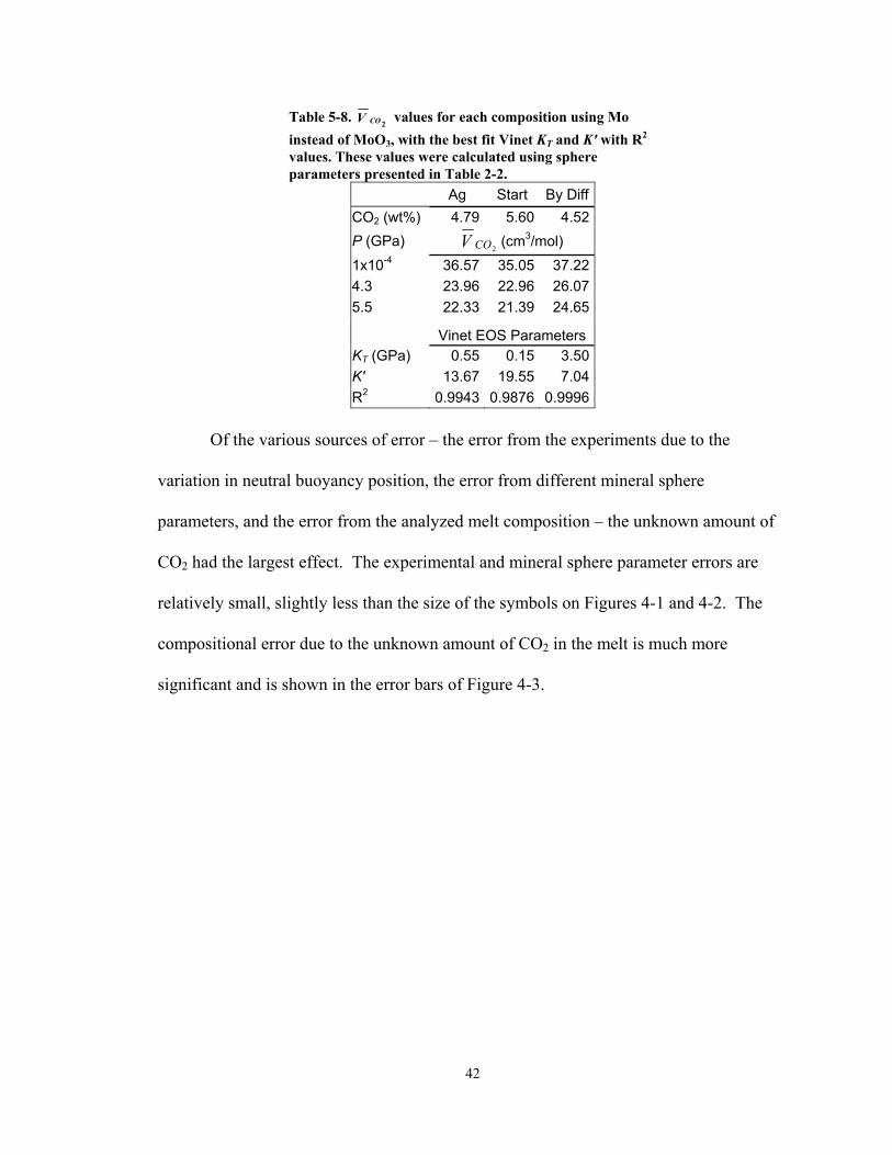
42

Table 5-8. 2COV values for each composition using Mo

instead of MoO3, with the best fit Vinet KT and K' with R2 values. These values were calculated using sphere parameters presented in Table 2-2.

Ag Start By DiffCO2 (wt%) 4.79 5.60 4.52P (GPa)

2COV (cm3/mol) 1x10-4 36.57 35.05 37.224.3 23.96 22.96 26.075.5 22.33 21.39 24.65

Vinet EOS Parameters KT (GPa) 0.55 0.15 3.50K' 13.67 19.55 7.04R2 0.9943 0.9876 0.9996

Of the various sources of error – the error from the experiments due to the

variation in neutral buoyancy position, the error from different mineral sphere

parameters, and the error from the analyzed melt composition – the unknown amount of

CO2 had the largest effect. The experimental and mineral sphere parameter errors are

relatively small, slightly less than the size of the symbols on Figures 4-1 and 4-2. The

compositional error due to the unknown amount of CO2 in the melt is much more

significant and is shown in the error bars of Figure 4-3.

43

Table 5-9

By D

iff

37.2

2

25.2

7

23.7

5

1.95

9.00

0.99

87

21.0

3

3.18

16.2

0

0.99

97

Sta

rt

35.0

5

22.7

3

21.1

4

0.08

21.8

4

0.98

39

17.2

2

1.54

17.8

3

0.99

76

5 A

g

(cm

3 /mol

) 36

.57

23.6

8

22.0

4

Vin

et E

OS

Par

amet

ers

0.34

15.3

2

0.99

25

Hyp

erbo

lic P

aram

eter

s 19

.23

1.97

17.3

5

0.99

85

By D

iff

37.2

2

25.0

9

23.5

6

1.70

9.46

0.99

84

20.8

8

3.01

16.3

6

0.99

96

Sta

rt

35.0

5

22.6

3

21.0

3

0.05

23.5

7

0.98

15

17.1

7

1.47

17.8

8

0.99

74

4 A

g

(cm

3 /mol

) 36

.57

23.5

6

21.9

0

Vin

et E

OS

Par

amet

ers

0.28

15.9

9

0.99

13

Hyp

erbo

lic P

aram

eter

s 19

.16

1.88

17.4

2

0.99

84

By D

iff

37.2

2

25.1

2

23.5

9

1.90

9.08

0.99

82

20.9

0

3.04

16.3

3

0.99

96

Sta

rt

35.0

5

22.7

0

21.1

2

0.07

22.3

3

0.98

34

17.2

1

1.52

17.8

4

0.99

76

3 A

g

(cm

3 /mol

) 36

.57

23.5

7

21.9

1

Vin

et E

OS

Par

amet

ers

0.29

15.8

7

0.99

14

Hyp

erbo

lic P

aram

eter

s 19

.16

1.88

17.4

2

0.99

84

By D

iff

37.2

2

25.1

0

23.5

6

1.70

9.46

0.99

84

20.8

8

3.02

16.3

5

0.99

96

Sta

rt

35.0

5

22.6

4

21.0

4

0.06

22.8

9

0.98

17

17.1

8

1.48

17.8

8

0.99

75

2 A

g

(cm

3 /mol

) 36

.57

23.5

7

21.9

1

Vin

et E

OS

Par

amet

ers

0.27

16.1

2

0.99

14

Hyp

erbo

lic P

aram

eter

s 19

.17

1.89

17.4

1

0.99

84

By D

iff

37.2

2

25.6

5

24.1

8

2.50

8.17

0.99

92

21.4

0

3.60

15.8

3

0.99

98

Sta

rt

35.0

5

22.8

8

21.3

2

0.13

20.0

7

0.98

69

17.3

0

1.65

17.7

5

0.99

79

1 A

g

(cm

3 /mol

) 36

.57

23.9

0

22.2

8

Vin

et E

OS

Par

amet

ers

0.49

14.0

7

0.99

42

Hyp

erbo

lic P

aram

eter

s 19

.37

2.13

17.2

1

0.99

88

P (G

Pa)

1x10

-4

4.3

5.5

KT

(GP

a)

K'

R2

a b y 0

R2

Tab

le 5

-9.

val

ues f

or e

ach

com

posi

tion

at p

ress

ure,

with

the

best

fit V

inet

KT a

nd K

' and

hyp

erbo

lic c

urve

par

amet

ers w

ith R

2 val

ues.

1-5

indi

cate

whi

ch sp

here

par

amet

er w

as u

sed,

see

Tab

le 5

-3.

44

6) Chapter 6

Application to the Earth and other Terrestrial Planets

The information from the 2COV compression curve enables more accurate

calculation of density and compressibility for carbonated magmas, such as kimberlites

and carbonatites. By being able to calculate magma density and knowing the depth of

origin of the magma, the minimum amount of CO2 necessary to cause the magma to be

buoyant and possibly erupt can be established (Figure 6-1). This may also indicate

minimum lithospheric abundances of CO2, compared to the magma source region, and

give insight into the origin and behavior of these carbonated magmatic systems.

Kimberlites

We have used ∂Vi/∂T values from Lange and Carmichael (1987) and Liu and

Lange (2003) for the liquid oxides (CaO, MgO, SiO2, etc), the OHV 2 values from Agee

(2008b) and the 2COV values from this study to calculate compression curves for primary

kimberlite melts using an expanded version of Equation (1-1). A proposed primary

kimberlite melt (Kopylova et al., 2007) contains 9.9 wt% H2O and 9.1 wt% CO2. In

order to determine its compression curve using the new CO2 data, we first determined a

“dry” kimberlite composition based on the primary melt above and then determined its

compression curve (without volatiles) using KT = 26.7 GPa, K’ = 4.0 (Agee and Walker,

1988, 1993) and TPdry

,ρ = 2.90 g/cm3 calculated from Lange and Carmichael (1987).

These KT and K’ values are for a komatiite melt because kimberlite has not been studied

for its elastic properties. We chose komatiite values because of the silicate melts studied,

it has a lower amount of SiO2 and a higher amount of CaO, and is therefore the closest

45

approximation of a kimberlite melt. From there we determined 2COV and OHV 2

at four

given pressures and used:

⎥⎦

⎤⎢⎣

⎡⎟⎟⎠

⎞⎜⎜⎝

⎛−−++

=

∑

∑TP

dryi

OHOHCOCOiiOHTPOHCO

TPCO

iii

TPvol

XMXMXMXVXV

XM

,,,

,

22222222ρ

ρ

(6-1)

to calculate the volatile-bearing kimberlite density, TPvol

,ρ , at those pressures and then fit a

Birch-Murnaghan curve to the points. Sparks et al. (2006) suggested that the kimberlite

source region could contain 5-20 wt% CO2 and Brey et al. (1991) discovered that

kimberlitic melts could contain more than 20 wt% dissolved CO2 at pressures greater

than 5-6 GPa. We added various amounts of CO2 and H2O to the dry kimberlite melt

(Table 6-1) and used the above technique to determine the shape of their compression

curves (Figure 6-1).

Table 6-1. Kimberlite melt compositions including ρ0, KT, and K' for Birch-Murnaghan EOS.

Kopylova et al. (2007) Dry H2O only CO2 only Max CO2

SiO2 26.70 32.95 29.37 29.66 23.07 TiO2 1.73 2.14 1.90 1.92 1.49 Al2O3 1.57 1.94 1.73 1.74 1.36 Cr2O3 0.36 0.44 0.40 0.40 0.31 FeO 7.58 9.35 8.34 8.42 6.55 MnO 0.18 0.22 0.20 0.20 0.16 MgO 28.25 34.86 31.07 31.38 24.40 CaO 12.90 15.92 14.19 14.33 11.14 Na2O 0.10 0.12 0.11 0.11 0.09 K2O 1.26 1.55 1.39 1.40 1.09 P2O5 0.40 0.49 0.44 0.44 0.35 H2O 9.88 0.00 10.87 0.00 10.00 CO2 9.07 0.00 0.00 10.00 20.00 Total 99.98 100.0 100.00 100.00 100.00 ρ0 (g/cm3) 1.94 2.90 2.06 2.56 1.76 KT (GPa) 1.77 26.70 2.48 9.80 0.96 K' 11.20 4.00 8.50 9.60 16.70

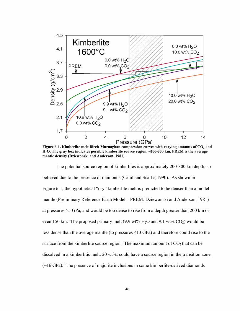
46

Figure 6-1. Kimberlite melt Birch-Murnaghan compression curves with varying amounts of CO2 and H2O. The gray box indicates possible kimberlite source region, ~200-300 km. PREM is the average mantle density (Dziewonski and Anderson, 1981).

The potential source region of kimberlites is approximately 200-300 km depth, so

believed due to the presence of diamonds (Canil and Scarfe, 1990). As shown in

Figure 6-1, the hypothetical “dry” kimberlite melt is predicted to be denser than a model

mantle (Preliminary Reference Earth Model – PREM: Dziewonski and Anderson, 1981)

at pressures >5 GPa, and would be too dense to rise from a depth greater than 200 km or

even 150 km. The proposed primary melt (9.9 wt% H2O and 9.1 wt% CO2) would be

less dense than the average mantle (to pressures ≤13 GPa) and therefore could rise to the

surface from the kimberlite source region. The maximum amount of CO2 that can be

dissolved in a kimberlitic melt, 20 wt%, could have a source region in the transition zone

(~16 GPa). The presence of majorite inclusions in some kimberlite-derived diamonds

47

may support this theory, as these particular garnets have been shown to form at pressures

≥13.5 GPa, the uppermost limit of the transition zone (Ringwood et al., 1992).

If the 2COV compression curve used is not the ideal one (KT = 0.36 GPa,

K’' = 15.12, CO2 = 4.8 wt%), but instead the curve based on the starting composition

(KT = 0.08 GPa, K’' = 21.84, CO2 = 5.5 wt%) or the composition with CO2 determined by

difference (KT = 2.00 GPa, K’' = 8.92, CO2 = 3.5 wt%), the elastic parameters of a

kimberlite compression curve change. To demonstrate this, we used the CO2 only

kimberlite composition (Table 6-1) and calculated Birch-Murnaghan compression curves

based on the different values of 2COV determined from the different

2COV compression

curves (Table 6-2, Figure 6-2).

Table 6-2. Birch-Murnaghan EOS elastic parameters for kimberlite melt with only 10.0 wt% CO2 based on different

2COV compression curves.

Ideal Starting By Difference ρ0 (g/cm3) 2.56 2.58 2.55 KT (GPa) 9.80 8.87 13.07 K' 9.60 11.35 6.80

48

Figure 6-2. Birch-Murnaghan compression curves for a kimberlite melt with only 10.0 wt% CO2 compared to the “dry” curve and the proposed primary melt – compositions in Table 6-1. The solid green curve is based on the ideal

2COV values, the dashed (- - -) green curve is based on the starting composition CO2 value, and the dashed/dotted (– · · –) green curve is based on the By Diff CO2 value.

The differences in the 10.0 wt%CO2 kimberlite compression curves determined

from the different 2COV curves are very small (Figure 6-2). As could be expected, the

curve that used 2COV calculated from a higher CO2 content (Starting amount-5.5 wt%

CO2) is slightly above the ideal curve (4.8 wt% CO2), while the curve that used 2COV

calculated from a lower CO2 content (By Diff amount-3.5 wt% CO2) is slightly below the

ideal curve. All three curves have similar compressional behaviors and crossover with

PREM at relatively the same point (~11 GPa).

We do not know how much CO2 is present in our experiments during the run, but

we are confident that it is there. The 2COV values we calculated are ideal, but given the

good fit of the compression curve to the density calculations of kimberlite melts, we feel

49

that they are a good first approximation. Also, given the relatively small variance in the

kimberlite curves based on different possible CO2 contents of experimental melts and

their 2COV values, we are confident that the ideal values are close to reality. The

2COV

values determined by these experiments can be used to calculate the density of

carbonated mantle melts. The density calculations can then be applied to magma mobility

in the mantle and planetary differentiation scenarios where CO2 is present.

50

Appendices

Appendix A Experiments ................................................................................................ 51

Appendix B Electron Microprobe................................................................................... 58

Appendix C FTIR............................................................................................................ 75

51

A) Appendix A

Experiments

This appendix gives the details of the experiments. Included is a schematic

diagram of the interior of an octahedron (Figure A-1), tables summarizing the conditions

of carbonated (Table A-1), non-carbonated (Table A-2), and “andesite” (Table A-3)

experiments along with back-scatted electron (BSE) microprobe images of analyzed

carbonated (Figures A-2 through A-10), non-carbonated (Figures A-11 through A-18),

and “andesite” (Figure A-19) experiments. Following those are the conversion steps

from Equation (1-1) to (2-4) to calculate 2COV .

Figure A-1. Cross section of ceramic octahedron with experimental set up. Drawn to scale.

52

Table A-1. Experimental run conditions and results for carbonated experiments. Pressure Notes

Sample (bars of oil) (GPa)

Temp(°C)

Ramp Rate

(°C/min)

Time (sec)

Spheres (μm) Position Spacers

(mm) Sleeve (mm) Alumina

A457 DG-5-1 58.2-56.6 4.7 1815 n/a 25 Fo

100 640x640600x640 NB . . . Yes

A460 DG-5-4 59.0-57.7 4.8 1825 n/a 30 Fo

100 650x480650x460 Float 3.44 3.78 . Yes

A464 DG-5-7 55.4 4.6 1800-1810 n/a 30 Fo

100 600x700750x500 NB 3.34

3.37 3.75

A488 DG-5-9 51.1-50.0 4.3 1800 450 30 Fo

100 510x530480x450 Sink 3.35

3.45 3.75 . No

A508 DG-5-11 69.9 5.6 1850 400 30 Fo 90 440x370390x370 Sink 3.40

3.20 3.70 . Yes

A555 DG-5-14 76.7 6.1 1950 350 30 Fo 90 500x460450x520 NB 3.40

3.43 3.76 reseating Yes

A561 DG-5-16 79.2 6.3 1950 350 30 Fo 90 500x380530x430 Float 3.34

3.32 3.80 . Yes

QP153 DG-5-17 112 1.0 1779 . 30 none n/a n/a n/a n/a looking for bubbles

A650 DG-5-18 58.4-58.5 4.8 1850 350 30 Fo

100 600x520560x510 Float 3.25

3.22 3.84 .

A675 DG-5-19 48.4-48.2 4.1 1800 350 30 Fo

100 570x430520x430 Sink 3.38

3.39 3.73

A696 DG-5-20 56.3-56.5 4.7 1800 350 30 none n/a n/a 3.31

3.32 3.72

A707 DG-5-21 56.4-56.3 4.7 1800 350 30 Fo

100 650x570630x590 NB 3.38

3.39 3.73 No

A718 DG-5-22 73.6 5.9 1950 350 35 Fo 90 580x510580x470 NB 3.32

3.33 3.82

A725 DG-5-23 70.9-71.1 5.7 1950 350 45 Fo 90 540x490

500x480 NB 3.393.40 3.79

The following figures are back-scattered electron images of polished carbonated

experiments. Arrows indicate top of the capsule during run.

Figure A-2. DG-5-9

Figure A-3. DG-5-11

53

Figure A-4. DG-5-14

Figure A-5. DG-5-16

Figure A-6. DG-5-17

Figure A-7. DG-5-19

Figure A-8. DG-5-21

Figure A-9. DG-5-22

54

Figure A-10. DG-5-23

Table A-2. Experimental run conditions and results for non-carbonated experiments.

Pressure Notes Sample (bars

of oil) (GPa) Temp (°C)

Ramp Rate

(°C/min)

Time(sec)

Spheres (μm) Position Spacers

(mm) Sleeve (mm) Alumina

A496 DG-N-3 45.6-44.9 3.9 1850 400 30 Fo

100510x420470x490 Sink 3.45

3.38 3.70 1845-1852 No

A501 DG-N-7 48.7 4.1 1850 400 30 Fo 100

480x420430x360 Float 3.40

3.50 3.80 .

No

A562 DG-N-8 65.8 5.3 1950 350 30 Fo 90

420x460580x420 Not sink 3.30

3.40 3.76 One sphere No

A591 DG-N-12 62.6-62.4 5.1 1925 350 30 Fo

90600x500600x400 Not float 3.37

3.39 3.76 One sphere No

A592 DG-N-13 69.9-68 5.6 1925 350 30 Fo

90950x500850x600 Float 3.30

3.40 3.70 .

Yes

A598 DG-N-14 62.1 5.1 1925 350 30 Fo 90

800x500550x450 NB 3.35 3.63

. No

A603 DG-N-15 59.4-59.1 4.9 1925 350 30 Fo

90770x590830x500 Not sink 3.30

3.35 3.82 One sphere

A608 DG-N-17 58.6-58.4 4.8 1925 350 30 Fo

90570x530550x590 NB/Float 3.40

3.41 3.74 .

No

A612 DG-N-18 54 4.5 1925 350 30 Fo 90

600x530490x550 Not sink 3.24

3.26 3.89 One sphere No

A617 DG-N-19 50.2-49.8 4.2 1900 350 30 Fo

90640x510520x580 NB 3.40 3.77 Furnace

ASU capsule Yes

A626 DG-N-20 45.4-44.9 3.9 1850 350 30 Fo

100580x510600x520 Sink 3.31

3.36 3.80 .

No

A654 DG-N-22 54.0-54.1 4.5 1925 350 45 Fo

90620x580600x580 Sink 3.19

3.20 3.80 .

No

A655 DG-N-23 48.6-48.7 4.1 1850 350 30 Fo

100560x470590x550 NB 3.28

3.29 3.90 .

No

A670 DG-N-26 51.6 4.3 1850 350 45 Fo 100

640x460640x500 Float 3.28

3.29 3.75 .

No

A724 DG-N-32 71.1 5.7 1975 350 45 Fo 90

560x460650x440 Not Sink 3.40

3.41 3.79 Furnace overnight No

A729 DG-N-33 66.4-66.7 5.4 1975 350 23 Fo

90630x570610x560 NB 3.34

3.35 3.75 Furnace 1.5 hr

55

The following figures are back-scattered electron images of polished non-

carbonated experiments. Arrows indicate top of the capsule during run.

Figure A-11. DG-N-7

Figure A-12. DG-N-14

Figure A-13. DG-N-17

Figure A-14. DG-N-19

Figure A-15. DG-N-20

Figure A-16. DG-N-22

56

Figure A-17. DG-N-23

Figure A-18. DG-N-33

Table A-3. Experimental run conditions for “andesite” experiment.

Pressure Notes Sample

(bars of oil) (GPa) Temp(°C)

Ramp Rate

(°C/min)

Time(sec)

Spheres(μm)

Spacers (mm)

Sleeve (mm) Alumina

A683 And-5-1 46.9-47.0 4.0 1900 350 60 none 3.27 3.27 3.71 No

Figure A-19. And-5-1

57

Conversion steps from the equation of Bottinga and Weill (1970) (Equation 1-1)

to the one used for calculating 2COV (Equation 2-4).

22222

,,,CO

TPN

iCOCOii

TPCO

iii

TPCO

ABAAi

iii

iiA

ABBBi

iiA

ABBi

iiA

iiiBBAA

iiiii

XXMXMXMV

XMXMXMXV

XMXMXV

XVXMXV

MXVXVX

VXMX

⎪⎭

⎪⎬⎫

⎪⎩

⎪⎨⎧

⎥⎦

⎤⎢⎣

⎡⎟⎠

⎞⎜⎝

⎛−−⎟

⎠

⎞⎜⎝

⎛=

⎥⎦

⎤⎢⎣

⎡⎟⎠

⎞⎜⎝

⎛−−=

⎟⎠

⎞⎜⎝

⎛−=

⎟⎠

⎞⎜⎝

⎛−=

=++

=

∑∑

∑∑

∑

∑

∑

∑

ρρ

ρρ

ρρ

ρ

ρ

ρ

K

58

B) Appendix B

Electron Microprobe

In this section we outline our attempts at using the electron microprobe to detect

carbon directly along with the results. For discussion of our Ag-coated attempts see

Chapter 3. After unable to accurately detect the carbon in out samples using the Ag-coat

and an accelerating voltage of 15 kV, a current of 2.5x10-8 A, and a beam diameter of

20 μm, we altered the operating conditions. Because we were also trying to detect O

directly, we altered operating conditions to an accelerating voltage of 12 kV, a current of

2.0x10-8 A, and a beam diameter of 20 μm, but to no avail.

Because we had some success detecting carbon in gold-coated (Au-coat)

carbonates, we then switched to an Au-coat for the experiments. The coat was applied

simultaneously to the samples and standards to bypass any issues with different coat

thickness between the standards and samples. However, we have not had much success

with the detection of carbon in quenched silicate melts. The wt% totals are extremely

high (110-130) for the Au-coated experiments, most obviously due to the high amount of

oxygen detected (50-55 wt% rather than 45 wt% expected, see Tables B-3 through B-10).

We also tried using different carbon standards (SiC, calcite and dolomite) and

different operating conditions, hoping to minimize the amount of carbon detected in

samples without carbon. This would then allow us to subtract out the background carbon

form the carbonated samples. This also has not yet worked. To ensure that the water

used in grinding the samples was not dissolving carbonates (Brooker, 1998; Brooker et

al., 2001a; Dasgupta et al., 2007; Wallace and Green, 1988), we used kerosene and

anhydrous alcohol in place of water for some carbonated experiments which we then

59

analyzed with the microprobe and FTIR, but no difference in results were apparent. See

Table B-2 for all Au-coated operating conditions and the experiments analyzed and

Tables B-3 through B-10 for the analytical results.

Two ways to detect elements using the microprobe are by area and by time.

Analysis by area takes the first order peak determined on the standard and uses the upper

and lower background limits set around that peak and to determine how much of the

element is in the sample by calculating the area under the curve. This is most used when

analyzing for an element whose peak may move relative to the standard peak. Analysis

by time is more common and uses the first order peak determined on the standard and

searches for the same peak on the sample. One problem when analyzing for carbon with

the microprobe is the presence of oxygen. The Kα carbon peak using the LDE2

spectrometer is located at ~124 mm, but there is a shoulder in the peak that could be a

secondary oxygen peak at ~130 mm. Because the amount of oxygen is so much greater

than that of carbon, interference from this potential oxygen peak can raise the

background in the location of the carbon peak. When analyzing carbon by area, this will

increase the amount of carbon detected if the background for carbon analysis is placed

too high, but lower it if the background is set to exclude the oxygen peak. When

analyzing carbon by time, the effect of the oxygen peak is less obvious, but still may

cause the amount of carbon detected to be too large.

60

Table B-1. Operating conditions, standards, and experiments analyzed with an Ag-coat by the electron microprobe.

Date Exp.

Analyzed Standards ElementsTest

Accl.Volt.

(KeV)

Current(nA)

Probe Dia.(μm)

Std Conditions Peak/Back (s) Notes

SiC C Andradite Fe, Al, Ca

Olivine Mg, Si, O 3/7/08 DG-5-1 DG-5-4 DG-5-8 Capsule

(DG-5-1) Mo

15 25 20

SiC C Chromite Cr

Andradite Fe, Al, Ca, O, Mg, Si

Olivine Mg, Si, O 4/30/08 DG-5-7

DG-5-8

Capsule (DG-5-1) Mo

15 25 20 O as time

Ag paste Samples coated on 4/1 Standards coated separately

SiC C 30/10 Olivine Mg, Si, O 30/15 O

Andradite Fe, Al, Ca 20/10 Mg, Si, Fe, Al, Ca, Mo

5/22/08 DG-5-1 DG-5-4

Capsule (DG-5-1) Mo

15 25 20

Time not area

Sample DG-5-4 charging

SiC C Olivine Mg, Si, O

Kaersutite Fe, Al, Ca 8/29/08 DG-5-4 DG-5-9 DG-N-3 Capsule

(DG-5-4) Mo

12 20 20 C as time

Samples coated on 8/27 Standards coated separately

SiC C 1 12 20 20 O on area Olivine Mg, Si, O 2 12 25 20 O as time

Kaersutite Fe, Al, Ca 3 12 20 20 O on area, no C 9/5/08

DG-5-4 DG-5-9 DG-N-3 DG-N-7 Capsule

(DG-5-4) Mo

SiC C Olivine Mg, Si, O

Kaersutite Fe, Al, Ca 2/27/09

DG-5-14 DG-5-16 DG-N-9

Capsule Mo

15 25 20 C on time Samples and standards coated together

61

Table B-2. Operating conditions, standards, and experiments analyzed with an Au-coat by the electron microprobe. Experiments marked with * were ground and cleaned using kerosene and anhydrous alcohol.

Date Exp.

Analyzed Standards ElementsTest

Accl.Volt.(KeV)

Current(nA)

Probe Dia.(μm)

Std Conditions Peak/Back (s) Notes

SiC C

Olivine Mg, Si, O

Kaersutite Fe, Al, Ca 8/27/09

DG-5-11 DG-5-14 DG-5-16 DG-N-9 DG-N-13 DG-N-14 DG-N-19

Capsule (DG-N-9) Mo

15 25 20

Dolomite C 1 15 20 10 30/10 Olivine Mg, Si, O 2 15 20 10 15/10

Kaersutite Fe, Al, Ca 3 15 25 20 10/5 11/6/09

DG-N-22 DG-N-21 DG-5-17 DG-N-17 DG-N-24 Capsule Mo 4 15 25 20 30/10

Samples and standards on 11/6

Dolomite C 1 12 20 10 Olivine Mg, Si, O 2a 10 20 20

Kaersutite Fe, Al, Ca 2b 10 20 20 Calcite Capsule

(DG-5-17) Mo 4 10 20 50

5a 10 40 50 5b 10 40 50 C on Area 6 10 60 50 7 10 80 50 8 10 100 50

12/4/09 12/5/09

DG-5-17* DG-N-22

9 10 80 50 10/5

Samples and standards on 12/3

Dolomite C 1 12 20 50 10/5 Olivine Mg, Si, O 2 12 40 50 10/5

Kaersutite Fe, Al, Ca 3 12 10 10 20/10 1/22/10 And-5-1* DG-5-19*

Capsule (And-5-1) Mo

Samples and standards on 1/21

Dolomite C Olivine Mg, Si, O

Kaersutite Fe, Al, Ca 3/25/10

DG-5-14 DG-5-16 DG-N-9 DG-N-17 DG-N-22 DG-N-25

Capsule (DG-5-14, DG-5-16)

Mo

15 25 20 20/10 Samples and standards on 3/25

Dolomite C 1 15 25 20 20/10 Olivine Mg, Si, O 2 10 40 50 20/10

Kaersutite Fe, Al, Ca 3 10 80 50 20/10 3/26/10 DG-5-22 DG-N-31

Capsule (DG-5-22) Mo

Samples and standards on 3/26

Dolomite C 1 15 25 20 20/10 Olivine Mg, Si, O 2 10 80 50 20/10

Kaersutite Fe, Al, Ca 3 10 60 50 20/10 4/16/10

DG-N-33 DG-N-22 DG-5-23 DG-N-22

Capsule (DG-N-22, DG-5-23)

Mo

Samples and standards on 4/15

62

These tables show an average of microprobe data for each experiment analyzed

and calculated oxide amounts on a given date under the same conditions, i.e. an analysis

taken with an accelerating voltage = 15 kV, a current = 2.5x10-8 A, a beam

diameter = 20 μm, and SiC as the carbon standard were not averaged with an analysis

taken with an accelerating voltage = 12 kV, a current = 2.0x10-8 A, a beam

diameter = 20 μm, and carbonate as the carbon standard. Also shown are the CO2

amounts determined from microprobe analyses (Probe Carbon), and the amount of CO2

determined by the difference from at total of 100 (By Difference). The Peak/Back (s)

row indicates the amount of time spent analyzing for the carbon peak, and the time spent

analyzing the background. The analyses without a Peak/Back value used a peak of 30

seconds and background of 10 seconds. Experiments with an * are those that were

ground using kerosene and alcohol, rather than water.

63

Table B-3. Average electron microprobe values and resultant oxides values including the wt% CO2 determined from the microprobe values and the amount when calculated by difference for carbonated experiments DG-5-1, 4, 7, 8, 9.

Sample DG-5-1 DG-5-4 DG-5-7 DG-5-8 DG-5-9

Date/Coat 3-7 Ag

5-22 Ag

3-7 Ag

5-22 Ag

9-5 Ag1

9-5 Ag2

4-30 Ag

8-27 Au

4-30 Ag

9-5 Ag1

Accel. Volt. (KeV) 15 15 15 15 12 12 15 15 15 12

Current (nA) 25 25 25 25 20 25 25 25 25 20 Probe Dia. (μm) 20 20 20 20 20 20 20 20 20 20

C Std SiC SiC SiC SiC SiC SiC SiC SiC SiC SiC Peak/Back (s) # of Analyses 6 26 7 17 9 5 17 4 20 22 Meas. Elm % Mg 17.97 14.56 13.24 14.33 17.35 17.19 15.02 14.36 15.19 16.46Al 2.46 3.58 3.01 4.02 4.41 2.70 4.12 2.65 3.97 4.01Si 17.82 19.43 22.01 18.18 21.52 24.25 20.13 19.28 19.03 20.08Ca 3.01 6.20 9.11 5.30 6.81 6.18 6.33 6.67 5.60 5.69Fe 13.50 7.83 6.02 6.26 8.62 7.65 7.98 8.13 8.93 7.82Mo 1.60 1.63 1.56 1.74 1.70 1.61 1.81 2.76 3.09 2.37O 38.93 44.42 42.31 44.20 55.05 29.96 43.73 42.33 41.66 46.20C 0.95 2.00 0.99 2.74 2.07 1.97 1.41 1.32 1.19 1.31Total 96.23 99.65 98.25 96.76 117.53 91.52 100.52 97.48 98.67 103.94

MgO 29.81 24.14 21.96 23.77 28.78 28.51 24.91 23.81 25.18 27.29Al2O3 4.65 6.77 5.69 7.59 8.33 5.10 7.78 5.00 7.51 7.57SiO2 38.11 41.57 47.10 38.89 46.03 51.88 43.06 41.24 40.72 42.96CaO 4.21 8.67 12.75 7.41 9.53 8.65 8.85 9.33 7.84 7.96FeO 17.37 10.08 7.75 8.05 11.09 9.84 10.26 10.46 11.49 10.06MoO3 2.40 2.44 2.34 2.61 2.56 2.41 2.72 4.13 4.64 3.56Probe Carbon CO2 3.48 7.32 3.63 10.05 7.57 7.23 5.18 4.83 4.36 4.81Total 100.02 100.99 101.20 98.36 113.89 113.63 102.76 98.80 101.74 104.21By Difference CO2 3.46 6.33 2.42 11.69 0.00 0.00 2.42 6.03 2.62 0.60Total 100.00 100.00 99.99 100.00 106.31 106.40 100.00 100.00 99.99 100.00

64

Table B-4. Average electron microprobe values and resultant oxides values including the wt% CO2 determined from the microprobe values and the amount when calculated by difference for carbonated experiments DG-5-11, 14, 16, 19.

Sample DG-5-11 DG-5-14 DG-5-16 DG-5-19*

Date/Coat 8-27 Au

2-27 Ag

8-27 Au

3-25 Au1

2-27 Ag

8-27 Au

3-25 Au1

1-22 Au1

1-22 Au2

1-22 Au3

Accel. Volt. (KeV) 15

15 15 15 15 15 15 12 12 12

Current (nA) 25 25 25 25 25 25 25 20 40 10 Probe Dia. (μm) 20

20 20 20 20 20 20 50 50 10

C Std SiC SiC SiC Dol SiC SiC Dol Dol Dol Dol Peak/Back (s) 20/10 20/10 10/5 10/5 20/10 # of Analyses 4 23 3 21 3 6 2 2 2 Meas. Elm % Mg 14.36 15.82 18.22 16.93 16.57 15.79 17.72 16.89 16.76 19.16Al 2.65 2.99 2.84 2.70 2.32 1.46 2.92 4.31 4.31 3.32Si 19.28 21.58 21.24 21.42 21.63 22.38 22.55 20.64 20.49 18.62Ca 6.67 6.66 6.84 7.00 7.03 8.26 7.27 6.17 6.16 4.69Fe 8.13 5.53 5.80 6.23 6.64 7.24 6.27 8.68 8.70 10.53Mo 2.76 2.34 1.77 2.48 2.33 1.82 2.09 2.99 3.05 3.37O 42.33 40.72 50.62 48.11 43.76 44.13 51.61 52.37 51.83 50.31C 1.32 0.63 0.90 4.75 0.79 1.27 6.19 6.46 6.94 6.12Total 97.48 96.27 108.23 109.62 101.07 102.35 116.62 118.50 118.23 116.12

MgO 23.81 26.24 30.21 28.07 27.48 26.18 29.38 28.01 27.79 31.76Al2O3 5.00 5.64 5.37 5.10 4.38 2.76 5.51 8.13 8.14 6.27SiO2 41.24 46.17 45.43 45.83 46.27 47.87 48.25 44.16 43.83 39.83CaO 9.33 9.31 9.57 9.79 9.84 11.56 10.17 8.63 8.61 6.56FeO 10.46 7.12 7.46 8.01 8.55 9.32 8.07 11.17 11.19 13.55MoO3 4.13 3.51 2.65 3.73 3.50 2.73 3.13 4.49 4.58 5.06Probe Carbon CO2 4.83 2.30 3.31 17.40 2.88 4.64 22.69 23.65 25.43 22.42Total 98.80 100.29 104.01 117.94 102.89 105.07 127.19 128.24 129.57 125.46By Difference CO2 6.03 2.01 0.00 0.00 0.00 0.00 0.00 0.00 0.00 0.00Total 100.00 100.00 100.69 100.54 100.01 100.43 104.50 104.58 104.14 103.04

65

Table B-5. Average electron microprobe values and resultant oxides values including the wt% CO2 determined from the microprobe values and the amount when calculated by difference for carbonated experiments DG-5-17. Sample DG-5-17*

Date/Coat 11-6 Au4

12-4/5 Au1

12-4/5Au2a

12-4/5Au2b

12-4/5Au4

12-4/5Au5a

12-4/5Au5b

12-4/5 Au6

12-4/5 Au7

12-4/5Au8

12-4/5Au9

Accel. Volt. (KeV) 15 12 10 10 10 10 10 10 10 10 10

Current (nA) 25 20 20 20 20 40 40 60 80 100 80 Probe Dia. (μm) 20 10 20 20 50 50 50 50 50 50 50

C Std Dol Dol Dol Cal Dol Dol Dol Dol Dol Dol Dol Peak/Back (s) 30/10 10/5 # of Analyses 4 2 2 2 2 2 2 2 2 2 2 Meas. Elm % Mg 14.61 17.32 18.18 18.25 18.36 17.83 17.82 17.80 18.18 18.25 18.25Al 4.30 4.57 4.78 4.76 4.72 4.79 4.81 4.82 4.49 4.47 4.51Si 19.60 21.53 22.44 22.76 22.31 22.50 22.79 22.53 22.38 22.49 22.39Ca 6.32 6.72 6.70 6.67 6.73 7.00 6.98 6.91 6.62 6.61 6.62Fe 8.63 9.04 9.16 8.91 9.47 9.22 9.26 9.26 9.19 9.16 9.16Mo 7.01 4.22 4.09 4.07 4.36 4.74 4.78 4.83 5.39 5.35 5.31O 49.36 58.85 62.14 62.68 61.25 59.89 59.10 60.59 59.51 60.44 60.60C 2.96 4.32 4.57 6.90 4.86 3.94 4.02 5.41 3.73 4.41 5.02Total 112.78 126.56 132.05 134.99 132.04 129.89 129.55 132.13 129.48 131.16 131.84

MgO 24.23 28.72 30.15 30.26 30.44 29.56 29.55 29.51 30.15 30.26 30.26Al2O3 8.12 8.63 9.03 8.98 8.91 9.05 9.09 9.11 8.47 8.44 8.51SiO2 41.94 46.06 48.01 48.69 47.73 48.14 48.74 48.20 47.88 48.11 47.90CaO 8.84 9.40 9.37 9.33 9.41 9.79 9.77 9.66 9.26 9.25 9.26FeO 11.10 11.63 11.78 11.46 12.18 11.86 11.91 11.91 11.82 11.78 11.78MoO3 10.51 6.33 6.14 6.10 6.53 7.10 7.16 7.24 8.09 8.03 7.97Probe Carbon CO2 10.85 15.81 16.73 25.28 17.79 14.44 14.73 19.80 13.65 16.14 18.38Total 115.58 126.58 131.20 140.11 132.99 129.93 130.96 135.43 129.31 132.00 134.05By Difference CO2 0.00 0.00 0.00 0.00 0.00 0.00 0.00 0.00 0.00 0.00 0.00Total 104.73 110.77 114.47 114.83 115.20 115.50 116.23 115.63 115.66 115.86 115.67

66

Table B-6. Average electron microprobe values and resultant oxides values including the wt% CO2 determined from the microprobe values and the amount when calculated by difference for carbonated experiments DG-5-22, 23.

Sample DG-5-22 DG-5-23

Date/Coat 3-26 Au1

3-26 Au2

3-26 Au3

4-16 Au1

4-16 Au2

4-16 Au3

Accel. Volt. (KeV) 15 10 10 15 10 10 Current (nA) 25 40 80 25 80 60 Probe Dia. (μm) 20 50 50 20 50 50 C Std Dol Dol Dol Dol Dol Dol Peak/Back (s) 20/10 20/10 20/10 20/10 20/10 20/10 # of Analyses 8 3 3 5 3 3 Meas. Elm % Mg 16.91 17.72 17.68 17.03 18.27 18.37 Al 2.78 2.63 2.59 3.35 3.58 3.66 Si 21.00 21.86 21.82 20.89 22.38 22.17 Ca 6.91 7.10 7.03 6.98 6.92 6.77 Fe 7.22 7.62 7.60 6.89 7.39 7.16 Mo 2.00 2.18 2.12 2.64 2.57 2.57 O 47.86 49.72 50.12 50.24 53.15 53.43 C 4.18 3.91 4.36 2.69 3.14 3.75 Total 108.84 112.74 113.34 110.71 117.39 117.87

MgO 28.03 29.38 29.32 28.25 30.30 30.46 Al2O3 5.25 4.96 4.90 6.33 6.76 6.91 SiO2 44.92 46.76 46.69 44.69 47.87 47.42 CaO 9.66 9.94 9.84 9.76 9.68 9.47 FeO 9.28 9.81 9.78 8.86 9.51 9.21 MoO3 3.00 3.28 3.19 3.96 3.86 3.85 Probe Carbon CO2 15.30 14.31 15.98 9.87 11.49 13.75 Total 115.45 118.44 119.69 111.72 119.47 121.08 By Difference CO2 0.00 0.00 0.00 0.00 0.00 0.00 Total 100.15 104.13 103.72 101.85 107.97 107.32

67

Table B-7. Average electron microprobe values and resultant oxides values including the wt% CO2 determined from the microprobe values and the amount when calculated by difference for non-carbonated experiments DG-N-3, 7, 9, 13, 14.

Sample DG-N-3 DG-N-7 DG-N-9 DG-N-13 DG-N-14

Date/Coat ? 9-5 Ag1

9-5 Ag3 ? 9-5

Ag1 9-5 Ag3

2-27 Ag

8-27 Au

3-25 Au1 8-27

Au 8-27 Au

Accel. Volt. (KeV) 12 12 12 12 15 15 15 15 15

Current (nA) 20 20 20 20 25 25 25 25 25 Probe Dia. (μm) 20 20 20 20 20 20 20 20 20

C Std SiC SiC SiC SiC Dol SiC SiC Peak/Back (s) 20/10 # of Analyses 10 10 5 7 10 5 23 2 6 7 6 Meas. Elm % Mg 15.45 17.95 17.93 15.24 17.55 17.42 16.28 18.39 15.61 17.32 17.33Al 3.88 4.27 4.45 3.99 4.05 4.20 2.81 1.94 2.70 2.08 3.83Si 18.95 21.69 21.47 18.89 21.66 21.67 21.52 21.90 20.39 23.64 19.64Ca 5.50 3.60 3.60 5.58 3.37 3.40 3.94 3.14 3.75 4.11 3.64Fe 9.12 9.03 9.47 8.80 7.21 6.84 9.46 7.59 8.78 8.72 9.66Mo 2.63 1.97 1.66 3.76 3.29 3.49 2.42 3.06 2.27 0.47 3.38O 41.74 51.94 51.28 41.65 48.46 47.98 43.39 48.48 41.70 52.34 50.79C 1.25 1.10 na 1.05 0.88 na 0.60 0.97 5.36 1.17 1.08Total 98.51 111.56 109.87 98.97 106.47 105.00 100.42 105.45 100.54 109.84 109.34

MgO 25.63 29.77 29.73 25.27 29.11 28.89 27.00 30.49 25.88 28.72 28.73Al2O3 7.33 8.06 8.42 7.54 7.66 7.94 5.31 3.66 5.09 3.92 7.24SiO2 40.53 46.41 45.94 40.40 46.34 46.36 46.03 46.85 43.62 50.58 42.02CaO 7.69 5.04 5.03 7.81 4.71 4.76 5.52 4.39 5.24 5.74 5.09FeO 11.73 11.62 12.19 11.32 9.27 8.80 12.17 9.76 11.29 11.22 12.42MoO3 3.94 2.95 2.49 5.64 4.93 5.24 3.63 4.58 3.40 0.71 5.06Probe Carbon CO2 4.58 4.04 0.00 3.86 3.22 0.00 2.20 3.55 19.63 4.28 3.94Total 101.42 107.89 103.79 101.85 105.24 101.98 101.86 103.28 114.16 105.18 104.52By Difference CO2 3.16 0.00 0.00 2.01 0.00 0.00 0.35 0.27 5.47 0.00 0.00Total 100.00 103.84 103.79 100.00 102.02 101.98 100.00 100.00 100.00 100.90 100.57

68

Table B-8. Average electron microprobe values and resultant oxides values including the wt% CO2 determined from the microprobe values and the amount when calculated by difference for non-carbonated experiments DG-N-17, 19, 21, 24, 25, 31, 33. Sample DG-N-17 DG-N-19 DG-N-21 DG-N-24 DG-N-25 DG-N-31 DG-N-33

Date/Coat 11-6 Au4

3-25 Au1 8-27

Au 11-6 Au1

11-6 Au2

11-6 Au4

3-25 Au1

3-25 Au1

3-26 Au2

3-26 Au3

4-16 Au1

Accel. Volt. (KeV) 15 15 15 15 15 15 15 15 10 10 15

Current (nA) 25 25 25 25 25 25 25 25 40 80 25 Probe Dia. (μm) 20 20 20 20 20 20 20 20 50 50 20

C Std Dol Dol SiC Dol Dol Dol Dol Dol Dol Dol Dol Peak/Back (s) 30/10 20/10 30/10 15/10 30/10 20/10 20/10 20/10 20/10 20/10 # of Analyses 3 8 5 4 1 1 7 9 3 3 5 Meas. Elm % Mg 18.97 17.57 16.63 16.69 16.47 18.02 16.16 17.87 20.35 20.19 17.83Al 3.83 3.96 3.92 2.57 3.41 2.80 3.02 2.79 2.56 2.51 3.17Si 21.79 20.57 20.19 19.95 20.89 23.98 20.47 22.45 26.31 26.11 22.20Ca 3.15 3.02 3.53 2.75 4.13 4.74 4.05 4.81 3.66 3.72 3.88Fe 7.26 6.87 9.06 7.12 9.27 8.35 8.68 9.76 8.37 8.48 7.87Mo 4.17 3.17 3.66 15.13 3.86 0.40 2.59 2.00 1.55 1.53 2.06O 55.82 50.38 47.66 50.69 48.09 53.40 50.95 50.73 57.82 58.22 55.86C 3.31 5.05 1.21 3.91 3.46 6.12 5.91 2.91 3.08 3.45 1.61Total 118.30 110.60 105.85 118.81 109.58 117.81 111.82 113.31 123.70 124.21 114.47

MgO 31.46 29.14 27.58 27.68 27.31 29.88 26.79 29.63 33.75 33.48 29.56Al2O3 7.23 7.49 7.41 4.86 6.44 5.29 5.71 5.27 4.84 4.74 5.99SiO2 46.61 44.00 43.18 42.68 44.69 51.30 43.79 48.04 56.29 55.85 47.50CaO 4.41 4.22 4.93 3.85 5.78 6.63 5.67 6.73 5.12 5.21 5.43FeO 9.34 8.84 11.66 9.16 11.93 10.74 11.16 12.55 10.77 10.91 10.13MoO3 6.26 4.76 5.49 22.70 5.79 0.61 3.88 3.00 2.32 2.30 3.08Probe Carbon CO2 12.14 18.52 4.42 14.33 12.68 22.42 21.67 10.66 11.29 12.65 5.91Total 117.45 116.97 104.67 125.25 114.62 126.88 118.67 115.87 124.37 125.14 107.59By Difference CO2 0.00 1.55 0.00 0.00 0.00 0.00 3.00 0.00 0.00 0.00 0.00Total 105.30 100.00 100.25 110.92 101.94 104.45 100.00 105.21 113.09 112.49 101.68

69

Table B-9. Average electron microprobe values and resultant oxides values including the wt% CO2 determined from the microprobe values and the amount when calculated by difference for non-carbonated experiment DG-N-22.

Sample DG-N-22

Date/Coat 11-6 Au1

11-6 Au2

11-6 Au3

3-25 Au1

4-16 Au1

4-16 Au2

4-16 Au3

Accel. Volt. (KeV) 15 15 15 15 15 10 10 Current (nA) 25 25 25 25 25 80 60 Probe Dia. (μm) 20 20 20 20 20 50 50 C Std Dol Dol Dol Dol Dol Dol Dol Peak/Back (s) 30/10 15/10 10/5 20/10 20/10 20/10 20/10 # of Analyses 5 2 1 7 5 3 3 Meas. Elm % Mg 13.33 12.93 12.73 16.11 18.83 19.56 19.53 Al 2.82 2.81 2.44 3.72 4.08 4.63 4.52 Si 14.52 13.84 13.37 19.11 22.09 23.64 23.83 Ca 1.64 1.54 1.43 3.14 3.36 3.80 3.71 Fe 2.60 2.37 2.23 9.02 8.85 9.40 9.12 Mo 2.66 2.91 2.77 3.22 3.06 3.37 3.71 O 54.59 55.55 55.64 42.41 56.53 61.43 62.17 C 3.28 5.11 6.58 5.16 2.07 3.01 2.94 Total 95.44 97.04 97.19 101.89 118.88 128.84 129.52

MgO 22.10 21.44 21.11 26.71 31.23 32.44 32.39 Al2O3 5.33 5.31 4.61 7.04 7.70 8.74 8.53 SiO2 31.07 29.60 28.60 40.89 47.27 50.57 50.98 CaO 2.29 2.15 2.00 4.39 4.70 5.32 5.19 FeO 3.34 3.05 2.87 11.60 11.39 12.10 11.73 MoO3 3.99 4.36 4.16 4.84 4.60 5.06 5.57 Probe Carbon CO2 12.02 18.72 24.11 18.90 7.58 11.02 10.76 Total 80.15 84.63 87.46 114.36 114.46 125.25 125.16 By Difference CO2 31.87 34.10 36.65 4.54 0.00 0.00 0.00 Total 100.00 100.00 100.00 100.00 106.88 114.23 114.39

70

Table B-10. Average electron microprobe values and resultant oxides values including the wt% CO2 determined from the microprobe values and the amount when calculated by difference for non-carbonated experiment DG-N-22.

Sample DG-N-22 continued

Date/Coat 12-4/5 Au1

12-4/5Au2a

12-4/5Au2b

12-4/5Au4

12-4/5Au5a

12-4/5Au5b

12-4/5Au6

12-4/5 Au7

12-4/5 Au8

12-4/5Au9

Accel. Volt. (KeV) 12 10 10 10 10 10 10 10 10 10 Current (nA) 20 20 20 20 40 40 60 80 100 80 Probe Dia. (μm) 10 20 20 50 50 50 50 50 50 50 C Std Dol Dol Cal Dol Dol Dol Dol Dol Dol Dol Peak/Back (s) 10/5 # of Analyses 2 2 2 2 2 2 2 2 2 2 Meas. Elm % Mg 16.13 16.03 16.14 16.24 16.95 16.98 16.94 16.64 16.66 16.71Al 3.89 4.13 4.20 4.06 3.74 3.78 3.76 3.99 4.00 4.03Si 21.04 20.70 20.86 20.30 20.59 20.81 20.73 20.81 20.82 20.80Ca 3.68 3.45 3.44 3.39 3.25 3.23 3.19 3.39 3.45 3.45Fe 8.46 8.98 9.02 9.30 9.61 9.64 9.51 9.25 9.15 9.27Mo 2.71 2.84 2.78 2.84 2.80 2.79 2.90 2.87 2.78 2.77O 46.41 46.61 47.10 45.68 44.44 42.99 45.17 43.42 44.58 44.82C 5.01 5.69 7.81 6.49 5.69 5.31 6.60 5.52 5.93 6.32Total 107.31 108.40 111.32 108.27 107.05 105.52 108.78 105.87 107.34 108.16

MgO 26.75 26.57 26.76 26.92 28.11 28.16 28.09 27.59 27.62 27.71Al2O3 7.34 7.79 7.93 7.66 7.06 7.14 7.09 7.53 7.55 7.61SiO2 45.01 44.27 44.62 43.42 44.04 44.52 44.35 44.51 44.53 44.50CaO 5.15 4.82 4.81 4.74 4.55 4.51 4.46 4.74 4.82 4.83FeO 10.88 11.55 11.60 11.96 12.36 12.40 12.23 11.90 11.76 11.92MoO3 4.06 4.26 4.16 4.25 4.20 4.18 4.34 4.31 4.17 4.15Probe Carbon CO2 18.34 20.85 28.60 23.78 20.83 19.44 24.16 20.21 21.71 23.16Total 117.53 120.12 128.47 122.73 121.14 120.35 124.74 120.78 122.16 123.86By Difference CO2 0.81 0.73 0.13 1.05 0.00 0.00 0.00 0.00 0.00 0.00Total 100.00 100.00 100.00 100.00 100.31 100.91 100.57 100.57 100.45 100.71

71

As stated previously, our samples contained metastable quench crystals which

complicate analysis. To avoid these, we created a carbonated “andesite” (And-5, Table

B-11) using the same materials used to create the synthetic komatiite mixes. Because of

the much higher Si and Al contents and lower Mg# of the andesite, this mix quenched to

a glass, much preferred in analysis. We placed the andesite mix in a Mo capsule, without

any mineral spheres, and melted it in the multi-anvil at 1900°C and 4.0 GPa for 60

seconds. The experiment was ground using kerosene and alcohol, coated with Au, and

then analyzed with the electron microprobe using various operating conditions (Table B-

12). The amount of C detected in the andesite (~4.5 wt% C) was similar to that detected

in the experimental melts (~5.7 wt% C), indicating that the problem of detecting C is

most likely not the presence of quench crystals.

Table B-11. Starting composition for carbonated "andesite" mix.

Oxide And-5SiO2 59.50 Al2O3 18.17 FeO 7.11 MgO 3.56 CaO 6.53 CO2 5.13 Total 100.00Mg# 47.13

72

Table B-12. Average electron microprobe values and resultant oxides values including the wt% CO2 determined from the microprobe values and the amount when calculated by difference for carbonated experiment And-5.

Sample And-5-1*

Date/Coat 1-22 Au1

1-22 Au2

1-22 Au3

Accel. Volt. (KeV) 12 12 12 Current (nA) 20 40 10 Probe Dia. (μm) 50 50 10 C Std Dol Dol Dol Peak/Back (s) 10/5 10/5 20/10 # of Analyses 4 4 4 Meas. Elm % Mg 2.20 2.21 2.20Al 10.98 10.95 10.98Si 28.56 28.90 27.96Ca 5.92 5.92 6.03Fe 5.86 5.95 6.03Mo 1.41 1.43 1.44O 54.51 54.54 54.84C 4.46 5.11 3.89Total 113.89 115.00 113.36

MgO 3.64 3.66 3.65Al2O3 20.75 20.68 20.75SiO2 61.10 61.83 59.81CaO 8.28 8.29 8.44FeO 7.53 7.65 7.75MoO3 2.12 2.15 2.16Probe Carbon CO2 16.33 18.71 14.24Total 119.76 122.98 116.79By Difference CO2 0.00 0.00 0.00Total 103.42 104.26 102.54

73

In an effort to accurately determine the amount of CO2 present in these

experiments with the electron microprobe, we used the conventional method of “by

difference.” Any deficit from an analytical total of 100 is assumed to indicate the

presence of a volatile, in this case CO2. Carbonated and non-carbonated experiments

were carbon-coated and analyzed with the microprobe using an accelerating voltage of

15 kV, a current of 2.5x10-8 A, and a beam diameter of 20 μm. The standards used were

almandine for Si, Al, and Fe; diopside for Ca and Mg; and CaMoO4 for Mo; oxygen was

calculated by stoichiometry. The totals were all close to 100 wt% (98-102 wt%) for the

non-carbonated experiments (Table B-13) indicating that any carbon previously detected

by the microprobe is erroneous. The totals of the carbonated experiments (Table B-14)

were also close to 100 wt% except for DG-5-9 (98.81 wt%) and DG-5-19 (97.90 wt%).

This may indicate that the carbon detected for the carbonated experiments is also wrong.

Since two experiments did have deficits reinforces the idea that CO2 is present in the melt

during the run but escapes after the run is completed. Unfortunately, there is no way of

knowing the amount of CO2 present during the run, which directly affects the calculation

of 2COV .

74

Table B-13. Average electron microprobe oxide values including the wt% CO2 calculated by difference for C-coated carbonated experiments DG-5-9, 14, 16, 19, 21, 22, 23.

Sample DG-5-9 DG-5-14 DG-5-16 DG-5-19 DG-5-21 DG-5-22 DG-5-23

Date/Coat 6-17 C

6-17 C

6-17 C

6-17 C

6-17 C

6-17 C

6-17 C

Accel. Volt. (KeV) 15 15 15 15 15 15 15 Current (nA) 25 25 25 25 25 25 25 Probe Dia. (μm) 20 20 20 20 20 20 20 # of Analyses 10 10 10 9 10 10 10 Meas. Ox% MgO 27.09 30.25 29.03 27.92 28.03 29.68 29.31 Al2O3 7.72 4.69 4.45 7.12 6.89 5.32 6.18 SiO2 42.38 45.64 45.19 41.72 43.53 44.55 44.04 CaO 8.16 9.24 9.65 7.92 8.74 8.51 8.63 FeO 10.41 7.45 8.89 9.90 7.90 8.79 8.50 MoO3 3.06 3.70 3.37 3.32 5.47 3.22 3.94 By Difference CO2 1.19 0.00 0.00 2.10 0.00 0.00 0.00 Total 100.00 100.98 100.58 100.00 100.56 100.07 100.60

Table B-14. Average electron microprobe oxide values including the wt% CO2 calculated by difference for C-coated non-carbonated experiments DG-N-7, 14, 20, 22, 23.

Sample DG-N-7 DG-N-14 DG-N-20 DG-N-22 DG-N-23

Date/Coat 6-17 C

6-17 C

6-17 C

6-17 C

6-17 C

Accel. Volt. (KeV) 15 15 15 15 15 Current (nA) 25 25 25 25 25 Probe Dia. (μm) 20 20 20 20 20 # of Analyses 10 10 10 10 10 Meas. Ox% MgO 28.26 30.31 29.36 28.61 29.40 Al2O3 7.58 6.63 7.66 7.25 7.34 SiO2 46.71 43.36 45.26 44.19 43.95 CaO 4.79 4.30 4.94 4.69 4.49 FeO 9.09 11.61 9.71 11.12 9.95 MoO3 5.32 4.64 3.48 5.46 5.19 By Difference CO2 0.00 0.00 0.00 0.00 0.00 Total 101.74 100.84 100.42 101.32 100.33

75

C) Appendix C

FTIR

Though we were not successful in detecting carbon in any form in our samples

with FTIR, the conditions we used and our attempts are presented here. All analytical

conditions are present in Table C-1 along with the amount of CO32- calculated from

composition to be in each sample.

Table C-1. Micro-FTIR analytical conditions with approximate amount of CO32-

present in sample. Date Sample Scans Res. (cm-1) Spot size (µm) CO3

2- (wt%)11/21/2008 DG-5-1 500 4 100 07.81 DG-5-1 500 4 170 07.81 8/19/2009 Dolomite 500 4 100 59.32 Calcite crystal 300 8 100 59.95 Calcite powdered 300 8 100 59.95 DG-5-9 300 8 170 07.81 DG-N-3 300 8 170 00.00 DG-5-7 50 8 transmission 07.81 8/28/2009 DG-5-4 300 8 170 07.81 DG-5-11 300 8 170 07.81 DG-N-7 300 8 170 00.00 2/4/2010 DG-5-17 300 8 100 07.81 And-5 300 8 100 06.99 MHA27 300 8 100 00.283 MHA26 300 8 100 00.373 MHA44 300 8 100 00.483 Juli12 300 8 100 00.575 We began with carbonated experiment DG-5-1 using 500 scans with a resolution

of 4 cm-1, and a square spot size of 100 µm (Figures C-1, C-9, C-10). We later used a

170 µm spot because it gave a better average of the heterogeneous run product (Figures

C-2, C-9, C-10). A single peak existed at approximately 1420 cm-1, rather than a doublet.

This is possible if CO32- is in a lattice coordinated with a cation such as Ca, Mg, or Fe.

To be sure of our peak, we also analyzed natural carbonated andesites which actually had

76

the carbonate doublet. Natural samples of dolomite and calcite, however, did have a

single peak in same area (Figure C-3).

Figure C-1. Micro-FTIR analyses of carbonated experiment DG-5-1 using 100 µm spot size. Five different analyses from different spots on the sample are shown. For the location of each spot see Figure C-10. Arrow indicates potential carbonate peak.

Figure C-2. Micro-FTIR analyses of carbonated experiment DG-5-1 using 170 µm spot size. Four different analyses from different spots on the sample are shown. For the location of each spot see Figure C-10. Arrow indicates potential carbonate peak.

77

Figure C-3. Spectra were taken in micro-reflectance mode. Dolomite conditions were 500 scans, 4 cm resolution, 100 µm spot. Calcite crystal and pressed powder of the same crystal conditions were 300 scans, 8 cm-1 resolution, and 100 µm spot. The pressed powder was analyzed to test the effect of many different crystal orientations on the resultant peak position.

We then analyzed a non-carbonated experiment, DG-N-3, and found the same

peak (Figures C-4, C-17, C-18). We then thought the peak was not in fact a carbonate

signal but a Si overtone. To double check we then analyzed samples that had melted

more, as experiment DG-5-1 had small amounts of unmelted alumina (see Figure C-9),

and therefore had a smoother surface (DG-5-9, DG-5-11), and the peak all but

disappeared (Figures C-5, C-13, C-14, C-15). To be sure, we ground one experiment

using only kerosene and anhydrous alcohol to ensure that the water used for the other

experiments was not dissolving any carbonate present (DG-5-17), but no carbonate peak

was detected (Figures C-5, C-16). To ensure that the method we were using (reflectance)

was not the cause of the undetectable carbonate, we used transmission on the bench on a

carbonated sample, DG-5-7. In order to set up the sample for transmission, we used a

SiC pick to powder the quenched melt, avoiding the Mo capsule and the mineral spheres.

78

The powder (0.128 mg) was then mixed with KBr (4.778 mg) and pressed into a disc and

placed in the bench transmission beam. There was not an obvious carbonate peak present

(Figure C-6). This method of plucking out the sample is not ideal due to the potential

loss and/or contamination of the sample. We tried doubly polishing some samples and

successfully got them to 120-360 μm thick, unfortunately this is not thin enough for the

beam to pass through. In order to be thin enough, the required thickness of the sample

would have to be ~80 μm or less. We did not test this because the presence of Mo blebs

would still have distorted the beam.

Figure C-4. Micro-FTIR analyses of non-carbonated experiments DG-N-3 and DG-N-7 using 300 scans, 8 cm-1 resolution, 170 µm spot size. Two different analyses from different spots on DG-N-3 and one spot from DG-N-7 are shown. For the location of each spot see Figures C-17 through C-20. Arrow indicates potential carbonate peak.

79

Figure C-5. Micro-FTIR analyses of carbonated experiments DG-5-4, DG-5-9, DG-5-11, and DG-5-17 using 300 scans, 8 cm-1 resolution, 170 µm spot size, 100 µm spot size for DG-5-17. Three different analyses from different spots on DG-5-4 and one spot from the other experiments are shown. For the location of each spot see Figures C-11 through C-16. Experiments DG-5-9, DG-5-11, and DG-5-17 had smoother surfaces, while DG-5-4 had a rougher surface. Notice that the “carbonate” peak is visible in all DG-5-4 analyses and in DG-5-9, but is not seen for DG-5-11 or DG-5-17.

Figure C-6. Transmission results of powdered and pressed carbonated experiment DG-5-7, there was no obvious carbonate peak present.

We then placed the carbonated “andesite” glass (And-5) under the microscope

(Figure C-21) to be analyzed in reflectance mode in case our inability to detect carbon

80

was due to sample heterogeneity or surface roughness due to the quench crystals. No

carbonate peak was obvious (Figure C-7). In case the detection limit of CO32- was too

high, we analyzed some natural carbonated andesites with 0.283-0.575 wt% CO32-.

There were small but measurable carbonate peaks at 1430 and 1520 cm-1, confirming a

very low detection limit (Figure C-8).

Figure C-7. Micro-FTIR analyses of carbonated experiment And-5 using 100 µm spot size. Five different analyses from different spots on the sample are shown. For the location of each spot see Figure C-21.

81

Figure C-8. Micro-FTIR analyses of carbonated natural andesites using 100 µm spot size. Four different andesites with varying carbonate contents are shown. Arrow indicates carbonate peak.

The following images show micro-FTIR analysis spots for experiments analyzed.

The actual spot is shown for those available. The capsules are approximately 1100 μm

across and 1400 μm tall, all images are arranged so the top of the capsule is at the top of

the image, and the images of the analysis spot are roughly to scale and oriented with the

capsule images.

82

Figure C-9. Reflected light image of carbonated experiment DG-5-1, numbers indicate FTIR analysis spots.

Figure C-10. Reflected light images of carbonated experiment DG-5-1 FTIR analysis spots. Spots 1 through 5 used 100 μm, 6 through 9 used 170 μm.

83

Figure C-11. Reflected light image of carbonated experiment DG-5-4, numbers indicate FTIR analysis spots.

Figure C-12. Reflected light images of DG-5-4 FTIR analysis spots, 170 μm.

Figure C-13. Reflected light image of carbonated experiment DG-5-9, number indicates FTIR analysis spot.

Figure C-14. Reflected light image of DG-5-9 FTIR analysis spot, 170 μm.

84

Figure C-15. Reflected light image of carbonated experiment DG-5-11 FTIR analysis spot, 170 μm.

Figure C-16. Reflected light image of carbonated experiment DG-5-17 FTIR analysis spot, 100 μm.

Figure C-17. Reflected light image of non- carbonated experiment DG-N-3, numbers indicate FTIR analysis spots.

Figure C-18. Reflected light images of DG-N-3 FTIR analysis spots, 170 μm.

85

Figure C-19. Reflected light image of non- carbonated experiment DG-N-7, number indicates FTIR analysis spot.

Figure C-20. Reflected light image of DG-N-7 FTIR analysis spot, 170 μm.

Figure C-21. Reflected light images of three And-5 FTIR analysis spots, 100 μm.

86

References

Agee, C. B. (2008a) Static compression of hydrous silicate melt and the effect of water on planetary differentiation. Earth and Planetary Science Letters. 265 (3-4): 641-654.

Agee, C. B. (2008b) Compressibility of water in magma and the prediction of density crossovers in mantle differentiation. Philosophical Transactions of the Royal Society of London Series A-Mathematical Physical and Engineering Sciences. 366 4239-4252.

Agee, C. B. and D. Walker. (1988) Static compression and olivine flotation in ultrabasic silicate liquid. Journal of Geophysical Research-Solid Earth and Planets. 93 (B4): 3437-3449.

Agee, C. B. and D. Walker. (1993) Olivine flotation in mantle melt. Earth and Planetary Science Letters. 114 (2-3): 315-324.

Anderson, A. T. (1975) Some basaltic and andesitic glasses. Reviews of Geophysics and Space Physics. 13 (1): 37-55.

Bockris, J. O., J. W. Tomlinson and J. L. White. (1956) The structure of the liquid silicates - Partial molar volumes and expansivities. Transactions of the Faraday Society. 52 (3): 299-310.

Bond, W. L. (1951) Making small spheres. Review of Scientific Instruments. 22 (5): 344-345.

Bottinga, Y. and D. F. Weill. (1970) Densities of liquid silicate systems calculated from partial molar volumes of oxide components. American Journal of Science. 269 (2): 169-182.

Bourgue, E. and P. Richet. (2001) The effects of dissolved CO2 on the density and viscosity of silicate melts: A preliminary study. Earth and Planetary Science Letters. 193 (1-2): 57-68.

Bowen, N. L. (1928) The Evolution of the Igneous Rocks. Princeton University Press, Princeton, pp. 332.

Brey, G. P., L. N. Kogarko and I. D. Ryabchikov. (1991) Carbon dioxide in kimberlitic melts. Neues Jahrbuch Fur Mineralogie-Monatshefte. (4): 159-168.

Brooker, R. A. (1998) The effect of CO2 saturation on immiscibility between silicate and carbonate liquids: An experimental study. Journal of Petrology. 39 (11-12): 1905-1915.

87

Brooker, R. A., S. C. Kohn, J. R. Holloway and P. F. McMillan. (2001a) Structural controls on the solubility of CO2 in silicate melts Part I: bulk solubility data. Chemical Geology. 174 (1-3): 225-239.

Brooker, R. A., S. C. Kohn, J. R. Holloway and P. F. McMillan. (2001b) Structural controls on the solubility of CO2 in silicate melts Part II: IR characteristics of carbonate groups in silicate glasses. Chemical Geology. 174 (1-3): 241-254.

Canil, D. and C. M. Scarfe. (1990) Phase relations in peridotite + CO2 systems to 12 GPa - Implications for the origin of kimberlite and carbonate stability in the Earth's upper mantle. Journal of Geophysical Research-Solid Earth and Planets. 95 (B10): 15805-15816.

Circone, S. and C. B. Agee. (1996) Compressibility of molten high-Ti mare glass: Evidence for crystal-liquid density inversions in the lunar mantle. Geochimica et Cosmochimica Acta. 60 (14): 2709-2720.

Dalton, J. A. and D. C. Presnall. (1998) Carbonatitic melts along the solidus of model lherzolite in the system CaO-MgO-Al2O3-SiO2-CO2 from 3 to 7 GPa. Contributions to Mineralogy and Petrology. 131 (2-3): 123-135.

Dasgupta, R. and M. M. Hirschmann. (2007) Effect of variable carbonate concentration on the solidus of mantle peridotite. American Mineralogist. 92 (2-3): 370-379.

Dasgupta, R. and D. Walker. (2008) Carbon solubility in core melts in a shallow magma ocean environment and distribution of carbon between the Earth's core and the mantle. Geochimica et Cosmochimica Acta. 72 (18): 4627-4641.

Dasgupta, R., M. M. Hirschmann and N. D. Smith. (2007) Partial melting experiments of peridotite CO2 at 3 GPa and genesis of alkalic ocean island basalts. Journal of Petrology. 48 (11): 2093-2124.

Dixon, J. E. (1997) Degassing of alkalic basalts. American Mineralogist. 82 (3-4): 368-378.

Dixon, J. E. and V. Pan. (1995) Determination of the molar absorptivity of dissolved carbonate in basanitic glass. American Mineralogist. 80 (11-12): 1339-1342.

Dixon, J. E., E. M. Stolper and J. R. Holloway. (1995) An experimental study of water and carbon dioxide solubilities in mid ocean ridge basaltic liquids 1. Calibration and solubility models. Journal of Petrology. 36 (6): 1607-1631.

Dobson, D. P., A. P. Jones, R. Rabe, T. Sekine, K. Kurita, T. Taniguchi, T. Kondo, T. Kato, O. Shimomura and S. Urakawa. (1996) In-situ measurement of viscosity and density of carbonate melts at high pressure. Earth and Planetary Science Letters. 143 (1-4): 207-215.

88

Dziewonski, A. M. and D. L. Anderson. (1981) Preliminary Reference Earth Model. Physics of the Earth and Planetary Interiors. 25 (4): 297-356.

Eggler, D. H. (1978) Effect of CO2 upon partial melting of peridotite in system Na2O-CaO-Al2O3-MgO-SiO2-CO2 to 35 kb, with an analysis of melting in a peridotite-H2O-CO2 system. American Journal of Science. 278 (3): 305-343.

Eggler, D. H. and M. Rosenhauer. (1978) Carbon dioxide in silicate melts 2. Solubilities of CO2 and H2O in CaMgSi2O6 (diopside) liquids and vapors at pressures to 40 kb. American Journal of Science. 278 (1): 64-94.

Fine, G. and E. Stolper. (1985) The speciation of carbon dioxide in sodium aluminosilicate glasses. Contributions to Mineralogy and Petrology. 91 (2): 105-121.

Fine, G. and E. Stolper. (1986) Dissolved carbon dioxide in basaltic glasses - Concentrations and speciation. Earth and Planetary Science Letters. 76 (3-4): 263-278.

Genge, M. J., G. D. Price and A. P. Jones. (1995) Molecular dynamics simulations of CaCO3 melts to mantle pressures and temperatures - Implications for carbonatite magmas. Earth and Planetary Science Letters. 131 (3-4): 225-238.

Ghosh, S., E. Ohtani, K. Litasov, A. Suzuki and T. Sakamaki. (2007) Stability of carbonated magmas at the base of the Earth's upper mantle. Geophysical Research Letters. 34 (22): doi:10.1029/2007GL031349.

Graham, E. K., J. A. Schwab, S. M. Sopkin and H. Takei. (1988) The pressure and temperature-dependence of the elastic properties of single-crystal fayalite Fe2SiO4. Physics and Chemistry of Minerals. 16 (2): 186-198.

Hazen, R. M. (1976) Effects of temperature and pressure on crystal structure of forsterite. American Mineralogist. 61 (11-1): 1280-1293.

Hazen, R. M. (1977) Effects of temperature and pressure on crystal structure of ferromagnesian olivine. American Mineralogist. 62 (3-4): 286-295.

Hirose, K. (1997) Partial melt compositions of carbonated peridotite at 3 GPa and role of CO2 in alkali basalt magma generation. Geophysical Research Letters. 24 (22): 2837-2840.

Hushur, A., M. H. Manghnani, J. R. Smyth, F. Nestola and D. J. Frost. (2009) Crystal chemistry of hydrous forsterite and its vibrational properties up to 41 GPa. American Mineralogist. 94 751-760.

89

Isaak, D. G., E. K. Graham, J. D. Bass and H. Wang. (1993) The elastic properties of single-crystal fayalite as determined by dynamical measurement techniques. Pure and Applied Geophysics. 141 393-414.

Jacobs, M. H. G. and B. H. W. S. de Jong. (2007) Placing constraints on phase equilibria and thermophysical properties in the system MgO-SiO2 by a thermodynamically consistent vibrational method. Geochimica Et Cosmochimica Acta. 71 (14): 3630-3655.

Kajiyoshi, K. (1986) High temperature equation of state for mantle minerals and their anharmonic properties. M.S. Thesis, Okayama Univ., Okayama, Japan. pp. 30.

King, P. L. and J. R. Holloway. (2002) CO2 solubility and speciation in intermediate (andesitic) melts: The role of H2O and composition. Geochimica et Cosmochimica Acta. 66 (9): 1627-1640.

Kopylova, M. G., S. Matveev and M. Raudsepp. (2007) Searching for parental kimberlite melt. Geochimica et Cosmochimica Acta. 71 (14): 3616-3629.

Kumazawa, M. and O. L. Anderson. (1969) Elastic moduli, pressure derivatives, and temperature derivatives of single crystal olivine and single crystal forsterite. Journal of Geophysical Research. 74 (25): 5961-5972.

Kuramoto, K. (1997) Accretion, core formation, H and C evolution of the Earth and Mars. Physics of the Earth and Planetary Interiors. 100 (1-4): 3-20.

Lange, R. A. (1994) The effects of H2O, CO2 and F on the density and viscosity of silicate melts. Reviews in Mineralogy. 30 331-369.

Lange, R. A. and I. S. E. Carmichael. (1987) Densities of Na2O-K2O-CaO-MgO-FeO-Fe2O3-Al2O3-TiO2-SiO2 liquids - New measurements and derived partial molar properties. Geochimica et Cosmochimica Acta. 51 (11): 2931-2946.

Lange, R. L. and I. S. E. Carmichael. (1990) Thermodynamic properties of silicate liquids with emphasis on density, thermal expansion, and compressibility. Reviews in Mineralogy. 24 25-64.

Liu, Q. and R. A. Lange. (2003) New density measurements on carbonate liquids and the partial molar volume of the CaCO3 component. Contributions to Mineralogy and Petrology. 146 (3): 370-381.

Liu, W. and B. S. Li. (2006) Thermal equation of state of (Mg0.9Fe0.1)2SiO4 olivine. Physics of the Earth and Planetary Interiors. 157 (3-4): 188-195.

Matsui, T. and M. H. Manghnani. (1985) Thermal expanison of single-crystal forsterite to 1023 K by Fizeau interferometry. Physics and Chemistry of Minerals. 12 201-210.

90

McDonough, W. F. and S. S. Sun. (1995) The composition of the Earth. Chemical Geology. 120 (3-4): 223-253.

McGuire, A. V., C. A. Francis and M. D. Dyar. (1992) Mineral standards for electron microprobe analysis of oxygen. American Mineralogist. 77 (9-10): 1087-1091.

Mysen, B. O., D. H. Eggler, M. G. Seitz and J. R. Holloway. (1976) Carbon dioxide in silicate melts and crystals 1. Solubility measurements. American Journal of Science. 276 (4): 455-479.

Palme, H. and H. S. C. O'Neill. (2003) Cosmochemical estimates of mantle composition, pp. 1-38. In The Mantle and Core (ed. R. W. Carlson) Vol. 2 Treatise on Geochemistry (eds. H. D. Holland and K. K. Turekian), Elsevier-Pergamon, Oxford.

Pan, V., J. R. Holloway and R. L. Hervig. (1991) The pressure and temperature dependence of carbon dioxide solubility in tholeiitic basalt melts. Geochimica et Cosmochimica Acta. 55 (6): 1587-1595.

Ringwood, A. E. (1966) The chemical composition and origin of the Earth, pp. 287-356. In Advances in Earth Science (ed. P. M. Hurley), M. I. T. Press, Cambridge, MA.

Ringwood, A. E., S. E. Kesson, W. Hibberson and N. Ware. (1992) Origin of Kimberlites and Related Magmas. Earth and Planetary Science Letters. 113 (4): 521-538.

Shartsis, L., S. Spinner and W. Capps. (1952) Density, expansivity, and viscosity of molten alkali silicates. Journal of the American Ceramic Society. 35 (6): 155-160.

Shaw, A. M., M. D. Behn, S. E. Humphris, R. A. Sohn and P. M. Gregg. (2010) Deep pooling of low degree melts and volatile fluxes at the 85°E segment of the Gakkel Ridge: Evidence from olivine-hosted melt inclusions and glasses. Earth and Planetary Science Letters. 289 311-322.

Smyth, J. R. (1975) High temperature crystal chemistry of fayalite. American Mineralogist. 60 1092-1097.

Sparks, R. S. J., L. Baker, R. J. Brown, M. Field, J. Schumacher, G. Stripp and A. Walters. (2006) Dynamical constraints on kimberlite volcanism. Journal of Volcanology and Geothermal Research. 155 (1-2): 18-48.

Stolper, E. and J. R. Holloway. (1988) Experimental determination of the solubility of carbon dioxide in molten basalt at low pressure. Earth and Planetary Science Letters. 87 (4): 397-408.

Sumino, Y. (1979) The elastic constants of Mn2SiO4, Fe2SiO4, and Co2SiO4, and the elastic properties of olivine group minerals at high temperatures. Journal of Physics of the Earth. 27 209-238.

91

Suzuki, A. and E. Ohtani. (2003) Density of peridotite melts at high pressure. Physics and Chemistry of Minerals. 30 (8): 449-456.

Suzuki, I. (1975) Thermal expansion of periclase and olivine, and their anharmonic properties. Journal of Physics of the Earth. 23 145-159.

Suzuki, I., O. L. Anderson and Y. Sumino. (1983) Elastic properties of a single-crystal forsterite Mg2SiO4, up to 1,200K. Physics and Chemistry of Minerals. 10 (1): 38-46.

Suzuki, I., K. Seya, H. Takei and Y. Sumino. (1981) Thermal expansion of fayalite, Fe2SiO4. Physics and Chemistry of Minerals. 7 (2): 60-63.

Takahashi, E. (1986) Melting of a dry peridotite KLB-1 up to 14 GPa - Implications on the origin of peridotitic upper mantle. Journal of Geophysical Research-Solid Earth and Planets. 91 (B9): 9367-9382.

Taran, Y., T. P. Fischer, B. Pokrovsky, Y. Sano, M. A. Armienta and J. L. Macias. (1998) Geochemistry of the volcano-hydrothermal system of El Chichon Volcano, Chiapas, Mexico. Bulletin of Volcanology. 59 (6): 436-449.

Taylor, W. R. (1990) The dissolution mechanism of CO2 in aluminosilicate melts - Infrared spectroscopic constraints on the cationic environment of dissolved [CO3]2-. European Journal of Mineralogy. 2 (5): 547-563.

Thibault, Y. and J. R. Holloway. (1994) Solubility of CO2 in a Ca-rich leucitite - Effects of pressure, temperature, and oxygen fugacity. Contributions to Mineralogy and Petrology. 116 (1-2): 216-224.

Tomlinson, J. W., M. S. R. Heynes and J. O. Bockris. (1958) The structure of liquid silicates 2. Molar volumes and expansivities. Transactions of the Faraday Society. 54 (12): 1822-1833.

Turekian, K. K. and S. P. Clark. (1975) The non-homogeneous accumulation model for terrestrial planet formation and the consequences for the atmosphere of Venus. Journal of the Atmospheric Sciences. 32 1257-1261.

Vinet, P., J. H. Rose, J. Ferrante and J. R. Smith. (1989) Universal features of the equation of state of solids. Journal of Physics-Condensed Matter. 1 (11): 1941-1963.

Wallace, M. E. and D. H. Green. (1988) An experimental determination of primary carbonatite magma composition. Nature. 335 (6188): 343-346.

Wendlandt, R. F. and B. O. Mysen. (1980) Melting phase relations of natural peridotite + CO2 as a function of degree of partial melting at 15kbar and 30kbar. American Mineralogist. 65 (1-2): 37-44.

92

Wyllie, P. J. and I. D. Ryabchikov. (2000) Volatile components, magmas, and critical fluids in upwelling mantle. Journal of Petrology. 41 (7): 1195-1206.

Zhang, Y. X. and A. Zindler. (1993) Distribution and evolution of carbon and nitrogen in Earth. Earth and Planetary Science Letters. 117 (3-4): 331-345.