Solving Partial Integro Differential Equations using Modified ...
Upload
khangminh22Category
view
2download
0
Master of Science (Mathematics) (DDE)
Semester – II
Paper Code – 20MAT22C4
PARTIAL DIFFERENTIAL
EQUATIONS
DIRECTORATE OF DISTANCE EDUCATION
MAHARSHI DAYANAND UNIVERSITY, ROHTAK
(A State University established under Haryana Act No. XXV of 1975)
NAAC 'A+’ Grade Accredited University

Material Production
Content Writer: Dr. Poonam Redhu
Copyright © 2020, Maharshi Dayanand University, ROHTAK
All Rights Reserved. No part of this publication may be reproduced or stored in a retrieval system or transmitted
in any form or by any means; electronic, mechanical, photocopying, recording or otherwise, without the written
permission of the copyright holder.
Maharshi Dayanand University
ROHTAK – 124 001
ISBN :
Price :
Publisher: Maharshi Dayanand University Press
Publication Year : 2021

Paper Code : 20MAT22C4
Partial Differential Equations
M. Marks = 100
Term End Examination = 80
Assignment = 20
Time = 3 Hours
Course Outcomes
Students would be able to:
CO1 Establish a fundamental familiarity with partial differential equations and their applications.
CO2 Distinguish between linear and nonlinear partial differential equations.
CO3 Solve boundary value problems related to Laplace, heat and wave equations by various methods. CO4 Use Green's function method to solve partial differential equations.
CO5 Find complete integrals of Non-linear first order partial differential equations.
Section-I
Method of separation of variables to solve Boundary Value Problems (B.V.P.) associated with one
dimensional Heat equation. Steady state temperature in a rectangular plate, Circular disc, Semi-infinite
plate. The Heat equation in semi-infinite and infinite regions. Solution of three dimensional Laplace
equations, Heat Equations, Wave Equations in Cartesian, cylindrical and spherical coordinates. Method
of separation of variables to solve B.V.P. associated with motion of a vibrating string. Solution of Wave
equation for semi-infinite and infinite strings. (Relevant topics from the book by O’Neil)
Section-II
Partial differential equations: Examples of PDE classification. Transport equation – Initial value problem.
Non-homogeneous equations. Laplace equation – Fundamental solution, Mean value formula, Properties
of harmonic functions, Green function.
Section-III
Heat Equation – Fundamental solution, Mean value formula, Properties of solutions, Energy methods.
Wave Equation – Solution by spherical means, Non-homogeneous equations, Energy methods.
Section-IV
Non-linear first order PDE – Complete integrals, Envelopes, Characteristics, Hamilton Jacobi equations
(Calculus of variations, Hamilton ODE, Legendre transform, Hopf-Lax formula, Weak solutions,
Uniqueness).
Books Recommended:
I.N. Sneddon, Elements of Partial Differential Equations, McGraw Hill, New York.
Peter V. O’Neil, Advanced Engineering Mathematics, ITP.
L.C. Evans, Partial Differential Equations: Second Edition (Graduate Studies in Mathematics) 2nd
Edition, American Mathematical Society, 2010.
H.F. Weinberger, A First Course in Partial Differential Equations, John Wiley & Sons, 1965. M.D.
Raisinghania, Advanced Differential equations, S. Chand & Co.

Contents
Chapter Section Title of Chapter Page No.
0 0 Notations 1-9
1 1 Heat, Wave and Laplace Equations 10-65
2 2 Laplace Equation and its solution 66-102
3 3 Heat Equations 103-120
4 3 Wave Equations 121-129
5 4 Nonlinear Partial Differential Equations 130-160

CHAPTER-0
1 (a) Geometric Notations
(i) Dimensional real Euclidean space
(ii) Real line
(iii) i
e Unit vector in the direction
(iv) A point x in is
(v) =open upper half-space
(vi) A point in will be denoted as , where t is time variable.
(vii) U,V,W denote open subsets of .We write if and is compact
i.e. V is compactly contained in U.
(viii) = boundary of U
U=closure of
(ix)
(x) =parabolic boundary of TU
(xi) = open ball in with centre x and radius r>0
(xii) =closed ball in with centre x and radius r>0
(xiii) =volume of unit ball in
=surface area of unit sphere in
(xiv) If s.t. and then and
(b) Notations for functions
(i) If ,we write where , u is smooth if u is infinitely
differentiable.
(ii) If u, v are two functions, we write if u, v agree for all arguments
means u is equal to v.
nR n
1R R
thi 0,0,0,...1,...0
nR 1 2, ,..., nx x x x
1 2, ,..., 0n n
n nR x x x x R x
1nR 1, ,..., ,nx t x x t
nR V U V V U V
U
U U U
0,TU U T
T T TU U
0 , nB x r y R x y r nR
, nB x r y R x y r nR
n 0,1B nR
2
12
n
r
n
n n 0,1B nR
, na b R 1 2, ,..., na a a a 1 2, ,..., nb b b b1
,n
i i
i
a b a b
12
2
1
n
i
i
a a
:u U R 1 2, ,..., nu x u x x x x U
u v
:u v
2 Partial Differential Equations
(iii) The support of a function u is defined as the set of points where the function is not zero and
denoted by spt u.
(iv) The sign function is defined by
(v) If
where
The function is the ith component of u
(vi) The symbol denotes the integral of f over dimensional surface in
(vii) The symbol denotes the integral of f over the curve C in
(viii) The symbol denotes the volume integral of S over and is an arbitrary point.
(ix) Averages:
=average of f over ball
=average of f over surface of ball
(x) A function is called Lipschitz continuous if
, for some constant C and all .We denote
(xi) The convolution of functions is denoted by .
0u x X f x
1 0
sgn 0 0
1 0
if x
x if x
if x
max ,0
min ,0
u u
u u
u u u
u u u
: mu U R
1 ,..., mu x u x u x x U 1 2, ,... mu u u u
iu
fdS
1n nR
C
fdlnR
V
fdxnV R x V
, ,
1n
B x r B x r
fdy fdyn r
,B x r
1
, ,
1n
B n r B n r
fds fdsn n r
,B x r
:u U R
u x u y C x y ,x y U
,
supx y Ux y
u x u yLip u
x y
,f g f g

Notations 3
(c) Notations for derivatives: Suppose
(i)
provided that the limit exists. We denote by
Similarly and and in this way higher order derivatives can be
defined.
(ii) Multi-index Notation
(a) A vector of the for where each is a non-negative integer is called
a multi- index of order
(b) For given multi-index ,define
(c) If i is a non-negative integer
The set of all partial derivatives of order i.
(d)
(iii)
=Laplacian of u
=trace of Hessian Matrix.
(iv) Let
Then we write
The subscript x or y denotes the variable w.r.t. differentiation is being taken
(d) Function Spaces
(i) (a)
(b)
(c)
: ,u U R x U
0
i
hi
u x u x he u xlt
x h
u
x
ixu
2
i jx x
i j
uu
x x
3
i j kx x x
i j k
uu
x x x
1 2, ,..., n i
1 2 ... n
1...1
u xD u x
nx xn
,iD u x D u x i
12
2k
k
D u x D u
1i i
n
x x
i
u u
1 2 1 2, . . , ,..., , , ,...,n
n nx y R i e x x x x y y y y
1,...,
nx x xD u u u
1,...,
ny y yD u u u
: u is continousC U u U R
C U u C u u is uniformly continous on bounded subsets of U
:kC U u U R u is k times continuous differentiable

4 Partial Differential Equations
(d) is uniformly continuous unbounded subsets of U for all
(e)
(ii) means has compact support.
Similarly, means has compact support.
(iii) The function is Lebsegue measurable over if
The function is Lebsegue measurable over if
(iv)
(v)
Similarly,
(vi) If is a vector, where then
similarly other operator follow.
(e) Notation for estimates:
(i) Big Oh(O)order
We say
as provided there exists a constant C such that , for all x
sufficiently close to .
(ii) Little Oh(o) order
We say
as ,provided
( ) { : |k kC U u C U D u
}k
: infC U u U R u is initly differentiable
cC U C U
k
cC U kC U
:u U R pL pL U
u
1
,1p
pp
L U
U
u u dx p
:u U R L
L Uu
sup
L UU
u ess u
:p pL U u U R u is Lebsegue measurableover L
:L U u U R u is Lebsegue measurableover L
p pL U L U
Du Du
2 2
p pL U L UD u D u
: mu U R 1 2, ,..., mu u u u ,kD u D u k
f O g 0x x f x C g x
0x
f o g 0x x
0
0x x
f xlt
g x

Notations 5
2 Inequalities
(i) Convex Function
A function is said to convex function if
(ii) Cauchy’s Inequality
(iii) Holder’s Inequality
Let ; ,
(iv) Minkowski’s Inequality
Let , and , Then
(v) Cauchy Schwartz Inequality
3 Calculus
(a) Boundaries
Let be open and bounded, k={1,2,…,}
Definitions:
(i) The boundary is if for each point there exists r>0 and a function
such that
Also, is analytic if is analytic.
(ii) If is , then along , the outward unit normal at any point is denoted by
.
(iii) Let then normal derivative of u is denoted by
(b) Gauss-Green Theorem
Let be a bounded open subset of and is . and also then
: nf R R
( (1 ) ) ( ) (1 ) ( )f x y f x f y
for all , and each 0 1.nx y R
2 2
2 2
a bab ,a b R
1 ,p q 1 1
1p q ,p qu L u v L u
p quv dx u v
L U L UU
1 p , pu v L U p p qu v u v
L U L U L U
.x y x y , nx y R
nU R
U kC 0x U kC
1: nR R 0 0
1 1, , ,...,n nU B x r x B x r x x x
U
U 1C U 0x U
0
1,..., nv x v v
1u C U .u
v Duv
U nR U 1C : nu U R 1u C U
i
i
x
U U
u dx uv dS
1,2,...,i n

6 Partial Differential Equations
(c) Integration by parts formula
Let then
Proof: By Gauss-Green’s Theorem
Or
Or
(d) Green’s formula
Let then
(i)
Proof:
Integrating by parts, taking the second function as unity
Hence proved.
(ii)
Proof:
(integrating by parts)
(iii)
Proof:
Similarly,
subtracting, we get the result.
1,u v C U
i i
i
x x
U U U
u vdx uv dx uv dS
i
i
x
U U
uv dx uv dS
i i
i
x x
U U U
u vdx uv dx uv dS
i i
i
x x
U U U
u vdx uv dx uv dS
2,u v C U
U U
uudx dS
i
ix
xU
udx u dx
i
i
x
U U
udx u dS
U
udS
.U U U
vDu Dvdx u vdx udS
. .U U U
Du Dvdx u vdx uDv dS
U u
vu vdx u dS
U U
v uu v v u dx u v dS
.U U U
vu vdx Du Dvdx udS
.U U U
uv udx Du Dvdx udS

Notations 7
(e) Conversion of n-dimensional integrals into integral over sphere
(i) Coarea formula
Let be Lipschitz continuous and assume that for a.e. ,the level set
is a smooth and n-1 dimensional surface in .Suppose also is smooth and summable.
Then
Cor. Taking
Let be continuous and summable then
for each point or we can say
for each r>0.
(f) To construct smooth approximations to given functions
Def: If is open, given .We define
Def. Standard Mollifier
Let such that
The constant c is chosen so that
Def. We define
for every .
Properties:
(i) The functions are since are .
(ii)
(by definition of n-tuple integral)
=1
: nu R R r R nx R u x r
nR : nf R R
n u rR
f Du dx fdS dr
0u x x x
: nf R R
00 ,n B x rR
fdx fdS dr
0
nx R
0 0, ,B x r B x r
dfdx fdS
dr
nU R 0 : ,U x U dist x U
nC R
2
1exp 1
: 1
0 1
c if xx x
if x
1nR
dx
1
:n
xx
0
C x C
1
n n
n
R R
xdx dx
nR
x dx

8 Partial Differential Equations
(g) Mollification of a function
If is locally integrable
We define the mollification of f
in
(by definition)
Properties:
(i)
(ii) almost everywhere as
(iii) If then uniformly on compact subset of almost everywhere.
Function Analysis Concepts
(i) space: Assume to be a open subset of and .If is measurable, we
define
Transformation from Ball to unit Ball
Let be a ball with centre x and radius r and be an arbitrary point of and z be an
arbitrary point of then relation between y and z is y=x+rz.
:f U R
:f f
U
U
x y f y dy 0,B
y f x y dy
f C U
f f 0
f C U f f U
pL U nR 1 p :f U R
1
1:
sup
p
pp
UL U
U
f dx if pf
ess f if p
,B x r 0,1B
,B x r 0,1B ,B x r
0,1B

CHAPTER-1 HEAT, WAVE AND LAPLACE EQUATIONS
Structure
1.1 Introduction
1.2 Method of separation of variables to solve B.V.P. associated with one-dimensional Heat equation
1.3 Steady state temperature in a rectangular plate, Circular disc and semi-infinite plate
1.4 Solution of Heat equation in semi-infinite and infinite regions
1.5 Solution of three dimensional Laplace, Heat and Wave equations in Cartesian, Cylindrical and
Spherical coordinates.
1.6 Method of separation of variables to solve B.V.P. associated with motion of a vibrating string
1.7 Solution of wave equation for semi-infinite and infinite strings
1.1 Introduction
In this section, the temperature distribution is studied in several cases. For finding the temperature
distribution we require to solve the Heat equation with different Boundary Value Problem (B.V.P.),
whereas to find the steady state temperature distribution we require to attempt a solution of Laplace
equation and to obtain motion of vibrating string we find a solution of Wave equation.
1.1.1 Objective
The objective of these content is to provide some important results to the reader like:
(i) Temperature distribution in a bar with ends at zero temperature, insulated ends, radiating ends
and ends at different temperature.
(ii) Steady state Temperature distribution in a finite, semi-infinite and infinite plate
(iii) Heat conduction in semi-infinite and infinite bar
(iv) Solution of Heat, Laplace and Wave equation in various cases
1.2. Method of Separation of Variables to solve B.V.P. associated with One Dimensional Heat
Equation
A parabolic equation of the type
2
2
1 ---(1)
u u
x k t
k being a dissasivity (constant) and ,u x t being temperature at a point ,x t of a solid at time t is known
as Heat Equation in one dimension.

10 Partial Differential Equations
We now proceed to discuss the method of separation of variables to solve B.V.P., with boundary
conditions:
0
0, 0 and , 0 ... 2
and
,0 and = ... 3t
u t u l t
uu x f x x
t
Suppose the solution of (1) is
, ... 4u x t X x T t
where X(x) is a function of x only and T(t) is a function of t only.
Therefore, we have
2 2
2 2
=
... 5
and
u dXT t
x dx
u d XT t
x dx
u dTX x
t dt
Inserting (5) into (1), we obtain
2
2
1d X dTT t X x
dx k dt
Dividing both sides by u(x,t)=X(x)T(t),we have
2
2
1 1 ... 6
d X dT
X dx kT dt
Now, L.H.S. of (6) is independent of t and R.H.S. is independent of x, either side of (6) can be equated to
some constant of separation. If constant of separation is2p , then
22 2
2
22
2
2
1 1 and
or 0 ... 7
0 ... 8
d X dTp p
X dx kT dt
d Xp X
dx
dTand p kT
dt
These equations have the solutions
2
1 2 and T ... 9px px kp tX x c e c e t Ae
In view of (2), (4) implies
0, 0 X 0 0 u t T t

Heat, Wave and Laplace Equations 11
Here, either X(0)=0 or T(t)=0. If T(t) is assumed to be zero identically then u(x,t)=X(x)T(t) is zero
identically, that is the temperature function is zero identically, which is of no interest. Thus, we take
X(0)=0
Similarly, , 0 X 0 X 0u l t l T t l
Thus, we have
X 0 =X 0 ... 10l
Now, applying (10) on (9), we get
1 2 1 20 and c 0pl plc c e c e
This system has a trivial solution
1 2 0c c
and so X(x)=0, then the temperature function becomes zero which is not being assumed.
2
2
2
1 2
Now, let 0, then 7 and 8 implies
0 and 0
and T ... 11
p
d X dT
dx dt
X x c x c t c
Now, applying (10) on (11), we obtain:
1 2 0
0
c c
X x
Again, the temperature function becomes zero and is of no interest.
So, assume that the constant of separation is -2p , so that
22
2
2
0 ... 12
0 ... 13
d Xp X
dx
dTkp T
dt
Solution of (12) is
1 2cos sin ... 14X x c px c px
In view of (10), (14) implies
1
2
0 0 and
X sin 0
for n 0, n being an integer.
X c
l c pl
pl n
np
l
For n0, we have infinite many solutions

12 Partial Differential Equations
sin ; n =1,2,. .. ... 15n n
n xX x a
l
Now, for , 13n
pl
gives
2
2 2
2
0
0, where n n
dT nk T
dt l
dT knor T
dt l
Its general solution is
... 16nt
nT t c e
Combining (15) and (16), we have
, sin ... 17nt
n n n
n xu x t c e a
l
where n =1,2,…
Now, for the general solution, we have
1
, sin ... 18
b
nt
n
n
n n n
n xu x t b e
l
where a c
giving
1
10 0
1
,0 sin ... 19
sin .
sin ... 20
n
n
n
t
n n
nt t
n n
n
n xu x b f x
l
u n xand b e
t l
n xb x
l
From (19) and (20), the constant nb can be determined easily and thus, (18) represents the solution of
Heat equation.
1.2.1 Ends of the Bar Kept at Temperature Zero
Suppose we want the temperature distribution u(x,t) in a thin, homogeneous bar of length L, given that
the initial temperature in the bar at time zero in the section at perpendicular to the x-axis is specified by
u(x,0)=f(x). The ends of the bar are maintained at temperature zero for all time. The boundary value
problem modeling this temperature distribution is

Heat, Wave and Laplace Equations 13
22
2 0 , 0 ... 1
0, , 0 0 ... 2
,0 0 ... 3
u ua x L t
t x
u t u L t t
u x f x x L
Put , ... 4u x t X x T t
into the equation (1) to get
2' '' ... 5XT a X T
where primes denote differentiation w.r.t. the variable of the function.
Then,
2
'' ' ... 6
X x T t
X x a T t
The R.H.S. of this equation is a function of t only and L.H.S. a function of x only and these variables are
independent. We could, e.g. choose any t, we like, thereby fixing the right side of the equation at a constant
value. The left side would then have to equal this constant for all x. We therefore, conclude that ''X
Xis
constant. But then 2
'T
a T must equal the same constant, which we will designate (The negative sign is
a convention; we would eventually get the same solution if we used ). The constant is called the
separation constant.
Thus, we have
2
'' 'X T
X a T
giving us two ordinary differential equations
2
" 0
' 0
X X
T a T
Now consider the boundary conditions. First
0, 0 0
0 0 or T 0
u t X T t
X t
If T 0t for all t, then the temperature in the bar is always zero. This is indeed the solution if f(x)=0.
Otherwise, we must assume that T(t) is non-zero for some t and conclude that
(0) 0X
Similarly,
, 0
0
u L t X L T t
X L

14 Partial Differential Equations
We now have the following problems for X and T
2
'' 0
0 0
and T'+ a 0
X X
X X L
T
We will solve for X x first because we have the most information about X. The problem is a regular
Strum-Liouville Problem on [0,L]. A value for for which the problem has a non-trivial solution is called
an eigen value of this problem. For such a , any non-trivial solution for X is called an eigen function.
Case 1: =0
Then, " 0,X so ,X x cx d Now 0 0,X d so .X x cx But then 0 0X L cL c
Thus, there is only the trivial solution for this case. We conclude that 0 is not an eigen value of problem.
Case 2: 0
Write 2 ,k with k >0. Then, equation for X(x) is
2'' 0X k X
with general solution
kx kxX x ce de
Now, 0 0X c d c d
Therefore, kx kx kx kxX x ce ce c e e
Next, 0kL kLX L c e e
Here, 0,kL kLe e because kL>0, so c=0. Therefore, there are no nontrivial solutions of the problems if
0 , and this problem has no negative eigen value.
Case 3: 0
Write 2k , with k>0. The general solution of
2'' 0X k X
is cos sinX x c kx d kx
Now, 0 0X c , so sinX x d kx .
Therefore, sin 0X L d kL
To have a non-trivial solution, we must be able to choose 0d .
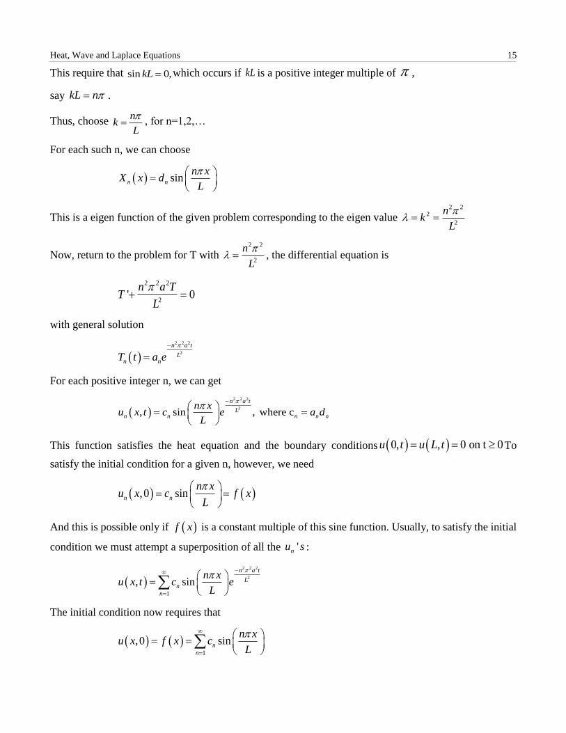
Heat, Wave and Laplace Equations 15
This require that sin 0,kL which occurs if kL is a positive integer multiple of ,
say kL n .
Thus, choose n
kL
, for n=1,2,…
For each such n, we can choose
sinn n
n xX x d
L
This is a eigen function of the given problem corresponding to the eigen value 2 2
2
2
nk
L
Now, return to the problem for T with 2 2
2
n
L
, the differential equation is
2 2 2
2' 0
n a TT
L
with general solution
2 2 2
2
n a t
Ln nT t a e
For each positive integer n, we can get
2 2 2
2
, sin , where c
n a t
Ln n n n n
n xu x t c e a d
L
This function satisfies the heat equation and the boundary conditions 0, , 0 on t 0u t u L t To
satisfy the initial condition for a given n, however, we need
,0 sinn n
n xu x c f x
L
And this is possible only if f x is a constant multiple of this sine function. Usually, to satisfy the initial
condition we must attempt a superposition of all the 'nu s :
2 2 2
2
1
, sin
n a t
Ln
n
n xu x t c e
L
The initial condition now requires that
1
,0 sinn
n
n xu x f x c
L

16 Partial Differential Equations
Which we recognize as the Fourier sine expansion of f x on [0.L]. Therefore, choose the 'nc s as the
Fourier sine coefficients of f x on [0,L]:
0
2sin
L
n
n xc f d
L L
With certain conditions on f x this Fourier sine series converges to f x for 0 x L and the formal
solution of the boundary value problem is
2 2 2
2
1 0
2, sin sin
n a tL
L
n
n n xu x t f d e
L L L
Example: As a special example, suppose the bar is kept at constant temperature A, except at its ends,
which are kept at temperature zero. Then,
0f x A x L
and
0
2 2sin 1 cos
2 = 1 1
L
n
n
n x Ac A dx n
L L n
A
n
The solution in this case is
2 2 2
2
2 2 2
2
1
2 1
1
2, 1 1 sin
2 14 1 = sin
2 1
n a tn
L
n
n a t
L
n
A n xu x t e
n L
n xAe
n L
We got the last summation from the preceding line by noticing that 1 1 0n
if n is even, so all the
terms in the series vanish for n even and we need only retain the terms with n odd. This is done by replacing
n with 2 1n , there by summing over only the odd positive integers.
Problems: Solve the following boundary value problem:
22
21. 0 , 0
0, , 0 0
,0 0
u ua x L t
t x
u t u L t t
u x x L x x L

Heat, Wave and Laplace Equations 17
2
2
2
2. 4 0 , 0
0, , 0 0
,0 0
u ux L t
t x
u t u L t t
u x x L x x L
2
23. 3 0 , 0
0, , 0 0
2 ,0 1 cos 0
u ux L t
t x
u t u L t t
xu x L x L
L
1.2.2 Temperature in a Bar with Insulated Ends
Consider heat conduction in a bar with insulated ends, hence no energy loss across the ends. If the initial
temperature is given by f x , then the temperature function is modeled by the B.V.P.
22
2 0 , 0
0, , 0 0
,0 0
u ua x L t
t x
u ut L t t
x x
u x f x x L
We will solve for ,u x t , leaving out some details, which are the same as in the preceding problem. Set
,u x t X x T t
And substitute into the heat equation to get
2
" 'X T
X a T
In which is the separation constant. Then,
" 0X X
and 2' 0T a T
as before. Also,
0, ' 0 0u
t X T tx
implies that ' 0 0X . The other boundary condition implies that ' 0X L . The other boundary
condition implies that ' 0X L . The problem for X is therefore

18 Partial Differential Equations
" 0 ... 1
' 0 ' 0 ... 2
X X
X X L
We seek values of for which this problem has non-trivial solutions.
Consider cases on :
Case 1: 0
The general solution for (1) is
X x cx d
Since ' 0 0X c , therefore, 0 is an eigen value of (1) with eigen function.
constant 0X x
Case 2: 0
Write 2k with 0k . Then, 2" 0,X k X with general solution
kx kxX x ce de
Now,
' 0 0 0
kx kx
X kc kd c d k
X x c e e
Next,
' 0 kL kLX L ck e e
This is zero only if c=0. But this forces 0X x , so choosing negative eigen value.
Case 3: 0
Set 2k , with 0k .Then,
2" 0X k X
with general solution
cos sinX x c kx d kx
Now, ' 0 0X dk
implies that d=0. Then, cos .X x c kx
Next, ' sin 0 X L ck kL

Heat, Wave and Laplace Equations 19
In order to get a non-trivial solution, we need 0c , and must choose k so that sin 0kL , therefore
kL n
for n, a positive integer, and this problem has eigen values
2 2
2
2
nk
L
; for n=1,2,…
Corresponding to such an eigen value, the eigen function is
cos n n
n xX x c
L
, for n=1,2,…
We can combine case 1 and case 3, by writing the eigen values as
2 2
2 for n=0,1,2,...
n
L
and eigen functions as
cosn n
n xX x c
L
This is a constant functions, corresponding to 0 , when n=0.
The equation for T is
2 2 2
2' 0
n a TT
L
When n=0, this has solutions
0 0 constant =dT t
If n=1,2,…, then
2 2 2
2
n a T
Ln nT t d e
Now let
0 0, constant =au x t
and
2 2 2
2
, cos
n a t
Ln n
n xu x t a e
L
, where n n na c d
Each of these functions satisfies the heat equation and boundary conditions. To satisfy the initial condition,
we must usually attempt a superposition of these functions:
2 2 2
2
0
0 1
, , cos
n a t
Ln n
n n
n xu x t u x t a a e
L
20 Partial Differential Equations
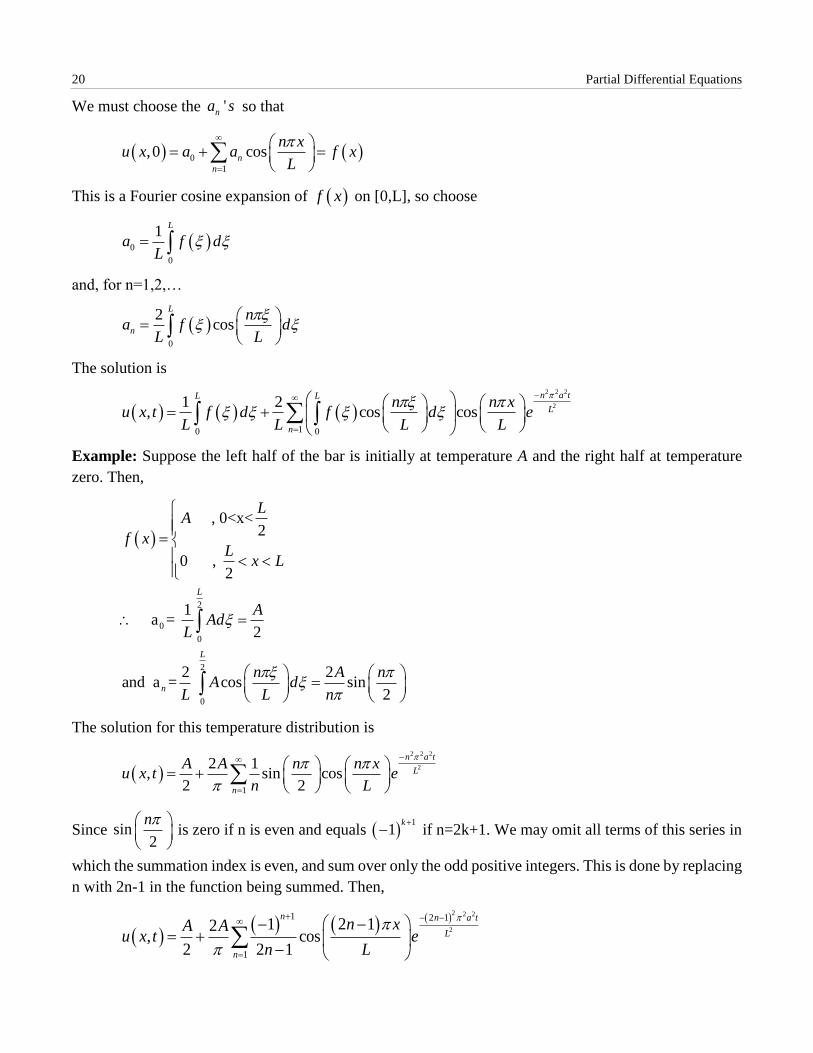
We must choose the 'na s so that
0
1
,0 cosn
n
n xu x a a f x
L
This is a Fourier cosine expansion of f x on [0,L], so choose
0
0
1L
a f dL
and, for n=1,2,…
0
2cos
L
n
na f d
L L
The solution is
2 2 2
2
10 0
1 2, cos cos
n a tL L
L
n
n n xu x t f d f d e
L L L L
Example: Suppose the left half of the bar is initially at temperature A and the right half at temperature
zero. Then,
2
0
0
2
0
, 0<x<2
0 , 2
1 a =
2
2 2and a = cos sin
2
L
L
n
LA
f xL
x L
AAd
L
n A nA d
L L n
The solution for this temperature distribution is
2 2 2
2
1
2 1, sin cos
2 2
n a t
L
n
A A n n xu x t e
n L
Since sin2
n
is zero if n is even and equals 1
1k
if n=2k+1. We may omit all terms of this series in
which the summation index is even, and sum over only the odd positive integers. This is done by replacing
n with 2n-1 in the function being summed. Then,
2 2 2
2
1 2 1
1
1 2 12, cos
2 2 1
n n a t
L
n
n xA Au x t e
n L

Heat, Wave and Laplace Equations 21
Problems:
Solve the following B.V.P.’s:
2
21. 0 , 0
0, , 0 0
u ,0 sin 0
u ux t
t x
u ut t t
x x
x x x
2
22. 4 0 2 , 0
0, 2 , 0 0
u ,0 2 0 2
u ux t
t x
u ut t t
x x
x x x x
3. A thin homogeneous bar of length L has insulated ends initial temperature B, a positive constant. Find
the temperature distribution in the bar.
4. A thin homogeneous bar of length L has initial temperature equal to a constant B and the right end
(x=L) is insulated, while the left end is kept at a zero temperature. Find the temperature distribution in the
bar.
5. A thin homogeneous bar of thermal diffusivity 9 and length 2 cm and insulated has its left end
maintained at temperature zero, while the right end is perfectly insulated. The bar has an initial temperature
given by 2f x x for 0<x<2. Determine the temperature distribution in the bar. What is lim ,t
u x t
?
1.2.3 Temperature Distribution in a Bar with Radiating End
Consider a thin, homogeneous bar of length L, with the left end maintained at temperature zero, while the
right end radiates energy into the surrounding medium, which also is kept at temperature zero. If the initial
temperature in the bar’s cross section at x is f(x), then the temperature distribution is modeled by the B.V.P.
22
2 0 , 0
0, 0, , , 0
,0 0
u ua x L t
t x
uu t L t Au L t t
x
u x f x x L
The boundary condition at L assumes that heat energy radiates from this end at a rate proportional to the
temperature at that end of the bar, A is a positive constant called the transfer co-efficient.
Let ,u x t X x T t to obtain, as before,
2
" 0
' 0
X X
T a T

22 Partial Differential Equations
Since,
0, 0 0, then
0 0
u t X T t
X
as 0T t , implies that , 0u x t which is possible only if 0f x . The condition at the right end of
the bar implies that
'
' 0
X L T t AX L T t
X L AX L
The problem for X x is therefore,
" 0
0 ' 0
X X
X X L AX L
From the strum-Liouville theorem, we can be confident that this problem has infinitely many eigen values
1 2, ,..., each of which is associated with a non-trivial solution, or eigen functions, nX x . We would
like, however, to know these solutions, so we will consider cases:
Cases 1: 0 ,
Then, the solution for X x is
X x cx d
Since, 0 0X d , then
X x cx
But then
'X x c AX L AcL
Then,
1 0c AL
But 1 0AL , so c=0 and we get only the trivial solution from this case. This means that 0 is not an eigen
value of this problem.
Case 2: 0 , write 2k , with 0k .Then,
2" 0X k X , so
kx kxX x ce de
Heat, Wave and Laplace Equations 23
Now, 0 0 .X c d d c
2 sinhkx kxX x c e e c kx
Then, ' 2 cosh sinhX L ck kL Ac kL
To have a non-trivial solution, we must have 0c and this requires that
2 cosh sinh 0k kL A kL
This is impossible because 0,Lk so the left side of this equation is a sum of positive numbers. Therefore,
this problem has no negative eigen value.
Case 3: 0, write 2 ,k with 0k . Then,
2" 0X k X , so
cos sinX x c kx d kx
Now, 0 0,X c so sin .X x d kx
Further, ' cos sin 0X L AX L dk kL Ad kL
To have a non-trivial solution, we must have 0d , and this requires that
cos sin 0k kL A kL
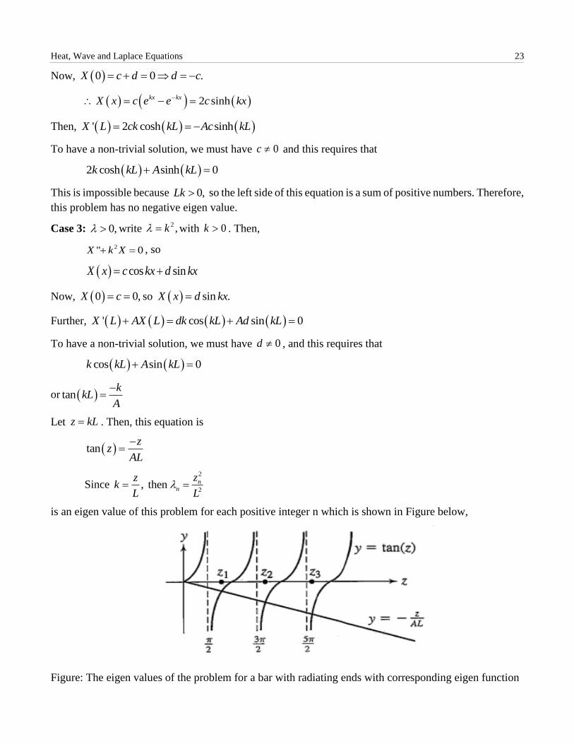
or tank
kLA
Let z kL . Then, this equation is
tanz
zAL
Since 2
2, then n
n
zzk
L L
is an eigen value of this problem for each positive integer n which is shown in Figure below,
Figure: The eigen values of the problem for a bar with radiating ends with corresponding eigen function

24 Partial Differential Equations
sin nn n
z xX x a
L
The equation for T is
2 2
2' 0na z T
TL
So
2 2
2
na z t
Ln nT t d e
For each positive integer n, let
2 2
2
, sin where cna z t
n Ln n n n n
z xu x t c e a d
L
Each such function satisfies the heat equation and the boundary conditions. To satisfy the initial
conditions, let
2
2
1
, sinn na z t
n Ln
n
z xu x t c e
L
we must choose the 'nc s so that
1
,0 sin nn
n
z xu x c f x
L
Unlike what we encountered in the other two examples, this is not a standard’s Fourier series, because of
the 'nz s . Indeed, we do not know these numbers, because they are solutions of a transcendental equation
we cannot solve exactly.
At this point we must rely on the Strum- Liouville theorem, which states that the eigen functions of the
Strum- Liouville problem are orthogonal on [0,L] with weight function 1. This means that if n and m are
distinct positive integers, then
0
sin sin 0
L
m nz x z xdx
L L
This is like the orthogonality relationship used to derive co-efficient of Fourier series and can be exploited
in the same way to find the
0
2
0
sin
sin
L
n
n L
n
z xf x dx
Lc
z xdx
L
With this choice of co-efficient, the solution is

Heat, Wave and Laplace Equations 25
2 2
20
1 2
0
sin
, sin
sin
n
L
na z t
n LL
n n
zf d
L z xu x t e
Lzd
L
Problems:
1. A thin, homogeneous bar of thermal diffusivity 4 and length 6 cm with insulated sides, has its end
maintained at temperature zero. Its right end is radiating (with transfer co-efficient 1
2) into the
surrounding medium, which has temperature zero. The bar has an initial temperature given by
6f x x x . Approximate the temperature distribution ,u x t by finding the fourth partial
sum of the series representation for ,u x t .
1.2.4 Heat Conduction in a Bar with Ends at Different Temperature
Consider a thin, homogeneous bar extending from 0 to x x L . The left end is maintained at constant
temperature 1T and the right end at constant temperature 2T . The initial temperature throughout the bar in
the cross-section at x is ( )f x .
The boundary value problem for the temperature distribution is:
22
2
1 2
(0 , 0)
(0, ) , ( , ) ( 0)
( ,0) ( ) (0 )
u ua x L t
t x
u t T u L t T t
u x f x x L
Put ( , ) ( ) ( )u x t X x T t into the heat equation to obtain,
2
" 0
' 0
X X
T a T
Unlike the preceding example, there is nothing in this partial differential equation that prevents separation
of the variables. The difficulty encountered here is with the boundary conditions which are non-
homogeneous ( (0, ) and ( , )u t u L t may be non-zero). To see the effect of this consider,
1(0, ) (0) ( )u t X T t T
If 1 0T , we could conclude that (0) 0X . But if 1 0T , this equation forces us to conclude that
1( ) constant(0)
TT t
X .This is a condition, we cannot except to satisfy. The boundary condition at L
possess the same problem.
We attempt to eliminate the problem by perturbing the function. Set
( , ) ( , ) ( )u x t U x t x

26 Partial Differential Equations
We want to choose ( )x to obtain a problem, we can solve.
Substitute ( , )u x t into the partial differential equation to get
22 2
2"( )
u ua a x
t x
We obtain the heat equation for U if "( ) 0x . Integrating twice, ( )x must have the form
( ) ...(1)x Cx D
Now, consider the boundary conditions, first
1(0, ) (0, ) (0)u t T U t
This condition becomes (0, ) 0U t if we choose ( )x so that
1(0) ...(2)T
The condition
2( , ) ( , ) ( )u L t T U L t L
becomes ( , ) 0U L t if
2( ) ...(3)L T
Now, use (2) and (3) to solve for C and D in (1),
1
1 2 2 1
(0)
1and ( ) ( )
D T
L CL T T C T TL
Thus, choose
2 1 1
1 ( ) ( )x T T x T
L
with this choice, the boundary value problem for ( , )U x t is
22
2
2 1 1
(0, ) ( , ) 0
1( ,0) ( ,0) ( ) ( ) ( )
U Ua
t x
U t U L t
U x u x x f x T T x TL
We have solved this problem earlier, with the solution 2 2 2
2
2 1
1 0
2 1( , ) ( ) ( ) sin sin
n a tL
L
n
n n xU x t f T T x T d e
L L L L
Once, we know this function, then
2 1 1
1( , ) ( , ) ( )u x t U x t T T x T
L

Heat, Wave and Laplace Equations 27
1.3 Steady–State Temperature in Plates
The two-dimensional Heat equation is
2 22 2 2
2 2
u u ua a u
t x y
The steady-state case occurs when we set 0u
t
. In this event, the Heat equation is Laplace’s equation
2 0u
A Dirichlet problem consists of Laplace’s equation, to be solved for (x,y) in a region R of the plane,
together with prescribed values the solution is to assumes on the boundary of R, which is usually a
piecewise smooth curve. If we think of R as a flat plate, then we are finding the steady-state temperature
distribution throughout a plate, given the temperature at all timers on its boundary.
1.3.1 Steady-State Temperature in a Rectangular Plate
Consider a flat rectangular plate occupying the region R in the xy-plane by 0 , 0 .x a y b Suppose
the right side is kept at constant temperature T, while the other sides are kept at temperature zero. The
boundary value problem for the steady-state temperature distribution is:
2 0 (0 ,0 )
( ,0) ( , ) 0 (0 )
(0, ) 0 (0 )
( , ) (0 )
u x a y b
u x u x b x a
u y y b
u a y T y b
Put ( , ) ( ) ( )u x y X x Y y into Laplace’s equation to get
" " 0
" "
X Y Y X
X Y
X Y
Since the left side depends only on x and the right side only on y, and these variables are independent,
both sides must equal the same constant.
" " (say)
X Y
X Y
Now, use the boundary condition:
( ,0) ( ) (0) 0 (0) 0
( , ) ( ) ( ) 0 ( ) 0
u x X x Y Y
u x b X x Y b Y b
and (0, ) (0) ( ) 0 (0) 0u y X Y y X
Therefore, ( )X x must satisfy

28 Partial Differential Equations
" 0
(0) 0
X X
X
and, Y must satisfy
" 0
(0) ( ) 0
Y Y
Y Y b
This problem for ( )Y y was solved in the article (Ends of the bar kept at temperature zero) with ( )X x in
place of ( )Y y and L in place of b.
The eigen values are
2 2
2n
n
b
with corresponding eigen functions
( ) sin for n=1,2,...n n
n yY y b
b
The problems for X is now
2 2
2" 0
(0) 0
nX X
b
X
The general solution of the differential equation is
( )n x n x
b bnX x ce de
Since (0) 0X c d d c and so
( ) 2 sinhn x n x
b bn n
n xX x c e e c
b
For each positive integer n, let
( , ) sinh sin ; where a 2n n n n n
n x n yu x y a b c
b b
For each n and any choice of the constant na this function satisfies Laplace’s equation and the zero
boundary conditions on three sides of the plate. For the non-zero boundary condition, we must use a
superposition
1
( , ) sin sinhn
n
n y n au a y T a
b b

Heat, Wave and Laplace Equations 29
This is a Fourier sine expansion of T on [a,b]. Therefore, choose the entire co-efficient
sinn y
b
as the Fourier sine co-efficient:
0
2sinh sin
2 1 1 ,
b
n
n
n a n ya T dy
b b b
T b
b n
in which we have used the fact that cos 1 ,n
n if n is an integer.
We now have
2 1
1 1
sinh
n
n
Ta
n an
b
The solution is
1
2 1( , ) 1 1 sinh sin
sinh
n
n
T n x n yu x y
n a b bn
b
As we have done before, observe that 1 1n
equals 0 if n is even, and equals 2 if n is odd. We can
therefore omit the even indices in this summation, writing the solution as:
1
4 1 (2 1) (2 1)( , ) sinh sin
(2 1)(2 1)sinhn
T n x n yu x y
n a b bn
b
Problems: 1. Solve for the steady-state temperature distribution in a flat plate covering the region
0 , 0 ,x a y b if the temperature on the vertical sides and the bottom side are kept at zero while the
temperature on the top side is a constant K.
2.Solve for the steady-state temperature distribution is a flat plate covering the region 0 , 0 ,x a y b
if the temperature on the left side is a constant 1T and that on right side a constant 2T , while the top and
bottom sides are kept at temperature zero.
[Hint: Consider two separate problems. In the first, the temperature on the left side is 1T and the other
sides are kept at temperature zero. In the second, the temperature on the right side is 2T , while the other
sides are kept at zero. The sum of solutions of these problems is the solution of the original problem.]

30 Partial Differential Equations
Remark: It is possible to treat the case where the four sides are kept at different temperature (not
necessarily constant), by considering four plates, in each of which the temperature is non-zero on only
one side of the plate. The sum of the solutions of these four problems is the solution for the original plate.
1.3.2 Steady-State Temperature in a Circular Disc
Consider a thin disk of radius R, placed in the plane so that its centre is the origin. We will find the steady-
state temperature distribution ( , )u r as a function of polar co-ordinates. The Laplace’s equation in polar
co-ordinates is
2 2
2 2 2
1 10
u u u
r r r r
for 0 and r R
Assume that the temperature is known on the boundary of the disk:
, for -u R f
In order to determine a unique solution for u, we will specify two additional conditions, First we seek a
bounded solution. This is certainly a physically reasonable condition. Second we assume periodically
conditions:
, , and ( , ) ( , )u u
u r u r r r
These conditions account for the fact that ( , )r and ( , )r are polar co-ordinates of the same point.
Attempt a solution
( , ) ( ) ( )u r F r G
Substitute this into the Laplace’s equation, we get
2
1 1"( ) ( ) '( ) ( ) ( ) "( ) 0F r G F r G F r G
r r
If ( ) ( ) 0F r G , this equation can be written
2 "( ) '( ) "( )
( ) ( )
r F r rF r G
F r G
Since the left side of this equation depends only on r and the right side only on , and these variables are
independent, both sides must equal same constant
2 "( ) '( ) "( )
( ) ( )
r F r rF r G
F r G
which gives

Heat, Wave and Laplace Equations 31
2 "( ) '( ) ( ) 0 ...(1)
and G"( )+ G( )=0
r F r rF r F r
Now, consider the boundary conditions. First
( , ) ( , ) ( ) ( ) ( ) ( )u r u r G F r G F r
Assuming ( )F r is not identically zero, then
( ) ( )G G
Similarly,
( , ) ( ) '( ) ( , ) ( ) '( )
'( ) '( )
u ur F r G r F r G
G G
The problem to solve ( )G is therefore
"( ) ( ) 0
( ) ( ) ... 2
'( ) '( )
G G
G G
G G
This is a periodic Strum-Liouville problem and first we solve it by considering different cases:
Case 1: 0
In this case, the equation reduces to
"( ) 0G
with the general solution
( )G c d
Now,
( ) ( ) 2 0
0
( )
G G c d c d d
d
G c
which satisfies '( ) '( )G G
Thus, 0 is an eigen value of the problem with eigen function
0( ) constantG c
Case 2: 0
Let 2n
Then, the differential equation (2) is

32 Partial Differential Equations
2"( ) ( ) 0G n G
with the general solution given by
( ) n nG ce de
Now,
( ) ( )
( ) 0
n n n n
n n
G G ce de ce de
G c e e c d c d
Also,
'( ) '( ) ( ) ( )
2 0 0
( ) 0
n n n nG G cn e e cn e e
cn c
G
Thus, we have no eigen value in this case.
Case 3: 0
Let 2k . Then, the differential equation (2) is
2"( ) ( ) 0G k G
with the general solution given by
( ) cos( ) sin( )G c k d k
Now,
( ) ( ) cos( ) sin( ) cos( ) sin( )
2 sin( ) 0
G G c k d k c k d k
d k
For a non-trivial solution, we take
for n=1,2...
for n=1,2...
k n
k n
Similarly, result holds for '( ) '( )G G
Thus, the general solution is given by
( ) cos( ) sin( )n n nG c n d n
Thus, the eigen values for the SLBVP (2) is
2 ; n=0,1,2,3...n
and the eigen function is

Heat, Wave and Laplace Equations 33
0 0( )
( ) cos( ) sin( )n n n
G c
G c n d n
Now, let 2n to get (1) as
2"( ) '( ) ( ) 0rF r rF r n F r
This is a second order Euler differential equation with general solution
0 0
( ) , for n=1,2,3...
and ( ) constant , for n=0
n n
n n nF r a r b r
F r a
The requirement that the solution must be bounded forces to choose each 0nb because
as 0nr r (centre of the disk).
Combining cases, we can write
( ) for n=0,1,2...n
n nF r a r
For n=0,1,2…, we now have functions of the form
( , ) ( ) ( ) cos( ) sin( )n
n n n n n nu r F r G a r c n d n
Setting and ,n n n n n nA a c B a d we have
( , ) cos( ) sin( )n
n n nu r r A n B n
These functions satisfy Laplace’s equation and the periodicity conditions, as well as the condition that
solutions must be bounded. For any given n, this function will generally not satisfy the initial condition
( , ) ( )u R f
For this, use the superposition
0
1
( , ) cos( ) sin( )n
n n
n
u r A r A n B n
Now, the initial condition requires that
0
1
( , ) ( ) cos( ) sin( )n n
n n
n
u R f A A R n B R n
This is the Fourier series expansion of ( )f on [ , ] . Thus, choose
0
1( )
2
1 1( )cos ( )cos
1 1and B ( )sin ( )sin
n
n n n
n
n n n
A f d
A R f n d A f n dR
R f n d B f n dR

34 Partial Differential Equations
Example: As a specific example, suppose the disk has radius 3 and that ( ) 2f . A routine
integration gives
0
1
2 , 0 for n=1,2,3...
2and ( 1)
.3
n
n
n n
A A
Bn
The solution for this condition is
1
1
2( , ) 2 ( 1) sin( )
3
for 0 3 and .
n
n
n
ru r n
n
r
Problems:
1. Find the steady-state temperature for a thin disk
i. of radius R with temperature on boundary is 2( ) cos for -f
ii. of radius 1 with temperature on boundary is 3( ) cos for -f
iii. of radius R with temperature on boundary is constant T.
2. Use the solution of steady-state temperature distribution in a thin disk to show that the temperature at
the centre of disk is the average of the temperature values on the circumference of the disk.
[Hint: For temperature on the centre of disk, we let 0r , so that 0
1( , ) ( )
2u r A f d
which is the average of ( )f , the temperature on the circumference of the disk.]
3. Find the steady-state temperature in the flat wedge-shaped plate occupying the region
0 , 0r k (in polar co-ordinates). The sides 0 and are kept at temperature zero and
the ark r k for 0 is kept at temperature T.
[Hint: The BVP for this situation is
2 2
2 2 2
1 10
( ,0) ( , ) 0 (0 )
( , ) (0 )
u u u
r r r r
u r u r r k
u k T
1.3.3 Steady-State Temperature Distribution in a Semi-infinite Strip
Find the steady-state temperature distribution in a semi-infinite strip 0, 0 1,x y pictured in figure.
The temperature on the top side and bottom side are kept at zero, while the left side is kept at temperature
T.
The boundary value problem modelling this problem is:

Heat, Wave and Laplace Equations 35
2 2
2 20 0 1, 0
( ,0) 0 ( ,1) (x 0)
u(0,y)=T (0 1)
u uy x
x y
u x u x
y
Put ( , ) ( ) ( )u x y X x Y y into Laplace’s equation to get
" "" " 0
X YX Y XY
X Y
Since the left side depends only on x and right side only on x, and these variables are independent, both
sides must equal the same constant:
" "X Y
X Y
Now, use the boundary conditions:
( ,0) ( ) (0) 0 (0) 0
( ,1) ( ) (1) 0 (1) 0
u x X x Y Y
u x X x Y y
Therefore, X must satisfy
" 0X X
and, Y must satisfy
" 0
(0) (1) 0
Y Y
Y Y
The solution for the equation for ( )Y y is given by (by above article)
( ) sin( ) for n=1,2,...n nY y a n y
with the eigen value given by
2 2
n n
The problem for ( )X x is now
2 2" 0X n X
The general solution of the differential equation is
( ) n x n x
n n nX x b e c e
Now, since ( , ) , so 0nu x y b , otherwise ( ) as x .nX x Thus, we have
( ) n x
n nX x c e

36 Partial Differential Equations
Thus, solution for each n is
( , ) sin( ) , where dn x
n n n n nu x y d e n y a c
For each n, using the superposition, we have
1
( , ) sin( )n x
n
n
u x y d e n y
We want to choose the constant nd , so that
1
(0, ) sin( )n
n
u y T d n y
which is Fourier sine expansion of T on [0,1]. Therefore, choose the entire co-efficient of sin( )n y as the
Fourier sine co-efficient:
1
0
2 sin( )
2 1 ( 1)
n
n
d T n y dy
T
n
[As in above article]
Problem:
1. Find a steady-state temperature distribution in the semi-infinite region 0 , 0x a y if the temperature
on the bottom and left sides are at zero and the temperature on the right side is kept at constant T.
2. Find the steady-state temperature distribution in the semi-infinite region 0 4, 0x y if the
temperature on the vertical sides are kept at constant T and temperature on the bottom side is kept at
zero.
[Hint: Assume two semi-infinite regions, first with left end at temperature T and right end and bottom
at temperature zero, second with right end at temperature zero and left end and bottom at temperature
zero. Sum of these two solutions is the solution of the original problem.]
3. Use your intuition to guess the steady-state temperature in a thin rod of length L if the ends are perfectly
insulated and the initial temperature is ( ) for 0 .f x x L
[Hint: The boundary value problem modelling this problem is
2 2
2 20 (0 ) ( 0)
(0, ) 0 ( , ) ( 0)
( ,0) ( ) (0 )
u ux L t
t x
u ut L t t
x x
u x f x x L

Heat, Wave and Laplace Equations 37
1.3.4 Steady-State Temperature in a Semi-infinite Plate
The B.V.P. is
2 2
2 20 (0 , 0)
( ,0) 0 ( , ) ( 0)
(0, ) (0 )
u uy b x
x y
u x u x b x
u y T y b
Put ( , ) ( ) ( )u x y X x Y y into the given Laplace equation, we obtain
'' '''' '' 0
X YX Y XY
X Y
Since the left side is depend on x only while right hand side is y only. So both side must be equal to
some constant. Let the constant of separation coefficient is . The above equation becomes
'' 0X X and '' 0Y Y
And the boundary condition ( ,0) ( ) (0) 0 (0) 0
( , ) ( ) ( ) 0 ( ) 0
u x X x Y Y
u x b X x Y b Y b
Here we have more information for problem Y with equations
'' 0
(0) 0 ( ) 0
Y
Y and Y b
In earlier article, we solve such problem and preceding like that, we have solution
sin 1,2,3...n n
n yY a for n
b
with the eigen value
2 2
2n
n
b
.
Now the problem for X is
2 2
2'' 0
nX X
b
The general solution is
( )n x n x
b bn n nX x b e c e
For a bounded solution in the given domain, we have to assume 0nb . Now the solution becomes
( )n x
bn nX x c e
. Thus the solution for each n by using the superposition is

38 Partial Differential Equations
1
( , ) sinn x
bn n n n
n
n yu x y d e where d a c
b
Now using the condition (0, ) ,u T T we have
1
(0, ) sinn
n
n yu y T d
b
which is a Fourier sine expansion of T on [0,1]. The
coefficient
0
2 sin
b
n
n yd T dy
b
2
1 1nT
n
1
2( , ) 1 1 sin
n xn
b
n
T n yu x y e
n b
1.3.5 Steady-State Temperature in an Infinite Plate
Suppose we want the steady-state temperature distribution in a thin, flat plate extending over the right
quarter plane 0, 0x y . Assume that the temperature on the vertical side 0x is kept at zero, while
the bottom side 0y is kept at a temperature ( )f x .
The BVP modelling this problem is:
2 2
2 20 ( 0, 0)
(0, ) 0 ( 0)
( ,0) ( ) ( 0)
u ux y
x y
u y y
u x f x x
Now solving as in previous examples we get
0
( , ) sin( ) ky
ku x y c kx e dk
Finally, we require that
0
( ,0) ( ) sin( )ku x f x c kx dk
This is the Fourier sine integral of ( ) on [0, )f x , so choose
0
2( )sin( )kc f k d
Thus, the solution for the problem is
Heat, Wave and Laplace Equations 39
0 0
2( , ) ( )sin( ) sin( ) kyu x y f k d kx e dk
Example: Assume that in the above problem
4 , 0 2( )
0 , 2
xf x
x
Then,
0
0
2( )sin( )
2 4sin( )
8 1 cos(2 )
kc f k d
k d
kk
Thus,
0
8 1 cos 2( , ) sin( ) kyk
u x y kx e dkk
1.4 Heat Equation in Unbounded Domains
Here, we will discuss the problems of temperature distribution in a bar with the space variable extending
over the real line or half line.
1.4.1 Heat Conduction in a Semi-Infinite Bar
Suppose we want the temperature distribution in a Bar stretching from 0 to along the x-axis. The left
end is kept at temperature zero and the initial temperature in the cross-section at x is ( )f x .
The boundary value problem for the temperature distribution is:
22
2 ( 0, 0)
( ,0) ( ) ( 0)
(0, ) 0 ( 0)
u ua x t
t x
u x f x x
u t t
As usual, we seek a solution, which is bounded.
Set,
2
( , ) ( ) ( ) to get
" 0 ( 0)
' 0 ( 0)
u x t X x T t
X X x
T a T t
Now as in previous examples, we get
40 Partial Differential Equations
2 2
( , ) sin( ) , where a k t
k k k ku x t d kx e d a b
Now, using the superposition
2 2
0
( , ) sin( ) ...(1)a k t
ku x t d kx e dk
Finally, we must satisfy the initial condition:
0
( ) ( ,0) sin( ) ...(2)kf x u x d kx dk
For this choice the 'kd s are the Fourier sine integral co-efficient of ( )f x ; so
0
2( )sin( )kd f k d
With this choice of the co-efficient, the function defined by (1) is a solution of the problem.
Example: Suppose
, 0 x( )
0 ,
xf x
x
Then, 0
2 2 sin( )( )sin( ) 1k
kd k d
k k
The solution is
2 2
0
2 sin( )( , ) 1 sin( ) k tk
u x t kx e dkk k
1.4.2 Heat Conduction in Infinite Bar
Suppose we want the temperature distribution in a Bar stretching from to along the x-axis. The
initial temperature in the cross-section at x is ( )f x . The boundary value problem for the temperature
distribution is:
22
2 ( , 0)
( ,0) ( ) ( )
u ua x t
t x
u x f x x
There are no boundary conditions, so we impose the physically realistic condition that solutions should
be bounded. As usual, we seek a solution, which is bounded.
Set,

Heat, Wave and Laplace Equations 41
2
( , ) ( ) ( ) to get
" 0 ( )
' 0 ( 0)
u x t X x T t
X X x
T a T t
Now as in previous examples, we get
2 2
( , ) ( cos( ) sin( )) , a k t
k k ku x t a kx b kx e
that satisfy the Heat equation and are bounded on the real line over all k>0. Now, using the superposition
2 2
0
( , ) ( cos( ) sin( )) ...(1)a k t
k ku x t a kx b kx e dk
Finally, we must satisfy the initial condition:
0
( ) ( ,0) ( cos( ) sin( )) ...(2)k kf x u x a kx b kx dk
For this choice the 'ka s and 'kb s are the Fourier sine integral co-efficient of ( )f x ; so
1( )cos( )ka f k d
and
1( )sin( )ka f k d
With this choice of the co-efficient, the function defined by (1) is a solution of the problem.
1.5 Solution of Heat, Laplace and Wave Equations
1.5.1 Solution of Three-Dimensional Heat Equations in Cartesian co-ordinates
It is a partial differential equation of the form:
2 2 22
2 2 2 ...(1)
u u u uh
t x y z
To find its solution by the method of separation of variables, suppose that the solution of (1) is
( , , , ) ( ) ( ) ( ) ( ) ...(2) u x y z t X x Y y Z z T t
where ( )X x is a function of x only, ( )Y y is a function of y only, ( )Z z is a function of z only and ( )T t is
a function of t only.
We get on separating the variables
2 2 2
2 2 2 2
1 1 1 1 ...(3)
d X d Y d Z dT
X dx Y dy Y dz h T dt

42 Partial Differential Equations
Choosing the constant of separation such that
2 2 22 2 2 2 2 2 2 2
1 2 3 1 2 32 2 2 2
1 1 1 1, , and ,where +
d X d Y d Z dTp p p p p p p p
X dx Y dy Z dz h T dt
Thus, we have the following three equations
22
12
22
22
22
32
2 2
0
0
0
0
d Xp X
dx
d Yp Y
dy
d Zp Z
dz
dTp h T
dt
with the solutions
2 2 2 22 21 2 3
1 1
2 2
3 3
( )
( ) cos sin
( ) cos sin
( ) cos sin
( )p p p h tp h t
X x A p x B p x
Y y C p y D p y
Y y E p z F p z
T t Ge Ge
Combining these solutions and using the superposition, we get
2 2 2 21 2 3
1 2 3
( )
1 1 2 2 3 3
, , 1
( , , , ) ( cos sin )( cos sin )( cos sin )p p p h t
p p p
u x y z t A p x B p x C p y D p y E p z F p z Ge
Corollary: The Heat equation in two-dimensional is
2 22
2 2
u u uh
t x y
The solution is
2 2 21 2
1 2
( )
1 1 2 2
, 1
( , , ) ( cos sin )( cos sin )p p h t
p p
u x y t A p x B p x C p y D p y Ee
1.5.2 Solution of Heat Equation in Cylindrical Polar Co-ordinates
In cylindrical co-ordinates, Heat equation has the form
2 2 2
2 2 2 2 2
1 1 1 ...(1)
u u u u u
r r r r z h t
To solve it by the method by separation of variables, we have
( , , , ) ( ) ( ) ( ) ( ) ...(2)u r z t R r Z z T t

Heat, Wave and Laplace Equations 43
giving
2 2
2 2
2 2 2 2
2 2 2 2
( ) ( ) , ( ) ( )
( ) ( ) ( ) , ( ) ( )
( ) ( )
u dR u d RZ z T t Z z T t
r dr r dr
u d u d ZR r Z z T t R r T t
d z dz
u dTR r Z z
t dt
Substituting all these values in equation (1), we get
2 2 2
2 2 2 2 2
1 1 1 1d R dR d d Z dT
R dr r dr r d dz h T dt
Using the method of separation of variables, we have
2 2 2
2
10 (3)
dT dTh t
h T dt dt
2 2
2 2 2
2 20 (4)
d Z d Zh t
dz dz
and
2 22 2
2 2
10 ...(5)
d d
d d
so that
2 22 2
2 2
2 22 2 2 2
2 2
1 1
10 where - ...(6)
d R dR
R dr r dr r
d R dRR
dr r dr r
with solution of (3) as
2 2
( ) h tT t ae
solution of (4) as
cos sinZ z b z c z
solution of (5) as
cos sine f
The equation (6) is Modified Bessel’s Equation and the solution is
( ) for fractional R r AJ r BJ r
and
( ) for integral R r AJ r BY r

44 Partial Differential Equations
where
2
0
12
( ) , where ( 1) ( 1)( 2)...( )2 1
( ) 1 ( )
rr
n
n r
r r
n
n n
x
xJ x n n n n r
n
J x J x
and
21
0
2 1 2( ) log ( )
2
n pn
n n
p
x n pY x J x
p x
Thus, the solution of Heat equation is
2 2
, ,
, , , cos sin cos sin ( )
h tu r z t ae b c e z f z AJ r BJ r
2 2
, ,
for fractional ,
and , , , cos sin cos sin ( )
h tu r a t ae b c e z f z AJ r BY r
for integral .
Corollary: In 2-dimesnion, the cylindrical heat Equation is
2 2
2 2 2 2
1 1 1
u u u u
r r r r h t
and the solution of Heat equation is
2 2
2 2
,
,
, , cos sin ( ) for fractional ,
and , , cos sin ( ) for integral .
h t
h t
u r t ae b c AJ r BJ r
u r t ae b c AJ r BY r
1.5.3 Solution of Heat Equation in Spherical Co-ordinates
In spherical polar co-ordinates, it has the form
2 2
2 2 2 2 2 2
2 1 1 1sin ...(1)
sin sin
u u u u u
r r r r r h t
Assuming ( , , , ) ( ) ( ) ( ) ( )u r t R r T t , equation (1) becomes
2 2
2 2 2 2 2 2
2 2 2
2
2 22 2
2 2
1 2 1 1 1sin
sin sin
1Let 0 ...(2)
1 =0 ...(3)
d R dR d d d dT
R dr Rr dr r d d r d h dt
dT dTh T
h T dT dt
d dm m
d d

Heat, Wave and Laplace Equations 45
with solution given by
2 2
( )
( )
h t
im
T t a
b
e
e
and
2 2 22 2
2 2
1 2sin ( 1) (say)
sin sin
d d m r d R r dRr n n
d d R dr R dr
giving
2
2 2 2
2
2
2
2 ( 1) 0 ...(4)
1sin ( 1) 0 ...(5)
sin sin
d R dRr r r n n R
dr dr
d d mn n
d d
Here (4), being homogeneous, if we put sr e and d
Dds
, reduces to
( 1)
1
( 1) 2 ( 1) 0
or ( )( ( 1)) 0
ns n s
n n
D D D n n R
D n D n R
R Ae Be
Ar Br
Putting cos in (5), so that
1sin
sin
d d d d d d
d d d d d d
we have
2
2
2
2 22
2 2
1 ( 1) 01
or (1 ) 2 ( 1) 01
d d mn n
d d
d d mn n
d d
which is associated Legendre equation, then the solution is of the form
(cos )
and hence solution of given problem is
2 21( , , , ) ( ) (cos )n n im
n
h tu r t Ar Br e e
Hence, summing overall n and trying superposition, the general solution of (1) may be expressed as

46 Partial Differential Equations
2 2
1, ,
( , , , ) ( ) (cos )n inn n
h t
n m
Bu r t A r e
re
is required solution.
1.5.4 Solution of Laplace Equation in Cartesian Co-ordinates
In Cartesian co-ordinates, the Laplace equation has the form
2 2 2
2 2 20 ...(1)
V V V
x y z
To solve it by the method of separation of variables, we have
( , , ) ( ) ( ) ( ) ...(1)V x y z X x Y y Z z
giving2 2 2 2 2 2
2 2 2 2 2 2YZ, Z and
V d X V d Y V d ZX XY
x dx y dy z dz
so that (1) gives
2 22 2
1 12 2
2 22 2
2 22 2
2 22 2 2 2 2
1 22 2
10 ...(2)
10 ...(3)
1 0 where ...(4)
d X d Xp p X
X dx dx
d Y d Yp p Y
Y dy dy
d Z d Zp p Z p p p
Z dz dz
The solutions of these equations are
1 1
2 2
( ) cos sin
( ) cos sin
( ) pz pz
X x A p x B p x
Y y C p y D p y
Z z Ee Fe
The combined solution of (1) is
1 1 2 2( , , ) ( cos sin )( cos sin ( )p
pz pzV x y z A p x B p x C p y D p y ce De
Using the superposition, we have
1 2
1 1 2 2
,
( , , ) ( cos sin )( cos sin ( )pz pz
p p
V x y z A p x B p x C p y D p y ce De
Corollary: In 2-dimesnion, the Laplace equation has the form
2 2
2 20 ...(1)
V V
x y
To solve it by the method of separation of variables, we have
( , ) ( ) ( ) ...(2)V x y X x Y y

Heat, Wave and Laplace Equations 47
giving 2 2 2 2
2 2 2 2Y and
V d X V d YX
x dx y dy
so that (1) gives
2 22
2 2
1 1d X d Yp
X dx Y dy
Now,
22
2
22
2
0 ...(3)
and 0 ...(4)
d Xp X
dx
d Yp Y
dy
The solutions of these equations are
( ) cos sin
( ) py py
X x A px B px
Y y Ce De
The combined solution of (1) is
( , ) ( cos sin )( )py py
pV x y A px B px ce De
Using the superposition, we have
( , ) [( cos sin )( )]py py
p
V x y A px B px ce De
1.5.5 Solution of Three-Dimensional Laplace Equation in Cylindrical Co-ordinates
In cylindrical co-ordinates, Laplace’s equation has the form
2 2 2
2 2 2 2
1 10 ...(1)
V V V V
r r r r z
Assuming that ( , , ) ( ) ( ) ( )V r z R r Z z , then (1) yields
2 2 2
2 2 2 2
1 1 1 10 ...(2)
d R dR d d Z
R dr rR dr r d Z dz
Since the variables are separated, we can take
2 22 2
2 2
2 22 2
2 2
1 1 and
0 and 0
Z d
z z d
Z dz
z d
yielding the general solutions as

48 Partial Differential Equations
( ) and ( ) cos sinz zZ z C DAe Be
Now, equation (2) reduces to
2 22
2 2
10
d R dRR
dr r dr r
Which is Bessel’s modified equation, having the solution
( ) ( ) ( )R r EJ r FJ r for fractional
and ( ) ( ) ( )R r EJ r FY r for integral .
Hence, the combined solution is
,
( , , ) cos sin ( ) ( )z zV r z Ae Be C D EJ r FJ r
,
for fractional .
,
( , , ) cos sin ( ) ( )z zV r z Ae Be C D EJ r FY r
,
for integral .
Corollary: 1. Taking constant A and B , the general solution can be written as
( ) ( ) ( )R r A J r B Y r
But ( )Y r as 0r , therefore if it is finite along the line 0r , then 0B , hence the solution is
( , , ) ( ) z iV r z A J r e
Trying the superposition, we can write the solution as:
, 0
( , , ) ( ) ( cos sin ) ( cos sinz zV r z J r e A B e C D
2. Solution of Laplace Equation in Two Dimension in Polar Co-ordinates
The Laplace equation has the form:
2 2
2 2 2
1 10 ...(1)
V V V
r r r r
To solve it by the method of separation of variables, we take
, ( ) ( ) ...(2)V r R r
giving

Heat, Wave and Laplace Equations 49
2 2
2 2
2 2
2 2
( ) ; ( ) and
( )
V dR V d R
r dr r dr
V dR r
d
Substituting all these in the equation (1), we get
2 22 2
2 2
1 1 (say)
d R dR dr r n
R dr dr d
so that we have
22 2
2
22 2
2
1 (say)
0 ...(3)
d R dRr r n
R dr dr
d R dRr r n R
dr dr
which is homogeneous and hence on putting
, so that logzr e z r and d d
D rdr dz
then the equation (3) reduces to
2
2 2
( 1) 0
0
D D D n r
D n r
Its auxiliary equation is
2 2 0
( )
nz nz
n n
D n
D n
R r Ae Be
Ar Br
Also, the equation for (1) is
22
2
1 ...(4)
dn
d
It has the solution
( ) cos sinC n D n
The combined solution is
, cos sin ...(5)n
n nV r C n D nAr Br
Also, for n=0, (3) and (4) becomes

50 Partial Differential Equations
22
2
2
2
0 ...(6)
and 0 ...(7)
d R dRr r
dr dr
d
d
Having the solution of (6) and (7) as
1 2
1 2
( ) logR r c c r
d d
Thus, for n=0, the solution is
1 2 1 2( , ) logV r c c r d d
Thus, the general solution is
1 2 1 2
1
( , ) log cos sinn n
n n n n
n
V r c c r d d A r B r C n D n
1.5.5 Solution of Laplace Equation in Spherical Co-ordinates
In spherical polar co-ordinates, it has the form
2 22
2 2 2
1 12 sin 0 ...(1)
sin sin
V V V Vr r
r r
Assuming ( , , ) ( ) ( ) ( )V r R r , equation (1) becomes
2 2 22
2 2
2 22 2
2 2
2 1 1sin
sin
1 0
r d R r dR d d d
R dr R dr d d d
d d
d d
with solution given by
( ) iCe
and
2 2 2
2 2
2 1sin ( 1) (say)
sin sin
r d R r dR d dn n
R dr R dr d d
giving
22
2
2
2
2 ( 1) 0 ...(2)
1sin ( 1) 0 ...(3)
sin sin
d R dRr r n n R
dr dr
d dn n
d d

Heat, Wave and Laplace Equations 51
Here (2), being homogeneous, if we put sr e and d
Dds
, reduces to
( 1)
1
( 1) 2 ( 1) 0
or ( )( ( 1)) 0
ns n s
n n
D D D n n R
D n D n R
R Ae Be
Ar Br
Putting cos in (4), so that
1sin
sin
d d d d d d
d d d d d d
we have
2
2
2
2 22
2 2
1 ( 1) 01
or (1 ) 2 ( 1) 01
d dn n
d d
d dn n
d d
which is associated Legendre equation, then the solution is of the form
(cos )
and hence solution of given problem is
1( , , ) ( ) (cos )n n i
nV r Ar Br e
Hence, summing overall n and trying superposition, the general solution of (1) may be expressed as
1,
( , , ) ( ) (cos )n inn n
n
BV r A r e
r
is required solution.
1.5.7 Solution of Three-Dimensional Wave Equation in Cartesian Co-ordinates
A partial differential equation of the form
22 2
2
uc u
t
is known as Wave equation, that is
2 2 2 22
2 2 2 2
2 2 2 2
2 2 2 2 2
1 ...(1)
u u u uc
t x y z
u u u u
x y z c t
with the conditions

52 Partial Differential Equations
0 at 0,
0 at y 0,
0 at z 0,
ux x a
x
uy a
y
uz a
z
and ( , , , ) 0 at 0u x y z t t
To solve the problem, we shall use the method of separation of variables and assume that
( , , , ) ( ) ( ) ( ) ( )u x y z t X x Y y Z z T t
Now proceed as in previous examples to get
1 2 3 1 2 3
2 2 231 21 2 3( , , , ) cos cos cos cosn n n n n n
nn n ctu x y z t n n n
a a a a
Therefore, using the superposition, the general solution is
1 2 3
1 2 3
2 2 231 21 2 3
, , 1
( , , , ) cos cos cos cosn n n
n n n
nn n ctu x y z t x y z n n n
a a a a
Corollary: Wave equation in two-dimensional is
2 2 2
2 2 2 2
1 ...(1)
u u u
x y c t
And the solution is given by
1 2
1 2
2 21 21 2
, 1
( , , ) cos cos cosn n
n n
n n ctu x y t x y n n
a a a
1.5.8 Solution of three-dimensional Wave equation in cylindrical co-ordinates
2 2 2 2
2 2 2 2 2 2
1 1 1 ...(1)
u u u u u
r r r r z c t
Let the solution is ( , , , ) ( ) ( ) ( ) ( ) ...(2)u r z t R x Z z T t
Choosing the constant the separation of variable such that
2 22 2 2
2 2 2
2 22 2
2 2
2 22 2
2 2
1 = -p p 0 ...(3)
10 ...(4)
10 ...(5)
d T d Tc T
c T dt dt
d dq q
d d
d Z d Zs s Z
Z dz dz

Heat, Wave and Laplace Equations 53
The equation (1) becomes
2 22 2
2 2
2 22
2 2
1
1( ) 0 ...(6)
d u du qs p
dr r dr r
d u du qR
dr r dr r
where 2 2 2s p . Equation (6) is the modified Bessel’s equation of order q has a solution
3 3( ) ( ) ( )q qR r A J r B J r for fractional q
and 3 3( ) ( ) ( )q qR r A J r B Y r for integral q .
Now
For a bounded solution, ( )qY r as 0r , therefore if it is finite along the line 0r , then 3 0B .
Thus, the general solution of equation(1) is
1 1 2 2 3 3
, ,
( , , , ) cos( ) sin( ) cos( ) sin( ) cos( ) sin( )q
p q s
u r z t CJ r A pct B pct A q B q A sz B sz
1.5.9 Solution of Three-dimensional Wave equation in Spherical co-ordinates
In polar spherical co-ordinates the Wave equation is
2 2 2 2
2 2 2 2 2 2 2 2 2
2 1 cot 1 1
sin
u u u u u u
r r r r r r c t
Assuming that the solution of (1) is
( , , , ) ( ) ( ) ( ) ( )u r t R r T t
Now proceed as in previous articles to get
1 1
2 21 2 1 1
2 2, ,
( , , , ) (cos ) (cos ) ( ) ( )im ipct m m
n nn np q s
u r t A e A e CP DP Er J pr Fr J pr
1.6
Method of separation of variables to solve B.V.P. associated with motion of a vibrating string
1.6.1 Solution of the problem of vibrating string with zero initial velocity and with initial
displacement
Let us consider an elastic string of length L , fastened at its ends on the x-axis and assume that it vibrates
in the xy plane. Initially the string is released from the rest and we want to find out the expression for
displacement function ( , ).y x t The B.V.P. modeling the motion of string is

54 Partial Differential Equations
2 22
2 20 , 0 ... 1
0, , 0 0 ... 2
,0 , (0 ) ... 3
( ,0) 0, 0 ... 4
y ya x L t
t x
y t y L t t
y x f x x L
yx x L
t
Here, it is assumed that f x is the initial displacement of the string before release and initial velocity is
zero. We find the solution of equation (1) by separation of variables. For this, we set ,y x t X x T t
and using this, we get
2
2
'' '''' ''
X TXT a X T or
X a T
Since the left side of this equation is a function of x only and right hand side is a function of t only where
x and t are independent, both must equal to some constant. Let the constant of separation is . The
above equation has become
2'' 0; '' 0 ... 5X X T a T
Since (0, ) (0) ( ) 0y t X T t
From here we conclude that (0) 0X . This assumes that ( )T t is non-zero for some t . Otherwise 0T is
zero for all time and we get the trivial solution, i.e., string would not move and it is possible only when
( ) 0f x means string is not displaced.
Similarly ( , ) ( ) ( ) 0y L t X L T t . Implies that ( ) 0X L .
The problem for X is
'' 0
(0) 0 ( )
X X
X X L
We have solved such types of problems earlier and the solution is
( ) sinn n
n xX x A
L
with eigen values
2 2
2
n
L
for 1,2,3...,n
Now the problem of ( )T t is
2 2
2'' 0
nT T
L
With the condition ( ,0)
0 ( ) '(0) 0 '(0) 0.y x
X x T Tt
Otherwise the solution becomes trivial.
Thus the general solution is

Heat, Wave and Laplace Equations 55
( ) cos sinn n n
n at n atT t C D
L L
By applying the condition '(0) 0T , we get 0nD . Hence for fixed n , the solution for
( ) cosn n
n atT t C
L
for 1,2,3...n
Now, for a fixed n , the solution of equation (1) is
( , ) sin cosn n n n n
n x n aty x t B where B A C
L L
Using the superposition, we obtain
1 1
( , ) ( , ) sin cosn n
n n
n x n aty x t y x t B
L L
Now, using the condition (3), we have
1
( ,0) ( ) sinn
n
n xy x f x B
L
Which is Fourier sine series and the value of constant coefficient nB is 0
2( )sin
L nf d
L L
Thus, we have
01 1
2( , ) ( , ) ( )sin sin cos
L
n
n n
n n x n aty x t y x t f d
L L L L
Corollary: In the above problem, if ( )f x is replaced by
, 02
( )
,2
Lx x
f xL
L x x L
The coefficient
2
02
2 2
2sin ( )sin
4sin
2
LL
Ln
n nB d L d
L L L
L n
n
Thus the solution becomes

56 Partial Differential Equations
2 21
4 1( , ) sin sin cos
2n
L n n x n aty x t
n L L
Since sin 02
n
if n is even and
1sin 2 1 1
2
kk
if n is odd positive integer. The solution
is
1
221
14( , ) sin sin cos
22 1
k
n
L n n x n aty x t
L Ln
1.6.2 Solution of the Problem of Vibrating String with Initial Velocity and Zero Initial Displacement
The B.V.P is
2 22
2 20 , 0 ... 1
0, , 0 0 ... 2
,0 0, (0 ) ... 3
( ,0) ( ), 0 ... 4
y ya x L t
t x
y t y L t t
y x x L
yx g x x L
t
Similarly to earlier article, the solution for X is
( ) sinn n
n xX x A
L
with eigen values
2 2
2
n
L
for 1,2,3...,n
The solution for T is
( ) cos sinn n n
n at n atT t C D
L L
And applying the condition (3), we have
( ,0) ( ) (0) 0 (0) 0y x X x T T
This implies 0nC and the solution for T is 1
( ) sinn n
n
n atT t D
L
Therefore, the general solution is
1 1
( , ) ( , ) sin sinn n n n n
n n
n x n aty x t y x t B where A D B
L L
… (5)
Now, using condition (4), we have

Heat, Wave and Laplace Equations 57
1
( ,0) ( )
( ,0) ( ) sinn
n
yx g x
t
y n a n xx g x B
t L L
Which is a Fourier sine series for ( )g x , the value of coefficient nB is
0
2( )sin
L
n
nB f d
n a L
01
2( , ) ( )sin sin sin
L
n
n n x n aty x t f d
n a L L L
Example: Solve the following B.V.P
2 22
2 20 , 0 ... 1
0, , 0 0 ... 2
,0 0, (0 ) ... 3
,04
( ,0) ... 4
0 ,4
y ya x L t
t x
y t y L t t
y x x L
Lx x
yx
Ltx L
1.6.3 The solution of the String Problem with Initial Velocity and with Displacement
Consider a string with both initial displacement ( )f x and initial velocity ( )g x . To solve this problem, we
firstly, formulate two separate problems, the first with initial displacement ( )f x and zero initial velocity,
and the second with zero initial displacement and initial velocity ( )g x . In earlier article, we solved the
problem of string with zero initial velocity and with displacement and initial velocity and with zero
displacement. Let 1( , )y x t be the solution of the first problem, and 2 ( , )y x t the solution of the second.
Now let 1 2( , ) ( , ) ( , ).y x t y x t y x t Then y satisfies the Wave equation and the boundary conditions.
1.7 Solution of Wave equation for Semi-infinite and Infinite Strings
1.7.1 Wave Motion for a Semi-infinite String
Let us consider an elastic string which is fixed at 0x and stretched from 0 to . The B.V.P.
for the motion of semi-infinite string is

58 Partial Differential Equations
2 22
2 20, 0 ... 1
0, 0 0 ... 2
,0 ( ), ( 0) ... 3
( ,0) ( ), 0 ... 4
y ya x t
t x
y t t
y x f x x
yx g x x
t
Here, this the problem of vibrating string with initial velocity and displacement. So we will separate the
problem in two parts: (i) zero initial velocity and with displacement (ii) with initial velocity and zero
displacement.
(i) Zero initial velocity
For this case ( ) 0g x . For a bounded solution, we firstly set ( , ) ( ) ( )y x t X x T t .
Using this in equation, we get
2
'' ''X T
X a T … (5)
In equation (5), the left side is a function of x only while right side is function of t . So each side must be
equal to some constant, let that separation of constant is . The equation (5) becomes
2
'' 0
'' 0
X X
T a T
… (6)
And the condition (2) and (4) becomes
(0, ) (0) ( ) 0 (0) 0 ... 7
( ,0) ( ) '(0) 0 '(0) 0 ... 8
y t X T t X
yx X x T T
t
Now we will discuss the cases for different values of .
Case 1: If 0
Then '' 0 ( )X X x Ax
Which is unbounded solution on the given domain, unless 0A . Thus, for this case we have a trivial
solution.
Case 2: if 0 , let 2p with 0p .
Then 2'' 0X p X with the solution
( ) px pxX x Ae Be
Now,
(0) 0 0
( ) px px
X A B A B
X x A e e

Heat, Wave and Laplace Equations 59
which is unbounded solution for 0p unless 0A . Thus ( ) 0X x , again we get a trivial solution.
Case 3: if 0 , let 2p with 0p .
Then 2'' 0X p X with the solution
( ) cos sinX x A px B px
Now, (0) 0 0
( ) sin
X C
X x D px
Thus for each 0p , 2p is an eigen value and ( ) sinp pX x D px .
Now the problem for T is
2 2'' 0T a p T with the solution
( ) cos( ) sin( )T t C pat D pat
Now, '(0) 0 0 0
( ) cos( )
T paD D
T t C pat
Thus for 0, ( ) cosp pp T t C pat
Therefore, for this case
( , ) sin cosp p p p py x t E px pat where E A C
Using the superposition, we have
0
( , ) sin cospy x t E px pat dp
Also it is given 0
( ,0) ( ) sin ( )py x f x E px dp f x
So 0
2( )sinpE f p d
(i) Zero initial displacement
For this case ( ) 0f x . For a bounded solution, we firstly set ( , ) ( ) ( )y x t X x T t .
Using this in equation, we get
2
'' ''X T
X a T
In equation, the left side is a function of x only while right side is function of t . So each side must be
equal to some constant, let that separation of constant is . The equation becomes

60 Partial Differential Equations
2
'' 0
'' 0
X X
T a T
And the condition (2) and (4) becomes
(0, ) (0) ( ) 0 (0) 0
( ,0) ( ) (0) 0 (0) 0
y t X T t X
y x X x T T
Now we will discuss the cases for different values of .
Case 1: If 0
Then '' 0 ( )X X x Ax
Which is unbounded solution on the given domain, unless 0A . Thus, for this case we have a trivial
solution.
Case 2: if 0 , let 2p with 0p .
Then 2'' 0X p X with the solution
( ) px pxX x Ae Be
Now,
(0) 0 0
( ) px px
X A B A B
X x A e e
Which is unbounded solution for 0p unless 0A . Thus ( ) 0X x , again we get a trivial solution.
Case 3: if 0 , let 2p with 0p .
Then 2'' 0X p X with the solution
( ) cos sinX x A px B px
Now, (0) 0 0
( ) sin
X C
X x D px
Thus for each 0p , 2p is an eigen value and ( ) sinp pX x D px .
Now the problem for T is
2 2'' 0T a p T with the solution
. ( ) cos( ) sin( )T t C pat D pat .
Now, (0) 0 0 0
( ) sin( )
T paC C
T t D pat
Thus for 0, ( ) sinp pp T t D pat

Heat, Wave and Laplace Equations 61
Therefore, for this case
( , ) sin sinp p p p py x t E px pat where E A D
Using the superposition, we have
0
( , ) sin sinpy x t E px pat dp
Also it is given
0
0
( ,0)( ) sin ( )
2sin
p
p
y xg x paE px dp g x
t
E f p dpa
Thus, the general solution is
0 0
2 1( , ) sin sin( )cosy x t f p d px pat dp
a p
1.7.2 Wave Motion for a Infinite String
Let us consider an elastic string which stretched over a real line. The B.V.P. for the motion of infinite
string is
2 22
2 2, 0 ... 1
,0 ( ), ( ) ... 2
( ,0)( ), ... 3
y ya x t
t x
y x f x x
y xg x x
t
Similar to previous article, we will separate the problem in two parts: (i) zero initial velocity and with
displacement (ii) with initial velocity and zero displacement.
Case (i) Zero initial velocity
For this case ( ) 0g x . For a bounded solution, we firstly set ( , ) ( ) ( )y x t X x T t . Using this in equation,
we get
2
'' ''X T
X a T
In equation, the left side is a function of x only while right side is function of t . So each side must be
equal to some constant, let that separation of constant is . The equation becomes
2
'' 0
'' 0
X X
T a T

62 Partial Differential Equations
and the condition becomes
( ,0) ( ) '(0) 0 '(0) 0y
x X x T Tt
Now we will discuss the cases for different values of .
Case 1: If 0
Then '' 0 ( )X X x Ax B
Which is unbounded solution on the given domain, unless 0A . Thus solution is ( )X x B for the eigen
value.
Case 2: if 0 , let 2p with 0p .
Then 2'' 0X p X with the solution
( ) px pxX x Ae Be
Since 0p , the first term in right hand side pxAe is unbounded in the domain [0, ) and the second
term pxBe is unbounded in the region ( ,0) Therefore, for a bounded solution, we have to assume that
0 0A and B . Therefore ( ) 0X x
Case 3: if 0 , let 2p with 0p .
Then 2'' 0X p X with the solution
( ) cos sinX x A px B px
The function ( )X x is always bounded for every 0p an so, we have
( ) cos sinp p pX x A px B px
Now the problem for T is
2'' 0T a T and
( ,0) ( ) '(0) 0 '(0) 0y
x X x T Tt
If 0, then we have
( )
'(0) 0 0
( )
T t Ct D
and T C
T t D
Is a solution for T . On the other hand, if 2 , 0p p , then the equation
2 2'' 0T a p T has the solution
cos sinT t E pat F pat

Heat, Wave and Laplace Equations 63
But
'(0) 0 0 0
( ) cosp p
T paF F
T t E pat
Therefore, for this case
( , ) cos sin cosp p p p p p p p py x t a px b px pat where a A E and b B E
Using the superposition, we have
( , ) cos sin cosp py x t a px b px pat dp
Also it is given ( ,0) ( ) cos sin cosp py x f x a px b px pat dp
Where
1cos
1sin
p
p
a f p dp
b f p dp
So 0
2( )sinpE f p d
(ii) Zero initial displacement
For this case ( ) 0f x . Similar to previous case, the eigen function for X is
( ) cos sp p pX x A px A in px with eigen values 2p with 0p . And the solution for T
( ) cos sinp p pT t E pat F pat
The problem is same as zero initial velocity except the condition ( ,0) 0y x .This implies
( ) (0) 0 (0) 0X x T T . We have 0pE . The solution becomes ( ) sinp pT t F pat
Therefore, for this case, the solution is
( , ) cos s sinp p p p p p p p py x t a px b in px pat where a A F and b B F
Using the superposition, we have
( , ) cos s sinp py x t a px b in px pat dp
Also it is given ( ,0)
( ) cos s sin ( )p p
y xg x pa a px b in px pat dp g x
t
.

64 Partial Differential Equations
The coefficient pa and
pb are given by
1cos
1sin
p
p
a g p dap
b g p dap
Problems:
1. Find the solution of B.V.P
2 22
2 20 , 0
0, , 0 0
,02
,0
,2
( ,0) cos 0
y ya x L t
t x
y t y L t t
Lx x
y xL
L x x L
y xx x x L
t L
2. Find the solution of B.V.P.
2 22
2 20, 0
(0, ) 0 0
(1 ) ,0 1,0
0 , 1
( ,0) 0 0
y ya x t
t x
y t t
x x xy x
x
yx x
t
Some other problems
The Heat Equation in an Infinite Cylinder
Suppose we want the temperature distribution in a solid, infinitely long, homogeneous circular cylinder
of radius R. Let the z-axis be along the axis of the cylinder. In cylindrical co-ordinates the Heat equation
is:
2 2 22 2 2
2 2 2 2
1 1u u u u ua u a
t r r r r z
We assume that the temperature at any point in the cylinder depends only on the time t and the distance r
from the z-axis, the axis of the cylinder. This means that 0u u
z
and the Heat equation is

Heat, Wave and Laplace Equations 65
1( , , ) ( ) (cos )n n i
nV r Ar Br e
22
2
1u u ua
t r r r
Here u is a function of r and t only. The boundary condition we will consider is
( , ) 0u R t
for 0t . This means that the outer surface is kept at temperature zero.
Now as in previous articles (left as an exercise for readers) we obtain,
2 2
2
0
02 21 1 0
2( , ) ( )
( )
n
na z t R
nR
n n
z rJ
zRu r t e f J d
R J z R
Solve the following exercise:
Exercise: A homogeneous circular cylinder of radius 2 and semi-infinite length has its base, which is
sitting on the plane 0z , maintained at a constant positive temperature K. The lateral surface is kept at
temperature zero. Determine the steady-state temperature of the cylinder if it has a thermal diffusivity of 2a , assuming that the temperature at any point depends only on the height z above the base and the
distance from the axis of the cylinder.
The Heat Equation in a Solid Sphere:
Consider a solid sphere of radius R centered at the origin. We want to solve for the steady-state temperature
distribution, given the temperature at all times on the surface
Solution: Here, it is natural to use spherical co-ordinates. We assume that temperature depends only on
distance from the origin R. The angle of declination from the z-axis , with 0u
, Laplace equation in
spherical co-ordinates is
2 2
2 2 2 2
2 1 cot0 ...(1)
for (0 ,0 )
u u u u
r r r r r
r R
The temperature is given on the surface
( , ) ( ) (0 ) ...(2)u R f
To solve this BVP, we set
( , ) ( ) ( ) ...(3)u r R r
(Remaining solution is left for readers as an exercise).

CHAPTER-2
LAPLACE EQUATION AND ITS SOLUTION
Structure
2.1 Introduction
2.2 Transport Equation
2.3 Non-Homogeneous Equations
2.4 Laplace Equation and its Fundamental Solution.
2.5 Mean-Value Formula
2.6 Properties of Harmonic Functions
2.7 Green Function
2.1 Introduction
To model the physical problems, the partial differential equations (PDEs) are the common method. PDEs
can be used to describe a wide variety of phenomena such as sound, heat, diffusion, electrostatics,
electrodynamics, fluid dynamics, elasticity, gravitation and quantum mechanics, etc. In this chapter, we
will discuss about different types of the partial differential equations, their classifications and the classical
and weak solutions, etc.
Partial Differential Equation
A partial differential equation (PDE) is differential equation that contain an unknown function and its
partial derivate with respect to two or more variables i.e., let U be an open subset of .nR An expression of
the form
-1( ( ), ( ),..., ( ), ( ), ) 0 ( )k kF D u x D u x Du x u x x x U …(1)
is called a kth-order partial differential equation, where
1
: ...k kn n nF R R R R U R
is given and :u U R is the unknown.
Example: The equation 0t xu u is a partial differential equation, the unknown function is u and
independent variables are and .x t
2.1.1 Classifications of Partial Differential Equations
Partial Differential Equations can be classified into four types
(a) Linear (b) Semi-linear (c) Quasi-linear (d) Non-linear.
Laplace Equation and its solution 67
(a) Linear Partial Differential Equation: A Partial Differential Equation (1) is said to linear PDE if it
has the form
( ) ( )a x D u f x
k
… (2)
for a given function anda k f Here, it is clear that the coefficients of derivate are a function of x
only. The above equation is said to be homogeneous if f=0.
For example: 0t xu u is a transport equation which is of first order, linear and homogeneous.
Some famous linear PDE are
1. Laplace equation 0 or 0xx
i
u u
2. Linear Transport Equation
1 2
0,
, ...n
n
t
x x x
u b u b R
Du u u u
3. Heat (Diffusion) Equation 0tu u
4. Wave equation 0ttu u
(b) Semi-linear Partial Differential Equation: A Partial Differential Equation (1) is said to semi-linear
PDE if it has the form
1
0( ) ,..., , , 0,a x D u a D u Du u x
k
… (3)
Here, coefficient of highest order derivative is a function of x only.
For example: ( ) 0xx x ta x u u u .
(c) Quasi-linear Partial Differential Equation: A Partial Differential Equation (1) is said to quasi PDE
if it has the form
1 1
0( ,..., , , ) ,..., , , 0,a D u Du u x D u a D u Du u x
k
… (4)
Here, coefficient of highest order derivative are lower order derivative and function of x but not same
order derivatives.
For example: 0u u u ux xx x t
(d) Nonlinear Partial Differential Equation: A Partial Differential Equation is non-linear in the highest
order derivatives.
For example: 2 0u u u u
xx x t

68 Partial Differential Equations
2.1.2 System of Partial Differential Equations
An expression of the form is said to be system of partial differential equations if it is represented by
-1( ( ), ( ),... ( ), ( ), ) 0 ( )k kF D u x D u x Du x u x x x U
is called a kth order system of partial differential equations in u where
1: ...
k kmn mn mn m mF R R R R U R
is given and 1 2, ,..., is the unknown function such that :m mu u u u u U R
For example:
1 2 30 where , ,u divu u u u u
Note: The classifications of system of partial differential equations are same as in case of a partial
differential equations.
2.1.3 Solution of PDE
An expression u which satisfies the given PDE (1) is called a solution of the Partial Differential Equation.
Well posed problem: A given problem in Partial Differential Equation is well posed (Hadaward) if it
satisfies
(i) existence
(ii) uniqueness
(iii) continuously depend on the data of given problem.
Classical Solution: If a solution of a given problem satisfies the above three conditions i.e., the solution
of kth order partial differential equation exists, is unique and is at least k times differentiable, then the
solution is called classical solution. Solutions of Wave equation, Lalpace, and Heat equation etc., are
classical solutions.
Weak Solution: If a solution of a given problem exists and is unique but does not satisfy the conditions
of differentiability, such solution is called weak solution.
For Example: The gas conservation equation
0t xu F u
models a shock wave in particular situation. So solutions exists, is unique, but not continuous. Such
solution is known as weak solution.
Note: There are several physical phenomenon in which the problem has a unique solution, but does not
satisfy the condition of differentiability. In such cases, we cannot claim that we are not able to find the
solution rather such solutions are called weak solutions
2.2 Transport Equation

Laplace Equation and its solution 69
Homogeneous Transport Equation
The simplest partial differential equation out of four important equations is the Transport equation with
constant coefficient
. 0tu b Du … (1)
in 0,nR , where 1 2 3( , , ..., )nb b b b b is a fixed vector in nR and : 0,nu R R is the unknown
function u=u(x, t ). Here 1,...,n
nx x x R denotes a typical point in space and 0t is the time variable.
Theorem: Initial Value Problem
Consider the homogeneous transport equation
. 0tu b Du in 0,nR ….(1)
{ 0}nu g on R t ….(2)
where and :n nb R g R R is known and 1,...,
nx x xDu D u u u for the gradient of u with respect to
the spatial variables x . The problem is to compute ( , )u x t .
Solution:
Let ( , )x t be any point in the [0, ).nR To solve equation (1) , we observe the L.H.S. of equation (1)
carefully, we find that it denotes the dot product of 1 1,..., ,
nx xu u u with 1,..., ,1nb b . So L.H.S. of equation
(1) tells that the derivative of u in the direction of ,1b is zero in 1nR dimensional space. So, the line
through ( , )x t in the direction of ( ,1)b is
( )
,( )
x s x sbs R
t s t s
… (3)
This line hits the plane : { 0}nR t at the point ( ,0)x tb when s t .
Define a parametric equation of line in the direction ,1b is
,z s u x sb t s … (4)
where s R is the parameter and :z R R .
Then, differentiating (4) w.r.t. s, we get
, . ,
0
tz s Du x sb t s b u x sb t s
(using (1))
z s is a constant function of s on the line (3).
70 Partial Differential Equations
u is constant on the line (4) through ,x t with the direction 1,1 nb R .
and ( ,0) ( )u x tb g x tb
By virtue of given initial condition (2), we deduce that
( , ) ( )u x t g x tb … (5) for and t 0.nx R
Hence, if we know the value of u at any point on each such line, we know its value everywhere in
0,nR and it is given by equation (5).
Conversely, if1g C , then ,u u x t defined by (5) is indeed a solution of given initial value problem.
From (5), we find that
.tu b D x tb
and
Du=Dg
Hence . . . 0tu b Du b Dg b Dg for (x ,t) in 0,nR and for t=0 ,0u x g x on 0nR t
Remark: If g is not 1C , then there is obviously no 1C solution of (1). But even in this case formula (5)
certainly provides a strong and in fact the only reasonable, candidate for a solution. We may thus
informally declare , , 0nu x t g x tb x R t to be a weak solution of given initial value problem
even should g not be 1C . This all makes sense even if g and thus u are discontinuous. Such a notion, that
a non-smooth or even discontinuous function may sometimes solve a PDE will come up again later when
we study nonlinear transport phenomenon.
2.3 Non-homogenous Problem
Theorem: Consider the non–homogeneous initial value problem of transport equation
. , 0, ...(1)
on { 0} ...(2)
n
t
n
u b Du f x t in R
u g R t
where , : , f : R [0, ) n n nb R g R R R is known and 1,...,
nx x xDu D u u u for the gradient of
u with respect to the spatial variables x . Solve the equation for u=u(x,t) with initial condition (2).
Solution: Fix a point 1, nx t R , as discussed before, the equation of line passing through ,x t in the
direction of ,1b is given by ,z s u x sb t s , where s is the parameter.
Differentiating this w. r. t. s
,z s f x sb t s (using (1))
Integrating w. r. t. s from –t to 0

Laplace Equation and its solution 71
0 0
,t t
z s ds f x sb t s ds
0
0 ,t
z z t f x sb t s ds
Substitute t+s= , ds=d
0
0 ,
t
z z t f x b t d
0
, ,0 ,
t
u x t u x bt f x b s t s ds ( replacing by s )
0
, ,0 ,
t
u x t u x bt f x b s t s ds
0
, ,
t
u x t g x bt f x b x t s ds , 0nx R t
It is the required solution of initial value problem for non-homogeneous transport equation.
2.4 Laplace’s Equation and its Fundamental Solution
We get the Laplace’s equation in several physical phenomenon such as irrotational flow of incompressible
fluid, diffusion problem etc. Let nU R be a open set, x R and the unknown is :u U R , u u x
then, the Laplace’s equation is defined as
0u … (1)
and Poisson’s equation
u f
where the function :f U R is given.
and also remember that the Laplacian of u is1
i i
n
x x
i
u u
.
Definition: Harmonic function
A 2C function 𝑢 satisfying the Laplace’s equation 0u is called a harmonic function.
Theorem: Find the fundamental solution of the Laplace’s equation (1).
Solution: Probably, it is to be noted that the Laplace equation is invariant under rotation. So we attempt
to find a solution of Laplace’s equation (1) in nU R , having the form (radial solution)
u x v r , …(2)

72 Partial Differential Equations
where 1
2 2 2
1 ... nr x x x and v is to be selected (if possible) so that 0u holds.
We note that
1
2 2 2
1
1... 2
2
in i
i
xrx x x
x r
0x
for i=1,2,…,n.
Thus, we have
' ,i
ix
xu v r
r
and
2 21
" '2 3
x xi iu v r v r
x x rr ri i
for i=1,…,n.
So
2 2
21 1 1
1 1''( ) '( ) " '
i i
n n ni i
x x
i i i
x x nu u v r v r v r v r
r r r r
Hence 0u if and only if
1
" ' 0n
v vr
If ' 0v , we deduce
" 1
log ' ''
v nv
v r
,
Integrating w. r. t. r,
log ' 1 log logv n r a
where log a is a constant.
Now, 1
'n
av
r
Again integrating
log 2
32
a r b n
v r ab n
nr

Laplace Equation and its solution 73
where a and b are constants.
Therefore, if r >0, the solution of Laplace’s equation is
2
log 2
3n
a x b n
au xb n
x
Without loss of generality, we take b=0. To find b, we normalize the solution i.e.
1u x dxnR
So, the solution is
2
1log 2
2
13
2n
x n
u x
nn n n x
… (3)
for each , 0nx R x and ( )n is the volume of the unit ball in .nR
We denote this solution by x and
2
1log 2
2
13
2n
x n
x
nn n n x
… (4)
defined for , 0nx R x , is the fundamental solution of Laplace’s equation.
Remarks: 1. We conclude that the solution of Laplace’s equation 0u , x is harmonic for 0x . So
the mapping ( )x x , 0x is harmonic.
2. Shifting the origin to a new point y, the Laplace’s equation remains unchanged. So x y is harmonic
for x y . If : nf R R is harmonic, then x y f y is harmonic for eachny R and x y .
3. If we take the sum of all different points y over nR , then
nR
x y f y dy is harmonic.
Since n
x
R
u x x y f y dy
is not valid near the singularity x y .

74 Partial Differential Equations
We must proceed more carefully in calculating .u
2.4.1 Fundamental Solution of Poission’s Equation
To solve the Poission equation is , where , : ,n nu f x U R f R R U is an open set and unknown
function is : .u U R
Solution: We know that ( ) ( ) forx x y f y x y is harmonic for each point ,ny R
and so is the sum of finitely many such expression constructed for different points yConsider the
convolution
( ) ( ) ( )nR
u x x y f y dy … (5)
Form equations (4) and (5), we have
2
1log( ) ( ) 2
2( )
1 ( )3
2
n
n
R
n
R
x y f y dy n
u xf y
dy nn n n x y
… (6)
For simplicity, we assume that the function f used in Poission’s equation is twice continuously
differentiable. Now, we show that ( )u x defined by equation (5) satisfies
(i) 2 ( )nu C R
(ii) in .nu f R
Consequently, the function in (6) provided us with a formula for a solution of Poission’s equation.
Proof of (i):
Define u as,
nR
u x x y f y dy
By change of variable x y z
( ) ( ) ( ) ( ) ( )n nR R
u x x f x z dz x f x y dy
By definition .ixu .is
( ) ( ) ( ) ( )( ) (*)
where 0 is a real number , (0,0,...,0,1,0,...,0) with 1 in the i position.
n
i i
R
n th
i i
u x he u x f x he f xy dy
h h
h e R e
Thus, on taking 0h in equation (*), we have
Laplace Equation and its solution 75
2 2
( ) ( )( ) (**)
for 1,2,3,...,
Similarly,
( ) ( )( ) (***)
for , 1,2,...,
n
n
i iR
i j i jR
u x f x yy dy
x x
i n
u x f x yy dy
x x x x
i j n
As the expression on the right hand side of equation (***) is continuous in the variable x, we see that
2 ( )nu C R
This proves (i).
Proof of (ii)
(ii) From part (i), we have
n
x
R
u x y f x y dy
Since y is singular at 0y , so we include it in small ball 0,B , where 0
Then,
0, 0,n
x x
B R B
u x y f x y dy y f x y dy
I J …(7)
where
0,
x
B
I y f x y dy
… (8)
0,n
x
R B
J y f x y dy
… (9)
Now,
0,
x
B
I y f x y dy
2
0,
nL RB
c D f y dy
2
2
2log
3
nc
nc
76 Partial Differential Equations
Now,
0,n
x
R B
J y f x y dy
0,n
y
R B
y f x y dy
, x yx y
Integrating by parts
0,0,n
y
BR B
f x yJ D y D f x y dy y ds y
where denoting the inward pointing unit normal along 0,B .
J K L
We take,
0,B
f x yL y ds y
0,
nL R
B
Df y ds y
2log
3
ncL
nc
… (10)
Now 0,n
y
R B
K D y D f x y dy
Integrating by parts
0,0,n BR B
yK y f x y dy f x y ds y
0,B
yf x y ds y
(since is harmonic)

Laplace Equation and its solution 77
1 2
2
1 1
, ,...,
1 1
( 2) ( )
( 2) 1 1
( 2) ( ) ( )
10
n
n
i i
i
n n
i
n
D yy y y
Alsoy y n n n y
y yn
n n n y yy n n y
yy
n n y
and y y
y
on 0,B
So,
1
1.
n
yD y
n n
on 0,B
Now, we have
1
0,
1n
B
K f x y ds yn n
,B x
K f y ds y f y
as 0 … (11)
Combining equations (5) to (11) and letting 0 , we have
u x f x
This completes the proof. Thus ( )u x given by (5) is the solution of Poission’s equation.
2.4.2 Some Important Properties (in Polar coordinates)
(i) 0 ( , )n x rR
fdx fds dr
(ii)
0 0( , ) 0 ( , )
r
B x r B x r
fdx fds dr
(iii)
0 0( , ) ( , )B x r B x r
dfdx fds
dr

78 Partial Differential Equations
2.5 Mean-value Theorem
Theorem: Mean-value formulas for Laplace’s equation
If u is a harmonic function. Then
, ,B x r B x r
u x uds udy
… (1)
for each ball ,B x r U .
OR
If u is harmonic function, prove that u equals to both the average of u over the sphere ,B x r and the
average of u over the entire ball ,B x r provided ,B x r U .
Proof: (Proof of Part I)
Set ,
:B x r
r u y ds y
… (2)
Shifting the integral to unit ball, if z is an arbitrary point of unit ball then
,
:B x r
r u x rz ds z
Then
0,1
' .B
r Du x rz zds z
And consequently, using Green’s formulas, we have
,
' .B x r
y xr Du y ds y
r
,
.B x r
Du y ds y
, where is unit outward normal to ,B x r .
,
'B x r
ur ds y
1
( , )
1
( ) n
B x r
u y dyn n r
,B x r
ru y dy
n = 0 0 ( , )u on B x r
Hence is constant and

Laplace Equation and its solution 79
0 0
,
lim limt t
B x t
r t u y ds y u x
…(3)
From (2) and (3), we have
,B x r
u x u y ds y
… (4)
(Proof of Part II)
Using coarea formula, we have
, 0 ,
r
B x r B x t
udy uds dt
1
0
r
nu x n n t dt
nu x n r
,
1n
B x r
u x udyn r
,B x r
udy … (5)
From (4) and (5), we have
, ,
( )B x r B x r
u x uds udy
Hence proved.
Converse of Mean- value Theorem
Theorem: If 2u C U satisfies the mean value formula
,B x r
u x uds
for each ball ,B x r U , then u is harmonic.
Proof: Suppose that u is not harmonic, so 0u . Therefore there exists a ball ,B x r U such that
0u within ,B x r .
But then for , we know that
,
0 ' 0B x r
rr u y dy
n
which is a contradiction. Hence u is harmonic in U .

80 Partial Differential Equations
2.6 Properties of Harmonic Functions
Here, we present an interesting deduction about the harmonic function, all based upon the mean-value
formula by assuming the following properties that nU R is open and bounded.
2.6.1 Strong Maximum Principle, Uniqueness
Theorem: Let 2u C U C U is harmonic within .U
(i) Then max maxu uU U
(ii) Furthermore, if U is connected and there exists a point 0x U such that
0 maxu x uU
,
then u is constant withinU .
Assertion (i) is the maximum principle for Laplace’s equation and (ii) is the strong maximum principle.
Proof: (ii) Suppose there exist a point 0x U such that
max0
u x u MU
… (1)
Then for 0 ,0
r dist x U , the mean value property implies
0,
0
0
( )
( , )
( , )
0
1
( )
( )
B x r
n
B x r
n
B x r
M u x udy
udyn r
Mdy
n r
M
Equality holds only if u M within 0 ,B x r . So we have, u y M for all 0 ,y B x r . To show that
this result holds for the set U .
Consider the set
X x U u x M
We prove that X is both open and closed.
X is closed since if x is the limit point of set X, then a sequence nx in X such that nx x

Laplace Equation and its solution 81
Since u is continuous so nu x u x .
So u x M
x X
X is closed.
To show that X is open, let x X , there exists a ball ,B x r U such that
,B x r
u x udy
So ,x B x r X .
Hence X is open.
But U is connected. The only set which is both open and closed in U is itself .U So U X .
Hence u x M x U . So u is constant in U .
(i) Using above result, we have 0u y u x for some y and suppose 0x U .
Since U is harmonic, so by mean value theorem, there exists a ball 0 ,B x r U such that
0
0
,B x r
u x uds y
0
1
,
1n
B x r
M u y ds yn n r
u y
Maximum value is less than u y , which is a contradiction.
Hence 0x U .
Remarks: 1. If U is connected and 2u C U C U satisfies
0u in U
u g on U
where 0g .
Then u is positive everywhere in U if g is positive somewhere on U .
2. An important application of maximum modulus principle is establishing the uniqueness of solutions to
certain boundary value problem for poission’s equation.

82 Partial Differential Equations
Theorem: (Uniqueness)
Let g C U , f C U . Then there exists at most one solution 2u C U C U of the boundary
value problem
u f in U
u g on U
Proof: Let u and u be two solutions of given boundary value problem, then
u f in U
u g on U
and
u f in U
u g on U
Let w u u
0w in U
0w on U
w is harmonic in U and w attains maximum value on boundary which is zero. If U is connected
then w is constant. So 0w in U
Hence u u in U .
2.6.2 Regularity
In this property, we prove that if 2u C is harmonic, then necessarilyu C . Thus harmonic functions
are automatically infinitely differentiable.
Theorem: If u C U satisfies the mean value property for each ball ,B x r U , then
u C U
Proof: Define a set ,U x U dist x U and be a standard mollifier.
Set u u
in U … (1)
We first show that u C U
.

Laplace Equation and its solution 83
Fix x U
, where 1 2, ,...,
nx x x x .
Let h be very small such that x he Ui
.
*u x u
1
n
U
x yu y dy
… (2)
1 x y he
iu x he u y dyi n
U
… (3)
Now using (2) and (3), we have
1
i
n
U
x y he x yu x he u x
iu y dy
h h
Taking the limit as 0h
1
1n
i i iU U
x y
x yuu y dy u y dy
x x x
Since nC R . So i
u
x
exists.
Similarly D u exists for each multi-index .
So u C U
.
We now show that u u on U .
Let x U then
u x x y u y dy
U
1
,
x yu y dy
nB x

84 Partial Differential Equations
0 ,
1n
B x r
ru y ds dr
(using the cor. of coarea formula)
1
0
1 n
n
rn n r u x dr
(by Mean value formula)
1
0
n
n
n n u x rr dr
0,
n
B
u x ydy
0,B
u x y dy
(by definition)
u x
So u u in U
and so u C U
for each 0 .
Note: The above property holds for each 0 . It may happen u may not be smooth or even continuous
upto U .
2.6.3 Local Estimate for Harmonic Functions
Theorem: Suppose u is harmonic in U . Then
(i) 1 ,00
CkD u x u
L B x rn kr
… (1)
For each ball 0( , )B x r U and each multiindex of order k .
(ii)
0
1C
n ,
12k
n
k
nkC
n
1,...k … (2)
Proof: We prove this by induction.
For 0, 0k .
To show
11 ,0
u x uL B x rnr n
By mean value theorem
0
,0
u x u y dy
B x r
for each ball 0 ,B x r U

Laplace Equation and its solution 85
0
0
,
1n
B x r
u x u y dyn r
1
00 ,
1n L B x r
u x un r
… (3)
1
0
0 00 ,n L B x r
CD u x u
r
Hence the result.
For k=1, To show
1
0
10 1 ,n L B x r
CDu x u
r
where
1
1
2n nC
n
Consider
2 2
2 2
1
...i i ix x x
n
u u ux x
0i
ux
So, ixu is harmonic. By mean value theorem
0
0
,2
i ix x
rB x
u x u dx
0 ,2
1
2
ixn
rB x
u dxr
n
0 ,2
1
2
in
rB x
uv dsr
n
(By Gauss- Green Theorem)

86 Partial Differential Equations
=
0 ,2
2n
i
rB x
uv dsr
0 ,
2
2n
rL B x
ur
… (4)
If 0 ,2
rx B x
then 0, ,
2
rB x B x r U
.
By equation (3)
21 ,
2
nru x u
L B xnn r
2
1 ,0
nu
L B x rnn r
Hence
1 2
1, ,0 02
nru u
L B x L B x rn r
… (5)
From (4) and (5)
12 .1 ,0 1 0
n nu x u
L B x rx nn ri
1 1 ,0 1 0
CD u x u
L B x rnr
Hence result is true for k=1.
Assume that result is true for each multiindex of order less than or equal to k-1 for all balls in U . Fix
0( , )B x r U and be multiindex with k
ix
D u D u for some 1,2,3,...,i n
where 1k . Consider the ball 0,r
B xk

Laplace Equation and its solution 87
0ix
D u x D u
0 ,
rL B x
k
knD u
r
… (6)
If 0 ,r
x B xk
then
0
1, ,k
B x r B x r Uk
By assumption, in the ball 1
,k
B x rk
1
11
10 1 ,
2 1
1
kn
kn k L B x r
k
n kD u x u
kn r
k
… (7)
From (6) and (7)
1
0
11
0 1 ,
2 1
1
kn
n k L B x r
n kknD u x u
r kn r
k
1
0
1
,
2k
n
n k L B x r
nku
n r
Since,
11
2 2 1
n
k
k
for all 2k
Hence result holds for k .
2.6.4 Liouville’s Theorem
We see that there are no nontrivial bounded harmonic functions on all of nR
Theorem: Suppose : nu R R is harmonic and bounded. Then u is constant.
Proof: Let 0 , 0nx R r , then by mean value theorem

88 Partial Differential Equations
0
0 0
,2
i ix x
rB x
Du x u x u dx
=
0 ,2
2n
n
rB x
uvdsn r
( By Guass Green’s theorem)
0 ,
2
2n
rL B x
ur
If 0 ,2
rx B x
then 0, ,
2
rB x B x r
1
0 ,
1 2n
L B x ru x u
n r
Hence
1
00 ,
2 2 1i
n
x L B x r
nu x u
r r n
1
0
1
1 ,
2n
n L B x r
nu
r n
120n
n
L R
nu
r
as 0r
Hence 0Du .
So u is constant.
Theorem: Representation Formula
Let 2 , 3n
cf C R n . Then any bounded solution of u f in nR (1)
of the form
nR
u x x y f y dy c nx R
For some constant c and x is the solution of Laplace’s equation.
Proof: Since 0x as x for 3n
x is bounded.

Laplace Equation and its solution 89
Let u be a solution of equation (1) which is represented as
nR
u x y f y dy
and it is bounded.
Since 2 nf C R and x is bounded for 3n . Let u be another bounded solution of equation (1)
Define w u u
0w
and w is bounded ( difference of two bounded functions)
By Liouville’s theorem
wconstant
oru u c
u u c
This is the required result.
Note: For n=2, 1
log2
x x
is unbounded as x and so may be
2R
x y f y dy
2.6.5 Analytically
Theorem: If u is harmonic in U then u is analytic inU .
Proof: Suppose that 0
x be any point in U . Firstly, we show that u can be represented by a convergent
power series in some neighbourhood of 0x .
Let 0
1,
4dist x U
Then M 1
0 ,2
1n L B x r
un r
… (1)
for each 0 0, , , ,2x B x r B x r B x r U
By estimates of derivatives
1
00 ,
k
n k L B x r
cD u x u
r

90 Partial Differential Equations
where
12k
n
k
nkc
n
for each k
So
1
00
1
0 ,,
2k
n
n k L B x rL B x r
nkD u x u
n r
12n nM
r
… (2)
By Sterling formula
1
2
0
1lim
! 2
k
kk
k
k e
!k kk ck e , where c is constant.
Hence,
!ce
… (3)
for some constant c and all multi indices .
Furthermore, the Multinomial theorem implies
!
1 ... 1!
kk
k
n
…(4)
where ! !n
Using (4) and (3) in (2)
0
1
0 ,
2!
n
L B x r
nD u x M ce n
r
1 22!
n n eMc
r
Taylor series foru at 0x is
0
0!
D u xx x
The sum taken over all multiindices.

Laplace Equation and its solution 91
We claim that this power series converges, provided
0 2 32n
rx x
n e
To verify this, let us compute for each N
The remainder term is
0 0 0
!N
N
D u x t x x x xR x
For some 0 1t , t depending on x.
1 2
2 3
2
2
N Nn
N n
n e rR x cM
r n e
1
2
N
N
cMn
02N
cM as 0N
Series is converges.
So u x is analytic in neighbourhood of 0x .
But 0x is arbitrary point of U .
So u is analytic in U .
2.6.6 Harnack’s Inequality
This inequality shows that the values of non-negative harmonic functions within open connected subset
of U , are comparable.
Theorem: For each connected open set V U , a positive constant c, depending only on V , such that
sup infVV
u c u … (1)
For all nonnegative harmonic functions u in U .
Thus in particular
1
u y u x cu yc
,x y V
Proof: Let 1
,4
r dist V U

92 Partial Differential Equations
Choose , ,x y V x y r . Then
,2 ,
1
2n n
B x r B y r
u x udz udzn r
=
,
1 1
2 2n n
B y r
udz u y
2nu x u y … (2)
Interchanging the role of x and y
2nu y u x … (3)
Combining (2) and (3)
1
22
n
nu y u x u y ,x y V
Since V is connected, V is compact, so V can be covered by a chain of finite number of balls 1i i
B
such that 0i jB B for i j each of radius 2
r.
Therefore,
1
2nNu x u y ,x y V
1
u x u yc
Similarly,
cu y u x
So, 1
u y u x cu yc
,x y V
2.7 Green’s Function:
Suppose that nU R is open, bounded and U is 1C . We introduced general representation formula for
the solution of Poisson’s equation
u f in U … (1)
subjected to the prescribed boundary condition
u g on U … (2)

Laplace Equation and its solution 93
Theorem: (Derivative of Green’s function)
Derive the Green’s function of equation (1) under the initial condition (2).
Proof: Let 2u C U is an arbitrary function and fix x U , choose 0 so small that ,B x U
and apply Green’s formula on the region ,V U B x to u y and y x .
Then, we have
V
u y y x y x u y dy
V
u yu y y x y x ds y
where denoting the outer unit normal vector on V . Also 0x y for x y .
Then
V
y x u y dy
,U B x
y x u yu y y x ds y
… (3)
Now
,
,
L B x
B x
u yy x ds y Du y x ds y
1
2
1( ) 0n
nc n n o
as 0 … (4)
Also
, 0,B x B
y x yu y ds y u y x ds y
Now
1
n
yD y
n n y , 0y
y
y =
y
1
0, 0,
1n
B B
yu y x ds y u y x ds y
n n

94 Partial Differential Equations
1
,
1n
B x
u y ds yn n
=
,B x
u y ds y u x
as 0 … (5)
Using (4) and (5) in equation (3) and making 0
U U
y x uy x ydy u y y x ds y u x
Thus
U U
y xuu x y x u y ds y y x u y dy
…(6)
This identity is valid for any point x U and for any function 2u C U and it gives the solution of
problem defined by equation (1) and (2) provided that ,u
u y
are known on the boundary U and the
value of u in U . But u
is unknown to us along the boundary. Therefore, we have to eliminate
u
to find the solution. For it, we define a correction term formula x y (for fixed x) given by the
solution of
0x in U
x y x on U …. (7)
Let us apply Green’s formula once more,
x
x x x
U U
uu y u y dy u y ds
Then we have
x
x x
U U
uu y dy u y dx
… (8)
Adding equation (6) and (8)
x
x
U U
y x yu x y x y u y dy u y dy
… (9)
Now we define Green’s function for the region U as
y x
Laplace Equation and its solution 95
, xG x y y x y , ,x y U x y … (10)
From equation (9) and (10)
,
,U U
G x yu x G x y u y dy u y ds x
… (11)
where
,
, .y
G x yD G x y y
is the outer normal derivative of G with respect to the variable y. Also
we observe that equation (11) is independent of u
.
Hence the boundary value problem given by equation (1) and (2) can be solved in term of Green’s function
and solution is given by equation (11) is known as Representation formula for Green’s
Function.
Note: Fix x U . Then regarding G as a function of y, we may symbolically write
xG in U
G = 0 on U
where x denoting the Dirac Delta function.
2.7.1 Symmetry of Green’s Function
Theorem: Show that for all , , ,x y U x y ,G x y is symmetric i.e. , ,G x y G y x .
Proof: For fix , ,x y U x y
Write
, , ,v z G x z w z G y z z U
Then
0 , 0v z z x w z z y
and 0w v on U .
Applying Green’s formula on , ,V U B x B y for sufficiently small 0 yields.
, ,B y B x
w v v wv w ds z w v ds y
… (1)
denoting the inward pointing unit vector field on , ,B x B y .
Now w is smooth near x , so

96 Partial Differential Equations
,
,
B x
B x
wvds Dw ds
1 0nc as 0 … (2)
We know that ,xv z z x z where x is smooth in U .Thus
0 0
, ,
lim limB x B x
vwds x z w z ds w x
Now we have
0,
limB x
v ww v ds z w x
Similarly,
0
,
limB y
w vv w ds z v y
Therefore from equation (1) , we have
w x v y
, ,G x y G y x
Hence proved.
2.7.2 Green’s Function for a Half Space
Definition: If 1 1,..., , n
n nx x x x R , its reflection in the plane nR is the point
1 1,..., ,n nx x x x .
Definition: Green’s function for the half space nR is
,G x y y x y x , ,nx y R x y
Example: Solve the boundary value problem
0u in nR
u g on nR
with the help of Green’s function.
Laplace Equation and its solution 97
Solution: Let , ,nx y R x y .
By definition, , xG x y y x y
We choose the corrector term
x y y x … (1)
where x is reflection of x w. r. t. nR .
Clearly 0x in nR
Now
2
1
2n
y xn n n y x
, 3n
1 1
1
n
y xy x
y n n y x
221 1
22
1
1n n
y x
y n n y x n y x
-----------------------------------------------------------
-----------------------------------------------------------
------------------------------------------------------------
2
2
2
1n nn
n
y xy n n y x
Adding 0y x on nR y x y x
So y x y x
Hence both conditions are satisfied.
So, Green’s function
,G x y y x y x is well defined.
So, using the representation formula
0 ,nR
Gu x g y x y ds y

98 Partial Differential Equations
ˆ, . ,n
G Gx y DG x y
y
n n n
Gy x y x
y y y
n n n n
n n
y x y x
n n y x n n y x
2 n
n
x
n n x y
,non R y x y x
2
n
n
n
R
g yxu x ds y
n n x y
nx R
This is the required solution and is known as Poisson’s formula.
The function
2 1, n
n
xK x y
n n x y
,n nx R y R
is Poisson’s kernel for nR .
2.7.3 Green’s Function for a Ball
Definition: If 0nx R , the point 2
xx
x is called the point dual to x with respect to 0,1B
Definition: Green’s function for the unit ball is ,G x y y x x y x
, 0,1 ,x y B x y .
Example: Solve the boundary value problem
0u in 0,1B
u g on 0,1B
with the help of Green’s function.
Solution: Fix any point 0 0,1x B and y x
The Green’s function is given by
,G x y y x y
We choose x y x y x

Laplace Equation and its solution 99
where x dual of x w. r. t. 0,1B
As we know y x is harmonic. So y x is also harmonic for y x . Similarly 2 n
x y x
is harmonic for y x .
Or x y x is harmonic for y x
So, 0x in 0,1B
On 0,1B :
x x y x
But
2 2
2 2 2 11 2
... nn n
xxx y x x y y
x x
2 2
2 2
1 2xyx y
x x
2 1 2x xy 1y
2 2
2x y xy
2
x y
So x x y x y x .
Hence both conditions of x y are satisfied.
So
,G x y y x x y x is well defined.
Hence solution of given problem is given by
0,1B
Gu x g y ds y
Now on 0,1B
.G G
y
, being the unit normal.

100 Partial Differential Equations
G y
y y
i
i
Gy
y
1y
2
i ii i
n n
i
y x xx yG
y n n x y n n x y
2
i i
n
y x y
n n x y
21
n
xG
n n x y
Therefore we have
2
0,1
1n
B
xu x g y ds y
n n x y
This is the required solution.
2.7.4 Energy Methods
Theorem: (Uniqueness)
There exists at most one solution 2u C U of the boundary value problem
u f in U
u g on U
where U is open, bounded and U is 1C .
Proof: Let u be another solution of given problem.
Let w u u then 0w in U
0w on U
Consider
i
ix
xU U
w wdx w w dx
Integrating by parts
i i ix x x
U U
w w dx w wvds
, being the unit normal
20
U
Dw dx

Laplace Equation and its solution 101
2
0Dw in U
0Dw in U
w constant in U
But 0w in U
Hence 0w in U
u u
Hence uniqueness of solution.
Dirichlet’s Principle: Let us demonstrate that a solution of the boundary value problem for Poisson’s
equation can be characterized as the minimize of an appropriate functional.
Thus, we define the energy functional
21
2U
I w Dw wfdx
w belonging to the admissible set 2 ( ) |A w C U w g on U
Theorem: Let 2u C U be a solution of Poisson’s equation. Then
minw A
I u I w
… (1)
Conversely, if u A satisfies (1) then u is a solution of boundary value problem
u f in U
u g on U … (2)
Proof: Let w A and u be a solution of Poisson’s equation. So
u f in U
0U
u f u w dx
U U
u u w dx f u w dx
Integrating by parts
0 . .U U U
Du D u w dx u w Du vds f u w dx
. 0 .U U
Du Du fu dx Du Dw fw dx

102 Partial Differential Equations
2
.U U
Du fu dx Du Dw fw dx
2 2 21 1
2 2U
Du fu dx Du Dw fw dx
(By Cauchy-Schwartz’s inequality)
So 2 21 1
2 2Du fu dx Dw fw dx
I u I w
Since u A , So
minw A
I u I w
Conversely, suppose that minw A
I u I w
For any cv C U , define i I u v , R
So i attains minimum for 0
' 0i for 0
21
2U
i Du Dv u v f dx
2 221
2U
Du Dv DuDv u v f dx
' 0 .U
i Du Dv vf dx
Integration by parts
0 .U U
v udx Du ds vfdx
0U
u f vdx cv C U
This is true for each function cv C U .
So u f in U .
So u is a solution of Poisson’s equation.

CHAPTER-3
HEAT EQUATIONS
Structure
3.1 Heat Equation – Fundamental solution
3.2 Mean value formula
3.3 Properties of solutions
3.4 Energy methods for Heat Equation
3.1 Definition: The non- homogeneous Heat (Diffusion) equation is
,tu u f x t … (1)
where nx U R , : 0,f U R , : 0,u U R , the Laplacian is taken w.r.t. spatial
variable x, and the function f is given while we have to solve this equation for the unknown function u.
If ( , ) 0f x t , then the equation
0t
u u … (2)
is known as homogeneous heat equation.
Physical interpretation: In typical applications, the Heat equation represents the evolution in time of the
density u of some quantity such as Heat, chemical concentration, etc. If V U is any smooth subregion,
the rate of change of the total quantity within V equals the negative of the net flux through V .
ˆ.V V
dudx F ds
dt
F being the flux density. Thus
tu divF … (3)
where V is arbitrary.
Theorem: (Fundamental Solution)
Find the fundamental solution of homogeneous Heat equation
0 [0, ) ...(1)tu u in U
where nU R is open.

104 Partial Differential Equations
Proof: It can be seen from the equation (1) that first order derivate involves w.r.t. to t and second order
derivate w.r.t. the space variables 1 2, ,...,
nx x x . Consequently, if u solves the equation (1), so does
2( , ) for u x t R .
So, we seek a solution of equation (1) of the form
1
,x
u x t vt t
…. (2)
for , 0. Here, ,nx R t are constants to be determined and the function : nv R R must be find.
Put x
yt
in equation (2), we have
1
,u x t v yt
... (3)
Differentiating (3) w. r. t. t and x
1 1
yDvu v yt
t t
1
2u v
t
Using these expression in equation (1) and simplifying
2 1
10v y yDv v
t
… (4)
Now, we simplify the equation (4) by putting 1
2 , so that the transformed equation involves the
variable y only and the equation is
. 0v y y Dv v … (5)
We seek a radial solution of equation (5) as
v y w r where r y ….(6)
where :w R R .
From equation (5) and (6), we have
2
3
'( ) '( ) ( )
1and ''( ) '( )
i
i i
i
y
i i
y y
i
y yv w y w y y r
y r
y yrv w r w r
r y r r
Heat Equations 105
1
" 'n
v y w rr
Using value of ( )v y in equation (4), we get
1
" ' 02
r nw w w
r
… (7)
Now, if we set 2
n and multiply by 1nr in equation (7).
Then we have
1'
' ' 02
n
nr w
r w … (8)
Integrating equation (8)
1 '
2
nn r w
r w a , where a is a constant
Assuming lim , ' 0r
w w
, we conclude 0a , so
1
'2
w rw … (9)
Integrating again, we have some constant b
2
4r
w be
…. (10)
where b is the constant of integration.
Combining (2) and (10) and our choices for , , we conclude that
2
2 4n
xbe
tt
solves the Heat equation (1)
To find b, we normalize the solution
, 1nR
u x t dx
2
4
2
1n
xt
n
R
be dx
t
2
2 1n
n
bt
t

106 Partial Differential Equations
2
1
4n
b
Here the function
2
4
2
1; , 0
4,
0 , , 0
xnt
n
n
e x R ttx t
x R t
is called the fundamental solution of the Heat equation.
Remarks: (i) is singular at the point (0,0).
(ii) Sometimes, we write ( , ) ,x t x t to emphasise that the fundamental solution is radial in the
variable r.
Theorem: Solution of Initial value problem
Solve the initial value (Cauchy) problem
0 (0, ) ...(1)
0 ...(2)
n
t
n
u u in R
u g on R t
associated with the homogeneous Heat equation, where n ng C R L R .
Proof: Let … (3)
be the fundamental solution of the equation (1). From earlier article, we note that ( , ) ( , )x t x t solves
the Heat equation away from the singularity (0,0) and thus so does ( , ) ( , ) for each fixed nx t x y t y R
. Consequently, the convolution
2
4
2
1,
4 n
x y
tn
R
u x t e g y dyt
nR
x y g y dy … (4)
Here, we will show that
(i) 0,nu C R
(ii) , , 0tu x t u x t , 0nx R t
(iii)
0
0
, ,0
lim ,x t x
u x t g x
for each point 0 , 0nx R t
2
4
2
1, ; , 0
4
xnt
nx t e x R t
t

Heat Equations 107
Proof: (i) Since the function
2
4
2
1x
tn
et
is infinitely differentiable with uniform bounded derivative of all
order on ,nR for 0 .
So 0,nu C R .
(ii) ,n
t t
R
u x y t g y dy
,nR
u x y t g y dy
0tu u (since x y is a solution of Heat equation)
(iii) Fix 0 nx R . Since g is continuous, given 0, 0 such that 0g y g x whenever
0 , ny x y R .
Then if 0
2x x
0 0, ,nR
u x t g x x y t g y g x dy
0
0
,
,
B x
x y t g y g x dy
0
0
,
,nR B x
x y t g y g x dy
I J … (5)
Now ,nR
I x y t dy
Furthermore, if 0
2x x
and 0y x then
0 01
2 2y x y x y x y x
Thus 01
2y x y x
Consequently
0 ,
2 ,n
L
R B x
J g x y t dy

108 Partial Differential Equations
2
0
4
2,n
x y
tn
R B x
ce dy
t
20
0
16
2,n
y xdy
tn
R B x
ce
t
2
116
2
0r
ntn
ce r dr
t
as 0t
Hence, if 0
2x x
and t>0 is small enough, 0, 2u x t g x .
The relation implies that
0
0
( , ) ( ,0)
, 0
lim ( , ) ( )n
x y x
x R t
u x t g x
Thus, we have proved that equation u(x,t) given by equation (4) is the solution of the initial value
problem.
Theorem: Non-homogeneous Heat Equation
Solve the initial value problem
(0, )
0 0
n
t
n
u u f in R
u on R t
associated with the non-homogeneous Heat equation, where 2
1 0,nf C R and f has compact
support.
Proof:
Define u as
2
4
20
1, ,
4 n
x ytt s
n
R
u x t e f y s dyds
t s
, 0nx R t …(1)
0
, ,n
t
R
x y t s f y s dyds … (2)
where 2
1 0,nf C R and f has compact support.
Then
(i) 2
1 0,nu C R

Heat Equations 109
(ii) , , ,tu x t u x t f x t , 0nx R t
(iii)
0, ,0
lim , 0x t x
u x t
for each point 0 nx R , 0nx R t
Proof: (i) Since has a singularity at (0,0) we cannot differentiate under the integral sign. Substituting
the variable 0, 0x y t s and again converting to original variable.
0
, , ,n
t
t
R
u x t y s f x y t s dyds
Since 2 0,nf C R and ,y s is smooth near 0s t , we compute
0
, , ,n
t
t t
R
u x t y s f x y t s dyds
, ,0nR
y t f x y dy (By Leibnitz’s rule)
2 2
0
, , ,n
t
i j i jR
ux t y s f x y t s dyds
x x x x
, 1,...,i j n
Thus, 2 2, 0,n
t xu D u C R .
(ii) Now
0
, , , ,n
t
t x
R
u x t u x t y s f x y t s dydst
, ,n
t
y
R
y s f x y t s dydss
0
, ,n
y
R
y s f x y t s dydss
I J K … (3)
Now
2
0
,n
t L LR
J f D f y s dyds c
Also, we have
( , ) ( , )n
t
y
R
I y s f x y t s dydss
, ,0nR
y t f x y dy
, ,nR
y f x y t dy K … (4)
, ,0nR
y t f x y dy
, ,0nR
y t f x y dy
, ,nR
y f x y t dy

110 Partial Differential Equations
Since solves the Heat equation.
Combining (2) –(4), we have
0
, , lim , ,n
t
R
u x t u x t y f x y t dy
,f x y , 0nx R t
(iii) 0
, , ,n
t
R
u x t y s f x y t s dyds
0
,n n
n
t
L R L R
R
u f y s dyds
0
t
f ds f t
Taking limit as 0t
0
lim , 0t
u x t
for each nx R .
3.2 Mean-Value Formula for the Heat Equation
Let nU R be open and bounded. Fix a time 0T .
Definition: The parabolic cylinder is defined as
0,TU U T
and the parabolic boundary of TU is denoted by T and is defined as
T T TU U

Heat Equations 111
Interpretation: We interpret TU as being the parabolic interior of 0,U T . We must note that TU
include to top U t T . The parabolic boundary T comprises the bottom and vertical sides of
0,U T , but not the top.
Definition (Heat ball): For fixed ,nx R t R and 0r , we define
1 1, ; , t and ,n
nE x t r y s R s x y t s
r
, ;E x t r is a region in space-time. Its boundary is a level set of fundamental solutions ,x y t s
for the Heat equation. The point ,x t is at the centre of the top. , ;E x t r is called a Heat ball.
Heat Ball
3.2.1 Theorem: Mean-Value Property for the Heat Equation
Prove that
2
2
, :
1, ,
4 n
E x t r
x yu x t u y s dyds
r t s
… (1)
for each Heat ball , ; TE x t r U . It is assumed that 2
1 Tu C U solve the homogeneous Heat equation
0tu u in 0,nR … (2)
Proof: The formula (1) is known as mean-value formula. We find that the right hand side of (1) involves
only ,u y s for times s t . It is reasonable, as the value ,u x t should not depend upon future times. We
may assume upon translating the space and time coordinates that
0, 0x t … (3)
So we can write Heat ball as
0,0;E r E r … (4)

112 Partial Differential Equations
and set
2
1,
E r
yr u y s dyds
r s
2
2
2
1
,E
yu ry r s dyds
s (by shifting the variable) … (5)
Differentiating (5), we obtain
2 2
211
' 2i
n
i y s
iE
y yr y u ru dyds
s s
2 2
1 2
12
ii y sn
E r
y yy u u dyds
r s s
(Again shifting to original ball)
A B … (6)
We introduce the useful function
2
log 4 log2 4
yns n r
s … (7)
Then
0, on E r …(8)
Since,
, ny s r on E r …(9)
be definition of Heat ball.
Now, we use (7) to write
11
14
i
n
s i yniE r
B u y dydsr
11
14 4
i
n
s sy iniE r
nu u y dydsr
… (10)
There is no boundary term since 0 on E r .
Integrating by parts with respect to s, we find
11
14 4
i
n
s y i sniE r
B nu u y dydsr
2
1 21
14 4
2 4i
n
s y iniE r
ynnu u y dyds
r s s

Heat Equations 113
11
1 24
i
n
s y iniE r
nnu u y dyds A
r s
This implies
' r A B
1
1
1 24
i
n
y iniE r
nn u u y dyds
r s
11
1 24
i i i
n
y y y ini E r
nnu u y dyds
r s
= 0
Therefore, is constant.
Thus
2
20 0
1lim 0,0 lim 4 0,0
nt tE t
yr t u dyds u
t s
…(11)
2 2
2 2
1
14
n
E t E
y ydyds dyds
t s s …(12)
From equation (4) and (11), we write
1
,4
u x t r …(13)
From (5) and (13), we have
2
2
, ;
1, ,
4 n
E x t r
x yu x t u y s dyds
r t s
… (14)
Hence proved.
3.3 Properties of Solution
3.3.1 Theorem: Strong Maximum Principle for the Heat Equation
Assume 2
1 T Tu C U C U solves the Heat equation in TU . Then
(i) max maxT TU
u u
(ii) Furthermore, if U is connected and there exists a point 0 0, Tx t U such that
0 0, maxTU
u x t u
Then u is constant in 0t
U .
Proof: Suppose there exists a point 0 0, Tx t U with

114 Partial Differential Equations
0 0, maxTU
u x t M u
It means that the maximum value of u occur at the point (x0,t0).
Then for all sufficiently small r>0,
0 0, ; TE x t r U
By using the mean-value property, we have
0 0,M u x t
0 0
2
0
2
, ; 0
1,
4 n
E x t r
x yu y s dyds M
r t s
… (1)
Since
0 0
2
0
2
, ; 0
11
4 n
E x t r
x ydyds
r t s
Form equation (1), it is clear that equality holds only if u is identically equal to M within 0 0, ;E x t r .
Consequently
,u y s M for all 0 0, , ;y s E x t r
Draw any line segment L in TU connecting 0 0,x t with some other point 0 0, Ty s U , with 0 0s t .
Consider
0 0 0min , int , ,r s s u x t M for all po s x y L s t t
Since u is continuous, the minimum is attained. Assume 0 0r s .Then
0 0,u z r M
for some point 0 0,z r on TL U and so
u M on 0 0, ;E z r r for all sufficiently small r>0
Since 0 0, ;E z r r contains 0 0L r t r for some small 0 , which is a contradiction.
Thus
0 0r s
Hence
u M on L …(2)

Heat Equations 115
Now fix any point x U and any time 00 t t . There exists points 0 1, ,..., ,mx x x x such that the line
segments in nR connecting 1ix to ix lie in U for 1,...,i m . (This follows since the set of points in U
which can be so connected to 0x by a polygonal path is nonempty, open and relatively closed in U ).
Select times 0 1 ... mt t t t . Then the line segments in 1nR connecting 1 1,i ix t to , 1,...,i ix t i m
lie in TU . According to step 1, u M on each such segment and so ,u x t M .
Remark: 1. From a physical perspective, the maximum principle states that the temperature at any point
x inside the road at any time (0 )t T is less than the maximum of the initial distribution or the
maximum of temperature prescribed at the ends during the time interval [0,t].
2. The strong maximum principle implies that if U is connected and 2
1 T Tu C U C U satisfies
0 in
0 on 0,
on 0
t Tu u U
u U T
u g U t
where 0g , then u is positive everywhere within TU if g is positive somewhere on U . This is another
illustration of infinite propagation speed for disturbances.
3. Similar results holds for minimum principle just by replacing “max” with “min”.
3.3.2 Theorem: Uniqueness on bounded domains
Let Tg C , Tf C U . Then there exists at most one solution 2
1 T Tu C U C U of the
initial/boundary-value problem
Tt
T
Uu u f in
u g on
… (1)
Proof: If u u are two solutions of (1). Then
Tt
T
Uu u f in
u g on
… (2)
and
t T
T
Uu u f in
onu g
… (3)
Let w u u , then from equation (2) and (3), we have
( ) 0t t tw w u u u u

116 Partial Differential Equations
0T
w on
apply previous theorem to w u u to get the result.
3.3.3 Regularity
Theorem: Smoothness
Suppose 2
1 ( )Tu C U solves the heat equation in TU . Then
Tu C U
This regularity assertion is valid even if u attains non-smooth boundary value on T .
Proof: We write
2, ; , ,C x t r y s x y r t r s t
To denote the closed circular cylinder of radius r , height 2r , and top centre point ,x t . Fix
0 0, Tx t U and choose 0r so small that 0 0, ; TC C x t r U .
Define also the smaller cylinder
0 0 0 0
3' , ; , " , ;
4 2
rC C x t r C C x t
,
which have the same top centre point 0 0,x t . Extend 0 in 00,nR t C
Assume that Tu C U and set , , ,v x t x t u x t 0,0nx R t t
Then
, 2 .t t tv u u v u D Du u
Consequently
0v on 0nR t … (1)
and
2 .t tv v u D Du u f in 00,nR t
Now, set
0
, , ,n
t
R
v x t x y t s f y s dyds
We know that

Heat Equations 117
00,
00
n
t
n
in R tv v f
on R tv
… (2)
Since ,v v A for some constant A , previous theorem implies v v , i.e.
0
, , ,n
t
R
v x t x y t s f y s dyds
Now suppose , "x t C . As 0 of the cylinder C, (1) and (3) imply
, , , , , 2 , . ,s
C
u x t x y t s y s y s u y s D y s Du y s dyds
Integrate the last term by parts:
, , , , 2 , . , ,s y
C
u x t x y t s y s y s D x y t s D y s u y s dyds
If u satisfies only the hypotheses of the theorem, we derive (4) with u u
replacing ,u being the
standard mollifier in the variables x and t, and let 0 .
Formula (4) has the form
, , , , ,C
u x t K x t y s u y s dyds , ''x t C
where
, , , 0K x t y s for all points , 'y s C
Since 1 on 'C .
Note that K is smooth on 'C C .
We see u is C within 0 0
1'' , ;
2C C x t r
Theorem: Local Estimate for Solutions of the Heat Equation
There exists for each pair of integers k, l=0,1,…, a constant ,k lC such that
1
,
2 2 , ;, ;
2
maxk lk l
x t k l n L C x t rrC x t
CD D u u
r
for all cylinder , ; , ;2 T
rC x t C x t r U and all solutions u of the Heat equation in TU .

118 Partial Differential Equations
Proof: Fix some point in TU . Upon shifting the coordinates, we may as well assume the point is (0,0).
Suppose first that the cylinder 1 0,0;1C C lies in TU . Let 1 1
0,0;2 2
C C
Then
1
, , , , ,C
u x t K x t y s u y s dyds 1
,2
x t C
for some smooth function K .
Consequently,
1
, , , , ,k l l k
x t t x
C
D D u x t D D K x t y s u y s dyds
1 1kl L C
C u
for some constant klC .
Now suppose the cylinder 0,0;C r C r lies in TU . Let 0,0;2 2
r rC C .
We define
2, ,v x t u rx r t
Then 0tv v in the cylinder 1C .
According to (1)
1 1
,k l
x t kl L CD D v x t C v
1,
2x t C
But 2 2, ,k l l k k l
x t x tD D v x t r D D u rx r t
and 1 121
1nL C L C r
v ur
Therefore,
12 2
2
max k l klx t l k n L C rrC
CD D u u
r
Note: If u solves the Heat equation within TU , then for each fixed time 0 t T , the mapping
,x u x t is analytic. However the mapping ,t u x t is not in general analytic.

Heat Equations 119
3.4 Energy Methods
(a) Uniqueness
Theorem: There exists at most one solution 2
1 Tu C U of
Tt
T
Uu u f in
u g on
… (1)
Proof: If u be another solution, w u u solves
Set
2 ,U
e t w x t dx 0 t T
Then
2 t
U
e t ww dx
2U
w wdx
22 0
U
Dw dx
and so
0 0e t e 0 t T
Consequently w u u in TU .
(b) Backwards Uniqueness
For this, suppose u and u are both smooth solutions of the Heat equation in TU , with the same boundary
conditions on U .
0
0,
TtUu u in
U Tu g on
… (1)
0
0,
TtUu u in
U Tu g on
… (2)
for some function g.
Theorem: Suppose 2, Tu u C U solve (1) and (2). If , ,u x t u x t x U then
u u within TU .
Proof: Write w u u and set
2 ,U
e t w x t dx 0 t T
Then
2
2U
e t Dw dx … (3)
Also

120 Partial Differential Equations
4 . t
U
e t Dw Dw dx
4 t
U
ww dx … (4)
2
4U
w dx
Since w=0 on U ,
2
U U
Dw dx w wdx
1 12 2
22
U U
w dx w dx
From (3) and (4)
2
2 24U
e t Dw dx
22 4
U U
w dx w dx
e t e t
Hence
2
e t e t e t 0 t T … (5)
Now if 0e t for all 0 t T , we are done. Otherwise there exists an interval 1 2, 0,t t T with
0e t for 1 2t t t , 2 0e t … (6)
Write
logf t e t 1 2t t t … (7)
Then
2
20
e t e tf t
e t e t
If 1 20 1, t t t then
1 11 1f t t f t f t
Also
1
1 11 ,e t t e t e t
and so
1
1 2 1 20 1e t t e t e t
0 1
This inequality implies 0e t for all times 1 2t t t , a contradiction.

CHAPTER-4
WAVE EQUATIONS
Structure
4.1 Wave Equation – Solution by spherical means
4.2 Non-homogeneous equations
4.3 Energy methods for Wave Equation
4.5 Wave Equation
The homogeneous Wave equation is
0ttu u … (1)
and the non-homogeneous Wave equation
ttu u f … (2)
Here 0t and x U , where nU R is open. The unknown is : 0, , ,u U R u u x t , and the
Laplacian is taken with respect to the spatial variables 1,..., nx x x . In equation (2) the function
: 0,f U R is given.
Remarks: 1. The Wave equation is a simplified model equation for a vibrating string (n=1). For n=2, it
is membrane and it becomes an elastic solid for n=3. u(x,t) represents the displacement in some direction
of the point x at time 0t for different values of n.
2. From physical perspective, it is obvious that we need initial condition on the displacement and velocity
at time t=0.
Solution of Wave equation by spherical means (for n=1)
Theorem: Derive the solution of the initial value problem for one-dimensional Wave equation
0tt xxu u in 0,R … (1)
, tu g u h on 0R t … (2)
where g, h are given at time t=0..
Proof: The PDE (1) can be factored as
0tt xxu u ut x t x
… (3)

122 Partial Differential Equations
Set
, ,v x t u x tt x
… (4)
Then, equation (4) becomes
, , 0t xv x t v x t , 0x R t … (5)
Equation (5) becomes the transport equation with constant coefficient (b=1).
Let ,0v x a x … (6)
We know that the fundamental solution of the initial-value problem consisting of transport equation (5)
and condition (6) is
, , , 0v x t a x t x R t … (7)
Combining equation (4) and (7), we obtain
, ,t xu x t u x t a x t in 0,R … (8)
Also
,0u x g x in R … (9)
By virtue of initial condition (2), Equations (8) and (9) constitute the non-homogeneous transport
problem. Hence its solution is
0
, 1
t
u x t g x t a x s t s ds
1
2
x t
x t
g x t a y dy
… (10) 2x t s y
The second initial condition in (2) imply
,0a x v x
,0 0,0t xu x u
' ,h x g x x R … (11)
Substituting (11) into (10)
1
, '2
x t
x t
u x t g x t h y g y dy
1 1
2 2
x t
x t
g x t g x t h y dy
…(12)
for , 0x R t .
This is the d’ Alembert’s formula.

Wave Equations 123
Application of d’ Alembert’s Formula
Initial/boundary-value problem on the half line 0R x .
Example: Consider the problem
0,
, 0 ...(1)
0 0 0,
tt xx
t
u u in R
u g u h on R t
u on x
where g, h are given, with
0 0, 0 0g h . … (2)
Solution: Firstly, we convert the given problems on the half-line into the problem on whole of R We do
so by extending the functions , ,u g h to all of R by odd reflection method as below we set.
, 0, 0,
, 0, 0
u x t for x tu x t
u x t for x t
… (3)
0
0
g x for xg x
g x for x
…(4)
0
0
h x for xh x
h x for x
…(5)
Now, problem (1) becomes
0,
0,
tt xx
t
u u Rin
R tonu g u h
…(6)
Hence, d’ Alembert’s formula for one-dimensional problem (6) implies
1 1
,2 2
x t
x t
u x t g x t g x t h y dy
…(7)
Recalling the definition of , ,u g h in equations (3)-(5), we can transform equation (7) to read for
0, 0x t
1 1
2 2 0,
01 1
2 2
x t
x t
x t
x t
g x t g x t h y dyif x t
u x tif x t
g x t g t x h y dy
…(8)
Formula (8) is the solution of the given problem on the half-line 0R x .

124 Partial Differential Equations
Solution of Wave Equation (for n=3)
Theorem: Derive Kirchhoff’s formula for the solution of three-dimensional (n=3) initial-value problem
0ttu u
in 3 0,R …(1)
u g on 3 0R t …(2)
tu h on 3 0R t …(3)
Solution: Let us assume that 2 3 0,u C R solves the above initial-value problem.
As we know
,
; , ,B x r
U x r t u y t ds y
…(4)
defines the average of .,u t over the sphere ,B x r . Similarly,
,
;B x r
G x r g y ds y
…(5)
,
;B x r
H x r h y ds y
…(6)
We here after regard U as a function of r and t only for fixed x.
Next, set
U rU , …(7)
,G rG H rH …(8)
We now assert that U solve
0,0
0
0
0 0,0
tt rr
t
RinU U
R tonU G
R tonU H
ronU
…(9)
We note that the transformation in (7) and (8) convert the three-dimensional Wave equation into the
one-dimensional Wave equation.
From equation (7)
tt ttU rU
2
rr rr U Ur
, Laplacian for n=3

Wave Equations 125
2rr rrU U
r rU rU
r rrr
U U … (10)
The problem (9) is one the half-line 0R r .
The d’ Alembert’s formula for the same, for 0 r t , is
1 1
; ,2 2
r t
r t
U x r t G r t G t r H y dy
… (11)
From (4), we find
0
, lim ; ,r
u x t U x r t
… (12)
Equations (7),(8),(11) and (12) implies that
0
; ,, lim
r
U x r tu x t
r
0
1lim
2 2
t r
rt r
G t r G t rH y dy
r r
'G t H t …(13)
Owing then to (13), we deduce
, ,
,B x t B x t
u x t t g y ds y t h y ds yt
…(14)
But
, 0,1B x t B
g y ds y g x tz ds z
… (15)
Hence
, 0,1
.B x t B
g y ds y Dg x tz zds zt
,
.B x t
y xDg y ds y
t
… (16)
Now equation (14) and (16) conclude

126 Partial Differential Equations
,
, .B x t
u x t g y Dg y y x th y ds y
(17)
for 3 , 0x R t .
The formula (17) is called KIRCHHOFF’S formula for the solution of the initial value problem (1)-(3)
in 3D.
4.6 Non-Homogeneous Problem
Now we investigate the initial-value problem for the non-homogeneous Wave equation
0,
0, 0 0
n
tt
n
t
u u f in R
u u on R t
… (1)
Motivated by Duhamel’s principle, which says that one can think of the inhomogeneous problem as a set
of homogeneous problems each starting afresh at a different time slice t = t0. By linearity, one can add up
(integrate) the resulting solutions through time t0 and obtain the solution for the inhomogeneous problem.
Assume that , ;u u x t s to be the solution of
., ., 0 ,
., 0, ., .,
n
tt
n
t
u s u s in R s
u s u s f s on R t s
… (2)
and set
0
, , ;
t
u x t u x t s ds , 0nx R t …(3)
Duhamel’s principle asserts that this is solution of equation (1).
Theorem: Solution of Non-homogeneous Wave Equation
Let us consider the non-homogeneous wave equation
0,
0, 0 0
n
tt
n
t
u u f in R
u u on R t
… (1)
1
2 0,n
nf C R and 2n . Define u as
0
, , ;
t
u x t u x t s ds , 0nx R t … (2)
Then
(i) 2 0,nu C R

Wave Equations 127
(ii) ttu u f in 0,nR
(iii)
0 0, ,0 , ,0
lim , 0, lim , 0tx t x x t x
u x t u x t
for each point 0 nx R , 0nx R t .
Proof: (i) If n is odd, 1
12 2
n n
and if n is even ,
21
2 2
n n
Also 2.,.; ,nu s C R s for each 0s and so 2 0,nu C R .
Hence 2 0,nu C R .
(ii) Differentiating u w.r.t t and x by two times, we have
0 0
, , ; , ; , ;
t t
t t tu x t u x t t u x t s ds u x t s ds
0
, , ; , ;
t
tt t ttu x t u x t t u x t s ds
0
, , ;
t
ttf x t u x t s ds
Furthermore,
0 0
, , ; , ;
t t
ttu x t u x t s ds u x t s ds
Thus,
, , ,ttu x t u x t f x t , 0nx R t
(iii) And clearly ,0 ,0 0tu x u x for nx R . Therefore equation (2) is the solution of equation (1).
Examples: Let us work out explicitly how to solve (1) for n=1. In this case, d’ Alembert’s formula gives
1
, ; ,2
x t s
x t s
u x t s f y s dy
0
1, ,
2
t x t s
x t s
u x t f y s dyds
i.e. 0
1, ,
2
t x s
x s
u x t f y t s dyds
, 0x R t … (5)
For n=3, Kirchhoff’s formula implies

128 Partial Differential Equations
,
, ; ,B x t s
u x t s t s f y s dS
So that
0 ,
, ,
t
B x t s
u x t t s f y s dS ds
0 ,
,1
4
t
B x t s
f y sdSds
t s
0 ,
,1
4
t
B x r
f y t rdSdr
r
Therefore,
,
,1,
4B x t
f y t y xu x t dy
y x
3 , 0x R t
solves (4) for n=3.
The integrand on the right is called a retarded potential.
4.7 Energy Methods
There is the necessity of making more and more smoothness assumptions upon the data g and h to ensure
the existence of a 2C solution of the Wave equation for large and large n. This suggests that perhaps some
other way of measuring the size and smoothness of functions may be more appropriate.
(a) Uniqueness
Let nU R be a bounded, open set with a smooth boundary U , and as usual set
0, ,T T T TU U T U U , where T>0. We are interested in the initial/boundary value problem
0
tt T
T
t
u u f in U
u g on
u h onU t
… (1)
Theorem: There exists at most one function 2
Tu C U solving (1).
Proof: If u is another such solution, then :w u u solves
0
0
0 0
tt T
T
t
w w in U
w on
w onU t
Set “energy”

Wave Equations 129
221
, ,2
t
U
e t w x t Dw x t dx 0 t T
Differentiating e(t), we have
.t tt t
U
e t w w Dw Dw dx
0t tt
U
w w w dx
There is no boundary term since w=0, and hence 0tw , on 0,U T . Thus for all
0 , 0 0,t T e t e and so , 0tw Dw within TU . Since 0w on 0U t , we conclude
0w u u in TU .
(b) Domain of Dependence
As another illustration of energy methods, let us examine again the domain of dependence of solutions
to the Wave equation in all of space.
Cone of dependence
For this, suppose 2u C solves
0ttu u in 0,nR
Fix 0 0, 0nx R t and consider the cone
0 0 0, 0 ,C x t t t x x t t .

CHAPTER-5
NONLINEAR PARTIAL DIFFERENTIAL EQUATIONS
Structure
5.1 Non-linear First Order PDE – Complete integrals
5.2 Envelopes
5.3 Characteristics
5.4 Hamilton Jacobi equations (Calculus of variations, Hamilton ODE)
5.5 Legendre Transform
5.6 Hopf-Lax Formula
5.7 Weak Solutions and Uniqueness
5.1 Definition: Let U is an open sunset of Rn , 1,...,n
nx x x R and let : nu U R R . A general form
of first-order partial differential equation for u u x is given by
, , 0F Du u x , … (1)
where : nF R R U R is a given function, Du is the vector of partial derivatives of u and ( )u x is the
unknown function.
We can write equation (1) as
1, 2 , 1 2
( , , )
( ..., , , , ,..., )n n
F F p z x
F p p p z x x x
for , ,np R z R x U .
Here, “p” is the name of the variable for which we substitute the gradient Du and “z” is the variable for
which we substitute ( )u x . We also assume hereafter that F is smooth, and set
1 2
1 2
, ,...,
, ,...,
n
n
p p p p
z z
x x x x
D F F F F
D F F
D F F F
.

Nonlinear Partial Differential Equations 131
Remark: The PDE , , 0F Du u x is usually accompanied by a boundary condition of the form u g
on .U Such a problem is usually called a boundary value problem. Here our main concern is to search
solution for the non-linear PDE
Complete Integral: Consider the non-linear first order PDE
, , 0F Du u x … (1)
Suppose first that nA R is an open set. Assume for each parameter 1,..., na a a A , we have a 2C
solution
;u u x a … (2)
of the PDE (1) and
1 1 1 1
2 1 2 2
1
2
...
...,
... ... ... ...
...
n
n
n n n n
a x a x a
a x a x a
a xa
a x a x a
u u u
u u uD u D u
u u u
… (3)
A 2C function ;u u x a (shown in equation (2)) is called a complete integral in U A provided
(i) ;u x a solves the PDE(1) for each a A
(ii) 2,rank D u D u na xa
,x U a A
Note: Condition (ii) ensures ;u x a ”depends on all the n independent parameters 1,..., na a ”.
Example 1: The eikonal equation,
1Du … (4)
Introduced by Hamilton in 1827 is an approximation to the equations which govern the behaviour of light
travelling through varying materials. A solution, depending on parameters 1,a b R is
; , .u x a b a x b … (5)
Example 2: The Clairaut’s equation is the PDE
.x Du f Du u … (6)
where : nf R R is given.
A complete integral is
;u x a a x f a x U … (7)
for na R .

132 Partial Differential Equations
Example 3: The Hamilton-Jacobi Equation
0tu H Du … (8)
with : nH R R is given and , : nu u x t R R R .A solution depending on parameters ,na R b R is
, ; ,u x t a b a x tH a b … (9)
where 0t .
Remark: For simplicity, in most of what follows, we restrict to 2n . We call the two variables ,x y .
Thus, we reduce to the case
, , , , 0x yF u u u x y … (7)
In this case, the solution ,u u x y is a surface in 3R . The normal direction to the surface at each point is
given by the vector , , 1x yu u .
5.2 Envelope
Definition: Let ;u u x a be a 1C function of x and U and A are open subsets of Rn. Consider the vector
equation
; 0aD u x a ,x U a A … (1)
Suppose that we can solve (1) for the parameter aas a 1C function of x ,
a x … (2)
Thus
; 0aD u x x x U …(3)
We can call
: ;v x u x x x U …(4)
is the envelope of the function .;a A
u a
Remarks: We can build new solution of nonlinear first order PDE by forming envelope and such types
of solutions are called singular integral of the given PDE.
Theorem: Construction of new solutions
Suppose for each a A as above that .;u u a solves the partial differential equation
, , 0F Du u x …(5)
Assume further that the envelope v , defined (3) and (4) above, exists and is a 1C function. Then v solves (5)
as well.

Nonlinear Partial Differential Equations 133
Proof: We have ;v x u x x
1
; ,i i j i
mj
x x a x
j
v x u x x u x x x
;ixu x x
for 1,...,i n .
Hence for each ,x U
, , ; , ; , 0F Dv x v x x F Du x x u x x x
Note: The geometric idea is that for each x U , the graph of v is tangent to the graph of .;u a for
a x . Thus .;xDv D u a at x , for a x .
Example 4: Consider the PDE
22 1 1u Du … (6)
The complete integral is
1
2 2, 1u x a x a 1x a
We find that
1
2 2
0
1a
x aD u
x a
provided a x x .
Thus 1v are singular integrals of (6).
5.3 Characteristics
Theorem: Structure of Characteristics PDE
Let 2( )u C U solves the non-linear PDE
, , 0F Du u x inU
Assume 1 2(.) ( , ,..., )nx x x x solves the ODE ( ), ( ), ( )
px D F p s z s x s ,
where
134 Partial Differential Equations
( ) . , ( ) ( (.))
Then (.) solves the ODE.
.
( ), ( ), ( ) ( ), ( ), ( ) ( ) (3)
p s Du x z s u x
p
p D F p s z s x s D F p s z s x s p sx z
and z(s) solves the ODE .
( ) ( ), ( ), ( ) . ( )p
z s D F p s z s x s p s for those s such that ( )x s U
Proof: Consider nonlinear first order PDE
, , 0F Du u x in U … (1)
subject now to the boundary condition
u g on … (2)
where U and :g R are given.
We suppose that andF g are smooth functions. Now we derive the method of characteristics which solves
(1) and (2) by converting PDE into appropriates system of ODE. Initially, we would like to calculate u(x)
by finding some curve lying within U, connecting x with a point 0x and along which we can calculate
u. Since equation (2) says onu g . So we know the value of u at one end 0x and we hope then to able
to find the value of u all along the curve, and also at the particular point x.
Let us suppose the curve is described parametrically by the function
1 ,..., nx s x s x s , the parameter s lying in some subinterval of R
Assuming u is a 2C solution of (1), we define
z s u x s … (3)
Set
p s Du x s … (4)
i.e. 1 ,..., np s p s p s , where
i
i
xp s u x s 1,...,i n . … (5)
So .z gives the values ofu along the curve and .p records the values of the gradient Du .
First we differentiate (5)
1
i j
ni j
x x
j
p s u x s x s
…(6)

Nonlinear Partial Differential Equations 135
where d
ds
We can also differentiate the PDE (1) with respect to x
1
, , , , , , 0j i i
nj
x x x
j j i
F F FDu u x u x s x s Du u x u Du u x
p z x
… (7)
We set
.
( ) ( ( ), ( ), ( )) ( 1,2,..., )j
j
Fx s p s z s x s j n
p
…(8)
Assuming (8) holds, we evaluate (7) at x x s and using equations (3) and (4), we have the identity
1
, , , , , , 0i j
ni
x x
j j i
F F Fp s z s x s u x s p s z s x s p s p s z s x s
p z x
Put this
expression and (8) into (6)
, , , ,i i
i
F Fp s p s z s x s p s z s x s p s
x z
…(9)
Lastly, we differentiate (3)
1 1
, ,n n
j j
j jj j
u Fz s x s x s p s p s z s x s
x p
…(10)
the second equality holding by (5) and (8). We summarize by rewriting equation (8)-(10) in vector notation
( ) ( ), ( ), ( ) ( ), ( ), ( ) . ( )
( ) ( ), ( ), ( ) . ( ) ...(11)
( ) ( ), ( ), ( )
x x
p
p
p s D F p s z s x s D F p s z s x s p s
z s D F p s z s x s p s
x s D F p s z s x s
This system of 2n+1 first order ODE comprises the characteristic equation of the nonlinear first order
PDE (1).
The functions 1 1. . ,..., . , . , . . ,..., .n np p p z x x x are called the characteristics.
Remark: The characteristics ODE are truly remarkable in that they form a closed system of equations for
. , . .x z u x and . .p Du x , whenever u is a smooth solution of the general nonlinear PDE(1).
We can use ( )X s in place of ( )x s .
Now we discuss some special cases for which the structure of characteristics equations is especially
simple.

136 Partial Differential Equations
(a) Article
Let us consider the PDE of the form , , 0F Du u x to be linear and homogeneous and thus has the form
, , . 0F Du u x b x Du x c x u x x U ….
(1)
Equation (1) can be written as
, , .F p z x b x p c x z
So characteristics equations are
px s D F b x
b x s (From last expression)
and .pz s D F p .b x s p s (From last expression)
c x s z s
Thus
x s b x s
z s c x s z s
…(2)
comprise the characteristics equations for the linear first order PDE(1).
Example 5: Solve two dimensional system
2 11 2x xx u x u u in U
onu g
…(3)
where U is the quadrant 1 20, 0x x and 1 20, 0x x U .
Solution: Comparing (3) with (1), we have
2 11 2, , 0x xF Du u x x u x u u
1 22 1, . , 0x xx x u u u
We get,
2 1, , 1b x s x x c x s
Now 1 2,b x s b x b x

Nonlinear Partial Differential Equations 137
2 1,x x
1 2 2 1,b x x b x x
The characteristics equations are
X s b X s
and z s c X s z s
Therefore z s z s
2 1,X s x s x s
1 2 2 1, ,x s x s x s x s
1 2x s x s and 2 1x s x s …(4)
Now 1 2 1x s x s x s
1 1 0x s x s
Auxiliary equation is 2 1 0D
D i
1 1 2cos sinx s c s c s … (5)
So 2 1 2cos sinx s c s c s …(6)
Integrate (5) w.r.t.s
2 1 2 3sin cosx s c s c s c …(7)
From (5), we have
1 1 2sin cosx s c s c s …(8)
Comparing (4) and (8)
2 1 2sin cosx s c s c s
2 1 2sin cosx s c s c s …(9)
From (7) and (9)
3 0c

138 Partial Differential Equations
Therefore 2 1 2sin cosx s c s c s …(10)
Taking 0s in (10)
2 20x c
2 0c 1 2 2, 0 0x s x s x at s
Therefore 1 1 cosx s c s …(11)
and 2 1 sinx s c s … (12)
Put 0s in (11)
1 10x c
Let 0
1 10x x c
Put value of0
1c x in (11) and (12)
0
1
0
2
cos
sin
x s x s
x s x s
Also we have
z s z s
dzz s
ds
Integrating w.r.t.s
0
0
0
0
log log
log
0
s
z s z
zs
z
z z e
z z
Therefore 0 sz s z e
Also u g on
1,0u x s g x s …(13)
We know that u x s z s

Nonlinear Partial Differential Equations 139
So 1 2,u x s x s z s
0
1 0 ,0 0u x z z …(14)
Put (14) in (13)
0 sz s g x e
Thus we have
0
1 1 cos cosx s c s x s
and 0
2 1 sin sinx s c s x s
and 0 sz s g x e
Now select s>0 and 0 0x , so that
0 0
1 2 1 2
0 0
1 2
, , cos , sin
cos sin
x x x s x s x s x s
x x s and x x s
Consider,
2 22 2 0 2 2 0
1 2
2 2 0
1 2
sin cosx x x s s x
x x x
We have
2
1
1 2
1
tan
tan
xs
x
xs
x
Thus
2
1
0
arctan2 2
1 2
s
x
x
u x s z s g x e
u x s g x x e
which is the required solution.
(b) Article
A quasilinear PDE is of the form
, , , . , 0F Du u x b x u x Du x c x u x … (1)

140 Partial Differential Equations
Equation (1) can be written as
, , , . ,F p z x b x z p c x z
Now ,pD F b x z
Thus the characteristic equations becomes
,pX s D F b X s z s
and .pz s D F p
, .
,
b X s z s p s
c X s z s
Consequently
,
,
X s b X s z s
z s c X s z s
..(2)
are the characteristic equations for the quasilinear first order PDE (1).
Example 6: Consider a boundary-value problem for a semilinear PDE
1 2
2
x xu u u in U
onu g
…(3)
where U is half-space 2 20 0x and x U .
Solution: Comparing (3) with (1), we have
1,1b and 2c z
Then (2) becomes
1 2
2
1, 1x x
z z
Consequently
1 0 2
00
0 0
,
1 1
x s x s x s s
g xzz s
sz sg x

Nonlinear Partial Differential Equations 141
where0 , 0x R s , provided the denominator is not zero.
Fix a point 1 2,x x U . We select 0s and 0x R , so that 1 2 0
1 2, , ,x x x s x s x s s
i.e.0
1 2 2,x x x s x .
Then
0
1 2
1 2 0, ,
1
g xu x x u x s x s z s
sg x
1 2
2 1 2
2 1 2
,1 01
g x xx g x x
x g x x
which is the required solution.
(c ) In this case, we will discuss about characteristics equation of fully nonlinear PDE.
Example 7: Consider the fully nonlinear problem
1 2
2
2
x xu u u in U
onu x
..(1)
where 1 10 , 0U x x U
Here 1 2, ,F p z x p p z . Then the characteristic equations becomes
1 1 2 2
1 2
1 2 2 1
,
2
,
p p p p
z p p
x p x p
We integrate these equations and we find
1 0 2 0 0
2 1
0 0 0 2
1 2
1 0 2 0
1 2
1 , 1
1
,
s s
s
s s
x s p e x s x p e
z s z p p e
p s p e p s p e
Since2
2u x on , 2
0 0 0
2 0, 2xp u x x .
Therefore, the PDE1 2x xu u u itself implies
20 0 0 0
1 2p p z x , and so
00
12
xp .
Thus we have,

142 Partial Differential Equations
01 0 2
20 2
01 2 0
2 1 , 12
, 22
s s
s
s s
xx s x e x s e
z s x e
xp s e p s x e
Fix a point 1 2,x x U . Choose s and 0x so that 0
1 2 0
1 2( , ) ( ( ), ( )) (2 ( 1), ( 1))2
s sxx x x s x s x e e
and so
2
1 2 0 2
1 2, , su x x u x s x s z s x e
2
1 24
16
x x
Exercise:
1. Find the characteristics of the following equations:
(a) 1 21 2 1 1
2 , ( ,1) ( )x x
x u x u u u x g x
(b) . (0, ), , ( , )n n
tu b Du f in R b R f f x t
2. Prove that the characteristics for the Hamiltonian-Jacobi equation
( , ) 0t
u H Du x
are
,
, . ,
,
x
p
p
p s D H p s x s
z s D H p s x s p s H p s x s
x s D H p s x s
5.4 Hamilton-Jacobi Equation
The initial-value problem for the Hamilton-Jacobi equation is
0,0
0
n
t
n
in Ru H Du
on R tu g
Here : 0,nu R R is the unknown, ,u u x t , and 1,...,
nx x xDu D u u u . The Hamiltonian
: nH R R and the initial function : ng R R are given.
Note: Two characteristic equations associated with the Hamilton-Jacobi PDE
, 0tu H Du x

Nonlinear Partial Differential Equations 143
are Hamilton’s ODE
( ), ( )
( ), ( )
p
x
x D H p s x s
p D H p s x s
which arise in the classical calculus of variations and in mechanics.
5.4.1 Derivation of Hamilton’s ODE from a Variational Principle (Calculus of Variation)
Article: Suppose that : n nL R R R is a given smooth function, which is called Lagrangian.
We write
1 1, ,..., , ,...,n nL L q x L q q x x
and
...
1
...
1
D L L Lq q q
n
D L L Lx x x
n
Where , nq x R
For any two fix points , nx y R and a time 0t and we introduce the action functional
0
. ,
t
I w L w s w s ds … (2)
where the functions 1 2. . , . ,..., .nw w w w belonging to the admissible class
2. 0, ; 0 ,nA w C t R w y w t x
Thus, a 2C curve .w belongs to A if it starts at the point y at time 0 and reaches the point x at time t.
According to the calculus of variations, we shall find a parametric curve .x A such that
.
. min .w A
I x I w
… (3)
i.e., we are seeking a function .x which minimizes the functional .I among all admissible candidates
.w A .

144 Partial Differential Equations
5.4.2 Theorem: Euler-Lagrange Equations
Prove that any minimizer .x A of I solves the system of Euler-Lagrange equations
(4) ,q x
dD L x s x s D L x s
ds 0 s t
Proof: Consider a smooth function : 0, nv t R satisfying
0 0v v t … (5)
and 1,..., nv v v
For c R , we define
. . .w x cv … (6)
Then, .w belongs to the admissible class A and .x being the minimizer of the action functional and so
. .I x I w
Therefore the real-valued function
. .i c I x cv
Has a minimizer at 0c and consequently
' 0 0i … (7)
provided ' 0i exists.
Next we shall compute this derivative explicitly and we get
0
,
t
i c L x s cv s x s cv s ds
And differentiating above equation w.r.t. c, we obtain
10
' , ,i i
t ni i
q x
i
i c L x cv x cv v L x cv x cv v ds
Set 0c and using (7), we have
10
0 ' 0 , ,i i
t ni i
q x
i
i L x x v L x x v ds
…(8)
Now we integrate (8) by parts in the first term inside the integral and using (5), we have

Nonlinear Partial Differential Equations 145
1 0
0 , ,i i
tni
q x
i
dL x x L x x v ds
ds
This identity is valid for all smooth functions 1,..., nv v v satisfying (5) and so
, , 0i iq x
dL x x L x x
ds
for 0 , 1,...,s t i n
Remark: We see that any minimizer .x A of .I solves the Euler-Lagrange system of ODE. It is also
possible that a curve .x A may solve the Euler-Lagrange equations without necessarily being a
minimizer, in this case .x is a critical point of .I . So, we can conclude that every minimizer is a critical
point but a critical point need not be a minimizer.
5.4.3 Hamilton’s ODE:
Suppose 2C function .x is a critical point of the action functional and solves the Euler-Lagrange equations.
Set
(1) ,qp s D L x s x s 0 s t
where .p is called the generalized momentum corresponding to the position .x and velocity .x .
Now we make important hypothesis:
(2) Hypothesis: Suppose for all , nx p R that the equation
,qp D L q x
can be uniquely solved for q as a smooth function of p and x, ,q q p x
Definition: The Hamiltonian H associated with the Lagrangian L is
, . , , ,H p x p q p x L q p x x , np x R
where the function .,.q is defined implicitly by (2).
Example: The Hamiltonian corresponding to the Lagrangian 21
,2
L q x m q x is
21
,2
H p x p xm
The Hamiltonian is thus the total energy and the Lagrangian is the difference between the kinetic and
potential energy.

146 Partial Differential Equations
5.4.4 Theorem: Derivative of Hamilton’s ODE
The functions .x and .p satisfy Hamilton’s equations
(3)
,
,
p
x
x s D H p s x s
p s D H p s x s
(0 )s t
Furthermore, the mapping ,s H p s x s is constant.
Proof: From (1) and (2), we have
,x s q p s x s
Let us write 1. . ,..., .nq q q
We compute for 1,...,i n
1
, , , , ,k kn
k
ki i k i i
H q L q Lp x p p x q x p x q x
x x q x x
,i
Lq x
x
(using (2))
and 1
, , , , ,k kn
i
k
ki i k i
H q L qp x q p x p p x q x p x
x p q p
,iq p x (again using (2))
Thus
, ,i i
i
Hp s x s q p s x s x s
p
and , , , ,i i i
H L Lp s x s q p s x s x s x s x s
x x x
,i
i
d Lx s x s
ds q
p s
Hence
1
,n
i i
i i i
d H HH p s x s p x
ds p x

Nonlinear Partial Differential Equations 147
1
0n
i i i i i
H H H H
p x x p
which shows that the mapping ( ( ), ( ))s H p s x s is constant.
5.5 Legendre transform:
Assume that the Lagrangian : nL R R satisfies following conditions
(i) the mapping q L q is convex …(1)
(ii)
limq
L q
q … (2)
whose convexity of the mapping in equation (2) implies L is continuous.
Note: In equation (2), we simplify the Lagrangian by dropping the x-dependence in the Hamiltonian so
that afterwards H=H(p).
Definition: The Legendre transform of L is
(3) * sup .nq R
L p p q L q
np R
Remark: Hamiltonian H is the Legendre transform of L, and vice versa:
*, *L H H L … (4)
We say H and L are dual convex functions.
Theorem: Convex duality of Hamiltonian and Lagrangian
Assume L satisfies (1),(2) and define H by (3),(4)
(i)Then
the mapping p H p is convex
And
limp
H p
p
(ii)Furthermore
*L H … (5)
Proof: For each fixed q , the function .p p q L q is linear, and the mapping
* sup .nq R
p H p L p p q L q
is convex.
Indeed, if ˆ0 1, . np p R ,

148 Partial Differential Equations
ˆ ˆ1 sup 1 .H p p p p q L q
ˆsup . 1 sup .q
p q L q p q L q
ˆ1H p H p
Fix any 0, 0p . Then
sup .nq R
H p p q L q
p
p Lp
p
qp
0,
maxB
p L
Therefore,
lim infp
H p
p
for all 0
From (4), we have
.H p L q p q , np q R
and
sup . *np R
L q p q H p H q
On the other hand
* sup . sup .np R
H q p q p r L r
sup inf .n
n r Rp R
p q r L r
… (6)
since q L q is convex.
Let there exists ns R such that
.L r L q s r q nr R
Taking p=s in (6)
* inf .nr R
H q s q r L r L q

Nonlinear Partial Differential Equations 149
5.6 Hopf-Lax Formula
Consider the initial-value problem for the Hamilton-Jacobi equation
0 0,
0
n
t
n
u H Du in R
u g on R t
… (1)
We know that the calculus of variations problem with Lagrangian leads to Hamilton’s ODE for the
associated Hamilton H. Hence these ODE are also the characteristic equations of the Hamilton-Jacobi
PDE, we infer there is probably a direct connection between this PDE and the calculus of variations.
Theorem: If nx R and 0t , then the solution ,u u x t of the minimization problem
0
, inf 0 ,
t
u x t L w s ds g y w y w t x
… (2)
is
, minx y
u x t tL g yt
… (3)
where, the infimum is taken over all C1 functions. The expression on the right hand side of (3) called
Hopf-Lax formula.
Proof: Fix anyny R and define
s
w s y x yt
0 s t
Then (0) and ( )w y w t y
The expression (2) of u implies
0
,
tx y
u x t L w s ds g y tL g yt
and therefore
, infny R
x yu x t tL g y
t
If .w is any 1C function satisfying w t x , then we have
0 0
1 1t t
L w s ds L w s dst t
(by Jensen’s inequality)
Thus if we write 0y w , we find

150 Partial Differential Equations
0
tx y
tL g y L w s ds g yt
and consequently
inf ,ny R
x ytL g y u x t
t
Hence
, infny R
x yu x t tL g y
t
Lemma 1: (A functional identity)
For each nx R and 0 s t , we have
, min ,ny R
x yu x t t s L u y s
t s
… (1)
In other words, to compute .,u t , we can calculate u at time s and then use .,u s as the initial condition
on the remaining time interval ,s t .
Proof: Fix ,0ny R s t and choose nz R so that
,y z
u y s sL g zs
… (2)
Now since L is convex and 1x z s x y s y z
t t t s t s
, we have
1x z s x y s y z
L L Lt t t s t s
Thus
,x z x y y z
u x t tL g z t s L sL g zt t s s
,x y
t s L u y st s
By (2). This inequality is true for eachny R . Therefore, since ,y u y s is continuous, we have
, min ,ny R
x yu x t t s L u y s
t s
…. (3)

Nonlinear Partial Differential Equations 151
Now choose w such that
,x w
u x t tL g wt
…(4)
and set : 1s s
y x wt t
. Then
x y x w y w
t s t s
.
Consequently
,x y
t s L u y st s
x w y w
t s L sL g wt s
,x w
tL g w u x tt
By (4). Hence
min , ,ny R
x yt s L u y s u x t
t s
…(5)
Lemma 2: (Lipschitz continuity)
The function u is Lipschitz continuous in 0,nR , and u g on 0nR t .
Proof: Fix ˆ0, , nt x x R . Chooseny R such that
,x y
tL g y u x tt
….(6)
Then
ˆ
ˆ, , infz
x z x yu x t u x t tL g z tL g y
t t
ˆ ˆg x x y g y Lip g x x
Hence
ˆ ˆ, ,u x t u x t Lip g x x
and, interchanging the roles of x̂ and x , we find
ˆ ˆ, ,u x t u x t Lip g x x … (7)

152 Partial Differential Equations
Now select nx R , t>0. Choosing y x in (*), we discover
, 0u x t tL g x …(8)
Furthermore,
, minny R
x yu x t tL g y
t
minny R
x yg x Lip g x y tL
t
maxnz R
g x t Lip g z L z
x y
zt
0,
max max .nw B Lip g z R
g x t w z L z
0,
maxB Lip g
g x t H
This inequality and (8) imply
,u x t g x Ct
For
C:= 0,
max 0 , maxB Lip g
L H
… (9)
Finally select ˆ,0nx R t t . Then .,Lip u t Lip g by (7) above. Consequently Lemma 1 and
calculations like those employed in step 2 above imply
ˆ ˆ, ,u x t u x t C t t
For the constant C defined by (9).
Theorem: Solving the Hamilton-Jacobi equation
Suppose , 0nx R t , and u defined by the Hopf-Lax formula
, minny R
x yu x t tL g y
t
is differentiable at a point , 0,nx t R . Then
, , 0tu x t H Du x t .

Nonlinear Partial Differential Equations 153
Proof: Fix , 0nq R h . Owing to Lemma 1,
, min ,ny R
x hq yu x hq t h hL u y t
h
,hL q u x t .
Hence
, ,u x hq t h u x t
L qh
.
Let 0h , to compute
. , ,tq Du x t u x t L q .
This inequality is valid for allnq R , and so
, , , max . , 0nt t
q Ru x t H Du x t u x t q Du x t L q
…(10)
The first equality holds since *H L .
Now choose z such that ,x z
u x t tL g zt
. Fix h>0 and set , 1
s ss t h y x z
t t
.
Then x z y z
t s
, and thus
, ,x z y z
u x t u y s tL g z sL g zt s
x z
t s Lt
That is,
, 1 ,h h
u x t u x z t ht t x z
Lh t
Let 0h to compute
. , ,t
x z x zDu x t u x t L
t t
Consequently
, , , max . ,nt t
q Ru x t H Du x t u x t q Du x t L q
, . ,
0
t
x z x zu x t Du x t L
t t
This inequality and (10) complete the proof.
154 Partial Differential Equations
Lemma 3: (Semiconcavity)
Suppose there exists a constant C such that
2
2g x z g x g x z C z (11)
for all , nx z R . Define u by the Hopf-Lax formula (*). Then
2
, 2 , ,u x z t u x t u x z t C z
for all , , 0nx z R t .
Remark: We say g is semiconcave provided (11) holds. It is easy to check (11) is valid if g is 2C and
2supnR
D g . Note that g is semiconcave if and only if the mapping 2
2
Cx g x x is concave for some
constant C.
Proof: Chooseny R so that ,
x yu x t tL g y
t
. Then putting y z and y z in the Hopf-Lax
formulas for ,u x z t and ,u x z t , we find
, 2 , ,u x z t u x t u x z t
2x y x y
tL g y z tL g yt t
x y
tL g y zt
2g y z g y g y z
2
C z , by (11)
Definition: A 2C convex function : nH R R is called uniformly convex(with constant 0 ) if
(12) 2
, 1i j
n
p p i j
i j
H p
for all , np R
We now prove that even if g is not semi-concave, the uniform convexity of H forces u to become semi-
concave for times t>0: it is a kind of mild regularizing effect for the Hopf-Lax solution of the initial- value
problem.

Nonlinear Partial Differential Equations 155
Lemma 4: (Semi-concavity Again)
Suppose that H is uniformly convex (with constant ) and u is defined by the Hopf-Lax formula. Then
21
, 2 , ,u x z t u x t u x z t zt
for all , , 0nx z R t .
Proof: We note first using Taylor’s formula that (12) implies
21 2
1 2 1 2
1 1
2 2 2 8
p pH H p H p p p
(13)
Next we claim that for the Lagrangian L, we have estimate
21 2
1 2 1 2
1 1 1
2 2 2 8
q qL q L q L q q
(14)
For all 1 2, nq q R . Verification is left as an exercise.
Now choose y so that ,x y
u x t tL g yt
. Then using the same value of y in the Hopf-Lax formulas
for ,u x z t and ,u x z t , we calculate
, 2 , ,u x z t u x t u x z t
2x z y x y
tL g y tL g yt t
x z y
tL g yt
1 1
22 2
x z y x z y x yt L L L
t t t
221 2 1
28
zt z
t t ,
The next-to-last inequality following from (14).
Theorem: Suppose , 0nx R t , and u defined by the Hopf-Lax formula is differentiable at a point
, 0,nx t R . Then
, , 0tu x t H Du x t

156 Partial Differential Equations
Proof: Fix , 0nq R h and using Lemma (1), then we have
, min ,ny R
x hq yu x hq t h hL u y t
h
,hL q u x t
Hence
, ,u x hq t h u x t
L qh
Let 0h , to compute
. , ,tq Du x t u x t L q for allnq R
and therefore
, , , max . , 0nt t
q Ru x t H Du x t u x t q Du x t L q
The first equality holds since *H L
Now choose z such that
,x z
u x t tL g zt
Fix h>0 and set
, 1s s
s t h y x zt t
Then x z y z
t s
and
, ,x z y z
u x t u y s tL g z sL g zt s
x z
t s Lt
, 1 ,h h
u x t u x z t ht t x z
Lh t
Let 0h to compute

Nonlinear Partial Differential Equations 157
. , ,t
x z x zDu x t u x t L
t t
Consequently
, , , max . ,nt t
q Ru x t H Du x t u x t q Du x t L q
, . ,
0
t
x z x zu x t Du x t L
t t
Hence , , 0tu x t H Du x t
5 .7 Weak Solutions and Uniqueness
Definition: We say that a Lipschitz Continuous function : 0,nu R R is a weak solution of the
initial-value problem
(15)
0 0,
0
n
t
n
u H Du in R
u g on R t
provided
(a) ,0u x g x nx R
(b) , , 0 . . , 0,n
tu x t H Du x t for a e x t R
(c) 21
, , , 1u x z t zu x t u x z t c zt
for some constant 0c and all , , 0nx z R t .
Theorem: Uniqueness of Weak Solution
Assume H is 2C and satisfies limp
H is convex and
H p
p
and : ng R R is Lipschitz continuous. Then there
exists at most one weak solution of the initial-value problem (15).
Proof: Suppose thatu andu are two weak solutions of (15) and write :w u u .
Observe now at any point ,y s where bothu andu are differentiable and solve our PDE, we have
, , ,t t tw y s u y s u y s

158 Partial Differential Equations
1
0
, ,
, 1 ,
H Du y s H Du y s
dH rDu y s r Du y s dr
dr
1
0
, 1 , . , ,DH rDu y s r Du y s dr Du y s Du y s
: , . ,b y s Dw y s
Consequently
. 0tw b Dw a.e. … (16)
Write : 0v w , where : 0,R is a smooth function to be selected later. We multiply(16) by
' w to discover
. 0tv b Dv a.e. …(17)
Now choose 0 and define : * , : *u u u u
, where is the standard mollifier in the x and t
variables. Then we have
,Du Lip u Du Lip u , … (18)
and
,Du Du Du Du a.e., as 0 …(19)
Furthermore inequality(c) in the definition of weak solution implies
2 2 1
, 1D u D u C Is
For an appropriate constant C and all 0 , , 2ny R s . Verification is left as an exercise.
Write
1
0
, : , 1 ,b y s DH rDu y s r Du y s dr
… (20)
Then (17) becomes
. .tv b Dv b b Dv a.e.
Hence
.tv div vb divb v b b Dv a.e. …(21)

Nonlinear Partial Differential Equations 159
Now
1
, 10
1 1k l l k l k
n
p p x x x x
k l
divb H rDu r Du ru r u dr
1
1Cs
…(22)
For some constant C, in view of (17) and (19). Here we note that H convex implies 2 0D H .
Fix 0 0, 0nx R t , and set
: max maxR DH p p Lip u …(23)
Define also the cone
0 0 0: , 0 ,C x t t t x x R t t
Next write
0 0,
,B x R t t
e t v x t dx
and compute for a.e. t>0:
0 0 0 0, ,
t
B x R t t B x R t t
e t v dx R vdS
0 0,
.B x R t t
div vb divb v b b Dvdx
0 0,B x R t t
R vdS
by (21)
0 0,
.B x R t t
v b v R dS
0 0,
.B x R t t
divb v b b Dvdx
0 0,
.B x R t t
divb v b b Dvdx
by (17), (20)
0 0,
11 .
B x R t t
C e t b b Dvdxt

160 Partial Differential Equations
by (22). The last term on the right hand side goes to zero as 0 , for a.e. 0 0t , according to (17), (18)
and the Dominated Convergence Theorem.
Thus
(24) 1
1e t C e tt
for a.e. 00 t t
Fix 0 r t and choose the function z to equal zero if
z Lip u Lip u
and to be positive otherwise. Since u u on 0nR t ,
0v w u u at t
Thus 0e . Consequently Gronwall’s inequality and (24) imply
11
0
r
C dSs
e r e e
Hence
u u Lip u Lip u on 0 0,B x R t r
This inequality is valid for all 0 , and sou u in 0 0,B x R t r . Therefore, in particular,
0 0 0 0, ,u x t u x t .
Copyright © 2022 FDOKUMEN