METHODS ARTICLEpublished: 21 July 2014

doi: 10.3389/fpls.2014.00329

Modeling tree crown dynamics with 3D partial differentialequationsRobert Beyer*, Véronique Letort and Paul-Henry Cournède

Ecole Centrale Paris, Applied Mathematics and Systems Laboratory, Châtenay-Malabry, France

Edited by:

Katrin Kahlen, HochschuleGeisenheim University, Germany

Reviewed by:

Lars Hendrik Wegner, KarlsruheInstitute of Technology, GermanyAndres Chavarria-Krauser,Heidelberg University, Germany

*Correspondence:

Robert Beyer, Ecole Centrale Paris,Applied Mathematics and SystemsLaboratory, Grande Voie des Vignes,92290 Châtenay-Malabry, Francee-mail: robert.beyer@ecp.fr

We characterize a tree’s spatial foliage distribution by the local leaf area density.Considering this spatially continuous variable allows to describe the spatiotemporalevolution of the tree crown by means of 3D partial differential equations. These offer aframework to rigorously take locally and adaptively acting effects into account, notablythe growth toward light. Biomass production through photosynthesis and the allocationto foliage and wood are readily included in this model framework. The system ofequations stands out due to its inherent dynamic property of self-organization andspontaneous adaptation, generating complex behavior from even only a few parameters.The density-based approach yields spatially structured tree crowns without relying ondetailed geometry. We present the methodological fundamentals of such a modelingapproach and discuss further prospects and applications.

Keywords: leaf area density, continuity equation, functional-structural plant model, crown plasticity, competition

for light, Beer-Lambert’s law

1. INTRODUCTIONIn terms of model scale, light sensitive functional-structuraltree growth modeling has experienced the emergence of varioustrends. Organ-level approaches bring about a high precision ofphysiological processes, averting inaccuracies and effects of scalenon-invariance, which may arise from simplifications in larger-scale approaches. Moreover, arbitrary small-scale biophysical orbiochemical processes can in principle be readily induced. TheLIGNUM model (Perttunen et al., 1996; Sievänen et al., 2008),the model by Sterck et al. (2005) or the L-Peach model (Allenet al., 2005) are examples of this model category. Local light inter-ception (cf. also Chelle and Andrieu, 2007 for a methods review)determines the production and allocation of biomass. Their detailof physiological and morphological processes is at the same timethe drawback of these models. On the one hand, the large num-ber of organs implies high computational costs—all the more incompetition scenarios of multiple trees. On the other hand, theirdetail can make these models susceptible to the propagation oferrors, which could have been compensated for in an averagingrough scale approach.

Other organ-level models like Greenlab (Yan et al., 2004;Cournède et al., 2006) a priori focus on the topology in termsof the plant’s structure. This implies the inability of easily tak-ing physiological and structural responses to varying local lightconditions into account. As one consequence, the approach can-not be straightforwardly applied to scenarios of competition forlight: An additional yet non local competition index provides forthis (Cournède et al., 2008). In another context of formal gram-mars used for tree growth simulation, Kurth and Sloboda (1999)present the 2D concept of the shadow-relevant cone of a shoot inorder to take local light conditions into account, which in turnaffect the rewriting system. Comparable methods have been usedby Purves et al. (2007) and Takenaka (1994).

Sonntag (1996) presents a model in which the spatial motionand allocation of leaf area is based on heuristic rules on a 2Dcellular space. Though quite different in terms of formalism, hisapproach bears conceptual resemblances to ours.

Models with a rougher scale use to impose certain charac-teristics on the crown shape. For instance, the Balance modelGrote and Pretzsch (2002) and the model by Sorrensen-Cothernet al. (1993) describe the crown shape in terms of disk-like hor-izontal layers. This technique implies advantages with regard tothe computational speed as well as a general robustness, com-pared to small-scale models. Yet it does so at the expense of athorough plastic spatial crown structure. When applied to compe-tition scenarios, these models often make use of empirically fittedcompetition indices (e.g., Pretzsch, 1992).

While being affiliated more with the latter forestry mod-els in the attempt to describe crown structure and dynamicsmacroscopically for applications at the stand level, the presentapproach attempts a middle course between the fine organ-centered way and the rougher pre-imposition of the crownform. We characterize a tree’s spatial foliage distribution viaits local leaf area density. The focusing on this variable cir-cumvents difficulties in terms of robustness in the geometri-cally detailed models accounting for individual leaf positions.At the same time, the locality allows for arbitrary spatialstructures.

Applying Beer Lambert’s law allows to express the local lightconditions within a crown as a function of the local leaf areadensity. Aiming at an increased future light interception, localleaf area density is assumed to tend to move toward the light.This approach, which induces the spatial expansion of the crown,translates directly into a partial differential equation. Details arespecified based on mass conservation and optimization consid-erations. The technique notably allows to account for a local and

www.frontiersin.org July 2014 | Volume 5 | Article 329 | 1

Beyer et al. Modeling crown dynamics with PDEs

spontaneous adaptiveness with regard to changing environmentallight conditions.

The mathematical approach of density-based partial differen-tial equations has long established itself in spatial biology andecology (cf. e.g., Okubo and Levin, 2002). In the context ofmacroscopic individual plant modeling, so far notably in the formof diffusion equations, it has proven applicable for root growthand proliferation (see Page and Gerwitz, 1974 for the originalapproach, Reddy and Pachepsky, 2001 for a review of later devel-opments and Dupuy et al., 2010 for a current advance). A 2Ddiffusion approach for the foliage of crops with the objective tomodel competition in different field densities, without consider-ing the vertical dimension, was presented by Beyer et al. (2014).Partial differential equations can generate, even from only a fewterms, complex self-adapting dynamics, which is indeed presentin biological systems. Attempts to reproduce this by simpler termsoften requires a larger model framework and set of parameters.The latter, in turn, requires large data sets, which are often notavailable.

In this article we will exemplify the use of the leaf areadensity-based partial differential equation approach by means ofa simplified model setup presented in section 2. The continuityof the approach suggests embedding into in the context of con-tinuously growing trees sensu (Hallé et al., 1978), i.e., “with nomarked endogenous cessation of extension [and] a more or lessconstant production of leaves and/or shoots throughout the year”(Barthélémy and Caraglio, 2007).

Since merely selected dynamics are presented, without con-structing a realistic model, we settle for illustrations of key qual-itative properties of the approach instead of quantitative datacomparison. Throughout the article, we will point out possibili-ties of extending and customizing process assumptions while pre-serving the advantages of the overall methodological framework.Extending future steps are discussed in section 3.

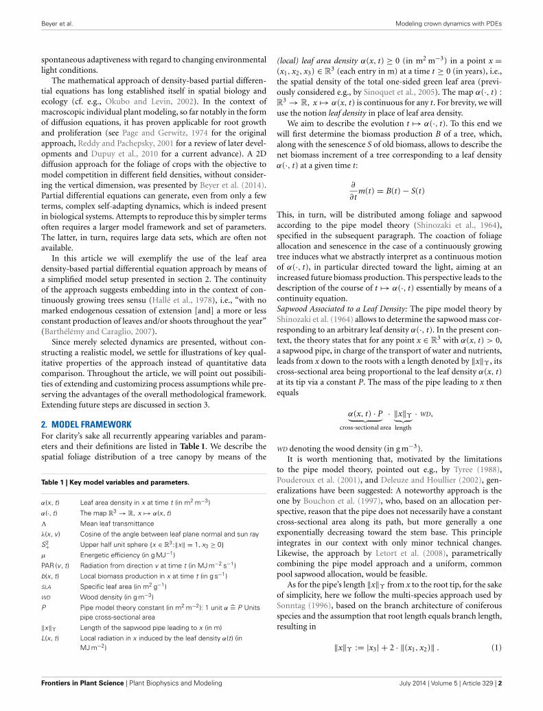
2. MODEL FRAMEWORKFor clarity’s sake all recurrently appearing variables and param-eters and their definitions are listed in Table 1. We describe thespatial foliage distribution of a tree canopy by means of the

Table 1 | Key model variables and parameters.

α(x, t) Leaf area density in x at time t (in m2 m−3)

α(·, t) The map R3 → R, x �→ α(x, t)

� Mean leaf transmittance

λ(x, v ) Cosine of the angle between leaf plane normal and sun ray

S2+ Upper half unit sphere {x ∈ R3:‖x‖ = 1, x3 ≥ 0}

μ Energetic efficiency (in g MJ−1)

PAR (v, t) Radiation from direction v at time t (in MJ m−2 s−1)

b(x, t) Local biomass production in x at time t (in g s−1)

SLA Specific leaf area (in m2 g−1)

WD Wood density (in g m−3)

P Pipe model theory constant (in m2 m−2): 1 unit α =̂ P Unitspipe cross-sectional area

‖x‖ϒ Length of the sapwood pipe leading to x (in m)

L(x, t) Local radiation in x induced by the leaf density α(t) (inMJ m−2)

(local) leaf area density α(x, t) ≥ 0 (in m2 m−3) in a point x =(x1, x2, x3) ∈ R

3 (each entry in m) at a time t ≥ 0 (in years), i.e.,the spatial density of the total one-sided green leaf area (previ-ously considered e.g., by Sinoquet et al., 2005). The map α(·, t) :R

3 → R, x �→ α(x, t) is continuous for any t. For brevity, we willuse the notion leaf density in place of leaf area density.

We aim to describe the evolution t �→ α(·, t). To this end wewill first determine the biomass production B of a tree, which,along with the senescence S of old biomass, allows to describe thenet biomass increment of a tree corresponding to a leaf densityα(·, t) at a given time t:

∂

∂tm(t) = B(t) − S(t)

This, in turn, will be distributed among foliage and sapwoodaccording to the pipe model theory (Shinozaki et al., 1964),specified in the subsequent paragraph. The coaction of foliageallocation and senescence in the case of a continuously growingtree induces what we abstractly interpret as a continuous motionof α(·, t), in particular directed toward the light, aiming at anincreased future biomass production. This perspective leads to thedescription of the course of t �→ α(·, t) essentially by means of acontinuity equation.Sapwood Associated to a Leaf Density: The pipe model theory byShinozaki et al. (1964) allows to determine the sapwood mass cor-responding to an arbitrary leaf density α(·, t). In the present con-text, the theory states that for any point x ∈ R

3 with α(x, t) > 0,a sapwood pipe, in charge of the transport of water and nutrients,leads from x down to the roots with a length denoted by ‖x‖ϒ , itscross-sectional area being proportional to the leaf density α(x, t)at its tip via a constant P. The mass of the pipe leading to x thenequals

α(x, t) · P︸ ︷︷ ︸cross-sectional area

· ‖x‖ϒ︸ ︷︷ ︸length

· WD,

WD denoting the wood density (in g m−3).It is worth mentioning that, motivated by the limitations

to the pipe model theory, pointed out e.g., by Tyree (1988),Pouderoux et al. (2001), and Deleuze and Houllier (2002), gen-eralizations have been suggested: A noteworthy approach is theone by Bouchon et al. (1997), who, based on an allocation per-spective, reason that the pipe does not necessarily have a constantcross-sectional area along its path, but more generally a oneexponentially decreasing toward the stem base. This principleintegrates in our context with only minor technical changes.Likewise, the approach by Letort et al. (2008), parametricallycombining the pipe model approach and a uniform, commonpool sapwood allocation, would be feasible.

As for the pipe’s length ‖x‖ϒ from x to the root tip, for the sakeof simplicity, here we follow the multi-species approach used bySonntag (1996), based on the branch architecture of coniferousspecies and the assumption that root length equals branch length,resulting in

‖x‖ϒ := |x3| + 2 · ‖(x1, x2)‖ . (1)

Frontiers in Plant Science | Plant Biophysics and Modeling July 2014 | Volume 5 | Article 329 | 2

Beyer et al. Modeling crown dynamics with PDEs

A more accurate choice for a particular species can be made bytaking specific characteristics of its branching geometry (such asbranching angles) and topology into account.

Finally, the sum of foliage and sapwood mass is given by

∫R3

α(x, t)

SLAdx︸ ︷︷ ︸

foliage mass

+∫

R3α(x, t) · P · ‖x‖ϒ · WD dx︸ ︷︷ ︸

sapwood mass

(2)

where SLA denotes the specific leaf area (in m2 g−1).

2.1. BIOMASS PRODUCTIONWe determine the amount of biomass produced throughphotosynthetic activity by a given leaf density. To this, wetake direct and diffuse radiation into account, cf. Fu andRich (1999), using the horizontal celestial coordinate system,with R

2 × {0} being the local horizon of a tree rooting in(0, 0, 0), and the vector (1, 0, 0) pointing north. The unitdirectional vector σ (t) ∈ S2+ := {x ∈ R

3 : ‖x‖ = 1, x3 ≥ 0},under which the sun is seen from the tree at daytime t readsσ (t) = (cos ( − Az (t)) · cos ( Alt (t)), sin ( − Az (t)(t)) · cos ( Alt(t)), sin ( Alt (t))), where Alt (t) and Az (t) denote the timedependent altitude and azimuth, respectively.

For diffusive radiation, a uniform diffuse model (uniformovercast sky) is applied, in which incoming diffuse radiation isassumed to be the same from all sky directions. Let PARdir (t)and PARdiff (t) (in MJ m-2) denote the photosynthetically activedirect and diffuse radiation at time t, respectively. Then the totalradiation from direction v ∈ S2+ at time t is

PAR (v, t) := PARdiff (t) + PARdir (t) · 1{v=σ (t)}(t),

with the indicator function 1A(x) := 1 if x ∈ A and 0 else.

2.1.1. Isolated TreeIncoming radiation is partly intercepted by the tree’s foliage andpartly passes through it. The fraction between 0 and 100% of radi-ation from direction v ∈ S2+ which actually reaches the point x ∈R

3 can be determined using Beer-Lambert’s law, where foliagecharacterized by leaf density acts as a light absorbing mediumwith locally varying α-concentration. This fraction reads

exp

(− � ·

∫x+R+·v

λ(ξ, v) · α(ξ, t) dξ

)(3)

where the extinction coefficient � ≤ 1 represents the mean lighttransmittance of foliage (Monteith, 1969; Nouvellon et al., 2000)and

λ(x, v) := N(x) · v

takes into account the angle between the sun ray and foliage in x,N(x) ∈ S2+ denoting the unit normal to the plane in which foliagein x lies. N(x) can be chosen according to leaf angle distributionmodels without further ado (Wang et al., 2007) provide a review.

Assuming that local biomass production is proportional to thetotal locally intercepted ratiation via an energy efficiency μ (in

g MJ−1) (Monteith, 1977), the instantaneous local biomass pro-duction b(x, t) (in g m−3 s−1) in x ∈ R

3 at time t for the leafdensity α(·, t) reads

b(x, t) = μ ·∫S2+

λ(x, v) · α(x, t) · exp

(− � ·

∫x+R+ ·v

λ(ξ, v) · α(ξ, t) dξ

)· PAR (v, t)︸ ︷︷ ︸

radiation reaching x from direction v︸ ︷︷ ︸radiation from direction v intercepted in x

dv. (4)

2.1.2. Population of TreesAt a time t, let α1(·, t), . . . , αn(·, t) denote the leaf densities ofn trees, shading each other and competing for light. Then theinstantaneous local biomass production of tree i ∈ {1, . . . , n} inx generalizes to

bi(x, t) = μ ·∫

S2+

(λi(x, v) · αi(x, t)

)2

n∑j = 1

λj(x, v) · αj(x, t)

·

exp

⎛⎜⎝−� ·

∫x+R+·v

n∑j = 1

λj(ξ, v) · αj(ξ, t) dξ

⎞⎟⎠·PAR(v, t)dv

The fraction λi(x,v)·αi(x,t)∑nj = 1 λj(x,v)·αj(x,t)

is the part of the incoming radia-

tion in x that is attributed to tree i’s foliage in x. In particular itreduces to 1 if two trees’ crowns do not occupy common space.

2.2. DYNAMICS2.2.1. Mass balanceWe determine the instantaneous change in living mass (conduc-tive sapwood and foliage mass) due to the production of new,and the senescence of old biomass. For convenience we assumethat the senescence of leaves as well as the loss of conductivity ofsapwood depend on time only. If sapwood and foliage that haveexisted for τW and τF years become nonconductive and senescent,respectively, then the living mass at time t reduces by

S(t) : =∫

R3

∂∂t α(x, t − τF)

SLAdx +

∫R3

∂

∂tα(x, t − τW ) ·

P · ‖x‖ϒ · WD dx.

At the same time it increases by the total instantaneous biomassproduction at t, i.e., B(t) := ∫

R3 b(x, t) dx. Thus we have

∂

∂tm(t) = B(t) − S(t) (5)

for the change in living mass at time t. A priori, the possibility∂∂t m(t) < 0 is not excluded for arbitrary parameters. However,since m(t) > S(t), it follows that m(t) > 0 and thus B(t) > 0 forall t ≥ 0.

www.frontiersin.org July 2014 | Volume 5 | Article 329 | 3

Beyer et al. Modeling crown dynamics with PDEs

2.2.2. Leaf density dynamicsWith this information on the global mass of the tree at hand, weconsider the variable

α̂(x, t) = α(x, t)∫R3 α(x, t)dx

,

i.e., the leaf density modulo mass, or (mass-)relative leaf density,with the property that

∫R3 α̂(x, t) dx = 1 for all t, which is under-

stood as an indicator of the spatial structure of the real leaf densityα(·, t). Instead of describing the course of α(·, t) directly, we do sofor α̂(·, t) and deduce α(·, t) as α(·, t) = λ(t) · α̂(·, t), where λ(t)is chosen such that the living mass corresponding to λ(t) · α̂(·, t)(cf. (2)) equals indeed m(t) yielded by (5). Thus

λ(t) = m(t)∫R3

α̂(x,t)SLA

dx + ∫R3 α̂(x, t) · P · ‖x‖ϒ · WD dx

. (6)

The continuity of the growth process of the trees we considersuggests a description of the course of α̂(·, t) in terms of a(mass-conserving) continuity equation,

∂

∂tα̂(x, t) = ∇x · φ(x, t), (7)

in which the relative leaf density is subject to a transport motioninduced by a continuous flux φ : R

3 × R+ → R3, itself deter-

mined by α(·, t). The idea of this transporting flux φ is that itincorporates both the effect of the allocation of new leaves and ofthe abscission of old ones on the spatial structure of foliage, whichin combination, induces what we describe as an abstract motionof leaf density.

A predominant driver in the spatial dispersal of leaf densityis the local expansion toward the light, aiming at an increase infuture light interception. We formally embed this factor in theabove framework, where it will take on the role of the flux φ. Forsome given leaf density α(·, t) let L : R

3 × R+ → R be definedby

L(x, t) =∫

S2+λ(x, v) · exp

(− � ·

∫x+R+·v

λ(ξ, v) · α(ξ, t) dξ

)·

PAR (v, t) dv (8)

The function L measures the intercepted light in x per m2 leafarea. The gradient ∇xL points locally in the direction of the great-est rate of increase of intercepted light. In addition, similar toBeyer et al. (2014) we define the flux to correspond to the existingleaf density in x, so that finally we have

φ(x, t) = k · α(x, t) · ∇xL(x, t) (9)

for a mobility constant k. This local gradient approach is moti-vated by “the observation that a tree is capable of acquiringalso gradient information about its environment and that growthmight be directed along these gradients (Schmidt and Wulff,1993; Aphalo and Ballare, 1995)” (Sonntag, 1996).

The term ∇x · φ describing a movement of leaf density towardthe light contains spatial derivates of a function of integrals overα, which makes (7) a partial integro-differential equation.

2.3. SIMULATIONSIn this section we illustrate some structural properties of themodel. For convenience we simplified radiation to be verticalonly. Some details of the numerical implementation of the modelare presented in the appendix.

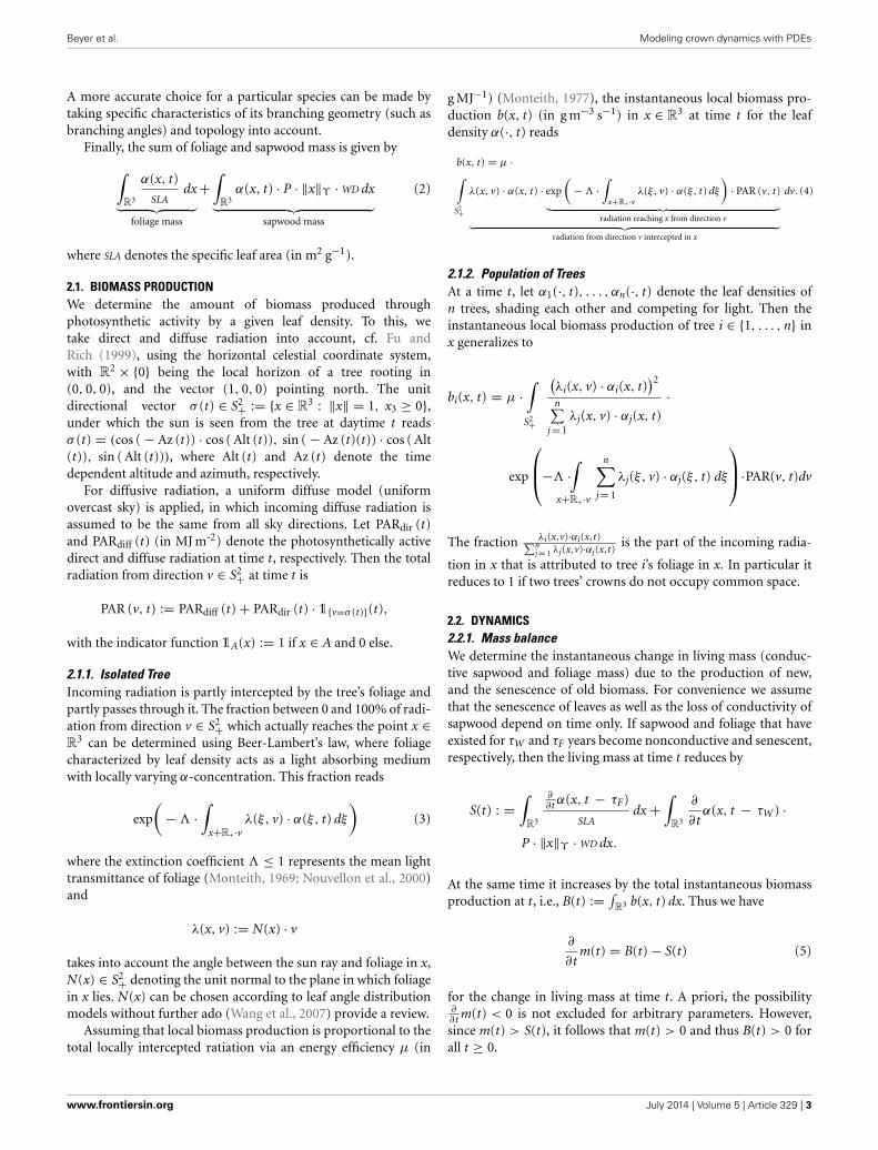
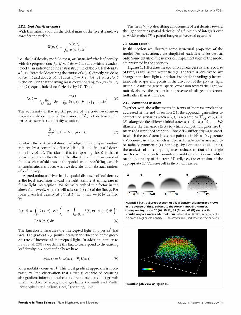
Figures 1, 2 illustrate the evolution of leaf density in the courseof time, as well as the vector field φ. The term is sensitive to anychange in the local light conditions induced by shading; φ instan-taneously adapts and points in the direction of the greatest lightincrease. Aside the general spatial expansion toward the light, wenotably observe the predominant presence of foliage at the crownhull rather than its interior.

2.3.1. Population of TreesTogether with the adjustments in terms of biomass productionaddressed at the end of section 2.1, the approach generalizes tocompetition scenarios when α(·, t) is replaced by

∑i≥1 αi(·, t) in

(8), alongside the different initial states α1(·, 0), α2(·, 0), . . .. Weillustrate the dynamic effects to which competition gives rise bymeans of a simplified scenario: Consider a sufficiently large stand,in which the trees’ stem bases, as a point set in R

2 × {0}, generatea Voronoi-tesselation which is regular. If radiation is assumed tobe radially symmetric (as done e.g., by Perttunen et al., 1998),the analysis of all competing trees reduces to that of a singleone for which periodic boundary conditions for (7) are addedon the boundary of the tree’s 3D cell, i.e., the extension of theappropriate 2D Voronoi cell in the x3-dimension.

FIGURE 1 | (x1, x3)-cross section of a leaf density-characterized crown

in the course of time, subject to the present model dynamics,

corresponding to t = 10 (A), 20 (B), 30 (C) and 40 (D) years with

simulation parameters adopted from Letort et al. (2008). A darker colorindicates a higher leaf density α. The arrows in (D) indicate the vector field φ.

FIGURE 2 | 3D view of Figure 1D.

Frontiers in Plant Science | Plant Biophysics and Modeling July 2014 | Volume 5 | Article 329 | 4

Beyer et al. Modeling crown dynamics with PDEs

Periodic boundary conditions induce that the light conditionson the other side of the boundary are considered identical to thosewithin, accounting for another tree growing in equal measure andshading its environment.

This implies that, when, for simplicity, further assumingthe essential light incidence to be vertical, periodic boundaryconditions reduce to no flux conditions on the boundary: There,due to the identical light conditions on the other side of theboundary, the light gradient ∇xL, governing the flux φ, changesfrom pointing further outwards to a zero flux.

Figure 3 shows the different stages of this scenario for anunderlying square tesselation.

The overly sharp boundary between two crowns is a conse-quence of the unrestrained mobility of foliage in this simplifiedapproach, and would fade when additional features correspond-ing to a branch structure are included, cf. section 3.

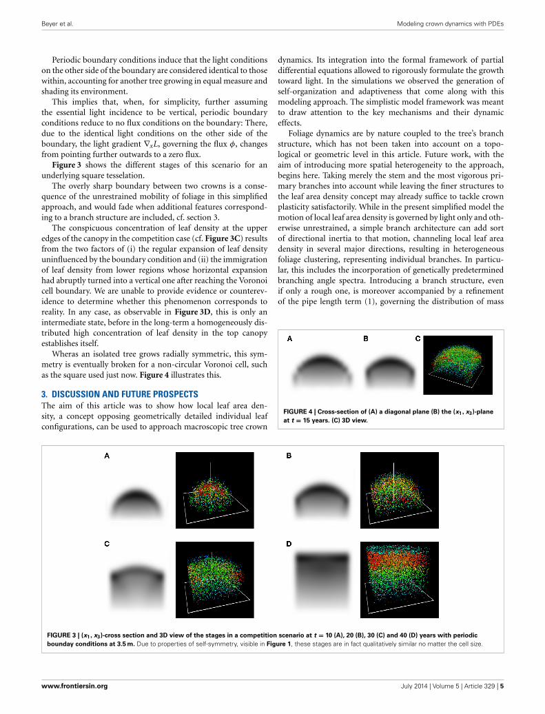
The conspicuous concentration of leaf density at the upperedges of the canopy in the competition case (cf. Figure 3C) resultsfrom the two factors of (i) the regular expansion of leaf densityuninfluenced by the boundary condition and (ii) the immigrationof leaf density from lower regions whose horizontal expansionhad abruptly turned into a vertical one after reaching the Voronoicell boundary. We are unable to provide evidence or counterev-idence to determine whether this phenomenon corresponds toreality. In any case, as observable in Figure 3D, this is only anintermediate state, before in the long-term a homogeneously dis-tributed high concentration of leaf density in the top canopyestablishes itself.

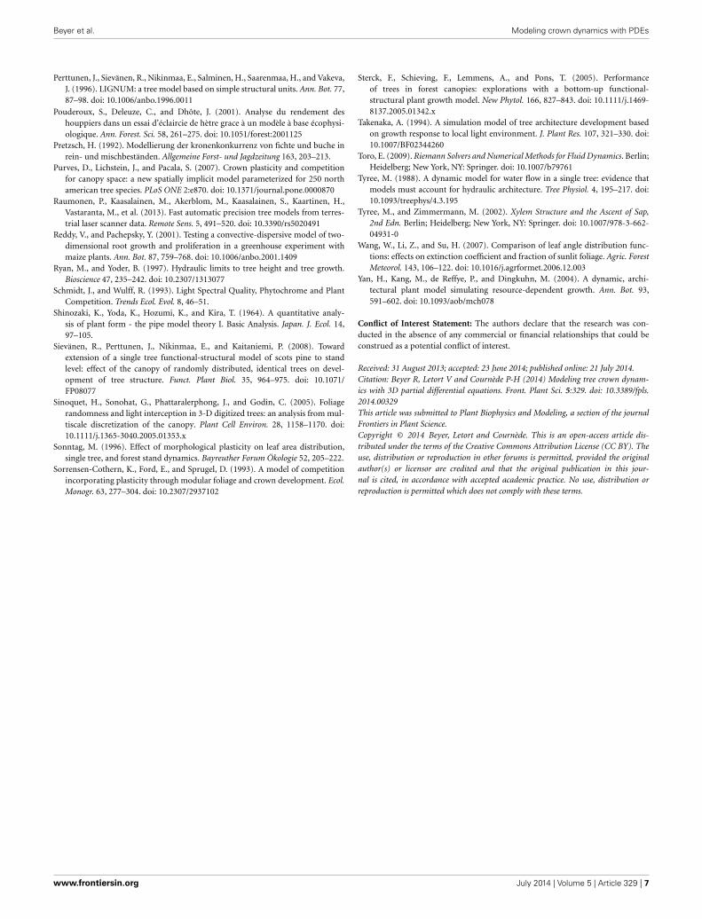
Wheras an isolated tree grows radially symmetric, this sym-metry is eventually broken for a non-circular Voronoi cell, suchas the square used just now. Figure 4 illustrates this.

3. DISCUSSION AND FUTURE PROSPECTSThe aim of this article was to show how local leaf area den-sity, a concept opposing geometrically detailed individual leafconfigurations, can be used to approach macroscopic tree crown

dynamics. Its integration into the formal framework of partialdifferential equations allowed to rigorously formulate the growthtoward light. In the simulations we observed the generation ofself-organization and adaptiveness that come along with thismodeling approach. The simplistic model framework was meantto draw attention to the key mechanisms and their dynamiceffects.

Foliage dynamics are by nature coupled to the tree’s branchstructure, which has not been taken into account on a topo-logical or geometric level in this article. Future work, with theaim of introducing more spatial heterogeneity to the approach,begins here. Taking merely the stem and the most vigorous pri-mary branches into account while leaving the finer structures tothe leaf area density concept may already suffice to tackle crownplasticity satisfactorily. While in the present simplified model themotion of local leaf area density is governed by light only and oth-erwise unrestrained, a simple branch architecture can add sortof directional inertia to that motion, channeling local leaf areadensity in several major directions, resulting in heterogeneousfoliage clustering, representing individual branches. In particu-lar, this includes the incorporation of genetically predeterminedbranching angle spectra. Introducing a branch structure, evenif only a rough one, is moreover accompanied by a refinementof the pipe length term (1), governing the distribution of mass

FIGURE 4 | Cross-section of (A) a diagonal plane (B) the (x1, x3)-plane

at t = 15 years. (C) 3D view.

FIGURE 3 | (x1, x3)-cross section and 3D view of the stages in a competition scenario at t = 10 (A), 20 (B), 30 (C) and 40 (D) years with periodic

bounday conditions at 3.5 m. Due to properties of self-symmetry, visible in Figure 1, these stages are in fact qualitatively similar no matter the cell size.

www.frontiersin.org July 2014 | Volume 5 | Article 329 | 5

Beyer et al. Modeling crown dynamics with PDEs

between foliage and wood according to the pipe model theory,thus determining secondary growth.

Taking into account the organization of growth units, i.e., asweakening our assumptions on neoformation and polycyclism insection 2.1.1, or considering immediate vs. delayed bud outbreak,would bring the model closer to actual tree architecture dynamics.

Alongside the phototropism considered in this article, morebiomechanical constraints that have feedback influences on thegrowth, such as hydraulic aspects sensu (Ryan and Yoder, 1997;Tyree and Zimmermann, 2002), in particular in the context ofgrowth limitation, the avoidance of interlocked growth due tomechanical stress of touching branches (Oliver and Larson, 1990)or gravitropism represent perspectives for model extensions.

The application and validation of a refined model based on thetheoretical framework presented in this paper will benefit fromempirical data on local leaf area density. Conceivable ways toobtain this include the following three, which are currently beingpractically explored: Firstly, from the direct recordings of locallight intensities at various positions {x(1), . . . , x(n)} ⊂ R

3 withina canopy, the map

{x(1), . . . , x(n)} → R≥0

x �→ α(x)

for a discrete, but arbitrary fine domain can be obtained byapplying Beer-Lambert’s law in the reverse way. Secondly, high-definition multi-directional 3D terrestrial laser scan data andappropriate skeletonization algorithms allow to relate to a leaflesstree a set of cylinders representing branch segments (Raumonenet al., 2013). Automatically removing all scan points correspond-ing to cylinder diameters (i.e., branch thicknesses) above a certainthreshold allows to spatially isolate recent shoots, for which then arelation to foliage can be assumed. Thirdly, scanning a tree at thebeginning of spring during the process of bud opening, when—in contrast to the case of a fully developed canopy—laser rays stillreasonably penetrate the crown, and deducting from this imagethe point cloud yielded by a scan of the completely leafless tree,may allow to obtain a local bud density, from which the the leafdensity can be deduced. Thus, assessing the spatial foliage distri-bution in terms of local leaf area density in a functional-structuralcrown dynamics model can make good use of this data type formodel calibration and validation.

The property of locally and spontaneously adapting to chang-ing light conditions suggests that the present partial differ-ential equation approach can be applied to competition sce-narios both in pure as in mixed tree groups. Empirical find-ings, based on laser scans, about the plasticity Bayer et al.(2013) may thus be approached from a functional-structuralmodeling point of view. These perspectives are currently beingexplored.

ACKNOWLEDGMENTSThe authors would like to thank Pascal Laurent-Gengoux andtwo anonymous reviewers for their helpful remarks. This workwas supported by a doctoral scholarship of the the Heinrich BöllFoundation.

REFERENCESAllen, M., Prusinkiewicz, P., and Dejong, T. (2005). Using L-Systems for Modeling

the Architecture and Physiology of Growing Trees: The L-PEACH Model. NewPhytol. 166, 869–880. doi: 10.1111/j.1469-8137.2005.01348.x

Aphalo, P., and Ballare, C. (1995). On the importance of information-acquiringsystems in plant-plant interactions. Funct. Ecol. 9, 5–14. doi: 10.2307/2390084

Barthélémy, D., and Caraglio, Y. (2007). Plant architecture: a dynamic, multileveland comprehensive approach to plant form, structure and ontogeny. Ann. Bot.99, 375–407. doi: 10.1093/aob/mcl260

Bayer, D., Seifert, S., and Pretzsch, H. (2013). Structural crown properties ofNorway spruce (Picea abies [L.] Karst.) and European beech (Fagus sylvatica[L.]) in mixed versus pure stands revealed by terrestrial laser scanning. Trees 27,1035–1047. doi: 10.1007/s00468-013-0854-4

Beyer, R., Etard, O., Cournède, P.-H., and Laurent-Gengoux, P. (2014). Modelingspatial competition for light in plant populations with the porous mediumequation. J. Math. Biol. doi: 10.1007/s00285-014-0763-1. [Epub ahead of print].

Bouchon, J., de Reffye, P., and Barthélémy, P. (1997). Modélisation et Simulation deL’architecture des Végétaux. Montpellier: INRA.

Chelle, M., and Andrieu, B. (2007). Modelling the light environment of virtual cropcanopies. Funct. Struct. Plant Model. Crop Product. 22, 75–89. doi: 10.1007/1-4020-6034-3_7

Cournède, P.-H., Kang, M., Mathieu, A., Barczi, J.-F., Yan, H., Hu, B., et al. (2006).Structural factorization of plants to compute their functional and architecturalgrowth. Simulation 82, 427–438. doi: 10.1177/0037549706069341

Cournède, P.-H., Mathieu, A., Houllier, F., Barthélémy, D., and de Reffye, P.(2008). Computing competition for light in the GREENLAB model of plantgrowth: a contribution to the study of the effects of density on resourceacquisition and architectural development. Ann. Bot. 101, 1207–1219. doi:10.1093/aob/mcm272

Deleuze, C., and Houllier, F. (2002). A flexible radial increment taper equationderived from a process-based carbon partitioning model. Ann. Forest Sci. 59,141–154. doi: 10.1051/forest:2002001

Dupuy, L., Gregory, P., and Bengough, A. (2010). Root growth models: towardsa new generation of continuous approaches. J. Exp. Bot. 61, 2131–2143. doi:10.1093/jxb/erp389

Fu, P., and Rich, P. (1999). “Design and implementation of the Solar Analyst:an ArcView extension for modeling solar radiation at landscape scales,” inProceedings of the 19th Annual ESRI User Conference, (San Diego).

Grote, R., and Pretzsch, H. (2002). A model for individual tree development basedon physiological processes. Plant Biol. 4, 167–180. doi: 10.1055/s-2002-25743

Hallé, F., Oldeman, R., and Tomlinson, P. (1978). Tropical Trees and Forests. Berlin:Springer-Verlag. doi: 10.1007/978-3-642-81190-6

Kurth, W., and Sloboda, B. (1999). Tree and stand architecture and growthdescribed by formal grammars. II. Sensitive trees and competition. J. Forest Sci.45, 53–63.

Letort, V., Cournède, P.-H., Mathieu, A., de Reffye, P., and Constant, T. (2008).Parametric identification of a functional-structural tree growth model andapplication to beech trees (Fagus sylvatica). Funct. Plant Biol. 35, 951–963. doi:10.1071/FP08065

Monteith, J. (1969). “Light interception and radiative exchange in crop stands,”in Physiological Aspects of Crop Yield, eds J. Eastin, F. Haskins, C. Sullivan, andC. van Bavel( Madison, WI: American Society of Agronomy and Crop ScienceSociety of America), 89–111.

Monteith, J. (1977). Climate and the efficiency of crop production in britain. Proc.R. Soc. Lond B 281, 277–294. doi: 10.1098/rstb.1977.0140

Nouvellon, Y., Begue, A., Moran, M., Seen, D., Rambal, S., Luquet, D., et al.(2000). PAR extinction in shortgrass ecosystems: effects of clumping, sky con-ditions and soil albedo. Agric. Forest Meteorol. 105, 21–41. doi: 10.1016/S0168-1923(00)00194-5

Okubo, A., and Levin, S. (2002). Diffusion and Ecological Problems, ModernPerspectives, 2nd Edn. Berlin; Heidelberg; New York, NY: Springer.

Oliver, C., and Larson, B. (1990). Forest stand dynamies. New York, NY: F. McGraw-Hill.

Page, E., and Gerwitz, A. (1974). Mathematical models, based on diffusion equa-tions, to describe root systems of isolated plants, row crops, and swards. PlantSoil 41, 243–254. doi: 10.1007/BF00017252

Perttunen, J., Sievänen, R., and Nikinmaa, E. (1998). LIGNUM: a model combin-ing the structure and the functioning of trees. Ecol. Modell. 108, 189–198. doi:10.1016/S0304-3800(98)00028-3

Frontiers in Plant Science | Plant Biophysics and Modeling July 2014 | Volume 5 | Article 329 | 6

Beyer et al. Modeling crown dynamics with PDEs

Perttunen, J., Sievänen, R., Nikinmaa, E., Salminen, H., Saarenmaa, H., and Vakeva,J. (1996). LIGNUM: a tree model based on simple structural units. Ann. Bot. 77,87–98. doi: 10.1006/anbo.1996.0011

Pouderoux, S., Deleuze, C., and Dhôte, J. (2001). Analyse du rendement deshouppiers dans un essai d’éclaircie de hètre grace à un modèle à base écophysi-ologique. Ann. Forest. Sci. 58, 261–275. doi: 10.1051/forest:2001125

Pretzsch, H. (1992). Modellierung der kronenkonkurrenz von fichte und buche inrein- und mischbeständen. Allgemeine Forst- und Jagdzeitung 163, 203–213.

Purves, D., Lichstein, J., and Pacala, S. (2007). Crown plasticity and competitionfor canopy space: a new spatially implicit model parameterized for 250 northamerican tree species. PLoS ONE 2:e870. doi: 10.1371/journal.pone.0000870

Raumonen, P., Kaasalainen, M., Akerblom, M., Kaasalainen, S., Kaartinen, H.,Vastaranta, M., et al. (2013). Fast automatic precision tree models from terres-trial laser scanner data. Remote Sens. 5, 491–520. doi: 10.3390/rs5020491

Reddy, V., and Pachepsky, Y. (2001). Testing a convective-dispersive model of two-dimensional root growth and proliferation in a greenhouse experiment withmaize plants. Ann. Bot. 87, 759–768. doi: 10.1006/anbo.2001.1409

Ryan, M., and Yoder, B. (1997). Hydraulic limits to tree height and tree growth.Bioscience 47, 235–242. doi: 10.2307/1313077

Schmidt, J., and Wulff, R. (1993). Light Spectral Quality, Phytochrome and PlantCompetition. Trends Ecol. Evol. 8, 46–51.

Shinozaki, K., Yoda, K., Hozumi, K., and Kira, T. (1964). A quantitative analy-sis of plant form - the pipe model theory I. Basic Analysis. Japan. J. Ecol. 14,97–105.

Sievänen, R., Perttunen, J., Nikinmaa, E., and Kaitaniemi, P. (2008). Towardextension of a single tree functional-structural model of scots pine to standlevel: effect of the canopy of randomly distributed, identical trees on devel-opment of tree structure. Funct. Plant Biol. 35, 964–975. doi: 10.1071/FP08077

Sinoquet, H., Sonohat, G., Phattaralerphong, J., and Godin, C. (2005). Foliagerandomness and light interception in 3-D digitized trees: an analysis from mul-tiscale discretization of the canopy. Plant Cell Environ. 28, 1158–1170. doi:10.1111/j.1365-3040.2005.01353.x

Sonntag, M. (1996). Effect of morphological plasticity on leaf area distribution,single tree, and forest stand dynamics. Bayreuther Forum Ökologie 52, 205–222.

Sorrensen-Cothern, K., Ford, E., and Sprugel, D. (1993). A model of competitionincorporating plasticity through modular foliage and crown development. Ecol.Monogr. 63, 277–304. doi: 10.2307/2937102

Sterck, F., Schieving, F., Lemmens, A., and Pons, T. (2005). Performanceof trees in forest canopies: explorations with a bottom-up functional-structural plant growth model. New Phytol. 166, 827–843. doi: 10.1111/j.1469-8137.2005.01342.x

Takenaka, A. (1994). A simulation model of tree architecture development basedon growth response to local light environment. J. Plant Res. 107, 321–330. doi:10.1007/BF02344260

Toro, E. (2009). Riemann Solvers and Numerical Methods for Fluid Dynamics. Berlin;Heidelberg; New York, NY: Springer. doi: 10.1007/b79761

Tyree, M. (1988). A dynamic model for water flow in a single tree: evidence thatmodels must account for hydraulic architecture. Tree Physiol. 4, 195–217. doi:10.1093/treephys/4.3.195

Tyree, M., and Zimmermann, M. (2002). Xylem Structure and the Ascent of Sap,2nd Edn. Berlin; Heidelberg; New York, NY: Springer. doi: 10.1007/978-3-662-04931-0

Wang, W., Li, Z., and Su, H. (2007). Comparison of leaf angle distribution func-tions: effects on extinction coefficient and fraction of sunlit foliage. Agric. ForestMeteorol. 143, 106–122. doi: 10.1016/j.agrformet.2006.12.003

Yan, H., Kang, M., de Reffye, P., and Dingkuhn, M. (2004). A dynamic, archi-tectural plant model simulating resource-dependent growth. Ann. Bot. 93,591–602. doi: 10.1093/aob/mch078

Conflict of Interest Statement: The authors declare that the research was con-ducted in the absence of any commercial or financial relationships that could beconstrued as a potential conflict of interest.

Received: 31 August 2013; accepted: 23 June 2014; published online: 21 July 2014.Citation: Beyer R, Letort V and Cournède P-H (2014) Modeling tree crown dynam-ics with 3D partial differential equations. Front. Plant Sci. 5:329. doi: 10.3389/fpls.2014.00329This article was submitted to Plant Biophysics and Modeling, a section of the journalFrontiers in Plant Science.Copyright © 2014 Beyer, Letort and Cournède. This is an open-access article dis-tributed under the terms of the Creative Commons Attribution License (CC BY). Theuse, distribution or reproduction in other forums is permitted, provided the originalauthor(s) or licensor are credited and that the original publication in this jour-nal is cited, in accordance with accepted academic practice. No use, distribution orreproduction is permitted which does not comply with these terms.

www.frontiersin.org July 2014 | Volume 5 | Article 329 | 7

Beyer et al. Modeling crown dynamics with PDEs

4. APPENDIXNUMERICAL IMPLEMENTATIONA finite volume scheme Toro (2009) is used, in which we con-sider αijk := 1

�2

∫�ijk

α(x, t)dx (with a similar notation for the

other variables) on a regular mesh with cells �ijk = [i�x, (i +1)�x[×[j�x, (j + 1)�x[×[k�x, (k + 1)�x] for i, j, k ∈ Z and�x 1.

The local light incidence (8) (and similarly the local biomassproduction (4)) for vertical radiation, v = e3, is computed as

Lijk(t) = λijk(e3) · exp

(− � · �x ·

∑κ≥k

λijk(e3) · αijk(t) ·

PAR (e3, t) dv

)

The general case for v ∈ S2+ is conceptually similar, yet technicallymore extensive: For a given v, the above sum reaches over all cells�i′j′k′ whose intersection with the line through the center of thecell �i′j′k′ and pointing in the direction v is non-empty, taking

into accout the individual length �i′j′k′(v) ≤ �x of this intersec-

tion by means of the additional coefficient�i′ j′k′ (v)

�x in the sumterm.

As for the PDE, let

φ1, ijk(t) = k · αi+1jk(t) + αijk(t)

2· Li+1jk(t) − Lijk(t)

�x

and φ2,ijk, φ3,ijk be defined accordingly for the other spatialentries. The standard discretization of the divergence is given by

divijk(t) = φ1,ijk(t) − φ1,i−1jk(t)

�x+ φ2,ijk(t)) − φ2,ij−1k(t)

�x

+φ3,ijk(t)) − φ3,ijk−1(t))

�x

and finally, using the Euler method for �t 1, we obtain

αijk(t + �t) = αijk(t) + �t · divijk(t).

Frontiers in Plant Science | Plant Biophysics and Modeling July 2014 | Volume 5 | Article 329 | 8