University of South FloridaScholar Commons

Graduate Theses and Dissertations Graduate School

3-28-2005

USFKAD: An Expert System For PartialDifferential EquationsSami M. KadamaniUniversity of South Florida

Follow this and additional works at: https://scholarcommons.usf.edu/etd

Part of the American Studies Commons

This Dissertation is brought to you for free and open access by the Graduate School at Scholar Commons. It has been accepted for inclusion inGraduate Theses and Dissertations by an authorized administrator of Scholar Commons. For more information, please contactscholarcommons@usf.edu.

Scholar Commons CitationKadamani, Sami M., "USFKAD: An Expert System For Partial Differential Equations" (2005). Graduate Theses and Dissertations.https://scholarcommons.usf.edu/etd/712

USFKAD: An Expert System For Partial Differential Equations

by

Sami M. Kadamani

A dissertation submitted in partial fulfillment of the requirements for the degree of

Doctor of Philosophy Department of Electrical Engineering

College of Engineering University of South Florida

Major Professor: Arthur David Snider, Ph.D. Kenneth A. Buckle, Ph.D. Stanley C. Kranc, Ph.D.

Wilfrido A. Moreno, Ph.D. Mohamed Elhamdadi, Ph.D.

Date of Approval: March 28, 2005

Keywords: eigen function, analytic solutions, pde, separation of variables, and symbolic computing

© Copyright 2005, Sami M. Kadamani

DEDICATION

This dissertation is dedicated to my wife Daid, and my two children Serene and Tareq.

Thank you for your patience, I would not have been able to accomplish this goal without

your support.

ACKNOWLEDGEMENTS

My deepest thanks to my advisor Dr. David Arthur Snider, for his belief in me and for

both his guidance and support. I would like to extend my gratitude to Chairperson Sam

Sakmar, Ph.D. and the members of the examining committee: Kenneth A. Buckle, Ph.D.,

Stanley C. Kranc, Ph.D., Wilfrido A. Moreno, Ph.D., and Mohamed Elhamdadi, Ph.D. In

addition I would like to extend my thanks to my friends Husam Elrabi and Krista

Morehead, whose input was invaluable.

i

TABLE OF CONTENTS LIST OF TABLES iii LIST OF FIGURES iv ABSTRACT v CHAPTER 1: INTRODUCTION 1 Need 1 Feasibility 3 CHAPTER 2: EXISTING SOFTWARE 5 CHAPTER 3: THE SEPARATION OF VARIABLES PROCEDURE AND ITS

DECISION TREE STRUCTURE 8 CHAPTER 4: DISCUSSION AND FLOW CHART FOR USFKAD 14 Decision Tree 15 Fundamental Concept 19 Example 1 22 On-Screen Inquires 26 CHAPTER 5: APPLICATION EXAMPLES 28 Example 1 28 Example 2 30 Example 3 31 Example 4 33 Example 5 34 Example 6 35 CHAPTER 6: RECOMMENDATIONS FOR FUTURE DEVELOPMENTS 37 REFERENCES 38 APPENDICES 39 APPENDIX A: COMPARISON OF SOLVING PARTIAL

DIFFERENTIAL EQUATIONS USING THE TRADITIONAL METHOD AND USFKAD 40

ii

Solution 1 43 Solution 2 47

APPENDIX B: READ ME 50 APPENDIX C: TO USE USFKAD.PDF 53 ABOUT THE AUTHOR End Page

iii

LIST OF TABLES Table 1: PDE Equation Type Matrix 21 Table 2: PDE BC Matrix 21 Table 3: Matrix Example 23

iv

LIST OF FIGURES

Figure 1: USFKAD Flow Chart 16-20

Figure 2: PDE Problem 40

Figures 3: (a-d) Decomposition of the PDE Problem 40

v

USFKAD: AN EXPERT SYSTEM FOR PARTIAL DIFFERENTIAL EQUATIONS

Sami M. Kadamani

ABSTRACT

USFKAD is an encoded expert system for the eigenfunction expansion of

solutions to the wave, diffusion, and Laplace equations: both homogeneous and

nonhomogenous; one, two, or three dimensions; Cartesian, cylindrical, or spherical

coordinates; Dirichlet, Neumann, Robin, or singular boundary conditions; in time,

frequency, or Laplace domain. The user follows a menu to enter his/her choices and the

output is a LaTeX file containing the formula for the solution together with the

transcendental equation for the eigenvalues (if necessary) and the projection formulas for

the coefficients. The file is suitable for insertion into a book or journal article, and as a

teaching aid. Virtually all cases are covered, including the Mellin, spherical harmonic,

Bessel, modified Bessel, spherical Bessel, Dini, Hankel, Weber, MacDonald, and

Kantorovich-Lebedev expansions, mixed spectrum, and rigid body modes.

1

CHAPTER 1

INTRODUCTION Need

Every practicing engineer whose specialty involves modeling of physical

phenomena, such as electromagnetic fields, temperature, sound, stress and strain, fluid

flow, diffusion, etc., has to deal with the mathematical syntax of the discipline - the

partial differential equation (PDE). For example, the electrical engineering undergraduate

classes in electromagnetic, semiconductor processing, thermal issues in electronic

packaging, etc. should be able to call on this mathematical concept, at least peripherally,

to provide the students some familiarity with the technical issues involved in the

quantitative models. However, this subject (PDEs) is vast, complicated, and compromises

have to be made in incorporating it into the undergraduate's curriculum. A 2-semester

course that deals honestly and rigorously with the subject is out of the question.

The compromises presently employed at undergraduate institutions are:

(1) A short treatment of PDEs that relies completely on numerical solvers; or

(2) A brief tutorial that covers the basics of the separation of variables technique.

Each of these is unsatisfactory. (1) is inferior to (2) because, even with the graphic

capabilities of today's hardware and software, it is extremely difficult for an

inexperienced undergraduate user to tell, from a vast assemblage of tabulations and

graphs, how the solutions will respond to changes in the boundary conditions or the

physical dimensions - issues of prime importance to engineering. For example consider

the frequency of the resonant mode of a rectangular cavity with sides X, Y and Z given

by: 2 21/ 1/ 1/c X Y Zω π= + + 2 . These are not a terribly complicated formula, but

contemplate trying to deduce it from graphs!

The eigenfunction expansions yielded by (2) do reveal these dependencies (and

are exact). The drawback of this solution procedure is the lack of time to impart expertise

in its implementation except for a few elementary cases - rectangular geometries and

ideal conductors, for instance. The electrical world of cables, motors, and antennas is

replete with cylindrical and spherical devices made of lousy materials, whose analyses

entail Bessel functions and transcendental eigenvalue equations. The present-day

curriculum has no room for the mastery of the ``special functions" that occupied the

toolbox of the 1950s engineer.

On the other hand, usually it is well within the capability of senior undergraduates

to verify most features of an eigenfunction solution expansion.

Therefore an expert system, USFKAD, for partial differential equations (a smart

software tool) that can automatically cull, from a library of eigenfunctions, the

assemblage constituting the solutions to explicit problems, together with relevant

graphics, would be a powerful enabler for undergraduate engineering training:

1. It would allow engineering analysis/design to proceed efficiently without

being sidetracked by concerns of mathematical solvability.

2. As such, it would cut across many engineering disciplines.

2

3

3. It could be used to give a perspective on the separation-of-variables technique

itself, by enabling “reverse-engineering” of the explicit solution formulas.

(This will be elaborated below.)

4. In fact it would be a research tool that the engineer could continue to use in

his professional career. Eigenfunction expansions are integral to the mode-

matching procedure that is used in contemporary computational

electromagnetism. And indeed, virtually every technical paper describing a

new numerical solver compares its results with eigenfunction expansions, as

testament to its accuracy.

Feasibility

USFKAD, the subject of this dissertation, focuses on the theme that the

mathematical structure, afforded by superposition, of the eigenfunction method for

solving the separable PDEs of engineering can be expressed by a compact, universal,

inviolate, and reasonably lucid algorithm; its formidability lies only in the details of its

implementation - that is, in the enormous variety of eigenfunctions that must be

employed for the curvilinear geometries. Thus it becomes feasible to contemplate a smart

computer program that exploits this structure to judiciously select, from a library of

eigenfunctions, the assemblage constituting the solutions to problems with explicit

initial/boundary conditions.

In the subsequent chapters, more discussion and a list of examples of PDE

solutions will be presented that progressively demonstrate the decision-tree nature of the

general separation of variables procedure. This will exemplify the thesis that by reverse-

4

engineering explicit solution formulas one can experience a tutorial intercourse with the

procedure itself.

5

CHAPTER 2

EXISITING SOFTWARE

Software for obtaining (analytic) solutions to ordinary differential equations

exists in several forms, including Mathematica [6] and MAPLE [7]. It has not received

universal adoption because extensive training in ordinary differential equations is already

part of the required curriculum for all SMET (Science, Mathematics, Engineering, and

Technology) students. For partial differential equations, MAPLE's pdsolve [Solution 1a]

is a step in the right direction, but its arcane solution format provides little assistance for

a non-expert in fitting the initial and boundary conditions that determine such

dependencies. An example of its output, the electrostatic potential inside a sphere with

charges distributed on the surface, is displayed as Solution 1a below. It is expressed

(correctly) in terms of hyper-geometric and complex signum functions. But comparing

this with the more recognizable solution display using USFKAD as shown in Solution 1b,

one can clearly see the obvious simplification and straight forwardness of USFKAD.

Solution 1a: Output from pdesolve

( )F , ,r t p _C1 r( )/1 2 + 1 4 _c1

_C3 ( )−2 ( )sin t 2( )/1 2 _c2

hypergeom⎛⎝⎜⎜ =

, ,⎡⎣⎢⎢

⎤⎦⎥⎥, + +

14

12 _c2

14 + 1 4 _c1 − + +

14 + 1 4 _c1

14

12 _c2

⎡⎣⎢⎢

⎤⎦⎥⎥

12 +

12 ( )cos 2 t

12

⎞⎠⎟⎟ _C5

( )sin _c2 p r _C1 r( )/1 2 + 1 4 _c1

_C3 ( )−2 ( )sin t 2( )/1 2 _c2

hypergeom⎛⎝⎜⎜ +

, ,⎡⎣⎢⎢

⎤⎦⎥⎥, + +

14

12 _c2

14 + 1 4 _c1 − + +

14 + 1 4 _c1

14

12 _c2

⎡⎣⎢⎢

⎤⎦⎥⎥

12 +

12 ( )cos 2 t

12

⎞⎠⎟⎟ _C6

( )cos _c2 p r 2 _C1 r( )/1 2 + 1 4 _c1

_C4 ( )−2 ( )sin t 2( )/1 2 _c2

( )csgn ( )cos t +

( )cos t hypergeom ⎡⎣⎢⎢

⎤⎦⎥⎥, + +

34

12 _c2

14 + 1 4 _c1 − + +

14 + 1 4 _c1

34

12 _c2

⎡⎣⎢⎢

⎤⎦⎥⎥

32, ,⎛

⎝⎜⎜

+ 12 ( )cos 2 t

12

⎞⎠⎟⎟ _C5 ( )sin _c2 p r 2 _C1 r

( )/1 2 + 1 4 _c1_C4 +

( )−2 ( )sin t 2( )/1 2 _c2

( )csgn ( )cos t ( )cos t hypergeom⎛⎝⎜⎜

, ,⎡⎣⎢⎢

⎤⎦⎥⎥, + +

34

12 _c2

14 + 1 4 _c1 − + +

14 + 1 4 _c1

34

12 _c2

⎡⎣⎢⎢

⎤⎦⎥⎥

32 +

12 ( )cos 2 t 1

2⎞⎠⎟⎟ _C6

( )cos _c2 p r _C2 r( )− /1 2 + 1 4 _c1

_C3 ( )−2 ( )sin t 2( )/1 2 _c2

hypergeom⎛⎝⎜⎜ +

, ,⎡⎣⎢⎢

⎤⎦⎥⎥, + +

14

12 _c2

14 + 1 4 _c1 − + +

14 + 1 4 _c1

14

12 _c2

⎡⎣⎢⎢

⎤⎦⎥⎥

12 +

12 ( )cos 2 t 1

2⎞⎠⎟⎟ _C5

( )sin _c2 p r _C2 r( )− /1 2 + 1 4 _c1

_C3 ( )−2 ( )sin t 2( )/1 2 _c2

hypergeom⎛⎝⎜⎜ +

, ,⎡⎣⎢⎢

⎤⎦⎥⎥, + +

14

12 _c2

14 + 1 4 _c1 − + +

14 + 1 4 _c1

14

12 _c2

⎡⎣⎢⎢

⎤⎦⎥⎥

12 +

12 ( )cos 2 t

12

⎞⎠⎟⎟ _C6

( )cos _c2 p r 2 _C2 r( )− /1 2 + 1 4 _c1

_C4 ( )−2 ( )sin t 2( )/1 2 _c2

( )csgn ( )cos t +

( )cos t hypergeom ⎡⎣⎢⎢

⎤⎦⎥⎥, + +

34

12 _c2

14 + 1 4 _c1 − + +

14 + 1 4 _c1

34

12 _c2

⎡⎣⎢⎢

⎤⎦⎥⎥

32, ,⎛

⎝⎜⎜

+ 12 ( )cos 2 t 1

2⎞⎠⎟⎟ _C5 ( )sin _c2 p r 2 _C2 r

( )− /1 2 + 1 4 _c1_C4 +

( )−2 ( )sin t 2( )/1 2 _c2

( )csgn ( )cos t ( )cos t hypergeom⎛⎝⎜⎜

, ,⎡⎣⎢⎢

⎤⎦⎥⎥, + +

34

12 _c2

14 + 1 4 _c1 − + +

14 + 1 4 _c1

34

12 _c2

⎡⎣⎢⎢

⎤⎦⎥⎥

32 +

12 ( )cos 2 t

12

⎞⎠⎟⎟ _C6

( )cos _c2 p r

6

Solution 1b: Output from USFKAD

7

mA0

1

1 ( , )e m mY rφ θ=∞

=−

Ψ = Ψ

Ψ = Σ Σ l ll l l

With

2 *0 0sin ( , )( , )1

m m

r r b

r

A d d YM f

Mb

π πφ φ θ φ θθ φ=

= ∫ ∫

=

l l

l

CHAPTER 3 THE SEPARATION OF VARIABLE PROCEDURE AND ITS DECISION TREE

STRUCTURE

The three most common partial differential equations encountered in engineering

physics are:

2

2

22

2

1 Poisson's Equation

2 Diffusion Equation ( )

3 Wave Equation

f

f it

ft

⎫⎪∇ Φ =⎪

∂Φ ⎪= ∇ Φ + ⎬∂ ⎪⎪∂ Φ

= ∇ Φ + ⎪∂ ⎭

These equations are solvable by the separation of variables process in the common

coordinate systems: Cartesian, cylindrical (polar), and spherical.

The Separation of Variables Technique is the most important analytical method in

engineering analysis for solving partial differential equations. The present exposition

borrows heavily from [1]; see also [4 and 5]. The successful execution of this procedure

for a given boundary value problem can be lengthy and tedious, because it involves three

different mathematical procedures:

1. the use of superposition to decompose a complicated problem into a set of

simpler ones;

2. the separation of the partial differential equation into a set of ordinary

differential equations in an appropriate coordinate system; and

8

3. the construction of eigenfunction expansions (which are generalizations of

the Fourier series) which satisfy the boundary conditions.

We shall briefly describe the solution procedure in such a way as to elucidate the

algorithmic (decision-tree) nature. Then we describe a new code, USFKAD, which

implements the algorithm in C++, generating a LaTeX output file for the solutions.

Appendix A solution 1 shows part of a straightforward and uncomplicated problem

solved using the traditional method and appendix A solution 2 using USFKAD. It could

be seen that how cumbersome, time consuming, tedious, and treacherous it is to solve a

problem manually.

The requisites for guaranteed success for the separation of variables are:

1 All boundary/initial conditions are applied at edges (surfaces, “manifolds”)

where one of the independent variables is constant.

2 All boundary/initial conditions are linear, taking the generic format

gnφαφ β ∂

+ =∂

(ii)

n is the coordinate that is constant on the boundary in question. If β = 0 (ii) is called a

Dirchlet condition (heat sink, electrical ground); if α = 0 (ii) is called a Neumann

condition (ideal insulation, magnetic wall); otherwise it is a Robin condition (imperfect

insulation). Also singular boundary conditions (singular points of the differential

equation, boundaries at infinity, Sommerfeld radiation conditions, etc.) may be

accommodated.

9

The given functions f or g (i), (ii) are called non-homogeneities; any equation is

homogenous when f or g is zero. By linearity, any system can be decomposed into a

superposition of systems in each of which only one equation is nonhomogenous.

Solutions to the homogenous forms of each of the three partial deferential

equations can be found in the form of products of functions depending on one

independent variable only, in the appropriate coordinate systems [1]. In a wide range of

engineering situations these one-dimensional functions are solutions of one of the

following four types of ordinary differential equations:

1 Constant co-efficient (Cartesian coordinates x, y, z, time t, angle θ )

2 Equidimensional (Cauchy-Euler) (polar coordinate radius)

3 Bessel (Cylindrical or spherical coordinate radius)

4 Legendre (azimuthal angle φ)

Associated with the ordinary differential equation for each independent variable (other

than time) are boundary conditions. After the decomposition step all of these boundary

conditions are homogenous with one exception. For the unexceptional ordinary

differential equations, the ordinary differential equation is second order and contains an

unspecified parameter called the separation constant. The ordinary differential equation,

separation constant, and boundary conditions constitute a Sturm-Louisville eignenvalue

problem. The steps for solving such a problem are [1]:

10

1. With the differential equation expressed in the generic form

2 1 0( ) " ( ) ' ( ) ( )a x y a x y a x y g x yλ+ + = (1)

write down the general solution as the sum of two independent

particular solutions with undetermined coefficients:

1 1 2 2( ; ) ( ; )y C y x C y xλ λ= + . (2)

The constant λ will appear as a parameter in the formulas.

Satisfy one of the boundary conditions:

( ) '( ) 0, ( ) '( ) 0y a y a y b y bα β γ δ+ = + = (3)

by the choice of and . In other words, use the relation 1C 2C

' '1 1 2 2 1 1 2 2[ ( ; ) ( ; )] [ ( ; ) ( ; )] 0C y a C y a C y a C y aα λ λ β λ λ+ + + = (4)

to express in terms of or vice versa. The resulting solution is a

constant multiple of (5)

1C 2C

' '2 2 1 1 1 2( ; ) [ ( ; ) ( ; )] ( ; ) [ ( ; ) ( ; )] ( ; )y x y a y a y x y a y a y xλ α λ β λ λ α λ β λ= + − + λ

3. The remaining boundary condition

( ; ) '( ; ) 0y b y bγ λ δ λ+ = (6)

Is regarded as an equation forλ . Insert (5) and solve it for the

eigenvalues { nλ }, which will form a sequence going to according

to whether and g have opposite or the same signs. The n

±∞

( ) ( ; )

2a th eigen

function n x y x nφ λ= should have n-1 interior zeros (assuming

that the eigen values are enumerated from n=1).

11

12

"

For the Dirichlet condition as an example of step (2): with differential

equations λΨ = Ψ (0) 0, and boundary conditions: Ψ = '( ) 0Xand Ψ = the general

solution is: 1 2cos sin .C X C Xλ λΨ = + Applying the boundary condition

yields 1 2(0) 0, (1) (0) 0,C CΨ = + = sin .C XλΨ =

For the Robin condition as another example: with differential equation " λΨ = Ψ ,

and boundary conditions: 0x'(0) (0) 0α =Ψ + and Ψ = '( ) ( ) 0X Xx Xα =Ψ + Ψ = the general

solution is 1 2cos sinC X C Xλ λΨ = + ; applying the boundary condition

0 1 2 0 1 2 2 1'(0) (0) (0) (1) [ (1) (0)] 0x x xy C C C C C Cα λ λ α λ= =+ Ψ = − + + + = + α = yields

0[ cos sin ].xC Xλ λ α λ=Ψ = − X

The ordinary differential equation in the final independent variable has a non-

homogenous boundary/initial condition and no unspecified parameters; it is not an

eigenvalue problem, but its “basic” solution, satisfying the homogenous boundary

condition only, is found as above.

The general separation of variables solution for a three-dimensional problem with

a single boundary non-homogeneity looks like:

1. Coordinates ξ, η, {Cartesian, cylindrical, or spherical} ν

, , , , , ,( ) ( ) ( ) ( )A H N Tα β δ α β δ α β δ α β δ tξ ηΣ Ξ ν

2. T is a sinusoid in time (wave equation) or exponential (diffusion equation)

or not present (time-independent Poisson’s equation, or frequency or

Laplace domain).

3. Two of the factorsΞ , H, N each satisfy a second order ordinary

differential equation with a parameter and one homogenous boundary

condition (holding for all values of the parameter), while the specified

values for the parameter enforce the second boundary condition. The

remaining factor satisfies only one homogenous boundary condition, and

its parameter is fixed by the others (through the partial differential

equation).

4. The coefficients , ,Aα β δ are determined from the boundary/initial

conditions by orthogonality.

13

14

CHAPTER 4

DISCUSSION AND FLOW CHART FOR USFKAD

The coding of the expert system USFKAD was completed and successfully tested.

The C++ [8] source contains about 5,000 lines of code and occupies 211 KB of computer

memory. The executable file occupies 1300 KB. USFKAD utilizes the Separation of

Variables technique.

USFKAD has been encoded as an expert system for the eigenfunction expansion

of solutions to the wave, diffusion, and Laplace equations: both homogeneous and

nonhomogeneous; one, two, or three dimensions; Cartesian, cylindrical, or spherical

coordinate systems; Dirichlet, Neumann, Robin, or singular boundary conditions; in time,

frequency, or Laplace domain. The user follows a menu to enter his/her choices and the

output is a LaTeX file containing the formula for the solution together with the

transcendental equation for the eigenvalues (if necessary) and the orthogonal-projection

formulas for the coefficients. The output file is suitable, among other things, for insertion

into a book or journal article, and as a teaching aid. Virtually all cases are covered,

including the Mellin, spherical harmonic, Bessel, modified Bessel, spherical Bessel, Dini,

Hankel, Weber, MacDonald, and Kantorovich-Lebedev expansions, mixed spectrum, and

rigid body modes.

The enabling attribute of this expert system is the observation that a decision-tree

algorithm can be constructed to assemble the eigenfunctions needed for any particular

15

problem. Input to the algorithm would be the particular PDE, the solution domain (time,

Laplace, or frequency), and the geometry and boundary conditions. The software begins

by scanning the boundaries looking for a nonhomogeneous boundary condition. It then

assembles the (non-eigenfunction) factor for this direction and the eigenfunction factors

for the other directions, writes this to a file, and moves on to the next boundary. Finally it

assembles and writes the Green's function terms if the PDE is nonhomogeneous, and the

transient or oscillatory terms. By passing generic variable names between subroutines

and exploiting the similarity of the logic for the Laplace, frequency, and time-

independent cases, the program needs only about 200 eigenfunction subroutines to cover

all the possibilities. Each such subroutine contains the requisite normalization constants

and the transcendental equations defining the eigenvalues.

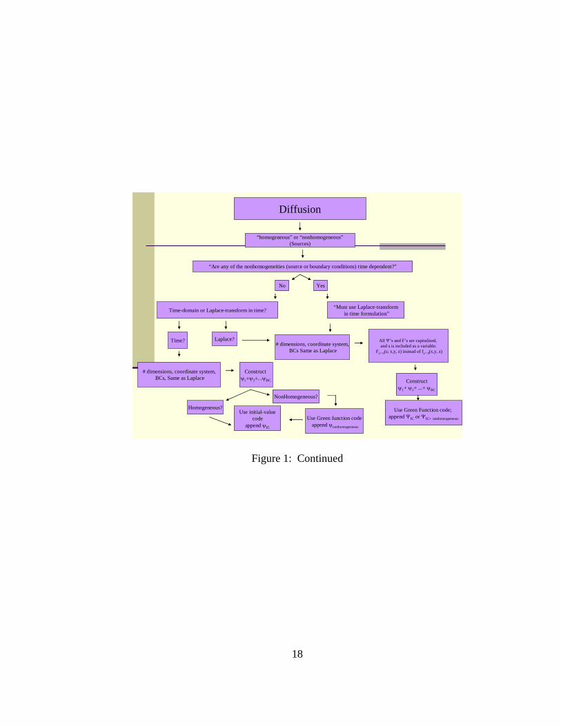
Decision Tree The flow chart below (Figure 1) depicts and describes the logic behind USFKAD.

Following the chart, one can be guided to reach a successful, complete, and

comprehensive solution to any appropriate partial differential equation along with its

specific boundary conditions. This flow chart represents the brain of USFKAD.

16

Type of Partial Differential Equations

LaplaceDiffusion

Wave

Figure 1: USFKAD Flow Chart

17

Laplace

“homogeneous”? “Nonhomogeneous” (Poisson Equation)?

Number of dimensions2 or 3?

Coordinate System?Rectangular, cylindrical (polar), or spherical

Boundary Conditions?

Next Boundary

Next Boundaryor

Next variable

Homogeneous or Nonhomogeneous?

Dirichlet, Neum. Or Robin?

Periodic?Regular?

Singular?

Construct

.

NonhomogeneousHomogeneous

Done

Use Green function code append ψnonhomogeneous

1 2 3... BCΨ +Ψ +Ψ +Ψ

Figure 1: Continued

18

Diffusion

“homogeneous” or “nonhomogeneous”(Sources)

“Are any of the nonhomogeneities (source or boundary conditions) time dependent?”

YesNo

“Must use Laplace-transformin time formulation”Time-domain or Laplace-transform in time?

Time? Laplace?

# dimensions, coordinate system,BCs, Same as Laplace

# dimensions, coordinate system,BCs Same as Laplace

Construct ψ1+ψ2+...ψBC.

Use initial-valuecode

append ψIC

Homogeneous?

Use Green function codeappend ψnonhomogeneous

NonHomogeneous?

Constructψ1+ ψ2+ ...+ ψBC

All Ψ’s and F’s are capitalized, and s is included as a variable:

Fx= 0(s; x,y, z) instead of fx= 0(x,y, z)

Use Green Function code; append ΨIC or ΨIC+ nonhomogeneous

Figure 1: Continued

19

Wave

Time?

NoYes

Homogeneous or Nonhomogeneous (sources)

Are any of the nonhomogeneities(source or boundary conditions)

time dependent?

Frequency?Laplace?

Must use Laplace or Frequency Domain

Proceed exactly like diffusion equation,time domain. The form for ΨIC has an extra term to account for the

initial value of

#dim, cord. Syst., BC’s same as Laplace

Proceed exactly like diffusion equation, Laplace Transform domain. The form ΨIC is slightly different.

# Dim?

Coordinate System?

Boundary Conditions: Lower, Upper

PeriodicSingularRegular

(Continued on next page)

Time, Laplace or Frequency Domain?

t∂∂ψ

Figure 1: Continued

20

PeriodicSingularRegular

Homogeneous

Next Variable

Constructψ1 +ψ2 +...+ψBC

Next Boundary Conditionor

Next Variable

Incoming or Outgoing Wave

Same as LaplaceDir., Neum., Robin, #N

Nonhomogeneous

Done Use Green’s function code, Append Ψnonhomogeneous

Figure 1: Continued

21

Fundamental Concept

The fundamental concept of USFKAD is contained in the following two matrices:

the PDE type matrix (table 1) and the PDE boundary condition (BC) matrix (table 2) as

illustrated below.

Table 1: PDE Equation Type Matrix

PDE Equation Type Matrix

Zero One Two Three Four Five Six Seven

eqtype

PDE Dimension Coordinate System Coordinate 1 Coordinate 2 Coordinate 3 Time Homogeneous or Nonhomogeneous?

0=Laplace 1,2,3 0=rectangular x=0; y=1 z=2 t=8 H=0, N=1

1=Diffusion, t 1=polar/ cylindrical theta=3; r2d=4

2=Diffusion, s 2=spherical phi=8 theta3=9 r3D=6

3=Wave, t theta=3; z=2 Rho=5

4=Wave, s

5=Wave, omega

Table 2: PDE BC Matrix PDE Boundary Condition Matrix

Zero One Two Three Four Five Six Seven Eight Nine

Row #0 R or S D,N,R N,H CC R or S D,N,R,O,I N,H x 0 (zero) X

Row #1 R or S D,N,R N,H CC R or S D,N,R,O,I N,H y 0 (zero) Y

Row #2 R or S D,N,R N,H CC R or S D,N,R,O,I N,H z 0 (zero) Z

Row #3 R D,N,R,P N,H CC R D,N,R,P N,H theta 0 (zero) THETA

Row #4 R or S D,N,R N,H CE R or S D,N,R,O,I N,H r (2d) a b

Row #5 R or S D,N,R N,H BB R or S D,N,R,O,I N,H rho a b

Row #6 R or S D,N,R N,H SB R or S D,N,R,O,I N,H r3D a b

Row #7 R D N,H CC R D N,H t 0 (zero) 0 (zero)

Row #8 S S H LG S S H phi 0 (zero) pi

Row #9 R or S P H SH R or S P H theta3d 0 (zero) 2 pi

22

The PDE type matrix (table 1) identifies all types of PDE’s including the number

of dimensions, coordinate system, coordinates, whether it is time dependent or not, and

whether it is homogeneous or not.

Now once the PDE Equation type has been selected the Boundary conditions must

be identified. The BC matrix virtually accounts for all types of PDE’s. Using the PDE

type matrix and the BC matrix, we came up with 200 different possible PDE cases or

scenarios that virtually cover and provide solutions for all PDE problems. To accomplish

this there are 200 subroutines in USFKAD code which provides solutions for each

possible PDE problems.

Example 1

Consider Laplace’s equation in a box, Homogeneous Dirichlet conditions at x=0

and X, homogeneous Dirichlet at y=0, nonhomogeneous Dirichlet at y=Y. homogeneous

Neumann condition at z=0, nonhomogeneous Neumann at z=Z. As the user inputs these

data, USFKAD fills in the BC matrix as shown on table 3.

23

Table 3: Matrix Example Column #0 #1 #2 #3 #4 #5 #6 #7 #8 #9

eqtype

PDE dim coord coord 1 coord 2 coord 3 time H, N?

0=Laplace 3 0=rect x=0; y=1 z=2 H=0

Boundary Conditions "mtrx"

Row #0 Regular D H CC R D H x 0 (zero) X

Row #1 Regular D H CC R D N y 0 (zero) Y

Row #2 Regular N H CC R N N z 0 (zero) Z

Row #3

Row #4

Row #5

Row #6

Row #7

Row #8

Row #9

Note that final solution will be

zYk

Xj

Yyk

Xxjb

yZk

Xj

Zzk

Xxja

jkkj

jkkj

22

11

22

01

)()(coshsinsin

)()(sinhcossin

ππππ

ππππ

++

+

∑∑

∑∑∞

=

∞

=

∞

=

∞

=

with

∫ ∫∫∫

==X Z

YyZXjk dxdzZ

zkX

xjzxfdz

Zzkdx

Xxj

a0 0

0

2

0

2

.cossin),(cos

1

sin

1 ππππ

24

∫ ∫∫∫

==X Y

ZzYXjk dxdyY

ykX

xjyxfdy

Yykdx

Xxj

b0 0

0

2

0

2

.sinsin),(sin

1

sin

1 ππππ

USFKAD scans down column 2, and then column 6, until it sees an N (nonhomogeneous)

in row 1, column 6. It begins to assemble the solution to the sub problem where all BCs

are homogeneous except at y=Y. Saving y for last, it looks at the x-row, row #0. It sees

the specifications

1. Constant coefficient DE (from column 3),

2. Dirichlet BC at the low end (from column 1),

3. Dirichlet BC at the high end (from column 5),

4. Homogeneous BC at both ends (because y has the only nonhomogeneous).

So USFKAD assembles the word "CCDDHH" from these columns and sends this

word and the symbol "x" to the eigenfunction searcher. The latter returns the

eigenfunction as "sin", the eigenvalues as "κx = π/X, 2π/X, …", and the superposition

type as "xκ

Σ ". (If the eigenvalues formed a continuum, the superposition type would be

"∫ dκx "). It also returns the formula for

∫X

dxX

xj

0

2sin

1π

and the weight factor for this DE

("1", hence blank, in this case.)

USFKAD writes each of these returned formulas to separate lists, and looks for

the next variable, z. It reads off the characteristics from row #2 of the BC matrix and

sends "z, CCNNHH" to the eigenfunction sorter, which returns the appropriate formulas

as before. They are concatenated with the earlier formulas in the corresponding lists.

25

Then USFKAD fetches the symbols for the y factor by sending "y, CCDDHN, κx,

κz", as read from row #1 and the previous lists, to the eigenfunction sorter (of course this

factor is not literally an eigenfunction). The latter returns the sinh function and the

2 2x zκ κ+ symbol, and USFKAD concatenates these with the other lists and merges all

the lists together, calling the result Ψ1.

Next USFKAD continues to scan columns 2 and 6, looking for the next "N"

(nonhomogeneous BC) marker. It finds "N" in row #2, column #6, so it assembles x, y

eigenfunctions and z-factors as before.

If the PDE itself is nonhomogeneous (as marked in column 7 of eqtype),

USFKAD assembles a sum for the eigenfunction expansion of the Green's function (Ψ3,

example 1, chapter 5).

In the time domain (as marked in column 0 of eqtype), USFKAD assembles the

time factors from the eigenvalues symbols it has accumulated (example 4, chapter 5).

In the frequency or Laplace domain (as marked in column 0 of eqtype), USFKAD

sends the eigenvalues (κx, …) and the transform variable (s or ω) (in accordance with

column #0 of eqtype) to the subroutine searcher for the nonhomogeneous factor. These

nonhomogeneous-factor subroutines simply incorporate them into the formula display

( 2x sκ + in example 5 and 2 2 2

x yω κ κ− − in example 6, chapter 5).

On-Screen Inquires USFKAD is invoked by answering a list of printed on-screen inquiries as follows:

Select the Partial Differential Equation:

26

0 - Laplace or Poisson: Laplacian Psi + f(interior) = 0;

l - Diffusion, Time Domain: d Psi/dt = Laplacian Psi + f(interior);

2 - Diffusion, s-plane: s Psi - Psi(t=0) = Laplacian Psi + F(interior);

3 - Wave, Time Domain: d2 Psi/dt2 = Laplacian Psi + f(interior);

4 - Wave, s-plane: s2 Psi - sPsi(t=o) - Psi'(t=0) = Laplacian Psi + F(interior);

5 - Wave, frequency domain: - omega2 Psi = Laplacian Psi + F(interior) .

Is the PDE homogeneous (enter 0) or nonhomogeneous (enter 1)?

Enter 1, 2, or 3 for 1, 2, or 3 dimensions.

Select the Coordinate System: 0 - Rectangular, 1 - Cylindrical or Polar, 2 - Spherical.

Select the boundary condition at the lower (upper) end for the coordinate x (y, z, r, rho,

and theta):

Enter 1 for Dirichlet, Homogeneous;

Enter 2 for Dirichlet, Nonhomogeneous;

Enter 3 for Neumann, Homogeneous;

Enter 4 for Neumann, Nonhomogeneous;

Enter 5 for Robin, Homogeneous;

Enter 6 for Robin, Nonhomogeneous;

Enter 7 for Periodic Boundary Conditions;

Enter 8 for Singular Boundary Condition;

Enter 9 for Singular, Sommerfeld Outgoing Wave Condition;

Enter 10 for Singular, Sommerfeld Incoming Wave Condition.

The output of USFKAD is a LaTeX file. It requires subsequent processing by

TeX software, which must be resident on the user's computer.

27

The above procedure and methodology are further illustrated through the six

different examples listed in the next chapter.

Further details on the lexicon of the software in expressing the physical

dimensions and boundary conditions appear in Appendices B and C, respectively.

CHAPTER 5

APPLICATION EXAMPLES

This chapter contains a list of examples of partial differential equation solutions

that progressively demonstrate the decision tree nature of the general separation of

variable procedure. Physical interpretations of these mathematical problems are stated

here in terms of heat and sound phenomena; they all have electrical counterparts.

Example 1 Steady state heat flow in a rectangle with edge and interior heat sources

(nonhomogeneous Laplace/Poisson equation in two dimensions, rectangular coordinates,

Dirichlet conditions on two sides, Neumann conditions on two sides):

2int

0

( , )(0, ) 0, ( , ) ( )

( ,0) ( ), ( , ) 0

erior

x X

y

f x yy X y f y

x f x x Yy y

=

=

∇ Ψ = −Ψ = Ψ =

∂Ψ ∂Ψ= =

∂ ∂

The solution is as follows:

1 2Ψ=Ψ +Ψ +Ψ3

1 cos ( ; ) ( )x

x y x xx y Aκ

κ η κ κΨ =∑

with

28

{ 0;sinh ( ) .

0

1 0;

2

1 0;

1 .sinh

2 30, , , ,...

( ; )

( ) cos ( )

x

x

x x

x

x

x

x

x

x

Y y ify x Y y otherwise

X

x x

ifX

otherwiseX

ifY

otherwiseY

X X Xy

A dx x N M f

N

M

κκ

κ κ

κ

κ

κ

κκ

y o x

π π πκ

η κ

κ κ

− =−

=

=

=

=

=

=

⎧=⎨⎩⎧⎪=⎨⎪⎩

∫

2 sin cosh ( )y

y yy x Aκ

κ κΨ =∑ yκ

with

0

0 0;1 .

sinh

2 3, , ,...

2( ) sin ( )y

y

y

y y

y

Y

y y x

if

otherwiseX

Y Y Y

XA dy y M f yY

M

κ

κκ

κ κ

π π πκ

κ κ =

=

=

=

⎧⎪=⎨⎪⎩

∫

3 cos sin ( , )

x yx y xx y A

κ κκ κ κ κΨ =∑ ∑ y

with

int2 20 0

1 0;

2 .

cos

2 30, , , ,...

2 3, , ,...

( , )2( , ) sinx

x

x

x

y

X Y eriorx y x y

x y

ifX

otherwiseX

X X X

Y Y Yf x yA dx dy x N y

Y

N

κ

κ

κ

π π πκ

π π πκ

κ κ κ κκ κ

=

=

=

=+

⎧= ⎨⎩

∫ ∫

Here we see some of the features of separation of variables:

29

1. The basic decomposition of the problem into three subproblems, each of which

contains only one nonhomogeneous equation.

2. Each subsolution expressed as a sum of terms containing an eigenfunction factor,

satisfying homogeneneous boundary conditions at each end, and a “non-

eigenfunction” factor, satisfying a homogeneous boundary condition at one end

only (note the exceptional form of the latter factor in 2Ψ , and of the

normalization constants for the cosine’s “DC” term when 0xκ = );

3. Coefficients computed by orthogonality to give the corresponding

nonhomogeneity;

4. The construction of the Green’s function out of the same eigenfunctions.

Example 2

Steady state heat flow in a cube with facial heat sources and imperfect facial

insulation (homogeneous Laplace equation in three dimensions, rectangular coordinates,

homogeneous Dirichlet conditions on four sides, nonhomogeneneous Dirichlet condition

on one side, homogeneous Robin condition on one side):

( )

2 0(0, , ) 0, ( , , ) 0

( , ,0) 0, ( , , ) ( , )

( ,0, ) 0, ( , , ) , , 0

z Z

y Y

y z X y z

x y x y Z f x yz z

x z x Y z x Y zy

α

=

=

∇ Ψ =Ψ = Ψ =∂Ψ ∂Ψ

= =∂ ∂

∂ΨΨ = + Ψ

∂=

The solution is

2 2sin ( ; ) cosh ( , )x y

x y y x y x yx y zAκ κ

κ η κ κ κ κ κΨ = +∑ ∑

30

with

{ }

2 20 0

2(

2 3, , ,...

( ; ) sin ( )

sin cos 0

1 0 0, ( ;0) .

2( , ) sin ( ; ) ( , )y x y

y

Y

x

y y y y

Y y y

Y y y

X Y

x y x y y z Z

Y

X X Xy y where are the nonzero solutions possibly imaginary to

Y Y

also if Y include y y

A dx dy x y N M f x yX

N

κ κ κ

κα

π π πκ

η κ κ κ

α κ κ

α κ η

κ κ κ η κ =+

+ +

=

=

+ =

+ = = =

=

=

∫ ∫

3

2 2

2 2

2 2

2 2 2 2

3 0;

.1) /( )

0 0;1 .

sinh

y

Y y

x y

x y

x y x y

ifY

otherwise

if

otherwiseZ

M

κ

α κ

κ κ

κ κκ κ κ κ

=

+

+ =

++ +

⎧⎪⎨⎪⎩

⎧⎪= ⎨⎪⎩

This example illustrates the straightforward extension of the procedure to three

dimensions and the transcendental equation that the Robin boundary condition invokes

for the eigenvalues.

Example 3

Steady state heat flow in a cylindrical sector with facial heat sources

(homogenous Laplace equation in the three dimensions inside a partial cylinder,

nonhomogenous Dirichlet condition on the top and one flat side, homogenous Dirichlet

conditions on the bottom and the curved wall, and a homogenous Neumann condition on

the other flat side):

31

( ) ( )

( ) ( ) (

2

0, ,0 , , 0,

,0, 0, , , , ,

( , , ) ( , )z Z

b z

z z f

Z f

θ

ρ θ θ

)zρ ρ ρθρ θ θ ρ

=Θ

=

∇ Ψ =

Ψ = Ψ =

∂Ψ= Ψ Θ =

∂Ψ =

The solution to this system is expressed

1 2

: : : :1 0 : :z :sin [ ( ) ( ) ( ) ( )] x cosh ( , )

withz z p z z zz z i z i z i z i z z p zd z b I I b A

ρ ρ ρκ ρ κ κ κ κ ρκ κ κ κ ρ κ κ ρ θ κ κ∞

Ψ = Ψ + Ψ

Ψ = ∫ Κ − Κ Κ∑

: : :

:

: :: 0 0 2 2

:

2 : : :

2 3, , ,...

2 sinh2 1( , ) sin ( ) ( ) ( ) ( ) ( , )[ ( )] cosh

cos ( ) ( ; ) ( , )

z z z

z

z

z zZ bz z z z i z i z i z

i Z z

z

Z Z Z

A dz d z b I I b fZ I b

J z A

ρ ρ ρ ρ

ρ

θρ θ

ρ ρρ κ κ κ κ

κ ρ

θ κ ρ θ ρ θ θ ρ θκθ κ

1 zθ

π π πκ

κ κ πκ κ ρ κ κ κ ρ κ κ ρ ρ

ρ π κ κ

κ θ κ ρ η κ κ κ:

=Θ

=

⎡ ⎤⎡ ⎤= ∫ ∫ Κ − Κ ⎢ ⎥⎣ ⎦ Θ⎢ ⎥⎣ ⎦

Ψ = ∑

:zi

∑

with

3 5, , ,.2 2 2θ ..π π πκ =Θ Θ Θ

For each value of :,:,

j

bθ ρθκ κ

θ ρ θκ κ = where are the positive roots of :,{ j

θ ρ θκ κ } 0:,( )J j

θ θ ρ θκ κ κ =

{ :

:

0;

: sin .( ; )

z if

z z otherwisez

ρθ

ρθ

κ

ρ θ κη κ

==

{

:

:

:

:

:

: : 2 201 ,

1 0,

1 .sin

2 2( , ) cos ( ) ( , )( )

b

z Za

ifz

otherwiseZ

A d d J M fb J j

M

θ ρ

θ θ ρθ

ρθ

ρ θ

ρ θ

θ ρ θ θ κ ρ θ κκ κ κ

κ

κκ θ

κ κ θ ρ κ θ κ ρ ρ θ ρΘ

=+

=

=Θ

=

∫ ∫ θ

32

This example illustrates the singular boundary condition for ρ = 0 and the Lebedev eigen

functions in ρ included by the nonhomogenous condition forθ = Θ . The singular

boundary condition includes a continuous, rather than discrete, spectrum. Other than [1],

the Lebedev expansions do not appear in any English language mathematics textbook

except [3], where their correctness is betrayed by a persistent systematic error in the

tabulations. Their omission is probably due to their intimidating nomenclature (note the

analytic condition of the subscript into the complex plane). Ignoring them is, however,

criminal, because (as we see) they occur in realistic problems; indeed, in the analysis of

edge diffraction [2] they are crucial.

Example 4

Sound wave inside a sphere (homogenous wave equations inside a sphere, time-

independent nonhomogenous Dirichlet conditions on the surface):

( )

22

2

( , , , ) ,r b

tr b t fθ φ θ=

∂ Ψ= ∇ Ψ

∂Ψ = = φ

The solution to this system is expressed

#1 #2

0( , )

steady state transient

transient transient transient

steady state m mmY rφ θ∞

= =−

Ψ = Ψ +Ψ

Ψ = Ψ +Ψ

Ψ =∑ ∑ l l Al ll l

with

( ) (

2 *0 0

#1 0 1

sin ( , ) ( , )1

, ( )cos

m m r r b

r

tranient m r r m rm p

A d d Y M f

Mb

Y j r tA

π πφ φ θ φ θ θ φ

)φ θ κ κ κ

=

∞ ∞

= =− =

= ∫ ∫

=

Ψ =∑ ∑ ∑

l l

l

l

l l ll l

with

, /r psκ = l b where sl, p is the pth positive zero of jl .

( ) ( ) ( ) ( )

( ) ( )

2 2 *0 0 0 3 2

1 ,

#2 0 1

2sin , , , ;0( )

sin, ( )

bm r m r steady state

p

rtransient m r m rm p

r

A d d r drY j r rb j s

tY j r A

π πκ φ φ θ φ θ κ θ φ

κφ θ κ κκ

+

∞ ∞

= =− =

⎡ ⎤= ∫ ∫ ∫ Ψ −Ψ⎣ ⎦

Ψ =∑ ∑ ∑

l l ll l

l

l l ll l

with

33

34

b, /r psκ = l where sl, p is the pth positive zero of jl .

( ) ( ) ( ) ( )2 2 *0 0 0 3 2

1 ,

2sin ,( )

bm r m r

p

A d d r drY j rb j s

π π θ φκ φ φ θ φ θ κ

+

∂Ψ= ∫ ∫ ∫

∂l l ll l

, , r; 0t

This example demonstrates the decomposition of the solution into a steady-state

component and a transient component. The time functions can be treated just like the

non-eigenfunctions in the previous solutions, except that they satisfy initial conditions

instead of boundary conditions.

Example 5

Transient heat flow in a rectangle with transient interior and edge heat sources

(nonhomogenous diffusion equations, two dimensions, rectangular coordinates,

homogenous Dirichlet conditions on two sides, homogenous Neumann condition on one

side, time-dependent nonhomogenous Neumann conditions on one side):

( )

( ) ( )

( ) ( ) (

2int , ,

0, 0, , 0

,0 0, , ,

erior

y Y

f x y tt

y X y

)x x Y f x ty y =

∂Ψ= ∇ Ψ +

∂Ψ = Ψ =

∂Ψ ∂Ψ= =

∂ ∂

With ( )int , ;eriorF x y s and ( );y YF x s= denoting the Laplace transforms of (int , ,erior )f x y t and ( , )y Yf x t= , respectively, the Laplace-transformed solution to this system is expressed

( )1 2

21 sin cosh ;

xx x xx syA

κκ κ

Ψ = Ψ +Ψ

Ψ = +∑ s κ

with

2 3, , ,...x X X Xπ π πκ =

( ) ( )202; sin

x

Xx x y Ys

;A s dx x M F x sX κ

κ κ =+= ∫

( )

2

2

2 2

2

0 01 .

sinh

sin cos , ;

x

x y

x

s

x x

x y x y

if sM

otherwises sY

x y A s

κ

κ κ

κ

κ κ

κ κ κ κ

+

⎧ ;+ =⎪

= ⎨⎪ + +⎩

Ψ =∑ ∑

with

( ) ( )int0 0 2 2

2 3, , ,...

2 30, , , ,...

( , ; ) , , 02, ; sin cos

1 0;

2 .

y

y

x

y

eriorX Yx y x y

x y

y

X X X

Y Y YF x y s x y t

A s dx dy x y NX s

ifYN

otherwiseY

κ

κ

π π πκ

π π πκ

κ κ κ κκ κ

κ

=

=

⎛ ⎞+Ψ == ∫ ∫ ⎜ ⎟⎜ ⎟+ +⎝ ⎠

⎧ =⎪⎪= ⎨⎪⎪⎩

This example demonstrates how the logic that solved Example 1 can be retooled to solve

Laplace domain problems; the transformed PDE is equivalent to a nonhomogenous

Laplace (Poisson) equation with the eigenvalues shifted and the initial condition wedded

with the nonhomogeneity.

Example 6 Wave launched from one end of a rectangular waveguide (homogeneous wave

equation in a semi-infinite rectangular waveguide, homogenous Dirichlet conditions on

the walls, nonhomogenous Dirichlet on the end face, frequency domain, outgoing wave at

infinity):

( ) ( ) ( ) ( )( ) ( )

22

2

0

0, , , , ,0, , , 0,

, ,0 , ,z

ty z X y z x z x Y z

x y f x y t=

∂ Ψ= ∇ Ψ

∂Ψ = Ψ = Ψ = Ψ

Ψ =

=

35

36

)yWith denoting the Fourier transforms of(0 ; ,zF xω= ( )0 , ,zf x y t= , the Fourier transforms of the solution to this system is expressed

( )2 2 2

sin sin ; ,x y

x y

i zx y xx ye Aω κ κ

κ κκ κ ω κ κ− − −Ψ =∑ ∑ y

with

( ) ( )0 0 0

2 3, , ,...

2 3, , ,...

2 2; , sin sin ; ,

x

y

X Yx y y y z

X X X

Y Y Y

A dx dy x y F x yX Y

π π πκ

π π πκ

ω κ κ κ κ ω=

=

=

= ∫ ∫

Again, the solution logic of Example 1 is reworked with a shift of the eigenvalues.

37

CHAPTER 6

RECOMMENDATIONS FOR FUTURE DEVELOPMENTS

To further enhance and build on the success of USFKAD, the following

recommendations are offered for future development of this expert system:

1. Offer a choice of output formats (postscript, Mathematics Markup Language)

2. Enable transport of the output to programs like MAPLE, MathCad, or

Mathematica for number crunching.

3. Offer graphical supplements to the outputs (such as sample eigenfunction graphs).

4. Develop graphic point-and-click input options to render it more convenient and

easy to use.

REFERENCES

1. Snider, A.D., Partial Differential Equations: Sources and Solutions, Prentice-Hall, Upper Saddle River, NJ, 1999. 2. Felsen, L.B., and Marcuvitz, N., Radiation and Scattering of Waves, IEEE Press, Piscataway, NJ 1994. 3. Polyanin, A.D., Linear Partial Differential Equations for Engineers and Scientists,

Chapman and Hall/Chemical Rubber Co., Boca Raton, 2001. 4. Cheb-Terrab, E.S., and von Bulow, K., A Computational Approach for the Analytical

Solving of Partial Differential Equations, Computer Physics Communications, v. 90, 102-116, 1995.

5. Kalnins, E.G. and Miller, Jr., W., Variable Separable in Mathematical Physics: From

Intuitive Concept to Computational Tool. (Working paper) 6. Wolfram Research, Inc., Mathematica, Version 5.1, Champaign, IL (2004). 7. Waterloo Maple, Inc., Maple V release 3 Canada, 2001. 8. Borland International, Borland C++ 5.02 Scotts Valley, CA, 1994.

38

39

APPENDIECES

APPENDIX A: COMPARISON OF SOLVING PARTIAL DIFFERENTIAL EQUATIONS USING THE TRADITONAL METHOD AND USFKAD

y

4 ( )f xΨ = π

40

1 ( )f yx

∂Ψ=

∂ 2 0∇ Ψ = 3 ( )f y

x∂Ψ

=∂

x

2 ( )f xΨ = π Figure 2: PDE Problem

Consider the boundary value problem shown in Figure 2. We take advantage of the

linearity of the equations to simplify the analysis. Suppose we compute the following

solutions to the following four sub problems shown in Figure 3 a-d: Decomposition of

Problems. y

1 0Ψ = π

11 ( )f y

x∂Ψ

=∂

21 0∇ Ψ = 1 0

x∂Ψ

=∂

x 1 0Ψ = π

(a) Figure 3: (a-d) Decomposition of the PDE Problem

Appendix A: y Continued

2 0Ψ = π

41

2 0x

∂Ψ=

∂ 2

2 0∇ Ψ = 2 0x

∂Ψ=

∂

x 2 2 ( )f xΨ = π

(b)

y

3 0Ψ =

π

3 0x

∂Ψ=

∂ 2

3 0∇ Ψ = 33 ( )f y

x∂Ψ

=∂

x

3 0Ψ = π

(c) y

( )4 4f xΨ =

π

4 0x

∂Ψ=

∂ 2

4 0∇ Ψ = 4 0x

∂Ψ=

∂

x

4 0Ψ = π (d)

Figure 3: Continued

Appendix A: Continued Problem 1: Find 1( , )x yΨ such that

inside the square (1) 21( , ) 0x y∇ Ψ =

11(0, ) ( )y f y

x∂Ψ

=∂

on the left edge (0<y<π ) (2)

1( , ) 0x πΨ = on the top edge (0<x<π ) (3)

1 ( , ) 0yx

π∂Ψ=

∂on the right edge (0<y<π ) (4)

on the bottom edge (0<x<1( ,0) 0xΨ = π ) (5)

Problem 2: Find 2 ( , )x yΨ such that

inside the square (6) 22 ( , ) 0x y∇ Ψ =

2 2( ,0) ( )x f xΨ = on the bottom edge (0<x<π ) (7)

2 ( , ) 0yx

π∂Ψ=

∂ on the right edge (0<y<π ) (8)

2 (0, ) 0yx

∂Ψ=

∂ on the left edge (0<y<π ) (9)

2 ( , ) 0x πΨ = on the top edge (0<x<π ) (10)

Problem 3: Find 3( , )x yΨ such that

inside the square (11) 23 ( , ) 0x y∇ Ψ =

33( , ) ( )y f y

xπ∂Ψ

=∂

on the right edge (0<y<π ) (12)

3 ( , ) 0x πΨ = on the top edge (0<x<π ) (13)

on the bottom edge (0<x<3( ,0) 0xΨ = π ) (14)

42

Appendix A: Continued

3 (0, ) 0yx

∂Ψ=

∂on the left edge (0<y<π ) (15)

Problem 4: Find 4 ( , )x yΨ such that

inside the square (16) 24 ( , ) 0x y∇ Ψ =

4 ( , ) ( )4x f xπΨ = on the top edge (0<x<π ) (17)

4 ( , ) 0yx

π∂Ψ=

∂on the right edge (0<y<π ) (18)

on the bottom edge (0<x<4 ( ,0) 0xΨ = π ) (19)

4 (0, ) 0yx

∂Ψ=

∂on the left edge (0<y<π ) (20)

By superposition, we have decomposed the original problem into a set of subproblems in

each of which only one boundary condition is nonhomogenous. Let’s give as an example

how to solve problem 4 by the traditional method.

Solution 1

Solving problem 4:

The solution of Laplace’s equation (16) can be expressed as a product of factors.

4 ( , ) ( ) ( )x y X x Y yΨ = (21)

If we substitute (21) into (1) we can get a form where only one variable occurs on each side of the equation:

43

Appendix A: Continued

2 22

4 2 2( , ) 0 ( ) ( ) ( ) ( )

"( ) ( ) ( ) "( )

x y X x Y y X x Y yx y

X x Y y X x Y y

∂ ∂∇ Ψ = = +

∂ ∂= +

"( ) "( )( ) ( )

X x Y yX x Y

⇒ = −y

(22)

The separated equation (22) implies:

"( )( )

X xX x

λ= or "( ) ( ) 0X x X xλ− = (23)

For some constant λ (separation constant) and "( ) ( ) 0Y y Y yλ+ = (24)

The general solution to the harmonic oscillator equation (23), can be expressed as:

1 2( ) cosh sinhX x a x a xλ λ= + if 0λ > (25)

1 2( )X x b b= + x if 0λ = (26)

1 2( ) cos sinX x c x c xλ λ= − + − if 0λ < (27)

As for the solutions for (24), they are:

1 2( ) cos sinY y d y d yλ λ= + if 0λ > (28)

if 1 2( )Y y e e y= + 0λ = (29)

1 2( ) cosh sinhY y g y g yλ λ= − + − if 0λ < (30)

From (2)-(5):

'( ) 0, '(0) 0X Xπ = = (31)

(32) (0) 0Y =

44

Appendix A: Continued

1 2'( ) sinh coshX x a x a xλ λ λ λ= + if 0λ > (33)

2'( )X x b= if 0X = (34)

1 2'( ) sin cosX x c x c xλ λ λ= − − − + − −λ if 0λ < (35)

Applying the boundary condition '(0) 0X = , we get

2'(0) 0X aλ= = if 0λ > (36)

if 2'(0) 0X b= = 0λ = (37)

2'(0) 0X cλ= − = if 0λ < (38)

So 1( ) coshX x a xλ= if 0λ > (39)

1( )X x b= if 0λ = (40)

1( ) cosX x c xλ= − if 0λ < (41)

Imposing '( ) 0X π = implies:

1'( ) sinh 0X aπ λ λπ= = if 0λ > (42)

if ( )' 0X π = 0λ = (43)

( ) 1' sinh 0X cπ λ λπ= − − = 0 if λ < (44)

Since we are not interested in trivial solutions, or can not equal zero, so we need to satisfy (42)-(44) by the selection of

1 1, ,a b 1cλ . The choice 0λ = is acceptable

1( )X x b⇒ = (=constant). No positive value for λ yield solutions, because the sin function in (42) never vanishes. However, the sin function vanishes whenever

1, 2,3...,nλ− = = and the corresponding solution (39)-(41) is cos nx. So we have 1c

45

Appendix A: Continued nontrivial solutions for the x factor in (21) if , applying (32) to

(28)-(30):

20, 1, 4,..., ,...nλ = − − −

if 1(0) 0Y d= = 0λ >

if ( ) 10 0Y e= = 0λ =

if 1(0) 0Y g= = 0λ <

and 2( ) sinhnY y g ny⇒ = 0 2( )Y y e y=

cos sinhn nx nyφ⇒ =

4 01

( , ) cos sinhnn

x y a y a nx ny∞

=

⇒ Ψ = +∑

Where 0 4 420 0

1 2( ) , 0 ( )0cossinhna f x dx a f x

nx

π π

π π= > =∫ ∫ nx

You see how long and cumbersome it was to do only problem 4. As for problems 3, 2,

and 1, we will get the following after a lot of manipulation:

Problem 3:

31

( , ) cosh sinnn

x y b nx ny∞

=

Ψ =∑ where 30

2 ( )sinsinhnb f y

n n

π

π π= ∫ nydy

Problem 2:

2 01

( , ) ( ) cos sinh ( )nn

x y c y c nx n yπ π∞

=

Ψ = − + −∑ where

46

Appendix A: Continued

0 220

1 ( )c f xπ

π= ∫ dx

0 20

2 ( ) cossinhnc f x

n

π

π π> = ∫ nxdx

Problem 1:

11

( , ) cosh ( )sinnn

x y d n xπ∞

=

Ψ = −∑ ny where

10

2 ( )sin .sinhnd f y

n nπ

π π−

= ∫ nydy .

The final answer will be

1 2 3 4( , ) ( , ) ( , ) ( , ) ( , )x y x y x y x y xΨ = Ψ +Ψ +Ψ +Ψ y . Solution 2 Complete solution using USFKAD.

1 2 3 4Ψ = Ψ +Ψ +Ψ +Ψ

( ) ( )1 sin coshy

y yy X x Aκ

κ κΨ = −∑ yκ

where

2 3, , ,...y Y Y Yπ π πκ =

( ) ( )0 02sin

y

Yy y xA dy y M f y

Y κκ κ == ∫

47

Appendix A: Continued

0 0

1 .sinh

y

y

y y

ifM

otherwiseX

κ

κ

κ κ

;=⎧⎪= ⎨⎪⎩

( ) ( )2 cos ;x

x y xx y Aκ

κ η κ κΨ =∑ x

where 2 30, , , ,...x X X X

π π πκ =

( ) ( )0

;sinh .

xy x

x

Y y ify

Y y otherwiseκ

η κκ

− =⎧⎪= ⎨ −⎪⎩

( ) ( )0 0cosx x

Xx x yA dx x N M f xκ κκ κ == ∫

1 0;

2 .x

xifXN

otherwiseX

κ

κ⎧ =⎪⎪= ⎨⎪⎪⎩

1 0;

1 .sinh

x

x

x

ifYM

otherwiseY

κ

κ

κ

⎧ =⎪⎪= ⎨⎪⎪⎩

( )3 sin coshy

y yy x Aκ

κ κΨ =∑ yκ

where 2 3, , ,...y Y Y Y

π π πκ =

( ) ( )02sin

y

Yy y x XA dy y M f y

Y κκ κ == ∫

0 0

1 .sinh

y

y

y y

ifM

otherwiseX

κ

κ

κ κ

;=⎧⎪= ⎨⎪⎩

( ) ( )4 cos ;x

x y xx y Aκ

κ η κ κΨ =∑ x

where 48

Appendix A: Continued

2 30, , , ,...x X X Xπ π πκ =

( )0

;sinh .

xy x

x

y ify

y otherwiseκ

η κκ

=⎧= ⎨⎩

( ) ( )0 cosx x

Xx x y YA dx x N M f xκ κκ κ == ∫

1 0;

2 .x

xifXN

otherwiseX

κ

κ⎧ =⎪⎪= ⎨⎪⎪⎩

1 0;

1 .sinh

x

x

x

ifYM

otherwiseY

κ

κ

κ

⎧ =⎪⎪= ⎨⎪⎪⎩

If you set X=Y=π , you will find that both the traditional method and USFKAD solutions are identical.

49

50

APPENDIX B: READ ME Welcome to USFKAD, the software for solving partial differential equations

analytically, by separation of variables. If you find this software is of value to you, please

consider making a donation to USF students via the Allen Gondeck scholarship fund,

through Prof. A. D. Snider, University of South Florida, ENB 118, Tampa FL 33620.

(Thank you.)

The task of constructing complete solutions by separation of variables is quite

tedious, and the software can do this for you only if you follow the format/notation

conventions precisely.

The current version handles (homogeneous or nonhomogeneous) (mixed)

Dirichlet, Neumann, constant-coefficient Robin boundary conditions, or singular

boundary conditions for the (possibly) nonhomogeneous Poisson, diffusion, or wave

equations, in the time, frequency, or Laplace domains.

You will have to label the dimensions of your domain to conform to one of the

following conventions:

1. 0 < x,y,z,θ < X,Y,Z,Θ

2. 0 < x,y,z < ∞ (Do not use -∞ < x,y,z < X,Y,Z)

3. -∞ < x,y,z < ∞

4. 0 < θ < 2π (periodic)

5. 0 < a < r < b < ∞

51

Appendix B: Continued 6. 0 < a < r < ∞

7. 0 < r < b < ∞

8. 0 < r < ∞

9. 0 < θ < 2π and 0 < φ < π (spherical coordinates)

Dirichlet boundary conditions take the form

ψ(0,y,z) = fx=0(y,z) ; ψ(X,y,z) = fx=X(y,z)

(and similarly for y, z, r, and θ).

Neumann boundary conditions take the form

∂ψ(0,y,z)/∂x = fx=0(y,z) ; ∂ψ(X,y,z)/∂x = fx=X(y,z)

(and similarly for y, z, r, ρ, and θ). Note that the relevant partial will not, in general,

be the external normal derivative.

Robin boundary conditions take the form

αx=0 ψ(0,y,z) + ∂ψ(0,y,z)/∂x = fx=0(y,z) ;

αX ψ(X,y,z) + ∂ψ(X,y,z)/∂x = fx=X(y,z)

(and similarly for y, z, r, ρ, and θ). Note that the relevant partial will not, in general,

be the external normal derivative. The coefficient α is presumed constant.

52

Appendix B: Continued To use the software, doubleclick on the .exe file, and follow the menu instructions

carefully. Give the name of your output file a .tex subscript. The software does not alert

the user if inconsistent parameters are input - it simply fails to produce an output file.

Run latex on the output file, and either view the .dvi result or dvips it to

postscript, and print out. You may make format changes to the .tex file if you wish.

Please inform A. D. Snider by email (snider@eng.usf.edu) if you feel the software

has returned an incorrect answer, or if you desire elaboration of the answer; include a

complete problem statement and the output .tex file, and your comments.

Enjoy!

Sami Kadamani

Dave Snider

53

APPENDIX C: ToUseUSFKAD.pdf

To use USFKAD: Create a folder on your hard drive, place it in root of the drive, and name it USFKAD. If you have several hard drives, you may use any drive you want. For this tutorial, d-drive is used. Location of the folder, will be d:\USFKAD> Open Windows Explorer, browse to d:\USFKAD and double click USFKAD program file. The Command Prompt will open, and you get a warning message. Click OK to proceed. Now you have to create the output file, and in this example it is named: testing.tex Remember the extension tex Type in your filename, in this case testing.tex Follow the instructions in USFKAD, and for this tutorial we used the following input: 0, 0, 2, 0, 1, 1, 2 and 2 This will create the file testing.tex in the folder d:\USFKAD Next step will be to create the dvi file. Click on Start, Run.. Type cmd in the Run window. This will open the command prompt. In the command promt, browse to your folder. “d:” will take you to the d drive, then cd usfkad, will change the directory to where the testing.tex file is. Type “d: cd usfkad” to get to d drive, and the usfkad folder Once you are in the correct folder, type latex to open the application. Then press enter to proceed after the welcome note. Open LaTeX by typing latex Type the file name, in this case testing. There is no need for the file extension, but it has to be tex when you created it. Type the filename, in this case testing This will give you a dvi output file. If there are any problems, you will see it on this screen The status of creating the dvi file Appendix C: Continued Next step will be to view dvi file. Click on Start, Run..

54

Type “yap” in the Run window. The program used to view the dvi file. In Yap window, choose open file, and select testing.dvi Open the testing.dvi file. Yap will show the final output Output from the testing.tex file crated with USFKAD

ABOUT THE AUTHOR

Sami M. Kadamani is currently an instructor at Hillsborough Community College

in Tampa, Florida. He completed his Bachelor of Science in Electrical Engineering from

the University of Delaware in 1983, and his Master of Science in Electrical Engineering

from North Carolina A & T State University in 1986. In 1986 Mr. Kadamani moved to

Tampa, Florida to pursue his Doctoral of Philosophy degree in Engineering Science at the

University of South Florida, which he completed in May 2005.