Radboud University, Nijmegen

IMAPP - Mathematics

2021/22

An Introduction toPartial Differential Equations

Stefanie Sonner

Preface

These lecture notes are written for the course “An Introduction to Partial Differential Equations”(NWI-WB046B) at Radboud University, Nijmegen. They provide an introduction to the vast re-search field of partial differential equations. Further details and many additional topics can befound in the monographs by L. Evans [3], W. Craig [1], Y. Pinchover and J. Rubinstein [8], W.A.Strauss [9] and A. Vasy [11]. To follow the course a solid understanding of analysis, calculus,linear algebra and ordinary differential equations is required.

We introduce and analyze basic types of partial differential equations. Solution methods, rep-resentation formulas for solutions and properties of solutions for classical linear equations of sec-ond order (Laplace, heat and wave equation) are discussed. Moreover, we study nonlinear partialdifferential equations of first order via the method of characteristics. We are mainly concernedwith the existence, uniqueness and regularity of solutions. This involves the use of fundamentalsolutions, maximum principles and energy methods.

Except for particularly simple cases, partial differential equations cannot be solved explicitly.In the analysis of partial differential equations, we are therefore mainly concerned with provingthe well-posedness and investigating the qualitative behavior of solutions. Different from ordinarydifferential equations, there is no general theory for partial differential equations. Typically, eachparticular type of partial differential equation requires an individual theory and specific methodsto study the existence and properties of solutions.

i

Contents

1 Introduction 11.1 Basic definitions . . . . . . . . . . . . . . . . . . . . . . . . . . . . . . . . . . . 11.2 Examples . . . . . . . . . . . . . . . . . . . . . . . . . . . . . . . . . . . . . . 31.3 Type classification of linear second order PDEs . . . . . . . . . . . . . . . . . . 51.4 Strategies for studying PDEs . . . . . . . . . . . . . . . . . . . . . . . . . . . . 61.5 Further notation . . . . . . . . . . . . . . . . . . . . . . . . . . . . . . . . . . . 71.6 Exercises . . . . . . . . . . . . . . . . . . . . . . . . . . . . . . . . . . . . . . 8

2 The Transport Equation 102.1 Motivation . . . . . . . . . . . . . . . . . . . . . . . . . . . . . . . . . . . . . . 102.2 The homogeneous case . . . . . . . . . . . . . . . . . . . . . . . . . . . . . . . 112.3 The inhomogeneous case . . . . . . . . . . . . . . . . . . . . . . . . . . . . . . 132.4 Exercises . . . . . . . . . . . . . . . . . . . . . . . . . . . . . . . . . . . . . . 14

3 The Laplace and Poisson Equation 153.1 Preliminaries . . . . . . . . . . . . . . . . . . . . . . . . . . . . . . . . . . . . 153.2 Motivation . . . . . . . . . . . . . . . . . . . . . . . . . . . . . . . . . . . . . . 173.3 Properties of harmonic functions . . . . . . . . . . . . . . . . . . . . . . . . . . 18

3.3.1 Mean value formulas . . . . . . . . . . . . . . . . . . . . . . . . . . . . 183.3.2 Maximum principles and uniqueness for boundary value problems . . . . 21

3.4 Fundamental solution . . . . . . . . . . . . . . . . . . . . . . . . . . . . . . . . 223.5 Green’s function and representation formula . . . . . . . . . . . . . . . . . . . . 243.6 Green’s function and existence result for the ball . . . . . . . . . . . . . . . . . 273.7 Energy methods . . . . . . . . . . . . . . . . . . . . . . . . . . . . . . . . . . . 30

3.7.1 Uniqueness . . . . . . . . . . . . . . . . . . . . . . . . . . . . . . . . . 303.7.2 Dirichlet’s principle . . . . . . . . . . . . . . . . . . . . . . . . . . . . 30

3.8 Exercises . . . . . . . . . . . . . . . . . . . . . . . . . . . . . . . . . . . . . . 32

4 The Heat Equation 384.1 Motivation . . . . . . . . . . . . . . . . . . . . . . . . . . . . . . . . . . . . . . 384.2 Fundamental solution . . . . . . . . . . . . . . . . . . . . . . . . . . . . . . . . 394.3 Initial value problems . . . . . . . . . . . . . . . . . . . . . . . . . . . . . . . . 41

4.3.1 Homogeneous case . . . . . . . . . . . . . . . . . . . . . . . . . . . . . 414.3.2 Inhomogeneous case . . . . . . . . . . . . . . . . . . . . . . . . . . . . 44

4.4 Maximum principles . . . . . . . . . . . . . . . . . . . . . . . . . . . . . . . . 46

ii

4.5 Uniqueness . . . . . . . . . . . . . . . . . . . . . . . . . . . . . . . . . . . . . 494.6 Energy methods . . . . . . . . . . . . . . . . . . . . . . . . . . . . . . . . . . . 494.7 Exercises . . . . . . . . . . . . . . . . . . . . . . . . . . . . . . . . . . . . . . 52

5 The Wave Equation 565.1 Motivation . . . . . . . . . . . . . . . . . . . . . . . . . . . . . . . . . . . . . . 565.2 D’Alembert’s formula (1D) . . . . . . . . . . . . . . . . . . . . . . . . . . . . . 575.3 Spherical means . . . . . . . . . . . . . . . . . . . . . . . . . . . . . . . . . . . 595.4 Kirchhoff’s formula (3D) . . . . . . . . . . . . . . . . . . . . . . . . . . . . . . 615.5 Poisson’s formula (2D) . . . . . . . . . . . . . . . . . . . . . . . . . . . . . . . 645.6 Inhomogeneous initial value problems . . . . . . . . . . . . . . . . . . . . . . . 665.7 Energy methods . . . . . . . . . . . . . . . . . . . . . . . . . . . . . . . . . . . 675.8 Exercises . . . . . . . . . . . . . . . . . . . . . . . . . . . . . . . . . . . . . . 69

6 Nonlinear First Order PDEs 746.1 The method of characteristics . . . . . . . . . . . . . . . . . . . . . . . . . . . . 746.2 Quasilinear equations . . . . . . . . . . . . . . . . . . . . . . . . . . . . . . . . 776.3 Fully nonlinear equations . . . . . . . . . . . . . . . . . . . . . . . . . . . . . . 79

6.3.1 Characteristic equations . . . . . . . . . . . . . . . . . . . . . . . . . . 796.3.2 Boundary data . . . . . . . . . . . . . . . . . . . . . . . . . . . . . . . 816.3.3 Local solution . . . . . . . . . . . . . . . . . . . . . . . . . . . . . . . 836.3.4 Straightening the boundary . . . . . . . . . . . . . . . . . . . . . . . . . 86

6.4 Exercises . . . . . . . . . . . . . . . . . . . . . . . . . . . . . . . . . . . . . . 87

iii

Chapter 1

Introduction

Partial differential equations (PDEs) are used to model a wide range of phenomena, in particular,in physics, engineering, chemistry, biology and finance. For instance, they are fundamental inthe modern understanding of sound, fluid dynamics, elasticity, general relativity and quantummechanics. They also play an important role in “pure mathematics”, in particular, in geometry andanalysis.

1.1 Basic definitions

A PDE is an equation for an unknown function u of several variables that involves partial deriva-tives of u. The order of the highest partial derivative is called the order of the PDE.

Definition 1.1. Let Ω ⊂ Rn be open, n ≥ 2 and k ∈ N. An expression of the form

F(Dku(x),Dk−1u(x), . . . , u(x), x) = 0, x ∈ Ω, (1.1)

is called a k-th order PDE, where

F : Rnk× Rnk−1

× . . . × Rn × R ×Ω→ R

is a given function and u : Ω→ R is the unknown.A classical solution of the PDE is a k-times continuously differentiable function u : Ω → R

that satisfies (1.1).

Here, we use the following notation to denote the partial derivatives. Let Ω ⊂ Rn, n ≥ 2, beopen, x = (x1, . . . , xn) ∈ Ω and u : Ω→ R be a scalar function.

• The partial derivatives of u at x, are defined as

∂u∂xi

(x) := limh→0

u(x + hei) − u(x)h

(if the limit exists),

for i = 1, . . . , n, where ei denotes the i-th standard basis vector of Rn. Commonly used arealso the notations ∂u

∂xi= ∂xiu = uxi .

1

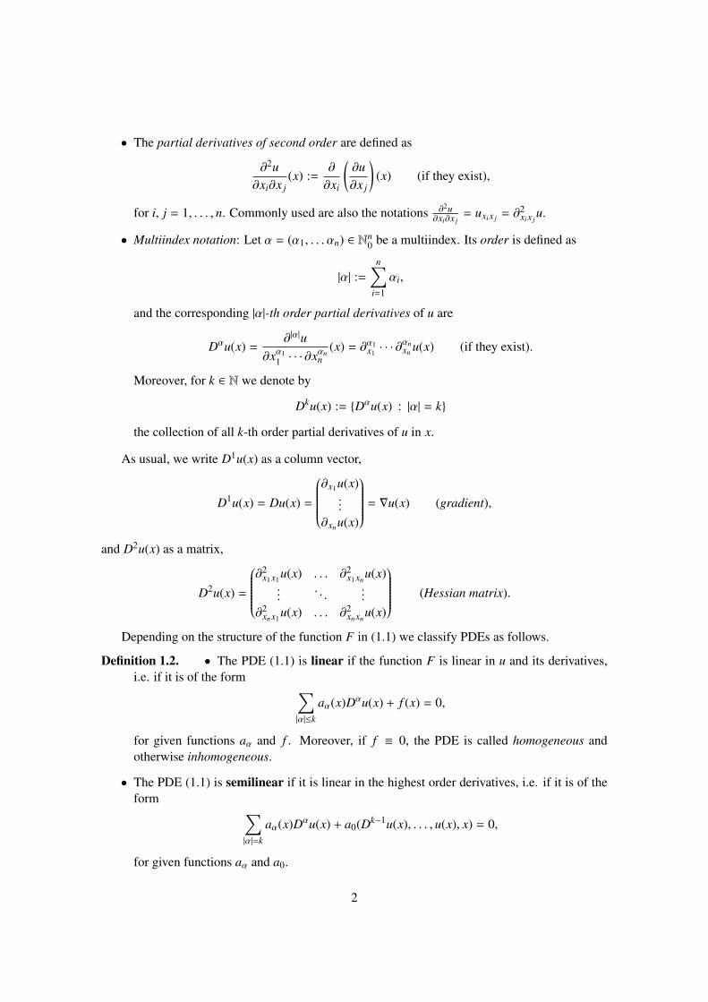
• The partial derivatives of second order are defined as

∂2u∂xi∂x j

(x) :=∂

∂xi

(∂u∂x j

)(x) (if they exist),

for i, j = 1, . . . , n. Commonly used are also the notations ∂2u∂xi∂x j

= uxi x j = ∂2xi x j

u.

• Multiindex notation: Let α = (α1, . . . αn) ∈ Nn0 be a multiindex. Its order is defined as

|α| :=n∑

i=1

αi,

and the corresponding |α|-th order partial derivatives of u are

Dαu(x) =∂|α|u

∂xα11 · · · ∂xαn

n(x) = ∂α1

x1· · · ∂αn

xn u(x) (if they exist).

Moreover, for k ∈ N we denote by

Dku(x) := Dαu(x) : |α| = k

the collection of all k-th order partial derivatives of u in x.

As usual, we write D1u(x) as a column vector,

D1u(x) = Du(x) =

∂x1u(x)

...

∂xnu(x)

= ∇u(x) (gradient),

and D2u(x) as a matrix,

D2u(x) =

∂2

x1 x1u(x) . . . ∂2

x1 xnu(x)

.... . .

...

∂2xn x1

u(x) . . . ∂2xn xn

u(x)

(Hessian matrix).

Depending on the structure of the function F in (1.1) we classify PDEs as follows.

Definition 1.2. • The PDE (1.1) is linear if the function F is linear in u and its derivatives,i.e. if it is of the form ∑

|α|≤k

aα(x)Dαu(x) + f (x) = 0,

for given functions aα and f . Moreover, if f ≡ 0, the PDE is called homogeneous andotherwise inhomogeneous.

• The PDE (1.1) is semilinear if it is linear in the highest order derivatives, i.e. if it is of theform ∑

|α|=k

aα(x)Dαu(x) + a0(Dk−1u(x), . . . , u(x), x) = 0,

for given functions aα and a0.

2

• The PDE (1.1) is quasilinear if it is of the form∑|α|=k

aα(Dk−1u(x), . . . , u(x), x)Dαu(x) + a0(Dk−1u(x), . . . , u(x), x) = 0,

for given functions aα and a0.

• The PDE (1.1) is fully nonlinear if F is a nonlinear function of the highest order derivativesDku.

For linear homogeneous equations the superposition principle holds, i.e. if u and v are bothsolutions of the PDE, then the same applies to αu + βv, for all α, β ∈ R. More generally, ifu1, . . . , um are solutions, then so is any linear combination of these solutions.

Typically, the difficulty of the analysis of a PDE increases with the degree of nonlinearity.

Instead of scalar equations we can also look at systems of PDEs which arise in many appli-cations. Here, several unknown functions u1, . . . , um, m ≥ 2, have to be determined that satisfy asystem of m PDEs.

Definition 1.3. An expression of the form (1.1) is called a k-th order system of PDEs if m ≥ 2and

F : Rmnk× Rmnk−1

× . . . × Rmn × Rm ×Ω→ Rm,

where u = (u1, . . . , um) : Ω → Rm is the unknown. Here, Dαu = (Dαu1, . . . ,Dαum) and Dku =

Dαu : |α| ≤ k.A classical solution of the system of PDEs is a k-times continuously differentiable function

u : Ω→ Rm that satisfies (1.1).

1.2 Examples

We briefly discuss several examples of PDEs that illustrate the variety of applications in differentfields.

Minimal surface equationLet Ω ⊂ R2 be open and bounded and u : Ω → R. Then, the surface area of the graph of u is

given by

J(u) =

∫Ω

√1 + |∇u(x)|2 dx.

A classical problem in the Calculus of Variations is the minimal surface problem: Minimize J(u)subject to prescribed boundary conditions. That is, among all functions u that satisfy u = g on theboundary ∂Ω, where g is given, find the function such that the surface area of its graph is minimal.

One can show that such a minimizer u satisfies the corresponding Euler–Lagrange equation

∇ ·

∇u√1 + |∇u|2

= 0 in Ω,

where · denotes the inner product in R2. This minimal surface equation is a quasilinear PDE ofsecond order.

3

The minimal surface problem is also known as the Plateau problem, named after the Belgianphysicist J. A. F. Plateau (1801 - 1883). He conducted experiments with soap films by dippingwire contours in a solution of soapy water.

Reaction-diffusion equationsReaction-diffusion equations are widely used to model phenomena in chemistry, physics and

biology. They describe the changes in space and time of concentrations of chemical substances ordensities of populations.

Let I ⊂ R be an open interval, U ⊂ Rn be open and Ω = I × U. Moreover, u : Ω → R is afunction of time t ∈ I and the spatial position x ∈ U. A reaction-diffusion equation is of the form

∂tu = d∆u + f (u) in I × U,

where ∆u = ∆xu =∑n

i=1 uxi xi denotes the Laplace operator or Laplacian with respect to x andd > 0 is the diffusion coefficient. The first term on the right hand side of the equation models thediffusion (particles or individuals move from regions with high concentrations to regions of lowconcentrations) and the given function f : R→ R describes local reactions. The reaction-diffusionequation is a semilinear PDE of second order.

More generally, we can consider reaction diffusion systems,

∂tu = D∆u + f (u) in I × U,

where u = (u1, . . . , um), D ∈ Rm×m is a diagonal matrix with positive coefficients and f : Rm → Rm

a given function. Reaction diffusion systems are used to model, e.g. ecological invasions, thespread of epidemics, tumor growth or reactions between several different chemical substances.

Korteweg de Vries equationLet I ⊂ R be an open interval, U ⊂ R be open and Ω = I ×U. The Korteweg de Vries equation

∂tu(t, x) − u(t, x)ux(t, x) + uxxx(t, x) = 0, (t, x) ∈ I × U,

describes shallow water waves in narrow channels and can predict the formation of solitons, i.e.wave packets that maintain its shape and travel with a constant speed. The Korteweg de Vriesequation is a semilinear PDE of third order.

The history of the Korteweg de Vries equation goes back to observations and experiments byJ. S. Russell in 1834. He discovered the phenomenon of solitons when observing a boat that wasfirst drawn along a narrow channel and then suddenly stopped. The mass of water which the boathad put in motion accumulated and rolled forward, forming a rounded, well-defined heap. Russelfollowed this heap on his horse for several kilometers and noticed that it seemed to travel alongthe channel without changing its form or speed.

Navier–Stokes equationsLet I ⊂ R be an open interval. The Navier–Stokes equations

∂tu + (u · ∇)u = ν∆u − ∇p + f in I × Rn,

∇ · u = 0,

describe the motion of an incompressible fluid in Rn, where ν > 0 is the viscosity of the fluid andf : Rn → Rn the external force. The fluid is described by its velocity field u : I × Rn → Rn and

4

pressure p : I×Rn → R. The Navier–Stokes equations are a system of semilinear PDEs of secondorder.

They play an important role in physical and engineering applications. They are used to model,e.g. the weather, ocean currents, blood flow in arteries and air flow around a wing, and enormouscomputational efforts are invested to solve them numerically.

They are also of great mathematical interest and their analysis is challenging. For the systemin R3 (and f = 0) the global existence of smooth solutions is still an open problem. It is one of theseven Millennium Prize Problems that were stated by the Clay Mathematics Institute in 2000. Fora correct solution to any of the problems an award of one million US dollars is offered.

1.3 Type classification of linear second order PDEs

In this course, we mainly focus on linear, scalar PDEs of second order, i.e. equations of the form

n∑i, j=1

ai j(x)uxi x j(x) +

n∑i=1

ai(x)uxi(x) + a0(x)u(x) = f (x), x ∈ Ω, (1.2)

that we now further classify. By Schwarz’ theorem, the Hessian matrix is symmetric if u is twicecontinuously differentiable and hence, we may assume that

ai j = a ji ∀i, j = 1, . . . , n.

Then, the coefficients ai j form a symmetric matrix

A(x) =

a11(x) . . . a1n(x)...

. . ....

an1(x) . . . ann(x)

, x ∈ Ω.

A useful type classification of the PDE (1.2) is based on the definiteness properties of A.

Definition 1.4. We call the linear second order PDE (1.2) elliptic if A(x) is positive or negativedefinite, parabolic if A(x) is singular (det A(x) = 0) and hyperbolic if one eigenvalue of A(x) hasa different sign than all the others (where eigenvalues are counted according to their multiplicity).

The following three examples are the archetypes of linear second order PDEs. We will studythem in detail in the following chapters. Each equation requires a different approach and hasessentially different properties.

Example 1.5. • Laplace equation

∆u = ux1 x1 + . . . + uxn xn = 0 in Ω,

where Ω ⊂ Rn is open, u : Ω→ R and ∆ is the Laplace operator or Laplacian.

We have A(x) = Id ∈ Rn×n and thus, the PDE is elliptic.

5

• Heat equationut − ∆u = 0 in Ω = I × U,

where t ∈ I denotes time, x ∈ U space, I ⊂ R is an open interval and U ⊂ Rn is open.Moreover, u : I × U → R and ∆u = ∆xu is the Laplace operator with respect to x.

We obtain a singular matrix A(t, x) =

(0 00 −Id

), Id ∈ Rn×n, and thus, the PDE is parabolic.

• Wave equationutt − ∆u = 0 in Ω = I × U,

where we use the same notation as for the heat equation.

In this case, we have A(t, x) =

(1 00 −Id

), and thus, the PDE hyperbolic.

1.4 Strategies for studying PDEs

A classical solution of a k-th order PDE is a k-times continuously differentiable function thatsatisfies the PDE pointwise in Ω ⊂ Rn. Often, a PDE possesses families of solutions, but thesolution u is uniquely determined if values of u and/or its derivatives are specified on the boundary∂Ω of Ω. A PDE together with these boundary conditions is called a boundary-value problem.In applications that involve time we typically consider sets if the form Ω = I × U, I = (t0, t1) ⊂R,U ⊂ Rn open. In this special case, the values of u and/or its derivatives specified at the initialtime t0 are called initial conditions and the values specified on ∂U boundary conditions.

In the ideal case, we find explicit solutions for a given PDE, but this is only possible in fewparticularly simple cases. This classical approach to PDEs that dominated the 19th century wasto develop methods for deriving explicit representation formulas for solutions. If such formulascannot be found, we aim at proving the existence and studying qualitative properties of solutions.In particular, we say that a problem is well-posed if the following properties hold:

• There exists a solution.

• The solution is unique.

• The solution depends continuously on the given data (e.g. parameters, boundary or initialvalues).

The continuous dependence on data is particularly important in applications, since the solutionshould change only slightly if we vary the data specifying the problem only slightly.

For many PDEs the notion of classical solutions is too restrictive and such solutions do notexist. However, one can weaken the concept of solutions and consider so-called weak solutionsor distributional solutions which are less regular and satisfy the PDE in a generalized sense. Forinstance, PDEs describing the occurrence of shocks (essentially, the appearance of discontinuitiesin the derivatives), require this notion. Moreover, even if classical solutions exist, it is often easierto prove the existence of weak solutions first and then to show that the solutions have a higherregularity and are, in fact, classical solutions of the problem.

6

Different from ordinary differential equations there is no general theory or approach for thesolvability of PDEs, except for very few specific cases. Typically, research in PDEs focuses onvarious, particular PDEs that are relevant in applications and on the development of specific meth-ods for the problem at hand.

In general, the difficulty of the analysis of a PDE increases with the degree of nonlinearity,with the order k of the PDE, with the number of variables n and with the number of equations m(i.e. systems of PDEs are typically more difficult to analyze than scalar equations).

In this course we mainly focus on simple prototypes for linear second order PDEs (Laplace,Poisson, heat and wave equation) and on nonlinear PDEs of first order. Typical questions weaddress are the following:

• existence and uniqueness of solutions

• qualitative properties of solutions (e.g. regularity, dependence on data)

• explicit representation formulas for solutions

• limitations of classical solutions

1.5 Further notation

We denote the inner product in Rn by · , the norm by | · | and bT and AT denote the transpose ofa vector b ∈ Rn or a matrix A ∈ Rn×m. Moreover, we denote the open ball with center x ∈ Rn andradius r > 0 by Br(x) = y ∈ Rn : |x − y| < r.

When we write Ω ⊂ Rn, then Ω = Rn or Ω ( Rn. For Ω ⊂ Rn, we denote by Ω its closure andby ∂Ω its boundary. We introduce the following spaces of continuous functions on Ω

C(Ω) = u : Ω→ R : u continuous,

C(Ω) = u ∈ C(Ω) : u can be continuously extended to ∂Ω.

Analogously, the spaces C(Ω;Rm) and C(Ω;Rm), m ≥ 2, are defined for vector-valued functionsu : Ω→ Rm.

Let now Ω ⊂ Rn be open. For k ∈ N we denote the space of k-times continuously differential-ble functions by

Ck(Ω) = u : Ω→ R : u is k-times continuously differentiable,

Ck(Ω) = u ∈ Ck(Ω) : Dαu can be continuously extended to ∂Ω for |α| ≤ k.

Analogously, we define the spaces Ck(Ω;Rm) and Ck(Ω;Rm), m ≥ 2, for vector-valued functionsu : Ω→ Rm.

7

1.6 Exercises

E1.1 Classification of PDEsDetermine the order and type (linear, semilinear, quasilinear, fully nonlinear) of each of thefollowing PDEs:

– Klein–Gordon equation

−utt + ∆u = m2u in (0,∞) × Rn, m > 0

– Burger’s equationut + uux = 0 in (0,∞) × R

– Monge–Ampere equationdet(D2u) = 0 in Rn

– Airy’s equationut + uxxx = 0 in (0,∞) × R

– Eikonal equation|Du| = 1 in Rn

– Porous medium equation

ut − ∆(um) = 0 in (0,∞) × Rn, m > 1

Here, t > 0 denotes time, x ∈ Rn space, ∆ is the Laplacian w.r.t. x and ∇ the gradient w.r.t x.

E1.2 Minimal Surface EquationLet Ω ⊂ Rn be open and bounded with smooth boundary ∂Ω. For v ∈ C1(Ω) the n-dimensionalsurface area of its graph (x, v(x)) : x ∈ Ω ⊂ Rn+1 is given by

J(v) =

∫Ω

√1 + |Ov(x)|2 dx.

Moreover, let g : ∂Ω→ R be a given continuous function and suppose that a minimizer u of thefunctional J exists within the set

v : v ∈ C1(Ω), v = g on ∂Ω

and it satisfies u ∈ C2(Ω). Prove that this minimizer u satisfies∫Ω

O ·

Ou(x)√1 + |Ou(x)|2

ϕ(x) dx = 0

for all functions ϕ ∈ C∞(Ω) with compact support in Ω.Remark: One can then conclude by the so-called Fundamental Lemma of the Calculus of Vari-ations that u is a solution of the minimal surface equation

O ·

Ou√1 + |Ou|2

= 0 in Ω.

Hint: Assuming that such a minimizer u exists consider the family of functions u + tϕ, t ∈ R, forarbitrary ϕ ∈ C∞(Ω) with compact support. Which condition satisfies B(t) := J(u + tϕ)?

8

E1.3 D’Alembert’s formula

Consider the one-dimensional wave equation

utt − uxx = 0 in (0,∞) × R. (1.3)

(a) Show that for arbitrary functions φ, ψ ∈ C2(R), the function

u(t, x) = φ(x − t) + ψ(x + t)

is a solution of (1.3).

(b) In addition, let the solution satisfy the following initial conditions

u(0, x) = f (x)

ut(0, x) = g(x)x ∈ R, (1.4)

where f ∈ C2(R) and g ∈ C1(R) are given. Use the ansatz in (a) to show that the solutionof the problem is given by D’Alembert’s formula

u(t, x) =12

(f (x + t) + f (x − t) +

∫ x+t

x−tg(y)dy

).

9

Chapter 2

The Transport Equation

2.1 Motivation

Assume a chemical is dissolved in a fluid and flows at a constant velocity c > 0 along a horizontalthin pipe of fixed cross section in the positive x-direction. Let u(t, x) denote the concentration ofthe substrate at time t ≥ 0 and position x ∈ R. The total amount of the chemical in the interval[a, z] ⊂ R is M =

∫ za u(t, x)dx. At a later time t + h, the molecules have moved to the right by ch

and therefore,

M =

∫ z

au(t, x)dx =

∫ z+ch

a+chu(t + h, x)dx.

Assuming that u is smooth, then differentiating with respect to z we obtain

u(t, z) = u(t + h, z + ch).

Finally, differentiating with respect to h and setting h = 0, it follows that

0 = ut(t, z) + cuz(t, z),

which is a one-dimensinal linear transport equation with constant coefficients.

More generally, let Ω = (0,∞)×R3, t > 0 denote time and x ∈ R3 the spatial position. In fluiddynamics, the continuity equation expresses the law of mass conservation. It is of the form

ρt + ∇ · (ρv) = 0 (0,∞) × R3,

10

where ρ : Ω → R3 denotes the density of the fluid, v : Ω → R3 the velocity field and ∇ thegradient with respect to x.

If we assume that the velocity of the fluid is given and constant v ≡ v ∈ R3, the density ρ

satisfies the linear transport equation with constant coefficients

ρt + v · ∇ρ = 0.

It is one of the simplest PDEs and can be solved explicitly.

2.2 The homogeneous case

We consider the linear transport equation with constant coefficients,

ut(t, x) +

n∑i=1

biuxi(t, x) = 0, (t, x) ∈ (0,∞) × Rn,

where b = (b1, . . . , bn)T ∈ Rn is a given, fixed vector. Typically, x ∈ Rn denotes a point in spaceand t > 0 the time. In compact notation, the equation can be written as

ut + b · ∇u = 0 in (0,∞) × Rn, (2.1)

where ∇u is the gradient of u with respect to x ∈ Rn.

Note that if u is a classical solution of (2.1), then the left hand side of (2.1) is the directional

derivative of u in the direction(1b

), and this directional derivative vanishes. In fact, for an arbitrary

point (t, x) ∈ (0,∞) × Rn we define

z(s) := u(t + s, x + sb), s > −t.

The chain rule then implies that

dds

z(s) =dds

u(t + s, x + sb) = ut(t + s, x + sb) + ∇u(t + s, x + sb) · b = 0,

where we used (2.1) in the last step. Hence,

z(s) = u(t + s, x + sb) ≡ const. ∀s > −t, (2.2)

i.e. the value u(t, x) is transported along the line

s 7→(tx

)+ s

(1b

).

Thus, if u ∈ C1((0,∞)×Rn)∩C((0,∞) × Rn) satisfies in addition to (2.1) the initial condition

u(0, x) = g(x), x ∈ Rn, (2.3)

for a given function g ∈ C1(Rn), then by (2.2) we have

u(t, x) = u(0, x − tb) = g(x − tb), t > 0, x ∈ Rn. (2.4)

The PDE (2.1) together with (2.3) is called an initial value problem.

11

Theorem 2.1. Consider the linear transport equation with constant coefficients (2.1). Then thefollowing holds:

(i) If u is a classical solution of (2.1), then

u(t + s, x + sb) ≡ const., s > −t,

for all (t, x) ∈ (0,∞) × Rn.

(ii) Let g ∈ C1(Rn) be given. Then the initial value problem (2.1), (2.3) has a unique solutionu ∈ C1((0,∞) × Rn) ∩C((0,∞) × Rn), which is given by

u(t, x) = u(0, x − tb) = g(x − tb),

for all (t, x) ∈ (0,∞) × Rn.

Proof. (i) was already shown.(ii): Uniqueness: If u is a classical solution, it satisfies (2.4), and this determines u uniquely.

Existence: If g is C1(Rn), then u ∈ C1((0,∞) × Rn) ∩C((0,∞) × Rn). Moreover,

ut(t, x) = ∇g(x − tb) · (−b),

∇u(t, x) = ∇g(x − tb),

and hence, ut + b · ∇u = 0.

Remark 2.2. We were looking for classical solutions of the transport equation, and hence, by (2.4)we need to require that g ∈ C1(Rn). If g is not of class C1(Rn), a classical solution does not exist.However, one could still use the formula (2.4) to define a solution which satisfies the PDE in aweak sense. We will come back to the concept of weak solutions later.

12

2.3 The inhomogeneous case

More generally, we consider the inhomogeneous initial value problem

ut + b · ∇u = f in (0,∞) × Rn,

u(0, ·) = g on Rn,(2.5)

where g ∈ C1(Rn) and f ∈ C1((0,∞) × Rn) are given. As before, the left-hand side of the PDE is

the directional derivative of u in the direction(1b

). Hence, for an arbitrary point (t, x) ∈ (0,∞)×Rn

the functionz(s) = u(t + s, x + sb), s > −t,

now satisfies

dds

z(s) = ut(t + s, x + sb) + ∇u(t + s, x + sb) · b = f (t + s, x + sb),

where the last equality holds by (2.5). Integrating the equation from −t to 0 and using the initialcondition yields

u(t, x) − g(x − tb) = z(0) − z(−t) =

∫ 0

−t

dds

z(s) ds

=

∫ 0

−tf (t + s, x + sb) ds =

∫ t

0f (r, x + (r − t)b) dr.

This yields the following result.

Theorem 2.3. Let b ∈ Rn, f ∈ C1((0,∞) × Rn) and g ∈ C1(Rn). Then the initial value problem(2.5) has a unique classical solution u ∈ C1((0,∞) × Rn) ∩C((0,∞) × Rn), which is given by

u(t, x) = g(x − tb) +

∫ t

0f (s, x + (s − t)b) ds, (t, x) ∈ (0,∞) × Rn. (2.6)

Proof. Uniqueness: We have shown that any classical solution u satisfies (2.6), and this determinesu uniquely.Existence: By assumption, f ∈ C1((0,∞) × Rn) and g ∈ C1(Rn), which implies that u defined by(2.6) is in the class C1((0,∞) × Rn) ∩ C((0,∞) × Rn). Moreover, u satisfies the initial conditionand we have

ut(t, x) = ∇g(x − tb) · (−b) + f (t, x) −∫ t

0b · ∇x f (s, x + (s − t)b)ds,

∇u(t, x) = ∇g(x − tb) +

∫ t

0∇x f (s, x + (s − t)b)ds.

Therefore, u is a solution of the initial value problem (2.5).

Note that in the proof we used the Leibniz rule: Assume that the functions a : I → R, b : I →R and f : I × R→ R are continuously differentiable. Then,

∂

∂t

∫ b(t)

a(t)f (t, s)ds = f (t, b(t))b′(t) − f (t, a(t))a′(t) +

∫ b(t)

a(t)

∂

∂tf (t, s)ds.

13

Remark 2.4. • We derived a solution formula for the transport equation by converting it intoa family of ordinary differential equations. This technique to solve first order PDEs is calledthe method of characteristics and will be further discussed later in a more general context.

• To obtain classical solutions we require that f and g are continuously differentiable. How-ever, the solution formula (2.6) also makes sense for non-differentiable (or even discontinu-ous) functions f and g, which would lead to weak solutions. The concept of weak solutionsis, in fact, essential for a satisfying theory for PDEs. We will come back to it later.

2.4 Exercises

E2.1 Transport equation

Let c ∈ R, b ∈ Rn be constant and g ∈ C1(Rn) be given. Write down an explicit formula for asolution u of the initial value problem

ut + b · ∇u + cu = 0 in (0,∞) × Rn,

u(0, ·) = g on t = 0 × Rn.

Hint: As in the lecture notes, transform the PDE into an ordinary differential equation and solvethis equation with the given initial condition.

14

Chapter 3

The Laplace and Poisson Equation

3.1 Preliminaries

Let Ω ⊂ Rn be open. In this chapter we consider the Laplace equation

∆u =

n∑i=1

uxi xi = 0 in Ω, (3.1)

and the Poisson equation

−∆u = f in Ω, (3.2)

where f : Ω→ R is a given function and u : Ω→ R is the unknown. They have many applicationsand typically model steady state phenomena.

Definition 3.1. Let Ω ⊂ Rn be open and u ∈ C2(Ω). If u satisfies the Laplace equation (3.1), thenu is called harmonic on Ω.

Moreover, u is called subharmonic if −∆u ≤ 0 on Ω, and superharmonic if −∆u ≥ 0 on Ω.

Example 3.2. The real and imaginary part of an analytic function are harmonic.Indeed, let the function f : Ω → C, where Ω ⊂ C is open, be analytic. Then, the real- and

imaginary part of f ,

u(x, y) = Re( f (x + iy)), v(x, y) = Im( f (x + iy)),

considered as functions u, v : Ω → R, Ω ⊂ R2, are C∞(Ω). Moreover, they satisfy the Cauchy-Riemann differential equations

ux = vy, uy = −vx.

Thus, differentiating these equations, we have

uxx + uyy = vyx − vxy = 0 and vxx + vyy = −uyx + uxy = 0,

which shows that u and v satisfy (3.1).

Before we analyze the Laplace and Poisson equation we recall several facts from integrationtheory.

15

Definition 3.3. Let Ω ⊂ Rn be open and bounded.

• We say that Ω has a Ck-boundary, if for every x ∈ ∂Ω there exists r > 0 and a functionϕ ∈ Ck(Rn−1) such that (possibly after reordering the coordinates)

Ω ∩ Br(x) = y ∈ Br(x) : yn > ϕ(y1, . . . , yn−1).

• If ∂Ω is of class C1, we can define the unit outer normal field ν : ∂Ω → Rn, where ν(x),|ν(x)| = 1, is the outward pointing unit normal vector at x ∈ ∂Ω.

The normal derivative of a function u ∈ C1(Ω) is defined as

∂u∂ν

(x) = ν(x) · ∇u(x), x ∈ ∂Ω.

Below are examples of domains that do not possess a C1-boundary. The outward pointing unitnormal vector in x cannot be defined.

We recall the Gauß-Green theorem and some direct consequences, a proof can be found in [4].

Theorem 3.4. Let Ω ⊂ Rn be open and bounded with C1-boundary ∂Ω. Then, for all u ∈ C1(Ω)we have ∫

Ω

uxi(x)dx =

∫∂Ω

u(x)νi(x)dS (x), i = 1, . . . , n.

16

Theorem 3.5. Let Ω ⊂ Rn be open and bounded with C1-boundary ∂Ω. Then, the followingproperties hold:

• Integration by parts: For all u,w ∈ C1(Ω) we have∫Ω

uxiw = −

∫Ω

uwxi +

∫∂Ω

uwνidS , i = 1, . . . , n.

• Green’s formulas: For all u,w ∈ C2(Ω) we have∫Ω

∆u =

∫∂Ω

∂νudS ,∫Ω

∇u · ∇w = −

∫Ω

u∆w +

∫∂Ω

u∂νwdS ,∫Ω

(u∆w − w∆u) =

∫∂Ω

(u∂νw − w∂νu)dS .

Proof. See Problem E3.1.

3.2 Motivation

Let Ω ⊂ Rn be open and bounded and suppose that u : Ω→ R denotes the density or concentrationof some quantity in equilibrium. Then, for an arbitrary open subset V ⊂ Ω with C1-boundary theamount

∫V u of the quantity contained in V does not change, i.e. the total flux through the boundary

∂V vanishes, ∫∂V

F · ν dS = 0,

where F : Ω→ Rn is the flux function. Therefore, by Theorem 3.4 we have∫V

div F =

∫∂V

F · ν dS = 0.

In many applications the flux function is proportional to the gradient of u but points in theopposite direction, i.e.

F(x) = −d∇u(x), x ∈ Ω,

for some constant d > 0. For instance, if u denotes the concentration of a chemical substance,then particles move from regions of high concentrations to regions of low concentrations and thisequation represents Fick’s law of diffusion. Hence, we obtain

div F = −d div(∇u) = −d∆u,

and thus,

−

∫V

d∆u = 0.

If u ∈ C2(Ω), the integrand is continuous and since V ⊂ Ω was arbitrary it follows that −d∆u = 0in Ω (see Problem E3.2). Therefore, u is a solution of the Laplace equation

∆u = 0 in Ω.

17

In many cases a physical system has an additional source Q. The flux through the boundary∂V then equals the amount generated by the source Q in V , i.e.∫

∂VF · ν dS =

∫V

Q.

By the same arguments as above we conclude that

−d∆u = Q,

and hence, u satisfies the Poisson equation

−∆u = f in Ω,

where f =Qd .

The Poisson equation is used to model, e.g. the steady-state temperature in a solid (u is thetemperature, f the heat source), the static deflection of a thin membrane in R2 (u is the deflection,f the pressure), electrostatics (u is the electrostatic potential, f the charge per unit volume) orNewtonian gravity (u is the gravitational potential, f the mass density).

3.3 Properties of harmonic functions

We first derive important properties of harmonic functions that have remarkable consequences forclassical solutions of the Laplace and Poisson equation.

3.3.1 Mean value formulas

Let Ω ⊂ Rn be open. Moreover, let x ∈ Ω and r > 0 be such that Br(x) ⊂ Ω. For a functionu ∈ C(Ω) we define the integral averages of u over balls Br(x) and spheres ∂Br(x),?

Br(x)u(y) dy :=

1|Br(x)|

∫Br(x)

u(y) dy,?∂Br(x)

u(y) dS (y) :=1

|∂Br(x)|

∫∂Br(x)

u(y) dS (y),

where |Br(x)| =∫

Br(x) 1dy denotes the volume of Br(x) and |∂Br(x)| =∫∂Br(x) 1dS (y) the surface

area of the sphere ∂Br(x).We will show that harmonic functions satisfy the mean-value property

u(x) =

?Br(x)

u(y) dy =

?∂Br(x)

u(y) dS (y) (3.3)

for all x ∈ Ω and r > 0 such that Br(x) ⊂ Ω.

Recall that if f ∈ C(Br(x)) then using polar coordinates we have∫Br(x)

f (y) dy =

∫ r

0

∫∂Bρ(x)

f (y) dS (y) dρ,

18

and by the transformation formula it follows that∫∂Br(x)

f (y) dS (y) = rn−1∫∂B1(0)

f (x + rz) dS (z).

In particular, this implies that

|∂Br(x)| = rn−1|∂B1(0)| and |Br(x)| =rn|∂Br(x)| =

rn

n|∂B1(0)|. (3.4)

We are now able to prove the mean-value-property.

Theorem 3.6 (Mean value formulas). Let Ω ⊂ Rn be open.

(a) If u is harmonic on Ω then u has the mean-value property (3.3).

(b) If u is subharmonic on Ω then u satisfies the inequalities

u(x) ≤?

Br(x)u(y) dy, (3.5)

u(x) ≤?∂Br(x)

u(y) dS (y), (3.6)

for all x ∈ Ω and r > 0 such that Br(x) ⊂ Ω.If u is superharmonic on Ω then u satisfies these inequalities with a reversed sign, i.e. with“≥” instead of “≤”.

Proof. First, we observe that (a) immediately follows from (b). Indeed, if u is harmonic, then uis subharmonic and superharmonic. Therefore, the inequalities hold with “≥” and “≤” and thus,equality must hold. This proves (3.3).

Moreover, assume that the inequalities hold for subharmonic functions and u is superharmonic.Then, −u is subharmonic and thus, the inequalities for u hold with “≥”. Therefore, it suffices toprove (b) for subharmonic functions.

To this end let u be subharmonic, x ∈ Ω and r > 0 such that Br(x) ⊂ Ω. We consider thefunction

ϕ(ρ) =

?∂Bρ(x)

u(y) dS (y), 0 < ρ ≤ r,

and prove that

ϕ′(ρ) ≥ 0, limρ→0

ϕ(ρ) = u(x). (3.7)

Then,u(x) = lim

ρ→0ϕ(ρ) ≤ ϕ(ρ) ∀0 < ρ ≤ r,

which is Inequality (3.6) for ρ = r. To show Inequality (3.5) we multiply the above inequality by|∂Bρ(x)| and integrate from 0 to r,

|Br(x)|u(x) =

∫ r

0|∂Bρ(x)|u(x)dρ ≤

∫ r

0

∫∂Bρ(x)

u(y)dS (y)dρ =

∫Br(x)

u(y)dy.

19

Dividing by |Br(x)| we obtain Inequality (3.5).Hence, it remains to prove (3.7). We rewrite ϕ using the transformation formula and (3.4) as

ϕ(ρ) =

?∂Bρ(x)

u(y)dS (y) =

?∂B1(0)

u(x + ρz) dS (z).

Differentiation now implies that

ϕ′(ρ) =

?∂B1(0)

∇u(x + ρz) · z dS (z) =

?∂Bρ(x)

∇u(y) ·y − xρ

dS (y)

=

?∂Bρ(x)

∂u∂ν

(y) dS (y) =1

|∂Bρ(x)|

∫∂Bρ(x)

∂u∂ν

(y) dS (y),

where we used that ν =y−xρ is the outer unit normal vector on ∂Bρ(x) at y.

Finally, we apply Green’s formula (Theorem 3.5) and obtain

ϕ′(ρ) =1

|∂Bρ(x)|

∫Bρ(x)

∆u(y) dy ≥ 0,

since u is subharmonic on Ω, which proves the first property in (3.7). To complete the proof weobserve that

|ϕ(r) − u(x)| ≤?∂Br(x)

|u(y) − u(x)| dS (y) ≤ supy∈∂Br(x)

|u(y) − u(x)| → 0 as r → 0.

since u is continuous on Br(x).

The converse of the mean value property also holds.

Theorem 3.7. Let Ω ⊂ Rn be open. If u ∈ C2(Ω) satisfies

u(x) =

?∂Br(x)

u(y) dS (y)

for all x ∈ Ω and r > 0 such that Br(x) ⊂ Ω, then u is harmonic on Ω.

Proof. See Problem E3.7.

20

3.3.2 Maximum principles and uniqueness for boundary value problems

An important consequence of the mean value property are the following maximum principles.

Theorem 3.8. Let Ω ⊂ Rn be open and bounded and u ∈ C2(Ω) ∩ C(Ω) be subharmonic on Ω.Then, the following properties hold:

(a) Maximum principle:maxx∈Ω

u(x) = maxx∈∂Ω

u(x)

(b) Strong maximum principle: If Ω is connected and if there exists x0 ∈ Ω such that

u(x0) = maxx∈Ω

u(x),

then u is constant in Ω.

Proof. Since Ω is bounded, the sets Ω and ∂Ω are compact. Thus, by the continuity of u, themaxima exist.

We observe that (a) is a consequence of (b). In fact, applying (b) on every connected compo-nent of Ω we conclude that

maxx∈Ω

u(x) ≤ maxx∈∂Ω

u(x).

However, since ∂Ω ⊂ Ω it obviously holds that

maxx∈∂Ω

u(x) ≤ maxx∈Ω

u(x),

which proves (a).To show (b) let x0 ∈ Ω be such that

M = u(x0) = maxx∈Ω

u(x)

and let A := x ∈ Ω : u(x) = M. Then, A ⊂ Ω is closed since it is the preimage of M under thecontinuous mapping u, A = u−1(M). On the other hand, if x ∈ A then there exists r > 0 such thatBr(x) ⊂ Ω. By Theorem 3.6 we conclude that

M = u(x) ≤?

Br(x)u(y)dy ≤ M,

where we used that u(y) ≤ M in the last inequality. This enforces that u ≡ M on Br(x) and provesthat A is also open. Consequently, A = Ω since it is open and bounded, which shows (b).

We remark that a similar statement holds for superharmonic functions if the maxima are re-placed minima. For harmonic functions we immediately obtain the following maximum principle.

Corollary 3.9 (Maximum principle for harmonic functions). Let Ω ⊂ Rn be open and boundedand u ∈ C2(Ω) ∩C(Ω) be harmonic on Ω. Then,

miny∈∂Ω

u(y) ≤ u(x) ≤ maxy∈∂Ω

u(y) ∀x ∈ Ω.

Moreover, if Ω is connected then either strict inequalities hold or u is constant.

21

Proof. We observe that the functions u and −u are both subharmonic. The statements are thereforedirect consequences of Theorem 3.8.

An important application of the maximum principle is the uniqueness of solutions of theDirichlet problem for Poisson’s equation

−∆u = f in Ω, (3.8)

u = g on ∂Ω, (3.9)

where Ω ⊂ Rn is open and bounded, and g ∈ C(∂Ω) and f ∈ C(Ω) are given functions. Theconditions in equation (3.9) are called Dirichlet boundary conditions.

A classical solution of the boundary value problem is a function u ∈ C2(Ω)∩C(Ω) that satisfies(3.8), (3.9).

Theorem 3.10 (Uniqueness of solutions). Let Ω ⊂ Rn be open and bounded, f ∈ C(Ω) andg ∈ C(∂Ω). Then, there exists at most one classical solution u ∈ C2(Ω) ∩ C(Ω) of the boundaryvalue problem (3.8), (3.9).

Proof. Assume that u and v are solutions of the boundary value problem, then their differencew = u − v satisfies

−∆w = 0 in Ω,

w = 0 on ∂Ω.

Hence, by Corollary 3.9

0 = miny∈∂Ω

w(y) ≤ w(x) ≤ maxy∈∂Ω

w(y) = 0 ∀x ∈ Ω,

which implies that w ≡ 0 in Ω.

3.4 Fundamental solution

We aim at deriving explicit representation formulas for the solution of Poisson’s equation. To thisend, we first consider the Laplace equation in Ω = Rn and construct a simple radial solution thatwe then use to build more complicated solutions.

To find explicit, special solutions of a PDE it is often useful to exploit symmetry properties ofthe equation. In fact, the Laplace operator is invariant under rotations (see Problem E3.4). Thismotivates to look for radial solutions of the Laplace equation (3.1) in Ω = Rn, i.e. solutions of theform

u(x) = v(r), r = |x|,

with a suitable function v : [0,∞)→ R. We observe that

rxi(x) =xi

|x|=

xi

r, x , 0, i = 1, . . . , n,

and hence, for the partial derivatives of u we obtain

uxi(x) = v′(r)xi

r, uxi xi(x) = v′′(r)

x2i

r2 + v′(r)1

r−

x2i

r3

.22

This implies that

∆u(x) = v′′(r) +

(nr−

1r

)v′(r) = v′′(r) +

n − 1r

v′(r).

Therefore, in this special case the PDE ∆u = 0 for x , 0 is equivalent to the ODE

v′′(r) +n − 1

rv′(r) = 0, r > 0.

If v′ , 0 thenddr

(ln |v′(r)|) =v′′(r)v′(r)

=1 − n

r

and thus,ln |v′(r)| = (1 − n) ln r + d = ln r1−n + d,

for some constant d ∈ R. Consequently,

|v′(r)| =ed

rn−1 ,

and we conclude that

v(r) =

b ln r + c if n = 2,b

(2−n)rn−2 + c if n ≥ 3,r > 0,

for some constants b, c ∈ R.For the particular choice

b = −1

|∂B1(0)|= −

1ωn, c = 0,

where ωn is the surface area of the unit sphere in Rn, we obtain the so-called fundamental solutionof the Laplace equation. The reason for choosing these particular constants will become apparentin the sequel.

Definition 3.11. The function Φ : Rn \ 0 → R,

Φ(x) = Φ(|x|) =

− 12π ln |x|, n = 2,

1(n−2)ωn

1|x|n−2 , n ≥ 3,

(3.10)

is called the fundamental solution of the Laplace equation.

By construction, ∆Φ = 0 in Rn \ 0, but note that Φ has a singularity at the origin. Moreover,for x , 0 the partial derivatives of Φ are

Φxi(x) = −1ωn

xi

|x|n, Φxi x j(x) = −

1ωn

(δi j

|x|n− n

xix j

|x|n+2

), (3.11)

i, j = 1, . . . , n, where δi j = 1 if i = j and δi j = 0 if i , j. Hence, Φxi x j is not integrable atthe singularity x = 0 and it is precisely this property that allows us to construct solutions of theDirichlet problem (3.8)-(3.9).

23

Remark 3.12. Recall that the function x 7→ |x|−s is integrable over a ball Br(0), r > 0, in Rn ifs < n.

The function x 7→ Φ(x) is harmonic for x , 0, and similarly, by shifting the origin, for anyy ∈ Rn the function x 7→ Φ(x − y) is harmonic for x , y. Moreover, taking a function f : Rn → R,then x 7→ f (y)Φ(x − y) is harmonic for every y ∈ Rn, x , y, and thus, the same applies to the sumof finitely many such expressions. This might suggest that the convolution

u(x) =

∫Rn

Φ(x − y) f (y) dy

is a solution of the Laplace equation (3.1). However, this is wrong since ∆Φ is not integrable nearthe singularity at x = y, and thus, interchanging differentiation and integration is not possible. Infact, the function u is not harmonic, but yields a solution of the Poisson equation in Ω = Rn (see[3]).

We will consider the Poisson equation in bounded domains and use the fundamental solutionΦ in (3.10) to construct a representation formula for the solution of the Dirichlet problem.

3.5 Green’s function and representation formula

We now derive a representation formula for solutions of the boundary value problem (3.8)-(3.9)

−∆u = f in Ω,

u = g on ∂Ω,

where Ω ⊂ Rn is open and bounded with C1 boundary ∂Ω, and f : Ω → R and g : ∂Ω → R arecontinuous.

First, we prove an integral representation formula for arbitrary functions u ∈ C2(Ω) that allowsto express u in terms of ∆u, u|∂Ω and ∂νu|∂Ω.

Proposition 3.13. Let Ω ⊂ Rn be open and bounded with C1-boundary ∂Ω and Φ be the funda-mental solution in (3.10). Then, for any u ∈ C2(Ω) we have

u(x) =

∫∂Ω

(Φ(y − x)

∂u∂ν

(y) − u(y)∂Φ

∂νy(y − x)

)dS (y) −

∫Ω

Φ(y − x)∆u(y) dy,

for all x ∈ Ω, where ∂Φ∂νy

= ν · ∇yΦ denotes the normal derivative with respect to y on ∂Ω.

Proof. Let x ∈ Ω and ε > 0 be such that Bε(x) ⊂ Ω. Moreover, let Vε = Ω \ Bε(x) and νε denotethe outer normal field of Vε. Then, for sufficiently small ε > 0 we have ∂Vε = ∂Ω∪∂Bε(x) and

νε(y) = ν(y), y ∈ ∂Ω, νε(y) =x − yε

, y ∈ ∂Bε(x).

24

Applying Green’s formula (Theorem 3.5) to u and Φ(· − x) on Vε we obtain∫Vε

u(y)∆Φ(y − x) − Φ(y − x)∆u(y) dy

=

∫∂Vε

u(y)∂Φ

∂νε(y − x) − Φ(y − x)

∂u∂νε

(y) dS (y)

=

∫∂Ω

u(y)∂Φ

∂ν(y − x) − Φ(y − x)

∂u∂ν

(y) dS (y) (3.12)

+

∫∂Bε(x)

u(y)x − yε· ∇Φ(y − x) dS (y)︸ ︷︷ ︸

=:Iε

−

∫∂Bε(x)

Φ(y − x)∂u∂νε

(y) dS (y)︸ ︷︷ ︸=:Jε

.

Note that for y ∈ Bε(x) we have

Φ(y − x) =

− 12π ln(ε), n = 2,

1(n−2)ωn

ε2−n, n ≥ 3,

and consequently,

|Jε| ≤ ωnεn−1 sup

y∈∂Bε(x)

∣∣∣∣∣ ∂u∂νε

(y)∣∣∣∣∣ |Φ(y − x)|

≤ sup

y∈∂Bε(x)

∣∣∣∣∣ ∂u∂νε

(y)∣∣∣∣∣ maxε, ε| ln(ε)| → 0 as ε→ 0.

Here, we used that ∇u is bounded, since u ∈ C2(Ω).To determine Iε we use (3.11) and observe that

x − yε· ∇Φ(y − x) =

1ωn

(y − x) · (y − x)ε|y − x|n

=1

ωnεn−1 =1

|∂Bε(x)|∀y ∈ ∂Bε(x).

Since u is continuous in x, this implies that

Iε =

?∂Bε(x)

u(y) dS (y)→ u(x) as ε→ 0.

25

Finally, we show that∫Vε

Φ(y − x)∆u(y)dy→∫

Ω

Φ(y − x)∆u(y)dy as ε→ 0.

Indeed, ∫Bε(x)|Φ(y − x)∆u(y)| dy ≤ sup

y∈Bε(x)|∆u(y)|

∫ ε

0

∫∂Bε(x)

|Φ(r)|dS (y)dr

≤

c∫ ε

0 r|ln(r)|dr, n = 2c∫ ε

0 rdr, n ≥ 3≤

cε2|ln(ε)|dr, n = 2c ε2 , n ≥ 3

→ 0 as ε→ 0,

where we used that |∆u| is bounded, since u ∈ C2(Ω).Using this estimate as well as the limits for Iε and Jε the proposition follows by taking the

limit in (3.12).

An immediate consequence is the smoothness of harmonic functions.

Theorem 3.14. Let Ω ⊂ Rn be open and u be harmonic on Ω. Then, u satisfies u ∈ C∞(Ω).

Proof. Let x0 ∈ Ω and r > 0 be such that Br(x0) ⊂ Ω. Applying the representation formula inProposition 3.13 to u and Br(x0) we obtain

u(x) =

∫∂Br(x0)

(Φ(y − x)∂νu(y) − u(y)∂νΦ(y − x)) dS (y) ∀x ∈ Br(x0).

The integrand and all partial derivatives with respect to x are continuous for x , y and ∂Br(x0) iscompact. Therefore, we can differentiate the right hand side and interchange differentiation andintegration. It follows that the right hand side is arbitrarily often continuously differentiable whichproves the statement.

The representation formula in Proposition 3.13 determines u(x), x ∈ Ω, if ∆u in Ω and u, ∂u∂ν

on ∂Ω are known. If we apply the formula to solve the Dirichlet problem (3.8)-(3.9), the first twoquantities are specified, but the normal derivative ∂u

∂ν on ∂Ω is unknown.To eliminate this term, for fixed x ∈ Ω, we introduce the corrector function wx. The corrector

function wx is the solution (if it exists!) of the boundary value problem

∆wx(y) = 0, y ∈ Ω, (3.13)

wx(y) = Φ(y − x), y ∈ ∂Ω.

Using Green’s formula (Theorem 3.5) and the fact that ∆wx = 0 we obtain

−

∫Ω

wx(y)∆u(y) dy =

∫∂Ω

u(y)∂wx

∂ν(y) − wx(y)

∂u∂ν

(y) dS (y)

=

∫∂Ω

u(y)∂wx

∂ν(y) − Φ(y − x)

∂u∂ν

(y) dS (y),

which implies that

0 = −

∫Ω

wx(y)∆u(y) dy +

∫∂Ω

u(y)∂wx

∂ν(y) − Φ(y − x)

∂u∂ν

(y) dS (y). (3.14)

26

Adding this equation to the representation formula in Proposition 3.13 we can eliminate the terminvolving the normal derivative ∂νu. Hence, we obtain a representation formula for solutions ofthe Dirichlet problem for Poisson’s equation. This motivates the definition of Green’s function.

Definition 3.15. Let Ω ⊂ Rn be open and bounded with C1-boundary. Then, the function Gdefined by

G(x, y) = Φ(y − x) − wx(y), x, y ∈ Ω, x , y,

where Φ is the fundamental solution and wx ∈ C2(Ω) the solution of (3.13), is called Green’sfunction for Ω.

Adding the representation formula in Proposition 3.13 and the equation (3.14) we obtain

u(x) = −

∫∂Ω

u(y)∂G∂ν

(x, y) dS (y) −∫

Ω

G(x, y)∆u(y) dy, x ∈ Ω.

This formula holds for arbitrary functions u ∈ C2(Ω). In particular, if u is a classical solution ofthe Dirichlet problem (and if Green’s function exists), it yields the desired representation formula.

Theorem 3.16. Let Ω ⊂ Rn be open and bounded with C1-boundary ∂Ω and assume that Green’sfunction G for Ω exists. Moreover, let f ∈ C(Ω) and g ∈ C(∂Ω). Then, a classical solutionu ∈ C2(Ω) of the Dirichlet problem (3.8)-(3.9) satisfies

u(x) = −

∫∂Ω

g(y)∂G∂ν

(x, y) dS (y) +

∫Ω

f (y)G(x, y) dy ∀x ∈ Ω.

Proof. The representation formula immediately follows from Proposition 3.13 and the above com-putations.

Remark 3.17. One can show that Green’s function G is symmetric, i.e.,

G(y, x) = G(x, y) ∀x, y ∈ Ω, x , y

(see Problem E3.15).

The explicit construction of Green’s function for a given Ω can be difficult, or may not even bepossible. It requires to solve the auxiliary Dirichlet problem (3.13), and this can be complicated, oreven impossible. However, Green’s function can be computed for geometrically simple domainsΩ which we will illustrate for the ball Br(0) ⊂ Rn.

3.6 Green’s function and existence result for the ball

Consider the Dirichlet problem (3.8)-(3.9) for Ω = Br(0). To determine Green’s function for agiven x ∈ Br(0) we need to find the solution wx of the auxiliary problem

∆wx = 0 in Br(0),

wx = Φ(· − x) on ∂Br(0).

27

The idea is to use the fundamental solution Φ(· − x), which is harmonic in Rn \ x, and toreflect the singularity outside of the sphere. Since Φ is radially symmetric, we make the followingansatz

wx(y) = Φ

(|y − x||y − x∗|

(y − x∗)), y ∈ ∂Br(0),

and aim to find a suitable x∗ < Br(0) such that |y−x||y−x∗ | is independent of y ∈ ∂Br(0). This can be

achieved by inversion on the sphere,

x 7→ x∗ =r2

|x|2x, x ∈ Br(0) \ 0.

In fact, then we have

|y − x|2

|y − x∗|2=

r2 − 2x · y + |x|2

r2 − 2 r2

|x|2 x · y + r4

|x|2

=|x|2

r2 , y ∈ ∂Br(0).

This leads to wx(y) = Φ(|x|r (y − x∗)

), y ∈ ∂Br(0), and extending wx to all y , x yields

wx(y) = Φ

(|x|r

(y − x∗))

=

Φ(|x|r y − r

|x| x), y , x, x , 0,

Φ(r), x = 0.

Certainly, wx ∈ C2(Br(0)), wx is harmonic on Br(0) and by construction, it satisfies

wx(y) = Φ

(|x|r|y − x∗|

)= Φ(|y − x|) = Φ(y − x), y ∈ ∂Br(0).

Thus, wx is the desired corrector function, and we obtain Green’s function for the ball,

G(x, y) = Φ(y − x) −

Φ(|x|r y − r

|x| x), x , 0, x , y,

Φ(r), x = 0.

We remark that in this case the symmetry of G can be directly verified.

To obtain an explicit representation formula for the solution of Dirichlet’s problem we compute

Gyi(x, y) = Φyi(y − x) − Φyi

(|x|r

y −r|x|

x)|x|r

= −1ωn

yi − xi

|y − x|n+

1ωn

|x|2

r2 yi − xi

|y − x|n=

1ωn

yi(|x|2

r2 − 1)

|y − x|n.

28

Since ν(y) =yr this implies that for y ∈ ∂Br(0),

∂G∂ν

(x, y) = ν(y) · ∇G(x, y) =1ωn

|x|2 − r2

r|x − y|n.

Hence, we expect that a solution of the Dirichlet problem (3.8)-(3.9) for Ω = Br(0) is given by therepresentation formula

u(x) =r2 − |x|2

rωn

∫∂Br(0)

g(y)|x − y|n

dS (y) +

∫Br(0)

f (y)G(x, y) dy

In the spacial case that f ≡ 0 we obtain the Poisson formula,

u(x) =r2 − |x|2

rωn

∫∂Br(0)

g(y)|x − y|n

dS (y), (3.15)

for solutions of the Dirichlet problem for Laplace’s equation in Ω = Br(0),

∆u = 0 in Br(0),

u = g on ∂Br(0).

So far, we have shown that classical solutions u ∈ C2(Br(0)) of the Dirichlet problem forLaplace’s equation on the ball Br(0) satisfy Poisson’s formula. Finally, we show that the represen-tation formula actually provides a solution if g ∈ C(∂Br(0)).

Theorem 3.18 (Existence for the ball). Suppose that g ∈ C(∂Br(0)), then Poisson’s formula(3.15) defines the unique classical solution u ∈ C2(Br(0)) ∩ C(Br(0)) of the Dirichlet problemfor Laplace’s equation in Ω = Br(0). Moreover, u ∈ C∞(Br(0)).

Proof. Poisson’s formula is a special case of Green’s representation formula in Theorem 3.16 forΩ = Br(0) and f = 0, namely

u(x) = −

∫∂Br(0)

g(y)ν(y) · ∇G(x, y)dS (y).

The integrand and all its partial derivatives with respect to x are continuous on Br(0) × ∂Br(0).Since ∂Br(0) is compact, the derivatives of u can be obtained by interchanging differentiation andintegration and therefore, the integral defines a function in C∞(Br(x)).

Next, we show that u is harmonic on Br(0). In fact, Green’s function G is harmonic with respectto the second variable and symmetric for x , y (cf. Remark 3.17). Hence, it is also harmonic withrespect to the first variable, ∆xG(x, y) = 0 = ∆yG(x, y), for all (x, y) ∈ Br(0)×∂Br(0). We concludethat

∆u(x) = −

∫∂Br(0)

g(y)ν(y) · ∇∆xG(x, y)dS (y) = 0, x ∈ Br(0).

To conclude the proof it remains to show that u ∈ C(Br(0)) and u|∂Br(0) = g. This followsfrom the continuity of g, an ε-δ-argument and by estimating the integrals involved (see ProblemE3.16).

Another region with a simple geometry for which we can construct a Green’s function is thehalf space

Ω = x = (x1, . . . , xn) ∈ Rn : xn > 0,

see Problem E.3.18.

29

3.7 Energy methods

So far, we used the mean value property and explicit representation formulas to derive the exis-tence, uniqueness and properties of solutions of the Laplace and Poisson equation. Now, we applya different approach, so-called energy methods that are based on L2-norms of solutions and itsderivatives. These methods foreshadow techniques that are used to study weak solutions of PDEs.

Definition 3.19. Let Ω ⊂ Rn be open and u ∈ C(Ω;Rm),m ∈ N. For 1 ≤ p < ∞ we defined theLp-norm of u by

‖u‖Lp(Ω) :=(∫

Ω

|u|pp

) 1p

,

where |y|p := (|y1|p + · · · + |ym|

p)1p for a vector y = (y1, . . . , ym) ∈ Rm.

Moreover, we call a function u ∈ C(Ω;Rm) integrable if ‖u‖L1(Ω) < ∞.

3.7.1 Uniqueness

In Theorem 3.10 we already proved uniqueness for solutions of the Dirichlet problem (3.8)-(3.9)based on the maximum principle. We now present an alternative proof using energy methods.

Theorem 3.20. Let Ω ⊂ Rn be open and bounded with C1-boundary ∂Ω. Then, for every f ∈ C(Ω)and g ∈ C(∂Ω) there exists at most one solution u ∈ C2(Ω) of the boundary value problem (3.8)-(3.9),

−∆u = f in Ω,

u = g on ∂Ω.

Proof. Suppose that v is another solution. Then, the difference w = u − v satisfies ∆w = 0 in Ω

and w|∂Ω = 0. Hence, multiplying the PDE by w and integrating over Ω it follows that

0 = −

∫Ω

w∆w =

∫Ω

|∇w|2 = ‖∇w‖2L2(Ω),

where we used integration by parts. Since ∇w is continuous, we conclude that ∇w ≡ 0 in Ω (seeProblem E3.2). Therefore, w must be constant, and since w|∂Ω = 0, this implies that w ≡ 0, i.e.u ≡ v.

3.7.2 Dirichlet’s principle

The Poisson equation describes, e.g. steady state deflections of a thin membrane or steady statedistributions of a chemical substrate. It is therefore natural that the solution of the Dirichlet prob-lem (3.8)-(3.9) corresponds to a minimum of some energy functional. In fact, we will see that thesolution can be characterized as a minimizer of an appropriate functional.

Let Ω ⊂ Rn be open and bounded with C1-boundary ∂Ω. For given f ∈ C(Ω) and g ∈ C(∂Ω)consider the energy functional

J(w) :=∫

Ω

(12|∇w|2 − w f

),

30

for w belonging to the admissible set

A =w ∈ C2(Ω) : w = g on ∂Ω

.

Theorem 3.21 (Dirichlet principle). Let Ω ⊂ Rn be open and bounded with C1-boundary ∂Ω,f ∈ C(Ω) and g ∈ C(∂Ω).

Assume that u ∈ C2(Ω) is a solution of the boundary value problem (3.8)-(3.9),

−∆u = f in Ω,

u = g on ∂Ω,

then

J(u) = minw∈A

J(w). (3.16)

Conversely, if u ∈ A satisfies (3.16), then u is a solution of the Dirichlet problem (3.8)-(3.9).

Proof. (i) Let u ∈ C2(Ω) be a solution of (3.8)-(3.9). Then, u ∈ A. Moreover, if w ∈ A, thenmultiplying the PDE by (u − w) and integrating over Ω we obtain

0 =

∫Ω

(−∆u − f )(u − w) =

∫Ω

(|∇u|2 − ∇u · ∇w − f u + f w

).

Note that no boundary term occurs since u,w ∈ A, which implies that (u − w)|∂Ω = 0. By theCauchy–Schwarz inequality it follows that

|∇u · ∇w| ≤ |∇u||∇w| ≤12|∇u|2 +

12|∇w|2,

where we used the inequality a2 + b2 − 2ab = (a − b)2 ≥ 0,∀a, b ∈ R, in the second step. Usingthis estimate in the equality above leads to

0 ≥∫

Ω

(12|∇u|2 − u f

)−

∫Ω

(12|∇w|2 − w f

),

i.e. J(w) ≥ J(u) for all w ∈ A.(ii) Conversely, let u ∈ A satisfy (3.16). For arbitrary v ∈ C∞c (Ω), where

C∞c (Ω) = u ∈ C∞(Ω) : supp(u) is compact in Ω,

consider the functionj(s) := J(u + sv), s ∈ R.

Then, since u + sv ∈ A, j : R → R is well-defined and has a minimum in s = 0. Moreover, j iscontinuously differentiable and

j′(s) =

∫Ω

((∇u + s∇v) · ∇v − f v) ,

since Ω is bounded and the integrand of J and its partial derivatives with respect to s are continuousfor s ∈ R, x ∈ Ω. Therefore,

0 = j′(0) =

∫Ω

(∇u · ∇v − v f

)=

∫Ω

(−∆u − f )v,

where we used integration by parts in the last step. Since v ∈ C∞c (Ω) was arbitrary and (−∆u− f ) ∈C(Ω), it follows that −∆u = f in Ω by the Fundamental Lemma of the Calculus of Variations (seeLemma 3.22). The boundary conditions (3.9) are satisfied, since u ∈ A.

31

If the data f and g or the boundary ∂Ω are less regular, it is not guaranteed thatA , ∅ or thatJ attains a minimum inA. It is therefore desirable to enlarge the admissible setA by consideringless regular classes of functions in order to ensure the existence of a minimizer. This minimizer isa natural candidate for a weak solution of Poisson’s equation.

Lemma 3.22 (Fundamental Lemma of the Calculus of Variations). Let Ω ⊂ Rn be open andbounded. If a function u ∈ C(Ω) satisfies∫

Ω

u(x)η(x)dx = 0 ∀η ∈ C∞c (Ω),

then u ≡ 0 in Ω.

Proof. By contradiction, we assume that u . 0 in Ω. Then, there exists x0 ∈ Ω such that u(x0) , 0.Since u is continuous, there exists δ > 0 such that Bδ(x0) ⊂ Ω and

u(x) >12

u(x0) > 0 or u(x) <12

u(x0) < 0 ∀x ∈ Bδ(x0).

We now choose a function ψ ∈ C∞c (Ω) with

supp(ψ) ⊂ Bδ(x0), ψ(x0) > 0, ψ ≥ 0 in Bδ(x0).

It then follows that ∫Ω

u(x)ψ(x)dx =

∫Bδ(x0)

u(x)ψ(x)dx , 0,

which is a contraction.

Lemma 3.22 can be shown for a larger class of functions. In particular, the assumption that uis continuous can be weakened, but the proof is more involved (see [2]).

3.8 Exercises

E3.1 Consequences of the Gauss–Green Theorem

Let Ω ⊂ Rn be open and bounded with C1-boundary ∂Ω and let ν : ∂Ω→ Rn denote the outwardpointing unit normal vector field of ∂Ω. We recall the Gauss–Green Theorem: If u ∈ C1(Ω) then∫

Ω

uxi =

∫∂Ω

uνi dS , i = 1, . . . , n.

Prove the following integration formulas:

(a) Integration by partsLet u, v ∈ C1(Ω). Then,∫

Ω

uxiv = −

∫Ω

uvxi +

∫∂Ω

uvνidS , i = 1, . . . , n.

32

(b) Green’s formulasLet u, v ∈ C2(Ω). Then,

(i)∫

Ω

∆u =

∫∂Ω

∂u∂ν

dS ,

(ii)∫

Ω

∇u · ∇v = −

∫Ω

u ∆v +

∫∂Ω

u∂v∂ν

dS ,

(iii)∫

Ω

(u∆v − v∆u) =

∫∂Ω

(u∂v∂ν− v

∂u∂ν

)dS .

E3.2 Averages

Let Ω ⊂ Rn be open and u ∈ C(Ω). Moreover, let x ∈ Ω and r > 0 be such that Br(x) ⊂ Ω.

(a) Show that

limr→0

1|Br(x)|

∫Br(x)

u(y)dy = u(x) ∀x ∈ Ω.

(b) Prove that ∫Br(x)

u(y)dy = 0 ∀Br(x) ⊂ Ω

implies that u ≡ 0 in Ω.

E3.3 Harmonic functions

Let V ⊂ R2 \ 0 and W ⊂ R3 \ 0 be open. Which of the following functions are harmonic,subharmonic, or superharmonic?

(i) u : V → R, u(x, y) = ln√

x2 + y2,

(ii) v : W → R, v(x, y, z) = ln√

x2 + y2 + z2,

(iii) w : W → R, w(x, y, z) = 1√x2+y2+z2

.

E3.4 Invariance of the Laplacian

Let u : Rn → R be an harmonic function and A ∈ Rn×n be an orthogonal matrix (i.e. AAT = Id).Show that v : Rn → R, v(x) = u(Ax), is also an harmonic function.

Remark: Note that this implies that the Laplacian is invariant under rotations.

E3.5 Neumann problem for the Poisson equation Let Ω ⊂ Rn be open and bounded with C1-boundary ∂Ω. Consider the Poisson equation with Neumann boundary conditions

−∆u = f in Ω,

∂u∂ν

= g on ∂Ω,

where f ∈ C(Ω) and g ∈ C(∂Ω) are given.

Show that if a classical solution u ∈ C2(Ω) of the problem exists then g and f must satisfy∫Ω

f (x)dx +

∫∂Ω

g(x)dS (x) = 0.

33

E3.6 Averages

Let Ω ⊂ Rn be open and u ∈ C(Ω). Show that the following statements are equivalent:

1|Br(x)|

∫Br(x)

u(y)dy = u(x) ∀x ∈ Ω, r > 0 s.t. Br(x) ⊂ Ω

1|∂Br(x)|

∫∂Br(x)

u(y)dS (y) = u(x) ∀x ∈ Ω, r > 0 s.t. Br(x) ⊂ Ω

E3.7 Converse of the mean value property

Prove the converse of the mean-value property (see Theorem 3.6):

Let Ω ⊂ Rn be open and u ∈ C2(Ω) satisfy

u(x) =1

|∂Br(x)|

∫∂Br(x)

u(y)dS (y) ∀x ∈ Ω s.t. Br(x) ⊂ Ω.

Then, u is harmonic on Ω.

E3.8 Mean value formulas

Let n ≥ 3 and u ∈ C2(Ω) be a solution of the boundary value problem

−∆u = f in Br(0),

u = g on ∂Br(0).

Modify the proof of the mean value formulas to show that

u(0) =1

|∂Br(0)|

∫∂Br(0)

g(x) dS (x) +1

(n − 2)|∂B1(0)|

∫Br(0)

(1|x|n−2 −

1rn−2

)f (x) dx.

Hint: Consider the function ϕ used in the proof of Theorem 3.6 and first show that

?∂Br(0)

g(x) dS (x) −?∂Bε(0)

u(x) dS (x) = −1

|∂B1(0)|

∫ r

ε

1ρn−1

∫Bρ(0)

f (x) dxdρ.

Then, use integration by parts to evaluate the integral on the right and side and take the limitε→ 0.

E3.9 Subharmonic functions

Let Ω ⊂ Rn be open and u ∈ C3(Ω). Prove that v = |∇u|2 is subharmonic if u is harmonic.

E3.10 Fundamental solution.

(a) Let r > 0 and consider the ball Br(0) ⊂ Rn. Show that the integral∫Br(0)

1|x|s

dx

is finite if and only if s < n.

34

(b) Derive the following estimates for the derivatives for the fundamental solution Φ : Rn \

0 → R of the Laplace equation,

|DΦ(x)| ≤c|x|n−1 , |D2Φ(x)| ≤

c|x|n

,

for some constant c > 0.

(c) Is the fundamental solution Φ integrable near the singularity, i.e. is the integral∫

Br(0) Φ

finite? What about the partial derivatives of first order and the Laplacian of Φ?

E3.11 Bound for the derivatives

Let Ω ⊂ Rn be open and u be harmonic on Ω. Show that

|uxi(x)| ≤nr

supy∈∂Br(x)

|u(y)|

for every x ∈ Ω and r > 0 such that Br(x) ⊂ Ω.

Hint: Use the mean-value property.

E3.12 Maxima and minima

Let Ω ⊂ Rn be open and bounded and u ∈ C2(Ω) ∩C(Ω). Prove that:

(a) If x ∈ Ω is a local maximum of u then ∆u(x) ≤ 0.

(b) Let u be a solution of the boundary value problem

∆u = u3 − u in Ω,

u =12

on ∂Ω.

Show that −1 ≤ u ≤ 1 throughout Ω.

E3.13 Maximum principle I

Let Ω ⊂ Rn be open and bounded and suppose that u ∈ C2(Ω) ∩ C(Ω) and v ∈ C2(Ω) ∩ C(Ω)are solutions of the following system of semilinear equations

∆u = −u2 − v2 − 2uv in Ω,

∆v = −v2 in Ω,

u|∂Ω = v|∂Ω = c on ∂Ω,

where the constant c > 0.

(a) Show that the solutions u and v are non-negative, i.e. u, v ≥ 0 in Ω.

(b) Consider their difference w = u − v prove that u and v satisfy u ≥ v in Ω.

E3.14 Maximum principle II

35

Use separation of variables to find a nonzero solution for the Dirichlet problem in the strip,

∆u = 0 in Ω,

u = 0 on ∂Ω,

where Ω = (x, y) ∈ R2 : 0 < y < π. What does this example tell us about the maximumprinciple?

Hint: Assume that the solution is of the form u(x, y) = X(x)Y(y) and solve the resulting ODEsfor X and Y.

E3.15 Symmetry of Green’s function

Let Ω ⊂ Rn be open and bounded with C1-boundary ∂Ω. Prove that if G is a Green’s functionon Ω, then

G(y, x) = G(x, y),

for all x, y ∈ Ω, x , y.

You only need to prove the statement for n ≥ 3, the case n = 2 can be shown similarly.

Hint: For fixed x, y ∈ Ω, x , y, consider

v(z) = G(x, z), w(z) = G(y, z), z ∈ Ω,

and show that w(x) = v(y).

E3.16 Existence result for the ball (Theorem 3.18)

Let g ∈ C(∂Br(0)). Show that the function u given by Poisson’s formula,

u(x) =r2 − |x|2

rωn

∫∂Br(0)

g(y)|y − x|n

dS (y),

satisfies u|∂Br(0) = g.

Hint: First, conclude using the representation formula in Theorem 3.13 that

r2 − |x|2

rωn

∫∂Br(0)

1|y − x|n

dS (y) = 1.

Then, use Poisson’s formula to show that

limx→x|u(x) − g(x)| = 0,

if x ∈ ∂Br(0).

E3.17 Green’s function for the half space

Let Φ be the fundamental solution of the Laplace equation. For the half space

Ω = x = (x1, x2, . . . , xn) : xn > 0

let x∗ := (x1, x2, . . . ,−xn) be the reflection of x on the plane ∂Ω.

36

(i) Show that G(x, y) = Φ(y − x) − wx(y) is the Green’s function for the Laplace equation onΩ, where wx(y) = Φ(y − x∗).

(ii) Find an integral representation for a solution u ∈ C2(Ω) of

∆u = 0 in Ω,

u = g on ∂Ω.

For this problem you can use results shown in the lecture notes for bounded domainswithout justifying their validity in unbounded domains.

E3.18 Harnack’s inequality

Use Poisson’s formula for the ball to prove that

rn−2 r − |x|(r + |x|)n−1 u(0) ≤ u(x) ≤ rn−2 r + |x|

(r − |x|)n−1 u(0),

whenever u is positive, continuous in Br(0), and harmonic in Br(0).

E3.19 Energy estimates

(a) Let Ω ⊂ Rn be open and u, v : Ω→ R be functions such that u2 and v2 are integrable overΩ. Show that for arbitrary ε > 0 the following inequality holds:

‖uv‖L1(Ω) ≤12

(1ε‖u‖2L2(Ω) + ε‖v‖2L2(Ω)

).

(b) Let Ω ⊂ Rn be open and bounded with C1-boundary ∂Ω and f ∈ C(Ω). Moreover, supposethat u ∈ C2(Ω) is a solution of the boundary value problem

−∆u + λu = f in Ω,

u = 0 on ∂Ω,

with some constant λ > 0. Use the inequality in (a) to show the estimate

‖ |Ou| ‖2L2(Ω) +λ

2‖u‖2L2(Ω) ≤

12λ‖ f ‖2L2(Ω).

37

Chapter 4

The Heat Equation

In this chapter, we consider the heat equation

ut(t, x) − ∆u(t, x) = 0, (t, x) ∈ Ω, (4.1)

and the inhomogeneous heat equation

ut(t, x) − ∆u(t, x) = f (t, x), (t, x) ∈ Ω, (4.2)

where Ω = (0,∞) × U and U ⊂ Rn, n ≥ 1, is open. Moreover, f : [0,∞) × U → R is given andu : [0,∞) × U → R is the unknown. Here, t > 0 denotes time, x ∈ U a point in space and ∆ = ∆x

is the Laplacian with respect to the space variable x.

4.1 Motivation

Typically, the heat equation (or diffusion equation) describes the time evolution of some quantitysuch as heat or a chemical concentration. Let U ⊂ Rn be open and V ⊂ U be an arbitrary open andbounded subset with C1-boundary. Moreover, we assume that u(t, x) is the density of a physicalquantity at time t ≥ 0 and the point x ∈ U. Then, the rate of change of the physical quantity withinV equals the negative flux through the boundary ∂V , i.e.

ddt

∫V

u(t, x) dx = −

∫∂V

F(t, x) · ν(x) dS (x),

where F : [0,∞) × U → Rn is the flux function. By the Gauß-Green theorem (Theorem 3.4), itfollows that ∫

∂VF(t, x) · ν(x) dS (x) =

∫V

div F(t, x) dx,

which implies that ∫V

ut = −

∫V

div F.

In many cases, the flux function F is proportional to the (spatial) gradient of u, but points in theopposite direction (since particles flow from regions of higher to regions of lower concentration),

F = −a∇u,

38

for some constant a > 0. Consequently, we have∫V

ut =

∫V

a∆u,

and since V ⊂ U was arbitrary it follows that

ut − a∆u = 0 in (0,∞) × U,

if u ∈ C2((0,∞) × U) (see Problem E3.2). For a = 1 we obtain the heat equation.If, in addition, the physical quantity is generated by a source Q, then we obtain the inhomoge-

neous heat equationut − a∆u = Q in (0,∞) × U

(cf. the derivation of Laplace’s equation).

4.2 Fundamental solution

As we noticed in the case of the Laplace equation, an important step in studying a PDE is often tofind a specific special solution (called fundamental solution) of the equation that allows to deriverepresentation formulas for solutions.

To construct a fundamental solution we consider the heat equation (4.1) in Ω = (0,∞)×Rn andexploit particular properties of the differential operator. If u is a solution, then for every λ ∈ R thefunction uλ(t, x) = (λ2t, λx) also solves the heat equation (see Problem E.4.1). Together with therotational invariance of the Laplace operator, this scaling invariance suggests to look for solutionsof the form u(t, x) = v

(|x|√

t

). Although this ansatz would lead to the solution, it turns out to be

quicker to seek for solutions of the form

u(t, x) = tαv(|x|√

t

)= tαv

(r√

t

), (4.3)

for some α ∈ R and a suitable function v : [0,∞) → R, where r = |x|. We compute the partialderivatives,

ut(t, x) = αtα−1v(

r√

t

)− tα−1 r

2√

tv′

(r√

t

),

uxi(t, x) = tαxi

r√

tv′

(r√

t

), i = 1, . . . , n,

uxi xi(t, x) = tα−1 x2i

r2 v′′(

r√

t

)+

tα√

tv′

(r√

t

) 1r−

x2i

r3

, i = 1, . . . , n,

and hence, inserting the ansatz (4.3) into the heat equation leads to

0 = ut(t, x) − ∆u(t, x)

= tα−1(αv

(r√

t

)− v′

(r√

t

) (r

2√

t+

(n − 1)t

r√

t

)− v′′

(r√

t

)).

39

Denoting s = r√t

and dividing the equation by tα−1 we obtain

αv(s) −(

s2

+n − 1

s

)v′(s) − v′′(s) = 0.

Moreover, choosing α = − n2 we can rewrite this ODE as

(sn−1v′(s)

)′+

12

(snv(s)

)′= 0,

and consequently,12

snv(s) + sn−1v′(s) = c,

for some c ∈ R. If we assume that v(s) → 0, v′(s) → 0 sufficiently fast as s → ∞, then c = 0. Weobtain

v′(s) = −s2

v(s),

which implies that

v(s) = be−s24 ,

for some constant b ∈ R. Recalling that α = − n2 and the ansatz (4.3), it follows that

u(t, x) =b

tn2

e−|x|24t , t > 0, x ∈ Rn.

For the particular choice of the constant b = 1(4π)

n2

, the function u(t, ·) is the density of the

n-dimensional normal distribution N(0, 2tId), and we obtain the fundamental solution of the heatequation.

Definition 4.1. The function Φ : (R \ 0) × Rn → R, defined by

Φ(t, x) =

1

(4πt)n2

e−|x|24t , t > 0, x ∈ Rn,

0, t < 0, x ∈ Rn,(4.4)

is called the fundamental solution of the heat equation (or heat kernel).

Lemma 4.2. The fundamental solution (4.4) satisfies Φ(t, ·) > 0 and∫Rn

Φ(t, x) dx = 1 for all t > 0.

Proof. The first statement is clear. To show the second one we observe that∫Rn

Φ(t, x) dx =1

(4πt)n2

∫Rn

e−|x|24t dx

=1

(2π)n2

∫Rn

e−|z|22 dz =

n∏i=1

1√

2π

∫ ∞

−∞

e−z2i2 dzi︸ ︷︷ ︸

=1

= 1.

40

Lemma 4.3. Let Φ be the fundamental solution in (4.4). For every compact interval [t1, t2] ⊂(0,∞) and α ∈ Nn+1

0 there exists an integrable function Fα with

|Dα(t,x)Φ(t, x)| ≤ Fα(x) for all (t, x) ∈ [t1, t2] × Rn.

Proof. See Problem E4.2.

Below, the one-dimensional heat kernel is plotted for different time instances.

4.3 Initial value problems

We now use the fundamental solution to construct solutions of initial value problems for the heatequation in (0,∞) × Rn.

4.3.1 Homogeneous case

Consider the initial value problem

ut − ∆u = 0 in (0,∞) × Rn,

u(0, ·) = g on Rn,(4.5)

where the given function g ∈ C(Rn) is bounded, i.e.

‖g‖L∞ := supx∈Rn|g(x)| < ∞.

Definition 4.4. A function u ∈ C((0,∞) × Rn) ∩ C1,2((0,∞) × Rn) that satisfies (4.5) is called aclassical solution, where

C1,2((0,∞) × Rn) :=v ∈ C1((0,∞) × Rn)) : D2

xv exists and

D2xv ∈ C((0,∞) × Rn;Rn×n)

.

41

Note that Φ solves the heat equation away from the singularity in t = 0, and so does thefunction (t, x) 7→ Φ(t, x − y) for every fixed y ∈ Rn. This motivates that the convolution

u(t, x) =

∫Rn

Φ(t, x − y)g(y) dy (4.6)

is a solution of the heat equation as well. In fact, we will show that (4.6) indeed yields a classicalsolution of the initial value problem (4.5). Since we are integrating over the whole space Rn weneed to be more careful when justifying that we can interchange differentiation and integration.

Theorem 4.5. Let g ∈ C(Rn) be a bounded function. Then, the function u defined by (4.6) satisfiesu ∈ C∞((0,∞) × Rn) ∩C((0,∞) × Rn). Moreover, u is a classical solution of (4.5) and

‖u(t, ·)‖L∞ ≤ ‖g‖L∞ ∀t ≥ 0.

Proof. Since g is bounded, it follows from the properties of the fundamental solution that theintegrand h(t, x, y) := Φ(t, x − y)g(y), (t, x, y) ∈ (0,∞) × Rn × Rn satisfies:

• For every fixed y, the function h(·, ·, y) is in C∞((0,∞) × Rn).

• For every fixed (t, x) the function h(t, x, ·) is integrable on Rn.

• For every compact set I × K ⊂ (0,∞) × Rn and α ∈ Nn+10 we have

|Dα(t,x)h(t, x, y)| ≤ ‖g‖L∞ sup

x∈KFα(x − y) =: Gα(y), (t, x, y) ∈ I × K × Rn,

by Lemma 4.3, and the function Gα is integrable.

Hence, by [4], Theorem 2 §11, we conclude that u ∈ C∞((0,∞) × Rn), and the derivatives can becomputed by differentiation under the integral sign. Therefore, we obtain

ut(t, x) − ∆u(t, x) =

∫Rn

(Φt − ∆Φ)(t, x − y)︸ ︷︷ ︸=0

g(y) dy = 0,

which shows that u satisfies the heat equation.It remains to show that u fulfills the initial data, u(0, ·) = g, i.e. for x ∈ Rn we have

u(t, x)→ g(x) as (t, x)→ (0, x).

Let x ∈ Rn and ε > 0. Since g is continuous, there exists δ > 0 such that

|g(y) − g(x)| < ε ∀|y − x| < 2δ. (4.7)

42

Therefore, if x ∈ Rn with |x − x| < δ, then by Lemma 4.2 we have

|u(t, x) − g(x)| =∣∣∣∣∣∫Rn

Φ(t, x − y)(g(y) − g(x)) dy∣∣∣∣∣

≤

∫Bδ(x)

Φ(t, x − y)|g(y) − g(x)| dy︸ ︷︷ ︸=:I

+

∫Rn\Bδ(x)

Φ(t, x − y)|g(y) − g(x)| dy︸ ︷︷ ︸=:J

.

By (4.7) and since Bδ(x) ⊂ B2δ(x), it follows that

I ≤ ε∫Rn

Φ(t, x − y) dy = ε.

For the second integral we obtain

J ≤ 2‖g‖L∞∫Rn\Bδ(x)

Φ(t, x − y) dy ≤c

tn2

∫Rn\Bδ(x)

e−|x−y|2

4t dy

=cωn

tn2

∫ ∞

δrn−1e−

r24t dr = cωn

∫ ∞

δ√t

sn−1e−s24 ds→ 0 as t → 0,

for some c > 0, where we used the change of variables s = r√t

in the last step. Consequently,|u(t, x) − g(x)| ≤ 2ε for all x ∈ Bδ(x) and t > 0 sufficiently small, which shows that u(0, ·) = g.

The last statement of the theorem is a direct consequence of Lemma 4.2.

Remark 4.6. In view of Theorem 4.5, the fundamental solution Φ formally satisfies the initialvalue problem

Φt − ∆Φ = 0 in (0,∞) × Rn,

Φ(0, ·) = δ0 on Rn,

where δ0 is the Dirac measure on Rn centered at x = 0. The Dirac measure (or Dirac distribution)is not a function in the usual sense. Formally, it has the properties∫

Rnδ0(x)dx = 1,

∫Rnδ0(x)ϕ(x)dx = ϕ(0) ∀ϕ ∈ C∞(Rn),

but a rigorous definition requires the theory of distributions.

Remark 4.7 (Infinite speed of progapation). Let g be as in Theorem 4.5. Moreover, we assumethat g ≥ 0 and g . 0. Then, the solution of (4.5) satisfies

u(t, x) =1

(4πt)n2

∫Rn

e−|x−y|2

4t g(y) dy > 0 ∀t > 0, x ∈ Rn.

Due to this observation we say that the heat equation forces an infinite speed of propagationof disturbances. In the context of heat conduction, that means that if the initial temperature isnonnegative and positive somewhere in Rn, then at any later time (no matter how short the timeinterval) the temperature is strictly positive everywhere. This is a characteristic property of the heatequation. As we will later see, the wave equation in contrast supports a finite speed of propagation.

Furthermore, we observe that the heat equation has an immediate smoothing effect. Even ifthe initial data g is only continuous, the solution is infinitely times continuously differentiable forall (t, x) ∈ (0,∞) × Rn.

43

4.3.2 Inhomogeneous case

We now consider the inhomogeneous initial value problem

ut − ∆u = f in (0,∞) × Rn,

u(0, ·) = 0 on Rn,(4.8)

where, for simplicity, we assume that f ∈ C1,2c ((0,∞) × Rn), i.e. f ∈ C1,2((0,∞) × Rn) and

supp( f ) ⊂ (0,∞) × Rn is compact.Note that by Theorem 4.5, for fixed s > 0 the function

u(t, x; s) :=∫Rn

Φ(t − s, x − y) f (s, y) dy, t > s, x ∈ Rn,

solves the initial value problem

ut( · , · ; s) − ∆u( · , · ; s) = 0 in (s,∞) × Rn,

u(s, · ; s) = f (s, · ) on Rn.(4.9)

This is a homogeneous initial value problem of the form (4.5) with starting time t = s and initialdata g = f (s, · ). To build a solution of the inhomogeneous problem (4.8) we apply Duhamel’sprinciple. Namely, integrating u(t, x; s) from s = 0 to s = t leads to

u(t, x) =

∫ t

0u(x, t; s) ds =

∫ t

0

∫Rn

Φ(t − s, x − y) f (s, y) dy ds, (4.10)

for t > 0, x ∈ Rn. The formal computation

(ut − ∆u)(t, x) = u(t, x; t)︸ ︷︷ ︸= f (t,x)

+

∫ t

0

(ut(t, x; s) − ∆xu(t, x; s)︸ ︷︷ ︸

=0

)ds = f (t, x)

indicates that the formula (4.10) indeed yields a solution. Due to the singularity of Φ, however,this formal calculation requires rigorous justification.

Theorem 4.8. Let f ∈ C1,2c ((0,∞) × Rn). Then, the function u defined by (4.10) satisfies u ∈

C1,2((0,∞) × Rn) ∩C((0,∞) × Rn), ut − ∆u = f in (0,∞) × Rn and for every x ∈ Rn

u(t, x)→ 0 as (t, x)→ (0, x),

i.e. u is a classical solution of the initial value problem (4.8).

Proof. First, we apply a change of variables and rewrite u as

u(t, x) =

∫ t

0

∫Rn

Φ(s, y) f (t − s, x − y) dy ds.

Since f has compact support, we can extend f by zero to a function f ∈ C1,2c (Rn+1). Similarly as

in the proof of Theorem 4.5, we can conclude that for any τ > 0 the function

u(t, x) =

∫ τ

0

∫Rn

Φ(s, y) f (t − s, x − y) dy ds

44

is in C1,2((0,∞)×Rn) and its derivatives can be obtained by differentiation under the integral sign.Moreover, we observe that f (t − s, ·) = 0 if |t − s| < δ for sufficiently small δ > 0, which impliesthat u(t, ·) = u(t, ·) for |t − τ| < δ. Consequently, for 0 < ε < t we obtain

ut(t, x) − ∆u(t, x) =

∫ t

0

∫Rn

Φ(s, y)( ft − ∆ f )(t − s, x − y) dy ds

=

∫ ε

0

∫Rn

Φ(s, y)( ft − ∆ f )(t − s, x − y) dy ds

+

∫ t

ε

∫Rn

Φ(s, y)(− fs − ∆y f )(t − s, x − y) dy ds =: Iε + Jε.

For the first integral we have

|Iε| ≤ ε‖ ft − ∆ f ‖L∞ max0<s<ε

∫Rn

Φ(s, y) dy = ε‖ ft − ∆ f ‖L∞ → 0 as ε→ 0.

To estimate the second integral we apply integration by parts and use that f has compact support,

Jε =

∫ t

ε

∫Rn

(Φs − ∆Φ)(s, y)︸ ︷︷ ︸=0

f (t − s, x − y) dy ds

−

∫Rn

((Φ(t, y) f (0, x − y)︸ ︷︷ ︸

=0

−Φ(ε, y) f (t − ε, x − y))

dy

=

∫Rn

Φ(ε, y) f (t − ε, x − y))

dy→ f (t, x) as ε→ 0.

The last limit follows from Theorem 4.5 and the assumption f ∈ C1,2c ((0,∞) × Rn) (see Problem

E4.4).Finally, we observe that

|u(t, x)| ≤ t‖ f ‖L∞ max0<s<t

∫Rn

Φ(s, y)dy ≤ t‖ f ‖L∞ → 0 as t → 0,

which shows that u satisfies the initial data.

Adding the solutions of (4.5) and (4.8) we obtain a solution for general inhomogeneous initialvalue problems.

Corollary 4.9. Let g ∈ C(Rn) be bounded and f ∈ C1,2c ((0,∞) × Rn). Then

u(t, x) =

∫Rn

Φ(t, x − y)g(y) dy +

∫ t

0

∫Rn

Φ(t − s, x − y) f (s, y) dy ds

is a classical solution of the initial value problem

ut − ∆u = f in (0,∞) × Rn,

u(0, ·) = g on Rn.

Proof. This immediately follows from Theorem 4.5 and Theorem 4.4.

45

4.4 Maximum principles

We prove maximum principles for classical solutions of the heat equation. First, we considerbounded, open sets U ⊂ Rn and later the case U = Rn. For T > 0 we define the parabolic cylinder

UT := (0,T ] × U,

and the parabolic boundary

ΓT := UT \ UT = ([0,T ] × ∂U) ∪ (0 × U).

Theorem 4.10. Let U ⊂ Rn be open and bounded. Assume that u ∈ C1,2(UT ) ∩ C(UT ) satisfiesut − ∆u ≤ 0 in UT . Then, the following statements hold:

(i) Weak maximum principle:

max(t,x)∈UT

u(t, x) = max(t,x)∈ΓT

u(t, x).

(ii) Strong maximum principle: If U is also connected and if there exists a point (t0, x0) ∈ UT

withu(t0, x0) = max

(t,x)∈UT

u(t, x),

then u is constant on Ut0 .

Remark 4.11. Similar statements hold replacing u by −u and the maxima by minima.

Note that if u is a solution of the heat equation and if u attains a maximum (or minimum) at aninterior point (x0, t0) ∈ UT , then u is constant at all earlier times t ≤ t0 provided that the boundaryand initial conditions are constant. However, the solution may change for t > t0 if the boundaryconditions alter at a later time t > t0.

Proof. We only prove the weak maximum principle (i). The proof of the strong maximum requiresa mean value formula for solutions of the heat equation (see, e.g. [3]).

Let L denote the differential operator Lu := ut − ∆u. First, suppose that Lu < 0 in UT . Weassume that u assumes a maximum in a point (t0, x0) ∈ (0,T ) × U. Then, ut(t0, x0) = 0 and the

46

Hessian D2u(t0, x0) is negative semidefinite. In particular, we have uxi xi(t0, x0) ≤ 0 and thereforeLu(t0, x0) = (ut − ∆u)(t0, x0) ≥ 0 which contradicts our assumption. Hence, we conclude that

max(t,x)∈UT

u(t, x) = max(t,x)∈∂UT

u(t, x).

Next, we show that the same holds true if Lu ≤ 0 in UT . To this end consider the perturbedfunction uε(t, x) = u(t, x) + εex1 for ε > 0. We observe that

Luε(t, x) = Lu(t, x) − εex1 < 0, (t, x) ∈ UT .

As we have shown above, this implies that

max(t,x)∈UT

uε(t, x) = max(t,x)∈∂UT

uε(t, x).

Taking the limit ε→ 0 yields the result for u.It remains to show that u cannot attain a maximum in a point (T, x0) with x0 ∈ U. As before,

we first assume that Lu < 0 in UT . Suppose that u assumes a maximum in (T, x0), x0 ∈ Ω. Then,D2u(T, x0) is negative semidefinite and thus −∆u(T, x0) ≥ 0. We conclude that

0 > (ut − ∆u)(T, x0) ≥ ut(T, x0).

However, ut(T, x0) < 0 is a contradiction to the original assumption that u(T, x0) is a maximum.Finally, the general case Lu ≤ 0 follows by considering the perturbed function uε(t, x) =

u(t, x) + εe−t for ε > 0. We obtain

Luε(t, x) = Lu(t, x) − εe−t < 0, (t, x) ∈ UT ,

and hence uε cannot attain a maximum on T ×U. Taking the limit ε→ 0 the result remains validfor u.

In order to derive maximum principles for the unbounded domain U = Rn we need an addi-tional growth condition for the solutions.

Theorem 4.12. Let u ∈ C1,2((0,T ]×Rn)∩C([0,T ]×Rn) be a classical solution of the initial valueproblem (4.5),

ut − ∆u = 0 in (0,T ] × Rn,

u(0, ·) = g on Rn,

where g ∈ C(Rn) is bounded, and assume that u satisfies the growth estimate

u(t, x) ≤ Aea|x|2 , for all (t, x) ∈ [0,T ] × Rn,

for some constants a, A > 0. Then,

sup(t,x)∈[0,T ]×Rn

u(t, x) = supx∈Rn

g(x).

47

Proof. First, we assume that 4aT < 1. Then, there exists ε > 0 such that

4a(T + ε) < 1. (4.11)

For fixed y ∈ Rn and δ > 0 we consider the function

uδ(t, x) := u(t, x) −δ

(T + ε − t)n2

e|x−y|2

4(T+ε−t) .

Note that we can rewrite uδ as

uδ(t, x) = u(t, x) − δ(4π)n2 Φ(T + ε − t, i(x − y)),

if we consider the fundamental solution Φ on (0,∞) × Cn. It is easy to verify that the function(t, x) 7→ Φ(T + ε − t, i(x − y)) satisfies the heat equation on (0,T ] × Rn. Consequently, we have

(uδ)t − ∆uδ = 0 on (0,T ] × Rn,

i.e. uδ solves the heat equation.Let U = Br(y), for any r > 0. Then, Theorem 4.10 implies that

max(t,x)∈UT

uδ(t, x) = max(t,x)∈ΓT

uδ(t, x).

For arbitrary x ∈ U we have that

uδ(0, x) ≤ u(0, x) = g(x),

i.e. uδ ≤ g on the subset 0 × U. On the set [0,T ] × ∂Br(y) we have

uδ(t, x) = u(t, x) −δ

(T + ε − t)n2

er2

4(T+ε−t) ≤ Aea(|y|+r)2−

δ

(T + ε)n2

er2

4(T+ε) .

Due to (4.11) it follows that 14(T+ε) = a + γ for some γ > 0, and thus

uδ(t, x) ≤ Aea(|y|+r)2− δ(4(a + γ))

n2 e(a+γ)r2

≤ supx∈Rn

g(x)

if we choose r large enough. Thus, we conclude that

uδ(t, x) ≤ supy∈Rn

g(y) for all (t, x) ∈ [0,T ] × Rn,

and taking the limit δ→ 0, the same remains true for u.Finally, if 4aT > 1 we apply the result iteratively on subsequent time intervals of length 1

8a .

48

4.5 Uniqueness

A direct consequence of the maximum principle is the uniqueness of solutions. However, a unique-ness result in Rn does not hold without additional growth assumptions on the solutions such as inTheorem 4.12. In fact, one can show that there exist infinitely many solutions of the initial valueproblem

ut − ∆u = 0 in (0,T ] × Rn,

u(0, ·) = 0 on Rn,

e.g. see [5], Chapter 7. Each of the solutions grows very rapidly, except for the trivial solutionu ≡ 0, which is the only physical solution.

Theorem 4.13. (i) Let U ⊂ Rn be open, bounded and connected. The initial-boundary valueproblem

ut − ∆u = f in UT ,

u = g on ΓT ,

where f and g are continuous functions, has at most one classical solution u ∈ C1,2(UT ) ∩C(UT ).

(ii) The initial value problem

ut − ∆u = f in (0,T ] × Rn,

u(0, ·) = g on Rn,

where f and g are continuous functions, has at most one classical solution u ∈ C1,2((0,T ]×Rn) ∩C([0,T ] × Rn) satisfying the growth condition

|u(t, x)| ≤ Aea|x|2 , (t, x) ∈ [0,T ] × Rn,

for some constants a, A > 0.

Proof. (i) Let u and v be two classical solutions of the initial-boundary value problem. Then, theirdifference w = u − v satisfies

wt − ∆w = 0 in UT , w = 0 on ΓT .

The weak maximum principle in Theorem 4.10 applied to w and −w implies that w ≤ 0 and w ≥ 0in UT and consequently, w ≡ 0.

(ii) The statement can be shown similarly, see Problem E4.8.

4.6 Energy methods

As for the Laplace and the Poisson equation, we now provide an alternative uniqueness proof forsolutions of initial-boundary value problems that is based on energy methods.

49

Let U ⊂ Rn be open and bounded. We consider the heat equation

ut − ∆u = f in UT ,

u(0, ·) = g on U,(4.12)

with either homogeneous Dirichlet boundary conditions

u = 0 on [0,T ] × ∂U, (4.13)

or homogeneous Neumann boundary conditions

∂u∂ν

= 0 on [0,T ] × ∂U, (4.14)

where ∂u∂ν denotes the normal derivative of u.

Theorem 4.14. Let U ⊂ Rn be open and bounded with C1-boundary ∂U. Suppose that f ∈ C(UT )and g ∈ C(U). Then, every solution u ∈ C1,2(UT ) of the initial-boundary value problem (4.12)-(4.13) or (4.12)-(4.14) satisfies the energy estimate

‖u(t, ·)‖2L2(U) + 2‖∇u‖2L2(Ut)≤ et

(‖g‖2L2(U) + ‖ f ‖2L2(UT )

),

for all t ∈ (0,T ].

For the proof of theorem we need Gronwall’s lemma.

Lemma 4.15 (Gronwall’s inequality). Let v : [0,T ]→ [0,∞) be an integrable function that satis-fies

v(t) ≤ a + b∫ t

0v(s) ds ∀t ∈ [0,T ], (4.15)

for some constants a, b ≥ 0. Then, we have

v(t) ≤ aebt ≤ a(1 + btebt) ∀t ∈ [0,T ].

Proof. Consider the function h(t) := b∫ t

0 v(s)ds. Then, (4.15) is equivalent to

w(t) := v(t) − h(t) ≤ a ∀t ∈ [0,T ].

We observe thath′(t) = bv(t) = bw(t) + bh(t),

which is a linear ODE with constant coefficients. Its solution satisfies

h(t) = h(0)ebt +

∫ t

0eb(t−s)bw(s)ds ≤ ab

∫ t

0eb(t−s)ds = a(ebt − 1),

where we used that h(0) = 0 and w(t) ≤ a. Therefore, it follows that

v(t) ≤ a + h(t) ≤ a + a(ebt − 1) = aebt,

which proves the lemma.

50

We now prove Theorem 4.14.

Proof of Theorem 4.14. Let t ∈ (0,T ]. We multiply the heat equation (4.12) by 2u and integrateover Ut, ∫ t

0

∫U

2u(s, x)us(s, x) − 2u(s, x)∆u(s, x) dx ds =

∫ t

0

∫U

2u(s, x) f (s, x) dx ds.

Observing that 2uus = (u2)s it follows that∫ t

0

∫U

2u(s, x)us(s, x) dx ds =

∫U

u2(t, x) dx −∫

Ug2(x) dx.

Consequently, using integration by parts (see Theorem 3.5) we obtain

‖u(t, ·)‖2L2(U) − ‖g‖2L2(U) −

∫ t

0

∫∂U

2u(s, x)∂u∂ν

(s, x)︸ ︷︷ ︸=0 by (4.13) or (4.14)

dS (x) ds +

∫ t

0

∫U

2∇u(s, x) · ∇u(s, x) dx ds

=

∫ t

0

∫U

2u(s, x) f (s, x) dx ds.

Using the estimate 2u f ≤ u2 + f 2 are rearranging the terms, we finally obtain

‖u(t, ·)‖2L2(U) + 2‖∇u‖2L2(Ut)≤ ‖g‖2L2(U) + ‖ f ‖2L2(UT ) +

∫ t

0‖u(s, ·)‖2L2(U) ds.

By Lemma 4.15 applied to v(t) = ‖u(t, ·)‖2L2(U) + 2‖∇u‖2

L2(Ut), it follows that

‖u(t, ·)‖2L2(U) + 2‖∇u‖2L2(Ut)≤ et(‖g‖2L2(U) + ‖ f ‖2L2(UT ))

for all t ∈ [0,T ].

An immediate consequence is the uniqueness of initial-boundary value problems.

Corollary 4.16. Let U ⊂ Rn be open and bounded. Moreover, let f and g be as in Theorem 4.14and h ∈ C([0,T ] × ∂U). Then, the initial-boundary value problem

ut − ∆u = f in UT ,

u = h on [0,T ] × ∂U,

u(0, ·) = g on U

has at most one classical solution u ∈ C1,2(UT ).

Proof. Let u and v be two solutions. Then, their difference w = u− v satisfies the initial-boundaryvalue problem (4.12)–(4.13) with g ≡ 0 and f ≡ 0. Thus, the energy estimate in Theorem 4.14implies that

‖w(s, ·)‖L2(U) = 0, s ∈ (0,T ],

and consequently, w ≡ 0.

51

4.7 Exercises

E4.1 Scalings

Suppose that u ∈ C∞((0,∞) × Rn) solves the heat equation

ut − ∆u = 0 in (0,∞) × Rn.

(a) Show that for every λ ∈ R the function uλ(t, x) := u(λ2t, λx), (t, x) ∈ (0,∞) × Rn, alsosolves the heat equation.

(b) Show that the function v(t, x) := x · ∇u(t, x) + 2t ut(t, x), (t, x) ∈ (0,∞)×Rn, solves the heatequation as well.

Hint: You can deduce it from (a), or verify it by direct computation.

E4.2 Derivatives of the fundamental solution

Show that, for every compact interval [t0, t1] ⊂ (0,∞) and any α ∈ Nn+10 , there exists an inte-

grable function Fα with

|Dα(t,x)Φ(t, x)| ≤ Fα(x) ∀(t, x) ∈ [t0, t1] × Rn.

Hint: First show that for all t ∈ [t0, t1] we have

|Dαx Φ(t, x)| ≤ C(t0)(1 + |x||α|)e−

|x|24t1 ,

for some constant C(t0) > 0 depending on t0. Then, show that the right hand side is integrableonRn. The integrable bounds for |Dα

(t,x)Φ| can be deduced from the bounds for the x-derivatives.

E4.3 Fourier’s method and superposition principle

Can you find an explicit solution of the following problem? Consider the one-dimensional heatequation

ut(t, x) = uxx(t, x) (t, x) ∈ (0,∞) × (0, 1),

u(t, 0) = u(t, 1) = 0 t ≥ 0,

u(0, x) = f (x) x ∈ [0, 1],

where f (x) =∑n

k=1 ck sin(kπx) and c1, . . . , cn ∈ R.

Hint: First consider and solve the auxiliary problems

∂

∂tuk(t, x) =

∂2

∂x2 uk(t, x),

uk(t, 0) = uk(t, 1) = 0,

uk(0, x) = sin(kπx).

To this end use the method of separation of variables, i.e. assume that the solution is of the formuk(t, x) = gk(x)hk(t) and solve the resulting ODEs for gk and hk.

52

E4.4 Inhomogeneous heat equation

Let τ > 0, f ∈ C1,2c ((0,∞) × Rn) and Φ be the fundamental solution of the heat equation.

(a) Show that the function

u(t, x) =

∫ τ

0

∫Rn

Φ(s, y) f (t − s, x − y)dyds

satisfies u ∈ C1,2((0,∞) × Rn) and

ut(t, x) − ∆u(t, x) =

∫ τ

0

∫Rn

Φ(s, y)( ft − ∆ f )(t − s, x − y)dyds.

(b) Show that ∫Rn

Φ(ε, y) f (t − ε, x − y)dy→ f (t, x) as ε→ 0.

Remark: These properties are used in the proof of Theorem 4.8.

E4.5 Heat equation on the half line

Let f ∈ C1,2c ((0,∞) × (0,∞)) and consider the initial-boundary value problem

ut(t, x) = uxx(t, x) + f (t, x), t > 0, x > 0,

u(t, 0) = 0, t > 0, (4.16)

u(0, x) = 0, x > 0.

(a) Show that for every solution v of the initial value problem

vt(t, x) = vxx(t, x) + f (t, x), t > 0, x ∈ R,

v(0, x) = 0, x ∈ R,

the function u = v + v is a solution of (4.16), where v is the function obtained by oddreflection of v, i.e. v(t, x) = −v(t,−x).

(b) Use (a) to show that the solution of (4.16) can be written as

u(t, x) =

∫ t

0

∫ ∞

0f (s, y)

(Φ(t − s, x − y) − Φ(t − s, x + y)

)dyds,

where Φ is the fundamental solution of the heat equation.

E4.6 Product Ansatz for the heat equation

Let u j ∈ C2((0,∞) × R) for j = 1, 2, . . . , n. Assume that u j solves the one-dimensional heatequation (u j)t − (u j)xx = 0. Show that

u(t, x1, x2, . . . , xn) :=n∏

j=1

u j(t, x j), x ∈ Rn, t > 0,

is a solution for the heat equation in Rn.

53

E4.7 Periodic temperature fluctuations

(a) Find λ ∈ C and ξ ∈ Rn such that

u(t, x) := ei(λt+ξ·x), x ∈ Rn, t > 0,

is a (bounded) solution for the heat equation.

(b) Let Rn+ = x ∈ Rn | x1 > 0 be the upper half space and let λ > 0. Use the ansatz

u(t, x) := ei(λt+ξ1 x1), x ∈ Rn+, t > 0,

to find a bounded solution for the boundary value problem

vt(t, x) − ∆xv(t, x) = 0, x ∈ Rn+, t > 0,

v(t, 0, x2, . . . , xn) = cos(λt), x2, . . . , xn ∈ R,

where v =Re(u) is the real part of u, and ξ1 ∈ C is to be determined.

(c) What is the behavior of the temperature distribution v in the set

Rd = x ∈ Rn | x1 = d,

for d > 0? In which distance d from the boundary R0 of Rn+ did the amplitude decrease to

half of the amplitude on the boundary?

E4.8 Uniqueness in Rn

Let f ∈ C1,2((0,T ] × Rn) ∩C([0,T ] × Rn) and g ∈ C(Rn). Show that the initial value problem

ut − ∆u = f in (0,T ] × Rn,

u(0, ·) = g on Rn,

has at most one classical solution satisfying the growth condition

|u(t, x)| ≤ Aea|x|2 , (t, x) ∈ [0,T ] × Rn,

for some constants a, A > 0.

E4.9 Comparison principle

Let U ⊂ Rn be open and bounded with C1-boundary ∂U.Assume that u1, u2 ∈ C1,2(UT )∩C(UT )are solutions of the (semilinear) initial-boundary value problems

∂tui(t, x) − ∆ui(t, x) = f (t, x, ui(t, x)), (t, x) ∈ UT ,

ui(t, x) = gi(t, x), (t, x) ∈ ΓT ,

where fi ∈ C(UT × R) and gi ∈ C(ΓT ), i = 1, 2. Show that if

f (t, x, u1) ≤ f (t, x, u2) in UT × R,

g1(t, x) ≤ g2(t, x) on ΓT ,

then, the solutions satisfy u1 ≤ u2 in UT .

54

E4.10 Maximum principle

Let U ⊂ Rn be open and bounded and assume that u ∈ C1,2(UT ). Consider the partial differentialoperator

Lu := ut − ∆u + b · ∇u + cu on UT ,

with b ∈ Rn and c ∈ C(UT ). Show that if Lu ≤ 0 and c ≥ 0 on UT then

maxUT

u ≤ maxΓT

u+,

where u+ = maxu, 0 is the positive part of u.

Hint: Use ideas applied in the proof of the maximum principle for the heat equation. First,consider the case that Lu > 0, and then extend the result for the case Lu ≥ 0.

E4.11 Energy methods

Let U ⊂ Rn be open and bounded with C1-boundary, where f ∈ C(UT ) and g ∈ C(U). Use theenergy method to prove uniqueness of classical solutions u ∈ C1,2((0,∞) × U) of the followinginitial-boundary value problem,

ut(t, x) − ∆u(t, x) + c2u(t, x) = f (t, x), t > 0, x ∈ U,

u(0, x) = g(x), x ∈ U,

au(t, x) +∂u∂ν

(t, x) = 0, t > 0, x ∈ ∂U,

where c ∈ R, a > 0 and ∂u∂ν denotes the normal derivative of u.

Hint: Let u, v be two solutions and consider their difference w = u − v. Multiply the resultingPDE for w by w and integrate over U.

55

Chapter 5

The Wave Equation

In this chapter we analyze the wave equation

utt − ∆u = 0 in (0,∞) × Rn, (5.1)

and the inhomogeneous wave equation

utt − ∆u = f in (0,∞) × Rn, (5.2)

where f : [0,∞) × Rn → R is given and u : [0,∞) × Rn → R is the unknown. As for the heatequation, ∆u = ∆xu is the Laplacian with respect to the spatial variable x ∈ U and t ≥ 0 denotestime.

5.1 Motivation

The wave equation is a simplified model for a vibrating string (n = 1), a membrane (n = 2) or anelastic solid (n = 3). In these cases, the solution u(t, x) denotes the displacement in a point x ∈ Rn

at time t > 0.Let V ⊂ Rn be any open set with C1-boundary. If the mass density is taken to be unity, the

acceleration within V is given by

d2

dt2

∫V

u(t, x) dx =

∫V

utt(t, x) dx,

and the net contact force is−

∫∂V

F(t, x) · ν(x) dS (x),

where F is the force acting through the boundary ∂V on V . By Newton’s law the net force equalsmass times acceleration and hence,∫

Vutt(t, x) dx = −

∫∂V

F(t, x) · ν(x) dS (x).

The Gauß–Green Theorem (Theorem 3.4) now implies that∫V

utt(t, x) dx = −

∫V

divx F(t, x) dx.

56

For elastic bodies, F is a function of the displacement gradient ∇u, and for small displacementsthe linearization

F(t, x) ≈ −a∇u(t, x),

for some a > 0, is often appropriate. This leads to the integral equation∫V

utt(t, x) dx =

∫V

a∆u(t, x) dx,

and if u ∈ C2((0,∞) × V), it follows that

utt − a∆u = 0 in (0,∞) × Rn,

since V was arbitrary (see Problem E3.2). If there is an additional volume force Q acting, wewould obtain the inhomogeneous wave equation

utt − a∆u = Q in (0,∞) × Rn.

In both cases, rescaling of the time variable leads to (5.1) and (5.2).

The physical interpretation of the wave equation suggests that we specify two initial condi-tions, the initial displacement u(0, ·) and the initial velocity ut(0, ·). First, we analyze the initialvalue problem for the homogeneous wave equation,

utt − ∆u = 0 in (0,∞) × Rn,

u(0, ·) = u0, ut(0, ·) = u1 on Rn,(5.3)

where u0 ∈ C2(Rn) and u1 ∈ C1(Rn).

Definition 5.1. A function u ∈ C2([0,∞) × Rn) that satisfies the IVP (5.3) is called a classicalsolution.

5.2 D’Alembert’s formula (1D)

In this section, we consider the one-dimensional case, n = 1. Let u be a classical solution of theIVP (5.3). Note that we can write the wave equation as

0 = utt − uxx = (∂t − ∂x)(∂t + ∂x)u.

Thus, if we define v := ut + ux, then v satisfies the initial value problem for a linear homogeneoustransport equation,

vt(t, x) − vx(t, x) = 0, (t, x) ∈ (0,∞) × R,

v(0, x) = u1(x) + u′0(x), x ∈ R.

By Theorem 2.1, the unique solution is given by

v(t, x) = u1(x + t) + u′0(x + t),

57

and hence, u satisfies the inhomogeneous transport equation

ut(t, x) + ux(t, x) = v(t, x) = u1(x + t) + u′0(x + t), (t, x) ∈ (0,∞) × R,

u(0, x) = u0, x ∈ R.

By Theorem 2.3, the unique solution of this initial value problem is

u(t, x) = u0(x − t) +

∫ t

0u1(x + (s − t) + s) + u′0(x + (s − t) + s)ds

= u0(x − t) +12

(u0(x + t) − u0(x − t)) +

∫ t

0u1(x + 2s − t)ds.

Finally, the substitution y = x + 2s − t yields D’Alembert’s formula

u(t, x) =12

(u0(x − t) + u0(x + t)) +12

∫ x+t

x−tu1(y)dy. (5.4)

Remark 5.2. Another way to solve the wave equation is via characteristic coordinates,

ξ = x + t, η = x − t.

Then, the wave equation takes the formuξη = 0,

and the solutions of this equation are of the form

u(t, x) = φ(ξ) + ψ(η) = φ(x + t) + ψ(x − t).

Using the initial conditions we obtain d’Alembert’s formula (see Problem E1.3).Conversely, (5.4) can be rewritten in the form u(t, x) = φ(x + t) + ψ(x − t) with suitable

functions φ, ψ ∈ C2(R), and it is easy to see that functions of this form satisfy the wave equation.This general form shows the simple geometry of the wave equation. The solution is a combinationof two waves, φ(x + t) is traveling to the right with speed 1 and ψ(x− t) is traveling to the left withspeed 1.

Theorem 5.3. Let u0 ∈ C2(R) and u1 ∈ C1(R). Then, d’Alembert’s formula (5.4) defines theunique classical solution u ∈ C2([0,∞) × R) of the initial value problem for the wave equation(5.3) in the case n = 1.

Proof. The regularity of u follows immediately from the regularity of u0 and u1. That the functionu defined by d’Alembert’s formula satisfies the wave equation and attains the initial values in (5.3)can be verified by direct calculation.

Furthermore, the above derivation shows that any classical solution u of the initial value prob-lem (5.3) satisfies (5.4), and the formula defines u uniquely.

Remark 5.4. • We observe that the smoothness of the solution of the wave equation dependson the smoothness of the initial conditions. This is essentially different from the heat andLaplace equation, whose solutions are infinitely times continuously differentiable.

58

• While the heat equation forces an infinite speed of propagation of disturbances, the waveequation has a finite speed of propagation of information. In fact, let x ∈ R and t > 0. Then,u(t, x) is uniquely determined by the values of u1 in the interval [x− t, x+ t] and by the valuesof u0 at the endpoints of this interval.

Conversely, if y ∈ R, the values u0(y) and u1(y) influence the value of the solution u(t, x) forthose values of x and t such that y − t ≤ x ≤ y + t. In particular, if x0 ∈ R, r > 0 and u0 andu1 vanish in the interval |x − x0| ≤ r then u(t, x) = 0 for all t and x such that |x − x0| ≤ r − t.

5.3 Spherical means

We aim to find solution formulas for the wave equation in higher space dimensions n ≥ 2. This canbe done by studying spherical means of the solution, i.e. averages over certain spheres. Namely,for x ∈ Rn, t > 0 and r > 0 we define

U(x; t, r) :=?∂Br(x)

u(t, y) dS (y).

It turns out that these averages as functions of t and r satisfy a PDE that, for odd space dimen-sions, can be converted into a one-dimensional wave equation. Using d’Alembert formula andtransforming back then leads to a solution formula for the wave equation in higher odd dimen-sions.

Using the transformation formula, we can rewrite U as

U(x; t, r) =

?∂Br(0)

u(t, x + y) dS (y) =1ωn

∫∂B1(0)

u(t, x + ry) dS (y),

and by settingU(x; t, r) := U(x; t,−r)

we get an extension for all r ∈ R. Note that whenever u is of class Ck the extension U(x; ·) is Ck

as well. Similarly, we define the (extended) spherical means for the initial data u0 and u1 by

U0(x; r) :=1ωn

∫∂B1(0)

u0(x + ry) dS (y),

U1(x; r) :=1ωn

∫∂B1(0)

u1(x + ry) dS (y).

59

We remark that the solution u can be recovered from U by taking the limit r → 0,

u(t, x) = limr→0

U(x; t, r) = U(x; t, 0).

As in the proof of Theorem 3.6 (mean value formulas), we conclude that for r > 0

Ur(x; t, r) =1

|∂Br(x)|

∫Br(x)

∆u(t, y) dy =1

|∂Br(0)|

∫Br(0)

∆xu(t, x + y) dy.

Since |∂Br(0)| =(

rρ

)n−1|∂Bρ(0)|, the right hand side can be expressed in terms of U, namely,

Ur(x; t, r) =

∫ r

0

(rρ

)1−n

|∂Bρ(0)|

∫∂Bρ(0)

∆xu(t, x + y) dS (y) dρ

= r1−n∆x

∫ r

0ρn−1U(x; t, ρ) dρ.

Multiplying the equation by rn−1 and taking the derivative with respect to r we obtain

∂r(rn−1Ur) = rn−1∆xU.

Thus, for r > 0 the spherical means satisfy Darboux’s equation

Urr +n − 1

rUr = ∆xU.

On the other hand, u is a solution of the wave equation utt − ∆u = 0, and hence, we obtain

∆xU(x; t, r) = ∆x1

|∂Br(0)|

∫∂Br(0)

u(t, x + y) dS (y)

=1

|∂Br(0)|

∫∂Br(0)

∆xu(t, x + y) dS (y)

=1

|∂Br(0)|

∫∂Br(0)

utt(t, x + y) dS (y) = Utt(x; t, r).

That is, U satisfies the initial value problem

Utt(x; t, r) − Urr(x; t, r) −n − 1

rUr(x; t, r) = 0 in (0,∞) × (0,∞),

U(x; 0, ·) = U0(x, ·), Ut(x; 0, ·) = U1(x, ·) on (0,∞).

By definition, our extension of U is an even function in r and hence,

Ur(x; t,−r) = −Ur(x; t, r),

Urr(x; t,−r) = Urr(x; t, r).

Therefore, the PDE for U holds for all r , 0, and we obtain the following result.

60

Theorem 5.5. Let u be a classical solution of the initial value problem (5.3). Then for all x ∈ Rn

the spherical means U(x; ·, ·) satisfy the Euler–Poisson–Darboux equation

Utt(x; t, r) − Urr(x; t, r) −n − 1

rUr(x; t, r) = 0, t ∈ (0,∞), r ∈ R,

and the initial data

U(x; 0, r) = U0(x; r), Ut(x; 0, r) = U1(x; r), r ∈ R.

Proof. That the spherical means satisfy the Euler–Poisson–Darboux equation was shown above.Moreover, we note that for x ∈ Rn and t ≥ 0 the function h(r) := U(x; t, r) satisfies h ∈ C2(R).Since h is even, the derivative h′ is odd, and hence, h(0) = 0. By L’Hospital’s rule we concludethat

limr→0

h′(r)r

exists and therefore, the Euler–Poisson–Darboux equation can be considered for all r ∈ R.

5.4 Kirchhoff’s formula (3D)

For n = 3 the Euler–Poisson–Darboux equation is

Utt(x; t, r) − Urr(x; t, r) −2r

Ur(x; t, r) = 0, t ∈ (0,∞), r ∈ R. (5.5)

This PDE can be transformed into a one-dimensional wave equation which can be solved byd’Alembert’s formula.

Theorem 5.6. Let u be a classical solution of the initial value problem (5.3) in three dimensions,n = 3. Then, for all x ∈ R3 the function

U(x; t, r) := rU(x; t, r), t > 0, r ∈ R,

where U denotes the spherical mean, is a classical solution of the initial value problem for theone-dimensional wave equation

Utt(x; t, r) − Urr(x; t, r) = 0, t ∈ (0,∞), r ∈ R, (5.6)

U(x; 0, r) = rU0(x; r), Ut(x; 0, r) = rU1(x; r), r ∈ R.

Moreover, if u0 ∈ C3(R3) and u1 ∈ C2(R3), then u is given by Kirchhoff’s formula

u(t, x) = Ur(x; t, 0) =1

4πt2

∫∂Bt(x)

(u0(y) + ∇u0(y) · (y − x) + tu1(y)) dS (y), (5.7)

t ≥ 0, x ∈ R3.

Proof. Differentiation implies that

Utt = rUtt, Ur = rUr + U, Urr = 2Ur + rUrr.

61

Hence by the Euler–Poisson–Darboux equation (5.5) we conclude that

Utt − Urr = r(Utt −

2r

Ur − Urr

)= 0 in (0,∞) × R.

We observe that U ∈ C2([0,∞) × R) and the initial conditions follow directly from the definitionof U and from those for U. Hence, U is a classical solution of the initial value problem (5.6) andby d’Alembert’s formula, we obtain

U(x; t, r) =12

((r − t)U0(x; r − t) + (r + t)U0(x; , r + t)) +12

∫ r+t

r−tyU1(x; y) dy.

Moreover, taking the derivative with respect to r we observe that

Ur(x; t, 0) = 0Ur(x; t, 0) + U(x; t, 0) = u(t, x)

and thus,

u(t, x) = Ur(x; t, 0)

=12

(U0(x;−t) + U0(x; t) − t(U′0(x;−t) − U′0(x; t)) + t(U1(x; t) + U1(x;−t))

).

To differentiate the last term we used the Leibniz rule. Since U0 and U1 are even in r, it followsthat

u(t, x) = U0(x; t) + tU′0(x; t) + tU1(x; t).

Finally, we observe that

U′0(x; t) =1

|∂B1(0)|

∫∂B1(0)

∇u0(x + ty) · y dS (y)

=1

|∂Bt(x)|

∫∂Bt(x)

∇u0(z) ·z − x

tdS (z),

and since |∂Bt(x)| = 4πt2, we obtain Kirchhoff’s formula

u(t, x) =1

4πt2

∫∂Bt(x)

(u0(y) + ∇u0(y) · (y − x) + tu1(y)) dS (y).

Remark 5.7. This method can be generalized for arbitrary odd space dimensions. In fact, forn = 2k + 1, k ∈ N, the Euler–Poisson–Darboux equation in Theorem 5.5 can be reduced to thewave equation in one space dimension via the function

U(x; t, r) :=(

1r ∂r

)k−1(r2k−1U(x; t, r)).

For details, see e.g. [3].

We have shown that every classical solution of (5.3) satisfies Kirchhoff’s formula. We nowprove the existence of classical solutions of the initial value problem by verifying that Kirchhoff’sformula indeed provides a classical solution.

62

Theorem 5.8. Let n = 2k + 1, k ∈ N, and u0 ∈ Ck+2(Rn), u1 ∈ Ck+1(Rn). Then the initial valueproblem for the wave equation (5.3) has a unique classical solution u ∈ C2([0,∞) × Rn).

For n = 3 it is given by Kirchhoff’s formula (5.7). Moreover, u(t, x), t > 0 and x ∈ R3, onlydepends on the initial data on ∂Bt(x).

Proof. We prove the theorem only for n = 3, for the general case, see [3].First, we show that Kirchhoff’s formula provides a classical solution. We can rewrite the

formula as

u(t, x) =1

|∂B1(0)|

∫∂B1(0)

u0(x + ty) + t∇u0(x + ty) · y + tu1(x + ty) dS (y)

=1

|∂B1(0)|

∫∂B1(0)

ddt

(tu0(x + ty)) + tu1(x + ty) dS (y).(5.8)

Due to the regularity of the initial data, the integrand is twice continuously differentiable withrespect to t, x and y and ∂B1(0) is compact. Therefore, we can interchange differentiation andintegration and the right hand side is in C2([0,∞) × Rn).

Let us consider the case u0 ≡ 0 first. Then, (5.7) can be written as

u(t, x) =t

|∂B1(0)|

∫∂B1(0)

u1(x + ty) dS (y) = tU1(x; t).

One the one hand, this implies that

∆u(t, x) =t

|∂Bt(0)|

∫∂Bt(0)

∆u1(x + y) dy.

On the other hand, differentiating with respect to t we obtain

ut = (tU1)t = U1 + t(U1)t, utt = (tU1)tt = 2(U1)t + t(U1)tt.

As previously observed for the spherical means (see the proof of Theorem 3.6 and the derivationof the Euler-Poisson-Darboux equation), it follows that

(U1)t(x; t) =1

|∂Bt(0)|

∫Bt(0)

∆u1(x + y) dy.

Moreover, note that |∂Bt(0)| = t2|∂B1(0)| which implies that ddt

1|∂Bt(0)| = − 2

t|∂Bt(0)| . Consequently,we have

(U1)tt(x; t) = −2t

(U1)t(x; t) +1

|∂Bt(0)|

∫∂Bt(0)

∆u1(x + y) dS (y),

and we conclude that

utt = 2(U1)t + t(U1)tt =t

|∂Bt(0)|

∫∂Bt(0)

∆u1(x + y) dS (y) = ∆u(t, x).

For the general case that u0 . 0 we note that also the term involving u0 in Kirchhoff’s formulasatisfies the wave equation. Indeed, if we replace u1 by u0 in the arguments above, it follows thatthe function

v(t, x) =1

|∂B1(0)|

∫∂B1(0)

tu0(x + ty) dS (y) = tU0(x; t)

63

solves the wave equation as well. Moreover, v is three times continuously differentiable and there-fore, vt also satisfies the wave equation. Finally, we observe that

vt(t, x) =1

|∂B1(0)|

∫∂B1(0)

ddt

(tu0(x + ty)) dS (y)

which is the first term in the formula (5.8).It remains to show that the function u given by (5.7) satisfies the initial conditions. To this end

we observe that by (5.8), u(0, x) = u0(x) and

ut(0, x) = (U1 + t(U1)t)(0, x) = u1(x).

The statement concerning the dependence of the solution on the initial data directly followsfrom Kirchhoff’s formula (5.7).

Remark 5.9. If we compare Kirchhoff’s formula with d’Alembert’s formula we observe that thelatter does not involve derivatives of the initial data. Hence, the solution of the wave equation att > 0 for n > 1 may be less regular than the initial data.

5.5 Poisson’s formula (2D)

For even dimensions a reduction of the Euler–Poisson–Darboux equation to a one-dimensionalwave equation is not possible. Instead, we consider the initial value problem for n = 2 as a problemin three space dimensions. More precisely, assuming that u ∈ C2([0,∞)×R2) is a solution of (5.3)for n = 2 let

u(t, x, x3) := u(t, x), (t, x, x3) ∈ [0,∞) × R2 × R.

Then, u satisfies the initial value problem

utt − ∆u = 0 in (0,∞) × R3,

u(0, ·) = u0, ut(0, ·) = u1 on R3,

where u0(x, x3) := u0(x) and u1(x, x3) := u0(x), x ∈ R2, x3 ∈ R. We can now apply Kirchhoff’sformula (5.7) and obtain

u(t, x) =1

4πt2

∫∂B3

t (x)(u0(y) + ∇u0(y) · (y − x) + tu1(y)) dS (y).

We observe that the integrand does not depend on the third space variable which allows us tosimplify the formula.

To distinguish dimensions we denote by Bkr(x) a ball in Rk with radius r > 0 around x. Let w be

a continuous function that is independent of y3. Then, using the parametrization (y1, y2,±γ(y1, y2))

with γ(y1, y2) =

√r2 − y2

1 − y22 for ∂B3

r (0), it follows that∫∂B3

r (0)w(y) dS (y, y3) = 2

∫B2

r (0)w(y)

√1 + |∇γ(y)|2 dy

= 2∫

B2r (0)

r√r2 − |y|2

w(y) dy.

64

Thus, for initial data u0 and u1 Kirchhoff’s formula yields Poisson’s formula

u(t, x) =1

4πt2

∫∂B3

t (x)(u0(y) + ∇u0(y) · (y − x) + tu1(y)) dS (y)

=1

2πt

∫Bt(x)

u0(y) + ∇u0(y) · (y − x) + tu1(y)√t2 − |y − x|2

dy, (5.9)

for the solution of the initial value problem (5.3) for n = 2.

This approach to first consider and solve the problem in dimension n = 3 is called the methodof descent.

Remark 5.10. For general even space dimensions n = 2k, k ∈ N, the method of descent can beapplied by considering the solution u(t, x, xn+1) = u(t, x) of the (n+1)-dimensional wave equation.

We now show that Poission’s formula provides a classical solution of the initial value problem(5.3) for n = 2, if the initial data is sufficiently regular.

Theorem 5.11. Let n = 2k, k ∈ N, and u0 ∈ Ck+2(Rn), u1 ∈ Ck+1(Rn). Then, the initial valueproblem for the wave equation (5.3) has a classical solution u ∈ C2([0,∞) × Rn).

For n = 2 it is given by Poisson’s formula (5.9). Moreover, u(t, x), t > 0, x ∈ R2, only dependson the initial data in Bt(x).

Proof. We only prove the theorem for n = 2. A proof of the general case can be found in [3].Poisson’s formula is Kirchhoff’s formula for initial data that are independent of the third space

variable x3. Therefore, by Theorem 5.8 it provides a classical solution for the initial value problem(5.3) for n = 2.

The statement concerning the dependence of solutions on initial data directly follows fromPoisson’s formula (5.9).

The set of points in [0,∞) × Rn that determine the value u(t, x), t > 0, x ∈ Rn, is called thedomain of dependence and forms a cone. If we change the initial conditions outside of this region,the value u(t, x) will not change. Similarly, for x0 ∈ R

n the domain of influence consists of allpoints in [0,∞) × Rn that are influenced by the values of the initial data in x0. This set forms aninverted cone.

Remark 5.12. Theorem 5.8 and Theorem 5.11 reveal two important properties of the wave equa-tion.

• For n ≥ 2 the solution can be less regular than the initial data. This is caused by a focusingeffect, i.e. irregularities in u0 may focus at a later time and cause u to be less regular. Thisis essentially different from solutions of the heat equation that are C∞ for t > 0 if the initialdata is bounded and continuous.

• The wave equation exhibits a finite speed of propagation, i.e. the value u(t, x) depends onlyon the values of u0 and u1 in the set Bt(x). In contrast, the solution of the heat equationdepends on the initial data u0 in the whole space Rn.

Huygen’s principle: In dimension n = 3, by Kirchhoff’s formula, the initial data in a givenpoint x ∈ R3 only affect the solution on the boundary (t, y) : t > 0, |y − x| = t of the cone

65

C = (t, y) : t > 0, |y − x| < t. That is, a disturbance in the point x propagates along a sharp wavefront.

On the other hand, in dimension n = 2, by Poission’s formula, the initial data in a given pointx ∈ Rn affect the solution in the whole set C. That is, a disturbance in the point x continues to havean effect even after the leading edge of the wavefront has passed.

5.6 Inhomogeneous initial value problems

We now consider the initial value problem for the inhomogeneous wave equation with vanishinginitial data,

utt − ∆u = f in (0,∞) × Rn,

u(0, ·) = 0 ut(0, ·) = 0 on Rn,(5.10)

where f : [0,∞) × Rn → R is given.As previously done for the heat equation we apply Duhamel’s principle and define

u(t, x) =

∫ t

0u(t, x; s) ds, (5.11)

where u(t, x; s), s ≥ 0, is the solution of the initial value problem

utt(·, ·; s) − ∆u(·, ·; s) = 0 in (s,∞) × Rn,

u(s, ·; s) = 0, ut(s, ·; s) = f (s, ·) on Rn,(5.12)

given by Theorem 5.8 and Theorem 5.11.

For a ∈ R we denote by bac the greatest integer less than or equal to a.

Theorem 5.13. Let n ≥ 1 and f ∈ Cbn2 c+1([0,∞) × Rn). Then u defined by (5.11) is a classical

solution of the initial value problem (5.10).

66

Proof. By Theorem 5.8 and Theorem 5.11 it follows that for s ≥ 0 the solution u(·, ·; s) of theinitial value problem (5.12) is in C2([s,∞) × Rn). Consequently, the function u defined by (5.11)satisfies u ∈ C2([0,∞) × Rn). Furthermore, computing the derivatives we observe that

ut(t, x) =

∫ t

0ut(t, x; s) ds + u(t, x; t) =

∫ t

0ut(t, x; s) ds,

utt(t, x) =

∫ t

0utt(t, x; s) ds + ut(t, x; t) =

∫ t

0utt(t, x; s) ds + f (t, x),

∆u(t, x) =

∫ t

0∆u(t, x; s) ds.

Therefore, since u(·, ·; s) satisfies the wave equation, it follows that

utt(t, x) − ∆u(t, x) =

∫ t

0utt(t, x; s) − ∆u(t, x; s) ds + f (t, x) = f (t, x).

Moreover, we observe that u(0, x) = 0 and ut(0, x) = 0 for x ∈ Rn, which shows that the initialconditions are satisfied as well.

An explicit representation formula for the dimensions n = 1, 2, 3 can be derived from (5.11)(see Exercises).

Corollary 5.14. Let u0 ∈ Cbn2 c+2(Rn), u1 ∈ Cb

n2 c+1(Rn) and f ∈ Cb

n2 c+1([0,∞) × Rn). Then, there

exists a classical solution of the general inhomogeneous problem

utt − ∆u = f in (0,∞) × Rn,

u(0, ·) = u0, ut(0, ·) = u1 on Rn.

Proof. The solution can be obtained by adding the solutions of the initial value problems (5.11)and (5.3).

5.7 Energy methods

The explicit solution formulas for the wave equation show that with increasing space dimensionn higher and higher regularity assumptions are required for the initial data u0 and u1 in order toobtain a classical solution. Energy “norms” are an alternative to measure the size and regularityof solutions. In this section we use energy methods to prove the uniqueness and to examine thedomain of dependence of solutions.

We derive an energy inequality for solutions of the initial value problem

utt − ∆u = f in (0,∞) × Rn,

u(0, ·) = u0, ut(0, ·) = u1 on Rn.(5.13)

To this end for a given point (t, x) ∈ (0,∞) × Rn we define the backwards wave cone (domainof dependence) by

C(t, x) =(s, x) : 0 ≤ s ≤ t, |x − x| ≤ t − s

,

and for t ∈ (0, t) the cone sections by

C(t; t, x) =(s, x) : 0 ≤ s ≤ t, |x − x| ≤ t − s

.

67

Theorem 5.15. Let u0 ∈ C2(Rn), u1 ∈ C1(Rn) and f ∈ C([0,∞)×Rn). Then, any classical solutionu ∈ C2([0,∞) × Rn) of (5.13) satisfies for all (t, x) ∈ (0,∞) × Rn and ε > 0 the energy estimate

‖ut(t, ·)‖2L2(Bt−t(x)) + ‖∇u(t, ·)‖2L2(Bt−t(x))

≤ eεt(‖u1‖

2L2(Bt(x)) + ‖∇u0‖

2L2(Bt(x)) +

1ε‖ f ‖2L2(C(t,x))

),

where t ∈ (0, t). If f ≡ 0, then ε = 0 is allowed.

Proof. Let t > 0, x ∈ Rn and ε > 0. To shorten notations we write Bt = Bt−t(x). Defining theenergy

e(t) =

∫Bt

(u2

t (t, ·) + |∇u(t, ·)|2), t > 0,

we observe that

e′(t) =

∫Bt

(2ut(t, ·)utt(t, ·) + 2∇ut(t, ·) · ∇u(t, ·)) −∫∂Bt

(u2

t (t, ·) + |∇u(t, ·)|2)

dS ,

since∫

Btg(y)dy =

∫ t−t0

∫∂Bρ(x) g(y)dS (y)dρ for a continuous function g. Using integration by parts

it follows that ∫Bt

(2ututt + 2∇ut · ∇u) =

∫Bt

2ut(utt − ∆u) +

∫∂Bt

2ut∇u · ν dS

=

∫Bt

2ut f +

∫∂Bt

2ut∇u · ν dS ,

where we used that u is a solution of the inhomogeneous wave equation (5.13). We further estimatethe right hand side using the inequalities 2ab ≤ a2 + b2 and 2ab ≤ εa2 + b2

ε , a, b ∈ R,∫Bt

2ut f +

∫∂Bt

2ut∇u · ν dS ≤ ε‖ut‖2L2(Bt)

+1ε‖ f ‖2L2(Bt)

+

∫∂Bt

(u2

t + |∇u|2)

dS .

Consequently, this estimate implies that

e′(t) ≤ ε‖ut(t, ·)‖2L2(Bt)+

1ε‖ f (t, ·)‖2L2(Bt)

≤ εe(t) +1ε‖ f ‖2L2(Bt)

,

68

and integrating the inequality from 0 to t we obtain

e(t) ≤ e(0) +1ε‖ f ‖2L2(C(t;t,x)) + ε

∫ t

0e(s)ds.

Finally, the energy inequality follows by Gronwall’s lemma applied to the function e.

An immediate consequence of the energy estimate in Theorem 5.15 is the uniqueness of solu-tions.

Corollary 5.16. Let u0, u1 and f be as in Theorem 5.15. Then, there exists at most one classicalsolution of the initial value problem (5.13).

Proof. Let u and v be two classical solution. Their difference w = u − v satisfies the initial valueproblem (5.13) with u0 = u1 = f ≡ 0. Hence, the energy inequality in Theorem 5.15 implies thatwt ≡ ∇w ≡ 0 in C(t, x) for all t > 0 and x ∈ Rn . Since w(0, ·) ≡ 0, we conclude that w ≡ 0.

The energy estimate in Theorem 5.15 also provides an alternative proof for the finite speed ofpropagation for solutions of the homogeneous wave equation.

Corollary 5.17. Let u0 ∈ C2(Rn), u1 ∈ C1(Rn) and u be a classical solution of the homogeneousinitial value problem (5.3).

If t > 0, x ∈ Rn and u0 ≡ u1 ≡ 0 on Bt(x), then u ≡ 0 within the cone C(t, x).

Proof. By the energy inequality for f ≡ 0 and u0 ≡ u1 ≡ 0 in Theorem 5.15 it follows that e(t) = 0for all 0 ≤ t ≤ t. Hence, we conclude that ut ≡ ∇u ≡ 0 on C(t, x), which implies that u ≡ 0 onC(t, x) as u(0, ·) ≡ 0.

We notice that any disturbance originating outside of Bt(x) has no effect on the solution withinthe cone C(t, x), and consequently, has a finite speed of propagation. We had already observedthis property based on the representation formulas for solutions in dimensions n = 1, 2, 3. Energymethods provide a much simpler proof and do not require the knowledge of explicit solutionformulas.

5.8 Exercises

E5.1 An initial value problemFind the solution of the initial value problem

uxx − 3uxt − 4utt = 0 in (0,∞) × R,

u(0, x) = x2, ut(0, x) = ex, x ∈ R.

Hint: Factor the partial differential operator as done in the lecture for the one-dimensionalwave equation.

E5.2 Spherical wavesA spherical wave is a solution of the three-dimensional wave equation of the form u(t, r), wherer = |x| is the distance to the origin. In spherical coordinates the wave equation takes the form

utt = urr +2r

ur in (0,∞) × (0,∞).

69

(a) Use the change of variables v = ru and show that v satisfies vtt = vrr. Note that you canconsider the equation for t > 0 and r ∈ R.

(b) Find a solution of the spherical wave equation with the initial conditions u(0, r) = u0(r),ut(0, r) = u1(r), assuming that u0 and u1 are even functions of r. To this end, first used’Alembert’s formula to solve the wave equation for v.

E5.3 Equipartition of the energy

Let u ∈ C2([0,∞) × R) solve the one-dimensional wave equation

utt − uxx = 0 in (0,∞) × R,

u(0, ·) = u0 on 0 × R,

ut(0, ·) = u1 on 0 × R.

Suppose that u0 ∈ C2(R), u1 ∈ C1(R) have compact support. The kinetic energy is

k(t) =12

∫ ∞

−∞

u2t (t, x) dx

and the potential energy is

p(t) =12

∫ ∞

−∞

u2x(t, x) dx.

Prove the following:

(a) k(t) + p(t) is constant, that is, the total energy is conserved.

(b) k(t) = p(t) for all large enough times t.

Hint: By d’Alembert’s formula

ut(t, x) = φ′(x + t) − ψ′(x − t),

ux(t, x) = φ′(x + t) + ψ′(x − t),

where φ′ = 12 (u′0 + u1) and ψ′ = 1

2 (u′0 − u1).

E5.4 Wave equation in 1D

Consider the initial value problem

utt − uxx = 0 in (0,∞) × R, (5.14)

u = u0, ut = u1 on 0 × R,

where u0 ∈ C2(R) and u1 ∈ C1(R).

(a) Verify that the function given by d’Alembert’s formula is a classical solution of the initialvalue problem (5.14).

(b) Consider the inhomogeneous initial value problem

utt − uxx = f in (0,∞) × R, (5.15)

u = 0, ut = 0 on 0 × R,

70

where f ∈ C2([0,∞) × R).A solution can be found by Duhamel’s principle: Show that the unique solution of theinitial-value problem (5.15) is given by

u(t, x) =

∫ t

0u(t, x; s)ds,

where u solves

utt(t, x; s) − uxx(t, x; s) = 0, t > s, x ∈ R,

u(s, x; s) = 0, ut(s, x; s) = f (s, x), x ∈ R,

for s > 0.

E5.5 Duhamel’s principle (n = 3)

Use Duhamel’s principle together with Kirchhoff’s formula to get an explicit formula for thesolution for the equation

utt − ∆u = f in (0,∞) × R3,

u(0, ·) = 0, ut(0, ·) = 0 on R3,

To obtain a classical solution, which regularity do you need to require for f ?

E5.6 Propagation of singularities

Use d’Alembert’s formula to express the solution of the initial value problem for the waveequation

utt − uxx = 0 in (0,∞) × R,

u(0, ·) = u0, ut(0, ·) = u1 on R,

where

(a) u1(x) = 0 and

u0(x) =

1 if − 1 ≤ x ≤ 1,0 else.

(b) u0(x) = 0 and

u1(x) =

1 if − 1 ≤ x ≤ 1,0 else.

Plot u(t0, x) for t0 = 0, 12 , 1, 2, x ∈ R.

In case (a), where are the discontinuities of u in space-time (t, x) ∈ (0,∞) × R?

In case (b), is u discontinuous? Is the derivative ux discontinuous, and if so, where?

Remark: Note that the function u is not a classical solution of the initial value problem.

71

E5.7 Wave equation in R3

Let u be a solution of the initial value problem

utt − ∆u = 0 in (0,∞) × R3,

u(0, ·) = u0, ut(0, ·) = u1 on R3.

We assume that the support of the functions u0 ∈ C3(R) and u1 ∈ C2(R) is compact. UseKirchhoff’s formula to show that u satisfies

|u(t, x)| ≤ct, for all x ∈ R3, t > 0,

for some constant c > 0.

E5.8 Energy and momentum densityFor a solution u(t, x) of the one-dimensional wave equation utt = uxx, the energy density isdefined as e = 1

2 (u2t + u2

x) and the momentum density as p = utux. Assume that u ∈ C3((0,∞) ×R).

(a) Show that ∂e∂t =

∂p∂x and ∂p

∂t = ∂e∂x .

(b) Show that both, e(t, x) and p(t, x) also satisfy the wave equation.

E5.9 Separation of variablesConsider the initial-boundary value problem for the wave equation in a bounded one-dimensionalinterval,

utt(t, x) − uxx(t, x) = 0 t > 0, x ∈ (0, 2π),

u(t, 0) = u(t, 2π) = 0 t ≥ 0,

u(0, x) = u0(x), ut(0, x) = u1(x) x ∈ (0, 2π),

where u0 =∑n

k=1ak√π

sin( kx2 ) and u1

∑nk=1

bk√π

sin( kx2 ) or some constants ak, bk ∈ R.

Show that the general solution can be written as

u(t, x) =

n∑k=1

ak cos(kt

2)

+ bksin( kt

2 )k2

1√π

sin(kx

2).

To this end use the method of separation of variables, i.e. assume that the solution is of theform u(t, x) = g(x)h(t) and solve the resulting ODEs for g and h.

E5.10 Wave equation in bounded domainsLet U ⊂ Rn be open and bounded with C1 boundary ∂U. For T > 0 we define

UT := U × (0,T ], ΓT := UT \ UT .

Consider the initial boundary value problem

utt − ∆u = f in UT ,

u = g on ΓT ,

ut = h on t = 0 × U,

(5.16)

72

where the functions f , g and h are twice continuously differentiable. Use energy methods toprove that there exists at most one classical solution u ∈ C2(UT ) of (5.16).

Hint: For w ∈ C2(UT ) consider the energy

e(t) :=∫

Uw2

t (t, x)︸ ︷︷ ︸Ekin

+ |∇w(t, x)|2︸ ︷︷ ︸Epot

dx, t ∈ [0,T ].

E5.11 Damped vibrating string

Let u describe the displacement from equilibrium of a flexible, elastic, infinite string. If signifi-cant air resistance r > 0 is present, the vibrating string is modeled by a wave equation with anadditional term proportional to the speed ut,

utt − uxx + rut = 0 in (0,∞) × R.

Let u denote a solution of the damped wave equation and assume that there exists R > 0 suchthat u vanishes for |x| ≥ R. Show that the energy

e(t) =

∫ ∞

−∞

u2t (t, x) + u2

x(t, x)dx

is preserved if r = 0 and decreases in time if r > 0.

E5.12 Maximum principle

Recall the maximum principle for the heat equation (Theorem 4.10). Construct a counterexam-ple to show that such a result does not hold for the wave equation.

73

Chapter 6

Nonlinear First Order PDEs

We analyze general nonlinear PDEs of first order,

F(∇u(x), u(x), x) = 0, x ∈ Ω, (6.1)

u(x) = g(x), x ∈ Γ, (6.2)

where Ω ⊂ Rn is open and Γ ⊂ ∂Ω is a C1-hypersurface in Rn. Moreover, the functions F ∈C1(Rn × R ×Ω) and g ∈ C1(Γ) are given, and u : Ω→ R is the unknown.

To solve the boundary value problem, we apply the method of characteristics, that transformsthe PDE (6.1) into an appropriate system of ODEs. The idea is that for a given x ∈ Ω we aim tofind a curve that connects x with a point γ ∈ Γ and along which we can calculate u.

We had applied this method to solve the linear transport equation in Chapter 2 and generalizeit now for nonlinear equations.

6.1 The method of characteristics

Let Ω ⊂ R2 be open and Γ ⊂ ∂Ω be a C1-hypersurface. We consider the linear boundary valueproblem

a(x, y) · ∇u(x, y) + b(x, y)u(x, y) = f (x, y), (x, y) ∈ Ω, (6.3)

u(x, y) = g(x, y), (x, y) ∈ Γ, (6.4)

where a ∈ C1(Ω;R2), b ∈ C1(Ω), f ∈ C1(Ω) and g ∈ C1(Γ). The PDE (6.3) can be written asux

uy

−1

· a1

a2−bu + f

= 0 in Ω.

If u ∈ C1(Ω) is a solution, the graph of u is a two-dimensional surface in R3, and since

ux

uy

−1

is

normal to the surface, the vector

a1(x, y)a2(x, y)

−b(x, y)u(x, y) + f (x, y)

, (x, y) ∈ Ω, lies in the tangent plane to

the graph of u in (x, y, u(x, y)).

74

Consequently, the system of first order ODEs,

x′(s) = a1(x(s), y(s)),

y′(s) = a2(x(s), y(s)), s > 0,

z′(s) = −b(x(s), y(s))z(s) + f (x(s), y(s)),

(6.5)

where z(s) = u(x(s), y(s)), define spatial curves lying on the graph of the solution u. These arethe characteristic equations and the solutions of these ODEs are called characteristic curves.We require that the initial data lies on Γ, and since each curve emanates from a different pointγ = (γ1, γ2) ∈ Γ we indicate this dependency by writing xγ, yγ, zγ, and hence, the initial conditionsare

xγ(0) = γ1, yγ(0) = γ2, zγ(0) = g(γ), γ ∈ Γ.

The idea of the method of characteristics is that solving the system of ODEs (6.5), we canreconstruct the solution u(x, y) of the original PDE for

(x, y) ∈ (xγ(t), yγ(t)) : γ ∈ Γ, t ∈ [0,T ) =: W,

for some T > 0. This is suitable, if W is a “large set”, i.e. an open neighborhood of Γ in Ω.

Certainly, a necessary condition is that

a(γ) < TγΓ, γ ∈ Γ,

where TγΓ denotes the tangent space of Γ in γ.

75

We notice that the first two equations in (6.5) are independent of the last equation, and thelast equation is a linear ODE for z that we can explicitly solve if x and y are known. This will bedifferent for quasi-linear and fully non-linear PDEs.

Example 6.1. Let Ω = (x, y) ∈ R2 : x > 0, y > 0 and Γ = (x, y) ∈ R2 : x > 0, y = 0 ⊂ ∂Ω.We consider the boundary value problem

xuy(x, y) − yux(x, y) = u(x, y), (x, y) ∈ Ω,

u(x, 0) = g(x), x > 0.

Hence, using the previous notation we have a =

(−yx

), b = −1 and f = 0, and the system of

characteristic equations is

x′(s) = −y(s),

y′(s) = x(s),

z′(s) = z(s),

with the initial conditions

x(0) = x0 > 0, y(0) = 0, z(0) = g(x0).

We observe that x′′ = −x, y′′ = −y and (x2 + y2)′ = 0. Therefore, the solutions are

x(s) = x0 cos s,

y(s) = x0 sin s,

z(s) = g(x0)es.

For a given (x, y) ∈ Ω there exist s ≥ 0, x0 > 0 such that (x(s), y(s)) = (x0 cos s, x0 sin s). Indeed,x0 =

√x2 + y2 and s = arctan x

y . Hence, we obtain

u(x, y) = u(x(s), y(s)) = z(s) = g(x0)es = g(√

x2 + y2)earctan( y

x ).

76

6.2 Quasilinear equations

Before we consider general nonlinear equations we analyze boundary value problems for quasi-linear equations,

a(x, u(x)) · ∇u(x) = b(x, u(x)), x ∈ Ω, (6.6)

u(x) = g(x), x ∈ Γ, (6.7)

where Ω ⊂ Rn is open, Γ ⊂ ∂Ω is a C1-hypersurface in Rn, a ∈ C1(Ω × R;Rn), b ∈ C1(Ω × R) andg ∈ C1(Γ).

As we observed for linear problems, we can rewrite the PDE (6.6) as(a(x, u(x))b(x, u(x))

)·

(∇u(x)−1

)= 0, x ∈ Ω. (6.8)

If u ∈ C1(Ω), then the graph of u is a hypersurface in Rn+1. Moreover, since(∇u(x)−1

), x ∈ Ω, is

normal to the graph of u in (x, u(x)), we observe that u is a solution of (6.6) if and only if the vector(a(x, u(x))b(x, u(x))

)is in the tangent space of the graph of u in (x, u(x)), for all x ∈ Ω. This motivates the

following definitions.

Definition 6.2. The characteristic equations for the quasilinear PDE (6.6) are

x′(s) = a(x(s), z(s)),

z′(s) = b(x(s), z(s)),(6.9)

with the initial conditions

x(0) = γ, z(0) = g(γ), γ ∈ Γ.

Moreover, the boundary data (6.7) is non-characteristic if

a(γ, g(γ)) < TγΓ ∀γ ∈ Γ.

The solutions of the characteristic equations are curves that lie on the graph of the solution uof (6.6). In particular, z(s) = u(x(s)), determines the values of the solution along the curve x(s).Different from linear and semilinear equations, the system of ODEs for x is not decoupled fromthe ODE for z.

Example 6.3. Let Ω = (x, y) ∈ R2 : y > 0 and Γ = (x, y) ∈ R2 : y = 0 = ∂Ω. We considerthe semilinear boundary value problem

ux(x, y) + uy(x, y) = u2(x, y) (x, y) ∈ Ω,

u(x, 0) = g(x) x ∈ R.

77

Hence, we have a =

(11

)and b = z2, and the system of characteristic equations is

x′(s) = 1,

y′(s) = 1,

z′(s) = z2(s),

with the initial conditions

x(0) = x0 ∈ R, y(0) = 0, z(0) = g(x0).

We obtain x(s) = x0 + s and y(s) = s, for s ≥ 0. The last equation implies that dzz2 = ds and hence,

− 1z = s − 1

z(0) , which leads to

z(s) =1

−s + 1z(0)

=z(0)

1 − sz(0)=

g(x0)1 − sg(x0)

, s ≥ 0,

as long as the denominator is nonzero.For given (x, y) ∈ Ω there exist s ≥ 0 and x0 ∈ R such that (x, y) = (x(s), y(s)) = (x0 + s, s).

Namely, x0 = x − y and s = y, and hence we obtain

u(x, y) = u(x(s), y(s)) = z(s) =g(x0)

1 − sg(x0)=

g(x − y)1 − yg(x − y)

,

if 1 − yg(x − y) , 0.

The system of characteristic equations and ODE theory can be used to prove the local existenceand uniqueness of solutions for the boundary value problem (6.6)–(6.7).

Theorem 6.4. If the boundary data is non-characteristic, then there exists a neighborhood U of Γ

in Ω such that there exists a unique solution u ∈ C1(U) of the boundary value problem (6.6)–(6.7)in U.

Proof. The theorem is a special case of the general result for nonlinear equations (see Theorem6.13).

The following lemma provides a condition that allows to verify whether the boundary data isnon-characteristic.

Lemma 6.5. The boundary data (6.7) is non-characteristic if and only if for every chart χ ∈C1(V;Rn) of Γ, V ⊂ Rn−1 open, we have

0 , det

∂χ1∂v1

(v) · · · ∂χ1∂vn−1

(v) a1(χ(v), g(χ(v)))...

......

∂χn∂v1

(v) · · · ∂χn∂vn−1

(v) an(χ(v), g(χ(v)))

∀v ∈ V. (6.10)

Proof. Let χ ∈ C1(V;Rn), V ⊂ Rn−1 open, be a chart of Γ and γ = χ(v) ∈ Γ ⊂ Rn. Then,the vectors ∂χ

∂v1(v), . . . , ∂χ

∂vn−1(v) form a basis of the tangent space TγΓ. Consequently, a(γ, g(γ)) is

linearly independent of the tangent space TγΓ if and only if (6.10) holds.

78

6.3 Fully nonlinear equations

We now consider boundary value problems for fully nonlinear equations (6.1)–(6.2),

F(∇u(x), u(x), x) = 0, x ∈ Ω,

u(x) = g(x), x ∈ Γ,

where Ω ⊂ Rn is open and Γ ⊂ ∂Ω is a C1-hypersurface in Rn. Moreover, we assume thatF ∈ C1(Rn × R ×Ω) and g ∈ C1(Γ).

From now on, we will use the notation

(p, z, x) 7→ F(p, z, x), p ∈ Rn, z ∈ R, x ∈ Ω,

i.e. p substitutes the gradient of u and z substitutes u.

6.3.1 Characteristic equations

We search for suitable characteristics. Suppose that u ∈ C2(Ω) is a solution of (6.1) and x : I → Ω

is a curve in Ω, where I ⊂ R is an interval. Let

z(s) := u(x(s)), (6.11)

p(s) := ∇u(x(s)), (6.12)

s ∈ I. We aim to derive a system of ODEs for x, z and p that allows to compute the solution u.Differentiating pi = uxi(x) we obtain

p′i(s) =

n∑j=1

uxi x j(x(s))x′j(s), i = 1, . . . , n. (6.13)

To eliminate the second order derivatives of u we differentiate the PDE (6.1) with respect to xi,

n∑j=1

Fp j(∇u, u, ·)ux j xi + Fz(∇u, u, ·)uxi + Fxi(∇u, u, ·) = 0. (6.14)

Consequently, we set

x′j(s) = Fp j(p(s), z(s), x(s)), j = 1, . . . , n, (6.15)

and inserting x = x(s) and (6.11)–(6.12) in (6.14) we obtain

n∑j=1

Fp j(p(s), z(s), x(s))uxi x j(x(s)) + Fz(p(s), z(s), x(s))pi(s)

+ Fxi(p(s), z(s), x(s)) = 0.

Finally, using this relation and (6.15) in the ODE (6.13) it follows that

p′i(s) = −Fxi(p(s), z(s), x(s)) − Fz(p(s), z(s), x(s))pi(s). (6.16)

79

Moreover, by (6.11) and (6.12) together with (6.15) we obtain

z′(s) =

n∑j=1

ux j(x(s))x′j(s) =

n∑j=1

p j(s)Fp j(p(s), z(s), x(s)).

Hence, for the PDE (6.1) we obtain the system of characteristic equations

x′(s) = ∇pF(p(s), z(s), x(s)), (6.17)

z′(s) = ∇pF(p(s), z(s), x(s)) · p(s), (6.18)

p′(s) = −∇xF(p(s), z(s), x(s)) − Fz(p(s), z(s), x(s))p(s). (6.19)

This systems consists of 2n+1 first order ODEs. The functions p, z and x are called characteristics.The curve x is the projection of the full characterstics (p, z, x) onto the set Ω ⊂ Rn and is thereforesometimes called the projected characteristic.

The following theorem summarizes our observations.

Theorem 6.6. Let Ω ⊂ Rn be open and u ∈ C2(Ω) be a solution of (6.1) in Ω. If x is a solution of(6.17), where z = u x and p = ∇u x, then z solves (6.18) and p solves (6.19) for those s suchthat x(s) ∈ Ω.

Remark 6.7. • In order to solve the system of characteristic equations (6.17)–(6.19) we stillneed to specify suitable initial values.

• If u is a C2-solution of (6.1), then (6.17)–(6.19) is an explicit system of ODEs for x, z = u xand p = ∇ux. The key step in the derivation was to set x′ = ∇pF such that the second orderderivatives of u dropped out. This avoids introducing ODEs for the derivatives of secondand higher order of u.

• In case of quasi-linear equations, the ODE for p is not required and the characteristic equa-tions reduce to a system of ODEs for x and z.

Example 6.8. Let Ω = (x, y) ∈ R2 : x > 0 and Γ = (x, y) ∈ R2 : x = 0 = ∂Ω. We considerthe fully nonlinear boundary value problem

ux(x, y)uy(x, y) = u(x, y) (x, y) ∈ Ω,

u(0, y) = y2, y ∈ R.

Thus, F(p, z, x) = p1 p2 − z, and the system of characteristic equations (6.17)–(6.19) is

x′(s) = p2(s),

y′(s) = p1(s),

z′(s) = 2p1(s)p2(s),

p′1(s) = p1(s),

p′2(s) = p2(s).

The solutions of the first two equations are

p1(s) = p1(0)es, p2(s) = p2(0)es,

80

and inserting these functions in the system of ODEs we obtain

x(s) = p2(0)(es − 1),

y(s) = y0 + p1(0)(es − 1),

z(s) = y20 + p1(0)p2(0)(e2s − 1),

where we used the initial values x(0) = 0, y(0) = y0 ∈ R and z(0) = y20.

We still need to determine suitable initial values for p. Since u(x, y) = y2 on Γ, we havep2(0) = uy(0, y) = 2y0. Furthermore, the PDE uxuy = u implies that p1(0)p2(0) = z(0) = u2

0, andconsequently, p2(0) =

y02 .

Finally, for a given (x, y) ∈ Ω, x , 4y, there exist s ≥ 0 and y0 ∈ R such that

(x, y) = (x(s), y(s)) =

(2y0(es − 1),

y0

2(es + 1)

).

In fact, we find

y0 =4y − x

4, es =

x + 4y4y − x

,

and therefore, the solution of the boundary value problem is given by

u(x, y) = u(x(s), y(s)) = z(s) = (y0)2e2s =(x + 4y)2

16.

This example illustrates that we need to specify suitable initial data for the system of charac-teristics (6.17)–(6.19), which we will do in the next subsection.

6.3.2 Boundary data

To simplify the arguments, from now on we assume that

Γ ⊂ x ∈ Rn : xn = 0 (6.20)

and Γ ⊂ Rn−1 is open. We will comment on the general case later.We look for suitable initial conditions

p(0) = p0, z(0) = z0, x(0) = x0,

for the system of characteristic equations (6.17)–(6.19) that allow to construct a solution of theboundary value problem (6.1)–(6.2). Since x(0) = x0 ∈ Γ, a necessary condition is that

z0 = z(0) = u(x(0)) = u(x0) = g(x0). (6.21)

To determine p(0) = p0 we note that u(x1, . . . , xn−1, 0) = g(x1, . . . , xn−1) near x0, and differentiat-ing with respect to xi we obtain

pi(0) = uxi(x0) = gxi(x0), i = 1, . . . , n − 1.

In addition, the PDE (6.1) should hold and hence, we obtain the following n equations that deter-mine p0 = ((p0)1, . . . , (p0)n),

(p0)i = gxi(x0), i = 1, . . . , n − 1,

F(p0, z0, x0) = 0.(6.22)

81

Definition 6.9. The conditions (6.21)–(6.22) are called compatibility conditions, and a triple(p0, z0, x0) ∈ R2n+1 satisfying (6.21)–(6.22) is called admissible.

We remark that that z0 is uniquely determined by g and the choice of x0 ∈ Γ, but a vector p0fulfilling (6.22) may not exist or may not be unique.

Now suppose that (p0, z0, x0) is an admissible triple. Then x(0) = x0, z(0) = z0 and p(0) = p0are possible initial values for the system of characteristics (6.17)–(6.19). We need to solve thissystem also for nearby initial values y ∈ Γ, and consequently, must ensure that the compatibilityconditions remain valid. Hence, we also want to solve (6.17)–(6.19) with initial values

p(0) = q(y), z(0) = g(y), x(0) = y,

where y ∈ Γ is close to x0 and q = (q1, . . . , qn) is a function such that

q(x0) = p0 (6.23)

and (q(y), g(y), y) is admissible, i.e.

qi(y) = gxi(y), i = 1, . . . , n − 1,

F(q(y), g(y), y) = 0.(6.24)

Lemma 6.10. Let F ∈ C2(Rn × R ×Ω) and (p0, z0, x0) be an admissible triple. If

Fpn(p0, z0, x0) , 0, (6.25)

then there exists a unique C2-solution q of (6.24) for all y ∈ Γ near x0.

Proof. Consider the function G : Rn × Rn → Rn, where

Gi(p, y) = pi − gxi(y), i = 1, . . . , n − 1,

Gn(p, y) = F(p, g(y), y).

Since (p0, z0, x0) is an admissible triple, G(p0, x0) = 0. Moreover, we obtain

DpG(p0, x0) =

1 0 . . . 00 1 0 . . . 0...

. . ....

0 . . . 0 1 0Fp1(p0, z0, x0) . . . . . . . . . Fpn(p0, z0, x0)

,

and consequently, det DpG(p0, x0) = Fpn(p0, z0, x0) , 0 by assumption (6.25). The ImplicitFunction Theorem now implies that the equation

G(p, y) = 0

is uniquely solvable for y near x0, i.e. there exists a function q such that p = q(y). Moreover, q istwice continuously differentiable if F ∈ C2C2(Rn × R ×Ω).

Definition 6.11. An admissible triple (p0, z0, x0) that satisfies (6.25) is called non-characteristic.

Note that, if Γ satisfies (6.20), for quasilinear equations the condition (6.25) coincides with theprevious condition for non-characteristic boundary data in Definition 6.2.

82

6.3.3 Local solution

We want to solve the system of characteristic equations (6.17)–(6.19) for non-characteristic initialdata (p0, z0, x0), where x0 ∈ Γ ⊂ x ∈ Rn : xn = 0, and values y ∈ Γ close to x0. By Lemma 6.10,there exists a function q such that p0 = q(x0) and (q(y), g(y), y) is admissible for all y ∈ Γ close tox0. Let y = (y1, . . . , yn−1) ∈ Γ (to simplify notations we omit here the zero in y = (y1, . . . , yn−1, 0))and let

p(s) = p(y, s) = p(y1, . . . , yn−1, s),

z(s) = z(y, s) = z(y1, . . . , yn−1, s),

x(s) = x(y, s) = x(y1, . . . , yn−1, s),

(6.26)

denote the solutions of the characteristic equations with initial data

p(0) = q(y), z(0) = g(y), x(0) = y. (6.27)

Lemma 6.12 (Local invertibility). Let (p0, z0, x0) be admissible, F ∈ C3(Rn × R × Ω) and letFpn(p0, z0, x0) , 0. Then, there exists an open interval I containing 0, a neighborhood W of x0 inΓ ⊂ Rn−1 and a neighborhood V of x0 in Rn such that for x ∈ V there is a unique (y, s) ∈ W × Iwith

x = x(y, s).

Moreover, the map x 7→ (y, s) is C2(V; W × I).

Proof. By Lemma 6.10 and since F ∈ C3(Rn×R×Ω), the function q is C2 and the solutions p, z, xof the characteristic equations in (6.26) as well. We observe that

x(x0, 0) = x0,

and hence, the claim follows from the Inverse Function Theorem if det Dx(x0, 0) , 0. By (6.26)and (6.27) we have

x(y, 0) = y,

and thus, we conclude that

∂x j

∂yi(x0, 0) =

δi j j = 1, . . . , n − 1,0 j = n,

83

for i = 1, . . . , n − 1. The characteristic equations (6.17) furthermore imply that

∂x j

∂s(x0, 0) = Fp j(p0, z0, x0).

Therefore, we obtain

Dx(x0, 0) =

1 · · · 0 Fp1(p0, z0, x0)...

. . ....

...

0 · · · 1...

0 . . . 0 Fpn(p0, z0, x0)

,and consequently,

det Dx(x0, 0) = Fpn(p0, z0, x0) , 0.

By Lemma 6.12, for every x ∈ V there exist unique solution y = y(x) and s = s(x) of theequation

x = x(y, s).

Finally, we define

u(x) := z(y(x), s(x)),

p(x) := p(y(x), s(x)),(6.28)

for x ∈ V and show that u is indeed a (local) solution of the PDE (6.1).

Theorem 6.13. Let F ∈ C3(Rn × R × Ω), g ∈ C2(Γ) and (p0, z0, x0) be admissible. Moreover, weassume that Fpn(p0, z0, x0) , 0. Then, u defined in (6.28) is a C2-function and the unique solutionof the initial value problem

F(∇u(x), u(x), x) = 0, x ∈ V,

u(x) = g(x), x ∈ Γ,

with ∇u(x0) = p0.

Proof. Let I and W be as in Lemma 6.12, y ∈ W and let

p(s) = p(y, s), z(s) = z(y, s), x(s) = x(y, s)

denote the solutions of the characteristic equations (6.26) with initial data (6.27).Step 1. First, we show that F vanishes along the characteristic curves, i.e.

f (y, s) := F(p(y, s), z(y, s), x(y, s)) = 0, s ∈ I. (6.29)

Indeed,f (y, 0) = F(p(y, 0), z(y, 0), x(y, 0))

(6.27)= F(q(y), g(y), y)

(6.24)= 0,

84

and

∂ f∂s

= ∇pF(p, z, x) · p′ + Fz(p, z, x)z′ + ∇xF(p, z, x) · x′

(6.17)−(6.19)= ∇pF(p, z, x) · (−∇xF(p, z, x) − Fz(p, z, x)p)

+ Fz(p, z, x)p · Fp(p, z, x) + ∇xF(p, z, x) · ∇pF(p, z, x) = 0,

which implies (6.29)Step 2. By (6.28) and Lemma 6.12 we conclude that

F(p(x), u(x), x) = 0, x ∈ V,

and therefore, it remains to show that p(x) = ∇u(x), x ∈ V . To this end we first prove that

∂z∂s

(y, s) = p(y, s) ·∂x∂s

(y, s), (6.30)

∂z∂yi

(y, s) = p(y, s) ·∂x∂yi

(y, s), i = 1, . . . , n − 1, (6.31)

for y ∈ W and s ∈ I. The first condition follows immediately from the system of characteristics,more precisely, from (6.18) and (6.17). To show the second equation let

ri(s) :=∂z∂yi

(y, s) − p(y, s) ·∂x∂yi

(y, s), i = 1, . . . , n − 1.

Then, ri(0) = gxi(y) − qi(y) = 0 by the compatibility conditions (6.23)–(6.24). Moreover, differen-tiating ri we obtain

r′i =∂

∂yi

∂z∂s−∂p∂s·∂x∂yi− p ·

∂

∂yi

∂x∂s

(6.30)=

∂p∂yi·∂x∂s−∂p∂s·∂x∂yi

(6.17),(6.19)=

∂p∂yi· ∇pF(p, z, x) − (−∇xF(p, z, x) − pFz(p, z, x)) ·

∂x∂yi

=∂

∂yiF(p, z, x) − Fz(p, z, x)

∂z∂yi

+ Fz(p, z, x)p ·∂x∂yi

Step 1= −Fz(p, z, x)

(∂z∂yi− p ·

∂x∂yi

)= −Fz(p, z, x)ri.

Consequently, ri satisfies a linear homogeneous ODE with initial data ri(0) = 0, and we concludethat ri ≡ 0 in I.

Step 3. We now show that p(x) = ∇u(x), x ∈ V , using the formulas (6.30) and (6.31). Indeed,

85

for j = 1, . . . , n, we obtain

∂u∂x j

(6.28)=

n−1∑i=1

∂z∂yi

∂yi

∂x j+∂z∂s

∂s∂x j

(6.30),(6.31)=

n−1∑i=1

(p ·

∂x∂yi

)∂yi

∂x j+

(p ·

∂x∂s

)∂s∂x j

= p ·

n−1∑i=1

∂x∂y j

∂yi

∂x j+∂x∂s

∂s∂x j

=

n∑k=1

pk∂xk

∂x j︸︷︷︸=δk j

= p j.

Step 4. Uniqueness. Two different solutions u and v with ∇u(x0) = p0 would lead via therelation

z(y, s) = u(x(y, s)), z(y, s) = v(x(y, s)),

to two different solutions of the initial value problem for the characteristic equations which isimpossible by Lemma 6.12. In fact, for every x ∈ V there exists a unique y ∈ W and s ∈ I suchthat x(y, s) = x.

Remark 6.14. In the quasilinear case, the compatibility conditions are a system of n linear equa-tions, and the non-characteristic condition ensures that there exists a unique solution.

For fully nonlinear equations the compatibility conditions are a system of nonlinear equationsand the non-characteristic condition is not sufficient to ensure that a solution exists.

6.3.4 Straightening the boundary

Theorem 6.13 can be extended for more general domains Ω ⊂ Rn. Let Ω ⊂ Rn be open andbounded and ∂Ω be of class C1, i.e. for every x0 ∈ ∂Ω there is an r > 0 and a C1-functionϕ : Rn−1 → R such that (possibly after relabeling and reorienting the coordinate axes)

Ω ∩ Br(x0) = x ∈ Br(x0) : xn > ϕ(x1, . . . , xn−1).

Via a change of coordinates near x0 we can flatten out ∂Ω near x0.

In fact, let x0 ∈ ∂Ω and consider r and ϕ as above. We define

Φi(x) := xi, for i = 1, . . . , n − 1,

Φn(x) := xn − ϕ(x1, . . . , xn−1),

86

and write y = Φ(x). Similarly, we define

Ψi(y) := yi, for i = 1, . . . , n − 1,

Ψn(y) := yn + ϕ(y1, . . . , yn−1),

and write x = Ψ(y). Then, Ψ = Φ−1 and the mapping x→ Φ(x) = y straightens out ∂Ω near x0.We reformulate the initial value problem (6.1)–(6.2) accordingly. Suppose that u : Ω→ R is a

solution and define V := Φ(Ω) and v(y) := u(Ψ(y)) for y ∈ V . Then,

u(x) = v(Φ(x)), x ∈ Ω,

and∇u(x) = ∇v( Φ(x)︸︷︷︸

=y

)DΦ(x).

Consequently, we obtain

0 = F(∇u(x), u(x), x) = F(∇v(y)DΦ(Ψ(y)), v(Ψ(y)),Ψ(y)),

and this equation is of the form

G(∇v(y), v(y), y) = 0, y ∈ V.

Moreover, with h(y) := g(Ψ(y)), in the new coordinates the initial value problem (6.1)–(6.2) takesthe form

G(∇v, v, ·) = 0 in V,

v = h on Φ(Γ).

This system is of the same form as the original one, but with a “flat” boundary near x0. Hence, oursimplifying assumption (6.20), Γ ⊂ x ∈ Rn : xn = 0, is not restrictive.

6.4 Exercises

E6.1 Solvability of first order PDEs

(a) Let Ω ⊂ Rn be open and let u ∈ C1(Ω) be a solution of the quasilinear PDE

a(x, u(x)) · ∇u(x) = 0, x ∈ Ω, (6.32)

where a ∈ C1(Ω × R;Rn).Show that the solution u is constant along every characteristic curve.

(b) Assume that Ω is open and bounded with C1-boundary ∂Ω and a(x, u(x)) = a(x), i.e.the equation (6.32) is linear. Moreover, suppose that the trajectories of the characteristiccurves are as in the figure below,

87

i.e. a vanishes only in one point x0 ∈ Ω, a(x) , 0 in Ω \ x0 and a(x) ·ν(x) < 0 for x ∈ ∂Ω.Does there exist a solution u ∈ C1(Ω) of the boundary value problem

a(x) · ∇u(x) = 0, x ∈ Ω, (6.33)

u(x) = g(x), x ∈ ∂Ω ?

(c) Now, assume that the trajectories look as follows:

Can then a solution u ∈ C1(Ω) of the boundary value problem (6.33) exist?

E6.2 Semilinear equation

Consider the semilinear boundary value problem

x2ux(x, y) − y2uy(x, y) = u2(x, y), (x, y) ∈ R2,

u = 1 on Γ,

where Γ = (x, y) ∈ R2 | x > 0, y = 2x.Verify that the boundary value problem is locally solvable and use the method of characteristicsto find an explicit solution.

E6.3 Method of characteristics

Use the method of characteristics to find a solution of the following boundary value problems(the shape of the boundary and the boundary values are determined by the second equation):

(a)

(y + u(x, y))ux(x, y) + yuy(x, y) = x − y

u(x, 1) = 1 + x

88

(b)

uux + uy = 1

u(x, x) =12

x

(c)

xux(x, y, z) + 2yuy(x, y, z) + uz(x, y, z) = 3u(x, y, z)

u(x, y, 0) = g(x, y)

Are the PDEs linear, semilinear or quasilinear? Do there exist unique local solutions of theboundary value problems? Do the solutions exist globally?

E6.4 Quasilinear equation

Consider the initial value problem

2u(x, y)ux(x, y) − yuy(x, y) = 2x,

u(1 + s2, s) = 1 − s2, s ∈ R.

Argue that there exists a unique solution in a sufficiently small neighborhood of (1 + s2, s)|s ∈R ⊂ R2 and compute the solution explicitly.

E6.5 Burger’s equation

Consider the inviscid Burgers’ equation

∂u∂t

+ u∂u∂x

= 0 in (0,∞) × R,

u(0, ·) = gε in R,

where the initial data gε ∈ C∞(R), ε > 0, is smooth and such that

gε(x) =

1 x ≤ 0,1 − x [ε, 1 − ε],0 x ≥ 1.

(a) Check whether the initial data is non-characteristic and solve the characteristic equations.Hint: Recall Problem 1, Sheet 12.

(b) Sketch the characteristic curves in the x-t–plane. For simplicity restrict yourself to thelimiting case ε→ 0. Pay special attention to what happens at the lines x = 1 and t = 1.

(c) Use part (b) to deduce a formula for the solution for times 0 ≤ t < 1 in the limit ε → 0.Which peculiarity occurs when t approaches 1?

E6.6 Fully nonlinear equation

89

Use the method of characteristics to solve the initial value problem

u +12

(ux)2 + uy = 0 in R × (−∞, 0),

u(x, 0) = −x2, x ∈ R,

where x ∈ R, y ≤ 0. Verify that the boundary data is non-characteristic and use the compatibilityconditions.

E6.7 Conservation laws

Consider in Ω = (0,∞) × Rn the equation

G(Du, ut, u, x, t) = ut + div F(u) = ut + F′(u) · ∇u = 0

with the initial conditionu = g on Γ = 0 × Rn.

(a) Show that the non-characteristic condition is satisfied on Γ.

(b) Compute the system of characteristics and show that the projected characteristic is astraight line along with the solution is constant.

(c) Derive an implicit formula for the solution u.

E6.8 Fully nonlinear equation

Consider the initial value problem

utux = 0 in (0,∞) × R,

u(0, x) = 1, x ∈ R,(6.34)

where t ∈ (0,∞).

(a) Does the local existence theorem apply? Explicitly check the non-characteristic and com-patibility conditions.

(b) Find all solutions of the initial value problem (6.34).Hint: Prove by contradiction that ux ≡ 0. To this end consider a shift of the initial surfaceΓ = 0 × R and solve the corresponding characteristic equations.

E6.9 Eikonal equation

The eikonal equation arises in problems of wave propagation and provides the foundation ofgeometrical optics. In R2 it takes the form

u2x + u2

y = n2 in R2,

where level sets of the solution correspond to wave fronts and n is the refraction index of themedium.

Find the solution of the eikonal equation for a medium with constant refraction index n = n0 ∈ R

and initial condition u(x, 2x) = 1.

90

Bibliography

[1] Craig, W., A course on Partial Differential Equations, Graduate Studies in Mathematics 197, American Mathe-matical Society, Providence, RI, 2018.

[2] Dacorogna, B., Introduction to the Calculus of Variations, Third Edition, Imperial College Press, Cambridge,2015.

[3] Evans, L., Partial Differential Equations, Graduate Studies in Mathematics 19, American Mathematical Society,Providence, RI, 1998.

[4] Forster, O., Analysis 3. Integralrechnung im Rn mit Anwendungen, Fifth edition, Vieweg + Teubner, Wiesbaden,2009.

[5] John, F., Partial Differential Equations, Fourth edition, Springer-Verlag, New York, 1995.

[6] Konigsberger, K., Analysis 1, Sixth edition, Springer-Lehrbuch, Springer-Verlag, Berlin, 2004.

[7] Muller, P., Partial Differential Equations I, Lecture notes, Ludwig-Maximilians-Universitat Munchen, 2009/10.

[8] Pinchover, Y., Rubinstein, J., An Introduction to Partial Differential Equations, Cambridge University Press, Cam-bridge, 2005.

[9] Strauss, W. A., Partial Differential Equations. An ntroduction, John Wiley & Sons, Inc., New York, 1992.

[10] Ulbrich, S., Partial Differential Equations, Lecture notes, Ludwig-Maximilians-Universitat Munchen, 2003.

[11] Vasy, A., Partial Differential Equations. An Accessible Route through Theory and Applications, Graduate Studiesin Mathematics 169, American Mathematical Society, Providence, RI, 2015.

[12] Walter, W., Gewohnliche Differentialgleichungen. Eine Einfuhrung, Fifth edition, Springer-Lehrbuch, Springer-Verlag, Berlin, 1993.

91