DIFFERENTIAL EQUATIONS
538
CORE COURSE B.Sc. MATHEMATICS UNIVERSITY OF CALICUT School of Distance Education, Calicut University P.O. Malappuram - 673 635, Kerala. (2019 Admission onwards) VI SEMESTER 19572 (MTS6 B13) DIFFERENTIAL EQUATIONS
-
Upload
khangminh22 -
Category
Documents
-
view
0 -
download
0
Transcript of DIFFERENTIAL EQUATIONS

CORE COURSE
B.Sc. MATHEMATICS
UNIVERSITY OF CALICUTSchool of Distance Education,
Calicut University P.O.Malappuram - 673 635, Kerala.
(2019 Admission onwards)
VI SEMESTER
19572
(MTS6 B13)
DIFFERENTIAL EQUATIONS

ii
UNIVERSITY OF CALICUT SCHOOL OF DISTANCE
EDUCATION
Self Learning Material
B.Sc. Mathematics (Sixth Semester)
(2019 Admission Onwards)
MTS6 B13 : DIFFERENTIAL EQUATIONS
Prepared by :
Dr.Bijumon R., Associate Professor and Head,
Department of Mathematics,
Mahatma Gandhi College, Iritty
Keezhur P.O., Kannur Dt.
Scrutinized by :
Dr.Vinod Kumar P., Associate Professor,
P.G. Department of Mathematics,
Thunchan Memorial Government College Tirur
Malappuram Dt.
SDE
Typewritten text
DISCLAIMER ''The author shall be solely responsible for the content and views expressed in this book''
SDE
Rectangle

Contents
1 Introduction 11.1 Definitions . . . . . . . . . . . . . . . . . . . . . . 11.2 Equations Associated with Primitives . . . . . . . 31.3 Solution of First Order Equations . . . . . . . . . . 41.4 Initial Value Problems . . . . . . . . . . . . . . . . 121.5 Mathematical Models; Direction Fields . . . . . . . 13
2 Solutions of Differential Equations 272.1 Solutions of Differential Equations . . . . . . . . . 27
3 First Order Linear Equations 373.1 Linear Equations . . . . . . . . . . . . . . . . . . . 373.2 Method of Variation of Parameters . . . . . . . . . 523.3 Bernoulli’s Equation . . . . . . . . . . . . . . . . . 56
4 Separable Equations 614.1 Solving Separable Equations . . . . . . . . . . . . . 62
4.1.1 Exercises Set A . . . . . . . . . . . . . . . . 844.2 By Substitution . . . . . . . . . . . . . . . . . . . . 894.3 Exercises . . . . . . . . . . . . . . . . . . . . . . . 91
iii

iv CONTENTS
4.4 Homogeneous Equation . . . . . . . . . . . . . . . 924.5 via Reducing to Homogeneous Equation . . . . . . 97
5 Linear and Nonlinear Equations 1005.1 Linear and Nonlinear Equations . . . . . . . . . . . 100
6 Exact Differential Equations 1166.1 Exact Differential Equations . . . . . . . . . . . . . 1166.2 Integrating factors . . . . . . . . . . . . . . . . . . 129
7 Picard’s Iteration Method 1387.1 Existence and Uniqueness of Solutions . . . . . . . 138
8 Equations of Second Order 1508.1 Equations of Second Order . . . . . . . . . . . . . 150
9 Wronskian 1609.1 Linear Homogeneous Equations . . . . . . . . . . . 161
10 With Constant Coefficients 17610.1 With Constant Coefficients . . . . . . . . . . . . . 177
10.1.1 Case 1 Two distinct real roots λ1 and λ2 . 17810.1.2 Case 2 Double Root . . . . . . . . . . . . . 17810.1.3 Case 3 Complex Roots . . . . . . . . . . . 18010.1.4 Exercises . . . . . . . . . . . . . . . . . . . 186
11 Reducing to First Order 18911.0.5 Exercises . . . . . . . . . . . . . . . . . . . 194
12 Euler-Cauchy Equation 195
13 Nonhomogeneous Equation 202
14 Method of Undetermined Coefficients 20514.1 Method of Undetermined Coefficients . . . . . . . . 205

CONTENTS v
15 Method of Variation of Parameters 232
16 Series Solutions 24316.1 Series Solutions . . . . . . . . . . . . . . . . . . . . 24316.2 Series Solutions . . . . . . . . . . . . . . . . . . . . 259
17 Laplace Transforms 26817.1 Introduction . . . . . . . . . . . . . . . . . . . . . 26817.2 The Laplace Transform . . . . . . . . . . . . . . . 27117.3 Inverse Laplace transform . . . . . . . . . . . . . . 287
18 Derivatives and Integrals 29718.1 Solution of Initial Value Problems . . . . . . . . . 297
18.1.1 Laplace Transforms of Derivatives . . . . . 29718.1.2 Solution of Initial Value Problems . . . . . 303
18.2 Integral of a Function . . . . . . . . . . . . . . . . 311
19 Unit Step and Impulse Functions 31719.1 First Shifting Theorem . . . . . . . . . . . . . . . . 32819.2 Dirac’s Delta Function . . . . . . . . . . . . . . . . 343
20 Differentiation and Integration 35220.1 Differentiation of Transforms . . . . . . . . . . . . 35220.2 Exercises . . . . . . . . . . . . . . . . . . . . . . . 358
20.2.1 Answers . . . . . . . . . . . . . . . . . . . . 35820.3 Integration of Transforms . . . . . . . . . . . . . . 358
21 Convolution and Integral Equations 36321.1 Convolution and Integral Equations . . . . . . . . 363
22 Two Point Boundary Value Problems 38122.1 Two Point Boundary Value Problems . . . . . . . . 38122.2 Eigen Value Problems . . . . . . . . . . . . . . . . 385

23 Fourier Series 39423.1 Introduction . . . . . . . . . . . . . . . . . . . . . . 39423.2 Periodic Functions . . . . . . . . . . . . . . . . . . 39523.3 Trigonometric Series . . . . . . . . . . . . . . . . . 39823.4 Fourier series of 2π periodic function . . . . . . . . 40723.5 over any Interval of Length 2π . . . . . . . . . . . 41723.6 Determination of Euler coefficients . . . . . . . . . 429
23.6.1 Evaluation of Euler Coefficients . . . . . . . 430
24 Even and Odd Functions 43424.1 Even and Odd Functions . . . . . . . . . . . . . . . 43524.2 Fourier Cosine Series . . . . . . . . . . . . . . . . . 43824.3 Fourier Sine Series . . . . . . . . . . . . . . . . . . 44024.4 Fourier Sine and Cosine Series . . . . . . . . . . . 44324.5 Fourier Sine Series . . . . . . . . . . . . . . . . . . 451
25 Even and Odd Extensions 45825.1 Introduction . . . . . . . . . . . . . . . . . . . . . . 45825.2 Half Range Series . . . . . . . . . . . . . . . . . . . 469
26 P.D.E. - A Quick Review 47726.1 Partial Differential Equations . . . . . . . . . . . . 47726.2 Relation to O.D.E. . . . . . . . . . . . . . . . . . . 48026.3 Separation of Variables . . . . . . . . . . . . . . . . 485
27 The Heat Equation 49027.1 Heat Conduction Equation . . . . . . . . . . . . . 490
28 Vibrating String-Wave Equation 50728.1 Vibrating String-Wave Equation . . . . . . . . . . 507
Syllabus 529

Chapter 1Introduction to Differential
Equations
Many of the general laws of nature – in physics, chemistry,
biology, and astronomy – find their most natural expression in the
language of differential equations. In this chapter we introduce
differential equations. We also describe mathematical modeling,
direction fields and solution of the differential equations.
1.1 Definitions
• An equation involving one dependent variable and its deriva-
tives with respect to one or more independent variables is
called differential equation.
1

2 CHAPTER 1. INTRODUCTION
• A differential equation involving only one independent vari-
able, and hence only ordinary derivatives, is called ordinary
differential equation (O. D. E.).
• A differential equation involving more than one independent
variable, and hence partial derivatives, is called partial dif-
ferential equation (P. D. E.).
• The order of a differential equation is the order of highest
derivative occurring in it.
• The degree of a differential equation is the degree of the
highest derivative occurs in it, after the differential equa-
tion has been cleared of radicals so far as derivatives are
concerned.
Example 1 Determine the order and degree of the following
differential equations. Also identify the partial differential equa-
tions.
1. dydt = cos t
2. (3x+ 2y) dydx+
(7x2 − y
)=
0
3. y′′ + 9y = 0
4. y(
dydx
)2+ 2x = 0
5. d2ydt2
−[1 +
(dydt
)2] 3
2
= 0
6. y(
dydx
)2+ 2x dy
dx − y = 0
7. t3y′′′ y′+2ety′′ = (t2+2)y2
8. ∂2z∂x2 + ∂2z
∂y2 = 0
9. y ∂u∂x − x∂u
∂y − z2 ∂u∂y = 0
10. ∂z∂x + ∂z
∂y = k z.

1.2. EQUATIONS ASSOCIATED WITH PRIMITIVES 3
Answer:
Order Degree Order Degree
1 1 1 6 1 2
2 1 1 7 3 1
3 2 1 8 2 1
4 1 2 9 1 1
5 2 2 10 1 1Also, differential equations given in 8, 9 and 10 are partial
differential equations.
1.2 Differential Equations Associated with
Primitives
We recall that primitive is a relation or equation between the
variables which involves arbitrary constants.
Example 2 Obtain the differential equation associated with the
primitive y = At2 +Bt+ C.
Solution
The given is a primitive with three arbitrary constants. We find a
differential equation that has no arbitrary constants.
Differentiating the given primitive successively, we get
dy
dt= 2At+B,
d2y
dt2= 2A,
d3y
dt3= 0.
Hence, d3ydt3
= 0 is the differential equation corresponding to the

4 CHAPTER 1. INTRODUCTION
given primitive.
Example 3 Show that the differential equation of all parabolas
having x -axis as the axis of symmetry is y(
d2ydx2
)+(
dydx
)2= 0.
Solution
Let the equation of a parabola having the x-axis as the axis of
symmetry be
y2 = a(x+ b).
Differentiating we get
2ydy
dx= a;
and differentiating once again we get
y
(d2y
dx2
)+(dy
dx
)2
= 0
and is the differential equation representing the parabolas having
x-axis as the axis of symmetry.
1.3 Solution of First Order Ordinary Dif-
ferential Equations
Explicit and Implicit Solutions
Definition A function y = g(t) is called a solution of a given
first order differential equation on some interval, say, a <t<b
(perhaps infinite) if g(t) is defined and differentiable throughout
that interval and is such that the equation becomes an identity
when y and y′ are replaced by g and g′, respectively.

1.3. SOLUTION OF FIRST ORDER EQUATIONS 5
Example 4 The function y = g(t) = e2t is a solution of the first
order differential equation
dy
dt= 2y for all t
because by differentiating we obtain
dg
dt= 2e2t
and when y and y′ are replaced by g and g′ , respectively, we see
that the equationdy
dt= 2y
reduces to the identity
2e2t = 2e2t.
• Solution given in the form y = g(t) as in the Definition above
is called explicit solution. i.e., y = g(t) = e2t is an explicit
solution of the differential equation y′ =2y.
• Some times a solution of a differential equation will
appear as an implicit function, i.e., implicitly given in the
form G(t, y) = 0; then it is called implicit solution.
Example 5 t2 + y2 − 1 = 0 (y > 0) is an implicit solution of the
differential equation
ydy
dt= −t

6 CHAPTER 1. INTRODUCTION
on the interval −1 < t < 1, as differentiating t2 + y2 − 1 = 0 with
respect to t and a rearrangement gives yy′ = −t.
General Solution and Particular Solutions
Definitions The solution of a first order ordinary differential
equation, which contains one arbitrary constant (say c, which can
take infinitely many values) is called the general solution. A
solution obtainable from the general solution by giving particular
value to the arbitrary constant c is called a particular solution.
The geometrical representation of the general solution is an
infinite family of curves called integral curves. Each integral
curve is associated with a particular value of c and is the graph of
the solution corresponding to that value of c.
Example 6 y = sin t+c, where c as arbitrary, is a general solution
of the differential equation
dy
dt= cos t
Each of the functions
y = sin t, y = sin t+ 3, y = sin t− 35, y = sin t− 4
√7
is a (particular) solution of the given differential equation.
The geometrical representation of the general solution y = sin t+c
is given in Fig. 1.1. It represents an infinite family of curves
(called integral curves). We note that only some of the curves
are displayed in Fig. 1.1.

1.3. SOLUTION OF FIRST ORDER EQUATIONS 7
Figure 1.1:
Example 7 y = cet is a general solution and y = −72e
t is a
particular solution of the differential equation dydt = y.
The number of arbitrary constants depends on the order of
the differential equation. If a differential equation is of order 2, its
general solution would have two arbitrary constants. For example,
we will see in a later chapter that the second order differential
equationd2y
dt2+ 25y = 0
has the general solution
y = A sin 5t+B cos 5t
where A and B are arbitrary constants. We also note that a
particular solution of the differential equation is
y = 3 sin 5t−√
2 cos 5t.

8 CHAPTER 1. INTRODUCTION
Singular Solutions
Definition (Singular solution) In some cases, there may be fur-
ther solutions of a given differential equation, which cannot be
obtained by assigning a definite value to the arbitrary constant in
the general solution. Such a solution is called a singular solution
of the differential equation.
Example 8 The differential equation
(y′)2 − xy′ + y = 0
has the general solution y = cx − c2, representing a family of
straight lines, where each line corresponds to a definite value of c.
A further a solution (that cannot be obtainable from the general
solution and hence called singular solution) is y = x2
4 , representing
a parabola. In this example, it can be seen that each particular
solution represents a tangent to the parabola represented by the
singular solution (Fig. 1.2).
Example 9 Solve the differential equation
dp
dt= 0.5p− 450. (1.1)
Also give a particular solution.
Solution
To solve Eq. (1.1) we need to find functions p(t) that, when
substituted into the equation, gives an identity. First, rewrite Eq.

1.3. SOLUTION OF FIRST ORDER EQUATIONS 9
Figure 1.2: Singular solution and particular solutions of the differen-tial equation (y′)2 − xy′ + y = 0.
(1.1) in the formdp
dt=p− 900
2. (1.2)
Obviously p = 900 is a solution. To find other solutions, we note
that if p 6= 900, Eq.(1.2) becomes
dp/dt
p− 900=
12. (1.3)
Letting u = ln |p− 100|, and using the chain rule
du
dt=du
dp· dpdt,
we haved
dtln |p− 100| = 1
p− 100dp
dt.

10 CHAPTER 1. INTRODUCTION
Hence Eq. (1.3) becomes
d
dtln |p− 900| = 1
2. (1.4)
Then, integrating both sides of Eq.(1.4), we obtain
ln |p− 900| = t
2+ C (1.5)
where C is an arbitrary constant of integration. Noting that
eln x = x for x > 0, and by taking the exponential of both sides of
Eq.(1.5), we find that
|p− 900| = e(t/2)+C = eCet/2
or
p− 900 = ±eCet/2
or
p = 900 + c et/2 (1.6)
where c = ±eC is also an arbitrary (nonzero) constant.
Attention! The solution p = 900 is a not a particular solution of
(1.6), since c is a nonzero arbitrary constant. The solution p = 900
can be included in the general solution if we take
p = 900 + c et/2
where c is an arbitrary constant.

1.3. SOLUTION OF FIRST ORDER EQUATIONS 11
Example 10 Solve the differential equation
dv
dt= 9.8− v
5.
Solution
The given differential equation can be written as
dv
dt= −1
5(v − 49).
Obviously v = 49 is a solution. To find other solutions, we note
that if v 6= 49,dv/dt
v − 49= −1
5.
Letting u = ln |v − 49|, and using the chain rule dudt = du
dvdvdt , we
haved
dtln |v − 49| = 1
v − 49· dvdt.
Hence the given equation takes the form
d
dtln |v − 49| = −1
5.
Integrating both sides, we obtain
ln |v − 49| = − t5
+ C

12 CHAPTER 1. INTRODUCTION
Noting that eln x = x for x > 0, the above gives
|v − 49| = e−t5+C
or
v − 49 = ± eCe−t/5
or
v = 49 + ce−t/5,
where c = ±eC is an arbitrary (non zero) constant. If we allow c
to take 0 also; then v = 49 + ce−t/5 includes all solutions.
1.4 Initial Value Problems
In many problems in Engineering or Physics one is not interested
in the general solution of a given differential equation, but only
in the particular solution y(t) satisfying a given initial condition,
say, the condition that at some point t0, the solution y(t) has a
prescribed value y0, viz., y(t0) = y0. Mathematically, an initial
value problem (I.V.P.) of the first order differential equation is
of the following form:
y′ = f(t, y), with the initial condition y(t0)= y0.
The solution to the initial value problem is unique, and it
is the particular solution of the differential equation that satisfies
the initial condition.
1.5. MATHEMATICAL MODELS; DIRECTION FIELDS 13
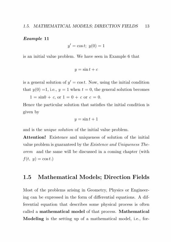
Example 11
y′ = cos t; y(0) = 1
is an initial value problem. We have seen in Example 6 that
y = sin t+ c
is a general solution of y′ = cos t. Now, using the initial condition
that y(0) =1, i.e., y = 1 when t = 0, the general solution becomes
1 = sin0 + c, or 1 = 0 + c or c = 0.
Hence the particular solution that satisfies the initial condition is
given by
y = sin t+ 1
and is the unique solution of the initial value problem.
Attention! Existence and uniqueness of solution of the initial
value problem is guaranteed by the Existence and Uniqueness The-
orem and the same will be discussed in a coming chapter (with
f(t, y) = cos t.)
1.5 Mathematical Models; Direction Fields
Most of the problems arising in Geometry, Physics or Engineer-
ing can be expressed in the form of differential equations. A dif-
ferential equation that describes some physical process is often
called a mathematical model of that process. Mathematical
Modeling is the setting up of a mathematical model, i.e., for-

14 CHAPTER 1. INTRODUCTION
mulating the problems of geometrical or physical type into math-
ematical terms by means of a differential equation, then finding
general solution to the differential equation following which par-
ticular solution is found out.
Example 12 (Geometrical problem) A curve is defined by the
condition that at each of its points (t, y), its slope is equal to
five times the abscissa of the point. Express this in terms of a
differential equation.
Solution
It is given that the slope dydt is equal to 5t. Hence the required
differential equation is dydt = 5t.
Example 13 (Physical problem) A particle of mass m moves along
the y-axis while subject to a force proportional to its displacement
y from a fixed point O in its path and directed toward O. Express
the condition by means of a differential equation.
Solution
Here force is given by –ky, where k is the proportionality con-
stant (−sign denotes the fact that the force acts in a direction
opposite to the displacement).
Hence from the equation
mass x acceleration = Force,
we obtain the desired differential equation as
md2y
dt2= −ky,
since the acceleration is given by d2ydt2.

1.5. MATHEMATICAL MODELS; DIRECTION FIELDS 15
Example 14 (A Falling Object) Suppose that an object is
falling in the atmosphere near sea level. Formulate a differential
equation that describes the motion.
Solution
1. We use m to denote mass of the object, t to denote time,
and v to represent the velocity of the falling object. We
measure m in kilograms, time t in seconds and velocity v in
meters/second.
2. Since velocity changes with time, we think of v as a function
of t ; in other words, t is the independent variable and v is
the dependent variable. v is taken to be positive in the
downward direction-that is, when the object is falling.
3. By Newton’s second law, the mass of the falling object times
its acceleration is equal to the net force on the falling object.
i.e.,
F = ma (1.7)
where m is the mass of the falling object, a is its acceleration,
and F is the net force exerted on the object. We measure a
in meters/second2, and F in Newtons. a is related to v by
a =dv
dt,

16 CHAPTER 1. INTRODUCTION
so we can rewrite Eq.(1.7) in the form
F = mdv
dt. (1.8)
Figure 1.3:
The forces that act on the object as it falls are as follows:
1. Gravity exerts a force equal to the weight of the object, or
mg, where g is the acceleration due to gravity (g is approxi-
mately equal to 9.8 m/s2 near the earth’s surface.)
2. A force due to air resistance, or drag, that is proportional
to the velocity, and has the magnitude γv, where γ is a
constant called the drag coefficient (The physical units for γ
are mass/time, or kg/s for this problem).
Before writing an expression for the net force F, we note that
gravity always acts in the downward (positive) direction, whereas

1.5. MATHEMATICAL MODELS; DIRECTION FIELDS 17
drag acts in the upward (negative) direction. Thus
F = mg − γv (1.9)
and Eq.(1.9) then becomes
mdv
dt= mg − γv (1.10)
Eq.(1.10) is a mathematical model of an object falling in the
atmosphere near sea level.
Remark The model in the previous example contains the three
constants m, g, and γ; the constants m and γ depend on the
particular object that is falling and they are usually different for
different objects; g is a physical constant, whose value is the same
for all objects.
Example 15 Formulate a differential equation that describes the
motion of an object falling in the atmosphere near sea level. Given
m = 5 kg and γ = 2.5kg/s.
Solution
Proceeding as in the previous example, we obtain Eq.(1.10).
Substituting m = 5 kg and γ = 2.5 kg/s in Eq. (1.10) and then
on simplification, we obtain
dv
dt= 9.8− v
2. (1.11)
Example 16 (Field Mice and Owls) Consider a population of
field mice who inhabit a certain rural area.

18 CHAPTER 1. INTRODUCTION
(a) In the absence of predators we assume that the mouse popu-
lation increases at a rate proportional to the current population.
Set up a mathematical model denoting time by t months and pop-
ulation by p(t).
(b) Write the differential equation if the proportionality constant
is 0.5 per month in (a) above.
(c) In addition to the problem in (b), suppose that several owls
live in the same area and that they kill 15 field mice per day. Write
the differential equation modeling this problem.
Solution
(a) In the absence of predators we assume that the mouse popu-
lation increases at a rate proportional to the current population.
If we denote time by t and the mouse population by p(t), then
the assumption about population growth can be expressed by the
equationdp
dt= rp (1.12)
where the proportionality factor r is called the rate constant or
growth rate.
(b) Suppose that time is measured in months and that the rate
constant r has the value 0.5/month. Then using (1.12),
dp
dt= 0.5p (1.13)
Each term in Eq.(1.13) has the units of mice/month.
(c) Now we add to the problem in (b) by supposing that several
owls live in the same neighborhood and that they kill 15 field mice

1.5. MATHEMATICAL MODELS; DIRECTION FIELDS 19
per day (i.e., 450 field mice per month.) To bring this informa-
tion into the model, we must add another term to the differential
equation (1.13), so that it becomes
dp
dt= 0.5p− 450. (1.14)
Remark A more general version of Eq. (1.14) is
dp
dt= rp− k (1.15)
where the growth rate r and the predation rate k are unspecified.
Geometrical Considerations, Isoclines
Consider a differential equation in the explicit form
dy
dt= f(t, y)
wheref is a given function of two variables t and y, and is called
the rate function.
The explicit form has the geometrical interpretation that the
slope of a solution y = y(t) has the value f(t0, y0) at the point
(t0, y0). This leads us to a useful graphical method for obtain-
ing a rough picture of the particular solution of the differential
equation. The procedure follows:
1. Evaluate the value of f at each point of a rectangular grid.
2. At each point of the grid, a short line segment (called lineal
element) is drawn whose slope is the value of f at that

20 CHAPTER 1. INTRODUCTION
point. Thus each lineal element is tangent to the graph of
the solution passing through that point.
3. In this way we obtain a field of lineal elements, called the
direction field (slope field) of y′ = f(t, y). With the help
of the lineal elements we can easily graph approximation
curves to the (unknown) solution curves of y′ = f(t, y) and
thus obtain a qualitatively correct picture of these solution
curves.
Procedure for Finding Direction Field
Consider a differential equation in the explicit form
dv
dt= f(t, v) (1.16)
where the rate function f is a given function of two variables t and
v. To find direction field we proceed as follows:
1. Suppose that the velocity v has a certain given valuev0.
2. Then, by evaluating the right side of Eq. (1.16), we can find
the corresponding value f(t, v0) of dvdt .
3. Display the above information graphically in the tv-plane by
drawing short line segments with slope f(t, v0) at several
points on the line v = v0.
4. As in the above way we obtain a field of lineal elements,
called the direction field (slope field).

1.5. MATHEMATICAL MODELS; DIRECTION FIELDS 21
We illustrate this method in the following example.
Example 17 (A Falling Object (continued)) Investigate the
behavior of solution of the differential equation
dv
dt= 9.8− v
5(1.17)
without solving the differential equation.
Solution
Heredv
dt= f(t, v)
where f(t, v) = 9.8− v5 .
Suppose that the velocity v has a certain given value. Then,
by evaluating the right side of Eq. (1.17), we can find the corre-
sponding value of dvdt .
1. For instance, if v = 40, then dvdt = 9.8 − 40
5 = 1.8. This
means that the slope of a solution v = v(t) has the value
f(t, 40) = 1.8 at any point wherev = 40. We display this
information graphically in the tv-plane by drawing short line
segments with slope 1.8 at several points on the linev = 40.
2. Similarly, if v = 50, then dvdt = 9.8− 50
5 = −0.2, so we draw
line segments with slope −0.2 at several points on the line
v = 50.
3. We obtain Fig. 1.4 by proceeding in the same way with other
values of v. Fig. 1.4 is the direction field (slope field) of the

22 CHAPTER 1. INTRODUCTION
given differential equation.
Figure 1.4: A direction field of Eq. (1.17): dvdt = 9.8− v
5
Now a solution of Eq. (1.17) is a function v = v(t) whose graph
is a curve in the tv-plane. The importance of the direction field
in Fig. 1.4 is that each line segment is a tangent line to one of
these solution curves. Thus, even though we have not found any
solutions, and no graphs of solutions appear in the figure, we can
draw some qualitative conclusions about the behavior of solutions:
1. For instance, if v is less than a certain critical value (i.e.,
the value of v, where dvdt = 0), then all the line segments have
positive slopes, and the speed of the falling object increases
as it falls.

1.5. MATHEMATICAL MODELS; DIRECTION FIELDS 23
2. If v is greater than a certain critical value, then the line
segments have negative slopes, and the speed of the falling
object decreases as it falls.
Now dvdt = 0 implies 9.8 − v
5 = 0 implies v = (5)(9.8) = 49 m/s.
It is the critical value of v that separates objects whose speed is
increasing from those whose speed is decreasing.
Figure 1.5: Direction field and equilibrium solution for Eq. 1.17
The constant function v(t) = 49 is a solution of Eq. (1.17),
since substituting v(t) = 49(so that dvdt = 0) into Eq. (1.17) makes
each side of the equation (1.17) to zero. Being a constant function,
the solution v(t) = 49 does not change with time, and is called
an equilibrium solution. It is the solution that corresponds
to a perfect balance between gravity and drag. The equilibrium
solution v(t) = 49 is shown by superimposing on the direction field
given in Fig. 1.5. From this figure we can conclude that all other

24 CHAPTER 1. INTRODUCTION
solutions seem to be converging to the equilibrium solution as t
increases.
Remark: In an earlier example we have seen that the general
solution of the differential equation
dv
dt= 9.8− v
5
is
v = v(t) = 49 + c e−15 t.
Also it can be seen that as t → ∞, e−15 t → 0 so that v(t) → 49,
the equilibrium solution.
Example 18 Find the equilibrium solution of
mdv
dt= mg − γv (m > 0, γ > 0).
Solutiondvdt = 0 implies mg − γv = 0 implies v = mg
γ .
Hence the equilibrium solution is
v =mg
γ.
Example 19 Find the equilibrium solution of
dv
dt= rp− k. (1.18)
Solutiondvdt = 0 gives rp− k = 0 implies p(t) = k
r .

1.5. MATHEMATICAL MODELS; DIRECTION FIELDS 25
Hence the equilibrium solution of Eq.(1.18) is p(t) = k/r.
Example 20 Investigate the solutions of
dp
dt= 0.5p− 450 (1.19)
graphically.
Solution
Figure 1.6: Direction field and equilibrium solution for Eq. (1.19)
A direction field for Eq.(1.19) is shown in Fig. 1.6. For suffi-
ciently large values of p it can be seen from the figure or directly
from Eq.(1.19) itself, that dp/dt is positive, so that solutions in-
crease. On the other hand, if p is small, then dp/dt is negative and
solutions decrease. Again, the critical value of p, which separates
solutions that increase from those that decrease, is the value of
p for which dp/dt is zero. Now dp/dt = 0 in Eq.(1.19) gives the

26 CHAPTER 1. INTRODUCTION
equilibrium solution
p(t) = 900
for which the growth term 0.5 and the term 450 in Eq.(1.19) are
exactly balanced. The equilibrium solution is superimposed in the
direction field shown in Fig. 1.6.

Chapter 2Solutions of Some Differential
Equations
2.1 Solutions of Differential Equations
Example 1[ A Falling Object (continued)] Consider a falling
object of mass m = 10 kg and drag coefficient γ = 2 kg/s. Sup-
pose the object is dropped from a height of 300m. Find its velocity
at any time t. How long will it take to fall to the ground, and how
fast will it be moving at the time of impact?
Solution
If the velocity is v, with the aid of Eq.(1.10) in the previous
chapter, the differential equation corresponding to the given prob-
lem is
10dv
dt= 10× 9.8− 2v.
27

28CHAPTER 2. SOLUTIONS OF DIFFERENTIAL EQUATIONS
i.e.,dv
dt= 9.8− v
5. (2.1)
The object is dropped means the initial velocity is zero, so we have
the initial condition
v(0) = 0. (2.2)
Writing (2.1) in the form
dv/dtv − (9.8)(5)
= −15.
and integrating both sides, we obtain
ln |v(t)− 49| = − t5
+ C
which gives
v(t)− 49 = e−t5+C
so that (by taking c = eC) it follows that
v(t) = 49 + ce−t5 .
That is, the general solution of Eq. (2.1) is
v = 49 + ce−t/5 (2.3)
where c is arbitrary. To determine c, we substitute t = 0 and
v = 0 from the initial condition (2.2) into Eq. (2.3), and obtain

2.1. SOLUTIONS OF DIFFERENTIAL EQUATIONS 29
c = −49. Then the solution of the initial value problem is
v = 49(1− e−t/5). (2.4)
Eq. (2.4) gives the velocity of the falling object at any positive
time (before it hits the ground).
Remark Graphs of the solution (2.3) for several values of c are
shown in Fig.2.1, with the solution (2.4) shown by the heavy curve.
It is evident that all solutions tend to approach the equilibrium
solution v = 49. This confirms the conclusions we reached earlier
on the basis of the direction fields in Fig.1.4 and Fig.1.5.
Figure 2.1:
To find the velocity of the object when it hits the ground, we
need to know the time at which impact occurs. In other words, we
need to determine how long it takes the object to fall 300 m. To

30CHAPTER 2. SOLUTIONS OF DIFFERENTIAL EQUATIONS
do this, we note that the distance x the object has fallen is related
to its velocity v by the equation v = dx/dt, or
dx
dt= 49(1− e−t/5). (2.5)
Consequently, by integrating both sides of Eq.(2.5), we have
x = 49t+ 245e−t/5 + c (2.6)
where c is an arbitrary constant of integration. The object starts
to fall when t = 0, so we know that x = 0 whent = 0. From
Eq.(2.6) it follows that c = −245, so the distance the object has
fallen at time t is given by
x = 49t+ 245e−t/5 − 245. (2.7)
Let T be the time at which the object hits the ground; then x =
300 when t = T . By substituting these values in Eq.(2.7), we
obtain the equation
300 = 49T + 245 e−T5 − 245
or
49T + 245eT/5 − 545 = 0. (2.8)
The value of T satisfying Eq. (2.8) can be approximated by a
numerical process (for example, Newton-Raphson Method) using a
scientific calculator or computer, with the result that T ∼= 10.51 s.

2.1. SOLUTIONS OF DIFFERENTIAL EQUATIONS 31
At this time, the corresponding velocity vT is found from Eq. (2.4)
to be vT∼= 43.01 m/s. The point (10.51, 43.01) is also shown in
Fig. 2.1.
Example 2 (Radioactivity, exponential decay) Experiments show
that a radioactive substance decomposes at a rate proportional to
the amount present at time t. Suppose at time t = 0, 2 grams of
a particular radioactive substance be present. Then what amount
of the substance will be there at time t (t > 0).
Solution
Step 1 (Setting up a mathematical model of the physical process)
Let y(t) denote the amount of substance present at time t. It is
given that rate of change dy/dt is proportional to y. Thus
dy
dt= ky,
where k is the proportionality constant of negative sign, which is a
constant depends only on the nature of the radioactive substance.
(For example, if the radioactive substance is radium, then k ≈−1.4× 10⁻¹¹ sec−1)
Step 2 (Solving the differential equation)
The given differential equation, by separating variables (a de-
tailed discussion will be made in the next chapter), gives
dy
y= k.

32CHAPTER 2. SOLUTIONS OF DIFFERENTIAL EQUATIONS
Integrating with respect to t,
ln y = kt+ C
Hence
y(t) = cekt, with c = eC
is the general solution to the differential equation dydt = ky.
Step 3 (Determination of a particular solution using the initial
conditions) The particular solution satisfying the given initial con-
dition can be obtained by finding out the particular value of c.
Now by putting t = 0, y = 2 in y(t) = cekt we get c = 2 and so
the unique solution to the initial value problem is y(t) = 2ekt.
Hence the amount of substance at time t is given by y(t) = 2ekt
Example 3 Find the curve through the point (1, 1) in the xy-
plane having at each of its points the slope is –y/x.
Solution
Step 1 (Setting up a mathematical model of the geometrical prob-
lem)
Here y is a function of x and it is given that the slope dy/dx is
–y/x. i.e., the differential equation is
dy
dx= −y
x.
Step 2 (Solving the differential equation)

2.1. SOLUTIONS OF DIFFERENTIAL EQUATIONS 33
Separating the variables, we obtain
dy
y= −dx
x.
Integration yields,
ln y = − lnx+ ln c
i.e.,
ln y + lnx = ln c
i.e.,
yx = c
i.e.,
y =c
x
That is, the general solution to the differential equation dydx = − y
x
is y(x) = cx , where c is an arbitrary constant.
Step 3 (Determination of a particular solution)
We want to find out the particular solution that passes through
the point (1,1). Now by putting x = 1, y = 1 in y(x) = cx we get
c = 1 and so the particular solution is y(x) = 1x .
Example 4 Let g denote the acceleration due to gravity (with
value 9.8ms−1) and s(t) the distance of a freely falling body in
vacuum at time t sec. Set up a mathematical model (i.e., set up a
differential equation) for the law that “the acceleration of a freely
falling body in vacuum is the acceleration due to gravity.” Also,

34CHAPTER 2. SOLUTIONS OF DIFFERENTIAL EQUATIONS
show that the particular solution such that s = 0 at time t = 0 is
s(t) =12gt2.
Solution
Step 1 (Setting up a mathematical model)
By the law, acceleration = g,
i.e.,d2s
dt2= g.
Step 2 (Solving the differential equation)
Integrating the differential equation, we get
ds
dt= gt+A,
where A is an arbitrary constant. Further integration yields,
s =12gt2 +At+B,
where B is also an arbitrary constant. This is the solution to the
differential equation.
Step 3 (Determination of a particular solution)
At time t = 0, s = 0. Also, since the body is freely falling, velocity
is zero, so that ds/dt = 0. Using these values, equations in Step 2
gives
A = 0, B = 0,

2.1. SOLUTIONS OF DIFFERENTIAL EQUATIONS 35
and we obtain the particular solution
s(t) =12gt2.
Exercises
In Exercises 1- 6, state the order of the given differential equation:
1. y′ + 5y = 0
2. y′′ + 4y = 0
3. y′ − y = 0
4. y′′′ = 6
5. y′ + y tanx = 0
6. y′ − 3y2 = 0
In Exercises 7-11, verify that the given function is a solution
of the differential equation given to the right of it.
7. y = ce−8x; y′ + 8y = 0
8. y = c1ex + c2e
−x; y′′ − y = 0
9. y = x4 + ax2 + bx+ c; y′′′ = 24x
10. y = A cosx; y′ + y tanx = 0
11. y = A cos 3x+B sin 3x; y′′ + 9y = 0
In Exercises 12-15 , verify that the given function is a so-
lution of the differential equation given to the right of it.
Graph the corresponding curves for some values of the con-
stant c.
12. y = ce−x; y′ + y = 0
13. y = ce−x + 4; y′ + y = 4

36CHAPTER 2. SOLUTIONS OF DIFFERENTIAL EQUATIONS
14. y = cx4; xy′ − 4y = 0
15. x2 + y2 = c; yy′ = −x In Exercises 16-19, verify that
the given function is a solution of the differential equation
given to the right of it and determine c so that the resulting
particular solution satisfies the given condition. Graph this
particular solution.
16. y = 3x+ c; y′ = 3; y = 1 when x = 0.
17. y = ce−x2+ 2; y′ + 2xy = 0; y = 0.5 when x = 0.
18. y = ce−x + 2; y′ + y = 2; y = 3.2 when x = 0.
19. y = x3 + c; y′ = 3x2; y = −1 when x = 1.
In Exercises 20-23, find a first order differential equation
involving both y and y′ for which the given function is a
solution.
20. y = cos 2x21.y = xe−x
21. y = −e−3x23.y = x3 − 78
22. y = e−x2
23. y = x3
24. y = tanx
25. x2 + y2 = 16.

Chapter 3First Order Linear Equations
In this chapter we discuss a method for the solution of first order
ordinary linear differential equations.
3.1 Linear First Order Differential Equa-
tions
A first order differential equation of the form
dy
dt+ p(t)y = g(t)
where p(t) and g(t) are functions of t alone, is a first order linear
differential equation.
If g(t) = 0 for every t, the equation is said to be
homogeneous. Otherwise it is said to be nonhomogeneous.
37

38 CHAPTER 3. FIRST ORDER LINEAR EQUATIONS
Determination of formula for the solution of the homoge-
neous linear differential equation
Consider the general first order linear equation
dy
dt+ p(t)y = g(t) (3.1)
where p and g are given functions of t alone.
By multiplying the differential equation (3.1) by a certain func-
tion µ(t), the resulting equation would be readily integrable. The
function µ(t) is called an integrating factor.
To determine an appropriate integrating factor, we multiply
Eq. (3.1) by an as yet undetermined function µ(t), obtaining
µ(t)dy
dt+ p(t)µ(t)y = µ(t)g(t). (3.2)
By the product rule of differentiation, we have
d
dt[µ(t)y] = µ(t)
dy
dt+dµ(t)dt
y.
Hence the left side of Eq. (3.2) is the derivative of the product
µ(t)y, provided that µ(t) satisfies the equation
dµ(t)dt
= p(t)µ(t). (3.3)

3.1. LINEAR EQUATIONS 39
If we assume temporarily that µ(t) is positive, then we have
dµ(t)/dtµ(t)
= p(t),
and hence, integration yields
ln µ(t) =∫p(t)dt+ k.
Now let k = 0. Then we obtain
ln µ(t) =∫p(t)dt.
Since exp (lnx) = x, for x > 0, and since our assumption is that
µ(t) > 0, the above gives
µ(t) = exp∫p(t)dt. (3.4)
Returning to Eq.(3.2), we have
d
dt[µ(t)y] = µ(t) g(t). (3.5)
Integrating, we obtain
µ(t) y =∫µ(t)g(t) dt+ c (3.6)
where c is an arbitrary constant. Sometimes the integral in Eq.
(3.6) can be evaluated in terms of elementary functions. However,
in general this is not possible, so the general solution of Eq. (3.1)

40 CHAPTER 3. FIRST ORDER LINEAR EQUATIONS
is
y =1µ(t)
[∫ t
t0
µ(s)g(s)ds+ c
](3.7)
where t0 is some convenient lower limit of integration. Observe
that Eq.(3.7) involves two integrations, one to obtain µ(t) from
Eq.(3.4) and the other to determine y from Eq.(3.7)
Working Method for the Solution of Linear Differential
Equations
To find the general solution of the linear differential equation
dy
dx+ p(t)y = g(t) (3.8)
1. Find the integrating factor by the formula
µ(t) = exp ∫ p(t)dt. (3.9)
2. Multiply Eq.(3.8) by µ(t) and obtain
d
dt[µ(t)y] = µ(t)g(t) (3.10)
3. Integrating the above, we obtain
µ(t) y = ∫ µ(t) g(t) dt + c. (3.11)
Example 1 Solve the linear differential equation
dy
dt− y = e2t.

3.1. LINEAR EQUATIONS 41
Solution
Here p(t) = −1, g(t) = e2t. Hence the integrating factor is given
by
µ(t) = e∫
p(t) dt = e∫−dt = e−t.
Using (3.11), implicit solution is given by
ye−t =∫e2te−tdt+ c.
The corresponding explicit solution is
y = et∫etdt+ cet
i.e., y(t) = e2t + cet
Example 2 Solve the differential equation
sin 2tdy
dt= y + tan t.
Solution
Given equation can be written as
dy
dt− y
sin 2t=
tan tsin 2t
=12
sec2 t,
which is in the linear form. The integrating factor is given by
µ(t) = e∫
p(t)dt = e−12
∫1
sin t cos tdt = e−
12
∫sec2 ttan t
dt
= e−12
log tan t =1√tan t
.

42 CHAPTER 3. FIRST ORDER LINEAR EQUATIONS
Hence, using (3.11) solution is given by
y1√tan t
=12
∫sec2 t√tan t
dt+ c
i.e.,y√tan t
=√
tan t+ c.
Example 3 At time t = 0 a tank contains Q0 lb of salt dissolved
in 100gal of water (Fig. 3.1). Assume that water containing 14 lb
of salt/gal is entering the tank at a rate of r gal/min and that the
well-stirred mixture is draining from the tank at the same rate.
Assuming that salt is neither created nor destroyed in the tank set
up the initial value problem that describes this flow process. Find
the amount of salt Q(t) in the tank at any time, and also find the
limiting amount QL that is present after a very long time. If r = 3
and Q0 = 2QL, find the time T after which the salt level is within
2% of QL. Also find the flow rate that is required if the value of
T is not to exceed 45 min.
Solution
1. The rate of change of salt in the tank, dQdt , is equal to the
rate at which salt is flowing in minus the rate at which it is
flowing out.
2. The rate at which salt enters the tank is the concentration14 lb/galtimes the flow rate r gal/min, or r
4 lb/min.

3.1. LINEAR EQUATIONS 43
Figure 3.1:
3. To find the rate at which salt leaves the tank, we need to
multiply the concentration of salt in the tank by the rate of
outflow, r gal/min.
4. Since the rates of flow in and out are equal, the volume of
water in the tank remains constant at 100 gal, and since the
mixture is ‘well-stirred’, the concentration throughout the
tank is the same, and is Q(t)100 lb/gal. Therefore the rate at
which salt leaves the tank is r Q(t)100 lb/min.
From the above information, the differential equation governing
the given process isdQ
dt=r
4− rQ
100. (3.12)
The initial condition is
Q(0) = Q0. (3.13)

44 CHAPTER 3. FIRST ORDER LINEAR EQUATIONS
Rewriting Eq. (3.12) in the standard form for a linear equation,
we havedQ
dt+rQ
100=r
4
Thus the integrating factor is ert/100and the general solution is
Q(t) = 25 + ce−rt/100
where c is an arbitrary constant. To satisfy the initial condition
(3.13), we must choose c = Q0 − 25. Therefore the solution of the
initial value problem (3.12), (3.13) is
Q(t) = 25 + (Q0 − 25)e−rt/100 (3.14)
or
Q(t) = 25(1− e−rt/100) +Q0e−rt/100 (3.15)
From Eq.(3.14) or (3.15), we can see that Q(t) → 25(lb)as t→∞,
so the limiting value QLis 25.
Now suppose that r = 3 and Q0 = 2QL = 50; then Eq.(??)
becomes
Q(t) = 25 + 25e−0.03t (3.16)
Since 2% of 25 is 0.5, we wish to find the time T at which Q(t)
has the value 25.5. Substituting t = T and Q = 25.5 in Eq. (3.16)

3.1. LINEAR EQUATIONS 45
and solving for T , we obtain1
T = (ln 50)/0.03 ∼= 130.4 min
To determine the value of r at T = 45, we use Eq. (3.14), set
t = 45, Q0 = 50, Q(t) = 25.5,and solve for r. We obtain
r = (100/45) ln 50 ∼= 8.69 gal/min
Example 4 Consider a pond that initially contains 10 million
gal of fresh water. Water containing an undesirable chemical flows
into the pond at the rate of 5 million gal/yr, and the mixture
in the pond flows out at the same rate. The concentration γ(t)
of chemical in the incoming water varies periodically with time
according to the expression γ(t) = 2 + sin 2t g/gal. Construct a
mathematical model of this flow process and determine the amount
of chemical in the pond at any time.
Solution
1. Since the incoming and outgoing flows of water are the same,
the amount of water in the pond remains constant at 107 gal.
2. Let us denote time by t, measured in years, and the chemical
by Q(t), measured in grams. Then the rate of change of
chemical in the pond, dQdt , is equal to the rate at which the
chemical flows into the pond minus the rate at which it is
flowing out.1Note that ln 50 is the natural logarithm of 50.

46 CHAPTER 3. FIRST ORDER LINEAR EQUATIONS
(a) The rate at which the chemical flows in is
γ× (5×10⁶) gal/yr = (5×10⁶) gal/ yr (2+sin 2t) g/gal
(b) The concentration of chemical in the pond is Q(t)107 g/gal,
so the rate of flow out is
(5× 10⁶) gal/yr [Q(t)/107] g/gal =Q(t)
2g/yr
From the above information, we obtain the differential equation
dQ
dt= (5× 10⁶)(2 + sin 2t)− Q(t)
2,
where each term has the units of g/yr.
Let q(t) = Q(t)/106. Then
dq
dt=
1106
dQ
dt,
sodQ
dt= 106dq
dt.
Substituting these values, we obtain
dq
dt+
12q = 10 + 5 sin 2t (3.17)
Initially, there is no chemical in the pond, so the initial condition
is
q(0) = 0. (3.18)

3.1. LINEAR EQUATIONS 47
The integrating factor of the linear differential equation is µ(t) =
e∫12dt = e
t2 . Multiplying Eq.(3.17) by this factor we obtain
d
dt(µ(t)q(t)) = (10 + 5 sin 2t)µ(t).
Integrating, we obtain
µ(t) q(t) = ∫ µ(t) (10 + 5 sin 2t) dt+ C
i.e.,
et/2q(t) = ∫ (10 + 5 sin 2t) et/2dt+ C
i.e.,
et/2q(t) = 20et/2 + 5 ∫ sin 2tet/2dt+ C
Take
I = ∫ sin 2t et/2dt
and apply integration by parts,
∫ uv′ = uv − ∫ u′v
with u = sin 2t and v′ = et/2. Then
I = sin 2tet/2
12
− ∫ 2 cos 2tet/2
12
dt
= 2 sin 2tet/2 − 4
{cos 2t︸ ︷︷ ︸
u
et/2︸︷︷︸v′
dt
with new u = cos 2t and v′ = et/2

48 CHAPTER 3. FIRST ORDER LINEAR EQUATIONS
= 2 sin 2tet/2 − 4
[cos 2t · e
t/2
12
−∫−sin 2t
2· e
t/2
12
dt
]= 2 sin 2t et/2 − 8 cos 2t et/2 − 16I.
Hence
I =117
[2 sin 2t et/2 − 8 cos 2t et/2
]Substituting this and simplifying, we obtain the general solution
q(t) = 20− 4017
cos 2t+1017
sin 2t+ ce−t/2
Using the initial condition we obtain
0 = q(0) = 20− 4017
+ c,
which gives
c = −300/17,
so the solution of the initial value problem (3.17) with (3.18) is
q(t) = 20− 4017
cos 2t+1017
sin 2t− 30017
e−t/2.
Exercises
In Exercises 1-10, find the general solution of the differential
equation.
1. dydt − y = 3
2. y′ + 2ty = 0
3. y′ + 2y = 6et
4. y′ − 4y = 2t− 4t2

3.1. LINEAR EQUATIONS 49
5. y′ + y = sin t
6. y′ + y = cos t
7. y′ + ky = cos t
8. y′ = (y − 1) cot t
9. ty′ − 2y = t3et
10. t2y′ + 2ty = sinh 3t
In Exercises 11-23, solve the given initial value problem.
11. y′ − y = et, y(1) = 0
12. y′ + y = (t+ 1)2, y(0) = 0
13. y′ − 2y = 2 cosh 2t+ 4 , y(0) = −1.25
14. ty′ − 3y = t4(et + cos t)− 2t2 , y(π) = π3eπ + 2π2
15. y′ − y cot t = 2t− t2 cot t, y(π2 ) = π2
4 + 1
16. y′ − y = 2te2t, y(0) = 1
17. y′ + 3y = te−3t, y(1) = 0
18. ty′ + 2y = t2 − t+ 1, y(1) = 12 , t > 0
19. y′ + (2/t)y = (cos t)/t2, y(π) = 0, t > 0
20. y′ − 4y = e4t, y(0) = 2
21. ty′ + 2y = sin t, y(π/2) = 1, t > 0
22. t3y′ + 4t2y = e−t, y(−1) = 0, t < 0
23. ty′ + (t+ 1)y = t, y(ln 2) = 1, t > 0

50 CHAPTER 3. FIRST ORDER LINEAR EQUATIONS
24. Consider a tank used in certain hydrodynamic experiments.
After one experiment the tank contains 150 L of a dye solu-
tion with a concentration of 1 g/L. To prepare for the next
experiment, the tank is to be rinsed with fresh water flowing
in at a rate of 2 L/min. the well-stirred solution flowing out
at the same rate. Find the time that will elapse before the
concentration of dye in the tank reaches 1% of its original
value.
25. A tank originally contains 100 gal of fresh water. Then water
containing 12 lb of salt per gallon is poured into the tank at
a rate of 2 gal/min, and the mixture is allowed to leave at
the same rate of 2 gal/min, with the mixture again leaving
at the same rate. Find the amount of salt in the tank at the
end of an additional 10 min.
26. Suppose that a sum S0 is invested at an annual rate of return
r compounded continuously.
27. Find the time T required for the original sum to double in
value as a function of r.
28. Determine T if r = 8%
29. Find the return rate that must be achieved if the initial
investment is to double in 8 years.
30. Raju borrows ‘ 8000to buy a motor bike. The lender charges
interest at an annual rate of 10%. Assuming that interest is

3.1. LINEAR EQUATIONS 51
compounded continuously and Raju makes payments contin-
uously at a constant annual rate k, determine the payment
rate k that is required to pay off the loan in 3 years. Also
determine how much interest is paid during the 3-year pe-
riod.
Answers
1. y = c et − 3
2. yet2
= c
3. y = c e−2t + 2 et
4. y = t2 + ce4t
5. y = c et + 12 (sin t − cos t)
6. y = 15 (2 cos t + sin t) + c e−2t
7. y = ( c + t) e−4t
8. y = 1 + c sin t
9. y = c t2 + t2 et
10. y = (13 t
2 )( cosh 3t + c)
11. y = (t + 1)et
12. y = −e−t + t2 + 1
13. y = (t + 1) e2t − 14e
−2t − 2
14. y = [et + sin t ] t3 + 2t2

52 CHAPTER 3. FIRST ORDER LINEAR EQUATIONS
15. y = t2 + sin t
16. y = 3et + 2(t− 1)e2t
17. y = (t2 − 1) e−3t
2
18. y = 3t4−4t3+6t2+112t2
19. y = sin tt2
20. y = (t+ 2)e4t
21. y = t−2[
π2
4 − 1− t cos t+ sin t]
22. y = − (1+t)e−t
t4, t 6= 0
23. y = t−1+2e−t
t , t 6= 0
24. t = 75 ln 100 min ∼= 345.4 min
25. Q = 50e−0.2(1− e−0.2) lb ∼= 7.42 lb
26. (a) ln 2r yr (b) 8.66 yr (c) 8.66
27. k = 3086.64 /yr 3× 3086.64− 8000 = ‘ 1259.92
3.2 Method of Variation of Parameters
Method of variation of parameter (M.V.P) is an alternative
method for finding the general solution of the linear differential
equation
y′ + p(t)y = g(t). (3.19)
A solution of the corresponding homogeneous equation (i.e.,
an equation with g(t) ≡ 0) is
y(t) = Ae−∫
p(t)dt (3.20)

3.2. METHOD OF VARIATION OF PARAMETERS 53
Using this function, let us try to find out a function A(t) such that
y(t) = A(t)e−∫
p(t)dt (3.21)
is the general solution of the nonhomogeneous linear equation in
(3.19). This attempt is suggested by the form of the general solu-
tion Ay(t)of the homogeneous equation and consists in replacing
the parameter A by a variable A(t). Therefore, this approach is
called the method of variation of parameters.
Working Method for solving by method of variation of
parameters
To solve the linear differential equation
y′ + p(t)y = g(t)
(i) First find the solution y(x)of the corresponding homogeneous
equation
y′ + p(t)y = 0
by the formula
y(t) = Ae−∫
p(t)dt
(ii) Then replace A by A(t) and find the function A(t) by sub-
stituting
y(t) = A(t)e−∫
p(t)dt
in the non-homogeneous linear differential equation.

54 CHAPTER 3. FIRST ORDER LINEAR EQUATIONS
Example 5 Applying method of variation of parameters solve
dy
dt− y = 3et.
Solution
Here p(t) = −1, g(t) = 3et.
Hence the general solution to the corresponding homogeneous equa-
tion is given by
y(t) = Ae−∫
p(t)dt = Ae−∫−1dt = Aet.
Replacing A by A(t), and assuming that y(t) = A(t)et is the gen-
eral solution of the nonhomogeneous equation, our next aim is
find the function A(t), by substituting y(t) = A(t)et in the given
nonhomogeneous differential equation, which gives
dA(t)dt
et +A(t)et −A(t)et = 3et
ordA(t)dt
et = 3et
ordA(t)dt
= 3.
Integrating, we obtain
A(t) = 3t+ c.

3.2. METHOD OF VARIATION OF PARAMETERS 55
Hence the general solution to the given differential equation is
y = (3t+ c)et.
Exercises
Solve the following equations by the method of variation of pa-
rameters:
1. y′ − y = t
2. ty′ + 2y = sin tt
3. y′ = e2t + y − 1
4. y′ + 2y = e−2t
5. ty′ − 2y = t4
6. (t+ 4)y′ + 3y = 3
7. y′ − 2y = t2e2t
8. y′ + yt = 3 cos 2t, t > 0
9. ty′ + 2y = cos t, t > 0
10. 2y′ + y = 3t2
11. y′ − y = e2x
Answers
1. y = c et − t− 1
2. t2y + cos t = c
3. y = e2t + 1 + c et
4. y = (t+ c)e−2t
5. 12 t
4 + c t2
6. y = 1 + c(t+4)3
7. y = ce2t + t3e2t
3
8. y = ct + 3 cos 2t
4t + 3 sin 2t2
9. y = c+cos t+t sin tt2
10. y = ce−t/2 + 3t2 − 12t+ 24
11. y = e2x + cex
56 CHAPTER 3. FIRST ORDER LINEAR EQUATIONS
3.3 Bernoulli’s Equation
A differential equation of the form
y′ + p(t)y = g(t)yn (3.22)
where p(t) and g(t) are functions of t alone is called Bernoulli’s
equation. (Note that here n may be any real number). We can
reduce equation (3.22) to the linear form as follows:
Dividing both sides of (3.22) by yn, we get
y−ny′ + p(t)y1−n = g(t)
Putting y1−n = z, this equation becomes
11− n
z′ + p(t)z = g(t)
i.e.,
z′ + (1− n)p(t)z = g(t)(1− n) (3.23)
Now (3.23) is in the linear form, solution of which is familiar to
us. After solving for z in (3.23), using y1−n = z, we get the value
of y, i.e., the solution of (3.22).
Example 6 Solve tdydt + y = ty3.
Solution

3.3. BERNOULLI’S EQUATION 57
Dividing the given differential equation by y3, we obtain
t
y3
dy
dt+
1y2
= t.
Putting 1y2 = z, the equation becomes
−12tdz
dt+ z = t.
i.e.,dz
dt− 2tz = −2.
The above is a linear differential equation and its integrating factor
is
µ(t) = e∫
p(t)dt = e∫− 2
tdt = e−2 ln|t| = eln|t|
−2
= |t|−2 =1t2.
Hence the solution is given by
z1t2
=∫−2
1t2dt+ c
orz
t2=
2t
+ c.
Now substituting z = 1t2
, the solution of the given differential
equation is
(2 + ct)ty2 = 1.
We can solve certain non linear first order ordinary differential

58 CHAPTER 3. FIRST ORDER LINEAR EQUATIONS
equation in a similar fashion as we solve a Bernoulli equation. This
is illustrated in the following Example.
Example 7 Solve dydt + t sin 2y = t3 cos2 y.
Solution
Dividing by cos2 y, we obtain
sec2 ydy
dt+ 2t tan y = t3
Put tan y = z. Then
sec2 ydy
dt=dz
dt
and the equation becomes the linear differential equation
dz
dt+ 2tz = t3.
Now the integrating factor is given by
µ(t) = e∫
p(t)dt = e∫
2t dt = et2.
So the solution is
zet2
=∫t3et
2dt+ c
or
zet2
=12
∫2t · t2et2dt+ c
or
zet2
=12
∫ueudu+ c,

3.3. BERNOULLI’S EQUATION 59
where u = t2. Hence
zet2
=12eu(u− 1) + c
or
zet2
=12et
2(t2 − 1) + c
or
tan yet2
=12et
2(t2 − 1) + c
or
tan y =12(t2 − 1) + ce−t2 .
Exercises
Solve the following equations:
1. y′ + ty = ty−1
2. y′ + t−1y = t−1y−2
3. 2ty′ = 10t3y5 + y
4. y′ + y = ty−1
5. y′ − y tan t = sin t cos2 ty2
6. y′ = y tan t− y2 sec t
7. ty′ + y = y2 log t
8. y′ + yt−1 = t3y4
9. y′ + ty1−x2 = ty1/2
10. ty′ + y2t−1 = y
11. (1− t2)y′ − ty = t2y2
12. ty′ + y = t2y2 log t
13. tdydt + y = t3y6
14. Solve the initial value problem y′ − yt−1 = 12y
−1; y(1) = 0.
Answers

60 CHAPTER 3. FIRST ORDER LINEAR EQUATIONS
1. y2 = 1 + cet−2
5. y3 cos3 t = 12 cos6 t+ c
6. (t+ c)y = sin t
7. y(log t+ 1) + cty = 1
8. (c− 3t)t3y3 = 1
9.√y+ 1
3(1− t2) = c(1− t2)1/4
10. x = y(log t+ c)
11. (1 + ty) = y(1 − t2)1/2(c +
sin−1 t)
12. t3y(1− log t) + cty = 1
13. (ty)−5 = 52 t−2 + c
14. t2 − y2 − t = 0.

Chapter 4Separable Equations
Certain first order differential equations can be reduced to the
form
N(y) dy = M(x)dx (4.1)
by algebraic manipulations. An equation that can be brought
to the form as in (4.1) is called an equation with separable variables,
or a separable equation, because in (4.1) the variables x and y
are separated so that terms involving x appear only on the right
and that of y appears only on the left. By integrating both sides
of (4.1), we obtain
∫N (y) dy =
∫M (x) dx + c (4.2)
where c is an arbitrary constant.
If we assume that f and g are continuous functions, the
61

62 CHAPTER 4. SEPARABLE EQUATIONS
integrals in (4.2) will exist, and by evaluating these integrals we
obtain the general solution of the given differential equation.
4.1 Identifying and Solving Separable Equa-
tions
Consider the first order differential equation
dy
dx= f(x, y). (4.3)
To identify when an equation of the above form is a separable
equation, we first rewrite Eq.(4.3) in the form
M(x, y) +N(x, y)dy
dx= 0. (4.4)
It is always possible to do this by setting M(x, y) = −f(x, y)and
N(x, y) = 1, but there may be other ways as well. If it happens
that M is a function of x only and N is a function of y
only, then Eq.(4.4) becomes
M(x) +N(y)dy
dx= 0. (4.5)
such an equation is said to be separable, because if it is written
in the differential form
M(x)dx+N(y)dy = 0, (4.6)

4.1. SOLVING SEPARABLE EQUATIONS 63
then, terms involving each variable may be placed on opposite
sides of the equation. The differential form (4.6) is also more sym-
metric and tends to suppress the distinction between independent
and dependent variables.
We now show that a separable equation can be solved by
integrating the functions M and N. To show this, let H1 and H2
be any antiderivatives of M and N, respectively. Thus
H ′1(x) = M(x), H ′
2(y) = N(y), (4.7)
and then Eq.(4.5) takes the form
H ′1(x) +H ′
2(y)dy
dx= 0. (4.8)
Since H2 is a function of y and y is a function of x, by the Chain
Rule for Functions of One Variable,1 we haved
dxH2(y) =
d
dyH2(y)
dy
dx.
1The Chain Rule for Functions of One VariableLet w = f(y) be a differentiable function of y and y = ϕ(x) be a differentiablefunction of x, then w is a differentiable composite function of x and thederivative dw
dxcould be calculated using the Chain Rule given by
dw
dx=
dw
dy· dy
dx.
As an example, using the Chain Rule, we find dwdx
, when w = cosh−1 y, andy = x2 as follows:
dw
dx=
d
dy(cosh−1 y)
d
dx(x2) =
1√y2 − 1
· 2x =2x√
x4 − 1.

64 CHAPTER 4. SEPARABLE EQUATIONS
Also noting that
H ′2(y) =
d
dyH2(y),
the above gives
H ′2(y)
dy
dx=
d
dyH2(y)
dy
dx=
d
dxH2(y). (4.9)
Hence, we can write Eq.(4.8) as
d
dxH1(x) +
d
dxH2(y) = 0.
i.e.,d
dx[H1(x) +H2(y)] = 0 (4.10)
Integrating Eq.(4.10), we obtain
H1(x) +H2(y) = c, (4.11)
where c is an arbitrary constant. Any differentiable function
y = φ(x) that satisfies Eq.(4.11) is a solution of Eq.(4.5); in other
words, Eq.(4.11) defines the solution implicitly rather than explic-
itly.
Example 1 Show that the differential equation
10y · dydx
+ 3x = 0 (4.12)
is separable. Illustrate the procedure discussed above by solving
this differential equation.

4.1. SOLVING SEPARABLE EQUATIONS 65
Solution
The given differential equation can be written as
3x+ 10ydy
dx= 0
Comparing with the standard equation,
M(x) = 3x and N(y) = 10y.
Hence given is a separable equation.
Since y is a function of x, by the chain rule
d
dxf(y) =
d
dyf(y)
dy
dx= f ′(y)
dy
dx.
Here f ′(y) = 10y. Hence
f(y) =10y2
2= 5y2.
Also 3x is the derivative of 3x2
2 . Hence (4.12) takes the form
d
dx
(3x2
2
)+
d
dx
(5y2)
= 0
i.e.,d
dx
(3x2
2+ 5y2
)= 0
By integrating, we obtain
3x2
2+ 5y2 = C.

66 CHAPTER 4. SEPARABLE EQUATIONS
Method of Solving Separable Equation
In practice, Eq.(4.11) is usually obtained from Eq.(4.6) by in-
tegrating the first term with respect to x and the second term with
respect to y. This is illustrated in the following example.
Example 2 Solve the differential equation dydx + 2xy = 0.
Solution
The given equation can be written in the form
2xdx+dy
y= 0.
The above is in the variable separable form with
M(x) = 2x and N(y) = 1y .
By integrating the first term of the differential equation with re-
spect to x and the second term with respect to y, we obtain
x2 + ln y = c
or ln y = −x2 + c.
Since exp lnw = w (for w > 0), the above yields
or
y = e−x2+c.
The above can also be written as y = Ce−x2, where C = ec in an
arbitrary constant.
Example 3 Solve the differential equation dydx = 1 + y2.
Solution

4.1. SOLVING SEPARABLE EQUATIONS 67
The given differential equation can be written as
dy
1 + y2= dx,
or
−dx+dy
1 + y2= 0
which is in the variable separable form with
M(x) = −1 and N(y) =1
1 + y2.
By integrating the first term of the differential equation with
respect to x and the second term with respect to y, we obtain
−x+ tan−1 y = c
or
tan−1 y = x+ c.
Separable Equation with Initial Condition
The differential equation (4.5), together with an initial condi-
tion
y(x0) = y0 (4.13)
form an initial value problem. To solve this initial value problem,
we must determine the appropriate value for the constant c in
Eq.(4.11). We do this by setting x = x0 and y = y0in Eq.(4.11)

68 CHAPTER 4. SEPARABLE EQUATIONS
with the result that
c = H1(x0) +H2(y0) (4.14)
Substituting this value of c in Eq.(4.11) and noting that
H1(x)−H1(x0) =∫ x
x0
M(s)ds
and
H2(y)−H2(y0) =∫ y
y0
N(s)ds,
we obtain ∫ x
x0
M(s)ds+∫ y
y0
N(s)ds = 0 (4.15)
Equation (4.15) is an implicit representation of the solution of the
differential equation (4.5) that also satisfies the initial condition
(4.13). We note that, to determine an explicit formula for the
solution, Eq. (4.15) must be solved for y as a function of x.
Example 4 Solve the initial value problem
ay′ = b− ky; y(0) = 0.
Solution
The given equation can be written in the form
−dx+a
b− kydy = 0.
The above is in the variable separable form with
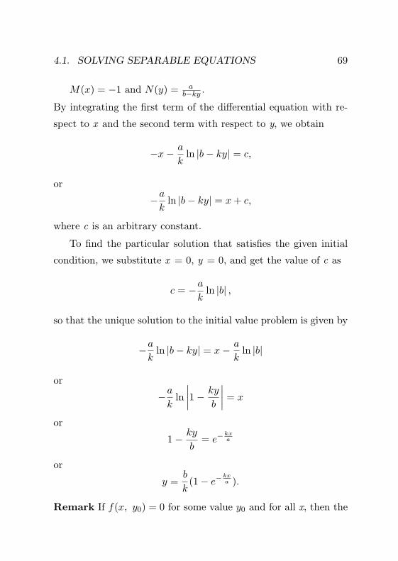
4.1. SOLVING SEPARABLE EQUATIONS 69
M(x) = −1 and N(y) = ab−ky .
By integrating the first term of the differential equation with re-
spect to x and the second term with respect to y, we obtain
−x− a
kln |b− ky| = c,
or
−ak
ln |b− ky| = x+ c,
where c is an arbitrary constant.
To find the particular solution that satisfies the given initial
condition, we substitute x = 0, y = 0, and get the value of c as
c = −ak
ln |b| ,
so that the unique solution to the initial value problem is given by
−ak
ln |b− ky| = x− a
kln |b|
or
−ak
ln∣∣∣∣1− ky
b
∣∣∣∣ = x
or
1− ky
b= e−
kxa
or
y =b
k(1− e−
kxa ).
Remark If f(x, y0) = 0 for some value y0 and for all x, then the

70 CHAPTER 4. SEPARABLE EQUATIONS
constant function y = y0 is a solution of the differential equation
dy
dt= f(x, y).
For example,dy
dx=
(y − 2) sin 3x1 + 3y2
has the constant solution y = 2. Other solutions can be found by
separating the variables and integrating.
Example 5 Solve the initial value problem
dy
dx=
3x2 + 4x+ 22(y − 1)
, (4.16)
with the initial condition
y(0) = −1 (4.17)
and determine the interval in which the solution exists.
Solution
The differential equation can be written as
2(y − 1)dy = (3x2 + 4x+ 2)dx.
Integrating the left side with respect to y and the right side with
respect to x gives
y2 − 2y = x3 + 2x2 + 2x+ c, (4.18)

4.1. SOLVING SEPARABLE EQUATIONS 71
where c is an arbitrary constant. To determine the solution sat-
isfying the prescribed initial condition, we substitute x = 0 and
y = −1in Eq.(4.18), obtaining c = 3. Hence the solution of the
initial value problem is given implicitly by
y2 − 2y = x3 + 2x2 + 2x+ 3 (4.19)
Since Eq.(4.19) is quadratic in y, and we obtain
y = 1±√x3 + 2x2 + 2x+ 4. (4.20)
Equation (4.20) gives two solutions of the differential equation,
only one of which, however, satisfies the given initial con-
dition.
Since the initial condition is y(0) = −1, i.e., y = −1 when
x = 0, we have to take the solution corresponding to the minus
sign in Eq.(4.20), so
y = φ(x) = 1−√x3 + 2x2 + 2x+ 4 (4.21)
is the solution of the initial value problem given by (4.16) and
(4.17). Finally to determine the interval in which the solution
(4.21) is valid, we must find the interval in which the quantity
under the radical is positive. The only real zero of this expression
is x = −2, so the desired interval is x > −2.
Attention! Note that if the plus sign is chosen by mistake in

72 CHAPTER 4. SEPARABLE EQUATIONS
Eq.(4.20), then we obtain the solution
y = ψ(x) = 1 +√x3 + 2x2 + 2x+ 4 (4.22)
of the same differential equation that satisfies the initial condition
y(0) = 3.
Example 6 A body of constant mass m is projected away from
the earth in a direction perpendicular to the earth’s surface with
an initial velocity v0. Assuming that there is no air resistance,
but taking into account the variation of earth’s gravitational field
with distance, find
(a) an expression for the velocity during the ensuing motion.
(b) the initial velocity that is required to lift the body to a given
maximum attitude ξ above the surface of the earth, and
(c) the least initial velocity for which the body will not return to
the earth (this velocity is called the escape velocity.)
Figure 4.1:
Solution
Let the positive y-axis point away from the center of the earth
along the line of motion with y = 0 lying on the earth’s surface

4.1. SOLVING SEPARABLE EQUATIONS 73
(Fig. 4.1). The gravitational force acting on the body (that is,
its weight) is inversely proportional to the square of the distance
from the center of the earth and is given by
w(y) = − k
(y +R)2(4.23)
where k is a constant, R is the radius of the earth, and the minus
sign signifies that w(y) is directed in the negative y direction. We
know that on the earth’s surface w(0) is given by −mg, where g is
the acceleration due to gravity at sea level. Therefore (4.23) gives
−mg = w(0) =−k
(0 +R)2
or
k = mgR2
and hence again by (4.23),
w(y) = − mgR2
(R+ y)2.
Since there are no other forces acting on the body, the equation
of motion is
mdv
dt= − mgR2
(R+ y)2(4.24)
and the initial condition is
v(0) = v0 (4.25)

74 CHAPTER 4. SEPARABLE EQUATIONS
By the chain rule for functions of one variable,
dv
dt=dv
dy
dy
dt= v
dv
dy. (4.26)
Hence Eq. (4.24) becomes
vdv
dy= − gR2
(R+ y)2. (4.27)
Separating the variables,
vdv = gR2 · dy
(R+ y)2.
Integrating,v2
2=
gR2
R+ y+ c. (4.28)
Since y = 0 when t = 0, the initial condition (4.26) at t = 0 can be
replaced by the condition that v = v0 when y = 0. Hence (4.28)
becomesv20
2= gR+ c
or
c =v20
2− gR.
Substituting this (4.28) gives,
v = ±
√v20 − 2gR+
2gR2
R+ y(4.29)
Note that Eq.(4.29) gives the velocity v as a function of y, the

4.1. SOLVING SEPARABLE EQUATIONS 75
altitude, rather than as a function of time. The plus sign must be
chosen if the body is rising, and the minus sign if it is falling back
to earth.
(b) To determine the maximum altitude ξ that the body reaches,
we note that at the maximum altitude, velocity is zero. Hence we
set v = 0 and y = ξ in Eq.(4.29) and then solve for ξ, obtaining
ξ =v20R
2gR− v20
(4.30)
Solving Eq.(4.30) for v0, we find the initial velocity required to lift
the body to the maximum altitude ξ, we obtain
v0 =
√2gR
ξ
R+ ξ(4.31)
(c) The escape velocity ve is found by letting ξ → ∞ in (4.31).
That is,
ve =
√2gR lim
ξ→∞
ξ
R+ ξ=
√2g R lim
ξ→∞
1Rξ + 1
=√
2gR. (4.32)
Example 7 (Separable and Linear First Order Differential Equa-
tions) Suppose that a sum of money is deposited in a bank that
pays interest at an annual rate r. The value S(t) of the invest-
ment at any time t depends on the frequency with which interest
is compounded as well as on the interest rate. Banks have various

76 CHAPTER 4. SEPARABLE EQUATIONS
policies concerning compounding: some compound monthly, some
weekly, some even daily.
(a) Assuming that compounding takes place continuously, set up
a simple initial value problem that describes the growth of the
investment. Then solve the initial value problem.
(b) Compare the result in the continuous model (a) with the sit-
uation in which compounding occurs at finite time intervals.
(c) In the case of continuous compounding, also assume that there
may be deposits or withdrawals in addition to the accrual of
interest. Set up and solve the initial value problem.
SolutiondSdt , the rate of change of the value of the investment, is equal
to the rate at which interest accrues, which is the interest rate r
times the current value of the investment S(t). Thus
dS(t)dt
= rS(t),
or simplydS
dt= rS (4.33)
is the differential equation that governs the process. Suppose the
value of the investment at initial time is, S0. Then
S(0) = S0. (4.34)

4.1. SOLVING SEPARABLE EQUATIONS 77
Then the solution of the initial value problem given by (4.33)
and (4.34) gives the balance S(t) in the account at any time t.
This initial value problem is readily solved, since the differential
equation (4.33) is both linear and separable.
Eqn. (4.33) can be written in the separable form
dS
S= r dt.
Integrating,
ln S = r t+ C.
Using the initial condition S = S0 at t = 0, we have
ln S0 = C
Hence general solution is
ln S = rt+ ln S0
or
lnS
S0= rt.
or
S(t) = S0ert (4.35)
Remark Thus a bank account with continuously compounding
interest grows exponentially.

78 CHAPTER 4. SEPARABLE EQUATIONS
(b) If interest is compounded once a year, then after t years
S(t) = S0(1 + r)t.
If interest is compounded twice a year, then at the end of 6
months the value of the investment is S0[1+(r/2)], and at the end
of 1 year it is S0[1 + (r/2)]2. Thus, after t years we have
S(t) = S0
(1 +
r
2
)2t
In general, if interest is compounded m times per year, then
S(t) = S0
(1 +
r
m
)mt. (4.36)
Remark We recall from calculus that
limm→∞
(1 +
r
m
)mt= ert,
and using this, we have
limm→∞
S0
(1 +
r
m
)mt= S0e
rt,
and hence the relation between formulas (4.35) and (4.36) is
justified.
(c) In the case of continuous compounding, let us suppose that
there may be deposits or withdrawals in addition to the accrual of
interest. If we assume that the deposits or withdrawals take place

4.1. SOLVING SEPARABLE EQUATIONS 79
at a constant rate k, then Eq. (4.33) is replaced by
dS
dt= rS + k,
or, in standard form,
dS
dt− rS = k, (4.37)
where k is positive for deposits and negative for withdrawals.
(4.37) is a first order linear equation. Its integrating factor is
µ(t) = e∫ −rdt = e−rt.
Hence,d
dt(µ(t)S(t)) = kµ(t)
Integrating,
(µ(t)S(t)) = ∫ kµ(t)dt+ c
i.e.,
e−rtS(t) = k ∫ e−rtdt+ c
i.e.,
e−rt S(t) =−kr· e−rt + c.
Hence general solution is
S(t) = cert − (k/r),

80 CHAPTER 4. SEPARABLE EQUATIONS
where c is an arbitrary constant. To satisfy the initial condition
(4.34),
S0 = S(0) = C − k
r
which gives
c = S0 + (k/r).
Thus the solution of the initial value problem (4.37), with (4.34)
is
S(t) = S0ert + (k/r)(ert − 1). (4.38)
The first term in expression (4.38) is the part of S(t) that is due to
the return accumulated on the initial amount S0, and the second
term is the part that is due to the deposit or withdrawal rate k.
Example 8 Suppose that one opens an individual retirement
account (IRA) at age 25 and makes annual investments of Rs.2000
thereafter in a continuous manner. Assuming a rate of return of
8%, what will be the balance in the IRA at age 65?
Solution.
We have
S0 = 0, r = 0.08, and k = Rs 2000,
and we wish to determine S(40). From Eq. (4.38) we have ( with
t = 40)
S(40) =20000.08
(e0.08×40 − 1) = (25, 000)(e3.2 − 1) = Rs 588, 313.
(4.39)
Remark It is interesting to note that the total amount invested

4.1. SOLVING SEPARABLE EQUATIONS 81
is 40×2000 = Rs. 80,000, so the remaining amount of Rs.508, 313
results from the accumulated return on the investment.
Example 9 Suppose that x0 bacteria are placed in a nutrient
solution at time t = 0, and that x = x(t) is the population of the
colony at a later time t. If food and living space are unlimited, and
if as a consequence the population at any moment is increasing at
a rate proportional to the population at that moment, find x as a
function of t.
Solution
Since the rate of increase of x is proportional to x itself, the
differential equation isdx
dt= kx,
where k is a proportionality constant.
By separating the variables,
dx
x= k dt,
Integrating,
lnx = kt+ c.
Since x = x0 when t = 0, we have
c = lnx0
so
lnx = kt+ lnx0

82 CHAPTER 4. SEPARABLE EQUATIONS
and
x = x0ekt. (4.40)
Example 10 Suppose the human population in the earth is in-
creasing at an overall rate of approximately 2 percent per year of
the population at that time. Find the ‘doubling time’ T, that is,
the time needed for the total number of people in the world to
increase by a factor of 2.
Solution
Here the population at any moment is increasing at a rate
proportional to the population at that moment, and it is given that
proportionality constant is 2 percent. i.e., k = 2100 = 0.02 = 1
50 .
Hence proceeding as in the previous example, we obtain
x = x0et/50 (4.41)
To find the doubling time T, that is, the time needed for the total
number of people in the world to increase by a factor of 2, we
replace (4.41) by
2x0 = x0eT/50.
This yields
T/50 = ln 2,
so
T = 50 ln 2 ∼= 34.65 years,
since natural logarithm of 2,ln 2 ∼= 0.693.

4.1. SOLVING SEPARABLE EQUATIONS 83
Example 11 A tank contains 50 gallons2 of brine (water with
a high salt content) in which 75 pounds3 of salt are dissolved.
Beginning at time t = 0, brine containing 3 pounds of salt per
gallon flows in at the rate of 2 gallon per minute, and the mixture
(which is kept uniform by stirring) flows out at the same rate.
When will there be 125 pounds of dissolved salt in the tank? How
much dissolved salt is in the tank at time after a long time?
Solution
If x = x(t) is the number of pounds of dissolved salt in the
tank at time t ≥ 0, then the concentration at that time is x/50
pounds per gallon.
The rate of change of x isdxdt =rate at which salt enters tank – rate at which salt leaves
tank.
Since
rate of entering = 3 · 2 = 6 lb/min
and
rate of leaving =(
x50
)· 2 = x
25 lb/min,
we havedx
dt= 6− x
25=
150− x
25.
Separating variables,
dx
150− x=
125dt.
2Gallon is a unit of volume for liquid measure equal to 4.55 litres.3Pounds is a unit of weight.

84 CHAPTER 4. SEPARABLE EQUATIONS
Integrating,
ln (150− x) = − 125t+ c.
Since x = 75 when t = 0, we see that c = ln 75, so
ln(150− x) = − 125t+ ln 75, ,
and therefore
150− x = 75e−t/25
or
x = 75(2− e−t/25).
Hence x = 125 implies et/25 = 3 or t/25 = ln 3. Thus x = 125
pounds after t = 25 ln 3 ∼= 27.47 minutes.
Also, when t is large we see that x is nearly 75·2 = 150 pounds,
as common sense tells us without calculation.
4.1.1 Exercises Set A
In Exercises 1-15, solve the differential equations.
1. y′ = ky
2. y′ − 2y + a = 0
3. y′ = −xy
4. xy′ + by = 0
5. (x log x)y′ = y
6. dydx −
2x
√y − 1 = 0
7. (x+ 2) dydx = xy
8. yy′ − 2xey2
= 0
9. 2 dydx = y cotx
10. y′ = (1 + x)(1 + y2)

4.1. SOLVING SEPARABLE EQUATIONS 85
11. dydx = − csc y
12. yy′ − 0.5 sin2 ax = 0
13. dydx − y tanhx = 0
14. y′ − y cot 2x = 0
15. (1 + x2) dydx = 1 + y2
In Exercises 16-23, solve the initial value problems.
16. dydx − y tan 2x = 0; y(0) = 2
17. 2xy′ − 3y = 0; y(1) = 4
18. (x+ 1)y′ − 2y = 0; y(0) = 1
19. xy′ log x− y = 0; y(2) = log 4
20. dydx = 2exy3; y(0) = 0.5
21. drdt + tr = 0; r(0) = r0
22. dr sin θ − 2r cos θ dθ = 0; r(π/2) = 2
23. (x2 + 1) dydx + y2 + 1 = 0; y(0) = 1
24. y′ = xy3√
1+x2, y(0) = 1
25. y′ = sec y; y(0) = 0
Answers
1. y = cekx
2. y = ce2x + 12a
3. y = ce−x2
2
4. yxb = c

86 CHAPTER 4. SEPARABLE EQUATIONS
5. y = c log x
6. y = (log x+ c)2 + 1
7. (x+ 2)2y = cex
8. e−y2+ 2x2 = c
9. y = c(sinx)1/2
10. y = tan(12x
2 + x+ c)
11. x− cos y = c
12. 4y2 = 2x− 1a sin 2ax+ c
13. y = c coshx
14. y2 = sin 2x+ c
15. tan−1 y = tan−1 x+ c
16. y2 cos 2x = 4
17. y = 4x3/2
18. y = (1 + x)2
19. y = log(2 + x)
20. y2 = (8− 4ex)−1
21. r = r0e−t2
2
22. r = 2 sin2 θ
23. y = 1−x1+x
24. 1y2 = 3− 2
√1 + x2
25. y = sin− 1x
Exercises Set B
In Exercises 1-11, solve the given differential equation.
1. dydx + x
y = 0
2. dydx +
√1−y2
1−x2 = 0
3. (1 + x)ydx+ (1− y)xdy = 0
4. (1 + x2)dy + x√
1− y2dx = 0
5. (x2 − yx2)dy + (y2 + xy2)ydx = 0

4.1. SOLVING SEPARABLE EQUATIONS 87
6. (ex + 1)ydy = ex(y + 1)dx
7.√
1 + x2dy +√
1 + y2dx = 0
8. sec2 x tan ydx+ sec2 y tanxdy = 0
9. ye2xdx− (1 + e2x)dy = 0
10. 3ex tan ydx+ (1− ex) sec2y dy = 0
11. Solve dydx = x−e−x
y+ey
In Exercises 12-17: (a) Find the solution of the given ini-
tial value problem in explicit form. (b) Determine (at least
approximately) the interval in which the solution is defined.
12. y′ = (1− 2x)y2, y(0) = −1/6
13. xdx+ ye−xdy = 0, y(0) = 1
14. y′ = 2x/(y + x2y), y(0) = −2
15. y′ = 2x/(1 + 2y), y(2) = 0
16. y′ = (3x2 − ex)/(2y − 5), y(0) = 1
17. sin 2xdx+ cos 3ydy = 0, y(π/2) = π/3
18. (Newton’s law of cooling). Assume that the rate at which a
hot body cools is proportional to the difference in tempera-
ture between it and its surroundings. A body is heated to
1100C and placed in air at 100C. After I hour its temper-
ature is 600C. How much additional time is required for it
to cool to 300C?

88 CHAPTER 4. SEPARABLE EQUATIONS
19. A pot of carrot and garlic soup cooling in air at 00C was
initially boiling at 1000C and cooled 200C during the first 30
minutes. How much will it cool during the next 30 minutes?
20. The radiocarbon in living wood decays at the rate of 15.30
disintegrations per minute (dpm) per gram of contained car-
bon. Using 5600 years as the half-life of radiocarbon, esti-
mate the age of each of the following specimens discovered
by archaeologists and tested for radioactivity:
a) a piece of a chair leg from the tomb of King Tutankhamen,
10.14 dpm;
b) a piece of a beam of a house built in Babylon during the
reign of king Hammurabi, 9.52 dpm;
c) dung of a giant sloth found 6 feet 4 inches under the
surface of the ground inside Gypsum Cave in Nevada, 4.17
dpm;
d) a hardwood spear-thrower found in Leonard Rock shelter
in Nevada, 6.42 dpm.
Answers
1. x2 + y2 = a2
2. sin−1 x+ sin−1 y =c
3. x− y + log xy = c
4. sin−1 y + 12 log(1 + x2) = c
5. 1x −
1y + 1
2y2 = c+ log x
6. ey = c(y + 1)(ex + 1)
7. sinh−1 x+ sinh−1 y = c
8. tanx tan y = c

4.2. BY SUBSTITUTION 89
9. 1 + e2x = cy2
10. tan y = c(1− ex)3
11. y2 − x2 + 2(ey − e−x) = c, y + ey 6= 0
12. (a) y = 1/(x2 − x− 6) (b) −2 < x < 3
13. (a) y = [2(1− x)ex − 1]1/2 (b) −1.68 < x < 0.77
14. (a) y = −[2 ln(1 + x2) + 4]1/2 (b) −∞ < x <∞
15. (a) y = −12 + 1
2
√4x2 − 15 (b) x > 1
2
√15
16. (a) y = 52 −
√x3 − ex + 13
4 (b) −1.4445 < x < 4.6297
17. (a) y = [π − arcsin(3 cos2 x)]/3 (b) |x− π/2| < 0.6155
18. ln 5ln 2 − 1 hours
19. 160C
20. (a) about 3330 years (b) about 3850 years
(c) about 10,510 years (d) about 7010 years
4.2 Equations Reducible to Separable Form:
By Substitution
Certain first order differential equations are not separable but can
be made separable by simple substitutions, which is illustrated
through the following examples.

90 CHAPTER 4. SEPARABLE EQUATIONS
Example 12 Solve the differential equation
(2x− 4y + 5)y′ + x− 2y + 3 = 0.
Solution
Put x− 2y = u.
Then, differentiating both sides with respect to x, we obtain
1− 2dy
dx=du
dx
ordy
dx=
12
(1− du
dx
)
Substituting these values in the given differential equation, we
obtain
(2u+ 5)12
(1− du
dx
)+ u+ 3 = 0
or
(2u+ 5)du
dx= 4u+ 11.
Separating variables, we get(2u+ 54u+ 11
)du = dx,

4.3. EXERCISES 91
which, by actual division,4 gives
12
(1− 1
4u+ 11
)du = dx.
On integration, we get
12
(u− 1
4log |4u+ 11|
)= x+ c
or
u− 14
log |4u+ 11| = 2x+ C,
where C=2c.
Putting u = x− 2y, the above equation becomes
4x + 8y + log 4x-8y+11= C.
4.3 Exercises
In Exercises 1-8, using appropriate substitutions, find the general
solution of the following differential equations.
1. y′ = (y − x)2
2. y′ = tan(x+ y)− 1
3. xy′ = e−xy − y.
4. y′ = (x+ ey − 1)e−y
5. y′ = y−x+1y−x+5
6. dydx = 1−2y−4x
1+y+2x
7. (2x− 4y + 5)dy = (x− 2y + 3)dx
4 Actual division gives, 2u+54u+11
= 12
(1− 1
4u+11
)

92 CHAPTER 4. SEPARABLE EQUATIONS
8. dydx = y
x
(log y
x + 1)
9. Solve the initial value problem:
2x2y dydx = tan(x2y2)− 2xy2; y(1) =
√π/2
* Hints: Substitution required in the exercises are:
1. y − x = u
2. x+ y = u
3. xy = u
4. x+ ey = u
5. y − x = u
6. y + 2x = u
7. x− 2y = u
8. y/x = u
9. x2y2 = u.
Answers
1. y = x+ 1+ce2x
1−ce2x
2. sin(x+ y) = cex
3. xy = log(x+ c)
4. x+ ey = cex
5. (y − x)2 + 10y − 2x = c
6. (y + 2x)2 + 2(y − x) = c
7. (x−2y)2+5(x−2y) = −x+c.
8. y = xecx or log yx = cx
9. log sin(x2y2) = x− 1
4.4 Equations Reducible to Separable Form:
Homogeneous Equation dydx = g
(yx
)If the right side of the equation
dy
dx= f(x, y)

4.4. HOMOGENEOUS EQUATION 93
can be expressed as a function of the ratio yx only, then the
equation is said to be homogeneous. More precisely, a differential
equation of the formdy
dx= g
(yx
)(4.42)
where g is any given function of yx [for example
( yx
)2, cos( y
x
), 1+
yx , etc.] is called a homogeneous equation.
The form of equation (4.42) suggests that we may introduce a
new variable u such that
u =y
x,
where y and u are functions of x. Then
y = xu.
Differentiating with respect to x, we get
dy
dx= u+ x
du
dx(4.43)
By inserting this into (4.42) and noting that g( y
x
)= g(u), we
obtain
u+ xdu
dx= g(u).
Separating the variables u and x, we have the separable form
du
g(u)− u=dx
x(4.44)

94 CHAPTER 4. SEPARABLE EQUATIONS
If we integrate (4.44) and then replace u by y/x, we obtain the
general solution of (4.42).
Example 13 Solve the first order differential equation
2xydy
dx− y2 + x2 = 0.
Solution
The given equation can be written as
dy
dx=y2 − x2
2xy=
( yx
)2 − 12( y
x
) , (4.45)
and hence is a homogenous equation.
Put u = yx . Then y = ux, which on differentiation with respect to
x yieldsdy
dx= u+ x
du
dx.
Substitution on the differential equation (4.45) gives
u+ xdu
dx=u2 − 1
2u
implies
xdu
dx=u2 − 1
2u− u = −u
2 − 12u
..
Separating the variables, we obtain
2u du1 + u2
= −dxx.

4.4. HOMOGENEOUS EQUATION 95
On integration, we obtain
ln∣∣1 + u2
∣∣ = − lnx+ ln c,
where c is an arbitrary constant. Hence
1 + u2 =1cx.
Replacing u by y/x, we obtain
1 +(yx
)2=
1cx
orx2 + y2
x2=
1cx
or
x2 + y2 =1c· x
i.e.,
x2 + y2 = Cx,
where C = 1c , is the general solution to the given differential equa-
tion.
Exercises
1. x(x− y) dydx + y2 = 0
2. dydx = −x2+3y2
3x2+y2
3. dydx = x2−4xy−2y2
2x2+4xy−y2
4. dydx = x2+y2
x2+xy
5. x(y − x)dy = (y + x)ydx

96 CHAPTER 4. SEPARABLE EQUATIONS
6. (xy − 2y2)dx− (x2 − 3xy)dy = 0
7. dydx = y+
√x2+y2
x
8. (x2 − 2xy − y2)dx− (x+ y)2dy = 0
9. (x3 − 3xy2)dy = (y3 + 3x2y)dx
10. xy2 dydx = x3 + y3
Answers
1. y = ceyx .
2. 2xy(x+y)2
+ log(x+ y) = c
3. x3 − 6x2y − 6xy2 − y3 = c
4. (x− y)2eyx = cx
5. xy = ceyx
6. y3 = cx2e−x
y
7. y +√x2 + y2 = cx2
8. c+ x3 = y3 + 3x2y + 3xy2
9. (x2 − y2)2 = cxy
10. y3 = 3x3(lnx+ c)

4.5. VIA REDUCING TO HOMOGENEOUS EQUATION 97
4.5 Equations Reducible to Separable Form:
via Reducing to Homogeneous Equation
Certain equation may not be in the homogeneous form, but can
be made to homogeneous form by appropriate change of variables.
This is illustrated in the following example.
Example 14 Solve dydx = x+2y−3
2x+y−3 .
Solution
The given equation is not readily homogeneous. But it can be
reduced to the homogeneous type by substituting
x = X + h and y = Y + k
where h and k are constants to be determined later. From the
substitution, we havedy
dx=dY
dX
and the equation takes the form
dY
dX=
(X + 2Y ) + (h+ 2k − 3)(2X + Y ) + ((2h+ k − 3)
(4.46)
Now, h and k are chosen so that h+2k−3 = 0 and 2h+k−3 = 0,
solving which we get h = 1 and k = 1. Therefore (4.46) takes the
formdY
dX=X + 2Y2X + Y
(4.47)
which is a homogeneous equation. By substituting
Y = V X anddY
dX= V +X
dV
dX,

98 CHAPTER 4. SEPARABLE EQUATIONS
equation (4.47) takes the form
X dVdX = 1+2V
2+V − V or dXX = 2+V
1−V 2dV or dXX =
[1/21+V + 3/2
1−v
]dV
Integration of the above yields
logX =12
log (1 + V )− 32
log (1− V ) + logC,
where C is an arbitrary constant. The above can be simplified to
X2(1− V )3 = C2(1 + V ).
Substituting the values of X and V, we get the required general
solution as
(x− y)3 = C2(x+ y − 2).
Exercises
1. dydx = x+2y−3
2x+y−3
2. dydx = 3x−5y−9
2x−4y−8
3. dydx = 2x+9y−20
6x+2y−10
4. dydx = x+7y+2
3x+5y+6
5. dydx = x+7y+2
3x+5y+6
6. .(x−y−2)dx+(x+y)dy = 0
7. (3x+y−5)dy = 2(x+y−1)dx
8. dydx = 2x+3y+4
4x+6y+5
9. (2x− 4y + 3) dydx + (x− 2y + 1) = 0
10. dydx = 2x+y−3
4x+2y+7
Answers
1. x+ y − 2 = c(x− y)3

4.5. VIA REDUCING TO HOMOGENEOUS EQUATION 99
2. (y − x+ 1)2 = c(4y − 3x+ 6)
3. (y − 2x)2 = c(2y + x− 5)
4. (x− y + 2)4 = c(x+ 5y + 2)
5. log(x− y + 2) = 2y − x+ c
6. log[(x+ 1)2 + (y − 1)2] + 2 tan−1[
y−1x+1
]= c
7. (x− y − 3)4 = c(2x+ y − 3)
8. 9 log(14x+ 21y + 22) + 21x− 42y + c = 0
9. log(4x− 8y + 5) = 4x+ 8y + c
10. 13 log(10x+ 5y + 11) = 5x− 10y − c.

Chapter 5Differences Between Linear and
Nonlinear Equations
5.1 Linear and Nonlinear Equations
The first theorem in this chapter says that if the underlying dif-
ferential equation of an initial value problem is linear, then the
solution to the IVP is unique. We will see that this need not be
true for initial value problems with non-linear differential equa-
tions.
Theorem 1 [Existence and Uniqueness Theorem for First-
Order Linear Equations] If the functions p and g are continuous
on an open interval I : α < t < β containing the point t = t0, then
there exists a unique function y = φ(t) that satisfies the linear
100

5.1. LINEAR AND NONLINEAR EQUATIONS 101
differential equation
y′ + p(t)y = g(t) (5.1)
for each t in I, and that also satisfies the initial condition
y(t0) = y0, (5.2)
where y0 is an arbitrary prescribed initial value.
Example 1 Use Theorem 1 to find an interval in which the initial
value problem
ty′ + 2y = 4t2 (5.3)
y(1) = 2 (5.4)
has a unique solution. Also find the solution.
Solution
Eq.(5.3) can be brought into the standard form (5.1) as follows:
y′ +2ty = 4t
Hence p(t) = 2/t and g(t) = 4t. Thus for this equation, g is
continuous for all t, while p is continuous only for t < 0or for t > 0.
The interval t > 0 contains the initial point t = 1; consequently,
Theorem 1 guarantees that the initial value problem (5.3) with
(5.4) has a unique solution on the interval 0 < t <∞.
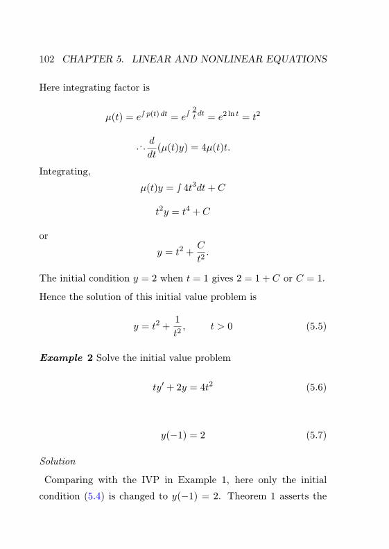
102 CHAPTER 5. LINEAR AND NONLINEAR EQUATIONS
Here integrating factor is
µ(t) = e∫ p(t) dt = e∫2t dt = e2 ln t = t2
... ddt
(µ(t)y) = 4µ(t)t.
Integrating,
µ(t)y = ∫ 4t3dt+ C
t2y = t4 + C
or
y = t2 +C
t2.
The initial condition y = 2 when t = 1 gives 2 = 1 + C or C = 1.
Hence the solution of this initial value problem is
y = t2 +1t2, t > 0 (5.5)
Example 2 Solve the initial value problem
ty′ + 2y = 4t2 (5.6)
y(−1) = 2 (5.7)
Solution
Comparing with the IVP in Example 1, here only the initial
condition (5.4) is changed to y(−1) = 2. Theorem 1 asserts the

5.1. LINEAR AND NONLINEAR EQUATIONS 103
existence of a unique solution for t < 0. Proceeding as in Example
1, the solution is given by y = t2 + 1t2, t < 0.
The following is a general version of Theorem 1.
Theorem 2 [Existence and Uniqueness Theorem for First-
Order Nonlinear Equations] Let the functions f and ∂f/∂y
be continuous in some rectangle (Fig.5.1) α < t < β, γ < y <
δcontaining the point (t0, y0). Then, in some interval t0−h < t <
t0 + h contained in α < t < β, there is a unique solution y = φ(t)
of the initial value problem
y′ = f(t, y), y(t0) = y0. (5.8)
Figure 5.1:
Remark If all the conditions of Theorem 2 except the continu-
ity of ∂f∂y are satisfied, then the solution has a solution (but not

104 CHAPTER 5. LINEAR AND NONLINEAR EQUATIONS
unique).
Figure 5.2:
Example 3 Apply Theorem 2 to the initial value problem
dy
dx=
3x2 + 4x+ 22(y − 1)
, y(0) = −1 (5.9)
Solution
Here
f(x, y) =3x2 + 4x+ 2
2(y − 1),
and
∂f
∂y=
3x2 + 4x+ 22
∂
∂y
(1
y − 1
)= −3x2 + 4x+ 2
2(y − 1)2.
Each of these functions is continuous everywhere except on the

5.1. LINEAR AND NONLINEAR EQUATIONS 105
line y = 1. Hence, a rectangle (Fig. 5.2) can be drawn about the
initial point (0,−1) in which both f and ∂f/∂y are continuous.
Hence, Theorem 2 guarantees that the initial value problem has a
unique solution in some interval about x = 0. It has been seen in
Example 5 of the previous chapter that the solution to the initial
value problem (5.9) is
y = 1−√x3 + 2x2 + 2x+ 4.
Also, the above solution is valid when x3 + 2x2 + 2x+ 4 > 0. The
only real zero of x3 + 2x2 + 2x + 4 = 0 is x = −2, and hence the
solution is valid only when x > −2.
Attention! We note that even though the rectangle can be
stretched infinitely far in both the positive and negative x-directions,
this does not necessarily mean that the solution exists for all x.
Indeed, the solution of the initial value problem (5.9) exists only
for x > −2.
[Attention! Theorem 1 is not applicable to the initial value prob-
lem (5.9) in Example 3, since the differential equation is nonlin-
ear.]
Example 4 (IVP with more than one solution) Can we apply
Theorem 2 to the IVP
dy
dx=
3x2 + 4x+ 22(y − 1)
, y(0) = 1 ?
Also solve the IVP.

106 CHAPTER 5. LINEAR AND NONLINEAR EQUATIONS
Solution
The initial point (0, 1) lies on the line y = 1. Since f and ∂f∂y
are not defined at y = 1, no rectangle can be drawn about (0, 1),
within which f and ∂f/∂y are continuous. Hence, Theorem 2 says
nothing about possible solutions of the given initial value problem.
Separating the variables we obtain
2(y − 1)dy = (3x2 + 4x+ 2)dx.
Integrating, we obtain
y2 − 2y = x3 + 2x2 + 2x+ c.
Further, if x = 0 and y = 1, then c = −1. Hence
y2 − 2y = x3 + 2x2 + 2x− 1.
Solving for y, the above quadratic equation in y gives
y = 1±√x3 + 2x2 + 2x (5.10)
Remark The above example deals a case where Theorem 1 and
Theorem 2 cannot be applied. Also note that this IVP has more
than one solution. Equation (5.10) provides two functions that
satisfy the given differential equation for x > 0 and also satisfy
the initial condition y(0) = 1.
Example 5 (IVP with infinite number of solutions) Can we apply

5.1. LINEAR AND NONLINEAR EQUATIONS 107
Theorem 2 to the initial value problem
dy
dt= y1/3, y(0) = 0 (5.11)
for t ≥ 0? Solve the initial value problem.
Solution
The function f(t, y) = y1/3 is continuous everywhere, but
∂f/∂y does not exist when y=0, and hence is not continuous there.
Thus Theorem 2 does not apply to this problem and no conclusion
can be drawn from it. However, by the remark following Theorem
2, the continuity of f does ensure the existence of solutions, but
not their uniqueness.
Obviously, the function
y = ψ(t) = 0, t ≥ 0 (5.12)
is a solution to the IVP (5.11).
To find other solutions of (5.11), we solve the differential equa-
tion. By separating variables,
y−1/3dy = dt.
Integrating,32y2/3 = t+ c.
Hence
y =[23(t+ c)
]3/2

108 CHAPTER 5. LINEAR AND NONLINEAR EQUATIONS
The initial condition y = 0 when t = 0 gives c = 0. Hence a
solution to the IVP is
y = φ1(t) =(
23t
)3/2
, t ≥ 0 (5.13)
Also the function
y = φ2(t) = −(
23t
)3/2
, t ≥ 0 (5.14)
is also a solution of the initial value problem. Also, for an arbitrary
positive t0, the functions
y = χ(t) =
{0 if 0 < t < t0
±[
23(t− t0)
]3/2 if t ≥ t0(5.15)
are continuous, differentiable (in particular at t = t0), and are
solutions of the initial value problem (5.15).
We conclude that the given IVP has an infinite number of
solutions.
Remark to Example 5
1. As noted in the solution of Example 5, the existence and
uniqueness theorem is not applicable if y = 0. i.e., when
the initial point (0, 0) lies on the t-axis. If the initial point
(t0, y0)is any point not on the t-axis, however, then the the-
orem guarantees that there is a unique solution of the differ-
ential equation y′ = y1/3 passing through (t0, y0).

5.1. LINEAR AND NONLINEAR EQUATIONS 109
Interval of Definition or Interval of Existence
According to Theorem 1, the solution of a linear equation
y′ + p(t)y = g(t),
subject to the initial condition y(t0) = y0, exists throughout any
interval about t = t0 in which the functions p and g are continuous.
Thus, vertical asymptotes or other discontinuities in the solution
can occur only at points of discontinuity of p or g. For instance,
the solution in Example 1 (with one exception) are asymptotic
to the y-axis, corresponding to the discontinuity at t = 0in the
coefficient p(t) = 2/t, but none of the solutions has any other
point where it fails to exist and to be differentiable. The one
exceptional solution shows that solutions may sometimes remain
continuous even at point of discontinuity of the coefficients.
On the other hand, for a nonlinear initial value problem satis-
fying the hypotheses of Theorem 2, the interval in which a solution
exists may be difficult to determine. The solution y = φ(t)is cer-
tain to exist as long as the point [t, φ(t)] remains within a region
in which the hypotheses of Theorem 2 are satisfied. This is what
determines the value of h in that theorem. However, since φ(t) is
usually not known, it may be impossible to locate the point [t, φ(t)]
with respect to this region. In any case, the interval in which a
solution exists may have no simple relationship to the function f
in the differential equation y′ = f(t, y). This is illustrated by the
following example.

110 CHAPTER 5. LINEAR AND NONLINEAR EQUATIONS
Example 6 Solve the initial value problem
y′ = y2, y(0) = 1 (5.16)
and determine the interval in which the solution exists.
Solution
Since f(t, y) = y2 and ∂f∂y = 2y are continuous everywhere, by
Theorem 2, the given initial value problem has a unique solution.
To find the solution, we separate the variables to obtain
dy
y2= dt
i.e.,
y−2dy = dt. (5.17)
Integrating,
−y−1 = t+ c.
Then, solving for y, we have
y = − 1t+ c
(5.18)
The initial condition y(0) = 1 gives c = −1, so
y =1
1− t(5.19)
is the solution of the given initial value problem. Clearly, the
solution becomes unbounded as t → 1; therefore, the solution

5.1. LINEAR AND NONLINEAR EQUATIONS 111
exists only in the interval −∞ < t < 1.
Example 7 Solve the initial value problem
y′ = y2, (5.20)
with the initial condition
y(0) = y0, (5.21)
and determine the interval in which the solution exists.
Solution
The only difference of the given IVP that in the previous exam-
ple is that the initial condition is replaced by y(0) = y0. Proceeding
as in the previous example, (5.18) gives c = − 1y0
, and hence
y =y0
1− y0t(5.22)
is the solution of the initial value problem (5.20) with the initial
condition (5.21). Observe that the solution (5.22) becomes un-
bounded as t → 1/y0, so the interval of existence of the solution
is {−∞ < t < 1
y0if y0 > 0
1y0< t <∞ if y0 > 0
Remark The above two examples illustrates another feature of
initial value problems for nonlinear equations; namely, the sin-
gularities of the solution may depend in an essential way on the
initial conditions as well as on the differential equation.

112 CHAPTER 5. LINEAR AND NONLINEAR EQUATIONS
General Solution do not provide all the solutions
Another way in which linear and nonlinear equations differ
concerns the concept of a general solution.
1. For a first order linear equation it is possible to obtain a so-
lution containing one arbitrary constant (called general solu-
tion), from which all possible solutions follow by specifying
values for this constant.
2. For nonlinear equations this may not be the case; even though
a solution containing an arbitrary constant may be found,
there may be other solutions that cannot be obtained by
giving values to this constant.
Example 8 y = ψ(t) = 0 for all t is a solution of the differential
equation
y′ = y2
that cannot be obtained from the solution (Ref. Example 6)
y = − 1t+ c
by assigning a value to c.
Remark We use the term “general solution” only when discussing
linear equations.
The above example leads to the following definition.
Definition (Singular solution) In some cases, there may be fur-
ther solutions of a given differential equation, which cannot be

5.1. LINEAR AND NONLINEAR EQUATIONS 113
obtained by assigning a definite value to the arbitrary constant in
the general solution. Such a solution is called a singular solution
of the differential equation.
Example 9 y = ψ(t) = 0 for all t is a singular solution of the IVP
y′ = y2, y(0) = 1
as it cannot be obtained from the solution
y = − 1t+ c
by assigning a value to c.
Exercises
In each of Exercises 1-6, determine (without solving the problem)
an interval in which the solution of the given initial value problem
is certain to exist.
1. (t− 3)y′ + (ln t)y = 2t, y(1) = 2
2. t(t− 5)y′ + y = 0, y(2) = 1
3. y′ + (tan t)y = sin t, y(π) = 0
4. (4− t2)y′ + 2ty = 3t2, y(−3) = 1
5. (4− t2)y′ + 2ty = 3t2, y(1) = −3
6. (ln t)y′ + y = cot t, y(2) = 3
In each of Exercises 7-12, state where in the ty-plane the
hypotheses of Theorem are satisfied.

114 CHAPTER 5. LINEAR AND NONLINEAR EQUATIONS
7. y′ = t−y2t+5y
8. y′ = (1− t2 − y2)12
9. y′ = (t2 − y2)32
10. y′ = ln |ty|1−t2+y2
11. dydt = 1+t2
3y−y2
12. dydt = (cot t)y
1+y
In each of Exercises 13-16, solve the given initial value prob-
lem and determine how the interval in which the solution
exists depends on the initial value y0.
13. y′ = −4 ty , y(0) = y0
14. y′ = 2ty2, y(0) = y0
15. y′ + y3 = 0, y(0) = y0
16. y′ = t2
y(1+t3), y(0) = y0
17. Consider the initial value problem y′ = y13 , y(0) = 0.
(a) Is there a solution that passes through the point (1, 1)?
If so, find it.
(b) Is there a solution that passes through the point (2, 1)?
If so, find it.
(c) Consider all possible solutions of the given initial value
problem. Determine the set of values that these solu-
tions have at t = 2.
Answers
1. 0 < t < 3
2. 0 < t < 5
3. π2 < t < 3π
2
4. −∞ < t < −2

5.1. LINEAR AND NONLINEAR EQUATIONS 115
5. −2 < t < 2
6. 1 < t < π
7. 2t+ 5y > 0 or 2t+ 5y < 0
8. t2 + y2 < 1
9. Everywhere
10. 1− t2 + y2 > 0 or 1− t2 + y2 < 0, t 6= 0, y 6= 0
11. y 6= 0, y 6= 3
12. y 6= nπ for n = 0, ±1, ±2, . . . y 6= −1
13. y = ±√y20 − 4t2 if y0 6= 0;|t| < |y0|
2
14. y = [(1/y0)− t2]−1 if y0 6= 0; y = 0 if y0 = 0;
interval is |t| < 1√y0
if y0 > 0; −∞ < t <∞ if y0 ≤ 0;
15. y = y0/√
2ty20 + 1 if y0 6= 0; y = 0 if y0 = 0;
interval is − 12y2
0< t <∞ if y0 6= 0; −∞ < t <∞ if y0 = 0
16. y = ±√
23 ln(1 + t3) + y2
0; −[1− exp(−3y20/2)]1/3 < t <∞

Chapter 6Exact Differential Equations
In this chapter we consider a class of equations known as exact
equations for which there is a well-defined method of solution. We
begin with solving a differential equation that is neither linear nor
separable.
6.1 Exact Differential Equations
Example 1 Solve the differential equation
2x+ y2 + 2xyy′ = 0 (6.1)
Solution
The equation is neither linear nor separable. However, we
observe that the function ψ(x, y) = x2 + xy2 of two variables x
116

6.1. EXACT DIFFERENTIAL EQUATIONS 117
and y has the property that
2x+ y2 =∂ψ
∂x, 2xy =
∂ψ
∂y(6.2)
Therefore the differential equation (6.1) can be written as
∂ψ
∂x+∂ψ
∂y
dy
dx= 0. (6.3)
Assuming that y is a function of x, and using the chain rule for
functions of one variable, we have
dψ
dx=∂ψ
∂x
dx
dx+∂ψ
∂y
dy
dx.
Hence we can write Eq.(6.3) in the equivalent form
dψ
dx= 0
i.e.,dψ
dx=
d
dx(x2 + xy2) = 0 (6.4)
Therefore
ψ(x, y) = x2 + xy2 = c, (6.5)
where c is an arbitrary constant, is an equation that defines solu-
tions of Eq.(6.1) implicitly.
Method of Solving Equations of the FormM(x, y)+N(x, y)y′ =
0

118 CHAPTER 6. EXACT DIFFERENTIAL EQUATIONS
Let the differential equation
M(x, y) +N(x, y)y′ = 0 (6.6)
be given. Suppose that we can identify a function ψ such that
∂ψ
∂x(x, y) = M(x, y),
∂ψ
∂y(x, y) = N(x, y), (6.7)
and such that ψ(x, y) = c defines y = φ(x) implicitly as a differ-
entiable function of x. Then
M(x, y) +N(x, y)y′ =∂ψ
∂x+∂ψ
∂y
dy
dx=
d
dxψ[x, φ(x)]
and the differential equation (6.6) becomes
d
dxψ[x, φ(x)] = 0. (6.8)
In this case Eq.(6.6) is said to be an exact differential equa-
tion. Solutions of Eq.(6.6), or the equivalent Eq.(6.8), are given
implicitly by
ψ(x, y) = c, (6.9)
where c is an arbitrary constant.
In Example 1 it was relatively easy to see that the differen-
tial equation was exact and, in fact, easy to find its solution, by
recognizing the required function ψ. For more complicated equa-
tions it may not be possible to do this so easily. A systematic

6.1. EXACT DIFFERENTIAL EQUATIONS 119
way of determining whether a given differential equation is exact
is provided by the following theorem.
Theorem Let the functions M, N, My, and Nx (where sub-
scripts denote partial derivatives) be continuous in the rectangular
region R : α < x < β, γ < y < δ. Then
M(x, y) +N(x, y)y′ = 0 (6.10)
is an exact differential equation in the region R if and only if
My(x, y) = Nx(x, y) (6.11)
at each point of R. That is, there exists a function ψ satisfying
ψx(x, y) = M(x, y), ψy(x, y) = N(x, y), (6.12)
if and only if M and N satisfy Eq.(6.11).
Proof The proof of this theorem has two parts. First we show
that if there is a function ψ such that Eqs.(6.12) are true, then
it follows that Eq.(6.11) is satisfied. Computing My and Nx from
Eqs.(6.12), we obtain
My(x, y) = ψxy(x, y), Nx(x, y) = ψyx(x, y). (6.13)
Since My and Nx are continuous, it follows that ψxy and ψyx are
also continuous. This guarantees their equality, and Eq.(6.11)

120 CHAPTER 6. EXACT DIFFERENTIAL EQUATIONS
follows.
We now show that if M and N satisfy Eq.(6.11), then Eq.(6.10)
is exact. The proof involves the construction of a function ψ sat-
isfying Eqs.(6.12)
ψx(x, y) = M(x, y), ψy(x, y) = N(x, y).
We begin by integrating the first of Eqs. (6.12) with respect to x,
holding y constant. We obtain
ψ(x, y) = Q(x, y) + h(y), (6.14)
whereQ(x, y) is any differentiable function such that ∂Q(x, y)/∂x =
M(x, y). For example, we might choose
Q(x, y) =∫ x
x0
M(s, y)ds (6.15)
where x0is some specified constant inα < x0 < β. The function h
in Eq.(6.14) is an arbitrary differentiable function of y, playing the
role of the arbitrary constant. Now we must show that it is always
possible to choose h(y) so that the second of Eqs(6.12) is satisfied,
that is, ψy = N . By differentiating Eq.(6.14) with respect to y
and setting the result equal to N(x, y), we obtain
ψy(x, y) =∂Q
∂y(x, y) + h′(y) = N(x, y).
6.1. EXACT DIFFERENTIAL EQUATIONS 121
Then, solving for h′(y), we have
h′(y) = N(x, y)− ∂Q
∂y(x, y). (6.16)
In order for us to determine h(y) from Eq.(6.16), the right side
of Eq.(6.16), despite its appearance, must be a function of y only.
To establish that this is true, we can differentiate the quantity in
question with respect to x, obtaining
∂N
∂x(x, y)− ∂
∂x
∂Q
∂y(x, y). (6.17)
By interchanging the order of differentiation in the second term of
Eq.(6.17), we have
∂N
∂x(x, y)− ∂
∂y
∂Q
∂x(x, y),
or, since ∂Q/∂x = M,
∂N
∂x(x, y)− ∂M
∂y(x, y),
which is zero on account of Eq.(6.11). Hence, despite its apparent
form, the right side of Eq.(6.16) does not, in fact, depend on x.
Then we find h(y) by integrating Eq.(6.16), and upon substituting
this function in Eq.(6.14), we obtain the required function ψ(x, y).
This completes the proof.

122 CHAPTER 6. EXACT DIFFERENTIAL EQUATIONS
Example 2 Solve the differential equation
(y cosx+ 2xey) + (sinx+ x2ey − 1)y′ = 0 (6.18)
Solution
Here taking
M = y cosx+ 2xey and N = sinx+ x2ey − 1,
we obtain
My(x, y) = cosx+ 2xey = Nx(x, y).
Hence the given equation is exact. Thus there is a ψ(x, y) such
that
ψx(x, y) = y cosx+ 2xey (6.19)
and
ψy(x, y) = sinx+ x2ey − 1. (6.20)
Integrating (6.19) with respect to x, we obtain
ψ(x, y) = y sinx+ x2ey + h(y), (6.21)
where h(y) is a function of y alone.
Setting ψy = N , from (6.21) and (6.20) we obtain
ψy(x, y) = sinx+ x2ey + h′(y) = sinx+ x2ey − 1.
Thus h′(y) = −1 and which on integration yields,
h(y) = −y.

6.1. EXACT DIFFERENTIAL EQUATIONS 123
The constant of integration can be omitted since any solution of
the differential equation h′(y) = −1 is satisfactory; we do not
require the most general one. Substituting for h(y) in Eq.(6.21)
gives
ψ(x, y) = y sinx+ x2ey − y.
Hence solutions of Eq.(6.18) are given implicitly by
y sinx+ x2ey − y = c (6.22)
Example 3 (A differential equation that is not exact) Examine
that differential equation
(3xy + y2) + (x2 + xy)y′ = 0 (6.23)
cannot be solved using the method discussed above.
Solution
Here taking
M = 3xy + y2 and N = x2 + xy,
we obtain
My(x, y) = 3x+ 2y, Nx(x, y) = 2x+ y;
Since My 6= Nx, the given equation is not exact. Hence the
procedure described above cannot produce a solution. We post-
pone the work of solving of this equation to the section Integrating
Factors, but only see that it cannot be solved by the procedure

124 CHAPTER 6. EXACT DIFFERENTIAL EQUATIONS
described above. For this, let us seek a function ψ such that
ψx(x, y) = 3xy + y2 (6.24)
and
ψy(x, y) = x2 + xy. (6.25)
Integrating , (6.24) yields
ψ(x, y) =32x2y + xy2 + h(y), (6.26)
where h is an arbitrary function of y alone. To try to satisfy the
equation (6.25), we compute ψy from Eq.(6.26) and set it equal to
N, yielding32x2 + 2xy + h′(y) = x2 + xy
or
h′(y) = −12x2 − xy. (6.27)
Since the right side of Eq.(6.27) depends on both x and y, it is
impossible to solve Eq.(6.27) for h(y). Thus there is no ψ(x, y)
satisfying both of Eqs.(6.24) and (6.25).
Working Method for Solving the Exact Equation
The following method helps to solve exact equation in an easy way.
If the differential equation
M(x, y) +N(x, y)y′ = 0

6.1. EXACT DIFFERENTIAL EQUATIONS 125
or, equivalently written in the form
M dx+N dy = 0
satisfies the (necessary) condition
∂M
∂y=∂N
∂x,
then it is exact. Then its solution is given by∫Mdx+
∫(terms in N not involving x) dy = c. (6.28)
Example 4 Show that the equation
(1 + 4xy + 2y2)dx+ (1 + 4xy + 2x2)dy = 0
is exact and solve it.
Solution
Here M = 1 + 4xy + 2y2and N = 1 + 4xy + 2x2.
Differentiating M partially with respect to y, we get
∂M
∂y= 4x+ 4y
and differentiating N partially with respect to x, we get
∂N
∂x= 4x+ 4y,

126 CHAPTER 6. EXACT DIFFERENTIAL EQUATIONS
so that∂M
∂y=∂N
∂x.
Hence, using (6.28),∫(1 + 4xy + 2y2)dx+
∫(1)dy = c
i.e.,
x+ 2x2y + 2xy2 + y = c
is the general solution.
Example 5 Solve the equation (1 + y) dydx = 1− x.
Solution
The given equation is
(1 + y)dy = (1− x)dx.
That is,
(1− x)dx− (1 + y)dy = 0.
Then, M = 1− x and N = −(1 + y) and
∂M
∂y= 0 =
∂N
∂x
and hence the equation is exact and its solution is given by
x− x2
2− y − y2
2= c.

6.1. EXACT DIFFERENTIAL EQUATIONS 127
Example 6 Solve the initial value problem
(y − 1)dx+ (x− 3)dy = 0; y(0) =23.
Solution
Here M = y − 1 and N = x− 3, and since
∂M
∂y= 1 =
∂N
∂x,
the given differential equation is exact.
Hence, using (6.28), we obtain the general solution as
xy − x− 3y = c.
Next to find the particular solution
Using the initial condition that y = 23at x = 0, we get the par-
ticular value of c as c = −2, so the unique solution to the initial
value problem is
xy − x− 3y = −2
or
xy − x− 3y + 2 = 0.
Exercises
Examine that the following equations are exact and then solve.
1.(x+ 2
y
)dy + ydx = 0
2. (y − x3) dx+ (x+ y3) dy = 0

128 CHAPTER 6. EXACT DIFFERENTIAL EQUATIONS
3. (y + y cos xy) dx+ (x+ x cosxy) dy = 0
4. (sin x sin y − xey) dy = (ey + cos x cos y)dx
5. dydx = −ax+by
bx+cy
6. (ex sin y − 2y sinx)dx+ (ex cos y + 2 cos x)dy = 0
7. (yexy cos 2x− 2exy sin 2x+ 2x)dx+ (xexy cos 2x− 3)dy = 0
8. (y/x+ 6x)dx+ (ln x− 2)dy = 0; x > 0
9. Solve the given initial value problem and determine at least
approximately where the solution is valid.
(2x− y)dx+ (2y − x)dy = 0, y(1) = 0
10. Find the value of b for which the given equation is exact,
and then solve it using that values of b.
(xy2 + bx2y)dx+ (x+ y)x2dy = 0
11. Assume that the equation
M(x, y) +N(x, y)y′ = 0,
meets the requirements of Theorem 1 in a rectangle R and
is therefore exact. Show that a possible function ψ(x, y)is
ψ(x, y) =∫ x
x0
M(s, y0)ds+∫ y
y0
N(x, t)dt,

6.2. INTEGRATING FACTORS 129
where (x0, y0) is a point in R.
12. Show that any separable equation
M(x) +N(y)y′ = 0
is also exact.
Answers
1. xy + ln y2 = c.
2. 4xy − x4 + y4 = c.
3. xy + sinxy = c.
4. xey + sinx cos y = c.
5. ax2 + 2bxy + cy2 = k
6. y = 0 is a solution. General solution is ex sin y+2y cosx = c;
7. exy cos 2x+ x2 − 3y = c
8. y lnx+ 3x2 − 2y = c
9. y = [x+√
28− 3x2]/2, |x| <√
28/3
10. b = 3, x2y2 + 2x3y = c
6.2 Integrating factors
Sometimes a given differential equation
M(x, y)dx+N(x, y)dy = 0 (6.29)

130 CHAPTER 6. EXACT DIFFERENTIAL EQUATIONS
may not be exact, but can be made exact by multiplying it by
a suitable non-zero function µ(x, y). This function is called an
integrating factor of equation (6.29). [Recall that this is the
procedure that we used in solving linear differential equations].
Method of Finding the Integrating Factor
The integrating factor µ(x, y) of the differential equation
M(x, y)dx+N(x, y)dy = 0
is determined using solving the differential equation
dµ
dx=My −Nx
Nµ.
If My−Nx
N is a function of x only, then there is an integrating factor
µ(x, y) = µ(x) that depends only on x; further µ(x) can be found
by solving the above equation, which is both linear and separable.
Example 7 Solve the differential equation
x dy − y dx = 0. (6.30)
Solution
The given differential equation is
−y dx+ x dy = 0.
Here
M = −y, N = x.

6.2. INTEGRATING FACTORS 131
The above differential equation is not exact, since
My = ∂M∂y = −1 and Nx = ∂N
∂x = 1.
Nowdµ
dx=My −Nx
Nµ =
−1− 1x
µ.
This impliesdµ
µ= −2
dx
x..
Integrating,
lnµ = −2 lnx = lnx−2 = ln( 1x2 ).
Hence µ = 1x2 is an integrating factor. Now, multiplying the given
differential equation with the integrating factor, we obtain
µ(−ydx+ xdy) = 0
i.e.,
− y
x2dx+
1xdy = 0.
On integrating, the above exact equation gives∫−yx2dx+
∫0 · dy = c.
i.e.,y
x= c,
which is the general solution of the given differential equation.

132 CHAPTER 6. EXACT DIFFERENTIAL EQUATIONS
Example 8 Make the following equation exact and hence solve:
y dx+ (x2y − x)dy = 0.
Solution
The given equation is not exact, since
∂M
∂y= 1 6= 2xy − 1 = −∂N
∂x.
Now, we have
My −Nx
N=
1− (2xy − 1)x2y − x
=−2(xy − 1)x(xy − 1)
= −2x,
which is a function only of x. Hence,
µ = e∫−(2/x) dx = e−2 ln x = x−2
is an integrating factor for the given differential equation. Multi-
plying the given equation by x−2,
x−2y dx+ (y − x−1)dy = 0
and hence solution is
−x−1y +y2
2= c.
II. If the expressionMy −Nx
−M(6.31)

6.2. INTEGRATING FACTORS 133
is a function of y alone, say h(y), then
µ = e∫
h(y) dy (6.32)
is also a function only of y which satisfies the equation
1µ
(N∂µ
∂x−M
∂µ
∂y
)=∂M
∂y− ∂N
∂x.
and is hence an integrating factor for
M(x, y) dx+N(x, y) dy = 0.
III. There is another useful technique for converting simple nonex-
act equations into exact ones. We illustrate this in the following
example.
Example 9 Solve the equation
y dx+ (x2y − x) dy = 0.
Solution
A rearrangement of the above differential equation gives
x2y dy − (x dy − y dx) = 0. (6.33)
We recall the differential formula
d(yx
)=x dy − y dx
x2. (6.34)
134 CHAPTER 6. EXACT DIFFERENTIAL EQUATIONS
We divide Eq.(6.33) by x2, and obtain it in the form
y dy − x dy − y dx
x2= 0.
and using (6.34) this can be written as
ydy − d(y/x) = 0.
Hence general solution is
12y2 − y
x= c.
Some Differential Formulas
In the above example, we have found an integrating factor for
the given differential equation by noticing in it the combination
x dy − y dx and using d(y/x) = (x dy − y dx)/x2 to exploit this
observation. The following are some other differential formulas
that are often useful in similar circumstances:
d
(x
y
)=ydx− xdy
y2(6.35)
d (x, y) = x dy + y dx (6.36)
d(x2 + y2
)= 2(x dx+ y dx) (6.37)

6.2. INTEGRATING FACTORS 135
d
(tan−1 x
y
)=ydx− xdy
x2 + y2(6.38)
d
(lnx
y
)=ydx− xdy
xy(6.39)
We see from these formulas that the very simple differential equa-
tion
ydx− xdy = 0
has
1/x2, 1/y2, 1/(x2 + y2), and 1/xy
as integrating factors, and thus can be solved in this manner in a
variety of ways.
Exercises
In Exercises 1-6, show that the given function is not exact but
becomes exact when multiplied by the given integrating factor.
Then solve the differential equation:
1. 2ydx+ xdy = 0, x
2. sin ydx+ cos ydy = 0, ex
3. xdy − ydx = 0, 1x2
4. y2dx+ (1 + xy)dy, exy
5. 2 cosπydx = π sinπydy, e2x
6. y cosxdx+ 3 sinxdy = 0, y2

136 CHAPTER 6. EXACT DIFFERENTIAL EQUATIONS
7. x2y3 + x(1 + y2)y′ = 0, µ(x, y) = 1/xy3
8.(
sin yy − 2e−x sinx
)dx +
(cos y+2e−x cos x
y
)dy = 0, µ(x, y) =
yex
Find integrating factors and solve the following initial value
problems.
9. 2dx+ secx cos ydy = 0, y(0) = 0
10. 2x2dx− 3xy2dy = 0, y(1) = 0
11. 2 sin y dx + cos y dy = 0, y(0) = π2
12. (2y + xy) + 2xdy = 0, y(3) =√
2
13. Show that if (Nx −My)/M = Q, where Q is a function of y
only, then the differential equation
M +Ny′ = 0
has an integrating factor of the form
µ(y) = exp∫Q(y)dy.
Answers
1. x2y = c
2. ex sin y = c
3. y = cx4.yexy = c
4. e2x cosπy = c
5. ex sin y = c

6.2. INTEGRATING FACTORS 137
6. y = 0 is a solution. General solution is x2+2 ln |y|−y−2 = c.
7. ex sin y + 2y cosx = c.
8. µ = 1(y+1)2
; x+ 1 = c(y + 1)
9. µ = cosx ; 2 sinx+ sin y = 0
10. µ = e2x; e2x sin y = 1
Table
Differential
equation
Integrating
Factor
Exact
Differential
Equation
General
solution
x dy −y dx = 0
1x2
xdy−ydxx2 = 0 y
x = c
x dy −y dx = 0
1y2
ydx−xdyy2 = 0 x
y = c
x dy −y dx = 0
1xy
xdy−ydxxy = 0 ln y
x = c
x dy −y dx = 0
1x2+y2
xdy−ydxx2+y2 = 0 tan−1 y
x=c
x dy −y dx = 0
1(xy)n
xdy+ydxxy = 0* lnxy = c*
x dy −y dx = 0
1(x2+y2)n
xdx+ydyx2+y2 = 0* ln
√x2 + y2=c*
*for n=1

Chapter 7Existence and Uniqueness of
Solutions - Picard’s Iteration
Method
We begin with some initial value problems.
7.1 Existence and Uniqueness of Solutions
(i) The initial value problem
∣∣y′∣∣+ |y| = 0, (7.1)
138

7.1. EXISTENCE AND UNIQUENESS OF SOLUTIONS 139
with the initial condition
y(0) = 1 (7.2)
has no solution because y ≡ 0 is the only solution of the differential
equation (7.1).
(ii) The initial value problem y′ = t, y(0) = 1 has precisely one
solution , namely y = t2
2 + 1.
(iii) The initial value problem ty′ = y − 1, y(0) = 1 has infinitely
many solutions, namely , y = 1 + ct, where c is arbitrary.
Remark From these examples we see that an initial value problem
y′ = f(t, y), y(t0) = y0 (7.3)
may have none, one, or more than one solution. This leads to the
following two fundamental questions.
1. Problem of existence Under what conditions does an initial
value problem of the form (7.3) have at least one solution?
2. Problem of uniqueness Under what conditions does the
problem have a unique solution, that is, only one solution?
Existence and Uniqueness Theorem If f and ∂f∂y are con-
tinuous in a rectangle R : |t| < a, |y| < b, then there is some
interval |t| ≤ h < a in which there exists a unique solution y = φ(t)
of the initial value problem
y′ = f(t, y), y(0) = 0. (7.4)

140 CHAPTER 7. PICARD’S ITERATION METHOD
The solution mentioned in the Existence and Uniqueness Theorem
has the form
φ(t) =∫ t
0f(s, φ(s))ds, (7.5)
where we have made use of the initial condition φ(0) = 0.
Since Eq. (7.5) contains an integral of the unknown function φ,
it is called an integral equation. This integral equation is not
a formula for the solution of the initial value problem, but it does
provide another relation satisfied by any solution of Eqs. (7.4).
Conversely, suppose that there is a continuous function y = φ(t)
that satisfies the integral equation (7.5); then, it can be shown
that, this function also satisfies the initial value problem (7.4).
One method of showing that the integral equation (7.5) has a
unique solution is known as the method of successive approx-
imations or Picard’s iteration method.
In Picard’s iteration method, we start by choosing an initial
function φ0, either arbitrarily or to approximate in some way the
solution of the initial value problem. The simplest choice is
φ0(t) = 0; (7.6)
then φ0 at least satisfies the initial conditions in Eqs.(7.4), al-
though not the differential equation. The next approximation φ1
is obtained by substituting φ0(s) for φ(s) in the right side of Eq.

7.1. EXISTENCE AND UNIQUENESS OF SOLUTIONS 141
(7.5) and calling the result of this operation φ1(t). Thus
φ1(t) =∫ t
0f(s, φ0(s))ds.
Similarly, φ2 is obtained from φ1 using the following:
φ2(t) =∫ t
0f(s, φ1(s))ds.
In general,
φn+1(t) =∫ t
0f(s, φn(s))ds. (7.7)
Example 1 Solve the initial value problem
y′ = 2t(1 + y), y(0) = 0 (7.8)
by the method of successive approximations.
Solution
Note first that if y = φ(t), then the corresponding integral
equation is
φ(t) =∫ t
02s[1 + φ(s)]ds. (7.9)
If the initial approximation is φ0(t) = 0, it follows that
φ1(t) =∫ t
02s[1 + φ0(s)]ds =
∫ t
02sds = t2. (7.10)

142 CHAPTER 7. PICARD’S ITERATION METHOD
Similarly,
φ2(t) =∫ t
02s[1 + φ1(s)]ds =
∫ t
02s[1 + s2]ds = t2 +
t4
2(7.11)
and
φ3(t) =∫ t
02s[1+φ2(s)]ds =
∫ t
02s[1 + s2 +
s4
2
]ds = t2+
t4
2+
t6
2 · 3.
(7.12)
Equations (7.10), (7.11), and (7.12) suggest that
φn(t) = t2 +t4
2!+t6
3!+ · · ·+ t2n
n!(7.13)
for each n ≥ 1, and this result can be established by mathematical
induction, as follows. Equation (7.13) is certainly true for n = 1;
see Eq. (7.10). We must show that if it is true for n = k, then it
also holds for n = k + 1. We have
φk+1(t) =∫ t
02s[1 + φk(s)]ds
=∫ t
02s(
1 + s2 +s4
2!+ · · ·+ s2k
k!
)ds
= t2 +t4
2!+t6
3!+ · · ·+ t2k+2
(k + 1)!(7.14)
and the inductive proof is complete.
Remark to Example It follows from Eq. (7.13) that φn(t) is

7.1. EXISTENCE AND UNIQUENESS OF SOLUTIONS 143
the nth partial sum of the infinite series
∞∑k=1
t2k
k!; (7.15)
hence limn→∞
φn(t) exists if and only if the series (7.15) converges.
Applying the ratio test, we see that, for each t,∣∣∣∣ t2k+2 k!(k + 1)!t2k
∣∣∣∣ =t2
k + 1→ 0 as k →∞. (7.16)
Thus the series (7.15) converges for all t, and its sum φ(t) is the
limit of the sequence {φn(t)}. Further, since the series (7.15) is a
Taylor series, it can be differentiated or integrated term by term
as long as t remains within the interval of convergence, which in
this case is the entire t-axis. Therefore, we can verify by direct
computation that φ(t) =∑∞
k=1t2k
k! is a solution of the integral
equation (7.9). Alternatively by substituting φ(t)for y in Eqs.
(7.8), we can verify that this function satisfies the initial value
problem. Identifying φ in terms of elementary functions, we have
the solution of the given IVP as φ(t) = et2 − 1.
Working Rule (Picard’s Iteration Method)
Consider the initial value problem
y′ = f(t, y), y(t0) = y0. (7.17)

144 CHAPTER 7. PICARD’S ITERATION METHOD
Then Picard’s iterative formula is
yn+1 = y0 +∫ t
t0
f(t, yn)dt(n = 1, 2, 3, . . . ) (7.18)
Example 2 Find approximate solutions by Picard’s iteration method
to the initial value problem y′ = 1 + y2 with the initial condition
y(0) = 0. Hence find the approximate value of y at t = 0.1 and
t = 0.2.
Solution Picard’s iteration’s (n+1)th step is given by (7.18).
In this problem
f(t, y) = 1 + y2; t0 = 0, y0 = y(t0) = y(0) = 0,
and hence
f(t, yn) = 1 + y2n.
Substituting these values in (7.18), we obtain
yn+1 = 0 +∫ t
0
(1 + y2
n
)dt(n = 1, 2, 3, . . . )
i.e., yn+1 = t+∫ t0 y
2ndt (n = 1, 2, 3, . . . )
Step 1 (n = 0):
y1 = t+∫ t
0y20dt

7.1. EXISTENCE AND UNIQUENESS OF SOLUTIONS 145
Putting y0 = 0, we obtain
y1 = t+∫ t
002dt = t.
Step 2 (n = 1):
y2 = t+∫ t
0y21dt
Putting y1 = t, we obtain
y2 = t+∫ t
0t2dt = t+
13t3.
Step 3 (n = 2):
y3 = t+∫ t
0y22dt
Putting y2 = t+ 13 t
3, we obtain
y3 = t+∫ t
0
(t+
13t3)2
dt
= t+13t3 +
215t5 +
163t7.
We can continue the process. But we take the above as an ap-
proximate solution to the given initial value problem. That is,
y = y(t) = t+13t3 +
215t5 +
163t7. (7.19)

146 CHAPTER 7. PICARD’S ITERATION METHOD
Substituting t = 0.1, and t = 0.2, in (7.19), we obtain
y(0.1) = 0.100334
and
y(0.2) = 0.202709.
The above are not exact values for y at the given x points, but
the approximate values.
Remark to Example The exact solution to the initial value
problem y′ = 1 + y2; y(0) = 0 can be obtained by separating
variables and the solution is given by
y(t) = tan t.
Also the series corresponding to tanx is
tanx = x+13x3 +
215x5 +
17315
x7 + . . .(−π
2< x <
π
2
)i.e.,
y(x) = tanx = x+13x3 +
215x5 +
17315
x7 + . . . (7.20)
The first three terms of y3 and the series in (7.20) are the same.
The series in (7.20) converges for |x| < π2 , and we can expect
that our sequence y1, y2, . . . converges to a function which is the
solution of our problem for |x| < π2 .
Exercises

7.1. EXISTENCE AND UNIQUENESS OF SOLUTIONS 147
In Exercises 1-7, solve the initial value problem by Piacrd’s itera-
tion method (Do three steps). Also find the exact solution.
1. y′ = y, y(0) = 1.
2. y′ = x+ y, y(0) = −1.
3. y′ = xy + 2x− x3, y(0) = 0.
4. y′ = y − y2, y(0) = 12 .
5. y′ = y2, y(0) = 1.
6. y′ = 2√y, y(1) = 0.
7. y′ = 3yx , y(1) = 1.
In Exercises 8-15, solve the initial value problem by Picard’s
iteration method (Do four steps). Also find the value of y at
the given points of x.
8. y′ = 2x− y, y(1) = 3. Also find y(1.1).
9. y′ = x− y, y(0) = 1. Also find y(0.2).
10. y′ = x2y, y(1) = 2. Also find y(1.2).
11. y′ = 3x+ y2, y(0) = 1. Also find y(0.1).
12. y′ = 2x+ 3y, y(0) = 1. Also find y(0.25).
13. 2 dydx = x+ y, y(0) = 2. Also find y(0.1).
14. dydx + y
x = 1x2 , y(1) = 1. Also find y(1.1).

148 CHAPTER 7. PICARD’S ITERATION METHOD
15. dydx − xy = 1, y(0) = 1. Also find y(1). Compare with the
exact solution and exact value.
16. Obtain the approximate solution of
dy
dx= x+ x4y, y(0) = 3
by Picard’s iteration method. Tabulate the values of y, for
x = 0.1(0.1)0.5, 3D.
Attention! In Exercise 13-15, first bring the differential equa-
tion to the standard form (7.17) before starting Picard’s iteration
procedure.
Answers
1. The approximations approach the exact solution y = ex.
2. y0 = 1, y n = −1− x+ xn+1
(n+1)! , y = −1− x
3. yn = x2 − x2n+2
2n(n+1)! , y = x2
4. y0 = 12 , y1 = 1
2 + x4 , y2 = 1
2 + x4 −
x3
48 , y3 = 12 + x
4 −x3
48 +x5
480 −x7
16128 Exact solution is y = 11+e−x
8 yn = 2 + x2 −∫ x1 xyn−1dx, y1 = x2 − 3x+ 5,
y2 = −x3
3 + 52x
2 − 5x+ 356 ; y(1) = 2.9147
9 y4 = 1− x+ x2 − x3
3 + x4
12 −x5
120 ; y(0.2) = 0.837.
10 2.544
11 1.1264

7.1. EXISTENCE AND UNIQUENESS OF SOLUTIONS 149
12 2.1826
13 y2 = 3 + x2
2 + 3x5
5 + x7
14 + 3x10
50 ; 2.105
14 0.995
15 yn(x) = 1 + x+∫ x0 xyn−1(x)dx, y1(x) = 1 + x+ x2
2 etc.
Exact solution (considering the given equation as linear dif-
ferential equation) is y = ex2
2
(∫ x0 e
x2
2 dx+ 1)

Chapter 8Differential Equations of
Second Order
8.1 Differential Equations of Second Order
In this chapter we consider the solution of second order differential
equations.
Definition A second order differential equation is said to be linear
if it can be written in the form
y′′ + p(t)y′ + q(t)y = r(t). (8.1)
If r(t) = 0 for every t, then equation (8.1) is said to be homoge-
150

8.1. EQUATIONS OF SECOND ORDER 151
neous; otherwise called nonhomogeneous. For example,
y′′ + 4ty′ + (t2 − 3)y = 0
is a homogeneous equation and
y′′ + 4y′ + t2y = e−t sin t
is a nonhomogeneous equation.
Any differential equation of the second order which cannot be
written in the form (8.1) is said to be nonlinear. For example,
y′′y + y′ = 0
and
y′′ + (ty′)2 = cos t
are nonlinear differential equations.
The functions p and q in (8.1) are called coefficients of the
equation.
Remark Instead of Eq. (8.1) we may have equations of the form
P (t)y′′ +Q(t)y′ +R(t)y = G(t). (8.2)
If P (t) 6= 0, we can divide Eq.(8.2) by P (t) and obtain Eq. (8.1)
with
p(t) =Q(t)P (t)
, q(t) =R(t)P (t)
, r(t) =G(t)P (t)
.

152 CHAPTER 8. EQUATIONS OF SECOND ORDER
Definition (Solution of a second order differential equation) A
function
y = ϕ(t)
is called a solution of a linear or nonlinear differential equation
of the second order on some interval, say a < t < b (perhaps
infinite), if ϕ(t) is defined and twice differentiable throughout that
interval and is such that the equation becomes an identity when
we replace the unspecified functions y and its derivatives by ϕ and
its corresponding derivatives.
Example 1 Verify that the functions y = cos t and y = sin t are
solutions of the homogeneous linear differential equation y′′ + y =
0.
Solution
y = cos t is defined and twice differentiable for all t. Also y′ =
− sin t and y′′ = cos t, and substitution of these values in the given
differential equation gives
− cos t+ cos t = 0,
an identity. Hence y = cos t is a solution to the given differential
equation. Similarly, it can be shown that y = sin t is also a solution
of the given differential equation.
Theorem Fundamental Theorem (Principle of Superposi-
tion)
If y1 and y2 are two solutions of the linear homogeneous differential

8.1. EQUATIONS OF SECOND ORDER 153
equation
L[y] = y′′ + p(t)y′ + q(t)y = 0, (8.3)
then the linear combination c1y1 + c2y2 is also a solution for any
values of the constants c1 and c2.
Example 2 Verify that the functions y = 7 cos t and y =√
2 cos t+
9 sin t are solutions of the homogeneous linear differential equation
y′′ + y = 0.
Solution
By Example 1,y = cos t and y = sin t are solutions of the given
differential equation. Hence, by Theorem any linear combination
of cos t and sin t, in particular y = 7 cos t andy =√
2 cos t+9 sin t,
is a solution of the differential equation.
Attention: The fundamental theorem does not hold for nonho-
mogeneous linear differential equations or for nonlinear differential
equations. We illustrate this in the following examples.
Example 3 (A nonhomogeneous linear differential equation for
which fundamental theorem fails)
Substitution shows that the functions
y = 1 + cos t
and
y = 1 + sin t

154 CHAPTER 8. EQUATIONS OF SECOND ORDER
are solutions of the nonhomogeneous linear differential equation
y′′ + y = 1,
but the functions
2 (1 + cos t) and (1 + cos t) + (1 + sin t)
are not solutions of this differential equation, showing that fun-
damental theorem fails in the case of nonhomogeneous linear dif-
ferential equations.
Example 4 (A nonlinear differential equation for which funda-
mental theorem fails)
Substitution shows that the functions
y = t2 and y = 1
are solutions of the nonlinear differential equation
y′′y − ty′ = 0,
but the functions
−t2 and t2 + 1
are not solutions of this differential equation, showing that funda-
mental theorem fails in the case of nonlinear differential equation.
General Solution, Basis
Definition Two functions y1(t) and y2(t) are said to be linearly
dependent on an interval I where both functions are defined, if
they are proportional on I, i.e., if

8.1. EQUATIONS OF SECOND ORDER 155
(a) y1(t) = ky2(t) or (b) y2(t) = ly1(t)
holds for all t on I ; here k and l are numbers, zero or not. If the
functions are not proportional on I, they are said to be linearly
independent.
Note If one of the functions y1 and y2 is identically zero on I,
then the functions are linearly dependent on I.
Example 5 The functions
y1 = 6t and y2 = 4t
are linearly dependent on any interval, since y1 = 64y2.
But the functions
y1 = t2 and y2 = t
are linearly independent on any interval because y1
y2= t 6= k,(i.e.,
y1
y2is not constant), so that no relation of the form y1 = ky2 or
y2 = ly1 can hold.
Similarly, it can be seen that
(a) cos t and sin t are linearly independent
(b) e2t and e−2t are linearly independent
(c) The functions y1 = t and y2 = t+ 1are linearly
independent on any interval.
Definition (Basis) Two linearly independent solutions of a linear
homogeneous second order differential equation on an interval I is
called a basis or a fundamental system of solutions on I.

156 CHAPTER 8. EQUATIONS OF SECOND ORDER
Theorem 2 A solution
y(t) = c1y1(t) + c2y2(t)
(c1, c2 arbitrary constants) is a general solution of the homo-
geneous second order differential equation
y′′ + p(t)y′ + q(t)y = 0
on an interval I of the t-axis if and only if the functions y1 and y2
constitute a basis of solutions of the differential equation on I,
i.e., if and only if they are not proportional on I.
Example 6 The functions y1 = e−t and y2 = e2t are solutions* of
the equation y′′−y′−2y = 0. Since y1
y2= e−3t is not a constant, the
solutions are linearly independent; hence they constitute a basis,
and the corresponding general solution for all t is
y = c1y1 + c2y2 = c1e−t + c2e
2t.
*The method of finding the solutions will be discussed later.
Example 7 The functions y1 = et and y2 = 3et are solutions of
the equation y′′ − 2y′ + y = 0. Since y2 = 3y1,the solutions are
linearly dependent; hence they do not form a basis.
Initial Value Problems and Boundary Value Problems
Since the general solution to a second order differential equa-

8.1. EQUATIONS OF SECOND ORDER 157
tion
y′′ + p(t)y′ + q(t)y = 0. (8.4)
contains two arbitrary constants, we need two conditions for ob-
taining a particular solution. In some cases these two conditions
are of the type
y(t0) = K, y′(t0) = L (8.5)
where t = t0 is a given point and K and L are given numbers.
The conditions in (8.5) are called initial conditions. Equation
(8.4) and conditions (8.5) together constitute what is known as an
initial value problem.
Some times the two conditions are of the type
y(A) = k1, y(B) = k2. (8.6)
These are called boundary conditions since they refer to the
end points (boundary points)A, B of an interval I. Eq. (8.4) and
conditions (8.6) together constitute what is known as a boundary
value problem.
Example 8 (Initial Value Problem) Solve the initial value prob-
lem
y′′ − y′ − 2y = 0, y(0) = 4, y′(0) = 1 ,
where it is given that y1 = e−x and y2 = e2x form a fundamental

158 CHAPTER 8. EQUATIONS OF SECOND ORDER
system of solutions of the given differential equation.
Solution
A general solution1 of the equation y′′ − y′ − 2y = 0 is given by
y = y(t) = c1e−t + c2e
2t.
Hence, by the first initial condition,
y(0) = c1e0 + c2e
0,
and so
c1 + c2 = 4. (8.7)
Differentiation of the general solution gives the function
y′ = y′(t) = −c1e−t + 2c2e2t.
y′(0) = −c1e0 + 2c2e0
and so
1 = −c1 + 2c2. (8.8)
Solving the Eqs. (8.7) and (8.8), we obtain
c1 =73, c2 =
53.
1Method of finding general solution of a second order differential equationwill be discussed in the coming chapters.

8.1. EQUATIONS OF SECOND ORDER 159
Hence the solution to the initial value problem is given by
y = y(t) =73e−t +
53e2t.

Chapter 9Solutions of Linear
Homogeneous
Equations-Wronskian
In this chapter we give a general theory for the solution of homo-
geneous equations
y′′ + p(t)y′ + q(t)y = 0 (9.1)
with continuous, but otherwise arbitrary variable coefficients f
and g.
160
9.1. LINEAR HOMOGENEOUS EQUATIONS 161
9.1 Linear Homogeneous Equations
Theorem 1 (Existence and Uniqueness Theorem for Initial Value
Problems) consider the initial value problem
y′′ + p(t)y′ + q(t) y = g(t), y(t0) = y0, y′(t0) = y′0 (9.2)
where p, q and g are continuous functions on some open interval
I that contains the point t0 . Then there exactly one solution
y = φ(t),of this problem and the solution exists throughout the
interval I.
Example 1 Find the longest interval in which the solution of the
initial value problem
(t2 − 3t)y′′ + ty′ − (t+ 3)y = 0, y(1) = 2, y′(1) = 1
is certain to exist.
Solution
If the given differential equation is written in the form of
Eq.(9.2), then
p(t) =1
t− 3, q(t) = − t+ 3
t(t− 3), and g(t) = 0.
The only points of discontinuity of the coefficients are t = 0 and
t = 3. Therefore, the longest open interval, containing the initial
point t = 1, in which all the coefficients are continuous is 0 < t < 3.
Thus, this is the longest interval in which Theorem guarantees that

162 CHAPTER 9. WRONSKIAN
the solution exists.
Example 2 Find the unique solution of the initial value problem
y′′ + p(t)y′ + q(t)y = 0, y(t0) = 0, y′(t0) = 0,
where p and q are continuous in an open interval I containing t0.
Solution
Obviously the function y = φ(t) = 0 for all t in I satisfies
the differential equation and initial conditions. By the uniqueness
part of Theorem, it is the only solution of the given problem.
Theorem 2 Fundamental Theorem (Principle of Superpo-
sition) If y1 and y2 are two solutions of the linear homogeneous
differential equation
L[y] = y′′ + p(t)y′ + q(t)y = 0, (9.3)
then the linear combination c1y1 + c2y2 is also a solution for any
values of the constants c1 and c2.
Proof
L[c1y1 + c2y2] = [c1y1 + c2y2]′′ + p[c1y1 + c2y2]′ + q[c1y1 + c2y2]
= c1y1′′
+ c2y2′′
+ c1py1′+ c2py2
′+ c1qy1 + c1qy1 + c2qy2
= c1[y1′′
+ py1′+ qy1] + c2[y2
′′+ py2
′+ qy2]
= c1L[y1] + c2L[y2]
= c1 · 0 + c2 · 0 since L[y 1] = 0 and L[y 2]
= 0.

9.1. LINEAR HOMOGENEOUS EQUATIONS 163
Hence the theorem.
Remark A special case of Theorem occurs if either c1 or c2 is
zero. Then we conclude that any constant multiple of a solution
of Eq.(9.3) is also a solution.
Definition (Wronskian) Wronskian of two solutions y1 and y2
of the homogeneous differential equation
y′′ + p(t)y′ + q(t)y = 0 (9.4)
is defined by
W [y1, y2] =
∣∣∣∣∣ y1 y2
y′1 y′2
∣∣∣∣∣ = y1y′2 − y2y
′1.
Theorem 3 Suppose that y1 and y2 are two solutions of
L[y] = y′′ + p(t)y′ + q(t)y = 0 (9.5)
and that the initial conditions
y(t0) = y0, y′(t0) = y′0 (9.6)
are assigned. Then it is always possible to choose the constant
c1, c2 so that
y = c1y1(t) + c2y2(t)
satisfies the differential equation (9.5) and the initial conditions

164 CHAPTER 9. WRONSKIAN
(9.6) if and only if the Wronskian
W [y1, y2] = y1y′2 − y′1y2
is not zero at t0.
Example 3 y1(t) = e−2t and y2(t) = e−3tare solutions of the
differential equation
y′′ + 5y′ + 6y = 0.
Find the Wronskian of y1 and y2. Comment.
Solution
The Wronskian of these two functions is
W =
∣∣∣∣∣ e−2t e−3t
−2e−2t −3e−3t
∣∣∣∣∣ = −e−5t.
Since W is nonzero for all values of t, the functions y1 and y2 can
be used to construct solutions of the given differential equation,
together with initial conditions prescribed at any value of t.
The next theorem justifies the term “general solution” that we
are used for the linear combinationc1y1 + c2y2.
Theorem 4 Suppose that y1 and y2 are two solutions of the dif-
ferential equation
L[y] = y′′ + p(t)y′ + q(t)y = 0. (9.7)

9.1. LINEAR HOMOGENEOUS EQUATIONS 165
Then the family of solutions
y = c1y1(t) + c2y2(t)
with arbitrary coefficients c1 and c2 includes every solution of
Eq.(9.7) if and only if there is a point t0 where the Wronskian
of y1 and y2 is not zero.
Theorem states that, if and only if the wronskian of y1 and y2 is
not everywhere zero, then the linear combination c1y1 + c2y2 con-
tains all solutions of Eq.(9.7). It is therefore natural (and we have
already done this in the preceding chapter) to call the expression
y = c1y1(t) + c2y2(t),
with arbitrary constant coefficients, general solution of Eq.(9.7).
The solutions y1 and y2 are said to form a fundamental set of
solutions of Eq.(9.7) if and only if their wronskian is nonzero.
Example 4 The functions y1 = t and y2 = t + 1 from a funda-
mental set of solutions, since
W (y1, y2) =
∣∣∣∣∣ y1 y2
y′1 y′2
∣∣∣∣∣ =∣∣∣∣∣ t 1 + t
1 1
∣∣∣∣∣ = t− (1 + t) = 1 6= 0.
Example 5 y1(t) = cosωt and y2(t) = sinωt are solutions of

166 CHAPTER 9. WRONSKIAN
y′′ + ω2y = 0. Their Wronskian is
W (y1, y2) =
∣∣∣∣∣ y1 y2
y′1 y′2
∣∣∣∣∣ =∣∣∣∣∣ cosωt sinωt
−ω sinωt ω cosωt
∣∣∣∣∣= ω(cos2 ωt+ sin2 ωt) = ω.
Hence y1 and y2 are fundamental set of solutions (i.e., linearly
independent) if and only if ω 6= 0.
Example 6 The solutions e−4t and te−4t are fundamental set of
solutions of y′′ + 8y′ + 16y = 0, since
W (y1, y2) =
∣∣∣∣∣ y1 y2
y′1 y′2
∣∣∣∣∣ =∣∣∣∣∣ e−4t xe−4t
−4e−4t e−4t − 4te−4t
∣∣∣∣∣ 6= 0
for any value of t. Hence a general solution of y′′ + 8y′ + 16y = 0
on any interval y = (c1 + c2t)e−4t.
Example 7 Suppose that y1(t) = er1t and y2(t) = er2t are two
solutions of an equation of the form
y′′ + f(t)y′ + g(t)y = 0
Show that they form a fundamental set of solutions if r1 6= r2.
Solution

9.1. LINEAR HOMOGENEOUS EQUATIONS 167
The Wronskian of y1 and y2 is
W (y1, y2) =
∣∣∣∣∣ y1 y2
y′1 y′2
∣∣∣∣∣ =∣∣∣∣∣ er1t er2t
r1er1t r2e
r2t
∣∣∣∣∣= (r2 − r1) exp[(r1 + r2)t].
Since the exponential function is never zero, and since we are
assuming that r2 − r1 6= 0, it follows that W is nonzero for every
value of t. Consequently, y1 and y2 form a fundamental set of
solutions.
Example 8 Show that y1(t) = t1/2 and y2(t) = t−1 form funda-
mental set of solutions of
2t2y′′ + 3ty′ − y = 0, t > 0.
Solution
Since
y1′(t) = 1
2 t−1/2 and y1
′′(t) = −1
4 t−3/2,
we have
2t2(−1
4t−3/2
)+ 3t
(12t−1/2
)− t1/2 =
(−1
2+
32− 1)t1/2 = 0.
Hence y1(t) = t1/2 is a solution. Similarly, it can be seen that
y2(t) = t−1 is a solution. It remains to show that they are linearly
independent.

168 CHAPTER 9. WRONSKIAN
The Wronskian of y1 and y2 is
W (y1, y2) =
∣∣∣∣∣ y1 y2
y′1 y′2
∣∣∣∣∣ =∣∣∣∣∣ t1/2 t−1
12 t−1/2 −t−2
∣∣∣∣∣ = −32t−3/2.
Since W 6= 0 for t > 0, it follows y1 and y2 form a fundamental
set of solutions.
Theorem 5 (Existence of a general solution)
Consider the differential equation
L[y] = y′′ + p(t)y′ + q(t)y = 0 (9.8)
whose coefficients p(t) and q(t) are continuous on some open in-
terval I. Choose some point t0 in I. Let y1 be solution of Eq. (9.8)
that also satisfies the initial conditions
y(t0) = 1, y′(t0) = 0,
and let y2 be the solution of Eq. (9.8) that satisfies the initial
conditions
y(t0) = 0, y′(t0) = 1.
Then y1 and y2 form a fundamental set of solutions.
The following example illustrates that a given differential equa-
tion has more than one fundamental set of solutions; indeed, it has
infinitely many.
Example 9 Find the fundamental set of solutions specified by the

9.1. LINEAR HOMOGENEOUS EQUATIONS 169
previous Theorem for the differential equation
y′′ − y = 0, (9.9)
using the initial point t0 = 0.
Solution
The characteristic equation is λ2 − 1 = 0. Hence λ = ±1.
Thus two solutions of the given differential equation are
y1(t) = et and y2(t) = e−t.
Also, W (y1, y2) = −2 6= 0, so y1 and y2 form a fundamental set of
solutions. However they are not the fundamental set of solutions
indicated by the previous Theorem because they do not satisfy the
initial conditions mentioned in that theorem at the point t0 = 0.
To find the fundamental solutions specified by the theorem, we
need to find the solutions satisfying the proper initial conditions.
Let us denote by y3(t) the solution of Eq.(9.9) that satisfies the
initial conditions
y(0) = 1, y′(0) = 0. (9.10)
The general solution of Eq.(9.9) is
y = c1et + c2e
−t, (9.11)
and the initial conditions (9.10) are satisfied if c1 = 1/2 and c2 =
1/2. Thus
y3(t) =12et +
12e−t = cosh t.

170 CHAPTER 9. WRONSKIAN
Similarly, if y4(t) satisfies the initial conditions
y(0) = 0, y′(0) = 1, (9.12)
then
y4(t) =12et − 1
2e−t = sinh t.
Since Wronskian of y3 and y4 is
W (y1, y2)(t) = cosh2 t− sinh2 t = 1 6= 0,
these functions also form a fundamental set of solutions. There-
fore, the general solution of Eq. (9.9) can be written as
y = k1 cosh t+ k2 sinh t, (9.13)
as well as in the form (9.11). We have k1 and k2 for the arbitrary
constants Eq.(9.13) because they are not the same as the constants
c1 and c2 in Eq. (9.11).
Theorem 6 (Abel’s Theorem)
If y1 and y2 are the solutions of the differential equation
L[y] = y′′ + p(t)y′ + q(t)y = 0 (9.14)
where p and q are continuous on an open interval I, then the

9.1. LINEAR HOMOGENEOUS EQUATIONS 171
Wronskian W (y1, y2)(t) is given by
W (y1, y2)(t) = c exp[−∫p(t)dt
], (9.15)
where c is a certain constant that depends that depends on y1 and
y2, but not on t. Further, W (y1, y2)(t) either is zero for all t in I
(if c = 0) or else is never zero in I (if c 6= 0).
Proof We start by noting that y1 and y2 satisfy
y′′1 + p(t)y′1 + q(t)y1 = 0,
y′′2 + p(t)y′2 + q(t)y2 = 0. (9.16)
If we multiply the first equation by −y2, multiply the second by
y1, and add the resulting equations, we obtain
(y1y′′2 − y′′1y2) + p(t)(y1y
′2 − y′1y2) = 0 (9.17)
Next, we let W (t) = W (y1, y2)(t) and observe that
W ′ = y1y′′2 − y′′1y2 (9.18)
Then we can write Eq.(9.17) in the form
W ′ + p(t)W = 0. (9.19)
Equation (9.19) can be solved immediately since it is both a first

172 CHAPTER 9. WRONSKIAN
order linear equation and a separable equation. Thus
W (t) = c exp[−∫p(t)dt
], (9.20)
where c is a constant. The value of c depends on which pair of
solutions of Eq. (9.14) is involved. However, since the exponential
function is never zero, W (t) is not zero unless c = 0, in which case
W (t) is zero for all t, which completes the proof of the theorem.
Example 10 Verify that the Wronskian of y1(t) = t1/2 and
y2(t) = t−1 of solutions of the equation
2t2y′′ + 3ty′ − y = 0, t > 0 (9.21)
is given by the equation
W (y1, y2)(t) = c exp[−∫p(t)dt
]for some c.
Solution
It can be seen that
W (y1, y2)(t) =
∣∣∣∣∣∣ t12 t−1
12 t−1
2 −t−2
∣∣∣∣∣∣ = −32t−3/2. (9.22)
To use Eq. (9.15) in the Abel’s theorem we must write the differ-
ential equation (9.21) in the standard form with the coefficient of

9.1. LINEAR HOMOGENEOUS EQUATIONS 173
y′′ equal to 1. Thus we obtain
y′′ +32ty′ − 1
2t2y = 0,
so p(t) = 3/2t. Hence, by Eq. (9.15),
W (y1, y2)(t) = c exp[−∫
32tdt
]= c exp
(−3
2ln t)
= c t−3/2. (9.23)
Equation (9.23) gives the Wronskian of any pair of solutions of
Eq. (9.21). For the particular solutions given in this example we
must choose c = −3/2, so as to make (9.22) and (9.23) equal.
Exercises
In each of Exercises 1-6, determine the longest interval in which
the given initial value problem is certain to have a unique twice
differentiable solution. Do not attempt to find the solution.
1. ty′′ + 3y = t, y(2) = 1, y′(2) = 3
2. (t− 1)y′′ − 3ty′ + 4y = sin t, y(−2) = 2, y′(−2) = 1
3. t(t− 4)y′′ + 3ty′ + 5y = 2, y(3) = 0, y′(3) = −1
4. y′′ + (cos t)y′ + 3(ln |t|)y = 0, y(3) = 2, y′(3) = 1
5. (x− 3)y′′ + xy′ + (ln |x|)y = 0, y(1) = 0, y′(1) = 1
6. (x− 2)y′′ + y′ + (x− 2)(tanx)y = 0, y(3) = 1, y′(3) = 2

174 CHAPTER 9. WRONSKIAN
In each of Exercises 7-8, find the fundamental set of solutions
specified by the Theorem 5 for the given differential equation
and initial point.
7. y′′ + y′ − 2y = 0, t0 = 0
8. y′′+5y′+4y = 0, t0 = 1 In each of Exercises 9-12, verify that
the functions y1 and y2 are solutions of the given differential
equation. Do they constitute a fundamental set of solutions?
9. y′′ + 4y = 0; y1(t) = cos 2t, y2(t) = sin 2t
10. y′′ − 2y′ + y = 0; y1(t) = et, y2(t) = tet
11. x2y′′−x(x+2)y′+(x+2)y = 0, x > 0; y1(x) = x, y2(x) =
xex
12. (1 − x cotx)y′′ − xy′ + y = 0, 0 < x < π; y1(x) =
x, y2(x) = sinx
Answers
1. 0 < t <∞
2. −∞ < t < 1
3. 0 < t < 4
4. 0 < t <∞
5. 0 < x < 3
6. 2 < x < 3π/2
7. y1(t) = 13e
−2t + 23e
t, y2(t) = −13e
−2t + 13e
t
8. y1(t) = −13e
−4(t−1) + 43e
−(t−1), y2(t) = −13e
−4(t−1) + 13e
−(t−1)

9.1. LINEAR HOMOGENEOUS EQUATIONS 175
9. Yes
10. Yes
11. Yes
12. Yes

Chapter 10
Homogeneous Second Order
Equations with Constant
Coefficients
In this chapter we show how to solve the homogeneous linear equa-
tion of the form
ay′′ + by′ + cy = 0, (10.1)
where a and b are constants.
176

10.1. WITH CONSTANT COEFFICIENTS 177
10.1 Second Order Equations with Constant
Coefficients
A differential equation of the form (10.1) is a homogeneous second
order linear differential equation with constant coefficients. (We
assume that a, b and c are real and the range of t considered is the
entire t-axis.)
We know that the solution of the first order homogeneous lin-
ear differential equation with constant coefficients y′ + ky = 0 is
an exponential function, namely y = ce−kt.
We thus infer that
y = eλt (10.2)
might be a solution of the differential equation (10.1) if λ is
properly chosen. Substituting the function (10.2) and its deriva-
tives y′ = λeλt and y′′ = λ2eλt into the equation (10.1), we obtain
(aλ2 + bλ+ c)eλt = 0.
Hence the function (10.2) is a solution of the differential equation
(10.1), if λ is a solution of the quadratic equation
aλ2 + bλ+ c = 0 (10.3)
The equation (10.3) is called the characteristic equation (or
auxiliary equation) of (10.1).
Since a, b and c are real, from elementary algebra we know

178 CHAPTER 10. WITH CONSTANT COEFFICIENTS
that, the characteristic equation may have
1. two distinct real roots if the discriminant b2 − 4ac > 0.
2. two complex conjugate roots, if the discriminant b2−4ac < 0.
3. a real double root. if the discriminant b2 − 4ac = 0.
We consider these cases in detail.
10.1.1 Case 1 Two distinct real roots λ1 and λ2
In this case
y1 = eλ1t, y2 = eλ2t
are solutions of the differential equation (10.1). The Wronskian
of y1 and y2 is found out to be (λ2 − λ) exp(λ1 + λ2)t. When λ1
and λ2 are distinct, then wronskian is never 0 on any interval, so
that y1 and y2 form a basis (fundamental system of solutions) on
any interval. Hence the general solution is given by
y = c1eλ1t + c2e
λ2t (10.4)
10.1.2 Case 2 Double Root
This case arises if and only if the discriminant of the characteristic
equation (10.3) is zero, i.e. if b2 − 4ac = 0. Then
λ1 = λ2 = −b/2a

10.1. WITH CONSTANT COEFFICIENTS 179
The double root is λ = −b/2a, and we have at first only one
solution y1 = eλt (whereλ = −b/2a). To find another solution y2,
we may apply the method of variation of parameters.
The idea of method of variation of parameters is to start with
y(t) = v(t)y1(t) where y1 = e−b2a t
and to determine v(t), so that y2(t) is a solution of (10.1).
We substitute y(t) and its derivatives into (10.1) and collect
terms, obtaining
v′′y1 = 0.
As y1 is nonzero, this implies that v′′ = 0. By two integrations,
v = c1t+ c2. Hence
y(t) = uy1 = (c1t+ c2)eλt = c1teλt + c2e
λt.
The second term on the right side of the above equation corre-
sponds to the original solution y1(t) = eλt , but the first term
arises from a second solution, namely,y2(t) = teλt. It can be veri-
fied that the Wronskian of y1 and y2 is never 0, so that
y1(t) = eλt, y2(t) = teλt
form a fundamental set of solutions.
The corresponding general solution is
y(t) = (c1 + c2t)eλt,
(λ = − b
2a
)

180 CHAPTER 10. WITH CONSTANT COEFFICIENTS
Attention: If λ is a simple root of (10.3), then the above is not
a solution of (10.1).
10.1.3 Case 3 Complex Roots
When the discriminantb2− 4ac < 0, we obtain complex roots that
occur in conjugate pairs, say λ1 = p + i q, λ2 = p − i q . Hence
we first obtain the basis
y1 = e(p+i q)t, y2 = e(p−i q)t
consisting of two complex functions. Practically one is interested
in the real solutions obtainable from these complex solutions.
Now taking θ = qt in the Euler formulae
ei θ = cos θ + i sin θ
and e−i θ = cos θ − i sin θ,
we obtain
y1 = e(p+i q)t = epteiqt = ept(cos qt+ i sin qt)
and
y2 = e(p−i q)t = epte−iqt = ept(cos qt− i sin qt).
Adding and subtracting the above two expressions for y1 and y2,

10.1. WITH CONSTANT COEFFICIENTS 181
we obtain
y1 + y2
2= ept cos qt, y1−y2
2 = ept sin qt .
The two functions on the right are real valued. Also, being
the linear combinations of the solutions y1 andy2, both ept cos qt
and ept sin qt are solutions of the differential equation (10.1). Since
their quotient cos qt/ sin qt is not constant on any interval, they are
linearly independent on any interval and hence form a fundamental
set of solutions. Hence in the case of complex roots a basis on any
interval is
ept cos qt, ept sin qt
and the corresponding general solution is
y(t) = ept(A cos qt+B sin qt), (10.5)
where A and B are arbitrary constants.
Working Rule: Determination of General Solution
To find the general solution of the differential equation
ay′′ + by′ + cy = 0 (10.6)
we first write the characteristic equation
aλ2 + bλ+ c = 0 (10.7)
and then the general solution of (10.6) is given by the following

182 CHAPTER 10. WITH CONSTANT COEFFICIENTS
table:Case Roots of
the char-
acteristic
equation
aλ2 + bλ +
c = 0
Basis of
ay′′ +
by′ +
cy = 0
General solution of
ay′′ + by′ + cy = 0
1 Distinct
real roots
λ1, λ2
eλ1t, eλ2t y(t) = c1eλ1t + c2e
λ2t
2 Real double
root
λ = − b2a
eλt, t eλt y(t) = (c1 + c2t)eλ t
3 Complex
conjugate
roots
λ1 =
p+ iq, and
λ2 = p− iq
ept cos qt
ept sin qt
y(t) =
ept (A cos qt+B sin qt)
Example 1 (Distinct real roots) Solve y′′ + y′ − 2y = 0.
Solution
The characteristic equation is λ2+λ−2 = 0, that has the roots
λ1 = 1 and λ2 = −2. The basis in this case is et and e−2t. Hence
general solution is given by
y = y(t) = c1et + c2e
−2t.

10.1. WITH CONSTANT COEFFICIENTS 183
Example 2 (Distinct real roots)
Find the solution of the initial value problem
y′′ − y′ − 2y = 0, y(0) = 0, y′(0) = 1.
Solution
The characteristic equation is
λ2 − λ− 2 = 0.
The roots are λ = −1 and λ = 2. Hence a basis is
e−t and e2t
and the general solution is
y = c1e−t + c2e
2t.
Noting that
y′ = −c1e−t + 2c2e2t
and using the initial conditions, we have
c1 + c2 = 0 and −c1 + 2c2 = 1.
Solving for c1 and c2, we obtain
c1 = −13, c2 =
13.
Hence solution to the IVP is
y = −13e−t +
13e2t.

184 CHAPTER 10. WITH CONSTANT COEFFICIENTS
Example 3 (Double root) Solve y′′ + 8y′ + 16y = 0.
Solution
The characteristic equation is λ2 +8λ+16 = 0, and the double
root λ = −4. The basis in this case is e−4t and te−4t. Hence,
general solution is given by
y = y(t) = (c1 + c2t)e−4t.
Example 4 (Double root) Find the solution of the initial value
problem
y′′ − 2y′ + y = 0, y(0) = 1, y′(0) = 2
Solution
The characteristic equation is λ2 − 2λ + 1 = 0 has the real
double root λ = 1. The basis in this case is
y1 = et and y2 = tet.
and general solution is y = (c1 + c2t)et. Noting that
y′ = (c1 + c2t)et + c2et,
the initial conditions give c1 = 1, c2 = 1.
Hence solution is
y = (1 + t)et.
Example 5 (Complex conjugate roots) Find a general solution of
the equation y′′ + 10y′ + 29y = 0.
Solution
10.1. WITH CONSTANT COEFFICIENTS 185
The characteristic equation is λ2 + 10λ + 29 = 0, that has
complex conjugate roots λ1 = p+ i q = −5+ i 2 and λ2 = p− i q =
−5−i 2. Here p = −5 and q = 2. The basis in this case is e−5t cos 2t
and e−5t sin 2t. Hence general solution is given by
y = y(t) = e−5t(A cos 2t+B sin 2t),
where A and B are arbitrary constants.
Example 6 (Complex conjugate roots) Find the solution of the
initial value problem
y′′ + ω2, y = 0y(0) = 1, y′(0) = ω,
where ω is a nonzero constant.
Solution
The characteristic equation is λ2 + ω2 = 0,and has complex
conjugate roots λ1 = p + i q = i ω and λ1 = p − i q = −i ω. Here
p = 0 and q = ω. The basis in this case is cosωt and sinωt. Hence
by (10.5), general solution is given by
y = y(t) = A cosωt+B sinωt,
where A and B are arbitrary constants. Noting that
y′ = −Aω sin ωt+Bω cos ωt,
the initial conditions give A = 1 and B = 1.

186 CHAPTER 10. WITH CONSTANT COEFFICIENTS
Hence solution is
y = cos ωt+ sinωt.
10.1.4 Exercises
In Exercises 1-10, solve the following differential equations.
1. y′′ − 9y = 0
2. y′′ + 9y = 0
3. y′′ − 8y′ + 16y = 0
4. y′′ + 6y′ + 9y = 0
5. y′′ + y′ + 0.25y = 0
6. y′′ + 2y′ = 0
7. 8y′′ − 2y′ − y = 0
8. y′′ + 2ky′ + k2y = 0
9. 2y′′ + 10y′ + 25y = 0
10. y′′ + 2y′ + (ω2 + 1)y = 0
11. Applying the method of variation of parameters solve y′′ +
6y′ + 9y = 0, using y1 = e2t as one of the solution. (Hint:
Follow the method described in the Case 3 for double root)
12. Verify directly that in the case of a double root, teλt with
λ = −a2 is a solution of y′′ + ay′ + by = 0.
13. Verify that if y′′ + ay′ + by = 0 does not have a double root,
then teλt is not a solution of it.
14. Assuming that y = y(t) = ept(A cos qt+B sin qt) is a solution
of y′′ + ay′ + by = 0, express a and b in terms of p and q.
10.1. WITH CONSTANT COEFFICIENTS 187
In Exercises 15-18, find a differential equation of the form
y′′ + ay′ + by = 0 for which the given functions constitute a
basis of solution.
15. e−αt, te−αt
16. e−t cos√
5t, e−t sin√
5t
17. cosh 6t, sinh 6t
18. e−t/2 cos 2t, e−t/2 sin 2t
19. In each of the following, find a differential equation of the
form y′′ + ay′ + by = 0 for which the given y is a general
solution. Also determine the constants so that the given
initial conditions are satisfied.
In Exercises 20- 25, solve the initial value problems.
20. y′′ − 16y = 0; y(0) = 1, y′(0) = 20
21. y′′ + 3y = 0; y(0) = 2, y′(0) = 3√
3
22. y′′ − 4y′ + 4y = 0; y(0) = 0, y′(0) = −3
23. y′′ + 4y′ + (4 + ω2)y = 0; y(0) = 1, y′(0) = ω − 2
24. y′′ + 6y′ + 9y = 0; y(0) = −4, y′(0) = 14
25. y′′ + 2αy′ + (α2 + π2)y = 0; y(0) = 3, y′(0) = −3α
Answers
1. y = c1e3t + c2e
−3t
2. y = A cos 3t+B sin 3t
3. y = (c1 + c2t)e4t
4. y = (c1 + c2t)e−3t

188 CHAPTER 10. WITH CONSTANT COEFFICIENTS
5. y = (c1 + c2t)e−t/2
6. y = c1 + c2e−2t
7. y = c1et/2 + c2e
−t/4
8. y = (c1 + c2t)e−kt
9. y = e−5t/2(A cos 52 t+B sin 5
2 t)
10. y = e−t(A cosωt+B sinωt)
20. y = 3e4t − 2e−4t
22. y = −3te2t
23. y = e−2t (cosωt+ sinωt)
24. y = (2t− 4)e−3t
25. y = 3e−at cosπt

Chapter 11Solution by Reducing to First
Order When One Solution is
Known
Suppose that we know one solutiony1(t), not everywhere zero, of
y′′ + p(t)y′ + q(t)y = 0 (11.1)
To find a second solution, let
y = v(t)y1(t); (11.2)
then
y′ = v′(t)y1(t) + v(t)y1′(t)
189

190 CHAPTER 11. REDUCING TO FIRST ORDER
and
y′′ = v′′(t)y1(t) + 2v′(t)y1′(t) + v(t)y′′1(t).
Substituting for y, y′, and y′′in Eq.(11.1), and collecting terms, we
find that
y1v′′ + (2y′1 + py1)v′ + (y′′1 + py′1 + qy1)v = 0 (11.3)
Since y1 is a solution of Eq.(11.1), the coefficient of v in Eq.(11.3)
is zero, so that Eq.(11.3) becomes
y1v′′ + (2y1
′+ py1)v′ = 0. (11.4)
Despite its appearance, Eq.(11.4) is actually a first order equation
for the function v′ and can be solved either as a first order lin-
ear equation or as a separable equation. Once v′ has been found,
then v is obtained by integration. Finally, y is determined from
Eq.(11.2). This procedure is called the method of reduction of or-
der, because the crucial step is the solution of a first order differen-
tial equation for v′ rather than the original second order equation
for y. Although it is possible to write down a formula for v(t), we
will instead illustrate how this method works by an example.
Example 1 Given that y1(t) = t−1 is a solution of
2t2y′′ + 3ty′ − y = 0, t > 0 (11.5)
by reducing to first order, find a fundamental set of solutions.

191
Solution
We sety = v(t)t−1; then
y′ = v′t−1 − vt−2, y′′ = v′′t−1 − 2v′t−2 + 2vt−3.
Substituting for y, y′, and y′′ in Eq.(11.5) and collecting terms, we
obtain
2t2(v′′t−1 − vt−2 + 2vt−2 + 2vt−3) + 3t(v′t−1 − vt−2)− vt−1
= 2tv′′ + (−4 + 3)v′t−2 + 2vt−3) + 3t(v′t−1 − vt−2)− vt−1
= 2tv′′ − v′ = 0 (11.6)
Note that the coefficient of v is zero, as it should be; this provides
a useful check on our algebra.
Separating the variables in Eq.(11.6) and solving for v′(t), we
find that
v′(t) = ct1/2
then
v(t) =23ct3/2 + k.
It follows that
y =23ct1/2 + kt−1 (11.7)
where c and k are arbitrary constants. The second term on the
right side of Eq. (11.7) is a multiple of y1(t)and can be dropped,

192 CHAPTER 11. REDUCING TO FIRST ORDER
but the first term provides a new solutiony2(t) = t1/2.
It can be seen that Wronskian of y1 and y2 is
W (y1, y2)(t) =32t−3/2, t > 0 (11.8)
Consequently, y1 and y2 form a fundamental set of solutions of the
equation.
Example 2 Find a basis of solutions for the following second-order
homogeneous linear equation for positive t :
t2y′′ − ty′ + y = 0. (11.9)
Solution
By inspection a solution isy1 = t, because y′1 = 1,and y′′1 = 0,
substitution gives −t · 1 + t = 0.
We sety = v(t)t; then
y′ = v′(t)t+ v(t);
y′′ = v′′(t)t+ 2v′(t)
Substituting for y, y′ and y′′ in Eq. (11.9) and collecting terms,
we obtain
t2[v′′(t) + 2v′(t)]− t[v′(t)t+ v(t)] + v(t)t = 0
i.e.,
t3v′′(t) + t2v′(t) = 0

193
i.e.,
td
dt(v′(t)) = −v′(t)
i.e.,ddt(v
′(t))v′(t)
= −1t.
Integrating,
ln v′(t) = − ln t+ ln c
where c is a arbitrary constant.
i.e.,
ln v′(t) = ln ct−1
i.e.,
v′(t) =c
t
Integrating,
v(t) = c ln t+ k,
where k is also an arbitrary constant.
Hence
y = ct ln t+ kt. (11.10)
The second term on the right of (11.10) is a multiple of y1(t)
and can be dropped, but the first term provides a new solution
y2(t) = t ln t. It can be verified that the Wronskian of y1 and
y2 is not equal to 0 for t > 0. Consequently y1 and y2 form a
fundamental set of solution of Eq. (11.9).

194 CHAPTER 11. REDUCING TO FIRST ORDER
11.0.5 Exercises
In Exercises 1 to 6, reduce to the first order and find a second
solution of the given order differential equation (one solution is
given)
1. ty′′ + 2y′ + ty = 0, y1 = sin tt
2. t2y′′ − 5ty′ + 9y = 0, y1 = t3
3. t2y′′ + ty′ +(t2 − 1
4
)y = 0, y1 = t−1/2 cos t
4. (1− t2)y′′ − 2ty′ + 2y = 0, y1 = t
5. t2y′′ + 2ty′ − 2y = 0, t > 0; y1(t) = t
6. t2y′′ − 4ty′ + 6y = 0, t > 0; y1(t) = t2
Answers
2. y2 = t31n |t|
3. y2 = t−1/2 sin t
5. y2 = t−2
6. y2 = t3

Chapter 12Euler-Cauchy Equation
Cauchy equation or Euler equation is a differential equation
of the form
t2y′′ + aty′ + by = 0 (12.1)
where a and b are constants.
(12.1) can be solved by algebraic manipulations. By substitut-
ing,
y = tm (12.2)
and its derivatives into the differential equation (12.1), we find
t2m(m− 1)tm−2 + atmtm−1 + btm = 0.
By omitting tm, which is not zero when t 6= 0, we obtain the
195
196 CHAPTER 12. EULER-CAUCHY EQUATION
auxiliary equation
m2 + (a− 1)m+ b = 0. (12.3)
Case 1: Distinct Real Roots
If the roots m1 and m2 of the equation (12.3) are different, then
the two functions
y1(t) = tm1 and y2(t) = tm2
constitute a basis of solutions of the differential equation (12.1)
for all t for which these functions are defined. The corresponding
general solution is
y = y(t) = c1tm1 + c2 t
m2 , (12.4)
where c1 , c2 are arbitrary constants.
Example 1 (Different roots) Solve t2y′′ + ty′ − y = 0.
Solution
Here a = 1, b = −1 and hence the auxiliary equation (12.3)
becomes
m2 − 1 = 0
having roots m1=1 and m2= −1.
Hence a basis of real solutions for all t 6= 0 is y1 = t and y2
= t1 and the corresponding general solution for all t 6= 0 is y= c1
t+ c2 t1.

197
Example 2 Solve x2y′′ − 2.5xy′ − 2y = 0.
Solution
[Here independent variable is x instead of t. Hence general
solution will have the form y = y(x) = c1xm1 + c2x
m2 .]
Here a = 2.5, b = 2 and hence the auxiliary equation (12.3)
becomes
m2 − 3.5m− 2 = 0
having roots m1 = 4and m2 = −12 .
Hence a basis of real solutions for all x 6= 0 is y1 = x4 and y1 = 1√x.
Hence the general solution for all x 6= 0 is
y1 = c1x4 + c2
1√x.
Case 2 : Double Real Root
The auxiliary equation (12.3) has a double root m1 = m2 if and
only if b = 14(1−a)2, and then m1 = m2 = 1−a
2 . In this critical case
we use the method of variation of parameters to find the second
solution and obtain
y2 = uy1 = (ln t)y1.
Thus writing m in place of m1, we get
y1 = tm and y2 = tm ln t, (12.5)
(where m = 1−a2 ) as the solutions of (12.1) in the case of a double

198 CHAPTER 12. EULER-CAUCHY EQUATION
root m of (12.3). It can be seen that these solutions are linearly
independent, and hence they constitute a basis of real solutions of
(12.1) for all positive t, and the corresponding general solution of
(12.1) is
y = (c1 + c2 ln t)tm, (12.6)
where c1, c2 are arbitrary.
Example 3 (Double root) Solve x2y′′ − 3xy′ + 4y = 0.
Solution
Here a = −3, b = 4 and hence the auxiliary equation (12.3)
becomes
m2 − 4m+ 4 = 0
which has the double root m = 2.
Hence a basis of real solutions for all positive x is x2 and x2 lnx,
and the corresponding general solution is
y = (c1 + c2 lnx)x2
Case 3: Complex Conjugate Roots
If the roots of (12.3) are complex, then they occur in conjugate
pair, say
m1 = µ+ i ν and m2 = µ− i ν.
Since eln t = t, we note that ti ν can be written as follows:
ti ν =(eln t)i ν
= ei ν ln t

199
= cos(v ln t) + i sin(v ln t), Using the Euler formula
eiθ = cos θ + i sin θ
Hence
tm1 = tµti ν = tµ[cos(v ln t) + i sin(v ln t)]tm2
= tµt−i ν = tµe−i ν ln t = tµ[cos(v ln t)− i sin(v ln t)].
Hence
tm1+tm2
2 = tµ cos(v ln t) and tm1−tm2
2i = tµ sin(v ln t)
and are the real solutions of (12.3) and hence the corresponding
general solution for all positive t,
y = tµ [A cos(v ln t) +B sin(v ln t)] (12.7)
Example 4 Solve t2y′′ + 7ty′ + 13y = 0.
Solution
Here a = 7, b = 13, and hence the auxiliary equation (??)
becomes
m2 + 6m+ 13 = 0
and gives
m = −3± 2 i.... µ = −3, v = 2.
Hence by (12.7), the general solution of the given equation is
y = t−3 [A cos(2 ln t) +B sin(2 ln t)] .

200 CHAPTER 12. EULER-CAUCHY EQUATION
Example 5 (General Solution in the case of a Double Root)
The Euler-Cauchy equation
x2yn + 0.6xy′ + 16.04y = 0
has the auxiliary equation m2 − 0.4m + 16.04 = 0. The roots
are complex conjugate, m1 = 0.2 + 4i and m2 = 0.2 − 4i, where
i =√−1. (We know from algebra that if a polynomial with real
coefficients has complex roots, these are always conjugate.) Now
use the trick of writing x = eln x and obtain
xm1 = x0.2+4i = x0.2(eln x)4i = x0.2e(4 ln x)t,
xm2 = x0.2−4i = x0.2(eln x)−4i = x0.2e−(4 ln x)t.
Next apply Euler’s formula with i = 4 lnx to these two formulas.
This gives
xm1 = x0.2[cos (4 lnx) + i sin (4 lnx)],
xm2 = x0.2[cos (4 lnx)− i sin (4 lnx)].
Add these two formulas, so that the sine drops out, and divide the
result by 2. Then subtract the second formula from the first, so
that the cosine drops out, and divide the result by 2i. This yields
x0.2 cos (4 lnx) and x0.2 sin (4 lnx)
respectively. By the superposition principle these are solutions of
the Euler-Cauchy equation. Since their quotient cot(4 lnx) is not

201
constant, they are linearly independent. Hence they form a basis
of solutions, and the corresponding real general solution for all
positive x is
y = x0.2[A cos (4 ln x) +B sin (4 lnx)].
Example 6 Find the electrostatic potential v = v(r) between
two concentric spheres of radii r1 = 5 cmand r2 = 10 cm kept at
potentials v1 = 110V and v2 = 0, respectively.
Solution
Physical Information. v(r) is a solution of the Euler-Cauchy
equation rv′′ + 2v′ = 0, where v′ = dv/dr.
The auxiliary equation is m2 +m = 0. It has the roots 0 and
−1. This gives the general solution
v(r) = c1 + c2/r.
From the “boundary condition” (the potentials on the spheres) we
obtain
v(5) = c1 +c25
= 110, v(10) = c1 +c210
= 0.
By subtraction, c210 = 110, c2 = 1100. From the second equation,
c1 = − c210 = −110. Hence
v(r) = −110 + 1100/r V.

Chapter 13Nonhomogeneous Equation
Solution of Nonhomogeneous Differential Equations
Consider the non homogeneous linear equation
L[y] = y′′ + p(t)y′ + q(t)y = g(t) (13.1)
where p, q, and g are given (continuous) functions on the open
interval I. The equation
L[y] = y′′ + p(t)y′ + q(t)y = 0, (13.2)
in which g(t) = 0 and p and q are the same as in Eq.(13.1), is
called the homogeneous equation corresponding to Eq.(13.1).
The following two results describe the structure of solutions of
the nonhomogeneous equation (13.1) and provide a basis for con-
structing its general solution.
202

203
Theorem 1 If Y1 and Y2 are two solutions of the non homogeneous
equation (13.1), then their difference Y1 − Y2 is a solution of the
corresponding homogeneous equation (13.2).
If, in addition, y1 and y2 are a fundamental set of solutions of
Eq. (13.2), then
Y1(t)− Y2(t) = c1y1(t) + c2y2(t), (13.3)
where c1 and c2 are certain constants.
Theorem 2 The general solution of the non homogeneous equa-
tion (13.1) can be written in the form
y = φ(t) = c1y1(t) + c2y2(t) + yp(t),
where y1 and y2 are a fundamental set of solutions of the corre-
sponding homogeneous equation (13.2), c1 and c2 are arbitrary
constants, and yp is some particular solution of the non homoge-
neous equation (13.1). That is, the general solution to (13.1)
has the form
y = yh + yp (13.4)
where yh, called complementary function, is the general
solution of the corresponding homogeneous equation (13.2) and yp
is the particular solution of equation (13.1) which contains no
arbitrary constant.
We are already familiar with methods of finding yh (i.e., gen-
eral solution of homogeneous equations). For determining the par-

204 CHAPTER 13. NONHOMOGENEOUS EQUATION
ticular solution yp various methods exist. In the coming chapters
we discuss three methods: (a) method of undetermined coeffi-
cients, (b) method of variation of parameters (c), and series solu-
tion.

Chapter 14Method of Undetermined
Coefficients
14.1 Method of Undetermined Coefficients
Method of undetermined coefficients is a simpler method
for determining the particular solution yp of second order non-
homogeneous differential equations of the form
ay′′ + by′ + cy = g(t) (14.1)
with constant coefficients. The disadvantage of this method is that
it is applicable only to those nonhomogeneous linear differential
equations whose right hand side g(t) is a single power of t, a poly-
nomial, an exponential function, a sine or cosine or a sum or a
205

206CHAPTER 14. METHOD OF UNDETERMINED COEFFICIENTS
product of such functions.
The Method of undetermined coefficients is based upon sub-
stituting the general form of the particular integral yp into the
differential equation (14.1) and then determining the specific form
by forcing the assumed particular integral to be a solution.
Working Rule for the Determination of General Solution
of Non-Homogeneous Equation
To determine the general solution of
ay′′ + by′ + cy = g(t) (14.1)
we proceed as follows:
Step1: Find the solution yh of the corresponding homogeneous
equation
ay′′ + by′ + cy = 0 (14.2)
Step 2: Find the particular solution yp of the non- homogeneous
equation using Rule 1 or Rule 2 (discussed below.)
Step 3: Then general solution of (14.1) is y = yh + yp.
RULE 1 (Basic Rule)
If g(t) in
ay′′ + by′ + cy = r(t)
is one of the functions in column 1 of the Table below, choose the
corresponding function yp in column 2 and determine its undeter-
mined coefficients by substituting yp into (14.1).
Table (Method of undetermined coefficients RULE 1)

14.1. METHOD OF UNDETERMINED COEFFICIENTS 207
In the following table we assume that
Pn(t) = antn + an−1t
n−1 + · · · + a1t+ a0.
Column 1 Column 2
Term in g(t) Choice for yp
kept Cept
Pn(t) (n = 0, 1, . . .) Kntn +Kn−1t
n−1 + · · · + K1t+K0
k cos qt K cos qt+M sin qt
k sin qt K cos qt+M sin qt
k ept cos qt ept (K cos qt+M sin qt)
k ept sin qt ept (K cos qt+M sin qt)
Pn(t)ept(Knt
n +Kn−1tn−1 + · · · + K1t+K0
)ept
Pn(t)ept cos qt (Kntn +Kn−1t
n−1 + · · · +K0)ept cos qt
+(Lntn + Ln−1t
n−1 + · · · + L0)ept sin qt
Pn(t)ept sin qt (Kntn +Kn−1t
n−1 + · · · +K0)ept cos qt
+(Lntn + Ln−1t
n−1 + · · · + L0)ept sin qt
Example 1 (Using Rule 1) Solve the nonhomogeneous equation
y′′ − 4y′ + 3y = 10e−2t. (14.3)
Solution
Step 1: It can be found out that the general solution to the
corresponding homogeneous equation
y′′ − 4y′ + 3y = 0

208CHAPTER 14. METHOD OF UNDETERMINED COEFFICIENTS
is
yh = c1et + c2e
3t.
Step 2: Determination of yp :
Here g(t) is 10e−2t, hence by Rule 1, the choice for yp is Ce−2t.
Substituting this into the given nonhomogeneous equation we get
y′′p − 4y′p + 3yp = 10e−2t
i.e.,
4Ce−2t − 4(−2Ce−2t) + 3Ce−2t = 10e−2t.
Hence
4C + 8C + 3C = 10
so that C = 23 .
Therefore yp = 23e
−2t.
Step 3: The general solution to the nonhomogeneous equation is
y = yh + yp = c1et + c2e
3t +23e−2t.
Example 2 (Using Rule 1) Solve the nonhomogeneous equation
y′′ + 4y = 8 t2.
Solution
Step 1: It can be found out that the general solution to the

14.1. METHOD OF UNDETERMINED COEFFICIENTS 209
corresponding homogeneous equation y′′ + 4y = 0 is
yh = A cos 2t+B sin 2t.
Step 2: Determination of yp :
Here g(t) is 8t2, hence by Rule 1, the choice for yp is
yp = K2t2 +K1t+K0.
Substituting this into the given nonhomogeneous equation,t
y′′p + 4yp = 8 t2.
i.e. 2K2 + 4(K2x2 +K1x+K0) = 8 t2.
Equating the coefficients of like powers of t, we get
4K2 = 8, 4K1 = 0, 2K2 + 4K0 = 0,
which gives
K2 = 2, K1 = 0, K2 = −1.
Hence
yp = 2t2 − 1.
Step 3: The general solution to the nonhomogeneous equation is
y = yh + yp = A cos 2t+B sin 2t+ 2t2 − 1.

210CHAPTER 14. METHOD OF UNDETERMINED COEFFICIENTS
Example 3 (Using Rule 1) Solve the nonhomogeneous equation
y′′ − y′ − 2y = 10 cos t.
Solution
Step 1: It can be found out that the general solution to the
corresponding homogeneous equation y′′ − y′ − 2y = 0 is
yh = c1e−t + c2e
2t.
Step 2: Determination of yp :
Here g(x)is 10 cosx, hence by Rule 1, the choice for yp is
yp = K cos t+M sin t.
Substituting this into the given nonhomogeneous equation,
y′′p − y′p − 2yp = 10 cos t.
i.e., (−3K − M ) cos x + (K − 3M ) sin x = 10 cos x.
By equating the coefficients of cos x and sin x on both sides,
−3K − M = 10 and K − 3M = 0,
which gives K = −3 and M = −1, so that
yp = −3 cos t− sin t.

14.1. METHOD OF UNDETERMINED COEFFICIENTS 211
Step 3: The general solution to the nonhomogeneous equation is
y = yh + yp = c1e−t + c2e
2t − 3 cos t− sin t.
Example 4 Find a particular solution of
y′′ − 3y′ − 4y = 3e2t. (14.4)
Solution
The choice for yp is
yp(t) = C e2t,
where C is a constant to be determined. Hence
y′p(t) = 2C e2t, y′′p(t) = 4C e2t,
and substituting for y, y′, and y′′ in Eq.(14.4), we obtain
(4C − 6C − 4C)e2t = 3e2t.
Hence, −6Ce2t must equal to 3e2t, so C = −12 . Thus a particular
solution is
yp(t) = −12e2t.
Example 5 Find a particular solution of
y′′ − 3y′ − 4y = 2 sin t (14.5)

212CHAPTER 14. METHOD OF UNDETERMINED COEFFICIENTS
Solution
The choice for yp is
yp(t) = A sin t+B cos t,
where A and B are to be determined. Then
y′p(t) = A cos t+B sin t, y′′p(t) = −A sin t−B cos t, .
By substituting these expressions for y, y′, and y′′ in Eq. (14.5)
and collecting terms, we obtain
(−A+ 3B − 4A) sin t+ (−B − 3A− 4B) cos t = 2 sin t. (14.6)
To satisfy Eq.(14.6), we must match the coefficients of sin t and
cos t on each side of the equation; thus A and B must satisfy the
equations
−5A+ 3B = 2,−3A− 5B = 0.
Hence A = −5/17 and B = 3/17, so a particular solution of
Eq.(14.5) is
yp(t) = − 517
sin t+317
cos t.
Example 6 Find a particular solution of
y′′ − 3y′ − 4y = −8et cos 2t (14.7)
Solution

14.1. METHOD OF UNDETERMINED COEFFICIENTS 213
The choice for yp is
yp(t) = Aet cos 2t+Bet sin 2t.
It follows that
y′p(t) = (A+ 2B)et cos 2t+ (−2A+B)et sin 2t
and
y′′p(t) = (−3A+ 4B)et cos 2t+ (−4A− 3B)et sin 2t
By substituting these expressions in Eq.(14.7), we find that A and
B must satisfy
10A+ 2B = 8, 2A− 10B = 0
Hence A = 10/13 andB = 2/13; therefore a particular solution of
Eq.(14.7) is
yp(t) =1013et cos 2t+
213et sin 2t..
RULE 1B (Sum Rule)
If g(t) in
ay′′ + by′ + cy = g(t) (14.8)
is a sum of functions in several lines of column 1 of the Table given
above, choose for yp the sum of functions in the corresponding
lines in column 2 and determine its undetermined coefficients by

214CHAPTER 14. METHOD OF UNDETERMINED COEFFICIENTS
substituting yp into (14.8). The following theorem is helpful in
this regard.
Theorem (Principle of Superposition) If y1(t) is a particular
solution of
y′′ + ay′ + by = g1(t)
and y2(t) is a particular solution of
y′′ + ay′ + by = g2(t),
then
y(t) = y1(t) + y2(t)
is a solution of
y′′ + ay′ + by = g1(t) + g2(t)..
Example 7 (Using Rule 1B/Principle of Superposition) Find a
particular solution of
y′′ − 3y′ − 4y = 3e2t + 2 sin t− 8et cos 2t (14.9)
Solution
By splitting up the right side of Eq.(14.9), we obtain the three
differential equations
y′′ − 3y′ − 4y = 3e2t,

14.1. METHOD OF UNDETERMINED COEFFICIENTS 215
y′′ − 3y′ − 4y = 2 sin t,
and
y′′ − 3y′ − 4y = −8et cos 2t.
Solutions of these three equations have been found in Examples
4,5, and 6 respectively.
Therefore a particular solution of Eq. (14.9) is their sum, and is
yp(t) = −12e2t +
317
cos t− 517
sin t+1013et cos 2t+
213et sin 2t.
Example 8 (Using Rule 1B) Solve the nonhomogeneous equation
y′′ − 3y′ + 2y = 4t+ e3t.
Solution
Step 1: It can be found out that the general solution to the
corresponding homogeneous equation y′′ − 3y′ + 2y = 0 is
yh = c1et + c2e
2t.
Step 2: Determination of yp : Here g(t) is 4t + e3t, hence by
Rule 1B, the choice for yp is
yp = K1t+K0 + Ce3t.
Substituting this into the given nonhomogeneous equation and

216CHAPTER 14. METHOD OF UNDETERMINED COEFFICIENTS
solving, we get
K1 = 2, K0 = 3, C =12
so that yp = 2t+ 3 + 12e
3t.
Step 3: The general solution to the nonhomogeneous equation is
y = yh + yp = c1et + c2e
2t + 2t+ 3 +12e3t.
Example 9 (Using Rule 1B) Solve the nonhomogeneous equation
(D2 − 2D + 3)y = t3 + sin t,
where D is the differential operator given by D ≡ ddt .
Solution
Step 1: It can be found out that the general solution to the
corresponding homogeneous equation (D2 − 2D + 3)y = 0 is
yh = et(A cos√
2t+B sin√
2t).
Step 2: Determination of yp : Here g(t) is t3 + sin t, hence the
choice for yp is
yp = K3t3 +K2t
2 +K1t+K0 +K cos t+M sin t.
Substituting this into the given nonhomogeneous equation and

14.1. METHOD OF UNDETERMINED COEFFICIENTS 217
solving,
K3 =927, K2 =
1827, K1 =
627, K0 = − 8
27, K =
14, M =
14,
so that
yp =127
(9t3 + 18t2 + 6t− 8) +14(cos t+ sin t).
Step 3: The general solution to the nonhomogeneous equation is
y = yh + yp = et(A cos√
2t+B sin√
2t)
+127
(9t3 + 18t2 + 6t− 8) +14(cos t+ sin t).
Example 10 Solve the nonhomogeneous equation
y′′ − 4y′ + 3y = sin 3x cos 2x.
Solution
We note that the given differential equation can be written as
y′′ − 4y′ + 3y =12
(sin 5x+ sinx) .
Step 1: The general solution to the corresponding homogeneous
equation y′′ − 4y′ + 3y = 0 is
yh = c1e3x + c2e
x.

218CHAPTER 14. METHOD OF UNDETERMINED COEFFICIENTS
Step 2: Determination of yp :
Here r(x) = 12 (sin 5x+ sinx) . Hence the choice for yp is
yp = K1 cos 5x+M1 sin 5x+K2 cosx+M2 sinx
Substituting this into the given nonhomogeneous equation and
solving, we get
K1 =10884
, M1 = − 11884
, K2 =110, M2 =
120.
Hence
yp =10884
cos 5x− 11884
sin 5x+110
cosx+120
sinx.
Step 3: The general solution to the nonhomogeneous equation is
c1ex + c2e
3x +10884
cos 5x− 11884
sin 5x+110
cosx+120
sinx
*Attention: If a term in g(t) is a solution of the homogeneous
equation corresponding to
ay′′ + by′ + cy = g(t),
we have to modify the choice of yp . We first consider an example.
Example 11 Find a particular solution of
y′′ − 3y′ − 4y = 2e−t (14.10)
14.1. METHOD OF UNDETERMINED COEFFICIENTS 219
Solution
We assume that choice for particular solution is yp(t) = Ae−t.
By substituting in Eq.(14.10), we obtain
(A+ 3A− 4A)e−t = 2e−t (14.11)
i.e.,
0 = 2e−t (14.12)
Since the left side of Eq.(14.12) is zero, there is no choice of A that
satisfies this equation. Therefore, there is no particular solution of
Eq.(14.10) of the assumed form. The reason for this possibly unex-
pected result becomes clear if we solve the homogeneous equation
y′′ − 3y′ − 4y = 0 (14.13)
that corresponds to Eq.(14.10). A fundamental set of solutions
of Eq.(14.13) is y1(t) = e−t and y2(t) = e4t. Thus our assumed
particular solution of Eq.(14.10) is actually a solution of the ho-
mogeneous equation (14.13); consequently, it cannot possibly be
a solution of the non-homogeneous equation (14.10). To find a
solution of Eq.(14.10), we must therefore consider functions of a
somewhat different form.
At this stage, we look for a first order equation analogous to
Eq.(14.10). One possibility is the linear equation
y′ + y = 2e−t. (14.14)

220CHAPTER 14. METHOD OF UNDETERMINED COEFFICIENTS
If we try to find a particular solution of Eq.(14.14) of the form
Ae−t, we will fail because e−t is a solution of the homogeneous
equation y′ + y = 0. However, to solve Eq.(14.14) we proceed as
follows: An integrating factor is µ(t) = et, and by multiplying by
µ(t) and then integrating both sides, we obtain the solution
y = 2te−t + ce−t. (14.15)
The second term on the right side of Eq.(14.15) is the general
solution of the homogeneous equation y′ + y = 0, but the first
term is a solution of the full nonhomogeneous equation (14.14).
Observe that it involves the exponential factor e−t multiplied by
the factor t. This is the clue that we were looking for.
We now return to Eq.(14.11) and assume a particular solution
of the form Y (t) = Ate−t. Then
Y ′(t) = Ae−t −Ate−t, Y ′′(t) = −2Ae−t +Ate−t (14.16)
Substituting these expressions for y, y′, and y′′ in Eq., we obtain
(−2A− 3A)e−t + (A+ 3A− 4A)te−t = 2e−t.
Hence −5A = 2, so A = −25 . Thus a particular solution is
Y (t) = −25te−t.
The method discussed in the above example suggests the following

14.1. METHOD OF UNDETERMINED COEFFICIENTS 221
modification rule.
RULE 2 (Modification rule) If g(t) in
ay′′ + by′ + cy = g(t) (14.17)
is one of the functions in column 1 of the Table and also a
solution of the homogeneous equation corresponding to (14.17),
the choice for yp is as follows:
Multiply the expression in the appropriate line of column 2 by
t if this solution corresponds to a simple root of the characteristic
equation of the corresponding homogeneous equation or by t2 if
this solution corresponds to a double root of the characteristic
equation of the corresponding homogeneous equation.
Example 12 (Using Rule 2 (Modification Rule)) Solve the initial
value problem
y′′ − y′ − 2y = 3e2t, y(0) = 0, y′(0) = −2.
Solution
Step 1: yh = c1e−t + c2e
2t
Step 2: Since e2t appears in g(t) andyh, we have to apply Rule
2. Since 2 is a simple root of the characteristic equation of the
corresponding homogeneous equation, we have to multiply e2t byt.
Hence a choice for yp is
yp = C te2t.

222CHAPTER 14. METHOD OF UNDETERMINED COEFFICIENTS
Substituting this into the non-homogeneous equation,
y′′p − y′p − 2yp = 3e2t
and we get
(Ct et
)′′−(C t et
)′− 2
(C t et
)= 3e2t,
which on simplification and solving for C gives C = 1.
Hence yp = t et
Step 3 Hence the general solution is
y = y(x) = yh + yp = c1e−t + c2e
2t + te2t.
Now to find the particular solution satisfying the given initial con-
ditions:
y(0) = 0 ⇒ c1 + c2 = 0.⇒ c1 = −c2.
Also, y′ = y′(t) = −c1e−t + 2c2e2t + e2t + 2te2t and hence
y′(0) = −2 ⇒ −c1+2c2+1 = −2 ⇒ 3c2 = −3 ⇒ c2 = −1.
Hence, c1 = − c2 = −1, and the general solution is given by
y = e−t − e2t + te2t.

14.1. METHOD OF UNDETERMINED COEFFICIENTS 223
Example 13 Find a particular solution of
y′′ + y = sin t (14.18)
Solution
The reduced homogeneous equation y′′ + y = 0 has
y = c1 sin t+ c2 cos t
as its general solution, so it is useless to take yp = A sin t+B cos tas
a trial for the particular solution. Our choice is
yp = t(A sin t+B cos t).
This yields
y′p = A sin t+B cos t+ t(A cos t−B sin t)
and
y′′p = 2A cos t− 2B sin t+ t(−A sin t−B cos t)
and by substituting in (14.18) we obtain
2A cos t− 2B sin t = sin t.
Hence
A = 0 and B − 12

224CHAPTER 14. METHOD OF UNDETERMINED COEFFICIENTS
satisfies our requirement, so
yp = −12 t cos t
is the desired particular solution.
RULE 2B (Modification and Sum Rules)
If g(t) in
ay′′ + by′ + cy = g(t) (14.19)
is a sum of functions in column 1 of the Table, and if at least one
of the functions is also a solution of the homogeneous equation
corresponding to (14.19), we use modification and sum rules for
the choice foryp. This is illustrated in the following example.
Example 14 (Using Rule 2B) Solve the nonhomogeneous equa-
tion
y′′ − 2y′ + y = (D − 1)2y = t+ et.
Solution
Step 1: It can be found out that the general solution to the
corresponding homogeneous equation y′′ − 2y′ + y = 0 is
yh = (c1 + c2t)et.
Step 2: Determination of yp:
Here g(t) is t+et. Note that et is a solution of the homogeneous
equation. Hence we have to apply Rule 2.

14.1. METHOD OF UNDETERMINED COEFFICIENTS 225
1 is double root of the characteristic equation
(λ− 1)2 = 0.
Hence by the modification rule the term et call for the particular
solution Ct2et, instead of Cet. Hence the choice for yp is
yp = K1t+K0 + Ct2et.
Substituting this into the given nonhomogeneous equation and
solving,
K1 = 1, K0 = 2, C =12,
so that
yp = t+ 2 +12t2et.
Step 3: The general solution to the nonhomogeneous equation is
y = yh + yp = (c1 + c2t)et + t+ 2 +12t2et.
Example 15 (Using Rule 2B) Solve the non homogeneous equa-
tion
y′′ − 4y′ + 4y = (D − 2)2y = t3e2t + te2t.
Solution
Step 1: The general solution to the corresponding homogeneous
equation y′′ − 4y′ + 4y = 0 is
yh = (c1 + c2t)e2t.

226CHAPTER 14. METHOD OF UNDETERMINED COEFFICIENTS
Step 2: Determination of yp :
Here g(t) is t3e2t + te2t. Note that e2t is a solution of the homoge-
neous equation. Hence we have to apply Rule 2. 2 is the double
root of the characteristic equation
(λ− 2)2y = 0.
Hence by Rule 2, the term t3e2t call for the particular solution
t2 · t5e2t = t5e2t and its linearly independent derivatives (not con-
tained in g(t)). Hence the choice for yp is
yp = K3t5e2t +K2t
4e2t +K1t3e2t +K0t
2e2t.
(Note that terms involving te2t and e2t are not included, since they
appear inyh.) Substituting this into the given nonhomogeneous
equation and solving, we get
K3 =120, K2 = 0, K1 =
16, K0 = 0,
so that
yp =120t5e2t +
16t3e2t.
Step 3: The general solution to the nonhomogeneous equation is
y = (c1 + c2t)e2t +120t5e2t +
16t3e2t.
Exercises Set A
In Exercises 1-7, find a particular solution of the differential equa-

14.1. METHOD OF UNDETERMINED COEFFICIENTS 227
tions. Also give the general solution. [Note: In the following ex-
ample, we have the independent variable x instead of the variable
t ].
1. y′′ + y = 3x2
2. y′′ − y′ − 2y = 6ex
3. y′′ + 2y′ + 3y = 27x
4. y′′ + y = 6 sinx
5. y′′ + 4y′ + 4y = 18 coshx
6. (D2 − 1)y = 2x2
7. (D2 − 5D + 4)y = 10 cosx
In Exercises 8-21, find a general solution of the following
differential equations:
8. y′′ + y = x2 + x
9. y′′ + 3y′ + 2y = x3 + x
10. y′′ + 3y′ + y = 3ex
11. d2ydx2 − 4 dy
dx + 3y = 10e−2x
12. y′′ − 2y′ + y = ex
13. y′′ − y′ − 2y = 6ex
14. (D2 − 1)y = 2x2
15. y′′ + 2y′ + y = cosx
16. (D2 + 1)y = 10ex sinx
17. y′′ − 3y′ + 2y = 4x+ e3x
18. (D2 + 1)y = sinx
19. d2ydx2 − 3 dy
dx + 2y = x2 + e4x.
20.(D2 + 4
)y = sin 2x.
21. d2ydx2 − 5 dy
dx + 6y = sin 3x.
In Exercises 22-24, solve the initial value problems.
22. y′′ − y′ − 2y = 3e2x, y(0) = 0, y′(0) = −2

228CHAPTER 14. METHOD OF UNDETERMINED COEFFICIENTS
23. y′′ − 4y′ + 3y = 4e3x, y(0) = −1, y′(0) = 3
24. y′′ + y′ − 2y = −6 sin 2x − 18 cos 2x, y(0) = 2, y′(0) = 2.
*Hint to Exercise 5: coshx = ex+e−x
2 .
Answers
1. 3x2 − 6, y = A cosx+B sinx+ 3x2 − 6
2. −3ex
3. 9x− 6
4. −3x cosx, y = A cosx+B sinx− 3x cosx
5. ex + 9e−x, y = (c1 + c2x) e−2x + ex + 9e−x
6. −2x2 − 4, y = c1ex + c2e
−x − 2x2 − 4
7. 1517 cosx− 25
17 sinx, y = c1ex + c2e
4x 1517 cosx− 25
17 sinx
8. A cosx+B sinx+ x2 + x− 2
9. c1e−x + c2e−2x + 1
8(4x3 − 18x2 + 46x− 51)
10. c1e−3−
√5
2x + c2e
−3+√
52
x + 35e
x
11. c1ex + c2e3x + 2
3e−2x
12. (c1 + c2x)ex + 12x
2ex
13. c1e−x + c2e2x − 3ex
14. c1e−x + c2e2x + 2x2 + 4

14.1. METHOD OF UNDETERMINED COEFFICIENTS 229
15. (c1 + c2x)ex + 12 sinx
16. A cosx+B sinx+ 2ex(sinx− 2 cosx)
17. c1ex + c2e2x + 2x+ 3 + 1
2e3x
18. A cosx+B sinx− x2 cosx
19. c1ex + c2e2x + e4x
6 + x2
2 + 3x4 + 7
4
20. A cos 2x+B sin 2x− x4 cos 2x
21. y = c1ex + c2e
3x + 1234 (15 cos 3x− 3 sin 3x) .
22. e−x − e2x + xe2x
23. e3x − 2ex + 2xe3x
24. 3 cos 2x− e−2x
Exercises Set B
In Exercises 1-11, find the general solution of each of the following
equations:
1. y′′ + 3y′ − 10y = 6e4x;
2. y + 4y = 3 sinx;
3. y′′ + 10y′ + 25y = 14e−5x;
4. y′′ − 2y′ + 5y = 25x2 + 12;
5. y′′ − y′ − 6y = 20e−2x;

230CHAPTER 14. METHOD OF UNDETERMINED COEFFICIENTS
6. y′′ − 3y′ + 2y = 14 sin 2x− 18 cos 2x;
7. y′′ + y = 2 cosx;
8. y′′ − 2y′ = 12x− 10;
9. y′′ − 2y′ + y = 6ex;
10. y′′ − 2y′ + 2y = ex sinx
11. y′′ + y′ = 10x4 + 2.
12. If k and b are positive constants, find the general solution of
y′′ + k2y = sin bx.
13. Use Principle of Superposition to find the general solution
of
a) y′′ + 4y = 4 cos 2x+ 6 cosx+ 8x2 − 4x.
b) y′′ + 9y = 2 sin 3x+ 4 sinx− 26e−2x + 27x3.
Answers to Exercises Set B
1. y = c1e2x + c2e
−5x + 13e
4x
2. y = c1 sin 2x+ c2 cos 2x+ sinx
3. y = c1e−5x + c2xe
−5x + 7x2e−5x;
4. y = ex(c1 cos 2x+ c2 sin 2x) + 2 + 4x+ 5x2
5. y = c1e3x + c2e
−2x − 4xe−2x

14.1. METHOD OF UNDETERMINED COEFFICIENTS 231
6. y = c1ex + c2e
2x + 2 sin 2x+ 3 cos 2x
7. y = c1 sinx+ c2 cosx+ x sinx
8. y = c1 + c2e2x + 2x− 3x2
9. y = c1ex + c2xe
x + 3x2ex
10. y = ex(c1 cosx+ c2 sinx)− 12xe
x cosx
11. y = c1 + c2e−x + 2x5 − 10x4 + 40x3 − 120x2 + 242x.
12. y =
{c1 sin kx+ c2 cos kx+ sin bx
k2−b2if b 6= k
c1 sin kx+ c2 cos kx− x cos kx2k if b = k
13. (a) y = c1 sin 2x+c2 cos 2x+x sin 2x+2 cosx−1−x+2x2.
(b) y = c1 sin 3x+ c2 cos 3x− 13x cos 3x+ 1
2 sinx− 2e−2x +
3x3 − 2x.

Chapter 15Method of Variation of
Parameters
The method discussed in the last chapter is simple and has im-
portant engineering applications. But it applies only to constant-
coefficient equations with special right sidesg(t). In this chapter
we discuss the so-called method of variation of parameters,
which is completely general (but more complicated). That is, it
also applies to differential equations
y′′ + p(t)y′ + q(t)y = g(t) (15.1)
with arbitrary variable functionsp, q, and g that are continuous
on some interval I. The method gives a particular solution yp of
232

233
(15.1) on I in the form
yp = −y1
∫y2g
Wdt+ y2
∫y1g
Wdt (15.2)
where y1, y2 form a fundamental set of solutions of the homogenous
equation
y′′ + p(t)y′ + q(t)y = 0 (15.3)
corresponding to (15.1) and
W = W (y1, y2) =
∣∣∣∣∣ y1 y2
y′1 y′2
∣∣∣∣∣ = y1y′2 − y2y
′1 (15.4)
is the Wronskian of y1, y2.
Theorem If the functionsp, q, and g are continuous on an open
interval I, and if the functions y1 and y2 are a fundamental set of
solutions of the homogeneous equation
y′′ + p(t)y′ + q(t)y = 0 (15.5)
corresponding to the nonhomogeneous equation
y′′ + p(t)y′ + q(t)y = g(t) (15.6)
then a particular solution of Eq. (15.6) is
yp(t) = −y1(t)∫ t
t0
y2(s) g(s)w(y1, y2)(s)
ds+ y2(t)∫ t
t0
y1(s) g(s)W (y1, y2)(s)
ds,

234CHAPTER 15. METHOD OF VARIATION OF PARAMETERS
where t0 is any conveniently chosen point in I. The general solution
is
y = c1y1(t) + c2y2(t) + yp(t).
Attention! Before applying (15.2), make sure that your equa-
tion is written in the standard form (15.1). If the equation is
F (t) y′′ +G(t)y′ +R(t) = S(t),
with F (t) 6= 0, divide by F (t) and bring it to the form (15.1).
The integration in (15.2) may often cause difficulties. If you
have a choice , apply the method of undetermined coefficients. It
is simpler.
Example 1 (Method of variation of parameters)
Solve the differential equation
y′′ + y = sec t.
Solution
Step 1: The corresponding homogeneous equation is given by
y′′ + y = 0 and the corresponding characteristic equation is
λ2 + 1 = 0
which gives
λ = ±i.

235
Hence
yh = e0t(A cos t+B sin t) = A cos t+B sin t
Step 2: From Step 1, the fundamental set of solutions of the
homogenous equation on any interval is
y1 = cos t, y2 = sin t.
Hence, we have the Wronskian
W (y1 , y2) =
∣∣∣∣∣ y1 y2
y′1 y′2
∣∣∣∣∣ = cos t cos t− sin t (− sin t) = 1.
Hence from (15.2), choosing the constants of integration to be
zero, we have
yp = − cos t∫
sin t sec t dt+ sin t∫
cos t sec t dt
= − cos t∫
sin tcos t
dt+ sin t∫
cos tcos t
dt
= − cos t(− ln |cos t|) + t sin t
= cos t ln |cos t|+ t sin t
Step 3: The general solution of the given nonhomogeneous
equation is
y = yh + yp = [c1 + ln |cos t|] cos t+ (c2 + t) sin t.

236CHAPTER 15. METHOD OF VARIATION OF PARAMETERS
Example 2 Solve by the method of variation of parameters:
(D2 + 4D + 4)y =e−2t
t2
Solution
Step 1: The solution of the corresponding homogeneous equation
(D2 + 4D + 4)y = 0 is
yh = (c1 + c2t)e−2t.
Step 2: As the basis of solutions of the homogenous equation on
any interval is
y1 = e−2t, y2 = te−2t,
we have the Wronskian
W (y1 , y2) =
∣∣∣∣∣ y1 y2
y′1 y′2
∣∣∣∣∣ =∣∣∣∣∣ e−2t te−2t
−2e−2t e−2t(1− 2t)
∣∣∣∣∣ = e−4t.
Hence from (15.2), choosing the constants of integration to be
zero, we have
yp = −e−2t
∫te−2t
e−4t
e−2t
t2dt+ te−2t
∫e−2t
e−4t
e−2t
t2dt
= −e−2t
∫1tdt+ te−2t
∫1t2dt = −e−2t ln |t|+ te−2t(−t−1)
= (− ln |t| − 1) e−2t

237
Step 3: The general solution of the given nonhomogeneous equa-
tion is
y = yh + yp = (c1 + c2t− ln |t| − 1)e−2t.
Euler-Cauchy Equations
Now we consider the differential equation in which the homoge-
neous equation is Euler-Cauchy.
Example 3 Solve the following nonhomogeneous Euler-Cauchy
equation
t2y′′ − 4ty′ + 6y = 21t−4
by the method of variation of parameters.
Solution
Step 1: The solution of the corresponding homogeneous Euler-
Cauchy equation t2y′′ − 4ty′ + 6y = 0 is
yh = c1t3 + c2t
2.
Step 2: As the basis of solutions of the homogenous equation on
any interval is
y1 = t3, y2 = t2,
we have the Wronskian
W (y1 , y2) =
∣∣∣∣∣ y1 y2
y′1 y′2
∣∣∣∣∣ =∣∣∣∣∣ t3 t2
3t2 2t
∣∣∣∣∣ = −t4.
Now to use (15.2), we have to bring the given differential equation

238CHAPTER 15. METHOD OF VARIATION OF PARAMETERS
to the standard form (15.1) 1
Dividing by t2, we obtain
y′′ − 4ty′ +
6t2y = 21t−6.
Comparing with the standard equation (15.1), we have
g(t) = 21 t−6.
Hence from (15.2), choosing the constants of integration to be
zero, we have
yp = −t3∫t221t−6
−t4dt+ t2
∫t3
21t−6
−t4dt
= 21t3∫t−8dt− 21t2
∫t7 dt
= 21t3t−7
−7− 21t2
t6
−6
=12t−4
Step 3 The general solution of the given nonhomogeneous equa-
tion is
y = yh + yp = c1t3 + c2t
2 +12t−4.
1Attention! Homogeneous equation corresponding the given differentialequation is not readily in the standard form of Euler-Cauchy equation.

239
Example 4 Solve
ty′′ − y′ = (3 + t)t2et.
Solution
When multiplied by t, the given equation becomes the Euler-
Cauchy equation
t2y′′ − ty′ = (3 + t)t3et. (15.7)
Step 1: The solution of the corresponding homogeneous Euler-
Cauchy equation t2y′′ − ty′ = 0 is
yh = c1 + c2t2.
Step 2: As the basis of solutions of the homogenous equation on
any interval is
y1 = 1, y2 = t2,
we have the Wronskian
W (y1 , y2) =
∣∣∣∣∣ y1 y2
y′1 y′2
∣∣∣∣∣ =∣∣∣∣∣ 1 t2
0 2t
∣∣∣∣∣ = 2t.
Now to use (15.2), we have to bring the given differential equation
to the standard form (15.1). Dividing (15.7) by t2, we obtain
y′′ − 1ty′ = (3 + t)tet.

240CHAPTER 15. METHOD OF VARIATION OF PARAMETERS
Comparing with the standard equation (15.1), we have
g(t) = (3 + t)tet.
Hence from (15.2), choosing the constants of integration to be
zero, we have
yp = −∫t2(3 + t)tet
2tdt+ t2
∫(3 + t)tet
2tdt
=12
∫(3 + t)t2et +
t2
2
∫(3 + t)etdt.
The rest of the work is left as an exercise to the student.
Exercises
In Exercises 1-10, find the general solution of the nonhomogeneous
equation using method of variation of parameters.
1. y′′ − 4y′ + 4y = e2t
t
2. y′′ + 2y′ + y = e−t cos t
3. y′′ − 2y′ + y = et
t3
4. (D2 − 2D + 1)y = 3t3/2et
5. (D2 + 4D + 4)y = 2 e−2t
t2
6. y′′ + 9y = sec 3t
7. y′′ + 9y = csc 3t
8. y′′ − 4y′ + 5y = e2t csc t

241
9. (D2 + 6D + 9)y = 16 e−3t
t2+1
10. (D2 + 2D + 2)y = 4e−t sec3 t
In Exercises 11-15, find the general solution of the nonhomo-
geneous Euler-Cauchy equation using method of variation of
parameters.
11. 4t2y′′ + 8ty′ − 3y = 7t2 − 15t3
12. (t2D2 − 2tD + 2)y = t3 cos t
13. (t2D2 + tD − 9)y = 48t5
14. (t2D2 − 4tD + 6)y = 7t4 sin t
15. (t2D2 + tD − 1)y = 1t2
In each of Exercises 16-18, verify that the given functions
y1 and y2 satisfy the corresponding homogeneous equation;
then find a particular solution of the given non homogeneous
equation (In Exercise 18, g is an arbitrary continuous func-
tion.)
16. t2y′′− t(t+2)y′+(t+2)y = 2t3, t > 0; y1(t) = t, y2(t) = tet
17. x2y′′ + xy′ + (x2 − 0.25)y = 3x3/2 sin x, x > 0; y1(x) =
x−1/2 sin x, y2(x) = x−1/2 cos x
18. (1− x)y′′ + xy′− y = g(x), 0 < x < 1; y1(x) = ex, y2(x) =
x.
Answers

242CHAPTER 15. METHOD OF VARIATION OF PARAMETERS
1. (c1 + c2t+ t ln |t| − t) e2t
2. (c1 + c2t− cos t) e−t
3. (c1 + c2t) et + 12
et
t
4.(c1 + c2t+ 12
35 t7/2)et
5. (c1 + c2t− 2 ln |t|) e−2t
11. c1t1/2 + c2t−3/2 + 1
3(t2 − t3)
12. c1t+ c2t2 − t cos t
13. c1t3 + c2t−3 + 3t5
16. yp(t) = −2t2
17. yp(x) = −32x
1/2 cosx
18. yp(x) =∫
xet−tex
(1−t)2 et g(t) dt

Chapter 16Series Solutions Near an
Ordinary Point
16.1 Series Solutions Near an Ordinary Point,
Part I
In previous chapters we described methods of solving second-order
linear differential equations with constant coefficients. We now
consider methods of solving second-order linear equations when
the coefficients are functions of the independent variable. In this
chapter we will denote the independent variable by x. It is
sufficient to consider the homogeneous equation
P (x)d2y
dx2+Q(x)
dy
dx+R(x)y = 0, (16.1)
243

244 CHAPTER 16. SERIES SOLUTIONS
since the procedure for the corresponding nonhomogeneous equa-
tion is similar.
Many problems in mathematical physics lead to equations of
the form (16.1) having polynomial coefficients;
examples include the Bessel equation
x2y′′ + xy′ + (x2 − υ2)y = 0, (16.2)
where υ is a constant, and the Legendre equation
(1− x2)y′′ − 2xy′ + α(α+ 1)y = 0, (16.3)
where α is a constant. For this reason, as well as to simplify the
algebraic computations, we primarily consider the case in which
the functions P, Q, and R are polynomials. However, as we will
see, the method of solution is also applicable when P, Q, and R
are general analytic functions.
For the present, then, suppose that P, Q, and R are
polynomials and that there is no factor (x − c) that is common
to all three of them. If there is such a common factor (x − c),
then divide it out before proceeding. Suppose also that we wish
to solve equation (16.1) in the neighborhood of a point x0. The
solution of equation (16.1) in an interval containing x0 is closely
associated with the behavior of P in that interval.
A point x0 such that P (x0) 6= 0 is called an ordinary point.
Since P is continuous, it follows that there is an open interval

16.1. SERIES SOLUTIONS 245
containing x0 in which P (x) is never zero. In that interval, which
we will call I, we can divide equation (16.1) by P (x) to obtain
y′′ + p(x)y′ + q(x)y = 0, (16.4)
where p(x) = Q(x)/P (x) and q(x) = R(x)/P (x) are continuous
functions on I. Hence, according to the existence and uniqueness
theorem (Theorem 1 in Page 161), there exists a unique solution
of equation (16.1) in the interval I that also satisfies the initial
conditions y(x0) = y0 and y′(x0) = y′0 for arbitrary values of y0 and
y′0. We discuss the solution of equation (16.1) in the neighborhood
of an ordinary point. On the other hand, if P( x0) = 0, then x0
is called a singular point of equation (16.1). In this case, because
(x− x0) is not a factor of P, Q, and R, at least one of Q(x0) and
R(x0) is not zero. Consequently, at least one of the coefficients
p and q in equation (16.4) becomes unbounded as x → x0, and
therefore existence and uniqueness theorem does not apply in
this case. The method to find solutions of equation (16.1) in the
neighborhood of a singular point is not discussed in this study
material.
We now take up the problem of solving equation (16.1) in the
neighborhood of an ordinary point x0. We look for solutions of the
form
y = a0 + a1(x− x0) + · · ·+ an(x− x0)n + · · · =∞∑
n=0
an(x− x0)n
(16.5)

246 CHAPTER 16. SERIES SOLUTIONS
and assume that the series converges in the interval |x − x0| < ρ
for some ρ > 0.
While at first sight it may appear unattractive to seek a solu-
tion in the form of a power series, this is actually a convenient and
useful form for a solution. Within their intervals of convergence,
power series behave very much like polynomials and are easy to
manipulate both analytically and numerically. Indeed, even if we
can obtain a solution in terms of elementary functions, such as
exponential or trigonometric functions, we are likely to need a
power series or some equivalent expression if we want to evaluate
the solution numerically or to plot its graph.
The most practical way to determine the coefficients an is to
substitute the series (16.5) and its derivatives for y, y′, and y′′ in
equation (16.1). The following examples illustrate this process.
The operations, such as differentiation, that are involved in the
procedure are justified so long as we stay within the interval of
convergence. The differential equations in these examples are also
of considerable importance in their own right.
Example 1 Find a series solution of the equation
y′′ + y = 0, −∞ < x <∞. (16.6)
Solution
We look for a solution of the form of a power series about

16.1. SERIES SOLUTIONS 247
x0 = 0
y = a0 + a1x+ a2x2 + a3x
3 + · · ·+ anxn + · · · =
∞∑n=0
anxn (16.7)
and assume that the series converges in some interval |x| < ρ.
Differentiating equation (16.7) term by term, we obtain
y′ =dy
dx= a1 + 2a2x+ 3a3x
2 + · · ·+nanxn−1 + · · · =
∞∑n=1
nanxn−1
(16.8)
and
y′′ = 2a2+3·2a3x+· · ·+n(n−1)anxn−2+· · · =
∞∑n=2
n(n−1)anxn−2.
(16.9)
Substituting the series (16.7), (16.8), and (16.9) into the equation
(16.6) and obtain
(2a2 + 3 · 2a3x+ 4 · 3a4x2 + · · · ) + (a0 + a1x+ a2x
2 + · · · ) = 0.
That is,∞∑
n=2
n(n− 1)anxn−2 +
∞∑n=0
anxn = 0.
To combine the two series, we need to rewrite at least one of them
so that both series display the same generic term. Thus, in the
first sum, we shift the index of summation by replacing n by n+2

248 CHAPTER 16. SERIES SOLUTIONS
and starting the sum at 0 rather than 2. We obtain
∞∑n=0
(n+ 2)(n+ 1)an+2xn +
∞∑n=0
anxn = 0
or∞∑
n=0
((n+ 2)(n+ 1)an+2 + an)xn = 0.
For this equation to be satisfied for all x, the coefficient of each
power of x must be zero; hence we conclude that
(n+ 2)(n+ 1)an+2 + an = 0, n = 0, 1, 2, 3, . . . (16.10)
Equation (16.10) is referred to as a recurrence relation. The
successive coefficients can be evaluated one by one by writing the
recurrence relation first for n = 0, then for n = 1, and so forth. In
this example equation (16.10) relates each coefficient to the second
one before it. Thus the even numbered coefficients (a0, a2, a4, . . .)
and the odd-numbered ones (a1, a3, a5, . . .) are determined sepa-
rately. For the even-numbered coefficients we have
a2 =a0
2 · 1=a0
2!, a4 = − a2
4 · 3=a0
4!, a6 = − a4
6 · 5= −a0
6!, . . .
These results suggest that in general, if n = 2k, then
an = a2k =(−1)k
(2k)!a0, k = 1, 2, 3, . . . (16.11)
We can prove equation (16.11) by mathematical induction.

16.1. SERIES SOLUTIONS 249
First, observe that it is true for k = 1. Next, assume that it is
true for an arbitrary value of k and consider the case k + 1. We
have
a2k+2 = − a2k
(2k + 2)(2k + 1)= − (−1)k
(2k + 2)(2k + 1)(2k)!a0 =
(−1)k
(2k + 2)!a0.
Hence equation (16.11) is also true for k + 1, and consequently it
is true for all positive integers k.
Similarly, for the odd-numbered coefficients
a3 = − a1
2 · 3= −a1
3!, a5 = − a3
5 · 4=a1
5!, a7 = − a5
7 · 6= −a1
7!, . . .
and in general, if n = 2k + 1, then
an = a2k+1 =(−1)k
(2k + 1)!a1, k = 1, 2, 3, . . .
Substituting these coefficients into equation (16.7), we have
y = a0 + a1x−a0
2!x2 − a1
3!x3 +
a0
4!x4 +
a1
5!x5
+ · · ·+ (−1)na0
(2n)!x2n +
(−1)na1
(2n)!x2n+1 + · · ·

250 CHAPTER 16. SERIES SOLUTIONS
= a0
[1− x2
2!+x4
4!+ · · ·+ (−1)n
(2n)!x2n + · · ·
]+a1
[x− x3
3!+x5
5!+ · · ·+ (−1)n
(2n+ 1)!x2n+1 + · · ·
]= a0
∞∑n=0
(−1)n
(2n)!x2n + a1
∞∑n=0
(−1)n
(2n+ 1)!x2n+1. (16.12)
We identify two series solutions of equation (16.6):
y1(x) =∞∑
n=0
(−1)n
(2n)!x2n and y2(x) =
∞∑n=0
(−1)n
(2n+ 1)!x2n+1.
Remark In Example 1 we knew from the start that sinx
and cosx form a fundamental set of solutions of equation (16.6).
However, if we had not known this and had simply solved equa-
tion (16.6) using series methods, we would still have obtained the
solution (16.12). In recognition of the fact that the differential
equation (16.6) often occurs in applications, we might decide to
give the two solutions of equation (16.12) special names, perhaps
C(x) =∞∑
n=0
(−1)n
(2n)!x2n, S(x) =
∞∑n=0
(−1)n
(2n+ 1)!x2n+1. (16.13)
Then we might ask what properties these functions have. For
instance, can we be sure that C(x) and S(x) form a fundamental
set of solutions? It follows at once from the series expansions that
C(0) = 1 and S(0) = 0. By differentiating the series for C(x) and

16.1. SERIES SOLUTIONS 251
S(x) term by term, we find that
S′(x) = C(x), C ′(x) = −S(x). (16.14)
Thus at x = 0, we have S′(0) = C(0) = 1 and C ′(0) = −S(0) = 0.
Consequently, the Wronskian of C and S at x = 0 is
W [C, S](0) =
∣∣∣∣∣ 1 0
0 1
∣∣∣∣∣ = 1, (16.15)
so these functions do indeed form a fundamental set of solutions.
By substituting −x for x in each of equations (16.15), we obtain
C(−x) = C(x) and S(−x) = −S(x). Moreover, by calculating
with the infinite series, we can show that the functions C(x) and
S(x) have all the usual analytical and algebraic properties of the
cosine and sine functions, respectively.
Definition of sinx and cosx in terms of initial value problem
Although you probably first saw the sine and cosine functions
defined in a more elementary manner in terms of right triangles,
it is interesting that these functions can be defined as solutions of
a certain simple second-order linear differential equation. To be
precise, the function sinx can be defined as the unique solution of
the initial-value problem y” + y = 0, y(0) = 0, y′(0) = 1; simi-
larly, cosx can be defined as the unique solution of the initial-value
problem y′′ + y = 0, y(0) = 1, y′(0) = 0. Many other functions
that are important in mathematical physics are also defined as
solutions of certain initial-value problems. For most of these func-

252 CHAPTER 16. SERIES SOLUTIONS
tions there is no simpler or more elementary way to approach
them.
Example 2 Find a series solution in powers of x of Airy’s1 equa-
tion
y′′ − xy = 0, −∞ < x <∞. (16.16)
Solution
For this equation P (x) = 1, Q(x) = 0, and R(x) = −x; hence
every point is an ordinary point. We assume that
y =∞∑
n=0
anxn (16.17)
and that the series converges in some interval |x| < ρ. The series
for y” is given by equation (16.9); as explained in the preceding
example, we can rewrite it as
y′′ =∞∑
n=0
(n+ 2)(n+ 1)an+2xn. (16.18)
Substituting the series (16.17) and (16.18) for y and y′′ into the
1Sir George Biddell Airy (1801 -1892), an English astronomer and mathe-matician, was director of the Greenwich Observatory from 1835 to 1881. Hestudied the equation named for him in an 1838 paper on optics. One reasonwhy Airy’s equation is of interest is that for x negative the solutions are similarto trigonometric functions, and for x positive they are similar to hyperbolicfunctions.

16.1. SERIES SOLUTIONS 253
left-hand side of equation (16.16), we obtain
∞∑n=0
(n+ 2)(n+ 1)an+2xn − x
∞∑n=0
anxn
=∞∑
n=0
(n+ 2)(n+ 1)an+2xn −
∞∑n=0
anxn+1 (16.19)
Next, we shift the index of summation in the second series on
the right-hand side of equation (16.19) by replacing n by n − 1
and starting the summation at 1 rather than zero. Thus we write
equation (16.16) as
2 · 1a2 +∞∑
n=1
(n+ 2)(n+ 1)an+2xn −
∞∑n=1
an−1xn = 0.
Again, for this equation to be satisfied for all x in some interval,
the coefficients of like powers of x must be zero; hence a2 = 0, and
we obtain the recurrence relation
(n+ 2)(n+ 1)an+2 − an−1 = 0 for n = 1, 2, 3, . . . (16.20)
Since an+2 is given in terms of an−1, the a′s are determined in
steps of three. Thus a0 determines a3, which in turn determines
a6, . . . ; a1 determines a4, which in turn determines a7, . . . , ; and
a2 determines a5, which in turn determines a8, . . . . Since a2 = 0,
we immediately conclude that a5 = a8 = a11 = · · · = 0.
For the sequence a0, a3, a6, a9, . . . we set n = 1, 4, 7, 10, . . .

254 CHAPTER 16. SERIES SOLUTIONS
in the recurrence relation:
a3 =a0
2 · 3, a6 =
a3
5 · 6=
a0
2 · 3 · 5 · 6,
a9 =a6
8 · 9=
a0
2 · 3 · 5 · 6 · 8 · 9, . . .
These results suggest the general formula
a3n =a0
2 · 3 · 5 · 6 · · · (3n− 1)(3n), n ≥ 4.
For the sequence a1, a4, a7, a10, . . . , we set n = 2, 5, 8, 11, . . .
in the recurrence relation:
a4 =a1
3 · 4, a7 =
a4
6 · 7=
a1
3 · 4 · 6 · 7,
a10 =a7
9 · 10=
a1
3 · 4 · 6 · 7 · 9 · 10, . . .
In general, we have
a3n+1 =a1
3 · 4 · 6 · 7 · · · (3n)(3n+ 1), n ≥ 4.
Thus the general solution of Airy’s equation is
y(x) =
a0
[1 +
x3
2 · 3+
x6
2 · 3 · 5 · 6+ · · ·+ x3n
2 · 3 · 5 · 6 · · · (3n− 1)(3n)+ · · ·
]
+a1
[x+
x4
3 · 4+
x7
3 · 4 · 6 · 7+ · · ·+ x3n+1
3 · 4 · 6 · 7 · · · (3n)(3n+ 1)+ · · ·
]

16.1. SERIES SOLUTIONS 255
= a0y1(x) + a1y2(x) (16.21)
where y1(x) and y2(x) are the first and second bracketed expres-
sions in equation (16.21).
Having obtained these two series solutions, we can now in-
vestigate their convergence. Because of the rapid growth of the
denominators of the terms in the series for y1(x) and for y2(x), we
might expect these series to have a large radius of convergence.
Indeed, it is easy to use the ratio test2 to show that both of these
series converge for all x.
Assume for the moment that the series for y1 and y2 do
converge for all x. Then, by choosing first a0 = 1, a1 = 0 and
then a0 = 0, a1 = 1, it follows that y1 and y2 are individually
solutions of equation (16.16). Notice that y1 satisfies the initial
conditions y1(0) = 1, y′1(0) = 0 and that y2 satisfies the initial
conditions y2(0) = 0, y′2(0) = 1. Thus W [y1, y2](0) = 1 6= 0, and
consequently y1 and y2 are a fundamental set of solutions. Hence
the general solution of Airy’s equation is
y = a0y1(x) + a1y2(x) −∞ < x <∞.
2If the sequence∣∣∣ an + 1
an
∣∣∣ , n = 1, 2, . . . is convergent with the limit L,
then the radius of convergence R of the power series
∞∑n = 0
an (z − z0)n = a0 + a1 (z − z0) + a2 (z − z0)
2 + . . .
is R = 1L
when L > 0 and R = ∞ when L = 0.
256 CHAPTER 16. SERIES SOLUTIONS
Example 3 Find a solution of Airy’s equation in powers of x− 1.
Solution
The point x = 1 is an ordinary point of equation (16.16), and
thus we look for a solution of the form
y =∞∑
n=0
an(x− 1)n,
where we assume that the series converges in some interval |x−1| <ρ. Then
y′ =∞∑
n=1
nan(x− 1)n−1 =∞∑
n=0
(n+ 1)an+1(x− 1)n,
and
y′′ =∞∑
n=2
n(n− 1)an(x− 1)n−2 =∞∑
n=0
(n+ 2)(n+ 1)an+2(x− 1)n
Substituting for y and y′′ in equation (16.16), we obtain
∞∑n=0
(n+ 2)(n+ 1)an+2(x− 1)n = x
∞∑n=0
an(x− 1)n. (16.22)
Now to equate the coefficients of like powers of (x − 1), we must
express x, the coefficient of y in equation (16.16), in powers of
x− 1; that is, we write x = 1 + (x− 1). Note that this is precisely
the Taylor series for x about x = 1. Then equation (16.22) takes

16.1. SERIES SOLUTIONS 257
the form
∞∑n=0
(n+ 2)(n+ 1)an+2(x− 1)n = (1 + (x− 1))∞∑
n=0
an(x− 1)n
=∞∑
n=0
an(x− 1)n +∞∑
n=0
an(x− 1)n+1.
Shifting the index of summation in the second series on the right
gives
∞∑n=0
(n+ 2)(n+ 1)an+2(x− 1)n =∞∑
n=0
an(x− 1)n+∞∑
n=1
an−1(x− 1)n.
Equating coefficients of like powers of x− 1, we obtain
2a2 = a0,
(3 · 2)a3 = a1 + a0,
(4 · 3)a4 = a2 + a1,
(5 · 4)a5 = a3 + a2,
...
The general recurrence relation is
(n+ 2)(n+ 1)an+2 = an + an−1 for n ≥ 1 . (16.23)
Solving for the first few coefficients an in terms of a0 and a1, we
find that

258 CHAPTER 16. SERIES SOLUTIONS
a2 =a0
2, a3 =
a1
6+a0
6, a4 =
a2
12+a1
12=
a0
24+a1
12,
a5 =a3
20+a2
20=
a0
30+
a1
120.
Hence
y = a0
[1 +
(x− 1)2
2+
(x− 1)3
6+
(x− 1)4
24+
(x− 1)5
30+ · · ·
]+a1
[(x− 1) +
(x− 1)3
6+
(x− 1)4
12+
(x− 1)5
120+ · · ·
](16.24)
In general, when the recurrence relation has more than two
terms, as in equation (16.23), the determination of a formula for
an in terms a0 and a1 will be fairly complicated, if not impossible.
In this example such a formula is not readily apparent. Lacking
such a formula, we cannot test the two series in equation (16.24)
for convergence by direct methods such as the ratio test. However,
we shall see shortly that even without knowing the formula for an,
it is possible to establish that the two series in equation (16.24)
converge for all x. Further, they define functions y3 and y4 that
are a fundamental set of solutions of the Airy equation (16.16).
Thus
y = a0y3(x) + a1y4(x)
is the general solution of Airy’s equation for ∞ < x <∞.

16.2. SERIES SOLUTIONS 259
16.2 Series Solutions Near an Ordinary Point,
Part II
In the preceding section we considered the problem of finding so-
lutions of
P (x)y′′ +Q(x)y′ +R(x)y = 0, (16.25)
where P, Q, and R are polynomials, in the neighborhood of an
ordinary point x0. Assuming that equation (16.25) does have a
solution y = φ(x) and that φ has a Taylor series
φ(x) =∞∑
n=0
an(x− x0)n (16.26)
that converges for |x−x0| < ρ, where ρ > 0, we found that the an
can be determined by directly substituting the series (16.26) for y
in equation (16.25).
Let us now consider how we might justify the statement that
if x0 is an ordinary point of equation (16.25), then there exist
solutions of the form (16.26). We also consider the question of the
radius of convergence of such a series. In doing this, we are led to
a generalization of the definition of an ordinary point.
Suppose, then, that there is a solution of equation (16.25) of
the form (16.26). By differentiating equation (16.26) m times and
setting x equal to x0, we obtain
m!am = φ(m)(x0). (16.27)

260 CHAPTER 16. SERIES SOLUTIONS
Hence, to compute an in the series (16.26), we must show that we
can determine φ(n)(x0) for n = 0, 1, 2, . . . from the differential
equation (16.25).
Suppose that y = φ(x) is a solution of equation (16.25) satis-
fying the initial conditions y(x0) = y0, y′(x0) = y′0. Then a0 = y0
and a1 = y′0. If we are solely interested in finding a solution of
equation (16.25) without specifying any initial conditions, then a0
and a1 remain arbitrary. To determine φ(n)(x0) and the corre-
sponding an for n = 2, 3, . . . , we turn to equation (16.25) with
the goal of finding a formula for φ′′(x), φ′′′(x), . . . .
Since φ is a solution of equation (16.25), we have
P (x)φ′′(x) +Q(x)φ′(x) +R(x)φ(x) = 0.
For the interval about x0 for which P is nonzero, we can write this
equation in the form
φ′′(x) = −p(x)φ′(x)− q(x)φ(x). (16.28)
where p(x) = Q(x)/P (x) and q(x) = R(x)/P (x) Observe that,
at x = x0, the right-hand side of equation (16.28) is known, thus
allowing us to compute φ′′(x0) : Setting x equal to x0 in equation
(16.28) gives
φ′′(x0) = −p(x0)φ′(x0)− q(x0)φ(x0) = −p(x0)a1 − q(x0)a0.
Hence, using equation (16.27) with m = 2, we find that a2 is given

16.2. SERIES SOLUTIONS 261
by
2!a2 = φ′′(x0) = −p(x0)a1 − q(x0)a0. (16.29)
To determine a3, we differentiate equation (16.28) and then set
x equal to x0, obtaining
3!a3 = φ′′′(x0) = −(p(x)φ′(x) + q(x)φ(x)
)′∣∣∣x=x0
= −2!p(x0)a2 −(p′(x0) + q(x0)
)a1 − q′(x0)a0.(16.30)
Substituting for a2 from equation (16.29) gives a3 in terms of a1
and a0.
Since P, Q, and R are polynomials and P (x0) 6= 0, all the
derivatives of p and q exist at x0. Hence we can continue to differ-
entiate equation (16.28) indefinitely, determining after each differ-
entiation the successive coefficients a4, a5, . . . by setting x equal
to x0.
Example 4 Let y = φ(x) be a solution of the initial value problem
(1 + x2)y′′ + 2xy′ + 4x2y = 0, y(0) = 0, y′(0) = 1.
Determine φ′′(0), φ′′′(0), and φ(4)(0).
Solution
To find φ′′(0), simply evaluate the differential equation when
x = 0 :
(1 + 02)φ′′(0) + 2 · 0φ′(0) + 4 · 02φ(0) = 0,

262 CHAPTER 16. SERIES SOLUTIONS
so
φ′′(0) = 0.
To find φ′′′(0), differentiate the differential equation with respect
to x :
(1+x2)φ′′′(x)+2xφ′′(x)+2xφ′′(x)+2φ′(x)+4x2φ′(x)+8φ(x) = 0.
(16.31)
Then evaluate the resulting equation (16.31) at x = 0 :
φ′′′(0) + 2φ′(0) = 0.
Thus
φ′′′(0) = −2φ′(0) = −2
because φ′(0) = y′(0) = 1.
Finally, to find φ(4)(0), first differentiate equation (16.31) with
respect to x :
(1 + x2)φ(4)(x) +2xφ′′′(x) + 4xφ′′′(x) + 4φ′′(x)
+(2 + 4x2)φ′′(x) + 8xφ′(x) + 8xφ′(x) + 8φ(x) = 0.
Evaluating this equation at x = 0 we find
φ(4)(0) + 6φ′′(0) + 8φ(0) = 0.
Finally, using φ(0) = 0 and φ′′(0) = 0, we conclude that φ(4)(0) =

16.2. SERIES SOLUTIONS 263
0.
Notice that the important property that we used in determin-
ing the an was that we could compute infinitely many derivatives
of the functions p and q. It might seem reasonable to relax our as-
sumption that the functions p and q are ratios of polynomials and
simply require that they be infinitely differentiable in the neigh-
borhood of x0. Unfortunately, this condition is too weak to ensure
that we can prove the convergence of the resulting series expansion
for y = φ(x). What is needed is to assume that the functions p and
q are analytic at x0; that is, they have Taylor series expansions
that converge to them in some interval about the point x0 :
p(x) = p0 + p1(x−x0)+ · · ·+ pn(x−x0)n + · · · =∞∑
n=0
pn(x− x0)n,
(16.32)
q(x) = q0 + q1(x− x0) + · · ·+ qn(x− x0)n + · · · =∞∑
n=0
qn(x− x0)n.
(16.33)
With this idea in mind, we can generalize the definitions of an
ordinary point and a singular point of equation (16.25) as follows:
if the functions p(x) = Q(x)/P (x) and q(x) = R(x)/P (x) are
analytic at x0, then the point x0 is said to be an ordinary point
of the differential equation (16.25); otherwise, it is a singular
point.

264 CHAPTER 16. SERIES SOLUTIONS
Now let us turn to the question of the interval of convergence
of the series solution. One possibility is actually to compute the
series solution for each problem and then to apply one of the tests
for convergence of an infinite series to determine its radius of con-
vergence. Unfortunately, these tests require us to obtain an ex-
pression for the general coefficient an as a function of n, and this
task is often quite difficult, if not impossible. However, the ques-
tion can be answered at once for a wide class of problems by the
following theorem.
Theorem 1 If x0 is an ordinary point of the differential equa-
tion (16.25)
P (x)y′′ +Q(x)y′ +R(x)y = 0,
that is, if p(x) = Q(x)/P (x) and q(x) = R(x)/P (x) are analytic
at x0, then the general solution of equation (16.25) is
y =∞∑
n=0
an(x− x0)n = a0y1(x) + a1y2(x),
where a0 and a1 are arbitrary, and y1 and y2 are two power series
solutions that are analytic at x0. The solutions y1 and y2 form a
fundamental set of solutions. Further, the radius of convergence
for each of the series solutions y1 and y2 is at least as large as the
minimum of the radii of convergence of the series for p and q.
Example 5 What is the radius of convergence of the Taylor series
for (1 + x2)−1 about x = 0?
Solution

16.2. SERIES SOLUTIONS 265
One way to proceed is to find the Taylor series in question,
namely,
11 + x2
= 1− x2 + x4 − x6 + · · ·+ (−1)nx2n + · · ·
Then it can be verified by the ratio test that ρ = 1. Another
approach is to note that the zeros of 1 + x2 are x = ±i. Since the
distance in the complex plane from 0 to i or to −i is 1, the radius
of convergence of the power series about x = 0 is 1.
Example 6 What is the radius of convergence of the Taylor series
for (x2 − 2x+ 2)−1 about x = 0? about x = 1?
Solution
First notice that
x2 − 2x+ 2 = 0
has solutions x = 1 ± i. The distance in the complex plane from
x = 0 to either x = 1 + i or x = 1 − i is√
2; hence the radius of
convergence of the Taylor series expansion∞∑
n=0anx
n about x = 0
is√
2.
The distance in the complex plane from x = 1 to either x = 1+i
or x = 1 − i is 1; hence the radius of convergence of the Taylor
series expansion∞∑
n=0bn(1− x)n about x = 1 is 1.
Example 7 Determine a lower bound for the radius of convergence
of series solutions about x = 0 for the Legendre equation
(1− x2)y′′ − 2xy′ + α(α+ 1)y = 0,

266 CHAPTER 16. SERIES SOLUTIONS
where α is a constant.
Solution
Note that P (x) = 1 − x2, Q(x) = −2x, and R(x) = α(α + 1)
are polynomials, and that the zeros of P, namely, x = ±1, are a
distance 1 from x = 0. Hence a series solution of the form∞∑
n=0anx
n
converges at least for |x| < 1, and possibly for larger values of x.
Indeed, it can be shown that if α is a positive integer, one of the
series solutions terminates after a finite number of terms, that
is, one solution is a polynomial, and hence converges not just for
|x| < 1 but for all x. For example, if α = 1, the polynomial solution
is y = x.
Example 8 Determine a lower bound for the radius of convergence
of series solutions of the differential equation
(1 + x2)y′′ + 2xy′ + 4x2y = 0 (16.34)
about the point x = 0; about the point x = −12 .
Solution
Again P, Q, andR are polynomials, and P has zeros at x = ±i.The distance in the complex plane from 0 to ±i is 1, and from −1
2
to ±i is√
1 + 14 =
√5
2 . Hence in the first case the series∞∑
n=0anx
n
converges at least for |x| < 1, and in the second case the series∞∑
n=0bn(x+ 1
2
)n converges at least for∣∣x+ 1
2
∣∣ < √5
2 .
An interesting observation that we can make about equation
(16.34) is the following. Suppose that initial conditions y(0) = y0
and y′(0) = y′0 are given. Since 1 + x2 6= 0 for all x, there exists

16.2. SERIES SOLUTIONS 267
a unique solution of the initial-value problem on −∞ < x < ∞.
On the other hand, it only guarantees a series solution of the form∞∑
n=0anx
n (with a0 = y0, a1 = y′0) for −1 < x < 1. The unique
solution on the interval −∞ < x < ∞ may not have a power
series about x = 0 that converges for all x.
Example 9 Can we determine a series solution about x = 0 for
the differential equation
y′′ + (sinx)y′ + (1 + x2)y = 0,
and if so, what is the radius of convergence?
Solution
For this differential equation, p(x) = sinx and q(x) = 1 + x2.
Recall from calculus that sinx has a Taylor series expansion about
x = 0 that converges for all x. Further, q also has a Taylor series
expansion about x = 0, namely, q(x) = 1 + x2, that converges for
all x. Thus there is a series solution of the form y =∞∑
n=0anx
n with
a0 and a1 arbitrary, and the series converges for all x.

Chapter 17Laplace and Inverse Laplace
Transforms
17.1 Introduction
The Laplace1 transformation is a powerful method for solving lin-
ear differential equations arising in engineering and mathematics.
In this method the given differential equation is transformed into
an algebraic equation (called subsidiary equation) and is solved
purely by algebraic manipulations. Finally the solution of the
subsidiary equation is transformed back to get the required solu-
tion of the original differential equation. Hence the place Laplace
transformation reduces the problem of solving a differential equa-
1French mathematician Pierre Simon De Laplace (1749-1827) made impor-tant contributions to celestial mechanics and probability theory.
268

17.1. INTRODUCTION 269
tion to an algebraic problem.
Before discussing the possible existence of∫∞a f(t) dt, it is
helpful to define certain terms. A function f is said to be piece-
wise continuous on an interval α ≤ t ≤ β if the interval can be
partitioned by a finite number of points α = t0 < t1 < · · · < tn = β
so that
1. f is continuous on each open subinterval ti−1 < t < ti.
2. f approaches a finite limit as the endpoints of each subinterval
are approached from within the subinterval.
In other words, f is piecewise continuous on α ≤ t ≤ β if it is
continuous there except for a finite number of jump discontinuities.
If f is piecewise continuous on α ≤ t ≤ β for every β > α, then
f is said to be piecewise continuous on t ≥ α. An example of a
piecewise continuous function is shown in Fig.17.1.
Figure 17.1:
The integral of a piecewise continuous function on a finite interval

270 CHAPTER 17. LAPLACE TRANSFORMS
is just the sum of the integrals on the subintervals created by
the partition points. For instance, for the function f(t) shown in
Fig.17.1, we have∫ β
αf(t)dt =
∫ t1
αf(t)dt+
∫ β
t1
f(t)dt (17.1)
For the function shown in Fig. 17.1 we have assigned values
to the function at the endpoints α and β , and at the partition
pointt1. However, as far as the integrals in Eq.(17.1) are con-
cerned, it does not matter whether f(t) is defined at these points,
or what values may be assigned to f(t) at these points. The values
of the integrals in Eq.(17.1) remain the same regardless.
Thus, if f is piecewise continuous on the intervala ≤ t ≤ A,
then∫ Aa f(t) dt exists. Hence, if f is piecewise continuous for t ≥ a,
then∫ Aa f(t) dt exists for each A > a. However, piecewise continu-
ity is not enough to ensure convergence of the improper integral∫∞a f(t) dt.
If f cannot be integrated easily in terms of elementary func-
tions, the definition of convergence of∫∞a f(t) dt may be difficult
to apply. Frequently, the most convenient way to test the con-
vergence or divergence of an improper integral is by the following
comparison theorem which is analogous to a similar theorem for
infinite series.
Theorem A (Comparison Theorem) If f is piecewise
continuous for t ≥ a, if |f(t)| ≤ g(t) when t ≥ M for some posi-
tive constant M, and if∫∞M g(t) dt converges, then
∫∞a f(t) dt also

17.2. THE LAPLACE TRANSFORM 271
converges. On the other hand, if f(t) ≥ g(t) ≥ 0 for t ≥ M , and
if∫∞M g(t) dt diverges, then
∫∞a f(t) dt also diverges.
Integral Transforms
Among the tools that are very useful for solving linear differ-
ential equations are integral transforms. An integral transform
is a relation of the form
F (s) =∫ β
αK(s, t) f(t) dt (17.2)
where K(s, t) is a given function, called the kernel of the trans-
formation, and the limits of integration α and β are also given. It
is possible that α = −∞ or β = ∞, or both. The relation (17.2)
transforms the function f into another function F, which is called
the transform of f. In the next definition we see that Laplace
transform makes use of the kernel K(s, t) = e−st.
17.2 The Laplace Transform
Definition Let f(t) be a given function which is defined for all
t ≥ 0. We multiply f(t) by e−st and integrate with respect to t
from 0 to ∞, then, if the resulting integral exists, it is a function
of s, denoted by F (s) and defined by
F (s) =∫ ∞
0e−stf(t)dt.
The function F (s) is called the place Laplace transformation

272 CHAPTER 17. LAPLACE TRANSFORMS
of the original function. In symbols we write
L[f(t)] =∫ ∞
0e−stf(t)dt = F (s)
where s is a real or complex parameter.
Remarks
1. If the integral∫∞0 e−stf(t)dt converges for some value of s,
then the Laplace transform of f(t) is said to exist, otherwise
it does not exist.
2. The operator L that transforms f(t) into F (s) is called the
Laplace transform operator.
Notation Original functions are denoted by lowercase letters and
their Laplace transforms by the same letters in capitals, so that
F (s) denotes the transform of f(t), and Y (s) denote the transform
of y(t), and so on.
Example 1 Find the Laplace transform of the following functions
(a) 0 (b) 1 (c) t (d) eat (e) e−at (f) ei at
Solution
(a) Here f(t) = 0. Hence
L[0] =∫ ∞
0e−st · 0dt =
∫ ∞
00dt = 0.
(b) L[1] =∫∞0 e−st · 1 dt =
∫∞0 e−stdt
Now the interval of integration of∫∞0 e−stdt is infinite and hence

17.2. THE LAPLACE TRANSFORM 273
the integral is an improper integral. We first evaluate it.∫ ∞
0e−stdt = lim
b→∞
∫ b
0e−stdt
= limb→∞
[e−st
−s
]b
0
=1−s
limb→∞
(e−sb − e0
)=
1−s
(0− 1) for s > 0, since
limb→∞
e−sb = 0, for s > 0
=1s, if s > 0
Hence
L[1] =1s
for s > 0.
(c) L[t] =∫∞0 e−st · t dt =
∫∞0 t e−stdt
Now we evaluate the improper integral∫∞0 t e−stdt as follows:
∫ ∞
0te−stdt = lim
b→∞
∫ b
0te−stdt = lim
b→∞
{[te−st
−s
]b
0
−∫ b
01.e−st
−sdt
}(17.3)
Now

274 CHAPTER 17. LAPLACE TRANSFORMS
limb→∞
[te−st
−s
]b
0
=1−s
limb→∞
{be−sb − 0
}=
1−s
limb→∞
b
esb(∞∞
form)
=1−s
limb→∞
1sesb
, treating b as variable,
s as constant and applying L′Hospital Rule
= 0, for s > 0 since limb→∞
e−sb = 0
Also, by part (b) above
limb→∞
∫ b
0e−stdt =
∫ ∞
0e−stdt =
1s
for s > 0.
Substituting these values in (17.3), we obtain
L(t) = 0− 1−s
× 1s
=1s2, if s > 0.
(d)
L[eat] =∫ ∞
0e−steatdt
=∫ ∞
0e−(s−a)tdt
= limb→∞
∫ b
0e−(s−a)tdt

17.2. THE LAPLACE TRANSFORM 275
= limb→∞
[e−(s−a)t
−(s− a)
]b
0
=1
s− a, if s− a > 0,
since then limb→∞
e−(s−a)b = 0
(e)
L[e−at] =∫ ∞
0e−ste−atdt
=∫ ∞
0e−(s+a)tdt = lim
b→∞
∫ b
0e−(s+a)tdt
= limb→∞
[e−(s+a)t
−(s+ a)
]b
0
=1
s+ a, if s+ a > 0, since then lim
b→∞e−(s+a)b = 0.
Aliter: (e) can also be obtained from (d) directly by replacing a
by −a.
(f)
L[eiat] =∫ ∞
0e−steiatdt =
∫ ∞
0e−(s−ia)tdt
= limb→∞
∫ b
0e−(s−ia)tdt = lim
b→∞
[e−(s−ia)t
−(s− ia)
]b
0

276 CHAPTER 17. LAPLACE TRANSFORMS
=1
−(s− ia)lim
b→∞
[e−stei at
]b0
=1
−(s− ia)lim
b→∞
(e−sbei ab − 1
)=
1−(s− ia)
(lim
b→∞e−sb lim
b→∞ei ab − 1
)=
1−(s− ia)
(0 − 1), since limb→∞
e−sb = 0
=1
s− ia, if s > 0.
Example 2 When n is a positive integer, find a reduction formula
for L[tn]and hence evaluate L[tn].
Solution
By the definition of Laplace transformation,
L[tn] =∫ ∞
0e−sttndt =
∫ ∞
0tne−stdt = lim
b→∞
∫ b
0tne−stdt. (17.4)
Now take u = tn, v′ = e−st in the integration by parts formula∫uv′ = uv −
∫u′v
and obtain∫ b
0tne−stdt =
[tne−st
−s
]b
0
−∫ b
0ntn−1 e
−st
−sdt.

17.2. THE LAPLACE TRANSFORM 277
Hence
limb→∞
∫ b
0tne−stdt =
1−s
limb→∞
[tne−st
]b0+n
slim
b→∞
∫ b
0tn−1e−stdt
(17.5)
Now
limb→∞
[tne−st
]b0
= limb→∞
bne−sb
= limb→∞
bn
esb(∞∞
form)
L= limb→∞
n bn−1
s esb, treating b as variable, s as constant
and applying L′Hopital′s Rule
=n
slim
b→∞
bn−1
esb( again in
∞∞
form)
L=n
slim
b→∞
(n− 1) bn−2
s esb( again in
∞∞
form)
L=n(n− 1)
s2lim
b→∞
(n− 2) bn−3
s esb(again in
∞∞
form )
...L=n!sn
limb→∞
1esb
= 0.
Substituting this in (17.5) and noting that
limb→∞
∫ b
0tn−1e−stdt =
∫ ∞
0tn−1e−stdt = L[tn−1],
we obtain that

278 CHAPTER 17. LAPLACE TRANSFORMS
L[tn] = ns L[tn−1] , if s > 0.
Hence the required reduction formula is
L[tn] =n
sL[tn−1] (17.6)
Evaluation of L[tn ]:
L[tn] =n
sL[tn−1]
= ns ·
n−1s L[tn−2], using the reduction
formula (17.6) with n replaced by n− 1
=n
s· n− 1
s· n− 2
sL[tn−3]
. . . . . . . . .
=n
s· n− 1
s· n− 2
s· . . . · 2
s· 1sL[t0]
=n
s· n− 1
s· n− 2
s· . . . · 2
s· 1s· 1s,
since L[t0] = L[1] = 1s
=n (n− 1) (n− 2) · . . . · 2 · 1
sn+1
=n!sn+1
Example 3 Using the definition of Laplace transformation prove

17.2. THE LAPLACE TRANSFORM 279
that
L[ta] =Γ(a+ 1)sa+1
,
for any positive number a (need not be positive integer). Hence
deduce that
L[ta] =a !sa+1
,
when a is a positive integer.
Note Γ seen above is the gamma function defined for a > 0 by
Γ(a) =∫ ∞
0e−xxa−1dx , where a > 0
Solution
By the definition of Laplace transformation we have
L[ta] =∫ ∞
0e−sttadt.
Now, let st = x, so that t = xs and dt = dx
s . Also, when t = 0, x =
0 and when t = ∞, x = ∞. Hence, if s > 0, we have
L[ta] =∫ ∞
0e−sttadt =
∫ ∞
0e−x
(xs
)a dx
s
=1
sa+1
∫ ∞
0e−xxadx =
Γ (a+ 1)sa+1
.
i.e., L[ta] = Γ(a+1)sa+1 , if s > 0.
When a is a positive integer, Γ(a+ 1) = a!.
Hence in that case L[ta] = a!sa+1

280 CHAPTER 17. LAPLACE TRANSFORMS
Theorem 1 (Linearity of the Laplace Transformation)
The Laplace transformation is a linear transformation.
i.e. if a and b are any two constants and f (t) and g (t) are
functions with Laplace transforms F (s) and G (s) respectively,
then
L[af(t) + bg(t)] = aL[f(t)] + bL[g(t)] = aF (s) + bG(s)
In particular, if k is a constant, L[kf(t)] = kL[f(t)] = kF (s).
Proof By the definition
L[af(t) + bg(t)] =∫ ∞
0e−st[af(t) + bg(t)]dt
= a
∫ ∞
0e−stf(t)dt+ b
∫ ∞
0e−stg(t)dt
= aL[f(t)] + bL[g(t)]
= aF (s) + bG(s).
Example 4 Find the Laplace transform of
(a) cos at (b) sin at
Solution
Recall the Euler formula eiθ = cos θ + i sin θ. Putting θ = at,
we obtain
eiat = cos at+ i sin at
Hence by the Linearity of the Laplace transformation (Theorem

17.2. THE LAPLACE TRANSFORM 281
1), we have
L[eiat] = L[cos at] + i L[sin at] (17.7)
We also know that
L[eiat]
=1
s− ia=
s+ ia
(s− ia)(s+ ia)=
s
s2 + a2+ i
a
s2 + a2(17.8)
Equating the real and imaginary parts of (17.7) and (17.8), we
obtain
L [cos at] = ss2+a2 and L [ sin at] = a
s2+a2 .
Aliter: The Laplace transform of cos at and sin at can be obtained
directly from the definition of Laplace transform as follows:
By the definition, L(cos at) =∫∞0 e−st cos atdt.
Take I =∫∞0 e−st cos atdt
Then
I =∫ ∞
0e−st cos at dt = lim
A→∞
∫ A
0e−st cos at dt
= limA→∞
{[e−st sin at
a
]A
0
−∫ A
0(−s) e−st sin at
adt
}
= limA→∞
sa
∫ A0 e−st sin atdt, if s > 0 [Here we have used the fact
that, since −1 ≤ sin aA ≤ 1 ⇒ −e−sA ≤ e−sA sin aA ≤ e−sA and
limA→∞
e−sA = 0, by the Sandwich Theorem, limA→∞
e−sA sin aA = 0

282 CHAPTER 17. LAPLACE TRANSFORMS
and hence limA→∞
e−sA sin aAa = 0]
= limA→∞
s
a
{[e−st
(− cos at
a
)]A
0
−∫ A
0(−s) e−st
(− cos at
a
)dt
}
=s
a
{1a
+s
a
∫ ∞
0e−st cos at dt
}= s
a
{1a + s
aI}
= sa2 − s2
a2 I, if s > 0.
...(1 + s2
a2
)I = s
a2 , if s > 0.
i.e., I = ss2+a2 , if s > 0.
i.e., L(cos at) = ss2+a2 , if s > 0.
Proceeding similarly, it can be seen that
L(sin at) = as2+a2 , if s > 0.
Example 5 Find the Laplace transform of
1. cosh at 2. sinh at
Solution
1. L[coshat] = L[12(eat + e−at
)]=
12L[eat]+
12L[e−at
],
by the linearity of the Laplace transformation
=12
[1
s− a
]+
12
[1
s+ a
]=
12
[s+ a+ s− a
s2 − a2
]=
s
s2 − a2

17.2. THE LAPLACE TRANSFORM 283
2. Since sinh at = eat−e−at
2 , we have
L[sinhat] = L[12(eat − e−at
)]=
12L[eat]− 1
2L[e−at
],
by the linearity of the Laplace transformation
=12
[1
s− a
]− 1
2
[1
s+ a
]=
12
[s+ a− s+ a
s2 − a2
]=
a
s2 − a2.
Theorem 2 (Existence theorem for Laplace transforms)
Suppose that
(i). f(t) is piecewise continuous on the finite interval 0 ≤ t ≤ A
for any positive A.
(ii). there exist real constants K, a, and M, with K and M pos-
itive, such that
|f(t)| ≤ Keat when t ≥M.
Then the Laplace transform of f(t) exists for all s > a.
Proof We have to show that∫∞0 e−stf(t) dt converges for s > a.
∫ ∞
0e−stf(t) dt =
∫ M
0e−stf(t) dt+
∫ ∞
Me−stf(t) dt. (17.9)
The first integral on the right side of Eq. (17.9) exists since f is
piecewise continuous on the interval 0 ≤ t ≤ A for any positive A
(and in particular for the interval 0 ≤ t ≤M).

284 CHAPTER 17. LAPLACE TRANSFORMS
Also, for t ≥M ,
∣∣e−stf(t)∣∣ ≤ ∣∣e−st
∣∣ |f(t)| = e−st |f(t)|
≤ K · e−st · eat = Ke(a−s)t
Hence, by Theorem A,∫∞M e−stf(t) dt converges provided
∫∞M e(a−s)t dt
converges. Now, we have∫ ∞
Me(a−s)t dt = lim
A→∞
∫ A
Me(a−s)tdt
= limA→∞
[e(a−s)t
a− s
]A
M
= limA→∞
[e(a−s)A − e(a−s)M
a− s
]
Since e(a−s)A → 0 as A → ∞ only when a − s < 0, the above
implies∫∞M e(a−s)t dt = − e(a−s)M
a−s , if a− s < 0.
Hence∫∞M e(a−s)tdt converges; hence
∫∞M e−stf(t) dt converges if
a− s < 0.
Hence the proof of the theorem.
Remark The conditions in the theorem are not necessary, as the
example f(t) = t−1/2 shows. This function has an infinite discon-
tinuity at t = 0, so it is not piecewise continuous, but its integral
from 0 to b exists; and since it is bounded for large t, its Laplace

17.2. THE LAPLACE TRANSFORM 285
transform exists. Indeed, for s > 0 we have
L [t−1/2] =∫ ∞
0e−stt−1/2 dt,
and the change of variable st = u gives
L [t−1/2] = s−1/2
∫ ∞
0e−u u−1/2 du.
Another change of variable, u = w2, leads to
L[t−1/2] = 2s−1/2
∫ ∞
0e−w2
dw.
Noting that∫∞0 e−w2
dw =√π/2, the above gives
L[t−1/2] =√π
s.
Example 6 Show that∫∞0 e−w2
dw =√π/2.
Solution
Take I =∫∞0 e−w2
dw. Then w being a dummy variable, we
can write
I2 =(∫ ∞
0e−x2
dx
)(∫ ∞
0e−y2
dy
)=∫ ∞
0
∫ ∞
0e−(x2+y2) dx dy.
The evaluation of the double integral is possible by changing to
polar coordinates [x2 + y2 = r2, dx dy = r dr dθ,0 ≤ r < ∞,

286 CHAPTER 17. LAPLACE TRANSFORMS
0 ≤ θ < 2π], and hence we obtain
I2 =π
2.
Hence ∫ ∞
0e−w2
dw = I =√π
2.
Exercises
Find the Laplace transform of the following functions
1. 1− e−t
2. cosh 2t− 1
3. 2e−at − 1
4. 1 + t− cos t+ sin t
5. 1−cos 2t4
6. cosh 2t− 1
7. sinh 2t− t
8. 14 (1− 2t+ sin 2t− cos 2t)
9. e2t−1−2t−2t2
8
10. t2−2πt−2+2eπ t
2π2
11. t3
6π2 − tπ4 + sin π t
π5
Answers
1. 1s2+s
2. 4s3−4s
3. 1s
(s−as+a
)4. 2s2+s+1
s2(s2+1)
5. 1s3+4s
6. 1s2
(s−as+a
)7. 8
s4−4s2
8. 1s2
(s−2s2+4
)9. 1
s4−2s3
10. s−π+π2sπ2s3(s−π)

17.3. INVERSE LAPLACE TRANSFORM 287
11. 1s4(s2+π2)
17.3 Inverse Laplace transform
Definition If L[f(t)] =F (s), then f(t) is called an inverse Laplace
transform of F (s). Symbolically,
f(t) = L −1[F (s)].
In other words, the inverse transform of a given function F (s) is
that function f(t) whose Laplace transform is F (s).
For example, L −1[
1s−a
]= eat, since L[eat] = 1
s−a .
Theorem 3(Linearity of the Inverse Laplace Transforma-
tion)
If a and b are any constants F (s) and G(s) are functions with
inverse Laplace transforms f(t) and g(t) respectively, then
L−1[aF (s) + bG(s)] = aL−1[F (s)] + bL−1[G(s)] = af(t) + bg(t).
Example 7 Find the inverse Laplace transform of:
1. 5s+3
2. . 2πs+π
3. 1s2+25
4. 12s2+16
5. ss2+25
6. 1s4
7. 1s2+81
8. 13s2+25
9. ss2+36
10. 1s5
11. 2s2+42

288 CHAPTER 17. LAPLACE TRANSFORMS
Solution
1. L−1[ 5s+3 ] = 5L−1[ 1
s+3 ], by the Linearity of the inverse Laplace
transformation
= 5e−3t, since L(e−3t
)= 1
s+3
2. L−1[ 2πs+π ] = 2πL−1[ 1
s+π ] = 2πe−πt,
3. L−1[ 1s2+25
] = 15L−1[ 5
s2+25] = 1
5 sin 5t
4. L−1[ 12s2+16
] = 3L−1[ 4s2+42 ] = 3 sin 4t
5. L−1[ ss2+25
] = L−1[ ss2+52 ] = cos 5t
6. L−1[ 1s4 ] = t3
3! = t3
6 , since L[t3]
= 3!s4
7. L−1[ 1s2+81
] = 19L−1[ 9
s2+92 ] = 19 sin 9t
8. L−1[ 13s2+25
] = 135 L−1[ 5
s2+52 ] = 135 sin 5t
9. L−1[ ss2+36
] = L−1[ ss2+62 ] = cos 6t
10. L−1[ 1s5 ] = t4
4! , since L[t4]
= 4!s5 = t4
24
11. L−1[ 2s2+42 ] = 1
2L−1[ 4s2+42 ] = 1
2 sin 4t
Example 8 Find the inverse Laplace transform of:
1. s+1s2+1
2. 5ss2+36
3. a1s + a2
s2 + a3s3
4. b1s + b2
s2 + b3s3 + b4
s4
Solution

17.3. INVERSE LAPLACE TRANSFORM 289
1. L−1[
s+1s2+1
]= L−1
[s
s2+1
]+L−1
[1
s2+1
], using the linearity of
the inverse Laplace transformation with F (s) = ss2+1
, G (s) =1
s2+1
= cos t+ sin t
2. L−1[ 5ss2+36
] = 5L−1[ ss2+62 ] = 5 cos 6t
3. L−1[a1s + a2
s2 + a3s3 ] = a1L−1[1s ] + a2L−1[ 1
s2 ] + a3L−1[ 1s3 ]
= a1 · 1 + a2t+ a3t2
2!= a1 + a2t+ a3
t2
2.
4. L−1[
b1s + b2
s2 + b3s3 + b4
s4
]= b1L−1
[1s
]+ b2L−1
[1s2
]+b3L−1
[1s3
]+ b4L−1
[1s4
]
= b1 + b2t+t2
2!b3 +
t3
3!b4
Method of Partial Fractions
We illustrate the method of partial fraction for finding inverse
Laplace transform through examples.
Case1. Unrepeated Factor s − a
Example 9 Find the inverse transform of s+1s(s2+s−6)
Solution
Take F (s) = s+1s(s−2)(s+3) = A1
s + A2s−2 + A3
s+3 .
Determination of A1, A2, and A3:

290 CHAPTER 17. LAPLACE TRANSFORMS
Multiplication by the common denominator s(s− 2) (s+ 3) gives
s+ 1 = (s− 2)(s+ 3)A1 + s(s+ 3)A2 + s(s− 2)A3.
Taking s = 0, s = 2, s = −3, we obtain, respectively,
1 = −2 · 3A1; 3 = 2 · 5A2;−2 = −3(−5)A3.
Hence A1 = −1/6, A2 = 3/10, and A3 = −2/15. Therefore,
y(t) = L−1[F (s)] = −16
+310e2t − 2
15e−3t.
Example 10 Find the inverse transform of 1s(s+1)(s+2)
Solution
Let1
s(s+ 1)(s+ 2)=A
s+
B
s+ 1+
C
s+ 2
which implies
1 = A(s+1) (s+2) + Bs(s+2) + Cs(s+1).
Putting s = 0, we get A= 12 , putting s = -1, we get B = -1 and
by putting s = -2, we get C= 12 .
L−1(1
s(s+ 1)(s+ 2)) = L−1(
1/2s− 1
(s+ 1)+
1/2(s+ 2)
)
=12L−1(
1s)− L−1(
1s+ 1
) +12L−1(
1s+ 2
)
=12− e−t +
12e−2t

17.3. INVERSE LAPLACE TRANSFORM 291
Case2. Repeated Factor (s− a)m
We recall that repeated factors(s−a)2, (s−a)3, etc., require partial
fractionsA2
(s−a)2+ A1
s−a ,A3
(s−a)3+ A2
(s−a)2+ A1
s−a , etc
respectively.
Example 11 Find the inverse transform of s3−4s2+4s2(s2−3s+2)
.
Solution
Take F (s) = s3−4s2+4s2(s2−3s+2)
.
It can be written as
F (s) =s3 − 4s2 + 4
s2(s− 2)(s− 1)=A2
s2+A1
s+
B
s− 2+
C
s− 1
Multiplication with s2(s− 2)(s− 1) gives
s3 − 4s2 + 4 = A2(s− 2)(s− 1) +A1s(s− 2)(s− 1)
+Bs2(s− 1) + Cs2(s− 2) (17.10)
For s = 1 this is 1 = C(−1), hence C = −1.
For s = 2 it is −4 = 4B, hence B = −1.
For s = 0 we get 4 = 2A2, hence A2 = 2.
Differentiation of (17.10) gives
3s2 − 8s = A2(2s− 3) +A1(s− 2)(s− 1)
+ further terms all containing a factor s.
For s = 0 this is 0 = −3A2 + 2A1. Hence A1 = 3A2/2 = 3.

292 CHAPTER 17. LAPLACE TRANSFORMS
Hence
y(t) = L−1[F (s)] = L−1
{2s2
+3s− 1s− 2
− 1s− 1
}= 2t+ 3− e2t − et.
Case 3. Unrepeated Complex Factors (s− a)(s− a )
If s − a with complex a = α + iβ is a factor of G(s), so is s − a
with a = α− iβ the conjugate. To (s− a)(s− a) = (s− α)2 + β2
there corresponds the partial fractionAs+B
(s−a)(s−a) or As+B(s−α)2+β2
We encounter such a situation in the next example.
Example 12 Find L−1[
3s+1(s−1)(s2+1)
].
Solution3s+ 1
(s− 1)(s2 + 1)=
A
s− 1+Bs+ C
s2 + 1
implies
3s+ 1 = A(s2 + 1) + (Bs+ C)(s− 1).
Putting s = 1, we get A = 2, putting s = 0, we get A − C = 1
implies C = 1. Comparing coefficients of s2 we get A + B = 0 or
B = −A = −2. Hence
3s+ 1(s− 1)(s2 + 1)
=2
s− 1+−2s+ 1s2 + 1
and
L−1(3s+ 1
(s− 1)(s2 + 1)) = L−1(
2s− 1
+−2s+ 1s2 + 1
)

17.3. INVERSE LAPLACE TRANSFORM 293
= 2L−1(1
s− 1)−2L−1(
s
s2 + 1)+L−1(
1s2 + 1
) = 2et−2 cos t+sin t
Example 13 Find the inverse transform of 1s2
(s+1s2+a
).
Solution1s2
(s+ 1s2 + a
)=As+B
s2+Cs+D
s2 + a
(OR can be written as 1s2
(s+1s2+a
)= A
s + Bs2 + Cs+D
s2+a).
This implies
s+ 1 = (As+B)(s2 + a) + (Cs+D)s2.
Putting s = 0, we get 1 = Ba, hence B = 1a .
Equating like powers of s, we obtain
A+ C = 0, B +D = 0, Aa = 1,
and hence
A =1a,D = −B = −1
a,C = −A = −1
a.
Hence1s2
(s+ 1s2 + a
)=
1a
(s+ 1s2
− s+ 1
s2 + (√a)2
)and
L−1
[1s2
(s+ 1s2 + a
)]

294 CHAPTER 17. LAPLACE TRANSFORMS
=1a
{L−1
[1s
]+ L−1
[1s2
]− L−1
[s
s2 + (√a)2
]− L−1
[1
s2 + (√a)2
]}
=1a
(1 + t− cos
√a t− sin
√a t√a
).
*Case 4. Repeated Complex Factors [(s− a)(s− a)]2
In this case the partial fractions are of the form
As+B
[(s− a)(s− a)]2+
Ms+N
(s− a)(s− a).
A problem of this type will be discussed in a coming chapter.
Exercises
In Exercises 1-18, find f(t) if L[f(t)] is:
1. 1s2+s
2. 1(s−a)(s−b) (a 6= b)
3. 4(s+1)(s+2)
4. 9s2+3s
5. 4s3−4s
6. 1s2+s
7. 1s2+4s
8. 8s4−4s2
9. 1s2
(s−2s2+4
)
10. 3s+16s2−s−6
11. s−as2(s+a)
12. 1s
(s−as+a
)13. 1
s3+4s
14. 1s2
(s−as+a
)15. 1
s4−2s3
16. 2s−πs3(s−π)
17. 1s4(s2+π2)
18. 3s+7s2−2s−3

17.3. INVERSE LAPLACE TRANSFORM 295
19. F (s) = 5s2+4
20. F (s) = 2s2+3s−4
21. F (s) = 2s−3s2−4
22. F (s) = 2s+1s2−2s+2
23. F (s) = 3−4ss2+4s+5
24. (Finding Laplace transforms of certain functions using their
Taylor series expansions)
(a) Using the Taylor series for sin t
sin t =∞∑
n=0
(−1)nt2n+1
(2n+ 1)!
and assuming that the Laplace transform of this series can
be computed term by term, verify that
L{sin t} =1
s2 + 1, s > 1.
(b) Let
f(t) =
{(sin t)/t t 6= 0,
1, t = 0.
Find the Taylor series for f about t = 0. Assuming that the
Laplace transform of this function can be computed term by
term, verify that
L{f(t)} = arctan(1/s), s > 1.
Hint to Exercise 17: 1s4(s2+π2)
= As3+Bs2+Cs+Ds4 + Es+F
s2+π2

296 CHAPTER 17. LAPLACE TRANSFORMS
Equating like powers of s and simplifying, we get
A = C = E = 0, B = − 1π4, D =
1π2, F =
1π4.
Hint to Exercise 18: s2 − 2s− 3 = (s− 3)(s+ 1)
Answers
1. 1− e−t
2. eat−ebt
a−b (a 6= b)
3. 4(e−t − e−2t
)4. 3
(1− e−3t
)5. cosh 2t− 1 or 1
2e2t + 1
2e−2t − 1.
6. 1− e−t
7. 14
(1− e−4t
)8. sinh 2t− 2t
9. 14 (1− 2t+ sin 2t− cos 2t)
10. 5e3t − 2e−2t
11. 2a −
2ae
−at − t
12. 2e−at − 1
13. 1−cos 2t4
14. 2(1−e−at)−ata
15. e2t−1−2t−2t2
8
16. t2−2πt−2+2eπ t
2π2
17. t3
6π2 − tπ4 + sin π t
π5
18. 4e3t − e−t
19. f(t) = 52 sin 2t
20. f(t) = 25e
t − 25e
−4t
21. f(t) = 2 cosh 2t− 32 sinh 2t
22. f(t) = 2et cos t+ 3et sin t
23. f(t) = −4e−2t cos t +
11e−2t sin t

Chapter 18Transform of Derivatives and
Integrals
18.1 Solution of Initial Value Problems
The Laplace transform is a method of solving differential equa-
tions. The crucial idea is that the Laplace transform replaces
operations of calculus by operations of algebra on transforms. We
will see that differentiation of f(t) is replaced by multiplication of
L(s) by s. Integration of f(t) is replaced by division of L[f(t)] by
s.
18.1.1 Laplace Transforms of Derivatives
Theorem 1 (Differentiation of f(t))
297

298 CHAPTER 18. DERIVATIVES AND INTEGRALS
Suppose that f is continuous and f ′ is piecewise continuous on
any interval 0 ≤ t ≤ A. suppose further that there exist constants
K, a, and M such that
|f(t)| ≤ Keat for t ≥M.
Then L[f ′(t)] exists for s > a, and
L[f ′(t)] = sL[f(t)] − f(0). (18.1)
Proof We have to show∫∞0 e−stf ′(t) dt is convergent. For this we
consider the integral∫ A0 e−stf ′(t) dt.
If f ′ has points of discontinuity in the interval 0 ≤ t ≤ A, let
them be denoted by t1, t2, · · · , tn.
Then∫ A
0e−stf ′(t) dt =
∫ t1
0e−stf ′(t) dt+
∫ t2
t1
e−stf ′(t) dt+···+∫ A
tn
e−stf ′(t) dt.
Integrating each term on the right by parts, we obtain∫ A
0e−stf ′(t) dt =
[e−stf(t)
]t10
+[e−stf(t)
]t10
[+[e−stf(t)
]t2t1
+ · · ·+[e−stf(t)
]Atn
[+s[∫ t1
0e−stf(t) dt+
∫ t2
t1
e−stf(t) dt].
+ · · ·+∫ A
tn
e−stf(t) dt

18.1. SOLUTION OF INITIAL VALUE PROBLEMS 299
Since f is continuous, the contributions of the integrand terms at
t1, t2, · · ·, tn cancel. Combining the integrals, we obtain∫ A
0e−stf ′(t) dt = e−sAf(A)− f(0) + s
∫ A
0e−stf(t) dt.
For A ≥M, we have |f(A)| ≤ KeaA. Hence,
|e−sAf(A)| ≤ Ke−(s−a)A
Hence e−sAf(A) → 0 as A → ∞ whenever s > a. Therefore, for
s > a,
L[f ′(t)] =∫ ∞
0e−stf ′(t) dt = sL[f(t)]− f(0).
This completes the proof of the theorem.
Corollary to Theorem 1:
L[f ′′(t)
]= s2L [f(t)]− sf(0)− f ′(0). (18.2)
Proof Applying (18.1) tof ′′(t), we get
L[f ′′(t)] = sL[f ′(t)] − f ′(0) = s [sL[f(t)]− f(0)]− f ′(0).
That is,
L[f ′′(t)
]= s2L [f(t)]− sf(0)− f ′(0).
This completes the proof.

300 CHAPTER 18. DERIVATIVES AND INTEGRALS
Proceeding similarly as in the Corollary above, we obtain
L[f ′′′(t)
]= s3L [f(t)]− s2f(0)− sf ′(0) − f ′′(0). (18.3)
By induction, we obtain the following extension of the above the-
orem.
Theorem 2 (Derivative of any order n)
L[f (n)(t)
]= snL [f(t)]−sn−1f(0)−sn−2f ′(0)− · · · −f (n−1)(0).
Example 1 Iff(t) = t sin at, find L[f(t)].
Solution
f(t) = t sin at, so f(0) = 0, f ′(t) = sin at+at cos at, f ′(0) = 0
f ′′(t) = a cos at+ a cos at− a2t sin at = 2a cos at− a2f(t)
Substituting these values in
L[f ′′(t)
]= s2L [f(t)]− sf(0)− f ′(0)
we obtain
L[2a cos at− a2f(t))] = s2L[f(t)]− s · 0− 0
implies (using Linearity of Laplace transformation to the left hand
side)
2aL[ cos at]− a2L[f(t)] = s2L[f(t)]

18.1. SOLUTION OF INITIAL VALUE PROBLEMS 301
Bringing L[f(t)] to the right hand side, the above becomes
(s2 + a2)L[f(t)] = 2aL[ cos at]
Noting that L[ cos at] = ss2+a2 , the above implies
(s2 + a2)L[f(t)] =2as
s2 + a2
or
L[t sin at] = L[f(t)] =2as
(s2 + a2)2.
Example 2 Iff(t) = t cos at, find L[f(t)].
Solution
If we proceed as in Example 2, we obtain
L[t cos at] =s2 − a2
(s2 + a2)2
Table: Some functions f(t) and their placeLaplace transforms
f(t) L[f(t)]
1 t cos at s2−a2
(s2+a2)2
2 tsinat 2as(s2+a2)2
Example 3 Find the inverse transform of 1(s2+a2)2
.

302 CHAPTER 18. DERIVATIVES AND INTEGRALS
Solution
1(s2 + a2)2
=1
2a2{(s2 + a2)− (s2 − a2)
(s2 + a2)2}
=1
2a2
{1
s2 + a2− (s2 − a2)
(s2 + a2)2
}.
Hence,
L−1
[1
(s2 + a2)2
]=
12a2
L−1
[1
s2 + a2
]− 1
2a2L−1
[s2 − a2
(s2 + a2)2
],
by the Linearity Theorem of
inverse Laplace transform
=1
2a2
1a
sin at− 12a2
t cos at
=1
2a3{sin at− at cos at}
Example 4 Find the inverse transform of s3
(s2+a2)2.
Solution
s3
(s2 + a2)2=s[(s2 + a2)− a2]
(s2 + a2)2=
s
s2 + a2− a2s
(s2 + a2)2
L−1
[s3
(s2 + a2)2
]= L−1
[s
s2 + a2
]− a2L−1
[s
(s2 + a2)2
]= cos at− a2 1
2at sin at = cos at− at
2sin at
Exercises
In Exercises 1 and 2, prove using differentiation theorem.

18.1. SOLUTION OF INITIAL VALUE PROBLEMS 303
1. L(t cosh at) = s2+a2
(s2−a2)2
2. L(t sinh at) = 2as(s2−a2)2
18.1.2 Solution of Initial Value Problems
The Laplace transform is useful in solving initial value problems.
Suppose we have to solve the second order linear differential equa-
tiond2y
dt2+ α
dy
dt+ βy = f(t) (18.4)
where α and β are constants, subject to the initial condition
y(0) = A, and y′(0) = B, where A and B are given constants.
Taking Laplace transform of both sides of equation (18.4) and
using the given initial conditions, we obtain an algebraic equation
for the determination of L [y(t)] = Y (s). The required solution
y(t) is then obtained by finding the inverse Laplace transform of
Y (s). The method can be extended to higher order differential
equations.
Notation
Suppose we denoteL [y(t)] = Y (s). Then we have
L[y′(t)
]= sY (s)− y(0).
L[y′′(t)
]= s2Y (s)− sy(0)− y′(0)
L[y′′′(t)
]= s3Y (s)− s2y(0)− sy′(0)− y′′(0) and so on.

304 CHAPTER 18. DERIVATIVES AND INTEGRALS
Example 5 Using Laplace transform, find the solution of
y′′ + 4y = 4t (18.5)
that satisfies the initial conditions y(0) = 1 and y′(0) = 5. Verify
the same using another method.
Solution
When L is applies to both sides of (18.5), we get
L[y′′] + 4L[y] = 4L[t]. (18.6)
Using Theorem and noting that L(t) = 1/s2, (18.6) becomes
s2 L[y]− s− 5 + 4L[y] =4s2
or
(s2 + 4)L[y] = s+ 5 +4s2,
so
L [y] =s
s2 + 4+
5s2 + 4
+4
s2(s2 + 4)
=s
s2 + 4+
5s2 + 4
+1s2− 1s2 + 4
=s
s2 + 4+
4s2 + 4
+1s2
(18.7)
i.e.,
L [y] = L [cos 2t] + L [2 sin 2t] + L [t]

18.1. SOLUTION OF INITIAL VALUE PROBLEMS 305
= L [cos 2t+ 2 sin 2t+ t].
so
y = cos 2t+ 2 sin 2t+ t
is the desired solution.
We can easily check this result, for the general solution of
(18.5) is seen by inspection to be
y = c1 cos 2t+ c2 sin 2t+ t,
and the initial conditions imply at once that c1 = 1 and c2 = 2.
Example 6 Solve the following initial value problem:
y′′ + y = sin 2t, (18.8)
with
y(0) = 2, y′(0) = 1 (18.9)
Solution
Taking the Laplace transform of the differential equation, we
have
s2Y (s)− sy(0)− y′(0) + Y (s) =2
s2 + 4.
Substituting for y(0) and y′(0)from the initial conditions and solv-
ing for Y (s), we obtain
Y (s) =2s3 + s2 + 8s+ 6(s2 + 1)(s2 + 4)
(18.10)

306 CHAPTER 18. DERIVATIVES AND INTEGRALS
Using partial fractions, we can write Y (s)in the form
Y (s) =as+ b
s2 + 1+cs+ d
s2 + 4=
(as+ b)(s2 + 4) + (cs+ d)(s2 + 1)(s2 + 1)(s2 + 4)
(18.11)
By expanding the numerator on the right side of Eq.(18.11) and
equating it to the numerator in Eq.(18.10), we find that
2s3 + s2 + 8s+ 6 = (a+ c)s3 + b(+d)s2 + (4a+ c)s+ (4b+ d)
for all s. Then, comparing coefficients of like powers of s, we have
a+ c = 2, b+ d = 1,
4a+ c = 8, 4b+ d = 6.
Hence,
a = 2, c = 0, b = 53 and d = −2
3 ,
from which we obtain
Y (s) =2s
s2 + 1+
5/3s2 + 1
− 2/3s2 + 4
(18.12)
Hence
y(t) = L−1[Y (s)] = 2 cos t+53
sin t− 13
sin 2t. (18.13)
Example 7 A small body of mass m = 2 is attached at the lower
end of an elastic spring whose upper end is fixed, the spring mod-
ulus being k = 10. Let y(t) be the displacement of the body from

18.1. SOLUTION OF INITIAL VALUE PROBLEMS 307
the position of static equilibrium. Determine the free vibrations of
the body, starting from the initial position y(0) = 2 with the ini-
tial velocity y′(0) = 4, assume that there is damping proportional
to the velocity, the damping constant being c = 4.
Solution
The differential equation governing the motion of the damped
mechanical system is
my′′ + cy′ + ky = 0.
Here using the given values, the differential equation is
2y′′ + 4y′ + 10y = 0
or
y′′ + 2y′ + 5y = 0.
Also the initial conditions are given by y(0) = 2 and y′(0) = 4.
i.e., we have solve the initial value problem
y′′ + 2y′ + 5y = 0; y(0) = 2 and y′(0) = 4.
Taking Laplace transform of both sides of the above differential
equation, we get
L(y′′) + 2L(y′) + 5L(y) = 0.
i.e., s2Y (s)− sy(0)− y′(0) + 2[sY (s)− y(0)] + 5Y (s) = 0,
where L [y(t)] = Y (s)

308 CHAPTER 18. DERIVATIVES AND INTEGRALS
i.e., s2Y (s)− s · 2− 4 + 2[sY (s)− 2] + 5Y (s) = 0
i.e., (s2 + 2s+ 5)Y (s)− 2s = 8 or Y (s) = 2s+8s2+2s+5
.
Now
Y (s) =2s
s2 + 2s+ 5=
2s(s+ 1)2 + 22
= 2· s+ 1(s+ 1)2 + 22
+3 · 2
(s+ 1)2 + 22
y(t) = L−1 [Y (s)] = 2L−1
[s+ 1
(s+ 1)2 + 22
]+ 3L−1
[2
(s+ 1)2 + 22
]= 2e−t cos 2t+ 3e−t sin 2t = e−t [2 cos 2t+ 3 sin 2t]
Example 8 Find the solution of the initial value problem
y(4) − y = 0 (18.14)
y(0) = 0, y′(0) = 1, y′′(0) = 0, y′′′(0) = 0 (18.15)
Solution
The Laplace transform of the differential equation (18.14) is
s4Y (s)− s3y(0)− s2y′(0)− sy′′(0)− y′′′(0)− Y (s) = 0.
Then, using the initial conditions (18.15) and solving for Y (s), we
have
Y (s) =s2
s4 − 1(18.16)

18.1. SOLUTION OF INITIAL VALUE PROBLEMS 309
A partial fraction expansion of Y (s) is
Y (s) =as+ b
s2 − 1+cs+ d
s2 + 1(18.17)
and it follows that
(as+ b)(s2 + 1) + (cs+ d)(s2 − 1) = s2 (18.18)
for all s. By setting s = 1 and s = −1, respectively in Eq.(18.17),
we obtain the pair of equations
2(a+ b) = 1, 2(−a+ b) = 1,
and therefore a = 0 and b = 12 . If we set s = 0 in Eq.(18.18) then
b− d = 0, so d = 12 . Finally, equating the coefficients of the cubic
terms on each side of Eq.(18.18), we find that a+ c = 0, so c = 0.
Thus,
Y (s) =1/2s2 − 1
+1/2s2 + 1
. (18.19)
Hence
y(t) = L−1[Y (s)] =sinh t+ sin t
2. (18.20)
More initial value problems will be discussed in the coming
chapters related to Laplace transforms.
Exercises
In Exercises 1-9, solve the following initial value problems by the
Laplace transform.

310 CHAPTER 18. DERIVATIVES AND INTEGRALS
1. y′ + 3y = 10 sin t, y(0) = 0
2. y′ + 0.2y = 0.01t, y(0) = −0.25
3. y′′ + ay′ − 2a2y = 0y(0) = 6, y′(0) = 0
4. y′′ − 4y′ + 3y = 6t− 8, y(0) = 0, y′(0) = 0
5. y′′ + 2y′ − 3y = 6e−2t, y(0) = 2, y′(0) = −14
6. y′ − 5y = 1.5e−4t, y(0) = 1
7. y′′ − y′ − 2y = 0, y(0) = 8, y′(0) = 7
8. y′′ + y = 2 cos ty(0) = 3, y′(0) = 4
9. y′′ + 0.04y = 0.0t2y(0) = −25, y′(0) = 0
10. y′′ − y′ − 6y = 0; y(0) = 1, y′(0) = −1
11. y′′ + 3y′ + 2y = 0; y(0) = 1, y′(0) = 0
12. y′′ − 2y′ + 4y = 0; y(0) = 2, y′(0) = 0
13. y(4) − 4y′′′ + 6y′′ − 4y′ + y = 0; y(0) = 0, y′(0) = 1, y′′(0) =
0, y′′′(0) = 1
14. y(4)− y = 0; y(0) = 1, y′(0) = 0, y′′(0) = 1, y′′′(0) = 0
15. y′′ + 2y′ + y = 4e−t; y(0) = 2, y′(0) = −1
16. y′′ − 2y′ + 2y = cos t; y(0) = 1, y′(0) = 0
Answers

18.2. INTEGRAL OF A FUNCTION 311
1. y = e−3t − cos t+ 3 sin t
2. y = 0.05t− 0.25
3. y = 2e−2at + 4eat
4. y = 2t+ et − e3t
5. y = −2e−2t + 112 e
−3t − 32e
t
10. y = 15(e3t + 4e−2t)
11. .y = 2e−t − e−2t
12. y = 2et cos√
3 t− (2/√
3)et sin√
3 t
13. y = tet − t2et + 23 t
3et
14. y = cosh t
15. y = 2e−t + te−t + 2t2e−t
16. y = 15(cos t− 2 sin t+ 4et cos t− 2et sin t)
18.2 Laplace Transform of the Integral of a
Function
Theorem 3 (Integration of f (t) )
L[∫ t
0f(u)du
]=
1sL[f(t)]; (s > 0, s > γ).

312 CHAPTER 18. DERIVATIVES AND INTEGRALS
Proof Take
g(t) =∫ t
0f(u)du.
Then
f(t) = g′(t).
Hence, by Theorem 1,
L[f(t)] = L[g′(t)] = sL[g(t)]− g(0) (18.21)
Here, g(0) =∫ 00 f(u)du = 0, (18.21) becomes
L[f(t)] = sL[g(t)],
which implies that
L[g(t)] =1sL[f(t)]
or
L[∫ t
0f(u)du
]=
1sL[f(t)].
Corollary to Theorem 3∫ t
0f(u)du = L−1
[1sF (s)
](18.22)
Proof This is obtained if we put L[f(t)] = F (s)in the above
result
Example 9 If L[f(t)] = 1s2(s2+a2)
, find f(t).
Solution
We do the work in two steps:

18.2. INTEGRAL OF A FUNCTION 313
Step 1: Evaluation of L−1[
1s ·
1s2+a2
].
By takingF (s) = 1s2+a2 , and noting that
f(t) = L−1[F (s)] = L−1
[1
s2 + a2
]=
1a
sin at,
(18.22) gives
L−1
[1s· 1s2 + a2
]= L−1
[1sF (s)
]=∫ t
0f(u)du
=∫ t
0
1a
sin au du
=1a
[− cos au
a
]t
0
=1a2
[1− cos at]
Step 2: Evaluation of L−1[
1s2 · 1
s2+a2
].
Now taking
F (s) =1s· 1s2 + a2
,
and noting from Step 1 that
f(t) = L−1[F (s)] = L−1
[1s· 1s2 + a2
]=
1a2
[1− cos at] ,

314 CHAPTER 18. DERIVATIVES AND INTEGRALS
(18.22) gives
L−1
[1s2· 1s2 + a2
]= L−1
[1s.
(1s· 1s2 + a2
)]= L−1
[1sF (s)
]=∫ t
0f(u)du
=∫ t
0
1a2
[1− cos au] du
=1a2
[u− sin au
a
]t
0
=1a2
[t− sin at
a
]
Example 10 If L[f(t)] = s+1s2(s2+1)
, find f(t).
Solution
We do the work in two steps:
Step 1: Evaluation of L−1[
1s ·
s+1s2+1
]: Take F (s) = s+1
s2+1, then
f(t) = L−1 [F (s)]=L−1
[s+ 1s2 + 1
]= L−1
[s
s2 + 1
]+ L−1
[1
s2 + 1
]= cos t+ sin t.

18.2. INTEGRAL OF A FUNCTION 315
Hence by (18.22),
L−1
[1s· s+ 1s2 + 1
]= L−1
[1sF (s)
]=
∫ t
0f(u)du =
∫ t
0(cosu+ sinu)du
= [sinu− cosu]t0 = sin t− cos t+ 1.
Step 2: Evaluation of L−1[
1s2 · s+1
s2+a2
].
Now take
F (s) =1s· s+ 1s2 + 1
,
then by Step 1
f(t) = L−1 [F (s)] = sin t− cos t+ 1
and by (18.22),
L−1
[1s2· s+ 1s2 + 1
]= L−1
[1s.
(1s
1s2 + a2
)]= L−1
[1sF (s)
]=∫ t
0f(u)du
=∫ t
0(sinu− cosu+ 1)du
= 1− cos t− sin t+ t.
Exercises
Find inverse transforms by integration.

316 CHAPTER 18. DERIVATIVES AND INTEGRALS
1. 1s2+4s
2. 1s(s2+ω2)
3. 1s3−s
4. 9s2
(s+1s2+9
)5. 4
s3+2s2
6. 1s5+s3
7. 1s2
(s−1s+1
)
8. π5
s4(s2+π2)
Answers
1. 14(1− e−4t)
2. (1− cosωt)/ω2
3. cosh t− 1
4. 1 + t− cos 3t− 13 sin 3t

Chapter 19Unit Step Function and
Impulse Function
In this chapter we define two important functions, the unit step
function and Dirac’s delta function. We also state and prove shift-
ing theorems.
Unit Step Function
The unit step function or Heaviside function, denoted
by uc, is defined by
uc(t) =
{0, if t < c
0, if t ≥ c(c ≥ 0 is fixed)
317

318 CHAPTER 19. UNIT STEP AND IMPULSE FUNCTIONS
Figure 19.1:
Notation The unit step function uc(t) is sometimes denoted by
u(t− c).
Example 1 Given
h(t) = uπ(t)− u2π(t), t ≥ 0.
Give the explicit form of h(t).
Solution
Using the definition of uc(t), we have
h(t) =
0− 0 = 0, 0 ≤ t < π,
1− 0 = 1, π ≤ t < 2π,
1− 1 = 0, 2π ≤ t < −∞,

319
Example 2 Express the function
f(t) =
2, 0 ≤ t < 4,
5, 4 ≤ t < 7,
−1, 7 ≤ t < 9,
1, t ≥ 9,
(19.1)
in terms of unit step functions.
Solution
We start with the function f1(t) = 2, which agrees with f(t)
on [0, 4). To produce the jump of three units at t = 4, we add
3u4(t) obtaining
f2(t) = 2 + 3u4(t),
which agrees with f(t) on [0, 7). The negative jump of six units
at t = 7 corresponds to adding −6u7(t), which gives
f3(t) = 2 + 3u4(t)− 6u7(t).
Finally, we must add 2u9(t) to match the jump of two units at
t = 9. Thus we obtain
f(t) = 2 + 3u4(t)− 6u7(t) + 2u9(t). (19.2)

320 CHAPTER 19. UNIT STEP AND IMPULSE FUNCTIONS
The Laplace Transform of uc
The Laplace transform of ucis determined as follows:
L[uc(t)] =∫ ∞
0e−stuc(t)dt =
∫ c
0e−st0dt+
∫ ∞
ce−stdt
=[e−st
s
]∞c
=e−cs
s(s > 0).
For a given function f determined for t ≥ 0, we will often want to
consider the related function g defined by
y = g(t) =
{0 when t < c,
f(t− c) when t ≥ c,
which represents a translation of f a distance c in the positive t
direction. In terms of the unit step function we can write g(t) in
the convenient form
g(t) = uc(t)f(t− c).
The unit step function is particularly important in transform use
because of the relation (in the following theorem) between the
transform of f(t) and that of its translation uc(t)f(t− c).
Theorem 1 (Shifting on the t-axis)
If F (s) = L[f(t)] exists for s > a ≥ 0, and if c is a positive
constant, then
L [uc(t)f(t− c)] = e−csL[f(t)] = e−csF (s), s > a. (19.3)

321
Proof
L[uc(t)f(t− c)] =∫ ∞
0e−stuc(t)f(t− c)dt
=∫ c
0e−stuc(t)f(t− c)dt+
∫ ∞
ce−stuc(t)f(t− c)dt
=∫ ∞
ce−stf(t− c)dt
=∫ ∞
0e−s(c+u)f(u)du, by putting t− c = u,
and noting u = 0, when t = c
= e−cs
∫ ∞
0e−suf(u)du
= e−csL[f(u)] = e−csF (s)
Corollary 1 If f(t) = L−1
[F (s)], then
L−1[e−csF (s)
]= uc(t) f (t − c) (19.4)
Proof (19.4) is obtained if we apply inverse Laplace transforma-
tion on both sides of (19.3).
Example 3 Find L[f(t)], where
f(t) =
{sin t, 0 ≤ t < π
4
sin t + cos (t− π4 ), t ≥ π
4
Solution
Note that
f(t) = sin t+ g(t),

322 CHAPTER 19. UNIT STEP AND IMPULSE FUNCTIONS
where
g(t) =
0, t < π
4
cos (t− π4 ), t ≥ π
4
= uπ4(t) cos (t− π
4 ).
Hence, by the linearity of Laplace transform,
L[f(t)] = L[sin t] + L[g(t)]
= L[sin t] + L[uπ4(t) cos(t− π
4 )]
= L[sin t] + e−πs4 L[cos t], using Theorem 1
=1
s2 + 1+e−
πs4 · s
s2 + 1
=1 + se−
πs4
s2 + 1.
Example 4 Find the inverse Laplace transform of 1−e−2s
s2 .
Solution
L−1
[1− e−2s
s2
]= L−1
[1s2
]− L−1
[e−2s
s2
]= t− u2(t) (t− 2), since L−1
[1s2
]= t
and using Corollary to Theorem 1
=
t, 0 ≤ t < 2
2, t ≥ 2

323
Corollary 2
L[uc(t)] =e−cs
s, (s > 0). (19.5)
Proof
With f(t− c) = 1 for all t, Theorem 1 gives
L[uc(t) ] = e−cs · 1s,
since L[1] = 1s
Example 5 Find the Laplace transform of the function
g(t) =
1, if 0<t<π
0, if π < t < 2π
sin t, if t>2π
Solution
We start with the function
f1(t) = 1,
which agrees with g(t) on 0 < t < π. The negative jump of one
units at t = π corresponds to adding −uπ(t), which gives
f2(t) = 1− uπ(t).
f2 agrees with g on 0 < t < 2π. At t = 2π we want sin t to come

324 CHAPTER 19. UNIT STEP AND IMPULSE FUNCTIONS
on, so we have to add u2π(t) sin t, which gives
g(t) = 1− uπ(t) + u2π(t) sin t.
Here sin t = sin(t − 2π), because of the periodicity. Hence the
above can be written as
g(t) = 1− uπ(t) + u2π(t) sin (t− 2π).
Hence,
L[g(t)] = L[1]− L[uπ(t)] + L [u2π(t) sin(t− 2π)]
Now
L[1] =1s,
and ( by Corollary 2)
L[uπ(t)] =e−πs
s.
Taking f(t) = sin t, and noting L [sin t] = F (s) = 1s2+1
, Theorem
1 gives
L[u2π(t) sin(t−2π) = L[u2π(t)f(t−2π)] = e−2πsF (s) = e−2πs 1s2 + 1
.
Hence
L[g(t)] =1s− e−πs
s+e−2πs
s2 + 1.

325
Example 6 Find the inverse transform of e−3s
s3 .
Solution
Taking F (s) = 1s3 , we have f(t) = L−1
[1s3
]= t2
2 , and hence
L−1
[e−3s
s3
]= u3(t)
(t− 3)2
2, by Corollary 1
=
{(t−3)2
2 if t ≥ 3
0 if t < 3
Example 7 Solve the initial value problem d2ydt2
+2y = r(t), y(0) =
0, y′(0) = 0,
where
r(t) =
{1 if t ≥ 1
0 if t < 1
Solution
Here note that r(t) is the step function u1(t). Now taking the
Laplace transform of both sides of the given differential equation,
we get
L(y′′) + 2L(y) = L (u1(t)) .
i.e., using (19.5),
s2Y (s)− sy(0)− y′(0) + 2Y (s) =e−s
s,
where L [y(t)] = Y (s)
i.e.,
(s2 + 2)Y (s) =e−s
s

326 CHAPTER 19. UNIT STEP AND IMPULSE FUNCTIONS
or
Y (s) =e−s
s(s2 + 2)=e−s
2
(1s− s
s2 + 2
).
Now
L−1[e−s 1
s
]= 1 · u(t− 1), using (19.3)
and
L−1[e−s s
s2+(√
2)2
]= cos(
√2(t− 1))u(t− 1), using (19.3)
Hence
y(t) = L−1 [Y (s)]
=12
[1− cos
√2(t− 1)
]u(t− 1)
Exercises
In Exercises 1-13, solve the differential equation using Laplace
transform.
1. y′′ − 2y′ − 8y = 4, y(0) = 0, y′(0) = 1.
2. 4y′′ + y = 0, y(0) = 0, y′(0) = 2.
3. y′′ + 4y′ + 5y = 0, y(0) = 1, y′(0) = 2.
4. y′′ + 2y′ + 2y = 0, y(0) = 0, y′(0) = 1.
5. y′′ + 3y′ + 2y = e−t, y(0) = 0, y′(0) = 0.
6. y′′ + 4y = sin 2t, y(0) = 0, y′(0) = 0.
7. y′′ + 4y′ + 3y = 0, y(0) = 3, y′(0) = 1.
8. y′′ + 4y′ + 3y = e−t, y(0) = y′(0) = 1.

327
9. d2xdt2
− 2dxdt + x = et; x = 2, dx
dt = −1 at t = 0.
10. d2ydt2
+ 6dydt + 5y = e−2t; y = 0, dy
dt = 1 when t = 0
11. y′′ + 2y′ − 3y = 10 sinh 2t, y(0) = 0, y′(0) = 4.
12. y′′ + 6y′ + 9y = sinx, y(0) = 1, y′(0) = 0.
13. (D2 + 4D + 13)y = e−t sin t, y(0) = y′(0) = 1.
In Exercises 14-17, find the inverse Laplace transform of the
given function.
14. se−πs
s2+4
15. e−πs
s2+2s+2
16. e−2s ss2+52 17.e−5s s
(s+3)2+1
Answers
1. y = 13e
4t + 16e
−2t − 12
2. y = 4 sin t2
3. y = e−2t(cos t+ 4 sin t)
4. y = e−t sin t
5. y = te−t − e−t + e−2t
6. y = 18 (sin 2t− 2t cos 2t)
7. y = 5e−t − 2e−3t

328 CHAPTER 19. UNIT STEP AND IMPULSE FUNCTIONS
8. y = 14(7e−t + 2te−1 − 3e−3t)
9. et(2− 3t+ 3t2)10.16(3e−t − 2e−2t − e−5t)
10. y = e2t + 53e
−2t − 2e−3t − 23e
t
14. cos 2(t− π) if t > π and = 0 otherwise
16. cos 5(t− 2) if t ≥ 2 and = 0 otherwise
17. [cos(t− 5) − 3 sin(t− 5)] e−3(t−5) if t ≥ 5 and = 0 otherwise
19.1 Shifting on the s-axis [First Shifting
Theorem]
Theorem 4 (Shifting on the s-axis)
If F (s) = L[f(t)], where s > a ≥ 0 and if c is a constant, then
L[ectf(t)] = F (s− c), s > a+ c. (19.6)
Thus, replacing s by s − c in the transform (“shifting on the s-
axis”) corresponds to multiplying the original function by ect. (Ref.
Fig.)
Proof By definition
F (s) = L[f(t)] =∫ ∞
0e−stf(t)dt

19.1. FIRST SHIFTING THEOREM 329
Figure 19.2:
Hence, with s− c in place of s, we have
F (s− c) =∫ ∞
0e−(s−c)tf(t)dt =
∫ ∞
0e−st
[ectf(t)
]dt=L[ectf(t)].
This completes the proof.
The following result is an immediate consequence of the
theorem.
Corollary 1
L[e−ctf(t)] = F (s+ c)
Example 8 Find L(ecttn
)(n = 1, 2, . . . )
Solution
Here take f(t) = tn, so F (s) = L [f(t)] = L [tn] = n !sn+1
Hence
L(ecttn
)= L[ectf(t)] = F (s− c) =
n !(s− c)n+1 .
Example 9 Find L(ect cos bt
)

330 CHAPTER 19. UNIT STEP AND IMPULSE FUNCTIONS
Solution
If we takef(t) = cos bt, then
F (s) = L [f(t)] = L [cos bt] =s
s2 + b2.
Hence
L(ect cos bt
)= L[ectf(t)] = F (s− c)]
=s− c
(s− c)2 + b2.
Example 10 Show that L(ect sin bt
)= b
(s−c)2+b2.
Solution is left as an exercise.
Exercises
In Exercises 1-6, find the Laplace transforms of the given functions.
1. 2tet
2. t2e−2t
3. e−2t cos t
4. e−at[A cos bt+B sin bt]
5. et(cosh 2t+ 1
2 sinh 2t)
6. e−t (2 cos 3t− sin 3t)
Answers
1. 2(s+2)3
2. 2(s+2)3
3. s+2(s+2)2+1
4. A(s+a)+Bb
(s+a)2+b2
5. s(s−1)2−4
6. 2(s+2)−1
(s+2)2+9
Table: Some functions f(t) and their Laplace transforms

19.1. FIRST SHIFTING THEOREM 331
f(t) L[f(t)]
1
ecttn, n = 1, 2, . . .n!
(s− c)n+1
2
ect cos bts− c
(s− c)2 + b2
3
ect sin btb
(s− c)2 + b2
Inverse Laplace Transform using Theorem 4
The following result is an immediate consequence of Theorem
4.
Corollary 2 (Inverse Laplace transform using Theorem 4)
If
L[f(t)] = F (s),
then
L−1 [F (s− c)] = ectf(t) = ectL−1 [F (s)] . (19.7)
Example 11 Find L−1[
1(s−1)4
].

332 CHAPTER 19. UNIT STEP AND IMPULSE FUNCTIONS
Solution
TakeF (s) = 1s4 , then f (t) = L−1 [F (s)] = L−1
[1s4
]= t3
3 !
Hence by (19.7) above,
L−1
[1
(s− 1)4
]= L−1 [F (s− 1)] = e1tf (t) = et
t3
3 !=t3et
6.
Example 12 Find the inverse transform of s+2(s+2)2+1
.
Solution
Take F (s) = ss2+1
, then f(t) = L−1[F (s)] = cos t
Here F (s− c) = F (s− (−2)) = s+2(s+2)2+1
.
Hence
L−1 [F (s− c)] = ectf(t) = ectL−1[F (s)] = ectL−1
[s
s2 + 1
]= e−2t cos t.
Example 13 Find the inverse transform of s(s−1)2−4
.
Solution
s
(s− 1)2 − 4=
s− 1 + 1(s− 1)2 − 22
=s− 1
(s− 1)2 − 22+
1(s− 1)2 − 22
TakingF (s− c) = F (s− 1) = s−1(s−1)2−22 , we have
L−1
(s− 1
(s− 1)2 − 22
)= et cosh 2t
Similarly takingF (s− a) = F (s− 1) = 1(s−1)2−22 , we have
L−1
(1
(s− 1)2 − 22
)= et
sinh 2t2

19.1. FIRST SHIFTING THEOREM 333
...L−1
(s
(s− 1)2 − 4
)= et
(cosh 2t+
sinh 2t2
)Example 14 Find the inverse transform of
s2 + 2s+ 3(s2 + 2s+ 2)(s2 + 2s+ 5)
Solution
To apply the methods of partial fractions, we write
s2 + 2s+ 3(s2 + 2s+ 2)(s2 + 2s+ 5)
=As+B
s2 + 2s+ 2+
Cs+D
s2 + 2s+ 5(19.8)
and obtain
s2 + 2s+ 3 = (As+B)(s2 + 2s+ 5) + (Cs+D)(9s2 + 2s+ 2)
Equating like powers of s, we obtain
A = C = 0, B =13, D =
23.
Now (19.8) can be written as
s2 + 2s+ 3(s2 + 2s+ 2)(s2 + 2s+ 5)
=1/3
(s+ 1)2 + 12+
2/3(s+ 1)2 + 22
,
and so
L−1
[s2 + 2s+ 3
(s2 + 2s+ 2)(s2 + 2s+ 5)
]

334 CHAPTER 19. UNIT STEP AND IMPULSE FUNCTIONS
=13L−1
[1
(s+ 1)2 + 12
]+
23L−1
[1
(s+ 1)2 + 22
]
=13e−t sin t+
13e−t sin 2t
=13e−t [sin t+ sin 2t] .
Example 15 Find L−1[
s(s+3)2+1
].
Solution
Step 1:
s
(s+ 3)2 + 1=
s+ 3− 3(s+ 3)2 + 1
=s+ 3
(s+ 3)2 + 1− 3
(s+ 3)2 + 1(19.9)
Step 2: Evaluation of L−1[
s+3(s+3)2+1
].
TakingF (s) = ss2+1
, we get f(t) = L−1 [F (s)] = L−1[
ss2+1
]= cos t
Hence by (19.9) above,
L−1
[s+ 3
(s+ 3)2 + 1
]= L−1 [F (s− (−3))] = e−3tf(t) = e−3t cos t
Step 3: Proceeding similarly,
L−1
[3
(s+ 3)2 + 1
]= 3e−3t sin t.
Using (19.9) and Linearity Theorem for Inverse transform, we ob-

19.1. FIRST SHIFTING THEOREM 335
tain...L−1
[s
(s+ 3)2 + 1
]= e−3t cos t− 3e−3t sin t
Example 16 Find the inverse transform of s(s−3)5
.
Solution
s
(s− 3)5=s− 3 + 3(s− 3)5
=1
(s− 3)4+
3(s− 3)5
L−1
[s
(s− 3)5
]= L−1
[1
(s− 3)4
]+ L−1
[3
(s− 3)5
]
= e3t t3
3!+ 3e3t t
4
4!=t3e3t
3!
[1 +
3t4
]Example 17 Find the inverse transform of 1+2s
(s+2)2(s−1)2
Solution By the method of partial fraction, we obtain
1 + 2s(s+ 2)2(s− 1)2
=13
1(s− 1)2
− 13
1(s+ 2)2
.
L−1
[1 + 2s
(s+ 2)2(s− 1)2
]=
13L−1 1
(s− 1)2− 1
3L−1 1
(s+ 2)2
=13ett− 1
3e−2tt =
t
3[et − e−2t
].
Example 18 Find L−1[
e−3s
(s−1)4
]Solution

336 CHAPTER 19. UNIT STEP AND IMPULSE FUNCTIONS
By Corollary 2 to Theorem 4,
L−1
[1
(s− 1)4
]= etL
−1
[1s4
]= et
t3
3!=t3et
6.
Letting F (s) = 1(s−1)4
, we have f (t) = t3et
6 , and hence Corollary
1 to Theorem 1(Shifting on the t-axis) , gives
L−1
[e−3s
(s− 1)4
]= u3(t)f(t− 3)
=16u3(t) (t− 3)3et−3
=
16(t−3)3et−3, t>3
0, t≤3
Example 19 Solve the initial value problem
y′′ + 2y′ + 2y = r(t),
r(t) =
{10 sin 2t if 0 < t < π,
0 if t > π
y(0) = 1, y′(0) = −5.
Solution
The given differential equation is
y′′ + 2y′ + 2y = [u(t− 0)− u(t− π)]10 sin 2t.

19.1. FIRST SHIFTING THEOREM 337
Taking Laplace transforms on both sides, we obtain
L[y′′ + 2y′ + 2y] = L {[u(t)− u(t− π)]10 sin 2t} .
That is,
(s2Y−s+5)+2(sY−1)+2Y = L {u(t)10 sin 2t}+L {u(t− π)10 sin 2t}(19.10)
Using the result (Second Shifting theorem; Shifting on the t-axis)
L [f(t− a)u(t− a)] = e−asL[f(t)] = e−asF (s), for s > a,
we have
L {u(t) sin 2t} = L {u(t− 0) sin 2(t− 0)}
= e−0sL[sin 2t]
=2
s2 + 4.
Also,
L {u(t− π) sin 2t} = L {u(t− π) sin 2(t− π)} ,
since sin 2(t− π) = sin(2t− 2π) = sin 2t
= e−πsL[sin 2t]
= e−πs 2s2 + 4
.

338 CHAPTER 19. UNIT STEP AND IMPULSE FUNCTIONS
Hence (19.10) becomes
(s2Y − s+ 5) + 2(sY − 1) + 2Y = 10 · 2s2 + 4
(1− e−πs).
i.e.,
(s2 + 2s+ 2)Y − s+ 3 =20
s2 + 4(1− e−πs)
i.e.,
(s2 + 2s+ 2)Y =20
s2 + 4(1− e−πs) + s− 3.
Hence,
Y =20
(s2 + 4)(s2 + 2s+ 2)− 20e−πs
(s2 + 4)(s2 + 2s+ 2)+
s− 3s2 + 2s+ 2
(19.11)
In the first fraction in (19.11) s2+4 contributes unrepeated1
complex roots 2i and −2i; also s2 +2s+2 contributes unrepeated
complex roots; hence the first fraction in (19.11) has a partial
fraction representation
20(s2 + 4)(s2 + 2s+ 2)
=As+B
s2 + 4+
Ms+N
s2 + 2s+ 2.
Multiplication by the common denominator gives
20 = (As+B)(s2 + 2s+ 2) + (Ms+N)(s2 + 4).
1Ref. the section Unrepeated Complex Factors (s−a)(s−a ) in the caseof partial fractions in the chapter “Laplace and Inverse Laplace Transforms”.

19.1. FIRST SHIFTING THEOREM 339
We determine A, B, M, N. Equating the coefficients of each power
of s on both sides gives the four equations
(a) [s3] : 0 = A+M
(b) [s2] : 0 = 2A+B +N
(c) [s] : 0 = 2A+ 2B + 4M
(d) [s0] : 2 0 = 2B + 4N
We can solve this, for instance, obtaining M = −A from (a), then
A = B from (c), then N = −3A from (b), and finally A = −2
from (d). Hence A = −2, B = −2, M = 2, N = 6, and the first
fraction in (19.11) has the representation
−2s− 2s2 + 4
+2s+ 6
(s+ 1)2 + 1
or−2s− 2s2 + 4
+2(s+ 1) + 4(s+ 1)2 + 1
or
−2s
s2 + 22− 2s2 + 22
+ 2 · s+ 1(s+ 1)2 + 1
+ 4 · 1(s+ 1)2 + 1
.
Its inverse transform (in the last two summands using First Shift-
ing Theorem) is
−2 cos 2t− sin 2t+ e−t(2 cos t+ 4 sin t). (19.12)
In the second fraction in (19.11) taken with the minus sign
we have the factor e−πs, so that from (19.12) and the second

340 CHAPTER 19. UNIT STEP AND IMPULSE FUNCTIONS
shifting theorem (shifting on the t-axis) [i.e., using
L−1[e−asF (s)
]= f (t − a)u(t− a)],
we get the inverse transform [Attention! The minus sign is in-
cluded in the following:]
−{−2 cos 2(t− π)− sin 2(t− π)+
e−(t−π) [2 cos(t− π) + 4 sin(t− π)]u(t− π)}
∗=−{−2 cos 2t− sin 2t+ e−teπ[−2 cos t− 4 sin t]
}u(t− π)
={2 cos 2t+ sin 2t+ e−teπ[2 cos t+ 4 sin t]
}u(t− π). (19.13)
2
2In the equality∗= above, we have used the following trigonometric identi-
ties:cos(A−B) = cos A cos B + sin A sin B
sin(A−B) = sin A cos B − cos A sin B
which in particular gives
cos 2(t− π) = cos(2t− 2π) = cos 2t;
sin 2(t− π) = sin(2t− 2π) = sin 2t;
cos(t− π) = − cos t; sin(t− π) = − sin t;
Thus, for t > π, since u(t− π) = 1, (19.13) gives
2 cos 2t + sin 2t + e−teπ[2 cos t + 4 sin t] (19.14)

19.1. FIRST SHIFTING THEOREM 341
Now, in the last fraction in (19.11) applying Corollary 2 to First
Shifting Theorem (Shifting on the s-axis) in page 331, i.e., using
L−1 [F (s− a)] = eatL−1 [F (s)] ,
we obtain
L−1
[s− 3
s2 + 2s+ 2
]= L−1
{s+ 1− 4
(s+ 1)2 + 1
}= L−1
{s+ 1
(s+ 1)2 + 1
}− 4L−1
{1
(s+ 1)2 + 1
}= e−t(cos t− 4 sin t) (19.15)
We conclude that:
1. The solution of the given initial value problem for 0 < t < π,
is the sum of (19.12) and (19.15); and is
y(t) = 3e−t cos t− 2 cos 2t− sin 2t for 0 < t < π
1. The solution of the given initial value problem fort > π,
is the sum of (19.12), (19.14) and (19.15); and is y(t) =
e−t[(3 + 2eπ) cos t+ 4eπ sin t] fort > π.
Exercises In Exercises 1-18, find the inverse Laplace transform
of the given function.

342 CHAPTER 19. UNIT STEP AND IMPULSE FUNCTIONS
1. nπ(s+2)2+n2π2
2. a1(s−3)2
+ 2a2(s−3)3
3. s(s+3)2+1
4. as+b(s+c)2+ω2
5. 1(s+1)(s2+2s+2)
6. 3s2+16s+26s(s2+4s+13)
7. 2(s−a)(s−a)2+b2
+ 8−6s16s2+9
8. 1s(s+2)3
9. 2s2−4(s+1)(s−2)(s−3)
10. 3s−8s2−4s+20
11. 6s−4s2−4s+20
12. 1(s−5)10
13. s−3(s−3)2+52
14. s+2(s+2)2+32
15. s(s−3)8
16. s(s+8)2+72
17. 1(s+1)2
18. 2(s−a)3
Answers
1. e−2t sinπt
2. e3t(a1t+ a2t
2)
3. e−3t (cos t− 3 sin t)
4. e−ct[a cosωt+ b−ac
ω sinωt]
5. e−t [1− cos t]
6. 2+e−2t cos 3t+2e−2t sin 3t
7. 2eat cos bt + 12 sin 3t
4 −38 cos 3t
4
8. 18−
18e
−2t− 14 te
−2t− 14 t
2e−2t
9. −16e
−t − 43e
2t + 72e
3t
10. 3e2t cos 4t− 12e
2t sin 4t
11. 6e2t cos 4t+ 2e2t sin 4t
12. e5t t9
9!
13. e3t cos 5t
14. e−2t cos 3t
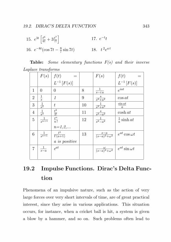
19.2. DIRAC’S DELTA FUNCTION 343
15. e3t[
t6
6! + 3 t7
7!
]16. e−8t(cos 7t− 8
7 sin 7t)
17. e−tt
18. t 2ea t
Table: Some elementary functions F(s) and their inverse
Laplace transformsF (s) f(t) =
L−1 [F (s)]
F (s) f(t) =
L−1 [F (s)]
1 0 0 8 1s−i a eiat
2 1s 1 9 s
s2+a2 cos at
3 1s2 t 10 1
s2+a2sin at
a
4 1s3
t2
2! 11 ss2−a2 cosh at
5 1sn+1
tn
n !
n=1,2,...
12 1s2−a2
1a sinh at
6 1sa+1
ta
Γ(a+1)
a is positive
13 s−a(s−a)2+ω2 eat cosωt
7 1s−a eat ω
(s−a)2+ω2 eat sinωt
19.2 Impulse Functions. Dirac’s Delta Func-
tion
Phenomena of an impulsive nature, such as the action of very
large forces over very short intervals of time, are of great practical
interest, since they arise in various applications. This situation
occurs, for instance, when a cricket ball is hit, a system is given
a blow by a hammer, and so on. Such problems often lead to
344 CHAPTER 19. UNIT STEP AND IMPULSE FUNCTIONS
differential equation of the form
ay′′ + by′ + cy = g(t),
where g(t) is large during a short interval t0 − τ < t < t0 + τ and
is otherwise zero.
We now show how to solve problems involving short impulses
by Laplace transforms.
In mechanics, the impulse I(τ) of a force g(t) over the time
interval t0 − τ < t < t0 + τ is defined to be the integral of g(t)
from t0 − τ to t0 + τ . i.e.,
I(τ) =∫ t0+τ
t0−τg(t) dt,
or, since g(t) = 0 outside of the interval (t0 − τ, t0 + τ),
I(τ) =∫ ∞
−∞g(t) dt.
Impulse is a measure of the strength of the forcing function.
The analog for an electric circuit is the integral of the electro
motive force applied to the circuit, integrated fromt0−τ to t0+τ .
Of particular practical interest is the case of a very short τ (and
its limit τ → 0), that is, the impulse of a force acting only for an
instant. To handle the case, we consider the function (with t0 = 0)

19.2. DIRAC’S DELTA FUNCTION 345
g(t) = dτ (t) =
12τ if − τ < t < τ
0 otherwise
(19.16)
where τ is small positive constant.
Its impulse I(τ) is 1, since
I(τ) =∫ ∞
−∞g(t) dt =
∫ τ
−τ
12τdt =
12τ
[t]τ−τ = 1.
Attention! In the above, τ > 0 plays an important role, because
only then [t]τ−τ = 2τ .
We note that
limτ→0
dτ (1) = 0, τ 6= 0. (19.17)
Also, since
I(τ) = 1 for each τ 6= 0
it follows that
limτ→0
I(τ) = 1. (19.18)
Equations (19.17) and (19.18) can be used to define unit impulse
functionδ, which imparts an impulse of magnitude one at t = 0
but is 0 for all values of t other than 0. i.e., the unit impulse
function δ is defined to have the properties
δ(t) = 0, t 6= 0 (19.19)

346 CHAPTER 19. UNIT STEP AND IMPULSE FUNCTIONS
and ∫ ∞
−∞δ(t) dt = 1. (19.20)
Attention! There is no ordinary function of the kind studied in
calculus that satisfies both (19.19) and (19.20), because an ordi-
nary function that is every where zero except at a single point
must have the integral 0, not 1. Though δ(t) is not a function in
the ordinary sense, it is a so-called “generalized function”.
Nevertheless, in impulse problems it is convenient to operate
on δ(t) as a ‘function’. The “function” δ defined by (19.18) and
(19.19) is usually called the Dirac delta function. δ(t) corre-
sponds to impulse at t = 0. A unit impulse at an arbitrary point
t = t0 is given by δ(t− t0). From equations (19.19) and (19.20) it
follows that
δ(t− t0) = 0, t 6= t0
and ∫ ∞
−∞δ(t− t0)dt = 1.
The delta function does not satisfy the conditions of Existence
Theorem for Laplace Transforms, but its Laplace transform can
be formally defined. Since δ(t) is defined as the limit of dτ (t) as
τ → 0,it is natural to define the Laplace transform of δ as a similar
limit of the transform of dτ . In particular, we will assume that
t0 > 0 and define L{δ(t− t0)} by the equation
L{δ(t− t0)} = limτ→0
L{dτ (t− t0)}. (19.21)
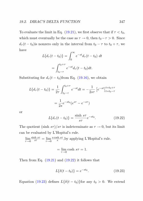
19.2. DIRAC’S DELTA FUNCTION 347
To evaluate the limit in Eq. (19.21), we first observe that if τ < t0,
which must eventually be the case as τ → 0, then t0−τ > 0. Since
dτ (t− t0)is nonzero only in the interval from t0 − τ to t0 + τ , we
have
L{dτ (t− t0)} =∫ ∞
0e−stdτ (t− t0) dt
=∫ t0+τ
t0−τe−stdτ (t− t0)dt.
Substituting for dτ (t− t0)from Eq. (19.16), we obtain
L{dτ (t− t0)} =12τ
∫ t0+τ
t0−τe−stdt = − 1
2sτ[e−st
]t=t0+τ
t=t0−τ
=12se−st0(esτ − e−sτ )
or
L{dτ (t− t0)} =sinh sτsτ
e−st0 . (19.22)
The quotient (sinh sτ)/sτ is indeterminate as τ → 0, but its limit
can be evaluated by L’Hopital’s rule.
limτ→0
sinh sτsτ = lim
τ→0
s cosh sτs ,by applying L’Hopital’s rule.
= limτ→0
cosh sτ = 1.
Then from Eq. (19.21) and (19.22) it follows that
L{δ(t− t0)} = e−st0 . (19.23)
Equation (19.23) defines L{δ(t − t0)}for any t0 > 0. We extend

348 CHAPTER 19. UNIT STEP AND IMPULSE FUNCTIONS
this result, to allow t0 to be zero, by letting t0 → 0 on the right
side of Eq. (19.23); thus
L{δ(t)} = limt0→0
e−st0 = 1 (19.24)
In a similar way it is possible to define the integral of the product
of the delta function and any continuous function f. We have∫ ∞
−∞δ(t− t0)f(t) dt = lim
τ→0
∫ ∞
−∞dτ (t− t0)f(t)dt (19.25)
Now∫∞−∞ dτ (t− t0)f(t)dt = 1
2τ
∫ t0+τt0−τ f(t)dt, using the definition (19.16)
of dτ (t)
= 12τ · 2τ · f(t∗), using the mean value theorem for integrals.
= f(t∗),
where t0 − τ < t∗ < t0 + τ. Hence t∗ → t0 as τ → 0, and it follows
from Eq.(19.25) that∫ ∞
−∞δ(t− t0)f(t) dt = f(t0). (19.26)
Example 20 Solve
y′′ + 3y′ + 2y = δ(t− 1), y(0) = 0, y′(0) = 0
Solution

19.2. DIRAC’S DELTA FUNCTION 349
Here t0 = 1. Hence Eq.(19.23) gives L[δ(t−1)] = e−s×1 = e−s.
Thus
L[y′′ + 3y′ + 2y] = L[δ(t− 1)]
gives
s2Y + 3sY + 2Y = e−s
or
Y =1
s2 + 3s+ 2e−s =
e−s
(s+ 1)(s+ 2)=(
1s+ 1
− 1s+ 2
)e−s.
Taking F (s)= 1s+1 −
1s+2 , we obtain
f(t) = L−1[F (s)] = L−1
[1
s+ 1
]− L−1
[1
s+ 2
]= e−t − e−2t.
Hence, by (Shifting on the t-axis) Theorem, we have
y(t) = L−1{e−sF (s)
}= u1(t)f(t− 1)
=
{0 (0 ≤ t ≤ 1)
e−(t−1) − e−2(t−1) (t > 1)
Example 21 Solve
y′′ + 2y′ + 2y = δ(t− π), y(0) = 1, y′(0) = 0.
Solution

350 CHAPTER 19. UNIT STEP AND IMPULSE FUNCTIONS
Takingt0 = π, Eq.(19.23) gives
L[δ(t− π)] = e−πs.
Now taking Laplace transform on both sides, the differential equa-
tion yields
(s2 + 2s+ 2) Y (s)− s− 2 = e−πs.
Hence
Y (s) =s+ 2
s2 + 2s+ 2+
e−πs
s2 + 2s+ 2.
Now
s+ 2s2 + 2s+ 2
=s+ 2
(s+ 1)2 + 1=
s+ 1(s+ 1)2 + 1
+1
(s+ 1)2 + 1
Since L−1[
ss2+1
]= cos t and L−1
[1
s2+1
]= sin t, we have
L−1
[s+ 1
(s+ 1)2 + 1
]= L−1
[s− (−1)
[s− (−1)]2 + 1
]= e−t cos t
and L−1[
1(s+1)2+1
]= L−1
[1
[s−(−1)]2+1
]= e−t sin t.
Hence
L−1
[s+ 2
s2 + 2s+ 2
]= e−t cos t+ e−t sin t.
Taking
F (s) =1
s2 + 2s+ 2=
1(s+ 1)2 + 1

19.2. DIRAC’S DELTA FUNCTION 351
and noting the already obtained fact that
f(t) = L−1[F (s)] = e−t sin t,
we have
L−1[e−πs · F (s)] = uπ(t) f(t− π)
= uπ(t) e−(t−π) sin (t− π)
Hence
y(t) = L−1[Y (s)] = e−t cos t+ e−t sin t+ uπ(t) e−(t−π) sin (t− π)

Chapter 20Differentiation and Integration
of Transforms
In this chapter we consider differentiation and integration of trans-
forms and finding out the corresponding operations for original
functions.
20.1 Differentiation of Transforms
Theorem 1 (Differentiation of Transforms)
If L[f(t)] = F (s), then
L[tnf(t)] = (−1)n dn
dsnF (s) = (−1)nF (n)(s) (n = 1, 2, 3, . . .)
(20.1)
352

20.1. DIFFERENTIATION OF TRANSFORMS 353
Proof By the definition of Laplace transform we have
F (s) = L[f(t)] =∫ ∞
0e−stf(t)dt.
Henced
dsF (s) =
d
ds
[∫ ∞
0e−stf(t)dt
].
On the RHS we have to perform first integration and then a dif-
ferentiation. Under certain conditions, it is permissible to inter-
change these operators.
Let us suppose that these conditions are satisfied in this case.
Moreover, when we take the differentiation under the integral sign,
since there are two variables s and t, we shall use the symbol ∂∂s .
Thus
d
dsF (s) =
∫ ∞
0
∂
∂s
{e−stf(t)dt
}=
∫ ∞
0e−st(−t)f(t)dt = −
∫ ∞
0e−st[t f(t)]dt
= −L [tf(t)],by the definition of Laplace transform.
Thus,
L[t f(t)] = − d
ds[F (s)] = −F ′(s) (20.2)
By a repeated application, it can be proved that
L[tnf(t)] = (−1)n dn
dsnF (s) = (−1)nF (n)(s), n = 1, 2, ...

354CHAPTER 20. DIFFERENTIATION AND INTEGRATION
Example 1 Find L[t eat]
Solution
Take f(t) = eat, then
F (s) = L [f (t)] = L[eat]
= 1s−a ; s > a
Hence using (20.2) above we have
L[teat] = − d
dsF (s) = − d
ds
(1
s− a
)=
1(s− a)2
, s > a;
Example 2 Show that L[tneat] = n!(s−a)n+1
Solution
We know that
L[eat] =1
s− a, s > a.
Hence, using theorem, we have
L[tneat] = (−1)n dn
dsn
(1
s− a
)= (−1)n(−1)
dn−1
dsn−1
(1
(s− a)2
)...
= (−1)n(−1)n n !(s− a)n+1
=n!
(s− a)n+1.
In particular,
L[teat] =1
(s− a)2, s > a;

20.1. DIFFERENTIATION OF TRANSFORMS 355
L[t2eat] =2
(s− a)3, s > a.
Example 3 Show that L[t2eat] = 2!(s−a)3
.
Solution
This is a particular case of the above example. If we prove
independently, then
L[t2eat] = (−1)2d2
ds2(F (s)) , where F (s) = L[eat]
= (−1)2d2
ds2
(1
s− a
)=
2!(s− a)3
.
Example 4 Find L[t sin t]
Solution
L[ sin t] = 1s2+1
implies that
L[t sin t] = − d
ds
(1
s2 + 1
)=
2s(s2 + 1)2
.
Example 5 Prove that L[t sin at] = 2as(s2+a2)2
.
Solution
Proceed as in the previous example.
Example 6 Find L[t2 cos t]
Solution

356CHAPTER 20. DIFFERENTIATION AND INTEGRATION
We know that L[cos t] = ss2+1
. Hence, by the theorem,
L[t2 cos t] = (−1)2d2
ds2
(s
s2 + 1
),
=d
ds
((s2 + 1)− 2s× s
(s2 + 1)2
), using
quotient rule of differentiation
=d
ds
(1− s2
(s2 + 1)2
)=
(s2 + 1)2(−2s)− (1− s2)(s2 + 1)4s(s2 + 1)4
, again using
quotient rule of differentiation
=2s3 − 6s(s2 + 1)3
, on simplification
Example 7 Find L[t2 coshπt].
Solution
L[t2 coshπt] = (−1)2d2
ds2
(s
s2 − π2
),
=2s3 + 6π2s
(s2 − π2)3,
on simplification.
Example 8 Find L[te−t sin t]
Solution
We have
L[sin t] =1
s2 + 1

20.1. DIFFERENTIATION OF TRANSFORMS 357
and hence by shifting on the s-axis theorem,
L[e−t sin t] =1
(s+ 1)2 + 1.
Now using Theorem 1 this implies
L[te−t sin t] = − d
ds
(1
(s+ 1)2 + 1
)=
2(s+ 1)((s+ 1)2 + 1)2
, using quotient rule
=2(s+ 1)
(s2 + 2s+ 2)2.
Example 9 Find L[te2t cos 5t].
Solution
We have L[cos 5t] = ss2+25
and hence
L[e2t cos 5t] =s− 2
(s− 2)2 + 25.
Now this implies by Theorem 1 that
L[te2t cos 5t] = − d
ds
(s− 2
(s− 2)2 + 25
)=
(s− 2)2 − 25[(s− 2)2 + 25]2
,
on simplification.

358CHAPTER 20. DIFFERENTIATION AND INTEGRATION
20.2 Exercises
In Exercises 1-7, find the Laplace transform.
1. t cos 2t
2. te2t
3. t cosh t
4. t2et
5. t sinh 2t
6. t2 sinh 2t
7. t2 cosωt
8. Using Differentiation of Transforms Theorem, derive the
following formulae:
(i) L−1[
s(s2+β2)2
]= 1
2β (t sinβt)
(ii) L−1[
1(s2+β2)2
]= 1
2β3 (sinβt− βt cosβt)
(iii) L−1[
s2
(s2+β2)2
]= 1
2β (sinβt+ βt cosβt)
20.2.1 Answers
1. s2−4(s2+4)2
2. 1(s−2)2
3. s2+1(s2−1)2
4. 2(s−1)3
5. 4s(s2−4)2
6.4(4+3s2)(s2−4)3
7. 2s(s2−3ω2)(s2+ω2)3
20.3 Integration of Transforms
Theorem 2 (Integration of Transform) If f(t) satisfies the
conditions of the existence of Laplace transform theorem and the

20.3. INTEGRATION OF TRANSFORMS 359
limit of f(t)t as t approaches to 0 from the right exists, then
L
[f(t)t
]=∫ ∞
sF (u)du ( s > γ ) (20.3)
Proof From the definition of Laplace transform it follows that∫ ∞
sF (u)du =
∫ ∞
s
[∫ ∞
0e−utf(t)dt
]du
Under the assumptions of the theorem it is possible to interchange
the order of integration, so that
∫ ∞
sF (u)du =
∫ ∞
0
[∫ ∞
se−utf(t)du
]dt =
∫ ∞
0f(t)
[∫ ∞
se−utdu
]dt
The integral over u on the right equals e−st
t , when s > γ and there-
fore, ∫ ∞
sF (u)du =
∫ ∞
0e−st f(t)
tdt = L
[f(t)t
], s > γ
Example 10 Find L[
1−et
t
]Solution
Here take f(t) = 1− et, then
F (s) = L [f (t)] = L[1]− L[et] =1s− 1s− 1

360CHAPTER 20. DIFFERENTIATION AND INTEGRATION
L[1− et
t
]= L
[f(t)t
]=
∫ ∞
sF (u)du, using Theorem 2
=∫ ∞
s
(1u− 1u− 1
)du
= [log u− log(u− 1)]∞s
=[log
u
u− 1
]∞s
= log 1− logs
s− 1
= − logs
s− 1= log
s− 1s
.
Example 11 Find L[
sin att
]Solution
Since L[sin at] = as2+a2 ,
L
[sin att
]=∫ ∞
s
a
u2 + a2du =
[tan−1 u
a
]∞s
=π
2− tan−1 s
a= cot−1 s
a
Inverse Transform: Corollary to (3)
Using (20.3) above, we have
L−1
[∫ ∞
sF (u)du
]=f(t)t. (20.4)
The following result is needed in the development of the coming
example.
RESULT Show that if∫∞s F (u)du = g(s), then F (u) = − d
dug(u).

20.3. INTEGRATION OF TRANSFORMS 361
Proof
− d
dug(u) = − lim
h→0
g(u+ h)− g(u)h
= − limh→0
∫∞u+h F (r)dr −
∫∞u F (r)dr
h
= limh→0
∫∞u F (r)dr −
∫∞u+h F (r)dr
h
= limh→0
∫ u+hu F (r)dr
h= F (u).
Example 12 Find the inverse transform of the function loge(1 +ω2
s2 )
Solution
Let∫∞s F (u)du = loge
(1 + ω2
s2
)Then using the above Result,
F (u) = − d
duloge
(1 +
ω2
u2
)= − d
duloge
(u2 + ω2
u2
)
=d
du
(2 log u− log(u2 + ω2)
)=
2u− 2uu2 + ω2
...f(t) = L−1 [F (s)] = L−1
[2s− 2ss2 + ω2
]= 2− 2 cosωt.
This function satisfies the conditions under which (20.3) holds.
Hence using (20.4), we obtain
L−1
[log(
1 +ω2
s2
)]= L−1
[∫ ∞
sF (u)du
]=f(t)t
=2t(1−cosωt).

362CHAPTER 20. DIFFERENTIATION AND INTEGRATION
Exercises
In Exercises 1-6, find the inverse Laplace transform of the given
function.
1. loges+as+b
2. loges
s−1
3. loges2+1
(s−1)2
4. cot−1 sω
5. cot−1 (s+ 1)
6. tan−1 1s
Answers
1. e−bt−e−at
t
2. et−1t
3.2(et−cos t)
t
4. sin ωtt
5. e−t sin tt
6. sin tt

Chapter 21Convolution and Integral
Equations
21.1 Convolution and Integral Equations
An important general property of Laplace transformation has to
do with product of transforms. It often happens that we are
given two transforms F (s) and G(s) whose inverses f(t) and g(t)
we know, and we would like to find the inverse of the product
F (s)G(s) from those known inverses f(t)and g(t). The inverse is
written
(f ∗ g)(t), which is a standard notation and is called the con-
volution of f and g. Definition follows:
Definition The convolution of f and g is a function h, usually
363

364CHAPTER 21. CONVOLUTION AND INTEGRAL EQUATIONS
written f ∗ g, defined by
h(t) = (f ∗ g)(t) =∫ t
0f(t− u)g(u)du.
Theorem 1 (Properties of Convolution)
(i). (Commutativity of convolution) f ∗ g = g ∗ f .(ii). (Distributive law) f ∗ (g + h) = f ∗ g + f ∗ h(iii). (Associative law) (f ∗ g) ∗ h = f ∗ (g ∗ h)(iv). f ∗ 0 = 0 ∗ f = 0.
Proof We prove only (i) leaving the rest to the exercises.
Put t – u = v, then du = − dv,
u = 0 implies v = t ; u = t implies v = 0.
Hence
(f ∗ g)(t) = −∫ 0
tf(v)g(t− v)dv =
∫ t
0g(t− v)f(v)dv = (g ∗ f)(t).
Theorem 2 (Convolution Theorem) If f(t) and g(t) are the
inverse transforms of F(s) and G(s) respectively, the inverse trans-
form of the product F(s)G(s) is the convolution of f(t)and g(t).
i.e.,
L−1 [F (s)G(s)] = (f ∗ g)(t) (21.1)
Proof of the Convolution Theorem
By definition
L−1 [F (s)] = f(t) and L−1 [G(s)] = g(t)
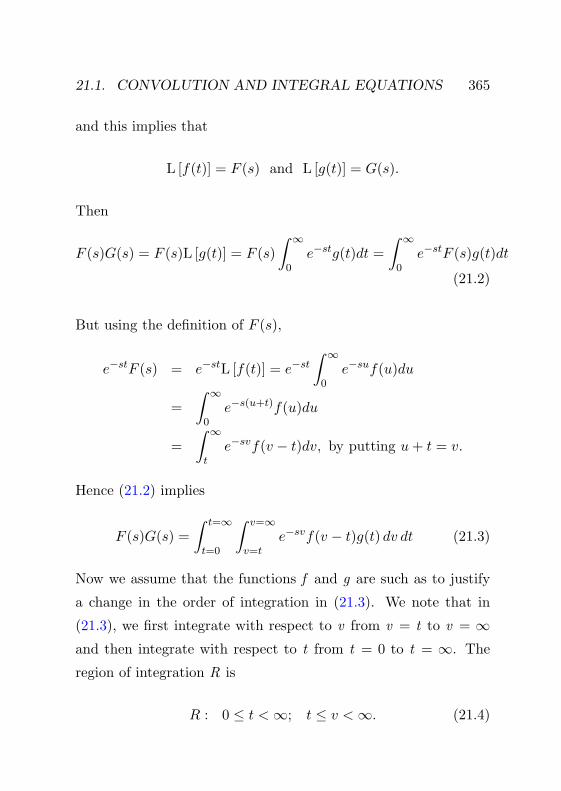
21.1. CONVOLUTION AND INTEGRAL EQUATIONS 365
and this implies that
L [f(t)] = F (s) and L [g(t)] = G(s).
Then
F (s)G(s) = F (s)L [g(t)] = F (s)∫ ∞
0e−stg(t)dt =
∫ ∞
0e−stF (s)g(t)dt
(21.2)
But using the definition of F (s),
e−stF (s) = e−stL [f(t)] = e−st
∫ ∞
0e−suf(u)du
=∫ ∞
0e−s(u+t)f(u)du
=∫ ∞
te−svf(v − t)dv, by putting u+ t = v.
Hence (21.2) implies
F (s)G(s) =∫ t=∞
t=0
∫ v=∞
v=te−svf(v − t)g(t) dv dt (21.3)
Now we assume that the functions f and g are such as to justify
a change in the order of integration in (21.3). We note that in
(21.3), we first integrate with respect to v from v = t to v = ∞and then integrate with respect to t from t = 0 to t = ∞. The
region of integration R is
R : 0 ≤ t <∞; t ≤ v <∞. (21.4)

366CHAPTER 21. CONVOLUTION AND INTEGRAL EQUATIONS
In order to change the order integration in (21.3), we have to find
the alternate form of the region R. For this we first draw a rough
sketch of the region R using the following facts:
We note that R is the intersection of the following two regions
in the vt plane:
(i) the upper half plane in the vt- plane (this region corresponds
to 0 ≤ t <∞ .)
(ii) the region to the right of the line v = t (this region corre-
sponds to t ≤ v ≤ ∞ .)
The region R is shown in Fig.21.1 where the shaded portion is
extended to infinity in the vt-plane.
Figure 21.1: The region of integration is the shaded portion that is
extended to infinity

21.1. CONVOLUTION AND INTEGRAL EQUATIONS 367
Referring to Fig. 21.1, we note that while v varies from 0 to ∞ ,
t varies from 0 to v. Hence the alternate form of (21.4) is
0 ≤ v <∞; 0 ≤ t ≤ v (21.5)
Now using the system of inequalities in (21.5) as the representation
of the region of integration, by changing the order of integration,
(21.3) yields
F (s)G(s) =∫ v=∞
v=0
∫ t=v
t=0e−svf(v − t)g(t)dt dv
=∫ v=∞
v=0e−sv
{∫ t=v
t=0f(v − t)g(t)dt
}dv (21.6)
Now, by the definition of convolution,∫ t=v
t=0f(v − t)g(t)dt = (f ∗ g)(v).
Hence, (21.6) becomes
F (s)G(s) =∫ v=∞
v=0e−sv(f ∗ g)(v)=L[(f ∗ g)(v)].
Hence
L−1 [F (s)G(s)] = (f ∗ g)(t)
This completes the proof.
Remark to Convolution Theorem

368CHAPTER 21. CONVOLUTION AND INTEGRAL EQUATIONS
By the notations as in theorem, (21.1) can be restated as
F (s)G(s) = L [(f ∗ g)(t)] . (21.7)
Example 1 Using convolution property, find L−1[
1s(s2+a2)
].
Solution
Let F (s) = 1s , G(s) = 1
s2+a2 , then
f(t) = L−1
(1s
)= 1; g(t) = L−1
(1
s2 + a2
)=
sin ata
.
Thus f(t− u) = 1; and hence
L−1
(1
s(s2 + a2)
)=∫ t
01 · sin au
adu =
∫ t
0
sin aua
du
= − 1a2
[cos au]t0 =1a2
[1− cos at]
Example 2 Using convolution property, find L−1[
1s2(s−a)
]Solution
Let
F (s) =1s2, G(s) =
1s− a
,
then
f(t) = L−1
(1s2
)= t; g(t) = L−1
(1
s− a
)= eat.

21.1. CONVOLUTION AND INTEGRAL EQUATIONS 369
Thus,
f(t− u) = t− u
and hence,
L−1
(1
s2(s− a)
)=
∫ t
0(t− u)︸ ︷︷ ︸
First Function
eau︸︷︷︸Derivative of the second function
du
=
(t− u)︸ ︷︷ ︸First Function
eau
a︸︷︷︸Second function
t
0
−∫ t
0(0− 1)︸ ︷︷ ︸
Derivative of the First Function
eau
a︸︷︷︸Second function
du
= − ta
+1a
∫ t
0eaudu
= − ta
+1a
[eau
a
]t
0
= − ta
+1a
(eat − 1a
)=
1a2
[eat − at − 1
].
Example 3 Using convolution property, find L −1[
1(s2+a2)2
].
Solution
L −1
[1
(s2 + a2)2
]= L −1
[1s
s
(s2 + a2)2
]Let
F (s) =1s, G(s) =
s
(s2 + a2)2,

370CHAPTER 21. CONVOLUTION AND INTEGRAL EQUATIONS
then
f(t) = L−1
(1s
)= 1; g(t) = L−1
(s
(s2 + a2)2
)=t sin at
2a; f(t−u) = 1 .
Hence
L−1
[1s
s
(s2 + a2)2
]=
∫ t
0
u sin au2a
du
=12a
{[−u cos au
a
]t
0
+∫ t
0
cos aua
du
}=
12a3
[sin at− at cos at] ,
on simplification.
Partial Fractions: Repeated Complex Factors [(s − a)(s −a)]2
In the chapter “Laplace and Inverse Laplace Transforms” we have
mentioned the case of repeated complex factors while undergoing
partial fraction. In that case the partial fractions are of the form
As+B
[(s− a)(s− a)]2+
Ms+N
(s− a)(s− a). (21.8)
In the following example we have a partial fraction of the formKω0
(s2+ω20)
2 [i.e., only first part of the general form (??).]
Solution of Initial Value Problems
Example 4 Solve the initial value problem
y′′ + ω02y = K sinω0t

21.1. CONVOLUTION AND INTEGRAL EQUATIONS 371
with y(0) = 0 and y′(0) = 0,
Solution
L[y′′ + ω02y] = L[k sinω0t]
gives s2Y + ω02Y = Kω0
(s2+ω20)
2
Hence
Y =Kω0
(s2 + ω02)2
The denominator is a repeated complex factor with roots s = iω0
and −iω0.
We find its inverse of Y by convolution. Taking F (s) = ω0
s2+ω20, we
have f(t) = L−1[F (s)] = sinω0t and so we obtain
y(t) = L−1(Y ) = L−1
[K
ω0· ω0
s2 + ω02· ω0
s2 + ω02
]= L−1
[K
ω0F (s)F (s)
]=
K
ω0L−1 [F (s)F (s)] , applying the linearity
=K
ω0(f ∗ f)(t), applying convolution
=K
ω0
∫ t
0f(t− u)f(u)du
=K
ω0
∫ t
0sin ω0(t− u) sinω0udu (21.9)
Now with C = ω0(t− u) and D = ω0u, the trigonometric identity
−2 sinC sinD = cos(C +D)− cos(C −D)

372CHAPTER 21. CONVOLUTION AND INTEGRAL EQUATIONS
gives
sin ω0(t− u) sinω0u = −12{cosω0t− cos(ω0t− 2ω0u)}
=12{cos(ω0t− 2ω0u)− cosω0t}
= 12 {cos(2ω0u− ω0t)− cosω0t} , since
cos(ω0t− 2ω0u) = cos[−(ω0t− 2ω0u)]
Using this (21.9) yields
y(t) =K
2ω0
∫ t
0{cos(2ω0u− ω0t)− cosω0t} du
=K
2ω0
∫ ω0t
0
{cosw
12ω0
dw
}− cosω0t
∫ t
0du,
where we have taken
w = 2ω0u − ω0t; w = −ω0t when u = 0;w = ω0t when u = t
So
y(t) =K
2ω0
(sin ω0t
2ω0− sin (−ω0t)
2ω0− t cosω0t
)=
K
2ω0
(sin ω0t
ω0− t cosω0t
)=
K
2ω20
(sin ω0t− ω0t cosω0t) .
Example 5 Find the solution of the initial value problem
y′′ + 4y = g(t), (21.10)

21.1. CONVOLUTION AND INTEGRAL EQUATIONS 373
y(0) = 3, y′(0) = −1. (21.11)
Solution
By taking the Laplace transform of the differential equation
and using the initial conditions, we obtain
s2Y (s)− 3s+ 1 + 4Y (s) = G(s),
where Y (s) = L[y(t)] and G(s) = L[g(t)].
Hence
Y (s) =3s− 1s2 + 4
+G(s)s2 + 4
. (21.12)
i.e.,
Y (s) = 3s
s2 + 4− 1
22
s2 + 4+
12
2s2 + 4
G(s) (21.13)
Then, we obtain
y(t) = L−1[Y (s)] = 3 cos 2t− 12 sin 2t+ 1
2
∫ t
0sin 2(t− u) g(u) du
(21.14)
If a specific forcing function g is given, then the integral in Eq.(??)
can be evaluated (by numerical means, if necessary).
Solution, Transfer Function
If we denote L [y(t)] = Y (s). Then we have
L[y′(t)
]= sY (s)− y(0)

374CHAPTER 21. CONVOLUTION AND INTEGRAL EQUATIONS
and
L[y′′(t)
]= s2Y (s)− sy(0)− y′(0). (21.15)
Hence applying Laplace transform on the differential equation
ay′′ + by′ + cy = g(t) (21.16)
after simplification, we obtain
(as2 + bs+ c)Y = (as+ b)y(0) + ay′(0) + L[g(t)].
Hence
Y (s) = [(as+ b)y(0) + ay′(0)]H(s) +G(s)H(s) (21.17)
with
G(s) = L[g(t)]
and
H(s) =1
as2 + bs+ c. (21.18)
H(s) is called the transfer function.
We write
Y (s) = Φ(s) + Ψ(s)
where
Φ(s) =(as+ b) y(0) + ay′(0)
as2 + bs+ c

21.1. CONVOLUTION AND INTEGRAL EQUATIONS 375
and
Ψ(s) =G(s)
as2 + bs+ c.
Then
y(t) = φ(t) + ψ(t)
where
φ(t) = L−1[Φ(s)]
and
ψ(t) = L−1[Ψ(s)].
Special Case 1:
If g(t) = 0 in (21.16), we have
ay′′ + by′ + cy = 0.
This together with the initial conditions y = (0) = y0 and y′(0) =
y′0 give the solution
y(t)= φ(t) = L−1
[(as+ b) y0 + ay′0as2 + bs+ c
].
Special case 2:
If (21.16) is together with the initial conditions y(0) = 0 andy′(0) =

376CHAPTER 21. CONVOLUTION AND INTEGRAL EQUATIONS
0, then solution is
y(t) = ψ(t) = L−1
[G(s)
ab2 + bs+ c
]= L−1[H(s)G(s)]
=∫ t
0h(t− u)g(u)du (21.19)
Special Case 2a:
If (21.16) is together with the initial conditions y(0) = 0 and
y′(0) = 0, and when G(s) = 1, then
g(t) = L−1[G(s)] = L−1[1]
= δ(t), the Dirac-delta function, since L[δ(t)] = 1.
Hence
ψ(s) = H(s).
i.e., y = h(t) is the solution of the initial value problem
ay′′ + by′ + cy = δ(t), y(0) = 0, y′(0) = 0.
h(t) is called the impulse response of the system.
Example 6 Solve the initial value problem
y′′ + 3y′ + 2y = g(t)
where g(t) =
{1, if 1 < t < 2
0, otherwise,,

21.1. CONVOLUTION AND INTEGRAL EQUATIONS 377
with the initial conditions y(0) = y′(0) = 0.
Solution
Comparing with Eq. (21.16) and using Eq. (21.18), we obtain
H(s) =1
s2 + 3s+ 2=
1s+ 1
− 1s+ 2
and hence
h(t) = L−1[H(s)] = L−1
[1
s+ 1− 1s+ 2
]= e−t − e−2t.
Hence
y = ψ(t) = L−1[H(s)G(s)] =∫ t
0h(t− τ)g(τ)dτ
We are given with g(t) = 1 if 1 < t < 2 and 0 elsewhere. Hence
three cases arise.
Case 1: If t < 1,
y = ψ(t) =∫ t
0h(t− τ)g(τ)dt
=∫ t
0h(t− τ)× 0× dt = 0.
Case 2: If 1 < t < 2, we have to integrate from 1 to t. This gives
y = ψ(t) =∫ t
1h(t− τ)g(τ)dτ

378CHAPTER 21. CONVOLUTION AND INTEGRAL EQUATIONS
=∫ t
1[e−(t−τ) − e−2(t−τ)]dτ =
[e−(t−τ) − 1
2e−2(t−τ)
]t
1
= e−0 − e−(t−1) − 12(e−0 − e−2(t−1)) =
12− e−(t−1) +
12e−2(t−1)
Case 3: If t > 2, we have to integrate from 1 to 2 only (not to t).
This gives
y = ψ(t) =∫ 2
1h(t− τ)g(τ)dτ
=∫ 2
1[e−(t−τ) − e−2(t−τ)]dτ =
[e−(t−τ) − 1
2e−2(t−τ)
]2
1
= e−(t−2) − e−(t−1) − 12[e−2(t−2) − e−2(t−1)].
Integral Equations
Convolution helps in solving certain integral equations, that
is, equations in which the unknown function y(t) appears under
the integral (and perhaps also outside of it). We solve an integral
equation in which integral is of the form of a convolution.
Example 7 Solve the integral equation
y(t) = t+∫ t
0y(τ) sin (t− τ) dτ
Solution
Step 1: By observation it can be seen that the integral is of the
form of a convolution. Hence we write the given equation as
y = t+ y ∗ sin t. (21.20)

21.1. CONVOLUTION AND INTEGRAL EQUATIONS 379
Step 2: We write Y = L(y). By an application of Convolution
Theorem taking f(t) = y(t) and g(t) = sin t, we have
L [y ∗ sin t] =L [(f ∗ g)(t)] = F (s)G(s) = L [y(t)] L [sin t] = Y (s)1
s2 + 1.
Hence applying Laplace transform, (21.20) becomes
Y (s) =1s2
+ Y (s)1
s2 + 1.
Solving for Y (s), we obtain
Y (s) =s2 + 1s4
=1s2
+1s4.
Step 3: Taking the inverse transform, we obtain
Y (t) = t+16t3.
Example 8 Solve
y(t) = t3 +∫ t
0sin(t− u)y(u)du
Solution
Using convolution,
L
[∫ t
0sin(t− u)y(u)du
]= L[sin t]L[y(t)].

380CHAPTER 21. CONVOLUTION AND INTEGRAL EQUATIONS
Hence by applying L on the given integral equation, we get
L[y(t)] = L[t3] + L[sin t]L[y(t)].
Hence,
L[y(t)]{1− L[sin t] } = L[t3]
or
L [y(t)] =L [t3]
1− L[sin t]=
3!/s4
1− 1/(s2 + 1)
=3!s4
(s2 + 1s2
)=
3!s4
+3!s6,
so
y(t) = L−1
[3!s4
+3!s6
]= t3 +
120t5
is the solution of the given integral equation.

Chapter 22Two Point Boundary Value
Problems
22.1 Two Point Boundary Value Problems
Since the general solution to a second order differential equation
y′′ + p(x)y′ + q(x)y = g(x) (22.1)
contains two arbitrary constants, we need two conditions for ob-
taining a particular solution. Some times the two conditions are
of the type
y(α) = y0, y(β) = y1. (22.2)
The conditions in (22.2) are called boundary conditions since
they refer to the boundary points α , β of an interval I. Eq. (22.1)
381
382CHAPTER 22. TWO POINT BOUNDARY VALUE PROBLEMS
and conditions (22.2) together constitute what is known as
a boundary value problem.
If the function g has the value zero for each x, and if the
boundary values y0 and y1 are also zero, then the problem (22.1)
with conditions (22.2) is called homogeneous. Otherwise, the
problem is nonhomogeneous.
Remark The solution of a boundary value problem given by equa-
tions (22.1) and (22.2) is unique if and only if no nonzero solution
y of (22.1) satisfies y(A) = y(B) = 0.
Example 1 (Boundary Value Problem) Solve
y′′ + 2y = 0, y(0) = 1, y(π) = 0.
Solution
The general solution to the given differential equation is
y = c1 cos√
2x+ c2 sin√
2x.
Using the first of boundary conditions, we obtain
y(0) = c1 = 1.
The second boundary condition implies that
c1 cos√
2π + c2 sin√
2π = 0,
so c2 = − cot√
2π. Thus the solution of the given boundary value

22.1. TWO POINT BOUNDARY VALUE PROBLEMS 383
problem is
y = cos√
2x− cot√
2π sin√
2x.
Example 2 (Boundary Value Problem) Solve
y′′ + y = 0, y(0) = 1, y(π) = a.
Solution
The general solution is given by
y = c1 cosx+ c2 sinx.
Using the first of the boundary conditions we have
y(0) = c1 = 1.
The second boundary condition gives
y(π) = −c1 = a.
These two conditions on c1are incompatible if a 6= −1, so the
problem has no solution in that case. However, if a = −1, then
both boundary conditions are satisfied provided that c1 = 1, where
c2 is still arbitrary.
In this case a solution to the given boundary value problem is
y = 3 cosx+ c2 sinx,

384CHAPTER 22. TWO POINT BOUNDARY VALUE PROBLEMS
where c2 is still arbitrary. This example illustrates that a homoge-
neous boundary value problem may have no solution, and also that
under special circumstances it may have infinitely many solutions.
Example 3 Solve the boundary value problem
y′′ + 2y = 0, y(0) = 0, y(π) = 0.
Solution
The general solution is given by
y = c1 cos√
2x+ c2 sin√
2x.
The first boundary condition requires that c1 = 0. The second
boundary condition gives c2 sin√
2π = 0. Since sin√
2π 6= 0 we
must have c2 = 0. Consequently, y = 0 for all x is the only solution
of the given boundary value problem. This example illustrates that
a homogeneous boundary value problem may have only the trivial
solution y = 0.
Example 4 Solve the boundary value problem
y′′ + y = 0, y(0) = 0, y(π) = 0.
Solution
The general solution is given by
y = c1 cosx+ c2 sinx.
22.2. EIGEN VALUE PROBLEMS 385
The first boundary condition requires that c1 = 0. The second
boundary condition is also satisfied when c1 = 0 regardless the
value of c2. Thus the solution of the given boundary value problem
is
y = c2 sinx,
where c2 is still arbitrary. This example illustrates that a homoge-
neous boundary value problem may have infinitely many solutions.
22.2 Eigen Value Problems
Consider the boundary value problem
y′′ + λy = 0, (22.3)
with the boundary conditions
y(0) = 0, y(π) = 0. (22.4)
We define eigen values and eigen functions as follows:
Definition The values of λ for which nontrivial solutions of (22.3)
and (22.4) occur are called eigen values, and the corresponding
nontrivial solutions are called eigen functions.
Example 5 Discuss whether λ = 1 is an eigen value of the bound-
ary value problem (22.3) and (22.4). Give some eigen functions.
Is λ = 2 an eigen value?
Solution

386CHAPTER 22. TWO POINT BOUNDARY VALUE PROBLEMS
Observe that the above boundary value problem (22.3) and
(22.4) is the same as the problems in Examples 3 and 4 if λ = 2
and λ = 1, respectively.
• Referring to Example 4, we note that for λ = 1 Eqs.(22.3)
and (22.4) have the solution
y = c2 sinx,
where c2 is an arbitrary constant. This shows that for λ = 1
Eqs.(22.3) and (22.4) have nontrivial solution. Hence λ = 1
is an eigen value. Any nonzero multiple of sinx is an eigen
function corresponding the eigen value λ = 1.
• Referring to Example 3, we note that for λ = 2 Eqs.(22.3)
and (22.4) have only the trivial solution y = 0. Hence λ = 2
is not an eigen value.
Example 6 Find all the eigen values and eigen functions of the
boundary value problem
y′′ + λy = 0, (22.5)
with the boundary conditions
y(0) = 0, y(π) = 0. (22.6)
Solution
22.2. EIGEN VALUE PROBLEMS 387
Case 1) If λ = 0, then (22.5) becomes
y′′ = 0.
Integrating (with respect to x ),
y′ = a,
where a is an arbitrary constant. One more integration (with
respect to x ) yields
y = y(x) = ax+ b,
where b is also an arbitrary constant.
By (22.6), y(0) = 0, and hence the above implies b = 0. Hence the
above reduces to
y = y(x) = ax.
Again by (22.6), y(π) = 0, hence the above implies aπ = 0 which
implies a = 0. Hence the above reduces to
y = y(x) = 0.
Hence we have only trivial solution when λ = 0. Hence 0 is not an
eigen value.
Case 2) If λ > 0, say λ = µ2, then (22.5) becomes
y′′ + µ2y = 0,

388CHAPTER 22. TWO POINT BOUNDARY VALUE PROBLEMS
and the characteristic equation corresponding to this second order
ordinary differential equation is
λ2 + µ2 = 0
i.e., λ2 = −µ2.
Hence the general solution of is
y(x) = A cosµx+B sinµx.
From the boundary condition in (22.6), it follows that
y(0) = A = 0 .
Hence
y(x) = B sinµx.
Again by (22.6),
y(π) = B sinµπ = 0.
Two cases arise: either B = 0 or sinµπ = 0.
The case of B = 0 leads to y(x) = 0 for 0 ≤ x ≤ π, which is the
trivial solution. As we are seeking for nontrivial solutions, we take
B 6= 0. Then
sinµπ = 0.
Since sine function has the value zero at every integer multiple of

22.2. EIGEN VALUE PROBLEMS 389
π, the above implies
µπ = nπ , n = 1, 2, 3, . . .
or
µ = n , n = 1, 2, 3, . . . .
Hence the corresponding values of λ are given by
λ = µ2 = n2 , n = 1, 2, 3, . . . .
Hence
λ1 = 1, λ2 = 4, λ3 = 9, . . . , λn = n2, . . .
are eigen values of the problem. Since the nontrivial solutions are
obtained from
y(x) = B sinµx = B sin√λx,
eigen functions corresponding to the eigen value λn = n2 (n =
1, 2, 3, . . .) are multiples of the functions sinnx(n = 1, 2, 3, . . .).
We will usually choose the multiplicative constant to be 1 and
write the eigen functions as
y1(x) = sinx, y2(x) = sin 2x, y3(x) = sin 3x, . . . , yn(x) = sinnx, . . . ,
noting that multiples of these functions are also eigen functions.

390CHAPTER 22. TWO POINT BOUNDARY VALUE PROBLEMS
Case 3) If λ < 0, say λ = −µ2, then (22.5) becomes
y′′ − µ2y = 0,
and the characteristic equation corresponding to this second order
ordinary differential equation is
λ2 − µ2 = 0
i.e., λ2 = µ2 ⇒ λ = ±µ.
Hence the general solution is
y(x) = Aeµx +Be−µx.
For the convenience of applying boundary conditions, recalling
the definitions of hyperbolic sine and cosine functions, we write
the above general solution as
y(x) = c1 coshµx+ c2 sinhµx.
By (22.6), y(0) = 0, and hence the above implies
c1 = 0.
Thus
y(x) = c2 sinhµx.

22.2. EIGEN VALUE PROBLEMS 391
Also by (22.6), y(π) = 0, and hence the above implies
c2 sinhµπ = 0.
Since µ 6= 0, sinhµπ 6= 0, hence we must have c2 = 0.
Hence
y(x) = 0.
Hence we have only trivial solution when λ < 0. Hence any λ <0
is not an eigen value.
We conclude that the boundary value problem (22.5) and (22.6)has
an infinite sequence of positive eigen values
λn = n2 for n = 1, 2, 3, . . .
and that the corresponding eigen functions are proportional to
sinnx. Further, there are no other real eigen values. There remains
the possibility that there might be some complex eigen values. We
mention (without proving) that the problem (22.3) and (22.4) have
no other complex eigen values.
Example 7 Find all the eigen values and eigen functions of the
boundary value problem
y′′ + λy = 0, (22.7)
with the boundary conditions
y(0) = 0, y(L) = 0. (22.8)

392CHAPTER 22. TWO POINT BOUNDARY VALUE PROBLEMS
Solution
Proceeding as in the previous example, it can be seen that the
boundary value problem (22.7) and (22.8) has an infinite sequence
of positive eigen values
λn = n2π2
L2 for n = 1, 2, 3, . . .
and that the corresponding eigen functions are given by
yn(x) = sin nπxL for n = 1, 2, 3, . . .
Exercises
In Exercises 1-3 solve the following boundary value problems (A
basis of solution is given in the bracket).
1. y′′ − 16y = 0; y(0) = 3, y(14) = 3e(e4x, e−4x)
2. y′′ + y′ − 2y = 0; y(0) = 0, y(1) = e− e−2(ex, e−2x)
3. y′′ − 2y′ = 0; y(0) = −1, y(12) = e− 2(1, e2x)
In Exercises 4-9 either solve the given boundary value prob-
lem or else show that it has no solution.
4. y′′ + y = 0; y(0) = 0, y(π) = 2
5. y′′ + 2y = 0; y(0) = 1, y(π) = 0
6. y′′ + 4y = cosx; y(0) = 0, y(π) = 0
7. y′′ + 4y = sinx; y(0) = 0, y(π) = 0
8. x2y′′ − 2xy′ + 2y = 0; y(1) = −1, y(2) = 1
9. x2y′′ + 3xy′ + y = x2; y(1) = 0, y(e) = 0
Answers

22.2. EIGEN VALUE PROBLEMS 393
1. y = 3e4x
2. y = ex − 2e−2x
3. y = −2 + e2x
4. y = −2 sinx
5. y = 1√2(cot
√2π cos
√2x+
sin√
2x)
6. No solution
7. y = c2 sin 2x+ 13 sinx
8. y = −52x+ 3
2x2
9. y = −19x
−1 + 19(1 −
e3)x−1 lnx+ 19x
2

Chapter 23Fourier Series of Periodic
Functions
23.1 Introduction
Periodic functions frequently occur in Engineering problems. If
these functions be represented in terms of simple periodic func-
tions such as sine and cosine series, then it is of great practical
importance. The French physicist Joseph Fourier (1768 - 1830)
showed in 1807 that an arbitrary periodic function could be ex-
pressed as a linear combination of sines and cosines. These linear
combinations are called Fourier series.
In this chapter we discuss basic concepts, facts and techniques in
connection with Fourier series. In certain sense these series are
more universal than Taylor series. Many discontinuous periodic
394

23.2. PERIODIC FUNCTIONS 395
functions of practical interest can be developed in Fourier series
but not in Taylor series.
23.2 Periodic Functions
Definitions A function f(x) is said to be periodic if it is defined
for all real x and if there is a positive number L such that
f(x+ L) = f(x)
for every real x.
The number L is called a period of f . The smallest of such
L > 0 (if it exists) is called the primitive period or fundamen-
tal period of f .
Remark If f(x+ L) = f(x) for every real number x,
then it follows that
f(x+ nL) = f(x)
for every real number x and for any positive integer n.
Examples
1. The primitive period of sin x is 2π, because
sin(x+ 2π) = sinx ∀ x ∈ R
and 2π is the smallest such positive number. Similarly, the
primitive period of cos x is 2π.

396 CHAPTER 23. FOURIER SERIES
2. The primitive period of sin 2x is π, because
sin 2 (x+ π) = sin(2x+ 2π) = sin 2x ∀ x ∈ R
and π is the smallest such positive number. Similarly, prim-
itive period of cos 2x is π.
3. The primitive period of sin 3x is 2π3 .
4. The primitive period of sin 2π x is 1, because
sin 2π (x+ 1) = sin(2πx+ 2π) = sin 2π x ∀ x ∈ R
and 1 is the smallest such positive number. Similarly, the
primitive period of cos 2π x is 1.
5. The primitive period of sinπ x and cosπ x is 2.
Examples of periodic functions without primitive periods
The following are some examples of periodic functions without
primitive periods.:
1. f(x) = k, for every real x, where k is a constant is a periodic
function, and any positive real number is a period. But f
has no primitive period.
2. f defined by
f(x) =
{1, whenx is rational
0, whenx is irrational

23.2. PERIODIC FUNCTIONS 397
is a periodic function, any positive rational number is a pe-
riod. But f has no primitive period.
Attention! Hereinafter we use the term period for primitive
period. i.e., L is the period of f(x) if L is the smallest positive
number for which
f(x+ L) = f(x) for every real x.
Exercises
In Exercises 1-6, determine whether the given function is periodic.
If so, find its fundamental period.
1. sin 7x
2. cos 4πx
3. sinh 2x
4. sin πxL
5. tanπx
6. x3
7. f(x) =
{2, 2n− 1 ≤ x < 2n
3, 2n ≤ x < 2n+ 1n = 0, ±1, ±2, . . .
8.
f(x) =
{1, 2n− 2 ≤ x < 2n
(−1)n, 2n ≤ x < 2n+ 2n = 0, ±1, ±2, . . .
Answers
1. L = 2π7
2. L = 12
3. Not periodic
4. L = 2L
5. L = 1
6. Not periodic

398 CHAPTER 23. FOURIER SERIES
7. L = 2 8. L = 4
23.3 Trigonometric Series
Definition A series of the form
a0 + a1 cosx+ b1 sinx+ a2 cos 2x+ b2 sin 2x+ · · ·
+an cosnx+ bn sinnx+ · · · ,
where a0, a1, b1, . . . , an, bn, . . . are real constants is called
a trigonometric series. Here an’s and bn’s are the coefficients
of the series.
Fourier Series of 2L Periodic Functions
The Fourier series of 2L periodic function f(x) initially defined
over the interval −L < x < L is given by the Fourier series
f(x) =a0
2+
∞∑n=1
(an cos n π x
L + bn sin n π xL
)(23.1)
where the coefficients are given by the Euler formulae1
a0 =1L
∫ L
−Lf(x)dx (23.2)
1Determination of Euler coefficients are done at the end section of thischapter.

23.3. TRIGONOMETRIC SERIES 399
an =1L
∫ L
−Lf(x) cos n π x
L dx, n = 1, 2, 3, . . . (23.3)
bn =1L
∫ L
−Lf(x) sin n π x
L dx, n = 1, 2, 3, . . . (23.4)
Theorem 1 (The Fourier Convergence Theorem:
Convergence and Sum of Fourier Series)
Suppose that f and f ′ are piecewise continuous on the inter-
val −L ≤ x < L. Further, suppose that f is defined outside the
interval −L ≤ x < L so that it is periodic with period 2L. Then
f has a Fourier series
a0
2+
∞∑n=1
(an cos n π x
L + bn sin n π xL
)... (23.5)
whose coefficients are given by Eqs. (23.2)-(23.4). The Fourier
series converges to f(x) at all points where f is continuous, and
converges to f(x−)+f(x+)2 at all points where f is discontinuous.
That is,
1. If x is a point of continuity, then the sum of the series in
(23.5) is f(x). i.e., at the point of continuity
f(x) =a0
2+
∞∑n=1
(an cos n π x
L + bn sin n π xL
). (23.6)

400 CHAPTER 23. FOURIER SERIES
2. If x is a point of discontinuity, then the sum of the series in
(23.6) is the average of left and right hand limits at x. i.e.,
at the point of discontinuity
f(x−) + f(x+)2
=a0
2+
∞∑n=1
(an cos n π x
L + bn sin n π xL
).
(23.7)
Example 1 Find the Fourier series for the 2-periodic function
f(x) =
{0, when − 1 < x < 0
1, when 0 < x < 1
Solution
Step 1: Here period is 2L = 2. ... L = 1. Substituting L = 1 in
formulae (23.1) to (23.4), we obtain
f(x) =a0
2+
∞∑n=1
(an cosnπ x+ bn sinnπ x) (23.8)
a0 =∫ 1
−1f(x)dx (23.9)
an =∫ 1
−1f(x) cosnπ x dx, n = 1, 2, 3, . . . (23.10)
bn =∫ 1
−1f(x) sinnπ x dx, n = 1, 2, 3, . . . (23.11)

23.3. TRIGONOMETRIC SERIES 401
Step 2: Determination Fourier coefficients using (23.9) to (23.11):
a0 =∫ 0
−10 · dx+
∫ 1
0dx =
∫ 1
0dx = 1.
an =∫ 0
−10 · cosnπ x dx+
∫ 1
01 · cosnπ x dx
=[sinnπxnπ
]1
0
= 0.
bn =∫ 0
−10 · sinnπ x dx+
∫ 1
01 · sinnπ x dx
=[−cosnπ x
nπ
]10
=1nπ
{− cosnπ + 1} =1nπ
{1− (−1)n}
...bn =
{0 , when n is even
2n π , when n is odd
Step 3: Substituting the above values in (23.8), we obtain the
Fourier series
f(x) =12
+2π
[sinπx
1+
sin 3πx3
+ . . .
].
Example 2 Find the Fourier series of the function
f(t) =
0,when −2<t<−1
k,when − 1 < t < 1
0,when 1<t<2

402 CHAPTER 23. FOURIER SERIES
with period 4.
Solution
Step 1: Here period is 2L = 4. ... L = 2. Substituting L = 2
in formulae (23.1) to (2c) and also changing the variable to t, we
obtain
f(t) =a0
2+
∞∑n=1
(an cos
nπ t
2+ bn sin
nπ t
2
)(23.12)
a0 =12
∫ 2
−2f(t)dt (23.13)
an =12
∫ 2
−2f(t) cos
nπ t
2dt, n = 1, 2, 3, . . . (23.14)
bn =12
∫ 2
−2f(t) sin
nπ t
2dt, n = 1, 2, 3, . . . (23.15)
Step 2: Determination Fourier coefficients using (23.13) to (23.15):
a0 =12
{∫ −1
−20 · dt+
∫ 1
−1k · dt +
∫ 2
10 · dt
}
=k
2
∫ 1
−1dt =
k
2[t] 1−1 = k.
an =12
∫ 1
− 1k . cos
nπ t
2dt =
k
2
∫ 1
− 1cos
nπ t
2dt
= k2 × 2
∫ 10 cos n π t
2 dt , as cosine functions are even and hence

23.3. TRIGONOMETRIC SERIES 403
∫ 1−1 cos n π t
2 dt = 2∫ 10 cos n π t
2 dt.
= k
[sin n π t
2n π2
]=
2knπ
sinnπ
2
an =
0 , when n is even
2kn π , when n = 1 , 5 , 9 ,
− 2kn π , when n = 3 , 7 , 11 ,
bn =12
∫ 1
−1k sin
nπ t
2dt =
k
2
∫ 1
−1sin
nπ t
2dt
= 0 for every n , since sine functions are odd and hence∫ 1−1 sin n π t
2 dt = 0.
Step 3: Substituting the above values in (23.12), we obtain the
Fourier series
f(t) =k
2+
2kπ
[cos
π t
2− 1
3cos
3π t2
+15
cos5π t2
− . . .
]Exercises Set A
In each of the following, find the Fourier series of the periodic
function f(t), of period 2L.
1. f(t) =
{0, −2 < t < 0
1, 0 < t < 2, 2L = 4.
2. f(t) =
{0, −1 < t < 0
t, 0 < t < 1, 2L = 2.

404 CHAPTER 23. FOURIER SERIES
3. f(t) =
{−1, −1 < t < 0
2t, 0 < t < 1, 2L = 2
4. Represent f(x) =
{0, −l ≤ x ≤ 0
1, 0 < x ≤ las a Fourier series in
the range [−l, l].
5. Find the Fourier series of f(x) =
{0, −2 ≤ x < 0
k, 0 ≤ x < 2given that f(x) has period 4.
6. Find the Fourier series of f(x) =
{2, −2 ≤ x < 0
x, 0 ≤ x < 2in
(−2, 2) .
7. Find the Fourier series of f(x) =
{−x, −2 ≤ x < 0
x, 0 ≤ x < 2with f(x+ 4) = f(x).
8. Find the Fourier series of the function
f(t) =
0,when −3<t<−1
1,when − 1 < t < 1
0,when 1<t<3
with period 6. In Exercises 9-10 , find the Fourier series for
the given function.
9. f(x) =
{1, −L ≤ x < 0
0, 0 ≤ x < L; f(x+ 2L) = f(x)

23.3. TRIGONOMETRIC SERIES 405
10. f(x) =
{x+ 1, −1 ≤ x < 0
1− x, 0 ≤ x < 1; f(x+ 2) = f(x)
Answers to Exercises Set A
1. 12 + 2
π
[sin π t
2 + 13 sin 3π t
2 + 15 sin 5π t
2 + . . .]
2. 14−
2π2
[cosπ t+ 1
9 sin 3π t+ · · ·]+ 1
π
[sinπ t− 1
2 sin 2π t+ · · ·]
3. 1− 4π2
[cosπ t+ 1
9 cos 3π t− · · ·]+ 2
π
[2 sinπ t− 1
2 sin 2π t+ . . .]
4. 12 + 2
π
∑∞n=1
sin2n+1πx
l2n+1 .
5. k2 + 2k
π
[sin πx
2 + 13 sin 3πx
2 + 15 sin 5πx
2 + · · ·]
6. 32 −
4π2
∑∞n=1
cos nxn2 − 2
π
∑∞n=1
sin nxn .
7. 1− 8π2
∑∞n=1
cos(2n−1)πx/2(2n−1)2
8. 13 +
∑∞n=1
2nπ sin nπ
3 cos nπx3 or 1
3 +√
3π
∑∞n=1 cos nπx
3
9. 12 −
2π
∑∞n=1
sin[(2n−1)πx/L]2n−1
10. 12 + 4
π2
∑∞n=1
cos(2n−1)πx(2n−1)2
Exercises Set B
1. Find the Fourier series of the function f(t) = t2 on (−l, l), L =
2l.
2. Find the Fourier series of the function f(t) = t on (−l, l), L =
2l.
406 CHAPTER 23. FOURIER SERIES
3. Find the Fourier series of f(t) =
{−1, −1 < t < 0
1, 0 < t < 1,
with period 2L = 2.
4. f(t) = 1− t2, −1 < t < 1, with period 2L = 2.
5. If f(x) = −x, −L < x < L and if f(x+2L) = f(x), find
a formula for f(x)
(a). in the interval L < x < 2L.
(b). in the interval −3L < x < −2L.
6. If f(x) =
{x+ 1, −1 < x < 0
x, 0 < x < 1and if f(x+2) = f(x),
find a formula for f(x)
(a). in the interval 1 < x < 2. (b) in the interval 8 < x <
9.
Answers to Exercises Set B
1. a0 = 2l2
3 , an = 4(−1)nl2
n2π2 , and the Fourier series is
f(t) =l2
3+
4l2
π2
[− cosπt+
122
cos 2πt− 132
cos 3πt+ · · ·]
2. bn = −2(−1)nl2
nπ , and f(t) = 2l2
π
[sinπt− sin 2πt
2 + · · ·]
3. 4π
[sinπ t+ 1
3 sin 3π t+ 15 sin 5π t+ 1
7 sin 7π t+ . . .]
4. 23 + 4
π2
[cosπ t− 1
4 cos 2π t+ 19 cos 3π t− . . .
]

23.4. FOURIER SERIES OF 2π PERIODIC FUNCTION 407
5. (a). f(x) = 2L− x in L < x < 2L
(b). f(x) = −2L− x in −3L < x < −2L
6. (a). f(x) = x− 1 in 1 < x < 2
(b). f(x) = x− 8 in 8 < x < 9
23.4 Fourier series of 2π periodic function
defined over the interval [−π, π]
We now consider the special case when 2L = 2π. That is, we
consider the case when the function is 2π periodic and initially
defined over [−π, π].
Suppose f(x) be defined over the interval [−π, π] and be a
periodic function with period 2π, so that f(x) is defined over the
set of real numbers. Then the Fourier series of f(x) is given by
the trigonometric series
a0
2+
∞∑n=1
(an cosnx+ bn sinnx) (23.16)
where the coefficients an’s and bn’s are determined by the Euler
formulae:
a0 =1π
∫ π
−πf (x) dx (23.17)
an =1π
∫ π
−πf (x) cosnx dx, n = 1, 2, 3, . . . (23.18)

408 CHAPTER 23. FOURIER SERIES
bn =1π
∫ π
−πf (x) sinnx dx, n = 1, 2, 3, . . . (23.19)
The series given in (23.16) is called the Fourier series corre-
sponding to f(x) and its coefficients obtained by the Euler for-
mulae (2a)− (2c) are called the Fourier coefficients of f(x).
Theorem 2 (Convergence and Sum of Fourier Series) If a
periodic function f(x) with period 2π is piecewise continuous in
the interval –π ≤ x ≤ π and has a left and right hand derivatives
at each point of that interval, then the Fourier series (23.16) of
f(x) is convergent. Also,
1. If x is a point of continuity, then the sum of the series in
(23.16) is f(x). i.e., at the point of continuity
f(x) =a0
2+
∞∑n=1
(an cosnx+ bn sinnx) (23.20)
2. If x is a point of discontinuity, then the sum of the series in
(23.20) is the average of left and right hand limits at x. i.e.,
at the point of discontinuity
f(x−) + f(x+)2
=a0
2+
∞∑n=1
(an cosnx+ bn sinnx) . (23.21)
Example 3 (Square wave) Find the Fourier series of f given by
f(x) =
{−k, when − π < x < 0
k, when 0 < x < πand f(x+ 2π) = f(x)

23.4. FOURIER SERIES OF 2π PERIODIC FUNCTION 409
and hence deduce the Madhav-Gregory series
π
4= 1− 1
3− 1
5− · · · .
Solution
The given function is defined over the interval [−π, π] . It is
also given that f(x + 2π) = f(x) . i.e., the given function f(x) is
of period 2π.
Step 1: Determination of Fourier coefficients using Euler formulae
(2a)-2(c):
a0 =1π
∫ π
−πf(x)dx =
1π
∫ 0
−π(−k) dx+
1π
∫ π
0k dx
=−kπ
[x] 0−π +
k
π[x]π0 =
−kππ
+kπ
π= 0.
an =1π
∫ π
−πf(x) cosnx dx =
1π
∫ 0
−π(−k) cosnx dx+
1π
∫ π
0k cosnx dx
=−kπ
[sinnxn
] 0
−π
+k
π
[sinnxn
]π
0
= 0
bn =1π
∫ π
−πf(x) sinnx dx =
1π
∫ 0
−π(−k) sinnx dx+
1π
∫ π
0k sinnx dx
=−kπ
[−cosnx
n
] 0
−π+k
π
[−cosnx
n
]π0
=2knπ
(1− cosnπ)
=2knπ
(1− (−1)n) .

410 CHAPTER 23. FOURIER SERIES
...bn =
{0, when n is even4knπ , when n is odd
In particular,
b1 =4kπ, b2 = 0, b3 =
4k3π, , b4 = 0, b5 =
4k5π, . . .
Step 2: The Fourier series of f(x) is obtained by putting the
coefficients obtained in Step 1 in Eq., and it is
4kπ
[sinx+
sin 3x3
+sin 5x
5+ . . .
](23.22)
Step 3: Deduction of the Madhav-Gregory series:
Using Theorem 2 at the point of continuity the series in (23.22)
converges to f(x). In other words, at the point of continuity the
sum of the series (23.22) is f(x). That is, at the point of continuity
f(x) =4kπ
[sinx+
sin 3x3
+sin 5x
5+ . . .
]. (23.23)
f(x) is continuous at x = π2 . Hence, by (23.23)
f(
π2
)=
4kπ
[sin π
2 +sin 3π
2
3+
sin 5π2
5+ . . .
](23.24)
By the definition of f, f(π2 ) = k. and by substituting
sin π2 = 1, sin 3π
2 = −1, sin 5π2 = 1, . . . in (23.24),
k =4kπ
[1− 1
3+
15− . . .
]

23.4. FOURIER SERIES OF 2π PERIODIC FUNCTION 411
Henceπ
4= 1− 1
3+
15− . . .
Example 4 (Square wave) Consider the 2π periodic function in
Example 3. Justify Theorem 2 at the point x = 0.
Solution
The function f defined by
f(x) =
{−k, when − π < x < 0
k, when 0 < x < πand f(x+ 2π) = f(x)
has a jump discontinuity at x = 0. Hence by Theorem 2,
f(0−) + f(0+)2
=a0
2+
∞∑n=1
(an cosn0 + bn sinn0) . (23.25)
By Example 3, a0 = 0, an = 0 (for n = 1, 2, . . .), and also
sinn0 = 0(for n = 1, 2, ...). Hence RHS of (23.25) is 0. Also,
f(0−) = limx→0−
f(x) = −k and f(0+) = limx→0+
f(x) = k hence LHS
of (23.25) also is 0. Hence Theorem 2 is verified.
Example 5 Find the Fourier series expansion for x2 in −π ≤ x ≤π.
Hence deduce that
1. 1− 122 + 1
32 − 142 + 1
52 − . . . = π2
12 .
2. 1 + 122 + 1
32 + 142 + 1
52 + . . . = π2
6 .
3. 1 + 132 + 1
52 + . . . = π2
8 .
Solution We postpone the solution of this example to the next
chapter “Fourier Series Even and Odd Functions.”

412 CHAPTER 23. FOURIER SERIES
Example 6 Find the Fourier series of the function
f(x) =
{x+ x2
π2
−π < x < π
when x = ±π
Deduce that 1 + 122 + 1
32 + . . . = π2
6 .
Solution
Step 1: Using the Euler’ formulae (2a)-(2b), we obtain
a0 = 1π
∫ π−π
(x+ x2
)dx = 2π2
3 , on simplification
an =1π
∫ π
−π
(x+ x2
)︸ ︷︷ ︸u
cosnx︸ ︷︷ ︸v′
dx
Using integration by parts,∫uv′ = uv −
∫u′v,
and on simplification, we obtain
an =
{4n2 ,
− 4n2 ,
if n is even
if n is odd
bn =1π
∫ π
−π
(x+ x2
)︸ ︷︷ ︸u
sinnx︸ ︷︷ ︸v′
dx
=
{− 2
n ,2n ,
if n is even
if n is odd, on simplification.

23.4. FOURIER SERIES OF 2π PERIODIC FUNCTION 413
Step 2: Hence, the Fourier series of f(x) is
π2
3+
∞∑n=1
[4 (−1)n
n2cosnx+
2n
(−1)n+1 sinnx]
i.e., the Fourier series is
π2
3− 4
[cosx− cos 2x
22+
cos 3x32
− cos 4x42
+ . . .
]
+2[sinx− sin 2x
2+
sin 3x3
− sin 4x4
+ . . .
](23.26)
Step 3: f(x) is discontinuous at x = π. Using Theorem 2,
at the point of discontinuity the series in (23.26) converges tof(x−)+f(x+)
2 . That is, at the point of discontinuity
f(x−) + f(x+)2
=π2
3−4[cosx− cos 2x
22+
cos 3x32
− cos 4x42
+ . . .
]
+2[sinx− sin 2x
2+
sin 3x3
− sin 4x4
+ . . .
](23.27)
By the definition f(π−) = limx→π−
(x+ x2) = π + π2 and by the 2π
periodicity of f,
f(π+) = f(−π+) = limx→−π+
(x+ x2) = −π + (−π)2 = −π + π2.
f(π−) + f(π+)2
=π + π2 − π + π2
2= π2.

414 CHAPTER 23. FOURIER SERIES
Hence, putting x = π, (23.27) gives
π2 =π2
3− 4
[cosπ − cos 2π
22+
cos 3π32
− cos 4π42
+ . . .
]i.e.,
π2 =π2
3− 4
[−1− 1
22− 1
32− 1
42− . . .
]The above simplifies to
1 +122
+132
+ . . . =π2
6.
Example 7 Find a0 and an if
x+ x2 =a0
2+
∞∑n=1
(an cosnx+ bn sinnx)
in −π < x < π with period 2π.
Solution done in the previous example.
Example 8 Find the Fourier series of the function
f(x) =
{0
π x4
−π < x ≤ 0
0 < x < πand f(x+ 2π) = f(x).
Solution
Step 1: Using the Euler’ formulae, we have
a0 = 1π
∫ π−π f (x) dx = π2
8 , on simplification
an =1π
∫ π
−πf (x) cosnx dx =
{0,
− 12n2 ,
if n is even
if n is odd

23.4. FOURIER SERIES OF 2π PERIODIC FUNCTION 415
bn =1π
∫ π
−πf (x) sinnx dx =
{− π
4n ,π4n ,
if n is even
if n is odd
Step 2: The corresponding Fourier series is
π2
16− 1
2
[cosx+
cos 3x32
+cos 5x
52+ . . .
]
+π
4
[sinx− sin 2x
2+
sin 3x3
− sin 4x4
+ . . .
]Example 9 Find the Fourier series of f defined by
f(x) = ex in (−π, π) and f(x+ 2π) = f(x).
Solution
Step 1: a0 = 1π
∫ π−π f(x)dx= 2 sinh π
π , on simplification
an = 1π
∫ π−π f(x) cosnx dx n = 1, 2, . . .
=2(−1)n sinhππ(1 + n2)
bn = −2n(−1)n sinhππ(1 + n2)
Step 2: The Fourier series is given by
sinhππ
{1 + 2
∞∑n = 1
(−1)n
n2 + 1(cosnx− n sinnx)
}.
Exercises
416 CHAPTER 23. FOURIER SERIES
1. Find the Fourier series expansion of
f(x) =
{−π,x,
−π < x < 0
0 < x < π
and also deduce that
π2
8=
112
+132
+152
+ · · ·
2. Find the Fourier series expansion of
f (x) =
{0,
π,
−π < x < 0
0 < x < π.
3. Obtain the Fourier series expansion of the following function
of period 2π :
f (x) = x− x2, −π < x < π.
Also deduce that
π2
12=
112− 1
22+
132− 1
42+
152
+ · · ·
Answers
1. −π4−
2π
[cosx+ cos 3x
32 + cos 5x52 + · · ·
]+3 sinx− sin 2x
2 +3 sin 3x3 −
sin 4x4 · · ·
2. π2 + 2
[sin x
1 + sin 3x3 + sin 5x
5 + · · ·]

23.5. OVER ANY INTERVAL OF LENGTH 2π 417
3.
x− x2 =π2
3+ 4
[cosx12
− cos 2x22
+cos 3x
32− · · ·
]
+2[sinx
1− sin 2x
2+
sin 3x3
− · · ·]
23.5 Fourier Series of 2π Periodic Function
defined over any Interval of Length 2π
Suppose the given 2π periodic functionf(x) be defined over any
interval of length 2π , say interval of the form [0, 2π] , [−π2 ,
3π2 ] ,
[π2 ,
5π2 ] , · · · and even [−π, π] .
The Fourier series of 2π periodic functionf(x) that is defined
over the interval [λ, λ+ 2π]is given by
f(x) =a0
2+
∞∑n=1
(an cosnx+ bn sinnx) (23.28)
where the coefficients an’s and bn’s are determined by the Euler
formulae:
a0 =1π
∫ λ+2π
λf(x)dx (23.29)
an =1π
∫ λ+2π
λf(x) cosnx dx, n = 1, 2, 3, . . . (23.30)

418 CHAPTER 23. FOURIER SERIES
bn =1π
∫ λ+2π
λf(x) sinnx dx, n = 1, 2, 3, . . . (23.31)
Example 10 Find the Fourier series of f given by
f(x) =
{1,
−1,
when − π2 < x < π
2
when π2 < x < 3π
2
and f(x) = f(x +
2π).
Solution
Step 1: f(x)is defined over the interval (−π2 ,
3π2 ) and since f(x) =
f(x+ 2π), the given function is 2π periodic.
The Fourier series is given by
f(x) =a0
2+
∞∑n=1
(an cosnx+ bn sinnx)
where (taking λ = −π2 in the Euler formulae)
a0 =1π
∫ 3π2
−π2
f(x)dx =1π
∫ 3π
2
−π2
1 dx+∫ 3π
2
−π2
(−1) dx
=
1π
(π − π) = 0.
an = 1π
∫ 3π2
−π2f(x) cosnx dx n = 1, 2, 3 , . . .
=1π
[sinnxn
]π2
−π2
−[sinnxn
]3π2
π2

23.5. OVER ANY INTERVAL OF LENGTH 2π 419
=1nπ
{3 sin
nπ
2− sin
3nπ2
}
We note that
sin 3nπ2 = sin 4nπ−nπ
2 = sin(2nπ − nπ2 )
= sin 2nπ cos nπ2 − cos 2nπ sin nπ
2
= − sin nπ2
Hence
an =1nπ
{3 sin
nπ
2−(− sin
nπ
2
)}=
4nπ
sinnπ
2.
=
0,
4nπ ,
− 4nπ ,
when n is even
when n = 1, 5, . . .
when n = 3, 7, . . .
bn = 1π
∫ 3π2
−π2f(x) sinnx dx, n = 1, 2, 3 ,. . .
=1π
∫ π
2
−π2
sinnx dx+∫ 3π
2
π2
(−1) sinnx dx
=
1π
{[−cosnx
n
]π2
−π2
+[cosnx
n
] 3π2
π2
}
=1nπ
{− cos
nπ
2+ cos
−nπ2
+ cos3nπ2
− cosnπ
2
}

420 CHAPTER 23. FOURIER SERIES
=1nπ
{− cos
nπ
2+ cos
3nπ2
}
We note that
cos 3nπ2 = cos 4nπ−nπ
2 = cos(2nπ − nπ2 )
= cos 2nπ cos nπ2 + sin 2nπ sin nπ
2
= cos nπ2
Hence
an =1nπ
{cos
nπ
2− cos
nπ
2
}= 0.
Step 3: The Fourier series of the given function is
f(x) =4π
[cosx− cos 3x
3+
cos 5x5
− . . .
].
Example 11 Find the Fourier series of f given by
f(x) = 12(π − x) when 0 < x < 2π and f(x) = f(x+ 2π).
Deduce thatπ
4= 1− 1
3+
15− 1
7+ . . .
Solution
Step 1: Here f(x) is defined over the interval (0, 2π) and since
f(x+ 2π) = f(x), the given function is 2π periodic.

23.5. OVER ANY INTERVAL OF LENGTH 2π 421
The Fourier series is given by
f(x) =a0
2+
∞∑n=1
(an cosnx+ bn sinnx) ,
where (taking λ = 0 in the Euler formulae)
a0 =1π
∫ 2π
0f(x)dx
an =1π
∫ 2π
0f(x) cosnx dx, n = 1, 2, 3, . . .
bn =1π
∫ 2π
0f(x) sinnx dx, n = 1, 2, 3, . . .
Step 2:
a0 =1π
∫ 2π
0f(x)dx =
1π
∫ 2π
0
12(π − x)dx
= − 14π
[(π − x)2
] 2π
0= 0.
an =1π
∫ 2π
0f (x) cosnx dx =
12π
∫ 2π
0(π − x)︸ ︷︷ ︸
u
cosnx︸ ︷︷ ︸v′
dx
=12π
{[(π − x) sinnx
n
]2π
0
+∫ 2π
0
sinnxn
dx
}
= 0, on simplification.
bn =1π
∫ 2π
0f (x) sinnx dx =
12π
∫ 2π
0(π − x)︸ ︷︷ ︸
u
sinnx︸ ︷︷ ︸v′
dx

422 CHAPTER 23. FOURIER SERIES
=12π
{[− (π − x) cosnx
n
]2π
0
+∫ 2π
0
cosnxn
dx
}
=1n.
Step 3: Fourier series of the given function is
12
(π − x) = sinx+sin 2x
2+
sin 3x3
+ . . .
Putting x = π2 in the above, we obtain
π
4= 1− 1
3+
15− 1
7+ . . .
Example 12 Find the Fourier series of the function
f(x) = x sinx , 0 < x < 2π
Solution
Here f(x) is defined over the interval [0, 2π] and since f(x) =
f(x+ 2π), the given function is 2π periodic.
Now
a0 =1π
∫ 2π
0f(x)dx =
1π
∫ 2π
0x︸︷︷︸u
sinx︸︷︷︸v′
dx
=1π
{[x(− cosx)]2π
0 −∫ 2π
0(− cosx)dx
}=
1π
{2π(− cos 2π) + [sinx]2π
0
}=
1π{−2π}
= −2.

23.5. OVER ANY INTERVAL OF LENGTH 2π 423
an =1π
∫ 2π
0f(x) cosnx dx =
1π
∫ 2π
0x sinx cosnx dx
=1π
∫ 2π
0x
[sin(1 + n)x+ sin(1− n)x
2
]dx,
since sinA cosB = sin(A+B)+sin(A−B)2 .
=12π
{∫ 2π
0x sin(1 + n)xdx+
∫ 2π
0x sin(1− n)xdx
}
=12π
{[x · − cos(1 + n)x
1 + n
]2π
0
−∫ 2π
0
− cos(1 + n)x1 + n
dx
}
+12π
{[x · − cos(1− n)x
1− n
]2π
0
−∫ 2π
0
− cos(1− n)x1− n
dx
}
=12π
{2π · − cos(1 + n)2π
1 + n+[sin(1 + n)x
(1 + n)2
]2π
0
}
+12π
{2π · − cos(1− n)2π
1− n+[sin(1− n)x
(1− n)2
]2π
0
}
=12π
{−2π1 + n
}+
12π
{−2π1− n
}
= −1(
11 + n
+1
1− n
)= − 2
1− n2
By a similar computation, we obtain
bn = 0.

424 CHAPTER 23. FOURIER SERIES
Step 3: Fourier series of the given function is
f(x) = −1− 2∞∑1
cosnx1− n2
.
Example 13 Find the Fourier series expansion of
f (x) =
{sinx,
0,
0 < x < π
π < x < 2π.
Also evaluate the series
11 · 3
− 13 · 5
+1
5 · 7− · · ·
Solution
Steps 1 and 2 (Details left to the exercise):
a0 =2π.
an =
2π
[1
1−n2
], when n is even
0, when n is odd
bn =1π
∫ 2π
0f(x) sinnx dx =
1π
∫ π
0sinx sinnx dx
=1π
∫ π
0
cos(1− n)x− cos(1 + n)x2
dx... (23.32)
= 12π
[sin(1−n)x
1−n − sin(1+n)x1+n
]π0, provided n 6= 1.

23.5. OVER ANY INTERVAL OF LENGTH 2π 425
When n = 1, from (23.32), we have
b1 =1π
∫ π
0
cos 0− cos(1 + n)x2
dx
=12π
[x− sin(1 + n)x
1 + n
]π
0
= 12 , if n = 1.
...bn =
{12 , when n = 1
0, when n 6= 1
Step 3: The Fourier series is
f(x) =1π
+12
sinx− 2π
[cos 2x22 − 1
+cos 4x42 − 1
+ · · ·]
(23.33)
Step 4: Evaluation of the series:
The given function is continuous at x = π2 . Putting x = π
2 in
(23.33) and noting that f(π2 ) = sin π
2 , we obtain
sin π2 =
1π
+12
sin π2 −
2π
[cos(2 · π
2 )1 · 3
+cos(4 · π
2 )3 · 5
+ · · ·]
i.e.,
1 =1π
+12− 2π
[−11 · 3
+1
3 · 5+ · · ·
]i.e.,
2π
[−11 · 3
+1
3 · 5+ · · ·
]=
1π− 1
2

426 CHAPTER 23. FOURIER SERIES
i.e.,2π
[−11 · 3
+1
3 · 5+ · · ·
]=
2− π
2π
i.e.,2π
[−11 · 3
+1
3 · 5+ · · ·
]=
2− π
2π
i.e.,−11 · 3
+1
3 · 5+ · · · =
2− π
4π
i.e.,1
1 · 3− 1
3 · 5+ · · · =
π − 24
.
Exercises
In Exercises 1-14, find the Fourier coefficients and the Fourier
series of the given function.
1. f(x) =
−1 ,
1 ,
0,
−π2 ≤ x < 0
if 0 ≤ x < π2
if π2 ≤ x < 3π
2
and f(x+ 2π) = f(x).
2. f(x) =
1, −π2≤x<
π2
0,π2≤x<
3π2
and f(x+ 2π) = f(x). Also deduce that
1− 13 + 1
5 −17 + ... = π
4 .
3.f(x) = x, 0 ≤ x < 2π, f(x+ 2π) = f(x).
4. f(x) =
{x,
π − x,
−π2 ≤ x < π
2π2 ≤ x < 3π
2
and f(x+ 2π) = f(x).

23.5. OVER ANY INTERVAL OF LENGTH 2π 427
5. f(x) =
−x, when−π2 ≤ x <
π2
x, whenπ2 ≤ x <
3π2
and f(x+ 2π) = f(x).
6. f(x) =
{x,
2π − x,
0 ≤ x < π
π ≤ x < 2πand f(x) = f(x + 2π).
Deduce that 1 + 132 + 1
52 + · · · = π2
8 .
7.f(x) = x2, 0 ≤ x < 2π, f(x+ 2π) = f(x).
8. Find the Fourier series expansion of
f(x) = (π−x)2
4 , 0 ≤ x < 2π with f(x+ 2π) = f(x).
9. f(x) =
{a,
−a,0 ≤ x < π
π ≤ x < 2πand f(x+ 2π) = f(x).
10. f(x) =
{x,
0,
0 < x < π
π < x < 2πand f(x+ 2π) = f(x).
11. f(x) = x(2π − x), x ∈ [0, 2π] and f(x+ 2π) = f(x).
12. f(x) =
{x(π − x)
−π(π − x)
if 0 < x < π
if π < x < 2πwith f(x+ 2π) =
f(x).
Also deduce that 1− 132 + 1
52 − . .. = π3
32 .
13. f(x) =
x,
π − x,
π − 2π,
0 < x < π2
π2 < x < 3π
23π2 < x < 2π
with f(x+ 2π) = f(x).
14. f(x) =
a,
0,
a,
0 < x < π2
π2 < x < 3π
23π2 < x < 2π
with f(x+ 2π) = f(x).
15. Show that in the range 0 to 2π, the expansion of ex with

428 CHAPTER 23. FOURIER SERIES
period 2π as Fourier series is
ex =e2π − 1π
{12
+∞∑
n =1
cosnxn2 + 1
−∞∑
n =1
n sinnxn2 + 1
}.
Answers
1. a0 = 0, an = 0, bn =
2
nπ , when n is odd
0, when n is a multiple of 44
nπ , when n is even but not multiple of 4and the Fourier series is
f(x) =2π
[sinx+
2 sin 2x2
+sin 3x
3+
2 sin 6x6
+ · · ·].
2. The Fourier series is 12 + 1
π
[2 cosx+ cos 2x+ 2
3 cos 3x+ . . .]
3. a0 = 2π, an = 0, bn = − 2n and the Fourier series is
f(x) = π − 2[sinx+
sin 2x2
+sin 3x
3+ · · ·
].
4. The Fourier series is 4π
[sinx− 1
9 sin 3x+ . . .]
5. an =
0, when n is even
− 2n , when n = 1, 5, 9, . . .
2n , when n = 3, 7, 11, . . .
, bn =
0, when n is even
− 4n2π
, when n = 1, 5, 9, . . .4
n2π, when n = 3, 7, 11, . . .
,
a0 = π, and the Fourier series is
f(x) =π
2−2[cosx− cos 3x
3+
cos 5x5
− · · ·]− 4π
[sinx− sin 3x
32+
sin 5x52
− · · ·].

23.6. DETERMINATION OF EULER COEFFICIENTS 429
6. a0 = π, an = 2(−1)n−2n2π
, bn = 0, and the Fourier series is
f(x) = π2 −
4π
[cosx+ 1
32 cos 3x+ 152 cos 5x+ · · ·
].
For the deduction, put x = 0.
8. The Fourier series is π2
12
[cos x12 + cos 2x
22 + cos 3x32 + · · ·
]. For the
deduction, put x = 0.
9. The Fourier series is 4aπ
[sinx+ sin 3x
3 + sin 5x5 + · · ·
].
10. The Fourier series is π4 −
2π
[cosx+ cos 3x
32 + cos 5x52 + · · ·
]+
sinx1
− sin 2x2
+sin 3x
3− · · ·
11.f(x) =2π2
3− 4
[cosx12
+cos 2x
22+
cos 3x32
+ · · ·]
12. 8π
[sinx+ sin 3x
32 + sin 5x52 + · · ·
]. For the deduction put x =
π2 .
13.4π
[sinx12
− sin 3x32
+sin 5x
52− · · ·
].
14.a
2+
2aπ
[cosx
1− cos 3x
3+
cos 5x5
− . . .
]
23.6 Determination of Euler coefficients an’s
and bn’s
Before proceeding further we recall some results:
1.∫ L−L dx = [x]L−L = 2L
2.∫ L−L cos n π x
L dx = 0, where n is an integer.

430 CHAPTER 23. FOURIER SERIES
3.∫ L−L sin n π x
L dx = 0, where n is an integer.
In the following m, n are integers:
4.∫ L−L cos m π x
L cos n π xL dx =
{0, wherem 6= n
L, wherem = n
5.∫ L−L sin m π x
L sin n π xL dx =
{0, wherem 6= n
L, wherem = n
6.∫ L−L sin m π x
L cos n π xL dx = 0, for allm, n
Proof
We prove only some results and leaving all other as exercise.
1. When n is an integer,
∫ L
−Lcos n π x
L dx =[sin n π x
Ln πL
]T
−L
=L
nπ
sinnπ + sinnπn
= 0.
2. ∫ L
−Lcos m π x
L cos n π xL dx
=12
(∫ L
−Lcos (m+ n) π x
L dx+∫ T
−Lcos (m− n) π x
L dx
)
=
{0, if m 6= n
L, if m = n
23.6.1 Evaluation of Euler Coefficients
Now we are ready to evaluate the Fourier coefficients:

23.6. DETERMINATION OF EULER COEFFICIENTS 431
(i) Evaluation of a0 :
Integrating both sides of the series
f(x) =a0
2+
∞∑n=1
(an cos n π x
L + bn sin n π xL
)(23.34)
with respect to x and in the range [−L, L],we obtain
∫ L
−Lf (x) dx =
∫ T
−L
(a0
2+
∞∑n=1
(an cos n π x
L + bn sin n π xL
))dx
(23.35)
If term-by-term integration of the series is allowed (this is jus-
tified, for instance, in the case of uniformly convergent series of
functions we may integrate term by term), then we obtain∫ L
−Lf(x) dx =
a0
2
∫ T
−Ldx+
∞∑n=1
(an
∫ T
−Lcos n π x
L dx+ bn
∫ T
−Lsin n π x
L dx
)(23.36)
By the results discussed just above, (23.36) reduces to∫ L
−Lf(x) dx =
a0
2· 2π
and hence a0 = 1π
∫ L−L f(x) dx.
(ii) Evaluation of am :

432 CHAPTER 23. FOURIER SERIES
Multiplying (23.34) by cos mπ xL and integrating with respect
to x and in the range [−L, L],we obtain∫ L
−Lf(x) cos mπ x
L dx =
∫ T
−L
(a0 +
∞∑n = 1
(an cos n π x
L + bn sin n π xL
))cos nmπ x
L dx
Assuming that the integration and summation can be inter-
changed, the above becomes∫ L
−Lf(x) cos m π x
L dx = a0
∫ T
−Lcos m π x
L dx
+∞∑
n = 1
(an
∫ L
−Lcos n π x
L cos m π xL dx+ bn
∫ T
−Lsin n π x
L cos mπ xL dx
)Again using the results noted, the above reduces to∫ L
−Lf (x) cos m π x
L dx = am
∫ T
−Lcos m π x
L cos m π xL dx = Lam
and hence am = 1L
∫ L−L f(x) cos m π x
L dx.
(ii) Evaluation of bm : Multiplying (23.34) by sin mπ xL and in-
tegrating with respect to x and in the range [−L, L],we obtain∫ L
−Lf(x) sin mπ x
L dx

23.6. DETERMINATION OF EULER COEFFICIENTS 433
=∫ T
−L
(a0 +
∞∑n = 1
(an cos nπ x
L + bn sin nπ xL
))sin mπ x
L dx
Assuming that the integration and summation can be inter-
changed, the above becomes∫ L
−Lf(x) sin mπ x
L dx = a0
∫ T
−Lsin mπ x
L dx
+∞∑
n = 1
(an
∫ L
−Lcos nπ x
L sin mπ xL dx+ bn
∫ T
−Lsin nπ x
L sin mπ xL dx
)Again using the results noted, the above reduces to∫ L
−Lf(x) sin mπ x
L dx = bm
∫ T
−Lsin mπ x
L sin mπ xL dx = Lbm
and hence bm = 1L
∫ L−L f(x) sin mπ x
L dx.
Writing n in place of m, we have the so-called Euler formu-
lae:
a0 =1L
∫ L
−Lf(x)dx
an =1T
∫ L
−Lf(x) cos n π x
L dx, n = 1, 2, 3, . . .
bn =1L
∫ L
−Lf(x) sin n π x
L dx, n = 1, 2, 3, . . .

Chapter 24
Fourier Series of Even and Odd
Functions
In this chapter we shall see that the tiresome work for the de-
termination of Fourier coefficients can be considerably reduced if
the given periodic function is odd or even. We first review the
concepts of even and odd functions.
434

24.1. EVEN AND ODD FUNCTIONS 435
24.1 Even and Odd Functions
Figure 24.1: Figure on the left side is the graph of an even function.
Figure on the right side is the graph of an odd function.
Definition A real valued function f is said to be even function
or simply even if
f(−x) = f(x) for all x.
The graph of an even function is symmetrical with respect the
y-axis.
Definition A real valued function f is said to be odd function
or simply odd if
f(−x) = −f(x) for all x.
The graph of such a function is not symmetrical with respect the
y-axis, but symmetrical with respect to the origin.
Results
1. The product of two even functions is even.
2. The product of two odd functions is even.

436 CHAPTER 24. EVEN AND ODD FUNCTIONS
3. The product of an even and an odd function is odd.
Examples
Assuming that the given functions are defined over the real line,
we have
1. cos nx, x sin x, sin x 2, sin2 x, π + x2, ex2
are all even func-
tions.
2. sin nx, x cosx are odd functions.
3. x + x2 is neither odd nor even. Similarly, ex and log x are
neither odd nor even.
4. f defined by f(x) = k, where k is a constant is an even
function.
5. If f(x) is an even function then f(x) cosnx is also even.
6. If f(x) is an even function then f(x) sinnx is odd.
7. If f(x) is an odd function then f(x) cosnx is odd.
8. If f(x) is an odd function then f(x) sinnx is even.
Properties of Even and Odd Functions
1. If f(x) is an even function, then∫ a
−af(x)dx = 2
∫ a
0f(x)dx.

24.1. EVEN AND ODD FUNCTIONS 437
2. If f(x) is an odd function, then∫ a
−af(x)dx = 0.
The above properties of even and odd functions can be used to
shorten the computational work to find the Fourier series of an
even or odd function for the interval [−L, L]. This is achieved via
simplifying the Euler formulae as below:
1. If f(x) is an even function, then
a0 =1L
∫ L
−Lf(x)dx =
2L
∫ L
0f(x)dx.
an =1L
∫ L
−Lf(x) cos nπ x
L dx =2L
∫ L
0f(x) cos nπ x
L dx n = 1, 2, 3 , . . .
bn =1L
∫ L
−Lf(x) sin nπ x
L dx = 0 n = 1, 2, 3 , . . .
2. If f(x) is an odd function, then
a0 =1L
∫ L
−Lf(x) dx = 0
an =1L
∫ L
−Lf(x) cos nπ x
L dx = 0 n = 1, 2, 3 , . . .
bn =1L
∫ L
−Lf(x) sin nπ x
L dx =2L
∫ L
0f(x) sin nπ x
L dx n = 1, 2, 3 , . . .

438 CHAPTER 24. EVEN AND ODD FUNCTIONS
24.2 Fourier Cosine Series
Fourier series for even 2L periodic function defined over
the interval [−L, L]
The Fourier series of an even 2L periodic function f(x) defined
over [−L, L] is a Fourier cosine series given by
f(x) =a0
2+
∞∑n =1
an cos nπ xL (24.1)
with coefficients given by
a0 =2L
∫ L
0f(x)dx, n = 1, 2, . . . (24.2)
and
an =2L
∫ L
0f(x) cos nπ x
L dx, n = 1, 2, . . . (24.3)
Example 1 Express the function
f(x) = x2, when − 1 < x < 1
as a Fourier series with period 2.
Solution
Step 1: Here the period 2L = 2. Hence L = 1. Also, since
f(−x) = (−x)2 = x2 = f(x),
the given function is even and hence its Fourier series is the Fourier

24.2. FOURIER COSINE SERIES 439
cosine series given by [Ref. (24.1), (24.2) and (24.3)]:
f(x) =a0
2+
∞∑n = 1
an cosnπ x , (24.4)
with coefficients given by
a0 = 2∫ 1
0f(x)dx (24.5)
and
an = 2∫ 1
0f(x) cosnπ x dx, n = 1, 2, . . . (24.6)
Step 2:
a0 = 2∫ 1
0x2 dx =
23.
an = 2∫ 1
0x2︸︷︷︸u
cosnπ x︸ ︷︷ ︸v′
dx
Applying integration by parts and on simplification, we obtain
an =4(−1)n
n2π2.
Step 3: The Fourier series is
f(x) =13
+4π2
[− cosπx+
122
cos 2πx− 132
cos 3πx+ · · ·]
Example 2 If f(x) is a periodic function with period 2l, find the
Fourier series of f(x) = x2, when − l < x < l.

440 CHAPTER 24. EVEN AND ODD FUNCTIONS
Solution Proceeding as in the previous example, we obtain
f(x) =l2
3+
4l2
π2
[− cos
πx
l+
122
cos2πxl− 1
32cos
3πxl
]
24.3 Fourier Sine Series
Fourier series for odd 2L periodic function defined over
the interval [−L, L]
The Fourier series of an odd 2L periodic function f(x) defined
over [−L, L] is a Fourier sine series given by
f(x) =∞∑
n =1
bn sin nπ xL (24.7)
with coefficients
bn =2L
∫ L
0f(x) sin nπ x
L dx, n = 1, 2, . . . (24.8)
Example 3 Express the function
f(x) = x, when − 1 < x < 1
as a Fourier series with period 2.
Solution
Step 1: Here the period 2L = 2. Hence L = 1. Also, since
f(−x) = −x = −f(x),

24.3. FOURIER SINE SERIES 441
the given function is odd and hence its Fourier series is the Fourier
sine series given by [Ref. (24.7), and (24.8)]:
f(x) =∞∑
n =1
an sinnπ x , (24.9)
with coefficients given by
bn = 2∫ 1
0f(x) sinnπ x dx, n = 1, 2, . . . (24.10)
Step 2:
bn = 2∫ 1
0x︸︷︷︸u
sinnπ x︸ ︷︷ ︸v′
dx
Applying integration by parts and on simplification
bn = − 2nπ
(−1)n,
Step 3: The required Fourier series is
f(x) =2π
[sinπx− sin 2πx
2+ · · ·
]Exercises Set A
In each of the following, find the Fourier series of the periodic
function f(t), of period 2L.
1. f(t) =
{0, −2 < t < 0
1, 0 < t < 2, 2L = 4.

442 CHAPTER 24. EVEN AND ODD FUNCTIONS
2. f(t) =
{0, −1 < t < 0
t, 0 < t < 1, 2 L = 2.
3. f(t) =
{−1, −1 < t < 0
2t, 0 < t < 1, 2 L = 2
4. Represent f(x) =
{0, −l ≤ x ≤ 0
1, 0 < x ≤ las a Fourier series in the
range [−l, l].
5. Find the Fourier series of f(x) =
{0, −2 ≤ x < 0
k, 0 ≤ x < 2given
that f(x) has period 4.
6. Find the Fourier series of f(x) =
{2, −2 ≤ x < 0
x, 0 ≤ x < 2in
(−2, 2)..
Answers to Exercises Set A
1. 12 + 2
π
[sin π t
2 + 13 sin 3π t
2 + 15 sin 5π t
2 + . . .]
2. 14−
2π2
[cosπ t+ 1
9 sin 3π t+ · · ·]+ 1
π
[sinπ t− 1
2 sin 2π t+ · · ·]
3. 1− 4π2
[cosπ t+ 1
9 cos 3π t− · · ·]+ 2
π
[2 sinπ t− 1
2 sin 2π t+ . . .]
4. 12 + 2
π
∑∞n=1
sin2n+1πx
l2n+1 .
5. k2 + 2k
π
[sin πx
2 + 13 sin 3πx
2 + 15 sin 5πx
2 + · · ·]
6. 32 −
4π2
∑∞n=1
cos nxn2 − 2
π
∑∞n=1
sin nxn .
Exercises Set B
1. Find the Fourier series of the function f(t) = t2 on (−l, l),L = 2l.
24.4. FOURIER SINE AND COSINE SERIES 443
2. Find the Fourier series of the function f(t) = t on (−l, l),L = 2l.
3. Find the Fourier series of f(t) =
{−1, −1 < t < 0
1, 0 < t < 1, with
period 2L = 2.
4. f(t) = 1− t2, −1 < t < 1, with period 2L = 2.
Answers to Exercises Set B
1. a0 = 2l2
3 , an = 4(−1)nl2
n2π2 , and the Fourier series is
f(t) =l2
3+
4l2
π2
[− cosπt+
122
cos 2πt− 132
cos 3πt+ · · ·]
2. bn = −2(−1)nl2
nπ , and f(t) = 2l2
π
[sinπt− sin 2πt
2 + · · ·]
3.4π
[sinπ t+
13
sin 3π t+15
sin 5π t+17
sin 7π t+ . . .
]
4.23
+4π2
[cosπ t− 1
4cos 2π t+
19
cos 3π t− . . .
]
24.4 Fourier Sine and Cosine Series of 2π
periodic functions
We now consider the special case when functions are 2π periodic.
Fourier series for even 2π periodic function defined over
the interval [−π, π]
Suppose f is defined over the interval [−π, π] and is an even
2π periodic function, then its Fourier series is a cosine series, called

444 CHAPTER 24. EVEN AND ODD FUNCTIONS
Fourier cosine series, and is given by:
f(x) =a0
2+
∞∑n=1
an cosnx (24.11)
where
a0 =2π
∫ π
0f(x)dx (24.12)
an =2π
∫ π
0f(x) cosnx dx n = 1, 2, 3 . . . (24.13)
Attention! By Theorem 2 in the previous chapter, the equality
in (24.11) holds only at the points of continuity.
Example 4 Find the Fourier series expansion for f(x) = x2 in
[−π, π] with f(x) = f(x+ 2π) ∀ x ∈ R.
Hence deduce that
1. 1− 122 + 1
32 − 142 + 1
52 − . . . = π2
12 .
2. 1 + 122 + 1
32 + 142 + 1
52 + . . . = π2
6 .
3. 1 + 132 + 1
52 + . . . = π2
8 .
Solution
Step 1: (Verifying that f is even)
Here for −π ≤ x ≤ π , we have by the definition of f,
f(−x) = (−x)2 = x2 = f(x).

24.4. FOURIER SINE AND COSINE SERIES 445
Hence by the 2π periodicity of f,
f(−x) = f(x)
for all real values of x. Hence f is an even function and hence
the Fourier series is the Fourier cosine series given by (??) whose
coefficients are given by (24.12) and (24.13).
Step 2: [Determination of Fourier coefficients using (24.12) and
(24.13)]
a0 =2π
∫ π
0f(x)dx
=2π
∫ π
0x2dx =
1π
[x3
3
]π
0
=2π2
3.
and an = 2π
∫ π0 f (x) cosnx dx
=2π
∫ π
0x2︸︷︷︸u
cosnx︸ ︷︷ ︸v′
dx
=2π
([x2 sinnx
n
]π
0
−∫ π
02x
sinnxn
dx
),
by integration by parts
=2π
(0−
∫ π
02x
sinnxn
dx
)=−4n π
∫ π
0x sinnx dx
=−4nπ
([−xcosnx
n
]π0−∫ π
0−cosnx
ndx
)

446 CHAPTER 24. EVEN AND ODD FUNCTIONS
=−4n π
(−π cosnπ
n+
1n
[sinnxn
]π
0
)=
4n2
cosnπ
=4n2
(−1)n . =
{4n2 ,
− 4n2 ,
if n is even
if n is odd
Step 3: Substituting the above values, the Fourier cosine series
of the given function is
f(x) =π2
3− 4
[cosx− cos 2x
22+
cos 3x32
− cos 4x42
+ . . .
](24.14)
Step 4: (Deduction)
(i) Since f is continuous at x = 0, by Theorem 1, equality in
(24.14) holds at x = 0. Also, and noting that f(0) = 02 = 0,
substituting x = 0 in (??) we obtain
0 = f(0) =π2
3− 4
[cos 0− cos 0
22+
cos 032
− cos 042
+ . . .
](24.15)
i.e., 0 = π2
3 − 4[1− 1
22 + 132 − 1
42 + . . .]
or π2
3 = 4[1− 1
22 + 132 − 1
42 + . . .]
orπ2
12= 1− 1
22+
132− 1
42+ · · · . (24.16)
(ii) Since f is continuous at x = π, noting that f(π) = π2, (??)
gives
π2 = f(π) =π2
3− 4
[cosπ − cos 2π
22+
cos 3π32
− cos 4π42
+ . . .
]

24.4. FOURIER SINE AND COSINE SERIES 447
i.e.,
π2 =π2
3− 4
[−1− 1
22− 1
32− 1
42− . . .
]or
2π2
3= 4
[1 +
122
+132
+142
+ . . .
]or
π2
6= 1 +
122
+132
+142
+ · · · . (24.17)
(iii) Adding the series in (24.16) and (24.17), we obtain
π2
12+π2
6= 2
[1 +
132
+152
+ · · ·]
orπ2
8= 1 +
132
+152
+ · · · .
Example 5 Find the Fourier series for f(x) = |x| in [−π, π] with
f(x) = f(x+ 2π) ∀ x ∈ Rand deduce that
1 +132
+152
+ . . . =π2
8.
Solution
Step 1: (Verifying that f is even)
Here for −π ≤ x ≤ π, we have by the definition of f,
f(−x) = |−x| = |x| = f(x).
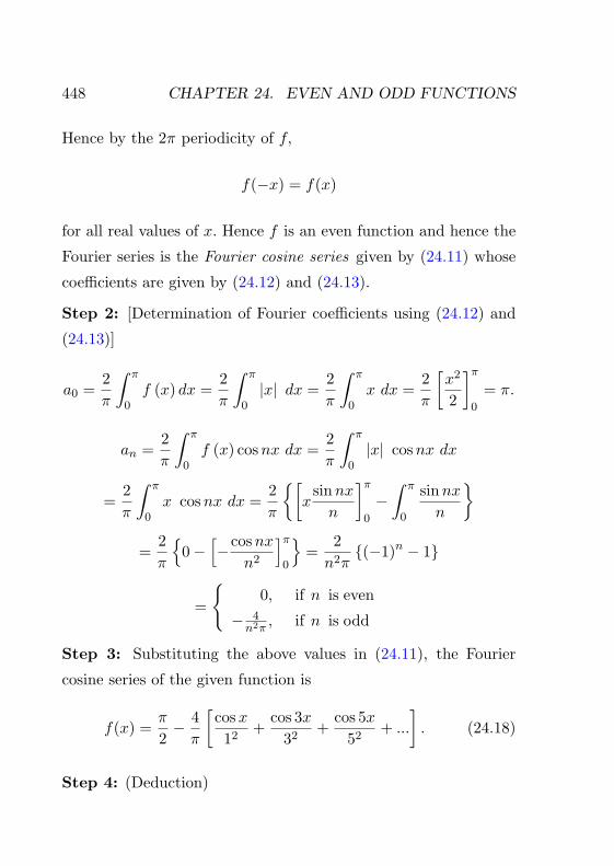
448 CHAPTER 24. EVEN AND ODD FUNCTIONS
Hence by the 2π periodicity of f,
f(−x) = f(x)
for all real values of x. Hence f is an even function and hence the
Fourier series is the Fourier cosine series given by (24.11) whose
coefficients are given by (24.12) and (24.13).
Step 2: [Determination of Fourier coefficients using (24.12) and
(24.13)]
a0 =2π
∫ π
0f (x) dx =
2π
∫ π
0|x| dx =
2π
∫ π
0x dx =
2π
[x2
2
]π
0
= π.
an =2π
∫ π
0f (x) cosnx dx =
2π
∫ π
0|x| cosnx dx
=2π
∫ π
0x cosnx dx =
2π
{[x
sinnxn
]π
0
−∫ π
0
sinnxn
}=
2π
{0−
[−cosnx
n2
]π0
}=
2n2π
{(−1)n − 1}
=
{0,
− 4n2π
,
if n is even
if n is odd
Step 3: Substituting the above values in (24.11), the Fourier
cosine series of the given function is
f(x) =π
2− 4π
[cosx12
+cos 3x
32+
cos 5x52
+ ...
]. (24.18)
Step 4: (Deduction)

24.4. FOURIER SINE AND COSINE SERIES 449
x = 0 is a point of continuity hence equality in (24.18) holds at
x = 0. Noting that f(0) = 0, substitution of x = 0 in (24.18)
yields
0 = f(0) =π
2− 4π
[cos 012
+cos 032
+cos 052
+ ...
]or
π
2=
4π
[112
+132
+152
+ ...
]or
112
+132
+152
+ ... =π2
8.
Example 6 Find the Fourier series of f(x) =
−x, −π ≤ x < 0
x, 0 ≤ x ≤π
and f(x+ 2π) = f(x) .
Solution Note that the given function is nothing but the same in
the previous Example.
Example 7 Find the Fourier series for f(x) = x sinx in [−π, π]
with f(x) = f(x+ 2π) ∀x ∈ R.
Solution
Step 1: (Verifying that f is even)
Here for −π ≤ x ≤ π , we have by the definition of f,
f(−x) = −x sin(−x) = −x(− sinx) = x sinx = f(x).

450 CHAPTER 24. EVEN AND ODD FUNCTIONS
Hence by the 2π periodicity of f,
f(−x) = f(x)
for all real values of x (except at multiples of π). Hence f is an
even function and hence the Fourier series is the Fourier cosine
series given by (24.11) whose coefficients are given by (24.12) and
(24.13).
Step 2: [Determination of Fourier coefficients using (24.12) and
(24.13)]
a0 =2π
∫ π
0f(x) dx =
2π
∫ π
0x sinx dx
=2π
[−x cosx]2π0 − 2
π
∫ π
0(− cosx) dx =
2π
(−π sinπ) = 2.
an =2π
∫ π
0f(x) cosnx dx =
2π
∫ π
0x sinx cosnx dx
=1π
∫ π
0x [sin(n+ 1)x− sin(n− 1)x] dx,
since 2 sinA cosB = sin(A+B) + sin(A−B)
=1π
∫ π
0x sin(n+ 1)x dx− 1
π
∫ π
0x sin(n− 1)x dx
=
− cos(n+1)π
n+1 , when n = 1
cos(n−1)πn−1 − cos(n+1)π
n+1 , when n 6= 1
Step 3: Substituting the above values, the Fourier cosine series

24.5. FOURIER SINE SERIES 451
of the given function is
f(x) = 1− 12
cosx− 2[
cos 2x22 − 1
− cos 3x32 − 1
+cos 4x42 − 1
− ...
].
24.5 Fourier Sine Series
Fourier series for odd 2π periodic function defined over
the interval [−π, π]
Suppose f is defined over the interval [−π, π] and is an odd 2π
periodic function, then its Fourier series is a sine series, called
Fourier sine series, and is given by:
f(x) =∞∑
n=1
bn sinnx (24.19)
where
bn =2π
∫ π
0f(x) sinnx dx (n = 1, 2, 3 , . . .) (24.20)
Example 8 Find the Fourier series of f given by
f(x) = x,
where −π < x < π and f(x) = f(x+ 2π) ∀ x ∈ R.
Solution
Step 1: (Verifying that f is odd)

452 CHAPTER 24. EVEN AND ODD FUNCTIONS
Here for −π < x < π, we have by the definition of f,
f(−x) = −x = −f(x).
Hence by the 2π periodicity of f,
f(−x) = −f(x)
for all real values of x (except at multiples of π). Hence f is an
odd function and hence the Fourier series is the Fourier sine series
given by (24.19) whose coefficients are given by (24.20).
Step 2: [Determination of Fourier coefficients using (24.20)]
bn =2π
∫ π
0f(x) sinnx dx =
2π
∫ π
0x sinnx dx
=2π
{[x
(− cosnx
n
)]π
0
−∫ π
0
(−cosnx
n
)dx
}
= 2nπ (−π cosnπ)= 2
n(−1)n+1, on simplification
=
{− 2
n ,2n ,
if n is even
if n is odd
Step 3: Substituting the above values in (24.17), the Fourier sine
series of the given function is
f(x) = 2[sinx− sin 2x
2+
sin 3x3
− ...
].

24.5. FOURIER SINE SERIES 453
Example 9 Find the Fourier series of f given by
f(x) = sinh ax,
where –π < x < π and f(x) = f(x+ 2π) ∀ x ∈ R.
Solution
Step 1: (Verifying that f is odd)
Here for −π < x < π, we have by the definition of f,
f(−x) = sinh(−ax) = − sinh ax = −f(x).
Hence by the 2π periodicity of f,
f(−x) = −f(x)
for all real values of x (except at multiples of π). Hence f is an
odd function and hence the Fourier series is the Fourier sine series
given by (24.19) whose coefficients are given by (24.20).
Step 2: [Determination of Fourier coefficients using (24.20)]
bn =2π
∫ π
0
(eax − e−ax
2
)sinnx dx (24.21)
We take I1 =∫ π0 eax sinnx dx and I2 =
∫ π0 e−ax sinnx dx.
Evaluation of I1 :
I1 =∫ π
0eax sinnx dx =
[eax(−cosnx
n
)]π0−∫ π
0aeax
(−cosnx
n
)dx

454 CHAPTER 24. EVEN AND ODD FUNCTIONS
=−eaπ cosnπ + 1
n+[aeax
(sinnxn2
)]π
0
−∫ π
0a2eax
(sinnxn2
)dx
i.e., (1 +
a2
n2
)I1 =
−eaπ cosnπ + 1n
=eaπ(−1)n+1 + 1
n.
Hence
I1 =n
n2 + a2
(eaπ(−1)n+1 + 1
).
In a similar manner,
I2 =n
n2 + a2
(e−aπ(−1)n+1 + 1
).
Substituting these values in (A), we obtain
bn =1π
(I1 − I2) =1π
{(−1)n+1n
a2 + n2
(eaπ − e−aπ
)}Step 3: Substituting the above values in (24.19), the Fourier sine
series of the given function is
f(x) =1π
∑{(−1)n+1n
a2 + n2
(eaπ − e−aπ
)}sinnx.
Exercises
In Exercises 1 to 6, prove the results.
1. The sum and the product of even functions are even functions.
2. The sum of odd functions is odd. The product of two odd
functions is even.

24.5. FOURIER SINE SERIES 455
3. The sum of even functions is even. The product of two even
functions is even.
4. The product of even and odd functions is odd.
5. If f(x) is odd, then |f(x)| and f2(x) are even functions.
6. If f(x) is even, then |f(x)| , f2(x) and f3(x)are even functions.
7. Find the Fourier series of f(x) = x2
4 ,−π < x < π with f(x +
2π) = f(x) . Also deduce that
1− 14
+19− 1
16+
125
+ ... =π2
12.
8. Find the Fourier series expansion of
f(x) = π2 − x2, −π < x < π with f(x) = f(x+ 2π).
9. Find the Fourier series of f(x) =
{π + x, −π < x < 0
π − x, 0 < x < π
and f(x) = f(x+ 2π).
10. Find the Fourier Coefficients and then Fourier series of f(x) ={π2 + x,
π2 − x,
−π < x < 0
0 < x < πand f(x+ 2π) = f(x)
11. Obtain the Fourier series expansion of the function f(x) ={1 + 2x
π ,
1− 2xπ ,
−π < x < 0
0 < x < πof period 2π : Also deduce that
π2
8 = 112 + 1
32 + 152 + · · ·
12. Obtain the Fourier series expansion of the following function of
period 2π : f(x) =
{−a,a,
−π < x < 0
0 < x < π. Also deduce that
π4 =
∑∞n=0
(−1)n
2n+1 .
13. Find the Fourier series expansion of

456 CHAPTER 24. EVEN AND ODD FUNCTIONS
f(x) =
{−1 + x, −π < x < 0
1 + x, 0 < x < πand f(x) = f(x+2π).
Also, deduce that π4 = 1− 1
3 + 15 − · · ·
14. Express cosh ax in Fourier series of period 2π with −π < x <
π.
15. Find the Fourier series of f given by
f(x) =
{−1 + x,
1 + x,
when − π < x < 0
when 0 < x < πand f(x) = f(x +
2π).
Hints to Exercises
9 to 11: If x is such that 0 < x < π, then −π < −x < 0, and
f(−x) = f(x).
12&13: If x is such that 0 < x < π, then −π < −x < 0, and
f(−x) = −f(x).
14: Given is an even function. 15: Given is an odd function.
Answers
7. f(x) = π2
12 − cosx+ 14 cos 2x− 1
9 cos 3x+ 116 cos 4x− ...
8. 2π2
3 − 4∑∞
n=1(−1)n cos nx
n2 .
9. π2 + 4
π
[cosx+ 1
9 cos 3x+ 125 cos 5x+ . . .
]10.
a0 = 0, an =
{0, whenn is even4
πn2 , whenn is odd
f(x) =4π
[1
cosx+
19
cos 3x+125
cos 5x+ ...
]

24.5. FOURIER SINE SERIES 457
11. 8π2
[cos x12 + cos 3x
32 + cos 5x52 + · · ·
]12. 4a
π
[sin x
1 + sin 3x3 + sin 5x
5 + · · ·]
13. bn = 2nπ −
2(π+1)(−1)n
nπ =
{− 2
n2
nπ + 2(π+1)nπ
when n is even
when n is oddand
f(x) = 2(π+2)π sinx − 2
2 sin 2x + 2(π+2)3π sin 3x − 2
4 sin 4x +2(π+2)
5π sin 5x− · · ·For the deduction, put x = π2 .
14. f(x) = 1aπ sinh aπ + a
π
∑∞n=1
(−1)n
a2+n2 [eaπ − e−aπ] cosnx.
15. f(x) = 2π
∑∞n=1
1n [1− (1 + π)(−1)n] sinnx.

Chapter 25Half Range Fourier Series -
Even and Odd Extensions
25.1 Introduction
In this chapter we will see that any function (that need not be
periodic) defined over a finite interval [0, L] can be represented
by means of Fourier series of period 2L. Before going into the
details we define the extension and restriction of functions.
Definition Suppose A ⊂ B ⊂ R and suppose that f : A → R
and g : B → R be two functions. We say that the function g is an
extension of the function f if
g(x) = f(x) ∀ x ∈ A.
458

25.1. INTRODUCTION 459
In that case we also say that f is the restriction of g on A.
Examples Suppose A = [0, L] and B = [−L, L] and consider
the functions
f(x) = x for x ∈ [0, L] (25.1)
and
g(x) = x for x ∈ [−L, L] (25.2)
Since g(x) = f(x) ∀ x ∈ [0, L]
g is an extension of the function f.
If we also consider the function h defined by
h(x) = |x| for x ∈ [0, L] (25.3)
then, since h(x) = f(x) ∀ x ∈ [0, L]
h is also an extension of f.
Figure 25.1:
Since g is an odd function, we say g is an odd extension of f
and since h is an even function, h is an even extension of f
(Fig.25.1)

460 CHAPTER 25. EVEN AND ODD EXTENSIONS
Consider the function f considered in Eq. (25.1) above. i.e.,
f is defined by
f(x) = x ∀ x ∈ [0, L] .
Clearly, the given function is defined only over an interval of
length L and is not periodic. But it can be extended to
an odd periodic function or an even periodic function as we will
discuss now. Depending on the type of extension there are two
Fourier series representations forf(x):
(i) when we consider odd periodic extension function the cor-
responding Fourier series would not contain cosine terms. As only
sine terms appear in the series and the half part (the cosine part)
are missing, the series is called half range Fourier sine series.
(i) when we consider even periodic extension function the cor-
responding Fourier series would not contain sine terms. As only
cosine appear in the series and the half part (the sine part) are
missing, the series is called half range Fourier cosine series.
Half Range Fourier Sine Series
g defined by (25.2) is an odd extension for f defined by (25.1).
If we also suppose that
g(x+ 2L) = g(x) for every x,
then g becomes a 2L periodic function and hence becomes an
odd 2L periodic extension of the function f . Being an odd
2L periodic function, the Fourier series for g is the Fourier sine

25.1. INTRODUCTION 461
series given by
g(x) =∞∑
n=1
bn sin nπ xL ,
where
bn =2L
∫ L
0g(x) sin nπ x
L dx.
We consider the above sine series as that one corresponds to the
given non-periodic function f and call it the half range Fourier
sine series for the function f .
Half Range Fourier Sine Series Formula
Suppose we are given with a function f(x) defined over the
interval 0 ≤ x ≤ L and that f need not be periodic. As
g(x) = f(x) for x ∈ [0, L], from the last two equations, the half
range Fourier sine series for the function f is given by
f(x) =∞∑
n=1
bn sin nπ xL (25.4)
where
bn =2L
∫ L
0f(x) sin nπ x
L dx (25.5)
Half Range Fourier Cosine Series
h defined by (25.3) is an even extension for f defined by (25.1). If
we also suppose that
h(x+ 2L) = h(x) for every x,
then h becomes a 2L periodic function and hence becomes an
even 2L periodic extension of the function f . Being an even
2L periodic function, the Fourier series for h is the Fourier cosine

462 CHAPTER 25. EVEN AND ODD EXTENSIONS
series given by
h(x) =a0
2+
∞∑n =1
an cos nπ xL ,
where
a0 =2L
∫ L
0h(x)dx
and
an =2L
∫ L
0h(x) cos nπ x
L dx.
We consider the above cosine series as that one corresponds to the
given non-periodic function f and call it the half range Fourier
cosine series for the function f .
Half Range Fourier Cosine Series Formula
Suppose we are given with a function f(x) defined over the
interval 0 ≤ x ≤ L and that f need not be periodic. As
h(x) = f(x) for x ∈ [0, π], from the last three equations, the half
range Fourier cosine series for the function f is given by
f(x) =a0
2+
∞∑n =1
an cos nπ xL (25.6)
where
a0 =2L
∫ L
0f(x)dx (25.7)
and
an =2L
∫ L
0f(x) cos nπ x
L dx (25.8)

25.1. INTRODUCTION 463
Example 1 Find the half range expansions of the function
f(t) =
2kl
t, when 0≤t< l2
2kl
(l−t), when l2≤t<l
Solution
Here, we take the given range 0 ≤ t ≤ l as the half range, so that
the full range is −l ≤ t ≤ l and we take the period as 2L = 2l.
(i) Half range sine series
Putting L = l and changing the variable x to t, gives
f(t) =∞∑
n =1
bn sin nπ tl (25.9)
and
bn =2l
∫ l
0f(t) sin nπ t
l dt
=2l
{∫ l/2
0
2ktl
sinnπt
ldt+
∫ l
l/2
2kl
(l − t) sinnπt
ldt
}
= 8kn2π2 sin nπ
2 , on simplification.
Hence, by (25.9), half range sine expansion of f(t) is given by
f(t) =8kπ2
[112
sinπt
l− 1
32cos
3πtl
+152
cos5πtl− ...
](ii) Half range cosine series

464 CHAPTER 25. EVEN AND ODD EXTENSIONS
Putting L = l and changing the variable x to t, we obtain
f(t) =a0
2+
∞∑n =1
an cos nπ tl (25.10)
and a0 = 2l
∫ l0 f(t) dt
an =2l
∫ l
0f(t) cos nπ t
l dt
That is,
a0 =2l
{∫ l/2
0
2ktldt+
∫ l
l/2
2kl
(l − t)dt
}
= k, on simplification
an =2l
{∫ l/2
0
2ktl
cosnπt
ldt+
∫ l
l/2
2kl
(l − t) cosnπt
ldt
}
=4kn2π2
(2 cos
nπ
2− cosnπ − 1
)Thus a2 = − 16k
22π2 , a6 = − 16k62π2 , a10 = − 16k
102π2 , and
an = 0 when n 6= 2, 6, 10, 14, . . . Hence, the half range cosine
expansion is
f(t) =k
2− 16k
π2
[122
cos2πtl
+162
cos6πtl
+ ...
]Example 2 Obtain the half range cosine series of
f(x) = x, when 0 < x < 2.

25.1. INTRODUCTION 465
Solution
Here, we take the given range 0 ≤ x ≤ 2 as the half range,
so that the full range is −2 ≤ t ≤ 2 and we take the period as
2T = 2× 2 = 4.
Half range cosine series is obtained as follows:
We have
a0 =2L
∫ L
0f(x)dx =
22
∫ 2
0f(x)dx
=∫ 2
0x dx
=[x2
2
]2
0
= 2.
an =2T
∫ T
0f(x) cos
nπx
Tdx =
22
∫ 2
0f(x) cos
nπx
2dx
=∫ 2
0x︸︷︷︸u
cos nπxc︸ ︷︷ ︸
v′
dt =4
n2π2[(−1)n − 1]
=
{0, when n is even
− 8n2π2 , when n is odd
Hence the half range Fourier cosine series is
...f(x) = 1− 8π2
[112
cosπx
2+
132
cos3πx2
+ · · ·]
Example 3 Find the half range sine series of the function

466 CHAPTER 25. EVEN AND ODD EXTENSIONS
f(x) =
x, when 0<x<1
2−x, when 1<x<2
in 0 ≤ x ≤ 2.
Solution
Here, we take the given range 0 ≤ x ≤ 2. as the half range,
so that the full range is −2 ≤ x ≤ 2. and we take the period as
2L = 2× 2 = 4. We have
bn =2L
∫ L
0f(x) sin
nπx
Ldx =
22
∫ 2
0f(x) sin
nπx
2dx
=∫ 1
0x · sin nπx
2dx+
∫ 2
1(2− x) sin
nπx
2dx
= 8n2π2 sin nπ
2 , on simplification.
Hence half range sine expansion of f(x) is given by
f(x) =∞∑
n = 1
bn sin nπxT =
∞∑n =1
bn sin nπx2 =
8π2
∞∑n=1
sinnπ
2sin
nπ x
2.
Exercises
1. Represent f(x) = x, 0 < x < 1 by half range (i) Fourier
sine series and
(ii) Fourier cosine series.
2. Expand f(x) = 2x as a series of cosines in [0, 1].
3. Represent f(x) = π − x, 0 < x < 1 by a Fourier cosine
series.

25.1. INTRODUCTION 467
4. Expand f(x) =
{l, 0 < x < l
22al (l − x), l
2 < x < las a half range
sine series in the interval 0 < x < l.
5. For the function f(x) =
{2x, 0 < x < 1
4− 2x, 1 < x < 2find (i)
Fourier cosine series and (ii) Fourier sine series of period 4.
6. Expand f(x) = x cos a as a half range cosine series in the
interval 0 < x < 2..
7. Represent f(x) = (x−1)2, 0 < x < 1 by Fourier sine series.
8. Express f(x) = x in half range cosine series of periodicity 2l
in the range 0 < x < l.
9. Find the half range Fourier cosine series with period 4 of the
function
f(x) =
{1, 0 < x < 1
0, 1 < x < 2
10. Find the half range Fourier sine series with period 6π of the
function
f(x) =
0, 0 < x < π
1, π < x < 2π
2, 2π < x < 3π

468 CHAPTER 25. EVEN AND ODD EXTENSIONS
11. Obtain the half range cosine series for
f(t) =
kt, when 0≤t≤ l2
k(l−t), when l2≤t≤l
12. Obtain the half range cosine series of
f(x) = x, when 0 < x < l.
Answers
1. (i) 12−
4π2
[cos πx
12 + cos 3πx32 + · · ·
](ii) 2
π
[sinπx− sin 2πx
2 + sin 3πx3 − · · ·
]2. f(x) = π
2 −8π
[cosx+ cos 3x
32 + · · ·]
3. (i) f(x) = π2 + 4
π
[cosx+ cos 3x
32 + · · ·]
(ii) f(x) = 2[sinx+ sin 2x
2 + sin 3x3 + · · ·
]4. 8a
π2
[sin πx
l − 132 sin 3πx
l + 152 sin 5πx
l + · · ·]
5. (i)∑∞
n=18
n2π2 sin nπ2 sin nπx
2 (ii) 5− 16π2
∑∞n=1
cos(2n−1)πx
(2n−1)2
6. cos a− 8n2π2
∑∞n=1
1(2n−1)2
cos (2n−1)π x2 .
7. f(x) = 4π3
∑∞n=1
[(−1)n+2n2π2−1]n3 cosnπ x
8. f(x) = l2 −
4lπ2
[112 cos πx
2 + 132 cos 3πx
2 + · · ·]
9. 12 + 2
π
∑∞n=1
(−1)n−1
2n−1 cos (2n−1)πx2

25.2. HALF RANGE SERIES 469
10.∑∞
n=12
nπ
(cos nπ
3 + cos 2nπ3 − 2 cosnπ
)sin nx
3
11. f(t) = kl4 −
8klπ2
[122 cos 2π t
l + 162 cos 6π t
l + · · ·]
12. f(x) = l2 −
4lπ2
[112 cos πx
2 + 132 cos 3πx
2 + · · ·]
25.2 Half Range Series of functions defined
over [0, π]
We now consider the special case in which the interval is [0, π]
instead of [0, L].
Half Range Fourier Sine Series Formula
As g(x) = f(x) for x ∈ [0, π], from the last two equations, the
half range Fourier sine series for the function f is given by
f(x) =∞∑
n=1
bn sinnx (25.11)
where
bn =2π
∫ π
0f(x) sinnx dx (25.12)
Half Range Fourier Cosine Series Formula
As h(x) = f(x) for x ∈ [0, π], from the last three equations, the
half range Fourier cosine series for the function f is given by
f(x) =a0
2+
∞∑n=1
an cosnx (25.13)

470 CHAPTER 25. EVEN AND ODD EXTENSIONS
where
a0 =2π
∫ π
0f(x)dx (25.14)
and
an =2π
∫ π
0f(x) cosnx dx (25.15)
Example 4 Obtain the (i) Fourier sine series and (ii) Fourier
cosine series for the function
f(x) = x for x ∈ [0, π]
Solution
(i) Half range Fourier sine series:
Step 1: If we consider odd 2π periodic extension, we get the half
range Fourier sine series (25.11) with coefficients given by (25.12).
Step 2: Determination of Fourier coefficients using (25.12).
bn =2π
∫ π
0x sinnxdx =
2π
[−x cosnx
n
]π
0
+2π
∫ π
0cosnxdx
= − 2nπ
(π cosnπ − 0) + 0 = − 2n
cosnπ =2n
(−1)n+1
=
{− 2
n ,2n ,
if n is even
if n is odd
Step 3: Substituting these values in (25.11), we obtain the half
range Fourier sine series
f(x) = 2[sinx− sin 2x
2+
sin 3x3
− ...
].
(i) Half range Fourier cosine series:

25.2. HALF RANGE SERIES 471
Step 1: If we consider even 2π periodic extension, we get the
Fourier half range cosine series given by (25.13) with coefficients
given by (25.14) and (25.15).
Step 2: Determination of Fourier coefficients using (25.14) and
(25.15).
a0 =2π
∫ π
0|x| dx =
2π
∫ π
0x dx =
2π
[x2
2
]π
0
= π.
an =2π
∫ π
0|x| cosnx dx =
2π
∫ π
0x cosnx dx
=2π
{[x
sinnxn
]π
0
−∫ π
0
sinnxn
}=
2π
{0−
[−cosnx
n2
]π0
}=
2n2π
{(−1)n − 1}
=
{0,
− 4n2π
,
if n is even
if n is odd
Step 3: Substituting these values in (25.13), we obtain the half
range Fourier cosine series
f(x) =π
2− 4π
[cosx12
+cos 3x
32+
cos 5x52
+ ...
].
Example 5 Obtain the (i) Fourier sine series and (ii) Fourier
cosine series for the function
f(x) = π − x, 0 < x < π.

472 CHAPTER 25. EVEN AND ODD EXTENSIONS
Assuming the convergence of the series at x = 0, deduce that
π2
8=
112
+132
+152
+ ...
Solution
(i) Half range Fourier sine series:
Using (25.11) and (25.12), half range Fourier sine series is obtained
as follows:
bn =2π
∫ π
0f(x) sinnxdx =
2π
∫ π
0(π − x) sinnxdx
= 2n , on simplification.
Hence
f(x) =∑
bn sinnx =∑ 2
nsinnx = 2
[sinx+
sin 2x2
+sin 3x
3+ ...
]
(ii) Half range Fourier cosine series:
Using (25.13), (25.14) and (25.15), half range Fourier cosine series
is obtained as follows:
a0 = 2π
∫ π0 f(x)dx = 2
π
∫ π0 (π − x)dx= π, on simplification.
an =2π
∫ π
0f(x) cosnx dx =
2π
∫ π
0(π − x)︸ ︷︷ ︸
u
cosnx︸ ︷︷ ︸v′
dx
=
{0,
4n2π
,
if n is even
if n is odd

25.2. HALF RANGE SERIES 473
Hence the half range Fourier cosine series for π − x in [0, π] is
f(x) =π
2+
4π
[cosx12
+cos 3x
32+
cos 5x52
+ ...
]. (25.16)
Deduction of the Series:
Assuming the convergence of the series at x = 0, from (25.16), we
obtain
π − 0 =π
2+
4π
[cos 012
+cos 032
+cos 052
+ ...
],
which on simplification yields,
π2
8=
112
+132
+152
+ ...
Example 6 Obtain the Fourier sine series for the function
f(x) = c , x ∈ [0, π].
Also deduce that π4 = 1− 1
3 + 15 −
17 + · · ·
Solution
Here bn = 2π
∫ π0 f(x) sinnxdx = 2
π
∫ π0 c sinnxdx
=
{0, when n is even4cnπ , when n is odd

474 CHAPTER 25. EVEN AND ODD EXTENSIONS
Hence the Fourier sine series is
f(x) =4cπ
[sinx+
sin 3x3
+ ...
]i.e.,
c =4cπ
[sinx+
sin 3x3
+ ...
]. (25.17)
Putting x = π2 in (25.17), we obtain
c =4cπ
[sin π
2 +sin 3π
2
3+ ...
].
Hence π4 = 1− 1
3 + 15 −
17 + · · ·
Example 7 Expand f(x) = cosx in the half range sine-series in
0 ≤ x < π.
Solution
Here bn = 2π
∫ π0 f(x) sinnxdx = 2
π
∫ π0 cosx sinnx dx
=
{4n
π(n2−1), when n is even
0, when n is odd
Hence the half range Fourier sine series for the given function is
cosx =4π
[2 sin 2x22 − 1
+4 sin 4x42 − 1
+6 sin 6x62 − 1
+ · · ·]
Exercises
1. Represent f(x) = x2, 0 ≤ x < π by a Fourier sine series.
2. Find the Fourier coefficient and represent f(x) = 1, 0 ≤ x < π

25.2. HALF RANGE SERIES 475
by Fourier sine series. Hence deduce that
π
4= 1− 1
3+
15− 1
7+ . . .
3. Show that the Fourier cosine series of sin x in the half range
0 ≤ x < π is sinx = 4π
[12 −
cos 2x1·3 − cos 4x
3·5 − cos 6x5·7 − · · ·
]4. Show that the function f(x) = cos 2x, x ∈ [0, π] is given by
the Fourier sine series cos 2x = − 4π
[sin x
3 − 35 sin 3x− · · ·
].
5. Show that the Fourier sine series of f(x) = π x8 (π − x) in the
half range 0 ≤ x < π is sin x13 + sin 3x
33 + sin 5x53 + · · ·
6. Show that the sine series for the function f(x) =
{x, 0 < x < π
2
0, π2 < x < π
is given by 2π
[sin x12 + π sin 2x
42 − sin 3x32 − π sin 4x
8 − · · ·].
7. Show that the sine series for the function f(x) =
{0, 0 < x < π
2
c, π2 < x < π
is given by
2cπ
[sinx
1− 2 sin 2x
2+
sin 3x3
+sin 5x
5− 2 sin 6x
6· · ·]
and the cosine series is given by
2cπ
[π
4− cosx
1+
cos 3x3
− cos 5x5
+ · · ·]
8. Show that the cosine series for the function
f(x) =
{πx4 , 0 < x < π
2π4 (π − x), π
2 < x < π

476 CHAPTER 25. EVEN AND ODD EXTENSIONS
is given by π2
16 −12
[cos 2x
12 + cos 6x32 + · · ·
]9. Show that f(x) = πx − x2, x ∈ [0, π] can be represented by
the Fourier sine series 8π
[sinx+ 1
33 sin 3x+ 153 sin 5x+ · · ·
].
10. Show that the Fourier cosine series of the function f(x) =
x sinx, x ∈ [0, π] is given by
1− cosx2
− 2 cos 2x1 · 3
+2 cos 3x
2 · 42 cos 4x
3 · 5+ · · ·
Hence deduce that 12 + 1
1·3 −1
3·5 + 15·7 − · · · = π
4 .
11. Expand f(x) = πx− x2, x ∈ [0, π] in Fourier cosine series.
12. Express f(x) = x sinx, x ∈ [0, π] in half range sine series.
Answers
1. f(x) = 2π
∑∞n=1(−1)n+1
{π2
n + 2n3 [(−1)n − 1]
}sinnx
2. bn = 2n π
[1 + (−1)n+1
], f(x) = 4
π
[sinx+ sin 3x
3 + . . .]
4. f(x) = 4π
[sinx− 1
32 sin 3x+ 152 sin 5x− . . .
]11. π x− x2 = π
6 − 2∑∞
n=11+(−1)n
n2 cosnx
12. f(x) = 1π
∑∞n=1
[cos π(1−n)
(1−n)2− cos π(1+n)
(1+n)2
]sinnx

Chapter 26Partial Differential Equations -
A Quick Review 1
26.1 Partial Differential Equations
An equation involving partial derivatives is a partial differential
equation. In this chapter we consider some partial differential
equations. We consider the solution of the wave equation also.
Some of the important linear partial differential equations of
the second order are given below:
One dimensional wave equation:
∂2u
∂t2= a2∂
2u
∂x2(26.1)
1Introductory Chapter on partial differential equations. Not mentioned inthe syllabus.
477

478 CHAPTER 26. P.D.E. - A QUICK REVIEW
One dimensional heat equation:
∂u
∂t= a2∂
2u
∂x2(26.2)
Two dimensional Laplace equation:
∂2u
∂x2+∂2u
∂y2= 0 (26.3)
Two dimensional Poisson equation:
∂2u
∂x2+∂2u
∂y2= f(x, y) (26.4)
Three dimensional Laplace equation:
∂2u
∂x2+∂2u
∂y2+∂2u
∂z2= 0. (26.5)
In the above c is a constant, t is time, and x, y, z are Cartesian
coordinates. Equation (26.4) with f not identically zero is non-
homogeneous, while the other equations are homogeneous.
Definition A solution of a partial differential equation in some
region R is a function which has all the partial derivatives appear-
ing in the equation in some domain containing R, and satisfies the
equation everywhere in R.
Example 1 Show that the functions
u = x2 − y2, u = ex cos y, u = log (x2 + y2)

26.1. PARTIAL DIFFERENTIAL EQUATIONS 479
are solutions of the two dimensional Laplace equation (26.3).
Solution
When u = x2 − y2, we have
∂u
∂x= 2x,
∂u
∂y= −2y,
∂2u
∂x2= 2 and
∂2u
∂y2= −2.
Hence ∂2u∂x2 + ∂2u
∂y2 = 0 so that u = x2 − y2 satisfies the two dimen-
sional Laplace equation (26.3). Similarly, it can be verified
u = ex cos y and u = log (x2 + y2) are also solutions of (26.3).
Example 2 Verify that u = x3 + 3xt2 is a solution of the one
dimensional wave equation (26.1), for a suitable value of a.
Solution
When u = x3 + 3xt2, we obtain
∂u
∂x= 3x2 + 3t2,
∂2u
∂x2= 6x,
∂u
∂t= 6xt and
∂2u
∂t2= 6x.
Putting the above values in the one dimensional wave equation
(26.1),
6x = a26x, for a = 1 or for a = −1.
Hence u = x3 + 3xt2 satisfies the one dimensional wave equation
when a = ±1
Theorem 1 (Fundamental Theorem for Linear Homoge-
480 CHAPTER 26. P.D.E. - A QUICK REVIEW
neous Partial Differential Equations)
If u1 and u2 are any solutions of a linear homogeneous partial
differential equation in some region, then
u = c1u1 + c2u2
where c1 and c2 are any constants, is also a solution of that equa-
tion in that region.
26.2 Relation to Ordinary Differential Equa-
tion
If a partial differential equation involves derivatives with respect to
one of the independent variables only, we can solve it like an ordi-
nary differential equation, treating the other independent variable
as constant. This is illustrated through the following examples.
Notation ux, uxx, uy, uyy, uxy, uyx denote the partial deriva-
tives∂u
∂x,∂2u
∂x2,∂u
∂y,∂2u
∂y2,
∂2u
∂x∂y,
∂2u
∂y∂x
respectively. More precisely,
ux(x, y) =∂u
∂x, uxx(x, y) =
∂2u
∂x2, uy(x, y) =
∂u
∂y,
uyy(x, y) =∂2u
∂y2, uxy(x, y) =
∂2u
∂x∂y, uyx(x, y) =
∂2u
∂y∂x

26.2. RELATION TO O.D.E. 481
Recall that under some conditions
∂2u
∂x∂y=
∂2u
∂y∂x.
i.e.,
uxy = uyx.
Example 3 Solve the partial differential equation
uxx + 4u = 0
where u is a function of two variables x and y.
Solution
Given
uxx + 4u = 0,
i.e.,∂2u
∂x2+ 4u = 0.
The given partial differential equation involves derivatives with
respect to the independent variable x only. We solve the given
partial differential equation, considering as an ordinary differential
equation in x, keeping y as constant. Then characteristic equation
is
λ2 + 4 = 0
and hence
λ = ±2i.

482 CHAPTER 26. P.D.E. - A QUICK REVIEW
Hence the solution to the given equation is given by u(x, y) =
f(y) cos 2x+g(y) sin 2x where f(y) and g(y) are arbitrary functions
of y alone.
Example 4 Solve the partial differential equation
uyy + 4u = 0
where u is a function of two variables x and y.
Solution
Here the partial differential equation involves only the derivatives
in the variable y. Proceeding as in Example 3, we obtain
u(x, y) = f(x) cos 2y + g(x) sin 2y
where f(x)and g(x)are arbitrary functions of x alone.
Example 5 Solve the partial differential equation
uxx − 4 = 0
where u is a function of two variables x and y.
Solution
The partial differential equation involves derivatives with respect
to the variable x only. Hence the given equation can be treated
as an ordinary differential equation in x with y as constant.
∂2u
∂x2− 4 = 0

26.2. RELATION TO O.D.E. 483
implies∂2u
∂x2= 4.
Integrating with respect to x, we obtain
∂u
∂x= 4x+ f(y),
where f(y) is an arbitrary function of y alone.
Integrating again with respect to x, we obtain
∂u
∂x= 2x2 + xf(y) + g(y).
Example 6 Solve the partial differential equation uy + 2 y u =
0, where u is a function of two variables x and y.
Solution
The given partial differential equation involves derivatives with
respect to the independent variable y only. We solve the given par-
tial differential equation, considering it as an ordinary differential
equation in y, keeping x as constant. By separating variables, the
given equation is∂u
u= −2y ∂y
Integrating,
log u = −y2 + log f(x)
or
u = f(x)e−y2.

484 CHAPTER 26. P.D.E. - A QUICK REVIEW
Example 7 Setting ux = p, solve uxy = ux.
Solution
uxy = ux
can be written as∂
∂y
(∂u
∂x
)=∂u
∂x
or∂
∂y(p) = p.
Since p is the dependent variable and y is the only independent
variable, the last equation can be considered as the first order
ordinary equationdp
dy= p (26.6)
regarding x as constant. By separating variables, (26.1)
becomesdp
p= dy
which on integration with respect to y partially yields
log p = y + log f(x)
where f(x) is an arbitrary function of x alone. Hence
p = eyf(x)
i.e.,∂u
∂x= eyf(x).

26.3. SEPARATION OF VARIABLES 485
Now considering y as a constant and integrating partially with
respect to x, we obtain the following as the solution of the given
equation
u = ey∫f(x)dx+ g(y)
where g(y) is an arbitrary function of y alone.
26.3 Product Method (Separation of Vari-
ables)
We now discuss the product method for finding the solution u(x, y)
of a given partial differential equation.
Example 8 Find the solution of ux + uy = 0 by separating vari-
ables (product method).
The given partial differential equation is
∂u
∂x+∂u
∂y= 0 . . . (26.7)
Let the solution of this equation be
u(x, y) = X(x)Y (y)
where X(x) is a function of x alone and Y (y) is a function of y
alone.
Let X ′ = dXdx and Y = dY
dy ,

486 CHAPTER 26. P.D.E. - A QUICK REVIEW
so that (26.7) becomes the form
X ′ Y +XY = 0
or
X ′ Y = −XY .
orX ′
X= − Y
Y.
In the last equation, the expression on the left involves func-
tions depending only on x while the expression on the right in-
volves functions depending only on y. Hence both expressions
must be equal to a constant2, say, k.
HenceX ′
X= − Y
Y= k. (26.8)
(26.8) yields two ordinary differential equations, viz,
X ′ − kX = 0. (26.9)
and˙6 Y + kY = 0 (26.10)
2Reason: If the expression on the left is not constant, then changing x willpresumably change the value of this expression but certainly not that on theright, since the latter does not depend on x. Similarly, if the expression onthe right is not constant, changing y will presumably change the value of thisexpression but certainly not that on the left.

26.3. SEPARATION OF VARIABLES 487
(26.9) is a linear differential equation in x :
dX
dx− kX = 0
and its solution is
X(x) = c1ekx.
(26.10) is a linear differential equation in y :
dY
dy+ kY = 0
and its solution is Y (y) = c2e−ky.
Hence solution to (26.7) is
u(x, y) = X(x)Y (y) = Cekxe−ky = Cek(x−y).
Exercises
In Exercises 1-3, verify that the functions are solutions of the one
dimensional wave equation (26.7) for a suitable value of a.
1. u = sin ωt sinωx
2. u = x2 + 4t2
3. u = e−t sin 3x
In Exercises 4-6, verify that the functions are solution of the
heat equation (26.8) for a suitable value of α

488 CHAPTER 26. P.D.E. - A QUICK REVIEW
4. u = e−2t cosx
5. u = e−t sin 3x
6. u = e−4t cosωx
In Exercises 7-12, verify that the following functions are so-
lutions of Laplace’s equation (26.9).
7. u = 2xy
8. u = ex sin y
9. u = tan 1(y/x)
10. u = x3 − 3xy2
11. u = sin x sinh y
12. u = x4 − 6x2y2 + y4
13. State the one dimensional wave equation. Show that the
function u(x, t) = v(x+ ct) + w(x− ct) is a solution of the
wave equation, where u and v are any twice differentiable
functions.
14. Show that u = (x2 + y2 + z2)−1/2 is a solution of the three
dimensional Laplace’s equation.
In Exercises 15 and 16, solve the following equation where u
is a function of two variables x and y.
15. ux + 2xu = 0 16. ux = 2xyu
In Exercises 17 and 18, setting ux = p, solve
17. uxy = 0
18. uxy + ux = 0
Solve the following systems of partial differential equations.

26.3. SEPARATION OF VARIABLES 489
19. ux = 0, uy = 0
20. . uxx = 0, uxy = 0
21. . uxx = 0, uxy = 0, uyy = 0
Answers
1. a = ±1
3. a = ±13 i
5. a = ±13
14. Hint: ∂2u∂x2 = 3x2(x2 + y2 + z2)−5/2 − (x2 + y2 + z2)−3/2.
Similarly, or by symmetry obtain ∂2u∂y2 ,
∂2u∂z2 .
15. u = f(y)e−x
16. u = f(y)exy
17. u =∫f(x)dx+ g(y))
18. e−y∫f(x)dx+ g(y))
20. u = cx+ f(y)
21. u = ax+ by + c

Chapter 27The Heat Equation
One of the partial differential equations that occur frequently
in applied mathematics is the heat equation. We describe the
equation and solve the equation under some conditions.
27.1 Heat Conduction Equation
We consider the temperature u in a long thin bar or wire of
constant cross section and homogeneous material which is oriented
along the x-axis and is perfectly insulated laterally, so that heat
flows in the x -direction only. Then u depends only on the axial
coordinate x and time t, so that u = u(x, t). Also suppose that
x = 0 and x = L are the axial coordinates corresponding to the
ends of the bar.
490

27.1. HEAT CONDUCTION EQUATION 491
Figure 27.1: A heat-conducting solid bar
The variation of temperature in the bar is governed by the
following partial differential equation:
α2uxx = ut, 0 < x < L, t > 0. (27.1)
The above equation is called heat conduction equation or one-
dimensional heat equation. In the above α2 depends only on
the material from which the bar is made and is defined by
α2 =κ
ρs,
where κ is the thermal conductivity, ρ is the density and s is the
specific heat of the material of the body.
Solution of Heat Conduction Equation with Boundary
and Initial Conditions
Now we shall solve the heat equation (27.1) for some important
types of boundary and initial conditions.

492 CHAPTER 27. THE HEAT EQUATION
The heat conduction equation is
α2u xx = ut, 0 < x < L, t > 0. (27.1)
Let us start with the case when the ends x = 0 and x = L of the
bar are kept at temperature zero. Then the boundary conditions
are
u(0, t) = 0, u(L, t) = 0, t > 0. (27.2)
Let f(x) be the initial temperature (i.e., temperature at timet = 0)
in the bar at the point with axial coordinate x. Then the initial
condition is
u(x, 0) = f(x). (27.3)
We shall determine a solution u(x, t) of (27.1) satisfying (27.2)
and (27.3).
We assume that u(x, t) = X(x)T (t).
Then using (27.2), for t > 0
u(0, t) = X(0)T (t) = 0 u(L, t) = X(L)T (t) = 0.
i.e.,
X(0)T (t) = 0 = X(L)T (t) for t > 0.
The above says that either T (t) = 0 for t > 0 or X(0) = 0 =
X(L). The first case is of no interest as T (t) = 0 implies u(x, t) =
X(x)T (t) = X(x)0 = 0 which means the temperature on the bar

27.1. HEAT CONDUCTION EQUATION 493
Figure 27.2: Boundary value problem for the wave equation.
is always zero. Hence hereinafter we consider the case
X(0) = 0 = X(L). (27.4)
Now we shall proceed step by step, as follows.
Step 1. By applying the product method1, or method of separat-
ing variables, we shall obtain two ordinary differential equation.
Step 2. We shall determine solutions of those two equations that
satisfy the boundary conditions.
Step 3. Those solutions will be composed so that the result will
be a solution of the heat equation (27.1), satisfying also the given
initial condition.1Product Method (or Method of Separating Variables) is discussed in the
previous chapter.

494 CHAPTER 27. THE HEAT EQUATION
The details are as follows.
Step 1 Applying the method of separation of variables we first
determine solutions of (27.1) that satisfy the boundary conditions
(27.2). We start from
u(x, t) = X(x)T (t). (27.5)
Substituting this expression into (27.1), we obtain the equation
α2X ′′ T = XT
where primes denote derivatives with respect to x and dots denote
derivatives with respect to t. To separate variables, we divide the
equation by α2X T, and obtain
X ′′
X=
1α2
T
T.
The expression on the left depends only on t, while the right
side depends only on x. We conclude that both expressions must
be equal to a constant, say, k. 2
That is,X ′′
X=
1α2
T
T= k.
2REASON: If the expression on the left is not constant, then changing xwill presumably change the value of this expression but certainly not that onthe right, since the latter does not depend on x. Similarly, if the expressionon the right is not constant, changing y will presumably change the value ofthis expression but certainly not that on the left.

27.1. HEAT CONDUCTION EQUATION 495
Hence we obtain two ordinary differential equations,
X ′′ − kX = 0 (27.6)
and
T − α2kT = 0. (27.7)
Case 1) If k = 0, then (27.6) becomes
X ′′ = 0.
Integrating (with respect to x ),
X ′ = a,
where a is an arbitrary constant. One more integration (with
respect to x ) yields
X = X(x) = ax+ b,
where b is also an arbitrary constant.
By (27.4), X(0) = 0, and hence the above implies b = 0. Hence
the above reduces to
X = X(x) = ax.
Again by (27.4), X(L) = 0, hence the above implies aL = 0 which

496 CHAPTER 27. THE HEAT EQUATION
implies a = 0. Hence the above reduces to
X = X(x) = 0.
This means that
u(x, t) = X(x)T (t) = 0T (t) = 0
which means the temperature on the bar is always zero. Hence we
ruled out the case k = 0.
Case 2) If k > 0, say k = µ2, then the characteristic equation
corresponding to the second order ordinary differential equation
(27.6) is
λ2 − µ2 = 0
i.e.,
λ2 = µ2.
Hence the general solution of (27.6) is
X(x) = Aeµx +Be−µx.
For the convenience of applying boundary conditions, recalling
the definitions of hyperbolic sine and cosine functions, we write
the above general solution as
X(x) = c1 cosh µx+ c2 sinh µx.

27.1. HEAT CONDUCTION EQUATION 497
By (27.4), X(0) = 0, and hence the above implies
c1 = 0.
Thus
X(x) = c2 sinh µx.
Also by (2A), X(L) = 0, and hence the above implies
c2 sin hµL = 0
Since µ 6= 0, sinh µL 6= 0,, hence we have c2 = 0. Hence
X(x) = 0.
This means that
u(x, t) = X(x)T (t) = 0T (t) = 0
which means the temperature on the bar is always zero. Hence we
ruled out the case k > 0.
Case 3) Hence we are left with the possibility of choosing k, neg-
ative, say, k = −λ, with λ > 0then equations (27.6) and (27.7)
takes the form
X ′′ + λX = 0 (27.8)
and
T + α2λT = 0. (27.9)

498 CHAPTER 27. THE HEAT EQUATION
If we take λ = µ2, then k = −µ2, so that we can also write
equations (27.6) and (27.7) in the form
X ′′ + µ2X = 0 (27.10)
and
T + α2µ2T = 0. (27.11)
Step 2 Consider equation (27.10). Its general solution is
X(x) = A cosµx+B sinµx. (27.12)
From the boundary conditions (27.4), it follows that
X(0) = A = 0 .
Hence
X(x) = B sinµx.
Again by (27.4),
X(L) = B sinµL = 0.
Two cases arise: either B = 0 or sinµL = 0.
The case of B = 0 leads to X(x) = 0 for 0 ≤ x ≤ L, so that
u(x, t) = X(x)T (t) = X(x)0 = 0

27.1. HEAT CONDUCTION EQUATION 499
which is no of interest. Hence we take
sinµL = 0.
This implies
µL = nπ , n = 1, 2, 3, . . .
or
µ =nπ
L, n = 1, 2, 3, . . .
Hence the only nontrivial solutions of Eq. (27.10) with boundary
conditions (2A) and (2B) are the eigen functions.3
Xn(x) = sinnπx
L, n = 1, 2, 3, . . .
associated with the eigen values
λn =n2π2
L2, n = 1, 2, 3, . . . (27.13)
Substituting n2π2
L2 for λ, Eq.(27.13) takes the form
T +n2π2α2
L2T = 0. (27.14)
The general solution of the first order differential equation (27.14)
3 Ref. section eigen value problems in chapter “ Two point Boundary ValueProblems”.

500 CHAPTER 27. THE HEAT EQUATION
is
Tn(t) = Bn exp(−n
2π2α2t
L2
), n = 1, 2, . . . (27.15)
where Bn is arbitrary constant. Neglecting the arbitrary constants
of proportionality, we conclude that the functions
un(x, t) = e−n2π2α2t/L2sin
nπx
L, n = 1, 2, . . . (27.16)
are solutions of the heat equation (27.1), satisfying the boundary
conditions (27.2).
Step 3 Now we have to obtain a solution that also satisfying the
initial condition (27.3)
u(x, 0) = f(x).
For this we form linear combinations of a set of fundamental solu-
tions and then choose the coefficients to satisfy the initial condi-
tions. Hence we form a linear combination of the functions (27.16)
and then choose the coefficients to satisfy Eq.(27.3). Here there
are infinitely many functions (27.16), so a general linear combina-
tion of them is an infinite series of the following form
u(x, t) =∞∑
n=1
cnun(x, t) =∞∑
n=1
cne−n2π2α2t/L2
sinnπx
L. . . (27.17)
where the coefficients are to be determined.
We assume that the infinite series of Eq.(27.17) converges and

27.1. HEAT CONDUCTION EQUATION 501
also satisfies Eqs.(27.1) and (27.2). To satisfy the initial condition
(27.3), we must have (with t = 0).
u(x, 0) =∞∑
n=1
cn sinnπx
L= f(x). . . . (27.18)
Hence, for (27.18) to satisfy (27.3), the coefficients cn must be
chosen such that u(x, 0) becomes a half-range expansion off(x),
namely, the Fourier sine series off(x). In that case,
cn =2L
∫ L
0f(x) sin
nπx
Ldx, n = 1, 2, . . . . . . (27.19)
The solution of our problem can be established, assuming that
f(x) is piecewise continuous on the interval0 ≤ x ≤ L, and has
one-sided derivatives at all interior points of that interval. Under
these assumptions, the series (27.17) with coefficients given by
(27.19) is the solution of the given heat problem with the given
boundary and initial conditions.
Example 1 Find the temperature u(x, t) in a long thin bar of
length L units with uniform cross section and homogeneous ma-
terial and is insulated laterally, so that heat flows only in the
direction of the bar, if the ends x = 0 and x = L of the bar are
kept at zero temperature and the initial temperature is
f(x) =
x when 0<x< L2
L−x when L2
<x<L

502 CHAPTER 27. THE HEAT EQUATION
Solution
cn =2L
{∫ L/2
0x sin
nπx
Ldx+
∫ L
L/2(L− x) sin
nπx
Ldx
}
= 4Ln2π2 sin nπ
2 , on simplification.
Hence
cn =
4L
n2π2 , when n = 1, 5, 9, ...
− 4Ln2π2 , when n = 3, 7, 11, ..
0, when n is even
.
Putting the above values of cn in (27.17), the solution is
u(x, t) =4Lπ2
[sin
πx
Le−π2α2t/L2 − 1
9sin
3πxle−9π2α2t/L2
+ . . .
]Example 2 Find the temperature u(x, t) in a metal rod of length
50 cm long with uniform cross section and homogeneous material
and is insulated laterally, so that heat flows only in the direction
of the bar, if the ends of the bar are kept at zero temperature and
the initial temperature is 20◦C.
Solution
Here L = 50 and f(x) = 20 for 0 < x < 50. Thus,
u(x, t) =∞∑
n=1
cne−n2π2α2t/2500 sin
nπx
50
where
cn =250
∫ 50
020 sin
nπx
50dx

27.1. HEAT CONDUCTION EQUATION 503
=40nπ
(1− cosnπ)
=
{80nπ , when n odd
0, when n even
Hence
u(x, t) =80π
[sin
πx
50e−π2α2t/2500 +
13
sin3πx50
e−9π2α2t/2500 + · · ·]
Exercises
In Exercises 1-4, find the temperature u(x,t) in a bar of silver
(length 10 cm, constant cross section of area 1 cm2, density 10.6
gm/cm3, thermal conductivity 1.04. cal/cm deg sec. Specific heat
0.056 cal/gm deg) which is perfectly insulated laterally, whose
ends are kept at temperature 0oC, and whose initial temperature
(in oC) is f (x ), where
1. f(x) = sin 0.1x
2. f(x) =
x, if 0 < x < 5
10− x, if 5 < x < 10
3. f(x) =
x, if 0 < x < 5
0, if 5 < x < 10
4. f(x) = x(10− x)
In Exercises 5-9, find the temperature u(x, t) in a bar of
length L = π which is perfectly insulated, also at the ends

504 CHAPTER 27. THE HEAT EQUATION
at x = 0 and x = L assuming that u(x,0 ) = f (x ), where
f(x) is given by
5. f(x) = 1
6. f(x) = x2
7. f(x) = 0.5 cos 2x
8. f(x) = sinx
9. f(x) =
x, if 0 < x < π/2
π − x, if π/2 < x < π.
Consider the conduction of heat in a rod 40 cm in length
whose ends are maintained at 0◦C for all t > 0. In each of
Exercises 10 through 13 find an expression for the tempera-
ture u(x, t) if the initial temperature distribution in the rod
is the given function. Suppose that α2 = 1.
10. u(x, 0) = 50, 0 < x < 40
11. u(x, 0) =
{x, 0 ≤ x < 20
40− x, 20 ≤ x ≤ 40
12. u(x, 0) = x, 0 < x < 40
13. u(x, 0) =
0, 0 ≤ x < 10
50, 10 ≤ x ≤ 30
0, 30 < x ≤ 40
27.1. HEAT CONDUCTION EQUATION 505
14. Find the solution of the heat conduction problem
uxx = 4ut, 0 < x < 2, t > 0;
u(0, t) = 0, u(2, t) = 0, t > 0;
u(x, 0) = 2 sin(πx/2)− sinπx+ 4 sin 2πx, 0 ≤ x ≤ 2.
15. Find the solution of the heat conduction problem
100uxx = ut, 0 < x < 1, t > 0;
u(0, t) = 0, u(1, t) = 0, t > 0;
u(x, 0) = 2(sin 2πx− sin 5πx), 0 ≤ x ≤ 1.
Answers
1. u(x, t) = sin 0.1πxe−1.752π2t/100
2. u(x, t) = 40π2
(sin 0.1πxe−0.0175π2t − 1
9 sin 0.3πxe−0.0175(3π)2t + ...)
4. u(x, t) = 800π3
(sin 0.1πxe−0.0175π2t + 1
33 sin 0.3πxe−0.0175(3π)2t +−...)
5. u(x, t) = 1
7. 0.5 cos 2x e−4t
9. u(x, t) = π4 −
8π
(14 cos 2te−4t + 1
36 cos 6te−36t + ...)
10. u(x, t) = 100π
∑∞n=1
1−cos nπn e−n2π2t/1600 sin nπx
40

506 CHAPTER 27. THE HEAT EQUATION
11. u(x, t) = 160π2
∑∞n=1
sin (nπ/2)n2 e−n2π2t/1600 sin nπx
40
12. u(x, t) = 80π
∑∞n=1
(−1)n+1
n2 e−n2π2t/1600 sin nπx40
13. u(x, t) = 100π
∑∞n=1
cos(nπ/4)−cos(3nπ/4)n e−n2π2t/1600 sin nπx
40
14. u(x, t) = 2e−π2t/16 sin(πx/2)−e−π2t/4 sinπx+4e−π2t sin 2πx
15. u(x, t) = (e−400π2t sin 2πx− e−2500π2t sin 5πx) · 2

Chapter 28Vibrating String-Wave
Equation
28.1 Vibrating String-Wave Equation
One of the partial differential equations that occurs frequently in
applied mathematics is the wave equation. In this chapter we
first describe one dimensional wave equation and then consider its
solution.
Suppose that an elastic string of the length L is tightly stretched
between two supports at the same horizontal level, so that the
x -axis lies along the string (Fig. 28.1) Let u(x, t) denote the
vertical displacement experienced by the string at the point x at
time t. We also make the following assumptions.
507

508 CHAPTER 28. VIBRATING STRING-WAVE EQUATION
Figure 28.1: A vibrating string
1. The mass of the string per unit length is constant (homo-
geneous string). The string is perfectly elastic and does not
offer any resistance to bending.
2. The tension caused by stretching the string before fixing it at
the endpoints is so large that the action of the gravitational
force on the string can be neglected.
3. The string performs a small transverse motion in a vertical
plane, that is, every particle of the string moves strictly ver-
tically and so that the deflection and the slope at every point
of the string remain small in absolute value.
Then u(x, t) satisfies the partial differential equation
a2uxx = utt (28.1)
in the domain 0 < x < L, t > 0. Eq.(28.1) is known as the
one-dimensional wave equation. The constant coefficient a2

28.1. VIBRATING STRING-WAVE EQUATION 509
in Eq.(28.1) is given by
a2 =T
ρ,
where T is the tension (force) in the string, and ρ is the mass per
unit length of the string material. a has the units of length/time;
i.e., a has the units of velocity.
Since the string is fixed at the ends x = 0 and x = L, we have
the two boundary conditions
u(0, t) = 0, u(L, t) = 0 for t > 0. (28.2)
Figure 28.2: Boundary value problem for the wave equation.
The form of the motion of the string will depend on the initial

510 CHAPTER 28. VIBRATING STRING-WAVE EQUATION
deflection (deflection at time t = 0) and on the initial velocity
(velocity at time t = 0.) Denoting the initial deflection by
f(x) and the initial velocity by g(x ), we have the two initial
conditions
u(x, 0) = f(x), 0 ≤ x ≤ L (28.3)
and
ut(x, 0) = g(x), 0 ≤ x ≤ L. (28.4)
In order for Eqs. (28.2), (28.3), and (28.4) to be consistent, it is
also necessary to require that
f(0) = f(L) = 0, g(0) = g(L) = 0. (28.5)
Solution to the wave equation by separation of variables
(Product Method)
We now find the value of u(x, t) that satisfy the one-dimensional
wave equation given by
a2uxx = utt (28.1)
and satisfying the two boundary conditions given by
u(0, t) = 0, u(L, t) = 0 for t > 0. (28.6)
and the two initial conditions given by
u(x, 0) = f(x), 0 ≤ x ≤ L (28.7)

28.1. VIBRATING STRING-WAVE EQUATION 511
and
ut(x, 0) = 0, 0 ≤ x ≤ L. (28.8)
[Eq.(28.8) means the initial velocity is 0. Here g(x) = 0.]
Step 1. The product method yields solutions of equation (28.1)
of the form
u(x, t) = X(x)T (t) (28.9)
which is a product of two functions X(x)and T (t), each depending
only one of the variables x and t, respectively.
Differentiating (28.9) twice with respect tox, we obtain
uxx = X ′′T,
where primes denote derivatives with respect to x. Differentiating
(28.9) twice with respect tot, we obtain
utt = X T ,
where dots denote derivatives with respect to t. By inserting this
into the differential equation (28.1), we obtain
a2X ′′T = X T
Division by a2XT yields
X ′′
X=
1a2
T
T.

512 CHAPTER 28. VIBRATING STRING-WAVE EQUATION
The expression on the left involves function depending only on
t while the expression on the right involves function depending
only on x. Hence both expression must be equal to a constant.
Thus,X ′′
X=
1a2
T
T= −λ,
where λ is arbitrary. This yield immediately two second order
ordinary linear differential equations, viz.
X ′′ + λX = 0 (28.10)
and
T + a2λT = 0. (28.11)
Step 2 We shall now determine solutions X and T of (28.10) and
(28.11) so that u given by (28.9) satisfies the boundary conditions
(28.6).
By substituting from Eq.(28.9) for u(x, t) in the boundary con-
ditions (28.6) (28.7), we find that X(x)must satisfy the boundary
conditions
X(0) = 0, X(L) = 0. (28.12)
Also, by substituting from Eq.(28.9) for u(x, t) in the initial con-
dition (28.8), we find that T (t)must satisfy the initial condition
X(0) = 0, X(L) = 0. (28.13)
Step3. We now determine X(x), T (t), and λ by solving Eq.

28.1. VIBRATING STRING-WAVE EQUATION 513
(28.10) subject to the boundary conditions (28.12) and Eq.(28.11)
subject to the initial condition (28.13).
The problem of solving the differential equation (28.10) subject
to the boundary conditions (28.12) is precisely the same problem
that arose in the previous chapter in connection with heat con-
duction equation. Thus we can use the results obtained there and
at the end of the chapter Two Point Boundary Value Problems.
Using those results, the problem (28.10) subject to (28.12) has
nontrivial solutions if and only if λ is an eigen value
λ =n2π2
L2for n = 1, 2, 3, . . . (28.14)
andX(x)is proportional to the corresponding eigen function sin nπxL .
Using the values of λ given by Eq.(28.14) in Eq.(28.11), we
obtain
T +n2π2a2
L2T = 0. (28.15)
Hence
T (t) = k1 cosnπat
L+ k2 sin
nπat
L, (28.16)
where k1 and k2 are arbitrary constants. The initial condition
(28.13) requires that k2 = 0. Hence
T (t) = k1 cosnπat
L.
Neglecting the arbitrary constants of proportionality, we conclude

514 CHAPTER 28. VIBRATING STRING-WAVE EQUATION
that the functions
un(x, t) = sinnπx
Lcos
nπat
L, n = 1, 2, 3, . . . (28.17)
satisfy the partial differential equation (28.1), the boundary con-
ditions (28.6), and the initial condition (28.8). These functions
are the fundamental solutions for the given problem.
To satisfy the remaining (nonhomogeneous) initial condition
(28.7), we consider a superposition (linear combination) of the fun-
damental solutions (28.8) with properly chosen coefficients. Thus
we assume that
u(x, t) has the form
u(x, t) =∞∑
n=1
cnun(x, t) =∞∑
n=1
cn sinnπx
Lcos
nπat
L, (28.18)
where the constants cn are to be determined. The initial condition
(28.7) requires that
u(x, 0) =∞∑
n=1
cn sinnπx
L= f(x). (28.19)
Hence, in order that (28.18) satisfy (28.7), the coefficients cn
must be chosen so that u(x, 0)becomes a half-range expansion
off(x), namely, the half range Fourier sine series off(x); we
obtain the Fourier coefficients as
cn =2L
∫ L
0f(x) sin
nπx
Ldx, n = 1, 2, 3, . . . (28.20)

28.1. VIBRATING STRING-WAVE EQUATION 515
It follows that u(x, t) given by (28.18), with coefficients (28.20) is
a solution of (28.1) that satisfies the conditions (28.6) to (28.8),
provided that the series (28.18) converges and also that the series
obtained by differentiating (28.18) twice (term wise) with respect
to x and t converge and have the sums uxx and utt respectively,
which are continuous.
For a fixed value of n the expression cos nπatL in Eq.(28.17)
is periodic in time with the period 2Lna . The quantities nπa
L for
n = 1, 2, 3, . . . are the natural frequencies of the string – that
is, the frequencies at which the string will freely vibrate. The
factor sin nπxL represents the displacement pattern occuring in the
string when it is executing vibrations of the given frequency. Each
displacement pattern is called a natural mode of vibration and is
periodic in the space variable x ; the spatial period 2Ln is called the
wavelength of the mode of frequency nπaL . Thus the eigen values
n2π2
L2 are proportional to the squares of the natural frequencies,
and the eigen functions sin nπxL give the natural modes.
Example 1 (Vibrating string if the initial deflection is triangular)
Find the solution of the wave equation (28.1) subject to the con-
ditions (28.6) to (28.8), where it is given the triangular initial
deflection
f(x) =
2kL
x, when 0<x< L2
2kL
(L−x), when L2
<x<L
and the initial velocity zero.
We solve the problem by finding u(x, t) given by (28.18), with

516 CHAPTER 28. VIBRATING STRING-WAVE EQUATION
coefficients (28.20):
cn =2L
∫ L
0f(x) sin
nπx
Ldx
=2L
{∫ L/2
0
2kLx sin
nπx
Ldx+
∫ L
L/2
2kL
(L− x) sinnπx
Ldx
}
= 8kπ2n2 sin nπ
2 , on simplification.
Hence,
u(x, t) =∞∑
n=1
8kπ2n2
sinnπ
2sin
nπx
Lcos
nπat
l
i.e.,
u(x, t) =8kπ2
[112
sinπx
Lcos
πat
L− 1
32sin
3πxL
cos3πatL
+ · · ·]
Example 2 A string is stretched and fastened at two points L
apart. Motion is started by displacing the string in the form
u = u(x, t) = a sinπx
l
from which it is released at time t = 0. Show that the displacement
at any point at a distance x from one end at time t is given by
u = a sinπx
lcos
πct
l.
Solution

28.1. VIBRATING STRING-WAVE EQUATION 517
Here initial deflection is
u(x, 0) = f(x) = a sinπx
l,
and initial velocity is
g(x) = 0.
Hence, we solve the problem by finding u(x, t) given by (28.18),
with coefficients (28.20):
cn =2L
∫ L
0a sin
πx
lsin
nπx
ldx
=
{a for n = 1
0 for n 6= 1, on simplification.
Substituting these values in (28.18), we obtain
u = u(x, t) = a sinπx
lcos
πct
l,
proving the result.
Example 3 Consider a vibrating string of length L = 30 that
satisfies the wave equation
4uxx = utt, 0 < x < 30, t > 0.
Assume that the ends of the string are fixed and that the string

518 CHAPTER 28. VIBRATING STRING-WAVE EQUATION
is set in motion with no initial velocity from the initial position
u(x, 0) = f(x) =
{x10 , 0 ≤ x ≤ 1030−x
20 , 10 < x ≤ 30
Find the displacement u(x, t)of the string and describe its motion
through one period.
Solution
Here a = 2 and L = 30. Hence the solution is given by
u(x, t) =∞∑
n=1
cn sinnπx
30cos
2nπt30
where
cn =230
{∫ 10
0
x
10sin
nπx
30dx+
∫ 30
10
30− x
20sin
nπx
30dx
}= 9
n2π2 sin nπ3 , n = 1, 2, . . . (on simplification)
Justification of the Solution
The solution given by (28.18) with coefficients cn given by (28.20)
is purely a formal expression. Now for the justification of whether
Eq.(28.18) actually represents the solution of the given problem
requires some further investigation. We establish the validity of
Eq.(28.18) indirectly.
First we will show that Eq.(28.18) is equivalent to
u(x, t) =12
[h(x− at) + h(x+ at)] , (28.21)
28.1. VIBRATING STRING-WAVE EQUATION 519
where h is the odd 2L periodic extension of the function f . [This
is obtained as follows: First take the odd extension to (−L, L)
of the function f defined on [0, L]. Then extend the so obtained
function to the entire real line by defining at other values of x as
a period function of period 2L.] That is,
h(x) =
{f(x), 0 ≤ x ≤ L,
−f(−x), −L < x < 0;(28.22)
and
h(x+ 2L) = h(x).
Being the odd 2L periodic extension of the function f , the
function h has the half range Fourier sine series representation of
f(x). Hence, using Eq.(28.19), we can write h as
h(x) =∞∑
n=1
cn sinnπx
L, (28.23)
where cn is given by (28.20)
cn =2L
∫ L
0f(x) sin
nπx
Ldx, n = 1, 2, 3, . . .
Now recalling the trigonometric identity
sin(A−B) = sinA cosB − cosA sinB,

520 CHAPTER 28. VIBRATING STRING-WAVE EQUATION
we have
h(x− at) =∞∑
n=1
cn sinnπ(x− at)
L=
∞∑n=1
cn sin(nπx
L− nπat
L
)
=∞∑
n=1
cn
(sin
nπx
Lcos
nπat
L− cos
nπx
Lsin
nπat
L
)and using the trigonometric identity
sin(A+B) = sinA cosB + cosA sinB,
we have
h(x+ at) =∞∑
n=1
cn sinnπ(x+ at)
L=
∞∑n=1
cn sin(nπx
L+nπat
L
)
=∞∑
n=1
cn
(sin
nπx
Lcos
nπat
L+ cos
nπx
Lsin
nπat
L
).
Adding the above two equations, we obtain
h(x− at) + h(x+ at) = 2∞∑
n=1
cn sinnπx
Lcos
nπat
L,
so using (28.18), we have
h(x− at) + h(x+ at) = 2u(x, t),
and this establishes Eq.(28.21).

28.1. VIBRATING STRING-WAVE EQUATION 521
From Eq.(28.21) we see that u(x, t) is continuous for 0 < x <
L, t > 0, provided that h is continuous on the interval (−∞, ∞).
This requires f to be continuous on the original interval [0, L].
Similarly, u is twice continuously differentiable with respect to
either variable in 0 < x < L, t > 0, provided that h is twice con-
tinuously differentiable on (−∞, ∞). This requires f ′ and f ′′ to be
continuous on [0, L]. Furthermore, since h′′ is the odd extension
of f ′′, we must also have f ′′(0) = f ′′(L) = 0. However, since h′ is
the even extension of f ′, no further conditions are required on f ′.
Provided that these conditions are met, uxx and uttcan be com-
puted from Eq.(28.21), and it can be shown that these derivatives
satisfy the wave equation.
Solution to the General Problem for the Elastic String
1. We now find the value of u(x, t) that satisfy the one-dimensional
wave equation given by
a2uxx = utt
satisfying the two boundary conditions given by
u(0, t) = 0, u(L, t) = 0 for t > 0.
and the two initial conditions given by
u(x, 0) = 0, 0 ≤ x ≤ L (28.24)
and
ut(x, 0) = g(x), 0 ≤ x ≤ L. (28.25)

522 CHAPTER 28. VIBRATING STRING-WAVE EQUATION
where g(x)is the initial velocity at the point x of the string.
The solution of the new problem can be obtained by following
the procedure described above for the problem (28.1), satisfying
(28.6), (28.7), and (28.8). By separating variables, we find that
the problem for X(x)is exactly the same as before. Thus, once
again, λ = n2π2
L2 and X(x) is proportional to the corresponding
eigen function sin nπxL . The differential equation for T (t)is again
Eq.(28.15)
T +n2π2a2
L2T = 0,
but with the initial condition
T (0) = 0, 0 ≤ x ≤ L. (28.26)
corresponding to the initial condition u(x, 0) = 0.
The general solution of Eq.(28.15) is given by (28.16)
T (t) = k1 cosnπat
L+ k2 sin
nπat
L,
but now the initial condition (28.26) requires that k1 = 0. Hence
T (t) = k2 sinnπat
L,
and hence the fundamental solutions for the problem (28.1), (28.6),
and (28.7) are
un(x, t) = sinnπx
Lsin
nπat
L, n = 1, 2, 3, . . . (28.27)

28.1. VIBRATING STRING-WAVE EQUATION 523
Each of the functions un(x, t) satisfies the wave equation (28.1),
the boundary conditions (28.7), and the initial condition (28.24).
To satisfy the remaining initial condition (28.25), we assume
that u(x, t)can be expressed as a linear combination of the fun-
damental solutions (28.27); that is,
u(x, t) =∞∑
n=1
knun(x, t) =∞∑
n=1
kn sinnπx
Lsin
nπat
L. (28.28)
To determine the values of the coefficients kn, we differentiate Eq.
(28.28) with respect to t, set t = 0, and use the initial condition
(28.25), and obtain the equation
ut(x, 0) =∞∑
n=1
nπa
Lkn sin
nπx
L= g(x). (28.29)
The above is Fourier sine series of period 2L for the functiong.
Hence the coefficients are given by
nπa
Lkn =
2L
∫ L
0g(x) sin
nπx
Ldx, n = 1, 2, 3, . . . (28.30)
Thus Eq.(28.28) , with the coefficients given by Eq.(28.30), consti-
tutes a solution to the problem of Eqs.(28.1), (28.6), (28.24) and
(28.25).
Use of Principle of Superposition
We now find the value of u(x, t) that satisfy the one-dimensional

524 CHAPTER 28. VIBRATING STRING-WAVE EQUATION
wave equation given by
a2uxx = utt
satisfying the two boundary conditions given by
u(0, t) = 0, u(L, t) = 0 for t > 0.
and the two initial conditions given by
u(x, 0) = f(x), 0 ≤ x ≤ L (28.31)
and
ut(x, 0) = g(x), 0 ≤ x ≤ L. (28.32)
where f(x) and g(x) are the initial position and velocity, respec-
tively, at the point x of the string.
Although this problem can be solved by separating variables,
as in the cases discussed so far, it is important to note that it can
also be solved simply by adding together the two solutions that
we obtained above (This is possible by the use of principle of su-
perposition.) To verify that this is true, let v(x, t) be the solution
of the problem (28.1), satisfying (28.6), (28.7), and (28.8), and
let w(x, t) be the solution of the problem of Eqs.(28.1), (28.6),
(28.24) and (28.25). Thus v(x, t) is given by (28.18), with co-
efficients (28.20), and w(x, t) is given by Eq.(28.27), with the
coefficients given by Eq.(28.30).
Now let
u(x, t) = v(x, t) + w(x, t).

28.1. VIBRATING STRING-WAVE EQUATION 525
First, we observe that
a2uxx − utt = (a2vxx − vtt) + (a2wxx − wtt) = 0 + 0 = 0, (28.33)
so u(x, t)satisfies the wave equation (28.1). Next, we have
u(0, t) = v(0, t) + w(0, t) = 0 + 0 = 0,
and
u(L, t) = v(L, t) + w(L, t) = 0 + 0 = 0.
(28.34)
so u(x, t)also satisfies the boundary conditions (28.2). Finally, we
have
u(x, 0) = v(x, 0) + w(x, 0) = f(x) + 0 = f(x), (28.35)
and
ut(x, 0) = vt(x, 0) + wt(x, 0) = 0 + g(x) = g(x). (28.36)
Thus u(x, t) satisfies the general initial conditions (28.31) and
(28.32).
Exercises
In Exercises 1-8, find the solutions u(x, y) of the following equa-
tions by separating variables (product method).
1. ux + uy = 0
2. ux − yuy = 0
3. ux + uy = 2(x+ y)u
4. uxy − u = 0

526 CHAPTER 28. VIBRATING STRING-WAVE EQUATION
5. ux − uy = 0
6. uxx + uyy = 0
7. x2uxy − 3y2u = 0
8. xux − yuy = 0
9. xuxx + 2ut = 0
10. tuxx + xut = 0
11. xuxx + uxt + ut = 0
12. uxx + uyy + xu = 0
13. uxx + (x+ y)uyy = 0
14. [p(x)ux]x − r(x)utt = 0
In Exercises 15-18, find the deflection u(x, t) of the vibrating
string (length L = πends fixed, anda2 = Tρ = 1) correspond-
ing to zero initial velocity and initial deflection.
15. 0.02sinx
16. k(sinx− sin 2x)
17. k(πx− x2)
18. k(π2x− x3)
In Exercises 19-20, find the deflection u(x, t) of the vibrating
string (lengthL = π, ends fixed, anda2 = Tρ = 1) if the initial
deflection f(x) and the initial velocity g(x ) are:
19. f(x) = 0, g(x) = 0.1 sin 2x
20. f(x) = 0.1 sinx, g(x) = −0.2 sinx
21. Solve the one dimensional wave equation
∂2u
∂t2= c2
∂2u
∂x2

28.1. VIBRATING STRING-WAVE EQUATION 527
subject to the boundary conditions
u(0, t) = 0, u(l, t) = 0
and the initial conditions
u(x, 0) = f(x ) and ∂u∂t
∣∣t=0
= g(x) for all t,
where f(x) is a given function and l is a constant.
22. A string is stretched and fastened to two points l apart.
Motion is started by displacing the string in the form u =
a sin πxl from which it is released at time t = 0. Show that
the displacement at any point at a distance x from one end
at time t is given by
u = u(x, t) = a sinπx
lcos
πct
l.
*Hint to the Exercise 22: Given the initial displacement
u(x, 0) = a sin πxl , initial velocity (i.e. velocity at time t = 0
is ∂u∂t
∣∣t=0
= 0.
Answers
1. u(x, y = kec(x−y)
2. u(x, y) = kycecx
3. u(x, y) = kex2+y2+c(x−y)
4. u(x, y) = kecx+ yc
9. xF ′′ − kF = 0, 2G+ kG = 0 with u(x, t) = F (x)G(t)
10. F ′′ − kxF = 0, G+ k tG = 0 with u(x, t) = F (x)G(t)

528 CHAPTER 28. VIBRATING STRING-WAVE EQUATION
11. F ′′ − k(F ′ + F ) = 0, G+ kG = 0 with u(x, t) = F (x)G(t)
12. F ′′ + (x+ k)F = 0, G− kG = 0 with u(x, y) = F (x)G(y)
13. Not separable
14. [p(x)F ′]′+k r(x)F = 0, G+kG = 0 with u(x, t) = F (x)G(t)
15. u(x, t) = 0.02 cos t sinx
16. u(x, t) = k(cos t sinx− cos 2t sin 2x)
17. u(x, t) = 8kπ
[cos t sinx− 1
33 cos 3t sin 3x+ . . .]
18. u(x, t) = 12k[cos t sinx− 1
23 cos 2t sin 2x+ . . .]

Syllabus
B.Sc. Mathematics: SEMESTER 6
MTS6 B13 : DIFFERENTIAL EQUATIONS
No. of Hours of Lectures/week: 5No. of Credits: 4
100 Marks [Int:20+Ext:80]
Aims, Objectives and Outcomes
Differential equations model the physical world around us. Manyof the laws or principles governing natural phenomenon are state-ments or relations involving rate at which one quantity changeswith respect to another. The mathematical formulation of suchrelations (modelling) often results in an equation involving deriva-tive (differential equations). The course is intended to find outways and means for solving differential equations and the topic has
529

530 Syllabus
wide range of applications in physics, chemistry, biology, medicine,economics and engineering.
On successful completion of the course, the students shall ac-quire the following skills/knowledge.
• Students could identify a number of areas where the mod-elling process results in a differential equation.
• They will learn what an ODE is, what it means by its solu-tion, how to classify DEs, what it means by an IVP and soon.
• They will learn to solve DEs that are in linear, separableand in exact forms and also to analyse the solution.
• They will realise the basic differences between linear and nonlinear DEs and also basic results that guarantees a solutionin each case.
• They will learn a method to approximate the solution suc-cessively of a first order IVP.
• They will become familiar with the theory and method ofsolving a second order linear homogeneous and nonhomoge-neous equation with constant coefficients.
• They will learn to find out a series solution for homogeneousequations with variable coefficients near ordinary points.
• Students acquire the knowledge of solving a differential equa-tion using Laplace method which is especially suitable todeal with problems arising in engineering field.
• Students learn the technique of solving partial differentialequations using the method of separation of variables
Syllabus

Syllabus 531
Text: Elementary Differential Equations and Boundary Value Prob-lems (11/e): William E Boyce, Richard C Diprima And DouglasB Meade John Wiley and Sons(2017) ISBN: 1119169879Module-I (22 hrs) 1.1: Some Basic Mathematical Models; Di-rection Fields1.2: Solutions of some Differential equations1.3: Classification of Differential Equations2.1: Linear Differential Equations; Method of Integrating Factors2.2: Separable Differential Equations2.3: Modelling with First Order Differential Equations2.4: Differences Between Linear and Nonlinear Differential Equa-tions2.6: Exact Differential Equations and Integrating Factors2.8: The Existence and Uniqueness Theorem (proof omitted)Module-II (23 hrs)3.1: Homogeneous Differential Equations with Constant Coeffi-cients3.2: Solutions of Linear Homogeneous Equations; the Wronskian3.3: Complex Roots of the Characteristic Equation3.4: Repeated Roots; Reduction of Order3.5: Nonhomogeneous Equations; Method of Undetermined Coef-ficients3.6: Variation of Parameters5.2: Series solution near an ordinary point, part15.3: Series solution near an ordinary point,part2Module-III (15 hrs)6.1: Definition of the Laplace Transform6.2: Solution of Initial Value Problems6.3: Step Functions6.5: Impulse Functions6.6: The Convolution IntegralModule-IV (20 hrs)10.1: Two-Point Boundary Value Problems

532 Syllabus
10.2: Fourier Series10.3: The Fourier Convergence Theorem10.4: Even and Odd Functions10.5: Separation of Variables; Heat Conduction in a Rod10.7: The Wave Equation: Vibrations of an Elastic StringReferences:
1. Dennis G Zill and Michael R Cullen: Differential Equationswith Boundary Value Problems(7/e):Brooks/Cole Cengage Learn-ing(2009)ISBN: 0-495-10836-7
2. R Kent Nagle, Edward B. Saff and Arthur David Snider: Fun-damentals of Differential Equations(8/e) Addison-Wesley(2012)ISBN: 0-321-74773-9
3. C. Henry Edwards and David E. Penney: Elementary Differ-ential Equations (6/e) Pearson Education, Inc. New Jersey(2008) ISBN 0-13-239730-7
4. John Polking, Albert Boggess and David Arnold : DifferentialEquations with Boundary Value Problems(2/e) Pearson Edu-cation, Inc New Jersey(2006) ISBN 0-13-186236-7
5. Henry J. Ricardo: A Modern Introduction to Differential Equa-tions Elsevier Academic Press(2009)ISBN: 978-0-12-374746-4
6. James C Robinson: An Introduction to Ordinary Differen-tial Equations Cambridge University Press (2004)ISBN: 0-521-53391-0