a logical account of linear partial differential equations

HAL Id: tel-02386294https://tel.archives-ouvertes.fr/tel-02386294

Submitted on 29 Nov 2019

HAL is a multi-disciplinary open accessarchive for the deposit and dissemination of sci-entific research documents, whether they are pub-lished or not. The documents may come fromteaching and research institutions in France orabroad, or from public or private research centers.

L’archive ouverte pluridisciplinaire HAL, estdestinée au dépôt et à la diffusion de documentsscientifiques de niveau recherche, publiés ou non,émanant des établissements d’enseignement et derecherche français ou étrangers, des laboratoirespublics ou privés.

Reflexive spaces of smooth functions : a logical accountof linear partial differential equations

Marie Kerjean

To cite this version:Marie Kerjean. Reflexive spaces of smooth functions : a logical account of linear partial differentialequations. Logic in Computer Science [cs.LO]. Université Sorbonne Paris Cité, 2018. English. NNT :2018USPCC144. tel-02386294

https://tel.archives-ouvertes.fr/tel-02386294

https://hal.archives-ouvertes.fr

Titre: Espaces réflexifs de fonctions lisses: un compte rendu logique des équations aux dérivées partielleslinéaires.

Résumé

La théorie de la preuve se développe depuis la correspondance de Curry-Howard suivant deux sources d’inspirations:les langages de programmation, pour lesquels elle agit comme une théorie des types de données, et l’étude séman-tique des preuves. Cette dernière consiste à donner des modèles mathématiques pour les comportements despreuves/programmes. En particulier, la sémantique dénotationnelle s’attache à interpréter ceux-ci comme desfonctions entre les types, et permet en retour d’affiner notre compréhension des preuves/programmes. La logiquelinéaire (LL) donne une interprétation logique des notions d’algèbre linéaire, quand la logique linéaire différentielle(DiLL) permet une compréhension logique de la notion de différentielle.

Cette thèse s’attache à renforcer la correspondance sémantique entre théorie de la preuve et analyse fonction-nelle, en insistant sur le caractère involutif de la négation dans DiLL. La première partie consiste en un rappel desnotions de linéarité, polarisation et différentiation en théorie de la preuve, ainsi qu’un exposé rapide de théoriedes espaces vectoriels topologiques. La deuxième partie donne deux modèles duaux de la logique linéaire dif-férentielle, interprétant la négation d’une formule respectivement par le dual faible et le dual de Mackey. Quandla topologie faible ne permet qu’une interprétation discrète des preuves sous forme de série formelle, la topologiede Mackey nous permet de donner un modèle polarisé et lisse de DiLL. Enfin, la troisième partie de cette thèses’attache à interpréter les preuves de DiLL par des distribuitons à support compact. Nous donnons un modèlepolarisé de DiLL où les types négatifs sont interprétés par des espaces Fréchet Nucléaires. Nous montrons queenfin la résolution des équations aux dérivées partielles linéaires à coefficients constants obéit à une syntaxe quigénéralise celle de DiLL, que nous détaillons.

Mots-clefs : théorie de la preuve, logique linéaire, sémantique dénotationnelle, espaces vectoriels topologies,théorie des distributions.

Title: Reflexive spaces of smooth functions: a logical account of linear partial differential equations.

Abstract

Around the Curry-Howard correspondence, proof-theory has grown along two distinct fields: the theory ofprogramming languages, for which formulas acts as data types, and the semantic study of proofs. The latter consistsin giving mathematical models of proofs and programs. In particular, denotational semantics distinguishes datatypes which serves as input or output of programs, and allows in return for a finer understanding of proofs andprograms. Linear Logic (LL) gives a logical interpretation of the basic notions of linear algebra, while DifferentialLinear Logic allows for a logical understanding of differentiation.

This manuscript strengthens the link between proof-theory and functional analysis, and highlights the role oflinear involutive negation in DiLL. The first part of this thesis consists in a quick overview of prerequisites onthe notions of linearity, polarisation and differentiation in proof-theory, and gives the necessary background in thetheory of locally convex topological vector spaces. The second part uses two classic topologies on the dual of atopological vector space and gives two models of DiLL: the weak topology allows only for a discrete interpretationof proofs through formal power series, while the Mackey topology on the dual allows for a smooth and polarisedmodel of DiLL. Finally, the third part interprets proofs of DiLL by distributions. We detail a polarized model ofDiLL in which negatives are Fréchet Nuclear spaces, and proofs are distributions with compact support. We alsoshow that solving linear partial differential equations with constant coefficients can be typed by a syntax similar tothe one of DiLL, which we detail.key-words : proof-theory, linear logic, denotational semantics, locally convex topological vector spaces, distribu-tion theory.

II

Contents

1 Introduction 2

I Preliminaries 9

2 Linear Logic, Differential Linear Logic and their models 10

2.1 The Curry-Howard correspondence . . . . . . . . . . . . . . . . . . . . . . . . . . . . . . . . . . 122.1.1 Minimal logic and the lambda-calculus . . . . . . . . . . . . . . . . . . . . . . . . . . . 122.1.2 LK and classical Logic . . . . . . . . . . . . . . . . . . . . . . . . . . . . . . . . . . . . 14

2.2 Linear Logic . . . . . . . . . . . . . . . . . . . . . . . . . . . . . . . . . . . . . . . . . . . . . . 162.2.1 Syntax and cut -elimination . . . . . . . . . . . . . . . . . . . . . . . . . . . . . . . . . 162.2.2 Categorical semantics . . . . . . . . . . . . . . . . . . . . . . . . . . . . . . . . . . . . 162.2.3 An example: Köthe spaces . . . . . . . . . . . . . . . . . . . . . . . . . . . . . . . . . . 22

2.3 Polarized Linear Logic . . . . . . . . . . . . . . . . . . . . . . . . . . . . . . . . . . . . . . . . 232.3.1 LLpol and LLP. . . . . . . . . . . . . . . . . . . . . . . . . . . . . . . . . . . . . . . . 242.3.2 Categorical semantics . . . . . . . . . . . . . . . . . . . . . . . . . . . . . . . . . . . . 26

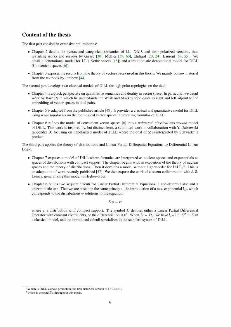
2.3.2.1 Mixed chiralities . . . . . . . . . . . . . . . . . . . . . . . . . . . . . . . . . . 272.3.2.2 Negative chiralities. . . . . . . . . . . . . . . . . . . . . . . . . . . . . . . . . 282.3.2.3 Interpreting MALLpol . . . . . . . . . . . . . . . . . . . . . . . . . . . . . . . 292.3.2.4 Interpreting LLpol . . . . . . . . . . . . . . . . . . . . . . . . . . . . . . . . . 31

2.4 Differential Linear Logic . . . . . . . . . . . . . . . . . . . . . . . . . . . . . . . . . . . . . . . 342.4.1 Syntax and cut-elimination . . . . . . . . . . . . . . . . . . . . . . . . . . . . . . . . . . 34

2.4.1.1 The syntax . . . . . . . . . . . . . . . . . . . . . . . . . . . . . . . . . . . . . 342.4.1.2 Typing: intuitions behind the exponential rules. . . . . . . . . . . . . . . . . . 362.4.1.3 Cut-elimination and sums . . . . . . . . . . . . . . . . . . . . . . . . . . . . . 37

2.4.2 Categorical semantics . . . . . . . . . . . . . . . . . . . . . . . . . . . . . . . . . . . . 402.4.2.1 ˚-autonomous Seely categories with biproduct and co-dereliction . . . . . . . . 402.4.2.2 Invariance of the semantics over cut-elimination . . . . . . . . . . . . . . . . . 432.4.2.3 Exponential structures . . . . . . . . . . . . . . . . . . . . . . . . . . . . . . . 45

2.4.3 A Smooth intuitionistic model: Convenient spaces . . . . . . . . . . . . . . . . . . . . . 452.5 Polarized Differential Linear Logic . . . . . . . . . . . . . . . . . . . . . . . . . . . . . . . . . . 49

2.5.1 A sequent calculus . . . . . . . . . . . . . . . . . . . . . . . . . . . . . . . . . . . . . . 492.5.2 Categorical semantics . . . . . . . . . . . . . . . . . . . . . . . . . . . . . . . . . . . . 50

2.5.2.1 Dereliction and co-dereliction as functors . . . . . . . . . . . . . . . . . . . . . 502.5.2.2 A polarized biproduct . . . . . . . . . . . . . . . . . . . . . . . . . . . . . . . 512.5.2.3 Categorical models of DiLLpol . . . . . . . . . . . . . . . . . . . . . . . . . . 52

3 Topological vector spaces 53

Closure and orthogonalities . . . . . . . . . . . . . . . . . . . . . . . . . . . . . . . . . . . . . . 55Filters and topologies . . . . . . . . . . . . . . . . . . . . . . . . . . . . . . . . . . . . . . . . . 55

3.1 First definitions . . . . . . . . . . . . . . . . . . . . . . . . . . . . . . . . . . . . . . . . . . . . 563.1.1 Topologies on vector spaces . . . . . . . . . . . . . . . . . . . . . . . . . . . . . . . . . 563.1.2 Metrics and semi-norms . . . . . . . . . . . . . . . . . . . . . . . . . . . . . . . . . . . 573.1.3 Compact and precompact sets . . . . . . . . . . . . . . . . . . . . . . . . . . . . . . . . 58

IV

3.1.4 Projective and inductive topolgies . . . . . . . . . . . . . . . . . . . . . . . . . . . . . . 583.1.5 Completeness . . . . . . . . . . . . . . . . . . . . . . . . . . . . . . . . . . . . . . . . . 59

3.2 Examples: sequences and measures . . . . . . . . . . . . . . . . . . . . . . . . . . . . . . . . . 603.2.1 Spaces of continuous functions . . . . . . . . . . . . . . . . . . . . . . . . . . . . . . . . 603.2.2 Spaces of smooth functions . . . . . . . . . . . . . . . . . . . . . . . . . . . . . . . . . 603.2.3 Sequence spaces . . . . . . . . . . . . . . . . . . . . . . . . . . . . . . . . . . . . . . . 61

3.3 Linear functions and their topologies . . . . . . . . . . . . . . . . . . . . . . . . . . . . . . . . . 623.3.1 Linear continuous maps . . . . . . . . . . . . . . . . . . . . . . . . . . . . . . . . . . . 623.3.2 Weak properties and dual pairs . . . . . . . . . . . . . . . . . . . . . . . . . . . . . . . . 633.3.3 Dual pairs . . . . . . . . . . . . . . . . . . . . . . . . . . . . . . . . . . . . . . . . . . . 65

3.4 Bornologies and uniform convergence . . . . . . . . . . . . . . . . . . . . . . . . . . . . . . . . 663.4.1 Polars and equicontinuous sets . . . . . . . . . . . . . . . . . . . . . . . . . . . . . . . . 663.4.2 Boundedness for sets and functions . . . . . . . . . . . . . . . . . . . . . . . . . . . . . 673.4.3 Topologies on spaces of linear functions . . . . . . . . . . . . . . . . . . . . . . . . . . . 683.4.4 Barrels . . . . . . . . . . . . . . . . . . . . . . . . . . . . . . . . . . . . . . . . . . . . 70

3.5 Reflexivity . . . . . . . . . . . . . . . . . . . . . . . . . . . . . . . . . . . . . . . . . . . . . . . 703.5.1 Weak, Mackey and Arens reflexivities . . . . . . . . . . . . . . . . . . . . . . . . . . . . 713.5.2 Strong reflexivity . . . . . . . . . . . . . . . . . . . . . . . . . . . . . . . . . . . . . . . 723.5.3 The duality of linear continuous functions . . . . . . . . . . . . . . . . . . . . . . . . . . 73

3.6 Topological tensor products and bilinear maps . . . . . . . . . . . . . . . . . . . . . . . . . . . . 743.6.1 The projective, inductive and B tensor products . . . . . . . . . . . . . . . . . . . . . . . 743.6.2 The injective tensor product . . . . . . . . . . . . . . . . . . . . . . . . . . . . . . . . . 763.6.3 The ε tensor product . . . . . . . . . . . . . . . . . . . . . . . . . . . . . . . . . . . . . 78

II Classical models of DiLL 79

4 Mackey and Weak topologies as left and right adjoint to pairing 80

Quantitative semantics . . . . . . . . . . . . . . . . . . . . . . . . . . . . . . . . . . . . . . . . 80CHU and its adjunctions to TOPVEC . . . . . . . . . . . . . . . . . . . . . . . . . . . . . . . . . 80

5 Weak topologies and formal power series 84

5.1 Multiplicative and additives connectives . . . . . . . . . . . . . . . . . . . . . . . . . . . . . . . 855.1.1 Spaces of linear maps . . . . . . . . . . . . . . . . . . . . . . . . . . . . . . . . . . . . . 855.1.2 Tensor and cotensor . . . . . . . . . . . . . . . . . . . . . . . . . . . . . . . . . . . . . 865.1.3 A ˚-autonomous category . . . . . . . . . . . . . . . . . . . . . . . . . . . . . . . . . . 885.1.4 Additive connectives . . . . . . . . . . . . . . . . . . . . . . . . . . . . . . . . . . . . . 88

5.2 A quantitative model of Linear Logic . . . . . . . . . . . . . . . . . . . . . . . . . . . . . . . . . 885.2.1 The exponential . . . . . . . . . . . . . . . . . . . . . . . . . . . . . . . . . . . . . . . . 895.2.2 The co-Kleisli category . . . . . . . . . . . . . . . . . . . . . . . . . . . . . . . . . . . . 945.2.3 Cartesian closedness . . . . . . . . . . . . . . . . . . . . . . . . . . . . . . . . . . . . . 965.2.4 Derivation and integration . . . . . . . . . . . . . . . . . . . . . . . . . . . . . . . . . . 985.2.5 An exponential with non-unit sequences . . . . . . . . . . . . . . . . . . . . . . . . . . . 99

5.3 A negative interpretation of DiLLpol . . . . . . . . . . . . . . . . . . . . . . . . . . . . . . . . . 101

6 Mackey topologies on convenient spaces 103

6.1 Models of Linear Logic Based on Schwartz’ ε product . . . . . . . . . . . . . . . . . . . . . . . 1046.2 Preliminaries: bornological notions . . . . . . . . . . . . . . . . . . . . . . . . . . . . . . . . . . 106

6.2.1 Bornological spaces . . . . . . . . . . . . . . . . . . . . . . . . . . . . . . . . . . . . . 1066.2.2 Mackey-completeness . . . . . . . . . . . . . . . . . . . . . . . . . . . . . . . . . . . . 1096.2.3 Convenient spaces . . . . . . . . . . . . . . . . . . . . . . . . . . . . . . . . . . . . . . 110

6.3 A positive model of MALL with bornological tensor . . . . . . . . . . . . . . . . . . . . . . . . 1116.3.1 Co-products of bornological spaces . . . . . . . . . . . . . . . . . . . . . . . . . . . . . 1116.3.2 A tensor product preserving the Mackey-topology . . . . . . . . . . . . . . . . . . . . . . 1126.3.3 A bornological ` for CHU . . . . . . . . . . . . . . . . . . . . . . . . . . . . . . . . . . 113

6.4 CONV and COMPL, a positive interpretation of DiLL . . . . . . . . . . . . . . . . . . . . . . . . 115

V

6.4.1 Multiplicative connectives . . . . . . . . . . . . . . . . . . . . . . . . . . . . . . . . . . 1156.4.1.1 An internal hom-set on convenient sets . . . . . . . . . . . . . . . . . . . . . . 1156.4.1.2 A duality theory for convenient spaces . . . . . . . . . . . . . . . . . . . . . . 1166.4.1.3 A chirality between convenient and Complete and Mackey spaces . . . . . . . . 117

6.4.2 Additive connectives and exponentials . . . . . . . . . . . . . . . . . . . . . . . . . . . . 119

III Distributions and Linear Partial Differentials Equations in DiLL 122

7 Distributions, a model of Smooth DiLL 123

7.1 (F)-spaces and (DF)-spaces . . . . . . . . . . . . . . . . . . . . . . . . . . . . . . . . . . . . . . 1257.1.1 The duality of (F)-spaces . . . . . . . . . . . . . . . . . . . . . . . . . . . . . . . . . . . 1257.1.2 (F)-spaces and the ε product . . . . . . . . . . . . . . . . . . . . . . . . . . . . . . . . . 125

7.2 Nuclear and Schwartz’ spaces . . . . . . . . . . . . . . . . . . . . . . . . . . . . . . . . . . . . 1267.2.1 Schwartz spaces . . . . . . . . . . . . . . . . . . . . . . . . . . . . . . . . . . . . . . . 1267.2.2 Nuclear spaces . . . . . . . . . . . . . . . . . . . . . . . . . . . . . . . . . . . . . . . . 1287.2.3 A polarized model of MALL . . . . . . . . . . . . . . . . . . . . . . . . . . . . . . . . 131

7.3 Kernel theorems and Distributions . . . . . . . . . . . . . . . . . . . . . . . . . . . . . . . . . . 1327.3.1 Kernel theorems for functions . . . . . . . . . . . . . . . . . . . . . . . . . . . . . . . . 1337.3.2 Distributions and distributions with compact support . . . . . . . . . . . . . . . . . . . . 1347.3.3 Distributions and convolution product . . . . . . . . . . . . . . . . . . . . . . . . . . . . 1357.3.4 Other spaces of distributions and Fourier transforms . . . . . . . . . . . . . . . . . . . . 136

7.4 Smooth Differential Linear Logic and its models . . . . . . . . . . . . . . . . . . . . . . . . . . 1367.4.1 The categorical structure of Nuclear and (F)-spaces. . . . . . . . . . . . . . . . . . . . . 1367.4.2 Smooth Differential Linear Logic . . . . . . . . . . . . . . . . . . . . . . . . . . . . . . 1377.4.3 A model of Smooth DiLL with distributions . . . . . . . . . . . . . . . . . . . . . . . . . 138

7.5 Higher-Order models with Distributions . . . . . . . . . . . . . . . . . . . . . . . . . . . . . . . 1407.5.1 Higher-order distributions and Kernel . . . . . . . . . . . . . . . . . . . . . . . . . . . . 1407.5.2 Dereliction and co-dereliction . . . . . . . . . . . . . . . . . . . . . . . . . . . . . . . . 1447.5.3 Co-multiplication, and the bialgebraic natural transformations . . . . . . . . . . . . . . . 1467.5.4 A model of MALL for our higher-order exponential . . . . . . . . . . . . . . . . . . . . 1477.5.5 An exponential for convenient spaces . . . . . . . . . . . . . . . . . . . . . . . . . . . . 148

8 LPDE and D´DiLL 150

8.1 Linear Partial Equations . . . . . . . . . . . . . . . . . . . . . . . . . . . . . . . . . . . . . . . 1518.1.1 Linear Partial Differential operators . . . . . . . . . . . . . . . . . . . . . . . . . . . . . 1518.1.2 Differentiation and convolution . . . . . . . . . . . . . . . . . . . . . . . . . . . . . . . 1538.1.3 Solving linear partial differential equations with constant coefficients . . . . . . . . . . . 153

8.1.3.1 Fundamental solutions . . . . . . . . . . . . . . . . . . . . . . . . . . . . . . . 1538.1.3.2 The space !D . . . . . . . . . . . . . . . . . . . . . . . . . . . . . . . . . . . 155

8.2 Discussion: Linear Logic for differential equations . . . . . . . . . . . . . . . . . . . . . . . . . 1568.3 D0 ´DiLL . . . . . . . . . . . . . . . . . . . . . . . . . . . . . . . . . . . . . . . . . . . . . . 158

8.3.1 Grammar and rules . . . . . . . . . . . . . . . . . . . . . . . . . . . . . . . . . . . . . . 1588.3.2 Models . . . . . . . . . . . . . . . . . . . . . . . . . . . . . . . . . . . . . . . . . . . . 159

8.3.2.1 A model with D0. . . . . . . . . . . . . . . . . . . . . . . . . . . . . . . . . . 1598.3.2.2 A model with any LPDOcc D . . . . . . . . . . . . . . . . . . . . . . . . . . . 159

8.4 D-DiLL . . . . . . . . . . . . . . . . . . . . . . . . . . . . . . . . . . . . . . . . . . . . . . . . 1608.4.1 The sequent calculus D´DiLL . . . . . . . . . . . . . . . . . . . . . . . . . . . . . . . 160

8.4.1.1 Grammar and rules . . . . . . . . . . . . . . . . . . . . . . . . . . . . . . . . 1608.4.1.2 Admissible rules . . . . . . . . . . . . . . . . . . . . . . . . . . . . . . . . . . 161

8.4.2 The cut-elimination procedure in D´DiLL . . . . . . . . . . . . . . . . . . . . . . . . . 1628.4.3 A concrete semantics without higher order . . . . . . . . . . . . . . . . . . . . . . . . . 162

9 Conclusion 169

Appendices

VI

Appendix A Index of symbols 176

Appendix B Models of Linear Logic based on the Schwartz ε-product. 179

B.0.0.1 Introduction . . . . . . . . . . . . . . . . . . . . . . . . . . . . . . . . . . . . 180B.1 Three Models of MALL . . . . . . . . . . . . . . . . . . . . . . . . . . . . . . . . . . . . . . . 183

B.1.1 Preliminaries . . . . . . . . . . . . . . . . . . . . . . . . . . . . . . . . . . . . . . . . . 183B.1.1.1 Reminder on topological vector spaces . . . . . . . . . . . . . . . . . . . . . . 184B.1.1.2 Reminder on tensor products and duals of locally convex spaces. . . . . . . . . 184B.1.1.3 Dialogue and ˚-autonomous categories . . . . . . . . . . . . . . . . . . . . . . 186B.1.1.4 A model of MALL making appear the Arens dual and the Schwartz ε-product . 187

B.1.2 Mackey-complete spaces and a first interpretation for ` . . . . . . . . . . . . . . . . . . 191B.1.2.1 A Mackey-Completion with continuous canonical map . . . . . . . . . . . . . 191B.1.2.2 A ` for Mackey-complete spaces . . . . . . . . . . . . . . . . . . . . . . . . . 192

B.1.3 Original setting for the Schwartz ε-product and smooth maps. . . . . . . . . . . . . . . . 198B.1.3.1 ˚-autonomous category of k-reflexive spaces. . . . . . . . . . . . . . . . . . . 198B.1.3.2 A strong notion of smooth maps . . . . . . . . . . . . . . . . . . . . . . . . . 205

B.1.4 Schwartz locally convex spaces, Mackey-completeness and ρ-dual. . . . . . . . . . . . . 207B.1.4.1 Preliminaries in the Schwartz Mackey-complete setting . . . . . . . . . . . . . 207B.1.4.2 ρ-reflexive spaces and their Arens-Mackey duals . . . . . . . . . . . . . . . . . 208B.1.4.3 Relation to projective limits and direct sums . . . . . . . . . . . . . . . . . . . 211B.1.4.4 The Dialogue category McSch. . . . . . . . . . . . . . . . . . . . . . . . . . 212B.1.4.5 Commutation of the double negation monad on McSch . . . . . . . . . . . . . 213B.1.4.6 The ˚-autonomous category ρ´Ref . . . . . . . . . . . . . . . . . . . . . . . 216

B.2 Models of LL and DiLL . . . . . . . . . . . . . . . . . . . . . . . . . . . . . . . . . . . . . . . 216B.2.1 Smooth maps and induced topologies. New models of LL . . . . . . . . . . . . . . . . . 216

B.2.1.1 C -Smooth maps and C -completeness . . . . . . . . . . . . . . . . . . . . . . . 217B.2.1.2 Induced topologies on linear maps . . . . . . . . . . . . . . . . . . . . . . . . 219B.2.1.3 A general construction for LL models . . . . . . . . . . . . . . . . . . . . . . . 221B.2.1.4 A class of examples of LL models . . . . . . . . . . . . . . . . . . . . . . . . 223B.2.1.5 A model of LL: a Seely category . . . . . . . . . . . . . . . . . . . . . . . . . 225B.2.1.6 Comparison with the convenient setting of Global analysis and Blute-Ehrhard-

Tasson . . . . . . . . . . . . . . . . . . . . . . . . . . . . . . . . . . . . . . . 227B.2.2 Models of DiLL . . . . . . . . . . . . . . . . . . . . . . . . . . . . . . . . . . . . . . . 228

B.2.2.1 An intermediate notion: models of differential λ-Tensor logic. . . . . . . . . . . 228B.2.2.2 A general construction for DiLL models . . . . . . . . . . . . . . . . . . . . . 232B.2.2.3 ρ-smooth maps as model of DiLL . . . . . . . . . . . . . . . . . . . . . . . . . 237B.2.2.4 k-smooth maps as model of DiLL . . . . . . . . . . . . . . . . . . . . . . . . . 238

B.2.3 Conclusion . . . . . . . . . . . . . . . . . . . . . . . . . . . . . . . . . . . . . . . . . . 239B.2.4 Appendix . . . . . . . . . . . . . . . . . . . . . . . . . . . . . . . . . . . . . . . . . . . 239

1

Chapter 1

Introduction

Differentiation in mathematics historically deals with functions defined on continuous sets, in which infinitesimalvariations of variables can be defined. Even though computation historically deals with discrete structures, theconcept of differentiation has recently made its way into several applied domains of computer science, e.g. innumerical analysis [39], in incremental computing [65], or in machine learning [3].

Semantics of programs have however essentially focussed on programs operating on discrete classes of re-

sources, relying on the guiding principle that programs compute using only a finite amount of resources. Thisconcept has been prominent in the development of denotational semantics, even essential to obtain the first modelsof λ-calculus in domain theory [70].

The rise of probabilistic languages, infinite data structures and machine learning has more recently promoteda movement towards continuous semantics: theoretical computer science, which has traditionally been associatedwith discrete mathematics and algebra, is now steadily moving towards analysis.

Independently, differentiation also appeared in proof theory through Differential Linear Logic [23]. LinearLogic and its differential refinement are formal proof systems allowing for the characterization of the conceptof linearity of proofs. Linear Logic [29] is a resource-aware refinement of intuitionnistic and classical logic,introduced after a study of denotational models of λ-calculus. Differential Linear Logic spawned from the carefulstudy of models of Linear Logic based on vector spaces [18, 19] [74]. While the former enriches Logic withtools from Algebra, the latter transports those of Differential Calculus. When Linear Logic had applications indevelopments in Type systems [12, 80], Differential Linear Logic may now lead to developments in differentialand probabilistic programming through differential λ-calculus [22].

This work draws formal links between Logic and the theory of topological vector spaces and distributions. Itdevelops several classical and smooth models of Differential Linear Logic using the theory of topological vec-tor spaces, and with these models embeds the theory of linear partial differential operators into a refinement ofDifferential Linear Logic.

The cornerstone of our approach is the intuition that semantics should carry over an essential aspect of the

syntax of Differential Linear Logic, namely the involutive negation, and operate on continuous spaces. We will

explain how this leads to the understanding of !E as a space of solutions to a Differential Equation.

Models of Differential Linear Logic

Linear Types and Differentiation. Through the Curry-Howard correspondence (detailed in section 2.1) formu-las A of a logical system can be understood as types of programs p : A. In particular, the logical implicationA ñ B is the type of programs p : A ñ B producing data of type B from data of type A. Linear Logic is alogical system which distinguishes a linear implication A ⊸ B, and a specific unary constructor !A, read as “ofcourse A", or the exponential of A . The usual implication is then defined using this two connectives:

!A⊸ B ” Añ B (1.1)

where ” stands for logical equivalence. Through the dereliction rule, Linear Logic expresses that a linear impli-cation is in particular a non-linear one. That is, we have a proof dA of the formula:

dA : pA⊸ Bq⊸ pAñ Bq.

2

Differential Linear Logic contains a dual rule named codereliction, which expresses the fact that a linear proof canbe extracted from a non-linear one. It is thought of as the best linear approximation of this proof at 01. That is, wehave a proof dA of the formula:

dA : pAñ Bq⊸ pA⊸ Bq.

As a linear map is its own differentiation, a cut-rule - semantically a composition between d and d - must result inthe identity:

dA ˝ dA “ IdA

In the last chapter (Chapter 8), we generalize this to interpret the theory of Linear Partial Differential Operators(LPDO) acting on distributions. We provide a dereliction rule dD,A which applies an operator D to a proofq : Añ B. The dereliction dD,A is then the rule which computes the solution p : Añ B such that

Dp “ q.

This is justified as a model of Differential Linear Logic in which distributions with vectorial values [67] interpretproofs.

Differential Linear Logic is a Type System for several Differential Operators, and in particular for

Linear Partial Differential Operators with Constant Coefficients.

Semantics of Linear Logic The field of Denotational semantics studies programs by interpreting them by func-tions. In particular, a program p : Añ B is interpreted by a function f : JAK //JBK. Thus typesA are interpretedby some spaces JAK. These spaces must be stable under some operations. Typically, one must be able to curry anduncurry:

JAKˆ JBK // JCK » JAK // pJBK // JCKq. (1.2)

To interpret higher-order functional programming, one must consider the type of programs Añ B as a spaceitself, i.e we must have a category with internal hom-set. If p : A ñ B, then p is interpreted by a functionf : JAK // JBK, which is itself an element of a space:

f P CpJAK, JBKq

Through the Curry-Howard isomorphism, matching in particular types of programs to formulas, denotational se-mantics also applies to logical systems: we consider logical systems as type systems for certain programs. Modelsof classical logics must in particular interpret the logical equivalence between a formula A and its double negation A.

JAK ” J AK.Models of Linear Logic [59] distinguish between linear functions ℓ P LpJAK, JBKqand non-linear functions

f P CpJAK, JBKq. Moreover, Linear Logic is a classical logic with a linear negation. If p_qK interprets this linearnegation, then a model of Linear Logic should satisfy:

JAK “ JAKKK.

Equation 1.2 in the linear context translates into the usual monoidal closedness:

LpJAKb JAK, JAKq » LpJAK,LpJAK, JAKqq.

Smooth semantics of Differential Linear Logic In denotational models of Differential Linear Logic, codere-liction d is interpreted by the operator mapping a function f P CpJAK, JBKq to its differential at 0: D0pfq PLpJAK, JBKq. Thus functions must be smooth: everywhere infinitely differentiable. Differential Linear Logic alsofeatures sums of proofs, and thus one must interpret proofs in an additive category, where each hom-set C8pA,Bqis endowed with a commutative monoidal law `A,B . This justifies searching for models of Differential LinearLogic within Algebra. In fact, Differential Linear Logic stemed from a study of vectorial models of Lineac Logic[18, 19] inspired from domain theory and coherent spaces. In these models, formulas were interpreted as vector

1and is interpreted in topological vector spaces with the differential at 0 of a function.

3

spaces of sequences, and proofs as power series between this spaces. The differentiation of a power series can thenbe computed immediately:

dA : x ÞÑ pf “ÿ

n

fn P CpA,Bqq ÞÑ f1pxqq,

where x P A, and fn is a n-monomial resulting from a n-linear map f P LpAbn

, Bq. In this thesis, we emphasizethe fact that formulas of Differential Linear Logic should be be interpreted by continuous objects , so as torejoin the mathematical intuitions about differentiation. A natural question to ask is then: is there of a model ofDifferential Linear Logic in which formulas and proofs are interpreted by continuous objects and differentiationon smooth functions between, let’s say, Banach spaces ?

Trying to interpret Linear Logic with traditional objects of analysis was tackled by Girard by constructingCoherent Banach spaces [32]. This attempt fails, as imposing a norm on spaces of smooth functions2 is too stronga requirement. Thus one must relax the condition on normed spaces and consider more generally topologicalvector spaces. Ehrhard [18] considers specific spaces of sequences, called Köthe spaces, which are in particularcomplete, and thus construct a model of DiLL with an involutive linear negation. This models however relies ona discrete setting, as operations are defined on bases of the considered vector spaces. Blute, Ehrhard, and Tassonused the convenient analysis setting introduced by Frölicher, Kriegl and Michor [26, 53]. They construct a modelof Intuitionistic Differential Linear Logic interpreting formulas by bornological Mackey-complete locally convexand Hausdorff topological vector spaces. Linear proofs are modeled by linear bounded maps and general proofsby a certain class of smooth functions which verifies equation 1.2.

Classical and smooth semantics of Differential Linear Logic Differential Linear Logic is also (linear) classi-cal. In the setting of vector spaces, the linear negation of a formula is interpreted by the space of linear forms onthe interpretation of a formula:

AK » LpJAK,Kq :“ A1.

In the setting of topological vector spaces, a model of classical Linear Logic must interpret formulas by reflexive

spaces, which by definition are a the topological vector spaces such that:

E » E2

However, the only smooth model of Differential Linear Logic [6] did not interpret classicality. In fact, reflexivityand smoothness work as opposite forces in the theory of topological vectors spaces. While interpreting smoothnessrequires some notion of completeness3 — that is spaces with a topology fine enough to make Cauchy filters con-verge — reflexivity requires a topology coarse enough so as to keep the dual E1 small enough. At the beginning ofthis thesis was thus the question of finding a smooth model for DiLL which would also feature a linear involutivenegation.

Reflexivity and (co-)dereliction We argue moreovoer that computations in Differential Linear Logic stronglycall for reflexivity. In that perspective, works by Mellies [62], inspired by semantics and which focuses on thegeometric nature of linear negation in logic, is clarifying. On one hand, smoothness and a linear involutive negationgives us an exponential interpreted as a space of distributions with compact support. Consider indeed reflexivespaces E and F . Then the interpretation of equation 1.1 gives us:

!E » C8pE,Rq1

and this interpretation of the exponential as a central space of functional analysis leads the way to an excitingtransfer of techniques between Proof Theory and Analysis. One the other hand, in a smooth model of DiLL,reflexivity leads to an elegant and general interpretation of dereliction and co-dereliction:

dE :

#C8pE,Rq1 Ñ E

φ ÞÑ φ|LpE,Rq P E2 » E

(1.3)

dE :

#E » E2 Ñ C8pE,Rq1

φ P LpE,Rq1 ÞÑ φ ˝D0 “ pf P C8pE,Rq ÞÑ φpD0pfqqq

(1.4)

2In fact Girard uses analytical functions.3see section 3.1.5

4

The equation on dE is made possible by the fact that LpE,Rq Ă C8pE,Rq, and the second by the factthat D0pfq is by definition a linear function for every f P C8pE,Rq. This understanding of dereliction and co-dereliction as operators on spaces of functions allows a generalization fromD0 to Differential Operators in Chapter8.

Functional analysis and distribution theory This thesis heavily uses tools from the theory of topological vectorspaces [66] [44] [51] and distribution theory [69] to construct denotational models of (classical) Differential LinearLogic. The algebraic constructions interpreting the linear implication, the multiplicative conjunction b and theduality are straightforward: they consist respectively in taking spaces of linear continuous maps LpE,F q, tensorproduct E b F , and the spaces of scalar linear continuous maps E1. The difficulty lies in choosing the goodtopology to put on these spaces. We interpret the exponential ! by spaces of distributions with compact supportC8pE,Rq1. On these spaces one can use the theory of Linear Partial Differential Operators [43].

While functional analysis was developed with an emphasis on cartesian structures and smooth functions, thesearch for models of Linear Logic stresses the role of tensor products and reflexivity. Under this light, severalresults of the theory of locally convex vector spaces find a nice interpretation: Schwartz’s Kernel theorem 7.3.5 in-terprets Seely’s isomorphism, and the Mackey-Arens theorem 3.5.3 gives an adjunction with CHU which generatesclassical models of DiLL (see Part II). Likewise, distribution theory gives an interpretation for the deduction rules

of Differential Linear Logic, and in particular those which are added to Linear Logic: the contraction rule c (seefigure 2.6) is interpreted by the convolution 7.3.17, and co-weakening w in the case of Linear Partial DifferentialEquations (see figure 2.6) corresponds to input of a fundamental solution (see definition 8.1.11).

Differential Linear Logic provides a polarized syntax for the theories of Topological vector spaces,

Distributions, and Linear Partial Differential Equations.

5

Content of the thesis

The first part consists in extensive preliminaries:

• Chapter 2 details the syntax and categorical semantics of LL, DiLL and their polarized versions, thusrevisiting works and surveys by Girard [30], Mellies [59, 60], Ehrhard [20, 24], Laurent [54, 55]. Wedetail a denotational model for LL ( Köthe spaces [18]) and a intuitionistic denotational model for DiLL

(Convenient spaces [6]).

• Chapter 3 exposes the results from the theory of vector spaces used in this thesis. We mainly borrow materialfrom the textbook by Jarchow [44].

The second part develops two classical models of DiLL through polar topologies on the dual:

• Chapter 4 is a quick perspective on quantitative semantics and duality in vector space. In particular, we detailwork by Barr [2] in which he understands the Weak and Mackey topologies as right and left adjoint to theembedding of vector spaces in dual pairs.

• Chapter 5 is adapted from the published article [48]. It provides a classical and quantitative model for DiLL

using weak topologies on the topological vector spaces interpreting formulas of DiLL.

• Chapter 6 refines the model of convenient vector spaces [6] into a polarized, classical ans smooth modelof DiLL. This work is inspired by, but distinct from, a submitted work in collaboration with Y. Dabrowski(appendix B) focusing on unpolarized model of DiLL where the dual of b is interpreted by Schwartz’ εproduct.

The third part applies the theory of distributions and Linear Partial Differential Equations to Differential LinearLogic.

• Chapter 7 exposes a model of DiLL where formulas are interpreted as nuclear spaces and exponentials asspaces of distributions with compact support. The chapter begins with an exposition of the theory of nuclearspaces and the theory of distributions. Then it develops a model without higher-order for DiLL0

4. This isan adaptation of work recently published [47]. We then expose the work of a recent collaboration with J.-S.Lemay, generalizing this model to Higher-order.

• Chapter 8 builds two sequent calculi for Linear Partial Differential Equations, a non-deterministic and adeterministic one. The two are based on the same principle: the introduction of a new exponential !D, whichcorresponds to the distributions φ solutions to the equation:

Dφ “ ψ

where ψ a distribution with compact support. The symbol D denotes either a Linear Partial DifferentialOperator with constant coefficients, or the differentiation at 05. When D “ D0, we have !DE » E2 » E ina classical model, and the introduced calculi specialises to the standard syntax of DiLL.

4Which is DiLL without promotion, the first historical version of DiLL [24].5which is denoted D0 throughout this thesis.

6

Models of DiLL: a panorama

This thesis brings a contribution to the semantic study of DiLL, by constructing several models of it. The mainbody of the manuscripts focuses on polarized models of DiLL0. Polarization in Linear Logic distinguishes twoclasses of formulas: the positive ones, preserved by the positive connectives, and the negatives ones, accordinglypreserved by the negative connectives. Thus polarized models of DiLL distinguish two kind of spaces, and relaxestopological conditions as not all spaces are required to bear all stability properties.

We give a survey of the characteristics of the existing models and of the ones constructed in this thesis in thefollowing figures:

Models of DiLL

Polarized Continuous spaces Quantitative semanticsE Ć K

N f “řfn

KOTHE [18], X

recalled in Section 2.2.3Finiteness spaces [19] X

Weak spaces [48] X X

Convenient spaces [6], X

recalled in Section 2.4.3Mackey-complete spaces X X

and Power series [49],k-reflexive spaces [17], X

recalled in section 6.1Mackey-complete Schwartz spaces [17], X

recalled in section 6.1Polarized convenient model, X X

Chapter 6Nuclear Fréchet spaces, X X

Chapter 7

Models of DiLL

Smooth Functions Involutive Linear Negation Higher-order

!E “ C8pE,Rq1 E » E2 !!E

KOTHE [18], X X

recalled in Section 2.2.3Finiteness spaces [19] X X

Wear spaces [48] X X

Convenient spaces [6], X X

Mackey-complete spaces [49] X

k-reflexive spaces [17], X X X

Mackey-complete Schwartz spaces [17], X X X

Polarized convenient model, X X X

Nuclear Fréchet spaces, X X X

7

Logic and Functional Analysis

The author believes that this semantic study allows one to draw solid ties between polarized Differential LinearLogic and the theory of topological vector spaces. We sum up these correspondences, while referring to a concretemodel in which they are verified.

Operations of DiLL

Logical operation Interpretation Example

A E a lcs That’s the case for every model considered above

Linear negation AK Linear topological dual E1 In all models except convenient spaces [6],where AK is interpreted by the bounded dual Eˆ.

` ε In [17] and its summary in section 6.1,and also chapter 6

?A C8pE1,Rnq In [6], [17],

Chapters 6 and 7

!A E1pEq :“ C

8pE,Rq1 When E “ Rn, this is the case in models of [6],[17] and Chapter 7

Â Ew The lcs E endowed with its weak topologyin Chapter 5

Â E or EM , a completion of E Any model with smooth functions

Á Eborn, the bornologification of E In Chapter 6

Exponentials for Differentials Equations

The last chapter details how exponentials should be understood as spaces of solutions for Differential Equations.We sum up the different interpretation of the rules of DiLL in the following table, indexing the different interpre-tations of the rules of DiLL or D´DiLL according to the differential operator considered:

Rules for Differentials Equations

Differential Operator D0 D a LPDOcc Id

Spaces of functions Linear functions functions f “ Dg all smooth functionsE1 DpC8pAqq C

8pAq

Exponential !DE “ D´1p!Eq !D0E :“ E2 » E !DA “ DpC8pAqq1!IdA “ !A “ C

8pAq1

Interpretation of dD : !E // !DE φ ÞÑ φ|pAq1 φ ÞÑ φ|DpC8pAqq

Interpretation of d : !D // !E x ÞÑ pf ÞÑ dpfqp0qpxqq φ ÞÑ pf ÞÑ φpDpfqqq

Interpretation of w : !E // 1 φ ÞÑşφ

Interpretation of w : 1 // !E 1 ÞÑ δ0

Interpretation of wD : !DE // 1 φ ÞÑşDφ

Interpretation of wD : 1 // !DE 1 ÞÑ ED

Interpretation of c : ?Eb?E // ?E f b g ÞÑ f ¨ g

Interpretation of c : !Eb!E // !E ψ b φ ÞÑ ψ ˚ φ

Interpretation of cD : ?DEb?E // ?E f b g ÞÑ f ¨ g

Interpretation of cD : !DEb!E // !E ψ b φ ÞÑ ψ ˚ φ

8

Part I

Preliminaries

9

Chapter 2

Linear Logic, Differential Linear

Logic and their models

Tout ce qui est vrai dans le livre est vrai, dans le livre. Tout ce qui n’est pas dans le livre n’est

pas dans le livre. Bien sûr tout ce qui est faux dans le livre est faux dans le livre. Tout ce qui

n’est pas dans le livre, n’est pas dans le livre, vrai ou faux.

Claude Ponti, La course en livre, 2017.

Linear Logic and its differential extension come from a rich entanglement of syntax and semantics. In partic-ular, Linear Logic comes from the understanding and decomposition of a model of propositional logic. We givein Section 2.2 give an overview of the syntax of Linear Logic, its cut-elimination procedure, and its categoricalsemantics. We will detail a model of LL constructed by Ehrhard, based on spaces of sequences. Section 2.3.1details polarized linear logics as introduced by Laurent [54]. We give a categorical semantics following definitionsby Melliès [61]. We introduce Differential Linear Logic in Section 2.4 as a sequent calculus, define its categoricalsemantics following definitions by Fiore [25] and give an example of a smooth Intuitionistic model [6]. In the lastSection 2.5, we detail a polarized version of Differential Linear Logic, and detail a categorical semantics for it. Itis an adaptation in a sequent calculus of the polarized differential nets by Vaux [79]. The categorical semanticsextends the definitions of Melliès [61].

As preliminaries, we want to introduce the Curry-Howard-Lambek correspondence. This correspondence be-tween theoretical programming languages, logic and categories justifies all the research conducted in this thesis:we look in semantics for intuitions about programming theory. Linear Logic and its Differential extension aretypical examples of this movement.

Notation 2.0.1. In this Chapter, we use a few times the basic vocabulary of Chapter 3, in order to give intuitions

on the syntax. Section 3.1 covers these definitions. In a first approach, the reader can skip the few reference to

the theory of topological vector spaces. Let us just say that the term lcs denotes a locally convex and Hausdorff

topological vector space.

10

Contents

2.1 The Curry-Howard correspondence . . . . . . . . . . . . . . . . . . . . . . . . . . . . . . . 12

2.1.1 Minimal logic and the lambda-calculus . . . . . . . . . . . . . . . . . . . . . . . . . . . 12

2.1.2 LK and classical Logic . . . . . . . . . . . . . . . . . . . . . . . . . . . . . . . . . . . 14

2.2 Linear Logic . . . . . . . . . . . . . . . . . . . . . . . . . . . . . . . . . . . . . . . . . . . . 16

2.2.1 Syntax and cut -elimination . . . . . . . . . . . . . . . . . . . . . . . . . . . . . . . . . 16

2.2.2 Categorical semantics . . . . . . . . . . . . . . . . . . . . . . . . . . . . . . . . . . . . 16

2.2.3 An example: Köthe spaces . . . . . . . . . . . . . . . . . . . . . . . . . . . . . . . . . 22

2.3 Polarized Linear Logic . . . . . . . . . . . . . . . . . . . . . . . . . . . . . . . . . . . . . . . 23

2.3.1 LLpol and LLP. . . . . . . . . . . . . . . . . . . . . . . . . . . . . . . . . . . . . . . . 24


2.3.2.1 Mixed chiralities . . . . . . . . . . . . . . . . . . . . . . . . . . . . . . . . . 27

2.3.2.2 Negative chiralities. . . . . . . . . . . . . . . . . . . . . . . . . . . . . . . . . 28

2.3.2.3 Interpreting MALLpol . . . . . . . . . . . . . . . . . . . . . . . . . . . . . . 29

2.3.2.4 Interpreting LLpol . . . . . . . . . . . . . . . . . . . . . . . . . . . . . . . . 31

2.4 Differential Linear Logic . . . . . . . . . . . . . . . . . . . . . . . . . . . . . . . . . . . . . 34

2.4.1 Syntax and cut-elimination . . . . . . . . . . . . . . . . . . . . . . . . . . . . . . . . . 34

2.4.1.1 The syntax . . . . . . . . . . . . . . . . . . . . . . . . . . . . . . . . . . . . 34

2.4.1.2 Typing: intuitions behind the exponential rules. . . . . . . . . . . . . . . . . . 36

2.4.1.3 Cut-elimination and sums . . . . . . . . . . . . . . . . . . . . . . . . . . . . 37


2.4.2.1 ˚-autonomous Seely categories with biproduct and co-dereliction . . . . . . . . 40

2.4.2.2 Invariance of the semantics over cut-elimination . . . . . . . . . . . . . . . . . 43

2.4.2.3 Exponential structures . . . . . . . . . . . . . . . . . . . . . . . . . . . . . . 45

2.4.3 A Smooth intuitionistic model: Convenient spaces . . . . . . . . . . . . . . . . . . . . . 45

2.5 Polarized Differential Linear Logic . . . . . . . . . . . . . . . . . . . . . . . . . . . . . . . . 49

2.5.1 A sequent calculus . . . . . . . . . . . . . . . . . . . . . . . . . . . . . . . . . . . . . 49


2.5.2.1 Dereliction and co-dereliction as functors . . . . . . . . . . . . . . . . . . . . 50

2.5.2.2 A polarized biproduct . . . . . . . . . . . . . . . . . . . . . . . . . . . . . . 51

2.5.2.3 Categorical models of DiLLpol . . . . . . . . . . . . . . . . . . . . . . . . . 52

11

2.1 The Curry-Howard correspondence

In this section, we will give two examples of the Curry-Howard correspondence: first we show the correspondencebetween minimal logic, the simply-typed λ-calculus and cartesian closed categories. Then we detail the sequentcalculus LK, thus omiting the Curry-Howard correspondance with the λµµ-calculus [16] and control categories[72].

2.1.1 Minimal logic and the lambda-calculus

This section consists in a very basic introduction to the Curry-Howard-Lambek correspondence. Programs areunderstood as terms of the λ-calculus. They are typed by formulas of minimal logic, and these types are interpretedin a cartesian closed category.

Definition 2.1.1. Consider A a set of atoms. Formulas of minimal implicative logic are terms constructed via thefollowing syntax: A,B :“ a P U | A //B

Definition 2.1.2. Consider X a set of variables. Terms of the λ-calculus are constructed via the following syntax:t, u :“ x | ptqu | λx.t

Typing judgements are denoted by Γ $ t : A, where t is a term and A a formula, and Γ a list of typingassignments t1 : A1. Then the λ-calculus is typed according to the following rules: to each variable x is assigned atype A, and then:

x P X, a P AΓ, x : a $ x : a

Γ $ t : A //B, u : A appΓ $ ptqu : B

Γ, x : A $ t : B //Γ $ λx.t : A //B

The β-reduction rule of λ- calculus is the following:

pλx.tqu // truxs.

It preserves typing according to the cut rule above.

Categories The categorical semantics of a proof system interprets formulas by objects of a given categoryC, and sequents A $ B as morphisms from an object A to an object B. We will see that the morphisms of acartesian closed category interpret the typing judgements of the simply typed λ-calculus.

Definition 2.1.3. [56] A category C consists in:

• A collection OpCq of objects,

• A collection ApCq of arrows such that each arrow f has a domain A P OpCq and B P OpCq: we writef : A //B and the collection of all arrows with domain A and codomain B is denoted by CpA,Bq.

• For each objects A, B and C a binary associative law: ˝ : CpA,Bq ˆ CpB,Cq // CpA,Cq.

• For each objectA an arrow 1A P CpA,Aq such that for any objectB, any arrows f : A //B and g : B //Awe have:

f ˝ 1A “ f and 1A ˝ g “ g.

A category is said to be small if the collection of its objects is a set. A category is said to be locally small ifevery hom-set CpA,Bq is a set. If C is a category, one construct its opposite category Cop with the same objectsbut with reverse arrows CoppB,Aq “ CpA,Bq.

Definition 2.1.4. A (covariant) functor F from categories C to D is a map between the collections of objects and thecollection of arrows fo C and D respectively such that:

Fpf : A //Bq : FpAq // FpBq and Fpf ˝ gq “ Fpfq ˝ Fpgq.

12

A contravariant functor F from a category C to a category D is a covariant functor from C to Dop. Withoutany further specifications, a functor is always supposed to be covariant.

Example 2.1.5. Consider C a locally small category. Then for every object C P C we have a covariant functor

CpC, _q : C // Set,B ÞÑ CpC,Bq, f P CpA,Bq ÞÑ f˚ : g P CpC,Aq ÞÑ f ˝ g P CpC,Bq

and a contravariant functor

Cp_, Cq : C // Set,A ÞÑ CpA,Cq, f P CpA,Bq ÞÑ ˚f : g P CpA,Cq ÞÑ g ˝ f P CpB,Cq.

Definition 2.1.6. We write F : C // D. A natural transformation η between two functors F : C // D and G :

C //D is a collection of morphisms indexed by objects of C such that:

ηA : FpAq // GpAq P DpFpAq,GpAqq

and such that for every object A,B P C, arrows f : A // B we have ηB ˝ Fpfq “ Gpfq ˝ ηA. This diagrammore precisely states the naturality in A of the collection of morphisms η.

FpAq

ηA

Fpfq // FpBq

ηB

GpAq

Gpfq // GpBq

Definition 2.1.7. Two functors F : C // D and G : D // C are respectively left adjoint and right adjoint if foreach object C P C and D P D we have a bijection:

CpC,GpDqq » DpFpCq, Dq

which is natural in C and D. We write F % G and we denote this as:

C D

F

G

%

Through this adjunction, there is a natural transformation d : F ˝ G // IdD which is called the co-unit, suchthat for any D P D dD : FpGpDqq //D is the morphism of D corresponding to 1GpDq P CpGpDq,GpDqq throughthe adjunction. Similarly, there is a natural transformation d : IdC //G ˝F // IdC which is called the unit, suchthat for any C P C dC : C // GpFpCqq is the morphism of C corresponding to 1FpV q P DpFpCq,FpCqq throughthe adjunction.

Definition 2.1.8. The categories C and D are said to be equivalent through an adjunction if the unit and the co-unitare isomorphisms.

The definition of product categories and bifunctors is straightforward [56]. A terminal object in a category C isan object K of C such that for every object A of C, there is a unique arrow tA : A // K.

Definition 2.1.9. A cartesian category is a category C endowed with a terminal object K and binary law ˆ :

C ˆ C // C such that for every objects A,B P C, there are arrows (projections)

πA : AˆB //A,

πB : AˆB //B

such that for every object C of C, for every arrows f P CpC,Aq, g P CpC,Bq, there is a unique arrow xf, gy PCpC,AˆBq satisfying f “ πA ˝ xf, gy and g “ πB ˝ xf, gy.

Then one can show that this binary rule ˆ is commutative and associative. The definition of a n-ary product isthus immediate. This category is cartesian closed if for every objectB P C we have a functor rB, _s : C //C and anadjunction:

CpAˆB,Cq » CpA, rB,Csq

Thus to the morphism idrA,Bs P CprA,Bs, rA,Bsq corresponds a unique morphism:

evA,B : rA,Bs ˆA //B.

13

Interpretation of the simply typed λ-calculus in categories Consider C a cartesian closed category. With everytyping judgement one assigns an object in C:

• If x is a variable, x : A is matched to an arbitrary object A P C,

• t : A //B is matched to rA,Bs.

To a typing context x1 : A1, ..., xn : An one assigns the product of the interpretation of the types. To everytyping derivation Γ $ t : B one assigns a morphism in CpΓ, Bq according to the following rules:

• To the axiom x1 : A1, ..., xn : An $ xi : Ai corresponds the i-th projection πi : A1 ˆ ... ˆ An // Ai onthe last item of a product.

• From an arrow f P CpA1 ˆ ... ˆ An ˆ A,Bq corresponding to x1 : A1, ..., xn : An, t : A $ u : B, oneconstructs via the closedness property an arrow in CpA1 ˆ ...ˆAn, rA,Bsq.

• From an arrow f P CpA1 ˆ ... ˆ An, rA,Bsq corresponding to x1 : A1, ..., xn : An $ u : A // B and anarrow g P CpB1 ˆ ...ˆ Bn, Aq corresponding to y1 : B1, ..., yn : Bm $ t : A, one constructs via evA,B anarrow in CpA1 ˆ ...ˆAn ˆB1 ˆ ...ˆBm, Bq.

2.1.2 LK and classical Logic

Classical logic is the logic satisfying the excluded middle: the formula A _ A is provable, even if one cannotconstruct a proof of A or a proof of A. This is equivalent as being allowed to eliminate the double-negation: ifwe can prove the negation of the negation of A, then one can prove A. In other words, if we have a proof thatthe negation of A implies the absurd, then this is a proof for A. Classical logic have been criticized for beingto non-constructive: a witness for the fact that the negation of A is impossible is not really an inhabitant of A.However, it was highlighted by Griffin [35] that classical logics has a computational content, as it allows to typeexceptions handlers.

This will be illustrated here by detailing the propositional classical sequent calculusLK introduced by Gentzen [28].A sequent calculus consists in formulas, sequents, and rules allowing to deduce sequents from axioms. A formula

is a tree constructed from atoms, logical connectives and constants. Let A be a set of atoms a P A.A sequent is an expression Γ $ ∆, where Γ and ∆ are both finite sequences of formulas. The (non-linear,

usual) intuition is that writing Γ $ ∆ means that from the conjunction of the formulas of Γ (i.e. from all theformulas of Γ), one can deduce the disjunction of the formulas of ∆.

Definition 2.1.10. The formulas of LK are defined according to the following grammar:

A,B :“ J | K | a | A_B | A^B.

In the above definition, _ denotes the disjunction (A or B) while ^ denotes the conjunction (A and B). Onealso defines an involutive negation p¨q on formulas:

J “ K K “ J pA_Bq “ A^ B pA^Bq “ A_ B.

As we are in a classical logic, A should be provable under the hypotheses of ∆ if and only if no contradictionarise from the set of hypotheses ∆, AK, or likewhise if one can prove ∆K, A. This justifies a monolateral presen-tation $ Γ of sequents, were $ ΓK,∆ stands for Γ $ ∆. The deduction rules for LK are detailed in figure 2.1.2.What happens between a bilateral and a monolateral presentation is the following: while in a bilateral presentation,one would need to introduce a rule (for example a logical rule introducing a connective) to the left and to the right,it is now enough to introduce it to the right. For example, a bilateral version of LK features the rules:

Γ $ A,∆ Γ $ B,∆^Radd

Γ $ A^B,∆

Γ, A $ ∆^L1add

Γ, A^B $ ∆

Γ, B $ ∆^L2add

Γ, A^B $ ∆

and

Γ, A $ ∆ Γ, B $ ∆_Ladd

Γ, A_B $ ∆

Γ $ A∆_R1add

Γ $ A_B∆

Γ,$ B∆_R2add

Γ $ A_B∆

Notice the symmetry between the introduction of a connective to the left and the introduction of its dual on theright. In the monolateral presentation of LK in figure 2.1.2, rules on the left are replaced by their dual rules on theright. What makes this logic classical is precisely the fact that A is involutive: a formula is logically isomorphicto its double negation.

14

The identity group

ax$ A, A

$ A,∆ $ A,Γcut

∆,Γ

The logical group

Jmull$ 1$ Γ

Kmul$ Γ,K

$ Γ, A,B_mull$ Γ, A_B

$ Γ, A $ ∆, B(^mull)

$ Γ,∆, A^B

Jadd$ Γ,J$ Γ, A $ Γ, B

^add$ Γ, A^B

$ Γ, A_addL$ Γ, A_B

$ Γ, B_addR$ Γ, A_B

The structural group

$ Γ, A,Acontraction

$ Γ, A

$ Γweakening

$ Γ, A

$ Γcommutation

$ σpΓq for σ P Sp| Γ |q.

Figure 2.1: The inference rules for LK.

Structural rules Structural rules of LK are the ones describing the operations on Γ and ∆ that do not changethe logical content of the sequent Γ $ ∆. Namely, contraction allows the duplication of a formula on the left (anhypothesis can be used twice), or on the right (if one can prove a formula once, then one can do it twice).

Additive and multiplicative rules When such structural rules are allowed, then each rule has two versions, anadditive one and a multiplicative one. Additive ones are the one that do not make a distinction between the contextof two given sequents of a rule, while multiplicative ones are those which concatenate the context of the premisses.These additive and multiplicative presentations are equivalent because of the structural rules. We will see later inSection 2.2 how linear logic, which restrains the use of structural rules on specific formulas, imposes a distinctionbetween an additive and a multiplicative disjunction or conjunction.

Reversible rules Another distinction is to be made between reversible and irreversible rules. Reversible rulesare the one such that if the provability of the conclusion is equivalent to provability of the premisses. Irreversiblerules are those for which this is not true. In LK, the additive rule for ^ and the multiplicative rule for _ are re-versible, while the other logical rules are irreversible. Again, polarized linear logic will refine this by distinguishingnegatives and positives formulas.

Proofs A proof consists in a proof tree, with axioms as leaves, inference rules at each branching and a sequentat the root. Let us introduce a few more definitions. An inference rule between two sequents is derivable if theconclusion sequent can be derived from the premisse. A sequent is provable in a proof system if it can be derivedfrom axioms using the inference rules of the proof system.

Example 2.1.11. Here are a few examples of proof-trees for derivable sequents in LK.ax

$ A, A_add$ A_ A

$ ∆, A $ ∆, B(^mul)

$ ∆,∆, A^Bcontraction

$ ∆, A^B

$ B,B $ ∆, A(^mul)

$ ∆, B,A^ B $ Γ, A_Bcut

$ Γ, B

A fundamental result of Gentzen is the cut-elimination theorem. It states that any sequent which is provable inLKadd is provable without the cut rule, and most importantly gives an deterministic algorithm to eliminate thecut-rules from a proof. That is, any provable sequent can be proved using only rules which will introduce itsconnectives. This theorem also implies that LK is coherent, meaning that $ K is not provable. Indeed, a cut-freeproof of K would imply an introduction rule for K.

15

2.2 Linear Logic

In this thesis LL (resp. ILL) always refers to classical (resp. Intuitionistic) Linear Logic. Likewise, DiLL (resp.IDiLL) always refers to classical (resp. Intuitionistic) Differential Linear Logic. We refer to a written course byO. Laurent [55] (in french) for a rigourous and detailed exposition of the notions which will be introduced in thisfirst section.

2.2.1 Syntax and cut -elimination

Linear Logic [29] implements the above remarks about the different computational behaviour of the rule by re-stricting the structural rules on formulas marked by a unary operator ?. Then additive rules and multiplicativerules are no longer equivalent, since formulas in a sequent cannot be duplicated or inserted at will. Linear Logicintroduces two structural rules allowing for the special role of the connective ? and its dual !. The dereliction dsays that A imply ?A: a linear proof is in particular a non-linear one. Dually, it means that as an object of thecontext, the hypothesis !A is stronger A. The promotion rule says that if the hypothesis are all reusable, then theconclusion can be made reusable.

Definition 2.2.1. The formulas of Linear Logic are

A,B :“ a | aK | 0 | 1 | J | K | AbB | A`B | A‘B | AˆB | !A | ?A

whereb (resp &) denotes the multiplicative (resp. additive) conjunction and ` (resp‘) denotes the multiplicative(resp. additive) disjunction.

The linear negation of a formula A is denoted AK and defined inductively as follows:

pA&BqK “ AK ‘BK pA‘BqK “ AK &BK

pA`BqK “ AK bBK pAbBqK “ AK `BK

!AK “ ?AK ?AK “ !AK

1K “ K KK “ 1 0K “ J JK “ 0

We extend the unary connective of LL to list of formulas: if Γ denotes the list A1, ...An, then !Γ is !A1, ..., !An.We give in figure 2.2 the inference rules for the sequents of Linear Logic. Linear Logic enjoys a terminating cut-elimination procedure [29]: we detail in figure 2.3 the cut-elimination rules for the exponential rules. The logicalcut-elimination rules for the other rules follow the pattern of the duality defined above.

2.2.2 Categorical semantics

We refer to a survey by Melliès [59] for an exhaustive study of the categorical semantics of Linear Logic. Wechoose here to detail the axiomatization by Seely, known as Seely categories, as it will fit well our study ofDifferential Linear Logic.

Monoidal and ˚-autonomous categories We first describe the structure of monoidal closed categories, whichare the good axiomatization for models of MLL. Although this is one the simplest categorical structures, find-ing examples of those in functional analysis is not at all straightforward, as it requires to solve "Grothendieck’s

problème des topologies" (see Section 3.6).

Definition 2.2.2. A symmetric monoidal category pC,b, 1q is a category C endowed with a bifunctor b and a unit1 with the following isomorphisms:

αA,B,C : pAbBq b C » Ab pB b Cq

ρA : Ab 1 » A, λA : I bA » A

symA,B : AbB » B bA

with the following triangle and pentagon commutative diagrams assuring the coherence of the associativity and thesymmetry.

16

The Identity rule

axiom$ A,AK

$ Γ, A $ AK,∆cut

$ Γ,∆

The multiplicative rules

(1)$ 1

$ ΓK

$ Γ,K

$ Γ, A,B`

$ Γ, A`B

$ Γ, A $ ∆, Bb

$ Γ,∆, AbB

The additive rules

J$ Γ,J

$ Γ, A $ Γ, B&

$ Γ, A&B

$ Γ, A‘L

$ Γ, A‘B

$ Γ, B‘R

$ Γ, A‘B

The Exponential Rules

$ Γw

$ Γ, ?A

$ Γ, ?A, ?Ac

$ Γ, ?A

$ Γ, Ad

$ Γ, ?A

$ ?Γ, A!

$ ?Γ, !A

Figure 2.2: The inferences rules for Linear Logic

$ ?Γ, A!

$ ?Γ, !A

$ ∆, AKd

$ ∆, ?AKcut

$ ∆, ?Γ

ù$ ?Γ, A $ ∆, AK

cut$ ∆, ?Γ

$ ?Γ, A!

$ ?Γ, !A

$ Γ, ?AK, ?AKc

$ Γ, ?AKcut

$ ∆, ?Γ

ù

$ ?Γ, A!

$ ?Γ, !A $ Γ, ?AK, ?AKcut

$ ∆,Γ, ?AK$ ?Γ, A

!$ ?Γ, !A

cut$ ∆, ?Γ

$ ?Γ, A!

$ ?Γ, !A

$ ∆w

$ ∆, ?AKcut

$ ∆, ?Γ

ù$ ∆

w$ ∆, ?Γ

$ ?Γ, A!

$ ?Γ, !A

$ ?∆, ?AK, B!

$ ?∆, ?AK, !Bcut

$ ?∆, ?Γ, !

ù

$ ?Γ, A!

$ ?Γ, !A $ ?∆, ?AK, Bcut

$ ?∆, ?Γ, B!

$ ?∆, ?Γ, !B

Figure 2.3: The logical cut-elimination rules for the exponential rules of LL

17

AbB

pAb 1q bB

ρAb1B

88

αA,1,B // Ab p1bBq

1AbλB

ff

pAbBq b pC bDqαA,B,CbD

**ppAbBq b Cq bD

αAbB,C,D

55

αA,B,CbD

pAb pB b pC bDqqq

pAb pB b Cqq bDαA,BbC,D // Ab ppB b Cq bDq

OO

Definition 2.2.3. A monoidal closed category is a symmetric monoidal category pC,b, 1q such that for each objectA we have a adjunction

_bA % rA, _s

which is natural in A. The object rA,Bs is called an internal-hom in C.

Definition 2.2.4. A ˚-autonomous category [1] is a symmetric monoidal closed category

pC, C , 1C , p¨⊸ ¨qCq

with an object K such that the transpose A // pA ⊸ Kq⊸ K to the natural transformation evA,K : A b pA ⊸

Kq // K is an isomorphism for every A.

Notation 2.2.5. We write δA “ evA,K.

Example 2.2.6. The category of finite-dimensional real vector spaces and linear functions between them, endowedwith the algebraic tensor product is ˚-autonomous.

The previous example allows us to introduce informally notations which will be recalled and formally definedin Chapter 3 and widely used throughout this thesis: when E is a real locally convex and Haussdorf topologicalvector space (for example, any finite-dimensional or any normed space will do), then we denote by E1 the vectorspace consisting of all the linear continuous scalar maps ℓ : E // R. Several topologies can be put on this vectorspace, although one has a canonical one which corresponds to the topology of uniform convergence on boundedsubsets of E. This topology is called the strong topology. When E is normed, this corresponds to endowing E1

with the following norm :

‖¨‖1 : f ÞÑ sup‖x‖ď1|fpxq|

Thus a space is said to be reflexive when it is linearly homeomorphic to its double dual.

Example 2.2.7. The category of Hilbert spaces is not ˚-autonomous: if indeed any Hilbert space is reflexive, thatis ismorphic to its double dual, Hilbert spaces and linear continuous functions between them is not a monoidalclosed category. Indeed, the space of linear continuous functions from a Hilbert space to itself is not a Hilbert, norit is reflexive in general. More generaly, the category of reflexive spaces and linear continuous maps between themis not ˚-autonomous, as reflexive spaces are not stable by topological tensor products nor by linear hom-sets.

Remark 2.2.8. We have pK⊸ Kq » 1C .

A particular degenerate example of ˚-autonomous categories are those where the duality is a strong monoidalendofunctor (see Definition 2.2.11) on pC, C , 1Cq:

Definition 2.2.9. A compact-closed category is a ˚-autonomous category where for each objects A and B there isan isomorphism natural in A and B:

A˚ bC B˚ » pAbC Bq

˚.

Example 2.2.10. The category of finite-dimensional real vector spaces is compact closed, as any finite dimensionalvector space is linearly isomorphic to its dual.

18

Interpreting MLL Consider A1, ..., An formulas of LL and $ A1, ..., An a sequent of formulas of LL. In amonoidal closed category C, we interpret Ai as an object JAiK:

• We interpret a formula AbB by JAKCJBK ans thus the formula 1 by 1C .

• We interpret K by 1˚.

• We interpret JA`BK- as JAKK ⊸ JBK.

Thus, in a ˚-autonomous category we have pJAKKb JBK˚q˚ “ JAK ⊸ JBK, and JAKK “ JAK˚.Therefore, there is a natural isomorphism between the set of morphisms

f : 1C // JA1K˚ ⊸ p....⊸ JAnKqCof C interpreting $ A1, ..., An and the set of morphisms f : A1 b ...An´1

//An. This being said, one constructsby induction on their proof tree the interpretation JπKK of a proof π ofMLL. We interpret the sequent $ A1, ..., Anas a morphism 1 // JA1 ` ¨ ¨ ¨`AnK.

• The interpretation of the axiom rule is $ AK, A is the morphism 1 // p1JAK PKAJ⊸ JAK.

• If f : JΓKK // JAK interprets proof π of $ Γ, A and g : JAK // J∆K interprets a proof π1 of $ AK,∆, thenthe proof of the sequent Γ,∆ resulting from the cut between the π and π1 is g ˝ f : JΓKK // J∆K.

• The interpretation of the introductions of 1 andK correspond respectively to the identity map 11C : 1C //1Can to the post-composition by the isomorphism rΓK » JΓK˚ ⊸ K.

• The interpretation of $ Γ, A,B and of $ Γ, A`B are the same.

• From maps f : JΓKK // JAK and g : J∆KK // JBK, one constructs the image of f and g by the bifunctorb: f b g : JΓKKb J∆KK // JAKb JBK.

Interpreting MALL The interpretation of the additive connectives and rules are done via a cartesian structurepˆ,J, tq on C, as detailed in Section 2.1.1. Recall that tA : A // K describe the fact that K is a terminal object.

In a ˚-autonomous category with a cartesian product, the dual pA˚ ˆ B˚q˚ of a product is a co-product,interpreting the connective ‘.

• If f : JΓKK // JAK interprets a proof of $ Γ, A then if we denote by ι1 : A // A b B the canonicalinjection of A in A ‘ B, the maps ι ˝ f : JΓKK // JA ‘ BK interprets the proof of $ Γ, A ‘ B. The rule‘R is treated likewise.

• If f : JΓKK // JAK interprets a proof of $ Γ, A and g : JΓKK // JBK interprets a proof of $ Γ, BK, theproduct xf, gy : JΓKK // JAKˆ JBK interprets the proof of $ Γ, A&B.

Strong monoidal co-monads Once the linear part of LL is interpreted, one needs to interpret non-linear proofs.This is done through linear/non-linear adjunctions [4], or equivalently through strong-monoidal co-monads [71].The second point of view is the one developed here.

Definition 2.2.11. A strong monoidal functor between two monoidal categories pC, C , 1Cq and pD,D, 1Dq is afunctor equipped with natural isomorphisms:

mA,B : FpAbC Bq » FpAq bD FpBq. and m0 : Fp1Cq » 1D

such that the following diagrams commute:

pFpxq bD Fpyqq bD FpzqαD

Fpxq,Fpyq,Fpzq //

Fpxq bD pFpyq bD Fpzqq

FpxbC yq bD Fpzq

FpαC

x,y,zq //

Fpxq bD Fpy bC zq

FppxbC yq bC zq

FpαC

x,y,zq // FpxbC py bC zqq

19

1D bD Fpxq

m0bid// Fp1Cq bD Fpxq

Fpxq

FpλC

xq // Fp1bC xq

Fpxq bD 1D

idbm0// Fpxq bD Fp1Cq

Fpxq

FpρCxq // FpxbC 1q

Definition 2.2.12. A comonad on a category C is an endofunctor T : C // C with natural transformations µ :

T // T ˝ T and d : T // Id satisfying the following commutative diagrams for each object A of C.

T 3pAq T 2pAqT pµAqqoo

T 2pAq

µT pAq

OO

T pAqµA

oo

µA

OO

T pAq T 2pAqdT pAq

oo

T 2pAq

T pdAq

OO

T pAq

IdµA

OO

µA

oo

From every adjunction F % G, one gets a comonad on D by composing F and G: F ˝ G : D Ñ D.With the above notations, the co-unit is dD : F ˝ GpDq // D is the image of 1GpDq via the isomorphismDpF ˝ GpDq, Dq » CpGpDq,GpDqq, and the comultiplication is µ : F ˝ G Ñ pF ˝ Gq2.

Definition 2.2.13. The coKleisli category of a co-monad T is the category CT whose objects are objects ofC, and such that CT pA,Bq “ CpTA,Bq.Then the identity in CT of an object A corresponds in C to dA : TA // A, and the composition of two arrowsf : TA //B and g : TB // C corresponds in CT to the arrow:

g ˝T f “ g ˝ Tf ˝ µA.

Then from every co-monad one constructs an adjunction between a category and its co-Kleisli:

CT CT

T

U

%

in which the functors T and U are deduced from T :

T :

$’&’%

CT Ñ C

A ÞÑ T pAq

f P CT pA,Bq ÞÑ Tf ˝ µA P CpT pAq, T pBqq

U :

$’&’%

C Ñ CT

A ÞÑ A

f : A //B ÞÑ f ˝ dA : T pAq //B

Interpreting the structural rules of LL Consider pC,b, 1, p.q˚q a Seely Category, that is a ˚-autonomous cat-egory with a cartesian product pˆ,Jq and endowed with a strong monoidal comonad ! : pC,ˆ,Jq // pC,b, 1q.Then we interpret the formulas of LL as previously and J!AK “ !JAK and J?AK “ p!pJAK˚qq˚.

20

Remark 2.2.14. This strong monoidal functor is said to satisfy Seely’s isomorphism:

!pAˆBq » !Ab !B (2.1)

The strong monoidal functor ! provides natural isomorphisms:

mA,B : !pAˆBq » !Ab !B, (2.2)

m0 : !J » 1. (2.3)

Then one defines the natural transformations:

cA :!A!∇A // !pAˆAq

mA,A

» !Ab !A (2.4)

wA :!A!nA // !J

m0» 1 (2.5)

The natural transformation c models the contraction rule by pre-composition. Likewise, w gives us the interpreta-tion for the weakening rule. The co-unit d gives us the interpretation of the dereliction rule by pre-composition.

Proposition 2.2.15. [59] The morphisms wA and dA define natural transformations w and d.

If moreover ! is a co-monad, then one gets the interpretation of the promotion rule: from the interpretationf : !JΓKK //A of a sequent $ ?Γ, A, one constructs:

prompfq : !JΓKKµJΓKK

// !!JΓKK!f

// !A.

Remark 2.2.16. Notice that the categorical interpretation of the promotion rule is the only one using the co-multiplication µ.

Remark 2.2.17. [59, 5.17.14] A co-monad which is a strong monoidal endofunctor on a category L leads to amonoidal adjunction between L and its co-Kleisli category L!:

L! K L

U

!

A smooth classical semantics, exponentials as distributions. In this paragraph we introduce informally theintuition which will guide our understanding of Differential Linear Logic. Indeed, the interpretation of a differen-tiation operator imposes a smoothness condition of the maps of the co-Kleisli category of the exponential.

Let us observe from a functional analysis point of view what has been defined previously. We interpret formulasA,B by R-vector space E and F with some topology allowing us to speak about limits, continuity and differen-tiability. The category L is then the category of these vector spaces and linear continuous maps between them.

Let us denote by C the co-Kleisli category L!. The maps f : E // F of this category are linear mapsf : !E ⊸ F , and can be described as power series between E and F in classic vectorial models of LL [18, 19].The multiplicative conjunction A b _ is then interpreted by a (topological) tensor product, whose right adjoint isthe hom-set LpA, _q.

The interpretation for 1, neutral for b, is thus the field R. Following remark 2.2.8, the interpretation for K issuch that LpK,Kq “ R, thus K is one-dimensional and:

K » 1 » R (2.6)

The duality p_q1 corresponds to some topological dual E˚ “ LpE,Rq, and thus via the definition of C and theproperties of a ˚-autonomous category we get:

!E » p!Eq2 » Lp!E,Rq1 » CpE,Rq1 (2.7)

Thus the exponential !E must be understood as the dual of the space of non-linear scalar functions defined onE, as a topological vector space of linear continuous scalar functions (also called linear forms) acting on non-linear

21

continuous scalar functions. Likewise, we get an intuition of the dual of the exponential as a space of non-linearfunctions.

?pE˚q » CpE,Rq (2.8)

If C is the category of vector spaces and smooth functions, then the exponential is interpreted as a space of distri-butions [67], see Section 7.3.2 and Chapter 7.

2.2.3 An example: Köthe spaces

In this section we give an overview of the structure ofKOTHE spaces [18] which were used to construct the firstvector-space model of linear logic and from which differential linear logic is inspired. We will make use in thissection of some basic notions from the theory of topological vector space. These are vector spaces endowed witha locally convex and Hausdorff topology making addition and scalar multiplication continuous. The first twosections of Chapter 3 cover all the notions used here.

If K “ R or K “ C, KN denotes the vector space of all sequences on K. Following Ehrhard, we write forE Ă K

N:EK :“ tpαnqn P K

N | @λ P E, pλn | αn |qn P ℓ1u.

Let us remark that this space is always a vector space. It is endowed with the initial topology induced1 by thesemi-norm qλ for λ P E:

qλ : α P EK ÞÑÿ

n

|λnαn|.

Proposition 2.2.18. [44, 1.7.E] A space of positive sequence P is said to be a Köthe set2 if it satisfies the following

conditions:

@α P P, Dn P N : αn ą 0 and @α, β P P, Dγ P P,@n : maxαn, βn ď γn.

If P is a Köthe set then PK is a lcs (that is, a locally convex and Hausdorff topological vector space, see Section

3.1).

This duality operation satisfies the classical axioms for an orthogonality, as detailed at the beginning of Chapter3:

E Ă EKK

EK “ EKKK

E Ă F ñ FK Ă EK

We now give the definition of Köthe spaces as used by Ehrhard, which coincide with the definition of perfect

sequence space by Schaefer and Köthe [51, 66]. We therefore call them perfect sequences spaces, as Köthe spaceswill be studied more generally in Chapter 3, Section 3.2.

Definition 2.2.19. A perfect sequence space is the data pX,EXq of a subset X Ă N and EX Ă KX such that

EKKX “ EX . It is endowed with its normal topology, that is with the projective topology induced by the semi-norms:

qα : pλnqn ÞÑ ‖pλnαnqn‖1 “ÿ| λnαn |

for all α P EXK. As the index will be clear form the context, we abusively note EX to denote the perfect sequence

space pX,EXq.

We recall now the setting that makes the category of a model of DiLL.

1that is, the coarsest topology such that the qλ are continuous2this notion is introduced independently in Section 3.2.3

22

Monoidal and cartesian structure. Let us denote by KOTHE the category of perfect sequence spaces and linearcontinuous function between them. We consider EX and FY two perfect sequence space, and denote by αi thesequence null at every index but i and equals 1 at i.

Linear maps ℓ between EX and FY can be seen as some matrix M P KXˆY , where Mi,j “ lpeiqj .

Proposition 2.2.20. [18, 2.10,2.11] The space E ⊸ F of linear continuous maps from EX to FY correspond to

the subset KXˆY of all M such that the sum: ÿ

i,j

Mi,jxiy1j

is absolutely converging for all x P E and y1 P FK.

In particular we have EK “ LpE,Kq. The tensor product of two pfs EX and FY is the pfs pE ⊸ FKqK. Inparticular, if for x P E and y P F we denote by xb y the sequence pxaybqa,b P KXˆY we have:

E b F “ txb y | x P E, y P F uKK.

This makes KOTHE a monoidal closed category.The product and co-product constructions are defined as the product and co-product of topological vector

spaces and preserve perfect sequence spaces. In particular, the normal topology of the product of two perfectsequence space corresponds to the product of the two normal topologies. However, as it is usual in locally convexspaces, the product and co-product constructions differ only on infinite sets.

Exponentials. The interpretation of exponentials formulas in Kothe spaces embodies with the intuition that non-linear proofs should be represented as analytic functions, and thus Kothe spaces are quantitative models. Considera set X and MpXq the set of all finite multi-sets of X . If µ is a finite multiset of X and x P E, we write:

xµ “ź

n

xµpnqn .

We define the set of scalar entire maps E ñ K as the vector space of matrices M P KMpXq such that for all

x P E, the following sum converges absolutely:

fpxq “ÿ

µPMpXq

Mµxµ.

Then we define !E as the perfect sequence space

!E “ pE ñ KqK.

The fact that ! defines a strong monoidal functor follows from combinatorial considerations, which are at stake inevery quantitative model of LL ([19], [49], [32]). Let us remark that when X is a singleton, then this definition forentire maps between K

X “ K and K is the usual definition for absolutely converging power series with infiniteradius of convergence.

Köthe spaces are in fact also a model of Differential Linear Logic (see Section 2.4). The mapping interpretingdifferentiations on maps of the co-Kleisli category, namely the codereliction, is then interpreted by the linearcontinuous morphism dE : E // !E such that

dEpxq :M P E ñ K ÞÑÿ

aPX

Mtauxa.

Let us note that from a more analytic point of view, Mtau corresponds to BfBxap0q and Mµ to B|µ|f

Bxµp1q1 ...x

µpnqn ...

p0q.

2.3 Polarized Linear Logic

In this thesis we will consider denotational models of LL in which formulas and their dual cannot be interpretedby the same type of spaces (e.g. Fréchet and DF spaces in Chapter 7), or where two different linear negationscoexist, the composition of which being the identity (as in chapter 6). This difference witnesses for polaritiesin the syntax. We recall the definition of polarized Linear Logic in Section 2.3.1. The semantic of polarizedLinear Logic is intricate: because of the difference of polarities one must decompose the notions of ‹-autonomouscategories and monoidal closedness along adjunctions. This is done in terms of chiralities in Section 2.5.2.

23

The Identity rule

(axiom)$ A,AK

$ N , A $ AK,M(cut)

$ N ,M


(1)$ 1

$ N(K)

$ N ,K

$ N , N,M(`)

$ N , N `M

$ N , P $M, Q(b)

$ N ,M, P bQ

The additive rules

J$ N ,J

$ N , N $ N ,M&

$ N , N &M

$ N , P‘L

$ N , P ‘Q

$ N , Q‘R

$ N , P ‘Q


$ Nw

$ N , ?P

$ N , ?P, ?Pc

$ N , ?P

$ N , Pd

$ N , ?P

$ ?N , N!

$ ?N , !N

Figure 2.4: The inferences rules for LLpol

Remark 2.3.1. As a disclaimer, let us point out that the smooth polarized model we develop in Chapter 6 (ad-junction between CONV and MACKEYCOMPL) and Chapter 7 (adjunction between NF and NDF) are not chiral-ities, as we have no good interpretation for the shifts. This is not an issue as all categories considered embedin TOPVEC and proofs are interpreted as arrows in TOPVEC (that is, as plain linear continuous maps). Thus aproof of $ N is interpreted as a function f P LpK, JN Kq (and not f P LpJˆ1K, JN Kq as axiomatized in section2.2.2) and a proof of $ P,N as an arrow f P LppJP K1µ, JN Kq as usually.

2.3.1 LLpol and LLP.

In this section we introduce the polarized syntax for LL. Linear Logic, as we have seen, distinguishes an addi-tive and a multiplicative version of conjunction and disjunction. The polarized fragment of Linear Logic LLpol [54]refines Linear Logic by distinguishing formulas whose introduction rule is reversible and those whose introductionrule is not. The first are called negative formulas, and the second are called positive formulas.

Definition 2.3.2. Formulas of LLpol are constructed according to the following grammar, with a set of negativeatoms N denoted by a or b.

Negative Formulas: N,M :“ a | ?P | N `M | K | N &M | J |Positive Formulas: P,Q :“ aK | !N | P bQ | 0 | P ‘Q | 1

Negation is defined as before on formulas. However, so as to agree with semantical consideration to come, wewill denote p qKL the negation operating on the positives, and p qKR the negation operating on the negatives.Remark then that negation transforms a negative formula into a positive formula, and conversely.

Sequents of LLpol are traditionally presented as focused sequents $ N1, ..., Nn | P, where a positive formulais isolated. This correspond to a proof-search presentation, where one tries to mechanically construct the proof-treeof a sequent. We will not emphasize this important aspect of proof-theory here, therefore we will use the samesequents as for LL. Note however that by construction, proofs contains at most one positive formula.

Definition 2.3.3. [55, 10.1] We say that a formula A is ?-fix if ?A $ A is derivable in LLpol. Then for any A,?A,J,K are ?-fix, and ?-fixeness is preserved by ` and &.

Observe now that, when all atoms in N are negative, for all negative formulas N the sequent ?A $ A isprouvable.

Proposition 2.3.4. IfA is a formula which is ?-fixe, and if N consists only in negative formulas, then the following

rules are admissible:

$ N wN$ N , A

$ N , A,AcN

$ N , A

$ N , Bdpol$ N , !B

24

The Identity rule

(axiom)$ A,AK

$ N , A $ AK,M(cut)

$ N ,M


(1)$ 1

$ N(K)

$ N ,K

$ N , N,M(`)

$ N , N `M

$ N , P $M, Q(b)

$ N ,M, P bQ

The additive rules

J$ N ,J

$ N , N $ N ,M&

$ N , N &M

$ N , P‘L

$ N , P ‘Q

$ N , Q‘R

$ N , P ‘Q


$ Nw

$ N , N

$ N , N,Nc

$ N , N

$ N , Pd

$ N , ?P

$ N , N!P$ N , !N

Figure 2.5: The inferences rules for LLP

Proof. The admissibility is proved using cut-elimination between the structural rules of LL´ pol and the proof of?AK $ AK.

Thus, one can consistently add to LLpol the previous rules, which consists respectively in weakening for allthe negative, contraction for all the negative, and a general promotion. This leads to the syntax of Polarized LinearLogic LLP detailed in figure 2.5.

Remark 2.3.5. Comparing generalized promotion anc co-dereliction For the readers already familiar with Dif-ferential Linear Logic (see Section 2.4), let us notice that the generalized promotion figuring in LLP constructsthe same proof trees than a polarized co-dereliction d, although the two behaves differently under cut-elimination:

• A cut between a generalized promotion and dereliction results in the same sequent than the cut-eliminationbetween a co-dereliction rule and a dereliction rule (semantically, the composition between the two is theidentity). This basically says that generalized promotion could act as a differentiation operator, as it is anoperation on smooth maps which is the identity on linear maps:

$ N , N!P$ N , !N

$M, NKd

$M, ?NKcut

$M,N

ù$ N , N $M, NK

cut$M,N

Chapter 8 brings more intuitions on the interpretation of this cut-elimination.

• Cut-elimination between a generalized promotion rule and a weakening rule results in several weakeningrules followed by a cut with the admissible sequent ?N $ N . On the contrary, cut-elimination betweend and a weakening results in the null proof tree 0.

• The difference between generalized promotion and codereliction rules is better understood when lookingat the cut-elimination between one of them and the contraction rule. Consider the cut-elimination betweengeneralized promotion and contraction:

$ N , N!P$ N , !N

$M, ?NK, ?NKc

$M, ?NKcut

$ N ,M

After cut-elimination, it results in a proof-tree where promotion is applied twice to N , and cut-eliminationapplied successively to every copy ofNK. On the contrary, cut-elimination between a co-dereliction rule and acontraction will applied twice the co-dereliction rule, but it will sum the possibilities for cut-elimination be-tween N and NK, and then apply weakening:

25

$ N , f : Añ R, g : Añ Rc

$ Γ,Kf,g : Añ R

$M, v : Ad

$M, D0p_qpvq : !Acut

$ Γ,M, D0pKf,gqpvq “ D0pfqpvq.gp0q ` fp0q.D0pgqpvq : R

ù (2.9)

$ Γ, f : Añ R, g : Añ R

$M, v : Ad


$ Γ,M, D0pfqpvq : R, g : Añ R

$w

$ δ0 : !Acut

$M,Γ, D0pfqpvq : R, gp0q : R

`$ Γ, f : Añ R, g : Añ R

$M, v : Ad


$ Γ,M, g : Añ R, D0pgqpvq : R$

w$ δ0 : !A

cut$M,Γ, fp0q : R, D0pgqpvq : R

This invites to consider co-dereliction as a different way to deal with promotion and resources, and may legit-imize DiLL without promotion.

Shifts. Negation changes the polarity of a formula but also its role: from hypothesis to conclusion and vice-versain logic, or from context to term and vice-versa in the calculus. It appears in game semantics [54] that one canadd a shift operation ˆ, which does change the polarity but not the role of the formula. It corresponds to adding adummy move at the beginning of the play. In our topological model, it will correspond adding points to our space,in order to make it complete (that is, in order to make any Cauchy sequence converge). Thus ˆ is interpreted bycompletion functor (see Proposition 3.1.24) from positive to negative, and the forgetful functor from negative topositive. We detail below the syntax of LLpol,Ö, corresponding to LLpol with shifts.

Definition 2.3.6. The formulas of LLpol,Ö are defined from a set A of negative atoms, and the following grammar:Negative Formulas N,M :“ a P A | ˆP | ?P || N `M | K | N ˆM | J |Positive Formulas: P,Q :“ aK | Ń | !N | P bQ | 0 | P ‘Q | 1

Definition 2.3.7. The inference rules for LLpol,Ö are the ones of LLpol to which is added the following. N is alist of negative formulas.

$ N , N´

$ N , Ń

$ N , Pˆ

$ N , ˆP

Then one defines:

ˆPKL “ ˆpPKRq ŃKR “ ˆpNKLq

Cut-elimination then represents the fact that ˆŃ is equivalent to N :

$ N , N´

$ N , Ń

$ N 1, NKR

ˆ$ N 1, ˆNKR

cut$ N ,N 1

reduces to$ N , N $ N 1, NKR

cut$ N ,N 1


In this section we give a definition for categorical models of LLpol. Several categorical axiomatizations of LLpol

exist. Let us mention the one using control or co-control categories [72] by Laurent [54], and the semantic studyof polarized languages with effect by Curien, Fiore and Munch [15], which extends to effects.

Traditionally, the importance of Intuitionistic Linear Logic is justified semantically: the categorical definitionof ILL is first done for Intuitionist Logic via a Seely Category, and the dualizing object requirement is added asa topcoat. The same phenomena appears for the different axiomatizations of models of DiLL, see Section 2.4.However, the new results of this thesis all stem from the tentative to place involutive linear negation at the centerof the syntax and the semantics of DiLL. As polarization appears naturally while looking for classical models odDiLL in functional analysis (see Chapters 6 and 7), we want to focus here on giving categorical models of LLpol

26

which emphasizes on this involutive negation. Chiralites, develloped by Melliès [60], are the good answer to thispoint of view.

We will show in Chapter 7 how the ` can be seen as a specific topological tensor product. Therefore, thefollowing axiomatization treats b and ` symmetrically, instead of defining ` from the internal hom ⊸ as it wasdone in Section 2.2. This has been done by Melliès when he introduced the notion of chiralities. They interpretin particular the polarized version of the multiplicative connectives of Intuitionistic Linear Logic. This will helpus distinguish between a negative interpretation of LLpol as in Chapter 5, and a polarized symmetrical one as inChapter 7.

All the definitions given in this section follow closely the ones of Curien, Fiore and Munch [15], but differ aswe interpret classical LLpol, and thus requires the interpretations of the negation to be involutive on the categoryinterpreting the negatives.

Remark 2.3.8. In Chapters 6 and 7 we give polarized models of Differential Linear Logic. As these models arein particular full subcategories of the category of topological vector spaces and linear continuous function, thedefinition below is not strictly necessary to describe them. However, it clarifies the role played by the differentnegations (interpreted as topological duals, which may or may not be completed), and the open the way to apossible categorical axiomatization of D´DiLL (see Chapter 8).

2.3.2.1 Mixed chiralities

Definition 2.3.9. A linear distributive category [14] is a category C with two monoidal structures pC,b, 1q andpC,`,Kq such that for every object A, B and C we have a map, natural in A, B, and C:

Ab pB ` Cq // pAbBq` C.

In particular, if pC, , 1,⊸,Kq is a ˚-autonomous category, and the bifunctor ` is defined on objects asA`B :“pA ⊸ Kq ⊸ B, then the category C is linearly distributive. The previous definition can then be seen as ageneralization of a ˚-autonomous category.

Definition 2.3.10. A (right) duality on a linear distributive category is a functor p´q˚ : C // Cop such that wehave adjunctions Ab´ % A˚ `´ and ´`B % ´bB˚.

Proposition 2.3.11. [14] A symmetric linear distributive category with a duality is a ˚-autonomous category.

Melliès [61] extends the definition of linear distributive categories to the one of dialogue chirality, which definesa polarized version of linear distributive categories. Beware that the definition used in [61] is more restrictive thanthe following. Indeed, Melliès uses a definition where the interpretation for the negation p´q˚ and ˚p´q form amonoidal equivalence. We only ask for a monoidal adjunction, as we will study models of LL in which objects arenot necessarily self-dual, or in which only the interpretation of the negative connectives are self-dual. This wouldcorrespond to a particular case of the mixed chirality introduced by Melliès [60]. We recall that a strong monoidal

adjunction corresponds to an adjunction between two strong monoidal functors3.

Definition 2.3.12. A mixed chirality consists in a pair of monoidal categories pA ,7, trueq and pB,6, falseqequipped with:

• a strong monoidal adjunction p´q˚ : A // Bop % ˚p´q : Bop //A,

pA ,7q pBop,6q

p´q˚

˚p´q

%

• an adjunction L : A // B % R : B // A ,

A B

L

R

%

3It is in fact enough to suppose the strong monoidality of one functor. This is also equivalent to the strong monoidality of the unit and co-unittransformations derived from the adjunction [59, 5.17.14]

27

• a family of bijections:χ : BpLa, b6 b1q » BpLpa7 ˚pbqq, b1q

natural inm, a, b such that χ respects the various associativity morphisms by making the following diagramscommute:

BpLppm7 nq7 aq, bq BpLa, pm7mq˚ 6 bq

BpLpm7 pn7 aqq, bq BpLpn7 aq,m˚ 6 bq BpLpaq, n˚ 6 pm˚ 6 bqq

assoc

χ

χ χ

assoc., monoidality of negation (2.10)

A dialogue chirality is a mixed chirality where the monoidal adjunction leads to an equivalence of categories.However this is too strong a requirement for us, and in the forthcoming definitions we will ask for thecomposition of functors to be the identity only on B (negative interpretation) or A (positive interpretation).

In the development of this thesis, mixed chiralities will interpret polarized MALL with categories pP,b, 1q and pN ,`,Kqfor positive and negative connectives respectively. The functors L and R are then shifts ˆ and ´.

Remark 2.3.13. We will show below that polarized MALL is indeed interpreted by a negative chirality (with somecoherence diagrams), consisting in two adjunctions, one of them being monoidal. When interpreting DifferentialLinear Logic, we get a strong monoidal adjunction between pL,b, 1q and pC,ˆ,Jq by ! and a forgetful functor.Dereliction and co-dereliction can then be interpreted an adjunction between pL,b, 1q and pC,ˆ,Jq, which is theidentity on L (see Section 2.5.2.3).

2.3.2.2 Negative chiralities.

We are in a case where, whether it is between shifts or (co)-derelictions, the adjunction between L and R alwaysresult in a reflection on B, that is L ˝ R “ IdB. This corresponds to a (left) polarized version of (left) closureadjunction as detailed in Definition 3.0.2:

B K A

U

p¨q

The typical topological example for this is the Cauchy completion in the category TOPVEC of locally convexseparated vector spaces and continuous linear maps: if F is complete, to any linear map f : E // F extendsuniquely to a continuous linear map F : E // F .

Notation 2.3.14. We now use N to denote the category on the right-hand side of the adjunctions in a chiral-

ity (previously denoted B, and P to denote the category on the left-hand side of the adjunctions in a chirality

(previously denoted A ).

Definition 2.3.15. A left polarized closure is an adjunctionL : P //N % R : N //P such thatL˝R “ IdN .The use of left here emphasizes the fact that the left adjoint is the one performing the closure, while the right oneis thought of as a forgetful functor.

We thus modify the definition by Melliès of dialogue chiralitiesby breaking the symmetry between A and B.

Definition 2.3.16. A negative chirality consists in a pair of monoidal categories pP,7, trueq and pN ,6, falseqequipped with:

• a strong monoidal left polarized closure, p´q˚ : P // N op % ˚p´q : N op // P,

• a left polarized closure, L : P // N % R : N // P,

• a family of bijectionsχ : N pLp, n6m1q » N pLpp7 ˚nq,m1q (2.11)

natural in p, n,m such that χ respects the various associativity morphisms by making the diagram 2.10commutes.

28

Remark 2.3.17. We leave to the reader a definition for positive chiralities, where the composition of adjoint func-tors are the identity on P , and where equation 2.11 takes place in P with ´ and p˚.

2.3.2.3 Interpreting MALLpol

A negative chirality is the basic structure to interpret MLLpol. We need an additional component to interpretformulas of LLpol, which basically says that there is only one closure operation between the interpretation ofnegative and positive formulas in our models of LLpol. What is done here corresponds to a version with closures(for the classical interpretation), and without effects of [15]. Thus here we interpret proofs as maps in the categoryof negatives connectives: through covariant adjunctions between N and P we could also have interpreted themas maps in the category of positive connectives.

Definition 2.3.18. A classical negative model of MLLpol consists in

• A negative chirality pP,b, 1q and pN ,`,Kq with a strong monoidal closure

p´qKL : P // N op % p´qKR : Nop // P,

pP,bq pN op,`q

p´qKL

p´qKR

%

and a polarized closureˆ : P // N % ´ : N // P

P P

ˆ

´

%

with a family of bijections:χ : N pLp, n`mq » N pLppb ˚nq,mq.

• A family of isomorphisms in P:closP : ´PKL » pˆP qKR

natural in P .

Then as ˆ´ » IdN » p´KLqKR one has the isomorphisms ´ˆP » PKLKR .

Remark 2.3.19. From the rest of the section it follows that a negative chirality is in particular a negative interpre-

tation [54] of LLpol.

Remark 2.3.20. The shifts L and R are used here to handle morphisms between object N and objects of P:applying a shift to P P P allows to consider f P N pˆP,Nq for N P N . A much simpler situation is the onewhere N and P are both sub-monoidal categories of a larger linear distributive category (Definition 2.3.9). Thiswill be the case latter in Chapter 7, where we will interpret positives and negatives in subcategories of the categoryof complete lcs and linear continuous maps.

The first difficulty in the theory of topological vector spaces will be to find chiralities for which the b and `

are associative. The semantics will rely on the fact negatives are those for which the parr is associative, positive arethose for which the tensor product is associative. Once this difficulty is overcome, we work towards an equivalenceof categories between the chiralities.

Definition 2.3.21. Consider M “ M1, ...,Mn a list of negative formulas and P a positive formula. Then oneinterprets a proof

[π]:

$M, P

29

of LLpol as a morphism in N :JπK P N pPKL ,M1 ` ...`Mnq.

Through the strong monoidal closure between the negations, this is equivalent to interpreting the proof of thesequent in PpM1

KR b ...bMNKR , P q.

The proof π1 of the sequent $M is interpreted as:

J$ π1K P N pˆ1,M1 ` ...`Mnq

Remark 2.3.22. Here we make use in our categorical interpretation and in our interpretation of sequents of a shiftˆ. As we required that ´ˆP » PKLKR , we could have replaced the use of ˆ by the functor p.qKLKRKL . We keepshifts for conciseness in the formulas, but keep in mind that this is not necessary when the composition of thenegation is the identity on the negatives.

The interpretation of the formulas follows immediately from the notation we used. The interpretation of deriv-able sequent is defined by induction on the last derivation rule used exactly as for LL. We detail now the interpre-tation of the proofs:

Axioms, shifts and cuts

• The interpretation of an axiom $ N,NKR corresponds to the identity morphism in N , as pNKRqKL » N .

• If f P N pPKL ,M1 ` ...`Mnq interprets $M1, ...,Mn, P, let us construct the interpretation of the proofπ of $M1, ...,Mn, ˆP in N pˆ1,M1 ` ...`MN ` ˆP q. As in N , we have via closP the isomorphisms

PKL » ˆ´PKL » ˆppˆP qKRq » ˆppˆP qKR b 1q,

and in to f corresponds a morphism f P N pˆppˆP qKR b 1q,M1 ` ...`Mnq, and thus via associativity of` and χ1,ˆP,M1`...`Mn

: N pL1, ˆP `M1 ` ...`Mnq » N pLp1b ˚ˆP q,M1 ` ...`Mnq we constructa morphism:

JπK P N pˆ1,M1 ` ...`MN ` ˆP q.

• If f P N pˆ1,M1` ...`Mnq interprets a proof π of$M1, ...,Mn, let us construct the interpretation of theproof π1 of$M1, ..., ´Mn in N p´Mn

KL ,M1`...`Mn1q. Via the associativity of ` and χ1,Mn,M1`...`Mn´1

we construct a morphism f P N pˆp1bMNKRq,M1 ` ...`Mn1

q. As 1bMNKR »MN

KR , via clos´Mn

we construct a morphism:Jπ1K P N p´Mn

KL ,M1 ` ...`Mn1q.

• As detailed before, the cut-rule corresponds to the composition in N . Consider f P N pJNK, JMKq in-

terpreting a proof of $ M, NKR as pNKRqKL » N , and g P N pˆ1, JM1K ` Nq interpreting a proof of

$M1, N . Then the proof π of the sequent resulting from the cut of the two previous ones is interpreted byfunctoriality of `:

JπK : 1 gÝÑ JM1K ` JNK

idJM1K`gÝÝÝÝÝÝÑ JM1K ` JMK.

Multiplicatives.

• If f P N pˆ1,M1`...`Mnq interprets$M1, ...,Mn, then the interpretation of the proof of$M1, ...,Mn´1`

Mn is still f .

• If f P N pPKL , JN Kq interprets a proof of $ N,P and g P N pQKL , JMKq interprets a proofs of $ N,Q,then f`g P N pPKL`QKL , JN K`JMKq interprets (up to the isomorphism pKLP`QKLq » pKLPbQqonthe domain) the proof of $ N,M, P bQ.

30

Additives. In order to deal with additives, one needs the distributivity of the multiplicative connectives over theadditive connectives:

N ` pM1 & ...&Mnq » pN `M1q& ...& pN `Mnq.

Definition 2.3.23. A classical model of MALLpol consists in

• A negative chirality pP,b, 1q and pN ,`,Kq with a strong monoidal left closure p´qKL : P // N op %p´qKR : N op //P, with a polarized closure ´ : N //P % ˆ : P //N such ˆ˝´ “ IdN , and witha family of bijections:

χ : N pLp, n`m1q » N pLppb ˚nq,m1q.

• A cartesian product pˆ,Jq on N pN ,ˆ,Jq such that ` is distributive over ˆ, through a family of naturalbijections:

distrN,M : N ` pM1 & ...&Mnq » pN `M1q& ...& pN `Mnq.


natural in P .


Then we interpret ‘ as the dual of ˆ: JP ‘QK :“ pJP KKL ˆ JGKKLqKR

. Because of the monoidal adjunctionbetween KL and KR , it is a co-product such that b distributes over it.

Let us detail how the additives rules are interpreted in this context, following the pattern detailed in Definition2.3.21.

• Consider f P N pˆ1, JΓK ` JNKq interpreting the proof of $ Γ, N and g P N pˆ1, JΓK ` JMKq inter-preting the proof of $ Γ,M . By composition of f with χ1,Γ,N we get a morphism f 1 “ f ˝ χ1,Γ,N PN pˆJΓK, JNKq and likewise we get a morphism g1 “ g ˝ χ1,Γ,M P N pˆJΓK, JMKq. By definition of aproduct we have xf 1, g1y P N pˆJΓK, pJMK ˆ JNKqq, which composed by χ´1

1,Γ,NˆM results in the desiredmorphism.

• If f P N pJKLP K, JΓKq interprets a proof of$ Γ, P , then we interpret a proof of$ Γ, P ‘Q by precompos-

ing with the map π1 : JP KKLˆJQKKL //JP KKL . As JP KKLˆJQKKL » ppJP KKL ˆ JQKKLqKR

qKL

“ JP K‘ JQKKL

by definition, we have indeed that f ˝ π1 interprets $ Γ, P ‘Q.

• The case for the right rule of the introduction of ‘ is treated likewise.

2.3.2.4 Interpreting LLpol

In Section 2.2.2 we interpreted ! as a co-monad on L. Here, we take the point of view of a strong monoidaladjunction between ! and the forgetful functor U .

Usually one requires Seely’s isomorphism :

!pN ˆMq » !N b !M. (2.12)

We are going to require the strong monoidality of ? instead of !: this is justified in a polarized setting by thefact that the above isomorphisms take place in the category interpreting the negative formulas, while the strongmonoidiality of ! would be interpreted in the category interpreting the positives formulas. Indeed, as it will ap-pear in Chapters 6 and 7, the negatives formulas are the one interpreted by some complete spaces (completenessin understood in this particular exeample in a wide sense: spaces may be Mackey-complete, or quasi-complete).Complete spaces play the role of co-domains F of smooth function f P C8pE,F q. Positive one the contrary maynot be complete, but may verify other properties preserved by inductive limits : in particular, they may be inter-preted by barreled spaces 3.4.22 or bornological spaces 6.2.13. Thus in a setting rich enough to interpret differenti-ation, and thus with some notion of completeness, negative formulas are interpret as complete spaces, and positiveones as the formulas which need not be complete.

31

However, in the theory of topological vector spaces, the Seely isomorphism is not true with a non-completedtensor product b. More specifically, when interpreting !E as a space of distribution, the Kernel theorem 7.3.5states this isomorphism for a completed tensor product. It does state the density of4 C8pE,Rq b C8pF,Rq inC8pE ˆ F,Rq and the fact that the topology induced by C8pE ˆ F,Rq on C8pE,Rq b C8pF,Rq is the injectivetopology. It is by completing the tensor product that we obtain thus an isomorphism, which is dualized to be statedin the above form 2.12.

With these arguments in mind, we want to have an interpretation for ! and ? such that !N “ ?KLpNKRq,satisfying:

?pP bQq »N ?P ` ?Q (2.13)

When the composition of the negations is not the identity on the positive (as it is the case in our negativechiralities), we have thus:

p!pN ˆMqqKLKR »P p!NKL b !MKRqKR

(2.14)

Thus, while Seely’s isomorphism 2.12 is most of the time described as a linear/non-linear monoidal adjunc-tion [59, Def. 21]:

pN 8,ˆq pP,bq

!

U

%

we ask here for a strong monoidal adjunction:

pP8,op,‘q pN op,`q

?

U

%

Remark 2.3.24. In an unpolarized setting, ! is a co-monad: L // L, and N 8 is the co-Kleisli category L!. Forany object N P N 8 we have an isomorphism between N and Up!Nq “ !N in N 8: the morphism N // !N

corresponds to f “ 1!N in L, while the morphism !N // N corresponds to g : !!Nd!NÝÝÑ !N

dNÝÝÑ N . They areindeed inverse from one another in N 8:

f ˝! g “ f ˝ !g ˝ µ!Nby definition of ˝! (2.15)

“ !dN ˝ !d!N ˝ µ!N (2.16)

“ !dNby the second commutative diagram for comonads, see 2.2.12 (2.17)

However, in N8 the second commutative diagram for comonads say that !dN and d!N are the same arrow: theyboth act as a unit for the composition ˝!, and thus are equal by the unicity of units. Moreover, we have:

g ˝! f “ dN ˝ d!Ng ˝ µN “ dN .

Thus g and f are inverse one another, and N »N 8 Up!Nq the adjunction between ! and U results in fact in aclosure on N 8. Likewise, the adjunction between ? and U (another functor denoted by U , as it is thought as aforgetful functor) is a closure on P8.

Definition 2.3.25. A classical model of LLpol consists in

• A negative chirality pP,b, 1q and pN ,`,Kq with a strong monoidal left closure p´qKL : P // N op %p´qKR : N op // P, with a polarized closure ´ : N // P % ˆ : P // N such ˆ ˝ ´ “ IdN ,

• A cartesian structure on N pN ,ˆ,Jq such that ˆ is distributive over `

• A co-cartesian category pP8,‘8, 08q and a co-cartesian category pN 8,ˆ8,J8qwith a strong monoidalleft closure

p´qKL,8 : P8 // N 8,op % p´qKR,8 : N

8,op // P8.

4In the context of topological vector spaces we have a biproduct and in particular E ˆ F » E ‘ F

32

• A strong monoidal right closure adjunction

? : pP8,op,‘, 0q // pN op,`, 1q % U : pN op,`, 1q // pP8,op,‘,Jq.


natural in P .


Interpreting the exponential connectives

Proposition 2.3.26. We define a strong monoidal functor from pN 8,ˆq to pP,bq by

!N “ ? ˝ UpNKRqKR

!ℓ “ ? ˝ UpℓKRqKR.

We interpret the formula ?P for P PP as5 ?UˆP .

Proof. It follows from the fact that,we have a closure between N 8 and P8,op, that is p´qKL,8˝p´qKR,8 “ IdN 8 .

Remark 2.3.27. The previously defined model is called classical as the double-negation is asked to be the identityon negatives. However, this definition would also suits an intuitionist setting by not asking the negation to define aclosure. Then ! as defined above would not necessarily be a strong monoidal functor between pN 8,ˆq and pP,bq.

The algebra structure of ? Let us detail how the exponential rules are interpreted in this context, following thepattern detailed in Definition 2.3.21. From the strong monoidality of !, one has natural isomorphisms in N :

mKP,Q : ?P ` ?Q » ?pP ‘Qq

m0 : ?0 » K

If we denote by ∇P : P ‘ P // P the co-diagonal, then we obtain as previously, see 2.4:

cP : ?P ` ?P // ?P

wP : K // ?P

These define natural transformations which interprets respectively the contraction and weakening rules, byprecomposition.

Interpreting the dereliction rule By definition, the co-unit of the adjunction

? : pP8,op,‘, 0q // pN op,`, 1q % U : pN op,`, 1q // pP8,op,‘,Jq

is a natural transformation dKN P N opp?UpNq, Nq which interprets the dereliction. We denote by

dN : N // ?UpNq

the morphism corresponding to dKN in N via the isomorphism N opp?UpNq, Nq » N pN, ?UpNqq.Thus consider a morphism f P N pPKR ,Mq interpreting the proof of $M,P . One constructs the interpreta-

tion of the proof of $M, ?P as the morphism f P N pˆ1,M ` ?UpˆP qq » N pˆp1b p?UpˆP qqKL :

ˆp1b p?UpˆP qqKL ˆpdˆP qKL

ÝÝÝÝÝÝÑ ˆppˆP qKLq » ˆ´PKL » PKRfÝÑM

Promotion is interpreted as before by functoriality of ! and U .

5We need to apply a shift to P before constructing !P because of our categorical definitions. In a interpretation where ?NK represents thespace of smooth scalar functions C8pN,Rq, it amounts of saying that one needs a complete domain to define smoothness.

33

2.4 Differential Linear Logic

Differential Linear Logic6 was introduced by Ehrhard and Regnier [23], based on the remark that, in Köthe spaces,the maps in the co-Kleisli category KOTHEp!X,Y q identify to power series:

f “ÿ

ně0

fn

where fn is a n-monomial7. This intuition applies to any quantitative model of LL, and in particular to the histoicstudy by Girard of normal functors [30], which leads to Linear Logic. From a power series one can extract alinear-map f1, which corresponds intuitively to its best linear approximation at 0. Indeed, if one considers the toyexample of real power series converging absolutely:

f : x ÞÑÿ

nPN

anxn

the linear map x ÞÑ a1x is exactly D0pfq : x ÞÑ f 1p0qx, the differential at 0 of f .We saw that the dereliction rule d of LL in interpreted as a natural transformation dA : A // !A, implying that

a linear map A ⊸ B can be seen as a non-linear one !A ⊸ B. In Köthe spaces and other quantitative models,we have a natural transformation d allowing to extract a linear map from a non-linear one, which correspondsintuitively to the differentiation at 0. This natural transformation is implemented syntactically and added to LL

under the form:

$ Γ, Ad$ Γ, !A

Ehrhard and Regnier introduce two additional rules: the co-contraction c allowing to sum in the domain ofnon-linear maps (and thus to differentiate at other points than 0), and the co-weakening w, representing the unitfor the cocontraction, that is the Dirac distributions at 0 δ0.

The first version of DiLL, introduced in [23] does not include the promotion rule, for the sake of a perfectlysymmetrical calculus. The promotion rule is however essential to type the λ-calculus and its differential ver-sion [22], and was studied particularly by Michele Pagani [64]. In the survery by Ehrhard [20], the version ofDiLL without promotion is called finitary DiLL. As usual in the literature, we will refer to DiLL without promo-tion as DiLL0. Moreover, DiLL0 will always denote the monolateral, thus linear classical, sequent calculus.

At the end of this section, we will get back to the denotational intuitions attached to DiLL (see Section 2.4.2):as explained above, the co-structural rules imply operations on function f P C8pE,F q, and functions must besmooth (see Definition 3.2.4). This is the definition of distributions: linear continuous functions acting on smoothfunctions. In a model of DiLL where non linear proofs are interpreted by smooth functions f P C8pE,F q thiswill appear under a smooth version of equation 2.7:

!E “ C8pE,Rq1.

Concerning the categorical semantics, we refer mainly to the monograph by Ehrhard [20] and the abstractby Fiore [25]. The following papers are also fundamental: [7, 24]. Blute, Cockett, and Seely investigated thecategorical axiomatization of differential calculus, thus generalizing models of DiLL, in a series of papers [8, 9].

2.4.1 Syntax and cut-elimination

2.4.1.1 The syntax

Definition 2.4.1. Formulas of DiLL0 are the same as for LL, and negation is defined likewise.

As detailed in the introduction of this section, DiLL0 does not feature a promotion rule but includes three newexponential rules, symmetrical to the ones of LL. While the weakening w, the contraction c and the derelictiond are called structural rules, accordingly to the intuitions described in Section 2.1.1, the newly introduced co-weakening w, co-contraction c and co-dereliction d are called the co-structural rules.

6Beware that DiLL is introduced there under the form of interaction nets, while we discuss here a formulation with sequents.See [20] and Zimmerman’s thesis [81] for a presentation of DiLL with sequents

7n-monomials from R to R are the functions x ÞÑ axn for a P R. In general, they are defined as x ÞÑ fpx, . . . , xq where f is a continuousor bounded n-linear map

34

The Identity rule

(axiom)$ A,BK

$ Γ, A $ AK,∆cut

$ Γ,∆


(1)$ 1

$ Γ(K)

$ Γ,K

$ Γ, A,B(`)

$ Γ, A`B

$ Γ, A $ ∆, B(b)

$ Γ,∆, AbB

The additive rules

J$ Γ,J

$ Γ, A $ Γ, B&

$ Γ, A&B

$ Γ, A‘L

$ Γ, A‘B

$ Γ, B‘R

$ Γ, A‘B


$ Γw

$ Γ, ?E

$ Γ, ?E, ?Ec

$ Γ, ?E

$ Γ, Ed

$ Γ, ?E

w$ !E

$ Γ, !E $ ∆, !Ec

$ Γ,∆, !E

$ Γ, Ed$ Γ, !E

Figure 2.6: The deriving rules for sequents of DiLL

35

Some version of DiLL features a Mix rule which concatenates the contents of sequents. It is quite natural froma denotational point of view as it corresponds to a structure of commutative b-monoid on K, e.g. in our modelsof vector space to the fact that we have a multiplication law on scalars [20, 2.3.1]. The version of DiLL used heredoes not feature the Mix rule.

Proofs of DiLL are then constructed from the rules in figure 2.6.

2.4.1.2 Typing: intuitions behind the exponential rules.

In this section, we give the intuitions from denotational semantics behind the rules of DiLL0. The models figuringin sections 2.4.3 and sections 7.4.3 implement them concretely in terms of distributions. Following the intuitionson denotational models of LL, a proof of $ ?AK, B is denoted by a smooth function f : A // B. In particular,elements of ?AK are scalar smooth functions f : A //R as the interpretation for K is R (equation 2.6). Therefore,the denotational meaning of the dereliction rule d is that a linear map should in particular be a smooth map8:

$ f : A⊸ Bd

$ f : !A⊸ B » Añ B

Weakening on a distribution φ P !A consists in taking the value of φ at the function which is constant and equalto 1. Dually, the interpretation of a proof of$ Γ, ?A, where ?A was introduced through weakening, consists in thetensor product of the interpretation of the proof of Γ and of the smooth function constant at 1

$ Γw

$ Γ, const1 : Añ K

The contraction rules means that given two smooth scalar functions on the same domain f : A // K and g :

A // K one can compute a unique smooth function on A: the function f ¨ g : x ÞÑ fpxqgpxq. Remember fromSection 2.2.2 that the interpretation of the contraction is a natural transformation cA : !A // !Ab !A which resultsfrom the diagonalA //AˆA and Seely’s isomorphism. It means that from the interpretation f P Lp!Ab!A,Bq ofa proof of $ !A, !A,B one gets the interpretation of the proof of $ !A,B by computing f ˝ c : x P !A ÞÑ fpx, xq.We have thus a good interpretation of the contraction in terms of smooth functions and distributions theory. When!A is a space of distributions on A (see Chapter 7) Seely’s isomorphism is exactly Schwartz’ Kernel theorem [67](see 7.3.5), which says to any smooth function h : Aˆ B ñ R, one can map an element of the completed tensorproduct limn fn b gn P pAñ RqbpB ñ Rq.

$ Γ, f : Añ K, g : Añ Kc

$ Γ, f ¨ g : Añ K

Let us now describe the denotational intuitions behind the new co-structural rules of DiLL0. The most intuitiveone is the co-dereliction: if f P Lp!A,Bq interprets a non-linear proof of $ ?AK, B, then the precomposition bythe interpretation dA : A // !A represents the best linear approximation of f .

$ AK, Ad

$ AK, !A $ f : ?AK, Bcut

$ D0f : AK, B

Following the intuitions of equation 2.7, we understand elements of !A as distributions φ, that is linear contin-uous forms, acting on smooth scalar functions in C8pA,Rq. Co-contraction says that given two such distributions,one can combine their action on the domain of a function they apply to,. It corresponds to the convolution product˚ between distributions9:

$ Γ, φ : !A $ ∆, ψ : !Ac

$ Γ,∆, φ ˚ ψ : !A $ f : Añ Rcut

$ Γ,∆, φ ˚ ψpfq “ φpx : A ÞÑ ψpy : A ÞÑ fpx`A yqqq : R

8In fact it means more: we should have an inclusion of the hom-sets, meaning that if these are topological vector spaces the topologiesshould agree

9we prove in Chapter 7, Proposition 7.4.12, that the concontraction is a model of DiLL with smooth functions interpreting non-linear proofsis indeed the convolution product

36

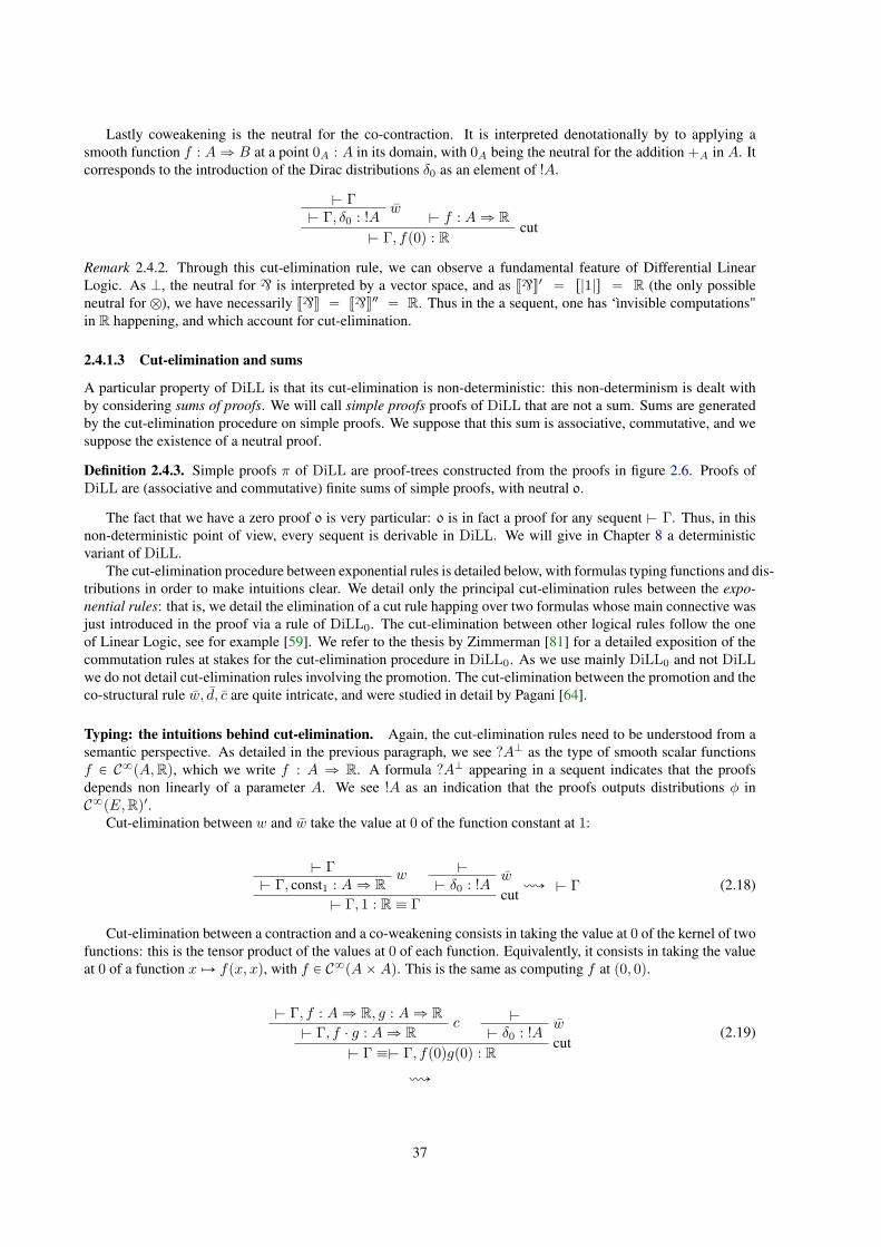
Lastly coweakening is the neutral for the co-contraction. It is interpreted denotationally by to applying asmooth function f : Añ B at a point 0A : A in its domain, with 0A being the neutral for the addition `A in A. Itcorresponds to the introduction of the Dirac distributions δ0 as an element of !A.

$ Γw

$ Γ, δ0 : !A $ f : Añ Rcut

$ Γ, fp0q : R

Remark 2.4.2. Through this cut-elimination rule, we can observe a fundamental feature of Differential LinearLogic. As K, the neutral for ` is interpreted by a vector space, and as J`K1 “ r|1|s “ R (the only possibleneutral for b), we have necessarily J`K “ J`K2 “ R. Thus in the a sequent, one has ‘ìnvisible computations"in R happening, and which account for cut-elimination.

2.4.1.3 Cut-elimination and sums

A particular property of DiLL is that its cut-elimination is non-deterministic: this non-determinism is dealt withby considering sums of proofs. We will call simple proofs proofs of DiLL that are not a sum. Sums are generatedby the cut-elimination procedure on simple proofs. We suppose that this sum is associative, commutative, and wesuppose the existence of a neutral proof.

Definition 2.4.3. Simple proofs π of DiLL are proof-trees constructed from the proofs in figure 2.6. Proofs ofDiLL are (associative and commutative) finite sums of simple proofs, with neutral 0.

The fact that we have a zero proof 0 is very particular: 0 is in fact a proof for any sequent $ Γ. Thus, in thisnon-deterministic point of view, every sequent is derivable in DiLL. We will give in Chapter 8 a deterministicvariant of DiLL.

The cut-elimination procedure between exponential rules is detailed below, with formulas typing functions and dis-tributions in order to make intuitions clear. We detail only the principal cut-elimination rules between the expo-

nential rules: that is, we detail the elimination of a cut rule happing over two formulas whose main connective wasjust introduced in the proof via a rule of DiLL0. The cut-elimination between other logical rules follow the oneof Linear Logic, see for example [59]. We refer to the thesis by Zimmerman [81] for a detailed exposition of thecommutation rules at stakes for the cut-elimination procedure in DiLL0. As we use mainly DiLL0 and not DiLL

we do not detail cut-elimination rules involving the promotion. The cut-elimination between the promotion and theco-structural rule w, d, c are quite intricate, and were studied in detail by Pagani [64].

Typing: the intuitions behind cut-elimination. Again, the cut-elimination rules need to be understood from asemantic perspective. As detailed in the previous paragraph, we see ?AK as the type of smooth scalar functionsf P C8pA,Rq, which we write f : A ñ R. A formula ?AK appearing in a sequent indicates that the proofsdepends non linearly of a parameter A. We see !A as an indication that the proofs outputs distributions φ inC8pE,Rq1.

Cut-elimination between w and w take the value at 0 of the function constant at 1:

$ Γw

$ Γ, const1 : Añ R

$w

$ δ0 : !Acut

$ Γ, 1 : R ” Γ

ù $ Γ (2.18)

Cut-elimination between a contraction and a co-weakening consists in taking the value at 0 of the kernel of twofunctions: this is the tensor product of the values at 0 of each function. Equivalently, it consists in taking the valueat 0 of a function x ÞÑ fpx, xq, with f P C8pAˆAq. This is the same as computing f at p0, 0q.

$ Γ, f : Añ R, g : Añ Rc

$ Γ, f ¨ g : Añ R

$w

$ δ0 : !Acut

$ Γ ”$ Γ, fp0qgp0q : R

(2.19)

ù

37

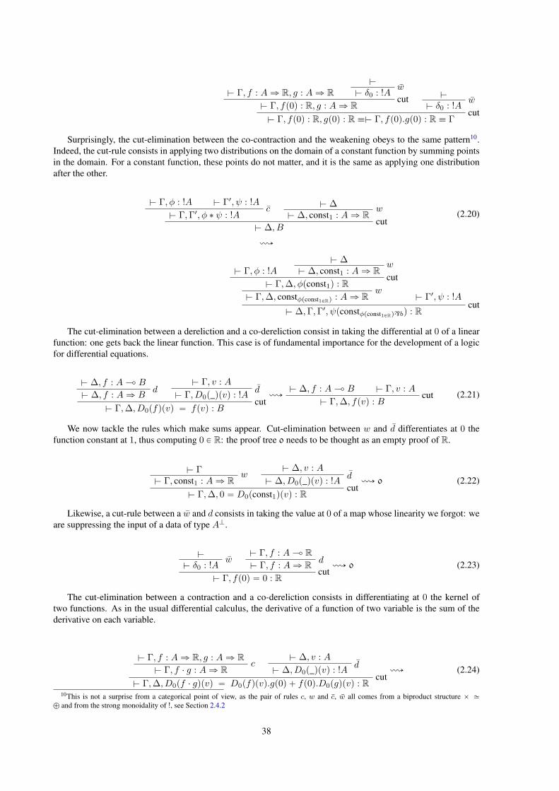
$ Γ, f : Añ R, g : Añ R

$w

$ δ0 : !Acut

$ Γ, fp0q : R, g : Añ R

$w

$ δ0 : !Acut

$ Γ, fp0q : R, gp0q : R ”$ Γ, fp0q.gp0q : R ” Γ

Surprisingly, the cut-elimination between the co-contraction and the weakening obeys to the same pattern10.Indeed, the cut-rule consists in applying two distributions on the domain of a constant function by summing pointsin the domain. For a constant function, these points do not matter, and it is the same as applying one distributionafter the other.

$ Γ, φ : !A $ Γ1, ψ : !Ac

$ Γ,Γ1, φ ˚ ψ : !A

$ ∆w

$ ∆, const1 : Añ Rcut

$ ∆, B

(2.20)

ù

$ Γ, φ : !A

$ ∆w

$ ∆, const1 : Añ Rcut

$ Γ,∆, φpconst1q : Rw

$ Γ,∆, constφpconst1PRq : Añ R $ Γ1, ψ : !Acut

$ ∆,Γ,Γ1, ψpconstφpconst1PRq`bq : R

The cut-elimination between a dereliction and a co-dereliction consist in taking the differential at 0 of a linearfunction: one gets back the linear function. This case is of fundamental importance for the development of a logicfor differential equations.

$ ∆, f : A⊸ Bd

$ ∆, f : Añ B

$ Γ, v : Ad

$ Γ, D0p_qpvq : !Acut

$ Γ,∆, D0pfqpvq “ fpvq : B

ù$ ∆, f : A⊸ B $ Γ, v : A

cut$ Γ,∆, fpvq : B

(2.21)

We now tackle the rules which make sums appear. Cut-elimination between w and d differentiates at 0 thefunction constant at 1, thus computing 0 P R: the proof tree 0 needs to be thought as an empty proof of R.

$ Γw

$ Γ, const1 : Añ R

$ ∆, v : Ad

$ ∆, D0p_qpvq : !Acut

$ Γ,∆, 0 “ D0pconst1qpvq : R

ù 0 (2.22)

Likewise, a cut-rule between a w and d consists in taking the value at 0 of a map whose linearity we forgot: weare suppressing the input of a data of type AK.

$w

$ δ0 : !A

$ Γ, f : A⊸ Rd

$ Γ, f : Añ Rcut

$ Γ, fp0q “ 0 : R

ù 0 (2.23)

The cut-elimination between a contraction and a co-dereliction consists in differentiating at 0 the kernel oftwo functions. As in the usual differential calculus, the derivative of a function of two variable is the sum of thederivative on each variable.

$ Γ, f : Añ R, g : Añ Rc

$ Γ, f ¨ g : Añ R

$ ∆, v : Ad


$ Γ,∆, D0pf ¨ gqpvq “ D0pfqpvq.gp0q ` fp0q.D0pgqpvq : R

ù (2.24)

10This is not a surprise from a categorical point of view, as the pair of rules c, w and c, w all comes from a biproduct structure ˆ »‘ and from the strong monoidality of !, see Section 2.4.2

38

$ Γ, f : Añ R, g : Añ R

$ ∆, v : Ad


$ Γ,∆, D0pfqpvq : R, g : Añ R

$w

$ δ0 : !Acut

$ ∆,Γ, D0pfqpvq : R, gp0q : R

`$ Γ, f : Añ R, g : Añ R

$ ∆, v : Ad


$ Γ,∆, g : Añ R, D0pgqpvq : R$

w$ δ0 : !A

cut$ ∆,Γ, fp0q : R, D0pgqpvq : R

The opposite case goes likewise: the cut-elimination between a co-contraction and a dereliction applies theconvolution of two distributions on a linear function. As it is linear, this is exactly the sum of the values of eachdistribution applied to the linear function.

$ Γ, φ : !A $ Γ1, ψ : !Ac

$ Γ,Γ1, φ ˚ ψ : !A

$ ∆, f : A⊸ Rd

$ ∆, f : Añ Rcut

$ Γ,Γ1,∆, φ ˚ ψpfq “ φpx ÞÑ ψpy ÞÑ fpx` yqqq “ φpx ÞÑ fpxqq ` ψpy ÞÑ fpyqq : R

ù (2.25)

$ Γ, φ : !A

$ ∆, f : A⊸ Bd

$ ∆, f : Añ Bcut

$ Γ,∆, φpfq : R`B ”$ φpfq : R`B, 1 : Rw

$ Γ,∆, φpfq : R`B, const1 : Añ R $ Γ1, ψ : !Acut

$ Γ1,Γ,∆, φpfq : R`B,ψpconst1q : R

`

$ Γ1, ψ : !A

$ ∆, f : A⊸ Bd

$ ∆, f : Añ Bcut

$ Γ1,∆, ψpfq : R`B ”$ φpfq : R`B, 1 : Rw

$ Γ1,∆, ψpfq : R`B, const1 : Añ R $ Γ, φ : !Acut

$ Γ,Γ1,∆, ψpfq : R`B, φpconst1q : R

Finally, the cut-elimination between a contraction and a co-contraction results in applying a convolution on akernel: by definition, each distribution applies to each sides of a kernel. We expose first an untyped version of thecut-elimination.

$ ∆, ?AK, ?AKc

$ ?AK$ Γ, φ : !A $ Γ1, ψ : !A

c$ Γ,Γ1, !A

cut$ Γ,Γ1,∆

ù (2.26)

$ ?AK, !A $ ?AK, !Ac

$ ?AK, ?AK, !A $ ∆, ?AK, ?AKcut

$ ∆, ?AK, ?AK, ?AK$ ?AK, !A $ ?AK, !A

c$ ?AK, ?AK, !A

cut$ ∆, ?AK, ?AK, ?AK, ?AK

:π:

where π stands for:

:$ ∆, ?AK, ?AK, ?AK, ?AK

c$ ∆, ?AK, ?AK, ?AK $ Γ, !A

cut$ ∆,Γ, ?AK, ?AK

c$ ∆,Γ, ?AK $ Γ1, !A

cut$ ∆,Γ,Γ1

39

The typed cut-elimination rule between the contraction and the co-contraction is :

$ ∆, f : Añ R, g : Añ Rc

$ f ¨ g : Añ R

$ Γ, φ : !A $ Γ1, ψ : !Ac

$ Γ,Γ1, φ ˚ φ : !Acut

$ Γ,Γ1,∆, φ ˚ ψpf ¨ gq “ φpx ÞÑ ψpy ÞÑ fpx´ yqgpx´ yqq : R

ù (2.27)

$ Id : !A⊸ !A $ Id : !A⊸ !Ac

$ c : φ b ψ ÞÑ φ ˚ ψ P !A b !A⊸ !A $ ∆, f : A ñ R, g : A ñ Rcut

$ ∆, g : A ñ R, cf “ φ1 b ψ1 ÞÑ pφ1 ˚ ψ1qpfq : !A b !A⊸ R

$ Id : !A⊸ !A $ Id : !A⊸ !Ac

$ c : !A b !A⊸ !Acut

$ ∆, cf : !A b !A⊸ R, cg : !A b !A⊸ R

:π:

where π stands for:

:$ ∆, cf : !Ab !A2 ⊸ R, cg : !Ab !A4 ⊸ R

c$ ∆, cf ¨ cg ˝ c2,4 : !Ab !Ab !A⊸ R $ Γ, φ : !A

cut$ ∆,Γ, cf ¨ cgp_, c2,4pφq, _q : ψ b ψ1 ÞÑ pψ ˚ φ ˚ ψ1pf ¨ gq : !A1 b !A3 ⊸ R

c$ ∆,Γ, cf ¨ cgp_, c2,4pφq, _q ˝ c1,3 : !A⊸ R $ Γ1, ψ : !A

cut$ ∆,Γ,Γ1 : cf ¨ cgpc1,3pψqc2,4pφqq “ φ ˚ ψpf ¨ gq : R

Remark 2.4.4. This cut rule corresponds to the Hopf rule in Hopf algebras [5].

Remark 2.4.5. Typing monolateral axioms, that is saying that IdE P LpE,Eq where E is a lcs (see 3) correspondsto an element of E1 ` E » E 1bE is by definition possible if and only if E has the approximation property (see[44, chapter 18]). When E ⊸ F is reflexive, this follows from the closed monoidal structure.


We describe in the first section a global method for constructing a model of DiLL (with promotion) from a Seelycategory. We describe in the second section a categorical axiomatization by Ehrhard of models of DiLL, makinguse of exponential structure and making a distinction between models of DiLL0 and those also interpreting thepromotion rule.

2.4.2.1 ˚-autonomous Seely categories with biproduct and co-dereliction

Following work by Fiore [25] we will describe how in a Seely category endowed with a biproduct, the interpretationfor the co-contraction and the coweakening follow immediately. A model of DiLL will therefore be a model ofLL where the cartesian product is a biproduct, provided with a natural transformation d : Id // ! interpreting thecodereliction rule. Remember from Section 2.2.2, that the interpretation for the weakening and the contraction arededuced from the strong monoidality of ! and the presence of a diagonal operator ∆ : A //AˆA.

Definition 2.4.6. A biproduct on a category L is a monoidal structure p˛, Iq together with natural transformations:

I I

A ˛A A ˛A

A

uA nA

∇A ∆A

such that pA, u,∇q is a commutative monoid and pA, n,∆q is a commutative comonoid.

40

Example 2.4.7. In the category of real vector spaces and linear maps, ˛ is the binary product, which correspondsindeed the the binary co-product, and the unit is the null vector space : I “ t0u.

Proposition 2.4.8. [25, prop 2.1] If C is endowed with a biproduct, then the diagram: A » A ˛ 11A˛uBÝÝÝÝÑ

A ˛ BnA˛1BÐÝÝÝÝ 1 ˛ B » B is a co-product with pI, uAq as initial object, while the diagram A » A ˛ 1

1A˛nBÐÝÝÝÝ

A ˛BuA˛1BÝÝÝÝÑ 1 ˛B » B is a product with pI, nAq as terminal object.

The following diagrams interpret in particular the cut-elimination rules 2.18 and 2.27:

Proposition 2.4.9. [25, prop 2.2] In a category with biproduct, the following diagrams are commutative.

A

I I

nAuA

1

A ˛A A A ˛A

A ˛A ˛A ˛A A ˛A ˛A ˛A

∇A

∆A˛∆A

∆A

1˛γA,A˛1

∇A˛∇A

where γA,B : A ˛B » B ˛A denotes the commutativity of ˛.

Definition 2.4.10. [25, 2.3] A biproduct structure p˛, Iq on a symmetric monoidal category pC,b, 1q is said to becompatible with the monoidal structure if the following diagrams commute:

Ab C1bn //

n

Ab Inb1

yy

1bu

I

u// Ab C

Ab C∆b1C //

∆

pA ˛Aq b C

∇b1C

pAb Cq ˛ pAb Cq

∇ // Ab C

The previous definition interprets in particular the cut-elimination rules of co-contraction and dereliction, and con-traction and co-dereliction (see Section 2.4.2.2).

A category C is enriched over commutative monoids if every hom-set Cpa, bq is endowed with a structure ofcommutative monoid pCpa, bq,`Cpa,bq, 0Cpa,bq compatible with composition. In the context of DiLL, this enrich-ment allows to interpret the sums of proofs. In fact, the enrichment over (commutative) monoids is equivalent tothe presence on C of a biproduct:

Proposition 2.4.11. [25, prop 2.3] A category C with finite product is enriched over commutative monoids if and only

if it is endowed with a biproduct structure.

Proof. Consider C a category endowed with a biproduct p˛, Iq. One defines a monoid on CpA,Bq by:

f ` g : A∆ÝÑ A ˛A

f˛gÝÝÑ B ˛B

∇ÝÑ B.

The neutral 0CpA,Bq corresponds to uB ˝ nA : A // I //B.Conversely, consider C a category such that for every objectsA,B, we have a commutative monoids pCpA,Bq,`CpA,Bq, 0CpA,Bqq, and

nite products AˆB. We show that this product is a biproduct. The map nA “ 0CpA,Iq makes I a terminal object.

Then one constructs ∆A as AˆA1AˆnA`nAˆ1ÝÝÝÝÝÝÝÝÝÑ Aˆ 1 » A.

The previous proposition has an important consequence for DiLL. In a monoidal closed and vectorial settingwhere hom-sets are in particular vector spaces, one cannot hope to distinguish the interpretation of the additiveconnective on finite indexes. This argues for a polarized semantics where, if we can’t distinguish between theinterpretation of the connective we can distinguish the interpretation of formulas they apply to.

41

Interpreting the (co-)contraction and the (co-)weakening Consider pC,b, 1, p.q˚q a ˚-autonomous categorywith a biproduct p˛, I, u,∆, n,∇q (following the notation of Definition 2.4.6) and endowed with a strong monoidalfunctor ! : pC, ˛,Jq //pC,b, 1q. Then we interprets the formulas of LL as in Section 2.2.2 and J!AK “ !JAK and J?AK “ p!pJAK˚qq˚.As in Section 2.2.2, we also write ` the interpretation in C of the multiplicative disjunction as the dual of b.

Proposition 2.4.12. In a ˚-autonomous category, the biproduct is self-dual: we have a family of isomorphisms

natural in A and B such that:

A˚ ˛B˚ » pA ˛Bq˚.

Let us recall the interpretation of the structural rules c and w. The strong monoidal functor ! provides naturalisomorphisms:

mA,B : !pAˆBq » !Ab !B, (2.28)

m0 : !J » 1. (2.29)

Then one defines the natural transformations, interpreting the structural morphisms:

cA :!A!∆A // !pAˆAq

mA,A

» !Ab !A (2.30)

wA :!A!nA // !J

m0» 1 (2.31)

Thanks to the biproduct structure, the co-structural rules are interpreted by similar morphisms. Indeed, one definesthe natural transformations:

cA :!Ab !Am´1A,A

» !pAˆAq!∇A // !A (2.32)

wA :1m´10» !J

!uA // !A (2.33)

Proposition 2.4.13. [25, 3.2] For every objectA, we have a commutative bialgebra p!A,wA, cA, wA, cAq: p!A,wA, cAqis a commutative comonoid, and p!A, wA, cAq is a commutative monoid.

Let us detail specifically the interpretation of proofs whose last derivable rule is amongst c, w, c, w:

• Consider a function f : !JAK˚ b !JAK˚ // JΓK interpreting the proof of $ Γ, ?A, ?A equivalent to $Γ, ?A`?A. Then the proof of $ Γ, ?A, and deduced by the contraction rule, is interpreted by f ˝ cJAK :

!JAK˚ // JΓK.

• Consider a function f : 1 // JΓK interpreting the proof of the sequent $ Γ. Then the sequent $ Γ, ?A

deduced by the weakening rule is interpreted by f ˝ wJAK˚ :!JAK˚ // JΓ |.

• Consider functions f : 1 // !JAK ` JΓK and g : 1 // !JAK ` J∆K interpreteting respectively the proofs ofthe sequents $ Γ, !A and $ ∆, !A. Then the proof of the sequent $ Γ,∆, !A deduced by the co-contractionrule, is interpreted by cApf ` gq : 1 » 1 ` 1 // !JAK ` JΓK ` J∆K, where we omitted to name explicitlythe associativity morphism for `.

• The interpretation of the co-weakening rule $!A is simply wJAK : 1 // J!AK.

Interpreting dereliction and codereliction In a model of LL, the dereliction rule is interpreted by the co-unitdA :!A // A of the monad !, see Section 2.2.2. For a model of DiLL one needs however to add an interpretationfor the codereliction. This is done by introducing a natural transformation

d : Id // !

satisfying the following coherence diagrams [25, 4.3].

EdE

((1

!E

dEvvE

(2.34)

42

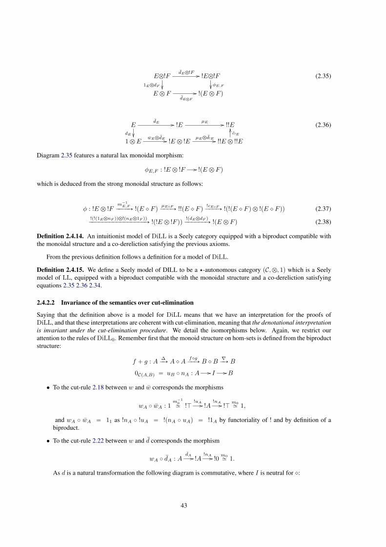
Eb!FdEb!F //

1EbdF

!Eb!FφE,F

E b FdEbF

// !pE b F q

(2.35)

EdE //

dE

!EµE // !!E

1b EwEbdE // !E b !E

µEbd!E // !!E b !!E

c!E

OO (2.36)

Diagram 2.35 features a natural lax monoidal morphism:

φE,F : !E b !F // !pE b F q

which is deduced from the strong monoidal structure as follows:

φ : !E b !Fm´1E,F

ÝÝÝÝÑ !pE ˛ F qµE˛FÝÝÝÑ !!pE ˛ F q

!cE˛FÝÝÝÑ !p!pE ˛ F q b !pE ˛ F qq (2.37)

!p!p1EbnF qqb!pnEb1F qqÝÝÝÝÝÝÝÝÝÝÝÝÝÝÝÝÑ !p!E b !F qq

!pdEbdF qÝÝÝÝÝÝÑ !pE b F q (2.38)

Definition 2.4.14. An intuitionist model of DiLL is a Seely category equipped with a biproduct compatible withthe monoidal structure and a co-dereliction satisfying the previous axioms.

From the previous definition follows a definition for a model of DiLL.

Definition 2.4.15. We define a Seely model of DILL to be a ‹-autonomous category pC,b, 1q which is a Seelymodel of LL, equipped with a biproduct compatible with the monoidal structure and a co-dereliction satisfyingequations 2.35 2.36 2.34.

2.4.2.2 Invariance of the semantics over cut-elimination

Saying that the definition above is a model for DiLL means that we have an interpretation for the proofs ofDiLL, and that these interpretations are coherent with cut-elimination, meaning that the denotational interpretation

is invariant under the cut-elimination procedure. We detail the isomorphisms below. Again, we restrict ourattention to the rules of DiLL0. Remember first that the monoid structure on hom-sets is defined from the biproductstructure:

f ` g : A∆ÝÑ A ˛A

f˛gÝÝÑ B ˛B

∇ÝÑ B

0CpA,Bq “ uB ˝ nA : A // I //B

• To the cut-rule 2.18 between w and w corresponds the morphisms

wA ˝ wA : 1m´10» !J

!uA // !A!nA // !J

m0» 1,

and wA ˝ wA “ 11 as !nA ˝ !uA “ !pnA ˝ uAq “ !1A by functoriality of ! and by definition of abiproduct.

• To the cut-rule 2.22 between w and d corresponds the morphism

wA ˝ dA : AdA // !A

!nA // !0m0» 1.

As d is a natural transformation the following diagram is commutative, where I is neutral for ˛:

43

A

dA

nA // I

dI

!A!nA // !I

As I is initial [25, 2.1], dI : I // !I » 1 is the only morphism from I to 1, thus dI “ u1. Thus, throughthe previous commutative diagram we have wA ˝ dA “ uI ˝ nA “ 0CpA,Iq by definition of the additivestructure on hom-sets. This justifies the reduction to a cut between a weakening and a codereliction to a zeroproof 0, the logical interpretation of the 0 morphisms in an category enriched over commutative monoids.

• The same approach shows that the cut-rule 2.23 between w and d corresponds the morphism wA˝dA “ uA˝n1 “ 0C1,A

, interpreting the zero proof 0, proving A from no hypothesis.

• The cut-rule 2.21 between d and d corresponds to the morphism dA ˝ dA, which is the identity by hypothesis,see diagram 2.34.

• The cut-rule 2.19 between the contraction c and the co-weakening w in interpreted by the morphism:

cA ˝ wA : 1m´10» !J

!uA // !A!∆A // !pAˆAq

mA,A

» !Ab !A.

As the product ˆ comes from the biproduct ˛, the terminal object J » 0 (which is the by definition the unitfor the product) is the unit for I , the unit of the biproduct. Thus we have by [25, prop 2.2]

!∆ ˝ !u “ !p∆ ˝ uq “ u ˛ u,

where we omit the explicit description of the isomorphism between I and I ˛ I . Thus:

cA ˝ wA : 1m´10» !I » !pI ˛ Iq

!puA˛uaq// !pA ˛Aqm´1A,A

» !Ab !A.

Through the strong monoidality of ! one can describe !puA ˛ uAq as !uA b !uA, and the above morphismscorrespond to the interpretation of the successive cut-rule between a co-weakening rule and one of theinstances of ?A in the sequent $ Γ, ?A, ?A. This is exactly the interpretation of the cut-eliminated proof-tree in 2.19.

• The case concerning the cut-rule 2.20 between the co-contraction c and the weakening w behave exactlylikewise, by symmetry of the definition of weakening (resp. contraction) with the one of the co-weakening(resp. co-contraction).

• The cut-rule 2.24 between the contraction and the co-dereliction is interpreted by:

cA ˝ dA : AdA // !A

!∆A // !pAˆAqmA,A

» !Ab !A.

By naturality of d we have that !∆A ˝ dA “ dA˛A ˝∆A, thus cA ˝ dA “ mA,A ˝ dA˛D∆A.

Moreover, the sum of proof trees resulting from the cut-rule is:

dA b wA ` wA b dA : Ab 1 » 1bA » A∆ //A ˛A

pdbwq˛pwbdqÝÑ p!Ab!Aq ˛ p!Ab!Aq

∇ // !Ab!A.

To show equality between cA ˝ dA and dA b wA ` wA b dA we must then prove:

dA˛A ˝mA,A “ ∇!Ab!A ˝ pdb wq ˛ pw b dq

which follows from the compatibility of the biproduct with b (Definition 2.4.10).

• The cut-rule 2.25 between the co-contraction and the dereliction is interpreted by:

dA ˝ cA : !Ab !Am´1A,A

» !pA ˛Aq!∇A // !A

dA //A.

By naturality of d we have that dA ˝ !∇A “ ∇A ˝ dA˛A, thus dA ˝ cA “ ∇A ˝ dA˛A ˝m´1A,A.

44

Moreover, the sum of proof trees resulting from the cut-rule is:

dA b wA ` wA b dA : !Ab !A∆ // p!Ab !Aq ˛ p!Ab !Aq

pdbwq˛pwbdqÝÑ pAb 1q ˛ p1bAq » pAb 1q ˛ pAb 1q » A ˛A

∇A //A.

To show the equality between cA ˝ dA and dA b wA ` wA b dA we must then prove:

dA˛A ˝m´1A,A “ pdb wq ˛ pw b dq ˝ .

which follows from the compatibility of the biproduct with b (Definition 2.4.10).

• The cut-rule 2.27 between the contraction and the co-contraction is interpreted by:

cA ˝ cA : !Ab !AmA,A

» !pAˆAq!∇A // !pAq

!∆A // !pAˆAqm´1A,A

» !AbA.

However by properties of the biproduct (see [25, 2.2], recalled in Proposition 2.4.9)

!∇A ˝ !∆A “ p∆A ˛∆Aq ˝ p1A ˛ γA,A˛Aq ˝ p∇A ˛∇Aq,

where γA,B : A ˛B » B ˛A is the commutation for ˛. As !rp∆A ˛∆Aq ˝ p1A ˛ γA,A˛Aq ˝ p∇A ˛∇Aqs isexactly the interpretation of the reduced cut-rule 2.27, we have our result.

2.4.2.3 Exponential structures

Ehrhard defines [20] the notion of exponential structures on a (pre)-additive ˚-autonomous category a as tu-ple p!, w, c, w, cq such that ! is an endofunctor on Ciso (the subcategory of C with only isomorphisms as ar-rows), and such that for every object A, p!A,wA, cA, wA, cAq is a commutative bialgebra. The isomorphisms arerequired to interpret the coherence rules. These morphisms moreover satisfy the following invariance diagrams,which axiomatize what has been proved before in Seely categories.

E

!E

E

d

d

Id

E

!E

1

d

w

0

E

!E

!Eb!E

c

d

db w ` w b d

!E

E

1

d

w

0

!Eb!E

!E

E

c

d

db w ` w b d

Figure 2.7: Commutative diagrams in Exponential structures

Remark 2.4.16. In Chapter 7 and 8 we develop concrete models of DiLL0, where ! is a functor but not an endo-functor. A proper categorical semantics for these models, intermediate between Seely categoriess and exponentialstructures, should be developed.

2.4.3 A Smooth intuitionistic model: Convenient spaces

We recall in this section how Mackey-complete lcs, linear bounded functions and conveniently smooth functions

define a model of Intuitionistic DiLL. This is a simplification of the article of Blute, Ehrhard and Tasson [7], as itdoes not require spaces to be bornological.

The first models of DiLL were constructed by Ehrhard as a vectorial generalisation of coherent spaces in Köthespaces [18] (see Section 2.2.3) and Finiteness spaces [19]. They are constructed from spaces of sequences. Once

45

DiLL was formalized a calculus of interaction nets [23] and its computational content axiomatized in the differ-ential λ-calculus [22], a natural question was the geometric nature of the differential used. Indeed, differentiationin the models was done over power series: but there is more to the theory of differentiation than extracting thelinear part of a power series. How far can the sequent calculus DILL model the general behaviour of differentialgeometry? This led Blute, Ehrhard and Tasson [7] to define a model of Intuitionistic DiLL, where functions aregeneral smooth, i.e everywhere and iteratively differentiable, functions, with no further restriction. The modelrelies on the work of Frölicher, Kriegl and Michor [26, 53] who define completeness conditions and good notionsof smoothness allowing for a cartesian closed category of smooth functions.

One of the specificites of this model is that linear maps are interpreted by linear bounded functions, which arenot continuous in general. The necessity to relax continuity of functions into their boundedness comes from thespecific definition of smoothness by Frölicher, Kriegl and Michor. The spaces satisfy a completeness conditionknown as Mackey-completeness, and are sometines asked to be moreover bornological ( [7, 26]). The bornologicalconditions modifies the topology of spaces in order to ensure that every bounded linear map is still continuous. Itis in fact unnecessary to the intuitionistic constructions of DiLL as we showed with Tasson [49]. We explain inSection 6, Chapter 6 how the bornological condition ensures a classical interpretation of DiLL.

We will sketch here the model of DiLL as detailed in [7], without the bornological condition. It correspondsthus to the summary made in sections 2, 3 and 4 of [49]. We will give more detail on the bornological conditionlater in section 6. We recall a few notion of Chapter 3. Contents of sections 3.4, 3.4.3 and 3.1 are enough tounderstand convenient vector spaces. We recall that an absolutely convex subset B of a vector space E is a subsetsuch that: @x, y P B,@λ P R, µ P R, |λ| ` |µ| ă 1 : λx` µy P B.

Definition 2.4.17. A locally convex and separated topological vector space (denoted as lcs) is a R-vector spaceE, R being R or C endowed with a topology, admitting a pre-basis of absolutely convex neighbourhoods, makingaddition and scalar multiplication continuous.

Let E and F denote lcs from now on. A bounded set in a lcs E is a subset B Ă E which is absorbed by any0-neighbourhood. That is, for any open set U containing 0, there exists λ P R such that B Ă λU . A bounded

function f : E // F is then a function such that the image by f of any bounded set in E is bounded in F .

Definition 2.4.18. We denote by LpE,F q the space of all bounded linear functions. We endow it with the topologyof uniform convergence on bounded subsets of E. This topology is generated by the open sets

WB,U “ tℓ | ℓpBq Ă Uu

where B is a bounded set in E and U an absolutely convex open set in F . In particular, a sequence of linearfunctions pℓnqn P LpE,F q converges towards ℓ P LpE,F q if and only if for every bounded set B Ă E, every0-neighbourhood U Ă F , there is N P N such that for n ě N , we have pℓn ´ ℓqpBq Ă U .

The product and direct sum of two lcs are endowed with the usual product and co-product topologies (seeSection 3.1.4). In particular, a bounded set in E ˆ F is a product of bounded sets. Remember also that on finiteindexes, products and direct sums coincide.

The use of bounded subsets simplifies the theory of topological vector spaces. If several notions of continuitycan be defined on bilinear functions (for example continuity is not equivalent to separate continuity) there is onlyone notion of bounded bilinear function and thus of tensor product for them.

Definition 2.4.19. We endow the tensor product E b F of two lcs with the finest topology making the canonicalbilinear map h : E ˆ F // E b F bounded. This makes E b F a lcs which is denoted E bB F .

Then one shows easily the following:

Proposition 2.4.20. [49, 3.4] The category of lcs endowed with bB is a monoidal closed category with internal

hom E ⊸ F “ LpE,F q.

We writeEˆ :“ LpE,Rq the bornological dual of a lcs E. In general, it differs from the topological dualE1. Itis the denotational interpretation of negation. Note that we won’t have in this modelE » Eˆˆ in general, and thuswe will not have a denotational model for classical DiLL.

In order to accommodate smooth functions, one needs a certain completeness condition on the lcs. Differentia-tion, and thus smoothness, is defined in term of limits of sequences in a given lcs F . If we want to compose smoothfunctions, or to prove cartesian closedness, most of the time we will be able to prove that the difference quotient isCauchy, i.e. that the quotients are getting closer and closer, but we won’t be able to prove directly that it converges.Knowing that Cauchy sequences converges is the definition of completeness. In their work Kriegl and Michorrequire a very weak completeness condition, which works well within the bounded setting.

46

Definition 2.4.21. A net ppxγqΓq is a family of elements of E indexed by a directed set Γ.

Definition 2.4.22. A Mackey-Cauchy net in E is a net pxγqγPΓ such that there is a net of scalars λγ,γ1 decreasingtowards 0 and a bounded set B of E such that:

@γ, γ1 P Γ, xγ ´ xγ1 P λγ,γ1B.

A space where every Mackey-Cauchy net converges is called Mackey-complete.

There exists a procedure of Mackey-completion, that can be thought of as a the interpretation of a shift ˆ (seeSection 2.3.1), and which allows to make a space Mackey-complete.

Proposition 2.4.23. [53, I.4.29] For every lcs E there is a Mackey-complete lcs E and a bounded embedding

ι : E Ñ E, unique up to bounded isomorphism, such that for every Mackey-complete lcs F , for every bounded

linear map f : E Ñ F there is a unique bounded linear map f : E Ñ F extending f such that f “ f ˝ ι.

We denote by MCO the category of Mackey-complete spaces and bounded linear maps.

Proposition 2.4.24. [49, 3.5] The category MCO endowed with the Mackey-completed tensor product b is a

monoidal closed category with internal hom E ⊸ F “ LpE,F q.

Products and co-products preserve Mackey-completeness, and thus pMCO,b,R,ˆ, t0uq is a model of MALL.We detail now the interpretation of the exponential ! as the dual of a space of smooth function. From now on wework with R-vector spaces.

Definition 2.4.25. Let E be a Mackey-complete lcs. Consider a curve c : RÑ E, then c is said to be derivable ifthe following limit exist for every t P R:

c1ptq “ limsÑ0

cpt` sq ´ cptq

s.

The definition of smoothness is co-inductive: the curve c is smooth if it is derivable and its derivative in every pointis smooth. We denote by CE the set of smooth curves in E.

The space CE is a Mackey-complete lcs when it is endowed with the topology of uniform convergence onbounded sets of each derivative separately [53, I.3.7]. A basis of 0-neighbourhoods for this topology is made ofWb,i,U , where B is a bounded set in R, i P N, U is a 0-neighbourhood in E, and

WB,i,U “ tc | @t P b, cpiqptq P Uu.

Definition 2.4.26. A function f : E Ñ F is smooth if it preserves smooth curves: @c P CE , f ˝ c P CF . Wedenote by C8pE,F q the space of smooth maps from E to F . This definition of smoothness is a generalization ofthe usual one for finite dimension topological vector spaces (see Boman’s theorem [10]).

This definition of smoothness does not imply continuity. In particular, the linear smooth maps are exactly thesmooth bounded ones.

The space C8pE,F q is endowed with the projective topology induced by the productścPCE

CF . In fact,the space C8pE,F q is the closed subspace of

ścPCE

CF whose elements pfcqc are those such that for everyg P C8pR,Rq, fc˝g “ fc ˝ g. It is Mackey-complete when F is Mackey-complete [53, I.3.11]. Let us denote bySmooth the category of Mackey-complete lcs and smooth maps between them.

Theorem 2.4.27. [53] The category Smooth is cartesian closed, meaning that forE, F , andGMackey-complete

lcs we have natural isomorphisms:

C8pE ˆ F,Gq » C8pE, C8pF,Gqq.

As explained in remark 2.7, in a ˚-autonomous category modelizing classical LL, one would want to interpret!E as C8pE,Rq1. It is not the case here, but it is close : the exponential is defined as the completion of the linearspan of all Dirac distributions δx in C8pE,Rqˆ.

δ :

#E Ñ C8pE,Cqˆ

x ÞÑ δx : f ÞÑ fpxq

47

Definition 2.4.28. We define the Mackey-complete lcs !E as the Mackey-completion ˜xδpEqy of the linear span ofδpEq “ tδx | x P Eu. If f P LinpE,F q is a smooth linear map, its exponential !f P Linp!E, !F q is definedon the set δpEq by !fpδxq “ δfpxq. It is then extended to the linear span of δpEq by linearity and to !E by theuniversal property of the Mackey-completion.

Thus ! defines an endofunctor on MCO. It is moreover a co-monad, with co-unit and co-multiplication:

dE :δx P !E ÞÑ x P E

µE :δx P !E ÞÑ δδx P !!E

This interpretation for the exponential gives an interpretation of non-linear proofs of LL as smooth maps.

Theorem 2.4.29. [7] The cokleisli category of the comonad ! over MCO is the category Smooth. In particular,

for any Mackey-complete spaces E and F ,

Lp!E,F q » C8pE,F q.

As Smooth is cartesian closed and MCO is monoidal closed, the previous theorem leads to the strongmonoidality of the functor !, defined from pMCO,ˆ, t0uq to pSmooth,b,Rq. If !E were defined as C8pE,Rqˆ

as in equation 2.7, and spaces were equal to their double bornological dual E » Eˆˆ this would follow from thefollowing computation:

C8pE ˆ F,Rqˆ » C8pE, C8pF,Rqqˆ (2.39)

» Lp!E, p!F qˆqˆ (2.40)

» Lp!E b !F,Rqˆ (2.41)

» !E b !F (2.42)

In the intuitionistic setting of convenient vector spaces, the computations are slightly more subtle.

Theorem 2.4.30. [7, 5.6] For any E, and F Mackey-complete spaces we have a natural isomorphism:

mE,F : !Eb!F » !pE ˆ F q.

Proof. We sketch the proof detailed byBlute, Ehrhard and Tasson in [6]. The goal is to construct a bilinear boundedmap h : !E ˆ !F // !pE ˆ F q, and to show that it is universal over bilinear maps on Mackey-complete spaces.The Mackey-completed tensor product b enjoys indeed a universal property in MCO [6, 3.1] and is thus unique.

The bilinear map h is defined as hpδx, δyq “ δpx,yq. If f : !E ˆ !F // G is another bilinear boundedmap between Mackey-complete lcs, one first shows that f is smooth, and thus f ˝ pδ, δq : E ˆ F // G issmooth and factors as a linear bounded map: f : !pE ˆ F q // G. One then easily shows that f “ f ˝ h. Thus!pE ˆ F q with h is universal, and we have thus an isomorphism between !pE ˆ F q and !Eb!F .

From the biproduct structure on MCO and the strong monoidality of !, we deduce as before a bialgebra structureon every object !E. The natural transformations making this bialgebraic structure are nicely defined on the Diracdistributions δx.

c : δx P !E ÞÑ δx b δx P !Eb!E (2.43)

w : δx P !E ÞÑ x P E (2.44)

c : δx b δy P !Eb!E ÞÑ δx`y P !E (2.45)

w : 1 P R ÞÑ δ0 P !E (2.46)

The co-dereliction is then the operator which extracts from a scalar map f P C8pE,Rq its differential at 0:

d : v P E ÞÑ

ˆf P C8pE,Rq ÞÑ lim

tÑ0

fptvq ´ fp0q

t

˙“ lim

tÑ0

δtv ´ δ0t

P !E

48

The Identity rule

(axiom)$ A,AK

$ N , A $ AK,M(cut)

$ N ,M

The additive rules

(1)$ 1

$ N(K)

$ N ,K

$ N , N,M(`)

$ N , N `M

$ N , P $M, Q(b)

$ N ,M, P bQ


J$ N ,J

$ N , N $ N ,M&

$ N , N &M

$ N , P‘L

$ N , P ‘Q

$ N , Q‘R

$ N , P ‘Q


$ Nw

$ N , ?P

$ N , ?P, ?Pc

$ N , ?P

$ N , Pd

$ N , ?P

w$ !N

$ N , !N $M, !Nc

$ N ,M, !N

$ N , Nd$ N , !N

Figure 2.8: The deduction rules for sequents of DiLL0,pol

2.5 Polarized Differential Linear Logic

2.5.1 A sequent calculus

We believe that the classical nature of DiLL is better understood in a polarized setting: we will support this claimin Chapter 7 by giving a polarized denotational model of DiLL, and in 8 by giving a computational interpretationin terms of differential equations. We describe here in terms of sequent calculus a polarized Differential LinearLogic, without promotion. This has been done in terms of interaction nets by Vaux [79].

Definition 2.5.1. The formulas of DiLL0,pol are constructed over a set N of negative atoms n, and makes adistinction between positive formulas P,Q and negative formulas N,M . They are constructed from the followinggrammar:

Negative Formulas: N,M :“ n | ?P | N `M | K | N ˆM | J |Positive Formulas: P,Q :“ nK | !N | P bQ | 0 | P ‘Q | 1

Its inference rules are describes in figure 2.8 and restricts the rules of DiLL0. The cut-elimination procedure forDiLL0,pol is directly deduced from the one of DiLL and LLpol.

DiLLpol with shift As LLpol, DiLLpol can be enhanced with shift, changing the polarity of a formula.

Definition 2.5.2. The formulas of DiLLpol,Ö are defined from a set N of negative atoms, and the followinggrammar:

Negative Formulas N,M :“ n P N | ˆP | ?P | N `M | K | N ˆM | J |Positive Formulas: P,Q :“ nK | Ń | !N | P bQ | 0 | P ‘Q | 1

Definition 2.5.3. The inference rules for DiLL0,pol,Ö are the ones of LLpol extended by the following rules. N

is a list of negative formulas.

$ N,N´

$ N, Ń

$ N,Pˆ

$ N, ˆP

Then one defines:

ˆPKL “ ´pPKRq ŃKR “ ˆpNKLq

49


In the categorical semantics of DiLL, co-dereliction is interpreted by a natural transformation d which is rightinverse to the interpretation d of the dereliction on every object:

dA ˝ dA “ idA.

Dereliction is the rule which allows to see a linear map as a smooth one: it corresponds to the co-unit of theco-monad, or in a presentation using an adjunction:

pL8,ˆq pL,bq

!

U

%

the dereliction of a linear map f P LpA,Bq is the smooth map Upfq P Lp!A,Bq. Conversely, the co-derelictionshould correspond to a forgetful functor U mapping a smooth function f P Lp!A,Bq to its differentiation at 0:D0pfq P LpA;Bq. However D0 is notably not compositional, and thus it does not define a functor from L to L!.In Section 2.5.2.1 we detail the categories in which the equation

d ˝ d “ Id

can be interpreted as a closure operation between functors. Then in Section 2.5.2.3 we give a categorical axioma-tization for models of DiLL0,pol.

Outlook 1. This section on the categorical semantics of DiLLpol is a first step towards a more unified framework.Indeed, while MLLpol is interpreted categorically in chiralities, we would like to interpreted the exponential rulesof DiLLpol in a chirality between the category of linear maps and the one of smooth maps, where the role of shiftsare played by the dereliction and the co-dereliction.

2.5.2.1 Dereliction and co-dereliction as functors

In this section we explore to which extent the dereliction and co-dereliction could be seen as functors, acting asshifts in a chirality. To see Differentiation as a functor, we detail here the ideas of synthetic differential geometry[50]. We denote by ˝ the composition in L and by ˝! the composition in L!. We will first recall the properties ofthe forgetful functor which was defined after Definition 2.2.13.

Proposition 2.5.4. Consider L a category and (!, d, µ) a co-monad on a small category L. Then one defines the

forgetful functor Ud : L // L! such that UdpAq “ A and Udpf : A //Bq “ f ˝ dA.

Proof. Let us define UdpAq “ A on objects of L, and if f P LpA,Bq, Ud “ f ˝ dA P Lp!A,Bq » L!pA,Bq.Then Fdp1Aq “ dA which correspond by definition to the unit in the co-kleisli category. Likewise, we have forg : B // C :

Udpg ˝ fq “ g ˝ f ˝ dA P L!pA,Cq.

However, in the co-Kleisli category L!, Udpgq ˝! Fdpfq “ g ˝ dB ˝ !pf ˝ dAq ˝ µA “ g ˝ dB ˝ !f ˝ !dA ˝µA “ g ˝ dB ˝ !f ˝ 1!A by the second law of co-monads. From the last equality, and by naturality of d, we deduceUdpgq ˝! Udpfq “ g ˝ f ˝ dA. Thus Ud is a functor.

While the previous proposition recalls that we can consider the dereliction as the forgetful functor between ourcategory with linear maps and its co-Kleisli category of (thought-as) smooth maps, the converse for dereliction ismore intricate. Indeed, consider the application D0 which maps f P L!pA,Bqq to D0f P LpA,Bq. Thus D0 isnot a functor as it not compositional:

D0pf ˝ gq “ x ÞÑ Dfp0qpgqpDpfqp0qpxq.

Thus to account for the arbitrary choice of 0, and view the codereliction as a functor, we introduce a newcategory:

50

Definition 2.5.5. Consider ! a co-monad on L.We denote L‚! the category whose object are those of L, and whose morphisms are morphisms of L! coupled

with points of the domain:L‚! pA,Bq “ Lp!A,Bq ˆ !A.

Composition is defined as follows: if pf, φq P L‚! pA,Bq and pg, ψq P L‚! pB,Cq, then:

pg, φq ˝!,¨ pf, ψq “ 0 if φ ‰ !fψ .

pg, p!fqψq ˝!,¨ pf, φq “ pg ˝! f, ψq

This composition is associative by associativity of ˝!. The unit is pdA, δ0q.

Proposition 2.5.6. Consider a model of DiLL as described by Fiore ([25], Section 2.4.2). As usual, we denote by

d : Id // ! the creation operator interpreting the codereliction rule, that is the natural transformation such that

d ˝ d “ Id. We denote by ˚ : !ˆ ! // ! the binatural transformation interpreting the cocontraction. Then let us

define:

U :

$’&’%

L‚! Ñ L

A ÞÑ A

pf : !A //B, φ P !Aq ÞÑ rv P A ÞÑ f ˝ pφ ˚ dApvqqs

(2.47)

Then U is a functor.

Example 2.5.7. One must think of U as the functor mapping f P C8pA,Bq and a (non-linear) point x P A to thelinear map v ÞÑ Dxfpvq. Then we have indeed:

Dxpf ˝ gqpvq “ Dfpxqpgq ˝Dxfpvq.

Proof. We have UpdA, δ0q “ rx P A ÞÑ dA ˝ pδ0 ˚ dApvqs, thus as δ0 is the neutral for ˚ we have:

UpdA, δ0qpxq “ dA ˝ dApvq “ v.

This shows that U preserves the neutrals. Consider now g P Lp!B,Cq, f P Lp!A,Bq and φ P !A. Then for v P Awe have by the chain rule:

Upg ˝! f, φqqpvq “ g ˝ !f ˝ µA ˝ ppp!fqφq ˚ dApvq

Upg, !fφq ˝ Upf, φqpvq “ g ˝ ppp!fqφq ˚ dBpf ˝ pφ ˚ dApvqqqq

Outlook 2. Notice that syntactically Differential Linear Logic manages to avoid seing Differentiation as a functor,by using the co-contraction, which allows to sum in the domain of a function.

2.5.2.2 A polarized biproduct

In models of Differential Linear Logic, the addition which is necessary on hom-sets can be defined through abiproduct structure 2.4.6. In a polarized setting, this biproduct is defined through a cartesian equivalence of cate-gories.

Definition 2.5.8. Consider a negative chirality pP,b, 1q and pN ,`,Kq with a strong monoidal closure p´qKL :

P //N % p´qKR : N //P, with a polarized closure ´ : N //P % ˆ : P //N such ˆ ˝ ´ “ IdN . Abiproduct structure consists in two monoidal structures p˛, Iq on N and p˛, Jq on P such that we have the strongmonoidal equivalences:

pN , ˛q pPop, ˛q

p´q˚

˚p´q

%

51

pN , ˛q pP, ˛q

L

R

%

with natural transformations IuNÝÝÑ N , N

NÝÝÑ N ˛ N, PnPÝÝÑ J and P ˛ P

∆PÝÝÑ P such that N, u,q is acommutative monoid and pP, n,∆q is a commutative comonoid.

Then the additive structures on the sets N pˆP,Nq interpreting proofs of $ N,P is defined as:

f ` g : ˆP // ˆpP ˛ P q » pˆP q ˛ pˆP qf˛gÝÝÑ N ˛N //N.

2.5.2.3 Categorical models of DiLLpol

Proposition 2.5.9. Consider a model of LLpol with a polarized biproduct:

• A negative chirality pP,b, 1q and pN ,`,Kq with a strong monoidal left closure p´qKL : P // N op %p´qKR : N op // P, with a polarized closure ´ : N // P % ˆ : P // N such ˆ ˝ ´ “ IdN ,

• A polarized biproduct p˛, Iq on N and p˛, Jq on P ,

• A co-cartesian category pP8,‘8, 0q and a cartesian category pN 8,op,ˆ8,Jq with a strong monoidal

left closure

p´qKL,8 : P8 // N 8,op % p´qKR,8 : N

8,op // P8.

• A strong monoidal right closure

? : pP8,op,‘, 0q // pN op,`, 1q % U : pN op,`, 1q // pP8,K,‘,Jq.

• A natural transformation:

d : ?U // IdN

which is thus defined between endofunctors of N .

Then these four adjunctions, together with the monoidal and biproduct structures, define a denotational model of

DiLLpol.

Outlook 3. We would like to interpret dereliction and co-dereliction as shifts between the categories P8 and N , and thusaxiomatizing a categorical model of DiLL the data of two chiralities: one between positives in P and negativesin N , and the other between P8 and N . However, as the codereliction does not lead to a functor from P8 toN because of non-compositionality (see Section 2.5.2.1), this is still work in progress. It should incorporate thebiproduct presentation, from which the interpretation of sums in hom-sets follows.

52

Chapter 3

Topological vector spaces

"Nej, jeg lever måske tusinder af dine dage, og min dag er hele årstider! Det er nogetså langt, du slet ikke kan udregne det!""Nej, for jeg forstår dig ikke! Du har tusinder af mine dage, men jeg har tusinder aføjeblikke til at være glad og lykkelig i! Holder al denne verdens dejlighed op, når dudør?""Nej," sagde træet, "den bliver vist ved længere, uendeligt længere, end jeg kan tænkedet!""Men så har vi jo lige meget, kun at vi regner forskelligt!"

Andersen, Det gamle egetræs sidste drøm, 1858.

Traditionally, one constructs a model of Linear Logic by defining the interpretation of formulas, thenthe one of linear proofs, and last one studies the possible interpretation for the exponential and non-linear proofs. We will inverse this order here: as we are looking for a nice and smooth interpretationof non-linear proofs, the necessary interpretation of the exponential connective will give us constraintson the topologies on our spaces.

This chapter tackles in its first section the basic definitions of the theory of topological vector spaces.In Section 3.2 we give examples of topological vector spaces made of functions (whether they aresequences or continuous measurable or smooth, functions). In Section 3.3 we introduce linear mapsand the notions of dual pairs and weak topologies. Section 3.4.3 exposes notion of bounded subset,of bornologies, and explains how these bornologies characterize the different topologies on spaces oflinear functions. Once that spaces of linear functions are well-understood, one can look for spaces onwhich the linear negation is involutive: the different possibilities for reflexivity are detailed in Section3.5. At last, Section 3.6 explains the theory of topological tensor products. Nothing exposed in thischapter is new and every result is referred to the literature. The book by Jarchow [44] is the majorreference.

As a foretaste for this chapter, we review the notion of orthogonalities and closures which are usedthroughout chapters 5, chapter 6 and 2.

53

Contents

Closure and orthogonalities . . . . . . . . . . . . . . . . . . . . . . . . . . . . . . . . . . . . . 55

Filters and topologies . . . . . . . . . . . . . . . . . . . . . . . . . . . . . . . . . . . . . . . . 55

3.1 First definitions . . . . . . . . . . . . . . . . . . . . . . . . . . . . . . . . . . . . . . . . . . . 56

3.1.1 Topologies on vector spaces . . . . . . . . . . . . . . . . . . . . . . . . . . . . . . . . . 56

3.1.2 Metrics and semi-norms . . . . . . . . . . . . . . . . . . . . . . . . . . . . . . . . . . . 57

3.1.3 Compact and precompact sets . . . . . . . . . . . . . . . . . . . . . . . . . . . . . . . . 58

3.1.4 Projective and inductive topolgies . . . . . . . . . . . . . . . . . . . . . . . . . . . . . . 58

3.1.5 Completeness . . . . . . . . . . . . . . . . . . . . . . . . . . . . . . . . . . . . . . . . 59

3.2 Examples: sequences and measures . . . . . . . . . . . . . . . . . . . . . . . . . . . . . . . . 60

3.2.1 Spaces of continuous functions . . . . . . . . . . . . . . . . . . . . . . . . . . . . . . . 60

3.2.2 Spaces of smooth functions . . . . . . . . . . . . . . . . . . . . . . . . . . . . . . . . . 60

3.2.3 Sequence spaces . . . . . . . . . . . . . . . . . . . . . . . . . . . . . . . . . . . . . . . 61

3.3 Linear functions and their topologies . . . . . . . . . . . . . . . . . . . . . . . . . . . . . . . 62

3.3.1 Linear continuous maps . . . . . . . . . . . . . . . . . . . . . . . . . . . . . . . . . . . 62

3.3.2 Weak properties and dual pairs . . . . . . . . . . . . . . . . . . . . . . . . . . . . . . . 63

3.3.3 Dual pairs . . . . . . . . . . . . . . . . . . . . . . . . . . . . . . . . . . . . . . . . . . 65

3.4 Bornologies and uniform convergence . . . . . . . . . . . . . . . . . . . . . . . . . . . . . . 66

3.4.1 Polars and equicontinuous sets . . . . . . . . . . . . . . . . . . . . . . . . . . . . . . . 66

3.4.2 Boundedness for sets and functions . . . . . . . . . . . . . . . . . . . . . . . . . . . . . 67

3.4.3 Topologies on spaces of linear functions . . . . . . . . . . . . . . . . . . . . . . . . . . 68

3.4.4 Barrels . . . . . . . . . . . . . . . . . . . . . . . . . . . . . . . . . . . . . . . . . . . . 70

3.5 Reflexivity . . . . . . . . . . . . . . . . . . . . . . . . . . . . . . . . . . . . . . . . . . . . . . 70

3.5.1 Weak, Mackey and Arens reflexivities . . . . . . . . . . . . . . . . . . . . . . . . . . . 71

3.5.2 Strong reflexivity . . . . . . . . . . . . . . . . . . . . . . . . . . . . . . . . . . . . . . 72

3.5.3 The duality of linear continuous functions . . . . . . . . . . . . . . . . . . . . . . . . . 73

3.6 Topological tensor products and bilinear maps . . . . . . . . . . . . . . . . . . . . . . . . . . 74

3.6.1 The projective, inductive and B tensor products . . . . . . . . . . . . . . . . . . . . . . 74

3.6.2 The injective tensor product . . . . . . . . . . . . . . . . . . . . . . . . . . . . . . . . . 76

3.6.3 The ε tensor product . . . . . . . . . . . . . . . . . . . . . . . . . . . . . . . . . . . . 78

54

Closure and orthogonalities

Let us describe a the notions of orthogonality and closure operators [74]: they generalize for example the operationsof completion, bornologification, of taking the Mackey or the Weak topology on a space.

Definition 3.0.1. Consider a set X . An orthogonality relation K Ă X ˆX is a symmetric relation. We define thedual of X: XK :“ ty P X | @x P X, px, yq P Ku. Then one has always X Ă XKK, and XK “ XKKK. A set issaid to be K-reflexive when X “ XKK.

Examples of orthogonality relations include polars of subsets (Section 3.4.1) and duality in sequence spaces (Sec-tion 3.2). Orthogonalities are defined in general in the context of posets, but we give here a definition in the contextof a category. A relevant example is the category of lcs and continuous linear injective maps between them.

Definition 3.0.2. Consider C a category. A closure operator ¯ is an idempotent endofunctor on C, with a naturaltransformation w : Id // ¯ such that ĎwA “ idA “ wA.

Note that according to this definition a closure operator is in particular an idempotent monad, where the multipli-cation is the identity.Another way of looking to closure operators are thus adjunction between a forgetful functor and a completion:

C K C

U

¯

such that ¯˝ U “ IdC .

Definition 3.0.3. A full subcategory C of a category L is said to be reflective when the inclusion functorU : C //Lhas a left adjoint ¯. Then U ˝ ¯ is a closure operator.

Closure operators and reflective subcategories are associated with many topological constructions: the topologicalclosure ¯(making a subset closed), the absolutely convex closed closure ¯abs, the completion ˜consists of particularof closure operators. In Chapter 2 we will in particular define a polarized version of this notion of closure.

Filters and topologies

The reader can be used to speak about topologies in terms of convergence of sequences: the set of open sets ona metric space F is entirely determined by the convergence of sequences pxnqn in this space. Otherwise said, iffor two norms on a vector space the convergent sequences are exactly the same, and have the same limits, then thenorms are equivalent. This is true only when the topology is determined by a metric (Definition 3.1.2): then thereexists a countable basis of open sets.In general, one cannot describe a topology only by its convergent sequences. A more general, non-countable,notion is needed:

Definition 3.0.4. Consider E a set. Then a filter F on E is a family of subsets of E, such that:

• H R F ,

• for all A,B P F , AXB P F ,

• If A P F and B Ă E is such that A Ă B, then B P F .

If pxnqn P EN, then the family tSn “ txk|k ě Nuu is a filter on pxnqn. A basis of a filter F is a familyF 1 Ă F such that every element of F contains an element of F 1: a basis describes the behaviour of F in terms ofconvergence. The convergence is itself described in terms of filters.

Definition 3.0.5. A topological space is a set E, such that for every x we have a filter Fpxq such that:

• every element of Fpxq contains x,

• for every U P Fpxq there exists V P Fpxq such that for all y P V , U P Fpyq.

55

Then Fpxq is called the filter of neighborhoods of x.

For example, a sub basis for the filter of neighborhood of a point x P F in a metric space F is the family of allopen balls of center x and of radius 1

n, for all n P N˚

Definition 3.0.6. Consider F a filter on a topological vector space E. F is said to be convergent towards x P E ifFpxq Ă F .

In the example of a filter corresponding to a sequence pxkqk in F , it means exactly that for every n ě 1, thereexists kn such that for every k ě kn, ‖xk ´ x‖ ă 1

n.

We have an equivalent definition of topological space, via a topology:

Definition 3.0.7. A topological space is a set E endowed with a collection T of subsets of E, called its topology,such that:

• H R T and E P T ,

• T is stable by arbitrary union,

• T is stable by finite intersection.

When comparing different topologies on a same vector space E, we will say that the topology T is coarser thanthe topology T 1, and that T 1 is finer than T , if any open set of T is in particular an open set of T 1. We will denotethis preorder on the topologies of E by ď:

Definition 3.0.8. If T and T 1 are two topologies on a space E, we say that T ď T 1 if and only if T Ă T 1.

Convergence in topological vector spaces can also be characterized in terms of convergence of nets:

Definition 3.0.9. A net in a topological space E is a family pxaqaPA of elements of E indexed by an ordered setA. A net is said to be converging towards x P E is for every neighborhood U of x, there exists b P A, such that forall a ě b, xa P U . A sub-net of pxaqaPA is a family pxbqbPB with B Ă A.

3.1 First definitions

3.1.1 Topologies on vector spaces

Linear topologies

Definition 3.1.1. [44, 6.7] A topological vector space is a K-vector space E over K “ R or K “ C, which is alsoa topological space, making addition and scalar multiplication continuous.

The topology of a lcsE, that is the collection of all its open sets, is denoted TE . A subset U Ă E is a neighborhood

of x P U if it contains an open set containing U .

Definition 3.1.2. A topological vector space is Hausdorff if its topology separates points: for any x, y P E suchthat x ‰ y there exists two open sets U, V of E such that U X V “ H , x P U and y P V .

Definition 3.1.3. A subset U P E is absolutely convex if for all x, y P Y , all λ, µ P K such that |λ| ` |µ| ď 1 wehave λx ` µv P Y . It is absorbent if for any x P E there exists λ P K such that x P λV . A topological vectorspace is said to be locally convex if it admits a sub-basis of absolutely convex absorbent open sets.

Closed and absolutely convex subsets of a topological vector space E are also called disks in E. The role ofabsolutely convex neighborhoods is to allow for linear combinations: if Y is absolutely convex, then for anyλ, µ P K we have the following equality between sets: λU ` µU “ pλ` µqY .

Notation 3.1.4. If E is a locally convex topological vector space, we write VEpxq the set of neighborhoods of x

in E. If B is a subset of E, we write acxpBq the absolutely convex hull of B in E, that is the smallest absolutely

convex set containing B. We will write B for the closure of B is E, that is the smallest closed set containing B.

When the topology on E is ambiguous, we will write BTE

for the closure of B in E endowed with TE .

As TE is stable under translations (addition is continuous), it is enough to specify a basis of 0-neighborhoodsto understand the topology of E. It will be called a 0-basis for E.

56

Proposition 3.1.5. If E admits a 0-basis of absorbing convex open sets, then the absolutely convex closures of

these sets is also a 0-basis for E [44, 2.2.2]. Their closure also forms a 0-basis. As any 0-neighborhood is

absorbent [44, 2.2.3], we will sometimes consider without any loss of a generality 0-basis consisting of closed

convex sets.

We sum up all the preceding definitions in the one of lcs, which will be our central object of study:

Terminology 3.1.6. We will denote by lcs a topological vector space which is locally convex and Hausdorff.

Proposition 3.1.7. Any lcs is also a uniform space, whose entourage are the sets tx ´ y | x, y P Uu Y ty ´ x |y, x P Uu for every 0-neighborhood U .

Isomorphisms

Notation 3.1.8. We shall write E „ F to denote an algebraic isomorphism between the vector spaces E and F ,

and E » F to denote a bicontinuous isomorphism between the lcs E and F . We will sometimes refer to the first

as linear isomorphism and to the second as linear homeomorphism.

The following proposition is deduced from the stability of the topology under sums and scalar multiplication andcaptures the intuitions of lcs:

Proposition 3.1.9. A linear function between two lcs is continuous if and only if it continuous at 0.

3.1.2 Metrics and semi-norms

From now on and for the rest of the thesis, E, F andGwill denote Hausdorff and locally convex topological vectorspaces. Let us describe some specific classes of lcs that the reader may be more familiar with:

• Metrizable spaces are the lcs such that the topology is generated by a metric, that is a positive symmetricsubadditive application dist : E ˆ E // R` which separates points. Open sets are then generated by the0-neighborhoods Un “ tx P E | distp0, xq ă nu.

• Normed spaces are the lcs such that the topology is generated by a norm, that is a positive homogeneous1

subadditive application ‖¨‖E // R` such that ‖x‖ “ 0 if and only if x “ 0. Open sets are then generatedby the 0-neighborhoods Un “ tx P E | ‖x‖ ă nu. Normed spaces are in particular metrizable spaces.

• Euclidean spaces are finite-dimensional R-vector spaces. They are normed vector spaces, with all normsequivalent to ‖¨‖2 : x P Rn ÞÑ

aři x

2i .

Metrizable spaces are also the lcs which admit a countable basis, and that’s what makes them useful:

Proposition 3.1.10. [44, 2.8.1] A lcs is metrizable if and only if it admits a countable basis of 0-neighborhoods.

Proposition 3.1.11. [44, 2.9.2] Any lcs is linearly homeomorphic to a dense subset of a product of metrizable lcs.

The notion of continuity on a lcs can be equivalently described in terms of topology or in terms of semi-norm. Asemi-norm on a vector space is a subadditive homogeneous positive application p : E // R`. It is notably notrequired that ppxq “ 0 implies that x “ 0.

Local convergence. The following definition will be used to define precise notions of convergence and com-pleteness. It allows to consider convergence locally, within normed spaces generated by some subsets of E. Atypical example of a semi-norm is the Minkowski gauge, defined on a vector space E for an absorbing convexsubset A Ă E:

qA : x ÞÑ inf t|λ| |λ P R˚`, x P λAu.

The gauge is not a norm as qApxq may be null for x ‰ 0. For x in the linear span of A we have however that qAseparates the points.

Definition 3.1.12. Consider U an absolutely convex subset of E. Then one defines the normed space EU as thelinear span of U , endowed with the norm qU .

1that is, the norm must verify: @λ ą 0, ‖λx‖ “ λ ‖x‖

57

Let us explain the equivalence of the description of TE in terms of topology or in terms of semi-norms (see forexample the introduction of Chapter II.4 in [66] for a more detailed presentation). Consider a family Q of semi-norms on E. Then the topology induced by the semi-norms q P Q is the projective topology generated by thisfamily, that is the smallest topology containing the reverse image of any open set of R˚` by q P Q. A 0-basis forthis topology is the collection of all

BA1,...,An,ǫ “ tx P E | @iqAipxq ă ǫu.

Consider conversely E a lcs and U a 0-basis consisting of absolutely convex subsets. Then the topology TE of Ecoincides with the one generated by the family of semi-norms pqU qUPU .

3.1.3 Compact and precompact sets

Definition 3.1.13. A subset K Ă E is:

1. compact if any net in K has a sub-net which converges in K.

2. precompact if for any 0-neighborhood U there exists a finite set M P E such that K Ă U `M .

3. relatively compact if its closure is compact in E.

Since a continuous function preserves open sets by inverse image, it follows that:

Proposition 3.1.14. If f : E // F is a continuous function, and if K is a compact in E, then fpKq is a compact

in F .

The preceding proposition applies in particular to Id : Eτ 1 // Eτ , when τ 1 is finer than τ :

Corollary 3.1.15. Consider E a lcs endowed with a topology τ 1, and τ another topology on E which is coarserthan τ 12. Then if K is compact in Eτ 1 , τ and τ 1 coincide on K.

Because compact sets are preserved by direct images of continuous function, they are used to construct topologieson spaces of continuous function. This is one of the essential bricks of this chapter. In euclidean spaces, that is Rand its finite products, compact sets are exactly the bounded and closed sets, but this is not the case in general.

3.1.4 Projective and inductive topolgies

We describe first products and coproducts of lcs.

Definition 3.1.16. Consider a I-indexed family of lcs pEiqiPI . We defineśiPI Ei as the vector space product

over I of the Ei, endowed with the coarsest topology on E making all pi continuous.

If Uj is a basis of 0-neighborhoods in Ej , then the follwoing is a subbasis for the topology onśiEi:

U “ tUi0 ˆśiPI,i‰i0

Eiu with Ui0 P Ui0 .

Definition 3.1.17. We define E :“À

iPI Ei as the algebraic direct sum of the vector spaces Ei, endowed with thefinest locally convex topology making every injection Ij : Ej Ñ E is continuous. Remember that the algebraicdirect sum E is the subspace of

śiEi consisting of elements pxiq having finitely many non-zero xi.

If Ui is a 0-basis in Ei, then a 0-basis forÀ

iEi [44, 4.3] is described by all the sets:

U “Ť8n“1

Ànk“1

Ťj Uj,k with Uj,k P Uj , j P J , k P N.

Note that this topology is finer than the topology induced byśEi on

ÀEi.

Proposition 3.1.18 ([44, 4.3.2]). I is finite if and only if the canonical injection fromÀ

iPI Ei tośiPI Ei is

surjective.

2That is we have an inclusion between the sets of open-sets: τ Ď τ 1

58

Proof. By the definition of the algebraic co-product, as the sets of elements of the product with finitely many non-zero composites, we have

ÀiPI Ei “

śiPI Ei when I is finite. The description of the sub-basis of the inductive

and projective topologies gives us the result. The converse proposition follows from the definition of the co-productas the set of finite tuples of the product: if product and co-product coincide, then the index I is finite.

The previous constructions are in fact particular casse of projective and inductive topologies, defined on pro-jective and inductive limits of topological vector spaces. On these notions, we refer respectively to [44, 2.6] and[44, 4.5, 4.6] and just recall the main definitions and results below.

Definition 3.1.19. Consider pEjqjPJ a family of lcs indexed by an ordered set J and a system pTj,k : Ek //Ejqjďksuch that Tj,j “ IdEj

and and for i ď j ď k we have Ti,k “ Ti,j ˝ Tj,k . Then the projective limit limÐÝJ Ej is thesub-lcs of

śj Ej such that Tj,kpxkq “ xj for all j ď k. It is endowed with the topology induced by

śjPJ Ej .

Definition 3.1.20. Consider pEjqjPJ a family of lcs indexed by a pre-ordered set J and a system of continuouslinear maps pSk,j : Ej //Ekqjďk such that Sj,j “ IdEj

and such that for i ď j ď k we have Si,k “ Si,j ˝ Sj,k .

• The inductive limit limÝÑjEj is defined as the quotient of

ÀJ Ej by the relations IdEi

´ IdEj˝ Sj,i for

alli ď j.

• It is endowed with the finest locally convex vector topology making all Q ˝ Sj : Ej // ‘i Ei // limÝÑiEi

continuous, where Q denotes the linear continuous projection ‘iEi // limÝÑiEi. This topology is not

necessarily Hausdorff even when all the Ej are.

• The limit is said to be reduced when the maps Si are injective, and regular when any bounded3 set in limÝÑiEi

is bounded in one of the Ei.

• A reduced and regular inductive limit limÝÑjEj is hausdorff if and only if all the Ej are.

• The limit is called strict when J “ N and the maps Si,j are lcs inclusions Ei Ă Ej . If Ei is closed in Ejwhen i ď j, then the limit is regular.

Remark 3.1.21. The fact that a condition on the bounded sets is necessary to guarantee a Hausdorff inductive limitis important. Bounded sets, and inductive limits, are well-behaving with positive connectives.

3.1.5 Completeness

The mere data of a topology is in general not enough to have a rich analytic theory. One needs another tool todeduce convergence of limits and then continuity of functions: we require some notion of completeness on spaces.

Definition 3.1.22. A net pxαqαPΛ Ă E is said to be a Cauchy-net if, for any 0-neighborhood U , there exists α P Λsuch that for all β ě α we have: xβ ´ xα P U . A lcs E is said to be complete if every Cauchy-net in E converges.

A normed space which is complete is called a Banach space. A metrizable space wich is complete is calleda Fréchet space or (F)-space. A closed subset of a complete space is complete. Products and co-products ofcomplete spaces are complete.

Theorem 3.1.23. If E is any lcs, then there exists a complete lcs E with a linear homeomorphism I : E // Esuch that IpEq is dense in E. Then E is unique up to linear homeomorphism.

Proof. We sketch the construction of [44, 3.3.3]. If E is metrizable, there exists an isometric embedding of Ein ℓ8pEq, the Banach space of bounded sequences in E (see Section 3.2.3 ). We write E the closure of IpEqin ℓ8pEq. If E is not metrizable, we embed E in the product of the metrizable space generated by each 0-neighborhood of a 0-basis (by Proposition 3.1.11), and take the closure of E in product of the completions of thesemetrizable space.

We recall the following classical result, which is proved in particular in [44, 3.9.1].

Proposition 3.1.24. Consider f : E // F a uniformly continuous map. Then there exists a unique uniformly

continuous map f : E // F which extends f . In particular, any continuous linear map in E // F where F is

complete admits a unique continuous linear extension in E // F .

3That is, any set which is absorbed by every 0-neighborhood, see Section 3.4

59

The notion of completeness defined above is the most famous one and when it is necessary it will be specified asCauchy-completeness. However, other notions of completeness can be defined. One can endow a lcs with othertopologies inferred from its dual, such as the weak or the Mackey-topology, and from that define an alternativeof completeness (see Definition 3.4.16). Other notions of completeness can also be defined as convergence ofCauchy-nets in some specific subsets of E: quasi-completeness is the convergence of Cauchy-nets in bounded sets(see Section 3.4).Let us recall a fundamental properties relating completeness and compactness:

Proposition 3.1.25. [44, 3.5.1] Consider E any lcs. A subset K Ă E is precompact if and only if it is relatively

compact in E, that is if and only if K is compact in E.

Remark 3.1.26. We will later state Grothendieck’ theorem ??, which allows to see E as a certain topology ona bidual of E. This is fundamental in our approach, and allows a model of a linear involutive negation, as itcorresponds to the isomorphism:

Ò P » pPKRqKL

of a polarized linear logic allowing to interpret the involutive negation.

3.2 Examples: sequences and measures

We will detail here some other fundamental examples of lcs, which will serve as running examples in the rest ofthe Chapter.

3.2.1 Spaces of continuous functions

We denote by CpE,F q the vector space of all continuous functions from E to F . We now define two standardtopologies on this space.

Definition 3.2.1. We denote by CcpE,F q the vector space CpE,F q endowed with the topology of uniform con-vergence on compact subsets of E. It is also known as the compact-open topology, and a sub-basis for it is

WK,U “ tf : E // F |fpKq Ă Uu

where K is any compact set in E and U ranges over a basis U of TF . If a net pfαqαPΛ converges to f in CcpE,F qwe say it converges towards f uniformly on compact subsets of E. It is the case if and only if for every compactsubset K of E, for every U P U , there exists α P Λ such that for every β ě α we have: fβpBq P U .

The neighborhoods WK,U clearly are absolutely convex.

Proposition 3.2.2. The vector space CcpE,F qendowed with the compact-open topology is a lcs. It is metrizable

when E admits a countable basis of compact subsets: this is the case for example when E is a euclidean space.

Definition 3.2.3. We denote by CspE,F q the vector space CpE,F q endowed with the topology of simple con-vergence E. This can be described as the topology induced by the basis consisting of the following collection ofsubsets.

Wx1,...xn,U “ tf : E // F |@i, fpxiq P Uu

where U ranges over a basis U of TF . In terms of nets, a net pfαqα converges to f in CspE,F q if and only if forevery x P E, the net pfαpxqqα converges to fpxq in F .

These are particular cases of convergences on bornologies: see Section 3.4.3 for more details.

3.2.2 Spaces of smooth functions

Consider n P N. We consider now the vector space C8pRn,Rq of smooth functions from Rn to F .

Definition 3.2.4. A function f : Rn //F is smooth if it is differentiable, and if its differentialDf : Rn //LpRn,Rqis smooth.

60

In the previous definition, the vector space LpRn,Rq is endowed with the compact-open topology, as a subspaceof CcpRn,Rq. It is in this case equivalent to the bounded-open topology which will be considered in Section 3.4.We consider also the vector space of all smooth functions with compact support: C8copR

n,Rq. A function f :

E // F has compact support if and only if there exists K Ă E compact such that f is null outside K.

Notation 3.2.5. Consider f P C8pRn,Rq and α P Nn. We denote by |α| the quantity α1 ` ...` αn . We write Bα

the following linear operator from C8pRn,Rq to C8pRn,Rq

Bα : f ÞÑ

ˆx ÞÑ

B|α|f

Bxα1

1 ...Bxα1

1

pxq

˙.

By definition of smoothness, Bαf is again a smooth function.

By default, and if nothing else is mentioned, these spaces of smooth functions will be considered as a lcs endowedwith the topology of uniform convergence of all derivatives on all compact subsets of Rn:

Definition 3.2.6. Consider U a 0-basis of F consisting of absolutely convex subsets. The space C8pRn,Rq andits subspace C8copR

n,Rq are endowed with the initial topology generated by the semi-norms4.

qK,m : f ÞÑ supxPK,|α|ăm

t|Bαfpxq|u

where K ranges over all compact subsets of Rn and m P N.

Notation 3.2.7. The lcs C8copRn,Rq is also called the space of test functions and denoted DpRnq. The lcs

C8pRn,Rq is denoted EpRnq. They are both the central objects of the theory of distributions (see Section 7.3.2)

[69].

3.2.3 Sequence spaces

Example 3.2.8. Let p P N` and ℓp the vector space of sequences pxnqn P RN such that

pÿ

iPN

|xi|pq

1p ă 8.

Then ℓp is a normed vector space when endowed with the norm ‖¨‖p defined as the finite-valued sum above. Thevector space ℓ8 is the space of all bounded real sequences, endowed with the supremum norm ‖¨‖8. They all areBanach spaces.

The following definition will be fundamental for the theory of nuclear spaces described later in Section7.2.2.

Example 3.2.9. [44, 1.7.E] Consider the space of scalar rapidly decreasing sequences:

s “ tpλnqn P KN|@k P N, pλnn

kqn P ℓ1u.

It is a lcs when endowed with the projective topology induced by the seminorms:

qk : pλnqn ÞÑ∥

∥pλnnkqn

∥

∥

1.

It is metrizable as its topology is generated from a countable family of seminorms, and its completeness followsfrom the one of ℓ1.

The preceding construction can be generalized to Köthe spaces, as defined in [44, 1.7.E].

Example 3.2.10. Consider P Ă RN` a set of positive sequences. It is a poset when endowed with the pointwise

ordering: α ď β if and only if for all n, αn ď βn. Suppose that no sequence in P is null, and that P is directed:

@α P P, Dn P N : αn ą 0 and @α, β P P, Dγ P P,@n : αn, βn ď γn. (3.1)

Then one defines the Köthe sequence space ΛpP q as:

ΛpP q :“ tpλnqn P KN|@α P P, pλnαnqn P ℓ1u.

It is endowed with the projective topology induced by the seminorms:

qα : pλnqn ÞÑ ‖pλnαnqn‖1 “ÿ

n

|λn|αn.

for all α P P . Thus if P is countable, ΛpP q is metrizable. The space ΛpP q is complete.

4That is, the coarsest topology on C8pRn,Rq making all the qK,m continuous

61

This definition is the basis for a first vectorial model of Linear Logic. In [18], Ehrhard interprets the formulas ofLinear Logic as special Köthe spaces, with a more restrictive definition which is detailed in Section 2.2.3. Theconnectives of Linear Logic are then interpreted as constructions on the sequence set P underlying the Köthespace, and proofs as linear continuous maps. Ehrhard’s Köthe spaces are in particular Köthe sets:

Remark 3.2.11. For all E, the space |EK| “ tp|αn|qn | pαnqn P EKu satisfies the condition 3.1. It is indeed

directed: if α, β P |EK|, define the sequence γ as γn “ max |αn|, |βn|. Then, for all pλnqn P E, as the seriesřn |λn|αn and

řn |λn|βn are absolutely converging, one has:

ÿ

n

γnλn “ 12přn |αn ´ βn|λn `

řn |αn ` βn|λnq (3.2)

ďřn |αn|λn `

řn |βn|λn (3.3)

thus γ P EK and as it is positive we have γ P |EK|. The space |EK| also satisfies the first requirement: for n P N,the sequence αn which is null at indexes k ‰ n and equals 1 at index n is of course in EK. In particular, all finitesequences are in EK.

Definition 3.2.12. A perfect sequence space is a pair pX,EXq, where X is a countable set, and EX is a subset ofKX such that

EKKX “ EX .

It is endowed with its normal topology, that is with the projective topology induced by the semi-norms:

qα : pλnqn ÞÑ ‖pλnαnqn‖1

for all α P EXK. Without loss of generality, we usually note EX to denote the perfect sequence space pX,EXq.

Thus a perfect sequence space EX is exactly the Köthe space EKKX “ ΛpEXKq as defined previously in example

3.2.10. It is a lcs as EXK fulfils the requirements for a Köthe set (Remark 3.2.11). Conversely, a Köthe space

ΛpP q “ PK is not necessarily a perfect sequence space, as the topology of ΛpP q is induced by P , which ingeneral differs from PKK.

A Köthe spaces of periodical functions. We expose here a remark by Schwartz [66], detailed by Jarchow [44,2.10.H].

Proposition 3.2.13. There exists a linear homeomorphism s » C8perpKq between the perfect sequence space of

rapidly decreasing sequences and scalar smooth periodic functions.

The homeomorphism is constructed by using the Fourier transform, which is recalled in Section 7.3.4.

3.3 Linear functions and their topologies

3.3.1 Linear continuous maps

ConsiderE and F two lcs. We writeE˚ the set of all linear formsE //K. We denoteE1 the dual ofE, that is thespace of all continuous linear mappings from E to K. We write LpE,F q the vector space of all continuous linearfunctions from E to F . We will see that several topologies make these vector spaces topological vector spaces.Let us describe a few well-known examples:

Example 3.3.1. Consider p P R˚` and let us write p˚ “ pp´1

. Then for the spaces of sequences of measurable mapsdescribed in Section 3.2, one has pLppµqq1 “ Lp˚pµq, and in particular pℓpq1 “ ℓp˚.

Example 3.3.2. The dual of c0, the space of sequences converging to 0 endowed with ‖.‖8, is ℓ1. Note that by thepreceding proposition the dual of ℓ1 is ℓ8.

Proof. For x P ℓ1, then evx : y P c0 ÞÑřxnyn is well defined by boundedness of x, and thus continuous for

the norm ‖¨‖1 on c0. Conversely, consider φ P c10. As φ is linear continuous on c0, there is M ą 0 such that forevery x P c0 |φpxq| ă M ‖x‖8. Let us define φn “ φpenq, en being the sequence such that enk “ 0 if n ‰ k andenn “ 1. Define xn “

φn

|φn|when φn is non-null, and xn “ 0 if φn is null. Let us denote xN “ px1, ..., xN , 0, . . . q

62

the finite sequence whose N first terms are the xn. As the sequence φ is converging towards 0, then φpxN q is welldefined for every N , and |φpxN q| ă 1. We just proved that for all N P N˚:

Nÿ

n“1

|φn| ăM.

We deduce that přNn“1 |φn|qN is a monotonous bounded sequence, and it is then converging. Thus φ P ℓ1, and as

pφnq1n “ φ we have the linear homeomorphism between c10 and ℓ1.

Example 3.3.3. Consider E a perfect sequence space as described in example 2.2.3. Then one has a linear isomor-phism from EK to E1, which maps a sequence pαqnqn to the linear continuous form:

α : pxnqn P E ÞÑÿ

n

αnxn.

In particular, one has ℓpK “ ℓp˚ and ℓ1

K “ ℓ8.

The central theorem of locally convex vector spaces is the Hahn-Banach theorem. We recall here two formulationsof this theorem, the analytic one and the geometric one. We omit here some more general formulations that won’tbe needed in this thesis.

Theorem 3.3.4. [44, 7.2.1] Consider E a locally convex topological R-vector space (not necessarily Hausdorff),

and F a subspace of E. Then every continuous linear form on F extends to a continuous linear form on E.

Corollary 3.3.5. A locally convex topological vector space is Hausdorff iff for every x P E ´ t0u there existsu P E1 such that upxq ‰ 0.

Theorem 3.3.6. [44, 7.3.4] Consider E a (non necessarily Hausdorff) locally convex topological R-vector space

E, A a closed absolutely convex subset of E, and K a compact subset of E such that A X K “ H. Then there

exists u P E1 such that for all x P A, y P K:

upxq ă α ă upyq.

Corollary 3.3.7. Consider A a non-empty closed and absolutely convex subset of E. Then if x ‰ A, there existsu P E1 such that for every y P A, |upyq| ď 1 and such that |upxq| ą 1.

In particular, if x P E is such that for every ℓ P E1, ℓpxq “ 0, then x “ 0.

3.3.2 Weak properties and dual pairs

Topological properties on E are usually considered with respect to the topology TE of E, but they can also bedefined weakly.

The weak topology

Definition 3.3.8. The weak topology σpE,E1q on E is the topology of uniform convergence on finite subsets ofE1. That is, a basis of 0-neighborhoods of σpE,E1q is:

Wℓ1,...,ℓn,ǫ “ tx P E | |l1pxq| ă ǫ, ...., |lnpxq| ă ǫu

for ℓ1, ...., ℓn P E1 and ǫ ą 0. We denote by Ew or Eσ the lcs E endowed with its weak topology. We will showlater that this change of topology on E does not change the dual of E (proposition 3.3.13).

The weak topology on E is the inductive topology generated by all the l P E1. This definition means that one cansee the specifications of Ew as properties which are verified when elements are precomposed by every l P E1:

Proposition 3.3.9. A sequence pxnqn P EN is weakly convergent towards x P E, that is σpE,E1q-convergent

towards x, if and only if for every l P E1 the sequence lppxnqqn converges towards lpxq in R.

One checks easily that this topology makes addition and scalar multiplication continuous, and that the basis of0-neighborhoods described above consists of convex sets. From the Hahn-Banach theorem 3.3.5, it follows that Eis separated:

63

Proposition 3.3.10. E endowed with σpE,E1q is a lcs.

Proof. As a consequence of Hahn-Banach separation theorem [44, 7.2.2.a], we have that E1 separates the pointsof E: if x, y P E are distinct, then there exists l P E1 such that lpxq ‰ lpyq. This makes E endowed with itsweak topology a Hausdorff topological vector space. It is locally convex as Wℓ1,¨¨¨ ,ℓn,ǫ is convex as soon as U isconvex.

The weak* topology. We will heavily make use of another kind of weak topology. The weak* topology on E1

is the weak topology generated on E1 by E when the later is viewed as a dual of E1.

Definition 3.3.11. The weak* topology on E1 is the topology σpE1, Eq of uniform convergence on finite subsetsof E. A basis of 0-neighborhoods of σpEq is:

Wx1,...,xn,ε “ tℓ P E1 | |ℓpx1q| ă ǫ, ...., |ℓpxnq| ă εu

for x1, ...., xn P E and ε ą 0. Once E1 is given or computed from a first topology on E, we construct lcs Eendowed with its weak* topology and denote it E1w˚ or E1σ˚.

As for the weak topology, we have the following:

Proposition 3.3.12. E1 endowed with σpE1, Eq is a lcs.

When it can be deduced from the context without any ambiguity, we will denote Eσ as E endowed with its weaktopology and E1

σpEq as E1 endowed with its weak* topology. The weak topology induced by E1 on E is thecoarsest topology τ on E such that pEτ q1 “ E:

Proposition 3.3.13. We have the linear isomorphisms pEσq1 „ E1 and pEσpEqq

1 „ E.

The well-known demonstration of this proposition uses the following lemma:

Lemma 3.3.14. Consider E a vector space and l, l1, ...ln linear forms on E. Then l lies in the vector spacegenerated by the family l1, . . . , ln (denoted Vectpl1, ...lnq) if and only if

Şnk“1 Kerplkq Ă Kerplq.

Proof. If l P Vectpl1, ...lnq then clearlyŞnk“1 Kerplkq Ă Kerplq. Conversely, suppose

Şnk“1 Kerplkq Ă Kerplq.

Without loss of generality, we can suppose the family tlku free. Let us show the result by induction on n. If n “ 1,then Kerplq “ Kerpl1q as they have the same codimension, and one has l “ lpx0q

l1px0ql1 for any fixed x0 R Kerplq.

Consider now l, l1, ...ln linear forms on E such thatŞnk“1 Kerplkq Ă Kerplq. Then by restricting l to Kerplnq we

obtain scalars λ1, ..., λn´1 such that

l|Kerplnq “n´1ÿ

k“1

λklk|Kerplq.

Then Kerplnq Ă Kerpl ´řn´1

k“1 λklkq, and we have our result by the case n “ 1.

Proof of Proposition 3.3.13. Let us show first that pEwq1 „ E1. As the weak topology on E is coarser than theinitial topology on E, we have E1 Ă pEwq1. Consider now a continuous linear form l on Ew. Then by continuityof l, and with the description of the weak topology given in Section 3.3.3, there exists l1, ..., ln P E1 and ǫ ą 0

such that

lpWl1,...ln,ǫq Ă tλ P K | |λ| ă 1u.

By homogeneity, we haveŞnk“1 Kerplkq Ă Kerplq and the preceding lemma implies that l P E1. Thus

pEwq1 „ E1. Both their topology being the weak* topology induced by points of E, we have pEwq1 » E1.

We can continue to write E1 for the dual of a space E, regardless whether it may be endowed with its weaktopology: pEwq1 „ E1. Moreover we will write E1w for pE1qw. The linear isomorphism E „ pE1w˚q

1 can be liftedto a linear homeomorphism when E is endowed with the weak topology σpE1q and E2 is endowed with the weak*topology σpE1q.

Proposition 3.3.15. For any lcs E one has Eσ » pE1σ˚q

1σ˚.

From Proposition 3.3.13, one deduces the following criterion for continuity between weak spaces.

64

Proposition 3.3.16. Consider E and F two open sets. A linear function f : E // Fw is continuous if and only if

for all ℓ P F 1, we have ℓ ˝ f P E1.

Proof. If f : Ew // Fw is continuous then for ℓ P F 1 we have ℓ ˝ f P pEwq1 “ E1. Conversely, suppose thatfor all ℓ P F 1, we have ℓ ˝ f P E1. Then the reverse image of an open set Wl1,...ln,ǫ by f contains Wl1˝f,...ln˝f,ǫ,which is always an open set in E as the li ˝ f are continuous, thus f is continuous.

Example 3.3.17. Beware that a perfect sequence space E as described in Section 2.2.3 is not endowed with itsweak topology: the normal and the weak topologies induced by EK “ E1 (example 3.3.1) differ. Indeed, the firstone is induced by all the semi-norms:

qα : x ÞÑÿ

n

|αnxn|

for all α P E 1 while the weak topology is induced by all the semi norms:

qα1,...,αk : x ÞÑ supi

ÿ

n

αinxn

3.3.3 Dual pairs

Concerning topologies, a lot of notions do not depend strictly on the topology of a lcs E, but rather on its dual: thefirst example is the one of bounded sets (Proposition 3.4.10). Thus one can vary the topology of E, as long as itdoes not change the dual, the bounded sets stay the same. We have a precise knowledge of the topologies whichdo not change the dual (see Theorem 3.5.3). This is why the concept of dual pair is fundamental. Some notionshowever depends on the topology: this is the case of completeness, or of compactness.

The process described earlier between E and E1 can be generalized to any pair of vector spaces forming a dualpair.

Definition 3.3.18. A dual pair consists of a pair of vector spacesE and F , and of a bilinear form x¨, ¨y : EˆF //Kwhich is not degenerate.

In particular, if E is a lcs, then pE1, Eq endowed with the application xℓ, xy “ ℓpxq is a dual pair. That thislinear form is non-degenerate on the left follows by definition, and that it is non degenerate on the right followsfrom theorem 3.3.7: if x is such that for every ℓ we have ℓpxq “ 0, then x “ 0.

Then the previous definition for the weak* topology on E1 can be generalized to any dual pair pE,F q, andleads to a weak topology σpF,Eq on F . This is done in chapter 8.1 of Jarchow’s textbook [44]. Note that the roleof the vector spaces in a dual pair are symmetric, and thus a dual pair also defines a weak topology σpE,F q on E.

In fact, from any separating sub-vector space F of E˚ or even KE , one can define a dual pair pE,F q: the

application px P E, ℓ P F q ÞÑ xx, ℓy “ lpxq is then bilinear and non-degenerate.

Proposition 3.3.19. The following function is a linear continuous injection of E into E2:

ιE :

#E ãÑ E1

˚

x ÞÑ evx : pℓ ÞÑ ℓpxqq(3.4)

This injection and the idea that E (or E) can be considered as a subspace of E2 is fundamental in this thesis.In particular, note that pE,E1q form a dual pair through this injection, with xevx, ℓy “ evxpℓq “ ℓpxq. Then theweak topology on E1, inherited from the dual pair pE,E1q, is exactly the same topology as the weak* topology,inherited from the dual pair pE1, Eq.

More generally, for any dual pair pF,Eq, the non degenerate bilinear application allows for the considerationof F as a subspace of E˚.

Proposition 3.3.20. [44, 8.1.4] Consider E a vector space and F a subspace of E˚. Then the bilinear form

x¨, ¨y : F ˆ E //K is non-degenerate if and only if F is dense in E˚ endowed with its weak* topology.

Proof. Suppose that F is dense in E˚, and consider x P E such that for every ℓ P F , ℓpxq “ 0. F being dense inE˚ equipped with its weak topology we have in particular that for every ℓ P E˚ , ℓpxq “ 0. As E˚ separates thepoints of E we have x “ 0.

Conversely, if F is not dense inE˚, then by corollary 3.3.7 for ℓ P E˚zF there exists x P E such that ℓpxq ‰ 0

but ℓ1pxq “ 0 for all ℓ1 P F . Since x ‰ 0, it makes the application F ˆ E //K degenerate.

65

Then we have:

Proposition 3.3.21. [44, 8.1.5] Consider pE,F q a dual pair. F endowed with its weak* topology σpF,Eq is

complete if and only if F “ E˚.

Proof. F “ E˚ is complete as E˚ » KE , which is complete as a product of complete spaces. Conversely, if F is

complete it is in particular closed, and thus F » E˚ by the previous proposition.

This results means in particular thatE1w˚ is complete if and only if every linear scalar map ℓ P E˚ is continuous.This almost never happen: then when looking for reflexive space (interpreting classical Linear Logic) which arealso complete (interpreting smoothness), we need therefore to look for other topologies on the dual.

3.4 Bornologies and uniform convergence

3.4.1 Polars and equicontinuous sets

Polars. Consider A Ă E. Its polar is defined as the set of all functions in E1 which have values bounded by 1 onA:

A˝ “ tl P E1|@x P A, |lpxq| ď 1u.

Notice that A˝ is absolutely convex and σpEq-closed in E1. Symmetrically one can define the polar B˝ Ă E

of a subset B Ă E1:

B˝ “ tx P E|@l P B, |lpxq| ď 1u.

Thus B˝ is absolutely convex and σpE1q-closed in E. The following theorem is known as the bipolar theoremand makes the polarization a orthogonality relation:

Theorem 3.4.1. Consider A Ă E. Then A˝˝ is the σpE1q closure of the absolutely convex hull of A:

A˝˝ “ acxpAqσpE1q

.

Proof. As a polar is absolutely convex and weakly closed, one has acxpAqσpE1q

Ă A˝˝. The converse inclusion isshown by making use of corollary 3.3.7.

Equicontinuity.

Notation 3.4.2. Let T be any set of functions f : E // F . Then for A Ă E we denote by T pAq the set

tfpxq | f P T, x P Au. For B Ă F we denote by T´1pBq the set tx P E | Df P T, fpxq P Bu.

Definition 3.4.3. A set of functions K Ă LpE,F q is equicontinuous if for all 0-neighborhood W Ă F , thereexists a 0-neighborhood V Ă E such that for all l P K, lpV q ĂW .

Note that equicontinuity does not depend on the topology which may be defined on E1, but only on the one ofE.

Example 3.4.4. Consider U a 0-neighborhood in E. Then U˝ is equicontinuous in E1.

We recall below the fundamental properties of equicontinuous subsets:

Proposition 3.4.5. [44, 8.5.1 and 8.5.2]

1. An equicontinuous subset H Ă LpE,F q is uniformly bounded, that is it sends a bounded set of E on a

bounded set of F (this amounts to be bounded in the topology LβpE,F q defined in Section 3.4.3).

2. The closure H of an equicontinuous subset H Ă LpE,F q in FE is still contained in LpE,F q and is

equicontinuous.

3. The Alaoglu-Bourbaki Theorem: the closure H of an equicontinuous subset H Ă E1 is weakly* compact.

66

Proof. ConsiderB a bounded set inE and V a 0-neighborhood in F . ThenH´1pV q is a 0-neighborhood inE, thusthere exists λ such that B Ă λH´1pV q, and by linearity of functions of H we get HpBq Ă λHpH´1pV qq Ă λV .

The second point follows immediately from the equicontinuity of H: one shows the equicontinuity of H byshowing that the reverse image of any closed 0-neighborhood V in F is in the 0-neighborhood U in E such thatHpUq Ă V .

The Alaoglu-Bourbaki theorem follows from the first two points. From 2 we have that it is enough to showthat the closure of H in K

E is compact. But for that it is enough to show that it is a product of compact sets in K,and since compact sets in K are closed bounded subsets the result follows from 1.

3.4.2 Boundedness for sets and functions

Working with lcs which may not have a metric, there exists no possibility to define bounded sets as a collection ofpoints which are uniformly at a finite distance from the origin. Instead, one defines a bornology, that is a collectionof sets which behaves as a family of bounded sets.

Definition 3.4.6. Consider E a vector space. A bornology on a vector space E is a collection B of sets B calledbounded, such that B is closed by downward inclusion, finite union and covers E.

Unlike continuity, boundedness works with direct images: a function is bounded if the direct image of abounded set in its domain is bounded in its codomain.

Several bornologies can be defined from the topology T of a lcs. The most used one is the so-called Von-Neumann bornology:

Definition 3.4.7. A subset B Ă E is said to be TE-bounded if for every 0-neighborhood U Ă E there exists ascalar λ P K such that

B Ă λU.

This notion of boundedness is compatible with, but not equivalent to, continuity:

Proposition 3.4.8. A linear continuous function l : E // F is TE-bounded.

Proof. ConsiderB Ă E bounded, and U a 0-neighborhood in F . Then there exists λ P K such thatB Ă λl´1pUq.Thus lpBq Ă lpλl´1pUqq Ă λU .

Beware that the converse proposition is false. In a non-normed lcs, bounded linear functions may not becontinuous.

Example 3.4.9. This example is given by Ehrhard in [18]. Consider the vector space ℓ1. It is a sequence space andthus one can define the pfs ℓ1

K. Following example 3.3.1, there exists a linear isomorphism between ℓ1K and ℓ8.

However as lcs, ℓ1K is not endowed with the norm8 but with the normal topology induced by ℓKK1 “ ℓ8

K.A reasoning similar to the one used in example 3.3.1 shows that ℓ8

K “ c0, thus the dual of the pfs ℓ8 is thesame as the one of ℓ8 normed by ‖¨‖8.

Through the Hahn-Banach theorem, one constructs a non-null linear function f : ℓ8 // K mapping everysequence in c0 to 0, which is continuous for ‖¨‖8. It is thus bounded for the Von-Neumann bornology inducedby ‖¨‖8. As ℓ8 as a normed space and ℓ8 as the pfs ℓ1

K have the same dual, they have the same bounded sets(see Proposition 3.4.10). Thus f is also a bounded linear form on ℓ1

K. It is however not continuous for the normaltopology induced by c0 on ℓ1

K: if it were continuous it would be null.

A fundamental property of TE-bounded sets is that one can test their boundedness scalarly:

Proposition 3.4.10. [44, 8.3.4] A set B is TE-bounded if and only if it is weakly bounded, that is if and only if for

every l P E1, lpBq is bounded in K.

Proof. One implication follows directly from Proposition 3.4.8. For the converse implication, we will only sketchhere the proof of Jarchow done in his chapter 8.3 [44]. It relies on the fact that it is exactly the same property forB to be weakly bounded and for B˝ to be absorbent: it means exactly that for every l P E1, there exists ρ ą 0

such that for every x P B, |lpxq| ă ρ. But B˝ is also absolutely convex and weakly closed: when B is weaklybounded, it is thus a barrel (see definition 3.4.22). Then the Banach-Mackey theorem [44, 8.3.3] tells us that notonly B˝ absorbs every point of E1, but it also absorbs globally every Banach disk A of E. This is enough to beable to prove then that B will be absorbed by any closed absolutely convex neighborhood U “ U˝˝, as B˝ willabsorb the Banach disk U˝.

67

This eases a lot the work on bounded sets of a lcs E as it allows, most of the times, to test a property in K andto infer it in E. For example, a function f : E // F is bounded is and only if for every l P F 1, l ˝ f is bounded.Other bornologies can be defined, and each one will be used to define a new topology on spaces of linear functionsin Section 3.4.3.

Definition 3.4.11. On any lcs E one defines the following bornologies:

• σpEq, the bornology of all finite subsets of E.

• βpEq, the bornology of all TE bounded sets of E, also called the Von-Neumann bornology of E. This isalso the bornology of all weakly bounded sets of E (Proposition 3.4.10).

• µpEq is the bornology of all absolutely convex compact sets in Eσ , that is of all the weakly compact abso-lutely convex sets. It is called the Mackey bornology, and plays an important role in Chapter 6.

• γpEq is the set of all absolutely convex compact subsets of E.

• pcpEq is the set of all absolutely convex precompact subsets of E.

All these bornologies relates to different notions of duality (Definition 3.4.16).

3.4.3 Topologies on spaces of linear functions

Let B a bornology on E. One defines on the space LpE,F q the topology of uniform convergence on sets of B,whose basis of 0-neighborhood is:

WB,U “ tℓ P LpE,F q | lpBq Ă Uu

for B P B and U a 0-neighborhood of E.All the bornologies considered in section 3.4.2 are saturated, meaning they are stable by bipolar (and thus by

absolutely convex closed hull by Theorem 3.4.1). If B is a bornology, then the topologies generated by B or by theset Bsat “ tB˝˝|B P Bu are the same (see [44, 8.4.1]). Thus one can restrict one’s attention to neighborhoods ofthe type WB˝˝,U .

We denote by LBpE,F q the vector space LpE,F q endowed with the topology TB described above. It is alocally convex topological vector space when F is. The fact that it is Hausdorff follows from the fact that we askedbornologies to cover E.

Proposition 3.4.12. Let E and F be two lcs, and B a bornology on E. Then the space LBpE,F q is a lcs.

Thus from a bornology on E one can define a topology on LpE,F q, and in particular on E1 “ LpE,Kq.Symmetrically, from any bornology on E1, one defines a topology on E:

Example 3.4.13. The weak* topology on E1 is the topology of uniform convergence on finite subsets of E. Theweak topology Ew on E is the topology of uniform convergence of E “ LpE1w˚ ,Kq on finite subsets of E1.

Note in particular that as E1 “ E1, (see 3.1.24) any bornology on E also defines a topology on E1.

The strong, simple, compact-open, and Mackey topologies.

Definition 3.4.14. From the bornologies previously constructed in Section 3.4 one define the following locallyconvex and hausdorff vector topologies on the vector space LpE,F q:

• the finite bornology on E defines the topology LσpE,F q of simple (sometimes called pointwise) conver-gence. A filter F Ă LσpE,F q converges towards l if and only if, for every x P E, Fpxq converges towardsfpxq in F ,

• the Von-Neumann bornology onE defines the strong topology LβpE,F q, also called the topology of uniformconvergence on bounded subsets of E or the bounded-open topology,

• Likewise, one defines the lcs LγpE,F q, LpcpE,F q and LµpE,F q.

Proposition 3.4.15. On the space LpE,F q, Ts ď Tpc ď Tµ ď Tβ .

68

Definition 3.4.16. Each one of these topologies leads in particular to a topology on the dual of E:

• the topology E1β “ LβpE,Kq is called the strong topology on E, is the most commonly used, and will bestudied in section 3.5.2,

• the weak topology E1σpEq was studied in Section 3.3.2,

• the Mackey-topology E1µ will be studied in Section 3.5,

• the Arens-dual is E1γ , and will be studied in Section 3.5.

Definition 3.4.17. Symmetrically:

• the Mackey topology EµpE1q on E: it is the topology on E of uniform convergence on weakly* compactsubsets of E1.

• the already known weak* topology EσpE1q on E,

• the strong topology EβpE1q of uniform convergence on weakly* bounded subsets of E1.

While a space endowed with its weak topology is called a weak space, a space which is endowed with itsMackey topology is sometime called a Mackey space in the literature.

The equicontinuous bornology on E1 defines also a topology on E, but it is exactly the original topology TE :

Proposition 3.4.18. Consider E a lcs. Then T pEq corresponds to the topology of uniform convergence on

equicontinuous subsets of E1.

Proof. We write T pEEq the topology on E of equicontinuous convergence on equicontinuous subsets of E. Thenif U is a 0-basis inE, the sets U˝˝ form a 0-basis of T pEEq as polars are equicontinuous (example 3.4.4). Choosinga 0-basis of closed disks one has U “ U˝˝ by the bipolar theorem 3.4.1 and thus T pEq “ T pEEq.

Note that finite subsets of E are in particular weakly-compact, which are in particular weakly bounded, thusbounded (Proposition 3.4.10). This leads to the following:

Proposition 3.4.19. ForE and F lcs, we have that the simple topology Ts on LpE,F q is coarser than the Mackey-

topology Tµ, which is coarser than the strong topology Tβ .

The preceding constructions for topologies differ in general, but some coincide on specific subsets of E:

Proposition 3.4.20. [44, 8.5.1] On every equicontinuous subsets H of LpE,F q, the topology TS of simple con-

vergence coincide with the topology Tpc of uniform convergence on precompact subsets .

Proof. Any finite subset is precompact, therefore the topology of simple convergence is coarser than the precompact-open one Ts ď Tpc. Let us prove that the converse is true. Consider l0 P H and let us show that neighborhoodof l0 for the precompact-open topology are in particular neighborhoods for the simple topology. Consider thusa precompact set S Ă E and a closed disk V in UF p0q (thus V “ V ˝˝ by the bipolar theorem 3.4.1). AsH is equicontinuous, there exists U P UEp0q such that for all l P H , lpUq Ă 1

2V . Since S is precompact,

there exists a finite subset A of H such that S Ă A ` 12U . Then if we set M “ 2A, we can compute that

pl0 `WM,V q XH Ă pl0 `WS,V q XH .

All these different dual topologies characterize completeness according to a theorem proved by Grothendieck:

Theorem 3.4.21. [51, 21,9.(2)] Consider xE2, E1y a dual pair, and B a bornology on E2. Then the completion

of E1 endowed with the topology of uniform convergence on B consists of all the linear functionals on E2 whose

restriction to sets B P B are weakly continuous.

This theorem relates completion (and thus the possiblity to work with smooth functions), with topologies ondual pairs. It will be used in particular to define chiralities of complete µ-reflexive spaces in Chapter 6, section 6.4.

69

3.4.4 Barrels

Barrels are yet another class of subsets of a lcs. The reader which is used to Banach spaces may have never heardof them: they coincide with the balls centred at 0 sets in normed lcs. They are important in this thesis as theycharacterize the topology of the double strong dual pE1βq

1β , and thus the reflexivity of a lcs E (see Section 3.5.2).

Definition 3.4.22. A subset U Ă E is a barrel if it is weakly closed, absorbent and absolutely convex. An lcs issaid to be barreled if any barrel of E is a 0-neighborhood.

The following fact was already used in the proof of Proposition 3.4.10:

Proposition 3.4.23. A subset B of E1 is weakly* bounded if and only if B˝ is a barrel in E.

Proof. Observe that by definition of boundedness, the polar B˝ of a weakly bounded subset B is absorbent: forall x P E, there exists ρ ą 0 such that for all l P B, |lpxq| ă ρ. Thus x P ρB˝. It is absolutely convex and weaklyclosed because it is a polar, and thus it is a barrel. Conversely if B˝ is a barrel, it absorbs any point of E, and thusB is weakly-bounded.

Thus a lcs is barreled if and only if it is endowed with the topology βpE,E1q, that is the topology of uniformconvergence on weakly-bounded sets of E1.

Proposition 3.4.24. [44, 8.5.6] A metrisable complete lcs (that is, a Fréchet lcs) E is always barreled.

In terms of models of polarized linear logic, barreledness is a positive property. It is preserved in general byinductive limits, and in specific cases by projective limits.

Proposition 3.4.25. [44, 11.3] Barreledness of lcs is preserved by quotient, inductive limits, and cartesian prod-

ucts.

3.5 Reflexivity

In this section, we will relate the theory of lcs with the fundamental equation of classical Linear Logic, that is thefact that a formula is equivalent to its double linear negation:

A » AKK.

This corresponds to reflexivity in denotational semantics based on lcs.:

E » E2.

Note that the above linear homeomorphisms depends on the topology of E (which determines E1), and on thetopology of E1 (which determines E2).

Definition 3.5.1. Consider B a bornology on E (see Definition 3.4.6). A lcs is said to be semi-B-reflexive if

ιE :

#E ãÑ E1

˚

x ÞÑ evx : pℓ ÞÑ ℓpxqq(3.5)

defines a linear isomorphisms E „ pE1Bq1. It is said to be B-reflexive if moreover the topologies of E and E2

corresponds, that is if E » pE1Bq1B.

The restriction linear morphism ιE is well defined: evx is continuous on E1B.As the strong topology is the most common topology on the dual, we will by default call semi-reflexivity andreflexivity what is defined above as semi-β-reflexivity and β-reflexivity. In particular Chapter 7 deals with strongreflexivity.

70

3.5.1 Weak, Mackey and Arens reflexivities

In this section we expose some classes of topology on the dual for which semi-reflexivity always holds. We alreadyshowed that every lcs is semi-σ-reflexive (Proposition 3.3.13): E „ pE1w˚q

1, and that any space endowed with itsweak topology is σ-reflexive: Ew » pE1w˚q

1w˚.

This is also true for the Mackey-topology, whose role is symmetric to that of the weak topology (see the funda-mental Mackey-Arens Theorem 3.5.3).

Proposition 3.5.2. Every lcs is semi-µ-reflexive:

E „ pE1µq1,

and any space endowed with its Mackey topology is µ-reflexive:

EµpE1q » pE1µq1µ.

Proof. Let us remark that the second linear homeomorphism follows directly form the first one: the Mackeytopology on E is the topology of uniform convergence on absolutely convex compact sets in E1

σpEq. If E is semi-µ-reflexive, the σpE1, Eq and σpE1, pE1µq

1q compact sets coincide, and thus the Mackey topology induced by E1

on E coincides with Mackey topology induced by E1 on E „ pE1µq1.

Let us prove the first equality. It follows from the fact that pE1σq „ E and from the fact that the Mackeytopology is finer than the weak one (every finite subset is indeed weakly compact) that we have a continuousinjection: E1µ ãÑ E1σ . Its transpose results in a linear inclusion:

E „ pE1σq1

ãÑ pE1µq1. (3.6)

Let us prove that it is surjective. Consider φ P pE1µq1. As φ is continuous, there exists a 0-neighborhood V in

E1µ such that for every ℓ P V , |φpℓq| ă 1. By definition of the Mackey topology, this means we have an absolutelyweakly* compact subset K of E such that we can take V “ K˝. This means that if we denote by p¨ ¨ ¨ q‚ thepolar in the dual pair ppE1µq

1, E1, q we have φ P K‚‚. K can indeed be considered as a subset of pE1µq1 through

the linear injection. However, thanks to the bipolar theorem 3.4.1, we have that K‚‚ is the absolutely convexσppE1µq

1, E1q-closed closure of K in pE1µq1. As K is σpE,E1q-compact it is in particular σppE1µq

1, E1q-compactand thus σppE1µq

1, E1q-closed. As is it moreover absolutely convex, we have K “ K‚‚. As K is a subset of E, weobtain φ P E.

This proposition implies in particular that for any topology T on E1 which is finer than the weak topologyand coarser than the Mackey-topology, we have pE1T q

1 „ E. This is proved by taking the double duals of thecontinuous injections: E1σ ãÑ E1T ãÑ E1µ. But we have more:

Theorem 3.5.3. The weak topology on E1 is the coarsest locally convex Hausdorff vector topology T such that

pE1T q1 “ E, and the Mackey-topology is the finest.

Proof. Let T be a locally convex Hausdorff vector topology on E1 such that pE1T q1 “ E. Then in particular

any evalutation function evx : E1 // K is continuous on E1T , thus T contains all the polars of the finite sets,and is finer than the weak topology. Moreover, we know that the topology T is also the topology of uniformconvergence on equicontinuous sets of pE1T q

1 “ E (Proposition 3.4.18). Thus any polar V ˝ of a 0-neighborhoodV in T is an equicontinuous set of E, thus is absolutely convex and weakly*-closed by the Alaoglu-Bourbakitheorem 3.4.5 . Therefore any closed absolutely convex 0-neighborhood V “ V ˝˝ of T is a 0-neighborhood forthe Mackey-topology. As T is also generated by its closed 0-neighborhood 3.1.5, we have that T is coarser thanthe Mackey-topology on E1.

Remark 3.5.4. In particular, any Mackey-dual is endowed with its Mackey-topology. Indeed, as pE1µpEqq

1 „ E

by proposition 3.5.2, we have that E1µpEq, which is endowed by µpE1, Eq by definition, is also endowed with its

Mackey-topology µpE1, E2q. With respect to what is done in the case of weak topologies, the topology µpE1, Eqon E1 should be called the Mackey* topology.

We now detail the stability properties of the weak and Mackey topologies:

Proposition 3.5.5. [44, 8.8]

• The weak topology on a projective limit of lcs is the projective limit of the weak topologies.

71

• The Mackey topology of an inductive limit of lcs is the inductive limit of the Mackey topologies.

• The dual of an injective limit of lcs is linearly isomorphic to the dual of the projective limit.

• [44, 8.8.11] The Mackey dual of a Haussdorf injective limit of lcs linearly homeomorphic to the projective

limite of the duals endowed with their respective Mackey topologies.

Theorem 3.5.3 has an important corollary:

Corollary 3.5.6. If E1τ is endowed with any topology comprised between the weak topology σpE1, Eq and theMackey-topology µpE1, Eq, then the dual of E1 is E.

Proof. It follows from the hypothesis on E that we have continuous linear injections E1w ãÑ E1τ ãÑ E1µ. Takingthe dual of these injections gives linear maps E // pE1τ q

1 // E. These maps are surjective by the Hahn Banachtheorem, and thus leads to a linear isomorphism pE1τ q

1 „ E.

In particular, as the Arens topology (see Definition 3.4.16) satisfies this hypothesis:

Corollary 3.5.7. Any lcs E is semi-γ-reflexive, that is we have the linear isomorphism: pE1γq1 “ E.

Thus the Arens dual acts as the Mackey dual or the weak dual in terms of semi-reflexivity. We also have that anArens dual is always γ-reflexive, meaning that we have a closure operator:

Proposition 3.5.8. For any lcs E, we have

E1γ » ppE1γq1γq1γ .

Proof. This proof is done for example by Schwartz at the beginning of [67]. We already have the linear isomor-phism by the previous corollary. Let us show that the two spaces in the isomorphism have the same topology.Consider any lcs F . Then the topology of pF 1γq

1γ “ F induces on F the topology of uniform convergence on

absolutely convex and compact subsets of F 1γ , while F is originally endowed with the topology of uniform conver-gence on equicontinuous subsets of F 1. Without loss of generality, F is also endowed with the topology of uniformconvergence on weakly closed equicontinuous subsets of F 1 . But by the Alaoglu-Bourbaki theorem 3.4.5, weaklyclosed equicontinuous sets are in particular weakly compact. As compact sets are weakly-compact, the topologyof pF 1γq

1γ is always finer than the one of F .

However, when F “ E1γ , then equicontinuous subsets of F 1 are by definition generated by the bornology γpE,E1q,and therefore E1γ » ppE

1γq1γq1γ .

3.5.2 Strong reflexivity

In the literature, reflexivity is usually defined with respect to the strong dual: the terms reflexive and semi-reflexiveare used for β-reflexive and semi-β-reflexive. Let us describe how β-reflexivity can be understood through adescription of the topology of E. The proof makes use of all the notion introduced above, relying on a fineunderstanding of the role played by the weak and Mackey-topology, and of when a space is endowed with thesetopologies.

Proposition 3.5.9. [44, 11.4.1] The following propositions are equivalent:

1. E is semi-β-reflexive,

2. The strong topology and the Mackey topology on E1 coincide: E1β » E1µ,

3. Ew is quasi-complete, that is every bounded Cauchy-filter converges weakly.

Proof. p1q ô p2q: As the strong topology is finer than the Mackey topology 3.4.15, and by the Mackey-Arenstheorem 3.5.3, as soon as a space E is semi-β-reflexive its dual E1 is endowed with its Mackey-topology. Theconverse follows immediately from the preceding Section 3.5.1.p2q ô p3q: If E1β is endowed with its Mackey topology, it means that every bounded sets in E is weakly-

compact, and in particular weakly complete. Conversely, if every bounded set B is weakly complete, from Propo-sition 3.1.25 it follows that its weak-closure is weakly-compact, and thus that the strong topology is coarser thanthe Mackey topology. As a weakly-compact set is always weakly-bounded, thus bounded by Proposition 3.4.10,the Mackey topology is always coarser than the strong topology and we have p2q ð p3q.

72

In terms of polarized linear logic, semi-reflexivity is a negative characterization: it is preserved by projective limits,and particular cases by inductive limits:

Proposition 3.5.10. [44, 11.4.5] Semi-reflexivity of lcs is preserved by closed subspaces, projective limits and

direct sums.

As semi-β-reflexivity can be modelled through a completeness condition, there exists a closure operator whichmakes any E-semi-reflexive: the quasi-completion of E is semi-β-reflexive and enjoys a functorial property asdescribed in Proposition 3.1.24. Obtaining reflexivity requires much more, and there exists no general closureoperator for reflexivity in the context of lcs.A semi-reflexive lcs E is reflexive if and only if E carries the same topology as pE1βq

1β , that is the topology of

uniform convergence on bounded subsets of E1β . Those are exactly the uniformly bounded subsets of E1, that isthe sets of functions sending uniformly a bounded set on a bounded set. As E carries the topology of uniformconvergence on equicontinuous subsets of E1 (Proposition 3.4.18), we have:

Proposition 3.5.11. A semi-reflexive space is reflexive if and only if the equicontinuous subsets of E1 and the

uniformly bounded ones coincide.

In particular, let us recall from Section 3.4.4 that a lcs is barreled if and only if it is endowed with the topologyβpE,E1q, that is the topology of uniform convergence on weakly-bounded sets of E1. This topology is exactly theone induced by the strong bidual pE1βq

1β on E. Thus:

Proposition 3.5.12. A semi-reflexive lcs E is reflexive if and only if it is barreled.

Thus reflexivity combines a positive requirement (barreledness, stable by inductive limits) and a negative require-ment (semi-reflexivity, stable by projective limits). This gives some intuition about where the difficulty lies forfinding good models of LL made of reflexive spaces.

Proposition 3.5.13. [44, 11.4.5] Reflexivity is preserved by cartesian products, direct sums, and strong duality.

Consider pEjqj an inductive system which is reduced (i.e. such that the maps Sk,j are injective) and such that the

Ej are all reflexive. Let E “ limÝÑjEj be the inductive limit of the pEjq. Then if for every bounded subset B Ă E ,

there exists j such that B is a bounded subset of Ej , then E is reflexive.

The following characterization is at the heart of Section 7.2.2. From the fact that a metrisable lcs is barreled 3.4.24,it follows that:

Proposition 3.5.14. [44, 11.34.3] Consider E a metrisable lcs. Then if E is semi-β-reflexive, it is β-reflexive and

complete.

Outlook 4. In a model of MLL, we will be looking for conditions allowing for reflexivity which are preserved bytensor product. This requires finding a closure operator which makes a space reflexive (to use the Weak, Mackeyor Arens dual), or to use a characterization restrictive enough so that it is preserved by some tensor product (asnuclearity, see Chapter 7). But even before that, one must choose the topology on the tensor product, and see underwhich condition this tensor product is associative. This is the content of the next Section 3.6 .

3.5.3 The duality of linear continuous functions

This short subsection is essential. It provides tools for proving adjunctions of the type LpE1, F q » LpF 1, Eq whenE is reflexive for some notion of reflexivity, thus constructing chiralities and models of MLL. Consider a linearcontinuous function f : E // F . Then by precomposition we obtain a linear function f 1 : F 1 // E1. For whichtopologies is f 1 continuous ? The next proposition sums up results which are easy consequences of Section 3.5.1.

Proposition 3.5.15. [44, 8.6.5]

Consider f : E // F linear. Then f˚ : F˚ // E˚ induces a linear map f 1 : F 1 // E1 if and only if f is

weakly continuous (i.e continuous with respect to the weak topology on E and F , i.e. continuous with respect to

weak* topology on F and any topology on E compatible with the dual E1). In that case f 1 is weakly* continuous.

Proof. The function f is weakly continuous if and only if f the reverse image of the polar of a finite subset of F 1

contains the polar of a finite subset of E1, if and only if f 1 maps finite subsets of F 1 to finite subsets of E1. As fmaps pE1wq

1 to pF 1wq1 we have then by the same reasoning that f 1 is weakly* continuous.

73

In particular, any continuous linear map f is weakly continuous, and thus has a transpose f 1 : F 1 // E1. Theconverse however is not always true: a function can be weakly continuous but not continuous, as F might contains0-neighborhoods which are not polars of finite subsets of F 1. The previous proposition generalizes to:

Proposition 3.5.16. Consider a linear map f : E // F and B and C bornologies on E and F respectively. Then

f 1 : F 1C// E1B is continuous if and only if for any B P B fpBq˝˝ P C.

Let us state very clearly the following easy proposition, which is fundamental throughout this thesis. It could alsobe deduced from Proposition 4.0.10, as reflexive spaces are barreled and thus endowed with their Mackey topology.

Proposition 3.5.17. ConsiderE andF strongly reflexive spaces. Then we have a linear homeomorphism LβpE1β , F q »

LβpF1β , Eq.

Proof. Consider f P LpE1β , F q. As f is continuous, it is weakly continuous, thus f 1 : F 1β // pE1βq1β is continuous.

As f is continuous and therefore bounded, it sends bounded sets to bounded sets, and thus f 1 is continuous. AsE isreflexive, f 1 is continuous from F 1β

//E. The mapping f ÞÑ f 1 is continuous: indeed, consider BF an absolutelyconvex and weakly closed bounded set in F and BE a bounded set in E. If f 1pBF

˝q Ď B˝˝E , then fpBE˝q Ď B˝˝F

. The situation being completely symmetrical, we have that for g P LpF 1β , Eq, we have g1 P LpE1β , F q, and g ÞÑ g1

is continuous.

3.6 Topological tensor products and bilinear maps

This section is fundamental for this thesis, as it explores the different topologies which allow to interpret theconnectives b and ` of linear logic. It also gives the bases for Schwartz’ Kernel Theorem 7.3.9, which allows tosee spaces of distributions as a strong monoidal functor interpreting the exponential.In algebra, the tensor product is defined through its universal property:

Definition 3.6.1. Consider E and F two vector spaces. Then there exists a unique pair ( E b F , h) where E b Fis a vector space and h a bilinear function from EˆF to EbF such that, for any vector space G and any bilinearfunction f : E ˆ F //G, there exists a unique linear map f : E b F //G such that:

f “ f ˝ g.

This changes as soon as spaces are endowed with a topology: the notions of continuity exist for bilinear functions,and through them different topologies on a tensor product. We detail some important topological tensor products.Most of them (bπ , bi, bγq are directly linked with a notion of bilinearity, and will interpret the multiplicativeconjunction b of DiLL in the next sections. The injective tensor product bε has the good behaviour of the dual`K of the multiplicative disjunction ` of DiLL.

In a classical setting, where bKK “ `K “ b, it makes then sense to require to have the interpretation of b equal

bε. This is at the heart of Chapter 7. We refer to the second book by Scwhartz on vectorial distributions for moredetails on various topological products and their associativity [68, II.1].

Notation 3.6.2. In this section b denotes the algebraic tensor product between two vector spaces. It also denotes

sometimes the multiplicative conjunction of LL. To design a lcs structure on the algebraic tensor product, we will

use indices bπ , bi, bε.

3.6.1 The projective, inductive and B tensor products

Definition 3.6.3. Let us denote BpE ˆ F,Gq the space of all continuous, and not only separately continuous,bilinear functions from E ˆF (endowed with the product topology) to G. We denote by BpE,F q the space of allseparately continuous bilinear functions from E ˆ F (endowed with the product topology) to G.

Definition 3.6.4. Consider BpEq (resp. BpF q) a bornology on E (resp. F ). A bilinear function u : EˆF //G isB-hypocontinuous if for every bounded sets BE P BpEq (resp. BF P BpF q), and for every open set V in G, thereexists an open set WF in F (resp. WE open in E) such that upBE ˆWF q Ă V (resp. upWE ˆ BF q Ă V ). Thismeans that the linear functions upBE , _q and up_, BF q are continuous. We denote by BBpE ˆ F,Gq the space ofall B-hypocontinuous functions from E ˆ F to G.

74

Definition 3.6.5. ConsiderE and F two lcs. The projective tensor productEbπF is the algebraic tensor product,endowed with the finest topology making the canonical bilinear map E ˆ F Ñ E b F continuous. The inductivetensor product E bi F is the algebraic tensor product, endowed with the finest topology making the canonicalbilinear map E ˆ F Ñ E b F separately continuous.

Definition 3.6.6. Consider BpEq (resp. BpF q) a bornology onE (resp. F ). Then the B-tensor product is defined asthe algebraic tensor product, endowed with the finest topology making the canonical bilinear mapEˆF Ñ EbFa B-hypocontinuous map. Remark that E bσ F » E bi F .

Proposition 3.6.7. ([44, 15.1,16.1] and [68, II.1]) Consider E and F two lcs. The projective, injective , B-

topology and inductive topology make E b F a locally convex topological vector space. E bπ F and E bε F are

always Hausdorff (whenE and F are). The spaceEbBF is Hausdorff as BpEq and BpF q are total by hypothesis.

Remark 3.6.8. A sub-basis of 0-neighborhoods on E bB F is given by a family of BE ˆ VF Y VE ˆ BF whereBE , BF are in BE and BF respectively, and VE and VF are absolutely convex and weakly closed 0-neighborhoodsin E an F respectively.

The projective topological tensor product can simply be characterized in terms of semi-norms:

Proposition 3.6.9. A family of semi-norms for E bπ F is:

πU,V “ qacxpUbV q

when U P U and V P V .

Then for each topological tensor product, we have a corresponding universal property:

Proposition 3.6.10. ConsiderE and F two lcs. Then if we write h P BBpEˆF,EbBF q (resp. BpEˆF,EbπF qthe canonical bilinear function from E ˆ F to E bB F (resp. E bπ F ) we have that for any vector space G and

any bilinear function f P BBpE ˆ F,Gq (resp.f P BpE ˆ F,Gq), there exists a unique continuous linear map

f : E bB F //G such that:

f “ f ˝ h.

Proof. The existence of f as a linear function follows from the universal property of the algebraic tensor product.It is defined on basic elements as fpx b yq “ fpx, yq. Its continuity is immediate, and it is unique as otherwiseone would be able to define on E b F a finer topology with a canonical bilinear function into B-hypocontinuous(resp. continuous).

Then the computation of the dual follows easily.

Proposition 3.6.11. • pE bπ F q1 is linearly isomorphic to BpE ˆ F,Kq.

• pE bB F q1 is linearly isomorphic to BBpE ˆ F,Kq.

Proposition 3.6.12. [44, 16.2.8] The tensor products bπ , bε and bi are commutative and associative.

Grothendieck’s “problème des topologies". Having a bornology on spaces of linear functions such that LpEbBF,Gq »LpE,LBpF,Gqq is not at all immediate: even if the tensor product is associative, its dual may not be, or equiva-lently a bounded set in EbBF may not be a tensor product of bounded sets. Let’s take the example of the β-tensorproduct: a β-hypocontinuous bilinear map f defined onEˆpFbβGq is continuous onEˆB1 andB2ˆpFbBGq,where B1 and B2 are bounded sets of F bβ G and E respectively. Thus f is β-hypocontinuous on pE bβ F q ˆGif and only if the bounded sets of the β-tensor product are exactly the finite sums of tensor products of boundedsubsets. Indeed BE bBF is bounded in E bβ F (as it is absorbed by 0-neighborhoods U bBF XBE b V ), andthus so are finite sums of tensor products of bounded subsets. The question of whether the converse was true ingeneral corresponds to the generalisation of a question for bounded sets of the projective tensor product asked byGrothendieck [36], which was answered negatively [73].

In his second book about distributions with vectorial values [68, page 16], Schwartz describes the lcs for whichthis “problèmes des topologies" is answered positively, for different tensor products. We recall some particularcases of them below:

• The compact subsets of the completed γ-tensor EbγF product of Fréchet lcs E and F (that is, metrisablecomplete lcs, see 7, Section 7.1.1) are tensor product of compact subsets of E and F .

• The completed β-tensor product is associative on duals of Fréchet spaces, and bounded subsets of it aretensor products of bounded subsets.

75

Comparing tensor products As explained before, in order to be able to work with smooth functions, somecompleteness notion will be needed in 6 and 7. However the tensor product of two complete space is not completein general, it needs to be completed:

Definition 3.6.13. Consider θ P tB, π, εu. We denote by EbθF the completion of the lcs E bθ F .

Proposition 3.6.14. On E b F , the inductive topology Ti is finer than the projective topology Tπ , which is finer

than the injective one Tε.

Example 3.6.15. We will show in Chapter 6 that the completion bε5 provides a satisfactory interpretation of the `for complete topological vector spaces. The projective tensor product, one the other hand, is the interpretation forthe multiplicative conjunctionb as by definition it satisfies a universal property with respect to continuous bilinearfunctions.

Example 3.6.16. The difference between projective and injective tensor product is illustrated by the followingclassical example. Consider ℓ1 the set of scalar sequences whose sum is absolutely bounded, E a lcs and U a basisof absolutely convex neighborhoods of 0 in E.

On the one hand, we define an absolutely Cauchy sequence in E as a sequence whose sum is absolutelybounded in each normed space EU for all U P U . We write l1tEu the space of all such sequences. Then l1 bπ Eis a dense subspace of l1tEu [44, 15.7]. This is proved by describing l1 bπ E as the vector space of all functionsN //E, endowed with the topology generated by the gauge functionals qU . These functions which are describedas finite sums are then dense in the functions f : N // E described as uniformly converging sums.

On the other hand, one defines unconditional Cauchy sequences in E as the sequences pxnq such that for any

permutation σ P ΣpNq, the sequence´ř

pďn xσppq

¯n

converges in the completion E of E. We write ℓ1xEy the

space of all such sequences, endowed with the topology generated by the semi-norms:

ǫU ppxnqnq :“ supaPU˝

ÿ

n

| ă a, xn ą |.

Notice that it is only by the hypothesis of absolute convergence on the sums of the pxnq that we can define suchsemi-norms. Then it is easy to see that the linear injective embedding:

z “mÿ

i“1

pλinqnPN b xi P l1 b E ÞÑ

˜mÿ

i“1

λinxi

¸

n

is continuous from ℓ1 bǫ E to ℓ1xEy. As previously, we can identity as vector spaces EpNq and l1 b E, and weobtain the desired result. Thus l1 bǫ E identifies with a dense subspace of ℓ1xEy [44, 16.5].

3.6.2 The injective tensor product

There exists a canonical injection of the algebraic tensor product EbF into the space of continuous bilinear mapsfrom E1 ˆ F 1 to K:

φ :

#E b F //BpE1w ˆ F

1w,Kq

xb y ÞÑ ppℓ, ℓ1q ÞÑ ℓpxqℓ1pyqq(3.7)

This definition makes sense: φpx b yq is indeed bilinear, but is also weakly continuous in ℓ and ℓ1. It is injectiveas E1 (resp. F 1) separates the points of E (resp. F ).

Lemma 3.6.17. If E and F are finite dimensional vector spaces, then BpE1w ˆ F1wq “ E b F .

Proof. If x P E and y P F , one maps the element xb y P E b F to the bilinear form:

θpxb yq : pl1, l2q P E1 ˆ F 1 ÞÑ l1pxql2pyq.

The linear function θ : E b F ÞÑ BpE1 ˆ F 1q thus defined is injective. Indeed, consider x P E and y P Fsuch that xb y P Kerpθq. Then either x “ 0 or y “ 0, thus xb y “ 0: otherwise one can find l1 P E1 and l2 P F 1

such that l1pxq ‰ 0 and l2pyq ‰ 0. As the dimension of E b F equals the dimension of BpE1 ˆ F 1q, θ defines anisomorphism between the two.

5 which identifies to the ε product of section 3.6.3 when spaces have the approximation property [44, Ch.18]

76

Proposition 3.6.18. [76, 42.4] φ induces a linear isomorphism: E b F “ BpE1w ˆ F1w,Kq.

Proof. Remember that E1 and F 1 are endowed with the weak* topology. Consider again the linear mapping

θ :

#E b F Ñ BpE1 ˆ F 1,Kq

xb y ÞÑ evxby : pl1, l2q P E1 ˆ F 1 ÞÑ l1pxql2pyq.

It is injective, as E1 (resp. F 1) separates E (resp. F ). Let us show it is surjective. Consider φ P BpE1, F 1q. As φ iscontinuous, there exist x1, ..., xn P E and y1, ..., ym P F such that

for all i, j, |l1pxiq| ă 1 and |l2pyjq| ă 1ñ |φpl1, l2q| ă 1.

Consider A the sub-vector space of E generated by the xi, and B the sub-vector space of F generated by the uj .Both A and B are finite dimensional. Thus, if A˝ (resp. B˝) denotes the polar of A (resp. B), we have:

E1 “ A1 ‘A˝ and F 1 “ B1 ‘B˝.

One sees by homogeneity that φ vanishes on pE1 ˆ B˝q and pA˝ ˆ F 1q. Thus φ is uniquely determined by itsrestriction to A1 ˆB1. As A and B are finite dimensional, we have our result thanks to Lemma 3.6.17.

From Proposition 3.6.18 it makes sense to define a topology on E b F from a topology on BpE1w ˆ F 1w,Kq, oreven on the space of separately continuous bilinear maps BpE1w ˆ F

1w,Kq which contains the previous one.

Definition 3.6.19. The injective tensor product E bε F is defined as the algebraic tensor product, endowed withthe topology induced by BepE

1w ˆ F 1w,Kq, where BepE

1w ˆ F 1w,Kq is the space BpE1w ˆ F 1w,Kq of separately

continuous bilinear functions endowed with the topology of uniform convergence on the product of equicontinuoussubsets of E1w and F 1w. We write EbǫF the completion of E bǫ F .

If U (resp. V) is a basis of absolutely convex 0-neighborhoods in E (resp. F ), then a family of semi-norms forE bǫ F is:

ǫU,V pÿxi b yiq “ supt|

ÿ

i

x1pxiq ¨ y1pyiq| | x

1 P U˝, y1 P V ˝u

where U P U and V P V .

Proposition 3.6.20. [44, 16.1] The injective tensor product of two lcs is a lcs, and preserves completeness, metriz-

ability and normablity. The completed injective tensor product commutes with projective limits.

Proposition 3.6.21. [44, 16.2.1,16.2.7] The injective tensor product is functorial, commutative and associative in

the category of lcs and continuous linear maps.

While the projective and inductive tensor products make good interpretations for the multiplicative conjunction ofLinear Logic, via their universal property 3.6.10, the injective tensor product provides a satisfactory interpretationof the `. The first clue is that it is well behaved with projective limits, see the above proposition. The second isthat it is exactly the operator which glues well spaces of smooth functions: the following example can be foundin [76, 44.1].

Example 3.6.22. For the topology described in Section 3.2 , we have a linear homeomorphism:

C8pRn, Eq » C8pRn,RqbεE.

This corresponds to the logical equivalence:

Añ B ” p?AKq` EK.

The injective tensor product does not characterize some continuity on bilinear forms, but a subclass of the contin-uous bilinear forms known as the integral ones.

Definition 3.6.23. Consider B P BpE ˆ F,Gq. It is an integral form if there exists U a 0-neighborhood in E andV a 0-neighborhood in F , µ a positive Radon measure on U˝ and V ˝ such that for all x, y P E ˆ F

Bpx, yq “

ż

U˝ˆV ˝y1pyq.x1pxqdµpx1, y1q.

We denote by IpE ˆ F,Gq the vector space of all integral forms in BpE ˆ F,Gq.

Proposition 3.6.24. [76, 49.1] The dual of the injective tensor product is the space of scalar integral forms:

pE bε F q1 “ IpE ˆ F,Kq.

77

3.6.3 The ε tensor product

With the injective tensor product comes another operator, which correspond to the completed injective tensorproduct (Definition 3.6.19) for a large class of lcs who have the approximation property (see [44, chapter 18]).Called the ε-tensor product, it gives a concrete representation of the elements of the completed injective tensorproduct whenever EεF » EbεF .

Definition 3.6.25. For E and F two lcs, we define EεF “ pE1γ bE E1γq1 as vector of E -hypocontinuous bilinear

forms on the duals E1γ and F 1γ (the definition of hypocontinuity is done in 3.6.4, the one of the Arens dual E1γ in3.4.16). It is endowed with the topology of uniform convergence on products of equicontinuous sets in E1, F 1.

As on equicontinuous subsets of E1 (resp. F 1), the weak topology and the compact-open topology coincide (seeProposition 3.4.20). The vector space pE1γbE F

1γq1 coincides also to the E -hypocontinuous functions on E1wˆF

1w,

which contains in particular the space of all continuous bilinear maps on E1w ˆ F1w.

Proposition 3.6.26. The lcs EεF induces on the tensor product E b F the injective tensor product topology.

The following proposition is proved by Jarchow in his textbook. It is interesting to notice that it is proved by usingthe semi-γ-reflexivity of any lcs:

E “ pE1γq1γ

and the fact that we have here a closure operator in the category of lcs: E1γ » ppE1γq1γq1γ . This is concretely

what is done every day in denotational models of LL, the equation E » EKK is used to show that LpEK, F q iscommutative and associative.

Proposition 3.6.27. [44, 16.2.6,16.1.3] The ε product is commutative and associative on complete lcs, and EεF

is complete if and only if E or F is complete.

Beware that Jarchow in his proof describes the ε product by using on the dual E1 the topology of uniform con-vergence on compact subsets of E. As we are dealing here with complete subsets our notations are coherent.Remember also that Jarchow uses the notation E1γ to denote the topology of uniform convergence on absolutely

convex compact subsets of E, which is coherent with our definition for E1γ 3.4.16 only when spaces are complete.

78

Part II

Classical models of DiLL

79

Chapter 4

Mackey and Weak topologies as left and

right adjoint to pairing

In this part, we describe two models of DiLL, each one using a specific topology on the dual allowing for aninvolutive linear negation. The first Chapter introduces the notion of quantitative versus smooth interpretation ofproofs, and the Weak spaces and Mackey spaces through an adjunction with the category of Chu spaces. The secondChapter 5 is adapted from a published article by the author and details a quantitative model of DiLL with weakspaces [48]. We highlight the fact that this gives a polarized model of DiLL with a linear negation involutive on thenegatives formulas. The third Chapter 6 takes inspiration from [17], so as to adapt the work of convenient spaceinto a polarized model of DiLL with Mackey spaces, with a linear negation involutive on the positive formulas.

Quantitative semantics and Cartesian closed categories

Introduced by Girard [30], quantitative semantics refines the analogy between linear functions and linear programs(consuming exactly once their input). Indeed, programs consuming exactly n-times their resources are seen asmonomials of degree n. General programs are seen as the disjunction of their executions consuming n-times theirresources. Mathematically, one can apply this idea by interpreting non-linear proofs as sums of n-monomials.These sums may be converging [18, 32, 49], finite [19], or formal [48].

Power series are an efficient answer to the issue of finding cartesian closed categories of non-linear functionsin a vectorial setting. The isomorphism between C8pE ˆ F,Gq and C8pE, C8pF,Gqq consists of combinatorialmanipulations on the monomials (see in particular Section 5.2). The convergence of the power series obtained asa result of these manipulations is proved in a second time, and uses the completeness of the spaces E, F and G.

However, one of the two guidelines for this thesis is the search for models of DiLL in which smooth functionsare not necessarily power series, and most importantly spaces are general topological vector spaces. The motivationcomes from the need to relate DiLL with functional analysis or differential geometry. One of the best settings for acartesian closed category of smooth functions was developed by Frölicher, Kriegl and Michor [26, 53] , by definingsmoothness as the preservation of smooth curves c : R //E (see Section 2.4.3). In Chapter 6, we adapt the resultsof [6] to a classical setting.

The Category of Chu spaces and its adjunctions to TOPVEC.

The category CHU of duals Pairs.

We describe the category CHU as described by Barr [2]. Chu spaces makes use of the monoidal closed structure ofthe category VEC of all vector space with linear maps between them, endowed with the usual tensor product, andtransform it into a ˚-autonomous category. We recall first the notion of dual pairs as described previously 3.3.18.

Definition 4.0.1. A dual pair is a couple pE,F q of two R-vector space together with a symetric bilinear and nondegenerate form:

x¨, ¨y :

#E ˆ F // R

px, yq ÞÑ xx, yy(4.1)

80

As in the litterature [44], when E is a vector space, so in particular when E is a lcs, we denote by E˚ theset of (not necessarily continuous) linear forms ℓ : E // K. Then for any dual pair pE,F, x¨, ÿq we have linearinjections:

E ãÑF˚

x ÞÑpx˚ : y ÞÑ xx, yyq

F ãÑ˚E

Y ÞÑp˚y : x ÞÑ xx, yyq.

The fact that these are injections comes from the non-degeneracy of the pairing. These definitions extend tofunctions, defining two endofunctors p¨q˚ and ˚p¨q on the category VEC of vector spaces and linear functions.

Definition 4.0.2. The category CHU has as objects dual pairs of vector spaces and as arrows pairs of linear maps:

pf : E1// E2, f

1 : F2// F1q : pE1, F1q // pE2, F2q

such that the following diagram commute:

E1 E2

F˚1 F˚2

f

p¨q˚ p¨q˚

f 1˚

We denote by CHUppE1, E2q, pF1, F2qq the vector space of such pairs of linear functions. Thanks to the symmetryof x., .y, the commutation of this this diagram is equivalent to the one of the following:

F2 F1

˚E2˚E1

f 1

˚p¨q ˚p¨q˚f

Then one defines on CHU a tensor product and internal hom-set which makes it a duality which makes it a˚-autonomous category.

Definition 4.0.3. Consider pE1, F1q and pE2, F2q two dual pairs with pairings denoted respectively by x¨, ÿ1 andx¨, ÿ2. As in Chapter 3 we write LpE,F q for the vector space of all linear functions between two vector spaces.

• pE1, F1qK “ pF1, E1q and the pairing of pE1, F1q

K is the symmetric to the pairing of pE1, F1q.

• pE1, F1qbpE2, F2q “ pE1bE2,CHUppE1, F2q, pF1, E2qqqwith a pairing defined by: xx1bx2, pℓ1, ℓ2qy “xℓ1px1q, x2y2 and then extended linearly on E1bE2. This definition is symmetric in pE1, F1q and pE2, F2qby the requirements on dual pairings.

• pE1, F1q⊸ pE2, F2q “ pCHUppE1, E2q, pF1, F2qq, E1bF2qwith a pairing defined as xpℓ1, ℓ2q, x1by2y “xℓ1px1q, y2y2.

Proposition 4.0.4. The category CHU is monoidal closed with tensor product b and neutral pK,Kq.

Proof. The monoidality of b in CHU follows from the one of the algebraic tensor product in the category ofvector spaces and linear maps. By definition, maps in CHUppE1, F1q b pE2, F2q, pE3, F3qq are pairs pf : E1 bE2

//E3, f1 : F3

//LpE1, F2qq verifying the naturality condition in definition 4.0.2. By the universal property ofthe algebraic tensor product on VEC, we have thus natural isomorphisms between CHUppE1, F1qbpE2, F2q, pE3, F3qqand pairs pf : E1

//LpE2, E3q, f1 : F3bE1

//F2q, which is exactly the definition of CHUppE1, F1q, LpE2, F2q, pE3, F3qqq.The commutative diagrams required for monoidality follow from the one of VEC.

Proposition 4.0.5. The category CHU is cartesian with product pE1, F1q ˆ pE2, F2q “ pE1 Ê2, F1 ‘ F2q. The

neutral for the cartesian product is then pt0u, t0uq.

81

Proof. The projections and factorisation of maps is straightforward from the algebraic product and co-product ofvector spaces.

Proposition 4.0.6. The category CHU is ˚-autonomous with duality the functor

p¨qK : pE,F q // pF,Eq, pf, f 1q // pf 1, fq.

We have then pE,F qK “ LppE,F q, pR,Rqq.

Proof. The functor p¨qK defines indeed an equivalence of categories between CHU and CHUop. As we havepE,F qK “ LppE,F q, pR,Rqq, this isomorphism is precisely induced by the transpose of the evaluation ppE,F qˆLppE,F q, pR,Rqq // pR,Rq.

A topological adjunction

Barr in [2] states a categorical interpretation for the Mackey-Arens theorem 3.5.3. Recall that this theorem saysthat amongst all topologies on a certain lcs E preserving the dual E1, the weak topology (Section 3.3.2) is thecoarsest one and the Mackey*-topology is the finest one (the Mackey topology on E is the topology of uniformconvergence on weak*-compact and absolutely convex subsets of E1, see Section 3.4.3).

Definition 4.0.7. We denote by P the functor from TOPVEC to CHU sending a lcs E on the pair pE,E1q, and alinear continuous function f : E // F on the pair pf, f 1q :, where f 1 : ℓ P F 1 ÞÑ pℓ ˝ fq P E1q.

Recall that, as all polar topologies, the weak and the Mackey topologies are functorial: they define an endo-functor on the category TOPVEC which is the identity on linear continuous maps. Indeed, if f P LpE,F q then fis continuous from Ew //Fw as for ℓ P F 1 we have ℓ ˝ f P E1 (see Proposition 3.3.16). Likewise f is continuousfrom Eµ to Fµ as the image by F 1 of a weak* compact in F 1 is weak* compact in E1. We thus define two functorsfrom CHU to TOPVEC. WhenE is a lcs,EσpE,F q andEµpE,F q are indeed locally convex and separated topologicalvector spaces [44, 8.4].

Definition 4.0.8. The functor W maps a dual pair pE,F q to the lcsEσpE,F q and acts as the identity on morphisms.The functor M maps a dual pair pE,F q to the lcs EµpE,F q.

Theorem 4.0.9. The weak functor W is right adjoint to P while the Mackey functor M is left adjoint to P .

MACKEY CHU WEAK

P

M

%

W

P

%

Proof. Consider E and F two lcs. By Proposition 3.3.16, the linear continuous functions from Ew to Fw areexactly the linear functions such that, in CHU pf, f 1q : pE,E1q // pF, F 1q. Thus if E is a space already en-dowed with its weak topology and pE2, F2q a dual pair, one has the linear isomorphisms LpE,F2,σpF2,E2qq “LppE,E1q, pE2, F2qq.

Let us show that M is left adjoint to P by using directly the Mackey-Arens Theorem 3.5.3. We know that theMackey-topology on a lcs E is the finest one preserving the dualE1. As it preserves the dual, we have that from anyfunction f in LpEµ, F q one deduces a linear function f 1 : F 1 // pEµq1. Thus for any dual pair pE1, F1q and lcsF one has an injection LpE1,µpE1,F1q, F q Ă LppE1, F1q, pF, F

1qq, by mapping f to the pair pf, ℓ P F 1 ÞÑ ℓ ˝ fq.Let us reason by contradiction and consider some arrow pf, f 1q between the dual pairs pE1, F1q and pF, F 1q whichdoes not correspond to a linear continuous function E1,µpE1,F1q

// F . Then consider on E1 the topology τ

consisting of the open sets of µpE1, F1q and those generated by the reverse image by f of the open sets of F . Thenby definition we have f 1 : F 1 // E1τ , thus E1τ Ă F1. But as the topology τ is by definition finer than µpE1, F1qwe have F1 “ pE1,µpE1,F1qq

1 Ă E1τ . Thus τ is a topology finer than the Mackey topology with dual F1 which isabsurd.

Following this adjunction, we could have described two models of MALL. Each one would consist of lcs withthe weak (resp. Mackey) topology inherited from their dual. The dual of a construction of LL would be definedalongside this construction. For example, if A and B are two formulas of LL, we would define in WEAK:

82

JAbBK “ pJAKb JBKqσpJAKbJBK,LpJAK,JBK1σq

JA`BK “ pLpJAK1σ, JBKqqσpLpJAK1σ,JBKq,JAK1bJBK1q

and likewise in the category MACKEY using the Mackey topology:

JAbBK “ pJAKb JBKqµpJAKbJBK,LpJAK,JBK1µq

JA`BK “ pLpJAK1µ, JBKqqµpLpJAK1µ,JBKq,JAK1bJBK1q

As this is easily extended to the additive, we would construct this way two models of MALL. However, what

we do in Chapters 5 and 6 adds more features and refines the semantics.The adjunction between weak spaces and Mackey spaces allows to give an equivalent of Proposition 3.5.17 for

Mackey spaces:

Proposition 4.0.10. Consider E and F two lcs endowed with their Mackey-topology. Then we have a linear

homeomorphism LµpE1µ, F q » LµpF

1µ, Eq.

Proof. A linear function f : E1µpEq

// F is continuous, if and only if f : E1 // Fw is continuous, if and only iff : F 1 // E2w is continuous, if and only if f : F 1µ

// E is continuous by Section 3.5.3. Thus we have a linearisomorphism f // f 1 between LpE1µ, F q » LpF 1µ, Eq. This isomorphism is continuous: let V be an absolutelyconvex 0-neighbourhood in E, and W an absolutely convex weakly compact set in F 1µ. As F is Mackey W ˝ isa 0-neighborhood on F . Likewise, as E is Mackey we can take V “ K˝, where K is absolutely convex andweakly compact in E1µ. Then if f 1pW q Ă V we have fpV ˝q Ă W ˝, and thus fpKq Ă W ˝ and conversely. ThuspWK,V ˝q

1 ĂWW,V and f ÞÑ f 1 is continuous.

Remark 4.0.11. In particular, any Mackey-dual is endowed with its Mackey-topology. Indeed, as

pE1µpEqq1 „ E

by proposition 3.5.2, we have that E1µpEq, which is endowed by µpE1, Eq by definition, is also endowed with its

Mackey-topology µpE1, E2q. With respect to what it done for weak topologies, the topology µpE1, Eq on E1

should be called the Mackey* topology.

83

Chapter 5

Weak topologies and formal power series

We consider the category WEAK of lcs endowed with their weak* topology σ˚pE,E1q and linear continuousfunctions between them. We show in the two first sections that WEAK is a model of MALL, and in the thirdSection we construct a co-monad generating formal power series on it, interpreting DiLL. In the last Section westate the fact that we have here a negative model of DiLL0,pol, according to the categorical definitions in Chapter2. This chapter is mainly built from the contents and the form of [48]. It is thus more detailed than most of thethesis, and may provide a nice introduction to the interpretation of DiLL in topological vector spaces.

Notation 5.0.1. We use the notations introduced in Chapter 3, that is E „ F denotes a linear isomorphisms

between the vector spaces E and F , while E » F denotes a linear homeomorphism between the lcs E and F (that

is, they have the same vectorial and topological structure).

Contents

5.1 Multiplicative and additives connectives . . . . . . . . . . . . . . . . . . . . . . . . . . . . . 85

5.1.1 Spaces of linear maps . . . . . . . . . . . . . . . . . . . . . . . . . . . . . . . . . . . . 85

5.1.2 Tensor and cotensor . . . . . . . . . . . . . . . . . . . . . . . . . . . . . . . . . . . . . 86

5.1.3 A ˚-autonomous category . . . . . . . . . . . . . . . . . . . . . . . . . . . . . . . . . . 88

5.1.4 Additive connectives . . . . . . . . . . . . . . . . . . . . . . . . . . . . . . . . . . . . 88

5.2 A quantitative model of Linear Logic . . . . . . . . . . . . . . . . . . . . . . . . . . . . . . . 88

5.2.1 The exponential . . . . . . . . . . . . . . . . . . . . . . . . . . . . . . . . . . . . . . . 89

5.2.2 The co-Kleisli category . . . . . . . . . . . . . . . . . . . . . . . . . . . . . . . . . . . 94

5.2.3 Cartesian closedness . . . . . . . . . . . . . . . . . . . . . . . . . . . . . . . . . . . . 96

5.2.4 Derivation and integration . . . . . . . . . . . . . . . . . . . . . . . . . . . . . . . . . . 98

5.2.5 An exponential with non-unit sequences . . . . . . . . . . . . . . . . . . . . . . . . . . 99

5.3 A negative interpretation of DiLLpol . . . . . . . . . . . . . . . . . . . . . . . . . . . . . . . 101

84

5.1 Multiplicative and additives connectives

Consider FpE,Cq some vector space of functions from E to C and ev : E Ñ FpE,Kq1. When FpE,Kq containsonly linear functions, ev is linear. When E1 Ă FpE,Kq, ev is injective, as E1 separates the points of E.

Notation 5.1.1. We write the following function as evFpE,Kq:

ev :

#E Ñ FpE,Kq1

x ÞÑ pevx : f ÞÑ fpxqq

If there is no ambiguity in the context, we will write ev for evE1

: E ÞÑ E2.

5.1.1 Spaces of linear maps

Among the topologies one can define on a space of linear maps (see Section 3.4.14), there is a very coarse onewhich leads to the weak topology on the dual.

Definition 5.1.2. Let us denote LσpE,F q the space of all continuous linear maps between E and F , endowedwith the topology of simple convergence on points of E.

A basis for the topology of simple convergence on LσpE,F q is the collection of all

Wx1,...xn,V “ tl P LσpE,F q|lpx1q P V, ..., lpxnq P V u

where n P N, xi P E and V is a neighbourhood of 0 in F .

Remark 5.1.3. For all lcs E, the weak* topology on E1 is exactly the topology of simple convergence on points ofE, thus, E1w˚ » LσpE,Kq.

We denote byEbF the algebraic tensor product between two lcsE and F . Later on, we will endow the tensorproduct with a suitable topology.

The next Proposition is fundamental and will allow us to show that the space of linear maps, endowed with thetopology of simple convergence, is already endowed with its weak topology. This is the main fact that will allowto see in WEAK a negative interpretation of DiLLpol.

Proposition 5.1.4 ([44, 15.3.5],[52, 39.7]). LσpEw, Fwq1 is algebraically isomorphic to E bi F

1.

Proof. We will sketch here the proof of Köthe [52], as the proof by Jarchow uses the projective tensor product.Consider first the space LpE,F q of all linear and not necessarily continuous maps between E and F , endowedwith the topology of simple convergence on points of E. If we choose an algebraic basis X of E, we haveLpE,F q „

śxPX Fx where Fx is a copy of F , and where the product

śxPX Fx is endowed with the product

topology. Thus LpE,F q1 „ pśxPX Fxq

1 „À

X F1x (the dual of a cartesian product is the direct sum of the

duals, see Proposition 5.1.19). Linear forms onÀ

X F1x are exactly finite sums of linear forms in F 1, each one

with a different domain Fx “ tfpxq | f P LpE,F qu. When we consider linear forms onÀ

X F1x as elements

of LpE,F q1, we write them as finite sumsř

1ďiďn li ˝ evxiwith xi P X and li P F 1. Thus the following linear

application is well-defined and surjective:

$&%

E bi F1 Ñ LpE,F q1

ÿ

1ďiďn

pxi bi liq ÞÑÿ

1ďiďn

li ˝ evxi

Köthe shows in detail in his proof why this morphism is injective, proving that LpE,F q1 is algebraicallyisomorphic to E bi F 1.

Now let us get back to LσpE,F q. This space is dense in LpE,F q when it is endowed with the topology ofsimple convergence on E, as for every pairwise distinct x1, ...xn P E and for every open set V in F we can finda continuous linear map f such that fpxiq P V . Indeed, without loss of generality, we suppose the family txiufree. Select y ‰ 0 P V , and for every i ď n li P E

1 such that for every j ď n lipxjq “ µi,j . The functionf : x ÞÑ

ři lipxqy is linear continuous, and sends xi on y. Thus for any neighbourhood Wx1,¨,xn,V in LpE,F q,

we have a function f P LinpE,F q X V , and thus we proced the desired density.Thus the dual of LσpE,F q is algebraically isomorphic to the dual of LpE,F q, that is to E bi F 1.

85

This Proposition allows us to write every linear function f P LσpE,F q1 as a unique finite sum

f “nÿ

i“1

li ˝ evxi

where li P F 1 and xi P E. Let us now recall how linear functions behave with respect to weak topologies.

Lemma 5.1.5. Functions in LσpE,Fwq are exactly the linear maps from E to F which, when postcomposed withany map from F 1, results in a map into E1.

Proof. By definition of the weak topology on F , a function f : Ew Ñ Fw is continuous if and only if for everyl P F 1 f ˝ l : E Ñ K is continuous. If f is linear, this means that f ˝ l P E1.

The following proposition follows from Proposition 3.3.16:

Proposition 5.1.6. For all E, F lcs, we have LpE,Fwq „ LpEw, Fwq, and thus LσpE,Fwq » LσpEw, Fwq

Proof. A continuous linear map from Ew to Fw is continuous from E to Fw, as the weak topology is coarser thanthe initial topology on E. Consider now f P LσpE,Fwq. For every l P F 1 we have f ˝ l P E1, thus f ˝ l P pEwq1.By the preceding lemma, we have f P LσpEw, Fwq.

5.1.2 Tensor and cotensor

Various ways exist to create a lcs from the tensor product of two lcs E and F . That is, several topologies existon the vector space E bi F , the most prominent in the literature being the projective topology bπ [44, III.15]and the injective topology bε [44, III.16] which are recalled in Section 3.6 in Chapter 3. These topologies behaveparticularly well with respect to the completion of the tensor product, and were originally studied in Grothendieck’sthesis [36].

However, we would like a topology onEbiF that would endow WEAK with a structure of symmetric monoidalclosed category. This is mainly why we use the inductive tensor product [36, I.3.1]. So as to define this topology,we need to mention the topological product of two lcs.

The tensor product

Definition 5.1.7. Consider E and F two lcs. E ˆ F is the algebraic cartesian product of the two vector spaces,endowed with the product topology, that is the coarsest topology such that the projections pE : E ˆ F Ñ E andpF : E ˆ F Ñ F are continuous.

Neighbourhoods of 0 in E ˆ F are generated by the sets U ˆ V , where U is a 0-neighbourhood in E and V isa 0-neighbourhood in F .

Definition 5.1.8. Let us recall that we denote by BpE ˆ F,Gq the space of all bilinear and separately continuousfunctions from E ˆ F to G. We endow it with the topology of simple convergence on E ˆ F . The vector spaceBpE ˆ F,Gq is then a lcs.

Proposition 5.1.9. ConsiderE, F andG three lcs, and f a bilinear map fromEˆF toG. Then f P BpEˆF,Gwqif and only if for every l P G1, l ˝ f P BpE ˆ F q.

Definition 5.1.10. Consider E and F two lcs. We endow E b F with the inductive topology , which is the finesttopology making the canonical bilinear map E ˆ F Ñ E bi F separately continuous. We denote this topologicalvector space E bi F .

Proposition 5.1.11. [36, I.3.1.13] For every lcs G, we have LpEbiF,Gq „ BpEˆF,Gq. Especially, pEbiF q1 „

BpE ˆ F q.

Proof. Let us write BpEˆF,Gq for the vector space of all bilinear maps from EˆF to G. As EˆF Ñ Ebi Fis separately continuous, the canonical isomorphism LpE bi F,Gq “ BpE ˆ F,Gq induces an injection fromLσpE bi F,Gq to BpE ˆ F,Gq. Let us show by contradiction that this injection is onto. Consider f P BpE ˆF,Gq such that its linearisation f P LpE bi F,Gq is not continuous. Let us denote E bτ F the vector spaceE bi F endowed with the coarsest topology τ making f continuous. Then, because f is separately continuous,EˆF Ñ Ebτ F is separately continuous. Thus τ is coarser than the inductive topology. This would implies thatf : E bi F Ñ G would be continuous. We have a contradiction.

86

Proposition 5.1.12 (Associativity of b in WEAK). Consider E, F , and G three lcs. Then

pEw bi pFw bi Gwqwqw » ppEw bi Fwqw bi Gwqw.

Proof. As the algebraic tensor product is associative we have pEwbi pFwbiGwqwqw “ ppEwbiFwqwbiGwqw.Let us show that the two spaces bear the same topology. The dual of the first space is pEw bi pFw bi Gwqwq1 “BpEw ˆ pFw bi Gwqwq according to Proposition 5.1.11. One can show as for Proposition 5.1.11 that BpEw ˆpFwbiGwqwq coincides to the space of all trilinear separately continuous functions on EwˆFwˆGw. Likewise,the dual of the second space is ppEw bi Fwqw bi Gwq “ BppEw bi Fwqw ˆ Gwq, which coincides also to thespace of all trilinear separately continuous functions on Ew ˆ Fw ˆ Gw. Then pEw bi pFw bi Gwqwqw andppEw bi Fwqw bi Gwqw are algebraically isomorphic and have the same dual, thus the same weak topology.

If f P LpE,F q, g P LpG,Hq, then one defines fbi g P LpEbiG,F biHq on basic elements as pfbi gqpxbiyq “ fpxq bi gpyq, and then extends it by linearity. The associativity mapping obviously satisfies the coherencediagrams for a monoidal category [56, VII.1].

Monoidal closedness

Proposition 5.1.13. Consider E, F and G three lcs. Then we have

LppEw bi Fwqw, Gwq „ BpEw ˆ Fw, Gwq.

Proof. A map f lies in LσppEw bi Fwqw, Gwq if and only if for every l P G1, l ˝ f P pEw bi Fwq1. But accordingto Proposition 5.1.11, we have pEw bi Fwq1 “ BpEw ˆ Fwq. Thus f P LσppEw bi Fwqw, Gwq if and only if thebilinear map corresponding to f is in BpEw ˆ Fw, Gwq.

Proposition 5.1.14. Consider E, F and G three lcs. Then we have

BpEw ˆ Fw, Gwq „ LpEw,LσpFw, Gwqwq.

Proof. Remember from Proposition 5.1.4 that LσpFw, Gwq1 “ F bi G1. Consider g a continuous linear function

from Ew to LσpFw, Gwqw. As the codomain of g is LσpFw, Gwq, we have that for x P E fixed, for all l P G1,y ÞÑ lpgpxqpyqq is continuous. To be continuous g must satisfy that for y and l P G1 both fixed, x ÞÑ lpgpxqpyqq iscontinuous. Consider l P G1 fixed. We see that l ˝ g corresponds to a separately continuous map in BpEw ˆ Fwq.Thus g can be seen as a function g in BpEw ˆFw, Gwq. The transformation of a map in BpEw, Fw ˆGwq into amap of LσpEw,LσpFw, Gwqwq is done likewise.

Thus we have an algebraic isomorphism between LσpEw,LσpFw, Gwqwq and LσppEw bi Fwqw, Gwq. Toshow that they bear the same weak topology, we just have to show that they have the same dual. But according toProposition 5.1.4, LσpEw,LσpFw, Gwqwq1 “ EwbiLσpFw, Gwq

1 “ EwbiFwbiG1w “ LσppEwbiFwqw, Gwq

1.

Theorem 5.1.15. The category WEAK is symmetric monoidal closed, as we have for each lcs Ew, Fw, Gw:

LσpEw,LσpFw, Gwqwq » LσppEw bi Fwqw, Gwqw

naturally in E and G.

The parr

Definition 5.1.16. The ` connective of linear logic is interpreted by the lcs E ` F :“ LσpE1, F q.

Proposition 5.1.17. The ` connective preserves the weak topology: indeed, for every lcs E and F , pE ` F qw »Ew ` Fw.

Proof. As E ` F » pE1 bi F1q1, the result follows immediately from the fact that a dual endowed with its weak

topology is also endowed with its weak* topology.

87

5.1.3 A ˚-autonomous category

According to Theorem 5.1.15, WEAK is a symmetric monoidal closed category, with evE : E Ñ E2 » LσpE,LσpE,Kqqbeing an isomorphism in this category for every object E by proposition 3.3.15. The use of weak topologies givesuse a model of the classical part of Linear Logic, that is a ˚-autonomous category [1].

Theorem 5.1.18. WEAK is a ˚-autonomous category, with dualizing object K.

Proof. Let us take K “ K “ 1 the dualizing object. Then the evaluation map

pA⊸ Kq bi AÑ K

leads by symmetry of b and closure exactly to ev : A Ñ ppA ⊸ Kq ⊸ K, that is ev : A Ñ A2. As shown inProposition 3.3.15, ev : AÑ A2 is an isomorphism in the category WEAK, and WEAK is ˚-autonomous.

5.1.4 Additive connectives

The additive connectives of linear logic are of course interpreted by the binary product and co-product betweenlcs. Finite product and co-product coincide (see Section 3.1.4). However, one infinite indexes, they behave differ-ently with respect to weak topology: the product preserves the weak topology, while the direct sum doesn’t. SeeProposition 5.1.21 and Section 5.3 for an interpretation of this phenomenon in terms of polarities. This sectioncompletes the definitions and results exposed in Chapter 3, Section 3.1.4 on product and co-product, and discussesespecially duality and weak topologies on (co)-products. Consider pEiqi a family of lcs indexed by a set I . Wedenote by E1i,w the dual of Ei endowed with its weak topology.

Recall from Proposition 3.1.18 that an index I of any family of lcs pEiqiPI is finite if and only if the canonicalinjection from

ÀiPI Ei to

śiPI Ei is surjective.

Proposition 5.1.19. For any index I and all lcs Ei pÀ

iPI Eiq1 „

śiPI E

1i and p

śiPI Eiq

1 „À

iPI E1i.

Proof. Consider l PśiPI E

1i. Then the function x P

ÀiPI Ei ÞÑ

ři lipxiq is well defined, linear and continuous.

Reciprocally, to any l P pÀ

iPI Eiq1 coincides the sequence pliq P

śiPI E

1i with li “ l ˝ Ii.

Consider now l P pśiPI Eiq

1. Then by definition of the product topology, li “ l|EiP E1i. As l is continuous,

there is H Ă I finite, and 0-neighbourhoods Ui for i P H such that

lpź

iPH

Ui ˆź

iRH

Eiq Ă tλ P K| |λ| ă 1u.

By homogeneity, li “ 0 for i R H , and l coincides to an element ofÀE1i. Conversely, an element of

ÀE1i

acts onśiEi as a continuous linear form.

Proposition 5.1.20 ([44, II.8.8 Theorem 5 and Theorem 10]). We have always pśiPI Eiqw »

śiPIpEiqw, but

pÀ

iPI Eiqw »À

iPIpEiqw holds only when I is finite.

We can now characterize the dual of a product and of a direct sum in the category WEAK.

Proposition 5.1.21. We have always pÀ

iPI Eiq1w »

śiPI E

1i,w but p

śiPI Eiq

1w »

ÀiPI E

1i,w holds only when I

is finite.

Proof. According to Proposition 5.1.19 we have pÀ

iPI Eiq1 “

śiPI E

1i. The first bears the weak topology induced

byÀ

iPI Ei, that is pÀ

iPI Eiq1 » p

śiPI E

1iqw and the second bears the product topology induced by all the Ei,

that isśiPI E

1i »

śiPIpE

1iqw. The previous Proposition gives us a linear homeomorphism between the two.

Likewhise, we have pśiPI Eiq

1 “À

iPI E1i, p

śiPI Eiq

1 » pÀ

iPI E1iqw and

ÀiPI E

1i »

ÀiPIpE

1iqw. Proposition

5.1.20 tells us that pśiPI Eiq

1w »

ÀiPI E

1i,w if and only if I is finite.

5.2 A quantitative model of Linear Logic

The structure presented here is very algebraic, Weak spaces providing us with practically no tools except the Hahn-Banach theorem. In particular, as they satisfy no completeness condition, one cannot work easily with the notion ofconverging power series. Power series are converging sums of monomials, and convergence in topological vector

88

spaces is mainly possible thanks to completeness1. This is why we simply chose to represent non-linear maps asfinite sequences over N of n-monomials. We also explore another possible exponential, inspired by what happensin the theory of formal power series, in Section 5.2.5.

Outlook 5. Can we prove that compositionality or cartesian closedness on a category of lcs as objects and powerseries as arrows implies the Mackey-completeness2 of the lcs?

The exponential we define here has a lot of similarities with the free symmetric algebra studied by Mellies,Tabareau and Tasson [63]. The difference here is that we consider sequences of monomials in the co-Kleislicategory and not n-linear symmetric maps. Therefore our exponential is the direct sum over n P N of the dualspaces of the spaces of n-monomials, and not a direct sum of symmetric n-tensor product of A.

5.2.1 The exponential

Monomials

Definition 5.2.1. LnpE,F q is the space of symmetric n-linear separately continuous functions from En to F , Wewrite LnpE,F q for the space of all symmetric n-linear maps from E to F .

An n-monomial from E to F is a function f : E Ñ F such that there is f P LnpE,F q verifying that for allx P E fpxq “ fpx, ..., xq. It is symmetric when for every permutation σ P Sn, for every x1, ..xn P E we havefpxσp1q, ..., xσpnqq “ fpx1, ..., xnq.

Proposition 5.2.2 (The Polarization formula [53, 7.13]). Consider f a n-monomial from E to F . Then we have

fpxq “ fpx, ..., xq where f is a symmetric n-linear function from E to F defined by:

For every x1, ...xn P E, fpx1, ..., xnq “1n!

ř1

d1,...,dn“0p´1qn´

řk dkfp

řk dkxkq.

Thus the sum in the polarization formula is indexed by the subsets of r1, ns. Another way to write it would bethe following:

For every x1, ...xn P E, fpx1, ..., xnq “ 1n!

ř1

IĂJ1,nKp´1qn´cardIfp

řkPI xkq.

Proof. Let us write for the multinomial coefficient:ˆ

n

k1, k2, . . . , km

˙“

n!

k1! k2! ¨ ¨ ¨ km!“

ˆk1

k1

˙ˆk1 ` k2k2

˙¨ ¨ ¨

ˆk1 ` k2 ` ¨ ¨ ¨ ` km

km

˙.

for every x1, ..., xn , we have

fpnÿ

j“1

xjq “ÿ

j1`...`jn“n

ˆn

k1, k2, . . . , kn

˙fpx1, ..., x1looomooon

k1 times

, ..., xn, ..., xnloooomoooonkn times

q

Thus

fpÿ

j

djxjq “ÿ

j1`...`jn“n

dk11 ...dknn

ˆn

k1, k2, . . . , kn

˙fpx1, ..., x1looomooon

k1 times


q

and

1

n!

1ÿ

d1,...,dn“0

p´1qpn´ř

j djqfpÿ

j

djxjq

“1ÿ

d1,...,dn“0

ÿ

j1`...`jn“n

p´1qpn´ř

j djqdk11 ...dknn

1

j1! ¨ ¨ ¨ jn!fpx1, ..., x1looomooon

k1 times


q

“ÿ

j1`...`jn“n

1

j1! ¨ ¨ ¨ jn!fpx1, ..., x1looomooon

k1 times


q1ÿ

d1,...,dn“0

p´1qpn´ř

j djqdk11 ...dknn

1It appears that the weakest completeness condition necessary to model quantitative linear logic should be Mackey completeness [49].2A very weak completeness condition, studied in sections 2.4.3 and 6, which was shown to be enough for power series in C-vector spaces

in [49].

89

Let us show thatř1

d1,...,dn“0p´1qn´

řj djdk11 ...d

knn is non-zero if and only if k1 “ ¨ ¨ ¨ “ kn “ 1. Indeed, if

there is an i such that ki ą 1, then there is j such that kj “ 0, as k1 ` ...` kn “ n. Let us suppose k1 “ 0. Then

1ÿ

d1,...,dn“0

p´1qpn´ř

j djqdk11 ...dknn “

1ÿ

d2,...,dn“0

p´1qpn´1´d2´...´dnqdk22 ...dknn

`1ÿ

d2,...,dn“0

p´1qn´d2´...´dndk22 ...dknn

“ 0

Thus 1n!

ř1

d1,...,dn“0p´1qpn´

řj djqfp

řj djxjq “ fpx1, ..., xnq.

Definition 5.2.3. Let us write HnpE,F q for the space of n-monomials over E endowed with the topology ofsimple convergence on points of E. For every lcs E and F , HnpE,F q is a lcs.

As a consequence of the polarization formula 5.2.2, we know that there is is a unique symmetric n-linear mapf associated to a n-monomial f .

Corollary 5.2.4. There is a bijection between HnpE,F q and LnpE,F q.

As we will endow HnpE,F q with its weak topology, we need to get a better understanding of its dual. To doso, we retrieve information from the dual of LnσpE,F q.

Proposition 5.2.5. For every lcs E and F , for every n P N, we have

HnpE,F q » LnσpE,F q.

Proof. The algebraic isomorphism between the two vector spaces follows from the previous corollary, as thefunction mapping a n-linear symmetric mapping to the corresponding n-monomial is clearly linear. As theyare both endowed with the topology of simple convergence of points of E (resp E ˆ ... ˆ E), this mapping isbicontinuous.

Notation 5.2.6. We write Ebn

s for the symmetrized nth-tensor product of E with itself3. We denote by Lns pE,F qthe vector space of all n-linear symmetric functions from E to F . Thus

Lns pE,F qw » LσpEbn

s , F q.

As also we have HnpEw, Fwq » HnpE,Fwq » LnσpE,Fwq by Proposition 5.2.5, the dual of HnpE,F q1 is thedual of LσpEb

n

s , F q. Proposition 5.1.4 thus gives us a way to compute it:

Proposition 5.2.7. For every lcs E and F , HnpE,Kq1 “ Ebn

s bi F1. That is, every continuous linear form θ on

HnpE,F q can be written as a finite sum of functions of the type l ˝ evx1b...bixnwith l P F 1 and x1, ...xn P E.

From this, we deduce that HnpEw, Fwq is a weak space: it is already endowed with its weak topology.

Corollary 5.2.8. For every lcs E and F , we have that HnpEw, Fwqw » HnpE,Fwq » HnpEw, Fwq.

Proof. The topology on HnpEw, Fwq is the topology of simple convergence on Ebn

sym, with weak convergence onF . This is exactly the topology induced by its dual Eb

n

sym bi F1.

3That is, the vector space Ebi ¨ ¨ ¨ bi E, quotiented by the equivalence relation x1 bi ...bi xn ” xσp1q bi ¨ ¨ ¨ bi xσpnq for all σ P Sn.

90

The exponential The exponential ! : WEAK Ñ WEAK is defined as a functor on the category of linear maps.In Equation 2.7, we detailed how the exponential in a model with smooth functions should be interpreted by aspace of distributions. The same reasonning applies here. Indeed, suppose we want non-linear proofs E ñ F

to be interpreted in some space of functions FpE,F q. As the category of weak spaces and these functions is theco-Kleisli category WEAK!, we have:

p!Eqw » pp!Eqwq2

» Lσp!E,Kq1

» FpE,Kq1

As we want our non-linear proofs to be interpreted by sequences of monomials, the definition of !E is straight-forward.

Definition 5.2.9. Let us define !E as the lcsÀ

nPN HnpE,Kq1.

As usual, we need to endow !E with its weak topology.

Proposition 5.2.10. We have p!Eq1 “śnH

npE,Kq, and thus p!Eqw » pśnH

npE,Kqq1.

Proof. According to Proposition 5.1.19, we have that

p!Eq1 “ź

n

HnpE,Kq2 “ź

n

HnpE,Kq.

Thus, p!Eq1 » pśnH

npE,Kqqw, as both spaces in this equality are endowed by the topology of simple con-vergence on !E. Then p!Eq1 »

śnH

npE,Kqw »śnH

npE,Kq. Taking the dual of these spaces, we get!Ew » p

śnH

npE,Kqq1.

As in spaces of linear functions, see Proposition 5.1.6, we have always that HnpE,Fwq » HnpEw, Fwq. Thus!pEwq »

ÀnPN HnpEw,Kq

1 »À

nPN HnpE,Kq1 » !E.

Notation 5.2.11. We will write without any ambiguity !E for !pEwq and !Ew for p!Eqw.

Definition 5.2.12. For f P LσpEw, Fwq we define

!f :

$&%

!Ew Ñ !Fw

φ ÞÑ ppgnq Pź

n

HnpF,Kq ÞÑ φppgn ˝ fqnq

Proposition 5.2.13. This makes ! a covariant functor on WEAK.

Proof. One has immediatly that for any lcs E, !IdE “ IdocE . Now consider three lcs E, F and G, and two linearcontinuous maps f P LσpEw, Fwq and gf P LσpFw, Gwq. Then by definition, for φ P !E one has :

!pg ˝ fqpφq “ phnq Pź

n

HnpG,Kq ÞÑ φpphn ˝ g ˝ fqnq.

On the other hand, one has immediatly:

!g ˝ !fpφq “ phnq Pź

n

HnpG,Kq ÞÑ p!fpφqqpphn ˝ gqnq

phnq ÞÑ φpphn ˝ g ˝ fqn.

91

Arithmetic of the composition ˝! We now would like to endow ! with its co-monadic structure whose structureis based on a good notion of composition in the co-Kleisli category WEAK!. For f P

śmHmpE,F q and g Pś

nHnpF,Gq, we would like to define f ˝! g P

śpH

ppE,Gq as

pg ˝! fqp “ÿ

k|p

gk ˝ f pk.

Proposition 5.2.14. The operation ˝! :śmHmpE,F q ˆ

śnH

npE,Gq // śpH

ppE,Gq is indeed a commu-

tative and associative operation.

Proof. Commutativity is immediate. For formal power series f , g, and h one has :

ppf ˝! gq ˝! hqp “ÿ

k|p

pf ˝! gqk ˝ h pk

“ÿ

k|p

ÿ

j|k

fj ˝ g kj˝ h p

k

“ÿ

j|p

fj ˝

¨˝ ÿ

j|k,k|p

g kj˝ h p

k

˛‚

“ÿ

j|p

fj ˝

¨˝ ÿ

j|k,k|p

gi“ kj˝ h p

ij

˛‚ renaming i “

k

j

“ÿ

j|p

fj ˝

¨˝ÿ

i| pj

gi ˝ h pij

˛‚

“ÿ

j|p

fj ˝ pg ˝! hq pj.

Remark 5.2.15. At this point we must pay attention to the arithmetic employed here. So as to avoid infinite sumsand a diverging term for pg ˝ fq04, we allow for only 0 to divide 0. Thus pg ˝ fq0 “ g0 ˝ f0.

Let us detail what happens when E “ F “ G “ R. Then we are in presence of formal power seriesf “ px ÞÑ anxnqn and g “ py ÞÑ bny

nq. Then

pg ˝! fqp : z ÞÑ pÿ

k|p

bka pkqzp.

Beware that even in the case of finite sums, this composition does not behave as the traditional composition betweenfunctions from R to R. If we consider f : x ÞÑ x ` x2 and g : y ÞÑ y2, we have g ˝! f : z ÞÑ x2 ` x4, while asfunctions of R one has g ˝ f “ x2 ` 2x3 ` x4.

Remark 5.2.16. Another composition of Formal power series, which coincide with the composition of real func-tions for converging power series, is given by the Faa di Bruno formula and detailed in Section 5.2.5.

The co-monadic structure

Theorem 5.2.17. The functor ! : LinÑ Lin is a co-monad. Its co-unit d : !Ñ 1 is defined by

dE

#!Ew Ñ Ew

φ ÞÑ φ1 P E2 » E

The co-unit is the operator extracting from φ P !E its part operating on linear maps. The co-multiplication

µ : !Ñ !! is defined as:

4The problem of the possible divergence of the nonzero term can be found also in the theory of formal power series [38, IV.4], wherecomposition is only allowed for series with no constant component.

92

µE

$’’’’’’&’’’’’’%

!Ew » pź

p

HppE,Kqq1 Ñ !!Ew »

˜ź

n

Hnprź

m

HmpE,Kqs1,Kq

¸1

φ P pź

p

HppE,Kqq1 ÞÑ

»–pgnqn ÞÑ φp

¨˝x P E ÞÑ

ÿ

k|p

gkrpfmqm ÞÑ f pkpxqs

˛‚p

q

fifl

We have indeed pfmqm ÞÑ f pkpxq P r

śmHmpE,Kqs1 for all x P E and k dividng p. As explained before, we

want to have on our co-Kleisli category a composition such that pg ˝ fqp “řk|p gk ˝ f p

k. The co-multiplication

µ : ! Ñ !! can be seen as a continuation-passing style transformation of this operation. Indeed, consider φ P !E.

We construct µpφq as a function in pśnH

np!E,Kqq1 mapping a sequence pgnqn to φ applied to the sequences of

p-monomials on E defined as

x P E ÞÑÿ

k|p

gkrpfmqm ÞÑ f pkpxqs.

This co-multiplication corresponds indeed to the composition ˝! between power series: if f PśnH

npE,F qand g P

śnH

npF,Gq, then:

g ˝! f “ g ˝ !f ˝ µ (5.1)

So as to show that ! is in fact a co-monad, we need to understand better the elements of !E. The space !E

is defined as ‘nHnpE,Kq1, so φ P !E can be described as a finite sum φ “řNn“1 φn with φn P HnpE,Kq1.

The proofs presented below are based more on the idea of non-linear continuations than on a combinatoric pointof view. The space !Ew “ p

śpH

ppE,Kqq1 can be thought of as a space of quantitative-linear continuations, Kbeing the space of the result of a computation.

Proof. We have to check the two equations of a co-monad, that is:

1. d!µ “ p!dqµ “ Id!

2. µ!µ “ p!µqµ

‚ Let us detail the computations of the first equation. Remember that we write evHnpF,Kq for ev : F ÞÑ

HnpF,Kq1. For every φ “řφp P !E, we have:

d!EµEpφq “ d!E

¨˝pgnqn P

źHnp!E,Kq ÞÑ φ

¨˝rx P E ÞÑ

ÿ

k|p

gkppfmqm P !E ÞÑ f pkpxqqsp

˛‚˛‚

“ d!E

¨˝pgnqn ÞÑ φ

¨˝rx P E ÞÑ

ÿ

k|p

gkpevHpkpE,Kqx qsp

˛‚˛‚

“ d!E

¨˝pgnqn ÞÑ

ÿ

p

φppx ÞÑÿ

k|p

gkpevHpkpE,Kqx qq

˛‚

As d!E maps a function in !Ew » pśnH

npE,Kqq1 to its restriction to LσpE,Kq, and then to the correspondingelement in !E, we have without using the isomorphism !E2 » !E:

d!EµEpφq “ g1 P !E1 ÞÑ

ÿ

p

φppx ÞÑÿ

k|p

gkpevHpkpE,Kqx qqlooooooooomooooooooon

‰0 if and only if k“1

“ g1 P !E1 ÞÑ

ÿ

p

φppx ÞÑ g1pevHppE,Kqx qq

As g1 lives in !E1 »śmHmpE,Kq, we can write g1 as a sequence pg1,mqm of m-monomials:

93

d!EµEpφq “ g1 P !E1 ÞÑ

ÿ

p

φppx ÞÑ evHpkpE,Kq

x pg1,pqq

“ g1 P !E1 ÞÑ

ÿ

p

φppx ÞÑ g1,ppxqq

“ g1 P !E1 ÞÑ

ÿ

p

φppg1,pq

“ g1 P !E1 ÞÑ φpg1q

With the isomorphism !E2 » !E we obtain d!µ “ Id!.The equation !dµ “ Id is proved likewise: consider φ “

řφp P !E. Then

!dµpφq “ !d

¨˝pgnqn P

źHnp!E,Kq ÞÑ

ÿ

p

φppx ÞÑÿ

k|p

gkpevHpkpE,Kqx qq

˛‚

“ phmqm Pź

HmpE,Kq ÞÑÿ

p

φppx ÞÑÿ

k|p

hk ˝ dpevHpkpE,Kqx qlooooooomooooooon

‰0 if an only if pk“1

q

“ phmqm Pź

HmpE,Kq ÞÑÿ

p

φppx ÞÑ hppxqq

“ phmqm ÞÑ φpphmqmq

“ φ

So !dµ “ Id.‚ The computations of the second equations follow immediatly from the functoriality of ! (proposition 5.2.13)

and the associativity of the composition ˝! (proposition 5.2.14). Indeed consider Ew a weak lcs, and IdE as anelement of LpE,Eq, and thus as an element of

śnH

npE,Eq. One has by associativity:

pId!!!E ˝! Id!!Eq ˝! Id!E “ Id!!!E ˝! pId!!E ˝! Id!Eq

Id!!!E ˝ !Id!!E ˝ µ!E ˝ !Id!E ˝ µE “ Id!!!E ˝! !pId!!E ˝! Id!Eq ˝ µE

Id!!!E ˝ !Id!!E ˝ µ!E ˝ !Id!E ˝! µE “ Id!!!E ˝ !Id!!E˝!Id!E ˝ !µE ˝ µE

As !IdE “ Id!E we have thus µ!E circµE “ !µE ˝ µE .

This co-monad is in fact strong monoidal by proposition 5.2.24.

Definition 5.2.18. The ? connective of linear logic is interpreted as the dual of !, that is

?E » p!Eq1 »ź

n

HnpE1,Kq.

We will write WEAK! for the co-Kleisli category of WEAK with !. We first show that morphisms of thiscategory are easy to understand, as they are just sequences of n-monomials.

5.2.2 The co-Kleisli category

The exponential above was chosen because of its co-Kleisli category. Indeed, we want to decompose non-linearproofs as formal sums of n-linear proofs, and the simplest way to do that is to interpret non-linear maps from E toF , that is linear maps from !E to F , as sequences of n-monomials from E to F .

Theorem 5.2.19. For all lcs E and F , Lσp!Ew, Fwq „śnPN HnpEw, Fwq.

Proof. Consider f P Lσp!Ew, Fwq. Define, for each n P N, fn : x P Ew ÞÑ fpevHnpEw,Kqx q. Then fn is

clearly the diagonalisation of an n-linear continuous function. Let us show that it is continuous from Ew to Fw.Consider l P F 1. Then x ÞÑ ev

HnpEw,Kqx is continuous from Ew to HnpEw,Kq

1, as the latter space is endowedwith the topology of simple convergence on HnpEw,Kq. The injection HnpEw,Kq

1ãÑ !Ew is continuous,

94

as !Ew » pÀ

kHkpEw,Kq

1qw according to Proposition 5.1.21, and as HnpEw,Kq1

ãÑÀ

kHkpEw,Kq

1 andÀkH

kpEw,Kq1w ãÑ p

ÀkH

kpEw,Kq1qw are continuous. The following n-monomial is continuous:

fn : EwevÝÑ HnpEw,Kq

1ãÑ

àk

HkpEw,Kq1

ãÑ pàk

HkpEw,Kq1qw

fÝÑ Fw

Thus fn P HnpEw, Fwq. To every f P Lσp!Ew, Fwq we associate this way pfnq PśnH

npEw, Fwq.Consider now pfnq P

śnH

npEw, Fwq and define f : φ P !Ew ÞÑ pl P F 1 ÞÑ φppl ˝ fnqnqq. The function fis well-defined as l ˝ fn P HnpEw,Kq for every n P N and every l P F 1. When φ is fixed, let us denote φf thefunction l P F 1 ÞÑ φppl ˝ fnqnqq. Then:

• the function l P F 1 ÞÑ l ˝ fn P HnpE,Kq is continuous as F 1 (resp. HnpE,Kq) is endowed with thetopology of simple convergence on points of F (resp. on points of E);

• the function l ÞÑ pl ˝ fnqn PśnH

npEw,Kq is then continuous by definition of the product topology;

• φf is then continuous.

Thus φf P F 2 » F . For each φ, there is y P F such that φf “ evy . We can now consider f : φ P !E ÞÑy P F . f is clearly linear in φ. It is continuous as !Ew is endowed with the topology of simple convergence onśnPN HnpEw,Kq.

Finally, one can check that the mappings θ : f P Lσp!Ew, Fwq ÞÑ pfnq PśnH

npEw, Fwq and ∆ : pfnq PśnH

npEw, Fwq ÞÑ f P Lσp!Ew, Fwq just described are mutually inverse.

Let us show now that the isomorphism described above is a homeomorphism.

Theorem 5.2.20. For all lcs E and F ,

Lσp!Ew, Fwq »ź

nPN

HnpEw, Fwq,

and therefore

Lσp!Ew, Fwqw » pź

nPN

HnpEw, Fwqqw »ź

nPN

HnpEw, Fwqw.

Proof. Let us show first that the function θ : f P Lσp!Ew, Fwq ÞÑ pfnq PśnH

npEw, Fwq is continuous. Itis enough to show that f ÞÑ fn is continuous. Consider pfγqγPΓ a net converging towards f in Lσp!Ew, Fwq.Thus for every φ P !Ew we have that fγpφq converges towards fpφq in Fw. For every x P E the net pfγpevx PHnpEw,Kq

1qqγ converges towards fpevxq in Fw. Thus the net pfγ,nq converges towards fn and θ in continuous.The proof that ∆ : pfnq P

śnH

npEw, Fwq ÞÑ f P Lσp!Ew, Fwq is continuous is done likewise.

Composition in WEAK! is thus given by the definition of a co-Kleisli category. If f P Lσp!E,F q and g PLσp!F,Gq we define:

g ˝ f : !EµEÝÑ !!E

!fÝÑ !F

gÝÑ G.

Notation 5.2.21. For f P Lσp!E,F q, we will write p rfmqm the corresponding sequences of monomials inśmHmpE,F q.

Proposition 5.2.22. For every f P Lσp!E,F q and g P Lσp!F,Gq, we have

Čpg ˝ fqp “ÿ

k|p

rgk ˝ rf pk.

Proof. By definition, for φ P !E,

g ˝ fpφq “ gp!fpδpφqq

“ gppgnq Pź

n

HnpF,Kq ÞÑ δpφqppgn ˝ fqnq

For every p P N˚, and x P E, we have:

95

pĆg ˝ fqppxq “ g ˝ fpevHppE,Kq

x q

“ gppgnq Pź

n

HnpF,Kq ÞÑ δpevHppE,Kq

x qppgn ˝ fqnqq

Now δpevHppE,Kqx q “ phjqj P H

jp!E,Kq ÞÑřk|p hkpev

HpkpE,Kqx q. Thus

pĆg ˝ fqppxq “ gppgnq Pź

n

HnpF,Kq ÞÑ δpevHppE,Kq

x qppgn ˝ fqnq

“ÿ

k|p

gkpfpevHpkpE,Kqx qq

“ÿ

k|p

gk ˝ fpk

5.2.3 Cartesian closedness

Let us show that WEAK!, endowed with the cartesian product described in Section 5.1.4, is cartesian closed.

Theorem 5.2.23. For every lcs E, F and G, we have:

ź

pPN

HppEw ˆ Fw, Gwq »ź

nPN

HnpEw,ź

mPN

HmpFw, Gwqq.

The equality above means also that

pź

p

HppEw ˆ Fw, Gwqqw » rź

n

HnpEw, rź

m

HmpFw, Gwqswqsw,

as pśmHmpFw, Gwqqwq »

śmHmpFw, Gwqw by Proposition 5.1.20, and since HppEw, Fwq is already en-

dowed with its weak topology by Proposition 5.2.8.

Proof. For every n P N, for every lcs E and F we have HnpE,F q » Lns pE,F q. We are therefore going to provethat for every lcs E, F and G:

ź

p

LpspEw ˆ Fw, Gwq »ź

n

Lns pEw,ź

m

Lms pFw, Gwqwq.

In the following, we will write ~x for some tuple px1, ...xnq in E ˆ ...ˆ E. Let us fix E, F and G, and define:

φ :

$&%

ź

p

LpspEw ˆ Fw, Gwq Ñź

n

Lns pEw,ź

m

Lms pFw, Gwqwqq

pfpq ÞÑr~x ÞÑ p~y ÞÑ fn`mppx1, 0q, ..., pxn, 0q, p0, y1q, ..., p0, ymqqqmsn

Let us show that φ is well-defined.

• Consider pfpqp Pśp L

pspEw ˆ Fw, Gwq, n P N, x P E, and m P N. Then

y P F ÞÑ fn`mppx1, 0q, ..., pxn, 0q, p0, y1q, ..., p0, ymqq

is m-linear and symmetric, and continuous from Fw to Gw as fn`m : Ew ˆ Fw Ñ Gw is continuous.

• Consider pfpqp Pśp L

pspEw ˆ Fw, Gwq and n P N. Then

x1, ..., xn P Ew ÞÑ py1, ..., ym P F ÞÑ fn`mppx1, 0q, ..., pxn, 0q, p0, y1q, ..., p0, ymqqq

is clearly n-linear and symmetric. It is continuous from Ew to Lms pFw, Gwq as the latter bears the topologyof simple convergence, and as fn`m is continuous from Ew ˆ fw to Gw. Since the weak topology onLms pFw, Gwq is coarser than the strong topology, the function considered is also continuous from Ew toLms pFw, Gwqw.

96

We want to define the inverse function ψ of φ. Thus ψ is a function fromśn L

ns pEw,

śm Lms pFw, Gwqq toś

p LpspEw ˆ Fw, Gwq. Consider

fn P Lns pEw,

ź

m

Lms pFw, Gwqq

and let us write fn,~x,m for pfnp~xqqm P LmpFw, Gwq. If p ě maxn,m, then the following function is n`m-linear:

ppx1, y1q, ..., pxp, ypqq ÞÑ fn,px1,...,xnq,mpy1, ..., ymq.

When p is fixed, ψpfqp collects all possible ways to produce a p-linear function as above, with p “ n`m. Asall possible permutations are considered, ψpfqp is symmetric.

ψ :

$’’’’’’’&’’’’’’’%

ź

n

Lns pEw,ź

m

Lms pFw, Gwqq Ñź

p

LpspEw ˆ Fw, Gwq

rfn : ~x ÞÑ pfn,~x,mqmsn ÞÑ rÝÝÝÑpx, yq ÞÑ

ÿ

I,JĂJ1,pKcardpIq“ncardpJq“mn`m“p

1`pn

˘fn,txiuiPI ,mptyjujPJqsp

where in the index of the sum I and J are disjoints subsets of J1, nK. Thus I and J forms a partition of J1, nK.If I “ ti1, . . . , inu and J “ tj1, ..., jmu, fn,txiuiPI ,mptyjujPJq is a notation for fn,pxi1

,...,xin q,mpyj1 , . . . , yjmq.

Let us show that ψ is well defined. Consider

rfn : x1, ..xn ÞÑ pfn,txiu,mqmsn Pź

n

Lns pEw,ź

m

Lms pFw, Gwqwq.

The function mapping ppx1, y1q, ..., pxp, ypqq P pEw ˆ Fwqp to fn,txiuiPI ,mptyjujPJq is n ` m-linear and

symmetric. For example, if n “ m “ 1, then the possible bilinear functions are:

ppx, yq, px1y1q ÞÑ f1,x,1py1q

andppx, yq, px1y1q ÞÑ f1,x1,1pyq.

Consider λ P K, then applied to pλ ¨ px1, y1q, px2, y2q, ..., pxp, ypqq “ ppλx1, λy1q, px2, y2q, ..., pxp, ypqq thisfunction results in λfn,txiuiPI ,mptyjujPJq, as I and J are disjoints.

It is continuous, as the restrictions to fixed terms in Ew or Fw are continuous. So ψ is well defined. Notethat both φ and ψ are continuous as the spaces Lns pE,F qw are endowed with the topology induced by their dualEb

n

symbi F1. Finally, one checks that φ and ψ are each other’s inverse. Consider f P

śp L

pspEwˆFw, Gwq. Then

ψpφpfqq coincides to the function mapping p to the function in LpspEwˆFw, Gwqmapping ppx1, y1q, . . . , pxp, ypqqto:

ÿ

I,JĂJ1,pKcardpIq“ncardpJq“mn`m“p

1`pn

˘fppxi1 , 0q, . . . , pxin , 0q, p0, yj1q, . . . , p0, yjmqq.

By n-linearity of fp this sum equals

fpppx1, y1q, . . . , pxp, ypqq.

Thus ψ ˝ φ “ Id. Consider now

g “ rgn : x1, ..xn ÞÑ pgn,tx1,...,xnu,mqmsn Pź

n

Lns pEw,ź

m

Lms pFw, Gwqq.

Let us show that φpψpgqq “ g. The function ψpgq maps p, ppz1, w1q, . . . , pzp, wpqq to

ÿ

I,JĂJ1,pKcardpIq“acardpJq“ba`b“p

1`pa

˘gn,tziuiPI ,mptwjujPJq.

97

The function φpψpgqq maps n P N, x1, ..., xn P E, m P N and y1, ..., ym P F to this function applied to n `m

and ppx1, 0q, ..., pxn, 0q, p0, y1q, ..., p0, ymqq. But notice that gn,tziuiPI ,mptwjujPJq is null as soon as one of the zior one of the wi is null. So φpψpgqq applied to n P N, x1, ..., xn P E, m P N and y1, ..., ym P F results in

1`n`mn

˘ÿ

I,JĂJ1,n`mKI“1,nJ“t1,mu

gn,tziuiPI ,mptwjujPJq

which is exactly gn,tx1,...,xnu,mpy1, . . . , ymq.

The Seely isomorphism

Proposition 5.2.24. For all lcs E and F we have:

!pEw ˆ Fwq » !Ew bi !Fw

Proof. This follows from the cartesian closedness of WEAK!, the monoidal closedness of WEAK, and the descrip-tion of WEAK! obtained in Theorem 5.2.19. Indeed

!pEw ˆ Fwq »ź

p

HppEw ˆ Fw,Kq1

»ź

n

HnpEw,ź

m

HmpFw,Kqwqq1

» Lσp!Ew,ź

m

HmpFw,Kqwqq1

» Lσp!Ew,Lσp!Fw,Kqwq

» p!Ew bi !Fwq2

» !Ew bi !Fw.

5.2.4 Derivation and integration

As a quantitative model of linear logic, this model interprets differential linear logic [20]. However, the interpre-tation of derivation remains combinatorial, and not as close to the usual differentiation operation as one wouldwish.

Definition 5.2.25. The co-dereliction rule of Differential linear logic is interpreted by:

dE :

$&%

Ew Ñ !Ew

x ÞÑ ppfnq Pź

n

HnpE,Kq ÞÑ f1pxqq

Proposition 5.2.26. For every space E, dE is a linear continuous function from Ew to !Ew.

Proof. Let us fix φ “ pφnqn P p!Ewq1 »śnH

npE,Kq. Then φ ˝ dE maps x P E to φ1pxq. As φ1 P E1, dE iscontinuous from Ew to !Ew.

For every lcs E, !E bears a structure of bialgebra. The following morphisms are derived from the biproductstructure of WEAK:

• The ∆ : !E Ñ !Ebi !E interprets the contraction rules of Linear Logic. It is coincides as !E Ñ !pEˆEq »!E bi !E, where the first computation is the functor ! composed with the diagonalisation morphism, and thesecond coincides to the Seely isomorphism.

• e : !E Ñ C is epφq “ φp1q P SpE,Cq. It interprets the weakening rule of Linear Logic.

98

•`

: !E bi !E Ñ !E is defined by`ph ÞÑ φpx ÞÑ ψpy ÞÑ hpx` yqqqq. It interprets the co-contraction rule

of Differential Linear Logic.

• ν : CÑ !E is νp1q “ ev0. It interprets the co-weakening rule of Differential Linear Logic.

Recall that ! is also a symmetric lax monoidal functor, see propositions 5.2.17. All these morphisms arenecessary to build a differential structure.

Proposition 5.2.27. WEAK endowed with coder is a differential category [8].

Proof. As shown by Fiore [25], it is enough to prove that the following diagrams hold:

• Strenght:

E bi !F !E bi !F !pE bi F q

E bi F

dE bi Id µE,F

Idbi dF dEbiF

• Comonad:

E !E

E

dE

dEId

E !E !!E

E bi 1 !E bi !E !!E bi !!E

dE µE

`

dE bi ν d!E bi µE

In our category, both branches of the strength diagrams computes the following function:

pxbi φq ÞÑ ppfnqn ÞÑ φpy ÞÑ f1pxbi yqqq .

The first comonad diagram is immediate by the definition of d. The second diagram computes the function

x P E ÞÑ pgpqp Pź

p

Hpp!E,Kq ÞÑ g1ppfnqn ÞÑ f1pxqq.

We do not have an interpretation of a syntactic integration in this category. Indeed, the existence of Ehrhard’santi-derivative operator [20, 2.3] would imply some sort of integration. We do not have a way to integrate inour spaces, as no completeness condition is verified. It is noticeable that if our spaces were β-reflexive, that isisomorphic to their bidual when the dual is endowed with the topology of uniform convergence over bounded sets,a weak integration would be available.

5.2.5 An exponential with non-unit sequences

Inspired by the substitution problem in the theory of formal power series [38, Chapter 1], we could have usedanother composition between sequences of monomials. Indeed, such sequences can be considered as generalizedformal power series. That is, to a sequence pfnqn coincides a formal sum

řfn, where no notion of convergence

is employed. A formal power series is a denumerable sum ApXq “řm amX

n where the ai are coefficients insome commutative ring R. If B “

řpBnX

p is another formal power series, one has:

BpApxqq “ÿ

p

bppApxqqp

99

For every n P N, Apxqp can be computed as if the sum in A were convergent. That is, BpAq “řk c

pkX

k with

cpk “

ÿ

ně0

ÿ

k1`...`kn“k

ak1 ˆ ak2 ˆ ...ˆ akn ˆ a0.

This sum is infinite, which causes a problem since no notion of convergence is employed here. However, if Ais non-unit, that is if a0 “ 0 this sum becomes finite:

cpk “

ÿ

pěně1

ÿ

měkiě1

k1`...`kn“p

ak1 ˆ ak2 ˆ ...ˆ akn .

With the same ideas, one can construct a comonad with a non-unit version of functor ! : WEAK Ñ WEAK

such that, in the co-Kleisli category WEAK! coincides with substitution if its morphisms are seen as formal powerseries f “

řně1 fn.

pg ˝ fqp : x ÞÑÿ

pěně1

ÿ

měkiě1

k1`...`kn“p

gnpfk1pxq, ..., fknpxqq

Remark 5.2.28. This formula is called the Faa di Bruno fomula. A categorical account of the construction belowwas given by Cockett and Seely [13].

Let us state briefly these definitions.

Definition 5.2.29. Let us define !1E as the lcsÀ

ně1 HnpE,Kq1.

Definition 5.2.30. For f P LσpEw, Fwq we define

!1f :

$&%

!1Ew Ñ !1Fw

φ ÞÑ ppgnq Pź

ně1

HnpF,Kq ÞÑ φppgn ˝ fqnq

This makes !1 a functor on WEAK. Such an exponential leads to a co-Kleisli category of non-unit sequencesof monomials.

Lσp!1Ew, Fwq »ź

ně1

HnpEw, Fwqw.

It is endowed with the usual co-unit, and co-multiplication allowing for a composition which coincides intu-itively to a substitution.

Proposition 5.2.31. The functor !1 : LinÑ Lin is a co-monad. Its co-unit d : !1 Ñ 1 is defined by

dE

#!1Ew Ñ Ew

φ ÞÑ φ1 P E2 » E

The co-unit is the operator extracting from φ P !1E its part operating on linear maps. The co-multiplication

µ : !1 Ñ !1!1 is defined by

µE

$’’’’’’’’’’’’&’’’’’’’’’’’’%

!1Ew » pź

pě1

HppE,Kqq1 Ñ !1!1Ew »

˜ź

ně1

Hnprź

mě1

HmpE,Kqs1,Kq

¸1

φ P pź

p

HppE,Kqq1 ÞÑ pgnqn ÞÑ

φp

¨˚x P E ÞÑ

ÿ

pěně1

ÿ

měkiě1

k1`...`kn“p

gnrpfmqm ÞÑ gnpfk1pxq, ..., fknpxqqs

˛‹‚p

q

The co-Kleisli category remains cartesian closed, and thus we obtain likewise a Seely isomorphism

!1pEw ˆ Fwq » !1Ew bi !1Fw.

As WEAK is ˚-autonomous, we obtain this way another model of linear logic.

100

5.3 A negative interpretation of DiLLpol

In this Section we revisit the previous results in terms of chiralities and negative interpretations. We show thatWEAK is a negative interpretation of LLpol, through its adjunction with CHU. According to Section 4, we have anadjunction between the categories WEAK and CHU:

WEAK CHU

P

W

%

This adjunction is a positive closure: if a lcsE is already endowed with its weak topology, then WpPpEqq » E.One also has a contravariant adjunction:

WEAK CHU

p´q1w

%

(5.2)

where, for Ew P WEAK Ew “ pE1, Eq P CHU and for pE,F q P CHU we define pE,F q1w “ FσpF,Eq. Then this

is indeed a contravariant adjunction which results in a negative closure (it is in fact a contravariant equivalence).

Proposition 5.3.1. Consider E and F weak spaces. By defining:

E ` F :“ LσpE1w, F q

we get an associative and commutative operator on WEAK

Proof. By Proposition 5.1.6, we have that for any weak space F , the lcs LσpE,Fwq is also a weak space.The operation is commutative: by duality, for any f P LσpE

1w, F q we construct a linear continuous functions

f 1 : F 1w// pE1wq

1w » E, and this operation is involutive and preserves the topologies. Thus E ` F » F ` E.

Let us show associativity. From commutativity we only need to show that E` pF `Gq is linearly homeomor-phic to G ` pE ` F q. Consider T P E ` pF ` Gq and define T : G1 // LpE1w, F q. We define its values in Fthrough their image under linear form ℓF P F

1 by Hahn-Banach theorem: ℓF pT pℓG, ℓEqq “ ℓGpT pℓE , ℓF q. Letus show that the linear map T takes indeed its values in LpE1w, F q: as F is endowed with its weak topology, T iscontinuous if and only if any ℓF P F 1, ℓ ˝ T is continuous, and this is the case by hypothesis. One sees easy thatthe linear isomorphism we defined is then an homeomorphism.

Thus we want to see WEAK as the interpretation for the negatives. We consider thus the adjunctions:

TOPVEC WEAK

p_qw

U

%

pTOPVEC,biq pWEAKop,`q

p_q1w

p_q1w

%

(5.3)

These are indeed adjunctions: if F is a vector space already endowed with its weak topology, then the spacesLpE,F q and LpEw, F q are exactly the same as they only depend of the dual E1 “ pEwq1.

Proposition 5.3.2. TOPVEC and WEAK form a negative chirality, which is extended without difficulties to products

and co-products.

As it is defined, the co-monad !E is naturally endowed with its weak topology. One has thus an adjunctionbetween TOPVEC and WEAK!,

WEAK! TOPVEC

!

U

%

101

were ! and U are strong monoidal functors, ! mapping spaces E to p!E, ?E1q while U is the identity on objects andmaps an arrow f to f ˝ d. It is strong monoidal by the Seely isomorphism.

102

Chapter 6

Mackey topologies on convenient spaces

In this Chapter, we refine DiLL intuitionnistic model of convenient spaces [6] into a classical polarized modelof DiLL where spaces are endowed with their Mackey topology and non-linear proofs are interpreted by smoothfunctions. In further work with Tasson [49], we argued that the bornological condition on the topologies was notnecessary to the constructions of intuitionnistic DiLL. However, as pointed out to the author by Dabrowski [17],bornological spaces are in particular endowed with their Mackey topologies. We thus detail in this Chapter howconvenient spaces (that is bornological and Mackey-complete lcs) are the interpretation of positive connectives ina polarized, smooth and classical model of DiLL.

In Section 6.1 we give an introduction to our work with Dabrowski [17] on unpolarized classical and smoothmodels of DiLL where ` is interpreted Schwartz ε product. In Section 6.2 we recall and prove some classicalresults about bornologies and Mackey-complete lcs. In Section 6.3 we give a positive model of MALL with achirality between bornological lcs and (some specific class of) Chu pairs. Finally, in Section 6.4 where we bringcompleteness in the picture, and the ε product appears as the interpretation of `. We describe a positive model ofMALL with a chirality between convenient lcs and Complete and Mackey lcs. This model is extended to a modelof DiLL through the methods of [6] in Section 6.4.2

Notation 6.0.1. In this chapter and in the following ones, we only consider vector spaces on K “ R.

Contents

6.1 Models of Linear Logic Based on Schwartz’ ε product . . . . . . . . . . . . . . . . . . . . . 104

6.2 Preliminaries: bornological notions . . . . . . . . . . . . . . . . . . . . . . . . . . . . . . . . 106

6.2.1 Bornological spaces . . . . . . . . . . . . . . . . . . . . . . . . . . . . . . . . . . . . . 106

6.2.2 Mackey-completeness . . . . . . . . . . . . . . . . . . . . . . . . . . . . . . . . . . . . 109

6.2.3 Convenient spaces . . . . . . . . . . . . . . . . . . . . . . . . . . . . . . . . . . . . . . 110

6.3 A positive model of MALL with bornological tensor . . . . . . . . . . . . . . . . . . . . . . . 111

6.3.1 Co-products of bornological spaces . . . . . . . . . . . . . . . . . . . . . . . . . . . . . 111

6.3.2 A tensor product preserving the Mackey-topology . . . . . . . . . . . . . . . . . . . . . 112

6.3.3 A bornological ` for CHU . . . . . . . . . . . . . . . . . . . . . . . . . . . . . . . . . 113

6.4 CONV and COMPL, a positive interpretation of DiLL . . . . . . . . . . . . . . . . . . . . . . 115

6.4.1 Multiplicative connectives . . . . . . . . . . . . . . . . . . . . . . . . . . . . . . . . . . 115

6.4.1.1 An internal hom-set on convenient sets . . . . . . . . . . . . . . . . . . . . . . 115

6.4.1.2 A duality theory for convenient spaces . . . . . . . . . . . . . . . . . . . . . . 116

6.4.1.3 A chirality between convenient and Complete and Mackey spaces . . . . . . . . 117

6.4.2 Additive connectives and exponentials . . . . . . . . . . . . . . . . . . . . . . . . . . . 119

103

Introduction Looking at the adjunctions between CHU and TOPVEC (see Section 4),

MACKEY CHU WEAK

P

M

%

W

P

%

and the categorical models of polarized linear logic (see Section 2.3.2),

P P

ˆ

´

%

we see that while weak topologies allow for a negative interpretation of DiLLpol, Mackey topologies should offera positive interpretation of DiLLpol.

We will introduce in this chapter the concept of spaces endowed with bornologies, which is to be put inadjunction with the concept of topological spaces which are spaces endowed with topologies. We already explainedin Chapter 3, section 3.4 how bounded sets can be described from a given topology. The converse is also possible,resulting in the following adjunction (Proposition 6.2.5):

TOP BORN

Born

Top

%

In order to obtain a nice interpretation of the positive1, one must work with spaces on which there is no hiatusbetween the topology and the Von-Neumann bornology. Such spaces are called bornological.

More precisely, we revisit in this Chapter the model of Blute, Ehrhard and Tasson [6], which was exposedunder a simplified form in Section 2.4.3, into a classical positive interpretation of DiLL. We start from the factthat every convenient space is endowed with its Mackey-topology, to construct a positive chirality were negationsare interpreted by the Mackey dual and the Mackey-completion of the dual. Let us stress that the name convenient

space denotes spaces which are not only Mackey-complete spaces as in [49] or [53], but the spaces which areMackey-complete and bornological as in [6] and [26]. We showed in [49] that Mackey-completion was enoughto have a smooth intuitionist model, and we show here that in fact the bornological condition allows a (polarized)positive interpretation.

This should be put in perspective with the work of the author with Y. Dabrowski [17], where the same de-composition could be possible for Schwartz and Mackey-complete or Nuclear and Mackey-complete spaces. Thusthe chirality between convenient spaces and complete and Mackey spaces is a classical refinement of [6] throughchiralities and Mackey-duals, and a polarized refinement of [17] which allows for smooth maps which are alwaysdifferentiable.

Notation 6.0.2. As in Chapter 3, we denote by LpE,F q the vector space of all linear continuous functions between

two lcs. We will also use the notation LpE,F q of Section 2.4.3 to denote the space of all linear bounded functions

between two lcs, endowed with the bornology of all equibounded sets. In particular, inE is a vector space endowed

with a bornology, we denote by Eˆ the bounded dual LpE,Kq of E, whose bounded sets are thus the polars B˝

of bounded sets of E.

6.1 Models of Linear Logic Based on Schwartz’ ε product

In this Section we recall the results of [17], presented in Appendix B, where the authors obtained smooth andclassical models of Differential Linear Logic.

k-reflexive spaces. This work features three models of LL with smooth maps, where smooth maps are thenrestricted those with continuous differentials in order to have a good interpretation for the codereliction. The firstone, to be considered as the one with less restrictions, is obtained by requiring the spaces to be k-complete: theabsolute convex closed hull of a compact set must be compact. This is noticeably a very lax condition allowing for

1Actually at time of writing this thesis, one only has a nice interpretation of the b

104

the associativity of the ε product [17, section 4]. This condition is preserved by the Arens dual (that is the dual E1

equipped with the topology of uniform convergence on absolutely convex compact subsets of E):

E‹k :“ E1ck

allowing for a dualityppE‹kq

‹kq‹k » E‹k

for any k-complete space. Spaces which are invariant under double duality are then called k-reflexive. Defining onk-complete spaces a notion of smooth maps following Meise [58], with iterated Gateau-differentials continuouson compacts, one obtains a cartesian closed category of smooth functions. Although this setting is not idealfor differentiation, an important property is that by defining smoothness relatively to some subcategories of thecategory of k-reflexive spaces, one defines new smooth models of LL.

Topologies induced by spaces of smooth functions [17, Section 6.1]. Based on this preceding notions ofsmoothness and completeness, one defines (at least) two smooth and classical models of LL. For two lcs E andF , we denote by C8copE,F q the space of infinitely many times Gâteaux-differentiable functions with derivativescontinuous on compacts with value in the space Ln`1

co pE,F q “ LcopE,LncopE,F qq with at each stage the topol-

ogy of uniform convergence on compact sets. We endow this space with the topology of uniform convergence oncompact sets of all derivatives in the space LncopE,F q.

Consider C Ă k ´Ref a small category, and define for E and F Mackey-complete spaces:

C8C pE,F q :“ tf : E // F |@X P C ,@c P C8copX,Eq, f ˝ c P C8copX,F qu

This space is endowed with the inductive topology induced by the family of C8copX,F q, for all XPC and allc P C8copX,Eq. We show that linear functions are in particular of that type of smooth functions, and thus theinclusion E1 Ă C8

CpE,Rq induces a topology on E1, which we denote by E1

C. This new definition for smooth

functions defines also a new topology on E which we describe now.We first consider C Ă k ´Ref a full Cartesian subcategory.Let C8 be the smallest class of locally convex spaces containing C8copX,Kq for X P C (X “ t0u included)

and stable by products and subspaces. Consider SC the functor on LCS of associated topology in this classdescribed by [45, 2.6.4]. This functor maps a lcs E to the vector space E endowed with the finest topology coarserthan the original one on E, such that SS pEq P C8.

With these definitions, it is possible to show if E is Mackey complete we have E1C» SC pE

1cq. In the article,

we construct moreover an inductive Mackey-completion procedure _M (see proposition 6.2.22) which is functorialwith respect to continuous linear maps. This is fundamental, as it allows to work well with the Mackey-Completionwithin TOPVEC. Let us point out that in [49], the authors only knew about a Mackey-completion with a universalproperty with respect to bounded maps, and that this stopped the progression towards a classical bornologicalmodel.

Then one defines on a Mackey-complete lcs E:

EKC :“ SC pE1cqM

We say that a space is C -reflexive if EKCKC » E. In particular, EKC is always C -reflexive.

Theorem 6.1.1. Consider C a small category of Banach spaces containing finite dimensional vector spaces. The

category of C -reflexive spaces is ˚-autonomous, with tensor product EbCF :“ pEKC εEKC qKC . It is a model of

LL, with the exponential defined by:

!CE :“ C8C pE,RqKC .

Two concrete examples of models smooth models of LL are generated in this way:

Example 6.1.2. If C consists of the category of all finite dimensional spaces, then C8copRn,Kq » sN [78, (7) p

383], where s denotes the Köthe space of rapidly decreasing sequences. This space is a universal generator fornuclear lcs, meaning that every nuclear lcs is a subset of a product of copies of s. Thus the associated topologyfuncto [45] is N pEq “ SFinpEq, and the induced model consists of Nuclear Mackey-complete spaces whichequals their double C -dual.

Example 6.1.3. If C is the category of Banach spaces, then C8 is the category of all Schwartz spaces, and theinduced model consists of all Mackey-complete Schwartz spaces which equal their double C -dual.

105

Perspective : Mackey topologies for reflexivity and completeness for the negatives We give here anotherperspective of these models. A first condition allows for reflexivity: the Arens-dual is the one used in k-reflexivespaces, which could thus for a model of Mall where the spaces are the one for which pE1cq

1c » E. These spaces

are the γ-reflexive ones (see Section 3.5). However, associativity of ε or of a dual tensor product requires more,and requires in particular a second condition which is the completeness one. By proving that pE˚k q

˚k is k-complete

when E is, we are able to define a "new" duality as the k-completion of the Arens dual, which still leads to theproperty that every dual is reflexive.

Schwartz Mackey-complete spaces and Nuclear Mackey-complete spaces behave likewise. If a space E isSchwartz, then absolutely convex weakly-compact subsets are compact [17, 3.4], and thus E1µ » E1c. WritingE˚S “ S pE1cq, this leads to:

ppE˚Sq˚Sq˚S » E˚S ,

allowing for a reflexivity condition. Mackey-completeness is then well-behaved with respect to this duality: if we

denote E˚ρ “ Sp ˆpE1cqMq where E is Schwartz Mackey-complete, we have that S ppE1cq

1cq is Mackey-complete

when E is, thus allowing for:ppE˚ρ q

˚ρ q˚ρ » E˚ρ

and for a good definition of smooth maps.

A drawback: differentiation The smooth maps f : E //F have differentials which are continuous on compactsubsets,thus bounded but necessarily continuous. As the spaces E on which these smooth maps are defined are notbornological in general, the smooth maps are not continuous and no interpretation of the co-dereliction is available:the differential at 0 of a conveniently smooth maps is a bounded linear map, but again in general not a continuousone. However in the setting of DiLL one requires an interpretation

d : E // C8pE,Rq1,

i.e. the differential at one point must be a linear continuous morphism.This is solved in [17] by restricting the useof conveniently smooth functions whose iterated differential is continuous at every point.

Replacing Schwartz and Mackey-complete by bornological and Mackey-complete What is done in the re-maining sections of this Chapter can be understood as a way to replace the Schwartz condition by a bornologicalcondition, allowing for an easier definition of differentiation on the smooth maps, which are then in particularcontinuous. We also consider a categorical perspective via chirality which we believe clarifies the situation.

Outlook 6. Can the bornologification of a space be understood as the embedding of a space E into a space ofsmooth functions C8C pE

1,Rq, for C a small cartesian category of k-reflexive lcs? This would amount to find auniversal generator for bornological spaces, and characterize it as some space of smooth functions C8co,CpR,Rq.

Remark 6.1.4. We only included the work of [17] in the appendix. We made this choice with to keep the mainbody of the thesis as concise as possible. We will not use the results of this paper, except for the construction ofa Mackey-completion functorial with respect with continuous linear functions, which is recalled and proved (seeTheorem 6.2.21).

Outlook 7. Let us emphasize that bornological spaces behave remarkably well with respect to Schwartzificationand Nuclearification [44, 13.2.4], and future work should try and interpret the structures of [17] in a chirality wherepositive formulas are interpreted as bornological spaces.

6.2 Preliminaries: bornological notions

6.2.1 Bornological spaces

In Chapter 3, we defined bounded sets in a lcs as the sets which were absorbed by open sets (Definition 3.4.7).They define a bornology (Definition 3.4.6), which is thus defined from the topology of E. The converse is alsopossible: from a bornology one can define a topology.

Definition 6.2.1. Consider BE a bornology on a vector space E. We define the topology TpBq as the collection ofsets which absorbs all the elements of B ( the so-called bounded sets). That is, a subset U Ă E is an open set of Eif and only if for every B P BE we have a scalar λ P K such that:

B Ă λU.

106

Note that this topology on E might enrich the bornology on E. The Von-Neumann bornology for TpBEqincludes BE but might be larger.

The theory of vector spaces endowed primarily with bounded sets (and not open sets) was intensively studiedby Hogbe-Nlend [40]. They are an analogue to the theory of topological vector spaces. The following definitionof BORN can be found in [53, 52.1] [26, 1.2] or [6].

Notation 6.2.2. We write BORN the category of vector spaces with bornologies and linear bounded maps, and

TOP the category of vector spaces with (non-necessarily separated locally convex vector) topologies and linear

continuous maps.

From an object of BORN one can construct a lcs whose open sets are exactly the one absorbing the boundedsets. The subsets absorbing all the bounded sets are called bornivorous.

Definition 6.2.3. Consider E P BORN with bornology BE . Then a subset U Ă E is said to be bornivorous if forevery B P BE there is a scalar λ P K such that B Ă λU .

We define Born as the functor from TOP to BORN matching a vector spaceE with a topology to he same vectorspace endowed with its (Von-Neuman) bornology, and which maps a linear continuous to itself. It is well definedas linear continuous functions are in particular bounded. Symmetrically, we consider also the functor Top fromBORN to TOP wich maps E to the lcs E with the topology of bornivorous subsets, and which is the identity onlinear bounded functions. We check that this functor is well-defined in the following Proposition.

Proposition 6.2.4. A linear bounded map between two vector spaces E and F endowed with respective bornolo-

gies BE and BF defines a linear continuous maps between E endowed with TpBEq and F endowed with TpBF q.

Proof. Consider a linear bounded map from E to F and V a subset of V wich absorbs every element of BF . Thenone sees immediately that ℓ´1 absorbs every element of BF and thus that ℓ is continuous between E endowed withTpBEq and F endowed with TpBF q.

Proposition 6.2.5. We have an adjunction:

BORN TOP

Top

Born

%

Proof. Consider E P BORN and F P TOP. Then a linear function f : E // BornpF q is bounded if and onlyif it sends every bounded set of BE in a set B1 Ă F which is absorbed by every open set of the topology ofF . Thus consider U 1 Ă F an open set of F . Then for any bounded set B of E, we have a scalar λ such thatfpBq Ă λU 1, thus B Ă λf´1pUq, thus f is continuous from ToppEq //F . One show likewise that to continuouslinear functions ToppEq // F coincides bounded linear ones from E // BornpF q.

Bornological lcs On some lcs, not-only do the open sets absorb the bounded subsets (by definition of bounded-ness in a lcs), but all the subsets that absorb the bounded sets are open sets. This means that the lcs E is invariantunder the composition of functor Top ˝Born. These spaces are called bornological [44, 13.1], and they have a nicecharacterization in terms of bounded linear maps.

Proposition 6.2.6. [44, 13.1.1] A lcs E is said to be bornological if one of these following equivalent propositions

is true:

1. For any other lcs F , any bounded linear map f : E // F is continuous, that is LpE,F q “ LpE,F q,

2. E is endowed with the topology Top ˝ BornpEq,

3. E is the topological inductive limits of the spaces EB (see Definition 3.1.12), for B bounded, closed and

absolutely convex.

4. E has the Mackey* topology of uniform convergence on the weak compact and absolutely convex subspaces

of E1, and any bounded linear form f : E //K is continuous.

This definition coincides in fact to the one of a β-bornological, but we won’t make use of bornologicality forother bornologies.

107

Proof. The equivalence between the first two Propositions follows from the adjunction 6.2.5.If we have (2), then we have indeed that a 0-neighbourhood in indEB absorbs every bounded set of E, thus is

a 0-neighbourhood in E. As a 0-neighbourhood in E is always one in the EB , we have E “ indEB .If we have (3), then as the Mackey topology is preserved by inductive limits [44, 11.3.1] and normed spaces

are endowed with their Mackey-topology, we have that E is endowed with its Mackey-topology. Now a linearbounded form on E is in particular linear bounded on each EB , thus linear continuous on EB . By definition of theinductive topology, f is linear continuous on E.

If we have (4), consider any bounded linear function f : E //F . Then from any ℓinF 1, ℓ ˝ f is bounded, thuscontinuous. Thus f is continuous from E to Fw˚. Thus f is continuous from Eµ to F by the adjunction 4.0.9.

Notation 6.2.7. We denote by BTOPVEC the category of bornological lcs and continuous (equivalently bounded)

linear maps between them.

Vector bornologies

Definition 6.2.8. A bornology is said to be a vector bornology if it is stable under addition and scalar multipli-cation. It is said to be convex if it is stable under convex closure. It is said to be separated if the only boundedsub-vector space in B is t0u.

Definition 6.2.9. We consider the category BORNVEC of vector spaces endowed with a convex separated vectorbornology, with linear bounded maps as arrows.

One of the reasons why working with bornologies instead of topologies is not that popular is because the imageby Top of E P BORNVEC may not have a separated topology. Counter examples are given in [26, 2.2], where aseparation procedure is used afterwards. However we have:

Proposition 6.2.10. If E is in BORNVEC and ToppEq is bornological, then it is a lcs.

Proof. The fact that the topology TpBEq is convex and makes addition and scalar multiplication continuous isimmediate. Let us show that TpBEq is separated: consider x and y two different points in E. Suppose that allopen sets containing x contain y. Then the vector space generated by x and y is absorbed by any open set. Indeed,consider an open set U in TpBEq. As the point txu is bounded there is a scalar λ such that x P λU . Thus, as y P Uby hypothesis, every element µx` µ1y is in µ2U for some scalar µ2. Thus the vector space generated by x and yis absorbed by every absorbing open set, it is thus bounded by Proposition 6.2.6.

Bornologication

Proposition 6.2.11. Consider E a lcs. Then Top ˝ BornpEq has the same bounded sets as E (meaning Born ˝Top ˝ BornpEq “ BornpEq ) and is thus bornological.

What makes this Proposition work is the fact that, when the bornology is already defined as a Von-NeumannBornology of subsets absorbed by open sets, then considering the topology of all bornivorous subsets won’t changethe bornology.

Proof. The bounded sets of Top ˝ BornpEq are those which are absorbed by every bornivorous subsets of E.Thus in particular they are absorbed by the open sets of E, and thus they are bounded in E. Now by definition

of Top ˝ BornpEq, any open set of this lcs absorbs the bounded sets of E. Thus the bounded sets of E are alsobounded in Top ˝ BornpEq.

The fact that it is bornological follows directly: we have Top ˝ Born ˝ Top ˝ BornpEq “ Top ˝ BornpEq, thusTop ˝ BornpEq satisfies the second criterion of Proposition 6.2.6.

Proposition 6.2.12. If E is a lcs, Top ˝ BornpEq is the coarsest bornological lcs topology on E which preserves

the bounded sets of E.

Proof. Any bornological topology on E absorbs the bounded sets of E and thus contains the open sets of Top ˝BornpEq.

Definition 6.2.13. We denote by sEborn the lcs Top ˝ BornpEq, which is called the bornologification of E.

From the previous Proposition it follows:

108

Proposition 6.2.14. We have the left polarized closure:

BTOPVEC BTOPVEC

U

Top˝Born

%

in which U denotes the forgetful functor, which leaves objects and maps unchanged.

One could likewise characterize the vector spacesE of BORNVEC in which every set absorbed by the open setsof ToppEq are exactly the bounded ones. These are the sets for which the bounded linear maps onto are exactlythose continuous onto ToppEq. See [26, 2.1] or the introduction of [6] for more detail.

Proposition 6.2.15. [44, 13.5] The direct sum of any family of bornological lcs is bornological, as is the quotient

of a bornological lcs by a closed subspace, as is the finite product of bornological lcs.

Because bounded sets in a metrizable lcs are generated by closed balls, one shows easily:

Proposition 6.2.16. Metrisable lcs are in particular bornological lcs, and thus they are endowed with their

Mackey-topology.

6.2.2 Mackey-completeness

Mackey-complete spaces were defined in Section 2.4.3 as those lcs in which Mackey-Cauchy nets were convergent.This definition is equivalent to the following one:

Definition 6.2.17. A lcs E is said to be Mackey-complete if for every bounded and absolutely convex subset B ofE, the normed space EB is complete. EB coincides with the linear span of B with the norm pB : x ÞÑ inftλ PK, x

λP Bu, see 3.1.12.

Thus we have in particular that Mackey-completeness is inherited by closed bounded inclusions, and thus byclosed continuous inclusions.

Let us note that this definition allows to use Mackey-completeness on vector spaces endowed with bornologiesand not topologies. Indeed Mackey-completeness depends only of the bounded subsets of a lcsE (and thus dependsonly of its dual E1 by Proposition 3.4.10), and does not depends directly of the topology of E.

Proposition 6.2.18. [53, I.2.15] Mackey-completeness is preserved by limits, direct sums, strict inductive limits of

sequences of closed embeddings. It is not preserved in general by quotient nor general inductive limits.

Proposition 6.2.19. [53, I.2.15] Let E and F be lcs. If F is Mackey-complete, then so is LβpE,F q.

Proof. Consider pfγqpγPΓq a Mackey-Cauchy net in BpE,F q. Each one of the nets pfγpxqqγPΓ converges towardsfpxq P F due to the Mackey-completeness of F . The function f thus defined is bounded and pfγqpγPΓq convergestowards f . Consider pfγqpγPΓq a Mackey-Cauchy net in BpE,F q: we are given a net pλγ,γ1q Ă R decreasingtowards 0 and an equibounded B in BpE,F q such that

fγ ´ fγ1 P λγ,γ1B.

Consider also x P E. As Bptxuq is bounded in F , pfγpxqqγPΓ is also a Mackey-Cauchy net. Besides, Fis Mackey-complete, so each of these Mackey-Cauchy nets converges towards fpxq P F . Let us show that f isbounded. Indeed, consider b a closed bounded set in E, and U a 0-neighbourhood in F . As B is equibounded,there is λ P C such that Bpbq Ă λU . Consider γ0 P Γ such that, if γ, γ1 ě γ0 then |λγ,γ1 | ă λ. Consider µ P C

such that fγ0pbq Ă µU . Then for all γ ě γ0, fγpbq Ď µU ` λU . Thus fpbq is in pλ ` µqU , thus in 3pλ ` µqU .We proved that fpbq is a bounded set, and so f is bounded.

Definition 6.2.20. We denote by MCO the category of Mackey-complete vector spaces with and continuous linearfunctions between them.

Kriegl and Michor only make use of a Mackey-completion which is functorial on bounded linear maps. Thisis very restrictive and made impossible to extend the results of [49] to modelize classical Linear Logic. Thedevelopments in this Chapter are made possible by the following key proposition:

109

Theorem 6.2.21. [17, 3.11] The full subcategory MCO Ă TOPVEC of Mackey-complete spaces is a reflective

subcategory with the Mackey completion p_M as left adjoint to inclusion .

Lemma 6.2.22. The intersection pEM of all Mackey-complete spaces containingE and contained in the completionE of E, is Mackey-complete and called the Mackey-completion of E.

We define EM ;0 “ E, and for any ordinal λ, the subspace

EM ;λ`1 “ Ypxnqně0PMpEM;λqΓptxn, n ě 0uq Ă E

where the union runs over all Mackey-Cauchy sequences MpEM ;λq of EM ;λ, and the closure is taken in thecompletion. We also let for any limit ordinal EM ;λ “ YµăλEM ;µ. Then for any ordinal λ, EM ;λ Ă pEM andeventually for λ ě ω1 the first uncountable ordinal, we have equality.

Proof. The first statement comes from stability of Mackey-completeness by intersection. It is easy to see thatEM ;λ is a subspace. At stage EM ;ω1`1, by uncountable cofinality of ω1 any Mackey-Cauchy sequence has to bein EM ;λ for some λ ă ω1 and thus each term of the union is in some EM ;λ`1, therefore EM ;ω1`1 “ EM ;ω1

.

Moreover if at some λ, EM ;λ`1 “ EM ;λ, then by definition, EM,λ is Mackey-complete (since we add withevery sequence its limit that exists in the completion which is Mackey-complete) and then the ordinal sequence iseventually constant. Then, we have EM,λ Ą pEM . One shows for any λ the converse by transfinite induction. For,let pxnqně0 is a Mackey-Cauchy sequence inEM ;λ Ă F :“ pEM . ConsiderA a closed bounded absolutely convexset in F with xn // x in FA. Then by [44, Prop 10.2.1], FA is a Banach space, thus Γptxn, n ě 0uq computed inthis space is complete and thus compact (since txu Y txn, n ě 0u is compact in the Banach space), thus its imagein E is compact and thus agrees with the closure computed there. Thus every element of Γptxn, n ě 0uq is a limitin EA of a sequence in Γptxn, n ě 0uq Ă EM ;λ thus by Mackey-completeness, Γptxn, n ě 0uq Ă F. We thusconclude to the successor step EM ;λ`1 Ă pEM , the limit step is obvious.

Thus we have a left polarized closure

TOPVEC MCO

pM

U

%

We will also make use of Lemma 3.7 of [17], which relates Mackey-completions and Mackey-duals.

Proposition 6.2.23. Consider E a space endowed with its Mackey-topology. Then EM is still endowed with the

Mackey-topology µpEM , E1q.

Proof. Remember that our Mackey-completion preserves the dual, thus µpEM , E1q is indeed the Mackey topologyon EM . Moroever EM is constructed as the intersection pEM of all Mackey-complete spaces containing E andcontained in the completion E of E . Therefore an absolutely convex weakly compact set in F 1 coincide for theweak topologies induced by F and rF and therefore also FM , which is in between them. Thus the continuousinclusions ppF 1µq

1µq // pFM q1µq

1µ

// pp rF q1µq1µ have always the induced topology. In the transfinite description of

the Mackey completion, the Cauchy sequences and the closures are the same in pp rF q1µq1µ and rF (since they havesame dual hence same bounded sets), therefore one finds the stated topological isomorphism.

6.2.3 Convenient spaces

In this section, we develop the theory of convenient spaces as defined by Frolicher and Kriegl [26], and studied in[6].

Definition 6.2.24. A lcs is said to be convenient if it is Mackey-complete and bornological.

Again, beware that the spaces called convenenient in [53] or [49] are just Mackey-complete, and not bornolog-ical. We defined Mackey-complete spaces as those spaces for which EB is always a Banach, when B is anabsolutely convex and closed bounded subset of E (definition 6.2.17).

By definition 2.4.22, a Mackey-Cauchy net is exactly a net which is Cauchy for one of the norms pB . Thus byProposition 6.2.6 a Mackey-complete bornological space is an inductive limit of Banach spaces.

110

Definition 6.2.25. A lcs E is said to be ultra-bornological if it can be represented as an inductive limit of Banachspaces (see [44, 13.1]).

Ultrabornological are in particular barrelled (see Section 3.4.4). Barrelledness is a very strong property, whichallows for a Banach-Steinhauss theorem [44, 11.1.3] saying that simple convergence and strong convergence arethe same for linear functions.

Definition 6.2.26. A set of functions B : tf : E // F u between two lcs is said to be simply bounded if for everyx P E, the set tfpxq|f P Bu is bounded in F . It is said to be strongly bounded, or equibounded, if for any boundedset B Ă E, the set

ŤfpBq is bounded in F . Simply bounded sets of linear continuous functions are exactly the

bounded subsets of LσpE,F q, while strongly bounded sets of linear continuous functions are exactly boundedsubset of LβpE,F q.

It is clear that strongly bounded sets of functions are in particular simply bounded. We show that under anassumption of Mackey-completeness, the converse is true for linear bounded functions

Proposition 6.2.27. Consider E a Mackey-complete space. Then a subset B Ă LpE,F q is simply bounded if and

only if it is strongly bounded.

Proof. Let b be a bounded set of E. Taking the absolutely convex closed closure of b, and because E is Mackey-complete, we can assume without loss of generality that EB is a Banach space. Since any bounded linear maps ona Banach space is also continuous, we can apply the classical Banach Steinhaus theorem on the restriction of B tolinear bounded functions on EB : it is equicontinuous. In particular, it sends bounded sets of EB to bounded setsof F and Bpbq is bounded.

Corollary 6.2.28. If E is Mackey-complete and bornological, then a subset B Ă LpE,F q is simply bounded ifand only if it is strongly bounded.

A fundamental property of convenient spaces is that Mackey-completeness is preserved by bornologification:

Proposition 6.2.29. If E is a Mackey-complete lcs, then sEborn is Mackey-complete.

Proof. By Proposition 6.2.11 the lcs sEborn :“ Top ˝ BornpEq has the same bounded sets as E. As Mackey-completeness only depends on the bounded sets, if E is Mackey-complete so is sEborn.

Thus if we Mackey-complete and then bornologify a lcs E we obtain a Mackey-complete and bornologicalvector space.

Notation 6.2.30. We denote by CONV the category of bornological Mackey-complete lcs, also called convenientspaces, and continuous linear maps between them. These are the convenient spaces in [6] and [26]. We denote by

EConv “ sEM,born

the closure operation which makes a lcs convenient, that is the bornologification of the Mackey-completion. Thanks

to Theorem 6.2.21, it enjoys a universal property with respect to linear bounded (hence continuous) maps from E

to a Mackey-complete lcs F .

In diagrams, this amounts to say that we have a polarised closure:

CONV MCO

U

¯born

%

6.3 A positive model of MALL with bornological tensor

6.3.1 Co-products of bornological spaces

By Proposition 6.2.15, we have that Mackey tensor and the co-product of lcs preserves the bornologicality ofspaces. That is, bornological spaces are well behaved with respect to the positive connectives of Linear Logic. Itis not the case however for the negative connectives of linear logic:

111

Proposition 6.3.1. [44, 13.5.4] The productśiPI Ei of any family pEiqI of bornological spaces is bornological

if and only if KI is bornological, if and only if the cardinal of I does not admit a Ulam measure [77].

Remark 6.3.2. The question of whether there are sets which carry a Ulam measure is an open question. In ZFChowever, if the cardinal of a set is accessible, then it does not admits a Ulam measure. There are models of ZFCin which every cardinal is accessible.

6.3.2 A tensor product preserving the Mackey-topology

Spaces of linear functions. The space of linear maps endowed with the topology of uniform convergence onbounded subsets is not necessarily bornological: we need to bornologize it.

Remark 6.3.3. The topological dual does not necessarily preserve the bornological condition. As recalled byErhhard [18], one can construct on the vector space ℓ8 a non-null bounded linear continuous function which sendsc0 (i.e. all sequences converging to 0) to the scalar 0. This function cannot be continuous on ℓ8 “ ℓ1

K, endowedwith its normal topology, as c0 is dense in ℓ1

K. Thus ℓ8 is not bornological.Remember from Section 2.2.3 that the normal topology of ℓ8 “ ℓ1

K is the topology of uniform convergenceon equicontinuous subsets of ℓ1.

More generally, one cannot prove without further hypothesis on a lcs E that if F is bornological, then so isLβpE,F q.

Definition 6.3.4. We denote by LbornpE,F q the lcs of all linear continuous functions between two lcs E and F ,endowed with the bornologification of the topology LβpE,F q.

The bounded tensor product. Let us recall more precisely the monoidal structure of BORNVEC as explainedby Kriegl and Michor [53, 5.7].

Proposition 6.3.5. The bounded tensor product on BORNVEC is symmetric and associative, and E bβ _ is left

adjoint to the hom-set functor which maps F to LpF, _q.

From this monoidal structure on BORNVEC, we deduce the monoidal structure of BTOPVEC:

Proposition 6.3.6. The β tensor product on BTOPVEC is symmetric ans associative, and E bβ _ is left adjoint to

the hom-set functor which maps F to LbornpF, _q.

Definition 6.3.7. Consider E and F two lcs. According to Section 3.6, the β-tensor E bβ F is the vector spaceE b F endowed with the finest lcs topology such that the canonical bilinear map hβ : E ˆ F // E bβ F isβ-hypocontinuous.

Neighbourhoods of 0 in E bβ F are then generated by the prebasis consisting of product of bounded sets in E(resp. F ) and 0-Neighbourhoods in F (resp. E). This tensor product enjoys a universal property with respect toβ-hypocontinuous functions: these are the bilinear function which, restricted to a bounded set of E (resp. F ) arecontinuous on F (resp. E). Then we recall from Section 3.6:

Proposition 6.3.8. If f : E ˆ F // G is β-hypocontinuous, then there is a unique linear continuous map

fβ : E bβ F //G such that f “ fβ ˝ hβ .

If E and F are bornological, then β-hypocontinuous bilinear functions f : E ˆ F // G are exactly thosewhich send a product of bounded sets BE ˆBF P EˆF to a bounded sets of G. As the bounded sets of a productare exactly product of bounded sets (this is straightforward from the definition of the product topology, see Section3.1.4), we have then the following fact:

Lemma 6.3.9. If E and F are bornological, then the β-hypocontinuous bilinear functions from E ˆ F to any lcsare exactly the bilinear bounded ones.

Thus on bornological lcs the β-tensor product is the bounded tensor product described by Kriegl and Michor[53, I.5.7]: EbβF is the algebraic tensor product with the finest locally convex topology such thatEˆF Ñ EbFis bounded.

Proposition 6.3.10. Consider E and F two bornological lcs. Then E bβ F is bornological.

112

Proof. Consider G a lcs. By definition of the β-tensor product, we have the algebraic equality:

LpE bβ F,Gq „ BβpE bβ F,Gq.

By the previous lemma, we have that BbetapE ˆ F,Gq „ BpE ˆ F,Gq, the space of bilinear bounded mapsbetween E ˆ F and G.

Consider now a bounded linear map f P LpE bβ F,Gq. This function coincide with a bounded bilinear mapf on E ˆ F : products of bounded sets in BE and BF respectively are bounded in E bβ F , and thus f sends aBE ˆ BF on a bounded set in G. Thus f P BbetapE bβ F,Gq, and thus f is continuous on E bβ F . ThereforeE bβ F is bornological.

We have thus a monoidal structure on BTOPVEC, where the tensor product need not be submitted to any closure

operation.

6.3.3 A bornological ` for CHU

A model in MACKEY We proved in Section 6.3.2 that BTOPVEC endowed with bβ is a symmetric monoidalcategory. Following our quest for classical models of DiLL, the natural idea then would be to define an interpre-

tation of ` as the dual of bβ in MACKEY: E `MACKEY F :“ pĘpEq1µborn

bβ ĘpF q1µborn

q1µ. This would result ina model of MALL in the category MACKEY, in which positive connectives are bornological lcs. We try now toformalize this idea that positives are interpreted by bornological lcs in a model made of Mackey lcs, through achirality between bornological lcs and Chu pairs. The following developments must then be read in analogy withSection 5.3 on Weak spaces.

Preconvenient dual pairs To obtain dual pairs wich result on bornological lcs, and not just Mackey lcs, a littlemore material is needed. Indeed, considering a dual pair pE1, E2q, the dual of sEborn

1,µpE1,E2qcontains but is not

restricted to E2. To have an adjunction, one would need to consider bornological dual pairs , which are the onecalled preconvenient by Frolicher and Kriegl in [26, 2.4.1].

Remember from Section 4 that we have the following right polarized closures, where P is the functor whichmaps a lcs E to the pair pE,E1q and M maps a pair pE1, E2q to E1,µpE1,E2q:

TOPVEC CHU

P

Mp_q

%

TOPVEC CHUop

PK

pMp_qq1µ

%

Definition 6.3.11. We denote by PRECONV the category of dual pairs pE1, E2q which are invariant the compo-sition of the functors P ˝ Born ˝ Top ˝M. That is, the dual of the bornologification of E1,µpE1,E2q is still E2.According to [26, 2.4.1] these are exactly the dual pairs such that E2 contains all the bounded linear forms on E1

endowed with the bornology of σpE1, E2q weakly bounded subsets. We denote by DPRECONV the category ofdual pairs pE2, E1q such that pE1, E2q P PRECONV.

Remark 6.3.12. Following Frölicher and Michor, we remark that a dual pair pE1, E2q is bornological if and onlyif the bornologification of the Mackey-topology on E1 is exactly the Mackey topology on E1.

Proposition 6.3.13. The following diagrams define a right polarized chirality:

BTOPVEC PRECONV

P

Mp_qborn

%

113

pBTOPVEC,bβ ,Rq pPRECONVop,`, pR,Rqq

PK

ĞpMp_qq1µborn

%

Proof. Remember that morphisms in CHU between pE1, E2q and pF1, F2q are pairs pf, f 1q inpLpE1, E2q, LpF2, F1qq such that such that the following diagram commute:

E1 E2

F˚1 F˚2

f

p¨q˚ p¨q˚

f 1˚

.

Let us show then that we have natural isomorphisms, for F a bornological lcs and pE1, E2q a bornological pair:

LpF, Eborn1,µpE1,E2qq » CHUppE1, E2q, pF, F

1qq.

By definition, as pE1, E2q is a preconvenient dual pair, we have Eborn1,µpE1,E2q

» E1,µpE1,E2q, and the adjunctionfollows from Section 4. The adjunction for the second diagram goes likewise, because we reversed the order of thevector spaces in the dual pair.

The second diagrams features strong monoidal adjunctions: by the universal property of bβ in BORNVEC andthe fact that when E is bornological we have LpE,F q “ LpE,F q. Moreover, when E and F are bornologicalthen pE bβ F q1 “ LpE bβ F,Rq “ LpE,Fˆq “ LpE,F 1q, and thus

PKpE bβ F q “ pE b F,LpE,F1qqK“ pLpE,F 1q, E b F q “ PKpEq` PKpF q.

Likewise, we have that when E and F are bornological E bβ F is bornological, and thus already endowed

with its Mackey-topology. Thus ĞMpE1, Eqborn

bβ ĞMpF 1, F qborn

“MpE b F,LpE,F 1qq

Notice that because the category PRECONV is not symmetric when it concerns its dual pairs, we are not here inthe setting of the negative chiralities defined in Section 2.3.2. Indeed, the second adjunction is betweenBTOPVEC

and DPRECONV when it should be between BTOPVEC and PRECONVop

Theorem 6.3.14. These adjunctions between BTOPVEC and DPRECONV define a positive interpretation of

MALL.

Proof. We showed the adjunctions in Proposition 6.3.13. We need now to show that the two closures define thesame action on the negatives. With the categorical notations of Section 2.5.2.3, this would amount to:

closN : ˆNKR » p´NqKL .

Thus we must prove that for any pair pN1, N2q P DPRECONV we have:

Pp ĞpMppP1, P2qqq1µborn

“ PKp ¯MppN1, N2qqborn

This equation is straighforward, as pMppP1, P2qqq1µ “ pP2qµpP1q, which is by definition bornological thus Pp ĞpMppP1, P2qqq1µ

born“

pP2, P1q, and likewise PKp ¯MppN1, N2qqborn

“ pP2, P1q

Remark 6.3.15. In this proof, we showed that the closure operation is the identity even on the interpretation of thenegatives. Thus one cannot argue that any computation is done here.

114

6.4 CONV and COMPL, a positive interpretation of DiLL

What has been done above for bornological spaces needs to be lifted to convenient spaces, that is bornological andMackey-complete spaces, in order to interpret smooth functions.

As explained in Section 6.1, we conducted in [17] a study on classical smooth models of Linear Logic in whichthe ` is interpreted as Swchartz’ ε product. What is done here is very similar, but takes the view point of chiralitiesand employs bornological spaces instead of Schwartz spaces. The construction with Schwartz spaces leads to a˚-autonomous category as the Schwartzification preserves the dual. This is not possible on bornological spaces:the bornologification does not preserve the dual. Thus we have indeed for a bornological space E:

pEKLqKR “ ĞppE1µq1µqborn

» E

but writing EK “ ĘpE1µqborn

we haveEKK fi E

as ĘpE1µqborn

may have as dual a vector space strictly included in E.Thus we make use of a polarized setting and of a dual characterization of bornological spaces (see proposition

6.4.9): a lcs is bornological if and only it is Mackey and its strong dual is complete.

6.4.1 Multiplicative connectives

6.4.1.1 An internal hom-set on convenient sets

This Section reviews results which can be found in [44, 13.1] or [26].

Proposition 6.4.1. If E is convenient (i.e. bornological and Mackey-complete), then E is endowed with the

topology βpE,E1q of uniform convergence on weakly bounded subsets of E1 (i.e on subsets B such that for every

x P E Bpxq is bounded in K). That is, a convenient lcs is barrelled , see Section 3.4.4.

Proof. If E is bornological it is linearly homeomorphic to the inductive limit of the EB , where B is an absolutelyconvex and weakly closed bounded subset of E (see Proposition 6.2.6). When E is Mackey-complete these EBare Banach spaces by definition. However a Banach space EB is always barrelled: it is as all lcs endowed with thetopology of uniform convergence on equicontinuous subsets of E1B and these are exactly the simply bounded sets,due to Banach Steinhaus theorem. Moreover, EB has its Mackey-topology, and the Mackey-topology µpE,E1qis preserved by inductive limits [44, 8.9.11]. Thus E as a bornological space is endowed with the topologyµpE,E1q “ indBµpEB , E

1Bq “ indBβpEB , E

1Bq. As a weakly bounded set in E1 is in particular a product

of weakly bounded subsets of E1B , and weak topologies are preserved by projective limits [44, 8.8.6], we have ourresult.

Thus, as a bornological space is always endowed in particular with its Mackey-topology µpE,E1q (see Propo-sition 6.2.6), we have that through the bipolar theorem:

Proposition 6.4.2. When E is a convenient space, the bornology µpE1q of absolutely convex and weakly compact

subsets of E1 and the one of absolutely convex and weakly closed bounded sets (i.e. of the bipolars of weakly

bounded sets in E1) coincide.

From the fact that the space of linear bounded maps to a Mackey-complete lcs from another lcs is Mackey-complete 6.2.19, we have immediately:

Proposition 6.4.3. If E is bornological and F is Mackey-complete, then LβpE,F q is Mackey-complete for any

lcs E.

From Proposition 6.4.2, we have thus:

Proposition 6.4.4. If E is convenient and F is Mackey-complete, then LµpE,F q is Mackey-complete for any lcs

E.

In particular, when we bornologise the hom-set we obtain a convenient space:

Corollary 6.4.5. If E and F are convenient vector spaces, the lcs LbornpE,F q is also convenient.

This results hints for a good chirality between convenient spaces (for the positives) and Mackey-complete spaces(for the negatives). In fact, in order to ensure a good behaviour of the Mackey duals (for the negation), we willneed to consider complete and Mackey lcs as interpretation for the negatives, see Theorem 6.4.16.

115

6.4.1.2 A duality theory for convenient spaces

We showed in Proposition 6.4.4 that the space of linear maps between a convenient space and a Mackey-completespace is Mackey-complete. When we consider linear scalar forms, we have a stronger result which appears forexample in [44, 13.2.6]:

Proposition 6.4.6. If E is bornological, then E1β is complete. Thus if E is bornological and Mackey-complete, E1µis complete.

Proof. The second assertion follows from the first by using Proposition 6.4.2. The first assertion is straightforward.Consider ℓ P ĂE1β . It is linear as the pointwise limit of linear map. It is bounded: consider B bounded in E, thenthere is ℓn P E1 such that pℓ´ ℓnq P B˝, thus ℓpBq Ă ℓpBq `B0,1 where B0,1 is the unit ball in R. Thus ℓpBq isbounded in R for anyB bounded, thus ℓ is bounded and thus continuous asE is bornological. thus E1β “ E1β .

Recall that the ε product (see Section 3.6.3), defined as EεF :“ LεpE1γ , F q is associative and commutative on

complete spaces.

Proposition 6.4.7. When E and F are convenient spaces, then we have a linear homeomorphism pE bβ F q1µ »

E1µεF1µ.

Proof. We have the following computations:

pE bβ F q1β » BpE ˆ F,Rqas E and F are bornological

» LpE,Fˆq

» LβpE,F1βqas E and F are bornological

As E and F are convenient, we have LβpE,F1βq » LµpE,F

1µq (Proposition 6.4.2). Moroever any weakly

compact set in E1µ is compact as E1µ is endowed with its Mackey topology (see [68]), and thus pE1µq1γ » pE

1µq1µ.

Finally, the equicontinuous subset of E seen as the dual of E1µ are exactly the subsets of µpE,E1q: equicontinuoussubsets of E are polars U˝ of open sets in E1µ, and open U sets in E1µ are by definition polars W ˝ of weaklycompact and absolutely convex subsets of E. By the bipolar theorem 3.4.1, equicontinuous subset of E are exactlythe subsets of µpE,E1q, and thus LµpE,F 1µq » LεpE,F

1µq » pE

1µqεpF

1µ by the preceding reasoning.

We will also make use of Lemma 3.7 of [17], which relates Mackey-completions and Mackey-duals. We recallit below:

Proposition 6.4.8. Consider E a space endowed with its Mackey-topology. Then EM is still endowed with the

Mackey-topology µpEM , E1q.

Proof. Remember that our Mackey-completion preserves the dual, thus µpEM , E1q is indeed the Mackey topologyon EM . Moroever EM is constructed as the intersection pEM of all Mackey-complete spaces containing E andcontained in the completion E of E . Therefore an absolutely convex weakly compact set in F 1 coincide for theweak topologies induced by F and rF and therefore also FM , which is in between them. Thus the continuousinclusions ppF 1µq

1µq // pFM q1µq

1µ

// pp rF q1µq1µ have always the induced topology. In the transfinite description of

the Mackey completion, the Cauchy sequences and the closures are the same in pp rF q1µq1µ and rF (since they havesame dual hence same bounded sets), therefore one finds the stated topological isomorphism.

We adapt now a proof which can be found in [51, 28.5.4] or [44, 13.2.4]. The same generalisation can be foundin the unpublished Master’s report [27] by Gach, directed by Kriegl.

Proposition 6.4.9. Let E be a Mackey lcs such that E1µ is complete. Then E is bornological.

This uses Grothendieck’ characterization of completeness (Theorem 3.4.21).

Proof. Let E be a Mackey space whose strong dual is complete. By proposition 6.2.6 we just have to show thatE1 “ Eˆ, i.e. that any bounded linear function on E is continuous. Consider f P Eˆ, let us show that f iscontinuous. We make use of Grothendieck’s Theorem 3.4.21, which says that E1µ » E1µ „ tf : E //K | @K ĂE,K abs. convex weakly compactf|K : KσpE,E1q

// Ku is continuous. Thus consider K a weakly compact

116

absolutely convex subset of E. We consider the normed space EK , normed with pK (see Definition 3.1.12). As Kis in particular bounded, we have that f is bounded and thus continuous on the normed space EK endowed withpK .

However on K Ă E the weak topology and pK coincide. Indeed the weak topology is coarser than the oneinduced by pK on EK (that is the intersection between EK and a weak-open set is an open set for pK), K iscompact in EK endowed with pK , and thus on K Ă E the weak topology and pK coincide [51, 28.5.2].

Thus on K pK and the weak topology σpE,E1q correspond, and a bounded linear function f is in particularlinear continuous on KσpE,E1q. Thus Eˆ „ E1.

Corollary 6.4.10. Let F be a Mackey lcs which is complete. Then F 1µ is bornological.

Proof. Let us denote E :“ F 1µ the Mackey-dual of E. Then E1µ » F as F is Mackey. Moreover, E1β is endowedwith a topology which is finer (any weakly compact absolutely convex set is in particular weakly bounded and thusbounded by Proposition 3.4.10). Thus as E1µ is complete, so is E1β . Thus by proposition 6.4.9, as E is Mackey asit is defined as a Mackey-dual, we have that E is bornological.

Corollary 6.4.11. When E and F are Mackey and complete, their respective dual E1µ and F 1µ are bornological.Since our Mackey-completion 6.2.22 preserve the dual, we have that:

E » pxE1Mµ q1µ,

F » pxF 1Mµ q1µ,that is E and F are the Mackey dual of convenient lcs.

Corollary 6.4.12. In particular, if E and F are Mackey and Complete

EεF

is Mackey, as EεF » pE1µ bβ F1µq1µ.

6.4.1.3 A chirality between convenient and Complete and Mackey spaces

In the previous section, we showed a dual characterization between bornological spaces, whose strong dual iscomplete, and complete and Mackey spaces, whose Mackey dual is bornological. We know prove a few moreresults in order to show that we are indeed in the context of a strong monoidal adjunction of duals.

Proposition 6.4.13. If E is a convenient space and F is complete and Mackey, then we have natural bijections:

LoppE,xF 1Mµ q » LpE1µ, F q,

which thus leads to and adjunction between

p_q1µ : CONV // COMPLMACKEY

andˆp_qMµ : COMPLMACKEY // CONV.

Proof. The functors are is well defined: if E is convenient the E1µ is complete by proposition 6.4.6. Conversely if

F is Mackey and complete, xF 1Mµ is convenient by corollary 6.4.11. Then the adjunction follows from the universalproperty of the Mackey-completion for continuous linear maps (see Proposition 6.2.22):

LpxF 1Mµ , Eq „ LpF 1µ, Eq

as E is Mackey-complete, and from proposition 4.0.10 as E and F 1µ are Mackey:

LpF 1µ, Eq “ LpE1µ, F q.

117

Remark 6.4.14. Beware that the terminology is particularly uneasy to handle: positives are interpreted by conve-nient lcs, which are the bornological and Mackey-complete ones, while negatives are interpreted by Mackey andComplete lcs. These Mackey and Complete lcs are Mackey-complete as they are complete, but they are more thanthat.

Proposition 6.4.15. When E and F are complete Mackey spaces, then we have a bounded linear isomorphism

(that is an isomorphism in CONV):

pEεF q1µM

» zpE1µqM

bM

βzpF 1µq

M

.

Proof. If E and F are complete and Mackey, we have by definition

pEεF q1µ “ LεpE1γ , F q “ LµpE

1µ, F q

as equicontinuous in E1γ are the absolutely convex compact subsets of E, which are exactly the weakly compact

as E is Mackey. As zpE1µqM

and zpF 1µqM

are convenient, we have on the other hand that: zpE1µqM

bM

βzpF 1µq

M

isconvenient, thus in particular Mackey and linearly homeomorphic to its double Mackey dual. Thus we get

zpE1µqM

bM

βzpF 1µq

M

» rLµpE1µ, F q1µsM

» ˆpEεF q1Mzµ

via the functoriality of Mackey-Completion 6.2.22 and Lemma 6.4.8.

Theorem 6.4.16. To sum up the two previous propositions, we have a strong monoidal adjunction:

pCONV, pbMβ q pCOMPLMACKEYop, εq

p_q1µ

zp_q1µM

%

where the composition of the adjoint functors is the identity on CONV. They satisfy for E and F objects of CONV

and G P COMPLMACKEY:

LpE pbMβ F, GM q » LpE,F 1µ `Gq. (6.1)

Proof. We are left with proving equation 6.1. Consider E and F convenient spaces andG a complete space. Then:

LppEbβF q, Gq » LpE bβ F,Gq as E bβ F is bornological (prop. 6.3.10

» LpE,LpF,G1µqq by the universal property of bβ in BORNVEC

» LpE,LβpF,G1µqq as E and F are bornological

» LpE,LµpF,G1µqq by Proposition 6.4.2

» LpE,F 1µ `Gq as F and G are endowed with their Mackey-topology

By functoriality of the Mackey-completion, and as F is already Mackey-complete, this is extended to an isomor-phism

LpE pbMβ F, GM q » LpE, pF 1µ `GqM q.

Remark 6.4.17. We not are here in presence of a positive chirality, as we do not have an adjunction:

CONV COMPLMACKEY

˜p_q

¯p_qborn

%

118

The functors are well defined : the completion E of a complete space is till endowed by its Mackey-topology by[44, 8.5.8]. The bornologification F born of a complete space (thus in particular Mackey-complete) is still Mackeycomplete as F born and F have the same bounded subsets.

Moreover, by the universal property of the completion one has LpE, F q “ LpE,F q when F is complete. AsE is bornological we have LpE,F q “ LpE,F q which embeds boundedly in LpE, F bornq as F and F born havethe same bounded subsets. However this embedding is not a bijection. Thus the categorical setting developed inSection 2.2.2 does not apply strictly speaking. It is however not an issue: both CONV and COMPLMACKEY embedfully and faithfully in the category TOPVEC and we interpret proofs as arrows in TOPVEC (that is, as plain linearcontinuous maps). Thus a proof of $ N is interpreted as a function f P LpR, JN Kq (and not f P LpKˆ1J, JN Kq asaxiomatized in Section 2.2.2) and a proof of $ P,N as an arrow f P LppJP K1µ, JN Kq as usually.

Example 6.4.18. A typical complete and Mackey lcs is any Banach or Fréchet space. In particular, spaces ofsmooth functions C8pRn,Rq are complete and Mackey as they are metrisable and thus bornological. A typicalconvenient space include any of the previous example, as well as any space of distribution which could be Mackey-complete without being complete.

Outlook 8. It may be enough to consider ultrabornological spaces instead of convenient ones as an interpretationfor positive connectives.

6.4.2 Additive connectives and exponentials

In the previous section we constructed a polarized model of MALL. The interpretation of the additive connec-tives is straightforward via the biproduct on vector spaces. Concerning the exponential, we choose an easy yetdisapointing solution by using the free exponential of Frolicher and Kriegl [? ].

We recall a few results from the literature:

Proposition 6.4.19. [44, 8.8] The Mackey topology is preserved via products, co-products and inductive limits.

Proposition 6.4.20. [53, 2.15] Mackey-completeness is preserved by products, co-products and projective limits.

Proposition 6.4.21. Bornological lcs are preserved by inductive limits of lcs ( [44, 13.1.5] ) and Mackey-completed

tensor product (Proposition 6.3.10)

Thus CONVMACKEY is endowed with a co-product and MACKEYMCO by product, which interprets the addi-tive connectives of linear logic. As in all lcs, they correspond and finite indexes, and gives us a bi-product.

In this Section, we first explain how the exponential detailed in [6] would give us an ad-hoc exponential in ourmodel, and then develop a new one more fitting to the polarized setting.

A space of functions in COMPLMACKEY. The preceding Section gives us a positive model of MALL, whichshould be extended into a model of DiLL or DiLL0. One could build a model of DiLL where positive would beinterpreted as bornological spaces, and negatives as pre-bornological Chu spaces as in Section 5.2. In this settingwithout any completeness requirements on the negative, no smooth interpretation for the proofs should be possible.

Let us sketch how we could construct a good interpretation of ? in COMPLMACKEY. One of the point ofFrolicher Kriegl and Michor is that “Smoothness of curves is a bornological concept" ( [53, 1.8]). Consider Ea Mackey-complete and bornological lcs. , thus the definition of Kriegl and Michor apply for spaces of smoothfunctions applies to E1µ:

Definition 6.4.22. [53, 3.11] Consider E a Mackey-complete and bornological lcs. Remember that then E1β » E1µis complete (see 6.4.6), and in particular Mackey-complete. The lcs C8pE1µ,Rq is the vector space of all smoothfunctions f : E1 // R such that for all smooth curve c : R // E1µ , f ˝ c P C8pR,Rq. It is endowed with thecoarsest locally convex and separated topology making:

c˚ : C8pE1µ,Rq // C8pR,Rq

continuous, when C8pR,Rq is endowed with its usual topology of uniform convergence of all derivatives of finiteorder on every compact of R.

Thus C8pE1,Rq is the projective limit of the spaces C8pR,Rq, indexed by curves c : R // R (Lemma [53,3.15]). This definition is to be put in relation with the higher order exponential constructed in Nuclear Spaces

119

(see Section 7.5), where spaces of scalar function E pEq are also constructed as projective limits2. As a projectivelimit of complete spaces, C8pE1,Rq is complete, however we have no proof that it is Mackey, and thus no goodconstruction of the interpretation of ? on the category COMPLMACKEY.

Outlook 9. If C8pE1,Rq was to be Mackey, then its Mackey dual would be bornological (Proposition 6.4.9) andthus we could define this way a functor ! : COMPLMACKEY // CONV, which would have to be proved strongmonoidal.

The Free exponential of Frolicher, Kriegl and Michor. The definitions of [6], recalled in Section 2.4.3 arehowever adapted easily to an adjunction between CONV and COMPLMACKEY. The exponential is the bornologi-fication of the Mackey-completion of the vector space having as basis the set of all δx P C8pE,Rq1, x P E.

!E :“ Ğă δpEq ąconv

Ă C8pE,Rqµ,

This is a little disappointing, as the exponential is as hoc: it needs to be bornologified and completed.

!E :“ Ğă δpEq ąconv

Ă C8pE,Rqµ,

Then we deduce from [26, 5.1.1], that we have a linear isomorphism preserving bounded subsets:

p!Eq1µ „ p!Eq1β „ C8pE,Rq.

As the spaces considered are not in general bornological (they are duals of bornological spaces), this is howevernot an isomorphism in TOPVEC. We need to bornologize these topologies to make this isomorphisms a topologicalone.

We begin by pointing out that, in the construction of [26, 5.1.1] and [6], bornologicality is not necessary todefine !E, and that only Mackey-completeness is necessary. This was already discussed in Section 2.4.3, and thedefinition on a theory of smooth functions on Mackey-complete spaces in [53]. Thus the functor ! described as anendofunctor of CONV in [6] is well defined as a functor ! : MCO // CONV.

Remark 6.4.23. The functor ! also defines a functor ! : MCO // CONV. and thus in particular an endofunctor ofMCO $

’&’%

MCO // CONV

E ÞÑ Ğă δpEq ąconv

f ÞÑ pδx ÞÑ δℓpxqq

(6.2)

Following [26, 5.1.1], when E,F P MCO we have a natural bounded linear isomorphism:

C8pE,F q „ Lβp!E,F q

resulting in an adjunction with bounded unit ηE P C8pE,Eq and co-unit dF : !F // F . Thus for E P MCO,ηE is a smooth, and for F P CONV, dF is a bounded, equivalently continuous as !F is bornological, linear map.More specifically, as !E is bornological, we have Lβp!E,F q » Lp!E,F q. The co-multiplication of this adjunction,which is defined as µE : !E // !!E; δx ÞÑ δδx is thus also continuous.

Proposition 6.4.24. For every E,F P MCO we have a bijection natural in E and F :

Lβp!E,F q „ C8pE,F q

Definition 6.4.25. Let us denote by COMPLMACKEY8 the category of Complete Mackey spaces and smooth

functions between them, as defined in Definition 6.4.22.

Definition 6.4.26. We define the following functors between COMPLMACKEY8 and CONV:

! :

$’&’%

COMPLMACKEY8 // CONV

E ÞÑ Ğă δpEq ąconv

f ÞÑ !pf P Lp!E,F qq ˝ µE

(6.3)

V :

$’’&’’%

CONV // COMPLMACKEY8

F ÞÑ FµpF ,F 1q

f ÞÑ f ˝ ιF ˝ dV pF q as defined in proof of prop. 6.4.24, and ιF : F ãÑ F

(6.4)

2They differs on the indexes of these projective limits

120

One easily check that these functors are covariant. The lcs V pF q is well defined as the Mackey-topology on acomplete lcs is still complete [44, 8.5.8]. From Proposition 6.4.24 and the strong monoidality of ! (see Proposition[6, 5.6] or Section 2.4.3) follows:

Proposition 6.4.27. We have a strong monoidal adjunction:

pCOMPLMACKEY8,ˆq pCONV,bβq

!

?β

%

The dual of this adjunction is:

pCOMPLMACKEY, εq pCONV8,‘q

W

?β

%

with CONV8 the category of convenient spaces and smooth functions, and:

W :

$’&’%

COMPLMACKEY // CONV8

E ÞÑ Econv

f ÞÑ pdE1q1 ˝ f

(6.5)

? :

$’’&’’%

CONV8 // COMPLMACKEY

E ÞÑ ČC8pE,Rqµp!Eq

f ÞÑ pµE1q1 ˝ C8pf, _q

(6.6)

Co-dereliction is interpreted as in [6], thus resulting in a polarized and classical model of Differential Linear Logic.

Outlook: Exponentials as spaces of compact support distributions The preceding constructions are howeverdeceptive, as neither !F nor ?E are proved to be intrinsically convenient (resp. Mackey). In Section 7.5, weconstruct an exponential !distrE (denote !E in that Section) as an inductive limit of spaces E 1pRnq of distributionswith compact support.

We hint in Section 7.5.5 how this exponential could lead to a model of DiLL, agreeing with the adjunction:

pCOMPLMACKEY8,ˆq pCONV,bβq

!distr

?β

%

121

Part III

Distributions and Linear Partial

Differentials Equations in DiLL

122

Chapter 7

Distributions, a model of Smooth DiLL

As we pointed out in throughout this thesis, in a denotational model with reflexive spaces the exponential shouldbe thought of as a space of distributions with compact support, that is:

!E » C8pE,Rq1.

Spaces of smooth functions are defined on euclidean spaces E “ Rn, and endowed with the topology of uniform

convergence of all derivatives on every compact subset of Rn (Definition 3.2.4). Their main property is to be

Fréchet and Nuclear, and as such they are reflexive (see Proposition 7.2.25). Thus we begin this Chapter byexposing the theory of Fréchet spaces and their dual in Section 7.1.1, then recall the definition and main propertiesof Schwartz and Nuclear spaces in Section 7.2.2, thus allowing for a polarized model of MALL. To interpret theexponentials, we detail in Section 7.3 the theory of distributions and their kernel theorems. This gives a model ofDiLL without higher-order, which is detailed in Section 7.4. We then extends this model to a model of DiLL0 inSection 7.5, by defining the exponential as a projective limit of spaces of distributions.

Notation 7.0.1. Unless it is mentioned otherwise, the notation E1 here always refer to the strong dual E1β of the

lcs E. However, when E1 is a reflexive space, it is Mackey and barrelled, and thus E1β » E1µ.

123

Contents

7.1 (F)-spaces and (DF)-spaces . . . . . . . . . . . . . . . . . . . . . . . . . . . . . . . . . . . . 125

7.1.1 The duality of (F)-spaces . . . . . . . . . . . . . . . . . . . . . . . . . . . . . . . . . . 125

7.1.2 (F)-spaces and the ε product . . . . . . . . . . . . . . . . . . . . . . . . . . . . . . . . 125

7.2 Nuclear and Schwartz’ spaces . . . . . . . . . . . . . . . . . . . . . . . . . . . . . . . . . . . 126

7.2.1 Schwartz spaces . . . . . . . . . . . . . . . . . . . . . . . . . . . . . . . . . . . . . . . 126

7.2.2 Nuclear spaces . . . . . . . . . . . . . . . . . . . . . . . . . . . . . . . . . . . . . . . 128

7.2.3 A polarized model of MALL . . . . . . . . . . . . . . . . . . . . . . . . . . . . . . . . 131

7.3 Kernel theorems and Distributions . . . . . . . . . . . . . . . . . . . . . . . . . . . . . . . . 132

7.3.1 Kernel theorems for functions . . . . . . . . . . . . . . . . . . . . . . . . . . . . . . . . 133

7.3.2 Distributions and distributions with compact support . . . . . . . . . . . . . . . . . . . . 134

7.3.3 Distributions and convolution product . . . . . . . . . . . . . . . . . . . . . . . . . . . 135

7.3.4 Other spaces of distributions and Fourier transforms . . . . . . . . . . . . . . . . . . . . 136

7.4 Smooth Differential Linear Logic and its models . . . . . . . . . . . . . . . . . . . . . . . . . 136

7.4.1 The categorical structure of Nuclear and (F)-spaces. . . . . . . . . . . . . . . . . . . . . 136

7.4.2 Smooth Differential Linear Logic . . . . . . . . . . . . . . . . . . . . . . . . . . . . . . 137

7.4.3 A model of Smooth DiLL with distributions . . . . . . . . . . . . . . . . . . . . . . . . 138

7.5 Higher-Order models with Distributions . . . . . . . . . . . . . . . . . . . . . . . . . . . . . 140

7.5.1 Higher-order distributions and Kernel . . . . . . . . . . . . . . . . . . . . . . . . . . . 140

7.5.2 Dereliction and co-dereliction . . . . . . . . . . . . . . . . . . . . . . . . . . . . . . . . 144

7.5.3 Co-multiplication, and the bialgebraic natural transformations . . . . . . . . . . . . . . . 146

7.5.4 A model of MALL for our higher-order exponential . . . . . . . . . . . . . . . . . . . . 147

7.5.5 An exponential for convenient spaces . . . . . . . . . . . . . . . . . . . . . . . . . . . . 148

124

7.1 (F)-spaces and (DF)-spaces

We begin this Chapter by briefly exposing the duality theory for metrisable spaces. Indeed, the strong dual E1β ofa metrisable space E is not necessarily metrisable. In fact, if E and E1 are metrisable, then E is normable [44,12.4.4]. Thus we will characterize the dual of metrisable spaces, which are necessarily complete, and built a modelof IMALL in which ` is in particular interpreted by the ε-product.

7.1.1 The duality of (F)-spaces

Definition 7.1.1. Recall from Chapter 3, section 3.1, that a lcs is metrisable if and only if it admits a countablebasis of 0-neighbourhoods. A (F)-space, or Fréchet lcs, is a complete and metrisable lcs.

Proposition 7.1.2. A metrizable lcs, and in particular a (F)-space, is endowed with its Mackey topology.

Proof. A metrizable set is in particular bornological, and thus is Mackey by proposition 6.2.6. Indeed, in a lcsmetrizable with a metric d, bounded sets are generated by the closed ball B of the points at distance dp0, xq ď 1

of the origin. Thus a set absorbing all bounded sets contains in particular λB for λ ą 0, and thus contains the openset λ

29B, and as such is a 0-neighbourhood.

Definition 7.1.3. A (DF)-space (dual of Fréchet) is a lcs E

• admitting a countable basis of bounded sets A “ pAnqn, that is a collection of bounded set such that everybounded set in included into an object of A,

• and such that if pUnqn is a sequence of closed and absolutely convex neighbourhoods of 0 whose intersectionU is bornivorous, then U is a neighbourhood of 0.

Remark 7.1.4. It is costless to ask that for every n, the set An is absolutely convex and An ` An Ă An`1. Wewill therefore always suppose that this is the case.

Although definition 7.1.3 may seem obscure, it is the right one for interpreting the dual and pre-dual of (F)-spaces.

Proposition 7.1.5 ([37] IV.3.1). • If F is metrisable, then its strong dual E1 is a complete (DF)-space.

• If E is a (DF)-space and F an (F)-space, then LβpE,F q is an (F)-space. In particular, E1 is an (F)-space.

Proposition 7.1.6 ([44] 12.4.2 and 15.6.2). The class of (DF)-spaces is preserved by countable inductive limits,

countable direct sums, quotient, completions and projective tensor product. The class of (F)-spaces is preserved

by products and completed projective tensor products bπ .

Remark 7.1.7. A (F)-space which is also a (DF)-space is necessarily a normable lcs. Thus a nuclear (Definition7.2.18) (F)-space and (DF)-space is a finite dimensional vector space (see proposition 7.2.21).

TOPVEC COMPL

˜

U

%

7.1.2 (F)-spaces and the ε product

Remember that (F)-spaces are the complete metrisable topological vector spaces. From the literature [44, 16.1.3,16.1.5, 16.2.6] we have:

Proposition 7.1.8. The ε product of two (F)-spaces is again a (F)-space, and it is associative and symmetric on

the category FRE of (F)-spaces and linear continuous maps.

An important result is that Grothendieck’s problem (see section 3.6) is resolved for the γ-tensor product onFréchet spaces.

Lemma 7.1.9. When E and F are (F)-spaces, the compact subsets of E bγ F are included in tensor products ofcompact subsets of E and F [44, 15.6.3]

125

We now detail a remark appearing in the introduction of the first book of Schwartz on distributions withvectorial values [67, Ch I, 1.].

Proposition 7.1.10. Complete Mackey-spaces, and in particular (F)-spaces are γ-reflexive.

Proof. Remember from section 3.5.1, corollary 3.5.7 that any lcs is semi-γ-reflexive. A lcs E is γ-reflexive, that islinearly homeomorphic to pE1γq

1γ if and only if it is endowed by the topology of uniform convergence on absolutely

convex compact subsets of E1γ .As a lcs E is always endowed by the topology of uniform convergence on equicontinuous subsets of E1, and

equicontinuous sets are in particular compact in E1γ (as they are weakly compact, and on equicontinuous sets thetopology of relatively compacts and the weak topology coincides, see 3.4.5 and 3.1.25), the topology induced bypE1γq

1γ „ E on E is finer than the topology of E.

As compact sets are in particular weakly compact, the topology induced by pE1γq1γ „ E on E is coarser than

the Mackey topology on E. Thus when E is Mackey and complete, the topology induced by pE1γq1γ „ E on E is

exactly the topology of E:pE1γq

1γ » E.

We endow FRE with the completion bπ of the projective tensor product, which preserves the class of (F)-spaces[44, 15.1.1]. Then according to the generalization of a result of Buchwalter [44, 16.1.7], ε represents indeed thedual of the tensor product:

Proposition 7.1.11. (Buchwalter equalities[44, 16.1.7]) When E and F are (F)-spaces, we have:

pEbπF q1γ » pE

1γεF

1γq

and

pEεF q1γ » E1γbπF1γ .

Again, as already noticed in section 3.4.3, beware that the notation of Jarchow is not the same as ours, butcoincides on complete spaces. We don’t detail the proof of the previous proposition, which is detailed in thelitterature: what makes the Buchwalter equalities work is the fact that (F)-spaces are γ-reflexive, but also that, dueto their metrisability, separately continuous and continuous bilinear maps defined on them coincide.

Proposition 7.1.12. Consider E, F (F)-spaces and G a complete space. Then we have: LγpEbπF,Gq »LγpE,LγpF,Gqq.

Proof. This is due to a particular case where Grothendieck’s “problème des topologies" is solved: any compact setin EbπF is the convex closure of the tensor product of a compact set in E and a compact set in F [68][ChapterII. 1. proposition 1]. Thus if we have the algebraic equality between LcpEbπF,Gq and LcpE,LpF,Gqq, theirtopology correspond. Now a linear continuous function between EbπF to G, coincide to a bilinear continuousfunction from E ˆ F to G. This function is in particular γ-hypocontinuous, and thus coincides to an element ofLcpE,LpF,Gqq. Conversely, as E and F are (F)-spaces, a bilinear separately continuous function from E b F toG in continuous, thus we have the injection LcpE,LpF,Gqq // LpEbπF,Gq.

Thus we have a strong monoidal functor: p_q1γ : pFRE, bπ,Rq // pCOMPLop, ε,Rq and a strong-monoidalfunctor p_q1γ : pFRE, ε,Rq // pCOMPLop, bπ,Rq. We would like to describe one of this functors as the left adjointin a strong monoidal adjunction, thus describing a polarized model of MALL. However the γ-dual (i.e. the Arensdual) of a complete space is not necessarily metrizable, but the β-dual of a (DF)-space is. However we saw thatthe class of DF subspaces preserved by bπ and its completion. Thus we want to state the above monoidal functorsusing the strong dual β, for which we have a good duality theory between (F)-spaces and (DF)-spaces.

7.2 Nuclear and Schwartz’ spaces

7.2.1 Schwartz spaces

Other convergence can be defined on the dual of E1, and plays an important role in this thesis. For example,Grothendieck’s theorem allows to understand the completion E of a lcs E as some double dual of E. We begin bydefining a notion of continuity by restricting it on equicontinuous subsets of E1.

126

Definition 7.2.1. A map f : E1 // F is said to be γ-continuous if, for every equicontinuous subset H Ă E1, therestriction of f to H is continuous for the relativised weak* topology σpE1, Eq on H .

To this notion of continuity coincides a notion of convergence for filters in E1:

Definition 7.2.2. A filter F Ă E1 (see Definition 3.0.4) is said to be γ-convergent, or to be continuously converging

towards ℓ, if there is an equicontinuous subset H Ă E1, H P F such that ℓ P H , and the restriction of F to Hconverges weakly in H .

Remark 7.2.3. [44, 9.1.3] This notion of convergence never coincides with a topology on E1 if E is infinitedimensional.

A stronger notion of convergence can be defined, relating the convergence of a filter locally in an equicon-tinuous subset, see definition 3.1.12. Remember that the polar of a 0-neighborhood U˝ is absolutely convex andweakly closed in E1w, and thus one can define local convergence in the normed space E1U˝ (see definition 3.1.12).In particular, as U˝ is weakly-complete, the normed space E1U˝ is a Banach.

Definition 7.2.4. Consider a filter F Ă E1. Then we say that F converges equicontinuously to ℓ if there is a0-neighbourhood U such that F ´ ℓ converges to 0 in the Banach space E1U˝ .

Then of course equicontinuous convergence implies continuous convergence to the same limit. Schwartz spacescharacterize the lcs where the converse is true.

Definition 7.2.5. A lcs E is a Schwartz space if every continuous filter in E1 converges equicontinuously.

Equivalently, it means that for every 0-neighbourhood U there is V Ă U such that U˝ is compact in E1V ˝ .Indeed, the filter whose trace is weakly-convergent in U˝ is then going to converge in E1V ˝ .

Example 7.2.6. Let us consider some example of Schwartz spaces:

• A space Ew˚ endowed with its weak* topology is always a Schwartz space: indeed, equicontinuous subsetsof pEw˚q are bipolars of finite subsets of E1, thus absolutely convex weak closures of finite subsets of E1. Ifa filter pℓγqγ converges weakly in some tℓ1, ..., ℓnu

˝˝ it will converge for the norm on Etℓ1,...,ℓnu˝˝ , whichis:

ℓ ÞÑ suptλ | λℓ P tℓ1, ..., ℓnu˝˝u.

• The spaces of smooth functions C8pRnq, C8pRnq and the euclidean spaces are Schwartz spaces, but noinfinite dimensional Banach space is.

Proposition 7.2.7. [44, 21.2.3] The class of Schwartz spaces is preserved by completions, cartesian products,

countable direct sums, projective tensor products, subspaces and quotients.

Proposition 7.2.8. [44, 10.4.1] A lcs E is Schwartz if and only if it is endowed with the topology of uniform

convergence on the sequences in E1 which converges equicontinuously to 0.

The previous proposition, which we won’t prove, leads to a closure operation making any lcs a Schwartz space:

Definition 7.2.9. Consider E any lcs. We denote by E0 the vector space E endowed with the topology Tc0 ofuniform convergence on the the sequences in E1 with converges equicontinuously to 0.

Then E0 is a Schwartz space. Its topology Tc0 is coarser than the original one TE as TE is the topology ofuniform convergence on every equicontinuous subset (proposition 3.4.18). But Tc0 is also finer than the weak*topology on E, which can be seen as the topology of uniform convergence on all finite sequences of E1 (as finitesequences can be considered in particular as equicontinuously converging to 0). Thus we have continuous linearembeddings:

E ãÑ E0 ãÑ Ew˚ .

Taking the dual of these embeddings leads by Hahn-Banach theorem 3.3.4 to linear continuous injectionsE1 //pE0q1 //E1,

thus:

Proposition 7.2.10. The dual of E0 is still pE0q1 “ E1.

Hence every weakly continuous linear map f : E // F also defines a weakly continuous linear map f :

E0// F , and E ÞÑ E0 is a closure operation (definition 3.0.2) in the category of weak spaces and continuous

linear maps.

127

Proposition 7.2.11. [44, 10.4.4] Tc0 is the finest Schwartz topology on E which is coarser than T .

We will now recall two fundamental properties of Schwartz spaces:

Proposition 7.2.12. [44, 10.4.3] A Schwartz space is normed if and only if it is finite dimensional.

Theorem 7.2.13. [44, 10.5.1] Every Schwartz space E is linearly homeomorphic to a subspace of the cartesian

product pc0qI0 for some set I .

Theorem 7.2.14. [44, 21.1.7] Schwartz spaces are preserved by arbritrary cartesian product, countable co-

product and arbitrary subspaces.

Proposition 7.2.15. [44, 10.4.3] Bounded subsets of a Schwartz space are precompact. Thus a complete Schwartz

space is γ-reflexive, and a (F)-space which is also a Schwartz space is β-reflexive.

Proof. When E is complete and Schwartz we have thus that the bounded sets of E are compact, and thus E1 isendowed with the γ-topology of uniform convergence on absolutely convex compact subsets of E.

Proposition 7.2.16. [44, 12.5.8] The Arens dual E1γ of a metrizable complete space is a Schwartz DF space.

Consider FRESCHW (resp. DFSCHW) the subcategory of TOPVEC made of (F)-space Schwartz (resp. (DF)-space) lcs. Because (F)-spaces are γ-reflexive, as metrizable spaces are in particular Mackey (see proposition7.1.2), we have thus a left polarized closure:

pFRESCHW, bπ,Rq pDFSCHWop, ε,Rq

p¨q1γ

p¨q1γ

%

Proof. The adjunction follows from the fact that a (F)-space is endowed with its γ-topology, or said otherwise thata (F)-space is γ-reflexive. Thus the dual f 1 of a linear map f : E1γ

// F is a linear map f 1 : F 1γ // pE1γq1γ , as E

is endowed with its Mackey topology (see [44, 8.6.5]). See section 3.5.3

We would like to extend this closure to a model of DiLL. This asks for a strong monoidal functor playing therole of an exponential. However, to prove this strong monoidality the setting of nuclear spaces is better-suited.The Kernel theorem 7.3.9, proving the strong monoidality of an exponential interpreted as a space of distributions,is also valid in our setting as spaces of distributions are Schwartz, but it uses the nuclearity of the spaces ofdistributions.

7.2.2 Nuclear spaces

The theory of nuclear spaces will allow us to interpreted the involutive negation of DiLL, and as the same timethe theory of exponentials as distributions. Nuclear lcs can be understood through two approaches: one uses thetheory of nuclear operators [44, 17.3] [76, 47] while the other uses the theory of topological vector spaces. Werefer to the book by Treves [76] for a nice introduction to these notions, although [44] contains all the necessarymaterial also.

Definition 7.2.17. A linear map f from a lcs E to a Banach X is said to be nuclear if there is an equicontinuoussequence panq in E1, a bounded sequence pynq in X , and a sequence pλnq P l1 such that for all x P E:

fpxq “ÿ

n

λnanpxqyn.

Definition 7.2.18. Consider E a lcs. We say that E is nuclear if every continuous linear map of E into any Banachspace is nuclear.

Proposition 7.2.19. [76, Thm 50.1] The following propositions are equivalent:

• E is nuclear,

128

• For every for every Hausdorff space E, there is a linear homeomorphism

E bπ F » E bǫ F,

• For every semi-norm p on E, there is a semi-norm q finer than p such that the continuous linear injection

pEpq1

ãÑ pEqq1 is nuclear.

Remember from section 3.1.2 that Ep denotes the normed space EKerppq normed by p, that Ep is thus aBanach space, and pEpq1 endowed with the dual Banach topology. pEpq1 is also the linear span in E’ of the polarUp˝ of the closed unit ball Up of p.One of the interests of nuclearity lies in its remarkable stability property:

Proposition 7.2.20 ([44] 21.2.3). The class of nuclear spaces is preserves by completions, projective limits, count-

able inductive limits, projective tensor products, subspaces and quotients.

Proposition 7.2.21. The only nuclear normed spaces are the finite-dimensional ones.

Proof. This uses the fact that bounded sets of nuclear lcs are precompact [76, prop. 50.2]: nuclear maps are inparticular compact (sending bounded onto relatively compact subsets). If E is nuclear, then for every absolutelyconvex neighbourhood U of E the linear mapping E // EU is compact, where EU denotes the normed associatedwith U , that is the quotient of E by the kernel of the semi-norm associated with U . In particular, the image of abounded set B is compact in any of the EU , thus precompact in E.

If moreover E is normed, then every bounded set is relatively compact, that is E has the Heine-Borel property.But only finite-dimensional normed space have the Heine-Borel property.

This proposition is important for the development of Smooth DiLL in section 7.4. It means that we have a gapbetween finite data (Rn) and the smooth computations we make from these data C8pRnq.

Example 7.2.22. The following lcs, introduced in 3.2, are nuclear (see [76, ch.51] for the proofs):

• Any finite dimensional vector space Rn,

• The spaces of smooth functions DpRnq “ C8c pRn,Rq, E pRnq “ C8pRn,Rq and their duals D1pRnq and

E 1pRnq (see section 3.2).

• The Köthe space s of rapidly decreasing sequences:

s “ tpλnqn P KN | @k P N, pλnn

kqn P ℓ1u.

This definition generalizes to spaces of rapidly decreasing sequences of tuples in pRmqZ.

• The space of tame functions

SpRnq :“ tf P C8pRnq,@P,Q P RrX1, ..., Xns, supx |P pxqQpBBxqfpxq| ă 8u1

and its dual S 1pRnq the space of tempered distributions. These spaces will be studied in section 7.3.4.

Interestingly, the nuclearity of the considered spaces of functions relies on the nuclearity of the Köthe space s.Indeed, the space of tempered functions is isomorphic to a subspace of s, the space of compact supported smoothfunctions is a subspace of the space of tempered functions; and the space of smooth functions is the projectivelimit of the space of smooth functions with compact support.

Outlook 10. This fact hints for a general correspondence between smooth models of LL and Köthe spaces, viaFourier transform (see [76, Theorem 51.3]).

Lemma 7.2.23. [66, III.7.2.2] Every bounded subset of a nuclear space is precompact.1The notation QpBBxq will be used in Chapter 8, and represents a linear partial differential operator with finite coefficients. If

QpX1, ...Xnq :“ř

αPNn aαXα11 ...X

αnn , then QpBBxq represents the operator

f P C8pRnq ÞÑ

˜x ÞÑ

ÿ

α

aαB|α|f

Bxα11 ...Bxαn

n

pxq

¸.

129

Proof. Consider E a nuclear space and B bounded in E. Consider U a basis of absolutely convex closed neigh-bourhoods of E. As a lcs, E embeds in the product of Banach

śUPU EU , and thus B embeds into

śUPU EU as a

product of bounded subsets via maps qU : E // ĂEU . These maps are in particular nuclear. Now we use the factthat nuclear maps are compact [76, 47.3], that is send a 0-neighbourhood U (the polar of the closure of the panqin definition 7.2.17 ) into a precompact set (the closed hull of the yk) by definition ??. Thus B, absorbed by U ,is precompact as its image is precompact, and we can recover B by reverse image by qU of open sets (thus opensets).

Proposition 7.2.24. A complete nuclear lcs E is semi-β-reflexive.

Proof. By lemma 7.2.23, the bounded sets of E are compact, and thus F 1 is endowed with the γ-topology ofuniform convergence on absolutely convex compact subsets of F . By the corollary to the Mackey-Arens theorem3.5.7, this makes F semi-reflexive.

It follows then immediately that:

Theorem 7.2.25. An (F)-space F which is also nuclear is reflexive.

Proof. A semi-β-reflexive metrisable space is β-reflexive: when F is metrisable E-equicontinuous sets and E-weakly bounded sets coincides in E1 [44, 8.5.1].

Corollary 7.2.26. A fundamental consequence of the previous lemma is that spaces of smooth functions and spacesdistributions with compact support, respectively denoted by EpRnq and E 1pRnq, defined in section are reflexive.

Another property of nuclear spaces is that they allow for a polarized model of MALL with nuclear (F)-spacesand nuclear (DF)-spaces, as the class of nuclear (DF)-spaces is stable by tensor product.

Proposition 7.2.27. • Consider E a lcs which is either an (F)-space or a (DF)-space. Then E is nuclear if

and only if E1 is nuclear [36, Chap II, 2.1, Thm 7].

• IF E is a complete (DF)-space and if F is nuclear, then LbpE,F q is nuclear. If moreover F is an (F)-space

or a (DF)-space, then LbpE,F q1 is nuclear [36, Chapter II, 2.2, Thm 9, Cor. 3]. As a corollary, the dual of

a nuclear (DF)-space is a nuclear (F)-space.

Proposition 7.2.28 ([36] Chapter II, 2.2, Thm 9). If E and F are both nuclear (DF)-spaces, then so is E bπ F .

A central result of the theory of nuclear spaces is the following proposition. It is proved by applying thehypothesis that E is reflexive and thus E1 is complete and barrelled, and thus applying the hypothesis of [76, 50.4].

Proposition 7.2.29 ([76] prop. 50.4). Consider E a nuclear (F)-space, and F a complete space. Then EbπF »LβpE

1, F q.

Proposition 7.2.29 follows from the fact that E b F is dense in LǫpE1, F q, due to the fact that nuclear spaces

satisfy a good approximation property (see [44, Chapter 18]). Thus when F is complete we have an isomorphismbetween the completed tensor product and the space of linear functions. As E is an (F)-space and thus barrelled,LεpE

1, F q » LβpE1, F q. The following result specifies Buchwalter equalities 7.1.11:

Proposition 7.2.30. [76, 50.7] When E and F are nuclear (F)-spaces, then writing b equivalently for the com-

pleted projective or completed injective tensor product, we have:

pEbF q1 » BpE,F q » E1bF 1.

Proof. Remember that BpE,F q represents the bilinear continuous scalar functions on E ˆ F . As E and F are inparticular metrizable, we have that BpE,F q “ BpE,F q, the space of separately continuous bilinear maps. ThusBpE,F q “ LpE,F 1q, and via Proposition 7.2.29 we have LpE,F 1q » E1bπF

1 as E is reflexive. Moreover, bπis universal for the continuous bilinear maps, and via the universal property for the completion we have moreover:pEbF q1 » BpE,F qwhen the last space is endowed with the topology of uniform convergence on bounded subsetsof EbF . Let us show that the linear isomorphism BpE,F q “ LpE,F 1q is also a linear homeomorphism whenBpE,F q is endowed with this topology convergence on bounded subsets of EbF . As open subsets of LpE,F 1qare generated by the WBE ,BF

˝ where BE and BF are bounded respectively in E and F , we must then show that:bounded subsets of EbF are contained in the absolutely convex closure of tensor products BE bBF of boundedsubsets of E and F respectively.

130

However, we know from proposition 7.2.20 that as E and F are nuclear, so is E b F . Thus bounded subsets ofE b F , E and F are precompact thanks to lemma 7.2.23, and thus relatively compact as these spaces are (F)-space and in particular complete. However, (F)-spaces satisfy Grothendieck problèmes des topologies for compactsubsets, as already seen in the proof of 7.1.12: a compact subset ofEbπF is the convex hull of a tensor of compactsets. This can be proved simply by considering that the elements of a projective tensor product of (F)-space areabsolutely convergent series ÿ

n

λnxn b yn

whereř| λn |ă 1 and pxnq and pynq are sequences converging to 0 in E and F respectively [76][45.1, corrolary

2]. Thus bounded subsets of E b F are contained in the convex balanced hull of tensor products BE b BF ofcompacts, thus bounded, subsets of E and F respectively, and we have BpE,F q » LpE,F 1q.

7.2.3 A polarized model of MALL

Notation 7.2.31. We write NF the category of Nuclear (F)-spaces and continuous linear maps, NDF the category of

complete Nuclear (DF)-spaces and continuous linear maps, and EUCL the subcategory of both formed of euclidean

spaces.

Let us begin with an important negative statement:

Remark 7.2.32. The categories of Nuclear (F)-spaces and the one of nuclear (DF)-spaces do not form a dialoguechirality (definition 2.3.12). Indeed, the strong dual E P NDF ÞÑ E1β P NDF is in adjunction with E P NDF ÞÑE1β P NF (see next proposition). However, there is no shift ´ : NF // NDF allowing to see Nuclear (F)-spacesas a particular case of Nuclear DF spaces. In fact, a nuclear (F)-space which is also a (DF)-space is necessarily aeuclidean space.

Proof. This proof follows [44, 12.4.4]: a lcs which is an (F)-space and a (DF)-space is normable. Following [44,9.31], if there is a linear topology on E1 such that the bilinear form px, ℓq P E ˆ E1 ÞÑ ℓpxq is continuous (andnot only separately continuous), then E is normable. In our case, the strong topology makes E1 a Fréchet space,and thus the separately continuous map on E ˆ E1 is continuous. As normable nuclear space, E is thus finitedimensional.

Thus one must interpret proofs as maps in a category including NF and its duals, for example the category ofcomplete lcs.

Notation 7.2.33. As in Chapter 6, we denote by COMPL the category of complete spaces and continuous linear

maps between them. We denote by _ : TOPVEC //COMPL the completion functor. As we are considering nuclear

spaces, we denote by b the completed projective or equivalently injective tensor product. Following the usual

convention in 6, NDFCOMPL denotes the category of complete and nuclear (DF)-spaces.

Proposition 7.2.34. We have a strong monoidal adjunction:

pNDFCOMPL,b,Rq pNFop, b,Rq

p¨q1β

p¨q1β

%

such that we have a natural isomorphism for E P NDFCOMPL, F,G P NF:

LβpE,F bGq » LβpEbF1, Gq

Proof. The fact that the left and right negations p_q1β send indeed an (F)-space on a (DF)-space follows fromproposition 7.1.6 and section 7.1.1. They are strong monoidal functors thanks to proposition 7.2.30. They areadjoint as the spaces in NF and NDF are reflexive: LpE,F 1q » LpF,E1q by proposition 3.5.17.

131

Consider E P NDFCOMPL, and F,G P NF. The equation LpE,F bGq » LpEbE1β , Gq follows from propo-sition 7.2.29 and the associativity of the projective tensor product:

LβpE,F bGq » LβppF bGq1, E1q by 3.5.17

» pF bGqbE1 by proposition 7.2.29, as F bG is a nuclear (F)-space

» GbpE1bF 2q by reflexivity of F and associativity of b

» GbpF 1bEq1 by proposition 7.2.30

» LpEbF 1, Gq by proposition 7.2.29.

Interpreting MALL Thus we have a polarized model of MALL, where formulas are interpreted as completespaces. Negative formulas are interpreted by Nuclear (F)-spaces. Positive spaces are interpreted as duals of nuclear(F)-spaces, thus complete nuclear (DF)-spaces. We interpret the formulas of MALL as in negative chiralities(definition 2.3.21). Consider M “ M1, ...,Mn a list of negative formulas and P a positive formula. Then oneinterprets a proof

[π]:

$M, P

of LLpol as a morphism in COMPL:JπK P LpP 1,M1b...bMnq.

Through the strong monoidal closure between the negations, this is equivalent to interpreting a proof of the sequentin COMPLpP 1 b ...bM 1

n, P q. A proof of the sequent $M is interpreted as:

JπK P LpR,M1b...bMnq

The interpretation of connectives follows the one of section 2.3.2.3. The only difference is that the cut-rule coin-cides to the composition of linear continuous functions in COMPL. The ˆ is interpreted as the completion makinga space in NDF complete.

7.3 Kernel theorems and Distributions

Traditionally, one tackles the search for a denotational model of LL by looking for a cartesian closed category,which will allow for an interpretation of the Seely isomorphism. Here, we take another point of view by lookingfor strong monoidal functors. Let us denote informally spaces of distributions are the duals of spaces of smoothfunctions: E 1pRnq :“ pC8pRn,Rqq1. In particular, if f is a function with compact support, then for any smoothfunction h the integral ż

fpxqhpxqdx

is well defined, and defines a distribution Tf : h ÞÑşfpxqhpxqdx. Now if you consider natural numbers n and m,

then any distribution k in C8pRn`m,Rq1 defines a linear operator, called Kernel,K : C8pRn,Rq //C8pRm,Rq1:

Kphqph1q “ kppx1, ..., xn, y1, ..., ymq ÞÑ hpxqh1pyqq.

Schwartz’s theorem says that the converse operation always possible: from a kernel K one can constructs a distri-bution k. In linear logic, if we denote !Rn :“ pC8pRn,Rqq1 this amounts to say that

!pRn ˆ Rmq „ !Rn ` !Rm.

In fact, because we will work with nuclear spaces, this ` is a completed tensor product, which is associative andcommutative on (F)-spaces.

In this Chapter we will try to look for denotational models of LL and DiLL in which the exponential is inter-preted by spaces of distributions. This will lead us to some intermediate syntax ( Smooth DiLL), of DiLL withouthigher order, and we will then exploit a categorical extension of distributions to interpret higher order terms.

132

Notation 7.3.1. If X is an open subset of Rn, we denote by C8C pXq the vector space of all smooth functions

f : X //R with compact support (i.e. there is K compact in X such that if x P XzK, fpxq “ 0). It is a lcs when

endowed with the topology of uniform convergence of all derivatives of finite order on every compact of X . This

topology has been described in Definition 3.2.6. This space is sometimes called the space of test functions, and

denoted by DpRnq or DpXq.

Notation 7.3.2. If X is an open subset of Rn, we denote by C8pXq the vector space of all smooth functions

f : X //R It is a lcs when endowed with the topology of uniform convergence of all derivatives of finite order on

every compact of X . This topology has been described Definition 3.2.6. Following the literature it is also denoted

by E pXq or E pRnq.

7.3.1 Kernel theorems for functions

Kernel theorems come from the fact that one can approximate functions with compact support by polynomials(their Taylor sums in fact, see Chapter 15 of [76]).

Proposition 7.3.3. [76, 39.2] Consider X (resp. Y ) an open subset of Rn (resp. Rm). Then the algebraic tensor

product C8c pXq b C8c pY q is sequentially dense in C8c pX ˆ Y q.

The proof of the previous theorem consists in approximating a function in C8c pX ˆ Y q by polynomials pPkqk,and then using partition of the unity g and h onthe projection on X or Y of the support of f , to define a sequence ofpolynomials pg b hqPk which converge to f in C8c pX ˆ Y q. This theorem is also true under a refined statement:Ckc p8, Xq b ClcpY q is sequentially dense in Ck`lc pX ˆ Y q2.

From this theorem we deduce:

Proposition 7.3.4. Consider X (resp. Y ) an open subset of Rn (resp. Rm). Then the algebraic tensor product

C8pXq b C8pY q is sequentially dense in C8pX ˆ Y q.

The following kernel theorem for functions is a direct consequence of the fact that the considered spaces offunctions are nuclear.

Theorem 7.3.5. [76, Theorems 39.2 and 51.6] Consider X (resp. Y ) an open subset of Rn (resp. Rm). Then we

have the linear homeomorphism:

C8pXqbC8pY q » C8pX ˆ Y q.

Proof. In the previous theorem, the connector b equivalently denotes the completed projective tensor product orthe completed injective tensor product, as it involves nuclear spaces. Let us show that the lcs C8pX ˆ Y q induceson the vector space C8pXq b C8pY q the topology bπ “ bǫ. As the second is dense in the first, and the first iscomplete, the completion of the second will be linearly homeomorphic to the first.

The topology induced by C8pX ˆ Y q is coarser than the projective topology: indeed the bilinear mappingC8pXqˆ C8pY q // C8pX ˆY q is separately continuous and thus continuous as we are dealing with (F)-spaces.

The topology induced by C8pX ˆ Y q is finer than the injective topology: tensor product A b B of equicon-tinuous sets in C8pXq1 and C8pY q1 respectively are equicontinuous in C8pX ˆ Y q1.

Thus the topology induced by C8pXˆY q on C8pXqbC8pY q is exactly the projective and injective topology.

Kernel theorems for other spaces of functions Various forms of kernel theorems exists for formal power series,holomorphic functions (spaces of holomorphic functions are also nuclear), spaces C8c pR

nq of smooth functionswith compact support, and measurable functions.

Let us emphasize what happens for measurable functions. From the same techniques one deduces that, for1 ď p ă 8, LppXq b LppXq is dense in LppX ˆ Y q where X and Y are measurable spaces (showing thatmeasurable maps forms a good basis to model probabilistic programs). However this density result on measurablemaps could not lead to an isomorphism as introduced in the introduction of section 7.3, by detailing the particularcase of L2pXq. The dual of L2pXq is also L2pXq, and any linear map k P L2pX ˆ Y q1 induces indeed a "kernel"K : L2pXq // L2pY q1 » L2pXq through the computation exposed in the introduction of the section:

Kpf P L2pXqq : g P L2pY q ÞÑ kppx, yq ÞÑ fpxqgpyqq.

2that is, every point of Ck`lc pX ˆ Y q is the limit of a sequence, and not only a filter, in Ck

c pXq b ClcpY q

133

This embedding of L2pX ˆ Y q1 into LpL2pXq, L2pY q1q is however not surjective. Indeed when X “ Y theidentity K “ IdL2pXq is an element of LpL2pXq, L2pXq1q “ LpL2pXq, L2pXqq, while it would coincide to

k : h P L2pX,Y q ÞÑ δx´yp‰ 0 iff x “ yq

which is not a measurable function on X ˆ Y .This coincides to the necessity to consider spaces of distributions in generality, spaces which includes in par-

ticular Dirac maps.

7.3.2 Distributions and distributions with compact support

Interpreting the exponential by spaces of distributions with compact support is recurrent in models of Linear Logic.Following a remark by Frölicher and Kriegl, the authors of [6] point out that their exponential coincides with thespace of distributions with compact support when the exponential is defined on a euclidean space R

n [26, 5.1.8].In Köthe spaces, Ehrhard notes that !1 contains the distributions with compact support on R.

Notation 7.3.6. The strong dual of DpXq is called the space of distributions and denoted D1pXq. The strong dual

of E pXq is called the space of distributions with compact support and denoted E 1pXq.

The idea is that distributions are generalized smooth functions and distributions with compact support aregeneralized functions with compact support.

Indeed, any smooth scalar function f defines a distribution

Tf : g P DpRnq ÞÑ

żfg

while smooth scalar function with compact support defines a distribution with compact support:

Tf : g P E pRnq ÞÑ

żfg.

The integral is well-defined as in each case, f or g has compact support.

Proposition 7.3.7. For any n P N, EpRnq is an pF q ´ space and E 1pRnq is a complete pDF q ´ space.

Example 7.3.8. A distribution must be considered as a generalized function, and acts as such. The key idea is that,if f P C8c pR

nq then on defines a compact distribution by

g P C8pRnq ÞÑ

żfpxqgpxqdx.

Typical examples of distributions which do not follow this pattern are the dirac distribution or its iterated deriva-tives: for x P Rn one defines the dirac at x as: δx : f P EpRnq ÞÑ fpxq. Then δpkq0 : f ÞÑ p´1qkf pkqp0q.

Taking the strong dual of the kernel theorem for functions 7.3.5 gives:

E1pRn ˆ R

mq » ppE pRnqbE pRmqq1.

Let us recall that as E pRnq is a nuclear space, the operator b equivalently denotes the projective tensor productbπ or the injective tensor product bε. However as E pRnq is a (F)-space we have through proposition 7.2.30 thatpE pRnqbE pRmqq1 » E 1pRnqbE 1pRmq and thus:

Theorem 7.3.9 ([76] 51.6). For any n,m P N we have:

E 1pRn`mq » E 1pRnqbπE1pRmq » LpE 1pRmq, EpRnqq

Definition 7.3.10. The support of a distribution φ P D1pRnq is the set of points x P Rn such that there is no

neighbourhood U of x, with a non-null function f P C8c pRnqwhose support is included in U such that φpfq “ 0.

Then the terminology is coherent: the distributions in D1pRnq which have compact support are exactly thedistributions which extends to E pRnq. This is proved for example by Hormander in [41, 1.5.2].

134

7.3.3 Distributions and convolution product

Definition 7.3.11. Consider n P N and Ω an open set in Rn. We consider the space of smooth functions with

compact support DpΩq :“ C8c pΩ,Rq endowed with the topology described in 3.2.2, and its strong dual D1pΩq :“C8c pΩ,Rq

1β .

Then we have in particular DpΩq Ă E pΩq, the first being dense in the second, and thus E 1pΩq Ă D1pΩq.

Definition 7.3.12. Consider f and g two continuous functions on Rn, one of which has compact support. Then

we have a continuous function f ˚ g with compact support:

f ˚ g : x ÞÑ

żfpx´ yqgpyqdy.

This operation called the convolution of functions, and is commutative and associative on functions when at leattwo of the functions considered have compact suupport[41, Thm 1.6.2].

Definition 7.3.13. We define the convolution between a distribution φ P D1pRnq and a function f P C8c pRnq as

the function φ ˚ f : x ÞÑ φpy ÞÑ fpx´ yqq. Then φ ˚ f P C8pRnq. In particular, beware that the function resultingfrom the convolution does not necessarily have a compact support.

Remark 7.3.14. For any f P C8c pRnq we have δ0 ˚ f “ f .

Convolution is now extended to a convolution product between distributions by the following unicity results.

Proposition 7.3.15. [41, Thm 1.6.3] C8c pRnq is sequentially dense in C8pRnq, and thus C8pRnq is weakly se-

quentially dense in D1pRnq.

Proof. The first assertion follows by definition of the topology on C8pRnq, and by multiplying a function f bypartition of the unity. Thus by Hahn-Banach C8pRnq is sequentially dense in D1pRnq endowed with its weaktopology.

Proposition 7.3.16. [41, Thm 1.6.4] Consider a continuous linear mapping U : C8c pRnq // C8pRq which com-

mutes with translations. Then there is a unique φ P D1pRnq such that Upfq “ φ ˚ f for all f P C8c pRnq.

Proof. The function φ : f ÞÑ Upfqp0q is linear and continuous and thus φ P D1pRnq. We have indeed for x P Rn:φ ˚ upxq “ φpy ÞÑ fpx ´ yqq “ Upy ÞÑ fpx ´ yqqp0q, and this equals Upfqpxq as U is invariant by translation.The unicity of φ follows from the previous theorem.

Definition 7.3.17. Consider ψ P E 1pRnq and φ P D1pRnq. Then φ ˚ ψ is the unique distribution in D1pRnq suchthat:

@f P DpRnq, pφ ˚ ψq ˚ f “ φ ˚ pψ ˚ fq.

This definition is made possible by the fact that f ÞÑ φ ˚ pψ ˚ fq is invariant by translation. Thus φ ˚ ψ isdefined as φ ˚ ψ : f ÞÑ φ ˚ pψ ˚ fqp0q “ φpy ÞÑ ψ ˚ fp0´ yqq “ φpy ÞÑ ψpz ÞÑ fpy ´ zqq.

Proposition 7.3.18. [41, Thm 1.6.5] The convolution product defines a commutative operation on E 1pRnq, and the

support of φ ˚ ψ is included in the sum of the support of φ and ψ respectively. If φ, φ1 P E 1pRnq and ψ P D1pRnq,then we have associativity:

φ ˚ pψ ˚ φ1q “ pφ ˚ ψq ˚ φ1

Remark 7.3.19. By definition and proposition 7.3.16, the convolution product is a bilinear continuous operation˚ : D1pRnqˆE 1pRnq //E 1pRnq. The previous theorem implies that it is a commutative and associative operation,and moreover that it preserves E 1pRnq: if φ and ψ have compact support, then so has φ ˚ ψ.

As a corollary, we have the following domains of definition for the convolution product. This classificationwill be important for the model considered below in section 7.4, and later in Chapter 8.

Proposition 7.3.20. The convolution product˚ defines a bilinear continuous function:

• from E 1pRnq ˆD1pRnq to D1pRnq,

• from E 1pRnq ˆ E 1pRnq to E 1pRnq.

135

7.3.4 Other spaces of distributions and Fourier transforms

We refer to [76] for this section, and in particular to Chapter 25.

Definition 7.3.21. The space of tempered functions is defined as

SpRnq :“ tf P C8pRnq,@P,Q P RrX1, ..., Xns, supxPRn

|P pxqQpBBxqfpxq| ă 8u

and is endowed with the topology generated by the semi-norms ‖_‖P : f ÞÑ supx |P pxqQpBBxqfpxq|.

We define on tempered functions a Fourier transform F and an inverse Fourier transform F :

F : f ÞÑ pf : ζ P Rn ÞÑ

żexpp´2iπxx, ζyqfpxqdxq,

F : f ÞÑ pf : x P Rn ÞÑ

żexpp2iπxx, ζyqfpζqdζq.

Theorem 7.3.22. F and F defines linear homeomorphisms of SpRnq into itself.

Moreover, we have continuous linear injections: D ãÑ S ãÑ E , and thus if we define S 1pRnq as the strongdual of SpRnq, we have the continuous linear injections

E1

ãÑ S 1 ãÑ D1.

The lcs S 1pRnq is called the space of tempered distributions on Rn. The Fourier transform of a tempered

distribution φ is then φ : f ÞÑ φpfq. Likewise, Fourier transform is a linear homeomorphism of S 1pRnq. Moreover,this operation behaves remarkably with respect to convolution and partial differential operators:

Proposition 7.3.23. [76, Chapter 30]

• Consider φ, ψ P E 1pRnq. Then the Fourier transform of the convolution is the scalar multiplication of the

Fourier transforms zφ ˚ ψ “ φψ3.

• Consider f P EpRnq and j P t1, ...., nu. Then Fp BfBxjqpζq “ iζjFpfqpζq.

Generalized to polynomials, the second points thus gives for any polynomialP P Rrx1, ..., Xns: FpP p BBx qpfqq “P piqFpfq.

7.4 Smooth Differential Linear Logic and its models

In this section we introduce a toy syntax called Smooth Differential Linear Logic for which Nuclear spaces anddistributions form a classical and smooth model. This is a calculus with no-higher order. We distinguish two classesof formulas, the finitary ones on which an exponential can be applied, and the smooth ones, which represents thoseon which an exponential has already been applied.

Outlook 11. This calculus should be seen as a toy calculus, allowing to play with the mathematical tools ofdistributions and (F)-spaces. This is useful, as it allows to highlight the traditional mathematical objects attached toDifferential Linear Logic. In section 7.5, we provide a higher order negative model of DiLL where the exponentialis interpreted as a space of higher order distributions.

7.4.1 The categorical structure of Nuclear and (F)-spaces.

Nuclear (F)-spaces gather all the stability properties to be a (polarized) model of LL, except that we do not havean interpretation for higher-order smooth functions. If !Rn is interpreted as E 1pRnq, we do not have an immediateway to define !!Rn.

3Beware that the multiplication between distribution is in general not possible [69], and that it is possible here only because the Fouriertransform of a convolution with compact support is a generalized function.

136

Definition 7.4.1. One defines the exponential as a space of Distributions:

!

#Rn ÞÑ !Rn “ E

1pRn,Rq

ℓ : Rn // Rm ÞÑ p?pℓq : φ P E 1pRnq ÞÑ φp_ ˝ ℓq P E 1pRmq(7.1)

From the kernel theorem 7.3.9 and example 7.2.22 it follows:

Theorem 7.4.2. The exponential ! : EUCL // NDF is a strong monoidal functor.

Definition 7.4.3. Dually, one defines the following functor:

?

#Rn ÞÑ ?Rn “ C8pRn,Rq

ℓ : Rn // Rm ÞÑ p?pℓq : f P C8pRn,Rq ÞÑ f ˝ ℓ1 P C8pRm,Rqq where ℓ1 is the dual of ℓ(7.2)

The the Kernel theorem on functions 7.3.5 states that ? is strong monoidal from pEUCL,‘q to pNUCL, bq.

Remark 7.4.4. The Kernel Theorem is all about proving the strong monoidality of ?, thus allowing for an interpre-tation of the co-structural rules c and w. The fact that there is a natural transformation from ?Rnb?Rm is the easypart, which allows for the interpretation of the structural rules c and w.

Thus the structure of Nuclear (F)-space or Nuclear (F)-spaces gives us a strong monoidal closure p_q1β :

NF // NDF $ p_q1β : NDF // NF:

pNDF, bπ,Rq pNFop, bǫ,Rq

p¨q1β

p¨q1β

%

and a strong monoidal functor:

pEUCL,ˆ,Rq pNDFop, bπ,Rq

p¨q1β

p¨q1β

%

but no interpretation for the shift. We must interpret proofs in the category of complete spaces.

7.4.2 Smooth Differential Linear Logic

In this section, we construct a version of DILL for which Nuclear spaces and distributions are a model, by dis-tinguishing several classes of formulas. We introduce now SDiLL: its grammar, defined in figure 7.1, separatesformulas into finitary ones and polarized smooth ones.

Definition 7.4.5. We call Smooth DiLL, denoted SDiLL, the sequent calculus whose formulas are constructedaccording to the grammar of figure 7.1, and whose rules are the ones of DiLL0 (without promotion, as usual).

Its rules are those of DiLL. Thus, the cut-elimination procedure is the same as the one defined originally [23].What makes it different is the grammar of its formulas: the construction of the formula !!A is not possible. We seethis Smooth Differential Linear Logic as a first step towards Chapter 8. In fact, we construct in the next section amodel of DiLL with higher-order, base on Nuclear and (F)-spaces.

If we forget about the polarisation of SDiLL, a model of it would be a model of DiLL where the object !!Adoes not need to be defined. It is thus a model of DiLL where ! does not need to be an endofunctor, but just a strongmonoidal functor ! : FIN // SMOOTH between two categories. The categories FIN and SMOOTH need to be botha model of MALL.

This distinction is necessary here to account for spaces of distributions and spaces of smooth functions, whichcannot be understood as part of the same ˚-autonomous category. Indeed, if both type of space are reflexive,

137

E,F :“ A | N | PFinitary formulas: A,B :“ a P A | 0 | 1 | J | K | AK | AbB | A`B | A‘B | AˆB.

Negative Smooth Formulas: N,M :“ A|?A | |N `M | N ˆM | PK

Positive Smooth Formulas: P,Q :“ A | !A | P bQ | P ‘Q | NK

Figure 7.1: The syntax of Smooth DiLL

$ Γw

$ Γ, ?A

$ Γ, ?A, ?Ac

$ Γ, ?A

$ Γ, Ad

$ Γ, ?A

$w

$ !A

$ Γ, !A $ ∆, !Ac

$ Γ,∆, !A

$ Γ, Ad$ Γ, !A

Figure 7.2: Exponential Rules of SDiLL

reflexive lcs are not preserved by topological tensor products nor spaces of linear maps. One must then refine thiscategory into two monoida subcategories of REFL, and construct an adjunction between the negation functors.

We also give a categorical semantics for an unpolarized version of SDiLL. Remember that considering thedevelopment by Fiore [25], if the product on FIN is a biproduct, the interpretation of w, c, w, c follow from thestrong monoidality of !. One then needs to make precise the interpretation of d and d.

7.4.3 A model of Smooth DiLL with distributions

A categorical model of DILL is clearly a model of SDILL. On the other hand, to interpret SDILL one does notneed the co-monadic structure on !. But then, in order to interpret the dereliction, one must ask for a naturaltransformation accounting for the lost co-unit of the co-monad.

Definition 7.4.6. A unpolarized categorical model of SDiLL consists of a model of MALL EUCL, and a model ofMALL with biproduct NUCL, equipped with wa strong monoidal functor

! : pEUCL,ˆq // pNUCL,bq,

a forgetful functor U : EUCL // NUCL strong monoidal in b,`,&,‘ and two natural transformation d : ! //Uand d : ! // U such that d ˝ d “ IdEUCL.

The model of smooth formulas is the one with biproduct, as the biproduct accounts for the necessity to sum theinterpretation of non-linear proofs, interpreted as maps in NUCL. Thus a polarized model of SDiLL would consistinto two polarized model of MALL, with a forgetful functor respecting polarities and an exponential inversing thepolarities. This would amount to describe 4 chiralities, and their respective coherence laws. We leave this to futurework, and describe a concrete polarized model of Smooth DiLL with Nuclear (F)-space or Nuclear DF spaces.

A concrete model of SDiLL. Positive formulas of SDiLL are interpreted as complete nuclearDF spaces. Nega-tive formulas are interpreted as Nuclear (F)-spaces. A sequent$ Γ, A of Smooth DiLL is intepreted as a continuouslinear map in LpJΓK1β , Aq.Remark 7.4.7. Notice that we are not here in the categorical context of chiralities. Nuclear (F)-space and NuclearDF lcs are not a chirality, as we don’t have of a (covariant) adjunction between the two interpreting the shifts.However, as the two are subcategories of TOPVEC, we don’t need these shifts to interpret the sequents, as they canbe interpreted as arrows of TOPVEC, that is continuous linear arrows.

Theorem 7.4.8. The categories of Euclidean, and (F)-space Nuclear, and DF Nuclear spaces, defines a model of

SmoothDiLL.

Proof. We interpret finitary formulas A as euclidean spaces. Without any ambiguity, we denote also by A theinterpretation of a finitary formula into euclidean spaces. The exponential is interpreted as !A “ E 1pAq, extendedby precomposition to functions. We explain the interpretation for the rules, which follow the intuition of [23]. Wedefine:

d :

"!A //A2

φ ÞÑ φ|A1d :

"A2 // !A

evx ÞÑ pf ÞÑ evxpD0pfqqq

138

Then we have indeed: d ˝ d “ IdA2 . The interpretation of w, c, w, c follows from the biproduct structure onEUCL and from the monoidality of !, as explained in 2.4.2.

We now detail the description of the bialgebraic structure on !Rn.

Proposition 7.4.9. The weakening and contraction have the following interpretation in NUCL:

w :

$&%

!Rn // R

φ ÞÑ

żφ

(7.3)

c :

#!Rn // !Rnb!Rn » !pRn ˆ R

nq

φ ÞÑ pf P E pRn ˆ Rnq ÞÑ φpx ÞÑ fpx, xqqq

(7.4)

Proof. The contraction rules is interpreted from the cartesian structure on EUCL and the Kernel Theorem: ifwe write : A // A ˆ A the diagonal morphisms, we have ! : !A // !pA ˆ Aq » !Ab!A. From theintroduction of section 7.3, remember that the isomorphism !pA ˆ Aq » !Ab!A » p?AKb?AKq1 coincides tok P !pAÂq ÞÑ phb h1 P ?AKb?AKq ÞÑ kppx, x1q ÞÑ hpxqh1px1qq.

Weakening is then interpreted by the exponentiation of the terminal morphism w “ !pnRnq, thus wpφ P !Rnq “consta P E pt0uq ÞÑ φpconsta ˝nRnq. Thus w, as a constant scalar function, identifies to a scalar in R. This scalaris its constant value. If φ coincides with the generalization of a function g P C8c pR

nq then we would have:

wpφq “ a ÞÑ a

ż

Rn

gpxqdx,

from which follows the notation used in the proposition.

Proposition 7.4.10. Thus the dual of the contraction is :

c1 :

#?Rnb?Rn // ?Rn » !pRn ˆ R

nq

f b g ÞÑ px ÞÑ fpxqgpxqq and then extended via the universal property of completion(7.5)

Proof. The dual c1 of c corresponds to the composition of the diagonalisation morphism and of the isomorphismresulting from the Kernel theorem on functions 7.3.5, which is exactly proved by density of ?Rn // ?Rn in?pRn ˆ R

nq .

Remark 7.4.11. During the proofs of this Chapter and of Chapter 8, we will equally use the interpretation c or c1

when interpreting the contraction.

We show that w, c have a direct interpretation which follows the intuitions of [6].

Proposition 7.4.12. The cocontraction and codereliction defined through the kernel theorem coincide in fact with

the convolution product of distributions and the introduction of δ0.

c :

"!Ab !A // !A

φb ψ ÞÑ φ ˚ ψw :

"R // !A

1 ÞÑ δ0 : pf P EpAq ÞÑ fp0qq

Proof. wA “ !pu : t0u //Aq coincides with wAp1q “ pf P EpAq ÞÑ f ˝ u “ fp0qq, thus w “ δ0.During the rest of the proof we use Fourier transforms and tamed distributions, as exposed in section 7.3.4. The

co-contraction is defined categorically as c “ ! ˝m´1A,A. In the categorical setting, addition in hom sets is defined

through the biproduct. But here the reasoning is done backward. We know that ‘ “ ˆ is a biproduct thanks to : AÂ //A; px, yq ÞÑ x` y, and thus ! : φ P !pAÂq ÞÑ pf P EpAq ÞÑ φppx, yq ÞÑ fpx` yqq. Moreoverif f P EpAÂq is the sequential limit of pfn b gnqn P pEpAq b EpAqqN (see theorem 7.3.9)

m´1A,Apφb ψqpfq “ lim

npφpfnqψpgnqq.

If we write by Fφ the Fourier transform of a distribution, we have that of Fφ ˚ ψ “ FφFψ. From the detailsabove we deduce moreover:

F cpφ, ψqpfq “ m´1A,Apφb ψq

ppx, yq ÞÑ fpx` yqq “ m´1A,Apφb ψqfxfy “ φpfqψpfq.

As distributions with compact support are temperate, we can apply the inverse Fourier transform to Fφ ˚ ψand and F cpφ, ψq, and thus c coincides to the convolution.

Outlook 12. Let us notice that we could use Sobolev spaces [76] as a model for exponentials in Smooth DiLL. Thiswould lead to the possibility of greater applications in the theory of Linear partial differential operators. Indeed,Sobolev spaces are reflexive when one considers derivatives in L2. However, we must refine the Kernel theoremto do so. This is work in progress.

139

7.5 Higher-Order models with Distributions

In Section 7.4 we constructed a strong monoidal functor ! : EUCL // NDF. This functor is also defined in anunpolarized way as ! : EUCL // REFL, the category of reflexive spaces. In this section, we construct a strongmonoidal co-monad on reflexive lcs with isomorphisms between them ! : REFLiso // REFLiso which generalizesthe exponential ! : EUCL // REFL.

This construction is based on the one for differential algebras developed by Kriegl, Michor [46], and bearssimilarity with the free exponential of Mellies, Tabareau and Tasson [63]. It differs however by the fact thatthe exponential is constructed as an injective limit, in order to have a good interpretation of the ` on negativespaces (see Section 7.5.4). The originality here consists in proving reflexivity of !E, and using it to construct theinterpretation of the rules of Differential Linear Logic, and on the fact that we index the limit defining C8pE,Rqby injections of euclidean spaces in E’, allowing thus to prove covariance of a functor ?.

This section emphasizes a behaviour of structural morphisms on !E which are lost in the case E “ Rn as Rn

is its own dual. Let us also note that what we do later should be further explored in terms of Kan extensions.

Notation 7.5.1. In this section, we will especially distinguish over linear continuous injective indexes f : Rn ⊸ E

and smooth scalar functions indexed by f : ff P E pRnq. We thus borrow the Linear Logic notation ⊸ to oppose

linear functions to non-linear ones.

This work is inspired by the construction of differential algebras in [46]. Note that while the authors take aninductive definition of spaces of functions, we define here inductively the space of distributions. Moreover, whilein their article the inductive limit of functions space is indexed by finite bases of a lcs, here we index the limit bylinear continuous injective functions f : Rn ⊸ E.

Categories with isomorphisms Let us highlight an important drawback in our work. Injectivity of the indices isneeded in order to have an order on these indices. Therefore, the space of functions we construct cannot be functo-rial with respect to every linear continuous morphism in TOPVEC, and is only defined on linear homeomorphismsbetween lcs. Thus, we do not have an exponential described as an endofunctor of REFL, but a functor of REFLiso,the category of Reflexive spaces and linear continuous isomorphisms between them towards. Indeed, one needs tocompose injective indices f with maps ℓ of the category (resp. their dual ℓ1), and these composition ℓ ˝ f (respℓ1 ˝ g) must stay injective. As shown by Treves [76, 23.2], ℓ1 is injective if and only if ℓ has dense image, andtherefore we have no choice but to ask for isomorphisms.

In his survey on Differential Linear Logic [23], Ehrhard encountered the same issue and proved that this modelsin particular the finitary part of Differential Linear Logic. The basic idea is that functoriality on the isomorphisms

is necessary to guaranty an involutive linear negation, but is not needeed to interpreted w, c, d, w, c, d. That is, wedo not have a model of LL nor a model of DiLL but we have a model of DiLL0.

Outlook 13. In this section, we will construct an exponential !E of a reflexive space E as an inductive limit ofspaces E 1pRnq, indexed by linear continuous functions f : Rn ⊸ E.

E1pEq :“ limÝÑ

f :Rn⊸E

E1f pR

nq.

We also consider the space E pEq, thought of as the space of smooth scalar functions onE C8pE,Rq, as a projectivelimit of spaces E pRq, indexed by inclusions f : Rn ⊸ E. The interpretation of the "why not" connective is thus :

?E :“ limÐÝf :Rn⊸E1

Ef pRnq.

7.5.1 Higher-order distributions and Kernel

In all this section the term reflexive refers to β-reflexive spaces. Without further indication, the notation E1 willrefer to the lcs E1β , the strong dual of the lcs E.

Definition 7.5.2. Consider E a lcs and two continuous linear injective functions f : Rn ⊸ E and g : Rm ⊸ E

such that n ě m. We say that f ě g whenf “ g|Rn

or said otherwise, when f “ g ˝ ιn,m where ιn,m : Rn // Rm is the canonical injection. This defines indeed anorder on the set of all linear continuous injective functions from an euclidean space to E. Then we consider the

140

family of spaces pE 1pRnq :“ C8pRnq1, f : Rn ⊸ Eqf , directed by the order above mentioned. If f ď g then wehave an inclusion seen as a linear continuous injective map Sf,g : E 1gpR

nq //E 1f pRmq, phi ÞÑ ph ÞÑ φph˝ ιn,mqq.

Definition 7.5.3. Consider E any lcs. We define then the space of distributions on E as the inductive limit4 in thecategory TOPVEC:

E1pEq :“ limÝÑ

f :Rn⊸E

E1f pR

nq

where f : Rn ⊸ E is linear continuous injective , and E 1f pRnq denotes the copy of E 1pRnq corresponding to

f : Rn ⊸ E.

Remark 7.5.4. With this definition we are basically saying that distributions with compact support on E are thedistributions with a finite dimensional compact support K Ă R

n.

Proposition 7.5.5. For any lcs E, E 1pEq is reflexive lcs.

Proof. As the inductive limit of reflexive and thus barrelled spaces, E 1pEq is barrelled (see [44, 11.3.1]). Thuswe just need to prove that E 1pEq is semi-reflexive, that is that every bounded closed subset of E 1pEq is weaklycompact (then we will have that the strong dual E1β coincides to the Mackey dual, and thus that we have the linearisomorphism pE1βq

1 „ E, see section 3.5.2).Let use a well known method and show that this inductive limit is regular, that is any bounded setB is contained

in one of the E 1f pRnq. Suppose that it is not. Then we have some bounded set B such that for every n there is fn

such that we have bn P BzE 1f pRnq. The lcs F “ limÝÑn

E 1fnpRnq is a strict (i.e. indexed by N) inductive limit of

spaces such that E 1fnpRn`1q is closed in E 1fn

pRn`1q, and as such it is regular ([44, 4.6.2]). But the topology on Fis the one induced its inclusion in E pEq, and thus the image BF of B in F is bounded. So as F is a regular limitBF should be included in one of the E 1fn

pRnq, and we have a contradiction.Thus any bounded set B of E 1pEq is bounded in one E 1f pR

nq. As these spaces are reflexive (as duals of nuclear(F)-spaces, see section 7.2.2), B is in particular E 1f pR

nq-weakly compact. But the dual of an inductive limit iscontained in the product of the duals ([44, 8.8]) and as such B is also weakly compact in E pEq. Thus E 1pEq issemi-reflexive, and as it is barrelled it is reflexive.

In fact, E 1pEq is can be characterized as an inductive limit of nuclear DF spaces. What we showed in theprevious proof is that any inductive limit of nuclear DF space is reflexive. By analogy with the strict inductive limitof Fréchet spaces which are denoted LF-spaces in the literature, we introduce in section 7.5.4 the characterizationof LNDF spaces. Now we show that our notation is indeed coherent with the one used in the previous sections.

Proposition 7.5.6. If E » Rm for some m, then E 1pEq » E 1pRmq, where E 1pRmq denotes here the usual space

of distributions on Rm with compact support.

Proof. If E » Rm, the linear continuous injective map id : Rm ⊸ R

m, results, by definition of the inductivelimit, in a linear continuous injective map E 1i dpR

mq » E 1pRmq // E 1pEq. Now consider φ P E 1pEq. Supposethat we have an index f : Rn // E on which φ is non-null. Then as f is an injection one has n ď m and thus alinear injection E 1pRnq ãÑ E 1pRmq. This injection is continuous: indeed any compact in R

n is compact in Rm,

and thus the topology induced by E 1pRmq on E 1pRnq is exactly the strong topology on E 1pRnq. As we have inparticular a linear map f : Rm // Rm, we have the desired equality.

Definition 7.5.7. For any reflexive space E we denote by E pEq the strong dual pE 1pEqq1β of E 1pEq. As the strongdual of a reflexive space it is reflexive.

We recall the duality between projective and inductive limits: the dual of a projective limit is linearly isomor-

phic to the inductive limit of the duals, however the topology may not coincide by [44, 8.8.12]. WhenE is endowedwith its Mackey topology (which is the case in particular when E is reflexive), then the topologies coincides.

Notation 7.5.8. We consider the projective system pE pRnq :“ C8pRnq, f : Rn ⊸ Eqf , directed by the order

above mentioned. We denote by Ef pRnq the lcs copy of E pRnq.

Proposition 7.5.9. When E is reflexive, the lcs E pEq is linearly homeomorphic to the projective limit

limÐÝf :Rn⊸E

Ef pRnq,

4see section 3.1.4

141

indexed by

Tg,f “ S1f,g : EgpRmq // Ef pR

nq, g ÞÑ g ˝ ιn,m

for f ď g, that is for f “ g ˝ ιn,m.

Proof. According to [44, 8.8.7], as F “ limÐÝf :Rn⊸EC8f pR

nq is reduced, then its dual is linearly isomorphic to

F 1 “ limÝÑf :Rn⊸E

C8f pRnq

by reflexivity of the spaces C8f pRnq. Let us prove that this is a linear homeomorphism. As a reflexive space,

Ef pRnqf is endowed with its Mackey topology. As the Mackey-topology is preserved by inductive limits, we havethat the topology on the lcs F 1 » E 1pEq » limÐÝf :Rn⊸E

C8f pRnq1 is also the Mackey-topology µpF, F 2q. But as

we know that E pEq is reflexive, this topology is exactly the strong dual topology.

Remark 7.5.10. Thus elements f P E pEq are families pff qf :Rn⊸E such that if f : Rn ⊸ E, g : Rm ⊸ F andf “ g ˝ ιn,m, we have :

ff “ fg ˝ ιn,m.

Remark 7.5.11. Thus we are saying that distributions a lcs E are in fact distributions with compact support in aneuclidean space, or equivalently that smooth functions a lcs E are those with are smooth when restricted to oneRn. This makes it possible to define multinomials on lcs E :

P px P Rkq “ÿ

IĂr|1,n|s

aαxα1

1 . . . xαI

nn

where we embed Rk in R

n for k ă n, and project it for k ą n. This definition, which as we said is inspiredby work on differential algebras [46]. One could thought of another setting restricted specifically to higher orderspaces of distributions and not to every reflexive space. Indeed, we would like to describe smooth scalar functionson a lcs E :“ E pRnq as :

h P E pRnq ÞÑ fp0q2,

thus taking into account that we have as input non-linear functions. This seems to indicate that we would like toconstruct smooth functions indexed by dirac functions, that is by functions δ : Rn ⊸ E1 “ E 1pRnq.

The Kernel Theorem As what was argued for negative interpretations of LLpol in 2.3.2, here we need to provethe Kernel theorem on negative spaces, that is on spaces of functions as E pEq. Indeed, the spaces of functionsare the one which can be described as projective limits, and projective limits are the one which commutes with acompleted projective tensor product. Let us highlight the fact that this theorem strongly depend of the fact that theconsidered spaces of functions are nuclear.

Theorem 7.5.12. For every lcs E and F we have a linear homeomorphism:

E pEqbπE pF q » E pE ‘ F q.

Proof. By section 3.6 or [44, 15.4.2] we have that the completed projective tensor product of two projective limitsindexed respectively by I and J is the projective limit, indexed by IˆJ with the pointwise order, of the completedtensor product. Thus:

E1pEqbπE

1pF q » p limÐÝf :Rn⊸E

E1f pR

nqqbπp limÐÝg:Rm⊸F

E1gpR

mqq

» limÐÝpf,gq

E1f pR

nqpbπE1gpR

mqq

» limÐÝpf,gq

E1pRn ‘ R

mq through the Kernel theorem 7.3.9

However, the direct sum Rn ˆ R

m is isomorphic to Rn`m as we deal here with finite indices. Thus any linear

continuous injective function h : Rk //E‘F is by definition of the biproduct topology a sum f`g : Rn‘Rm ⊸

142

E ‘ F 5. Indeed, as h is linear we have that h´1pE, 0q is a sub-linear space of Rk, that is an euclidean space Rn

for n ď k. Thus the indexing by pairs pf, gq : Rn`m // E ˆ F coincide with the indexation by linear smoothfunctions h : Rk // E ˆ F 1, with corresponding pre-order, and thus:

E1pEqbπE

1pF q » limÐÝf :Rk // EˆF

E1pRkq

» E1pE ˆ F q

Now we proceed to the definition of a functor ?, which agrees to the previous characterization ?E » C8pE1,Rqwhen E » R

n.

Notation 7.5.13. We denote by REFLiso and linear homeomorphism between them.

Proposition 7.5.14. We extend the definition of E pEq to a functor ? : REFLiso // REFLiso, by:

? :

$’&’%

REFLiso // REFLiso

E ÞÑ E pE1q

ℓ : E // F ÞÑ ?ℓ : E pE1q // E pF 1q

(7.6)

As E pF 1q is a projective limit, ?ℓ is defined by postcomposition with the projections πg : E pE1q // EgpRmq, for

g : Rm ⊸ F 1 as `?ℓppff qf P Ef pR

nqq˘g“ fℓ1˝g.

Here ℓ1 : F 1 ⊸ E1 denotes the transpose of ℓ.

This is well defined as C8ℓ˝f :Rn⊸F pRn,Rq ãÑ E pF 1q. The linear map ?ℓ is continuous as the composition of

?ℓ with the projections πf is continuous, and injective as ℓ1 is injective.

Proof. We check immediately that indeed ?Id “ Id. Let us see that ? is covariant: consider ℓ1 : E // F andℓ2 : F // G linear continuous surjective functions between the lcs E, F and G. Consider h : Rk // G1, andf “ pff qf P ?E. Let us write f “ pℓ2 ˝ ℓ1q1 ˝ h : Rk // E1. Then by definition:

pp?pℓ2 ˝ ℓ1qqpfqqh “ ff

Consider g : Rm ⊸ F 1. Thenpp?ℓ1qpfqqg “ fℓ11˝g

Moreover one has for any g P E pF q:p?pℓ2qpgqh “ gℓ12˝h

.

Thuspp?ℓ2 ˝ ?ℓ1qfqh “ p?ℓ2rp?ℓ1qpfqsqh “ p?ℓ1pfqqℓ12˝h “ fℓ11˝ℓ12˝h “ ff .

Thus ? is covariant.

Notation 7.5.15. We denote by REFLiso the category of reflexive lcs and linear continuous isomorphisms between

them.

Definition 7.5.16. We define the functor ! : REFLiso // REFLiso defined as:

! :

$’&’%

REFLiso // REFLiso

E ÞÑ E1pEq

ℓ : E // F ÞÑ !ℓ P E pF 1q

(7.7)

where !ℓ is defined by precomposition with the injections ιf :R // E : E 1f pRnq ãÑ E 1pEq by

!ψ ˝ ιf pff P C8f pR

n,Rqq “ fℓ˝f :Rn⊸F .

The functoriality of ! follows from the one of ?, as we have indeed !E :“ p?E1q1 and !ℓ “ p?ℓ1q1.5Notice here the link between direct sum, biproduct and sums of smooth functions f : RK //E and g : Rk //F , as exposed in section

2.4.2.

143

Remark 7.5.17. We showed previously that when E » Rn, then ?E » E pRnq. The notation !E :“ E 1pEq is still

coherent with the euclidean case, as pRnq1 » Rn and thus E pE1q1 » E 1pRnq when E » R

n.

Remark 7.5.18. Let us point out that constructing E pEq and E 1pEq as projective and inductive limits over linearfunctions f : Rn ⊸ E 1 (thus embedding into the dual of the codomain E and not into E itself) would have madethe definition of the codereliction and the co-multiplication much easier. Indeed, for example, the coderelictionwould have been defined as :

x P E ÞÑ f P E pEq ÞÑ D0pfqpf1pxqq,

where f 1 : E2 » E // Rn denotes the transpose of f . However, we must index E 1pEq by f : Rn ⊸ E in orderto make E a covariant functor (proposition 7.5.14).

Outlook 14. In order to avoid the use of isomorphisms in REFL, and to have the functoriality of ! with respectto any linear continuous function E ⊸ F , we could try to define the following. Consider E and F two lcs andℓ : E ⊸ F a linear continuous map. Let φ P E 1pEq and we denote by f : Rn ⊸ E the linear continuousinjections indexing E 1pEq.

Then one defines a linear continuous injection as :

zℓ ˝ F :Rn

Kerpℓ ˝ fq// E.

The quotient vector space Rn

Kerpℓ˝fq is finite dimensional and thus isomorphic to some Rp, for p ď n. We denote

by πn,p the projection of Rn onto Rp. Then one could define:

E pℓqpφqpgq “ pgyℓ˝f ˝ πn,pqf .

The linear continuous map zℓ ˝ f is indeed injective, while gyℓ˝f ˝ πn,p P C8pRn,Rq. However, one still needsto check that the dereliction, co-multiplication and co-dereliction stated below are still natural with that definitionof ! on maps.

7.5.2 Dereliction and co-dereliction

Remark 7.5.19. A guideline in defining the structural morphisms on !E are the structural morphisms on the con-venient exponential of [6], as detailed in section 2.4.3. Indeed, in this model of DiLL, the exponential is theMackey-completion (and bornologification) of the vector spaces generated by all the dirac maps δx P C8pEq1.What is important is that every structural operation is defined on the dirac map. For example, the coderelictiondconv maps δx to x, while the co-multiplication maps δx to δδx .

In our context, the mapping δx must be understood as the linear continuous function which maps x P E toppff qf P E pE1q ÞÑ fpf´1pxqq in E 1pEq, which is well defined as we show below.

Definition 7.5.20. We define the dereliction as the natural transformation d : ! // IdREFL such that:

dE :

#!pEq // E2 » E P REFL

φ ÞÑ pℓ P E1 ÞÑ φppℓ ˝ fqf :Rn⊸E P E pEqq(7.8)

This is well defined as ℓ ˝ f is a linear continuous injectivefunction from Rn to R, and thus is smooth and belongs

in particular to E pRnq.

Remark 7.5.21. As we are working with reflexive spaces, dE could have been described equivalently as a naturaltransformation

d : IdREFL// ?

by the following:

dE :

#E // E pE1q

x ÞÑ pevx ˝ f P LpRn,Rqqf :Rn⊸E1

(7.9)

Proposition 7.5.22. The map dE :o cE //E is linear continuous, and natural with respect to linear homeomor-

phisms.

144

Proof. dE is clearly linear, and it is continuous as it is continuous on every E 1f pRnq. Let us show that it is a natural

transformation. Consider ℓ : E // F linear continuous. We must then show:

dF ˝ !ℓ “ ℓ ˝ dE

Consider φ P !E. Then !ℓpφq : g P E pF q ÞÑ φpgℓ˝f qf :Rn⊸E , ans thus

dF ˝ !ℓpφq “ lF P F1 ÞÑ φplF ˝ ℓ ˝ fqf :Rn⊸E .

Conversely, ℓ ˝ dEpφq “ ℓplE P E1 ÞÑ φppl ˝ fqf q, thus :

ℓ ˝ dEpφq “ ℓplE P E1 ÞÑ φpplE ˝ fqf q.

Seeing ℓ ˝ dEpφq P F as an element of the dual of F 1, we have thus

ℓ ˝ dEpφq “FP F1 ÞÑ φplF ˝ ℓ ˝ fqf .

Let us study the interpretation of the codereliction. We denote by D0 the operator which maps a function to itsdifferential at 0.

D0 :

$’&’%

C8pRnq // pRnq1

f ÞÑ

˜v P Rn ÞÑ lim

t // 0

fptxq ´ fp0q

t“

nÿ

i“1

Bf

Bxip0qvi

¸

The operator D0 is then linear in f . It is continuous as the reciprocal image of the polar B0,1 of the unit ballcontains the set of all functions in C8pRnq whose partial derivatives of order one have maximal value 1 on thecompact t0u.

Definition 7.5.23. We define the codereliction with respect to indices f which contains x in their image. We provethat this is well-defined.

dE :

#E // !E » pE pEqq1

x ÞÑ pff P C8f pR

n,Rqqf :Rn⊸E1 ÞÑ D0ff pf´1pxqq where f is injective such that x P Impfq .

(7.10)

Before proving that the codereliction is indeed well-defined, let us point out that the arbitrary in the choice off´1pxq does not matter morally : f´1pxq is the linear argument of the differentiation.

Proof. This is well defined thanks to the same reasoning as before: suppose that f ď g. Then we have f “ g˝ιn,m.Thus by definition of the projective limit we have ff “ fg ˝ ιn,m and:

D0ff pf´1pxqq “ D0pfg ˝ ιn,mqppg ˝ ιn,mq

´1pxqq

“ D0fgpD0ιn,mpι´1n,mpg

´1pxqqqq

“ D0fgpιn,mpι´1n,mpg

´1pxqqq as ιn,m is linear

“ D0fgpg´1pxqqq

As any couple of linear functions f : Rn ⊸ E and g : Rm //E is bounded by f ` g : Rn`m //E, we havethe unicity required.

Proposition 7.5.24. The map dE : E // !E is linear continuous and natural with respect to linear homeomor-

phisms..

Proof. The linearity is deduced by the linearity of the indices f : Rn ⊸ E. The continuity follows from theone of D0. To prove its naturality, we must prove that for any linear continuous function ℓ : E // F we have:!ℓ ˝ dE “ dF ˝ ℓ. Consider a family pggqg P E pF q » limÝÑg

C8g pRmq and x P E. On one hand dF ˝ ℓpxq

maps pggqg to D0ggpg´1pℓpxqqq when ℓpxq is in the image of g. On the other hand, !ℓ ˝ dEpxq maps pggqg to

dEpxqppgℓ˝f qf :Rn⊸Eq “ D0gℓ˝f pf´1pxqq when x is in the image of f . Thus when we consider g “ ℓ ˝ f , which

has indeed x in his image, we have indeed p!ℓ ˝ dEpxqqppggqgq “ pdF ˝ ℓpxqqppggqgq.

145

Remark 7.5.25. As we are working with reflexive spaces, dE could have been described equivalently by its trans-pose, a natural transformation d : ? // IdREFL by:

dtE :

#E pE1q // E2 » E

pff qf :Rn⊸E1 ÞÑ pℓ P E1 ÞÑ D0ff pf´1pℓqq

(7.11)

Proposition 7.5.26. For any lcs E we have:

dE ˝ dE “ IdE .

Proof. Consider x P E. Then dE ˝ dEpxq “ dE`pff qf ÞÑ D0fpf

´1pxq˘“ ℓ ÞÑ D0pℓ˝fqpf

´1pxq for any f withx in its image, thus asℓ ˝ f is linear we have ℓ ÞÑ D0pℓ ˝ fqpf

´1pxqq “ ℓ ÞÑ ℓ ˝ fpf´1pxqq “ ℓpxq.

7.5.3 Co-multiplication, and the bialgebraic natural transformations

We define co-multiplication as:

µE :

$’&’%

!E // !!E

φ ÞÑ

˜pggqg P E p!Eq » limÝÑ

g

C8g pRmq

¸ÞÑ ggpg

´1pφqq when φ P Impgq and g is injective(7.12)

This is well defined, as we can show as for the dereliction 7.8 and the codereliction 7.10 that the termggpg

´1pφqq is unique when g : Rm // !E linear and gg P C8g pR

mq vary. There is necessarily at least onelinear function g : Rm // !E which has φ in its image.

Proposition 7.5.27. The co-multiplication µE : !E // !!E is linear continuous and natural with respect to linear

homeomorphisms.

Proof. Consider a linear continuous function ℓ : E // F between two lcs. We need to show that we have anequality between the functions µF ˝ !ℓ and !!ℓ ˝ µE . On one hand, we have for φ P !E and pggqg P E p!F q,

pµF ˝ !ℓqpφqppggq “ ggpg´1prphhqh P E pF q ÞÑ φphℓ˝f qhsq

On the other hand,

p!!ℓ ˝ µEqpφq “ !!ℓppphh:Rm // !E ÞÑ hhph´1ppφf qf qqq

“ pggqg ÞÑ“ppphh:Rm // !E ÞÑ hhph

´1ppφf qf qq‰pg!ℓ˝hqh

“ pggqg ÞÑ g!ℓ˝hpphq´1pφf qf qqq

By denoting g “ !ℓ ˝ h, we have h “ p!ℓq´1 ˝ g on the image of !ℓ, and thus

p!!ℓ ˝ µEqpφqpggqg “ g!ℓ˝hpphq´1pφf qf qqq

“ ggpg´1 ˝ !ℓppφf qf qq

and the last line results exactly in ggpg´1prphhqh P E pF q ÞÑ φphℓ˝f qhsq by definition of !ℓ.

Theorem 7.5.28. The structure p!, d, µq defines a co-monad on REFL.

Proof. Let us check that the morphisms of 2.2.12 are satisfied.1. Consider φ P !E. On one hand, we have d!E ˝ µEpφq : h P E 1pEq1 ÞÑ pµEpφqqph ˝ gqg:Rn⊸!E , thus

d!E ˝ µEpφqphq “ ph ˝ gpg´1pφqq when φ P Impgq, thus d!E ˝ µEpφqphq “ hpφq. Through the isomorphism!E » p!E1q1, we have thus

d!E ˝ µE “ Id!E .

146

On the other hand, we have !dE : ψ P !!E ÞÑ ppff qf P E pEq ÞÑ ψppfdE˝gqg:Rm // !Eqq. Thus

!dE ˝ µEpφq “ pff qf P E pEq ÞÑ fdE˝gpg´1pφqq

when φ P Impgq. Consider f : Rm ⊸ E linear continuous injective such that dEpφq P Impfq. Then writingg “ dE ˝ f in the above equation we have, as g´1 “ f´1 ˝ dE

!dE ˝ µEpφqpff qf “ ff pf´1pdEpφqqq (7.13)

Remember that dEpφq coincides to the vector x P E such that for all ℓ P E1 we have ℓpxq “ φppℓ ˝ fqf :Rn⊸Eq.However in equation 7.13 ff ˝ f

´1 is a linear continuous function from Impfq to R. It can be extended throughHahn-Banach to a linear continuous injectivefunction also denoted ff ˝ f

´1 from E to R, that is ff ˝ f´1 P E1.Thus we have !dE ˝ µEpφqpff qf “ pφppff ˝ f

´1 ˝ fqf q “ φpff q and we have the desired identity.2. Let us show that !pµEq ˝ µE “ µ!E ˝ µE for all E. One the one hand, !ppµEq : !!E // !!!E sends φ and a

projective limit of functions pggqg P E p ocE!Eq to φppgµE˝hqh P E p!Eq. On the other hand µ!E sends φ P !!E

and pggqg P E p!!Eq to ggpg´1pφqq.

Consider ψ P !E and φ “ µEpψq, we know that φpphhq P E p!Eqq “ hhph´1pψqq for any h : Rn // !E

containing ψ in its image. Consider a projective limit of functions pggqg P E p!!Eq. Thus on the one hand we have:

!pµEqpφqppggqgq “ φppgµE˝hqhq P E p!Eq

“ gµE˝hph´1pψqq for any h containing ψ in its image.

On the other hand we have:

µ!Epφqppggqgq “ ggpg´1pφqq for g such that φ P Impgq

Thus we have the desired equality.

Theorem 7.5.29. The endo-functor ! : REFL //REFL forms a co-monad with co-dereliction d and co-multiplication

µ. We also have a natural transformation d : Id // ! such that for any E P REFL, dE ˝ dE “ IdE .

7.5.4 A model of MALL for our higher-order exponential

The product and biproduct of topological vector spaces 3.1.4 are linearly homeomorphic on finite indexed andforms a biproduct, which leads to the usual sum on hom-sets as described in proposition 2.4.8.

Let us explore the monoidal structure. It should be clear now that the difficulty in constructing a model ofMLL in topological vector spaces is to choose the topology which will make the tensor product associative andcommutative on the already chosen category of lcs. The kernel theorem implies that one should interpret ` as thecompleted tensor bε, and thus the tensor product as its dual (which may not equal the completed projective productbπ in general). Thus we consider the categoryCREFL of complete reflexive lcs and continuous linear maps, whichcontains in particular nuclear (F)-spaces and their duals, and thus all spaces of smooth functions and their dual, thespaces of compact-supported distributions. Following [44, 16.2.7], bε is associative and commutative on completespaces.

If we study more closely the definition of spaces of Higher-order smooth functions, we see that they reflexivityfollows the one of a more restrictive of spaces.

Definition 7.5.30. A lcs is said to be a LNF-space if it is a regular projective limit of nuclear Fréchet spaces. Thecategory of LNF-spaces and linear continuous injective maps is denoted LNF.

Example 7.5.31. A typical example of LNF-space are the spaces E pEq, when E is any lcs.

Remark 7.5.32. Observe that this definition is again the result of a good interplay between topologies and bornolo-gies. This should be characterized in terms of the categories TOPVEC and BORNVEC.

Proposition 7.5.33. A LNF-space E is always β-reflexive.

Proof. As nuclear (F)-space are reflexive (proposition 7.2.27), and as reflexive spaces are stables by projectivelimit (proposition 3.5.13), a LNDF space is reflexive.

147

By using the same proofs as those computing the dual of E pEq, one can characterize the duals of LNF-space.

Definition 7.5.34. A lcs E is said to be a LNDF-space if it is an inductive limit of nuclear complete (DF)-spaces.

Corollary 7.5.35. As an inductive limit of reflexive and thus barrelled lcs, a LNDF space is barrelled. Followingthe methods of the proof 7.5.5, we show that any LNDF space is semi-reflexive, and thus any LNDF space isreflexive.

Proposition 7.5.36. The class of LNDF spaces is stable by completed projective tensor product (equivalently,

completed tensor product).

Proof. This follows from the fact that completed tensor product preserves projective limits [44], and by the factthat nuclear and (DF)-spaces are stable by projective tensor product (propositions 7.1.6, 7.2.20).

Proposition 7.5.37. The dual of a LNF-space is a LNDF-space.

Proof. Again, by [44, 8.8.12], the dual E1 of a LNF-space E “ limÝÑiEi identifies as a linear space to a projective

limit of complete nuclear (DF)-spaces. As the limit limÝÑiEi is regular, we have that any bounded set in E is

bounded in some of the Ei. Thus the strong topology on E1 coincide with the projective topology.

Notation 7.5.38. We denote by LNDF (resp. LNF) the category of LNDF-spaces (resp. LNF-spaces) and isomor-phisms between them.

Because we defined spaces of functions E pEq as projective limit, we have still a good knowledge of theinterpretation of the ` between LNF spaces (which are thus the interpretation of negatives formulas). Indeed, thecompleted injective tensor product bε of a projective limit of lcs is the projective limit of the completed injectivetensor products [44, 16.3.2]. Taking the duals of theorem 7.5.12 applied to E1 and F 1 gives us immediately:

Proposition 7.5.39. For any reflexive spaces E and F we have a linear homeomorphism:

?Ebε?F » ?pE b F q.

Thus we have a model of polarized DiLL0 with distributions, from which proofs are interpreted as arrows inTOPVEC as in our previous section (see also [23]).

7.5.5 An exponential for convenient spaces

In this section we sketch how the exponential constructed here also could also fit the polarized refinement ofconvenient spaces developed in Chapter 6. We recall in the diagram below the model of MALL at stakes:

pCONV, pbMβ q pCOMPLMACKEYop, εq

p_q1µ

Ęp_q1µconv

%

Proposition 7.5.40. The lcs !E “ E 1pEq “:“ limÝÑf :Rn⊸EE 1f pR

nq (see Definition 7.5.3) is a Mackey-complete

and bornological lcs.

Proof. Bornological spaces are stable by inductive limits (Section 3.4.2 and [44, 13.1]), thus !E is bornological.We proved also that !1E is reflexive (Proposition 7.5.5), and as such it is weakly quasi-complete ( every boundedCauchy sequence converges weakly), and thus Mackey-complete (if B is bounded in E, a Cauchy sequence inE ´B is in particular bounded, and if it converges weakly it converges in EB).

Proposition 7.5.41. The lcs E pEq is in particular Nuclear, and thus has the Approximation property (that is, if E

is Nuclear, for every lcs F we have E1 b F dense in LpE,F q).

Proof. This follows directly from the fact that the class of Nuclear lcs is stable by projective limits [44, 21.2.3],and from the fact that nuclear spaces have the approximation property ( [44, 21.2.2]).

148

As the injective tensor product is exactly the topology induced on the tensor product F1 b F2 by F1εF2, wehave for any lcs E1 and E2 :

E pE1qbεE pE2q » E pE1qεE pE2q.

Thus the higher-order kernel theorem 7.5.12 gives us a strong monoidal functor :

? : pREFL,ˆq // pMACKEYCOMPL, εq.

149

Chapter 8

LPDE and D ´ DiLL

We provide in this chapter a sequent calculus whose syntax and semantics describe the resolution of linear partialdifferential equations with constants coefficients. In section 8.1, we review the theory of linear partial differentialoperators on distributions, and introduce a specific space of distributions !DE. We then discuss in Section 8.2 thepossible extensions of DiLL to Linear Partial Differential Equations. In Section 8.3, we give a non-deterministicsequent calculus for which D0 and Linear Partial Differential Equations with constant coefficients give a model.In 8.4, we give a deterministic sequent calculus for which Linear Partial Differential Equations with constantcoefficients give a model. For the two sequent calculi detailed above, the cut-elimination rule between derelictionand co-dereliction is interpreted by the resolution of the Differential Equation at stake.

Contents

8.1 Linear Partial Equations . . . . . . . . . . . . . . . . . . . . . . . . . . . . . . . . . . . . . . 151

8.1.1 Linear Partial Differential operators . . . . . . . . . . . . . . . . . . . . . . . . . . . . . 151

8.1.2 Differentiation and convolution . . . . . . . . . . . . . . . . . . . . . . . . . . . . . . . 153

8.1.3 Solving linear partial differential equations with constant coefficients . . . . . . . . . . . 153

8.1.3.1 Fundamental solutions . . . . . . . . . . . . . . . . . . . . . . . . . . . . . . 153

8.1.3.2 The space !D . . . . . . . . . . . . . . . . . . . . . . . . . . . . . . . . . . . 155

8.2 Discussion: Linear Logic for differential equations . . . . . . . . . . . . . . . . . . . . . . . 156

8.3 D0 ´ DiLL . . . . . . . . . . . . . . . . . . . . . . . . . . . . . . . . . . . . . . . . . . . . . 158

8.3.1 Grammar and rules . . . . . . . . . . . . . . . . . . . . . . . . . . . . . . . . . . . . . 158

8.3.2 Models . . . . . . . . . . . . . . . . . . . . . . . . . . . . . . . . . . . . . . . . . . . 159

8.3.2.1 A model with D0. . . . . . . . . . . . . . . . . . . . . . . . . . . . . . . . . 159

8.3.2.2 A model with any LPDOcc D . . . . . . . . . . . . . . . . . . . . . . . . . . 159

8.4 D-DiLL . . . . . . . . . . . . . . . . . . . . . . . . . . . . . . . . . . . . . . . . . . . . . . . 160

8.4.1 The sequent calculus D ´ DiLL . . . . . . . . . . . . . . . . . . . . . . . . . . . . . . 160

8.4.1.1 Grammar and rules . . . . . . . . . . . . . . . . . . . . . . . . . . . . . . . . 160

8.4.1.2 Admissible rules . . . . . . . . . . . . . . . . . . . . . . . . . . . . . . . . . 161

8.4.2 The cut-elimination procedure in D ´ DiLL . . . . . . . . . . . . . . . . . . . . . . . . 162

8.4.3 A concrete semantics without higher order . . . . . . . . . . . . . . . . . . . . . . . . . 162

150

8.1 Linear Partial Equations

In this section we give very quick and partial background in the theory of linear partial differential equationswith constant coefficients. We are not considering in this Section border conditions, regularity of the solutions toequations with non-constant coefficients, nor modern research subjects in this theory such as non-linear equations.

Outlook 15. As in the previous chapter, we are almost always considering distributions and equations defined on awhole euclidean space R

n. The Kernel theorem also restrict to open subsets of euclidean subsets, and the study ofpartial differential equations which are not necessarily linear with constant coefficients requires to work on specificsubsets of euclidean spaces. Translating this in logic and type systems, via subtyping, is work which is still to bedone.

We refer mainly to the books by Hormander for this section [41], [42]. We also refer to the book by Treves[75] for a more categorical point of view.

8.1.1 Linear Partial Differential operators

Functions with compact support Let us recall the properties of DpRnq, which differ from the ones of C8pRnq.

Proposition 8.1.1. [76, Ch.13, Ex.II] The lcs DpRnq is linearly homeomorphic to the strict inductive limit limÝÑKnC8pKn,Rq

indexed by the closed balls of radius n Kn ĂP Rn, ordered by inclusion.

This limit is in particular regular (see Definition 3.1.20), as C8pKnq is closed in C8pKn`1q. The spaces whichare strict countable inductive limits of (F)-spaces are called LF -spaces in the literature. They are in particularcomplete (see [44, 4.6]) and barreled (see Proposition 3.4.25). A countable inductive limit of nuclear spaces is alsonuclear (see Proposition 7.2.20). As such, a strict countable inductive limit of nuclear fréchet spaces is completeand nuclear, thus semi-reflexive (see proposition 7.2.25) and reflexive as it is barreled. This combination of stabilityproperties proves the following proposition:

Proposition 8.1.2. The lcs DpRnq is a complete nuclear and reflexive space.

Linear Partial Differential operators For α “ pα1, ..., αnq P Nn we write Bα the linear continuous function:

f P C8pRn,Rq ÞÑ x P Rn ÞÑB|α|f

Bxα1

1 ...Bxαnnpxq

where |α| denotes the sum α1 ` ¨ ¨ ¨ ` αn of the coefficients of α.

Definition 8.1.3. Consider smooth functions aα P C8pRn,Rq indexed by multi-indices α P Nn . Then a Linear

Partial Differential Operator (LPDO) is defined as an operator D : DpRnq //DpRnq of the form:

D “ÿ

αPNn

aαBα.

D is a LPDO with constant coefficients (denoted as LPDOcc) when the aα are constants. Notice that D could alsohave been defined as an endomorphism of E pRnq, as the support of Bαf is contained in the support of f . We willsometimes consider this point of of view, and in particular when defining !DE in Section 8.1.3.2.

Proposition 8.1.4. [76] D is a linear continuous endomorphism of DpRnq (resp. E pRnq).

Proof. Remember that E pRnq is endowed with the topology generated by the semi-norms:

‖f‖N,K :“ supxPK,|α|ďN

|Bαfpxq|

where N P N and K is a compact subset of Rn. If 9BN,K denotes the open ball for ‖_‖N,K , then pBαq´1p 9BN,Kq

contains 9BN`|α|,K . Thus any LPDO is continuous as the finite linear combination with continuous factors ofcontinuous maps.

151

Example 8.1.5. LPDO’s with constant coefficients appear in several phenomena. Let us recall the definition of theLaplacian:

2 “

nÿ

i“1

B2

Bx2i,

or of the heat operator, for λ ą 0:

f P EpRn ` 1q ÞÑBf

Bt´ λ2f

where f takes as variables t and x1, ..., xn.

Remark 8.1.6. In the literature, LPDO’s with constant coefficients are sometimes written

P pDq “Nÿ

n“1

ÿ

αPNn

aαBα

where P “řαPNn aαX

α P RrX1, ...Xns is a polynomial with n variables.

Definition 8.1.7. The definition of D is then extended to D1pRnq (resp. E 1pRnq) as follows: the derivative of adistribution ψ P E 1pEq or ψ P D1pEq is defined as:

Dpψq : f ÞÑ ψ

˜ÿ

α

p´1qαaαBαf

Bxα

¸.

We denote by D the LPDOcc:

D :“ÿ

α

p´1qαaαBα

Bxα

This definition agrees with the intuition that distributions are generalized functions. In that case indeed, the differ-entiation of the generalized function is the generalized differentiated function:

Dψgpfq “

ż

y

gpyq

˜ÿ

α

p´1qαaαBαf

Bxαpyq

¸dy

“

ż

y

˜ÿ

α

aαBαg

Bxαpyq

¸fpyqdy by integration by part

“ ψDgpfq

A fundamental example Consider the interpretation for the dereliction and co-dereliction in NUCL:

dE : φ P E1pEq ÞÑ pℓ P E1 ÞÑ φpℓqq P E2 » E

dE : ψ P E2 ÞÑ pf P E pEq ÞÑ ψpD0pfqq

Remember that in the definition of the codereliction, we have ψ “ evx for some x. Moreover, one could define aspreviously D0 on distributions ψ P E 1pEq:

D0pψq : f ÞÑ p´1qψpD0fq

which is again a distribution D0pψq P E 1pEq.Looking now at D0 as a differential operator on distribution, we have in NUCL:

dE : φ P E1pEq ÞÑ φD0pE pEqq P E

2 » E

dE : ψ P E2 ÞÑ ´D0pψq

Here, we would like indeed to generalize by replacing D0 by D and E2 by !DE (see Section 8.1.3.2).

Dpφq “ φ ˝D “ f ÞÑÿ

α

aαBαpfq,

so that when g P C8copRnq we have Dpf ÞÑ

şfgq “ f ÞÑ

şfDpgq.

152

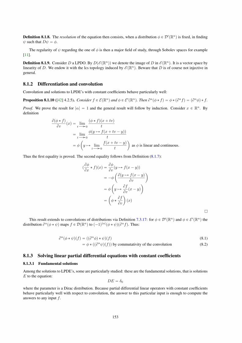
Definition 8.1.8. The resolution of the equation then consists, when a distribution φ P D1pRnq is fixed, in findingψ such that Dψ “ φ.

The regularity of ψ regarding the one of φ is then a major field of study, through Sobolev spaces for example[11].

Definition 8.1.9. Consider D a LPDO. By DpE pRnqq we denote the image of D in E pRnq. It is a vector space bylinearity of D. We endow it with the lcs topology induced by E pRnq. Beware that D is of course not injective ingeneral.

8.1.2 Differentiation and convolution

Convolution and solutions to LPDE’s with constant coefficients behave particularly well:

Proposition 8.1.10 ([42] 4.2.5). Consider f P EpRnq and φ P E 1pRnq. Then Bαpφ ˚ fq “ φ ˚ pBαfq “ pBαφq ˚ f .

Proof. We prove the result for |α| “ 1 and the general result will follow by induction. Consider x P Rn. By

definition

Bpφ ˚ fq

Bvpxq “ lim

t // 0

pφ ˚ fqpx` tvq

t

“ limt // 0

φpy ÞÑ fpx` tv ´ yqq

t

“ φ

ˆy ÞÑ lim

t // 0

fpx` tv ´ yq

t

˙as φ is linear and continuous.

Thus the first equality is proved. The second equality follows from Definition (8.1.7):

pBφ

Bx˚ fqpxq “

Bφ

Bvpy ÞÑ fpx´ yqq

“ ´φ

ˆBpy ÞÑ fpx´ yq

Bv

˙

“ φ

ˆy ÞÑ

Bf

Bvpx´ yq

˙

“

ˆφ ˚

Bf

Bv

˙pxq

This result extends to convolutions of distributions via Definition 7.3.17: for φ P D1pRnq and φ P E 1pRnq thedistribution Bαpφ ˚ ψq maps f P DpRnq to p´1q|α|pφ ˚ ψqpBαfq. Thus:

Bαpφ ˚ ψqpfq “ ppBαφq ˚ ψqpfq (8.1)

“ φ ˚ ppBαψqpfqq by commutativity of the convolution (8.2)

8.1.3 Solving linear partial differential equations with constant coefficients

8.1.3.1 Fundamental solutions

Among the solutions to LPDE’s, some are particularly studied: these are the fundamental solutions, that is solutionsE to the equation:

DE “ δ0

where the parameter is a Dirac distribution. Because partial differential linear operators with constant coefficientsbehave particularly well with respect to convolution, the answer to this particular input is enough to compute theanswers to any input f .

153

Definition 8.1.11. A fundamental solution for the LPDOD consists in a distribution ψ P D1pRnq1 to the equation:

Dψ “ δ0.

Remark 8.1.12. Notice that such a fundamental solution is in general not unique: if φ is such that Dφ “ 0, thenED ` φ is also a fundamental solution to D.

Example 8.1.13. Because of linear partial differential operators, we are working with distributions whose supportis not necessarily compact. Indeed, the existence of a fundamental solution is not ensured when distributions mustapply to any smooth function. The typical example is

D : f P C8pR,Rq ÞÑ f 1,

where f 1 is the derivative of the real, one-variable function f . If f has compact support, one can define:

ED : f ÞÑ

ż 0

8

f

and one has indeed DEDpfq “ fp0q. This however is not possible in full generality when f P C8pRnq. Observethat it would be enough for the partial derivative of f to be bounded by an integrable function for x big enough.Then the derivative of f would be integrable, and ED could be defined. Extended to any partial differentialoperator, this says that if any partial derivative Bαf , α P N

n of f are integrable on Rn, then ED can be defined.

This idea is implemented in the construction of a tamed fundamental solution ED P S 1pRRq [43].

Notation 8.1.14. Consider D : E pRnq // E pRnq a LPDO. When a fundamental solution for D exists and it is

fixed, it is denoted by ED P D1pRnq.

Remark 8.1.15. We will recall later in theorem 8.1.18 that when D is a LPDO with constant coefficients there isalways of at least one fundamental solution for D.

The resolution of LPDOs with constant coefficients is always possible, and particularly elegant, due to thebehaviour of convolution with respect to partial differentiation.

Proposition 8.1.16. Consider D “řα aαB

α a LPDO with constant coefficients. Suppose that D admits a

fundamental solution ED. Then for any φ P E 1pRnq we have:

DpED ˚ φq “ φ. (8.3)

Proof. Thanks to the bilinearity of the convolution product

DpED ˚ φq “ÿ

α

aαrBαpED ˚ φqs

“ pÿ

α

aαBαEDq ˚ φ thanks to equation 8.1 and the bilinearity of ˚,

“ δ0 ˚ φ by definition of ED,

“ φ

Remark 8.1.17. Beware that equation 8.3 is valid in D1pRnq, but not in E 1pRnq. Indeed, the convolution betweenφ P E 1pRnq and ψ P D1pRnq only yields a distribution ψ ˚ φ P D1pRnq. This is by construction of the convolutionfollowing proposition 7.3.16. It is also a particular case of the theorem of support [42, Thm 4.2.4] which says thatthe support of convolution φ ˚ ψ of two distributions φ P D1pRnq and ψ P E 1pRnq is contained is the sum of therespective supports of ψ and φ. We do not emphasize on support and singularities of distributions here.

Theorem 8.1.18. Every LPDEcc admits a fundamental solution ED P D1pRnq.

1note that we do not ask for ψ P E 1pRnq, as this is not possible in general, even for the LPDO with constant coefficients

154

Comments on the proof. Several constructions of a fundamental solution exist: we refer to the one of Mal-grange, refined and exposed by Hormander [41, Thm 3.1.1] or to [42, 7.3.10] which gives a fundamental solutionwith optimal local growth. Others construct a fundamental solution which is temperate [43]. The proof starts witha technical Lemma [41, 3.1.1], which says that for any smooth function with compact support f P DpRnq, wehave that

|fp0q| ď C ‖pcoshpǫ|x|qDpfq‖1, 1deg P

(8.4)

where C does not depend of f . Thus if Dpfq “ Dpgq, one has Dpf ´ gq “ 0 and fp0q “ gp0q. Then definesthe function E on DpDpRnqq as EpDpfqq “ fp0q. This function is well defined, linear and continuous. Theabove majoration allows then to extend this function to E P D1pRnq through Hahn-Banach 3.3.6. The theorem isin fact much more precise as we have information about the local growth of ED. We do not have in general thatED P E

1pRnq.

Remark 8.1.19. Notice that equation 8.4 ensures that ED is well defined on DpDpRnqq, as for f P DpDpRnqq thefunction g such that f “ Dg is unique. This is not true for functions in DpE pRnqq

8.1.3.2 The space !D

This section studies the question of which space is the good interpretation of !DRn for " the space of distributionswhich are solutions to a LPDEcc "

Let us sum up the situation: the computation EDpgq is well defined as soon as g P DpRnq, as Theorem 8.1.18shows that ED P D1pRnq. If f P DpRnq, then obviously Dpfq P DpRnq and we have:

EDpDpfqq “ DEDpfq “ fp0q.

If f P E pRnq (that is, f does not necessarily have compact support) is such that pDpfqq P DpRnq, thenEDpDpfqqis well defined, and we have alsoEDpDpfqq “ fp0q. However, when f P E pRnq and Dpfq does not have compactsupport, then EDpDpfqq is not defined, and thus we can’t compute fp0q as ED applied to Dpfq. Let us export thisthis reasoning to distributions.

Definition 8.1.20. We denote by !DRn the sub-vector space of D1pRnq consisting of the distributions φ P D1pRnq

such that Dφ P E 1pRnq.!DR

n :“ tφ P D1pRnq | Dφ P E1pRnqu

Example 8.1.21. A typical example of distribution in !DRn is ED , as DED “ δ0 P E 1pRnq.

Proposition 8.1.22. Endowed with the topology inherited from D1pRnq, the space !DRn is a lcs. Moreover, we

have the topological embeddings2 E 1pRnq ãÑ !DRn

ãÑ D1pRnq.

Proof. If we consider D as linear continuous endomorphism:

D : D1pRnq //D1pRnq

then !DRn is the inverse image of E 1pRnq by D. As E pRnq is closed in DpRnq, and as D is continuous, then

!D is a closed sub-locally convex topological vector space of D1pRnq. It is Hausdorff: consider φ ‰ φ1 areboth distributions, and if Dφ and Dφ1 both have compact support. Consider V and V 1 disjoint neighbourhoodsD1pRnq of φ and φ1 respectively. Then as E 1pRnq is dense in D1pRnq, V X E 1pRnq and V X E 1pRnq are twonon-empty open sets contained in !DR

n whose intersection is empty and containing respectively φ and φ1. Thetopological embeddings follows from the fact that if φ has compact support, then Dφ has compact support: thusE 1pRnq Ă !DR

n. This embedding is topological as D1pRnq and E 1pRnq carry the same topology. The otherembedding follows from the fact that by definition, !DRn is a sub-lcs of D1pRnq.

Notation 8.1.23. We denote by ?DRn the lcs p!DR

nq1 endowed with the strong topology on the dual.

AsD commutes with convolution (proposition 8.1.10) and as the convolution of two distributions with compactsupport has compact support, we have immediately:

Corollary 8.1.24. For any φ P !DRn and any ψ P E pRnq we have φ ˚ ψ P !DRn.

Corollary 8.1.25. For f P ?DRn and g P C8pRnq, Dpf ˚ gq is defined as Df ˚ g. It is coherent with the notationwhen f P DpRnq, as partial differentiation commutes with convolution (Proposition 8.1.10).

2that is, the linear continuous injections

155

Analogy with DiLL Defining !D0Rn as the inverse image of E 1pRnq by D0 in D1pRnq does not make any sense.

Indeed, D0f is a linear function: it has compact support if and only if it is null. Thus with the definition usedbefore, we have ?D0

Rn “ t0u and !D0

Rn “ R

n.

Remark 8.1.26. Although D0 is not a LPDOCC, δ0 kind of behaves as a fundamental solution to D0. Indeed, if afunction f P C8pRn,Rq is such that there is g P C8pRn,Rq such that:

D0g “ f,

then f is necessarily linear, and thus one can take g “ f “ δ0 ˚ f .

The good definition for “the space of distributions solutions to D0ψ “ φ “ is

?D0Rn :“ D´1

0 pE pRnqq,

and thus!D0

Rn » LpRn,Rq1 » R

n.

In that case dereliction and codereliction rules are interpreted in NUCL by:

dD0: !Rn // !D0

Rn, ψ ÞÑ pℓ ÞÑ ψpℓqq

dD0: !D0

Rn // !Rn, φ “ evx ÞÑ pf ÞÑ φpD0pfqq.

However if we look for a fundamental solution ED0P E2, it must satisfy:

ED0pD0fq “ fp0q

and thus in particular, for any ℓ P E1, we have ED0pℓq “ ED0

pD0ℓq “ ℓp0q “ 0. Thus the analogy with

fundamental solutions does not hold between D0 and LPDOcc, outside of the interpretation of dereliction and

co-dereliction.

Outlook 16. One should explore the similarities between the work of Ehrhard on anti-derivatives [20], and theproof theory of fundamental solutions as described in this chapter.

8.2 Discussion: Linear Logic for differential equations

In the previous semantical study, we saw the appearance of a connective !D such that E1pEq Ă !DE Ă DpEq1

when E » Rn. This space is D´1pE 1pEqq, that is it represents the space of distributions φ which are solutions to

the equationDφ “ ψ,

when ψ P E 1pEq. We noticed that defining !D0E as D´1

0 pE 1pEqq was not meaningful and that the good analogywas !D0

E “ pD0pE pRnqq “ pRnq2 » R

n.We also saw that while E » E2 represents the space of distributions with solutions to D0φ “ ψ, the space

!DE represents the space of distributions solutions to Dφ “ ψ. In sections 8.3 and 8.4, we develop thus a syntaxfor LPDE, where the interactions between !DA and !A mimic the ones between A and !A in DiLL.

Remark 8.2.1. In the semantics developed in the previous section, (??) is only valid when E is euclidean, but itshould extend to higher order in view of the results in section 7.5.

Remark 8.2.2. Beware that all the intuitions cannot be retrieved from the model of chapter 7. In particular whilewe have E » E2 ãÑ !E, we have here an embedding !E ãÑ !DE. The interpretation of !E as D1pEq wouldhave yield the inverse embedding between !E and !DE, thus alike the embedding E » E2 ãÑ !E. However, wereally need to use distribution with compact support as the interpretation of the exponential, as they are needed ina convolution product (interpreting co-contraction).

156

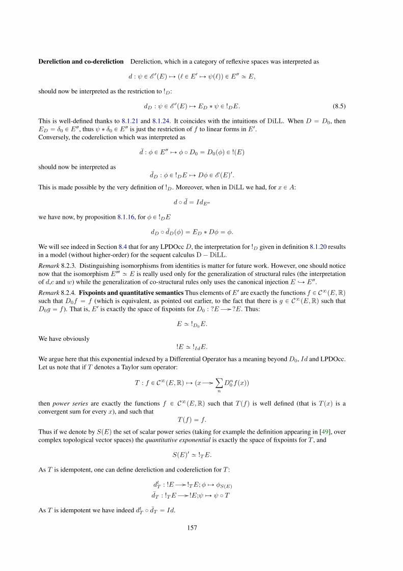
Dereliction and co-dereliction Dereliction, which in a category of reflexive spaces was interpreted as

d : ψ P E1pEq ÞÑ pℓ P E1 ÞÑ ψpℓqq P E2 » E,

should now be interpreted as the restriction to !D:

dD : ψ P E1pEq ÞÑ ED ˚ ψ P !DE. (8.5)

This is well-defined thanks to 8.1.21 and 8.1.24. It coincides with the intuitions of DiLL. When D “ D0, thenED “ δ0 P E

2, thus ψ ˚ δ0 P E2 is just the restriction of f to linear forms in E1.Conversely, the codereliction which was interpreted as

d : φ P E2 ÞÑ φ ˝D0 “ D0pφq P !pEq

should now be interpreted asdD : φ P !DE ÞÑ Dφ P E pEq1.

This is made possible by the very definition of !D. Moreover, when in DiLL we had, for x P A:

d ˝ d “ IdE2

we have now, by proposition 8.1.16, for φ P !DE

dD ˝ dDpφq “ ED ˚Dφ “ φ.

We will see indeed in Section 8.4 that for any LPDOccD, the interpretation for !D given in definition 8.1.20 resultsin a model (without higher-order) for the sequent calculus D´DiLL.

Remark 8.2.3. Distinguishing isomorphisms from identities is matter for future work. However, one should noticenow that the isomorphism E3 » E is really used only for the generalization of structural rules (the interpretationof d,c and w) while the generalization of co-structural rules only uses the canonical injection E ãÑ E2.

Remark 8.2.4. Fixpoints and quantitative semantics Thus elements ofE1 are exactly the functions f P C8pE,Rqsuch that D0f “ f (which is equivalent, as pointed out earlier, to the fact that there is g P C8pE,Rq such thatD0g “ f ). That is, E1 is exactly the space of fixpoints for D0 : ?E // ?E. Thus:

E » !D0E.

We have obviously!E » !IdE.

We argue here that this exponential indexed by a Differential Operator has a meaning beyondD0, Id and LPDOcc.Let us note that if T denotes a Taylor sum operator:

T : f P C8pE,Rq ÞÑ px //ÿ

n

Dn0 fpxqq

then power series are exactly the functions f P C8pE,Rq such that T pfq is well defined (that is T pxq is aconvergent sum for every x), and such that

T pfq “ f.

Thus if we denote by SpEq the set of scalar power series (taking for example the definition appearing in [49], overcomplex topological vector spaces) the quantitative exponential is exactly the space of fixpoints for T , and

SpEq1 » !TE.

As T is idempotent, one can define dereliction and codereliction for T :

dtT : !E // !TE;φ ÞÑ φSpEq

dT : !TE // !E;ψ ÞÑ ψ ˝ T

As T is idempotent we have indeed dtT ˝ dT “ Id.

157

The Identity rule

(axiom)$ A,AK

$ Γ, A $ AK,∆(cut)

$ Γ,∆


(1)$ 1

$ Γ(K)

$ Γ,K

$ Γ, N,M(`)

$ Γ, N `M

$ Γ, P $ ∆, Q(b)

$ Γ,∆, P bQ

The additive rules

J$ Γ,J

$ Γ, N $ Γ,M&

$ Γ, N &M

$ Γ, P‘L

$ Γ, P ‘Q

$ Γ, Q‘R

$ Γ, P ‘Q


$ Nw

$ N , ?P

$ N , ?P, ?Pc

$ N , ?P

$ N , ?DPdD$ N , ?P

w$ !N

$ N , !N $M, !Nc

$ N ,M, !N

$ N , !DNdD$ N , !N

Figure 8.1: The deriving rules for sequents of D0 ´DiLL

8.3 D0 ´ DiLL

We introduce in this section a toy polarized sequent calculus, with sums, for which both D0 and LPDOcc D area model. This sequent calculus captures the idea that dereliction and codereliction correspond to the resolution

of a differential equation. We justify this idea by giving two semantics for D0 ´DiLL without higher order: onewhich corresponds to the semantics of Chapter 7, and another one corresponding to the resolution of LPDEcc.

8.3.1 Grammar and rules

Definition 8.3.1. The formulas of D0 ´DiLL are constructed with the following polarized syntax:

N,M :“?A | ?DA | N `M | N ˆM

P,Q :“!A | !DA | P bQ | P ‘Q

Definition 8.3.2. Then the negation is the one of LL, with the addition definitions:

!DAK “ ?DA

K ?DAK “ !DA

K

Then the proofs of D0 ´DiLL are constructed according to the rules in figure 8.3.1. Notice that these are therules of polarized DiLL (see 2.8), with modified the dereliction and the codereliction accounting for the introduc-tion of the newly introduced connectives ?D and !D.

Cut-elimination The cut elimination procedure in D0 ´DiLL follows exactly the one of DiLLpol (see section2.4.1.3). In particular, the cut between the dereliction dD and the codereliction dD is:

$ N , ?DPdD$ N , ?P

$M, !DNdD$M, !Ncut

$ N ,M

ù$ N , ?DP $M, !DN

cut$ N ,M

and the one between contraction and codereliction involves the usual co-weakening:

$ Γ, ?A, ?Ac

$ Γ, ?A

$ ∆, !DAdD$ ∆, !A

cut$ Γ,∆

ù

158

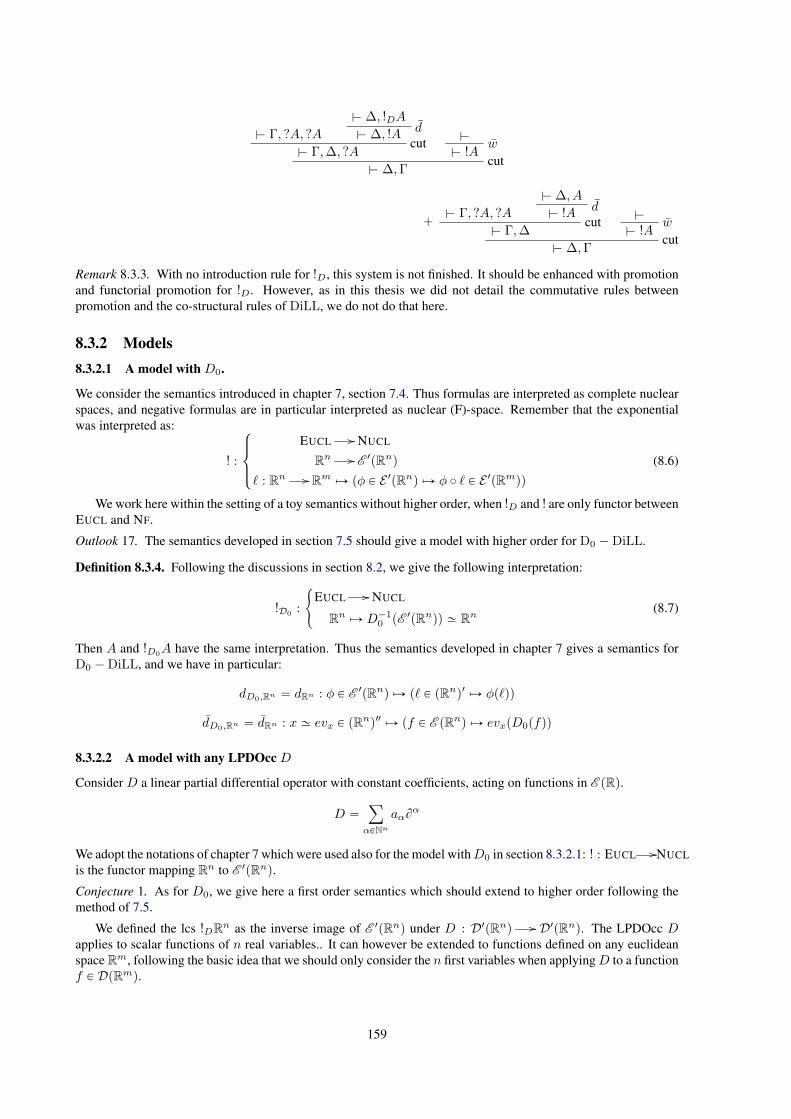
$ Γ, ?A, ?A

$ ∆, !DAd$ ∆, !A

cut$ Γ,∆, ?A

$w

$ !Acut

$ ∆,Γ

`$ Γ, ?A, ?A

$ ∆, Ad$ !A

cut$ Γ,∆

$w

$ !Acut

$ ∆,Γ

Remark 8.3.3. With no introduction rule for !D, this system is not finished. It should be enhanced with promotionand functorial promotion for !D. However, as in this thesis we did not detail the commutative rules betweenpromotion and the co-structural rules of DiLL, we do not do that here.

8.3.2 Models

8.3.2.1 A model with D0.

We consider the semantics introduced in chapter 7, section 7.4. Thus formulas are interpreted as complete nuclearspaces, and negative formulas are in particular interpreted as nuclear (F)-space. Remember that the exponentialwas interpreted as:

! :

$’&’%

EUCL // NUCL

Rn // E 1pRnq

ℓ : Rn // Rm ÞÑ pφ P E 1pRnq ÞÑ φ ˝ ℓ P E 1pRmqq

(8.6)

We work here within the setting of a toy semantics without higher order, when !D and ! are only functor betweenEUCL and NF.

Outlook 17. The semantics developed in section 7.5 should give a model with higher order for D0 ´DiLL.

Definition 8.3.4. Following the discussions in section 8.2, we give the following interpretation:

!D0:

#EUCL // NUCL

Rn ÞÑ D´1

0 pE 1pRnqq » Rn

(8.7)

Then A and !D0A have the same interpretation. Thus the semantics developed in chapter 7 gives a semantics for

D0 ´DiLL, and we have in particular:

dD0,Rn “ dRn : φ P E1pRnq ÞÑ pℓ P pRnq1 ÞÑ φpℓqq

dD0,Rn “ dRn : x » evx P pRnq2 ÞÑ pf P E pRnq ÞÑ evxpD0pfqq

8.3.2.2 A model with any LPDOcc D

Consider D a linear partial differential operator with constant coefficients, acting on functions in E pRq.

D “ÿ

αPNn

aαBα

We adopt the notations of chapter 7 which were used also for the model withD0 in section 8.3.2.1: ! : EUCL //NUCL

is the functor mapping Rn to E 1pRnq.

Conjecture 1. As for D0, we give here a first order semantics which should extend to higher order following themethod of 7.5.

We defined the lcs !DRn as the inverse image of E 1pRnq under D : D1pRnq // D1pRnq. The LPDOcc D

applies to scalar functions of n real variables.. It can however be extended to functions defined on any euclideanspace Rm, following the basic idea that we should only consider the n first variables when applyingD to a functionf P DpRmq.

159

Definition 8.3.5. Consider m ď n and f P E pRmq, one defines an extension of f to Rn as f : px1, ...xnq ÞÑ

fpx1, ..., xmq, and thus defines D on E pRmq. It m ą n and f P DpRmq, one define Dpfq as D applied to therestriction of f to R

n: Dpfq :“ Dppx1, . . . , xnq ÞÑ fpx1, . . . , xn, 0, . . . , 0qq.

This definition is fundamental, at is accounts for the deterministic cut-elimination of the system D´DiLL,introduced in section 8.4.

Remark 8.3.6. We reused here a convention in mathematical physics (see for example the introduction of chapter52 in [76]). One denotes by Dx the operator D applied to a function f P C8c pR

nˆRmq, to indicate that D applies

only to the variable x of the function px, yq P Rn ˆ Rm ÞÑ fpx, yq.

Definition 8.3.7. We define the functor: !D : EUCL // TOPVEC.

!D :

$’&’%

EUCL // NDF

Rn ÞÑ !DR

n

ℓ : Rn // Rm ÞÑ pφ P !DRn ÞÑ ψ : pf P ?DR

mq ÞÑ φpf ˝ ℓqqq

(8.8)

This functor is well defined: consider ℓ : Rn //Rm and φ P !DRn, then for any f P ?DRm : Dpp!Dℓqpφqqpfq “p!DℓqpφqpDpfqq “ φpDpf ˝ ℓq “ φppDpfq ˝ ℓq. As D has compact support and ℓ is linear continuous, so haspDpfq ˝ ℓ.

Definition 8.3.8. We define the following natural transformations dD : ! // !D and dD : !D ÞÑ !.

dD,Rm :

#E1pRmq // !DR

m

ψ ÞÑ ED ˚ ψ

dD,Rm :

#!DR

m // !Rm

ψ ÞÑ pf P E pRmq ÞÑ Dpψqpfqq

The codereliction is well defined thanks to Proposition ??. The dereliction is well defined thanks to Corollary8.1.24 and Example 8.1.21. Moreover, this denotational interpretation is unchanged under the cut-eliminationprocedure, as by Proposition 8.1.16:

@φ P !DRn, dD,Rn ˝ dD,Rnpφq “dD,RnpDφq P E

1pRnq

“ ED ˚ pDφq

“ φ P D1pRnq

Remark 8.3.9. Let us note that to extend this model to higher order, one cruelly misses a proof of the fact that!DR

n is reflexive.

8.4 D-DiLL

We now depart from the intuitions conveyed by D0 and DiLL, to study more specifically the case of Linear PartialDifferential Operators with constant coefficients.

8.4.1 The sequent calculus D ´ DiLL

8.4.1.1 Grammar and rules

We introduce a generalisation of (higher-order, polarized, without promotion) DiLL, where the role of A » AKK

in the exponential rules d and d is played by a new formula !DA. The other exponential rules are moreover replacedby equivalent rules involving !D, in order to account for the specificities of the convolution and the fundamentalequation. In particular, this modification implies that this sequent calculus does not involve sums of proofs (seeSection 8.3). The formulas of D´DiLL are constructed following the same grammar as those of D0 ´DiLL:

Definition 8.4.1. The formulas of D´DiLL are constructed with the following polarized syntax:

N,M :“?A | ?DA | N `M | N ˆM

P,Q :“!A | !DA | P bQ | P ‘Q

160

The Identity rule

(axiom)$ A,AK

$ Γ, A $ AK,∆(cut)

$ Γ,∆

The additive rules

(1)$ 1

$ Γ(K)

$ Γ,K

$ Γ, N,M(`)

$ Γ, N `M

$ Γ, P $ ∆, Q(b)

$ Γ,∆, P bQ


J$ Γ,J

$ Γ, N $ Γ,M&

$ Γ, N &M

$ Γ, P‘L

$ Γ, P ‘Q

$ Γ, Q‘R

$ Γ, P ‘Q

The exponential rules

$ N wD$ N , ?DP

$ N , ?P, ?DPc

$ N , ?DP

$ N , ?DPd

$ N , ?P

$wD

$ !DN

$ N , !N $M, !DNcD

$M,N , !DN

$ N , !DNdD$ N , !N

Figure 8.2: Rules for D´DiLL

Definition 8.4.2. The negation is the one of LL, with the additional definitions:

!DAK “ ?DA

K ?DAK “ !DA

K

Remark 8.4.3. Let us relate the specific form of the co-contraction with the "coabs" rule in the parcimonious typesof Mazza [57]:

Γ;∆ $ t : A Γ1; ∆1 $ u : !A

Γ,Γ1; ∆,∆1 $ t :: u : !A

which underlines that a modified version of the co-dereliction should type the constructions of lists. Now rememberthat semantically, !DA is interpreted as a space which contains !A “ E 1pAq. Thus the D-co-contraction cD couldimply that one should see the type !DA as the type of lists of elements of type !A. The operation extracting the firstelement of a list should then be typed by dD.

Remark 8.4.4. Thus the connectives !D and ?D are only introduced via coweakening and weakening, which isquite weak. As for D0 ´DiLL, one should add to the present sequent calculus functorial promotions rules for !D(which are well interpreted in the semantics were !D : EUCL // NUCL is indeed a functor). This is not done here,as the meaning in terms of distributions of cut-elimination rules between a promotion for !D and structural rules isnot clear.

8.4.1.2 Admissible rules

Before going to cut-elimination, let us show that the version of the structural rule c, w, c, w involving only !N andnot !DN are admissible in D´DiLL.

Proposition 8.4.5. The rules w, w are admissible in D´DiLL.

Proof. The following proof-trees can be understood through their interpretation in terms of distributions and partialdifferential operators. For example, wD : R // !DE is the introduction of a fundamental solution 1 ÞÑ ED. Thusthe usual coweakening w : 1 P R ÞÑ δ0 P !E is exactly wp1q “ dD ˝ wDp1q “ DED “ δ0.

w$ !N =

$wD

$ !DNdD$ !N

$ Nw

$ N , ?P=

$ N wD$ N , ?DP

dD$ N , ?P

161

Proposition 8.4.6. The rules c and c are admissible in D´DiLL.

Proof. In terms of distributions and fundamental solutions, cD and c are both interpreted as the convolution, butthey are not defined on the same spaces. The usual cocontraction is the convolution between to distributions withcompact support cpφ, ψq “ φ ˚ ψ while cD asks for one of them to be in !DE “ D´1pE 1pEqq Ă D1pEq. Thuscpφ, ψq “ φ ˚ ψ “ DpED ˚ φq ˚ ψ “ dD ˝ cDpdDpφq, ψqqq.

$ N , !N $M, !Nc

$ N ,M, !N=

$ N , !Nwd

$ !DNcD

$ N , !DN $M, !NcD

$ N ,M, !DNdD$ N ,M, !N

$ N , ?P, ?Pc

$ N , ?P=

$ N , ?P, ?PwD

$ N , ?P, ?P, ?DA cD$ N , ?P, ?DA cD$,N , ?DP

dD$ N , ?P

Proposition 8.4.7. The rules wD, cD, wD and cD are admissible in DiLL, when !DA is equivalent to A.

8.4.2 The cut-elimination procedure in D ´ DiLL

This cut-elimination is inspired by the one of DiLL and by the calculus of distributions, see section 8.1. We de-scribe the cut-elimination rules and commutative rules in figure 8.3. They are best understood from the semanticalpoint of view developed in section 8.4.3.

Notice that the differences between DiLL and D´DiLL makes the cut-elimination procedure much simpler:cuts between dD and wd or dD and wD are not possible. Moreover, the fact that the contraction and co-contractionrules are no longer symmetrical suppress the need for sums of proofs. Thus proofs of D´DiLL are simple proofs.

The commutative rules for the exponential rules of D´DiLL are the same as the ones of DiLL (see [81]), andare immediate as the exponential rules are multiplicative and do not interfere with the context.

8.4.3 A concrete semantics without higher order

Let us define formally the semantics of D´DiLL which was used informally throughout the last sections. Thissection is peculiar, as it uses the notations used in mathematical physics to interpret the rules of D´DiLL, seetheorem 8.4.11.

In this section we show that the categories EUCL, NDF and NF, together with distributions of compact supportand a LPDO D with contant coefficients, form a first-order model of D´DiLL. As for Smooth DiLL, we define!D as a strong monoidal functor between EUCL and NDF. Extending this to a higher-order model could be possibleusing the same techniques as in section 7.5.Consider D : D1pRnq //D1pRnq a LPDOcc:

Dpf, xq “ÿ

αPNn

aαBαfpxq.

In section 8.3.2.2 we saw that we could make D act on any euclidean space:

Definition 8.4.8. If m ă n and f P DpRmq, one defines an extension of f to Rm as f : px1, ...xnq ÞÑ

fpx1, ..., xmq, and thus define D on DpRmq. It m ą n and f P DpRmq, one define Dpfq as D applied tothe restriction of f to R

n: Dpfq :“ Dppx1, . . . , xnq ÞÑ fpx1, . . . , xn, 0, . . . , 0qq.

Remark 8.4.9. In particular, the fundamental solution ED P !DRn can be restricted or extended to ED P R

m, forany m.

162

$ N wD$ N , ?DN

K$

wD$ !DN

cut$ N

ù $ N

$ N , ?DNK, ?NK

cD$ N , ?DN

K$

wD$ !DN

cut$ N

ù$ N , ?DN

K, ?NK$

w$ !N

cut$ N , ?NKD

$wD

$ !DNcut

$ N

$ N , !DN $ N 1, !NcD

$ N ,N 1, !DN

$M wD$M, ?DN

K

cut$ N ,N 1,M

ù

$ N , !DN

$M wD$M, ?DN

K

cut$ N ,M

w$ N ,M, ?NK $ N 1, !N

cut$ N ,N 1,M

$ N , ?DNK

dD$ N , ?NK

$M, !DNdD$M, !Ncut

$ N ,M

ù$ N , ?DN

K $M, !DNcut

$ N ,M

$ N , ?DNK, ?NK

cD$ N , ?DN

K

$M, !DN $M1, !NcD

$M,M1, !DNcut

$ N ,M1,M

ù

$ N , ?DNK, ?NK $M, !DN

cut$ N ,M, ?NK $M1, !N

cut$ N ,M,M1

Figure 8.3: Cut-elimination for the exponential rules of D´DiLL

163

We interpret finitary formulas A,B as euclidean spaces. One has indeed 1 » K “ R and J » 0 “ t0u. Theconnectives of LL are interpreted in EUCL, NF and NDF as in section 7.4.

Definition 8.4.10. We recall the definition of the functor !D which was made explicit in section 8.3.2.2:

!D :

$’&’%

EUCL // TOPVEC

Rm ÞÑ !DR

m

ℓ : Rm // Rpφ P !DRm ÞÑ pf P DpDpRpq ÞÑ φpf ˝ ℓqq

(8.9)

The introduction of !D breaks the symmetry of the Kernel theorem:

Theorem 8.4.11. Consider D : D1pRnq // D1pRnq a LPDOcc. Then for any m ě 0, we have natural isomor-

phisms

mD,n : !DpRn`nq » !DR

nbπ!Rn.

Proof. This theorem encodes the definition 8.3.5, which allows to extends D defined on EpRnq to EpRn`mq.This theorem is then directly deduced from the Kernel theorem 7.3.5: as EpRn`mq » EpRnqbEpRmq we haveDpEpRn`mqq » DEpRnqbEpRmq. Taking the dual gives us the desired result.

From this strong monoidal isomorphism and the biproduct structure on TOPVEC, one deduces the interpretationof wD, wD, cD and cD, following the categorical procedure introduced by Fiore (see section 2.4.2.1). Theseinterpretations are to be compared to the ones for the model of DiLL with distributions of Chapter 7, which aredetailed in Section 7.4.3.

Definition 8.4.12. We give the following interpretation for wD, wD, cD and cD:• In Section 2.4.2), we interpreted the coweakening as the map wA :! // !A resulting of the application of the

functor ! on the initial map uA : I // A . Concretely, we have I “ t0u uRmp0 P t0uq ÞÑ 0 P Rm , and

!DpuAqp1q “ δ0. Applying !D to uA gives exaclty the same result : !DpuAqp1q “ δ0, but this is not what we

want here. Thus one defines:

wD :

#R // !DR

m

1 ÞÑ pED ˚ !DpuAqp1qq “ ED(8.10)

Notice that ED was given in !DRn, but it is extended to !DR

m following Definition 8.4.8.• The cocontraction c : !D b ! // !D is interpreted by the convolution product (see prop. 7.4.12)

cD :

#!DR

mb!Rm // !DRm

φb ψ ÞÑ φ ˚ ψ(8.11)

and is well defined thanks to corollary 8.1.24.• The interpretation of weakening wD : !D // 1 is defined as:

wD : φ P !DRm ÞÑ

żDφ.

It is well defined as by definition Dφ has compact support. As explained in Section 7.4.3, integration ondistributions with compact support ψ P E 1pEq is defined as ψ applied to a function constant at 1:

żψ “ ψpconst1q.

When ψ is the generalization of a function f with compact support, then we have indeed

ψpconst1q “

ż1 ¨ f “

żf.

• The contraction cD : !D // !D b ! is interpreted as in proposition 7.4.9 by:

cD :

#?DR

mb?Rm // ?DpRmq

f b g ÞÑ px ÞÑ fpxqgpxqq(8.12)

164

Remark 8.4.13. Notice that the interpretation of cD follows the intuitions of theorem 8.4.11:

f P DpE pRm ˆ Rmqq

is in fact in DpE pRmqqbE pRmq, as differentiation occurs only on the first m variables. In particular, if m ą 0,then the differentiation on R

m ˆ Rn is defined as:

D b IdRm : C8pRn ˆ Rmq // C8pRn ˆ R

mq

Thus the fundamental solution ED P !DpRm`nq corresponds to ED b δ0 P !DRn b !Rm.

Dereliction and the codereliction are defined as previously for D0 ´DiLL (see Section 8.3.2.1).

Definition 8.4.14. We interpret the dereliction dD : ! // !D as

dD,Epφ P E1pRnqq ÞÑ pED ˚ φq

and codereliction dD : ! // !D as

dD,E : pφ P !DRnq ÞÑ pDφq P E 1pRnq.

Proposition 8.4.15. This denotational semantics of the rules of D´DiLL is preserved by cut-elimination (see

figure 8.3).

In figure 8.4.3, we provide the cut-elimination rules annotated with the interpretation of the proofs, to supportthe proof of proposition 8.4.15.

Proof. • Cut elimination between dD and dD. By equation 8.3 one has for every φ P E 1pRnq and f P EpRnq:

dD,E ˝ dD,Epφqpfq “ ED ˚ pφpDpfqq

“ φpED ˚Dpfqq

“ φpfq

• Cut elimination between wD and wD:

wD ˝ wDp1 P Rq “

żDED “

żδ0 “ 1

• Cut elimination between cD and wD: by definition of the interpretation of cD, one has:

cD ˝ wDp1q “ pfD, gq P DpE pRnqq b E pRnq ÞÑ wDpx ÞÑ fpxqgpxqq.

Thus as wDp1q “ ED, and by making use of remark 8.4.13, we have:

cD ˝ wDp1q “ EDbδ0ppx ÞÑ fpxqgpxqqq

which corresponds to the interpretation of the reduced cut-rule.

• Cut elimination between cD and wD: consider φ P !DRm and ψ P !Rm. We are used to see the cocontrac-

tion as the convolution between distribution, but remember that we can also understand it as the resultingdistribution which sums in the codomain of its function (see Proposition 7.4.12). Then:

wD ˝ cDpφ, ψq “

żDrf P EDpR

mq ÞÑ φpx ÞÑ ψpx1 ÞÑ fpx` x1qqqs

“

żrf ÞÑ φpx ÞÑ Dψpx1 ÞÑ fpx` x1qqqs

“ φpx ÞÑ Dψpx1 ÞÑ const1px` x1qqq

“ φpconstDψpconst1qq

Again by definition 8.3.5, D applies only to φ. Thus the interpretation of the cut-rule and its reduced formcorresponds.

165

• Cut elimination between cD and cD: consider φ P !DRm and ψ P !Rm. Then up to the kernel isomorphism

we have:cD ˝ cD “ !DpAÂq

!DAÝÝÝÝÑ !DA!DAÝÝÝÑ !DpAÂq

Thus

cD ˝ cDpφ P !DpAÂqq “ f P DE pAÂq ÞÑ pcDφqpx ÞÑ fpx, xqq

“ f ÞÑ φppx, yq ÞÑ fpx, xqfpy, yqq.

Through the Kernel isomorphism we can suppose by density that φ “ φ1 b ψ, with φ1 P !DA and ψ P !A,and f “ f 1 b g with f 1 P ?DAK and g P ?AK. Thus

pcD ˝ cDqpφ P !DpAÂqq “ f 1bg ÞÑ φ1 b ψppx, yq ÞÑ f 1pxqgpyqq

“ f 1bg ÞÑ φ1pf 1qφpgq,

and the last proposition corresponds to the interpretation of the reduced cut-rule between cD and cD.

166

$ N wD$ N , φ ÞÑ pDφqpconst1q : ?DN

K$

wD$ ED : !DN

cut$ N , δ0pconst1q “ 1 : K

ù $ N , 1 : K

$ N , Df : ?DNK, g :?NK

cD$ N , Df ¨ g : ?DN

K$

wD$ ED : !DN

cut$ N , EDpDf ¨ gq “ δ0pf ¨ gq “ fp0qgp0q : R

ù$ N , Df : ?DN

K, g :?NK$

w$ δ0 : !N

cut$ N , Df :?NKD , gp0q : R

$wD

$ ED!DNcut

$ N , EDpDfq “ fp0q : R, gp0q : R

$ N , ψ : !DN $ N 1, φ : !NcD

$ N ,N 1, ψ ˚ φ : !DN

$M, 1 : RwD

$M, Dpconst1q :?NK

cut$ N ,N 1,M, pψ ˚ φqpDpconst1qq “ pDψ ˚ φqpconst1q : R

ù

$ N , ψ : !DN

$M wD$M, Dpconst1q : ?DN

K

cut$ N ,M, Dpψqpconst1q : R

w$ N ,M, constDpψqpconst1q :?N

K $ N 1, φ : !Ncut

$ N ,N 1,M, ψpconstDpψqpconst1qq : R

$ N , Df : ?DNK

dD$ N , f : ?NK

$M, ψ : !DNdD$M, Dψ : !Ncut

$ N ,M, Dψpfq “ ψpDfq : R

ù$ N , Df : ?DN

K $M, ψ : !DNcut

$ N ,M, ψpDfq : R

$ N , Df : ?DNK, g :?NK

cD$ N , Df ¨ g : ?DN

K

$ N , ψ : !DN $ N 1, φ : !NcD

$ N ,N 1, ψ ˚ φ : !DNcut

$ N ,M1,M, pψ ˚ φqpDf ¨ gq “ pψ ˚ φqDpf ¨ gq : R

ù

$ N , ψ : ?DNK, φ : ?NK $M, !DN

cut$ N ,M, ?NK $M1, !N

cut$ N ,M,M1

Figure 8.4: Cut-elimination for the exponential rules of D´DiLL, annotated with the semantics

167

Chapter 9

Conclusion

In this thesis, we conducted a study of the semantics of Differential Linear Logic: our goal was to find a model ofDiLL in which functions were smooth (making coincide the intuitions of analysis concerning differentiation andthe requirements of logic), and spaces continuous and reflexive (as DiLL features an involutive linear negation).

We met this goal by constructing several model for it. During this study, it appeared that a polarized was betterfit to interpret DiLL, as we may want to interpret differently the linear negation on the positives or and the negative( Chapter 6), or as a space and its dual may not belong to a same monoidal closed category (Chapter 7). Throughoutthis study, we highlighted the fact spaces distributions with compact support are the canonical interpretation for theexponential. In this spaces of distributions, one can resolve Linear Partial Differential Equations, and we providea sequent calculus supporting the idea that the exponential is the space of solutions for a Linear Partial DifferentialEquation.

Directly following this thesis: Among other points, let us mention what could appear in this thesis and is not:

1. Categorical models of DiLL0,pol presented in section 2.5.2.3 are not optimal. Indeed, they always providefor an interpretation of the promotion rule, even when this one does not figure in DiLL0. Moreover, thesymmetry between the dereliction and codereliction rules is broken in the categorical axiomatization: dere-liction comes with the strong monoidal adjunction between ! and U , while codereliction is ad-hoc. In viewof results in Chapter 8, we should have a symmetric axiomatization.

2. In Chapter 6, one would want an interpretation for the exponential which is intrinsically bornological, thusemphasizing on the fact that the adjunction between convenient spaces and complete Mackey spaces is thegood linear classical refinement of convenient spaces.

3. In Chapter 7, we detailed a model of DiLL using the theory of Nuclear Spaces. One should explore the linkbetween this model and the model of Köthe spaces, using in particular Fourier transformation. In particular,as any nuclear fréchet space is a subset of a denumerable product of the Kothe spaces of rapidly decreasingsequences [44, 21.7.1], introducing subtyping may lead to a complete semantics.

4. In Chapter 8, the proof that !DE is reflexive is cruelly missing. We also miss a good notion of categoricalmodel for D´DiLL.

5. Chapter 8 gives a logical account for the notion of fundamental solution for Linear Partial DifferentialOperator. Let us note that the Cauchy Problem for Linear Partial Differential Equation behaves well withrespect to solutions defined on cones, and that a link with the recent models of probabilistic programmingby Ehrhard, Pagani and Tasson may exists [21].

6. This thesis emphasized the importance of reflexivity when constructing models of Differential Linear Logic.One should now investigate the differential λ-calculus in terms of linear continuations, and linear exceptions,in the spirit of [16] and [35].

What’s more important: In Chapter 8, we build a deterministic sequent calculus D´DiLL with a concretefirst-order denotational model in which applying the dereliction rule corresponds to solving a linear partial differ-ential equation, with the basic intuition that several exponential exists, and each one is associated with a LinearDifferential Operator

169

1. The priority is to work towards completing the Curry-Howard-Lambek correspondence for Linear PartialDifferential Equations. This means finding the good categorical axiomatization for models of D´DiLL,and most importantly refining the differential λ-calculus [22] into a deterministic calculus for Linear PartialDifferential Equations. This should be done by understanding computationally the proof of the Existence ofED.

2. In Chapter 7, we gave a sequent calculus D-DiLL, which corresponds to a fixed Linear Partial DifferentialOperator D. We would like to generalize this procedure, by constructed a graduated sequent calculus à laBLL [34], which would describe any Linear Partial Differential operator with constant coefficient.

3. Of course, the global objective is to work towards a computational understanding of non-linear Partial Dif-ferential Equations.

170

Bibliography

[1] BARR, M. ˚-autonomous categories, vol. 752 of Lecture Notes in Mathematics. Springer, Berlin, 1979. Withan appendix by Po Hsiang Chu.

[2] BARR, M. On ˚-autonomous categories of topological vector spaces. Cahiers Topologie Géom. Différentielle

Catég. 41, 4 (2000).

[3] BAYDIN, A. G., PEARLMUTTER, B. A., RADUL, A. A., AND SISKIND, J. M. Automatic differentiation inmachine learning: a survey. Journal of Machine Learning Research 18 (2017), 153:1–153:43.

[4] BENTON, P. N. A mixed linear and non-linear logic: Proofs, terms and models. In Computer Science Logic

(Berlin, Heidelberg, 1995), L. Pacholski and J. Tiuryn, Eds., Springer Berlin Heidelberg, pp. 121–135.

[5] BLUTE, R. Hopf algebras and linear logic. Mathematical Structures in Computer Science 6, 2 (1996),189–217.

[6] BLUTE, R., EHRHARD, T., AND TASSON, C. A convenient differential category. Cah. Topol. Géom. Différ.

Catég. (2012).

[7] BLUTE, R., EHRHARD, T., AND TASSON, C. A convenient differential category. Cah. Topol. Géom. Différ.

Catég. 53, 3 (2012), 211–232.

[8] BLUTE, R. F., COCKETT, J. R. B., AND SEELY, R. A. G. Differential categories. Math. Structures Comput.

Sci. 16, 6 (2006).

[9] BLUTE, R. F., COCKETT, J. R. B., AND SEELY, R. A. G. Cartesian differential categories. Theory Appl.

Categ. (2009).

[10] BOMAN, J. Differentiability of a function and of its compositions with functions of one variable. Math.

Scan., 20 (1967).

[11] BREZIS, H. Analyse fonctionnelle : théorie et applications. Éditions Masson, 1983.

[12] CAIRES, L., AND PFENNING, F. Session types as intuitionistic linear propositions. In CONCUR 2010 -

Concurrency Theory, 21th International Conference, CONCUR 2010, Paris, France, August 31-September 3,

2010. Proceedings (2010), pp. 222–236.

[13] COCKETT, J., AND SEELY, R. The faa di bruno construction. Theory and applications of categories 25, 15(2011), 394–425.

[14] COCKETT, J. R. B., AND SEELY, R. A. G. Weakly distributive categories. J. Pure Appl. Algebra 114, 2(1997), 133–173.

[15] CURIEN, P.-L., FIORE, M., AND MUNCH-MACCAGNONI, G. A Theory of Effects and Resources: Adjunc-tion Models and Polarised Calculi. In Proc. POPL (2016).

[16] CURIEN, P.-L., AND HERBELIN, H. The duality of computation. In ICFP ’00) (2000).

[17] DABROWSKI, Y., AND KERJEAN, M. Models of linear logic based on the schwartz ε product. 2017.

[18] EHRHARD, T. On Köthe sequence spaces and linear logic. Mathematical Structures in Computer Science

(2002).

171

[19] EHRHARD, T. Finiteness spaces. Mathematical Structures in Computer Science 15, 4 (2005).

[20] EHRHARD, T. A model-oriented introduction to differential linear logic. preprint (2011).

[21] EHRHARD, T., PAGANI, M., AND TASSON, C. Measurable cones and stable, measurable functions: a modelfor probabilistic higher-order programming. PACMPL 2, POPL (2018), 59:1–59:28.

[22] EHRHARD, T., AND REGNIER, L. The differential lambda-calculus. Theoretical Computer Science 309, 1-3(2003).

[23] EHRHARD, T., AND REGNIER, L. Differential interaction nets. Theoretical Computer Science 364, 2 (2006).

[24] EHRHRARD, T., AND REGNIER, L. Böhm trees, krivine machine and the taylor expansion of ordinarylambda-terms. Lecture Notes in Computer Science. Springer Verlag. (2006).

[25] FIORE, M. Differential structure in models of multiplicative biadditive intuitionistic linear logic. TLCA

(2007).

[26] FRÖLICHER, A., AND KRIEGL, A. Linear spaces and Differentiation theory. Wiley, 1988.

[27] GACH. Topological versus bornological concepts in infinite dimensions. Mater’s Thesis, 2004.

[28] GENTZEN, G. Untersuchungen über das Logische Schließen I. Mathematische Zeitschrift 39 (1935), 176–210.

[29] GIRARD, J.-Y. Linear logic. Theoret. Comput. Sci. 50, 1 (1987).

[30] GIRARD, J.-Y. Normal functors, power series and λ-calculus. Ann. Pure Appl. Logic, 2 (1988).

[31] GIRARD, J.-Y. Theoret. Comput. Sci. 227, 1-2 (1999). Linear logic, I (Tokyo, 1996).

[32] GIRARD, J.-Y. Coherent Banach spaces: A continuous denotational semantics. Theor. Comput. Sci. (1999).

[33] GIRARD, J.-Y. Between logic and quantic: a tract. In Linear logic in computer science, vol. 316 of London

Math. Soc. Lecture Note Ser. Cambridge Univ. Press, Cambridge, 2004, pp. 346–381.

[34] GIRARD, J.-Y., SCEDROV, A., AND SCOTT, P. J. Bounded linear logic: A modular approach to polynomial-time computability. Theor. Comput. Sci. 97, 1 (1992), 1–66.

[35] GRIFFIN, T. A formulae-as-types notion of control. In Conference Record of the Seventeenth Annual ACM

Symposium on Principles of Programming Languages, San Francisco, California, USA, January 1990 (1990),pp. 47–58.

[36] GROTHENDIECK, A. Produits tensoriels topologiques et espaces nucléaires. Memoirs of the AMS 16 (1966).

[37] GROTHENDIECK, A. Topological vector spaces. Gordon and Breach Science Publishers, 1973. TraducteurO. Chaljub.

[38] HENRICI, P. Applied and computational complex analysis, vol. Vol. 1. John Wiley and sons, 1988.

[39] HILDEBRAND, F. Introduction to Numerical Analysis: Second Edition. Dover Books on Mathematics. DoverPublications, 2013.

[40] HOGBE-NLEND. Bornologies and Functional Analysis. Math. Studies 26, North Holland, Amsterdam, 1977.

[41] HÖRMANDER, L. Linear partial differential operators. Die Grundlehren der mathematischen Wis-senschaften, Bd. 116. Academic Press, Inc., Publishers, New York; Springer-Verlag, Berlin-Göttingen-Heidelberg, 1963.

[42] HÖRMANDER, L. The analysis of linear partial differential operators. I. Classics in Mathematics. Springer-Verlag, Berlin, 2003. Distribution theory and Fourier analysis.

[43] HÖRMANDER, L. On the division of distributions by polynomials. Ark. Mat. 3, 6 (12 1958), 555–568.

[44] JARCHOW, H. Locally convex spaces. B. G. Teubner, 1981.

172

[45] JUNEK, H. Locally Convex Spaces and Operator Ideals. Leipzig: B. G. Teubner, 1983.

[46] KAINZ, G., KRIEGL, A., AND MICHOR, P. C8-algebras from the functional analytic view point. Journal

of Pure and Applied Algebra 46, 1 (1987), 89 – 107.

[47] KERJEAN, M. A logical account for linear partial differential equations. In LICS 2018 (2011).

[48] KERJEAN, M. Weak topologies for linear logic. Logical Methods in Computer Science 12, 1 (2016).

[49] KERJEAN, M., AND TASSON, C. Mackey-complete spaces and power series. MSCS (2016).

[50] KOCK, A. A simple axiomatics for differentiation. Mathematica Scandinavica 40 (1977), 183–193.

[51] KÖTHE, G. Topological Vector spaces. I. Springer-Verlag, New York, 1969.

[52] KÖTHE, G. Topological vector spaces. II. Springer-Verlag, New York, 1979.

[53] KRIEGL, A., AND MICHOR, P. W. The convenient setting of global analysis. Mathematical Surveys andMonographs. AMS, 1997.

[54] LAURENT, O. Etude de la polarisation en logique. Thèse de doctorat, Université Aix-Marseille II, Mar.2002.

[55] LAURENT, O. Théorie de la démonstration. University Lecture, 2008.

[56] MACLANE. Categories for the Working Mathematician. Springer, 1998.

[57] MAZZA, D. Simple parsimonious types and logarithmic space. In Proceedings of CSL (2015), pp. 24–40.

[58] MEISE, R. Spaces of differentiable functions and the approximation property. In Approximation Theory and

Functional Analysis, J. B. Prolla, Ed., vol. 35 of North-Holland Mathematics Studies. North-Holland, 1979,pp. 263 – 307.

[59] MELLIÈS, P.-A. Categorical semantics of linear logic. Société Mathématique de France (2008).

[60] MELLIÈS, P.-A. Dialogue categories and chiralities. Publ. Res. Inst. Math. Sci. 52, 4 (2016), 359–412.

[61] MELLIÈS, P. A. A micrological study of negation. Ann. Pure Appl. Logic 168, 2 (2017), 321–372.

[62] MELLIÈS, P.-A. Une étude micrologique de la négation. habilitation, Université Paris Diderot, 2017.

[63] MELLIÈS, P.-A., TABAREAU, N., AND TASSON, C. An explicit formula for the free exponential modalityof linear logic. In Automata, languages and programming. Part II, vol. 5556 of Lecture Notes in Comput.

Sci. Springer, Berlin, 2009.

[64] PAGANI, M. The Cut-Elimination Thereom for Differential Nets with Boxes. In TLCA) (2009).

[65] PAIGE, R., AND KOENIG, S. Finite differencing of computable expressions. ACM Trans. Program. Lang.

Syst. (1982), 402–454.

[66] SCHAEFER, H. Topological vector spaces, vol. GTM 3. Springer-Verlag, 1971.

[67] SCHWARTZ, L. Théorie des distributions à valeurs vectorielles. I. Ann. Inst. Fourier, Grenoble 7 (1957).

[68] SCHWARTZ, L. Théorie des distributions à valeurs vectorielles. II. Ann. Inst. Fourier. Grenoble 8 (1958).

[69] SCHWARTZ, L. Théorie des distributions. Publications de l’Institut de Mathématique de l’Université deStrasbourg, No. IX-X. Nouvelle édition, entiérement corrigée, refondue et augmentée. Hermann, Paris, 1966.

[70] SCOTT, D. S. Data types as lattices. SIAM J. Comput. 5, 3 (1976), 522–587.

[71] SEELY, R. Linear logic, *-autonomous categories and cofree coalgebras. In In Categories in Computer

Science and Logic (1989), American Mathematical Society.

[72] SELINGER, P. Control categories and duality: on the categorical semantics of the lambda-mu calculus.Mathematical Structures in Computer Science 11, 2 (2001), 207–260.

173

[73] TASKINEN, J. A counterexample to “problème des topologies” of Grothendieck. In Séminaire d’Analyse

Fonctionelle 1985/1986/1987, vol. 28 of Publ. Math. Univ. Paris VII. Univ. Paris VII, Paris, 1988, pp. 165–169.

[74] TASSON, C. Sématiques et syntaxes vectorielles de la logique linéaire. PhD thesis, Université Paris Diderot,2009.

[75] TREVES, F. Locally Convex Spaces and Linear Partial Differential Equations. Springer, Berlin, Heidelberg,1966.

[76] TRÈVES, F. Topological vector spaces, distributions and kernels. Academic Press, New York-London, 1967.

[77] ULAM, S. Zur Masstheorie in der Allgemeinen Mengenlehre. Fund. Math. 16 (1930), 140–160.

[78] VALDIVIA, M. Topics in Locally Convex Spaces. North-Holland Mathematics Studies. Elsevier Science,1982.

[79] VAUX, L. λ-calcul différentiel et logique classique : interactions calculatoires. PhD thesis, Université AixMarseille 2, 2007.

[80] WADLER, P. A syntax for linear logic. Lecture Notes in Comput. Sci. 802 (1994), 513–529.

[81] ZIMMERMANN, S. Vers une ludique différentielle. PhD thesis, Université Paris Diderot, 2013.

174

Appendices

175

Appendix A

Index of symbols

We indicate symbols, and then give the name of the mathematical object they denote, and the page or section in

which they are introduced.

Categories

• TOPVEC: the category of Hausdorff and locally convex topological vector spaces and linear continuousbounded maps between them.

• BORNVEC: the category of vector spaces endowed with a vector bornology, with linear bounded mapsbetween them.

The following categories are full and faithful subcategories of TOPVEC.

• KOTHE, model of DiLL : the category of kothe spaces, page 22.

• MCO, model of intuitionist DiLL: the category of Mackey-Complete spaces, page 45.

• CHU, model of MALL : the category of Chu spaces, Section 4.

• WEAK, model of DiLL: the category oflcs endowed with their Weak topology, Chapter 5.

• bTOPVEC: the category of bornological lcs, page 107.

• MACKEY : the category of lcs endowed with their Mackey topology, Section 4.

• CONV, model of iDiLL [6] and interpretation for the positives formulas of a model in Section 6.4 : thecategory of bornological and Mackey-Complete spaces.

• COMPL : the category of Complete lcs, Section 3.1.5.

• MACKEYCOMPL, interpretation for the negative formulas a model of DiLL Section ?? the category of lcswhich are Mackey and Complete, see Section 6.4.

• NUCL: the category of Nuclear lcs, Section 7.2.2.

• NF, NDF interpreting negatives (resp. positives) in Chapter 7 : the category of Nuclear Fréchet (resp.Nuclear DF) lcs, Section 7.1.1.

Chapter 2

• LpE,F q, LinpE,F q, LpE,F q : the vector space of all (resp. of all bounded, resp of all continuous) linearfunctions betwenn the lcs E and F .

• w, c, d : the weakening, contraction and dereliction rules of LL, page 17.

• pT, d, µq : a co-monad with co-unit d and co-multiplication µ., page 20.

176

• L! Co-Kleisli category of the co-monad !, page 20.

• ˆ, ´ : the shifts of LLpol, page 24.

• N , P : categories involved in a model of LLpol, page 28.

• w, c, d : the co-weakening, co-contraction, co-dereliction rules of DiLL, page 35.

• ˛, , u, , n : a biproduct structure on a category , page 40.

Chapter 3

• EB : when B is a absolutely convex and weakly-closed subset of E, it is the vector space generated by B,normed by the distance to B, page 57

• E the completion of a lcs E, page 59.

• limÝÑ, limÐÝ : the lcs injective (resp. projective) limit of |cs, page 58.

• C8c pRnq “ DpRnq : the vector space of all smooth functions f : Rn // R with compact support, endowed

with the topology of uniform convergence of compact subsets of every derivatives of finite order, page 60

• C8pRnq “ E pRnq : the vector space of all smooth functions f : Rn // R, endowed with the topology ofuniform convergence of compact subsets of every derivatives of finite order, page 60.

• Ew, E1w˚ : the weak and weak* topologies on E and E1 respectively, page 63.

• Eµ˚, E1µ : the Mackey* and Mackey topologies on E and E1 respectively, page 68.

• E1β : the strong dual, page 68

• bπ , bπ: the projective tensor product, the completed projective tensor product, page 74.

• bε, bε: the injective tensor product, the completed injective tensor product, page 74.

Chapter 5

• bi: the inductive tensor product, page 86.

• HnpE,F q: The space of n-linear symmetric separately continuous functions from E to F , page 89.

• ! : the exponential for which arrows in the co-kleisli category are formal power series.

• !1: the exponential for which arrows in the co-kleisli category are formal power series without constantcoefficients, whose composition correspond to the Faa di Bruno Formula.cde"

Chapter 6

• ¯p_qborn

: the bornologification of a lcs , page 108.

• ˆp_qM

: the Mackey-completion of a lcs, page 110.

• _conv : The bornologification of the Mackey-completion, making a space convenient, page 111.

• Eµ : The Mackey topology on the lcs E, considered as the dual (equivalently pre-dual) of E1µ, page 69.

• ε: the ε product, page 78.

Chapter 7

• D1pRnq “ C8c pRnq1β , the space of distributions„ page 132.

• E 1pRnq “ C8pRnq1β , the space of distributions with compact support, page 132.

177

• f, f 1, g, g1, h, h1... : smooth functions, sometimes with compact support. If it is not explicitly mentioned, f 1

will never designate the derivative of f , as f is not in general a function defined on R.

• φ, φ1, ψ, ψ1 . . . : Distributions, sometimes with compact support. Beware that Hormander [41, 42] usesreverse notations for functions and distributions.

Chapter 8

• D0 : the operator mapping a smooth function to its differential at 0 (which is linear continuous).

• D : a Linear Partial Differential Operator with constant coefficients.

D “ÿ

αPNn

aαBαf

Bxα

D :“ÿ

αPNn

p´1qαaαBαf

Bxα

• D0 ´DiLL : a non-deterministic sequent calculus for which both D and D0 results in a model.

• D ´DiLL : a deterministic sequent calculus for which D results in a model.

178

Appendix B

Models of Linear Logic based on the

Schwartz ε-product.

This chapter consist in a submitted paper in collaboration with Y. Dabrowksi. In contrary to chap-ters 6, 7, we develop here an unpolarized, and therefore more difficult, approach to smooth andreflexive model of DiLL. From the interpretation of Linear Logic multiplicative disjunction as theε-product defined by Laurent Schwartz, we construct several models of Differential Linear Logicbased on usual mathematical notions of smooth maps. We isolate a completeness condition, calledk-quasi-completeness, and an associated notion stable by duality called k-reflexivity, allowing for a˚-autonomous category of k-reflexive spaces in which the dual of the tensor product is the reflexiveversion of the ε product. We adapt Meise’s definition of Smooth maps into a first model of DifferentialLinear Logic, made of k-reflexive spaces. We also build two new models of Linear Logic with con-veniently smooth maps, on categories made respectively of Mackey-complete Schwartz spaces andMackey-complete Nuclear Spaces (with extra reflexivity conditions). Varying slightly the notion ofsmoothness, one also recovers models of DiLL on the same ˚-autonomous categories. Throughoutthe article, we work within the setting of Dialogue categories where the tensor product is exactly theε-product (without reflexivization).

179

B.0.0.1 Introduction

Smooth models of classical Linear Logic. Since the discovery of linear logic by Girard [29], thirty years ago,many attempts have been made to obtain denotational models of linear logic in the context of some classes ofvector spaces with linear proofs interpreted as linear maps [5, 6, 18, 19, 33]. Models of linear logic are ofteninspired by coherent spaces, or by the relational model of linear logic. Coherent Banach spaces [31], coherentprobabilistic or coherent quantum spaces [33] are Girard’s attempts to extend the first model, as finiteness spaces[19] or Köthe spaces [18] were designed by Ehrhard as a vectorial version of the relational model. Following theconstruction of Differential linear logic [24], one would want moreover to find natural models of it where non-linear proofs are interpreted by some classes of smooth maps. This requires the use of more general objects offunctional analysis which were not directly constructed from coherent spaces. We see this as a strong point, as itpaves the way towards new computational interpretations of functional analytic constructions, and a denotationalinterpretation of continuous or infinite data objects.

A consequent categorical analysis of the theory of differentiation was tackled by Blute, Cockett and Seely [8, 9].They gave several structure in which a differentiation operator is well-behaved. Their definition then restricts tomodels of Intuitionistic Differential Linear Logic. Our paper takes another point of view as we look for modelsof classical DiLL, in which spaces equal some double dual. We want to emphasize on the classical computationalnature of Differential Linear Logic.

Three difficulties appear in this semantical study of linear logic. The equivalence between a formula andits double negation in linear logic asks for the considered vector spaces to be isomorphic to their double duals.This is constraining in infinite dimension. This infinite dimensionality is strongly needed to interpret exponentialconnectives. Then one needs to find a good category with smooth functions as morphisms, which should give aCartesian closed category. This is not at all trivial, and was solved by using a quantative setting, i.e. power seriesas the interpretation for non-linear proofs, in most of the previous works [18, 19, 31, 33]. Finally, imposing areflexivity condition to respect the first requirement usually implies issues of stability by natural tensor productsof this condition, needed to model multiplicative connectives. This corresponds to the hard task of finding ˚-autonomous categories [Ba79]. As pointed out in [20], the only model of differential Linear logic using smoothmaps [6] misses annoyingly the ˚-autonomous property for classical linear logic.

Our paper solves all these issues simultaneously and produces several denotational models of classical linearlogic with some classes of smooth maps as morphism in the Kleisli category of the monad. We will show that theconstraint of finding a ˚-autonomous category in a compatible way with a Cartesian closed category of smoothmaps is even relevant to find better mathematical notions of smooth maps in locally convex spaces. Let us explainthis mathematical motivation first.

A framework for differential calculus. It seems that, historically, the development of differential calculus be-yond normed spaces suffered from the lack of interplay between analytic considerations and categorical, syntheticor logic ones. Partially as a consequence, analysts often forgot looking for good stability properties by duality andfocused on one side of the topological or bornological viewpoint.

Take one of the analytic summary of the early theory in the form of Keller’s book [Kel]. It already givesa unified and simplified approach based on continuity conditions of derivatives in various senses. But it is well-known that in order to look for good categorical properties such as Cartesian closedness, the category of continuousmaps is not a good starting point, the category of maps continuous on compact sets would be better. This appearsstrongly in all the developments made to recover continuity of evaluation on the topological product (instead ofconsidering the product of a Cartesian closed category), which is unavoidable for full continuity of compositionof derivatives in the chain rule. This leads to considering convergence notions beyond topological spaces onspaces of linear maps, but then, no abstract duality theory of those vector convergence spaces or abstract tensorproduct theory is developed. Either one remains with spaces of smooth maps that have tricky composition (ofmodule type) between different notions of smoothness or composition within the classes involving convergencevector spaces whose general theory remained underdeveloped with respect to locally convex spaces. At the end,everything goes well only on restricted classes of spaces that lack almost any categorical stability properties, andnobody understands half of the notions introduced. The situation became slightly better when [58] consideredk-space conditions and obtained what analysts call kernel representation theorems (Seely isomorphisms for linearlogicians), but still the class of spaces considered and the k-space conditions on products limited having a goodcategorical framework for the hugest classes of spaces: the only classes stable by products were Fréchet spacesand (DFM)-spaces, which are by their very nature not stable by duality.

The general lesson here is that, if one wants to stay within better studied and commonly used locally convex

180

spaces, one should better not stick to functions continuous on products, and the corresponding projective topologi-cal tensor product, but always take tensor products that come from a ˚-autonomous category, since one also needsduality, or at least a closed category, to control the spaces of linear maps in which the derivatives take values. ˚-autonomous categories are the better behaved categories having all those data. Ideally, following the developmentof polarization of Linear logic in [MT] inspired by game semantics, we are able to get more flexibility and allowlarger dialogue categories containing such ˚-autonomous categories as their category of continuation. We will getslightly better categorical properties on those larger categories.

A better categorical framework was later found and summarized in [? KM] the so-called convenient smooth-ness. A posteriori, as seen [Ko], the notion is closely related to synthetic differential geometry as diffeologicalspaces are. It chooses a very liberal notion of smoothness, that does not imply continuity except on very specialcompact sets, images of finite dimensional compact sets by smooth maps. It gives a nice Cartesian closed categoryand this enabled [6] to obtain a model of intuitionistic differential linear logic. As we will see, this may givethe wrong idea that this very liberal notion of smoothness is the only way of getting Cartesian closedness and italso takes the viewpoint of focusing on bornological properties. This is the main reason why, in our view, theydon’t obtain ˚-autonomous categories since bornological locally convex spaces have complete duals which givesan asymmetric requirement on duals since they only need a much weaker Mackey-completeness on their spaces towork with their notion of smooth maps. We will obtain in this paper several models of linear logic using conve-niently smooth maps, and we will explain logically this Mackey-completeness condition in section 6.2. It is exactlya compatibility condition on F enabling to force our models to satisfy !E ⊸ F “ p!E ⊸ 1q ` F . Of course, asusual for vector spaces, our models will satisfy the mix rule making the unit for multiplicative connectives self-dualand this formula is interpreted mathematically as saying that smooth maps with value in some complete enoughspace are never a big deal and reduced by duality to the scalar case. But of course, this requires to identify the rightcompleteness notion.

A smooth interpretation for the `. Another insight in our work is that the setting of models of Linearlogic with smooth maps offers a decisive interpretation for the multiplicative disjunction. In the setting of smoothfunctions, the epsilon product introduced by Laurent Schwartz is well studied and behave exactly as wanted: undersome completeness condition, one indeed has C8pE,RqεF » C8pE,F q. This required for instance in [58] somerestrictive conditions. We reduce these conditions to the definition B.1.27 of k-complete spaces, which is alsoenough to get associativity and commutativity of ε. The interpretation of the tensor product follows as the negationof the ε product. We would like to point out that plenty of possibilities exists for defining a topological tensorproduct (see subsection 2.2 for reminders), and that choosing to build our models from the ε product offers asimplifying and intuitive guideline.

With this background in mind, we can describe in more detail our results and our strategy.

Organisation of the first part about MALL The first part of the paper will focus on building several ˚-autonomous categories. This work started with a negative lesson the first author learned from the second author’sresults in [Ker]. Combining lots of strong properties on concrete spaces as for instance in [BD, D] will never beenough, it makes stability of these properties by tensor product and duality too hard. The only way out is to get aduality functor that makes spaces reflexive for this duality in order to correct tensor products by double dualization.The lesson is that identifying a proper notion of duality is therefore crucial if one wants to get an interesting analytictensor product. From an analytic viewpoint, the inductive tensor product is too weak to deal with extensions tocompletions and therefore the weak dual or the Mackey dual, shown to work well with this tensor product in [Ker],and which are the first duality functors implying easy reflexivity properties, are not enough for our purposes. Theinsight is given by a result of [S] that implies that another slightly different dual, the Arens dual always satisfies thealgebraic equality ppE1cq

1cq1c “ E1c hence one gets a functor enabling to get reflexive spaces, in some weakened sense

of reflexivity. Moreover, Laurent Schwartz also developed there a related tensor product, the so called ε-productwhich is intimately related. This tensor product is a dual tensor product, generalization of the (dual) injective tensorproduct of (dual) Banach spaces and logicians would say it is a negative connective (for instance, as seen from itscommutation with categorical projective limits) suitable for interpreting `. Moreover, it is strongly related withSeely-like isomorphisms for various classes of non-linear maps, from continuous maps (see e.g. [76]) to smoothmaps [58]. It is also strongly related with nuclearity and Grothendieck’s approximation property. This is thus awell established analytic tool desirable as a connective for a natural model of linear logic. We actually realize thatmost of the general properties for the Arens dual and the ε-product in [S] are nicely deduced from a very general˚-autonomous category we will explain at the end of the preliminary section 2. This first model of MALL that wewill obtain takes seriously the lack of self-duality of the notion of locally convex space and notices that adjoining a

181

bornology with weak compatibility conditions enables to get a framework where building a ˚-autonomous categoryis almost tautological. This may probably be related to some kind of Chu construction (cf. [Ba96] and appendixto [Ba79]), but we won’t investigate this expectation here. This is opposite to the consideration of bornologicallocally convex vector spaces where bornology and topology are linked to determine one another, here they can bealmost independently chosen and correspond to encapsulating on the same space the topology of the space and ofits dual (given by the bornology).

Then, the work necessary to obtain a ˚-autonomous category of locally convex spaces is twofold, it requires toimpose some completeness condition required to get associativity maps for the ε-product and then make the Arensdual compatible with some completion process to keep a reflexivity condition and get another duality functor withduals isomorphic to triple duals. We repeat this general plan twice in sections 4 and 5 to obtain two extremecases where this plan can be carried out. The first version uses the notion of completeness used in [S], or rathera slight variant we will call k-quasi-completeness and builds a model of MALL without extra requirement thanbeing k-quasi-complete and the Arens dual of a k-quasi-complete space. This notion is equivalent to a reflexivityproperty that we call k-reflexivity. This first ˚-autonomous category is important because its positive tensor productis a completed variant of an algebraic tensor product γ having universal properties for bilinear maps which havea so-called hypocontinuity condition implying continuity on product of compact sets (see section 2.2 for morepreliminary background). This suggested us a relation to the well-known Cartesian closed category (equivalent tok-spaces) of topological spaces with maps all maps continuous on compact sets. Using strongly that we obtaineda ˚-autonomous category, this enables us to provide the strongest notion of smoothness (on locally convex spaces)that we can imagine having a Cartesian closedness property. Contrary to convenient smoothness, it satisfies amuch stronger continuity condition of all derivatives on compacts sets. Here, we thus combine the ˚-autonomouscategory with a Cartesian closed category in taking inspiration of the former to define the latter. This is developedin subsection 4.2.

Then in section 5, we can turn to the complementary goal of finding a ˚-autonomous framework that will bewell-suited for the already known and more liberal notion of smoothness, namely convenient smoothness. Here, weneed to combine Mackey-completeness with a Schwartz space property to reach our goals. This is partially basedon preliminary work in section 3 that actually makes appear a strong relation with Mackey duals which can actuallyreplace Arens duals in this context, contrary to the first author’s original intuition alluded to before. Technically,it is convenient to decompose our search for a ˚-autonomous category in two steps. Once identified the rightduality notion and the corresponding reflexivity, we produce first a Dialogue category that deduces its structurefrom a kind of intertwining with the ˚-autonomous category obtained in section 2. Then we use [MT] to recovera ˚-autonomous category in a standard way. This gives us the notion of ρ-dual and the ˚-autonomous categoryof ρ-Reflexive spaces. As before, those spaces can be described in saying that they are Mackey-complete withMackey-complete Mackey dual (coinciding with Arens dual here) and they have the Schwartz topology associatedto their Mackey topology. We gave the name ρ-dual since this was the first and more fruitful way (as seen itsrelation developed later with convenient smoothness) of obtaining a reflexive space by duality, hence the letter ρfor reflexive, while staying close to the letter σ that would have remembered the key Schwartz space property, butwhich was already taken by weak duals.

At the end of the first part of the paper, we have a kind of generic methodology enabling to produce ˚-autonomous categories of locally convex spaces from a kind of universal one from section 2. We also have obtainedtwo examples that we want to extend to denotational models of full (differential) Linear logic in the second part.

Organisation of the second part about LL and DiLL. In the second part of the paper, we develop a theoryfor variants of conveniently smooth maps, which we restrict to allow for continuous, and not only bounded, differ-entials. We start with the convenient smoothness setting in section 6. Actually we work with several topologicalvariants of this setting (all having the same bornologification). To complement our identification of a logical mean-ing of Mackey-completeness, we also relate the extra Schwartz property condition with the logical interpretationof the transpose of the dereliction dtE˚ ⊸ p!Eq˚. This asks for the topology on E˚ to be finer than the oneinduced by p!Eq˚. If moreover one wants to recover later a model of differential linear logic, we need a morphism:d :!E // E such that d ˝ d “ IdE . This enforces the fact that the topology on E˚ must equal the one induced byp!Eq˚. In this way, various natural topologies on conveniently smooth maps suggest various topologies on duals.We investigate in more detail the two extreme cases again, corresponding to well-known functional analytic con-ditions, both invented by Grothendieck, namely Schwartz topologies and the subclass of nuclear topologies. Weobtain in that way in section 6 two denotational models of LL on the same ˚-autonomous category (of ρ-reflexivespaces), with the same Cartesian closed category of conveniently smooth maps, but with two different comonads.We actually show this difference in remark B.2.24 using Banach spaces without the approximation property. This

182

also gives an insight of the functional analytic significance of the two structures. Technically, we use dialoguecategories again, but not trough the models of tensor logic from [MT], but rather with a variant we introduce tokeep Cartesian closed the category equipped with non-linear maps as morphisms.

Finally, in section 7, we extend our models to models of (full) differential linear logic. In the k-reflexive spacecase, we have already identified the right notion of smooth maps for that in section 4, but in the ρ-reflexive case,which generalizes convenient vector spaces, we need to slightly change our notion of smoothness and introducea corresponding notion of ρ-smoothness. Indeed, for the new ρ-reflexive spaces which are not bornological, thederivative of conveniently smooth maps are only bounded and need not be in spaces of continuous linear mapswhich are the maps of our ˚-autonomous categories. Taking inspiration of our use of dialogue categories andits interplay with Cartesian closed categories in section 6, we introduce in section 7.1 a notion merging dialoguecategories with differential λ-categories of [BEM] and realize the correction of derivative we need in a generalcontext in section 7.2. This enables us to get a class of models of DiLL with at least 3 new different models inthat way, one on k-reflexive spaces (section 7.4) and two being on the same category of ρ-reflexive spaces withρ-smooth maps (section 7.3). This is done concretely by considering only smooth maps whose derivatives aresmooth in their non-linear variable with value in (iterated) spaces of continuous linear maps.

A first look at the interpretation of Linear Logic constructions For the reader familiar with other denota-tional models of Linear Logic, we would like to point out some of the constructions involved in the first modelk ´Ref . Our two other main models make use of similar constructions, with a touch of Mackey-completeness.

First, we define a k-quasi-complete space as a space in which the closed absolutely convex cover of a compactsubset is still compact. We detail a procedure of k-quasi-completion, which is done inductively.

We take as the interpretation EK of the negation the k-quasi completion of E1c, the dual of E endowed with thecompact-open topology, at least when E is k-quasi-complete. We define !E as C8copE,Kq

K, the k-quasicompletionof the dual of the space of scalar smooth functions. This definition is in fact enforced as soon as we have a ˚-autonomous category with a co-Kleisli category of smooth maps. Here we define the space of smooth functions asthe space of infinitely many times Gâteaux-differentiable functions with derivatives continuous on compacts, witha good topology (see subsection B.1.3.2). This definition, adapted from the one of Meise, allows for Cartesianclosedeness.

We then interpret the ` as the (double dual of) the ε product: EεF “ LǫpE1c, F q, the space of all linear

continuous functions from E1c to F endowed with the topology of uniform convergence on equicontinuous subsetsof E1. The interpretation of b is the dual of ε, and can be seen as the k-quasi-completion of a certain topologicaltensor product bγ .

The additive connectives ˆ and ‘ are easily interpreted as the product and the co-product. In our vectorialsetting, they coincide in finite arity.

In the differential setting, codereliction d is interpreted as usual by the transpose of differentiation at 0 of scalarsmooth maps.

B.1 Three Models of MALL

B.1.1 Preliminaries

We will be working with locally convex separated topological vector spaces. We will write in short lcs for suchspaces, following [K] in that respect. We refer to the book by Jarchow [Ja] for basic definitions. We will recall thedefinitions from Schwartz [S] concerning the ε product. We write E “ F when two lcs are equal algebraically andE » F when the lcs equal topologically as well.

Remark B.1.1. We will call embedding a continuous linear mapE //F which is one-to-one and with the topologyof E induced from this inclusion. In the functional analytic literature [K2, p 2] this is called topological monomor-phism and abbreviated monomorphism, this is also the case in [S]. This disagrees with the categorical terminology,hence our choice of a more consensual term. A monomorphism in the category of separated locally convex vectorspaces is an injective continuous linear map, and a regular monomorphism is a embedding with closed image (aclosed embedding). A regular monomorphism in the category of non-separated locally convex spaces coincidewith an embedding but we won’t use this category.

Remark B.1.2. We will use projective kernels as in [K]. They are more general than categorical limits, which aremore general than projective limits of [K], which coincide with those categorical limits indexed by directed sets.

183

B.1.1.1 Reminder on topological vector spaces

Definition B.1.3. Consider E a vector space. A bornology on E is a collection of sets (the bounded sets of E)such that the union of all those sets covers E, and such that the collection is stable under inclusion and finite unions.

When E is a topological vector space, one defines the Von-Neumann bornology β as those sets which areabsorbed by any neighbourhood of 0. Without any other precision, the name bounded set will refer to a boundedset for the Von-Neumann bornology. Other examples of bornology are the collections γ of all absolutely convexcompact subsets of E, and σ of all bipolars of finite sets. When E is a space of continuous linear maps, one canalso consider on E the bornology ε of all equicontinuous parts of E. When E is a lcs, we only consider saturatedbornologies, namely those which contain the subsets of the bipolars of each of its members.

Definition B.1.4. Consider E, F , G topological vector spaces and h : E ˆ F ÞÑ G a bilinear map.

• h is continuous if it is continuous from E ˆ F endowed with the product topology to G.

• h is separately continuous if for any x P E and y P F , hpx, .q is continuous from F to G and hp., yq iscontinuous from E to G.

• Consider B1 (resp. B2) a bornology on E (resp. F ). Then h is said to be B1,B2 hypocontinuous [S2] iffor every 0-neighbourhood W in G, every bounded set AE in E, and every bounded set AF in F , there are0-neighbourhoods VF Ă F and VE Ă E such that hpAE ˆ VF q Ă W and hpVE ˆ AF q Ă W . Whenno precision is given, an hypocontinuous bilinear map is a map hypocontinuous for both Von-Neumannbornologies.

Consider A an absolutely convex and bounded subset of a lcs E. We write EA for the linear span of A in E. Itis a normed space when endowed with the Minkowski functional

||x||A ” pApxq “ inf λ P R

` | x P λA(.

A lcs E is said to be Mackey-complete (or locally complete [Ja, 10.2]) when for every bounded closed and abso-lutely convex subset A, EA is a Banach space. A sequence is Mackey-convergent if it is convergent in some EB .This notion can be generalized for any bornology B on E: a sequence is said to be B-convergent if it is convergentis some EB for B P B.

Consider E a lcs and τ its topology. Recall that a filter in E1 is said to be equicontinuously convergent if itis ε-convergent. E is a Schwartz space if it is endowed with a Schwartz topology, that is a space such that everycontinuously convergent filter in E1 converges equicontinuously. We refer to [HNM, chapter 1] and [Ja, sections10.4, 21.1] for an overview on Schwartz topologies. We recall some facts below.

The finest Schwartz locally convex topology coarser than τ is the topology τ0 of uniform convergence onsequences ofE1 converging equicontinuously to 0. We write S pEq “ S pE, τq “ pE, τ0q. We have S pEq1 “ E1,and S pEq is always separated. A lcsE is a Schwartz space if and only if S pEq “ E, if and only if the completionE is a Schwartz space. We do know also that S pEq is Mackey-complete as soon as E is (as both space have thesame dual, they have the same bounded sets by Mackey-Arens Theorem). Any subspace of a Schwartz space is aSchwartz space.

B.1.1.2 Reminder on tensor products and duals of locally convex spaces.

Several topologies can be associated with the tensor product of two topological vector space.

Definition B.1.5. Consider E and F two lcs.

• The projective tensor productEbπF is the finest locally convex topology onEbF makingEˆF Ñ EbπFcontinuous.

• The inductive tensor productEbiF is the finest locally convex topology onEbF makingEˆF Ñ EbiFseparately continuous.

• The hypocontinous tensor product Ebβ F is the finest locally convex topology on EbF making EˆF ÑE bβ F hypocontinuous.

184

• The γ tensor product E bγ F is the finest locally convex topology on E b F making E ˆ F Ñ E bγ Fγ-hypocontinuous.

• Suppose that E and F are duals. The ε-hypocontinous tensor product E bβe F is the finest locally convextopology on E b F making E ˆ F Ñ E bβe F ε-hypocontinuous.

• Consider B1 (resp. B2) a bornology on E (resp. F ).The B1´B2-hypocontinous tensor product EbB1,B2F

is the finest locally convex topology on E b F making E ˆ F Ñ E bB1,B2F B1,B2-hypocontinuous.

All the above tensor products, except the last one, are commutative and thebπ product is associative. With thelast generic notation one gets i “ σ,σ, β “ β,β , γ “ γ,γ ,bβe “ ε,ε and we will sometimes consider during proofsnon-symmetric variants such as: ε,γ , σ,γ etc. Note that the injective tensor product ε ‰ ε,ε is a dual version we willdiscuss later. It does not have the above kind of universal properties.

Definition B.1.6. One can define several topologies on the dual E1 of a lcs E. We will make use of :

• The strong dualE1β , endowed with the strong topology βpE1, Eq of uniform convergence on bounded subsetsof E.

• The Arens dual E1c endowed with the topology γpE1, Eq of uniform convergence on absolutely convexcompact subsets of E.

• The Mackey dual E1µ, endowed with the Mackey topology of uniform convergence on absolutely convexweakly compact subsets of E.

• The weak dual E1σ endowed with the weak topology σpE1, Eq of simple convergence on points of E.

• The ε-dual E1ε of a dual E “ F 1 is the dual E1 endowed with the topology of uniform convergence onequicontinuous sets in F 1.

Remember that when it is considered as a set of linear forms acting on E1, E is always endowed with the topologyof uniform convergence on equicontinuous parts of E1, equivalent to the original topology of E, hence pE1µq

1ǫ »

pE1cq1ǫ » pE

1σq1ǫ » E. A lcs is said to be reflexive when it is topologically equal to its strong double dual pE1βq

1β .

The Mackey-Arens theorem [Ja, 8.5.5] states that whenever E1 is endowed with a topology finer that the weaktopology, and coarser than the Mackey topology, then E “ E2 algebraically. Thus one has

E “ pE1cq1. (B.1)

As explained by Laurent Schwartz [S, section 1], the equality E » pE1cq1c holds as soon as E is endowed with

its γ topology, i.e. with the topology of uniform convergence on absolutely convex compact subsets of E1c. Heproves moreover that an Arens dual is always endowed with its γ-topology, that is: E1c » ppE

1cq1cq1c. This fact is the

starting point of the construction of a ˚-autonomous category in section B.1.4.

The ε-product has been extensively used and studied by Laurent Schwartz [S, section 1]. By definition EεF “pE1c bβe F

1cq1 is the set of ε-hypocontinuous bilinear forms on the duals E1c and F 1c. When E,F have their γ

topologies this is the same as EεF “ pE1c bγ F1cq1.

The topology on EεF is the topology of uniform convergence on products of equicontinuous sets in E1, F 1. IfE,F are quasi-complete spaces (resp. complete spaces , resp. complete spaces with the approximation property)so is EεF (see [S, Prop 3 p29, Corol 1 p 47]). The ε tensor product Ebε F coincides with the topology on EbFinduced by EεF (see [S, Prop 11 p46]), bε is associative, and EbεF » EεF if E,F are complete and E has theapproximation property.

The ε-product is also defined on any finite number of space as εiEi, the space of ε-equicontinuous multilinearforms on

śipEiq

1c„ endowed the the topology of uniform convergence on equicontinuous sets. Schwartz proves the

associativity of the ε-product when the spaces are quasi-complete. We do so when the spaces are Mackey-completeand Schwartz, see lemma B.1.51.

185

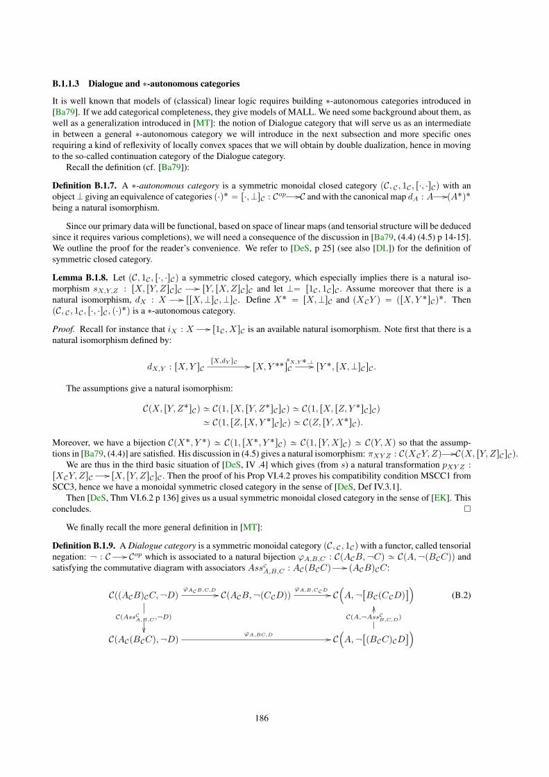
B.1.1.3 Dialogue and ˚-autonomous categories

It is well known that models of (classical) linear logic requires building ˚-autonomous categories introduced in[Ba79]. If we add categorical completeness, they give models of MALL. We need some background about them, aswell as a generalization introduced in [MT]: the notion of Dialogue category that will serve us as an intermediatein between a general ˚-autonomous category we will introduce in the next subsection and more specific onesrequiring a kind of reflexivity of locally convex spaces that we will obtain by double dualization, hence in movingto the so-called continuation category of the Dialogue category.

Recall the definition (cf. [Ba79]):

Definition B.1.7. A ˚-autonomous category is a symmetric monoidal closed category pC, C , 1C , r¨, ¨sCq with anobjectK giving an equivalence of categories p¨q˚ “ r¨,KsC : Cop //C and with the canonical map dA : A //pA˚q˚

being a natural isomorphism.

Since our primary data will be functional, based on space of linear maps (and tensorial structure will be deducedsince it requires various completions), we will need a consequence of the discussion in [Ba79, (4.4) (4.5) p 14-15].We outline the proof for the reader’s convenience. We refer to [DeS, p 25] (see also [DL]) for the definition ofsymmetric closed category.

Lemma B.1.8. Let pC, 1C , r¨, ¨sCq a symmetric closed category, which especially implies there is a natural iso-morphism sX,Y,Z : rX, rY, ZsCsC // rY, rX,ZsCsC and let K“ r1C , 1CsC . Assume moreover that there is anatural isomorphism, dX : X // rrX,KsC ,KsC . Define X˚ “ rX,KsC and pXCY q “ prX,Y ˚sCq

˚. ThenpC, C , 1C , r¨, ¨sC , p¨q

˚q is a ˚-autonomous category.

Proof. Recall for instance that iX : X // r1C , XsC is an available natural isomorphism. Note first that there is anatural isomorphism defined by:

dX,Y : rX,Y sCrX,dY sC // rX,Y ˚˚sC

sX,Y˚,K// rY ˚, rX,KsCsC .

The assumptions give a natural isomorphism:

CpX, rY, Z˚sCq » Cp1, rX, rY, Z˚sCsCq » Cp1, rX, rZ, Y ˚sCsCq

» Cp1, rZ, rX,Y ˚sCsCq » CpZ, rY,X˚sCq.

Moreover, we have a bijection CpX˚, Y ˚q » Cp1, rX˚, Y ˚sCq » Cp1, rY,XsCq » CpY,Xq so that the assump-tions in [Ba79, (4.4)] are satisfied. His discussion in (4.5) gives a natural isomorphism: πXY Z : CpXCY, Zq //CpX, rY, ZsCsCq.

We are thus in the third basic situation of [DeS, IV .4] which gives (from s) a natural transformation pXY Z :

rXCY, ZsC // rX, rY, ZsCsC . Then the proof of his Prop VI.4.2 proves his compatibility condition MSCC1 fromSCC3, hence we have a monoidal symmetric closed category in the sense of [DeS, Def IV.3.1].

Then [DeS, Thm VI.6.2 p 136] gives us a usual symmetric monoidal closed category in the sense of [EK]. Thisconcludes.

We finally recall the more general definition in [MT]:

Definition B.1.9. A Dialogue category is a symmetric monoidal category pC, C , 1Cq with a functor, called tensorialnegation: : C // Cop which is associated to a natural bijection ϕA,B,C : CpACB, Cq » CpA, pBCCqq andsatisfying the commutative diagram with associators AssCA,B,C : ACpBCCq // pACBqCC:

CppACBqCC, Dq

CpAssCA,B,C

, Dq

ϕACB,C,D // CpACB, pCCDqqϕA,B,CCD // C

´A,

“BCpCCDq

‰¯

CpACpBCCq, DqϕA,BC,D // C

´A,

“pBCCqCD

‰¯CpA, AssC

B,C,Dq

OO(B.2)

186

B.1.1.4 A model of MALL making appear the Arens dual and the Schwartz ε-product

We introduce a first ˚-autonomous category that captures categorically the part of [S] that does not use quasi-completeness. Since bornological and topological concepts are dual to one another, it is natural to fix a saturatedbornology on E in order to create a self-dual concept. Then, if one wants every object to be a dual object as ina ˚-autonomous category, one must consider only bornologies that can arise as the natural bornology on the dual,namely, the equicontinuous bornology. We could take a precompactness condition to ensure that, but to makeappear the Arens dual and ε-product (and not the polar topology and Meise’s variant of the ε-product), we useinstead a compactness condition. A weak-compactness condition would work for the self-duality requirement byMackey Theorem but not for dealing with tensor products.

We will thus use a (saturated, topological) variant of the notion of compactology used in [Ja, p 157]. We saythat a saturated bornology BE on a lcs E is a compactology if it consists of relatively compact sets. Hence, thebipolar of each bounded set for this bornology is an absolutely convex compact set in E, and it is bounded for thisbornology. A separated locally convex space with a compactology will be called a compactological locally convex

space.

Definition B.1.10. Let LCS be the category of separated locally convex spaces with continuous linear maps andCLCS the category of compactological locally convex spaces, with maps given by bounded continuous linearmaps. For E,F P CLCS the internal Hom LbpE,F q is the above set of maps given the topology of uniform con-vergence on the bornology of E and the bornology of equibounded equicontinuous sets. We call E1b “ LbpE,Kq(its bornology is merely the equicontinuous bornology, see step 1 of next proof). The algebraic tensor productEHF is the algebraic tensor product with the topology having the universal property for BE , BF -hypocontinuousmaps, and the bornology generated by bipolars of sets AC for A P BE , C P BF .

Note that we didn’t claim that EHF is in CLCS, it may not be. It gives a generic hypocontinuous tensorproduct. Note that composition of bounded continuous linear maps are of the same type, hence CLCS is indeed acategory.

Recall also that LCS is complete and cocomplete since it has small products and coproducts, kernels andcokernels (given by the quotient by the closure Imrf ´ gs) [K, 18.3.(1,2,5), 18.5.(1)].

In order to state simultaneously a variant adapted to Schwartz spaces, we introduce a variant:

Definition B.1.11. Let Sch Ă LCS be the full subcategory of Schwartz spaces and CSch Ă CLCS the fullsubcategory of Schwartz compactological lcs, namely those spaces which are Schwartz as locally convex spacesand for which E1b is a Schwartz lcs too.

This second condition is well-known to be equivalent to the bornology being a Schwartz bornology [HNM],and to a more concrete one:

Lemma B.1.12. For E P CLCS, E1b is a Schwartz lcs if and only if every bounded set in BE is included in theclosed absolutely convex cover of a BE-null sequence.

Proof. E1b is Schwartz if and only ifE1b “ S pE1bq.But S pE1bq is known to be the topology of uniform convergenceon pBEqc0 the saturated bornology generated by BE-null sequences of E “ pE1bq

1 [Ja, Prop 10.4.4]. Since bothbornologies are saturated this means [K, 21 .1. (4)] that E1b is a Schwartz space if and only if BE “ pBEqc0 .

We call SLbpE,F q the same lcs as LbpE,F q but given the bornology pBLbpE,F qqc0 namely the associatedSchwartz bornology. Note that SLbpE,Kq “ E1b as compactological lcs for E P CSch.

Theorem B.1.13. CLCS (resp. CSch) is a complete and cocomplete ˚-autonomous category with dualizing object

K and internal Hom LbpE,F q (resp. SLbpE,F q).

1. The functor p.q1c : LCS // CLCSop giving the Arens dual the equicontinuous bornology, is right adjoint to

Upp.q1bq, with U the underlying lcs and Upp.q1bq ˝ p.q1c “ IdLCS. The functor p.q1σ : LCS //CLCSop giving

the weak dual the equicontinuous bornology, is left adjoint to Upp.q1bq and Upp.q1bq ˝ p.q1σ “ IdLCS.

2. The functor U : CLCS // LCS is left adjoint and also left inverse to p.qc, the functor E ÞÑ Ec the space

with the same topology and the absolutely convex compact bornology. U is right adjoint to p.qσ , the functor

E ÞÑ Eσ the space with the same topology and the saturated bornology generated by finite sets. U, p.qc, p.qσare faithful.

187

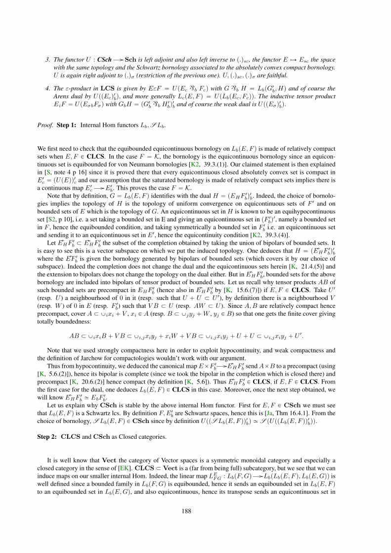
3. The functor U : CSch // Sch is left adjoint and also left inverse to p.qsc, the functor E ÞÑ Esc the space

with the same topology and the Schwartz bornology associated to the absolutely convex compact bornology.

U is again right adjoint to p.qσ (restriction of the previous one). U, p.qsc, p.qσ are faithful.

4. The ε-product in LCS is given by EεF “ UpEc `b Fcq with G `b H “ LbpG1b, Hq and of course the

Arens dual by UppEcq1bq, and more generally LcpE,F q “ UpLbpEc, Fcqq. The inductive tensor product

EiF “ UpEσbFσq with GbH “ pG1b `b H1bq1b and of course the weak dual is UppEσq

1bq.

Proof. Step 1: Internal Hom functors Lb,SLb.

We first need to check that the equibounded equicontinuous bornology on LbpE,F q is made of relatively compactsets when E,F P CLCS. In the case F “ K, the bornology is the equicontinuous bornology since an equicon-tinuous set is equibounded for von Neumann bornologies [K2, 39.3.(1)]. Our claimed statement is then explainedin [S, note 4 p 16] since it is proved there that every equicontinuous closed absolutely convex set is compact inE1c “ pUpEqq

1c and our assumption that the saturated bornology is made of relatively compact sets implies there is

a continuous map E1c // E1b. This proves the case F “ K.Note that by definition, G “ LbpE,F q identifies with the dual H “ pEHF

1bq1b. Indeed, the choice of bornolo-

gies implies the topology of H is the topology of uniform convergence on equicontinuous sets of F 1 and onbounded sets of E which is the topology of G. An equicontinuous set in H is known to be an equihypocontinuousset [S2, p 10], i.e. a set taking a bounded set in E and giving an equicontinuous set in pF 1bq

1, namely a bounded setin F , hence the equibounded condition, and taking symmetrically a bounded set in F 1b i.e. an equicontinuous setand sending it to an equicontinuous set in E1, hence the equicontinuity condition [K2, 39.3.(4)].

Let EpHF 1b Ă ErHF 1b the subset of the completion obtained by taking the union of bipolars of bounded sets. Itis easy to see this is a vector subspace on which we put the induced topology. One deduces that H “ pEpHF 1bq1bwhere the EpF 1b is given the bornology generated by bipolars of bounded sets (which covers it by our choice ofsubspace). Indeed the completion does not change the dual and the equicontinuous sets herein [K, 21.4.(5)] andthe extension to bipolars does not change the topology on the dual either. But in EpHF 1b, bounded sets for the abovebornology are included into bipolars of tensor product of bounded sets. Let us recall why tensor products AB ofsuch bounded sets are precompact in EHF 1b (hence also in EpHF 1b by [K, 15.6.(7)]) if E,F P CLCS. Take U 1

(resp. U ) a neighbourhood of 0 in it (resp. such that U ` U Ă U 1), by definition there is a neighbourhood V(resp. W ) of 0 in E (resp. F 1b) such that V B Ă U (resp. AW Ă U ). Since A,B are relatively compact henceprecompact, cover A Ă Yixi ` V , xi P A (resp. B Ă Yjyj `W , yj P B) so that one gets the finite cover givingtotally boundedness:

AB Ă YixiB ` V B Ă Yi,jxiyj ` xiW ` V B Ă Yi,jxiyj ` U ` U Ă Yi,jxiyj ` U1.

Note that we used strongly compactness here in order to exploit hypocontinuity, and weak compactness andthe definition of Jarchow for compactologies wouldn’t work with our argument.

Thus from hypocontinuity, we deduced the canonical mapEˆF 1b //EpHF 1b sendAˆB to a precompact (using[K, 5.6.(2)]), hence its bipolar is complete (since we took the bipolar in the completion which is closed there) andprecompact [K, 20.6.(2)] hence compact (by definition [K, 5.6]). Thus EpHF 1b P CLCS, if E,F P CLCS. Fromthe first case for the dual, one deduces LbpE,F q P CLCS in this case. Moreover, once the next step obtained, wewill know EpHF 1b » EbF

1b.

Let us explain why CSch is stable by the above internal Hom functor. First for E,F P CSch we must seethat LbpE,F q is a Schwartz lcs. By definition F,E1b are Schwartz spaces, hence this is [Ja, Thm 16.4.1]. From thechoice of bornology, SLbpE,F q P CSch since by definition UppSLbpE,F qq

1bq » S pUppLbpE,F qq

1bqq.

Step 2: CLCS and CSch as Closed categories.

It is well know that Vect the category of Vector spaces is a symmetric monoidal category and especially aclosed category in the sense of [EK]. CLCS Ă Vect is a (far from being full) subcategory, but we see that we caninduce maps on our smaller internal Hom. Indeed, the linear map LEFG : LbpF,Gq //LbpLbpE,F q, LbpE,Gqq iswell defined since a bounded family in LbpF,Gq is equibounded, hence it sends an equibounded set in LbpE,F qto an equibounded set in LbpE,Gq, and also equicontinuous, hence its transpose sends an equicontinuous set in

188

pLbpE,Gqq1 (described as bipolars of bounded sets in E tensored with equicontinuous sets in G1) to an equicon-

tinuous set in pLbpE,F qq1. This reasoning implies LEFG is indeed valued in continuous equibounded maps andeven bounded with our choice of bornologies. Moreover we claim LEFG is continuous. Indeed, an equicontinuousset in pLbpLbpE,F q, LbpE,Gqqq1 is generated by the bipolar of equicontinuous C set in G1, a bounded set B in Eand an equibounded set A in pLbpE,F qq and the transpose consider ApBq Ă F and C to generate a bipolar whichis indeed equicontinuous in pLbpF,Gqq1. Hence, LEFG is a map of our category. Similarly, the morphism givingidentity maps jE : K // LbpE,Eq is indeed valued in the smaller space and the canonical iE : E // LbpK, Eqindeed sends a bounded set to an equibounded equicontinuous set and is tautologically equicontinuous. Now allthe relations for a closed category are induced from those in Vect by restriction. The naturality conditions areeasy.

Let us deduce the case of CSch. First, let us see that for E P CSch,

SLbpE,SLbpF,Gqq “ SLbpE,LbpF,Gqq (B.3)

By definition of boundedness, a map f P LbpE,LbpF,Gqq sends a Mackey-null sequence in E to a Mackey-null sequence inLbpF,Gq hence by continuity the bipolar of such a sequence is sent to a bounded set in SLbpF,Gq,hence from lemma B.1.12, so is a bounded set in E. We deduce the algebraic equality in (B.3). The topology ofLbpE,Hq only depends on the topology ofH , hence we have the topological equality since both target spaces havethe same topology. It remains to compare the bornologies. But from the equal target topologies, again, the equicon-tinuity condition is the same on both spaces hence boundedness of the mapLbpE,SLbpF,Gqq //LbpE,LbpF,Gqqis obvious. Take a sequence fn of maps Mackey-null in LbpE,LbpF,Gqq hence in the Banach space generatedby the Banach disk D of another Mackey-null sequence pgnq. Let us see that tgn, n P N uoo is equiboundedin LbpE,SLbpF,Gqq. For take B Ă LbpE,LbpF,Gqq the disk for pgnq with ||gn||B // 0 and take a typicalgenerating bounded set A “ txn, n P N uoo Ă E for xn BE-Mackey-null. Then gnpAq Ă tgmpxnq,m, n PN uoo “: C and ||gmpxnq||pBpAqqoo ď ||gm||B ||xn||A and since BpAq is bounded by equiboundedness of B,pgmpxnqq is Mackey-null, hence C is bounded in SLbpF,Gq and hence D “ tgn, n P N uoo is equiboundedas stated. But since D is also bounded in LbpE,LbpF,Gqq it is also equicontinuous, hence finally, bounded inLbpE,SLbpF,Gqq. This gives that fn Mackey-null there which concludes to the bornological equality in (B.3).

As a consequence, for E,F,G P CSch, the previous map LEFG induces a map

LEFG : SLbpF,Gq // SLbpLbpE,F q, LbpE,Gqq // SLbpSLbpE,F q, LbpE,Gqq

“ SLbpSLbpE,F q,SLbpE,Gqq

coinciding with the previous one as map. Note that we used the canonical continuous equibounded mapLbpLbpE,F q, Gq //LbpSLbpE,obviously given by the definition of associated Schwartz bornologies which is a smaller bornology.

Step 3: ˚-autonomous property.

First note that LbpE,F q » LbpF1b, E

1bq by transposition. Indeed, the space of maps and their bornologies are the

same since equicontinuity (resp. equiboundedness) E // F is equivalent to equiboundedness (resp. equiconti-nuity) of the transpose F 1b // E1b for equicontinuous bornologies (resp. for topologies of uniform convergence ofcorresponding bounded sets). Moreover the topology is the same since it is the topology of uniform convergence onbounded sets of E (identical to equicontinuous sets of pE1bq

1) and equicontinuous sets of F 1 (identical to boundedsets for F 1b). Similarly SLbpE,F q » SLbpF

1b, E

1bq since on both sides one considers the bornology generated by

Mackey-null sequences for the same bornology.It remains to check LbpE,LbpF,Gqq » LbpF,LbpE,Gqq. The map is of course the canonical map. Equi-

boundedness in the first space means sending a bounded set in E and a bounded set in F to a bounded set in Gand also a bounded set in E and an equicontinuous set in G1 to an equicontinuous set in F 1. This second conditionis exactly equicontinuity F // LbpE,Gq. Finally, analogously, equicontinuity E // LbpF,Gq implies it sendsa bounded set in F and an equicontinuous set in G1 to an equicontinuous set in E1 which was the missing part ofequiboundedness in LbpF,LbpE,Gqq. The identification of spaces and bornologies follows. Finally, the topologyon both spaces is the topology of uniform convergence on products of bounded sets of E,F .

Again, the naturality conditions of the above two isomorphisms are easy, and the last one induces from Vect

again the structure of a symmetric closed category, hence lemma B.1.8 concludes to CLCS ˚-autonomous.Let us prove the corresponding statement for CSch. Note that (B.3) implies the compactological isomorphism

SLbpE,SLbpF,Gqq » SLbpE,LbpF,Gqq » SLbpF,LbpE,Gqq » SLbpF,SLbpE,Gqq.

189

Hence, application of lemma B.1.8 concludes in the same way.

Step 4: Completeness and cocompleteness.

Let us describe first coproducts and cokernels. This is easy in CLCS it is given by the colimit of separatedlocally convex spaces, given the corresponding final bornology. Explicitely, the coproduct is the direct sum ofvector spaces with coproduct topology and the bornology is the one generated by finite sum of bounded sets,hence included in finite sums of compact sets which are compact [K, 15.6.(8)]. Hence the direct sum is in CLCS

and clearly has the universal property from those of topolocial/bornological direct sums. For the cokernel off, g : E // F , we take the coproduct in LCS, Cokerpf, gq “ F pf ´ gqpEq with the final bornology, i.e. thebornology generated by images of bounded sets. Since the quotient map is continuous between Hausdorff spaces,the image of a compact containing a bounded set is compact, hence Cokerpf, gq P CLCS. Again the universalproperty comes from the one in locally convex and bornological spaces. Completeness then follows from the˚-autonomous property since one can see limiEi “ pcolimipEiq

1bq1b gives a limit.

Similarly in CSch the colimit of Schwartz bornologies is still Schwartz since the dual is a projective limit ofSchwartz spaces hence a Schwartz space (cf lemma B.1.18). We therefore claim that the colimit is the Schwartztopological space associated to the colimit in CLCS with same bornology. Indeed this is allowed since there aremore compact sets hence the compatibility condition in CLCS is still satisfied and functoriality of S in lemmaB.1.18 implies the universal property.

Step 5: Adjunctions and consequences.

The fact that the stated maps are functors is easy. We start by the adjunction for U in (2): LCSpUpF q, Eq “LbpF,Ecq “ CLCSpF,Ecq since the extra condition of boundedness beyond continuity is implied by the fact thata bounded set in F is contained in an absolutely convex compact set which is sent to the same kind of set by acontinuous linear map. Similarly, LCSpE,UpF qq “ LbpEσ, F q “ CLCSpEσ, F q since the image of a finiteset is always in any bornology (which must cover E and is stable by union), hence the equiboundedness is alsoautomatic.

For p3q, since pEσq1b “ E1σ is always Schwartz, the functor p.qσ restricts to the new context, hence the ad-junction. Moreover UppEcq1bq “ S pE1cq by construction. The key identity SchpUpF q, Eq “ LbpF,Ecq “CSchpF,Escq comes from the fact that a Mackey-null sequence in F is send by a continuous function to aMackey-null sequence for the compact bornology hence to a bounded set in Esc. All naturality conditions areeasy.

Moreover, for the adjunction in (1), we have the equality as set (using involutivity and functoriality of p.q1b andthe previous adjunction):

CLCSoppF,E1cq “ LbppEcq1b, F q “ LbpF

1b, Ecq “ LCSpUpF 1bq, Eq,

CLCSoppE1σ, F q “ LbpF, pEσq1bq “ LbpEσ, F

1bq “ LCSpE,UpF 1bqq.

The other claimed identities are obvious by definition.

The second named author explored in [Ker] models of linear logic using the positive product i and p.q1σ . Wewill use in this work the negative product ε and the Arens dual p.q1c appearing with a dual role in the previous result.Let us summarize the properties obtained in [S] that are consequences of our categorical framework.

Corollary B.1.14. 1. LetEi P LCS, i P I. The iterated ǫ-product is εiPIEi “ Up`b,iPIpEiqcq, it is symmetricin its arguments and commute with limits.

2. There is a continuous injection pE1εE2εE3q // E1εpE2εE3q.

3. For any continuous linear map f : F1// E1 (resp. continuous injection, closed embedding), so is fεId :

F1εE2// E1εE2.

Note that (3) is also valid for non-closed embeddings and (2) is also an embedding [S], but this is not acategorical consequence of our setting.

190

Proof. The equality in (1) is a reformulation of definitions, symmetry is an obvious consequence. Commutationwith limits come from the fact that U, pqc are right adjoints and `b commutes with limits from universal properties.

Using associativity of `b: E1εpE2εE3q “ UppE1qc `b rUppE2qc `b pE3qcqscq hence functoriality and thenatural transformation coming from adjunction Id // pUp¨qqc concludes to the continuous map in (2). It ismoreover a monomorphism since E // pUpEqqc is one since UpEq // UppUpEqqcq is identity and U reflectsmonomorphisms and one can use the argument for (3).

For (3) functorialities give definition of the map, and recall that closed embeddings in LCS are merely regularmonomorphisms, hence a limit, explaining its commutation by (1). If f is a monomomorphism, in categoricalsense, so is Upfq using a right inverse for U and so is pfqc since Uppfqcq “ f and U reflects monomorphisms asany faithful functor. Hence it suffices to see `b preserves monomorphisms but g1, g2 : X // E `b F correspondby Cartesian closedness to mapsXbF

1b

//E that are equal when composed with f : E //G if f monomorphism,hence so is f `b idF .

In general, we have just seen that ε has features for a negative connective as `, but it lacks associativity. Wewill have to work to recover a monoidal category, and then models of LL. In that respect, we want to make our fixof associativity compatible with a class of smooth maps, this will be the second leitmotiv. We don’t know if thereis an extension of the model of MALL given by CLCS into a model of LL using a kind of smooth maps.

B.1.2 Mackey-complete spaces and a first interpretation for `

Towards our goal of obtaining a model of LL with conveniently smooth maps as non-linear morphisms, it is naturalto follow [53] and consider Mackey-complete spaces as in [6, KT]. In order to fix associativity of ε in this context,we will see appear the supplementary Schwartz condition. This is not such surprising as seen the relation withMackey-completeness appearing for instance in [Ja, chap 10] which treats them simultaneously. This Schwartzspace condition will enable to replace Arens duals by Mackey duals (lemma B.1.19) and thus simplify lots ofarguments in identifying duals as Mackey-completions of inductive tensor products (lemma B.1.23). This willstrongly simplify the construction of the strength for our doubly negation monad later in section B.1.4. Technically,this is possible by various results of [K] which points out a nice alternative tensor product η which replaces ε-product exactly in switching Arens with Mackey duals. But we need to combine η with S in a clever way in yetanother product ζ in order to get an associative product. Said in words, this is a product which enables to ensureat least two Schwartz spaces among three in an associativity relation. This technicality is thus a reflection of thefact that for Mackey-complete spaces, one needs to have at least 2 Schwartz spaces among three to get a 3 termassociator for an ε-product. In course of getting our associativity, we get the crucial relation S pS pEqεF q “S pEqεS pF q in corollary B.1.24. This is surprising because this seems really specific to Schwartz spaces and weare completely unable to prove an analogue for the associated nuclear topology functor N , even if we expect it forthe less useful associated strongly nuclear topology. We conclude in Theorem B.1.26 with our first interpretationof ` as ζ.

B.1.2.1 A Mackey-Completion with continuous canonical map

Note that for a γ-Mackey-Cauchy sequence, topological convergence is equivalent to Mackey convergence (sincethe class of bounded sets is generated by bounded closed sets).

Remark B.1.15. Note also that is E Ă F is a continuous inclusion, then a Mackey-Cauchy/convergent sequencein E is also Mackey-Cauchy/convergent in F since a linear map is bounded.

We now recall two alternative constructions of the Mackey-completion, from above by intersection and frombelow by union. The first construction is already considered in [PC].

Lemma B.1.16. The intersection pEM of all Mackey-complete spaces containing E and contained in the comple-tion E of E, is Mackey-complete and called the Mackey-completion of E.

We define EM ;0 “ E, and for any ordinal λ, the subspace EM ;λ`1 “ Ypxnqně0PMpEM;λqΓptxn, n ě 0uq Ă E

where the union runs over all Mackey-Cauchy sequences MpEM ;λq of EM ;λ, and the closure is taken in thecompletion. We also let for any limit ordinal EM ;λ “ YµăλEM ;µ. Then for any ordinal λ, EM ;λ Ă pEM andeventually for λ ě ω1 the first uncountable ordinal, we have equality.

Proof. The first statement comes from stability of Mackey-completeness by intersection (using remark B.1.15). Itis easy to see that EM ;λ is a subspace. At stage EM ;ω1`1, by uncountable cofinality of ω1 any Mackey-Cauchy

191

sequence has to be in EM ;λ for some λ ă ω1 and thus each term of the union is in some EM ;λ`1, thereforeEM ;ω1`1 “ EM ;ω1

.

Moreover if at some λ, EM ;λ`1 “ EM ;λ, then by definition, EM,λ is Mackey-complete (since we add withevery sequence its limit that exists in the completion which is Mackey-complete) and then the ordinal sequence iseventually constant. Then, we have EM,λ Ą pEM . One shows for any λ the converse by transfinite induction. For,let pxnqně0 is a Mackey-Cauchy sequence inEM ;λ Ă F :“ pEM . ConsiderA a closed bounded absolutely convexset in F with xn // x in FA. Then by [Ja, Prop 10.2.1], FA is a Banach space, thus Γptxn, n ě 0uq computed inthis space is complete and thus compact (since txu Y txn, n ě 0u is compact in the Banach space), thus its imagein E is compact and thus agrees with the closure computed there. Thus every element of Γptxn, n ě 0uq is a limitin EA of a sequence in Γptxn, n ě 0uq Ă EM ;λ thus by Mackey-completeness, Γptxn, n ě 0uq Ă F. We thusconclude to the successor step EM ;λ`1 Ă pEM , the limit step is obvious.

B.1.2.2 A ` for Mackey-complete spaces

We first define a variant of the Schwartz ǫ-product:

Definition B.1.17. For two separated lcs E and F , we define EηF “ LpE1µ, F q the space of continuous lin-ear maps on the Mackey dual with the topology of uniform convergence on equicontinuous sets of E1. Wewrite ηpE,F q “ pE1µβeF

1µq1 with the topology of uniform convergence on products of equicontinuous sets

and ζpE,F q ” EζF for the same space with the weakest topology making continuous the canonical maps toηpS pEq, F q and ηpE,S pF qq.

This space EηF has already been studied in [K2] and we can summarize its properties similar to the Schwartzǫ product in the next proposition, after a couple of lemmas.

We first recall an important property of the associated Schwartz topology from [45]. These properties followfrom the fact that the ideal of compact operators on Banach spaces in injective, closed and surjective. Especially,from [45, Corol 6.3.9] it is an idempotent ideal.

Lemma B.1.18. The associated Schwartz topology functor S commutes with arbitrary products, quotients andembeddings (and as a consequence with arbitrary projective kernels or categorical limits).

Proof. For products and (topological) quotients, this is [45, Prop 7.4.2]. For embeddings (that he calls topologicalinjections), this is [45, Prop 7.4.8] based on the previous ex 7.4.7. The consequence comes from the fact that anyprojective kernel is a subspace of a product, as a categorical limit is a kernel of a map between products.

We will also often use the following relation with duals

Lemma B.1.19. If E is a Schwartz lcs, E1c » E1µ so that for any lcs F , EηF » EεF topologically. Thus for anylcs E, E1µ » pS pEqq1c.

Proof. Take K an absolutely convex σpE1, Eq-weakly compact in E, it is an absolutely convex closed set in Eand precompact as any bounded set in a Schwartz space [Ho, 3, 15 Prop 4]. [Bo2, IV.5 Rmq 2] concludes to Kcomplete since E // pE1µq

1σ continuous with same dual and K complete in pE1µq

1σ , and since K precompact, it is

therefore compact in E. As a consequence E1c is the Mackey topology. Hence, EηF “ LpE1µ, F q “ LpE1c, F q “EεF algebraically and the topologies are defined in the same way. The last statement comes from the first andE1µ » pS pEqq1µ.

Proposition B.1.20. Let E,F,G,H , be separated lcs, then:

1. We have a topological canonical isomorphisms ζpE,F q “ ζpF,Eq,

EηF “ FηE » ηpE,F q

and we have a continuous linear map EεF //EηF //EζF which is a topological isomorphism as soon

as either E or F is a Schwartz space. In general, EεF is a closed subspace of EηF .

2. EηF is complete if and only if E and F are complete.

3. If A : G // E, B : H // F are linear continuous (resp. linear continuous one-to-one, resp. embeddings)

so are the tensor product map pAηBq, pAζBq both defined by pAηBqpfq “ B ˝ f ˝At, f P LpE1µ, F q.

192

4. IfF “ KiPIpAiq´1Fi is a projective kernel so areEηF “ KiPIp1ηAiq

´1EηFi andEζF “ KiPIp1ζAiq´1EζFi.

Moreover, both η, ζ, ε commute with categorical limits in LCS.

5. ηpE,F q is also the set of bilinear forms on E1µ ˆ F 1µ which are separately continuous. As a consequence,

the Mackey topology ppE1µβeF1µq1µq1µ “ E1µiF

1µ is the inductive tensor product.

6. A set is bounded in ηpE,F q or ζpE,F q if and only if it is ǫ-equihypocontinuous on E1β ˆ F1β .

Proof. It is crucial to note that ηpE,F q, ηpS pEq, F q, ηpE,S pF qq are the same space algebraically since pS pEqq1µ »E1µ.

(2) is [K, 40.4.(5)] and (1) is similar to the first statement there. With more detail functoriality of Mackey dualgives a mapLpE1µ, F q //LpF 1µ, pE

1µq1µq and since pE1µq

1µ

//E continuous we have also a mapLpF 1µ, pE1µq1µq //LpF 1µ, Eq.

This explains the first map of the first isomorphism (also explained in [Ja, Corol 8.6.5]). The canonical linear mapfrom a bilinear map in ηpE,F q is clearly in EηF , conversely, if A P EηF , xAp.q, .yF,F 1 is right ǫ-hypocontinuousby definition and the other side of the hypocontinuity comes from the At P FηE.

The closed subspace property is [K2, 43.3.(4)].(3) for η is [K2, 44.4.(3,5,6)]. For ζ since A,B are continuous after taking the functor S , one deduces AηB

is continuous (resp one-to-one, resp. an embedding using lemma B.1.18) on

ηpS pGq, Hq // ηpS pEq, F q, ηpG,S pHqq // ηpE,S pF qq

and this conclude by universal properties of projective kernels (with two terms) for ζ. Since the spaces are thesame algebraically, the fact that the maps are one-to-one also follows.

(4) The η case with kernels is a variant of [K2, 44.5.(4)] which is also a direct application of [K2, 39.8.(10)].As a consequence EζF is a projective kernel of S pEqηF “ KiPIp1ηAiq

´1rS pEqsηFi and, using lemma B.1.18again, of :

EηS pF q “ Eη´KiPIA

´1i S pFiq

¯“ KiPIp1ηAiq

´1`EηS pFiq

˘.

The transitivity of locally convex kernels (coming from their universal property) concludes.For categorical limits, it suffices commutation with products and kernels. In any case the continuous map

I : plimEiqηF // limpEiηF q comes from universal properties , it remains to see it is an algebraic isomor-phism, since then the topological isomorphism will follow from the kernel case. We build the inverse as fol-lows, for f P F 1µ, the continuous evaluation map EiηF “ LpF 1µ, Eiq // Ei induces a continuous linear mapJf : limpEiηF q // plimEiq. It is clearly linear in f and gives a bilinear map J : limpEiηF q ˆ F

1µ

// plimEiq.We have to see it is separately continuous yielding a linear inverse map I´1 and then continuity of this map. Wedivide into the product and kernel case.

For products one needs for g PśiPIpEiηF q Jpg, .q

t : pśiPI Eiq

1 // pF 1µq1 send equicontinuous sets i.e.

a finite sum of equicontinuous set in the sumřiPI E

1i to an equicontinuous set in pF 1µq

1. But absolutely convexweakly compact sets are stable by bipolars of sum, since they are stable by bipolars of finite unions [K, 20.6.(5)](they don’t even need closure to be compact, absolutely convex cover is enough), hence it suffices to see the caseof images of equicontinuous setsE1i //F but they are equicontinuous by assumption. This gives the separate con-tinuity in this case. Similarly, to see the continuity of I´1 in this case means that we take A Ă F 1 equicontinuousand a sum of equicontinuous sets Bi in p

śiPI Eiq

1 and one notices that pI´1qtpA ˆřBiq Ă

řpI´1qtpA ˆ Biq

is a sum of equicontinuous sets in pśiPIpEiηF qq

1 and it is by hypothesis equicontinuous.For kernels, of f, g : E // G, I : Kerpf ´ gqηF // KerpfηidF ´ gηidF q is an embedding by (3)

since source and target are embeddings in EηF , the separate continuity is obtained by restriction of the one ofEηF ˆ F 1µ // E Ą Kerpf ´ gq and similarly continuity by restriction of EηF // LpF 1µ, Eq.

For ζ, this is then a consequence of this and lemma B.1.18 again. (5) is an easier variant of [S, Rmq 1 p 25].Of course ηpE,F q is included in the space of separately continuous forms. Conversely, if f : E1µ ˆ F 1µ

// Kis separately continuous, from [Ja, Corol 8.6.5], it is also separately continuous on E1σ ˆ F 1σ and the non-trivialimplication follows from [K, 40.4.(5)]. For the second part, the fact that both algebraic tensor products havethe same dual implies there is, by Arens-Mackey Theorem, a continuous identity map ppE1µβeF

1µq1µq1µ

// E1µiF1µ.

Conversely, one uses the universal property of the inductive tensor product which gives a separately continuous mapE1µˆF

1µ

//E1µβeF1µ. But applying functoriality of Mackey duals on each side gives for each x P E1µ a continuous

map F 1µ // ppE1µβeF1µq1µq1µ and by symmetry, a separately continuous map E1µ ˆ F 1µ

// ppE1µβeF1µq1µq1µ. The

universal property of the inductive tensor product again concludes.(6) can be obtained for η with the same reasoning as in [K2, 44.3.(1)]. For ζ the first case gives by definition

equivalence with ǫ-equihypocontinuity both on pS pEqq1βˆF1β and onE1βˆpS pF qq1β . But the second implies that

193

for equicontinuous on E’, one gets an equicontinuous family on pS pF qq1β » F 1β and the first gives the converse,and the other conditions are weaker, hence the equivalence with the first formulation.

We then deduce a Mackey-completeness result:

Proposition B.1.21. If L1 and L2 are separated Mackey-complete locally convex spaces, then so are L1ηL2 and

L1ζL2.

Proof. Since both topologies on the same space have the same bounded sets (proposition B.1.20.(6)), it sufficesto consider L1ηL2. Consider a Mackey-Cauchy sequence pxnqně0, thus topologically Cauchy. By completenessof the scalar field, xn converges pointwise to a multilinear form x on

ś2

i“1pLiq1µ. Since the topology of the

η-product is the topology of uniform convergence on products of equicontinuous parts (which can be assumedabsolutely convex and weakly compact), xn // x uniformly on these products (since pxnq Cauchy in the Banachspace of continuous functions on these products). From proposition B.1.20.(5) we only have to check that thelimit x is separately continuous. For each y P pL2q

1, and B a bounded set in L1ηL2 “ LppL2q1µ, L1q, one

deduces Bpyq is bounded in ppL1q1µq1 “ L1 with its original topology of convergence on equicontinuous sets

of L11. Therefore, pxnpyqq is Mackey-Cauchy in L1, thus Mackey-converges, necessarily to xpyq. Therefore xpyqdefines an element of ppL1q

1µq1. With the similar symmetric argument, x is thus separately continuous, as expected.

We have thus obtained the topological convergence of xn to x in L1ηL2. It is easy to see xn Mackey convergesto x in L1ηL2 in taking the closure of the bounded set from its property of being Mackey-Cauchy. Indeed, theestablished topological limit xn // x transfers the Mackey-Cauchy property in Mackey convergence as soon asthe bounded set used in Mackey convergence is closed.

We will need the relation of Mackey duals and Mackey completions:

Lemma B.1.22. For any separated lcs F , we have a topological isomorphism ppF 1µq1µqM

» pp pFM q1µq1µ.

Proof. Recall also from [K, 21.4.(5)] the completion of the Mackey topology has its Mackey topology ČppF 1µq1µq “pp rF q1µq1µ therefore an absolutely convex weakly compact set in F 1 coincide for the weak topologies induced by F

and rF and therefore also FM , which is in between them. Thus the continuous inclusions ppF 1µq1µq //pFM q1µq

1µ

//pp rF q1µq1µhave always the induced topology. In the transfinite description of the Mackey completion, the Cauchy sequencesand the closures are the same in pp rF q1µq1µ and rF (since they have same dual hence same bounded sets), thereforeone finds the stated topological isomorphism.

Lemma B.1.23. If L,M are separated locally convex spaces we have embeddings:

L1µβeM1µ

// pLζMq1ǫ // pLηMq1ǫ // L1µrβeM 1µ,

with the middle duals coming with their ǫ-topology as biduals of L1µβeM1µ. The same holds for:

L1µiM1µ

// pLηMq1µ // L1µriM 1µ.

Finally, pLηMq1ǫ Ă L1µpMβeM 1µ as soon as either L or M is a Schwartz space, and in any case we have pLζMq1ǫ Ă

L1µpMβeM 1µ.

Proof. Step 1: First line of embeddings.

From the identity continuous map LηM // LζM , there is an injective linear map pLζMq1 // pLηMq1. Notethat, on L1µM

1µ, one can consider the strongest topology weaker than pS pLqq1µβeM

1µ and L1µβepS pMqq1µ. Let

us call it L1µζM1µ and see it is topologically equal to L1µβeM

1µ by checking its universal property. We know

by definition the map L1µζM1µ

// L1µβeM1µ. Conversely, there is an ε-equihypocontinuous map pS pLqq1µ ˆ

M 1µ

//L1µζM1µ so that for every equicontinuous set inM 1, the corresponding family is equicontinuous pS pLqq1µ “

L1µ//L1µζM

1µ from the topological equality. Similarly, by symmetry, one gets for every equicontinuous set in L1µ,

an equicontinuous family of maps M 1µ

// L1µζM1µ. As a consequence, the universal property gives the expected

map L1µβeM1µ

//L1µζM1µ concluding to equality. As a consequence, since by definition pL1µζM

1µq1 “ LζM is the

dual kernel for the hull defining the ζ tensor product, one gets that an equicontinuous set in the kernel is exactly an

194

equicontinuous set in pL1µζM1µq1 “ pL1µβeM

1µq1 namely an ǫ-equihypocontinuous family. This gives the continuity

of our map pLζMq1ǫ // pLηMq1ǫ and even the embedding property (if we see the first as bidual of L1µζM1µ but we

only stated an obvious embedding in the statement).We deduce that L1µβeM

1µ » L1µζM

1µ

// pLζMq1ǫ is an embedding from [K, 21.3.(2)] which proves that theoriginal topology on a space is the topology of uniform convergence on equicontinuous sets.

We then build a continuous linear injection pLηMq1ǫ // L1µrβeM 1µ to the full completion.Since both spaces

have the same dual, it suffices to show that the topology on LηM is stronger than Grothendieck’s topologyIlf pL1µβeM

1µq following [K] in notation. Indeed, let C in LηM equicontinuous. Assume a net in C con-

verges pointwise xn // x P C in the sense xnpa, bq // xpa, bq, a P L1µ, b P M 1µ. For equicontinuous sets

A Ă L1µ, B ĂM 1µ which we can assume absolutely convex weakly compact, it is easy to see C is equicontinuous

on products AˆB. Thus it is an equicontinuous bounded family in C0pAˆBq thus relatively compact by Arzela-Ascoli Theorem [Ho, 3.9 p237]. Thus since any uniformly converging subnet converges to x, the original net mustconverge uniformly on A ˆ B to x. As a consequence the weak topology on C coincides with the topology ofLηM , and by definition we have a continuous identity map, pLηM, Ilf pL1cβeM

1cqq // LηM . By Grothendieck’s

construction of the completion, the dual of the first space is the completion and this gives the expected injectionbetween duals. Since a space and its completion induce the same equicontinuous sets, one deduces the continuityand induced topology property with value in the full completion.

Step 2: Second line of embeddings.

It suffices to apply pp.q1µq1µ to the first line. We identified the first space in proposition B.1.20.(5) and the last

space as the completion of the first (hence of the second and this gives the induced topologies) in the proof oflemma B.1.22.

Step 3: Reduction of computation of Mackey completion to the Schwartz case.

It remains to see the pLζMq1ǫ is actually valued in the Mackey completion.Note that as a space, dual of a projective kernel, pLζMq1ǫ is the inductive hull of the mapsA “ pS pLqεMq1ǫ //pLζMq1ǫ “

C and B “ pLεS pMqq1ǫ // pLζMq1ǫ “ C. Therefore, it suffices to check that the algebraic tensor product isMackey-dense in both these spaces A,B that span C since the image of a bounded set in A,B being bounded inC, there are less Mackey-converging sequences in A,B. This reduces the question to the case L or M a Schwartzspace. By symmetry, we can assume L is.

Step 4: Description of the dual pLζMq1 “ pLεMq1 for L Schwartz and conclusion.

We take inspiration from the classical description of the dual of the injective tensor product as integral bilinearmaps (see [K2, 45.4]). As in [S, Prop 6], we know any equicontinuous set (especially any point) in pLεMq1 isincluded in the absolutely convex weakly closed hull Γ of AB with A equicontinuous in L1, B in M 1. Since thedual of L1µpMβeM 1

µ is the same, this weakly closed hull can be computed in this space too. Moreover, since L isa Schwartz space, we can and do assume that A “ txn, n P N u is a ǫ-Mackey-null sequence in L1µ, since theygenerate the equicontinuous bornology as a saturated bornology. We can also assume A,B are weakly compactand B absolutely convex.

Any element f P LεM defines a continuous map on A ˆ B (see e.g. [S, Prop 2] and following remark). Weequip A ˆ B with the above weakly compact topology to see f |AˆB P C0pA ˆ Bq. For µ a (complex) measureon Aˆ B (i.e. µ P pC0pAˆ Bqq1, we use measures in the Bourbaki’s sense, which define usual Radon measures[S4]) with norm ||µ|| ď 1 so that

şAˆB

fpzqdµpzq “ µpf |AˆBq “: wµpfq make sense.Note that |wµpfq| ď ||f ||C0pAˆBq which is a seminorm of the ǫ-product, so that µ defines a continuous linear

map wµ P pLεMq1. Note also that if f is in the polar of AB, so that |wµpfq| ď 1 and thus by the bipolar theorem,wµ P Γ. We want to check the converse that any element of w P Γ comes from such a measure. But if H is thesubspace of C0pAˆBqmade of restrictions of functions f P LεM , w induces a continuous linear map on H with|wpfq| ď ||f ||C0pAˆBq, Hahn-Banach theorem enables to extend it to a measure wµ, ||µ|| ď 1. This concludes tothe converse.

195

Define the measure µn byşAˆB

fpzqdµnpzq “1

µp1txnuˆBq

şAˆB

fpzq1txnuˆBpzqdµpzq using its canonicalextension to semicontinuous functions. Note that by Lebesgue theorem (dominated by constants)

wµpfq “8ÿ

n“0

µp1txnuˆBqqwµnpfq

As above one sees that the restriction of wµnto f P LεM belongs to the weakly closed absolute convex hull of

txnu ˆB. Thus since B absolutely convex closed wµnpfq “ fpxn b ynq for some yn P B. We thus deduces that

any wµ P Γ has the form:wµpfq “ř8n“0 µp1txnuˆBqqfpxn b ynq. Since the above convergence holds for any f ,

this means the convergence in the weak topology:

wµ “8ÿ

n“0

µp1txnuˆBqqxn b yn. (B.4)

Let D the equicontinuous closed disk such that xn tends to 0 in pL1qD. Consider the closed absolutely convexcover Λ “ ΓpDBq. The closed absolutely convex cover can be computed in pLεMq1ǫ or pLεMq1σ , both spaceshaving same dual [K, 20.7.(6) and 8.(5)], and DB being equicontinuous [S, Corol 4 p 27, Rmq p 28], so is Λ [K,21.3.(2)] hence it is weakly compact by Mackey Theorem, so complete in pLεMq1ǫ [Bo2, IV.5 Rmq 2], so that Λ istherefore a Banach disk there. But ||xnyn||pLεMq1

Λď 1 so that since

ř8n“0 |µp1txnuˆBqq| ď 1 the above series is

summable in pLεMq1Λ and thus Mackey converges in pLεMq1ǫ. As a conclusion, Γ Ă L1µpMβeM 1µ and this gives the

final statement.

The above proof has actually the following interesting consequence:

Corollary B.1.24. For any E,F separated locally convex spaces, we have the topological isomorphism:

S

´rS pEqsεF

¯“ rS pEqsεrS pF qs.

Proof. We have the canonical continuous map rS pEqsεF // rS pEqsεrS pF qs, hence since the ε-product ofSchwartz spaces is Schwartz (see below proposition B.1.50), one gets by functoriality the first continuous linearmap:

S

´rS pEqsεF

¯// rS pEqsεrS pF qs. (B.5)

Note that we have the algebraic equality rS pEqsεF “ LpE1µ, F q “ LpE1µ,S pF qq “ rS pEqsεrS pF qswhere the crucial middle equality comes from the map (see [Ja, Corol 8.6.5])

LpE1µ, F q “ LpE1µ, pF1µq1µq “ LpE1µ, prS pF qs1µq

1µq “ LpE1µ,S pF qq.

To prove the topological equality, we have to check the duals are the same with the same equicontinuous sets.We can apply the proof of the previous lemma (and we reuse the notation there) with L “ S pEq, M “ F orM “ rS pF qs. First the space in which the Mackey duals are included L1µriM 1

µ is the same in both cases, and theduals are described as union of absolutely convex covers, it suffices to see those unions are the same to identify

the duals. Of course, the transpose of (B.5) gives´rS pEqsεrS pF qs

¯1Ă

´rS pEqsεF

¯1so that we have to show

the converse. From (B.4) and rewriting xnyn as 1λnxnλnyn with λn “

b||xn||L1

C, one gets that both sequences

x1n “ p 1λnxnq, y

1npµq “ pλnynq are null sequences for the equicontinuous bornology of E1, F 1 and therefore

included in equicontinuous sets for the duals of associated Schwartz spaces. This representation therefore givesthe equality of duals. Finally, to identify equicontinuous sets, in the only direction not implied by (B.5), we mustsee that an ε-null sequence wνn of linear forms in the dual is included in the closed absolutely convex cover of atensor product of two such sequences in rS pEqs1, rS pF qs1. From the null convergence, νn can be taken measureson the same A ˆ B, for each νn, we have a representation wνn “

řzmpνnqx

1my

1mpνnq where x1m is a fixed

sequence and py1mpνnqqm are null sequences in the same Banach space M 1B . Moreover

ř|zmpνnq| ď ||νn|| // 0

from the assumption that νn is a null sequence in the Banach space generated by Γ (we can assume ||νn|| ‰ 0

otherwise wνn “ 0). Therefore, we rewrite, the series as wνn “ř

1||νn||

zmpνnqx1my

1mpνnq||νn|| and we gather all

the sequence py1mpνnq||νn||qm into a huge sequence converging to 0 in M 1B which generates the equicontinuous

set B1 of pS pMqq1 we wanted. px1mq generates another such equicontinuous set A1. This concludes to wνn PΓpA1B1q so that the equicontinuous set generated by our sequence pwνnq must be in this equicontinuous set forprS pEqsεrS pF qsq1.

196

We are ready to obtain the associativity of the ζ tensor product:

Proposition B.1.25. Let L1, L2, L3 be lcs with L3 Mackey-complete, then there is a continuous linear map

Ass : L1ζpL2ζL3q // pL1ζL2qζL3.

If also L1 is Mackey-complete, this is a topological isomorphism.

Proof. First note that we have the inclusion

L1ζpL2ζL3q Ă LppL1q1µ, LσppL2q

1µ, L3qq “ LppL1q

1µipL2q

1µ, L3q.

Since L3 is Mackey-complete, such a map extends uniquely to the Mackey completion LppL1q1µpMi pL2q

1µ, L3q and

since lemma B.1.23 gives pL1ηL2q1µ as a subspace, we can restrict the unique extension and get our expected linear

map:i : L1ζpL2ζL3q // LppL1ηL2q

1µ, L3q “ pL1ηL2qηL3.

It remains to check continuity. Since the right hand side is defined as a topological kernel, we must checkcontinuity after applying several maps. Composing with

J1 : pL1ηL2qηL3// pL1εS pL2qqεS pL3q,

one gets a map J1˝iwhich is continuous since it coincides with the composition of the map obtained from corollaryB.1.24:

I1 : L1ζpL2ζL3q // L1εS pS pL2qεL3q “ L1εpS pL2qεS pL3qq

with a variant i1 : L1εpS pL2qεS pL3qq //pL1εS pL2qqεS pL3q of i in the Schwartz case, so that i1 ˝I1 “ i˝J1.And i1 is continuous since the equicontinuous set in their duals are generated by tensor products of equicontinuoussets for the base spaces (easy part in the corresponding associativity in [S]). The case of composition with J2 :

pL1ηL2qηL3// pS pL1qεL2qεS pL3q is similar and easier.

The last two compositions are gathered in one using corollary B.1.24 again. We have to compose with the map

J3 : pL1ηL2qηL3//´S

`S pL1qεL2

˘¯εL3 “

´pS pL1qqεpS pL2qq

¯εL3 “

´S

`L1εpS pL2qq

˘¯εL3.

Again we use the canonical continuous factorization via L1ζpL2ζL3q // pS pL1qqε´pS pL2qqεL3

¯and use

the same argument as before between ε-products.

We can now summarize the categorical result obtained, which gives a negative connective, hence an interpre-tation of `.

Theorem B.1.26. The full subcategory Mc Ă LCS of Mackey-complete spaces is a reflective subcategory with

reflector (i.e. left adjoint to inclusion) the Mackey completion pM . It is complete and cocomplete and symmetric

monoidal with product ζ which commutes with limits.

Proof. The left adjoint relation Mcp pEM , F q “ LCSpE,F q is obvious by restriction toE Ă pEM and functorialityof pM [PC, Prop 5.1.25]. As usual, naturality is easy. As a consequence, limits in Mc are those of LCS andcolimits are the Mackey-completed colimits. The unit for ζ is of course K. The associator has been built inProposition B.1.25. With EζF “ LpE1µ, F q, we saw the braiding is the transpose map, left unit λF is identityand right unit is identification ρE : pE1µq

1ǫ » E. Taking the Mackey-dual of expected maps in relations (pentagon,

triangle and hexagon identities) one gets the transposed relations, which restrict to the known relations for pLCS, iqas symmetric monoidal category. By Mackey-density obtained in proposition B.1.23, the relations extend to theexpected relations for the transpose maps. Hence, transposing again (i.e. applying functor p¨q1ǫ from dual spaceswith linear maps preserving equicontinuous sets to LCS) imply the expected relations. We already saw in lemmaB.1.20 the commutation of limits with ζ.

197

B.1.3 Original setting for the Schwartz ε-product and smooth maps.

In his original paper [S], Schwartz used quasi-completeness as his basic assumption to ensure associativity, insteadof restricting to Schwartz spaces and assuming only Mackey-completeness as we will do soon inspired by section3. Actually, what is really needed is that the absolutely convex cover of a compact set is still compact. Indeed,as soon as one takes the image (even of an absolutely convex) compact set by a continuous bilinear map, onegets only what we know from continuity, namely compactness and the need to recover absolutely convex sets, forcompatibility with the vector space structure, thus makes the above assumption natural. Since this notion is relatedto compactness and continuity, we call it k-quasi-completeness.

This small remark reveals this notion is also relevant for differentiability since it is necessarily based on somenotion of continuity, at least at some level, even if this is only on Rn as in convenient smoothness. Avoiding thetechnical use of Schwartz spaces for now and benefiting from [S], we find a ˚-autonomous category and an adaptednotion of smooth maps.

We will see this will give us a strong notion of differentiability with Cartesian closedness. We will come backto convenient smoothness in the next sections starting from what we will learn in this basic example with a strongernotion of smoothness.

B.1.3.1 ˚-autonomous category of k-reflexive spaces.

Definition B.1.27. A (separated) locally convex space E is said to be k-quasi-complete, if for any compact setK Ă E, its closed absolutely convex cover ΓpKq is complete (equivalently compact [K, 20.6.(3)]). We denote byKc the category of k-quasi-complete spaces and linear continuous maps.

Remark B.1.28. There is a k-quasi-complete space which is not quasi-complete, hence our new notion of k-quasi-completeness does not reduce to the usual notion. Indeed in [78], is built a completely regular topological spaceWsuch that C0pW q with compact-open topology is bornological and such that it is an hyperplane in its completion,which is not bornological. If C0pW q were quasi-complete, it would be complete by [Ja, Corol 3.6.5] and this isnot the case. C0pW q is k-quasi-complete since by Ascoli Theorem twice [Bo, X.17 Thm 2] a compact set for thecompact open topology is pointwise bounded and equicontinuous, hence so is the absolutely closed convex coverof such a set, which is thus compact too.

The following result is similar to lemma B.1.16 and left to the reader.

Lemma B.1.29. The intersection pEK of all k-quasi-complete spaces containingE and contained in the completionE of E, is k-quasi-complete and called the k-quasi-completion of E.

We define E0 “ E, and for any ordinal λ, the subspace Eλ`1 “ YKPCpEλqΓpKq Ă E where the union runsover all compact subsets CpEλq of Eλ with the induced topology, and the closure is taken in the completion. Wealso let for any limit ordinal Eλ “ YµăλEµ. Then for any ordinal λ, Eλ Ă pEK and eventually for λ large enough,we have equality.

Definition B.1.30. For a (separated) locally convex space E, the topology kpE1, Eq on E1 is the topology ofuniform convergence on absolutely convex compact sets of pEK . The dual pE1, kpE1, Eqq “ p pEKq1c is nothing but

the Arens dual of the k-quasi-completion and is writtenE1k.We letE˚k “xE1k

K. A (separated) locally convex space

E is said k-reflexive if E is k-quasi-complete and if E “ pE1kq1k topologically. Their category is written k ´Ref .

From Mackey theorem, we know that pE1kq1 “ pE˚k q

1 “ pEk.We first want to check that k´Ref is logically relevant in showing that pE1kq

1k and E˚k are always in it. Hence

we will get a k-reflexivization functor. This is the first extension of the relation E1c “ ppE1cq1cq1c that we need.

We start by proving a general lemma we will reuse several times. Of course to get a ˚-autonomous category,we will need some stability of our notions of completion by dual. The following lemma says that if a completioncan be decomposed by an increasing ordinal decomposition as above and that for each step the duality we consideris sufficiently compatible in terms of its equicontinuous sets, then the process of completion in the dual does notalter any kind of completeness in the original space.

Lemma B.1.31. Let D a contravariant duality functor on LCS, meaning that algebraically DpEq “ E1. Weassume it is compatible with duality (pDpEqq1 “ E). Let E0 Ă Eλ Ă ĂE0 an increasing family of subspaces of thecompletion ĂE0 indexed by ordinals λ ď λ0. We assume that for limit ordinals Eλ “ YµăλEµ and, at successorordinals that every point x P Eλ`1 lies in ΓpLq, for a set L Ă Eλ, equicontinuous in rDpEλ0

qs1.Then any complete set K in DpE0q is also complete for the stronger topology of DpEλ0

q.

198

Proof. Let E “ E0. Note that since DpEq “ Dp rEq we have DpEq “ DpEλq algebraically.Take a net xn P K which is a Cauchy net in DpEλ0

q. Thus xn // x P K in DpE0q. We show by transfiniteinduction on λ that xn // x in DpEλq.

First take λ limit ordinal. The continuous embeddings Eµ // Eλ gives by functoriality a continuous identitymap DpEλq //DpEµq for any µ ă λ. Therefore since we know xn // x in any DpEµq the convergence takesplace in the projective limit Dλ “ proj limµăλDpEµq.

But we have a continuous identity map DpEλq // Dλ and both spaces have the same dual Eλ “ YµăλEµ.For any equicontinuous set L in pDpEλqq1 xn is Cauchy thus converges uniformly in C0pLq on the Banach spaceof weakly continuous maps. It moreover converges pointwise to x, thus we have uniform convergence to x on anyequicontinuous set i.e. xn // x in DpEλq.

Let us prove convergence in DpEλ`1q at successor step assuming it in DpEλq. Take an absolutely convexclosed equicontinuous set L in pDpEλ`1qq

1 “ Eλ`1, we have to show uniform convergence on any such equicon-tinuous set. Since L is weakly compact, one can look at the Banach space of weakly continuous functions C0pLq.Let ιL : DpEλ`1q //C0pLq. ιLpxnq is Cauchy by assumption and therefore converges uniformly to some yL. Wewant to show yLpzq “ ιLpxqpzq for any z P L. Since z P Eλ`1 there is by assumption a set M Ă Eλ equicontinu-ous in rDpEλ0

qs1 such that z P ΓpMq computed in Eλ`1. Let N “ ΓpMq computed in Eλ0, so that z P N . Since

M is equicontinuous in pDpEλ0qq1 we conclude that so is N and it is also weakly compact there. One can apply

the previous reasoning to N instead of L (since xn Cauchy in DpEλ0q, not only in DpEλ`1q). ιN pxnq // yN

and since z P L X N and using pointwise convergence yLpzq “ yN pzq. Note also ιN pxqpzq “ ιLpxqpzq.Moreover, for m P M Ă Eλ, ιN pxnqpmq // ιN pxqpmq since tmu is always equicontinuous in pDpEλqq1 sothat ιN pxqpmq “ yN pmq. Since both sides are affine on the convex N and weakly continuous (for ιN pxq sincex P DpEλ0

q “ E1λ0), we extend the relation to any m P N and thus ιN pxqpzq “ yN pzq. Altogether, this gives the

expected yLpzq “ ιLpxqpzq. Thus K is complete as expected.

Lemma B.1.32. For any separated locally convex space, E˚k “ ppE1kq1kq1k is k-reflexive. A space is k-reflexive if

and only if E “ pE1cq1c and both E and E1c are k-quasi-complete. More generally, if E is k-quasi-complete, so are

pE1kq1c “ pE

1cq1c and pE˚k q

1c and γpEq “ γppE1cq

1cq “ γppE˚k q

˚kq.

Remark B.1.33. The example E “ C0pW q in Remark B.1.28, which is not quasi-complete, is even k-reflexive.Indeed it remains to see that E1c is k-quasi-complete. But from [Ja, Thm 13.6.1], it is not only bornological butultrabornological, hence by [Ja, Corol 13.2.6], E1µ is complete (and so is F “ S pE1µq. But for a compact set inE1c, the closed absolutely convex cover is closed inE1c, henceE1µ, hence complete there. Thus, by Krein’s Theorem[K, 24.5.(4)], it is compact in E1c, making E1c k-quasi-complete.

Proof. One can assume E is k-quasi-complete (all functors start by this completion) thus so is pE1cq1c by [Bo2,

IV.5 Rmq 2] since pE1cq1c

// E continuous with same dual (see [S]). There is a continuous map pE˚k q1c

// pE1cq1c

we apply lemma B.1.31 to E0 “ E1c, Eλ the λ-th step of the completion in lemma B.1.29. Any ΓpKq in theunion defining Eλ`1 is equicontinuous in ppEλ`1q

1cq1 so a fortiori in ppEλ0

q1cq1 for λ0 large enough. We apply

the lemma to another K closed absolutely convex cover of a compact set of pE˚k q1c computed in pE1cq

1c therefore

compact there by assumption. The lemma gives K is complete there contains the bipolar of the compact computedin pE˚k q

1c which must also be compact as a closed subset of a compact. In this case we deduced pE˚k q

1c “ pE

1kq1k is

k-quasi-complete.Clearly ppE1kq

1kq1k “ ppE

˚k q1kq1k

//E˚k continuous. Dualizing the continuous pE1kq1k

//E one getsE1k //ppE1kq1kq1k “

ppE˚k q1kq1k

//E˚k and since the space in the middle is already k-quasi-complete inside the last which is the k-quasi-completion, it must be the last space and thus E˚k k-reflexive and we have the stated equality.

For the next-to-last statement, sufficiency is clear, the already noted pE1kq1k “ pE˚k q

1c

// pE1cq1c

// E inthe k-quasi-complete case which implies pE1cq

1c » E if pE1kq

1k » E and E˚k “ ppE1kq

1kq1k “ ppE1kq

1kq1c “ E1c

implies this space is also k-quasi-complete. For the comparison of absolutely convex compact sets, note thatpE˚k q

˚k

// pE1cq1c ensures one implication and if K P γppE1cq

1cq we know it is equicontinuous in pE1cq

1 hence [K,

21.4.(5)] equicontinuous in pxE1cKq1 and as a consequence included in an absolutely convex compact in pxE1c

Kq1c “

pE˚k q˚k , i.e. K P γppE˚k q

˚kq. γpEq “ γppE1cq

1cq is a reformulation of E1c » ppE

1cq1cq1c.

We consider γ ´Kc the full subcategory of Kc with their γ-topology, and γ-Kb the full subcategory of LCS

made of spaces of the form E1c with E k-quasi-complete.We first summarize the results of [S]. We call γ ´ LCS Ă LCS the full subcategory of spaces having their

γ-topology, namely E “ pE1cq1c. This is equivalent to saying that subsets of absolutely convex compact sets in E1c

199

are (or equivalently are exactly the) equicontinuous subsets in E1. With the notation of Theorem B.1.13, this canbe reformulated by an intertwining relation in CLCS which explains the usefulness of these spaces:

E P γ ´ LCSô pE1cqc “ pEcq1b ô pEcq

1b “ rUppEcq

1bqsc (B.6)

Proposition B.1.34. k-quasi-complete spaces are stable by ε-product, and pKc, ε,Kq form a symmetric monoidal

category . Moreover, if E,F are k-quasi-complete, a set in EεF is relatively compact if and only if it is ε-

equihypocontinuous. Therefore we have canonical embeddings:

E1cβeF1c

// pEεF q1c // E1cpKβeF 1c.

Proof. The characterization of relatively compact sets is [S, Prop 2 ], where it is noted that the direction provingrelative compactness does not use any quasi-completeness. It gives pEεF q1c “ pEεF q

1ǫ with the epsilon topology

as a bidual of E1cβeF1c and in general anyway a continuous linear map:

pEεF q1c // pEεF q1ǫ (B.7)

For a compact part in EεF , hence equicontinuous in pE1cβeF1cq1, its bipolar is still ε-equihypocontinuous hence

compact by the characterization, as we have just explained. This gives stability of k-quasi-completeness.Associativity of ε is Schwartz’ Prop 7 but we give a reformulation giving a more detailed proof that pKc, εq

is symmetric monoidal. The restriction to Kc of the functor p¨qc of Theorem B.1.13 gives a functor we still callp¨qc : Kc // CLCS. It has left adjoint pK ˝ U . Note that for E,F P Kc, EεF “ pK ˝ UpEc `b Fcq from ourprevious stability of Kc. Moreover, note that

@E,F P Kc, pEεF qc “ Ec `b Fc (B.8)

thanks to the characterization of relatively compact sets, since the two spaces were already known to have sametopology and the bornology on the right was defined as the equicontinuous bornology of pE1cβeF

1cq1 and on the

left the one generated by absolutely convex compact sets or equivalently the saturated bornology generated bycompact sets (using EεF P Kc). Lemma B.1.36 concludes to pKc, ε,Kq symmetric monoidal. They also makep¨qc a strong monoidal functor.

We could deduce from [S] the embeddings, but we prefer seeing them as coming from CLCS.Let us apply the next lemma to the embedding of our statement. Note that by definitionE1cβeF

1c “ UppEcq

1bHpFcq

1bq,

and pEεF q1ε “ UppEc `b Fcq1bq “ UppEcq

1bbpFcq

1bq so that we got the embeddings for E,F P LCS:

E1cβeF1c

// pEεF q1ε // E1cpKβeF 1c (B.9)

which specializes to the statement in the k-quasi-complete case by the beginning of the proof to identify the middleterms.

We have used and are going to reuse several times the following:

Lemma B.1.35. Let E,F P CLCS (resp. with E,F 1b having moreover Schwartz bornologies) we have thetopological embedding (for U the map giving the underlying lcs):

UpEHF1bq // UpEbF

1bq // r pK ˝ U spEHF 1bq. (B.10)

presp. UpEHF1bq // UpEbF

1bq // r pM ˝ U spEHF

1bq. q (B.11)

Proof. Recall that for E,F P CLCS, EHF has been defined before the proof of Theorem B.1.13 and is thealgebraic tensor product. Let us explain that, even before introducing the notion of k-quasi-completion, we alreadychecked the result of the statement. By construction we saw pEbF 1bq

1b “ E1b `b F “ LbpE,F q “ pEF

1bq1b, hence

by ˚-autonomy EbF 1b “ ppEHF1bq1bq1b “ pLbpE,F qq

1b and it has been described as a subspace EpHF 1b inside the

completion (in step 1 of this proof) with induced topology, obtained as union of bipolars of AB or AB (image ofthe product), for A bounded in E, B bounded in F 1b. Hence the embeddings follows from the fact we checked ABis precompact, and of course closed in the completion hence compact and the bipolar is one of those appearing inthe first step of the inductive description of the k-quasicompletion.

200

For the case E,F 1b having Schwartz bornologies, bounded sets are of the form A Ă Γpxn, n P N q, B Ă

Γpym,m P N q with pxnq, pymq Mackey-null in their respective bornologies. Take C,D absolutely convex pre-compact sets bounded in the respective bornologies with ||xn||C // 0, ||ym||D // 0, hence ||xnym||pCDqoo ď||xn||C ||ym||D and since we checked in the proof of Theorem B.1.13 that pCDqoo is precompact hence bounded,xnym can be gathered in a Mackey-null sequence has the one whose bipolar appears in the first term of theMackey-completion.

We have also used the elementary categorical lemma:

Lemma B.1.36. Let pC, C , Iq a symmetric monoidal category and D a category. Consider a functor R : D // Cwith left adjoint L : C //D and define J “ LpIq, and EDF “ LpRpEqCRpF qq. Assume that for any E,F P D,LpRpEqq “ E, RpJq “ I and

RpEDF q “ RpEqCRpF q.

Then, pD,D, Jq is a symmetric monoidal category.

Proof. The associator is obtained as AssDE,F,G “ LpAssCRpEq,RpF q,RpGqq and the same intertwining defines the

braiding and units and hence transports the relations which concludes. For instance in the pentagon we used therelation LpAssC

RpEq,RpF qCRpGq,RpHqq “ AssDE,FDG,H

.

We deduce a description of internal hom-sets in these categories: we write LcopE,F q, the space of all con-tinuous linear maps from E to F endowed with the topology of uniform convergence on compact subsets of E.When E is a k-quasi-complete space, note this is the same lcs as LcpE,F q, endowed with the topology of uniformconvergence on absolutely convex compacts of E.

Corollary B.1.37. For E P γ ´ Kc and F P Kc (resp. F P Mc), one has LcpE1c, F q » EεF , which isk-quasi-complete (resp. Mackey-complete).

Proof. Algebraically, EεF “ LpE1c, F q and the first space is endowed with the topology of uniform convergenceon equicontinuous sets in E1c which coincides with subsets of absolutely convex compact sets since E has itsγ-topology.

Using that for E P γ-Kb, E “ F 1c for F P Kc, hence E1c “ pF1cq1c P Kc by lemma B.1.32.

Corollary B.1.38. Consider E P γ-Kb , F P Kc (resp. F P Mc) then LcpE,F q is k-quasi-complete (resp.Mackey-complete).

Proposition B.1.39. γ´Kc Ă Kc is a coreflective subcategory with coreflector (right adjoint to inclusion) pp¨q1cq1c,

which commutes with pK on γ-Kb. For F P γ´Kc, ¨pKγ F 1c : LCS //Kc (resp. Kc //Kc, γ´Kc //γ´Kc)

is left adjoint to Fε ¨ (resp. Fε ¨, ppFε ¨q1cq1c). More generally, for F P Kc,¨pKγ,εF 1c : LCS //Kc is left adjoint to

Fε ¨ . Finally, γ-Kb is stable bypKγ .

Proof. (1) We start by proving the properties of the inclusion γ´Kc Ă Kc. LetE P Kc. We know the continuousmap pE1cq

1c

// E and both spaces have the same dual, therefore for K compact in pE1cq1c its closed absolutely

convex cover is the same computed in both by the bipolar Thm [K, 20.7.(6) and 8.(5)] and it is complete in Eby assumption so that by [Bo2, IV.5 Rmq 2] again also in pE1cq

1c which is thus k-quasi-complete too. Hence, by

functoriality of Arens dual, we got a functor: pp¨q1cq1c : Kc // γ ´Kc. Then we deduce from functoriality the

continuous inverse maps LpF,Eq // LppF 1cq1c, pE

1cq1cq “ LpF, pE1cq

1cq // LpF,Eq (for F P γ ´Kc, E P Kc)

which gives the first adjunction. The unit is η “ id and counit given by the continuous identity maps: εE :

ppEq1cq1c

// E.(2) Let us turn to proving the commutation property with completion. ForH P γ-Kb,H “ G1c “ ppG

1cq1cq1c, G P

Kc we thus have to note that the canonical map pp pHKq1cq1c

// pHK is inverse of the map obtained from canonicalmap H // pHK by applying functoriality: H // p pHKq1cq

1c and then k-quasi-completion (since we saw the target

is in γ ´Kc:) pHK // pp pHKq1cq1c.

(3) For the adjunctions of tensor products, let us start with a heuristic computation. Fix F P γ ´ Kc,E PLCS, G P Kc. From the discussion before (B.6), LγpF 1c, Gq » FεG thus, there is a canonical injection

KcpEpKγ F 1c, Gq “ LpEγF1c, Gq // LpE,LγpF

1c, Gqq “ LpE,FεGq.

201

But an element inLpE,FεGq sends a compact set inE to a compact set in FεG therefore an ǫ-equihypocontinuousset by proposition B.1.34 which is a fortiori an equicontinuous set in LpF 1c, Gq. This gives the missing hypoconti-nuity to check the injection is onto.

Let us now give a more abstract alternative proof of the first adjunction. Fix F P γ ´ Kc. Let us define¨pKγ F 1c : LCS //Kc as the composition pM ˝ U ˝ p¨bpFcq

1bq ˝ p.qc so that we will be able to describe the unique

adjunction by composing known adjunctions. (Similarly, for F P Kc one can define ¨pKγ,εF 1c : LCS // Kc as

the same composition pM ˝ U ˝ p¨bpFcq1bq ˝ p.qc). We have to check this is possible by agreement on objects. This

reads for E P LCS as application of (B.10), (B.6) and reformulation of the definition ¨γ ¨ “ Upp¨qcHp¨qcq :

pK ˝ UpEcbpFcq1bq “ pK ˝ UpEcHpFcq1bq “ pK ˝ UpEcHpF 1cqcq “ EpKγ F 1c.

The case F P Kc is similar since by definition ¨γ,εp¨q1c “ Upp¨qcHpp¨qcq1bq.

Then, to compute the adjunction, one needs to know the adjoints of the composed functors, which are fromTheorem B.1.13 and the proof of proposition B.1.34. This gives as adjoint U ˝ p¨`b Fcq ˝ p.qc “ ¨εF.

(4) The second adjunction is a consequence and so is the last if we see ¨pKγ F 1c : γ ´ Kc // γ ´ Kc as

composition of i : γ ´ Kc // Kc, ¨pKγ F 1c : Kc // Kc and the right adjoint of i (which we will see is not

needed here). Indeed, by proposition B.1.34, for E P γ ´Kc, E1cpKγ F 1c “ E1cpKβeF 1c is the k-quasi-completion ofpEεF q1c P γ ´Kb, and therefore from the commutation of γ-topology and k-quasi-completion in that case, thatwe have just established in (2), it is also in γ ´ Kc. Hence, the adjunction follows by composition of previousadjunctions and we have also just proved that γ-Kb is stable bypKγ .

We emphasize expected consequences from the ˚-autonomous category we will soon get since we will usethem in slightly more general form.

Corollary B.1.40. For any Y P Kc, X, Z1, ..., Zm, Y1, ..., Yn P γ ´Kc, T P k ´Ref the following canonicallinear maps are continuous

evX1c : pY εXqpKγ X 1c // Y, comp˚T 1c : pY εT qpKγ ppT 1cεZ1 ¨ ¨ ¨ εZmq˚kq˚k

// pY εZ1 ¨ ¨ ¨ εZmq,

compT 1c : pY1ε ¨ ¨ ¨ εYnεT qγpT1cεZ1 ¨ ¨ ¨ εZmq // pY εY1 ¨ ¨ ¨ εYnεZ1 ¨ ¨ ¨ εZmq,

compσT 1c : pY εY1 ¨ ¨ ¨ εYnεT qσ,γpT1cεZ1 ¨ ¨ ¨ εZmq // pY εY1 ¨ ¨ ¨ εYnεZ1 ¨ ¨ ¨ εZmq,

Moreover for any F,G P Kc, V,W P γ´Kb and U,E any separated lcs, there are continuous associativity maps

Assε : EεpFεGq // pEεF qεG, Assγ : pUpKγ V qpKγ W // UpKγ pVpKγ W q,

Assγ,ε : VpKγ pTεXq // pVpKγ T qεX.

Proof. (1) From the adjunction, the symmetry map in LppY εXq, pXεY qq “ LppY εXqpKγ X 1c, Y q gives the firstevaluation map.

(2) For the associativity Assε, recall that using definitions and (B.8) (using F,G P Kc):

EεpFεGq “ UpEc `b rFεGscq “ UpEc `b rFc `b Gcsq // UprEc `b Fcs`b Gcq// UprUpEc `b Fcqsc `b Gcq “ pEεF qεG,

where the first map is UpAss`b

Ec,Fc,Gcq and the second obtained by functoriality from the unit ηEc`bFc

: Ec `bFc // rUpEc `b Fcqsc.

(3) For the associativity Assγ , we know from the adjunction again, since V 1c ,W1c P γ ´Kc, V “ pV 1c q

1c,W “

pW 1cq1c:

LppUpKγ V qpKγ W,UpKγ pVpKγ W qq “ LppUpKγ V q,W 1cεÚpKγ pVpKγ W q

¯q “ LpU, V 1cε

´W 1cεÚpKγ pVpKγ W q

¯¯q.

Then composing withAssε (note the γ tensor product term is the term requiring nothing but k-quasi-completenessfor the adjunction to apply) gives a map:

LpUpKγ,ε´V 1cεW

1c

¯1c,ÚpKγ pVpKγ W q

¯q » LpU,

´V 1cεW

1c

¯εÚpKγ pVpKγ W q

¯q // LpU, V 1cε

´W 1cεÚpKγ pVpKγ W q

¯¯q

202

Since an equicontinuous set in´V 1cεW

1c

¯1c

is contained in an absolutely convex compact set, one gets by

universal properties a continuous linear map: UpKγ,ε´V 1cεW

1c

¯1c

// UpKγ´V 1cεW

1c

¯1c.

Finally by functoriality and the embedding of proposition B.1.34 there is a canonical continuous linear map:

UpKγ´V 1cεW

1c

¯1c

// UpKγ pVpKγ W q. Dualizing, we also have a map which we can evaluate at the identity map com-

posed with all our previous maps to get Assγ :

LpUpKγ pVpKγ W q,´UpKγ pVpKγ W q

¯q // LpUpKγ,ε

´V 1cεW

1c

¯1c,´UpKγ pVpKγ W q

¯q

(4) We treat similarly the map comp˚T 1c in the case m “ 2, for notational convenience. It is associated toevT 1c ˝ pidevpZ1q1c

q ˝ pidevpZ2q1cidq via the following identifications. One obtains first a map between Hom-sets

using the previous adjunction:

L´”`pY εT qpKγ pppT 1cεZ1qεZ2q

˚kq˚k

˘pKγ pZ2q

1c

ıpKγ pZ1q

1c, Y

¯“ LppY εT qpKγ pppT 1cεZ1qεZ2q

˚kq˚k , pY εZ1qεZ2q.

We compose this twice with Assγ and the canonical map pE˚k q˚k

// E for E k-quasi-complete:

L´pY εT qpKγ

”´ppT 1cεZ1qεZ2qpKγ pZ2q

1c

¯pKγ pZ1q

1c

ı, Y

¯// L´pY εT qpKγ

”´pppT 1cεZ1qεZ2q

˚kq˚kpKγ pZ2q

1c

¯pKγ pZ1q

1c

ı, Y

¯//

L´”pY εT qpKγ

´pppT 1cεZ1qεZ2q

˚kq˚kpKγ pZ2q

1c

¯ıpKγ pZ1q

1c, Y

¯// L´”´

pY εT qpKγ pppT 1cεZ1qεZ2q˚kq˚k

¯pKγ pZ2q

1c

ıpKγ pZ1q

1c, Y

¯.

Note that the first associativity uses the added pp¨q˚kq˚k making the Arens dual of the space k-quasi-complete as it

should to use Assγ and the second since pppT 1cεZ1qεZ2q˚kq˚kpKγ pZ2q

1c P γ ´Kb from Proposition B.1.39.

Note that T 1c P Kc is required for definition of evpZiq1chence the supplementary assumption T P k ´Ref and

not only T P γ ´Kc.(5)By the last statement in lemma B.1.32, we already know that ppT 1cεZ1 ¨ ¨ ¨ εZmq

˚kq˚k and T 1cεZ1 ¨ ¨ ¨ εZm have

the same absolutely convex compact sets. Hence for any absolutely compact set in this set comp˚T 1c induces anequicontinuous family in LpY1 ¨ ¨ ¨ εYnεT, Y εY1 ¨ ¨ ¨ εYnεZ1 ¨ ¨ ¨ εZmq. But now by symmetry on ε product and ofthe assumption on Yi, Zj one gets the second hypocontinuity to define compT 1c by a symmetric argument.

(6)One uses compT 1c on ppY 1c q1cεY1 ¨ ¨ ¨ εYnεT q “ pY εY1 ¨ ¨ ¨ εYnεT q algebraically, since pY 1c q

1c P γ´Kc. This

gives the separate continuity needed to define compσT 1c , the one sided γ-hypocontinuity follows from comp˚T 1cas in

(5).(7) We finish by Assγ,ε. We know from the adjunction again composed with Assε and symmetry of ε that we

have a map:

LpTεX, pVpKγ T qε´V 1cεX

¯q // LpTεX, V 1cε

´pVpKγ T qεX

¯q “ LpVpKγ pTεXq, pVpKγ T qεXq

Similarly, we have canonical maps:

Lp`TεX

˘pKγ pVpKγ T q1c,

´V 1cεX

¯q » LpTεX, ppVpKγ T q1cq1cε

´V 1cεX

¯q // LpTεX, pVpKγ T qε

´V 1cεX

¯q

Lp`XεT

˘pKγ`T 1cεV

1c

˘,´XεV 1c

¯q // Lp

`TεX

˘pKγ``V 1cεT

1c

˘1c

˘1c,´V 1cεX

¯q // Lp

`TεX

˘pKγ pVpKγ T q1c,

´V 1cεX

¯q.

The image of compT 1c P Lp`XεT

˘pKγ`T 1cεV

1c

˘,´XεV 1c

¯q gives Assγ,ε since X,V 1c P γ ´Kc.

We refer to [MT, T] for the study of dialogue categories from their definition, already recalled in subsection2.3. Note that ˚-autonomous categories are a special case.

We state first a transport lemma for dialogue categories along monoidal functors, which we will use severaltimes.

Lemma B.1.41. Consider pC,bC , 1Cq, and pD,bD, 1Dq two symmetric monoidal categories, R : C // D afunctor, and L : D // C the left adjoint to R which is assumed strictly monoidal. If is a tensorial negation onC, then E ÞÑ Rp LpEqq is a tensorial negation on D.

203

Proof. Let ϕC the natural isomorphism making a tensorial negation. Let us call the natural bijections given bythe adjunction

ψA,B : DpA,RpBqq » CpLpAq, Bq.

Define

ϕDA,B,C “ ψ´1

A, pLpBbDCqq˝ ϕC

LpAq,LpBq,LpCq ˝ ψAbDB, pLpCqq : DpAbD B,F p pLpCqqqq //DpA,F p pLpB bD Cqqqq

It gives the expected natural bijection:

DpAbD B,F p pLpCqqqq » CpLpAbD Bq, pLpCqqq “ CpLpAq bC LpBqq, pLpCqqq

» CpLpAq, pLpB bD Cqqqq » DpA,F p pLpB bD Cqqqq

where we have used strict monoidality of L: LpBbDCq “ LpBqbC LpCq, and the structure of dialogue categoryon C.

It remains to check the compatibility relation (B.2). For it suffices to note that by naturality of the adjunction,one has for instance:

DpAssDA,B,C , F p pLpDqqqq “ ψ´1AbDpBbDCq, pLpDqq

˝ CpLpAssDA,B,Cq, pLpDqqq ˝ ψpAbDBqbDC, pLpDqq.

and since LpAssDA,B,Cq “ AssCLpAq,LpBq,LpCq from compatibility of a strong monoidal functor, the new commu-

tative diagram in D reduces to the one in C by intertwining.

Remark B.1.42. Note that we have seen or will see several examples of such monoidal adjunctions:

• between pKcop, εq and pCLCSop,`bq through the functors L “ p¨qc and R “ p ˆK ˝ Uq (proof of proposi-tion B.1.34 and (B.8)),

• between pCSchop,`bq and pMcSchop, εq through the functors L “ p¨qsc and R “ p ˆM ˝ Uq(propositionB.1.65).

Theorem B.1.43. Kcop is a dialogue category with tensor product ε and tensorial negation p¨q˚k which has a

commutative and idempotent continuation monad pp¨q˚kq˚k .

Its continuation category is equivalent to the ˚-autonomous category k ´ Ref with tensor product EkF “pE˚k εF

˚k q˚k , dual p.q˚k and dualizing object K. It is stable by arbitrary products and direct sums.

Proof. The structure of a dialogue category follows from the first case of the previous remark since pCLCSop,`b, p¨q1bq

is a ˚-autonomous category, hence a Dialogue category by Theorem B.1.13 and then the new tensorial negation isRp Lp¨qq “ ˆK ˝ p¨q1c which coincides with p¨q˚k on Kc. The idempotency of the continuation monad comes fromlemma B.1.32.

In order to check that the monad is commutative, one uses that from [T, Prop 2.4], the dialogue categoryalready implies existence of right and left tensor strengths say tX,Y , τX,Y . Note that in order to see they commute,it suffices to see the corresponding result after applying p¨q˚k . Then from proposition B.1.34, the two maps obtained

on xX 1cK pbKβexY 1c

Kmust be extensions by continuity of an ǫ-hypocontinuous multilinear map on X 1c bβe Y

1c , which

is unique by [K2, 40.3.(1)] which even works in the separately continuous case but strongly requires known theseparate continuity of the extension. Hence we have the stated commutativity.

The ˚-autonomous property follows from the following general lemma.

Lemma B.1.44. Let pCop,`C , I, q a dialogue category with a commutative and idempotent continuation monadand D Ă C the full subcategory of objects of the form C,C P C. Then D is equivalent to the Kleisli category ofthe comonad T “ in C. If we define ¨D¨ “ p p¨q `C p¨qq, then pD,D, I, q is a ˚-autonomous categoryand : Cop //D is strongly monoidal.

Proof. From the already quoted [T, Prop 2.9] of Hagasawa, the cited Kleisli category (or Continuation cate-gory C ) is a ˚-autonomous category since we start from a Dialogue category with commutative and idempo-tent continuation monad. Consider : C // D. Dp A, Bq “ Copp B, Aq “ C pA,Bq which givesthat is fully faithful on the continuation category. The map : D // C is the strong inverse of theequivalence since ˝ » IdD by choice of D, and idempotency of the continuation and the canonical map

204

J A P C p pAq, idC pAqq “ Copp A, pT paqq is indeed natural in A and it is an isomorphism in C . There-fore we have a strong equivalence. Recall that the commutative strength tA,B : A`C T pBq //T pA`C Bq, t

1A,B :

T pAq`C B // T pACBq in Cop, implies that we have isomorphisms

IA,B “ ´T pt1A,Bq ˝ tT pAq,B

¯˝ J2op

pA`CBq: pA`C Bq » p A`C Bq » p A`C Bq

with commutation relations IA,B “ ´T ptA,Bq ˝ t

1A,T pBq

¯˝ J2op

pA`CBq. This gives in D the compatibility map

for the strong monad: µA,B “ Iop´1A,B : pA `C Bq » AD B. Checking the associativity and unitarity for

this map is a tedious computation left to the reader using axioms of strengths, commutativity, functoriality. Thisconcludes.

B.1.3.2 A strong notion of smooth maps

During this subsection, K “ R so that we deal with smooth maps and not holomorphic ones while we explore theconsequence of our ˚-autonomy results for the definition of a nice notion of smoothness.

We recall the definition of (conveniently) smooth maps as used by Frolicher, Kriegl and Michor: a map f :

E //F is smooth if and only if for every smooth curve c : R //E, f ˝ c is a smooth curve. See [53]. They defineon a space of smooth curves the usual topology of uniform convergence on compact subsets of each derivative.Then they define on the space of smooth functions between Mackey-complete spaces E and F the projectivetopology with respect to all smooth curves in E (see also section 6.1 below).

As this definition fits well in the setting of bounded linear maps and bounded duals, but not in our setting usingcontinuous linear maps, we make use of a slightly different approach by Meise [58]. Meise works with k-spaces,that is spaces E in which continuity on E is equivalent to continuity on compacts subsets of E. We change hisdefinition and rather use a continuity condition on compact sets in the definition of smooth functions.

Definition B.1.45. ForX,F separated lcs we callC8copX,F q the space of infinitely many times Gâteaux-differentiablefunctions with derivatives continuous on compacts with value in the space Ln`1

co pE,F q “ LcopE,LncopE,F qqwith

at each stage the topology of uniform convergence on compact sets. We put on it the topology of uniform conver-gence on compact sets of all derivatives in the space LncopE,F q.

We denote by C8copXq the space C8c pX,Kq.

One could treat similarly the case of an open set Ω Ă X. We always assume X k-quasi-complete.Our definition is almost the same as in [58], except for the continuity condition restricted to compact sets.

Meise works with k-spaces, that is spaces E in which continuity on E is equivalent to continuity on compactssubsets of E. Thus for X a k-space, one recovers exactly Meise’s definition. Since a (DFM) space X is a k-space([KM, Th 4.11 p 39]) his corollary 7 gives us that for such an X , C8copX,F q is a Fréchet space as soon as F is.Similarly for any (F)-space or any (DFS)-space X then his corollary 13 gives C8copX,Rq is a Schwartz space.

As in his lemma 3 p 271, if X k-quasi-complete, the Gâteaux differentiability condition is automaticallyuniform on compact sets (continuity on absolutely convex closure of compacts of the derivative is enough forthat), and as a consequence, this smoothness implies convenient smoothness. We will therefore use the differentialcalculus from [53].

One are now ready to obtain a category.

Proposition B.1.46. k´Ref is a category withC8copX,F q as spaces of maps, that we denote k´Ref8. Moreover,

for any g P C8copX,Y q, Y,X P k ´ Ref , any F Mackey-complete, ¨ ˝ g : C8copY, F q // C8copX,F q is linear

continuous.

Proof. For stability by composition, we show more, consider g P C8copX,Y q, f P C8copY, F qwithX,Y P k´Ref

and F PMc we aim at showing f ˝g P C8copX,F q. We use stability of composition of conveniently smooth maps,we can use the chain rule [KM, Thm 3.18]. This enables to make the derivatives valued in F if F is Mackey-complete so that, up to going to the completion, we can assume F P Kc since the continuity conditions are thesame when the topology of the target is induced. This means that we must show continuity on compact sets ofexpressions of the form

px, hq ÞÑ df lpgpxqqpdk1gpxq, ..., dklgpxqqph1, ..., hmq,m “lÿ

i“1

ki, h P Qm.

205

First note that LcopX,F q » X 1cεF , LncopX,F q » pX1cqεnεF fully associative for the spaces above.

Of course for K compact in X , gpKq Ă Y is compact, so df l ˝ g is continuous on compacts with value inpY 1c q

εlεF so that continuity comes from continuity of the map obtained by composing various Comp˚Y , Assε fromCorollary B.1.40 (note Assγ is not needed with chosen parentheses):

´´...´`pY 1c q

εlεF˘bγ

``pX 1cq

εk1εY˘˚k

˘˚k

¯bγ ...

¯bγ

``pX 1cq

εklεY˘˚k

˘˚k

¯//`pX 1cq

εmεF˘

and this implies continuity on products of absolutely convex compact sets of the corresponding multilinear mapeven without pp¨q˚kq

˚k since from lemma B.1.32 absolutely convex compact sets are the same in both spaces (of

course with same induced compact topology). We can compose it with the continuous function on compacts withvalue in a compact set (on compacts in x):x ÞÑ pdf lpgpxqq, dk1gpxq, ..., dklgpxqq. The continuity in f is similarand uses hypocontinuity of the above composition (and not only its continuity on products of compacts).

We now prove the Cartesian closedeness of the category k ´ Ref , the proofs being slight adaptation of thework by Meise [58]

Proposition B.1.47. For any X P k ´Ref , C8copX,F q is k-quasi-complete (resp. Mackey-complete) as soon as

F is.

Proof. This follows from the projective kernel topology on C8c pX,F q, Corollary B.1.38 and the correspondingstatement for C0pK,F q forK compact. In the Mackey-complete case we use the remark at the beginning of step 2of the proof of Theorem B.1.56 that a space is Mackey-complete if and only if the bipolar of any Mackey-Cauchysequence is complete. We treat the two cases in parallel, if F is k-quasi-complete (resp Mackey-complete), takeL a compact set (resp. a Mackey-Cauchy sequence) in C0pK,F q, M its bipolar, its image by evaluations Lx arecompact (resp. a Mackey-null sequence) in F and the image of M is in the bipolar of Lx which is complete inF hence a Cauchy net in M converges pointwise in F . But the Cauchy property of the net then implies as usualuniform convergence of the net to the pointwise limit. This limit is therefore continuous, hence the result.

The following two propositions are an adaptation of the result by Meise [58, Thm 1 p 280]. Remember thoughthat his ε product and E1c are different from ours, they correspond to replacing absolutely convex compact sets byprecompact sets. This different setting forces him to assume quasi-completeness to obtain a symmetric ε-productin his sense.

Proposition B.1.48. For any k-reflexive space X , any compact K, and any separated k-quasi-complete space F

one has C8c pX,F q » C8c pXqεF,C0pK,F q » C0pKqεF . Moreover, if F is any lcs, we still have a canonical

embedding JX : C8c pXqεF // C8c pX,F q.

Proof. We build a map evX P C8copX, pC8copXqq

1cq defined by evXpxqpfq “ fpxq and show that ¨ ˝ evX :

C8copXqεF “ LǫppC8copXqq

1c, F q // C8copX,F q is a topological isomorphism and an embedding if F only

Mackey-complete. The case with a compact K is embedded in our proof and left to the reader.(a) We first show that the expected j-th differential evjXpxqphqpfq “ djfpxq.h indeed gives a map:

evjX P C

0copX,L

jcopX, pC

8copXqq

1cqq.

First note that for each x P X , evjXpxq is in the expected space. Indeed, by definition of the topology f ÞÑ djfpxqis linear continuous in LpC8copXq, L

jcopX,Rqq Ă LpppC8copXqq

1cq1c, L

jcopX,Rqq “ pC8copXqq

1cεpX

1cqεj . Using

successively Assǫ from Corollary B.1.40 (note no completeness assumption on pC8copXqq1c is needed for that)

hence evjXpxq P p¨ ¨ ¨ ppC8copXqq

1cεX

1cq ¨ ¨ ¨ εX

1cq “ LjcopX, pC

8copXqq

1cq. Then, once the map well-defined, we

must check its continuity on compacts sets in variable x P K Ă X , uniformly on compacts sets for h P Q,one must check convergence in pC8copXqq

1c. But everything takes place in a product of compact sets and from the

definition of the topology on C8copXq, evjXpKqpQq is equicontinuous in pC8copXqq

1. But from [K, 21.6.(2)] thetopology pC8copXqq

1c coincides with pC8copXqq

1σ on these sets. Hence we only need to prove for any f continuity

of djf and this follows by assumption on f . This concludes the proof of (a).(b) Let us note that for f P LεppC

8copXqq

1c, F q, f ˝ evX P C8copX,F q. We first note that f ˝ evjXpxq “

djpf ˝ evXqpxq as in step (c) in the proof of [58, Thm 1]. This shows for F “ pC8copXqq1c that the Gâteaux

derivative is djevX “ evjX and therefore the claimed evX P C8copX, pC

8copXqq

1cq.

(c)f ÞÑ f ˝ evX is the stated isomorphism. The monomorphism property is the same as (d) in Meise’s proof.Finding a right inverse j proving surjectivity is the same as his (e) . Let us detail this since we only assume k-quasi-completeness on F . We want j : C8copX,F q // C8copXqεF “ LpF 1c, C

8copXqq for y1 P F 1, f P C8copX,F q

206

we define jpfqpy1q “ y1 ˝ f . Note that from convenient smoothness we know that the derivatives are y1 ˝ djfpxqand djfpxq P pX 1cq

εnεF “ pX 1cqεnεpF 1cq

1c algebraically so that, since pF 1cq

1c k-quasi-complete, one can use evF 1c

from Corollary B.1.40 to see y1 ˝ djfpxq P pX 1cqεn and one even deduces (using only separate continuity of evF 1c )

its continuity in y1. Hence jpfqpy1q is valued in C8copXq and from the projective kernel topology, jpfq is indeedcontinuous. The simple identity showing that j is indeed the expected right inverse proving surjectivity is the sameas in Meise’s proof.

Proposition B.1.49. For any space X1, X2 P k ´Ref and any Mackey-complete lcs F we have:

C8copX1 ˆX2, F q » C8copX1, C8copX2, F qq.

Proof. Construction of the curry map Λ is analogous to [58, Prop 3 p 296]. Since all spaces are Mackey-complete,we already know from [KM, Th 3.12] that there is a Curry map valued in C8pX1, C

8pX2, F qq, it suffices to seethat the derivatives djΛpfqpx1q are continuous on compacts with value C8copX2, F q. But this derivative coincideswith a partial derivative of f , hence it is valued pointwise in C8copX2, F q Ă C8copX2, pFKq. Since we already knowall the derivatives are pointwise valued in F , we can assume F k-quasi-complete. But the topology for whichwe must prove continuity is a projective kernel, hence we only need to see that dkpdjΛpfqpx1qqpx2q continuouson compacts in x1 with value in LjcpX1, C

0pK2, LjcpX2, F qqq. But we are in the case where the ε product is

associative, hence the above space is merely C0pK2qεLjcpX1, L

jcpX2, F qq “ C0pK2, L

jcpX1, L

jcpX2, F qqq. We

already know the stated continuity in this space from the choice of f . The reasoning for the inverse map is similarusing again the convenient smoothness setting (and Cartesian closedness C0pK1, C

0pK2qq “ C0pK1ˆK2q).

B.1.4 Schwartz locally convex spaces, Mackey-completeness and ρ-dual.

In order to obtain a ˚-autonomous category adapted to convenient smoothness, we want to replace k-quasi-completeness by the weaker Mackey-completeness and adapt our previous section.

In order to ensure associativity of the dual of the ε-product, Mackey-completeness is not enough as we sawin section B.1.2. We have to restrict simultaneously to Schwartz topologies. After some preliminaries in sub-section 5.1, we thus define our appropriate weakened reflexivity (ρ-reflexivity) in subsection 5.2, and investigatecategorical completeness in 5.3.

We want to put a ˚-autonomous category structure on the category ρ´Ref of ρ-reflexive (which impliesSchwartz Mackey-complete) locally convex spaces with continuous linear maps as morphisms.

It turns out that one can carry on as in section B.1.3 and put a Dialogue category structure on Mackey-completeSchwartz spaces. Technically, the structure is derived via an intertwining from the one in CSch in Theorem B.1.13.This category can even be seen as chosen in order to fit our current Mackey-complete Schwartz setting. We actuallyproved all the results first without using it and made appear the underlying categorical structure afterwards.

Then the continuation monad will give the ˚-autonomous category structure on ρ´Ref where the internalhom is described as

E ⊸ρ F “ pprE˚ρ sεF q

˚ρ q˚ρ

and based on a twisted Schwartz ε-product. The space is of course the same (as forced by the maps of the category)but the topology is strengthened. Our preliminary work on double dualization in section 6.2 make this constructionnatural to recover an element of ρ´Ref anyway.

B.1.4.1 Preliminaries in the Schwartz Mackey-complete setting

We define Mc (resp. Sch) the category of Mackey-complete spaces (resp Schwartz space) and linear continuousmaps. The category McSch is the category of Mackey-complete Schwartz spaces.

We first recall [Ja, Corol 16.4.3]. Of course it is proven their for the completed variant, but by functoriality, theoriginal definition of this product is a subspace and thus again a Schwartz space.

Proposition B.1.50. If E and F are separated Schwartz locally convex spaces, then so is EεF .

We can benefit from our section 3 to obtain associativity:

Proposition B.1.51. pMcSch, εq is a symmetric monoidal complete and cocomplete category. McSch Ă Mc

is a reflective subcategory with reflector (left adjoint to inclusion) S and the inclusion is strongly monoidal.

Moreover on LCS, S and pM commute and their composition is the reflector of McSch Ă LCS.

207

Proof. From Theorem B.1.26, we know pMc, ζq is of the same type and for E,F PMcSch, lemma B.1.20 withthe previous lemma gives EεF “ EζF P McSch. Hence, we deduce McSch is also symmetric monoidal andthe inclusion strongly monoidal. The unit of the adjunction is the canonical identity map ηE : E // S pEq andcounit is identity satisfying the right relations hence the adjunction. From the adjunction the limits in McSch arethe limits in Mc and colimits are obtained by applying S to colimits of Mc. It is easy to see that McSch ĂSch Ă LCS are also reflective, hence the two ways of writing the global composition gives the commutation ofthe left adjoints.

B.1.4.2 ρ-reflexive spaces and their Arens-Mackey duals

We define a new notion for the dual of E, which consists of taking the Arens-dual of the Mackey-completion ofthe Schwartz space S pEq, which is once again transformed into a Mackey-complete Schwartz space E˚ρ .

Definition B.1.52. For a lcs E, the topology S ρpE1, Eq on E1 is the topology of uniform convergence on

absolutely convex compact sets of S pEqM

. We write E1S ρ “ pE1,S ρpE1, Eqq “ pS pEq

M

q1c. We write

E˚ρ “S pE1

S ρqM

and E1R“ S pE1

S ρq.

Remark B.1.53. Note that E1S ρ is in general not Mackey-complete: there is an Arens dual of a Mackey-complete

space (even of a nuclear complete space with its Mackey topology) which is not Mackey-complete using [BD,thm 34, step 6]. Indeed take Γ a closed cone in the cotangent bundle (with 0 section removed) 9T˚Rn. ConsiderHörmander’s space E “ D1ΓpR

nq of distributions with wave front set included in Γ with its normal topology inthe terminology of [BD, Prop 12,29]. It is shown there that E is nuclear complete. Therefore the strong dualis E1β “ E1c. Moreover, [BD, Lemma 10] shows that this strong dual if E 1Λ, the space of compactly supporteddistributions with a wave front set in the open cone Λ “ ´Γc with a standard inductive limit topology. This dualis shown to be nuclear in [BD, Prop 28]. Therefore we have E1c “ E1

S ρ. Finally, as explained in the step 6 of theproof of [BD, Thm 34] where it is stated it is not complete, as soon as Λ is not closed (namely by connectednesswhen Γ R tH, 9T˚Rnu), then E1c is not even Mackey-complete. This gives our claimed counter-example. The factthat E above has its Mackey topology is explained in [D].

First note the functoriality lemma :

Lemma B.1.54. p¨q˚ρ and p¨q1R

are contravariant endofunctors on LCS.

Proof. They are obtained by composing S , p¨q1c and pM (recalled in Theorem B.1.26).

From Mackey theorem and the fact that completion does not change the dual, we can deduce immediately that

we have the following algebraic identities S ppE1S ρq

1S ρq “ pE

1S ρq

1S ρ “

S pEqM

.From these we deduce the fundamental algebraic equality:

pE˚ρ q˚ρ “

S pEqM

(B.12)

Definition B.1.55. A lcs E is said ρ-reflexive if the canonical map E // S pEqM

“ pE˚ρ q˚ρ gives a topological

isomorphism E » pE˚ρ q˚ρ .

We are looking for a condition necessary to make the above equality a topologically one. The followingtheorem demonstrates an analogous to E1c “ ppE

1cq1cq1c for our new dual. For, we now make use of lemma B.1.31.

Theorem B.1.56. Let E be a separated locally convex space, then E˚ρ is ρ-reflexive. As a consequence, if E is

ρ-reflexive, so is E˚ρ and S ppE1cq1cq » E » S ppE1µq

1µq topologically. Moreover, when E is Mackey-complete

pE˚ρ q˚ρ “ pE

˚ρ q1R

and E have the same bounded sets.

Proof. Note that the next-to-last statement is obvious since if E ρ-reflexive, we have pE˚ρ q “ ppE˚ρ q˚ρ q˚ρ and the

last space is always ρ-reflexive. Moreover, from the two first operations applied in the duality, one can and doassume S pEq is Mackey-complete.

Let us write also CM p.q “p.M for the Mackey-completion functor and for an ordinal λ,C λM pEq “ EM,λ from

lemma B.1.16.Note also that since the bounded sets in E and S pEq coincide by Mackey Theorem [Ho, Th 3 p 209], one is

Mackey-complete if and only if the other is.

Step 1: S ppE1µq1µq is Mackey-complete if S pEq is Mackey-complete.

208

This follows from the continuity S ppE1µq1µq //S pEq and the common dual, they have same bounded sets, hence

same Mackey-Cauchy/converging sequences.

Step 2: S ppE1S ρq

1S ρq is Mackey-complete if S pEq is Mackey-complete.

First note that a space is Mackey-complete if and only if any K, closed absolutely convex cover of a Mackey-Cauchy sequence, is complete. Indeed, if this is the case, since a Mackey-Cauchy sequence is Mackey-Cauchyfor the saturated bornology generated by Mackey-null sequences [Ja, Thm 10.1.2], it is Mackey in a normed spacehaving a ball (the bipolar of the null sequence) complete in the lcs, hence a Banach space in which the Cauchysequence must converge. Conversely, if a space is Mackey-complete, the sequence converges in some Banachspace, hence its bipolar in this space is compact, and thus also in the lcs and must coincide with the bipolarcomputed there which is therefore compact hence complete.

We thus apply lemma B.1.31 to K the closed absolutely convex cover of a Mackey-Cauchy sequence inS ppE1

S ρq1S ρq, E0 “ S pE1

S ρq, D “ S pp¨q1cq, Eλ “ C λM pE0q eventually yielding to the Mackey completion so

thatDpEλ0q “ S ppE1

S ρq1S ρq for λ0 large enough and withDpE0q “ S ppE1µq

1µq using lemma B.1.19. The result

will conclude since the above bipolar K computed in DpEλ0q must be complete by Mackey-completeness of this

space hence complete in S ppE1S ρq

1S ρq by the conclusion of lemma B.1.31 and hence the bipolar computed in

there which is a closed subset will be complete too. We thus need to check the assumptions of lemma B.1.31. Theassumption at successor ordinal comes from the definition of C

λ`1M since any point there z satisfy z P N “ ΓpLq

with L “ ttn, n P N u a Mackey-Cauchy sequence in Eλ. Thus there is an absolutely convex bounded B Ă Eλwith ptnq Cauchy in the normed space pEλqB Ă pEλ0

qB . We know tn // t in the completion so t P N .But sinceEλ0

is Mackey-complete, this last space is a Banach space, tn //t and it is contained in C1 “ ts0 “2t, sn “ 2ptn ´ tq, n P N uoo. ||sn||B // 0 we can define rn “ sn

a||sn||B which converges to 0 in pEλ0

qB .Hence trn, n P N u is precompact as any converging sequence and so is its bipolar say C computed in the Banachspace pEλ0

qB , which is also complete thus compact. C is thus compact inEλ0too. Since ||sn||C ď

a||sn||B

//0it is Mackey-null for the bornology of absolutely convex compact sets of Eλ0

. Thus C1 is equicontinuous inpDpEλ0

qq1 and so is tn as expected.

Step 3: Conclusion.

Note we will use freely lemma B.1.19. If S pEq is Mackey-complete, and Z “ pE1S ρq

1S ρ then from step 2,

S pZq,S pZ 1S ρq are Mackey-complete and as a consequence Z 1

S ρ “ Z 1µ and then pZ 1S ρq

1S ρ “ pZ

1S ρq

1µ “ pZ

1µq1µ

topologically. In particular we confirm our claimed topological identity:

pE˚ρ q˚ρ ” CM pS pZqq “ S pZq ” S ppE˚ρ q

1S ρq.

From the continuous linear identity map: pZ 1µq1µ

// Z one gets a similar map S ppZ 1S ρq

1S ρq

// S pZq.Similarly, since there is a continuous identity map Z //S pZq, one gets a continuous linear map Z 1µ //Z 1c “

pH 1cq1c

// S pE1S ρq

M

” H . Since the last space is a Schwartz topology on the same space, one deduces a continu-

ous map S pZ 1µq // S pE1S ρq

M

. Finally, an application of Arens duality again leads to a continuous identity map:Z // pZ 1µq

1µ “ ppZq

1S ρq

1S ρ. This concludes to the equality S ppZ 1

S ρq1S ρq “ S ppZ 1µq

1µq “ S ppZ 1µq

1cq “ S pZq.

As a consequence if E is ρ-reflexive, it is of the form E “ S pZq and one deduces S ppE1cq1cq “ E “ S ppE1µq

1µq.

Consider E a Mackey-complete and Schwartz space. Then pE˚ρ q˚ρ “ S

«ˆS pE1cq

M˙1

c

ffand we have con-

tinuous linear maps E1c // S pE1cq // S pE1cqM

// ČS pE1cq which by duality and functoriality give continuouslinear maps: ´

ČS pE1cq¯1c

// pE˚ρ q˚ρ

// S ppE1cq1cq // E. (B.13)

Let us show that a ρ-dual Y “ E˚ρ is always ρ-reflexive (for which we can and do assume E is Mackey-complete and Schwartz). According to equation (B.12), as Y is Mackey-complete and Schwartz we already have

209

the algebraic equality pY ˚ρ q˚ρ “ Y . The above equation gives a continuous identity map pY ˚ρ q

˚ρ Ñ Y . Now accord-

ing to step 2 of this proof Y 1c ” pE1S ρq

1S ρ “ Z and pY 1µq

1µ are Mackey-complete. Thus pY ˚ρ q

˚ρ “ S prS pY 1c qs

1cq “

S prY 1µs1µq. However the equation (B.13) gives a continuous identity map pE˚ρ q

˚ρ Ñ

S pEqM

, which by dualityand functoriality of S leads to a continuous identity map Y Ñ pY ˚ρ q

˚ρ . Every ρ-dual is thus ρ-reflexive.

Let us show the last statement, since a space and its associated Schwartz space have the same bounded sets,we can assume E Mackey-complete and Schwartz. As a consequence of the equation (B.13) and of the nextlemma, the bounded sets in the middle term pE˚ρ q

˚ρ have to coincide too, and the last statement of the proposition

is shown.

Lemma B.1.57. If E is Mackey-complete lcs, then rČS pE1cqs1c has the same bounded sets as E.

Proof. Since E is Mackey-complete bounded sets are included in absolutely convex closed bounded sets whichare Banach disks. On E1 the topology TBb

of uniform convergence on Banach disk (bornology Bb) coincides withthe topology of the strong dual E1β .

Moreover, by [Ja, Th 10.1.2] Bb-Mackey convergent sequences coincide with pBbq0-Mackey convergent se-quences but the closed absolutely convex cover of a null sequence of a Banach space is compact in this Banachspace, therefore compact in E, thus they coincide with εppE1cq

1q-null sequences (i.e. null sequences for Mackeyconvergence for the bornology of absolutely convex compact sets). Therefore S pE1cq “ S pE1, TBb

q “ S pE1βq.As a consequence, combining this with [Ja, Th 13.3.2], the completion of S pE1cq is linearly isomorphic to the dual

of both the bornologification and the ultrabornologification of E. Therefore, the bounded sets in pČS pE1cqq1c are by

Mackey theorem the bounded sets for σpE, ČS pE1cqq “ σpE, pEborq1q namely the bounded of Ebor or E.

The ρ-dual can be understood in a finer way. Indeed, the Mackey-completion on E1R“ S pE1

S ρq is unneces-sary, as we would get a Mackey-complete space back after three dualization.

Proposition B.1.58. For any lcs E,

ppE1Rq1Rq1R» xE1

R

M” E˚ρ

and if E Mackey-complete, pE1Rq1R“ pE˚ρ q

˚ρ .

Proof. We saw in step 3 of our theorem B.1.56 that, for any Mackey-complete Schwartz space E, first pE1Rq1R

isMackey-complete hence pE1

Rq1R“ pE˚ρ q

˚ρ and then (B.13) gives a continuous identity map ppE1

Rq1Rq // E. By

functoriality one gets a continuous linear map:E1R

// ppE1Rq1Rq1R. Moreover ppE1

Rq1Rq1R“ ppxE1

R

Mq1Rq1R

is Mackey-

complete by step 2 of our previous theorem, thus the above map extends to xE1R

M//ppE1

Rq1Rq1R. This is of course the

inverse of the similar continuous (identity) map given by (B.13): ppxE1R

Mq1Rq1R

//xE1R

Mwhich gives the topological

identity.

We finally relate our definition with other previously known notions:

Theorem B.1.59. A lcs is ρ-reflexive, if and only if it is Mackey-complete, has its Schwartz topology associated to

the Mackey topology of its dual µpsqpE,E1q and its dual is also Mackey-complete with its Mackey topology. As a

consequence, Arens=Mackey duals of ρ-reflexive spaces are exactly Mackey-complete locally convex spaces with

their Mackey topology such that their Mackey dual is Mackey-complete.

Remark B.1.60. A k-quasi-complete space is Mackey-complete hence for a k-reflexive space E, S ppE1µq1µq is

ρ-reflexive (since E1c k-quasi-complete implies that so is E1µ which is a stronger topology). Our new setting is apriori more general than the one of section 4. We will pay the price of a weaker notion of smooth maps. Note thata Mackey-complete space need not be k-quasi-complete (see lemma B.1.61 below).

Proof. If E is ρ-reflexive we saw in Theorem B.1.56 that E » S ppE1µq1µq and both E,E1

R“ S pE1µq (or E1µ) are

Mackey-complete with their Mackey topology.Conversely, if E with µpsqpE,E1q is Mackey-complete as well as its dual, E1

S ρ “ E1c and thus E1R“ S pE1cq

which has the same bornology as the Mackey topology and is therefore Mackey-complete too, hence E1R“ E˚ρ .

Therefore we have a map pE1, µpsqpE1, Eqq // E1R“ S pE1cq. Conversely, note that E1c “ pE

1, µpE1, Eqq fromlemma B.1.19 so that one gets a continuous isomorphism.

From the completeness and Schwartz property and dualisation, and then lemma B.1.19 again, there is a con-tinuous identity map pE˚ρ q

1R“ S prS pE1cqs

1cq “ S ppE1µq

1µq “ E, which is Mackey-complete. Therefore

pE˚ρ q˚ρ “ pE

1Rq1R“ E, i.e. E is ρ-reflexive.

210

For the last statement, we already saw the condition is necessary, it is sufficient since for F Mackey-completewith its Mackey topology with Mackey-complete Mackey-dual, S pF q is ρ-reflexive by what we just saw and sothat pS pF qq1c is the Mackey topology on F 1, by symmetry rS prS pF qs1cqs

1c “ F and therefore F is both Mackey

and Arens dual of the ρ-reflexive space S prS pF qs1cq.

Several relevant categories appeared. M Ă LCS the full subcategory of spaces having their Mackey topology.µSch Ă LCS the full subcategory of spaces having the Schwartz topology associated to its Mackey topology.Mb Ă LCS the full subcategory of spaces with a Mackey-complete Mackey dual. And then by intersectionalways considered as full subcategories, one obtains:

McµSch “McX µSch, MbµSch “MbX µSch, , McMb “MbXMc,

µMcMb “McMbXM, ρ´Ref “McMbX µSch.

We can summarize the situation as follows: There are two functors p.q1c and µ the associated Mackey topology(contravariant and covariant respectively) from the category ρ´Ref to µMcMb the category of Mackey dualsof ρ-Reflexive spaces (according to the previous proposition). There are two other functors p.q˚ρ ,S and they arethe (weak) inverses of the two previous ones.

Finally, the following lemma explains that our new setting is more general than the k-quasi-complete settingof section 4:

Lemma B.1.61. There is a space E PMcµSch which is not k-quasi-complete.

Proof. We take K “ R (the complex case is similar). Let F “ C0pr0, 1sq the Banach space with the topology ofuniform convergence. We take G “ S pF 1µq “ F 1c which is complete since F ultrabornological [Ja, Corol 13.2.6].

Consider H “ Spantδx, x P r0, 1su the vector space generated by Dirac measures and E “ pHM the Mackeycompletion with induced topology (since we will see E identifies as a subspace of G). Let K be the unit ballof F 1, the space of measures on r0, 1s. It is absolutely convex, closed for any topology compatible with duality,for instance in G, and since G is a Schwartz space, it is precompact, and complete by completeness of G, hencecompact. By Krein-Millman’s theorem [K, 25.1.4] it is the closed convex cover of its extreme points. Those areknown to be δx,´δx, x P r0, 1s [K, 25.2.(2)]. Especially, E is dense in G, which is therefore its completion. Bythe proof of lemma B.1.22, the Mackey-topology of E is induced by G and thus by lemma B.1.18, S pEµq is alsothe induced topology from G. Hence E P McµSch. But by Maharam decomposition of measures, it is knownthat F 1 has the following decomposition (see e.g. [Ha, p 22]) as an ℓ1-direct sum:

F 1 “ L1pt0, 1uωq‘12ω

‘1 ℓ1pr0, 1sq

and the Dirac masses generate part of the second component, so thatH Ă ℓ1pr0, 1sq in the previous decomposition.But the bounded sets inG are the same as in F 1β (by principle of uniform boundedness), hence Mackey-convergencein G implies norm convergence in F 1β , so that by completeness of ℓ1pr0, 1sq, E Ă ℓ1pr0, 1sq. Hence Lebesguemeasure (which gives one of the summands L1pt0, 1uωq) gives λ R E. Finally, consider δ : r0, 1s // K Ă G

the dirac mass map. It is continuous since a compact set in F is equicontinuous by Ascoli theorem, which givesexactly uniform continuity of δ on compact sets in F . Hence δpr0, 1sq is compact in E while its absolutely convexcover in G contains λ so that the intersection with E cannot be complete, hence E is not k-quasi-complete.

B.1.4.3 Relation to projective limits and direct sums

We now deduce the following stability properties from Theorem B.1.59.

Corollary B.1.62. The class of ρ-reflexive spaces is stable by countable locally convex direct sums and arbitraryproducts.

Proof. Let pEiqiPI a countable family of ρ-reflexive spaces, and E “ ‘iPIEi. Using Theorem B.1.59, we aimat proving that E is Mackey-complete, has its Schwartz topology associated to the Mackey topology of its dualµpsqpE,E

1q and its dual is also Mackey-complete with its Mackey topology.From the Theorem B.1.59, Ei itself has the Schwartz topology associated to its Mackey topology. From [K,

22. 5.(4)], the Mackey topology on E is the direct sum of Mackey topologies. Moreover the maps Ei // S pEiqgive a direct sum map E // ‘iPI S pEiq and thus a continuous map S pEq // ‘iPI S pEiq since a countabledirect sum of Schwartz spaces is a Schwartz space. Conversely the maps Ei // E give maps S pEiq // S pEq

211

and by the universal property this gives S pEq » ‘iPIS pEiq. Therefore, if all spacesEi are ρ-reflexive, E carriesthe Schwartz topology associated to its Mackey topology. From [KM, Th 2.14, 2.15], Mackey-complete spacesare stable by arbitrary projective limits and direct sums, thus the Mackey-completeness condition on the space andits dual (using the computation of dual Mackey topology from [K, 22. 5.(3)]) are also satisfied.

For an arbitrary product, [K, 22. 5.(3)] again gives the Mackey topology, universal properties and stabilityof Schwartz spaces by arbitrary products give the commutation of S with arbitrary products and the stability ofMackey-completeness can be safely used (even for the dual, uncountable direct sum).

Lemma B.1.63. For pEi, i P Iq a (projective) directed system of Mackey-complete Schwartz locally convex spaceif E “ proj limiPI Ei , then:

ppEq˚ρ q˚ρ »

””proj lim

iPIppEiq

˚ρ q˚ρ qı˚ρ

ı˚ρ.

The same holds for general locally convex kernels and categorical limits.

Proof. The bidualization functor and universal property of projective limits give maps pEq˚ρ q˚ρ

// ppEiq˚ρ q˚ρ and

then ppE˚ρ q˚ρ

// proj limiPIppEiq˚ρ q˚ρ , (see [K, 19.6.(6)] for l.c. kernels) and bidualization and ρ-reflexivity

concludes to the first map. Conversely, the canonical continuous linear map in the Mackey-complete Schwartzcase ppEiq˚ρ q

˚ρ q “ ppEiq

1cq˚ρ q // Ei gives the reverse map after passing to the projective limit and double ρ-dual.

The localy convex kernel case and the categorical limit case are identical.

Proposition B.1.64. The category ρ´Ref is complete and cocomplete, with products and countable direct sums

agreeing with those in LCS and limits given in lemma B.1.63

Proof. Bidualazing after application of LCS-(co)limits clearly gives (co)limits. Corollary B.1.62 gives the productand sum case.

B.1.4.4 The Dialogue category McSch.

We first deduce from Theorem B.1.13 and a variant of [S, Prop 2] a useful:

Lemma B.1.65. Let `sb be the ` of the complete ˚-autonomous category CSch given byA`sbB “ S pLbppAq1b, Bq.

Then we have the equality in CSch:

@E,F PMcSch, Esc `sb Fsc “ pEεF qsc. (B.14)

As a consequence, pMcSch, ε,Kq is a symmetric monoidal category.

Proof. We already know that pMcSch, ε,Kq is symmetric monoidal but we give an alternative proof using lemmaB.1.36.

All spaces E,F are now in McSch. Note that pEscq1b is S pE1cq with equicontinuous bornology, which isa Schwartz bornology, hence a continuous linear map from it to any F sends a bounded set into a bipolar of aMackey-null sequence for the absolutely convex compact bornology. Hence

UpEsc `b Fscq “ UpLbppEscq1b, Fscqq “ LǫpS pE1cq, F q “ LǫpE

1c, F q “ EεF

since the boundedness condition is satisfied hence equality as spaces, and the topology is the topology of conver-gence on equicontinuous sets, and the next-to-last equality since F Schwartz. Moreover an equicontinuous set inLǫpS pE1cq, F q coincide with those in LǫpE1c, F q and an equibounded set in LbppEscq1b, Fscq only depends on thetopology on E, hence in CLCS:

LbppEscq1b, Fscq “ LbppEcq

1b, Fscq

Now in CSch we have Esc `sb Fsc “ SLbppEscq1b, Fscq “ SLbppEcq

1b, Fscq and Fsc “ SLbppFcq

1b,Kq

hence (B.3) gives:

Esc `sb Fsc “ SLbppEcq1b,SLbppFcq

1b,Kqq “ SLbppEcq

1b, LbppFcq

1b,Kqq “ SLbppEcq

1b, Fcq

so that the bornology is the Schwartz bornology associated to the ǫ-equicontinuous bornology of EεF (the oneof Ec `b Fc). It remains to identify this bornology with the one of rEεF ssc. Of course from this description theidentity map Esc `sb Fsc // rEεF ssc is bounded, one must check the converse.

212

This is a variant of [S, Prop 2]. Thus take an absolutely convex compact K Ă EεF “ LpE1c, F q and asequence txn, n P N u Ă pEεF qK , with ||xn||K // 0. We must check it is Mackey-null in Ec `b Fc. For take asusual tyn, n P N u another sequence with ||yn||K // 0 and C “ tyn, n P N uoo such that ||xn||C // 0. It sufficesto check that C is ε-equicontinous in EεF , the bornology of Ec `b Fc.

For instance, one must show that for A equicontinuous in E1, D “ pCpAqqoo is absolutely convex compactin F (and the similar symmetric condition). But since E is Schwartz, it suffices to take A “ tzn, n P N uoo

with zn ǫ-null in E1 and especially, Mackey-null. But D Ă tynpzmq, n,m P N uoo so that it suffices to see thatpynpzmqqn,mPN 2 is Mackey-null (since F is Mackey-complete, this will imply Mackey-null for the bornologyof Banach disk, hence with compact bipolar). But from [S, Prob 2bis p 28] since C is bounded in EεF it isε-equihypocontinuous on E1β ˆ F

1β and hence it sends an equicontinuous set as A to a bounded set in F , so that D

is bounded in F . Finally, ||pynpxmqq||D ď ||xn||A||ym||C hence the claimed Mackey-null property.Let us prove again that pMcSch, ε,Kq is symmetric monoidal using lemma B.1.36 starting from pCSch,`sb,Kq.

We apply it to the adjunction p¨qsc : McSch // CSch with left adjoint pM ˝ U using U from TheoremB.1.13.(3). The lemma concludes since the assumptions are easily satisfied, especially EεF “ UprEεF sscq “

pM ˝ UprEεF sscq from stability of Mackey-completeness and using the key (B.14)

We will now use lemma B.1.41 to obtain a Dialogue category.

Proposition B.1.66. The negation p.q˚ρ gives McSchop the structure of a Dialogue category with tensor product

ε.

Proof. Proposition B.1.51 or lemma B.1.65 gives McSchop the structure of a symmetric monoidal category. Wehave to check that p.q˚ρ : McSchop //McSch is a tensorial negation on McSchop.

For, we write it as a composition of functors involving CSch. Note that p¨qsc : McSch //CSch the com-position of inclusion and the functor of the same name in Theorem B.1.13 is right adjoint to L :“ pM ˝ U incombining this result with the proof of Proposition B.1.51 giving the left adjoint to McSch Ă Sch. Then onMcSch,

p.q˚ρ “ pM ˝S ˝ p¨q1c “ L ˝S ˝ p¨q1b ˝ p¨qc “ L ˝ p¨q1b ˝ p¨qsc.

Lemma B.1.41 and the following remark concludes.

B.1.4.5 Commutation of the double negation monad on McSch

Tabareau shows in his theses [T, Prop 2.9] that if the continuation monad of a Dialogue category is commu-tative and idempotent then, the continuation category is ˚-autonomous. Actually, according to a result attributedto Hasegawa [MT], for which we don’t have a published reference, it seems that idempotency and commutativityare equivalent in the above situation. This would simplify our developments since we chose our duality functor toensure idempotency, but we don’t use this second result in the sequel.

Thus we check pp¨q˚ρ q˚ρ is a commutative monad. We deduce that from the study of a dual tensor product. Let

us motivate its definition first.As recalled in the preliminary section the ε-product is defined as EεF “ pE1c bβe F

1cq1. Moreover, we saw in

Theorem B.1.56 that when E is ρ-reflexive (or E P µSch) then E “ S ppE1cq1cq. Recall also from [Ja, 10.4] that a

Schwartz space is endowed with the topology of uniform convergence on the ǫ-null sequences of E1.Thus when E P µSch, its equicontinuous subsets εpE1q are exactly the collection RpE1cq of all sets included

in the closed absolutely convex cover of a εpppE1cq1cq1q-Mackey-null sequence.1

Remember also from section B.1.1.1 that every Arens-dual E1c is endowed with its γ-topology of uniform con-vergence on absolutely convex compact subsets of E. Thus if γpE1cq is the bornology generated by absolutelyconvex compact sets, the equicontinuous sets of pppE1cq

1cq1q equals γpE1cq, as E is always endowed with the topol-

ogy of uniform convergence on equicontinuous subsets of E1. Thus RpE1cq “ pγpE1cqq0 is the bornology generated

by bipolars of null sequences of the bornology γpE1cq (with the notation of [Ja, subsection 10.1]). We write ingeneral RpEq “ pγpEqq0.

We call RpEq the saturated bornology generated by γ-null sequences. Note that they are the same as nullsequences for the bornology of Banach disks hence [Ja, Th 8.4.4 b] also for the bornology of absolutely convexweakly compact sets.

1Remember that a Mackey-null sequence is a sequence which Mackey-converges to 0. By [Ja, Prop 10.4.4] any such Mackey-null sequenceis an equicontinuous set: indeed the associated Schwartz topology is the topology of uniform convergence on those sequences and converselyusing also the standard [K, 21.3.(2)].

213

Definition B.1.67. The R-tensor product E bR F is the algebraic tensor product endowed with the finest locallyconvex topology making E ˆ F Ñ E b F a pRpEq ´RpF qq-hypocontinuous bilinear map. We define LRpE,F qthe space of continuous linear maps with the topology of convergence on RpEq.

Note that with the notation of Theorem B.1.13, for any E,F P LCS, this means

E bR F “ UpEscHFscq, LRpE,F q “ UpLbpEsc, Fscqq.

Pay attention E1R“ LRpS p pEM q,Kq ‰ LRpE,Kq in general, which may not be the most obvious convention

when E RMcSch.For the reader’s convenience, we spell out an adjunction motivating those definitions even if we won’t really

use it.

Lemma B.1.68. Let E,F,G separated lcs. If F is a Schwartz space, so is LRpE,F q. Moreover, if we also assumeE PMcµSch, then:

LRpE,F q » E1RεF.

Finally if E,F,G are Schwartz spaces and F PMbµSch, then we have an algebraic isomorphism:

LpE bR F,Gq // LpE,LRpF,Gqq.

Proof. For the Schwartz property, one uses [Ja, Th 16.4.1], it suffices to note that LRpE,Kq is a Schwartz spaceand this comes from [Ja, Prop 13.2.5]. If E is Mackey-complete Schwartz space with E “ S ppE1µq

1µq then

pE1Rq1c “ pE

1µq1µ and therefore E1

RεF “ LppE1

Rq1c, F q “ LpE,F q and the topology is the one of convergence on

equicontinuous sets, namely on RpEq “ RppE1Rq1cq since Mackey-null sequences coincides with γpEq-null ones

since E Mackey-complete and thus does not depend on the topology with same dual.Obviously, there is an injective linear map

LpE bR F,Gq // LpE,LRpF,Gqq

Let us see it is surjective. For f P LpE,LRpF,Gqq defines a separately continuous bilinear map and if K P RpF qthe image fp.qpKq is equicontinuous by definition. What is less obvious is the other equicontinuity. For pxnqně0

a γpEq-null sequence, i.e null in EK for K absolutely convex compact set, we want to show tfpxnq, n ě 0uequicontinuous, thus take U˝ in G1 an equicontinuous set, since G is a Schwartz space, it is contained in the closedabsolutely convex cover of a εpG1q-null sequence, say tyn, n ě 0u with ||yn||V ˝ // 0. fpKq is compact thusbounded, thus fpKqtpV ˝q is bounded in LRpF,Kq “ S pF 1cq or in F 1c. Thus pfpxnqtpymqqn,m is Mackey-null inF 1c. Since F “ S ppF 1cq

1cq, F

1c “ F 1µ and as recalled earlier RpF 1cq “ εpF 1q. If moreover, F 1c is Mackey-complete,

pfpxnqtpymqqn,m is Mackey for the bornology of Banach disks hence in RpF 1cq, thus it is equicontinuous in F 1.

We continue with two general lemmas deduced from lemma B.1.35.

Lemma B.1.69. Let X,Y P Sch and define G “ pXεY q1ε the dual with the topology of convergence on equicon-tinuous sets from the duality with H “ X 1c bβe Y

1c . Then we have embeddings

H Ă G Ă pHM , ppHq1µq1µ Ă ppGq

1µq1µ Ă pp pHM q1µq

1µ, S pppHq1µq

1µq Ă S pppGq1µq

1µq Ă S ppp pHM q1µq

1µq.

Proof. We apply lemma B.1.35 to pXcq1b, pYcq

1b which have a Schwartz bornology since X,Y P Sch. Note that

H “ UppXcq1bHpYcq

1bq and that

UppXcq1bbpYcq

1bq “ U

´”ppXcq

1bq1b `b ppXcq

1bq1b

ı1b

¯“ U

´”Xc `b Yc

ı1b

¯“ G.

Lemma B.1.35 concludes exactly to the first embedding. The second follows using lemma B.1.22 and the thirdfrom lemma B.1.18.

Lemma B.1.70. Let X,Y P µSch and define G “ pXεY q1ε the dual with the topology of convergence onequicontinuous sets from the duality with H “ X 1µ bR Y

1µ. Then we have embeddings

H Ă G Ă pHM , ppHq1µq1µq Ă ppGq

1µq1µ Ă pp pHM q1µq

1µ, S pppHq1µq

1µq Ă S pppGq1µq

1µq Ă S ppp pHM q1µq

1µq.

As a consequence for X,Y PMcµSch, we have topological identities pXεY q˚ρ »S pHq

M

and

ppXεY q˚ρ q˚ρ » pX

1c bR Y

1c q˚ρ .

214

Proof. This is a special case of the previous result. Indeed since X P µSch so that X 1c “ X 1µ, X “ S ppX 1cq1µq “

S ppX 1cq1cq, equicontinuous sets in its dual are those in RpX 1cq “ RpX 1µq, hence:

pXεY q “ pX 1cβeY1c q1 “ pX 1cRY

1c q1, X 1cβeY

1c » X 1cRY

1c .

The Mackey-complete case is a reformulation using only the definition of p¨q˚ρ (and the commutation in Propo-sition B.1.51).

Let us state a consequence on X bκ Y :“ ppX bR Y q1µq1µ P µ´ LCS. We benefit from the work in lemma

B.1.23 that made appear the inductive tensor product.

Proposition B.1.71. For any X P Mb X µ´ LCS, Y P µ´ LCS, then the canonical map is a topological

isomorphism:

I : X pbMκ Y » X pbMκ ppYM q. (B.15)

Proof. Let us write for short F “ S pp¨q1µq,G “ pM ˝ p¨q1µ, p¨qµ “ pp¨q1µq1µ. Note that from the canonical

continuous linear map FpXq // GpXq one deduces a continuous identity map FpGpXqq //X “ FpFpXqq.Similarly, using lemma B.1.70 for the equality, one gets by functoriality the continuous linear map:

I : X pbκY “ G´FpXqεFpY q

¯//X pbκppYM q.

For the converse, we apply lemma B.1.23 to L “ FpXq and M “ FpY q, we know that rFpXqεFpY qs1ǫ “rFpXqηFpY qs1ǫ induces on L1µM

1µ the ǫ-hypocontinuous tensor product. Using the reasoning of the previous

lemma to identify the tensor product, this gives a continuous map

L1µβeM1µ “ XµRYµ // rFpXqεFpY qs1ǫ //XµpMR Yµ.

This gives by definition of hypocontinuity a continuous linear map in LpYµ, LRpXµ, XµpMR Yµq. Note that fromthe computation of equicontinuous sets and lemma B.1.19, we have the topological identity:

LRpXµ, XµpMR Yµqq “ LǫppS pX 1µqq1c, XµpMR Yµqq » S pX 1µqεpXµpMR Yµq.

From this identity, one gets LRpXµ, X pbκY qq “ S pX 1µqεpXµpMR Yµq is Mackey-complete since S pX 1µq “

FpXq is supposed so and XµpMR Yµ is too by construction.

As a consequence by functoriality of Mackey-completion, the map we started from has an extension toLpxYµM,S pX 1µqεpXµpMR Yµqq “

LpxYµM, LRpXµ, pXµpMR Yµqqq. A fortiori, this gives a separately continuous bilinear map and thus a continuous lin-

ear map extending the map we started from:

J : XµixYµ

M // pXµpMR Yµq

We apply lemma B.1.23 again to L “ FpXq and M “ FppYM q, we know that rFpXqεFppYM qs1µ “

rFpXqηFppYM qqs1µ induces on L1µM1µ the inductive tensor product. Therefore, using also [Ja, Corol 8.6.5], one

gets a continuous linear map

J : Xµ bi rxYµMsµ //

”XµpMR Yµ

ıµ“ X pbκY.

In turn this maps extends to the Mackey completionXµpbM

ixYµ

M“ rX pbMκ ppYM qsµ and our map J : XµpbκppYM q //X pbMκ Y

which is the expected inverse of I .

Corollary B.1.72. T “ pp¨q˚ρ q˚ρ is a commutative monad on pMcSchop, ε,Kq.

Proof. Fix X,Y P McSch. Hence there is a continuous identity map JY : pY ˚ρ q˚ρ

// Y. In order to build thestrength, we use lemma B.1.23 and pY ˚ρ q

˚ρ “ pY

˚ρ q1R

to get the the identity

pXεppY ˚ρ q˚ρ q˚ρ “ CM

´S

´“XεppY ˚ρ q

1Rq‰1µ

¯¯“ S

´“X 1µpMi rpY ˚ρ q1cs1µ

¯“ S

´X 1µpMi pxY 1µ

Mq¯“ S

´X 1µpb

M

κ pxY 1µMq¯

215

and similarly pXεY q˚ρ “ S

´X 1µpb

M

κ Y1µ

¯.

Hence applying proposition B.1.71 to X 1µ, Y1µ one gets that the canonical map is an isomorphism:

pXεY q˚ρ // pXεppY ˚ρ q˚ρ q˚ρ hence by duality the topological isomorphism:

IX,Y : ppXεppY ˚ρ q˚ρ q˚ρ q˚ρ » ppXεY q

˚ρ q˚ρ and we claim the expected strength is

tX,Y “ JXεT pY q ˝ I´1X,Y PMcSchoppXεT pY q, T pXεY qq.

Instead of checking the axioms directly, one uses that from [T, Prop 2.4], the dialogue category already implies ex-istence of a strength say τX,Y so that it suffices to see τX,Y “ tX,Y to get the relations for a strength for t. Of coursewe keep working in the opposite category. From the axioms of a strength, see e.g.[T, Def 1.19,(1.10),(1.12)], and ofa monad, we know that τX,Y “ JXǫT pY q˝T pτX,Y q˝J

´1T pXǫY q. Hence it suffices to see I´1

X,Y “ T pτX,Y q˝J´1T pXǫY q

or equivalenty ppIX,Y q˚ρ q´1 “ pJ´1

T pXǫY qq˚ρ ˝ pτX,Y q

˚ρ . But recall that the left hand side is defined uniquely by con-

tinuous extension, hence it suffices to see the restriction agrees on X 1µY1µ and the common value is determined for

both sides by axiom [T, (1.12)].Finally with our definition, the relation for a commutative monad ends with the map JT pXqεT pY q and the map

obtained after removing this map and taking dual of both sides is determined as a unique extension of the samemap, hence the commutativity must be satisfied.

B.1.4.6 The ˚-autonomous category ρ´Ref .

Definition B.1.73. We thus consider ρ´Ref , the category of ρ-reflexive spaces, with tensor product E bρ F “ppEµ bR Fµq

˚ρ q˚ρ and internal hom E ⊸ρ F “ pppE

˚ρ qεF q

˚ρ q˚ρ .

Recall Eµ “ pE1µq1µ. For E P ρ´Ref we deduce from lemma B.1.68 that E ⊸ρ F » ppLRpE,F qq

˚ρ q˚ρ .

The tensor product E bρ F is indeed a ρ-reflexive space by Theorem B.1.56.We are ready to get that ρ´Ref is ˚-autonomous.

Theorem B.1.74. The category ρ´Ref endowed with the tensor productbρ, and internal Hom ⊸ρ is a complete

and cocomplete ˚-autonomous category with dualizing object K. It is equivalent to the Kleisli category of the

comonad T “ pp¨q˚ρ q˚ρ in McSch.

Proof. Corollary B.1.64 has already dealt with categorical (co)completeness. pMcSch, ǫ,Kq is a dialogue cat-egory by proposition B.1.66 with a commutative and idempotent continuation monad by Corollary B.1.72 andTheorem B.1.56.

The lemma B.1.44 gives ˚-autonomy. As a consequence, the induced `ρ is E `ρ F “ ppEεF q˚ρ q˚ρ and the

dual is still p¨q˚ρ . The identification of ⊸ρ is obvious while ρ comes from lemma B.1.70.

B.2 Models of LL and DiLL

From now on, to really deal with smooth maps, we assume K “ R.

B.2.1 Smooth maps and induced topologies. New models of LL

Any denotational model of linear logic has a morphism interpreting dereliction on any space E: dE : E // ?E.In our context of smooth functions and reflexive spaces, it means that the topology on E must be finer than the oneinduced by C8pE˚,Kq. From the model of k-reflexive spaces, we introduce a variety of new classes of smoothfunctions, each one inducing a different topology and a new smooth model of classical Linear Logic. We show inparticular that each time the ` is interpreted as the ε-product.

We want to start from the famous Cartesian closedness [KM, Th 3.12] and its corollary, but we want anexponential law in the topological setting, and not in the bornological setting. We thus change slightly the topologyon (conveniently)-smooth maps C8pE,F q between two locally convex spaces. We follow the simple idea toconsider spaces of smooth curves on a family of base spaces stable by product, thus at least on any Rn. Since wechoose at this stage a topology, it seems reasonable to look at the induced topology on linear maps, and singling outsmooth varieties indexed by Rn does not seem to fit well with our Schwartz space setting for ρ-reflexive spaces,but rather with a stronger nuclear setting. This suggests that the topology on smooth maps could be a guide to thechoice of a topology even on the dual space. In our previous developments, the key property for us was stability by

216

ε product of the topology we chose, namely the Schwartz topology. This property is shared by nuclearity but thereare not many functorial and commonly studied topologies having this property. We think the Seely isomorphismis crucial to select such a topology in transforming stability by tensor product into stability by product.

B.2.1.1 C -Smooth maps and C -completeness

We first fix a small Cartesian category C that will replace the category of finite dimensional spaces Rn as parameterspace of curves.

We will soon restrict to the full category FˆDFS Ă LCS consisting of (finite) products of Fréchet spacesand strong duals of Fréchet-Schwartz spaces, but we first explain the most general context in which we know ourformalism works. We assume C is a full Cartesian small subcategory of k ´ Ref containing R, with smoothmaps as morphisms.

Proposition B.1.49 and the convenient smoothness case suggests the following space and topology. For anyX P C , for any c P C8copX,Eq a (k ´Ref space parametrized) curve we define C8

CpE,F q as the set of maps f

such that f ˝ c P C8copX,F q for any such curve c. We call them C -smooth maps. Note that . ˝ c is in general notsurjective, but valued in the closed subspace:

rC8copX,F qsc “ tg P C8copX,F q : @x ‰ y : cpxq “ cpyq ñ gpxq “ gpyqu.

One gets a linear map . ˝ c : C8CpE,F q // C8copX,F q. We equip the target space of the topology of uniform

convergence of all differentials on compact subsets as before. We equip C8CpE,F q with the projective kernel

topology of those maps for all X P C and c smooth maps as above, with connecting maps all smooth mapsC8copX,Y q inducing reparametrizations. Note that this projective kernel can be identified with a projective limit(indexed by a directed set). Indeed, we put an order on the set of curves C8copC , Eq :“ \XPCC

8copX,Eq „

(where two curves are identified with the equivalence relation making the preorder we define into an order). Thisis an ordered set with c1 ď c2 if c1 P C8copX,Eq, c2 P C

8copY,Eq and there is f P C8copX,Y q such that c2 ˝f “ c1.

This is moreover a directed set. Indeed given ci P C8copXi, Eq, one considers c1i P C8copXi ˆ R, Eq, c1ipx, tq “

tcipxq so that c1i ˝ p., 1q “ ci giving ci ď c1i. Then one can define c P C8copX1 ˆ R ˆ X2 ˆ R, Eq given bycpx, yq “ c11pxq ` c

12pyq. This satisfies c ˝ p., 0q “ c11, c ˝ p0, .q “ c12, hence ci ď c1i ď c. We claim that C8

CpE,F q

identifies with the projective limit along this directed set (we fix one c in each equivalence class) of rC8copX,F qscon the curves c P C8copX,Eq with connecting maps for c1 ď c2, . ˝ f for one fixed f such that c2 ˝ f “ c1.This is well-defined since if g is another curve with c2 ˝ g “ c1, then for u P rC8copX2, F qsc2 for any x P X1,u ˝ gpxq “ u ˝ fpxq since c2pgpxqq “ c1pxq “ c2pfpxqq hence ¨ ˝ g “ ¨ ˝ f : rC8copX2, F qsc2 // rC8copX1, F qsc1does not depend on the choice of f .

For a compatible sequence of such maps in rC8copX,F qsc, one associates the map u : E // F such that upxqis the value at the constant curve cx equal to x in C8copt0u, Eq “ E. For, the curve c P C8copX,Eq satisfies forx P X , c˝ cx “ ccpxq, hence u˝ c is the element of the sequence associated to c, hence u˝ c P rC8copX,F qsc. Sincethis is for any curve c, this implies u P C8

CpE,F q and the canonical map from this space to the projective limit is

therefore surjective. The topological identity is easy.We summarize this with the formula:

C8C pE,F q “ proj limcPC8copX,Eq

rC8copX,F qsc (B.16)

For C “ Fin the category of finite dimensional spaces, C8FinpE,F q “ C8pE,F q is the space of convenientlysmooth maps considered by Kriegl and Michor. We call them merely smooth maps. Note that our topology on thisspace is slightly stronger than theirs (before they bornologify) and that any C -smooth map is smooth, since all ourC Ą Fin. Another important case for us is C “ Ban the category of Banach spaces (say, to make it into a smallcategory, of density character smaller than some fixed inaccessible cardinal, most of our considerations would bebarely affected by taking the category of separable Banach spaces instead).

Lemma B.2.1. We fix C any Cartesian small and full subcategory of k´Ref containing R and the above pro-jective limit topology on C8

C. For any E,F,G lcs, with G k-quasi-complete, there is a topological isomorphism:

C8C pE,C8C pF,Gqq » C8C pE ˆ F,Gq » C8C pE ˆ F qεG.

Moreover, the first isomorphism also holds for G Mackey-complete, and C8CpF,Gq is Mackey-complete (resp.

k-quasi-complete) as soon as G is. If X P C then C8CpX,Gq » C8copX,Gq and if only X P k ´Ref there is a

continuous inclusion: C8copX,Gq // C8CpX,Gq.

217

Proof. The first algebraic isomorphism comes from [KM, Th 3.12] in the case C “ Fin (since maps smooth onsmooth curves are automatically smooth when composed by “smooth varieties" by their Corollary 3.13). Moregenerally, for any C , the algebraic isomorphism works with the same proof in using Proposition B.1.49 instead oftheir Proposition 3.10. We also use their notation f_, f^ for the maps given by the algebraic Cartesian closednessisomorphism.

Concerning the topological identification we take the viewpoint of projective kernels, for any curve c “pc1, c2q : X //EˆF , one can associate a curve pc1ˆc2q : pXˆXq //EˆF , pc1ˆc2qpx, yq “ pc1pxq, c2pyqqand for f P C8pE,C8pF,Gqq, one gets p¨ ˝ c2qpf ˝ c1q “ f^ ˝ pc1ˆ c2q composed with the diagonal embeddinggives f^ ˝ pc1, c2q and thus uniform convergence of the latter is controlled by uniform convergence of the former.This gives by taking projective kernels, continuity of the direct map.

Conversely, for f P C8pEˆF,Gq, p¨ ˝ c2qpf_ ˝ c1q “ pf ˝ pc1ˆ c2qq_ with c1 on X1, c2 on X2 is controlledby a map f ˝ pc1 ˆ c2q with pc1 ˆ c2q : X1 ˆX2

// E ˆ F and this gives the converse continuous linear map(using proposition B.1.49).

The topological isomorphism with the ε product comes from its commutation with projective limits as soon aswe note that rC8copX,Gqsc “ rC

8copX,RqscεG but these are also projective limits as intersections and kernels of

evaluation maps. Therefore this comes from lemma B.1.20 and from proposition B.1.48.Finally, C8

CpF,Gq is a closed subspace of a product of C8copX,Gq which are Mackey-complete or k-quasi-

complete if so is G by proposition B.1.47.For the last statement, since id : X //X is smooth, we have a continuous map I : C8

CpX,Gq //C8copX,Gq

in case X P C . Conversely, it suffices to note that for any Y P C , c P C8copY,Xq, f P C8copX,Gq, thenf ˝ c P C8copY,Gq by the chain rule from proposition B.1.46 and that this map is continuous linear in f for c fixed.This shows I is the identity map and gives continuity of its inverse by the universal property of the projectivelimit.

We now want to extend this result beyond the case G k-quasi-complete in finding the appropriate notion ofcompleteness depending on C .

Lemma B.2.2. Consider the statements:

1. F is Mackey-complete.

2. For any X P C , JX : C8copXqεF // C8copX,F q is a topological isomorphism

3. For any lcs E, JCE : C8

CpEqεF // C8

CpE,F q is a topological isomorphism.

4. For any X P C , f P pC8copXqq1c, any c P C8copX,F q Ă C8copX, F q “ C8copXqεF , we have pfεIdqpcq P F

instead of its completion (equivalently with its k-quasi-completion).

We have equivalence of (2),(3) and (4) for any C Cartesian small and full subcategory of k ´Ref containing R.They always imply (1) and when C Ă FˆDFS, (1) is also equivalent to them.

This suggests the following condition weaker than k-quasi-completeness:

Definition B.2.3. A locally convex space E is said C -complete (for a C as above ) if one of the equivalentconditions (2),(3),(4) are satisfied.

This can be the basis to define a C -completion similar to Mackey completion with a projective definition (asintersection in the completion) based on (2) and an inductive construction (as union of a chain in the completion)based on (4).

Proof. (2) implies (3) by the commutation of ε product with projective limits as in lemma B.2.1 and (3) implies(2) using C8

CpX,F q “ C8copX,F q, for X P C . (2) implies (4) is obvious since the map pfεIdq gives the same

value when applied in C8copXqεF . Conversely, looking at u P C8copX,F q Ă C8copX, F q “ L`pC8copXqq

1c, F

˘, (4)

says that the image of the linear map u is valued in F instead of F , so that since continuity is induced, one getsu P L

`pC8copXqq

1c, F

˘which gives the missing surjectivity hence (2) (using some compatibility of JX for a space

and its completion).Let us assume (4) and prove (1). We use a characterization of Mackey-completeness in [KM, Thm 2.14 (2)], we

check that any smooth curve has an anti-derivative. As in their proof of (1) implies (2) we only need to check anysmooth curve has a weak integral inE (instead of the completion, in which it always exists uniquely by their lemma2.5). But take Lebr0,xs P pC8copRqq

1, for a curve c P C8pR, F q it is easy to see that pLebr0,xsǫIdqpcq “şx0cpsqds

218

is this integral (by commutation of both operations with application of elements of F 1). Hence (4) gives exactlythat this integral is in F instead of its completion, as we wanted.

Let us show that (1) implies (2) first in the case C “ Fin and take X “ Rn. One uses [? , Thm 5.1.7]which shows that S “ SpanpevRnpRnqq is Mackey-dense in C8pRnq1c. But for any map c P C8pRn, F q, thereis a unique possible value of f P LpC8pRnq1c, F q such that JXpfq “ c once restricted to SpanpevRnpRnqq.Moreover f P LpC8pRnq1c, F q exists and Mackey-continuity implies that the value on the Mackey-closure of Slies in the Mackey closure of F in the completion, which is F . This gives surjectivity of JX .

In the case X P C Ă FˆDFS, it suffices to show that S “ SpanpYkPN evpkqX pXk`1qq is Mackey dense in

C8pXq1c. Indeed, one can then reason similarly since for c P C8copX,F q and f P LpC8copXq1c, F q with JXpfq “ c

satisfies f ˝ evpkqX “ cpkq which takes value in F by convenient smoothness and Mackey-completeness, hencealso Mackey limits so that f will be valued in F . Let us prove the claimed density. First recall that C8copXq is aprojective kernel of spaces C0pK, pX 1cq

ǫkq via maps induced by differentials and this space is itself a projectivekernel of C0pK ˆ Lkq for absolutely convex compact sets K,L Ă X . Hence by [K, 22.6.(3)], pC8copXqq

1 is alocally convex hull (at least a quotient of a sum) of the space of signed measures pC0pK ˆ Lkqq1. As recalled inthe proof of [58, Corol 13 p 279], every compact set K in X P FˆDFS is a compact subset of a Banach space,hence metrizable. Hence the space of measure signed measures pC0pK ˆ Lkqq1 is metrizable too for the weak-*topology (see e.g. [DM]), and by Krein-Millman’s Theorem [K, 25.1.(3)] every point in the (compact) unit ballis a weak-* limit of an absolutely convex combination of extreme points, namely Dirac masses [K, 25.2.(2)],and by metrizability one can take a sequence of such combinations, which is bounded in pC0pK ˆ Lkqq1. Henceits image in E “ pC8copXqq

1 is bounded in some Banach subspace, with equicontinuous ball B (by image of anequicontinuous sets, a ball in a Banach space by the transpose of a continuous map) and converges weakly. Butfrom [58, Prop 11 p 276], C8copXq is a Schwartz space, hence there is an other equicontinuous set C such that Bis compact in EC hence the weakly convergent sequence admitting only at most one limit point must convergenormwise in EC . Finally, we have obtained Mackey convergence of this sequence in E “ pC8copXqq

1 and lookingat its form, this gives exactly Mackey-density of S.

B.2.1.2 Induced topologies on linear maps

In the setting of the previous subsection, E1 Ă C8CpE,Rq. From Mackey-completeness, this extends to an in-

clusion of the Mackey completion, on which one obtains an induced topology which coincides with the topologyof uniform convergence on images by smooth curves with source X P C of compacts in this space. Indeed, thedifferentials of the smooth curve is also smooth on a product and the condition on derivatives therefore reduces tothis one. This can be described functorially in the spirit of S .

We first consider C Ă k ´Ref a full Cartesian subcategory.Let C8 be the smallest class of locally convex spaces containing C8copX,Kq for X P C (X “ t0u included)

and stable by products and subspaces. Let SC the functor on LCS of associated topology in this class describedby [45, 2.6.4]. This functor commutes with products.

Example B.2.4. If C “ t0u then C8 “ Weak the category of spaces with their weak topology, since K is auniversal generator for spaces with their weak topology. Thus the weak topology functor is St0upEq.

Example B.2.5. If C8 Ă D8 (e.g. if C Ă D) then, from the very definition, there is a natural transformationid // SD

// SC with each map E // SDpEq // SC pEq is a continuous identity map.

Lemma B.2.6. For any lcs E, pSC pEqq1 “ E1 algebraically.

Proof. Since t0u Ă C , there is a continuous identity map E // SC pEq // St0upEq “ pE1σq1σ. The Mackey-

Arens theorem concludes.

As a consequence, E and SC pEq have the same bounded sets and therefore are simultaneously Mackey-complete. Hence SC commutes with Mackey-completion. Moreover, the class C8 is also stable by ε-product,since this product commutes with projective kernels and C8copX,KqεC

8copY,Kq “ C8copXˆY,Kq and we assumed

X ˆ Y P C .

We now consider the setting of the previous subsection, namely we also assume R P C , C small and identifythe induced topology E1

CĂ C8

CpE,Rq.

Lemma B.2.7. For any lcs E, there is a continuous identity map: E1C

// SC pE1cq.

If moreover E is C -complete, this is a topological isomorphism.

219

Proof. For the direct map we use the universal property of projective kernels. Consider a continuous linear mapf P LpE1c, C

8copX,Kqq “ C8copX,KqεE and the corresponding JXpfq P C8copX,Eq, then by definition of the

topology ¨ ˝JXpfq : C8C pX,Eq //C8copX,Rq is continuous and by definition, its restriction to E1 agrees with f ,hence f : E1

C//C8copX,Kq is also continuous. Taking a projective kernel over all those maps gives the expected

continuity.Conversely, if E is C -complete, note that E1c // E1

Cis continuous using again the universal property of a

kernel, it suffices to see that for any X P C , c P C8CpX,Eq then ¨ ˝ c : E1c //C8

CpX,Kq is continuous, and this is

the content of the surjectivity of JX in lemma B.2.2 (2) since ¨ ˝ c “ J´1X pcq. Hence since E1

CP C8 by definition

as projective limit, one gets by functoriality the continuity of SC pE1cq // E1

C.

We are going to give more examples in a more restricted context. We now fix Fin Ă C Ă FˆDFS.

But the reader may assume C Ă Ban if he or she wants, our case is not such more general. Note that thenC8

CpE,F q “ C8pE,F q algebraically. For it suffices to see C8copX,F q “ C8pX,F q for any X P FˆDFS

(since then the extra smoothness condition will be implied by convenient smoothness). Note that any such X isultrabornological (using [Ja, Corol 13.2.4], [Ja, Corol 13.4.4,5] since a DFS space is reflexive hence its strong dualis barrelled [Ja, Prop 11.4.1] and for a dual of a Fréchet space, the quoted result implies it is also ultrabornological,for products this is [Ja, Thm 13.5.3]). By Cartesian closedness of both sides this reduces to two cases. Forany Fréchet space X , Fréchet smooth maps are included in C8copX,F q which is included in C8pX,F q whichcoincides with the first space of Fréchet smooth maps by [KM, Th 4.11.(1)] (which ensures the continuity ofGateaux derivatives with value in bounded linear maps with strong topology for derivatives, those maps being thesame as continuous linear maps as seen the bornological property). The case of strong duals of Fréchet-Schwartzspaces is similar using [KM, Th 4.11.(2)]. The index C in C8

CpE,F q remains to point out the different topologies.

Example B.2.8. If C “ FˆDFS (say with objects of density character smaller than some inaccessible cardinal)then C8 Ă Sch, from [58, Corol 13 p 279]. Let us see equality. Indeed, pℓ1pN qq1c Ă C8copℓ

1pN q,Kq andpℓ1pN qq1c “ pℓ

1pN qq1µ (since on ℓ1pN q compact and weakly compact sets coincide [HNM, p 37]), and pℓ1pN qq1µis a universal generator of Schwartz spaces [HNM, Corol p 36], therefore C8copℓ

1pN q,Kq is also such a universalgenerator. Hence we even have C8 “ Ban8 “ Sch. Let us deduce even more of such type of equalities.

Note also that SympE1cεE1cq Ă C8copE,Kq is a complemented subspace given by quadratic forms. In case

E “ H is an infinite dimensional Hilbert space, by Buchwalter’s theorem H 1cεH1c “ pHpπHq1c and it is well-

known that ℓ1pN q » D is a complemented subspace (therefore a quotient) of HpπH as diagonal copy (see e.g.[Ry, ex 2.10]) with the projection a symmetric map. Thus D1c Ă H 1cεH

1c and it is easy to see it is included in

the symmetric part SympE1cεE1cq. As a consequence, C8copH,Kq is also such a universal generator of Schwartz

spaces.Finally, considerE “ ℓmpN , Cqm P N ,m ě 1. The canonical multiplication map from Holder ℓmpN , Cqπm //ℓ1pN , Cq

is a metric surjection realizing the target as a quotient of the symmetric subspace generated by tensor powers (in-deed

řakek is the image of p

řa1mk ekq

m so that pℓ1pN , Cqq1c Ă SymprpℓmpN , Cqq1csεmq. ThusC8copℓ

mpN , Cq,Kqis also such a universal generator of Schwartz spaces.

We actually checked that for any C Ă FˆDFS with ℓ1pN q P C or ℓ2pN q P C or ℓmpN , Cq P C thenC8 “ Sch so that

S “ SBan “ SHilb “ SC “ SFˆDFS.

As a consequence, we can improve slightly our previous results in this context:

Lemma B.2.9. Let C Ă FˆDFS as above. For any lcs E, there is a continuous identity map: E1C

//SC pE1µq //SC pE

1cq.

If moreover E is Mackey-complete, this is a topological isomorphism.

Proof. Indeed by definition SC pE1µq is described by a projective limit over mapsLpE1µ, C

8copX,Kqq “ EηC8copX,Kq “

C8copX,KqεE Ă C8copX,Eq by the Schwartz property. As in lemma B.2.7, the identity map E1C

//SC pE1µq. But

by functoriality one has also a continuous identity map SC pE1µq // SC pE

1cq and in the Mackey-complete case

SC pE1cq // E1

Cby lemma B.2.7. (This uses that Mackey-complete implies C -complete in our case by the last

statement in lemma B.2.2).

Example B.2.10. Note also that if D is a quotient with quotient topology of a Fréchet space C with respect toa closed subspace, then C8copD,Kq is a subspace of C8copC,Kq with induced topology. Indeed, the injection isobvious and derivatives agree, and since from [K, 22.3.(7)], compacts are quotients of compacts, the topology isindeed induced. Therefore if D is obtained from C Ă Fre, the category of Fréchet spaces, by taking all quotientsby closed subspaces, then C8 “ D8.

220

Example B.2.11. If C “ Fin then Fin8 “ Nuc, since C8copRn,Kq » sN [78, (7) p 383], a countable direct

product of classical sequence space s, which is a universal generator for nuclear spaces. Thus, the associatednuclear topology functor is N pEq “ SFinpEq.

We now provide several more advanced examples which will enable us to prove that we obtain different comon-ads in several of our models of LL. They are all based on the important approximation property of Grothendieck.

Example B.2.12. If E a Fréchet space without the approximation property (in short AP, for instance E “ BpHqthe space of bounded operators on a Hilbert space), then from [58, Thm 7 p 293], C8copEq does not have the ap-proximation property. Actually, E1c Ă C8copEq is a continuously complemented subspace so that so is ppE1cq

˚ρ q˚ρ Ă

ppC8copEqq˚ρ q˚ρ . But for any Banach space E1c “ S pE1µq is Mackey-complete so that pE1cq

˚ρ “ S pEq, ppE1cq

˚ρ q˚ρ “

E˚ρ “ E1c “ S pE1µq. Thus since for a Banach space E has the approximation property if and only if S pE1µq hasit [Ja, Thm 18.3.1], one deduces that ppC8copEqq

˚ρ q˚ρ does not have the approximation property [Ja, Prop 18.2.3].

Remark B.2.13. We will see in appendix in lemma B.2.40 that for any lcs E, ppC8FinpEqq˚ρ q˚ρ is Hilbertianizable,

hence it has the approximation property. This implies that N pE1µq Ă C8FinpEq with induced topology is notcomplemented, as soon as E is Banach space without AP, since otherwise ppN pE1µqq

˚ρ q˚ρ Ă ppC8FinpEqq

˚ρ q˚ρ

would be complemented and ppN pE1µqq˚ρ q˚ρ “ ppE

1cq˚ρ q˚ρ “ E1c would have the approximation property, and this

may not be the case. This points out that the change to a different class of smooth function in the next section isnecessary to obtain certain models of DiLL. Otherwise, the differential that would give such a complementationcannot be continuous.

We define E˚C

for E PMcSch as the Mackey completion of SC pp pEM q1µq, i.e. since SC S “ SC :

E˚C “ SC pE˚ρ q.

Proposition B.2.14. Let Fin Ă C Ă FˆDFS a small and full Cartesian subcategory. The full subcategory

C ´Mc ĂMcSch of objects satisfying E “ SC pEq is reflective of reflector SC . pC ´Mcop, ε,K, p¨q˚Cq is a

Dialogue category.

Proof. Since E // SC pEq is the continuous identity map, the first statement about the reflector is obvious. C ´Mc is stable by ε-product since SC pEqεSC pF q is a projective kernel of C8copXqεC

8copY q “ C8copX ˆ Y q P C

8.

We use Proposition B.1.66 to get pMcSch, ǫ,K, p¨q˚ρ q. One can apply Lemma B.1.41 since we have SC ˝ p¨q˚ρ “

p¨q˚C

and I : C ´Mc ĂMcSch satisfies SC pIpEεF qq “ IpEεF q “ IpEqεIpF q. This concludes.

B.2.1.3 A general construction for LL models

We used intensively Dialogue categories from [MT, T] to obtain ˚-autonomous categories, but their notion ofmodels of tensor logic is less fit for our purposes since the Cartesian category they use need not be Cartesianclosed. For us trying to check their conditions involving an adjunction at the level of the Dialogue category wouldimply introducing a non-natural category of smooth maps while we have already a good Cartesian closed category.Therefore we propose a variant of their definition using relative adjunctions [U].

Definition B.2.15. A linear (resp. and commutative) categorical model of λ-tensor logic is a complete and cocom-plete dialogue category pCop,`C , I, q with a (resp. commutative and idempotent) continuation monad T “ ,jointly with a Cartesian category pM,ˆ, 0q, a symmetric strongly monoidal functor NL : M // Cop having aright -relative adjoint U . The model is said to be a Seely model if U is bijective on objects.

This definition is convenient for its concision, but it does not emphasize that M must be Cartesian closed.Since our primitive objects are functional, we will prefer an equivalent alternative based on the two relations westarted to show in lemma B.2.1, namely an enriched adjointness of Cartesian closedness and a compatibility with`.

Definition B.2.16. A (resp. commutative) λ-categorical model of λ-tensor logic is a complete and cocompletedialogue category pCop,`C , 1C “ K, qwith a (resp. commutative and idempotent) continuation monad T “ ,jointly with a Cartesian closed category pM,ˆ, 0, r¨, ¨sq, and a functor NL : M // Cop having a right -relativeadjoint U , which is assumed faithful, and compatibility natural isomorphisms in M, C respectively:

ΞE,F : UpNLpEq`C F q // rE,UpF qs,Λ´1E,F,G : NLpEq`C

´NLpF q`C G

¯//NLpE ˆ F q`C G

221

satisfying the following six commutative diagrams (where Ass`, ρ, λ, σ` are associator, right and left unitors andbraiding in Cop and ΛM, σˆ, ℓ, r are the curry map, braiding and unitors in the Cartesian closed category M)expressing an intertwining between curry maps:

UŃLpEq`C

ŃLpF q`C G

¯ΞE,NLpF q`CG // rE,UpNLpF q`C GqsridE ,ΞF,Gs // rE, rF,UpGqss

UŃLpE ˆ F q`C G

¯UpΛE,F,Gq

OO

ΞEˆF,G // rE ˆ F,UpGqs

ΛM

OO

compatibility of Ξ with the (relative) adjunctions (written » and ϕ, the characteristic isomorphism of the dialoguecategory Cop):

Mp0, UŃLpEq`C F

¯q

» // Cp pNLp0qq, NLpEq`C F qϕ

op

NLpEq,F,NLp0q// Cp pF `C NLp0qq, NLpEqq

MpUŃLpEq`C F

¯q

MpIMq

OO

MpΞE,F q // MprE,UpF qsq “MpE,UpF qq

»

OO

compatibility with associativity:

NLpEq`C

ŃLpF q`C G

¯

Ass`NLpEq,NLpF q,G

Λ´1E,F,G // NLpE ˆ F q`C G

ρNLpEˆF q`CG //ŃLpE ˆ F q`C K

¯`C G

ŃLpEq`C NLpF q

¯`C G

pNLpEq` ρNLpF qq` G//ŃLpEq`C pNLpF q`C Kq

¯`C G

Λ´1E,F,K

`CG

OO

compatibility with symmetry,

NLpEq`C NLpF q

σ`

NLpEq,NLpF q

NLpEq` ρNLpF q // NLpEq`C

ŃLpF q`C K

¯ Λ´1E,F,K // NLpE ˆ F q`C K

NLpσÊ,F

q`CK

NLpF q`C NLpEq

NLpF q` ρNLpEq // NLpF q`C

ŃLpEq`C K

¯ Λ´1F,E,K // NLpF ˆ Eq`C K

and compatibility with unitors for a given canonical isomorphism ǫ : K //NLp0Mq:

NLp0Mq`C NLpF qNLp0Mq` ρNLpF q // NLp0Mq`C

ŃLpF q`C K

¯ Λ´10M,F,K // NLp0M ˆ F q`C K

NLpℓF q`CK

K `C NLpF q

ǫ`CNLpF q

OO

λ´1

NLpF q // NLpF qρNLpF q // NLpF q`C K

NLpEq`C NLp0MqNLpEq` ρNLp0Mq // NLpEq`C

ŃLp0Mq`C K

¯Λ´1E,0M,K // NLpE ˆ 0Mq`C K

NLprEq`CK

NLpEq`C K

NLpEq`Cǫ

OO

id // NLpEq`C K

The model is said to be a Seely model if U is bijective on objects.

In our examples, U must be thought of as an underlying functor that forgets the linear structure of C and seesit as a special smooth structure in M. Hence we could safely assume it faithful and bijective on objects.

222

Proposition B.2.17. A Seely λ-model of λ-tensor logic is a Seely linear model of λ-tensor logic too

Proof. Start with a λ-model. Let

µ´1E,F “ ρ´1

NLpEˆF q ˝ Λ´1E,F,K ˝ pidNLpEq ` ρNLpF qq : NLpEq`C NLpF q //NLpE ˆ F q

using the right unitor ρ of Cop, and composition in C. The identity isomorphism ǫ is also assumed given. Since µis an isomorphism it suffices to see it makes NL a lax symmetric monoidal functor. The symmetry condition isexactly the diagram of compatibility with symmetry that we assumed and similarly for the unitality conditions. Thefirst assumed diagram with Λ used in conjection with U faithful enables to transport any diagram valid in the Carte-sian closed category to an enriched version, and the second diagram concerning compatibility with associativity isthen the only missing part needed so that µ satisfies the relation with associators of `,ˆ.

Those models enable to recover models of linear logic. We get a linear-non-linear adjunction in the sense of[Ben] (see also [PAM, def 21 p 140]).

Theorem B.2.18. pCop,`C , I, ,M,ˆ, 0, NL,Uq a Seely linear model of λ-tensor logic. Let D Ă C the full

subcategory of objects of the form C,C P C. Then, N “ UpDq is equivalent to M. ˝ NL : N // D is left

adjoint to U : D //N and forms a linear-non-linear adjunction. Finally ! “ ˝NL ˝U gives a comonad on Dmaking it a ˚-autonomous complete and cocomplete Seely category with Kleisli category for ! isomorphic to N .

Proof. This is a variant of [T, Thm 2.13]. We already saw in lemma B.1.44 that D is ˚-autonomous with thestructure defined there. Composing the natural isomorphisms for F P D, E PM

MpE,UpF qq » CoppNLpEq, F q » Dp pNLpEqq, F q,

one gets the stated adjunction. The equivalence is the inclusion with inverse : M //N which is based on thecanonical map in C, ηE : E // E which is mapped via U to a corresponding natural transformation in M. Itis an isomorphism in N since any element is image of U enabling to use the -relative adjunction for E P C:

MpUpEq, Up Eqq » CoppNLpUpEqq, Eq » CoppNLpUpEqq, Eq »MpUpEq, UpEqq.

Hence the element corresponding to identity gives the inverse of ηE . Since D is coreflective in C, the coreflectorpreserves limits enabling to compute them in D, and by ˚-autonomy, it therefore has colimits (which must coincidewith those in C). By [PAM, Prop 25 p 149], since U : D // N is still a bijection on objects, the fact that D isa Seely category follows and the computation of its Kleisli category too. The co-unit and co-multiplication of theco-monad ! come from the relative adjunction U %neg NL, and correspond respectively to the identity on E inM , and to the composition of the unit of the adjunction by ! on the left and U on the right.

Remark B.2.19. In the previous situation, we checked thatUpEq » Up Eq in M and we even obtained a naturalisomorphismU˝ » U and this has several consequences we will reuse. First is necessarily faithful on C sinceif pfq “ pgq then U ˝ pfq “ U ˝ pgq hence Upfq “ Upgq and U is assumed faithful hence f “ g. Letus see that as a consequence, as for ε, `C preserves monomorphisms. Indeed if f : E // F is a monomorphism, pf `C idGq is the application of the p¨q ` G for the ˚-autonomous continuation category, hence a rightadjoint functor, hence pf `C idGq is a monomorphism since right adjoints preserve monomorphisms. Since is faithful one deduces f `C idG is a monomorphism too.

B.2.1.4 A class of examples of LL models

We now fix Fin Ă C Ă FˆDFS. Recall that then C8CpE,F q “ C8pE,F q algebraically for any lcs E,F . The

index C remains to point out the different topologies.

Definition B.2.20. We define E˚C

as the Mackey completion of SC pp pEM q1µq. Thus we can define C -reflexivespaces as satisfying E “ pE˚

Cq˚C

. We denote by C ´ ref the category of C -reflexive spaces and linear maps.

The dialogue category C ´Mc enables to give a situation similar to ρ´Ref . First for any lcs E, pE˚Cq1 “

Mackey ´ completeE algebraically from lemma B.2.6.

Corollary B.2.21. For any lcs E , E˚C

is C -reflexive, and pE˚Cq1C

is Mackey-complete, hence equal to pE˚Cq˚C

223

Proof. We saw E˚C“ SC pE

˚ρ q but from lemma B.2.6 and commutation of SC “ S ˝ SC with Mackey

completions, rSC pEqs˚ρ “ E˚ρ . Hence composing and using Theorem B.1.56, one gets the claimed reflexivity:

ppE˚C q˚C q˚C “ SC

”ppE˚ρ q

˚ρ q˚ρ

ı“ SC

”E˚ρ

ı“ E˚C

Similarly pE˚Cq1C“ SC ppE

˚ρ q1Rq which is Mackey-complete by the same result.

Theorem B.2.22. Let Fin Ă C Ă FˆDFS a full Cartesian small subcategory. C ´ ref is a complete and

cocomplete ˚-autonomous category with tensor product ECF “ pE˚CεF˚

Cq˚C

and dual p.q˚C

and dualizing object

K. It is stable by arbitrary products. It is equivalent to the Kleisli category of C ´ Mc and to ρ-Ref as a

˚-autonomous category via the inverse functors: SC : ρ-Ref // C -Ref and S pr.sµq : C -Ref // ρ-Ref.

Proof. This is a consequence of lemma B.1.44 applied to the Dialogue category pC ´Mcop, ǫ,K, p¨q˚Cq from

proposition B.2.14. Recall from the previous proof that pSC pEqq1µ “ E1µ and ppEq˚

Cq˚C“ SC ppE

˚ρ q˚ρ q. This

implies the two functors are inverse of each other as stated.We show they intertwine the other structure. We already noticed E˚

C“ SC pE

˚ρ q. We computed in lemma

B.1.23:pE˚ρ εF

˚ρ q1µ » pE

˚ρ ηF

˚ρ q1µ » pE

˚ρ q1µpMi pF˚ρ q1µ » pE˚C εF˚C q1µ

Since ε product keeps Mackey-completeness, one can compute p¨q˚C

and p¨q˚ρ by applying respectively SC ppM qand S ppM q, which gives the missing topological identity:

SC

´pE˚ρ εF

˚ρ q˚ρ

¯» pE˚C εF

˚C q˚C .

Let C´ ref8,C ´Mc8 the Cartesian categories with same spaces as C´ ref ,C ´Mc and C -smooth maps,namely conveniently smooth maps. Let U : C ´ ref // C ´ ref8 the inclusion functor (forgetting linearity andcontinuity of the maps). Note that, for C Ă D , C ´Mc8 Ă D ´Mc8 is a full subcategory.

Theorem B.2.23. Let Fin Ă C Ă FˆDFS as above. C ´ ref is also a Seely category with structure extended

by the comonad !C p¨q “ pC8Cp¨qq˚

Cassociated to the adjunction with left adjoint !C : C ´ ref8 // C ´ ref and

right adjoint U .

Proof. We apply Theorem B.2.18 to C “ C ´Mc so that D “ C ´ ref and N “ C ´ ref8. For that wemust check the assumptions of a λ-categorical model for M “ C ´Mc8. Lemma B.2.1 shows that M is aCartesian closed category since the internal hom functor C8

CpE,F q is almost by definition in C ´Mc. Indeed it is

a projective limit of C8copXqεF which is a projective kernel of C8copXqεC8copY q “ C8copX ˆ Y q with X,Y P C as

soon as F P C ´Mc. The identity in lemma B.2.2 gives the natural isomorphisms for the p¨q˚C

-relative adjunction(the last one algebraically using C8

CpEq P C ´Mc):

C8C pE,F q » C8C pEqεF » LpF 1c, C8C pEqq “ LpF˚C , C

8C pEqq “ CoppC8C pEq, F

˚C q

It remains to see that C8C

: M // C is a symmetric unital functor satisfying the extra assumptions needed for aλ-categorical model. Note that Lemmas B.2.1 and B.2.2 also provide the definitions of the map Λ,Ξ respectively,the second diagram for Ξ. The diagram for Ξ comparing the internal hom functors is satisfied by definition of themap Λ which is given by a topological version of this diagram. Note that unitality and functoriality of C8

Care

obvious and that ΛE,F,G is even defined for any G P Mc. It remains to prove symmetry and the second diagramfor Λ. We first reduce it to C replaced by Fin. For, note that, by their definition as projective limit, there is acontinuous identity map C8

CpEq //C8FinpEq for any lcs E, and since smooth curves only depend on the bornology,

C8FinpEq » C8FinpN pEqq topologically (recall N “ SFin is the reflector of I : Fin ´Mc Ă C ´Mc, whichis a Cartesian functor [45], and thus also of I8 : Fin ´Mc8 Ă C ´Mc8 by this very remark.) Composingboth, one gets easily a natural transformation JC ,F in : C8

C// I ˝ C8Fin ˝N . It intertwines the Curry maps Λ as

follows for G PMc:

C8CpEqε

´C8

CpF qεG

¯JC,FinpEqεpJC,FinpF qεGq // C8FinpN pEqqε

´C8FinpN pF qqεG

¯

C8CpE ˆ F qεG

ΛE,F,G

OO

JC,FinpEˆF qεG // C8FinpN pEq ˆN pF qqεG

ΛN pEq,N pF q,G

OO

224

Now, the associativity, symmetry and unitor maps are all induced from McSch, hence, it suffices to prove thecompatibility diagrams for Λ in the case of C8Fin with G P McSch. In this case, we can further reduce it usingthat from naturality of associator, unitor and braiding, they commute with projective limits as ε does, and from itsconstruction in lemma B.2.1 ΛE,F,G is also a projective limit of maps, hence the projective limit description of C8Finreduces those diagrams to E,F finite dimensional. Note that for the terms with products E ˆ F the cofinality ofproduct maps used in the proof of lemma B.2.1) enables to rewrite the projective limit forEˆF with the product ofprojective limits for E,F separately. The key to check the relations is to note that the target space of the diagramsis a set of multilinear maps on pC8pRn ˆRmqq1, G1 and to prove equality of the evaluation of both compositionon an element in the source space, by linearity continuity and since V ecteRn`mpRn`mq “ pC8pRn ˆRmqq1, itsuffices to evaluate the argument in pC8pRn ˆRmqq1 on Dirac masses which have a product form. Then whenreduced to a tensor product argument, the associativity and braiding maps are canonical and the relation is obviousto check.

Remark B.2.24. In C ´ ref we defined !CE “ ppC8CpEqq˚

Cq so that moving it back to ρ-Ref via the isomorphism

of ˚-autonomous category of Theorem B.2.22, one gets S pr!CEsµq “ ppC8CpEqq˚ρ q. Let us apply Lemma B.2.40

and Example B.2.12. For C “ Fin one gets a space with its ρ-dual having the approximation property, whereasfor C “ Ban, one may get one without it since p!C S pEqq˚ρ “ ppC8copEqq

˚ρ q˚ρ if E is a Banach space (since

we have the topological identity C8CpE,Kq » C8

CpS pEq,Kq coming from the identical indexing set of curves

coming from the algebraic equality C8copX,Eq “ C8BanpX,Eq “ C8pX,Eq “ C8copX,S pEqq). Therefore, if Eis a Schwartz space associated to a Banach space in Ban without the approximation property:

S pr!FinEsµqŁ !BanE

(since both duals are algebraically equal to C8pE,Kq, the difference of topology implies different duals alge-braically). It is natural to wonder if there are infinitely many different exponentials obtained in that way fordifferent categories C . It is also natural to wonder if one can characterize ρ-reflexive spaces (or even Banachspaces) for which there is equality S pr!FinEsµq “ !BanE.

B.2.1.5 A model of LL: a Seely category

We referred to [PAM] in order to produce a Seely category. Towards extensions to DiLL models it is better to makemore explicit the structure we obtained. First recall the various functors. When f : E // F is a continuous linearmap with E,F P C ´Mc, we used !C f :!CE // !CF defined as p¨ ˝ fq˚

C. Hence !C is indeed a functor from

C ´Mc to C ´´Ref .Since C8

Cis a functor too on C ´Mc8, the above functor is decomposed in a adjunction as follows. For

F : E //F C -smooth, C8CpF qpgq “ g ˝F, g P C8

CpF,Rq and for a linear map f as above, Upfq is the associated

smooth map, underlying the linear map. Hence we also noted !CF “ pC8CpF qq˚

Cgives the functor, left adjoint to

U : C ´Mc // C ´Mc8 and our previous !C is merely the new !C ˝ U .For any E P C ´ ref , we recall the continuous isomorphism from E to pE˚

Cq˚C“ S ppE1µq

1µq

evE :

#E Ñ pE˚C q

˚C “ E

x ÞÑ pl P E˚C ÞÑ lpxqq

Note that if E is only Mackey-complete, the linear isomorphism above is still defined, in the sense that we takethe extension to the Mackey-completion of l ÞÑ lpxq, but it is only bounded/smooth algebraic isomorphism (butnot continuous) by Theorem B.1.56. However, ev´1

E is always linear continuous in this case too.We may still use the notation eE for any separated locally convex space E as the bounded linear injective map,

obtained by composition of the canonical map E // pEM and ev pEM . We also consider the similar canonical maps:

Lemma B.2.25. For any space E P C ´Mc, there is a smooth map (the Dirac mass map):

δE :

#E Ñ pC8C pEqq

1 Ă!CE

x ÞÑ pf P C8C pE,Kq ÞÑ fpxq “ δEpxqpfqq,

Proof. We could see this directly using convenient smoothness, but it is better to see it comes from our λ-categorical model structure. We have an adjunction:

C8C pE, !CEq » C ´McoppC8C pEq, p!CEq˚C q “ C ´McppC8C pEq

˚C q˚C , C

8C pEqq

and δE is the map in the first space, associated to ev´1C8

CpEq in the last.

225

Hence, δE is nothing but the unit of the adjunction giving rise to !C , considered on the opposite of the contin-uation category.

As usual, see e.g. [PAM, section 6.7], the adjunction giving rise to !C produces a comonad structure on thisfunctor. The counit implementing the dereliction rule is the continuous linear map dE :!C pEq // E obtained inlooking at the map corresponding to identity in the adjunction:

C8C pE,Eq » C ´McoppC8C pEq, pEq˚C q “ C ´McpE˚C , C

8C pEqq » C ´McppC8C pEqq

˚C , Eq

The middle map ǫC8C

E P C ´McpE˚C, C8

CpEqq is the counit of the p¨q˚

C-relative adjunction and it gives dE “

ev´1E ˝ pǫ

C8C

E q˚C

when E P C ´ ref . The comultiplication map implementing the promotion rule is obtained aspE “!C pδEq “ pC

8CpδEqq

˚C

.We can now summarize the structure. Note, that we write the usual J, unit for ˆ as 0, for the t0u vector space.

Proposition B.2.26. The functor !C is an exponential modality for the Seely category of Theorem B.2.23 in the

following way:

• p!C , p, dq is a comonad, with dE “ ev´1E ˝ pǫ

C8C

E q˚C

and pE “!C pδEq “ pC8CpδEqq

˚C.

• !C : pC ´ ref ,ˆ, 0q Ñ pC ´ ref ,b,Kq is a strong and symmetric monoidal functor, thanks to the isomor-

phisms m0 : K »!C p0q and (the map composing tensor strengths and adjoints of Ξ,Λ of λ-tensor models):

m2E,F :!CEb!C !F “

´pC8C pEq

˚C q˚C `C pC

8C pF q

˚C q˚C

¯˚C

»´C8C pE,Kq`C C8C pF,Kq

¯˚C

»´C8C pE, C

8C pF,Kqq

¯˚C

» pC8pE ˆ F,Kqq˚C »!C pE ˆ F q

• the following diagram commute:

!CEbC !CFm2

E,F //

pEbC pF

!pE ˆ F qpEˆF // !C !C pE ˆ F q

!C x!Cπ1,!Cπ2y

!C !CEbC !C !CF

m2!C E,!C F

// !C p!CEˆ!CF q

Moreover, the comonad induces a structure of bialgebra on every space !CE and this will be crucial to obtainmodels of DiLL [20]. We profit of this section for recalling how all the diagrams there not involving coderelictionare satisfied. In general, we have maps giving a commutative comonoid structure (this is the coalgebra part of thebialgebra, but it must not be confused with the coalgebra structure from the comonad viewpoint):

• cE : !CE Ñ !C pE ˆ Eq » !CE b !CE given by cE “ pm2E,Eq

´1˝!C p∆Eq with ∆Epxq “ px, xq thecanonical diagonal map of the Cartesian category.

• WEAKE “ pm0q´1˝!C pnEq : !CE Ñ !C 0 » R with nE : E //0 the constant map, hence more explicitlyWEAKEphq “ hp1q for h P !CE and 1 P C8

CpEq the constant function equal to 1.

This is exactly the structure considered in [Bie93, Chap 4.6] giving a Seely category (in his terminology anew-Seely category) the structure of a Linear category (called L!

b-model in [25]) from his Definition 35 in hisThm 25. See also [PAM, 7.4] for a recent presentation. This especially also contains the compatibility diagramsof [20, 2.6.1]. Especially, pE : p!CE,WEAKE, cEq // p!C !CE,WEAK!CE, c!CEq is a comonoid morphism as in[20, 2.6.3]. Also !C is given the structure of a symmetric monoidal endofunctor on C ´ ref , p!C , µ0, µ2q makingWEAKE, cE coalgebra morphisms. For instance, µ0 : R // !C pRq (the space of distributions) is given by [Bie93,Chap 4 Prop 20] as !C pvRq˝m

0, i.e. µ0p1q “ δ1 with vR : 0 //R the map with uRp0q “ 1. By [Bie93], a Linearcategory with products is actually the same thing as a Seely category. This is what is called in [25] a L!

b,ˆ-model.So far, this structure is available in the setting of Theorem B.2.18, and we will use it in this setting later.

As explained in [25], the only missing piece of structure to get a bicomoid structure on every !CE is a biproductcompatible with the symmetric monoidal structure, or equivalently a Mon-enriched symmetric monoidal category,where Mon is the category of monoids. This is what he calls a L!

b,˚-model.

226

His Theorem 3.1 then provides us with the two first compatibility diagrams in [20, 2.6.2] and the seconddiagram in [20, 2.6.4].

In our caseÈ : E Ê //E is the sum when seeing E Ê “ E ‘E as coproduct and its unit u : 0 //E

is of course the 0 map. Hence pC ´Mc, 0,ˆ, u,`;n,∆q is indeed a biproduct structure. And compatibility with

the monoidal structure, which boils down to biadditivity of tensor product, is obvious. One gets cocontraction andcoweakening maps:

• cE : !CE b !CE » !C pE ˆ Eq Ñ !CE is the convolution product, namely it corresponds to !C pÈq.

• wE : R » !C p0q Ñ !CE is given by wEp1q “ pev0q˚C

with ev0 “ C8CpuEq i.e. ev0pfq “ fp0q.

From [25, Prop 3.2] p!CE, cE ,WEAKE, cE ,wEq is a commutative bialgebra. The remaining first diagram in [20,2.6.4] is easy and comes in our case for f P C8

Cp!Eq from

r!C pδE ˝ uEqspfq “ δδ0pfq “ δ1pλ ÞÑ fpλpδ0qq “ r!CwEpδ1qspfq “ r!CwEpµ0p1qqspfq.

To finish checking the assumptions in [20], it remains to check the assumptions in 2.5 and 2.6.5. As [25] is aconference paper, they were not explicitly written there.

E

!E

dEhh

1wE

550

OO E

!E

dEjj

!E b !EcE

44ρ´1E˝pdEbWEAKEq`λ´1

E˝pWEAKEbdEq

OO

(B.17)

!E!0 //

WEAKE ''

!E

1wE

77 !E!pf`gq //

cE

!F

!E b !E!fb!g // !F b !F

cF

OO (B.18)

The first is ev´1E ˝pǫ

C8C

E q˚C˝pC8

CpuEqq

˚C“ ev´1

E ˝pC8CpuEq˝ǫ

C8C

E q˚C“ ev´1

E ˝ppuEq˚Cq˚C“ uE “ 0 as expected.

The second is ev´1E ˝ pǫ

C8C

E q˚C˝ pC8

CpÈqq

˚C“ ev´1

E ˝ pC8CpÈq ˝ ǫ

C8C

E q˚C“ ev´1

E ˝ ppÈq˚Cq˚C˝ pǫ

C8C

E q˚Cbpǫ

C8C

E q˚C

which gives the right value sinceÈ “ r´1

E ˝ pidE ˆ nEq ` ℓ´1E ˝ pnE ˆ idEq.

The third diagram comes from nEuE “ 0 and the last diagram from`Y ˝pf ˆ gq ˝∆X “ f ` g which is the

definition of the additive structure on maps.

B.2.1.6 Comparison with the convenient setting of Global analysis and Blute-Ehrhard-Tasson

In [6], the authors use the Global setting of convenient analysis [? KM] in order to produce a model of Intuitionisticdifferential Linear logic. They work on the category CONV of convenient vector spaces, i.e. bornological Mackey-complete (separated) lcs, with continuous (equivalently bounded), linear maps as morphisms. Thus, apart for thebornological requirement, the setting seems really similar to ours. It is time to compare them.

First any bornological space has its Mackey topology, let us explain why S : CONV // ρ´Ref is anembedding giving an isomorphic full subcategory (of course with inverse p¨qµ on its image). Indeed, forE P CONV

we use Theorem B.1.59 in order to see that S pEq P ρ´Ref and it only remains to note that E1µ is Mackey-complete.

As in Remark B.1.33, E bornological Mackey-complete, thus ultrabornological, implies E1µ and even SpE1µqcomplete hence Mackey-complete (and E1c k-quasi-complete).

Said otherwise, the bornological requirement ensures a stronger completeness property of the dual than Mackey-

completeness, the completeness of the space, our functor pyp¨q1µq1µ should thus be thought of as a replacement of thebornologification functor in [? ] and pp¨q˚ρ q

˚ρ is our analogue of their Mackey-completion functor in [53] (recall

that their Mackey completion is what we would call Mackey-completion of the bornologification). Of course, wealready noticed that we took the same smooth maps and S : CONV8 // ρ´Ref8 is even an equivalence ofcategories. Indeed, E // Eborn is smooth and gives the inverse for this equivalence.

Finally note that E˚ρ εF “ LβpE,F q algebraically if E P CONV since E˚ρ εF “ LǫppE˚ρ q1c, F q “ LRpE,F q

topologically and the space of continuous and bounded linear maps are the same in the bornological case. LβpE,F q //LRpE,F qis clearly continuous hence so is S pLβpE,F qq // S pLRpE,F qq “ LRpE,F q.

227

But the closed structure in CONV is given by pLβpE,F qqborn which uses a completion of the dual and hencewe only have a lax closed functor property for S , in form (after applying pp¨q˚ρ q

˚ρ ) of a continuous map:

S ppLβpE,F qqbornq // ppE˚ρ εF q˚ρ q˚ρ . (B.19)

Similarly, most of the linear logical structure is not kept by the functor S .

B.2.2 Models of DiLL

Smooth linear maps in the sense of Frlicher are bounded but not necessarily continuous. Taking the differential at0 of functions in C8pE,F q thus would not give us a morphisms in k´Ref , thus we have no interpretation for thecodereliction d of DiLL. We first introduce a general differential framework fitting Dialogue categories, and showthat the variant of smooth maps introduce in section B.2.2.4 allows for a model of DiLL.

B.2.2.1 An intermediate notion: models of differential λ-Tensor logic.

We refer to [20, 20] for surveys on differential linear logic.According to Fiore and Ehrhard [20, 25], models of differential linear logic are given by Seely ˚-autonomous

complete categories C with a biproduct structure and either a creation operator natural transformation BE :!EE //!Eor a creation map/codereliction natural transformation dE : E // !E satisfying proper conditions. We recalledin subsection B.2.1.5 the structure available without codereliction. Moreover, in the codereliction picture, onerequires the following diagrams to commute [20, 2.5, 2.6.2,2.6.4]:

EdE

((0

!E

WEAKEuu1

EdE

**pdEbwEq˝ρE`pwEbdEq˝λE

!E

cEtt!E b !E

!E

dE

E

dE

DD

idE

// E

(B.20)

Eb!FdEb!F //

EbdE ((

!Eb!Fµ2E,F // !pE b F q

E b FdEbF

66(B.21)

EdE //

λE

!EpE // !!E

1b EwEbdE // !E b !E

pEbd!E // !!E b !!E

c!E

OO (B.22)

Then from [25, Thm 4.1] (see also [20, section 3]) the creation operator BE “ cE ˝ p!E b dEqWe again need to extend this structure to a Dialogue category context. In order to get a natural differential

extension of Cartesian closed category, we use differential λ-categories from [BEM]. This notion gathers themaybe very general Cartesian differential categories of Blute-Cockett-Seely to Cartesian closedness, via the keyaxiom (D-curry), relating applications of the differential operator D and the curry map Λ for f : C Â //B (wedon’t mention the symmetry of Cartesian closed category pC ˆ C Âq Â » pC Âq ˆ pC Âq):

DpΛpfqq “ Λ´Dpfq ˝ xpπ1 ˆ 0Aq, π2y

¯: pC ˆ Cq // rA,Bs.

We also useDiagpEq “ EÊ the obvious functor. We also suppose that the Cartesian structure is a biproduct,a supposition that is equivalent to supposing a Mon-enriched category as shown by Fiore [25].

The idea is that while D encodes the usual rules needed for differential calculus, d encodes the fact that wewant the derivatives to be smooth, that is compatible with the linear duality structure we had before.

Definition B.2.27. A (resp. commutative) model of differential λ-tensor logic is a (resp. commutative) λ-categorical model of λ-tensor logic with dialogue category pCop,`C , 1C “ K, q with a biproduct structurecompatible with the symmetric monoidal structure, a Cartesian closed category pM,ˆ, 0, r¨, ¨sq, which is a dif-ferential λ-category with operator D internalized as a natural transformation DE,F : rE,F s // rDiagpEq, F s (so

228

that D in the definition of those categories is given by MpDE,F q : MpE,F q //MpEÊ,F q with M the basicfunctor to sets of the closed category M). We assume U : C //M and : Cop // C are Mon-enriched functors.We also assume given an internalized differential operator, given by a natural transformation

dE,F : NLpUpEqq`C F //NLpUpEqq`C p E `C F q

satisfying the following commutative diagrams (with the opposite of the counit of the relative adjointness relation,giving a map in C written: ǫNLE : E //NLpUpEqq ” NLE) expressing compatibility of the two differentials.We have a first diagram in M:

UŃLE `C F

¯

ΞE,F

UpdE,F q// UŃLE `C p E `C F q

UpNLEq`CpǫNLE `CF qq// U

ŃLE `C pNLE `C F q

¯

ridUpEq,ΞE,F s˝ΞE,NLpEq`CF

rUpEq, UpF qs

DUpEq,UpF q// rUpE ˆ Eq, UpF qsΛM

UpEq,UpEq,UpF q // rUpEq, rUpEq, UpF qss

and weak differentiation property diagram in C:

NLpUpEqq`C F

ρNLpUpEqq`CF

dE,F // NLpUpEqq`C p E `C F qAss

`C

NLpUpEqq, E,F // pNLpUpEqq`C Eq`C F

NLpUpEqq`Cρ E`CF

pNLpUpEqq`C Kq`C F

dE,K`CF // pNLpUpEqq`C p E `C Kqq`C F

The idea is that while D encodes the usual rules needed for a Cartesian Differential Category, d encodes thefact that we want the derivatives to be smooth, that is compatible with the linear duality structure we had before.

Theorem B.2.28. pCop,`C , I, ,M,ˆ, 0, NL,U,D, dq a Seely model of differential λ-tensor logic. Let D Ă Cthe full subcategory of objects of the form C,C P C, equipped with ! “ ˝NL˝U as comonad on D making it a

˚-autonomous complete and cocomplete Seely category with Kleisli category for ! isomorphic to N “ UpDq. With

the dereliction dE as in subsection B.2.1.5 and the codereliction interpreted by: dE “ ´pNLpEq `C ρ

´1 Eq ˝

dE,K ˝ ρNLpEq

¯˝ pwE b IdEq ˝ λE , this makes D a model of differential Linear Logic.

Proof. The setting comes from Theorem B.2.18 giving already a model of Linear logic. Recall from subsectionB.2.1.5 that we have already checked all diagrams not involving codereliction. We can and do fix E “ C so thatǫ E : E // E is an isomorphism that we will ignore safely in what follows.

Step 1: Internalization of D-curry from [BEM]

Let us check:

NLpEq`NLpEq` p E `Kq NLpEq` pNLpEq`KqNLpEq`dE,Koo NLpE ˆ Eq`K

ΛE,E,Koo

dEÊ,K

NLpE ˆ Eq` p E `Kq

ΛE,E, E`K

kk

NLpE ˆ Eq` pp Eq‘2q`KqNLpEÊq`pπ2`Kqoo

Indeed using compatibility with symmetry from definition of λ-categorical models, it suffices to check a flippedversion with the derivation acting on the first term. Then applying the faithful U , intertwining with Ξ and usingthe compatibility with DE,F the commutativity then follows easily from D-curry.

Step 2: Internalization of chain rule D5 from [BEM]

229

For g PMpUpEq, UpF qq “Mp0, rUpEq, UpF qsq »Mp0, UpNLpEq`C F q » Cp pNLp0qq, NLpEq`C F `C

Kq, which gives a map h : pKq //NLpEq`CF`CK. One gets dE,F ˝h : pKq //NLpEq`C E`CF`CKgiving by characteristic diagram of dialogue categories (for Cop, recall our maps are in the opposite of this dialoguecategory) a map dH : F //NLpEq`C E `C K. We leave as an exercise to the reader to check that D5 canbe rewritten as before:

NLpUpEqq`C p E `C Kq NLpUpEqq`C KdE,Koo NLpUpF qq`C K

NLpgq`CKoo

dF,K NLpUpEqq`C NLpUpEqq`C p E `C Kq

´NLp∆UpEqqΛ

´1E,E

˘`Cp E`CKq

OO

NLpUpF qq`C p pF q`C KqNLpgq`CdH

oo

Note that we can see dH in an alternative way using our weak differentiation property. Composing with aminor isomorphism, if we see h : pKq // pNLpEq `C Kq `C F then one can consider pdE,K ` F q ˝ h and itgives dE,F ˝ h after composition by a canonical map. But if H : pF q // pNLpEq`C Kq is the map associatedto h by the map ϕ of dialogue categories, the naturality of this map gives exactly dH “ dE,K ˝ H. Note that ifg “ Upg1q, by the naturality of the isomorphisms giving H , it is not hard to see that H “ ǫNLE ˝ pg1q.

Step 3: Two first diagrams in (B.20).

For the first diagram,by functoriality, it suffices to see dE,K ˝ pNLpnEq`Kq “ 0. Applying step 2 to g “ nE ,one gets H “ uNLpEq`K hence dH “ dE,K ˝H “ 0 as expected thanks to axiom D1 of [BEM] giving Dp0q “ 0.

For the second diagram, we compute cEdE “ pm2E,Eq

´1 ˝ pNLp∆UpEqqq ˝ ´pNLpuEq`C ρ

´1 Eq ˝ dE,K ˝

ρNLpEq

¯˝ λE . We must compute rNLpuEq`C p E `C Kqs ˝ dE,K ˝ pNLp∆UpEqq`Kq using step 2 again with

g “ ∆UpEq “ Up∆Eq, hence H “ ǫNLE ˝ p∆Eq “ ǫNLE ˝` E .

Using (B.23) below, one gets dH “ pNLpnEq `` E `Kq ˝ Isom, so that, using Isom ˝ p∆UpEq ˆ nEq ˝

∆UpEq “ ∆UpEq, one obtains

CDE :“ rNLpuEq`C p E `C Kqs ˝ dE,K ˝ pNLp∆UpEqq`Kq “ pNLp∆UpEq ˝ uEq` E `Kq ˝ dE2,K.

Hence, noting that by naturality NLp0q` E `Kq “ NLp0q` E`K and using the formula in step 1,

CDEΛ´1E,E,K “ NLp0q` E`K

ài“1,2

pNLpuE2q` πi `Kq ˝ dE2,KΛ´1E,E,K

“ NLp0q` E`K

”pNLpuEq`C

”pNLpuEq` E `KqqdE,K

ıq, p

”pNLpuEq` E `KqqdE,K

ı`C NLpuEqq

ı.

On the other hand, we can compute pwE b dEq ˝ λE “ ´pNLpuEq`C ρ

´1 Eq ˝ λ

´1 ˝ pNLpuEq`C dE,Kq ˝

pNLpEq`C ρNLpEqq¯˝λE . From the symmetric computation, one sees (in using is additive) that our expected

equation reduces to proving the formula which reformulates our previous result:

CDE˝Λ´1E,E,K “ λ´1˝pNLpuEq`C

”pNLpuEq` E`KqqdE,K

ıq`ρ´1˝p

”pNLpuEq` E`KqqdE,K

ı`CNLpuEqq

Step 4: Final Diagrams for codereliction.

To prove (B.22),(B.21), one can use [25, Thm 4.1] (and the note added in proof making (14) redundant, but wecould also check it in the same vein as below using step 2) and only check (16) and the second part of his diagram

(15) on BE “ ´pNLpEq `C ρ

´1 Eq ˝ dE,K ˝ ρNLpEq

¯. Indeed, our choice dE “ pBEq ˝ pwE b IdEq ˝ λE is

exactly the direction of this bijection producing the codereliction.One must check:

!EEBE //

cEE

!EpE // !!E

!E!EEpEbBE // !!E b !E

B!E

OO

230

and recall cE “ pm2E,Eq

´1 ˝ pNLp∆Eqq, pE “ pNLpδEqq, and pm2E,Eq

´1 “ pΛ´1E,Epǫ

` ǫ qq,with

Λ´1E,E “ ρNLpEÊqΛ

´1E,E,KpNLpEq` ρNLpEqq, ǫ : E // E the counit of self-adjunction.

Hence our diagram will be obtained by application of (after intertwining with ρ) if we prove:

NLpUpEqq`C p E `C Kq NLpUpEqq`C KdE,Koo NLpUp!Eqq`C K

NLpδEq`CKoo

d!E,K NLpUpEqq`C NLpUpEqq`C p E `C Kq

ŃLp∆EqΛ

´1E,E

˘`Cp E`CKq

OO

NLpUp!Eqq`C p p!Eq`C KqNLpδEq`CpdE,K˝ǫ

qoo

This is the diagram in step 2 for g “ δE if we see that dH “ pdE,K ˝ ǫ q. For, it suffices to see H “ ǫ , which

is essentially the way δE is defined as in proposition B.2.25.We also need to check the diagram [25, (16)]which will follow if we check the (pre)dual diagram:

NLpE ˆ Eq` p E `Kq NLpEq` pNLpEq`KqNLpEq`dE,Koo NLpE ˆ Eq`K

ΛE,E,Koo

NLpEq` p E `Kq

ΛE,E, E`K˝pNLpUp`

Eqq`p E`Kqq

kk

NLpEq`KdE,Koo

NLpUp`

Eqq`K

OO

Using step 1 and step 2 with g “ UpÈq, it reduces to:

NLpE2q` p E `Kq NLpE2q` pp Eq‘2q`KqNLpE2q`pπ2`Kqoo

NLpEq` p E `Kq

pNLpUp`

Eqq`p E`Kqq

OO

NLpUp`

Eqq`dH// NLpE2q`NLpE2q` pp Eq‘2q`Kq

pNLp∆E2 qΛ´1

E2,E2 q`Cpp Eq‘2

`CKq

OO

Recall that here, from step 2, dH “ dE2,K ˝H. In our current case, we noticed that H “ ǫNLE2 ˝ pÈq. Using

(B.23) with E2 instead of E, and Isom ˝ pidE2 ˆ nE2q∆E2 “ idE2 , the right hand side of the diagram we mustcheck reduces to the map NLpUp

Èqq` pπ2 ˝ p

Èqq`K “ NLpUp

Èqq` E `K as expected, using only

the defining property ofÈ from the coproduct.

Let us turn to proving the first diagram in [25, (15)], which will give at the end dE ˝ dE “ IdE . Moduloapplying and intertwining with canonical isomorphisms, it suffices to see:

NLpUpEqq`KdE,K

ssNLpUpEqq` E `K NLpUp0qq` E `K

NLpnEq` E`Koo E `K

ǫNLE `K

kk

»oo

(B.23)

For it suffices to get the diagram after precomposition by any h : K // E (using the D is closed with unit K for the closed structure). Since E P D this is the same thing as g “ h : E » E // K so that one canapply naturality in E of all the maps in the above diagram. This reduces the diagram to the case E “ K.

But from axiom D3 of [BEM], we have DpIdUpEqq “ π2, projection on the second element of a pair, forE P C. When we apply the compatibility diagram between D and dE,E to d E , which corresponds through Ξ toIdU pEq, we have (for π2 PMpE ˆ E,Eq the second projection):

M”Isom ˝ U

`NLE `C pǫ

NLE `C Eq

˘˝ UpdE,Eq ˝ Uppǫ

NLE `Kq ˝ pIEqq

ı“ π2

Here we used IE : K // E ` E used from the axiom of dialogue categories corresponding via ϕ toid E and where we use MpΞE,E ˝ pUppǫ

NLE `Kq ˝ pIEqqqq “ IdUpEq. This comes via naturality for ϕ from the

association via ϕ of pǫNLE `Kq˝pIEq to the map ǫNLE : E //NLpEq, and then from the use of the compatibilityof Ξ with adjunctions in definition B.2.16 jointly with the definition of ǫNL as counit of adjunction, associating itto IdUpEq. Thus applying this to E “ K and since we can always apply the faithful functors U,M to our relationand compose it with the monomorphism applied above after UpdE,Eq and on the other side to UpIKq » Id, it iseasy to see that the second composition is also π2.

231

B.2.2.2 A general construction for DiLL models

Assume given the situation of Theorem B.2.18, with C having a biproduct structure with U, Mon-enriched andassume that M is actually given the structure of a differential λ-category with operator internalized as a naturaltransformation DE,F : rE,F s // rDiagpEq, F s (so that D in the definition of those categories is given byMpDE,F q : MpE,F q // MpE ˆ E,F q with M the basic functor to sets of the closed category M) and Ubijective on objects. Assume also that there is a map D1E,F : NLpEq`C F //NLpE Êq`C F in C, natural inE such that

ΞEÊ,F ˝ UpD1E,F q “ DUpEq,UpF q ˝ ΞE,F .

andD1E,F “

´ρ´1NLpE2q ˝D

1E,K ˝ ρNLpEq

¯`C F. (B.24)

Our non-linear variables are the first one after differentiation.We assume `C commutes with limits and finite coproducts in C and recall from remark B.2.19 that it preserves

monomorphisms and that is faithful. Note that since C is assumed complete and cocomplete, it has coproducts‘ “ ˆ, by the biproduct assumption, and that pE ˆ F q “ pEq ‘ pF q since : Cop // C is left adjoint toits opposite functor : C // Cop which therefore preserves limits. We will finally need the following:

pE ˆ F q`C G

»

ǫNLEˆF`CG // NLpE ˆ F q`C G

NLpUppidEˆ0F q˝rqq`CG // NLpEq`C G

´ E `C G

¯ˆ´ F `C G

¯π1 // E `C G

ǫNLE `CG

OO(B.25)

This reduces to the case G “ K by functoriality and then, this is a consequence of naturality of ǫNL sincethe main diagonal of the diagram taking the map via the lower left corner is nothing but ppidE ˆ 0F q ˝ rq withr : E // E ˆ 0 the right unitor for the Cartesian structure on C.

We want to build from that data a new category MC giving jointly with C the structure of a model of differentialλ-tensor logic.

MC has the same objects as M (and thus as C too) but new morphisms that will have as derivatives maps fromC, or rather from its continuation category. Consider the category DiffN with objects t0u ˆ N Y t1u ˆ N ˚

generated by the following family of morphisms without relations: one morphism d “ di : p0, iq // p0, i ` 1qfor all i P N which will be mapped to a differential and one morphism j “ ji : p1, i ` 1q // p0, i ` 1qfor all i P N which will give an inclusion. Hence all the morphism are given by dk : p0, iq // p0, i ` kq,dk ˝ j : p1, i` 1q // p0, i` k ` 1q.

We must define the new Hom set. We actually define an internal Hom. Consider, for E,F P C the functorDiffE,F , DiffE : DiffN // C on objects by

DiffEpp0, iqq “ NLpUpEqi`1q`C K, DiffEpp1, i` 1qq “ pNLpUpEqq`C pp Eq`Ci`1

`C Kqq

with the obvious inductive definition p Eq`Ci`1 `C K “ E `C

”p Eq`Ci`C K

ı. Then we define DiffE,F “

DiffE `C F.

The images of the generating morphisms are defined as follows:

DiffEpdiq “ Λ´1UpEq2,UpEqi,K ˝ pD

1E,NLpUpEqiq`CK

q ˝ ΛUpEq,UpEqi,K,

DiffEpji`1q “”ρNLpUpEqi`1q ˝ Λ

´1UpEq,UpEqi`1,K ˝

ŃLpUpEqq`C

”Λ´1UpEq;i`1,K ˝ ppǫ

NLE q`Ci`1

`C Kqı¯ı

where we wrote

Λ´1UpEq;i`1,F

“ Λ´1UpEq,UpEiq,F ˝ ¨ ¨ ¨ ˝ pNLpUpEqq

`Ci´1`C Λ´1

UpEq,UpEq,F q

Since M has all small limits, one can consider the limit of the functorU˝DiffE,F and write it rUpEq, UpF qsC .Since U bijective on objects, this induces a Hom set:

MCpUpEq, UpF qq “MprUpEq, UpF qsCq.

232

We defineNLCpUpEqq as the limit in C ofDiffE . Note that, since `C commutes with limits in C,NLCpUpEqq`C

F is the limit of DiffE,F “ DiffE `C F .From the universal property of the limit, it comes with canonical maps

DkE,F : NLCpUpEqq`C F //DiffE,F pp1, kqq, j “ jE,F : NLCpUpEqq`C F //DiffE,F pp0, 0qq.

Note that jE,F “ jE,K `C F is a monomorphism since for a pair of maps f, g with target NLCpUpEqq `C

F , using that lemma B.2.29 below implies that all DiffEpji`1q are monomorphisms, one deduces that all thecompositions with all maps of the diagram are equal, hence, by the uniqueness in the universal property of theprojective limit, f, g must be equal.

Moreover, since U : C //M is right adjoint to ˝NL, it preserves limits, so that one gets an isomorphismΞMC

UpEq,F : UpNLCpUpEqq`C F q » UplimDiffE,F q » rUpEq, UpF qsC . It will remain to build ΛMC but we canalready obtain dE,F .

We build it by the universal property of limits, consider the maps (obtained using canonical maps for themonoidal category Cop)

Dp1,kqE,F : NLCpUpEqq`C F

Dk`1E,F // pNLpUpEqq`C pp Eq

`Ck`1 `C Kqq`C F» // DiffE, E`CF pp1, kqq

J1 : NLCpUpEqq`C FD1

E,F // pNLpUpEqq`C pp Eq`C Kqq`C F» // DiffE, E`CF pp0, 0qq

Those maps extends uniquely to a cone enabling to get by the universal properties of limits our expectedmap:dE,F . This required checking the identities

DiffE, E`CF pdkq ˝ J1 “ DiffE, E`CF pjkq ˝D

p1,kqE,F

that comes fromDiffE,F pdk ˝j1q˝D

1E,F “ DiffE,F pjk`1q˝D

1`kE,F (by definition ofD1`k

E,F as map coming froma limit) which is exactly the previous identity after composition with structural isomorphisms and NLpEk`1q`C

ǫNLE `C F which is a monomorphism, hence the expected identity, thanks to the next:

Lemma B.2.29. In the previous situation, ǫNLE is a monomorphism.

Proof. Since : Cop // C is faithful, it suffices to see pǫNLE q : pNLpUpEqq // E is an epimorphism.But its composition with the epimorphism E //E, as counit of an adjunction with faithful functors , is alsothe counit of ˝NL with right adjoint U which is faithful too, hence the composition is an epimorphism too. ButUp Eq » UpEq by the proof of Theorem B.2.18, thus Up pǫNLE qq is an epimorphism and U is also faithful soreflects epimorphisms.

Theorem B.2.30. In the above situation, pCop,`C , I, ,MC ,ˆ, 0, r., .sC , NLC , U,D, dq has a structure of Seely

model of differential λ-tensor logic.

Proof. For brevity, we call Ak “ p1, kq, k ą 0, A0 “ p0, 0q “ B0, Bk “ p0, kq

Step 1: MC is a Cartesian (not full) subcategory of M and U : C //MC , NLC : MC// C are again functors,

the latter being right -relative adjoint of the former.

Fix

g PMCpUpEq, UpF qq “ Cp K,NLCpUpEqq`CF q //Cp K,NLpUpEqq`CF q » Cp F,NLpUpEqqq Q d0g.

Similarly, composing with DkE,F one obtains:

dkg P Cp K,DiffE,KpAkq`C F q » Cp F,DiffE,KpAkq.

We first show thatNLpgq “ ¨˝g : NLpUpF qq //NLpUpEqq induces via the monomorphisms j a mapNLCpgq :NLCpF q // NLCpEq such that jE,KNLCpgq “ NLpgqjF,K. This relation already determines at most oneNLCpgq, one must check such a map exists in using the universal property for NLCpEq. We must build maps:

NLkCpgq : NLCpF q //DiffE,KpAkq

233

with NL0Cpgq “ NLpgqjF,K satisfying the relations for k ě 0 (j0 “ id):

DiffE,Kpdk ˝ jkq ˝NLkCpgq “ DiffE,Kpjk`1q ˝NL

k`1C pgq. (B.26)

An abstract version of Faà di Bruno’s formula will imply the form of NLkCpgq, that we will obtain it as sumof NLk,πC pgq : DiffF,KpA|π|q // DiffE,KpAkq for π “ tπ1, ..., π|π|u P Pk the set of partitions of rr1, kss. Wedefine it as

NLk,πC pgq “ pNLp∆

|π|`1

E q`C Idq ˝ IsomAss|π| ˝ rd0g `C d

|π1|g `C ¨ ¨ ¨`C d|π|π||g `C idKs

with IsomAssk : NLpEq`C pNLpEq`CE1q`C ¨ ¨ ¨`C pNLpEq`CEkq » NLpEk`1q`C pE1`C ¨ ¨ ¨`CEkq and∆k : E //Ek the diagonal of the Cartesian category C. We will compose it with dPk : NLCpF q //ś

πPPkDiffF,KpA|π|q

given by the universal property of product composing to d|π| in each projection.Then using the canonical sum map ΣkE :

śki“1E » ‘

ki“1E

//E obtained by universal property of coproductcorresponding to identity maps, one can finally define the map inspired by Faà di Bruno’s Formula:

NLkCpgq “ Σ|Pk|DiffE,KpAkq

˝´ ź

πPPk

NLk,πC pgq

¯˝ dPk .

Applying U and composing with Ξ, (B.26) is then obtained in using the chain rule D5 on the inductive proof ofFaà di Bruno’s Formula, using also that U is additive.

Considering NLCpgq `C G : NLCpF q `C G // NLCpEq `C G which induces a composition on MC ,one gets that MC is a subcategory of M (from the agreement with previous composition based on intertwin-ing with j) as soon as we see idUpEq P MCpUpEq, UpEqq. This boils down to building a map in C, IMC

:

pKq //NLCpUpEqq`CE using the universal property such that jE,E˝IMC“ IM : pKq //NLpUpEqq`CE

corresponds to identity map. We define it in imposing DkE,E ˝ IMC

“ 0 if k ě 2 and

D1E,E ˝ I “ NLp0Eq`C iC : pKq » NLp0q`C pKq //NLpEq`C E `C E

with iC P Cp pKq, E `C Eq » Cp E, Eq corresponding to identity via the compatibility for the dialoguecategory pCop,`C ,K, q. This satisfies the compatibility condition enabling to define a map by the universalproperty of limits because of axiom D3 in [BEM] implying (recall our linear variables are in the right contrary totheirs) DpIdUpEqq “ π2, Dpπ2q “ π2π2 (giving vanishing starting at second derivative via D-curry) and of coursepǫNLE `C Eq ˝ iC “ IM from the adjunction defining ǫNL.

As above we can use known adjunctions to get the isomorphism

MCpUpEq, UpF qq “Mp0, rUpEq, UpF qsCq » CoppNLp0q, pNLCpUpEqq`C F qq

» Cp pKq, NLCpUpEqq`C F q » CoppNLCpUpEqq, F q(B.27)

where the last isomorphism is the compatibility for the dialogue category pCop,`C ,K, q. Hence the map idUpEqwe have just shown to be in the first space gives ǫNLC

E : E //NLCpUpEqq with jE,K ˝ ρNLCpUpEqq ˝ ǫNLC

E “

ρNLpUpEqq ˝ ǫNLE .

Let us see that U is a functor too. Indeed ǫNLC

E `C F : E `C F // NLCpUpEqq `C F can be composedwith the adjunctions and compatibility for the dialogue category again to get:

CpE,F q // Cp E,F q » Cp K, E `C F q // Cp NLp0q, NLCpUpEqq`C F q,

the last space being nothing but MCpUpEq, UpF qq “ Mp0, rUpEq, UpF qsCq giving the wanted Upgq for g PCpE,F q which is intertwined via j with the M valued one, hence U is indeed a functor too. The previous equalityis natural in F via the intertwining with j and the corresponding result for M.

Now one can see that (B.27) is natural in UpEq, F . For it suffices to note that the first equality is natural bydefinition and all the following ones are already known. Hence the stated -relative adjointeness.

This implies U preserve products as right adjoint of ˝NLC , hence the previous products UpEq ˆ UpF q “UpE ˆ F q are still products in the new category, and the category MC is indeed Cartesian.

Step 2: Curry map

234

It remains a few structures to define, most notably the internalized Curry map: ΛCE,F,G : NLCpE ˆ F q `C

G //NLCpEq`C

ŃLCpF q`C G

¯. We use freely the structure isomorphisms of the monoidal category C.

For we use the universal property of limits as before, we need to define:

ΛkE,F,G : NLCpE ˆ F q`C G //DiffE,pNLCpF q`CGqpAkq

satisfying the relations for k ě 0 (j0 “ id):

DiffE,pNLCpF q`CGqpdk ˝ jkq ˝ ΛkE,F,G “ DiffE,pNLCpF q`CGqpjk`1q ˝ Λ

k`1E,F,G. (B.28)

Since DiffE,pNLCpF q`CGqpAkq » NLCpF q `C

ŃLpEq `C p Eq

`Ck `C K¯`C G we use again the same

universal property to define the map ΛkE,F,G and we need to define:

Λk,lE,F,G : NLCpE ˆ F q`C G //Diff

F,

ŃLpEq`Cp Eq`Ck`CK

¯`CG

pAlq.

satisfying the relations:

DiffF,

ŃLpEq`Cp Eq`Ck`CK

¯`CG

pdl ˝ jlq ˝ Λk,lE,F,G “ Diff

F,

ŃLpEq`Cp Eq`Ck`CK

¯`CG

pjl`1q ˝ Λk,l`1E,F,G.

(B.29)But we can consider the map:

Dk`lEˆF,G : NLCpE ˆ F q`C G // pNLpUpE ˆ F qq`C pp pE ˆ F qq

`Ck`l `C Kqq`C G

Let us describe an obvious isomorphism of the space of value to extract the component we need. First, usingthe assumptions on `C and :

pp pE1 ˆ E2qq`Ck`l `C Kqq`C G »

à

i:rr1,k`lss // t1,2up Ei1 `C Ei2 `C ¨ ¨ ¨`C Eik`l

q`C G

»à

i:rr1,k`lss // t1,2up pE1q

`Cp#f´1pt1uqq

`C pE2q`Cp#i

´1pt2uqqq`C G.

Hence using also ΛE,F,. one gets:

Λ : pNLpUpE ˆ F qq`C pp pE ˆ F qq`Ck`l `C Kqq`C G

»à

i:rr1,k`lss // t1,2uDiffF pA#i´1pt2uqqq`C

´DiffEpA#i´1pt1uqqq`C G

¯.

Composing with Pk,l a projection on a term with #i´1pt1uq “ k, one gets the map Pk,l ˝ Λ ˝ Dk`lEˆF,G “

ΛklE,F,G we wanted. One could check this does not depend on the choice of term using axiom (D7) of DifferentialCartesian categories giving an abstract Schwarz lemma, but for simplicity we choose ip1q “ ¨ ¨ ¨ “ iplq “ 2 whichcorresponds to differentiating all variables in E first and then all variables in F . The relations we want to checkwill follow from axiom (D-curry) of differential λ-categories.

Then to prove the relation (B.29) we can prove it after composition by a Λ (hence the left hand side ends with

application ofD1F,NLpUpF qlq`CK

`C

´DiffEpAkq`CG

¯). We can then applyDiffF pBlq`C

´DiffEpjkq`CG

¯

which is a monomorphism and obtain, after decurryfying and applyingU and various Ξ, maps in rUpF q2ÛpF qlÛpEqk`1, UpGqs, and finally only prove equality there, the first variable F being a non-linear one.

Of course, we start from DiffEˆF,Gpdk`l ˝ jk`lq ˝Dk`lEˆF,G “ DiffEˆF,Gpjk`l`1q ˝D

k`l`1EˆF,G and use an

application of (B.25):”DiffF pBlq`C

´DiffEpjkq`C G

¯ı˝DiffF,DiffEpAkq`CGpjlq ˝ Pk,l ˝ Λ

“ Isom ˝ ΛE,F,DiffF pBlq`C

`DiffEpBkq`CG

˘ ˝NLp0l,kq ˝DiffEˆF,Gpjk`lq

235

with 0l,k : UpE ˆ F q ÛpF ql ÛpEqk » UpE ˆ F q Ûp0ˆ F ql ÛpE ˆ 0qk //UpE ˆ F qk`l`1 the mapcorresponding to idEˆF ˆ p0E ˆ idF ql ˆ pidE ˆ 0F q

k. We thus need the following commutation relation:

NLp0l`1,kq ˝DiffEˆF,Gpdk`lq “ Isom ˝NLp01,0q ˝ pD1

EˆF,`DiffF pBlq`CDiffEpBkq`CG

˘q ˝NLp0l,kq

This composition NLp01,0q ˝ D1EˆF,. gives exactly after composition with some Ξ the right hand side of (D-curry), hence composing all our identities, and using canonical isomorphisms of λ-models of λ-tensor logic, andthis relation gives the expected (B.29) at the level of rUpF q2 ˆ UpF ql ˆ UpEqk`1, UpGqs.

Let us turn to checking (B.28). It suffices to check it after composition with the monomorphismDiffEpBkq`C

jF,G. Then the argument is the same as for (B.29) in the case k “ 0 and with E and F exchanged. The inverse ofthe Curry map is obtained similarly.

Step 3: MC is a differential λ-category.

We first need to check that MC is Cartesian closed, and we already know it is Cartesian. Since we definedthe internalized curry map and Ξ one can use the first compatibility diagram in the definition B.2.16 to defineΛMC . To prove the defining adjunction of exponential objects for Cartesian closed categories, it suffices to seenaturality after applying the basic functor to sets M . From the defining diagram, naturality in E,F of ΛMC :

rE ˆ F,UpGqsC // rE, rF,UpGqsCsC will follow if one checks the naturality of ΞCE,F and ΛC

E,F,G that we mustcheck anyway while naturality in UpGq and not only G will have to be considered separately.

For ΛC´1E,F,G, take e : E // E1, f : F // F 1, g : G1 //G the first two in MC the last one in C. We must see

ΛC´1E,F,G ˝ rNLCpeq `C pNLCpfq `C gqs “ rNLCpe ˆ fq `C gs ˝ Λ

C´1E1,F 1,G1 and it suffices to see equality after

composition with the monomorphism jU´1pEˆF q,G : NLCpEˆF q`CG //NLpEˆF q`CG. But by definition,jU´1pEˆF q,GΛ

C´1E,F,G “ Λ´1

E,F,GpNLpEq ` jU´1pF q,GqjU´1pEq,NLCpF q`G and similarly for NLC functors whichare also induced from NL, hence the relation comes from the one for Λ of the original model of λ-tensor logic westarted with. The reasoning is similar with Ξ. Let us finally see that MpΛMC q is natural in UpGq, but again fromstep 1 composition with a map g P MCpUpGq, UpG

1qq Ă MpUpGq, UpG1qq is induced by the one from M andso is ΛMC from ΛM in using the corresponding diagram for the original model of λ-tensor logic we started withand all the previous induced maps for Ξ,ΛC . Hence also this final naturality in UpGq is induced.

Having obtained the adjunction for a Cartesian closed category, we finally see that all the axioms D1–D7of Cartesian differential categories in [BEM] and D-Curry is also induced. Indeed, our new operator D is alsoobtained by restriction as well as the left additive structure. Note that as a consequence the new U is still aMon-enriched functor.

Step 4: pMC , Cq form a λ-categorical model of λ-tensor logic and Conclusion.

We have already built all the data for definition B.2.16, and shown -relative adjointness in step 1. It remainsto see the four last compatibility diagrams.

But from all the naturality conditions for canonical maps of the monoidal category, one can see them aftercomposing with monomorphisms NLC

//NL and induce them from the diagrams for NL.Among all the data needed in definition B.2.27, it remains to build the internalized differential DC

E,F for D in

M⌋ and see the two compatibility diagrams there. From the various invertible maps, one can take the first diagramas definition of DC

UpEq,UpF q and must see that, then MpDCUpEq,UpF qq is indeed the expected restriction of D. Let

jE,FM : rUpEq, UpF qsC // rUpEq, UpF qs the monomorphism. It suffices to see jEÊ,FM ˝DC

UpEq,UpF q ˝ ΞCE,F “

ΞEÊ,F ˝ UpD1E,F ˝ jE,F q (note that this also gives the naturality in E,F of d from the one of D1). Hence from

the definition of DC , it suffices to see the following diagram:

UŃLCpUpEqq`C F

¯

ΞEÊ,F ˝UpD1E,F ˝jE,F q

UpNLCpUpEqqq`CpǫNLC

E`CF qq˝UpdE,F q// U

ŃLCpUpEqq`C pNLCpUpEqq`C F q

¯

ridUpEq,ΞC

E,F sC˝ΞC

E,NLCpUpEqq`CF

rUpE ˆ Eq, UpF qs rUpE ˆ Eq, UpF qsC

jEÊ,FMoo rUpEq, rUpEq, UpF qsCsC .

pΛMC

UpEq,UpEq,UpF qq´1

oo

236

First we saw from induction of our various maps that the right hand side of the diagram can be written withoutmaps with index C:

pΛMUpEq,UpEq,UpF qq

´1 ˝ridUpEq,ΞE,F s˝ΞE,NLpEq`CF ˝UpNLpUpEqqq`C pǫNLE `C F qq˝UpjE, E`CF ˝dE,F q.

The expected diagram now comes the definition of dE,F by universal property which gives jE, E`CF ˝dE,F “J1 “ Isom ˝ D1

E,F and similarly DiffE,F pj1q ˝ D1E,F “ D1E,F ˝ jE,F so that composing the above diagrams

(and an obvious commutation of the map involving ǫNL through various natural isomorphisms) gives the result.For the last diagram in definition B.2.27, since j “ jE, E`CF is a monomorphism, it suffices to compose dE,F

and the equivalent map stated in the diagram by j and see equality, and from the recalled formula above reducingit to D1E,F , this reduces to (B.24).

B.2.2.3 ρ-smooth maps as model of DiLL

Our previous categories from Theorem B.2.23 cannot give a model of DiLL with C ´ ref8 as category withsmooth maps. If one wants to obtain a differential map since the map won’t be with value in E ⊸C F but inspaces of bounded linear maps LbdpE,F q. We will have to restrict to maps with iterated differential valued inEbCk ⊸C F :“ E ⊸C p¨ ¨ ¨ pE ⊸C F q ¨ ¨ ¨ q. This is what we did abstractly in the previous subsection that willenable us to obtain efficiently a model.

Lemma B.2.31. The categories of Theorem B.2.23 satisfy the assumptions of subsection B.2.2.2.

Proof. We already saw in Theorem B.2.23 that the situation of Theorem B.2.18 is satisfied with dialogue categoryC “ pC ´Mcop, ǫ,K, p¨q˚

Cq, and M “ C ´Mc8. We already know that ε-product commutes with limits and

monomorphisms and the biproduct property is easy. The key is to check that we have an internalized derivative.From [53] we know that we have a derivative d : C8

CpE,F q // C8

CpE,LbpE,F qq and the space of bounded linear

maps LbdpE,F q Ă C8CpE,F q the set of conveniently smooth maps. Clearly, the inclusion is continuous since

all the images by curves of compact sets appearing in the projective kernel definition of C8CpE,F q are bounded.

Thus one gets d : C8CpE,F q // C8

CpE, C8

CpE,F qq » C8

CpE ˆ E,F q. It remains to see continuity. For by the

projective kernel definition, one must check that for c “ pc1, c2q P C8copX,EˆEq, f ÞÑ df ˝ pc1, c2q is continuousC8

CpE,F q //C8copX,F q. But consider the curve c3 : XˆXˆR //E given by c3px, y, tq “ c1pxq`c2pyqt, since

X ˆX ˆR P C , we know that f ˝ c3 is smooth and Btpf ˝ c3qpx, y, 0q “ dfpc1pxqqpc2pyqq and its derivativesin x, y are controlled by the seminorms for C8

CpE,F q, hence the stated continuity. It remains to note that M

is a differential λ-category since we already know it is Cartesian closed and all the properties of derivatives arewell-known for conveniently smooth maps. For instance, the chain rule D7 is [KM, Thm 3.18].

Concretely, one can make explicit the stronger notion of smooth maps considered in this case.We thus consider dk the iterated (convenient) differential giving dk : C8

CpE,F q // C8

CpE,LbdpE

bβk, F qq.Since EbCk ⊸C F is a subspace of LbdpEbβk, F q (unfortunately this does not seem to be in general boundedlyembedded), we can consider:

C8C´ref pE,F q :“!u P C8C pE,F q : @k ě 1 : dkpuq P C8C pE,E

bCk ⊸C F q).

Remark B.2.32. A map f P C8C´refpE,F q will be called C´ref -smooth. In the case C “ Ban, we say ρ-smooth

maps, associated to the category ρ-Ref, and write C8ρ “ C8Ban´Ref. Actually, for Fin Ă C Ă FˆDFS, from

the equivalence of ˚-autonomous categories in Theorem B.2.22, and since the inverse functors keep the bornologyof objects, hence don’t change the notion of conveniently smooth maps, we have algebraically

C8C´ref pE,F q “ C8ρ pS pEµq,S pFµqq.

Hence, we only really introduced one new notion of smooth maps, namely, ρ-smooth maps. Of course, the topolo-gies of the different spaces differ.

Thus dk induces a map C8C´refpE,F q // C8

CpE,EbCk ⊸C F q (d0 “ id) and we equip C8C´ref

pE,F q withthe corresponding locally convex kernel topology Kn,ě0pd

nq´1pC8pE,Ebn ⊸ F qq with the notation of [K] andthe previous topology given on any C8pE,Ebk ⊸ F q.2

2 This definition is quite similar to one definition (for the corresponding space of value Ebk ⊸ F which can be interpreted as a space ofhypocontinuous multilinear maps for an appropriate bornology) in [58] except that instead of requiring continuity of all derivatives, we requiretheir smoothness in the sense of Kriegl-Michor.

237

We call C ´ ref8C´ref the category of C -reflexive spaces with C8C´refas spaces of maps. Then from section

B.2.2.2 we even have an induced d : C8C´refpE,F q // C8C´ref

pE,EbCk ⊸C F q.Let us call d0pfq “ dfp0q so that d0 : C8C´ref

pE,F q // C8C´refpE,F q is continuous. Recall also that we

introduced BE “ cE ˝ p!E b dEq and dually BE “ p!E b dEqcE :!E // !EE. We conclude to our model:

Theorem B.2.33. Let Fin Ă C Ă FˆDFS as above. C ´ ref is also a Seely category with biproducts

with structure extended by the comonad !C´ref p¨q “ pC8C´ref

p¨qq˚C

associated to the adjunction with left adjoint

!C´ref : C ´ ref8´C´ref// C ´ ref and right adjoint U . It gives a model of DiLL with codereliction pd0q

˚C

.

Proof. This is a combination of Theorem B.2.30, B.2.28 and the previous lemma.

Remark B.2.34. One can check that

1. for any E P C ´ ref , BEBE ` idE is invertible,

2. The model is Taylor in the sense of [20, 3.1], i.e. for any f1, f2 :!C´refE // F if f1BE “ f2BE thenf1 ` f2wEWEAKE “ f2 ` f1wEWEAKE.

Indeed, the Taylor property is obvious since df1 “ df2 in the convenient setting implies the same Gâteaux deriva-tives, hence f1 ` f2p0q “ f2 ` f1p0q on each line hence everywhere.

For (1), we define the inverse by pIEq˚C with IE : C8CpEq // C8

CpEq as in [20, 3.2.1] by IEpfqpxq “ş1

0fptxqdt, which is a well-defined weak Riemann integral by Mackey-completeness of the space [53].By [20], the two conditions reformulate the two fundamental theorems of calculus. See also [CL] for a further

developments on the two conditions above.

Remark B.2.35. Let us continue our comparison of subsection B.2.1.6. Let us see that ifE,F P CONV,C8C´refpE,F q “

C8CpE,F q so that we didn’t introduce a new class of smooth maps for convenient vector spaces. Our notion of

smoothness turning our model into a model of DiLL is only crucial on the extra-spaces we added to get a ˚-autonomous category in ρ´Ref . For, it suffices to see that f P C8

CpE,F q is ρ-smooth. But (B.19) gives that the

derivative automatically smooth with value LβpE,F q by convenient smoothness is also smooth by compositionwith value E˚ρ εF as expected. Since this equation only depends on the source space E to be bornological, itextends to spaces for higher derivatives, hence the conclusion.

Hence we have a functor S : CONV8 // C ´ ref8´C´ref for any C as above. We don’t think this is anequivalence of category any more, as was the corresponding functor in B.2.1.6. But finding a counterexample toessential surjectivity may be difficult, even thought we didn’t really try.

B.2.2.4 k-smooth maps as model of DiLL

We now turn to improve the ˚-autonomous category k ´ Ref of section B.1.3 into a model of DiLL using themuch stronger notion of k-smooth map considered in subsection B.1.3.2. For X,Y P k ´ Ref , C8copX,Y q ĂC8pX,Y q, hence there is a differential map d : C8copX,Y q //C8copX,LβpX,Y qq but it is by definition valued inC0copX,LcopX,Y qq. But actually since the derivatives of these map are also known, it is easy to use the universal

property of projective limits to induce a continuous map: d : C8copX,Y q //C8copX,LcopX,Y qq. Finally, note thatLcopX,Y q “ X˚k εY , hence the space of value is the one expected for the dialogue category Kcop from TheoremB.1.43.

For simplicity, in this section we slightly change k ´Ref to be the category of k-reflexive spaces of densitycharacter smaller than a fixed inaccessible cardinal κ, in order to have a small category C “ k´Ref and in orderto define without change C8

CpX,Y q

We call k ´ Ref8 the category of k-reflexive spaces with maps C0copX,Y q as obtained in subsection . We

call Kc8 the category of k-quasi-complete spaces (with density character smaller than the same κ) with mapsC8

CpX,Y q. This is easy to see that this forms a category by definition of C8

C. We first check our assumptions to

produce models of LL. We call C8C

: Kc8 //Kcop the functor associating C8CpXq “ C8

CpX,Rq to a space X .

Lemma B.2.36. pKcop, ε,K, p¨q˚ρ ,Kc8,ˆ, 0, C8C, Uq is a Seely linear model of λ-tensor logic.

Proof. We checked in Theorem B.1.43 that C “ pKcop, ε,K, p¨q˚ρ q is a dialogue category. Completeness andcocompleteness are obvious using the k-quasicompletion functor to complete colimits in LCS. Lemma B.2.1gives the maps Ξ,Λ and taking the first diagram as definition of ΛM one gets Cartesian closedness of M “pKc8,ˆ, 0, C

8Cp¨, ¨qq, and this result also gives the relative adjunction. The other compatibility diagrams are

reduced to conveniently smooth maps C8Fin as in the proof of Theorem B.2.23.

238

Note that since k ´Refop is already ˚-autonomous and isomorphic to its continuation category

Lemma B.2.37. The categories of the previous lemma satisfy the assumptions of subsection B.2.2.2.

Proof. The differential λ-category part reduces to convenient smoothness case. The above construction of d makeeverything else easy.

Theorem B.2.38. k´Ref is also a complete Seely category with biproducts with ˚-autonomous structure extended

by the comonad !cop¨q “ pC8cop¨qq

˚k associated to the adjunction with left adjoint !co : k´Ref co // k´Ref and

right adjoint U . It gives a model of DiLL with codereliction pd0q˚k .

Proof. Note that on k´Ref which corresponds to D in the setting of subsection B.2.2.2, we know that C8co “ C8C

by the last statement in lemma B.2.1. But our previous construction of d implies that the new class of smooth mapsobtained by the construction of subsection B.2.2.2 is again C8co. The result is a combination of Theorem B.2.30,B.2.28 and the previous lemmas.

B.2.3 Conclusion

This work is a strong point for the validity of the classical setting of Differential Linear Logic. Indeed, if the proof-theory of Differential Linear Logic is classical, we present here the first smooth models of Differential LinearLogic which comprehend the classical structure. Our axiomatization of the rules for differential categories withinthe setting of Dialogue categories can be seen as a first step towards a computational classical understandingof Differential Linear Logic. We plan to explore the categorical content of our construction for new models ofSmooth Linear Logic, and the diversity of models which can be constructed this way. Our results also argue foran exploration of a classical differential term calculus, as initiated by Vaux [Vaux], and inspired by works on thecomputational signification of classical logic [? ] and involutive linear negation [Mu].

The clarification of a natural way to obtain ˚-autonomous categories in an analytic setting suggests to reconsiderknown models such a [31] from a more analytic viewpoint, and should lead the way to exploit the flourishingoperator space theory in logic, following the inspiration of the tract [33]. An obvious notion of coherent operatorspace should enable this.

This interplay between functional analysis, physics and logic is also strongly needed as seen the more andmore extensive use of convenient analysis in some algebraic quantum field theory approaches to quantum gravity[BFR]. Here the main need would be to improve the infinite dimensional manifold theory of diffeomorphismgroups on non-compact manifolds. From that geometric viewpoint, differential linear logic went only half theway in considering smooth maps on linear spaces, rather that smooth maps on a kind of smooth manifold. Byproviding nice ?-monads, our work suggests to try using ?-algebras for instance in k-reflexive or ρ-reflexive spacesas a starting point (giving a base site of a Grothendieck topos) to capture better infinite dimensional features thanthe usual Cahier topos. Logically, this probably means getting a better interplay between intuitionist dependenttype theory and linear logic. Physically, this would be useful to compare recent homotopic approaches [BSS] withapplications of the BV formalism [FR, FR2]. Mathematically this probably means merging recent advances inderived geometry (see e.g. [To]) with infinite dimensional analysis. Since we tried to advocate the way linear logicnicely captures (for instance with two different tensor products) infinite dimensional features, this finally stronglysuggests for an interplay of parametrized analysis in homotopy theory and parametrized versions of linear logic [?].

B.2.4 Appendix

We conclude with two technical lemmas only used to show we have built two different examples of ! on the samecategory ρ-Ref.

Lemma B.2.39. For any ultrabornological spaces Ei, any topological locally convex hull E “ ΣiPIAipEiq, thenwe have the topological identity:

S pE1µq “ KiPIpAtiq´1pS ppEiq

1µq.

Proof. We start with case where Ei are Banach spaces. By functoriality one gets a map between two topologieson the same space (see for Mackey duals [K, p 293]):

S pE1µq //KiPIpAtiq´1pS ppEiq

1µqq “: F.

239

In order to identify the topologies, it suffices to identify the duals and the equicontinuous sets on them. From [K,22.6.(3)], the dual of the right hand side is F 1 “ ΣiPIpA

tti qpS ppEiq

1µq1 “ ΣiPIpBiqpEiq //E where the injective

continuous map to E is obtained by duality of the previous surjective map (and the maps called Bi again are infact compositions of Atti and the isomorphism between rS ppEiq

1µqs

1 “ Ei). From the description of E the mapabove is surjective and thus we must have F 1 “ E as vector spaces.

Let us now identify equicontinuous sets. From continuity of S pE1µq // F every equicontinuous set in F 1

is also equicontinuous in E “ pS pE1µqq1. Conversely an equicontinuous set in E “ pS pE1µqq

1 is contained inthe absolutely convex cover of a null-sequence pxnqně0 for the bornology of absolutely convex weakly-compactsets, (thus also for the bornology of Banach disks [Ja, Th 8.4.4 b]). By a standard argument, there is pynqně0 nullsequence of the same type such that pxnqně0 is a null sequence for the bornology of absolutely convex compactsets in a Banach space EB with B the closed absolutely convex cover of pynqně0.

Of course pynqnďm can be seen inside a minimal finite sum Gm “ ΣiPImpBiqpEiq1 and Gm is increasing in F

so that one gets a continuous map I : ind limmPN Gm // F 1. Moreover each Gm being a finite hull of Banachspace, it is again a Banach space thus one gets a linear map j : EB // ind limmPN Gm “ G. Since I ˝ j iscontinuous, j is a sequentially closed map, EB is Banach space, G a (LB) space therefore a webbed space, by DeWilde’s closed graph theorem [K2, 35.2.(1)], one deduces j is continuous. Therefore by Grothendieck’s Theorem[K, 19.6.(4)], there is a Gm such that j is valued in Gm and continuous again with value in Gm. Thereforepjpxnqqně0 is a null sequence for the bornology of absolutely convex compact sets in Gm. We want to note it isequicontinuous there, which means it is contained in a sum of equicontinuous sets.

By [K, 19.2.(3)], Gm is topologically a quotient by a closed linear subspaceÀ

iPImpBiqpEiq

1H . By [K,22.2.(7)] every compact subset of the quotient space

ÀiPIm

pBiqpEiq1H of a Banach space by a closed subspace

H is a canonical image of a compact subset of the direct sum, which can be taken a product of absolutely convexcovers of null sequences.Therefore our sequence pjpxnqqně0 is contained in such a product which is exactly an

equicontinuous set in Gm “´KiPImpA

tiq´1pS ppEiq

1µq¯1

[K, 22.7.(5)] (recall also that for a Banach space

S ppEiq1µq “ pEiq

1c). Therefore it is also equicontinuous in F 1 (by continuity of F //G1m). This concludes to the

Banach space case.For the ultrabornological case decompose Ei as an inductive limit of Banach spaces. Get in this way a three

terms sequence of continuous maps with middle term KiPIpAtiq´1pS ppEiq

1µq and end point the corresponding

iterated kernel coming from duals of Banach spaces by transitivity of Kernels/hulls. Conclude by the previous caseof equality of topologies between the first and third term of the sequence, and this concludes to the topologicalequality with the middle term too.

Lemma B.2.40. For any lcs E, ppC8FinpEqq˚ρ q˚ρ is Hilbertianizable, hence it has the approximation property.

Proof. We actually show that F “ ppC8FinpEqq˚ρ q˚ρ “ S r

´CM

”pC8FinpEqq

1µ

ı¯1µs is Hilbertianizable (also called

a (gH)-space) [H, Rmk 1.5.(4)].Note that G “ C8FinpEq is a complete nuclear space. It suffices to show that for any complete nuclear space

G, S r´CM

”G1µ

ı¯1µs is a complete (gH) space. Of course, we use lemma B.1.31 but we need another description

of the Mackey completion C λM pG

1µq . We let E0 “ G1µ, Eλ`1 “ YtxnuPRMCpEλqγpxn, n P N qEλ “ YµăλEµ

for limit ordinals.Here RMCpEλq is the set of sequences pxnq P EN

λ which are rapidly Mackey-Cauchy in the sense that if xis their limit in the completion there is a bounded disk B Ă Eλ`1 such that for all k, pxn ´ xq P n´kB for nlarge enough. For λ0 large enough, Eλ0`1 “ Eλ0

and any Mackey-Cauchy sequence xn in Eλ0, let us take its

limit x in the completion and B a closed bounded disk in Eλ0such that ||xn ´ x||B // 0 one can extract xnk

such that ||xnk´ x||B ď k´k so that pxnk

´ xq P k´lB for k large enough (for any l) thus pxnkq P RMCpEλ0

qthus its limit is in Eλ0`1 “ Eλ0

which is thus Mackey-complete. To apply lemma B.1.31 with D “ N pp¨q1µqqone needs to see that txn, n P N u is equicontinuous in DpEλ0

q1. But since Eλ0is Mackey-complete, one can

assume the bounded disk B is a Banach disk and ||xn ´ x||B “ Opn´kq so that xn is rapidly convergent. From[Ja, Prop 21.9.1] tpxn´xq, n P N u is equicontinuous for the strongly nuclear topology associated to the topologyof convergence on Banach disks and a fortiori equicontinuous for DpEλ0

q1. By translation, so is txn, n P N u asexpected. From application of lemma B.1.31, Hλ0 :“ N rpCM pG

1µqq

1µs is complete since N rpG1µq

1µs is already

complete (G is complete nuclear so that N rpG1µq1µs //G continuous and use again [Bo2, IV.5 Rmq 2]).

Hλ0 is nuclear thus a (gH)-space. SinceHλ0 is a complete (gH) space, it is a reduced projective limit of Hilbertspaces [H, Prop 1.4] and semi-reflexive [H, Rmk 1.5 (5)]. Therefore its Mackey=strong dual [K, 22.7.(9) ] is an

240

inductive limit of the Mackey duals, thus Hilbert spaces.One can apply lemma B.2.39 to get S prHλ0sµq as a projective kernel of S pHq with H Hilbert spaces. But

from [Bel, Thm 4.2] this is the universal generator of Schwartz (gH) spaces, therefore the projective kernel is stillof (gH) space.

For λ0 as above, this concludes to S rpCM ppC8FinpEqq

1µqq

1µs (gH) space, as expected.

241

Bibliography

[Ba79] M BARR,:*-autonomous categories LNM 752 Springer-Verlag Berlin 1979.

[Ba96] M BARR,:The Chu construction,Theory Appl. Categories, 2 (1996), 17–35 .

[Ba00] M BARR,:On *-autonomous categories of topological vector spaces. Cah. Topol. Gom. Diffr. Catg.,41(4):243–254, 2000.

[Bel] S.F. BELLENOT,:The Schwartz-Hilbert variety,Michigan Math. J. Vol 22, 4 (1976), 373–377.

[Ben] N. BENTON,:A mixed linear and non-linear logic: Proofs, terms and models. In Proceedings of CSL-94,number 933 in Lecture Notes in Computer Science. Springer-Verlag, 1994.

[Bi] K.D. BIERSTEDT, An introduction to locally convex inductive limits. [15] Gavin Bierman. On intuitionisticlinear logic. PhD Thesis. University of Cambridge Computer Laboratory, December 1993.

[Bie93] G. BIERMAN. On intuitionistic linear logic. PhD Thesis. University of Cambridge Computer Laboratory,December 1993.

[Bie95] G. BIERMAN. What is a categorical model of intuitionistic linear logic? In Mariangiola Dezani-Ciancaglini and Gordon D. Plotkin, editors, Proceedings of the second Typed Lambda-Calculi and Ap-

plications conference, volume 902 of Lecture Notes in Computer Science, pages 73–93. Springer-Verlag,1995.

[Bo] N. BOURBAKI, Topologie gnrale. Chap 5 10 Springer Berlin 2007 (reprint of Hermann Paris 1974) .

[Bo2] N. BOURBAKI, Espaces vectoriels topologiques. Chap 1 5 Springer Berlin 2007 (reprint of Masson Paris1981) .

[BD] C. BROUDER and Y. DABROWSKI Functional properties of Hörmander’s space of distributions having a

specified wavefront set. Commun. Math. Phys. 332 (2014) 1345–1380

[BEM] A. BUCCIARELLI, T. EHRHARD, G. MANZONETTO: Categorical Models for Simply Typed ResourceCalculi Electr. Notes Theor. Comput. Sci., 265, 213–230, (2010)

[BFR] R. BRUNETTI, K. FREDENHAGEN, K. REJZNER: Quantum gravity from the point of view of locallycovariant quantum field theory. Commun. Math. Phys. 345, 741–779 (2016)

[CL] J.R.B. COCKETT, and J-S. LEMAY Integral Categories and Calculus Categories. Preprint 2017.Arxiv:1707.08211

[DL] B.J. DAY, and M.L. LAPLAZA On embedding closed categories. Bull. AUSTRAL. MATH. SOC VOL. 18(1978),357–371.

[D] Y. DABROWSKI:Functional properties of Generalized Hörmander spaces of distributions I:Duality theory,completions and bornologifications. arXiv:1411.3012

[DW] M. DE WILDE Closed Graph Theorems and Webbed spaces . Pitman London, 1978.

[DG] A. DEFANT and W. GOVAERTS Tensor Products and spaces of vector-valued continuous functions.manuscripta math. 55, 433–449 (1986)

[DM] C. DELLACHERIE and P-A. MEYER, Probability and Potential. North-Holland 1978.

242

[vD] D. van DULST (Weakly) Compact Mappings into (F)-Spaces. Math. Ann. 224, 111–115 (1976)

[EK] S. EILENBERG and G.M. KELLY. Closed categories. Proc. Conf. Categorical Algebra (La Jolla 1965),257–278.

[FR] K. FREDENHAGEN and K. REJZNER:Batalin-Vilkovisky formalism in the functional approach to classicalfield theory, Commun. Math. Phys. 314 (2012) 93-127.

[FR2] K. FREDENHAGEN and K. REJZNER: Batalin-Vilkovisky formalism in perturbative algebraic quantumfield theory, Commun. Math. Phys. 317 (2013), 697-725.

[Gir01] J.-Y. GIRARD. Locus solum: from the rules of logic to the logic of rules. Mathematical Structures in

Computer Science, 11(3):301–506, 2001.

[Gir11] J.-Y. GIRARD. Geometry of interaction V: logic in the hyperfinite factor. Theoretical Computer Science,412(20):1860–1883, 2011.

[Ha] M. HAYDON, Non-Separable Banach Spaces. In Functional Analysis: Surveys and Recent Results II

Edited by Klaus-Dieter Bierstedt, Benno Fuchssteiner. North-Holland Mathematics Studies Volume 38,1980, 19–30.

[HN] H. HOGBE-NLEND. Théorie des bornologies et applications. LNM 213 Springer 1971.

[HN2] H. HOGBE-NLEND Bornologies and functional Analysis. North Holland 1977.

[HNM] H. HOGBE-NLEND and V.B. MOSCATELLI Nuclear and conuclear spaces North-Holland 1981.

[H] R. HOLLSTEIN: Generalized Hilbert spaces. Results in Mathematics, Vol. 8 (1985)

[Ho] J. HORVATH: Topological Vector Spaces and Distributions. Reading: Addison-Wesley (1966)

[Ja] H. JARCHOW: Locally Convex Spaces. Stuttgart: B. G. Teubner (1981)

[Kel] H.H. KELLER Differential Calculus in locally convex spaces Lecture Notes in Mathematics 417 SpringerBerlin 1974.

[Ker] M. KERJEAN Weak topologies for Linear Logic Logical Method in Computer Science, Volume 12, Issue

1, Paper 3, 2016 .

[KT] M. KERJEAN and C. TASSON Mackey-complete spaces and power series - A topological model of Differ-

ential Linear Logic Mathematical Structures in Computer Science, 2016, 1–36. .

[Ko] A. KOCK Convenient vector spaces embed into the Cahier Topos. Cah. Topol. Gom. Diffr. Catg., 27(1):3–17, 1986.

[K] G. KTHE Topological vector spaces I . Springer New-York 1969.

[K2] G. KTHE Topological vector spaces II . Springer New-York 1979.

[KM] A. KRIEGL, and P.W. MICHOR: The Convenient Setting of Global Analysis. Providence: AmericanMathematical Society (1997)

[MT] P.-A. MELLIÈS and N. TABAREAU Resource modalities in tensor logic. Annals of Pure and Applied

Logic, 161, 5 2010, 632–653.

[PAM] P.-A. MELLIÈS. Categorical semantics of linear logic. In Interactive models of computation and program

behavior, volume 27 of Panorama Synthèses, pages 1–196. Soc. Math. France, Paris, 2009.

[Mu] G. MUNCH: Syntax and Models of a non-Associative Composition of Programs and Proofs Thèse de

l’université Paris 7 Diderot. 2013 https://tel.archives-ouvertes.fr/tel-00918642/

[PC] P. PÉREZ-CARRERAS, J. BONET, Barrelled Locally convex spaces. North-Holland 1987.

[P] A. PIETSCH Nuclear Locally convex Spaces. Springer 1972.

243

[Ry] R.A. RYAN. Introduction to tensor products of Banach Spaces, Springer London 2002.

[S] L. SCHWARTZ Théorie des distributions valeurs vectorielles. AIHP. 7(1957), 1–141.

[S2] L. SCHWARTZ Théorie des distributions valeurs vectorielles II. AIHP. 8(1958), 1–209.

[S3] L. SCHWARTZ Propriétés de EpF pour E nucléaire. Séminaire Schwartz, tome 1(1953-1954), exp n19.

[S4] L. SCHWARTZ. Radon Measures on arbitrary Topological spaces and cylindrical measures, Oxford Uni-versity Press 1973.

[Sch] H.H. SCHAEFER Topological Vector Spaces. Springer (1999)

[BSS] M. BENINI, A. SCHENKEL, U. SCHREIBER The stack of Yang-Mills fields on Lorentzian manifolds.Preprint 2017. arXiv:1704.01378

[DeS] W.J. SCHIPPER Symmetric Closed Categories. Mathematical Centre Tracts 64, Amsterdam 1965

[T] N. TABAREAU: Modalité de ressource et contrôle en logique tensorielle Thèse de l’université Paris 7

Diderot. 2008 https://tel.archives-ouvertes.fr/tel-00339149v3

[Th] H. THIELECKE: Categorical structure of ContinuationPassing Style PhD thesis, University of Edinburgh.1997

[To] B. TOËN: Derived algebraic geometry EMS Surveys in Mathematical Sciences. 1 (2), 2014, 153–240.

[U] F. ULMER Properties of dense and relative adjoint functors J. Alg. 8(1), 1968, 77–95.

[Vaux] L. VAUX The differential lambda-mu-calculus. Theoretical Computer Science, 379(1-2):166–209, 2007.

[W] J. WENGENROTH: Derived Functors in Functional Analysis. Berlin: Springer (2003), volume 1810 ofLecture Notes in Mathematics

244

a logical account of linear partial differential equations

Documents

Transcript of a logical account of linear partial differential equations