Differential Equations 7

Direction Fields and Euler's Method7.2

3

Direction Fields and Euler's Method

Unfortunately, it’s impossible to solve most differential

equations in the sense of obtaining an explicit formula for

the solution.

In this section we show that, despite the absence of an

explicit solution, we can still learn a lot about the solution

through a graphical approach (direction fields) or a

numerical approach (Euler’s method).

4

Direction Fields

5

Direction Fields

Suppose we are asked to sketch the graph of the solution of

the initial-value problem

y = x + y y(0) = 1

We don’t know a formula for the solution, so how can we

possibly sketch its graph? Let’s think about what the

differential equation means.

6

Direction Fields

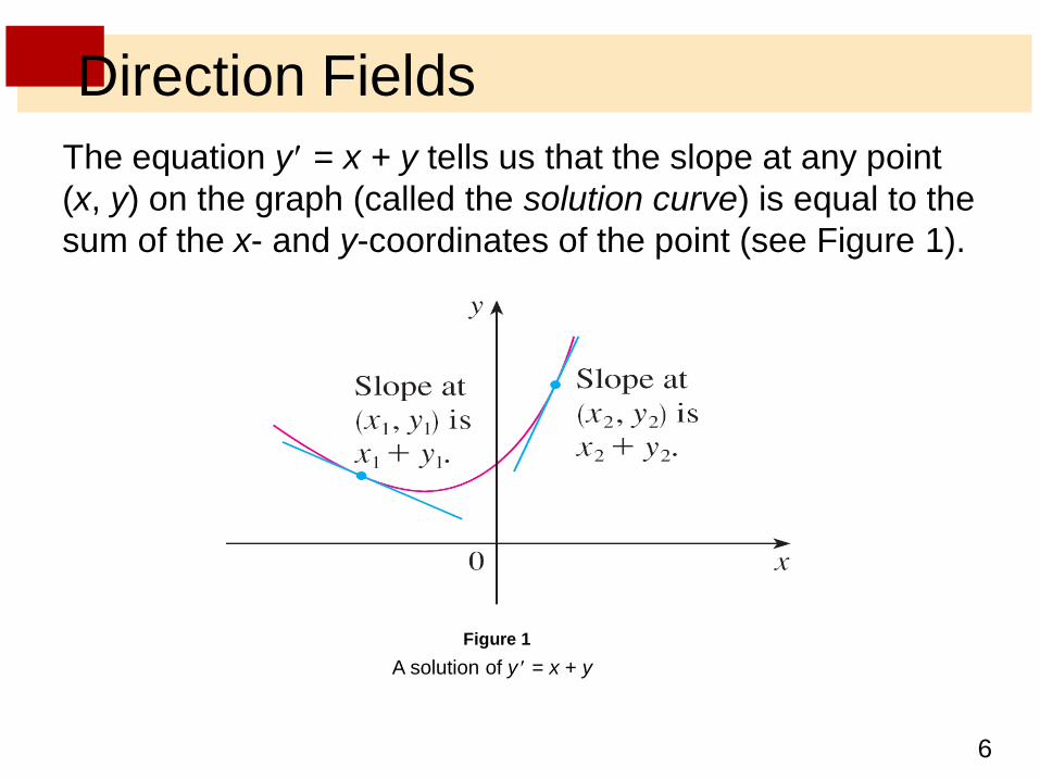
The equation y = x + y tells us that the slope at any point

(x, y) on the graph (called the solution curve) is equal to the

sum of the x- and y-coordinates of the point (see Figure 1).

Figure 1

A solution of y = x + y

7

Direction Fields

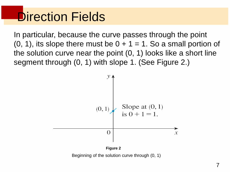
In particular, because the curve passes through the point

(0, 1), its slope there must be 0 + 1 = 1. So a small portion of

the solution curve near the point (0, 1) looks like a short line

segment through (0, 1) with slope 1. (See Figure 2.)

Figure 2

Beginning of the solution curve through (0, 1)

8

Direction Fields

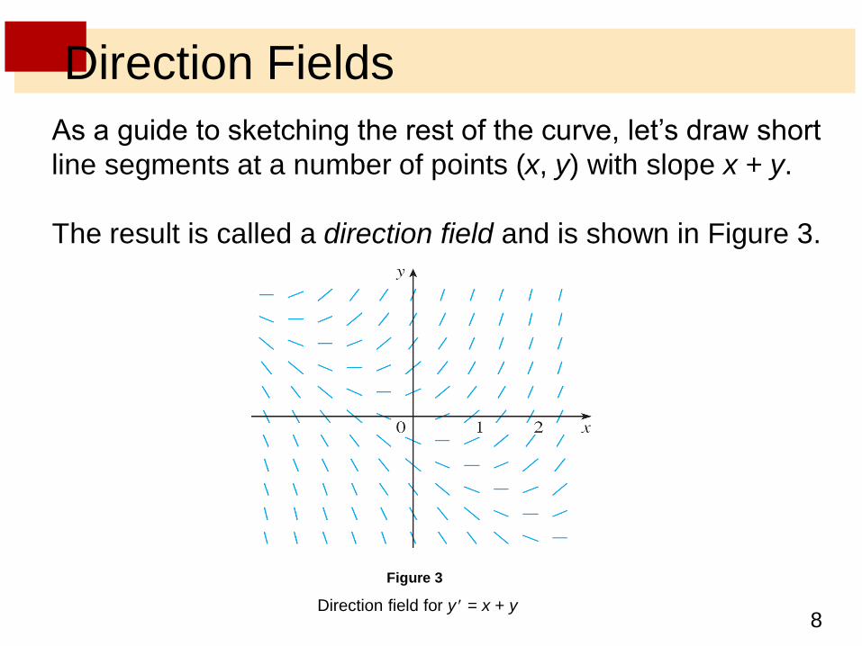
As a guide to sketching the rest of the curve, let’s draw short

line segments at a number of points (x, y) with slope x + y.

The result is called a direction field and is shown in Figure 3.

Figure 3

Direction field for y = x + y

9

Direction Fields

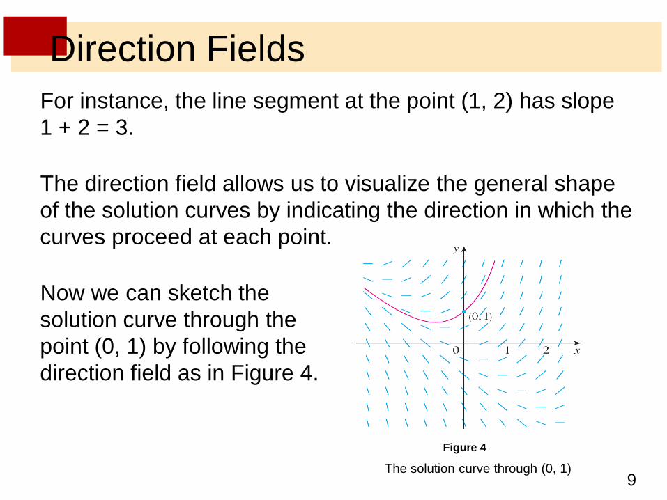
For instance, the line segment at the point (1, 2) has slope

1 + 2 = 3.

The direction field allows us to visualize the general shape

of the solution curves by indicating the direction in which the

curves proceed at each point.

Now we can sketch the

solution curve through the

point (0, 1) by following the

direction field as in Figure 4.

Figure 4

The solution curve through (0, 1)

10

Direction Fields

Notice that we have drawn the curve so that it is parallel to

nearby line segments.

In general, suppose we have a first-order differential

equation of the form

y = F(x, y)

where F(x, y) is some expression in x and y.

The differential equation says that the slope of a solution

curve at a point (x, y) on the curve is F(x, y).

11

Direction Fields

If we draw short line segments with slope F(x, y) at several

points (x, y), the result is called a direction field (or slope

field).

These line segments indicate the direction in which a

solution curve is heading, so the direction field helps us

visualize the general shape of these curves.

12

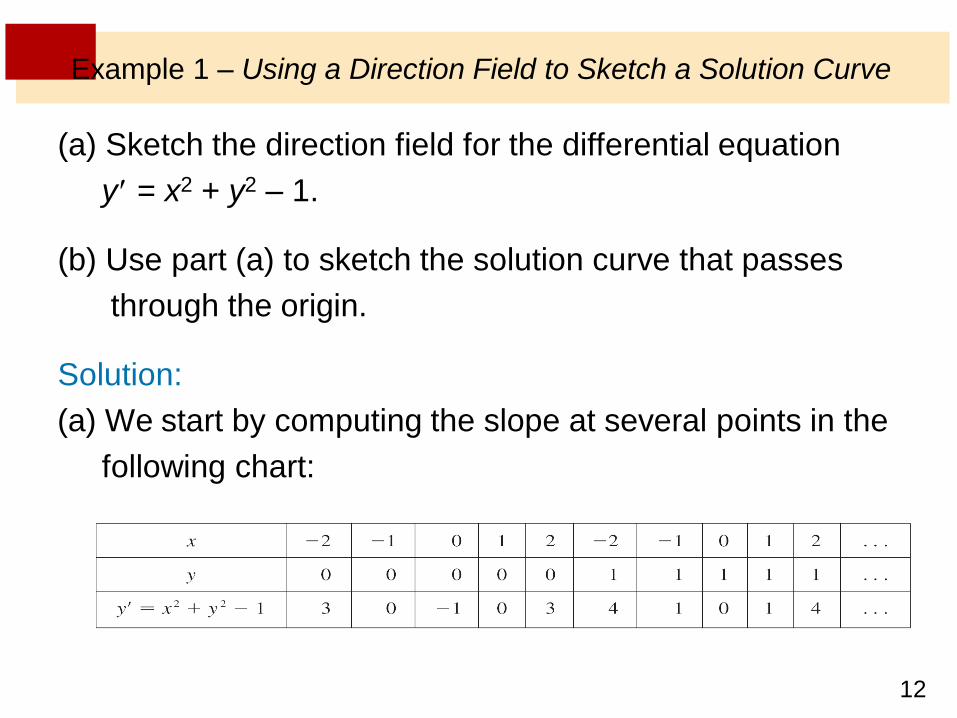
Example 1 – Using a Direction Field to Sketch a Solution Curve

(a) Sketch the direction field for the differential equation

y = x2 + y2 – 1.

(b) Use part (a) to sketch the solution curve that passes

through the origin.

Solution:

(a) We start by computing the slope at several points in the

following chart:

13

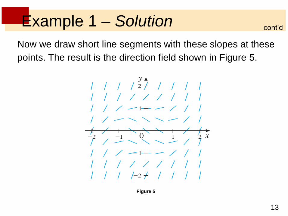
Example 1 – Solution

Now we draw short line segments with these slopes at these

points. The result is the direction field shown in Figure 5.

cont’d

Figure 5

14

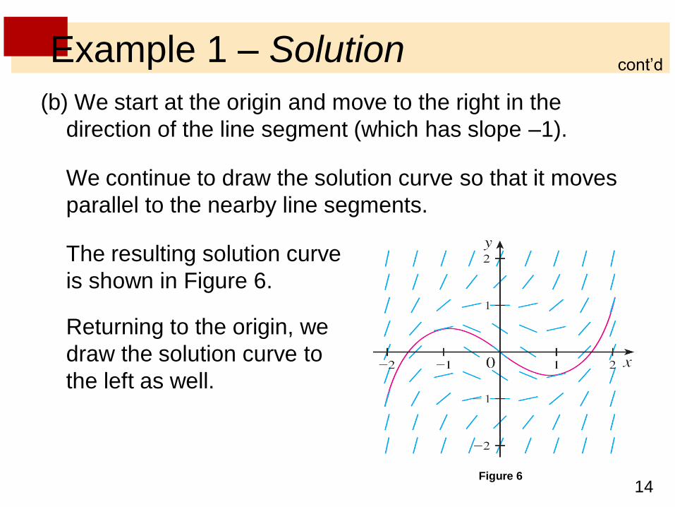
Example 1 – Solution

(b) We start at the origin and move to the right in the

direction of the line segment (which has slope –1).

We continue to draw the solution curve so that it moves

parallel to the nearby line segments.

The resulting solution curve

is shown in Figure 6.

Returning to the origin, we

draw the solution curve to

the left as well.

cont’d

Figure 6

15

Direction Fields

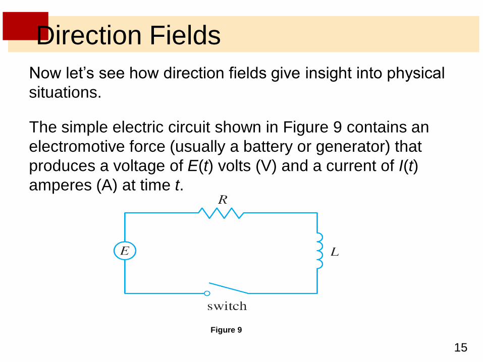
Now let’s see how direction fields give insight into physical

situations.

The simple electric circuit shown in Figure 9 contains an

electromotive force (usually a battery or generator) that

produces a voltage of E(t) volts (V) and a current of I(t)

amperes (A) at time t.

Figure 9

16

Direction Fields

The circuit also contains a resistor with a resistance of

R ohms and an inductor with an inductance of

L henries (H).

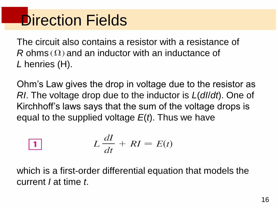
Ohm’s Law gives the drop in voltage due to the resistor as

RI. The voltage drop due to the inductor is L(dI/dt). One of

Kirchhoff’s laws says that the sum of the voltage drops is

equal to the supplied voltage E(t). Thus we have

which is a first-order differential equation that models the

current I at time t.

17

Direction Fields

A differential equation of the form

y = f(y)

in which the independent variable is missing from the right

side, is called autonomous.

For such an equation, the slopes corresponding to two

different points with the same y-coordinate must be equal.

This means that if we know one solution to an autonomous

differential equation, then we can obtain infinitely many

others just by shifting the graph of the known solution to the

right or left.

18

Euler’s Method

19

Euler’s Method

The basic idea behind direction fields can be used to find

numerical approximations to solutions of differential

equations.

We illustrate the method on the initial-value problem

that we used to introduce direction fields:

y = x + y y(0) =1

The differential equation tells us that y (0) = 0 + 1 = 1, so the

solution curve has slope 1 at the point (0, 1).

As a first approximation to the solution we could use the

linear approximation L(x) = x + 1.

20

Euler’s Method

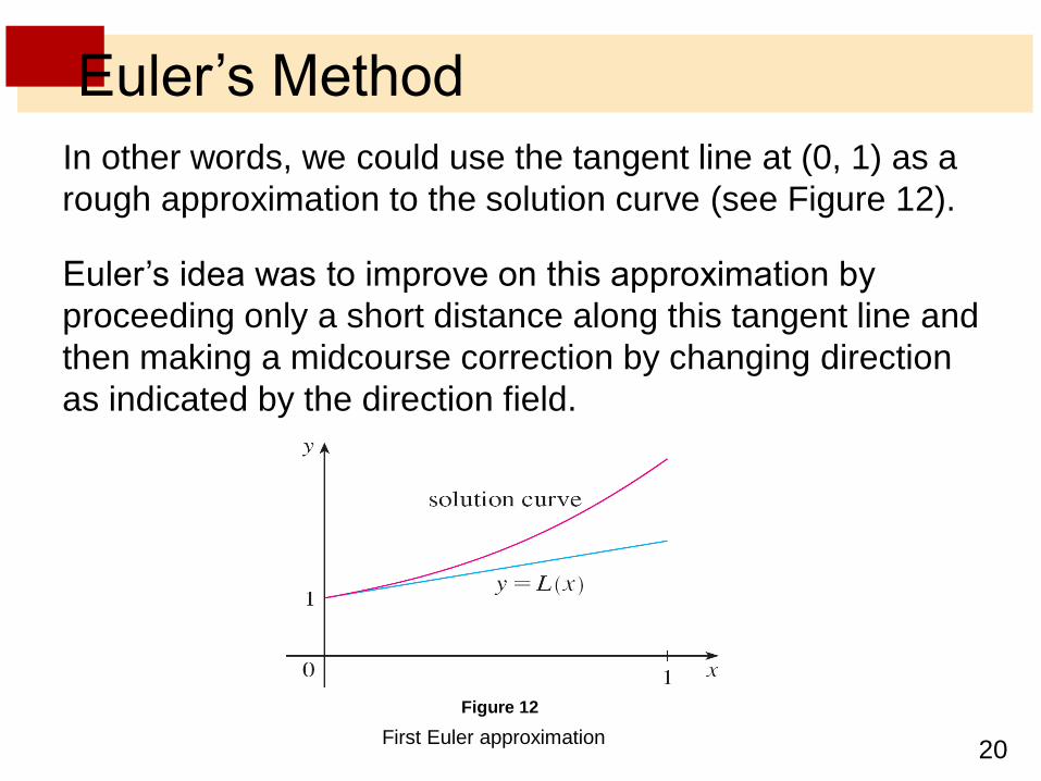
In other words, we could use the tangent line at (0, 1) as a

rough approximation to the solution curve (see Figure 12).

Euler’s idea was to improve on this approximation by

proceeding only a short distance along this tangent line and

then making a midcourse correction by changing direction

as indicated by the direction field.

Figure 12

First Euler approximation

21

Euler’s Method

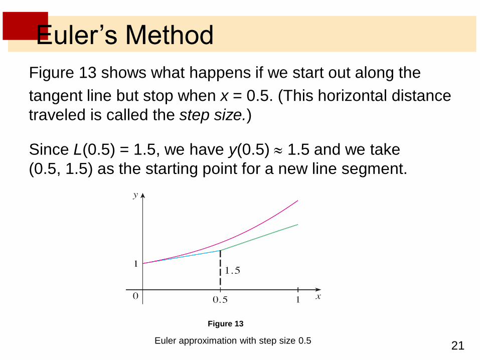
Figure 13 shows what happens if we start out along the

tangent line but stop when x = 0.5. (This horizontal distance

traveled is called the step size.)

Since L(0.5) = 1.5, we have y(0.5) 1.5 and we take

(0.5, 1.5) as the starting point for a new line segment.

Figure 13

Euler approximation with step size 0.5

22

Euler’s Method

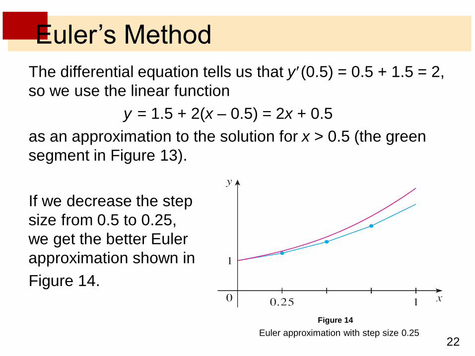
The differential equation tells us that y (0.5) = 0.5 + 1.5 = 2,

so we use the linear function

y = 1.5 + 2(x – 0.5) = 2x + 0.5

as an approximation to the solution for x > 0.5 (the green

segment in Figure 13).

If we decrease the step

size from 0.5 to 0.25,

we get the better Euler

approximation shown in

Figure 14.

Figure 14

Euler approximation with step size 0.25

23

Euler’s Method

In general, Euler’s method says to start at the point given by

the initial value and proceed in the direction indicated by the

direction field.

Stop after a short time, look at the slope at the new location,

and proceed in that direction.

Keep stopping and changing direction according to the

direction field.

Euler’s method does not produce the exact solution to an

initial-value problem—it gives approximations.

24

Euler’s Method

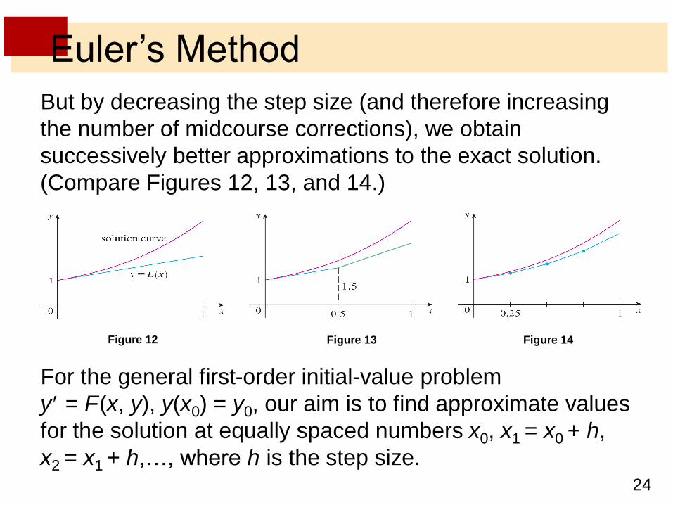
But by decreasing the step size (and therefore increasing

the number of midcourse corrections), we obtain

successively better approximations to the exact solution.

(Compare Figures 12, 13, and 14.)

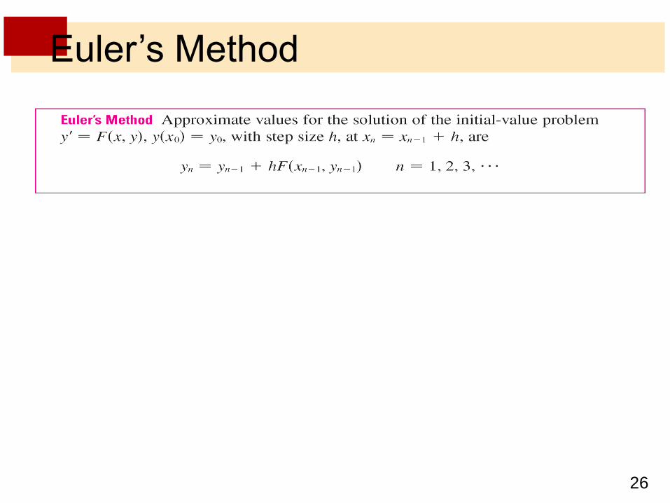
For the general first-order initial-value problem

y = F(x, y), y(x0) = y0, our aim is to find approximate values

for the solution at equally spaced numbers x0, x1 = x0 + h,

x2 = x1 + h,…, where h is the step size.

Figure 12 Figure 13 Figure 14

25

Euler’s Method

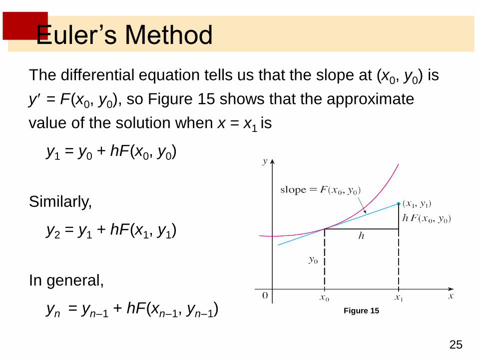
The differential equation tells us that the slope at (x0, y0) is

y = F(x0, y0), so Figure 15 shows that the approximate

value of the solution when x = x1 is

y1 = y0 + hF(x0, y0)

Similarly,

y2 = y1 + hF(x1, y1)

In general,

yn = yn–1 + hF(xn–1, yn–1) Figure 15

26

Euler’s Method

27

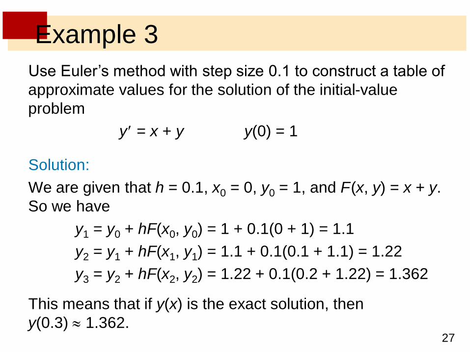
Example 3

Use Euler’s method with step size 0.1 to construct a table of

approximate values for the solution of the initial-value

problem

y = x + y y(0) = 1

Solution:

We are given that h = 0.1, x0 = 0, y0 = 1, and F(x, y) = x + y.

So we have

y1 = y0 + hF(x0, y0) = 1 + 0.1(0 + 1) = 1.1

y2 = y1 + hF(x1, y1) = 1.1 + 0.1(0.1 + 1.1) = 1.22

y3 = y2 + hF(x2, y2) = 1.22 + 0.1(0.2 + 1.22) = 1.362

This means that if y(x) is the exact solution, then

y(0.3) 1.362.

28

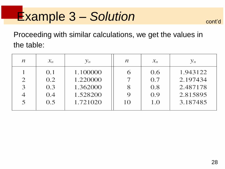
Example 3 – Solution

Proceeding with similar calculations, we get the values in

the table:

cont’d

29

Euler’s Method

For a more accurate table of values in Example 3 we could

decrease the step size.

But for a large number of small steps the amount of

computation is considerable and so we need to program a

calculator or computer to carry out these calculations.

30

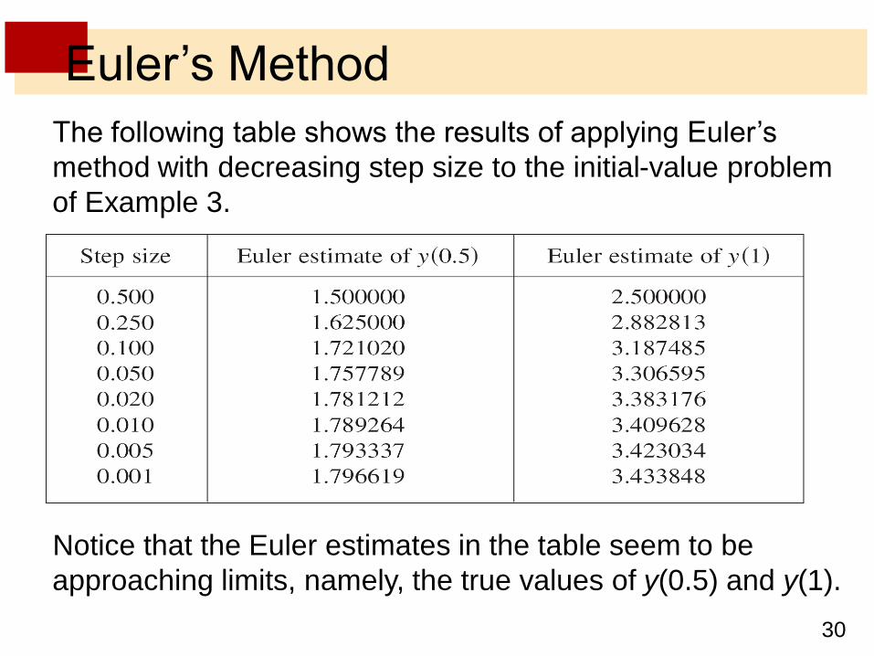
Euler’s Method

The following table shows the results of applying Euler’s

method with decreasing step size to the initial-value problem

of Example 3.

Notice that the Euler estimates in the table seem to be

approaching limits, namely, the true values of y(0.5) and y(1).

31

Euler’s Method

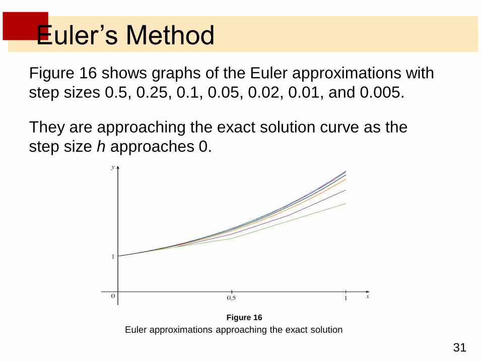
Figure 16 shows graphs of the Euler approximations with

step sizes 0.5, 0.25, 0.1, 0.05, 0.02, 0.01, and 0.005.

They are approaching the exact solution curve as the

step size h approaches 0.

Figure 16

Euler approximations approaching the exact solution