Nonlinear Dispersive Partial Differential Equations of Physical ...

University of Central Florida University of Central Florida

STARS STARS

Electronic Theses and Dissertations, 2004-2019

2014

Nonlinear Dispersive Partial Differential Equations of Physical Nonlinear Dispersive Partial Differential Equations of Physical

Relevance with Applications to Vortex Dynamics Relevance with Applications to Vortex Dynamics

Robert VanGorder University of Central Florida

Part of the Mathematics Commons

Find similar works at: https://stars.library.ucf.edu/etd

University of Central Florida Libraries http://library.ucf.edu

This Doctoral Dissertation (Open Access) is brought to you for free and open access by STARS. It has been accepted

for inclusion in Electronic Theses and Dissertations, 2004-2019 by an authorized administrator of STARS. For more

information, please contact [email protected].

STARS Citation STARS Citation VanGorder, Robert, "Nonlinear Dispersive Partial Differential Equations of Physical Relevance with Applications to Vortex Dynamics" (2014). Electronic Theses and Dissertations, 2004-2019. 4835. https://stars.library.ucf.edu/etd/4835

https://stars.library.ucf.edu/



https://stars.library.ucf.edu/etd

http://network.bepress.com/hgg/discipline/174?utm_source=stars.library.ucf.edu%2Fetd%2F4835&utm_medium=PDF&utm_campaign=PDFCoverPages

https://stars.library.ucf.edu/etd

http://library.ucf.edu/

mailto:[email protected]

https://stars.library.ucf.edu/etd/4835?utm_source=stars.library.ucf.edu%2Fetd%2F4835&utm_medium=PDF&utm_campaign=PDFCoverPages



NONLINEAR DISPERSIVE PARTIAL DIFFERENTIALEQUATIONS OF PHYSICAL RELEVANCE WITH

APPLICATIONS TO VORTEX DYNAMICS

by

ROBERT ASHTON VAN GORDERB.S. University of Central Florida, 2009M.S. University of Central Florida, 2013

A dissertation submitted in partial fulfillment of the requirementsfor the degree of Doctor of Philosophyin the Department of Mathematics

in the College of Sciencesat the University of Central Florida

Orlando, Florida

Spring Term2014

Major Professors:D. J. Kaup and K. Vajravelu (Co-chairs)

c⃝ 2014 by ROBERT ASHTON VAN GORDER

ii

ABSTRACT

Nonlinear dispersive partial differential equations occur in a variety of areas within

mathematical physics and engineering. We study several classes of such equations, including

scalar complex partial differential equations, vector partial differential equations, and finally

non-local integro-differential equations. For physically interesting families of these equations,

we demonstrate the existence (and, when possible, stability) of specific solutions which are

relevant for applications. While multiple application areas are considered, the primary appli-

cation that runs through the work would be the nonlinear dynamics of vortex filaments under

a variety of physical models. For instance, we are able to determine the structure and time

evolution of several physical solutions, including the planar, helical, self-similar and soliton

vortex filament solutions in a quantum fluid. Properties of such solutions are determined

analytically and numerically through a variety of approaches. Starting with complex scalar

equations (often useful for studying two-dimensional motion), we progress through more

complicated models involving vector partial differential equations and non-local equations

(which permit motion in three dimensions). In many of the examples considered, the qual-

itative analytical results are used to verify behaviors previously observed only numerically

or experimentally.

iii

ACKNOWLEDGMENTS

I began my research efforts here at UCF nearly 8 years ago, attending a seminar run by K.

Vajravelu in the fall of 2006. Later, in 2007, I began research with D. J. Kaup. These have

been my two most consistent collaborators throughout my time here at UCF, and as my time

here is rapidly coming to an end, I must thank them. Most of all, I appreciate the trust they

put in me to do things in my own way. I thank A. Kassab, R. N. Mohapatra, and A. Nevai

for serving on the dissertation committee, and performing the duties entailed. Additionally, I

thank M. Baxter, J. P. Brennan, M. R. Caputo, S. R. Choudhury, J. Haussermann, J. Hearns,

C. Huff, K. Mallory, K. Reger, B. K. Shivamoggi, and K. Theaker for fruitful collaborations

and discussions through my years at UCF.

I am grateful for the financial support of a UCF Trustee’s Fellowship (2009-2011)

and for the National Science Foundation Graduate Research Fellowship (2011-2014, grant

number 1144246). This support has allowed me to conduct the research contained within

this document relatively free of other commitments.

iv

TABLE OF CONTENTS

LIST OF FIGURES . . . . . . . . . . . . . . . . . . . . . . . . . . . . . . . . . . . . xiv

CHAPTER 1 INTRODUCTION . . . . . . . . . . . . . . . . . . . . . . . . . . . . 1

CHAPTER 2 PERIODIC SOLUTIONS OF SOME NONLINEAR DISPERSIVE PDES 10

2.1 Integrable stationary solution for the fully nonlinear local induction equation

describing the motion of a vortex filament . . . . . . . . . . . . . . . . . . . 10

2.1.1 Background . . . . . . . . . . . . . . . . . . . . . . . . . . . . . . . . 10

2.1.2 Stationary solution governed by an integrable equation . . . . . . . . 13

2.2 General rotating quantum vortex filaments under the 2D local induction ap-

proximation (LIA) . . . . . . . . . . . . . . . . . . . . . . . . . . . . . . . . 17

2.2.1 Background . . . . . . . . . . . . . . . . . . . . . . . . . . . . . . . . 18

2.2.2 Formulation . . . . . . . . . . . . . . . . . . . . . . . . . . . . . . . . 22

2.2.3 Analytical and numerical properties of the rotating filament solutions 26

2.2.4 Small amplitude perturbations along a filament . . . . . . . . . . . . 32

2.2.5 Numerical solutions and comparison with the analytical results . . . . 34

v

2.2.6 Discussion . . . . . . . . . . . . . . . . . . . . . . . . . . . . . . . . . 40

2.3 Exact solution for the self-induced motion of a vortex filament in the arclength

representation of the LIA . . . . . . . . . . . . . . . . . . . . . . . . . . . . . 45

2.3.1 Background . . . . . . . . . . . . . . . . . . . . . . . . . . . . . . . . 45

2.3.2 Stationary solutions . . . . . . . . . . . . . . . . . . . . . . . . . . . . 48

2.3.3 Discussion . . . . . . . . . . . . . . . . . . . . . . . . . . . . . . . . . 56

2.4 Exact stationary solution method for the Wadati-Konno-Ichikawa-Shimizu

(WKIS) equation . . . . . . . . . . . . . . . . . . . . . . . . . . . . . . . . . 56

2.4.1 Background . . . . . . . . . . . . . . . . . . . . . . . . . . . . . . . . 57

2.4.2 Stationary solutions . . . . . . . . . . . . . . . . . . . . . . . . . . . . 59

2.4.3 Alternate formulation . . . . . . . . . . . . . . . . . . . . . . . . . . . 64

2.4.4 Discussion . . . . . . . . . . . . . . . . . . . . . . . . . . . . . . . . . 67

CHAPTER 3 STABILITY RESULTS FOR CERTAIN PERIODIC OR LOCALIZED

SOLUTIONS . . . . . . . . . . . . . . . . . . . . . . . . . . . . . . . . . . . . . . . . 68

3.1 Orbital stability for rotating planar vortex filaments in the Cartesian and

arclength forms of the local induction approximation . . . . . . . . . . . . . 68

3.1.1 Introduction to the problem . . . . . . . . . . . . . . . . . . . . . . . 69

3.1.2 Stability methods . . . . . . . . . . . . . . . . . . . . . . . . . . . . . 71

3.1.3 The Cartesian problem . . . . . . . . . . . . . . . . . . . . . . . . . . 72

vi

3.1.4 The arclength problem . . . . . . . . . . . . . . . . . . . . . . . . . . 77

3.1.5 Discussion . . . . . . . . . . . . . . . . . . . . . . . . . . . . . . . . . 80

3.2 Orbital stability for stationary solutions of theWadati-Konno-Ichikawa-Schimizu

(WKIS) equation . . . . . . . . . . . . . . . . . . . . . . . . . . . . . . . . . 82

3.2.1 Introduction to the problem . . . . . . . . . . . . . . . . . . . . . . . 82

3.2.2 Properties of the stationary solutions . . . . . . . . . . . . . . . . . . 83

3.2.3 Stability result . . . . . . . . . . . . . . . . . . . . . . . . . . . . . . 89

3.2.4 Discussion . . . . . . . . . . . . . . . . . . . . . . . . . . . . . . . . . 90

3.3 Stability for a localized soliton . . . . . . . . . . . . . . . . . . . . . . . . . . 91

3.3.1 Background . . . . . . . . . . . . . . . . . . . . . . . . . . . . . . . . 92

3.3.2 Parameterized family of rational solitons . . . . . . . . . . . . . . . . 93

3.3.3 Orbital stability analysis . . . . . . . . . . . . . . . . . . . . . . . . . 98

3.3.4 Discussion . . . . . . . . . . . . . . . . . . . . . . . . . . . . . . . . . 100

CHAPTER 4 BREAKDOWN OF SINGLE VALUED SOLUTIONS AND VORTEX

COLLAPSE . . . . . . . . . . . . . . . . . . . . . . . . . . . . . . . . . . . . . . . . . 102

4.1 Scaling laws and accurate small-amplitude stationary solution for the LIA . . 102

4.1.1 Formulation and scaling the LIA . . . . . . . . . . . . . . . . . . . . 103

4.1.2 Accurate perturbation approach for the stationary solution . . . . . . 107

vii

4.1.3 Connection with arclength solution and implicit solution . . . . . . . 112

4.1.4 Discussion . . . . . . . . . . . . . . . . . . . . . . . . . . . . . . . . . 117

4.2 Non-monotone space scales and self-intersection of filaments . . . . . . . . . 119

4.2.1 Single loop case . . . . . . . . . . . . . . . . . . . . . . . . . . . . . . 122

4.2.2 Double loop case . . . . . . . . . . . . . . . . . . . . . . . . . . . . . 124

4.2.3 Analytical calculation . . . . . . . . . . . . . . . . . . . . . . . . . . . 127

4.2.4 Discussion . . . . . . . . . . . . . . . . . . . . . . . . . . . . . . . . . 130

4.3 Scaling laws and unsteady solutions under the integrable 2D local induction

approximation . . . . . . . . . . . . . . . . . . . . . . . . . . . . . . . . . . . 131

4.3.1 Spatial scalings for the 2D LIA . . . . . . . . . . . . . . . . . . . . . 132

4.3.2 The scaled helix . . . . . . . . . . . . . . . . . . . . . . . . . . . . . . 133

4.3.3 Self-similar filament structures . . . . . . . . . . . . . . . . . . . . . . 134

4.3.4 Self-intersection and vortex kinks . . . . . . . . . . . . . . . . . . . . 137

4.3.5 Self-similar vortex filaments and kink solutions . . . . . . . . . . . . . 144

CHAPTER 5 POTENTIAL FORMULATIONS FOR SUPERFLUID MODELS . . 150

5.1 Potential equation describing the motion of a vortex filament in superfluid

4He in the Cartesian frame of reference . . . . . . . . . . . . . . . . . . . . . 150

5.1.1 Background . . . . . . . . . . . . . . . . . . . . . . . . . . . . . . . . 151

viii

5.1.2 LIA for vortex filament in a superfluid . . . . . . . . . . . . . . . . . 152

5.1.3 First integral . . . . . . . . . . . . . . . . . . . . . . . . . . . . . . . 155

5.1.4 4D dynamical system . . . . . . . . . . . . . . . . . . . . . . . . . . . 156

5.1.5 Discussion . . . . . . . . . . . . . . . . . . . . . . . . . . . . . . . . . 166

5.2 Motion of a helical vortex filament in superfluid 4He under the extrinsic po-

tential form of the LIA . . . . . . . . . . . . . . . . . . . . . . . . . . . . . . 167

5.2.1 Background . . . . . . . . . . . . . . . . . . . . . . . . . . . . . . . . 168

5.2.2 Helical vortex filament . . . . . . . . . . . . . . . . . . . . . . . . . . 170

5.2.3 Approximations to the LIA . . . . . . . . . . . . . . . . . . . . . . . 177

5.2.4 Rotating planar filaments . . . . . . . . . . . . . . . . . . . . . . . . 180

5.2.5 Discussion . . . . . . . . . . . . . . . . . . . . . . . . . . . . . . . . . 187

5.3 Self-similar vortex dynamics in superfluid 4He under the Cartesian represen-

tation of the quantum LIA . . . . . . . . . . . . . . . . . . . . . . . . . . . . 190

5.3.1 Background . . . . . . . . . . . . . . . . . . . . . . . . . . . . . . . . 192

5.3.2 Analytical properties in the α, α′ → 0 limit . . . . . . . . . . . . . . . 195

5.3.3 Constant phase solution yielding a linear filament . . . . . . . . . . . 196

5.3.4 Non-constant phase as a function of amplitude . . . . . . . . . . . . . 196

5.3.5 Constant modulus solution R(η) = R0 . . . . . . . . . . . . . . . . . 198

5.3.6 Small oscillation solutions . . . . . . . . . . . . . . . . . . . . . . . . 199

ix

5.3.7 Asymptotic solution for large η . . . . . . . . . . . . . . . . . . . . . 202

5.3.8 Numerical simulations . . . . . . . . . . . . . . . . . . . . . . . . . . 203

5.3.9 Singular solutions R(0) > 0 . . . . . . . . . . . . . . . . . . . . . . . 205

5.3.10 Non-singular solutions R(0) = 0 . . . . . . . . . . . . . . . . . . . . . 208

5.3.11 Discussion . . . . . . . . . . . . . . . . . . . . . . . . . . . . . . . . . 210

5.3.12 Remark on self-similarity in other frames of reference . . . . . . . . . 214

5.3.13 Remark on the destruction of similarity by a normal flow impinging

on the vortex . . . . . . . . . . . . . . . . . . . . . . . . . . . . . . . 216

5.3.14 Physical Implications . . . . . . . . . . . . . . . . . . . . . . . . . . . 219

5.4 Quantum vortex dynamics under the tangent representation of the LIA . . . 223

5.4.1 Formulation including normal and binormal friction . . . . . . . . . . 225

5.4.2 Perturbation of the planar filament due to superfluid friction terms . 227

5.4.3 Purely self-similar filament structures . . . . . . . . . . . . . . . . . . 230

5.4.4 Formulation including normal fluid flow . . . . . . . . . . . . . . . . . 232

5.4.5 Helical filaments . . . . . . . . . . . . . . . . . . . . . . . . . . . . . 233

5.4.6 A soliton in the small-amplitude regime when the normal fluid flow

dominates . . . . . . . . . . . . . . . . . . . . . . . . . . . . . . . . . 235

5.4.7 A soliton in the intermediate regime . . . . . . . . . . . . . . . . . . 236

5.4.8 Quasi-similarity solution with temporal drift . . . . . . . . . . . . . . 237

x

5.4.9 Discussion . . . . . . . . . . . . . . . . . . . . . . . . . . . . . . . . . 238

CHAPTER 6 SOLUTIONS UNDER THE EXACT (NON-POTENTIAL) 3D VEC-

TOR QUANTUM LIA . . . . . . . . . . . . . . . . . . . . . . . . . . . . . . . . . . . 245

6.1 Decay of helical Kelvin waves on a vortex filament under the quantum LIA . 245

6.1.1 Background . . . . . . . . . . . . . . . . . . . . . . . . . . . . . . . . 246

6.1.2 Propagation of a helical filament driven by the normal fluid . . . . . 248

6.1.3 Constructing the decaying helical filament . . . . . . . . . . . . . . . 252

6.1.4 Properties of the decay term µ(t) . . . . . . . . . . . . . . . . . . . . 253

6.1.5 The case of vanishing normal fluid velocity . . . . . . . . . . . . . . . 255

6.1.6 The role of normal fluid velocity on vortex motion and persistence . . 258

6.1.7 Discussion . . . . . . . . . . . . . . . . . . . . . . . . . . . . . . . . . 263

6.2 Dynamics of a planar vortex filament under the quantum LIA . . . . . . . . 264

6.2.1 Background . . . . . . . . . . . . . . . . . . . . . . . . . . . . . . . . 265

6.2.2 A purely planar vortex filament . . . . . . . . . . . . . . . . . . . . . 267

6.2.3 Deformation of a planar filament due to superfluid parameters . . . . 270

6.2.4 Discussion . . . . . . . . . . . . . . . . . . . . . . . . . . . . . . . . . 283

6.3 Solitons and other waves on a quantum vortex filament . . . . . . . . . . . . 288

6.3.1 Background . . . . . . . . . . . . . . . . . . . . . . . . . . . . . . . . 288

xi

6.3.2 A map from the quantum LIA into a cubic complex Ginsburg-Landau

equation . . . . . . . . . . . . . . . . . . . . . . . . . . . . . . . . . . 289

6.3.3 Stokes wave solutions for the quantum LIA . . . . . . . . . . . . . . . 293

6.3.4 Soliton on a quantum vortex filament . . . . . . . . . . . . . . . . . . 293

6.3.5 Traveling waves on a quantum vortex filament . . . . . . . . . . . . . 295

6.3.6 Discussion . . . . . . . . . . . . . . . . . . . . . . . . . . . . . . . . . 300

CHAPTER 7 NON-LOCAL DISPERSIVE RELATIONS AND CORRESPONDING

VORTEX DYNAMICS . . . . . . . . . . . . . . . . . . . . . . . . . . . . . . . . . . . 303

7.1 Non-local dynamics of the self-induced motion of a planar vortex filament . . 303

7.1.1 Background . . . . . . . . . . . . . . . . . . . . . . . . . . . . . . . . 305

7.1.2 Biot-Savart formulation for a parameterized filament curve . . . . . . 307

7.1.3 An integral equation for the non-local planar vortex filament . . . . . 308

7.1.4 The non-local planar vortex filament . . . . . . . . . . . . . . . . . . 310

7.1.5 Comparison with known solution for the LIA . . . . . . . . . . . . . . 316

7.1.6 Discussion . . . . . . . . . . . . . . . . . . . . . . . . . . . . . . . . . 318

7.2 Self-induced motion of a Cartesian helical vortex filament under the Biot-

Savart model . . . . . . . . . . . . . . . . . . . . . . . . . . . . . . . . . . . 319

7.2.1 Time evolution of a helical filament . . . . . . . . . . . . . . . . . . . 322

xii

7.2.2 Approximating the relations for ω and β in the case of small and

intermediate wave numbers . . . . . . . . . . . . . . . . . . . . . . . 326

7.2.3 Comparison with the LIA and numerical approximations . . . . . . . 332

7.2.4 Discussion . . . . . . . . . . . . . . . . . . . . . . . . . . . . . . . . . 334

CHAPTER 8 CONCLUSIONS . . . . . . . . . . . . . . . . . . . . . . . . . . . . . 336

LIST OF REFERENCES . . . . . . . . . . . . . . . . . . . . . . . . . . . . . . . . . 340

xiii

LIST OF FIGURES

2.1 Phase portraits for ψ(x) when ψ(0) = 0 (a), 0.5 (b), 1 (c), 1.1 (d) while

ψ′(0) = 1. . . . . . . . . . . . . . . . . . . . . . . . . . . . . . . . . . . . . . 16

2.2 Plots of ψ(x) when ψ(0) = 0 (a), 1 (b), while ψ′(0) = 1. . . . . . . . . . . . . 16

2.3 Plots of the solutions R(x) to (2.34) in the phase space (R,R′) when (a) Θ1 =

0, (b) Θ1 = 0.1. The helical filament corresponds to (R,R′) = (0.2517, 0) and

gives the minimal possible values of J , namely J = −0.8660. The functions

R(x) corresponding to planar filaments are found in (a), while the functions

R(x) which are always positive are found in (b). This latter class of solutions

corresponds to neither planar nor helical filaments; rather, such solutions

correspond to generalized rotating filaments. . . . . . . . . . . . . . . . . . 30

2.4 Plots of the vortex filament solutions (2.27), when R′(0) = 0, Θ(0) = 1, and

(a) R(0) = 1, Θ′(0) = 0, (b) R(0) = 3, Θ′(0) = 0, (c) R(0) = 1, Θ′(0) = 0.05,

(d) R(0) = 1, Θ′(0) = 0.5, (e) R(0) = 1, Θ′(0) = 1, (f) R(0) = 1, Θ′(0) = 2.5,

(g) R(0) = 2, Θ′(0) = 1.5, (h) R(0) = 3, Θ′(0) = 1.5, (i) R(0) = 3, Θ′(0) = 5. 36

xiv

2.5 Cross sections of the vortex filament solutions (2.27) in the y-z plane, when

R′(0) = 0, Θ(0) = 1, and (a) R(0) = 1, Θ′(0) = 0, (b) R(0) = 3, Θ′(0) = 0, (c)

R(0) = 1, Θ′(0) = 0.05, (d) R(0) = 1, Θ′(0) = 0.5, (e) R(0) = 1, Θ′(0) = 1, (f)

R(0) = 1, Θ′(0) = 2.5, (g) R(0) = 2, Θ′(0) = 1.5, (h) R(0) = 3, Θ′(0) = 1.5,

(i) R(0) = 3, Θ′(0) = 5. Though the three-dimensional plots of the filaments

in Fig. 2.4 may appear unstructured in some cases, this view directed along

the x-axis shows that all solutions exhibit at least some symmetry. . . . . . . 37

2.6 Phase portrait in (q, qs) for the solution to the fully nonlinear oscillator equa-

tion modelling the local induction equation under the arclength representa-

tion. . . . . . . . . . . . . . . . . . . . . . . . . . . . . . . . . . . . . . . . . 50

2.7 Plots of the solution q(s) given in (2.71) for various values of the amplitude A.

Note that the period of the solutions is strongly influenced by the amplitude.

The nonlinear dependence of the period T with the amplitude A is shown

graphically in Fig. 2.8. . . . . . . . . . . . . . . . . . . . . . . . . . . . . . 51

2.8 Plot of the period T (A) of the solution (2.71) versus the amplitude A. The

exact relation is found by numerically plotting (2.72). Note that both the

A < 1/√3 and A > 1/

√3 asymptotic expansions are excellent fits to the

exact relation. . . . . . . . . . . . . . . . . . . . . . . . . . . . . . . . . . . 54

xv

2.9 Relative error |T (A)−Tapprox|/|T (A)| of the approximations to T (A). We also

include the lowest order approximation T (A) ≈ 4 ln(2√2m) for the A > 1/

√3

case. We see the good agreement with the A < 1/√3 asymptotics and A >

1/√3 asymptotics where needed. . . . . . . . . . . . . . . . . . . . . . . . . 55

2.10 Phase portraits for the space-periodic solutions ψ(x) to the WKIS equations,

which exist for −1 < I < 0. We fix k = 1. . . . . . . . . . . . . . . . . . . . 62

2.11 Plots of the space-periodic solutions ψ(x) to the WKIS equation, which exist

for (a) I = −0.1, (b) I = −0.4, (c) I = −0.7, and (d) I = −0.9. Here, k = 1. 63

2.12 Plot of the period T of the space-periodic solutions ψ(x) to the WKIS equation

for various values of the constant of motion I. Here, k = 1. . . . . . . . . . 66

3.1 Plot of the problem geometry for ω > 0 in the Cartesian reference frame. The

curve represents the planar vortex filament. As time increases, the structure

rotates about the x-axis. . . . . . . . . . . . . . . . . . . . . . . . . . . . . 74

3.2 Plot of the solution profiles ψ(x) with spectral parameter ω and constant of

motion E. Clearly, both parameters strongly influence the amplitude and

space-period of the stationary solutions. Each stationary solution ψ(x) corre-

sponds to a planar vortex filament as shown in Fig. 3.1. . . . . . . . . . . . 75

3.3 Plots of the solutions ψ(x) for various values of k and various amplitudes ψ(0). 87

3.4 Plot of the period T (k, I) given in formula (3.29) as a function of k for various

values of I ∈ (−1, 0). . . . . . . . . . . . . . . . . . . . . . . . . . . . . . . 88

xvi

3.5 Time-evolution of the localized soliton (3.35) corresponding to ω = −0.2. . . 96

3.6 Influence of the spectral parameter, ω < 0, on the wave envelopes. As |ω|

increases, the amplitude increases like 3√|ω| yet the mass of the wave remains

fixed. Hence, a greater proportion of mass is allocated near the center of the

wave, in the case of large amplitude solitons. Note that by amplitude, we

refer to deviation of the mean wave-height (which is√|ω|) - the total height

of the wave, in this model, is 4√

|ω|. . . . . . . . . . . . . . . . . . . . . . . 97

4.1 Plot of the spatial geometry. The curve represents the planar vortex filament

described by Φ(x, t) = e−iγtϕ(µ(x)) for periodic ψ(µ(x)). As time increases,

the structure rotates about the x-axis. . . . . . . . . . . . . . . . . . . . . . 106

4.2 Plot of the perturbation solutions (4.20) for ψ(x) obtained through the method

of multiple scales against numerical solutions obtained via the Runge-Kutta-

Fehlberg method (RKF45) [29]. The valid region for the approximation (4.14)

is A < 1/√3 ≈ 0.577, and in this region the results agree nicely. For larger

A, the agreement breaks down, as the solutions fall out of resonance with the

true solutions. . . . . . . . . . . . . . . . . . . . . . . . . . . . . . . . . . . 110

xvii

4.3 Plot of the absolute error between the perturbation solutions (4.20) for ψ(x)

obtained through the method of multiple scales and the numerical solutions

obtained via the Runge-Kutta-Fehlberg method (RKF45) [29]. The agreement

is strong for small amplitude solutions, while the agreement gradually breaks

down for larger amplitudes. . . . . . . . . . . . . . . . . . . . . . . . . . . . 111

4.4 Plot of the x-period T (A) for the stationary solution x-dependence function

ϕ(x). In addition to the exact value (4.29), we plot two approximate quan-

tities, namely the approximation found through multiple scales (4.21) and

the asymptotic approximation (4.32) to the true result (4.29). We consider

A ∈ [0,√2]. . . . . . . . . . . . . . . . . . . . . . . . . . . . . . . . . . . . . 115

4.5 We demonstrate the relative error between the approximations to the period

T (A) and the true solution (4.29). Both are extremely accurate for small A,

and gradually lose accuracy for larger A, though the asymptotic approxima-

tion (4.32) outperforms the multiple scale approximation (4.21) nicely. That

said, in its region of validity (A < 1/√3), the multiple scale approximation

(4.21) is rather accurate for only a first order perturbation result. . . . . . . 116

xviii

4.6 Schematic of a self-intersection for the planar vortex filament governed by a

solution ϕ(x) to equation (4.36). Self-intersection occurs at spatial coordinate

f(x∗) where the parametrization x attains the value x∗ such that f(x∗) =

f(x∗) and ϕ(x∗) = ϕ(x∗). It is necessary for ϕ(x1) = ϕ(x2) for all x∗ < x1 <

x2 < x∗ in order to have a single loop. For multiple loops, similar yet more

complicated conditions must hold. . . . . . . . . . . . . . . . . . . . . . . . 121

4.7 Plot of the numerical solution for a single loop vortex filament described by

ϕ(x) when ϕ(x) satisfies (4.38), ϕ(0.1) = 0.6, ϕ′(0.1) = −0.1. The x scaling is

f(x) = x2/2. The space coordinate is parametrized by x ∈ [−2.12, 3.00]. . . 123

4.8 Plot of the numerical solution for a double loop vortex filament described by

ϕ(x) when ϕ(x) satisfies (4.39), ϕ(0.1) = 0.5, ϕ′(0.1) = −0.095. The x scaling

is f(x) = cos(x). The space coordinate is parametrized by x ∈ [−4.0, 2.5]. . 125

4.9 Plot of the analytical solution for a single loop vortex filament described by

ϕ(x) when ϕ(x) satisfies (4.44). The x scaling is f(x) = x2/2, while the

amplitude of the solution is taken to be A = 0.25. The space coordinate is

parametrized by x ∈ [x∗(A), x∗(A)] while on the loop. . . . . . . . . . . . . 129

xix

4.10 A vortex filament loop formed at t = 0 by two scaled helical vortex filament

segments as defined in (4.65). Before t = 0, the two filament sections do

not form a closed loop, and for t > 0 the filaments separate and the loop is

broken. Therefore, the loop is a highly localized temporal event. The loop can

redevelop at a later time. Here the scaling is µ(x) = cos(x), and to illustrate

the results graphically we take k = 2π, A = 1, γ = 1. For time, we take t = 0. 140






the results graphically we take k = 2π, A = 1, γ = 1. For time, we take t = 10. 141






the results graphically we take k = 2π, A = 1, γ = 1. . . . . . . . . . . . . . 143

xx

4.13 Time evolution of a vortex filament kink solution of the type described by

(4.69). We set t = 1, and we have taken C = 1 + i, γ = 1, ϵ = 0.25. While

oscillations initially appear along the filament, these die off as time becomes

large, and therefore the filament tends to the limit (4.72) as time grows. . . . 147









5.1 Vortex filament at temperature T = 1K where we have α = 0.005 and α′ =

0.003. We set U1 = γ = t = 1 and ρ(0) = σ(0) = 0.01, ρ′(0) = σ′(0) = 0. . . 158

5.2 Vortex filament at temperature T = 1K where we have α = 0.005 and α′ =

0.003. We set U1 = γ = t = 1 and ρ(0) = σ(0) = 0.1, ρ′(0) = σ′(0) = 0. Note

the influence of the initial condition (compared with Fig. 5.1). . . . . . . . 159

5.3 Vortex filament at temperature T = 1.5K we have α = 0.073 and α′ = 0.018.

We set U1 = γ = t = 1 and ρ(0) = σ(0) = 0.01, ρ′(0) = σ′(0) = 0. . . . . . . 160

xxi

5.4 Vortex filament at temperature T = 1.5K we have α = 0.073 and α′ = 0.018.

We set U1 = γ = t = 1 and ρ(0) = σ(0) = 2, ρ′(0) = σ′(0) = 0. Again,

we see that the solutions do depend strongly in the initial condition. Here

the filament exhibits far less regularity in structure than in the “small initial

condition” case. . . . . . . . . . . . . . . . . . . . . . . . . . . . . . . . . . 161

5.5 Plot of the modulus |Φ| =√ρ2 + σ2 given I: T = 1K, α = 0.005, α′ = 0.003,

ρ(0) = σ(0) = 0.1; II: T = 1.5K, α = 0.073, α′ = 0.018, ρ(0) = σ(0) = 0.1; II:

T = 1.5K, α = 0.073, α′ = 0.018, ρ(0) = σ(0) = 0.5. We set U1 = γ = t = 1,

ρ′(0) = σ′(0) = 0 in all plots. Note the intermittent behavior apparent in II

and III. . . . . . . . . . . . . . . . . . . . . . . . . . . . . . . . . . . . . . . 163

5.6 Phase portrait of (y(x), z(x)) for x ∈ [0, 2000] given T = 1K, α = 0.005,

α′ = 0.003, ρ′(0) = σ′(0) = 0 ρ(0) = σ(0) = 0.1, γ = t = 1. We have

taken U1 = 1 (left image) to demonstrate a radially symmetric solution and

U2 = 20 (right image) to demonstrate the structures that may develop when

the normal fluid velocity, U1, becomes large. . . . . . . . . . . . . . . . . . . 164

5.7 Phase portrait of (y(x), z(x)) for x ∈ [0, 2000] given T = 1K, α = 0.005,

α′ = 0.003, ρ′(0) = σ′(0) = 0 ρ(0) = σ(0) = 0.1, U1 = t = 1. We have

taken γ = 0.001 (left image) and γ = 100 (right image) to demonstrate the

spectrum of structures possible. . . . . . . . . . . . . . . . . . . . . . . . . . 165

xxii

5.8 Schematic of the problem geometry for a prototypical helical vortex filament.

The helical vortex filament is oriented along the x-axis, with amplitude A

and wave-number k. The angular frequency, ω, will dictate the motion of this

helical vortex filament. . . . . . . . . . . . . . . . . . . . . . . . . . . . . . 172

5.9 Plot of the nonlinear dependence of the amplitude A given in Eq. (5.22) on

the wave number k and the normal fluid velocity U . The permissible wave

numbers satisfy k > U/γ, and for the sake of demonstration we normalize

γ = 1. As the normal fluid velocity increases, the permitted amplitude values

decrease, owing to the added instability induced by the normal fluid. We

observe a unique peak value in amplitude at some wave number kA for each

fixed value of U . . . . . . . . . . . . . . . . . . . . . . . . . . . . . . . . . . 175

5.10 Plots of the nonlinear dispersion relation Eq. (5.23) for ω(k) in the non-

degenerate case α = 0. When k = 0, ω(0) = 0 while ω > 0 for k > 0. . . . . 176

5.11 Schematic of the problem geometry for a planar vortex filament. The planar

vortex filament is oriented along the x-axis, with radius A and x-period T (A).

The angular frequency, ω = γ (by assumption (5.42)) determined the motion

of the vortex filament with time. The temporal period is then 2π/γ. . . . . 181

xxiii

5.12 Plot of the approximation (5.54) to the space period T (A) of the planar vortex

filament given by the method of multiple scales. Also plotted are the exact

numerical values for T (A) that may be found by numerically integrating (5.44)

in order to construct a solution. Clearly, the multiple scales approximation

is a very good fit for small-amplitude solutions. Periodic solutions exist for

A <√

2/3 ≈ 0.81649. . . . . . . . . . . . . . . . . . . . . . . . . . . . . . . 185

5.13 Plot of the space periodic part of the planar vortex filament, for various values

of A. Solid lines denote the perturbation approximation (5.53) while the

dashed lines denote numerical simulations via RKF45 method of numerical

integration. We see remarkable agreement for small amplitude solutions. For

the large amplitude solutions, the numerics and analytics begin to go out of

phase for large x, due to the small error in the approximate period (5.54) and

the true period. . . . . . . . . . . . . . . . . . . . . . . . . . . . . . . . . . 186

5.14 Plot of small-amplitude solutions (5.93) corresponding to (4.13) over space

x ∈ [0, 15] given (a) t = 0.1, (b) t = 1, and (c) t = 10. We fix γ = 1; changes

in γ would simply manifest as a dilation of the temporal variable t, thereby

altering (up to a scale) the temporal variation shown in (a) - (c). . . . . . . 201

5.15 Plot of singular self-similar solutions r for (5.63)-(5.64). The red (lower)

solution denotes (α, α′) = (0, 0), the blue (middle) solution denotes (α, α′) =

(0.005, 0.003), and the green (upper) solution denotes (α, α′) = (0.073, 0.018).

Here R(0) = 1, R′(0) = Θ′(0) = 0, Θ(0) = 2. . . . . . . . . . . . . . . . . . 206

xxiv

5.16 Plot of self-similar solutions R(η) and Θ(η) for (5.63)-(5.64) given (a) (α, α′) =

(0, 0), (b) (α, α′) = (0.005, 0.003), and (c) (α, α′) = (0.073, 0.018). When the

superfluid friction parameters are zero, the solution R(η) oscillates about a

fixed point. Yet, with the addition as even small superfluid friction parame-

ters, the solution R → ∞ as |η| → ∞. Here R(0) = 1, R′(0) = Θ′(0) = 0,

Θ(0) = 2. . . . . . . . . . . . . . . . . . . . . . . . . . . . . . . . . . . . . . 207

5.17 Plot of non-singular self-similar solutions r for (5.63)-(5.64) given (a) (α, α′) =

(0, 0), (b) (α, α′) = (0.005, 0.003), and (c) (α, α′) = (0.073, 0.018). Here

R(0) = ϵ = 10−3, R′(0) = Θ′(0) = 0, Θ(0) = 2. Taking ϵ = 10−3 is sufficient

to numerically approximate the non-singular vortex filament solution. . . . 209

5.18 The deformation of planar filaments due to superfluid friction as given ana-

lytically by (5.122). The black line represents α = α′ = 0, while the blue line

represents α = 0.005, α′ = 0.003. . . . . . . . . . . . . . . . . . . . . . . . . 241

5.19 The self-similar solutions for α = α′ = 0 (black line), α = 0.005, α′ = 0.003

(blue line) corresponding to the fully nonlinear equation (5.124). . . . . . . 242

5.20 Helical solutions are plotted for U = 1, k = 2 (black line) and U = 1, k = 5

(blue line). As the wave number k increases, the period increases while the

amplitude (in Cartesian coordinates) decreases. . . . . . . . . . . . . . . . . 243

xxv

5.21 Soliton solutions (5.134) are given in (d), for α = 0.005 (black line) and α =

0.073 (blue line) in the presence of a normal fluid (U = 1). The perturbation

size of these soliton excitations of the tangent filament is ϵ = 0.01 (though

the corresponding value of the perturbation is much larger in the Cartesian

frame). . . . . . . . . . . . . . . . . . . . . . . . . . . . . . . . . . . . . . . 244

6.1 Plot of the numerical solution for µ(t) governed by equation (6.20) along

with the small time asymptotic solution (6.29) and the large time asymptotic

solution (6.25). Parameter values are fixed at A = 0.5, k = U = 1, γ = 2. For

small time (t < α−1), the approximation (6.29)) is a good fit to the numerical

solution, whereas when time is large (t > α−1), the approximation (6.25)

accurately describes the numerical solution. With this, we find that helical

perutrbations along the line vortex filament decay slowly on small time scales,

and then more rapidly for larger time scales. . . . . . . . . . . . . . . . . . 256

6.2 Plot of the time evolution of a helical filament solution corresponding to A =

0.5, γ = 2, k = 1, T=1K (i.e., α = 0.005, α′ = 0.003) and U = 0. Times

referenced are (a) t = 0, (b) t = 100, (c) t = 300, (d) t = 500. . . . . . . . . 260

xxvi

6.3 Plot of the time evolution of a helical filament solution corresponding to A =

0.5, γ = 2, k = 1, T=1K (i.e., α = 0.005, α′ = 0.003) and U = 1. Times

referenced are (a) t = 0, (b) t = 100, (c) t = 300, (d) t = 500. Note that the

decay of the helical perturbations along the filament is markedly slower than

in the case of U = 0 (which was considered in Fig. 6.2). . . . . . . . . . . . 261

6.4 Plot of the (a) translation β(t) of the x-coordiate (the translational motion

of the helical waves along the filament) and (b) the effective frequency ω(t)/t

for a helical filament solution corresponding to A = 0.5, γ = 2, k = 1,

for various temperatures and normal fluid velocity. The temperature T =

1K correspond to α = 0.005, α′ = 0.003, while T = 1.5K corresponds to

α = 0.073, α′ = 0.018. . . . . . . . . . . . . . . . . . . . . . . . . . . . . . . 262

6.5 Plot of the deformed planar filament described by (6.58) when the temperature

of the superfluid is T=1K (α = 0.005, α′ = 0.003) and V = 1. The filament

is given by numerically solving (6.59)-(6.60) subject to ϕ(0) = 0.1, ψ(0) = 0,

ϕ′(0) = 0, ψ′(0) = 0. . . . . . . . . . . . . . . . . . . . . . . . . . . . . . . . 278


of the superfluid is T=1.5K (α = 0.073, α′ = 0.018) and V = 1. The filament


ϕ′(0) = 0, ψ′(0) = 0. . . . . . . . . . . . . . . . . . . . . . . . . . . . . . . . 279

xxvii


of the superfluid is T=1.5K (α = 0.073, α′ = 0.018) and V = −1. The filament


ϕ′(0) = 0, ψ′(0) = 0. . . . . . . . . . . . . . . . . . . . . . . . . . . . . . . . 280


of the superfluid is T=1.5K (α = 0.073, α′ = 0.018) and V = 0. The filament


ϕ′(0) = 0, ψ′(0) = 0. . . . . . . . . . . . . . . . . . . . . . . . . . . . . . . . 281

6.9 Comparison of the deformed planar filament described by (6.58) when the

temperature of the superfluid is T=1.5K (α = 0.073, α′ = 0.018) and V = 1,

along with the classical planar filament corresponding to α = α′ = 0. In both

cases, the filaments are given by numerically solving (6.59)-(6.60) subject to

ϕ(0) = 0.1, ψ(0) = 0, ϕ′(0) = 0, ψ′(0) = 0. The blue curve represents the

T=1.5 deformed planar filament, while the black curve represents the classical

planar filament. . . . . . . . . . . . . . . . . . . . . . . . . . . . . . . . . . 282

6.10 Large-time plot of the deformed planar filament described by (6.58) when the

temperature of the superfluid is T=1.5K, with the same conditions given in

Fig. 6.7. Segments of the filament which continue to amplify are removed, to

show what might be expected experimentally after such segments dissipate or

disassociate with the rest of the filament. The filament is locally planar near

x = 0, while for large x the filament takes on a helical appearance. . . . . . 287

xxviii

6.11 Plot of the solution to the dynamical system (6.106) when α = 0.073, α′ =

0.018, η = 0.1. Initial conditions are F (0) = 1, F ′(0) = 0 and G(0) = 0. . . 298

6.12 Phase space plot of the solution to the dynamical system (6.106) when α =

0.073, α′ = 0.018, η = 0.1. Initial conditions are F (0) = 1, F ′(0) = 0 and

G(0) = 0. . . . . . . . . . . . . . . . . . . . . . . . . . . . . . . . . . . . . . 299

7.1 Numerical plots of the rotational velocity, ω, and transverse velocity, β, of

a helical vortex filament when non-local dynamics are accounted for. The

results use the LIA near the logrithmic singularlity, so these are the solutions

(7.51)-(7.52). Note that we set ϵ = 10−5 in all plots. The precise value of ϵ

is not important, since a change in the value of ϵ results in a scaling of the

plots, therefore the value of ϵ does not influence the qualitative features of the

solutions. . . . . . . . . . . . . . . . . . . . . . . . . . . . . . . . . . . . . . 325

7.2 Numerical plots and approximations to the integrand given in (7.53) for vari-

ous values of the physical parameters. We set ϵ = 10−5 in all plots. For small

and intermediate values of k and A, the approximation to the integrand (7.53)

is very accurate, and hence the approximating formula (7.58) for the integral

term in (7.51) is accurate. . . . . . . . . . . . . . . . . . . . . . . . . . . . . 328

xxix

7.3 Numerical plots and approximations to the integrand given in (7.54) for vari-

ous values of the physical parameters. We set ϵ = 10−5 in all plots. Ahain, for

small and intermediate values of k and A, the approximation to the integrand

(7.54) is very accurate, and hence the approximating formula (7.61) for the

integral term in (7.52) is accurate. . . . . . . . . . . . . . . . . . . . . . . . . 329

7.4 Comparison of the numerical plots and approximate solutions for the rota-

tional velocity, ω, and transverse velocity, β, of a helical vortex filament when

non-local dynamics are accounted for. The numerical results use the LIA

near the logrithmic singularlity, so these are the solutions (7.51)-(7.52). Note

that we set ϵ = 10−5 in all plots. We also take A = 0.1. The analytical ap-

proximations obtained in (7.62)-(7.63) are superior to the LIA (7.65) results

when k is either small or in the intermediate range. Once k becomes large,

both approximations lose accuracy. This is due to the fact that, for large

k, the integral terms in (7.51)-(7.52) are rapidly oscillating. The approxima-

tions (7.62)-(7.63) are useful when the decay in the integrals dominates the

oscillations, which is not true for large k. In the regime where the approxima-

tions are useful, note that the LIA underestimates both velocities, while the

approximation (7.62)-(7.63) overestimates the velocities. . . . . . . . . . . . 335

xxx

CHAPTER 1

INTRODUCTION

We shall be concerned with a few particular families of nonlinear dispersive partial differential

equations. By dispersive, one means that waves of different wavelengths travel at different

phase velocities. Fairly common examples of such partial differential equations would be

the nonlinear Schrodinger (NLS) equation and the Korteweg-de Vries (KdV) equation. For

our purposes, the types of equations we consider often deal with curvature, so that the time

evolution of a solution curve is determined by structure of the curve. Such partial differential

equations naturally appear in studies of vortex dynamics, particularly vortex filaments, and

this will be the primary application we consider. While other applications will be discussed

when they fit the theme of a particular chapter, the motion of a vortex filament under a

variety of conditions will be an application common to all chapters.

The types of equations we shall be interested in will often take one of a few forms,

consisting of either a single scalar equation, vector equations, or non-local equation, and

the order of this investigation shall proceed in this general direction, with Chapters 2,3,4,5

considering scalar partial differential equations, Chapter 6 considering a vector partial dif-

ferential equation, and Chapter 7 dealing with a specific nonlocal equation.

1

In Chapter 2, we shall explore a class of periodic solutions to four specific equations

which are useful in mathematical physics. The first of these is the partial differential equation

governing the motion of a planar vortex filament under the local induction approximation

(LIA) in the Cartesian coordinate frame, which takes the form [98]

iut = − uxx[1 + |ux|2]3/2

. (1.1)

For more general rotating filaments (those that happen too be strongly non-planar), it is

more appropriate to apply the partial differential equation [17]

iut = − uxx[1 + |ux|2]3/2

− 1

2

ux(u∗xuxx − uxu

∗xx)

[1 + |ux|2]3/2, (1.2)

where ∗ denotes complex conjugation. For both models, planar filaments have been shown

to exist [99, 109] and correspond to one type of stationary solution. For the latter model,

helical stationary solutions also exist. The most interesting solutions are those which are

neither planar nor helical, yet are still essentially stationary states of the model. We find

that solutions of this equation can exhibit a wide variety of behaviors. If one considers the

arclength - tangent vector frame (which is derived treating the tangent vector to the filament

as the unknown quantity which must be solved for), one obtains an equation of the form [95]

iut = −uxx +2u∗u2x1 + |u|2

. (1.3)

This equation has the property that its planar solutions can be obtained in closed form, in

terms of an elliptic function. In contrast, planar solutions to the equations corresponding

to the Cartesian frame can, at best, be solved for implicitly. We end the chapter with a

2

discussion of periodic solutions to the Wadati-Konno-Ichikawa-Shimizu (WKIS) equation,

which is a type of integrable evolution equation inspired by the derivative NLS which has

been shown to have application in high energy physics [64]. The WKIS equation [101] takes

the form

iut = −

(u√

1 + |u|2

)xx

. (1.4)

In Chapter 3, we consider the oribital stability of some of the periodic solutions to

models considered in Chapter 2. To do so, we invoke the Vakhitov-Kolokolov (VK) stability

criterion, which relates the orbital stability of a solution to the change in the integral of

motion

P (uω(x, t)) =

∫|uω(x, t)|2dx (1.5)

with respect to a spectral parameter, ω. Doing so, we are able to determine when the planar

filaments in both the Cartesian and arclength - tangent vector models are orbitally stable.

Similarly, we are able to determine when the space-periodic solutions to the WKIS model are

orbitally stable. The stability criterion is typically applied to situations where the solution

is a soliton which decays as x → ±∞. However, the solutions studied here are periodic in

space, so we modify the method and define the quantity P over a single period, as opposed to

the real-line. In the limit where the period is taken to infinity, one may recover the standard

VK criterion. As a matter of fact, it is possible to apply the criterion to other types of

waves, and we demonstrate this by considering the orbital stability properties of a family of

Peregrine solitons (which are one possible model of rogue waves [73]). Provided the change

in P with respect to the spectral parameter is of constant sign and finite, we can consider

3

such situations where the modulus u is not time-constant. Our findings seem to suggest

that it will be possible to consider the orbital stability of a more broad class of nonlinear

dispersive equations, and this is commented on in the conclusions given in Chapter 8.

In Chapter 4, we take the local vortex filament models to the maximal extent of their

applicability in order to determine the structure of the vortex filaments upon self-intersection,

which allows us to form vortex loops. We first consider a type of scaling for the planar vortex

filaments. With this scaling, we are able to define piecewise continuous solutions to the LIA,

which we then use to construct self-intersecting vortex filaments. We do this using planar

filaments (corresponding to steady state solutions) and self-similar filaments (which give

unsteady vortex filament solutions). These types of solutions allow us to study situations

where there are sharp kinks in the vortex filaments. Self intersections and sharp kinks are two

vortex filament configurations which would physically destroy vortex filaments in standard

fluids, so these types of solutions give us insight into cases where vortexes may break apart.

Regarding the vortex models, the first three chapters essentially address the motion of

a vortex filament in a standard fluid, or the limit where superfluid effects become negligible.

In a superfluid, however, the requisite models will be more complicated. In Chapter 5, we

consider the motion of vortex filaments in a superfluid under the quantum form of the LIA.

This formulation accounts for superfluid friction and a normal fluid velocity impinging on

the vortex filament. The focus of Chapter 5 will be on potential forms of the quantum LIA.

By potential, we mean that these models involve an unknown complex potential field which

must be solved for, and hence these models are essentially two-dimensional. (The potential

4

function will often be written u(x, t) = y(x, t) + iz(x, t), where y and z denote coordinates

orthogonal to x.) Since one dimension is neglected, these models are best when the motion

of filaments is primarily rotational. In Cartesian coordinates, the potential approximation

to the LIA takes the form [102]

iut = aF (|ux|2)uxx+ bG(|ux|)ux , (1.6)

where a and b are complex coefficients which shall depend on physical parameters. Under

a number of assumptions or reductions, we study a variety of solutions to this equation.

Planar solutions and their generalizations are first studied. We next consider a family of

helical solutions. The helical vortex filament solutions correspond to Kelvin waves [89] which

ride along the vortex filaments. While the potential models can accurately approximate

the rotational properties of these waves, they fail to account for the transverse velocity.

We address this point later when the vector equations are studied. As an example of the

unsteady types of solutions possible, we consider self-similar solutions for the potential form

of the Cartesian formulation of the quantum LIA.

Regarding Chapter 6, in this chapter we turn our attention to the exact vector form of

the quantum LIA. While the potential equations studied in Chapter 5 approximate the full

vector equations, the potential equations discussed in previous chapters essentially confine

the motion of the filament solutions (and any waves along the filament) to two spatial

dimensions. By considering the vector equations, we can study the full three-dimensional

motion of the filaments. We consider the quantum LIA, as opposed to the standard fluid

LIA, which omits certain parameters, since the standard LIA is simply the limit where all

5

superfluid parameters are taken to zero. We first study the decay of helical Kelvin waves on

a quantum vortex filament. We start with waves of constant amplitude, and show that these

correspond to a critical wave number. These solutions can be described in exact form. When

we consider other wave numbers, we find that the helical Kelvin waves either amplify (and

diverge at t → ∞) or they decay (which is the physically reasonable case). The situation

where the helical filaments decay to line filaments, we are able to give a nice analytical

description of the problem. By assuming a helical filament solution with amplitude, phase,

and transverse velocity, all dependent on time, we reduce the vector form of the quantum

LIA into a system of three time-dependent ordinary differential equations. The analysis of

these equations then lends insight into the behavior of helical Kelvin waves on a quantum

vortex filament.

We are also able to study the planar filaments in the context of a quantum fluid.

There are two possibilities. First, in order for the planar filament to maintain its form,

the normal fluid velocity must take on a very specific (and space-variable) form. While this

gives a nice mathematical solution, due to the restriction on the type of normal fluid velocity

allowed, this case is not particularly interesting in terms of physical application. In the more

physically appealing case, where the normal fluid velocity is not confined, we show that a

filament which is planar in the standard fluid LIA should become deformed when superfluid

parameters are included. Interestingly, the deformed planar filaments demonstrate an in-

teresting amplification/de-amplification property when the normal fluid velocity is aligned

along the filament. The role of superfluid friction is to introduce torsional effects as the

6

filaments rotate. This has the effect of giving the deformed planar filaments a structure

which appears to be a hybrid of planar and helical shapes.

Our final investigation in Chapter 6 involves a generalization of the Hasimoto trans-

formation (which takes the standard fluid LIA and maps it into a cubic NLS equation [42])

whereby we take the quantum form of the LIA and map it into a type of complex Ginzburg-

Landau equation (a natural complex-coefficient generalization of NLS), [114]

iut = auxx + b|u|2u+ c(u2 − u∗2)u+ A(t)u , (1.7)

where a, b, and c are complex-valued constants depending on the physical parameters and

A(t) is an arbitrary differentiable time-dependent function. To simplify the mathematics,

we take c = 0, without loss of qualitative information in the cases we consider. From here,

we are able to consider Stokes waves and even solitons on a quantum vortex filament. We

also study a class of traveling wave solutions. The most important solutions here would be

the solitons, and the results here generalize the Hasimoto solitons found over forty years ago

for the standard fluid LIA to solitons under the quantum LIA for the first time.

Finally, in Chapter 7, we turn our attention to non-local equations governing the

motion of vortex filaments. The LIA itself is a local approximation to the non-local Biot-

Savart dynamics, so these results are a more general form of those considered in earlier

chapters. Hence, although it appears concise and rather elegant, this equation is quite

complicated to solve. In Chapter 7, we present two solutions to this model. First, we consider

planar filaments. The integro-differential equation is too hard to solve exactly, but we are able

7

to use the method of multiple scales in order to obtain an accurate analytical approximation

for the problem. The second class of solutions studied are the helical filaments. For these

solutions, we are able to exactly determine the rotational and translational velocities in

terms of the other model parameters. Therefore, we are able to determine the form and

motion of both planar and helical vortex filaments in a qualitative sense, under the non-local

Biot-Savart model.

Each of the chapters consists of material published or submitted for publication by the

author. The material has been organized in such as way that permits each chapter to be more

or less self contained. Therefore, one should be able to read the chapters independently. Some

of the studied equations will feature in more than one chapter, and are cross referenced where

needed. The actual analytical methods and approaches are self contained for each chapter,

so it will not be necessary to read one chapter in order to understand the mathematics of

another. Still, redundancies are kept to a minimum whenever possible. Chapters 2 through

4 constitute a study of potential forms for the simpler dispersion relations considered here.

Chapter 5 constitutes a generalization of some of these results to the more complicated

case where superfluid effects are added to the vortex filament dynamics, and this chapter

is completely self contained. Chapter 6 contains some results on the full three-dimensional

vortex dynamics under the quantum form of the LIA. Finally, Chapter 7 brings us back to

the study of the self-induced motion of a vortex filament in a standard fluid. Two specific

solution types are considered under this case, and each is compared to the corresponding

8

results under the LIA. There is a common reference list for all chapters, given in alphabetical

order, at the end of this document.

9

CHAPTER 2

PERIODIC SOLUTIONS OF SOME NONLINEAR

DISPERSIVE PDES

2.1 Integrable stationary solution for the fully nonlinear local

induction equation describing the motion of a vortex filament

We demonstrate an implicit exact stationary solution to the fully nonlinear local induction

equation describing the motion of a vortex filament. The solution, which is periodic in the

spatial variable, is governed by a second order nonlinear equation which has two exact first

integrals. These results were considered in Van Gorder [99].

2.1.1 Background

Recently Shivamoggi and van Heijst [84] reformulated the Da Rios-Betchov equations in

the extrinsic vortex filament coordinate space, and were able to find an exact solutions

to an approximate equation governing a localized stationary solution. The approximation

in the governing equation was due to the Shivamoggi and van Heijst’s consideration of a

10

first order approximation of dxds

= 1/√

1 + y2x + z2x. Previously, an order zero approximation

to this equation was considered by Dmitriyev [26]. Such approximations result in exact

solutions, but these solutions may break down outside of specific parameter regimes; namely,

for all but very small value of the amplitude parameter. Herein, we avoid making the

simplifying assumption on dxds. Although this results in a far more representative governing

equations for large amplitudes, the governing equations are far more complicated. Such

governing equations were then solved with a perturbation technique (in Van Gorder [98])

which suggested oscillating solutions in the large amplitude regime.

We begin with a review of some of the derivations in [98], as these shall be essential

in both motivating the solutions as well as providing needed components with which to

actually perform the computations. The self-induced velocity of a vortex filament in the

LIA is given by (Da Rios [24], Arms and Hama [8]) v = γκt × n, where t and n are unit

tangent and unit normal vectors to the vortex filament, respectively, κ is the curvature and

γ is the strength of the vortex filament. Consider the vortex filament essentially aligned

along the x-axis and assume the deviations from the x-axis to be small (Dmitriyev [26]):

r = xix + y(x, t)iy + z(x, t)iz. We then have that

t =dr

ds=dr

dx

dx

ds= (ix + yxiy + zxiz)

dx

dsand v = ytiy + ztiz , (2.1)

where

dx

ds=

1√1 + y2x + z2x

. (2.2)

11

We compute

κn =dt

ds=dt

dx

dx

ds=d2r

dx2

(dx

ds

)2

+dr

dx

(d

dx

dx

ds

)dx

ds

= − (yxyxx + zxzxx)

(dx

ds

)4

ix +(yxx+ z2xyxx − yxzxzxx

)(dxds

)4

iy

+(zxx+ y2xzxx − yxzxyxx

)(dxds

)4

iz .

(2.3)

Placing (2.1) and (2.3) into v = γκt× n, we obtain

v = γ (yxzxx − zxyxx)

(dx

ds

)3

ix − γzxx

(dx

ds

)3

iy + γyxx

(dx

ds

)3

iz , (2.4)

so

yt = −γzxx(dx

ds

)3

= −γzxx(1 + y2x + z2x

)−3/2(2.5)

and

zt = γyxx

(dx

ds

)3

= γyxx(1 + y2x + z2x

)−3/2(2.6)

must hold. Defining Φ = −(y + iz), (2.5) reduces to

iΦt + γ(1 + |Φx|2

)−3/2Φxx = 0 . (2.7)

In order to recover y and z once a solution Φ to (2.7) is known, note that y = −Re Φ and

z = −Im Φ. A first order approximation of the factor raised to the power −3/2 results

in Eq. (9) of Shivamoggi and van Heijst [84] after an appropriate transformation (since an

approximation was taken early in [84], the transformation Φ → iΦ is needed to bring a first

order approximation of (2.7) into the form given in [84]). A zeroth order approximation

was considered earlier by Dmitriyev [26]. Note that equation (2.7) is very similar to the

equation ivt + vss − 2v∗v2s/(1 + |v|2) = 0 obtained by Umeki [95], where v denotes directly

12

the tangential vector of the filament. While both are obtained through different derivations,

both are equivalent to the localized induction approximation (LIA).

2.1.2 Stationary solution governed by an integrable equation

Observe that (2.7) is similar in form to the Schrodinger equation for a free particle, only

with a function of |Φx| replacing the constant coefficient. Let us assume a solution of the

form Φ(x, t) = e−iγtψ(x) where ψ ∈ R. Then (2.7) is reduced to

ψ +(1 + (ψ′)

2)−3/2

ψ′′ = 0 . (2.8)

Multiplying by 2ψ′ and integrating, we obtain the first integral

ψ2 − 2√1 + (ψ′)2

= C , (2.9)

where C is a constant of motion determined by any specified boundary or initial data. In the

case where ψ(0) = 0 and ψ′(0) = 1 (as in [84]; locally near |x| << 0), C = −√2. Algebraic

manipulation of (2.9) leads to (ψ2 − C)2ψ′2 = 4− (ψ2 − C). Separating variables ψ and x,

we obtain the implicit relation

± x+ C2 =

∫ ψ (q2 − C)dq√4− (q2 − C)2

=1

2

∫ ψ2−C ξdξ√(C + ξ)(2 + ξ)(2− ξ)

. (2.10)

If we perform the integration on (2.10), we obtain

± x+ C2 =

− 2C−2

F(

ψ√2+C

,√2+C√C−2

)− E

(ψ√2+C

,√2+C√C−2

)if C = 2,

sgn(ψ)

tanh−1

(2√4−ψ2

)−√4− ψ2

if C = 2,

(2.11)

13

where F and E denote elliptic integrals of the first and second kind, respectively. In this

sense, ψ is akin to a composite Jacobi amplitude. We remark that a similar solution was

obtained by Hasimoto [41], through a different derivation. Hasimoto’s derivation started

with v = Y iy, as opposed to v = ytiy + ztiz. Assuming a stationary solution, Hasimoto’s

assumption leads to Yxx +Ωγ(1 + Y 2

x )3/2Y = 0 (in our notation, as the coordinate system of

Hasimoto differs from ours). While similar in form to (2.8), there is some information loss

going from the solution ϕ (which, implicitly, contains y(x) and z(x)) to the solution Y (x)

of Hasimoto’s equation. Hasimoto presents a solution Y = Acn(ξ, k) (where x = x(ξ), ξ is

a parametrization linking Y and x implicitly), which has initial conditions Y (0, k) = A and

Y ′(0) = 0. Mapping these conditions into our solution for ϕ, which obeys the same type

of ODE, we find these conditions imply C = −2 (which can be obtained from (2.11) in the

limiting case C → −2). Observe that we cannot, with the transformation given in Hasimoto

[41], recover the solutions satisfying initial data given in [84] (ψ(0) = 0 and ψ′(0) = 1).

Hence, our solution can be seen as a generalization of the implicit solution of Hasimoto,

which is equivalent to our solution in the C = −2 case.

Exact inversion of relation (2.11) to obtain ψ is not possible given the appearance of

two distinct elliptic functions; however, we can numerically invert the relation to recover ψ

for given initial data, which would determine C and C2 exactly. Note that we can just as

easily attempt to solve (2.8) numerically for such initial data, and we obtain the types of

solutions one would expect from the inversion of (2.11). Numerical integration yields the

expected periodic solutions for ψ (see Fig. 2.1). The fact that the relation (2.11) depends

14

on C (and thus, on the initial data) is shown in Fig. 2.2, where we see that the amplitude

and period are dependent on initial data. Note that the intercepts on the phase portraits

(Fig. 2.1) can be calculated exactly from (2.9): For instance, when ψ′(0) = 1, the ψ = 0

intercepts are ψ′ = ±√

4−√2+(ψ(0))2

((ψ(0))2−√2)2

and the ψ′ = 0 intercepts are ψ = ±√

(ψ(0)2 + 2−√2).

The oscillatory solutions should not be surprising, as (2.8) essentially defines a non-

linear oscillator. Suppose we were to define a solution Φ(x, t) = e+iγtχ(x) where χ(x) ∈ R

(this differs from the above solution, as we have taken +γ as opposed to −γ in the exponen-

tial). The resulting stationary equation then reads χ′′ =(1 + (χ′)2

)3/2χ. For non-negative

initial data, near x = 0 we have χ′′ > χ which suggests that, locally, χ is bounded below by

a function χ satisfying χ′′ = χ. Using initial data χ(0) = 0, χ′(0) = 1, χ(x) = sinh(x). So,

χ(x) grows at least as fast as sinh(x), suggesting that the Φ(x, t) = e+iγtχ(x) solution is not

reasonable.

15

(a) (b) (c) (d)

Figure 2.1: Phase portraits for ψ(x) when ψ(0) = 0 (a), 0.5 (b), 1 (c), 1.1 (d) while ψ′(0) = 1.

(a) (b)

Figure 2.2: Plots of ψ(x) when ψ(0) = 0 (a), 1 (b), while ψ′(0) = 1.

16

2.2 General rotating quantum vortex filaments under the 2D

local induction approximation (LIA)

In his study of superfluid turbulence in the low-temperature limit, Svistunov [92] derived

a Hamiltonian equation for the self-induced motion of a vortex filament. Under the local

induction approximation (LIA), the Svistunov formulation is equivalent to a nonlinear dis-

persive partial differential equation. In this section, we consider a family of rotating vortex

filament solutions for the LIA reduction of the Svistunov formulation, which we refer to as

the 2D LIA (since it permits a potential formulation in terms of two of the three Cartesian

coordinates). This class of solutions contains the well-known Hasimoto-type planar vortex

filament as one reduction and helical solutions as another. More generally, we obtain solu-

tions which are periodic in the space variable. A systematic analytical study of the behavior

of such solutions is carried out. In the case where vortex filaments have small deviations from

the axis of rotation, closed analytical forms of the filament solutions are given. A variety of

numerical simulations are provided to demonstrate the wide range of rotating filament be-

haviors possible. Doing so, we are able to determine a number of vortex filament structures

not previously studied. We find that the solution structure progresses from planar to helical,

and then to more intricate and complex filament structures, possibly indicating the onset of

superfluid turbulence. These results were presented in Van Gorder [109].

17

2.2.1 Background

The self-induced velocity of the vortex in the reference frame moving with the superfluid

according to the local induction approximation (LIA) was given by Hall and Vinen [39, 40].

(This model is also referred to as the HVBK model, or Hall-Vinen-Bekarevich-Khalatnikov

model. See Bekarevich and Khalatnikov [13].) Under a local induction approximation (LIA),

the Biot-Savart law inherent in such models can be approximated, and Schwarz [81] obtained

a type of quantum LIA

v = γκt× n+ αt× (U− γκt× n)− α′t× (t× (U− γκt× n)) . (2.12)

Here U is the dimensionless normal fluid velocity, t and n are the unit tangent and unit nor-

mal vectors to the vortex filament, κ is the dimensionless average curvature, γ = Γ ln(c/κa0)

is a dimensionless composite parameter (Γ is the dimensionless quantum of circulation, c is

a scaling factor of order unity, a0 ≈ 1.3× 10−8cm is the effective core radius of the vortex),

α and α′ are dimensionless friction coefficients which are small (except near the λ-point; for

reference, the λ-point is the temperature (which at atmospheric pressure is ≈ 2.17K) below

which normal fluid Helium transitions to superfluid Helium[51]). Regarding reasonable val-

ues of α and α′, Table 1 of Schwarz[81] shows that at temperature T = 1K we have α = 0.005

and α′ = 0.003, while at temperature T = 1.5K we have α = 0.073 and α′ = 0.018. Thus, it

makes sense to consider these friction terms as small parameters.

18

In the α, α′ → 0 limit (the zero-temperature limit), the motion of vortex lines is

described by the standard Biot-Savart law

dr

dt=

κ

4π

∫(r0 − r)× dr0

|r0 − r|. (2.13)

Often the Biot-Savart law (2.13) is replaced by the LIA. In this case, self-induced velocity

of a vortex filament is approximated by [8, 24]

v = γκt× n , (2.14)

where κ is the quantized curvature and γ is the strength of the vortex filament. Hasimoto

[42] obtained a 1-soliton solution of the LIA in the curvature-torsion frame. Exact stationary

solutions to the LIA in extrinsic coordinate space have been discussed by Kida [49] in the

case of torus knots, planar solutions, and helices; some of these solutions are given by elliptic

integrals.

Hasimoto [41] considered a planar vortex filament in the curvature-torsion frame of

reference. This influential and often cited paper demonstrates the relation between the

curvature of a vortex filament and elastica. Such a solution was also considered by Kida

[49], who obtained results in terms of elliptic integrals in the moving (time-dependent) arc

length coordinate frame, with stability results for some filaments in this framework provided

later [50]. Fukumoto [33] considered the influence of background flows on such stationary

states. For the Cartesian frame, some preliminary results were determined in Van Gorder

[99], though only some special solutions were given. There is an alternate formulation, given

by Umeki [95, 96], which provides the LIA in an arc-length coordinate frame. The Hasimoto

19

filament can be determined exactly in this frame (as is also true of the curvature-torsion

frame), and the results were worked out by Van Gorder [100]. However, the conversion be-

tween the arc-length and Cartesian solutions is not simple, so it is worthwhile to consider

the Cartesian case directly. Small amplitude space-periodic solutions of planar type were ob-

tained through a multiple scales analysis by Van Gorder [105]. Such solutions are valid in the

small-amplitude regime when the nonlinearity becomes sufficiently weak, though solutions

break down after that.

In the present section, we shall be interested in generalized rotating vortex filaments.

In order to describe such vortex filaments, we will employ the form of the LIA described

in Boffetta et al. [17] (which we refer to as the 2D LIA, for reasons outlined later) and

derived from the Svistunov model [92]. We show that the model contains both planar and

helical filaments (those most often studied in the literature), and that these are really two

narrow special cases of rotating planar vortex filaments. In particular, when the solutions

have constant amplitude and space-variable phase, they correspond to the helical filaments

of Sonin [89]. Meanwhile, when the phase is constant in space, and the amplitude varies,

we recover the planar vortex filaments of Hasimoto type. Each of these solutions is rather

narrow, and in general we will have solutions in between these two extremes.

We shall first provide a formulation of the 2D LIA of Boffetta et al. [17]. We

demonstrate why this model is useful for studying non-planar filaments (such as filaments

which may exhibit large spatial changes). The remainder of the section constitutes an

analytical and numerical study of the generalized rotating filaments. First, we determine the

20

system of nonlinear differential equations governing the structure of such a vortex filament.

We show that, in general, the phase and amplitude of such a filament are strongly coupled.

The change in the phase can be given strictly in terms of the amplitude, which allows us to

write one equation for the amplitude which itself depends on two parameters. Studying this

equation, we demonstrate the existence of space-periodic filament solutions (in particular,

filaments that are periodic in the y and z components, y(x+T, t) = y(x, t) and z(x+T, t) =

z(x, t)). We show that the period T can be calculated in terms of the model parameters.

While the complexity of the differential equation governing the amplitude prevents exact

solutions, we can obtain approximate solutions which are perturbative in nature. One of

these types of solutions is like the planar filament, whereas the other is quite distinct. Finally,

numerical solutions are provided for a variety of cases, in order to demonstrate the range of

solutions possible.

The results indicate a wide variety of behaviors not previously demonstrated mathe-

matically, which hold both helical and planar solutions are rather narrow special cases. In

some of the more exotic solutions, we expect degeneracy into turbulence to occur. Hence,

some of the solutions discussed here may be useful in the study of the onset of superfluid

turbulence. So, these solutions are not a minor generalization of the exact planar or helical

filament solutions already known. Rather, consideration of this more general formulation

shows us that there are a wide variety of behaviors possible for rotating filaments in the

Svistunov model under the LIA.

21

2.2.2 Formulation

First we consider the LIA (2.14) directly. Let us assume r(x, t) = (r1(x, t), r2(x, t), r3(x, t)),

where the rk’s are functions to be determined by the LIA. Calculating t and κn and taking

the cross product, we obtain the PDE system

(r1)t = γ(r2)2x

((r3)x(r2)x

)x

((r1)

2x + (r2)

2x + (r3)

2x

)−3/2, (2.15)

(r2)t = γ(r3)2x

((r1)x(r3)x

)x

((r1)

2x + (r2)

2x + (r3)

2x

)−3/2, (2.16)

(r3)t = γ(r1)2x

((r2)x(r1)x

)x

((r1)

2x + (r2)

2x + (r3)

2x

)−3/2. (2.17)

If the filament is aligned along the x-axis and includes a translational velocity term (which

means that the waves along a vortex filament are permitted to move along the reference axis,

in addition to the rotational motion), we take r1(x, t) = x + βt. In this case, we identify r2

and r3 with the y and z axes, as r2(x, t) = y(x, t) and r3(x, t) = z(x, t), respectively. As a

result, the system (2.15)-(2.17) becomes

β = γyxzxx − zxyxx

(1 + y2x + z2x)3/2

, (2.18)

yt = − γzxx

(1 + y2x + z2x)3/2

, zt =γyxx

(1 + y2x + z2x)3/2

. (2.19)

From (2.19), it makes sense to consider a potential function Φ(x, t) = y(x, t)+ iz(x, t), which

would put (2.18)-(2.19) into the form

β =γ

2i

Φ∗xΦxx − ΦxΦ

∗xx

(1 + |Φx|2)3/2, (2.20)

iΦt + γΦxx

(1 + |Φx|2)3/2= 0 . (2.21)

22

The best way to understand these conditions would be that (2.21) gives a potential formu-

lation of the LIA provided that the consistency condition (2.20) is satisfied. When β = 0,

there is no drift. In certain situations, it may suffice to find a solution Φ to (2.21) such that

the right hand side of (2.20) is very small (though not zero), which results in an approximate

solution to the LIA.

The derivation outlined above has been used in many studies, as it is useful when

either the amplitude or wave-number are small. Shivamoggi and van Heijst [84] reformulated

the Da Rios-Betchov equations in the extrinsic vortex filament coordinate space and were

able to find an exact solutions to an approximate equation governing a localized stationary

solution. In doing so, they re-derived the Cartesian form of the LIA (refereed to as the

extrinsic form of the LIA), and obtained a truncated approximation - assuming a very small

amplitude. Van Gorder [98, 99] employed this formulation to study a number of special case

solutions. Limitations and benefits to this type of formulation can be seen in [106], where

(for the helical case) the direct approach using (2.21) (and extensions to the quantum case,

where α, α′ = 0) is most useful when perturbations along filaments are of sufficient bounded

variation. Of course, if Φ∗xΦxx − ΦxΦ

∗xx is a constant, then we can calculate a parameter β

which takes care of the translation. For more complicated scenarios, when Φ∗xΦxx−ΦxΦ

∗xx is

not a constant in x, the solution of (2.21) will be an approximation to the LIA, rather than

an exact solution.

In the case of a purely planar vortex filament, Φ(x, t) = e−itϕ(x), where ϕ(x) is

real-valued. In this case, Φ∗xΦxx − ΦxΦ

∗xx ≡ 0, so there is no drift, hence a (2.21) is exactly

23

equivalent to the LIA. In the case where Φ∗xΦxx−ΦxΦ

∗xx is small, though not identically zero,

(2.21) is still a reasonably good approximation to the LIA (which itself is an approximation

to the fully non-local vortex filament dynamics). However, in the case where Φ∗xΦxx−ΦxΦ

∗xx

is not small, we evidently need a different formulation, as a solution to (2.21) will not

adequately approximate a solution of the LIA. This formulation should somehow involve

a term of the form Φ∗xΦxx − ΦxΦ

∗xx, and should collapse down to (2.21) when the term

Φ∗xΦxx − ΦxΦ

∗xx vanishes. When this term does vanish, there is no translation of the waves

along the filament, and the only motion is rotation.

As it turns out, the formulation of Boffetta et al. [17], derived in a completely different

fashion, shall be of use to us here. In the context of superfluids in the low-temperature limit

(i.e., in the absence of superfluid friction parameters), the Cartesian form of the LIA was

previously derived by Svistunov in 1995 [92], where the Cartesian representation of the LIA

dynamics are represented as a Hamiltonian system for a single periodic vortex line along one

axis. Introducing potential Ψ(x, t) = y(x, t)+iz(x, t), Svistunov showed that the Biot-Savart

law (2.13) could be written in Hamiltonian form

iΨt =δ

δΨ∗H[w] , (2.22)

where

H[Ψ] =κ

4π

∫ ∫1 +Re[Ψ∗

x(x1)Ψx(x2)]√(x1 − x2)2 + |Ψ(x1)−Ψ(x2)|2

dx1dx2 . (2.23)

24

This is a type of 2D Biot-Savart law. Introducing a cutoff at the vortex filament radius

a < |r− r0|, the Hamiltonian reduces to the LIA

H[Ψ] = 2κ

4πln(ℓ/a)

∫ √1 + |Ψx(x1)|2dx1 = κγL[w] , (2.24)

where γ = 12π

ln(ℓ/a) is the filament strength, ℓ is a characteristic length scale, and L[w]

is the total vortex line length. So, under the LIA, the Hamiltonian is just a scaling of the

total vortex length. In equation (4) of Boffetta et al. [17], it was shown that the equation

of motion for this Hamiltonian becomes

iΨt +

(Ψx√

1 + |Ψx|2

)x

= 0 , (2.25)

where here we have used a different scaling of t to remove a factor of two from (2.25). It

shall be this equation that we are interested in. Symmetry properties of this model have

been discussed by Sonin [90]. Helical waves from the Cartesian form of the LIA (2.25) were

considered by Sonin [89]. For more on such Hamiltonian formulations, see Goldstein and

Petrich [37], Langer and Singer [52] and references therein. Fukumoto and Miyajima [34]

construct an integrable hierarchy for the localized induction equation, and determine Kida-

type solutions. One area of interest is vortex line reconnections. While a simplification of

the full Biot-Savart law which neglects global behavior in favor of local behavior, the LIA

has been shown to admit solutions which do permit self-crossings [81, 92, 105], so it can

qualitatively describe vortex line reconnection events in strong turbulence. In contrast, the

LIA is not very useful for the study of weak Kelvin wave turbulence, since resonant wave

interactions are not present in the simplified LIA model [17].

25

Performing the differentiation in x on the second term in (2.25), we obtain exactly

the type of formulation needed:

iΨt + γΨxx

(1 + |Ψx|2)3/2+γ

2

Ψx (Ψ∗xΨxx −ΨxΨ

∗xx)

(1 + |Ψx|2)3/2= 0 . (2.26)

Note that when Ψ∗xΨxx − ΨxΨ

∗xx → 0, (2.26) reduces to (2.21) as required (so it accounts

for the planar case perfectly). On the other hand, (2.26) also accounts for situations where

Ψ∗xΨxx − ΨxΨ

∗xx is large. Therefore, this equation is ideal for studying non-planar rotating

vortex filaments.

2.2.3 Analytical and numerical properties of the rotating filament solutions

We first outline properties of a general rotating filament under (2.25). Later, we shall examine

more explicit properties of such filaments, in order to construct analytical or numerical

solutions. To model a rotating filament, we assume a solution of the form

Ψ(x, t) = e−γitψ(x) . (2.27)

In general, ψ must be complex-valued (in order to capture all possible physical behaviors).

This class of solution can describe a planar vortex filament when ψ is real-valued; however,

when ψ is permitted to be complex-valued, a far wider range of solutions are possible. The

Hasimoto-type solutions derived previously move without change in form [49]. This is in

direct analogy to the solutions originally obtained by Hasimoto [41]. However, if we relax

26

one condition, namely that ψ be a real-valued function, we can obtain a more general class of

solutions. Such solutions will correspond to bending or twisting of the Hasimoto solutions.

Writing ψ in polar form will be more useful, so we consider functions real-valued R(x)

and Θ(x) such that ψ(x) = R(x) exp(iΘ(x)). Once such a solution is known, then by the

definition of Ψ(x, t) we shall have the vortex filament

r(x, t) = (x, y(x, t), z(x, t)) = (x,Re[e−iγtψ(x)], Im[e−iγtψ(x)])

= (x,R(x) cos(i Θ(x)− γt), R(x) sin(i Θ(x)− γt)) .(2.28)

Equation (2.26) then gives

R +R′′ −RΘ′2 + i(2R′Θ′ +RΘ′′)(

1 +R′2 +R2Θ′2)3/2 = 0 . (2.29)

Since R and Θ are real-valued functions, we can separate real and imaginary parts. We

obtain the real-valued system

R +R′′ −RΘ′2(

1 +R′2 +R2Θ′2)3/2 = 0 and 2R′Θ′ +RΘ′′ = 0 . (2.30)

Solving the latter for Θ′, we find Θ′(x) = Θ1R−2(x) where Θ1 is a constant of integration.

If Θ1 = 0, we effectively have a reduction to the real-valued case considered when studying

a planar vortex filament moving without change in form. In such a case, one has

R +R′′(

1 +R′2)3/2 = 0 , (2.31)

which is exactly what one gets from (2.21) in the case of a planar filament. This directly

gives the Hasimoto planar filament in the Cartesian frame of reference. Various properties

of these planar filaments have been discussed previously [99, 105]. On the other hand, when

27

R(x) is constant, say R(x) = R0, we obtain a complex exponential solution corresponding to

a solution of the form Θ(x) = Θ1x+Θ0: Ψ(x, t) = R0 exp(i[Θ1x+Θ0−t]). When placed back

into (2.28), this gives a helical solution. Hence, we may recover the helical solutions of [89]

in the constant R(x) case. We remark that in the case of the full Hall-Vinen model (2.12)

with non-zero friction parameters α > 0 and α′ > 0, the motion of purely helical vortex

filaments have been described recently by Van Gorder [106], although the model considered

there used the form of the LIA corresponding to (2.21) in the case where Ak is sufficiently

small - and thus neglected any translational effects.

Both the planar and helical filaments are narrow special cases. For the more general

case where Θ1 = 0 and R is not constant, the first equation in (2.30) becomes

R +R′′ −Θ2

1R−3(

1 +R′2 +Θ21R

−2)3/2 = 0 . (2.32)

Note that (2.32) is equivalent to

d

dx

R2 − 1√

1 +R′2 +Θ21R

−2

= 0 , (2.33)

so a first integral for (2.32) is given by

R2 − 1√1 +R′2 +Θ2

1R−2

= I , (2.34)

where I is an integration constant. The dynamics of (2.34) will therefore depend on two

explicit parameters, Θ1 and I, as well as on the amplitude of the filament at the origin, R(0).

It is possible to find bounded periodic solutions R(x) to (2.34). In order for such solutions

to exist, we should restrict I∗(Θ1) < I < I∗(Θ1), where I∗(Θ1) and I∗(Θ1) are constants that

28

depends on the value of Θ1 taken. From the form of (2.34), we should have I∗(Θ1) > −1. On

the other hand, assume that we have a bounded periodic solution satisfying R∗ ≤ R(x) ≤ R∗,

so that R′ = 0 when either R = R∗ or R = R∗. Then, we must have

R2∗ −

1√1 + Θ2

1R−2∗

= I , (2.35)

therefore I∗(Θ1) < R2∗.

It is perhaps easiest to view the dependence of a solution R(x) on the constants Θ1

and I by way of phase portraits, since these are useful for displaying periodic solutions. The

cases for Θ1 = 0 and Θ1 = 0 are qualitatively distinct. In particular, when Θ1 = 0, we

obtain planar filaments which correspond to periodic R(x) with Rmin = −Rmax, therefore

R(x) takes both positive and negative values - as seen in Fig. 2.3(a). In contrast, when

Θ1 = 0, we cannot have R(x) = 0 for any x, else we have a division by zero. The result

is that R(x) remains positive for all x, and profiles for this case are demonstrated in Fig.

2.3(b). Note that there exists a single point at which R′(x) ≡ 0 for all x and R(x) = R0,

a constant. This point in the phase space corresponds directly to a helical filament with

amplitude R0.

29

(a) (b)

Figure 2.3: Plots of the solutions R(x) to (2.34) in the phase space (R,R′) when (a) Θ1 = 0,

(b) Θ1 = 0.1. The helical filament corresponds to (R,R′) = (0.2517, 0) and gives the minimal

possible values of J , namely J = −0.8660. The functions R(x) corresponding to planar

filaments are found in (a), while the functions R(x) which are always positive are found in

(b). This latter class of solutions corresponds to neither planar nor helical filaments; rather,

such solutions correspond to generalized rotating filaments.

30

We should remark that it is possible to solve (2.34) implicitly by separating variables.

After appropriate manipulations, such a solution can be put into the implicit form

x = ±1

2

∫ R(x)2−I

R2∗−I

ξdξ√(4− ξ2)(ξ + I)−Θ2

1ξ2. (2.36)

This solution is not particularly enlightening, so numerical results shall be considered later

for many different values of Θ1 and I. However, this formula does give one a way to calculate

the period of such a solution, assuming the upper and lower bounds on R(x) are known. A

period T occurs when the solution trajectory goes from R∗ to R∗ and then back to R∗.

Since the equation (2.34) depends only on R2 and not on R explicitly, the solution should be

symmetric in the sense that exactly half of the period occurs when the trajectory goes from

R∗ to R∗. Therefore, we obtain the following formula for the period T of the function R(x):

T =

∫ R∗2−I

R2∗−I

ξdξ√(4− ξ2)(ξ + I)−Θ2

1ξ2. (2.37)

We make one final interesting point before moving on to some specific cases. Recall

that Θ′(x) = Θ1R(x)−2. If R(x) is periodic with period T , then so is Θ′(x). Further, one

may show that the integral of a periodic function is periodic (and the period is preserved),

therefore Θ(x) is periodic with period T . We then have that ψ(x) is periodic whenever

its amplitude |ψ(x)| is periodic. This in turn implies that the filament is periodic in the

space variable with respect to the y and z components, that is to say, y(x + T, t) = y(x, t)

and z(x + T, t) = z(x, t) for all x and all t. This makes sense, as the manner of motion is

rotational.

31

2.2.4 Small amplitude perturbations along a filament

Let us introduce the functions ζ = R′/R, ξ = Θ′. We obtain the coupled system

1 +ζ ′ + ζ2 − ξ2

1 +R2(ζ2 + ξ2)= 0 ,

ξ′ + 2ζξ = 0 .

(2.38)

Assuming a small amplitude solution |ψ| = |R| << 1, say |R| ≈ ϵ for a small parameter

ϵ > 0, and noting that such an assumption does not imply that ζ is small, we obtain the

simpler system

ζ ′ + ζ2 − ξ2 = −1 ,

ξ′ + 2ζξ = 0 .

(2.39)

We find two classes of solutions to this transformed equation. The first family of

solutions is parametrized by an arbitrary constant a ∈ R and reads

ξ(x) = 0 and ζ(x) = − tan(x+ a) . (2.40)

Writing these in terms of R and Θ gives

R(x) =ϵ√

1 + tan2(x+ a)and Θ(x) = Θ0 . (2.41)

The profile for the vortex filament is then

r(x, t) =

(x,

ϵ cos(t−Θ0)√1 + tan2(x+ a)

,− ϵ sin(t−Θ0)√1 + tan2(x+ a)

). (2.42)

Note that this solution depends on three parameters: a, ϵ and Θ0.

32

The second class of solutions is also parametrized by an arbitrary constant a ∈ R and

is given by

ξ(x) = − 8√a2 + 64 + a cos(2x)

and ζ(x) = −1

2

ξ′(x)

ξ(x)= − a sin(2x)√

a2 + 64 + a cos(2x). (2.43)

We find

R(x) = ϵ

√√a2 + 64 + a cos(2x) and Θ(x) = Θ0 + tan−1

(√a2 + 64− a

8tan(x)

).

(2.44)

The vortex filament is then described in the asymptotic limit by the formula

r(x, t) =

(x, ϵ

√√a2 + 64 + a cos(2x) cos

(Θ0 − t+ tan−1

(√a2 + 64− a

8tan(x)

)),

ϵ

√√a2 + 64 + a cos(2x) sin

(Θ0 − t+ tan−1

(√a2 + 64− a

8tan(x)

))).

(2.45)

Again, this is a three-parameter family of vortex filament solutions.

The analytical solution in the small amplitude regime given here are in good agree-

ment with numerical solutions, which shall be discussed in the next part of the section. The

first solution presented here corresponds to a rotation of the planar filament, due to the pa-

rameter Θ0. The second solution, however, is quite distinct from this. In fact, the solution

(2.45) is a hybrid of the planar and helical solutions. The amplitude effectively behaves likes

a planar filament, but the phase is space-variable. This is in contrast to the planar filament,

which corresponds to space-independent phase. Meanwhile, the true helical filament has a

constant amplitude and a linear dependence of the phase on the space variable x. So, the

solution (2.45) is distinct from each of the two simpler cases. In terms of the phase portraits

33

in Fig. 2.3, the family of solutions (2.41) behave like the solutions shown in Fig. 2.3(a),

whereas the family of solutions (2.45) behave like those shown in Fig. 2.3(b).

2.2.5 Numerical solutions and comparison with the analytical results

In order to capture the behavior of the filaments corresponding to w(x, t) with unconstrained

amplitude and phase, we resort to numerical simulations of the coupled system of ordinary

differential equations (2.29), obtaining numerical solutions for R(x) and Θ(x). Taking the

initial conditions R(0) = R0, R′(0) = 0 gives a periodic solution for R. Note that using

R′(0) = 0 does not change this fact: it simply translates the graph of R along the x-axis.

Likewise, we set Θ(0) = Θ0, Θ′(0) = Θ1. The choice of Θ0 is not particularly interesting;

however, by varying Θ1, we can obtain qualitatively different solutions. For Θ1 = 0, we obtain

planar vortex filaments. However, as Θ1 increases, these solutions give way to more complex

solution forms which become irregular in shape. As Θ1 increases further, the solutions

become more like the regular helical solution. So, it seems that the planar vortex filaments

and the helical vortex filaments are on two ends of a spectrum of solutions parametrized by

Θ1.

In Fig. 2.4, we plot the filament solutions in the Cartesian reference frame for dis-

tinct model parameters. Note that (a) and (b) depict planar filaments, while (f) depicts a

perturbed helical filament. The filaments intermediate to these two are given in (c),(d) and

(e). In particular, (c) demonstrates the bending of a planar filament when torsion increases.

34

In (d) and (e), this planar filament gradually is deformed (through appropriate choice of

parameters) into a helical filament, though (d) and (e) exhibit less regularity than either a

planar or a helical filament. Finally, (g),(h) and (i) demonstrate more exotic behaviors which

occur at larger amplitudes. These larger-amplitude filaments likely give way to superfluid

turbulence. In Fig. 2.5, we provide a cross-section in the y − z-plane (directed along the

x-axis), so as to more clearly depict the structures present in Fig. 2.4.

35

(a) (b) (c)

(d) (e) (f)

(g) (h) (i)

Figure 2.4: Plots of the vortex filament solutions (2.27), when R′(0) = 0, Θ(0) = 1, and (a)

R(0) = 1, Θ′(0) = 0, (b) R(0) = 3, Θ′(0) = 0, (c) R(0) = 1, Θ′(0) = 0.05, (d) R(0) = 1,

Θ′(0) = 0.5, (e) R(0) = 1, Θ′(0) = 1, (f) R(0) = 1, Θ′(0) = 2.5, (g) R(0) = 2, Θ′(0) = 1.5,

(h) R(0) = 3, Θ′(0) = 1.5, (i) R(0) = 3, Θ′(0) = 5.

36

(a) (b) (c)

(d) (e) (f)

(g) (h) (i)

Figure 2.5: Cross sections of the vortex filament solutions (2.27) in the y-z plane, when

R′(0) = 0, Θ(0) = 1, and (a) R(0) = 1, Θ′(0) = 0, (b) R(0) = 3, Θ′(0) = 0, (c) R(0) = 1,

Θ′(0) = 0.05, (d) R(0) = 1, Θ′(0) = 0.5, (e) R(0) = 1, Θ′(0) = 1, (f) R(0) = 1, Θ′(0) = 2.5,

(g) R(0) = 2, Θ′(0) = 1.5, (h) R(0) = 3, Θ′(0) = 1.5, (i) R(0) = 3, Θ′(0) = 5. Though the

three-dimensional plots of the filaments in Fig. 2.4 may appear unstructured in some cases,

this view directed along the x-axis shows that all solutions exhibit at least some symmetry.

37

The numerical solution in the first panel is a planar vortex filament, with ψ real-

valued. Increasing Θ1, we find that the phase Θ(x) becomes increasingly linear, although

periodic oscillations appear added to this linear trend. These oscillations are smoothed as

Θ1 increases further. As Θ1 increases, and Θ(x) exhibits more of a linear trend, the solutions

take on the form of helical filaments. For the pure helical filament, R(x) = R0 for all x, i.e.

the amplitude is constant. As both amplitude and phase increase in value, the pure helical

structure gives way to a filament which creates more intricate shapes. While the structures

appear nearly chaotic, they actually are ordered, and exhibit certain symmetries.

The numerical results shown in panels (c) and (d) of 2.4, corresponding to those

solutions which lie in between the planar and helical filaments, show clear agreement with

the small amplitude results of the previous subsection, namely the small amplitude solution

(2.45). For this solution, the modulus of the potential function, |R(x)|, is strictly positive

yet periodic, while the phase, Θ(x), is increasing yet exhibits an oscillatory behavior about a

linear trend. Indeed, from the small amplitude solution (2.45), it is clear that the amplitude

satisfies

0 < ϵ

√√a2 + 64− a ≤ R(x) ≤ ϵ

√√a2 + 64 + a . (2.46)

This is in contrast to the planar filament, which changes signs on each period. Regarding

the phase, from (2.45) we have that

Θ1 =

√a2 + 64− a

8or a =

4(1−Θ21)

Θ1

. (2.47)

38

Hence, the arbitrary constant a in (2.45) is determined uniquely by the value of the parameter

Θ1. If we expand Θ(x) found in (2.45) in a Taylor series in x, and make use of (2.47), we

find

Θ(x) = Θ0 +Θ1x+Θ1(1−Θ21)

x3

3+

2− 3Θ21

15x5 +O(x7)

. (2.48)

So, in the small amplitude case, Θ1 = 0 corresponds exactly to the planar filament (Θ(x) =

Θ0), while Θ1 = 1 corresponds to a helical case (Θ(x) = Θ0 +x). For 0 < Θ1 < 1, we obtain

the intermediate solutions shown numerically in parts (c)-(d) of Figs. 2.4-2.5.

When ψ takes the form of an amplitude function with constant phase, ψ(x) =

R(x)e−iκ, we obtain the planar vortex filament, along the lines studied by Hasimoto and

others [41, 49, 50, 105]. If the initial conditions for this type of solution are varied, we see

that the filaments will twist with increasing x (this is best seen in Fig. 2.4(c) and Fig.

2.5(c)). We begin to see the emergence of solutions which are intermediate to the purely

planar filaments (which rotate along the reference axis, yet remain on a plane) and the heli-

cal filaments (which form a rotating helical structure about the reference axis). Hence, the

solution shown in Fig. 2.4(c) is a deformation of the Hasimoto solution to the LIA. This

twisted planar filament is deformed further due to additional variations in the initial data,

and it eventually becomes more helical in appearance.

When ψ is a simple complex exponential (ψ(x) = Ae−iκx), we obtain filaments that

form a helix about the reference axis. This helix rotates in a cork-screw manner as time

increases. Such solutions were previously considered in the low temperature limit by Sonin

[89]. If such a ψ is perturbed, we obtain a nearly helical filament which has been deformed

39

in a manner which changes the periodicity of the filament in space. Such filaments are seen

in the cross-section provided in Fig. 2.5 (d), (e) and (f). In particular, Fig. 2.4(f) represents

a helical filament under a slight perturbation. In contrast, Figs. 2.5(e) and (d) demonstrate

progressively greater deviations from the helical filament.

For larger amplitudes or sufficiently large initial change in in the phase of ψ, we

obtain solutions that become far more complicated in form. While many of these types

of solutions, as shown in Fig. 2.4(g), (h), and (i), appear almost chaotic in form, the

corresponding cross-sections in Fig. 2.5 demonstrate that these solutions do exhibit order.

Of course, unlike the planar or helical filaments, which have the possibility of being robust

and maintaining their form in the face of structural perturbations, it is not likely that

some of these more complicated structures would persist. More likely, vortex filaments with

initial profiles matching some of these more complicated forms would likely give way to more

complicated turbulence and reconnection events, due to excessive bending of the thin vortex.

In this regime, non-local effects from the full Biot-Savart law (2.13) are likely to be needed.

2.2.6 Discussion

Physically, our results correspond to rotating vortex filaments which are open (the filaments

do not cross) and remain within a finite distance from the reference axis. By varying two

parameters, we have shown that there are essentially four classes of solutions. The most tame

are planar and helical vortex filaments, and which can be exactly described analytically. Note

40

that the planar filament is the unique filament with space-variable curvature and zero torsion,

while the pure helical filament has constant curvature and variable torsion. Intermediate

to these two types of filaments are a class of solutions which merge properties of both

types of filaments, and are essentially irregular helical filaments. These irregular helical

filaments have variable curvature and torsion, which makes them much more complicated

to solve analytically. In the small-amplitude regime, such filaments are approximated by

the expression (2.45). Overall, these filaments are rather well-behaved and appear likely to

persist.

Meanwhile, the fourth class of solutions occur at larger amplitudes or for more sharp

increases of the phase of the stationary solutions. These solutions are more complicated and

must be obtained numerically, since perturbation results are not useful in the intermediate

amplitude regime. Some of these solutions are highlighted in Fig. 2.4 (g),(h),(i). While the

solutions may appear disordered or chaotic, they actually do exhibit a form of regularity,

as see by inspecting Fig. 2.5. Such solutions give us insight into the transition to strong

turbulence in the Svistunov model we have considered here. Since the LIA approximates such

turbulence, the cost is that such solutions exhibit far more regularity than might be expected.

That said, these structures appear too intricate to persist in the case of superfluid friction

(such as that included in the Hall-Vinen model), and these filaments would likely give way to

turbulence in experiments. These filaments would also be likely candidates for single-filament

reconnection events. This would occur when the vortex filament curves sharply, breaks, and

the reconnects elsewhere along the filament. Of course, in terms of mathematics, such a

41

solution would not be well-defined (it would be multivalued). To overcome this, one can

introduce an alternate scaling r(x, t) = (f(x), y(x, t), z(x, t)). Picking f appropriately, one

could obtain solutions along a curve as opposed to a straight line, which would permit a

description of the intersecting filament solutions. This was considered for planar filaments

perturbatively in [105].

In addition to being useful for the study of the zero temperature limit of superfluid

turbulence, the solutions to the 2D LIA (both analytical and numerical) are useful as a

baseline of comparison for more complicated models. One such model is the full Biot-Savart

law (2.13), which is complicated enough to mandate numerical solutions alone. Of course,

the full Biot-Savart model of self-induced motion is non-local, whereas the LIA is a local

model. As has previously been discussed, the LIA is most useful (and, in most agreement

with the Biot-Savart law) in the case of strong turbulence. For weak turbulence [17], the

LIA is much less useful, and other models may be considered, such as a truncated LIA that

permits resonant wave interactions which are not present in the simplified LIA model [17].

Understanding the time evolution of a vortex filament solution to the 2D LIA is also useful in

that such a solution serves as a baseline of comparison for solution to the more complicated

models which include superfluid friction parameters. Indeed, for 1 >> α > α′ > 0, the

solutions can be viewed as perturbations to the solutions presented here (at least in the

rotating filament case).

Regarding other reference fames, since the motion of a self-induced vortex filament is

often described in terms of curvature and torsion, we shall note how to recover these quan-

42

tities from the Cartesian representation here. Using the Cartesian representation r(x, t) =

(x,R(x) cos(Θ(x) − t), R(x) sin(Θ(x) − t)), one can obtain the curvature at a point C(x, t)

and the torsion at a point T (x, t) using the standard formulas

C(x, t) = |rx × rxx||rx|3

and T (x, t) =(rx × rxx) · rxxx

|rx × rxx|2. (2.49)

While these expressions are rather complicated for arbitrary R and Θ, let us consider the

special cases of planar and helical filaments. For the planar filament, Θ(x) = Θ0, a constant,

so we find

C(x, t) = |R′′(x)|(1 +R′2)3/2

and T (x, t) = 0 . (2.50)

This is in agreement with what we know of the planar filament, in that it has zero torsion.

As mentioned above, the deformation of the planar filament (obtained by perturbing the

condition Θ(x) = Θ0 so that Θ(x) has a small x-dependent contribution) twists the filament,

resulting in non-zero torsion. On the other hand, if instead we assume R(x) = R0, the

constant amplitude solution results in

C(x, t) =√R4

0Θ′6 +R2

0Θ′4 +R2

0Θ′′2(

1 +R20Θ

′2)3/2 , (2.51)

T (x, t) =Θ′5 + 3Θ′Θ′′2 −Θ′2Θ′′′

R20Θ

′6 +Θ′4 +Θ′′2 cos(Θ(x)− t)− Θ′′(2Θ′3 +Θ′′′)

R20Θ

′6 +Θ′4 +Θ′′2 sin(Θ(x)− t) . (2.52)

In the case of a purely helical filament, Θ(x) = κx, and we have

C(x, t) = R0k2

1 +R20k

2and T (x, t) =

k

1 +R20k

2cos(kx− t) . (2.53)

We see that the purely helical filament has positive constant curvature. Torsion varies

depending on both x and t in a manner consistent with a helical curve.

43

It has been suggested [57] that chaos is possible in some parameter regimes for the

full HVBK model (including superfluid friction parameters). While this was for self-similar

solutions, the same comment could of course be made for the HVBK model without the

self-similarity restriction. Then, once the superfluid friction parameters are included (in the

“warmer” temperature regime of about 1K), it is possible that the larger amplitude solutions

here would give way to chaos. In principle, for small α and α′, the full HVBK model is a

perturbation of the low-temperature LIA considered here. It would make sense, then, to

consider a perturbation to the larger amplitude solutions, to account for α and α′, to first

order. Such an analysis would cast light onto the stability of such solutions under small

perturbations. Such small perturbations would likely either:

(i) cause instabilities that would grow into turbulence, or

(ii) case decay of the filament due to the drag terms.

In other words, we might expect the rotating filaments discussed here to either degen-

erate into a turbulent regime (non-integrable turbulence, more precisely) or to slowly decay

into a line filament (so that small perturbations along the filament die off as time grows).

This is a promising area of future work.

44

2.3 Exact solution for the self-induced motion of a vortex

filament in the arclength representation of the LIA

We review two formulations of the fully nonlinear local induction equation approximating

the self-induced motion of the vortex filament (in the local induction approximation), cor-

responding to the Cartesian and arclength coordinate systems, respectively. The arclength

representation, put forth by Umeki, results in a type of 1+1 derivative nonlinear Schrodinger

(NLS) equation describing the motion of such a vortex filament. We obtain exact stationary

solutions to this derivative NLS equation; such exact solutions are a rarity. These solu-

tions are periodic in space and we determine the nonlinear dependence of the period on the

amplitude. The results here were obtained in the reference Van Gorder [100].

2.3.1 Background

While solutions under various approximations to the LIA are indeed useful for certain ap-

plications, the study of the fully nonlinear equations governing the self-induced motion of a

vortex filament in the LIA is itself with merit. The fully nonlinear equation governing the

self-induced motion of a vortex filament in the LIA was previously derived in Van Gorder

[98, 99] in the Cartesian coordinate space. To this end, consider the vortex filament essen-

tially aligned along the x-axis: r = xix + y(x, t)iy + z(x, t)iz. We then have that

t =dr

ds=dr

dx

dx


dx

ds(2.54)

45

and v = ytiy + ztiz, wheredxds

= 1/√1 + y2x + z2x. From the governing equation v = γκt×n,

we compute the quantities

yt = −γzxx(dx

ds

)3

= −γzxx(1 + y2x + z2x

)−3/2,

zt = γyxx

(dx

ds

)3

= γyxx(1 + y2x + z2x

)−3/2,

(2.55)

and, upon defining Φ(x, t) = y(x, t) + iz(x, t), it was shown in Van Gorder [99] that the

coupled system of real partial differential equations (2.55) reduces to the single complex

partial differential equation

iΦt + γ(1 + |Φx|2

)−3/2Φxx = 0 . (2.56)

Dmitriyev [26] considered the approximation iΦ + γΦxx = 0, while Shivamoggi and van

Heijst [84] considered a quadratic approximation to the nonlinearity in (2.56). The full

nonlinear equation was obtained in [98]. In order to recover y and z once a solution Φ

to (2.56) is known, note that y = Re Φ and z = Im Φ. Some mathematical properties

of equation (2.56) were discussed in Van Gorder [99] in the case where periodic stationary

solutions are possible, though a systematic study of all such stationary solutions was not

considered. Spatially-periodic solutions (2.56) were shown to be governed by an implicit

relation involving the sum of elliptic integrals of differing kinds. The amplitude of such

periodic solutions was shown to obey |ψ| <√2.

The formulation (2.56), corresponding to the Cartesian coordinate system, is one

possible way to describe the fully nonlinear self-induced motion of a vortex filament in the

LIA. Umeki [95] obtained an alternate formulation, applying an arclength-based coordinate

46

system as opposed to a Cartesian coordinate system. Umeki defines r = t × ts, where s is

the arclength element. Now, tt = t × tss. Let us write t = (τx, τy, τz). Then Umeki defines

the complex field v by

τx + iτy =2v

1 + |v|2, τz =

1− |v|2

1 + |v|2. (2.57)

The relation tt = t× tss then implies

(τx + iτy)t = i((τx + iτy)ssτz − (τx + iτy)τzss) , (2.58)

2τzt = i((τ ∗x + iτ ∗y )ss(τx + iτy)− (τ ∗x + iτ ∗y )(τx + iτy)ss) . (2.59)

From here, Umeki [95] then found

ivt + vss − 2v∗v2s/(1 + |v|2) = 0 , (2.60)

where v denotes directly the tangential vector of the filament. While the Cartesian and

arc-length formulations are obtained through different derivations, both formulations are

equivalent to the localized induction equation (LIE). Umeki [96] showed that there exists a

transformation between solutions to (2.56) and solutions to (2.60). A plane wave solution to

(2.60) exists [96], and Umeki [96] was also able to show that the famous 1-soliton solution

of Hasimoto [42] is given by

v(s, t) =ν sech (k(s− ct))

ν sech2 (k(s− ct))− 2

(tanh (k(s− ct))− ic

2k

), (2.61)

ν = 2k2/(4k2 + c2), 0 < ν < 1/2 in the arclength representation.

47

2.3.2 Stationary solutions

We now turn our attention to obtaining stationary solutions, which has not been done for

the local induction equation in the arclength representation. Let us consider the ansatz

v(s, t) = e−iα2tq(αs) , (2.62)

where q is assumed to be a real-valued function, which puts (2.60) into the form

q + qss −2qq2s1 + q2

= 0 . (2.63)

Hence, the solution (2.62) is invariant under α ∈ R, so without loss of generality we shall

consider α = 1 henceforth. We should remark that a factor of e+iα2t in (2.62) results in

unstable solutions, so the ‘−’ case in the exponent is what we limit our attention to. Also

note that (2.63) is essentially a nonlinear oscillator provided 2q2s < 1 + q2.

Our goal is to obtain an exact solution for (2.63), and defining a conserved quantity

will greatly help in constructing a second integral. To this end, let us define the quantity

E = −q2s − q2 − 1

(1 + q2)2, (2.64)

E ∈ (0, 1). Observe that the quantity is conserved:

dE

ds= − 2qs

(1 + q2)

(q + qss −

2qq2s1 + q2

)= 0 . (2.65)

For a fixed value of E, we find that

q2s = (1 + q2)(1− (1 + q2)E

), (2.66)

48

and, upon separating variables,

∫ q

q0

dξ√(1 + ξ2) (1− (1 + ξ2)E)

= ±(s− s0) , (2.67)

where q0 = q(s0) is a second arbitrary constant. Performing the required integration, we

obtain the expression

1√EF

( √E√

1− Eq,

√1− E√E

i

)= ±(s− s) , (2.68)

where s is a constant involving s0 and q0. Here, F is the elliptic integral of the first kind.

Inverting (2.68) to obtain q(s), we find that

q(s) =

√1− E√E

sn

(±√E(s− s),

√1− E√E

i

), (2.69)

where sn(a, b) denotes the Jacobi elliptic function. While (2.69) is a closed form expression,

it involves the conserved quantity E, which is perhaps not so satisfying. Note that the

amplitude of q may be found from (2.66); setting qs = 0, we find that the amplitude A =

A(E) is given by

A = maxs

|q(s)| =√1− E√E

. (2.70)

It follows that E = 1/(1 + A2), hence (2.69) becomes

q(s) = A sn

(± 1√

1 + A2(s− s), Ai

). (2.71)

With this we have obtained an exact stationary solution q(s) in terms of amplitude A. In

Fig. 2.6 we plot the phase portrait for q versus qs, which demonstrates the exact periodic

solutions. In Fig. 2.7, we display solution profiles for various values of the amplitude A.

49

Figure 2.6: Phase portrait in (q, qs) for the solution to the fully nonlinear oscillator equation

modelling the local induction equation under the arclength representation.

50

Figure 2.7: Plots of the solution q(s) given in (2.71) for various values of the amplitude A.

Note that the period of the solutions is strongly influenced by the amplitude. The nonlinear

dependence of the period T with the amplitude A is shown graphically in Fig. 2.8.

51

We should remark that in the Cartesian case, solutions to models which are low-order

approximations to the fully nonlinear model agree well for small amplitudes, and we expect

the same will hold here (though we omit the details of any approximating models here).

A similar exact solution was obtained by Hasimoto [41], through a different deriva-

tion, for a two-dimensional model (recall that our model is three-dimensions). Hasimoto’s

derivation started with v = Y iy, as opposed to v = ytiy + ztiz. Assuming a stationary

solution, Hasimoto’s assumption leads to an equation Yxx +Ωγ(1 + Y 2

x )3/2Y = 0. Hasimoto

finds a solution Y = Acn(ξ, k) (where x = x(ξ), ξ is a parametrization linking Y and x im-

plicitly), which has initial conditions Y (0, k) = A and Y ′(0) = 0. Hence, Hasimoto’s solution

for the two-dimensional problem is a direct analogy to the solution for the three-dimensional

problem we’ve found here under the arclength representation.

Observe the nonlinear dependence of the period on the amplitude. From this exact

relation, we see that the period T = T (A) obeys the relation

T (A) = 4√1 + A2

∫ π2

0

dθ√1 + A2 sin2 θ

= 4K

(A√

1 + A2

),

(2.72)

where K is the elliptic quarter period. Recalling the asymptotic expansion

K(m) ≈ π

2+π

8

m2

1−m2− π

16

m4

1−m2(2.73)

which is a good approximation for m < 1/2, we have

T (A) ≈ 2π +π

2A2 − π

4

A4

1 + A2, (2.74)

52

which in turn is a good approximation for the small-amplitude regime A < 1/√3. The

large amplitude asymptotics are slightly less standard. For m > 2, there exists an accurate

asymptotic expansion

4K

(1− 1

m

)≈ J(m) , (2.75)

where

J(m) =4

(1 +

1

m+

5

16m2+

7

32m3

)ln(2√2m)

−(

1

m+

7

8m2+

17

24m3

).

(2.76)

When m > 2, the argument of K is less than or equal to 1/2. Thus,

T (A) ≈ J

( √1 + A2

√1 + A2 − A

)(2.77)

is a good approximation for A > 1/√3.

In Fig. 2.8, we plot the the period T (A) of the solution (2.71) versus the amplitude

A. The approximate asymptotic solutions are also included in their valid regions. Then, in

Fig. 2.9, we plot the relative error in these approximations, showing the agreement between

the exact and asymptotic solutions. For the A > 1/√3 asymptotics, only retaining the loga-

rithmic term (as a lowest order approximation) is not completely sufficient, as demonstrated

in Fig. 2.9.

53

Figure 2.8: Plot of the period T (A) of the solution (2.71) versus the amplitude A. The

exact relation is found by numerically plotting (2.72). Note that both the A < 1/√3 and

A > 1/√3 asymptotic expansions are excellent fits to the exact relation.

54

Figure 2.9: Relative error |T (A) − Tapprox|/|T (A)| of the approximations to T (A). We also

include the lowest order approximation T (A) ≈ 4 ln(2√2m) for the A > 1/

√3 case. We

see the good agreement with the A < 1/√3 asymptotics and A > 1/

√3 asymptotics where

needed.

55

2.3.3 Discussion

We have found an exact stationary solution for the self-induced motion of a vortex filament

in the arclength representation of the LIA. Such a formula is interesting in both its simplicity

and its potential applications. Note that this representation is simpler than that found in the

Cartesian representation; in particular, the integral representation permits a clean inversion

so that we may obtain solutions in the form (2.71). In the Cartesian case, however, the

solutions were defined implicitly by a linear combination of elliptic integrals, which was

then inverted numerically. Umeki [96] gives a relation between the arclength and Cartesian

representations which can be used to map the arclength formula into a formula for the

Cartesian representation. This involves complicated mathematical expressions and we omit

the details of this inversion here.

2.4 Exact stationary solution method for the

Wadati-Konno-Ichikawa-Shimizu (WKIS) equation

We consider a method of obtaining exact implicit relations governing stationary solutions

to the Wadati-Konno-Ichikawa-Shimizu (WKIS) equation. After a suitable transform, we

put the WKIS equation into the form of a nonlinear ordinary differential equation. This

equation has exact first and second integrals of motion. From this second integral, the exact

equation governing the stationary solution to the WKIS equation is obtained. This relation

56

may easily be inverted and plotted, to give the exact solution profiles. Furthermore, an

exact formula for the period of oscillation in terms of the model parameters is obtained. The

results presented in this section were considered in Van Gorder [101].

2.4.1 Background

The Wadati-Konno-Ichikawa-Shimizu (WKIS) equation [35]-[20] reads

iut +

(u√

1 + |u|2

)xx

= 0 . (2.78)

Wadati, et al. [118] proposed a new scheme of the inverse scattering method, and applied

it, for example, to a type of derivative NSL. Shimizu and Wadati [82] extended this and

proposed a new integrable nonlinear evolution equation.

While the WKIS equation is an interesting integrable equation with desireable prop-

erties, it has not been frequently studied in the literature. Lakshmanan and Ganesan [53]

showed that a generalized version of Hirota’s equation with linear inhomogeneities is equiv-

alent to a generalized continuum Heisenberg ferromagnetic spin chain equation as well as

to a generalized WKIS-type equation. They showed this using both geometrical and gauge

methods. Then, Lakshmanan and Ganesan [54] considered the equivalence of generalized

versions of these equations through a moving helical space curve formalism and stereographic

representation. The scattering problem was considered and it was shown that an infinite

number of constants of motion can exist for these systems. Boiti, et al. [19] also consid-

57

ered the spectral problem of the WKIS equation and certain nonlinear evolution equations

related to it. The Backlund transformations (BTs) together with the completeness relations

of the eigenfunctions of the relevant generating operators were found. The elementary BTs

were found and it was shown that they can be cast into a form similar to that found by

Darboux for the Schrodinger spectral problem. The nonlinear superposition formulae are

also explicitly written. Ying, et al. [122] studied the nonlinearization of spectral problems

of the WKIS equation and presented its integrable decomposition.

In the present section, we shall study stationary solutions to the WKIS equation.

First, we derive a first integral governing the spatial part of the stationary solution. Then,

for certain parametric values, we show that the WKIS equation admits a closed-form implicit

representation for the stationary solution. In a subset of this parameter regime, we are

able to demonstrate the existence of periodic solutions in the space variable of the form

u(x, t) = e−iktψ(x). It is worthwhile to note that this was done recently for two equations

arising in vortex dynamics [99, 100] to which the WKIS equation is similar. Finally, we

provide an alternate formulation of the first integral of the WKIS equation, which nicely

demonstrates the oscillatory nature of these periodic solutions. The period, which depends

nonlinearly on the model parameters, may be computed in an exact manner.

58

2.4.2 Stationary solutions

Let us assume a stationary solution of the form

u(x, t) = e−iktψ(x) , (2.79)

where ψ(x) is a real field. We shall assume k = 0. When k = 0, we obtain the trivial solution

ψ(x) =Ax+ b√

1− (Ax+ b)2. (2.80)

When k = 0, we obtain the ordinary differential equation

kψ +

(ψ√

1 + ψ2

)′′

= 0 . (2.81)

Equation (2.81) is integrable, though it may be hard to see from this form. Let us define a

new dependent variable ϕ by

ϕ(x) =ψ(x)√

1 + ψ(x)2. (2.82)

Note that −1 < ϕ(x) < 1 for all x. Then, (2.81) is put into the form

ϕ′′ +kϕ√1− ϕ2

= 0 . (2.83)

Multiplying by 2ϕ′ and performing one integration, we find that (2.83) becomes

ϕ′2 − 2k√1− ϕ2 = 2kI , (2.84)

where I ∈ R is a constant. We have taken the arbitrary constant of integration to take the

form 2kI as it will lead to later simplifications in the solution form. Solving for ϕ′, we find

that

ϕ′ = ±√

2k√1− ϕ2 + 2kI . (2.85)

59

Then, separating variables, we obtain the implicit integral relation∫ ϕ

ϕ0

dξ√2k√

1− ξ2 + 2kI= ±(x− x0) , (2.86)

which fixes ϕ. Here, ϕ0 = ϕ(x0) is a second arbitrary constant. Let us make the change of

variable ν =√

1− ξ2. Then,

± (x− x0) = −∫ √

1−ϕ2

√1−ϕ20

νdν√(1− ν2)(2kν + 2kI)

= χ(ϕ) . (2.87)

Note that (2.83) is a dynamical problem

ϕ′′ = − d

dϕU(ϕ) , (2.88)

with potential U(ϕ) = −k√1− ϕ2. Then, under the assumption of an oscillating solution

ϕ, we require the kinetic energy kI to satisfy min U < kI < 0, i.e., −k < kI < 0. With

k > 0, the constant of motion I satisfies −1 < I < 0.

From (2.87), we have (for −1 < I < 0)

χ(ϕ) =i

√2(I + 1)

kE

√I +

√1− ϕ2

I − 1,

√I2 − 1

I + 1

− i

√2

k(I + 1)F

√I +

√1− ϕ2

I − 1,

√I2 − 1

I + 1

,

(2.89)

where F and E are elliptic integrals of the first and second kind, respectively. The solution

ϕ(x) is then governed by the implicit relation

±i√k

2(x− x) =

√I + 1E

√I +

√1− ϕ2

I − 1,

√I2 − 1

I + 1

− 1√

I + 1F

√I +

√1− ϕ2

I − 1,

√I2 − 1

I + 1

.

(2.90)

60

We may convert the explicit relation (2.90) back into a relation for ψ. Note that

√I +

√1− ϕ2 =

√I +

1√1 + ψ2

=

√√1 + ψ2 + I√1 + ψ2

. (2.91)

We then obtain

±i√k

2(x− x) =

√I + 1E

√√

1+ψ2+I√1+ψ2

I − 1,

√I2 − 1

I + 1

− 1√I + 1

F

√√

1+ψ2+I√1+ψ2

I − 1,

√I2 − 1

I + 1

.

(2.92)

In Fig. 2.10, we provide a phase portrait describing solutions to (2.81). In Fig. 2.11,

we display several of these solutions as functions of x. As expected, the system is unstable

for k < 0, while oscillatory solutions are obtained for k > 0.

61

Figure 2.10: Phase portraits for the space-periodic solutions ψ(x) to the WKIS equations,

which exist for −1 < I < 0. We fix k = 1.

62

(a) (b)

(c) (d)

Figure 2.11: Plots of the space-periodic solutions ψ(x) to the WKIS equation, which exist

for (a) I = −0.1, (b) I = −0.4, (c) I = −0.7, and (d) I = −0.9. Here, k = 1.

63

2.4.3 Alternate formulation

The formulation in §2 is one possibility. Here, we present an alternate formulation, which

gives us an equivalent yet different form for the first integrals. Let us define θ(x) by ϕ(x) =

sin θ(x). Without any loss of generality, we take −π2≤ θ ≤ π

2. This way, cos θ(x) ≥ 0. Then

(2.83) becomes

θ′′ + tan(θ)(k sec(θ)− θ′

2)= 0 . (2.93)

There exists a constant J such that

cos(θ)θ′√2k cos(θ) + J

= 1 (2.94)

for all x. Integrating this relation, it is clear that θ(x) satisfies the implicit relation

∫ θ(x)

θ0

cos ξdξ√2k cos ξ + J

= ±(x− x0) , (2.95)

where θ0 = θ(x0) and x0 is a constant.

From this formulation, it is clear to see that the period T of any periodic solution is

given by

T = 4

∫ π2

0

cos ξdξ√2k cos ξ + J

. (2.96)

If we desire the period in terms of the representation given with I as opposed to J , note that

the maximal value of ϕ is given by ϕmax =√1− I2. Then, from (2.87) we have

T =4√2k

∫ √1−I2

0

dξ√I +

√1− ξ2

=1

4√2k

∫ 1

|I|

νdν√(1− ν2)(ν − |I|)

. (2.97)

64

Evaluation of the latter integral yields the exact formula

T =8√kK

(√2(1− |I|)

2

)− 4√

kE

(√2(1− |I|)

2

), (2.98)

where E and K denote elliptic integrals of the second and third kind, respectively.

In Fig. 2.12, we plot the period T as a function of the integration constant I. The

period is bounded and increasing in I and decreasing in k, and we find that the extreme

values are given by

T =2π√k

at I = −1 (2.99)

and

T =1√k

(8K

(√2

2

)− 4E

(√2

2

))≈ 9.4306√

kat I = 0 . (2.100)

65

Figure 2.12: Plot of the period T of the space-periodic solutions ψ(x) to the WKIS equation

for various values of the constant of motion I. Here, k = 1.

66

2.4.4 Discussion

What we have done here is reformulate the WKIS equation as a nonlinear ordinary differential

equation. The governing equation has two integrals of motion, and the latter results in an

exact implicit relation connecting the solution to the space variable, x. From these implicit

relations, we may recover the exact solution. These solutions connect two steady states,

resulting in the observed oscillatory (space-periodic) stationary solutions. An alternate, yet

equivalent, formulation is provided as well. With these, we are able to construct an exact

nonlinear relation between the model parameters and the period of oscillation in space.

We see that when the integral of motion has a constant of motion −1 < I < 0, there

will always exist a space-periodic solution of finite period, and the dependence of the period

on the model parameters is given in (2.98). As I → −1+, the amplitude of the solutions

tends to zero. Meanwhile, when I → 0−, the solutions become singular on a finite domain.

This behavior is demonstrated in Figs. 2.10 and 2.11. We also find that solutions exist for

other regions (I < −1 and I > 0). However, these solutions are either singular at infinitely

many points or non-periodic.

67

CHAPTER 3

STABILITY RESULTS FOR CERTAIN PERIODIC OR

LOCALIZED SOLUTIONS

3.1 Orbital stability for rotating planar vortex filaments in the

Cartesian and arclength forms of the local induction

approximation

The local induction approximation (LIA) is commonly used to study the motion of a vortex

filament in a fluid. The fully nonlinear form of the LIA is equivalent to a type of derivative

nonlinear Schrodinger (NLS) equation, and stationary solutions of this equation correspond

to rotating planar vortex filaments. Such solutions were first discussed in the plane by

Hasimoto [41], and have been described both in Cartesian three-space and in the arclength

formulation in subsequent works. Despite their interest, fully analytical stability results

have been elusive. In the present section, we present elegant and simple proofs of the

orbital stability for the stationary solutions to the derivative nonlinear Schrodinger equations

governing the self-induced motion of a vortex filament under the LIA, in both the extrinsic

(Cartesian) and intrinsic (arclength) coordinate representations. Such results constitute an

68

exact criterion for the orbital stability of rotating planar vortex filament solutions for the

vortex filament problem under the LIA. The results presented in this section were originally

obtained in Van Gorder [103].

3.1.1 Introduction to the problem

We now consider orbital stability results for the solutions obtained in Sections 2.1 and 2.3.

While there have been some studies on the stability of a vortex filament in various physi-

cal situations, these studies often are numerical or approximate. Widnall [119] studied the

stability of helical vortex filaments; in particular, the stability of helical vortex filaments of

small pitch were considered using the so-called “cut-off approximation” and numerical inte-

gration. Tsai and Widnall [93] then studied the stability of short waves on a vortex filament

embedded in a strain field; see also Moore and Saffman [67] and Aref and E.P. Flinchem

[7]. Regarding the stability of multiple helical vortex filaments, Okulov [68] considered the

problem of N helical vortex arrays. There have been a number of simulations and numerical

analyses for stability of vortex dynamics in a variety of situations. For instance, Fenton and

Karma [30] discussed vortex filament stability in the context of a three-dimensional contin-

uous myocardium with fiber rotation. This illustrates the fact that, while vortex problems

are quite old and have been well-represented in the literature, there is still active interest in

the stability of vortex solutions to a variety of flows.

69

Planar vortex filaments correspond to space-periodic stationary solutions of the LIA,

so it makes sense to apply the Vakhitov-Kolokolov (VK) stability criterion to determine

the orbital stability of such solutions. The governing equations are strongly nonlinear, so

we apply the method discussed in Van Gorder [104] for the integrable WKIS model, in

order to determine the orbital stability of these stationary solutions in an exact analytical

manner. That is to say, our results are completely analytical, and involve no numerical

approximations. In this way, the results are rather elegant and we show that the sign of the

spectral parameter of the filament solution completely determines the orbital stability of the

solutions. We remark that linear stability for related filaments (solitary waves and traveling

waves) were considered by Kida [50] through numerical approximations.

While there are multiple formulations of the LIA, corresponding to different refer-

ence frames, in the present section we shall consider two coordinate frames, namely the

Cartesian and arclength frames. The Cartesian frame allows us to visualize the vortex fila-

ments directly, and we shall be able to more easily determine the meaning of the stability

results in terms of the types of vortex motion. The arclength frame is also useful, since it

permits us to determine the vortex filament as an exact closed-form function of the single

arclength variable along which the filament resides in terms of the spectral parameter (in a

generalization of the exact solution given previously[100]). We do not consider the intrinsic

curvature-torsion frame here, although this analysis can be carried out along the same lines.

70

3.1.2 Stability methods

In order to discuss the orbital stability of such a stationary solution, a useful tool is the

Vakhitov-Kolokolov (VK) stability criterion [97], which has been applied to discuss the sta-

bility of stationary solutions in one or many spectral parameters; see [61, 87, 58, 66] for some

applications. The criterion has been applied to a variety of nonlinear Schrodinger (NLS)-type

equations such as those governing optical solitons [72, 46], perturbed cubic NLS equations

[65], NLS quations governing solitons in self-induced transparent media [18], two-dimensional

NLS equations [79], and two-component lattice NLS equations [63], to name a few areas of

application. Therefore, it is reasonable to consider the criterion for the desired stationary

solutions to the type of derivative NLS equation which results from the fully nonlinear LIA

governing a planar vortex filament.

Consider the Vakhitov-Kolokolov (VK) stability criterion governing orbital stability

of a solution Φ(x, t) = e−iωtψω(x) to a derivative NLS equation such that ψω(x+T ) = ψω(x).

Defining the integral of motion

P (Φ(x, t)) =

∫ T

0

|Φ(x, t)|2 dx =

∫ T

0

|ψω(x)|2dx , (3.1)

the VK criterion state that the stationary solution is orbitally stable at some ω = ω0 provided

that

d

dωP (ψω(x)) < 0 (3.2)

for ω = ω0. Here we take the periodic form of the criterion, since we shall be interested in

spatially periodic solutions. As such, we define P over a single period T . (If we were con-

71

cerned with solitary wave solutions ψ, we would define P with an integration over the real

line.) For periodic ψ, this criterion is in analogue to Lyapunov stability. This criteria was

originally applied to the standard NLS equation, in the case of solitary wave solutions. Since

then, the criterion has been applied to a number of Hamiltonian systems (many exhibit-

ing U(1)-invariance, or even more general symmetries). Generalizations to non-integrable

situations are possible in some cases; see Yang [121].

3.1.3 The Cartesian problem

Van Gorder [98, 99] considered the Cartesian coordinate space r = (x, y, z) and transformed

the LIA v = γκt× n into the potential form

iΦt + γ(1 + |Φx|2

)−3/2Φxx = 0 , (3.3)

where Φ = y + iz. This is a non-standard derivative nonlinear Schrodinger (NLS) equation.

Note that (3.3) is U(1)-invariant. Once a solution to (3.3) is known, the position of the

vortex filament is given by r(x, t) = (x,ReΦ(x, t), ImΦ(x, t)). A stationary solution to the

LIA takes the form Φ(x, t) = e−iωγtψ(x) (where ω is the spectral parameter), and this puts

equation (3.3) into the form

ωψ + (1 + ψ′2)−3/2ψ′′ = 0 . (3.4)

Here we assume real-valued ψ, since this is consistent with planar vortex filaments. Space-

periodic solutions of this type were explored in [99]. This equation has periodic solutions for

72

ω > 0 corresponding to planar vortex filaments, which are therefore given by the formula

r(x, t) = (x, cos(ωγt)ψ(x),− sin(ωγt)ψ(x)). The period of such solutions depends strongly

on ω. When ω ≤ 0, this equation has only ψ ≡ 0 as a periodic solution. Equation (3.4)

admits the first integral [98] ωψ2 − 2(1 + ψ′2)−1/2 = −E, where E is a constant. We find

that E ∈ (0, 2) for ω > 0 and E > 2 when ω < 0. It may be shown that any real-

valued space-periodic function ψ is bounded like −√(2− E)/ω ≤ ψ ≤

√(2− E)/ω. In Fig.

3.1 we show a schematic diagram of the coordinate geometry with a sample planar vortex

filament imposed. In Fig. 3.2, we show the influence of the spectral parameter ω on the

shape. Clearly, small values of the spectral parameter permit large amplitude solutions. The

spectral parameter ω also strongly influences the period of the solutions.

73

Figure 3.1: Plot of the problem geometry for ω > 0 in the Cartesian reference frame. The

curve represents the planar vortex filament. As time increases, the structure rotates about

the x-axis.

74

Figure 3.2: Plot of the solution profiles ψ(x) with spectral parameter ω and constant of

motion E. Clearly, both parameters strongly influence the amplitude and space-period

of the stationary solutions. Each stationary solution ψ(x) corresponds to a planar vortex

filament as shown in Fig. 3.1.

75

First, consider the case of ω > 0. We have the period

T (E, ω) = 4

∫ √(2−E)/ω

0

(E + ωη2)dη√(2− E − ωη2)(2 + E + ωη2)

. (3.5)

In order to determine the orbital stability of such periodic solutions, we shall look at the

influence of the spectrum on the quantity (3.2). We define P (E, ω) over one closed orbit, so

for any fixed E we define (in accordance with the definition (3.1))

P (E, ω) =

∫ T

0

ψ2(x)dx

= 2

∫ ψmax

ψmin

η2(E + ωη2)dη√

(2− E − ωη2)(2 + E + ωη2)

=

∫ √(2−E)/ω

0

4(E + ωη2)η2dη√(2− E − ωη2)(2 + E + ωη2)

.

(3.6)

We have P (E, ω) = ω−3/2µ+(E), where we define

µ+(E) = 2

∫ 2

E

ρ√ρ− E√

(2− ρ)(2 + ρ)dρ . (3.7)

We find that µ+(0) = 83K(√

22

)= 4.9443 (where K denotes the elliptic integral of the

third kind), µ+(2) = 0, and µ+(E) is monotone decreasing on E ∈ (0, 2). Then, for fixed

E ∈ (0, 2), we have

∂P

∂ω= − 3

2ω5/2µ+(E) < 0 (3.8)

for any fixed orbit corresponding to an E ∈ (0, 2). By the VK stability criterion, the solutions

ψω(x) are orbitally stable.

For ω < 0, a standard perturbation analysis shows that an unbounded solution ψω(x)

where lim|x|→∞ |ψω(x)| = ∞ is unstable. We omit the details. We have established the

following result:

76

Theorem 1: A non-zero stationary solution e−iωtψ(x) for the fully nonlinear partial differ-

ential equation (3.3) governing the self-induced motion of a vortex filament in the LIA is

stable if its spectrum is positive definite (it has no negative energy excited states, ω > 0) and

it is unstable if its spectrum contains negative energy excitations (ω < 0). Since ω > 0 cor-

responds to space-periodic solutions, the space-periodic stationary solutions (corresponding

to the planar vortex filaments) are stable in the Cartesian frame of reference.

3.1.4 The arclength problem

Umeki [95] obtained an alternate formulation of the LIA, using the intrinsic arclength based

coordinate system as opposed to the extrinsic Cartesian coordinate system. Umeki defines

r = t × ts, where s is the arclength element. The LIA then takes the form tt = t × tss.

Writing t = (τx, τy, τz), Umeki [95] defines the complex field v by

τx + iτy = 2v(1 + |v|2

)−1, τz =

(1− |v|2

) (1 + |v|2

)−1. (3.9)

The relation tt = t× tss then implies

ivt + vss − 2v∗v2s(1 + |v|2

)−1= 0 . (3.10)

Note that (3.10) is U(1)-invariant. A mapping between the intrinsic and extrinsic LIA

formulations was provided recently by Umeki [96]. Regarding planar vortex filaments, an

exact form for the stationary solution was given in the arclength representation in [100]. Due

to the difference in structure between the arclength and Cartesian systems, the amplitude

77

of the exact stationary solutions was not bounded like was the case in the Cartesian frame

[100].

Under the assumption of a stationary solution e−iωtq(s), ω = 0 (corresponding to a

planar vortex filament [100]), (3.10) reduces to

ωq + qss − 2qq2s(1 + q2

)−1= 0 . (3.11)

When ω = 0, (3.10) reduces to qss − 2qq2s(1 + q2)−1 = 0. Constructing the first integral we

have qs/(1 + q2) = I0, which admits the singular solution q(s) = tan(I0s+ I1) for I0 = 0, or

a constant solution if I0 = 0. We shall therefore restrict our attention to ω = 0.

For ω = 0, we introduce the quantity I = (ω(1 + q2) − q2s)(1 + q2)−2. This quantity

is conserved:

dI

ds= − 2qs

(1 + q2)2

ωq + qss −

2qq2s1 + q2

= 0 . (3.12)

First consider the ω > 0 case. If qs = 0, then ω = (1+ q2)I, hence the maximal value of q is

given by qmax =√

ω−II, where 0 < I < ω if ω > 0, while qmin takes the negative of this value.

Taking qmax = A, it will be more useful to express I in terms of A. We have I = ω√1+A2 . So,

q2s = ω(1 + q2)(1− (1 + q2)(1 + A2)−1

). (3.13)

The period T (A,ω) is then given by

T (A,ω) =4√ω

∫ A

0

dξ√(1 + ξ2)

(1− 1+ξ2

1+A2

) . (3.14)

From (3.14), it is apparent that

P (A, ω) =

∫ T

0

|v(s, t)|2 dx =4√ω

∫ A

0

ξ2dξ√(1 + ξ2)

(1− 1+ξ2

1+A2

) . (3.15)

78

We then have P (A,ω) = ν(A)/√ω, where

ν(A) = 4

(1 + A2)E

(A√

1 + A2

)−K

(A√

1 + A2

). (3.16)

Here again K is the complete elliptic integral of the first kind, while E is the complete elliptic

integral of the second kind. We find that ν ′(A) > 0 for all A > 0, while ν(0) = 0, hence

ν(A) > 0 for all positive A. Then,

dP

dω= − ν(A)

2ω3/2< 0 , (3.17)

for all ω > 0 and all A > 0. By the VK stability criterion outlined, the solutions q(x) are

orbitally stable when ω > 0.

Consider next the case where ω ≤ 0. To get real and bounded solutions, if qmax is a

local maximum, we have qmax =√

|ω|−|I||I| , where ω < I < 0. Then, |I| = |ω|

1+q2max, and

q2s = −|ω|(1 + q2)

(1− 1 + q2

1 + q2max

)≤ 0 , (3.18)

with equality holding only when ω = 0. Since we assume q to be real, the only possibility is

qs ≡ 0 and ω = 0. Hence, bounded real-valued solutions do not exist for ω < 0. Consider the

solution q(s) ≡ qmax, which is constant and satisfies (3.18). As we see from (3.11), the only

possible constant solution is the zero solution q(s) ≡ 0. We have demonstrated the following

result:

Theorem 2: A bounded stationary solution e−iωtq(s) for the derivative nonlinear Schrodinger

equation (3.10) governing the self-induced motion of a vortex filament in the arclength repre-

sentation of the LIA exists and is stable if its spectrum is positive definite (ω > 0). Bounded

79

solutions do not exist for negative spectral parameters (ω < 0). As ω > 0 corresponds to

space-periodic solutions, the space-periodic stationary solutions (corresponding to the planar

vortex filaments) are stable in the arclength frame of reference.

In the case ω = 1, the exact solution to (3.11) was given in equation (14) of Van

Gorder [100]. Modifying this solution to account for arbitrary ω > 0, we obtain the new

exact solution

v(s, t) = e−iωtq(s) = Ae−iωt sn

(√ω

1 + A2(s− s0), Ai

), (3.19)

where sn denotes the appropriate Jacobi elliptic function, A is the amplitude, and s0 is an

arbitrary constant.

3.1.5 Discussion

We have determined the orbital stability of stationary solutions for the self-induced motion

of a vortex filament under the LIA under both the Cartesian and arclength formulations.

While these formulations describe the same physical scenario, they result in structurally

distinct types of nonlinear dispersion equations. For both models, the stationary solutions

are orbitally stable provided that the spectrum is positive definite. This agreement should

be expected from the physics, since both models are describing the same phenomenon in

different frameworks. What this means is that the planar vortex filaments (described by the

space-periodic stationary solutions) in a standard fluid are stable under small perturbations

80

or disturbances, when modeled under the LIA. Mathematically, the results are interesting

from the standpoint of their simplicity: The power integral P may be determined in an

exact analytical form for the spectral parameter ω. Hence, we determine the orbital stability

exactly, without resorting to numerical simulations or even analytical approximations or

perturbations.

The Cartesian results are likely the most physically telling. Here the sign of ω indi-

cates the direction of motion of the filament (i.e., the manner in which the planar filament

rotates), so the way in which the planar filament rotates influences the orbital stability of

the stationary state corresponding the the planar filament. As such, the manner of rotation

directly influences the persistence of a planar filament. The planar filament corresponding

to ω > 0 persists, whereas for ω < 0 the planar filament does not develop.

As mentioned before, the method employed here was applied to the integrable WKIS

model in [104] to determine the orbital stability of space-periodic stationary solutions arising

in that model. Compared to the nonlinear dispersion relations (3.3) and (3.10) considered,

we see that the WKIS model is also a member of such a family of equations. This high-

lights the fact that for some families of dispersion relations we may apply the analytical

method discussed here to deduce the orbital stability of space-periodic stationary solutions.

Indeed, the method is concise and can be applied to a number of other derivative nonlinear

Schrodinger (NLS) type equations admitting space-periodic stationary solutions.

On a final note, the orbital stability presented here is one type of stability. One could

also consider transverse stability of the space-periodic solutions. Due to the form of the

81

stationary solution, we know that |Φ(x, t)| is U(1)-invariant, which means that the modulus

|Φ(x, t)| is time-independent. For other types of solution, this is not the case, so a different

analysis would be called for. Such considerations are needed when we consider only locally

stationary states, such as traveling waves on the vortex filament, since these are not true

stationary states.

3.2 Orbital stability for stationary solutions of the

Wadati-Konno-Ichikawa-Schimizu (WKIS) equation

We determine the orbital stability properties of the space-periodic stationary solutions to

the Wadati-Konno-Ichikawa-Shimizu (WKIS) equation previously obtained in Section 2.4.

The stability result is completely analytic, whereas most results for similar equations are

numerical. The method is concise and can be applied to a number of other derivative

nonlinear Schrodinger (NLS) type equations admitting space-periodic stationary solutions.

The method presented here was published in Van Gorder [104].

3.2.1 Introduction to the problem

Very recently, the present author studied stationary solutions to the WKIS equation [101],

and these results were highlighted in Section 2.4. It was shown that there exist space-periodic

82

solutions of the form u(x, t) = e−iktψ(x). Such space-periodic stationary solutions have

been found in related derivative NLS models of the form iut = F (|ux|, |u|)uxx; for example,

such solutions describe the Hasimoto [41] planar vortex filament in variety of geometries

[98, 99, 100]. The period T of such solutions, which depends nonlinearly on the model

parameters, may be computed in an exact manner in terms of elliptic functions.

The space-periodic solutions for the integrable WKIS demonstrate the variety of

solutions possible for various types of derivative NLS equations. However, it is natural to

wonder if such solutions are orbitally stable or unstable. In the present section, we determine

the orbital stability of the space-periodic stationary solutions for the WKIS model. The

results are completely analytical, in contrast to mainly numerical results in the literature for

many types of derivative NLS equations.

3.2.2 Properties of the stationary solutions

Let us assume a stationary solution of the form

u(x, t) = e−iktψ(x) , (3.20)

where ψ(x) is a real field. We shall assume the spectral parameter k satisfies k = 0. When

k = 0, we showed that the only finite solution is constant [101]. Using (3.20) in the WKIS

equation, it is clear that ψ(x) satisfies

kψ +

(ψ√

1 + ψ2

)′′

= 0 . (3.21)

83

Equation (3.21) is integrable, though it may be hard to see from this form. Let us define a

new function ϕ(x) by

ϕ(x) =ψ(x)√

1 + ψ(x)2. (3.22)

Note that −1 < ϕ(x) < 1 for all x. Then, (3.21) is put into the form

ϕ′′ +kϕ√1− ϕ2

= 0 . (3.23)

Now, (3.23) is a dynamical problem

ϕ′′ = − d

dϕU(ϕ) , (3.24)

with potential U(ϕ) = −k√

1− ϕ2. Assuming a space-periodic solution ϕ(x), the kinetic

energy kI satisfies min U < kI < 0, i.e., −k < kI < 0. So, the spectral parameter satisfies

k > 0 and the constant of motion satisfies −1 < I < 0.

A first and second integral for (3.23) was constructed [101], and it was found that

± (x− x0) =

∫ ϕ

ϕ0

dξ√2k√1− ξ2 + 2kI

, (3.25)

where ϕ0 is another constant of motion. The solution ϕ(x) is then governed by the implicit

relation in terms of elliptic integrals F and E:

±i√k

2(x− x) =

√I + 1E

√I +

√1− ϕ2

I − 1,

√I2 − 1

I + 1

− 1√

I + 1F

√I +

√1− ϕ2

I − 1,

√I2 − 1

I + 1

.

(3.26)

84

Inverting the relation (3.22), an implicit relation for ψ(x) reads

±i√k

2(x− x) =

√I + 1E

√√

1+ψ2+I√1+ψ2

I − 1,

√I2 − 1

I + 1

− 1√I + 1

F

√√

1+ψ2+I√1+ψ2

I − 1,

√I2 − 1

I + 1

.

(3.27)

Since ϕ(x) is periodic, then so is ψ(x). Furthermore, by (3.22), both must share the same

period. Let T (k, I) denote this period. Then from (3.25), we have

T (k, I) = 2

∫ ϕmax

ϕmin

dξ√2k√1− ξ2 + 2kI

=2√2√k

∫ √1−I2

0

dξ√√1− ξ2 + I

=4√2√k

∫ 1

|I|

ζdζ√(1− ζ2)(ζ − |I|)

.

(3.28)

Integrating, we have

T (k, I) =8√kE

(√2(1− |I|)

2

)− 4√

kK

(√2(1− |I|)

2

), (3.29)

where we correct a couple typos (note, for instance, that the square roots need to include

1− |I| in equation (21) of Van Gorder [101]. Here E and K denote elliptic integrals of the

second and third kind, respectively.

From these formulas, it may still be hard to visualize the behavior of the solutions

ψ(x). In Fig. 3.3, we plot solutions ψ(x) for various amplitudes. In Fig. 3.4, we plot the

period T (k, I) as a function of the spectral parameter k, for various values of I. The solutions

85

show the space periodicity of ψ(x). As k increases, the period of solutions decreases rapidly.

So, for large k, the solutions oscillate rapidly.

86

Figure 3.3: Plots of the solutions ψ(x) for various values of k and various amplitudes ψ(0).

87

Figure 3.4: Plot of the period T (k, I) given in formula (3.29) as a function of k for various

values of I ∈ (−1, 0).

88

3.2.3 Stability result

In order to discuss the orbital stability of such a stationary solution, a useful tool is the

Vakhitov-Kolokolov (VK) stability criterion [97], which has been applied to discuss the sta-

bility of stationary solutions in one or many spectral parameters; see [61, 87, 58, 66] for some

applications.

Consider the Vakhitov-Kolokolov (VK) stability criterion governing orbital stability

of a solution Φ(x, t) = e−iωtψω(x) to a derivative NLS equation such that ψω(x+T ) = ψω(x).

We apply the method as outlined in the previous section. Returning to the present problem,

for a stationary solution (3.20), the power integral is defined by

P (k, I) =1

2

∫ T

0

|u(x, t)|2dx =1

2

∫ T (k,I)

0

ψ(x)2dx . (3.30)

The implicit form of the integral will be far more useful, since we do not have an explicit

formula for ψ in terms of x. An integral in ψ is more complicated, so in keeping with

the notation of the previous section, we develop a formulation in terms of ϕ. Note that

ψ2 = ϕ2/(1− ϕ2). We then use the power integral given by

P (k, I) =

∫ ϕmax

ϕmin

ξ2

(1− ξ2)

dξ√2k√

1− ξ2 + 2kI

=

√2√k

∫ √1−I2

0

ξ2dξ

(1− ξ2)√√

1− ξ2 + I

=

√2√k

∫ 1

|I|

1− ζ2

ζ√(1− ζ2)(ζ − |I|)

dζ .

(3.31)

Evaluating the integral, we find

P (k, I) =µ(I)√k, (3.32)

89

where we define the function µ(I) by

µ(I) = 2

(1 + |I||I|

)Π

(−1− |I|

2|I|,

√2(1− |I|)

2

)− 4E

(√2(1− |I|)

2

)(3.33)

where Π denotes the incomplete elliptic integral of the third kind. We find that µ(−1) = 0,

limI→0− µ(I) = +∞, and µ(I) is monotone increasing on I ∈ (−1, 0). Hence, µ(I) is positive

on I ∈ (−1, 0). Now,

∂P

∂k= − µ(I)

2k3/2< 0 (3.34)

for all k > 0 and all I ∈ (−1, 0). Space-periodic solutions ψ(x) exist if and only if k > 0

and I ∈ (−1, 0). Therefore, by the VK stability criterion, the stationary solution (3.20)

with space-periodic ψ(x) is orbitally stable provided it exists. We have therefore show the

following stability result:

Theorem 3: A non-zero stationary solution e−iωtψ(x) with space-periodic ψ(x) (meaning

−1 < I < 0) to the WKIS equation is orbitally stable if its spectrum is positive definite (it

has no negative energy excited states, i.e. k > 0).

3.2.4 Discussion

Previously, it was shown that space-periodic stationary solutions exist for the WKIS equation

[101]. However, the stability of such solutions was unknown. Given a periodic solution ψ(x)

to (3.21) (which exists for −1 < I < 0), we have been able to prove that a non-zero stationary

solution e−iωtψ(x) for the WKIS equation is orbitally stable if its spectrum is positive definite

90

(it has no negative energy excited states, i.e. k > 0). Hence, the class of stationary solutions

with space-periodic behavior, such as those displayed in Fig. 3.3, are indeed orbitally stable.

Of interest, note that the stability result was completely analytic, as opposed to

numerical. Hence, we can view this as an exact as opposed to approximate result. The

method can likely be applied to a number of other types of derivative NLS equations, in

order to deduce orbital stability of space-periodic stationary solutions. Like in the present

case, we would expect many cases to exhibit exact results, likely in terms of elliptic functions

and integrals.

3.3 Stability for a localized soliton

The Peregrine soliton is one possible model of a rogue wave. Importantly, this type of soliton

corresponds nicely to rogue waves recently observed experimentally in a water tank [21] and

in an optical fiber [48]. Starting with a family of Peregrine solitons indexed by their spectral

parameter, we analytically demonstrate a type of instability in the Peregrine soliton through

a concise orbital stability analysis. This analysis is completely analytical, and to verify the

approach we also discuss a numerical linear instability analysis. We give the growth/decay

rate for these solitons as a function of the initial amplitude, which for each soliton shall

depend on the spectral parameter. The procedure outlined here follows that of Van Gorder

[110].

91

3.3.1 Background

The generation of rogue waves has been a topic of much research and debate [70]. The

interaction of solitons with background waves or currents has been considered [69], and

generation of such waves through instabilities has been analytically modeled through the use

of Akhmediev breathers [27]. In the absence of wave-current interaction the Benjamin-Feir

(BF) or modulational instability [14] and an essentially linear space-time focusing [47] have

been considered as possible candidates for rogue wave formation. Physically, these rogue

wave have traditionally been considered in studies of freak ocean waves [28]. Recently, rogue

waves were observed experimentally in a water tank [21]. However, attention has also been

directed toward the role of rogue waves in optics [88].

The Peregrine soliton [73] is one type of rational solitary wave solution to the cubic

NLS iψt +12ψxx + |ψ|2ψ = 0. This type of soliton occurs as a degenerate limit of both

Kuznetsov-Ma and Akhmediev breathers [91]. The soliton is localized in both space and

time, and therefore it reproduces the transient nature of rogue waves in a qualitative man-

ner. Importantly, the Peregrine soliton corresponds nicely to rogue waves recently observed

experimentally in a water tank [21]. The Peregrine soliton has also been found experimen-

tally in optical fiber [48], and such solitons can also occur in superfluids and Bose-Einstein

condensates [16], as well as plasmas [9]. Mathematical properties of Peregrine solitons were

considered in [91]. A vector Peregrine solition is possible [12], as are so-called higher order

Peregrine solitons [43]. The structural stability under generalized forms of the standard NLS

92

have been considered [4, 10]; such studies involve studying the effect of adding small terms

to the NLS has on the resulting rogue wave solitons. A linear modulation stability analysis

was recently considered for a class of rogue waves in the presence of an unstable condensate

[123]. Modulational instability of the PT -symmetric and anti-symmetric rogue waves have

also been considered [15]. Note that one may consider a Peregrine soliton on a fluctuating

background [83].

In this section, we shall study the orbital instability of a family of Peregrine solitons.

Members of this family are rational solitons which are parameterized by the spectral param-

eter ω. After demonstrating the existence of this family for all ω < 0, we demonstrate the

orbital instability of these Peregrine solitons through a concise analytical stability analysis.

This stability analysis is completely analytical and relatively straightforward. Still, to verify

the analytical method we shall also consider a numerical linear instability analysis, which is

shown to agree with the analytical results. Physically, we are able to provide the growth or

decay rate for these solitons as a function of the initial amplitude at t = 0. It is noteworthy

that the amplitude of these solitons depends fundamentally on the spectral parameter, hence

the phase and amplitude of the solitons are closely related.

3.3.2 Parameterized family of rational solitons

We shall be interested in a family of such rational solitons, indexed by their spectral pa-

rameters. This type of scaling follows from symmetry properties of the NLS equation, and

93

a special case was considered in [2] (see equation (7) of that paper). Assuming a ratio-

nal soliton ψω(x, t) = ρω(x, t)e−iωt, where ω < 0 is the spectral parameter, we find (after

calculations we omit here)

ψω(x, t) =√|ω|(1− 4(1 + 2|ω|it)

1 + 4[|ω|x2 + ω2t2]

)e−iωt . (3.35)

The standard Peregrine soliton corresponds to ω = −1, so (3.35) constitutes a family of

such solitons, scaled by the spectral parameter. Solitons (3.35) have a maximum amplitude

A(t = 0) = 3√

|ω|, which is three times the mean wave-height√

|ω|. (Note that the mean

or background waves are given by√|ω|e−iωt.) It shall be most useful to define a shifted

solution ψω = ψω −√

|ω|e−iωt to remove the background. (This shifting was done for

the spectrally transformed version of the soliton [1] where it was shown that the Peregrine

soliton has a triangular spectrum at every stage of its development, which points to a possible

application where one might identify the occurrence of such rogue waves by detecting their

spectral signatures.) Initial mass is conserved with respect to the spectral parameter, M =∫∞−∞ |ψω(x, 0)|dx = 2π. Yet, as |ω| increases, A increases while M remains fixed, so larger

amplitude waves allocate a greater proportion of their mass near the origin. This suggests

that waves of greater amplitude may have greater decay rates, and indeed this is true. Let t∗

be the time taken for the wave to decay to an amplitude A(t∗) = α√|ω|, where 1 < α < 3.

One finds that t∗ = 12|ω|

√9−α2

α2−1= 9

2A2

√9−α2

α2−1and hence the greater the initial amplitude,

the greater the rate of decay. For instance, the time taken for a soliton (3.35) to decay to

one-half the initial wave height (α = 1.5) is t∗ = 10.4571/A2. Since the solitons (3.35) are

94

symmetric with respect to t = 0, this value is equivalent to the time it takes a wave to grow

(in particular, to double its height).

The time-evolution of one such soliton, corresponding to ω = −0.2, is given in Fig.

3.5. The influence of the spectral parameter ω on the envelope profiles is demonstrated in

Fig. 3.6.

95

Figure 3.5: Time-evolution of the localized soliton (3.35) corresponding to ω = −0.2.

96

Figure 3.6: Influence of the spectral parameter, ω < 0, on the wave envelopes. As |ω|

increases, the amplitude increases like 3√

|ω| yet the mass of the wave remains fixed. Hence,

a greater proportion of mass is allocated near the center of the wave, in the case of large

amplitude solitons. Note that by amplitude, we refer to deviation of the mean wave-height

(which is√|ω|) - the total height of the wave, in this model, is 4

√|ω|.

97

3.3.3 Orbital stability analysis

The inclusion of the spectral parameter has given us some indication how a Peregrine soliton

should behave depending on amplitude. While the wave naturally has a tendency to decay

asymptotically in time, one may wonder if the wave is robust against spectral perturbations,

and for this the inclusion of the spectral parameter in (3.35) is essential. To demonstrate

that the Peregrine soliton is orbitally unstable we apply the Vakhitov-Kolokolov stability

criterion [97], which has been applied to discuss the stability of stationary solutions in one

or many spectral parameters; see [61, 87, 58, 66] for some applications. The criterion has

been applied to a variety of integrable equations [63], and relates the change in the soliton

charge with respect to the spectral parameter to the orbital stability of that soliton.

Define the soliton charge or momentum by

P (ψ) =1

2

∫ ∞

−∞|ψ(x, t)|2dx . (3.36)

Since (3.35) includes a background, we use the shifted function ψω (which results in the

charge relative to and not including the background). A straightforward calculation shows

P (ψω) = 2π[|ω|(1 + 4ω2t2)]−1/2 . (3.37)

When applicable, the Vakhitov-Kolokolov stability criterion implies that ddωP (uω) < 0 is a

necessary condition for linear stability of the orbit. On the other hand, if ddωP (uω) > 0,

then the solution is orbitally unstable (in such a case, the linear stability analysis shows the

existence of spectral values on the right half of the complex plane, implying linear instability).

98

We find

dP

dω= π(1 + 12ω2t2)[|ω|(1 + 4ω2t2)]−3/2 > 0 (3.38)

for finite t. So, we expect the family of solitons (3.35) to be orbitally unstable. Mathemati-

cally, this means that given a rogue wave solution (3.35), say ψ(x, t), the difference between

ψ and a perturbation of this function, say ψpert, will grow so that ψ and ψpert are drastically

different. (Contrast this to the orbitally stable case, where the two functions can be made

to remain arbitrarily close, under sufficiently small perturbations.) Regarding the specific

manner of instability, the waves must collapse under perturbations. This is consistent with

the fact that the Peregrine soliton is considered one possible model of rogue waves, and that

such structures are highly localized phenomenon which are highly sensitive to initial data

and hence perturbations.

The result is interesting since the VK-type criterion is usually applied to solitons with

the modulus |ψ| strictly a function of x. Often, a soliton with time-dependent modulus is

much harder to study in a spectral sense, because the spectrum becomes time-dependent.

Of course, the instability here could be determined by introducing a small perturbation to

the soliton (3.35), Ψ = (ρω+ a(x, t)+ ib(x, t))e−iωt, where |a|, |b| << 1 and ρω is the rational

factor of (3.35). The evolution of these small perturbations is governed by (see, e.g., )

∂∂t

ab

= J

ab

, where the operator matrix J is given by

J =

0 −12∂2

∂x2− ω − |ρω|2

−(−1

2∂2

∂x2− ω − 3|ρω|2

)0

. (3.39)

99

The spectrum of J is in general time-dependent, since ρω depends not only on space (as is

often the case) but also on time. Still, for a desired value of ω, we may numerically determine

the spectrum of the operator J [22], which upon calculation implies linear instability (when

ω < 0) due to the small perturbation (a(x, t) + ib(x, t))e−iωt at all finite times. Note that

this calculation is possible since ρω is well-behaved, even though it depends on time. Indeed,

we may show that ω2 ≤ |ρω|2 ≤ 9ω2 for all x ∈ R and all t ≥ 0. It is also possible to study

the rate of soliton instability [45] by calculating the maximal eigenvalue of J , though this is

complicated again by the appearance of the time variable in the operator J . However, note

that the instability rate is not related to the magnitude of dPdω

[45].

3.3.4 Discussion

In summary, we have constructed a family of scaled Peregrine solitons, where the scaling

is due to a spectral parameter ω < 0. The initial mass of the wave is invariant under this

spectral parameter, while the initial amplitude scales as the square of the spectral parameter,

A ∼ ω2. Therefore, large amplitude solitons of this type concentrate a greater percentage of

their mass near the origin. We calculate that the rate of decay of the solitons scales as A−2,

so large-amplitude solitons decay quickly. The important contribution is that we were able to

show that a family of scaled Peregrine soltons are orbitally unstable using a concise analytical

approach. Such an approach (typically used for stationary solitons - solitons for which the

complex modulus is time-independent) was successful here since the temporal behavior of

100

the solitons is rather tame. The analytical results are in agreement with a numerical linear

stability analysis, which suggests linear instability of the solitons under small perturbations.

While the eigenvalues of J are time-dependent, and hence the rate of instability

is too complicated for an analytical analysis, it is reasonable to say that larger amplitude

solitons are less stable than their small-amplitude counterparts. This is evident, since the

large-amplitude solitons have faster growth and decay rates (the time for such rogue waves

to form and dissipate is small, and scales as ∼ A−2 with the amplitude A). Since the

amplitude of the rogue waves modeled by the Peregrine solitons are three times the ambient

wave-heights, this means that the Peregrine solitons exhibit a higher rate of instability in the

presence of large ambient wave-heights. On the other hand, when ambient wave-heights are

rather small, the Peregrine soliton survives longer (though not eternally like many solitons,

since it is still a localized phenomenon).

101

CHAPTER 4

BREAKDOWN OF SINGLE VALUED SOLUTIONS AND

VORTEX COLLAPSE

4.1 Scaling laws and accurate small-amplitude stationary

solution for the LIA

We provide a formulation of the local induction approximation (LIA) for the motion of a

vortex filament in the Cartesian reference frame (the extrinsic coordinate system) which

allows for scaling of the reference coordinate. For general monotone scalings of the refer-

ence coordinate, we derive an equation for the planar solution to the derivative nonlinear

Schrodinger equation governing the LIA. We proceed to solve this equation perturbatively in

small amplitude through an application of multiple scales analysis, which allows for accurate

computation of the period of the planar vortex filament. The perturbation result is shown

to agree strongly with numerical simulations, and we also relate this solution back to the

solution obtained in the arclength reference frame (the intrinsic coordinate system). The

scaling laws and matched / self-intersecting solutions considered in this and the next section

were first considered in Van Gorder [105].

102

4.1.1 Formulation and scaling the LIA

Alternate scaling of the LIA can be useful both for physical analysis and for computational

reasons. For instance, the infinite domain due to x ∈ R can be mapped into a closed and

bounded interval, which can assist with analytical and numerical analysis. We first determine

the influence of such transforms. Let us consider the scaled position vector

r = f(x)ix + y(x, t)iy + z(x, t)iz , (4.1)

where f(x) denotes a general scaling of the x-coordinate. This is one of two possible equiv-

alent such scalings, with the other being

r = xix + y(f−1(x), t)iy + z(f−1(x), t)iz (4.2)

provided f−1, the inverse map of f , exists. For this reason, we will often be interested in

monotone scalings f so that the inversion f−1 is well-defined. We chose to work with (4.1)

as opposed to (4.2) since it gives more computationally tractable results. From (4.1), we

compute

t =dr

ds=dr

dx

dx

ds= (f ′, yx, zx)

dx

ds(4.3)

and v = (0, yt, zt) , where

dx

ds=

1√f ′2 + y2x + z2x

. (4.4)

103

We then have κn = dtds

= dtdx

dxds, giving

κn =[f ′′(y2x + z2x)− f ′(yxyxx + zxzxx)

] dxds

ix

+[yxxzx − yxzxzxx + yxxf

′2 − f ′f ′′yx

] dxds

iy

+[zxxy

2x − zxyxyxx + zxxf

′2 − f ′f ′′zx

] dxds

iz ,

(4.5)

so that v = γκt× n = γt× (κn) becomes

v = γ(yxzxx − zxyxx)

(dx

ds

)3

ix

− γ(f ′zxx − f ′′zx)

(dx

ds

)3

iy

+ γ(f ′yxx − f ′′yx)

(dx

ds

)3

iz .

(4.6)

Matching the two representation of v, we obtain the constraint yxzxx − zxyxx = 0 and the

real-valued system

yt = −γ(f ′zxx − f ′′zx)

(dx

ds

)3

, (4.7)

zt = γ(f ′yxx − f ′′yx)

(dx

ds

)3

. (4.8)

Introducing the complex potential function

Φ(x, t) = y(x, t) + iz(x, t) , (4.9)

the PDE system reduces to

iΦt + γ (f ′Φxx − f ′′Φx)(f ′2 + |Φx|2

)−3/2

= 0 . (4.10)

Note that (4.10) is a complicated nonlinear Schrodinger equation with variable coefficients

(f ′ and f ′′ in general depend on x). However, with the scaling Φ(x, t) = Ψ(µ, t) where

104

µ = f(x), we may reduce (4.10) to

iΨt + γ(1 + |Ψµ|2

)−3/2Ψµµ = 0 , (4.11)

for non-degenerate f . Hence, (4.10) yields solutions of the LIA. The transformed equation

(4.11) matches exactly that studied in [98, 99].

The form of (4.10) (and hence (4.11)) is U(1)-invariant, just like many of its derivative

NLS relatives, hence it makes sense to consider stationary solutions of the form Φ(x, t) =

e−iγtϕ(x) to (4.10) (and Ψ(µ, t) = e−iγtψ(µ) to (4.11)).

To summarize, the permitted scalings are that for which:

(i) the LIA is invariant under monotone scalings of the x coordinate;

(ii) the LIA is invariant under scalings of the form e−iγt.

Together, these conditions guarantee the existence of planar vortex filaments de-

scribed by Ψ(x, t) = e−iγtψ(µ(x)). In the extrinsic three-dimensional Cartesian frame, the

position of the planar vortex filament at any time t is then given by

r = µ(x)ix + cos(γt)ψ(µ(x))iy − sin(γt)ψ(µ(x))iz , (4.12)

To better visualize such vortex filaments, see Fig. 4.1, where we consider a periodic function

ψ(µ(x)). The vortex filament rotates about the x-axis as time increases. So, by determining

ψ(µ(x)), we determine the spatial structure of the planar vortex filament completely, the

inclusion of a factor e−iγt providing the motion of such a filament in time.

105

Figure 4.1: Plot of the spatial geometry. The curve represents the planar vortex filament

described by Φ(x, t) = e−iγtϕ(µ(x)) for periodic ψ(µ(x)). As time increases, the structure

rotates about the x-axis.

106

4.1.2 Accurate perturbation approach for the stationary solution

Let us consider the stationary solution Ψ(µ, t) = Ae−iγtψ(µ) to the scaled equation (4.11),

where we let the parameter A > 0 be the amplitude and normalize maxψ = 1. Then, we

obtain the ordinary differential equation

ψ +(1 + A2ψ′2

)−3/2

ψ′′ = 0 . (4.13)

The simplest nonlinear approximation to equation (??) takes the form

ψ +

(1− 3

2A2ψ′2

)ψ′′ = 0 . (4.14)

As discussed in a forthcoming work, (4.14) has periodic real-valued solutions for

A < 1/√3 ≈ 0.577. For small A, (4.14) is a good approximation to (4.13). It then makes

sense to consider a perturbation solution, in terms of the small parameter A2. However,

standard perturbation will yield inaccurate solutions which fall out of resonance with the

true solution due to the appearance of secular terms. Hence, we shall be interested in

applying the method of multiple scales to (4.14). To proceed, assume there exists parameter

δ(A2) such that d/dµ = δ(A2)(d/dη) where η = δ(A2)µ. Then, we consider the perturbation

solution ψ(µ) = ψ(η;A2) = ψ0(η;A2) + A2ψ1(η;A

2) + O(A4), δ(A2) = δ0 + A2δ1 + O(A4).

Equation (4.14) becomes

ψ + δ2(1− 3

2A2δ2ψ2

η

)ψηη = 0 , (4.15)

giving

δ20ψ0,ηη + ψ0 = 0 , ψ0(0) = 1 , ψ0,η(0) = 0 , (4.16)

107

δ20ψ1,ηη + ψ1 =3

2δ40ψ

20,η(ψ0)ηη − 2δ0δ1ψ0,ηη ,

ψ1(0) = 0 = (ψ1)η(0) .

(4.17)

The quantities at η = 0 follow from the fact that we desire space-periodic ψ with amplitude

A. As we assume a solution Ψ = Aψ exp(−iγt), it follows that the amplitude of ψ must be

1 (then the amplitude of Ψ is A). Without loss of generality, we take η = 0 to correspond

to a peak (this can be translated by η 7→ η′ + η0 if need be). Thus, ψη(x) = 0. Assuming

ψ = ψ0 + A2ψ1 + · · · , it follows that ψ0(0) = 1, ψ0,η(0) = 0, ψ1(0) = 1 and ψ1,η(0) = 0.

Normalizing to get 2π-periodic solutions, we pick δ0 = 1, obtaining ψ0(η) = cos(η).

From here, we have

(ψ1)ηη + ψ1 =

(2δ1 −

3

8

)cos(η) +

3

8cos(3η) , (4.18)

so picking δ1 = 3/16 prevents any secular terms. We then obtain

ψ1(η) =3

64(cos(η)− cos(3η)) =

3

16sin2(η) cos(η) . (4.19)

Therefore, we have obtained the perturbation solution

ψ(µ) = cos

([1 +

3

16A2

]µ

)+

3

16A2 sin2

([1 +

3

16A2

]µ

)cos

([1 +

3

16A2

]µ

).

(4.20)

Consider the standard case µ(x) = x. From Eq. (4.20), we see that the approximate period

of small-amplitude solutions satisfies

T (A) ≈ 2π

[1 +

3

16A2

]−1

≈ 2π − 3π

8A2 +

9π

128A4 . (4.21)

108

In order to demonstrate the agreement between the solution (4.20) and the true solution,

we plot the numerical solution along with the perturbation solution in Fig. 4.2. Since the

perturbation and numerical results agree so nicely, the difference between the two is not

easily ascertainable, so we plot their errors separately, in Fig. 4.3.

109

Figure 4.2: Plot of the perturbation solutions (4.20) for ψ(x) obtained through the method of

multiple scales against numerical solutions obtained via the Runge-Kutta-Fehlberg method

(RKF45) [29]. The valid region for the approximation (4.14) is A < 1/√3 ≈ 0.577, and in

this region the results agree nicely. For larger A, the agreement breaks down, as the solutions

fall out of resonance with the true solutions.

110

Figure 4.3: Plot of the absolute error between the perturbation solutions (4.20) for ψ(x)

obtained through the method of multiple scales and the numerical solutions obtained via the

Runge-Kutta-Fehlberg method (RKF45) [29]. The agreement is strong for small amplitude

solutions, while the agreement gradually breaks down for larger amplitudes.

111

4.1.3 Connection with arclength solution and implicit solution

In this section, take µ(x) = x, so that Φ(x, t) = Ψ(µ, t). In Van Gorder [100], an exact

stationary solution for the arclength formulation of the LIA was given by

v(s, t) = e−itq(s) = Be−itsn

(s− s√1−B2

, Bi

), (4.22)

where B is the amplitude (in the arclength frame), s is a constant, and s is the arclength

element. It was shown in [95] that the Cartesian quantity Φ(x, t) and the arclength quantity

v(s, t) are related by

|Φx|2 =2|v|2

(1− |v|2)2,

dx

ds=

1− |v|2

1 + |v|2. (4.23)

Noting that |Φx| = ϕ′(x) and |v| = q(s), we have that ϕ′2 = 2q2(1 − q2)−2. Separating

variables, and using the form of dx/ds given in (4.23), we obtain

ϕ(x) =√2

∫ s(x)

s

Bsn(

s−s√1−B2 , Bi

)1 +B2sn2

(s−s√1−B2 , Bi

)ds . (4.24)

Performing the integration exactly is not possible (in closed form). And then, one must still

contend with the arclength variable s(x). So, while this formula offers a connection between

the exact arclength solution to the planar vortex filament problem and that of the Cartesian

problem, it is not very practical. We can compare this formula to the direct solution for

ϕ(x). A first integral of (4.13) (when µ = x and hence ψ(µ) = ϕ(x)) is

ϕ2 − 2

A2√

1 + A2ϕ′2= −E . (4.25)

112

If ϕ(0) = 1, ϕ′(0) = 0, then E = (2 − A2)/A2 > 0 since |A| <√2 for any periodic solution.

Solving (4.25) for ϕ′ and separating variables as needed,

x = ±∫ 1

ϕ

A3(ζ2 + E)√4− A4(ζ2 + E)2

dζ . (4.26)

Changing variables to ξ = ζ2 + E ,

x = ±A3

2

∫ 2/A2

ϕ2+E

ξdξ√(ξ − E)(2− A2ξ)(2 + A2ξ)

. (4.27)

Eq. (4.27) is an implicit solution which is not easily inverted. However, we may still extract

information out of this relation more easily than is the case when dealing with (4.24). In

the previous section, we approximated the period of a space-periodic planar vortex filament

using perturbation. We shall now be interested in comparing that approximation with a

true exact relation between the period T and amplitude A for a space-periodic solution to

the vortex filament problem.

If we consider the phase portrait, a quarter-period T (A)/4 occurs when ϕ goes from

ϕ = 0 to ϕ = 1, so from Eq. (4.27) we obtain the exact yet implicit relation

T (A) = 2A3

∫ 2/A2

E

ξdξ√(ξ − E)(2− A2ξ)(2 + A2ξ)

. (4.28)

Now, in the valid region 0 < A <√2, the definite integral (4.28) can be evaluated in terms

of elliptic integrals to give the relation

T (A) = 8E (A/2)− 4K (A/2) , (4.29)

whereK is the complete elliptic integral of the first kind and E is the complete elliptic integral

of the second kind. Recall that the period of the solutions in the arclength representation

113

[100], the period of the space-periodic solution was a bit simpler, involving only the elliptic

integral K.

In order to extract more information from Eq. (4.29), we turn to the small-θ asymp-

totics

K(θ) =π

2

(1 +

1

4

θ2

1− θ2− 1

8

θ4

1− θ2

), (4.30)

E(θ) =π

2

(1− 1

4θ2 − 3

64θ4). (4.31)

Using (4.30)-(4.31) in (4.29), and approximating where needed,

T (A) ≈ 2π − 3π

8A2 − 7π

256A4 . (4.32)

Note that the approximation (4.32) to the period T (A) obtained through the fully nonlinear

relation (4.27) for ϕ is in extremely good agreement with the approximation obtained through

the method of multiple scales (4.21) for the period T (A). In Fig. 4.4, we plot the exact period

T (A) found in (4.29), along with the approximations shown in (4.21) and (4.32). In Fig.

4.5, we plot the relative error between the approximations and the exact values.

114

Figure 4.4: Plot of the x-period T (A) for the stationary solution x-dependence function

ϕ(x). In addition to the exact value (4.29), we plot two approximate quantities, namely

the approximation found through multiple scales (4.21) and the asymptotic approximation

(4.32) to the true result (4.29). We consider A ∈ [0,√2].

115

Figure 4.5: We demonstrate the relative error between the approximations to the period

T (A) and the true solution (4.29). Both are extremely accurate for small A, and gradually

lose accuracy for larger A, though the asymptotic approximation (4.32) outperforms the

multiple scale approximation (4.21) nicely. That said, in its region of validity (A < 1/√3),

the multiple scale approximation (4.21) is rather accurate for only a first order perturbation

result.

116

4.1.4 Discussion

We have derived the fully nonlinear form of the local induction approximation (LIA) govern-

ing the motion of a vortex filament. Permitting a scaling of the free coordinate along which

the vortex is aligned (x, in our case) permits us to have greater flexibility in computing

solutions, both analytically and numerically. Such vortex solutions are a variation on the

theme of planar vortex filaments, and take the form

r = (f(x), cos(γt)ϕ(x),− sin(γt)ϕ(x)) . (4.33)

The main analytical benefit is that such a solution form can capture a greater range of phys-

ical behaviors (particularly when the scale is non-monotone), while numerical simulations

can be made easier by taking a scale f : R → I where I is a compact interval (numerical

integration on such a compact interval can often be simpler than on an unbounded domain

such as the real line).

In the case of monotone scalings f(x) = µ, we have a very elegant way to determine

the planar contribution ϕ(x) = ψ(µ) to the vortex filament structure, obtaining a nonlin-

ear ordinary differential equation (ODE) governing ψ; see (4.13). For monotone scalings,

we therefore find that ψ is a strict function of µ and therefore the ODE (4.13) has only

constant coefficients, making its solution possible. The planar solution is equivalent to a

stationary solution of the form Φ = e−γtψ(µ). The main stationary solution of interest is

periodic for small amplitudes A, so this is the solution we focus on next. While numerical

solutions can be obtained, we compute a perturbation solution, scaling both the function and

117

the variable by the amplitude A of solutions through a multiple scales approach. We com-

pare the perturbation solution to numerical solutions, finding that the perturbation solution

accurately captures the structure of the planar vortex filament (in particular, the spacial

period of oscillation for such solutions). We find that the spatial period T (A) is given by

the approximation

T (A) ≈ 2π

(1 +

3

16A2

)−1

, (4.34)

for small A.

Properties of the planar vortex filament in the arclength system (the intrinsic coor-

dinate frame) were considered in [100], and we have compared the two formulations. The

primary benefit of the arclength frame is that it allows for exact solutions, in terms of elliptic

sn functions. The Cartesian framework, however, gives us a clearer view of exactly what

is going on with the structure of the vortex filament. While there is no exact solution, the

perturbation result does work nicely for small amplitude periodic solutions. Despite the fact

that there is no exact closed-form solution for ψ(µ), we are able to derive an exact relation

for the period T (A) in terms of elliptic integrals, obtaining

T (A) = 8E (A/2)− 4K (A/2) , (4.35)

which agrees nicely with the approximation found through perturbation for small A; see Fig.

4.4. This is also reminiscent of the period for the arclength representation of the planar

solution discussed in [100]. Note that there is a bound A <√2 on the amplitude A of

the space-periodic function ψ(µ), as will be discussed in a forthcoming work. As such, the

118

maximal period occurs with amplitude A = 0 and is T (0) = 2π while the minimal period

solution occurs with amplitude A =√2 and is T (

√2) = 3.3886. Hence, the period T (A)

of a space-periodic solution is related in an inverse manner to the amplitude A of such a

solution.

4.2 Non-monotone space scales and self-intersection of filaments

We now discuss non-monotone coordinate scalings and their application for finding self-

intersections of vortex filaments. These self-intersecting vortex filaments are likely unstable

and collapse into other structures or dissipate completely.

Up to this point we have considered only monotone scalings f(x) in (4.1), since these

permit well-behaved solutions to (4.11). As we’ve shown, such solutions can be studied

analytically, and in some cases exactly. However, in situations where f(x) is non-monotone,

we may still assume a stationary solution of the form Φ(x, t) = e−iγtϕ(x). While ψ(µ)

from (4.13) was defined on the real µ-axis in the case of monotone µ = f(x), for non-

monotone f(x) it is possible that the domain of ϕ(x) will be restricted. Assuming a solution

Φ(x, t) = e−iγtϕ(x), (4.10) reduces to

ϕ+f ′ϕ′′ − f ′′ϕ′(f ′2 + ϕ′2

)3/2 = 0 . (4.36)

The ordinary differential equation (4.36) is degenerate when f is not strictly monotone, i.e.

if there exists a point x = a at which f ′(a) = 0. In order for a planar vortex filament

119

to have self-intersections, there should exist points x∗ < x∗ such that f(x∗) = f(x∗) and

ϕ(x∗) = ϕ(x∗), but for x∗ < x1 < x2 < x∗, f(x1) = f(x2) and ϕ(x1) = ϕ(x2) can not hold

simultaneously. If such x1 and x2 exist, then there can be a loop (if not, then we just have

a constant valued function). Then from (4.1) we must have r(x∗, t) = r(x∗, t) for all t ≥ 0.

If we have such points x∗ < x1 < x2 < x∗, there there is at least one loop formed. This loop

is parametrized by θ ∈ [x∗, x∗] as

r(θ, t) = f(θ)ix + cos(γt)ϕ(θ)iy − sin(γt)ϕ(θ)iz , (4.37)

with the loop closing since r(x∗, t) = r(x∗, t). In Fig. 4.6 we provide a schematic of the planar

loop vortex filament. Now that we have some conditions on parametrized crossings and loop

strictures on a vortex filament, we provide some examples to show that these structures can

actually occur as solutions to the equation governing a vortex filament of planar type.

120

Figure 4.6: Schematic of a self-intersection for the planar vortex filament governed by a

solution ϕ(x) to equation (4.36). Self-intersection occurs at spatial coordinate f(x∗) where

the parametrization x attains the value x∗ such that f(x∗) = f(x∗) and ϕ(x∗) = ϕ(x∗). It

is necessary for ϕ(x1) = ϕ(x2) for all x∗ < x1 < x2 < x∗ in order to have a single loop. For

multiple loops, similar yet more complicated conditions must hold.

121

4.2.1 Single loop case

As our first numerical case, we consider an example of a parametrized single loop on a vortex

filament. Let us consider the scaling f(x) = x2/2. We then have

ϕ+xϕ′′ − ϕ′(x2 + ϕ′2

)3/2 = 0 . (4.38)

Unlike in the simpler case of monotone f , here we cannot easily solve the differential equation

(4.38) analytically. So, we resort to numerical solutions. It is useful to assign a specific xN

as a numerical initial point. Picking xN = 0 is problematic, since (4.38) is degenerate at

that point. So, we shall take xN to be small yet positive. We find that loops are not

obtained for many parameter values. However, they can occur for our choice of f . Taking,

for instance, xN = 0.1, ϕ(xN) = 0.6, ϕ′(xN) = −0.1, we find that ϕ(2.059) = ϕ(−2.059)

while f(x) = f(−x) by the form of f selected, so we pick x∗ = −2.059 and x∗ = 2.059.

To make sure the loop is closed, the derivatives should differ at each point. We calculate

ϕ′(x∗) = 3.589 while ϕ′(x∗) = 0.857, so the loop does close. So, in the prescribed geometry,

we have found a closed filament loop. As mentioned above, the loop must remain closed for

all t ≥ 0. The resulting single loop planar vortex filament is displayed in Fig. 4.7.

122

Figure 4.7: Plot of the numerical solution for a single loop vortex filament described by ϕ(x)

when ϕ(x) satisfies (4.38), ϕ(0.1) = 0.6, ϕ′(0.1) = −0.1. The x scaling is f(x) = x2/2. The

space coordinate is parametrized by x ∈ [−2.12, 3.00].

123

4.2.2 Double loop case

Let us now consider a double loop structure on a vortex filament. Let us take the scaling

f(x) = cos(x). We then have

ϕ+− sin(x)ϕ′′ + cos(x)ϕ′(

sin2(x) + ϕ′2)3/2 = 0 . (4.39)

Taking xN = 0.1, ϕ(xN) = 0.5, ϕ′(xN) = −0.095, we numerically solve (4.39). Defining

−x[1]∗ = 2.35 = x∗[1], x[2]∗ = −3.89, x∗[2] = 2.395, we have that ϕ(x

[1]∗ ) = ϕ(x∗[1]) and

ϕ(x[2]∗ ) = ϕ(x∗[2]). Yet, since f(x) = cos(x), we have f(x

[1]∗ ) = f(x∗[1]) and f(x

[2]∗ ) = f(x∗[2]).

So, the conditions for crossing are satisfied at spatial coordinates cos(x[1]∗ ) = −0.70 and

cos(x[2]∗ ) = −0.73. We verify that the derivatives differ at each point, so the loop structures

close off at the required points. (If the derivatives do not differ, then the filament my become

tangent to itself, and therefore not close to form a loop, at the required point.) Hence, we

have obtained a double loop structure on a vortex filament. The resulting double loop planar

vortex filament is displayed in Fig. 4.8.

One may continue with multi-loop structures, but these get progressively harder to

construct, since one must guess an appropriate transform of space variable f(x) and deduce

values of the crossings. Further, since this is done numerically (such analytical constructions

are very challenging), there is a bit of guess work involved in the initial conditions which

permit solutions ϕ(x) which allow for the crossings.

124

Figure 4.8: Plot of the numerical solution for a double loop vortex filament described by ϕ(x)

when ϕ(x) satisfies (4.39), ϕ(0.1) = 0.5, ϕ′(0.1) = −0.095. The x scaling is f(x) = cos(x).

The space coordinate is parametrized by x ∈ [−4.0, 2.5].

125

While these loop structures have been shown to exist numerically for appropriate

scales f and planar components ϕ, in practice one would not expect these structures to

persist. A more physically relevant situation would be for a vortex filament to cross (or

come close to crossing, since physically the vortex core has non-trivial diameter), a loop

structure is monentarily formed, and then the filament is disrupted. Depending on the

ambient fluid, one could have that:

(i) the vortex filament sheds the loop, and realign as a non-crossing well-defined curve;

(ii) the loop collapses, with the filament stretching laterally to realign as a non-intersecting

curve;

(iii) the loop dominates, with the “tails” decaying, resulting in a vortex ring.

While the present results point toward either of those outcomes, note that one would

need to retain more structure than the LIA permits in order to fully model the dynamics

of such vortex filament crossings. In order to study such complicated dynamics, the full

integral form of the BiotSavart law would be required. At best, the LIA provides a sort of

first order approximation to such behavior, though it fails to pick up on the complicated

dynamics of these situations, which would lead from a vortex filament crossing to one of the

possible outcomes listed. That the LIA can pick up on the occurrence of such interactions,

given its simplicity relative to the full Biot-Savart law, is still beneficial.

126

4.2.3 Analytical calculation

While numerical results are easiest for the case of self-intersections, we remark that analytical

approximations can be obtained, at a cost. Indeed, when f ′(x0) = 0 for some x0, then

(4.36) degenerates (the coefficient of ϕ′′ vanishes, decreasing the order of the equation). To

counter this, we must have two solution branches, which we match at x0. However, while

the matching preserves continuity, it cannot preserve continuity of the first derivative (on

each side of x0, that is x < x0 and x > x0, the slope of the branches must differ). Without

loss of generality, take x0 = 0. Then, in order to match a positive and negative branch, we

consider the following piecewise defined solution:

ϕ(x) =

−ψ(f(x)) x∗ < x < 0 ,

0 x = 0 ,

ψ(f(x)) 0 < x < x∗ ,

(4.40)

where ψ(µ) is a solution as was found in the monotone case and x∗ < 0 < x∗ such that

f(x∗) = f(x∗) = T/2 where T is the period of ψ. From the form of (4.36), if ψ is a solution,

then so is −ψ. Hence, each branch is a solution (when f ′ = 0). This representation is not

unique, as we could have reversed the signs in (4.40). To get both functions to match at

x = 0, we use a modified form of (4.20) where ψ(0) = 0, ψ′(0) = 1 (which gives a sine, as

opposed to cosine, representation). This is equivalent to translation of the solution in (4.20)

by −π/2 on the x-axis. So, to lowest order (one can add higher order corrections, but we

127

suppress them for brevity) (4.40) becomes

ϕ(x) =

− sin([1 + 3

16A2]f(x)

)x∗ < x < 0 ,

0 x = 0 ,

sin([1 + 3

16A2]f(x)

)0 < x < x∗ .

(4.41)

Note that ϕ(x∗) = −ψ(f(x∗)) = −ψ(T/2) = 0 = ψ(T/2) = ψ(f(x∗)) = ϕ(x∗) by construc-

tion, so ϕ(x∗) = ϕ(x∗).

For example, consider again the f(x) = x2/2 case. We pick

x∗(A) = −

√2π

[1 +

3

16A2

]−1

, (4.42)

x∗(A) =

√2π

[1 +

3

16A2

]−1

. (4.43)

We then get (to lowest order)

ϕ(x) =

− sin([

1 + 316A2]x2

2

)x∗(A) < x < 0 ,

0 x = 0 ,

sin([

1 + 316A2]x2

2

)0 < x < x∗(A) .

(4.44)

Note that ϕ(x∗(A)) = − sin(π) = 0 = sin(π) = ϕ(x∗(A)). Furthermore, let

x1(A) = −

√π

[1 +

3

16A2

]−1

, (4.45)

x2(A) =

√π

[1 +

3

16A2

]−1

. (4.46)

128

Figure 4.9: Plot of the analytical solution for a single loop vortex filament described by ϕ(x)

when ϕ(x) satisfies (4.44). The x scaling is f(x) = x2/2, while the amplitude of the solution

is taken to be A = 0.25. The space coordinate is parametrized by x ∈ [x∗(A), x∗(A)] while

on the loop.

129

Then ϕ(x1(A)) = − sin(π/2) = −1 = 1 = sin(π/2) = ϕ(x2(A)). So, there exist

x1(A) and x2(A) such that x∗(A) < x1(A) < x2(A) < x∗(A), ϕ(x∗(A)) = ϕ(x∗(A)), and

ϕ(x1(A)) = ϕ(x2(A)), so a loop is indeed formed. The solution (4.44) is shown in Fig. 4.9,

in the case of A = 0.25. The single-loop structure is prominent.

We remark that since ϕ is continuous on x ∈ [−√π,

√π], yet ϕ′ has a discontinuity

at a single point x = 0, the matched solution is a class of “weak” solution.

4.2.4 Discussion

For monotone scalings f we were able to obtain the nice analytical results discussed above.

We also discuss non-monotone coordinate scalings f and their application for finding self-

intersections of vortex filaments. An equation governing the stationary solution ϕ(x) was

given in (4.36). This equation becomes singular at points where monotonicity of f fails,

yielding solutions which, in some cases, permit self-intersection of the curve r given in (4.1).

Such a self-intersection results in a vortex filament loop. While such a situation is not

tractable analytically, we provide numerical simulations to demonstrate that such results

are at the very least mathematically possible. We also outline some general criteria which

would permit a loop filament structure. These self-intersecting vortex filaments essentially

“break” the LIA formulation, meaning that once intersection occurs, the LIA is not sufficient

to study the dynamics of the loop solutions. Such solutions are likely unstable and collapse

into other structures or dissipate completely. These types of dynamics are quite interesting,

130

and would certainly merit future work. Analytical results, under weaker conditions than

monotonicity, yet stronger conditions than just arbitrary non-monotone transforms, could

be possible, maybe in the case of the specific examples considered here. Some analytical

results were given for the non-monotone scalings, and it was shown that such solutions may

be constructed in a piecewise manner. These analytical solutions are continuous, yet fail to

have a continuous derivative. In this sense, we may view such solutions as weak solutions.

Nevertheless, these analytical results agree qualitatively with the numerical simulations.

4.3 Scaling laws and unsteady solutions under the integrable 2D

local induction approximation

We give a formulation of the 2D LIA (2.25) that accounts for functional scalings of the

spatial variable, as was done recently for stationary states of the LIA by Van Gorder [105]

(and this was shown in the previous two sections). In the present section, we focus on

scalings of unsteady vortex filaments, in particular rotating and self-similar vortex filaments.

Conditions for self-intersections of filaments under this formulation are given, which enables

us to study the formation of loops that arise when unsteady filaments intersect. Furthermore,

we are able to study the time evolution of kinks that may form along a vortex filament, and

we show that such kink solutions can persist in time. The results presented for unsteady

vortex filaments were considered in Van Gorder [111].

131

4.3.1 Spatial scalings for the 2D LIA

The scaled position vector describing the vortex is

r = µ(x)ix + y(x, t)iy + z(x, t)iz , (4.47)

where µ(x) denotes a general scaling of the x-coordinate. This is one of two possible equiv-

alent such scalings, with the other being

r = xix + y(µ−1(x), t)iy + z(µ−1(x), t)iz (4.48)

provided µ−1, the inverse map of µ, exists.

The form of µ(x) strongly impacts the structure of the vortex filament. The unscaled

LIA corresponds to µ(x) = x. For monotone scalings µ′ > 0, the dual mapping (4.48) exists.

However, for non-monotone scaling, the situation becomes more complicated.

Introducing the complex potential function Φ(x, t) = y(x, t) + iz(x, t) and taking the

2D LIA discussed in Chapter 2, one obtains the dispersion equation

iΦt + γµ′Φxx − µ′′Φx

[µ′2 + |Φx|2]3/2+

γ

2µ′|Φx|2Φxx − Φ2

xΦ∗xx

[µ′2 + |Φx|2]3/2= 0 . (4.49)

Defining the function Ψ so that Φ(x, t) = Ψ(µ, t), (4.10) reduces to

0 = iΨt + γΨµµ

[1 + |Ψµ|2]3/2+γ

2

|Ψµ|2Ψµµ −Ψ2µΨ

∗µµ

[1 + |Ψµ|2]3/2

= iΨt + γ∂

∂µ

(Ψµ√

1 + |Ψµ|2

).

(4.50)

This gives a conservation law for Ψ. Note that when µ(x) = x, (4.50) is the 2D LIA (2.25).

132

In addition to these scalings, note that every solution to (4.11) is U(1)-invariant in

time (invariant under scalings Ψ(µ, t) 7→ eiαtΨ(µ, t). Furthermore, solutions are invariant

under addition by complex constants, Ψ(µ, t) 7→ Ψ(µ, t) + C. From both properties, we see

that if Ψ(µ, t) is a solution then so is C−Ψ(µ, t). Physically, this means that there is a type

of superposition principle

r(x, t) = r0(x) + rΨ(x, t) , (4.51)

where r0(x) is an arbitrary line filament and rΨ(x, t) is any filament solution to the potential

form of the LIA.

4.3.2 The scaled helix

To model helical vortex filaments, we take Ψ(µ, t) = A exp(kµ(x) − ωγt), where A is the

amplitude of the helical solution, k is the wave number, and ω is the frequency. In terms of

the vortex filament, A represents the maximal deviation from the central axis of rotation,

while ω gives the rotational motion. Hence, for the helical filament we have that the distance

between the filament and the central axis of rotation remains constant for all time. Under

such an assumption, we necessarily find thatω − k2

(1 + A2k2)1/2

A exp(kx− ωγt) = 0 , (4.52)

hence we have the exact dispersion relation

ω =k2

(1 + A2k2)1/2> 0 . (4.53)

133

Then, for a choice of scaling µ(x), we have the exact solution

Φ(x, t) = A exp

(i

[kµ(x)− k2γt

(1 + A2k2)1/2

]). (4.54)

The vortex filament (in Cartesian coordinates) is then given by

r(x, t) = µ(x)ix + A cos

(kµ(x)− k2γt

(1 + A2k2)3/2

)iy

+ A sin

(kµ(x)− k2γt

(1 + A2k2)3/2

)iz .

(4.55)

Such a solution is useful, since it permits us to study irregular helical filaments.

Indeed, by appropriately choosing the scaling µ(x), one may obtain a variety of various

helical filaments. While such filaments always remain a fixed distance from the reference

axis, their spatial behaviors can vary wildly. Such filaments are the simplest time-dependent

filaments.

4.3.3 Self-similar filament structures

Let us turn our attention to self-similar vortex filament structures under the scaled LIA.

Unlike helical or planar filaments which exist at certain specific scales, the self-similar struc-

tures correspond to solutions with a type of scale independence (that is, solutions appear

the same at different scales). Such solutions are sometimes referred to as quasi-stationary

solutions, since they satisfy such a scaling property yet depend strongly on time at a fixed

spatial coordinate (unlike stationary states). We consider a solution of the form

Ψ(µ, t) =√

2γtϕ(η) , η =µ(x)√2γt

. (4.56)

134

Equation (4.11) is then put into the form

i (ϕ− ηϕ′) +

(ϕ′√

1 + |ϕ′|2

)′

= 0 . (4.57)

It is clear that (4.57) always admits a solution of the form ϕ(η) = Cη, where C

is a complex-valued constant. In turn, this gives Φ(x, t) =√2γtCη = Cµ(x). Hence, the

filament r(x, t) = (µ(x),Re(C)µ)x), Im(C)µ(x)) is a solution. In this case the solution is sta-

tionary. If µ(x) = x, this corresponds to a line filament, while for µ(x) = x, more interesting

behaviors are possible. Note that this solution is time-independent, demonstrating what we

mean by quasi-steady solutions. In this particular case, the exact filament solution ends up

independent of time due to the self-similarity assumption. However, for more complicated

solutions, we do not expect completely time-independent filament motion.

As it turns out, this linear solution in µ is an indicator of the average behavior

along a perturbed filament. It is possible to show numerically that solutions behave like

ϕ(η) = Cη+ϵϕ(η), where the linear term gives something like the line filament, and the ϕ(η)

perturbation gives deviations of a realistic filament from this more idealized linear trend.

Under such an assumption on the form of ϕ(η), we find that (neglecting higher-order terms

in ϵ)

i(ϕ− ηϕ′

)+(1 + |C|2

)−1/2ϕ′′ = 0 , (4.58)

where prime denotes differentiation with respect to the similarity variable η. The solution

is found to be

ϕ(η) = exp

(i

2

(1 + |C|2

)1/2η2). (4.59)

135

In the small ϵ limit, we therefore have

ϕ(η) = Cη + ϵ exp

(i

2

√1 + |C|2η2

). (4.60)

Converting this back into the x, t coordinate system, we have

Φ(x, t) = Ψ(µ(x), t)

= Cµ(x) + ϵ√2γt exp

(i

2

√1 + |C|2µ(x)

2

2γt

),

(4.61)

where we neglect order ϵ2 and higher terms. The self-similar filament is then given in

Cartesian coordinates by

r(x, t) = µ(x)ix

+

[Re(C)µ(x) + ϵ

√2γt cos

(√1 + |C|2µ(x)

2

4γt

)]iy

+

[Im(C)µ(x) + ϵ

√2γt sin

(√1 + |C|2µ(x)

2

4γt

)]iz

(4.62)

when we neglect order ϵ2 and higher perturbations.

The large-time dynamics of these filaments will depend strongly on the form of the

similarity function ϕ. If ϕ(0) = 0, then the filament remains bounded as t → ∞ provided

µ(x)ϕ′(0) exists and is finite. If ϕ′(0) = 0, then the solution converges to the zero solution

in the asymptotic time limit. This means that the self-similar solution does not persist, and

dissipates to the line filament oriented along the x axis. In other words, the self-similar

perturbations along such a filament gradually decay for large time.

136

In the case where ϕ′(0) = 0 yet is finite, and ϕ(0) = 0, the vortex filament persists.

In the limit t→ 0, we must then have

limt→∞

√2γtϕ(η) = lim

σ→∞σϕ(µ(x)/σ) = lim

σ∗→0

ϕ(µ(x)σ∗)

σ∗

= limσ∗→0

µ(x)ϕ′(µ(x)σ∗) = µ(x)ϕ′(0) .

(4.63)

In this case, the self-similar filament persists and asymptotically approaches the line filament

r(x, t) = (µ(x),Re(ϕ′(0))µ(x), Im(ϕ′(0))µ(x)).

In the case where ϕ(0) = 0, we have |Φ(x, t)| → ∞ as t → ∞. So, ϕ(0) = 0 is

necessary condition for a self-similar filament to be bounded. This would give the kink-

type solutions previously studied for the quantum LIA in the presence of superfluid friction

parameters.

4.3.4 Self-intersection and vortex kinks

As was previously discussed in Van Gorder, vortex filaments which cross (self-intersect)

can be constructed as a limiting case of the LIA. The example used previously was an

approximation to the planar filaments (obtained using a multiple scales approach). It was

shown that, in the small-amplitude regime, certain scaled planar filaments can be constructed

which exhibit self-intersection. While solutions exist mathematically at and past the point

of intersection, physically we expect that the filament will break, with a vortex ring type

structure developing.

137

In the present section, we shall study the self-intersection of these vortex filaments

without making the assumption of small amplitude filament solutions. Recall that small

amplitude solutions correspond to filaments which exhibit only small deviations from the

reference axis. In fact, vortex filament breakdown, reconnection, and self-intersection can

be in response to large deviations from the reference axis. Hence, it makes sense to consider

self-intersection of filaments which have non-small deviations from the reference axis.

Let Ψ1(µ, t) and Ψ2(µ, t) be distinct solutions to the scaled LIA. It then makes sense

to consider a weak solution

Φ(x, t) =

Ψ1(µ(x), t) , x ≥ 0 ,

Ψ2(µ(x), t) , x < 0 .

(4.64)

The function Φ(x, t) is continuous for all x and t provided that Φ(0, t) = Ψ1(µ(0), t) =

Ψ2(µ(0), t). However, Φ is not in general differentiable in x at x = 0.

It is important to recall that the LIA permits a very useful property: if Ψ(µ, t) is

a solution to (4.11), then so is −Ψ(µ, t), Ψ(−µ, t) and −Ψ(µ, t). It makes sense to take

Ψ1 = Ψ, Ψ2 = −Ψ for some solution Ψ to the scaled LIA. Indeed, Ψµ(µ(0), t)µ′(0) = 0 is

a required condition for Φx(0, t) to be continuous. This can hold if either µ′(0) = 0 or if

Ψµ(µ(0), t) = 0. If either of these conditions hold, we have a solution Φ ∈ C1(R × (0,∞))

with continuous partial derivatives. On the other hand, if Ψµ(µ(0), t)µ′(0) = 0 (which is

true in general, unless we pick very specific functional forms of µ), then we have a solution

Φ ∈ C0(R× (0,∞)) which is continuous yet does not have continuous partial derivatives. To

enforce the existence of Φxx, we need additional conditions resulting in Φxx = 0 at x = 0. So,

138

it is not feasible to have a classical solution with continuous second order partial derivatives

in x. Hence, (4.64) is a weak solution.

While a solution such as (4.64) loses regularity at x = 0, this should make physical

sense. At t = 0, we essentially make a sharp turn or kink in the vortex filament, which under

appropriate conditions will result in a self-intersection of the filament.

Note that the helical filaments, even with a rescaling of x, cannot self-intersect if we

take Ψ1 = Ψ, Ψ2 = −Ψ, where Ψ is some helical solution. This lies in the fact that the

complex modulus of such solutions is always a positive constant, which simply means that a

purely helical filament will always remain at a constant positive distance from the reference

axis. Yet, recalling that solutions are preserved under the scaling Ψ 7→ C −Ψ, let us define

Φ(x, t) =

A exp(i[kµ(x)− ωt]) , x ≥ 0 ,

2A− A exp(i[kµ(x)− ωt]) , x < 0 .

(4.65)

This is a weak solution to the scaled LIA. This function is continuous at x = 0 provided

t = 0. Then when t > 0, the function becomes discontinuous. This solution can be used

to model an event where two filament sections approach (t < 0), intersect (t = 0) and then

separate (t > 0). Interestingly, in this case at t = 0 a loop filament can be formed. To see

such a solution, in Figs. 4.10-4.11 we take µ(x) = cos(x) and k = 2π. At t = 0, a loop

is formed when both parts of the vortex filament intersect at (−1, A, 0) and (1, A, 0). The

filament sections are also tangent at the point (0, A, 0). When t > 0 in general, the two

filament sections do not agree at (−1, A, 0) and (1, A, 0), so the loop breaks down.

139

Figure 4.10: A vortex filament loop formed at t = 0 by two scaled helical vortex filament

segments as defined in (4.65). Before t = 0, the two filament sections do not form a closed

loop, and for t > 0 the filaments separate and the loop is broken. Therefore, the loop is a

highly localized temporal event. The loop can redevelop at a later time. Here the scaling is

µ(x) = cos(x), and to illustrate the results graphically we take k = 2π, A = 1, γ = 1. For

time, we take t = 0.

140





µ(x) = cos(x), and to illustrate the results graphically we take k = 2π, A = 1, γ = 1. For

time, we take t = 10.

141

Due to the scaling function µ(x) = cos(x), the vortex filament in Figs. 4.10-4.11 was

confined to the interval [−1, 1] along the x-axis. In this case, the entire filament forms a

closed loop at t = 0. However, it is possible to have vortex filaments of arbitrary length which

still form a loop along part of their length. A general solution to the LIA will take values

on x ∈ R, and even in infinite length vortex filaments can we construct loops. In fact, it is

possible to construct filaments with any number of loops in this manner. To demonstrate

this, we take the weak solution (4.65) with the scaling µ(x) = |x| and plot the resulting

vortex filament in Fig. 4.12. At t = 0, this solution gives a vortex filament intersection when

x = 0, 1, 2, . . . . When t increases, the filament no longer have self-intersections, so the loops

dissipate, as was the case in Figs. 4.10-4.11.

142





µ(x) = cos(x), and to illustrate the results graphically we take k = 2π, A = 1, γ = 1.

143

4.3.5 Self-similar vortex filaments and kink solutions

In the case of a vortex filament which exhibits self-similarity, we can construct a kink so-

lution using the same method employed above to demonstrate self-intersecting filaments.

Let Φ(x, t) =√2γtϕ(η) denote a self-similar solution to (4.11). Then, there exists a weak

solution (4.64) with a kink at x = 0 which we may construct from the formula

Φ(x, t) =

√2γtϕ(µ(x)/

√2γt) , x ≥ 0 ,

−√2γtϕ(µ(x)/

√2γt) , x < 0 ,

(4.66)

provided that ϕ(µ(0)/√2γt) = 0 for all t > 0. This makes sense only if µ(0) = 0, so we may

recast this solution as

Φ(x, t) =

√2γtϕ(η) , η ≥ 0 ,

−√2γtϕ(η) , η < 0 ,

(4.67)

where ϕ(0) = 0. The condition ϕ(0) = 0 is not excessive. Indeed, as was shown earlier, this

condition is necessary for a self-similar vortex filament to remain bounded as t→ ∞.

So, in the t→ ∞ limit, we have that the self-similar filament takes the form

limt→∞

Φ(x, t) = Φ(x) =

ϕ′(0)µ(x) , x ≥ 0 ,

−ϕ′(0)µ(x) , x < 0 ,

(4.68)

Hence, we have shown that a self-similar vortex filament with a kink will tend towards a

steady state solution in the asymptotic time limit. Since such a solution is distinct from

the zero solution (which itself is the line filament oriented along the x axis), the self-similar

144

solution persists in time. This limiting solutions is in general discontinuous. However,

there are some exceptions. Clearly, when ψ′(0) = 0 the function Φ(x) is zero and hence

continuous. This corresponds to a line filament. On the other hand, if µ(0) = 0, then Φ(x)

is continuous. So, continuous asymptotic behavior of the kink solutions is possible provided

µ is appropriately selected.

In the case where ϕ(0) = 0, such as what occurs when there are small oscillations

along a line filament (such as when we have a solution of the form (4.60)), the kink vortex

filament formed by the piecewise solution (4.67) is continuous at t = 0 alone. For t > 0,

such an initial kink solution breaks into two separate filaments. However, there is a way to

construct a kink filament which remains continuous. Let us define the function

Φ(x, t) =

Cµ(x) + ϵ

√2γtϕ

(µ(x)√2γt

), x ≥ 0 ,

−Cµ(x) + ϵ√2γtϕ

(µ(x)√2γt

), x < 0 ,

(4.69)

where ϕ is as defined in (4.59). For x > 0 the filament is aligned along

r(x) = (µ(x),Re(C)µ(x), Im(C)µ(x)) , (4.70)

while when x < 0 the filament is aligned along

r(x) = (µ(x),−Re(C)µ(x),−Im(C)µ(x)) . (4.71)

For µ(x) such that µ(0) = 0, we have that (4.69) maintains continuity for all t > 0. (The

case of (4.67) would have included a − sign in front of the small ϵ amplitude perturbations,

which would have broken continuity of Φ(x, t) at x = 0 for all t > 0.) One may verify that,

145

in the limit t→ ∞,

limt→∞

Φ(x, t) =

Cµ(x) , x ≥ 0 ,

−Cµ(x) , x < 0 .

(4.72)

In Figs. 4.13-4.15 we demonstrate one such vortex kink solution of the form (4.69). For

small time, the oscillations along the curve persist, while for large time the filament gradually

becomes linear, as suggested by (4.72).

146

Figure 4.13: Time evolution of a vortex filament kink solution of the type described by

(4.69). We set t = 1, and we have taken C = 1 + i, γ = 1, ϵ = 0.25. While oscillations

initially appear along the filament, these die off as time becomes large, and therefore the

filament tends to the limit (4.72) as time grows.

147





148





149

CHAPTER 5

POTENTIAL FORMULATIONS FOR SUPERFLUID MODELS

5.1 Potential equation describing the motion of a vortex filament

in superfluid 4He in the Cartesian frame of reference

We obtain the fully nonlinear local induction equation describing the motion of a vortex

filament in superfluid 4He. As the relevant friction parameters are small, we linearize terms

involving such parameters, while keeping the remaining nonlinearities, which accurately de-

scribe the curvature of the vortex filament, intact. The resulting equation is a type of

nonlinear Schrodinger equation, and, under an appropriate change of variables, this equa-

tion is shown to have a first integral. This is in direct analogy to the simpler equation

studied previously in Chapter 2. While this first integral is mathematically interesting, it is

not particularly useful for actually computing solutions to the nonlinear partial differential

equation which governs the vortex filament. As such, we introduce a new change of depen-

dent variable, which results in a nonlinear four-dimensional system that can be numerically

integrated. Integrating this system, we recover solutions to the fully nonlinear local induc-

tion equation describing the motion of a vortex filament in superfluid 4He. We find that the

150

qualitative features of the solutions depend not only on the superfluid friction parameters,

but also strongly on the initial conditions taken, the curvature and the normal fluid velocity.

The formulation and results present in this section are due to Van Gorder [102].

5.1.1 Background

One current area of research interest lies in superfluids, a state of matter which behaves like

a fluid without viscosity and with extremely high thermal conductivity. Along these lines,

Shivamoggi [85] considered vortex motion in superfluid 4He by reformulating the Hall-Vinen

equation in the extrinsic vortex filament coordinate space. As mentioned in Shivamoggi [85],

vortices in superfluids are perhaps better suited for applications of the LIE/LIA compared

with their ordinary fluid counterparts, as the thin cores of such vortices correspond more

readily to the asymptotic nature of the LIA; see also Schwarz [81]. In Shivamoggi [85],

a first-order approximation to the nonlinearities was considered. We shall now obtain the

fully nonlinear LIE for superfluid 4He describing the motion of a vortex filament in such

a superfluid. As the relevant friction parameters are small, we linearize such terms, while

keeping the remaining nonlinearities, which accurately describe the curvature of the vortex

filament, intact. The resulting equation is a type of nonlinear Schrodinger equation, and,

under an appropriate change of variables, this equation is shown to have a first integral.

This is in direct analogy to the simpler equation studied in Van Gorder [99]; indeed, in the

limit where the superfluid parameters are taken to zero, we recover the results of Van Gorder

151

[99]. While this first integral is mathematically interesting, it is not particularly useful for

actually computing solutions to the nonlinear partial differential equation which governs the

vortex filament. As such, we introduce a new change of dependent variable, resulting in a

nonlinear four-dimentional system which can be numerically integrated. The influence of the

physical parameters on solutions to these equations can then be studied.

5.1.2 LIA for vortex filament in a superfluid

Including the effect of frictional force exerted the normal fluid on a vortex, recall that the self-

induced velocity of the vortex in the reference frame moving with the superfluid according

to the local induction equation is given in the non-dimensional form

v = γκt× n+ αt× (U− γκt× n)− α′t× (t× (U− γκt× n)) , (5.1)

whereU is the dimensionless normal fluid velocity, t and n are the unit tangent and unit nor-

mal vectors to the vortex filament, κ is the dimensionless average curvature, γ = Γ ln(c/κa0)

is a dimensionless composite parameter (Γ is the dimensionless quantum of circulation, c is

a scaling factor of order unity, a0 ≈ 1.3 × 10−8 is the effective core radius of the vortex),

α and α′ are dimensionless friction coefficients which are small (except near the λ-point;

for reference, the λ-point is the temperature (≈ 2.17K) below which normal fluid Helium

transitions to superfluid Helium (Landau and Lifshitz [51])).

152

If we consider the vortex to be aligned along the x axis and set U = U1ix, (5.1)

reduces to

v = (1− α′)γκt× n+ αt×U+ αγκn− α′U1t+ α′U1ix , (5.2)

assuming the deviations along the x axis to be sufficiently bounded in variation. We assume

a solution of the form

r = xix + y(x, t)iy + z(x, t)iz . (5.3)

By bounded in variation, we mean that we only consider solutions which may be expressed in

the form (5.3). This means that solutions must be uniquely expressed in terms of functions of

x. In the case of a vortex filament which folds back on itself, clearly the resulting solutions

will be multi-valued in x, and hence cannot be expressed in the form (5.3). This also

excludes the possibility of singularities at finite x. Thus, only single-branched non-singular

solutions are discussed under the present framework. That said, we are not required to

make any assumptions on the growth rate of ∥r∥, and such a solution is permitted to grow

fast provided it is of bounded variation. Note that this restriction also prevents the strong

bending or twisting of a vortex.

Employing the relations

v =dr

dt= ytiy + ztiz , (5.4)

t =dt


dx

ds, (5.5)

153

κn =− (yxyxx + zxzxx)dx

dsix

+

(yxx

dx

ds− (y2xyxx + yxzxzxx)

)dx

dsiy

+

(zxx

dx

ds− (zxyxyxx + z2xzxx)

)dx

dsiz ,

(5.6)

dx

ds=

1√1 + y2x + z2x

, (5.7)

and making the change of dependent variable

Φ(x, t) = y(x, t) + iz(x, t) , (5.8)

we find that (5.2) becomes

i

(Φt +

α′U1Φx

(1 + |Φx|2)1/2

)− αU1Φx

+

((1 + α′) γ

(1 + |Φx|2)3/2− i

αγ

(1 + |Φx|2)2

)Φxx = 0 .

(5.9)

This is the fully nonlinear LIE describing the motion of a vortex filament in a superfluid.

In the (α, α′) → (0, 0) limit, note that (5.9) becomes (2.7). As was shown in Chapter 2,

the nonlinear term in (2.7) plays a strong role in shaping solutions and hence should not be

neglected. However, α and α′ are small in value and hence nonlinear terms involving these

terms are negligible. Then, linearizing the terms with α and α′ coefficients, we reduce (5.9)

into the more tractable equation

iΦt + (α′ + iα) (iU1Φx + γΦxx) +γΦxx

(1 + |Φx|2)3/2= 0 . (5.10)

154

5.1.3 First integral

In Chapter 2, we showed that the α, α′ → 0 reduction had both first and second integrals,

which permitted implicit exact solutions in terms of elliptic integrals. Before proceeding

further, we should show that (5.10) has a similar, albeit more complicated and less physically

intuitive, first integral. To this end, map x into ξ where ξ = x−(α′+ iα)U1t and map Φ(x, t)

into Ψ(ξ, t), giving a coordinate change

ξ = x− (α′ + iα)U1t ,

Ψ(ξ, t) = Φ (x− (α′ + iα)U1t, t) .

(5.11)

We then obtain from (5.10) the modified equation

iΨt + γ

[(α′ + iα) +

1

(1 + |Ψξ|2)3/2

]Ψξξ = 0 . (5.12)

Equation (5.12) is in the form iΨt + γF (|Ψξ|)Ψξξ = 0, so as in Van Gorder (2011) let us

assume a solution of the form Ψ(ξ, t) = ψ(ξ)e−iγt. Then, we obtain the ordinary differential

equation

ψ +

[(α′ + iα) +

1(1 + ψ′2

)3/2]ψ′′ = 0 . (5.13)

Multiplying (5.13) by 2ψ′ and integrating over an appropriate contour, we obtain the first

integral

ψ2 + (α′ + iα)ψ′2 − 2√1 + ψ′2

= C , (5.14)

where C ∈ C is a constant of integration. From (5.14), we see that

P 2V 3 + 2(Q− P )PV 2 + (Q− P )2V − 4 = 0 , (5.15)

155

where for simplicity we have taken P = α′ + iα, Q = ψ2 −C and V = 1+ ψ′2. Then, (5.15)

has three solutions V1, V2, V3 in V , which are functions of ψ and system parameters. For

each Vk there exist two solutions for ψ′, namely ψ′ = ±√Vk(ψ)− 1. Hence, there are six

possible solutions to (5.14). However, in the P → 0 limit (i.e., the (α, α′) → (0, 0) limit),

(5.15) becomes Q2V = 4, and hence we recover the solutions of Chapter 2, which satisfy the

nonlinear ordinary differential equation

ψ′2 =4 + C − ψ2

ψ2 − C. (5.16)

5.1.4 4D dynamical system

The form of (5.14) suggests that, as in the simpler case (2.7), periodic solutions to (5.10)

should be possible, at the very least in the small α, α′ limits. To this end, let us assume

a more physically reasonable solution Φ(x, t) = e−it (ρ(x) + iσ(x)). Equation (5.10) then

yields the four dimensional ordinary differential system

ρ′′ =γ−1α (U1 (ασ

′ − α′ρ′)− σ)[α2 + α′2 + 2α′

(1 + ρ′2 + σ′2

)3/2+(1 + ρ′2 + σ′2

)3]+

γ−1((

1 + ρ′2 + σ′2)3/2 + α′)(U1 (α

′σ′ + αρ′)− ρ)[α2 + α′2 + 2α′

(1 + ρ′2 + σ′2

)3/2+(1 + ρ′2 + σ′2

)3]σ′′ =

γ−1((

1 + ρ′2 + σ′2)3/2 + α′)(U1 (α

′σ′ − αρ′)− σ)[α2 + α′2 + 2α′

(1 + ρ′2 + σ′2

)3/2+(1 + ρ′2 + σ′2

)3]− γ−1α (U1 (ασ

′ + α′ρ′)− ρ)[α2 + α′2 + 2α′

(1 + ρ′2 + σ′2

)3/2+(1 + ρ′2 + σ′2

)3]

(5.17)

156

which can be integrated numerically.

We then recover the solutions

y(x, t) = Re(Φ) = ρ(x) cos(γt) + σ(x) sin(γt) ,

z(x, t) = Im(Φ) = σ(x) cos(γt)− ρ(x) sin(γt) .

(5.18)

Clearly, these solutions are 2π-periodic in t. Note that, due to the form of (5.10), γ is not

distributed among all terms other than the Φt term, hence we cannot simply assume that Φ

contains a factor of e−iγt. This is why γ still appears in the equations, despite the fact that

it can be scaled out of the simpler model for a standard fluid. As we shall see, γ strongly

influences the form of the vortex filament.

Solving (5.17) numerically, we obtain the solutions (5.18). In order to do so, we shall

need reasonable values of the physical parameters. From Table 1 of Schwarz (1985) we obtain

reasonable value for α and α′: at temperature T = 1K we have α = 0.005 and α′ = 0.003,

while at temperature T = 1.5K we have α = 0.073 and α′ = 0.018. Note that that α′ can

scale as order α, and hence it can have an important contribution. In Figs. 5.1-5.4, we

reconstruct the full solutions using (5.18). Note that the results display strong sensitivity to

initial conditions.

157

Figure 5.1: Vortex filament at temperature T = 1K where we have α = 0.005 and α′ = 0.003.

We set U1 = γ = t = 1 and ρ(0) = σ(0) = 0.01, ρ′(0) = σ′(0) = 0.

158

Figure 5.2: Vortex filament at temperature T = 1K where we have α = 0.005 and α′ = 0.003.

We set U1 = γ = t = 1 and ρ(0) = σ(0) = 0.1, ρ′(0) = σ′(0) = 0. Note the influence of the

initial condition (compared with Fig. 5.1).

159

Figure 5.3: Vortex filament at temperature T = 1.5K we have α = 0.073 and α′ = 0.018.

We set U1 = γ = t = 1 and ρ(0) = σ(0) = 0.01, ρ′(0) = σ′(0) = 0.

160

Figure 5.4: Vortex filament at temperature T = 1.5K we have α = 0.073 and α′ = 0.018. We

set U1 = γ = t = 1 and ρ(0) = σ(0) = 2, ρ′(0) = σ′(0) = 0. Again, we see that the solutions

do depend strongly in the initial condition. Here the filament exhibits far less regularity in

structure than in the “small initial condition” case.

161

In Fig. 5.5, we plot the modulus |Φ| =√ρ2 + σ2. Observe the intermittent behavior

in the plots for cases II and III corresponding to T = 1.5K. Thus, at this higher thermal

level, the regular oscillatory behavior apparent at lower temperatures gives way to a more

complicated pattern. Similarly, the numerical findings suggest that an increase in the normal

fluid velocity can destabilize the circular form of the vortex filament (in the y − z-plane),

mirroring the effect seen in Fig. 5.4, where the solutions exhibit a far less uniform circular

structure. For large enough values of the normal fluid velocity, we find numerical solutions

that become asymmetric in the y − z-plane (see Fig. 5.6). Meanwhile, increasing the pa-

rameter γ has the reverse effect: circular symmetry is maintained and even reinforced as γ

is increased, whereas the solutions become asymmetric when γ << 1 (Fig. 5.7).

162

Figure 5.5: Plot of the modulus |Φ| =√ρ2 + σ2 given I: T = 1K, α = 0.005, α′ = 0.003,

ρ(0) = σ(0) = 0.1; II: T = 1.5K, α = 0.073, α′ = 0.018, ρ(0) = σ(0) = 0.1; II: T = 1.5K,

α = 0.073, α′ = 0.018, ρ(0) = σ(0) = 0.5. We set U1 = γ = t = 1, ρ′(0) = σ′(0) = 0 in all

plots. Note the intermittent behavior apparent in II and III.

163

Figure 5.6: Phase portrait of (y(x), z(x)) for x ∈ [0, 2000] given T = 1K, α = 0.005,

α′ = 0.003, ρ′(0) = σ′(0) = 0 ρ(0) = σ(0) = 0.1, γ = t = 1. We have taken U1 = 1

(left image) to demonstrate a radially symmetric solution and U2 = 20 (right image) to

demonstrate the structures that may develop when the normal fluid velocity, U1, becomes

large.

164

Figure 5.7: Phase portrait of (y(x), z(x)) for x ∈ [0, 2000] given T = 1K, α = 0.005,

α′ = 0.003, ρ′(0) = σ′(0) = 0 ρ(0) = σ(0) = 0.1, U1 = t = 1. We have taken γ = 0.001 (left

image) and γ = 100 (right image) to demonstrate the spectrum of structures possible.

165

5.1.5 Discussion

We’ve derived the fully nonlinear local induction equation describing the motion of a vortex

filament in superfluid 4He. Upon linearizing terms involving the two superfluid parameters,

a less nonlinear form of this equation was studied. The resulting equation is a type of

potential-less nonlinear Schrodinger equation, and, under an appropriate change of variables,

this equation is shown to have a first integral. This property is shared with the analogous

equation governing the motion of a vortex in a standard fluid, as was studied in Chapter

2. Indeed, in the limit where (α, α′) → (0, 0), equation (5.10) reduces to the equation

studied in Chapter 2. In the limit (α, α′) → (0, 0), the six possible formal solutions to

(5.10) reduce to the two solution branches found in Chapter 2. While this first integral

is mathematically interesting, it involves a plane-wave type function with a complex wave-

speed, and hence it is not particularly useful for actually computing solutions to the nonlinear

partial differential equation which governs the vortex filament. Introducing a new change of

dependent variable, Φ(x, t) = e−it (ρ(x) + iσ(x)), we obtained a nonlinear four-dimentional

ODE system governing ρ(x) and σ(x), which we were then able to numerically integrate.

Unlike the special exact solution in (Shivamoggi [85]), the present solutions are valid for a

far wider region of physical parameters: for instance, for large values of γ and U . Integrating

this system, we recover solutions to the fully nonlinear local induction equation describing

the motion of a vortex filament in superfluid 4He. We find that the qualitative features of

166

the solutions depend not only on the superfluid parameters, but also strongly on the initial

conditions, the curvature, and the normal fluid velocity.

5.2 Motion of a helical vortex filament in superfluid 4He under

the extrinsic potential form of the LIA

We study the motion of helical vortex filaments in superfluid 4He under the exact fully

nonlinear LIA considered in potential form discussed in the previous section. Nonlinear

dispersion relations governing the helical Kelvin wave on such a vortex filament are derived

in exact form, from which we may exactly calculate the phase and group velocity of the

Kelvin wave. With this, we classify the motion of a helical Kelvin wave on a vortex filament

under the LIA. The dispersion relations and results which follow are exact in nature, in

contrast to most results in the literature, which are usually numerical approximations. As

such, our results accurately capture the qualitative behavior of the Kelvin waves under the

LIA. Extensions to other frameworks are discussed. The results on helical vortex filaments

under the potential form of the quantum LIA present in this section are due to Van Gorder

[106].

167

5.2.1 Background

The superfluid regime is one in which the LIA can usefully be applied as a reasonable approx-

imation, due to zero viscosity which allows the persistence of vortex filament structures[39,

40]. In this setting, the LIA can be used to model Kelvin waves on a vortex filament in super-

fluid 4He. In the present section, we study a vortex filaments under the Cartesian reference

frame (the extrinsic coordinate system[102]) for the LIA. Recently, a cubic approximation

to this model was considered[85]. The fully nonlinear form of the LIA, however, is required

in order to pick up the full qualitative features of the solutions under the LIA.

Kelvin waves have previously been considered in a number of settings [85] in order to

study superfluid turbulence. That said, exact solutions for either the fully nonlinear or the

approximate forms of the Hall-Vinen form of the LIA including superfluid friction parameters

are rare. However, classification of solutions to such models are useful, as they set the

foundation for numerical solutions under more complicated conditions, such as reconnection.

The approximate (some terms with α, α′ were dropped) solution presented by Shivamoggi

[85] was that of a propagating damped Kelvin kink on a vortex, which is reminiscent of

the soliton on a vortex filament studied by Hasimoto [42]. Some results for Hasimoto-type

[41] planar vortex filaments have also been given [100]. Helical waves are a useful type of

solution, and have been considered for the standard LIA [89] (corresponding to setting the

superfluid friction parameters to zero).

168

It should be noted, however, that for non-zero values of the superfluid friction pa-

rameters, there are no helical solutions studied for any of the models in the literature, full

or approximate. Upon writing the LIA for a superfluid in potential form, we are able to

construct helical Kelvin wave solutions, and accordingly determine the relevant exact dis-

persion relations between the frequency ω and wave number k. In the case where the friction

parameters are non-zero, the amplitude A of a helical Kelvin wave is bounded and depends

non-linearly on the wave number k. A degenerate case is also mentioned, which highlights a

qualitative difference in the two friction parameters introduced by Hall and Vinen[40]. Com-

parisons of the present results with those for approximating models [85, 55] related to the

fully nonlinear LIA are made; while such models agree with the fully nonlinear LIA for small

wave number solutions, the agreement breaks down for larger values of the wave number,

both quantitatively and qualitatively. We are able to determine the helical solutions exactly

in terms of the model parameters, and for each case we are able to determine the phase and

group velocity of the solutions in closed form. Therefore, we are able to completely classify

the motion of a helical filament in superfluid 4He under the LIA. For the Laurie et al. [55]

model, we also give results for the planar vortex filament.

The present results allow us to see exactly how the inclusion of the superfluid fric-

tion parameters influences the qualitative behavior of filament solutions in general, and the

quantitative behavior of helical structures in particular. Such a solution is fundamental,

and serves as a baseline of comparison with other analytical solutions, and also for more

169

complicated solutions which must be found numerically. For these reasons, the results here

further our understanding of solutions occurring at the onset of superfluid turbulence.

As discussed above, Van Gorder[102] determined the derivative NLS equation result-

ing from the LIA:

iΦt +α′UiΦx

(1 + |Φx|2)1/2− αγiΦxx

(1 + |Φx|2)2− αUΦx +

(1− α′)γΦxx

(1 + |Φx|2)3/2= 0 . (5.19)

This describes the motion of a type of vortex filament which moves about the x-axis. Prop-

agation of a wave along the x-axis is made possible as the filament rotates in a corkscrew

manner: the filament rotates, with an excitation propagating in the x-direction. Again, this

formulation is useful if the filament is aligned along the x-axis, for which the above rela-

tions are well-defined. If the filament alignment deviates too much from this (for instance,

if the filament bends back on itself), then the formulation breaks down, and a full three-

dimensional simulation may be needed. Still, in the regime where this form of the LIA is

valid, exact solutions are possible, which are of course the most preferred.

5.2.2 Helical vortex filament

We shall now be interested in helix solutions to the LIA, of the form Φ(x, t) = A exp(i(kx−

ωt+ x0)). These can describe the propagation of a Kelvin wave on a helical vortex filament

under the LIA. Mapping the potential form of a solution into the Cartesian representation,

one obtains r = xix + A cos(kx − ωt + x0)iy + A sin(kx − ωt + x0)iz. Such a solution takes

170

the form of a helix oriented along the x-axis which rotates in time; see Fig. 5.8. Assuming

such a helical solution, we arrive at necessary and sufficient conditions (separating real and

imaginary parts) on the model parameters:

− ω +α′Uk

(1 + A2k2)1/2+

γ(1− α′)k2

(1 + A2k2)3/2= 0 , (5.20)

αi

(−Uk + γk2

(1 + A2k2)2

)= 0 . (5.21)

When these conditions are satisfied, a helical solution exists. In order to determine the precise

motion, one needs to determine the angular frequency as a function of the wave number and

the physical parameters. With this information, the position of the helix structure can be

determined at any time t.

We have two cases, one degenerate and one non-degenerate, depending on α. In the

degenerate case where α = 0, it is condition (5.21) that degenerates, leaving the wave number

k and the amplitude A arbitrary (unlike in the α = 0 case, where they are related in a fixed

manner). However, since physically we should have α > α′, then both friction parameters

should vanish in this case. Hence, we reduce to the standard LIA, which has been studied

elsewhere.

171

Figure 5.8: Schematic of the problem geometry for a prototypical helical vortex filament.

The helical vortex filament is oriented along the x-axis, with amplitude A and wave-number

k. The angular frequency, ω, will dictate the motion of this helical vortex filament.

172

If α = 0, condition (5.21) implies k(1 + A2k2)−2 = U/γ, a condition fixing A and k

in terms of one another. It is simpler to solve for amplitude in terms of wave number, and

thus this condition implies that the amplitude must satisfy the condition

A =1

k

√√γk/U − 1 , (5.22)

provided k > U/γ; such solutions do not exist for k ≤ U/γ. Placing (5.22) into (5.20), we

find

ω = U5/4γ−1/4k5/4(α′√k+ (1− α′)

√γ

U

). (5.23)

We then find that the phase velocity is

vp =ω

k= U5/4γ−1/4k1/4

(α′√k+ (1− α′)

√γ

U

), (5.24)

while the group velocity is

vg =∂ω

∂k= U5/4γ−1/4k1/4

(3α′

4√k+

5

4(1− α′)

√γ

U

). (5.25)

From the condition (5.22), we see that for large wave numbers, the amplitude must be small.

Meanwhile, for large normal velocity flows, the wave number, obeying k > U/γ must be

sufficiently large, leading to solutions of sufficiently small amplitude.

We plot the amplitude of a helical solution in the α = 0 regime in Fig. 5.9 for various

values of normal fluid velocity (normalizing γ = 1). As expected, the increased instability

due to higher normal fluid velocities decreases the permitted size of the helical solutions (an

increase in U decreases the amplitude A). Interestingly, a maximal amplitude solution exists

for wave number kA, where kA = 16U9γ

. This maximal value of A is given by Amax =3√3γ

16U.

173

The dispersion relation ω(k) for the angular frequency given by (5.23) scales as k5/4

for large k, so the phase and group velocities scale as k1/4. An increase in the superfluid

friction parameter α serves to increase the angular frequency, along with the phase and group

velocities. The dispersion relation ω(k) is plotted in Fig. 5.10.

We should remark that, in the case where α = 0 yet U = 0, condition (5.21) implies

k = 0, so the only helical solution is a constant. In this case, the solution simply corresponds

to a line vortex filament r = (x, 0, 0) (a zero-curvature solution). This is reasonable: the

normal fluid velocity is driving the helical structure through the friction parameters, so

without the normal flow, a non-zero friction parameter makes no sense. Mathematically, the

degenerate case has the following properties.

First, the angular frequency is then given by

ω =α′Uk

(1 + A2k2)1/2+

γ(1 + α′)k2

(1 + A2k2)3/2. (5.26)

The phase velocity in this case is

vp =α′U

(1 + A2k2)1/2+

γ(1 + α′)k

(1 + A2k2)3/2, (5.27)

while the group velocity is

vg =α′U

(1 + A2k2)3/2+γ(1 + α′)(2− A2k2)k

(1 + A2k2)5/2. (5.28)

Note that vg changes sign once as k increases from zero to infinity, so there exists a finite

wave number, say k∗, at which ω attains a unique maximum. Setting vg(k∗) = 0, we find

that k∗ satisfies the complicated cubic expression

α′U + 2γ(1− α′)k∗ + α′UA2k∗2 − γ(1− α′)A2k∗3 = 0 . (5.29)

174

Figure 5.9: Plot of the nonlinear dependence of the amplitude A given in Eq. (5.22) on

the wave number k and the normal fluid velocity U . The permissible wave numbers satisfy

k > U/γ, and for the sake of demonstration we normalize γ = 1. As the normal fluid velocity

increases, the permitted amplitude values decrease, owing to the added instability induced

by the normal fluid. We observe a unique peak value in amplitude at some wave number kA

for each fixed value of U .

175

Figure 5.10: Plots of the nonlinear dispersion relation Eq. (5.23) for ω(k) in the non-de-

generate case α = 0. When k = 0, ω(0) = 0 while ω > 0 for k > 0.

176

Note that when α′ = 0, we have k∗ =√2/A. So, since α′ is small, it makes sense to consider

a perturbation expansion for k∗ in α′. Doing so, we find that maximal amplitude solutions

correspond to the wave number given by

k∗ =

√2

A+

3U

4γα′ +

(3U

4γ− 3

√2U2A

64γ2

)α′2 +O(α′3) . (5.30)

In the case of α = 0, the LIA model admits helical solutions with bounded angular

frequency ω. Unlike in the α = 0 case, here the amplitude A is unrestricted, so large-

amplitude solutions are possible. Furthermore, there are no restrictions on the wave number,

so negative wave numbers are even possible.

Regarding the asymptotics of the dispersion relation, in the k → +∞ limit, we find

that

ω ∼ α′U

A+γ(1 + α′)

A3

1

k, (5.31)

while in the k → −∞ limit, we find

ω ∼ −α′U

A− γ(1 + α′)

A3

1

|k|. (5.32)

So, there is some negative wave number k− < 0 at which ω(k−) = 0.

5.2.3 Approximations to the LIA

In the present section, we shall consider two approximations to the fully nonlinear form of

the LIA used above. We highlight the utility and shortcomings of each reduced model.

177

Taking an approximation to the LIA, Shivamoggi[85] obtained a linearized model,

which preserved up to cubic nonlinearity affiliated with the curvature of a vortex filament

while linearizing the superfluid friction terms α and α′. An approximate locally stationary

wave solution was then presented.

If one takes a cubic approximation of the nonlinear contribution due to arclength, and

drops nonlinear terms which are multiplied with superfluid friction parameters, we arrive at

the cubic derivative NLS equation

iΦt + (α′i− α)UΦx + (1− α′ − αi)γΦxx −3γ

2|Φx|2Φxx = 0 . (5.33)

Assuming a helical Kelvin wave, we obtain the conditions

ω − α′Uk − (1− α′)γk2 +3γ

2A2k4 = 0 , (5.34)

αi(−Uk + γk2) = 0 . (5.35)

Here, a few features of the solutions are apparent. First, if α = 0, the wave number depends

only on U (the normal velocity) and γ (the strength of the filament). If α = 0, the wave

number is arbitrarily determined. In either case, α does not enter into the helical solution.

Now, in the α = 0 case, k = U/γ, so the angular frequency is

ω =U2

γ

1− 3A2U2

2γ2

. (5.36)

Some observations are in order. Note that there is no amplitude restriction on the solution.

Also, when U = 0 and α = 0, note that k = 0 necessarily, in which case Φ = constant.

178

In the case where α = 0, (5.35) becomes degenerate and the angular frequency reads

ω = α′Uk + (1− α′)γk2 − 3γ

2A2k4 . (5.37)

In contrast to the fully nonlinear LIA, note that for the cubic approximation to the LIA, the

angular frequency is unbounded in wave number k. For helical vortex filaments satisfying

(5.37), the phase velocity is given by

vp = α′U + (1− α′)γk − 3γ

2A2k3 , (5.38)

whereas the group velocity is given by

vg = α′U + 2(1− α′)γk − 6γA2k3 . (5.39)

Laurie et al. [55] derived a local nonlinear equation (LNE) from the Biot-Savart law,

which was proposed as a simple model for the motion of Kelvin waves. The LNE is simpler

than the fully nonlinear LIA, yet permits energy exchange between Kelvin waves, unlike the

linearized LIA. The LNE of Laurie et al. [55] reads

iΨt + γ∂

∂x

(Λ− 1

4|Ψx|4

)Ψx

= 0 . (5.40)

Here γ = κ/(4π) > 0 (κ is the quantum of velocity circulation) and Λ > 0 scales as the

natural logarithm of the mean intervortex distance over the vortex core radius. Nonlinearity

in this equation is responsible for the energy transfer among the Kelvin wave modes. Making

the change of variable Φ(x, t) = (4Λ/5)−1/4Ψ(x, t), and letting γ = γΛ, we obtain the scaled

equation

iΦt + γ(1− |Φx|4

)Φxx = 0 . (5.41)

179

Assuming a helical solution, ω = γk2 (1− A4k4). Like in the case of the cubic approximation

to the LIA, the angular frequency is unbounded for the helix solution to the LNE. However,

like in the case of the full nonlinear LIA, there exists a maximum value of ω (beyond this

value, ω decays to −∞). The phase velocity is vp = γk (1− A4k4), while the group velocity

is vg = 2γk (1− 3A4k4). Setting the group velocity to zero, we find that ω attains a unique

maximum value at k∗ = 3−1/4/A, which is approximately half the value of k∗ found for the

fully nonlinear LIA. Thus, while the LNE picks up the qualitative maximum, the quantitative

agreement is quite off.

5.2.4 Rotating planar filaments

For small-amplitude space-periodic planar vortex filaments, we shall now show that the LNE

(5.41) provides an accurate approximation.

Consider the stationary solution

Φ(x, t) = Ae−iγtϕ(x) , (5.42)

for real-valued ϕ(x), which describes a distinct structure from that of the helical Kelvin

waves discussed above: namely, it gives a rotating planar vortex filament; see Fig. 5.11

for the problem geometry. In particular, from the form of the time-dependence, Eq. (5.42)

describes a rotating planar vortex filament, which moves around the x-axis as time progresses.

180

Figure 5.11: Schematic of the problem geometry for a planar vortex filament. The planar

vortex filament is oriented along the x-axis, with radius A and x-period T (A). The angular

frequency, ω = γ (by assumption (5.42)) determined the motion of the vortex filament with

time. The temporal period is then 2π/γ.

181

Both of the LIA models (5.33) and (5.19) do not permit real-fields ϕ due to the

appearance of α and α′, as previously discussed by Van Gorder [102]. Since the LNE was

derived differently than the LIA models, it can support such structures. With an assumption

(5.42), the planar vortex filament can be described in Cartesian coordinates as

r = xix + A cos(γt)ϕ(x)iy − A sin(γt)ϕ(x)iz . (5.43)

Under the assumption of such a stationary solution (5.42), (5.41) gives

ϕ+(1− A4ϕ′4

)ϕ′′ = 0 . (5.44)

Without loss of generality, consider ϕ normalized such that ϕ(0) = 1, ϕ′(0) = 0. A first

integral for (5.44) is then

ϕ2 + ϕ′2 − A4

3ϕ′6 = 1 . (5.45)

In order to have a helical solution of the form (5.42), we need ϕ to be periodic and continuous.

Then, there must exist some x ∈ R at which ϕ = 0. At such a point, ϕ′2 − A4

3ϕ′6 = 1, which

is an algebraic equation for the derivative of ϕ at such a point. This condition is equivalent

to the existence of a positive root to A4

3µ3 − µ + 1 = 0, or, in transformed coordinates,

ν3 − ν + A2√3= 0. We find that a necessary and sufficient condition for the existence of

a positive root ν > 0 is A ≤√2/3. Hence, A ≤

√2/3 is a necessary condition for the

existence of a periodic solution ϕ for (5.44).

In order to directly solve (5.45), we would need to separate variables, which involves

solving a cubic for ϕ′2, and then performing an integration over the positive branch. To

make matters worse, the integral cannot be evaluated in closed form (which is expected,

182

from the non-integrability of the LNE (5.41); see [55]). We therefore bypass such an exact

method, and we instead seek a perturbation solution. Primitive perturbation theory does

not adequately capture the periodicity of the true solution, so we consider the method of

multiple scales. To do so, let us assume a solution of the form

ϕ(x) = ϕ(η, A4) = ϕ0(η) + A4ϕ1(η) +O(A8) (5.46)

where

η = δ(A4)x and δ(A4) = δ0 + A4δ1 +O(A8) . (5.47)

Eq. (5.44) is then reduced to

ϕ+ δ2(A4)(1− δ4(A4)A4ϕ4η)ϕηη = 0 , (5.48)

which results in the terms

δ20(ϕ0)ηη + ϕ0 = 0 ,

ϕ0(0) = 1 , (ϕ0)η(0) = 0 , ϕ0(η + 2π) = ϕ0(η) ,

(5.49)

δ20(ϕ1)ηη + ϕ1 =(δ60(ϕ0)

4η − 2δ0δ1

)(ϕ0)ηη ,

ϕ1(0) = 0 , (ϕ1)η(0) = 0 , ϕ1(η + 2π) = ϕ1(η) ,

(5.50)

where the periodic condition is to ensure that the solutions are 2π-periodic in η (and hence

2π/δ(A4)-periodic in x). The periodicity requirement forces δ0 = 1, and thus the zeroth

order solution is found to be ϕ0(η) = cos(η).

Using this solution in Eq. (5.50), we have

(ϕ1)ηη + ϕ1 =

(2δ1 −

1

8

)cos(η) +

3

16cos(3η)− 1

16cos(5η) . (5.51)

183

In order to remove secular contributions, we set δ1 = 1/16 so that δ(A4) = 1+A4/16+O(A8).

Then, using the initial conditions in (5.50), we obtain

ϕ1(η) =1

48cos(η)− 3

128cos(3η) +

1

384cos(5η)

=1

48sin2(η)

(5− 2 cos2(η)

)cos(η) .

(5.52)

From here, the perturbation solution reads

ϕ(x) =

1 +

A4

48sin2

([1 +

A4

16

]x

)×(5− 2 cos2

([1 +

A4

16

]x

))cos

([1 +

A4

16

]x

).

(5.53)

The period T (A) of the solution is then approximated as

T (A) ≈ 2π

(1 +

A4

16

)−1

= 2π − π

8A4 +

π

128A8 +O(A12) . (5.54)

Comparing the period T (A) computed in Eq. (5.54) with an exact value is useful in deter-

mining the accuracy of the approximation (5.53). From Eq. (5.45), we find

ϕ′ =√µ(ϕ2 − 1, A) , (5.55)

where

µ(ζ, A) =4 +

12A2ζ + 4

√9A4ζ2 − 4

2/3

2A212A2ζ + 4

√9A4ζ2 − 4

1/3(5.56)

is the branch of the cubic ζ + µ− A4µ3/3 = 1 giving real solutions for small A. Separating

variables in (5.55) and integrating, we obtain

x =

∫ 1

ϕ

dξ√µ(ξ2 − 1, A)

. (5.57)

184

Figure 5.12: Plot of the approximation (5.54) to the space period T (A) of the planar vortex

filament given by the method of multiple scales. Also plotted are the exact numerical values

for T (A) that may be found by numerically integrating (5.44) in order to construct a solution.

Clearly, the multiple scales approximation is a very good fit for small-amplitude solutions.

Periodic solutions exist for A <√2/3 ≈ 0.81649.

185

Figure 5.13: Plot of the space periodic part of the planar vortex filament, for various values

of A. Solid lines denote the perturbation approximation (5.53) while the dashed lines de-

note numerical simulations via RKF45 method of numerical integration. We see remarkable

agreement for small amplitude solutions. For the large amplitude solutions, the numerics

and analytics begin to go out of phase for large x, due to the small error in the approximate

period (5.54) and the true period.

186

Now, integrating over one quarter-period,

T (A) = 4

∫ 1

0

dξ√µ(ξ2 − 1, A)

. (5.58)

The integral (5.58) is too complicated to evaluate exactly. However, it may certainly be

plotted numerically as a function of A. In Fig. 5.12, we plot the exact relation for the period

T (A) given in (5.58) along with the approximate value obtained by multiple scales analysis in

Eq. (5.54). As expected, for small A, the agreement between the approximate solution and

the exact relation is good. With this, we have enough information to accurately determine

the motion of a planar vortex filament. In Fig. 5.13, we plot the planar part (ϕ(x)) of such

a vortex filament, for various values of A. To recover the three-dimensional structure, one

would use ϕ in (5.43) to recover a structure like that shown in Fig. 5.11.

We have demonstrated that the LNE permits a planar vortex filament solution of the

Hasimoto type, in addition to the class of helical vortex filaments presented in the previous

section.

5.2.5 Discussion

Under the assumption of a helical vortex filament, we have determined the dispersion rela-

tions describing the motion of this helical vortex filament in superfluid 4He under the fully

nonlinear form of the LIA (which is the most true form of the LIA to the Biot-Savart formu-

lation) corresponding to the Hall and Vinen [39, 40] formulation. With this we have been

187

able to determine the phase and group velocities, effectively classifying all possible motions

of a helical vortex filament under the LIA. Our results include the effect of both superfluid

friction parameters, as well as normal fluid velocity, along the lines of the Hall and Vinen

[39, 40] framework.

The helical vortex filaments are free of α (yet depend on α′) due to the orientation

of the filaments. However, as we’ve shown, there is a qualitative disconnect between the

α = 0 and α = 0 solutions. This is in agreement with a finding of Shivamoggi [85], where

in the case of a Hasimoto-type 2D planar vortex solution[41], “the friction term associated

with α appears again to be able to change the vortex motion aspects in a qualitative way.”

The α = 0 (zero temperature limit) has already been considered by Sonin [89]. While α′

enters into the helix solution explicitly, its effects are relatively minor. In the α = 0 and

α′ → 0 limit, we have ω = U3/4γ1/2k5/4 and for small non-zero α′ we simply have a linear

perturbation of this quantity.

There are two sensible reductions of the fully nonlinear form of the LIA:

(i) an integrable cubic reduction preserving lowest order nonlinearity [85];

(ii) a non-integrable quintic reduction useful for studying Kelvin wave interactions [55].

For sake of comparison with the fully nonlinear LIA, we may determine the dispersion

relations (and other associated quantities) for these two reduced models. The three models

considered become exactly comparable in the limit α = α′ = U = 0, which corresponds to the

standard LIA. For small values of the wave number k the agreement between the angular

frequency, phase velocity, and group velocity all agree qualitatively in the case of helical

188

Kelvin waves. However, for the cubic approximating model, there is a fixed wave number

k = U/γ, while for the other models there is a continuous spectrum. For large values of the

wave number k, both approximating models break down, as they fail to capture enough of

the nonlinearity governing the vortex filament motion. For the two approximating models,

the angular frequency becomes unbounded for large k in the α = 0 degenerate case, while

the fully nonlinear LIA (5.19) ensures bounded angular frequency for all k in the degenerate

case. For very small k, the cubic approximation to the LIA is the best fit. However,

for intermediate k, the angular frequency from the local nonlinear equation produces the

qualitative peak observed in the full nonlinear LIA (5.19). Hence there is utility in each

model, though one must be mindful of the parameter regimes for which each simplified

model is used.

In summary, some qualitative results are:

• the fully nonlinear LIA demonstrates that the amplitude A of a helical wave is strongly

related to the wave number k;

• the approximating models lose the dependent of the amplitude A on the wave number

k;

• the cubic approximation is valid for the unique wave number k = U/γ, while the fully

nonlinear LIA is valid for an unbounded continuous spectra of wave numbers k;

• in the k → 0, U → 0 limit, the full and approximating models are in qualitative

agreement, while for k → ∞, only the fully nonlinear model is physically consistent;

189

• the amplitude of a helical wave under the fully nomlinear model is always bounded,

and assumes a maximal value of Amax =3√3γ

16Uat wave number kA = 16U

9γ.

Rotating planar Kelvin waves have also been shown to exist for the LNE, and explicit

perturbation solutions have been developed for the small amplitude regime. This formulation

is much simpler than that given previously for the fully nonlinear LIA[102]. In particular, by

considering a multiple scales analysis, we have been able to accurately construct perturbation

solutions for these planar vortex filaments. Using the results, we can determine the nonlinear

dependence of the spatial period of such planar filaments on their amplitude. In the α, α′ →

0 regime (i.e., the low-temperature regime), we have therefore obtained accurate planar

filaments. Unlike the helical filaments, the planar filaments lie on a plane which rotates

about the x-axis, along the same lines as the Hasimoto filament which was related to elastica

[41].

5.3 Self-similar vortex dynamics in superfluid 4He under the

Cartesian representation of the quantum LIA

We determine conditions under which the fully nonlinear form of the local induction ap-

proximation (LIA) governing the motion of a vortex filament in superfluid 4He (that is, the

Hall-Vinen model) in the Cartesian frame of reference permits the existence of self-similar

solutions, even in the presence of superfluid friction parameters. Writing the Cartesian Hall-

190

Vinen LIA in potential form for the motion of a vortex filament, we find that a necessary

condition for self-similarity is that the normal-fluid component vanishes (which makes sense

in the low temperature limit), and we reduce the potential form of the Hall-Vinen LIA to

a complex nonlinear ordinary differential equation governing the behavior of a similarity

solution. In the limit where superfluid friction parameters are negligible, we provide some

analytical and asymptotic results for various regimes. While such analytical results are useful

for determining the qualitative behavior of the vortex filament in the limit where superfluid

friction parameters vanish, numerical simulations are needed to determine the true behavior

of the filaments in the case of non-zero superfluid friction parameters. While the superfluid

friction parameters are small, the numerical results demonstrate that the influence of the su-

perfluid friction parameters on the self-similar vortex structures can be strong. We classify

two types of filaments from the numerical results: singular filaments (which demonstrate

growing oscillations and hold kink-type solutions as a special case) and bounded filaments

(whose behavior is a bounded function of x). We also comment on how to include the

case where there is a non-zero normal fluid, and we find a transformation of the self-similar

solutions into non-similar solutions that can account for this. The results considered here

on self-similar vortex dynamics under the potential form of the quantum LIA were first

published in Van Gorder [107].

191

5.3.1 Background

We shall demonstrate that self-similar solutions exist to the vortex filament problem (2.12)

for superfluid 4He, even in the presence of superfluid friction parameters, under the Hall-

Vinen model in the natural Cartesian coordinate frame (hereafter referred to as the Cartesian

form of the LIA, or the extrinsic coordinate model). We shall then explore various properties

of these vortex filament solutions. Previously, Lipniacki [56, 57] demonstrated self-similarity

for a version of the corresponding local induction equation where the dependent quantities

were curvature and torsion (this is the classical intrinsic coordinate frame). In both studies,

the normal fluid flow was taken to be zero, and the influence of the superfluid parameters on

the curvature and torsion was studied. Thus, while self-similar solutions have been shown for

the intrinsic coordinate system with curvature and torsion, self-similar solution have not been

considered for the extrinsic Cartesian form of the LIA. Such solutions for the extrinsic form

of the LIA would be useful, since the extrinsic frame of reference corresponds directly to the

physical geometry of the problem in Cartesian coordinates. For a mathematical treatment

of similarity solutions in the curvature-torsion reference frame, see [38]. The case studied

therein was for the standard fluid model, corresponding to the α, α′ → 0 limit. Additionally,

note that the α, α′ → 0 limit corresponds to the zero temperature limit. Svistunov explored

this case in [92], and proposed a model in Cartesian coordinates.

We obtain the potential form of the Hall-Vinen model and reduce it, through an

appropriate similarity transformation, into a complex-valued ordinary differential equation

192

with appropriate choice of similarity variable. To do so, we must assume that the normal

fluid velocity is zero, as way done by Lipniacki [56, 57] in the curvature-torsion frame. In the

case of very small superfluid friction, the parameters α and α′ drop out, and we may obtain

some analytical results corresponding to the temperature zero limit. These results allow us to

understand the qualitative features of some of the interesting solutions, and are highlighted

next in this section. Most interesting are the small amplitude solutions (which measure small

deviations of the vortex filament from its central axis of rotation) and asymptotic solutions,

valid for large values of the similarity variable. We then obtain numerical solutions for the

self-similar solutions in the presence of the superfluid friction parameters α and α′. These

solutions display a strong sensitivity to both initial conditions and the superfluid friction

parameters. These solutions are classified as either singular or non-singular, depending on

their behavior as time goes to infinity. The singular solutions can be used to construct vortex

filament kinks, while the non-singular solutions can exhibit more exotic behavior. Finally,

we discuss various aspects of the solutions obtained. We also discuss why it is necessary to

set the normal fluid velocity to zero for the self-similar filament solutions.

We shall again use the potential form of the quantum LIA

iΦt +α′UiΦx

(1 + |Φx|2)1/2− αγiΦxx

(1 + |Φx|2)2− αUΦx +

(1 + α′)γΦxx

(1 + |Φx|2)3/2= 0 . (5.59)

In the general, the nonlinear equation (5.59) does not admit a self-similar solution

(as may be verified; we revisit this point later in the discussions). However, in the slightly

less general case of U = 0, we have a similarity solution. While this may seem excessively

193

restricting, note that superfluid turbulence in the absence of a normal-fluid component is

still of physical relevance [5]. It has been shown that bundle reconnections are possible (at

temperature 1.65K) in the case where the normal fluid velocity is zero [3]. Actually, the

U = 0 limit corresponds to the low temperature limit, where there is physically little or no

normal fluid influence [117]. Later, we shall discuss a way by which we may include the case

of non-zero normal fluid velocity. To do so, we will transform the self-similar solution into a

new solution, which breaks the self-similarity at larger time scales.

To see this, we introduce what can be verified as being a unique (up to multiplicative

scaling) similarity transformation

Φ(x, t) =√γtf(η) where η =

x√γt. (5.60)

Despite the reduction U = 0, this solution still takes into account the superfluid friction

parameters α and α′, and hence is still of relevance. Invoking the similarity transformation

(5.60), we obtain from (5.59) the ordinary differential equation

i

2(f − ηf ′) +

(1 + α′

(1 + |f ′|2)3/2− i

α

(1 + |f ′|2)2

)f ′′ = 0 , (5.61)

where prime denotes differentiation with respect to η. Next, writing f(η) in the form

f(η) = R(η) exp (iΘ(η)) , (5.62)

we obtain the coupled system

η

2RΘ′ + (1 + α′)

R′′ −RΘ′2(1 +R2Θ′2 +R′2

)3/2 + αRΘ′′ − 2R′Θ′(

1 +R2Θ′2 +R′2)2 = 0 , (5.63)

194

1

2(R− ηR′) + (1 + α′)

RΘ′′ − 2R′Θ′(1 +R2Θ′2 +R′2

)3/2 − αR′′ −RΘ′2(

1 +R2Θ′2 +R′2)2 = 0 . (5.64)

For space-time variables (x, t), solutions can be plotted in the Cartesian reference

frame r = (x, y, z) given by

r =

(x,√γtR

(x√γt

)cos

(Θ

(x√γt

)),√γtR

(x√γt

)sin

(Θ

(x√γt

))). (5.65)

5.3.2 Analytical properties in the α, α′ → 0 limit

The behavior of solutions to the standard and superfluid models are qualitatively similar,

with quantitative differences arising from the inclusion of the superfluid friction parameters.

To recover the standard fluid case, we set α = α′ = 0 in (5.63)-(5.64) to obtain

η

2RΘ′ +

R′′ −RΘ′2(1 +R2Θ′2 +R′2

)3/2 = 0 ,1

2(R− ηR′) +

RΘ′′ − 2R′Θ′(1 +R2Θ′2 +R′2

)3/2 = 0 . (5.66)

Since the standard and superfluid solutions are qualitatively similar (since the derivative

NLS equation arising from the superfluid case is a type of structural perturbation of the

derivative NLS equation arising from the standard fluid case), and since the standard fluid

equations are amenable to analysis, we shall consider analytical properties of self-similar

solutions governed by (5.66).

We should note that self-similar solutions in the case where U = 0 have been studied

previously. Lipniacki [56, 57] has studied such self-similar solutions in the intrinsic formu-

lation of the LIA (the curvature-torsion frame). Svistunov [92] obtained a formulation for

Cartesian frame in the temperature zero limit, corresponding to the α, α′ → 0 limit.

195

5.3.3 Constant phase solution yielding a linear filament

In the special case where the phase is constant, say Θ(η) = Θ0, we obtain the equations

R′′ = 0 and R − ηR′ = 0. These equations are satisfied only for R(η) = Cη, where C is an

arbitrary scaling constant. As such, we recover

f(η) = CeiΘ0η = (C1 + iC2)η , (5.67)

for appropriate real-valued constants C1 and C2. Mapping back to Φ(x, t), we have

Φ(x, t) =√γt(C1 + iC2)

x√γt

= (C1 + iC2)x , (5.68)

hence y(x, t) = C1x and z(x, t) = C2x. With this, we have shown that any constant phase

solution must be linear in x and constant in t. Note that this case corresponds to R(0) = 0.

Physically, this solution corresponds to the unperturbed line filament r = (x,C1x, c2x).

5.3.4 Non-constant phase as a function of amplitude

From the form of (5.66), it is clear that the phase Θ and amplitude R of a solution (5.62)

are strongly coupled. From (5.66), we find

η2RΘ′

R′′ −RΘ′2 = − 1(1 +R2Θ′2 +R′2

)3/2 =12(R− ηR′)

RΘ′′ − 2R′Θ′ . (5.69)

Note that the middle term in (5.69) is always negative and finite (for any real-valued R and

Θ), and hence so are the left and right terms. Setting the left and right hand sides equal,

196

and then manipulating the resulting equation (including multiplying the final expression by

2η), we have

2η2R2Θ′Θ′′ − 6η2RR′Θ′2 + 2ηR2Θ′2 = 2η(R− ηR′)R′′ . (5.70)

Observe that the left hand side of (5.70) is nearly a total derivative. Indeed, we find that

(5.70) is equivalent to

R8 d

dη

η2Θ′2R−6

= 2η(R− ηR′)R′′ . (5.71)

Cross multiplying and integrating, we obtain

η2Θ′2R−6 =

∫ η

0

2ξ(R(ξ)− ξR′(ξ))R′′(ξ)

R8(ξ)dξ . (5.72)

Solving equation (5.72) for Θ′2 gives

Θ′2 =R6(η)

η2

∫ η

0

2ξ(R(ξ)− ξR′(ξ))R′′(ξ)

R8(ξ)dξ , (5.73)

which is an exact relation for the change of the phase Θ (in η) as a function of the amplitude

R and its derivatives. We then have the local representation

Θ(η) = Θ0 +

∫ η

0

Θ′(ξ)dξ = Θ0 +

∫ η

0

√R6(ξ)

ξ2

∫ ξ

0

2ζ(R(ζ)− ζR′(ζ))R′′(ζ)

R8(ζ)dζdξ . (5.74)

For small η, we write R(η) = R(0) +R′(0)η + R′′(0)2η2 +O(η3), so (5.74) becomes

Θ(η) ≈ Θ0+

∫ η

0

√R(0)6

ξ2

∫ ξ

0

2ζR′′(0)

R(0)7dζdξ = Θ0+

∫ η

0

√R′′(0)

R(0)dξ = Θ0+

√R′′(0)

R(0)η . (5.75)

Since this holds true in the small-η regime, it is clear, then, that

Θ′(0) =

√R′′(0)

R(0). (5.76)

197

Hence the initial dataR′′(0), R(0) and Θ′(0) are closely related. In particular, whenR(0) = 0,

this relation allows us to determine R′′(0) in terms of R(0) and Θ′(0) alone. While this follows

from (5.75), it could have also been obtained from setting η = 0 in equation (5.66). As such,

we see that the local solution (5.74) is consistent with the system (5.66). Likewise, from

(5.66), we can determine Θ′′(0) as

Θ′′(0) = 2Θ′(0)R′(0)

R(0)− 2

(1 +R(0)2Θ′(0)2 +R′(0)2

)3/2, (5.77)

and making use of (5.76), we see that Θ′′(0) can be completely described in terms of R and

its derivative at η = 0, to wit:

Θ′′(0) = 2R′(0)

√R′′(0)/R(0)

R(0)− 2

(1 +R(0)R′′(0) +R′(0)2

)3/2. (5.78)

Therefore, we can completely determine the curvature of a filament at the origin η = 0 in

terms of the initial data R(0), R′(0), Θ(0), and Θ′(0).

5.3.5 Constant modulus solution R(η) = R0

Let us now consider the case where f(η) = R0 exp(iΘ(η)), a constant modulus solution to

(5.61). (Of course, we pick R0 > 0 to avoid the zero solution.) Equation (5.70) then reduces

to

2η(ηΘ′′ +Θ′) = 0 , (5.79)

which admits a solution

Θ(η) = Θ0 + C ln(|η|) (5.80)

198

for η = 0. So, a constant amplitude solution f takes the form

f(η) = R0 exp(iΘ0 + iC ln(|η|)) = R0 cos(Θ0 + C ln(|η|)) + iR0 sin(Θ0 + C ln(|η|)) . (5.81)

The R(η) = R0 solution then corresponds to a filament of the form

r =

(x,R0

√γt cos

(Θ0 + C ln

∣∣∣∣ x√γt

∣∣∣∣) , R0

√γt sin

(Θ0 + C ln

∣∣∣∣ x√γt

∣∣∣∣)) . (5.82)

5.3.6 Small oscillation solutions

The obtained self-similar solution f(η) scales as a linear function of η for large η. About this

linear function appear oscillations, and in the present section we shall attempt to describe

this behavior analytically. Let us assume a solution of the form

f(η) = qη + Ag(η) , (5.83)

where q is the coefficient of the linear dominating term for |η| → ∞, g(η) is the function

holding the deviations from this linear function (in particular, the oscillations), and A the

the maximal magnitude of the deviations. As seen in the numerical simulations, the devia-

tions are small. So, it make quantitative sense to consider A as a perturbation parameter.

Assuming a solution of the form

g(η) = g0(η) + Ag1(η) +O(A2) , (5.84)

we find

i

2(g0 − ηg′0) +

1

(1 + q)3/2g′′0 = 0 , (5.85)

199

i

2(g1 − ηg′1) +

1

(1 + q)3/2g′′1 =

3

2(1 + q)5/2(g0 + g∗0)g

′′0 , (5.86)

To solve (5.85), let us make the substitution G(η) = g0(η)− ηg′0(η), which reduces (5.85) to

G′(η) =i

2(1 + q)3/2ηG(η) , (5.87)

hence

G(η) = exp

(i

4(1 + q)3/2η2 + c0

). (5.88)

Then G(η) = g0(η)− ηg′0(η) yields the solution

g0(η) = c1η + c2η

∫ η 1

ξ2exp

(i

4(1 + q)3/2ξ2

)dξ

=

c1 − c2

√i

√π

2erfi

(√i

2(1 + q)3/4η

)− c2ηexp

(i

4(1 + q)3/2η2

)η .

(5.89)

Since we want only the oscillatory contribution as η → ∞, we compute the asymptotics

g0(η) =

(c1 +

√−iπ2

c2

)η

+ exp

(i

4(1 + q)3/2η2

)−(1 + (1 + q)3/4

)c2 +

2ic2(1 + q)9/4

1

η2+O

(1

η4

).

(5.90)

Picking c1 = −√−iπc2/2, we remove the linear growth term. The constant c2 becomes a

scaling, so we take c2 = 2/√iπc(q) (where c(q) is a scaling factor) to simplify the resulting

expression, obtaining

g0(η) = c(q)

i− erfi

(√i

2(1 + q)3/4η

)η − c(q)

√2

π(1− i) exp

(i

4(1 + q)3/2η2

). (5.91)

Observe that the linear growth rate, q, of these solutions strongly influences the manner of

oscillation. Picking c(q) appropriately, the function g0(η) has maximal modulus equal to

unity.

200

(a) (b)

(c)

Figure 5.14: Plot of small-amplitude solutions (5.93) corresponding to (4.13) over space

x ∈ [0, 15] given (a) t = 0.1, (b) t = 1, and (c) t = 10. We fix γ = 1; changes in γ would

simply manifest as a dilation of the temporal variable t, thereby altering (up to a scale) the

temporal variation shown in (a) - (c).

201

Using this perturbation result, up to order O(A2) we have that the vortex filament is

described by

r =(x,√γt Re g0(η),

√γt Im g0(η)

)= (1,Re q, Im q) x+

(0,Re g0

(x√γt

), Im g0

(x√γt

))A√γt+O(A2) .

(5.92)

In order to get a better feeling for the oscillations, let us take q = 0 to remove the linear

trend. Then we obtain

r =

(x,A

√γt Re g0

(x√γt

), A

√γt Im g0

(x√γt

))+O(A2) . (5.93)

Taking q = 0, we see that |g0(η)| ≤ |g0(0)| for all η ≥ 0. So, to normalize our expression, we

take c(0) = 1/g0(0) =√2π(1 + i)/4. Then

g0(η) =

√2π(1 + i)

4

i− erfi

(√i

2(1 + q)3/4η

)η − exp

(i

4(1 + q)3/2η2

)(5.94)

and g0(η) has maximum modulus equal to unity on η ≥ 0. Replacing η = x/√γt, we can

plot the similarity solution (5.93), and we do so in Fig. 5.14. Note that we have scaled the

solution so that A = 1 in the latter two components, since we are only interested in the

qualitative shape of the vortex filament at this juncture.

5.3.7 Asymptotic solution for large η

Let us consider the asymptotics for the singular solution. We substitute R(η) = η−1r(η), and

keeping highest order contributions in (5.66) η (that is, we discard terms of order O(η−2))

202

we find

r′′ +η

2rΘ− rΘ′2 = 0 and rΘ′′ −

(η2+ 2Θ′

)r′ + r = 0 . (5.95)

Defining ζ = r′/r and ξ = Θ′, we have the coupled system of first order differential equations

ζ ′ + ζ2 +(η2− ξ)ξ = 0 and ξ′ − 2ζξ − η

2ζ + 1 = 0 . (5.96)

We find the solution ζ(η) = 1/η and ξ(η) = η/2. Then, r(η) = r0η so R(η) = r0, a constant.

Meanwhile, Θ(η) = Θ0 + η2/4. So, in the large η limit, we have f(η) = r0eiΘ0 exp(iη2/4).

Picking Θ0 = 0, we have f(η) = r0 cos(η2/4) + ir0 sin(η

2/4). The solution in the large η

regime is then given as

r =

(x, r0

√γt cos

(x2

4γt

), r0

√γt sin

(x2

4γt

)). (5.97)

Note that this solution is in complete agreement with the complex exponential term which

gives oscillations to the small-amplitude solution (5.94). This makes complete sense for the

present case, as the solutions tend toward pure oscillations for large magnitudes |η|. Hence

this asymptotic result agrees completely with the large η limit of the small-amplitude case

when the linear trend is removed. We shall see that this also agrees with the numerical

solutions presented in the following section.

5.3.8 Numerical simulations

At this point, we solve the transformed version of the LIA (5.63)-(5.64). Instead of using

(5.65), however, note that if we consider the transformed coordinate system (η, τ) in place

203

of (x, t), where η is the similarity variable and τ is the transformed time τ =√γt (under

which η reads η = x/τ), we have the simpler expression

r = (η,R(η) cosΘ(η), R(η) sinΘ(η)) (5.98)

where r = r/τ is the time-normalized position vector. Thus, through a numerical simulation

of solutions R(η) and Θ(η) to (5.63)-(5.64), we can recover the vortex structure r for the

superfluid 4He case (and, if need be, convert the results back to the original coordinates

(x, t)). We shall therefore obtain numerical solutions to (5.63)-(5.64) and plot them in the

natural coordinates (5.98).

The influence of the superfluid friction parameters α and α′ will be of most inter-

est, since these were excluded from the analytical results. Although the superfluid friction

parameters are small, as we shall demonstrate, they are certainly not negligible.

Before we begin, let us take a look at the linearized system. We find that (5.63)-(5.64)

has a linearized form 1 + α′ αR

−α 1 + αR

R′′

Θ′′

+M(R,R′,Θ,Θ′) = 0 , (5.99)

where M is a vector with entries consisting of R,R′,Θ and Θ′. We see that

det

1 + α′ αR

−α 1 + αR

= [α2 + (1 + α′)2]R , (5.100)

so the system is non-degenerate for all α and α′, provided that R = 0. If, however, R = 0 (for

instance, if we invoke the initial condition R(0) = 0), then the linearized system (5.99) for the

204

nonlinear system (5.63)-(5.64) becomes degenerate. This must be taken into consideration

as we proceed, when we desire solutions satisfying R(0) = 0, as this condition is needed for

the non-singular solutions.

5.3.9 Singular solutions R(0) > 0

The first order of business is calibrating initial conditions. We should take R(0) > 0 for

singular solutions, but the remaining three condition can be selected somewhat arbitrarily.

We therefore take R(0) = 1 for the singular solutions, so that solutions become singular in

the t→ ∞ limit.

In Fig. 5.15, we provide solutions which oscillate for small η and in the limit η → ±∞

tend toward a line. The solutions satisfy R′(0) = Θ′(0) = 0 and Θ(0) = 2. These are kink-

solutions: at η = 0 they alter their position (turning in the reverse direction). Note that the

solutions are very sensitive to the superfluid friction parameters. Both the (α, α′) = (0, 0)

and (α, α′) = (0.005, 0.003) cases give rapid oscillations near the origin, yet they diverge from

one another, with the filaments ending up with drastically different orientations. Meanwhile,

for the (α, α′) = (0.073, 0.018) case, the solutions oscillate far less rapidly and the vortex

filament rapidly diverges from the other two cases. Note that, in the small α, α′ limit, the

numerical results agree well with the analytical formula (5.75). In particular, note that for

small η, the phase is accurately approximated by (5.75). On the other hand, in the large η

case, the numerical solutions agree well with the asymptotic formula (5.97).

205

Figure 5.15: Plot of singular self-similar solutions r for (5.63)-(5.64). The red (lower) solution

denotes (α, α′) = (0, 0), the blue (middle) solution denotes (α, α′) = (0.005, 0.003), and the

green (upper) solution denotes (α, α′) = (0.073, 0.018). Here R(0) = 1, R′(0) = Θ′(0) = 0,

Θ(0) = 2.

206

(a) (b)

(c)

Figure 5.16: Plot of self-similar solutions R(η) and Θ(η) for (5.63)-(5.64) given (a)

(α, α′) = (0, 0), (b) (α, α′) = (0.005, 0.003), and (c) (α, α′) = (0.073, 0.018). When the

superfluid friction parameters are zero, the solution R(η) oscillates about a fixed point. Yet,

with the addition as even small superfluid friction parameters, the solution R → ∞ as

|η| → ∞. Here R(0) = 1, R′(0) = Θ′(0) = 0, Θ(0) = 2.

207

The difference in these three vortex filaments lies in the behavior of R(η). To demon-

strate this, we plot R(η) and Θ(η) in Fig. 5.16, for each parameter set in Fig. 5.15. Again,

we see the small η agreement with the formula (5.75) and the large η agreement with the

asymptotic formula (5.97). Compare these solutions with Figs. 3-4 of [56], where relatively

large values of the superfluid friction parameters were taken. For large values of α, the oscil-

lations along the mean curve die off, leaving a V -shaped filament. As α is made progressively

closer to zero, the oscillations increase in frequency, yielding the behavior we see in Fig. 5.15.

In the curvature-torsion model studied by Lipniacki, the filament becomes more wavy as α

is decreased toward zero.

5.3.10 Non-singular solutions R(0) = 0

For the non-singular solutions, we require R(0) = 0 so that limt→∞ |√γtf(x/

√γt)| < ∞.

That is, so that ∥(y(x, t), z(x, t))∥ < ∞ as t → ∞. As shown previously, the linearized

system (5.99) is degenerate at R = 0, which will naturally complicate the numerical solution

for the non-singular case since the needed initial condition results in such a degeneracy. To

get around this, we introduce a slight perturbation 0 < ϵ << 1 so that R(0) = ϵ. This will

permit us to approximate the non-singular vortex filament. We find that taking ϵ = 10−3

will suffice; for ϵ < 10−3, we notice no qualitative difference in the solutions. The other

initial conditions are again taken to be R′(0) = Θ′(0) = 0 and Θ(0) = 2, which provides us

with symmetric solutions.

208

(a) (b)

(c)

Figure 5.17: Plot of non-singular self-similar solutions r for (5.63)-(5.64) given (a)

(α, α′) = (0, 0), (b) (α, α′) = (0.005, 0.003), and (c) (α, α′) = (0.073, 0.018). Here

R(0) = ϵ = 10−3, R′(0) = Θ′(0) = 0, Θ(0) = 2. Taking ϵ = 10−3 is sufficient to numerically

approximate the non-singular vortex filament solution.

209

In Fig. 5.17, we plot the non-singular solutions for various values of the superfluid

friction parameters. Note that these solutions appear similar to those in Fig. 5 of Lipniacki

[56]. The plots of Lipniacki appear more well-behaved, since α = 1 is taken. Since α scales

positively with temperature, this large value of α corresponds to warmer temperatures.

Indeed, we see that for small α << 1, the behavior of the solutions for the Cartesian model

similar: the solutions are bounded, and appear to have two attractive regions.

5.3.11 Discussion

After a series of reasonable assumptions and transformations, we have reduced the fully non-

linear local induction approximation (2.12) for the motion of a vortex filament in superfluid

4He derived in [102] to an ordinary differential equation of the form

i

2(f − ηf ′) +

(1 + α′

(1 + |f ′|2)3/2− i

α

(1 + |f ′|2)2

)f ′′ = 0 , (5.101)

where η = x/√γt is a similarity variable. The vortex filament in the Cartesian frame is then

given by

r =(x,√γt Re f(η),

√γt Im f(η)

). (5.102)

From this formulation of the self-similar solution, we have been able to study various prop-

erties of the resulting vortex filament. Analytical solutions have been considered for the

α, α′ → 0 regime, which is the limit under which the superfluid model reduces to the stan-

dard fluid model. In this case, we have been able to study the filament solutions in a

210

qualitative manner. Of course, in order to determine the influence of superfluid friction

parameters on the self-similar solutions, we need to consider numerical simulations. These

simulations demonstrate the existence of two classes of solutions, depending on whether the

solution is singular or not. (A singular solution is one in which f(0) = 0, since this implies

that the limit√γtf(x/

√γt) is unbounded as t→ ∞).

The results corresponding to the α, α′ → 0 limit were considered, and effectively

describe self-similar solutions to the Cartesian form of the LIA for a standard fluid. This

model was previously considered in [98, 99] where planar and helical vortex filaments were

obtained by Van Gorder. The self-similar solutions obtained here are distinct from those

solutions. We were able to determine that solutions grow linearly in η, the similarity variable.

The solutions are shown to oscillate about a linear curve of the form s = (η,Aη,Bη).

Note that s is the form of a constant-phase solution (Θ(η) = Θ0). For the non-constant

phase solutions, an elegant representation for the phase Θ(η) has been given in terms of the

amplitude R(η):

Θ(η) = Θ0 +

∫ η

0

√R6(ξ)

ξ2

∫ ξ

0

2ζ(R(ζ)− ζR′(ζ))R′′(ζ)

R8(ζ)dζdξ . (5.103)

In this case, we also find that the boundary data is related like Θ′(0) =√R′′(0)/R(0).

The case of small-amplitude oscillations was considered perturbatively, and an ana-

lytic form of the oscillations (with the linear trend removed) was given to order O(A), where

A is the bound on the amplitude of the oscillations. We prove that the oscillations should

211

go as

exp

(i

4(1 + q)3/2η2

)(5.104)

once the linear trend is removed. While this analytic form of the oscillations was given in

the α, α′ → 0 limit, it agrees completely with what we see in the numerics for the α = 0,

α′ = 0 case.

In order to better understand this behavior, we consider an asymptotic approximation

of the solution in the η → +∞ limit. The resulting asymptotic solutions (with linear trend

removed) take the form

r =

(x, r0

√γt cos

(x2

4γt

), r0

√γt sin

(x2

4γt

)), (5.105)

which is in complete agreement with the O(A) perturbation result.

While our numerical study is far from exhaustive, we have shown that the solution to

the system (5.63)-(5.64) is very sensitive to the values of the superfluid friction parameters

α and α′. Furthermore, in the case of singular solutions (those solutions with R(η) > 0 as

η → 0+, the normalized filament tends infinitely far from the origin as η → ±∞. In other

words, ∥r∥ → ∞ as η → ±∞ for the singular solutions. For the non-singular solutions (those

solutions with R → 0 as η → 0+), we observe that ∥(y(x, t), z(x, t))∥ < ∞ as η → ±∞.

Hence, the non-singular solutions are bounded for all η.

We thus recover singular solutions, which grow as x becomes large, when f(0) = 0.

Kink-type solutions fall within this class [57]. Such solutions are strongly influenced by the

values of the superfluid friction parameters. Even a small increase in the superfluid friction

212

parameters can lead to a drastic increase in where the filament is positioned at large x. These

are the solutions which agree qualitatively well with the analytical solutions in the α, α′ → 0

limit. The difference in parameteric values of α and α′ influences orientation as x → ±∞

and in the frequency of oscillations. In particular, as α and α′ increase, the frequency of

oscillations diminishes, owing to the increased friction and hence energy loss.

On the other hand, we recover a second class of solutions when f(0) = 0. For any

fixed x, this class of solutions remains bounded for all time. These solutions are of small

magnitude, and exhibit more exotic forms of oscillations than do the singular solutions:

the solutions exhibit small oscillatory excitations at some small positive value of η, before

decaying back down toward zero. Such solutions are effectively small excitations of the

solution r = (x, 0, 0). Note that when α and α′ are sufficiently large (such as in the T = 1.5K

case), these solutions appear very similar in form to a class of solutions obtained by Lipniacki

[57], though those solutions were obtained in a different manner than the solutions presented

here.

Note that, in principle, there exists a correspondence between the curvature-torsion

solutions and the Cartesian solutions discussed here. Going from the Cartesian frame to the

curvature-torsion frame is relatively straightforward, since the curvature and torsion along

an arclength element can be calculated directly in terms of the Cartesian solutions. Going

int he reverse direction is more complicated. There is an additional frame, the tangent-

arclength frame proposed by Umeki [96], which can be seen as a natural bridge between the

two. Mapping from the curvature-torsion frame into the tangent-arclength frame is more

213

straightforward. Then, one may use the maps provided by Umeki to connect the tangent-

arclength frame solutions to Cartesian solutions. While the solutions are more complicated

for the case where superfluid friction is considered (as opposed to the standard LIA), the

transformations between the various coordinate frames are identical.

5.3.12 Remark on self-similarity in other frames of reference

Solutions also exist in the literature for the arclength form of the LIA; helical solutions were

previously obtained by Umeki [95]-[96] while planar vortex filaments were constructed by Van

Gorder [100]. We are not aware of any self-similar solutions to the arclength formulation of

the LIA for either a standard fluid or a superfluid. The arclength frame is one of two extrinsic

real space frames (the other being the Cartesian frame discussed here). In the intrinsic frame,

in particular the related torsion-curvature framework, Lipniacki [56]-[56] demonstrated the

existence of self-similar solutions in a superfluid formulation of the LIA (retaining one of

the superfluid friction parameters). As such, we find it likely that self-similar solutions are

possible for the arclength form of the LIA for a superfluid.

Note that, for the Cartesian frame, the similarity transform used for the superfluid

was the same as that used for the regular fluid: Φ(x, t) =√γtf(η) with η = x/

√γt. It

makes sense, then, to determine whether the arclength form of the LIA for a standard fluid

214

permits self-similar solutions. Recall [95, 100] that the LIA in the arclength frame reads

ivt + vss −2v∗v2s1 + |v|2

= 0 , (5.106)

where ∗ denotes complex conjugation, v(s, t) : R × (0,∞) → C, s is the arclength and t

remains the time. The assumption v(s, t) = g(η) where η = s/√t leads to a similarity

solution, which is governed by the equation

− i

2ηg′ + g′′ − 2g∗g′2

1 + |g|2= 0 . (5.107)

Hence, the curvature-torsion form of the LIA, the Cartesian form of the LIA, and the

arclength form of the LIA all share the same similarity transform, which is simply that of

the heat equation: η = x/√t. The differences in the outer scaling factors (the tν factor in

the similarity solution tνf(η)) are dependent on the frame taken. Clearly, the appearance of

self-similar solutions, such as those presented here, are intrinsic to the LIA and completely

independent of the reference frame taken.

Owing to the rather simple representation for a planar filament in the arclength frame

[100] compared to the more complicated result for the Cartesian frame, it may be possible

that some vortex filaments in superfluid 4He may be more succinctly described in an arclength

coordinate frame. The derivation of the Hall-Vinen model in the arclength frame will yield

a generalization of (5.106), which shall account for superfluid friction parameters. This will

be taken up in a subsequent work.

215

5.3.13 Remark on the destruction of similarity by a normal flow impinging on

the vortex

We mentioned that the normal fluid velocity must be zero in order to permit self-similarity;

indeed, including terms with UΦx would remove the possibility of similarity for any transform

Φ(x, t) = tνf(xtβ). It is natural, then, to wonder what effect a small perturbation in U (i.e.,

|U | << 1) would have on destroying similarity. Assuming a solution (5.60) for (5.59) with

U = 0, we find that (5.61) becomes

i

2(f − ηf ′) +

(1 + α′

(1 + |f ′|2)3/2− i

α

(1 + |f ′|2)2

)f ′′ + U

√γt

α′

(1 + |f ′|2)1/2− α

f ′ = 0 .

(5.108)

What this shows is that deviations from the self-similar solution, for even small yet fixed

normal fluid velocity U , will deviate as√t due to the addition of non-zero normal flow.

Hence, the normal flow destroys the self-similarity. If we view the term with U√γt as a

structural perturbation to equation (5.61), the perturbation grows with order O(t1/2) in t.

So, there is no reasonable way to view such a term as a small perturbation of the self-similar

solution for all time, and similarity is destroyed with the introduction of U = 0.

With all of that said, there is a way to obtain solutions to the U = 0 problem, and,

in fact, we can describe such solutions in terms of the similarity solutions already obtained

in previous sections. Consider the α > 0 and α′ = 0 case (which is physically relevant and is

considered in a number of studies. Instead of assuming a purely self-similar solution, let us

consider a solution with a self-similar contribution that is allowed to drift in time. To that

216

end, let us assume a solution

Φ(x, t) =√γtF (σ) where σ =

x√γt

− iw(t) = η − iw(t) . (5.109)

Here, the new variable σ modifies the pure similarity variable η by adding a drift term w(t)

(which itself takes the form of a Wick rotation). Then, in the place of (5.108), we obtain

i

2(F − σF ′) +

(1

(1 + |F ′|2)3/2− i

α

(1 + |F ′|2)2

)F ′′ = 0 , (5.110)

where prime denotes differentiation with respect to σ, while w(t) satisfies

w + 2γtdw

dt− 2αU

√γt = 0 . (5.111)

The drift term must then read

w(t) =2αU

1 + γ

√γt . (5.112)

Here, terms in the derivative Φt has cancelled the contribution of the form 2αU√γtΦx.

Note that (5.110) is simply (5.61) under the replacement f → F and η → σ. Hence, one

may use the solutions derived above in order to obtain solutions to F (σ).

We may use this new transformation to determine the asymptotic behavior of a so-

lution F (σ). Assume that f(η) ≈ r0 exp(iη2/4) asymptotically. Then, F (σ) ≈ r0 exp(iσ

2/4)

asymptotically, and hence Φ(x, t) goes as

Φ(x, t) ≈ r0√γt exp

(i

[x2

4γt− α2U2γ

(1 + γ)2t

])exp

(αU

1 + γx

). (5.113)

asymptotically. Due to the fact that σ is the addition of a pure similarity variable and a

Wick rotation of a scaling of time, the asymptotic properties of this solution differ in a subtle

217

yet significant way from the U = 0 case considered before. While the oscillatory behavior

is still present in the asymptotic result, there is now a real-values exponential, which makes

the filament arbitrarily large as x→ ∞. However, this is not inconsistent with the numerical

results, where for the singular filaments, taking η → ∞ yielded unbounded limits. Therefore,

the addition of U = 0 has not altered the qualitative properties of the asymptotic behavior

of the vortex filaments. However, it has modified the type of solution. Instead of pure self-

similar solutions which are quasi-static, we obtain filaments which drift and deform at a rate

depending on the strength of the normal fluid flow U .

The actual manner in which U influences the filament can be seen through two effects.

First, there is a modification to the local behavior, such as the types of waves or oscillations

which form along the vortex filament. Since there is now a term which scales as α2U2γ(1+γ)2

t

influencing the oscillations, large time scales and small time scales have strong effects on the

manner of oscillations. Previously, only small time scales had significant effects. The second

effect is what we alluded to above. The manner of growth of the singular vortex filament

away from the center axis of rotation was of the order√t in the U = 0 case. Now, with the

inclusion of U = 0, the growth rate is more accurately approximated by√γt exp

(αU1+γ

x).

Hence, there is now growth in space and time.

These modifications are completely consistent with what one might expect from

(5.108). Indeed, in the limit where t << 1, the results obtained here are essentially the

same as for the U = 0 case. So, the influence of the normal fluid on a similarity solution is

218

felt at larger times, and the similarity breaks down for those times. The manner in which

similarity is lost is best seen through the function F (σ) ans its asymptotics.

5.3.14 Physical Implications

The solutions obtained (through both the asymptotic and the numerical results) are in

agreement with the studies by Lipniacki and Svistunov in the α, α′ → 0 limit. What we

have done here is show that self-similarity is still inherent in vortex solutions to the LIA,

even when superfluid friction parameters are included. Hence, the Hall-Vinen formulation of

vortex dynamics in superfluid 4He admits self-similarity of solutions when there is no normal

flow impinging on the vortex. Such a normal flow disrupts the vortex. Even when solutions

do exist in the presence of normal flow impinging on the vortex, the resulting solutions do

not maintain self-similarity. In other words, the behavior of the vortex filament may vary

strongly with the size of the length scale. In the no normal fluid case, the self-similarity

inherent in the obtained solutions physically implies that the solutions exhibit the same

general behavior at arbitrary length scales.

While the addition of the superfluid friction parameters complicated the form of the

nonlinear PDE we must solve, including such terms is necessary, as we have seen from the

numerical simulations that such parameters strongly influence the vortex filament solutions.

Indeed, as was shown in Figures 2-4, rather drastic quantitative changes can appear given

seemingly minor increases in the superfluid friction parameters. Since the parameters scale

219

positively with temperature, what we have really done here is demonstrate the influence

of temperature on the self-similar motion of a vortex filament in superfluid 4He. As the

temperature increases, the singular filaments take on a sharp V -shape (a kink-shape) toward

the z axis. Furthermore, the waves or oscillations on these vortex filament solutions diminish

for larger temperatures. In a way, this is in qualitative agreement with the finding in [94]

that for multiple vortex filaments, the vortex tangle is smoother for positive temperatures

than for the zero temperature case. For the non-singular solutions which are always bounded

in distance from the axis of orientation, the solutions appear as excitations near the origin,

and then tend toward the line filament r = (x, 0, 0) for larger x. The form of these local

excitations depends strongly on the superfluid friction parameters.

Many of the numerical plots agree with the results for the curvature-torsion model

studied by Lipniacki. While many of the solutions are given for the “warm” case of α = 1

(recall that α scales positively with temperature), many qualitative features remain. The

singular solutions feature kinks near the origin. As the filament travels away from the origin

on either side, the filament will develop waves or oscillations, depending on the size of the

superfluid friction parameter α. Indeed, as α increases, the waves or oscillations tend to

dissipate. On the other hand, the non-singular vortex filament solutions remain confined to

a bounded region.

Since the Hall-Vinen model is an extension of the LIA which includes superfluid ef-

fects, it is natural to question whether the solutions are reasonable approximations to the

non-local model governing the vortex filaments. This point was discussed by Lipniacki [56],

220

and it was argued that for increasing spatial scales, the similarity solutions are reasonable,

whereas for decreasing spatial scales, the similarity solutions fail to be accurate representa-

tions of the true vortex filament motions, and nonlinear effects are needed. More accurate

solutions in the decreasing scale case can be obtained through the simulation of a generalized

Biot-Savart law which accounts for superfluid friction. The comments hold for the Cartesian

case, as well.

Since the LIA, and therefore the Hall-Vinen model, are approximations to the true

motion of vortex filaments, the degree to which these self-similar solutions approximate the

true solutions is worth considering. In cases where the filaments are not tightly coiled, vortex

filament interactions would involve local crossings. While the full Biot-Savart law is needed

to understand arbitrary crossings, simple crossing can be approximated locally for this basic

case. For more complicated filaments, such as those with many waves or oscillations, or those

featuring many loops (as is true of some of the non-singular vortex filaments), interactions

may occur at a number of places, so LIA will not be as useful an approximation.

As remarked before, a normal fluid impinging on the vortex filament will destroy

self-similarity. This does not mean that the solution is completely destroyed, only that

it is modified. Indeed, the solution may simply be perturbed by some quantity. If this

perturbation or excitation is small, it is likely that the solution can, more-or-less, maintain

its form, modified only by a perturbation term. This would make sense in the context of

the stability results of Banica and Vega [11], who consider the standard (α = α′ = 0) model

under the curvature-torsion frame and determine that the kink-type similarity solutions are

221

indeed stable under sufficiently small perturbations. While the proof for the α > 0, α′ > 0

case has never been considered, it is reasonable that, under small enough perturbations and

small enough superfluid friction parameters, the solutions will remain robust. For very large

perturbations (i.e., large normal fluid velocity) the similarity solutions likely break down,

but this is also physically reasonable.

As addressed in the previous subsection, if we introduce a new variable σ which shifts

the similarity variable by a function of time alone, then we can study the influence of a

normal fluid impinging on the solutions. What we find is that the similarity solutions are

transformed into functions of this new variable. The greatest differences occur for large

values of time, whereas for small time, the solutions are essentially the same as the purely

self-similar ones. For large time, the singular solutions exhibit a faster rate of growth away

from the central axis along which the vortex is aligned. These effects are only in the presence

of superfluid friction; when α → 0, we have σ → η, and the normal fluid influence is nil.

In the small temperature limit (under 1K), the normal fluid effects are negligible, as

stated previously. It has been shown experimentally that the vortex lines are able to decay

under these conditions [25]. It was assumed that occasional vortex reconnection gives rise

to kinks on the vortex line. These kinks were considered as superpositions of Kelvin waves.

Kelvin waves can lose energy by emitting sound (phonons), hence the observed decay even in

the absence of friction effects due to the normal fluid. For future work, it may be interesting

to study the dynamics of Kelvin waves related to such filament kinks. In principle, these

might best be modeled as the superposition of solitons on the filament (with the solitons

222

representing decaying Kelvin waves), which makes sense in light of the fact that the standard

LIA is integrable. This also has possible topological implications for the propagation of

Kelvin waves along vortex filaments which demonstrate breakdown and reconnection. In

particular, such solutions would break the similarity observed here. However, such similarity

breaking would be of a distinct kind from that observed when U becomes non-negligible. In

such a case, the addition of a drift term is not likely to be sufficient, and a more involved

approach to representing such solutions would be required.

5.4 Quantum vortex dynamics under the tangent representation

of the LIA

We derive the Local Induction Approximation (LIA) for a quantum vortex filament in the

arclength coordinate frame where the tangent vector is the unknown function. The equation

for the tangent vector to the filament is then converted to a potential form, which ends

up being a type of nonlinear Schrodinger equation that governs the tangential LIA model

(T-LIA). Such a formulation was previously derived by Umeki for the standard fluid model

(in the absence of superfluid friction terms). While it is challenging to generalize many of

the exact solutions found for the standard LIA to the quantum LIA model, we demonstrate

that the T-LIA model actually facilitates this generalization nicely. Indeed, under the T-

LIA model, we are able to construct a variety of solutions. The Hasimoto solution related to

223

elastica is one of the fundamental solutions present for the standard fluid model; however,

using the T-LIA model, we are able to demonstrate the existence of such a solution, thereby

extending the Hasimoto solution to the superfluid case. In the zero temperature limit, purely

self-similar solutions are shown to exist for the T-LIA model. As the superfluid warms (so

that the influence of the normal flow is no longer negligible), the analogue to the self-similar

solution is a new class of solutions, which depend on the similarity variable as well as a time-

dependent additive scaling. In other words, the self-similar structures gradually deform as

the magnitude of the normal fluid velocity increases, which makes complete physical sense.

When dealing with small deviations from the central axis of alignment, we can describe such

solutions analytically. There exists a family of helical vortex filaments in the presence of a

normal fluid impinging on the vortex, in complete agreement with the previously studied

results for the LIA model. Finally, a number of soliton solutions are shown to exist in different

regimes of the T-LIA model. The present results for the T-LIA model were considered in

Van Gorder [108].

Perhaps the most standard form of the LIA and quantum LIA models would be the

curvature-torsion form, which is one type of intrinsic form. A natural extrinsic form would be

the Cartesian form of these models (Boffetta [17]; Van Gorder [98]), which has the advantage

of yielding vortex filament solutions which are easily viewed geometrically. A less studied

form of the LIA was derived by Umeki [95], who put the LIA into a form strictly involving

the tangent vector to a filament. The resulting vector PDE admits a natural potential

form, resulting in a new type of nonlinear Schrodinger equation (where the space variable is

224

arclength). One very natural benefit to such an approach was that certain solutions become

much easier to represent, with even closed form solutions possible (Umeki [96]; Van Gorder

[100]).

Due to the fact that this formulation appears very natural for the LIA, it is reasonable

to apply such a tangent-arclength formulation to the quantum LIA model, and this shall be

our focus. We derive two explicit potential forms of this Tangent-LIA (T-LIA) model. We

consider the low temperature limit when the influence ofU is negligible, and demonstrate the

existence and properties of two very fundamental solutions: planar filaments (along the lines

of the Hasimoto solution related to elastica) and self-similar structures. Then, we include

the effects of the normal fluid velocity U, and demonstrate the existence of helical and

soliton solutions, which are driven by the normal fluid velocity. In addition, we determine

the manner in which self-similar structures are disrupted under the inclusion of the normal

fluid impinging on the quantum vortex. So, the T-LIA model is shown to be useful for

understanding the qualitative structure of a variety of quantum LIA solutions.

5.4.1 Formulation including normal and binormal friction

In the low temperature limit, the influence of the normal fluid impinging on the filament is

often neglected, so we set U → 0, where U is the magnitude of the normal fluid velocity

U. This condition is vacuously satisfied when α, α′ → 0, and this limit corresponds to the

zero temperature limit. Svistunov [92] explored this case, and Boffetta et al. [17] proposed

225

a model in Cartesian coordinates. Many studies on specific structures in the quantum LIA

model have taken the normal fluid velocity to zero, as it permits one to study such structures

without the influence of drift or other distorting effects on the filaments [5, 3, 117].

Setting U = 0, differentiating with respect to the arclength variable s, and performing

several vector manipulations, we have that the quantum LIA model (2.12) becomes

t = t× tss − α[ts × (t× ts)− t× (t× tss)]

+ α′[ts × (t× (t× ts)) + t× (ts × (t× ts)) + t× (t× (t× tss))]

= t× tss − α[(|ts|2 + t · tss)t− (t · ts)ts − |t|2tss]− α′[2(t · ts)t× ts + |t|2t× tss]

=∂

∂s

t× ts − α[(t · ts)t− |t|2ts] + α′|t|2t× ts

(5.114)

t =∂

∂s

(1− α′|t|2)t× ts − α[(t · ts)t− |t|2ts]

. (5.115)

We have also rescaled relevant quantities to remove the γ factor. Forcing t to be a unit

tangent vector, the equation simplifies slightly to

t =∂

∂s(1− α′)t× ts − α[(t · ts)t− ts] . (5.116)

This gives us a representation of the quantum LIA dynamics strictly in terms of the tangent

vector to the filament, t. Next, we introduce the potential function v ∈ C, where for

t(t, x) = (t1(x, t), t2(x, t), t3(x, t)) we set

t1 + it2 =2v

1 + |v|2, t3 =

1− |v|2

1 + |v|2. (5.117)

226

This v is the same potential function used by Umeki in the standard fluid (α = α′ = 0) case.

We obtain (scaling t 7→ (1− α′)t)

ivt + vss −2v2sv

∗

1 + |v|2− αi

[vss −

2v2sv∗

1 + |v|2− 4vvsv

∗s

1− |v|4

]= 0 , (5.118)

where α = α/(1 − α′). This formulation is a clear generalization of the Umeki formulation

of the standard LIA (Umeki 2010). Indeed, taking α, α′ → 0, we recover that model. It was

shown that the Umeki formulation admits several exact solutions (Umeki 2013).

We should note that while a plane wave of the form v(s, t) = Aei(ks−ωt) exists for the

standard LIA (even in the arclength form; see Umeki [96]), such a simple solution cannot

exist for the model (5.118). The reason for this discrepancy is that such a helical solution’s

development is fundamentally associated with the normal fluid velocity (Van Gorder [106]).

We shall then show that including a non-zero magnitude for the normal fluid velocity grants

us the existence of a family of helical filaments.

5.4.2 Perturbation of the planar filament due to superfluid friction terms

A planar vortex filament is one of the important general forms of a vortex filament which

can be given analytically and was studied in Chapter 2. For the arclength-tangent frame,

Van Gorder [100] obtained an exact solution in the case corresponding to α, α′ = 0. Here

the results shall be extended to the non-zero α, α′ regime.

227

A planar filament in the Umeki formulation takes the form of a stationary state

v(s, t) = e−iωtq(s). In Chapter 2, it was shown that an exact solution exists for the α = 0

case and takes the form

v(s, t) = e−iωtqω(s) = Ae−iωt sn

(√ω

1 + A2(s− s0), Ai

). (5.119)

If we assume a first order perturbation solution, we find that the order one correction is

purely complex, that is v(s, t) = e−iωt[qω(s) + iαQ(s)], where Q(s) satisfies

ωQ+Q′′ +2q′ω

2Q− 4q′ωqωQ′

1 + q2ω= q′′ω +

2q′ω2qω

1− q2ω. (5.120)

The first order correction due to α then takes the form

Q(s) = −qω(s)∫ s

0

(1 + qω(ζ)2)2

qω(ζ)2

∫ ζ

0

4qω(ξ)2q′ω(ξ)

2 + ωqω(ξ)(1− qω(ξ)4)

(1 + qω(ξ)2)3(1− qω(ξ)2)dξdζ . (5.121)

The modified form of the planar vortex filament due to the superfluid friction parameters is

then

v(s, t) = e−iωtqω(s)

×[1− iα

∫ s

0

(1 + qω(ζ)2)2

qω(ζ)2

∫ ζ

0

4qω(ξ)2q′ω(ξ)

2 + ωqω(ξ)(1− qω(ξ)4)

(1 + qω(ξ)2)3(1− qω(ξ)2)dξdζ

],

(5.122)

where qω(s) is the Jacobi sn function defined in (5.119).

Some notes are in order. The qualitative change in the planar filament is primarily

due to α and not α′, and α′ is often neglected and set to zero in the literature. We see

from the planar vortex filament that the first order correction due to α is rather drastic,

highlighting the complications in extending the LIA to the superfluid case.

228

As A goes to zero, note that the first order correction (5.121) does not diverge. The

inner integral scales as A, the outer integral gives a contribution of at worst order A−2,

so performing both integrations we have a term of order at worst A−1. The factor qω(s)

outside of the integral gives another multiplicative factor of A, and this the first order

correction (5.121) is (at worst) of order O(1) as A tends toward zero. Actually performing

the integrations for the appropriately defined qω(s), we find that the correction should go as

order A. This makes sense, as the correction should tend toward zero as the unperturbed

parent term goes to zero. Another way to more easily see this is to consider (5.120) directly

when A is small. This gives ωQ + Q′′ = Aq′′ω(s) + O(A2). The correction can be shown to

then take the form

Q(s) =A√ω

∫ s

0

sin(√ω[s− ξ])q′′ω(ξ)dξ . (5.123)

Physically, the inclusion of superfluid friction parameters disrupts the planar filament

in such a way that the resulting filament curves or bends so that it no longer lies on a plane.

Indeed, while the unperturbed filament lies along a plane described by (cos(t), sin(t)) for any

t (the plane itself rotates), the stationary part of the perturbed solution is complex (with

non-trivial real and imaginary parts) which means that the solution no longer lies on a plane.

It is natural to wonder if such filaments are spectrally stable. The planar filament

in the standard fluid LIA is orbitally stable (as was shown in Chapter 3), however this

deformation of the planar filament is not simply a perturbed solution to the same nonlinear

Schrodinger equation. Rather, the entire governing equation is changed (for α > 0), so we

are dealing with a structural perturbation of the problem as well. Hence, the question of

229

stability is not as simple as treating the solution (5.119) as a perturbation of (5.122). Rather,

such a stability analysis should be performed on general perturbations of solutions to (5.118)

directly.

5.4.3 Purely self-similar filament structures

Similarity solutions (solutions which maintain their form independent of scale) have been

considered for the curvature-torsion and Cartesian reference frames in the absence of a normal

fluid impinging on the filament. These results are reviewed in the previous section. Here we

shall consider self-similar solution to the T-LIA model.

Let us take the similarity variable η = s/√t and the similarity solution v(s, t) = g(η).

The potential equation (5.118) reduces to

− i

2ηg′ + g′′ − 2g′2g∗

1 + |g|2− αi

[g′′ − 2g′2g∗

1 + |g|2− 4g|g′|2

1− |g|4

]= 0 , (5.124)

where prime denotes differentiation with respect to the similarity variable. From here one

can separate real and imaginary parts of g and solve numerically. In order to determine the

qualitative properties of the solution dependence on α, we shall consider a small-amplitude

solution (corresponding to a vortex filament with small deviation in s and t). Doing so, we

neglect terms of order two or higher, obtaining the linearized expression

− i

2ηg′ + (1− αi)g′′ = 0 . (5.125)

230

We find that

g′(η) = ϵ exp

(− α

1 + α2η2)

cos

(η2

1 + α2

)+ i sin

(η2

1 + α2

), (5.126)

where ϵ is a small parameter of the order of magnitude of the small-amplitude solution. From

here, we recover the approximation to the small amplitude solution,

g(η) = δ1 + ϵ

∫ η

0

cos

(ν2

1 + α2

)exp

(− αν2

1 + α2

)dν

+ i

[δ2 + ϵ

∫ η

0

sin

(ν2

1 + α2

)exp

(− αν2

1 + α2

)dν

],

(5.127)

where δ1, δ2 are sufficiently small parameters. So, in the absence of the normal fluid, purely

self-similar filament structures can exist.

What we have therefore shown is that, in the absence of a normal fluid impinging

on the vortex, there exist filament structures which are completely self-similar in nature.

These self-similar structures are completely determined by (5.124). In the situation where

deviations of the filament from a reference axis are small, the self-similar filaments can be

approximated according to formula (5.127).

In terms of the physics of the problem, the existence of such solutions implies that, in

the low temperature limit where U → 0, well-organized structures are possible. The natural

scaling for the similarity goes as x ∼√t. At large length and time scales, the solutions

mirror their own behavior at small time scales. For small deviations from a central axis, the

behaviors manifest as solutions which oscillate about this central axis, at all scales. This self-

similarity is rather idealized. In the following section, we shall see what is preserved of the

self-similarity when a non-zero normal fluid velocity is introduced. Fonda [32] demonstrate

231

the agreement of the self-similar solutions obtained under LIA with experiments on Kelvin

waves (at a temperature of 1.98K).

5.4.4 Formulation including normal fluid flow

For larger temperatures, the normal fluid impinging on the vortex matters qualitatively,

and should be included. On the other hand, the friction parameter α′ does not influence

the behavior of the solutions strongly (much less so than α), and shall be neglected in this

section. One may write U = Ut+Uan+Ubb where b is the binormal vector. As discussed in

Shivamoggi [86], the transverse velocity components Ua and Ub often result in an algebraic

rescaling of the Kelvin waves along the filament, while U (the velocity component along the

filament) influences the filament in a qualitative manner. Therefore, we consider consider

U = 0 and Ua = Ub = 0 to determine the qualitative features of the filament solutions to the

quantum LIA model. Umeki [96] developed a transformation between the Cartesian LIA and

the arclength LIA variables. Making use of this transformation, we can derive the arclength

form of the quantum LIA model including the normal fluid, through the Cartesian form of

the quantum LIA model. We find that, upon setting α′ = 0 and differentiating (2.12) with

respect to s, the quantum LIA model becomes (making use of the same potential function v

defined in (5.117))

ivt + vss −2v2sv

∗

1 + |v|2− αi

[vss −

2v2sv∗

1 + |v|2− 4vvsv

∗s

1− |v|4

]− αU

(1 + |v|2

1− |v|2

)2

vs = 0 , (5.128)

232

where the final term is the influence due to the normal fluid impinging on the vortex. If

the magnitude of the normal fluid velocity is small, it is sufficient to consider the results of

the previous section. On the other hand, if the magnitude U is large, the final term is more

dominant than the term involving only α. The model is most useful when perturbations

along the vortex filament are small. When they are large, one may wish to use the full form

of the quantum LIA given in (2.12).

5.4.5 Helical filaments

Unlike in the zero normal flow case, when U = 0 there exists an exact planar wave solution

to (5.128). Such a solution manifests as a helical structure when plotted in the coordinate

frame (t1, t2). Assuming v(s, t) = A exp(i[kx− ωt]), we have

ω − k2 +2A2k2

1 + A2− αi

[(1 + A2

1− A2

)k2 − U

(1 + A2

1− A2

)2

k

]= 0 . (5.129)

Separating real and imaginary parts, ω =(

1−A2

1+A2

)k2, A =

√k−Uk+U

, so ω = kU . The solution

is then

v(s, t) =

√k − U

k + Ueik(x−Ut) . (5.130)

Note that while this solution does not explicitly depend on the superfluid friction parameter,

α, it does require that α > 0, which yields a unique value of the amplitude A. This solution

also requires k > U . On the other hand, if α = 0, the amplitude would not be specified, so

233

there would exist an infinite family of solutions, one for each value of A ∈ (0, 1). In that

case, the solution does not involve U .

The existence of such a helical structure is to be expected. Such solutions naturally

exist in the Cartesian frame of reference. In the zero-temperature limit of the Cartesian

frame, helical filaments were studied by Sonin [89]. More recently, helical filament solutions

for the positive temperature case (which includes α > 0 and α′ > 0) have also been studied

(Van Gorder [106]). Like in the Cartesian frame (Van Gorder [106]), there exists a relation

between the permitted region for the wave number and the magnitude of the normal fluid

velocity. In particular, if the magnitude of the normal fluid velocity is high, the vortex

filament exists only if the wave number is sufficiently large. In other words, there can be no

slowly rotating helical vortices in the presence of strong normal fluid flow.

The exact solution (5.130) also demonstrates that this rotating helix cannot exist for

U = 0. Indeed, in the absence of a normal fluid contribution, we would be left with a helix

v(s, t) = eiks. However, such a helix is time-independent (so there can be no rotation). Such

a standing solution would be highly unlikely for the physical problem. Hence, the rotation

helical solution is actually driven by the normal fluid flow. There is no explicit dependence

on α, in complete agreement with the Cartesian formulation (Van Gorder [106]). However,

the existence of this solution does depend on α > 0; from (5.129), if α > 0, then we may

determine the exact form of the amplitude in terms of k and U . Without such a specification,

the amplitude of the helix is undetermined.

234

5.4.6 A soliton in the small-amplitude regime when the normal fluid flow dom-

inates

One of the more famous solutions for the standard fluid LIA is the Hasimito 1-soliton [42].

However, finding such a general soliton in the quantum LIA model in either the curvature-

torsion or Cartesian frames has not been done, due to the added complication of the highly

nonlinear terms associated with superfluid friction. If one is willing to linearize such equa-

tions, it is possible to obtain locally stationary structures which behave as solitary waves

(Shivamoggi [85, 86]).

Let us now consider a soliton in the small α, large U limit where (5.128) reduces to

ivt + vss −2v2sv

∗

1 + |v|2− αU

(1 + |v|2

1− |v|2

)2

vs = 0 . (5.131)

In particular, consider v(s, t) = e−iωα2U2tp(S), where S = αUs. The resulting equation is

rather complicated to solve, even numerically. Under the assumption of a small-amplitude

solution, with ϵ << 1 the maximal deviation of the filament from the reference axis, we find

(neglecting terms of nonlinearity order greater than three) that

ωp+d2p

dS2− 2p

(dp

dS

)2

− (1 + 4p2)dp

dS= 0 . (5.132)

The choice of ω is ours, since we use it as a scaling parameter. In the case of ω = −6, we

have p(S) = ϵe−2S as an exact solution. So, when deviations from the reference axis are

small, we have soliton solutions which scale like v(s, t) = ϵe6iα2U2te−2S = ϵe6iα

2U2te−2αUs for

s ≥ 0. Such solutions have maximal amplitude at zero arclength and gradually decay as the

235

arclength becomes large. Therefore, the time evolution of a small soliton-type perturbation

localized at s = 0 can be determined in the case where U dominates α, that is, for the case

of strong normal fluid flow. Note that, in the Cartesian geometry, one can view s = 0 as

occurring at a wall. As s increases and one moves away from the wall, the filament gradually

decays to a straight line filament.

5.4.7 A soliton in the intermediate regime

For the intermediate regime, where neither small α nor large U dominate, it is still possible

to seek a soliton solution. Assume v(s, t) = e−(ω1+iω2)α2U2tp(S), where S = αUs. Note that

the time dependence is no longer only a phase contribution. For solutions to remain bounded

in time, it is necessary that ω1 > 0. We again assume small deviations from the reference

axis, of magnitude ϵ << 1. The equation governing p then becomes

(ω2−iω1)p+(1−αi) d2p

dS2−2(1−αi)p∗

(dp

dS

)2

+4αipdp

dS

(dp

dS

)∗

−(1+4|p|2) dpdS

= 0 . (5.133)

It makes sense to seek a solution p(S) = ϵe(r1+ir2)S. We obtain an algebraic system of four

equations for the four unknowns ω1, ω2, r1 and r2, resulting in the solution

v(s, t) = ϵ exp

(6iαU

1 + 9α2

[s+ αU

1 + α2

1 + 9α2t

])exp

(− 2αU

1 + 9α2

[s+ α2U

13 + 45α2

1 + 9α2t

]).

(5.134)

What we see is that, in the intermediate regime (where neither α nor U dominate), the

soliton solution decays both a arclength and time increase. This is in contrast to the soliton

236

in the large U regime, where there is only decay for large s and persistence of a non-zero

perturbation for all time. Hence, in this intermediate case, the filament asymptotically

decays so that is has no deviation from the reference axis, as t → ∞. Furthermore, due to

the damping term involving α, as α increases in value the soliton decays more rapidly.

5.4.8 Quasi-similarity solution with temporal drift

For non-zero U , there is not a pure similarity solution. The break-down of self-similarity in

the U = 0 case was previously highlighted in Van Gorder [107]. However, there does exist a

transformation which maps a pseudo-similarity solution into the similarity solution obtained

for the U = 0 case. Let us consider a solution of the form v(s, t) = h(ζ), where ζ = η + χ(t)

and η = s/√t is the similarity variable introduced before. Neglecting terms of order two or

higher (valid for small deviations from the centralized axis),

− i

2ζh′ + (1− αi)h′′ +

(i

2χ′(t) + iχ(t)− αU

√t

)h′ = 0 . (5.135)

When the rightmost term is zero, this equation reduces to an equation of the form (5.125).

This, in turn, means that the function χ must satisfy the first order ODE i2χ′(t) + iχ(t) −

αU√t = 0, the solution of which reads

χ(t) = −2iαU

√t−

√2F

(√t

2

), where F (σ) = e−σ

2

∫ σ

0

eξ2

dξ (5.136)

is Dawson’s integral. Therefore, for filaments with small deviation from the centralized axis,

we have that h(ζ) = g(ζ), g is the function given in (5.126) (which will need to have real

237

and imaginary parts regrouped) and

ζ = η − 2iαU

√t−

√2F

(√t

2

)=

s√t− 2iαU

√t−

√2F

(√t

2

). (5.137)

Thus, we have obtained a variation of the pure similarity solution given in the previous

section, which includes the influence of the non-zero normal fluid velocity. The influence of

the normal fluid velocity is to induce a sort of drift term, which adds a temporal correction

to the similarity variable.

Since α << 1, and the correction to η is of the order√t, the similarity solutions are

disrupted for only large time scales. For the small time scales (when the solution is like that

of the purely self-similar case), the filaments remain bounded for all t and all s. However,

for large time-scales, the similarity solutions give way to solutions involving the composite

variable ζ. If s is particularly large, the influence of the correction is small. However, for

time scales much larger than the arclength scale, the correction dominates. The growth of

this correction is like O(t1/2), while the decay of the similarity part of ζ goes like O(t−1/2).

5.4.9 Discussion

We obtain the quantum LIA model in terms of the tangent vector to the vortex filament.

Under an appropriate transformation, this vector PDE is put into potential form, resulting in

a type of nonlinear Schrodinger equation (NLS). This is in analogy to the result of Umeki [95]

for the LIA. We demonstrate that this formulation is actually rather useful, as it permits us

238

to construct a number of solutions analytically. Many of these solutions (the planar, helical,

and self-similar filaments) were known for the standard LIA, yet had not been analytically

extended to the quantum LIA model in the presence of superfluid friction or a normal fluid

impinging on the filament. Additionally, some solitary wave perturbations were constructed,

which model soliton Kelvin waves along the filament. Note that we considered two reductions

of the quantum LIA (2.12), namely (5.118) and (5.128), each of which models a qualitatively

distinct situation.

The primary utility in using the tangent form of the quantum LIA model developed

here lies in the fact that it permits one to construct solutions, either analytically or nu-

merically, with relative ease, since the quantum LIA model is put into a potential equation

which is a kind of NLS. Both the influence of superfluid friction and the normal fluid are

taken into account through such a model. The main drawback to this formulation is that

the solutions are given for the tangent vector to the filament, as opposed to a more obviously

useful quantity. However, using the transformation of Umeki [96], it is possible to map every

solution obtained here into a solution in the Cartesian reference frame. It is noteworthy that

this procedure is apparently simpler than attempting to obtain the solutions directly in the

Cartesian frame, as the potential equation obtained there (Van Gorder [102]) is not so simple

to solve in the case of some of the filaments obtained here (for instance, the deformations

of the planar filaments). In Figs. 5.18-5.21, we provide some of the solutions obtained here,

after they have been mapped back to the Cartesian frame of reference. We demonstrate the

239

effect of the superfluid friction parameters on the planar filament, the self-similar filament,

the helical filament, and one of the soliton filaments.

One qualitative feature we notice is that solutions can essentially be separated into

two groups: those which exist in the low-temperature limit (U = 0), and those which require

U > 0. The former include the self-similar vortex filament; when U = 0, these filaments are

strongly perturbed by the oncoming flow, resulting in a loss of pure self-similarity. On the

other hand, the helical and soliton solutions are driven by this flow. This becomes very clear

when one considers the tangent form of the quantum LIA model.

240

Figure 5.18: The deformation of planar filaments due to superfluid friction as given ana-

lytically by (5.122). The black line represents α = α′ = 0, while the blue line represents

α = 0.005, α′ = 0.003.

241

Figure 5.19: The self-similar solutions for α = α′ = 0 (black line), α = 0.005, α′ = 0.003

(blue line) corresponding to the fully nonlinear equation (5.124).

242

Figure 5.20: Helical solutions are plotted for U = 1, k = 2 (black line) and U = 1, k = 5

(blue line). As the wave number k increases, the period increases while the amplitude (in

Cartesian coordinates) decreases.

243

Figure 5.21: Soliton solutions (5.134) are given in (d), for α = 0.005 (black line) and

α = 0.073 (blue line) in the presence of a normal fluid (U = 1). The perturbation size

of these soliton excitations of the tangent filament is ϵ = 0.01 (though the corresponding

value of the perturbation is much larger in the Cartesian frame).

244

CHAPTER 6

SOLUTIONS UNDER THE EXACT (NON-POTENTIAL) 3D

VECTOR QUANTUM LIA

In the previous chapters, we have thus far studied potential formulations of vortex models,

which allow for the vortex filament solution to be recast as the solution of a scalar nonlinear

dispersive partial differential equation. As mentioned before, such an approach in general

neglects certain features of the true solutions. The most general approach to study quan-

tum LIA vortex filament solutions would then be to consider nonlinear dispersive partial

differential equation where the unknown function is a vector-valued function, rather than a

scalar-valued function. This shall be the focus of the present chapter.

6.1 Decay of helical Kelvin waves on a vortex filament under the

quantum LIA

We study helical Kelvin waves driven by a normal fluid moving along a vortex filament in the

quantum form of the local induction approximation (LIA) in vector form (without additional

simplifications, and including friction terms). The motion of such Kelvin waves is both

245

translational (along a reference axis) and rotational (in the plane orthogonal to the reference

axis). We first present an exact closed form solution for the motion of these Kelvin wanes in

the case of a constant amplitude helix. Such solutions exist for a critical wave number and

correspond exactly to the Donnelly-Glaberson instability, so perturbations of such solutions

either decay to line filaments or blow-up (the latter is non-physical). This leads us to consider

helical Kelvin waves which decay to line filaments. Unlike in the case of constant amplitude

helical solutions, the dynamics are much more complicated for the decaying helical waves,

owing to the fact that the rate of decay of the helical perturbations along the vortex filament

is not constant in time. We give an analytical and numerical description of the motion

of decaying helical Kelvin waves, from which we are able to ascertain the influence of the

physical parameters on the temporal decay, translational motion along the filament, and

rotational motion, of these waves. The results presented here originate from Van Gorder

[112].

6.1.1 Background

We will now work with the vector equation

v = γκt× n+ αt× (U− γκt× n)− α′t× (t× (U− γκt× n)) (6.1)

which was introduced earlier. We shall study the motion of helical Kelvin waves along a

quantum vortex filament under the Schwarz model (6.1). The time evolution of the vortex

filament will be described in the Cartesian reference frame, as this permits one to view the

246

filaments directly. There are three main components of the time evolution for such nonlinear

waves: translation along a central axis, rotation about the central axis, and decay. In the

case of no decay (i.e., the amplitude of the waves remains constant in time, so the waves are

eternal), the filament can be described exactly - in closed form. This solution corresponds to

the critical wave number for the Donnelly-Glaberson instability [23, 36, 71]. When the Kelvin

waves are allowed to decay, which is more physically relevant yet much harder to investigate

mathematically, we are able to obtain a dynamical system which governs the time evolution

of the translational and rotational motion, in addition to the decay rate. Unlike what may be

inferred from the eternal solution, the decay of the Kelvin waves is not constant in time, and

we are able to demonstrate mathematically that the rate of decay should gradually increase

until the helical Kelvin waves dissipate, leaving a line filament. Numerical simulations verify

the analytical results. The influence of the normal fluid velocity, the superfluid friction

parameters, and the wave number of the Kelvin waves on the time evolution is discussed in

detail.

While a number of studies on helical filaments exist, they can gradually be split

into two groups. First, there are studies on helical filaments in the classical LIA (see for

instance Kida [49]; Sonin [89]), which correspond to the zero temperature limit (α, α′ = 0).

Of course, there is no dissipation in such limits, yet dissipative waves are the physically

interesting case. Secondly, there are a number of approximations to the full vector equation

(6.1). Assuming that translational effects are small (or negligible, through a change of the

spatial coordinate), one may define a potential form of the quantum LIA. This has been

247

done for the Cartesian (Van Gorder [102]) and arclength-tangent (Van Gorder [108]) frames.

In such formulations, the filaments are assumed to satisfy some constraints (for instance,

they should be of sufficient bounded variation - see (Van Gorder [106])). The benefit of the

present study is that we consider the full vector equation (6.1) without making any such

simplifying assumptions. This allows us to take into account strong translation of Kelvin

waves along the filament. Furthermore, we are able to consider decay of the Kelvin waves

in time, which is not accessible under potential forms of the quantum LIA. As we shall see,

the translation and decay are not constant in time, so the approach taken here is required

in order to study such quantum vortex dynamics.

6.1.2 Propagation of a helical filament driven by the normal fluid

Assume that the filament is aligned on the same axis along which the normal fluid is directed.

Choosing our geometry in this way, we may write the normal fluid velocity as U = (U, 0, 0)

and the vortex filament as r = (x, y(x, t), z(x, t)). A line filament will take the form r0 =

(x, 0, 0). We shall show that under the Schwarz quantum LIA model (6.1), the normal fluid

velocity U induces helical perturbations in the line filament. To do so, we equivalently

demonstrate the existence of a helical filament of the form

r = (x+ βt, A cos(kx− ωt+ x0), A sin(kx− ωt+ x0)) (6.2)

248

to the Schwarz model. Here, A is the amplitude, β is the translation of the central axis along

which the filament is aligned due to time, k is the wavenumber, ω is the frequency, and x0

is some constant which may be calibrated subject to any helical initial condition

For simplicity, denote η = kx − ωt + x0. We compute several quantities needed for

the right hand side of (6.1):

dx

ds=

1√1 + A2k2

, (6.3)

t =(1,−Ak sin(η), Ak cos(η))√

1 + A2k2, κn =

(0,−Ak2 cos(η),−Ak2 sin(η))(1 + A2k2)

, (6.4)

κt× n =(A2k3, Ak2 sin(η),−Ak2 cos(η))

(1 + A2k2)3/2, (6.5)

t× (κt× n) = −κn , t× [t× (κt× n)] = −κt× n , (6.6)

t×U =(0, AkU cos(η), AkU sin(η))√

1 + A2k2, (6.7)

t× (t×U) =(−A2k2U,−AkU sin(η), AkU cos(η))

1 + A2k2. (6.8)

On the other hand, the left hand side of (6.1) is given by

rt = (β,Aω sin(η),−Aω cos(η)) . (6.9)

Placing these into (6.1), we obtain three equations, one for each of the x, y and z components.

Simplifying these, and noting that the z equation is equivalent to the y equation, we obtain

the three parameter restrictions

β =(1− α′)γA2k3

(1 + A2k2)3/2+α′A2k2U

1 + A2k2, (6.10)

Aω =(1− α′)γAk2

(1 + A2k2)3/2+

α′AkU

1 + A2k2, (6.11)

249

0 =αAkU√1 + A2k2

− αγAk2

1 + A2k2. (6.12)

Equation (6.10) gives the translation of the first coordinate. The remaining two conditions

determine the frequency ω and the wave number k. Compared to helical solutions found in

Chapter 5, note that the result for the potential form of the quantum LIA accurately gave

the first term for ω, but the second term involving U is off by a factor, since the term giving

this factor was approximated. From (6.12), we find that the wave number must take the

critical value

k∗ =U√

γ2 − A2U2. (6.13)

Using (6.13) and (6.10) in (6.11), we find that

ω∗ =U2

γ2

√γ2 − A2U2 . (6.14)

Equation (6.10) should then read β = A2k∗ω∗ = A2U3γ−2. The constant-amplitude helical

filament driven by the normal fluid velocity U is then given by

r(x, t) =

(x+

A2U3

γ2t, A cos (η) , A sin (η)

), (6.15)

where

η =U√

γ2 − A2U2x+

U2

γ2

√γ2 − A2U2t+ x0 . (6.16)

A necessary condition for the existence of such a helical vortex filament solution to the

quantum LIA is that A < γ/|U |, so the amplitude of the helical perturbations to the line

filament must be bounded.

In either the small amplitude or small U limit, the vortex filament (6.16) collapses to a

line filament. So, it is clear that the helical perturbations that rise along the line filament are

250

driven by the normal fluid impinging on the superfluid. The normal fluid flow also induces

a drift, which manifests in the t-dependence of the x-coordinate of (6.16). This drift is of

order U3, so if the magnitude of the velocity is small, the drift is very small, whereas if the

velocity is large, the translational motion greatly exceeds the rotational motion.

Note that such filaments solutions are eternal, in the sense that they do not decay.

These solutions correspond to the onset of the Donnelly-Glaberson instability of Kelvin waves

driven by the normal fluid flow. The critical value of k = k∗ therefore corresponds to the

critical wave number for this instability. Such helical structures, while eternal, should be

unstable. This means that, under small perturbations, the helical filaments will not maintain

their form. This makes sense, in light of the fact that there are dissipation effects (such as

the friction parameters) in contrast to the driving force due to the normal fluid flow. At

k = k∗, these effects are balanced, whereas under a small perturbation one or the other

effects on the vortex filament may dominate.

Blow-up of this type of filament is non-physical, but the decay of such a filament into a

line filament (that is, the dissipation of the helical waves along the filament) is physically rel-

evant. Therefore, we should generalize the particular solution in this section (corresponding

to the critical wave number for the Donnelly-Glaberson instability) to account for dissipa-

tion. In order to obtain solutions which exhibit both translational and rotational motion in

addition to decay, a more complicated analysis is required, and we perform this analysis in

the next section.

251

6.1.3 Constructing the decaying helical filament

The solution obtained in the previous section does not decay in time: the motion of the

helical vortex filament is rotational and translational, but there is no dissipation of the

helical waves. In order to account for the decay, it may be tempting to simply include terms

of the form exp(−rt), where r is some positive constant, to (6.15) (multiplying the sine

and cosine terms). Unfortunately, things are not so simple: doing so, one obtains factors of

exp(−2rt) in the expressions for ω, implying that ω is not a constant parameter. In order

to avoid such contradictions, we must assume that ω is not a constant in time, nor do we

assume the decay rate is constant in time. To this effect, let us consider a filament solution

of the form

r(x, t) = (x+ β(t), A exp(−µ(t)) cos(ν(x, t)), A exp(−µ(t)) sin(ν(x, t))) , (6.17)

where ν(x, t) = kx−ω(t)+x0. Following similar derivations to those in the previous section,

we find that such a decaying vortex filament solution (6.17) exists provided that

dβ

dt=

(1− α′)γA2k3

(1 + A2k2 exp(−2µ(t)))3/2+

α′A2k2U

1 + A2k2 exp(−2µ(t))

exp(−2µ(t)) , (6.18)

dω

dt=

(1− α′)γk2

(1 + A2k2 exp(−2µ(t)))3/2+

α′kU

1 + A2k2 exp(−2µ(t)), (6.19)

dµ

dt=

αγk2

1 + A2k2 exp(−2µ(t))− αkU√

1 + A2k2 exp(−2µ(t)). (6.20)

Equations (6.18)-(6.20) constitute a system of differential equations governing the transla-

tional (dβdt), rotational (dω

dt), and decay (dµ

dt) effects on the helix in the quantum LIA. The

252

first two of these equations give us

β(t) = A2k

∫ t

0

dω

dt(τ) exp(−2µ(τ))dτ , (6.21)

ω(t) =

∫ t

0

(1− α′)γk2

(1 + A2k2 exp(−2µ(t)))3/2+

α′kU

1 + A2k2 exp(−2µ(t))

dτ . (6.22)

Hence, provided we can find µ(t), the quantities β(t) and ω(t) are able to be calculated.

From (6.20), we can separate variables and obtain an implicit relation for µ(t):∫ µ(t)

0

1 + A2k2 exp(−2w)

γk2 − kU√

1 + A2k2 exp(−2w))dw = αt . (6.23)

Note that when α = 0, the decay rate is zero. Therefore, the helical solutions to the

classical LIA do not decay.

In the case where the amplitude is very small, A << 1, we ignore the order A2 terms,

obtaining β(t) = β0 (a constant, meaning that there is no translation),

ω(t) =(1− α′)γk2 + α′kU

t , (6.24)

and

µ(t) = αk(γk − U)t . (6.25)

From the latter, we see that a necessary condition for decay of the filament is k > U/γ.

6.1.4 Properties of the decay term µ(t)

Assume that γ > |U |. Then, (6.20) has an equilibrium µ∗ which is given by the formula

µ∗ =1

2ln

(U2

γ2 − (1 + A2)U2

). (6.26)

253

In order to µ∗ to exist and be positive, we must have the condition

γ2 − 2U2

U2< A2 <

γ2 − U2

U2(6.27)

on the initial amplitude A. As may be verified easily, the positive equilibrium µ∗ is always

unstable.

Even without the condition γ > |U |, the function µ(t) can be shown to increase under

reasonable conditions. From the form of (6.20), if the right hand side of (6.20) is initially

positive, then it should remain positive for all time. Since we take µ(0) = 0, this means that

we should have

αγk2

1 + A2k2− αkU√

1 + A2k2> 0 , or, equivalently,

k√1 + A2k2

>U

γ. (6.28)

For small time, we have that µ(t) is approximately given by

µ(t) ≈ αk

(γk − U

√1 + A2k2

1 + A2k2

)t . (6.29)

Since µ(t) is increasing in time, we should have that exp(−2µ(t)) → 0 as t → ∞.

This is equivalent to taking the amplitude to zero, so in this limit the solutions is equivalent

to (6.25). In Fig. 6.1, we plot a numerical solution to (6.20) in addition to the small-time

approximation (6.29) and the large-time approximation (6.25). We see that the approxima-

tion (6.29) is reasonable for t < α−1, whereas the approximation (6.25) is a good fit to the

true solution provided t > α−1. These solutions indicates an interesting facet of the decay of

the helical filament, namely, that the exponential rate of decay is not constant. Instead, the

filament decays more slowly for small time values and decays more rapidly for large time.

254

This suggests that such vortex filaments would be observed on small time scales, before

decaying to line filaments when time increases.

6.1.5 The case of vanishing normal fluid velocity

In the small U limit, note that we obtain

dµ

dt=

αγk2

1 + A2k2 exp(−2µ(t))(6.30)

which admits the exact solution

µ(t) =1

2LambertW

(A2k2 exp(A2k2 − 2αγk2t)

)+ αγk2t− 1

2A2k2 . (6.31)

This function is approximately linear (as seen by plotting the first term), and an accurate

linear approximation is given by

µ(t) ≈ αγk2

1 + A2k2t . (6.32)

When U = 0, (6.19) reduces to

dω

dt=

(1− α′)γk2

(1 + A2k2 exp(−2µ(t)))3/2=

1− α′

α

1√1 + A2k2 exp(−2µ(t))

dµ

dt. (6.33)

Integrating both sides of this equation once, and performing relevant algebraic manipulations,

we find

ω(t) =1− α′

αµ(t) +

1− α′

αln

1 +

√1 + A2k2 exp(−2µ(t))

1 +√1 + A2k2

. (6.34)

255

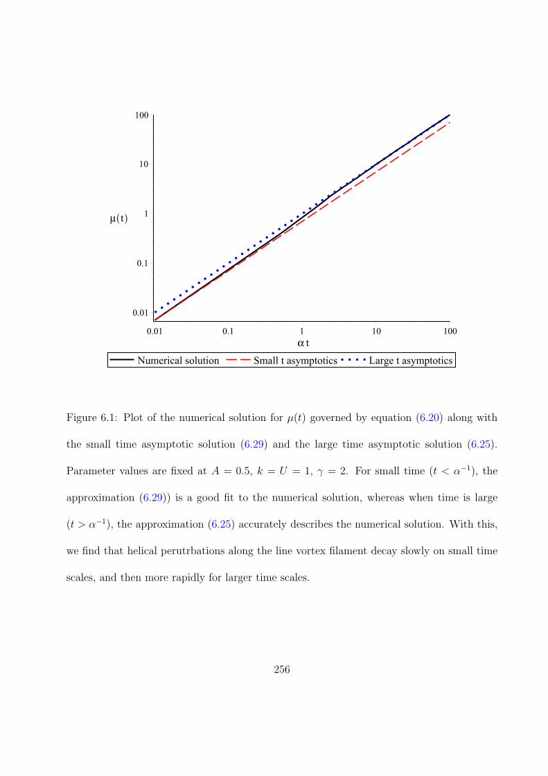
Figure 6.1: Plot of the numerical solution for µ(t) governed by equation (6.20) along with

the small time asymptotic solution (6.29) and the large time asymptotic solution (6.25).

Parameter values are fixed at A = 0.5, k = U = 1, γ = 2. For small time (t < α−1), the

approximation (6.29)) is a good fit to the numerical solution, whereas when time is large

(t > α−1), the approximation (6.25) accurately describes the numerical solution. With this,

we find that helical perutrbations along the line vortex filament decay slowly on small time

scales, and then more rapidly for larger time scales.

256

Obtaining the linear approximation like that of (6.32), we have

ω(t) ≈ (1− α′)γk2

(1 + A2k2)3/2t , (6.35)

which is completely consistent with the dispersion relation obtained under LIA for a standard

fluid when we set α′ = 0.

When U = 0, the translation effects (6.18) should be given by

dβ

dt=

(1− α′)γA2k3

(1 + A2k2 exp(−2µ(t)))3/2exp(−2µ(t)) =

1− α′

α

A2k exp(−2µ(t))√1 + A2k2 exp(−2µ(t))

dµ

dt, (6.36)

which gives a solution of the form

β(t) =1− α′

αk

√1 + A2k2 −

√1 + A2k2 exp(−2µ(t))

. (6.37)

Up to first order, this solution is approximated like

β(t) ≈ (1− α′)γA2k3

(1 + A2k2)3/2t (6.38)

when t is small enough. Setting α′ = 0, we again recover the expected result from the

standard fluid LIA. When t is large, we should have exp(−2µ(t)) → 0 and therefore

β(t) ≈ 1− α′

αk

√1 + A2k2 − 1

. (6.39)

What we find is that, when the effects of the normal fluid velocity are negligible

(U = 0), we obtain the helical filament

r(x, t) ≈(x+

(1− α′)γA2k3

(1 + A2k2)3/2t

)ix + A exp

(− αγk2

1 + A2k2t

)cos

(kx− (1− α′)γk2

(1 + A2k2)3/2t

)iy

+ A exp

(− αγk2

1 + A2k2t

)sin

(kx− (1− α′)γk2

(1 + A2k2)3/2t

)iz ,

(6.40)

257

which gradually decays to a line filament with exponential rate of decay αγk2

1+A2k2= O(α) as

time increases. Quantum vortex filaments in the U = 0 case are still physically relevant

(Vinen 2001; Araki, Tsubota & Nemirovskii 2002; Alamri, Youd & Barenghi 2008), and the

results here show that small helical excitations along such filaments should still decay despite

the absence of the normal fluid.

6.1.6 The role of normal fluid velocity on vortex motion and persistence

While exact solutions for µ(t) are not forthcoming in the presence of a non-zero normal

fluid velocity, we observe that the solutions should be approximately linear, with the slope

gradually increasing as t increases (as discussed above). For small t (t < α−1), we obtain

β(t) ≈(1− α′)γA2k3

(1 + A2k2)3/2− α′A2k2U

1 + A2k2

t , (6.41)

ω(t) ≈

(1− α′)γk2

(1 + A2k2)3/2− α′kU

1 + A2k2

t , (6.42)

µ(t) ≈

αγk

1 + A2k2− αkU√

1 + A2k2

t , (6.43)

while for large t (t > α−1) we have the approximations β(t) ≈ β0, ω(t) ≈ (1− α′)γk2 + α′kU t,

and µ(t) ≈ αk(γk−U)t (which is exactly what we found previously, in the small amplitude

limit).

Both attributes of the vortex motion, namely translation and rotation, are increased

when we increase the normal fluid velocity. Increasing the normal fluid velocity, we see that

solutions will decay more slowly, and therefore persist for longer periods of time. Both of

258

these observations make sense in light of the fact that the normal fluid velocity is expected

to drive the vortex. Therefore, increasing the normal fluid velocity results in faster-moving

and longer-lasting helical vortex filaments.

In Fig. 6.2, we plot the time evolution of a helical vortex filament as described by the

solution of the system of nonlinear differential equations (6.18)-(6.20). We take the normal

fluid velocity to be zero. In Fig. 6.3 we do the same, while taking a non-zero normal fluid

velocity.

From Fig. 6.4, we see that the translational motion of the helical Kelvin waves

along the vortex filament is strongly influenced by both the normal fluid velocity and the

magnitude of the superfluid friction parameters. Naturally, in increase in the normal fluid

velocity results in an increase in the rate of propagation of a helical Kelvin wave along

the x-axis. On the other hand, an increase in the superfluid friction parameters slows the

propagation of such helical Kelvin waves. While these results are completely intuitive, an

analysis of the nonlinear system (6.18)-(6.20) is needed to justify these conclusions for a

filament in the LIA. Meanwhile, the effective frequency (ω(t)/t) is not strongly influenced by

the normal fluid velocity, nor is it strongly influenced by the superfluid friction parameters.

This follows from the fact that the leading order term in the dispersion relation (6.19) does

not depends on either α, α′ or on U , and the only term involving U has the multiplication

α′U so that any effects of U are small.

259

(a) (b)

(c) (d)

Figure 6.2: Plot of the time evolution of a helical filament solution corresponding to A = 0.5,

γ = 2, k = 1, T=1K (i.e., α = 0.005, α′ = 0.003) and U = 0. Times referenced are (a) t = 0,

(b) t = 100, (c) t = 300, (d) t = 500.

260

(a) (b)

(c) (d)

Figure 6.3: Plot of the time evolution of a helical filament solution corresponding to A = 0.5,

γ = 2, k = 1, T=1K (i.e., α = 0.005, α′ = 0.003) and U = 1. Times referenced are (a) t = 0,

(b) t = 100, (c) t = 300, (d) t = 500. Note that the decay of the helical perturbations along

the filament is markedly slower than in the case of U = 0 (which was considered in Fig. 6.2).

261

(a) (b)

Figure 6.4: Plot of the (a) translation β(t) of the x-coordiate (the translational motion of the

helical waves along the filament) and (b) the effective frequency ω(t)/t for a helical filament

solution corresponding to A = 0.5, γ = 2, k = 1, for various temperatures and normal fluid

velocity. The temperature T = 1K correspond to α = 0.005, α′ = 0.003, while T = 1.5K

corresponds to α = 0.073, α′ = 0.018.

262

6.1.7 Discussion

For the eternal solutions (which do not decay in time), there is a requirement that the wave

number is fixed. In other words, for fixed values of the parameters A, γ, U there is a unique

wave number k = k∗ given by (6.13) such that a constant-amplitude helical filament solution

exists. This restriction in turn implies that the amplitude of such a helical filament must

be bounded like A < γ/|U |. This still allows the amplitude to be large enough for the helix

to exhibit translational motion in addition to pure rotation, as is evident from the solution

form presented in (6.15). The dispersion relation is close to that obtained in Van Gorder

[106], though the dispersion relation ω obtained here is exact, while that of Van Gorder [106]

was approximate (since an approximate potential form of the quantum LIA was assumed).

For the solutions which are permitted to decay in time, some observations are in

order. The rate of decay of the filament, µ(t)/t, is not constant in time but rather varies

according to (6.20). We see from the asymptotics of µ that the greatest rate of decay is for

large time, so the helical perturbations along the filament decay slowly at first and more

rapidly as time progresses. Since the translational effects are tied to the decay rate of the

filament through a term of the form exp(−2µ(t)), the greatest translation of the filament

occurs for small time, while translation of the filament ceases for asymptotically large time.

This makes sense: as the helical filament decays into a line filament, translational effects

diminish since there is no translation of a line filament. This is demonstrated in Fig. 6.4.

Therefore, the Kelvin waves rotate and also move along the x-axis while decaying. The more

263

they decay in amplitude, the slower the motion along the x-axis. Meanwhile, the rotational

motion persists, even as the waves decay.

In the case of constant-amplitude helical waves along a filament (i.e., eternal so-

lutions), the wave number is fixed (at a value corresponding to the Donnelly-Glaberson

instability), while when the helical filament is allowed to decay to a line filament we have no

such restriction on the wave number. However, we do still have a restriction on the possible

value of k which permit the filament to decay, k/√1 + A2k2 > U

γ. Rearranging this, we

obtain a condition on A: A <√

γ2

U2 − 1k2< γ

|U | . Therefore, the restriction on the amplitude

is stronger when we permit the helical waves to decay. This is physically reasonable, as it

is sensible to describe small-amplitude Kelvin waves along a vortex filament using LIA. For

large-amplitude perturbations, non-local effects will influence the solutions, so the full Biot-

Savart law under the HVBK model would be more reasonable for describing the filament

dynamics.

6.2 Dynamics of a planar vortex filament under the quantum

LIA

The Hasimoto planar vortex filament is one of the rare exact solutions to the classical local

induction approximation (LIA). This solution persists in the absence of friction or other

disturbances, and is hence rather idealized, as it maintains its form over time. As such, the

264

dynamics of such a filament have not been extended to more complicated physical situations.

We consider the planar vortex filament under the quantum LIA, which accounts for superfluid

friction and the velocity of a normal fluid impinging on the filament. We show that, for

most interesting situations, a filament which is planar in the absence of friction and normal

fluid at zero temperature will gradually deform due to friction effects and the normal fluid

flow corresponding to warmer temperatures. The influence of friction is to induce torsion,

so the filaments bend as they rotate. Furthermore, the flow of a normal fluid along the

vortex filament length will have an amplifying effect on the initial planar perturbations of

a line filament, reminiscent of the Donnelly - Glaberson instability seen in helical filament

structures. For warmer temperatures, these effects increase in magnitude. A number of

nice qualitative results are analytical in nature, and these results are verified numerically for

physically interesting cases. The results on the deformed planar filaments present under the

quantum LIA were considered in Van Gorder [113].

6.2.1 Background

While the planar filament has been studied under multiple models, for the quantum LIA

such filaments have so far been approximated (numerically or analytically) under potential

forms of the LIA (as discussed in Chapter 5). These are approximations to the LIA, valid

under certain restrictions such as that deviations from a reference axis must remain small of

be of sufficient bounded variation, and thus a more direct approach could be enlightening. In

265

particular, while such potential formulations are useful in some parameter regimes, there are

often restrictions (such as on amplitude of any waves along a filament, on the wave number

of solutions, and so on) that must be obeyed. In the present section, we work directly

with the LIA, as opposed to any approximating potential form. While this means that the

mathematics may not be as elegant, we benefit from having a precise representation of the

solutions. We shall consider the quantum LIA directly in Cartesian coordinates, since this

allows for easy visualization of the vortex filament solutions. Our goal in doing this is to

determine both qualitative and quantitative effects of the superfluid friction parameters and

the normal fluid velocity on the planar vortex filaments. In this way, we extend the planar

filaments of Hasimoto valid under the classical LIA to a new type of filament under the

quantum form of the LIA.

We review the planar filament in the classical fluid model, and attempt to extend

such a solution to the quantum fluid model directly. A solution of this type is possible only

when the normal fluid velocity varies in space and takes a particular form, meaning that

such a solution is of narrow applicability. Next, we overcome such difficulties by defining

a different type of filament, which happens to be planar at α, α′ = 0 yet non-planar away

from the origin when α, α′ > 0. Such a solution is the true generalization of the planar

filament for the quantum LIA, and indeed this solution allows us to study the dynamics of

a planar filament in the quantum LIA. The influence of the normal fluid velocity and of the

superfluid friction parameters on this family of solutions is discussed both through analytical

approximation and numerical simulation. The results suggest that the friction parameters

266

result in a twisting of the filaments, while the normal fluid directed along the filament results

in a type of amplification, reminiscent of the Donnelly - Glaberson instability [23, 36, 71] for

helical filaments under the quantum LIA.

6.2.2 A purely planar vortex filament

The general form of a rotating planar vortex filament under LIA is given by

r(x, t) = (x, cos(γt)ψ(x),− sin(γt)ψ) , (6.44)

where ψ is some unknown function to be determined. Note that the solution lies on a plane

which intersects the x-axis and rotates in time around the x-axis. We shall be most interested

in a normal fluid velocity vector oriented along the vortex filament, U = (U, 0, 0), since this

will often drive Kelvin waves along the filament.

Placing the solution representation (6.44) into the classical LIA (2.14), we find that

γκt× n = γ(0, sin(γt), cos(γt))ψ′′

(1 + ψ′2)3/2(6.45)

while

rt = γ(0,− sin(γt),− cos(γt))ψ ; (6.46)

Therefore, (6.44) is a solution to the classical LIA provided that

ψ +ψ′′

(1 + ψ′2)3/2= 0 . (6.47)

267

If we carry out similar computations for the quantum LIA (2.12), and set all three compo-

nents of the resulting vectors equal, we shall find

0 = −α ψ′ψ′′

(1 + ψ′2)2+ α′V

ψ′2

1 + ψ′2, (6.48)

sin(γt)ψ = − sin(γt)

(1− α′)ψ′′

(1 + ψ′2)3/2− αV ψ′

(1 + ψ′2)1/2

+ cos(γt)

αψ′′

(1 + ψ′2)2− α′V ψ′

1 + ψ′2

,

(6.49)

− cos(γt) = cos(γt)

(1− α′)ψ′′

(1 + ψ′2)3/2− αV ψ′

(1 + ψ′2)1/2

− sin(γt)

αψ′′

(1 + ψ′2)2− α′V ψ′

1 + ψ′2

,

(6.50)

where V = U/γ. Each of these equations has a term of the form

αψ′′

(1 + ψ′2)2− α′V ψ′

1 + ψ′2, (6.51)

which vanishes in the α, α′ → 0 limit. Meanwhile, the analogue to (6.47) in the quantum

case is apparently

ψ +(1− α′)ψ′′

(1 + ψ′2)3/2− αV ψ′

(1 + ψ′2)1/2= 0 . (6.52)

Let us assume that (6.51) holds equal to zero. This would then imply that (6.52) takes the

form

ψ +

(1− α′ − α2

α′

)ψ′′

(1 + ψ′2)3/2= 0 . (6.53)

Let ψ(x) be a bounded and periodic solution of (6.47). Then, the scaling

ψ(x) =

√1− α′ − α2

α′ ψ

(x√

1− α′ − α2/α′

)(6.54)

is a solution of (6.53). This provides a nice link between the classical and quantum LIA

solutions, and shows that a purely planar solution is possible, provided that the consistency

268

term (6.51) vanishes. That said, the consistency term (6.51) does not, in general vanish. To

see why, note that a planar filament solution to (6.47) is periodic. On the other hand, let us

rescale the coefficients in (6.51) to obtain the differential equation

h′′ = h′ + h′3. (6.55)

After obtaining a first integral, we should have

h′ = ± 1√Ce−2x − 1

, (6.56)

and therefore at some finite value of x, h should become singular. Since this incompatible

with a planar solution, we conclude that (6.51) does not vanish when ψ is a bounded and

periodic function as given in (6.54). Note that a solution (6.54) may still remain a very

good approximation to a true filament solution. In this case, the consistency term should be

sufficiently small. Indeed, the consistency term is of order α, whereas the solution (6.54) is

determined by an equation of order unity.

There is a fix that allows us to obtain a solution (6.54) while also satisfying the

consistency condition (6.51), but this involves picking the normal fluid velocity in a very

specific way. In particular, if instead of considering a constant velocity for the normal fluid

flow, we were to pick U = (U(x), 0, 0), then we can use (6.51) to determine conditions on

such a function U(x). Doing so, one finds

U(x) =α

α′γ

ψ′′

ψ′(1 + ψ′2). (6.57)

While this is, of course, a rather narrow restriction on the form of U, it does permit a very

elegant solution (6.54).

269

As it turns out, a purely planar vortex filament moving without change in form is

simply too specialized to exist in a superfluid under normal conditions (the exact solution

we get when U = U(x) takes a specific form is certainly not what one would call general

in any sense). Rather, it makes more sense to consider a family of vortex filaments what

generalize the planar filament in the sense that they reduce to the planar filament in the

limit α, α′ = 0. For α, α′ > 0, such filaments would not be confined to a plane which rotates

about the reference axis, but would rather exhibit planar behavior in a local sense, while

exhibiting other behaviors asymptotically for large |x|. In a way, we could view such vortex

filaments as deformations of the planar filaments, with the deformations do the the influence

of both the superfluid friction parameters and the normal fluid velocity.

6.2.3 Deformation of a planar filament due to superfluid parameters

When attempting to construct a purely planar quantum generalization of the planar filament

found in the classical LIA, it became clear that in most cases (for instance, when U is a

constant vector) there are too few degrees of freedom if we assume that the time evolution

of the vortex filament follows (6.44). In order to obtain the most useful generalization of

the classical planar filament, we need to consider that the superfluid parameters can cause

the filament to become non-planar in a variety of ways. Amplification or deamplification

of waves along a quantum vortex filament is possible, while modified torsion due to the

superfluid friction parameters is also an issue. To account for such effects, we propose a

270

solution of the form

r(x, t) = (x, cos(γt)ϕ(x) + sin(γt)ψ(x), cos(γt)ψ(x)− sin(γt)ϕ(x)) . (6.58)

Placing (6.58) in (2.12), we obtain the differential equations

ϕ+(1− α′)ϕ′′

(1 + ϕ′2 + ψ′2)3/2+

αψ′′

(1 + ϕ′2 + ψ′2)2− αV ϕ′

(1 + ϕ′2 + ψ′2)1/2

− α′V ψ′

(1 + ϕ′2 + ψ′2)− αϕ′(ψ′ϕ′′ − ϕ′ψ′′)

(1 + ϕ′2 + ψ′2)2= 0 ,

(6.59)

ψ +(1− α′)ψ′′

(1 + ϕ′2 + ψ′2)3/2− αϕ′′

(1 + ϕ′2 + ψ′2)2− αV ψ′

(1 + ϕ′2 + ψ′2)1/2

+α′V ϕ′

(1 + ϕ′2 + ψ′2)− αψ′(ψ′ϕ′′ − ϕ′ψ′′)

(1 + ϕ′2 + ψ′2)2= 0 .

(6.60)

By including two unknown functions, we obtain two differential equations for two unknown

functions, as opposed to two differential equations for one unknown function (as was the

case for the purely planar filament). The motion of the filament (6.58) is not purely planar,

though it contains the pure planar filament as a reduction (taking ψ → 0 gives the pure

planar filament).

Since we should have a planar filament when α, α′ → 0, we should take ϕ to be of order

unity and ψ to be of order α. While a complete analytical analysis of (6.59)-(6.60) is not

possible since the equations are too complicated, we can make some qualitative observations.

If we assume ψ = αΨ for some function Ψ of order unity, and we neglect order α2 and higher

terms, we should have

ϕ+(1− α)ϕ′′

(1 + ϕ′2)3/2− αV ϕ′

(1 + ϕ′2)1/2= 0 , (6.61)

Ψ +(1− α)Ψ′′

(1 + ϕ′2)3/2− αVΨ′

(1 + ϕ′2)1/2=

ϕ′′

(1 + ϕ′2)2− α′V

α

ϕ′

1 + ϕ′2. (6.62)

271

While simplified from (6.59)-(6.60), these equations are still too complicated to solve exactly,

owing to the fact that (6.61) does not have a first integral for α = 0. In the case where the

amplitude A of a solution ϕ is sufficiently small, we should find

ϕ(x) = A cos

(√4(1− α′)− α2V 2

2(1− α′)x

)exp

(αV

2(1− α′)x

)+O(A3) . (6.63)

For small A, the order A3 corrections are negligible. Near the origin, the solutions maintain

a planar appearance, since the exponential growth or decay rate is of order α. The solutions

will amplify for either x > 0 or x < 0, depending on the sign of V . So, there is amplification

driven by the normal fluid along the direction in which the normal fluid points. This is

analogous to the Donnelly - Glaberson instability seen when a normal fluid flow is directed

along a helical vortex filament.

In the case where V = 0, there is no amplification in the lowest-order term. However,

as we shall see later, nonlinear terms will cause amplification for both large negative and

large positive values of x. Such effects are only captured by considering higher order terms

in A.

It is possible to exploit the symmetry of equations (6.59)-(6.60) to obtain a single

complex equation. Defining W = ϕ+ iψ, and adding i times (6.60) to (6.59), we obtain

W +(1− α′)W ′′

(1 + |W ′|2)3/2− αVW ′

(1 + |W ′|2)1/2

+ i

α′VW ′

1 + |W ′|2− αW ′′

(1 + |W ′|2)2− α

2

W ′(W ′∗W ′′ −W ′W ′′∗)

(1 + |W ′|2)2

= 0 .

(6.64)

Here, ∗ denotes complex conjugation. Note that (6.64) implies that (6.59)-(6.60) can be

mapped to a three-dimensional real system, despite the fact that (6.59)-(6.60) is a four-

272

dimensional real dynamical system. This is due to a certain type of symmetry that exists in

the equations (6.59)-(6.60) which is inherited from the LIA itself. To demonstrate this, let

us consider the representation W (x) = R(x) exp(i∫ x0θ(σ)dσ), where R and θ are real-valued

functions. Placing this representation into (6.64), and separating the resulting equation into

real and imaginary parts, we obtain

R +(1− α′)(R′′ −Rθ2)

(1 +R′2 +R2θ2)3/2+

α(2R′θ +Rθ′)

(1 +R′2 +R2θ2)2− αV R′

(1 +R′2 +R2θ2)1/2

− α′V Rθ

(1 +R′2 +R2θ2)+αR′[(2R′2 −RR′′)θ +R2θ2 +RR′θ′]

(1 +R′2 +R2θ2)2= 0 ,

(6.65)

(1− α′)(2R′θ +Rθ′)

(1 +R′2 +R2θ2)3/2− α(R′′ −Rθ2)

(1 +R′2 +R2θ2)2− αV Rθ

(1 +R′2 +R2θ2)1/2

+α′V R′

(1 +R′2 +R2θ2)+αRθ[(2R′2 −RR′′)θ +R2θ2 +RR′θ′]

(1 +R′2 +R2θ2)2= 0 .

(6.66)

Equations (6.65)-(6.66) constitute a three-dimensional dynamical system. This system can

be solved provided that it is non-degenerate. Writing the system in the form

[(1− α′)√

1 +R′2 +R2θ2 − αRR′θ]R′′ + αR(1 +R′2)θ = F1(R,R′, θ) , (6.67)

− α(1 +R2θ2)R′′ + [(1− α′)R√

1 +R′2 +R2θ2 − αR2R′θ]θ′ = F2(R,R′, θ) , (6.68)

for appropriately defined F1 and F2. The determinant of the Jacobian of the left hand side

of (6.67)-(6.68) must not vanish, which is equivalent to the condition

(αR2R′θ+(1−α′))√1 +R′2 +R2θ2−R[αR′θ+(α′−α′2−α2)(1+R′2+R2θ2)] = 0 . (6.69)

In the limit α, α′ → 0, this condition becomes

√1 +R′2 +R2θ2 = 0 , (6.70)

273

which is always true. Therefore, given small enough α and α′, the system (6.65)-(6.66) is

non-degenerate, and a solution does exist.

Equations (6.65)-(6.66) are no simpler to study than (6.59)-(6.60). However, let us

assume that any deviations from the reference axis are small, so that |R| ≤ ϵ << 1. Let

us also define the function ξ(x) = R′(x)/R(x), which itself should be of order unity. Then,

neglecting terms of order ϵ2 and higher, equations (6.65)-(6.66) are reduced to

1 + (1− α′)(ξ′ + ξ2 − θ2) + α(2ξθ + θ′)− αV ξ − α′V θ = 0 , (6.71)

and

(1− α′)(2ξθ + θ′)− α(ξ′ + ξ2 − θ2)− αV θ + α′V ξ = 0 , (6.72)

respectively. To study the qualitative effects of the remaining nonlinearity, we set V = 0,

which is physically relevant in the low-temperature limit and also in the case of superfluid

Helium 3. We obtain

β + 2ξθ + θ′ = 0 , (6.73)

β′ + ξ′ + ξ2 − θ2 = 0 , (6.74)

where

β =α

α2 + (1− α′)2and β′ =

1− α′

α2 + (1− α′)2. (6.75)

This system admits two equilibrium points when β > 0: (ξ∗, θ∗) = (−β/(2ν), ν) and

(ξ∗, θ∗) = (β/(2ν),−ν), where

ν =

√β′ +

√β′2 + β2

2. (6.76)

274

A linear stability analysis shows that the equilibrium (−β/(2ν), ν) is unstable, whereas

(β/(2ν),−ν) is linearly stable. Eigenvalues of the Jacobian for system (6.73)-(6.74) take the

form λ± = βθ∗±2iθ∗, so the stable solutions should spiral inward toward the equilibrium, while

the unstable solutions should spiral outward from the equilibrium, in the (ξ, θ) phase space.

If we consider the time reversal (more accurately, “space-reversal” since ξ and θ depend on

space variable x), the equilibrium points switch stability properties. This suggests that on

one half of the x-axis, the perturbations along the vortex filament decay, whereas for the

opposite half of the x-axis such perturbations amplify. Therefore, the amplification of planar

perturbations along the vortex filament is possible even without the normal fluid velocity.

From the analysis above, we draw several conclusions about the deformation of a

planar vortex filament in the quantum form of the LIA. First, the effect of V , the scaled

normal fluid velocity, is to amplify the planar wave along the direction which the normal

fluid velocity vector is pointing. The rate of amplification is moderated by the friction

parameter α, which is small. The smaller the parameter α, the slower the amplification

(in the perturbative limit). Amplification is still possible when V = 0. The inclusion of

superfluid friction parameters results in a non-trivial phase term, θ. This feature implies

that there are torsion effects not present in the classical planar filament. If the initial

condition is θ(0) = 0, then such effects are small near the origin, but can become large for

large values of |x|. These are all behaviors that are absent in the classical planar filament,

but which are suggested by the mathematics above in the case of a quantum planar filament.

275

In order to verify some of the behaviors suggested by the analytics above, we turn

to numerical solutions. Since (6.65)-(6.66) are non-degenerate and are equivalent to (6.59)-

(6.60), a solution pair (ϕ(x), ψ(x)) exists (at least locally) for reasonable values of α, α′ and

V . We find that the standard RKF45 method is sufficient to numerically approximate the

solutions of (6.59)-(6.60) to a desirable accuracy. When ψ(x) ≡ 0, we obtain the classical

planar vortex filament solution. Therefore, the initial condition ψ(0) = 0 makes sense. We

take ϕ(0) > 0 to be the distance of the planar filament from the reference axis at the origin.

Conditions ϕ′(0) = ψ′(0) = 0 are not required, but they enforce a nice local symmetry at

the origin.

In Fig. 6.5, we consider the planar filament in the T = 1K case in the presence of a

normal fluid velocity directed along the positive x-axis, while in Fig. 6.6 we do the same for

the T = 1.5K case. Amplification of waves along the line filament occur much more rapidly

when temperature increases, since α increases and hence the combined effect αV increases -

resulting in more exponential growth.

The numerical simulations suggest that the planar filaments do amplify due to the

normal fluid flow, and that the direction of the normal fluid flow along the filament determines

where this amplification takes place. This is shown nicely when comparing Figs. 6.6 and 6.7,

which model the same situation only with the direction of U reversed. Numerical results

also show that the greater the speed of the normal fluid, the greater the amplification.

Both the direction and rate of amplification (as a function of temperature and normal fluid

velocity) are in agreement with the qualitative analysis performed above. In particular, this

276

is in complete agreement with what was suggested by the analytical approximation in the

small-amplitude limit, (6.63).

The rate of amplification is greater when α is larger, hence the planar filaments

amplify more rapidly in warmer temperatures. In the case where V = 0, the amplification

occurs in a symmetric way for both large negative and large positive x, as seen in Fig. 6.8.

Thus, amplification can occur due to frictional effects, since the model is nonlinear. In cases

where V ≈ 0 is still physically relevant, such as the low temperature limit or for superfluid

Helium 3, this implies that amplification can still occur. Such amplification in the absence

of a driving normal fluid velocity agrees with what was suggested by the reduction to polar

coordinates in the approximate equations (6.73)-(6.74).

Near the origin, the solutions all appear planar in form. However, for larger values of

|x|, the solutions undergo torsion effects due to the interaction with the fluid modeled by the

superfluid friction parameters, α and α′. This is best seen when we compare a true planar

filament solution to the classical LIA (α, α′ = 0) with one of the quantum vortex filaments.

We do this in Fig 6.9, where we see that close to the origin the two filaments agree, whereas

as one gets further from the origin, the effects of the superfluid friction parameters result in

a bending of the rotating filament, while the influence of the normal fluid velocity causes an

amplification or de-amplification. For negative x, the quantum filament eventually takes on

a helical form, which contrasts with the planar form of the classical filament. For positive

x, the quantum filament undergoes strong amplification.

277

Figure 6.5: Plot of the deformed planar filament described by (6.58) when the temperature

of the superfluid is T=1K (α = 0.005, α′ = 0.003) and V = 1. The filament is given by

numerically solving (6.59)-(6.60) subject to ϕ(0) = 0.1, ψ(0) = 0, ϕ′(0) = 0, ψ′(0) = 0.

278


of the superfluid is T=1.5K (α = 0.073, α′ = 0.018) and V = 1. The filament is given by


279


of the superfluid is T=1.5K (α = 0.073, α′ = 0.018) and V = −1. The filament is given by


280


of the superfluid is T=1.5K (α = 0.073, α′ = 0.018) and V = 0. The filament is given by


281

Figure 6.9: Comparison of the deformed planar filament described by (6.58) when the tem-

perature of the superfluid is T=1.5K (α = 0.073, α′ = 0.018) and V = 1, along with the

classical planar filament corresponding to α = α′ = 0. In both cases, the filaments are given

by numerically solving (6.59)-(6.60) subject to ϕ(0) = 0.1, ψ(0) = 0, ϕ′(0) = 0, ψ′(0) = 0.

The blue curve represents the T=1.5 deformed planar filament, while the black curve repre-

sents the classical planar filament.

282

6.2.4 Discussion

In summary, the quantum planar vortex filament differs from the well-known classical planar

vortex filament in some important qualitative respects. First, there is an amplification of the

planar perturbations of the quantum filament along the axis of orientation. This is caused

by the normal fluid velocity directed along the filament. Next, while the classical planar

filament maintained its form, the extension to the quantum model results in a filament that

undergoes torsion effects due to the superfluid friction parameters. This causes a bending

of the once planar filament the farther removed from x = 0 we look. On the de-amplified

end of the filament, this results in an almost helical appearance for the filament. On the

amplified end of the filament, an interesting pattern is formed that exhibits regularity but

is not as uniform as a helical structure.

While a thermal study is beyond the scope of the results considered here, it makes

sense to consider α and α′ as functions of time, so that we can consider the qualitative

effect of warming a superfluid which houses a planar filament, since an increase in such

parameters would correspond to a warming of the superfluid. In the case where both friction

parameters are zero, the classical planar filament solution is valid. If such a filament exists

at temperature T≈ 0K, then as the superfluid is warmed, we qualitatively expect that the

filament will deform as follows. There will be a minor amplification / de-amplification of the

filament along / against the direction of the normal fluid. This amplification will become

more drastic as the superfluid continues to warm. While this occurs, the amplifying and de-

283

amplifying parts of the filament gradually bend as the effects of friction increase, meaning

that the filament no longer exists within a plane rotating about the reference axis. As such,

the filament is no longer planar.

What these results suggest is that a planar vortex filament structure in a superfluid

should be a localized structure, in contrast to the classical fluid case, where such a filament

maintains its form globally. Due to the effect of superfluid friction parameters and the

normal fluid velocity, we see that on one side of the reference axis, the filament takes on a

helical form far enough away from x = 0, whereas on the opposite side of the reference axis

the filament undergoes strong amplification. Near x = 0, however, the solution maintains

a planar form, even for larger values of the superfluid friction parameters or the normal

fluid velocity. From this, localized planar structures can exist in a superfluid, even if such

structures are no longer global like in the classical LIA.

In the case of helical Kelvin waves on a quantum vortex filament, it is known that

waves of constant amplitude correspond to the critical wave number for Donnelly - Glaberson

instability. If these solutions are perturbed, they will either decay to line filaments or they

will amplify and blow-up. This instability is driven by the normal fluid flow along the

reference axis of the vortex filament, which results in an amplification of the Kelvin waves if

the amplitude is large enough at the initial time. This behavior is global, in that the decay or

blow-up occurs along the entire helical filament. In the case of the deformed planar filament,

a similar phenomenon to the Donnelly - Glaberson instability is seen, where the normal fluid

velocity directed along the vortex filament results in amplification of the perturbations along

284

the line filament. However, unlike in the case of the helical perturbations, the amplification

of the planar filament is local in nature, with a strong dependence on the direction of the

normal fluid velocity. While the helical Kelvin waves amplify or decay uniformly for all

x depending on the model parameters, the decay or amplification of the deformed planar

filament is non-uniform in x.

With regards to physical experiments, the section of the filament which undergoes

strong amplification may break down or dissipate, leaving a vortex filament line on half of

the spatial domain. This half of the filament will be planar near x = 0, and helical as one

moves away from the origin, in the direction of the x-axis on which the filament persists.

Such a vortex filament is shown in Fig. 6.10. In this way, the planar segment of the filament

may persist in time, although other sections of the filament may dissipate. This strong local

behavior is in contrast to the more uniform behavior of a helical filament, which will either

decay to a line filament or continue to amplify (leading to dissipation).

In the case where the amplification of the deformed planar filament is strong (i.e.,

the warmer superfluid case), non-local effects will likely play a considerable role in the time

evolution of the vortex filament. Therefore, while the amplification under LIA is continuous

in the direction of the normal fluid flow, realistically any tendency for the amplitude to grow

without bound would likely be mitigated by non-local effects once the amplitude was large

enough. So, while amplification is still expected along the lines shown here, any amplification

is expected to be bounded for the HVBK model which includes non-local effects through

the Biot-Savart integral term. This in turn implies that the results obtained here under

285

LIA would be expected to agree with experiments qualitatively, while specific quantitative

details for any specific physical parameters would require these non-local effects, particularly

in the case where deviations from the reference axis are large (as occurs in locations where

the planar filaments amplify). The first step in studying the non-local effects would be to

consider whether planar vortex filament exists under the full Biot-Savart dynamics, which is

what the classical LIA approximates.

286

Figure 6.10: Large-time plot of the deformed planar filament described by (6.58) when

the temperature of the superfluid is T=1.5K, with the same conditions given in Fig. 6.7.

Segments of the filament which continue to amplify are removed, to show what might be

expected experimentally after such segments dissipate or disassociate with the rest of the

filament. The filament is locally planar near x = 0, while for large x the filament takes on a

helical appearance.

287

6.3 Solitons and other waves on a quantum vortex filament

The quantum form of the local induction approximation (LIA, a model approximating the

motion of a thin vortex filament in superfluid) including superfluid friction effects is put

into correspondence with a type of cubic complex Ginsburg-Landau equation, in a manner

analogous to the Hasimoto map taking the classical LIA into the cubic nonlinear Schrodinger

equation. From this formulation, we determine the form and behavior of Stokes waves,

1-solitons, and other traveling wave solutions under normal and binormal friction. The

most important of these solutions is the soliton on a quantum vortex filament, which is

a natural generalization of the 1-soliton solution constructed mathematically by Hasimoto

which motivated subsequent real-world experiments. We also conjecture on the possibility

of chaos in such systems, and on the existence more complicated solitons such as breathers.

The various types of solutions obtained in this section were reported in Van Gorder [114].

6.3.1 Background

A number of studies exist on the solutions to the quantum LIA. In the α, α′ → 0 limit, these

solutions should collapse into solutions of the classical LIA. One highly important class

of solutions to the classical LIA would be the 1-soliton solution found by Hasimoto (and

mentioned in Chapter 2), by way of what is now referred to as the Hasimoto transformation,

which puts the classical LIA into correspondence with the cubic NLS. While a number

288

of solutions to the quantum LIA have been studied either numerically or analytically, the

Hasimoto 1-soliton have never been extended to the quantum LIA. The purpose of this

section is to fill this important gap. Applying a method analogous to that of Hasimoto,

we are able to put the quantum LIA (2.12) into correspondence with a type of complex

Ginzburg-Landau equation (a natural complex-coefficient generalization of NLS). From this,

we study Stokes waves, 1-solitons, and other traveling wave solutions. Each of these solutions

generalizes known results for the classical LIA. We also conjecture on the possibility of chaos

in such systems.

6.3.2 A map from the quantum LIA into a cubic complex Ginsburg-Landau

equation

Differentiating with respect to the arclength variable s, and performing several vector ma-

nipulations, we have that the quantum LIA (2.12) becomes

t =∂

∂s

(1− α′|t|2)t× ts − α[(t · ts)t− |t|2ts]

+

∂

∂sαt×U− α′t× (t×U) .

(6.77)

Taking t to be a unit vector, the equation simplifies slightly to

t =∂

∂s(1− α′)t× ts + αts + αt×U− α′(t ·U)t . (6.78)

This puts the quantum LIA (2.12) into the form of a vector conservation law.

In what follows, we shall take U = 0, for brevity of the calculations. Many studies on

specific structures in the quantum LIA model have taken the normal fluid velocity to zero,

289

as it permits one to study such structures without the influence of drift or other distorting

effects on the filaments[5, 3, 117]. The physical applicability of such a scenario is limited to

the very low temperature regime in superfluid Helium 4. On the other hand, in the case of

superfluid Helium 3, the normal fluid velocity U is zero (because Helium 3 is very viscous,

unlike Helium 4, so it is always at rest or in solid body rotation, but α and α′ are not zero

[31]). Similar results were recently attempted in the case of U = 0 [86], however the system

was not solved and only the limiting reduction to α, α′ = 0 was given. Some qualitative

observations were also given at lowest order.

Let b denote the binormal vector, and take κ and τ to be the curvature and torsion,

respectively. Recall that ts = κn, ns = −κt + τb, bs = −τn. After setting U = 0, we can

write (6.78) as t = (1− α′)(κb)s + αtss.

Let us define the function ψ(s, t) = κ(s, t) exp(i∫ s0τ(s, t)ds) and also a new vector-

valued function by m = (n+ ib) exp(i∫ s0τ(s, t)ds). Note that ms = −ψt and ts =

12(ψ∗m+

ψm∗), where ∗ denotes complex conjugation. Additionally, (κb)s =i2(ψsm

∗ − ψ∗sm). The

quantum LIA (6.78) therefore takes the form

t =i

2(1− α′)(ψsm

∗ − ψ∗sm) +

α

2(ψ∗m+ ψm∗)s . (6.79)

290

We seek to derive an equation for ψ in analogy to that which was obtained by Hasi-

moto in the case of a standard fluid (i.e., α = α′ = 0). On the one hand, note that

ms = −ψt− ψt

= −(ψ + α|ψ|2ψ)t+ i(1− α′)− α

2ψψ∗

sm

− i(1− α′) + α

2ψψsm

∗ .

(6.80)

On the other hand, assume that we have a representation for m of the form

m = am+ bm∗ + ct . (6.81)

First, observe that

a+ a∗ =1

2(m ·m∗ + m∗ ·m) =

1

2

∂

∂t(m ·m∗) = 0 , (6.82)

therefore a must take the form a = iϕ(s, t), for some real-valued function ϕ. By a similar

process, b ≡ 0. We should also find that

c = −m · t = −(i(1− α′) + α)ψs . (6.83)

Therefore, we have the representation

m = iϕ(s, t)m− (i(1− α′) + α)ψs(s, t)t . (6.84)

Differentiation of this representation with respect to arclength gives

ms = iϕsm− iϕψt− (i(1− α′) + α)ψsst

− 1

2(i(1− α′) + α)ψs(ψ

∗m+ ψm∗) .

(6.85)

291

Clearly, the coefficients of t, m and m∗ in equations (6.80) and (6.85) should match

exactly. The m∗ coefficients already match exactly. Setting the m coefficients equal, we

obtain

ϕs =1− α′

2

∂

∂s|ψ|2 − αi

2(ψ∗ψs − ψψ∗

s) , (6.86)

hence

ϕ(s, t) =1− α′

2|ψ|2 + α(Re(ψ))(Im(ψ)) + A(t)

=1− α′

2|ψ|2 − iα

4(ψ2 − ψ∗2) + A(t) ,

(6.87)

where A(t) is an arbitrary function of time. Despite the appearance of i, this representation

is real-valued, since ψ2 − ψ∗2 is purely imaginary. Matching the coefficients of t, we obtain

ψ + α|ψ|2ψ = iϕψ + (i(1− α′) + α)ψss . (6.88)

Using (6.87), we obtain an evolution equation for the function ψ:

ψ = iA(t)ψ + (i(1− α′) + α)ψss

+

(i(1− α′)

2− α

)|ψ|2ψ +

α

4(ψ2 − ψ∗2)ψ .

(6.89)

Evidently, for the solutions we take interest in, the term ψ2 − ψ∗2 will be small (negligible),

so we remove it. This term would need to be considered in the the case of higher-order

perturbations to the system (at order α2). Making this reasonable reduction, we obtain

ψ = iA(t)ψ + (i(1− α′) + α)ψss +

(i(1− α′)

2− α

)|ψ|2ψ . (6.90)

Under an appropriate scaling of time (T = (1−α′)t) and by defining a function Ψ such that

ψ(s, t) =√2Ψ(s, T ) exp(i

∫ t0A(t)dt), we can reduce (6.90) into

ΨT = (i+ ϵ)Ψss + (i− 2ϵ)|Ψ|2Ψ , (6.91)

292

where ϵ = α/(1− α′) << 1. Eq. (6.91) is a type of complex Ginzburg-Landau equation. If

we take α, α′ = 0 (which corresponds to a standard fluid), then ϵ = 0, and (6.91) reduces to

the cubic NLS, and therefore these results are completely consistent with those of Hasimoto

for the standard fluid LIA.

6.3.3 Stokes wave solutions for the quantum LIA

A Stokes wave solution exists for the classical LIA. To recover a Stokes wave along a quantum

vortex filament, we assume a solution of the form Ψ(s, T ) = P (T ), so that

iPT + (1 + 2iϵ)|P |2P = 0 . (6.92)

Writing P (T ) = R(T ) exp(iΘ(T )), we find RT = −2ϵR3 and ΘT = R2, which gives R(T ) =

(1 + 4ϵT )−1/2 and Θ(T ) = (4ϵ)−1 ln(1 + 4ϵT ). P (T ) then takes the form

P (T ) =cos(

ln(1+4ϵT )4ϵ

)+ i sin

(ln(1+4ϵT )

4ϵ

)√1 + 4ϵT

. (6.93)

Taking ψ(s, t) = P (T ) exp(i∫ t0A(t)dt) gives us the general form of a Stokes wave. In the

ϵ = 0 limit, we obtain the standard Stokes wave of constant modulus.

6.3.4 Soliton on a quantum vortex filament

The most interesting solution associated with the Hasimoto transformation of the LIA is

likely the soliton on a vortex filament. It is natural to wonder if such a soliton solution is

293

possible for the quantum LIA. In order to obtain a soliton, we shall consider a stationary

solution Ψ(s, T ) =√2ωq(S) exp(−iωt), with S =

√ωs. This puts (6.91) into the form

(1− ϵi)q′′ + 2(1 + 2ϵi)|q|2q + q = 0 , (6.94)

or, equivalently,

q′′ + 2

(1− ϵ2

1 + ϵ2+

3ϵi

1 + ϵ2

)|q|2q −

(1

1 + ϵ2+

ϵi

1 + ϵ2

)q = 0 . (6.95)

Since ϵ = O(α) and α << 1, we may neglect terms of order ϵ2 and higher, to obtain

q′′ + 2 (1 + 3ϵi) |q|2q − (1 + ϵi) q = 0 . (6.96)

When ϵ = 0 (corresponding to the standard fluid case), we find q(S) = sech(S), so any

solution for ϵ > 0 should reduce to this case in the ϵ→ 0 limit. We should therefore consider

a solution of the form q(S) = ρ(S) exp(iϵθ(S)). This has the interpretation that curvature is

determined by the ϵ = 0 case, while ϵ > 0 influence the torsion of the filament. Making the

relevant transformation, discarding contributions of order ϵ2 or higher, and splitting (6.96)

into real and imaginary parts, we obtain

ρ′′ + 2ρ3 − ρ = 0 , 2ρ′θ′ + ρθ′′ + 6ρ3 − ρ = 0 . (6.97)

Clearly, ρ(S) = sech(S), which is just the soliton from the standard fluid case. We then find

that

θ′(S) = (C1 + 5 tanh(S)− 2 tanh3(S)) cosh2(S) . (6.98)

This derivative blows up rapidly for all values of C1 except for C1 = 3. When C1 = 3,

θ′(S) → 1/2 as S gets large. This in turn implies that θ(S) would grow linearly as S gets

294

large. Therefore, we pick C1 = 3, and upon integrating (6.98) we find

θ(S) = C0 −3

2S +

3

4(cosh(2S)− sinh(2S)) + 2 ln(cosh(S)) . (6.99)

There is a far simpler, yet still rather accurate, way to represent θ by way of an asymptotic

expansion. We find that

θ(S) = C0 +7

4− 2 ln(2) +

S

2+

11

4e−2S +O(e−4S) . (6.100)

Picking C0 = 2 ln(2)− 7/4 to simplify the expansion,

θ(S) =S

2+

11

4e−2S +O(e−4S) . (6.101)

This solution gives a linear growth in S, for large enough S. We therefore have that q(S) is

accurately approximate by

q(S) = sech(S) exp

(iϵ

S

2+

11

4e−2S

)(6.102)

up to order ϵ2. Putting this solution back into the natural variables s and t, we obtain a

soliton on a quantum vortex filament:

ψ(s, t) =√2ωsech(

√ωs) exp (iµ(s, t)) , (6.103)

µ(s, t) =α

1− α′

(√ω

2s+

11

4e−2

√ωs

)− (1− α′)ωt . (6.104)

6.3.5 Traveling waves on a quantum vortex filament

The solution (6.103)-(6.104) constitutes a soliton along a vortex filament. The solution is

stationary, with only the phase depending on time. It is, however, possible to consider a

295

traveling wave along a vortex filament. In the case, both the phase and the amplitude of

ψ would vary in time. Let us define Ψ(s, T ) = Ψ(ξ), where ξ = s − ηT . Ignoring terms of

order ϵ2 and higher, we obtain

Ψ′′ + η(ϵ− i)Ψ′ + (1 + 3ϵi)|Ψ|2Ψ = 0 . (6.105)

Writing Ψ(ξ) = F (ξ) exp(i∫ ξ0G(ν)dν), we obtain the system

F ′′ − FG2 + ηϵF ′ + ηFG+ F 3 = 0 ,

2F ′G+ FG′ − ηF ′ + ηϵFG+ 3ϵF 3 = 0 ,

(6.106)

which is effectively a third-order dynamical system. The system (6.106) has the interesting

property that it has either one or infinitely many equilibrium points, depending on the

value of the wave speed, η. If η = 3/2, there exist infinitely many equilibria of the form

(F ,G) = (F,−2F2), where F ∈ R. On the other hand, when η = 3/2, the only equilibrium

is the zero equilibrium (F ,G) = (0, 0).

From numerical simulations, we find that there is an interesting bursting pattern

associated with the solutions to (6.106). For large negative values of ξ, the phase and

amplitude functions are reasonably well-behaved. Then, near some finite value ξ = ξ0

(which in general depends on both ϵ and η), there is a bursting behavior to the phase G(ξ),

near where the amplitude F (ξ) reaches its minimal value. Past ξ0, the phase switches signs

and gradually the dynamics become more tame. This behavior is demonstrated in Fig. 6.11.

This behavior becomes more clear when we view the system in phase space. In Fig. 6.12,

we plot the solution to (6.106) in the phase space (F, F ′, G). The solution corresponds to a

296

trajectory which originates infinitely far from the origin as ξ → −∞, then approaches the

origin, goes through a bursting pattern, and then leaves the origin in a similar manner to

which it came.

297

Figure 6.11: Plot of the solution to the dynamical system (6.106) when α = 0.073, α′ = 0.018,

η = 0.1. Initial conditions are F (0) = 1, F ′(0) = 0 and G(0) = 0.

298

Figure 6.12: Phase space plot of the solution to the dynamical system (6.106) when

α = 0.073, α′ = 0.018, η = 0.1. Initial conditions are F (0) = 1, F ′(0) = 0 and G(0) = 0.

299

6.3.6 Discussion

With this, we have successfully transformed the quantum LIA into a type of complex

Ginzburg-Landau equation (6.91), by use of a method analogous to the Hasimoto trans-

formation for a standard fluid vortex filament. Doing so, we are able to reduce the quantum

LIA (6.78) (a vector conservation law) into a complex scalar PDE (6.91), which makes the

system far more amenable to mathematical analysis. Such a mapping between the quantum

LIA and this PDE is also desirable from a physical point of view, since it allows for greater

qualitative comparison of the quantum and standard fluid LIA solutions.

Upon transforming the quantum LIA into a complex Ginzburg-Landau equation

(6.91), we were able to study a number of solutions. First we obtained Stokes wave type

solutions. In the case of a standard fluid, these solutions takes the form of oscillating waves

with constant amplitudes. However, we were able to demonstrate that for a quantum fluid

modeled under LIA, such solutions have an algebraic decay rate and therefore dissipate as

time becomes large. The period of oscillation for such solutions is variable, as well, as grad-

ually increases in time. Since the function ψ used in this section is a composite function of

curvature and torsion, the physical interpretation for these solutions to the quantum LIA is

that the curvature of the filament decreases in time, while the torsion increases in time, in

contrast to the standard fluid solutions, where curvature is constant.

A second and rather fundamental solution is that of the soliton on a vortex filament.

Hasimoto originally employed the aforementioned transform in order to demonstrate the

300

existence of a soliton on a vortex filament under the standard LIA. In the present section,

we have been able to demonstrate analogously that such a soliton also exists under the

quantum LIA. The soliton takes the form of a sech function (i.e., a bright soliton), which

is what one finds for the standard fluid case as well. However, the inclusion of superfluid

friction parameters results in the appearance of an additional phase factor that depends on

arclength. Therefore, the curvature of the filament solution corresponding to a 1-soliton

does not change when we go from the classical to the quantum LIA, while the torsion is

modified - by a factor that scales as α - when we go from the classical to the quantum LIA.

The Hasimoto formulation has proven useful in experiments [44], and we expect the present

results should be similarly useful for experiments in superfluid vortex dynamics. Breather

solitons have been found on the classical LIA [80] (with no superluid friction parameters

present), and one extension of these results would be to consider breather solitons for the

quantum LIA.

We considered a family of traveling waves solutions. The phase of the waves undergo

a type of bursting behavior, during which they change sign (going from positive to negative).

However, we did not find more complicated dynamics, such as chaos. Still, there are other

possible solutions to the PDE (6.91), so more complex dynamics are certainly possible.

Indeed, chaos has been shown to arise from related models [6]. Chaos in the quantum LIA

was previously conjectured [57], but as of yet has not been shown. Note that our derivations

exclude any strong effects from the normal fluid velocity vector, U. It is possible to include

the effects of the normal fluid, although the derivations will be much more complicated

301

and lengthy. Due to the added complexity of the resulting equation, it may be possible to

demonstrate chaotic behavior in the analogous equations which account for the normal fluid

flow. It is also possible that the inclusion of the term ψ2 − ψ∗2 will give more complicated

dynamics in some instances.

302

CHAPTER 7

NON-LOCAL DISPERSIVE RELATIONS AND

CORRESPONDING VORTEX DYNAMICS

In all of the previous discussions, we have considered local models. However, the full non-

local model which the LIA replaces is needed in order to study more complicated solutions.

What we do in the present section is provide two types of solutions for the non-local model

governing the self-induced motion of vortex filaments. For each, we are able to obtain a good

analytical description of the solutions, despite the formulation is non-local, nonlinear, and

singular. The results are compared to the more common results known for the LIA.

7.1 Non-local dynamics of the self-induced motion of a planar

vortex filament

The local induction approximation (LIA) serves as a local approximation to the non-local

Biot-Savart law governing the self-induced motion of a vortex filament. The Hasimoto planar

vortex filament is a rare example of an exact solution form for the LIA. It is natural to wonder

whether such a vortex filament solution would exist for the full non-local Biot-Savart law, and

303

if so, whether the non-local effects would drastically modify the solution properties. Noting

this, we demonstrate that a planar vortex filament solution does exist for the non-local

Biot-Savart formulation governing the self-induced motion of a vortex filament, provided

that a non-linear integral equation (governing the spatial structure of such a filament) has a

non-trivial solution. The integral equation is too complicated to solve in any exact manner,

since it takes on a non-linear form and is singular. However, by using a strained parameters

approach, we are able to obtain an accurate analytical approximation to the solution of this

integral equation under physically reasonable assumptions. We then compare the obtained

results with those known in the case of the LIA, in order to ascertain the influence of the

non-locality inherent in the Biot-Savart formulation. Interestingly, we find that the LIA and

Biot-Savart formulations both admit solutions with very similar spatial structures, while the

non-locality primarily influences the motion of the filament, with planar filaments found in

the Biot-Savart formulation rotating at nearly twice the speed of those found in the LIA

for comparable parameter values. Physically these results show that planar vortex filaments

exist and maintain their form under the non-local Biot-Savart formulation, with the primary

influence of the non-locality being on the motion of the filaments. Mathematically, the

results constitute a solution to a non-local integro-differential equation in space and time

variables, since we obtain a type of solution for the non-local Biot-Savart dynamics. The

results presented in this section feature in the paper Van Gorder [115].

304

7.1.1 Background

The self-induced motion of a thin vortex filament is commonly studied by use of the the

Biot-Savart law. However, since the Biot-Savart law involves an integral term with logarith-

mic singularity, it is very common to apply the LIA in order to approximate the self-induced

motion of such a vortex filament. This approximation takes the integral equatiion corre-

sponding to the Biot-Savart law and reduces it into a vector partial differential equation,

the solution of which gives the time evolution of the position of the vortex filament in space.

Corresponding to this approximation, the classical Da Rios equations for the motion of a

vortex filament in a standard fluid [8, 24] have been studied for a wide variety of vortex

configurations. 1-solitons on a filament[42], torus knots [49], helical filaments [89], planar

filaments [41], and self-similar structures [107] are some of the solutions found, illustrating

the different physical scenarios possible. One reason that the LIA is of interest is that it is a

limiting case (the zero-temperature limit) for the motion of a vortex filament in a superfluid;

see Chapter 5.

While the planar filament is well-studied under the dynamics resulting from the LIA,

it is natural to wonder whether such a vortex filament solution would exist for the full non-

local Biot-Savart law, and if so, whether the non-local effects would drastically modify the

solution properties. This issue has not been addressed before in the literature, and hence

shall be the focus of this section. We first show that the question of the existence of a planar

vortex filament solution for the non-local Biot-Savart formulation governing the self-induced

305

motion of a vortex filament can be recast into a question of whether a solution exists for

a kind of singular and nonlinear integral equation involving an unknown function which

shall give the spatial profile of the planar filament. Due to the nonlinearity and singularity

inherent in the integral equation, an exact solution is not possible to obtain. We therefore

resort to an analytical method, valid for filaments with sufficiently small deviations from the

reference axis, to describe the properties of the solution. Using this method, we construct

an accurate approximate solution of order A3 (where A denotes the maximal deviation from

the reference axis). This solution shares some features with the solution of [105], since the

method employed is similar.

The assumption of small deviations from the reference axis is completely physically

reasonable, and hence so is the solution obtained here. We compare the obtained analytical

approximation with those results known in the case of the LIA. We find that the LIA and

Biot-Savart formulations both admit solutions with very similar spatial structures, which

makes sense in light of the fact that the spatial structure is unchanging in time. We see that

the non-locality inherent in the Biot-Savart formulation primarily influences the rotational

motion of the filament. Therefore, we show that planar vortex filament solutions previously

discussed in the context of the LIA can actually exist for the more complicated Biot-Savart

formulation, with the primary change being in the rate of the rotational motion of the

filament. Meanwhile, structurally the LIA and Biot-Savart planar filaments are quite similar.

306

7.1.2 Biot-Savart formulation for a parameterized filament curve

Let the curve r represent the vortex filament. The self-induced motion of a thin vortex

filament is given by the Biot-Savart law

rt =κ

4π

∫ℓ

(s− r)× ds

|s− r|3. (7.1)

Here, r denotes a space point in R3 lying on the filament, κ denotes the circulation, and

ℓ is the path traced out along the filament. This representation is non-local, meaning that

distant parts of the filament can effect the behavior of the filament at a specific point. Since

this equation is non-local, it is difficult to solve for most vortex configurations. Often, the

LIA is used to replace the integral in (7.1) with a far simpler relation, viz.,

rt = t× n , (7.2)

where t is the tangent vector and n denotes the normal vector to r multiplied by the curva-

ture. The right hand side of (7.2) is the binormal vector (up to scaling).

We shall be interested in a Cartesian representation of a vortex filament, so let us

write r = (x, y, z). Equation (7.1) gives the vector relation

(xt, yt, zt) =κ

4π

∫(s1 − x, s2 − y, s3 − z)× (ds1, ds2, ds3)

[(s1 − x)2 + (s2 − y)2 + (s3 − z)2]3/2. (7.3)

This gives the time evolution for each component of r. If we desire a solution curve r to the

Biot-Savart law (7.1), we must be able to solve (7.3) for the position components. Depending

on the type of solution sought, solving this system may vary from difficult to impossible.

307

Note that (7.3) is singular when (s1, s2, s3) = (x, y, z), which further complicates the

solution of such a model. To overcome this, we shall apply the LIA to the region near

(x, y, z), while we shall maintain the full Biot-Savart law outside of such a region. In other

words, the time evolution of the solution curve r = (x, y, z) shall consist of one component

giving a local effect very near each point on the curve (the LIA term) and one component

giving the non-local effect (sufficiently removed from the point).

7.1.3 An integral equation for the non-local planar vortex filament

Recall that under the LIA the planar vortex filament takes the form

r(x, t) = (x, cos(ωt)ψ(x), sin(ωt)ψ(x)) , (7.4)

where ψ is a real-valued, twice differentiable function of x alone. The constant ω is a

parameter to be determined, which has the interpretation of giving the rotational velocity

of the filament. The solution (7.4) is interesting, in that it describes a filament which is

aligned along a plane intersecting the x-axis. The motion consists of a rotation about the x

axis. Given the complexity of the LIA, which is essentially a vector system of PDEs, such

an elegant solution is rather remarkable. It is essentially a stationary state for the LIA.

Assuming a solution of the form (7.4), the time evolution due to the Biot-Savart

formulation (7.1) is

rt(x, t) =κ

4π

∫R

(r(x, t)− r(s, t))× ds

|r(s, t)− r(x, t)|3. (7.5)

308

We calculate

|r(s, t)− r(x, t)|3 =((s− x)2 + cos2(ωt)(ψ(s)− ψ(x))2 + sin2(ωt)(ψ(s)− ψ(x))2

)3/2=((s− x)2 + (ψ(s)− ψ(x))2

)3/2,

(7.6)

(r(x, t)− r(s, t))× ds

= (0, sin(ωt) (ψ(s)− ψ(x))− (s− x)ψ′(s) ds,

− cos(ωt) (ψ(s)− ψ(x))− (s− x)ψ′(s) ds) ,

(7.7)

rt(x, t) = (0,−ω sin(ωt)ψ(x), ω cos(ωt)ψ(x)) . (7.8)

Placing these expressions into (7.5), we obtain the equations

− ω sin(ωt)ψ(x) = sin(ωt)κ

4π

∫R

(ψ(s)− ψ(x))− (s− x)ψ′(s)

((s− x)2 + (ψ(s)− ψ(x))2)3/2ds , (7.9)

and

ω cos(ωt)ψ(x) = − cos(ωt)κ

4π

∫R

(ψ(s)− ψ(x))− (s− x)ψ′(s)

((s− x)2 + (ψ(s)− ψ(x))2)3/2ds . (7.10)

Both of these equations are equivalent, so we obtain the single equation

ωψ(x) =κ

4π

∫R

(s− x)ψ′(s)− (ψ(s)− ψ(x))

((s− x)2 + (ψ(s)− ψ(x))2)3/2ds . (7.11)

Equation (7.11) constitutes a non-linear and singular integral equation for the unknown

function ψ(x). While superficially the integral appears to be singular with a singularity

of degree three, note that the integrand actually has a first degree singularity. Indeed,

309

expanding the integrand about s = x, we find

(s− x)ψ′(s)− (ψ(s)− ψ(x))

((s− x)2 + (ψ(s)− ψ(x))2)3/2=

1

2

ψ′′(x)

(1 + ψ′2(x))3/21

|s− x|

+

(1

3

ψ′′′(x)

(1 + ψ′2(x))3/2− 3

4

ψ′(x)ψ′′2(x)

(1 + ψ′2(x))5/2

)sgn(s− x)

+O(|s− x|) .(7.12)

Therefore, the integral (7.11) itself should have a singularity of strength ln(|s − x|) for

|s − x| << 1. Since (7.11) is non-linear and singular, this is little hope in obtaining an

exact solution, and even numerical methods will be difficult to apply due to the form of the

nonlinear dependence of the integrand on ψ. In the next section, we apply the method of

multiple scales to the solution of the integral equation (7.11). In order to avoid the singularity

at s = x, we apply the LIA for |s− x| < ϵ, for some small ϵ. Then, for |s− x| > ϵ, we keep

the Biot-Savart integral term. This results in an extension of the LIA results which accounts

for non-local effects.

7.1.4 The non-local planar vortex filament

In this section, we obtain an approximate analytical solution to the integral equation (7.11).

Once a solution ψ is obtained, we will have recovered the planar vortex filament (7.4). We

shall split the Biot-Savart integral into two parts, corresponding to both |s − x| < ϵ and

|s − x| > ϵ, where ϵ is a small length parameter. For such small ϵ, the contribution on

|s− x| < ϵ is adequately approximated by the LIA. For a planar filament of the form (7.4),

310

the LIA gives

− κ

4πln(ϵ)

ψ′′(x)

(1 + ψ′2(x))3/2(0,− sin(ωt), cos(ωt)) (7.13)

as the approximation to the “local effects” near s = x for any x ∈ R. The scaling factor

of ln(ϵ) makes sense, in light of the form of (7.12). For the region |s − x| > ϵ, we keep the

integral (7.11) as it is. We therefore approximate (7.11) with the integro-differential equation

ωψ(x) = − κ

4πln(ϵ)

ψ′′(x)

(1 + ψ′2(x))3/2+

κ

4π

∫|s−x|>ϵ

(s− x)ψ′(s)− (ψ(s)− ψ(x))

((s− x)2 + (ψ(s)− ψ(x))2)3/2ds . (7.14)

If we were to neglect the integral term (disregard non-local effects), we obtain the purely

local ODE

ωψ(x) = − κ

4πln(ϵ)

ψ′′(x)

(1 + ψ′2(x))3/2, (7.15)

and picking the scaling parameter ω = κ4π

ln(ϵ) we would have

ψ +ψ′′

(1 + ψ′2)3/2= 0 , (7.16)

which is the ODE governing the spatial structure of the planar vortex filament.

Recall that the planar vortex filament obtained under the LIA is naturally bounded

in terms of deviation from the reference axis. In other words, for the solution ψ valid under

LIA, ψ is bounded. In particular, it may be shown that ψ <√2 (see Chapters 2-4) in order

to have a periodic solution in space. Making a similar assumption for the non-local case, let

us assume that the maximal deviation of the filament from the reference axis is 0 < A < 1,

so that |ψ(x) ≤ A| for all x ∈ R.

Under the assumption of a small amplitude solution ψ, it makes sense to consider

a perturbation solution in the parameter A. However, as seen in Chapter 4, secular terms

311

arising from regular perturbation cause blow-up of the approximations to the LIA solution.

As discussed in Chapter 4, an effective way to overcome such difficulties would be to introduce

a strained parameter which also depends on the parameter A. From the form of the equation

(7.14), we consider an expansion

ψ(x) = A(Ψ0(X) + A2Ψ1(X)) +O(A5) , (7.17)

where

X = (1 + ηA2 +O(A4))x . (7.18)

Without loss of generality, we take Ψ0(0) = 1, Ψ′0(0) = 0 so that the maximal amplitude

of ψ occurs at x = 0. We also take Ψ1(0) = Ψ′1(0) = 0. The parameter η will be selected

in order to remove secular terms. Placing (7.17) into integro-differential equation (7.14), we

find that

ωΨ0 +κ

4πln(ϵ)Ψ′′

0 −κ

4π

∫|σ|>ϵ

σΨ′0(σ +X)− (Ψ0(σ +X)−Ψ0(X))

|σ|3dσ = 0 . (7.19)

Let us assume that Ψ0(X) = cos(X). While this may seem rather arbitrary, we know that

from the LIA that the order A contribution should scale like cos(X). We shall select the

scale parameter ω to accommodate this selection. Under this assumption, note that∫|σ|>ϵ

σΨ′0(σ +X)− (Ψ0(σ +X)−Ψ0(X))

|σ|3dσ =

(Ci(ϵ)ϵ2 − ϵ sin(ϵ)− cos(ϵ) + 1

ϵ2

)cos(X)

=

(γ − 1

2+ ln(ϵ) +O(ϵ2)

)cos(X) .

(7.20)

312

Here, γ denotes the Euler-Mascheroni constant, γ ≈ 0.57721, while Ci denote the cosine

integral function

Ci(y) = −∫ ∞

y

cos(θ)

θdθ = γ + ln(y)− 1

4y2 +O(y4) . (7.21)

Since ϵ is assumed to be small, we ignore terms of order ϵ2 and higher. Equation (7.19) then

reduces to (ω − κ

4π

[ln(ϵ) +

(γ − 1

2+ ln(ϵ)

)])cos(X) = 0 , (7.22)

which in turn gives us the condition

ω =κ

4π

(γ − 1

2+ 2 ln(ϵ)

). (7.23)

Taking this value of the scaling parameter ω, we have that Ψ0(X) = cos(X) is the first term

in the perturbation expansion (7.17).

To calculate the next term in the perturbation expansion, Ψ1(X), we collect terms of

order A3, finding

ωΨ1 +κ

4πln(ϵ)Ψ′′

1 −κ

4π

∫|σ|>ϵ

σΨ′1(σ +X)− (Ψ1(σ +X)−Ψ1(X))

|σ|3dσ

=κ

4πln(ϵ)

(3

2Ψ′

02Ψ′′

0 − 2ηΨ′′0

)+

3ηκ

4π

∫|σ|>ϵ

σΨ′0(σ +X)− (Ψ0(σ +X)−Ψ0(X))

|σ|3dσ

− 3κ

8π

∫|σ|>ϵ

[σΨ′0(σ +X)− (Ψ0(σ +X)−Ψ0(X))][Ψ0(σ +X)−Ψ0(X)]

|σ|5dσ .

(7.24)

313

Evaluating the right-hand side at Ψ0(X) = cos(X), we obtain

ωΨ1 +κ

4πln(ϵ)Ψ′′

1 −κ

4π

∫|σ|>ϵ

σΨ′1(σ +X)− (Ψ1(σ +X)−Ψ1(X))

|σ|3dσ

=3κ

32πln(ϵ) cos(3X)− 3κ

8π

(133

144− 7γ

12− 2

3ln(2)− 7

12ln(ϵ)

)cos(2X)

+κ

4π

((2η − 3

8

)ln(ϵ) + 3η

(γ − 1

2+ ln(ϵ)

))cos(X)− 3κ

8π

(γ

12+

1

12ln(ϵ)− 19

144

).

(7.25)

Here, we have used the fact that∫|σ|>ϵ

[σΨ′0(σ +X)− (Ψ0(σ +X)−Ψ0(X))][Ψ0(σ +X)−Ψ0(X)]

|σ|5dσ

=

(133

144− 7γ

12− 2

3ln(2)− 7

12ln(ϵ)

)cos(2X)

+γ

12+

1

12ln(ϵ)− 19

144+O(ϵ2) ,

(7.26)

and have neglected terms of order ϵ2 and higher. A fundamental solution set for Ψ1 in the

equation (7.24) consists of cos(X) and sin(X). Therefore, to prevent secular growth, we

must remove the term with cos(X) from the right hand side of equation (7.25). To do so,

we pick the straining parameter η so that the coefficient of cos(X) vanishes. Therefore, we

must solve (2η − 3

8

)ln(ϵ) + 3η

(γ − 1

2+ ln(ϵ)

)(7.27)

for η, obtaining

η =3

8

ln(ϵ)

5 ln(ϵ) + γ − 12

=3

40 + 4(

2γ−1ln(ϵ)

) . (7.28)

For sufficiently small ϵ, we have that ϵ ≈ 340.

A particular solution to (7.25) will then involve the functions cos(3X), cos(2X) and

a constant. However, if we pick the conditions Ψ1(0) = Ψ′1(0) = 0, we should also have a

314

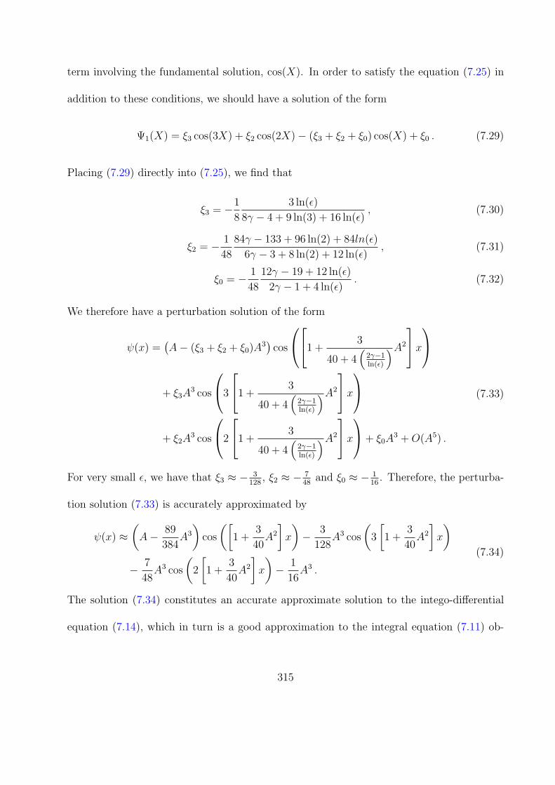
term involving the fundamental solution, cos(X). In order to satisfy the equation (7.25) in

addition to these conditions, we should have a solution of the form

Ψ1(X) = ξ3 cos(3X) + ξ2 cos(2X)− (ξ3 + ξ2 + ξ0) cos(X) + ξ0 . (7.29)

Placing (7.29) directly into (7.25), we find that

ξ3 = −1

8

3 ln(ϵ)

8γ − 4 + 9 ln(3) + 16 ln(ϵ), (7.30)

ξ2 = − 1

48

84γ − 133 + 96 ln(2) + 84ln(ϵ)

6γ − 3 + 8 ln(2) + 12 ln(ϵ), (7.31)

ξ0 = − 1

48

12γ − 19 + 12 ln(ϵ)

2γ − 1 + 4 ln(ϵ). (7.32)

We therefore have a perturbation solution of the form

ψ(x) =(A− (ξ3 + ξ2 + ξ0)A

3)cos

1 + 3

40 + 4(

2γ−1ln(ϵ)

)A2

x

+ ξ3A3 cos

3

1 + 3

40 + 4(

2γ−1ln(ϵ)

)A2

x

+ ξ2A3 cos

2

1 + 3

40 + 4(

2γ−1ln(ϵ)

)A2

x+ ξ0A

3 +O(A5) .

(7.33)

For very small ϵ, we have that ξ3 ≈ − 3128

, ξ2 ≈ − 748

and ξ0 ≈ − 116. Therefore, the perturba-

tion solution (7.33) is accurately approximated by

ψ(x) ≈(A− 89

384A3

)cos

([1 +

3

40A2

]x

)− 3

128A3 cos

(3

[1 +

3

40A2

]x

)− 7

48A3 cos

(2

[1 +

3

40A2

]x

)− 1

16A3 .

(7.34)

The solution (7.34) constitutes an accurate approximate solution to the intego-differential

equation (7.14), which in turn is a good approximation to the integral equation (7.11) ob-

315

tained from the full non-local Biot-Savart formulation. Therefore, under the non-local Biot-

Savart formulation, a planar vortex filament can still exist, and an accurate approximation

is given by (7.34).

7.1.5 Comparison with known solution for the LIA

The method of strained parameters used here was applied to the standard LIA in the case

of a planar vortex filament in Chapter 4. In that paper, the ϵ influence was suppressed in a

parameter, so we redo the calculations here in order to preserve the parameters κ and ϵ.

Dropping the integral term from (7.14), we have that a vortex filament under LIA is

determined by the solution of

ωψ +κ

4πln(ϵ)

ψ′′

(1 + ψ′2)3/2= 0 . (7.35)

Assuming a solution like that of (7.17), we find that Ψ0(X) = cos(X) provided ω = κ4π

ln(ϵ).

The next term in the perturbation expansion is then governed by

Ψ1 +Ψ′′1 =

(2η − 3

8

)cos(X) +

3

8cos(3X) . (7.36)

Picking η = 316

to remove the secular term, we obtain

Ψ1(X) =3

64cos(X)− 3

64cos(3X) . (7.37)

We therefore have the perturbation solution

ψ(x) =

(A+

3

64A3

)cos

([1 +

3

16A2

]x

)− 3

64A3 cos

(3

[1 +

3

16A2

]x

)+O(A5) . (7.38)

316

Note that ω is the rotational velocity of the filament. Let us denote by ωBS and ωLIA

the rotational velocity for the solutions calculated by the Biot-Savart rule (7.34) and with

only the LIA (7.38), respectively. With ωLIA = κ4π

ln(ϵ), we have

ωBS = 2ωLIA +κ(2γ − 1)

8π= 2ωLIA + (6.1434× 10−3)κ . (7.39)

We see that the direction of the rotation is the same in both cases (for small enough ϵ), while

the speed of rotation is different. Indeed, |ωBS| ≈ 2|ωLIA|, so the rotational speed when non-

local effects are considered is approximately double that of the case where non-local effects

are neglected. This suggests that non-local effects are not negligibly small in comparison to

LIA effects alone, but rather that non-local effects can be on the same order of magnitude

as local effects found through use of the LIA alone.

The period of the LIA filament solution over space is approximately TLIA, where

TLIA =2π

1 + 316A2

≈ 2π − 3π

8A2 +O(A4) , (7.40)

while the period of the solution approximating the full Biot-Savart model has a period of

approximately TBS, where

TBS =2π

1 + 340A2

≈ 2π − 3π

20A2 +O(A4) . (7.41)

The absolute error between these periods is then

|TBS − TLIA| =9π

40A2 +O(A4) . (7.42)

So, while corrections to the rotational velocity are rather large when comparing the LIA and

Biot-Savart solutions, corrections to the spatial period of the planar solutions are only of

317

order A2. From this, we infer that the primary influence of the non-locality is on the motion

of the planar vortex filaments, rather than on the structure of such filaments.

7.1.6 Discussion

A planar solution has been constructed for the full non-local Biot-Savart dynamics governing

the self-induced motion of a vortex filament. Under the assumption of a planar vortex

filament solution with arbitrary (unknown) spatial structure determined by ψ(x), the Biot-

Savart dynamics reduce to a stationary (independent of time) integral equation for the

unknown ψ(x). (Actually, since the formulation also depends on a ψ′ under the integral,

this equation is a type of integro-differential equation.) The integral in this formulation is

then approximated near a singularity of logarithmic order by the LIA, whereas away from

the singularity the integral form is maintained. Therefore, there is a part of the solution

due to the LIA, and another non-local part. This solution is interesting in a mathematical

sense, due to the fact that it provides us with an accurate approximation to a solution of the

singular and nonlinear integro-differential equation (7.11). Even numerical solution of such

an integro-differential equation would be challenging. The results suggest that at the very

least some of the solutions present under the LIA can also be extended to the Biot-Savart

formulation.

Physically, the approximate analytical solution obtained through a strained parameter

approach is quite useful. While we assume that the deviations A from the central axis are

318

sufficiently small, this is physically reasonable in light of the fact that the planar filaments

only exist for the LIA when A <√2. So, the large A case is not physically interesting. For

the solutions obtained in [105], the perturbation solutions were useful for A < 0.7. Plotting

the solutions for various A, we see that the order A3 effects are mostly negligible, so a planar

filament can be approximated by

r(x, t) = xix + A cos

(κ

4π

(γ − 1

2+ 2 ln(ϵ)

)t

)cos

([1 +

3

40A2

]x

)iy

+ A sin

(κ

4π

(γ − 1

2+ 2 ln(ϵ)

)t

)cos

([1 +

3

40A2

]x

)iz .

(7.43)

The approximate solutions suggest that the spatial structure of the planar filaments

found here for the Biot-Savart dynamics is relatively unchanged from the structure of the

solutions under LIA. The difference apparent when comparing the LIA and Biot-Savart

solutions lies in the motion, rather than the structure, of the planar filaments. From the

perturbation solutions, we have that the rotational velocity for the LIA formulation (given

by ωLIA) and the Biot-Savart formulation (given by ωBS) relate like ωBS ≈ 2ωLIA. Therefore,

the primary effect of the non-locality is to increase the velocity of the filament.

7.2 Self-induced motion of a Cartesian helical vortex filament

under the Biot-Savart model

The thin helical vortex filament is one of the fundamental exact solutions possible under the

LIA. The LIA is itself an approximation to the non-local Biot-Savart dynamics governing

319

the self-induced motion of a vortex filament, and helical filaments have also been considered

under the Biot-Savart dynamics in a variety of configurations and assumptions. In the

present section, we consider the motion of such a helical filament in the Cartesian reference

frame by determining the curve defining this helical filament mathematically. In order to

do so, we consider a matched approximation to the Biot-Savart dynamics, with local effects

approximated by the LIA in order to avoid the logrithmic singularity inherent in the Biot-

Savart formulation. This, in turn, allows us to determine the rotational and translational

velocity of the filament in terms of a local contribution (which is exactly that which is found

under the LIA) and a non-local contribution. Performing our calculations in such a way,

we can easily compare our results to those of the LIA. Both exact numerical results and

approximate analytical results are given. For small wave number k, the transverse velocity

scales as k2, while for large wave numbers, the transverse velocity scales as k. On the other

hand, the rotational velocity attains a maximum value at some finite k, which corresponds

exactly to the wave number giving the maximal torsion.

Ricca [77] demonstrated that torsion strongly influences the structure of helical fila-

ments. Widnall [119], Ricca [77] give numerics for helical filaments of small pitch (large wave

numbers) and small amplitude regime, while Ricca [77] also gives an analytic result for the

infinite-torsion case, valid when the pitch is small (wave number is large). The analytical

results discussed here are complementary to those studies, since we obtain accurate analytics

in the small and intermediate wave number regime (the large pitch regime). For cases we

320

consider, the torsion τ must be bounded like 0 < τ < 2A−1 where A is the amplitude of the

helix.

We now study helical vortex filaments under Biot-Savart dynamics in the Cartesian

frame. Doing so, we quickly recover the representations for the rotational and transverse

velocity of the helical filament in terms of the wave number and radius of the helix. The

benefit of considering the results in Cartesian form is that we immediately can visualize

the stricture of the filament, so we can use these velocities to give a closed-form position

of the helical filament curve at an arbitrary time t > 0. As opposed to using the “cut-

off” approximation in the way mentioned above, we simply replace the “local” dynamics

in the Biot-Savart law directly with the LIA, while the non-local effects remain in integral

form. That is, local effects are taken on a region |x − s| < ϵ (where x is a point on the

filament and s denotes points within a small neighborhood of ϵ), while non-local effects are

considered on |x − s > ϵ|. The LIA is simpler to work with than other approaches for the

inner region, since it gives an exact result (as opposed to an analytical result which must

be approximated numerically). This approach has previously been employed numerically in

order to study quantum turbulence [81]. Furthermore, by using the LIA for the local region,

we can meaningfully compare the non-local formulation with existing results valid strictly

under the LIA. The results of this section were considered in Van Gorder [116].

321

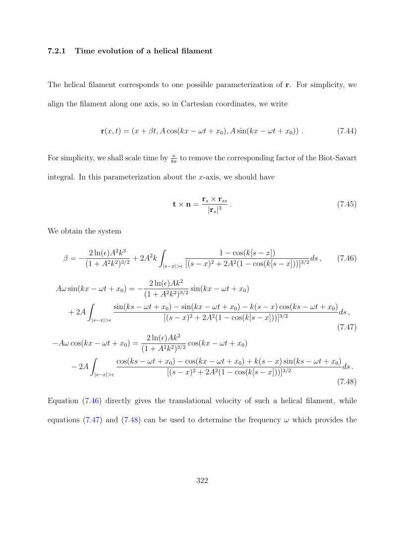
7.2.1 Time evolution of a helical filament

The helical filament corresponds to one possible parameterization of r. For simplicity, we

align the filament along one axis, so in Cartesian coordinates, we write

r(x, t) = (x+ βt, A cos(kx− ωt+ x0), A sin(kx− ωt+ x0)) . (7.44)

For simplicity, we shall scale time by κ8π

to remove the corresponding factor of the Biot-Savart

integral. In this parameterization about the x-axis, we should have

t× n =rs × rss|rs|3

. (7.45)

We obtain the system

β = − 2 ln(ϵ)A2k3

(1 + A2k2)3/2+ 2A2k

∫|s−x|>ϵ

1− cos(k[s− x])

[(s− x)2 + 2A2(1− cos(k[s− x]))]3/2ds , (7.46)

Aω sin(kx− ωt+ x0) = − 2 ln(ϵ)Ak2

(1 + A2k2)3/2sin(kx− ωt+ x0)

+ 2A

∫|s−x|>ϵ

sin(ks− ωt+ x0)− sin(kx− ωt+ x0)− k(s− x) cos(ks− ωt+ x0)

[(s− x)2 + 2A2(1− cos(k[s− x]))]3/2ds ,

(7.47)

−Aω cos(kx− ωt+ x0) =2 ln(ϵ)Ak2

(1 + A2k2)3/2cos(kx− ωt+ x0)

− 2A

∫|s−x|>ϵ

cos(ks− ωt+ x0)− cos(kx− ωt+ x0) + k(s− x) sin(ks− ωt+ x0)

[(s− x)2 + 2A2(1− cos(k[s− x]))]3/2ds .

(7.48)

Equation (7.46) directly gives the translational velocity of such a helical filament, while

equations (7.47) and (7.48) can be used to determine the frequency ω which provides the

322

rotational motion. In particular, we take i(7.47) - (7.48), from which we obtain

ωei[kx−ωt+x0] = − 2 ln(ϵ)k2

(1 + A2k2)3/2ei[kx−ωt+x0]

+ 2ei[kx−ωt+x0]∫|s−x|>ϵ

(1− ik[s− x])eik[s−x] − 1

[(s− x)2 + 2A2(1− cos(k[s− x]))]3/2ds .

(7.49)

Simplifying this equation, and noting that the integral should have both a real and imaginary

part, we obtain

ω = − 2 ln(ϵ)k2

(1 + A2k2)3/2+ 2

∫|σ|>ϵ

cos(kσ)− 1 + kσ sin(kσ)

[σ2 + 2A2(1− cos(kσ))]3/2dσ

+ 2i

∫|σ|>ϵ

sin(kσ)− kσ cos(kσ)

[σ2 + 2A2(1− cos(kσ))]3/2dσ .

(7.50)

Note that the integrand of the integral multiplying the i is an odd function, therefore the

integral over (−∞, ϵ) is the negative of the integral over (ϵ,∞), hence this integral is zero.

This makes sense, as ω should be real-valued. On the other hand, the real part of the integral

has an integrand which is an even function, so the total integral is just twice the integral

over (ϵ,∞). We therefore obtain

ω = − 2 ln(ϵ)k2

(1 + A2k2)3/2+ 4

∫ ∞

ϵ


[σ2 + 2A2(1− cos(kσ))]3/2dσ . (7.51)

In a similar manner, the translational velocity along the x-axis is given by

β = − 2 ln(ϵ)A2k3

(1 + A2k2)3/2+ 4A2k

∫ ∞

ϵ

1− cos(kσ)

[σ2 + 2A2(1− cos(kσ))]3/2dσ . (7.52)

With ω and β known, we can describe the motion of the helical vortex filament (7.44) exactly.

In Fig. 7.1, we plot the rotational and translational velocity parameters for various values

of the physical constants.

323

The integral term in (7.51) is equivalent to equation (19) of Widnall [119], except that

integral was approximated in a different way by using the “cut-off” approximation. In this

method, a function of the same singular order is added and subtracted under the integral,

in order to remove the logarithmic divergence. The remaining singularity is shifted to an

auxiliary integral, which can itself be evaluated in terms of a cosine integral. The quantities

were Fourier transformed in Widnall [119] which helps in computation of the integrals. See

equation (36) of Widnall [119]. The resulting approximations were then solved numerically.

324

Figure 7.1: Numerical plots of the rotational velocity, ω, and transverse velocity, β, of a

helical vortex filament when non-local dynamics are accounted for. The results use the LIA

near the logrithmic singularlity, so these are the solutions (7.51)-(7.52). Note that we set

ϵ = 10−5 in all plots. The precise value of ϵ is not important, since a change in the value of

ϵ results in a scaling of the plots, therefore the value of ϵ does not influence the qualitative

features of the solutions.

325

We see that there exists a particular finite value of the wave number k for which

the rotational velocity of the filament is maximal. On the other hand, the behavior of the

translational velocity is a bit more complicated. For small k, β scales like β ∼ k2, while for

large k, the integral term dominates, giving β ∼ k.

7.2.2 Approximating the relations for ω and β in the case of small and inter-

mediate wave numbers

For s sufficiently far from s = 0, reasonable approximations to the integrands in (7.51) and

(7.52) are


[σ2 + 2A2(1− cos(kσ))]3/2≈ cos(kσ)− 1 + kσ sin(kσ)

(1 + A2k2)3/2σ3(7.53)

and

1− cos(kσ)

[σ2 + 2A2(1− cos(kσ))]3/2≈ 1− cos(kσ)

(1 + A2k2)3/2σ3, (7.54)

respectively. The first approximation, (7.53), is of the same flavor of that used in equation

(3.21) in Ricca [77]. These approximations are valid for small and intermediate values of

the wave number k, since this is when the decay of the integrals dominates the oscillations

sufficiently fast. We shall say more on the large-k situation later. While it is possible to

obtain more accurate approximations, these approximations are accurate enough for our

qualitative analysis. In Figs. 7.2 and 7.3, we give plots of the integrands (7.53) and (7.54)

along with their approximations. The approximations are seen to be very accurate, provided

that the helical filaments are of bounded variation (Ak and k sufficiently bounded). Even

326

for the intermediate values used in the figures, the approximations are very accurate. Only

when A or k become very large would we see any breakdown in the approximations. While

the large-A case is not particularly physical (since such solutions would be highly unstable,

while we are considering solutions which persist in time, a priori, through the assumption

(7.44)), it is possible to have large wave numbers, and we discuss this case later.

327

Figure 7.2: Numerical plots and approximations to the integrand given in (7.53) for various

values of the physical parameters. We set ϵ = 10−5 in all plots. For small and intermediate

values of k and A, the approximation to the integrand (7.53) is very accurate, and hence the

approximating formula (7.58) for the integral term in (7.51) is accurate.

328

Figure 7.3: Numerical plots and approximations to the integrand given in (7.54) for various

values of the physical parameters. We set ϵ = 10−5 in all plots. Ahain, for small and

intermediate values of k and A, the approximation to the integrand (7.54) is very accurate,

and hence the approximating formula (7.61) for the integral term in (7.52) is accurate.

329

We first have∫ ∞

ϵ


[σ2 + 2A2(1− cos(kσ))]3/2dσ ≈

∫ ∞

ϵ


(1 + A2k2)3/2σ3dσ

=cos(kϵ)− 1 + kϵ sin(kϵ)− k2ϵ2Ci(kϵ)

2ϵ2(1 + A2k2)3/2,

(7.55)

where Ci is the cosine integral. We find that

cos(kϵ)− 1 + kϵ sin(kϵ)

ϵ2=k2

2+O(ϵ2) (7.56)

and

Ci(kϵ) = γ + ln(k) + ln(ϵ) +O(ϵ2) , (7.57)

hence

∫ ∞

ϵ


[σ2 + 2A2(1− cos(kσ))]3/2dσ ≈ − k2

2(1 + A2k2)3/2

(γ − 1

2+ ln(k) + ln(ϵ)

)+O(ϵ2) .

(7.58)

Here, γ ≈ 0.5772 is the Euler-Mascheroni constant. We neglect terms of order ϵ2 and higher,

since ϵ << 1. Returning to Ricca [77], this expression is similar to his equation (3.27). The

difference is the dependence on the wave number, which is scaled out in Ricca [77]. (More

precisely, the results in Ricca [77] involved scaling torsion, τ = k/(1 + A2k2).) Keeping k

present, we will be able to directly compare our results with the LIA. Ricca [77] obtained

this integral in the limit τ → ∞. For this to occur, the wave number must be large and

A must become small as k becomes large. We do not consider this, since for finite A the

torsion will not be infinite. Rather, for finite A > 0, the torsion will attain a maximal value

of τ = 2A−1 at k = A−1. The τ → ∞ limit then corresponds to A → 0, k → ∞ provided

Ak → ν, for ν < ∞. This is a very restrictive limit, since A → 0 essentially gives us a line

330

filament. What all of this means is that we should maintain the parameters k and A in our

development, as opposed to scaling them out and taking any particular limit, in order to

capture the behavior of arbitrary helical filaments.

Regarding the second integral, we have∫ ∞

ϵ

1− cos(kσ)

[σ2 + 2A2(1− cos(kσ))]3/2dσ ≈

∫ ∞

ϵ

1− cos(kσ)

(1 + A2k2)3/2σ3dσ

=kϵ sin(kϵ) + 1− cos(kϵ)

2ϵ2− k2

2Ci(kϵ) ,

(7.59)

and using

kϵ sin(kϵ) + 1− cos(kϵ)

ϵ2=

3

2k2 +O(ϵ2) , (7.60)

we find

∫ ∞

ϵ

1− cos(kσ)

[σ2 + 2A2(1− cos(kσ))]3/2dσ ≈ k2

2(1 + A2k2)3/2

(3

2− γ − ln(k)− ln(ϵ)

)+O(ϵ2) .

(7.61)

Using the approximations (7.58) and (7.61) in equations (7.51) and (7.52), respec-

tively, we have the approximations

ωapprox = −k2(2γ − 1 + 2 ln(k) + 4 ln(ϵ))

(1 + A2k2)3/2(7.62)

and

βapprox =A2k3(3− 2γ − 2 ln(k)− 4 ln(ϵ))

(1 + A2k2)3/2. (7.63)

331

The curve describing the helical vortex filament, including non-local effects, is then

given by the approximation

r(x, t) ≈x+

A2k3(3− 2γ − 2 ln(k)− 4 ln(ϵ))

(1 + A2k2)3/2t

ix

+ A cos

(kx+

k2(2γ − 1 + 2 ln(k) + 4 ln(ϵ))

(1 + A2k2)3/2t+ x0

)iy

+ A sin

(kx+

k2(2γ − 1 + 2 ln(k) + 4 ln(ϵ))

(1 + A2k2)3/2t+ x0

)iz .

(7.64)

7.2.3 Comparison with the LIA and numerical approximations

If one were to strictly consider the LIA, as is often done, one would obtain (upon removing

the integral terms from (7.46)-(7.48))

ωLIA = − 2 ln(ϵ)k2

(1 + A2k2)3/2> 0 and βLIA = A2kωLIA = − 2 ln(ϵ)A2k3

(1 + A2k2)3/2> 0 , (7.65)

Under the LIA, the motion of a helical vortex filament then takes the form

r(x, t) =

x− 2 ln(ϵ)A2k3

(1 + A2k2)3/2t

ix + A cos

(kx+

2 ln(ϵ)k2

(1 + A2k2)3/2t+ x0

)iy

+ A sin

(kx+

2 ln(ϵ)k2

(1 + A2k2)3/2t+ x0

)iz .

(7.66)

In terms of the parameters calculated through the LIA, we have that the approxima-

tions found for small and intermediate k

ωapprox = 2ωLIA − k2(2γ − 1 + 2 ln(k))

(1 + A2k2)3/2(7.67)

and

βapprox = 2βLIA +A2k3(3− 2γ − 2 ln(k))

(1 + A2k2)3/2. (7.68)

332

In Fig. 7.4, we plot these approximate solutions against both the LIA solutions and direct

numerical integration of the integrals in (7.51)-(7.52). For small and intermediate k (k of

order unity or smaller), these approximations are in strong agreement with the numerical in-

tegrations. For larger k, of order 10, the approximations tend to over-estimate the numerical

value of β and ω slightly, whereas the LIA underestimates these values. The approximations

are still more accurate than the LIA. For much larger k, say of order 102 and greater, both

the approximation (7.62)-(7.63) as well as the LIA lose their usefulness. This is due to the

fact that the integral term has an integrand which rapidly oscillates for large k.

333

7.2.4 Discussion

From the plots, it is clear that there exists a critical value of the wave number for which

the rotational velocity is maximal. In the approximation (7.62)-(7.63), the LIA, and the

numerical approximations, this value is nearly the same. Since the values are approximately

the same, we use the LIA, finding that this critical wave number is give approximately by

k∗ ≈√2A−1. Note that this corresponds to the maximal value of torsion (since torsion τ is

given by τ = k(1 + A2k2)−1). So, the larger the torsion, the greater the rotational velocity.

On the other hand, the plots indicate that the transverse velocity is always increasing, as

mentioned when we considered the numerical results before.

In summary, the approximations (both LIA and those of (7.62)-(7.63)) are accurate

for small and intermediate k (with the approximation (7.62)-(7.63) being best), while there

is a sharp breakdown in the approximations for larger k. For both ω and β, the breakdown

for large k is due to the fact that the integrals oscillate rapidly.

It is worth mentioning that there is a quantum form of the LIA, which is essentially

the LIA applied to the HVBK model. It should be feasible to extend the resent results to

that case, at least in the case of helical filaments with constant amplitude A. The exact

form of a helical filament under the quantum LIA was discussed in Chapter 6. In the case of

decaying filaments (A = A(t) such that A → 0 as t → ∞), the non-local development may

be possible analytically, but will be much more complicated.

334

Figure 7.4: Comparison of the numerical plots and approximate solutions for the rotational

velocity, ω, and transverse velocity, β, of a helical vortex filament when non-local dynamics

are accounted for. The numerical results use the LIA near the logrithmic singularlity, so

these are the solutions (7.51)-(7.52). Note that we set ϵ = 10−5 in all plots. We also take

A = 0.1. The analytical approximations obtained in (7.62)-(7.63) are superior to the LIA

(7.65) results when k is either small or in the intermediate range. Once k becomes large,

both approximations lose accuracy. This is due to the fact that, for large k, the integral

terms in (7.51)-(7.52) are rapidly oscillating. The approximations (7.62)-(7.63) are useful

when the decay in the integrals dominates the oscillations, which is not true for large k.

In the regime where the approximations are useful, note that the LIA underestimates both

velocities, while the approximation (7.62)-(7.63) overestimates the velocities.

335

CHAPTER 8

CONCLUSIONS

In this report, we have studied a number of nonlinear dispersive partial differential equa-

tions of relevance to various physical scenarios. The most common application has been to

vortex filament dynamics, although other applications have been mentioned and considered.

The physical applicability of the results increases as the governing models become more

complicates and take into account more reasonable assumptions.

Among some of the more interesting results discussed here, we were able to demon-

strate the existence of space-periodic solutions for the Cartesian and arclength-tangent for-

mulations of the LIA governing the motion of a vortex filament in Chapter 2, and we deter-

mined orbital stability properties for these solutions in Chapter 3. These solutions correspond

to rotating planar filaments. Similar results were discussed for the integrable WKIS model

in Chapters 2-3. We were also able to demonstrate a variety of rotating non-planar filament

solutions under the 2D Cartesian LIA, in Chapter 2. Meanwhile, in Chapter 4, we were able

to consider several pathological solutions which model vortex self-intersections and kinks.

Many of the vortex filament solution forms present under the LIA in Chapters 2 - 4

were generalized to the case of superfluids under various potential forms of the quantum LIA

336

in Chapter 5. In particular, we were able to demonstrate mathematical properties of helical,

self-similar, planar, and soliton solutions under the quantum LIA. However, the potential

forms of the quantum LIA are approximations to the full vector form of the LIA, and in

Chapter 6 we study the exact vector form of the quantum LIA. In Chapter 6, we study

planar, helical, and soliton solutions under the exact vector form of the quantum LIA, and

we are able to determine the motion of such vortex filament solutions analytically. Many

of the results we determine mathematically verify known experimental or numerical results

from the literature.

Physically, the LIA is still not the most general model one can consider, since it ignores

non-local effects. In Chapter 7, we consider the non-local equation governing the motion of a

vortex filament in a classical fluid. While the non-local effects are most useful for complicated

fluid flow dynamics, such as vortex mergers or the analysis of many-vortex models, we

restrict our attention to two solution types which can be studied analytically. Still, these

two solutions, namely the planar and helical vortex filaments, are rather fundamental, and we

compare our non-local results to those discussed in earlier chapters for the LIA. We find that

non-local effects result primarily in an increase in the velocity of the filament solutions (both

rotational and transverse velocity is increased), while the spatial structure of the filaments

is largely unchanged. Note that it is possible to extend such results to the superfluid or

quantum fluid case (see below), although such results will be much more complicated.

Regarding future work, the extension of the present results to other vortex configura-

tions, or to other nonlinear dispersive partial differential equations not studied here, seems

337

like an obvious avenue. Regarding the solutions considered here, it may be useful to extend

other solutions to account for the effects of the the non-local formulation given in Chapter

7.

While the dispersive partial differential equations considered in Chapter 3 permit a

nice and rather elegant stability analysis, for more complicated dispersion relations such

stability results are expected to be far less elegant. A work-in-progress is on an orbital

stability result for nonlinear dispersive partial differential equations of the form

iut = F (|u|2, |ux|2)uxx +G(|u|2)u , (8.1)

which is a generalization of known results for generalized NLS equation of the form

iut = auxx +G(|u|2)u . (8.2)

As seen when comparing the work in Chapter 6 with that of Chapter 5, considering

the full three-dimensional dynamics of quantum vortex filaments can be rather involved. The

same can be said of accounting for non-locality. However, considering the quantum form of

the vortex filament equation which uses the Biot-Savart dynamics instead of the LIA would

be quite interesting. Such a formulation would account for both superfluid effects and the

effect of non-locality on the motion of a vortex filament in a quantum fluid. Any results in

the literature are numerical in nature, so analytical results in this area would be quite nice,

since they may lead to qualitative observations which are ignored or not considered in the

parameter regions explored numerically.

338

One open problem with regards to the quantum vortex filament is whether or not the

quantum vortex filament equation (in any form) admits chaotic solutions. While thy has

been hypothesized before due to the complicated dynamics inherent in the vortex filament

equations, there has never been a specific example given. It is the author’s opinion that

the best chance to observe chaos in a quantum vortex filament under LIA would be in the

Hasimoto-type transformation which puts the quantum LIA into correspondence with a cubic

complex Ginsburg-Landau equation. In a work-in-progress, the author has already found a

rich variety of bifurcations in this model.

339

LIST OF REFERENCES

[1] N. Akhmediev, A. Ankiewicz, J. M. Soto-Crespo, and J. M. Dudley, Rogue wave early warningthrough spectral measurements?, Physics Letters A 375 (2011) 541-544.

[2] N. Akhmediev, A. Ankiewicz, and M. Taki, Waves that appear from nowhere and disappearwithout a trace, Physics Letters A 373 (2009) 675-678.

[3] S.Z. Alamri, A. J. Youd, and C. F. Barenghi, Reconnection of superfluid vortex bundles,Physical Review Letters 101 (2008) 215302.

[4] A. Ankiewicz, N. Devine, and N. Akhmediev, Are rogue waves robust against perturbations?,Physics Letters A 373 (2009) 3997-4000.

[5] T. Araki, M. Tsubota, and S. K. Nemirovskii, Energy Spectrum of Superfluid Turbulence withNo Normal-Fluid Component, Physical Review Letters 89 (2002) 145301.

[6] I. S. Aranson and L. Kramer, The world of the complex Ginzburg-Landau equation, Reviewsof Modern Physics 74 (2002) 99-143.

[7] H. Aref and E.P. Flinchem, Dynamics of a vortex filament in a shear flow, Journal of FluidMechanics 148 (1984) 477-497.

[8] R. J. Arms and F. R. Hama, Localized-induction concept on a curved vortex and motion of anelliptic vortex ring, Physics of Fluids 8 (1965) 553-559 .

[9] H. Bailung, S. K. Sharma, and Y. Nakamura, Observation of Peregrine solitons in a multi-component plasma with negative ions, Physical Review Letters 107 (2011) 255005.

[10] U. Bandelow and N. Akhmediev, Persistence of rogue waves in extended nonlinear Schrdingerequations: Integrable SasaSatsuma case, Physics Letters A 376 (2012) 1558-1561.

[11] V. Banica and L. Vega, On the stability of a singular vortex dynamics, Communications inMathematical Physics 286 (2009) 593-627.

[12] F. Baronio, A. Degasperis, M. Conforti, and S. Wabnitz, Solutions of the vector nonlinearSchrdinger equations: evidence for deterministic rogue waves, Physical Review Letters 109(2012) 044102.

[13] I.L. Bekarevich and I.M. Khalatnikov, Phenomenological derivation of the equations of vortexmotion in He II, Sov. Phys. JETP 13 (1961) 643-646.

340

[14] T.B. Benjamin and J.E. Feir, The disintegration of wave trains on deep water Part 1. Theory,Journal of Fluid Mechanics 27 (1967) 417-430.

[15] Yu. V. Bludov, R. Driben, V. V. Konotop, and B. A. Malomed, Instabilities, solitons androgue waves in PT -coupled nonlinear waveguides, Journal of Optics 15 (2013) 064010.

[16] Y.V. Bludov, V.V. Konotop, and N. Akhmediev, Matter rogue waves, Physical Review A 80(2009) 033610.

[17] G. Boffetta, A. Celani, D. Dezzani, J. Laurie, and S. Nazarenko, Modeling Kelvin WaveCascades in Superfluid Helium, Journal of Low Temperature Physics 156 (2009) 193-214.

[18] M. Blaauboer, B.A. Malomed, and G. Kurizki, Spatiotemporally Localized MultidimensionalSolitons in Self-Induced Transparency Media, Physical Review Letters 84 (2000) 1906-1909.

[19] M. Boiti, V. S. Gerdjikov and F. Pempinelli, The WKIS system: Backlund transformations,generalized Fourier transforms and all that, Progress of Theoretical Physics 75 (1986) 1111-1141.

[20] F. Calogero and A. Degasperis, Spectral Transform and Solitons: Tools to Solve and Investi-gate Nonlinear Evolution Equations, Volume 1. Volume 13 of Studies in Mathematics and ItsApplications (Elsevier Amsterdam, 1982).

[21] A. Chabchoub, N. P. Hoffmann, and N. Akhmediev, Rogue wave observation in a water wavetank, Physical Review Letters 106 (2011) 204502.

[22] S.M. Chang, S. Gustafson, K. Nakanishi, and T.P. Tsai, Spectra of linearized operators forNLS solitary waves, SIAM J. Math. Analysis 39(4) (2007) 1070-1111.

[23] D.K. Cheng, W.M. Cromar, and R.J. Donnelly, Influence of an Axial Heat Current onNegative-Ion Trapping in Rotating Helium II, Physical Review Letters 31 (1973) 433-436.

[24] L.S. Da Rios, Sul moto d’un liquido indefinite con un filetto vorticoso di forma qualunque,Rendiconti del Circolo Matematico di Palermo 22 (1906) 117.

[25] S.I Davis, P.C Hendry, and P.V.E McClintock, Decay of quantized vorticity in superfluid 4Heat mK temperatures, Physica B 280 (2000) 43-44.

[26] V.P. Dmitriyev, Helical waves on a vortex filament, American Journal of Physics 73 (2005)563-565.

[27] J. M. Dudley, G. Genty, F. Dias, B. Kibler, and N. Akhmediev, Modulation instability, Akhme-diev Breathers and continuous wave supercontinuum generation, Optics Express 17 (2009)21497-21508.

[28] K. Dysthe, H. E. Krogstad, and P. Muller, Oceanic rogue waves, Annual Review of FluidMechanics 40 (2008) 287-310.

341

[29] E. Fehlberg, Low-order classical Runge-Kutta formulas with step size control and their appli-cation to some heat transfer problems, NASA Technical Report 315 (1965).

[30] F. Fenton and A. Karma, Vortex dynamics in three-dimensional continuous myocardium withfiber rotation: filament instability and fibrillation, Chaos 8 (1998) 20-47.

[31] S. N. Fisher and G. R. Pickett, Quantum Turbulence in Superfluid 3He at Very Low Temper-atures, Progress in Low Temperature Physics 16 (2009) 147-194.

[32] E. Fonda, D. P. Meichle, N. T. Ouellette, S. Hormoz, K. R. Sreenivasan, and D. P. Lathrop,Visualization of Kelvin waves on quantum vortices, arXiv:1210.5194 (2012)

[33] Y. Fukumoto, Stationary configurations of a vortex filament in background flows, Proceedingsof the Royal Society of London A 453 (1997) 1205-1232.

[34] Y. Fukumoto and M. Miyajima, The localized induction hierarchy and the Lund-Regge equa-tion, Journal of Physics A: Mathematical and General 29 (1996) 8025-8034.

[35] V. Gerdjikov, G. Vilasi, and A. B. Yanovski, Integrable Hamiltonian Hierarchies: Spectraland Geometric Methods. Volume 748 of Lecture Notes in Physics (Springer Berlin Heidelberg,2008).

[36] W.I. Glaberson, W.W. Johnson, and R.M. Ostermeier, Instability of a Vortex Array in He II,Physical Review Letters 33 (1974) 1197-1200.

[37] E.E. Goldstein and D.M. Petrich, Solitons, Euler’s equation, and vortex patch dynamics, Phys-ical Review Letters 69 (1992) 555-558.

[38] S. Gutierrez, J. Rivas, and L. Vega, Formation of Singularities and Self-Similar Vortex Mo-tion Under the Localized Induction Approximation, Communications in Partial DifferentialEquations 28 (2003) 927-968.

[39] H.E. Hall and W.F. Vinen, The rotation of liquid helium II. I. Experiments on the propagationof second sound in uniformly rotating helium II, Proceedings of the Royal Society of LondonA 238 (1956) 204-214.

[40] H.E. Hall and W.F. Vinen, The rotation of liquid helium II. II. The theory of mutual frictionin uniformly rotating helium II, Proceedings of the Royal Society of London A 238 (1956)215-234.

[41] H. Hasimoto, Motion of a Vortex Filament and its relation to Elastica, Journal of the PhysicalSociety of Japan 31 (1971) 293-294.

[42] H. Hasimoto, A soliton on a vortex filament, Journal of Fluid Mechanics 51 (1972) 477-485.

[43] J.S. He, H.R. Zhang, L.H. Wang, K. Porsezian, and A.S. Fokas, Generating mechanism forhigher-order rogue waves, Physical Review E 87 (2013) 052914.

342

[44] E. J. Hopfinger and F.K. Browand, Vortex solitary waves in a rotating, turbulent flow, Nature295 (1982) 393-395.

[45] B. Ilan, Y. Sivan, and G. Fibich, A quantitative approach to soliton instability, Optics Letters36 (2011) 397-399.

[46] Y.V. Kartashov, V.A. Vysloukh, and L. Torner, Rotary solitons in Bessel optical lattices,Physical Review Letters 93 (2004) 093904.

[47] C. Kharif and E. Pelinovsky, Physical mechanisms of the rogue wave phenomenon, EuropeanJournal of Fluid Mechanics B - Fluids 22 (2003) 603-634.

[48] B. Kibler, J. Fatome, C. Finot, G. Millot, F. Dias, G. Genty, N. Akhmediev, and J. M. Dudley,The Peregrine soliton in nonlinear fibre optics, Nature Physics 6 (2010) 790-795.

[49] S. Kida, A vortex filament moving without change of form, Journal of Fluid Mechanics 112(1981) 397-409.

[50] S. Kida, Stability of a steady vortex filament, Journal of the Physical Society of Japan 51(1982) 1655-1662.

[51] L. D. Landau and E. M. Lifshitz, Fluid Mechanics, Addison and Wesley (1959).

[52] J. Langer and D.A. Singer, Lagrangian aspects of the Kirchhoff elastic rod, SIAM Review 38(1996) 605-618.

[53] M. Lakshmanan and S. Ganesan, Equivalent forms of a generalized Hirota’s equation withlinear inhomogeneities, Journal of the Physical Society of Japan 52 (1983) 4031-4033.

[54] M. Lakshmanan and S. Ganesan, Geometrical and gauge equivalence of the generalized Hirota,Heisenberg and Wkis equations with linear inhomogeneities, Physica A 132 (1985) 117-142.

[55] J. Laurie, V.S. L’vov, S. Nazarenko, and O. Rudenko, Interaction of Kelvin Waves and Non-Locality of the Energy Transfer in Superfluids, Physical Review B 81 (2010) 104526.

[56] T. Lipniacki, Quasi-static solutions for quantum vortex motion under the localized inductionapproximation, Journal of Fluid Mechanics 477 (2003) 321-337.

[57] T. Lipniacki, Shape-preserving solutions for quantum vortex motion under localized inductionapproximation, Physics of Fluids 15 (2003) 1381-1395.

[58] P. Lundquist, D. R. Andersen, and Yu. S. Kivshar, Multicolor solitons due to four-wave mixing,Physical Review E 57 (1998) 3551-3555.

[59] F. Maggioni, S.Z. Alamri, C.F. Barenghi, and R.L. Ricca, Kinetic energy of vortex knots andunknots, Il Nuovo Cimento C 32 (2009) 133-142.

[60] F. Maggioni, S.Z. Alamri, C.F. Barenghi, and R.L. Ricca, Velocity, energy, and helicity ofvortex knots and unknots, Physical Review E 82 (2010) 026309.

343

[61] V.G. Makhankov, Y.P. Rybakov, and V.I. Sanyuk, Localised nontopological structures: con-struction of solutions and stability problems, Physics-Uspekhi 37 (1994) 113-137.

[62] B. A. Malomed, P. Drummond, H. He, A. Berntson, D. Anderson, M. Lisak, Spatiotemporalsolitons in multidimensional optical media with a quadratic nonlinearity, Physical Review E56 (1997) 4725-4735.

[63] B.A. Malomed, D.J. Kaup, and R.A. Van Gorder, Unstaggered-staggered solitons in two-component discrete nonlinear Schrdinger lattices, Physical Review E 85 (2012) 026604.

[64] A. Melikyan and G. Weber, Integrable theories and generalized graded Maillet algebras, Journalof Physics A: mathematical and Theoretical 47 (2014) 065401.

[65] F.G. Mertens, N.R. Quintero, and A.R. Bishop, Nonlinear Schrodinger equation with spa-tiotemporal perturbations, Physical Review E 81 (2010) 016608.

[66] D. Mihalache, D. Mazilu, and L. Torner, Stability of walking vector solitons, Physical ReviewLetters 81 (1998) 4353-4356.

[67] D.W. Moore and P.G. Saffman, The instability of a straight vortex filament in a strain field,Proceedings of the Royal Society of London A 346 (1975) 413-425.

[68] V. L. Okulov, On the stability of multiple helical vortices, Journal of Fluid Mechanics 521(2004) 319-342.

[69] M. Onorato, D. Proment, A. Toffoli, Triggering rogue waves in opposing currents, PhysicalReview Letters 107 (2011) 184502.

[70] M. Onorato, S. Residori, U. Bortolozzo, A. Montina, and F. T. Arecchi, Rogue waves and theirgenerating mechanisms in different physical contexts, Physics Reports 528 (2013) 47-89.

[71] R.M. Ostermeier and W.I. Glaberson, Instability of vortex lines in the presence of axial normalfluid flow, Journal of Low Temperature Physics 21 (1975) 191-196.

[72] E.A. Ostrovskaya, Y.S. Kivshar, D.V. Skryabin, andW.J. Firth, Stability of Multihump OpticalSolitons, Physical Review Letters 83 (1999) 296-299.

[73] D. H. Peregrine, Water waves, nonlinear Schrodinger equations and their solutions, Journalof the Australian Mathematical Society, Series B: Applied Mathematics 25 (1983) 16-43.

[74] R.L. Ricca, Rediscovery of da Rios equations, Nature 352 (1991) 561-562.

[75] R.L. Ricca, Physical interpretation of certain invariants for vortex filament motion under LIA,Physics of Fluids A 4 (1992) 938-944.

[76] R.L. Ricca, Torus knots and polynomial invariants for a class of soliton equations, Chaos 3(1993) 83-91.

344

[77] R. L. Ricca, The effect of torsion on the motion of a helical vortex filament, Journal of FluidMechanics 273 (1994) 241-259.

[78] R.L. Ricca, D.C. Samuels, and C.F. Barenghi, Evolution of vortex knots, Journal of FluidMechanics 391 (1999) 29-44.

[79] N.N. Rosanov, A.G. Vladimirov, D.V. Skryabin, and W.J. Firth, Internal oscillations of soli-tons in two-dimensional NLS equation with nonlocal nonlinearity, Physics Letters A 293 (2002)45-49.

[80] H. Salman, Breathers on quantized superfluid vortices, Physical Review Letters 111 (2013)165301.

[81] K.W. Schwarz, Three-dimensional vortex dynamics in superfluid 4He: Line-line and line-boundary interactions, Physical Review B 31 (1985) 5782-5804.

[82] T. Shimizu and M. Wadati, A New Integrable Nonlinear Evolution Equation, Progress ofTheoretical Physics 63 (1980) 808-820.

[83] H. J. Shin, Deformation of a Peregrine soliton by fluctuating backgrounds, Physical Review E88 (2013) 032919.

[84] B.K. Shivamoggi and G.J.F. van Heijst, Motion of a vortex filament in the local inductionapproximation: Reformulation of the Da Rios-Betchov equations in the extrinsic filament co-ordinate space, Physics Letters A 374 (2010) 1742-1744.

[85] B.K. Shivamoggi, Vortex motion in superfluid4 He: Reformulation in the extrinsic vortex-filament coordinate space, Physical Review B 84 (2011) 012506.

[86] B. K. Shivamoggi, Vortex motion in superfluid 4He: effects of normal fluid flow, EuropeanPhysical Journal B 86 (2013) 275.

[87] D.V. Skryabin and W.J. Firth, Instabilities of higher-order parametric solitons: Filamentationversus coalescence, Physical Review E 58 (1998) R1252-R1255 .

[88] D. R. Solli, C. Ropers, P. Koonath, and B. Jalali, Optical rogue waves, Nature 450 (2007)1054-1057.

[89] E.B. Sonin, Dynamics of helical vortices and helical-vortex rings, EPL 97 (2012) 46002.

[90] E.B. Sonin, Symmetry of Kelvin-wave dynamics and the Kelvin-wave cascade in the T=0superfluid turbulence, Physical Review B 85 (2012) 104516.

[91] V. I. Shrira and V. V. Geogjaev, What makes the Peregrine soliton so special as a prototypeof freak waves?, Journal of Engineering Mathematics 67 (2010) 11-22.

[92] B. Svistunov, Superfluid turbulence in the low-temperature limit, Physical Review B 52 (1995)3647-3653.

345

[93] C.Y. Tsai and S.E. Widnall, The stability of short waves on a straight vortex filament in aweak externally imposed strain field, Journal of Fluid Mechanics 73 (1976) 721-733.

[94] M. Tsubota, T. Araki and S.K. Nemirowskii, Dynamics of vortex tangle without mutual frictionin superfluid 4He, Physical Review B 62 (2000) 11751-11762.

[95] M. Umeki, A locally induced homoclinic motion of a vortex filament, Theoretical and Compu-tational Fluid Dynamics 24 (2010) 383-387.

[96] M. Umeki, A real-space representation of a locally induced vortex filament, Theoretical andApplied Mechanics Japan 61 (2013) 195.

[97] M.G. Vakhitov and A.A. Kolokolov, Stationary solutions of the wave equation in a mediumwith nonlinearity saturation, Soviet Radiophysics 16 (1973) 783-789.

[98] R. A. Van Gorder, Motion of a vortex filament in the local induction approximation: a per-turbative approach, Theoretical and Computational Fluid Dynamics 26 (2012) 161-171.

[99] R. A. Van Gorder, Integrable stationary solution for the fully nonlinear local induction equationdescribing the motion of a vortex filament, Theoretical and Computational Fluid Dynamics26 (2012) 591-594.

[100] R. A. Van Gorder, Exact solution for the self-induced motion of a vortex filament in thearclength representation of the local induction approximation, Physical Review E 86 (2012)057301.

[101] R. A. Van Gorder, Exact stationary solution method for the Wadati-Konno-Ichikawa-Schimizu (WKIS) equation, Progress of Theoretical Physics 128 (2012) 993-999.

[102] R. A. Van Gorder, Fully nonlinear local induction equation describing the motion of a vortexfilament in superfluid 4He, Journal of Fluid Mechanics 707 (2012) 585-594.

[103] R. A. Van Gorder, Orbital Stability for Rotating Planar Vortex Filaments in the Cartesianand Arclength Forms of the Local Induction Approximation, Journal of the Physical Societyof Japan 82 (2013) 094005.

[104] R. A. Van Gorder, Orbital stability for stationary solutions of the Wadati-Konno-Ichikawa-Schimizu (WKIS) equation, Journal of the Physical Society of Japan 82 (2013) 064005.

[105] R. A. Van Gorder, Scaling laws and accurate small-amplitude stationary solution for themotion of a planar vortex filament in the Cartesian form of the local induction approximation,Physical Review E 87 (2013) 043203.

[106] R. A. Van Gorder, Motion of a helical vortex filament in superfluid 4He under the extrinsicform of the local induction approximation, Physics of Fluids 25 (2013) 085101

[107] R. A. Van Gorder, Self-similar vortex dynamics in superfluid 4He under the Cartesian rep-resentation of the Hall-Vinen model including superfluid friction, Physics of Fluids 25 (2013)095105.

346

[108] R. A. Van Gorder, Quantum vortex dynamics under the tangent representation of the localinduction approximation, Journal of Fluid Mechanics 740 (2014) 5-16.

[109] R. A. Van Gorder, General rotating quantum vortex filaments in the low-temperature Svis-tunov model of the LIA, submitted (2014).

[110] R. A. Van Gorder, Orbital instability of the Peregrine soliton, submitted (2014).

[111] R. A. Van Gorder, Scaling laws and unsteady solutions of the integrable 2D local inductionapproximation, submitted (2014).

[112] R. A. Van Gorder, Decay of helical Kelvin waves on a vortex filament under the quantumLIA, submitted (2014).

[113] R. A. Van Gorder, Dynamics of a planar vortex filament under the quantum local inductionapproximation, submitted (2014).

[114] R. A. Van Gorder, Solitons and other waves on a quantum vortex filament, submitted (2014).

[115] R. A. Van Gorder, Non-local dynamics of the self-induced motion of a planar vortex filament,submitted (2014).

[116] R. A. Van Gorder, Self-induced motion of a Cartesian helical vortex filament under the Biot-Savart model, submitted (2014).

[117] W.F. Vinen, Decay of superfluid turbulence at a very low temperature: The radiation of soundfrom a Kelvin wave on a quantized vortex, Physical Review B 64 (2001) 134520.

[118] M. Wadati, K. Konno, and Y.-H. Ichikawa, A Generalization of Inverse Scattering Method,Journal of the Physical Society of Japan 46 (1979) 1965-1966.

[119] S.E. Widnall, The stability of a helical vortex filament, Journal of Fluid Mechanics 54 (1972)641-663.

[120] S.E. Widnall, The structure and dynamics of vortex filaments, Annual Review of Fluid Me-chanics 7 (1975) 141-165.

[121] J. Yang, Nonlinear Waves in Integrable and Nonintegrable Systems, SIAM MathematicalModelling and Computation. Philadelphia, PA, USA (2010).

[122] X. Ying, Z. Ruguang, and W. Jianwen, An integrable decomposition of the WKIS equation,Journal of Xuzhou Normal University (Natural Science Edition) 29(4) (2011) 27-32.

[123] V. E. Zakharov and A. A. Gelash, Nonlinear stage of modulation instability, Physical ReviewLetters 111 (2013) 054101.

347

Nonlinear Dispersive Partial Differential Equations of Physical ...

Documents

Transcript of Nonlinear Dispersive Partial Differential Equations of Physical ...