Journal of Computational and Applied Mathematics 215 (2008) 409–418www.elsevier.com/locate/cam

hp-Adaptive least squares spectral element method for hyperbolicpartial differential equations

Árpád Galvãoa, Marc Gerritsmaa,∗, Bart De Maerschalckb

aDepartment of Aerospace Engineering, Delft University of Technology, Kluyverweg 1, 2629 HS Delft, The NetherlandsbVon Karman Institute for Fluid Dynamics, Waterloosesteenweg 72, 1640 Sint Genesius, Belgium

Received 10 September 2005

Abstract

This paper describes a hp-adaptive spectral element formulation which is used to discretize the weak formulation obtained byminimizing the residuals in the L2-norm. The least-squares error indicator will be briefly discussed. Refinement of the numericalapproximation is based on an estimate of the regularity of the underlying exact solution; if the underlying exact solution is sufficientlysmooth polynomial enrichment is employed, in areas with limited regularity h-refinement is used. For this purpose the Sobolevregularity is estimated. Functionally and geometrically non-conforming neighbouring elements are patched together using so-calledmortar elements. Results of this approach are compared to uniform h- and p-refinement for a linear advection equation.© 2007 Elsevier B.V. All rights reserved.

MSC: 65M50; 65M60; 65M70

Keywords: Least-squares formulation; Spectral element method; Mortar element method; Error indicator; Sobolev regularity estimation

1. Introduction

The least-squares spectral element method (LSQSEM) is a novel approach to solve systems of partial differen-tial equations. The method combines the least-squares formulation with a spectral approximation. The method wasdeveloped simultaneously by Proot and Gerritsma [18,16,17] and Pontaza and Reddy [14,15].

LSQSEM combines the locality of the finite element method, the symmetric positiveness of the least-squares for-mulation and the higher order accuracy of spectral methods. In addition, the least-squares formulation circumventscompatibility requirements between approximating function spaces in mixed problems, such as the inf–sup conditionfor the incompressible Navier–Stokes equations.

Despite these advantages LSQSEM becomes a very expensive method when higher order approximations are useduniformly throughout the whole computational domain. Therefore, an adaptive scheme has been developed, whichsignals regions that require refinement and takes the appropriate steps to reduce the error locally.

∗ Corresponding author.E-mail addresses: M.I.Gerritsma@LR.TUDelft.nl (M. Gerritsma), demaersc@vki.ac.be (B. De Maerschalck).

0377-0427/$ - see front matter © 2007 Elsevier B.V. All rights reserved.doi:10.1016/j.cam.2006.03.063

410 Á. Galvão et al. / Journal of Computational and Applied Mathematics 215 (2008) 409–418

This technique requires three new ingredients compared to the LSQSEM algorithms published previously. First ofall a method should be developed which patches together elements of different sizes and with different numericalrepresentations such as different polynomial degrees. One way of doing so is to use the discontinuous least-squaresformulation [4], but in the current paper the mortar element method (MEM) is employed [2,5,10].

Next an error indicator needs to be used to flag which elements need to be refined. Having established whichelements will be refined, we now need to decide how to refine; decrease the element size, h-refinement, or increasethe polynomial degree, p-enrichment. This decision is based on the estimated regularity of the exact solution. A morethorough discussion of hp-adaptive refinement applied to the LSQSEM can be found in [2].

The outline of this paper is as follows: Section 2 gives a brief introduction to the LSQSEM. Section 3 presents away to patch together elements with different sizes and different approximating function spaces. Section 4 introducesa least-squares error estimator which flags the elements eligible for refinement. In order to establish how to refinewe need a regularity estimator as described in Section 5. The resulting hp-adaptive LSQSEM scheme is applied to aspace–time linear advection equation in Section 6. Conclusions are drawn in Section 7.

2. The least-squares spectral element method

The LSQSEM combines the least-squares formulation with a spectral element discretization. In this section bothingredients will be addressed succinctly.

2.1. The least-squares formulation

The least-squares formulation is based on the minimization of the residual in a suitable norm. For convenience oneusually minimizes the residual in the L2-norm. In addition, we rewrite the differential equation in an equivalent firstorder system of differential equations to mitigate continuity requirements between adjacent elements and reduce thecondition number of the resulting system of algebraic equations.

Introduce

Lu= f, x ∈ �, (2.1)

as a system of first order partial differential equations defined on the domain � and supplemented with the boundaryconditions

Ru= g, x ∈ � ⊂ ��. (2.2)

Let L be a linear differential operator which maps elements from the function space X into the function space Y ,L : X −→ Y , such that there exist two constants C1, C2 > 0 for which we have

C1‖u‖X �‖Lu‖Y �C2‖u‖X ∀u ∈ X. (2.3)

Both inequalities, coercivity and continuity, respectively, assert that ‖Lu‖Y defines a norm equivalent to ‖u‖X. Sominimizing ‖u−uex‖X is equivalent to minimizing ‖L(u−uex)‖Y =‖Lu−f ‖Y . Here uex denotes the exact solution.

If we chose for Y the Hilbert space Y = L2(�), minimization of the residual amounts to

Find u ∈ X such that (Lu,Lv)L2(�) = (f,Lv)L2(�) ∀v ∈ X. (2.4)

Instead of using the infinite-dimensional function space X to look for a minimizer, we generally restrict ourselves to afinite-dimensional space Xh in which case the least-squares formulation reads

Find uh ∈ Xh such that (Luh,Lvh)L2(�) = (f,Lvh)L2(�) ∀vh ∈ Xh. (2.5)

For a more extensive treatment of the least-squares formulation, see [7,8].

Á. Galvão et al. / Journal of Computational and Applied Mathematics 215 (2008) 409–418 411

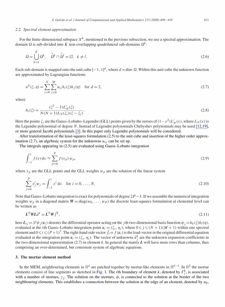
2.2. Spectral element approximation

For the finite-dimensional subspace Xh, mentioned in the previous subsection, we use a spectral approximation. Thedomain � is sub-divided into K non-overlapping quadrilateral sub-domains �k:

�=K⋃

k=1

�k,◦�k ∩ ◦�l =�, k = l. (2.6)

Each sub-domain is mapped onto the unit cube [−1, 1]d , where d=dim �. Within this unit cube the unknown functionare approximated by Lagrangian functions

uh(�, �)=N∑

i=0

M∑j=0

uijhi(�)hj (�) for d = 2, (2.7)

where

hi(�)= (�2 − 1)L′N(�)

N(N + 1)LN(�i )(�− �i ). (2.8)

Here the points �i are the Gauss–Lobatto–Legendre (GLL) points given by the zeroes of (1−x2)L′N(x), where LN(x) isthe Legendre polynomial of degree N . Instead of Legendre polynomials Chebyshev polynomials may be used [12,19],or more general Jacobi polynomials [3]. In this paper only Legendre polynomials will be considered.

After transformation of the least-squares formulation (2.5) to the unit cube and insertion of the higher order approx-imation (2.7), an algebraic system for the unknowns uij can be set up.

The integrals appearing in (2.5) are evaluated using Gauss–Lobatto integration

∫ 1

−1f (x) dx ≈

P∑p=0

f (xp)wp, (2.9)

where xp are the GLL points and the GLL weights wp are the solution of the linear system

P∑j=0

xijwj =

∫ 1

−1xi dx for i = 0, . . . , N . (2.10)

Note that Gauss–Lobatto integration is exact for polynomials of degree 2P−1. If we assemble the numerical integrationweights wp in a diagonal matrix W= diag(w0, . . . , wP ) the discrete least-squares formulation at elemental level canbe written as

LTWL uk = LTW f k , (2.11)

here Lij =L�j (xi ) denotes the differential operator acting on the j th two-dimensional basis function �j =hk(�)hl(�),evaluated at the ith Gauss–Lobatto integration point xi = (�s , �t ), where 0�j �(N + 1)(M + 1) within one spectralelement and 0� i�(P+1)2. The right-hand side vector fi=f (xi ) is the load-vector in the original differential equationevaluated at the integration point xi = (�s , �t ). The vector of unknowns uk

j are the unknown expansion coefficients inthe two-dimensional representation (2.7) in element k. In general the matrix L will have more rows than columns, thuscomprising an over-determined, but consistent system of algebraic equations.

3. The mortar element method

In the MEM, neighbouring elements in Rd are patched together by mortar-like elements in Rd−1. In R2 the mortarelements consist of line segments as sketched in Fig. 1. The ith boundary of element k, denoted by �k

i , is associatedwith a number of mortars, �j . The solution on the mortars, �, is connected to the solution at the border of the twoneighbouring elements. This establishes a connection between the solution at the edge of an element, denoted by ub,

412 Á. Galvão et al. / Journal of Computational and Applied Mathematics 215 (2008) 409–418

Mortar γ

Computational domain

Ω1

Ω2 Ω3

Ω2 Ω3

Ω1

Fig. 1. The mortar element approach—patching the element edges with one approximation space.

and the mortar solution �. If we choose a polynomial approximation for � on the mortar, we can express the expansioncoefficients at the boundary of the element, ub, in terms of the expansion coefficients of the solution on the mortar, �,as

ub = Z �. (3.1)

The precise relation is inconsequential as long as the matrix Z is of full rank for at least one of the elements associatedwith the mortar. This condition prevents the appearance of spurious mortar solutions.

Having established the relation between the elemental boundary unknowns and the mortar unknowns, we can expressthe global system in terms of the inner element unknowns, ui and the mortar unknowns � only:

uk =[ ub

ui

]=

( Z 0

0 I

) [ � ui

]= [Zk]uk , (3.2)

where uk represents the true unknowns, i.e. the projected mortar values and the internal unknowns.This transformation converts the least-squares formulation at the element level, as given in (2.11), into

LTWL uk = LTW f k ⇐⇒ [Zk]TLTWL[Zk]uk = [Zk]TLTW f k . (3.3)

Assembling all element contributions by summing over the projected element matrices gives the global system to besolved.

In this paper the solution on the mortar is defined by an L2-projection of the element boundary solution∫�

kl

(u|�k − �)� ds = 0 ∀ sides l and k = 1, . . . , K , (3.4)

where � ∈ PM(�k

l ) and M is the polynomial degree of the mortar solution. M should be greater or equal than the degreeof the solution in the adjoining elements to prevent spurious mortar solutions. When the Lagrangian basis functionsdefined in Section 2 are employed, the vertex condition [10] is automatically satisfied. For a more extensive treatmentof the MEM the reader is referred to [2,5,10].

4. The error estimator

Having discussed how to match spectral elements with different size and polynomial representation, we now haveto find a way to detect those elements that need refinement.

In the least-squares formulation we select the solution which minimizes the residual globally over the whole domain�. Having obtained such a minimizing solution we can evaluate the least-squares functional locally over every sub-domain A ⊂ �. This gives

�2A = ‖Luh − f ‖2

L2(A)= ‖L(uh − uex)‖2L2(A)

, (4.1)

due to the linearity of L. Well-posedness of problem (2.3) then implies that

C1‖e‖2X(A) ��2A �C2‖e‖2X(A), (4.2)

Á. Galvão et al. / Journal of Computational and Applied Mathematics 215 (2008) 409–418 413

where e = uh − uex. This means that the effectivity index A,X, defined by

A,X = �A

‖e‖X(A)

, (4.3)

which compares the estimated error �A to the exact error in the X-norm is bounded by

√C1 �A �

√C2. (4.4)

Alternatively, we may compare the estimated norm �A with the residual norm ‖R‖L2(A) using the fact that the residualnorm is norm equivalent to ‖e‖X. Denoting this effectivity index by A,R gives the rather trivial result

A,R := �A

‖Luh − f ‖Y (A)

≡ 1. (4.5)

Based on this observation �A will be used to identify those regions (elements in case A = �k) which are selected forrefinement. This estimator has also been used by Liu [9] and Berndt et al. [1].

5. Estimation of the Sobolev regularity

Having found a way to match functionally and geometrically non-conforming elements and an indicator ��k whichflags elements for refinement, we now have to determine how to refine. This choice is based on the smoothness ofthe underlying exact solution. If the exact solution is locally sufficiently smooth, polynomial enrichment is employed.However, if on the other hand, the underlying exact solution has limited smoothness h-refinement is used.

Let be a spectral element with size parameter h and polynomial degree p. Let uex be the exact solution in

that element, where uex ∈ Hk , where k �0 denotes the Sobolev regularity of the exact solution. Let u

hp denote the

LSQSEM solution with uhp ∈ Hq , 0�q �k then

‖uex − uh

p‖Hq �C

(h)sk−q

(p)k−q‖u

ex‖Hk , (5.1)

where s =min(p + 1, k) and C is a generic constant. This error estimate tells us that if the solution is very smooth(k very large) then the error decreases more rapidly by increasing p in the denominator. For practical purposesthe function is considered smooth if k > p + 1 and non-smooth when k �p + 1, in which h-refinement is moreeffective.

So the choice between h-refinement and p-enrichment is dictated by the Sobolev index of the exact solution. Althoughthe exact solution is in general not available, we can still estimate this index from its numerical approximation. Houstonet al. [6] have developed a method to estimate the Sobolev index from a truncated Legendre series. They assume thatthe one-dimensional solution is in L2(−1, 1) which allows for a Legendre expansion

u(x)=∞∑i=0

aiLi(x) with ai = 2i + 1

2

∫ 1

−1u(x)Li(x) dx. (5.2)

By Parseval’s identity the fact that u ∈ L2(−1, 1) is equivalent to convergence of the series

∞∑i=0

|ai |2 2

2i + 1. (5.3)

In [6] it is shown that if

∞∑i=[k+1]

|ai |2 2

2i + 1

�(i + k + 1)

�(i − k + 1), (5.4)

414 Á. Galvão et al. / Journal of Computational and Applied Mathematics 215 (2008) 409–418

converges, then u ∈ Hkw(−1, 1), where

Hkw =

⎧⎨⎩u ∈ L2(−1, 1)

k∑j=0

∫ 1

−1|D(j)u(x)|2(1− x2)j dx <∞

⎫⎬⎭ , (5.5)

for integer values of k. By using the �-function in (5.4) this identity can be extended to fractional Sobolev spaces, see[6] for details.

Given the Legendre coefficients ai , convergence of the series in (5.4) can be established by well-known techniquessuch as the ratio test, or the root test.

In this work the root test is employed. This leads to the calculation of

lk = log((2k + 1)/2|ak|2)2 log k

. (5.6)

If limk→∞ lk > 12 then u ∈ H

l−1/2−�w (−1, 1) ∀� > 0. Else u ∈ L2(−1, 1). Since in a numerical solution only a finite

number of Legendre coefficients ai are available, this test is applied to the highest Legendre coefficient available inthe numerical approximation. Based on the estimated Sobolev index l − 1

2 , the decision is made whether to refine themesh, or to increase the polynomial degree locally.

This one-dimensional estimate of the Sobolev index can be extended to multi-dimensional problems by treating eachco-ordinate direction separately, see [6] for details. Several test have been conducted to establish the validity of thisestimator.

Proposition 5.1. If an element at refinement level r with characteristic mesh size hr and polynomial degree pr

isflagged for refinement by the error indicator, we calculate lp by (5.6). Then for the Sobolev index kp = lp − 1

2 wehave { If kp > pr

+ 1 then pr+1 ← pr

+ 1,

If kp �pr + 1 then hr+1

← hr/2.

(5.7)

6. Application to the space–time linear advection equation

This section uses the one-dimensional, linear advection problem to validate the presented hp-adaptive theory. Theapplication of LSQSEM to hyperbolic equations has been studied by De Maerschalck [11,13,12].

The model problem is defined as

�u

�t+ a

�u

�x= 0 with 0�x�L, t �0, a ∈ R, (6.1)

u(0, t)= 0, (6.2)

u(x, 0)=⎧⎨⎩

1

2− 1

2cos

(2�

x − x0

L0

)if x0 �x�x0 + L0,

0 if elsewhere,

(6.3)

where a is the advection speed and L is the length of the domain in spatial direction. On the left boundary of thedomain a Dirichlet boundary condition, u(0, t) = 0, is imposed. The initial disturbance, u(x, 0), is a cosine-hill withoffset x0 and width L0. We use a space–time formulation that treats the one-dimensional advection problem witha two-dimensional least-squares formulation and considers the time variable t as second spatial variable. Instead ofcalculating the solution over the whole domain at once, we use a semi-implicit approach. The domain is subdividedinto several space–time strips for which the solution is approximated using the LSQSEM, see [11] for details. In thefollowing, 32 time strips are used within the domain �= [0, 1], where each time strip has initially 32 cells. Each timestrip uses the solution at the previous strip as initial condition, except for the first strip that uses the prescribed initialcondition (6.3). All time strips use the Dirichlet condition (6.2) on the left boundary. The advection speed a = 0.85,x0 = 0.13 and L0 = x0 + 0.5. The exact solution of this problem uex ∈ H 5/2−�(�), for all � > 0. The regularity of the

Á. Galvão et al. / Journal of Computational and Applied Mathematics 215 (2008) 409–418 415

0 0.5 1

X

0

0.1

0.2

0.3

0.4

0.5

0.6

0.7

0.8

0.9

1

Y

Fig. 2. Illustration of the unstructured mesh and continuous propagation of the cosine-hill with hp-refinement.

exact solution is limited in space–time along the lines x − at = x0 and x − at = x0 + L0. For all other points in thespace–time domain the solution is infinitely smooth.

6.1. Illustration of a hp-adaptive strategy

Note that even though only the second derivative is discontinuous, the regularity estimator accurately identifies theregion with limited regularity as depicted in Fig. 2. No h-refinement is used in the smooth parts of the domain.

Fig. 3 shows the final polynomial degree distribution. We imposed the so-called one-level adaptivity, where thedifference in refinement level between neighbouring elements may not be more than one. In the regions where the exactsolution is zero neither p-enrichment nor h-refinement is used. Along the cosine-hill polynomials of degree N = 4 areused, the light grey strip. The only place where the algorithm uses higher order elements is along the lines with limitedregularity. Along these lines both p-enrichment and h-refinement are employed.

The reason high order elements are used along these lines is that in order to predict the Sobolev regularity accuratelyenough, one needs sufficiently high Legendre coefficients. This is also illustrated by the convergence plots for one timestrip, Figs. 4 and 5.

Note that no coarsening is applied in this example.In both figures it can be seen that adaptive p- and adaptive hp-refinement is much more efficient than adaptive

h-refinement, even for a relatively smooth problem as considered in this paper. Initially, in the refinement process onlypolynomial enrichment is employed which is illustrated by the fact that the curves for p- and hp-refinement coincide atlow NDOF . Once the available Legendre coefficients are sufficiently high to identify the regions with limited regularity,h-refinement is applied locally. Figs. 4 and 5 show that once h-refinement is used p-refinement converges faster thanhp-convergence. This behaviour is deceptive, because the hp-adaptive scheme could be improved by simultaneouslylower the polynomial degree in those elements that are split.

Another way to improve the performance of the algorithm is to adapt only a certain percentage of the elementsflagged for refinement. Elements with high errors generally pollute neighbouring elements and by adapting only theelements with the highest error, the error in the other elements decreases as well although these elements get no specialtreatment.

Both these techniques, adaptive coarsening and adapting only a certain percentage of elements flagged for refinement,are incorporated in the code.

416 Á. Galvão et al. / Journal of Computational and Applied Mathematics 215 (2008) 409–418

0 0.5 1

X

0

0.1

0.2

0.3

0.4

0.5

0.6

0.7

0.8

0.9

1

Y

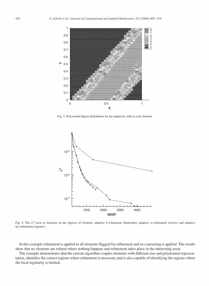
8765432

Fig. 3. Polynomial degree distribution for hp-adaptivity with in each element.

1000 2000 3000 4000

NDOF

10-7

10-6

10-5

L2

Fig. 4. The L2-error as function on the degrees of freedom, adaptive h-refinement (diamonds), adaptive p-refinement (circles) and adaptivehp-refinement (squares).

In this example refinement is applied to all elements flagged for refinement and no coarsening is applied. The resultsshow that no elements are refined where nothing happens and refinement takes place in the interesting areas.

The example demonstrates that the current algorithm couples elements with different size and polynomial represen-tation, identifies the correct regions where refinement is necessary and is also capable of identifying the regions wherethe local regularity is limited.

Á. Galvão et al. / Journal of Computational and Applied Mathematics 215 (2008) 409–418 417

1000 2000 3000 4000

NDOF

10-4

10-3

10-2

H1

Fig. 5. The H 1-error as function on the degrees of freedom, adaptive h-refinement (diamonds), adaptive p-refinement (circles) and adaptivehp-refinement (squares).

7. Conclusions

We have shown that the MEM is an elegant way to match functional and geometrical non-conforming neighbouringelements. Moreover, it appears that the solution propagates continuously across the element boundaries.

The error indicator marks correctly the elements which need refinement.The Sobolev regularity estimator leads indeed to h-refinement where it is to be expected, near the foot of the cosine-

hill, despite the fact that for the Sobolev regularity estimator only low order Legendre coefficients are available. SinceLSQSEM does not require artificial diffusion to stabilize the numerical scheme, no smearing of the numerical solutiontakes place, which would increase the estimated Sobolev regularity.

No coarsening of the grid has been applied. Once the critical regions in the problem have been resolved, smallelements may be merged if their estimated error is below a certain tolerance. Alternatively, the polynomial degree maybe lowered if the estimated error is below a certain tolerance. The choice whether to merge elements or to decrease thepolynomial degree can be based on the estimated Sobolev regularity.

References

[1] M. Berndt, T.A. Manteuffel, S.F. McCormick, Local error estimation and adaptive refinement for first-order system least squares (FOSLS),Electron. Trans. Numer. Anal. 6 (1997) 35–43.

[2] A. Galvão, hp-adaptive least squares spectral element method for hyperbolic partial differential equations, 〈http://www.aero.lr.tudelft.nl/∼marc/hpAdaptiveLSQSEM.pdf〉, TUDelft, 2005.

[3] M.I. Gerritsma, T.N. Phillips, Spectral element method for axisymmetric stokes problems, J. Comput. Phys. 164 (2000) 81–103.[4] M.I. Gerritsma, M.M.J. Proot, Analysis of a discontinuous least-squares spectral element method, J. Sci. Comput. 17 (2002) 323–334.[5] R.D. Henderson, G.E. Karniadakis, Unstructured spectral methods for simulation of turbulent flows, J. Comput. Phys. 122 (1995) 191–217.[6] P. Houston, B. Senior, E. Süli, Sobolev regularity estimation for hp-adaptive finite element methods, Report NA-02-02, University of Oxford,

UK, 2002.[7] B.-N. Jiang, The Least-Squares Finite Element Method, Theory and Applications in Computational Fluid Dynamics and Electromagnetics,

Springer, Berlin, 1998.[8] B.-N. Jiang, On the least-squares method, Comput. Methods Appl. Mech. Engrg. 152 (1998) 239–257.[9] J.-L. Liu, Exact a posteriori error analysis of the least squares finite element method, Appl. Math. Comput. 116 (2000) 297–305.

[10] Y. Maday, C. Mavriplis, A. Patera, Non-conforming mortar element methods: application to spectral discretizations, SIAM 7 (1989) 392–418.[11] B. De Maerschalck, Space–time least-squares spectral element method for unsteady flows—application and evaluation for linear and non-linear

hyperbolic scalar equations, 〈http://www.aero.lr.tudelft.nl/∼bart〉, 2003.

418 Á. Galvão et al. / Journal of Computational and Applied Mathematics 215 (2008) 409–418

[12] B. De Maerschalck, M.I. Gerritsma, The use of the Chebyshev approximation in the space–time least-squares spectral element method, Numer.Algorithm 38 (2005) 173–196.

[13] B. De Maerschalck, M.I. Gerritsma, Higher-order Gauss–lobatto integration for non-linear hyperbolic equations, J. Sci. Comput. 27 (2006)201–214.

[14] J.P. Pontaza, J.N. Reddy, Spectral/hp least squares finite element formulation for the incompressible Navier–Stokes equation, J. Comput. Phys.190 (2003) 523–549.

[15] J.P. Pontaza, J.N. Reddy, Space–time coupled spectral/hp least squares finite element formulation for the incompressible Navier–Stokes equation,J. Comput. Phys. 197 (2004) 418–459.

[16] M.M.J. Proot, M.I. Gerritsma, A least-squares spectral formulation for the Stokes problem, J. Sci. Comput. 17 (2002) 311–322.[17] M.M.J. Proot, M.I. Gerritsma, Least-squares spectral elements applied to the Stokes problem, J. Comput. Phys. 181 (2002) 454–477.[18] M.M.J. Proot, The least-squares spectral element method, Ph.D. Thesis, TU Delft, 2003.[19] M.M.J. Proot, M.I. Gerritsma, Application of the least-squares spectral element method using Chebyshev polynomials to solve the incompressible

Navier–Stokes equations, Numer. Algorithm 38 (2005) 155–172.