THE LEAST-SQUARES GALERKIN SPLIT FINITE ELEMENT METHOD FOR BUOYANCYDRIVEN FLOW

1 Copyright © 2010 by ASME

Proceedings of the ASME 2010 International Design Engineering Technical Conferences & Computers and Information in Engineering Conference

IDETC/CIE 2010 August 15-18, 2010, Montreal, Quebec, Canada

DETC2010-29157

THE LEAST-SQUARES GALERKIN SPLIT FINITE ELEMENT METHOD FOR BUOYANCY-DRIVEN FLOW

Rajeev Kumar* Department of Mechanical

and Aerospace Engineering UTA Box 19018

The University of Texas at Arlington Arlington, TX 76019

[email protected]

Brian H. Dennis† Department of Mechanical

and Aerospace Engineering UTA Box 19018

The University of Texas at Arlington Arlington, TX 76019 [email protected]

* Research Associate. Student member ASME † Assistant Professor, Member ASME

ABSTRACT The least-squares finite element method (LSFEM), based on minimizing the l2-norm of the residual is now well established as a proper approach to deal with the convection dominated fluid dynamic equations. The least-squares finite element method has a number of attractive characteristics such as the lack of an inf-sup condition and the resulting symmetric positive system of algebraic equations unlike Galerkin finite element method (GFEM). However, the higher continuity requirements for second-order terms in the governing equations force the introduction of additional unknowns through the use of an equivalent first-order system of equations or the use of C1

continuous basis functions. These additional unknowns lead to increased memory and computational requirements that have limited the application of LSFEM to large-scale practical problems. A novel finite element method is proposed that employs a least-squares method for first-order derivatives and a Galerkin method for second order derivatives, thereby avoiding the need for additional unknowns required by a pure LSFEM approach. When the unsteady form of the governing equations is used, a streamline upwinding term is introduced naturally by the least-squares method. Resulting system matrix is always symmetric and positive definite and can be solved by iterative solvers like pre-conditioned conjugate gradient method. The method is stable for convection-dominated flows and allows for equal-order basis functions for both pressure and velocity. The method has been successfully applied here to solve complex buoyancy-driven flow with Boussinesq approximation in a square cavity with differentially heated vertical walls using low-order C0 continuous elements.

1 INTRODUCTION The buoyancy driven flow in a square cavity with differentially heated walls is one of the least pursued areas in finite element methods, although it has been an extensively explored area in finite difference methods. Physics involved in the buoyancy driven flow inside a square domain has relevance to a variety of practical problems such as nuclear reactor insulation, ventilation of rooms, solar energy collection and convective heat transfer associated with boilers and electronics etc. Buoyancy driven flows have added complexity in the form of coupling between transport properties of the flow and the thermal fields. Internal flow problems like one being discussed are more complex compared to external flows due to the fact that unlike the external flows where flow outside the boundary layer can be considered unaffected by boundary layer, over here the flow outside the boundary layer forms a core surrounded by boundary layers on the four walls. The confined core and surrounding boundary layer interact and this interaction causes added complexity especially at higher Rayleigh numbers (Ra) and larger temperature differences [1-3].

Davis [4] used a false transient approach based on a stream function-vorticity finite difference method employing forward difference and second order central difference for time and space derivatives respectively to solve natural convection in a square cavity within the Boussinesq approximation. He used Richardson extrapolation to obtain high accuracy benchmark solutions.

Chenoweth and Paolucci [5] investigated the steady state flow in rectangular cavities with large temperature differences between vertical isothermal walls of rectangular cavities. They

Proceedings of the ASME 2010 International Design Engineering Technical Conferences & Computers and Information in Engineering Conference

IDETC/CIE 2010 August 15-18, 2010, Montreal, Quebec, Canada

DETC2010-29157

mailto:[email protected]

mailto:[email protected]


used transient form of the flow equations, simplified for low Mach numbers.

Vierendeels et al [6] solved full Navier-Stokes equations for low speed compressible flows to simulate buoyancy-driven flow inside a square domain without resorting to Boussinesq approximation or low Mach number approximation. The low Mach number stiffness was tackled by appropriate discretization and local pre-conditioning. Their study employing multigrid provides benchmark solutions for the thermally driven flows in a square cavity.

Recently lattice Boltzmann method which is based on discrete lattice kinetic theory has gained tremendous popularity as an alternative to traditional numerical methods like finite difference, finite elements and finite volume methods for solving the fluids problems. Some of the relevant noteworthy works are those of Chen et al [7], Eggels and Somers [8] and more recently by Dixit and Babu [9] to name a few.

A novel finite element method is proposed that employs a least-squares method for first-order derivatives and a Galerkin method for second order derivatives, thereby avoiding the need for additional unknowns required by a pure LSFEM approach. When the unsteady form of the governing equations is used, a streamline upwinding term is introduced naturally by the least-squares method. In the present formulation only the primitive variables of velocity, pressure and temperature are solved for and an equal-order basis function is used for all of them meaning no restrictive Ladyzhenskaya-Babuska-Brezzi (LBB) condition that need to be satisfied in the Galerkin based methods [10-12]. Resulting system matrix is symmetric and positive definite and can be solved by iterative solvers like pre-conditioned conjugate gradient (pcg) method. We call this method the least square Galerkin split finite element method (LSGSFEM). Its advantage over LSFEM can be qualitatively underlined by the fact that it used only four variables at each node whereas Tang [13] employed seven variables per node to solve the same problem using least-squares based V-p--T-q formulation in Ra-range of 103-106. In three dimensions, the proposed method would require only five variables in the solution vector as against eleven variables for LSFEM using V-p--T-q formulation. This is the main reason that limited the application of the LSFEM in practical fluid dynamics problems. A detailed comparison of the proposed method and LSFEM in terms on accuracy and performance, authors believe, would be a matter of a separate study. The proposed method has been successfully applied to incompressible and compressible Navier-Stokes flows [14-17]. The intent of this study is to test and validate the proposed method by simulating the complex buoyancy-driven flow with Boussinesq approximation in a square cavity with differentially heated vertical sides (Fig. 1).

2 MATHMATICAL FORMULATION This study assumes a Newtonian fluid with constant properties except density in body force term of the momentum equation. We considered time-dependent incompressible flow with thermal convection. The Boussinesq-approximation relates the density changes to the temperature changes and thereby couples temperature-field with the flow-field. The governing

equations for the thermal convection flow using conservation of mass, momentum and energy can be written as:

2

2

2

2

c2

2

2

2

2

2

2

2

y

T

x

Tα

y

Tv

x

Tu

t

T

TTgβy

v

x

v

y

p

ρ

1

y

vv

x

vu

t

v

y

u

x

u

x

p

ρ

1

y

uv

x

uu

t

u

0y

v

x

u

(1)

With boundary conditions:

u = v = 0 on all four walls. 0y

TTy)T(L,,Ty)T(0, CH

and

on top and bottom walls. Here u and v are the velocity components in x and y directions respectively. The density is denoted by , pressure by p and T is the temperature. Symbols ν and are for the kinematic viscosity and the thermal diffusivity respectively. TH and TC are temperatures at the hot wall and the cold wall respectively, and L is the length of the square domain and β is the coefficient of thermal expansion. The equations were non-dimensionalized as follows:

2

2

CH

C

αρ

Lpp

TT

TTT,

α

Lvv,

α

Luu,

L

yy,

L

xx

and

Where variables with etc.uy,x and are the non-dimensionalized variables. With these non-dimensional variables we get the following non dimensional form of the governing equations. For the sake of clarity .. has been dropped from the non-dimensional equations

2

2

2

2

2

2

2

2

2

2

2

2

y

T

x

T

y

Tv

x

Tu

t

T

PrTRay

v

x

vPr

y

p

y

vv

x

vu

t

v

y

u

x

uPr

x

p

y

uv

x

uu

t

u

0y

v

x

u

(2)

And the boundary conditions are:

u = v = 0 on all four walls. 0y

TTy)T(1,,Ty)T(0, CH

and on

top and bottom walls (Fig. 1). Here Pr and Ra are the dimensionless numbers called Prandtl number and Rayleigh number respectively. These are given as:

2

3CH

ν

PrL)TTgβRa

α

νPr

(and respectively.

3 LSGSFEM FORMULATION LSGS method is based on time-dependent formulation of Navier Stokes equations. Time derivatives are discretized using Euler backward differences as:

t

vv

t

v

t

uu

t

u

n1nn1n

and (3)


and non-linear terms are linearized in time to get the matrix form of the system

fU 1n L (4) Here U = (u, v, p, T)T is the vector of unknowns, the vector f = (0, un, vn

+ ∆tRaPrTn, Tn)T and the operator L is given as

Pr 0

0 Pr

0 0

n 2

n 2

x y

I tV t

I tV t

L

2

0 0

0

0

0 n

tx

ty

I tV t

(5)

Where nV

is the velocity field vector at previous time step and I, an mm identity matrix, m being number of nodes per element. The residual vector is given as

fU 1n L R (6) The residual is minimized using a suitable weighting operator that comes from LSFEM applied to Euler’s equations. LSFEM gives a symmetric system of equations and the inherent streamline upwinding term provides stability for convection dominated cases. Let us consider the x-component of the incompressible Euler’s equations.

0x

puV

t

u

(7)

After discretizing the unsteady term using Euler backward differences and linearizing in time this can be written as

n1nn1n ux

pΔtuVΔtu

1n

(8)

Application of LSFEM to this equation as

n

Ω

T

ii

n

i

1n

Ω

j

j

n

j

T

ii

n

i

udΩx

NΔt0NVΔtN

WdΩx

NΔt0NVΔtN

x

NΔt0NVΔtN

(9)

where W = (u,v,p)T is the vector of unknowns and N is the element shape function. Integration of equation (9) gives the contribution of x-momentum equation to the Euler-Lagrange equation as

T 2 2UP x x

n+1

T 2 T 2x x x

[M]+ t [C]+[C] + t [K ] 0 t[M ]+ t [C ]

0 0 0 W = g

t[M ] + t [C ] 0 t [K ]

(10)

Where g is the right hand side vector as in equation (9) and

T

TT nx

NM = N N d , M = N d , C = N V . N d ,

x

T

Tn

x x

y y yC = V . y d , [K ] = d , and

x x x

Tn nUPK = V . N V . N d

. The streamline upwinding term

in [Kup] is introduced by the LSFEM. Similar contribution from y-component of Euler’s equation and the continuity equation results in a symmetric system of equations. The

weighting operator for LSGS method, S , therefore is taken from LSFEM applied to inviscid part of governing equations (5) as

n

n

n

VΔtI000

0y

ΔtVΔtI0

0x

Δt0VΔtI

00yx

S (11)

Hence minimizing of the residual in (6) using the weighting operator in (11) leads to following weak form for LSGSFEM

0dΩ f) - U (N) ( 1n

Ω

T LS (12)

Introducing the finite element approximation m

n 1 n 1 n 1h i i

i

U U N U (13)

where m is the number of nodes per element and Ni is the element shape function associated with ith node. Substituting the approximation into the weak formulation in (12) leads to linear algebraic equations

[K]Un+1 = F Global stiffness matrix [K] and the vector F result from assembling the element stiffness matrices and vectors respectively given by

e e

T Ti j iΩ Ω

ke ( N ) ( N ) dΩ; fe ( N ) f dΩ. S L S

Weighting operator S ensures split treatment to first order terms and second order terms in the governing equation. Thus, the first order term are treated like LSFEM and the second order viscous terms get treated similar to GFEM. The LSFEM provides the inherent streamline upwinding term as shown below (10). Integrals containing second order terms are resolved the Galerkin way through integration by parts. Importantly, since C0 continuous elements are used, subsequent second order derivatives vanish resulting in a symmetric matrix system. It is also a standard practice [18, 19] to ignore computationally expensive second order derivatives for linear elements.

4 COMPUTATION OF DERIVED VARIABLES Variables like vorticity, stream function and Nusselt number are computed from the solution as post-processing products. Method of obtaining these is described in this section.

4.1 Vorticity, Z: Vorticity at each node was computed by using the definition of vorticity, ω = × V. For two dimensional case it becomes

y

u

x

vωz

(14)

A variable X can be expanded using the basis set N as

iXNXn

ii , where n is the number of nodes per element and Ni

and Xi are the element shape function and the value of variable X respectively associated with ith node. Using this expansion for ωz, u and v we can write (14) as

y

uN

x

vNωN iiii

izi

(15)


Applying Galerkin method to (15) gives the system of equations

Ω

i

T

j

iΩ

i

T

j

iΩ

zi

T

ji udΩy

NNvdΩ

x

NNωdΩNN (16)

which is solved to get values of vorticity at each node. No boundary condition is specified.

4.2 Stream Function, Stream function was computed from the relation between stream function and the velocity components

x

v

y

u

y

ψ

x

ψψ

2

2

2

22

(17)

Anticlockwise circulation is taken as positive and clockwise circulation as negative . Finite element expansion with the help of basis set Nfor the variables , u and v similar to that in previous section and application of Galerkin method gives the system of equations.

Ω

i

T

ji

Ω

i

T

ji

Ω

i

T

j2

i vdΩx

NNudΩ

y

NNψdΩNN

(18)

Integral involving second order term is treated by Green’s theorem and the resulting boundary term is ignored because of no slip condition on all the four walls. Final form of system of equations resulting that needs to be solved in order to get nodal values of is

Ω

i

T

ji

Ω

i

T

ji

Ω

iT

ji udΩy

NNvdΩ

x

NNψdΩNN (19)

4.3 Nusselt Number, Nu: Nusselt number is the ratio of convection heat transfer to fluid conduction heat transfer under the same conditions. Davis [4] in his paper computed average Nusselt numbers throughout the cavity, on the vertical midplane and on the vertical hot wall on the right side. On the hot wall he also computed maximum and minimum Nusselt numbers along with their locations. Component of Nusselt number in x-direction averaged over a vertical plane is given by

dyx

TuTdy(x,y)qNu

1

0

1

0 xx

(20)

The component of heat flux in x-direction, qx(x,y) was

computed in a similar way using relation x

TuTy)(x,q

x

and Galerkin treatment to it as before, getting system of equations

Ω

i

T

ji

Ω

iT

ji0

Ω

xiT

ji TdΩy

NNTdΩNNuqdΩNN (21)

Once Nux is computed, overall average Nusselt number, uN is computed as

dxNuuN1

0 x (22)

Similarly other values of Nusselt numbers can be computed. Integrals in (20) and (22) were computed using Simpson’s method. To get more accurate values, the nodal values of integrand were first interpolated to finer resolution using cubic spline method.

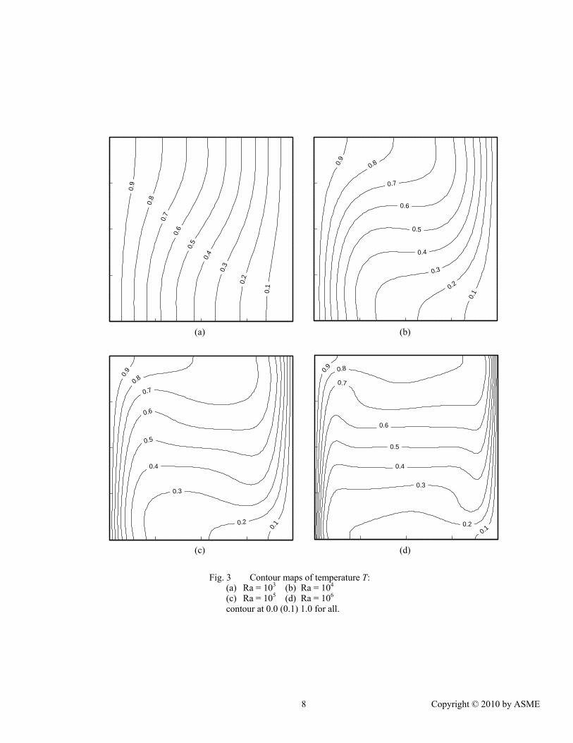
5 NUMERICAL RESULTS Computations were carried out in the Rayleigh number range of 103 – 106 and value of Prandtl number, Pr was taken as 0.71 which is the value for air at room temperature. Davis [4] used uniform meshes with 10, 20 and 40 element per side for Ra = 103 and 104 and 10, 20, 40, 60 and 80 element-meshes for Ra = 105 and 106. He also used Richardson extrapolation in order to get the exact solution. Uniform meshes with 10, 20 and 40 elements per side for Ra = 103; 20, 30, 40 and 60 element-meshes for Ra = 104; 20, 30, 40, 60 and 80 element-meshes for Ra = 105 and 40, 50, 60, 80 and 100 element-meshes for Ra = 106 were used in present study. Gaussian quadrature with one-point reduced integration was used to compute the integrals. A time step size, ∆t = 0.001 was used for Ra = 103 – 105, whereas for highly nonlinear case of Ra = 106, time step ∆t = 0.0005 and under relaxation factor of 0.6 was used. For all the cases a tolerance of 10-9 or maximum of 8000 iterations were used for pcg-iterations at each time step. An external tolerance of 10-6 for l2-norm of residual was used as stopping criterion. Results have been compared with the benchmark results by Davis. Contour plots for stream function, horizontal and vertical velocity components, temperature and vorticity are presented in Figs 2-6. Contours match well with those by Davis. The streamline contours are fully anti-symmetric with respect to the center of the cavity and for lower Rayleigh numbers maximum value of stream function occurs at the center of the cavity. For higher Rayleigh numbers there are two maxima on both sides of the center. Various other parameters were computed similar to those computed by Davis. Typical results for Ra = 106 are presented in Tables I. These values are compared with those obtained by Davis on uniform 40×40 and 80×80 meshes. It should be noted that Davis used a finite difference method that was first order in time and second order in space. The definition and nomenclature for the quantities compared in the table are same as those by Davis, which are

midψ Magnitude of the stream function at the cavity-center

axmψ Maximum value of stream function

umax Maximum x-velocity on vertical mid-plane vmax Maximum y-velocity on horizontal mid-plane

uN Average Nusselt number (Nu) throughout the cavity

21Nu Average Nusselt number on the vertical mid-plane

0Nu Average Nusselt number on the vertical hot surface

maxNu Maximum value of local Nu on the vertical hot surface

minNu Minimum value of local Nu on the vertical hot surface

To obtain more accurate values for these quantities and their locations, the node point data were first interpolated using a cubic-spline interpolation to a finer resolution. The values thus computed were further refined using Richardson extrapolation:

)2(1h

ffC

ln(2)/ff

fflnα

Chff

αα

h/2h

/2hh/2

hh

α

hextpn

and

where (23)


Here h is given by 1/N, and N is the number of elements in one direction in the finest mesh and h is the value for next finest mesh used for a particular Rayleigh number case (see tables I). The computed value of gives roughly the order of convergence. Convergence plots for umax and vmax are shown in Fig. 7. The slopes of the plots average around 2, which is expected as umax and vmax are the primary solution variables. Convergence rates for derived variables like stream function and Nusselt numbers are less than quadratic. The pcg iterations required at each time step quickly declined as the solution progressed towards convergence. The variation of pcg iterations for the Ra-range tested was recorded for 40×40 mesh run at t = 0.001. A typical plot is shown in Fig. 8. The figure also shows the total number of pcg-iterations to reach the converged solutions. Typical results listed in table I show the correct trend and the extrapolated values are close to benchmarks values by Davis [4].

6 CONCLUDING REMARKS Complex buoyancy-driven flow in a square cavity with differentially heated vertical walls and Boussinesq approximation has been solved using a novel finite element method called least-squares Galerkin split finite element method (LSGSFEM) that employs a least-squares method for first-order derivatives and a Galerkin method for second order derivatives, thereby avoiding the need for additional unknowns required by a pure LSFEM approach. This method has inherent streamline upwinding term, allows for equal-order basis functions for velocity, pressure and temperature thereby avoids LBB condition. Resulting system of equations is always symmetric. Non-linear terms are treated by linearization in time. Results were obtained using low-order C0 continuous elements and compare well with the standard published results.

7 ACKNOWLEDGEMENTS The authors would like to acknowledge the partial support for this research by the US Department of Energy through grant number DE-FG36-08GO88170.

8 REFERENCES [1] Ostrach, S., 1988, “Natural Convection in Enclosures”,

ASME Trans. J. Heat Transfer,110, pp. 1175-1190. [2] Gebhart, B., 1979, “Buoyancy Induced Fluid Motions

Characteristics of Applications in Technology: The 1978 Freeman Scholar Lecture”, ASME Trans. J. Heat Transfer,101, pp. 5-28.

[3] Hoogendoorn, C. J., 1986, “Natural Convection in Enclosures”, Proc. Eighth Int. Heat Transfer Conf., Hemisphere Publishing Corp., San Francisco (1986) Vol. 1, pp. 111-120

[4] Davis, G. De Vahl, 1983, “Natural Convection of Air in a Square Cavity: A Bench Mark Numerical Solution”, Int. J. Numer. Methods Fluids, Vol. 3, pp. 249-264.

[5] Chenoweth, D. R. and Paolucci, S., 1986, “Natural Convection in an Enclosed Vertical Air Layer with Large Horizontal Temperature Differences”, J. Fluid Mech. Vol. 169, pp. 173-210.

[6] Vierendeels, J., Dick, E., 2003, “Benchmark Solutions for the Natural Convective Heat Transfer Problem in a Square Cavity with Larrge horizontal Temperature

Differences”, Int. J. Numer. Meths Heat Fluid Flow, Vol. 13, pp. 1057-1078.

[7] Chen, Y., Ohashi, H. and Akiyama, M., 1994, “Thermal Lattice Bhatnagar-Gross-Krook Model without Nonlinear Deviations in Macrodynamic Equations”, Phys. Rev. E Vol. 50, pp. 2776-2783.

[8] Eggels, J. G. M. and Somers, J. A., 1995, “Numerical Simulation of Free Convection Flow using Lattice Boltzmann Scheme”, Int. J Heat Fluid Flow Vol. 16, pp. 357-364

[9] Dixit, H. N. and Babu, V, 2006, “Simulation of High Rayleigh Number Natural Convection in a Square Cavity using Lattice Boltzmann Method”, Int. J. Heat and Mass Transfer Vol. 49, pp. 727-739

[10] Carey, G. F. and Oden, J. T. 1986, “Finite Elements: Fluid Mechanics”, Prentice Hall, IV.

[11] Baker, A. J., Kim, J. W., Freels, J. D. and Orzechowski, J. A, 1987, “On a Finite Element CFD Algorithm for Compressible, Viscous and Turbulent Aerodynamics Flows”, Int. J. Numer. Methods Fluids, Vol. 7, pp. 1235-1259

[12] Hughes, T. J. R., 1987, “Recent Progress in the Development and Understanding of SUPG Methods with Special Reference to the Compressible Euler and Navier-Stokes Equations”, Int. J. Numer. Methods Fluids, Vol. 7, pp. 1261-1275.

[13] Tang Li, Q. and Tsang, T. T., 1993, “A Least-Squares Finite Element Method for Time-Dependent Incompressible Flows with Thermal Convection”, Int. J. Numer. Methods Fluids, Vol. 17, pp. 271-289.

[14] Dennis, B. H. and Rajeev Kumar, 2007, “A Least-squares/Galerkin Finite Element Method for Incompressible and Compressible Viscous Flows”, 14th International Conf. on Finite Elements in Flow Problems, Santa Fe, New Mexico, USA.

[15] Dennis, B. H. and Rajeev Kumar, 2008, “A Least-squares/ Galerkin Split Finite Element Method for Incompressible Navier-Stokes Problems”, ASME IDETC/CIE, Brooklyn, New York, USA.

[16] Rajeev Kumar and Dennis, B. H., 2009, “Unsteady Incompressible Flow Computations with Least-squares/ Galerkin Split Finite Element Method”, ASME Early Career Tech. Conf., Arlington, Texas, USA.

[17] Dennis, B. H. and Rajeev Kumar, 2009, “A Least-squares/ Galerkin Split Finite Element Method for Compressible Navier-Stokes Equations”, ASME IDETC/CIE, San Diego, California, USA.

[18] Lin, H and Atluri, S. N., 2001, “The Meshless Local Petrov-Galerkin (MLPG) Method for Solving Incompressible Navier-Stokes Equations”, Computer Modeling in Engineering & Sciences, Vol. 2(2), pp. 117-142.

[19] Donea, J. and Huerta, A., 2003, “Finite Element Methods for Flow Problems”, John Wiley Publishers.


Fig. 1 Computational domain and the boundary conditions

TABLE I: Typical comparison of results at Ra = 106

Mesh midψ max

ψ

x, y

umax z

vmax x uN 21Nu 0Nu maxNu minNu

0.025 16.845 17.3750

0.15, 0.55 69.063 0.842

238.5350.038 8.655 8.673 8.619 16.464

0.068 0.905 0.98

0.02 16.728 17.1730

0.16, 0.55 68.303 0.845

230.2960.038 8.673 8.705 8.664 16.613

0.057 0.973 0.999

60.01 16.663 17.1005

0.15, 0.55 67.892 0.847

226.4190.038 8.682 8.713 8.684 16.603

0.05 1.031 0.991

h' = 0.0125* 16.598

17.0051 0.15, 55

67.488 0.848

223.8700.038 8.691 8.726 8.705

16.588 0.047

1.042 0.999

LSGSFEM

h = 0.01* 16.568 16.962

0.15, 0.54067.303 0.849

222.4650.038 8.695 8.732 8.715

16.621 0.046

1.045 0.999

Extrapolated solutions 16.511

16.9046 0.150, 0.539 66.982 220.86 8.702 8.737 8.729

16.809 0.044

1.047 0.999

Benchmark solutions Davis [4]

16.32 16.75

0.151, 0.54764.63 0.850

219.36 0.0379 8.800 8.799 8.817

17.925 0.0378

0.989

*see extrapolation equation (23)


Fig. 2 Contour maps of stream function : (a) Ra = 103; contour at -1.1739 (0.11739) 0 (b) Ra = 104; contour at -5.1199 (0.51199) 0 (c) Ra = 105; contour at -9.7780, -8.80(0.9778) 0 (d) Ra = 106; contour at -16.49, -14.84(1.649) 0

(a) (b)

(c) (d)

-1.1739

-1.0565

-0.9391

-0.8217

-0.7043

-0.5869

-0.4696

-0.3522

-0.2348

-0.1174

-5.1199

-4.6079

-3.5839

-2.5600

-1.5360

-0.5120

-4.0959

-3.0719

-2.0480

-1.0240

-9.7880

-9.7880

-8.8000

-6.5253

-3.2627-1.0876

-7.6129

-5.4378

-2.1751

-16.4900

-16.4900

-16.4900

-14.8400

-12.8256

-10.9933

-9.1611

-7.3289

-5.4967

-3.6644

-1.8322


0.1

0.9

0.8

0.7

0.6

0.4

0.3

0.2

0.5

0.6

0.5

0.4

0.3

0.2

0.1

0.7

0.80.9

0.10.2

0.3

0.4

0.5

0.6

0.7

0.80.9

0.10.2

0.3

0.4

0.5

0.6

0.70.8

0.9

Fig. 3 Contour maps of temperature T:(a) Ra = 103 (b) Ra = 104 (c) Ra = 105 (d) Ra = 106 contour at 0.0 (0.1) 1.0 for all.

(a) (b)

(c) (d)


3.6478

-3.6478

0.0000

-2.8372

-1.2159

-0.4053

-2.0266

2.8372

2.0266

1.2159

0.4053

-16.4400

16.4400

-12.7867

-9.1333

-5.4800

-1.8267

12.78679.1333

5.4800

1.82670.0000

-43.0000-33.4444

-23.8889-14.3333

43.000033.4444

23.8889

14.3333

-4.7778

4.7778

0.00

00

-81.4536

-54.3024

-27.1512

0.0000

81.4536

54.3024

27.1512

108.6048

-108.6048

0.0000

0.0000

Fig. 4 Contour maps of horizontal velocity u:(a) Ra = 103; contour at -3.6478 (0.72956) 3.6478 (b) Ra = 104; contour at -16.440 (3.2880) 16.440 (c) Ra = 105; contour at -43.0 (8.6) 43.0 (d) Ra = 106; contour at -135.756 (27.151) 135.756

(a) (b)

(c) (d)


3.7058 -3.7058

2.8823

2.0588

1.2353

0.4118

-2.8823

-2.0588

-1.2353

-0.4118

0.0

00

0

19.6400-19.6400

-15.2756

-10.9111

-6.5467

-2.1822

15.2756

10.9111

6.5467

2.18220.0000

-68.2

68.2

53.0

37.9

22.711.4

-53.0

-37.9

-22.7-11.6

0.0

0.0

0.0

-22

1.3

11

022

1.3

11

0

- 13

2.7

86

6

0.0000

0.0000

0.0000

88

.52

44

Fig. 5 Contour maps of vertical velocity v:(a) Ra = 103; contour at -3.7058 (0.74116) 3.7058 (b) Ra = 104; contour at -19.640 (3.928) 19.640 (c) Ra = 105; contour at -68.2 (13.64) 68.2 (d) Ra = 106; contour at -221.311 (44.262) 221.311

(a) (b)

(c) (d)


-32.3520

-23.9978

-7.2894

9.4190

26.1274

17.7732

34.4816

34

.48

16

17

.773

2

34

.48

16

17.7

73

2

-15.6436

1.0648

-124.1000

-63.1667

-2.2333

58.7000

119.6333180.5667

58

.70

00

11

9.6

33

3

180.5667

40.0000

360.0000680.0000

40.0000

360.0000680.0000

-600.0000

-600.0000

-280

.000

0

-280

.000

0

488.4800

-1338.6600

-1338.6600

488.4800

488.4800

Fig. 6 Contour maps of vorticity ω:(a) Ra = 103; contour at -32.352 (8.354) 51.19 (b) Ra = 104; contour at -124.10 (54.84) 424.3 (c) Ra = 105; contour at -600 (322.0) 2600 (d) Ra = 106; contour at -3165.8 (1827.14) 15105.6

(a) (b)

(c) (d)


0

500

1000

1500

2000

1 10 100 1000 10000Number of time steps

pcg-

itera

tions

/ tim

e st

ep ,

Ra = 106, n = 1709, p = 5.88×105

Ra = 105, n = 849, p = 1.99×105

Ra = 104, n = 1143, p = 1.94×105

Ra = 103, n = 1490, p = 1.87×105

Fig. 7 Convergence-rate plots: (a) umax (b) vmax

Ra = 103, ∆ Ra = 104, Ra = 105 and Ra = 106

avg. slope ~ 2.15

-1

-0.5

0

0.5

1

1.5

-2.4 -2 -1.6 -1.2 -0.8log h

log

(err

or%

) ,

(a)

avg. slope ~ 2.40

-1

-0.5

0

0.5

1

1.5

-2.4 -2 -1.6 -1.2 -0.8log h

log

(err

or%

) ,

(b)

Fig. 8 A typical convergence plot for 40×40 mesh (l2-norm of residual → 10-6) n : number of time steps, p : number of pcg-iterations

THE LEAST-SQUARES GALERKIN SPLIT FINITE ELEMENT METHOD FOR BUOYANCYDRIVEN FLOW

Documents

Transcript of THE LEAST-SQUARES GALERKIN SPLIT FINITE ELEMENT METHOD FOR BUOYANCYDRIVEN FLOW