Constraint preserving discontinuous Galerkin method for ideal

compressible MHD on 2-D Cartesian grids

Praveen Chandrashekar∗† and Rakesh Kumar‡

Abstract

We propose a constraint preserving discontinuous Galerkin method for ideal compress-ible MHD in two dimensions and using Cartesian grids, which automatically maintains theglobal divergence-free property. The approximation of the magnetic field is achieved usingRaviart-Thomas polynomials and the DG scheme is based on evolving certain moments ofthese polynomials which automatically guarantees divergence-free property. We also developHLL-type multi-dimensional Riemann solvers to estimate the electric field at vertices whichare consistent with the 1-D Riemann solvers. When limiters are used, the divergence-freeproperty may be lost and it is recovered by a divergence-free reconstruction step. We showthe performance of the method on a range of test cases up to fourth order of accuracy.

Keywords: Ideal compressible MHD, divergence-free, discontinuous Galerkin method, multi-dimensional Riemann solvers

1 Introduction

The equations governing ideal, compressible MHD are a mathematical model for plasma andform a system of non-linear hyperbolic conservation laws. While it is natural to try to useGodunov-type numerical methods which have been very successful for other non-linear hyper-bolic conservation laws [45], the MHD equations have an additional feature in the form of aconstraint on the magnetic field B, i.e., the divergence of B must be zero, which may not besatisfied by standard schemes. The non satisfaction of this constraint can yield wrong solutionsand the methods can also be unstable [47]. Hence various strategies have been developed overthe years to deal with this issue. Projection-based methods [11] use standard schemes to up-date the solution and a posteriori correct the magnetic field to make the divergence to be zeroby solving an elliptic equation. Hyperbolic divergence cleaning methods have been developedin [20] by introducing an extra Lagrange multiplier or pressure variable. Constrained transportmethods [22], [25] are designed to automatically keep some discrete measure of the divergenceto be invariant. A key idea in most of these methods is the staggered storage of variables withthe magnetic field components being located on the faces and the remaining hydrodynamic vari-ables being located in cell centers. Divergence-free reconstruction of magnetic field have beendeveloped in conjunction with approximate Riemann solvers [7], [1], [2], [3] which also preservea discrete divergence constraint. Another class of methods [40], [31], [10], [49], [15] aims toconstruct a stable scheme without explicitly making the divergence to be zero and are basedon Godunov’s symmetrized version of the MHD model [26]; moreover these methods are notconservative since the symmetrized model has source terms.

Many of the ideas first developed in a finite volume setting have been extended to discon-tinuous Galerkin methods which provide a good framework for constructing high order accu-rate schemes. A locally divergence-free basis was used in combination with Rusanov fluxes

∗Corresponding author†TIFR Center for Applicable Mathematics, Bangalore, India. Email: praveen@tifrbng.res.in‡TIFR Center for Applicable Mathematics, Bangalore, India. Email: rakesh@tifrbng.res.in

1

arX

iv:2

007.

1305

6v1

[m

ath.

NA

] 2

6 Ju

l 202

0

in [18]. A similar approach based on Godunov’s symmetrized MHD model has also been devel-oped [27], whereas entropy stable DG schemes using SBP type operators have been developedin [21], [9], [38]. The divergence-free reconstruction idea has been combined in a DG schemein [6] for induction equation and for Maxwell’s equations in [30]. DG schemes which automati-cally preserve the divergence condition have been developed in [36], [35] using central DG ideaand in [24], [14] using Godunov approach. Maintaining the positivity of solutions is very im-portant and recent work shows a close link between this property and a discrete divergence-freecondition [50], see also [31]. DG schemes which in practice are positive have been developedin standard formulations under the assumption that the Lax-Friedrich scheme is positive [16].A provably positive DG scheme has been developed in [51] based on Godunov’s symmetricMHD form and locally divergence-free basis, but the solutions are not guaranteed to be globallydivergence-free and the method is not conservative due to the use of Godunov’s symmetrizedMHD model.

In the present work, we develop a DG scheme based on tensor product polynomials and inparticular using Raviart-Thomas polynomials for the approximation of the magnetic field. Thisbuilds on the initial work done for induction equation in [14] and is similar in spirit to [24], whichdeveloped up to third order schemes using Brezzi-Douglas Marin (BDM) polynomials (see [12],Section III.3.2) for the magnetic field.

1. We develop arbitrarily high order DG schemes for ideal MHD which automatically preservethe divergence constraint and the solutions are globally divergence-free.

2. The magnetic field is approximated using Raviart-Thomas polynomials which have tensorproduct structure. The degrees of freedom are evolved with a hybrid scheme defined bothon faces and cells.

3. We develop multi-dimensional HLL and HLLC Riemann solvers which are consistent withtheir 1-D counterparts.

4. We couple the DG scheme with divergence-free reconstruction method when a TVD-typelimiter is applied since the limiter can destroy the divergence-free property.

Because of the DG foundations, we can achieve arbitrarily high order of accuracy with thisapproach, at least for smooth solutions. The discretization and evolution of the magnetic fieldhas a hybrid nature in the sense that the scheme is defined both on the faces and inside thecells. The method requires numerical fluxes both on the cell faces and the cell corners. Oncell faces, a 1-D Riemann problem is present which can be solved approximately, e.g., usingHLL-type of schemes. At the cell corners, multiple states meet defining a multi-dimensionalRiemann problem. A HLL-type solver can also be formulated for such problems [4], [5], and inparticular when using DG methods, it is important that this solver should be consistent withthe 1-D Riemann solver. In case of discontinuous solutions, some form of TVD-type limitingstrategy is required to control spurious numerical oscillations. But such a limiter applied on themagnetic field can destroy the divergence-free property of the solutions; we then perform a localdivergence-free reconstruction of the solution following the ideas in [30] which are extended tothe case of Raviart-Thomas polynomials. While we cannot prove positivity of solutions in theframework of divergence-free schemes, we show that a heuristic application of scaling limiters canlead to stable computations, but this topic is still an open problem in the context of constraintpreserving schemes which rely on Riemann solvers.

The rest of the paper is organized as follows. In Section (2) we list the MHD equationsand introduce suitable notation necessary in the paper. Section(3) explains the structure ofthe approximating polynomial spaces and resulting degrees of freedom. Section (4) shows howto construct the magnetic field inside the cell given the degrees of freedom of the Raviart-Thomas polynomials. The DG scheme is explained in Section (5) for both the hydrodynamic andmagnetic variables, and we also discusses constraint satisfaction on the magnetic field divergence

2

by the numerical scheme. The computation of the numerical fluxes is explained in Section (6)and the limiting procedure in Section (7). We then present an extensive set of numerical resultsin Section (8).

2 Ideal MHD equations

In the following, we consider only the two dimensional case and it is then convenient to arrangethe variables in the following way to deal with the divergence constraint. Let ρ, p be the densityand pressure of the gas, E be the total energy per unit volume and v = (vx, vy, vz) be the gasvelocity. The components of the magnetic field are B = (Bx, By, Bz). Define

U = [ρ, ρv, E , Bz]>, B = (Bx, By)

then the 2-D ideal MHD equations can be written as a system of conservation laws

∂U

∂t+∇ · F (U ,B) = 0,

∂Bx∂t

+∂Ez∂y

= 0,∂By∂t− ∂Ez

∂x= 0 (1)

where Ez is the electric field in the z direction given by

Ez = vyBx − vxByand the fluxes F = (Fx,Fy) are of the form

Fx =

ρvxP + ρv2

x −B2x

ρvxvy −BxByρvxvz −BxBz

(E + P )vx −Bx(v ·B)vxBz − vzBx

, Fy =

ρvyρvxvy −BxByP + ρv2

y −B2y

ρvyvz −ByBz(E + P )vy −By(v ·B)

vyBz − vzBy

where the total pressure P and energy E are given by

P = p+1

2|B|2, E =

p

γ − 1+

1

2ρ|v|2 +

1

2|B|2

Since magnetic monopoles do not exist, the magnetic field B must have zero divergence. In factif the divergence is zero at the initial time, then under the action of the induction equation, itremains zero at future times also, and hence is referred to as an involution constraint. Since weconsider only 2-D problems in this work, the divergence-free condition is equivalent to the 2-Ddivergence of B being zero, i.e.,

∇ ·B =∂Bx∂x

+∂By∂y

= 0

In the above discussion, we have written the equations in the form (1) which is suitable forthe implementation of the divergence-free scheme in 2-D. For the computation of the numericalfluxes, we have to consider all the equations together in conservation form which can be writtenas

∂U∂t

+∂Fx∂x

+∂Fy∂y

= 0 (2)

where

U =

ρρvxρvyρvzEBxByBz

, Fx =

ρvxP + ρv2

x −B2x

ρvxvy −BxByρvxvz −BxBz

(E + P )vx −Bx(v ·B)0−Ez

vxBz − vzBx

, Fy =

ρvyρvxvy −BxByP + ρv2

y −B2y

ρvyvz −ByBz(E + P )vy −By(v ·B)

Ez0

vyBz − vzBy

3

Let Ax = F ′x(U) and Ay = F ′y(U) be the flux Jacobians. The Jacobian matrices have realeigenvalues given by

λ(Ad) = vd − cfd, vd − csd, vd − ca, vd, 0, vd + ca, vd + csd, vd + cfd, d = x, y

where csd, cfd are the slow and fast magnetosonic speeds and ca is the Alfven wave speed. TheAlfven wave speed is given by

ca =|Bd|√ρ

and the magnetosonic speeds are given by

csd =

√1

2

[a2 + |b|2 −

√(a2 + |b|2)2 − 4a2b2d

], cfd =

√1

2

[a2 + |b|2 +

√(a2 + |b|2)2 − 4a2b2d

]where

a =

√γp

ρ, b =

|B|√ρ

with a being the sound speed.

3 Approximation spaces

We map each cell to the reference cell [−12 ,+

12 ] × [−1

2 ,+12 ] with coordinates (ξ, η). Define the

tensor product polynomials by

Qr,s = spanξiηj : 0 ≤ i ≤ r, 0 ≤ j ≤ s

As basis functions for polynomials, we will first construct one dimensional orthogonal polyno-mials given by

φ0(ξ) = 1, φ1(ξ) = ξ, φ2(ξ) = ξ2 − 1

12, φ3(ξ) = ξ3 − 3

20ξ, φ4(ξ) = ξ4 − 3

14ξ2 +

3

560

whose mass matrix is diagonal with entries given by mi =∫ + 1

2

− 12

φ2i (ξ)dξ. Let k ≥ 0 be the degree

of approximation. The hydrodynamic variables U are approximated in each cell in the spaceQk,k, which can be written as

U(ξ, η) =

k∑i=0

k∑j=0

Uijφi(ξ)φj(η) ∈ Qk,k (3)

Note that this approximation is in general discontinuous across the cell faces.Let us approximate the normal component of B on each face by one dimensional polynomials

of degree k. On the vertical faces of cells, we will approximate the x-component of B by

bx(η) =

k∑j=0

ajφj(η) ∈ Pk(η) (4)

while on the horizontal faces, the y-component is approximated by

by(ξ) =k∑j=0

bjφj(ξ) ∈ Pk(ξ) (5)

4

b+ x(η)

b− x(η)

b−y (ξ)

b+y (ξ)

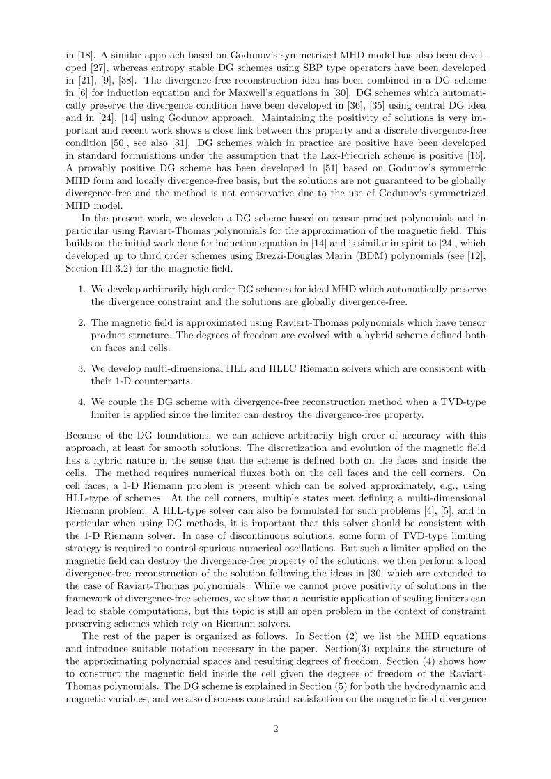
α

β

0 1

32

Figure 1: Location of dofs for B

For k ≥ 1, let us also define certain cell moments which we will use in determining the magneticfield inside the cells. These moments are defined as

αij = αij(Bx) :=1

mij

∫ + 12

− 12

∫ + 12

− 12

Bx(ξ, η)φi(ξ)φj(η)dξdη, 0 ≤ i ≤ k − 1, 0 ≤ j ≤ k

βij = βij(By) :=1

mij

∫ + 12

− 12

∫ + 12

− 12

By(ξ, η)φi(ξ)φj(η)dξdη, 0 ≤ i ≤ k, 0 ≤ j ≤ k − 1

where mij is given by

mij =

∫ + 12

− 12

∫ + 12

− 12

[φi(ξ)φj(η)]2dξdη = mimj

The test functions used to define the α moments belong to Qk−1,k and those used to define the βmoments belong to Qk,k−1. In fact, these quantities correspond to the degrees of freedom used todefine the Raviart-Thomas polynomials [41], which provide H(div,Ω) conforming approximationof vector fields. In our numerical approach, the quantities bx, by, α, β form the discretization ofthe magnetic field and these quantities will be evolved forward in time by a DG scheme. Usingthis information we will reconstruct the magnetic field B inside the cells. We note that α00 andβ00 are the mean values of Bx and By in the cells and a0, b0 are the mean values of the normalcomponent of B on the corresponding faces.

The next section describes how to construct the vector field B from the information containedin the face and cell moments by solving a local reconstruction problem. We are in particularinterested in obtaining approximations which are globally divergence-free vector fields.

Definition 1 (Globally divergence-free). We will say that a vector field B defined on a meshis globally divergence-free if

1. ∇ ·B = 0 in each cell K

2. B · n is continuous at each face F

4 RT reconstruction problem

Consider a cell as shown in Figure 1. We are given normal components of B on the faces in theform of polynomials b±x (η) ∈ Pk and b±y (ξ) ∈ Pk, and also the set of cell moments

αij , 0 ≤ i ≤ k − 1, 0 ≤ j ≤ k, βij , 0 ≤ i ≤ k, 0 ≤ j ≤ k − 1

5

Using this information, we want to construct the magnetic field vector inside the cell.

RT reconstruction problem: Find Bx ∈ Qk+1,k and By ∈ Qk,k+1 such that

Bx(±12 , η) = b±x (η), η ∈ [−1

2 ,12 ], By(ξ,±1

2) = b±y (ξ), ξ ∈ [−12 ,

12 ]

1

mij

∫ + 12

− 12

∫ + 12

− 12

Bx(ξ, η)φi(ξ)φj(η)dξdη = αij , 0 ≤ i ≤ k − 1, 0 ≤ j ≤ k

1

mij

∫ + 12

− 12

∫ + 12

− 12

By(ξ, η)φi(ξ)φj(η)dξdη = βij , 0 ≤ i ≤ k, 0 ≤ j ≤ k − 1

Since dim Qk+1,k = dim Qk,k+1 = (k + 1)(k + 2), we have 2(k + 1)(k + 2) coefficients to bedetermined. On the faces we are given 4(k+1) pieces of information in terms of the polynomialsb±x , b±y , and inside the cell, we have 2k(k+ 1) pieces of information in terms of the cell momentsα, β, and hence we have as many equations as the number of unknowns.

Theorem 1. (1) The RT reconstruction problem has a unique solution. (2) If the data bx, by, α, βcorrespond to a divergence-free vector field, then the reconstructed field is also divergence-free.

For a proof of the above theorem, we refer the reader to [12], [14]. Note that this recon-struction is very local to each cell; it uses data in the cell and on its faces. We remark that thisreconstruction is different from the reconstruction performed in finite volume methods to recoverthe solution from cell averages. In the present case, we have the full information available in(bx, by, α, β) and it is converted into a spatial polynomial (Bx, By) by the RT reconstructionstep. The two sets od data (bx, by, α, β) and (Bx, By) contain the same information and are twodifferent ways to represent the magnetic field.

Properties of B The vector field B obtained from this reconstruction process satisfies certainconditions. Firstly, note that B · n has a unique value at a face common to two cells, i.e., thenormal component of B is continuous at all the faces. Secondly, if the data b±x , b

±y , αij , βij comes

from a divergence-free vector field, then the reconstructed field is also divergence-free [14]. Hence,the vector field B will be globally divergence-free also. The initial data must be generatedcarefully in order to ensure divergence-free condition. An initial divergence-free vector fieldhas a corresponding stream function which we interpolate to a continuous space of Qk+1,k+1

polynomials. The polynomials bx, by on the faces are set equal to the curl of this interpolatedstream function and the cell moments α, β are obtained by computing the integrals exactly witha Gauss-Legendre rule where we again use the curl of the interpolated stream function, and isexplained in Appendix C. The DG scheme to be explained in later sections will then ensurethat the solutions remain divergence-free at future times also.

We will now give the solution of the reconstruction problem at different orders. To do this,we first write the reconstructed magnetic field components as a tensor product of orthogonal1-D polynomials

Bx(ξ, η) =

k+1∑i=0

k∑j=0

aijφi(ξ)φj(η) ∈ Qk+1,k, By(ξ, η) =

k∑i=0

k+1∑j=0

bijφi(ξ)φj(η) ∈ Qk,k+1 (6)

Reconstruction for k = 0 In this case we have constant approximation on the faces for thenormal components

b±x (η) = a±0 , b±y (ξ) = b±0

and the vector field inside the cell is of the form

Bx(ξ, η) = a00 + a10φ1(ξ), By(ξ, η) = b00 + b01φ1(η)

6

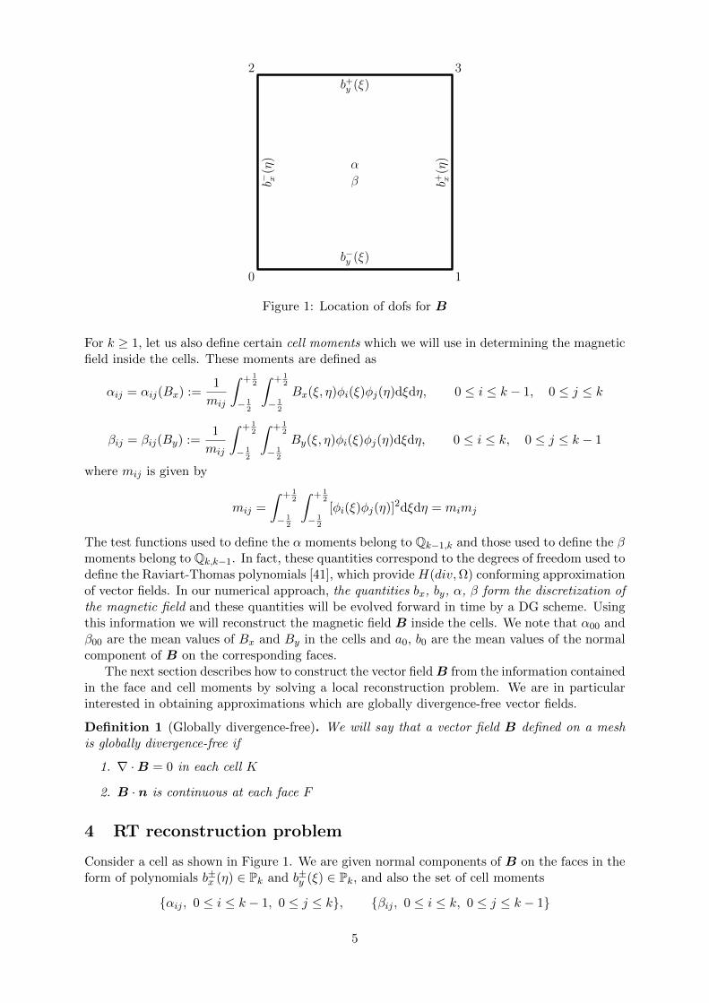
aij = αij , i = 0, 0 ≤ j ≤ 1

a10 = a+0 − a−0

a20 = 3(a−0 + a+0 − 2α00)

a11 = a+1 − a−1

a21 = 3(a−1 + a+1 − 2α01)

bij = βij , 0 ≤ i ≤ 1, j = 0

b01 = b+0 − b−0b02 = 3(b−0 + b+0 − 2β00)

b11 = b+1 − b−1b12 = 3(b−1 + b+1 − 2β10)

Table 1: Solution of RT reconstruction problem for k = 1

aij = αij , 0 ≤ i ≤ 1, 0 ≤ j ≤ 2

a20 = 3(a−0 + a+0 − 2α00)

a30 = 10(a+0 − a−0 − α10)

a21 = 3(a−1 + a+1 − 2α01)

a31 = 10(a+1 − a−1 − α11)

a22 = 3(a−2 + a+2 − 2α02)

a32 = 10(a+2 − a−2 − α12)

bij = βij , 0 ≤ i ≤ 2, 0 ≤ j ≤ 1

b02 = 3(b−0 + b+0 − 2β00)

b03 = 10(b+0 − b−0 − β01)

b12 = 3(b−1 + b+1 − 2β10)

b13 = 10(b+1 − b−1 − β11)

b22 = 3(b−2 + b+2 − 2β20)

b23 = 10(b+2 − b−2 − β21)

Table 2: Solution of RT reconstruction problem for k = 2

which has a dimension of four. The solution of the reconstruction problem is given by

a00 =1

2(a−0 + a+

0 ), b00 =1

2(b−0 + b+0 ), a10 = a+

0 − a−0 , b01 = b+0 − b−0

Note that no cell moments are present at this order and the reconstruction is determined by theface solution alone.

Reconstruction for k = 1 In this case we have linear approximation on the faces and inaddition, there are four cell moments. The solution of the reconstruction problem is given inTable 1.

Reconstruction for k = 2 In this case we have quadratic approximation on the faces andin addition, there are 12 cell moments. The solution of the reconstruction problem is given inTable 2.

Reconstruction for k = 3 In this case we have cubic approximation on the faces and inaddition, there are 24 cell moments. The solution of the reconstruction problem is given inTable 3.

5 Numerical scheme

The basic unknowns in our scheme are the polynomials bx, by approximating the normal com-ponent of B on the cell faces, the cell moments α, β, and the polynomials approximating thehydrodynamic variables and Bz inside the cells which are grouped inside the set U . We willdevise DG schemes to evolve all these quantities forward in time. We perform spatial discretiza-tion using DG scheme and then solve the resulting set of ODE using a Runge-Kutta scheme fortime integration.

5.1 Discontinuous Galerkin method for B on the faces

The normal component of B has been approximated on the faces of our mesh and we want toconstruct a numerical scheme to evolve these values forward in time. If we observe the equation

7

aij = αij , 0 ≤ i ≤ 2, 0 ≤ j ≤ 3

a30 = 10(a+0 − a−0 − α10)

a40 =35

3(3a−0 + 3a+

0 − 6α00 − α20)

a31 = 10(a+1 − a−1 − α11)

a41 =35

3(3a−1 + 3a+

1 − 6α01 − α21)

a32 = 10(a+2 − a−2 − α12)

a42 =35

3(3a−2 + 3a+

2 − 6α02 − α22)

a33 = 10(a+3 − a−3 − α13)

a43 =35

3(3a−3 + 3a+

3 − 6α03 − α23)

bij = βij , 0 ≤ i ≤ 3, 0 ≤ j ≤ 2

b03 = 10(b+0 − b−0 − β01)

b04 =35

3(3b−0 + 3b+0 − 6β00 − β02)

b13 = 10(b+1 − b−1 − β11)

b14 =35

3(3b−1 + 3b+1 − 6β10 − β12)

b23 = 10(b+2 − b−2 − β21)

b24 =35

3(3b−2 + 3b+2 − 6β20 − β22)

b33 = 10(b+3 − b−3 − β31)

b34 =35

3(3b−3 + 3b+3 − 6β30 − β32)

Table 3: Solution of RT reconstruction problem for k = 3

b+ xb− x

b−y

b+y

U c

Bcx

Bcy

Ue

Bex

Bey

Un

Bnx

Bny

Uw

Bwx

Bwy

Us

Bsx

Bsy

Figure 2: Stencil and variables for DG scheme

8

governing Bx, we see that it evolves in time only due to the y derivative of the electric field Ez.Restricting ourselves to a vertical face, we see that we have a one dimensional PDE for Bx whichcan discretized using a 1-D DG scheme applied on the face. Multiplying by a test function φi(η)and integrating by parts on a vertical face yields∫ + 1

2

− 12

∂bx∂t

φidη −1

∆y

∫ + 12

− 12

Ezdφidη

dη +1

∆y[Ezφi] = 0, 0 ≤ i ≤ k

where Ez is obtained from a 1-D Riemann solver and Ez is obtained from a multi-D Riemannsolver. The face integral is computed using (k + 1)-point Gauss-Legendre quadrature whichresults in the semi-discrete scheme

midaidt− 1

∆y

∑q

Ez(ηq)dφidη

(ηq)ωq +1

∆y[Ez(

12)φi(

12)− Ez(−1

2)φi(−12)] = 0 (7)

Similarly on the horizontal faces, using a test function φi(ξ), the DG scheme for By is given by∫ + 12

− 12

∂by∂t

φidξ +1

∆x

∫ + 12

− 12

Ezdφidξ

dξ − 1

∆x[Ezφi] = 0, 0 ≤ i ≤ k

Using (k+ 1)-point Gauss-Legendre quadrature on the face, we obtain the semi-discrete scheme

midbidt

+1

∆x

∑q

Ez(ξq)dφidξ

(ξq)ωq −1

∆x[Ez(

12)φi(

12)− Ez(−1

2)φi(−12)] = 0 (8)

5.2 Discontinuous Galerkin method for B in the cells

For k ≥ 1 we have additional cell moments that are required to reconstruct the magnetic fieldinside the cells. We can derive evolution equations for these moments using the inductionequation and using integration by parts to transfer derivatives onto the test functions. Thisleads to the following set of semi-discrete equations,

mijdαijdt

=

∫ + 12

− 12

∫ + 12

− 12

∂Bx∂t

φi(ξ)φj(η)dξdη = − 1

∆y

∫ + 12

− 12

∫ + 12

− 12

∂Ez∂η

φi(ξ)φj(η)dξdη

= − 1

∆y

∫ + 12

− 12

[Ez(ξ,12)φi(ξ)φj(

12)− Ez(ξ,−1

2)φi(ξ)φj(−12)]dξ

+1

∆y

∫ + 12

− 12

∫ + 12

− 12

Ez(ξ, η)φi(ξ)φ′j(η)dξdη, 0 ≤ i ≤ k − 1, 0 ≤ j ≤ k

and

mijdβijdt

=

∫ + 12

− 12

∫ + 12

− 12

∂By∂t

φi(ξ)φj(η)dξdη =1

∆x

∫ + 12

− 12

∫ + 12

− 12

∂Ez∂ξ

φi(ξ)φj(η)dξdη

=1

∆x

∫ + 12

− 12

[Ez(12 , η)φi(

12)φj(η)− Ez(−1

2 , η)φi(−12)φj(η)]dη

− 1

∆x

∫ + 12

− 12

∫ + 12

− 12

Ez(ξ, η)φ′i(ξ)φj(η)dξdη, 0 ≤ i ≤ k, 0 ≤ j ≤ k − 1

Note that the numerical fluxes Ez required in the face integrals are obtained from a 1-D Riemannsolver. We observe that this is not a Galerkin method because the equation for α, β has testfunctions which are different from the RT polynomials. For example, in the α equation, we usetest functions from Qk−1,k whereas Bx ∈ Qk+1,k.

9

5.3 Discontinuous Galerkin method for U inside cells

The hydrodynamic variables and Bz which are grouped into the variable U are approximatedby Qk,k polynomials inside each cell. We will apply a standard DG scheme to the first equationin (1); multiplying this equation by a test function Φi(ξ, η) and performing an integration byparts over one cell, we get∫ + 1

2

− 12

∫ + 12

− 12

∂U c

∂tΦi(ξ, η)dξdη−

∫ + 12

− 12

∫ + 12

− 12

[1

∆xFx∂Φi

∂ξ+

1

∆yFy∂Φi

∂η

]dξdη

+1

∆x

∫ + 12

− 12

F+x Φi(

12 , η)dη − 1

∆x

∫ + 12

− 12

F−x Φi(−12 , η)dη

+1

∆y

∫ + 12

− 12

F+y Φi(ξ,

12)dξ − 1

∆y

∫ + 12

− 12

F−y Φi(ξ,−12)dξ = 0

where the test functions Φi, i = 0, 1, . . . , (k + 1)2 − 1, are the tensor product basis functionsof Qk,k arranged as a one dimensional sequence, F−x , F+

x are the numerical fluxes on the left

and right faces obtained from a 1-D Riemann solver, and, F−y , F+y are the numerical fluxes

on bottom and top faces obtained from a 1-D Riemann solver. The integral inside the cell isevaluated using a tensor product of (k + 1)-point Gauss-Legendre quadrature while the faceintegrals are evaluated using (k + 1)-point Gauss-Legendre quadrature. The fluxes used in theabove DG scheme are computed from the solution variables in the following way,

Fx = Fx(U c, Bcx, B

cy), Fy = Fy(U

c, Bcx, B

cy)

F+x = Fx((U c, b+x , B

cy), (U

e, b+x , Bey)), F−x = Fx((Uw, b−x , B

wy ), (U c, b−x , B

cy))

F+y = Fy((U

c, Bcx, b

+y ), (Un, Bn

x , b+y )), F−y = Fy((U

s, Bsx, b−y ), (U c, Bc

x, b−y ))

and Figure 2 shows the notation used for the arguments in the flux functions. On the faces, wemake use of the normal component bx, by that is already available on the face, and the remainingcomponent is obtained from the RT reconstruction B inside the cell.

5.4 Constraints on the magnetic field

We have completely specified the spatial discretization for all the variables. We are moreoverinterested in ensuring that the magnetic field remains divergence-free at all times if the initialcondition was divergence-free. The continuity of the normal component of B is ensured since thisis directly approximated in terms of the 1-D polynomials bx, by. To be globally divergence-free,the vector field B must have zero divergence.

Theorem 2. The DG scheme satisfies

d

dt

∫K

(∇ ·B)φdxdy = 0, ∀φ ∈ Qk,k

and since ∇ ·B ∈ Qk,k this implies that ∇ ·B is constant with respect to time. If ∇ ·B = 0everywhere at the initial time, then this is true at any future time also.

The proof can be found in [14] and so we do not repeat it here. In many applications, shocksor other discontinuities may be present or they can develop even from smooth initial data. Inthese situations, some form of limiter is absolutely necessary in order to control the numericaloscillations and keep the computations stable. However, if a limiter is used in a post-processingstep which is how limiters are applied in DG schemes, then the limited solution may not bedivergence-free. We will address this issue subsequently in the paper.

10

Ez, Fx

Ez, Fy

Ez

(UL, bx, BLy ) (UR, bx, B

Ry )

(UD, BDx , by)

(UU , BUx , by)

(a) (b)

Figure 3: (a) Face quadrature points and numerical fluxes. (b) 1-D Riemann problems at avertical and horizontal face of a cell

6 Numerical fluxes

A major component of the DG scheme is the specification of numerical fluxes required on thefaces and vertices of the cells. We use Gauss-Legendre quadrature on the faces and the requirednumerical fluxes are shown in figure (3a). The electric field Ez is required at the cell vertices andthe face quadrature points. The numerical fluxes Fx, Fy are not required at the cell vertices butonly at the face quadrature points which are interior to each face. These fluxes are determinedby approximate solution of 1-D and 2-D Riemann problems. On the cell faces, we have a 1-DRiemann problem since the solution is possibly discontinuous. For example at a vertical cellface, see Figure 3b, we have the left state (UL, Bx, B

Ly ) and a right state (UR, Bx, B

Ry ). Note

that Bx which is the normal component on a vertical face, has the same value on both sides sincethis component is directly approximated on the face. The tangential component By is obtainedby the RT reconstruction in the two cells adjacent to the vertical face and can be discontinuous.We now have the two conserved state variables UL = U(UL, Bx, B

Ly ) and UR = U(UR, Bx, B

Ry )

and let Fx denote the numerical flux obtained by solving the 1-D MHD Riemann problemcorresponding to these two states. Note that we have to solve the Riemann problem for the fullMHD system (2) to obtain this flux. From this flux, we can obtain the fluxes required for ourDG scheme as follows.

Fx =

(Fx)1

(Fx)2

(Fx)3

(Fx)4

(Fx)5

(Fx)8

, Ez = −(Fx)7

Similarly, at any horizontal face, see Figure 3b, we have the bottom state UD = U(UD, BDx , By)

and top state UU = U(UU , BUx , By), where we now see that the normal component By is con-

tinuous. The solution of the 1-D MHD Riemann problem with the two states UD, UU yields the

11

bnx

bsx

beybwy x

y

U sw

=(U sw

, b sx , b w

y )

Unw=(Unw, bnx, bwy)

Use =

(Use ,

bsx, bey)

U ne=(U ne

, b nx , b e

y )

Une

Use

Unw

Usw

U∗eU∗w

Us∗

Un∗

U∗∗ x

y

A B

CD Sn∆t

Ss∆t

Sn∆t

Ss∆t

Se∆t

Se∆t

Sw∆t

Sw∆t

(a) (b)

Figure 4: Wave model for 2-D Riemann problem: (a) initial condition, (b) waves and solutionat time ∆t. The space-time view of the Riemann fan corresponding to Figure 4b is shown inFigure 5.

numerical flux Fy from which we obtain the fluxes required for our DG scheme

Fy =

(Fy)1

(Fy)2

(Fy)3

(Fy)4

(Fy)5

(Fy)8

, Ez = (Fx)6

Around each vertex, there are four states that define a 2-D Riemann problem as shown infigure (4a). For example at South-West position, the hydrodynamic variables U sw are evaluatedfrom the South-West cell solution which is a two dimensional polynomial, the x component of Bis obtained from the 1-D polynomial bsx on the South face and the y-component of B is obtainedfrom the 1-D polynomial bwy on the West face. The remaining three states are determined in a

similar manner. The solution of this 2-D Riemann problem yields the electric field Ez which isrequired to update the magnetic field variables stored on the faces in terms of the polynomialsbx, by. In the following sections, we consider the 1-D Riemann problem in the x-direction withinitial data

U(x, 0) =

UL, x < 0

UR, x > 0

and explain how the x-component of the flux is computed from approximate Riemann solvers.

6.1 Local Lax-Friedrich flux

The local Lax-Friedrich flux or the Rusanov flux [42] is very simple and robust. For the xdirection, the numerical flux is given by

Fx =1

2[Fx(UL) + Fx(UR)]− 1

2αLRx (UR − UL), αLRx = maxαx(UL), αx(UR) (9)

12

Figure 5: Riemann fan in space-time for the 2-D Riemann problem. Figure 4b shows the viewof the Riemann fan when looking down on the t-axis.

where αx(U) is the maximum eigenvalue of the x directional flux Jacobian. For the MHD system,the maximum wave speeds along the two directions are given by

αx = |vx|+ cfx, αy = |vy|+ cfy

The electric field that is obtained from this flux is

Ez(UL,UR) = −(Fx)7 =1

2(ELz + ERz ) +

1

2αLRx (BR

y −BLy ) (10)

Finally, we need to specify the electric field Ez at the vertices of the cells. At any vertex, wehave four states that come together giving rise to a 2-D Riemann problem as shown in Figure 4a.The electric field at the vertex is estimated as [5], [24]

Ez =1

4(Eswz + Esez + Enwz + Enez )−1

2αy

(Bnwx +Bne

x

2− Bsw

x +Bsex

2

)+

1

2αx

(Bney +Bse

y

2−Bnwy +Bsw

y

2

) (11)

whereαd = maxαd(Usw), αd(Use), αd(Unw), αd(Une), d = x, y

Note that since the normal component of B is continuous across the cell faces, we actually haveBnwx = Bne

x , Bswx = Bse

x , Bswy = Bnw

y and Bsey = Bne

y .

Consistency with 1-D solver Now consider a situation where the four states actually forma 1-D Riemann problem, e.g., Usw = Unw = UL and Use = Une = UR. Then we have αx = αLRx ,and the electric field at the vertex given by equation (11) reduces to

Ez =1

2(ELz + ERz ) +

1

2αLRx (BR

y −BLy ) = Ez(UL,UR)

13

which coincides with the electric field given by the 1-D Riemann solver in equation (10). Hencethe estimate (11) of the electric field at the vertices has the important continuity propertythat it reduces to the estimate obtained from the 1-D Riemann solver if the 2-D Riemann datacorresponds to a 1-D Riemann data. Moreover, this consistency property is essential to maintainone dimensional solution structures aligned with the grid when solving the problem using thetwo dimensional scheme.

6.2 HLL Riemann solver in 1-D

In the HLL solver [29], we consider only the slowest and fastest waves in the solution of theRiemann problem. Let us denote these speeds by SL = αmin

x (UL,UR) and SR = αmaxx (UL,UR)

with SL < SR, and there is an intermediate state U∗ between these two waves. The intermediatestate is obtained by satisfying the conservation law over the Riemann fan leading to

U∗ =SRUR − SLUL − (FRx −FLx )

SR − SLand the flux is obtained by satisfying the conservation law over one half of the Riemann fan

F∗x = FLx + SL(U∗ − UL) = FRx + SR(U∗ − UR) =SRFLx − SLFRx + SLSR(UR − UL)

SR − SLThe intermediate state and the above flux are required in the transonic case where SL < 0 < SR.The numerical flux in the general case is given by

Fx =

FLx SL > 0

FRx SR < 0

F∗x otherwise

The electric field is obtained from the seventh component of the numerical flux and is given by

Ez(UL,UR) = −(Fx)7 =

ELz SL > 0

ERz SR < 0SRE

Lz −SLE

Rz −SLSR(BR

y −BLy )

SR−SLotherwise

Moreover, since the Riemann data satisfies BLx = BR

x , the HLL solver automatically givesB∗x = BL

x = BRx and (Fx)6 = 0. The wave speed estimates are taken as

αminx (UL,UR) = minvLx − cLfx, vx − cfx, αmax

x (UL,UR) = maxvRx + cRfx, vx + cfx

where the quantities with an overbar are based on Roe average state if it is physically admissibleor based on average of primitive variables, otherwise.

6.3 HLL solver in 2-D

Consider a 2-D Riemann problem with data

U =

Usw x < 0, y < 0

Unw x < 0, y > 0

Use x > 0, y < 0

Une x > 0, y > 0

which is illustrated in Figure 4a. The four states give rise to four 1-D Riemann solutions and astrongly interacting state in the middle as shown in Figure 4b. Similar to Balsara [5], we haveassumed that the waves are bounded by four wave speeds which are defined as

Sw = minαminx (Usw,Use), αmin

x (Unw,Une), Se = maxαmaxx (Usw,Use), αmax

x (Unw,Une)

14

Ss = minαminy (Usw,Unw), αmin

y (Use,Une), Sn = maxαmaxy (Usw,Unw), αmax

y (Use,Une)and U∗w,U∗e,Un∗,Us∗ are the intermediate states obtained from the 1-D HLL solution. Thestrongly interacting state in the middle is given by

U∗∗ =1

2(Se − Sw)(Sn − Ss)

[2SeSnUne − 2SnSwUnw + 2SsSwUsw − 2SsSeUse

− Sn(Fnex −Fnwx ) + Ss(Fsex −Fswx )− (Sn − Ss)(F∗ex −F∗wx )

− Se(Fney −Fsey ) + Sw(Fnwy −Fswy )− (Se − Sw)(Fn∗y −Fs∗y )

]where the transverse fluxes F∗wx , F∗ex , Fs∗y , Fn∗y are yet to be specified. In particular, themagnetic field components are given by

B∗∗x =1

2(Se − Sw)(Sn − Ss)

[2SeSnB

nex − 2SnSwB

nwx + 2SsSwB

swx − 2SsSeB

sex

− Se(Enez − Esez ) + Sw(Enwz − Eswz )− (Se − Sw)(En∗z − Es∗z )

]

B∗∗y =1

2(Se − Sw)(Sn − Ss)

[2SeSnB

ney − 2SnSwB

nwy + 2SsSwB

swy − 2SsSeB

sey

+ Sn(Enez − Enwz )− Ss(Esez − Eswz ) + (Sn − Ss)(E∗ez − E∗wz )

]To determine the fluxes F∗∗x ,F∗∗y at the vertex, we follow [48] and write down the jump conditionsacross the slanted sides of the space-time Riemann fan, see Figure 5, which are given by

F∗∗y = Fn∗y − Sn(Un∗ − U∗∗)F∗∗y = Fs∗y − Ss(Us∗ − U∗∗)F∗∗x = F∗ex − Se(U∗e − U∗∗)F∗∗x = F∗wx − Sw(U∗w − U∗∗)

This is an over-determined set of equations which can be solved by a least-squares methodfollowing the ideas in [48]. Our interest is only in the estimation of the electric field E∗∗z andwe will not concern ourselves in computing all components of F∗∗x ,F∗∗y . The electric field occursin both the flux components; the sixth component of the first two equations and the seventhcomponent of the last two equations contain the electric field and these equations are given by

E∗∗z = En∗z − Sn(Bn∗x −B∗∗x )

E∗∗z = Es∗z − Ss(Bs∗x −B∗∗x )

E∗∗z = E∗ez + Se(B∗ey −B∗∗y )

E∗∗z = E∗wz + Sw(B∗wy −B∗∗y )

(12)

This is still an over-determined set of equations since there is only one unknown E∗∗z but fourequations. The least-squares solution of this set of equations is just the average of the abovefour equations

E∗∗z =1

4(En∗z + Es∗z + E∗ez + E∗wz )−1

4Sn(Bn∗

x −B∗∗x )− 1

4Ss(B

s∗x −B∗∗x )

+1

4Se(B

∗ey −B∗∗y ) +

1

4Sw(B∗wy −B∗∗y )

(13)

15

Hence the electric field is given by

Ez =

E∗wz Sw > 0

E∗ez Se < 0

Es∗z Ss > 0

En∗z Sn < 0

E∗∗z otherwise

Note that E∗wz , etc. are the electric fields obtained from the 1-D HLL solver. The aboveformula is implemented in computer code using if-else-if statements. Also, since the normalcomponents of magnetic field are continuous we actually have Bn∗

x = Bnex = Bnw

x , Bs∗x = Bse

x =Bswx , B∗ey = Bne

y = Bsey and B∗wy = Bnw

y = Bswy .

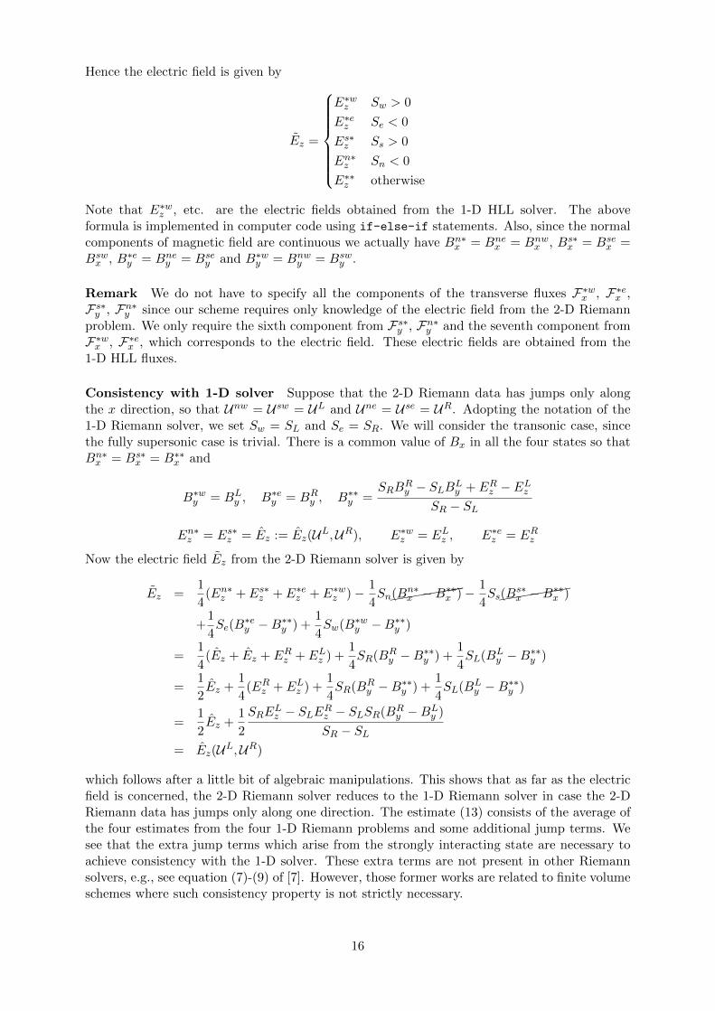
Remark We do not have to specify all the components of the transverse fluxes F∗wx , F∗ex ,Fs∗y , Fn∗y since our scheme requires only knowledge of the electric field from the 2-D Riemannproblem. We only require the sixth component from Fs∗y , Fn∗y and the seventh component fromF∗wx , F∗ex , which corresponds to the electric field. These electric fields are obtained from the1-D HLL fluxes.

Consistency with 1-D solver Suppose that the 2-D Riemann data has jumps only alongthe x direction, so that Unw = Usw = UL and Une = Use = UR. Adopting the notation of the1-D Riemann solver, we set Sw = SL and Se = SR. We will consider the transonic case, sincethe fully supersonic case is trivial. There is a common value of Bx in all the four states so thatBn∗x = Bs∗

x = B∗∗x and

B∗wy = BLy , B∗ey = BR

y , B∗∗y =SRB

Ry − SLBL

y + ERz − ELzSR − SL

En∗z = Es∗z = Ez := Ez(UL,UR), E∗wz = ELz , E∗ez = ERz

Now the electric field Ez from the 2-D Riemann solver is given by

Ez =1

4(En∗z + Es∗z + E∗ez + E∗wz )− 1

4Sn(((((((

(Bn∗x −B∗∗x )− 1

4Ss((((((

(Bs∗x −B∗∗x )

+1

4Se(B

∗ey −B∗∗y ) +

1

4Sw(B∗wy −B∗∗y )

=1

4(Ez + Ez + ERz + ELz ) +

1

4SR(BR

y −B∗∗y ) +1

4SL(BL

y −B∗∗y )

=1

2Ez +

1

4(ERz + ELz ) +

1

4SR(BR

y −B∗∗y ) +1

4SL(BL

y −B∗∗y )

=1

2Ez +

1

2

SRELz − SLERz − SLSR(BR

y −BLy )

SR − SL= Ez(UL,UR)

which follows after a little bit of algebraic manipulations. This shows that as far as the electricfield is concerned, the 2-D Riemann solver reduces to the 1-D Riemann solver in case the 2-DRiemann data has jumps only along one direction. The estimate (13) consists of the average ofthe four estimates from the four 1-D Riemann problems and some additional jump terms. Wesee that the extra jump terms which arise from the strongly interacting state are necessary toachieve consistency with the 1-D solver. These extra terms are not present in other Riemannsolvers, e.g., see equation (7)-(9) of [7]. However, those former works are related to finite volumeschemes where such consistency property is not strictly necessary.

16

6.4 HLLC Riemann solver in 1-D

The HLLC Riemann solver [46] includes a middle contact wave in addition to the slowest andfastest waves and thus contains two intermediate states U∗L,U∗R. In the case of MHD, thereare several variants of the solver [28], [37]. To simplify the notation, we denote the velocitycomponents as (u, v, w) in this section. Following Batten [8], we take the speed of the middlewave from the HLL intermediate state

SM =(ρu)∗

ρ∗=

(SR − uR)ρRuR − (SL − uL)ρLuL − (PR − PL)

(SR − uR)ρR − (SL − uL)ρL

The intermediate states have the form

U∗L =

ρ∗Lρ∗LSMρ∗Lv

∗L

ρ∗Lw∗L

E∗LB∗xB∗yB∗z

, U∗R =

ρ∗Rρ∗RSMρ∗Rv

∗R

ρ∗Rw∗R

E∗RB∗xB∗yB∗z

with the common intermediate value of the magnetic field being equal to the HLL intermediatestate. The intermediate density is obtained from the jump conditions across the left and rightwaves

ρ∗α = ραSα − uαSα − SM

, α = L,R

Li [37] proposes to take the intermediate velocities from the jump conditions across the left andright waves,

v∗α = vα +BαxB

αy −B∗xB∗y

ρα(Sα − uα), w∗α = wα +

BαxB

αz −B∗xB∗z

ρα(Sα − uα), α = L,R

and defines the energy as

E∗α =(Sα − uα)Eα − Pαuα + P ∗SM +Bα

x (vα ·Bα)−B∗x(v∗ ·B∗)Sα − SM

, α = L,R

where P ∗ is the common intermediate total pressure given by

P ∗ = PL + ρL(SL − uL)(SM − uL) = PR + ρR(SR − uR)(SM − uR)

and v∗,B∗ are the values from the HLL intermediate state. Once the two intermediate statesare determined, the numerical flux is given by

Fx =

FLx SL > 0

FRx SR < 0

FLx + SL(U∗L − UL) SL ≤ 0 ≤ SMFRx + SR(U∗R − UR) SM ≤ 0 ≤ SR

The electric field is obtained from the seventh component of the flux

Ez(UL,UR) = −(Fx)7 =

ELz SL > 0

ERz SR < 0

ELz − SL(B∗y −BLy ) SL ≤ 0 ≤ SM

ERz − SR(B∗y −BRy ) SM ≤ 0 ≤ SR

But due to the definition of B∗y from the HLL intermediate state, the two intermediate valuesof the electric field are identical and equal to the HLL estimate of the electric field.

17

6.5 HLLC Riemann solver in 2-D

We will assume the same type of wave modeling in 2-D as we adopted in case of HLL solver,except that there is an intermediate wave in all the four 1-D Riemann problems. We do notendow any more sub-structure in the strongly interacting state. The jump conditions across the2-D Riemann fan given in (12) are still valid since we have a common electric field and magneticfield in the intermediate states of the 1-D Riemann fan. The definition of the electric field atthe vertex thus matches with that obtained from the HLL solver. Consequently, the consistencywith the 1-D Riemann solvers also follows in same way as it was proved for the HLL solver.

7 Limiting procedure

The basic unknowns in our scheme are the normal component of bx, by on the faces, the additionalcell moments α, β stored inside the cells, and the remaining variables U inside the cell. As longas we don’t apply any limiter on bx, by, α, β, our algorithm is guaranteed to preserve the initialdivergence. However, for computing discontinuous solutions, some form of limiter is absolutelynecessary to control spurious numerical oscillations. If any form of limiter is applied which aposteriori modifies these solution variables, then the divergence will not be preserved and somecorrection has to be applied to recover divergence-free property. We now detail the steps in ourlimiting strategy including a divergence-free reconstruction step. The choice of which variableset is limited is an important one for systems of conservation laws, and it is found in manystudies that applying the limiter to characteristic variables as opposed to conserved variables,gives better control on oscillations and leads to more accurate solutions [19]. Hence, our limitingstrategy will be based on limiting the set of characteristic variables.

7.1 TVD-type limiter

Step 1

Using the basic solution variables for the magnetic field, we perform the RT reconstruction toobtain the polynomial B(ξ, η) representation in each cell. We now have the complete solutionin the cell and we proceed to apply a TVD/TVB limiter to this solution polynomial. The basicidea in this process is to check if the linear part of the solution in a cell is smooth relativeto the variation of the cell averages around the cell [17]. Consider the cell indexed by (i, j).Observe that in the expansion (3), (6), the components U10, a10, b10 give a measure of the xderivative and U01, a01, b01 give a measure of the y derivatives. Form the vector of slopes in thetwo directions

Uxi,j =

(U10)i,j(a10)i,j(b10)i,j

, Uyi,j =

(U01)i,j(a01)i,j(b01)i,j

and the differences of the cell averages

Ux−i,j =

(U00)i,j − (U00)i−1,j

(a00)i,j − (a00)i−1,j

(b00)i,j − (b00)i−1,j

, Ux+i,j =

(U00)i+1,j − (U00)i,j(a00)i+1,j − (a00)i,j(b00)i+1,j − (b00)i,j

Uy−i,j =

(U00)i,j − (U00)i,j−1

(a00)i,j − (a00)i,j−1

(b00)i,j − (b00)i,j−1

, Uy+i,j =

(U00)i,j+1 − (U00)i,j(a00)i,j+1 − (a00)i,j(b00)i,j+1 − (b00)i,j

The values a00, a10, a01, b00, b10, b01 are known from the polynomial B(ξ, η). Let Rx,Lx,Ry,Lybe the matrix of right and left eigenvectors based on the cell average state. We now convert theabove slopes to characteristic variables

Wxi,j = LxUxi,j , Wx±

i,j = LxUx±i,j , Wyi,j = LyUyi,j , Wy±

i,j = LyUy±i,j

18

Now apply the minmod limiter on each of the characteristic variables

(Wxi,j)

m = minmod[Wxi,j , βWx−

i,j , βWx+i,j ,M

xi,j∆x

2]

(Wyi,j)

m = minmod[Wyi,j , βW

y−i,j , βW

y+i,j ,M

yi,j∆y

2]

where the minmod function is defined as

minmod[a, b, c, δ] =

a |a| < δ

smin(|a|, |b|, |c|) s = sign a = sign b = sign c

0 otherwise

If (Wxi,j)

m = (Wxi,j) and (Wy

i,j)m = (Wy

i,j) then we do not change the solution in this cell.Otherwise, convert them back to conserved variables by multiplying with the matrices Rx, Ry

(Uxi,j)m = Rx(Wxi,j)

m, (Uyi,j)m = Ry(Wyi,j)

m

and reset the first order components of U to the limited values, i.e., U10 = (Uxi,j)m and U01 =(Uyi,j)m, while setting all higher modes to zero. Similarly, we also reset the modes a10, a01, b01, b10

of the magnetic field and kill the higher modes of B(ξ, η) if the limiter is active in the currentcell. The magnetic field at this stage will not be divergence-free and we will correct this in alater step.

Step 2

We now loop over the all the faces in the mesh and apply a limiter to the solution polynomials(bx, by) which reside on the faces by making use of the cell solution B that has already beenlimited in the previous step. Consider a vertical face on which we have the polynomial bx(η) =∑k

j=0 ajφj(η). We also have the limited solution polynomials B(ξ, η) in the two adjacent cells

of this face and we can evaluate them on the face. From the left cell we obtain1

BLx (1

2 , η) =k+1∑i=0

k∑j=0

aLijφi(12)φj(η) =

k∑j=0

aLj φj(η), aLj =k+1∑i=0

aLijφi(12)

and similarly from the right cell we obtain

BRx (−1

2 , η) =k+1∑i=0

k∑j=0

aRijφi(−12)φj(η) =

k∑j=0

aRj φj(η), aRj =k+1∑i=0

aRijφi(−12)

We now compare the three solutions at the face via a minmod function to decide on the smooth-ness and modify the solution on the face as follows

aj ← minmod(aj , βa

Lj , βa

Rj

), j = 1, . . . , k

where β ∈ [1, 2] can be chosen to be greater than unity in order to allow larger slope similar tothe MC limiter. Note that we do not modify the mean value on the face which corresponds toa0 and this is important to perform divergence-free reconstruction in the next step. A similarprocedure is applied to limit the face solution polynomials by(ξ) located on the horizontal facesin the mesh.

1Here the indices i, j denote the solution modes and not the cell indices.

19

Step 3

The final step will restore the divergence-free condition on the magnetic field in those cells wherethe limiter has been active. This involves using the limited facial solution polynomials b±x (η),b±y (ξ) to reconstruct a divergence-free vector field B(ξ, η) inside the cell. This is achieved bydetermining the cell moments αij , βij in a divergence-free manner, after which the RT recon-struction can be performed. The procedure at different orders is explained in Appendix (B). Atsecond and third order, the reconstruction can be performed using the limited facial solutionalone while at fourth order, we need an additional information from inside the cell, which istaken as the quantity ω = b01 − a10 and approximates the curl of B. Note that the quantitiesa10, b01 are available to us after the cell solution B(ξ, η) has been limited in Step 1 and wealready have a limited estimate of the quantity ω.

7.2 Positivity limiter

The density and pressure have to remain positive since otherwise the problem is ill-posed andthe computations would break down. High order positivity preserving schemes are usually builton the basis of a first order positive scheme. In a DG scheme, the solution is discontinuousand can be scaled in each cell to make it positive [52], [53]. However, a constraint preservingDG scheme like the one proposed in this work and also the scheme in [24], do not have a fullydiscontinuous solution since the normal component of B has to be continuous. Hence the localscaling limiter idea cannot be applied since scaling the B field in one cell changes the field inthe neighbouring cells. The staggered storage of magnetic field variables also complicates theconstruction and analysis of positive schemes. Moreover, to the best of our knowledge, thereis no first order, provably positive, divergence-free scheme based on Godunov-type approachavailable in the literature. However, if we do not demand strictly divergence-free solutions, thenprovably positive schemes can be developed as in [16], which uses a standard DG approach, andas in [51] where locally divergence-free basis is used for B which is fully discontinuous acrossthe cell faces and hence can be scaled in a local manner to achieve positivity.

Since there is no rigorous theory of positivity preservation in the framework of constraintpreserving, high order DG schemes applied to the MHD system at present, we take a heuris-tic approach to ensure positivity property whose success can only be judged from numericalexperiments. The approach we take here is to ensure that the solution is positive at all thequadrature points where the solution is used to compute the quadratures and fluxes involved inthe DG scheme. The set of points S includes the (k + 1)2 GL quadrature points inside the cell,the 4(k + 1) GL quadrature points on the faces and the four corner points. The positivity isachieved by scaling the solution in each cell by following the ideas in [53], [16]. We apply thisscaling to the hydrodynamic variables stored in U and the RT polynomial B. These polyno-mials are used to compute all the cell and face integrals in the DG scheme. However, we donot scale the basic degrees of freedom of the magnetic field which are bx, by, α, β, which allowsus to maintain the divergence-free property of the magnetic field. The scaling limiter relies onthe fact that the average values on the cells and faces are already positive. In some difficultproblems like a strong blast wave with low plasma beta (i.e., where thermodynamic pressure pis much smaller than the magnetic pressure 1

2 |B|2), see Section (8.9), the average pressure mayalso be negative in a few cells, in which case we have to set the pressure to a small positivevalue. While this is not an ideal solution to this problem, it does allow us to maintain stabilityof the computations as shown in the results section. The positivity limiter is applied after theTVB limiter and so the B field has already been limited and is not so badly behaved.

8 Numerical results

We have explained the semi-discrete version of the DG scheme in the previous sections whichleads to a system of coupled ODE. Starting from the specified initial condition, these ODE are

20

integrated forward in time using Runge-Kutta schemes. For k = 1 and k = 2, we use the secondand third order strong stability preserving RK schemes [43], respectively, while for k = 3 we usethe 5-stage, fourth order SSPRK scheme [33], [44]. The time step is computed as

∆t =CFL

max( |vx|+cfx

∆x +|vy |+cfy

∆y

)where the wave speeds are based on cell average values and the maximum is taken over allthe cells in the grid. We also use a shock indicator as explained in [23] in most of these testcases and the limiter is applied only in those cells which are marked by the indicator. Unlessstated otherwise, in all the test cases we use CFL = 0.95/(2k + 1), where k is the degree of theapproximating polynomials. The initial condition of the magnetic field variables must be setcarefully to ensure that it is divergence-free [14], and this is explained in Appendix (C). A highlevel view of the algorithm in given in Algorithm (1).

Algorithm 1: Constraint preserving scheme for ideal compressible MHD

Allocate memory for all variables;Set initial condition for U , bx, by, α, β;Loop over cells and reconstruct Bx, By;Set time counter t = 0;while t < T do

Copy current solution into old solution;Compute time step ∆t;for each RK stage do

Loop over vertices and compute vertex flux;Loop over faces and compute all face integrals;Loop over cells and compute all cell integrals;Update solution to next stage;Loop over cells and do RT reconstruction (bx, by, α, β)→ B;Loop over cells and apply limiter on U ,B;Loop over faces and limit solution bx, by;Loop over cells and perform divergence-free reconstruction;Apply positivity limiter;

endt = t+ ∆t;

end

8.1 Alfven wave

This test case involves the propagation of circularly polarized wave over the rectangular domain[0, 1/ cosα] × [0, 1/ sinα] and it is used to test accuracy and convergence of numerical algo-rithms [47]. The parameter α is the angle of wave propagation relative to x−axis and it is takento be π/6. The initial condition is given by

ρ = 1, v = v⊥(− sinα, cosα, 0), p = 0.1

Bx = B‖ cosα−B⊥ sinα, By = B‖ sinα+B⊥ cosα, Bz = vz

whereB‖ = 1, B⊥ = v⊥ = 0.1 sin(2π(x cosα+ y sinα))

We have taken periodic boundary conditions in both directions. The numerical solution iscomputed up to time T = 1 with γ = 5/3. In Figure 6, we have compared the error and

21

1023× 101 4× 101 6× 101 2× 102

Grid size

10−11

10−10

10−9

10−8

10−7

10−6

10−5

10−4

L1

erro

rn

orm

inρ

k=1

k=2

k=3

1023× 101 4× 101 6× 101 2× 102

Grid size

10−12

10−11

10−10

10−9

10−8

10−7

10−6

10−5

10−4

L1

erro

rn

orm

inρv x

k=1

k=2

k=3

1023× 101 4× 101 6× 101 2× 102

Grid size

10−12

10−11

10−10

10−9

10−8

10−7

10−6

10−5

10−4

L1

erro

rn

orm

inBx

k=1

k=2

k=3

Figure 6: Comparison of convergence results obtained from HLLC flux for the smooth Alfvenwave problem using degree k = 1, 2, 3. The dashed line shows second, third and fourth orderrates.

convergence rates obtained using HLLC flux for k = 1, 2, 3. In case of all proposed schemesthe optimal rates of 2, 3 and 4 have been achieved for all the variables, i.e., with degree kpolynomials, the error is O(hk+1). We have observed similar results with HLL and LxF fluxes(not shown here).

8.2 Smooth magnetic vortex

This test case involves the propagation of a smooth, constant density vortex along an obliquedirection to the computational mesh and it is truly multidimensional in nature [2]. The prob-lem is initialized over the computational domain [−10, 10] × [−10, 10], with periodic boundaryconditions in both directions. The initial unperturbed primitive variables are given by

ρ = 1, p = 1, v = (1, 1, 0), B = (0, 0, 0)

and γ = 5/3. A vortex is initialized at the origin by adding the fluctuations in velocity andmagnetic field which are given by

δvx = − κ

2πy exp(0.5(1− r2)), δvy =

κ

2πx exp(0.5(1− r2)), δvz = 0

δBx = − µ

2πy exp(0.5(1− r2)), δBy =

µ

2πx exp(0.5(1− r2)), δBz = 0

and the perturbation in pressure is given by

δp =

[1

8π

( µ2π

)2(1− r2)− 1

2

( κ2π

)2]

exp(1− r2)

We have set the parameters κ = 1 and µ = 1 in the initial condition. The smooth vortex returnsto its initial position after some fixed time-period and facilitates us to measure the accuracy andconvergence of the numerical algorithms. The numerical simulations are performed up to timeT = 20 using CFL=0.95. The convergence of the error for some of the variables with respectto grid refinement and for HLLC flux are shown in Figure 7, which indicates that the optimalrates of 2, 3 and 4 have been achieved for k = 1, 2, 3, respectively.

To study the usefulness of using high order methods, we compute the vortex problem ondifferent meshes and polynomial degree so that the total number of degrees of freedom areroughly matched. The error norm as a function of the number of degrees of freedom are shownin Figure 8. We observe that to obtain same error level, a low order method (small degree k)requires more degrees of freedom than a high order method (large degree k).

8.3 Brio-Wu shock tube

This is a classical shock tube problem for MHD [13] and solution of this problem contains thefast rarefaction wave, the intermediate shock followed by a slow rarefaction wave, the contact

22

1026× 101 2× 102 3× 102 4× 102

Grid size

10−11

10−10

10−9

10−8

10−7

10−6

10−5

10−4

L1

erro

rn

orm

inρv x

k=1

k=2

k=3

1026× 101 2× 102 3× 102 4× 102

Grid size

10−10

10−9

10−8

10−7

10−6

10−5

10−4

10−3

L1

erro

rn

orm

inE

k=1

k=2

k=3

1026× 101 2× 102 3× 102 4× 102

Grid size

10−11

10−10

10−9

10−8

10−7

10−6

10−5

10−4

L1

erro

rn

orm

inBx

k=1

k=2

k=3

Figure 7: Comparison of convergence results obtained from HLLC flux for the smooth vortexproblem using degree k = 1, 2, 3. The dashed line shows second, third and fourth order rates.

104 105

Number of degree of freedom

10−8

10−7

10−6

10−5

10−4

10−3

L1

erro

rn

orm

inBx

k=1

k=2

k=3

104 105

Number of degree of freedom

10−8

10−7

10−6

10−5

10−4

10−3

L1

erro

rn

orm

inρv x

k=1

k=2

k=3

(a) (b)

Figure 8: Comparison of convergence results obtained from HLLC flux for the smooth vortexproblem using degree for different degree as a function of number of degrees of freedom.

23

discontinuity, a slow shock, and a fast rarefaction wave. The initial condition has a discontinuity;for x < 0, the state is given by

ρ = 1, p = 1, v = (0, 0, 0), B = (0.75, 1, 0)

and for x > 0, it is given by

ρ = 0.125, p = 0.1, v = (0, 0, 0), B = (0.75,−1, 0)

which corresponds to Sod test case for hydrodynamics. The value of γ is taken to be 5/3. Wehave computed the numerical solution for degree k = 1, 2, 3 and LxF, HLL, HLLC fluxes at timeT = 0.2 using 800 cells. In Figure 9, we have compared the numerical solutions obtained usingdifferent fluxes with the reference solution computed using Athena code2 with 10000 cells. Thenumerical results show that all the waves have been captured crisply and with very little or nooscillations. In Figure 10, we show zoomed view of the density plot around the compound wave,contact and shock waves, where we also compare with the results from Athena code using 800cells. We can observe that the present method yields very good results. The resolution of theshock wave is quite good from all the solvers and the HLLC solver yields the best resolution,especially of the contact wave since only this solver explicitly includes the contact wave in itsconstruction. In Figure 11, we perform computations at different degree and meshes so thatthe total number of degrees of freedom is similar in each case. We compare also with the finitevolume results from Athena at the same resolution. While the degree k = 1 results compare wellwith Athena, the higher order results are slightly diffused in the contact region due to use ofcoarser mesh and a TVD-type limiter. A more sophisticated limiter with good sub-cell resolutionis required to achieve accurate results with high order schemes in the presence of discontinuities.

8.4 Consistency of 2-D Riemann solver

We take the Brio-Wu Riemann data to create a 2-D Riemann problem with Usw = Unw = ULand Use = Une = UR. The estimate of Ez from both the 1-D and 2-D HLL Riemann solvers issame and equal to −2.5400697250351683 whereas if we use only the first term in (13), we geta value of −1.2700348625175841, which has a very different magnitude. We run the Brio-Wucomputation using both the consistent and inconsistent versions of the 2-D HLL Riemann solveron a 2-D domain [−1, 1] × [−1, 1] with a mesh of 100 × 100 cells. The resulting magnetic fieldcomponent Bx is shown in Figure 12. We see that the consistent solver keeps the constancy ofBx whereas the inconsistent version is not able to do so.

8.5 Rotated shock tube

The initial condition is a Riemann problem which is aligned at an angle to the mesh [47]. Wetake the domain to be [−1,+1] × [−1,+1] with Neumann boundary conditions, and the initialdiscontinuity is across the line x + y = 0. Throughout the domain, the density ρ = 1 and themagnetic field is

Bx = B⊥ cosα−B‖ sinα, By = B⊥ sinα+B‖ cosα, Bz = 0

In the region x+ y < 0, the remaining quantities are given by

p = 20, v = 10(cosα, sinα, 0)

and for x+ y > 0p = 1, v = −10(cosα, sinα, 0)

2Code taken from https://github.com/PrincetonUniversity/athena-public-version at git version273e451e16d3a5af594dd0a

24

−0.4 −0.2 0.0 0.2 0.4 0.6 0.8x

0.2

0.4

0.6

0.8

1.0

ρ

Ref

LxF

HLL

HLLC

−0.4 −0.2 0.0 0.2 0.4 0.6 0.8x

−1.00

−0.75

−0.50

−0.25

0.00

0.25

0.50

0.75

1.00

By

Ref

LxF

HLL

HLLC

−0.4 −0.2 0.0 0.2 0.4 0.6 0.8x

0.2

0.4

0.6

0.8

1.0

ρ

Ref

LxF

HLL

HLLC

−0.4 −0.2 0.0 0.2 0.4 0.6 0.8x

−1.00

−0.75

−0.50

−0.25

0.00

0.25

0.50

0.75

1.00By

Ref

LxF

HLL

HLLC

−0.4 −0.2 0.0 0.2 0.4 0.6 0.8x

0.2

0.4

0.6

0.8

1.0

ρ

Ref

LxF

HLL

HLLC

−0.4 −0.2 0.0 0.2 0.4 0.6 0.8x

−1.00

−0.75

−0.50

−0.25

0.00

0.25

0.50

0.75

1.00

By

Ref

LxF

HLL

HLLC

Figure 9: Brio-Wu test case with 800 cells. Comparison of ρ and By obtained with differentfluxes. Top row: k = 1, middle row: k = 2, bottom row: k = 3

25

−0.15 −0.10 −0.05 0.00 0.05 0.10x

0.625

0.650

0.675

0.700

0.725

0.750

0.775

0.800

ρ

Ref

LxF

HLL

HLLC

Athena

0.10 0.11 0.12 0.13 0.14 0.15x

0.30

0.35

0.40

0.45

0.50

0.55

0.60

0.65

ρ

Ref

LxF

HLL

HLLC

Athena

0.250 0.255 0.260 0.265 0.270 0.275 0.280x

0.12

0.14

0.16

0.18

0.20

0.22

0.24

0.26

0.28

ρ

Ref

LxF

HLL

HLLC

Athena

(a) (b) (c)

Figure 10: Brio-Wu test case with 800 cells and degree k = 1. Comparison of ρ obtainedwith different fluxes and Athena code (a) around compound wave, (b) around contact wave, (c)around shock region.

−0.15 −0.10 −0.05 0.00 0.05 0.10x

0.625

0.650

0.675

0.700

0.725

0.750

0.775

0.800

ρ

Ref

k = 1

k = 2

k = 3

Athena

0.10 0.11 0.12 0.13 0.14 0.15x

0.30

0.35

0.40

0.45

0.50

0.55

0.60

0.65

ρ

Ref

k = 1

k = 2

k = 3

Athena

0.250 0.255 0.260 0.265 0.270 0.275 0.280x

0.12

0.14

0.16

0.18

0.20

0.22

0.24

0.26

0.28

ρ

Ref

k = 1

k = 2

k = 3

Athena

(a) (b) (c)

Figure 11: Brio-Wu test case with same number of degrees of freedom and HLLC flux. Athena(1600 cells), k = 1, 800 cells, k = 2, 534 cells, k = 3, 400 cells. Comparison of ρ (a) aroundcompound wave, (b) around contact wave, (c) around shock region.

26

(a) (b)

Figure 12: Brio-Wu test case with HLL flux and 100 × 100 mesh. Color plot of Bx using(a) consistent 2-D Riemann solver, (b) inconsistent 2-D Riemann solver.

where α = π/4 is the orientation of the initial discontinuity. Note that this represents a onedimensional Riemann problem when viewed along the line x = y. The solution is computed upto the time T = 0.08/ cosα and we plot the solution along the line x = y. At this final time,the solution along this line is not affected by the flow features that develop due to boundaryconditions. The exact solution should have B‖ = −Bx sinα + By cosα = 5/

√4π and B⊥ =

Bx cosα+By sinα = 5/√

4π along the line x = y. The constancy of B⊥ is difficult to obtain innumerical schemes which do not satisfy the divergence-free constraint. Numerical solutions arecomputed over a grid of size 128×128 using LxF, HLL, and HLLC fluxes. In Figure 13, we havecompared the relative percentage error on the magnetic field B‖ for the considered fluxes andk = 1, 2, 3. Though we cannot clearly classify which flux is best, the LxF and HLL fluxes yieldthe smallest and very similar levels of error, while the errors for HLLC are highest. However,even the largest observed error is similar to what is observed with other standard constraintpreserving schemes [47]. The large errors are observed only at the location of the discontinuityand the error is small in other regions, which is a benefit obtained due to the divergence-freemethods.

8.6 Orszag-Tang vortex

This test case is first proposed in [39] and used as a benchmark test case for many numericalalgorithms for MHD. We initialize the problem with smooth initial data which later leads to theformation of more complex flow having many discontinuities as the non-linear system evolvesforward in time. If the divergence error is not controlled sufficiently during simulations thennumerical schemes may show instability [34], [36]. Even higher order local divergence free DGschemes also shows instability with time [34]. The initial condition is given by

ρ =25

36π, p =

5

12π, v = (− sin(2πy), sin(2πx), 0)

B =1√4π

(− sin(2πy), sin(4πx), 0)

We have performed the numerical computations over the domain [0, 1] × [0, 1] with periodicboundary conditions on all sides. The numerical solutions are computed up to the time T = 0.5.In Figure 14, we have compared the LxF, HLL, and HLLC flux for density variable and k = 1, 2, 3

27

k=

1

−1.00 −0.75 −0.50 −0.25 0.00 0.25 0.50 0.75 1.00x

−0.04

−0.03

−0.02

−0.01

0.00

0.01

0.02

0.03

%er

ror

inB||

−1.00 −0.75 −0.50 −0.25 0.00 0.25 0.50 0.75 1.00x

−0.05

−0.04

−0.03

−0.02

−0.01

0.00

0.01

%er

ror

inB||

−1.00 −0.75 −0.50 −0.25 0.00 0.25 0.50 0.75 1.00x

−1

0

1

2

3

%er

ror

inB||

k=

2

−1.00 −0.75 −0.50 −0.25 0.00 0.25 0.50 0.75 1.00x

0.00

0.05

0.10

0.15

0.20

0.25

0.30

%er

ror

inB||

−1.00 −0.75 −0.50 −0.25 0.00 0.25 0.50 0.75 1.00x

−0.04

−0.02

0.00

0.02

0.04

0.06

%er

ror

inB||

−1.00 −0.75 −0.50 −0.25 0.00 0.25 0.50 0.75 1.00x

−1.5

−1.0

−0.5

0.0

0.5

1.0

%er

ror

inB||

k=

3

−1.00 −0.75 −0.50 −0.25 0.00 0.25 0.50 0.75 1.00x

−0.6

−0.4

−0.2

0.0

0.2

0.4

%er

ror

inB||

−1.00 −0.75 −0.50 −0.25 0.00 0.25 0.50 0.75 1.00x

−0.4

−0.3

−0.2

−0.1

0.0

0.1

%er

ror

inB||

−1.00 −0.75 −0.50 −0.25 0.00 0.25 0.50 0.75 1.00x

−2

−1

0

1

2

3

4

%er

ror

inB||

LxF HLL HLLC

Figure 13: Comparison of the percentage error on the parallel magnetic field B‖ for rotatedshock tube test over a grid of size 128×128 using LxF, HLL, and HLLC fluxes. First row degreek = 1, second row degree k = 2, and third row degree k = 3.

28

over a mesh of size 128×128. We can observe from the Figure 14 that HLLC flux resolves featuresmore sharply in comparison to HLL and LxF flux, e.g., in the central part of the domain. Thesolution on a finer mesh of 512 × 512 cells is shown in Figure 15 and we observe that all thefeatures are now resolved more sharply. To study the effectiveness of high order methods, we alsoperform computations on different resolutions by matching the number of degrees of freedom asshown in Figure 16. As the degree is increased from 1 to 3, the mesh size is reduced so that allthree cases have approximately the same number of degrees of freedom. We can see from thefigures that the case k = 3 which has a smaller mesh size is still able to capture the solutionfeatures. In Figure 17, we show results of long time simulation upto time t = 5 units. Thesolution becomes turbulent at long times but the computations remain stable. We also monitorthe divergence norm as a function of time, as shown in Figure 18. Theoretically, the numericalscheme must preserve the divergence at all times. In practice, due to round off errors, we seethat it is not exactly preserved and is not exactly zero, but the values remain small and do notincrease with time.

8.7 Rotor test

This test case was first proposed in [7], but we use the version given in [47]. This problemdescribes the spinning of a dense rotating disc of fluid in the center while ambient fluid are atrest. The magnetic field wraps around the rotating dense fluid turned it into an oblate shape.If the numerical scheme is not sufficiently control the divergence-error in the magnetic field,distortion can be observed in Mach number [34]. The computational domain is [0, 1] × [0, 1]with periodic boundary conditions on all sides, and the initial condition is given as follows. Forr < r0,

ρ = 10, v =u0

r0(−(y − 1

2), (x− 12), 0)

and for r0 < r < r1

ρ = 1 + 9f, v =fu0

r(−(y − 1

2), (x− 12), 0), f =

r1 − rr1 − r0

and for r > r1

ρ = 1, v = (0, 0, 0)

with r0 = 0.1, r1 = 0.115 and u0 = 2. The rest of the quantities are constant and given by

p = 1, B =1√4π

(5, 0, 0)

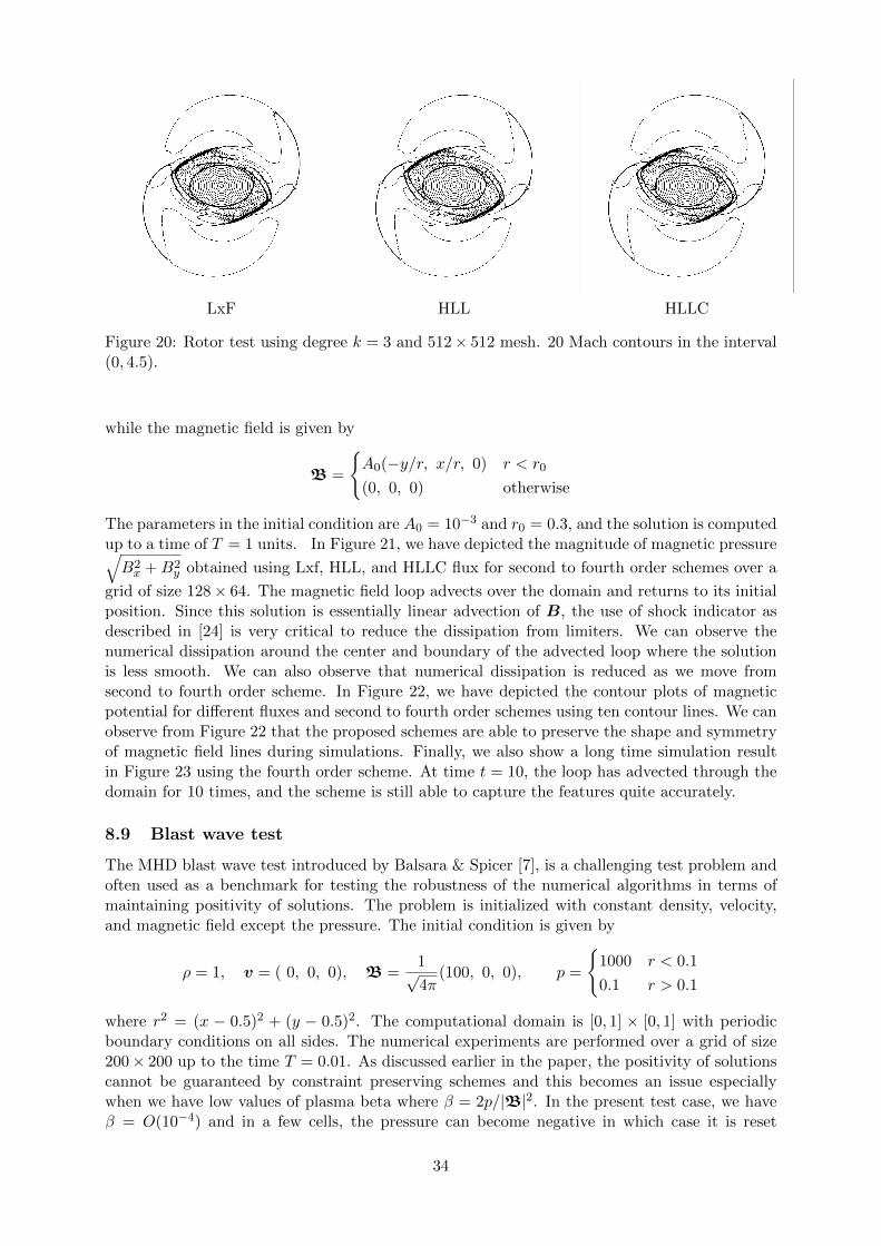
We set γ = 1.4 and domain is discretized with 512× 512 mesh points. The numerical solutionsare computed using LxF, HLL, HLLC flux up to the time T = 0.15 units. In Figure 19, we haveshown the Mach number for considered fluxes and degree 1 to 3 over a mesh of size 128× 128.We can observe from the figures that in all cases, circularly rotating velocity field in the centralpart is captured well and the solutions remain stable. The results on a finer mesh of 512× 512cells is shown in Figure 20, and we can observe that all the solution features are now resolvedvery sharply.

8.8 Magnetic field loop test

This test case [25] involves the advection of magnetic field loop over a periodic domain. Thenumerical simulations are performed over the computational domain [−1,+1]×[−0.5,+0.5] withperiodic boundary conditions in both directions. The initial density, pressure and velocity areuniform in the domain and given by

ρ = 1, p = 1, v = (2, 1, 0)

29

LxF HLL HLLC

Figure 14: Orszag-Tang test using LxF, HLL, HLLC fluxes on 128 × 128 mesh. 30 densitycontours in (0.08, 0.5). Top row: k = 1, middle row: k = 2, bottom row: k = 3

30

LxF HLL HLLC

Figure 15: Orszag-Tang test using LxF, HLL, HLLC fluxes on 512×512 mesh and degree k = 3.30 density contours in the interval (0.08, 0.5).

(a) (b) (c)

Figure 16: Orszag-Tang test using HLL flux at time 0.5 units. (a) k = 1, 512 × 512 cells, (b)k = 2, 342× 342 cells, (c) k = 3, 256× 256 cells. 30 density contours in the interval (0.08, 0.5).The degree and mesh size are chosen so that all three cases have nearly the same number ofdegrees of freedom.

31

t = 0.5 t = 1 t = 2

t = 3 t = 4 t = 5

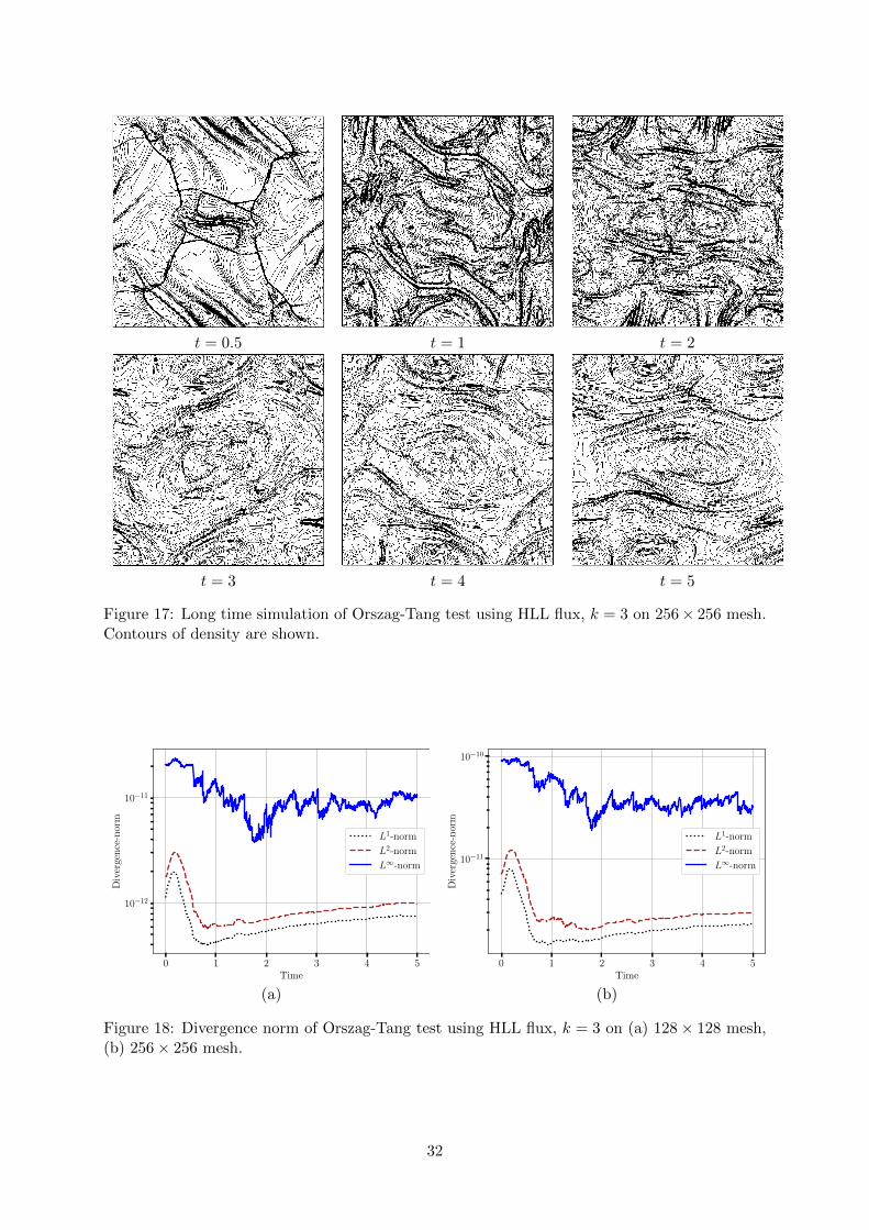
Figure 17: Long time simulation of Orszag-Tang test using HLL flux, k = 3 on 256× 256 mesh.Contours of density are shown.

0 1 2 3 4 5Time

10−12

10−11

Div

erge

nce

-nor

m

L1-norm

L2-norm

L∞-norm

0 1 2 3 4 5Time

10−11

10−10

Div

erge

nce

-nor

m

L1-norm

L2-norm

L∞-norm

(a) (b)

Figure 18: Divergence norm of Orszag-Tang test using HLL flux, k = 3 on (a) 128× 128 mesh,(b) 256× 256 mesh.

32

LxF HLL HLLC

Figure 19: Rotor test using degree k = 1 (top row), degree k = 2 (middle row) and degree k = 3(bottom row) over 128× 128 mesh. 20 Mach contours in (0, 4.5).

33

LxF HLL HLLC

Figure 20: Rotor test using degree k = 3 and 512× 512 mesh. 20 Mach contours in the interval(0, 4.5).

while the magnetic field is given by

B =

A0(−y/r, x/r, 0) r < r0

(0, 0, 0) otherwise

The parameters in the initial condition are A0 = 10−3 and r0 = 0.3, and the solution is computedup to a time of T = 1 units. In Figure 21, we have depicted the magnitude of magnetic pressure√B2x +B2

y obtained using Lxf, HLL, and HLLC flux for second to fourth order schemes over a

grid of size 128× 64. The magnetic field loop advects over the domain and returns to its initialposition. Since this solution is essentially linear advection of B, the use of shock indicator asdescribed in [24] is very critical to reduce the dissipation from limiters. We can observe thenumerical dissipation around the center and boundary of the advected loop where the solutionis less smooth. We can also observe that numerical dissipation is reduced as we move fromsecond to fourth order scheme. In Figure 22, we have depicted the contour plots of magneticpotential for different fluxes and second to fourth order schemes using ten contour lines. We canobserve from Figure 22 that the proposed schemes are able to preserve the shape and symmetryof magnetic field lines during simulations. Finally, we also show a long time simulation resultin Figure 23 using the fourth order scheme. At time t = 10, the loop has advected through thedomain for 10 times, and the scheme is still able to capture the features quite accurately.

8.9 Blast wave test

The MHD blast wave test introduced by Balsara & Spicer [7], is a challenging test problem andoften used as a benchmark for testing the robustness of the numerical algorithms in terms ofmaintaining positivity of solutions. The problem is initialized with constant density, velocity,and magnetic field except the pressure. The initial condition is given by

ρ = 1, v = ( 0, 0, 0), B =1√4π

(100, 0, 0), p =

1000 r < 0.1

0.1 r > 0.1

where r2 = (x − 0.5)2 + (y − 0.5)2. The computational domain is [0, 1] × [0, 1] with periodicboundary conditions on all sides. The numerical experiments are performed over a grid of size200× 200 up to the time T = 0.01. As discussed earlier in the paper, the positivity of solutionscannot be guaranteed by constraint preserving schemes and this becomes an issue especiallywhen we have low values of plasma beta where β = 2p/|B|2. In the present test case, we haveβ = O(10−4) and in a few cells, the pressure can become negative in which case it is reset

34

k = 1 k = 2 k = 3

Figure 21: Contour plots of√B2x +B2

y for loop advection test using 128 × 64 mesh at time

t = 1; 10 contours are shown in the range (0, 0.00109). Top row: LxF flux, middle row: HLLflux, bottom row: HLLC flux.

k = 1 k = 2 k = 3

Figure 22: Contour plots of magnetic potential for loop advection test using 128 × 64 mesh attime t = 1; 10 contours. First row LxF flux, second row HLL flux, third row HLLC flux.

35

(a) t = 1 (b) t = 10

Figure 23: Contour plots of√B2x +B2

y for loop advection test at time t = 1 and t = 10 using

128× 64 mesh, degree k = 3 and HLL flux.

to a small value. This happens in at most one or two cells, also infrequently during the timeiterations. In Figures 24, we have shown numerical solution for degree k = 1 for squared velocity,pressure and magnetic pressure. The results at higher degree are not shown as they look similarto the case of k = 1.

9 Summary and conclusions

The paper develops an arbitrary order discontinuous Galerkin method for the compressible idealMHD equations which naturally preserves the divergence-free condition on the magnetic field.This is known to be an important structural property of the solutions whose satisfaction is di-rectly related to the accuracy and robustness of the method. The magnetic field is approximatedin terms of Raviart-Thomas polynomials which automatically ensures that the normal compo-nent of the magnetic field is continuous across the cell faces. The DG scheme evolves the degreesof freedom using a combination of face-based and cell-based DG schemes which automaticallypreserves the divergence of the magnetic field. Being a DG method, it requires numerical fluxeswhich are supplied via an approximate Riemann solver. We have proposed simple HLL-typemulti-dimensional Riemann solvers which are consistent with their 1-D counterparts. Since wedeal with non-linear flows, the solutions can develop discontinuities which requires some formof non-linear limiter but this can destroy the condition on the divergence. We can recover thedivergence-free property by performing a local divergence-free reconstruction which makes useof information on the divergence and curl of the magnetic field. Many numerical tests presentedhere show the accuracy and robustness of the method. The positivity property of the scheme ishowever not possible to prove at present within the framework of divergence-free DG schemes,but we show that a heuristic application of scaling limiter can yield stable computations.

Acknowledgments

Praveen Chandrashekar would like to acknowledge support from SERB-DST, India, under theMATRICS grant (MTR/2018/000006) and Department of Atomic Energy, Government of India,under project no. 12-R&D-TFR-5.01-0520. Rakesh Kumar would like to acknowledge fundingsupport from the National Post-doctoral Fellowship (PDF/2018/002621) administered by SERB-DST, India.

36

(a) v2x + v2

y (LxF) (b) v2x + v2

y (HLL) (c) v2x + v2

y (HLLC)

(d) p (LxF) (e) p (HLL) (f) p (HLLC)

(g) 12(B2

x +B2y) (LxF) (h) 1

2(B2x +B2

y) (HLL) (i) 12(B2

x +B2y) (HLLC)

Figure 24: Blast test case using LxF, HLL and HLLC flux for degree k = 1 on 200 × 200mesh with 40 contours. Top row: velocity square, middle row: pressure, bottom row: magneticpressure

37

A Eigenvectors of the MHD system

This section lists the right and left eigenvectors of the flux Jacobian in the x direction whichare taken from [32], [13]. The eigenvector formulae correspond to the following ordering of theconserved variables: [ρ, ρvx, ρvy, ρvx, Bx, By, Bz, E ]. Define b = (bx, by, bz) = (Bx, By, Bz)/

√ρ

and b2 = b2x + b2y + b2z. The sound speed, fast and slow speeds are given by

a2 =γp

ρ, c2f,s =

1

2

[a2 + b2 ±

√(a2 + b2)2 − 4a2b2x

]Define

(βy, βz) =

(By ,Bz)√B2

y+B2z

If B2y +B2

z 6= 0,(1√2, 1√

2

)otherwise

(αf , αs) =

(√a2−c2s,

√c2f−a2)√

c2f−c2sIf B2

y +B2z 6= 0 or γp 6= B2

x,(1√2, 1√

2

)otherwise,

Γf = αfcfvx − αscssgn(Bx)(βyvy + βzvz),

Γa = sgn(Bx)(βzvy − βyvz),Γs = αscsvx + αfcf sgn(Bx)(βyvy + βzvz).

The right eigenvectors are given by

r1 =

αfαf (vx − cf )

αfvy + αscsβysgn(Bx)αfvz + αscsβzsgn(Bx)

0aαsβy√

ρaαsβz√

ρ

αf (v2

2 + c2f − γ2a

2)− Γf

, r2 =

00

−βzsgn(Bx)βysgn(Bx)

0

− βz√ρ

βy√ρ

−Γa

, r3 =

αsαs(vx − cs)

αsvy − αfcfβysgn(Bx)αsvz − αfcfβzsgn(Bx)

0

−aαfβy√ρ

−aαfβz√ρ

αs(v2

2 + c2s − γ2a

2)− Γs

r4 =

1vxvyvz000v2

2

, r5 =

0000100Bx

, r6 =

αsαs(vx + cs)

αsvy + αfcfβysgn(Bx)αsvz + αfcfβzsgn(Bx)

0

−aαfβy√ρ

−aαfβz√ρ

αs(v2

2 + c2s − γ2a

2) + Γs

r7 =

00

−βzsgn(Bx)βysgn(Bx)

0βz√ρ

− βy√ρ

−Γa

, r8 =

αfαf (vx + cf )

αfvy − αscsβysgn(Bx)αfvz − αscsβzsgn(Bx)

0aαsβy√

ρaαsβz√

ρ

αf (v2

2 + c2f − γ2a

2) + Γf

38

The left eigenvectors are given by

l1 =1

2a2

γ1αfv2 + Γf , (1− γ)αfvx − αfcf , (1− γ)αfvy + csαsβysgn(Bx), . . .

(1− γ)αfvz + csαsβzsgn(Bx),−(γ − 1)αfBx, (1− γ)αfBy + aαs√ρβy, . . .

(1− γ)αfBz + aαs√ρβz, (γ − 1)αf

,l2 =

1

2

[Γa, 0, −βzsgn(Bx), βysgn(Bx), 0, −√ρβz, √ρβy, 0

],

l3 =1

2a2

γ1αsv2 + Γs, (1− γ)αsvx − αscs, (1− γ)αsvy − cfαfβysgn(Bx), . . .

(1− γ)αsvz − cfαfβzsgn(Bx), −Bx(γ − 1)αs, (1− γ)αsBy − aαf√ρβy, . . .

(1− γ)αsBz − aαf√ρβz, (γ − 1)αs

,l4 =

[1− 1

2τv2, τvx, τvy, τvz, τBx, τBy, τBz, −τ

],

l5 =[0, 0, 0, 0, 1, 0, 0, 0

],

l6 =1

2a2

γ1αsv2 − Γs, (1− γ)αsvx + αscs, (1− γ)αsvy + cfαfβysgn(Bx), . . .

(1− γ)αsvz + cfαfβzsgn(Bx), −Bx(γ − 1)αs, (1− γ)αsBy − aαf√ρβy, . . .

(1− γ)αsBz − aαf√ρβz, (γ − 1)αs

,l7 =

1

2

[ga, 0, −βzsgn(Bx), βysgn(Bx), 0,

√ρβz, −√ρβy, 0

],

l8 =1

2a2

γ1αfv2 − Γf , (1− γ)αfvx + αfcf , (1− γ)αfvy − csαsβysgn(Bx), . . .

(1− γ)αfvz − csαsβzsgn(Bx),−(γ − 1)αfBx, (1− γ)αfBy + aαs√ρβy, . . .

(1− γ)αfBz + aαs√ρβz, (γ − 1)αf

,B Limiting and divergence-free reconstruction

When the solution on the faces bx, by is limited as explained in Section (7), we lose the divergence-free property of the magnetic field. To recover this property, we have to perform a divergence-freereconstruction step. We explain this reconstruction process for second, third and fourth orderaccuracy. The fifth order version is given in [30] together with more details on the reconstructionidea. The resulting polynomial has the structure of the BDM polynomial on rectangles, see [12],Equation (3.29). Here we explain how the RT polynomial can be modified to recover divergence-free property. In two dimensions, the BDM polynomial has (k+ 1)(k+ 2) + 2 degrees of freedomwhile its divergence has 1

2k(k + 1) coefficients. Up to third order accuracy, the reconstructioncan be performed using only the solution on the faces (bx, by), but at fourth order and higher,we need additional information which is supplied in the form of the curl of the magnetic field.This additional information is available to us via the cell moments α, β.

For example, at fourth order, the BDM polynomial has (3 + 1)(3 + 2) + 2 = 22 degrees offreedom, while the face solution (bx, by), which are polynomials of degree 3, provide (4 + 4 +4 + 4) − 1 = 15 degrees of freedom, where one piece of information is redundant since the facesolution satisfies

∫∂K B · nds = 0 on each cell K. The divergence-free condition on the BDM

polynomial yields 12(3)(3 + 1) = 6 conditions. So we have a total of 15 + 6 = 21 equations but

22 coefficients to be determined. Hence we need to supply one additional piece of informationto completely determine the BDM polynomial.

We have the following inclusions P2k ⊂ BDM(k) ⊂ RT(k) and the RT polynomial has many

more basis functions than the BDM polynomial. In the reconstruction process, we set some ofthe coefficients a, b in the RT polynomial to zero but this does not affect the accuracy sinceonly coefficients aij , bij with i+ j > k are set to zero, and we retain the Pk part of the solution.

39

B.1 Degree k = 1

The divergence of the vector field B ∈ RT(1) is given by

∇ ·B =a10

∆x+b01

∆y+

(2a20

∆x+b11

∆y

)φ1(ξ) +

(a11

∆x+

2b02

∆y

)φ1(η)

+ 2

(a21

∆x+b12

∆y

)φ1(ξ)φ1(η)

The coefficients aij , bij are related to the face solution and cell moments according to Table 1.The constant term is already zero. The linear terms can be made zero by setting

α00 =1

2(a−0 + a+

0 ) +1

12(b+1 − b−1 )

∆x

∆y

β00 =1

2(b−0 + b+0 ) +

1

12(a+

1 − a−1 )∆y

∆x

This will however destroy the conservation property since α00, β00 are cell averages of Bx, Byrespectively. The bilinear term can be made zero by individually setting a21 = b12 = 0 whichyields

α01 =1

2(a−1 + a+

1 ), β10 =1

2(b−1 + b+1 )

By this process we would have modified all the cell moments and the resulting reconstructioncoincides with that of Balsara.

B.2 Degree k = 2

The divergence of the vector field B ∈ RT(2) is given by

∇ ·B =

[1

∆x

(a10 +

a30

10

)+

1

∆y

(b01 +

b03

10

)]+

[2

∆xa20 +

1

∆y

(b11 +

b13

10

)]φ1(ξ)

+

[1

∆x

(a11 +

a31

10

)+

2

∆yb02

]φ1(η) +

[3

∆xa30 +

1

∆y

(b21 +

b23

10

)]φ2(ξ)

+ 2

[a21

∆x+b12

∆y

]φ1(ξ)φ1(η) +

[1

∆x

(a12 +

a32

10

)+

3

∆yb03

]φ2(η)

+

[2

∆xa22 +

3

∆yb13

]φ1(ξ)φ2(η) +

[3

∆xa31 +

2

∆yb22

]φ2(ξ)φ1(η)

+ 3

[a32

∆x+b23

∆y

]φ2(ξ)φ2(η)

The constant term is already zero. The linear terms can be made zero by setting

α00 =1

2(a−0 + a+

0 ) +1

12(b+1 − b−1 )

∆x

∆y, β00 =

1

2(b−0 + b+0 ) +

1

12(a+

1 − a−1 )∆y

∆x

The quadratic terms are zero by choosing

α10 = a+0 − a−0 +

1

30(b+2 − b−2 )

∆x

∆y, β01 = b+0 − b−0 +

1

30(a+

2 − a−2 )∆y

∆x

and also setting a21 = b12 = 0 which yields

α01 = 12(a−1 + a+

1 ), β10 = 12(b−1 + b+1 )

40

In the cubic terms, we set each coefficient to zero, a22 = a31 = a32 = b22 = b13 = b23 = 0, whichyields

α02 = 12(a−2 + a+

2 )

α11 = a+1 − a−1

β20 = 12(b−2 + b+2 )

β11 = b+1 − b−1

Finally, in the biquadratic term, we set a32 = b23 = 0 to obtain

α12 = a+2 − a−2 , β21 = b+2 − b−2

B.3 Degree k = 3

The divergence of the vector field B ∈ RT(3) is given by

∇ ·B =

[1

∆x

(a10 +

a30

10

)+

1

∆y

(b01 +

b03

10

)]+

[1

∆x

(2a20 +

6

35a40

)+

1

∆y

(b11 +

b13

10

)]φ1(ξ)

+

[1

∆x

(a11 +

a31

10

)+

1

∆y

(2b02 +

6

35b04

)]φ1(η)

+

[3

∆xa30 +

1

∆y

(b21 +

b23

10

)]φ2(ξ) +

[1

∆x

(a12 +

a32

10

)+

3

∆yb03

]φ2(η)

+

[1

∆x

(2a21 +

6

35a41

)+

1

∆y

(2b12 +

6

35b14

)]φ1(ξ)φ1(η)

+

[4

∆xa40 +

1

∆y

(b31 +

b33

10

)]φ3(ξ) +

[1

∆x

(2a22 +

6

35a42

)+

3

∆yb13

]φ1(ξ)φ2(η)

+

[3

∆xa31 +

1

∆y

(2b22 +

6

35b24

)]φ2(ξ)φ1(η) +

[1

∆x

(a13 +

a33

10

)+

4

∆yb04

]φ3(η)

+3

[a32

∆x+b23

∆y

]φ2(ξ)φ2(η) +

[1

∆x

(2a23 +

6

35a43

)+

4

∆yb14

]φ1(ξ)φ3(η)

+

[4

∆xa41 +

1

∆y

(2b32 +

6

35b34

)]φ3(ξ)φ1(η)

+

[3

∆xa33 +

4

∆yb24

]φ2(ξ)φ3(η) +

[4

∆xa42 +

3

∆yb33

]φ3(ξ)φ2(η)

+

[4

∆xa43 +

4

∆yb34

]φ3(ξ)φ3(η)

The constant term is already zero. The linear terms can be made zero by setting

α00 =1

2(a−0 + a+

0 ) +1

12(b+1 − b−1 )

∆x

∆y, β00 =

1

2(b−0 + b+0 ) +

1

12(a+

1 − a−1 )∆y

∆x

The quadratic terms which are coefficients of φ2(ξ), φ2(η) become zero by choosing

α10 = a+0 − a−0 +

1

30(b+2 − b−2 )

∆x

∆y, β01 = b+0 − b−0 +

1

30(a+

2 − a−2 )∆y

∆x

The coefficient of φ1(ξ)φ1(η) gives only one equation but there are two unknowns; adding anextra equation ω = β10 − α01, we can solve for the two coefficients

α01 =1(

1 + ∆y∆x

) (r2 − ω + r1∆y

∆x

), β10 = ω + α01

41

where r1 = 12(a−1 + a+

1 ) and r2 = 12(b−1 + b+1 ). The cubic terms are zeros by choosing

α20 = −1

2(b+1 − b−1 )

∆x

∆y+

3

140(b+3 − b−3 )

∆x

∆y, β02 = −1

2(a+

1 − a−1 )∆y

∆x+

3

140(a+

3 − a−3 )∆y

∆x

and setting 2a22 + 635a42 = 2b22 + 6

35b24 = a31 = b13 = 0, which yields

α02 = 12(a−2 + a+

2 )

α11 = a+1 − a−1

β20 = 12(b−2 + b+2 )

β11 = b+1 − b−1

In the higher order term greater then three, we set each coefficient to zero, a32 = b23 =2a23 + 6

35a43 = b14 = a41 = 2b32 + 635b34 = a33 = b24 = a42 = b33 = a43 = b34 = 0, which

yields

α12 = a+2 − a−2

α03 = 12(a+

3 + a−3 )

α21 = 6(r1 − α01)

α13 = α+3 − α−3

α22 = 0

α23 = 0

β21 = b+2 − b−2β12 = 6(r2 − β10)

β30 = 12(b+3 + b−3 )

β22 = 0

β31 = b+3 − b−3β32 = 0

We see that at fourth order, we need an extra information which we took in the form of thequantity ω in order to complete the divergence-free reconstruction. Note ω gives us informationabout the curl of the magnetic field.

C Setting the initial condition

Let ψh ∈ Qk+1,k+1 be a continuous interpolation of the magnetic potential ψ which can be

achieved using (k + 2)× (k + 2) GLL nodes. Then we can set the magnetic field as Bx = ∂ψh∂y ,

By = −∂ψh∂x which will be exactly divergence-free. But in our work, we want to set the initial

condition in terms of the polynomials bx, by and the moments α, β. We can perform an L2

projection of∇×(ψhez) to initialize bx, by which will be exact, and the moments can be computedusing the same GLL nodes for quadrature as are used to define ψh. Let ξi, i = 1, 2, . . . , k + 2denote the GLL nodes and let `i(ξ), i = 1, 2, . . . , k+ 2 be the Lagrange polynomials. Define thebarycentric weights

wj =1∏k+2

i=1,i 6=j(ξj − ξi)Then the derivatives of Lagrange polynomials at the GLL nodes are given by

Dij = `′j(ξi) =wjwi

1

ξi − ξj, i 6= j, Dii = `′i(ξi) = −

k+2∑j=1,j 6=i

Dij

The derivatives of the potential at the GLL nodes are given by

∂ψh∂x

(ξi, ξj) =1

∆x[D · ψ(:, j)]i,

∂ψh∂y

(ξi, ξj) =1

∆y[D · ψ(i, :)]j

The cell moments are initialized as α = αh(∂yψh) and β = βh(−∂xψh) where the superscript hdenotes that we compute the integrals using (k + 2)2-point GLL quadrature which is exact forthe integrands involved in the cell moments.

42

D Running the code

The code is written in Fortan90 and works only in serial. Some OpenMP has been implementedbut this is not properly tested and may have some bugs. Each test case must be implementedin a header files like alfven.h and the test case is selected while compiling the code along withsome other options. The way to compile the code ismake <problem> \

DEGREE=0 |1 |2 |3 \NX=<integer> \NY=<integer> \FLUX=lxf | hll | hllc \LIMIT=none | tvd | weno | mdl \INDICATOR=no | yes \POSLIM=no | yes \CHECKPOS=no | yes

• <problem> can be alfven, vortex, ot, rotor, rstube, loop, briowu, blast

• NX and NY are grid sizes in x and y directions.

• LIMIT=none is default; if you don’t want limiter, this parameter need not be specified.

For example to run the vortex test which does not require any limiter, compile and run like thismake vortex DEGREE=3 NX=100 NY=100 FLUX=hll

. / mhd > log . txt &

The solution is saved in Tecplot format in files named avg####.plt which can be viewed usingVisIt. These files contain the cell average solution. A more detailed solution with sub-samplingis also written at initial and final times in files sol000.plt and sol0001.plt respectively. Sometest cases write specialized files also which is shown at the end of the code run. There are manyPython scripts available for making plots, e.g.,visit −nowin −cli −s <path to>/contour_ot . py Rho

will generate contour plots of density, whilevisit −nowin −cli −s <path to>/pseudo_ot . py Rho

will generate color plots of density.

References

[1] D. S. Balsara, Divergence-Free Adaptive Mesh Refinement for Magnetohydrodynamics,Journal of Computational Physics, 174 (2001), pp. 614–648.

[2] , Second-Order–accurate Schemes for Magnetohydrodynamics with Divergence-free Re-construction, The Astrophysical Journal Supplement Series, 151 (2004), pp. 149–184.

[3] , Divergence-free reconstruction of magnetic fields and WENO schemes for magneto-hydrodynamics, Journal of Computational Physics, 228 (2009), pp. 5040–5056.

[4] , Multidimensional HLLE Riemann solver: Application to Euler and magnetohydrody-namic flows, Journal of Computational Physics, 229 (2010), pp. 1970–1993.

[5] , Multidimensional Riemann problem with self-similar internal structure. Part I – Ap-plication to hyperbolic conservation laws on structured meshes, Journal of ComputationalPhysics, 277 (2014), pp. 163–200.

43

[6] D. S. Balsara and R. Kappeli, Von Neumann stability analysis of globally divergence-free RKDG schemes for the induction equation using multidimensional Riemann solvers,Journal of Computational Physics, 336 (2017), pp. 104–127.

[7] D. S. Balsara and D. S. Spicer, A staggered mesh algorithm using high order Godunovfluxes to ensure solenoidal magnetic fields in magnetohydrodynamic simulations, Journal ofComputational Physics, 149 (1999), pp. 270–292.

[8] P. Batten, N. Clarke, C. Lambert, and D. M. Causon, On the Choice of Wavespeedsfor the HLLC Riemann Solver, SIAM Journal on Scientific Computing, 18 (1997), pp. 1553–1570.

[9] M. Bohm, A. R. Winters, G. J. Gassner, D. Derigs, F. Hindenlang, and J. Saur,An entropy stable nodal discontinuous Galerkin method for the resistive MHD equations.Part I: Theory and numerical verification, Journal of Computational Physics, (2018),p. 108076.

[10] F. Bouchut, C. Klingenberg, and K. Waagan, A multiwave approximate Riemannsolver for ideal MHD based on relaxation. I: Theoretical framework, Numerische Mathe-matik, 108 (2007), pp. 7–42.

[11] J. Brackbill and D. Barnes, The Effect of Nonzero ∇ · B on the numerical solution ofthe magnetohydrodynamic equations, Journal of Computational Physics, 35 (1980), pp. 426–430.

[12] F. Brezzi and M. Fortin, Mixed and Hybrid Finite Element Methods, vol. 15 of SpringerSeries in Computational Mathematics, Springer New York, New York, NY, 1991.

[13] M. Brio and C. Wu, An upwind differencing scheme for the equations of ideal magneto-hydrodynamics, Journal of Computational Physics, 75 (1988), pp. 400–422.

[14] P. Chandrashekar, A Global Divergence Conforming DG Method for Hyperbolic Con-servation Laws with Divergence Constraint, Journal of Scientific Computing, 79 (2019),pp. 79–102.

[15] P. Chandrashekar and C. Klingenberg, Entropy Stable Finite Volume Scheme forIdeal Compressible MHD on 2-D Cartesian Meshes, SIAM Journal on Numerical Analysis,54 (2016), pp. 1313–1340.

[16] Y. Cheng, F. Li, J. Qiu, and L. Xu, Positivity-preserving DG and central DG methodsfor ideal MHD equations, Journal of Computational Physics, 238 (2013), pp. 255–280.

[17] B. Cockburn, S. Hou, and C.-W. Shu, The Runge-Kutta Local Projection Discontin-uous Galerkin Finite Element Method for Conservation Laws. IV: The MultidimensionalCase, Mathematics of Computation, 54 (1990), p. 545.

[18] B. Cockburn, F. Li, and C.-W. Shu, Locally divergence-free discontinuous Galerkinmethods for the Maxwell equations, Journal of Computational Physics, 194 (2004), pp. 588–610.

[19] B. Cockburn, S.-Y. Lin, and C.-W. Shu, TVB Runge-Kutta local projection discontin-uous Galerkin finite element method for conservation laws III: One-dimensional systems,Journal of Computational Physics, 84 (1989), pp. 90–113.

[20] A. Dedner, F. Kemm, D. Kroner, C.-D. Munz, T. Schnitzer, and M. Wesenberg,Hyperbolic Divergence Cleaning for the MHD Equations, Journal of Computational Physics,175 (2002), pp. 645–673.

44

[21] D. Derigs, A. R. Winters, G. J. Gassner, S. Walch, and M. Bohm, Ideal GLM-MHD: About the entropy consistent nine-wave magnetic field divergence diminishing idealmagnetohydrodynamics equations, Journal of Computational Physics, 364 (2018), pp. 420–467.

[22] C. R. Evans and J. F. Hawley, Simulation of magnetohydrodynamic flows - A con-strained transport method, The Astrophysical Journal, 332 (1988), p. 659.

[23] G. Fu and C.-W. Shu, A new troubled-cell indicator for discontinuous Galerkin methodsfor hyperbolic conservation laws, Journal of Computational Physics, 347 (2017), pp. 305–327.

[24] P. Fu, F. Li, and Y. Xu, Globally Divergence-Free Discontinuous Galerkin Methodsfor Ideal Magnetohydrodynamic Equations, Journal of Scientific Computing, 77 (2018),pp. 1621–1659.

[25] T. A. Gardiner and J. M. Stone, An unsplit Godunov method for ideal MHD viaconstrained transport, Journal of Computational Physics, 205 (2005), pp. 509–539.

[26] S. Godunov, Symmetric form of the magnetohydrodynamic equation, Chislennye MetodyMekh. Sploshnoi Sredy, 3 (1972), pp. 26–34.

[27] T. Guillet, R. Pakmor, V. Springel, P. Chandrashekar, and C. Klingenberg,High-order magnetohydrodynamics for astrophysics with an adaptive mesh refinement dis-continuous Galerkin scheme, Monthly Notices of the Royal Astronomical Society, 485(2019), pp. 4209–4246.

[28] K. F. Gurski, An HLLC-Type Approximate Riemann Solver for Ideal Magnetohydrody-namics, SIAM Journal on Scientific Computing, 25 (2004), pp. 2165–2187.

[29] A. Harten, P. D. Lax, and B. van Leer, On Upstream Differencing and Godunov-TypeSchemes for Hyperbolic Conservation Laws, SIAM Review, 25 (1983), pp. 35–61.

[30] A. Hazra, P. Chandrashekar, and D. S. Balsara, Globally constraint-preservingFR/DG scheme for Maxwell’s equations at all orders, Journal of Computational Physics,394 (2019), pp. 298–328.

[31] P. Janhunen, A Positive Conservative Method for Magnetohydrodynamics Based on HLLand Roe Methods, Journal of Computational Physics, 160 (2000), pp. 649–661.

[32] G.-S. Jiang and C.-c. Wu, A High-Order WENO Finite Difference Scheme for theEquations of Ideal Magnetohydrodynamics, Journal of Computational Physics, 150 (1999),pp. 561–594.

[33] J. F. B. M. Kraaijevanger, Contractivity of Runge-Kutta methods, BIT NumericalMathematics, 31 (1991), pp. 482–528.

[34] F. Li and C.-W. Shu, Locally Divergence-Free Discontinuous Galerkin Methods for MHDEquations, J. Sci. Comput., 22-23 (2005), pp. 413–442.

[35] F. Li and L. Xu, Arbitrary order exactly divergence-free central discontinuous Galerkinmethods for ideal MHD equations, Journal of Computational Physics, 231 (2012), pp. 2655–2675.

[36] F. Li, L. Xu, and S. Yakovlev, Central discontinuous Galerkin methods for ideal MHDequations with the exactly divergence-free magnetic field, Journal of Computational Physics,230 (2011), pp. 4828–4847.

45

[37] S. Li, An HLLC Riemann solver for magneto-hydrodynamics, Journal of ComputationalPhysics, 203 (2005), pp. 344–357.

[38] Y. Liu, C.-W. Shu, and M. Zhang, Entropy stable high order discontinuous Galerkinmethods for ideal compressible MHD on structured meshes, Journal of ComputationalPhysics, 354 (2018), pp. 163–178.

[39] S. A. Orszag and C.-M. Tang, Small-scale structure of two-dimensional magnetohydro-dynamic turbulence, Journal of Fluid Mechanics, 90 (1979), p. 129.

[40] K. G. Powell, P. L. Roe, T. J. Linde, T. I. Gombosi, and D. L. De Zeeuw, ASolution-Adaptive Upwind Scheme for Ideal Magnetohydrodynamics, Journal of Computa-tional Physics, 154 (1999), pp. 284–309.

[41] P. A. Raviart and J. M. Thomas, A mixed finite element method for 2-nd order ellipticproblems, in Mathematical Aspects of Finite Element Methods, I. Galligani and E. Magenes,eds., vol. 606, Springer Berlin Heidelberg, Berlin, Heidelberg, 1977, pp. 292–315.

[42] V. Rusanov, The calculation of the interaction of non-stationary shock waves and obsta-cles, USSR Computational Mathematics and Mathematical Physics, 1 (1962), pp. 304–320.

[43] C.-W. Shu and S. Osher, Efficient Implementation of Essentially Non-oscillatory Shock-capturing Schemes, J. Comput. Phys., 77 (1988), pp. 439–471.

[44] R. J. Spiteri and S. J. Ruuth, A New Class of Optimal High-Order Strong-Stability-Preserving Time Discretization Methods, SIAM Journal on Numerical Analysis, 40 (2002),pp. 469–491.

[45] E. F. Toro, Riemann Solvers and Numerical Methods for Fluid Dynamics, Springer BerlinHeidelberg, Berlin, Heidelberg, 2009.

[46] E. F. Toro, M. Spruce, and W. Speares, Restoration of the contact surface in theHLL-Riemann solver, Shock Waves, 4 (1994), pp. 25–34.

[47] G. Toth, The ∇ · B constraint in shock-capturing magnetohydrodynamics codes, Journalof Computational Physics, 161 (2000), pp. 605–652.

[48] J. Vides, B. Nkonga, and E. Audit, A simple two-dimensional extension of the HLLRiemann solver for hyperbolic systems of conservation laws, Journal of ComputationalPhysics, 280 (2015), pp. 643–675.

[49] A. R. Winters and G. J. Gassner, Affordable, entropy conserving and entropy stableflux functions for the ideal MHD equations, Journal of Computational Physics, 304 (2016),pp. 72–108.

[50] K. Wu, Positivity-Preserving Analysis of Numerical Schemes for Ideal Magnetohydrody-namics, SIAM Journal on Numerical Analysis, 56 (2018), pp. 2124–2147.

[51] K. Wu and C.-W. Shu, A Provably Positive Discontinuous Galerkin Method for Multidi-mensional Ideal Magnetohydrodynamics, SIAM Journal on Scientific Computing, 40 (2018),pp. B1302–B1329.

[52] X. Zhang and C.-W. Shu, On maximum-principle-satisfying high order schemes forscalar conservation laws, Journal of Computational Physics, 229 (2010), pp. 3091–3120.

[53] , On positivity-preserving high order discontinuous Galerkin schemes for compress-ible Euler equations on rectangular meshes, Journal of Computational Physics, 229 (2010),pp. 8918–8934.

46