An adaptive spacetime discontinuous Galerkin method for cohesive models of elastodynamic fracture
35
INTERNATIONAL JOURNAL FOR NUMERICAL METHODS IN ENGINEERING Int. J. Numer. Meth. Engng 2010; 81:1207–1241 Published online 1 September 2009 in Wiley InterScience (www.interscience.wiley.com). DOI: 10.1002/nme.2723 An adaptive spacetime discontinuous Galerkin method for cohesive models of elastodynamic fracture Reza Abedi 1 , Morgan A. Hawker 2, ‡ , Robert B. Haber 1, ∗, † and Karel Matouˇ s 3 1 Department of Mechanical Science and Engineering, University of Illinois at Urbana-Champaign, 1206 West Green Street, Urbana, IL 61801, U.S.A. 2 C&I Engineering, Louisville, KY 40218, U.S.A. 3 Computational Science and Engineering, University of Illinois at Urbana-Champaign, 1304 West Springfield Ave., Urbana, IL 61801, U.S.A. SUMMARY This paper describes an adaptive numerical framework for cohesive fracture models based on a space- time discontinuous Galerkin (SDG) method for elastodynamics with elementwise momentum balance. Discontinuous basis functions and jump conditions written with respect to target traction values simplify the implementation of cohesive traction–separation laws in the SDG framework; no special cohesive elements or other algorithmic devices are required. We use unstructured spacetime grids in a h-adaptive implementation to adjust simultaneously the spatial and temporal resolutions. Two independent error indi- cators drive the adaptive refinement. One is a dissipation-based indicator that controls the accuracy of the solution in the bulk material; the second ensures the accuracy of the discrete rendering of the cohesive law. Applications of the SDG cohesive model to elastodynamic fracture demonstrate the effectiveness of the proposed method and reveal a new solution feature: an unexpected quasi-singular structure in the velocity response. Numerical examples demonstrate the use of adaptive analysis methods in resolving this structure, as well as its importance in reliable predictions of fracture kinetics. Copyright 2009 John Wiley & Sons, Ltd. Received 11 June 2008; Revised 15 June 2009; Accepted 7 July 2009 KEY WORDS: cohesive model; fracture mechanics; discontinuous Galerkin; spacetime; finite element; elastodynamics, adaptive remeshing ∗ Correspondence to: Robert B. Haber, Department of Mechanical Science and Engineering, University of Illinois at Urbana-Champaign, 1206 West Green Street, Urbana, IL 61801, U.S.A. † E-mail: [email protected] ‡ Formerly, Department of Theoretical and Applied Mechanics, University of Illinois at Urbana-Champaign, IL, U.S.A. Contract/grant sponsor: NSF; contract/grant number: ITR/AP DMR 01-21695 Contract/grant sponsor: Center for Process Simulation and Design (CPSD); contract/grant number: ITR/AP DMR 03-25939 Contract/grant sponsor: Center for Simulation of Advanced Rockets (CSAR) Contract/grant sponsor: U.S. Department of Energy; contract/grant number: B341494 Copyright 2009 John Wiley & Sons, Ltd.
Transcript of An adaptive spacetime discontinuous Galerkin method for cohesive models of elastodynamic fracture

INTERNATIONAL JOURNAL FOR NUMERICAL METHODS IN ENGINEERINGInt. J. Numer. Meth. Engng 2010; 81:1207–1241Published online 1 September 2009 in Wiley InterScience (www.interscience.wiley.com). DOI: 10.1002/nme.2723
An adaptive spacetime discontinuous Galerkin method for cohesivemodels of elastodynamic fracture
Reza Abedi1, Morgan A. Hawker2,‡, Robert B. Haber1,∗,† and Karel Matous3
1Department of Mechanical Science and Engineering, University of Illinois at Urbana-Champaign,1206 West Green Street, Urbana, IL 61801, U.S.A.2C&I Engineering, Louisville, KY 40218, U.S.A.
3Computational Science and Engineering, University of Illinois at Urbana-Champaign, 1304 West Springfield Ave.,Urbana, IL 61801, U.S.A.
SUMMARY
This paper describes an adaptive numerical framework for cohesive fracture models based on a space-time discontinuous Galerkin (SDG) method for elastodynamics with elementwise momentum balance.Discontinuous basis functions and jump conditions written with respect to target traction values simplifythe implementation of cohesive traction–separation laws in the SDG framework; no special cohesiveelements or other algorithmic devices are required. We use unstructured spacetime grids in a h-adaptiveimplementation to adjust simultaneously the spatial and temporal resolutions. Two independent error indi-cators drive the adaptive refinement. One is a dissipation-based indicator that controls the accuracy of thesolution in the bulk material; the second ensures the accuracy of the discrete rendering of the cohesivelaw. Applications of the SDG cohesive model to elastodynamic fracture demonstrate the effectivenessof the proposed method and reveal a new solution feature: an unexpected quasi-singular structure in thevelocity response. Numerical examples demonstrate the use of adaptive analysis methods in resolving thisstructure, as well as its importance in reliable predictions of fracture kinetics. Copyright q 2009 JohnWiley & Sons, Ltd.
Received 11 June 2008; Revised 15 June 2009; Accepted 7 July 2009
KEY WORDS: cohesive model; fracture mechanics; discontinuous Galerkin; spacetime; finite element;elastodynamics, adaptive remeshing
∗Correspondence to: Robert B. Haber, Department of Mechanical Science and Engineering, University of Illinois atUrbana-Champaign, 1206 West Green Street, Urbana, IL 61801, U.S.A.
†E-mail: [email protected]‡Formerly, Department of Theoretical and Applied Mechanics, University of Illinois at Urbana-Champaign, IL,U.S.A.
Contract/grant sponsor: NSF; contract/grant number: ITR/AP DMR 01-21695Contract/grant sponsor: Center for Process Simulation and Design (CPSD); contract/grant number: ITR/AP DMR03-25939Contract/grant sponsor: Center for Simulation of Advanced Rockets (CSAR)Contract/grant sponsor: U.S. Department of Energy; contract/grant number: B341494
Copyright q 2009 John Wiley & Sons, Ltd.
1208 R. ABEDI ET AL.
1. INTRODUCTION
This paper presents a framework for implementing cohesive models of elastodynamic fracturewithin the spacetime discontinuous Galerkin (SDG) finite element method. This section reviews theuse of cohesive models in computational fracture mechanics and summarizes the requirements fora successful numerical implementation. We emphasize the suitability and effectiveness of adaptiveSDGmethods in achieving high-resolution realizations of cohesive traction–separation laws (TSLs).Indeed, the implementation described in this work delivers extremely accurate numerical solutionsthat led to the discovery of quasi-singular velocity response in cohesive elastodynamic fracture.
1.1. Related work
Dynamic material failure is important in a number of scientific and engineering applications,including earthquake modeling [1] semiconductor chip manufacturing processes [2], impact andfragmentation studies [3], armor engineering [4], delamination of composite materials [5], and bonefracture [6]. A variety of numerical methods for modeling dynamic fracture have been proposed.For example, damage parameters describe the degradation of the bulk material’s strength and stiff-ness in smeared cracking and damage models [7, 8].Molecular dynamics (MD) simulations [9–12]have reproduced many features of experimental observations of crack propagation [13]. However,the high cost of MD simulations limits their application to length scales on the order of micrometersand time scales on the order of nanoseconds; hence; they are not useful for many scientific and engi-neering studies. Lattice dynamics models [14] also predict certain crack patterns observed in exper-iments, but are primarily intended for qualitative studies rather than simulations of specific materialmicrostructures. They describe material as a collection of discrete point masses arranged in a latticepattern and connected by linear springs that can fail suddenly in a brittle fashion.Nodal release finiteelement models [15, 16] represent crack growth by duplicating nodes near the crack tip and allowingthem to move independently. Thus, the crack opens along the common face between two adjacentelements, resulting in discrete increments of crack advance. Non-physical artifacts and instabilitiesarising from this discontinuous representation of crack extension can be mitigated by graduallyreleasing the nodal forces at duplicated nodes. However, it is difficult to link these models to themicrostructural properties of materials, and they are not currently in wide use for dynamic fracturemechanics.
Cohesive models are among the most effective, and are currently the most popular, class ofcontinuum numerical models for dynamic fracture. They developed from the cohesive zone modelsfirst introduced by Dugdale [17] and Barenblatt [18]. In contrast to smeared damage models, cohe-sive fracture models represent crack surfaces as sharp material interfaces that can be implementedeither between adjacent finite elements, as in [19], or within elements, as in the extended finiteelement method [20–23] and the generalized finite element method [24, 25]. Cohesive modelssimulate crack initiation and extension by modeling the macroscopic effects of various non-lineardamage processes in the neighborhood of the crack tip. A constitutive relation, called a TSL,describes the tractions acting across a cohesive interface as non-linear, bounded functions of theinterface separation. The TSL eliminates the crack-tip stress singularities that arise in classicalfracture mechanics [26] and introduces a microscopic material length scale that is essential tocontinuum fracture models.
TSLs appear in various forms, such as piecewise linear [5, 27], trapezoidal [27], rigid-linear[28], polynomial [29], or exponential [19, 30, 31]. Recently, Matous and co-workers introduced
Copyright q 2009 John Wiley & Sons, Ltd. Int. J. Numer. Meth. Engng 2010; 81:1207–1241DOI: 10.1002/nme

A SPACETIME DISCONTINUOUS GALERKIN METHOD 1209
a multiscale cohesive model based on microscopic features and physics [32]. Brittle models forelastodynamic fracture are the focus of this paper, but cohesive models have also been proposedfor other types of materials and physical settings, such as ductile fracture and shear band formation[33, 34]. Rate-dependent cohesive models [35, 36] address strain-rate hardening effects that havebeen observed experimentally [37]. Costanzo and Walton [35] include thermomechanical couplingeffects in a cohesive model that attempts to capture the effects of the rapid rise in temperatureinduced by high strain rates in the vicinity of propagating crack tips, as observed experimentally by,for example, Zehnder and Rosakis [38]. Cohesive models that account for geometric nonlinearitiesare appropriate when large deformation gradients are present [31, 39], as is generally the case inthe crack-tip region.
1.2. Implementation of cohesive models within the SDG method
There are two primary requirements that any numerical implementation of a cohesive fracturemodel must satisfy. First, the kinematic model must admit jumps in the displacement field acrosscohesive interfaces, and second, some means must be available to enforce the traction–separationrelation. Secondary considerations that might favor one method over another include numericalefficiency and scalability, balance properties for momentum and energy, adaptive capabilities andease of implementation.
This paper presents a scheme for implementing cohesive models within an adaptive SDG finiteelement method [40–42]. The SDG method is implemented on fully unstructured spacetime mesheswith basis functions that are discontinuous across all spacetime element boundaries. The discreteSDG model enforces momentum balance to within machine precision over every spacetime elementwith respect to the appropriate Riemann fluxes on the inter-element boundaries. Although themethod is dissipative, adaptive mesh refinement effectively limits the relatively mild numericalenergy losses.
When implemented on suitable spacetime grids that satisfy a causality constraint [43], the SDGformulation supports a patch-by-patch,§ advancing-front solution scheme with O(N ) computationalcomplexity, where N is the number of elements in the spacetime mesh. The causal spacetimesolution scheme has a coarse-grained parallel structure that facilitates scalable, asynchronousparallel implementations that incur relatively small communications overhead. The patchwisesolution method also facilitates adaptive spacetime meshing algorithms wherein mesh refinementand coarsening operations are implemented locally on individual elements or patches [44]. Themesh adapts simultaneously in space and time; hence, smaller effective time steps are used wherethe spatial resolution is high, and larger effective time steps are used in elements with largerspatial diameters. Notably, there are no global constraints on the time-step size that would limit themethod’s efficiency. Thus, the adaptive SDG method efficiently captures shocks and other movingsolution features, such as the near-tip fields of growing cracks, by concentrating mesh refinementalong the spacetime trajectories of the moving fronts.
The discontinuous nature of the SDG formulation provides a framework that naturally incorpo-rates cohesive models. Displacement discontinuities are admissible between elements, so there is noneed for cohesive interface elements or other special algorithmic devices. The only modifications
§A patch is a small collection of contiguous finite elements, cf. Section 3.1.
Copyright q 2009 John Wiley & Sons, Ltd. Int. J. Numer. Meth. Engng 2010; 81:1207–1241DOI: 10.1002/nme
1210 R. ABEDI ET AL.
needed to introduce a cohesive interface in the SDG framework are to relax the weak enforcementof the kinematic compatibility conditions and to use the TSL to compute the target momentumfluxes (tractions) in place of the Riemann values. These modifications are easily accomplished,as described in 2.4. In cases where the bulk material model is linearly elastic, nonlinearities dueto the TSL arise only in those patches that intersect cohesive surfaces. Thus, the expense of anon–linear solution can be avoided in most patches.
An effective adaptive analysis strategy is essential to resolve accurately the TSL and to ensurenumerical stability. Adaptive algorithms typically use a posteriori error indicators for the bulkresponse to control the mesh size. However, to date and to the authors’ knowledge, no methodin the literature directly addresses the accuracy of the discrete representation of the TSL. Inthis work, we use two adaptive error indicators: an energy-based error indicator that limits thenumerical dissipation in each element to control the accuracy of the bulk solution and a secondcohesive error indicator that limits the error in the fracture energy along cohesive interfaces. Thiscombination provides a robust scheme for high-resolution dynamic simulations of cohesive fracturewith excellent shock capturing capabilities. In this paper, adaptive meshing is used only to ensuresolution accuracy. However, adaptive spacetime meshing can also be used to track crack paths thatare not known a priori. This application of adaptive spacetime meshing will be addressed in asubsequent paper.
Adouani et al. [45] present a stable, adaptive method for propagating cracks within a time-discontinuous Galerkin framework. Their method also uses spacetime finite elements, but differsfrom the fully discontinuous method described here in that the basis functions only admit discon-tinuities across constant-time interfaces between slabs of elements. They use special interfaceelements to model displacement jumps in space across crack surfaces, and employ meshing andsolution strategies that are distinct from the ones described here.
In the remainder of this paper, we extend the SDG formulation for elastodynamics to incorporatecohesive models in a manner that supports most TSLs. After discussing novel aspects of ouradaptive implementation, we study the impact of the proposed adaptive error indicator for thecohesive tractions. Numerical examples demonstrate the ability of adaptive SDGmodels to generatevery high-resolution solutions that respond dynamically to changes in the process zone size andthat accurately portray the response within the cohesive process zone. In particular, we presentnew findings relating to quasi-singular velocity response in the vicinity of cohesive crack tipsthat propagate along weak interfaces embedded in a stronger matrix (e.g. low-strength, bimaterialinterfaces).
2. FORMULATION
In this section, we develop an SDG finite element method for linearized elastodynamics that incor-porates a cohesive model. In particular, we show that the SDG formulation for linear elastodynamicspresented in [41] requires only a modest extension of the target flux definitions to accommodatethe cohesive model. We use the notation for differential forms on spacetime manifolds introducedin [41] to summarize the spacetime theory. Although less familiar to some readers, this approachdelivers a direct, coordinate-free notation that greatly simplifies the formulation on unstructuredspacetime grids. In contrast to tensor notation, for example, the Stokes Theorem expressed informs notation does not require unit vectors ‘normal’ to spacetime d-manifolds. Such objectsare not well defined, given the absence of an inner product for spacetime vectors in classical
Copyright q 2009 John Wiley & Sons, Ltd. Int. J. Numer. Meth. Engng 2010; 81:1207–1241DOI: 10.1002/nme
A SPACETIME DISCONTINUOUS GALERKIN METHOD 1211
mechanics. Expositions of differential forms and the exterior calculus on manifolds can be foundin [46, 47]. We provide conventional component expansions of the SDG equations to clarify theformulation.
2.1. Spacetime analysis domain and differential forms notation
Let D be the reference spacetime domain, an open (d+1)-manifold in Ed ×R, where d is the spatialdimension. The coordinates (x1, . . . , xd , t)=(x, t) in D are defined with respect to the orderedbasis (e1, . . . ,ed ,et ) and are understood to be material coordinates associated with the undeformedconfiguration of a body followed by the time coordinate. The dual basis is denoted (e1, . . . ,ed ,et ).From here on, we adopt the standard summation convention with Latin indices ranging from 1 to d .We employ differential forms with scalar, vector and tensor coefficients and follow the conventionthat symbols displayed in italic bold fonts denote forms, while symbols in upright bold fontsdenote vector or tensor fields. Thus, r and r denote the differential form for stress and the stresstensor field, respectively, as explained below.
The standard basis for spacetime 1-forms is {dx1, . . . ,dxd ,dt}. The spacetime volume elementis the (d+1)-form given by � :=dx1∧·· ·∧dxd ∧dt , where ‘∧’ is the exterior product operator onforms; cf [47–49]. We have the standard basis for d-forms, {�dx j ,�dt}, in which � is the Hodge staroperator and the indices of �dx j shall, from here on, be treated as subindices for purposes of thesummation convention. These satisfy dxi ∧�dx j =�ij�,dt∧�dx j =0,dt∧�dt=� and dxi∧�dt=0.
For the case d=2, we have �=dx1∧dx2∧dt,�dx1=dx2∧dt,�dx2=−dx1∧dt and �dt=dx1∧dx2. The temporal insertion is defined in terms of the standard insertion (contraction) operatoras, i := iet , in which et is a vector field on D with uniform value et . For d=2, we have i�dx1=−dx2, i�dx2=dx1 and i�dt=0.
Let a and b be r - and s-forms on D, respectively, let a and b be m- and n-tensor fields on Dwith m�n, and let w be a scalar field on D. We write aa and bb to denote an r -form and ans-form with tensor coefficients of order m and n, respectively. The exterior product of aa and bbis the (r+s)-form with tensor coefficients of order m−n given by
aa∧bb :=a(b)(a∧b) (1)
We introduce a special 1-form with vector coefficients, dx :=eidxi , and a corresponding d-formwith co-vector coefficients, �dx :=ei�dxi .
2.2. Continuum formulation
2.2.1. Mechanical fields. Let the ordered set P={Q�}M�=1 be a partition of the spacetime domainD into M open subdomains with regular boundaries. Let L2(D) and H1(Q) be the HilbertianSobolev spaces of order 0 on D and order 1 on Q, respectively. We define a broken Sobolev spaceon P, V :={w∈L2(D) :w|Q� ∈H1(Q�),�=1, . . . ,M}, in which w is a vector field on D (i.e. a0-form with vector coefficients), and note that V admits vector fields with jumps between adjacentsubdomains.
Next, we define the kinematic fields for the SDG formulation. Let u∈V denote the displacementfield on D, a 0-form with vector coefficients (i.e. a vector field) with the component represen-tation, u=u=uiei . The velocity v and the linearized strain E are 1-forms on D with co-vectorcoefficients given by v :=vdt= udt= uieidt and E :=E∧dx=Ei jei ⊗e j ∧ekdxk =Ei jeidx j , whereEi j := 1
2 (ui, j +u j,i ). The strain–velocity is the 1-form defined by e :=E+v.
Copyright q 2009 John Wiley & Sons, Ltd. Int. J. Numer. Meth. Engng 2010; 81:1207–1241DOI: 10.1002/nme
1212 R. ABEDI ET AL.
The force-like fields are d-forms on D with vector coefficients. We introduce the stress,
r=r∧�dx=�i jei ⊗e j ∧ek �dxk =�i jei �dx j (2)
and the linear momentum density,
p=p�dt=�uiei �dt (3)
These combine to form the spacetime linear momentum flux,
M=r−p (4)
The body force density is the (d+1)-form given by
b=b�=biei� (5)
In the above expressions, p and b denote the vector fields for linear momentum density and bodyforce density on D, and r denotes the stress tensor field on D.
2.2.2. Kinematic compatibility. Kinematic compatibility requires the traces of the displacementfield, u+ and u−, from opposing sides of any spacetime d-manifold �⊂D to match. That is,
(u+−u−)|� =0 (6)
In lieu of (6), we enforce an equivalent system of jump conditions [40] on the boundaries of allsubdomains Q⊂D:
(e∗−e)|�Q = 0 (7a)
(u∗0−u0)|�Q = 0 (7b)
in which a subscript ‘0’ indicates a local projection of the subscripted quantity onto VQ0 :={w∈
H1(Q) :e(w)=0}, that is, the zero-energy subspace of V|Q characterized by vanishing velocityand strain [41]. A superscript ‘∗’ denotes a physically consistent target value that is uniquelydefined on any d-manifold embedded in D by prescribed boundary or initial data, or by the solutionto a local Riemann problem; cf. [41]. Specific definitions for the target values are presented inSection 2.2.5.
2.2.3. Momentum and energy balance. Balance of linear momentum requires that∫�Q
M+∫Q
�b=0 ∀Q⊂D (8)
in which � is the mass density per unit volume in the reference configuration. Equation (8) alsoimplies balance of angular momentum when the stress tensor r is symmetric [41].
Let �J be the jump set of M on D. The system
(dM+�b)|Q\�J = 0 ∀Q⊂D (9a)
(M∗−M)|Q∩(�J∪�Q)= 0 ∀Q⊂D (9b)
Copyright q 2009 John Wiley & Sons, Ltd. Int. J. Numer. Meth. Engng 2010; 81:1207–1241DOI: 10.1002/nme

A SPACETIME DISCONTINUOUS GALERKIN METHOD 1213
enforces (8) via the Stokes theorem while accounting for possible jumps in M. It also enforcescompatibility with a target momentum flux M∗ that is defined uniquely on every d-manifoldembedded in D; cf. 2.2.5. The component form of (9a) is [�i j, j +�(bi − ui )]ei�=0 on Q\�J. Thus,(9a) is the familiar equation of motion.
Energy balance requires ∫�Q
N+∫Qu∧�b=0 ∀Q⊂D (10)
where the spacetime flux of total energy N is the d-form with scalar coefficients given by N=− i�+u∧r, in which the total energy density, � :=(U0+T0)�, is a (d+1)-form whose scalar coefficientis the sum of the internal and kinetic energy densities, U0 and T0.
2.2.4. Constitutive model. From here on, we assume linear elastodynamic response. That is, weassume there exists a spacetime total energy density field of the form
�(e)= 12 e∧Ce= 1
2 (Ei jCi jkl Ekl +�vi�
i jv j )� (11)
where C is a linear transformation of 1-forms into d-forms such that
r+p= ��
�e⇒r+p=Ce (12a)
r= ��
�E⇒r=CE or �i j =Ci jkl Ekl (12b)
p= ��
�v⇒p=Cv or pi =��i jv j (12c)
in which �i j is the Kronecker delta and the components Ci jkl of the positive-definite elasticitytensor exhibit the usual major and minor symmetries—a structure that imposes symmetry on thecoefficients of r. The momentum flux is related to the strain–velocity via the linear transformation
M= Ce :=C(E−v) (13)
and the spacetime flux of total energy for linear elastodynamic response reduces to
N= 12 (u∧M+e∧ ir) (14)
2.2.5. Boundary and initial conditions. Consider a subdomain Q⊂D. The target values u∗0,e
∗,and M∗ in (7a), (7b) and (9b) provide a unified mechanism for enforcing boundary conditionsconsistent with prescribed boundary and initial data on �Q∩�D or with causality on �Q\�D. Weuse undecorated symbols and symbols decorated with a superscript ‘+’ to denote, respectively,the interior and exterior traces of a quantity on �Q. A superscript ‘R’ indicates a value on �Q thatsolves a local Riemann problem, as described in [41].¶ An underlined symbol denotes prescribed
¶These values are called Godunov values in [41], but the nomenclature, Riemann values, adopted here is moreappropriate.
Copyright q 2009 John Wiley & Sons, Ltd. Int. J. Numer. Meth. Engng 2010; 81:1207–1241DOI: 10.1002/nme

1214 R. ABEDI ET AL.
(a) (b)
Figure 1. Alternative partitions of �Q. (a) temporal partition and (b) causal partition.
initial or boundary data on �D. Next, we introduce two partitions that determine how the targetvalue is computed on different parts of �Q.
The temporal partition of �Q helps to determine the target value u∗0 on �Q (see Figure 1(a)). We
define the temporal inflow boundary of Q as �Qti :={x∈�Q : i�(a�Q(x))<0} in which the volumevector a�Q encodes the local orientation of �Q. The temporal outflow boundary is �Qto=�Q\�Qti.The earlier value of u0 always determines u∗
0. Thus, u∗0=u0 on �Qto (so (7b) is trivially satisfied),
and u∗0 is determined on �Qti either by outflow values from an earlier subdomain or by prescribed
initial data:
u∗0|�Qti =
{u+0 on �Qti\�Dti
u0 on �Qti∩�Dti(15)
We use a separate causal partition of �Q to determine the target values for e∗ and M∗ based onprescribed initial/boundary data or on the characteristics associated with elastic wave propagation(see Figure 1(b)). We say that a spacetime d-manifold is causal if and only if it has a zerointersection with the union of the dynamic domains of influence of all its points. Causality impliesthat all characteristic directions at all points on a causal subdomain of �Q are either all outward orall inward relative to Q. We partition �Q into its causal and noncausal parts, �Qc and �Qnc, andwe further partition �Qc into a causal inflow part �Qci and a causal outflow part �Qco accordingto whether the local characteristic directions are all inward or all outward relative to Q (seeFigure 1(b)).
In general, the target values (M∗,e∗) depend on the interior and exterior traces on �Q of M ande, as well as on the local orientation of �Q. The earlier limiting values control the target values on�Qc, while Riemann values control on noncausal interfaces on the interior of D. In the latter case,we write (M∗,e∗)=(MR(M,M+,a�Q),eR(e,e+,a�Q)), in which the volume vector a�Q encodesthe local orientation of �Q. For simplicity, we assume either pure Dirichlet or pure Neumannconditions at each point on the noncausal domain boundary. That is, we partition the noncausaldomain boundary, �Dnc, into disjoint Neumann and Dirichlet parts. A prescribed momentum fluxM determines M∗ on the Neumann part, �DM, where e is unconstrained. A prescribed strain–velocity e determines e∗ on the Dirichlet part, �De, where M is unconstrained. For each Q⊂D,
Copyright q 2009 John Wiley & Sons, Ltd. Int. J. Numer. Meth. Engng 2010; 81:1207–1241DOI: 10.1002/nme

A SPACETIME DISCONTINUOUS GALERKIN METHOD 1215
we write
M∗ =
⎧⎪⎪⎪⎪⎪⎨⎪⎪⎪⎪⎪⎩
M on �Qco∪(�Q∩�De)
M+ on �Qci\�Dci
MR(M,M+,a�Q) on �Qnc\�Dnc
M on �Q∩(�Dci∪�DM)
(16)
e∗ =
⎧⎪⎪⎪⎪⎪⎨⎪⎪⎪⎪⎪⎩
e on �Qco∪(�Q∩�DM)
e+ on �Qci\�Dci
eR(e,e+,a�Q) on �Qnc\�Dnc
e on �Q∩(�Dci∪�De)
(17)
Detailed expressions for the Riemann values are provided in [41]. They provide physically andmathematically correct values on material interfaces �Qnc\�Dnc that hold whether or not a shockis present.
2.2.6. Continuum problem statement. Our SDG finite element method derives from a continuumproblem in which the displacement field u is the only independent unknown solution field. Let thekinematic relations between u and e (cf. Section 2.2.2) and the spacetime constitutive relation (13)be strongly enforced, and let u∗
0,M∗ and e∗ be defined as in (15), (16) and (17). Then we seek
u∈V such that the jump conditions for kinematic compatibility (7) and the equation of motion(9) are satisfied. Satisfaction of (7) and (9) implies energy balance in the continuum setting, hence,we do not explicitly enforce (10).
2.3. Discrete formulation
We obtain a discontinuous Galerkin finite element method from the continuum problem by associ-ating the partition P with a spacetime finite element mesh and by considering a finite-dimensionalsubspace,
Vh ={w∈V :w|Q ∈VQh ∀Q∈P}
in which VQh =PkQ (Q), where PkQ (Q) is the space of vector fields on element Q whose compo-
nents are complete polynomials of order kQ . The polynomial order kQ can be adjusted on aper-element basis in a hp-adaptive scheme. However, this option is not exercised in the h-adaptiveresults reported in Section 4. The same relations are enforced strongly as in the continuum problem,while the following discrete-weighted residual statement weakly enforces (7) and (9). Find uh ∈Vhsuch that, for all Q∈P,∫
Qw∧(dMh+�b)+
∫�Q
{w∧(M∗h−Mh)+(e∗h−eh)∧ iM}
+∫
�Qtiw0∧(u∗
h−uh)�dt=0 ∀w∈VQh (18)
Copyright q 2009 John Wiley & Sons, Ltd. Int. J. Numer. Meth. Engng 2010; 81:1207–1241DOI: 10.1002/nme

1216 R. ABEDI ET AL.
in which a subscript ‘h’ denotes an explicit function of uh and its first-order partial derivatives,and is a constant introduced for dimensional consistency [41]. The Stokes theorem applied to(18) leads to the discrete weak form that defines our finite element method:∫
Q(−dw∧Mh+w∧�b)+
∫�Q
{w∧M∗h+(e∗h−eh)∧ iM}
+∫
�Qtiw0∧(u∗
h−uh)�dt=0 ∀w∈VQh (19)
The discrete solution to (19) exactly satisfies the integral forms of balance of linear momentumand balance of angular momentum over every spacetime element Q∈P [41].
To facilitate implementation, and for the benefit of readers who might not be familiar withdifferential forms notation, we present an alternative statement of (19) using conventional tensorcomponent expressions. First, however, we must introduce a mapping of the spacetime fromEd ×R to Ed+1 to enable the construction of normal vector fields on spacetime d-manifolds. Thismapping establishes an arbitrary metric on spacetime that is not intrinsic to elastodynamics. Whileit compromises the formal invariance of our formulation, it introduces no error. Specifically, weintroduce an arbitrary reference velocity magnitude c and define a pseudo-time, t=ct , whosedimension is length. All spacetime fields are now written as functions of (x, t), and all temporalderivatives are taken with respect to the pseudo-time t . The component expansion of Equation (19)is∫
Q{−wi, j�
i jh +�wi u
ih+�wi b
i }dV+∫
�Q{wi (�
i jh )∗n j −wi (p
ih)
∗nt −[[Ei j ]]�i j nt +[[ui ]]�i j n j }dS
+∫
�Qi(w0)i [[ui ]]nt dS=0 ∀w∈V Q (20)
where [[ f ]] := f ∗− f,dS and dV are spacetime surface and volume differentials in Ed+1, and n=niei +nte
t is the outward spacetime unit normal vector field on �Q in which et is the orthonormalbasis vector in the pseudo-time direction.
2.4. Extension of the SDG framework to incorporate a cohesive model
2.4.1. Modifications to the SDG model. In this section, we extend the SDG formulation to incor-porate a cohesive model. There are three basic requirements to accomplish this objective: (i)identification of the set of material cohesive interfaces, (ii) a provision to admit displacementdiscontinuities across cohesive interfaces and (iii) a means to enforce a traction–separation relationacross cohesive interfaces. We accomplish the first requirement by aligning the spacetime meshwith the trajectories of the cohesive interfaces; we use �C to denote the collection of time-liked-manifolds that cover these trajectories. Since the SDG formulation already accommodates jumpsacross inter-element boundaries, the second requirement is accomplished simply by writing e∗ =eon �C in (17) to relax the compatibility constraint. We address the third requirement by extendingthe definition of the target momentum flux in (16) to match the cohesive traction from the TSLon �C.
Wemodify the disjoint partition of �Dnc to include cohesive interfaces: �Dnc=�DM∪�De∪�DC ,where �DC=�D∩�C. We introduce �DC to accommodate cohesive interfaces on the domain
Copyright q 2009 John Wiley & Sons, Ltd. Int. J. Numer. Meth. Engng 2010; 81:1207–1241DOI: 10.1002/nme

A SPACETIME DISCONTINUOUS GALERKIN METHOD 1217
boundary that can arise in models with symmetry or periodic boundary conditions. The targetvalues for M and e are redefined as
M∗ =
⎧⎪⎪⎪⎪⎪⎪⎪⎪⎨⎪⎪⎪⎪⎪⎪⎪⎪⎩
M on �Qco∪(�Q∩�De)
M+ on �Qci\�Dci
MR(M,M+,a�Q) on �Qnc\(�Dnc∪�C)
M on �Q∩(�Dci∪�DM)
MC on �Q∩�C
(21)
e∗ =
⎧⎪⎪⎪⎪⎪⎪⎪⎪⎨⎪⎪⎪⎪⎪⎪⎪⎪⎩
e on �Qco∪(�Q∩(�DM∪�C))
e+ on �Qci\�Dci
eR(e,e+,a�Q) on �Qnc\(�Dnc∪�C)
e on �Q∩(�Dci∪�De)
eC on �Q∩�C
(22)
in which MC is a solution-dependent value determined by the traction–separation relation on �C.Since all cohesive interfaces are material surfaces, �C is comprised entirely of vertical (i.e. time-parallel) d-manifolds. In this case, eC|�C =v|�C. By assigning the interior trace of v to e�, werelax the compatibility condition on cohesive interfaces. Let en be the spatial vector field withunit magnitude that is everywhere normal to �C. Then the restriction of the spacetime momentumflux to �C simplifies to M|�C =r|�C = t�dxC, in which t and �dxC are the surface traction and thespacetime d-volume element on �C. The target momentum flux on �C is then fully defined by
MC= tc∧�dxC (23)
in which tc is the cohesive traction vector generated by the traction–separation relation.
2.4.2. Cohesive traction–separation relation. In principle, any traction–separation relation can beimplemented within the above SDG framework. However, for definiteness and to support thenumerical examples in Section 4, here we restrict our attention to two spatial dimensions (d=2) andto the history-independent, exponential relationship developed by Xu and Needleman to describebrittle, elastodynamic fracture [19]:
tc= �
�D(24)
in which the potential is the free energy density per unit area and D=�nen+�tet is the jump inthe displacement field across �C, where en and et are the spatial vector fields with unit magnitudethat are everywhere normal and tangent to �Q∩�C.
Copyright q 2009 John Wiley & Sons, Ltd. Int. J. Numer. Meth. Engng 2010; 81:1207–1241DOI: 10.1002/nme
1218 R. ABEDI ET AL.
Let n and t denote the work of separation in the normal and tangential directions, and let �nand �t be the critical separations at which the cohesive traction components, tn and tt, attain theirmaximum values, �C and �C. Then, we follow [19, 30] in which the scalar potential is
(D)=n+n exp
(−�n
�n
){[1−r+ �n
�n
]1−q
r−1−[q+
(r−q
r−1
)�n
�n
]exp
(−�t
2
�t2
)}(25)
where q=t/n and r =�∗n/�n, with �∗
n being the value of �n after complete shear separationwhen tn=0. This specialization of the potential leads to n=e�C�n and t=
√e/2�C�t.
As in [19], we set r =0,�C=√2e�C and �n=�t, so that n=t⇔q=1. Combining the above
relations, we obtain expressions for the cohesive traction components:
tn = �C�n
�exp
(1− �n
�− �t
2
�2
)(26a)
tt = 2�C�t
�
(1+ �n
�
)exp
(1− �n
�− �t
2
�2
)(26b)
in which � :=�n=�t. The smooth structure of (26) facilitates numerical quadrature as well as thesolution of the resulting non-linear finite element equations by, for example, a Newton–Raphsonprocedure.
3. IMPLEMENTATION
In contrast to methods that use a sequence of global time steps to advance the solution in time, weimplement our SDG method on unstructured spacetime meshes that admit nonuniform refinementin both space and time. We construct our spacetime meshes subject to a causality constraintthat enables a direct, patch-by-patch, advancing-front solution procedure that interleaves meshgeneration with patch-level solution procedures. The use of this constraint leads to an algorithm,with linear computational complexity in the number of patches, that is well-suited to parallel andadaptive implementation. The following subsections describe the basic SDG meshing and solutionprocedure, the implementation of the cohesive model within the SDG framework, and a spacetimeadaptive refinement strategy that simultaneously controls overall numerical dissipation as well asthe error in fracture energy.
3.1. Spacetime meshing and advancing-front solution procedure
We say that a spacetime mesh is patchwise causal if and only if the elements in the mesh canbe organized into groups of contiguous elements called patches, such that the boundary of eachpatch consists exclusively of causal manifolds (see Section 2.2.5). Inter-element boundaries withinthe patch can be noncausal; hence, the elements within the patch must be solved simultaneously.However, the dependency graph between patches defines a partial ordering wherein the solution oneach patch depends only on boundary data and solutions on earlier patches in the partial ordering.Thus, patches can be solved locally, without approximation, using only boundary data and outflowdata from previously solved patches (see [41] for details). Furthermore, elements at the same level
Copyright q 2009 John Wiley & Sons, Ltd. Int. J. Numer. Meth. Engng 2010; 81:1207–1241DOI: 10.1002/nme

A SPACETIME DISCONTINUOUS GALERKIN METHOD 1219
Figure 2. Pitching tents in spacetime. Wire-frame-rendered clusters of tetrahedra indicate newly constructed,unsolved patches; the shaded, triangulated surface depicts the current front in each image.
in the partial ordering are mutually independent and can be solved in parallel. This causality-basedpartial ordering is the basis of our advancing-front solution procedure.
We use the Tent Pitcher meshing procedure [43] to construct causal spacetime meshes in 2D×time, as illustrated in Figure 2. Tent Pitcher begins with a constant-time triangulation of the spatialdomain at the initial analysis time; this is the initial front. A front is a triangulated spacetime surface,generally with nonuniform time coordinates. Tent Pitcher constructs a new front by advancingin time a local-minimum vertex of the current front. A local-minimum vertex is a vertex whosetime coordinate is less than or equal to the time coordinates of all its neighboring vertices. Theline segment between the old and new positions of the advancing vertex is called a tent pole.Each time the front advances, Tent Pitcher fills the volume between the old and new fronts with apatch (or tent) of tetrahedral elements that share the tent pole as a common edge. We refer to theprocess of erecting a new tent pole and generating the corresponding patch of elements as pitchinga tent.
In order to guarantee that every patch is causal, we require every triangular facet in each newfront to be a causal manifold. Tent Pitcher limits the height of each new tent pole to satisfy thiscausality constraint. Unfortunately, advancing the front sequentially, subject only to the causalityconstraint, can lead to a locking condition in which it is impossible to advance the front further.Tent Pitcher enforces a second constraint on the tent-pole height, called the progress constraint,to ensure that this locking condition does not occur (see [43] for details).
Each new causal patch can be solved independently of all subsequent patches, using data onlyfrom the spacetime domain boundary and from adjacent, previously solved elements. Tent Pitcherpasses the geometric description of each new patch, along with all required material and face flagsto the SDG finite element routines for solution. The finite element routines compute the SDGsolution on the new patch and return it to Tent Pitcher. Tent Pitcher stores the new patch solution,updates the current front to the new front, and locates a new local-minimum vertex in preparationfor pitching the next tent. Thus, the processes of spacetime mesh generation and finite elementsolution are interleaved at the patch level. The tent-pitching cycle repeats until the entire spacetimeanalysis domain is covered.
This patchwise solution method has several advantages. First, it delivers linear computationalcomplexity in the number of patches (if the maximum degree of any vertex in the spatial trian-gulation is bounded). There is no need to assemble and store a global system of equations;the finite element routines are written to solve a single patch at a time. The patchwise solution
Copyright q 2009 John Wiley & Sons, Ltd. Int. J. Numer. Meth. Engng 2010; 81:1207–1241DOI: 10.1002/nme

1220 R. ABEDI ET AL.
procedure localizes the nonlinearity of the cohesive model to only those patches that containcohesive faces. Assuming linear response in the bulk material (as we do here), we can solvemost patches using linear analysis methods. The local structure also facilitates adaptive analysis,as described in Section 3.3. If the error in the current patch is unacceptable, the mesh can berefined locally; only the solution on that particular patch need to be discarded. Thus, the overallcost of the adaptive solution is reduced relative to adaptive methods that require recalculation ofthe solution over a global time step. Finally, the patch-by-patch solution technique lends itself toparallel computation. Multiple tents can be pitched and solved simultaneously on separate proces-sors, subject only to the partial ordering constraint for patches. The local characteristics of thealgorithm minimize interprocessor communication.
3.2. Implementing a cohesive model within the SDG framework
Our implementation of the cohesive model involves three relatively simple extensions to the basicSDG algorithm. These are: identification of spacetime element faces associated with the trajectory�C of the cohesive interface, use of the TSL to compute the target momentum flux M∗ on �C (seeSection 2.4), and solution of the resulting non-linear equations. We begin by aligning edges inthe initial spatial triangulation with the cohesive interfaces and by setting a boundary-type flag forevery triangle edge to indicate whether the edge is associated with �DM,�De, an interior surfacewhere Riemann values are required, or a cohesive interface. Then, as Tent Pitcher constructs thespacetime mesh, vertical element faces are assigned the boundary-type flag of the triangle edgethey are built over. Since cohesive interfaces are material surfaces, their trajectories in spacetimeare always vertical. Thus, Tent Pitcher automatically identifies all spacetime element faces on �C
as cohesive faces.Whenever the finite element solution algorithm encounters a spacetime element face that Tent
Pitcher has flagged as cohesive, it uses (23) and (24) to implement the traction–separation relationas it evaluates MC in (21). Our current implementation uses the Xu and Needleman potential (25)and the simplified component relations (26). However, the implementation is completely modularsuch that any traction–separation relation could be easily substituted for (26). In particular, ourmethod is extensible to large-deformation, irreversible and history-dependent traction–separationrelations.
3.3. Adaptive analysis
The distinct length and time scales associated with macroscopic response, shock fronts‖ and frac-ture process zones make elastodynamic crack propagation an inherently multi-scale phenomenon.As such, its analysis calls for numerical meshes that are strongly graded in both space and time.Furthermore, the motions of shocks and propagating cracks suggest that the mesh grading shouldevolve to follow the trajectories of these features. Since very short time increments are requiredto capture these local effects, a numerical simulation should avoid imposing a global, spatiallyuniform time step.
Our use of unstructured spacetime meshes is responsive to these requirements. The SDGmodel facilitates the construction of strongly graded meshes because nonconforming meshesare fully admissible. However, the complex trajectories of shocks and crack tips are not easily
‖Here we use ‘shocks’ to refer to weak shocks in the derivatives of the displacement field.
Copyright q 2009 John Wiley & Sons, Ltd. Int. J. Numer. Meth. Engng 2010; 81:1207–1241DOI: 10.1002/nme

A SPACETIME DISCONTINUOUS GALERKIN METHOD 1221
predicted a priori, hence, adaptive analysis methods are generally needed to capture these dynamicphenomena. This section describes adaptive extensions of the SDG method that ensure an accuratesolution, especially when shocks and moving crack-tip fields are present. Geometric aspects ofadaptive mesh refinement and coarsening are described in Section 3.3.1. Adaptive methods forcontrolling numerical dissipation and the error associated with fracture energy are described inSections 3.3.2 and 3.3.3.
3.3.1. Adaptive mesh refinement and coarsening. We use an adaptive extension of the Tent Pitcheralgorithm, as described in [44], to implement adaptive refinement and coarsening within our patch-by-patch, advancing-front solution algorithm. Rather than adapting patches of spacetime elementsdirectly, Tent Pitcher implements adaptive refinement by managing the triangulation of the currentfront. Each time a patch is solved, local error indicators (see below) are computed for each elementin the patch and tested against a user-specified, per-element target error.
If any error indicator is too far above its target value in a given element, then that element ismarked for refinement and the solver rejects the patch when it is returned to Tent Pitcher. TentPitcher, in turn, discards the rejected patch and, using a newest vertex bisection algorithm (see [44]for details), refines the corresponding facets of the current front. This procedure effectively refinesthe spacetime mesh in both space and time when tent pitching is resumed, because the causalityconstraint dictates shorter tent-pole heights (local time steps) at vertices associated with refinedfacets. Note that Tent Pitcher discards the solution only on the rejected patch. The solutions on allpreviously solved patches are unaffected due to the patchwise causal structure of the spacetimegrid, hence, the amount of redundant calculation is minimized when the front is refined.
If all the error indicators in a given element are too far below their target values, then thatelement is marked as coarsenable when it is returned to Tent Pitcher. Otherwise, if an element isneither coarsenable nor marked for refinement, the element is marked as acceptable. Tent Pitcheraccepts the solution on the current patch if all elements in the patch are either acceptable orcoarsenable. In this case, Tent Pitcher stores the patch solution, advances the front and copies thestatus (acceptable or coarsenable) from the patch elements to the corresponding facets of the newfront. When all the elements surrounding a vertex in the front are marked as coarsenable, TentPitcher implements a special spacetime operation, as described below, to delete the vertex fromthe front.
Coarsening operations in conventional adaptive algorithms involve remeshing followed by aprojection of the solution from the old mesh onto the new mesh. The projection introduces errorthat limits convergence rates to O(h), even for higher-order elements in regions where the solutionis smooth. Tent Pitcher implements coarsening in spacetime with special coarsening patches whosecausal inflow facets match the causal outflow facets of previously solved patches, and whosecausal outflow facets generate a new front in which one of the vertices in the old front has beendeleted. This approach eliminates the projection operation in conventional remeshing procedures.Hence, it preserves the full convergence rates of higher-order elements and preserves elementwisebalance of linear and angular momentum. See Figure 1 in [50] for illustrations of the geometries ofspacetime patches that perform coarsening and other adaptive meshing operations without incurringprojection error.
3.3.2. Adaptive control of numerical dissipation. Since our underlying SDG method is dissipative,we limit numerical dissipation to ensure an accurate solution. Further, to achieve an efficient
Copyright q 2009 John Wiley & Sons, Ltd. Int. J. Numer. Meth. Engng 2010; 81:1207–1241DOI: 10.1002/nme
1222 R. ABEDI ET AL.
solution, we seek to distribute the numerical dissipation evenly over the spacetime mesh. Let εQD
denote the numerical dissipation error for element Q, expressed as the total energy dissipationover Q less the physical dissipation associated with cohesive crack propagation. Recalling (10)and (14) and enforcing the target flux values, we find that
εQD= 1
2
∫�Q
(u∗∧M∗+e∗∧ iM∗)+∫Qu∧�b (27)
Let εD be the target dissipation per element. The dissipation on element Q is consideredacceptable when εD�ε
QD�εD, where εD=(1−�)εD and εD=(1+�)εD, in which �>0 is a
user-specified parameter. Refinement is required when εQD>εD, and element Q might be coarsen-
able (depending on whether it is also coarsenable with respect to the cohesive traction errordefined in Section 3.3.3) when ε
QD<εD. The parameter � should be chosen sufficiently large to
avoid undesirable cycling between coarsening and refinement. We use �=0.2 in our currentimplementation.
Although it is not used directly in our adaptive algorithms, the total energy dissipation overD with respect to the target flux on �D, denoted by εD, provides a useful measure of solutionaccuracy. It is given by
εD := 1
2
∫�D
(u∗∧M∗+e∗∧ iM∗)+∫Du∧�b.= ∑
Q∈Ph
εQD (28)
3.3.3. Adaptive enforcement of the cohesive traction–separation relation. Cohesive models canfrustrate numerical stability when too few elements are included in the active cohesive processzone [51]. A common response to this problem is to use quasi-static estimates of process-zone sizeto determine a maximum diameter for cohesive elements that applies throughout an elastodynamicsimulation. However, this approach is not conservative, since the process-zone size decreases fromthe quasi-static value with increasing crack velocity. Ideally, adequate resolution within activeprocess zones should be enforced adaptively during the course of a simulation in response to anevolving solution. Beyond meeting this basic stability requirement, the discrete solution shouldtrack the traction–separation relation with sufficient precision to ensure that the work of separationand the history of crack-tip motion are modeled accurately. Adaptive control of the numericaldissipation is not always sufficient to meet these requirements, so we introduce a second adaptiverefinement criterion that directly limits the error in the work of separation, a fundamental quantityin fracture mechanics that governs crack kinetics. Our numerical experience indicates that thisrefinement criterion can play an important role in capturing the correct kinetics of fast-movingcohesive process zones.
We define a cohesive energy error, εC, to measure the error in the fracture energy induced bythe mismatch between the tractions t generated by the trace of the finite element stress solutionand the target tractions tc generated by the TSL on �C:
εC=‖(t−tc) ·v‖L1(�C) (29)
In differential forms notation, the traction t on the cohesive surface is simply the restriction to �C
of the trace from the element interiors of the d-form r. This is the analogue of computing t=r ·n
Copyright q 2009 John Wiley & Sons, Ltd. Int. J. Numer. Meth. Engng 2010; 81:1207–1241DOI: 10.1002/nme

A SPACETIME DISCONTINUOUS GALERKIN METHOD 1223
in tensor notation. The cohesive energy error on element Q is given by
εQC =‖(t−tc) ·v‖L1(�Qc)
(30)
Let εC be the target value of the elementwise cohesive energy error. The cohesive energy error onelement Q is acceptable when εC�ε
QC�εC, where εC=(1−�)εC and εC=(1+�)εC. Refinement
is required when εQC>εC, and element Q might be coarsenable (depending on whether it is also
coarsenable with respect to the dissipation error) when εQC<εC.
3.4. Postprocessing
We require special procedures to postprocess data computed on unstructured spacetime gridsbecause these data do not naturally align with constant-time planes. We also need to extracttrajectories of certain ‘landmark’ positions along the cohesive interface to interpret the fracturehistory implied by our SDG solutions. These special locations include nominal positions for thecrack tip, the leading and trailing edges of the process zone, and the core of singular fields thatmight develop in the vicinity of the crack tip. This section describes special conventions andprocedures that address these requirements, as well as per-pixel-accurate rendering methods usedto visualize and animate the data.
Cohesive models replace a mathematically sharp crack tip with a cohesive process zone that hasa finite size, but in general, no clear boundary. Thus, no crack-tip position exists in a conventionalsense, and we need to introduce conventions to define a nominal crack-tip position as well asthe extent of the process zone. Here, we define the nominal crack-tip position as the location xcwhere the critical separation �c, corresponding to the peak cohesive stress in the TSL, is attained.Neither the leading nor the trailing edge of the cohesive process zone is sharply defined in theexponential TSL of Xu and Needleman. Therefore, we also introduce conventions to identifynominal positions for these features. The trailing edge of the process zone is associated with theposition where complete separation first occurs across the cohesive interface. Since the tractiononly vanishes asymptotically for large separations, we identify the trailing edge with the positionxT where the separation takes the value �T>�C and the traction reduces to 1% of the peak cohesivestress. The leading edge of the process zone is identified with the separation on the loading branchwhere the TSL exhibits a significant deviation from linearity. In this study, we identify the leadingedge of the cohesive process zone as the position, xL, where the separation attains the value�L=0.80 �c. The cohesive process zone is defined as the region between xT and xL, and its sizeis given by �=|xL−xT|.
The crack-tip velocity is distinct from the material velocity at the crack tip, since the tipof a propagating crack is not a material location. Common practice for computing crack-tipvelocity in semi-discrete models involves recording the crack-tip position at discrete-timeintervals and then applying a finite difference operator. Alternatively, one can differen-tiate a curve fit locally to the discrete data [19, 52]. All of these approaches filter dataover discrete-time increments and tend to filter out meaningful high-frequency responseinformation along with numerical noise. In this work, we compute crack velocities analyt-ically by applying the implicit function theorem to the definition of the nominal crack-tipposition xc.
Let the separation (normal, tangential or mixed, depending on the fracture mode) on a spacetimecohesive manifold � be given by �= f (x, t). Then the trajectory of the nominal crack tip is the
Copyright q 2009 John Wiley & Sons, Ltd. Int. J. Numer. Meth. Engng 2010; 81:1207–1241DOI: 10.1002/nme

1224 R. ABEDI ET AL.
set, C={(x, t)∈� : f (x, t)=�c}. By the implicit function theorem, the analytical crack-tip velocitya at any position (xc, t)∈C where f is differentiable is given by
a(xc, t)=−� f
�t� f
�x
∣∣∣∣∣∣∣∣(xc,t)
(31)
The structure of SDG basis functions implies that f is differentiable almost everywhere along thecrack-tip trajectory C. Using Equation (31), we can compute and plot crack-tip velocity historiesto any desired resolution. Rather than resort to filtering, we rely on convergence under intenseadaptive mesh refinement to distinguish high-frequency physical response from numerical noisein the examples reported in Section 4.
We use special per-pixel rendering software developed by Zhou et al. [53] to visualize ourspacetime data sets. This software evaluates high-order finite element solutions and their derivativesdirectly at every pixel. The resulting high-resolution images reflect the raw solution data, withoutsmoothing or interpolation in the graphics rendering pipeline. Numerical artifacts are readilyapparent, hence, we are better able to judge the quality of our solutions. A series of constant-timeimages can be viewed sequentially to animate the motions of elastic waves and running cracks.
4. NUMERICAL RESULTS
This section presents numerical results that demonstrate the effectiveness of the SDG implemen-tation of cohesive models. We study a middle-crack tension specimen to explore the model’sconvergence properties and stability. In particular, we compare crack-tip velocity histories predictedby the SDG model with those reported in [19] and investigate in some detail the development ofthe cohesive process zone and associated quasi-singular response in the material velocity field.All of the studies in this section are based on tetrahedral spacetime elements with complete cubicpolynomial bases.
4.1. Analysis model for middle-crack tension specimen
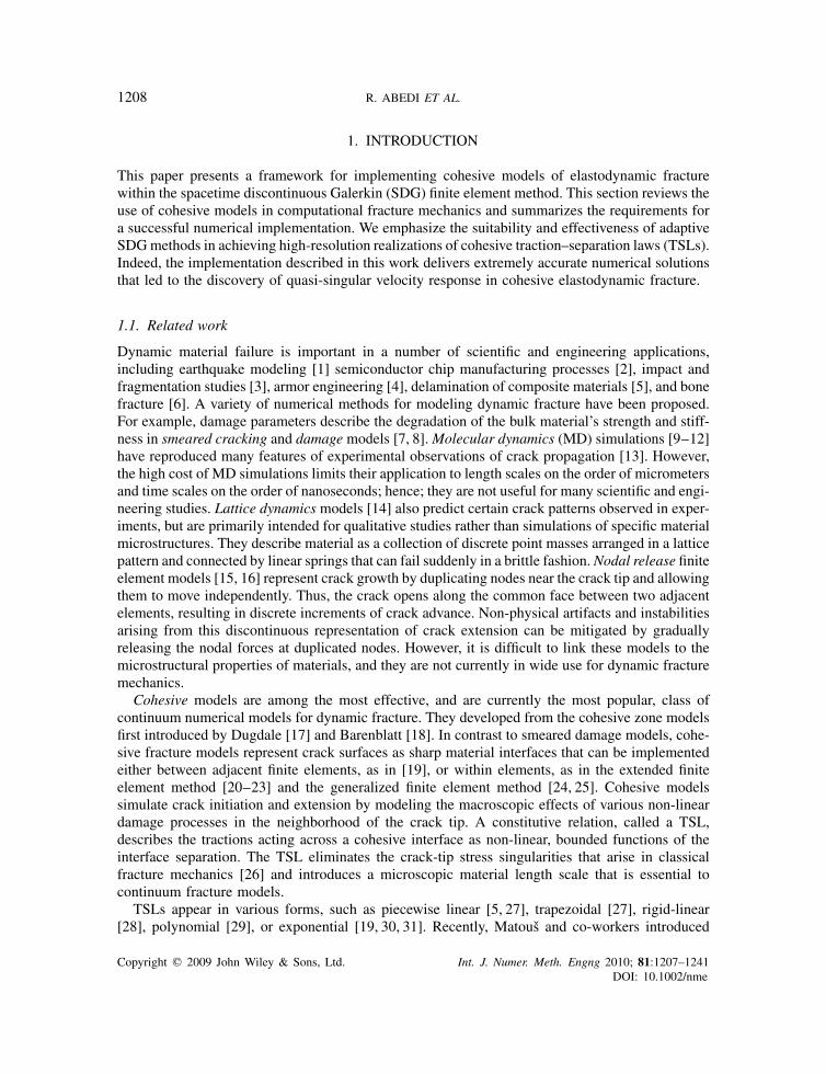
We analyze cohesive crack growth in a middle-crack tension specimen subject to plane-strainconditions and loaded by a uniform, prescribed velocity along two opposite edges. We applysymmetry conditions to model a single quadrant with dimensions, L=10mm,W =3mm and initialcrack length, a0=4.25mm, as shown in Figure 3. The cohesive interface extends to the right ofthe initial crack-tip position along the bottom edge of the quadrant. We use a material model thatapproximates the elastic properties of polymethyl methacrylate: Young’s modulus, E=3.24GPa;the Poisson ratio, =0.35; and mass density, �=1190kg/m3. The dilatational, shear and Rayleighwave speeds are given by [19, 26].
cd =√
E(1− )
�(1+ )(1−2 ), cs =
√E
2�(1+ ), cR ≈cs
0.862+1.14
1+ (32)
For the given values of the material parameters, these speeds are cd =2090m/s,cs =1004m/s,and cR =938m/s. The cohesive properties for the TSL are based on those used in [19]. We use
Copyright q 2009 John Wiley & Sons, Ltd. Int. J. Numer. Meth. Engng 2010; 81:1207–1241DOI: 10.1002/nme

A SPACETIME DISCONTINUOUS GALERKIN METHOD 1225
Figure 3. Model for middle-crack tension specimen.
two values of the cohesive strength in the examples below: either �C=0.1E=324MPa, identicalto that in [19], or �C=0.01E=32.4MPa. The critical separation distance for both the normal andtangential directions is �=4.0×10⁻⁴mm.
A uniform, prescribed velocity, ramping linearly from zero to a sustained value v, is appliedalong the top edge of the model, as depicted in Figure 3. The duration of the prescribed-velocityramp is t0=0.1�s. For purposes of studying the effects of varying the cohesive strength �C,we seek loads that vary in proportion to the strength. The boundary traction induced by theprescribed velocity v is, roughly, proportional to E v/cd. Therefore, we fix the non-dimensionalgroup, (E v)/(�Ccd), to maintain an invariant relation between the induced boundary traction andthe cohesive strength. Thus, holding E and cd constant, we use v=15 and 1.5m/s for �C=324and 32.4MPa, respectively.
4.2. Convergence of the model and performance of two adaptive criteria
Cohesive models for quasi-static fracture analysis require adequate resolution of the cohesiveprocess zone to maintain numerical stability [5, 54]. It is also essential to resolve the process zonein dynamic fracture studies, but robust minimum requirements for maintaining stability have notyet been established for this class of problems. Further, the minimum requirements for stabilitygenerally do not suffice to ensure an accurate simulation of cohesive material failure. We use twoerror indicators in our h-adaptive implementation, as described in Section 3.3, to guarantee bothstability and accuracy. The dissipation error indicator addresses the accuracy of our model forthe dynamic response in the bulk material, while the cohesive energy error indicator ensures theaccuracy and stability of our numerical rendering of the TSL. The studies in this section demonstratethe effectiveness and convergence properties of the adaptive error indicators, both for the dissipationindicator alone and for the two indicators in combination. We use �C=0.01E=32.4MPa andv=1.5m/s, and we compute the crack-tip trajectory using the position xc, cf. Section 3.4.
4.2.1. Convergence study using only the dissipation error indicator. We study the convergence ofthe crack-tip trajectory with varying levels of adaptive mesh refinement, as controlled by the targetper-element dissipation defined in Section 3.3.2. We deactivate the cohesive error indicator in thisstudy, so that the target dissipation is the only control on adaptive refinement.
Copyright q 2009 John Wiley & Sons, Ltd. Int. J. Numer. Meth. Engng 2010; 81:1207–1241DOI: 10.1002/nme

1226 R. ABEDI ET AL.
2 4 6 8 104
5
6
7
8
9
10
2 4 6 8 100
0.2
0.4
0.6
0.8
1
(a) (b)
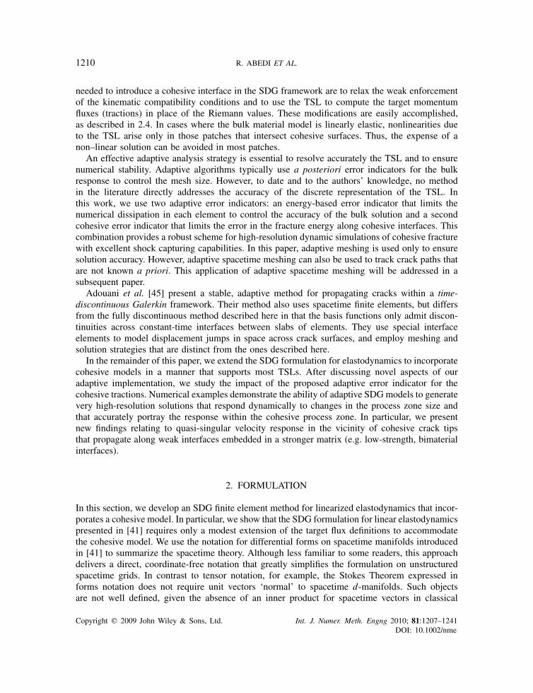
Figure 4. Convergence of crack-tip trajectory and velocity with decreasing target dissipation per element,εD. (a) Crack length and (b) Crack-tip velocity.
Figure 4 shows the convergence of the crack-tip trajectory (or, equivalently, the crack-lengthhistory a(t)) as the target per-element dissipation, εD, decreases; that is, with increasing adaptiverefinement. The model becomes unstable, due to inadequate resolution of the active process zone,when εD is larger than the values displayed in the figure. The crack-tip trajectory is virtuallyidentical to the results displayed for εD=10−11 J when we specify smaller values for εD.
Figure 4(b) shows the convergence of the crack-tip velocity, normalized by the Rayleigh wavespeed cR, as εD decreases. These time-derivative data sets naturally exhibit more numerical noisethan the crack-tip trajectory data and, therefore, require more adaptive refinement for convergence.We emphasize that here we are plotting velocity as pointwise analytical derivatives obtained directlyfrom the cubic polynomial basis functions, cf. (31). This provides a far more stringent test than themethods commonly used with semi-discrete data sets. Nonetheless, the noise is nearly eliminatedfor sufficiently small values of εD. On the other hand, the results for εD=10−9 J, the largest valueconsistent with numerical stability, show considerable scatter and a delayed onset of rapid crackextension relative to the converged solutions.
4.2.2. Convergence with error indicators for both bulk dissipation and cohesive fracture energy.Reducing εD serves to increase the overall level of mesh refinement, but it does not directly ensuresufficient resolution of the TSL in the process zone. Since the process-zone size decreases asthe crack velocity increases [55], models designed to adequately resolve the quasi-static processzone might eventually lose accuracy, or even stability, in dynamic analysis. Furthermore, adaptiverefinement based solely on dissipation is a relatively expensive means to ensure accurate resolutionof the TSL, because the increased level of refinement applies to the entire spacetime analysisdomain, not just the neighborhood of the cohesive process zone. Even for very small values ofεD, the crack-tip-velocity history contains some numerical noise, as shown in Figure 4(b). Thus,it is useful to introduce a second adaptive error indicator ε
QC, cf. Section 3.3.3, to control directly
the error in the fracture energy and thereby ensure a stable and accurate resolution of the processzone.
Copyright q 2009 John Wiley & Sons, Ltd. Int. J. Numer. Meth. Engng 2010; 81:1207–1241DOI: 10.1002/nme

A SPACETIME DISCONTINUOUS GALERKIN METHOD 1227
2 4 6 8 104
5
6
7
8
9
10
2 4 6 8 100
0.2
0.4
0.6
0.8
1
(a) (b)
Figure 5. Convergence of crack-tip trajectory and velocity with decreasing target cohesive energy errorper element, εC for εD=10−9 J. (a) Crack length and (b) Crack-tip velocity.
The two error indicators play complementary roles. The dissipation indicator governs the overallaccuracy of the spacetime solution, especially the resolution of sharp wave fronts in the bulkmaterial, while the cohesive error indicator ensures an accurate rendering of the TSL along thecohesive interface. This approach improves computational efficiency because the cohesive errorindicator provides a means to boost mesh refinement locally in the vicinity of the cohesive processzone without affecting the global level of refinement.
We choose εD=10−9 J, the largest value of εD that ensures stability in Section 4.2.1, and activatethe cohesive error indicator to study its effectiveness. The crack-tip trajectory corresponding toεD=10−9 J differs significantly from the better-resolved solutions (Figure 4), hence, it serves as agood reference for testing the cohesive error indicator. Figure 5(a) shows the convergence of thecrack-tip trajectory as the target per-element cohesive energy error εC decreases. The gray curvefor εC=∞ corresponds to the solution with εD=10−9 J and without the cohesive error criterion.The black curves show results for adaptive runs with both the diffusive and cohesive error criteriaactive. The crack-tip trajectories for smaller values of εC (not shown) are virtually identical to theone for εC=10−11 J.
Figure 5(b) shows the convergence of the crack-tip velocity history with respect to εC. Thenumerical noise decreases as εC decreases, and the lag in the onset of crack extension vanishes.There is a period of near-zero tip velocity that marks the transition from a stationary crack tocohesive crack propagation. This feature is less clearly defined for larger values of εC�10−11 J.Energy flowing into the cohesive process zone during this initiation stage is largely devoted to theformation of a quasi-singular velocity field, as described in the next section. Once the singularfield becomes well established, the crack tip accelerates as the energy flow is redirected to theformation of new crack surface.
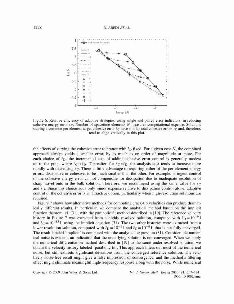
Figure 6 shows how enhancing dissipation-based adaptive analysis with adaptive control ofthe cohesive energy error improves computational efficiency. The plot shows cost, measured bythe number of spacetime elements N , as a function of cohesive energy error εC for differentcombinations of εD and εC at time t=6�s. The black curve shows results for dissipation errorcontrol alone, with no direct control over the cohesive error. Each of the patterned curves shows
Copyright q 2009 John Wiley & Sons, Ltd. Int. J. Numer. Meth. Engng 2010; 81:1207–1241DOI: 10.1002/nme
1228 R. ABEDI ET AL.
–9 –8 –7 –64
4.5
5
5.5
6
6.5
7
7.5
8
Figure 6. Relative efficiency of adaptive strategies, using single and paired error indicators, in reducingcohesive energy error εC. Number of spacetime elements N measures computational expense. Solutionssharing a common per-element target cohesive error εC have similar total cohesive errors εC and, therefore,
tend to align vertically in this plot.
the effects of varying the cohesive error tolerance with εD fixed. For a given cost N , the combinedapproach always yields a smaller error, by as much as on order of magnitude or more. Foreach choice of εD, the incremental cost of adding cohesive error control is generally modestup to the point where εC≈ εD. Thereafter, for εC<εD, the analysis cost tends to increase morerapidly with decreasing εC. There is little advantage to requiring either of the per-element energyerrors, dissipative or cohesive, to be much smaller than the other. For example, stringent controlof the cohesive energy error cannot compensate for dissipation due to inadequate resolution ofsharp wavefronts in the bulk solution. Therefore, we recommend using the same value for εCand εD. Since this choice adds only minor expense relative to dissipation control alone, adaptivecontrol of the cohesive error is an attractive option, particularly when high-resolution solutions arerequired.
Figure 7 shows how alternative methods for computing crack-tip velocities can produce dramat-ically different results. In particular, we compare the analytical method based on the implicitfunction theorem, cf. (31), with the parabolic fit method described in [19]. The reference velocityhistory in Figure 7 was extracted from a highly resolved solution, computed with εD=10−9 Jand εC=10−13 J, using the implicit equation (31). The two other histories were extracted from alower-resolution solution, computed with εD=10−9 J and εC=10−9 J, that is not fully converged.The result labeled ‘implicit’ is computed with the analytical expression (31). Considerable numer-ical noise is evident, an indication that the underlying solution is not converged. When we applythe numerical differentiation method described in [19] to the same under-resolved solution, weobtain the velocity history labeled ‘parabolic fit’. This approach filters out most of the numericalnoise, but still exhibits significant deviations from the converged reference solution. The rela-tively noise-free result might give a false impression of convergence, and the method’s filteringeffect might eliminate meaningful high-frequency response along with the noise. While numerical
Copyright q 2009 John Wiley & Sons, Ltd. Int. J. Numer. Meth. Engng 2010; 81:1207–1241DOI: 10.1002/nme

A SPACETIME DISCONTINUOUS GALERKIN METHOD 1229
2 4 6 8 100
0.2
0.4
0.6
0.8
1
Figure 7. Comparison of methods for computing crack speed a.
differentiation is a suitable choice for many applications, analytical extraction of crack-tip velocitiesmight be preferred for studies that demand high-precision and reliability.
4.3. Dynamic fracture under shock loading conditions
This section presents numerical results for a model of dynamic fracture with high cohesive strength.We describe the details of crack-growth initiation and the development of quasi-singular velocityresponse which, to our knowledge, has not previously been reported in the literature on cohe-sive fracture. For purposes of comparison, we investigate the same problem studied by Xu andNeedleman in [19]. The model parameters are given in Section 4.1; the only differences from theparameters used in the previous section are that the cohesive strength and the applied boundaryvelocity are 10 times larger: �C=0.1E=324MPa and v=15m/s. The terminal time of the simu-lation is t=18.0�s.
The capabilities of the adaptive SDG method to resolve shocks accurately and to control thefidelity of the numerical approximation of the TSL are key to the integrity of this study. Theadaptive analysis parameters, εD=10−11 J and εC=10−10 J, generate a spacetime mesh at the endof the simulation with a total of 117 million tetrahedra arranged in 20 million patches. A detail ofthe spacetime mesh at an intermediate stage of the analysis appears in Figure 8. This discretizationyields a total numerical energy dissipation of 4.5% of the net energy inflow from the prescribed-velocity loading, while the linear and angular momentum balance to within machine precisionglobally, as well as locally on each element. The total cohesive energy error is 2.1×10⁻⁴ J, or10.4% of the energy needed to completely debond the plates.
Figure 9 presents a series of still images from an animation of the SDG solution generated bythe per-pixel-accurate rendering procedure described in Section 3.4. Only the upper-right quadrantof the center-cracked plate is shown. The color field∗∗ depicts the log of the strain-energy density,
∗∗On-line version only. Color is mapped to gray scale in the printed version for Figures 9, 10 and 13.
Copyright q 2009 John Wiley & Sons, Ltd. Int. J. Numer. Meth. Engng 2010; 81:1207–1241DOI: 10.1002/nme

1230 R. ABEDI ET AL.
Figure 8. Detail of adaptively refined spacetime mesh at t=4.15�s with the time axis in the verticaldirection. The left face of the spacetime volume corresponds to the cohesive surface, where the denselymeshed region at the left follows the trajectory of the moving process zone. Other dense regions capture
various wavefronts as they move through the bulk material.
where blue indicates zero energy density and violet indicates peak values. The height field depictsthe modulus of the material velocity.
Figure 9(a) shows the progress through the plate of the primary wavefront generated by theapplied loads at an early time, t=1.00�s, as well as secondary waves generated along the freesurface and Rayleigh waves traveling along the top and right surfaces. Figure 9(b) shows a time,t=1.85�s, shortly after the primary wave reaches the crack plane. Wave scattering effects anda sharp gradient in the strain-energy density field are visible. A sharp spike in the velocity fieldstarts to form, indicating the initiation stage of crack propagation. This spike develops into thequasi-singular structure described below. Figure 10 shows a detail view of the crack-tip regionin which the solution is reflected about the crack plane to clarify the overall response in theplate. Figure 9(c) shows a later stage of crack propagation, where the velocity spike is more fullydeveloped. Distinct wavefronts corresponding to scattered dilatational and shear waves are clearlyvisible at this stage.
The crack-tip velocity increases as propagation continues, until the velocity asymptoticallyapproaches the Rayleigh wave speed, cR. This acceleration tends to reduce the size of the active
Copyright q 2009 John Wiley & Sons, Ltd. Int. J. Numer. Meth. Engng 2010; 81:1207–1241DOI: 10.1002/nme

A SPACETIME DISCONTINUOUS GALERKIN METHOD 1231
Figure 9. Visualization of crack propagation over time; upper-right quadrant of center-cracked plate. Colordepicts log of strain-energy density; height field is modulus of material velocity. Initial crack-tip positionis slightly to the left of midpoint of bottom edge. (a) t=1.00�s; (b) t=1.85�s; (c) t=2.60�s; (d)
t=3.75�s; (e) t=6.25�s; and (f) t=9.00�s.
process zone. At the same time, propagation reduces the net section ahead of the crack tip,leaving less material to resist the tensile loading. Both effects strengthen the quasi-singular velocityresponse over time, as shown in Figures 9(d) and (e). There is a sharp release of kinetic energyfrom the quasi-singular structure in the velocity field when the crack breaks through the freeboundary. This event sends sharp wavefronts through the plate interior and generates strongRayleigh waves that travel in two directions along the broken plate’s free boundaries, as depicted inFigure 9(f).
Asymptotic dynamic solutions for a running, mathematically sharp crack in a linear elasticmedium exhibit an r−1/2 singular form in the material velocity field [26], where r is the radialdistance from the core of the singularity at the crack tip. Spikes in the velocity field surrounding
Copyright q 2009 John Wiley & Sons, Ltd. Int. J. Numer. Meth. Engng 2010; 81:1207–1241DOI: 10.1002/nme

1232 R. ABEDI ET AL.
Figure 9. Continued.
the running crack tip, evident in Figure 9, suggest a similar structure in our simulation results. Thiswould be an unexpected finding, if true. Cohesive models eliminate the associated singularitiesin the stress and strain fields by construction, hence, it is generally assumed that the velocitysingularity is similarly annihilated.
Figure 11 presents a detailed analysis of the material velocity field in the neighborhood of apropagating crack tip. The figure shows a log–log plot of velocity magnitude versus radial distancer at t=5.0�s, a time when the spike in the velocity field is well formed. The distance r is measuredrelative to the ‘core’ of the apparent singularity at x0, the position where the exponents of r in theexpansions of the velocity field ahead of and behind the crack tip match. The velocity data in thisplot are generated by directly evaluating the trace of the raw finite element solution for u alongthe intersections of the constant-time plane with cohesive faces of individual spacetime elements.We sample multiple points within each intersected face to obtain a detailed plot of the velocitydistribution. After identifying regions ahead of and behind the crack tip where the slope of thelog–log plot is nearly constant (indicated by the shaded bands in Figure 11), we identify the core
Copyright q 2009 John Wiley & Sons, Ltd. Int. J. Numer. Meth. Engng 2010; 81:1207–1241DOI: 10.1002/nme

A SPACETIME DISCONTINUOUS GALERKIN METHOD 1233
Figure 10. Detail view of developing quasi-singular velocity field at t=1.85�s. Solution data are reflectedabout the crack plane to cover half the plate. The viewpoint position, relative to the layout in Figure 3,
is above and to the right of the crack tip.
0 1
0
0.5
Figure 11. Analysis of quasi-singular velocity field, behind and ahead of moving crack tip, at t=5.0�s.The modulus of the material velocity is v :=|v|, and shaded bands indicate ranges used to compute linearexpansions:(A) logv=−0.500logr−1.5456; (B) logv=−0.500logr−1.749. Adaptive error tolerances
are εD=10−11 J and εC=10−10 J.
location by adjusting x0 until the slopes in the two regions match. We take the matching value ofthe slope as the exponent of r in the singular form.
For the data plotted in Figure 11, we found x0=7.13363mm. The resulting exponent matchesclosely the theoretical value for a mathematically sharp crack, − 1
2 , for two decades of r behindx0 and one decade ahead. However, in contrast to the singular solution for a sharp, propagatingcrack, our highly resolved numerical solutions deviate from the singular structure for small radii
Copyright q 2009 John Wiley & Sons, Ltd. Int. J. Numer. Meth. Engng 2010; 81:1207–1241DOI: 10.1002/nme

1234 R. ABEDI ET AL.
1 2 3 4 54
4.5
5
5.5
6
6.5
7
1 2 3 4 50
0.2
0.4
0.6
0.8
1
(a)
(b)
Figure 12. Trajectory and velocity of nominal crack tip; SDG solution compared with results from [19].(a) Crack-tip position and (b) Crack-tip velocity.
r<10−3.3mm, indicating a non-singular core. As it happens, the size of the non-singular core andthe size of the process zone at the given time, �=10−3.1mm (cf. Section 3.4), are of similar ordersof magnitude, indicating that the cohesive process zone does indeed prevent a true singularity fromforming. We use the term quasi-singular to describe this structure comprised of a non-singular coreembedded within a zone that follows a singular form down to a small, but finite, radius. Figure 12compares the crack-tip trajectory and velocity history predicted by the SDG cohesive model withcorresponding results reported in [19] for two prescribed velocities, v=15m/s and v=30m/s.Following the method in [19], we define the crack-tip position xc in terms of the largest value ofx along the cohesive interface for which �n��n.
Figure 12(a) compares crack-tip positions from the SDG solution with those reported in [19].Xu and Needleman do not present results for the crack-tip trajectory directly, so we integrate their
Copyright q 2009 John Wiley & Sons, Ltd. Int. J. Numer. Meth. Engng 2010; 81:1207–1241DOI: 10.1002/nme
A SPACETIME DISCONTINUOUS GALERKIN METHOD 1235
velocity data to plot the crack-tip position over time. Differences in the crack-tip trajectory arevisible for both values of the prescribed velocity, but these are more pronounced for the fasterloading, v=30m/sec.
Figure 12(b) compares crack-tip velocity histories predicted by the SDG method with thosereported in [19]. To facilitate comparison, we employ the same numerical differentiation schemeused in [19] to extract crack-tip velocities from the SDG solutions, rather than the analyticalmethod used elsewhere in this work. This involves passing a quadratic polynomial through threesuccessive values of xc and recording the time derivative of the polynomial at the middle point asthe crack-tip velocity. Comparison of the velocity solutions reveals larger differences than thoseobtained for crack-tip position. There is a modest lag in crack initiation in the results from [19]that is more pronounced in the data for v=15m/s. This difference is likely due to the moreaccurate resolution of the formation of the quasi-singular velocity field in the SDG solution, sincethis phenomenon tends to delay initiation. The acceleration of the crack tip to the Rayleigh wavespeed is noticeably more gradual in the SDG solution, which reaches the asymptotic value at amuch later time for v=15m/s. The relatively abrupt increase in crack-tip velocity at t=4.31�sin the SDG solution is associated with the arrival of a reflected wave at the crack tip.
In contrast to the results from [19], the SDG crack-tip velocity for v=30m/s does not overshootthe Rayleigh speed. This difference can be attributed to the local balance properties of the SDGsolution, its ability to adaptively track the dramatic decrease in the process-zone size as the velocityapproaches the Rayleigh speed (cf. [55]), and the use of higher-order elements. Our results indicatethat the overshoot is not an artifact of the chosen definition for xc, nor is it due to a lifting-off modeof separation, as suggested in [19]. Since theoretical results forbid crack-tip velocities between theRayleigh and dilatational wave speeds for mode-I propagating cracks [56], the overshoot reportedin [19] is likely due to discretization error associated with the non-adaptive solution’s inability totrack the shrinking process zone.
Whether a Mode-I crack is able to attain velocities approaching the theoretical limiting speed,cR, depends on the specific material system, the loading conditions under consideration and thetime scale at which velocity is measured. Experimental observations in homogeneous materialswith amorphous microstructures subjected to far-field loading show that time-averaged crack-tipvelocities rarely exceed roughly 0.5cR due to micro-cracking and branching [37, 57]. These studiesare sometimes cited to support the contention that crack-tip velocities never approach the theoreticallimit in brittle materials. However, these observations apply only to macroscopic, time-averagedvelocities. Fine-scale measurements by Sharon and Fineberg [58] demonstrate that instantaneouscrack-tip velocities do, in fact, approach the theoretical limit between intermittent micro-crackingevents. They found that microcracking causes only a temporary drop in the primary crack-tipvelocity as energy flowing into the tip is briefly redirected elsewhere.
The lower limit on the macroscopic, time-averaged crack velocity is not universal for all brittlematerial systems and for all loading conditions. Lee and Knauss [59, 60] report macroscopic crackvelocities that approach cR for mode-I cracks growing along weak joints between identical brittlesolids as the ratio of the strength of the bonded interface to the strength of the surrounding materialapproaches zero. This limiting situation pertains to the present example, as we have made noprovision for material failure in the bulk. Weak interfaces are not rare in practice. For example, theyare commonly created in manufacturing processes simply by scoring the surface of an otherwiseuniform plate. The form and intensity of the loading and the material microstucture are alsoimportant. Winkler et al. [61] observed supersonic crack growth along weak crystallographic planeswhen the crack tip is directly loaded by a laser-induced, expanding plasma.
Copyright q 2009 John Wiley & Sons, Ltd. Int. J. Numer. Meth. Engng 2010; 81:1207–1241DOI: 10.1002/nme

1236 R. ABEDI ET AL.
Computational studies of brittle fracture processes, including microcracking and branching, callfor numerical models that capture reductions in process-zone size and quasi-singular response ascrack-tip velocities approach cR. The adaptive SDG cohesive model’s ability to predict detailedresponse under these conditions is indicative of the method’s robustness and reliability and suggeststhat it is a suitable tool for multi-scale scientific studies of dynamic fracture in brittle materials.
4.4. Non-planar crack growth: dewetting of a circular inclusion
This final example demonstrates the SDG cohesive model’s ability to simulate mixed-mode fractureand non-planar crack growth. The analysis domain is a 4mm×4mm square comprised of a stiff,circular inclusion of radius 1mm centered in a matrix of more flexible material. The matrix materialproperties are Young’s modulus, E=3.24GPa; The Poisson ratio, =0.35; and mass density,�=1190kg/m3. The inclusion has the same properties, except the elastic modulus is 32.4GPa.This produces wave speeds that are faster than the matrix by a factor of
√10. A cohesive interface
bonds the matrix to the inclusion. We model the response of the cohesive interface with theXu–Needleman description [19], with cohesive strength, �C=32.4MPa, and critical separationdistance for both the normal and tangential directions, �=4.0×10⁻⁴mm. The cohesive interfaceextends all the way around the inclusion, except for an interval from 17◦ to 22◦, measured clockwisefrom the top of the inclusion, where we impose traction-free conditions to model an initial flawin the cohesive bond. We enforce symmetry boundary conditions along the left and right edgesof the square domain to simulate an infinite strip of similar inclusions. We enforce plane-strainconditions throughout the model.
Figure 13 shows results for a prescribed velocity, applied uniformly along the top and bottomedges of the domain, whose magnitude ramps linearly over an interval of 0.1�s from zero to asustained value, v=7m/s. Figure 13(a) depicts a time slightly after the wavefronts reach the topand bottom edges of the inclusion. As is evident from the response along the bottom edge, theaction of the primary wave alone does not fracture the undamaged cohesive interface. However,the upper primary wave does initiate a fracture as it interacts with the flaw near the top of theinclusion. Part of the energy of the primary wavefronts is reflected by the cohesive bi-materialinterface, and part is transmitted to the interior of the inclusion. The greater wave speeds withinthe inclusion cause the interior waves to advance ahead of the wavefronts in the matrix, as shownin Figure 13(a). The interior waves combine with the lower primary wave to nucleate a secondcrack when they reach the bottom portion of the cohesive interface. The upper and lower crackseach propagate dynamically in two directions along the cohesive interface until the inclusion iseventually completely debonded. Figure 13(b) shows the configuration of the upper and lowercracks at a later time, just prior to complete debonding. At this stage, some of the crack-tip speedsare sufficient to generate quasi-singular velocity fields. Neither crack path is symmetric due to theasymmetric placement of the initial flaw.
5. CONCLUSIONS
We have presented a new framework for implementing cohesive fracture models within a spacetimediscontinuous Galerkin finite element method that provides a robust environment for modelingdynamic, cohesive fracture. The elementwise balance properties and adaptive analysis capabilitiesof the SDG method enable it to resolve crack-tip fields and sharp wave fronts, whether they be
Copyright q 2009 John Wiley & Sons, Ltd. Int. J. Numer. Meth. Engng 2010; 81:1207–1241DOI: 10.1002/nme
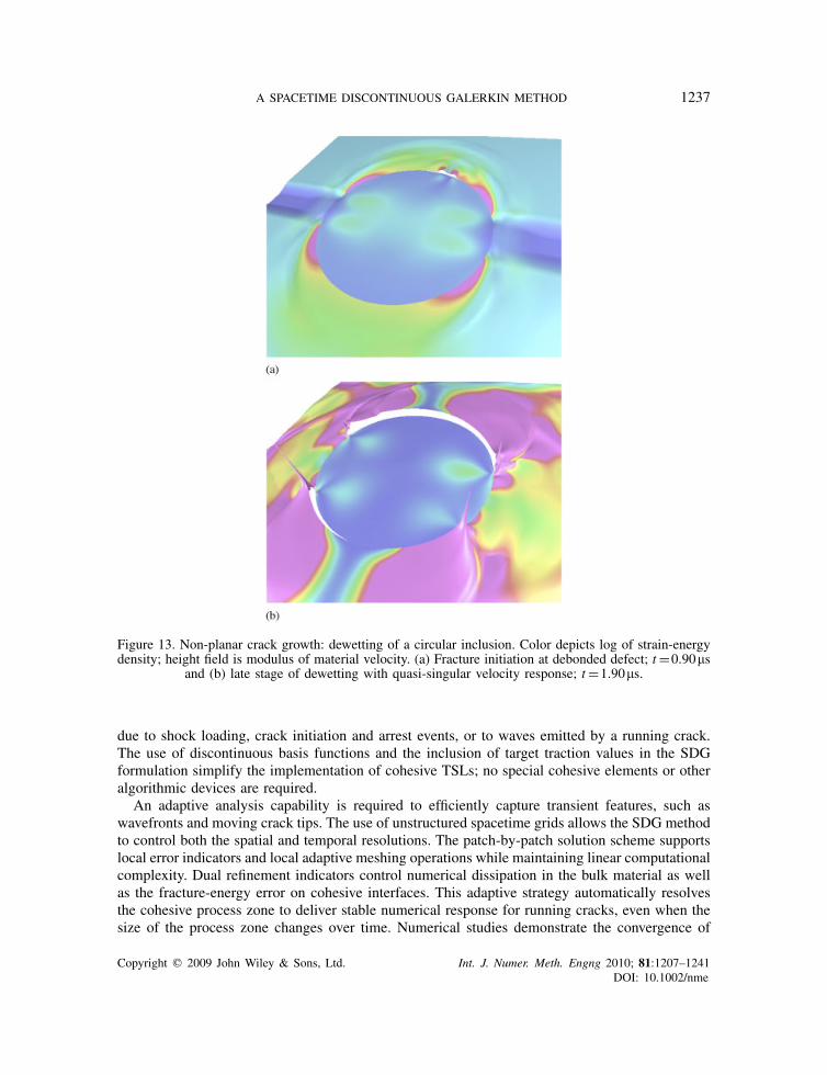
A SPACETIME DISCONTINUOUS GALERKIN METHOD 1237
Figure 13. Non-planar crack growth: dewetting of a circular inclusion. Color depicts log of strain-energydensity; height field is modulus of material velocity. (a) Fracture initiation at debonded defect; t=0.90�s
and (b) late stage of dewetting with quasi-singular velocity response; t=1.90�s.
due to shock loading, crack initiation and arrest events, or to waves emitted by a running crack.The use of discontinuous basis functions and the inclusion of target traction values in the SDGformulation simplify the implementation of cohesive TSLs; no special cohesive elements or otheralgorithmic devices are required.
An adaptive analysis capability is required to efficiently capture transient features, such aswavefronts and moving crack tips. The use of unstructured spacetime grids allows the SDG methodto control both the spatial and temporal resolutions. The patch-by-patch solution scheme supportslocal error indicators and local adaptive meshing operations while maintaining linear computationalcomplexity. Dual refinement indicators control numerical dissipation in the bulk material as wellas the fracture-energy error on cohesive interfaces. This adaptive strategy automatically resolvesthe cohesive process zone to deliver stable numerical response for running cracks, even when thesize of the process zone changes over time. Numerical studies demonstrate the convergence of
Copyright q 2009 John Wiley & Sons, Ltd. Int. J. Numer. Meth. Engng 2010; 81:1207–1241DOI: 10.1002/nme
1238 R. ABEDI ET AL.
various aspects of the fracture response as the adaptive tolerances are tightened. Using the twoadaptive error indicators in combination substantially improves computational efficiency.
The SDG solution structure enables an analytical technique for computing crack-tip velocityfrom an implicit definition of the crack-tip position. This method neither masks numerical noisenor filters out meaningful high-frequency response. Thus, it promotes more objective evaluationsof solution quality and convergence and reveals the full detail of the simulated response.
Our numerical solutions reveal new detail and unexpected qualitative features of cohesive,elastodynamic fracture. The presence of a quasi-singular velocity field and the fact that the crack-tipvelocity does not exceed the Rayleigh wave speed, even under large impact velocities, are the mostnotable. Comparisons with previous solutions indicate that careful control of the discretizationerror is necessary to simulate accurately and reliably the dynamics of moving crack tips. Forexample, the adaptive SDG model’s ability to capture the energetics of the quasi-singular velocityfield surrounding running crack tips probably explain the differences in crack kinetics between ourresults and previous solutions. Our new findings are due entirely to the improved accuracy andresolution made possible by the adaptive SDG implementation since the underlying continuummodel is the same as in previous studies. Further investigations of the structure and effects of thequasi-singular velocity field will be reported in a separate paper.
Our numerical experience suggests various modifications of our SDG implementation to improveefficiency. First, our h-adaptive method could be promoted to a hp-adaptive strategy to exploitthe SDG formulation’s ability to accommodate distinct polynomial orders in adjacent elements.Quadrature-free methods could reduce the cost of assembling the patch equations [62], and parallelsolution methods could be applied to our patchwise meshing and solution processes. A parallelimplementation, based on the ParFUM and CHARM++ frameworks [63, 64], is under develop-ment.
The implementation of cohesive models described in this paper is restricted to predefinedcohesive surfaces. In continuing work, we are extending the adaptive SDG method to simulatecrack nucleation and crack propagation along arbitrary, solution-dependent paths. Rather thanintroduce discontinuity surfaces on element interiors, as in [22, 21, 23], we use adaptive spacetimemeshing operations to generate new cohesive surfaces in the SDG discretization that align withevolving crack trajectories.
Various extensions to the SDG mechanics formulation and to the cohesive model are needed tobroaden our simulation capabilities. Provisions for finite-deformation response, in both the bulkmaterial and cohesive models, are necessary for many studies. Rate-dependent and thermome-chanical cohesive models [35, 36] provide more accurate descriptions of certain fracture processeswhere high strain rates accompanied by significant temperature increases have been observed[38, 65]. Various alternatives to the Xu–Needleman cohesive model are better suited to trackingsolution-dependent crack paths, such as those with initially rigid behavior and inelastic unloading[28, 31]. Another possibility is to use damage models to evolve the cohesive properties, as in [66].The modular structure of our implementation promotes the development and investigation of thesealternative models.
Three-dimensional geometry is an important consideration in many fracture applications wheretwo-dimensional idealizations are inadequate. Thus, we are interested in extending our imple-mentation to 3D×time. The mechanics theory and finite element formulation presented hereare fully extensible to three spatial dimensions and present no special difficulties. The primarychallenge involves spacetime meshing. For non-adaptive meshing, where the spatial discretiza-tion is fixed, the mathematical theory that underlies Tent Pitcher is provably extensible to any
Copyright q 2009 John Wiley & Sons, Ltd. Int. J. Numer. Meth. Engng 2010; 81:1207–1241DOI: 10.1002/nme
A SPACETIME DISCONTINUOUS GALERKIN METHOD 1239
dimension. However, the extension of certain aspects of the h-adaptive meshing algorithm remainopen for future research. Although the task of building a fully three-dimensional code should notbe underestimated, the problem is not as daunting as it might seem. Tent Pitcher’s primary concernis with modeling the current front, which consists of a conventional three-dimensional space meshaugmented with a time coordinate at each vertex. True spacetime elements are only generated whena vertex advances in time and are not part of the meshing algorithm’s fundamental data structure.Thus, there is some reason for optimism that this goal can be realized. Visualization of spacetimedata need not be significantly more difficult than in other three-dimensional models. By passinga constant-time plane through the spacetime data set, we obtain a conventional three-dimensionalmodel for visualization. If successfully extended, the powerful adaptive capabilities and intrinsicscalability of the SDG approach should prove beneficial in attaining the level of accuracy andefficiency required for reliable dynamic fracture simulations in three dimensions.
ACKNOWLEDGEMENTS
The authors gratefully acknowledge the contributions of Shuo-Heng Chung, Scott Miller, Jeff Erickson,Yong Fan, Michael Garland, Jayandran Palaniappan, Laxmikant Kale, Shripad Thite, Aaron Becker andYuan Zhou to this work. Support from the Center for Process Simulation and Design (CPSD) and the Centerfor Simulation of Advanced Rockets (CSAR) at the University of Illinois is gratefully acknowledged. TheU.S. National Science Foundation supports research in CPSD via grant NSF DMR 01-21695. The CSARresearch program is supported by the U.S. Department of Energy through the University of Californiaunder subcontract B341494.
REFERENCES
1. Wilkins SJ, Schultz RA. 3d cohesive end-zone model for source scaling of strike-slip interplate earthquakes.Bulletin of the Seismological Society of America 2005; 95(6):2232–2258.
2. Kiyono SS, Yonehara K, Graf RS, Howell WJ. Consideration of mechanical chip crack on fbga packages. 2001Proceedings. Fifty-first Electronic Components and Technology Conference (Cat. No.01CH37220), San Diego,CA, U.S.A., 2001; 193–197.
3. Pandolfi A, Ortiz M. An efficient adaptive procedure for three-dimensional fragmentation simulations. Engineeringwith Computers 2002; 18:148–159.
4. Denoual C, Hild F. A damage model for the dynamic fragmentation of brittle solids. Computer Methods inApplied Mechanics and Engineering 2000; 183:247–258.
5. Geubelle PH, Baylor JS. Impact-induced delamination of composites: a 2d simulation. Composites Part B 1998;29B:589–602.
6. Gasser TC, Holzapfel GA. A numerical framework to model 3-d fracture in bone tissue with application tofailiure of the proximal femur. Proceedings of the IUTAM Symposium, Symposium on Discretization Methods forEvolving Discontinuities, Lyon, France, 2006; 199–212.
7. Johnson E. Process region changes for rapidly propagating cracks. International Journal of Fracture 1992;55:47–63.
8. Oliver J, Huespe AE, Samaniego E. A study on finite elements for capturing strong discontinuities. InternationalJournal for Numerical Methods in Engineering 2003; 56:2135–2161.
9. Abraham FF, Brodbeck D, Rafey RA, Rudge WE. Instability dynamics of fracture: a computer simulationinvestigation. Physical Review Letters 1994; 73:272–276.
10. Nakano A, Kalia RK, Vashishta P. Dynamics and morphology of brittle cracks: a moleculardynamics study ofsilicon nitride. Physical Review Letters 1995; 75:3138–3141.
11. Buehler MJ, Alexander H, Gao H, Duchaineau M, Abraham FF, Brodbeck D, Ridge WE, Xu X. Atomic plasticity:description and analysis of a one-billion atom simulation of ductile materials failure. Computer Methods inApplied Mechanics and Engineering 2004; 193:5257–5282.
Copyright q 2009 John Wiley & Sons, Ltd. Int. J. Numer. Meth. Engng 2010; 81:1207–1241DOI: 10.1002/nme

1240 R. ABEDI ET AL.
12. Buehler MJ, Hartmaier A, Duchaineau MA, Abraham FF, Gao H. The dynamical complexity of work-hardening:a large-scale molecular dynamics simulation. Acta Mechanica Sinica (English Series) 2005; 21(2):103–111.
13. Ravi-Chandar K. Dynamic fracture of nominally brittle materials. International Journal of Fracture 1998;90:83–102.
14. Marder M, Gross SP. Origin of crack tip instabilities. Journal of the Mechanics and Physics of Solids 1995;43:1–48.
15. Anderson H. A finite element representation of stable crack growth. Journal of the Mechanics and Physics ofSolids 1973; 21:337–356.
16. Yatomi M, Bettinson AD, O’Dowd NP, Nikbin KM. Modelling of damage development and failure in notched-barmultiaxial creep tests. Fatigue and Fracture of Engineering Material and Structures 2004; 27(4):283–295.
17. Dugdale DS. Yielding of steel sheets containing slits. Journal of the Mechanics and Physics of Solids 1960;8:100–104.
18. Barenblatt GI. The mathematical theory of equilibrium of cracks in brittle fracture. Advanced Applied Mechanics1962; 7:55–129.
19. Xu XP, Needleman A. Numerical simulations of fast crack growth in brittle solids. Journal of the Mechanicsand Physics of Solids 1994; 42:1397–1434.
20. Belytschko T, Black T. Elastic crack growth in finite elements with minimal remeshing. International Journalfor Numerical Methods in Engineering 1999; 45:601–620.
21. Moes N, Dolbow J, Belytschko T. A finite element method for crack growth without remeshing. InternationalJournal for Numerical Methods in Engineering 1999; 46:131–150.
22. Dolbow J, Moes N, Belytschko T. Discontinuous enrichment in finite elements with a partition of unity method.International Journal for Numerical Methods in Engineering 2000; 36(3):235–260.
23. Remmers JJC, de Borst R, Needleman A. A cohesive segments method for the simulation of crack growth.Computational Mechanics 2003; 31:69–77.
24. Strouboulis T, Babuska I, Copps K. The design and analysis of the generalized finite element method. ComputerMethods in Applied Mechanics and Engineering 2000; 181:43–69.
25. Strouboulis T, Copps K, Babuska I. The generalized finite element method. Computer Methods in AppliedMechanics and Engineering 2001; 190:4081–4193.
26. Freund LB. Dynamic Fracture Mechanics. Cambridge University Press: Cambridge, U.K., 1990.27. Tvergaard V, Hutchinson JW. The relation between crack growth resistance and fracture process parameters in
elastic–plastic solids. Journal of the Mechanics and Physics of Solids 1992; 40:1377–1397.28. Camacho GT, Ortiz M. Computational modelling of impact damage in brittle materials. International Journal of
Solids and Structures 1996; 33:2899–2938.29. Needleman A. A continuum model for void nucleation by inclusion debonding. Journal of Applied Mechanics
1987; 54:525–532.30. Xu XP, Needleman A. Void nucleation by inclusion debonding in a crystal matrix. Modelling and Simulation in
Materials Science and Engineering 1993; 1:111–132.31. Ortiz M, Pandolfi A. Finite-deformation irreversible cohesive elements for three-dimensional crack-propagation
analysis. International Journal for Numerical Methods in Engineering 1999; 44:1267–1282.32. Matous K, Kulkarni M, Geubelle P. Multiscale cohesive failure modeling of heterogeneous adhesives. Journal
of the Mechanics and Physics of Solids 2008; 56:1511–1533.33. Li H, Chandra N. Analysis of crack growth and crack-tip plasticity in ductile materials using cohesive models.
International Journal of Plasticity 2003; 19:849–882.34. Pandolfi A, Krysl P, Ortiz M. Finite element simulations of ring expansion and fragmentation: the capturing of
length and time scales through cohesive models of fracture. International Journal of Fracture 1999; 95:279–297.35. Costanzo F, Walton JR. Steady growth of a crack with a rate and temperature sensitive cohesive zone. Journal
of the Mechanics and Physics of Solids 2002; 50:1649–1679.36. Zhou F, Molinari JF, Shioya T. A rate-dependent cohesive model for simulating dynamic crack propagation in
brittle materials. Engineering Fracture Mechanics 2005; 72:1383–1410.37. Fineberg J, Marder M. Instability in dynamic fracture. Physics Reports 1999; 313:1–108.38. Zehnder AT, Rosakis AJ. On the temperature distribution at the vicinity of dynamically propagating cracks.
Journal of the Mechanics and Physics of Solids 1991; 39:385–415.39. Fagerstrom M, Larsson R. Theory and numerics for finite deformation fracture modeling using strong
discontinuities. International Journal for Numerical Methods in Engineering 2006; 66:911–948.
Copyright q 2009 John Wiley & Sons, Ltd. Int. J. Numer. Meth. Engng 2010; 81:1207–1241DOI: 10.1002/nme

A SPACETIME DISCONTINUOUS GALERKIN METHOD 1241
40. Petracovici B. Analysis of a spacetime discontinuous Galerkin method for elastodynamics. Ph.D. Thesis,Department of Mathematics, University of Illinois at Urbana-Champaign, 2004.
41. Abedi R, Haber RB, Petracovici B. A spacetime discontinuous Galerkin method for elastodynamics withelement-level balance of linear momentum. Computer Methods in Applied Mechanics and Engineering 2006;195:3247–3273.
42. Abedi R, Haber RB, Thite S, Erickson J. An h-adaptive spacetime-discontinuous Galerkin method for linearizedelastodynamics. Revue Europeenne de Mecanique Numerique (European Journal of Computational Mechanics)2006; 15(6):619–642.
43. Erickson J, Guoy D, Ungor A, Sullivan J. Building spacetime meshes over arbitrary spatial domains. Proceedingsof the 11th International Meshing Roundtable, Ithaca, NY, U.S.A., 2002; 391–402.
44. Abedi R, Chung SH, Erickson J, Fan Y, Garland M, Guoy D, Haber RB, Sullivan J, White S, Zhou Y. Space–time meshing with adaptive refinement and coarsening. Proceedings of the 20th Annual ACM Symposium onComputational Geometry, Association for Computing Machinery, 2004; 300–309.
45. Adouani H, Tie B, Berdin C, Aubry D. Adaptive numerical modeling of dynamic crack propagation. Journal dePhysique IV (Proceedings) 2006; 134:501–506.
46. Arnold VI. Mathematical Methods of Classical Mechanics (2nd edn). Springer: New York, 1989.47. Spivak M. Calculus on Manifolds. W. A. Benjamin: New York, 1965.48. Bishop RL, Goldberg SI. Tensor Analysis on Manifolds. Prentice-Hall: Englewood Cliffs, NJ, 1980. Reprinted
By Dover (1980).49. Fleming WH. Functions of Several Variables. Addison-Wesley: Reading, MA, 1964.50. Palaniappan J, Miller ST, Haber RB. Sub-cell shock capturing and spacetime discontinuity tracking for nonlinear
conservation laws. International Journal for Numerical Methods in Fluids 2008; 57:1115–1135.51. Morrissey JW, Rice JR. Crack front waves. Journal of the Mechanics and Physics of Solids 1998; 46:467–487.52. Needleman A, Rosakis AJ. The efect of bond strength and loading rate on the conditions governing the attainment
of intersonic crack growth along interfaces. Journal of the Mechanics and Physics of Solids 1999; 47:2411–2449.53. Zhou Y, Garland M, Haber RB. Pixel-exact rendering of spacetime finite element solutions. Proceedings of IEEE
Visualization 2004. Institute of Electrical and Electronics Engineers, Inc., 2004; 425–432.54. Matous K, Geubelle PH. Finite element formulation for modeling particle debonding in reinforced elastomers
subjected to finite deformations. Computer Methods in Applied Mechanics and Engineering 2006; 196(1–3):620–633.
55. Yu H, Suo Z. Intersonic crack growth on an interface. Proceedings of the Royal Society 2000; 456(1993):223–246.56. Broberg KB. The near-tip field at high crack velocities. International Journal of Fracture 1989; 39:1–13.57. Sharon E, Gross S, Fineberg J. Energy dissipation in dynamic fracture. Physical Review Letters 1996; 76:2117.58. Sharon E, Fineberg J. Confirming the continuum theory of dynamic brittle fracture for fast cracks. Nature 1999;
397(6717):333–335.59. Lee O, Knauss W. Dynamic crack propagation along a weakly bonded plane in a polymer. Experimental Mechanics
1989; 29:342–345.60. Lee O, Knauss W. A reconciliation of dynamic crack velocity and Rayleigh wave speed in isotropic brittle solids.
International Journal of Fracture 1994; 65:97–114.61. Winkler S, Shockey D, Curran D. Crack propagation at supersonic velocities—I. International Journal of Fracture
Mechanics 1970; 6:151–158.62. Atkins HL, Shu CW. Quadrature-free implementation of discontinuous Galerkin method for hyperbolic equations.
American Institute of Aeronautics and Astronautics Journal 1998; 36:775–782.63. Lawlor OS, Chakravorty S, Wilmarth TL, Choudhury N, Dooley I, Zheng G, Kale LV. ParFUM: a parallel
framework for unstructured meshes for scalable dynamic physics applications. Engineering with Computers 2006;22:215–235.
64. Zheng G. Achieving high performance on extremely large parallel machines: performance prediction and loadbalancing. Ph.D. Thesis, Department of Computer Science, University of Illinois at Urbana-Champaign, 2005.
65. Tzou DY. Experimental evidence for the temperature waves around a rapidly propagating crack tip. Journal ofHeat Transfer 1992; 114:1042–1051.
66. Allix O, Corigliano A. Modeling and simulation of crack propagation in mixed modes interlaminar fracture.International Journal of Fracture 1996; 77:111–140.
Copyright q 2009 John Wiley & Sons, Ltd. Int. J. Numer. Meth. Engng 2010; 81:1207–1241DOI: 10.1002/nme