Multiplicative Schwarz Algorithms for the Galerkin BoundaryElement MethodMatthias Maischak � Ernst P. Stephan y Thanh Tran zMay 30, 1997AbstractWe study the multiplicative Schwarz method for the p-version Galerkin boundary ele-ment method for a hypersingular and a weakly singular integral equation of the �rst kindand for the h-version for a hypersingular integral equation of the �rst kind. We prove thatthe rate of convergence of the multiplicative Schwarz operator is strictly less than 1 for theh-version for both two level and multilevel methods, whereas for the p-version we show thatthe convergence rate grows only logarithmically in p for the 2-level method. Computationalresults are presented for both the h-version and the p-version which support our theory.Key words: h-version Galerkin boundary element method, p-version Galerkin boundaryelement method, multiplicative Schwarz, multigrid algorithmAMS Subject Classi�cation (1991): 65N55, 65N381 Introduction.We study multiplicative Schwarz methods for the h and p versions of the Galerkin boundaryelement method applied to hypersingular and weakly singular integral equations on open orclosed curves. These equations are integral reformulations for boundary value problems withthe Laplace equation and the Dirichlet or Neumann boundary conditions (see [4]). Applicationof the Galerkin method to solve these integral equations yields linear systems with dense,symmetric and positive-de�nite sti�ness matrices. Since the condition numbers of these matricesgrow like h�1 in the h version and like p2 in the p version (see [10]), the convergence rate of theconjugate gradient algorithm approaches 1 (the non-convergent status of the iterative method)like 1 � ch1=2 as h ! 0 and like 1 � c=p as p ! 1 with a positive constant c. We shallpropose for both versions multiplicative Schwarz algorithms which signi�cantly improve therate of convergence of the conjugate gradient method.We shall analyze for the h-version a 2-level method which corresponds to a multigrid al-gorithm using the Gau�-Seidel algorithm for smoothing, and a multilevel method which cor-responds to a multigrid algorithm using the Jacobi smoother. We shall prove that both the�Institut f�ur Angewandte Mathematik, University of Hannover, GermanyyInstitut f�ur Angewandte Mathematik, University of Hannover, GermanyzSchool of Mathematics, University of New South Wales, Sydney, 2052, Australia1

2-level and multilevel methods yield an error reduction which is independent of the mesh sizesand number of levels. This is an improved result compared with [8].For the p-version we propose a 2-level method which has an error reduction factor approach-ing one like (1� C log�2 p)1=2 as p!1.The analysis is based on the abstract framework of [3] (see also [13]) which requires twomain ingredients. The �rst ingredient is estimates for the extremum eigenvalues of the additiveSchwarz operator which is correspondingly de�ned from the multiplicative operator. For theboundary integral operators considered in this paper, these estimates were recently obtained forboth versions [10, 11]. The second ingredient is a strengthened Cauchy-Schwarz inequality. Wewill in this paper prove inequalities of this type for both versions for the hypersingular integralequation, and for the p-version for the weakly singular equation. A strengthened Cauchy-Schwarz inequality for the h-version of the Galerkin method applied to the weakly singularintegral equation is still an open question to us. It is noted that since the equations consideredin this paper yield dense sti�ness matrices, the proofs of these inequalities are much morecomplicated than those appear in the �nite element method where di�erential operators areconsidered which yield sparse matrices.In Section 2 we introduce the gereral setting of multiplicative Schwarz methods and recallthe abstract analysis from [3, 13]. We prove in Section 3 strengthened Cauchy-Schwarz inequal-ities for the hypersingular equation (Lemmas 3.2 and 3.12) and appropriately apply the resultof Section 2 to obtain estimates for the rates of convergence (Theorems 3.3, 3.9, and 3.13).Similar treatment for the weakly singular equation is proceeeded in Section 4 (Lemma 4.2 andTheorem 4.3). In Section 5 we present our numerical results which clearly underline the the-ory. Some useful lemmas which are used in the proofs of the strengthened Cauchy-Schwarzinequalities are proved in the Appendix.For simplicity of notation, the integral equations considered in this paper are de�ned on theinterval (�1; 1). A generalization to a polygonal curve is straight forward.2 General setting of multiplicative Schwarz methods.Multiplicative (and additive) Schwarz methods are in general de�ned via a subspace decompo-sition of the space of test and trial functions together with projections onto these subspaces.More precisely, let V = V0 + V1 + � � �+ VN�1; (1)and let Pj : V ! Vj , j = 0; : : : ; N � 1, be projections de�ned bya(Pjv; �) = a(v; �) 8v 2 V; � 2 Vj :Here a(�; �) is a symmetric and positive-de�nite bilinear form on V . The multiplicative Schwarzoperator is then de�ned as PMS = I �EN�1;where I is the identity map andEN�1 = (I � P0)(I � P1) � � �(I � PN�1)2

is the error propagation operator. We note thatPAS = N�1Xj=0 Pjis the corresponding additive Schwarz operator.By de�ning E�1 := I and Ei := (I � Pi)Ei�1; i = 0; : : : ; N � 1;we obtain Ej�1 �Ej = PjEj�1which in turn yields I �Ei = iXj=0PjEj�1; i = 0; : : : ; N � 1: (2)We now present in this section some results which were mainly proved in [3] and [13]. Weinclude the proofs here for completeness. These results will be used in the analysis of thefollowing sections.Lemma 2.1 For any v 2 V there holdsN�1Xi=0 a(PiEi�1v; Ei�1v) = a(v; v)� a(EN�1v; EN�1v):Proof. We have, for i = 0; : : : ; N � 1,a(Eiv; Eiv) = a((I � Pi)Ei�1v; (I � Pi)Ei�1v)= a(Ei�1v; Ei�1v)� 2a(PiEi�1v; Ei�1v) + a(PiEi�1v; PiEi�1v)= a(Ei�1v; Ei�1v)� 2a(PiEi�1v; Ei�1v) + a(PiEi�1v; Ei�1v)= a(Ei�1v; Ei�1v)� a(PiEi�1v; Ei�1v);or equivalently a(PiEi�1v; Ei�1v) = a(Ei�1v; Ei�1v)� a(Eiv; Eiv):Summing up we obtain the desired result. 2The analyses in [3] and [13] suggest that we would have to prove a strengthend Cauchy-Schwarz inequality corresponding to the decomposition (1). The following lemma shows that itis possible to avoid the coarse grid subspace V0 in this inequality and use instead a bound forthe maximum eigenvalue of the additive Schwarz operator.Lemma 2.2 Let � be an (N � 1)� (N � 1) matrix whose elements �ij, i; j = 1; : : : ; N � 1 arede�ned by �ij := supu2Vi;v2Vj a(u; v)a(u; u)1=2a(v; v)1=2 :3

If there exist positive constants C1 and C2 such thata(PASv; v) � C2a(v; v) 8v 2 V; (3)and that C1 � 2maxfC2; k�k22g;then there holds for any v 2 Va(PASv; v) � C1N�1Xj=0 a(PjEj�1v; Ej�1v):Proof. Using (2) we obtaina(Piv; v) = a(Piv; Ei�1v) + a(Piv; (I � Ei�1)v)= a(Piv; Ei�1v) + a(Piv; P0v) + i�1Xj=1a(Piv; PjEj�1v)= a(Piv; P0v) + iXj=1 a(Piv; PjEj�1v);implying N�1Xi=1 a(Piv; v) = N�1Xi=1 a(Piv; P0v) + N�1Xi=1 iXj=1 a(Piv; PjEj�1v) = T1 + T2: (4)Cauchy-Schwarz's inequality impliesT1 � N�1Xi=1 a(Piv; v)!1=2 N�1Xi=1 a(PiP0v; P0v)!1=2 : (5)On the other hand it follows from the de�nitions of �ij and the k � k2-norm of matrices thatT2 = N�1Xi=1 iXj=1 a(Piv; PjEj�1v)� N�1Xi=1 iXj=1 �ija(Piv; v)1=2a(PjEj�1v; Ej�1v)1=2� k�k2 N�1Xi=1 a(Piv; v)!1=2 N�1Xi=1 a(PjEj�1v; Ej�1v)!1=2 : (6)Inequalities (4), (5), and (6) yieldN�1Xi=1 a(Piv; v) � 2N�1Xi=1 a(PiP0v; P0v) + 2k�k22 N�1Xj=1 a(PjEj�1v; Ej�1v):4

This inequality and (3) implyN�1Xi=0 a(Piv; v) � 2N�1Xi=0 a(PiP0v; P0v) + 2k�k22 N�1Xj=1 a(PjEj�1v; Ej�1v)� 2C2a(P0v; P0v) + 2k�k22 N�1Xj=1 a(PjEj�1v; Ej�1v)� C1 N�1Xj=0 a(PjEj�1v; Ej�1v):The lemma is proved. 2Theorem 2.3 If there exist positive constants C0; C2 satisfyingC0a(v; v)� a(PASv; v) � C2a(v; v) 8v 2 V;and a constant C1 satisfying C1 � 2maxfC2; k�k22g;then there holds kEN�1vk2a � �1� C0C1� kvk2a:Here k � ka is the norm given by the bilinear form a(�; �).Proof. For any v 2 V we have using Lemma 2.2a(v; v) � C�10 a(PASv; v) � C1C�10 N�1Xi=0 a(PiEi�1v; Ei�1v):Using Lemma 2.1 we deducea(v; v)� C1C�10 (a(v; v)� a(EN�1v; EN�1v)) ;which implies kEN�1vk2a � �1� C0C1� kvk2a:The theorem is proved. 2Remark 2.4 If we use the multiplicative Schwarz method as a preconditioner for the CG-scheme, we have to use the symmetrized versionBA = I �E�N�1EN�1:The condition number is bounded by�(BA) � 1 + kE�N�1EN�1ka1� kE�N�1EN�1ka = 1 + kEN�1k2a1� kEN�1k2a � 1 + (1� C0=C1)1� (1� C0=C1) = 2C1C0 � 1:Remark 2.5 C0 is a lower bound for the minimum eigenvalue and C2 is an upper bound forthe maximum eigenvalue of the additive Schwarz operator PAS.5

3 Multiplicative Schwarz methods for the hypersingular inte-gral equation.We consider the hypersingular integral equationDv(x) := � 1�f:p: Z� v(y)jx� yj2 dsy = f(x); x 2 � = (�1; 1); (7)where f.p. denotes a �nite part integral in the sense of Hadamard. Let e� be an arbitrary closedcurve containing �. We de�ne, as in [7], the Sobolev spaceseH1=2(�) = nvje� : v 2 H1loc(IR2) and vje�n� = 0o ;and H�1=2(�) being the dual space of eH1=2(�) with respect to the L2 inner product on �. Aswas shown in [4], D is continuous and invertible from eH1=2(�) to H�1=2(�). Moreover, D isstrongly elliptic, i.e., there exists a constant > 0 such thathDv; vi � kvk2eH1=2(�);where h�; �i denotes the L2 duality on �. Hence D de�nes a continuous, symmetric and positive-de�nite bilinear form a(v; w) = hDv;wi for v; w 2 eH1=2(�).3.1 The h-version.We consider a uniform mesh of size h on �xj = �1 + jh; h = 2N ; j = 0; : : : ; N; (8)and de�ne on this mesh the space Vh of continuous piecewise-linear functions on � which vanishat the endpoints of �. We note that Vh is a subset of eH1=2(�). The h-version boundary elementmethod for Equation (7) reads as:Find uh 2 Vh such that a(uh; vh) = hf; vhi for any vh 2 Vh: (9)The stability and convergence of the scheme (9) was proved in [12]. It is known that thecondition number of the matrix system derived from (9) is N2. We show in this paper thatthe multiplicative Schwarz method yields a preconditioned system which has convergence ratestrictly less than 1.3.1.1 2-level method.Let �h;j , j = 1; : : : ; N � 1 denote the hat functions forming a basis for Vh. We then decomposeVh as Vh = VH + Vh;1 + � � �+ Vh;N�1; (10)6

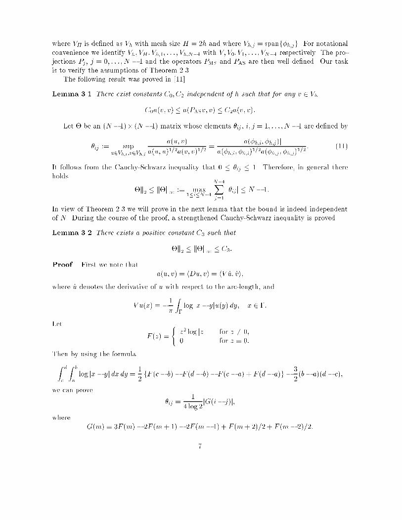
where VH is de�ned as Vh with mesh size H = 2h and where Vh;j = spanf�h;jg. For notationalconvenience we identify Vh; VH ; Vh;1; : : : ; Vh;N�1 with V; V0; V1; : : : ; VN�1 respectively. The pro-jections Pj , j = 0; : : : ; N � 1 and the operators PMS and PAS are then well de�ned. Our taskis to verify the assumptions of Theorem 2.3.The following result was proved in [11].Lemma 3.1 There exist constants C0; C2 independent of h such that for any v 2 VhC0a(v; v)� a(PASv; v) � C2a(v; v):Let � be an (N � 1)� (N � 1) matrix whose elements �ij , i; j = 1; : : : ; N � 1 are de�ned by�ij := supu2Vh;i;v2Vh;j a(u; v)a(u; u)1=2a(v; v)1=2 = ja(�h;i; �h;j)ja(�h;i; �h;i)1=2a(�h;j ; �h;j)1=2 : (11)It follows from the Cauchy-Schwarz inequality that 0 � �ij � 1. Therefore, in general thereholds k�k2 � k�k1 := max1�i�N�1N�1Xj=1 j�ij j � N � 1:In view of Theorem 2.3 we will prove in the next lemma that the bound is indeed independentof N . During the course of the proof, a strengthened Cauchy-Schwarz inequality is proved.Lemma 3.2 There exists a positive constant C3 such thatk�k2 � k�k1 � C3:Proof. First we note that a(u; v) = hDu; vi = hV _u; _vi;where _u denotes the derivative of u with respect to the arc-length, andV u(x) = � 1� Z� log jx� yju(y) dy; x 2 �:Let F (z) = ( z2 log jzj for z 6= 0;0 for z = 0:Then by using the formulaZ dc Z ba log jx� yj dx dy = 12 fF (c� b)� F (d� b)� F (c� a) + F (d� a)g � 32(b� a)(d� c);we can prove �ij = 14 log 2 jG(i� j)j;where G(m) = 3F (m)� 2F (m+ 1)� 2F (m� 1) + F (m+ 2)=2 + F (m� 2)=2:7

This implies k�k1 � 12 log 2 1Xm=0 jG(m)j;and hence it su�ces to prove that P1m=0 jG(m)j � C. To do so, we de�nef(x) = F (x + 1) + F (x � 1)� 2F (x) for any x 2 IRto obtain G(m) = 12 (f(m+ 1) + f(m� 1)� 2f(m)) :Since f 00(x) = 2 log jx2 � 1jx2 for any x 6= 0 and x 6= �1;f is a concave function on (1;1), which results in G(m) < 0 for m � 2. By the mean valuetheorem there exist � and �0 2 (0; 1) such that if � = ��0 thenjG(m)j = 12 [2f(m)� f(m+ a)� f(m� a)]= 12 �f 0(m� �)� f 0(m+ �)�= ��2 �f 00(m� �) + f 00(m+ �)�= � log (m2 � �2)2((m� 1)2 � �2)((m+ 1)2 � �2)! : (12)(For the mean value theorem argument used above, the reader is referred to [1, p. 101].) Wenote that (m2 � �2)2((m� 1)2 � �2)((m+ 1)2 � �2) = 1�1� 2m�1m2��2� �1 + 2m+1m2��2 � � 11� � 2m�1m2��2 �2 : (13)Since 2m� 1m2 � �2 � 4m < 1 when m � 6;we deduce from (12) and (13)jG(m)j � � log�1� 4m� = 1Xi=1 1i+ 1 � 4m�2i for any m � 6;which in turn yields1Xm=6 jG(m)j � 1Xm=6 1Xi=1 1i+ 1 � 4m�2i� Z 16 1Xi=1 1i+ 1 �4x�2i dx+ 1Xi=1 1i+ 1 �46�2i!8

= 1Xi=1 1i+ 1 Z 16 �4x�2i dx+ 1Xi=1 1i+ 1 �23�2i!= 6 1Xi=1 1(2i� 1)(i+ 1) �23�2i + 1Xi=1 1i+ 1 �23�2i!� 7 1Xi=1�23�i = 14:This completes the proof of the lemma. 2As a consequence we obtain, due to the abstract Theorem 2.3,Theorem 3.3 Let C0, C2, and C3 be given by Lemmas 3.1 and 3.2, and let C1 = 2maxfC2; C3g.Then for any v 2 Vh there holdskEN�1vkeH1=2(�) � �1� C0C1�1=2 kvkeH1=2(�):Remark 3.4 Due to the subspace decomposition (10) we see that this 2-level multiplicativeSchwarz algorithm corresponds to the unsymmetric 2-level multigrid algorithm using the Gau�-Seidel smoother.3.1.2 Multilevel method.We shall in this subsection design a multilevel method for the hypersingular equation. Theanalysis for this method is slightly di�erent from that of the general framework in Section 2.The main reason for this di�erence is the non-availability of a strengthened Cauchy-Schwarzinequality which can yield an estimate like Lemma 3.2.Starting with a coarse meshN 1 : �1 = x11 < x12 = 0 < x13 = 1;we divide each subinterval into two equal intervals. Hence, if hl is the meshstep of N l, l =1; : : : ; L� 1, then hl = 2hl+1. For l = 1; : : : ; L, let V l be the spline space associated with N lwhich contains continuous and piecewise-linear functions vanishing at the endpoints �1. Letn�l1; : : : ; �lNlo be the nodal basis for V l, where Nl = 2l � 1 is the dimension of V l. We thendecompose V l as V l = NlXi=1 V li ;with V li = spanf�lig for i = 1; : : : ; Nl. Eventually, V L is decomposed asV L = LXl=1 NlXi=1 V li : (14)Let Tl = NlXi=1 PV li for l = 1; : : : ; L; (15)9

where PV li : V L ! V li is de�ned for any v 2 V L bya(PV li v; w) = a(v; w) for all w 2 V li ;and let E := LYl=1(I � Tl):The multilevel multiplicative Schwarz operator is now de�ned asPMS = I � E:Analogously, we de�ne PAS = LXl=1 Tl:Letting E0 := I and El := (I � Tl)El�1; l = 1; : : : ; L;we deduce El�1 � El = TlEl�1;which in turn yields I � El = lXk=1TkEk�1; l = 1; : : : ; L: (16)The following lemma follows easily in the same manner as Lemma 2.1.Lemma 3.5 For any v 2 V LLXl=0 a(TlEl�1v; El�1v) � a(v; v)� a(El�1v; El�1v):The following two lemmas were proved in [11]:Lemma 3.6 There exists a positive constant C0 independent of h and L such that for anyv 2 V L there holds a(v; v)� C�10 a(PASv; v):Lemma 3.7 There exist constants C1 > 0 and 2 (0; 1) such that for any v 2 V k where1 � k � l � L there holds a(Tlv; v) � C1 2(l�k)a(v; v):The above lemma plays the role of Lemma 3.2 in the analysis of the multilevel method. Wealso need the following technical lemma:Lemma 3.8 For any k = 1; : : : ; L and v 2 V L there holdsa(Tkv; Tkv) � C1a(Tkv; v);where C1 is the constant given by Lemma 3.7.10

Proof. By using the Cauchy-Schwarz inequality for the symmetric and positive-de�nitebilinear form a(Tk�; �), and Lemma 3.7 we obtaina(Tkv; Tkv) � a(Tkv; v)1=2a(TkTkv; Tkv)1=2 � C1=21 a(Tkv; v)1=2a(Tkv; Tkv)1=2;which implies a(Tkv; Tkv)1=2 � C1=21 a(Tkv; v)1=2:The lemma is proved. 2Theorem 3.9 Let C0, C1, and be given by Lemmas 3.6 and 3.7. Then for any v 2 V LkEvkeH1=2(�) � (1� 1=C2)1=2kvkeH1=2(�);where C2 := 2C�10 1 + C21 2(1� )2! :Proof. The theorem is proved if we can prove thata(v; v)� C2 (a(v; v)� a(Ev;Ev)) for v 2 V L:By Lemma 3.5 it su�ces to provea(v; v)� C2 LXk=1 a(TkEk�1v; Ek�1v) for v 2 V L: (17)We have from Lemma 3.6, the Cauchy-Schwarz inequality, the inequality 2ab � a2 + b2, notingthat E0 = I ,a(v; v) � C�10 LXl=1 a(Tlv; v)= C�10 LXl=1 �a(TlEl�1v; El�1v) + a(Tl(I � El�1)v; (I �El�1)v)+ 2 a(Tl(I �El�1)v; El�1v)�� 2C�10 LXl=1 a(TlEl�1v; El�1v) + LXl=2 a(Tl(I � El�1)v; (I � El�1)v)!= 2C�10 LXl=1 a(TlEl�1v; El�1v) +A! : (18)Let S =P1j=0 j = 1=(1� ). It follows successively from (16), the Cauchy-Schwarz inequality,Lemmas 3.7 and 3.8 thatA = LXl=2 l�1Xk=1 l�1Xm=1a(TlTkEk�1v; TmEm�1v)11

� LXl=2 l�1Xk=1 l�1Xm=1a(TlTkEk�1v; TkEk�1v)1=2a(TlTmEm�1v; TmEm�1v)1=2� C12 LXl=2 l�1Xk=1 l�1Xm=1 2l�k�m�a(TkEk�1v; TkEk�1v) + a(TmEm�1v; TmEm�1v)�= C1 LXl=2 l�1Xk=1 l�1Xm=1 2l�k�ma(TkEk�1v; TkEk�1v)� C21 LXl=2 l�1Xk=1 l�1Xm=1 2l�k�ma(TkEk�1v; Ek�1v)� C21 S LXl=2 l�1Xk=1 l�ka(TkEk�1v; Ek�1v)= C21 S L�1Xk=1 LXl=k+1 l�ka(TkEk�1v; Ek�1v)� C21 2S2 L�1Xk=1 a(TkEk�1v; Ek�1v): (19)Inequalities (18) and (19) yield (17) and theorem is proved. 2Remark 3.10 Due to the subspace decomposition (14) this multilevel multiplicative Schwarzalgorithm corresponds to the unsymmetric multigrid algorithm using the Jacobi-smoother.3.2 The p-version.We shall in this subsection design a multiplicative method for the p-version of the Galerkinboundary element method applied to the hypersingular integral equation.We de�ne on the mesh (8) the space V p of continuous functions on � whose restrictionson �j := (xj�1; xj), j = 1; : : : ; N , are polynomials of degree at most p, p � 1. In order toguarantee that these functions belong to eH1=2(�), we also require that the functions vanish atthe endpoints �1 of �. For the p-version of the Galerkin scheme, we approximate the solutionof (7) by functions in V p and increase the accuracy of the approximation not by reducing h(which is �xed) but by increasing p. More explicitly, the p-version boundary element methodfor Equation (7) reads as:Find u�p 2 V p such that a(u�p; vp) = hf; vpi for any vp 2 V p: (20)The stability and convergence of the scheme (20) was proved in [9]. Note that the dimension ofV p is dim V p = pN � 1. Choosing a basis for V p, we derive from (20) a system of equations tobe solved for u�p. In practice, we use the following basis. Let �k , k = 1; : : : ; N � 1, be de�nedas hat functions satisfying �k(xl) = ( 1 if k = l;0 if k 6= l:12

For q = 2; : : : ; p and j = 1; : : : ; N we also de�ne Lq;j as the a�ne image onto �j ofLq(x) = Z x�1 Lq�1(s) ds;where Lq�1 is the Legendre polynomial of degree q � 1. We extend Lq;j by 0 outside �j . It isclear that B = f�1; : : : ; �N�1;L2;1; : : : ;L2;N ; : : : ;Lp;1; : : : ;Lp;Ngis a basis for V p. Solving the equation (20) amounts to solvingAN N = fN ; (21)where the matrix AN has entries a(v; w) with v; w 2 B. The condition number of (21) growsat least like p2 and at most like p3. We will de�ne a multiplicative Schwarz method to solveinstead of (21) a preconditioned system which has condition number growing signi�cantly slowerthan p2.We decompose V p as a direct sumV p = V0 � V p1 � � � � � V pN ; (22)where V0 := spanf�1; : : : ; �N�1g;the space of continuous piecewise-linear functions on � vanishing at �1, andV pj := spanfL2;j ; : : : ;Lp;jg for j = 1; : : : ; N: (23)The space V0 serves the same purpose as the coarse grid space in the h-version. We note thatfunctions in V pj are supported in ��j .With the projections Pj appropriately de�ned as in Section 2, we can de�ne the multiplica-tive and additive Schwarz operators asPMS = I � EN and PAS = NXj=0Pj ;where EN = (I � P0)(I � P1) � � �(I � PN):Analogously to Lemma 3.1, we haveLemma 3.11 [10] There exist constants C0; C2 independent of p and N such that for anyv 2 V p there holds C0(1 + log2 p)a(v; v)� a(PASv; v) � C2a(v; v):Our next task is to show a strengthened Cauchy-Schwarz inequality for this version.13

Lemma 3.12 Let V pi be de�ned as in (23) and let�ij := supu2V pi ;v2V pj a(u; v)a(u; u)1=2a(v; v)1=2 ; i; j = 1; : : : ; N:Then there exists a constant C independent of i; j; p such that�ij � C(ji� jj+ 1)2 :If � = f�ijg1�i;j�N , then there holds k�k2 � C3;where C3 = C�2=3.Proof. Let u =Ppk=2 ukLk;i and v =Ppl=2 vlLl;j . Then we havea(u; v) = pXk=2 pXl=2 ukvlhDLk;i;Ll;jiL2(�j)= pXk=2 pXl=2 ukvl 2j�ij 2j�j j hV Lk�1;i; Ll�1;jiL2(�j): (24)Due to Lemma A.6 (compare with [5, Lemma 1]) we have with j�ij = j�j j = h and dist(�i;�j) =h(ji� jj � 1), i 6= j,hV Lk�1;i; Ll�1;jiL2(�j) � C j�ij j�jjmax(j�ij=2; j�jj=2)k+l�2dist(�i;�j)k+l�2p(2k � 1)(2l� 1)= C h2(1=2)k+l�2(ji� jj � 1)k+l�2p(2k � 1)(2l� 1)� C h2(k� 1)(l� 1)(ji� jj � 1)k+l�2p(2k � 1)(2l� 1) : (25)From (24) and (25) we obtainja(u; v)j � C pXk=2 pXl=2 jukj jvlj(k� 1)(l� 1)(ji� jj � 1)k+l�2p(2k � 1)(2l� 1)= C pXk=2 pXl=2 jukj(k� 1)p2k � 1 jvlj(l � 1)p2l � 1 1(ji� jj � 1)k+l�2� C0@ pXk=2 jukj(k � 1)p2k � 1!21A1=20@ pXl=2 jvlj(l� 1)p2l� 1!21A1=2 �� � 1(ji� jj � 1)k+l�2�k;l=2;:::;p 2 : (26)14

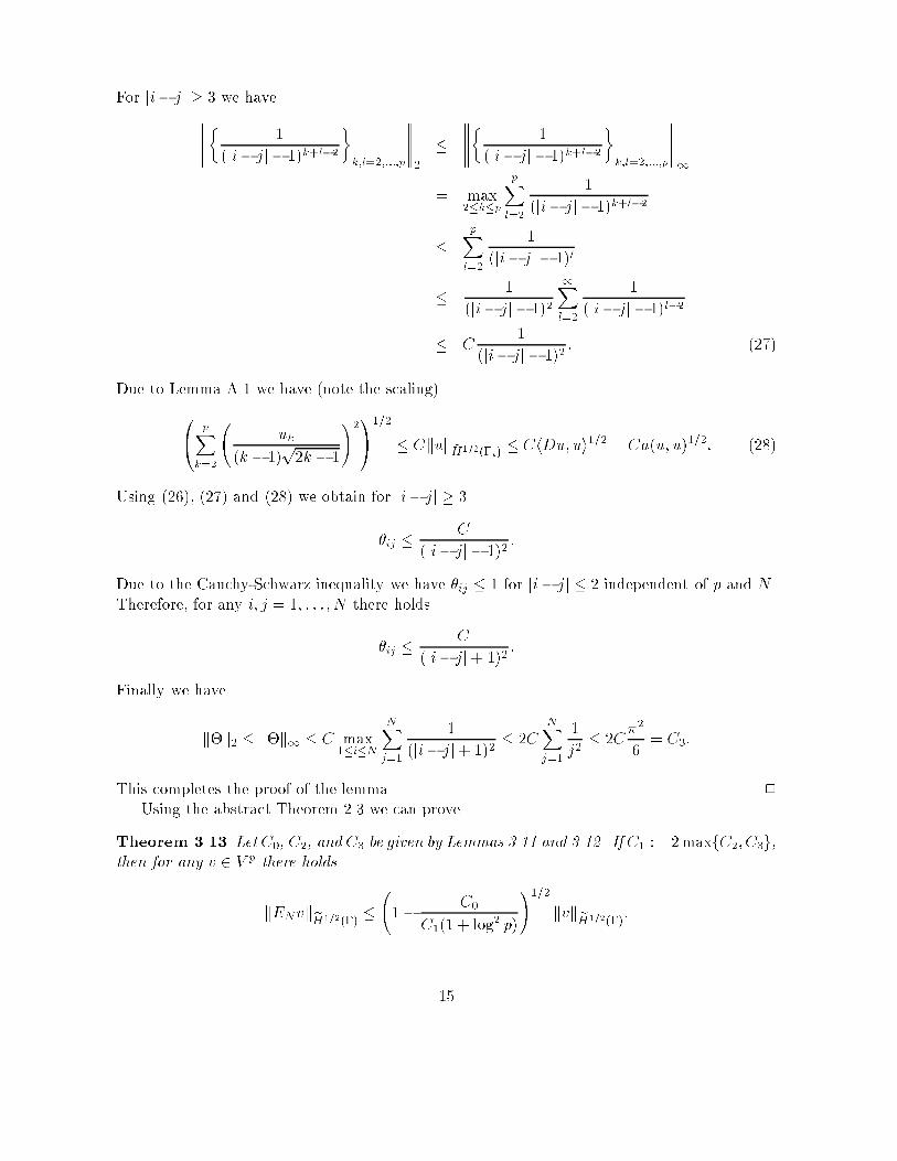
For ji� jj � 3 we have � 1(ji� jj � 1)k+l�2�k;l=2;:::;p 2 � � 1(ji� jj � 1)k+l�2�k;l=2;:::;p 1= max2�k�p pXl=2 1(ji� jj � 1)k+l�2� pXl=2 1(ji� jj � 1)l� 1(ji� jj � 1)2 1Xl=2 1(ji� jj � 1)l�2� C 1(ji� jj � 1)2 : (27)Due to Lemma A.1 we have (note the scaling)0@ pXk=2 jukj(k � 1)p2k � 1!21A1=2 � Ckuk ~H1=2(�i) � ChDu; ui1=2 = Ca(u; u)1=2: (28)Using (26), (27) and (28) we obtain for ji� jj � 3�ij � C(ji� jj � 1)2 :Due to the Cauchy-Schwarz inequality we have �ij � 1 for ji� jj � 2 independent of p and N .Therefore, for any i; j = 1; : : : ; N there holds�ij � C(ji� jj+ 1)2 :Finally we havek�k2 � k�k1 � C max1�i�N NXj=1 1(ji� jj+ 1)2 � 2C NXj=1 1j2 � 2C�26 = C3:This completes the proof of the lemma. 2Using the abstract Theorem 2.3 we can proveTheorem 3.13 Let C0, C2, and C3 be given by Lemmas 3.11 and 3.12. If C1 := 2maxfC2; C3g,then for any v 2 V p there holdskENvkeH1=2(�) � 1� C0C1(1 + log2 p)!1=2 kvkeH1=2(�):15

4 A multiplicative method for the weakly singular integral equa-tion.We shall now in this section design a multiplicative algorithm for the p-version Galerkin methodapplied to the weakly integral equation of the formV u(x) := � 1� Z� log jx� yj u(y) dsy = f(x); x 2 � = (�1; 1): (29)As was shown in [4], V is continuous and invertible from eH�1=2(�) toH1=2(�). Here the Sobolevspace H1=2(�) is de�ned as the space of functions which are traces of functions in H1loc(IR2) andeH�1=2(�) is its dual. It is known that there exists a constant > 0 such thathV v; vi � kvk2eH�1=2(�);where h�; �i denotes the L2 duality on �. Hence V de�nes a continuous, symmetric and positive-de�nite bilinear form a(v; w) = hV v; wi for v; w 2 eH�1=2(�). We de�ne on the mesh (8)the space �V p of piecewise continuous functions on � whose restrictions on �j := (xj�1; xj),j = 1; : : : ; N , are polynomials of degree at most p, p � 1. For the p-version of the Galerkinscheme, we approximate the solution of (29) by functions in �V p and increase the accuracy ofthe approximation not by reducing h (which is �xed) but by increasing p. More explicitly, thep-version boundary element method for Equation (29) reads as:Find u�p 2 �V p such that a(u�p; vp) = hf; vpi for any vp 2 �V p: (30)The stability and convergence of the scheme (30) was proved in [9]. Note that the dimension of�V p is dim �V p = (p+ 1)N . Choosing a basis for �V p, we derive from (30) a system of equationsto be solved for u�p. In practice, we use the following basis. Let �k , k = 1; : : : ; N , be de�ned aspiecewise constant functions satisfying�k(x) = ( 1 if x 2 (xk�1; xk);0 otherwise:For q = 1; : : : ; p and j = 1; : : : ; N we also de�ne Lq;j as the a�ne image onto �j of the Legendrepolynomial Lq of degree q. We extend Lq;j by 0 outside �j . It is clear thatB = f�1; : : : ; �N ; L1;1; : : : ; L1;N ; : : : ; Lp;1; : : : ; Lp;Ngis a basis for �V p. Solving the equation (30) amounts to solvingAN N = fN ; (31)where the matrix AN has entries a(v; w) with v; w 2 B. The condition number of (31) grows atleast like p2 and at most like p3. We will de�ne a multiplicative Schwarz method to solve insteadof (31) a preconditioned system which has condition number growing signi�cantly slower thanp2. 16

We decompose �V p as a direct sum�V p = �V0 � �V p1 � � � � � �V pN ; (32)where �V0 := spanf�1; : : : ; �Ng;the space of piecewise constant functions on �, and�V pj := spanfL1;j; : : : ; Lp;jg for j = 1; : : : ; N: (33)The space �V0 serves the same purpose as the coarse grid space in the h-version. We note thatfunctions in �V pj are supported in ��j .With the projections Pj de�ned appropriately as in Section 2 we can de�ne the multiplicativeand additive Schwarz operators asPMS = I � EN and PAS = NXj=0Pj ;where EN = (I � P0)(I � P1) � � �(I � PN):Similarly to Lemma 3.11, we haveLemma 4.1 [10] There exist constants C0 and C2 independent of p and N such that for anyv 2 �V p there holds C0(1 + log2 p)a(v; v)� a(PASv; v) � C2a(v; v):Again our next task is to prove a strengthened Cauchy-Schwarz inequality.Lemma 4.2 Let �V pi be de�ned as in (33), and let�ij := supu2�V pi ;v2�V pj a(u; v)a(u; u)1=2a(v; v)1=2 :Then, if 0 < h � 1, there exists a constant C independent of i; j; p such that�ij � C(ji� jj+ 1)2 :Moreover, if � = f�ijg1�i;j�N , then k�k2 � C3;where C3 := C�2=3. 17

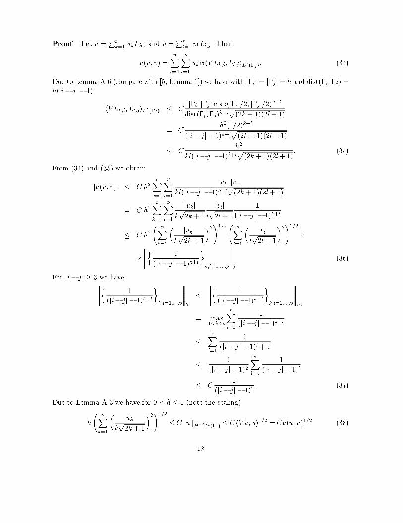
Proof. Let u =Ppk=1 ukLk;i and v =Ppl=1 vkLl;j . Thena(u; v) = pXk=1 pXl=1 ukvlhV Lk;i; Ll;jiL2(�j): (34)Due to Lemma A.6 (compare with [5, Lemma 1]) we have with j�ij = j�j j = h and dist(�i;�j) =h(ji� jj � 1) hV Lk;i; Ll;jiL2(�j) � C j�ij j�jjmax(j�ij=2; j�jj=2)k+ldist(�i;�j)k+lp(2k + 1)(2l+ 1)= C h2(1=2)k+l(ji� jj � 1)k+lp(2k + 1)(2l+ 1)� C h2kl(ji� jj � 1)k+lp(2k+ 1)(2l+ 1) : (35)From (34) and (35) we obtainja(u; v)j � C h2 pXk=1 pXl=1 jukj jvljkl(ji� jj � 1)k+lp(2k+ 1)(2l+ 1)= C h2 pXk=1 pXl=1 jukjkp2k+ 1 jvljlp2l+ 1 1(ji� jj � 1)k+l� C h2 pXk=1� jukjkp2k + 1�2!1=2 pXl=1 � jvljlp2l + 1�2!1=2 �� � 1(ji� jj � 1)k+l�k;l=1;:::;p 2 (36)For ji� jj � 3 we have � 1(ji� jj � 1)k+l�k;l=1;:::;p 2 � � 1(ji� jj � 1)k+l�k;l=1;:::;p 1= max1�k�p pXl=1 1(ji� jj � 1)k+l� pXl=1 1(ji� jj � 1)l + 1� 1(ji� jj � 1)2 1Xl=0 1(ji� jj � 1)l� C 1(ji� jj � 1)2 : (37)Due to Lemma A.3 we have for 0 < h � 1 (note the scaling)h pXk=1� jukjkp2k + 1�2!1=2 � Ckuk ~H�1=2(�i) � ChV u; ui1=2 = Ca(u; u)1=2: (38)18

Using (36), (37) and (38) we obtain for ji� jj � 3�ij � C(ji� jj � 1)2 :Due to the Cauchy-Schwarz inequality we have �ij � 1 for ji� jj � 2 independent of p and N .Therefore, for any i; j = 1; : : : ; N there holds�ij � C(ji� jj+ 1)2 :Finally we havek�k2 � k�k1 � C max1�i�N NXj=1 1(ji� jj+ 1)2 � 2C NXj=1 1j2 � 2C�26 = C3:This completes the proof of the lemma. 2Using the abstract Theorem 2.3 we can proveTheorem 4.3 Let C0, C2, and C3 be given by Lemmas 4.1 and 4.2. If C1 := 2maxfC2; C3g,then for any v 2 �V p there holdskENvkeH�1=2(�) � 1� C0C1(1 + log2 p)!1=2 kvkeH�1=2(�):5 Numerical results.We consider the hypersingular integral equation (7) with the right hand side f(x) � 1. Wesolve the Galerkin equations (20) for the p-version by the multiplicative Schwarz algorithm,for di�erent subspace decompositions and observe the expected behavior of the convergencerate with respect to N and p (see Tab. 1). For the h-version we note the considerably lowercontraction rates of the 2-level method compared with the multilevel method in Tab. 3. But ifwe take into account the high costs of solving a system of mesh width H = 2h in each iterationstep we see that the multilevel method is the far superior method.Analogously we consider the weakly singular integral equation (29) with the right hand sidef(x) � 1. We solve the Galerkin equations (30) for the p-version by the multiplicative Schwarzalgorithm. The numerical results in Tab. 2 show the expected behavior of the convergence rate.In the case of the h-version we observe that the elements of the Galerkin matrixaij = a(�h;i; �h;j) = hD�h;i; �h;ji = � 1� Z xh;j+1xh;j�1 f:p: Z xh;i+1xh;i�1 �h;i(y)�h;j(x)jx� yj2 dsy dsx =: ai�jdepend only on the di�erence i� j for an uniform mesh. Therefore we can reduce the memoryused to store the Galerkin matrix from O(N2) to O(N). In a more general case we have to usea clustering or multipole technique to reduce the amount of memory needed. This also reducesthe amount of time for computing the Galerkin matrix. On a vectorcomputer SNI VPP 300/4we have achieved a performance of 1000 MFlops/s.19

In the case of the p-version we calculate the elements of the Galerkin matrix analytically.Due to the smaller size of the Galerkin matrix we can store the full matrix in the main memory.We have to note that our subspace decomposition in this case is actually a reordering of thebasis functions. Therefore the projections involved are simply�ed considerably.Contraction ratep N=2 N=4 N=8 N=162 0.2156 0.2974 0.3763 0.39653 0.3807 0.4005 0.4198 0.42564 0.4516 0.4908 0.5274 0.53795 0.5116 0.5297 0.5475 0.55296 0.5483 0.5744 0.6001 0.60757 0.5807 0.5964 0.6121 0.61698 0.6036 0.6238 0.6442 0.65029 0.6245 0.6383 0.652410 0.6405 0.6572 0.6745Table 1: Hypersingular integral equation, p-versionContraction ratep N=2 N=4 N=8 N=161 0.2056 0.3119 0.3765 0.39672 0.3794 0.4014 0.4198 0.42563 0.4502 0.4927 0.5274 0.53784 0.5109 0.5302 0.5475 0.55295 0.5476 0.5752 0.6001 0.60756 0.5802 0.5967 0.6121 0.61697 0.6032 0.6243 0.6442 0.65028 0.6241 0.6386 0.65249 0.6401 0.6576 0.674510 0.6550 0.6680Table 2: Weakly singular integral equation, p-versionA AppendixLemma A.1 Let I = (�1; 1) and u = Ppk=2 ukLk, 2 � p. Then there exists a constant C20

Contraction rateN 2-level multilevel3 0.0470531 0.16034397 0.0926110 0.240196515 0.1011592 0.248805931 0.1036045 0.252970163 0.1062307 0.2541706127 0.1078721 0.2544758255 0.1088143 0.2545517511 0.1093568 0.25457061023 0.1096628 0.2545753Table 3: Contraction rates for the hypersingular integral equation, h-versionindependent of u and p such that kuk2~H1=2(I) � C pXk=2u2k 1k3 :Proof. From the de�nition of the interpolation norm k � k ~H1=2(I) by the real K-method [2] wehave kuk2~H1=2(I) = kuk2[L2(I);H10(I)]1=2 = Z 10 �t�1=2 infu=v+w(kvkL2(I) + tkwkH10 (I))�2 dtt : (39)We have u =Ppk=2 ukLk 2 H10(I). Therefore u = v+w with w 2 H10(I) implies also v 2 H10(I).Therefore it is su�cient to take the in�mum in H10(I).kuk2~H1=2(I) = Z 10 t�2 infv2H10 (I)(kvkL2(I) + tku � vkH10(I))!2 dt: (40)Due to v 2 H10(I) we can expand v also in antiderivatives of Legendre polynomialsv = 1Xk=2 vkLk:For the norms in (40) there holdku� vk2H10(I) � pXk=2(uk � vk)Lk�1 + Xk 6=2;:::;p vkLk�1 2L2(I)= pXk=2(uk � vk)2 22k � 1 + Xk 6=2;:::;p v2k 22k � 1 ; (41)21

and, due to Lemma A.2, kvk2L2(I) � C 1Xk=2 v2kk�5: (42)Letl�2 = ((vk) : 1Xk=2 v2k2k � 1 <1) and l02 = f(vk) 2 l�2 : vk = 0 if k 6= 2; : : : ; pg � IRp�1:Using the the monotonicity of the square function and the inequality a2 + b2 � (a + b)2 whena; b � 0 we obtain from (40), (41), and (42)kuk2~H1=2(I) = Z 10 t�2 infv2H10 (I)(kvkL2(I) + tku� vkH10(I))!2 dt= Z 10 t�2 infv2H10(I)�kvkL2(I) + tku � vkH10(I)�2 dt� Z 10 t�2 infv2H10(I)�kvk2L2(I) + t2ku� vk2H10(I)� dt� Z 10 t�2 inf(vk)2l�2 C 1Xk=2 v2kk�5 + t2 pXk=2(uk � vk)2 22k � 1 + t2 Xk 6=2;:::;p v2k 22k � 1!dt= Z 10 t�2 inf(vk)2l02 C pXk=2 v2kk�5 + t2 pXk=2(uk � vk)2 22k � 1!dt= Z 10 t�2 pXk=2 infvk2IR�Cv2kk�5 + t2(uk � vk)2 22k � 1� dt: (43)Note that if f(x) = ax2 + b(x� c)2 then minx2IR f(x) = f( bca+b) = c2 aba+b . Therefore we obtainfrom equation (43)kuk2~H1=2(I) � Z 10 t�2 pXk=2 infvk2IR�Cv2kk�5 + t2(uk � vk)2 22k � 1� dt= Z 10 t�2 pXk=2 u2k t2Ck�5 22k�1Ck�5 + t2 22k�1 dt= pXk=2 u2k Z 10 Ck�5 22k�1Ck�5 + t2 22k�1 dt= pXk=2 u2k �2sCk�5 22k � 1� C pXk=2 u2kk�3: (44)This completes the proof. 222

Lemma A.2 Let I = (�1; 1) and v =P1k=2 vkLk. Then there holdskvk2L2(I) � C 1Xk=2 v2k 1k5 :Proof. With the normalized antiderivatives of Legendre polynomials de�ned by L�k =Lk=kLkkL2(I), there holds due to the proof of [6, Lemma 3.1]kvk2L2(I) = 1Xk=2 vkkLkkL2(I)L�k 2L2(I) � C 1Xk=2 v2kk�2kLkk2L2(I):Due to kLkk2L2(I) = 12k � 1(Lk � Lk�2) 2L2(I)= 1(2k� 1)2 � 22k + 1 + 22k� 3�= 4(2k+ 1)(2k� 1)(2k� 3) � Ck3 (k � 2) (45)there holds kvk2L2(I) � C 1Xk=2 v2k 1k5 :This completes the proof. 2Lemma A.3 Let u(x) = Ppk=1 ukLk(x=h). Then there exists a constant C independent of u,h and p such that kuk2~H�1=2(�h;h) � C min(h; h2) pXk=1 u2k 1k3 :Proof. Due to ~H�1=2(�h; h) = (H1=2(�h; h))0 we havekuk ~H�1=2(�h;h) = supv2H1=2(�h;h) (u; v)kvkH1=2(�h;h) :For v(x) =Ppk=1 vkLk(x=h) with vk = uk=k2 there holdskuk ~H�1=2(�h;h) � (u; v)kvkH1=2(�h;h) = hPpk=1 u2k 1k2 22k+1kvkH1=2(�h;h) :Due to Lemma A.4 we havekvk2H1=2(�h;h) � Cmax(1; h) pXk=1 v2k k = Cmax(1; h) pXk=1 u2k 1k3 :This completes the the proof. 223

Lemma A.4 Let v(x) =Ppk=1 vkLk(x=h). Then there exists a constant C independent of v, hand p such that kvk2H1=2(�h;h) � Cmax(1; h) pXk=1 v2k k:Proof. Let I = (�1; 1). From the de�nition of the interpolation norm k � kH1=2(�h;h) by thereal K-method [2] we havekvk2H1=2(�h;h) = kvk2[L2(�h;h);H1(�h;h)]1=2 = Z 10 �t�1=2 infv=w+a(kwkL2(�h;h) + tkakH1(�h;h))�2 dtt :(46)With w(x) =Ppk=1 wkLk(x=h) we havekvk2H1=2(�h;h) � Z 10 �t�1=2 infw (kwkL2(�h;h) + tkv � wkH1(�h;h))�2 dtt� 2 Z 10 t�2 infw (kwk2L2(�h;h) + t2kv � wk2H1(�h;h)) dt:With ~v =Ppk=1 vkLk, ~w =Ppk=1 wkLk we obtainkvk2H1=2(�h;h) � 2 Z 10 t�2 infw (kwk2L2(�h;h) + t2kv � wk2H1(�h;h)) dt= 2 Z 10 t�2 infw (hk ~wk2L2(I) + t2 �1hk~v0 � ~w0k2L2(I) + hk~v � ~wk2L2(I)�) dt� 2 Z 10 t�2 infw (hk ~wk2L2(I) + t2max(h; 1h )k~v � ~wk2H1(I)) dt: (47)By the orthogonality property of the Legendre polynomials we havek ~wkL2(I) = pXk=1w2k 22k + 1 :On the other handk~v0 � ~w0k2L2(I) = k pXk=1(vk � wk)L0kk2L2(I)= pXk=1 pXm=1(vk � wk)(vm � wm)(L0k; L0m)= pXk=1 pXm=1 k3=2(vk � wk)m3=2(vm � wm)(L0k; L0m)k�3=2m�3=2� pXk=1(vk � wk)2k3!1=2 f(L0k; L0m)k�3=2m�3=2gk;m=1;:::;p 2 pXm=1(vm � wm)2m3!1=2= f(L0k; L0m)k�3=2m�3=2gk;m=1;:::;p 2 pXk=1(vk � wk)2k3: (48)24

It follows from the de�nition of matrix norms that f(L0k; L0m)k�3=2m�3=2gk;m=1;:::;p 2 � f(L0k; L0m)k�3=2m�3=2gk;m=1;:::;p 1= max1�k�p k�3=2 pXm=1(L0k; L0m)m�3=2! : (49)Lemma A.5 and a straightforward calculation givek�3=2 pXm=1(L0k; L0m)m�3=2 == k�3=2 pXm=1m�3=22 [(k�1)=2]Xl=0 [(m�1)=2]Xn=0 (2(m� 2n)� 1)�k�1�2l;m�1�2n� k�3=2 pXm=1m�3=22 k�1Xl=0 m�1Xn=0(2(m� n)� 1)�k�1�l;m�1�n= k�3=2 pXm=1m�3=22 k�1Xl=0 m�1Xn=0(2n+ 1)�l;n= k�3=22 k�1Xl=0(2l+ 1) pXm=1m�3=2m�1Xn=0 �l;n= k�3=22 k�1Xl=0(2l+ 1) pXm=l+1m�3=2� k�3=22 k�1Xl=0(2l+ 1) Z pm=l+1m�3=2 dm� k�3=22 k�1Xl=0(2l+ 1)(l+ 1)�1=2=2� k�3=22 k�1Xl=0(l + 1)1=2� 2: (50)Inequalities (48), (49), and (50) yieldk~v0 � ~w0k2L2(I) � 2 pXk=1(vk � wk)2k3:This inequality and (47) implykvk2H1=2(�h;h) �� 2 Z 10 t�2 infwk h pXk=1w2k 22k + 1 + t2max(h; 1h) pXk=1(vk � wk)2� 22k + 1 + 2k3�!dt25

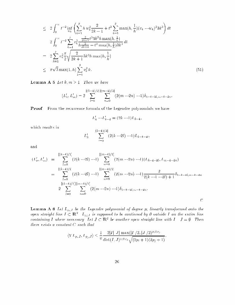
� 2 Z 10 t�2 infwk pXk=1 hw2k 22k + 1 + t2 pXk=1max(h; 1h)(vk � wk)23k3! dt= 2 Z 10 t�2 pXk=1 v2k 22k+1 t23k3hmax(h; 1h)h 22k+1 + t2max(h; 1h )3k3 dt= 2 pXk=1 v2k �2s 22k + 13k3hmax(h; 1h)� �p3max(1; h) pXk=1 v2k k: (51)Lemma A.5 Let k;m � 1. Then we have(L0k; L0m) = 2 [(k�1)=2]Xl=0 [(m�1)=2]Xn=0 (2(m� 2n)� 1)�k�1�2l;m�1�2n:Proof. From the recurrence formula of the Legendre polynomials we haveL0k � L0k�2 = (2k� 1)Lk�1;which results in L0k = [(k�1)=2]Xl=0 (2(k� 2l)� 1)Lk�1�2l;and(L0k; L0m) = [(k�1)=2]Xl=0 (2(k� 2l)� 1) [(m�1)=2]Xn=0 (2(m� 2n)� 1)(Lk�1�2l; Lm�1�2n)= [(k�1)=2]Xl=0 (2(k� 2l)� 1) [(m�1)=2]Xn=0 (2(m� 2n)� 1) 22(k� 1� 2l) + 1�k�1�2l;m�1�2n= 2 [(k�1)=2]Xl=0 [(m�1)=2]Xn=0 (2(m� 2n)� 1)�k�1�2l;m�1�2n: 2Lemma A.6 Let Lpi;I be the Legendre polynomial of degree pi linearly transformed onto theopen straight line I � IR2. Lpi;I is supposed to be continued by 0 outside I on the entire linecontaining I where necessary. Let J � IR2 be another open straight line with �I \ �J = ;. Thenthere exists a constant C such thathV Lpi;I ; Lpj;J i � 1� 2jI j jJ j max(jI j=2; jJ j=2)pi+pjdist(I; J)pi+pjq(2pi + 1)(2pj + 1) :26

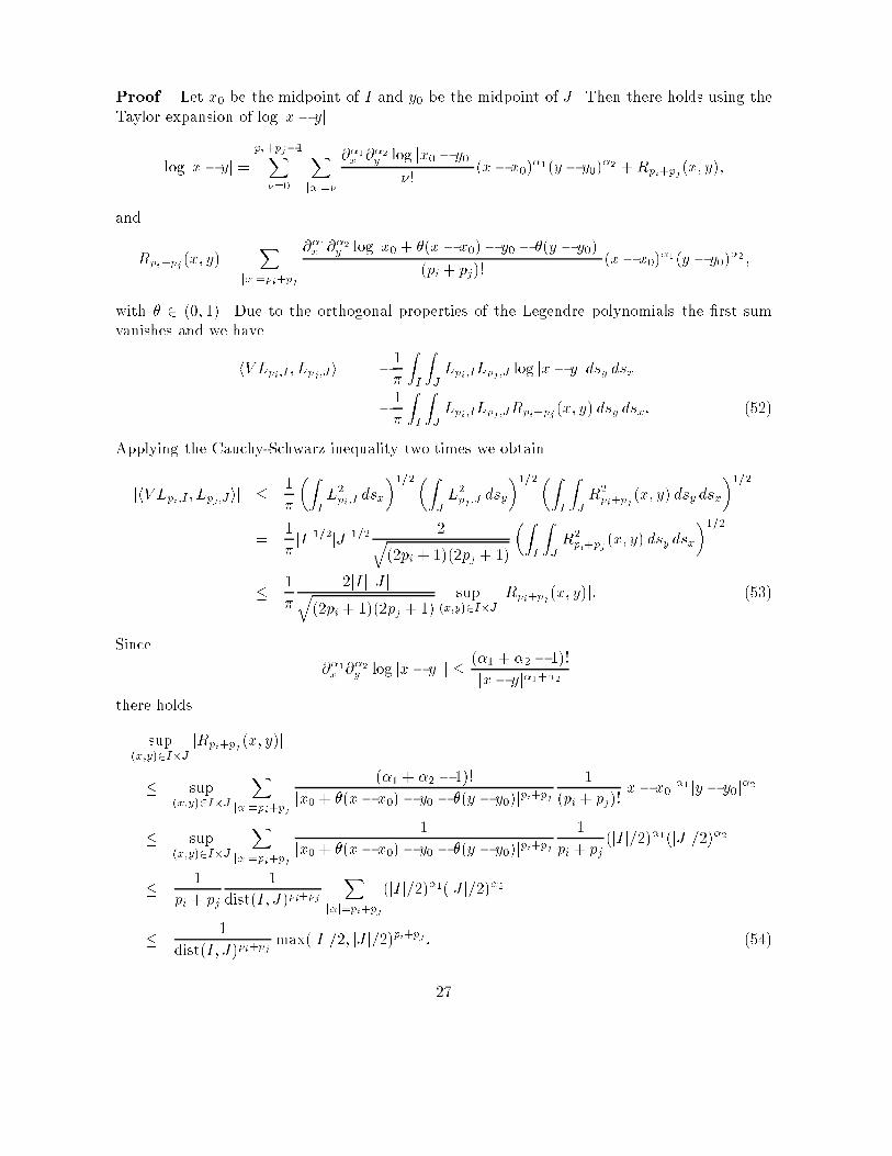
Proof. Let x0 be the midpoint of I and y0 be the midpoint of J . Then there holds using theTaylor expansion of log jx� yjlog jx� yj = pi+pj�1X�=0 Xj�j=� @�1x @�2y log jx0 � y0j�! (x� x0)�1(y � y0)�2 +Rpi+pj(x; y);andRpi+pj(x; y) = Xj�j=pi+pj @�1x @�2y log jx0 + �(x � x0)� y0 � �(y � y0)j(pi + pj)! (x� x0)�1(y � y0)�2 ;with � 2 (0; 1). Due to the orthogonal properties of the Legendre polynomials the �rst sumvanishes and we havehV Lpi;I ; Lpj;Ji = � 1� ZI ZJ Lpi;ILpj;J log jx� yj dsy dsx= � 1� ZI ZJ Lpi;ILpj;JRpi+pj(x; y) dsy dsx: (52)Applying the Cauchy-Schwarz inequality two times we obtainjhV Lpi;I ; Lpj;Jij � 1� �ZI L2pi;I dsx�1=2�ZJ L2pj ;J dsy�1=2�ZI ZJ R2pi+pj (x; y) dsy dsx�1=2= 1� jI j1=2jJ j1=2 2q(2pi + 1)(2pj + 1) �ZI ZJ R2pi+pj (x; y) dsy dsx�1=2� 1� 2jI j jJ jq(2pi + 1)(2pj + 1) sup(x;y)2I�J jRpi+pj(x; y)j: (53)Since j@�1x @�2y log jx� yj j � (�1 + �2 � 1)!jx� yj�1+�2there holdssup(x;y)2I�J jRpi+pj (x; y)j� sup(x;y)2I�J Xj�j=pi+pj (�1 + �2 � 1)!jx0 + �(x� x0)� y0 � �(y � y0)jpi+pj 1(pi + pj)! jx� x0j�1 jy � y0j�2� sup(x;y)2I�J Xj�j=pi+pj 1jx0 + �(x� x0)� y0 � �(y � y0)jpi+pj 1pi + pj (jI j=2)�1(jJ j=2)�2� 1pi + pj 1dist(I; J)pi+pj Xj�j=pi+pj(jI j=2)�1(jJ j=2)�2� 1dist(I; J)pi+pj max(jI j=2; jJ j=2)pi+pj : (54)27

Inequalities (53) and (54) implyjhV Lpi;I ; Lpj;Jij � 1� 2jI j jJ jq(2pi + 1)(2pj + 1) 1dist(I; J)pi+pj max(jI j=2; jJ j=2)pi+pj :This completes the proof. 2References[1] T. M. Apostol, Mathematical Analysis: A Modern Approach to Advanced Calculus, 1957,Addison-Wesley, Reading, Massachusetts.[2] J. Bergh, J. L�ofstr�om, Interpolation spaces, no. 223 in Grundlehren der mathematischenWissenschaften, Springer-Verlag, Berlin, 1976.[3] J. H. Bramble, J. E. Pasciak, J. Wang and J. Xu, Convergence Estimates for ProductIterative Methods with Applications to Domain Decomposition, Math. Comp. 57 (1991),1{21.[4] M. Costabel, Boundary Integral Operators on Lipschitz Domains: Elementary Results,SIAM J. Math. Anal. 19 (1988), 613{626.[5] N. Heuer, E�cient Algorithms for the p-Version of the Boundary Element Method, J.Integral Equations Appl., 8 (1996), 337{361.[6] N. Heuer, E.P. Stephan, T. Tran, A Multilevel Additive Schwarz Method for the h-p Versionof the Galerkin Boundary Element Method, Math. Comp. (to appear).[7] J. L. Lions and E. Magenes, Non-Homogeneous Boundary Value Problems and ApplicationsI, Springer-Verlag, New York, 1972.[8] T. von Petersdor� and E.P. Stephan, Multigrid Solvers and Preconditioners for First KindIntegral Equations, Numer. Meth.Part.Di�.Eqns.,8 (1992), 443{450.[9] E. P. Stephan and M. Suri, On the Convergence of the p-Version of the Boundary ElementGalerkin Method, Math. Comp. 52 (1989), 31{48.[10] E. P. Stephan and T. Tran, Additive Schwarz Algorithms for the p-Version BoundaryElement Method, Applied Mathematics Report AMR95/13, Apr. 1995, University of NewSouth Wales.[11] T. Tran and E. P. Stephan, Additive Schwarz Methods for the h-Version Boundary ElementMethod, Appl.Anal. 60 (1996) 63{84.[12] W. L. Wendland and E. P. Stephan, A Hypersingular Boundary Integral Method for Two-Dimensional Screen and Crack Problems, Arch. Rational. Mech. Anal. 112 (1990), 363{390. 28

[13] J. Xu, Iterative Methods by Space Decomposition and Subspace Correction, SIAM Review,34 (1992), 581{613.

29