Probing the spacetime fabric: from fundamental discreteness ...

SISSA–INTERNATIONAL SCHOOL FOR

ADVANCED STUDIES

DOCTORAL THESIS

Probing the spacetime fabric:from fundamental discreteness to quantum geometries

Author:Marco LETIZIA

Supervisor:Prof. Stefano LIBERATI

A thesis submitted in partial fulfillment of the requirementsfor the degree of Doctor of Philosophy

in

Astroparticle Physics

September 14, 2017

i

Declaration of AuthorshipThe research presented in this thesis was conducted in SISSA – InternationalSchool for Advanced Studies between September 2013 and August 2017.This thesis is the result of the author’s own work, except where explicit ref-erence is made to the results of others. The content of this thesis is based onthe following research papers published in refereed Journals or preprintsavailable on arxiv.org:

• R. G. Torromé, M. Letizia and S. LiberatiPhenomenology of effective geometries from quantum gravityIn: Phys. Rev. D92.12, p. 124021, arXiv: 1507.03205 [gr-qc].

• M. Letizia and S. LiberatiDeformed relativity symmetries and the local structure of spacetimeIn: Phys. Rev. D95.4, p. 046007, arXiv: 1612.03065 [gr-qc].

• A. Belenchia, M. Letizia, S. Liberati, and E. Di CasolaHigher-order theories of gravity: diagnosis, extraction and reformulation vianon-metric extra degrees of freedomIn: arXiv: 1612.07749 [gr-qc]

To be published or submitted soon:

• A. Belenchia, D. M. T. Benincasa, M. Letizia and S. LiberatiEntanglement entropy in discrete spacetimesto appear in the Classical and Quantum Gravity focus issue on theCausal Set approach to quantum gravity (early 2018).In: arXiv: 1710.xxxxx [gr-qc]

• E. Alesci, M. Letizia, S. Liberati and D. PranzettiPoymer scalar field in Loop Quantum Gravity (temporary)In preparation.

ii

SISSA–INTERNATIONAL SCHOOL FOR ADVANCED STUDIES

Abstract

Doctor of Philosophy

Probing the spacetime fabric:from fundamental discreteness to quantum geometries

by Marco LETIZIA

This thesis is devoted to the study of quantum aspects of spacetime.Specifically, it targets two frameworks: theories that predict, or have a builtin, fundamental spacetime discreteness and effective models where the de-parture from a classical spacetime emerges at intermediate scales.

The first part of this work considers the effects of the coexistence ofLorentz invariance, spacetime discreteness and nonlocality in Causal SetTheory, from the point of view of entanglement entropy. We show that,in a causal set, the entanglement entropy follows a spacetime volume lawand we investigate how to recover the area law. Furthermore, we discusshow our results are a direct consequence of the intrinsic nonlocality of thetheory.

Whether Lorentz invariance is preserved in Loop Quantum Gravity is,on the other hand, still a subject of debate. We address this theme by de-riving the equations of motion of a scalar field coupled to the quantumgeometry. We show what is the outcome of the different way fundamentaldiscreteness is achieved in this theory.

On the other end of the spectrum, models in which modifications tothe classical description of spacetime can be considered in the continuumregime at a mesoscopic scale are examined. In particular, we analyze acertain class of models in which quantum gravitational degrees of freedomare integrated out and the effective dynamics for matter is given in termsof a momentum-dependent spacetime metric. We show that some of thesecases can be embedded in a consistent geometrical framework provided byFinsler geometry.

Finally we review and compare our main results and discuss future per-spectives.

iii

Acknowledgements

You know who you are, thank you.

iv

Contents

Declaration of Authorship i

Abstract ii

Acknowledgements iii

1 Introduction 11.1 Quantum gravity phenomenology . . . . . . . . . . . . . . . 1

1.1.1 Space(time?) discreteness in quantum gravity . . . . 3Aside on entanglement entropy . . . . . . . . . . . . . 4

1.1.2 Classical limit vs continuum limit . . . . . . . . . . . 41.2 Causal Set Theory . . . . . . . . . . . . . . . . . . . . . . . . . 6

1.2.1 Kinematics . . . . . . . . . . . . . . . . . . . . . . . . . 61.2.2 Discreteness, Lorentz invariance and nonlocality . . . 71.2.3 Dynamics . . . . . . . . . . . . . . . . . . . . . . . . . 9

1.3 Loop Quantum Gravity . . . . . . . . . . . . . . . . . . . . . 101.3.1 Basics of canonical Loop Quantum Gravity . . . . . . 10

ADM formalism and Ashtekar variables . . . . . . . 10Holonomies and fluxes . . . . . . . . . . . . . . . . . . 12Kinematics . . . . . . . . . . . . . . . . . . . . . . . . . 13Area operator . . . . . . . . . . . . . . . . . . . . . . . 14

1.3.2 A symmetry-reduced model . . . . . . . . . . . . . . 151.4 Geometry and Lorentz symmetry . . . . . . . . . . . . . . . . 17

1.4.1 Doubly Special Relativity . . . . . . . . . . . . . . . . 19Aside on the Einstein and Weak Equivalence Principles 21

2 Spacetime entanglement entropy in Causal Set Theory 222.1 Introduction . . . . . . . . . . . . . . . . . . . . . . . . . . . . 222.2 Spacetime entropy . . . . . . . . . . . . . . . . . . . . . . . . 232.3 Scalar fields in causal set theory and the Sorkin–Johnston

vacuum . . . . . . . . . . . . . . . . . . . . . . . . . . . . . . . 242.3.1 Discretizing continuum Green functions . . . . . . . 252.3.2 Nonlocal wave operators on causal sets . . . . . . . . 25

2.4 Spacetime entropy in Causal Set Theory . . . . . . . . . . . . 262.4.1 The setup . . . . . . . . . . . . . . . . . . . . . . . . . 272.4.2 Premise on the spectrum of the Pauli–Jordan . . . . . 282.4.3 Spacetime entropy . . . . . . . . . . . . . . . . . . . . 28

Local Green functions . . . . . . . . . . . . . . . . . . 31Nonlocal Green functions . . . . . . . . . . . . . . . . 33Dependence on the nonlocality scale . . . . . . . . . . 34

2.4.4 The cutoff and the kernel of the Pauli–Jordan . . . . . 362.5 Summary and outlook . . . . . . . . . . . . . . . . . . . . . . 38

v

3 Polymer scalar fields in Loop Quantum Gravity 423.1 Introduction . . . . . . . . . . . . . . . . . . . . . . . . . . . . 423.2 Polymer quantization of a scalar field . . . . . . . . . . . . . 42

3.2.1 Regularization and quantization of the scalar Hamil-tonian constraint . . . . . . . . . . . . . . . . . . . . . 45

3.3 Effective dynamics . . . . . . . . . . . . . . . . . . . . . . . . 473.4 Comments . . . . . . . . . . . . . . . . . . . . . . . . . . . . . 51

4 Finsler geometry from Doubly Special Relativity 544.1 Introduction . . . . . . . . . . . . . . . . . . . . . . . . . . . . 54

4.1.1 Basics of Finsler geometry . . . . . . . . . . . . . . . . 554.1.2 The Legendre transform . . . . . . . . . . . . . . . . . 574.1.3 Geodesics, Berwald spaces and normal coordinates . 584.1.4 Derivation of Finsler geometries from modified dis-

persion relations . . . . . . . . . . . . . . . . . . . . . 594.1.5 Results for κ-Poincaré . . . . . . . . . . . . . . . . . . 60

4.2 q-de Sitter inspired Finsler spacetime . . . . . . . . . . . . . . 624.2.1 q-de Sitter . . . . . . . . . . . . . . . . . . . . . . . . . 624.2.2 Finsler spacetime from the q-de Sitter mass Casimir . 634.2.3 Christoffel symbols and geodesic equations . . . . . . 65

4.3 Conclusions and outlook . . . . . . . . . . . . . . . . . . . . . 69

5 Effective geometries from quantum gravity 715.1 Introduction . . . . . . . . . . . . . . . . . . . . . . . . . . . . 715.2 Cosmological spacetimes from quantum gravity . . . . . . . 725.3 Exact derivation of the quantum geometry . . . . . . . . . . 735.4 Dispersion relation on a quantum, cosmological spacetime . 745.5 Phenomenology of the rainbow dispersion relation . . . . . 765.6 Conclusions . . . . . . . . . . . . . . . . . . . . . . . . . . . . 78

6 Conclusions 80Outlook . . . . . . . . . . . . . . . . . . . . . . . . . . 82

Bibliography 85

A Entanglement entropy of nonlocal scalar fields via the replica trick 95A.1 The replica trick . . . . . . . . . . . . . . . . . . . . . . . . . . 95A.2 The case of the nonlocal scalar field theories from CST . . . . 96

IR and UV behavior of the entanglement entropy . . 97

B Propagation of massless particles 99

vi

List of Figures

1.1 Sprinkling in 2D Minkowski diamond. . . . . . . . . . . . . . 71.2 Cartoon illustrating the nonlocality of causal sets. . . . . . . 8

2.1 Inner and outer diamonds for a sprinkling in 2D Minkowski. 272.2 Spectrum of i∆ for the local and nonlocal models in D = 2. . 29

(a) σi∆ in two dimensions for the local Green function. . . 29(b) σi∆ in two dimensions for the nonlocal Green function. 29

2.3 Spacetime volume law. . . . . . . . . . . . . . . . . . . . . . . 30(a) Spacetime volume law for the local theory in two di-

mensions. . . . . . . . . . . . . . . . . . . . . . . . . . . 30(b) Spacetime volume law for the local theory in two di-

mensions. . . . . . . . . . . . . . . . . . . . . . . . . . . 302.4 σi∆ for the local model in D = 3. . . . . . . . . . . . . . . . . 312.5 Area law for the local theory in D = 2. . . . . . . . . . . . . . 32

(a) Log law, local theory D = 2. . . . . . . . . . . . . . . . . 32(b) Log law, local theory D = 2 detail. . . . . . . . . . . . . 32

2.6 Local theory in D = 3. Plots of the cutoff on σi∆ and theassociated SEE. . . . . . . . . . . . . . . . . . . . . . . . . . . 32(a) σi∆, local theory D = 3 with a = 5−1. . . . . . . . . . . 32(b) SEE, local theory D = 3 with a = 5−1. . . . . . . . . . . 32(c) σi∆, local theory D = 3 with a = 10−1.. . . . . . . . . . 32(d) SEE, local theory D = 3 with a = 10−1. . . . . . . . . . 32(e) σi∆, local theory D = 3 with a = 50−1.. . . . . . . . . . 32(f) SEE, local theory D = 3 with a = 50−1. . . . . . . . . . 32

2.7 Local theory in D = 4. Plots of the cutoff on σi∆ and theassociated SEE. . . . . . . . . . . . . . . . . . . . . . . . . . . 33(a) σi∆, local theory D = 4 with a = 4−1. . . . . . . . . . . 33(b) SEE, local theory D = 4 with a = 4−1. . . . . . . . . . . 33

2.8 Nonlocal theory in D = 2. Plots of the cutoff on σi∆ and theassociated SEE. . . . . . . . . . . . . . . . . . . . . . . . . . . 33(a) σi∆, nonlocal theory D = 2. . . . . . . . . . . . . . . . . 33(b) SEE, nonlocal theory D = 2. . . . . . . . . . . . . . . . . 33

2.9 Nonlocal theory in D = 3. Plots of the cutoff on σi∆ and theassociated SEE. . . . . . . . . . . . . . . . . . . . . . . . . . . 34(a) σi∆, nonlocal theory D = 3 with a = (2π)−1. . . . . . . 34(b) SEE, nonlocal theory D = 3 with a = (2π)−1. . . . . . . 34(c) σi∆, nonlocal theory D = 3 with a = 10−1. . . . . . . . 34(d) SEE, nonlocal theory D = 3 with a = 10−1. . . . . . . . 34(e) σi∆, nonlocal theory D = 3 with a = 50−1. . . . . . . . 34(f) SEE, nonlocal theory D = 3 with a = 50−1. . . . . . . . 34

2.10 Nonlocal theory in D = 4. Plots of the cutoff on σi∆ and theassociated SEE. . . . . . . . . . . . . . . . . . . . . . . . . . . 35(a) σi∆, nonlocal theory D = 4 with a = 6−1. . . . . . . . . 35

vii

(b) SEE, nonlocal theory D = 4 with a = 6−1. . . . . . . . . 35(c) σi∆, nonlocal theory D = 4 with a = 50−1. . . . . . . . 35(d) SEE, nonlocal theory D = 4 with a = 50−1. . . . . . . . 35

2.11 Comparison of the spectrum of i∆ btween the local and non-local model in D = 3. . . . . . . . . . . . . . . . . . . . . . . . 36

2.12 Dependence of the spectrum of i∆ on the nonlocality scale. . 36(a) Dependence of the spectrum of i∆ on the nonlocality

scale in D = 2. . . . . . . . . . . . . . . . . . . . . . . . 36(b) Dependence of the spectrum of i∆ on the nonlocality

scale in D = 3. . . . . . . . . . . . . . . . . . . . . . . . 362.13 Dimension of the kernel in D = 2. . . . . . . . . . . . . . . . 37

(a) Dimension of the kernel for the local theory in D = 2. . 37(b) Dimension of the kernel for the local theory in D = 2

with cutoff. . . . . . . . . . . . . . . . . . . . . . . . . . 372.14 Representation of the regions which are causally connected

and disconnected to the inner diamond in 2D Minkowski. . 372.15 Upper and lower triangles for a sprinkling of a causal dia-

mond in 2D Minkowski. . . . . . . . . . . . . . . . . . . . . . 382.16 SEE of a spacelike partition for the nonlocal theory in D = 3. 39

(a) SEE of a spacelike partition without cutoff. . . . . . . . 39(b) SEE of a spacelike partition with cutoff. . . . . . . . . . 39

viii

List of Tables

2.1 Table of coefficients in Eq.(2.12) for D = 2, 3, 4. The numberof coefficients for every dimension corresponds to the “mini-mal” nonlocal operators, i.e., the operators constructed withthe minimum number of layers. . . . . . . . . . . . . . . . . . 26

ix

To my family

1

Chapter 1

Introduction

1.1 Quantum gravity phenomenology

Our current description of physical phenomena is based on two fundamen-tal blocks: Quantum Field Theory (QFT) and General Relativity (GR). Thesetheories have seen an extraordinary experimental success in their respectiverange of applicability. The former has revolutionized our understanding ofmatter and forces at the microscopic level. The latter is by far the mostsuccessful theory providing a classical description of gravity, and its inter-action with matter, at sufficiently large scales. On the other hand, a fullcharacterization of gravity at the quantum level is still missing.

One could actually be satisfied with this picture. Indeed, there is nounambiguous proof that gravity should be described as a quantum interac-tion at some energy (or length) scale. Still, there are a number of argumentssuggesting that we should at least change our understanding of gravity at amicroscopic level. Some of them come from the QFT side such as, for exam-ple, the presence of unpleasant ultraviolet divergences (typically removedthrough a renormalization procedure) and the singular behavior of correla-tion functions in the coincidence limit. Others coming from the gravity side,like the presence of singularities in spacetimes which are solutions of Ein-stein’s equations (see the Penrose-–Hawking singularity theorems [71, 73]).Some other arguments are more conceptual and aesthetic, like the “quest”for a unified framework for gravitational and quantum physics.

However, we do know that the typical scale at which QG effects arepredicted to be relevant is given by the Planck scale `P ≈ 10−35 m (EP ≈1019 GeV). This expectation emerges from various arguments dealing withsituations in which one cannot ignore either quantum or gravitational ef-fects. For example, if one combines the speed of light c, the Newton con-stant G and the reduced Planck constant ~ one gets the following lengthand mass scales

`P =

√G~c3, mP =

√c~G. (1.1)

These are the natural scales emerging when relativistic, gravitational andquantum effects are non-negligible1. Another, more operational, possibil-ity is to study the way localization of a particle is achieved in QFT and inGR. Starting from some very simple arguments [45], though heuristics, it ispossible to obtain the well established relation δ x & c~/E, where c is thespeed of light and ~ is the reduced Planck constant, which tells us that inorder to localize a point particle of mass m in its rest frame the procedure

1There are other set of scales that one can consider, e.g. the Planck energyEP =√

~c5/Gand the Planck time tP =

√~G/c5

Chapter 1. Introduction 2

should involve an exchange of energy between the probe (a point masslessor ultra-relativistic particle) and the target greater than 1/m. According toSpecial Relativity this is sufficient to create extra copies of the particle ofwhich we want to measure the position. In order to have a meaningful pro-cedure we get to the limit δ xrest & ~/(mc). This fact seems to suggest thatis not possible at all to define a sharp position in QFT.

We can however recover the infinitely sharp position measurement inthe (ideal) limit m→∞where the pair production becomes ineffective. Letus turn to analyze the problem of localization in QFT when gravitationaleffects are not negligible. In this case the infinite mass limit is not an option,even ideally. In the framework of GR we know that when a certain amountof energy E is confined in a region δ x ≤ RSchw ∝ GE/c4, where G is theNewton constant, there is a black hole formation. Therefore if we try tolocalize a particle with a precision better than δ x = RSchw one ends up witha black hole. Putting all the relationships together one gets

E2 =c5~G⇒ δ x ∝

√G~c3

= `P . (1.2)

Since the Schwarzschild radius increases with the particle mass while theCompton wavelength decreases with it, one cannot do any better than thePlanck length.

Due to the nature of the above arguments the phenomenology asso-ciated with QG models has been relegated to the realm of theoretical (orphilosophical) speculation for a long time. As a matter of fact, researchon the QG problem started almost right after the introduction of GR andthe Quantum theory (1930s, see [126]), while a substantial effort in the di-rection of an associated phenomenology programme did not start until thesecond half of the 1990s. Nowadays, there are several theories, or models,approaching the QG problem, e.g. Loop Quantum Gravity (LQG) [125],String Theory (ST) [122], Causal Set Theory (CST) [49], Causal Dynami-cal Triangulation (CDT) [11], Group Field Theory (GFT) [115], Asymptoti-cally safe quantum gravity [117], Horava—Lifshitz (HL) gravity [76] just toname a few. Each of these approaches is at a different stage of developmentand, for the most part, they are unable to provide a direct prediction thatcould be testable experimentally or observationally and that could be usedto disprove any of these proposals. However they gave rise to a numberof effective (or toy) models, incorporating one or more features of the fulltheories. These models have played in the past twenty years a major role inthe phenomenological investigations of QG effects [12, 77]. Some instancesof typical QG effects that can be incorporated into effective models include:

• Lorentz violation and modified dispersion relations

• Spacetime discreteness

• Nonlocality

• Deformations of relativistic symmetries

• Non-standard quantization techniques

• Generalized uncertainty principles


• Higher derivative models

• Extra dimensions

Some possibilities have been extensively explored, e.g. Lorentz violat-ing effects in matter [95], while others, such as nonlocal effects, representlargely uncharted territories.

In the rest of this chapter, we will dedicate some space to some (ex-pected) QG features which are of phenomenological interest and we willintroduce the reader to some theories incorporating these elements. It isalso worth pointing out that, to different degrees, all that we are going todiscuss is intimately related to the faith of Lorentz symmetry at the funda-mental quantum level. For instance, spacetime discreteness (to be discussedin the next section) has dramatically different consequences in a model thatpreserve Lorentz invariance (LI) (and/or the relativity principle) with re-spect to a framework that does not.

Typically symmetries simplify our lives by restricting the possible al-lowed processes in a given theory. If we break a symmetry, what usu-ally happens (depending on the way a given symmetry is broken) is thata given phenomenon that was not permitted becomes permitted, e.g. if webreak Lorentz symmetry in the matter sector we have vacuum Cherenkovradiation and photon decay. Most of the time this is good news for QGphenomenology as it allows us to say something about a given theory if acertain process is not observed (even better if it is observed).

If we instead change a bit our “low-energy” theories in such a way thatsymmetries are untouched (or deformed), then the new effects are moresubtle and the phenomenological investigation is more challenging. Thatis why in QG phenomenology is not enough to just “crank up” the energyin ground based experiments but one has to resort to multiple lines of ex-perimental/observational investigations such as high energy accelerators[46], cosmological and astrophysical tests [80, 139] and, more recently, low-energy, macroscopic quantum systems [42].

Also, we should stress that the Planck scale does not need to be the onlyscale associated with QG effects. For instance, in HL gravity, the mass scalesrelated to Lorentz violating effects are typically (and sometimes requiredto be) different and below the Planck scale. A similar situation emergesin nonlocal theories. The nonlocality scale does not need to coincide withthe Planck scale. This poses an opportunity for QG phenomenology as itseffects could potentially be observed at much lower energies than expected.

1.1.1 Space(time?) discreteness in quantum gravity

A rather straightforward step in the direction of trying to solve the problemof singularities in gravity and QFT is to assign some degree of discretenessto the background spacetime structure. This is indeed a crucial feature ofmany QG proposals and there are ways to argue that this would be a nat-ural outcome when trying to merge gravity with the quantum paradigm(see, for example, the the issue of localization discussed in Sec.1.1 and [10,67, 78] for a discussion about the existence of a minimal length in QG). Onthe other hand there is not a unique way of introducing a minimal scale in aquantum theory of gravity. In particular we will be interested in two cases:theories in which discreteness is a built in feature and theories in which


one starts with a continuum structure and discreteness emerges as a “sideeffect” of the quantization.

CST falls into the first category. In CST, spacetime is given by a dis-crete set of points with some partial ordering relation (a causal set). We canfind an example of the second kind of discreteness in LQG. In general, itis not known how to connect states in the Hilbert space of LQG to contin-uum classical geometries, making their interpretation rather difficult. Onthe other hand, one finds that the spectra of geometrical operators such aslength, area and volume operators, are discrete (much like the case of theangular momentum operator in Quantum Mechanics). This is an indicationthat Planck scale geometry in LQG is discontinuous rather than smooth, al-though one does not start with a discrete structure. Note that, another keydifference between the discrete structure of CST and the one of LQG liesin the fact that the first one is covariant in nature, meaning that it is a dis-cretization of space AND time together. Any point in a causal set representsa “spacetime event”. On the other hand, in LQG, the geometrical operatorswhose spectra are quantized, are operators referring to purely spatial con-cepts. The issue of whether, in LQG, spatial discretization implies a discretetemporal evolution is still an open question.

In this kind of approaches, discreteness is considered as a fundamentalfeature of nature. In other theories, such as CDT, discreteness is a compu-tational tool (a regulator) and at the end one is interested in the continuumlimit.

Aside on entanglement entropy

Another consequence of the fact that classical backgrounds in GR are givenby continuum manifolds is the singular behavior of entanglement entropyin QFT. It is known that to get a finite results one has to impose a cutoff inmomenta (or, equivalently, a minimum length). By doing so, one gets anentanglement entropy (in D spacetime dimensions) which is proportionalto a hypersurface of codimension two [52]. Now, if the two subregions arethe exterior and the interior of a black hole, and the minimum length istaken to be the Planck length `P , the magnitude of the resulting entangle-ment entropy is the same of the Bekenstein–Hawking entropy. Whether allof the Bekenstein–Hawking entropy can be interpreted as entanglement en-tropy of quantum fields living on the black hole spacetime is debatable, butcertainly it represents a contribution to the total balance. A natural cutoff in-troduced by the fundamental spacetime discreteness should instead ensurethe finiteness of the entanglement entropy. Moreover, it is worth noticingthat the short distance regularity of correlation functions (achieved, for in-stance, by modifying the equations of motion with higher derivative terms),is not guaranteed to allow for a finite entanglement entropy [111].

1.1.2 Classical limit vs continuum limit

Now that we have argued that fundamental discreteness may be an im-portant feature of QG, it is natural to wonder whether the continuum limitmust coincide with the classical limit. We already know that, in some sense,performing both limits one should get something that looks like GR, at leastapproximately. Having said that, what happens if one considers the two


limits separately? Is that even a possibility? The answer to this questionheavily relies on the QG proposal at hand, but one can try to draw someconclusions on general grounds. Suppose that the discretization scale is

proportional to the Planck length, `discr ∝√

G~c3

. The classical limit wouldbe given by the ~ → 0 limit. This limit also implies `discr → 0. Therefore,it would seem that the classical limit implies the continuum limit and thatspacetime discreteness is essentially a quantum feature. This is indeed alogical possibility. On the other hand we know that already in QuantumMechanics, the classical limit is still partially an open question as the limit~→ 0 is not enough to have a well defined classical limit. In order to knowwhat is the correct procedure one would have to know more about the the-ory (and its dynamics). Let us now consider the continuum limit first.

If such a limit is possible and it does not imply a classical limit as well,one would expect to recover something like GR plus quantum corrections(something like higher curvature models [138, 140]). Also, one can explorethe possibility that although the fundamental theory is still discrete, its dy-namics at “low energies” can be well approximated by a continuum de-scription (see for example [23, 30] and [3, 8]). Strictly speaking, the lattercase is not a continuum limit but, from the phenomenological point of view,it is one of the most relevant cases.

As an illustrative example, let us consider a theory in which spacetimeis fundamentally described by some quantum degrees of freedom, say sim-plices or spin network vertices in GFT. In that context, the “continuum ap-proximation” is a regime in which, using some collective effective variables,the behavior of a large number of fundamental constituents is considered.In the “classical approximation” one, instead, neglects the quantum natureof those degrees of freedom. In this case, the two limits are not coincidentnor they commute in general (see [114] for more details). There are alsoother possibilities that are both classical and continuum but non-trivial atthe same time. One example is the so-called relative locality limit in whichone neglects both ~ and G while keeping their ratio fixed EP =

√~c5/G.

In this limit, quantum and gravitational effects are switched off, but theremay be new phenomena at scales comparable with EP . Notice that, in thisapproximation, `P → 0.

As a result of these arguments, it is reasonable to not assume that theclassical and continuum limits are chained one to the other or commute,and one should explore all the phenomenology associated with the fact thethey might be independent limits. In particular, in Chapter 5, we will showan example of continuum but non-classical limit using a toy model devel-oped in [30] which is based on general assumptions about the underlyingQG theory.


1.2 Causal Set Theory

CST is an approach to quantum gravity where spacetime discreteness andcausal order represent the fundamental building blocks. It was introducedthe late 80s [49] and it is based on results which show the fundamentalnature of causal order in Lorentzian geometry.

Given a spacetime, i.e., a couple (M, g) composed of a differentiablemanifoldM and a metric g, the causal order is defined by the set of space-time pointsM— now seen as merely a set of events, without its standardmanifold-like topological character — and a partial order relation (in spa-tiotemporal terms, given two points x, y ∈ M, x ≺ y means that x is inthe causal past of y). It is known that, starting from (M,≺), it is possibleto recover all the mathematical structures of spacetime geometry [72, 104,116, 132]: its topology, differential structure and its metric up to a conformalfactor.

This missing piece of information requires to define a measure on space-time in order to recover the volume information and fix the conformal fac-tor. This is one of the main motivations for the assumption of discretenesswhich is at the basis of CST. In fact, there is a natural notion of volumein a discrete framework which is counting elements [132]. Therefore, in adiscrete structure, one might be able to gather all the information neededto reconstruct the full geometry. As already discussed, there are also var-ious physical reasons to assume the small-scale structure of spacetime tobe discrete and they come from quantum mechanical arguments. In thissetup, the natural discretization scale emerging from these arguments —the Planck scale — is such that `P → 0 if ~→ 0, i.e., spacetime discretenessis inherently quantum [132] (see the discussion in Section 1.1.2).

Causal Set theory combines discreteness and causal order to produce adiscrete structure on which a quantum theory of spacetime can be formu-lated. A causal set as a locally finite partial order. More precisely, it is a pair(C,) given by a set C, and a partial order relation that is

• Reflexive: ∀x ∈ C, x x,

• Antisymmetric: ∀x, y ∈ C, x y x⇒ x = y,

• Transitive: ∀x, y, z ∈ C, x y z ⇒ x z,

• Locally finite: ∀x, y ∈ C, cardz ∈ C : x z y <∞.

The first three axioms are valid for any spacetime without closed timelikecurves, while the locally finiteness axiom implies discreteness.

The basic hypothesis of the causal set programme is that, at small scalesspacetime is discrete and the continuum description is recovered only as amacroscopic approximation. Thus, in CST, spacetime discreteness is funda-mental and the continuum is an emergent concept.

1.2.1 Kinematics

Specifying a dynamics is not an easy task in CST. On the other hand a largenumber of results has been produced in the past years which are based onits kinematical properties. How do we generate causal sets without spec-ifying a dynamics? For phenomenological purposes we will be interested


in causal sets which are well approximated by a given spacetime (for ex-ample Minkowski spacetime or de Sitter). For this reason, one needs tochose a procedure that respect the Volume-Number correspondence, i.e., thepossibility of recovering volume information by counting elements, whichis at the basis of the CST programme. It is important to note that, a naïveregular discretization is never compatible with this correspondence, as itcan be shown by boosting a regular lattice [141]. In order to implementthe volume-number correspondence a discretization given by some kind ofrandom lattice is needed.

A causal set C can be generated from a Lorentzian spacetime (M, g)via the sprinkling process. This consists of a random Poisson process ofselecting points in M, with density ρ, so to respect the volume-numbercorrespondence on average, i.e., the expected number of points in a space-time region of volume V is 〈N〉V = ρV . The sampled points are thenendowed with the casual order of (M, g) restricted to the points, see Fig-ure 1.1. A causal set C is said to be well-approximated by a spacetime (M, g)—M≈ C — if it can arise with high probability by sprinkling intoM.

FIGURE 1.1: Sprinkling of 500 points in a 2D diamond of Minkowski spacetime.Blue line in the right panel represent links, i.e., the irreducible relations not implied

by the others via transitivity.

The sprinkling process is not a process that dynamically generates causalsets, i.e., at this point we have not introduced any law for the dynam-ics. It is a kinematical tool. Nonetheless, this process allows one to de-scribe, for instance, the dynamics of fields propagating on causal sets whichare well-approximated by spacetimes of interest. In particular, for the restof this work we will be mainly concerned with causal sets that are well-approximated by D-dimensional Minkowski spacetimes.

1.2.2 Discreteness, Lorentz invariance and nonlocality

A distinctive feature of CST is the preservation of LI at a fundamental level.But what does LI mean in a discrete framework? LI is refereed to the con-tinuum approximation to the discrete structure rather than to the causal setitself. Whenever a continuum is a good approximation, discreteness mustnot, in and of itself, serve to distinguish a local Lorentz frame at any point


[61, 74]. The fate of LI has been study extensively, and in rigurous math-ematical terms, in [48]. The conclusion is a theorem demonstrating that,not only the sprinkling process is LI, but every single realization does notdefine a preferred frame. The proof of the first part is based on the factthat causal information is Lorentz invariant and so is the Poisson distribu-tion since probabilities depend only on the covariantly defined spacetimevolume. The proof of the second part works by showing that there doesnot exist, in Minkowski spacetime, a measurable equivariant map, i.e. thatcommutes with Lorentz transformations, which can associate a preferreddirection to sprinklings, and it is based on the non-compact nature of theLorentz group. In spacetime other than Minkowski, the existence of lo-cal LI can be claimed on similar grounds. Also, LI has been shown to bepreserved in models of QFT in causal set theory, in the continuum limit.Having said that, it is worth noticing that, even if one is not interested inCST, the sprinkling process provides a way to study QFT in a LI discretebackground.

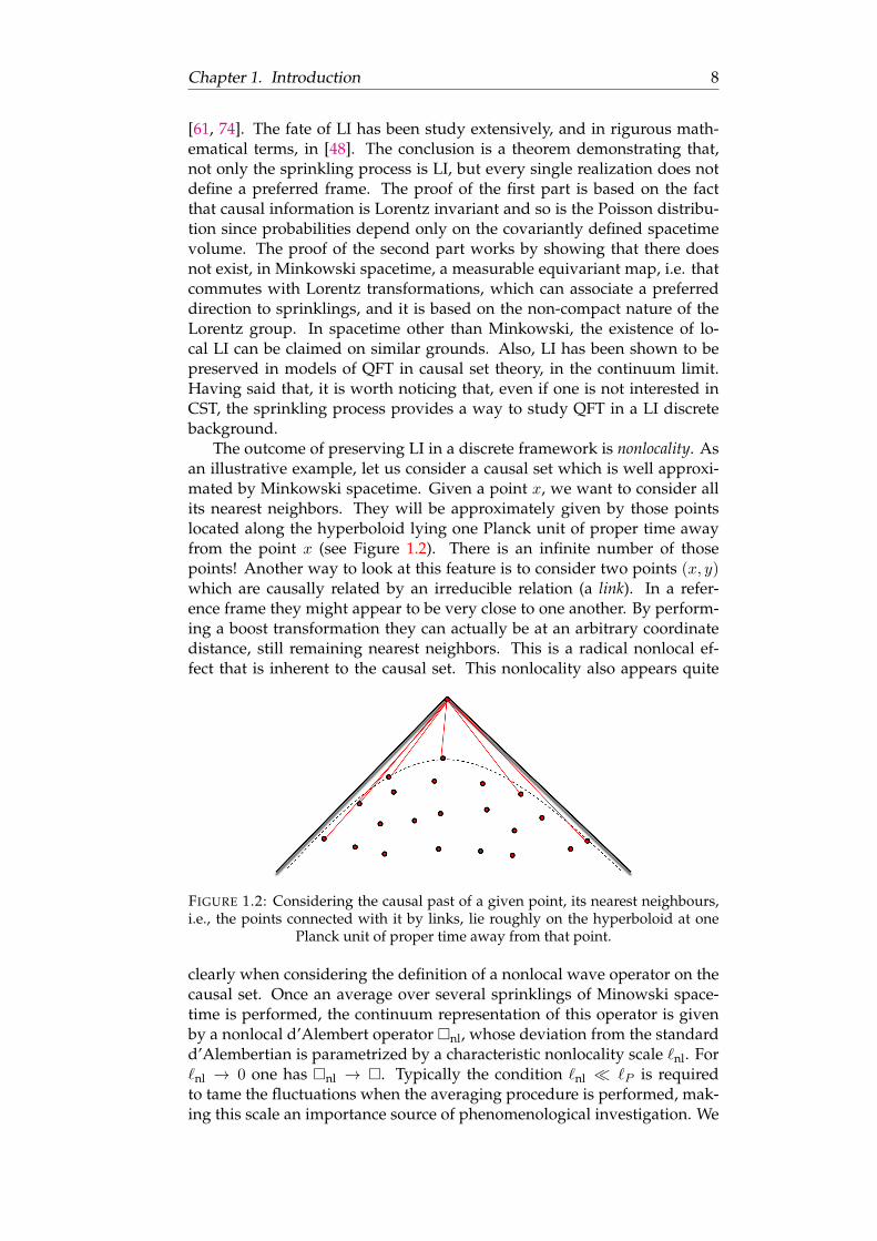
The outcome of preserving LI in a discrete framework is nonlocality. Asan illustrative example, let us consider a causal set which is well approxi-mated by Minkowski spacetime. Given a point x, we want to consider allits nearest neighbors. They will be approximately given by those pointslocated along the hyperboloid lying one Planck unit of proper time awayfrom the point x (see Figure 1.2). There is an infinite number of thosepoints! Another way to look at this feature is to consider two points (x, y)which are causally related by an irreducible relation (a link). In a refer-ence frame they might appear to be very close to one another. By perform-ing a boost transformation they can actually be at an arbitrary coordinatedistance, still remaining nearest neighbors. This is a radical nonlocal ef-fect that is inherent to the causal set. This nonlocality also appears quite

FIGURE 1.2: Considering the causal past of a given point, its nearest neighbours,i.e., the points connected with it by links, lie roughly on the hyperboloid at one

Planck unit of proper time away from that point.

clearly when considering the definition of a nonlocal wave operator on thecausal set. Once an average over several sprinklings of Minowski space-time is performed, the continuum representation of this operator is givenby a nonlocal d’Alembert operator nl, whose deviation from the standardd’Alembertian is parametrized by a characteristic nonlocality scale `nl. For`nl → 0 one has nl → . Typically the condition `nl `P is requiredto tame the fluctuations when the averaging procedure is performed, mak-ing this scale an importance source of phenomenological investigation. We


will see in Chapter 2 how the fundamental discreteness and the nonlocalityaffect the behavior of the entanglement entropy of a quantum field in CST.

1.2.3 Dynamics

Although we will not be interested in this aspect, it is worth briefly review-ing what are the current lines of investigation in the direction of having adynamics in CST.

Since causal sets do not admit a natural space and time splitting, it isclear that a Hamiltonian framework is not viable for describing causal setdynamics. On the other hand, a path-integral formulation should be inprinciple more promising. The (discrete) partition function is of the follow-ing form

Z =∑CeiSBDG , (1.3)

where SBDG is known as the Benincasa–Dowker–Glaser action and it rep-resents an action for causal sets which correspond to the Einstein–Hilbertaction in the continuum (see [43, 44, 50, 60, 69]). Another possibility is givenby the so-called Rideout–Sorkin classical sequential growth models. In thisapproach, starting from the empty set, a causal set is grown element byelement in a Markovian way [123].


1.3 Loop Quantum Gravity

Loop Quantum Gravity is a theory formulated to quantize gravity at thenon-perturbative level in a fully background independent fashion. Thedevelopment of the theory has been pursued in mainly two directions:the canonical and the covariant approach. The first one is based on theArnowitt–Deser–Misner (ADM) decomposition and a pair of nonstandardcanonical variables defined on a fixed time hypersurface [146]. The latter isa path integral approach (the spin foam programme [118]).

Research in LQG is, for the most part, carried out using standard QFTtechniques with minimal additional structure. In particular, in the canonicalformalism, the starting point is the Hamiltonian of GR written in Ashtekarvariables and the quantization techniques are inspired by methods used inlattice gauge theories.

The most relevant results obtained in the context of LQG include: thediscreteness of the spectra of geometrical operators (such as the area oper-ator) [25, 26, 127, 131]; the computation of black hole entropy [19, 20, 124];the avoidance of the cosmological initial singularity in LQC (see [2, 3, 21,28, 32] for reviews on the subject).

In this thesis we are interested in gaining some insights on the fate ofLorentz symmetry in LQG. We do this in a very pragmatic way, i.e. bystudying the behavior of scalar fields in a quantum background describedby LQG. In particular, we will quantize the scalar field using a quantizationprocedure, inspired by techniques used in the gravitational sector, knownas polymer quantization, which has been shown to be background indepen-dent [27, 59, 86, 87], in the spirit of the LQG programme. We will also im-pose some conditions on the background geometry, inspired by the prop-erties of homogeneity and isotropy of Minkowski spacetime, and we willderive an effective equation of motion.

In what follows we will introduce the reader to some basic elementsof canonical LQG, the computation of the spectrum of the area operatorand a simplified version of the theory based on symmetry reduction at thequantum level [5, 7], that will be used in Chapter 3 as a framework for ourcomputations.

1.3.1 Basics of canonical Loop Quantum Gravity

The canonical approach to LQG is based on the ADM formalism and onan appropriate choice of phase space variables. In what follows we willbriefly review its construction without dwelling on technicalities. We willalso not discuss dynamics and we will limit ourselves to the introductionof the kinematical Hilbert space which is enough to discuss spectra of ge-metrical operators. We refer the reader to [24, 125, 146] for more details.

ADM formalism and Ashtekar variables

First of all, we foliate the four dimensional manifold M into spacelike hy-persurface Σt. This means that we are considering globally hyperbolicspacetimes. The induced splitting of the metric tensor reads as

gµν =

(−N2 +NaN

a Na

Na qab

). (1.4)


The physically relevant information to determine the classical solutionsis contained into the pairs of conjugate variables given by the spatial three-metric qab and the extrinsic curvature Kab = 1

2Ln hab, where Latin indicesfrom the beginning of the alphabet denote spatial indices, n is the unit nor-mal to Σt, and L is the Lie derivative.

From Kab, we can construct

P ab =

√q

2

(Kab − qabK

), (1.5)

which contains the same information of Kab. The non-vanishing Poissonbrackets are

qab(x), P cd(y) = 2κδc(aδdb)δ

(3)(x− y), (1.6)

where κ = 8πG/c3.The Hamiltonian in the ADM formalism is given as

H = H[N ] +Ha[Na], (1.7)

with

H[N ] =

∫Σt

d3xN

[κ√q

(P abPab −

1

2P 2

)−√q

2κ

(3)

R

], (1.8)

Ha[Na] = −2

∫Σt

d3xNa∇bP ba. (1.9)

H and Ha are known as the Hamiltonian constraint and spatial diffeomor-phism constraint. Consistency of the dynamics forces both of them to van-ish, we write

H ≈ 0, Ha ≈ 0, (1.10)

where ≈ means weak equality, i.e. an equality that can be used only afterPoisson brackets have been computed. This means that the Hamiltonian His weakly zero, however Poisson brackets involving it are generically non-zero.H and Ha should be regarded as generators of gauge symmetries. In

particular, only those phase space functions whose Poisson brackets arevanishing with both H and Ha are physically relevant, being independentof the choice of coordinates.Ha[Na] generates infinitesimal spatial diffeomorphisms along the vec-

tor field ~N while H encodes the dynamics of the theory. If the Einsteinequations are satisfied, then H generates diffeomorphisms orthogonal toΣt. The lapse function and shift vector appear in the as Lagrange multipli-ers in the Hamiltonian. They correspond to a choice of gauge and determinethe relative positions of neighbouring Cauchy surfaces.

We now introduce an additional local SU(2) gauge symmetry by choos-ing our phase space to be described by the new variables Eai and Ki

a, whichare related to the ADM variables by the following relations

q qab = EaiEbi ,√q K b

a = KaiEbi, (1.11)

where i = 1, 2, 3 are internal indeces. We can look at Eai as a densitisedtetrad

√qeai , with qab = eai e

bi, and write the extrinsic curvature as Kab =


Kiaeib, using the co-tetrad eib. Internal indices i, j are trivially raised and

lowered by the Kronecker δij . The non-vanishing Poisson brackets are nowwritten as

Kia(x), Ebj (x) = κδ(3)(x, y)δbaδ

ij . (1.12)

Since we now have new degrees of freedom, we need to introduce anadditional constraint known as the Gauss law

Gij [Λij ] =

∫Σt

d3xΛijKa[iEaj] ≈ 0, (1.13)

and it generates internal SU(2) transformations under which observableshave to be invariant.

Given this new symmetry, it is natural to introduce the spin connectionΓia, defined as

∇aeib = ∂aeib − Γcabe

ic + εijkΓjae

kb = 0. (1.14)

We can then define new variables as

Aia = Γia + βKia, Eai = β−1Eai , (1.15)

where β is known as the Barbero–Immirzi parameter and it represents anambiguity in the construction of the connection variables. It can be shownthat Aia indeed transforms as a connection. We can then compute the newPoisson brackets. They are given by

Aia(x), Ebj (x) = κδ(3)(x, y)δbaδij . (1.16)

The ADM constraints become (up to a term proportional to Gij)

H[N ] =

∫Σt

d3xN

(β2 E

aiEbj

2√qεijkF kab −

1 + β2

√q

Ki[aK

jb]E

aiEbj

),

Ha[Na] =

∫Σt

d3xEaiL ~NAai,(1.17)

where F iab = 2∂[aAib] + εijkAjaAkb is the curvature of the connection.

Holonomies and fluxes

In order to construct gauge invariant quantities we choose, as subset ofphase space function to quantize, holonomies, i.e. parallel transports of ourconnection along curves, and fluxes, i.e. smearings of the conjugate variableEai over surfaces.

Holonomies hjc(A) along a curve c : [0, 1] → Σt in a certain represen-tation j of SU(2) can be defined as the solution to the following equation

d

dthjc(A, t) = hjc(A, t)A(c(t)), (1.18)

evaluated at t = 1, where A(c(t)) = Aia(c(t))ca(t)τ

(j)i and τ

(i)i are the three

generators of SU(2) in the representation j. The solution can be written as

hc(A) = P exp

(∫cA

), (1.19)


where P denotes a path-ordered integral.Fluxes are constructed by integrating Eai (we omit the tilde from now

on), contracted with a smearing function ni, over a surface S as

En(S) :=

∫SEai n

idSa =

∫SEai n

iεabcdxb ∧ dxc. (1.20)

To construct the quantum theory we need the Poisson brackets. For thesake of simplicity, we choose our surface S such that it intersects the curvec once in the point c(s) and from below w.r.t. the orientation of S. In thiscase, we obtain

hjc(A), En(S) = κhjc1(A)(τ

(j)i ni

)hjc2(A), (1.21)

where c1 = c|t∈[0,s] and c2 = c|t∈[s,1].

Kinematics

The quantum kinematics can be constructed by promoting the above intro-duced variables to quantum operators obeying appropriate commutationrelations.

The essential feature of LQG is to promote to operators the holonomieshjc rather than the connectionsAia themselves. The Poisson algebra of holonomiesand fluxes is well defined and the resulting Hilbert space is unique. Moreprecisely, requiring the three-diffeomorphism invariance (there must be aunitary action of such diffeomorphism group on the representation by mov-ing edges and surfaces in space), there is a unique representation of theholonomy-flux algebra that defines the kinematic Hilbert space Hkin. Thisresult is known as the LOST theorem [93]. The kinematical Hilbert space isalso known as the spin networks Hilbert space.

A spin network state can be expressed as

|s〉 = |Γ, jc, in〉, (1.22)

and it contains three pieces of information: the graph Γ ⊂ Σt, which is givenby a finite number of edges c and nodes n; a collection of spin quantumnumbers jc, one for each edge; the intertwiners in at the nodes n.

The wave functional on the spin network is given by

ΨΓ,ψ = ψ(hjc1c1 (A), ..., hjcncn (A

), (1.23)

where the wave function ψ is SU(2) invariant and satisfies the Gauss con-straint. Specifically, this is realized by considering functions that joint thecollection of holonomies (in the arbitrary spin representation) into an SU(2)invariant complex number by contracting all the gauge indices with the in-tertwiners, the latter being invariant tensors localized at each node. Thestates (1.22) are called cylindrical functions. The space of these functions iscalled Cyl.


We now promote our choice of classical phase space variables to quan-tum operators. Their action on the state (1.22) is given by

hjcΨΓ,ψ(A) = hjcΨΓ,ψ(A), (1.24)

En(S)ΨΓ,ψ(A) = iEn(S),ΨΓ,ψ(A), (1.25)

where the last expression is realized by considering (1.21).A key result in LQG is the construction of the kinematic scalar product

between two cylindrical functions. Indeed, the discreteness of area andvolume operators spectra, mainly based on the compactness of the SU(2)group, can be obtained from it. The kinematic scalar product is defined as

〈ΨΓ|ΨΓ′〉 =

0 if Γ 6= Γ′,∫ ∏

c∈Γ dhjcψ†Γ(hj1c1 , ...)ψΓ′(h

j1c1 , ...) if Γ = Γ′,

(1.26)

where the integrals∫dhjc are performed with the SU(2) Haar measure. The

inner product vanishes if the graphs Γ and Γ′ do not coincide and it is in-variant under spatial diffeomorphisms, even if the individual states are not.This happens because the coincidence between two graphs is a diffeomor-phism invariant notion. Therefore, there is no information about the posi-tion of the graph in (1.26).

Area operator

In this part we will briefly show how to construct the area operator in LQG.The volume operator is obtained with a similar construction and it will notbe discussed here.

First of all we need to write the area A(S) of a surface S in terms of ourbasic variables. Classically, we have

A(S) =

∫Ud2u

√det(X∗q)(u), (1.27)

where X : U → S is an embedding of the coordinate chart U into S, andX∗q is the induced metric on S. We can partition U into disjoint subsetsU = ∪iUi, so that

A(S) =∑i

∫Ui

d2u√

det(X∗q)(u). (1.28)

In the limit of small Ui one has∫Ui

d2u√

det(X∗q)(u) =

∫X(Ui)

√qqabdsadsb ≈ β

√Ek(Ui)Ek(Ui), (1.29)

where Ek(Ui) =∫UiEakdUa. Therefore

A(S) = limUi→0

β∑i

√Ek(Ui)Ek(Ui). (1.30)

We can now promote A(S) to an operator in the Hilbert space by using theaction of the flux operator on a state.


For simplicity, we consider a Wilson loop as our state, Ψ = Tr(hjc(A)), inthe case where the curve c intersect the surface S only once. We obtain

Ek(Ui)Ek(Ui)|Ψ〉 = (i)2|Tr(hjc1(τ(j)k τ (j)k)hjc2) = κ2j(j + 1)|Ψ〉. (1.31)

Since the operator above acts diagonally, we can use the spectral theoremto deal with the square root, hence obtaining

A(S)|Ψ〉 = βκ√j(j + 1)|Ψ〉. (1.32)

This result can be easily generalized to more complex structures [146]. No-tice that the spectrum depends on the Barbero–Immirzi parameter β.

1.3.2 A symmetry-reduced model

Quantum Reduced Loop Gravity (QRLG) is a framework for the quantiza-tion of symmetry-reduced sectors of GR. In particular, it was initially ap-plied to cosmological models (an inhomogeneous extension of Bianchi I)[4, 6] and then it was realized that it corresponds to a gauge fixing in whichthe components of the triads are diagonal at the level of the quantum theory[7].

More specifically, QRLG implements the restriction to the diagonal spa-tial metric tensor and triads along some fiducial directions, along whichone can define coordinates x, y, z. The spatial line element reads

dl2 = a21dx

2 + a22dy

2 + a23dz

2, (1.33)

where ai = ai(t, x, y, z).The graph now contains only three kinds of links, each of them being

the set of links li along a fiducial direction.Inverse densitized triads are taken to be diagonal (indeces are not summed)

Eia = piδia, |pi| = a1a2a3

ai, (1.34)

and this implies a SU(2) gauge fixing condition in the internal space. Itis realized by projection of SU(2) group elements, which live in the linksli, onto the U(1) representations obtained by stabilizing the SU(2) groupalong the internal direction ~Ul = ~ui, with ~ui unit vectors along the threedirections. Connections are generically given by

Aia = ciuia + ..., ci =

β

Nai, (1.35)

dots indicate non-diagonal terms that can be disregarded in certain situa-tions [4, 6]. With these choices, Γ becomes a cuboidal graph.

The kinematical Hilbert space now reads

RHkin = ⊕Γ

RHΓ, (1.36)

where RHΓ is the reduced Hilbert space for a fixed reduced graph.


Spin network sates in LQG can be written as

ΨΓ,jl,in = 〈h|Γ, jl, in =∏n∈Γ

in ·∏l

Djl(hl), (1.37)

where jl are labels for irreducible representations of SU(2) on each link,Djl(hl) are Wigner matrices in the representation j and in are intertwiners.The dot denotes contractions of the SU(2) indeces and the products extendover all the links and nodes of Γ.

The basis of states in the reduced model is obtained by projecting theWigner matrices on the state of the maximum or minimum magnetic num-ber ml = ±jl, for the angular momentum component Jl = ~J · ~ul along thelink l:

lDjlmlml(hl) = 〈ml, ~ul|Djl(hl)|ml, ~ul〉, hl ∈ SU(2). (1.38)

Then the reduced states are called reduced spin networks and are given by

RΨΓ,ml,in(h) =∏n∈Γ

〈jl, in|ml, ~ul〉 ·l∏l

Djlmlml, ml = ±jl, (1.39)

where 〈jl, in|ml, ~ul〉 are reduced intertwiners.Finally, the reduction of canonical variables to Rhli and RE(s) is ob-

tained by smearing along links of the reduced graph Γ and across surfacesS perpendicular to these links, respectively.

The scalar constraint operator neglecting the scalar curvature term isgiven by that of LQG considering only the Euclidean part and replacingLQG operators with the reduced ones.


1.4 Geometry and Lorentz symmetry

Metric theories of gravity are based on the metric postulate [153]. It es-sentially says that spacetime is locally Minkowskian, or, equivalently, thatspacetime is a pseudo-Riemannian manifold, whose geodesics representthe possible trajectories of test particles. One could see special relativityand local LI as consequences of this fact. This is of course an assumption,and one may be tempted to relax this requirement. In particular, it is con-ceivable that close to the Planck scale Minkowski spacetime might not bea trustworthy description of the spacetime fabric. This consideration leadsus to wonder if LI is a fundamental symmetry of nature. While in CST,this is essentially the case, in other approaches LI can be considered as asymmetry emerging below some energy scale.

From the phenomenological point of view, violations of LI are encodedinto the dispersion relation2, which is given by

E2 = m2 + p2 +∞∑n=1

an(µ,M)pn, (1.40)

where p =√|~p|2, an are dimensional coefficients, µ is some particle physics

mass scale and M is the mass scale characterizing the physics responsiblefor the departure from standard LI (usually, but not necessarily, identifiedwith the Planck mass). When an = 0, ∀n, then the dispersion relation is theCasimir of the Poincaré algebra and LI is recovered.

Following our line of reasoning, explicit Lorentz invariance violations(LIVs) are known to be incompatible with pseudo-Riemannian geometry(see also [88]). One way to deal with this issue is to add vector or ten-sor fields to the gravitational Lagrangian that spontaneously break Lorentzsymmetries. An example of effective theory based on this prescription isknown as Einstein-æther theory [81] and the action of the theory includesthe Einstein–Hilbert term plus the most general Lagrangian for a unit, time-like vector field (representing the æther) with all of the covariant contribu-tions having at most two derivatives. Another example is provided by thework of Kostelecky and Samuel [89]. In this thesis we will be interested inyet another possibility, that is abandoning the realm of pseudo-Riemanniangeometry.

Before moving to the main points of this section, some considerationsare in order. First of all, contrary to the group of rotations, which is com-pact, SO(3, 1) is a non-compact group. Among other things, this meansthat although we have tested LI for small values of the boost parameterswe cannot extend our conclusions for arbitrarily large boosts. In particularLorentz contraction causes the transformation of large spatial distances in areference frame into ultra short spatial distances in another reference frame.

Of course this classical picture does not take into consideration the factthat the nature of spacetime as such scales may be completely different. In-stead, according to pseudo-Riemnnian geometry, flat spacetime is a betterand better approximation as we consider smaller patches3. Consequently,

2This is strictly speaking true in the case of rotationally invariant free field modifications.The study of generic LI violating effects require an effective field theory approach.

3This also implies that (classically) at those scales gravity becomes unimportant, whileon the other hand QG arguments suggest that spacetime will be highly fluctuating.


this distinction between short and long scales is not compatible with thelinearity of Lorentz transformations in Special Relativity, that does not al-low for a privileged length scale discriminating between those two regimes.Whatever structure is going to replace pseudo-Riemannian geometry at thefundamental level, will have to deal with this issue.

On the other hand, deformations of the relativistic transformations arepossible so to integrate a second invariant energy (or length) scale [13], leav-ing the number of generators untouched. Under these symmetry groups,dispersion relationns of the kind (1.40) (with some an 6= 0) can poten-tially be invariant. Therefore, in an attempt to provide a spacetime descrip-tion of this kind of symmetries, it would be interesting to understand ifthese can be related to some new local structure of spacetime, possibly de-scribed by some maximally symmetric background generalizing a pseudo-Riemannian structure and Minkowski spacetime.

It has been shown in a series of papers [15, 68] that Finsler geometry[33, 144] allows to reconstruct a spacetime structure starting from modifieddispersion relations (MDRs) of the kind in eq.(1.40)4. Finsler structures arethe most studied generalizations of Riemannian geometry and are definedstarting from norms on the tangent bundle instead than from inner prod-ucts. When a Finsler manifold is reconstructed from a MDR (we will reviewthe precise prescription in Chapter 4), the physical picture will be that testparticles with different energies will “experience different geometries” inthe sense that the metric and, in general, also the affine structure of space-time, will become velocity-dependent (or, equivalently, momentum-dependent).That is, we can describe the motion of test particles with MDRs using aneffective metric of the following kind

gFµν(x, p(x)) = gµν(x) + hµν(x, p(x)), (1.41)

giving rise to deformed equations of motion

xµ + Γµρσ(x, p(x))xρxσ = 0, (1.42)

where Γµρσ(x, p(x)) are the Christoffel symbols associated with the Finslermetric gFµν(x, p(x)). Indeed, Finsler geometry can be seen as a consistentmathematical framework to characterize what are known as rainbow geome-tries [92, 101].

Let us stress that such models of Finslerian spacetimes do not have to beconsidered as definitive proposals for the description of quantum gravita-tional phenomena at a fundamental level. We take here the point of view forwhich, between the full quantum gravity regime and the classical one, thereis an intermediate phase where a continuous spacetime can be described ina semi-classical fashion. In particular, if the underlying QG theory predictsthat spacetime is in some way discrete, then we assume that a meaningfulcontinuum limit can be performed and that this limit is not equivalent toa classical limit (see Section 1.1.2). The outcome of this hypothetical pro-cedure would be a spacetime that can be described as continuum but stillretaining some quantum features of the fundamental theory (causing the

4A similar situation appears in analogue models. In fact there it can be shown that de-partures from exact LI at low energies can be naturally described using Finsler geometries[36, 152].


deviation from a pseudo-Riemannian structure). Then the departure fromthe purely classical theory will be weighed by a non-classicality parameter(potentially involving the scale of Lorentz breaking/deformation) and inthe limit in which this parameter goes to zero, the completely classical de-scription of spacetime is recovered (see e.g. [30, 149] for a concrete exampleof such a construction).

1.4.1 Doubly Special Relativity

The most severe constraints have been so far obtained considering the MDRas a by-product of an effective field theory with Planck suppressed Lorentzviolating operators [95]. However there is an alternative approach that triesto reconcile the relativity principle with the presence of a fundamental high-energy scale. This proposal goes under the name of Doubly or DeformedSpecial Relativity (DSR) [13].

The essence of this idea is to change (or deform) the transformationsbetween inertial observers in such a way that there are two invariant quan-tities, the speed of light c and a fundamental energy scale EP (or mass scalemP ). This resonates very well with was we discussed in the previous sec-tion. If the fundamental scale emerging from QG is promoted to be an ob-server independent quantity, it would soften the tension in the distinctionbetween high energy and low energy regimes in a relativistic framework.Indeed, in DSR models, relativistic transformations becomes nonlinear, po-tentially overcoming this issue.

There are a least two ways of realizing DSR models. One way is to intro-duce nonlinear representations of the standard Poincaré Lie group. This isa case where the new observer independent scale of DSR characterizes rep-resentations of a still classical/undeformed Poincaré Lie group. Anotherway is to adopt the formalism of Hopf algebras. In essence, the differencebetween the two approaches is that, in the first case one substitutes thestandard Poincaré generators with new generators, adapted to the nonlin-ear representation. In the second case, not only the commutators, but alsothe coproduct rules are changed and the action of symmetry transforma-tions on products of functions is not deducible from the action on a singlefunction using the Leibniz rule.

Hopf algebras were proposed a few decades ago to describe symmetriesof noncommutative spacetimes [102]. In the QG context, a particular caseof Hopf algebras has attracted some attention in the past years, the case ofκ-Poincaré [99, 100, 103]. Gravity in 2 + 1 dimensions can be quantized as atopological field theory and can be coupled to point particles, representedby topological defects. In [66] it was shown that, after integrating away thegravitational degrees of freedom, particles are described by representationsof the κ-Poincaré group (where κ is an energy scale). At this stage, thisresults cannot be extended to 3 + 1 dimensions, but the κ-Poincaré groupcan be easily extended to higher dimensions.

In this thesis we will be interested in studying the κ-Poincaré group inthe relative locality limit, briefly introduced in Section 1.1.2, in which oneneglects both ~ and G while keeping their ration fixed EP =

√~c5/G. In

this case, one can effectively ignore any noncommutativity in the coordi-nates (driven by ~) while keeping the deformed relativistic properties. Inthis framework, the non-standard symmetries of spacetime, can be related


to a non-trivial curvature in momentum space. In particular, κ-Poincaré isassociated with a de Sitter momentum space [70]. We will be interested inthe 1 + 1 dimensional case and we will discuss the dynamics of free parti-cles, therefore the structure of the coproducts will not play any role. In 1+1dimension, the κ-Poincaré algebra is then given by the following commu-tators among generators

[P,E] = 0, [N,P ] =κ

2

(1− e−2E/κ

)− 1

2κP 2, [N,E] = P. (1.43)

We give here the coproducts for the sake of completeness

∆E = E ⊗ I + I⊗ E, ∆P = P ⊗ I + e−E/κ ⊗ P, (1.44)

∆N = N ⊗ I + e−E/κ ⊗N,

and the antipods and counits

S(E) = −E, S(P ) = −e−E/κP, S(N) = −e−E/κN (1.45)ε(E) = ε(P ) = ε(N) = 0.

Finally, the Casimir is given by

Cκ =

(2κ sinh

E

2κ

)2

− eE/κP 2. (1.46)

All these relationships are written in the so-called bycrossproduct basis. Incan be shown that a change of basis in the generators amounts to a diffeo-morphism in momentum space [70]. For κ→∞, one recovers the Poincaréalgebra.

While there is a rather clear understanding of DSR models in momen-tum space, the picture in spacetime is less clear and it represents a subjectof debate. On the other hand, such a picture would allow these models tobe more competitive in comparison to LIV scenarios. Here is where Finslercomes to the rescue as a framework that could accommodate this kind ofphysics, as we anticipated in the previous Section. In particular in [15], aFinsler spacetime realizing the symmetries of κ-Poincaré in 1 + 1 dimen-sions was found and it was shown to reproduce the results of the usualcomputations in momentum space.

Among all the possible Finsler structures, a particular case is given byBerwald spaces. These are the Finsler spaces that are the closest to be Riem-manian (we will provide a more precise definition in Chapter 4). If a Finslerspace is of the Berwald type then any observer in free fall looking at neigh-bouring test particles would observe them move uniformly over straightlines accordingly to the Weak Equivalence Principle [107]. Interestinglyenough the Finsler metric correspondent to κ-Poincaré symmetries foundin [15] appears to be a member of this class. However, we shall see that thiscome about in a somewhat trivial way as a straightforward consequence ofthe flatness of the metric in coordinate space. With this in mind, it would beinteresting to consider examples of curved metrics associated to more gen-eral deformed algebras so to check if for these the local structure of space-time does not reduce to the Minkowski spacetime but rather to the Finslergeometry with κ-Poincaré symmetries and furthermore for checking if also


these geometries are of the Berwald type. This will be the main subject ofChapter 4.

Aside on the Einstein and Weak Equivalence Principles

With a momentum-dependent metric tensor, one generically expects viola-tions of the Equivalence Principles. Metric theories of gravity, identified bythe metric postulate, can also be characterized as those theories satisfyingthe Einstein Equivalence Principle (EEP)[153]. The latter can be expressedas follows

Einstein Equivalence Principle. The Einstein Equivalence Principle states that:

• The Weak Equivalence Principle is valid.

• The outcome of any local non-gravitational experiment is independent of thevelocity of the freely-falling reference frame in which it is performed (localLorentz invariance).

• The outcome of any local non-gravitational experiment is independent ofwhere and when in the universe it is performed (local position invariance).

The content of the WEP can be stated as follows

Weak Equivalence Principle. Any observer in free fall looking at neighbouringtest particles would observe them moving uniformly over straight lines, indepen-dently of their composition.

It appears that any theory of gravity that is, in some sense, based on DSRwould violate the EEP (by construction the theory would not be LI). On theother hand, the EEP could be deformed by asking that local LI is substitutedwith local DSR invariance. Regarding the WEP, the notion of “moving uni-formly” is related to acceleration and hence to the affine structure of space-time. Therefore, given a momentum-dependent metric tensor, the study ofthe geodesic equations and the spray coefficients will determine whether areference frame, physically realizing the WEP, can be constructed. We willsee in Chapter 4 that, in the context of Finsler geometry, this amounts to ver-ify whether the Finsler structure is of the Berwald type. This kind of inves-tigation, carefully considering its limitations, could potentially shed somelight on the possibility of constructing a metric theory of gravity based onDSR symmetries.

22

Chapter 2

Spacetime entanglemententropy in Causal Set Theory

2.1 Introduction

The concept of entanglement entropy plays a crucial role in several areasof modern quantum physics, from the study of condensed matter systemsto black holes. It is essentially a measure of the correlation between sub-parts of a quantum system. It is traditionally defined as S = Trρ log ρ−1,where ρ is the reduced density matrix of the subsystem. Consider a bi-partite system, whose parts are labeled by A and B, that is described by adensity matrix ρAB ∈ Lin(HA ⊗HB). The entropy of subsystem A is givenby SA = −TrρA log ρA, where ρA ≡ TrBρAB is the reduced density matrix ofsystem A and is obtained by tracing over the degrees of freedom of systemB. Some of the properties of S are:

• S(ρ) ≥ 0

• S(ρ) = 0 ⇔ ρ is pure

• S(ρ) = S(UρU †) with U a unitary transformation

• concavity: S(∑

i λiρi) ≥∑

i λiS(ρi) with λi > 0 :∑

i λi = 1

• SAB = SA + SB if ρAB = ρA ⊗ ρB

• strong subadditivity: SABC + SB ≤ SAB + SBC

• dimHA = d ⇒ SA ≤ log(d) and SA = log(d) ⇒ ρA = d−11

When the two systems are uncorrelated, ρAB = ρA⊗ ρB , knowing the partsallows one to reconstruct the entire system. On the contrary, if the systemsare maximally entangled knowing the parts gives no information on thewhole.

In the context of QFT, entanglement entropy is also known as geometricentropy [53]. The system in this case is partitioned geometrically, startingfrom a state ρΣ defined on a fixed time hypersurface Σ and then tracingout the degrees of freedom living “outside” a given subregion R. As wementioned in the Introduction, this entropy is typically a divergent quantitydue to the vacuum fluctuations with infinitely high frequencies near theboundary of R.

This notion is now widely believed to be of great importance in the con-text of QG research for several reasons. For instance: its divergences arethought to be strongly connected with the local structure of spacetime (see

Chapter 2. Spacetime entanglement entropy in Causal Set Theory 23

Sec.1.1.1); it is a relevant concept whenever a spacetime possesses an eventhorizon (black holes, Rindler observers and others); gravity and its dynam-ics can emerge from quantum entanglement (see Jacobson’s derivation [82,83] and Van Raamsdonk’s work [150]). Because it’s formulated as a purelyspatial notion, the traditional ways of thinking about entanglement entropymight not be suitable for QG investigations.

Motivated by these considerations, a global definition of entropy thatcan be applied to any globally hyperbolic region of spacetime and is par-ticularly useful in the context of CST, was recently proposed by R. Sorkin[134]. We will refer to this quantity as spacetime entanglement entropy(SEE).

This gives on one hand a theory (CST) that provides us with a way ofintroducing a fundamental cutoff in a Lorentz invariant fashion and, onthe other, a covariant definition of entanglement entropy. Equipped withthese tools, we will investigate in this chapter the behavior of the SEE in acausal set that is well approximated by a causal diamond in two, three andfour dimensions for two families of scalar Green functions. In particular,we focus on trying to motivate how the familiar area law in the continuumemerges from the fundamental discrete structure.1

The chapter is organized as follow: in Section 2.2 we briefly review thenovel notion of entanglement entropy introduced in [134]; in Section 2.3,we introduce the reader to the basics of QFT in a causal set, the Sorkin–Johnston vacuum and the kind of scalar Green functions that we will usein our study; in Section 2.4, we introduce and present the main results ofour work and, finally, in Section 2.5, we conclude with a discussion of ourresults and an outlook for further developments.

2.2 Spacetime entropy

In [134] a covariant definition for the entropy of a Gaussian field expressedentirely in terms of spacetime correlation functions was introduced. Con-sider the ground state |0〉 of a free real scalar field φ whose Wightman (W)function is given by the following expression

W (x, y) = 〈0|φ(x)φ(y)|0〉, (2.1)

which, by Wick’s theorem, determines all the other n-point correlation func-tions. The imaginary part of W is the Pauli-Jordan (PJ) function

i∆(x, y) = [φ(x), φ(y)], (2.2)

which can be alternatively written in terms of the retarded (Gret) and ad-vanced (Gadv = GTret) Green functions as

∆(x, y) = Gret(x, y)−Gadv(x, y). (2.3)

Given a spacetime region R the SEE is defined as

S(R) =∑

λ ln |λ|, (2.4)

1An analogous investigation was carried out in [137] for two spacetime dimensions.


where λ are the solutions of the generalized eigenvalue problemWR v = iλ∆R v

v /∈ Ker[∆R],(2.5)

and the subscript R indicates the restriction of the correlation function topairs of points (x, y) ∈ R. For any vector in the kernel of i∆, the associatedλ is not defined, hence we just exclude them (it can be shown that theywould not contribute to the entropy anyway, see [134]).

It can be proven that [134] the SEE of a globally hyperbolic region ofspacetime coincides with the standard entanglement entropy of any Cauchysurface Σ of such region, i.e.

S(D(Σ)) = Sent(Σ), (2.6)

where D(Σ) is the causal domain of development of Σ and Sent(Σ) is thestandard entanglement entropy of surface Σ.

2.3 Scalar fields in causal set theory and the Sorkin–Johnston vacuum

Being a covariant definition of entropy that does not require the notion ofa state on a spatial hypersurface, the notion of entropy given in Section2.2 can be successfully applied to quantum fields living on causal sets. Asmentioned the Section 1.2, we will be dealing with causal sets (generatedby a sprinkling process) that are well approximated by a flat continuum(Minkowski) spacetime.

It can be shown that, in general, a causal set does not admit the notion ofa Cauchy hypersurface. This represents an obstacle when trying to imple-ment traditional quantization techniques. For this reason in [1, 84, 136] (seealso [135] for a recent pedagogical introduction) a different starting pointwas assumed to define a free scalar field theory: rather than starting fromthe equations of motion and the canonical commutation relations (CCR),one can start with the (retarded) Green function GR only. Given Gret onecan write the the PJ function as in (2.3) and use it to rewrite the CCR in anexplicitly covariant way(see Eq.(2.2)). The PJ function gives the imaginarypart of the W function

∆ = 2 i=(W )⇒W =i∆

2+R. (2.7)

Is it possible unambiguously choose the vacuum if there are no equa-tions of motion available? The answer is yes. In particular one can choosethe W function to be of the positive part of i∆, i.e.

WSJ :=i∆ +

√−∆2

2= Pos(i∆). (2.8)

Since for a Gaussian scalar field the two-point function fully determinesthe theory, this prescription allows us to formulate a consistent scalar fieldtheory with the retarded Green function as the only input. In particular,eq.(2.8) specifically selects a vacuum state known as the Sorkin–Johnston


(SJ) vacuum. It can be shown that definition (2.8) is equivalent to requiringthe following three conditions for W :

• Positivity W ≥ 0

• Commutator ∆ = 2=(W )

• Othogonal support W W ∗ = 0

The first two are common to the two-point function of any state, whilethe third specifically selects the SJ vacuum [135]. This prescription yieldsdistinguished ground states for a quantum scalar field in any globally hy-perbolic region of spacetime or causal set, without making explicit referenceto any notion of positive frequency.

Now that we have established that one can define a quantum scalarfield on a causal set starting from Green functions alone, we will see whatthe possible choices of retarded Green functions are.

2.3.1 Discretizing continuum Green functions

The first possibility is to directly discretize the continuum Green functionson a causal set. This has been done in [85] and the strategy is to replacethe continuum retarded Green functions with discrete analogs written interms of objects that are well-defined on a causal set. The expressions forthe retarded Green function in two, three and four spacetime dimensionsare given by

G(2)ret (x, y) =

1

2Cxy (2.9)

G(3)ret (x, y) =

1

2π

(πρ12

)1/3 ((C + I)2

)−1/3

xy(2.10)

G(4)ret (x, y) =

√ρ

2π√

6Lxy, (2.11)

for x ≺ y and zero otherwise. The matrix Cxy is known as the causal matrixand given any two elements a, b ∈ C, Ca,b = 1 if a causally precedes b andzero otherwise, for all a, b ∈ C. Ca,b can be used as a full specification ofthe causal set itself. The matrix Lxy is the link matrix and given any twoelements a, b ∈ C, La,b = 1 if there are no elements c ∈ C s.t. a ≺ c ≺ b andzero otherwise, for all a, b ∈ C. Finally, ρ = N/V is the density of sprinkledspacetime points.

Note that the discrete Green functions given above are defined only interms of causal properties of the causal set.

2.3.2 Nonlocal wave operators on causal sets

The second possibility is to invert a wave operator properly constructedon the causal set itself. It was shown in [133] that discrete wave operatorscan be defined on the causal set in terms of nearest neighbors2. Such opera-tors, once averaged over sprinklings of Minkowski spacetime, give rise tononlocal operators which reduce to the standard d’Alembertian operator in

2The notion of nearness is given by the cardinality of the set of points between the causalpast and the causal future of a couple of elements x 4 y, i.e. |z ∈ C : x 4 z 4 y|.


the continuum limit. We report here the general expression for the discreteoperators in any spacetime dimension D (see [69] for further details)

(B(D)ρ φ)(x) = ρ2/D

aφ(x) +

Lmax∑n=0

bn∑

y∈In(x)

φ(y)

, (2.12)

where a, bn are dimension dependent coefficients, ρ = `−D, ` is the discrete-ness scale and In(x) represents the set of past n-th neighbors of x. In theliterature the first sum in eq. (2.12) is referred to as sum over layers, whereeach In is a layer.

a b0 b1 b2 b3D = 2 -2 4 -8 4

D = 3 − 1Γ[5/3]

(π

3√

2

)2/31

Γ[5/3]

(π

3√

2

)2/3− 27

8Γ[5/3]

(π

3√

2

)2/39

4Γ[5/3]

(π

3√

2

)2/3

D = 4 −4/√

6 4/√

6 −36/√

6 64/√

6 −32/√

6

TABLE 2.1: Table of coefficients in Eq.(2.12) for D = 2, 3, 4. The number of coeffi-cients for every dimension corresponds to the “minimal” nonlocal operators, i.e.,

the operators constructed with the minimum number of layers.

These operators are derived in such a way to reproduce, in the con-tinuum limit, the standard d’Alembertian once averaged over sprinklings.However, whereas this average is well behaved in the local limit the vari-ance is not. In order to solve this problem, a new length scale, which wecall the nonlocality scale, can be introduced [133]. This scale serves to smearthe action of the previous operators on the whole past of a given point xand leads to discrete operators given by

(B(D)ρ φ)(x) = (ερ)2/D

aφ(x) +∞∑m=0

bm∑

y∈Im(x)

φ(y)

, (2.13)

where ε = (`/`k)D with `k the nonlocality scale and

bm = ε(1− ε)mLmax∑n=0

(m

n

)bnε

n

(1− ε)n. (2.14)

Finally, by inverting the expressions in (2.13) the retarded nonlocal Greenfunction can be obtained.

2.4 Spacetime entropy in Causal Set Theory

In this section we report the results of our work, i.e., the computation ofthe SEE, introduced in Section 2.2, for a scalar field in a causal set that iswell approximated by Minkowski spacetime. First we will discuss how thesystem is organized, including the geometrical setup and the choice of statefor the scalar field. Then we will present the results of the computations fortwo, three and four spacetime dimensions. Note that our analysis partially


overlaps with the one presented in [137], where a similar computation wascarried out in a two dimensional causal set for the massless local Greenfunction. Also we will not discuss here the fine details of our analysis, aswe will confine ourselves to the main ideas and the most relevant outcomes.We invite the reader to look at [40] for the full investigation.

2.4.1 The setup

Our geometrical configuration is a fixed causal set C that is well approxi-mated by a causal diamond in Minkowski spacetime. A causal diamond,or Alexandrov open set, is defined as the intersection of the future lightcone of a point p with the past light cone of a point q, i.e., I+(p) ∩ I−(q) .We then consider a smaller causal diamond inside the first one, centered atthe same point and with sides parallels to the ones of the large diamond.In any number of dimensions, the ratio between the volume V of the outerdiamond and the volume Vd of the inner diamond is fixed to be V/Vd = 4.

The scalar field is prepared in the SJ vacuum of the large diamond. Oncewe have theWSJ(x, y) and ∆(x, y) matrices ((x, y) vary over the elements ofC) we numerically solve the generalized eigenvalue problem (2.5) restrictedto the inner diamond. By applying formula (2.4), we compute the SEE ofthe scalar field in the inner diamond with respect to the complementary re-gion. The resulting entropy can be interpreted, in the continuum limit, asthe EE of the horizontal diagonal of the small diamond (green line in Figure2.1) with respect to its complement given by the segments that extend thediagonal to the larger diamond (black segments in Figure 2.1). Note thatthe diagonal of the big diamond is a Cauchy surface. We consider this con-figuration in two, three and four spacetime dimensions, for the local andnonlocal massless Green functions introduced in the previous section.

At this point we want to remind the reader that, in D spacetime dimen-sions, the area law corresponds to a entropy that grows like that “area” of ahypersurface of codimension two. We will generically refer to this behavioras an area law.

FIGURE 2.1: Inner and outer diamonds for a sprinkling in 2D Minkowski, withN = 2048 and V/Vd = 4.


2.4.2 Premise on the spectrum of the Pauli–Jordan

In Section 2.2 we mentioned that one has to exclude the vectors in the kernelof i∆ in the computation of the SEE in order to have a well defined eigen-value problem. As a preliminary analysis we look at the spectrum of thisoperator (we will sometimes refer to it as σi∆) in the continuum and in thecausal set case. The eigevalues of i∆ in the continuum have dimensions ofa length squared L2, while in the causal set they have dimensions L2−D, inD dimensions. To compare the two spectra, we match their dimensions byusing a factor of ρ.

The two dimensional continuum case was studied in [129] where theauthors found that the eigenvalues of i∆ are of the form αcont = `d/(2k),where `d is the side of the diamond and k = πn

`d, with n = ±1,±2, ..., is

the wavenumber of the eigenfunctions [129], and can be rewritten in termsof the volume of the diamond as αcont =

√V /(2k). The usual cutoff is

then implement by retaining all the eigenvalues of i∆ up to a minimumvalue αcontmin associated with a maximum wavenumber kmax that, in turn,can be related to a minimum wavelength `min = 2π k−1

max. If we want totranslate this cutoff in the discrete causal set, we can identify `min with thefundamental discreteness scale ` = ρ−1/D and multiply by a factor of ρ, toobtain3

αcsmin = ρ

√V

2kmax= ρ

√V

4π` =

V

4π√N, (2.15)

where we used ρ = N/V .In Figure 2.2a, we have the log-log plot of the positive part of σi∆ in

the continuum (red dots), in the causal set (blue dots) and the cutoff λcsmin(black dashed line) for the local Green function in 2D. The spectrum inthe continuum follows a power law behavior as a function of n, while thespectrum in the causal set matches the one in the continuum approximatelyup to the value of the cutoff, after which it changes drastically. On the basisof this fact, we expect a different behavior for the entropy in the two cases.

At the moment, we do not have the exact spectrum of this operator inthe continuum in higher dimensions for the local and nonlocal Green func-tions. Nevertheless, we can look at the spectra in the causal set and we cansee the it has the same shape of the two dimensional case (for instance, seeFigures 2.2 for the localand nonlocal models in two dimensions).

2.4.3 Spacetime entropy

Let us consider first the entropy associated with the large diamond (i.e., ofthe outer diamond in Fig. 2.1) in any number of dimensions. It is easy toshow explicitely how how the SEE computation gives a zero entropy forthe SJ state which is a pure state. Indeed, the fact that WSJ = Pos(i∆)implies that the eigenvalues of the problem in Eq. (2.5) are all either zero orone. Since i∆ is a skew-symmetric and Hermitian matrix, its rank is evenand its non-zero eigenvalues come in positive and negative pairs. Partiallyfollowing the notation in [85], we write its normalized eigenvectors andeigenvalues as follows

i∆ua = αaua, i∆va = −αava, i∆wc = 0, (2.16)3This result agrees with the one presented in [137].


1 5 10 50 100n

0.001

0.010

0.100

1

α2 d-loc

(A) Plot of σi∆ in two dimensions for thelocal Green function in the continuum (reddots), in C (blue dots) and the continuum

cutoff (black dashed line) (N=200)

1 5 10 50 100 500 1000n

10-5

0.001

0.010

0.100

1

α2 d-nl

(B) Plot of σi∆ in two dimensions for thenonlocal Green function (N=2048)

FIGURE 2.2: Spectrum of i∆ for the local and nonlocal models in D = 2.

where αa > 0, 2s is the rank of i∆, a = 1, ..., s and c = 1, ..., p − 2s (p is thenumber of elements in C).4 The eigenvectors form an orthonormal basis forCp and they can be chosen such that

ua = v∗a, wc = w∗c , u†aub = v†avb = δab, u

†avb = w†cua = w†cva = 0. (2.17)

We can therefore decompose the matrix as follows

i∆ =s∑

a=1

αauau†a −

s∑a=1

αavav†a. (2.18)

Since WSJ = Pos(i∆) it can be written as

WSJ =s∑

a=1

αauau†a. (2.19)

Let us consider now the eigenvectors ua with positive eigenvalues. Thegeneralized eigenvalue problem (2.5), applied to the large diamond, gives

WSJ ua = αua = λαua ⇒ λ = 1. (2.20)

Given the orthogonality relations (2.17), for the va one gets

WSJ va = 0 = λα va ⇒ λ = 0. (2.21)

Therefore S =∑λ lnλ = 0.

We now consider the entropy of the small causal diamond obtained bytracing over the d.o.f. in its complement. To do this we numerically solveEq. (2.5) restricted to the points inside the small diamond. We do this fordifferent values of sprinkling density ρ and, since the fundamental scale isrelated to the density as ` = ρ−1/D, we are effectively computing the SEE asa function of the fundamental discreteness scale.

Before presenting the results, a couple of comments are in order. First,for a given number of elements N in the causal set, the range of scales thatwe investigate in different spacetime dimensions varies. For instance, to

4Note that in Section 2.4.2, the index i referred to the length of each vector while herea, b, c are labels.


have ` = 0.01 with a unit fiducial volume V = 1, we need N = 108, 106, 104

forD = 4, 3, 2 respectively. While in two dimensions it is relatively easily toreach these densities, for higher dimensions this is not the case and this willbe a source of uncertainty in the interpretation of our results. The secondpoint is that we need to keep in mond that the nonlocal models containa new scale `k, the nonlocality scale introduced in Section 2.3.2, thereforeit is natural to expect some departure from the local models as we probedifferent values of the cutoff.

For D = 2, 3, 4 and for local and nonlocal Green functions, we find thatthe entropy scales linearly with the number of points of the inner diamondsNd (see Figures 2.3a).5 Since Nd ∝ ρ, the SEE follows a spacetime volume law.Contrary to the ordinary case where the entropy is infinite unless a UVcutoff is introduced, in this case (for any finite value of Nd) the entropy isfinite.

This result was already known to the community and it was presentedin [137] for a local massless Green function in D = 2.

This behavior can be traced back to the part of the spectrum of eigenval-ues of i∆ which does not follow a power law (see Section 2.4.2 and Figures2.2a and 2.2b) and smoothly interpolates between the continuum behaviorand zero. This fact can be verified by applying the cutoff of the continuumto the spectrum in the causal set, so that we only retain those eigenvaluesthat follow the continuum behavior.

500 1000 1500 2000Nd

100

200

300

400

500

600

S2 d-loc

(A) Local theory in two dimensions.500 1000 1500 2000 2500

Nd

200

400

600

800

1000

1200

S3d-nl

(B) Nonocal theory in three dimensions.

FIGURE 2.3: Spacetime volume law.

Since we do not have the exact spectrum for i∆ in dimensions higherthan two and for the nonlocal Green functions, we generalize the cutoff(2.15) using general arguments. In particular we assume that in the con-tinuum the eigenvalues are still of the form λcont ∝ V 1/D/k where V 1/D isthe scale that characterize the geometrical setup (the typical scale of thediamond in D dimensions), and we use the prescription used to deriveEq. (2.15). We relate the maximum wavenumber with the discretizationscale by kmax = 2π/`, we rewrite ` in term of the causal set density ρ andfinally we multiply by ρ to have an expression that is dimensionally con-sistent. We introduce a real parameter a ≥ 0 to take into account possibleoverall numerical factors coming from the exact spectrum and we write thecutoff in D dimensions as

αcs,Dmin = a ρ `V1D = a ρ1− 1

DV1D = a V

2D−1N1− 1

D . (2.22)5The choice of studying the entropy as a function of the number of points in the small

diamonds is customary. One can also consider the total number of pointsN , the two are, onaverage, related as Nd = (Vd/V )N .


The magnitude of the eigenvalues of i∆ grows withN as it can be seen fromFigure 2.4. Eq. (2.22) allows the cutoff to track this growth so that it is at thesame location relative to the spectrum for every N . Changing the value ofa translates the cutoff vertically in the (n, α) plane in Figure 2.2 (for a givenvalue of N ). Note that a = 0 corresponds to not having a cutoff. We thenlook at the behavior of the SEE as a function of this parameter.

1 5 10 50 100 500 1000n

10-6

10-5

10-4

0.001

0.010

0.100

α

FIGURE 2.4: σi∆ for the local model in D = 3 in the outer diamond. The red dotsare for N=2048 and the blue dots are for N=3072.

Our procedure is to truncate the spectrum of i∆ and WSJ = Pos(i∆)in the big diamond, by retaining only the eigenvectors compatible with thecutoff (2.22). We then restrict both matrices by evaluating them at the pointsof C that are in the inner diamond, we call the restricted matrices ∆d andWd. At this point, we apply the cutoff again (now as a function of Vd andNd) to the spectrum of i∆d, we truncate Wd accordingly and we solve thegeneralized eigenvalue problem (2.5).

Local Green functions

As a first check, we reproduced the results of [137] for the local Green func-tion in two dimensions, see Figure 2.5. The SEE after imposing the cutofffollows a logarithmic law which corresponds to an area law in two space-time dimensions (the surface of codimension two is a point). Moreover thecoefficient of the logarithm is approximately 1/3 as in [129, 137] and in thetraditional computation [52], if we exclude data for small values of the den-sity.

In Figure 2.6 the entropy is plotted for the local model in D = 3 forvarious choices of the cutoff. We find that, if we include part of the smalleigenvalues of i∆ that do not follow the power law behavior, the growthof the entropy is faster than an area law, almost with ρ(∝ Nd). Increasingthe coefficient a in front of the cutoff, the entropy starts growing at a slowerrate, up to the point in which it becomes linear with ρ1/3(∝ `), essentiallyfollowing an area law.

Similar considerations apply forD = 4. We find, for a = 1/4, an approx-imate scaling with ρ1/2 = `−2, as it is shown in Figure 2.7. After imposingthe cutoff, for the typical values of the density that we can explore in D = 4(roughly in the interval ρ ∈ [103, 105]), we are left with a small number (∼ 5,for ρ ≈ 104) of eigenvalues of i∆ in the small diamond. This is probably the


0.5 1.0 1.5 2.0 2.5 3.0 3.5

Nd

4π

1.6

1.8

2.0

2.2

2.4

S2 d-loc

(A) SEE for the local theory with cutoffαmin =

√Nd/(4π),

Sfit = 1.84 + 0.398 logαmin.

2.0 2.5 3.0 3.5

Nd

4π

2.0

2.1

2.2

2.3

2.4S2 d-loc

(B) Excluding values at low densities.Sfit = 1.90 + 0.332 logαmin.

FIGURE 2.5: Area law for the local theory in D = 2.

1 2 5 10 20 50n

10-5

10-4

0.001

0.010

αd

(A) N=3072 and a = 5−1.20 25 30 35

ρ1/3

0.5

1.0

1.5

S3 d-loc

(B) Sfit = −0.385 + 0.053ρ1/3,N=103-104.

1 5 10 50 100n

10-5

10-4

0.001

0.010

αd

(C) N=3072 and a = 10−1.20 25 30 35

ρ1/3

2

4

6

S3 d-loc

(D) Sfit = −2.05 + 0.22ρ1/3 + 0.000021ρ,N=103-1.4 · 104.

1 5 10 50 100n

10-5

10-4

0.001

0.010

αd

(E) N=3072 and a = 50−1.20 25 30

ρ1/3

50

100

150

S3 d-loc

(F) Sfit = 11.5402 + 0.0045ρ,N=103-1.4 · 104.

FIGURE 2.6: Local theory in D = 3. Plots of the cutoff on σi∆ and the associatedSEE.

source of the fluctuations of the entropy around the scaling with the area inFigure 2.7.


1 2 5 10n

0.002

0.005

0.010

αd

(A) N=5120 and a = 4−1.100 150 200 250 300

ρ1/2

0.2

0.4

0.6

0.8

S4 d-loc

(B) Sfit = −0.1654 + 0.0028ρ1/2,N=103-1.4 · 104.

FIGURE 2.7: Local theory in D = 4. Plots of the cutoff on σi∆ and the associatedSEE.

Nonlocal Green functions

For the nonlocal Green functions, we performed an analogous analysis tothat of the local ones, at fixed values of the nonlocality scale `k. A crucialdifference with respect to the local models is that in the numerical simu-lations we have to take into account the constraint `k > ` = ρ−1/D. Thistranslates into a lower limit on the sprinkling density ρ > `−Dk .

For the nonlocal model in two dimensions, we fix `k = 0.2 and we findthat the cutoff in the spectrum of i∆ that allows us to recover a logarithmicbehavior for the entropy is close to the one of the local theory. In Figure 2.8we can see that the magnitude of the entropy is also very close to the localcase.

1 5 10 50 100n

10-6

10-5

10-4

0.001

0.010

0.100

αd

(A) N=2048 and αmin =√Nd/(2π).

3 4 5 6 7 8 9

Nd

2π

2.2

2.4

2.6

2.8

S2 d-nl

(B) Sfit = 1.968 + 0.332 logαmin.

FIGURE 2.8: Nonlocal theory inD = 2. Plots of the cutoff on σi∆ and the associatedSEE.

In higher dimensions we again compare the location of the cutoff withthe corresponding entropy. For D = 3 the resulting area law is shown inFigure 2.9 (`k = 0.2). We can see that there is some intermediate phase(around a = 10−1) in which the entropy follows a linear scaling with thearea only for large Nd, while for small densities the growth is slower. Thiseffect does not seem to be present in the local models and therefore couldbe due to the presence of the nonlocality scale. We will return to this pointat the end of this section. For a = 1/(2π) this effect goes away and we findan approximate area law S ∝ ρ1/3. Again, by including part of the smalleigenvalues, the entropy appears to grow faster than ρ1/3.


1 5 10 50 100n

10-5

10-4

0.001

0.010

αd

(A) N=3072 and a = (2π)−1.20 22 24 26 28 30

ρ13

14

15

16

17

18

19

S3 d-nl

(B) Sfit = 3.25 + 0.50ρ1/3,N=2 · 103-8 · 103.

1 5 10 50 100n

10-6

10-5

10-4

0.001

0.010

αd

(C) N=3072 and a = 10−1.15 20 25 30 35

ρ1320

25

30

35

40

S3 d-nl

(D) Sfit = −29.76+0.23ρ1/3 +17.84 log ρ1/3,N=103-104.

1 5 10 50 100n

10-5

10-4

0.001

0.010

αd

(E) N=3072 and a = 50−1.20 25 30

ρ13

100

200

300

400

S3 d-nl

(F) Sfit = −125.7347 + 11.7394ρ1/3 +0.0042ρ,

N=103-104.

FIGURE 2.9: Nonlocal theory inD = 3. Plots of the cutoff on σi∆ and the associatedSEE.

Even for the nonlocal theory in four dimensions we find a phase inwhich the area law is approximately valid for large densities while the en-tropy grows slower for small densities, see Figure 2.10. Again, due to thevery small number of residual eigenvalues in the small diamond for largervalues of a and for the range of densities that we can explore, we do not,yet, have complete data to confirm the presence of a pure area law phase.Nevertheless, preliminary results suggest that the situation is analogous tothe case inD = 3. In this case the nonlocality scale was fixed to be `k = 0.15.

Dependence on the nonlocality scale

We dedicate this section to briefly comment on the possible dependenceof our entropy results for the non local Green functions on the nonlocalityscale `k, leaving a more detailed investigation for future works.


1 5 10 50 100 500n

10-6

10-5

10-4

0.001

0.010

αd

(A) N=5120 and a = 6−1.100 150 200

ρ12

10

20

30

40

50

60

70

S4 d-nl

(B) Sfit = −87.733 − 0.092ρ1/2 +32.398 log ρ1/2,N=103-1.6 · 104.

1 5 10 50 100 500n

10-6

10-5

10-4

0.001

0.010

αd

(C) N=5120 and a = 50−1.100 150 200 250

ρ12

100

200

300

400

500

600

700

S4 d-nl

(D) Sfit = 111.0833 + 2.3666ρ1/2 + 0.0017ρ,N=103-104.

FIGURE 2.10: Nonlocal theory in D = 4. Plots of the cutoff on σi∆ and the associ-ated SEE.

In Figure 2.12 the spectrum of i∆ for D = 2, 3 for various values of`k is plotted. One can see that the dependence on the nonlocality scale isbarely noticeable in two dimensions while it is more pronounced in threedimensions. For instance, it could be logarithmic inD = 2 and a power lawin higher dimensions. In both cases higher values of `k seem to suppress thespectrum. As a consequence of this dependence, the cutoff and hence theSEE, must depend on the nonlocality scale. Given that the the eigevaluesof i∆ have dimensions of L2 (in the continuum, for both local and nonlocalGreen functions), and the entropy is dimensionless, `k should enter in adimensionless combination with another dimensionful scale.

We pointed out at the beginning of this section that the spectrum ofi∆ is very similar in both the local and nonlocal cases. Although this isqualitatively true, in the nonlocal case it is typically more concave as canbe seen in a direct comparison in three dimensions in Figure 2.11. Thisdifference, most likely due to the presence of the nonlocality scale, may bethe reason for the non-standard behavior of the entropy at the intermediatescales described previously. If the area law is due to the part of the spectrumin the local theory with constant slope, then it is a logical possibility that inthe nonlocal case the variation of the slope would imply a more complexstructure of the entropy for different cutoffs.

We postpone additional considerations on this subject to the summaryof this chapter.


1 5 10 50 100 500 1000n

10-6

10-5

10-4

0.001

0.010

0.100

α

FIGURE 2.11: Comparison of the spectrum of i∆ between the local and nonlocalmodel in D = 3 (N = 2048).

5 10 50 100 5001000n

10-5

10-4

0.001

0.010

0.100

1

α2 d-nl

ℓk0.2

0.4

0.6

(A) Two dimensional case.

1 5 10 50 100 500n

10-7

10-6

10-5

10-4

0.001

0.010

0.100α3 d-nl

ℓk0.2

0.25

0.3

0.35

0.4

(B) Three dimensional case.

FIGURE 2.12: Dependence of the spectrum of i∆ on the nonlocality scale.

2.4.4 The cutoff and the kernel of the Pauli–Jordan

As we mentioned in the previous section the spectrum of i∆ on the causalset, compared to the continuum theory with the cutoff, contains a largenumber of non-zero eigenvalues that interpolate between the power lawbehavior (common to the continuum) and zero. These values are typicallyvery small as can be seen from the plots in the previous section. Using thecutoff in the discrete framework we are effectively putting all these valuesinside the kernel of i∆.

It can be shown that vectors w ∈ Ker(i∆) define vanishing linear com-binations of the field evaluated on the causal set elements, i.e.,

∑wiφ

i = 0,where i runs over the elements of C. In the continuum these relations arejust the equations of motion for the scalar field. In the causal set, the num-ber of these vectors (the dimension of the kernel) is rather small comparedto the number of elements in C where the field takes its values [135]. Thisamounts to saying that the equations of motion for the scalar field in thecausal set are a highly underdetermined system, because we have morevariables (φi) than equations dim(ker(i∆)).

For instance, in two dimensions the number of variables φi grows likeN , while it can be shown that dim(ker(i∆)) is of order lnN . By applyinga cutoff to the eigenvalues of i∆ we are effectively enlarging its kernel. Inparticular, using (2.15), dim(ker(i∆)) = aN , where a . 1, see Figure 2.13.We argue that this could be the reason why the entropy has a different scal-ing with the number of elements once the cutoff is implemented. In thecontinuum, the entanglement entropy of the small diamond is due to its


correlations with regions (1) and (2) in Figure 2.14. In fact, the lateral di-amond are not in causal contact with the central one. The regions (3) and(4) do not contribute because the field there is related to the field in (1),(2) and the central diamond by the equations of motion. In the causal set,the number of relationships between the values of the fields in the regions(1),(2) and (3),(4) does not correspond to the number of links. This mightbe the source of the larger entropy associated with the inner region whenthe cutoff is not implemented.

1000 2000 3000 4000N

2

4

6

8

10

12

dim(ker)

(A) dim(keri∆)fit = −0.964 + 1.079 logN

1000 2000 3000 4000N

1000

2000

3000

4000

dim(kercut)

(B) dim(keri∆)fit = −71.23 + 0.95N

FIGURE 2.13: Dimension of the kernel in D = 2.

FIGURE 2.14: Regions which are causally connected and disconnected to the innerdiamond in 2D Minkowski.

Let us now consider another situation: take a causal diamond and di-vide it in two equal disjoint triangles using its diagonal as in Figure 2.15,we call this configuration a spacelike partition. In the continuum, given someinitial data on the diameter (which in this case is a Cauchy hypersurface),one can predict all the values of the field in the upper triangle, by usingthe equations of motion. Indeed, if the field is prepared in the SJ vacuum,one can argue on general grounds that the SEE of the upper triangle withrespect to the lower one is zero because they contain the same information,given the causal structure of the diamond.

Therefore the expectation would be that, at least after the cutoff on thespectrum of i∆ has been implemented, the entropy should be vanishingalso in the causal set case.


-1.0 -0.5 0.0 0.5 1.00.0

0.5

1.0

1.5

2.0

2.5

FIGURE 2.15: Upper and lower triangles for a sprinkling of a causal diamond in2D Minkowski, with N = 2048.

As it can be seen from Figure 2.16, the behavior of the entropy is in-stead similar to the entanglement entropy in the case of the inner diamondvs its complement. This means that the additional conditions provided bythe enlarged kernel are not enough to take into account all the possible re-lationships between the field in the upper triangle and in the lower one.What replaces a spatial hypersurface in a causal set is the notion of maximalanti-chain. An anti-chain is a setA of elements in C such that, for all x, y ∈ Aneither x ≺ y nor y ≺ x (a set of unrelated elements). An anti-chain isthen said to be maximal when by adding any near elements to it it ceases tobe an anti-chain. Nevertheless, a maximal anti-chain Amax cannot play therole of a Cauchy hypersurface because there are going to be links betweensome points in the future and in the past of A that do not go through ele-ments of Amax.6 Hence, we conclude that the fundamental discretenss andnonlocality of a causal set are the source of this entropy.

Before concluding it is worth pointing out a crucial difference betweenthe spacelike partition and the entanglement entropy. If we do not imposeany cutoff in the computation of the entanglement entropy in the contin-uum and the SEE in the causal set the two cannot be meaningfully com-pared. This is because while the latter is finite, the former is divergent. Onthe other hand, in the case just discussed, a comparison between the con-tinuum and the causal set is possible even without a cutoff, because theentropy is finite in both cases.

2.5 Summary and outlook

In this chapter we studied the behavior of the entanglement entropy of ascalar field on a causal set using the covariant approach introduced in [134].

6We remind the reader that a link is given by a pair of elements x, y, such that @ z : x ≺z ≺ y.


1000 2000 3000 4000 5000ρ

500

1000

1500

2000

S3 d-loc, sl

(A) Sfit = 12.91 + 0.44ρ.20 25 30

ρ13

10

20

30

40

50

60

70

S3 d-loc, sl

(B) a = 10−1 andSfit = −11.9462 +2.0077ρ1/3 + 4.7123 log ρ1/3.

FIGURE 2.16: SEE of a spacelike partition for the nonlocal theory in D = 3.

We found that the entanglement entropy follows a spacetime volumelaw in two, three and four spacetime dimensions for both the local andnonlocal Green functions. By generalizing the two dimensional case, wedefined a cutoff on the spectrum of i∆ that has the right scaling with thedensity of the causal set, thus allowing us to recover an area law in all casesconsidered. In particular, by studying the behavior of the entropy whilevarying the cutoff in such a way to consistently include or exclude parts ofthe spectrum of i∆ (this is done by changing the parameter a, introducedin Eq. (2.22)), we conclude that the small eigenvalues that do not followthe (expected) behavior of the spectrum in the continuum are responsiblefor the scaling with the spacetime volume. As a consequence, by retainingonly the part of the spectrum that follows a power law with constant slopewe find an area law.

We also made a connection between the equations of motion of thescalar field, defined by the vectors in the kernel of i∆, with the scalingof the entropy with ρ. While this interpretation seems to be a reasonableexplanation of this effect, it fails when tested against the case that we callspacelike partition of the causal set (see Figure 2.16). This is a case in whichin the continuum, using the fact that the field is in a pure state and that thediagonal of the diamond is a Cauchy hypersurface, one can show that thespacetime entropy for the upper and lower triangles should be vanishing.Without imposing any cutoff in the causal set case this entropy scales againwith the spacetime volume. Therefore, the natural expectation might havebeen that the entropy should have been zero also in the causal set after thetruncation of the spectrum of i∆. Instead the resulting entropy follows thesame scaling with the area that we found in the case of the entanglemententropy of a small diamond vs its complement. This led us to conclude thatalthough the cutoff tames the growth of the entropy as a function of the fun-damental cutoff, it is not enough to compensate for the intrinsic nonlocalityof the causal set.

If one were to interpret this entropy as an entanglement entropy, the factthe the entropy of the upper triangle equals the entropy of the lower oneimplies that the SJ vacuum is a pure state. On the other hand, since they arenot vanishing, the sum of the two entropies do not equal the entropy of thefull diamond, the latter being zero. This means that the two subsystems arecorrelated and indeed the two regions are causally connected. Given thatthe diameter of the diamond is not a Cauchy hypersurface in the causal setcase (the best that one can do is to introduce a maximal anti-chain, which is


the analogue of a spacelike surface, see Sec. 2.4.4), some of this correlationwill not be “recorded” at the boundary of the two regions (the diameter)leading to a non zero entropy even with an enlarged kernel of i∆.

We then raise the following question: is this kind of entropy also con-tributing to the entanglement entropy of the small diamond vs its comple-ment? The quick answer is yes, after all it is easy to convince ourselvesthat these kind of causal correlations should also be present in this case. Onthe other hand, from the computation of the SEE in two dimensions for thelocal Green function with the cutoff, the resulting entropy matches almostexactly the traditional computation in the continuum, with a small depar-ture for small densities (see Figure 2.5). Hence, one would be tempted tosay that these causal correlations should affect the SEE only for small valuesof the density, far from the continuum limit. However, the entropy of thespacelike partition (that should be dominated by these kind of correlations)appears to be a monotonically growing function of the density and this factseems to disfavor this interpretation. If one accepts the fact that causal cor-relations are an important part in the total budget of the SEE, then one canask the further question: how is it possible that the computation in the con-tinuum matches the one in the causal set?

We do not yet have a clear argument to explain these results. It is possi-ble that there is a simple way to interpret the outcomes of our computationsand we just missed it or, it could be a signal that something in the way QFTis constructed in CST or in the definition of SEE, have to be modified. Be-fore concluding this part of the discussion we would like to point out oneparticular aspect of this investigation: the strictly exact result for the entan-glement entropy in the continuum with the traditional computation basedon the knowledge of the state on a spatial Cauchy hypersurface is a di-vergent. So one can gain very little information by comparing it with theSEE in the causal set unless a cutoff is introduced. Per contra, the spacelikepartition, and possibly other configurations, allows us to directly compareresults in the causal set with results in the continuum without the need ofa cutoff, since both are finite, and they seem to provide important tools forunderstanding various aspects of CST.

A distinctive feature of the nonlocal models is that the spectrum of i∆seems to be more concave than in the local models (for a given value of thedensity), and this effect appears to be more pronounced as we increase thenumber of spacetime dimensions. Hence, the behavior of the SEE is richeras we select which eigenvalues to include in our analysis. In particular, wefound that for some values the parameter a the SEE follows an area lawonly for large densities (see Figures 2.9d and 2.10b). This suggests that,at least for these models, the complete SEE may be composed of variousphases, dictated by the shape of the spectrum of i∆. It is possible that thechoice of a that corresponds to the continuum result is not the one that givesa pure area law scaling. Indeed, there are some computations (see [110]and the Appendix A) showing that the entanglement entropy of a theorywith modified wave operators (Lorentz violating and Lorentz invariant),characterized by the presence of a new UV scale, do follow an area law athigh energies but the fundamental area is not given by the square of thecutoff but by a combination of the cutoff and the new UV scale, e.g. it couldbe a geometric mean of the two. This is a possibility in our theory sincethe Green functions that we consider in this work give rise to this kind of


modified wave operators in the continuum.Of course, having the exact computation for the SEE and of the tradi-

tional entanglement entropy in the continuum for the Green functions thatwe considered would also allow one to identify precisely what the cutoffneeded for a comparison with the continuum is.

42

Chapter 3

Polymer scalar fields in LoopQuantum Gravity

3.1 Introduction

In the Introduction to this thesis, we briefly discussed how different ap-proaches to QG realize the paradigm of the fundamental discreteness ofspacetime in different ways, focusing in particular on the difference be-tween CST and LQG. In the first case, fundamental discreteness is a built infeature and it is imposed in a explicitly covariant fashion, i.e. by discretiz-ing spacetime as a whole. In LQG instead, fundamental discreteness is abyproduct of the quantization, i.e., operators associated with geometricalproperties of space have discrete spectra.

We dedicated Chapter 2 to the study of the effect of the covariant (andLorentz invariant) discrete structure of CST on the entanglement entropyof scalar fields. In this chapter, we will introduce the first steps of our in-vestigation in the direction of formulating a dynamics for a scalar field inLQG. We will see that there are two major factors causing a departure fromthe standard description: the discreteness of space provided by the graphΓ, defined by the node of a spin network state of the quantum geometry,where the field takes values and a non standard quantization, known aspolymer quantization, which is suitable for a background independent quan-tization of matter fields (a real free scalar field in our case). The final goal isto understand how these ingredients affect the dynamics of the scalar fieldwith particular attention to the fate of Lorentz symmetry.

The computation that we are going to present here is not complete andthere is a certain number of assumptions made to simplify the problem thatwe will highlight along the way. Nevertheless, we will be able to drawsome general conclusions on the basis of our results.

In the first part we will review polymer quantization and the relevanttechniques used to regularize and quantize the matter contribution to thescalar constraint. In the second part we will define an effective Hamilto-nian, based on the assumption that there is no backreaction on the geom-etry, and use it the derive the equations of motion for the scalar field. Inthe final part we will discuss our results and comment on possible futuredevelopments.

3.2 Polymer quantization of a scalar field

In this section, we will review the basics of polymer quantization appliedto a real scalar field, loosely following [47].

Chapter 3. Polymer scalar fields in Loop Quantum Gravity 43

The action for a minimally couple scalar field reads

S(φ) =1

2λ

∫MdDx√−g (gµν∂µφ∂νφ− V (φ)) , (3.1)

where λ is coupling constant of dimensions ~−1, and g is the determinantof the spacetime metric. Note that with this convention the scalar field hasdimensions L1−D/2.

The Legendre transform gives the following Hamiltonian in the ADMformalism:

H(φ) =

∫ΣdD−1x

[Naπ∂aφ+N

(λ

2√qπ2 +

√q

2λqab∂aφ∂bφ

+

√q

2λV (φ)

)]=

∫Σt

dD−1x(NaV(φ)

a +NH(φ)sc

),

(3.2)

where Σ is a constant time spatial slice. N and Na are the lapse functionand the shift vector respectively, while V(φ)

a and H(φ)sc are the contributions

of the scalar field to the vector and scalar constraints. q is the determinantof the spatial metric and π is the conjugate momentum to the scalar fieldwhich in our convention has dimension of L−D/2.

The total vector constraint is the sum of V(φ)a with the gravitational part

and it generates (spatial) diffeomorphisms. H(φ)sc is the matter field part of

the smeared scalar constraint and it contains the dynamics of the field inthe diffeo-invariant phase space. It can be written as:

H(φ)sc [N ] := H

(φ)kin[N ] +H

(φ)der[N ] +H

(φ)pot [N ], (3.3)

where

H(φ)kin[N ] :=

∫Σt

dD−1xN

(λ

2√qπ2

), (3.4)

H(φ)der[N ] :=

∫Σt

dD−1xN

(√q

2λqab∂aφ∂bφ

), (3.5)

H(φ)pot [N ] :=

∫Σt

dD−1xN

(√q

2λV (φ)

). (3.6)

We quantize the system of gravity and matter by using the techniquesdescribed in [145, 147] for LQG adapted to QRLG. The total Hilbert spaceis given by1

H(tot)kin =R H(gr)

kin ⊗H(φ)kin, (3.7)

the latter being the following Hilbert space:

H(φ)kin := a1 Uπ1 + ...an Uπn : ai ∈ C, n ∈ N. (3.8)

To define this Hilbert space, the polymer variable 〈φ|Uπ〉 = Uπ(φ) repre-senting the scalar field φ is assigned to every function π : Σ → R of finitesupport v1, ..., vn and it can be considered as an element of the Hilbert

1R refers to the symmetry-reduced model, see Section 1.3.2.


space above, whose states are defined as

Uπ(φ) = ei∑v∈Σ πvφv := 〈φ|π〉, (3.9)

where v ∈ Σ labels a countable set of points v1, ..., vn in the manifold Σ,and φv = φ(v1), ..., φ(vn) is the value of the field at those points. Thenormalization is provided given two states Uπ(φ) and Uπ′(φ) with supporton the same set of points by the following scalar product

〈π|π′〉 = δπ,π′ . (3.10)

Therefore the two states are orthogonal unless they are defined on the sameset of points and the have the same values for the functions π and π′ at thosepoints.

The basic variables act as follows

Uπ|π′〉 = |π + π′〉, (3.11)

Π(V )|π〉 = ~∑v∈V

πv|π〉, (3.12)

with Π(V ) being the scalar field momentum smeared over a volume V ∈ Σ.It can be written as

Π(V ) =

∫VdDx π(x). (3.13)

Note that Π(V ) has dimensions of LD−1 and it is a density of weight zero,given that π transforms as a measure.

In the case of a single point x, one denotes the states as

〈φ|x;π〉 = eiπxφx , (3.14)

for which the scalar product reads

〈x;π|y;π′〉 = δx,yδπ,π′ . (3.15)

The action of the basic operators is analogous to Eq.s (3.11). The smearedmomentum operator around a point x as

Π(x) :=

∫dD−1y χε(x, y)π(y), (3.16)

where we introduced the characteristic function χε(x, y) of the box Bε(x)centered in x with coordinate volume εD−1. Precisely,

V(Bε(x)) := V(x, ε) = εD−1√q +O(εD), (3.17)

which allows us to smear a function at the point x around an infinitesimalneighborhood, such that

f(x) =

∫dD−1δ(D−1)(x− y) f(y) = lim

ε→0

1

εD−1

∫d3y χε(x, y)f(y). (3.18)

The full Hilbert spaceH(φ)kin := L2(RΣ

Bohr) can be obtained from the singlepoint one L2(RBohr), where RBohr denotes the Bohr compactification of a


line, and the Bohr measure is defined as∫RBohr

dµBohr(φ)eiπxφx = δ0,x. (3.19)

This method for treating scalar fields realizes a polymer representation inthe momentum polarization (also known as the point-holonomy represen-tation) [22, 27, 59, 86, 87].

This prescription closely follows the one that leads to the spin networkstates. Indeed, one can think: i) to the set of points v as the graph Γ, ii) to thevariables πv as the analogous of the spin coloring jl for the links l of a spinnetwork with links l ∈ Γ, iii) to (3.11) as the counterpart of the holonomy-flux algebra. Indeed, in both cases, the field φ and the connection A arenot well defined operators on their respective Hilbert spaces, but only theirholonomized versions. The latter act by multiplication creating new pointholonomies in the case of the scalar field and new links in the gravitationalcase. The conjugate variables (π andE) are well defined operators that readas eigenvalues the coloring of the holonomized field, i.e., the value of thefield πv of the point holonomies base on the “graph” v and the value of thespins of the holonomies based on the graph Γ respectively. As in full LQG,the π fields have support on the set of nodes of the lattice Γ (a cuboidalgraph in our case).

3.2.1 Regularization and quantization of the scalar Hamiltonianconstraint

In this part we will briefly mention some relevant techniques used to quan-tize the classical Hamiltonian (3.3) and we refer the reader to [22, 27, 47]for more details. For the sake of simplicity we restrict our analysis to 3 + 1dimensions.

Before quantizing the scalar part of the Hamitonian constraint we needto regularize it. This procedure is carried on by rewriting (3.3) in terms ofholonomies and fluxes for the gravitational part and point-holonomies andsmeared momenta for the parts involving the scalar field.

The gravitational part is regularized using methods developed for thefull theory, restricted to a cuboidal graph [47]. In this description, mattercoupled to a dynamical spacetime is regularized by a reduction to fieldscoupled to a dynamical lattice.

We will now consider a free massless scalar field, so that the potentialterm in (3.3) is zero. We therefore need to regularize the kinetic and deriva-tive parts, H(φ)

kin and H(φ)der . First of all we need to replace the spatial metric

with the triads eia. To do so we can use the following identities

e2

q= 1,

√qqab =

1

4√qεijkε

acdejcekdεilmε

befeleemf , (3.20)

and we introduce the volume V(R) of a region R using its definition

V(R) =

∫Rd3x√q. (3.21)


The resulting expression reads as

H(φ)sc = lim

ε→0

[λ

2

∫d3xN(x)π(x)

∫d3yπ(y)

∫d3t

e

(V(t, ε))3/2

×∫d3u

e

(V(u, ε))3/2χε(x, y)χε(t, x)χε(u, y)

+1

8λ

∫d3xN(x)εijkε

acd∂aφ(x)ejc

(V(x, ε))1/4

ekd(V(x, ε))1/4

×∫d3yεilmε

bef∂bφ(y)ele

(V(y, ε))1/4

emf

(V(y, ε))1/4χε(x, y)

].

(3.22)

To remove the denominators one uses the Thiemann’s trick [146], given bythe following expression

eia(x) =2δV(R)

δEai=

2

n(V(R))n−1

δ(V(R))n

δEai

=4

nγκ(V(R))n−1Aia(x), (V(R))n.

(3.23)

Now, we need to rewrite the Hamiltonian so that it can live on a dis-crete quantum geometry. A method of discretization of the scalar constraintvia a triangularization of the spatial manifold has been developed for puregravity [148] and for gravity coupled to a scalar field [147]. The idea is toreplace the summation

∫Σ with the sum over all ordered tetrahedra. The

sum over tetrahedra becomes the sum over all the nodes v of the triangula-tion and over all the tetrahedra ∆l,l′,l′′ created by triple of links emanatingfrom the nodes v. Given a cubolation (see Section 1.3.2 for an introductionto the QRLG framework), each node v is always surrounded by three pairsof links oriented along fixed perpendicular directions. They always createeight tetrahedra around the node. Finally the integration over each tetra-hedron

∫∆l,l′,l′′

turns into the sum over the eight possibilities of choosing atriple of perpendicular links among each tetrahedron of the triangulation∆(v) at each node v. Once this procedure has been performed, one uses thefollowing expansion

Tr(τ ih−1laVn(R), hla) = −Tr(τ iεAa,Vn(R)+O(ε2)) ≈ 1

2εAia,Vn(R),

(3.24)to rewrite the parts with the connections in terms of SU(2) holonomies.Here Tr denotes the trace over SU(2) algebra and τ i = − i

2σi, where σi are

Pauli matrices.As a last step before the quantization we need to rewrite also the spa-

tial derivatives of the scalar field as operators acting on the matter Hilbertspace, using point-holonomies U(x) = eiαφ(x), where α has dimensions ofL. In particular, following [147], one has that dφ(x) = U−1(x)dU(x)/ıα andthe derivative of the scalar field at the vertex v can be approximated by thefollowing expression

∂pφ(v) ≈ − ı

2εα

U(v + ~ep)− U(v − ~ep)U(v)

=eıα(φv+~ep−φv) − eıα(φv−~ep−φv)

2ıεα,

(3.25)


where φv+~ep is the field at the point v + ~ep, which is the nearest node of valong the link ep of length ε. The two relevant limits are now given by thefollowing expressions

limε→0

1

2iεα

U(v + ~ep)− U(v − ~ep)U(v)

= ∂pφ(x) +O(ε), (3.26)

limα→0

1

2iεα

U(v + ~ep)− U(v − ~ep)U(v)

=φ(v + ~ep)− φ(v − ~ep)

2ε+O(α). (3.27)

The scalar field contribution to the scalar constraint is quantized by thecanonical method: the cubolation of the spatial manifold is given by thegraph Γ at which the state is based (links and nodes of the cubolation arelinks and nodes of Γ), while holonomies, volumes, and matter variablesare changed into quantum operators acting on states belonging to the totalHilbert space:

H|Γ;ml, iv;π〉R = (H(φ)kin + H

(φ)der)|Γ;ml, iv;π〉R. (3.28)

Once the Poisson brackets have been substituted by quantum commutatorsand the limit ε → 0 has been performed (removing the dependence on theregulator), the action of the total scalar constraint operator reads as

H(φ)|Γ;ml, iv;π〉R =∑v

Nv

(211λ

(8πγl2p)32

Σ(x)v Σ(y)

v Σ(z)v

(∆

(x), 14

v ∆(y), 1

4v ∆

(z), 14

v

)2

Π2v

+211(8πγl2p)

12

34λ

(Σ(x)v Σ(y)

v Σ(z)v

) 34

×

(Σ(x)v

) 34

(∆

(y), 38

v

)2(∆

(z), 38

v

)2(eıα(φv−~ex−φv) − eıα(φv+~ex−φv)

2ı

)2

+(

Σ(y)v

) 34

(∆

(x), 38

v

)2(∆

(z), 38

v

)2(eı(φv−~ey−φv) − eı(φv+~ey−φv)

2ı

)2

+(

Σ(z)v

) 34

(∆

(x), 38

v

)2(∆

(y), 38

v

)2(eı(φv−~ez−φv) − eı(φv+~ez−φv)

2ı

)2

+(8πγl2p)

34

2λ

(Σ(x)v Σ(y)

v Σ(z)v

) 12V (φv)

)|Γ;ml, iv;Uπ〉R

(3.29)

3.3 Effective dynamics

We are interested in finding some kind of effective dynamics for the scalarfield φ(x), or some expression of the field in terms of the point-holonomiesUx(φ), in this framework. As stated in the introduction to this chapter, thereare a lot of issues that we need to consider and we look at this procedure asa first step in the construction of a consistent model.

First of all, we neglect the backreaction of matter on the geometry. Thismeans that the gravitational part of the state |Γ;ml, iv〉R ⊗ |Γ;π〉R evolves


according to the following equation

ı∂

∂t|Γ;ml, iv〉R = H(gr)|Γ;ml, iv〉R, (3.30)

where H(gr) is the gravitational contribution to the scalar constraint. Now,we consider an effective Hamiltonian for the matter sector given asHeff =R 〈Γ;ml, iv|H(φ)|Γ;ml, iv〉R, effectively tracing out the gravitationaldegrees of freedom. Given that we are constructing a toy model, we willonly consider one spatial direction and suppress the other two.

The effective Hamiltonian for the scalar field is then give by the follow-ing explicit expression

Heff =∑v

Nv

[211λ

(8πγl2p)32

Σ(x)v Σ(y)

v Σ(z)v

(∆

(x), 14

v ∆(y), 1

4v ∆

(z), 14

v

)2

Π2v

+211(8πγl2p)

12

34λ

(Σ(x)v Σ(y)

v Σ(z)v

) 34(

Σ(x)v

) 34

(∆

(y), 38

v

)2(∆

(z), 38

v

)2

×

(eıα(φv−~ex−φv) − eıα(φv+~ex−φv)

2ıα

)2 .

(3.31)

We mimic the standard procedure by writing Hamilton’s equations ofmotion for the point-holonomy and the smeared momentum using the ef-fective Hamiltonian (3.31). We then compute the expectation values of theevolved operators (in the Heisenberg picture) in a gaussian state for matter.The gaussian state is defined as 2

|φ〉G =∏vi

Ai

∫dπie

− (πi−π0i )2

2σ2 +ıφ0i πi |π(vi)〉. (3.32)

The state is peaked around some configuration (φ0, π0), where vi =

v1, ..., vn is the set of vertices and Ai = (π)−1/4σ−1/2i is the normalization

of the state.We therefore compute the following operators

ˆUv = ı[Heff, Uv

], (3.33)

ˆΠv = ı[Heff, Πv

], (3.34)

using the commutation relations between the polymer variables given by[Π(V ), Ux(φ)

]= αfV (x)Ux(φ). (3.35)

2Strictly speaking we should consider a summation over πi. We choose to integrate forsimplicity.


The results are

Ûv =ıαNvAv2

(ΠvUv + UvΠv

)= ıαNv

Av2

(2UvΠv + αUv

), (3.36)

ˆΠv =1

4ıαNvBvXv

(Uv+~ex − Uv−~ex

Uv

)2

(3.37)

+1

4ıαNv+~exBv+~exXv+~ex

Uv+2~ex − UvU2v+~ex

Uv

− 1

4ıαNv−~exBv−~exXv−~ex

Uv − Uv−2~ex

U2v−~ex

Uv,

where

Av =212λ

(8πγl2p)32

Σ(x)v Σ(y)

v Σ(z)v

(∆

(x), 14

v ∆(y), 1

4v ∆

(z), 14

v

)2

, (3.38)

Bv =212(8πγl2p)

12

34λ

(Σ(x)v Σ(y)

v Σ(z)v

) 34, (3.39)

Xv =(

Σ(x)v

) 34

(∆

(y), 38

v

)2(∆

(z), 38

v

)2

. (3.40)

Now, for simplicity, we can take the coefficients of the geometry N,A,B,Xto be the same for every vi (Nv+~ex = Nv for example), since our purpose isto find an effective dynamics in a homogeneous and isotropic background.

We now compute the expectation values of the Hamilton’s equations(3.33) in the gaussian state (3.32). The general expression for the evolutionof the expectation value in the Heisenberg picture is the following

〈 Â〉 =d

dt〈A〉 = ı〈

[H, A

]〉. (3.41)

Using (3.36), the right-hand sides read as

〈 Ûv〉G =ıNvAv απ0 e−α

2

4σ−ıαφ0

v , (3.42)

〈 ˆΠv〉G =1

4ıαNvBvXv

[e−2ıα(φ0

v+~ex−φ0

v)−2α2

σ2 + e−2ıα(φ0v−~ex−φ

0v)−2α

2

σ2 (3.43)

− 2e−ıα(φ0v+~ex

+φ0v−~ex−2φ0

v)− 32α2

σ2 − e−2ıα(φ0v−φ0

v−~ex )−2α2

σ2

+ e−ıα(φ0v−2~ex

+φ0v−2φ0

v−~ex )− 32α2

σ2 + e−ıα(φ0v+2~ex

+φ0v−2φ0

v+~ex)− 3

2α2

σ2

−e−2ıα(φ0v−φ0

v+~ex)−2α

2

σ2

].

Note that, for the sake of simplicity, the integrals in the gaussian state(3.32) over the variable πi are taken from −∞ to +∞. The second equation


can also be written as

〈 ˆΠv〉G =1

4ıαNvBvXv

[e−

2α2

σ2

(e−2ıα∆+

1 + e2ıα∆−1 − e−2ıα∆−1 − e2ıα∆+1

)+e

−3α2

2σ2

(e−ıα∆+

2 + e−ıα∆−2 − 2e−ıα∆2

)]

=NvBvXv

e−2α2

σ2

2α

(sin(2α∆−1 )− sin(2α∆+

1 ))

+e−3α2

2σ2

4ıα

(e−ıα∆+

2 + e−ıα∆−2 − 2e−ıα∆2

) , (3.44)

where

∆+1 = φ(v + e)− φ(v),

∆−1 = φ(v)− φ(v − e),∆+

2 = φ(v + 2e) + φ(v)− 2φ(v + e),

∆−2 = φ(v − 2e) + φ(v)− 2φ(v − e),∆2 = φ(v + e) + φ(v − e)− 2φ(v) = ∆+

1 −∆−1 .

are finite differences that reduce to first and second derivatives for e → 0times the appropriate power of ε = |e|.

The expectation values of the left-hand sides of (3.33) are given by thefollowing expressions

d

dt〈Uv〉G = −ıαφ0

v e−ıαφ0

v−α2

σ2 = −ıαφ0v 〈U〉G , (3.45)

d

dt〈Πv〉G = π0

v , (3.46)

where we assumed that σ and α are time independent.Finally, the expectation values of the two Hamilton equations (3.33) are

φ0v =−NvAv π0, (3.47)

π0v =NvBvXv

e−2α2

σ2

2α

(sin(2α∆−1 )− sin(2α∆+

1 ))

+e−3α2

2σ2

4ıα

(e−ıα∆+

2 + e−ıα∆−2 − 2e−ıα∆2

) . (3.48)

There is another way to obtain the two equations (3.47) and (3.48). Onecan compute the expectation value of the effective Hamiltonian (3.31) onthe gaussian state (3.32) and obtain a semiclassical expression 〈Heff〉G . Thenequations (3.47) and (3.48) emerge from the classical field equations

φ0v =

δ〈Heff〉Gδπ0

v

, (3.49)

π0v = −δ〈Heff〉G

δφ0v

. (3.50)


We verified explicitly that the two procedures lead to the same set of equa-tions.

Combining together Hamilton’s equations, the second order equationof motion read as

φ0v

Nv Av=−NvBvXv

e−2α2

σ2

2α

(sin(2α∆−1 )− sin(2α∆+

1 ))

(3.51)

+e−3α2

2σ2

4ıα

(e−ıα∆+

2 + e−ıα∆−2 − 2e−ıα∆2

) .In the limit α → 0 and ε → 0, we recover at the first nonzero order, thefamiliar Klein Gordon equation with the geometrical coefficients comingfrom the underlying quantum geometry

φ0v

Nv Av= ε2NvBvXv∂

2xφ, (3.52)

where the residual factor of ε2 are expected to be eaten up by the corre-sponding expansion of the coefficients of the geometry. If we send α → 0,keeping ε fixed we get

φ0v

Nv Av=NvBvXv

4(φ(v + 2e) + φ(v − 2e)− 2φ(v)) , (3.53)

where the right-hand side is the difference corresponding to the discretesecond derivative.

3.4 Comments

Eq. (3.51) is the main result of our computation. On the left-hand side wehave a single second order time derivative, while on the right-hand side wehave finite differences of the field taken at nearby vertices of the graph Γ.

Finite differences are used to approximate ordinary derivatives whendealing with numerical solutions of differential equations or, in quantumfield theory, when a spatial regulator is introduced, e.g. a regular lattice. Inthese cases, the regulator ε is considered small and, typically, one is inter-ested in the ε → 0 limit. In our case instead, the underlying discreteness,and hence the parameter ε, is physical. We should imagine the limit ε → 0,not as a process in which the points of the spatial graph get closer and closerbut rather as a procedure in which we are raising the density of points (withrespect to a fiducial background metric). In this picture the finite differencesapproximating spatial derivatives are always local terms (being expressedin terms of nearest neighbors). When the “density of vertices” goes to infin-ity, then we recover ordinary spatial derivatives. Of course, to have a welldefined continuum limit one should probably consider not only graph witha large number of elements but also a superposition of a large number ofspin-network states.3

3We do not consider this possibility for the moment as it lies beyond the scopes of thischapter, see however [9]


The scale α is instead coming from polymer quantization. Althoughone is not usually allowed to expand the quantum operators in powersof α, due to the structure of the Hilbert space, it is reasonable to considerthis limit after taking expectation values over semiclassical coherent states.From Eq.(3.53), we recover a sort of discretized version of the Klein–Gordonequation. This is expected since, if we ignore the polymer structure, wequantum field behaves as if it is living on a regular lattice.

Of course the natural question that needs to be address is whether thereis hope for such a model to be Lorentz invariant. It is probably prematureto try to give a precise answer to this question as there are assumptions andsimplifications in our computation that need to be properly understood.4 Inparticular, a crucial point is the understanding of the role of the geometricalcoefficients Eq. (3.51). To be consistent in performing an expansion in ε oneshould also take into account the expansion of the geometrical terms, afterconsidering semiclassical states for the quantum geometry (as it is usuallydone in LQC for instance), since they depend on ε. However we can try todiscuss the various aspects of this model on general grounds.

First of all, the presence of a fundamental discreteness scale might affectthe time evolution as well. Indeed, the meaning of the time derivatives onthe left-hand side of Eq. (3.51) depends on the properties of the underlyinggeometry through the lapse function. For instance, a deparametrization ofthe model in terms of a physical clock field T would generate a dependenceof the lapse on the conjugate momentum PT which in turns will carry in-formation about the discreteness scale ε. This might generate an effectivediscrete time evolution possibly generating finite differences in the tempo-ral part of Eq. (3.51). Similar considerations are valid for a choice of timethat involves only internal geometrical variables, allowing to link the timeevolution to the fact that the volume of the universe changes in discretesteps proportional to the Planck volume `4Planck.

Another important point is that there are actually three scales in thisframework: the Planck length, which is a quantum scale that is related tothe smallest values of the spectra of geometrical operators, the discretenessscale ε, characterizing semiclassical states, and the polymer scale α. Follow-ing the discussion in [146], the discreteness scale, which for a general spin-network can be considered as the average length of the edges, is boundedfrom below by the Planck length. This means that the continuum limit can-not be considered without taking the classical limit first. Also, in orderto have well-behaved semiclassical states one needs to keep ε `Planck.The polymer scale α has the dimensions of a length as well, hence to fullycapture its phenomenological consequences one needs to understand its re-lationship with the other two. In particular, if α ∝ ε, then the continuumlimit gets synchronized with the non-polymer limit. In this case, polymerquantization results to be strongly linked with spatial discreteness.

In concluding this part, we can say that a careful analysis of the relation-ships among the scales characterizing this models is crucial for the under-standing of its low-energy behavior and for potential phenomenological ap-plications, especially in relation to Lorentz invariance (both at low-energyand in the fundamental theory). We also want to underline the fact that themodel just described can be easily improved in the treatment of both the

4For a discussion on how to improve our computation see Chapter 6.


scalar field (a discussion about the proper treatment of coherent states inthe framework of geometrical quantization can be found in [75, 142, 154])and the state of the quantum geometry. The latter can also be chosen tobe a semiclassical state similar to the gaussian state for the scalar field inEq.3.32. A more complete analysis, based on the computations presentedin this chapter, can be found in [9].

54

Chapter 4

Finsler geometry from DoublySpecial Relativity

4.1 Introduction

Departure from standard LI have been nowadays considered in essentiallyall Quantum Gravity (QG) scenarios as it represents a major source of phe-nomenological investigations (see [95]). On the other hand, DSR modelshave mostly been studied on their own within momentum space in theHamiltonian formalism, and only recently potential connections with otherQG approaches have been established (see for instance [17, 18, 55, 65]). Inparticular, a spacetime picture capable of accommodating the features ofDSR models would make them competitive with respect to LIV scenarios.One possibility is certainly provided by noncommutative geometry. In thisscenario, quantum groups act covariantly on noncommutive spacetimes(the case of κ-Poincaré is considered in [103]). On the other hand, Finslergeometry produce a consistent mathematical framework to deal with thissituation in the classical case, when spacetime coordinates are commutativebut still endowed with deformed symmetries (the so-called relative localitylimit, see Section 1.1.2).

We are interested in an example of (quantum) deformation of the ordi-nary Poincaré group given by the κ-Poincaré (κP) Hopf algebra [99, 100,103]. As we already mentioned in Section 1.4.1, κP symmetries have beenshown to characterize the kinematics of particles living on a flat spacetimeand non-trivial momentum space with a de Sitter geometry [16, 70, 90, 91]and they have been shown to naturally emerge in the context of 2 + 1 di-mensional QG coupled to point particles (see e.g. [64]).

In this chapter, we will introduce the reader to the procedure presentedin [68] to derive a Finsler structure starting from the MDR of a point par-ticle. We will then review the results of [15], where the specific case of κPwas investigated. We will see that, indeed, the Finsler geometry associatedwith κP represents an instance of the kind of spacetimes we are interestedin (see Section 1.4), i.e., a flat maximally symmetric spacetime that is notMinkowski, respecting DSR symmetries.

Among all the possible Finsler structures, a particular case is given byBerwald spaces. Interestingly enough the Finsler metric correspondent toκP symmetries found in [15] appears to be a member of this class. How-ever, this come about in a somewhat trivial way as a straightforward conse-quence of the flatness of the metric in coordinate space. With this in mind,it would be interesting to consider examples of curved metrics associated tomore general deformed algebras so to check if for these the local structure

Chapter 4. Finsler geometry from Doubly Special Relativity 55

of spacetime does not reduce to the Minkowski spacetime but rather to theFinsler geometry with κP symmetries and furthermore for checking if alsothese geometries are of the Berwald type.

Missing a definitive derivation of such hypothetical curved and de-formed geometries based on some quantum gravity model, one has to re-sort also in this case to study a case for which a deformed group of sym-metry is available and a Finslerian metric can be derived. In this sense acase of particular interest is the q-de Sitter (qdS) Hopf algebra [31, 98], aquantum deformation of the algebra of isometries of the de Sitter space-time. It represents a case in which curvature of momentum space is presenttogether with curvature in spacetime in the context of a well defined rela-tivistic framework.1 As such, this represents the perfect arena for our anal-ysis.

The purpose of this chapter is then twofold. After reviewing some ba-sics of Fiensler geometry and presenting the analysis of [15], we will showthat there exists a Finsler spacetime associated to the mass Casimir of qdSand explicitly compute the associate Finsler metric and Christoffel sym-bols. We will then discuss how, in the limit in which the curvature goesto zero, one recovers the Finsler structure of κP thus providing an exampleof a curved Finsler spacetime whose local limit is not trivially given by theMinkowski spacetime. In the second part we will discuss how, in a particu-lar limit, the Finsler structure associated with qdS becomes of the Berwaldtype. Finally, we will discuss what are the consequences of these resultsand speculate about possible phenomenological studies.

4.1.1 Basics of Finsler geometry

In this part we are going to review some elements of Finsler geometry. InFinsler geometry one starts by equipping a smooth manifoldM with a gen-eral length measure, instead of a metric, defined by a Finsler function F .The length of a curve γ : τ → γ(τ) is given by

`(γ) =

∫dτF (γ, γ). (4.1)

Asking for reparametrization invariant implies that F has to be homo-geneous of degree one with respect to its second argument. Based on thislength integral one can describe the geometry of a manifold purely by ten-sors derived from the Finsler function.

Definition 4.1.1. Let M be a D-dimensional manifold and TM its tangent bun-dle. A continuous real function F : TM → R is a Finsler function if it satisfies:

• F is smooth on the tangent bundle without the zero section (the slit tangentbundle) TM \ 0;

• F is homogeneous of degree one with respect to the fibre coordinates of TM

F (x, λv) = λF (x, v), ∀λ > 0;

1See [35] for a description of particles with modified dispersion relation in the context ofHamilton geometry.


• The Hessian gFab of F 2 with respect to the tangent space coordinates has con-stant rank and is non-degenerate on the slit tangent bundle

gFab =1

2

∂2 F 2

∂va∂vb.

Given the definition of a Finsler function one can define a Finsler spaceas

Definition 4.1.2. A D-dimensional manifold M equipped with a Finsler functionF is called a Finsler space (M,F ).

The homogeneity properties of the norm, and of other derived objects,will play a fundamental role through Euler’s theorem. It is then useful tostate its content

Theorem 4.1.1. Let f : V → R be a homogeneous differentiable function of degrees, i.e., f(λx) = λsf(x), from a vector space V into the real numbers. The functionf satisfies the following partial differential equation

xa∂f

∂xa= sf.

Let us see some consequences of this theorem. First of all, we introducethe Finsler metric tensor as

Definition 4.1.3. The Hessian of F 2 with respect to the tangent space coordinatesy is called the Finsler tensor (or first fundamental tensor)

gFab(x, v) =1

2

∂2 F 2(x, v)

∂va∂vb.

We will often refer to this tensor as Finsler metric. One can then easilycheck that the Finsler metric is homogeneous of degree zero

gFab(x, λv) = gFab(x, v). (4.2)

Using Euler’s theorem one can check the following relationship

gFab(x, v)vavb =1

2

∂2 F 2(x, v)

∂va∂vbvavb =

1

2

∂ F 2(x, v)

∂vava = F 2. (4.3)

Therefore the norm can be written as

F (x, v) =√gFab(x, v)vavb. (4.4)

Moreover, since F 2 is a homogeneous function of degree two in the veloci-ties, the metric satisfies the following relations

vα∂gµν∂vα

= vµ∂gµν∂vα

= vν∂gµν∂vα

= 0. (4.5)

Given that, by definition, gµν is non degenerate, the inverse exists and itsatisfies gµν(x, v)gνρ(x, v) = δρµ.

Definition 4.1.4. Let (M,F ) be a Finsler space. The third derivative of F 2 withrespect to the tangent space coordinates v defines the componentsCabc of the Cartan


tensor

Cabc(x, v) =1

4

∂3F 2(x, v)

∂va∂vb∂vc.

It is a completely symmetric tensor (if the norm is at least C3) homoge-neous of degree one in the second argument. Consequently, it satisfies thefollowing property:

Cabc(x, v)va = Cabc(x, v)vb = Cabc(x, v)vc = 0, (4.6)

which can be proved using Euler’s theorem. The Cartan tensor can be usedto measure the deviation from Riemannian geometry. Indeed, if the norm isinduced by a scalar product, the Cartan tensor is zero (see Deicke’s theorem[58]).

Definition 4.1.5. Let (M,F ) be a Finsler space. The first derivative of F 2 withrespect to the tangent space coordinates v defines the components ωa of the Finslerone-form

ωa =1

2

∂F 2

∂va.

Due to Euler’s theorem, vaωa = F 2. Later in this Chapter, we will alsosee how the Finsler one-form is related to the canonical momentum.

Given the above definitions, a few comments are in order. Rieman-nian geometry is a special case of Finsler geometry in which the norm isgiven by an inner product, i.e. the metric gFab(x, v) does not depend onv ∈ TxM . The construction discussed in this section is, strictly speaking,valid in the Euclidean signature. The extension to Lorentzian signature, al-though not obvious, it is possible and it has been extensively studied in theliterature [38, 120, 121]. For our purposes, we will assume that all the con-struction goes through in the indefinite case without major issues. This is arather safe assumption for us because we will consistently treat the Finslerstructure as a small deformation, therefore the signature will be essentiallyinherited from the underlying pseudo-Riemannian structure. Finally, theFinsler metric, being homogeneous of degree zero in its second argument,cannot be defined on the zero section of the tangent bundle. This is whyFinsler geometry is usually defined on the slit tangent bundle TM \ 0.This mathematical detail is not usually of much relevance as in most of thephysical situations one is interested in systems with non-zero velocities. Onthe other hand there are ways to overcome this issue and we will dedicatesome space to this point later in this chapter.

4.1.2 The Legendre transform

For physical applications it is useful to describe all the structure introducedso far in terms of positions and momenta rather than position and veloci-ties. Since velocities are tangent vectors while momenta are tangent forms,we need to move our analysis to the cotangent bundle. The Legendre trans-form permits this passage.

The form dual to a given vector is defined as

ωµ = gµν(x, v)vν . (4.7)


It can be rewritten as

ωµ =1

2

∂F 2(x, v)

∂vµ. (4.8)

If g is non degenerate then the transformation is invertible. Therefore wecan define the a norm on forms as

1

2G2(x, ω) = vν(ω)ων −

1

2F 2(x, v(ω)), (4.9)

orG(x, ω) = F (x, v(ω)). (4.10)

The tensor obtained from this new norm is given by

hµν =1

2

∂2G2

∂ωµ∂ων, (4.11)

and it plays the same role of the inverse metric in pseudo-Riemannian ge-ometry. If the vector v is rescaled to λv, the associated form ω goes to λω.Therefore the normG is homogeneous of degree one in ω. This constructionshows that Finsler geometry can be formulated in the tangent space as wellas in the cotangent space.

4.1.3 Geodesics, Berwald spaces and normal coordinates

Berwald spaces are Finsler spaces that are just a bit more general than Riemannianand locally Minkowskian spaces. They provide examples that are more properlyFinslerian, but only slightly so [33].

The statement above is a good intuitive description of what Berwaldspaces are. One of the (equivalent) technical characterizations of Berwaldspaces is the following [33]:

• The quantities ∂2x(Gµ), with Gµ := Γµρσ(x, x)xρxσ, do not depend on

xµ.

The objects Γµρσ are the usual Christoffel symbols defined as

Γµρσ(x, x) =1

2gµν (∂ρgσν + ∂σgρν − ∂νgρσ) , (4.12)

that for a general Finsler metric depend on xµ. The coefficientsGµ are calledspray coefficients and they appear in the geodesic equations, obtained byminimizing the action (4.1), as

xσ + 2Gσ =F

Fxσ, (4.13)

where the right-hand side is vanishing for a constant speed parametrization(e.g., F = 1). In other words a Finsler space is of the Berwald type whenthe Gµ are purely quadratic in the velocities2.

In pseudo-Riemannian geometry, normal coordinates can be defined ina neighbourhood of a point p (Fermi coordinates along a curve γ), suchthat the Christoffel symbols of the connection vanish at p (along γ) [105].

2For an introduction to the various kind of connections that one can define in Finslergeometry see [33].


This procedure fails in pseudo-Finsler geometry if the space is not Berwald(see [51], [33] and references therein). Therefore in Finsler geometry theexistence of free falling observers looking at nearby free falling particlesmoving in straight lines is not guaranteed3. In this respect, Berwald spacesplay an important role in determining whether a given Finsler structureviolates the Weak Equivalence Principle (WEP).

4.1.4 Derivation of Finsler geometries from modified dispersionrelations

In this section we review the procedure introduced in [68] for deriving theFinsler geometry associated with a particle with a modified dispersion re-lation.

Let us start by considering the action of a particle with a constraint im-posing the on-shell relationM(p) = m2

I =

∫ [xµpµ − λ

(M(p)−m2

)]dτ, (4.14)

where λ is a Lagrange multiplier that transforms appropriately under anarbitrary change of time parameter to ensure reparametrization invarianceof the action i.e., λ(τ)dτ = λ(τ ′)dτ ′. In order to find the explicit expressionof the Lagrangian we use Hamilton’s equations that read as

pµ = λ∂Mxµ

. (4.15)

If the relation above is invertible, one is able to rewrite the action in termsof velocities and the multiplier hence obtaining4

I =

∫L(x, x, λ)dτ. (4.16)

We can also eliminate the multiplier using the equation of motion obtainedvarying the action with respect to it so to get the expression of the La-grangian in terms of velocities only L(x, x, λ(x, x)).

Finally we can identify the Finsler norm through the following relation

L(x, x, λ(x, x)) = mF (x, x), (4.17)

and the Finsler metric is then given by the Hessian matrix of F 2 as in (4.1.3).Since the action (4.14) is reparametrization invariant by construction, thenorm (4.17) is homogeneous of degree one in the velocities.

At this point, using (4.4), the action can be written as

I = m

∫Fdτ = m

∫ √gµν(x, x)xµxνdτ, (4.18)

3See however [107] and [119] for a generalization of normal coordinates which is adaptedto the framework of Finsler geometry that shares most of the properties of the standarddefinition.

4The symbols x and x, when taken as arguments of functions, generically refer to boththe time and spatial component of the coordinates and the velocities.


which correspond to the action of a free relativistic particle propagating ona spacetime described by a velocity dependent metric.

Using the definition of generalized momentum, one can now simplyrelate the four-momentum to the Finsler norm as

pµ = m∂F

∂xµ= m

gµν xν

F. (4.19)

Note that this relation is related to the form introduced in(4.1.5) by a factorof F−1. This makes the momentum pµ invariant under the rescaling x→ λxand reparametrization invariant. It is essentially the form associated withthe normalized vector F−1xµ. If these variables are used to perform theLegendre transform (introduced in the Section 4.1.2) from the Lagrangianto the Hamiltonian the result is

H = pµxµ − L = m

gµν xν xµ

F−mF = 0. (4.20)

This is essentially a consequence of reparametrization invariance and ho-mogeneity and it implies that any trajectory will automatically satisfy themass-shell conditionM(p) = m2, without the need of imposing the equa-tions of motion. Indeed, using the inverse metric gµν one recovers the dis-persion relation in a simple way as

m2 = gµν(x(p))pµpν . (4.21)

4.1.5 Results for κ-Poincaré

In this subsection we will briefly review the results obtained in [15], regard-ing the Finsler structure associated with the κP group. The mass Casimir ofthe κP algebra, at first order in the deformation parameter `, is given by5

C` = p20 − p2

1 (1 + `p0) . (4.22)

It can be derived from (1.46), upon introducing a representation of thephase space coordinates xµ = t, x and pµ = p0, p1, with the ordinarysymplectic structure given by

xµ, xν = 0,

xµ, pν = −δµν ,xµ, xν = 0.

(4.23)

Following the procedure outlined in the previous subsection, the associatedFinsler norm reads as

F` =√t2 − x2 +

`m

2

tx2

t2 − x2, (4.24)

5The κP algebra can be derived from the qdS algebra in an appropriate limit (seeSec. 4.2.1). See also [70].


and, using (4.1.3), the Finsler metric is

gF`µν(x, x) =

1 + 3m`tx4

2(t2−x2)5/2

m`x3(x2−4t2)2(t2−x2)

5/2

m`x3(x2−4t2)2(t2−x2)

5/2 −1 +m`t3(2t2+x2)2(t2−x2)

5/2

. (4.25)

It can be easily checked that the metric above satisfies the relations (4.5) andthat it can be rewritten in momentum space as follows

gF`µν(x, p) =

1 + 32`p0p4

1m4 − `

2

p31(p2

1−4p20)

m4

− `2

p31(p2

1−4p20)

m4 −1 + `2

p30(2p2

0+p21)

m4

. (4.26)

Using this expression, the dispersion relation can be simply given as

g µνF` pµpν = p20 − p2

1 (1 + `p0) . (4.27)

In [15], it was also shown that the Killing vectors associated with themetric (4.25) are compatible with the κP symmetries.

Interestingly enought, it can be easily proven that the Finsler metric as-sociated with κP has vanishing Christoffel symbols and that the relationΓµρσ = 0 trivially satisfies the conditions for a Berwald space. This wasexpected since, in [15], a deformation of a special-relativistic particle wasconsidered and in that case the metric had no dependence on coordinates,meaning that the spacetime geometry was flat.

The subsequent question is whether that was a coincidence or not. Inother words, since all locally Minkowskian spacetimes are Finsler space-times of the Berwald type [33], do Berwald spaces play an important roleregarding the local structure of spacetime with DSR-like symmetries or it isjust a trivial consequence of local flatness? To answer this question we shallthen examine the Finsler geometry of a spacetime related to the qdS massCasimir that reduces to the κP Finsler geometry when the curvature goesto zero.

Before moving to the next section it is worth mentioning that, whendealing with Finsler spacetimes, geometrical objects, like the norm or thecurvature, might not be well defined along certain directions. For instance,Eq.(4.24) is singular for t2 = x2. This seems to be a consequence of dealingwith a non-homogeneous mass Casimir while working in a reparametriza-tion invariant framework. Non-homogeneous terms in the Casimir gener-ates additional terms in the norm but, the requirements of homogeneity inthe velocities coming from the theory of Finsler spaces (see Sec.4.1.1) onlyallows for normalized tangent vectors to appear, causing the presence ofthe singular denominators. These kind of issues will also be present inour analysis in the following sections. One way to avoid this problem isto use an Hamiltonian formulation of the system, as done in [35]. In theHamiltonian framework one typically loses full reparametrization invari-ance in exchange for a non-zero Hamiltonian (directly identified with themass Casimir). This procedure is equivalent to considering the cotangentvectors ωµ instead of the reparametrization invariant variables pµ (see Sec-tion 4.1.1 and Section 4.1.4). It can be shown that this analysis can be recast


in terms of a Lagrangian functional without singular denominators. Unfor-tunately by following this path one also loses the homogeneity propertiesrequired to correctly identify a Finsler norm. It is also possible that suchsingular behaviors might solved by performing a non-perturbative study.A full discussion on these themes is beyond the purposes of our investiga-tion.

4.2 q-de Sitter inspired Finsler spacetime

In what follows we shall explicitly investigate the Finsler metric associatedto a q-de Sitter Hopf algebra and consider its local limit to prove that itreproduces the κ-Poincaré Finsler geometry. We shall then also investigateif q-de Sitter Finsler geometry is per-se of the Berwald type.

4.2.1 q-de Sitter

Let us start by denoting the key features of the 1+1D qdS Hopf algebra[34]. Using the notation of [34], the commutators among the symmetrygenerators are

[P0, P ] = HP, [P0, N ] = P −HN,

[P,N ] = cosh(w/2)1− e

−2wP0H

2w/H− 1

Hsinh(w/2)e

−wP0H Θ,

(4.28)

whereΘ =

[ewP0H (P −HN)2 −H2e

wP0H N2

], (4.29)

and P0, P,N refer to the generators of time translation, space translationand boost respectively, H is the Hubble rate and w is the deformation pa-rameter.

For the coproducts, which are used to express the conservation of mo-mentum when dealing with multiple particles, one has

∆(P0) = 1⊗ P0 + P0 ⊗ 1, ∆(P ) = e−wP0H ⊗ P + P ⊗ 1,

∆(N) = e−wP0H ⊗N +N ⊗ 1,

(4.30)

while the antipodes are

S(P0) = −P0, S(P ) = ewP0H P1, S(N) = e

wP0H N. (4.31)

Finally the mass Casimir is

CqdS = H2 cosh(w/2)

w2/4sinh2

(wP0

2H

)− sinh(w/2)

w/2Θ. (4.32)

The parameter w is usually assumed to be a dimensionless combinationof a fundamental length scale ` and the dS radius H−1. There are variouspossible choices (see for example [106]) and we will focus on the one thatgives back the classical dS algebra for `→ 0 and the κP algebra for H → 0,i.e., w = H`.


Upon introducing a representation of the phase space coordinates xµ =t, x and pµ = p0, p1, with the ordinary symplectic structure given by

xµ, xν = 0,

xµ, pν = −δµν ,xµ, xν = 0.

(4.33)

the generators are represented, at first order in `,H and H`, by

P0 =p0 −Hxp,P1 =p1,

N =p1t+ p0x−H(p1t

2 p1x2

2

)− `x

(p2

0 +p2

1

2

)+H`p1x

(p1t+

3

2p0x

),

(4.34)

and the Casimir reads as

CqdS = p20 − p2

1 (1 + ` p0) (1− 2H t) . (4.35)

From the expression above, as previously anticipated, taking the limit H →0 one recovers the Casimir of the κP algebra, while in the limit ` → 0 theCasimir of the classical de Sitter algebra is obtained.

4.2.2 Finsler spacetime from the q-de Sitter mass Casimir

We start by considering the action of a free particle with a constraint impos-ing the mass shell condition in terms of the Casimir (4.35) and it is given by

I =

∫ [xµpµ − λ(τ)

(CqdS −m2

)]dτ, (4.36)

where λ(τ) is a lagrange multiplier enforcing the on-shell condition that werewrite as

CqdS = m2 → p20 = m2 + a−2(t)p2

1 (1 + ` p0) , (4.37)

where a(t) = eHt = 1 +Ht+O(H2) is the classical dS scale factor.The associated equations of motion are given by

t = λ[2p0 − ` a−2p2

1

], (4.38a)

x = −2λ a−2 p1 (1 + `p0) , (4.38b)

and they can be inverted to give6

p0 =t

2λ+ ` a2 x

2

8λ2, (4.39a)

p1 = −a2 x

2λ

(1− ` t

2λ

). (4.39b)

6Assuming λ ∼ O(1).


Therefore the Lagrangian in (4.36) written in terms of velocities and theLagrange multiplier reads as

L =t2 − a2 x2

4λ+ `

a2 tx2

8λ2+ λm2. (4.40)

In the limit a(t) → 1 we recover the Lagrangian in [15], as expected. TheLagrangian above can be minimized with respect to λ to give

λ =1

2

√t2 − a2 x2

m+`

2

a2 tx2

t2 − a2 x2. (4.41)

The Lagrangian (4.40) can now be written in terms of velocities only and itreads as

L = m

(√t2 − a2 x2 +

`m

2

a2 tx2

t2 − a2 x2

). (4.42)

The expression above is of degree one in the velocities and therefore it de-fines the following Finsler norm7

F =√t2 − a2 x2 +

`m

2

a2 tx2

t2 − a2 x2. (4.43)

According to the relation (4.1.3), a Finsler metric can be derived from(4.43) and it reads as

gFµν(x, x) =

1 + 3a4m`tx4

2(t2−a2x2)5/2

mà4x3(a2x2−4t2)2(t2−a2x2)

5/2

mà4x3(a2x2−4t2)2(t2−a2x2)

5/2 −a2 +mà2 t3(2t2+a2x2)

2(t2−a2x2)5/2

. (4.44)

When `→ 0 the metric above reduces to the one of a classical de Sitter spacein coordinate time and for a(t)→ 1 the Finsler metric assocaited with κP isrecovered. The norm (4.43) and the metric (4.44) satisfy all the identities ofa proper Finsler spacetime introduced in Sec.4.1.1.

Using (4.41) one can rewrite (4.38) to get

p0 =mt√

t2 − a2x2−`m2a2x2

(a2x2 + t2

)2(t2 − a2x2

)2 , (4.45a)

p1 = − ma2x√t2 − a2x2

+`m2a2t3x(t2 − a2x2

)2 , (4.45b)

and the following relations can be found as well

mt√t2 − a2x2

= p0 +à−2p2

1

2m2

(a−2p2

1 + p20

), (4.46a)

max√t2 − a2x2

= −a−1p1

(1 +

`

m2p3

0

). (4.46b)

7It is worth noticing that, while finishing this work, the paper [96] appeared. The authorsarrive to a similar result working in conformal time instead of comoving time.


Using the relations above one recovers the mass shell condition as

m2 =

(m t√

t2 − a2x2

)2

−

(ma x√t2 − a2x2

)2

= p20 − a−2 p2

1(1 + `p0). (4.47)

and the Finsler metric (4.44) can be rewritten in terms of momenta as

gFµν(x, p) =

1 + 32`p0p4

1m4 −a

2

`p31(p2

1−4p20)

m4

−a2

`p31(p2

1−4p20)

m4 −a2 + a2

2

`p30(2p2

0+p21)

m4

. (4.48)

By comparing (4.43) with the Finsler norm associated with the κP symme-tries in [15], it can be noted that the two are conformally related as in theclassical case.

Using (4.45) and (4.46) it can be shown that the inverse metric satisfiesthe following relations

gµνF (x, x)pµ(x)pν(x) = m2, (4.49a)

gµνF (x, p)pµpµ = p20 − a−2p2

1(1 + `p0). (4.49b)

We have shown so far that a particle with the qdS mass Casimir can bedescribed in terms of a Finsler geometry through the norm (4.43) and themetric (4.44, 4.48) and we noticed that this structure is conformally relatedto the one of κP introduced in [15].8

In the tangent space, the corrections to the ordinary Minkowski norm(or metric) are given by terms which are of the form `mf(x) or `mg(p/m) inmomentum space, with f and g some functions of velocities and momentarespectively. These kinds of corrections are typical of rainbow gravity scenar-ios [101] (see also [97]). Similar results where also found in [30, 149] wherethe propagation of particle in a quantum geometry was analyzed and thedeviations from the classical results were given in terms of a dimensionlessnon-classicality parameter β, involving expectation values of the geometri-cal operators over a state of the quantum geometry, and functions of p/m,without an explicit dependence on any fundamental scale. In the frame-work presented here, the analogous parameter would be represented bythe dimensionless combination `m, which makes manifest the presence ofa fundamental scale.

In the following subsection, we will explicitly derive the worldline of aparticle propagating on this Finsler geometry associated to the dispersionrelation CqdS = m2 and we will study the associated Christoffel symbols.

4.2.3 Christoffel symbols and geodesic equations

Worldlines in Finsler geometry can be derived using Euler–Lagrange equa-tions which is equivalent to computing the geodesic equations given by

xµ + Γµρσ(x, x)xρxσ = 0, (4.50)

8The analsysis of the Killing equation, needed to prove the full equivalence between thesymmetries of the Finsler geometry compatible with the qdS mass Casimir and the the qdSHopf algebra, is not among the objectives of this work. See however [96].


once the parameter τ has be chosen to be affine. The Christoffel symbolsare defined as in Riemannian geometry

Γµρσ(x, x) =1

2gFµν(x, x)

(∂ρg

Fσν + ∂σg

Fρν − ∂νgFρσ

), (4.51)

but now they depend on the velocities through the metric tensor.From (4.44), they are explicitly given by

Γ000 =

3Hm`ta4x4(4t2 + a2x2

)4(t2 − a2x2

)7/2 , (4.52a)

Γ001 =

Hmà4x3(4t2 − a2x2

)2(t2 − a2x2

)5/2 , (4.52b)

Γ100 =−

Hmà2x3(16t4 − 2a2t2x2 + a4x4

)2(t2 − a2x2

)7/2 , (4.52c)

Γ011 =Ha2 − 1

4

Hmà2t(4t6 + 10t4a2x2 + 7t2a4x4 − 6a6x6

)(t2 − a2x2

)7/2 , (4.52d)

Γ101 =H −

3Hmà2t3x2(4t2 + a2x2

)4(t2 − a2x2

)7/2 , (4.52e)

Γ111 =−

Hmà4x3(a2x2 − 4t2

)2(t2 − a2x2

)5/2 . (4.52f)

In the limit ` → 0 they reduce to the Christoffel symbols of a classical deSitter space while for H → 0 they vanish in agreement with the fact thatin this limit the Finsler metric of κP is recovered. We also notice that thecorrection terms to the classical results are proportional to the combinationH`.

With the parametrization F = 1 applied to the norm (4.43), the geodesicequations are specifically given by

t+H a2x2(1− 2`mt

)= 0, (4.53a)

x+Hx(2t+ `ma2x2

)= 0, (4.53b)

and their dependence on the mass m signals a violation of the WEP.


In order to explore the consequences of these corrections one can ex-pand (4.52) up to second order in H obtaining

Γ000 ' 3H`mt

(4t2x4 + x6

4(t2 − x2

)7/2 +Ht(16t4x4 + 18t2x6 + x8

)4(t2 − x2

)9/2), (4.54a)

Γ011 'H + 2H2t−H`mt

(4t6 + 10t4x2 + 7t2x4 − 6x6

4(t2 − x2

)7/2 + (4.54b)

+Ht(8t8 + 60t6x2 + 72t4x4 − 41t2x6 + 6x8

)4(t2 − x2

)9/2),

Γ101 'H − 3H`mt3x2

(4t2 + x2

4(t2 − x2

)7/2 +Ht(8t4 + 24t2x2 + 3x4

)4(t2 − x2

)9/2),

(4.54c)

and similarly for the other components. One finds terms that are purelyof order H` and others that are of order H`Ht. If t is at most O(H−1),the second kind of corrections is never bigger than the first one and thisis true also for the higher order corrections since they are all multiplier bycoefficients of the type H`(Ht)n−1.

Therefore, if one neglects correction terms which are proportional toH`, the Christoffel symbols become independent of xµ and this conditionis preserved as long as t is not larger than H−1. In this limit the Finslerstructure associated to qdS is approximately of the Berwald type and theChristoffel symbols are the same of a classical dS spacetime.

What happens at the metric tensor in this limit? Expanding (4.44) up tofirst order in H one gets

gF00 = 1 +3`mtx4

2(t2 − x2

)5/2 +3Ht`mtx4

(4t2 + x2

)2(t2 − x2

)7/2 , (4.55a)

gF11 = −1 + 2Ht+`mt3

2

( (2t2 + x2

)(t2 − x2

)5/2 +Ht(4t4 + 10x2t2 + x4

)(t2 − x2

)7/2),

(4.55b)

gF01 = gF10 = −`mx3

(4(4Ht+ 1)t4 − (2Ht+ 5)x2t2 + (Ht+ 1)x4

)2(t2 − x2

)7/2 . (4.55c)

In the metric above the constant H always comes together with thecoordinate time t and this is also true for higher order terms that wouldcome with coefficients of the type (Ht)n. Therefore, while at the level of theChristoffel symbols these terms can be neglected as long as t . H−1, thisis not true for the metric tensor as one would get terms which are of thesame order as the terms of O(`) i.e., `(Ht)n ∼ ` for t ∼ H−1. The metric is,therefore, still of Finslerian type form.

Having said that, at first order in H and ` and ignoring terms propor-tional to H` not enhanced by a factor of t, the geodesic equations (4.50) arenow the same that one would obtain from a classical dS spacetime9. They

9Note that analogous conclusions can be obtained in the framework presented in [35]under similar hypothesis.


are given by

t+Hx2 = 0, (4.56a)x+ 2Htx = 0, (4.56b)

where any dependence on the mass has disappeared. Comparing (4.56)with (4.53), it is clear that in the former case the additional mass depen-dent term behaves like a force carrying the particle away from the classicalgeodesic motion.

On the other hand, the chronometric structure will still be velocity de-pendent and it will contain information on both the fundamental scale `and the curvature scale H . For example, in the equations above, the deriva-tives are performed with respect to an affine parameter. In this respect, withthe usual definition of proper time, from the metric (4.48) one obtains

∆τ =

∫ t2

t1

√gF00 dt =

∫ t2

t1

(1 +

3

2

`p0 p41

m4

)dt = ∆t

(1 +

3

2

`p0 p41

m4

)(4.57)

where we chose dx = 0, so that no other components of the metric need tobe considered and p0 = const (in this frame there are no effects associatedwith H). Therefore the proper time turns out to be momentum (or veloc-ity) dependent and particles with different energy will experience differentelapsed proper time intervals ∆τ , given the same coordinate time interval∆t.

Let us now compute the trajectory of a particle as a function of coordi-nate time to show that indeed the non trivial structure of momentum spaceis not lost. Since the Lagrangian (4.42) does not depend on the spatial coor-dinate x, Euler–Lagrange equations tell us that the generalized momentum(4.45b) is conserved, i.e., p1 = 0. Therefore eq. (4.45b) can be integrated, inthe gauge τ(t) = t with the condition x(0) = 0, and the result is given by

x(t) =p1t√p2

1 +m2

[1− Ht

2

(1 +

m2

p21 +m2

)]− `p1t (1−Ht) , (4.58)

for an incoming particle. The derivative of (4.58) gives the speed of propa-gation that reads as10

v(t) =p1√

p21 +m2

[1−Ht

(1 +

m2

p21 +m2

)]− `p1(1− 2Ht)

m2→0−−−−→ v(t) = 1−Ht− `p1(1− 2Ht).

(4.59)

Before going to the conclusion, let us briefly recap the results of thissection. Eq.s (4.54) show that, in general, the qdS Finsler geometry is notof the Berwald type, since the spray coefficients (defined in Sec. 4.1.3) arenot quadratic in the velocities. However, it turns out that, in the specificregime t . H−1, the Christoffel symbols become velocity-independent, andidentical to the ones of a classical dS spacetime, and the Finsler geometry isapproximately of the Berwald type.11. Yet, the chronometric structure of the

10This result is in agreement with what has been found in [34, 96].11Taking this limit is equivalent to ignore correction terms proportional to (H`)n which

are not enhanced by a factor of tn.


model does not become classical and the non trivial structure of the Finslermetric is maintained.

4.3 Conclusions and outlook

In this chapter, we extended the relationship between theories with de-formed relativistic symmetries and Finsler geometry by including the pres-ence of spacetime curvature. In the first part, we have shown that the prop-agation of particles with deformed de Sitter symmetries, given by the qdSHopf algebra, can be described in terms of a velocity and coordinate depen-dent Finsler norm and we noted that the latter is conformally related to thekP Finsler norm introduced in [15]. Then, we studied the affine structure ofthe model by computing the generalized Christoffel symbols and pointingout that in general they remain velocity dependent. This allowed us to con-clude that the qdS Finsler spacetime is not in general of the Berwald typeand therefore the WEP is violated.

Nevertheless, we have shown that when the correction terms propor-tional to H` (the product of the inverse of the curvature scale and the fun-damental length scale) can be disregarded, the affine structure become clas-sical, at least for a time scale which is at most comparable with the Hubbletime H−1. In this limit the Finsler structure becomes of the Berwald typeand the WEP is recovered. On the other hand, in the same regime, thechronometric structure does not become completely classical. Indeed, thetypical DSR effects, such as momentum dependent speeds of propagationfor massive and massless particles, are still present and they come with bothPlanck scale and curvature corrections.

Deformations of the standard Poincaré algebra have been largely con-sidered in the literature in the last twenty years but they are mostly usedto described kinematical properties of particles with modified dispersionrelations in a well defined relativistic framework. Whether these symmetrygroups can be used to construct families of momentum dependent (metric)theories of gravity, which would modify GR incorporating some QG fea-tures, is currently an open question. In the absence of concrete and realis-tic proposals for such kinds of theories, the study of deformed symmetrygroups of non-flat spacetimes is a first step in understanding if such theo-ries can be constructed.

As we anticipated in the introduction, two fundamental ingredients ofany metric theory of gravity are LI and the WEP. The former can somehowbe extended to include deformed symmetry groups and we have shownthat indeed the qdS Finsler spacetime locally reduces to the flat κP Finslerspacetime introduced in [15]. Therefore one may think of building a the-ory of gravity whose solutions locally look like a flat spacetime with κPsymmetries e.g., the κP Finsler spacetime. However, the WEP is broken inqdS. Indeed, we found that the corrections to the ordinary geodesic equa-tions come with a mass dependence. This additional component is negligi-ble in the limit of small curvature and for typical time scales smaller thanthe Hubble time. In this limit the Finsler structure associated with qdS be-comes of the Berwald type, which represents a subclass of Finsler spaces forwhich free falling (Fermi) normal coordinates can be defined and any freefalling observer looking at neighboring free falling particles observes them


moving uniformly over straight lines (formally implementing the idea ofthe Einstein’s elevator, see also [107] and [119]). Therefore, comparing thegeodesic equations in this limit to the ones obtained without any approxi-mation, we realized that the correction terms can be interpreted as force-likecontributions.

The most stringent bounds on violations of the WEP come from highprecision Eötvös-type experiments, but they are mostly performed in thegravitational field produced by the Earth and for macroscopic, compositebodies (see [153] and references therein). The relevant parameter used toconstrain violations of the WEP is the so called Eötvös ratio η that measuresthe fractional difference in acceleration between two bodies and it is cur-rently bounded to be less or equal than about 10−13. Obviously, this boundcannot be directly applied to the present framework and tests of the WEPon cosmological scales would be more appropriate.

On the other hand, assuming that today’s total energy density can becompletely associated with the cosmological constant and that the universeis described by the qdS Finsler geometry, one can try to estimate how goodis the Berwald approximation. Today’s value of the Hubble parameter isapproximately given by H0 ' 68 (km/s)/Mpc which corresponds, in sec-onds, to H0 ' 2.2× 10−18 s−1. Assuming that ` is of the order of the Plancklength `P ' 1.6 × 10−35 m, the dimensionless combination `H , in naturalunits, is given by `H ' 3.7× 10−62 1. Since this is the combination driv-ing the correction terms in the geodesic equations, we expect the violationof the WEP to be very much suppressed in this context.

At this point, one may wonder whether the effective gravitational dy-namics for this theory can be described in terms of a sort of metric-affinetheory of gravity12 (at least for a time scale t . tH ), where the connectionsare the ones associated with a classical dS spacetime while the chronomet-ric properties are given by the velocity dependent Finsler metric of qdS. Inthis case the Ricci tensor would be constructed solely on the basis of theclassical connections and the Ricci scalar would be the contraction of theFinsler metric with the Ricci tensor. Still, it would be interesting to have adefinite model providing such a dynamics.

Finally, one can also speculate that similar effects would be present insome kind of κP-like deformation of the spherically symmetric gravita-tional field generated by a mass M . This would actually provide a frame-work to realistically test DSR models through tests of the WEP, as a boundon η could imply a bound on the fundamental scale `. 13 We hope to furtherdevelop these themes in future works.

12See e.g. [151] for background material.13In the limit in which the Finsler structure is of the Berwald type, we do not consider

energy dependent velocities as sources of WEP violations because particles with the samemasses and same initial velocities will (approximately) experience the same acceleration.

71

Chapter 5

Effective geometries fromquantum gravity

5.1 Introduction

As we briefly discussed in the Introduction, in phenomenological investiga-tions of QG theories, there are tipically two limits playing a major role, thecontinuum and the classical limit. Noticeably these two limits do not needto coincide and their order does matter in extracting phenomenological con-sequences. A very illustrative and general example in this sense was pre-sented in a recent paper [30], where a mechanism for emergence of cosmo-logical spacetime geometry from a quantum gravity setting was discussed.Such a mechanism was based on very general assumption about the exis-tence of quantum gravitational degrees of freedom to be described in termsof a state Ψ0 in a Hilbert space HG, which can be considered “heavy" com-pared to the matter degrees of freedom (in the Born-Oppenheimer sense).Assuming negligible back reaction of the matter degrees of freedom on thegravitational ones, one can suitably trace away the latter so to obtain aneffective continuous spacetime characterised by a dimensionless parame-ter measuring its degree of classicality and in principle energy dependent(from here the name of rainbow geometry [92, 101]). In [30] a low mo-mentum approximation was used to derive a modified dispersion relationshowing a different limit speed of propagation for elementary particles plushigher order terms in momentum.

In this chapter we shall revise the analysis of [30] and discuss its phe-nomenological implications. In particular, we avoid any low momentumapproximation and perform an exact computation. By doing this we shallshow that while a rainbow (energy dependent) geometry indeed emergesfrom the framework devised in [30], the related modified dispersion rela-tion is momentum independent and does not rely on the explicit form ofthe scale factor which determines the geometry. So we show that the re-sult obtained in the low momentum limit by [30] is an exact result, i.e. nomomentum dependent departures from Lorentz invariance appear. Finally,we shall discuss in detail what kind of phenomenological constraints canbe derived for such modified dispersion relation and which perspectivesfor improvements are offered by this general treatment.

Chapter 5. Effective geometries from quantum gravity 72

5.2 Cosmological spacetimes from quantum gravity

Following [30] we shall start by considering a massive scalar field φ mini-mally coupled to gravity in cosmological setting. When performing a sepa-ration of the homogeneous and the inhomogeneous degrees of freedom, asin the analysis presented in [23], one can describe the classical dynamics fora mode ~k of the field (up to second order) via an Hamiltonian of the form

H~k = H0 −1

2H−1

0

[π2~k

+ (~k2 a4 +m2a6)φ2~k

], (5.1)

withH0 the Hamiltonian of the homogeneous gravitational degrees of free-dom (a, πa) and where (φ~k, π~k) are the variables in the phase space of the~k-mode of the scalar field [23]. After formal quantization of matter andgravity, (5.1) can be used to define a Schrödinger-like equation [30]. Theformal procedure followed in [23, 30] for quantizing of the Hamiltonian(5.1) is to consider the product space H = HG ⊗ Hm, with HG the Hilbertspace for the gravitational degrees of freedom andHm the Hilbert space formatter, represented here by a scalar field. Assuming negligible back reac-tion by matter one can write a generic state Ψ ∈ H as Ψ = ψ0 ⊗ ϕ, whereϕ ∈ Hm is the state associated to matter, and ψ0 ∈ HG is a generic gravita-tional state for the homogenous degrees of freedom (which will be evolvedonly thought H0). We can then trace away the gravitational degrees of free-dom described by ψ0, and so formally obtain an effective Hamiltonian forthe matter sector

Htraced~k

=1

2

[〈ψ0|H−1

0 |ψ0〉 π2~k

+ 〈ψ0|Ω(~k,m)|ψ0〉 φ2~k

], (5.2)

withΩ(~k,m) = ~k2H−1

0 a4 + m2H−10 a6 . (5.3)

It is worth stressing that this result does not rely on the specific form ofHG.The Hamiltonian (5.2) is similar to the one of a quantum scalar field in

a classical FRLW spacetime given by the following line element

gµνdxµdxν = −N2dt2 + a2

(dx2 + dy2 + dz2

). (5.4)

The quantum Hamiltonian of a ~k-mode is then given by [109]

Heff~k,m

=1

2

N

a3

[π2~k

+ (~k2a4 + m2a6)φ2~k

]. (5.5)

Following [30] one can then use the formal analogy between the traced,QG-derived, Hamiltonian (5.2) and the quantum Hamiltonian (5.5). Thematching of the two operators requires that the relations [30]

a6 +~k2

m2a4 − δ = 0, and

N

a3= 〈ψ0|H−1

0 |ψ0〉 , (5.6)

are simultaneously satisfied, where parameter δ is defined by

δ :=〈Ω(~k,m)〉m2〈H−1

0 〉. (5.7)


As pointed out in [30], in contrast with the standard FLRW metric, inthis case the metric (5.4) allows for a non-trivial dependence of N and a on~k, due to the conditions (5.6). Thus, modes with different momenta willin general see different spacetimes properties, hence the name of rainbowgeometry.

5.3 Exact derivation of the quantum geometry

Let us first of all introduce, for the sake of convenience, the parameters ηand ξ by

δ =~k2

m2

〈H−10 a4〉〈H−1

0 〉+〈H−1

0 a6〉〈H−1

0 〉:=

~k2

m2ξ + η. (5.8)

The three solutions of the first equation in (5.6) can be written in the follow-ing form

a2n =− 1

3

~k2

m2+ un

(~k6

m6− 27

2

(~k2

m2ξ + η

)+

1

2

√−27∆

)1/3

+

+~k4/m4

un

(~k6

m6− 27

2

(~k2

m2ξ + η

)+

1

2

√−27∆

)1/3

,(5.9)

with n = 1, 2, 3 and un = 1, (1/2)(−1 + ı√

3), (1/2)(−1− ı√

3).It is possible to distinguish all the cases studying the discriminant given by

∆ =

(~k2

m2ξ + η

)[4~k6

m6− 27

(~k2

m2ξ + η

)]. (5.10)

It is easy to see that the study of the sign of (5.10) boils down to the studyof the following equation

4

27

~k6

m6−

(~k2

m2ξ + η

)= 0. (5.11)

This equation is exactly the equation4

27

~k6

m6= δ that differentiates the two

branches in [30].It can be shown that for ∆ = 0 (one multiple root and all the roots

are real) the solutions a22 and a2

3 collapse to a double root that is real butnegative. For ∆ > 0 (three real distinct roots) all the solutions are real butonly a2

1 is positive. On the other hand, for ∆ < 0 (one real root and twocomplex conjugate roots), a2

1 is real and positive while a22 and a2

3 are twocomplex conjugate solutions. Hence it turns out that only the first solutiona2

1 is positive over the possible values of k, ξ and η. From now on, the real,positive solution a2

1 will be denoted by a2.


Classical limit

It is natural to require for classical spacetimes, that is, spacetimes where quan-tum effects are disregarded, to be independent of the momentum label ~k.This condition can be implemented at the level of equation (5.6) that can berewritten, using (5.8), as

(a6 − η) +~k2

m2(a4 − ξ) = 0. (5.12)

It can be checked that the solution of the above equation that is independentof ~k is a6 = η together with the condition η2 = ξ3. The latter requirementis exactly the classicality condition given in [30]. This solution can also befound by solving the equation ∂a2/∂|~k|2 = 0 using the explicit form of thescale factor given in (5.9).

Parameter of non-classicality

While it is clear that there are two independent parameters associated tothe non-classicality of the fundamental Hamiltonian, η and ξ, we can alsodefine, following [30], a parameter β which is more convenient for measur-ing the departure of our geometry from its classical limit. This is definedby the expression

β ≡ 〈H−10 a4〉

〈H−10 a6〉2/3〈H−1

0 〉1/3− 1 =

ξ

η2/3− 1. (5.13)

It is trivial to see that β = 0 when the above derived classicality conditionξ = η2/3 is met. Furthermore the expansion of a2 around ~k = ~0 (equal to thenon-relativistic expansion given in [30]) is

a2(~k2/m2) ≈ η1/3

1 +β

3

(~k/η1/6

m

)2 . (5.14)

Thus we see in the low momentum limit ~k/m 1, the parameter β againmeasures the deviation from classicality.

5.4 Dispersion relation on a quantum, cosmologicalspacetime

The dispersion relation for a~k-mode of a scalar field with massm in a FRLWspacetime is determined by the equations of motion of the Hamiltonian(5.5) in the classical limit,

φ~k =N

a3π~k, π~k = −φ~k

N

a3(~k2 a4 + m2 a6). (5.15)

Therefore one has

φ~k =

(− 3H +

˙N

N

)φ~k − N

2 φ~k

(~k2

a2+ m2

), (5.16)


where we use the definition of the Hubble rate H = ˙a/a.In the eikonal approximation the mode of the field can be written as

φ~k(t) = A~k(t)eıθ~k(t), (5.17)

where the following conditions hold

θ2 A

A, θ θ2. (5.18)

Using (5.17) and (5.18) in (5.16) (together with the assumption that also ge-ometrical variables are slowly varying N , a θ), the dispersion relation ofa ~k-mode reads as

k20

N2=~k2

a2+m2, (5.19)

where in the eikonal approximation k0 ≡ θ.We now introduce a comoving cosmological observer with four-velocity

uµ = (1/Nobs, 0, 0, 0). 1. This observer will experience a metric defined as

gobsµν dxµdxν = −N2

obsdt2 + a2

obs

(dx2 + dy2 + dz2

). (5.20)

In this framework it is natural not to assume that the ~k-mode of the fieldand the observer experience the same spacetime (i.e. metric tensor). As amatter of fact gobsµν is still the homogeneous and isotropic rainbow metricsatisfying the constraints (5.6) but it is evaluated at |~k| = 0. Therefore themetric experienced by a cosmological observer coincides with the metric ofmacroscopic objects with m |~k|, as it should be expected.Then the energy and the momentum of the particle measured by the ob-server are the following

E = uµkµ =k0

Nobs, ~p 2 =

(gµνobs + uµuν

)kµkν =

~k2

a2obs

, (5.21)

The on-shell relation written in terms of the (E, ~p) variables reads as

−m2 = −f2E2 + g2~p2, (5.22)

where the rainbow functions are defined as f := NobsN

and g := aobsa [30].

The previous relation can be rewritten as

E2 =1

f2m2 +

g2

f2~p 2. (5.23)

Using the second constraint in (5.6) and recalling that the expectation value〈ψ0|H−1

0 |ψ0〉 depends only on the gravitational degrees of freedom there-fore it is the same for the observer and for the ~k-mode of the field, one canwrite

E2 =a4

a4obs

~p2 +a6

a6obs

m2. (5.24)

1Indeed also observers on Earth can be considered as almost comoving given that thepeculiar velocity of Earth is only about 360 Km/s (β = v/c ≈ 10−3) with respect to theCMB/cosmological frame


By means of the equation in (5.6) and the definition of δ in terms of η and ξ,it follows the relation

m2 a6

a6obs

= m2(−~k2

m2

a4

a6obs

+~k2

m2

ξ

a6obs

+η

a6obs

). (5.25)

The relation (5.24) can then be written as

E2 =

[a2obs c

2 ~p2(1 + β) + c4m2η1/3]η2/3

a6obs

. (5.26)

At this point we use the fact that the comoving observer has zero or neg-ligible peculiar velocity and accordingly, making use of (5.14), one can usethe relation a6

obs = η. This allows us to rewrite the dispersion relation (5.24)as

E2 = m2 c4 + (1 + β) ~p 2 c2, (5.27)

where we have explicitly introduced c for the present (classical) value of thespeed of light in vacuum.

Remarkably, in our quantum gravity derived geometry the dispersionrelation (5.27) is indeed exact, since no further assumptions than the onesdefining the model as realized in [30] have been used in deriving this re-lation. Thus, (5.27) is valid not only in the low energy limit |~k|/m 1 assuggested in [30] but also in the high energy limit m/|~k| → 0 and it doesnot show corrections proportional to higher power of the momentum2.

5.5 Phenomenology of the rainbow dispersion relation

Having now derived an exact form of the dispersion relation induced bythe deviation from classicality of the effective spacetime geometry, it is pos-sible to address the kind of phenomenological constraints which can be de-rived in this context. In this sense we have to take into account two facts.First, the above derivation was done for a scalar field in a cosmological(homogeneous and isotropic) setting. We do not know how this treatmentgeneralises to different background geometries and different fields. For thefirst point we shall hence avoid statements based on ground based exper-iments or particle phenomenology in strong gravity environments wherethe isotropy and homogeneity requirements for the metric will fail. Sec-ond, the treatment as proposed in [1] clearly differentiates between quan-tum gravitational and quantum matter degrees of freedom (the former be-ing traced out). If the quantum nature of the fields is a necessary require-ment for seeing quantum features of spacetime then when dealing withlow-energy classical gravitational waves one can assume that they wouldpropagate at the standard speed of light c.

Given these facts one can envisage three possible scenarios:

2We take the point of view that since the peculiar velocity of the observer is negligible,we use (5.14) to justify the choice of a2

obs. One might wonder whether the choice of a non-comoving frame would bring additional corrections to (5.27). This is probably the case.However, these corrections would be proportional to the velocity of the frame and not tothe particle momentum and as such would not be intrinsic to the particle physics.


• Scenario 1: field dependent β. Let us assume for the moment thatthe parameter of deviation from classicality β depends on the type offield considered. Even sticking to cosmological constraints this wouldseverely constraint the parameter. Just to make an example if lightand electrons have different limit speeds the constraints on the rel-ative difference would be (|∆c2|/c2)γ,e = O(10−16) just using the ab-sence of gamma decay in electron-positron pair for the 80 TeV photonsreaching us from the Crab nebula and the deduced at least compara-ble energy for the electrons responsible of such photons via inverseCompton scattering [95] (the constraint can be reduced to O(10−15) ifone prefers to use 20 TeV gamma rays reaching us from cosmologicaldistances, e.g. from an active galactic nuclei as Markarian 501 [56]).

• Scenario 2: Universal β. The expression (5.13) shows that the param-eter β only depends on the quantum gravity state ψ ∈ HG. Thisprovides an argument in favour of the universality of the expres-sion (5.27). However, universality of β has strong consequences forthe phenomenology of (5.27). In this case the only observable effectswould be associated to the interaction of matter with gravity3 which,as said before, could be unaffected by the gravitational quantum cor-rection and hence characterized by the geometric limit speed c as setby the classical limit of the metric. Therefore if β > 0, one wouldnaturally expect that particles will be able to rapidly loose energy viavacuum Cerenkov radiation of gravitons. Constraints from the obser-vation of ultra high energy cosmic rays where derived in [108]. Therate of energy loss was calculated to be

dE

dt=Gp4

3(cp − c)2 (5.28)

where cp = c√

1 + β is the speed of the particle and G is Newton’sconstant. The corresponding constraint from the observation of highenergy cosmic rays is β . O(10−15). This bound assumes that thecosmic rays are protons, uses the highest record energy 3 ·1020 eV, andassumes that the protons have traveled over at least 10 kpc. Assuming(as normally given) that these cosmic ray reach us from extra-galacticdistances improves the limit up to β . O(10−19) [108].

If β is taken to be negative, although bounded from below (β ≥ −1)assuming η and ξ positive, then the speed of gravity is higher than thelimit speed of massive particles. In this case one can still put a boundon the value of the parameter considering emission of photons fromgravitational waves through ordinary Cerenkov effect, but it is muchless stringent being based on precision tests of General Relativity. Inthis context the prediction of the orbital decay of binary pulsars agreeswith cg = c at 1% [54, 79].

For the sake of completeness, we report here the bound that can beextracted from the direct detection of gravitational waves GW150914[113]. The deviation of the speed of gravitational waves from the

3Within the matter sector a universal β could be reabsorbed by a simple redefinition ofthe speed of light and of the particle masses.


speed of light is parametrized in [143] with a mass term in the grav-itational dispersion relation, i.e. E2 = p2 c2 + m2

g c4. The observation

gave an upper limit of mg ≤ 1.2 · 10−22 Ev/c2, or a Compton wave-length λg ≥ 1013 km [143]. Using the lowest observed frequency of35Hz, one obtains the upper limit 1 − cg/c . 7 · 10−19. A modelindependent analysis was carried out in [57], where the time delaybetween gravitational wave signals detected at widely separated de-tectors was used. The resulting bound constrains the speed of gravitywithin 20% of the speed of light. The authors point out that, withjust few detections from the LIGO-Virgo-Kagra network, one wouldbe able to constrain the speed of gravity to within 1% of the speedof light. It is also worth pointing out that, a combined detection of agravitational wave signals with electromagnetic counterparts wouldprovide a bound several order of magnitude stronger [62, 63, 94, 112].

• Scenario 3: Time dependent β. Within a cosmological context itis still conceivable that the classicalization of the universe has pro-gressed in time starting from a relatively large value of β which hasbeen driven towards zero with cosmological expansion. This hypoth-esis would require some plausible argument for the initial value of βand his evolution in time. Determining such evolution is beyond thescope of this work but one can easily foresee that a varying β couldbe easily be responsible for interesting phenomenology. For exampleif a universal (except for gravity) β(t) had a dramatic transition fromapproximately one (quantum phase) to zero (classical phase) in theearly universe this would reproduce the basic setting for bi-metricvarying speed of light scenario (see e.g. [37]) which can lead to aspectrum of primordial perturbations and a resolution of the horizonproblem. From the point of view of phenomenological constraints thisscenario could be tested via future observation of primordial gravita-tional waves imprint in the B modes of the cosmic microwave back-ground (as the scalar to tensor ratio would be modified if the speedof light/inflaton and gravity do not coincide). In the most generalcase that different matter field are endowed with different β withnon-negligible differences in the early universe, constraints on ∆βcould be provided by Big Bang nucleosynthesis and CMB observa-tions (e.g. via possible modifications of the physic at recombination).

5.6 Conclusions

In conclusion one can say that the framework developed in [23, 30] and inthe present work offers a very general prediction for a regime, stemmingfrom a quantum treatment of the gravitational sector, where a continuousspacetime has emerged but might retain a quantum nature which can beprobed by quantum fields. In this chapter we have shown that an exacttreatment of the emergent rainbow (~k-depedent) geometry lead, surpris-ingly, to a dispersion relation which is of relativistic form albeit character-ized by a shift in the limit speed of propagation. In particular, differentlyfrom [30], in deriving our main result (5.27) we did not need to use the gen-eral explicit solution (5.9) that we derived in Section 5.3 or any expansion


of it for low momenta but we only used the equation that has to be satis-fied by the rainbow scale-factor (5.12). So if (as it seems to be hinted bythe present derivation) the non-classicality parameter β is universal for anynon-gravitational field, then no Lorentz violation will be detectable in thematter sector of the Standard Model and only gravity-matter phenomenol-ogy might be able to show any deviation from standard physics (see [130]for an example of a universal, but frequency-dependent, correction to thedispersion relation in the context of deformed special relativity and its phe-nomenological implications).

Of course, the simplicity of the present model does not allow to havesharp predictions for what regards the phenomenology associated to thisapproach. Still we have seen that present constraints on the value of β arealready very stringent both in the first two of the above discussed scenar-ios (if β > 0). This seems to hint that if this framework is indeed realisedin nature then, after the continuous limit, a “classicalization" (β → 0) ofspacetime should be achieved before it could leave a strong imprint on cos-mological observations well explained by the standard model of cosmology.It would be hence important to further develop this framework by investi-gation a possible time evolution of the β factor in the early universe. This inturn could allow to discuss interesting phenomenology (e.g. varying speedof light scenarios) and cast constraints.

It would be also interesting to investigate what are the consequences ofabandoning the non-backreaction hypothesis which was at the root of thismodel so far. We can speculate about two possible effects. The first one isthat, since the gravitational state ψ (including also non-homogeneous de-grees of freedom) will now depend on the state of matter, then the param-eters ξ and η will generically depend on the momentum kµ of each mattermode (and hence β will do so as well). Secondly, if one relaxes the test-field approximation, the backreaction will allow the Newton constant GNto appear in the computations as an additional scale beside the dimension-less parameter β. These two facts could potentially lead to higher ordercorrections to the dispersion relation which are not emerging in the presentanalysis.

Finally, this framework has been so far developed only for cosmologicalsolutions. It would be interesting to extend it to more general backgroundssuch as very high precision ground based experiments with quantum ob-jects (e.g. Bose–Einstein condensates [14]) could be more appropriate to testthis kind of tiny deviations from classical spacetime.

80

Chapter 6

Conclusions

The quest for a theory of QG is as old as GR itself and it has been engagingresearchers in the field for almost a century now. For all this time the lackof experimental guidance has been the main reason for the development ofan enormous variety of theoretical approaches to this problem, each pro-posal being based on one or more concepts or techniques that are consid-ered more essential than others. For instance, one could start by assum-ing fundamental discreteness and Lorentz invariance as in CST, or mak-ing background independence and non-perturbative techniques the centralbuilding blocks of the theory as in LQG, while in Horava—Lifshitz gravitythe guiding principle is renormalizability.

However, in the last twenty years the idea that the QG regime is actu-ally experimentally accessible has started to gain support by the commu-nity, perhaps as a consequence of decades of theoretical speculation. Fromthe phenomenological point of view, the plethora of QG approaches stim-ulates the need to be able to distinguish among the various predictions ofdifferent models in a refined way. As an example, modified dispersion rela-tions are typically a common feature of Lorentz violating and DSR theoriesbut their phenomenology is actually different, to which degree dependingon the specific models. Similarly, it is important to point out what are theunique features associated with models that realize spacetime discretenessin a particular way.

Specifically, Chapter 2 of this thesis is dedicated to investigating the dis-tinct way discretization is incorporated in CST. A causal set is in fact at thesame time discrete and Lorentz invariant and the outcome of this union isan instrinsic nonlocality. We study the consequences of this structure fromthe point of view of entanglement entropy. As we already pointed out inthe introductory chapter, the latter has become a standard tool of investiga-tion in QG research due to its potential connections with the fundamentalstructure of spacetime. One could indeed argue that the typical divergencesof the entanglement entropy in QFT are essentially due to the fact that thebackground is a continuous manifold. Therefore in ordinary QFT on a clas-sical spacetimes, one has to introduce a cutoff to make the entanglemententropy finite and this choice is often implicitly justified by the expectationthat QG would somehow provide a physical motivation for the existence ofa minimal length. More specifically, we analyze the entanglement entropyof a scalar field living on a causal set using a covariant approach introducedin [134].

Our computation shows that while the entropy is indeed regularizedby the presence of a fundamental scale, in CST the area law is replaced bya spacetime volume law. We show that this result is common to local and

Chapter 6. Conclusions 81

nonlocal Green functions for two, three and four spacetime dimensions. Wealso study how, truncating the spectrum of the Pauli–Jordan matrix in theappropriate way, it is possible to recover the area law in all the cases weconsider, hence making contact with the results in the continuum. The sec-ond point of our analysis is that in the nonlocal models the presence of anew scale induces a more complex structure of the entanglement entropywith possible subleading terms for small values of the density. In the lastpart of Chapter 2 we extensively discuss how all these effects are directconsequences of the specific kind of Lorentz invariant discretization imple-mented in CST.

Another framework that provides a fundamental discreteness scale isLQG. In this case the classical variables are functionals defined on a contin-uum spatial hypersurface and geometrical operators acquire discrete spec-tra after quantization. In Chapter 3, we start posing the basis for the studyof modified wave equations for scalar fields coupled to the quantum geom-etry described by LQG.

There are here two ingredients that cause a departure from the stan-dard picture: the background discrete quantum geometry and the non stan-dard quantization procedure known as polymer quantization, a techniqueimported from the gravitational sector that allows one to perform a back-ground independent quantization of matter fields in the spirit of the LQGprogramme. Given that, at least at the kinematical level, the discretiza-tion predicted by LQG is purely spatial, our analysis reveals that only thespatial part of the wave equation acquires non-standard features while thetemporal part is untouched. Although, this might seem to suggest that thedynamics cannot be Lorentz invariant there are other elements that have tobe taken into consideration. For instance, the time parameter used for theevolution could be taken to be a clock field. The coupling of this field withthe quantum geometry might induce a discrete time evolution that could inprinciple modify the temporal part of the wave equation so to give, looselyspeaking, an overall Lorentz invariant dynamics. It is also possible that themodified wave equation is invariant under a deformed symmetry grouppreserving the discretization scale and maintaining the relativity principle.

It is rather clear at this point that the presence of a fundamental scale isstrictly related to the fate of Lorentz symmetry. Departures from Lorentz in-variance are usually parametrized by modifications to the special relativis-tic dispersion relation weighted by a dimensionful parameter representingthe scale at which the modifications become important.1 Lorentz transfor-mations, being linear, cannot preserve this new scale and therefore theseMDR are Lorentz violating. On the other hand, as we already mentionedearlier, DSR relativistic theories admit an additional non trivial invariantenergy scale beside the speed of light. In this framework, the relativityprinciple is preserved even with a non homogeneous dispersion relation.In Chapter 4 we show that by adopting the framework of Finsler geometrya velocity-dependent (or equivalently, momentum-dependent) spacetimemetric can be extracted from a modified dispersion relation compatible withthe symmetries of q-de Sitter, a deformation of the standard de Sitter group,

1It can be shown that in CST, the discrete d’Alembertian operator, once averaged overseveral sprinklings of Minkowski spacetime, has a continuum representation in terms ofa nonlocal continuum wave operator with an associated undeformed dispersion relation,hence preserving Lorentz symmetry.


offering a consistent geometrical scheme for treating what are known asrainbow geometries. We analyze the properties of this spacetime and we re-cover the dynamics of point-like particles usually obtained with the Hamil-tonian formalism, in a fully reparametrization invariant way. Moreoverwe find that the Finsler spacetime associated with q-de Sitter is not of theBerwald type, the subclass of Finsler spaces for which the weak equiva-lence principle holds. However, we evaluate with an order of magnitudeestimation that the deviation from the free falling trajectory is extremelysuppressed.

In Chapter 5, we study a model in which a mechanism for the emer-gence of a cosmological spacetime geometry from a quantum gravity set-ting is proposed. The hypothesis on the underlying quantum geometry arerather general and, after integrating out the quantum gravitational degreesof freedom in a Born–Oppenheimer approximation, we show with an ex-act computation that the effective geometry turns out to be a cosmologicalrainbow geometry. We also compute the dispersion relation of point-likeparticles measured by a comoving observer and show that it does not con-tain momentum dependent modifications of the dispersion relation. Theparameter determining the departure from the ordinary classical spacetimeis a combination of expectation values of products of geometrical operatorover the gravitational quantum state. In the limit in which the products canbe factorized, the background becomes completely classical. This modelrepresents an example of a non trivial spacetime which is the result of acontinuum but non classical limit.

Outlook

Having reviewed the main results presented in this thesis, we now discusssome open questions and possible future developments of our work.

• For what concerns the computation of the entanglement entropy incausal set theory, one key result that we hope to obtain in the nearfuture is the precise computation of the amount of information, en-coded in causal relations, that is not explained by the equations ofmotion and that gives rise to a non vanishing entropy in the case ofthe spacelike partition. It can be argued that this kind of entropyhas to contribute to the total balance also in the case of the entan-glement entropy, posing a problem with respect to the confrontationwith the continuum limit in which causally related spacetime pointsshould not contribute to the entanglement entropy. Another possibil-ity in this direction is the study of the SEE for different topologies andspacetimes with curvature.

We presented a generalization to higher dimensions and non localmodels of the two dimensional cutoff on the PJ matrix needed tomatch the continuum results, based on dimensional arguments andnumerical simulations. However, a direct computation of the SEE inthe continuum would allow us to check our results, in particular forthe nonlocal models for which the behavior of the entropy is richerthan in the local models.


• The procedure that we followed in Chapter 3 produced a modifiedKG equation with non linear combinations of finite difference replac-ing second order spatial derivatives.

In obtaining our result, we ignore possible dependence of the spreadσ on the phase space variables while generically it is implied by thedynamical evolution and the requirement that the state remains sharplypeaked around a classical configuration. This is a point that we willaddress in the near future. Moreover, if our objective is to find cor-rections to the ordinary dynamics in Minkowski spacetime or in acosmological background, we should also consider coherent states ofgravity beside the matter ones.

A part from representing a framework suitable for investigating LI,this model can be easily used to extend results obtained in the contextof LQC, where, until now, polymer quantized gravitational variableshad been coupled to field quantized with the standard prescriptionwhile it would be natural to use polymer quantization for both.

• The study of the Finsler geometry associated with the q-de Sitter grouprevealed that these kind of models are expected to violate the WEP.This Finsler spacetime is essentially a spacetime that reduces to theclassical de Sitter spacetime when the typical length of the deforma-tion goes to zero, while reproduces the Finsler spacetime associatedwith κ-Poincaré in the limit in which the curvature goes to zero. Inthis sense it represent an example of curved spacetime with local κ-Poincaré symmetries. It would then be interesting if one could in-troduce an analogous model in the spherically symmetric case. Thiswould provide a natural framework to test DSR models through vio-lations of the WEP.

It would be interesting to explicitly explore the symmetries of theFinsler geometry associated with the q-de Sitter using the (general-ized) Killing equations to check if the results for κ-Poincaré are alsovalid in this case.

Another development could be the study of the connections associ-ated with a Finsler structure to see if all the properties of the momen-tum space of q-de Sitter or κ-Poincaré can be reconstructed.

• The system investigated in Chapter 5 is probably too simplified toprovide a really viable model for phenomenology. It should be pos-sible however to make a direct comparison between the results ob-tained for the scalar field with similar computations for vector fields,spinors and perturbations of the metric tensor itself, that in the low-energy limit should be approximately described by perturbations ofthe effective rainbow metric.

In conclusion, the work presented in this thesis covers some aspectsof the investigation of the quantum properties of spacetime, from theo-ries with fundamental discreteness to effective low-energy descriptions interms of rainbow geometries. We think that formulating convincing proce-dures to extract the effective dynamics of matter fields couple to quantumspacetimes is of capital importance in the direction of building a consistent


phenomenological framework to test QG theories that differ in the way fun-damental discretization is implemented. On the other side of the spectrum,Finsler geometry provides a solid geometrical structure for the descriptionof rainbow geometries that can emerge for models with deformed or bro-ken relativistic symmetries seen as departures from the classical descriptionof spacetime at intermediate scales.

We think that all these themes will prove themselves quite relevant forthe advancement of QG phenomenology in the next coming years.

85

Bibliography

[1] Niayesh Afshordi, Siavash Aslanbeigi, and Rafael D. Sorkin. “A Dis-tinguished Vacuum State for a Quantum Field in a Curved Space-time: Formalism, Features, and Cosmology”. In: JHEP 08 (2012), p. 137.arXiv: 1205.1296 [hep-th].

[2] Ivan Agullo and Alejandro Corichi. “Loop Quantum Cosmology”.In: Springer Handbook of Spacetime. Ed. by Abhay Ashtekar and Ves-selin Petkov. 2014, pp. 809–839. arXiv: 1302.3833 [gr-qc].

[3] Ivan Agullo and Parampreet Singh. “Loop Quantum Cosmology: Abrief review”. In: (2016). arXiv: 1612.01236 [gr-qc].

[4] Emanuele Alesci and Francesco Cianfrani. “A new perspective oncosmology in Loop Quantum Gravity”. In: Europhys. Lett. 104 (2013),p. 10001. arXiv: 1210.4504 [gr-qc].

[5] Emanuele Alesci and Francesco Cianfrani. “Quantum Reduced LoopGravity”. In: PoS FFP14 (2016), p. 153. arXiv: 1506.07484 [gr-qc].

[6] Emanuele Alesci and Francesco Cianfrani. “Quantum-Reduced LoopGravity: Cosmology”. In: Phys. Rev. D87.8 (2013), p. 083521. arXiv:1301.2245 [gr-qc].

[7] Emanuele Alesci, Francesco Cianfrani, and Carlo Rovelli. “Quantum-Reduced Loop-Gravity: Relation with the Full Theory”. In: Phys. Rev.D88 (2013), p. 104001. arXiv: 1309.6304 [gr-qc].

[8] Emanuele Alesci et al. “Cosmological singularity resolution fromquantum gravity: the emergent-bouncing universe”. In: (2016). arXiv:1612.07116 [gr-qc].

[9] Emanuele Alesci et al. “Polymer scalar fields in LQG”. In: (). In prepa-ration.

[10] D. Amati, M. Ciafaloni, and G. Veneziano. “Can Space-Time Be ProbedBelow the String Size?” In: Phys. Lett. B216 (1989), pp. 41–47.

[11] J. Ambjorn, J. Jurkiewicz, and R. Loll. “Emergence of a 4-D worldfrom causal quantum gravity”. In: Phys. Rev. Lett. 93 (2004), p. 131301.arXiv: hep-th/0404156 [hep-th].

[12] Giovanni Amelino-Camelia. “Quantum-Spacetime Phenomenology”.In: Living Reviews in Relativity 16.1 (2013), p. 5. ISSN: 1433-8351.

[13] Giovanni Amelino-Camelia. “Relativity in space-times with shortdistance structure governed by an observer independent (Planck-ian) length scale”. In: Int. J. Mod. Phys. D11 (2002), pp. 35–60. arXiv:gr-qc/0012051 [gr-qc].

[14] Giovanni Amelino-Camelia et al. “Constraining the Energy-MomentumDispersion Relation with Planck-Scale Sensitivity Using Cold Atoms”.In: Phys. Rev. Lett. 103 (17 2009), p. 171302.

http://arxiv.org/abs/1205.1296








http://arxiv.org/abs/hep-th/0404156

http://arxiv.org/abs/gr-qc/0012051

BIBLIOGRAPHY 86

[15] Giovanni Amelino-Camelia et al. “Realization of doubly special rel-ativistic symmetries in Finsler geometries”. In: Phys. Rev. D90.12 (2014),p. 125030. arXiv: 1407.8143 [gr-qc].

[16] Giovanni Amelino-Camelia et al. “Relative-locality distant observersand the phenomenology of momentum-space geometry”. In: Class.Quant. Grav. 29 (2012), p. 075007. arXiv: 1107.1724 [hep-th].

[17] Giovanni Amelino-Camelia et al. “Relativistic Planck-scale polymer”.In: (2017). arXiv: 1707.05017 [gr-qc].

[18] Giovanni Amelino-Camelia et al. “Spacetime-noncommutativity regimeof Loop Quantum Gravity”. In: Phys. Rev. D95.2 (2017), p. 024028.arXiv: 1605.00497 [gr-qc].

[19] A. Ashtekar, John C. Baez, and Kirill Krasnov. “Quantum geometryof isolated horizons and black hole entropy”. In: Adv. Theor. Math.Phys. 4 (2000), pp. 1–94. arXiv: gr-qc/0005126 [gr-qc].

[20] A. Ashtekar et al. “Quantum geometry and black hole entropy”.In: Phys. Rev. Lett. 80 (1998), pp. 904–907. arXiv: gr-qc/9710007[gr-qc].

[21] Abhay Ashtekar and Aurelien Barrau. “Loop quantum cosmology:From pre-inflationary dynamics to observations”. In: Class. Quant.Grav. 32.23 (2015), p. 234001. arXiv: 1504.07559 [gr-qc].

[22] Abhay Ashtekar, Stephen Fairhurst, and Joshua L. Willis. “Quantumgravity, shadow states, and quantum mechanics”. In: Class. Quant.Grav. 20 (2003), pp. 1031–1062. arXiv: gr-qc/0207106 [gr-qc].

[23] Abhay Ashtekar, Wojciech Kaminski, and Jerzy Lewandowski. “Quan-tum field theory on a cosmological, quantum space-time”. In: Phys.Rev. D79 (2009), p. 064030. arXiv: 0901.0933 [gr-qc].

[24] Abhay Ashtekar and Jerzy Lewandowski. “Background indepen-dent quantum gravity: A Status report”. In: Class. Quant. Grav. 21(2004), R53. arXiv: gr-qc/0404018 [gr-qc].

[25] Abhay Ashtekar and Jerzy Lewandowski. “Quantum theory of ge-ometry. 1: Area operators”. In: Class. Quant. Grav. 14 (1997), A55–A82. arXiv: gr-qc/9602046 [gr-qc].

[26] Abhay Ashtekar and Jerzy Lewandowski. “Quantum theory of ge-ometry. 2. Volume operators”. In: Adv. Theor. Math. Phys. 1 (1998),pp. 388–429. arXiv: gr-qc/9711031 [gr-qc].

[27] Abhay Ashtekar, Jerzy Lewandowski, and Hanno Sahlmann. “Poly-mer and Fock representations for a scalar field”. In: Class. Quant.Grav. 20 (2003), pp. L11–1. arXiv: gr-qc/0211012 [gr-qc].

[28] Abhay Ashtekar and Parampreet Singh. “Loop Quantum Cosmol-ogy: A Status Report”. In: Class. Quant. Grav. 28 (2011), p. 213001.arXiv: 1108.0893 [gr-qc].

[29] Siavash Aslanbeigi, Mehdi Saravani, and Rafael D. Sorkin. “Gener-alized causal set d‘Alembertians”. In: JHEP 06 (2014), p. 024. arXiv:1403.1622 [hep-th].

[30] Mehdi Assanioussi, Andrea Dapor, and Jerzy Lewandowski. “Rain-bow metric from quantum gravity”. In: Phys. Lett. B751 (2015), pp. 302–305. arXiv: 1412.6000 [gr-qc].


















BIBLIOGRAPHY 87

[31] A Ballesteros et al. “Quantum structure of the motion groups of thetwo-dimensional Cayley-Klein geometries”. In: Journal of Physics A:Mathematical and General 26.21 (1993), p. 5801.

[32] Kinjal Banerjee, Gianluca Calcagni, and Mercedes Martin-Benito. “In-troduction to loop quantum cosmology”. In: SIGMA 8 (2012), p. 016.arXiv: 1109.6801 [gr-qc].

[33] D Bao, SS Chern, and Z Shen. “An Introduction to Riemannian FinslerGeom”. In: Graduate Texts in Math 200 (2000).

[34] Leonardo Barcaroli and Giulia Gubitosi. “Kinematics of particles withquantum-de Sitter-inspired symmetries”. In: Phys. Rev. D93.12 (2016),p. 124063. arXiv: 1512.03462 [gr-qc].

[35] Leonardo Barcaroli et al. “Hamilton geometry: Phase space geome-try from modified dispersion relations”. In: Phys. Rev. D 92 (8 2015),p. 084053.

[36] Carlos Barcelo, Stefano Liberati, and Matt Visser. “Refringence, fieldtheory, and normal modes”. In: Class. Quant. Grav. 19 (2002), pp. 2961–2982. arXiv: gr-qc/0111059 [gr-qc].

[37] Bruce A. Bassett et al. “Geometrodynamics of variable-speed-of-lightcosmologies”. In: Phys. Rev. D 62 (10 2000), p. 103518.

[38] John K. Beem. “Indefinite Finsler spaces and timelike spaces”. In:Canad. J. Math. 22 (1970), pp. 1035–1039.

[39] Alessio Belenchia, Dionigi M. T. Benincasa, and Stefano Liberati.“Nonlocal Scalar Quantum Field Theory from Causal Sets”. In: JHEP03 (2015), p. 036. arXiv: 1411.6513 [gr-qc].

[40] Alessio Belenchia et al. “Spacetime entropy in causal set theory”. In:(). In preparation.

[41] Alessio Belenchia et al. “Spectral Dimension from Nonlocal Dynam-ics on Causal Sets”. In: Phys. Rev. D93.4 (2016), p. 044017. arXiv:1507.00330 [gr-qc].

[42] Alessio Belenchia et al. “Tests of quantum-gravity-induced nonlo-cality via optomechanical experiments”. In: Phys. Rev. D95.2 (2017),p. 026012. arXiv: 1611.07959 [gr-qc].

[43] Dionigi M. T. Benincasa and Fay Dowker. “The Scalar Curvature ofa Causal Set”. In: Phys. Rev. Lett. 104 (2010), p. 181301. arXiv: 1001.2725 [gr-qc].

[44] Dionigi M. T. Benincasa, Fay Dowker, and Bernhard Schmitzer. “TheRandom Discrete Action for 2-Dimensional Spacetime”. In: Class.Quant. Grav. 28 (2011), p. 105018. arXiv: 1011.5191 [gr-qc].

[45] V.B. Berestetskii, E.M. Lifshitz, and L.P. Pitaevski. Quantum Electro-dynamics. Course of theoretical physics. Butterworth-Heinemann, 1982.ISBN: 9780750633710.

[46] Micheal S. Berger, V. Alan Kostelecký, and Zhi Liu. “Lorentz andCPT Violation in Top-Quark Production and Decay”. In: Phys. Rev.D93.3 (2016), p. 036005. arXiv: 1509.08929 [hep-ph].

[47] Jakub Bilski, Emanuele Alesci, and Francesco Cianfrani. “Quantumreduced loop gravity: Extension to scalar fields”. In: Phys. Rev. D 92(12 2015), p. 124029.











BIBLIOGRAPHY 88

[48] Luca Bombelli, Joe Henson, and Rafael D. Sorkin. “Discreteness with-out symmetry breaking: A Theorem”. In: Mod. Phys. Lett. A24 (2009),pp. 2579–2587. arXiv: gr-qc/0605006 [gr-qc].

[49] Luca Bombelli et al. “Space-time as a causal set”. In: Phys. Rev. Lett.59 (5 1987), pp. 521–524.

[50] Michel Buck et al. “Boundary Terms for Causal Sets”. In: Class. Quant.Grav. 32.20 (2015), p. 205004. arXiv: 1502.05388 [gr-qc].

[51] H. Busemann. “On Normal Coordinates in Finsler Spaces.” In: Math-ematische Annalen 129 (1955), pp. 417–423.

[52] Pasquale Calabrese and John L. Cardy. “Entanglement entropy andquantum field theory”. In: J. Stat. Mech. 0406 (2004), P06002. arXiv:hep-th/0405152 [hep-th].

[53] Curtis G. Callan Jr. and Frank Wilczek. “On geometric entropy”.In: Phys. Lett. B333 (1994), pp. 55–61. arXiv: hep - th / 9401072[hep-th].

[54] S. Carlip. “Aberration and the speed of gravity”. In: Physics LettersA 267.2 (2000), pp. 81 –87. ISSN: 0375-9601.

[55] Francesco Cianfrani et al. “Symmetries of quantum spacetime inthree dimensions”. In: Phys. Rev. D94.8 (2016), p. 084044. arXiv: 1606.03085 [hep-th].

[56] Sidney Coleman and Sheldon L. Glashow. “High-energy tests ofLorentz invariance”. In: Phys. Rev. D 59 (11 1999), p. 116008.

[57] Neil Cornish, Diego Blas, and Germano Nardini. “Bounding the speedof gravity with gravitational wave observations”. In: (2017). arXiv:1707.06101 [gr-qc].

[58] Arno Deicke. “Über die Finsler-Räume mit Ai= 0”. In: Archiv derMathematik 4.1 (1953), pp. 45–51.

[59] Marcin Domagala, Michal Dziendzikowski, and Jerzy Lewandowski.“The polymer quantization in LQG: massless scalar field”. In: Pro-ceedings, 3rd Quantum Geometry and Quantum Gravity School: Zakopane,Poland, February 28-March 13, 2011. 2012. arXiv: 1210.0849 [gr-qc].

[60] Fay Dowker and Lisa Glaser. “Causal set d’Alembertians for vari-ous dimensions”. In: Class. Quant. Grav. 30 (2013), p. 195016. arXiv:1305.2588 [gr-qc].

[61] Fay Dowker, Steven Johnston, and Rafael D. Sorkin. “Hilbert Spacesfrom Path Integrals”. In: J. Phys. A43 (2010), p. 275302. arXiv: 1002.0589 [quant-ph].

[62] John Ellis, Nick E. Mavromatos, and Dimitri V. Nanopoulos. “Com-ments on Graviton Propagation in Light of GW150914”. In: Mod.Phys. Lett. A31.26 (2016), p. 1675001. arXiv: 1602.04764 [gr-qc].

[63] Xi-Long Fan et al. “Speed of Gravitational Waves from Strongly LensedGravitational Waves and Electromagnetic Signals”. In: Phys. Rev. Lett.118.9 (2017), p. 091102. arXiv: 1612.04095 [gr-qc].

[64] Laurent Freidel, Jerzy Kowalski-Glikman, and Lee Smolin. “2+1 grav-ity and doubly special relativity”. In: Phys. Rev. D69 (2004), p. 044001.arXiv: hep-th/0307085 [hep-th].
















BIBLIOGRAPHY 89

[65] Laurent Freidel, Robert G. Leigh, and Djordje Minic. “Quantum Grav-ity, Dynamical Phase Space and String Theory”. In: Int. J. Mod. Phys.D23.12 (2014), p. 1442006. arXiv: 1405.3949 [hep-th].

[66] Laurent Freidel and Etera R. Livine. “Effective 3-D quantum gravityand non-commutative quantum field theory”. In: Phys. Rev. Lett. 96(2006), p. 221301. arXiv: hep-th/0512113 [hep-th].

[67] Luis J. Garay. “Quantum gravity and minimum length”. In: Int. J.Mod. Phys. A10 (1995), pp. 145–166. arXiv: gr-qc/9403008 [gr-qc].

[68] Florian Girelli, Stefano Liberati, and Lorenzo Sindoni. “Planck-scalemodified dispersion relations and Finsler geometry”. In: Phys. Rev.D75 (2007), p. 064015. arXiv: gr-qc/0611024 [gr-qc].

[69] Lisa Glaser. “A closed form expression for the causal set d’Alembertian”.In: Class. Quant. Grav. 31 (2014), p. 095007. arXiv: 1311.1701 [math-ph].

[70] Giulia Gubitosi and Flavio Mercati. “Relative Locality in κ-Poincaré”.In: Class. Quant. Grav. 30 (2013), p. 145002. arXiv: 1106.5710 [gr-qc].

[71] Stephen Hawking. “The occurrence of singularities in cosmology.III. Causality and singularities”. In: Proc. Roy. Soc. Lond. A300 (1967),pp. 187–201.

[72] Stephen W Hawking, A Ro King, and PJ McCarthy. “A new topol-ogy for curved space–time which incorporates the causal, differen-tial, and conformal structures”. In: Journal of mathematical physics 17.2(1976), pp. 174–181.

[73] S.W. Hawking and G.F.R. Ellis. The Large Scale Structure of Space-Time.Cambridge Monographs on Mathematical Physics. Cambridge Uni-versity Press, 1973. ISBN: 9780521099066.

[74] Joe Henson. “Discovering the Discrete Universe”. In: Proceedings,Foundations of Space and Time: Reflections on Quantum Gravity: CapeTown, South Africa. 2010. arXiv: 1003.5890 [gr-qc].

[75] Hoshang Heydari. “Geometric formulation of quantum mechanics”.In: (2015). arXiv: 1503.00238 [quant-ph].

[76] Petr Horava. “Quantum Gravity at a Lifshitz Point”. In: Phys. Rev.D79 (2009), p. 084008. arXiv: 0901.3775 [hep-th].

[77] Sabine Hossenfelder. “Experimental Search for Quantum Gravity”.In: Workshop on Experimental Search for Quantum Gravity NORDITA,Stockholm, Sweden, July 12-16, 2010. 2010. arXiv: 1010.3420 [gr-qc].

[78] Sabine Hossenfelder. “Minimal Length Scale Scenarios for Quan-tum Gravity”. In: Living Rev. Rel. 16 (2013), p. 2. arXiv: 1203.6191[gr-qc].

[79] J.P. Hsu and D. Fine. 100 Years of Gravity and Accelerated Frames: TheDeepest Insights of Einstein and Yang-Mills. Advanced series on theo-retical physical science. World Scientific, 2005. ISBN: 9789812703408.

[80] T. Jacobson, Stefano Liberati, and D. Mattingly. “A Strong astro-physical constraint on the violation of special relativity by quan-tum gravity”. In: Nature 424 (2003), pp. 1019–1021. arXiv: astro-ph/0212190 [astro-ph].













http://arxiv.org/abs/astro-ph/0212190

http://arxiv.org/abs/astro-ph/0212190

BIBLIOGRAPHY 90

[81] Ted Jacobson. “Einstein-aether gravity: A Status report”. In: PoS QG-PH (2007), p. 020. arXiv: 0801.1547 [gr-qc].

[82] Ted Jacobson. “Entanglement Equilibrium and the Einstein Equa-tion”. In: Phys. Rev. Lett. 116.20 (2016), p. 201101. arXiv: 1505.04753[gr-qc].

[83] Ted Jacobson. “Thermodynamics of space-time: The Einstein equa-tion of state”. In: Phys. Rev. Lett. 75 (1995), pp. 1260–1263. arXiv: gr-qc/9504004 [gr-qc].

[84] Steven Johnston. “Feynman Propagator for a Free Scalar Field on aCausal Set”. In: Phys. Rev. Lett. 103 (2009), p. 180401. arXiv: 0909.0944 [hep-th].

[85] Steven Paul Johnston. “Quantum Fields on Causal Sets”. PhD thesis.Imperial Coll., London, 2010. arXiv: 1010.5514 [hep-th].

[86] Wojciech Kaminski, Jerzy Lewandowski, and Marcin Bobienski. “Back-ground independent quantizations: The Scalar field. I.” In: Class.Quant. Grav. 23 (2006), pp. 2761–2770. arXiv: gr-qc/0508091 [gr-qc].

[87] Wojciech Kaminski, Jerzy Lewandowski, and Andrzej Okolow. “Back-ground independent quantizations: The Scalar field II”. In: Class.Quant. Grav. 23 (2006), pp. 5547–5586. arXiv: gr-qc/0604112 [gr-qc].

[88] V. Alan Kostelecký. “Gravity, Lorentz violation, and the standardmodel”. In: Phys. Rev. D 69 (10 2004), p. 105009.

[89] V. Alan Kostelecký and Stuart Samuel. “Spontaneous breaking ofLorentz symmetry in string theory”. In: Phys. Rev. D 39 (2 1989),pp. 683–685.

[90] Jerzy Kowalski-Glikman. “De sitter space as an arena for doublyspecial relativity”. In: Phys. Lett. B547 (2002), pp. 291–296. arXiv:hep-th/0207279 [hep-th].

[91] Jerzy Kowalski-Glikman and Sebastian Nowak. “Doubly special rel-ativity and de Sitter space”. In: Class. Quant. Grav. 20 (2003), pp. 4799–4816. arXiv: hep-th/0304101 [hep-th].

[92] Rene Lafrance and Robert C. Myers. “Gravity’s rainbow”. In: Phys.Rev. D51 (1995), pp. 2584–2590. arXiv: hep-th/9411018 [hep-th].

[93] Jerzy Lewandowski et al. “Uniqueness of Diffeomorphism InvariantStates on Holonomy–Flux Algebras”. In: Communications in Mathe-matical Physics 267.3 (2006), pp. 703–733. ISSN: 1432-0916.

[94] Xiang Li et al. “GRB/GW association: Long-short GRB candidates,time-lag, measuring gravitational wave velocity and testing Einstein’sequivalence principle”. In: Astrophys. J. 827.1 (2016), p. 75. arXiv:1601.00180 [astro-ph.HE].

[95] Stefano Liberati. “Tests of Lorentz invariance: a 2013 update”. In:Class. Quant. Grav. 30 (2013), p. 133001. arXiv: 1304.5795 [gr-qc].

[96] Iarley P. Lobo, Niccoló Loret, and Francisco Nettel. “Investigation onFinsler geometry as a generalization to curved spacetime of Planck-scale-deformed relativity in the de Sitter case”. In: (2016). arXiv: 1611.04995 [gr-qc].


















BIBLIOGRAPHY 91

[97] Iarley P. Lobo, Niccoló Loret, and Francisco Nettel. “Rainbows with-out unicorns: Metric structures in theories with Modified DispersionRelations”. In: (2016). arXiv: 1610.04277 [gr-qc].

[98] Jerzy Lukierski, Anatol Nowicki, and Henri Ruegg. “Real forms ofcomplex quantum anti-De Sitter algebra U-q(Sp(4:C)) and their con-traction schemes”. In: Phys. Lett. B271 (1991), pp. 321–328. arXiv:hep-th/9108018 [hep-th].

[99] Jerzy Lukierski and Henri Ruegg. “Quantum kappa Poincare in anydimension”. In: Phys. Lett. B329 (1994), pp. 189–194. arXiv: hep-th/9310117 [hep-th].

[100] Jerzy Lukierski et al. “q-deformation of Poincaré algebra”. In: PhysicsLetters B 264.3 (1991), pp. 331 –338. ISSN: 0370-2693.

[101] Joao Magueijo and Lee Smolin. “Gravity’s rainbow”. In: Class. Quant.Grav. 21 (2004), pp. 1725–1736. arXiv: gr-qc/0305055 [gr-qc].

[102] S. Majid. Foundations of Quantum Group Theory. Cambridge Univer-sity Press, 2000. ISBN: 9780521648684.

[103] S. Majid and H. Ruegg. “Bicrossproduct structure of kappa Poincaregroup and noncommutative geometry”. In: Phys. Lett. B334 (1994),pp. 348–354. arXiv: hep-th/9405107 [hep-th].

[104] David B Malament. “The class of continuous timelike curves deter-mines the topology of spacetime”. In: Journal of mathematical physics18.7 (1977), pp. 1399–1404.

[105] F. K. Manasse and C. W. Misner. “Fermi Normal Coordinates andSome Basic Concepts in Differential Geometry”. In: Journal of Math-ematical Physics 4.6 (1963), p. 735. ISSN: 00222488.

[106] Antonino Marciano et al. “Interplay between curvature and Planck-scale effects in astrophysics and cosmology”. In: JCAP 1006 (2010),p. 030. arXiv: 1004.1110 [gr-qc].

[107] E. Minguzzi. “Special coordinate systems in pseudo-Finsler geome-try and the equivalence principle”. In: (2016). arXiv: 1601.07952[gr-qc].

[108] Guy D. Moore and Ann E. Nelson. “Lower bound on the propaga-tion speed of gravity from gravitational Cherenkov radiation”. In:JHEP 09 (2001), p. 023. arXiv: hep-ph/0106220 [hep-ph].

[109] Viatcheslav Mukhanov and Sergei Winitzki. Introduction to quantumeffects in gravity. Cambridge University Press, 2007. ISBN: 9780521868341,9781139785945.

[110] Dmitry Nesterov and Sergey N. Solodukhin. “Gravitational effectiveaction and entanglement entropy in UV modified theories with andwithout Lorentz symmetry”. In: Nucl. Phys. B842 (2011), pp. 141–171.arXiv: 1007.1246 [hep-th].

[111] Dmitry Nesterov and Sergey N. Solodukhin. “Short-distance regu-larity of Green’s function and UV divergences in entanglement en-tropy”. In: JHEP 09 (2010), p. 041. arXiv: 1008.0777 [hep-th].










http://arxiv.org/abs/hep-ph/0106220



BIBLIOGRAPHY 92

[112] Atsushi Nishizawa and Takashi Nakamura. “Measuring Speed ofGravitational Waves by Observations of Photons and Neutrinos fromCompact Binary Mergers and Supernovae”. In: Phys. Rev. D90.4 (2014),p. 044048. arXiv: 1406.5544 [gr-qc].

[113] “Observation of Gravitational Waves from a Binary Black Hole Merger”.In: Phys. Rev. Lett. 116 (6 2016), p. 061102.

[114] Daniele Oriti. “Group Field Theory and Loop Quantum Gravity”.In: 2014. arXiv: 1408.7112 [gr-qc].

[115] Daniele Oriti. “The Group field theory approach to quantum grav-ity: Some recent results”. In: AIP Conf. Proc. 1196 (2009), pp. 209–218.arXiv: 0912.2441 [hep-th].

[116] Onkar Parrikar and Sumati Surya. “Causal Topology in Future andPast Distinguishing Spacetimes”. In: Class. Quant. Grav. 28 (2011),p. 155020. arXiv: 1102.0936 [gr-qc].

[117] Roberto Percacci. “Asymptotic Safety”. In: (2007). arXiv: 0709.3851[hep-th].

[118] Alejandro Perez. “The Spin Foam Approach to Quantum Gravity”.In: Living Rev. Rel. 16 (2013), p. 3. arXiv: 1205.2019 [gr-qc].

[119] Christian Pfeifer. “The tangent bundle exponential map and locallyautoparallel coordinates for general connections on the tangent bun-dle with application to Finsler geometry”. In: Int. J. Geom. Meth. Mod.Phys. 13.03 (2016), p. 1650023. arXiv: 1406.5413 [math-ph].

[120] Christian Pfeifer and Mattias N. R. Wohlfarth. “Causal structure andelectrodynamics on Finsler spacetimes”. In: Phys. Rev. D84 (2011),p. 044039. arXiv: 1104.1079 [gr-qc].

[121] Christian Pfeifer and Mattias N. R. Wohlfarth. “Finsler geometricextension of Einstein gravity”. In: Phys. Rev. D85 (2012), p. 064009.arXiv: 1112.5641 [gr-qc].

[122] J. Polchinski. String Theory: Volume 2, Superstring Theory and Beyond.Cambridge Monographs on Mathematical Physics. Cambridge Uni-versity Press, 1998. ISBN: 9781139457415.

[123] D. P. Rideout and R. D. Sorkin. “Classical sequential growth dynam-ics for causal sets”. In: Phys. Rev. D 61 (2 1999), p. 024002.

[124] Carlo Rovelli. “Black hole entropy from loop quantum gravity”. In:Phys. Rev. Lett. 77 (1996), pp. 3288–3291. arXiv: gr-qc/9603063[gr-qc].

[125] Carlo Rovelli. “Loop Quantum Gravity”. In: Living Reviews in Rela-tivity 11.1 (2008), p. 5. ISSN: 1433-8351.

[126] Carlo Rovelli. “Notes for a brief history of quantum gravity”. In: Re-cent developments in theoretical and experimental general relativity, grav-itation and relativistic field theories. Proceedings, 9th Marcel GrossmannMeeting, MG’9, Rome, Italy, July 2-8, 2000. Pts. A-C. 2000, pp. 742–768.arXiv: gr-qc/0006061 [gr-qc].

[127] Carlo Rovelli and Lee Smolin. “Discreteness of area and volumein quantum gravity”. In: Nucl. Phys. B442 (1995). [Erratum: Nucl.Phys.B456,753(1995)], pp. 593–622. arXiv: gr-qc/9411005 [gr-qc].















BIBLIOGRAPHY 93

[128] Mehdi Saravani and Siavash Aslanbeigi. “Dark Matter From Space-time Nonlocality”. In: Phys. Rev. D92.10 (2015), p. 103504. arXiv: 1502.01655 [hep-th].

[129] Mehdi Saravani, Rafael D. Sorkin, and Yasaman K. Yazdi. “Space-time entanglement entropy in 1 + 1 dimensions”. In: Class. Quant.Grav. 31.21 (2014), p. 214006. arXiv: 1311.7146 [hep-th].

[130] Lee Smolin. “Falsifiable predictions from semiclassical quantum grav-ity”. In: Nuclear Physics B 742.1 (2006), pp. 142 –157. ISSN: 0550-3213.

[131] Lee Smolin. “Recent developments in nonperturbative quantum grav-ity”. In: (1992). arXiv: hep-th/9202022 [hep-th].

[132] Rafael D. Sorkin. “Causal sets: Discrete gravity”. In: Lectures on quan-tum gravity. Proceedings, School of Quantum Gravity, Valdivia, Chile,January 4-14, 2002. 2003, pp. 305–327. arXiv: gr-qc/0309009 [gr-qc].

[133] Rafael D. Sorkin. “Does locality fail at intermediate length-scales”.In: (2007). arXiv: gr-qc/0703099 [GR-QC].

[134] Rafael D. Sorkin. “Expressing entropy globally in terms of (4D) field-correlations”. In: J. Phys. Conf. Ser. 484 (2014), p. 012004. arXiv: 1205.2953 [hep-th].

[135] Rafael D. Sorkin. “From Green Function to Quantum Field”. In: Int.J. Geom. Meth. Mod. Phys. 14.08 (2017), p. 1740007. arXiv: 1703 .00610 [gr-qc].

[136] Rafael D. Sorkin. “Scalar Field Theory on a Causal Set in HistoriesForm”. In: J. Phys. Conf. Ser. 306 (2011), p. 012017. arXiv: 1107.0698[gr-qc].

[137] Rafael D. Sorkin and Yasaman K. Yazdi. “Entanglement Entropy inCausal Set Theory”. In: (2016). arXiv: 1611.10281 [hep-th].

[138] Thomas P. Sotiriou and Valerio Faraoni. “f(R) Theories Of Grav-ity”. In: Rev. Mod. Phys. 82 (2010), pp. 451–497. arXiv: 0805.1726[gr-qc].

[139] Floyd W. Stecker et al. “Searching for Traces of Planck-Scale Physicswith High Energy Neutrinos”. In: Phys. Rev. D91.4 (2015), p. 045009.arXiv: 1411.5889 [hep-ph].

[140] K. S. Stelle. “Classical Gravity with Higher Derivatives”. In: Gen. Rel.Grav. 9 (1978), pp. 353–371.

[141] Sumati Surya. “Directions in Causal Set Quantum Gravity”. In: (2011).arXiv: 1103.6272 [gr-qc].

[142] V.M. Taveras. Loop Gravity: An Application and an Extension. 2009.

[143] “Tests of General Relativity with GW150914”. In: Phys. Rev. Lett. 116(22 2016), p. 221101.

[144] The differential geometry of Finsler spaces. 1959.

[145] T. Thiemann. “Kinematical Hilbert spaces for Fermionic and Higgsquantum field theories”. In: Class. Quant. Grav. 15 (1998), pp. 1487–1512. arXiv: gr-qc/9705021 [gr-qc].

[146] T. Thiemann. Modern Canonical Quantum General Relativity. CambridgeMonographs on Mathematical Physics. Cambridge University Press,2007. ISBN: 9781139467599.



















BIBLIOGRAPHY 94

[147] T. Thiemann. “QSD 5: Quantum gravity as the natural regulatorof matter quantum field theories”. In: Class. Quant. Grav. 15 (1998),pp. 1281–1314. arXiv: gr-qc/9705019 [gr-qc].

[148] T Thiemann. “Quantum spin dynamics (QSD)”. In: Classical and Quan-tum Gravity 15.4 (1998), p. 839.

[149] Ricardo Gallego Torromé, Marco Letizia, and Stefano Liberati. “Phe-nomenology of effective geometries from quantum gravity”. In: Phys.Rev. D92.12 (2015), p. 124021. arXiv: 1507.03205 [gr-qc].

[150] Mark Van Raamsdonk. “Building up spacetime with quantum en-tanglement”. In: Gen. Rel. Grav. 42 (2010). [Int. J. Mod. Phys.D19,2429(2010)],pp. 2323–2329. arXiv: 1005.3035 [hep-th].

[151] Vincenzo Vitagliano, Thomas P. Sotiriou, and Stefano Liberati. “Thedynamics of metric-affine gravity”. In: Annals Phys. 326 (2011). [Erra-tum: Annals Phys.329,186(2013)], pp. 1259–1273. arXiv: 1008.0171[gr-qc].

[152] Silke Weinfurtner, Stefano Liberati, and Matt Visser. “Analogue space-time based on 2-component Bose-Einstein condensates”. In: Lect. NotesPhys. 718 (2007), pp. 115–163. arXiv: gr-qc/0605121 [gr-qc].

[153] Clifford M. Will. “The Confrontation between General Relativity andExperiment”. In: Living Reviews in Relativity 9.3 (2006).

[154] J. L. Willis. “On the low-energy ramifications and a mathematicalextension of loop quantu m gravity”. PhD thesis. The PennsylvaniaState University, Pennsylvania, USA, 2004.







95

Appendix A

Entanglement entropy ofnonlocal scalar fields via thereplica trick

In this appendix, we briefly review the computation of the entanglemententropy of a quantum field using the replica trick [53, 110] and use it in thecase of the nonlocal scalar field theory emerging from CST in the continuumlimit in two, three and four spacetime dimensions.

A.1 The replica trick

Let us consider a quantum field φ(x) on a d-dimensional spacetime withcoordinates xµ = (τ, x, zi, i = 1, ..., d − 2), where τ is the Euclidean time,and a hypersurface Σ defined by the condition x = 0. The coordinates zi

are therefore the coordinates on Σ.Entanglement entropy is computed by preparing the field in the vac-

uum state and then tracing out the degrees of freedom which are inside(outside) the surface Σ. The computation goes as follows.

First, we define the vacuum state of scalar field by a path integral overhalf of the Euclidean space defined by τ ≤ 0 in such a way that the fieldassumes the boundary condition φ(τ = 0, x, z) = φ0(x, z),

Φ[φ0(x, z)] =

∫φ(xµ)|τ=0=φ0(x,z)

Dφ e−W [φ], (A.1)

where W [φ] is the action of the field. The surface Σ, given by (τ = 0, x = 0),separates the boundary data in two parts φ−(x, z) for x < 0 and φ+(x, z) forx > 0. Now tracing over φ−(x, z) one obtains a reduced density matrix

ρ(φ1+, φ

2+) =

∫Dφ− Φ(φ1

+, φ−)Φ(φ2+, φ−), (A.2)

where the path integral goes over fields defined on the whole Euclideanspace-time except a cut (τ = 0, x > 0). In the path integral the field φ(xµ)takes a boundary value φ2

+ above the cut and φ1+ below the cut.

The trace of n-th power of the density matrix (A.2) is given by the Eu-clidean path integral over fields defined on an n-sheeted covering of the cutspace-time. Essentially one considers n copies of this space-time attachingone copy to the next through the cut gluing analytically the fields. Passingfrom Cartesian coordinates (τ, x) to polar ones (r, α), the cut corresponds

Appendix A. Entanglement entropy of nonlocal scalar fields via thereplica trick

96

to the values α = 2πk with k = 1, 2, ..., n. This n-fold space is geometricallya flat cone Cn with a deficit angle 2π(n− 1). Therefore one has

Trρn = Z[Cn], (A.3)

where Z[Cn] is the Euclidean path integral over the n-fold cover of the Eu-clidean space, i.e. over the cone Cn.

It can be shown that it is possible in (A.3) to analytically continue tonon-integer values of n → β. With that said, one observes that −Trρ ln ρ =−(β∂β − 1) ln ρβ|β=1, where ρ = ρ

Trρ . In polar coordinates (r, α), the conicalspace Cβ is defined by making the coordinate α periodic with the period2πβ, where (1 − β) is very small. Then introducing W (β) = lnZ[Cβ], onehas

S = (β∂β − 1)W (β)|β=1. (A.4)

At this point in order to calculate W (β) one can use the heat kernel methodin the context of manifolds with conical singularities (see [110] and refer-ences therein).

Once the effective action W (β) is calculated, the entanglement entropyis simply given by the following formula

S =A(Σ)

12(4π)(d−2)/2

∫ ∞ε2

ds

sPd−2(s), (A.5)

where ε is a UV cut-off that makes the integral finite (s has dimensions of alength squared) and

Pd−2(s) =2

Γ(d−22 )

∫ ∞0

dp pd−3 e−sF (p2). (A.6)

F (p2) is the Fourier transform of kinetic operator of a non-interactingLorentz invariant scalar field theory.

A.2 The case of the nonlocal scalar field theories fromCST

We will now apply the procedure described above to the case of nonlocalscalar field theories from CST. In particular we will consider the continuumd’Alembertians obtained by averaging the operators (2.13) over all sprin-klings of Minkowski spacetime. The result of the averaging process is givenby the following expression

(d)ρkφ(x) = ρ2/d

aφ(x) + ρ

Lmax∑n=0

bnn!

∫J−(x)

e−ρV (x,y) [ρV (x, y)]n φ(y) dy

,

(A.7)where ρk = l−dk , lk being the nonlocality scale, J−(x) is the causal past of xand V (x, y) is the spacetime volume between the past light cone of x andthe future light cone of y.

Following the discussion in [29], the momentum space representationof (A.7) can be considered for p2 ρ

−2/dk (IR limit) and p2 ρ

−2/dk (UV


97

limit). The former is universal and given by

Fρk(p2)→ −p2, for p2 ρ−2/dk , (A.8)

while the latter depends on the spacetime dimensions and can be given as

Fρk(p2)→ a ρ2/dk + b ρ

2/d+1k k−d + ..., for p2 ρ

−2/dk . (A.9)

From Eq.(A.9), one can see that the nonlocal d’Alembertian goes to aconstant in the UV. This term correspons to a delta function for the Greenfunctions in real space in the coincident limit and it is essentially a remnantof the fundamental discreteness of the causal set (see the discussion in [29]).This term can be subtracted and one can define a regularized d’Alembertianoperator as

Freg(p2) =a ρ

2/dk Fρk(p2)

a ρ2/dk − Fρk(p2)

. (A.10)

The operator (A.10) maintains the correct IR limit given by Eq.(A.8) andpossesses the new UV behavior displayed by the following expression

Freg → −a2

bρ

2/d−1k pd + ..., for p2 ρ

−2/dk . (A.11)

In order to compute the entanglement entropy via the replica trick we needto Wick rotate the operator Freg or, equivalently, its retarded propagator.However this cannot be done on the retarded propagator because the con-tour, ΓR, would cross singularities. To avoid this problem one must use theFeynman propagator whose contour can be Wick rotated without crossingany singularities (see [39, 41, 128] for further details).

IR and UV behavior of the entanglement entropy

The behavior of (A.10) for p2 ρ2/dk , for negligible nonlocal effects, is given

by eq.(A.8). Hence the entanglement entropy computed solely on the basisof this contribution scales with the area of the surface Σ. In particular, ind = 2, 3, 4, the entropy is given by

S(2)loc =

1

6A(Σ) ln (L/ε)

S(3)loc =

A(Σ)

12√π

1

ε

S(4)loc =

A(Σ)

48π

1

ε2,

(A.12)

where L is a IR cutoff and ε is a UV cutoff needed to make the entanglemententropy finite.

In the UV the entropy is dominated by the UV behavior of the momen-tum space d’Alembertian. For d = 2, 3, 4 the expansion of (A.10) in the limit


98

p2 ρ2/dk is given by the following expressions

F (2)(p2)→ −p2

2,

F (3)(p2)→ − p3

ρ1/3k

,

F (4)(p2)→ − p4

ρ1/2k

.

(A.13)

By using (A.13) in (A.5) and (A.6), one can estimate the leading contri-bution to the entanglement entropy in the limit p2 ρ

2/dk for the nonlocal

models in the continuum. The results are

S(2)UV ∝ A(Σ) ln (L/ε) ,

S(3)UV ∝

A(Σ)

ε2/3 l1/3k

,

S(4)UV ∝

A(Σ)

ε lk.

(A.14)

where lk = ρ1/dk . In d = 3, 4, the scaling of the entropy with respect to

the cutoff ε is weaker with respect to the local case due to the presence ofthe nonlocality scale. In d = 2, the nonlocality scale does not enter the UVexpansion of the wave operator, hence the leading contribution to the en-tanglement entropy in the UV is untouched with respect to the local theory.

99

Appendix B

Propagation of masslessparticles

Let us apply the procedure reviewed in Sec.5.2 to a massless field θ. Theconstraints (5.6) read as

Nθ

a3θ

= 〈H−1〉, Nθ

a3θ

~k2 a4θ = 〈Ω(~k,m = 0)〉. (B.1)

In this case it is possible to solve for a2θ straightforwardly from (B.1),

a2θ =

1

|~k|

(〈Ω(~k,m)〉〈H−1

0 〉

)1/2. (B.2)

For m = 0 one has that (see (5.3))

Ω(~k,m = 0) = ~k2 H−10 a4. (B.3)

It follows that

〈Ω(~k,m = 0)〉 = ~k2 〈H−10 a4 〉 = ~k2 〈H−1

0 〉 ξ. (B.4)

Hence in the massless case the scale-factor a2θ and the lapse time function

Nθ are independent of ~k,

a2θ =

(〈H−10 a4〉〈H−1

0 〉

)1/2=√ξ, Nθ =

(〈H−1

0 a4〉)3/4 〈H−1

0 〉1/4 = ξ3/4 〈H−1

0 〉.

(B.5)Therefore, massless particles with different ~k experience the same scale-factor and hence the same metric. Moreover, it can be seen from (B.5) thatthe scale factor carries information only about the parameter ξ and doesnot depend on η. It is not possible to reconstruct β probing the quantumgeometry using only massless test particles. Hence, even if spacetime hasquantum features (β 6= 0), still massless particles would see it as classical.

Note that in the classical limit β → 0, one can write

ξ =〈H−1

0 a4〉〈H−1

0 〉→ a4

cl, (B.6)

η =〈H−1

0 a6〉〈H−1

0 〉→ a6

cl, (B.7)

Appendix B. Propagation of massless particles 100

and the metric defined by (B.5) becomes an ordinary FRW flat metric givenby the following line element

ds2 = g(cl)µν dx

µdxν = −N2cldt

2 + a2cl(dx

2 + dy2 + dz2). (B.8)

If we assume that the weak equivalence principle holds and no backreac-tion, then Eq. (B.8) has to provide the same metric given by the classicallimit of the one experienced by a massive field. This is indeed the casegiven that in the limit β → 0 the general rainbow scale factor a2, introducedin (5.9) for a massive scalar field, reduces to a2(~k,m, ξ, η)→ a2

0 =√ξ = η1/3

giving then the classical scale factor by means of Eqs. (B.6) and (B.7).

Probing the spacetime fabric: from fundamental discreteness ...

Documents

Transcript of Probing the spacetime fabric: from fundamental discreteness ...