Quantum Physics, Quantum

Spacetime and Quantum Geometry

Sergio Doplicher

Universita di Roma “Sapienza”

February 16, 2016

Colloquium ”Levi - Civita”, 17 Febbraio 2016

1. Why Quantum

2. Why Quantum Spacetime

3. Quantum Minkowski Space

4. Quantum Geometry

5. QFT on QST

6. Comments on QST and Cosmology

1

Why Quantum

2

In a physical theory,

the observable quantities are described by the selfad-joint elements in a C* Algebra A

(a Banach * algebra s.t. ||A∗A|| = ||A||2; equivalently auniformly closed * algebra of linear bounded operatorson a Hilbert space);

the physical states are described by states of that alge-bra

(i.e. positive normalized linear functionals)

and the expectation value of the observable A in thestate ω is given by ω(A).

3

Thus the uncertainty of A in ω is

(∆A)2 =< (A− < A > I)2 > .

If AB = BA, then A and B are compatible; otherwise,

in any state of the system,

∆A∆B & (1/2)| < AB −BA > |.

(Elementary consequence of Schwarz’s inequality for

the positive semidefinite sesquilinear form assigning to

A,B the number ω(A∗B)).

If the C* Algebra generated by the observables is com-mutative, it can be identified with C0(Ω) for some lo-cally compact space Ω, the phase space of a ClassicalTheory.

Noncommutativity of A is equivalent to the presence ofany (hence of all) the following properties:

1. There is a pair of observables which cannot be mea-sured simultaneously.

2. There is an observable A and a pure state where A

does not take a precise value (Quantum fluctuations).

3. There are pairs of distinct pure states which canbe superposed, giving rise to a pure state distinct fromboth.

4. there exists a pair of distinct pure states with a

nonzero transition probability from each to the other.

5. While time evolution in deterministic, measuring

some observable in some pure state produces a state

which is no longer pure.

Thus commutativity characterizes Classical Theories,

Noncommutatity is the sole responsible of the unintu-

itive features of Quantum Mechanics.

Is this choice a ”capriccio” or even a ”stravaganza”?

NO. It was IMPOSED on us by Nature, after nearly 30

years of misunderstandings of what Nature was telling

us.

Is QM relevant only at the atomic scale? NO:

- Superconductors (LHC);

- Specific heat of metals, ambient temperatures;

- The largest system we can think of, CMB, is a Quan-

tum System.

A word on the ”Black body problem” is here in order.

4

(S.M.McMurry: Quantum Mechanics, Addison - Wesley, 1994).

6

Thus classically equilibrium matter - radiation was im-

possible! Great failure of Classical Physics at the end

of the XIX Century.

CMB = Black Body radiation at T = 2.725 degrees

Kelvin, temperature fluctuations 0.0002 degree, angu-

lar size = that of a full Moon.

Horizon Problem

Solved by inflation hypothesis, but also by Quantum

Spacetime.

How did the Quantum picture of the World emerge?

** To explain the experimental curve of the spectrum

of the black body radiation we had to assume that

(Planck, 1900):

the energy of a one dimensional harmonic oscillator of

frequency ν can only take values which are integral mul-

tiples of hν (h = Planck constant).

** To explain the photoelectric effect we had to assume

that (Einstein, 1905):

Electromagnetic Radiation of frequency ν consists of an

integer number of indivisible units (photons) of energy

hν.

** To explain why matter is stable and with a discretespectrum of spectral lines (while the Planetary Model ofatoms, confirmed by the Rutherford experiment (1911),would be instable, with continuos emission / absorptionspectra according to Classical Physics!) we had to as-sume that:

Bohr (1911 - 1924): Atomic bound states have (asPlanck’s oscillator) a discrete set of energy levels, theconservation of energy is respected in jumps by emission/ absorption of a single photon:

En − Em = hνnm

This would explain the discrete nature of the observedemission / absorption spectra (hence would explain whywe see colors!), and stability of atoms.

BUT WHY?

Dramatic wreck in Classical Physics.

The answer was somehow implicit in the famous three

1905 papers of Einstein!

The photon is indivisible like a particle, but is governed

by a wave equation (Maxwell Equations)!

If the electron, as the photon, is also governed by a

wave equation, discrete energy levels arise as the dis-

crete serie of frequencies produced by a vibrating string.

Schroedinger equation.

But: a bullet shot through an open window does not

feel the window; while a wave gets diffracted going

through an opening in a dam.

Thus precision in one component of the coordinates im-plies imprecision in the same component of the speed.

And, for the electron too, the precision in one compo-

nent of the coordinates would imply imprecision in the

same component of the momentum.

Ideed:

Heisenberg (1927): assigning a point in phase space to

an electron has NO operational meaning: in any mea-

surement process which is actually at least conceptually

possible, we must have:

∆q∆p & ~

(~ = Planck constant per unit radiant).

(The three 1905 papers by Einstein included that on

Special Relativity. Key point: Operational definition of

physical quantities to criticize the notion of simultane-

ity. Heisenberg analysis took up that lesson 22 years

later!)

Can this fact be implemented by a precise mathematical

scheme? Yes:

pq − qp = −i~

(Born; Born and Jordan; Born, Heisenberg and Jordan,

1925; gives precise mathematical shape to Quantum

Conditions invented by Heisenberg).

Dirac (1926 - 1930): (Heisenberg - Born - Jordan and

Schroedinger approaches are just special representa-

tions of a new picture, where:) Observables are de-

scribed by Operators (selfadjoint operators acting on

a Hilbert space); spectrum = possible values; discrete

spectrum and continuos spectrum; for the Energy Op-

erator (Hamiltonian) the discrete spectrum describes

BOUND STATES.

The assumptions of Planck and of Bohr, stability of

atoms, discrete emission - absorption spectra, . . .

explained!

The lesson that Nature was whispering in those nearly

30 years eventually understood.

Modern view: the observables are selfadjoint elements

of a C* algebra, Hilbert spaces arise as representation

spaces (e.g. determined by a state, GNS construction).

Heart of QM: Uncertainty Relations as a shadow of

Noncommutativity.

Probabilistic aspects are a consequence.

Copernicus; Darwin; Freud; Quantum Mechanics!

LAWS OF NATURE; Naturalism; Ethics and primacy

of Culture.

Why QST

QM finitely many d. o. f.

∆q∆p & ~

positions = observables, dual to momentum;

in QFT, local observables:

A ∈ A(O);

O (double cones) - spacetime specifications, in terms of

coordinates - accessible through measurements of local

observables. Allows to formulate LOCALITY:

7

AB = BA

whenever

A ∈ A(O1), B ∈ A(O2, ),

and

O1,O2

are spacelike separated.

”Unreasonable effectiveness”.

OK at all accessible scales (down to 10−17cm., LHC atCERN); in QFT at all scales, if we neglect GRAVITA-TIONAL FORCES BETWEEN ELEMENTARY PAR-TICLES.

8

If we DON’T:

Heisenberg: localizing an event in a small region costs

energy (QM);

Einstein: energy generates a gravitational field (CGR).

A strong gravitational field can generate ”closed trapped

surfaces”.

QM + CGR:

PRINCIPLE OF Gravitational Stability against localization

of events [DFR, 1994, 95]:

The gravitational field generated by the concentra-

tion of energy required by the Heisenberg Uncer-

tainty Principle to localize an event in spacetime

should not be so strong to hide the event itself

to any distant observer - distant compared to the

Planck scale.

Spherically symmetric localization in space with accu-

racy a: an uncontrollable energy E of order 1/a has to

be transferred;

Schwarzschild radius R ' E

(in universal units where ~ = c = G = 1).

9

Hence we must have that

a & R ' 1/a;

so that

a & 1,

i.e. in CGS units

a & λP ' 1.6 · 10−33cm. (1)

(Planck length).

(FOLKLORE).

But elaborations in two significant directions are sur-

prisingly recent.

First, if we consider the energy content of a generic

quantum state where the location measurement is per-

formed, the bounds on the uncertainties should also

depend upon that energy content.

Second, if we consider generic uncertainties, the argu-

ment above suggests that they ought to be limited by

uncertainty relations.

To the first point:

background state: spherically symmetric distribution,

total energy E within a sphere of radius R, with E < R.

If we localize, in a spherically symmetric way, an event

at the origin with space accuracy a, due to the Heisen-

berg Principle the total energy will be of the order

1/a+ E.

Reasoning as above, we must then have

1

a+ E < R.

Thus, if R − E is much smaller than 1, the “minimal

distance” will be much larger than 1.

Indication that Quantum Spacetime solves the Horizon

Problem.

To the second point:

The condition that closed trapped surfaces do not arise

implies that the ∆qµ must satisfy UNCERTAINTY

RELATIONS.

Should be implemented by commutation relations,

making spacetime into a QUANTUM SPACETIME.

Dependence of Uncertainty Relations, hence of Com-

mutators between coordinates, upon background quan-

tum state i.e. upon metric tensor. Hard problem.

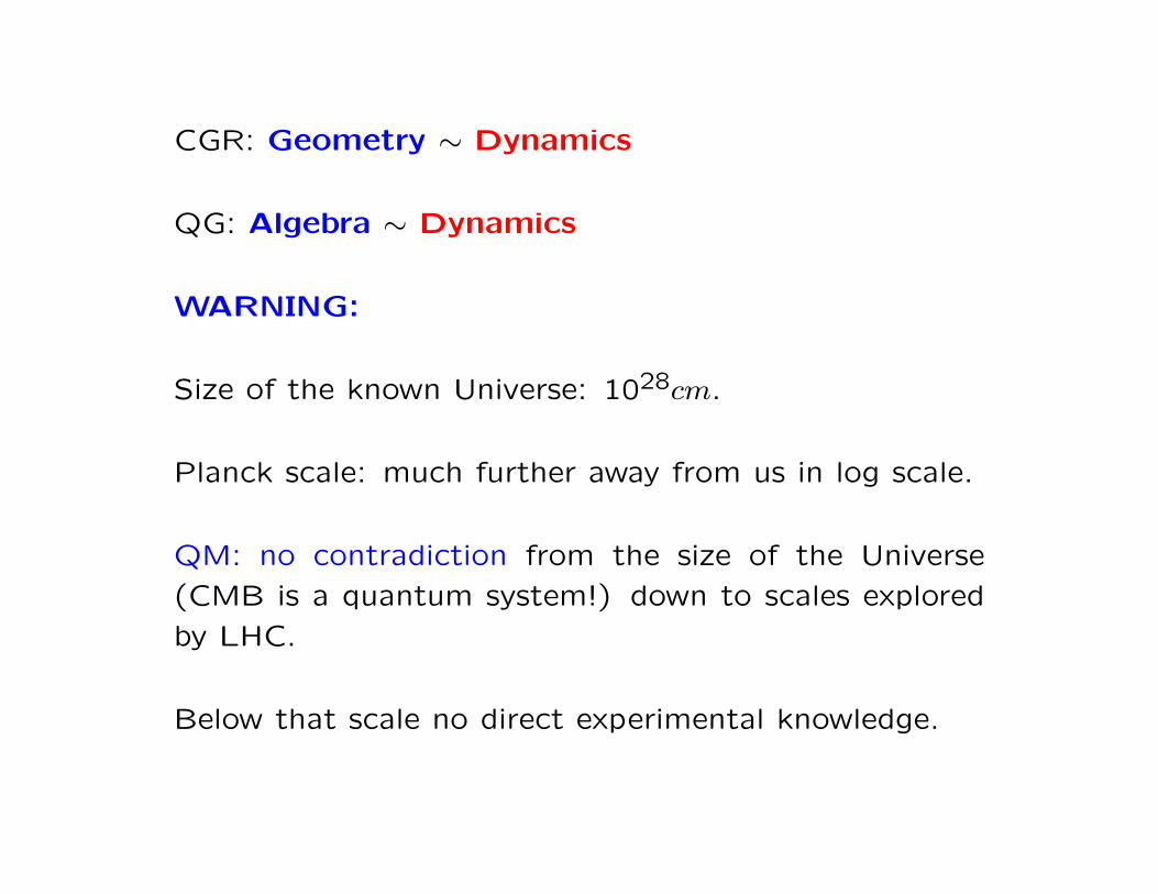
CGR: Geometry ∼ Dynamics

QG: Algebra ∼ Dynamics

WARNING:

Size of the known Universe: 1028cm.

Planck scale: much further away from us in log scale.

QM: no contradiction from the size of the Universe

(CMB is a quantum system!) down to scales explored

by LHC.

Below that scale no direct experimental knowledge.

GR: no contradiction from the size of the Universe down

to scales of order 10−2cm.

Below, nothing is known.

The (Planck length), 10−33cm, is very far. .

Quantum Minkowski Space

The Principle of Gravitational Stability against localization

of events implies :

∆q0 ·3∑

j=1

∆qj & 1;∑

1≤j<k≤3

∆qj∆qk & 1. (2)

[DFR 1994 - 95]; see also [TV 2012] [DMP 2013]

Must be implemented by SPACETIME commutation

relations

10

[qµ, qν] = iλ2PQµν (3)

imposing Quantum Conditions on the Qµν.

SIMPLEST solution:

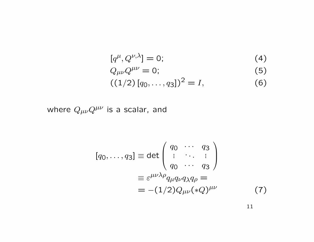
[qµ, Qν,λ] = 0; (4)

QµνQµν = 0; (5)

((1/2) [q0, . . . , q3])2 = I, (6)

where QµνQµν is a scalar, and

[q0, . . . , q3] ≡ det

q0 · · · q3... . . . ...q0 · · · q3

≡ εµνλρqµqνqλqρ =

= −(1/2)Qµν(∗Q)µν (7)

11

is a pseudoscalar, hence we use the square in the Quan-tum Conditions.

Basic model of Quantum Spacetime; implements ex-

actly Space Time Uncertainty Relations and is fullyPoincare covariant.

The classical Poincare group acts as symmetries; trans-lations, in particular, act adding to each qµ a real mul-tiple of the identity.

Gel’fand - Naimark Theorem: the classical MinkowskiSpace M is described by the commutative C* algebraof continuous functions vanishing at infinity on M ; theclassical coordinates can be viewed as commuting self-adjoint operators affiliated to that C* Algebras.

The noncommutative C* algebra of Quantum Space-

time can be associated to the above relations. The

procedure [DFR] applies to more general cases.

Assuming that the qλ, Qµν are selfadjoint operators and

that the Qµν commute strongly with one another and

with the qλ, the relations above can be seen as a bundle

of Lie Algebra relations based on the joint spectrum of

the Qµν.

Regular representations are described by representa-

tions of the C* group algebra of the unique simply con-

nected Lie group associated to the corresponding Lie

algebra.

The C* algebra of Quantum Spacetime is the C* alge-bra of a continuos field of group C* algebras based onthe spectrum of a commutative C* algebra.

In our case, that spectrum - the joint spectrum of theQµν - is the manifold Σ of the real valued antisymmetric2 - tensors fulfilling the same relations as the Qµν do: ahomogeneous space of the proper orthocronous Lorentzgroup, identified with the coset space of SL(2, C) modthe subgroup of diagonal matrices. Each of those ten-sors, can be taken to its rest frame, where the elec-tric and magnetic part are parallel unit vectors, by aboost, and go back with the inverse boost, specified bya third vector, orthogonal to those unit vectors;thus Σ can be viewed as the tangent bundle to twocopies of the unit sphere in 3 space - its base Σ1.

Irreducible representations at a point of Σ1: Shroedinger

p, q in 2 d. o. f..

The fibers, with the condition that I is not an inde-

pendent generator but is represented by I, are the C*

algebras of the Heisenberg relations in 2 degrees of free-

dom - the algebra of all compact operators on a fixed

infinite dimensional separable Hilbert space.

The continuos field can be shown to be trivial. Thus

the C* algebra E of Quantum Spacetime is identified

with the tensor product of the continuous functions

vanishing at infinity on Σ and the algebra of compact

operators.

Optimally localized states: those minimizing

Σµ(∆ωqµ)2;

minimum = 2, reached by states concentrated on Σ1,

at each point ground state of harmonic oscillator.

(Given by an optimal localization map composed with

a probability measure on Σ1).

Optimally localized states = ”points”

The classical limit of QST is M ×Σ1, i.e. M acquires

compact extra dimensions (two copies of the unit sphere

in 3 - space).

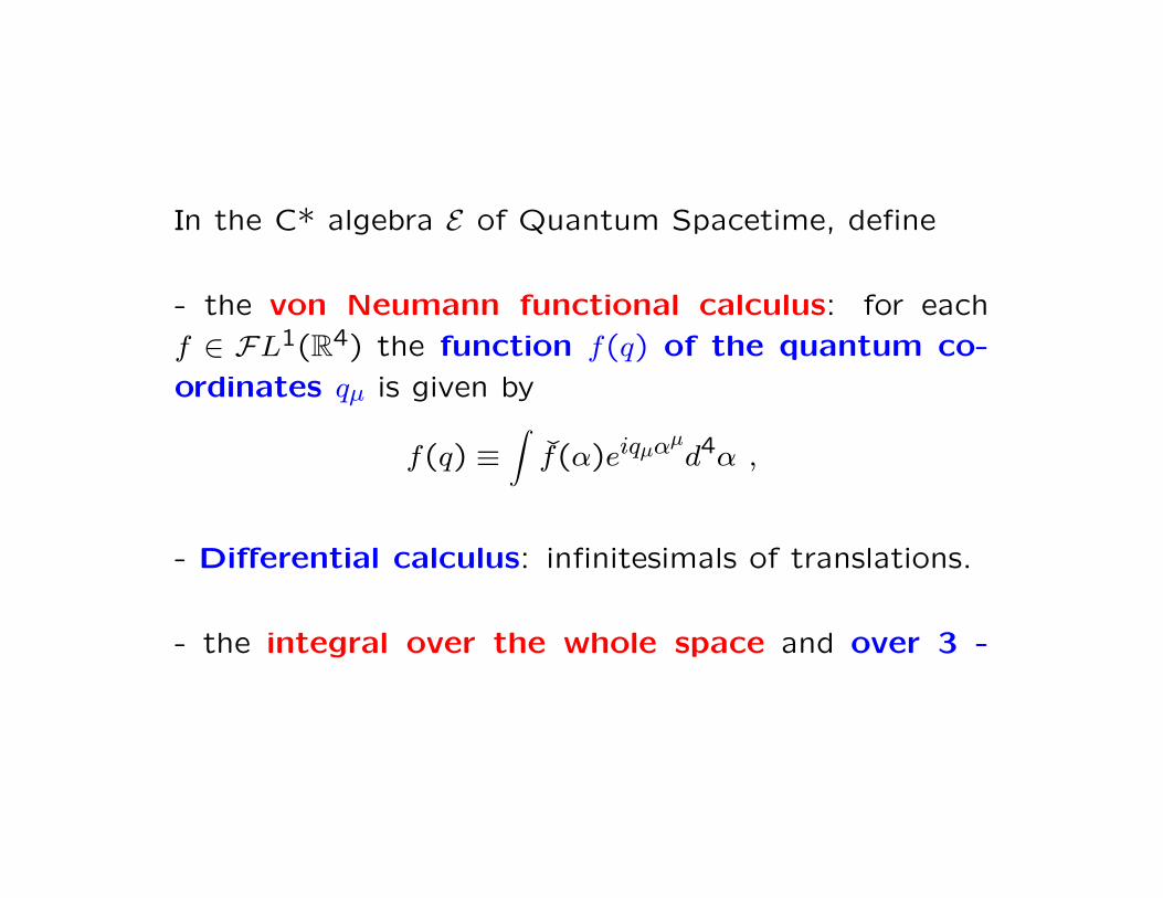
In the C* algebra E of Quantum Spacetime, define

- the von Neumann functional calculus: for each

f ∈ FL1(R4) the function f(q) of the quantum co-

ordinates qµ is given by

f(q) ≡∫f(α)eiqµα

µd4α ,

- Differential calculus: infinitesimals of translations.

- the integral over the whole space and over 3 -

space at q0 = t by∫d4qf(q) ≡

∫f(x)d4x = f(0) = Trf(q),∫

q0=tf(q)d3q ≡

∫eik0tf(k0, ~0)dk0 =

= limmTr(fm(q)∗f(q)fm(q))),

where the trace is the ordinary trace at each point ofthe joint spectrum Σ of the commutators, i.e. a Zvalued trace.

But on more general elements of our algebra both mapsgive Q - dependent results.

Important to define the interaction Hamiltonian to beused in the Gell’Mann Low formula for the S - Matrix.

Current investigations (D. Bahns, K. Fredenhagen, G.

Piacitelli, S.D.) concern models of QST where the al-

gebra of the commutators [q, q] is not central or not

even abelian.

Quantum Geometry

But to explore more thoroughly the Quantum Geometry

of Quantum Spacetime we must consider independent

events.

Quantum mechanically n independent events ought to

be described by the n − fold tensor product of E with

itself; considering arbitrary values on n we are led to

use the direct sum over all n.

If A is the C* algebra with unit over C, obtained adding

the unit to E, we will view the (n + 1) tensor power

12

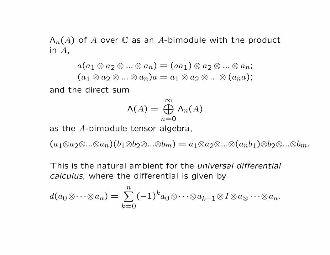
Λn(A) of A over C as an A-bimodule with the productin A,

a(a1 ⊗ a2 ⊗ ...⊗ an) = (aa1)⊗ a2 ⊗ ...⊗ an;

(a1 ⊗ a2 ⊗ ...⊗ an)a = a1 ⊗ a2 ⊗ ...⊗ (ana);

and the direct sum

Λ(A) =∞⊕n=0

Λn(A)

as the A-bimodule tensor algebra,

(a1⊗a2⊗...⊗an)(b1⊗b2⊗...⊗bm) = a1⊗a2⊗...⊗(anb1)⊗b2⊗...⊗bm.

This is the natural ambient for the universal differentialcalculus, where the differential is given by

d(a0⊗· · ·⊗an) =n∑

k=0

(−1)ka0⊗· · ·⊗ak−1⊗I⊗a⊗ · · ·⊗an.

As usual d is a graded differential, i.e., if φ ∈ Λ(A), ψ ∈Λn(A), we have

d2 = 0;

d(φ · ψ) = (dφ) · ψ + (−1)nφ · dψ.

Note that A = Λ0(A) ⊂ Λ(A), and the d-stable subal-

gebra Ω(A) of Λ(A) generated by A is the universal

differential algebra. In other words, it is the subalgebra

generated by A and

da = I ⊗ a− a⊗ I

as a varies in A.

In the case of n independent events one is led to de-

scribe the spacetime coordinates of the j − th event by

qj = I ⊗ ...I ⊗⊗q⊗ I...⊗ I (q in the j - th place); in this

way, the commutator between the different spacetime

components of the qj would depend on j.

A better choice is to require that it does not; this

is achieved as follows.

The centre Z of the multiplier algebra of E is the algebra

of all bounded continuos complex functions on Σ; so

that E, and hence A, is in an obvious way a Z−bimodule.

We therefore can, and will, replace, in the definition of

Λ(A), the C - tensor product by the Z−bimodule−tensorproduct so that

dQ = 0.

As a consequence, the qj and the 2−1/2(qj − qk), j dif-ferent from k, and 2−1/2dq, obey the same space-time commutation relations, as does the normalizedbarycenter coordinates, n−1/2(q1+q2+ ...+qn); and thelatter commutes with the difference coordinates.

These facts allow us to define a quantum diagonal map

from Λn(E) to E1 (the restriction to Σ1 of E),

E(n) : E ⊗Z · · · ⊗Z E −→ E1

which factors to that restriction map and a conditionalexpectation which leaves the functions of the barycen-ter coordinates alone, and evaluates on functions of the

difference variables the universal optimally localized map(which, when composed with a probability measure onΣ1, would give the generic optimally localized state).

Replacing the classical diagonal evaluation of a functionof n arguments on Minkowski space by the quantum

diagonal map allows us to define the Quantum Wick

Product.

But working in Ω(A) as a subspace of Λ(A) allows usto use two structures:

- the tensor algebra structure described above, whereboth the A bimodule and the Z bimodule structures en-ter, essential for our reduced universal differential cal-culus;

- the pre - C* algebra structure of Λ(A), which allows

us to consider, for each element a of Λn(A), its modulus

(a∗a)1/2, its spectrum, and so on.

In particular we can study the geometric operators: sep-

aration between two independent events, area, 3 - vol-

ume, 4 - volume, given by

dq;

dq ∧ dq;

dq ∧ dq ∧ dq;

dq ∧ dq ∧ dq ∧ dq,

where, for instance, the latter is given by

V = dq ∧ dq ∧ dq ∧ dq =

εµνρσdqµdqνdqρdqσ.

Each of these forms has a number of spacetime com-

ponents:

e.g. 4 the first one (a vector), 1 the last one (a pseu-

doscalar).

Each component is a normal operator;

Theorem. For each of these forms, the sum of the

square moduli of all spacetime components is bounded

below by a multiple of the identity of unit order of

magnitude.

Although that sum is (except for the 4 - volume!)

NOT Lorentz invariant, the bound holds in any Lorentz

frame.

In particular,

- the four volume operator has pure point spectrum, atdistance 51/2 − 2 from 0;

- the Euclidean distance between two independent eventshas a lower bound of order one in Planck units.

Two distinct points can never merge to a point.

However, of course, the state where the minimum isachieved will depend upon the reference frame wherethe requirement is formulated.

(The structure of length, area and volume operators onQST has been studied in full detail [BDFP 2011]).

Thus the existence of a minimal length is not at all in

contradiction with the Lorentz covariance of the model.

A mathematical sideline, unfortunately without appli-

cations to physics (so far): for a suitable pairing, the

above differential is the Hodge dual of the Hochhschild

boundary.

To this purpose, we first define on Λ(A) an A-valued

pairing, the shuffling product, by

< a0 ⊗ ...⊗ an, b0 ⊗ ...⊗ bm >= δn,ma0b0...anbn,

so that it is a left resp right A-module map on the left

resp. right term. The restriction to Ω(A) is immedi-

ately seen to have noteworthy properties, namely:

< a0da1...dan, (db1...dbn)bn+1 >= a0[a1, b1]...[an, bn]bn+1;

< dφ, aψb >= a < dφ, ψ > b;

< ωφ, (dψ)λ >=< ω, (dψ) >< φ, λ >;

< λdψ, φω >=< λ, φ >< dψ, ω >;

with a, b ∈ A, and φ, ψ, λ, ω ∈ Ω(A).

Thus, the shuffling product induces on the universal

differential algebra a pairing which measures the non-

commutativity. In general it will be degenerate.

For any algebra with unit and with a trace, the A-valued

pairing we just described is turned into an interesting

pairing with values in the complex numbers by compo-

sition with a trace τ . Namely, let τ be a complex valued

linear map defined on a two sided ideal J, such that

τ(ab) = τ(ba), a ∈ A, b ∈ J;

τ is faithful if a in A fulfills τ(ab) = 0 for all b in J only

if a = 0.

If ΛJ(A) denotes the differential ideal in Λ(A) generated

by J, we have that ΛJ(A) is the span of elements a0 ⊗

...⊗ an where aj ∈ J for at least one j, and

< φ,ψ >∈ J, φ ∈ Λ(A), ψ ∈ ΛJ(A).

Let δ denote the Hochhschild boundary defined by

δ(a0 ⊗ ...⊗ an) =

n−1∑k=0

(−1)ka0⊗...⊗ak−1⊗akak+1⊗ak+2⊗...⊗an+(−1)nana0⊗...⊗an−1.

Then we have

Proposition. The Hochhschild boundary is a Hodge

dual of the differential for the pairing τ(< ·, · >), namely

τ(< δω, φ >) = τ(< ω, dφ >), ω, φ ∈ Λ(A).

QFT on QST

The geometry of Quantum Spacetime and the freefield theories on it are fully Poincare covariant.

One can introduce interactions in different ways, allpreserving spacetime translation and space rotation co-variance, all equivalent on ordinary Minkowski space,providing inequivalent approaches on QST; but all ofthem, sooner or later, meet problems with Lorentzcovariance, apparently due to the nontrivial action ofthe Lorentz group on the centre of the algebra of Quan-tum Spacetime.

On this points in our opinion a deeper understanding isneeded.

13

The previously described ”basic model” of QFT is taken

as a background, modifying the S matrix for polinomial

field interactions.

( Quantum Gravity would require a dynamical role of

the commutators! Beyond the horizon).

For instance, the interaction Hamiltonian on quantum

spacetime

HI(t) = λ∫q0=t

d3q : φ(q)n :

would be Q - dependent; no invariant probability

measure or mean on Σ; integrating on Σ1 [DFR 1995]

breaks Lorentz invariance.

Covariance is preserved by Yang Feldmann equations

but missed again at the level of scattering theory.

The Quantum Wick product selects a special frame

from the start. The interaction Hamiltonian on the

quantum spacetime is then given by

HI(t) = λ∫q0=t

d3q : φ(q)n :Q

where

: φn(q) :Q= E(n)(: φ(q1) · · ·φ(qn) :)

which does not depend on Q any longer, but brakes

Lorentz invariance at an earlier stage

The last mentioned approach takes into account, in the

very definition of Wick products, the fact that in our

Quantum Spacetime n (larger or equal to two) distinct

points can never merge to a point. But we can use the

canonical quantum diagonal map which associates to

functions of n independent points a function of a single

point, evaluating a conditional expectation which on

functions of the differences takes a numerical value,

associated with the minimum of the Euclidean distance

(in a given Lorentz frame!).

The “Quantum Wick Product” obtained by this

procedure leads to an interaction Hamiltonian on the

quantum spacetime given by as a constant operator–

valued function of Σ1 (i.e. HI(t) is formally in the

tensor product of C(Σ1) with the algebra of field oper-

ators).

The interaction Hamiltonian on the quantum spacetime

is then given by

HI(t) = λ∫q0=t

d3q : φ(q)n :Q

This leads to a unique prescription for the interaction

Hamiltonian on quantum spacetime. When used in the

Gell’Mann Low perturbative expansion for the S - Ma-

trix, this gives the same result as the effective non

local Hamiltonian determined by the kernel

exp

−

1

2

∑j,µ

aµj

2δ(4)

(1

n

n∑j=1

aj

).

The corresponding perturbative Gell’Mann Low formulais then free of ultraviolet divergences at each termof the perturbation expansion [BDFP 2003] .

However, those terms have a meaning only after a sortof adiabatic cutoff: the coupling constant should bechanged to a function of time, rapidly vanishing at in-finity, say depending upon a cutoff time T.

But the limit T →∞ is difficult problem, and there areindications it does not exist.

A major open problems is the following.

Suppose we apply this construction to the renormal-ized Lagrangean of a theory which is renormalizable on

the ordinary Minkowski space, with the counter terms

defined by that ordinary theory, and with finite renor-

malization constants depending upon both the Planck

length λP and the cutoff time T .

Can we find a natural dependence such that in the limit

λP → 0 and T →∞ we get back the ordinary renormal-

ized Gell-Mann Low expansion on Minkowski space?

This should depend upon a suitable way of performing

a joint limit, which hopefully yields, for the physical

value of λP , to a result which is essentially independent

of T within wide margins of variation; in that case,

that result could be taken as source of predictions to

be compared with observations.

Comments on QST and cosmology

Heuristic argument we started with: commutators be-

tween coordinates ought to depend on gµ,ν; it suggests

a scenario:

Rµ,ν − (1/2)Rgµ,ν = 8πTµ,ν(ψ);

Fg(ψ) = 0;

[qµ, qν] = iQµ,ν(g);

as said this describes a scenario, not explicitly known

equations; but should manifest some features:

14

Algebra is Dynamics.

Expect: dynamical minimal length.

In particular, divergent near singularities. Would solve

Horizon Problem, without inflationary hypothesis.

How solid are these heuristic arguments?

Exact semiclassical EE, spherically simmetric case: min-

imal length is at least λP [DMP, 2013].

Suggests:

massless scalar field semiclassical coupling with gravity;

use Quantum Wick product to define Energy - Momen-

tum Tensor Tµ,νQ (q);

Exact EE with source ω⊗ηx(Tµ,νQ (q)), where ω is a KMS

state and ηx is a state on E optimally localized at x;

these simplifying ansaetze imply a solution describing

spacetime without the horizon problem [DMP 2013].

Thus QST with a constant minimal length builds by

itself a dynamical one!

Work in progress (Morsella, Piacitelli, Pinamonti, Tomassini,

. . . , SD): search better grounds for the use of the

Quantum Wick Product on curved spacetime.

Also: possible emergence of an effective inflationary

potential as an effect of Quantum Spacetime.

Problem of the Cosmological Constant.

Dark matter.

Is Dark Matter really dark? A pale quantum - gravita-

tional moonshine might be possible.

On QST a U(1) Gauge theory becomes a U(∞) theory,

with gauge group (at each point of Σ) U(CI +K), and

neutral scalar fields are no longer gauge invariant.

Warning: Quantum effects at Planck scale result from

extrapolation of EE to that scale.

But: Newton’s law is experimentally checked only for

distances not less than .01 centimeter! (Adelberger

et al, 2003, 2004), i.e. we are extrapolating 31 steps

down in base 10 - log scale; while the size of the

known universe is ”only” 28 steps up.

15

References

Sergio Doplicher, Klaus Fredenhagen, John E. Roberts:

”The quantum structure of spacetime at the Planck

scale and quantum fields”, Commun.Math.Phys. 172

(1995) 187-220;

Luca Tomassini, Stefano Viaggiu: ”Physically moti-

vated uncertainty relations at the Planck length for an

emergent non commutative spacetime”, Class. Quan-

tum Grav. 28 (2011) 075001;

Luca Tomassini, Stefano Viaggiu: ”Building non com-

mutative spacetimes at the Planck length for Fried-

mann flat cosmologies”, arXiv:1308.2767;

16

Sergio Doplicher, Gerardo Morsella, Nicola Pinamonti:”On Quantum Spacetime and the horizon problem”, J.Geom. Phys. 74 (2013), 196-210;

Dorothea Bahns, Sergio Doplicher, Klaus Fredenhagen,Gherardo Piacitelli: ”Quantum Geometry on QuantumSpacetime: Distance, Area and Volume Operators”,Commun. Math. Phys. 308, 567-589 (2011);

Sergio Doplicher: ”The Principle of Locality. Effective-ness, fate and challenges”, Journ. Math. Phys. 2010,50th Anniversary issue;

Gherardo Piacitelli: ”Twisted Covariance as a Non In-variant Restriction of the Fully Covariant DFR Model”,Commun. Math. Phys.295:701-729,2010;

Gherardo Piacitelli: ”Non Local Theories: New Rules

for Old Diagrams”, Journal-ref: JHEP 0408 (2004)

031;

Dorothea Bahns: ”Ultraviolet Finiteness of the aver-

aged Hamiltonian on the noncommutative Minkowski

space” 2004; arXiv:hep-th/0405224.

D. Bahns , S. Doplicher, K. Fredenhagen, G. Piacitelli:

”Ultraviolet Finite Quantum Field Theory on Quantum

Spacetime”, Commun.Math.Phys.237:221-241, 2003.

Sergio Doplicher: ”Spacetime and Fields, a Quantum

Texture”, Proceedings of the 37th Karpacz Winter School

of Theoretical Physics, 2001, 204-213; arXiv:hep-th/0105251

E. G. Adelberger, B. R. Heckel and A. E. Nelson, Ann.Rev. Nucl. Part. Sci. 53, 77 (2003). arXiv:hep-ph/0307284

C.D. Hoyle, D.J. Kapner, B.R. Heckel, E.G. Adelberger,J.H. Gundlach, U. Schmidt, H.E. Swanson: ”Sub-millimeterTests of the Gravitational Inverse-square Law”, Journal-ref: Phys.Rev.D70:042004,2004 arXiv:hep-ph/0405262

A recent survey:

D. Bahns , S. Doplicher, G.Morsella, G. Piacitelli: ”Quan-tum Spacetime and Algebraic Quantum Field Theory”,arXiv:1501.03298; in ”Advances in Algebraic QuantumField Theory”, R. Brunetti, C. Dappiaggi, K. Freden-hagen, J. Yngvason, Eds. ; Springer, 2015