Compactness properties for trace-class operators and applications to quantum mechanics
Upload
khangminh22Category
view
1download
0
Quantum Mechanics

Quantum Mechanics
An Introduction for Device Physicists and Electrical Engineers
Second Edition
David K Ferry
Arizona State University,Tempe, USA
Institute of Physics PublishingBristol and Philadelphia
c� IOP Publishing Ltd 2001
All rights reserved. No part of this publication may be reproduced, storedin a retrieval system or transmitted in any form or by any means, electronic,mechanical, photocopying, recording or otherwise, without the prior permissionof the publisher. Multiple copying is permitted in accordance with the termsof licences issued by the Copyright Licensing Agency under the terms of itsagreement with the Committee of Vice-Chancellors and Principals.
British Library Cataloguing-in-Publication Data
A catalogue record for this book is available from the British Library.
ISBN 0 7503 0725 0
Library of Congress Cataloging-in-Publication Data are available
Commissioning Editor: James RevillPublisher: Nicki DennisProduction Editor: Simon LaurensonProduction Control: Sarah PlentyCover Design: Victoria Le BillonMarketing Executive: Colin Fenton
Published by Institute of Physics Publishing, wholly owned by The Institute ofPhysics, London
Institute of Physics Publishing, Dirac House, Temple Back, Bristol BS1 6BE, UK
US Office: Institute of Physics Publishing, The Public Ledger Building, Suite1035, 150 South Independence Mall West, Philadelphia, PA 19106, USA
Typeset in TEX using the IOP Bookmaker MacrosPrinted in the UK by J W Arrowsmith Ltd, Bristol
Contents
Preface to the first edition ix
Preface to the second edition x
1 Waves and particles 11.1 Introduction 11.2 Light as particles—the photoelectric effect 31.3 Electrons as waves 51.4 Position and momentum 9
1.4.1 Expectation of the position 101.4.2 Momentum 131.4.3 Non-commuting operators 151.4.4 Returning to temporal behaviour 17
1.5 Summary 21References 22Problems 23
2 The Schrodinger equation 252.1 Waves and the differential equation 262.2 Density and current 282.3 Some simple cases 30
2.3.1 The free particle 312.3.2 A potential step 32
2.4 The infinite potential well 362.5 The finite potential well 392.6 The triangular well 492.7 Coupled potential wells 552.8 The time variation again 57
2.8.1 The Ehrenfest theorem 592.8.2 Propagators and Green’s functions 60
2.9 Numerical solution of the Schrodinger equation 64References 69Problems 71
vi Contents
3 Tunnelling 733.1 The tunnel barrier 74
3.1.1 The simple rectangular barrier 743.1.2 The tunnelling probability 76
3.2 A more complex barrier 773.3 The double barrier 80
3.3.1 Simple, equal barriers 823.3.2 The unequal-barrier case 843.3.3 Shape of the resonance 87
3.4 Approximation methods—the WKB method 893.4.1 Bound states of a general potential 923.4.2 Tunnelling 94
3.5 Tunnelling devices 943.5.1 A current formulation 943.5.2 The p–n junction diode 993.5.3 The resonant tunnelling diode 1023.5.4 Resonant interband tunnelling 1043.5.5 Self-consistent simulations 107
3.6 The Landauer formula 1083.7 Periodic potentials 113
3.7.1 Velocity 1173.7.2 Superlattices 118
3.8 Single-electron tunnelling 1213.8.1 Bloch oscillations 1223.8.2 Periodic potentials 1243.8.3 The double-barrier quantum dot 127
References 131Problems 133
4 The harmonic oscillator 1364.1 Hermite polynomials 1394.2 The generating function 1434.3 Motion of the wave packet 1464.4 A simpler approach with operators 1494.5 Quantizing the ��-circuit 1534.6 The vibrating lattice 1554.7 Motion in a quantizing magnetic field 159
4.7.1 Connection with semi-classical orbits 1624.7.2 Adding lateral confinement 1634.7.3 The quantum Hall effect 165
References 167Problems 168
Contents vii
5 Basis functions, operators, and quantum dynamics 1705.1 Position and momentum representation 1725.2 Some operator properties 174
5.2.1 Time-varying expectations 1755.2.2 Hermitian operators 1775.2.3 On commutation relations 181
5.3 Linear vector spaces 1845.3.1 Some matrix properties 1865.3.2 The eigenvalue problem 1885.3.3 Dirac notation 190
5.4 Fundamental quantum postulates 1925.4.1 Translation operators 1925.4.2 Discretization and superlattices 1935.4.3 Time as a translation operator 1965.4.4 Canonical quantization 200
References 202Problems 204
6 Stationary perturbation theory 2066.1 The perturbation series 2076.2 Some examples of perturbation theory 211
6.2.1 The Stark effect in a potential well 2116.2.2 The shifted harmonic oscillator 2156.2.3 Multiple quantum wells 2176.2.4 Coulomb scattering 220
6.3 An alternative technique—the variational method 222References 225Problems 226
7 Time-dependent perturbation theory 2277.1 The perturbation series 2287.2 Electron–phonon scattering 2307.3 The interaction representation 2347.4 Exponential decay and uncertainty 2377.5 A scattering-state basis—the � -matrix 240
7.5.1 The Lippmann–Schwinger equation 2407.5.2 Coulomb scattering again 2427.5.3 Orthogonality of the scattering states 245
References 246Problems 247
viii Contents
8 Motion in centrally symmetric potentials 2498.1 The two-dimensional harmonic oscillator 249
8.1.1 Rectangular coordinates 2508.1.2 Polar coordinates 2518.1.3 Splitting the angular momentum states with a magnetic field2568.1.4 Spectroscopy of a harmonic oscillator 258
8.2 The hydrogen atom 2648.2.1 The radial equation 2658.2.2 Angular solutions 2678.2.3 Angular momentum 268
8.3 Atomic energy levels 2708.3.1 The Fermi–Thomas model 2738.3.2 The Hartree self-consistent potential 2758.3.3 Corrections to the centrally symmetric potential 2768.3.4 The covalent bond in semiconductors 279
8.4 Hydrogenic impurities in semiconductors 284References 286Problems 287
9 Electrons and anti-symmetry 2889.1 Symmetric and anti-symmetric wave functions 2899.2 Spin angular momentum 2919.3 Systems of identical particles 2939.4 Fermion creation and annihilation operators 2959.5 Field operators 298
9.5.1 Connection with the many-electron formulation 2999.5.2 Quantization of the Hamiltonian 3019.5.3 The two-electron wave function 3029.5.4 The homogeneous electron gas 305
9.6 The Green’s function 3079.6.1 The equations of motion 3109.6.2 The Hartree approximation 3129.6.3 Connection with perturbation theory 3149.6.4 Dyson’s equation 3199.6.5 The self-energy 321
References 323Problems 324
Solutions to selected problems 325
Index 341
Preface to the first edition
Most treatments of quantum mechanics have begun from the historical basis ofthe application to nuclear and atomic physics. This generally leaves the impor-tant topics of quantum wells, tunnelling, and periodic potentials until late in thecourse. This puts the person interested in solid-state electronics and solid-statephysics at a disadvantage, relative to their counterparts in more traditional fieldsof physics and chemistry. While there are a few books that have departed fromthis approach, it was felt that there is a need for one that concentrates primarilyupon examples taken from the new realm of artificially structured materials insolid-state electronics. Quite frankly, we have found that students are often justnot prepared adequately with experience in those aspects of quantum mechan-ics necessary to begin to work in small structures (what is now called mesoscopicphysics) and nanoelectronics, and that it requires several years to gain the materialin these traditional approaches. Students need to receive the material in an orderthat concentrates on the important aspects of solid-state electronics, and the mod-ern aspects of quantum mechanics that are becoming more and more used in ev-eryday practice in this area. That has been the aim of this text. The topics and theexamples used to illustrate the topics have been chosen from recent experimentalstudies using modern microelectronics, heteroepitaxial growth, and quantum welland superlattice structures, which are important in today’s rush to nanoelectronics.
At the same time, the material has been structured around a senior-levelcourse that we offer at Arizona State University. Certainly, some of the materialis beyond this (particularly chapter 9), but the book could as easily be suitedto a first-year graduate course with this additional material. On the other hand,students taking a senior course will have already been introduced to the ideas ofwave mechanics with the Schrodinger equation, quantum wells, and the Kronig–Penney model in a junior-level course in semiconductor materials. This earliertreatment is quite simplified, but provides an introduction to the concepts that aredeveloped further here. The general level of expectation on students using thismaterial is this prior experience plus the linear vector spaces and electromagneticfield theory to which electrical engineers have been exposed.
I would like to express thanks to my students who have gone throughthe course, and to Professors Joe Spector and David Allee, who have read themanuscript completely and suggested a great many improvements and changes.
David K FerryTempe, AZ, 1992
ix

Preface to the second edition
Many of my friends have used the first edition of this book, and have suggesteda number of changes and additions, not to mention the many errata necessary. Inthe second edition, I have tried to incorporate as many additions and changes aspossible without making the text over-long. As before, there remains far morematerial than can be covered in a single one-semester course, but the additionsprovide further discussion on many topics and important new additions, suchas numerical solutions to the Schrodinger equation. We continue to use thisbook in such a one-semester course, which is designed for fourth-year electricalengineering students, although more than half of those enrolled are first-yeargraduate students taking their first quantum mechanics course.
I would like to express my thanks in particular to Dragica Vasileska, whohas taught the course several times and has been particularly helpful in pointingout the need for additional material that has been included. Her insight into theinterpretations has been particularly useful.
David K FerryTempe, AZ, 2000
x
Chapter 1
Waves and particles
1.1 Introduction
Science has developed through a variety of investigations more or less over thetime scale of human existence. On this scale, quantum mechanics is a veryyoung field, existing essentially only since the beginning of this century. Evenour understanding of classical mechanics has existed for a comparatively longperiod—roughly having been formalized with Newton’s equations published inhis Principia Mathematica, in April 1686. In fact, we have just celebrated morethan 300 years of classical mechanics.
In contrast with this, the ideas of quantum mechanics are barely morethan a century old. They had their first beginnings in the 1890s with Planck’sdevelopment of a theory for black-body radiation. This form of radiation isemitted by all bodies according to their temperature. However, before Planck,there were two competing views. In one, the low-frequency view, this radiationincreased as a power of the frequency, which led to a problem at very highfrequencies. In the other, the high-frequency view, the radiation decreased rapidlywith frequency, which led to a problem at low frequencies. Planck unified theseviews through the development of what is now known as the Planck black-bodyradiation law:
���� �� ���
����
�����
�� �
�� (1.1)
where � is the frequency, � is the temperature, � is the intensity of radiation,and �� is Boltzmann’s constant ����� � ���� ����. In order to achieve thisresult, Planck had to assume that matter radiated and absorbed energy in small,but non-zero quantities whose energy was defined by
� � �� (1.2)
where � is now known as Planck’s constant, given by � � � ���� J s. WhilePlanck had given us the idea of quanta of energy, he was not comfortable with
1
2 Waves and particles
this idea, but it took only a decade for Einstein’s theory of the photoelectriceffect (discussed later) to confirm that radiation indeed was composed of quantumparticles of energy given by (1.2). Shortly after this, Bohr developed his quantummodel of the atom, in which the electrons existed in discrete shells with welldefined energy levels. In this way, he could explain the discrete absorption andemission lines that were seen in experimental atomic spectroscopy. While hismodel was developed in a somewhat ad hoc manner, the ideas proved correct,although the mathematical details were changed when the more formal quantumtheory arrived in 1927 from Heisenberg and Schrodinger. The work of thesetwo latter pioneers led to different, but equivalent, formulations of the quantumprinciples that we know to be important in modern physics. Finally, anotheressential concept was introduced by de Broglie. While we have assigned particle-like properties to light waves earlier, de Broglie asserted that particles, likeelectrons, should have wavelike properties in which their wavelength is relatedto their momentum by
� ��
��
�
��
� (1.3)
� is now referred to as the de Broglie wavelength of the particle.Today, there is a consensus (but not a complete agreement) as to the general
understanding of the quantum principles. In essence, quantum mechanics is themathematical description of physical systems with non-commuting operators; forexample, the ordering of the operators is very important. The engineer is familiarwith such an ordering dependence through the use of matrix algebra, where ingeneral the order of two matrices is important; that is �� �� ��. In quantummechanics, the ordering of various operators is important, and it is these operatorsthat do not commute. There are two additional, and quite important, postulates.These are complementarity and the correspondence principle.
Complementarity refers to the duality of waves and particles. That is, forboth electrons and light waves, there is a duality between a treatment in termsof waves and a treatment in terms of particles. The wave treatment generally isdescribed by a field theory with the corresponding operator effects introduced intothe wave amplitudes. The particle is treated in a manner similar to the classicalparticle dynamics treatment with the appropriate operators properly introduced.In the next two sections, we will investigate two of the operator effects.
On the other hand, the correspondence principle relates to the limitingapproach to the well known classical mechanics. It will be found that Planck’sconstant, �, appears in all results that truly reflect quantum mechanical behaviour.As we allow � � �, the classical results must be obtained. That is, the truequantum effects must vanish as we take this limit. Now, we really do not vary thevalue of such a fundamental constant, but the correspondence principle assertsthat if we were to do so, the classical results would be recovered. What thismeans is that the quantum effects are modifications of the classical properties.These effects may be small or large, depending upon a number of factors such astime scales, size scales and energy scales. The value of Planck’s constant is quite

Light as particles—the photoelectric effect 3
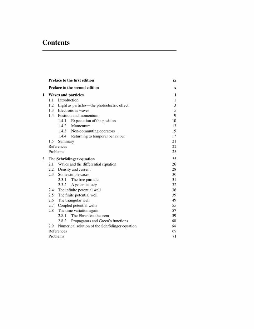
Figure 1.1. In panel (a), we illustrate how light coming from the source L and passingthrough the two slits S� and S� interferes to cause the pattern indicated on the ‘screen’ onthe right. If we block one of the slits, say S�, then we obtain only the light intensity passingthrough S� on the ‘screen’ as shown in panel (b).
small, ����� � ����� J s, but one should not assume that the quantum effects
are small. For example, quantization is found to affect the operation of modernmetal–oxide–semiconductor (MOS) transistors and to be the fundamental propertyof devices such as a tunnel diode.
Before proceeding, let us examine an important aspect of light as a wave. Ifwe create a source of coherent light (a single frequency), and pass this throughtwo slits, the wavelike property of the light will create an interference pattern, asshown in figure 1.1. Now, if we block one of the slits, so that light passes throughjust a single slit, this pattern disappears, and we see just the normal passage of thelight waves. It is this interference between the light, passing through two differentpaths so as to create two different phases of the light wave, that is an essentialproperty of the single wave. When we can see such an interference pattern, it issaid that we are seeing the wavelike properties of light. To see the particle-likeproperties, we turn to the photoelectric effect.
1.2 Light as particles—the photoelectric effect
One of the more interesting examples of the principle of complementarity is thatof the photoelectric effect. It was known that when light was shone upon thesurface of a metal, or some other conducting medium, electrons could be emittedfrom the surface provided that the frequency of the incident light was sufficientlyhigh. The curious effect is that the velocity of the emitted electrons dependsonly upon the wavelength of the incident light, and not upon the intensity of theradiation. In fact, the energy of the emitted particles varies inversely with thewavelength of the light waves. On the other hand, the number of emitted electronsdoes depend upon the intensity of the radiation, and not upon its wavelength.Today, of course, we do not consider this surprising at all, but this is after it
4 Waves and particles
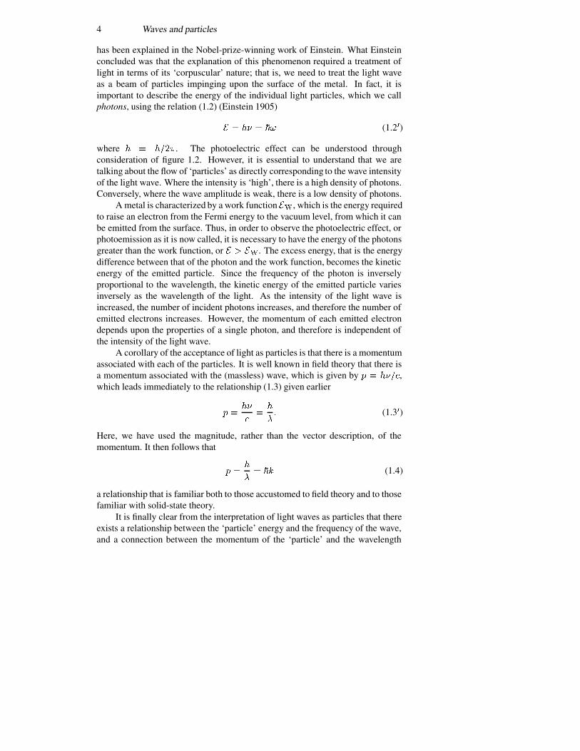
has been explained in the Nobel-prize-winning work of Einstein. What Einsteinconcluded was that the explanation of this phenomenon required a treatment oflight in terms of its ‘corpuscular’ nature; that is, we need to treat the light waveas a beam of particles impinging upon the surface of the metal. In fact, it isimportant to describe the energy of the individual light particles, which we callphotons, using the relation (1.2) (Einstein 1905)
� � �� � �� (1.2�)
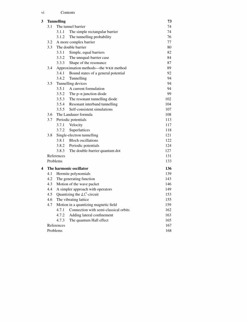
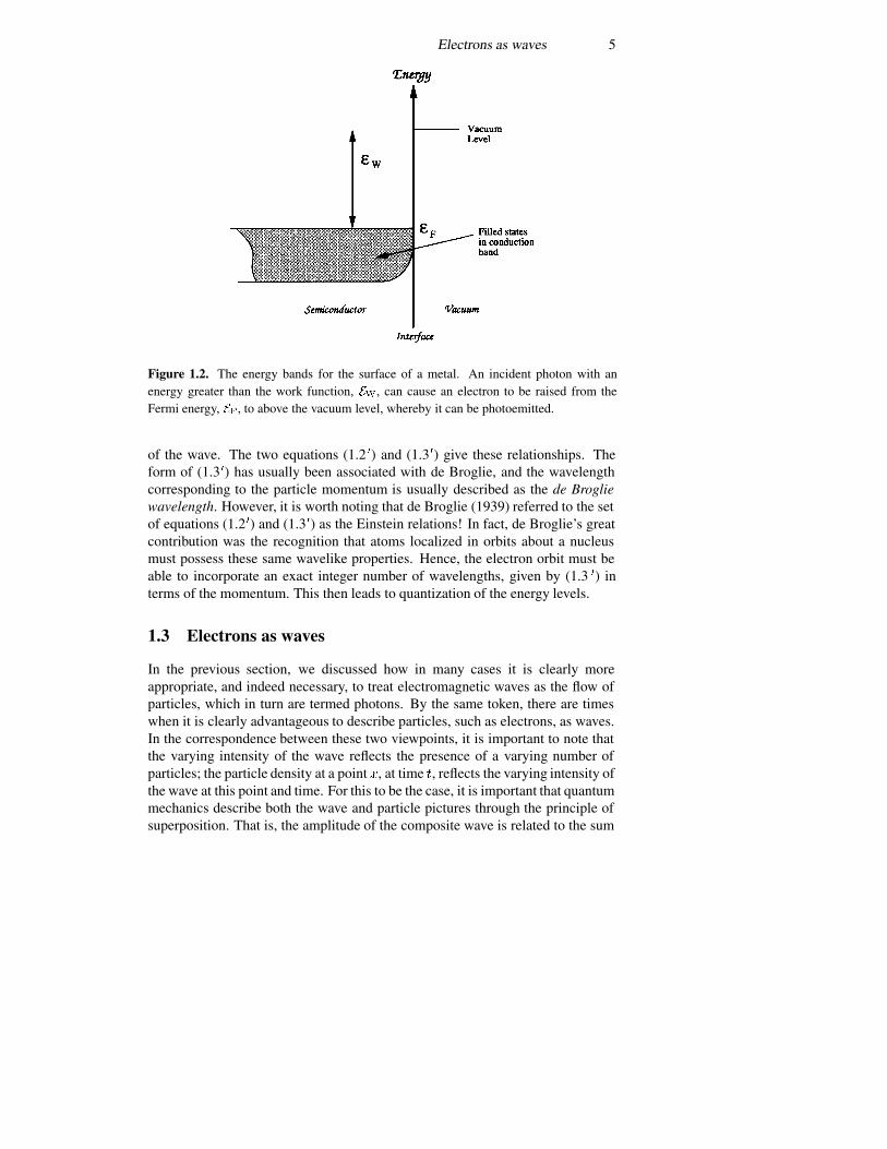
where � � ����. The photoelectric effect can be understood throughconsideration of figure 1.2. However, it is essential to understand that we aretalking about the flow of ‘particles’ as directly corresponding to the wave intensityof the light wave. Where the intensity is ‘high’, there is a high density of photons.Conversely, where the wave amplitude is weak, there is a low density of photons.
A metal is characterized by a work function ��, which is the energy requiredto raise an electron from the Fermi energy to the vacuum level, from which it canbe emitted from the surface. Thus, in order to observe the photoelectric effect, orphotoemission as it is now called, it is necessary to have the energy of the photonsgreater than the work function, or � � ��. The excess energy, that is the energydifference between that of the photon and the work function, becomes the kineticenergy of the emitted particle. Since the frequency of the photon is inverselyproportional to the wavelength, the kinetic energy of the emitted particle variesinversely as the wavelength of the light. As the intensity of the light wave isincreased, the number of incident photons increases, and therefore the number ofemitted electrons increases. However, the momentum of each emitted electrondepends upon the properties of a single photon, and therefore is independent ofthe intensity of the light wave.
A corollary of the acceptance of light as particles is that there is a momentumassociated with each of the particles. It is well known in field theory that there isa momentum associated with the (massless) wave, which is given by � � ����,which leads immediately to the relationship (1.3) given earlier
� ���
��
�
� (1.3�)
Here, we have used the magnitude, rather than the vector description, of themomentum. It then follows that
� ��
�� � (1.4)
a relationship that is familiar both to those accustomed to field theory and to thosefamiliar with solid-state theory.
It is finally clear from the interpretation of light waves as particles that thereexists a relationship between the ‘particle’ energy and the frequency of the wave,and a connection between the momentum of the ‘particle’ and the wavelength
Electrons as waves 5
Figure 1.2. The energy bands for the surface of a metal. An incident photon with anenergy greater than the work function, ��, can cause an electron to be raised from theFermi energy, ��, to above the vacuum level, whereby it can be photoemitted.
of the wave. The two equations (1.2 �) and (1.3�) give these relationships. Theform of (1.3�) has usually been associated with de Broglie, and the wavelengthcorresponding to the particle momentum is usually described as the de Brogliewavelength. However, it is worth noting that de Broglie (1939) referred to the setof equations (1.2�) and (1.3�) as the Einstein relations! In fact, de Broglie’s greatcontribution was the recognition that atoms localized in orbits about a nucleusmust possess these same wavelike properties. Hence, the electron orbit must beable to incorporate an exact integer number of wavelengths, given by (1.3 �) interms of the momentum. This then leads to quantization of the energy levels.
1.3 Electrons as waves
In the previous section, we discussed how in many cases it is clearly moreappropriate, and indeed necessary, to treat electromagnetic waves as the flow ofparticles, which in turn are termed photons. By the same token, there are timeswhen it is clearly advantageous to describe particles, such as electrons, as waves.In the correspondence between these two viewpoints, it is important to note thatthe varying intensity of the wave reflects the presence of a varying number ofparticles; the particle density at a point �, at time �, reflects the varying intensity ofthe wave at this point and time. For this to be the case, it is important that quantummechanics describe both the wave and particle pictures through the principle ofsuperposition. That is, the amplitude of the composite wave is related to the sum

6 Waves and particles
of the amplitudes of the individual waves corresponding to each of the particlespresent. Note that it is the amplitudes, and not the intensities, that are summed, sothere arises the real possibility for interference between the waves of individualparticles. Thus, for the presence of two (non-interacting) particles at a point �, attime �, we may write the composite wave function as
���� �� � ����� �� � ����� ��� (1.5)
This composite wave may be described as a probability wave, in that the squareof the magnitude describes the probability of finding an electron at a point.
It may be noted from (1.4) that the momentum of the particles goesimmediately into the so-called wave vector � of the wave. A special form of(1.5) is
���� �� � ����������� ������������ (1.6)
where it has been assumed that the two components may have different momenta(but we have taken the energies equal). For the moment, the time-independentsteady state will be considered, so the time-varying parts of (1.6) will besuppressed as we will talk only about steady-state results of phase interference.It is known, for example, that a time-varying magnetic field that is enclosed by aconducting loop will induce an electric field (and voltage) in the loop throughFaraday’s law. Can this happen for a time-independent magnetic field? Theclassical answer is, of course, no, and Maxwell’s equations give us this answer.But do they in the quantum case where we can have the interference between thetwo waves corresponding to two separate electrons?
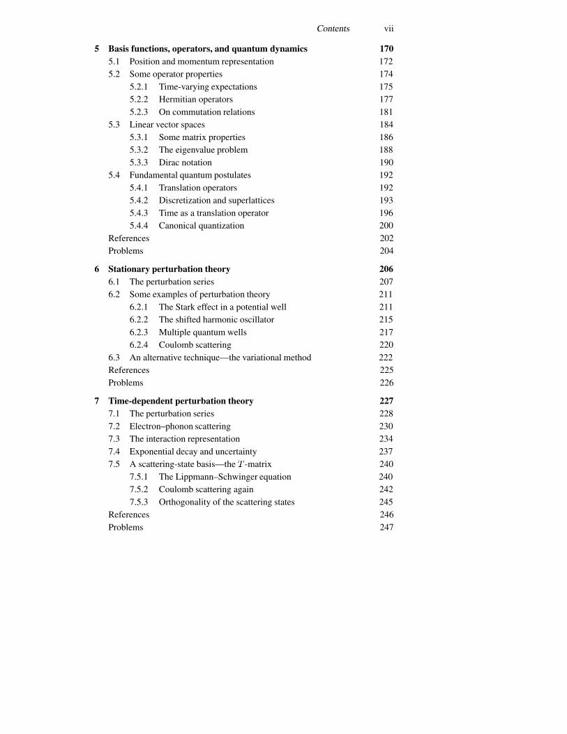
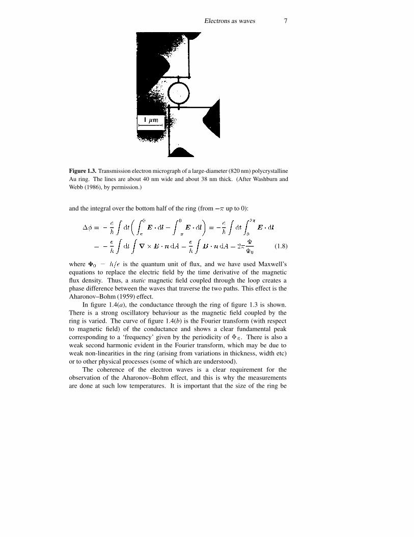
For the experiment, we consider a loop of wire. Specifically, the loop is madeof Au wire deposited on a Si�N� substrate. Such a loop is shown in figure 1.3,where the loop is about 820 nm in diameter, and the Au lines are 40 nm wide(Webb et al 1985). The loop is connected to an external circuit through Au leads(also shown), and a magnetic field is threaded through the loop.
To understand the phase interference, we proceed by assuming that theelectron waves enter the ring at a point described by � � ��. For the moment,assume that the field induces an electric field in the ring (the time variation willin the end cancel out, and it is not the electric field per se that causes the effect,but this approach allows us to describe the effect). Then, for one electron passingthrough the upper side of the ring, the electron is accelerated by the field, as itmoves with the field, while on the other side of the ring the electron is deceleratedby the field as it moves against the field. The field enters through Newton’s law,and
� � �� �
�
� ��� (1.7)
If we assume that the initial wave vector is the same for both electrons, then thephase difference at the output of the ring is given by taking the difference of theintegral over momentum in the top half of the ring (from an angle of � down to 0)
Electrons as waves 7
Figure 1.3. Transmission electron micrograph of a large-diameter (820 nm) polycrystallineAu ring. The lines are about 40 nm wide and about 38 nm thick. (After Washburn andWebb (1986), by permission.)
and the integral over the bottom half of the ring (from�� up to 0):
�� � �
�
�
���
���
�
� � ���
��
��
� � ��
�� �
�
�
���
���
�
� � ��
� �
�
�
���
���� � � �� �
�
�
�� � � �� � ��
�
��
(1.8)
where �� � ��� is the quantum unit of flux, and we have used Maxwell’sequations to replace the electric field by the time derivative of the magneticflux density. Thus, a static magnetic field coupled through the loop creates aphase difference between the waves that traverse the two paths. This effect is theAharonov–Bohm (1959) effect.
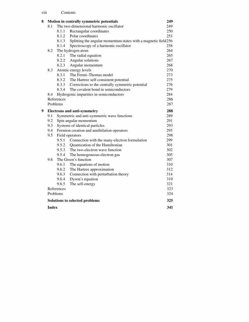
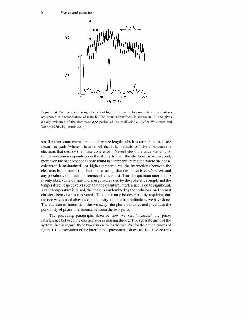
In figure 1.4(a), the conductance through the ring of figure 1.3 is shown.There is a strong oscillatory behaviour as the magnetic field coupled by thering is varied. The curve of figure 1.4(b) is the Fourier transform (with respectto magnetic field) of the conductance and shows a clear fundamental peakcorresponding to a ‘frequency’ given by the periodicity of � �. There is also aweak second harmonic evident in the Fourier transform, which may be due toweak non-linearities in the ring (arising from variations in thickness, width etc)or to other physical processes (some of which are understood).
The coherence of the electron waves is a clear requirement for theobservation of the Aharonov–Bohm effect, and this is why the measurementsare done at such low temperatures. It is important that the size of the ring be
8 Waves and particles
Figure 1.4. Conductance through the ring of figure 1.3. In (a), the conductance oscillationsare shown at a temperature of 0.04 K. The Fourier transform is shown in (b) and givesclearly evidence of the dominant ��� period of the oscillations. (After Washburn andWebb (1986), by permission.)
smaller than some characteristic coherence length, which is termed the inelasticmean free path (where it is assumed that it is inelastic collisions between theelectrons that destroy the phase coherence). Nevertheless, the understanding ofthis phenomenon depends upon the ability to treat the electrons as waves, and,moreover, the phenomenon is only found in a temperature regime where the phasecoherence is maintained. At higher temperatures, the interactions between theelectrons in the metal ring become so strong that the phase is randomized, andany possibility of phase interference effects is lost. Thus the quantum interferenceis only observable on size and energy scales (set by the coherence length and thetemperature, respectively) such that the quantum interference is quite significant.As the temperature is raised, the phase is randomized by the collisions, and normalclassical behaviour is recovered. This latter may be described by requiring thatthe two waves used above add in intensity, and not in amplitude as we have done.The addition of intensities ‘throws away’ the phase variables and precludes thepossibility of phase interference between the two paths.
The preceding paragraphs describe how we can ‘measure’ the phaseinterference between the electron waves passing through two separate arms of thesystem. In this regard, these two arms serve as the two slits for the optical waves offigure 1.1. Observation of the interference phenomena shows us that the electrons
Position and momentum 9
must be considered as waves, and not as particles, for this experiment. Once more,we have a confirmation of the correspondence between waves and particles as twoviews of a coherent whole. In the preceding experiment, the magnetic field wasused to vary the phase in both arms of the interferometer and induce the oscillatorybehaviour of the conductance on the magnetic field. It is also possible to vary thephase in just one arm of the interferometer by the use of a tuning gate (Fowler1985). Using techniques which will be discussed in the following chapters, thegate voltage varies the propagation wave vector � in one arm of the interferometer,which will lead to additional oscillatory conductance as this voltage is tuned,according to (1.7) and (1.8), as the electric field itself is varied instead of usingthe magnetic field. A particularly ingenious implementation of this interferometerhas been developed by Yacoby et al (1994), and will be discussed in later chaptersonce we have discussed the underlying physics.
Which is the proper interpretation to use for a general problem: particle orwave? The answer is not an easy one to give. Rather, the proper choice dependslargely upon the particular quantum effect being investigated. Thus one choosesthe approach that yields the answer with minimum effort. Nevertheless, the greatmajority of work actually has tended to treat the quantum mechanics via the wavemechanical picture, as embodied in the Schrodinger equation (discussed in thenext chapter). One reason for this is the great wealth of mathematical literaturedealing with boundary value problems, as the time-independent Schrodingerequation is just a typical wave equation. Most such problems actually lie in theformulation of the proper boundary conditions, and then the imposition of non-commuting variables. Before proceeding to this, however, we diverge to continuethe discussion of position and momentum as variables and operators.
1.4 Position and momentum
For the remainder of this chapter, we want to concentrate on just what propertieswe can expect from this wave that is supposed to represent the particle (orparticles). Do we represent the particle simply by the wave itself? No, becausethe wave is a complex quantity, while the charge and position of the particle arereal quantities. Moreover, the wave is a distributed quantity, while we expectthe particle to be relatively localized in space. This suggests that we relate theprobability of finding the electron at a position � to the square of the magnitudeof the wave. That is, we say that
����� ���� (1.9)
is the probability of finding an electron at point � at time �. Then, it is clear thatthe wave function must be normalized through
��
��
����� ���� �� � �� (1.10)

10 Waves and particles
While (1.10) extends over all space, the appropriate volume is that of the systemunder discussion. This leads to a slightly different normalization for the planewaves utilized in section 1.3 above. Here, we use box normalization (the term‘box’ refers to the three-dimensional case):
������
� ���
����
����� ���� �� � �� (1.11)
This normalization keeps constant total probability and recognizes that, for auniform probability, the amplitude must go to zero as the volume increaseswithout limit.
There are additional constraints which we wish to place upon the wavefunction. The first is that the system is linear, and satisfies superposition. Thatis, if there are two physically realizable states, say �� and ��, then the total wavefunction must be expressable by the linear summation of these, as
���� �� � ������� �� ������� ��� (1.12)
Here, �� and �� are arbitrary complex constants, and the summation representsa third, combination state that is physically realizable. Using (1.12) in theprobability requirement places additional load on these various states. First, each�� must be normalized independently. Secondly, the constants � � must now satisfy(1.10) as��
��
����� ���� �� � � � �������
��
������ ���� �� �����
��
��
������ ���� ��
� ����� ������ (1.13)
In order for the last equation to be correct, we must apply the third requirement of��
��
������ ������� �� �� �
��
��
������ ������� �� �� � (1.14)
which is that the individual states are orthogonal to one another, which must bethe case for our use of the composite wave function (1.12) to find the probability.
1.4.1 Expectation of the position
With the normalizations that we have now introduced, it is clear that we areequating the square of the magnitude of the wave function with a probabilitydensity function. This allows us to compute immediately the expectation value,or average value, of the position of the particle with the normal definitionsintroduced in probability theory. That is, the average value of the position isgiven by
��� �
��
��
������ ���� �� �
��
��
����� ������� �� ��� (1.15)
Position and momentum 11
In the last form, we have split the wave function product into its two componentsand placed the position operator between the complex conjugate of the wavefunction and the wave function itself. This is the standard notation, and designatesthat we are using the concept of an inner product of two functions to describe theaverage. If we use (1.10) to define the inner product of the wave function and itscomplex conjugate, then this may be described in the short-hand notation
����� �
��
��
����� ������ �� �� � � (1.16)
and��� � ��� ���� (1.17)
Before proceeding, it is worthwhile to consider an example of theexpectation value of the wave function. Consider the Gaussian wave function
���� �� � � ��������������� (1.18)
We first normalize this wave function as��
��
����� ���� �� � ��
��
��
�������� �� � ���� � � (1.19)
so that � � �����. Then, the expectation value of position is
��� � ���
��
��
���������� ��������� ��
����
��
��
�����
�� � � (1.20)
Our result is that the average position is at � � . On the other hand, theexpectation value of �� is
���� � ���
��
��
����������� ��������� ��
����
��
��
������
�� ��
� (1.21)
We say at this point that we have described the wave function correspondingto the particle in the position representation. That is, the wave function is afunction of the position and the time, and the square of the magnitude of thisfunction describes the probability density function for the position. The positionoperator itself, �, operates on the wave function to provide a new function, so theinner product of this new function with the original function gives the averagevalue of the position. Now, if the position variable � is to be interpreted asan operator, and the wave function in the position representation is the natural
12 Waves and particles
function to use to describe the particle, then it may be said that the wave function���� �� has an eigenvalue corresponding to the operator �. This means that wecan write the operation of � on ���� �� as
����� �� � ����� �� (1.22)
where � is the eigenvalue of � operating on ���� ��. It is clear that the use of(1.22) in (1.7) means that the eigenvalue � � ���.
We may decompose the overall wave function into an expansion over acomplete orthonormal set of basis functions, just like a Fourier series expansionin sines and cosines. Each member of the set has a well defined eigenvaluecorresponding to an operator if the set is the proper basis set with which todescribe the effect of that operator. Thus, the present use of the positionrepresentation means that our functions are the proper functions with which todescribe the action of the position operator, which does no more than determinethe expectation value of the position of our particle.
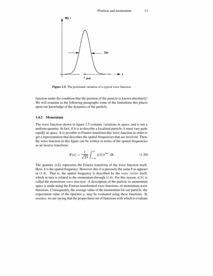
Consider the wave function shown in figure 1.5. Here, the real part of thewave function is plotted, as the wave function itself is in general a complexquantity. However, it is clear that the function is peaked about some point � ����.While it is likely that the expectation value of the position is very near this point,this cannot be discerned exactly without actually computing the action of theposition operator on this function and computing the expectation value, or innerproduct, directly. This circumstance arises from the fact that we are now dealingwith probability functions, and the expectation value is simply the most likelyposition in which to find the particle. On the other hand, another quantity isevident in figure 1.5, and this is the width of the wave function, which relates tothe standard deviation of the wave function. Thus, we can define
����� � ��� ��� �������� (1.23)
For our example wave function of (1.18), we see that the uncertainty may beexpressed as
�� ������ � ���� �
��
�� � �
���� (1.24)
The quantity �� relates to the uncertainty in finding the particle at theposition ���. It is clear that if we want to use a wave packet that describesthe position of the particle exactly, then �� must be made to go to zero. Sucha function is the Dirac delta function familiar from circuit theory (the impulsefunction). Here, though, we use a delta function in position rather than in time;for example, we describe the wave function through
���� �� � ��� ������� (1.25)
The time variable has been set to zero here for convenience, but it is easy toextend (1.25) to the time-varying case. Clearly, equation (1.25) describes the wave
Position and momentum 13
Figure 1.5. The positional variation of a typical wave function.
function under the condition that the position of the particle is known absolutely!We will examine in the following paragraphs some of the limitations this placesupon our knowledge of the dynamics of the particle.
1.4.2 Momentum
The wave function shown in figure 1.5 contains variations in space, and is not auniform quantity. In fact, if it is to describe a localized particle, it must vary quiterapidly in space. It is possible to Fourier transform this wave function in order toget a representation that describes the spatial frequencies that are involved. Then,the wave function in this figure can be written in terms of the spatial frequenciesas an inverse transform:
���� �����
��
��
�������� ��� (1.26)
The quantity ���� represents the Fourier transform of the wave function itself.Here, � is the spatial frequency. However, this � is precisely the same � as appearsin (1.4). That is, the spatial frequency is described by the wave vector itself,which in turn is related to the momentum through (1.4). For this reason, ���� iscalled the momentum wave function. A description of the particle in momentumspace is made using the Fourier-transformed wave functions, or momentum wavefunctions. Consequently, the average value of the momentum for our particle, theexpectation value of the operator �, may be evaluated using these functions. Inessence, we are saying that the proper basis set of functions with which to evaluate
14 Waves and particles
the momentum is that of the momentum wave functions. Then, it follows that
��� � ���� ��� � �
��
��
���� ��� (1.27)
As an example of momentum wave functions, we consider the position wavefunction of (1.18). We find the momentum wave function from
���� �� �����
��
��
���� ������� �� ��������
��
��
���������� ��
��������
������
��
��
��
�� �� ����
�
��� �
�
�������
����
(1.28)
This has the same form as (1.18), so that we can immediately use (1.20) and (1.21)to infer that ��� � � and ���� � �
� .Suppose, however, that we are using the position representation wave
functions. How then are we to interpret the expectation value of the momentum?The wave functions in this representation are functions only of � and �. Toevaluate the expectation value of the momentum operator, it is necessaryto develop the operator corresponding to the momentum in the positionrepresentation. To do this, we use (1.27) and introduce the Fourier transformscorresponding to the functions �. Then, we may write (1.27) as
��� � �
��
��
��
��
��
��
��������������
�
��
��
�����������
��
���
��
��
��
��
��
��������������
��
��
�� ����� �
������
� � ��
��
��
�����
��
����������� ����
������
� � ��
��
��
��������
������� (1.29)
In arriving at the final form of (1.29), an integration by parts has been done fromthe first line to the second (the evaluation at the limits is assumed to vanish), afterreplacing � by the partial derivative. The third line is achieved by recognizing thedelta function:
��� ��� ��
��
��
��
�� ���������� (1.30)
Thus, in the position representation, the momentum operator is given by thefunctional operator
� � ��� �
��� (1.31)
Position and momentum 15
1.4.3 Non-commuting operators
The description of the momentum operator in the position representation is that ofa differential operator. This means that the operators corresponding to the positionand to the momentum will not commute, by which we mean that
��� �� � ��� �� �� �� (1.32)
The left-hand side of (1.32) defines a quantity that is called the commutatorbracket. However, by itself it only has implied meaning. The terms containedwithin the brackets are operators and must actually operate on some wavefunction. Thus, the role of the commutator can be explained by considering theinner product, or expectation value. This gives
���� ��� ���� � ���
���� �
�
���
��
���
�
����
��� ���� (1.33)
If variables, or operators, do not commute, there is an implication that thesequantities cannot be measured simultaneously. Here again, there is another anddeeper meaning. In the previous section, we noted that the operation of theposition operator � on the wave function in the position representation producedan eigenvalue �, which is actually the expectation value of the position. Themomentum operator does not produce this simple result with the wave functionof the position representation. Rather, the differential operator produces a morecomplex result. For example, if the differential operator were to produce asimple eigenvalue, then the wave function would be constrained to be of the form�������� (which can be shown by assuming a simple eigenvalue form as in(1.22) with the differential operator and solving the resulting equation). Thisform is not integrable (it does not fit our requirements on normalization), andthus the same wave function cannot simultaneously yield eigenvalues for bothposition and momentum. Since the eigenvalue relates to the expectation value,which corresponds to the most likely result of an experiment, these two quantitiescannot be simultaneously measured.
There is a further level of information that can be obtained from the Fouriertransform pair of position and momentum wave functions. If the position isknown, for example if we choose the delta function of (1.25), then the Fouriertransform has unit amplitude everywhere; that is, the momentum has equalprobability of taking on any value. Another way of looking at this is to say thatsince the position of the particle is completely determined, it is impossible tosay anything about the momentum, as any value of the momentum is equallylikely. Similarly, if a delta function is used to describe the momentum wavefunction, which implies that we know the value of the momentum exactly, thenthe position wave function has equal amplitude everywhere. This means that ifthe momentum is known, then it is impossible to say anything about the position,as all values of the latter are equally likely. As a consequence, if we want todescribe both of these properties of the particle, the position wave function and
16 Waves and particles
its Fourier transform must be selected carefully to allow this to occur. Then therewill be an uncertainty �� in position, as indicated in figure 1.5, and there will bea corresponding uncertainty �� in momentum.
To investigate the relationship between the two uncertainties, in position andmomentum, let us choose a Gaussian wave function to describe the wave functionin the position representation. Therefore, we take
���� ��
�������������
��
��
��
�� (1.34)
Here, the wave packet has been centred at ����� � �, and
��� � �
��������
��
��
��
�� ��
���
�� �� � � (1.35)
as expected. Similarly, the uncertainty in the position is found from (1.23) as
����� ��
��������
��
��
��
�� ��
���
��� ��
��
�������
��
��
��
�� ��
���
��� � �� (1.36)
and �� � �.The appropriate momentum wave function can now be found by Fourier
transforming this position wave function. This gives
���� �����
��
��
��������� ��
��
��������������
�����
��
��
�� ��� � �����
��
���
�
��
�
���������
��� � (1.37)
We note that the momentum wave function is also centred about zero momentum.Then the uncertainty in the momentum can be found as
����� � ���
��
�
��
��
��������� �� �
��
��� (1.38)
Hence, the uncertainty in the momentum is ����. We now see that the non-commuting operators � and � can be described by an uncertainty ���� � ���.It turns out that our description in terms of the static Gaussian wave function is aminimal-uncertainty description, in that the product of the two uncertainties is aminimum.

Position and momentum 17
The uncertainty principle describes the connection between the uncertaintiesin determination of the expectation values for two non-commuting operators. Ifwe have two operators � and �, which do not commute, then the uncertaintyrelation states that
���� � ����������� (1.39)
where the angular brackets denote the expectation value, as above. It is easilyconfirmed that the position and momentum operators satisfy this relation.
It is important to note that the basic uncertainty relation is only really validfor non-commuting operators. It has often been asserted for variables like energy(frequency) and time, but in the non-relativistic quantum mechanics that we areinvestigating here, time is not a dynamic variable and has no correspondingoperator. Thus, if there is any uncertainty for these latter two variables, it arisesfrom the problems of making measurements of the energy at different times—andhence is a measurement uncertainty and not one expected from the uncertaintyrelation (1.39).
To understand how a classical measurement problem can give a result muchlike an uncertainty relationship, consider the simple time-varying exponential����� . We can find the frequency content of this very simple time variation as
� ��� ��
� � ������ (1.40)
Hence, if we want to reproduce this simple exponential with our electronics, werequire a bandwidth ���� that is at least of order ��� . That is, we require
�� ��
�� �� � � (1.41)
where we have used ����� to replace the angular frequency with the energyof the wave and have taken � � � . While this has significant resemblanceto the quantum uncertainty principle, it is in fact a classical result whose onlyconnection to quantum mechanics is through the Planck relationship. The factthat time is not an operator in our approach to quantum mechanics, but is simply ameasure of the system progression, means that there cannot be a quantum versionof (1.41).
1.4.4 Returning to temporal behaviour
While we have assumed that the momentum wave function is centred at zeromomentum, this is not the general case. Suppose, we now assume that themomentum wave function is centred at a displaced value of �, given by � �.Then, the entire position representation wave function moves with this averagemomentum, and shows an average velocity �� � ���� . We can expect thatthe peak of the position wave function, �����, moves, but does it move withthis velocity? The position wave function is made up of a sum of a great many
18 Waves and particles
Fourier components, each of which arises from a different momentum. Does thisaffect the uncertainty in position that characterizes the half-width of the positionwave function? The answer to both of these questions is yes, but we will try todemonstrate that these are the correct answers in this section.
Our approach is based upon the definition of the Fourier inverse transform(1.26). This latter equation expresses the position wave function ���� as asummation of individual Fourier components, each of whose amplitudes is givenby the value of ���� at that particular �. From the earlier work, we can extendeach of the Fourier terms into a plane wave corresponding to that value of �, byintroducing the frequency term via
���� �����
��
��
������������� ��� (1.42)
While the frequency term has not been shown with a variation with �, it mustbe recalled that each of the Fourier components may actually possess a slightlydifferent frequency. If the main frequency corresponds to the peak of themomentum wave function, then the frequency can be expanded as
���� � ����� � �� � �����
��
��������
� � � � � (1.43)
The interpretation of the position wave function is now that it is composed ofa group of closely related waves, all propagating in the same direction (weassume that ���� � for � � , but this is merely for convenience and is notcritical to the overall discussion). Thus, ���� � is now defined as a wave packet.Equation (1.43) defines the dispersion across this wave packet, as it gives thegradual change in frequency for different components of the wave packet.
To understand how the dispersion affects the propagation of the wavefunctions, we insert (1.43) into (1.42), and define the difference variable �� � ��. Then, (1.42) becomes
���� � ��
���
�������������
��
��� �����������
��� � (1.44)
where �� is the leading term in (1.43) and � � is the partial derivative in thesecond term of (1.43). The higher-order terms of (1.43) are neglected, as thefirst two terms are the most significant. If is factored out of the argument ofthe exponential within the integral, it is seen that the position variable varies as� � ��. This is our guide as to how to proceed. We will reintroduce �� withinthe exponential, but multiplied by this factor, so that
���� � ��
���
�����������������������
��
��
��� �����������
����������
��� �
��
���
�������������
��
��
��� ���������������
��� �
� ����������������� ��� �� (1.45)

Position and momentum 19
The leading exponential provides a phase shift in the position wave function. Thisphase shift has no effect on the square of the magnitude, which represents theexpectation value calculations. On the other hand, the entire wave function moveswith a velocity given by � �. This is not surprising. The quantity � � is the partialderivative of the frequency with respect to the momentum wave vector, and hencedescribes the group velocity of the wave packet. Thus, the average velocity of thewave packet in position space is given by the group velocity
�� � �� ���
��
��������
� (1.46)
This answers the first question: the peak of the position wave function remainsthe peak and moves with an average velocity defined as the group velocity of thewave packet. Note that this group velocity is defined by the frequency variationwith respect to the wave vector. Is this related to the average momentum givenby ��? The answer again is affirmative, as we cannot let �� take on any arbitraryvalue. Rather, the peak in the momentum distribution must relate to the averagemotion of the wave packet in position space. Thus, we must impose a value on�� so that it satisfies the condition of actually being the average momentum of thewave packet:
�� ����
��
��
��� (1.47)
If we integrate the last two terms of (1.47) with respect to the wave vector, werecover the other condition that ensures that our wave packet is actually describingthe dynamic motion of the particles:
� � �� �����
���
��
��� (1.48)
It is clear that it is the group velocity of the wave packet that describes the averagemomentum of the momentum wave function and also relates the velocity (andmomentum) to the energy of the particle.
Let us now turn to the question of what the wave packet looks like with thetime variation included. We rewrite (1.42) to take account of the centred wavepacket for the momentum representation to obtain
���� � �
�
��
��
�
���������
��
��
�������������� ��� (1.49)
To proceed, we want to insert the above relationship between the frequency(energy) and average velocity:
� ����
���
�
����� ���
� ����
��� ��� �
������
� (1.50)
20 Waves and particles
If (1.50) is inserted into (1.49), we recognize a new form for the ‘static’ effectivemomentum wave function:
���� ���
��
�
����������������� ���
����
��� � �
��
��
��(1.51)
which still leads to ��� � , and � � ����. We can then evaluate the positionrepresentation wave function by continuing the evaluation of (1.49) using theshort-hand notation
�� �
��� � �
��
��(1.52a)
and� � � ��� (1.52b)
This gives
���� �� �
��
��
��
�
�����������������
��
��
������������
��
�
��
���������������������� ���
���
�
���
���� (1.53)
This has the exact form of the previous wave function in the positionrepresentation with one important exception. The exception is that the timevariation has made this result unnormalized. If we compute the inner productnow, recalling that the terms in � � are complex, the result is
����� ��
���� � �
� �������������
� (1.54)
With this normalization, it is now easy to show that the expectation value of theposition is that found above:
�� � ��� ��
������ ��� (1.55)
Similarly, the standard deviation in position is found to be
����� � �� � � ��� �
����
�����
�� (1.56)
This means that the uncertainty in the two non-commuting operators and �increases with time according to
� ��
�
� �
����
������ (1.57)
Summary 21
The wave packet actually gets wider as it propagates with time, so the timevariation is a shift of the centroid plus this broadening effect. The broadening of aGaussian wave packet is familiar in the process of diffusion, and we recognizethat the position wave packet actually undergoes a diffusive broadening as itpropagates. This diffusive effect accounts for the increase in the uncertainty. Theminimum uncertainty arises only at the initial time when the packet was formed.At later times, the various momentum components cause the wave packet positionto become less certain since different spatial variations propagate at differenteffective frequencies. Thus, for any times after the initial one, it is not possiblefor us to know as much about the wave packet and there is more uncertainty inthe actual position of the particle that is represented by the wave packet.
1.5 Summary
Quantum mechanics furnishes a methodology for treating the wave–particleduality. The main importance of this treatment is for structures and times, bothusually small, for which the interference of the waves can become important. Theeffect can be either the interference between two wave packets, or the interferenceof a wave packet with itself, such as in boundary value problems. In quantummechanics, the boundary value problems deal with the equation that we willdevelop in the next chapter for the wave packet, the Schrodinger equation.
The result of dealing with the wave nature of particles is that dynamicalvariables have become operators which in turn operate upon the wave functions.As operators, these variables often no longer commute, and there is a basicuncertainty relation between non-commuting operators. The non-commutingnature arises from it being no longer possible to generate a wave function thatyields eigenvalues for both of the operators, representing the fact that they cannotbe simultaneously measured. It is this that introduces the uncertainty relationship.
Even if we generate a minimum-uncertainty wave packet in real space, it iscorrelated to a momentum space representation, which is the Fourier transformof the spatial variation. The time variation of this wave packet generates adiffusive broadening of the wave packet, which increases the uncertainty in thetwo operator relationships.
We can draw another set of conclusions from this behaviour that will beimportant for the differential equation that can be used to find the actual wavefunctions in different situations. The entire time variation has been found toderive from a single initial condition, which implies that the differential equationmust be only first order in the time derivatives. Second, the motion has diffusivecomponents, which suggests that the differential equation should bear a strongresemblance to a diffusion equation (which itself is only first order in the timederivative). These points will be expanded upon in the next chapter.
22 Waves and particles
References
Aharonov Y and Bohm D 1959 Phys. Rev. 115 485de Broglie L 1939 Matter and Light, The New Physics (New York: Dover) p 267 (this is
a reprint of the original translation by W H Johnston of the 1937 original Matiere etLumiere)
Einstein A 1905 Ann. Phys., Lpz. 17 132Fowler A B 1985 US Patent 4550330Landau L D and Lifshitz E M 1958 Quantum Mechanics (London: Pergamon)Longair M S 1984 Theoretical Concepts in Physics (Cambridge: Cambridge University
Press)Washburn S and Webb R A 1986 Adv. Phys. 35 375–422Webb R A, Washburn S, Umbach C P and Laibowitz R B 1985 Phys. Rev. Lett. 54 2696–99Yacoby A, Heiblum M, Umansky V, Shtrikman H and Mahalu D 1994 Phys. Rev. Lett. 73
3149–52
Problems 23
Problems
1. Calculate the energy density for the plane electromagnetic wave describedby the complex field strength
�� � �����������
and show that its average over a temporal period � is � � ����������.
2. What are the de Broglie frequencies and wavelengths of an electron anda proton accelerated to 100 eV? What are the corresponding group and phasevelocities?
3. Show that the position operator � is represented by the differentialoperator
���
��
in momentum space, when dealing with momentum wave functions. Demonstratethat (1.32) is still satisfied when momentum wave functions are used.
4. An electron represented by a Gaussian wave packet, with average energy100 eV, is initially prepared with �� � ������ and �� � �������. How muchtime elapses before the wave packet has spread to twice the original spatial extent?
5. Express the expectation value of the kinetic energy of a Gaussian wavepacket in terms of the expectation value and the uncertainty of the momentumwave function.
6. A particle is represented by a wave packet propagating in a dispersivemedium, described by
� �
�
��� �
���
�� �
��
What is the group velocity as a function of ?7. The longest wavelength that can cause the emission of electrons from
silicon is 296 nm. (a) What is the work function of silicon? (b) If silicon isirradiated with light of 250 nm wavelength, what is the energy and momentum ofthe emitted electrons? What is their wavelength? (c) If the incident photon flux is� � � ��, what is the photoemission current density?
8. For particles which have a thermal velocity, what is the wavelength at300 K of electrons, helium atoms, and the �-particle (which is ionized ���)?
9. Consider that an electron is confined within a region of 10 nm. If weassume that the uncertainty principle provides a RMS value of the momentum,what is their confinement energy?
10. A wave function has been determined to be given by the spatial variation
���� �
�� � � � � ��� � �� � � � � � elsewhere.
24 Waves and particles
Determine the value of �, the expectation value of �, ��, � and ��. What is thevalue of the uncertainty in position–momentum?
11. A wave function has been determined to be given by the spatial variation
���� �
��� ���
���
��� � � � �
� elsewhere.
Determine the value of �, the expectation value of �, ��, � and ��. What is thevalue of the uncertainty in position–momentum?
Chapter 2
The Schrodinger equation
In the first chapter, it was explained that the introductory basics of quantummechanics arise from the changes from classical mechanics that are brought toan observable level by the smallness of some parameter, such as the size scale.The most important effect is the appearance of operators for dynamical variables,and the non-commuting nature of these operators. We also found a wave function,either in the position or momentum representation, whose squared magnitude isrelated to the probability of finding the equivalent particle. The properties of thewave could be expressed as basically arising from a linear differential equationof a diffusive nature. In particular, because any subsequent form for the wavefunction evolved from a single initial state, the equation can only be of first orderin the time derivative (and, hence, diffusive in nature).
It must be noted that the choice of a wave-function-based approach toquantum mechanics is not the only option. Indeed, two separate formulations ofthe new quantum mechanics appeared almost simultaneously. One was developedby Werner Heisenberg, at that time a lecturer in Gottingen (Germany), during1925. In this approach, a calculus of non-commuting operators was developed.This approach was quite mathematical, and required considerable experience towork through in any detail. It remained until later to discover that this calculuswas actually representable by normal matrix calculus. The second formulationwas worked out by Erwin Schrodinger, at the time a Professor in Vienna, overthe winter vacation of 1927. In Schrodinger’s formulation, a wave equationwas found to provide the basic understanding of quantum mechanics. Althoughnot appreciated at the time, Schrodinger presented the connection between thetwo approaches in subsequent papers. In a somewhat political environment,Heisenberg received the 1932 Nobel prize for ‘discovering’ quantum mechanics,while Schrodinger was forced to share the 1933 prize with Paul Dirac for advancesin atomic physics. Nevertheless, it is Schrodinger’s formulation which is almostuniversally used today, especially in textbooks. This is especially true for studentswith a background in electromagnetic fields, as the concept of a wave equation isnot completely new to them.
25
26 The Schrodinger equation
In this chapter, we want now to specify such an equation—the Schrodingerequation, from which one version of quantum mechanics—wave mechanics—hasevolved. In a later chapter, we shall turn to a second formulation of quantummechanics based upon time evolution of the operators rather than the wavefunction, but here we want to gain insight into the quantization process, andthe effects it causes in normal systems. In the following section, we will givea justification for the wave equation, but no formal derivation is really possible(as in the case of Maxwell’s equations); rather, the equation is found to explainexperimental results in a correct fashion, and its validity lies in that fact. Insubsequent sections, we will then apply the Schrodinger equation to a varietyof problems to gain the desired insight.
2.1 Waves and the differential equation
At this point, we want to begin to formulate an equation that will provide us witha methodology for determining the wave function in many different situations,but always in the position representation. We impose two requirements on thewave equation: (i) in the absence of any force, the wave packet must move in afree-particle manner, and (ii) when a force is present, the solution must reproduceNewton’s law � � ��. As mentioned above, we cannot ‘derive’ this equation,because the equation itself is the basic postulate of wave mechanics, as formulatedby Schrodinger (1926).
Our prime rationale in developing the wave equation is that the ‘wavefunction’ should in fact be a wave. That is, we prefer the spatial and temporalvariations to have the form
� � ��������� (2.1)
in one dimension. To begin, we can rewrite (1.42) as
���� �� �����
��
��
������������� ��� (2.2)
Because the wave function must evolve from a single initial condition, it mustalso be only first order in the time derivative. Thus, we take the partial derivativeof (2.2) with respect to time, to yield
�
�� � ��
��
��
��
������������� �� (2.3)
which can be rewritten as
� ��
��
����
��
��
�������������� ��� (2.4)
In essence, the energy is the eigenvalue of the time derivative operator,although this is not a true operator, as time is not a dynamic variable. Thus, it
Waves and the differential equation 27
may be thought that the energy represents a set of other operators that do representdynamic variables. It is common to express the energy as a sum of kinetic andpotential energy terms; for example
� � � � � ���
��� � ��� ��� (2.5)
The momentum does operate on the momentum representation functions, but byusing our position space operator form (1.31), the energy term can be pulled outof the integral in (2.4), and we find that the kinetic energy may be rewritten using(1.4) as
��
���
����
��(2.6)
but we note that the factor of �� can be obtained from (2.2) as
������ ��
����
���
��
��
�����
������������ ��
� � ���
��
��
�������������� �� (2.7)
so that we can collect the factors inside the integrals to yield
���
��� � �
�
��
���
���� � ��� ������ ��� (2.8)
This is the Schrodinger equation. We have written it with only one spatialdimension, that of the �-direction. However, the spatial second derivative isproperly the Laplacian operator in three dimensions, and the results can readilybe obtained for that case. For most of the work in this chapter, however, we willcontinue to use only the single spatial dimension.
This new wave equation is a complex equation, in that it involves thecomplex factor �
���. We expect, therefore, that the wave function ���� ��is a complex quantity itself, which is why we use the squared magnitude in theprobability definitions. This wave function thus has a magnitude and a phase,both of which are important quantities. We will see below that the magnitude isrelated to the density (charge density when we include the charge itself) whilethe phase is related to the ‘velocity’ with which the density moves. This leadsto a continuity equation for probability (or for charge), just as in electromagnetictheory.
Before proceeding, it is worthwhile to detour and consider to some extenthow the classical limit is achieved from the Schrodinger equation. For this, letus define the wave function in terms of an amplitude and a phase, according to���� �� � ������. The quantity � is known as the action in classical mechanics(but familiarity with this will not be required). Let us put this form for the wave
28 The Schrodinger equation
function into (2.8), which gives (the exponential factor is omitted as it cancelsequally from all terms)
����
�����
��
���
�
��
���
��
���
���
��
���
����
��
�
��
��
��
���
��
��
���
����� �� (2.9)
For this equation to be valid, it is necessary that the real parts and the imaginaryparts balance separately, which leads to
��
���
�
��
���
��
��� � �
��
���
���
���� � (2.10)
and��
���
�
��
���
����
�
�
��
��
��
��� �� (2.11)
In (2.10), there is only one term that includes Planck’s constant, and this termvanishes in the classical limit as � � �. It is clear that the action relates to thephase of the wave function, and consideration of the wave function as a single-particle plane wave relates the gradient of the action to the momentum and thetime derivative to the energy. Indeed, insertion of the wave function of (2.2)leads immediately to (2.5), which expresses the total energy. Obviously, here thevariation that is quantum mechanical provides a correction to the energy, whichcomes in as the square of Planck’s constant. This extra term, the last term on theleft of (2.10), has been discussed by several authors, but today is usually referredto as the Bohm potential. Its interpretation is still under discussion, but this termclearly gives an additional effect in regions where the wave function amplitudevaries rapidly with position. One view is that this term plays the role of a quantumpressure, but other views have been expressed. The second equation, (2.11), canbe rearranged by multiplying by �, for which (in vector notation for simplicity ofrecognition)
���
���� �
���
���
�� �� (2.12)
The factor �� is obviously related to ����, the square of the magnitude of the wavefunction. If the gradient of the action is the momentum, then the second term isthe divergence of the probability current, and the factor in the parentheses is theproduct of the probability function and its velocity. We explore this further in thenext section.
2.2 Density and current
The Schrodinger equation is a complex diffusion equation. The wave function� is a complex quantity. The potential energy � ��� ��, however, is usually areal quantity. Moreover, we discerned in chapter 1 that the probabilities were
Density and current 29
real quantities, as they relate to the chance of finding the particle at a particularposition. Thus, the probability density is just
� ��� �� � ����� ������ �� � ����� ����� (2.13)
This, of course, leads to the normalization of (1.10), which just expresses the factthat the sum of the probabilities must be unity. If (2.13) were multiplied by theelectronic charge �, it would represent the charge density carried by the particle(described by the wave function).
One check of the extension of the Schrodinger equation to the classical limitlies in the continuity equation. That is, if we are to relate (2.13) to the localcharge density, then there must be a corresponding current density � , such that�� � ��� �
���
���� � � (2.14)
although we use only the �-component here. Now, the complex conjugate of (2.8)is just
������
��� �
��
��
����
���� ��� ������� ��� (2.15)
We now use (2.13) in (2.14), with (2.8) and (2.15) inserted for the partialderivatives with respect to time, as (we neglect the charge, and will find theprobability current)
����
��� �
��
��������� �������� (2.16)
where the terms involving the potential energy have cancelled. The terms in thebrackets can be rewritten as the divergence of a probability current, if the latter isdefined as
�� ��
����������� �������� (2.17)
If the wave function is to be a representation of a single electron, then this‘current’ must be related to the velocity of that particle. On the other hand, ifthe wave function represents a large ensemble of particles, then the actual current(obtained by multiplying by �) represents some average velocity, with an averagetaken over that ensemble.
The probability current should be related to the momentum of the wavefunction, as discussed earlier. The gradient operator in (2.17) is, of course, relatedto the momentum operator, and the factors of the mass and Planck’s constantconnect this to the velocity. In fact, we can rewrite (2.17) as
�� �
����� �������� (2.18)
In general, when the momentum is a ‘good’ operator, which means that it ismeasurable, the eigenvalue is a real quantity. Then, the imaginary part vanishes,
30 The Schrodinger equation
and (2.18) is simply the product of the velocity and the probability, which yieldsthe probability current.
The result (2.18) differs from the earlier form that appears in (2.12). If theexpectation of the momentum is real, then the two forms agree, as the gradient ofthe action just gives the momentum. On the other hand, if the expectation of themomentum is not real, then the two results differ. For example, if the averagemomentum were entirely imaginary, then (2.18) would yield zero identically,while (2.12) would give a non-zero result. However, (2.12) was obtained byseparating the real and imaginary parts of (2.9), and the result in this latterequation assumed that � was entirely real. An imaginary momentum wouldrequire that � be other than purely real. Thus, (2.9) was obtained for a very specialform of the wave function. On the other hand, (2.18) results from a quite generalwave function, and while the specific result depended upon a plane wave, theapproach was not this limited. If (2.2) is used for the general wave function, then(2.18) is evaluated using the expectation values of the momentum, and suggeststhat in fact these eigenvalues should be real, if a real current is to be measured.
By real eigenvalues, we simply recognize that if an operator � canbe measured by a particular wave function, then this operator produces theeigenvalue �, which is a real quantity (we may assert without proof that one canonly measure real numbers in a measurement). This puts certain requirementsupon the operator �, as we note that
��� � ��� ��� � ��� ��� � � (2.19)
for a properly normalized wave function. Now,
�� � ��� ���� � ������ � ������ � ��� ���� (2.20)
where the symbol � indicates the adjoint operator. If the eigenvalues are real,as required for a measurable quantity, the corresponding operator must be self-adjoint; for example, � � �� �� � � ��. Such operators are known asHermitian operators. The most common example is just the total-energy operator,as the energy is most often measured in systems. Not all operators are Hermitian,however, and the definition of the probability current allows for considerationof those cases in which the momentum may not be a real quantity and may notbe measurable, as well as those more normal cases in which the momentum ismeasurable.
2.3 Some simple cases
The Schrodinger equation is a partial differential equation both in position spaceand in time. Often, such equations are solvable by separation of variables, andthis is also the case here. We proceed by making the ansatz that the wave functionmay be written in the general form ���� �� � ��������. If we insert this into
Some simple cases 31
the Schrodinger equation (2.15), and then divide by this same wave function, weobtain
��
�
��
��� �
��
���
���
���� � ���� (2.21)
We have acknowledged here that the potential energy term is almost always astatic interaction, which is only a function of position. Then, the left-hand sideis a function of time alone, while the right-hand side is a function of positionalone. This can be achieved solely if the two sides are equal to a constant. Theappropriate constant has earlier been identified as the energy � . These lead to thegeneral result for the energy function
���� � ������� (2.22)
and the time-independent Schrodinger equation
���
��
���
���� � ������� � ������ (2.23)
This last equation describes the quantum wave mechanics of the static system,where there is no time variation. Let us now turn to a few examples.
2.3.1 The free particle
We begin by first considering the situation in which the potential is zero. Thenthe time-independent equation becomes
���
���� ������ � � (2.24)
where����
��� � � �
����
��� (2.25)
The solution to (2.24) is clearly of the form of sines and cosines, but here we willtake the exponential terms, and
���� � ����� ������� (2.26)
These are just the plane-wave solutions with which we began our treatment ofquantum mechanics. The plane-wave form becomes more obvious when the timevariation (2.22) is re-inserted into the total wave function. Here, the amplitude isspatially homogeneous and requires the use of the box normalization conditionsdiscussed in the previous chapter.
If we are in a system in which the potential is not zero, then the solutionsbecome more complicated. We can redefine the wave vector � as
� �
���� � � ���
��� (2.27)
32 The Schrodinger equation
If the potential is slowly varying with distance, then the phase of the wave functionmakes a great many oscillations in a distance over which the variation in potentialis small. Then, we can still use the result (2.26) for the wave function. However,for this to be the case, we require that the spatial variation be small. One might tryto meet this requirement with the Bohm potential, the last term on the left-handside of (2.10), but this earlier result was obtained by assuming a very special formfor the wave function. In the present case, it is desired that the variation of themomentum with position not lead to extra terms in the Schrodinger equation, andthis requirement can be simply stated by requiring
�
�
��
��� � (2.28)
which simply says that the variation over a wavelength should be small. Formost cases, this can be handled by treating rapid variation in the potentialthrough boundary conditions, but we shall return to a treatment of the spatiallyvarying potential through an approximation technique (the WKB approximation)in chapter 3. This approximate treatment of the wave function in the spatiallyvarying potential case uses the solutions of (2.26), with the exponential factorsreplaced by
���
��
��
����� � � �����
����
�� (2.29)
However, it is important to note that solutions such as (2.29) do not satisfy theSchrodinger equation, and rely upon a sufficiently slow variation in the potentialwith position. The problem is that when the potential varies with position, (2.23)changes from a simple second-order ordinary differential equation to one withvarying coefficients. These usually generate quite unusual special functions asthe solutions.
2.3.2 A potential step
To begin to understand the role that the potential plays, let us investigate a simplepotential step, in which the potential is defined as
� ������ � �� �� � � (2.30)
where ���� is the Heaviside step function in which � � for � � �, and � �for � � �. This is shown in figure 2.1. Thus, the potential has a height of � � forpositive �, and is zero for the negative-� region. This potential creates a barrierto the wave function, and a wave incident from the left (the negative region) willhave part (or all) of its amplitude reflected from the barrier. The results that areobtained depend upon the relative energy of the wave. If the energy is less than��, the wave cannot propagate in the region of positive �. This is clearly seenfrom (2.27), as the wave vector is imaginary for � � � �. Only one exponent

Some simple cases 33
Figure 2.1. Schematic view of the potential of (2.30) which is non-zero (and constant)only in the positive half-space.
Figure 2.2. The various wave vectors are related to the energy of the wave: (a) the casefor � � ��; (b) the case for � � ��.
can be retained, as we require that the wave function remain finite (but zero) as���.
Case I. � � ��Let us first consider the low-energy case, where the wave is a non-
propagating wave for � � �. In the negative half-space, we consider the wavefunction to be of the form of (2.26), composed of an incident wave (the positive-exponent term) and a reflected wave (the negative-exponent term). That is, wewrite the wave function for � � � as
����� � ����� ������� (2.31)
where the energy and the wave vector � are related by (2.25). This behaviour isshown in figure 2.2(a). In the positive half-space, the solution of the Schrodingerequation is given by
�� � ����� (2.32)
34 The Schrodinger equation
where
� �
������ � � �
��� (2.33)
Here, we have defined a wave function in two separate regions, in which thepotential is constant in each region. These two wave functions must be smoothlyjoined where the two regions meet.
While three constants are defined �������, one of these is defined bythe resultant normalization of the wave function (we could e.g. let � � �without loss of generality). Two boundary conditions are required to evaluatethe other two coefficients in terms of �. The boundary conditions can vary withthe problem, but one must describe the continuity of the probability across theinterface between the two regions. Thus, one boundary condition is that the wavefunction itself must be continuous at the interface, or
����� � ������ ��� � �� (2.34)
To obtain a second boundary condition, we shall require that the derivative ofthe wave function is also continuous (that this is a proper boundary conditioncan be found by integrating (2.23) over a small increment from � to � ,which shows that the derivative of the wave function is continuous as long as thisrange of integration does not include an infinitely large potential or energy). Insome situations, we cannot specify such a boundary condition, as there may notbe a sufficient number of constants to evaluate (this will be the case in the nextsection). Equating the derivatives of the wave functions at the interface leads to
��
�������
���
�������
� ������ � ���� (2.35)
This last equation can be rearranged by placing the momentum term in thedenominator on the right-hand side. Then adding (2.34) and (2.35) leads to
�
��
��
� � �� (2.36)
This result can now be used in (2.34) to find
�
��
� � �
� � �� (2.37)
The amplitude of the reflected wave is unity, so there is no probability amplitudetransmitted across the interface. In fact, the only effect of the interface is to phaseshift the reflected wave; that is, the wave function is � � ��
���� � ������ � ���������� (2.38)
where � � ����
���
�� (2.39)
Some simple cases 35
The probability amplitude is given by
�������� � ����� � � ������� �� � � �� (2.40)
As may have been expected, this is a standing-wave pattern, with the probabilityoscillating from 0 to twice the value of ��. The first peak occurs at a distance� � �����, that is, the distance to the first peak is dependent upon the phase shiftat the interface. If the potential amplitude is increased without limit, �� ��, thedamping coefficient ��, and the phase shift approaches . However, the firstpeak occurs at a value of �� � ��, which also leads to the result that the wavefunction becomes zero at � � �. We cannot examine the other limit ��� � ��,as we do not have the proper transmitted wave, but this limit can be probed whenthe transmission mode is examined. It may also be noted that a calculation of theprobability current for � � � leads immediately to zero as the wave function isreal. Thus, no probability current flows into the right half-plane. It is a simplecalculation to show that the net probability current in the left half-plane vanishesas well, as the reflected wave carries precisely the same current away from theinterface as the incident wave carries toward the interface.
Case II. � � ��We now turn to the case in which the wave can propagate on both sides of
the interface. As above, the wave function in the left half-space is assumed to beof the form of (2.31), which includes both an incident wave and a reflected wave.Similarly, the transmitted wave will be assumed to be of the form
�� � ������ (2.41)
where
�� �
��
���� � ���� (2.42)
The relationships between this wave vector and that for the region � � � areschematically described in figure 2.2(b). Again, we will match both the wavefunction and its derivative at � � �. This leads to
����� � ������ ��� � �
�� �
�������
� �� �
�������
� ������� � �����(2.43)
These equations can now be solved to obtain the constants � and � in termsof �. One difference here from the previous treatment is that these will be realnumbers now, rather than complex numbers. Indeed, adding and subtracting thetwo equations of (2.43) leads to
�
��
��
� � ��
�
��� � ��� � ��
� (2.44)
36 The Schrodinger equation
Here, we see that if �� � �, �� � � and the amplitude of the reflected wavevanishes, and the amplitude of the transmitted wave is equal to the incident wave.
The probability current in the left-hand and right-hand spaces is foundthrough the use of (2.17). For the incident and transmitted waves, these currentsare simply
�� ����
�
���
� � ��
���� �
��
�� (2.45)
The transmission coefficient is defined as the ratio of the transmitted current tothe incident current, or
� ���
���
������ � ����
(2.46)
which becomes unity when the potential goes to zero. By the same token, thereflection coefficient can be defined from the ratio of the reflected current to theincident current, or
� � ���
���
�� � ��
� � ��
��� (2.47)
This leads to the result that� �� � �� (2.48)
A critical point arises when �� � �, that is, the energy is resonant with thetop of the potential barrier. For this energy, the reflection coefficient from (2.47)is 1, so the transmission coefficient must vanish. The forms that have been usedto solve for the wave function in the right-hand plane are not appropriate, as theyare of exponential form. Here, however, the second derivative vanishes as the twoterms with the potential energy and the energy cancel each other. This leads toa solution of the form �� � � � �, but � must vanish in order for the wavefunction to remain finite at large . For the derivative of the wave function thento be continuous across the interface, (2.43) must become � �. As a result ofthe first of equations (2.43), we then must have � � ��. However, this constantwave function has no probability current associated with it, so the incident waveis fully reflected, consistent with � � �. It is also reassuring that � � �� isconsistent with (2.36) in the limit of � � �, which also occurs at this limitingvalue of the energy.
For energies above the potential barrier height, the behaviour of the waveat the interface is quite similar in nature to what occurs with an optical waveat a dielectric discontinuity. This is to be expected as we are using the waverepresentation of the particle, and should expect to see optical analogues.
2.4 The infinite potential well
If we now put two barriers together, we have a choice of making a potential inwhich there is a barrier between two points in space, or a well between two pointsin space. The former will be treated in the next chapter. Here, we want to consider
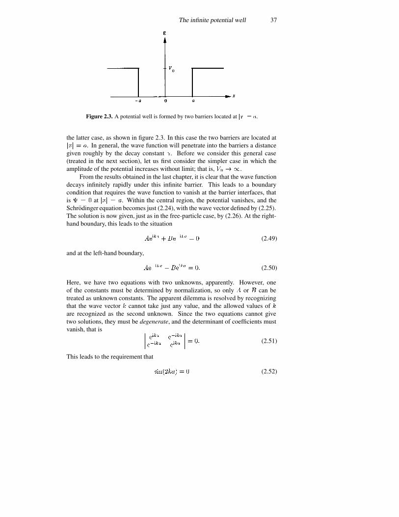
The infinite potential well 37
Figure 2.3. A potential well is formed by two barriers located at ��� � �.
the latter case, as shown in figure 2.3. In this case the two barriers are located at��� � �. In general, the wave function will penetrate into the barriers a distancegiven roughly by the decay constant �. Before we consider this general case(treated in the next section), let us first consider the simpler case in which theamplitude of the potential increases without limit; that is, �� ��.
From the results obtained in the last chapter, it is clear that the wave functiondecays infinitely rapidly under this infinite barrier. This leads to a boundarycondition that requires the wave function to vanish at the barrier interfaces, thatis � � � at ��� � �. Within the central region, the potential vanishes, and theSchrodinger equation becomes just (2.24), with the wave vector defined by (2.25).The solution is now given, just as in the free-particle case, by (2.26). At the right-hand boundary, this leads to the situation
����� ������� � � (2.49)
and at the left-hand boundary,
������ ������ � �� (2.50)
Here, we have two equations with two unknowns, apparently. However, oneof the constants must be determined by normalization, so only � or � can betreated as unknown constants. The apparent dilemma is resolved by recognizingthat the wave vector � cannot take just any value, and the allowed values of �are recognized as the second unknown. Since the two equations cannot givetwo solutions, they must be degenerate, and the determinant of coefficients mustvanish, that is
����
���� �����
����� ����
����� �� (2.51)
This leads to the requirement that
������ � � (2.52)
38 The Schrodinger equation
or
� ���
���� �
������
����� � �� �� �� � � � � (2.53)
Thus, there are an infinity of allowed energy values, with the spacing increasingquadratically with the index �.
In order to find the wave function corresponding to each of the energy levels,we put the value for � back into one of the equations above for the boundaryconditions; we chose to use (2.49). This leads to
�
�� ����� � �������� (2.54)
Thus, as we move up the hierarchy of energy levels, the wave functions alternatebetween cosines and sines. This can be summarized as
���� �
�� ��������� � odd� �� �������� � even
(2.55)
These can be combined by offsetting the position, so that
���� � � �� �����
�� ���� (2.56)
This last solution fits both boundary conditions, and yields the two solutions of(2.55) when the multiple-angle expansion of the sine function is used. Of course,each indexed wave function of (2.56) corresponds to one of the Fourier expansionterms in the Fourier series that represents a square barrier. In fact, (2.24) is justone form of a general boundary value problem in which the Fourier series is avalid solution.
We still have to normalize the wave functions. To do this, we use (2.56), andthe general inner product with the range of integration now defined from�� to �.This leads to
������� � ��
��
��
�� ������
�� ���� � �� (2.57)
This readily leads to the normalization
� ����� (2.58)
If the particle resides exactly in a single energy level, we say that it is in apure state. The more usual case is that it moves around between the levels and onthe average many different levels contribute to the total wave function. Then thetotal wave function is a sum over the Fourier series, with coefficients related tothe probability that each level is occupied. That is,
���� ���
������ �����
� � ���
(2.59)
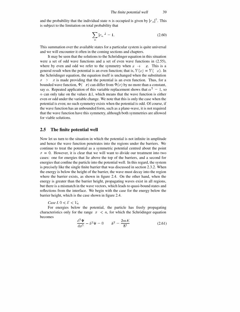
The finite potential well 39
and the probability that the individual state � is occupied is given by �����. Thisis subject to the limitation on total probability that
�
�
����� � �� (2.60)
This summation over the available states for a particular system is quite universaland we will encounter it often in the coming sections and chapters.
It may be seen that the solutions to the Schrodinger equation in this situationwere a set of odd wave functions and a set of even wave functions in (2.55),where by even and odd we refer to the symmetry when � � ��. This is ageneral result when the potential is an even function; that is, � ��� � � ����. Inthe Schrodinger equation, the equation itself is unchanged when the substitution� � �� is made providing that the potential is an even function. Thus, for abounded wave function,����� can differ from���� by no more than a constant,say �. Repeated application of this variable replacement shows that �� � �, so� can only take on the values ��, which means that the wave function is eithereven or odd under the variable change. We note that this is only the case when thepotential is even; no such symmetry exists when the potential is odd. Of course, ifthe wave function has an unbounded form, such as a plane-wave, it is not requiredthat the wave function have this symmetry, although both symmetries are allowedfor viable solutions.
2.5 The finite potential well
Now let us turn to the situation in which the potential is not infinite in amplitudeand hence the wave function penetrates into the regions under the barriers. Wecontinue to treat the potential as a symmetric potential centred about the point� � �. However, it is clear that we will want to divide our treatment into twocases: one for energies that lie above the top of the barriers, and a second forenergies that confine the particle into the potential well. In this regard, the systemis precisely like the single finite barrier that was discussed in section 2.3.2. Whenthe energy is below the height of the barrier, the wave must decay into the regionwhere the barrier exists, as shown in figure 2.4. On the other hand, when theenergy is greater than the barrier height, propagating waves exist in all regions,but there is a mismatch in the wave vectors, which leads to quasi-bound states andreflections from the interface. We begin with the case for the energy below thebarrier height, which is the case shown in figure 2.4.
Case I. � � � � ��
For energies below the potential, the particle has freely propagatingcharacteristics only for the range ��� � �, for which the Schrodinger equationbecomes
���
���� �
�� � � �� �
�
��(2.61)
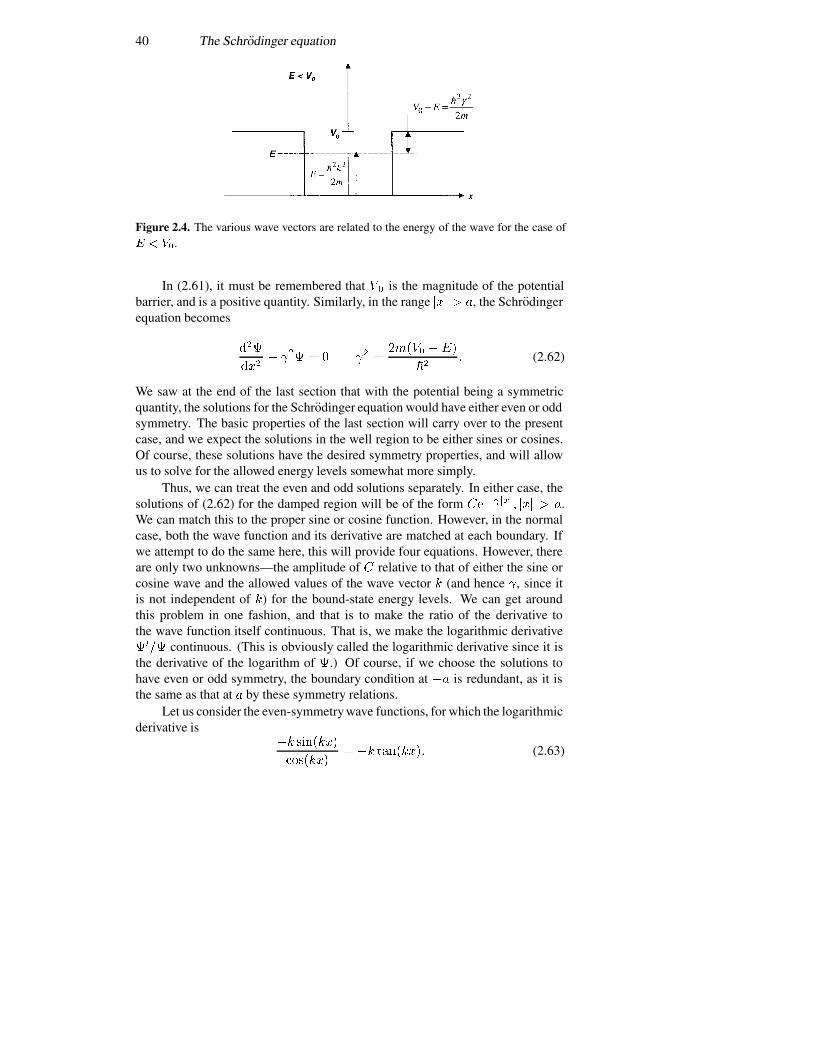
40 The Schrodinger equation
Figure 2.4. The various wave vectors are related to the energy of the wave for the case of� � ��.
In (2.61), it must be remembered that �� is the magnitude of the potentialbarrier, and is a positive quantity. Similarly, in the range ��� � �, the Schrodingerequation becomes
���
���� ��� � � �� �
����� ���
��� (2.62)
We saw at the end of the last section that with the potential being a symmetricquantity, the solutions for the Schrodinger equation would have either even or oddsymmetry. The basic properties of the last section will carry over to the presentcase, and we expect the solutions in the well region to be either sines or cosines.Of course, these solutions have the desired symmetry properties, and will allowus to solve for the allowed energy levels somewhat more simply.
Thus, we can treat the even and odd solutions separately. In either case, thesolutions of (2.62) for the damped region will be of the form ������� ��� � �.We can match this to the proper sine or cosine function. However, in the normalcase, both the wave function and its derivative are matched at each boundary. Ifwe attempt to do the same here, this will provide four equations. However, thereare only two unknowns—the amplitude of � relative to that of either the sine orcosine wave and the allowed values of the wave vector (and hence �, since itis not independent of ) for the bound-state energy levels. We can get aroundthis problem in one fashion, and that is to make the ratio of the derivative tothe wave function itself continuous. That is, we make the logarithmic derivative���� continuous. (This is obviously called the logarithmic derivative since it isthe derivative of the logarithm of �.) Of course, if we choose the solutions tohave even or odd symmetry, the boundary condition at �� is redundant, as it isthe same as that at � by these symmetry relations.
Let us consider the even-symmetry wave functions, for which the logarithmicderivative is
� ����
������� � ����� (2.63)
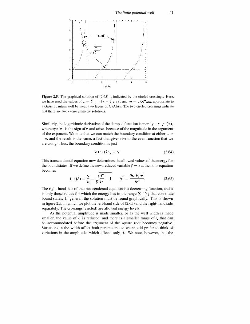
The finite potential well 41
Figure 2.5. The graphical solution of (2.65) is indicated by the circled crossings. Here,we have used the values of � � � ��, �� � ��� ��, and � � ������ , appropriate toa GaAs quantum well between two layers of GaAlAs. The two circled crossings indicatethat there are two even-symmetry solutions.
Similarly, the logarithmic derivative of the damped function is merely�� ������,where ������ is the sign of � and arises because of the magnitude in the argumentof the exponent. We note that we can match the boundary condition at either � or��, and the result is the same, a fact that gives rise to the even function that weare using. Thus, the boundary condition is just
� ������� � �� (2.64)
This transcendental equation now determines the allowed values of the energy forthe bound states. If we define the new, reduced variable � � ��, then this equationbecomes
������ ��
��
���
��� � �� �
�����
��� (2.65)
The right-hand side of the transcendental equation is a decreasing function, and itis only those values for which the energy lies in the range � ��� that constitutebound states. In general, the solution must be found graphically. This is shownin figure 2.5, in which we plot the left-hand side of (2.65) and the right-hand sideseparately. The crossings (circled) are allowed energy levels.
As the potential amplitude is made smaller, or as the well width is madesmaller, the value of � is reduced, and there is a smaller range of � that canbe accommodated before the argument of the square root becomes negative.Variations in the width affect both parameters, so we should prefer to think ofvariations in the amplitude, which affects only �. We note, however, that the
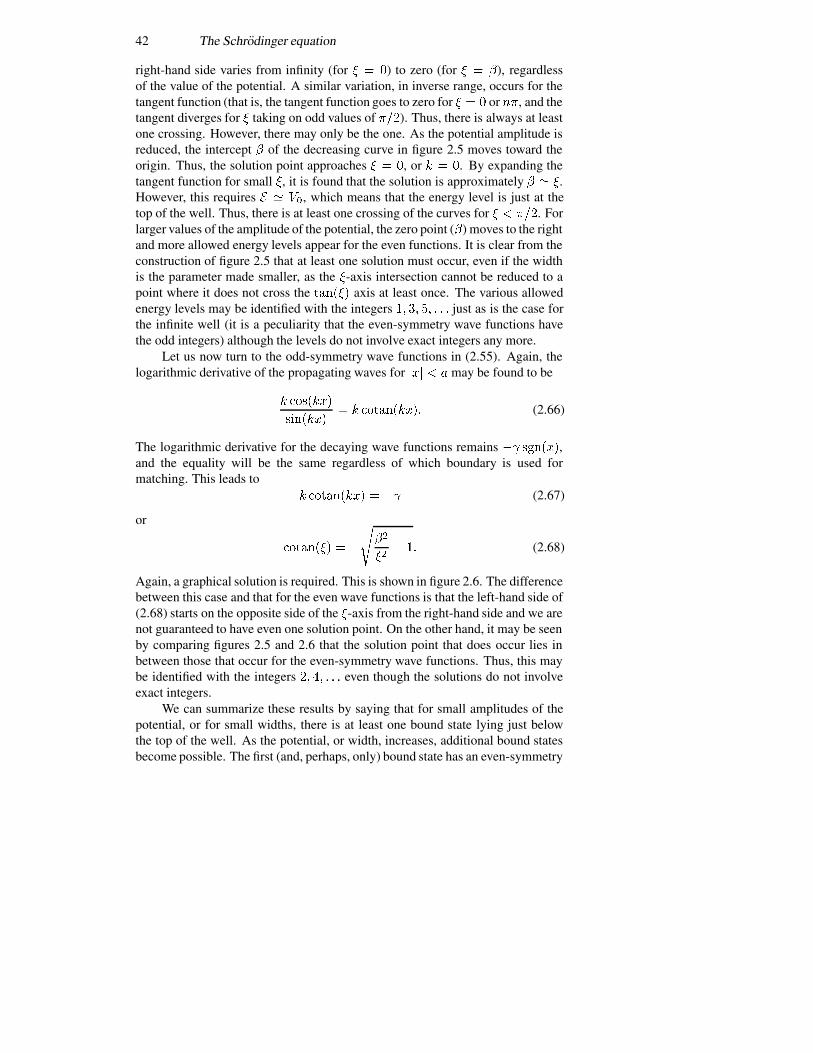
42 The Schrodinger equation
right-hand side varies from infinity (for � � �) to zero (for � � �), regardlessof the value of the potential. A similar variation, in inverse range, occurs for thetangent function (that is, the tangent function goes to zero for � � � or ��, and thetangent diverges for � taking on odd values of ���). Thus, there is always at leastone crossing. However, there may only be the one. As the potential amplitude isreduced, the intercept � of the decreasing curve in figure 2.5 moves toward theorigin. Thus, the solution point approaches � � �, or � � �. By expanding thetangent function for small �, it is found that the solution is approximately � � �.However, this requires � � ��, which means that the energy level is just at thetop of the well. Thus, there is at least one crossing of the curves for � � ���. Forlarger values of the amplitude of the potential, the zero point (�) moves to the rightand more allowed energy levels appear for the even functions. It is clear from theconstruction of figure 2.5 that at least one solution must occur, even if the widthis the parameter made smaller, as the �-axis intersection cannot be reduced to apoint where it does not cross the ������ axis at least once. The various allowedenergy levels may be identified with the integers �� � � just as is the case forthe infinite well (it is a peculiarity that the even-symmetry wave functions havethe odd integers) although the levels do not involve exact integers any more.
Let us now turn to the odd-symmetry wave functions in (2.55). Again, thelogarithmic derivative of the propagating waves for �� � � may be found to be
� �� ���
������ � �������� (2.66)
The logarithmic derivative for the decaying wave functions remains �� ����,and the equality will be the same regardless of which boundary is used formatching. This leads to
� �������� � �� (2.67)
or
�������� � �
���
��� � (2.68)
Again, a graphical solution is required. This is shown in figure 2.6. The differencebetween this case and that for the even wave functions is that the left-hand side of(2.68) starts on the opposite side of the �-axis from the right-hand side and we arenot guaranteed to have even one solution point. On the other hand, it may be seenby comparing figures 2.5 and 2.6 that the solution point that does occur lies inbetween those that occur for the even-symmetry wave functions. Thus, this maybe identified with the integers �� �� even though the solutions do not involveexact integers.
We can summarize these results by saying that for small amplitudes of thepotential, or for small widths, there is at least one bound state lying just belowthe top of the well. As the potential, or width, increases, additional bound statesbecome possible. The first (and, perhaps, only) bound state has an even-symmetry
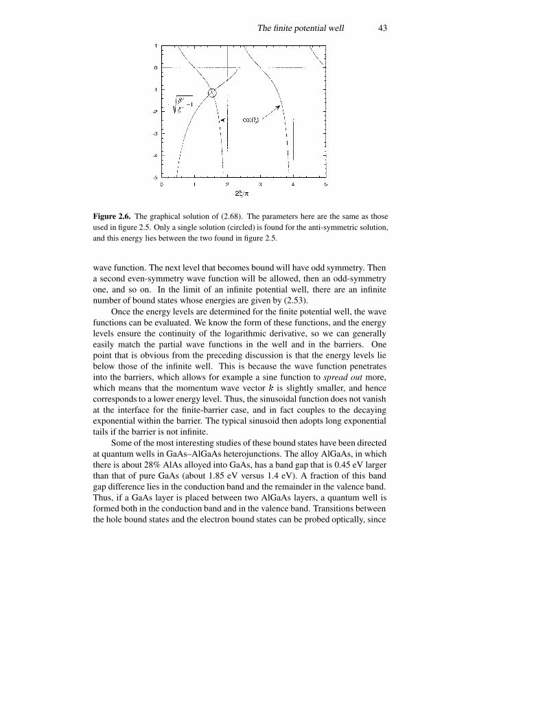
The finite potential well 43
Figure 2.6. The graphical solution of (2.68). The parameters here are the same as thoseused in figure 2.5. Only a single solution (circled) is found for the anti-symmetric solution,and this energy lies between the two found in figure 2.5.
wave function. The next level that becomes bound will have odd symmetry. Thena second even-symmetry wave function will be allowed, then an odd-symmetryone, and so on. In the limit of an infinite potential well, there are an infinitenumber of bound states whose energies are given by (2.53).
Once the energy levels are determined for the finite potential well, the wavefunctions can be evaluated. We know the form of these functions, and the energylevels ensure the continuity of the logarithmic derivative, so we can generallyeasily match the partial wave functions in the well and in the barriers. Onepoint that is obvious from the preceding discussion is that the energy levels liebelow those of the infinite well. This is because the wave function penetratesinto the barriers, which allows for example a sine function to spread out more,which means that the momentum wave vector � is slightly smaller, and hencecorresponds to a lower energy level. Thus, the sinusoidal function does not vanishat the interface for the finite-barrier case, and in fact couples to the decayingexponential within the barrier. The typical sinusoid then adopts long exponentialtails if the barrier is not infinite.
Some of the most interesting studies of these bound states have been directedat quantum wells in GaAs–AlGaAs heterojunctions. The alloy AlGaAs, in whichthere is about 28% AlAs alloyed into GaAs, has a band gap that is 0.45 eV largerthan that of pure GaAs (about 1.85 eV versus 1.4 eV). A fraction of this bandgap difference lies in the conduction band and the remainder in the valence band.Thus, if a GaAs layer is placed between two AlGaAs layers, a quantum well isformed both in the conduction band and in the valence band. Transitions betweenthe hole bound states and the electron bound states can be probed optically, since
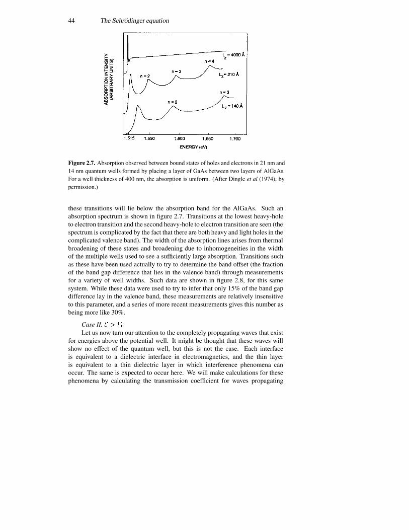
44 The Schrodinger equation
Figure 2.7. Absorption observed between bound states of holes and electrons in 21 nm and14 nm quantum wells formed by placing a layer of GaAs between two layers of AlGaAs.For a well thickness of 400 nm, the absorption is uniform. (After Dingle et al (1974), bypermission.)
these transitions will lie below the absorption band for the AlGaAs. Such anabsorption spectrum is shown in figure 2.7. Transitions at the lowest heavy-holeto electron transition and the second heavy-hole to electron transition are seen (thespectrum is complicated by the fact that there are both heavy and light holes in thecomplicated valence band). The width of the absorption lines arises from thermalbroadening of these states and broadening due to inhomogeneities in the widthof the multiple wells used to see a sufficiently large absorption. Transitions suchas these have been used actually to try to determine the band offset (the fractionof the band gap difference that lies in the valence band) through measurementsfor a variety of well widths. Such data are shown in figure 2.8, for this samesystem. While these data were used to try to infer that only 15% of the band gapdifference lay in the valence band, these measurements are relatively insensitiveto this parameter, and a series of more recent measurements gives this number asbeing more like 30%.
Case II. � � ��
Let us now turn our attention to the completely propagating waves that existfor energies above the potential well. It might be thought that these waves willshow no effect of the quantum well, but this is not the case. Each interfaceis equivalent to a dielectric interface in electromagnetics, and the thin layeris equivalent to a thin dielectric layer in which interference phenomena canoccur. The same is expected to occur here. We will make calculations for thesephenomena by calculating the transmission coefficient for waves propagating
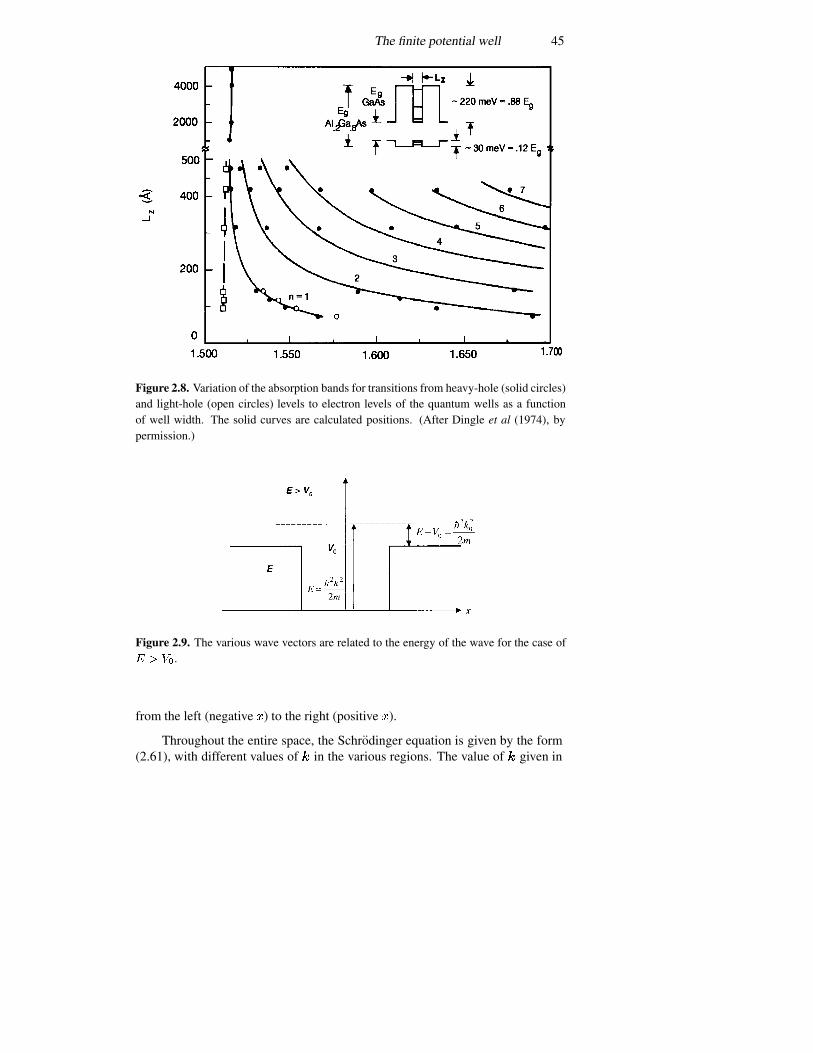
The finite potential well 45
Figure 2.8. Variation of the absorption bands for transitions from heavy-hole (solid circles)and light-hole (open circles) levels to electron levels of the quantum wells as a functionof well width. The solid curves are calculated positions. (After Dingle et al (1974), bypermission.)
Figure 2.9. The various wave vectors are related to the energy of the wave for the case of� � ��.
from the left (negative �) to the right (positive �).
Throughout the entire space, the Schrodinger equation is given by the form(2.61), with different values of � in the various regions. The value of � given in
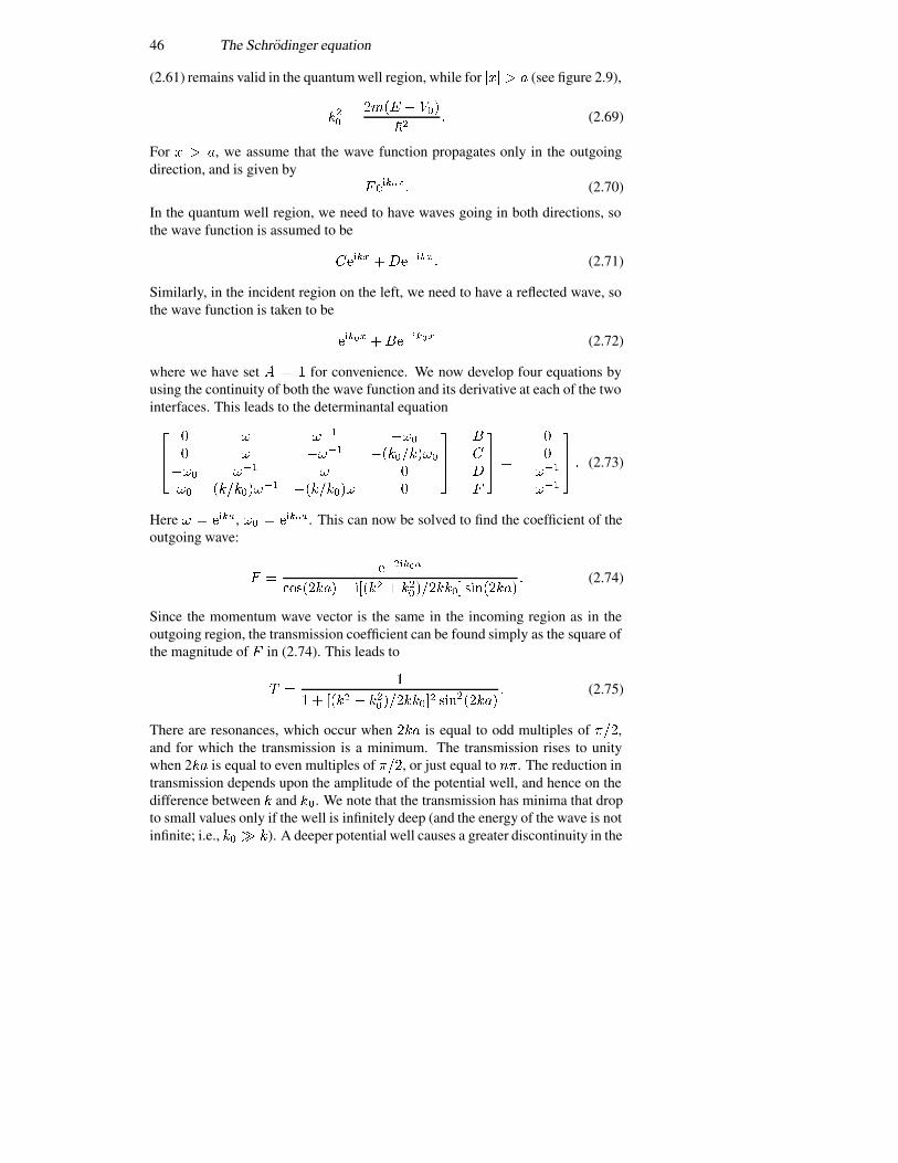
46 The Schrodinger equation
(2.61) remains valid in the quantum well region, while for ��� � � (see figure 2.9),
����
���� � ���
��� (2.69)
For � � �, we assume that the wave function propagates only in the outgoingdirection, and is given by
� ������ (2.70)
In the quantum well region, we need to have waves going in both directions, sothe wave function is assumed to be
���� ������� (2.71)
Similarly, in the incident region on the left, we need to have a reflected wave, sothe wave function is taken to be
����� �������� (2.72)
where we have set � � � for convenience. We now develop four equations byusing the continuity of both the wave function and its derivative at each of the twointerfaces. This leads to the determinantal equation
���
� �� � �
� � �� ������� �
� � �� � � ������
�� ������� �
���
��
��� �
�� ��
��
��� � (2.73)
Here � ����, � � �����. This can now be solved to find the coefficient of theoutgoing wave:
� ��������
������� ����� � ��������� �������
� (2.74)
Since the momentum wave vector is the same in the incoming region as in theoutgoing region, the transmission coefficient can be found simply as the square ofthe magnitude of � in (2.74). This leads to
� ��
� � ���� � ��������� � ��
������� (2.75)
There are resonances, which occur when ��� is equal to odd multiples of ���,and for which the transmission is a minimum. The transmission rises to unitywhen 2�� is equal to even multiples of ���, or just equal to ��. The reduction intransmission depends upon the amplitude of the potential well, and hence on thedifference between � and ��. We note that the transmission has minima that dropto small values only if the well is infinitely deep (and the energy of the wave is notinfinite; i.e., �� � �). A deeper potential well causes a greater discontinuity in the
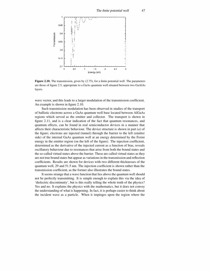
The finite potential well 47
Figure 2.10. The transmission, given by (2.75), for a finite potential well. The parametersare those of figure 2.5, appropriate to a GaAs quantum well situated between two GaAlAslayers.
wave vector, and this leads to a larger modulation of the transmission coefficient.An example is shown in figure 2.10.
Such transmission modulation has been observed in studies of the transportof ballistic electrons across a GaAs quantum well base located between AlGaAsregions which served as the emitter and collector. The transport is shown infigure 2.11, and is a clear indication of the fact that quantum resonances, andquantum effects, can be found in real semiconductor devices in a manner thataffects their characteristic behaviour. The device structure is shown in part (a) ofthe figure; electrons are injected (tunnel) through the barrier to the left (emitterside) of the internal GaAs quantum well at an energy determined by the Fermienergy in the emitter region (on the left of the figure). The injection coefficient,determined as the derivative of the injected current as a function of bias, revealsoscillatory behaviour due to resonances that arise from both the bound states andthe so-called virtual states above the barrier. These are called virtual states as theyare not true bound states but appear as variations in the transmission and reflectioncoefficients. Results are shown for devices with two different thicknesses of thequantum well, 29 and 51.5 nm. The injection coefficient is shown rather than thetransmission coefficient, as the former also illustrates the bound states.
It seems strange that a wave function that lies above the quantum well shouldnot be perfectly transmitting. It is simple enough to explain this via the idea of‘dielectric discontinuity’, but is this really telling the whole truth of the physics?Yes and no. It explains the physics with the mathematics, but it does not conveythe understanding of what is happening. In fact, it is perhaps easier to think aboutthe incident wave as a particle. When it impinges upon the region where the
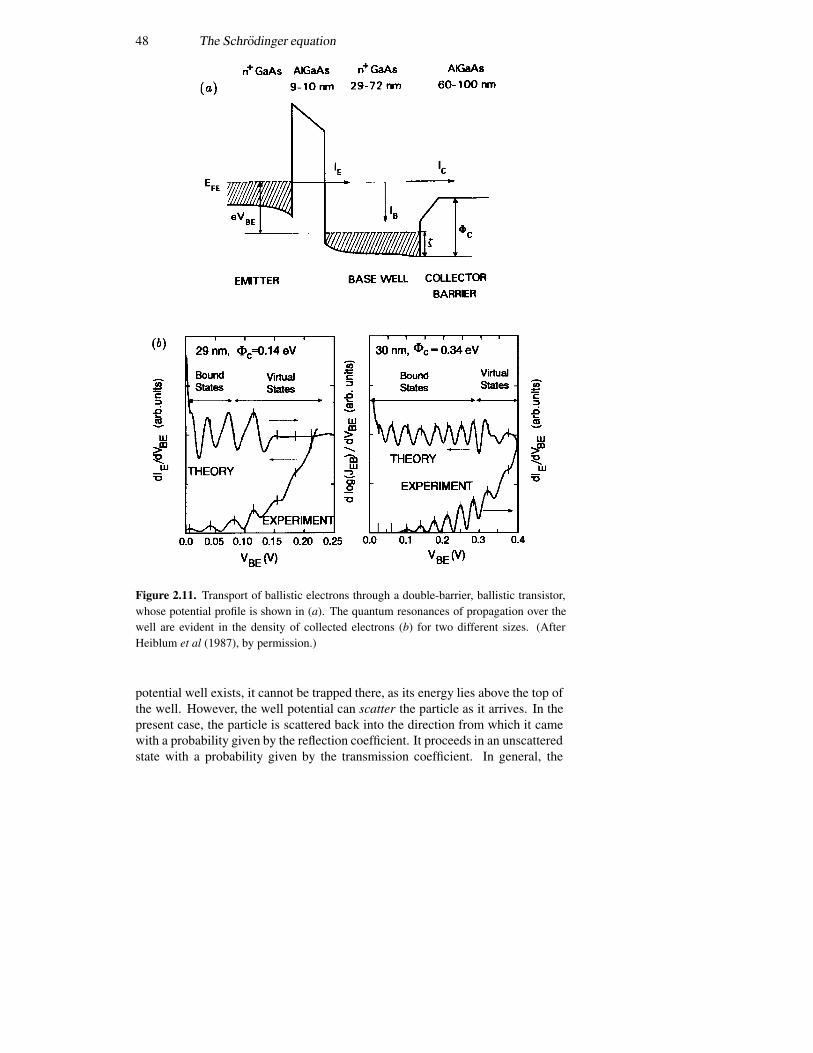
48 The Schrodinger equation
Figure 2.11. Transport of ballistic electrons through a double-barrier, ballistic transistor,whose potential profile is shown in (a). The quantum resonances of propagation over thewell are evident in the density of collected electrons (b) for two different sizes. (AfterHeiblum et al (1987), by permission.)
potential well exists, it cannot be trapped there, as its energy lies above the top ofthe well. However, the well potential can scatter the particle as it arrives. In thepresent case, the particle is scattered back into the direction from which it camewith a probability given by the reflection coefficient. It proceeds in an unscatteredstate with a probability given by the transmission coefficient. In general, the

The triangular well 49
scattering probability is non-zero, but at special values of the incident energy, thescattering vanishes. In this case, the particle is transmitted with unit probability.This type of potential scattering is quite special, because only the direction of themomentum (this is a one-dimensional problem) is changed, and the energy of theparticle remains unchanged. This type of scattering is termed elastic, as in elasticscattering of a billiard ball from a ‘cushion’ in three dimensions. We will seeother examples of this in the following chapters.
Before proceeding, it is worthwhile to discuss the material systems that wereused in the preceding examples, both theoretical and experimental. While onemight at first glance think it quite difficult to put different materials togethereffectively, this is allowed today through the efficiency of molecular-beamepitaxy. In this growth process, materials can be grown almost one atomic layerat a time. This is facilitated in the GaAs–AlAs system, since these two materialshave almost identical lattice constants. Hence, one can alloy the two materials tocreate a ‘new’ semiconductor with a band gap somewhere between that of GaAsand that of AlAs. Moreover, one can change the material system from the alloy to,for example, GaAs within one atomic layer. So, it is quite easy to create designerstructures with molecular-beam epitaxial growth of semiconductor materials. Theexamples discussed in the preceding paragraphs are just some of the structuresthat can be easily made with this growth technology.
2.6 The triangular well
Another type of potential well is quite common in everyday semiconductordevices, such as the common metal–oxide–semiconductor (MOS) transistor(figure 2.12(a)). The latter is the workhorse in nearly all microprocessors andcomputers today, yet the presence of quantization has not really been highlightedin the operation of these devices. These devices depend upon capacitive controlof the charge at the interface between the oxide and the semiconductor. If weconsider a parallel-plate capacitor made of a metal plate, with an insulator madeof silicon dioxide, and a second plate composed of the semiconductor silicon, weessentially have the MOS transistor. Voltage applied across the capacitor variesthe amount of charge accumulated in the metal and in the semiconductor, in bothcases at the interface with the insulator. On the semiconductor side, contacts(made of n-type regions embedded in a normally p-type material) allow one topass current through the channel in which the charge resides in the semiconductor.Variation of the current, through variation of the charge via the capacitor voltage,is the heart of the transistor operation.
Consider the case in which the semiconductor is p-type, and hence thesurface is in an ‘inverted’ condition (more electrons than holes) and mobileelectrons can be drawn to the interface by a positive voltage on the metal plate(the channel region is isolated from the bulk of the semiconductor by the inversionprocess). The surface charge in the semiconductor is composed of two parts:
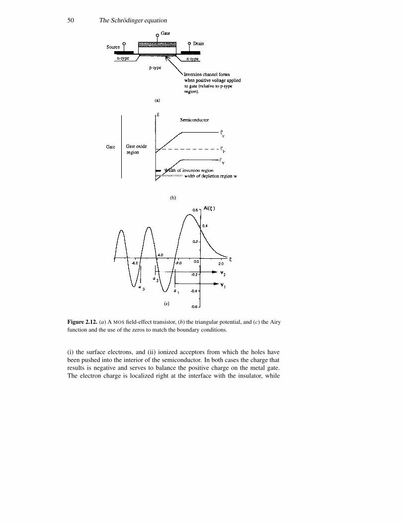
50 The Schrodinger equation
Figure 2.12. (a) A MOS field-effect transistor, (b) the triangular potential, and (c) the Airyfunction and the use of the zeros to match the boundary conditions.
(i) the surface electrons, and (ii) ionized acceptors from which the holes havebeen pushed into the interior of the semiconductor. In both cases the charge thatresults is negative and serves to balance the positive charge on the metal gate.The electron charge is localized right at the interface with the insulator, while

The triangular well 51
the ionized acceptor charge is distributed over a large region. In fact, it is thelocalized electron charge that is mobile in the direction along the interface, andthat is quantized in the resulting potential well. The field in the oxide is then givenby the total surface charge through Gauss’s law (we use the approximation of aninfinite two-dimensional plane) as
�� ��
������� � ��� (2.76)
where � is the thickness of the layer of ionized acceptors �� (normal to thesurface), the surface electron density �� is assumed to be a two-dimensional sheetcharge, and the permittivity is that of the oxide. On the semiconductor side ofthe interface, the normal component of � is continuous, which means that �in (2.76) is discontinuous by the dielectric constant ratio. Thus, just inside theinterface, (2.76) represents the field if the oxide permittivity is replaced by that ofthe semiconductor. However, just a short distance further into the semiconductor,the field drops by the amount produced by the surface electron density. Thus, theaverage field in the semiconductor, in the region where the electrons are located,is approximately
�� ��
��
���� �
��
�
�� (2.77)
In this approximation, a constant electric field in this region gives rise to a linearpotential in the Schrodinger equation (figure 2.12(b)). We want to solve for justthe region inside the semiconductor, near to the oxide interface. Here, we canwrite the Schrodinger equation in the form
�
��
��
���
��� ���� � �� ��� � (2.78)
We assume that the potential barrier at the interface is infinitely high, so noelectrons can get into the oxide, which leads to the boundary condition that��� � . The other boundary condition is merely that the wave function mustremain finite, which means that it also tends to zero at large values of .
While the previous discussion has been for the case of a MOS transistor,such as found in silicon integrated circuits, quite similar behaviour arises in theGaAs–AlGaAs heterojunction high-electron-mobility transistor (HEMT). In thiscase, the AlGaAs plays a role similar to the oxide in the MOS transistor, withthe exception that the dopant atoms are placed in this layer. The dopants nearthe interface are ionized, with the electrons falling into a potential well on theGaAs side of the interface, a process that is facilitated by the barrier created bythe difference in the two conduction band edges, as shown in figure 2.13. Thereare very few ionized dopants in the GaAs, although the interface electric field stillsatisfies (2.76). This field is created by the positively charged, ionized donors andthe negatively charged electrons in the potential well. By placing a metal gate onthe surface of the AlGaAs layer, bias applied to the gate can affect the densityof the carriers in the quantum well, reducing them to zero. This is a depletion
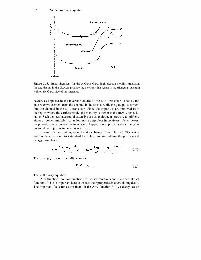
52 The Schrodinger equation
Figure 2.13. Band alignment for the AlGaAs–GaAs high-electron-mobility transistor.Ionized donors in the GaAlAs produce the electrons that reside in the triangular quantumwell on the GaAs side of the interface.
device, as opposed to the inversion device of the MOS transistor. That is, thegate removes carriers from the channel in the HEMT, while the gate pulls carriersinto the channel in the MOS transistor. Since the impurities are removed fromthe region where the carriers reside, the mobility is higher in the HEMT, hence itsname. Such devices have found extensive use as analogue microwave amplifiers,either as power amplifiers or as low-noise amplifiers in receivers. Nevertheless,the potential variation near the interface still appears as approximately a triangularpotential well, just as in the MOS transistor.
To simplify the solution, we will make a change of variables in (2.78), whichwill put the equation into a standard form. For this, we redefine the position andenergy variables as
� �
������
��
����� �� �
���
��
���
�����
����� (2.79)
Then, using � � � � ��, (2.78) becomes
���
���� �� � �� (2.80)
This is the Airy equation.Airy functions are combinations of Bessel functions and modified Bessel
functions. It is not important here to discuss their properties in excruciating detail.The important facts for us are that: (i) the Airy function Ai(��) decays as an
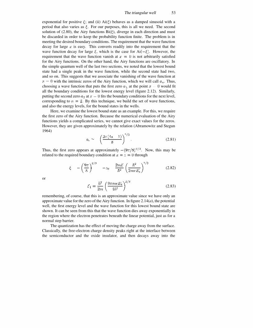
The triangular well 53
exponential for positive �; and (ii) Ai(�) behaves as a damped sinusoid with aperiod that also varies as �. For our purposes, this is all we need. The secondsolution of (2.80), the Airy functions Bi(�), diverge in each direction and mustbe discarded in order to keep the probability function finite. The problem is inmeeting the desired boundary conditions. The requirement that the wave functiondecay for large � is easy. This converts readily into the requirement that thewave function decay for large �, which is the case for Ai����. However, therequirement that the wave function vanish at � � � is not arbitrarily satisfiedfor the Airy functions. On the other hand, the Airy functions are oscillatory. Inthe simple quantum well of the last two sections, we noted that the lowest boundstate had a single peak in the wave function, while the second state had two,and so on. This suggests that we associate the vanishing of the wave function at� � � with the intrinsic zeros of the Airy function, which we will call � �. Thus,choosing a wave function that puts the first zero �� at the point � � � would fitall the boundary conditions for the lowest energy level (figure 2.12). Similarly,putting the second zero �� at � � � fits the boundary conditions for the next level,corresponding to � � �. By this technique, we build the set of wave functions,and also the energy levels, for the bound states in the wells.
Here, we examine the lowest bound state as an example. For this, we requirethe first zero of the Airy function. Because the numerical evaluation of the Airyfunctions yields a complicated series, we cannot give exact values for the zeros.However, they are given approximately by the relation (Abramowitz and Stegun1964)
�� � �
������� ��
�
����� (2.81)
Thus, the first zero appears at approximately ���������. Now, this may berelated to the required boundary condition at � � � � � through
� � �
��
�
����� ��� �
��
��
���
���
����(2.82)
or
�� ���
�
����
���
����(2.83)
remembering, of course, that this is an approximate value since we have only anapproximate value for the zero of the Airy function. In figure 2.14(a), the potentialwell, the first energy level and the wave function for this lowest bound state areshown. It can be seen from this that the wave function dies away exponentially inthe region where the electron penetrates beneath the linear potential, just as for anormal step barrier.
The quantization has the effect of moving the charge away from the surface.Classically, the free-electron charge density peaks right at the interface betweenthe semiconductor and the oxide insulator, and then decays away into the
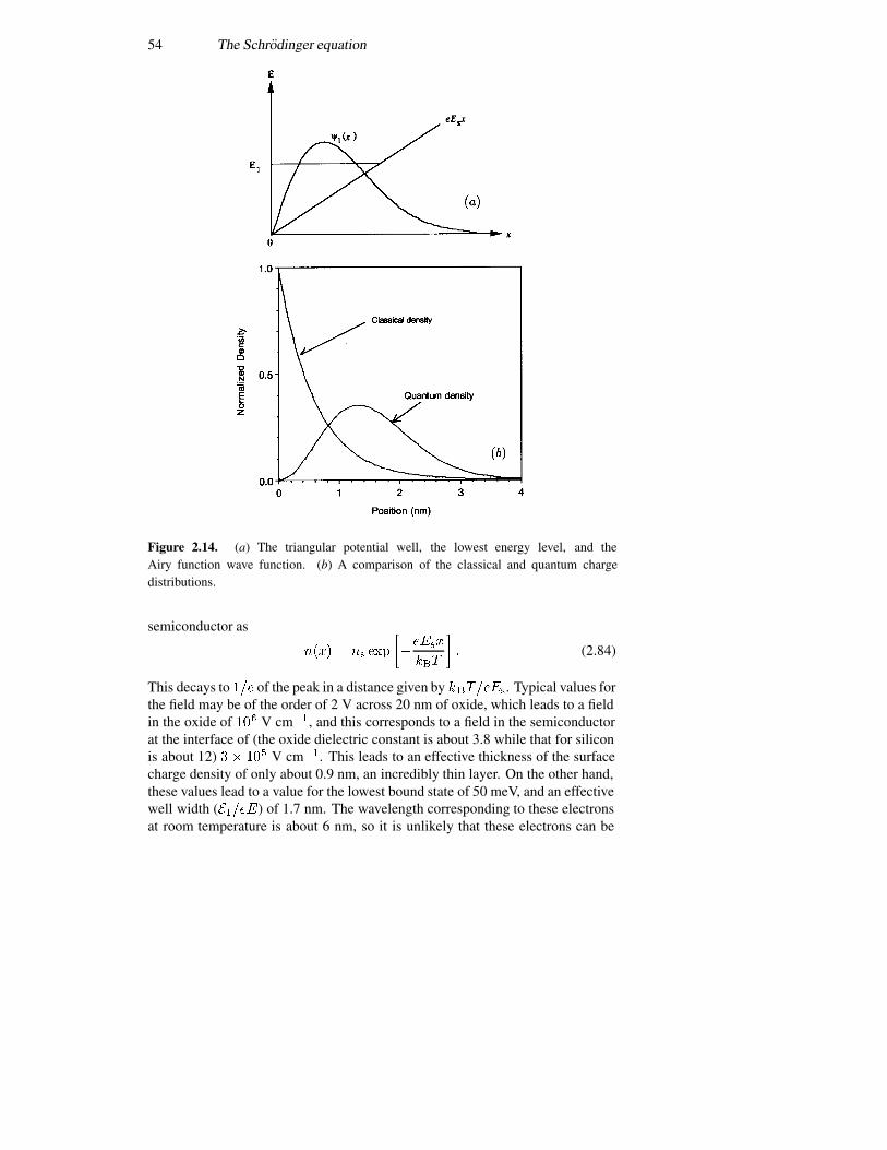
54 The Schrodinger equation
Figure 2.14. (a) The triangular potential well, the lowest energy level, and theAiry function wave function. (b) A comparison of the classical and quantum chargedistributions.
semiconductor as
���� � �� ���
��
����
���
�� (2.84)
This decays to ��� of the peak in a distance given by �������. Typical values forthe field may be of the order of 2 V across 20 nm of oxide, which leads to a fieldin the oxide of ��� V cm��, and this corresponds to a field in the semiconductorat the interface of (the oxide dielectric constant is about 3.8 while that for siliconis about 12) �� ��� V cm��. This leads to an effective thickness of the surfacecharge density of only about 0.9 nm, an incredibly thin layer. On the other hand,these values lead to a value for the lowest bound state of 50 meV, and an effectivewell width (�����) of 1.7 nm. The wavelength corresponding to these electronsat room temperature is about 6 nm, so it is unlikely that these electrons can be
Coupled potential wells 55
confined in this small distance, and this is what leads to the quantization of theseelectrons. The quantized charge density in the lowest bound state is proportionalto the square of the wave function, and the peak in this density occurs at thepeak of the wave function, which is at the zero of the first derivative of the Airyfunction. These zeros are given by the approximate relation (Abramowitz andStegun 1964)
��
� � �
������� ��
�
����(2.85)
which for the lowest subband leads to ����� � ����������. This leads to the peakoccurring at a distance from the surface (e.g., from�� �) of
� �
���
�����
���� ����
�
����� ����������
�(2.86)
which for the above field gives a distance of 1.3 nm. The effective width of thequantum well, mentioned earlier, is larger than this, as this value is related to the‘half-width’. This value is smaller than the actual thermal de Broglie wavelengthof the electron wave packet. The quantization arises from the confinement ofthe electron in this small region. In figure 2.14(b), the classical charge densityand that resulting from the quantization is shown for comparison. It may beseen here that the quantization actually will decrease the total gate capacitanceas it moves the surface charge away from the interface, producing an effectiveinterface quantum capacitance contribution to the overall gate capacitance (inseries with the normal gate capacitance to reduce the overall capacitance).In small transistors, this effect can be a significant modification to the gatecapacitance, and hence to the transistor performance.
2.7 Coupled potential wells
What if there are two closely coupled potential wells? By closely coupled, it ismeant that these two wells are separated by a barrier, as indicated in figure 2.15.However, the barrier is sufficiently thin that the decaying wave functions reachcompletely through the barrier into the next well. This will be quite important inthe next chapter, but here we want to look at the interference that arises betweenthe wave functions in the two wells. To simplify the problem, we will assume thatthe potential is infinite outside the two wells, zero in the wells, and a finite valuebetween the wells; for example
��� �
���� ��� ��� � � ��� ��� ���� ��� ���.
(2.87)
(Note that the well width here is given by �, while it was �� in the precedingsections on quantum wells.) Within the wells, the wave function is given by a
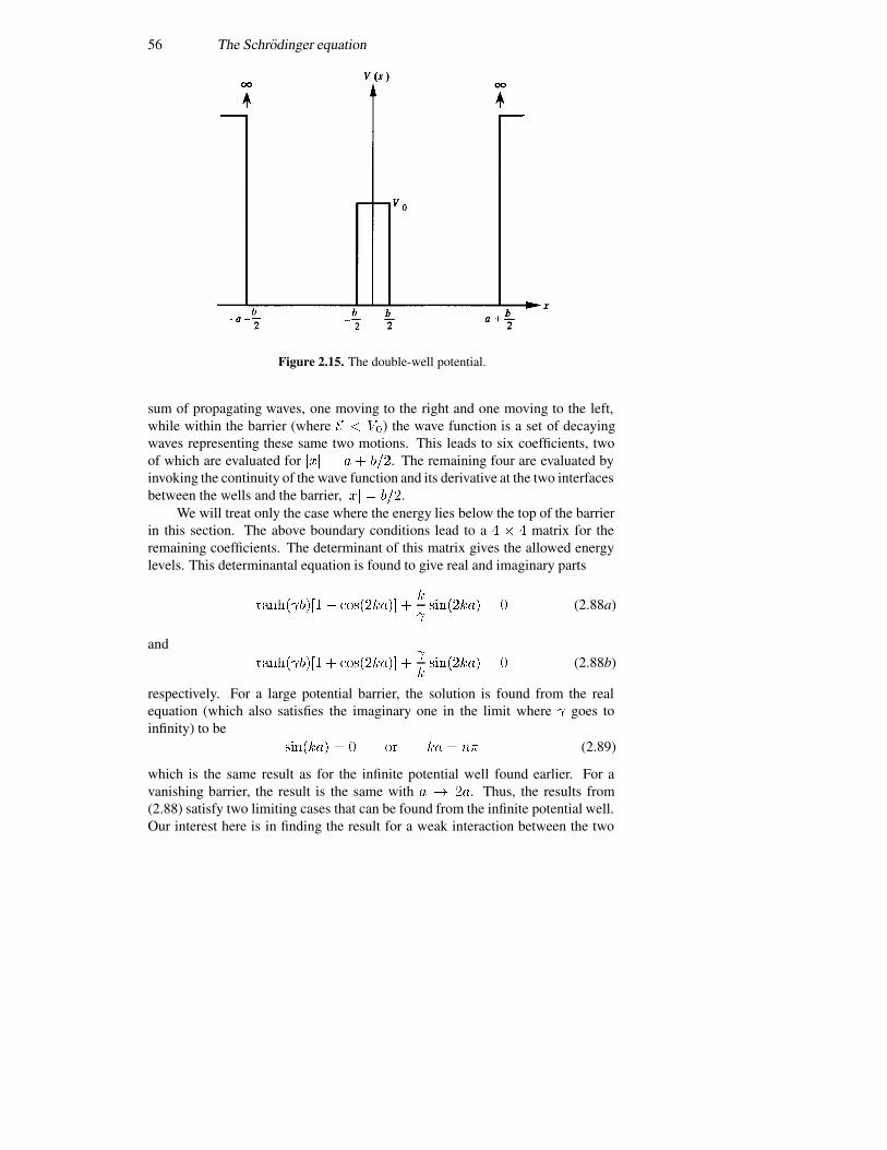
56 The Schrodinger equation
Figure 2.15. The double-well potential.
sum of propagating waves, one moving to the right and one moving to the left,while within the barrier (where � � ��) the wave function is a set of decayingwaves representing these same two motions. This leads to six coefficients, twoof which are evaluated for ��� � � � ���. The remaining four are evaluated byinvoking the continuity of the wave function and its derivative at the two interfacesbetween the wells and the barrier, ��� � ���.
We will treat only the case where the energy lies below the top of the barrierin this section. The above boundary conditions lead to a � � � matrix for theremaining coefficients. The determinant of this matrix gives the allowed energylevels. This determinantal equation is found to give real and imaginary parts
��������� � ������ ��
�������� � � (2.88a)
and�������� � � ������ �
�
�������� � � (2.88b)
respectively. For a large potential barrier, the solution is found from the realequation (which also satisfies the imaginary one in the limit where � goes toinfinity) to be
������ � � � �� � � (2.89)
which is the same result as for the infinite potential well found earlier. For avanishing barrier, the result is the same with � � ��. Thus, the results from(2.88) satisfy two limiting cases that can be found from the infinite potential well.Our interest here is in finding the result for a weak interaction between the two
The time variation again 57
wells. To solve for the general case, we will assume that the barrier is very large,and expand the hyperbolic tangent function around its value of unity for the verylarge limit. In addition, we expand �������� in (2.88a) about its relevant zero,where the latter is given by (2.89). This then leads to the approximate solutions
������� � ����� ����� ������� (2.90)
The pre-factor is very near zero, and the hyperbolic tangent function is very nearlyunity, so there is a small shift of the energy level both up and down from the boundstate of the single well. The lower level must be the symmetric combination of thewave functions of the two individual wells, which is the symmetric combinationof wave functions that are each symmetric in their own wells. This lower levelmust be the symmetric combination since we have already ascertained that thelowest energy state is a symmetric wave function for a symmetric potential. Theupper level must then be the anti-symmetric combination of the two symmetricwave functions. The actual levels from (2.90) can be found also by expanding thesine function around the zero point to give approximately
�� � �� � ������� (2.91)
While this result is for the approximation of a nearly infinite well, the generalbehaviour for finite wells is the same. The two bound states, one in each well thatwould normally lie at the same energy level, split due to the interaction of the wavefunctions penetrating the barrier. This leads to one level (in both wells) lying at aslightly lower energy due to the symmetric sum of the individual wave functions,and a second level lying at a slightly higher energy due to the anti-symmetricsum of the two wave functions. We will return to this in a later chapter, wherewe will develop formal approximation schemes to find the energy levels moreexactly. In figure 2.16, experimental data on quantum wells in the GaAs/AlGaAsheterojunction system are shown to illustrate this splitting of the energy levels(Dingle et al 1975). Here, the coupling is quite strong, and the resulting splittingis rather large.
2.8 The time variation again
In each of the cases treated above, the wave function has been determined to beone of a number of possible eigenfunctions, each of which corresponds to a singleenergy level, determined by the eigenvalue. The general solution of the problemis composed of a sum over these eigenfunctions, with coefficients determined bythe probability of the occupancy of each of the discrete states. This sum can bewritten as
���� ��
�
�������� (2.92)
In every sense, this series is strongly related to the Fourier series, where theexpansion basis functions, our eigenfunctions, are determined by the geometry
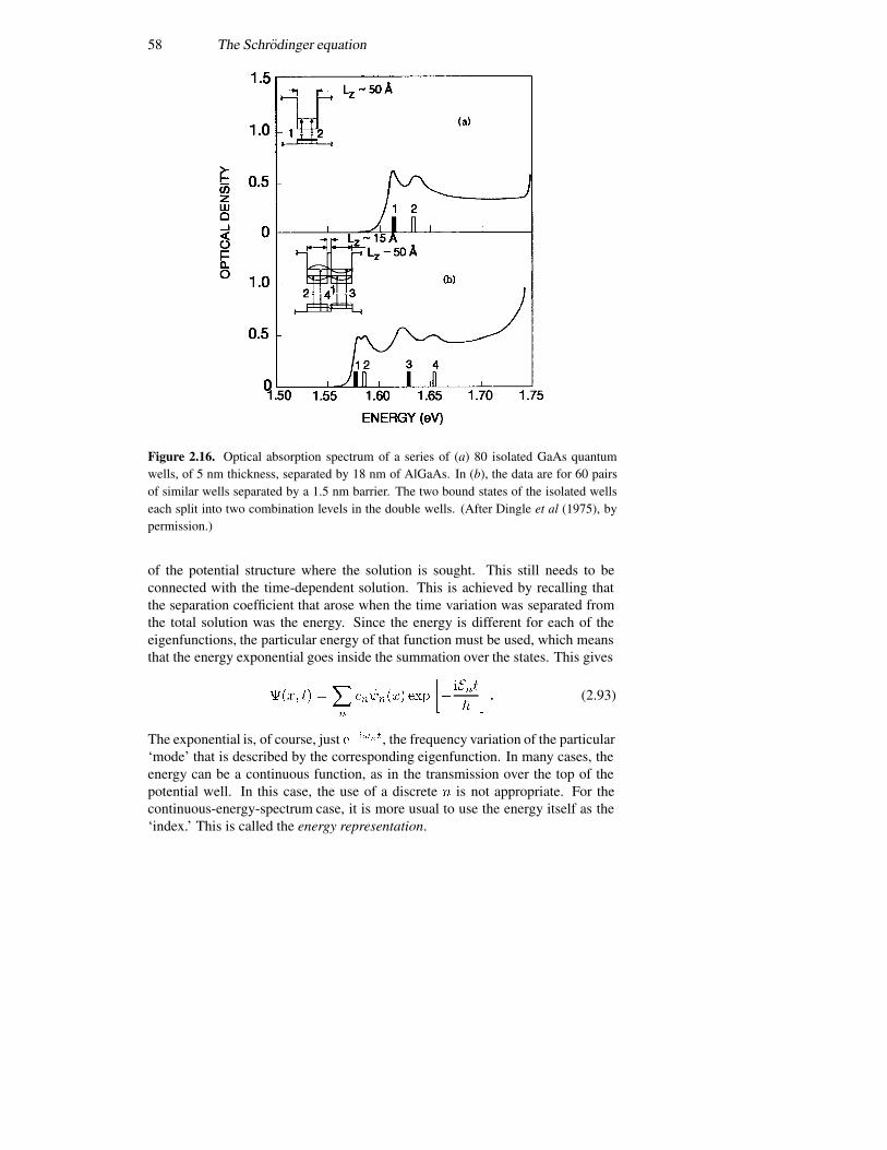
58 The Schrodinger equation
Figure 2.16. Optical absorption spectrum of a series of (a) 80 isolated GaAs quantumwells, of 5 nm thickness, separated by 18 nm of AlGaAs. In (b), the data are for 60 pairsof similar wells separated by a 1.5 nm barrier. The two bound states of the isolated wellseach split into two combination levels in the double wells. (After Dingle et al (1975), bypermission.)
of the potential structure where the solution is sought. This still needs to beconnected with the time-dependent solution. This is achieved by recalling thatthe separation coefficient that arose when the time variation was separated fromthe total solution was the energy. Since the energy is different for each of theeigenfunctions, the particular energy of that function must be used, which meansthat the energy exponential goes inside the summation over the states. This gives
���� �� ��
�
������� ���
��
����
�
�� (2.93)
The exponential is, of course, just ������, the frequency variation of the particular‘mode’ that is described by the corresponding eigenfunction. In many cases, theenergy can be a continuous function, as in the transmission over the top of thepotential well. In this case, the use of a discrete � is not appropriate. For thecontinuous-energy-spectrum case, it is more usual to use the energy itself as the‘index.’ This is called the energy representation.
The time variation again 59
2.8.1 The Ehrenfest theorem
Let us now return to the concept of the expectation value. We recall that theexpectation value of the position is found from
��� � ��� ��� �
��
��
����� ������� �� ��� (2.94)
What is the time variation of the position? Here, we do not refer specifically tothe momentum or velocity operator, but to the time derivative of the expectationvalue of the position. These are two different things. In the first case, we areinterested in the expectation value of the momentum operator. In the second, weare interested in whether the expectation value of the position may be changing.As stated, the problem is to determine whether the time derivative of the positionis indeed the expectation value of the momentum.
Consider, for example, the situations discussed above for the various boundstates for the potential wells, say the infinite well or the triangular well, whereall states are bound. The time derivative of (2.91) is given by (it is assumed thatthe position operator is one of a set of conjugate variables and does not have anintrinsic time variation)
����
���
�
��
��� �� �
����
���� � �
����
����
� �
������
�����
����
���� �
�� ��� (2.95)
The continuity equation has been used to get the last term on the first line fromthe previous one. For the states in the wells considered, the first term in thesecond line vanishes since the wave function itself vanishes exponentially at thelarge-� limits. Since these states are not current-carrying states, the current �also vanishes and the time derivative of the position expectation vanishes. By notbeing a current-carrying state, we mean that the bound states are real, and so thecurrent (2.17) is identically zero. This is not the case for the propagating wavesolutions that exist above the potential barriers, for example in the finite potentialwell.
If the current does not vanish, as in the propagating waves, then the last termin (2.95) is identically the expectation value of the momentum. If (2.17) is usedin (2.95), we find (in vector notation and with volume integrations)
����
���
�� �� �
�
���
��������� ������ ��
��
��
��������� (2.96)
where we have used ������ � ������ �������. The last term expressesthe desired result that the time derivative of the expectation value of the position is
60 The Schrodinger equation
given by the expectation value of the momentum. The important point here is thatwe are working with expectation values and not with the operators themselves.The connection between position and momentum in classical mechanics carriesover to a connection between their expectation values in quantum mechanics.
How does this carry over to Newton’s law on acceleration? In the beginning,this was one of the points that we wanted to establish—that the classical equationsof motion carried over to equivalent ones in quantum mechanics. To express thisresult, let us seek the time derivative of the expectation value of the momentum:
����
��� � � �
�
��
���������
�
� ����
���
��
������
���
�
������
��
���
�
� ��
��
������
������
���
�
��
��
������
���
�
������������
����� ��� (2.97)
The first two terms in the last line can be combined and converted to a surfaceintegral which vanishes. This follows since the momentum operator has realeigenvalues and is a Hermitian operator, and thus is self-adjoint. These two termsmay be expressed as
����� ���� ��� ���� � ��� ��������� ��� ����
� ��� ����� ��� ���� � � (2.98)
The last term just becomes the gradient of the potential, and
����
��� ���� ����� (2.99)
Thus, the time derivative of the momentum is given by the expectation value ofthe gradient of the potential. This is a very interesting result, since it says thatrapid variations in the potential will be smoothed out by the wave function itself,and it is only those variations that are of longer range and survive the averagingprocess that give rise to the acceleration evident in the expectation value of themomentum. This result is known as Ehrenfest’s theorem.
2.8.2 Propagators and Green’s functions
Equation (2.93), which we developed earlier, clearly indicates that the wavefunction can easily be obtained by an expansion in the basis functions appropriateto the problem at hand. It goes further, however, and even allows us to determinefully the time variation of any given initial wave function. This follows from theSchrodinger equation being a linear differential equation, with the time evolution
The time variation again 61
deriving from a single initial state. To see formally how this occurs, consider acase where we know the wave function at � � � to be ���� ��. This can be usedwith (2.93) to determine the coefficients in the generalized Fourier series, whichthis latter equation represents as
�� �
���
�������� �� ��� (2.100)
This can be re-inserted into (2.93) to give the general solution
���� �� ���
���
��������������� �� ���
��
���
�
����
�
����� �� �� ������� �� ��� (2.101)
where the propagator kernel is
���� �� �� �� ���
��
���������� ���
�����
�
�� (2.102)
The kernel (2.102) describes the general propagation of any initial wavefunction to any time � � �. In fact, however, this is not required, and we couldset the problem up with any initial state at any time ��. For example, say that weknow that the wave function is given by ���� ��� at time ��. Then, the Fouriercoefficients are found to be
�� �
���
�������� ��� ���
������
���� (2.103)
Following the same procedure—that is, re-introducing this into (2.90)—thegeneral solution at arbitrary time for the wave function is then
���� �� �
����� �� �� �������� ��� ��
� (2.104)
where
���� �� �� ��� ���
��
���������� ���
������� ���
�
�� (2.105)
We note that the solution is a function of � � ��, and not a function of thesetwo times separately. This is a general property of the linear solutions, and isalways expected (unless for some reason the basis set is changing with time). Theinteresting fact about (2.104) is that we can find the solutions either for � � � �,or for � � ��. This means that we can propagate forward in time to find thefuture solution, or we can propagate backward in time to find the earlier state thatproduced the wave function at ��.
62 The Schrodinger equation
In general, it is preferable to separate the propagation in forward and reversetimes to obtain different functions for retarded behaviour (forward in time) andfor advanced behaviour (backward in time). We can do this by introducing theretarded Green’s function as
����� ��� �� ��� � ������ ������� ��� �� ��� (2.106)
where � is the Heaviside function. Hence, the retarded Green’s function vanishesby construction for � � ��. Similarly, the advanced Green’s function can bedefined as
����� ��� �� ��� � ����� � ������ ��� �� ��� (2.107)
which vanishes by construction for � � ��. These can be put together to give
���� ��� �� ��� � ������� ��� �� ��������� �
�� �� ����� (2.108)
We can compute the kernel from the general Schrodinger equation itself.To see this, note that when � � ��, equation (2.105) becomes just a sum over acomplete set of basis states, and a property of these orthonormal functions is that
���� ��� ��� ��� � �� � ��� (2.109)
which is expected just by investigating (2.102). This suggests that we can developa differential equation for the kernel, which has the unique initial condition(2.109). This is done by beginning with the time derivative, as (for a free wavepropagation, � � �)
�
�� �
�
�
�
���������
�����
��
�������� ���
�
�
� ��
�
��
�
������������ �
�������� ���
�
�
� ��
��� (2.110)
or
���
�� �
��
��
��
��� (2.111)
The easiest method for solving this equation is to Laplace transform in time, andthen solve the resulting second-order differential equation in space with the initialboundary condition (2.109) and vanishing of � at large distances. This leads to(we take �� as zero for convenience)
���� ��� �� �
��
� ���
������ ����
����
�� (2.112)
It may readily be ascertained that this satisfies the condition (2.109) at � � �.
The time variation again 63
The definition of the kernel (2.105) is, in a sense, an inverse Fouriertransform from a frequency space, with the frequency defined by the discrete (orcontinuous) energy levels. In this regard the product of the two basis functions,at different positions, gives the amplitude of each Fourier component (in timeremember, as we are also dealing with generalized Fourier series in space).Another way of thinking about this is that the kernel represents a summation overthe spectral components, and is often called the spectral density. In fact, if weFourier transform (2.102) in time, the kernel is just
���� ��� �� ��
�
��
����������
��� � ���(2.113)
where �� � ����. It is clear that the numerical factors included in the definitionof the Green’s functions convert the denominator to energy and cancel the factori. The difference between the retarded and advanced Green’s functions lies in theway in which the contour of the inverse transform is closed, and it is typical toadd a convergence factor � as in
���� ��� �� ��
�
��
����������
��� � � � ���(2.114)
where the upper sign is used for the retarded function and the lower sign is usedfor the advanced function.
In the preceding paragraphs, we have developed a complicated formulationof the propagator kernel �. It is reasonable to ask why this was done, andthe answer lies in the manner in which normal circuits are analysed. That is,when electrical engineers study circuits, the response function for those circuitsis developed. Usually, this is the response of the linear circuit to an impulsivedriving function ��� � ���� �� � ��. If this function is denoted as ���, then theresponse to an arbitrary input ��� is given by
���� �
��
�
��� ����� �� (2.115)
This convolution integral represents the systematic integration of the inputfunction as the summation of the responses to a weighted sum of delta functionsin time. In Laplace transform space, this is written as
����� � �������� (2.116)
where the tildes represent the Laplace transforms of the individual quantities.Equation (2.104) allows us to perform the same process with the wave functionin quantum mechanics. In this latter equation, ��� �� ��� represents an arbitraryinitial condition in space and time. The kernel represents the impulse reponseof the quantum system, and the integration over these initial space and time
64 The Schrodinger equation
variables is the convolution integral. While it is not immediately obvious thatthis integration is a convolution, the integration represents the same phenomenonwith the exception that the initial wave function��� �� ��� occurs only at the initialtime and place (which corresponds to setting � � � in (2.115) and integrating overthe space variable).
Suppose we take the initial Gaussian wave packet, described by (1.18) withthe normalization of (1.19), as the initial wave function. This is given by
����� ��� ��
�������������������� � (2.117)
Here, the argument of the exponential is dimensionless, so we insert a spreadvalue �� as the normalization. Hence, (2.117) is rewritten as
����� �� ��
�������
�������������� (2.118)
Using the kernel of (2.112), the wave function at an arbitrary time and place isgiven by
���� �� �
��
����
�
����
��
��
���
������ ����
��� ���
���
����
�
��
����
�
�������
�� ��
����� � ������
��
�
���
��
���
��� �
��
����� � ������
�� ��
� � �������
�� ���
���
���� � �����������
���
�� ��
����� � ������
��
�(2.119)
which is essentially (1.53) obtained in an easier fashion (here � � � ���). Thus,
if we can find the kernel, or the Green’s functions, to describe a quantum system,then the evolution of an individual wave packet is found by the simple integration(2.104).
2.9 Numerical solution of the Schrodinger equation
If some arbitrary function is known at a series of equally spaced points, one canuse a Taylor series to expand the function about these points and evaluate it in theregions between the known points. Consider the set of points shown in figure 2.17for example. Here, each point is separated from its neighbours by the value (inposition). This allows us to develop a finite-difference scheme for the numericalevaluation of the Schrodinger equation. If we first expand the function in a Taylor
Numerical solution of the Schrodinger equation 65
Figure 2.17. A one-dimensional, equi-distant mesh for the evaluation of the Schrodingerequation by numerical methods.
series about the points on either side of ��, we get
���� � �� � ����� � ���
��
��������
������� ���� � �� � ���
��
�����
(2.120a)
���� � �� � ������ ���
��
��������
������� ���� � �� � ���
��
�����
� (2.120b)
The factor ����� is the truncation error. In the two equations on the right-handside, we have used a short-hand notation for the node index i. If we now subtractthe two equations on the right-hand side, we obtain an approximate form for thederivative at ��:
��
��
�����
����� � ����
��� (2.121)
We can as easily take an average value in between, and rewrite (2.121) as
��
��
���������
����� � ��
�
��
��
���������
��� � ����
�� (2.122)
These last two forms are important for now developing the second derivative ofthe function, as
���
���
�����
�
����
��������
�����
��������
��
�
�
����� � ��
��
�� � ����
�
�
����� � ���� � ���
��� (2.123)
Hence, the Schrodinger equation can now be written as
�
��
��������� ����� � ���� � ���� � ���� (2.124)
Of course, the trouble with an eigenvalue equation such as the Schrodingerequation is that solutions are only found for certain values of the energy �. Thismeans that the energies (eigenvalues) must be found initially before the wavefunctions can be determined. However, the form (2.124) easily admits to thisproblem, given a reasonable set of computational routines on a modern computer.Equation (2.124) can be rewritten in the form
��� � (2.125)
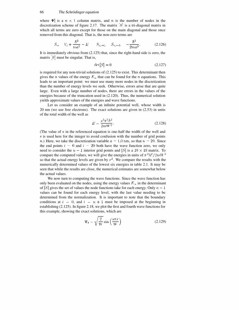
66 The Schrodinger equation
where �� is a � � � column matrix, and � is the number of nodes in thediscretization scheme of figure 2.17. The matrix ��� is a tri-diagonal matrix inwhich all terms are zero except for those on the main diagonal and those onceremoved from this diagonal. That is, the non-zero terms are
��� � �� ���
����� ������ � ������ � �
��
����� (2.126)
It is immediately obvious from (2.125) that, since the right-hand side is zero, thematrix ��� must be singular. That is,
����� � (2.127)
is required for any non-trivial solutions of (2.125) to exist. This determinant thengives the � values of the energy �� that can be found for the � equations. Thisleads to an important point: we must use many more nodes in the discretizationthan the number of energy levels we seek. Otherwise, errors arise that are quitelarge. Even with a large number of nodes, there are errors in the values of theenergies because of the truncation used in (2.120). Thus, the numerical solutionyields approximate values of the energies and wave functions.
Let us consider an example of an infinite potential well, whose width is20 nm (we use free electrons). The exact solutions are given in (2.53) in unitsof the total width of the well as
� �������
�� �� (2.128)
(The value of � in the referenced equation is one-half the width of the well and� is used here for the integer to avoid confusion with the number of grid points�.) Here, we take the discretization variable � � �� ��, so that � � �. Sincethe end points � and � � both have the wave function zero, we onlyneed to consider the � � � interior grid points and ��� is a � � � matrix. Tocompare the computed values, we will give the energies in units of � �
����� �
so that the actual energy levels are given by ��. We compare the results with thenumerically determined values of the lowest six energies in table 2.1. It may beseen that while the results are close, the numerical estimates are somewhat belowthe actual values.
We now turn to computing the wave functions. Since the wave function hasonly been evaluated on the nodes, using the energy values �� in the determinantof ��� gives the set of values the node functions take for each energy. Only �� �values can be found for each energy level, with the last value needing to bedetermined from the normalization. It is important to note that the boundaryconditions at � , and � � � � must be imposed at the beginning inestablishing (2.125). In figure 2.18, we plot the first and fourth wave functions forthis example, showing the exact solutions, which are
�� �
��
���
����
�(2.129)
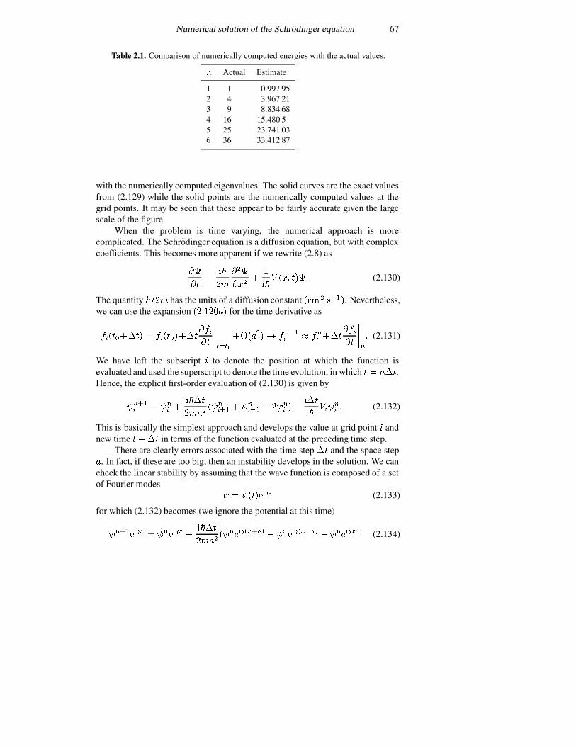
Numerical solution of the Schrodinger equation 67
Table 2.1. Comparison of numerically computed energies with the actual values.
� Actual Estimate
1 1 0.997 952 4 3.967 213 9 8.834 684 16 15.480 55 25 23.741 036 36 33.412 87
with the numerically computed eigenvalues. The solid curves are the exact valuesfrom (2.129) while the solid points are the numerically computed values at thegrid points. It may be seen that these appear to be fairly accurate given the largescale of the figure.
When the problem is time varying, the numerical approach is morecomplicated. The Schrodinger equation is a diffusion equation, but with complexcoefficients. This becomes more apparent if we rewrite (2.8) as
��
���
��
��
���
����
�
��� ��� ���� (2.130)
The quantity ���� has the units of a diffusion constant ��� ���. Nevertheless,we can use the expansion �������� for the time derivative as
�������� � ������������
��������
� ����� ���� � �� �������
�����
� (2.131)
We have left the subscript to denote the position at which the function isevaluated and used the superscript to denote the time evolution, in which � � ���.Hence, the explicit first-order evaluation of (2.130) is given by
����� � ��
� �����
�������
��� � ����� � ���
� �����
����
�� � (2.132)
This is basically the simplest approach and develops the value at grid point andnew time ���� in terms of the function evaluated at the preceding time step.
There are clearly errors associated with the time step �� and the space step�. In fact, if these are too big, then an instability develops in the solution. We cancheck the linear stability by assuming that the wave function is composed of a setof Fourier modes
� � ��������� (2.133)
for which (2.132) becomes (we ignore the potential at this time)
��������� � ������� �����
����� ����������� � ����������� � �������� (2.134)
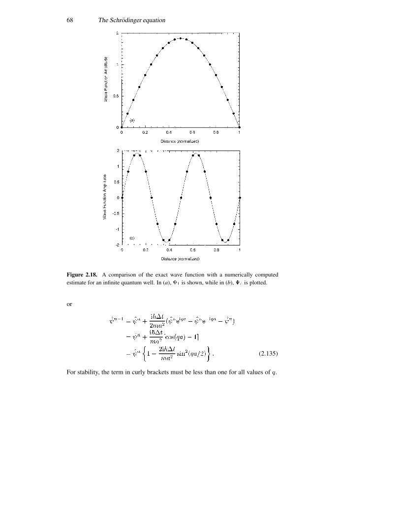
68 The Schrodinger equation
Figure 2.18. A comparison of the exact wave function with a numerically computedestimate for an infinite quantum well. In (a), �� is shown, while in (b),�� is plotted.
or
����� � ��� �����
����� ������� � ��������
�
����
� ��� �����
���������� �
� ���
� �
�����
�������������
�� (2.135)
For stability, the term in curly brackets must be less than one for all values of �.
Numerical solution of the Schrodinger equation 69
This can only occur if
�
�����
���� �� (2.136a)
or
�� ����
��� (2.136b)
For example, for the previous example, in which � � � ��, the time step must besmaller than ���� ���� for a free electron and less than ���� ���� for anelectron in GaAs. This is a severe limitation for many applications.
An improvement is to go to a second-order method, due to Crank andNicholson (1947) (see also Richtmyer and Morton 1967). In this, a two-stepapproach is utilized in which an estimate for ����
�is obtained using (2.132).
Once this estimate is obtained, an improved value is found by including this inthe update of the final value of the wave function via
�����
� ��
��
����
���� ��
��� � ��
��� � ���
���
���
�����
�
�
�����
���� ����
��� � ������� � �����
���
���
�����
����
� (2.137)
In essence, this is a form of a predictor–corrector algorithm to estimate the timevariation. The intrinsic advantage is that the growth factor (the bracketed term in(2.135)) becomes
� � ��� �����
������ �����
� � ��������
��� �����(2.138)
and the magnitude is less than unity for all values of the coefficients. This meansthat any combination of � and �� can be used, and the solution is, in principle,stable. This is, of course, an oversimplification, and the solutions must be checkedfor stability (convergence) with variable values of, for example, �� for a givenvalue of �.
References
Abramowitz M and Stegun I A 1964 Handbook of Mathematical Functions (Washington,DC: US National Bureau of Standards) p 450
Brandt S and Dahmen H D 1985 The Picture Book of Quantum Mechanics (New York:Wiley)
Cassidy D C 1991 Uncertainty—the Life and Science of Werner Heisenberg (New York:Freeman)
Crank J and Nicholson P 1947 Proc. Camb. Phil. Soc. 43 50Dingle R, Gossard A C and Wiegman W 1975 Phys. Rev. Lett. 34 1327–30Dingle R, Wiegman W and Henry C H 1974 Phys. Rev. Lett. 33 827–30Eisberg R M 1961 Fundamentals of Modern Physics (New York: Wiley)Heiblum M, Fischetti M V, Dumke W P, Frank D J, Anderson I M, Knoedler C M and
Osterling L 1987 Phys. Rev. Lett. 58 816–19

70 The Schrodinger equation
Landau R H and Paez M J 1997 Computational Physics; Problem Solving with Computers(New York: Wiley)
Moore W 1989 Schrodinger, Life and Thought (Cambridge: Cambridge University Press)Pais A 1991 Neils Bohr’s Time (Oxford: Clarendon)Potter D 1973 Computational Physics (Chichester: Wiley)Richtmyer R D and Morton K W 1967 Difference Methods for Initial-Value Problems (New
York: Interscience)Schrodinger E 1926 Ann. Phys., Lpz. 79 361, 79 489, 81 109
Problems 71
Problems
1. For the wave packet defined by ����, shown below, find ����. What are�� and ��?
2. If a Gaussian wave packet approaches a potential step (� � � for � � �,�� � �), it is found that it becomes broader for the region � � �. Why?
3. Assume that ����� are the eigenfunctions in an infinite square well(� �� for ��� � ���). Calculate the overlap integrals
� ���
����
���������� ���
4. Suppose that electrons are confined in an infinite potential well of width0.5 nm. What spectral frequencies will result from transitions between the lowestfour energy levels? Use the free-electron mass in your computations.
5. A particle confined to an infinite potential well has an uncertainty that isof the order of the well width, �� � . The momentum can be estimated as itsuncertainty value as well. Using these simple assumptions, estimate the energy ofthe lowest level. Compare with the actual value.
6. In terms of the momentum operator � � ����, and
���
��� �
���
and using the fact that ��� � ��� � � in a bound state, with
���� � ����� ���� � �����
���� � ����� ���� � �����
use the uncertainty principle to estimate the lowest bound-state energy. (Hint:recall the classical relation between the average kinetic and potential energies.)
7. Consider a potential well with � � ��� eV for ��� � ��, and � � �for ��� � ��, with � ��� nm. Write a computer program that computes theenergy levels for � � � (use a mass appropriate for GaAs, � � ��� ����� kg).How many levels are bound in the well, and what are their energy eigenvalues?
72 The Schrodinger equation
Using a simple wave-function-matching technique, plot the wave functions foreach bound state. Plot the transmission coefficient for � � �.
8. For the situation in which a linear potential is imposed on a system,compute the momentum wave functions. Show that these wave functions forma normalized set.
9. Using the continuity of the wave function and its derivative at each interiorinterface, verify (2.83).
10. Consider an infinite potential well that is 10 nm wide. At time zero, aGaussian wave packet, with half-width of 1 nm, is placed 2 nm from the centreof the well. Plot the evolving wave functions for several times up to the stablesteady state. How does the steady state differ from the initial state, and why doesthis occur?
11. Verify that (2.107) is the proper solution for the kernel function.12. For an infinite potential well of width 20 nm, compute the energies
associated with the transitions between the five lowest levels. Give the answers ineV.
13. For a finite potential well of width 20 nm and height 0.3 eV (usean effective mass appropriate to GaAs electrons, � � �������), compute theenergy needed to ionize an electron (move it from the lowest energy level to thetop of the well). If a 0.4 eV photon excites the electron out of the well, what is itskinetic energy? What is its wavelength?
14. For a finite potential well of width 20 nm and height 0.3 eV (usean effective mass appropriate to GaAs electrons, � � �������), carry outa numerical evaluation of the energy levels. Use enough grid points in the‘forbidden’ region to assure that the wave function is thoroughly damped. Howmany bound states are contained in the well?
15. Consider a potential well with �� � � for � � �, and � ��� � �� for� � �, with � � ���� �� ��. Using a numerical procedure, compute the tenlowest energy levels in the quantum well.

Chapter 3
Tunnelling
When we dealt in the last chapter (section 2.7) with the double potential well,coupled through a thin barrier, it was observed that the wave function penetratedthrough the barrier and interacted with the wave function in the opposite well.This process does not occur in classical mechanics, since a particle will in all casesbounce off the barrier. However, when we treat the particle as a wave, then thewave nature of barrier penetration can occur. This is familiar in electromagneticwaves, where the decaying wave (as opposed to a propagating wave) is termedan evanescent wave. For energies below the top of the barrier, the wave isattenuated, and it decays exponentially. Yet, it takes a significant distance forthis decay to eliminate the wave completely. If the barrier is thinner than thiscritical distance, the evanescent wave can excite a propagating wave in the regionbeyond the barrier. Thus, the wave can penetrate the barrier, and continueto propagate, with an attenuated amplitude, in the trans-barrier region. Thisprocess is termed tunnelling, with analogy to the miners who burrow througha mountain in order to get to the other side! This process is quite important inmodern semiconductor devices, and Leo Esaki received the Nobel prize for firstrecognizing that tunnelling was important in degenerately doped p–n junctiondiodes.
Since Esaki’s discovery of the tunnel diode, tunnelling has become importantin a variety of situations. In reverse biased p–n junctions, Zener breakdownoccurs when electrons in the valence band can tunnel across the gap into theconduction band when a sufficiently high electric field has been applied to bringthese two bands to the same energy levels (on opposite sides of the junction).Similarly, resonant tunnelling diodes have been fabricated in heterostructuressuch as GaAs–AlGaAs, and we will discuss these in some detail in a later section.Finally, as semiconductor devices become smaller, particularly the metal–oxide–semiconductor field-effect transistor (MOSFET), where a thin layer of silicondioxide is used as the gate insulator, this thin oxide becomes susceptible toleakage currents via tunnelling through the oxide.
In this chapter, we will address this tunnelling process. First we will treat
73
74 Tunnelling
those few cases in which the tunnelling probability can be obtained exactly. Thenwe will discuss its use in solid-state electronics. Following this, we will move toapproximate treatments suitable for those cases in which the solution is not readilyobtainable in an exact manner. Finally, we turn to periodic tunnelling structures,which give rise for example to the band structure discussed in semiconductors.
3.1 The tunnel barrier
The general problem is that posed in figure 3.1. Here, we have a barrier, whoseheight is taken to be ��, that exists in the region ��� � �. To the left andto the right of this barrier, the particle can exist as a freely propagating wave,but, in the region ��� � �, and for energies � � ��, the wave is heavilyattenuated and is characterized by a decaying exponential ‘wave’. Our interest isin determining just what the transmission probability through the barrier is for anincident particle. We are also interested in the transmission behaviour for energiesabove the top of the barrier. To solve for these factors, we proceed in precisely thesame fashion as we did for the examples of the last chapter. That is, we assumewaves with the appropriate propagation characteristics in each of the regions ofinterest, but with unknown coefficients. We then apply boundary conditions, inthis case the continuity of the wave function and its derivative at each interface,in order to evaluate the unknown coefficients. We consider first a simple barrier.
3.1.1 The simple rectangular barrier
The simple barrier is shown in figure 3.1. Here the potential is defined to existonly between �� and �, and the zero of potential for the propagating waves oneither side is the same. We can therefore define the wave vector � in the region��� � �, and the decaying wave vector � in the region ��� � �, by the equations(� � ��)
� �
���
��� � �
���
����� � �� (3.1)
respectively. To the right and left of the barrier, the wave is described bypropagating waves, while in the barrier region, the wave is attenuated. Thus,we can write the wave function quite generally as
���� �
�������� ������ � � ����� ������ ��� � �
����� � ����� � � �.(3.2)
We now have six unknown coefficients to evaluate. However, we can get onlyfour equations from the two boundary conditions, and a fifth from normalizingthe incoming wave from one side or the other. If we keep the most general set ofsix coefficients, we will have incoming waves from both sides, both of which mustbe normalized in some fashion. For our purposes, however, we will throw away
The tunnel barrier 75
Figure 3.1. The simple rectangular tunnelling barrier.
the incoming wave from the right, and assume that our interest is in determiningthe transmission of a wave incident from the left. In a later section, though, wewill need to keep both solutions, as we will have multiple barriers with multiplereflections. Here, however, while we keep all the coefficients, we will eventuallyset � � �. We can count on eventually using the principle of superposition, asthe Schrodinger equation is linear; thus, our approach is perfectly general.
The boundary conditions are applied by asserting continuity of the wavefunction and its derivative at each interface. Thus, at the interface � � ��,continuity of these two quantities gives rise to
������ ������ � ����� ����� (3.3a)
���������������� � ������� ������ (3.3b)
As in the last chapter, we can now solve for two of these coefficients in terms ofthe other two coefficients. For the moment, we seek � and � in terms of � and�. This leads to the matrix equation
�
�
��
����
��� � �
���
���������
��� � �
���
���������
��� � �
���
����������
��� � �
���
����������
���� �
�
� (3.4)
Now, we turn to the other boundary interface. The continuity of the wave functionand its derivative at � � � leads to
���� � � ����� � ���� ������ (3.5a)
������� � � ������ � ������ ������� (3.5b)

76 Tunnelling
Again, we can solve for two of these coefficients in terms of the other two. Here,we seek to find � and � in terms of � and � (we will eliminate the former twothrough the use of (3.4)). This leads to the matrix equation
�
�
��
����
��� � �
��
��������� �
��� � �
��
����������
�
��� � �
��
���������
��� � �
��
����������
���� �
�
�� (3.6)
From the pair of equations (3.4) and (3.6), the two propagating coefficientson the left of the barrier, � and �, can be related directly to those on the right ofthe barrier,� and � , with the two under the barrier dropping out of consideration.This leads to the matrix equation
�
�
��
�� ��
�� ��
��
�
�� (3.7)
Here, the elements are defined by the relations
�� �
��� � �
���
���� � �
��
���������� �
��� � �
��
���� � �
���
����������
�
�������
�
�
��� � ��
��
�������
������ (3.8)
�� �
��� � �
��
���� � �
���
������ �
��� � �
���
���� � �
��
�����
� �
�
�
��� � ��
��
������� (3.9)
�� ��
�� �� ��
��� (3.10)
It is a simple algebraic exercise to show that, for the present case, the determinantof the matrix M is unity, so this matrix has quite interesting properties. It is nota unitary matrix, because the diagonal elements are complex. In the simple case,where we will take � � �, the transmission coefficient is simply given by thereciprocal of �����, since the momentum is the same on either side of the barrierand hence the current does not involve any momentum adjustments on the twosides.
3.1.2 The tunnelling probability
In the formulation that leads to (3.7), � and � are incoming waves, while � and� are outgoing waves. Since we are interested in the tunnelling of a particle fromone side to the other, we treat an incoming wave from only one of the two sides,so that we will set � � � for this purpose. Then, we find that � � ���. The

A more complex barrier 77
transmission probability is the ratio of the currents on the two sides of the barrier,directed in the same direction of course, so
� ��
������� (3.11)
Inserting the value for this from (3.8), we find
� �
�����������
��� � ��
���
�����������
���
��
�
��� ��
���
�����������
� (3.12)
There are a number of limiting cases that are of interest. First, for a very weakbarrier, in which ���� �, the transmission coefficient becomes
� ��
� ������ (3.13)
On the other hand, when the potential is very strong, where ��� � �, thetransmission coefficient falls off exponentially as
� �
����
�� ��
��
����� (3.14)
It is important to note that the result (3.13) is valid only for a weak potentialfor which the energy is actually below the top of the barrier. If we consider anincident energy above the barrier, we expect the barrier region to act as a thindielectric and cause interference fringes. We can see this by making the simplesubstitution suggested by (3.1) through � � �� �. This changes (3.12) into
� �� � ��� ��
�
��� � ���
����
�����������
(3.15)
which is precisely the result (2.75) obtained in the last chapter (with a suitablechange in the definition of the wave function in the barrier region). Thus, abovethe barrier, the transmission has oscillatory behaviour as a function of energy, withresonances that occur for �� �� � �. The overall behaviour of the tunnellingcoefficient is shown in figure 3.2.
3.2 A more complex barrier
In the previous section, the calculations were quite simple as the wave momentumwas the same on either side of the barrier. Now, we want to consider a somewhat
78 Tunnelling
Figure 3.2. Tunnelling (transmission) probability for a simple barrier (for generic values).
more realistic barrier in which the momentum differs on the two sides of thebarrier. Consider the barrier shown in figure 3.3. The interface at � � �� is thesame as treated previously, and the results of (3.4) are directly used in the presentproblem. However, the propagating wave on the right-hand side of the barrier(� � �) is characterized by a different wave vector through
�� �
���
���� � ���� (3.16)
Matching the wave function and its derivative at � � � leads to
������ � � ������ � ��� ����� (3.17a)
���������� � � ������� � ����� ������� (3.17b)
This result is an obvious modification of (3.5). This will also occur for the matrixequation (3.6), and the result is
��
����
���� � �
��
���������� �
���� � �
��
�����������
�
���� � �
��
����������
���� � �
��
�����������
���� �
�
�� (3.18)
A more complex barrier 79
Figure 3.3. A more complex tunnelling barrier.
We can now eliminate the coefficients � and � by combining (3.6) and (3.18).The result is again (3.7), but now the coefficients are defined by
��� �
��� � �
���
����� � �
��
��������������
�
���� � �
��
���� � �
���
��������������
�
��
�
�� �
��
�
���������
�
�
���� � �
�
��
��������
����������
(3.19)
��� �
���� � �
��
���� � �
���
���������������
�
��� � �
���
����� � �
��
��������������
� �
��
�
���� � ��
��
�������� �
�
�
���
�� �
��������
�����������
(3.20)
80 Tunnelling
and the complex conjugate symmetry still holds for the remaining terms.The determinant of the matrix M is also no longer unity, but is given by
the ratio ����. This determinant also reminds us that we must be careful incalculating the transmission coefficient as well, due to the differences in themomenta, at a given energy, on the two sides of the barrier. We proceed as in theprevious section, and take � � � in order to compute the transmission coefficient.The actual transmission coefficient relates the currents as in (2.45)–(2.48), and wefind that
� ����
�
�������
�������� � ���
� ���� � ������ � ��
��
����� � �����������
� (3.21)
In (3.21), there are two factors. The first factor is the one in the numerator, whichdescribes the discontinuity between the propagation constants in the two regionsto the left and to the right of the barrier. The second factor is the denominator,which is the actual tunnelling coefficient describing the transparency of thebarrier. It is these two factors together that describe the total transmission ofwaves from one side to the other. It should be noted that if we take the limitingcase of �� � �, we recover the previous result (3.12).
There is an important relationship that is apparent in (3.21). The resultrepresented by (3.21) is reciprocal in the two wave vectors. They appearsymmetrical in the transmission coefficient � . This is a natural and importantresult of the symmetry. Even though the barrier and energy structure of figure 3.3does not appear symmetrical, the barrier is a linear structure that is passive (thereis no active gain in the system). Therefore, the electrical properties should satisfythe principle of reciprocity, and the transmission should be the same regardless offrom which direction one approaches the barrier. This is evident in the form ofthe transmission coefficient (3.20) that is obtained from these calculations.
3.3 The double barrier
We now want to put together two tunnel barriers separated by a quantum well.The quantum well (that is, the region between the two barriers) will have discreteenergy levels because of the confinement quantization, just as in section 2.5. Wewill find that, when the incident wave energy corresponds to one of these resonantenergy states of the quantum well, the transmission through the double barrier willrise to a value that is unity (for equal barriers). This resonant tunnelling, in whichthe transmission is unity, is quite useful as an energy filter.
There are two approaches to solving for the composite tunnellingtransmission coefficient. In one, we resolve the entire problem from firstprinciples, matching the wave function and its derivative at four differentinterfaces (two for each of the two barriers). The second approach, which wewill pursue here, uses the results of the previous sections, and we merely seek
The double barrier 81
Figure 3.4. Two generic barriers are put together to form a double-barrier structure.
knowledge as to how to put together the transmission matrices that we alreadyhave found. The reason we can pursue this latter approach effectively is thatthe actual transmission matrices found in the previous sections depend only uponthe wave vectors (the �s and �), and the thickness of the barrier, ��. They do notdepend upon the position of the barrier, so the barrier may be placed at an arbitrarypoint in space without modifying the transmission properties. Thus, we considerthe generic problem of figure 3.4, where we have indicated the coefficients inthe same manner as that in which they were defined in the earlier sections. Todifferentiate between the two barriers, we have used primes on the coefficients ofthe right-hand barrier. Our task is to now relate the coefficients of the left-handbarrier to those of the right-hand barrier.
We note that both � and �� describe a wave propagating to the right.Denoting the definition of the thickness of the well region as �, we can simplyrelate these two coefficients via
�� � ����� (3.22)
where � is the propagation constant in the well region. Similarly, � and � � relatethe same wave propagating in the opposite direction. These two can thus berelated by
�� � � ������ (3.23)
These definitions now allow us to write the connection as a matrix in the followingmanner:
�
�
��
������ �� �����
���
��
�� (3.24)
Equation (3.24) now defines a matrix M�, where the subscript indicates the wellregion. This means that we can now take the matrices defined in sections 3.1 and3.2 for the left-hand and right-hand regions and write the overall tunnelling matrixas
�
�
�� �M�� �M�� �M��
��
� �
�� (3.25)
82 Tunnelling
From this, it is easy to now write the composite ��� as
���� � ������������� ����������
���� (3.26)
and it is apparent that the resonance behaviour arises from the inclusion of theoff-diagonal elements of each transmission matrix, weighted by the propagationfactors. At this point, we need to be more specific about the individual matrixelements.
3.3.1 Simple, equal barriers
For the first case, we use the results of section 3.1, where a simple rectangularbarrier was considered. Here, we assume that the two barriers are exactly equal,so the same propagation wave vector � exists in the well and in the regions tothe left and right of the composite structure. By the same token, each of the twobarriers has the same potential height and therefore the same �. We note that thisleads to a magnitude-squared factor in the second term of (3.26), but not in thefirst term with one notable exception. The factor of � ���� does cancel since we areto the left of the right-hand barrier (��-direction) but to the right of the left-handbarrier (��-direction). Thus, the right-hand barrier contributes a factor of � �����,and the left-hand barrier contributes a factor of � ����, so the two cancel each other.In order to simplify the mathematical details, we write the remainder of (3.8) as
��� � ������� (3.27)
where
��� �
���������� �
��� � ��
���
���������� (3.28)
is the magnitude and
� � � �����
�� � ��
���
�� ������
�(3.29)
is the phase of ���. We can then use this to write
������� � �����
� � ������ � ������
������� ��������� ��
� ������� � �����
�� � ������������
� �������� �� (3.30)
The first term, the combination within the parentheses, is just the determinant ofthe individual barrier matrix, and is unity for the simple rectangular barrier. Thus,the overall transmission is now
������� � � � ������
������� �������� �� (3.31)
In general, the cosine function is non-zero, and the composite term of (3.31)is actually larger than that for the single barrier ��, with
���� ���
�������off resonance� (3.32)

The double barrier 83
Figure 3.5. The transmission through a double barrier system composed of AlGaAsbarriers and a GaAs well. Here, the barrier height is 0.25 eV and the thicknesses are4 nm. The well is taken to be 2 nm thick so that only a single resonant level is present inthe well.
However, for particular values of the wave vector, the cosine term vanishes, and
������ � � ��� � � ���� ���
�� (3.33)
These values of the wave vector correspond to the resonant levels of a finite-depth quantum well (the finite-well values are shifted in phase from the infinite-well values by �, which takes the value ���� in the latter case). Hence, as wesupposed, the transmission rises to unity at values of the incident wave vector thatcorrespond to resonant levels of the quantum well. In essence, the two barriers actlike mirrors, and a resonant structure is created just as in electromagnetics. Theincoming wave excites the occupancy of the resonance level until an equilibriumis reached in which the incoming wave is balanced by an outgoing wave and theoverall transmission is unity. This perfect match is broken up if the two barriersdiffer, as we see below.
In figure 3.5, we plot the transmission for a double quantum well in whichthe barriers are 0.25 eV high and 4 nm thick. The well is taken to be 2 nm thick.Here, it is assumed that the well is GaAs and the barriers are AlGaAs, so that thereis only a single resonant level in the well. It is clear that the transmission rises tounity at the value of this level. We will return later to the shape of the resonanttransmission peak, and how it may be probed in some detail experimentally.
84 Tunnelling
Figure 3.6. The potential structure for a general double barrier. The definition of thevarious constants is given for each region.
3.3.2 The unequal-barrier case
In the case where the two barriers differ, the results are more complicated, andgreater care is necessary in the mathematics. The case we consider is indicatedin figure 3.6. Here, we have individual wave vectors for the regions to the leftand right of the composite barrier, as well as in the well. In addition, the decayconstants of the two barriers differ, so the thicknesses and heights of the twobarriers may also be different. Nevertheless, the result (3.26) still holds and willbe our guide for obtaining the solution.
The definitions of the various functions are now taken from (3.19) and (3.20).We define the important quantities as
�� � ������ (3.34)
where � � ���������������. This leads to
���� �
��
�
�� �
��
�
���������� �
�
�
���� � ��
��
�����������
(3.35)
The double barrier 85
���� �
��
�
���� � ��
��
����������� �
�
�
����� �
�����������
(3.36)
���� �
��
�
�� �
����
������������ �
�
�
����� � ��
�
����
������������
(3.37)
���� �
��
�
����� � ��
�
����
������������ �
�
�
������ �
������������
(3.38)
���� � � �������� � ��
�� � ��� �������
�� �� � ���� (3.39)
���� � � �������� � ��
��� � �� �������
�� � � �� � ���� (3.40)
���� � � ��������� � ��
�
��� � ���� ��������
�� ��� � ���� (3.41)
���� � ��������� � ������ � ����
��������
�� � � ��� � ����� (3.42)
These results for the phases and magnitudes of the individual terms of thetransmission matrices can now be used in (3.26) to yield the net transmissionmatrix element, following the same procedure as above:
������� � ��������� ���������
� � �����������������
� ��������
���� � ���� � ���� � ����
�� (3.43)
Now, as opposed to what was the case in the last sub-section, the first term(in the parentheses) does become unity. There is still a resonance, which occurswhen the argument of the cosine function is an odd multiple of �. This is nota simple resonance, as it is in the previous case. Rather, the resonance involvesphase shifts at each of the two interfaces. It is, however, convenient that theproducts of the wave vectors and the barrier thicknesses (the last terms in the fourequations above for the phases) all reduce to a single term, that is � ���� � ��.This contribution to the phase shifts arises from the fact that the resonant energylevel sinks below the infinite-quantum-well value due to the penetration of thewave function into the barrier region. This penetration is affected by the fact thatthe barrier has a finite thickness, and this term is a correction for the difference inthickness of the two sides. Obviously, if the thicknesses of the two barriers weremade equal this term would drop out, and we would be left with the simple phaseshifts at each boundary to consider.
At resonance, the overall transmission does not rise to unity because of themismatch between the two barriers, which causes the first term to differ from
86 Tunnelling
unity. To find the actual value, we manipulate (3.43) somewhat to find theappropriate value. For this, we will assume that the attenuation of the barriers israther high, so that the transmission of either would be� �. Then, on resonance,we can write (3.43) as
������� � ��������� ����������
�
� ��
�����
���
���
��������
��������
��� (3.44)
Now, let us use (3.35) and (3.36) to write
�����
����
���
� ������ � ���
��� � ������ � ���� ����������
� ������ � ���
��� � ������ � ���� ����������
� ������
�
��� � ������ � ���� ����������
� �� �� (3.45)
and����
����
� ����
(3.46)
where we have used (3.21) in the limit ��� � �. We can do a similar evaluationfor the other factor in (3.44), and finally can write (incorporating the ratio � ���to get the currents)
� �����
��� ��� ������� �������
������� � ����
� (3.47)
Equation (3.47) is significant in that if the two transmissions are equal, a value ofunity is obtained for the net transmission. On the other hand, if the two are notequal, and one is significantly different from the other, the result is that
� � �������
� (3.47a)
This implies that the transmission on resonance is given by the ratio of theminimum of the two individual barrier transmissions to the maximum of thesetwo.
The opposite extreme is reached when we are away from one of the resonantlevels. In this case, the maximum attenuation is achieved when the cosine functionhas the value of unity, and the resulting minimum in overall transmission is givenby the value
� � ����� (3.48)
in the limit of low transmission. It is clear from these discussions that if we are tomaximize the transmission on resonance in any device application, it is importantto have the transmission of the two barriers equal under any bias conditions thatcause the resonance to appear.
The double barrier 87
3.3.3 Shape of the resonance
It is apparent from the shape of the transmission curve in figure 3.5 that there is avery sharp resonance that coincides with the resonant energy level in the quantumwell. We can analyse this resonance more by considering it to have a Lorentzianshape around the maximum, that is
�
� ���� � �
�� ���
��
��� (3.49)
In fact, this form holds quite accurately over orders of magnitude in transmission(Price 1999). In essence, this means that we can write �����
� � ��, with� � ��. From (3.27), we identify
��� � � � ��
��� �
� ���
��
�(3.50)
and
��
�� � � � ��
�� � �
� ���
��
�� (3.51)
Hence, �� must have two zeros located at � � �� � ��. One of these is azero of � and the other is a zero of �. Thus, when the energy � is swept throughthe resonance energy ��, the phase angle ���� � is swept through an amountapproaching �. Price (1999) has pointed out that this has an analogy with formalwave propagation theory, so that one can assign a transit time for passage of anelectron through the double barrier structure as
�������� � ������ ��
��
����
� ������
�
�� � (3.52)
In figure 3.5, the width at half-maximum is about 4.5 meV, so at the resonance,the transit time is approximately 0.15 ps. Away from resonance, the transit timeis smaller, so that the transit time lengthens at the resonance energy, an effect firstnoted by Bohm (1951).
While it is quite difficult to measure the transit time of the electron throughthe resonant structure, creative methods have been found to measure the phaseshift. In chapter 1, we discussed the experiments of Yacoby et al (1994) to createan Aharonov–Bohm loop in a semiconductor nanostructure. In subsequent work,they embedded a semiconductor quantum dot in one leg of the ring (Yacoby et al1995). The structure is shown in figure 3.7. The quantum dot is a two-dimensionalelectron gas at the interface of a GaAlAs/GaAs heterostructure, which is furtherconfined by lateral in-plane gates. Propagation through the quantum dot isfacilitated by two tunnelling quantum point contacts which, along with the dotitself, are located in one leg of the Aharonov–Bohm (A–B) loop. Measurementsof the transmitted current through the A–B ring give the total phase through each

88 Tunnelling
Figure 3.7. (a) A schematic description of the modified Aharonov–Bohm ring’s circuit.The shaded regions are metallic gates. (b) An SEM micrograph of the structure. The whiteregions are the metal gates. The central metallic island is biased via an air bridge (B)extending to the right. The dot is tuned by the plunger (P). Summary of the experimentallymeasured phases within two transmission peaks (Æ and�; the broken lines are only guidesto the eye). The expected behaviour of the phase in a one-dimensional resonant tunnellingmodel is shown by the solid line. (After Yacoby et al (1995), by permission.)
branch in terms of the interference between the two legs. This phase interferenceis measured by varying the magnetic field through the ring. When the size of thedot is tuned by a plunger gate (P in figure 3.7), the resonant energy is sweptthrough the Fermi energy of the remaining parts of the system. By this gatevoltage tuning the resonance shape is swept through the transmission energy, anda change in phase by a factor of � is found, as shown in figure 3.7(c). This shiftis expected from the previous discussion, but the transition is sharper than theauthors expected. Several reasons were presented by Yacobi et al (1995) for this,but it may simply be that the sharpness of the resonant transmission peak resultsfrom a simple two-barrier effect, with the remaining properties of the quantum dot

Approximation methods—the WKB method 89
irrelevant to the overall experiment. That is, the phase behaviour of the electronsin the dot is irrelevant to resonant transmission through discrete dot levels coupledby the quantum point contacts.
3.4 Approximation methods—the WKB method
So far, the barriers that we have been treating are simple barriers in the sensethat the potential � ��� has always been piecewise constant. The reason forthis lies in the fact that if the barrier height is a function of position, then theSchrodinger equation is a complicated equation that has solutions that are specialfunctions. The example we treated in the last chapter merely had a linear variationof the potential—a constant electric field—and the result was solutions that wereidentified as Airy functions which already are quite complicated. What are weto do with more complicated potential variations? In some cases, the solutionscan be achieved as well known special functions—we treat Hermite polynomialsin the next chapter—but in general these solutions are quite complicated. Onthe other hand, nearly all of the solution techniques that we have used involvepropagating waves or decaying waves, and the rest of the problem lay inmatching boundary conditions. This latter, quite simple, observation suggestsan approximation technique to find solutions, the Wentzel–Kramers–Brillouin(WKB) approach (Wentzel 1926, Kramers 1926, Brillouin 1926).
Consider figure 3.8, in which we illustrate a general spatially varyingpotential. At a particular energy level, there is a position (shown as �) at which thewave changes from propagating to decaying. This position is known as a turningpoint. The description arises from the simple fact that the wave (particle) wouldbe reflected from this point in a classical system. In fact, we can generally extendthe earlier arguments and definitions of this chapter to say that
���� �
���
���� � � ���� � � � ��� (3.53)
and
���� �
���
���� ������ � � � ��� (3.54)
These solutions suggest that, at least to zero order, the solutions can be taken assimple exponentials that correspond either to propagating waves or to decayingwaves.
The above ideas suggest that we consider a wave function that is basicallya wave-type function, either decaying or propagating. We then adopt the results(3.53) and (3.54) as the lowest approximation, but seek higher approximations.To proceed, we assume that the wave function is generically definable as
���� � ������ (3.55)
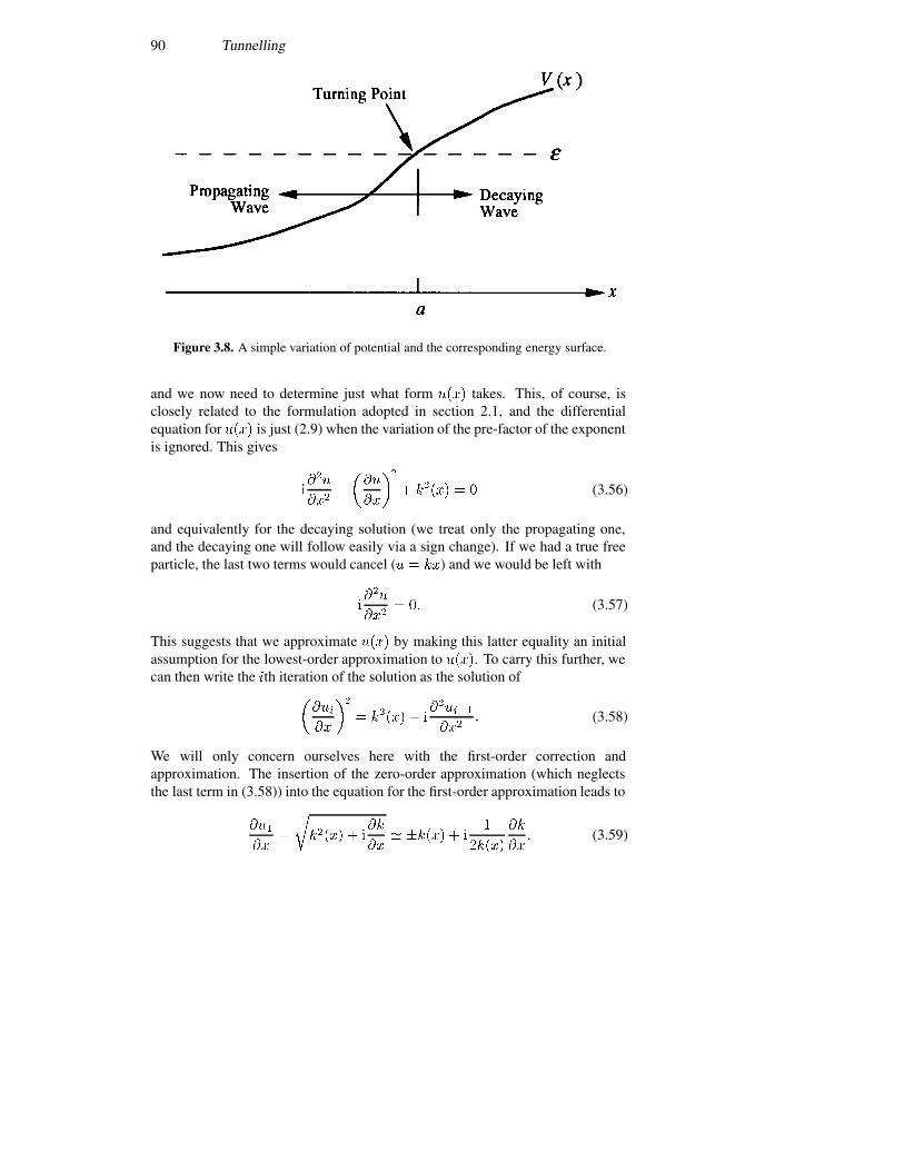
90 Tunnelling
Figure 3.8. A simple variation of potential and the corresponding energy surface.
and we now need to determine just what form ���� takes. This, of course, isclosely related to the formulation adopted in section 2.1, and the differentialequation for ���� is just (2.9) when the variation of the pre-factor of the exponentis ignored. This gives
����
����
���
��
��� �
���� � � (3.56)
and equivalently for the decaying solution (we treat only the propagating one,and the decaying one will follow easily via a sign change). If we had a true freeparticle, the last two terms would cancel (� � ��) and we would be left with
����
���� �� (3.57)
This suggests that we approximate ���� by making this latter equality an initialassumption for the lowest-order approximation to ����. To carry this further, wecan then write the �th iteration of the solution as the solution of
����
��
��� �
���� � �������
���� (3.58)
We will only concern ourselves here with the first-order correction andapproximation. The insertion of the zero-order approximation (which neglectsthe last term in (3.58)) into the equation for the first-order approximation leads to
���
���
������ � �
��
��� ����� � �
�
�����
��
��� (3.59)

Approximation methods—the WKB method 91
In arriving at this last expression, we have assumed, in keeping with theapproximations discussed, that the second term on the right-hand side in (3.59) ismuch smaller than the first term on the right. This implies that, in keeping withthe discussion of section 2.1, the potential is slowly varying on the scale of thewavelength of the wave packet.
The result (3.59) can now be integrated over the position, with an arbitraryinitial position as the reference point. This gives
�� � �
��
����� ��� ��
��� ���� � ���� (3.60)
which leads to
���� ��������
�
�� �
��
����� ���
�� (3.61)
The equivalent solution for the decaying wave function is
���� ��������
�
��
��
����� ���
�� (3.62)
It may be noted that these results automatically are equivalent to the requirementof making the current continuous at the turning point, which is achieved via thesquare-root pre-factors.
To see how this occurs, we remind ourselves of (2.14) and (2.16). There, itwas necessary to define a current which was continuous in the time-independentsituation. Using (2.18), we then require the continuity of
�� � � ������ (3.63)
This continuity of current was used both in the last chapter, and in this chapter,to determine the transmission coefficient. Now, if we are to infer a connectionformula for the wave function, then we must use a generalization of (3.63) to saythat
����
� (3.64)
must be continuous. It is the recognition of this fact that leads to the forms (3.61)and (3.62) for the wave functions on either side of the interface of figure 3.8.These connection formulas are the heart of the WKB technique, but they havetheir source in the decomposition of the wave function discussed in section 2.2.
The remaining problem lies in connecting the waves of one type with thoseof the other at the turning point. The way this is done is through a method calledthe method of stationary phase. The details are beyond the present treatment, butare actually quite intuitive. In general, the connection formulas are written interms of sines and cosines, rather than as propagating exponentials, and this willinsert a factor of two, but only in the even functions of the propagating waves. In
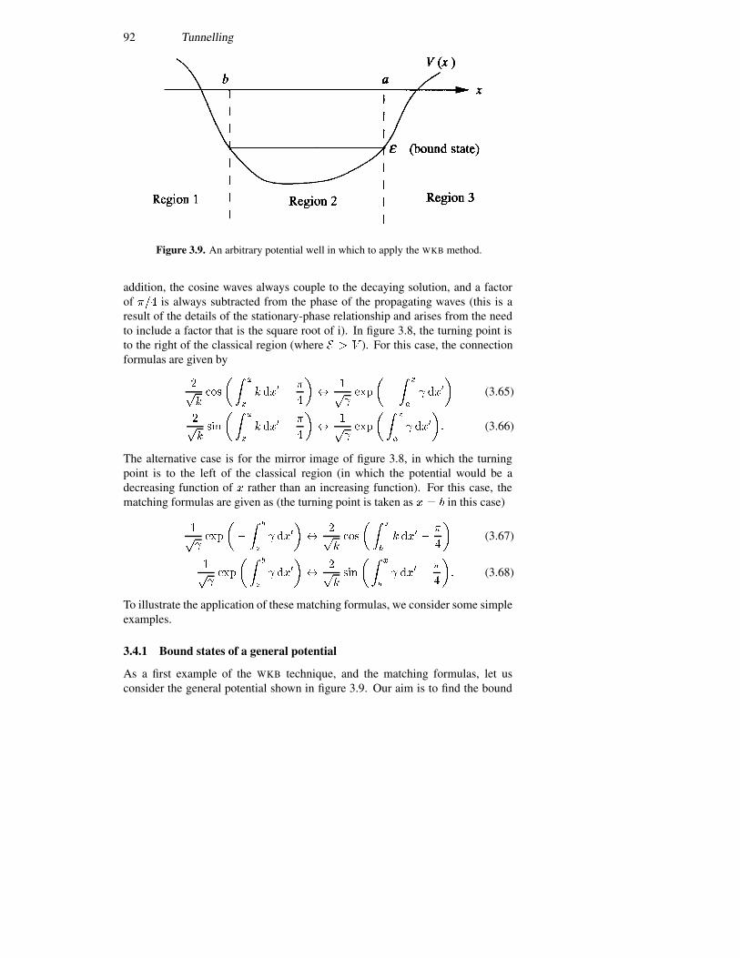
92 Tunnelling
Figure 3.9. An arbitrary potential well in which to apply the WKB method.
addition, the cosine waves always couple to the decaying solution, and a factorof ��� is always subtracted from the phase of the propagating waves (this is aresult of the details of the stationary-phase relationship and arises from the needto include a factor that is the square root of i). In figure 3.8, the turning point isto the right of the classical region (where � � � ). For this case, the connectionformulas are given by
������
�� �
�
� ��� � �
�
�� ��
���
��� �
�
� ���
�(3.65)
�����
���
�
� ��� � �
�
�� ��
���
���
�
� ���
�� (3.66)
The alternative case is for the mirror image of figure 3.8, in which the turningpoint is to the left of the classical region (in which the potential would be adecreasing function of � rather than an increasing function). For this case, thematching formulas are given as (the turning point is taken as � � � in this case)
�����
��� �
�
� ���
�� ��
����
�� �
�
� ��� � �
�
�(3.67)
� �����
�� �
�
� ���
�� ��
���
�� �
�
� ��� � �
�
�� (3.68)
To illustrate the application of these matching formulas, we consider some simpleexamples.
3.4.1 Bound states of a general potential
As a first example of the WKB technique, and the matching formulas, let usconsider the general potential shown in figure 3.9. Our aim is to find the bound

Approximation methods—the WKB method 93
states, or the energy levels to be more exact. It is assumed that the energy level ofinterest is such that the turning points are as indicated; that is, the points � � �and � � � correspond to the turning points. Now, in region 1, to the left of � � �,we know that the solution has to be a decaying exponential as we move away from�. This means that we require that
����� �������
���
�
�
� ���
�� � �� (3.69)
At � � �, this must match to the cosine wave if we use (3.67). Thus, we knowthat in region 2, the wave function is given by
����� �����
�� �
�
� ��� � �
�� � � � �� (3.70)
We now want to work our way across to � � �, and this is done quite simply withsimple manipulations of (3.70), as
����� �����
���
�
� ��� ��
� �
��
�����
���
�
� ��� ��
�
������
�� �
�
� ��� �� �
�
� ��� ��
�
� � ����
���
�
� ���
����
���
�
� ��� � �
�
������
���
�
� ���
���
���
�
� ��� � �
�� (3.71)
We also know that the solution for the matching at the interface � � � mustsatisfy (3.65), as the wave function in region 3 must be a decaying wave function.This means that at this interface, ����� must be given only by the second term of(3.71). This can only be achieved by requiring that
��
���
�
� ���
�� � (3.72)
or ��
�
� ��� � ��� ���
� � � � � � � � (3.73)
This equation now determines the energy eigenvalues of the potential well, at leastwithin the WKB approximation.
If we compare (3.73) with the result for a sharp potential as the infinitequantum well of (2.53), with � � ��, we see that there is an additional phase shiftof � on the left-hand side. While one might think that this is an error inherent inthe WKB approach, we note that the sharp potentials of the last chapter violate theassumptions of the WKB approach (slowly varying potentials). The extra factor of� arises from the soft variation of the potentials. Without exactly solving thetrue potential case, one cannot say whether or not this extra factor is an error, butthis factor is a general result of the WKB approach.
94 Tunnelling
3.4.2 Tunnelling
It is not necessary to work out the complete tunnelling problem here, since we areinterested only in the decay of the wave function from one side of the barrierto the other (recall that the input wave was always normalized to unity). Itsuffices to say that the spirit of the WKB approximation lies in the propagation (ordecaying) wave vector, and the computation of the argument of the exponentialdecay function. The result (3.73) is that it is only the combination of forwardand reverse waves that matter. For a barrier in which the attenuation is relativelylarge, only the decaying forward wave is important, and the tunnelling probabilityis approximately
� � ���
�� �
��
�
� ��
�(3.74)
which implies that it is only the numerical coefficients (which involve thepropagating and decaying wave vectors) that are lost in the WKB method. Thistells us that we can use the limiting form of (3.14) (� � ��), or the equivalentlimit of (3.21), with the argument of the exponential replaced with that of (3.74).
3.5 Tunnelling devices
One of the attractions of tunnelling devices is that it is possible to apply textbookquantum mechanics to gain an understanding of their operation, and still achievea reasonable degree of success in actually getting quantitative agreement withexperimental results. The concept of the tunnel ‘diode’ goes back several decades,and is usually implemented in heavily doped p–n junctions. In this case, thetunnelling is through the forbidden energy gap, as we will see below. Here,the tunnelling electrons make a transition from the valence band, on one sideof the junction, to the conduction band on the other side. More recently, effort hascentred on resonant tunnelling devices which can occur in a material with a singlecarrier type. Each of these will be discussed below, but first we need to formulatea current representation for the general tunnelling device.
3.5.1 A current formulation
In the treatment of the tunnelling problem that we have encountered in thepreceding sections, the tunnelling process is that of a single plane-wave energystate from one side of the barrier to the other. The tunnelling process, in thisview, is an energy-conserving process, since the energy at the output side is thesame as that at the input side. In many real devices, the tunnelling process canbe more complex, but we will follow this simple approach and treat a generaltunnelling structure, such as that shown in figure 3.10. In the ‘real’ device, thetunnelling electrons are those within a narrow energy range near the Fermi energy,where the range is defined by the applied voltage as indicated in the figure. Forthis simple view, the device is treated in the linear-response regime, even though
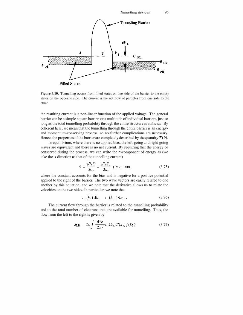
Tunnelling devices 95
Figure 3.10. Tunnelling occurs from filled states on one side of the barrier to the emptystates on the opposite side. The current is the net flow of particles from one side to theother.
the resulting current is a non-linear function of the applied voltage. The generalbarrier can be a simple square barrier, or a multitude of individual barriers, just solong as the total tunnelling probability through the entire structure is coherent. Bycoherent here, we mean that the tunnelling through the entire barrier is an energy-and momentum-conserving process, so no further complications are necessary.Hence, the properties of the barrier are completely described by the quantity � ���.
In equilibrium, where there is no applied bias, the left-going and right-goingwaves are equivalent and there is no net current. By requiring that the energy beconserved during the process, we can write the �-component of energy as (wetake the �-direction as that of the tunnelling current)
� �����
�
���
��������
� ����� (3.75)
where the constant accounts for the bias and is negative for a positive potentialapplied to the right of the barrier. The two wave vectors are easily related to oneanother by this equation, and we note that the derivative allows us to relate thevelocities on the two sides. In particular, we note that
������ ��� � ������� ���� � (3.76)
The current flow through the barrier is related to the tunnelling probabilityand to the total number of electrons that are available for tunnelling. Thus, theflow from the left to the right is given by
��� � ��
����
������������ �������� (3.77)
96 Tunnelling
where the factor of 2 is for spin degeneracy of the electron states, the ���� � isthe normalization on the number of � states (related to the density of states in �space), and ����� is the electron distribution function at the barrier. Similarly,the current flow from the right to the left is given by
��� � ��
����������
�������� ����������� (3.78)
Now, we know that the tunnelling probability is equal at the same energy,regardless of the direction of approach, and these two equations can be combinedas
� � ��
����
������������ ����������� ���� � ����� (3.79)
where we have related the energy on the left to that on the right through the bias,as shown in figure 3.10, and expressed in (3.75). In the following, we will dropthe subscript ‘L’ on the energy, but care must be used to ensure that it is evaluatedon the left of the barrier.
Before proceeding, we want to simplify some of the relationships in (3.79).First, we note that the energy is a scalar quantity and can therefore be decomposedinto its -component and its transverse component, as
� � �� � �� (3.80)
and��� � ���� ���� (3.81)
We would like to change the last differential to one over the -component ofenergy, and
��� �
���
���
�����
������� (3.82)
The second term on the right-hand side is unity, so it drops out. The first termmay be evaluated from (3.75) as
��
����
����
� ���� (3.83)
The velocity term here will cancel that in (3.79), and we can write the finalrepresentation of the current as
� ��
��
����������
���� � ��������� � ���� ���� � �� � ������ (3.84)
At this point in the theory, we really do not know the form of the distributionsthemselves, other than some form of simplifying assumption such as saying thatthey are Fermi–Dirac distributions. In fact, in metals, the distribution functionsare well approximated by Fermi–Dirac distributions. In semiconductors,
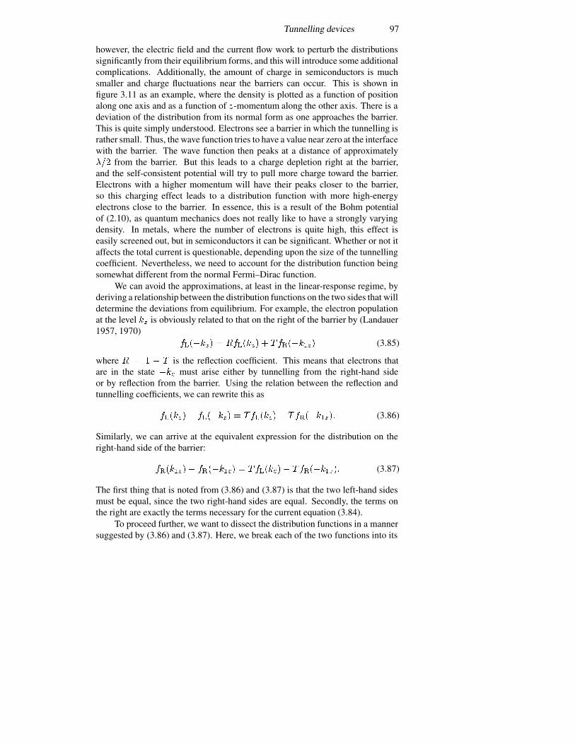
Tunnelling devices 97
however, the electric field and the current flow work to perturb the distributionssignificantly from their equilibrium forms, and this will introduce some additionalcomplications. Additionally, the amount of charge in semiconductors is muchsmaller and charge fluctuations near the barriers can occur. This is shown infigure 3.11 as an example, where the density is plotted as a function of positionalong one axis and as a function of �-momentum along the other axis. There is adeviation of the distribution from its normal form as one approaches the barrier.This is quite simply understood. Electrons see a barrier in which the tunnelling israther small. Thus, the wave function tries to have a value near zero at the interfacewith the barrier. The wave function then peaks at a distance of approximately��� from the barrier. But this leads to a charge depletion right at the barrier,and the self-consistent potential will try to pull more charge toward the barrier.Electrons with a higher momentum will have their peaks closer to the barrier,so this charging effect leads to a distribution function with more high-energyelectrons close to the barrier. In essence, this is a result of the Bohm potentialof (2.10), as quantum mechanics does not really like to have a strongly varyingdensity. In metals, where the number of electrons is quite high, this effect iseasily screened out, but in semiconductors it can be significant. Whether or not itaffects the total current is questionable, depending upon the size of the tunnellingcoefficient. Nevertheless, we need to account for the distribution function beingsomewhat different from the normal Fermi–Dirac function.
We can avoid the approximations, at least in the linear-response regime, byderiving a relationship between the distribution functions on the two sides that willdetermine the deviations from equilibrium. For example, the electron populationat the level �� is obviously related to that on the right of the barrier by (Landauer1957, 1970)
������� � ������� � ��������� (3.85)
where � � � � � is the reflection coefficient. This means that electrons thatare in the state ��� must arise either by tunnelling from the right-hand sideor by reflection from the barrier. Using the relation between the reflection andtunnelling coefficients, we can rewrite this as
������� ������� � �������� ���������� (3.86)
Similarly, we can arrive at the equivalent expression for the distribution on theright-hand side of the barrier:
�������� �������� � �������� ���������� (3.87)
The first thing that is noted from (3.86) and (3.87) is that the two left-hand sidesmust be equal, since the two right-hand sides are equal. Secondly, the terms onthe right are exactly the terms necessary for the current equation (3.84).
To proceed further, we want to dissect the distribution functions in a mannersuggested by (3.86) and (3.87). Here, we break each of the two functions into its
98 Tunnelling
Figure 3.11. A quantum charge distribution, with a single tunnelling barrier located in thecentre. The charge is plotted as a function of position along one axis and as a function ofthe �-component of momentum along the other. The double-barrier structure is indicatedby the heavier lines parallel to the momentum axis that are drawn at the centre of thedensity.
symmetric and anti-symmetric parts, as
����� � � ����� � ������ (3.88)
and where we assume that each is still multiplied by the appropriate term for thetransverse directions. Thus, we may write the two parts as
� ����� ��
������� � ������� (3.89a)
������ ��
�������� �������� (3.89b)
Equations (3.86) and (3.87) now require that the two anti-symmetric parts of thedistribution functions must be equal (the two left-hand sides, which are equal, arejust the anti-symmetric parts), or
������� � ��
������ � ������� (3.90)
This can now be used to find a value for the anti-symmetric term from the valuesof the symmetric terms, as
������� � � �� ������� � �������� � �������� (3.91)
and
������ ��
�
�
�� ��� ������� � ��������� (3.92)
It is this quantity, the anti-symmetric part of the distribution function, that isresponsible for the tunnelling current (or for any current). The normalization

Tunnelling devices 99
of the symmetric part is the same as the equilibrium distribution function. Thatis, each of these normalizes to give the proper total density on either side of thebarrier. For this reason, many authors linearize the treatment by replacing thesymmetric part of the total distribution function with the Fermi–Dirac distributionfunction, and this is perfectly acceptable in the linear-response regime. Thecharge deviation that we saw in figure 3.11 is symmetric, but its effect is reflectedin the ratio of the transmission to the reflection coefficients that appears in (3.92).Technically, the distortion shown in this latter value differs from the calculationthat has been carried out here to find the anti-symmetric part of the overalldistribution. However, both of these corrections are small (we are in linearresponse), and the effect of the factor ����� � � introduces corrections that canaccount for both effects. When � is near unity, the latter factor can be muchlarger than unity. In principle, such corrections must include the extra high-energycarriers near the barrier, but this is an after-the-fact assertion. In the next section,we will see how the corrections of figure 3.11 should properly be included. Thefinal equation for the current is then
� ��
��
����������
����
� ����
�� � ������ ���� � ���� � ���� � �� � ������
(3.93)
(The factor of 2 in (3.92) cancels when the two distributions in (3.84) are puttogether, using the fact that the distribution on the right of the barrier is for anegative momentum, which flips its sign in the latter equation.)
3.5.2 The p–n junction diode
The tunnel diode is essentially merely a very heavily doped p–n junction, so thebuilt-in potential of the junction is larger than the band gap. This is shown infigure 3.12(a). When a small bias is applied, as shown in figure 3.12(b), thefilled states on one side of the junction overlap empty, allowed states on the otherside, which allows current to flow. So far, this is no different from a normaljunction diode, other than the fact that the carriers tunnel across the forbiddengap at the junction rather than being injected. However, it may be noted fromfigure 3.12(b) that continuing to increase the forward bias (the polarity shown)causes the filled states to begin to overlap states in the band gap, which areforbidden. Thus, the forward current returns to zero with increasing forwardbias, and a negative differential conductance is observed. When combined withthe normal p–n junction injection currents, an -shaped conductance curve isobtained, which leads to the possibility of the use of the device for many novelelectronic applications. In the reverse bias direction, the overlap of filled andempty (allowed) states continues to increase with all bias levels, so no negativeconductance is observed in this direction of the current.
When the electric field in the barrier region is sufficiently large, theprobability of tunnelling through the gap region is non-zero; for example,
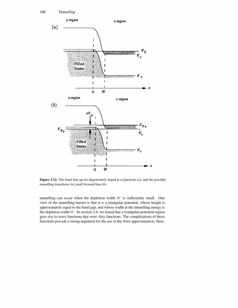
100 Tunnelling
Figure 3.12. The band line-up for degenerately doped p–n junctions (a), and the possibletunnelling transitions for small forward bias (b).
tunnelling can occur when the depletion width � is sufficiently small. Oneview of the tunnelling barrier is that it is a triangular potential, whose height isapproximately equal to the band gap, and whose width at the tunnelling energy isthe depletion width� . In section 2.6, we found that a triangular-potential regiongave rise to wave functions that were Airy functions. The complications of thesefunctions provide a strong argument for the use of the WKB approximation. Here,
Tunnelling devices 101
we can take the decay coefficient as
���� �
����
������
���
�
����
��
�� � � � �
� elsewhere
(3.94)
where we have factored the energy gap out of the potential term and evaluatedthe electric field as ����� . The last term in the square root accounts forthe transverse energy, since the tunnelling coefficient depends upon only the �-component of momentum (the �-component of energy must be reduced below thetotal energy by the transverse energy). This expression must now be integratedaccording to (3.74) over the tunnelling region, which produces
� � ���
�� �
� �
�
�������
���
�
����
��
��
�
� ���
��
�
������
�� �
������
��(3.95)
where we have expanded the radical to lowest order, and retained only the leadingterm in the transverse energy since it is considerably smaller than the band gap. Itturns out that the result (3.95) is not sensitive to the actual details of the potential,since it is actually measuring the area under the –� curve. Different shapesgive the same result if the areas are equal. Recognizing this assures us that theapproximation (3.95) is probably as good as any other. We can rewrite (3.94) as
� � �� ���
����
��
�(3.96)
where
�� ��
�
���
����� (3.97)
This can now be used in (3.92) to find the current.We first will tackle the transverse energy integral. To lowest order, we
note that the term involving the Fermi–Dirac functions is mainly a function ofthe longitudinal �-component of the energy, which we will show below, so thetransverse terms are given by
� ������
�
����� ��
����������� ����� ��
�� ��������� � ��������� (3.98)
The limits on the previous integral are set by the fact that the transverse energycan only increase up to the sum of the Fermi energies on the two sides of thejunction (measured from the band edges) reduced by the longitudinal energy.
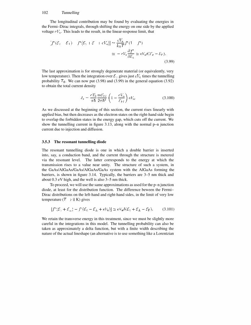
102 Tunnelling
The longitudinal contribution may be found by evaluating the energies inthe Fermi–Dirac integrals, through shifting the energy on one side by the appliedvoltage ���. This leads to the result, in the linear-response limit, that
�� ���� � ���� � ���� � �� � ����� ����
���� ���� � ��
� � ����� �
���� ������ � ����
(3.99)
The last approximation is for strongly degenerate material (or equivalently, verylow temperature). Then the integration over �� gives just ��� times the tunnellingprobability ��. We can now put (3.98) and (3.99) in the general equation (3.92)to obtain the total current density
�� ����
��
���
����
���
���
���
����� (3.100)
As we discussed at the beginning of this section, the current rises linearly withapplied bias, but then decreases as the electron states on the right-hand side beginto overlap the forbidden states in the energy gap, which cuts off the current. Weshow the tunnelling current in figure 3.13, along with the normal p–n junctioncurrent due to injection and diffusion.
3.5.3 The resonant tunnelling diode
The resonant tunnelling diode is one in which a double barrier is insertedinto, say, a conduction band, and the current through the structure is meteredvia the resonant level. The latter corresponds to the energy at which thetransmission rises to a value near unity. The structure of such a system, inthe GaAs/AlGaAs/GaAs/AlGaAs/GaAs system with the AlGaAs forming thebarriers, is shown in figure 3.14. Typically, the barriers are 3–5 nm thick andabout 0.3 eV high, and the well is also 3–5 nm thick.
To proceed, we will use the same approximations as used for the p–n junctiondiode, at least for the distribution function. The difference beween the Fermi–Dirac distributions on the left-hand and right-hand sides, in the limit of very lowtemperature (� � � K) gives
�� ���� � ���� � ���� � �� � ����� � ������ � �� � ���� (3.101)
We retain the transverse energy in this treatment, since we must be slightly morecareful in the integrations in this model. The tunnelling probability can also betaken as approximately a delta function, but with a finite width describing thenature of the actual lineshape (an alternative is to use something like a Lorentzian
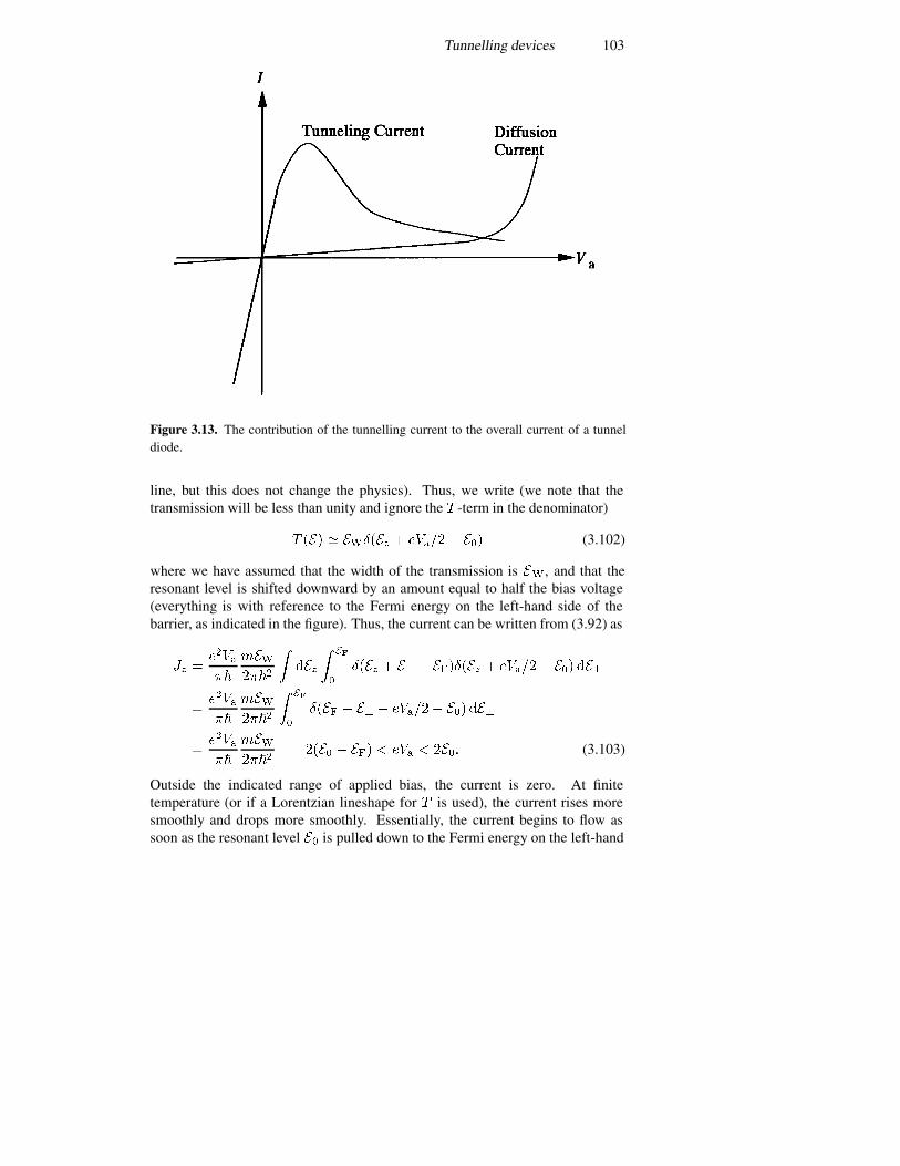
Tunnelling devices 103
Figure 3.13. The contribution of the tunnelling current to the overall current of a tunneldiode.
line, but this does not change the physics). Thus, we write (we note that thetransmission will be less than unity and ignore the � -term in the denominator)
� ��� � ����� � ������ ��� (3.102)
where we have assumed that the width of the transmission is ��, and that theresonant level is shifted downward by an amount equal to half the bias voltage(everything is with reference to the Fermi energy on the left-hand side of thebarrier, as indicated in the figure). Thus, the current can be written from (3.92) as
�� �������
�������
����
� ��
�
��� � �� � ������ � ������ ��� ���
�������
�������
� ��
�
��� � �� � ������ ��� ���
�������
�������
���� � ��� � ��� � ���� (3.103)
Outside the indicated range of applied bias, the current is zero. At finitetemperature (or if a Lorentzian lineshape for � is used), the current rises moresmoothly and drops more smoothly. Essentially, the current begins to flow assoon as the resonant level �� is pulled down to the Fermi energy on the left-hand
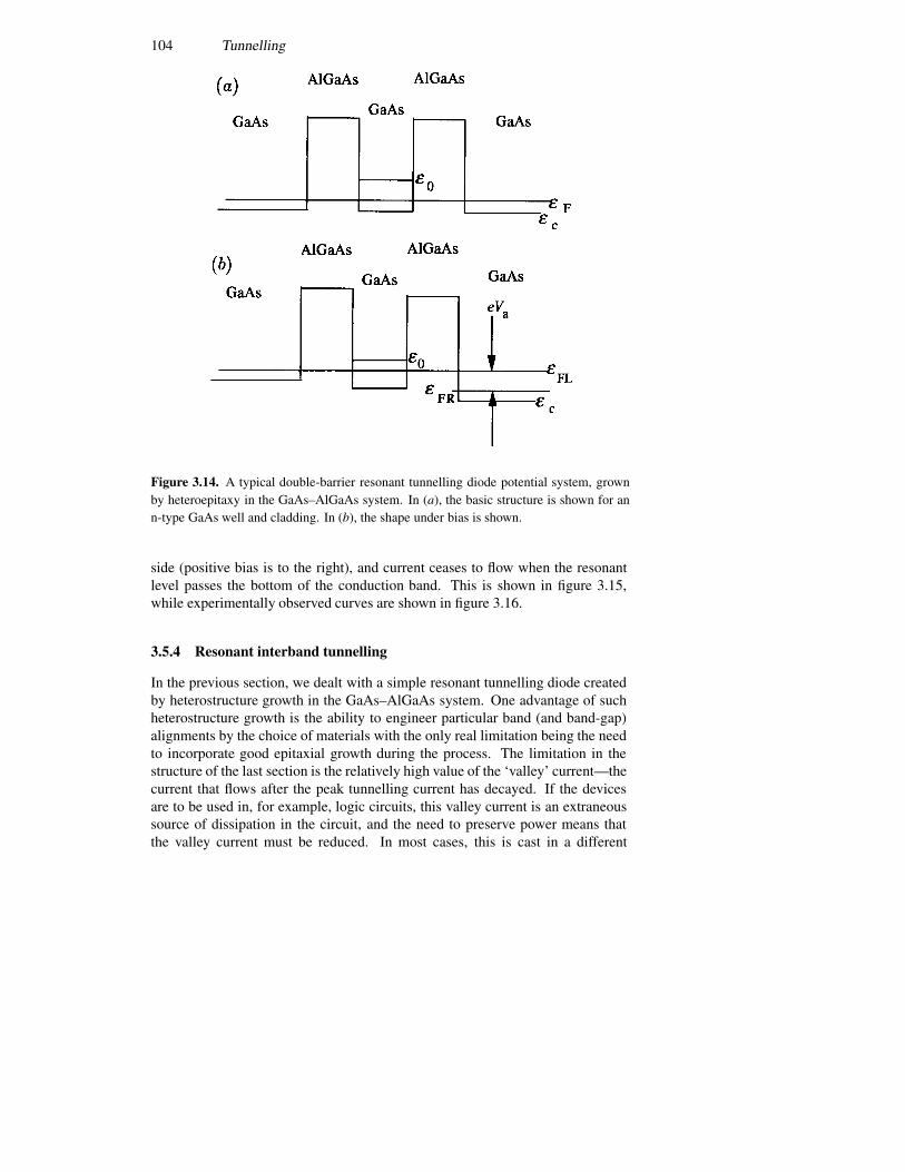
104 Tunnelling
Figure 3.14. A typical double-barrier resonant tunnelling diode potential system, grownby heteroepitaxy in the GaAs–AlGaAs system. In (a), the basic structure is shown for ann-type GaAs well and cladding. In (b), the shape under bias is shown.
side (positive bias is to the right), and current ceases to flow when the resonantlevel passes the bottom of the conduction band. This is shown in figure 3.15,while experimentally observed curves are shown in figure 3.16.
3.5.4 Resonant interband tunnelling
In the previous section, we dealt with a simple resonant tunnelling diode createdby heterostructure growth in the GaAs–AlGaAs system. One advantage of suchheterostructure growth is the ability to engineer particular band (and band-gap)alignments by the choice of materials with the only real limitation being the needto incorporate good epitaxial growth during the process. The limitation in thestructure of the last section is the relatively high value of the ‘valley’ current—thecurrent that flows after the peak tunnelling current has decayed. If the devicesare to be used in, for example, logic circuits, this valley current is an extraneoussource of dissipation in the circuit, and the need to preserve power means thatthe valley current must be reduced. In most cases, this is cast in a different
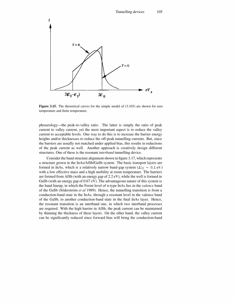
Tunnelling devices 105
Figure 3.15. The theoretical curves for the simple model of (3.103) are shown for zerotemperature and finite temperature.
phraseology—the peak-to-valley ratio. The latter is simply the ratio of peakcurrent to valley current, yet the most important aspect is to reduce the valleycurrent to acceptable levels. One way to do this is to increase the barrier energyheights and/or thicknesses to reduce the off-peak tunnelling currents. But, sincethe barriers are usually not matched under applied bias, this results in reductionsof the peak current as well. Another approach is creatively design differentstructures. One of these is the resonant interband tunnelling device.
Consider the band structure alignment shown in figure 3.17, which representsa structure grown in the InAs/AlSb/GaSb system. The basic transport layers areformed in InAs, which is a relatively narrow band-gap system (�� � ��� ��)with a low effective mass and a high mobility at room temperature. The barriersare formed from AlSb (with an energy gap of 2.2 eV), while the well is formed inGaSb (with an energy gap of 0.67 eV). The advantageous nature of this system isthe band lineup, in which the Fermi level of n-type InAs lies in the valence bandof the GaSb (Soderstrom et al 1989). Hence, the tunnelling transition is from aconduction-band state in the InAs, through a resonant level in the valence bandof the GaSb, to another conduction-band state in the final InAs layer. Hence,the resonant transition is an interband one, in which two interband processesare required. With the high barrier in AlSb, the peak current can be maintainedby thinning the thickness of these layers. On the other hand, the valley currentcan be significantly reduced since forward bias will bring the conduction-band
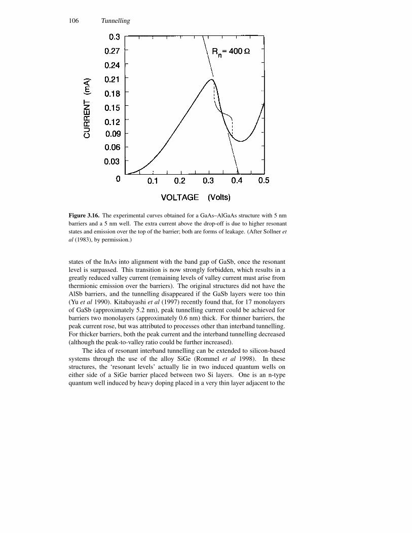
106 Tunnelling
Figure 3.16. The experimental curves obtained for a GaAs–AlGaAs structure with 5 nmbarriers and a 5 nm well. The extra current above the drop-off is due to higher resonantstates and emission over the top of the barrier; both are forms of leakage. (After Sollner etal (1983), by permission.)
states of the InAs into alignment with the band gap of GaSb, once the resonantlevel is surpassed. This transition is now strongly forbidden, which results in agreatly reduced valley current (remaining levels of valley current must arise fromthermionic emission over the barriers). The original structures did not have theAlSb barriers, and the tunnelling disappeared if the GaSb layers were too thin(Yu et al 1990). Kitabayashi et al (1997) recently found that, for 17 monolayersof GaSb (approximately 5.2 nm), peak tunnelling current could be achieved forbarriers two monolayers (approximately 0.6 nm) thick. For thinner barriers, thepeak current rose, but was attributed to processes other than interband tunnelling.For thicker barriers, both the peak current and the interband tunnelling decreased(although the peak-to-valley ratio could be further increased).
The idea of resonant interband tunnelling can be extended to silicon-basedsystems through the use of the alloy SiGe (Rommel et al 1998). In thesestructures, the ‘resonant levels’ actually lie in two induced quantum wells oneither side of a SiGe barrier placed between two Si layers. One is an n-typequantum well induced by heavy doping placed in a very thin layer adjacent to the

Tunnelling devices 107
Figure 3.17. Band lineup for a GaSb well, AlSb barriers, embedded in InAs. The resonantlevel will lie in the valence band of the GaSb, while the transport layers are n-type InAs.All energies are shown in eV.
hetero-interface. The silicon transport layer on this side of the barrier is n-type aswell. The other quantum well naturally forms in the valence band when strainedSiGe is grown on unstrained Si, but this well is further enhanced by implantinga narrow, p-doped region. The transport layer on this side of the barrier is p-typeas well. Hence, the structure is a basic Si p–n junction, in which a strained SiGelayer is placed within the depletion region, and resonant levels are induced indopant-induced quantum wells on either side of the strained layer. Peak-to-valleyratios in the structure are not very good, but the advantage is that this is a resonantinterband diode compatible with silicon integrated circuit processing.
3.5.5 Self-consistent simulations
When we are dealing with devices such as the resonant-tunnelling diode, it isimportant to understand that real devices must be solved self-consistently. Thatis, the actual potential � ��� will change with the applied bias—this change willhave a dependence on position and not just the obvious one on the amplitudedifference between the two ends of the device. For example, as the voltage isramped up from zero to a value just beyond the peak current, there is charge inthe quantum well (the well is charged as the resonant level is reduced to a positionnear the cathode Fermi level). However, when approaching the peak current fromthe high voltage side, the well is empty. Just this simple charging/discharging ofthe well implies a difference in the detailed positional dependence of the potential.This is an effect in most devices, not merely the tunnelling devices.
The potential is given by a solution to Poisson’s equation, which is obtained
108 Tunnelling
from electrostatic theory as
��� ��� ��
���� �
���� ��
�(3.104)
where we have indicated that both the charge density � and the potential � areboth time and position dependent (we deal only with a one-dimensional problemhere). The Schrodinger equation gives us the wave function for a particularpotential. This wave function can be used to determine the charge density at aposition � through
���� � ������� ���� � ����� (3.105)
where it is assumed that the wave function represents electrons and that � �, thebackground charge density, is also negative. If the latter is uniform (which is notthe usual case), and the wave function is normalized over a distance , (3.105)can be simplified to be
���� � ��
������ ���� �
�
�(3.106)
so that ��
�
���� �� � ��
���
�
����� ���� ��� �
� (3.107)
This last form just ensures the normalization of the wave function in the regionof interest, and also ensures that the total device is space-charge neutral. Thisneutrality is a requirement on all devices—the total charge in the device mustsum to zero.
The procedure by which a quantum device is solved self-consistently is toset up a recursive loop. The potential determines the wave function throughSchrodinger’s equation. The wave function determines the charge density, asa function of position, in the device. This charge density then determines thenew potential through Poisson’s equation. This loop can be iterated until aconvergent solution is obtained. This is done at each time step in a time-dependentdevice. Needless to say, this looping of the equations to reach convergence isa major time consuming process in simulation. The device calculations of theprevious sub-sections ignore this need to establish self-consistent solutions. Thisdoes not invalidate them; rather, it is necessary to understand that they are atbest approximations and estimations of the behaviour of a real device in suchcircumstances. Such a self-consistent solution is illustrated later in figure 3.20.
3.6 The Landauer formula
The general approach that was used to evaluate the current equation (3.93)was to expand the difference between the distribution functions and use theresulting ‘delta functions’ to define a range of energies over which the tunnelling
The Landauer formula 109
probability is summed. These energies correspond to those states that are fullon one side of the barrier and empty on the other side (and, of course, allowed).Through the entire process, the current is ‘metered’ by the tunnelling probability.By this, we mean that the current is limited by this process. One question thathas been raised is quite obvious: we have a current passing through a regiondefined by the tunnelling barriers and their cladding layers; we have a voltagedrop as well. Yet, there is no dissipation within the system being considered!Where does the dissipation occur? It must occur in the contacts, since the currentflows through the active tunnelling region in an energy-conserving fashion, as wehave assumed. Thermalization of the carriers must occur in the contact. Thus,the tunnelling region determines the current flow for a given voltage drop (ordetermines the voltage required for a given current flow), but the dissipationoccurs at the boundaries. This is quite unusual, but can be correct in smallsystems, referred to as mesoscopic systems. We can examine this contact effectfurther.
Let us integrate (3.92) over the transverse dimensions, so that it can berewritten as
� ��
���
����������
����
� ����
�� � ������ ���� � ���� � ���� � �� � �����
�����
��
��
����
����
����
� ����
�� � ������� � �� � ���
�����
��
��
����
���
�
���� ��� � ���
�� � ��� � ���
�����
��
����
����� ����
�� � ���� (3.108)
Here, �� is an average transverse energy. The second fraction in (3.108) is aninteresting quantity, in that it is essentially just ��
��, where �� is the wave vector
corresponding to this average energy. This fraction is just the number of allowedtransverse states that can contribute to the current. If we call this latter quantity�, then we can write (3.108) as (we use � � ��� to write only the conductance�)
� ���
��
������
��
�� ��(3.109)
where it is assumed that energy conservation ensures that there is no change inthe number of transverse states. If we refer to the transverse states by the termtransverse modes, then (3.108) is termed the Landauer formula (the notation usedhere is a simple version, assuming no mode coupling). It is normally seen onlyin small mesoscopic systems applications, but it is clear that its applications areeven to normal tunnelling structures so long as we recall just what the summationmeans.
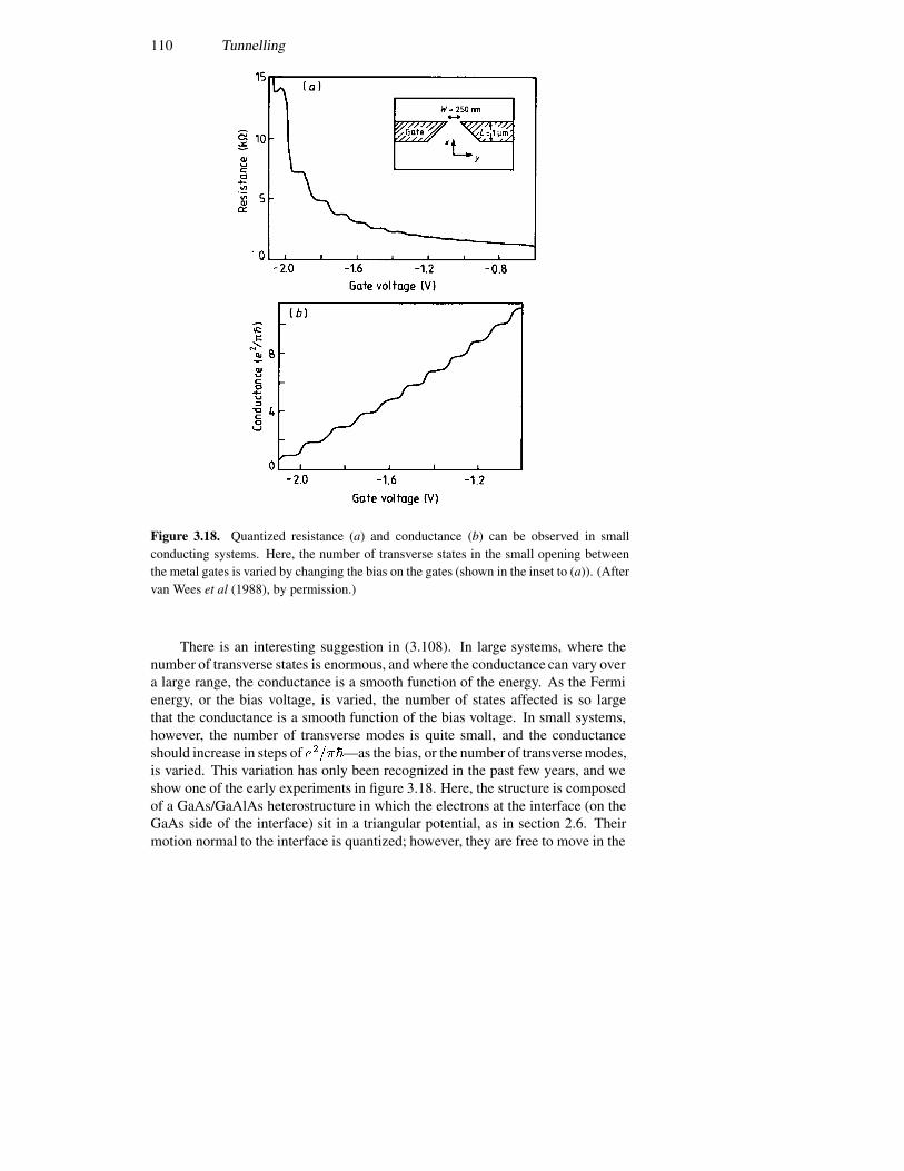
110 Tunnelling
Figure 3.18. Quantized resistance (a) and conductance (b) can be observed in smallconducting systems. Here, the number of transverse states in the small opening betweenthe metal gates is varied by changing the bias on the gates (shown in the inset to (a)). (Aftervan Wees et al (1988), by permission.)
There is an interesting suggestion in (3.108). In large systems, where thenumber of transverse states is enormous, and where the conductance can vary overa large range, the conductance is a smooth function of the energy. As the Fermienergy, or the bias voltage, is varied, the number of states affected is so largethat the conductance is a smooth function of the bias voltage. In small systems,however, the number of transverse modes is quite small, and the conductanceshould increase in steps of �����—as the bias, or the number of transverse modes,is varied. This variation has only been recognized in the past few years, and weshow one of the early experiments in figure 3.18. Here, the structure is composedof a GaAs/GaAlAs heterostructure in which the electrons at the interface (on theGaAs side of the interface) sit in a triangular potential, as in section 2.6. Theirmotion normal to the interface is quantized; however, they are free to move in the
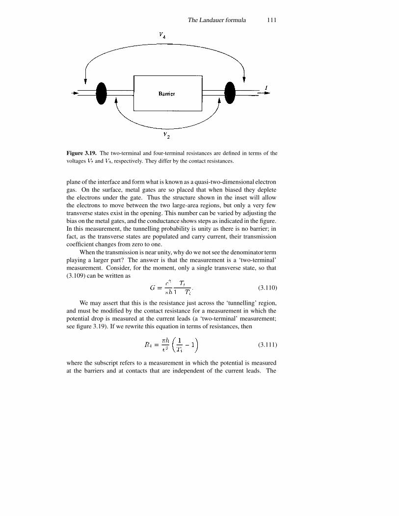
The Landauer formula 111
Figure 3.19. The two-terminal and four-terminal resistances are defined in terms of thevoltages �� and ��, respectively. They differ by the contact resistances.
plane of the interface and form what is known as a quasi-two-dimensional electrongas. On the surface, metal gates are so placed that when biased they depletethe electrons under the gate. Thus the structure shown in the inset will allowthe electrons to move between the two large-area regions, but only a very fewtransverse states exist in the opening. This number can be varied by adjusting thebias on the metal gates, and the conductance shows steps as indicated in the figure.In this measurement, the tunnelling probability is unity as there is no barrier; infact, as the transverse states are populated and carry current, their transmissioncoefficient changes from zero to one.
When the transmission is near unity, why do we not see the denominator termplaying a larger part? The answer is that the measurement is a ‘two-terminal’measurement. Consider, for the moment, only a single transverse state, so that(3.109) can be written as
� ���
��
��
�� ��
� (3.110)
We may assert that this is the resistance just across the ‘tunnelling’ region,and must be modified by the contact resistance for a measurement in which thepotential drop is measured at the current leads (a ‘two-terminal’ measurement;see figure 3.19). If we rewrite this equation in terms of resistances, then
�� ���
��
��
��
� �
�(3.111)
where the subscript refers to a measurement in which the potential is measuredat the barriers and at contacts that are independent of the current leads. The

112 Tunnelling
Figure 3.20. The potential profile for a resonant tunnelling diode, in which a depletionregion (to the left of the barriers) creates a contact resistance to balance the current-carryingpreferences of the barriers and the contacts.
difference lies in the fact that the contacts are areas where equilibration occurs. Ifwe recognize that the original form of the current density (3.83) implied a two-terminal definition, we can say that
�� ���
��
�
��
(3.112)
and the difference is given by
�� � �� ��� �� ���
��� (3.113)
The last form defines the contact resistance ��.Contact resistances are a function of all basic dissipative structures, even
though the dissipation in the present problem is actually in the contact.Nevertheless, when the contacts want to carry a current different from thatof the ‘barrier’ regions, for a given voltage drop, then additional resistanceoccurs in the structure. This is shown in figure 3.20 for a model of a resonanttunnelling diode, in which the potential throughout the device can be obtainedself-consistently from Poisson’s equation. The curvature to the left of the barriersis due predominantly to carrier depletion here which leads to a ‘contact’ resistancein the structure.
How are we to interpret the difference between the two-terminal and thefour-terminal conductances, and therefore how are we to interpret the Landauerformula? If we are truly in the boundary regions, where the distribution functionis a Fermi–Dirac distribution, then we can use the two-terminal formula, providedthat we compute the total transmission over the entire region between the
Periodic potentials 113
boundaries, with the full variation of the self-consistent potential with positionin that region. On the other hand, if we separate the current contacts and thepotential contacts, a four-terminal formula may be used, as long as it is interpretedcarefully. Effects such as those in figure 3.11 must be carefully included in theregion over which the transmission coefficient is being calculated (or measured).Even with a four-terminal measurement, it must be ascertained that the actualcontact resistance differences are just those expected and no unusual effects havebeen overlooked.
3.7 Periodic potentials
At this point, we want to turn our attention to an array of quantum wells, whichare spaced by barriers sufficiently thin that the wave functions can tunnel throughin order to couple the wells together. In this sense, we create a periodic potential.Due to the extreme complexity of the true periodic potential, for purposes ofcalculation it is preferable to simplify the model considerably. For that purpose,we will assume square barriers and wells, as shown in figure 3.21. Although thepotential model is only an approximation, it enables us to develop the essentialfeatures, which in turn will not depend crucially upon the details of the model.The importance of this model is in the energy band structure of crystalline media,such as semiconductors in which the atoms are arranged in a periodic array, andthe atomic potentials create a periodic potential in three dimensions in which theelectrons must move. The important outcomes of the model are the existence ofranges of allowed energies, called bands, and ranges of forbidden energies, calledgaps. We have already, in the previous sections, talked about band gaps in p–njunctions. Here, we review just how periodic potentials give rise to such bandsand gaps in the energy spectrum.
The (atomic) potential is represented by the simple model shown infigure 3.21, and such details as repulsive core potentials will be ignored. Ourinterest is in the filtering effect such a periodic structure has on the energyspectrum of electron waves. The periodic potential has a basic lattice constant(periodicity) of � � � � �. We are interested in states in which � � ��. TheSchrodinger equation now becomes
���
��
����
������� � � � � � � � (3.114a)
and
���
��
����
������� � ����� � � � � � �� (3.114b)
Of course, shifts of the �-axis by the amount � bring in other regions in which(3.114) is found to be the appropriate equation. Nevertheless, there will be apoint at which we will force the periodicity onto the solutions. We also expectthat the wave function will be periodic with the same periodicity as the potential,
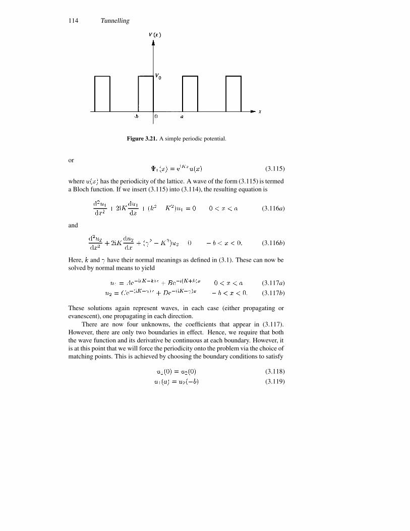
114 Tunnelling
Figure 3.21. A simple periodic potential.
or����� � �������� (3.115)
where ���� has the periodicity of the lattice. A wave of the form (3.115) is termeda Bloch function. If we insert (3.115) into (3.114), the resulting equation is
�������
� ��������
� ��� ������ � � � � � (3.116a)
and
�������
� ��������
� ��� ������ � � � � � � � (3.116b)
Here, � and � have their normal meanings as defined in (3.1). These can now besolved by normal means to yield
�� � ��������� ���������� � � � � (3.117a)
�� � ���������� ������������ � � � � � (3.117b)
These solutions again represent waves, in each case (either propagating orevanescent), one propagating in each direction.
There are now four unknowns, the coefficients that appear in (3.117).However, there are only two boundaries in effect. Hence, we require that boththe wave function and its derivative be continuous at each boundary. However, itis at this point that we will force the periodicity onto the problem via the choice ofmatching points. This is achieved by choosing the boundary conditions to satisfy
���� � ���� (3.118)
����� � ������ (3.119)
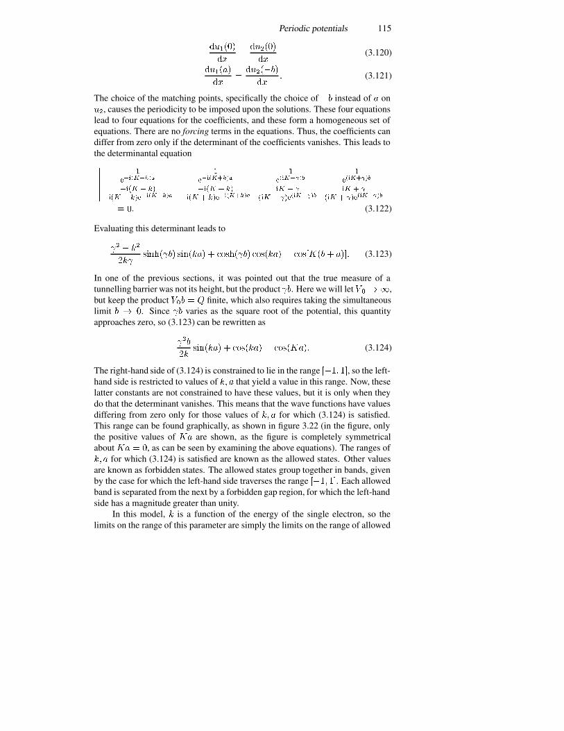
Periodic potentials 115
������
���
������
��(3.120)
������
���
�������
��� (3.121)
The choice of the matching points, specifically the choice of �� instead of � on��, causes the periodicity to be imposed upon the solutions. These four equationslead to four equations for the coefficients, and these form a homogeneous set ofequations. There are no forcing terms in the equations. Thus, the coefficients candiffer from zero only if the determinant of the coefficients vanishes. This leads tothe determinantal equation������
� � �� ����������� ���������
��������� ���������
���� � �� ���� � �� �� � � �� � �
���� � ��������������� � ����������� ��� � ���������� ��� � ����������
������
� �� (3.122)
Evaluating this determinant leads to
�� � ��
���������� ������� ������� ������� � ��� ��� ���� (3.123)
In one of the previous sections, it was pointed out that the true measure of atunnelling barrier was not its height, but the product ��. Here we will let � � ��,but keep the product ��� � finite, which also requires taking the simultaneouslimit � � �. Since �� varies as the square root of the potential, this quantityapproaches zero, so (3.123) can be rewritten as
���
��������� ������� � �������� (3.124)
The right-hand side of (3.124) is constrained to lie in the range �� ��, so the left-hand side is restricted to values of � � that yield a value in this range. Now, theselatter constants are not constrained to have these values, but it is only when theydo that the determinant vanishes. This means that the wave functions have valuesdiffering from zero only for those values of � � for which (3.124) is satisfied.This range can be found graphically, as shown in figure 3.22 (in the figure, onlythe positive values of �� are shown, as the figure is completely symmetricalabout �� � �, as can be seen by examining the above equations). The ranges of� � for which (3.124) is satisfied are known as the allowed states. Other valuesare known as forbidden states. The allowed states group together in bands, givenby the case for which the left-hand side traverses the range �� ��. Each allowedband is separated from the next by a forbidden gap region, for which the left-handside has a magnitude greater than unity.
In this model, � is a function of the energy of the single electron, so thelimits on the range of this parameter are simply the limits on the range of allowed
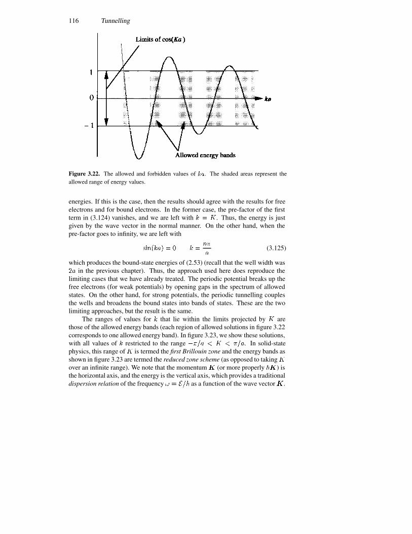
116 Tunnelling
Figure 3.22. The allowed and forbidden values of ��. The shaded areas represent theallowed range of energy values.
energies. If this is the case, then the results should agree with the results for freeelectrons and for bound electrons. In the former case, the pre-factor of the firstterm in (3.124) vanishes, and we are left with � � �. Thus, the energy is justgiven by the wave vector in the normal manner. On the other hand, when thepre-factor goes to infinity, we are left with
������� � � � ���
�(3.125)
which produces the bound-state energies of (2.53) (recall that the well width was�� in the previous chapter). Thus, the approach used here does reproduce thelimiting cases that we have already treated. The periodic potential breaks up thefree electrons (for weak potentials) by opening gaps in the spectrum of allowedstates. On the other hand, for strong potentials, the periodic tunnelling couplesthe wells and broadens the bound states into bands of states. These are the twolimiting approaches, but the result is the same.
The ranges of values for � that lie within the limits projected by � arethose of the allowed energy bands (each region of allowed solutions in figure 3.22corresponds to one allowed energy band). In figure 3.23, we show these solutions,with all values of � restricted to the range ���� � � � ���. In solid-statephysics, this range of � is termed the first Brillouin zone and the energy bands asshown in figure 3.23 are termed the reduced zone scheme (as opposed to taking�over an infinite range). We note that the momentum� (or more properly ��) isthe horizontal axis, and the energy is the vertical axis, which provides a traditionaldispersion relation of the frequency � � ��� as a function of the wave vector�.
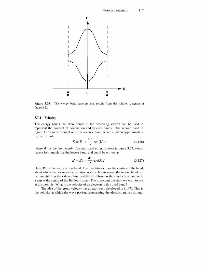
Periodic potentials 117
Figure 3.23. The energy band structure that results from the solution diagram offigure 3.22.
3.7.1 Velocity
The energy bands that were found in the preceding section can be used torepresent the concept of conduction and valence bands. The second band infigure 3.23 can be thought of as the valence band, which is given approximatelyby the formula
� � �� ���
�������� (3.126)
where �� is the band width. The next band up, not shown in figure 3.23, wouldhave a form much like the lowest band, and could be written as
� � �� �
��
��������� (3.127)
Here, �� is the width of this band. The quantities �� are the centres of the band,about which the cosinusoidal variation occurs. In this sense, the second band canbe thought of as the valence band and the third band as the conduction band witha gap at the centre of the Brillouin zone. The important question we wish to askat this point is: What is the velocity of an electron in this third band?
The idea of the group velocity has already been developed in (1.47). This isthe velocity at which the wave packet, representing the electron, moves through
118 Tunnelling
space. Here, the radian frequency � is defined by the energy structure of (3.127).We can use (1.47) to evaluate this velocity as
�� ���
���
�
�
��
���
���
���������� (3.128)
This is an interesting result. The velocity is zero at � � � as expected. It thenrises with increasing � until reaching a peak at �� � ���, and then decreases.As the electron cycles through the entire conduction band (under the influence ofan electric field for example), its velocity oscillates and the average value is zero.Indeed, if we apply an electric field to increase �, we have
��� � ���� �
� (3.129)
and the velocity varies as
�� ����
�����
������
��
�
�� (3.130)
The velocity oscillates with a frequency
�� ���
�(3.131)
and this is known as the Bloch frequency. Of course, the presence of scatteringprocesses in real materials keeps this from happening, and the electron cannotmove very far away from ���� � �. However, if one could accelerate theelectron over the maximum of (3.128), then the velocity would be decreasing andone conceivably could have a negative differential conductance. What is actuallyhappening when the electron undergoes Bloch oscillations is that it is samplingthe entire Brillouin zone. The Brillouin zone is a full Fourier transform of thelattice, so that a summation over all �-states in the band localizes the electron inreal space at one lattice site. It is thought that the electron vibrates around thislocalized position.
The problem in real crystals is that the value of� needed to reach�� � ���is large. If the lattice constant is typically 0.25 nm, then � � � ��� ���. If wetry to accelerate the electron to this value, we require � � ����. Even if thescattering time is as large as 0.1 ps (at high energy), this requires an electric fieldof 400 kV cm��. This is an enormous field. On the other hand, if the periodicitycould be enhanced to make � much larger, then some interesting effects couldoccur. This is the goal of superlattices.
3.7.2 Superlattices
While the fields required in the previous section were unusually high, Esaki andTsu (1970) put forward the idea of reducing the size of the Brillouin zone in �-space by creating superlattices. The idea was to grow, by molecular-beam epitaxy,
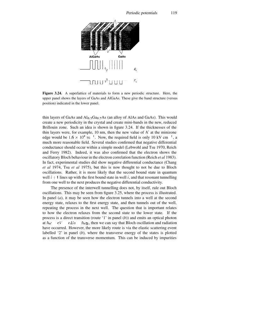
Periodic potentials 119
Figure 3.24. A superlattice of materials to form a new periodic structure. Here, theupper panel shows the layers of GaAs and AlGaAs. These give the band structure (versusposition) indicated in the lower panel.
thin layers of GaAs and Al���Ga���As (an alloy of AlAs and GaAs). This wouldcreate a new periodicity in the crystal and create mini-bands in the new, reducedBrillouin zone. Such an idea is shown in figure 3.24. If the thicknesses of thethin layers were, for example, 10 nm, then the new value of � at the minizoneedge would be ��� � ��� ���. Now, the required field is only 10 kV cm��, amuch more reasonable field. Several studies confirmed that negative differentialconductance should occur within a simple model (Lebwohl and Tsu 1970, Reichand Ferry 1982). Indeed, it was also confirmed that the electron shows theoscillatory Bloch behaviour in the electron correlation function (Reich et al 1983).In fact, experimental studies did show negative differential conductance (Changet al 1974, Tsu et al 1975), but this is now thought to not be due to Blochoscillations. Rather, it is more likely that the second bound state in quantumwell ��� lines up with the first bound state in well �, and that resonant tunnellingfrom one well to the next produces the negative differential conductivity.
The presence of the interwell tunnelling does not, by itself, rule out Blochoscillations. This may be seen from figure 3.25, where the process is illustrated.In panel (a), it may be seen how the electron tunnels into a well at the secondenergy state, relaxes to the first energy state, and then tunnels out of the well,repeating the process in the next well. The question that is important relatesto how the electron relaxes from the second state to the lower state. If theprocess is a direct transition (route ‘1’ in panel (b)) and emits an optical photonat �� � �� � ��� � ���, then we can say that Bloch oscillation and radiationhave occurred. However, the more likely route is via the elastic scattering eventlabelled ‘2’ in panel (b), where the transverse energy of the states is plottedas a function of the transverse momentum. This can be induced by impurities
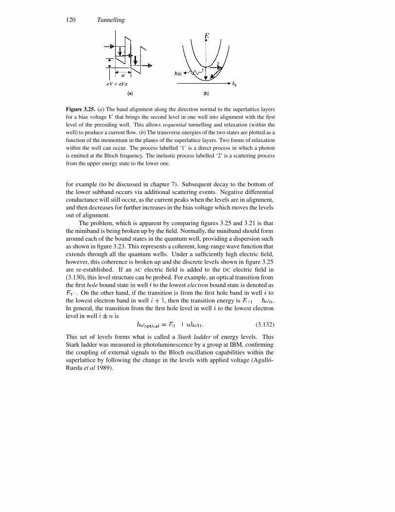
120 Tunnelling
Figure 3.25. (a) The band alignment along the direction normal to the superlattice layersfor a bias voltage � that brings the second level in one well into alignment with the firstlevel of the preceding well. This allows sequential tunnelling and relaxation (within thewell) to produce a current flow. (b) The transverse energies of the two states are plotted as afunction of the momentum in the planes of the superlattice layers. Two forms of relaxationwithin the well can occur. The process labelled ‘1’ is a direct process in which a photonis emitted at the Bloch frequency. The inelastic process labelled ‘2’ is a scattering processfrom the upper energy state to the lower one.
for example (to be discussed in chapter 7). Subsequent decay to the bottom ofthe lower subband occurs via additional scattering events. Negative differentialconductance will still occur, as the current peaks when the levels are in alignment,and then decreases for further increases in the bias voltage which moves the levelsout of alignment.
The problem, which is apparent by comparing figures 3.25 and 3.21 is thatthe miniband is being broken up by the field. Normally, the miniband should formaround each of the bound states in the quantum well, providing a dispersion suchas shown in figure 3.23. This represents a coherent, long-range wave function thatextends through all the quantum wells. Under a sufficiently high electric field,however, this coherence is broken up and the discrete levels shown in figure 3.25are re-established. If an AC electric field is added to the DC electric field in(3.130), this level structure can be probed. For example, an optical transition fromthe first hole bound state in well � to the lowest electron bound state is denoted as���. On the other hand, if the transition is from the first hole band in well � tothe lowest electron band in well � � �, then the transition energy is ��� � ���.In general, the transition from the first hole level in well � to the lowest electronlevel in well �� � is
��������� � ��� � ����� (3.132)
This set of levels forms what is called a Stark ladder of energy levels. ThisStark ladder was measured in photoluminescence by a group at IBM, confirmingthe coupling of external signals to the Bloch oscillation capabilities within thesuperlattice by following the change in the levels with applied voltage (Agullo-Rueda et al 1989).
Single-electron tunnelling 121
3.8 Single-electron tunnelling
As a last consideration in this chapter, we want to consider tunnelling throughthe insulator of a capacitor (which we take to be an oxide such as SiO � foundin MOS structures). The tunnelling through the capacitor oxide is an exampleof a very simple physical system (the single capacitor) that can exhibit quitecomplicated behaviour when it is made small. The capacitor is formed byplacing an insulator between two metals or by the oxide in an MOS structure,as discussed in section 2.6. Consider, for example, the tunnelling coefficientfor such an insulator, in which the barrier height is approximately 3 eV, andthe thickness of the insulator (assumed to be SiO�) is about 3 nm. Althoughthe tunnelling coefficient is small (we may estimate it to be of the order of����), the actual current density that can flow due to tunnelling is of the order
of a few picoamperes per square centimetre. If the barriers are semiconductors,rather than metals, then the current can be two orders of magnitude larger, and,of course, the tunnelling coefficient will become much larger under a bias fieldwhich distorts the shape of the potential barrier. Thus, in general, oxide insulatorsof this thickness are notoriously leaky due to tunnelling currents, even though thetunnelling probability is quite low for a single electron (there are of course a greatnumber of electrons attempting to tunnel, so even though the probability of oneelectron tunnelling is quite low, the number making it through is significant).
What if the area of the capacitor is made small, so that the capacitance is alsoquite small? It turns out that this can affect the operation of tunnelling through theoxide significantly as well. When an electron tunnels through the oxide, it lowersthe energy stored in the capacitor by the amount
� ���
��� (3.133)
For example, the voltage across the capacitor changes by the amount
� ��
�� (3.134)
What this means is that the tunnelling current cannot occur until a voltageequivalent to (3.134) is actually applied across the capacitor. If the voltage onthe capacitor is less than this, no tunnelling current occurs because there is notsufficient energy stored in the capacitor to provide the tunnelling transition. Whenthe capacitance is large, say � ��
��� F, this voltage is immeasurably small incomparison with the thermally induced voltages (�����). On the other hand,suppose that the capacitance is defined with a lateral dimension of only 50 nm.Then, the area is ��� � ��
�����, and our capacitor discussed above has a
capacitance of ��������� F, and the required voltage of (3.134) is 5.7 mV. Thesecapacitors are easily made, and the effects easily measured at low temperatures.In figure 3.26, we show measurements by Fulton and Dolan (1987) on suchstructures. The retardation of the tunnelling current until a voltage according
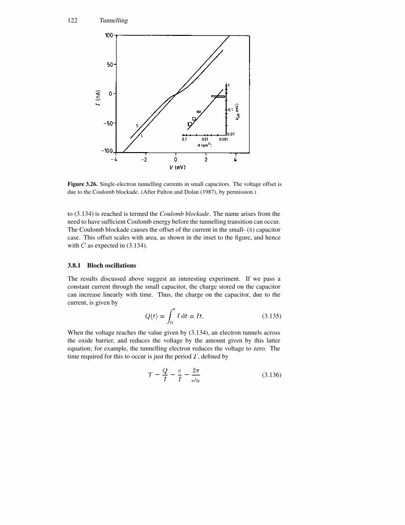
122 Tunnelling
Figure 3.26. Single-electron tunnelling currents in small capacitors. The voltage offset isdue to the Coulomb blockade. (After Fulton and Dolan (1987), by permission.)
to (3.134) is reached is termed the Coulomb blockade. The name arises from theneed to have sufficient Coulomb energy before the tunnelling transition can occur.The Coulomb blockade causes the offset of the current in the small- (S) capacitorcase. This offset scales with area, as shown in the inset to the figure, and hencewith � as expected in (3.134).
3.8.1 Bloch oscillations
The results discussed above suggest an interesting experiment. If we pass aconstant current through the small capacitor, the charge stored on the capacitorcan increase linearly with time. Thus, the charge on the capacitor, due to thecurrent, is given by
���� �
��
�
� �� � ��� (3.135)
When the voltage reaches the value given by (3.134), an electron tunnels acrossthe oxide barrier, and reduces the voltage by the amount given by this latterequation; for example, the tunnelling electron reduces the voltage to zero. Thetime required for this to occur is just the period � , defined by
� ��
��
�
��
��
��(3.136)
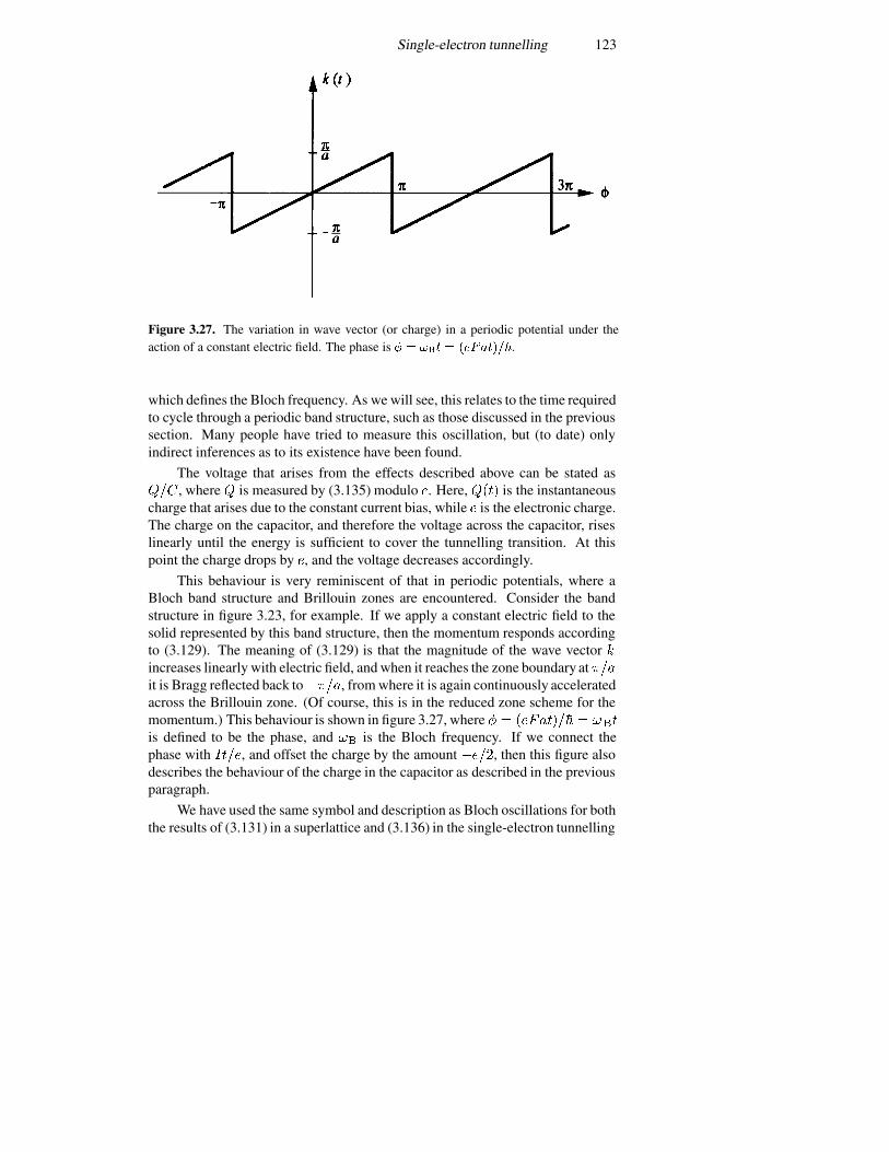
Single-electron tunnelling 123
Figure 3.27. The variation in wave vector (or charge) in a periodic potential under theaction of a constant electric field. The phase is � � ��� � ��������.
which defines the Bloch frequency. As we will see, this relates to the time requiredto cycle through a periodic band structure, such as those discussed in the previoussection. Many people have tried to measure this oscillation, but (to date) onlyindirect inferences as to its existence have been found.
The voltage that arises from the effects described above can be stated as���, where � is measured by (3.135) modulo �. Here, ���� is the instantaneouscharge that arises due to the constant current bias, while � is the electronic charge.The charge on the capacitor, and therefore the voltage across the capacitor, riseslinearly until the energy is sufficient to cover the tunnelling transition. At thispoint the charge drops by �, and the voltage decreases accordingly.
This behaviour is very reminiscent of that in periodic potentials, where aBloch band structure and Brillouin zones are encountered. Consider the bandstructure in figure 3.23, for example. If we apply a constant electric field to thesolid represented by this band structure, then the momentum responds accordingto (3.129). The meaning of (3.129) is that the magnitude of the wave vector �increases linearly with electric field, and when it reaches the zone boundary at ���it is Bragg reflected back to����, from where it is again continuously acceleratedacross the Brillouin zone. (Of course, this is in the reduced zone scheme for themomentum.) This behaviour is shown in figure 3.27, where � � ������� � ��is defined to be the phase, and � is the Bloch frequency. If we connect thephase with ����, and offset the charge by the amount ����, then this figure alsodescribes the behaviour of the charge in the capacitor as described in the previousparagraph.
We have used the same symbol and description as Bloch oscillations for boththe results of (3.131) in a superlattice and (3.136) in the single-electron tunnelling

124 Tunnelling
description. That this is correct can be illustrated by utilizing the dualism thatexists in electromagnetics and electrical circuits. The dual of voltage is current.The dual of flux ����� is charge ���. Hence, we can use these dual relationshipsin (3.131) as
�� ����
�� ��
�
���� ��
�
�(3.137)
which is just a rearranged version of (3.136). Thus, the two processes are in factjust duals of one another and the Bloch oscillation describes the same physicsin each case—cycling of a particle through a periodic potential. In the case ofsingle-electron tunnelling, we have not yet identified the existence of this periodicpotential, but it must exist. Then the vertical axis in figure 3.27 becomes thevoltage across the capacitor, which charges until a level is reached to provide theenergy necessary for an electron to tunnel through the oxide.
3.8.2 Periodic potentials
The drop in charge, given by the tunnelling of the electron through the smallcapacitor, does not occur with sudden sharpness, when we operate at a non-zero temperature. Thus, it is possible to approximate the result of (3.135), andfigure 3.27, by the expression for the charge on the capacitor as
�� ��
�������� (3.138)
which symmetrizes the charge about zero (for zero current bias), and the changeoccurs now when the instantaneous charge reaches half-integer charge (droppingto the negative of this value so that the net tunnelling charge is a single electron).Now, we want to create a Hamiltonian system, which we can quantize, to producethe effective periodic potential structures of the previous section. For this, wedefine the phase of the charge to be
� � ��� (3.139)
We take this phase to have the equivalent coordinate of position given in theprevious section (we will adjust it below by a constant), and this means thatwe can extend the treatment to cases in which there is not a constant currentbias applied. Rather, we assert that the phase behaves in a manner that describessome equivalent position. The position is not particularly important for periodicpotentials and does not appear at all in figure 3.23 for the band structure. We nowtake the momentum coordinate to correspond to
���
�� � (3.140)
Now, this choice is not at all obvious, but it is suggested by the comparison abovebetween the time behaviour of the charge, under a constant current bias, and the
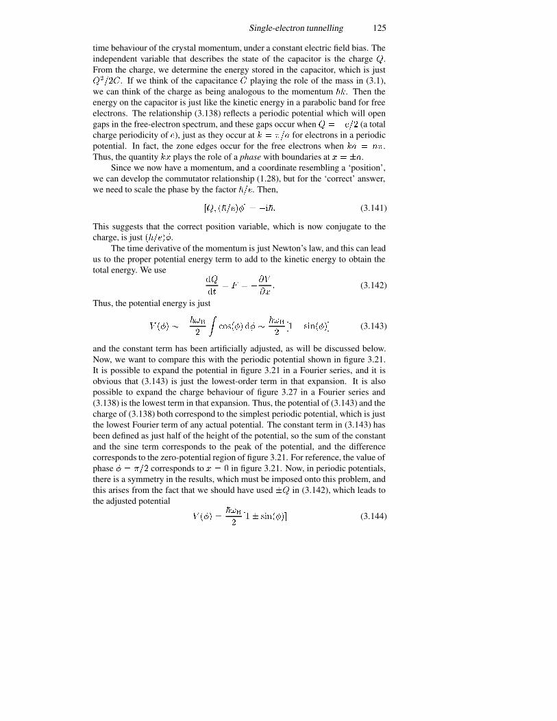
Single-electron tunnelling 125
time behaviour of the crystal momentum, under a constant electric field bias. Theindependent variable that describes the state of the capacitor is the charge �.From the charge, we determine the energy stored in the capacitor, which is just�����. If we think of the capacitance � playing the role of the mass in (3.1),we can think of the charge as being analogous to the momentum ��. Then theenergy on the capacitor is just like the kinetic energy in a parabolic band for freeelectrons. The relationship (3.138) reflects a periodic potential which will opengaps in the free-electron spectrum, and these gaps occur when � � ���� (a totalcharge periodicity of �), just as they occur at � � ��� for electrons in a periodicpotential. In fact, the zone edges occur for the free electrons when �� � ��.Thus, the quantity �� plays the role of a phase with boundaries at � � ��.
Since we now have a momentum, and a coordinate resembling a ‘position’,we can develop the commutator relationship (1.28), but for the ‘correct’ answer,we need to scale the phase by the factor ���. Then,
�� ������ � ���� (3.141)
This suggests that the correct position variable, which is now conjugate to thecharge, is just �����.
The time derivative of the momentum is just Newton’s law, and this can leadus to the proper potential energy term to add to the kinetic energy to obtain thetotal energy. We use
��
��� � �
��
��� (3.142)
Thus, the potential energy is just
� �� � �����
���� � �
����
��� ����� (3.143)
and the constant term has been artificially adjusted, as will be discussed below.Now, we want to compare this with the periodic potential shown in figure 3.21.It is possible to expand the potential in figure 3.21 in a Fourier series, and it isobvious that (3.143) is just the lowest-order term in that expansion. It is alsopossible to expand the charge behaviour of figure 3.27 in a Fourier series and(3.138) is the lowest term in that expansion. Thus, the potential of (3.143) and thecharge of (3.138) both correspond to the simplest periodic potential, which is justthe lowest Fourier term of any actual potential. The constant term in (3.143) hasbeen defined as just half of the height of the potential, so the sum of the constantand the sine term corresponds to the peak of the potential, and the differencecorresponds to the zero-potential region of figure 3.21. For reference, the value ofphase � ��� corresponds to � � in figure 3.21. Now, in periodic potentials,there is a symmetry in the results, which must be imposed onto this problem, andthis arises from the fact that we should have used �� in (3.142), which leads tothe adjusted potential
� �� �����
��� ����� (3.144)
126 Tunnelling
Figure 3.28. The energy band spectrum for the single-tunnelling capacitor.
which shifts the � � � point to � � ����. The leading term in the potential justoffsets the energy, and can be ignored. The Hamiltonian is then
� ���
���
����
������� (3.145)
This Hamiltonian is in a mixed position and momentum representation. Theenergy can be written out if we use just a momentum representation, and thisis achieved by using (3.138) to eliminate the phase, as
� ���
���
����
��
�� (3.146)
This energy is shown in figure 3.28. The zone boundaries are at the values ofcharge � � ����. At these two points, gaps open in the ‘free-electron’ energy(the first term in the above equation). These gaps are of ���. We note also that theenergy bands have all been offset upward by the constant potential term, whichwe ignored in (3.146). This is also seen in the Kronig–Penney model treated inthe previous section.
The simple capacitor seems to exhibit the very complicated behaviourexpected from a periodic potential merely when it is made sufficiently smallthat tunnelling through the oxide can occur (and the capacitance is sufficiently
Single-electron tunnelling 127
small that the energy is large compared with the thermal energy). In reality, nosuch periodic potential exists, but the very real behaviour of the charge, which isrepresented in figure 3.27, gives rise to physical behaviour equivalent to that of aperiodic potential. Thus, we can use the equivalent band structure of figure 3.28to investigate other physical effects, all of which have their origin in the strangeperiodic behaviour of the charge on the capacitor.
3.8.3 The double-barrier quantum dot
To understand the Coulomb blockade somewhat more quantitatively, we considerthe double-barrier structure shown in figure 3.14 as it may be created withextremely small lateral dimensions so that the capacitance of each barrier satisfies
� ���
��� ��� (3.147)
as required for Coulomb blockade. The quantum well region, since it is laterallyconfined to a small dimension, may be termed a quantum dot. In general, eachof the two capacitors (barriers) will have some leakage, but the equivalent circuitis as shown in figure 3.29(a). The leakage is indicated as the shunt resistancethrough each capacitor. This leakage, or tunnelling resistance, represents thecurrent flow when the electrons tunnel through the barrier. In this sense, theseresistances are different from ordinary resistances. In the latter, charge and currentflow is essentially continuous. Here, however, the current flow only occurs whenthe electrons are tunnelling, and this is for a very short time. The charge on thetwo capacitors is related to the two voltages, and is given by
�� � ���� �� � ����� (3.148)
The net charge on the quantum dot island is given by
���� � �� ��� � ��� (3.149)
where � is the net number of excess electrons on the island. The sum of thejunction voltages is the applied voltage ��, so that combining the two equationsabove, the voltage drops across the two junctions are just
�� ��
���
��������� ��� � ����� �� ��
���
���������� (3.150)
The electrostatic energy can be written as
� ����
���
����
���
��
����
�������� ���
����� (3.151)
In addition, we must consider the work done by the voltage source incharging the two capacitors. This is an integral over the power delivered to the
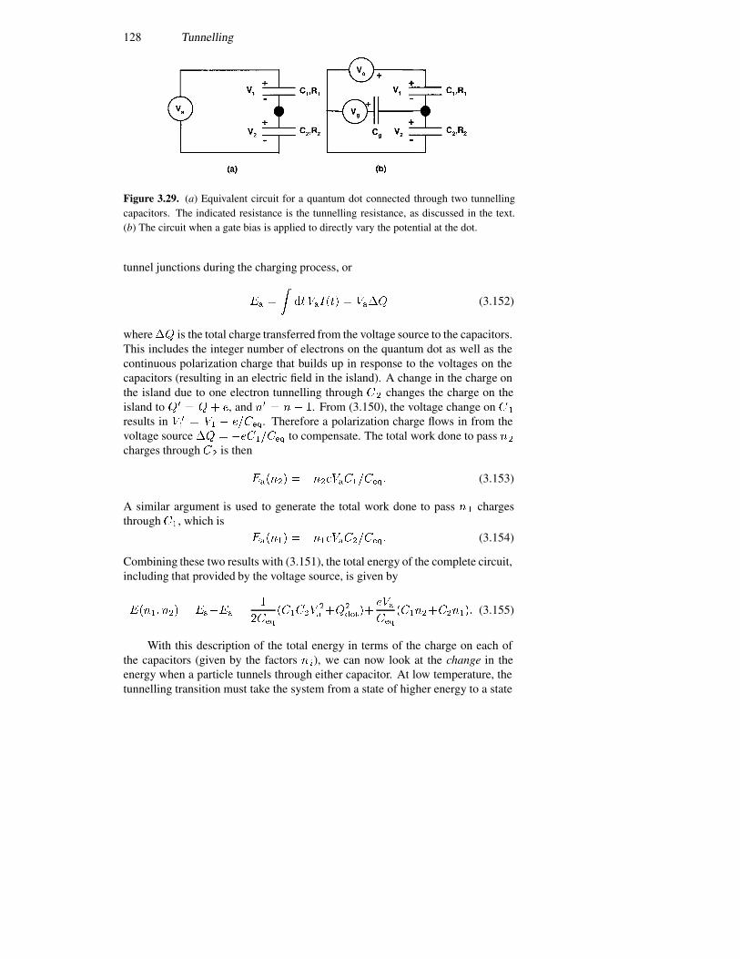
128 Tunnelling
Figure 3.29. (a) Equivalent circuit for a quantum dot connected through two tunnellingcapacitors. The indicated resistance is the tunnelling resistance, as discussed in the text.(b) The circuit when a gate bias is applied to directly vary the potential at the dot.
tunnel junctions during the charging process, or
�� �
��� ������ � ���� (3.152)
where�� is the total charge transferred from the voltage source to the capacitors.This includes the integer number of electrons on the quantum dot as well as thecontinuous polarization charge that builds up in response to the voltages on thecapacitors (resulting in an electric field in the island). A change in the charge onthe island due to one electron tunnelling through � � changes the charge on theisland to �� � �� �, and �� � �� �. From (3.150), the voltage change on ��
results in � �
� � �� � �����. Therefore a polarization charge flows in from thevoltage source �� � �������� to compensate. The total work done to pass ��
charges through �� is then
������ � ������������ (3.153)
A similar argument is used to generate the total work done to pass �� chargesthrough ��, which is
������ � ������������ (3.154)
Combining these two results with (3.151), the total energy of the complete circuit,including that provided by the voltage source, is given by
���� ��� � ����� ��
����
�������� ���
�����������
����������� (3.155)
With this description of the total energy in terms of the charge on each ofthe capacitors (given by the factors ��), we can now look at the change in theenergy when a particle tunnels through either capacitor. At low temperature, thetunnelling transition must take the system from a state of higher energy to a state

Single-electron tunnelling 129
of lower energy. The change in energy for a particle tunnelling through � � is
����� ����� ��������� �� � ��
�
������
����
������ � ���
����
�������
���
��
���
���
�� ����� � �����
�� (3.156)
The value of the charge on the dot ���� is prior to the tunnelling process.Similarly, the change in energy for a particle tunnelling through � � is given by
���� � ����� �������� � �� ���
�
������
����
������ � ���
����
�������
���
��
���
���
�� ����� � �����
�� (3.157)
According to this discussion, only those transitions are allowed for which �� � ��; e.g., the initial state is at a higher energy than the final state.
If we consider a system in which the dot is initially uncharged, ���� � �,then (3.156) and (3.157) reduce to
������ � ���
����
��������
���
� �� (3.158)
Initially, at low voltage, the leading term on the right-hand side makes �� �.Hence, no tunnelling can occur until the voltage reaches a threshold that dependsupon the lesser of the two capacitors. For the case in which �� � �� � �,the requirement becomes ���� � ����. Tunnelling is prohibited and no currentflows below this threshold voltage. This region of Coulomb blockade is a directresult of the additional Coulomb energy which is required for an electron to tunnelthrough one of the capacitors.
Now, consider the situation when we make an additional contact, throughanother capacitor, to the quantum dot as shown in figure 3.29(b). A new voltagesource, ��, is coupled to the quantum dot through an ideal capacitor � � (notunnelling is possible through this capacitor). This additional voltage sourcemodifies the charge balance on the quantum dot, so that
�� � ����� � ���� (3.159)
The charge on the quantum dot now becomes
���� � �� ��� ��� � ���� (3.160)
The voltages across the two junctions is also modified, and we can write
�� ��
�
���� � ����� � ���� � ��� � � �� � ���
�� ��
�
����� � ���� � ����(3.161)
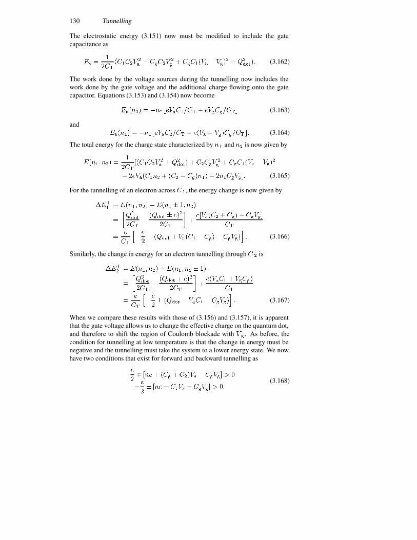
130 Tunnelling
The electrostatic energy (3.151) now must be modified to include the gatecapacitance as
�� ��
���
�������� � �����
�� � ������� � ���
� �������� (3.162)
The work done by the voltage sources during the tunnelling now includes thework done by the gate voltage and the additional charge flowing onto the gatecapacitor. Equations (3.153) and (3.154) now become
������ � ������������ � ��������� (3.163)
and������ � ������������ � ���� � ���������� (3.164)
The total energy for the charge state characterized by � � and �� is now given by
����� ��� ��
���
��������� ���
���� � ������� � ������� � ���
�
� ��������� � ��� � ������� ��������� (3.165)
For the tunnelling of an electron across ��, the energy change is now given by
���� � ����� �������� � �� ���
�
������
���
������ � ���
���
��������� � ���� �����
��
��
��
���
�� ����� � ����� � ���� �����
�� (3.166)
Similarly, the change in energy for an electron tunnelling through � � is
���� � ����� ��������� �� � ��
�
������
���
������ � ���
���
�������� � �����
��
��
��
���
�� ����� � ���� � �����
�� (3.167)
When we compare these results with those of (3.156) and (3.157), it is apparentthat the gate voltage allows us to change the effective charge on the quantum dot,and therefore to shift the region of Coulomb blockade with � �. As before, thecondition for tunnelling at low temperature is that the change in energy must benegative and the tunnelling must take the system to a lower energy state. We nowhave two conditions that exist for forward and backward tunnelling as
��
�� ���� ��� � ����� � �����
��
�� ���� ���� � ����� �
(3.168)
Single-electron tunnelling 131
Figure 3.30. A stability diagram for the single-electron quantum dot. The parameters arediscussed in the text, and it is assumed that the temperature is � � �. The shaded regionsare where the dot electron number is stable and Coulomb blockade exists.
The four equations (3.168) may be used to generate a stability plot in the �� �� ���plane, which shows stable regions corresponding to each value of �, and for whichno tunnelling can occur. This diagram is shown in figure 3.30 for the case in which�� � �� � � and �� � �� ��� � ���. The lines represent the boundariesgiven by (3.168). The trapezoidal shaded areas correspond to regions where nosolution satisfies (3.168) and hence where Coulomb blockade exists. Each ofthe regions corresponds to a different number of electrons on the quantum dot,which is stable in the sense that this charge state does not change easily. The gatevoltage allows us to ‘tune’ between different stable regimes, essentially addingor subtracting one electron at a time to the dot region. For a given gate bias, therange of �� over which Coulomb blockade occurs is given by the vertical extentof the shaded region. The width of this blockaded region approaches zero as thegate charge approaches half-integer values of a single electron charge, and heretunnelling occurs easily. It is at these gate voltages that tunnelling current peakscan be observed as the gate bias is varied.
In figure 3.30, the superlattice behaviour of the charge in terms of either thegate voltage or the charging voltage �� is clear. This gives a distance betweenthe current peaks for tunnelling through the structure of �� � � ��� � ����.Between these peaks the number of electrons on the quantum dot remainsconstant. We will return to the quantum dot in chapter 8, where we begin to worryabout the quantum levels within the dot itself. To this point, we have ignored thefact that the quantum dot may be so small that the energy levels within the dot arequantized. Yet, this can occur, and the behaviour of this section is modified. Asremarked, we return to this in chapter 8, where we deal with spectroscopy of justthese quantum levels.
References
Agullo-Rueda F, Mendez E E and Hong J M 1989 Phys. Rev. B 40 1357

132 Tunnelling
Bohm D 1951 Quantum Theory (Englewood Cliffs, NJ: Prentice-Hall)Brillouin L 1926 C. R. Acad. Sci. 183 24Chang L L, Esaki L and Tsu R 1974 Appl. Phys. Lett. 24 593Esaki L and Tsu R 1970 IBM J. Res. Dev. 14 61Ferry D K and Goodnick S M 1997 Transport in Nanostructures (Cambridge: Cambridge
University Press)Fulton and Dolan 1987 Phys. Rev. Lett. 59 109Grabert H and Devoret M H (ed) 1992 Single Charge Tunneling, Coulomb Blockade
Phenomena in Nanostructures (ASI Series B 294) (New York: Plenum)Kitabayashi H, Waho T and Yamamoto M 1997 Appl. Phys. Lett. 71 512Kramers H A 1926 Z. Phys. 39 828Landauer R 1957 IBM J. Res. Dev. 1 223Landauer R 1970 Phil. Mag. 21 863Lebwohl P A and Tsu R 1970 J. Appl. Phys. 41 2664Price P 1999 Microelectron. J. 30 925Reich R K and Ferry D K 1982 Phys. Lett. A 91 31Reich R K, Grondin R O and Ferry D K 1983 Phys. Rev. B 27 3483Rommel S L et al 1998 Appl. Phys. Lett. 73 2191Soderstrom J R, Chow D H and McGill T C 1989 Appl. Phys. Lett. 55 1094Sollner T L C G, Goodhue W D, Tannenwald P E, Parker C D and Peck D D 1983 Appl.
Phys. Lett. 43 588Tsu R, Chang L L, Sai-Halasz G A and Esaki L 1975 Phys. Rev. Lett. 34 1509van Wees B J, van Houten H, Beenakker C W J, Williamson J G, Kouwenhouven L P,
van der Marel D and Foxon C T 1988 Phys. Rev. Lett. 60 848Wentzel G 1926 Z. Phys. 38 518Yacoby A, Heiblum M, Umansky V and Shtrikman H 1994 Phys. Rev. Lett. 73 3149Yacoby A, Heiblum M, Mahalu D and Shtrikman H 1995 Phys. Rev. Lett. 74 4047Yu E T, Collins D A, Ting D Z-Y, Chow D H and McGill T C 1990 Appl. Phys. Lett. 57
2675
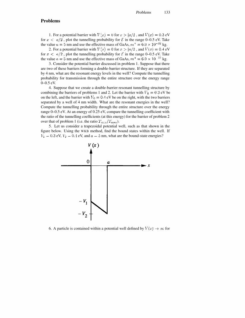
Problems 133
Problems
1. For a potential barrier with � ��� � � for � � �����, and � ��� � ��� eVfor � � �����, plot the tunnelling probability for � in the range 0–0.5 eV. Takethe value � � � nm and use the effective mass of GaAs, �� � ���� ����� kg.
2. For a potential barrier with � ��� � � for � � �����, and � ��� � �� eVfor � � �����, plot the tunnelling probability for � in the range 0–0.5 eV. Takethe value � � � nm and use the effective mass of GaAs, �� � ���� ����� kg.
3. Consider the potential barrier discussed in problem 1. Suppose that thereare two of these barriers forming a double-barrier structure. If they are separatedby 4 nm, what are the resonant energy levels in the well? Compute the tunnellingprobability for transmission through the entire structure over the energy range0–0.5 eV.
4. Suppose that we create a double-barrier resonant tunnelling structure bycombining the barriers of problems 1 and 2. Let the barrier with � � � ��� eV beon the left, and the barrier with �� � �� eV be on the right, with the two barriersseparated by a well of 4 nm width. What are the resonant energies in the well?Compute the tunnelling probability through the entire structure over the energyrange 0–0.5 eV. At an energy of 0.25 eV, compare the tunnelling coefficient withthe ratio of the tunnelling coefficients (at this energy) for the barrier of problem 2over that of problem 1 (i.e. the ratio ���������).
5. Let us consider a trapezoidal potential well, such as that shown in thefigure below. Using the WKB method, find the bound states within the well. If�� � ��� eV, �� � �� eV, and � � � nm, what are the bound-state energies?
6. A particle is contained within a potential well defined by � ��� � � for

134 Tunnelling
� � � and � ��� � �� for � � �. Using the WKB formula, compute the bound-state energies. How does the lowest energy level compare to that found in (2.78)(� � ��)?
7. Consider the tunnelling barrier shown below. Using the WKB form for thetunnelling probability � ���, calculate the tunnelling coefficient for � � � ���.
8. A particle moves in the potential well � ��� � ��. Calculate the boundstates with the WKB approximation.
9. In the WKB approximation, show that the tunnelling probability for adouble barrier (well of width , barriers of width �, as shown in figure 3.4, and aheight of each barrier of ��) is given by
� ��
���� � �������� �� �� � ��� �
where
� � ��
������
�
��� ��
�
and
� �
� �
�
���� ���
What value must have so that only a single resonant level exists in the well?10. In (3.124), the values for which the right-hand side reach �� must be
satisfied by the left-hand side having ���� � ��, which leads to the energiesbeing those of an infinite potential well. Show that this is the case. Why? Theimportance of this result is that the top of every energy band lies at an energy
Problems 135
defined by the infinite potential well, and the bands form by spreading downwardfrom these energies as the coupling between wells is increased.
11. Consider a single rectangular barrier in which the barrier height is 2.5 eV.A free electron of energy 0.5 eV is incident from the left. If the barrier is 0.2 nmthick, what are the tunnelling and reflection coefficients?
12. In an infinite potential of width 15 nm, an electron is initialized with thewave function ���� � ���� �������, where � is the width of the well. Developa time-dependent solution of the Schrodinger equation to show how this wavefunction evolves in time.
13. Solve the two-dimensional Schrodinger equation for a two-dimensionalinfinite potential well with �� � � �� and �� � � ��. Determine the sevenlowest energy levels.
14. Consider a potential barrier which is described by � ��� � ����. Usingthe WKB method, compute the tunnelling coefficient as a function of energy for� � .
Chapter 4
The harmonic oscillator
One of the most commonly used quantum mechanical systems is that of the simpleharmonic oscillator. Classically, the motion of the system exhibits harmonic,or sinusoidal oscillations. Typical examples are a mass on a spring and asimple linear pendulum, the latter of which will be explored here. Quantummechanically, the motion described by the Schrodinger equation is more complex.Although quite a simple system in principle, the harmonic oscillator assumesalmost overwhelming importance due to the fact that almost any interactionpotential may be expanded in a series with the low-order terms cast into a formthat resembles this system. The sinusoidal motion of classical mechanics is thesimplest system that produces oscillatory behaviour, and therefore is found inalmost an infinity of physical systems. Thus, the properties of the harmonicoscillator become important for their use in describing quite diverse physicalsystems. In this chapter, we will develop the general mathematical solution for thewave functions of the harmonic oscillator, then develop a simple operator algebrathat allows us to obtain these wave functions and properties in a much more usableand simple manner. We then turn to two classic examples of systems in which weuse the results for the harmonic oscillator to explain the properties: the simple��-circuit and vibrations of atoms in a crystalline lattice.
The simplest example of sinusoidal behaviour in classical physics is that ofa mass on a linear spring, in which the mass responds to a force arising fromthe extension or compression of the spring (figure 4.1). The differential equationdescribing this is just
����
���� � � ��� (4.1)
where� is the mass and� is the spring constant. Instead of solving this equationclassically, we instead write the total energy, using the square of the momentum� � � ����� and the potential energy � � ����� that arises from integratingthe right-hand side, as
� ���
�������
�(4.2)
136

The harmonic oscillator 137
Figure 4.1. A simple mass on a spring.
where we have introduced the oscillator frequency � through � � �� �. This isthe energy function that is used in the Schrodinger equation to find the quantummechanical motion of the simple harmonic oscillator. We will explore thetransition from classical dynamics to quantum dynamics in the next chapter.
The simple pendulum is one of the first problems one attacks in introductoryphysics. Quite simply, a mass � is suspended by a rigid rod of length � froma fixed point, about which it can rotate. The angle that the rod makes with thevertical is given by �. As the rod is pushed away from the vertical, gravityprovides a restoring force of value ��, which is directed directly downward(figure 4.2), and which leads to a force that tends to reduce the angular deflectionof the rod, given by ��� ��� �. We may then write the differential equation forthe angular deflection � as
��
��
����
��
�� ��� ��� �� (4.3)
The factor in the parentheses on the left-hand side is just the angular velocityof the pendulum, so the left-hand side is the time derivative of the angularmomentum, and the right-hand side is the restoring force on the angle. Welinearize this equation by expanding the sine function for small angles, so theresulting equation is just
��
��
����
��
����� � �� (4.4)
We can easily develop the Hamiltonian for this, by remarking that this latterquantity is the sum of the kinetic and potential energies, just as for the mass on aspring discussed in the previous paragraph. The kinetic energy is obtained fromthe momentum as ���, and this is evaluated using the angular momentumin (4.3) and the mass of the pendulum (neglecting the mass of the rod itself).
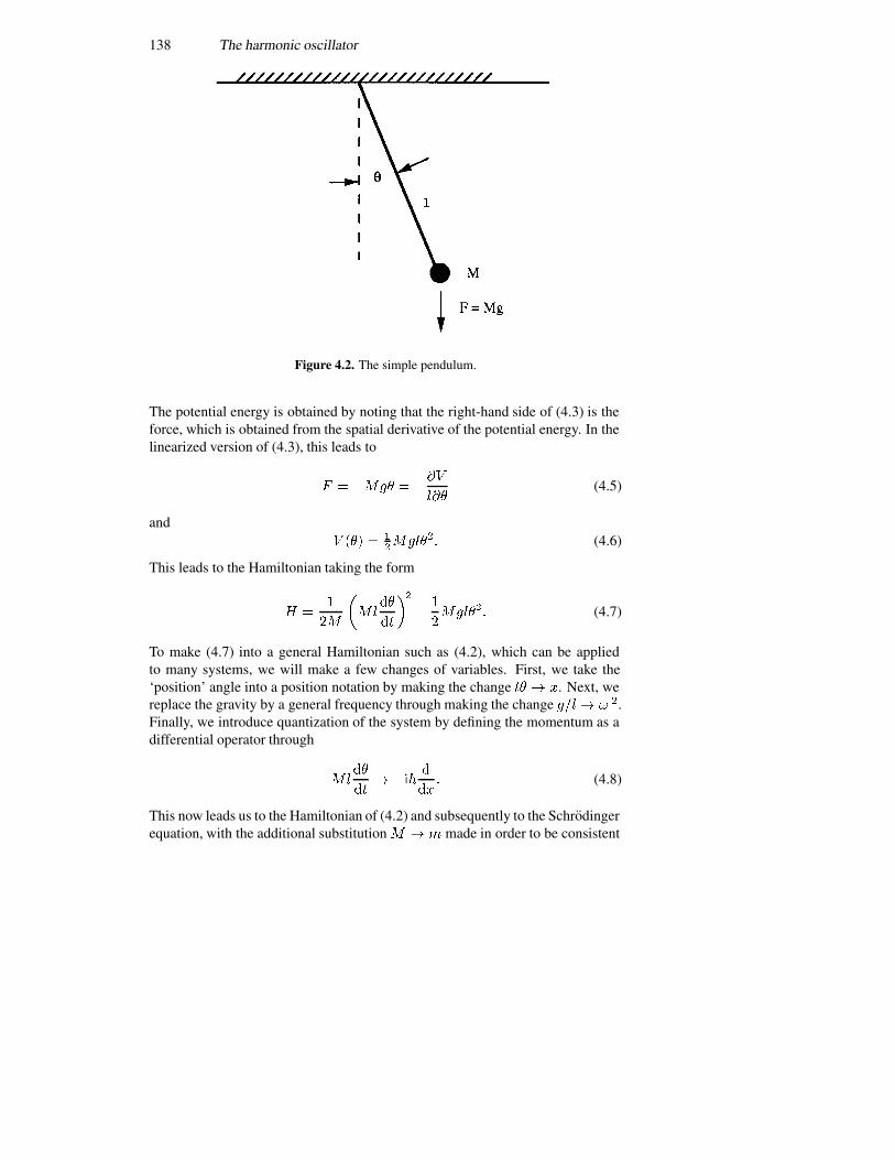
138 The harmonic oscillator
Figure 4.2. The simple pendulum.
The potential energy is obtained by noting that the right-hand side of (4.3) is theforce, which is obtained from the spatial derivative of the potential energy. In thelinearized version of (4.3), this leads to
� � ���� � ���
���(4.5)
and� ��� � �
������� (4.6)
This leads to the Hamiltonian taking the form
� ��
��
���
��
�
���
�
������� (4.7)
To make (4.7) into a general Hamiltonian such as (4.2), which can be appliedto many systems, we will make a few changes of variables. First, we take the‘position’ angle into a position notation by making the change �� � . Next, wereplace the gravity by a general frequency through making the change ���� � �.Finally, we introduce quantization of the system by defining the momentum as adifferential operator through
����
�� ���
�
�� (4.8)
This now leads us to the Hamiltonian of (4.2) and subsequently to the Schrodingerequation, with the additional substitution � � made in order to be consistent
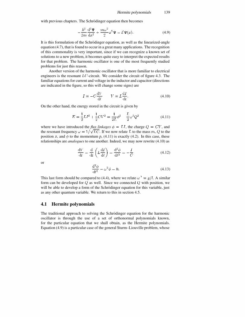
Hermite polynomials 139
with previous chapters. The Schrodinger equation then becomes
�
��
��
���
�������
���� � ������ (4.9)
It is this formulation of the Schrodinger equation, as well as the linearized-angleequation (4.7), that is found to occur in a great many applications. The recognitionof this commonality is very important, since if we can recognize a known set ofsolutions to a new problem, it becomes quite easy to interpret the expected resultsfor that problem. The harmonic oscillator is one of the most frequently studiedproblems for just this reason.
Another version of the harmonic oscillator that is more familiar to electricalengineers is the resonant ��-circuit. We consider the circuit of figure 4.3. Thefamiliar equations for current and voltage in the inductor and capacitor (directionsare indicated in the figure, so this will change some signs) are
� � �� ��
��� � �
��
��� (4.10)
On the other hand, the energy stored in the circuit is given by
��
���� �
�
��� � �
�
��� �
�
����� (4.11)
where we have introduced the flux linkages � �� , the charge � � �� , andthe resonant frequency � � ��
���. If we now relate � to the mass �, � to the
position �, and to the momentum , (4.11) is exactly (4.2). In this case, theserelationships are analogues to one another. Indeed, we may now rewrite (4.10) as
��
���
�
��
����
��
��
��
���� � �
�(4.12)
or��
���� �� � �� (4.13)
This last form should be compared to (4.4), where we relate � � � ���. A similarform can be developed for � as well. Since we connected � with position, wewill be able to develop a form of the Schrodinger equation for this variable, justas any other quantum variable. We return to this in section 4.5.
4.1 Hermite polynomials
The traditional approach to solving the Schrodinger equation for the harmonicoscillator is through the use of a set of orthonormal polynomials known,for the particular equation that we shall obtain, as the Hermite polynomials.Equation (4.9) is a particular case of the general Sturm–Liouville problem, whose
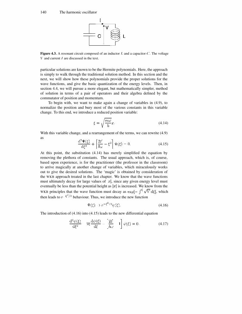
140 The harmonic oscillator
Figure 4.3. A resonant circuit composed of an inductor � and a capacitor �. The voltage� and current � are discussed in the text.
particular solutions are known to be the Hermite polynomials. Here, the approachis simply to walk through the traditional solution method. In this section and thenext, we will show how these polynomials provide the proper solutions for thewave functions, and give the basic quantization of the energy levels. Then, insection 4.4, we will pursue a more elegant, but mathematically simpler, methodof solution in terms of a pair of operators and their algebra defined by thecommutator of position and momentum.
To begin with, we want to make again a change of variables in (4.9), tonormalize the position and bury most of the various constants in this variablechange. To this end, we introduce a reduced position variable:
� �
���
��� (4.14)
With this variable change, and a rearrangement of the terms, we can rewrite (4.9)as
������
����
���
��� ��
����� � �� (4.15)
At this point, the substitution (4.14) has merely simplified the equation byremoving the plethora of constants. The usual approach, which is, of course,based upon experience, is for the practitioner (the professor in the classroom)to arrive magically at another change of variables, which miraculously worksout to give the desired solutions. The ‘magic’ is obtained by consideration ofthe WKB approach treated in the last chapter. We know that the wave functionsmust ultimately decay for large values of ���, since any given energy level musteventually be less than the potential height as ��� is increased. We know from the
WKB principles that the wave function must decay as ��� � ��� ���, which
then leads to ������ behaviour. Thus, we introduce the new function
����� ����������� (4.16)
The introduction of (4.16) into (4.15) leads to the new differential equation
������
���� ��
�����
���
�����
�
����� � �� (4.17)
Hermite polynomials 141
At this point, no more magic is possible. We have forced the overall wavefunction to have the decay properties expected from WKB considerations. Now,the resulting equation, (4.17), does not have a recognizable form (for the novice),and the hard work must begin.
It is possible that the solutions to (4.17) are in terms of some specialfunctions discovered by a mathematician long ago, but unless we are experiencedthis is not an obvious result. Therefore, we take a tried and true brute-forceapproach. We shall assume a polynomial solution, with terms of the form � �.In fact, we do know some properties of the solutions. First, we have a second-order differential equation in position, and two boundary conditions (vanishingof the wave function) for large positive and negative �. Thus, we expect to havetwo independent solutions. We also know that the potential is an even function,so we expect the wave functions to be of either even or odd parity; for example���� � ������. In looking for two independent solutions, we will keep thisparity in mind, since it is quite likely that one solution will have one parity, whilethe second will have the opposite parity. We also know that the reduced wavefunctions ���� have these same properties, plus they must diverge less rapidlythan the exponential for the overall wave functions to vanish for large �. It turnsout that this is an enormous collection of information, which will prove quitesufficient for solving the problem completely!
Now, with the above considerations fully in mind, we make the substitutioninto (4.17) of a power series in the form
���� ��
�
����� (4.18)
This leads to the equation
�
�
����� �����
���� �����
� �
���
��� �
����
�
�� �� (4.19)
We make the change � � � � � in the first term of the series, so that each termis of the same order in �. For the series to vanish, as required by the differentialequation, each coefficient of each power of � must also vanish. This leads to aniterative relation
���� � ������ � �� ��
��� ����� ����� (4.20)
This result is excellent for our preconceived expectations. First, only even termsor odd terms (in the exponents of the power series (4.18)) are coupled. Thus,the even series and the odd series are the two independent solutions. Secondly,�� and �� are the two constants needed for the second-order differential equationand each of these two governs only one of the two independent solutions. Thus,the needs for parity and two independent solutions are both satisfied. Finally,we can ensure that the solutions do not diverge for large values of the variable �only if we terminate the series at some finite value of �. (If we do not terminate
142 The harmonic oscillator
the series, (4.20) tells us that the reduced wave function will diverge as � ��
forlarge ���, which diverges faster than the exponential factor introduced in (4.16).Thus, we must terminate the series at some finite order.) Which value should wechoose? It doesn’t matter. We recall that in a Fourier series expansion, we getan entire family of solutions with different values of �. The same is true here.Each choice of � gives one member of the entire family of solutions. Thus, inorder to terminate the solutions for some value of �, we set the numerator of theright-hand side of (4.20) to zero, which leads to
�� � ��� �
���� � � �� �� �� �� � � � � (4.21)
This equation is perhaps the most important one to come from considering theharmonic oscillator. It clearly tells us that the modes of vibration of the oscillatorare quantized. Each allowed mode has a particular amplitude given by theappropriate wave function for that value of �, and the energy stored in that modeis given by (4.21). If we want to give the oscillator more energy, it must be byat least one quantum of value �� and this lifts the oscillator into a higher-lyingstate with a wave function of higher index �. Similarly, if the oscillator is to loseenergy, it must do so in units of ��, and consequently drops into states with wavefunctions of lower index �. It is found that the problems that can be put into theharmonic oscillator form are those that involve particles that have integer spin, andare thus termed bosons (for the appearance of Bose–Einstein statistics). Examplesare photons (light particles of integer spin) and phonons (lattice vibrations of zerospin). Each quantum unit of excitation for these particles comes in units of ��,and these are said to be single photons, or phonons, or some other type of boson.
The actual solutions to (4.17) are polynomials known as the Hermitepolynomials. The two constants �� and �� are taken to have an actual value setby normalization considerations. For this purpose, we modify (4.20) to
�� � ���� ���� ��
���� ������ � � �� (4.22)
The initial sets of these polynomials can be found from (4.21) and (4.22) as (weassign an overall sign that makes the highest-power term positive)
����� � �
����� � �� � �
����� � ��� � ��� � �� (4.23)
for the even-symmetry functions, and
����� � ��
����� � ��� � ���
����� � ���� � ���� � ���� (4.24)

The generating function 143
Figure 4.4. The lowest four weighted Hermite polynomials.
for the lowest odd-symmetry functions. The coefficients of the leading terms areset by a condition, discussed below, relating to the generating function, but do notprovide normalization. The actual normalization will be described below with amethodology that does not require us to integrate each and every function. Weplot four of these in figure 4.4.
4.2 The generating function
At this point, we diverge from the main line of discussion in order to developsome general properties of the Hermite polynomials, properties such as thenormalization and orthonormality properties. This is most efficiently done byusing what is known as a generating function, which we define in the following
144 The harmonic oscillator
manner:
� ��� �� �
��
���
��
�������� (4.25)
The generating function is determined as a power series in �, with the coefficientsgiven by the Hermite polynomials of the appropriate order. Our problem now isto determine what the proper form of � ��� �� should be.
To begin the task of identifying the function � ��� ��, we shall take thederivative with respect to the argument of the Hermite polynomials. This leads to
��
���
��
���
��
��
������
��� (4.26)
Now we must identify the last partial derivative. If we look carefully at the sixlowest-order Hermite polynomials given at the end of the last section, it may beseen that for these
������
��� ���������� (4.27)
This is a general result that can be established from the properly normalizedpower series representations for the Hermite polynomials. The proof is left tothe problems. Using (4.27), we find that
��
��� ��� ��� �� (4.28)
and� ��� �� � � ��� ������ � (4.29)
The coefficient may be obtained from (4.25) as
� ��� �� �
��
���
��
�������� (4.30)
Again, by looking at the first six Hermite polynomials in the preceding section,we observe immediately that for � odd, all of them vanish at 0, which is requiredby their anti-symmetric behaviour. For the even values, we note that we can castthe three even ones in the form ������������������, which leads to the values����� �������� � � � for � � �� �� �� � � � � . We insert this directly into (4.30), andthen make the change of index � ���, so that we achieve
� ��� �� �
��
���
���
������ � ���
�
� (4.31)
Finally, we can write the generating function as
� ��� �� � ����
���� � ���������� � (4.32)

The generating function 145
This result is based upon our rather free manner in which the coefficient of thelowest-order term was obtained. Thus, the relations that we are using are all basedupon this first assumption, and we must eventually show this to be the proper case.
By the use of the generating function, we can find a general relationship forthe Hermite polynomial. To begin, we note that the generating function (4.25) hasbeen defined so that
����� �
���
���� ��� ��
����
� (4.33)
Using (4.31), this leads to
����� �
���
�����
��������
����
�
���
� ��
����������
�
����
�
���
� ��
����������
�
���������
� �������� ��
������
�
� (4.34)
While one might jump to the use of this to verify the initial values used inthe definitions of the Hermite polynomials in this last section, recall that thesedefinitions were built into the generating function, and should naturally resultfrom its use. However, it is this simple formula for the Hermite polynomials thatleads to the coefficients found in (4.23) and (4.24). Thus, it is actually (4.34) thatgives us the lower-ordered Hermite polynomials listed in these latter equations.
The orthonormality of the Hermite polynomials can be examined throughthe use of combinations of the generating functions. Consider, for example, theintegral
� �
��
��
� ��� ��� ��� ������
��
�
��
��
������������
�����������
�
��
� ������
��
���������� ��
������� �
����
������
��� (4.35)
Now, on the other hand, instead of the generating functions, we use the seriesexpansions in terms of Hermite polynomials, as
� �
��
��
�����
��
�������
�����
��
�������
��� ��
146 The harmonic oscillator
�
��
���
��
��
��
���
��
��
��
��
�������������� ��� (4.36)
The two equations (4.35) and (4.36) must be exactly equal term by term, becausewe began with two equivalent formulations. Thus, terms in (4.36) for which� �� � must vanish in the integral of (4.36), which provides the orthogonalityof the Hermite polynomials. When � � �, equating the proper terms in (4.35)and (4.36) leads to �
�
��
�������������� �� �
�������� (4.37)
where �� is the Kronecker delta function, and is unity for � � � and zerootherwise. Now, the truth is found; the values of the lowest-order terms forthe Hermite polynomials in the previous section, and that we used to get thegenerating functions, do not normalize the wave functions. In fact, they arisefrom the convenient relation (4.34), obtained from the generating function, butthe orthonormal forms of ���� used, for example, in (4.18) must be rewritten as
����� �������
��
�
��������� (4.38)
and the full wave function is
���� �������
��
��
���������
������
���
�
�� (4.39)
4.3 Motion of the wave packet
In the classical harmonic oscillator, which is our simple linear pendulum, theposition of the pendulum oscillates back and forth across the point � � , whichis the point � in the present coordinates. We want to examine this effect onthe quantized harmonic oscillator, and the quantized wave functions describingthis oscillator. We can write the total wave function, at � � , as
�� � ���
������ (4.40)
where the expansion wave functions are our normalized, and generalized, Hermitepolynomials described by (4.39). Just as in (2.100), the expansion coefficients � �are given by
�� �
��
��
������� � �� (4.41)
We also need to recall that the fact that the probability must sum to unity requiresthat �
�
����� � �� (4.42)
Motion of the wave packet 147
We use (4.21) and (2.93) to write the time-varying total wave function as
���� �� � ��������
�
������������� (4.43)
where we recall that � is defined by the force (we replaced the gravitation constantby the square of the frequency). Thus, this frequency is not a variable, but definesthe force constants of the problem.
If we calculate the average energy in the harmonic oscillator, we do so bythe use of (1.17), or
��� � ��� ��� ��
�
������� (4.44)
so the measured energy is a weighted average of the energy values of thequantized levels of the harmonic oscillator. The probability of any particularenergy eigenvalue �� is given by �����. Again, we may use (1.17) to computethe average position � as
��� ��
�
���
�
�
�����������
��
��
������������ ��
���
���
��
�������������� (4.45)
where the last line defines the matrix element ��� between the two differentgeneralized Hermite polynomials. We need to compute this quantity to determinethe various values of the average position as a function of time. Now, the integralmay be expressed as
��� ���
��������
��
��
������������������� ��
�
��
��������
�
�
��
��
����
����������� �� (4.46)
where we have re-introduced the reduced space variables. The approach toevaluate this expression follows that utilizing the generating function that led to(4.35). Consider the integral
� �
��
��
� � � ��� ��� ���������
��
�
��
��
�����������
��������������
�
��
� �������������
��
��
����������� ��
��������
��������
�����
�� ���
��
��
���
�
�
����� ��
��� (4.47)
148 The harmonic oscillator
Now, by the same token, we can utilize the opposite side of the integral, obtainedfrom (4.36), as
� �
��
��
�����
��
�������
�����
��
��������
������ ��
�
�����
��
��
�����
��
��
��
��
������������
������
�����
�
��� (4.48)
The term that we are interested in has � � � in both (4.47) and (4.48). Moreover,we must set � � in (4.47). This leaves us with terms like ������ �� in (4.47),while in (4.48) the terms are like ����. In comparing these two terms, we see that� � �� �. From this relationship, we can write the equivalence (for � � �) as
������������ ��
��� �
��
��
��
����� (4.49)
or��� � ��
�������� �����
�������� (4.50)
where, for the second term, one replaces � by ��� on the left-hand side of (4.49).Caution must be exercised at this point, because the Hermite polynomials are notcompletely orthogonalized in these expansions, but this is corrected when we usethis result in (4.46), which leads to
��� �
��
�
��� �
������
��
������
�� (4.51)
The matrix element couples one level only to that level just above or below it.Thus, the position increases in time by moving from one energy level to the nexthigher (or next lower) excitation level. Finally, the average of the position is givenby
��� ���
�����
��������������
�
��
�
��
�����
�����������
��� �
������
��
������
�
�
��
��
�����
�����������
��� �������������� (4.52)
The basic time dependence is clearly determined by the force parameters throughthe frequency and mass.
Computing the average of the momentum is a somewhat more direct process.For this, however, we will use a symmetrized version:
��� � ���� ������� (4.53)
A simpler approach with operators 149
in order to ensure that the result is a real quantity. As for the case of the position,we expect that this will result in a series:
��� ��
�
���
�
�
�������������� (4.54)
where
��� ���
���������
��
��
������������������� ��
�
��
��������
��
�
��
��
����
��������� � (4.55)
and the momentum operator is in the reduced coordinates. Now, using thesymmetrized form of the momentum leads us to the representation of the integralas
�� � ��� ��� ����� � ��� ��� � ���� ��
� �
��
��
����
������
����� �����
�����
�
�� (4.56)
The derivative has been expressed earlier in (4.25), so the integral becomes
� ��
�
����������� � �������� (4.57)
which, when properly normalized through (4.52), becomes
��� � ���
���
������ �
��� �
������
� (4.58)
This now leads to the expectation of the momentum as
��� �
���
�
�����
����������
��� � ������������� (4.59)
It is reassuring that if we develop ��� � � ������� using (4.52), the same answeris obtained for the expectation value of the momentum, as expected from thetreatment of section 2.8.1 and equation (2.96). We also note that the momentumincreases or decreases on moving from one energy level to the next higher, orlower, respectively, energy level.
4.4 A simpler approach with operators
The Hamiltonian developed for the harmonic oscillator is doubly quadratic; thatis, it contains one term quadratic in the momentum and one term quadratic in the
150 The harmonic oscillator
position. We want to rearrange this Hamiltonian, by introducing a set of operatorsthat combine the position and momentum in a way that leads to a simpler approachto the problem. The rationale is based upon the fact that we have discovered thatboth the position and momentum expectation values vary by the ‘jump’ of thestate from one eigenfunction to another by moving up or down in the energylevels. We suppose that a proper combination of the individual operators willprovide a new set of operators that corresponds only to upward movement, or onlyto downward movement, among the energy levels. This will be the case, and asa result the entire approach becomes somewhat simpler. Because of the variouscoefficients in the Hamiltonian, the operators will be defined by combinationsof these coefficients as well; the guiding principle will be that the Hamiltonianshould be a simple product of the resulting operators.
With the above concepts in mind, we begin by defining the pair of adjointoperators in terms of the position and momentum operators as
� �
���
� �
��� �
�
��
�(4.60a)
�� �
���
� �
��� �
�
��
�� (4.60b)
These operators may be combined in the manner
��� ���
� �
��� �
�
��
���� �
�
��
�
��
��
���
������
�����
�
�(4.61)
or, upon comparing with the Hamiltonian,
� � ������� �
��� (4.62)
By comparing with the energy in (4.21), we assume that the product is the numberof particles in a level, so this product is called the number operator. We will showbelow that this product of operators (unusually) produces a non-operator, called a�-number (for constant number), that gives the quantum number of the energylevel corresponding to a particular state, when operating on the Hamiltonianeigenstates.
The momentum and position operators satisfy a basic commutator relationsince they are non-commuting operators. We expect that the above operators arealso non-commuting since they arise from combinations of these non-commutingoperators. The reverse product to (4.61) is given by
��� ���
� �
��� �
�
��
���� �
�
��
�
��
��
���
������
�����
�
�(4.63)
A simpler approach with operators 151
and so��� � ��� � �� (4.64)
This establishes the desired commutator relation. We note that both terms in(4.64) are �-numbers, from which the Hamiltonian can be defined.
The operator pair ��� is a �-number, so if we multiply a function by thisquantity, when the function is one of the eigenfunctions of the harmonic oscillatorHamiltonian, we expect to obtain the corresponding eigenvalue, that is
����� � ���� (4.65)
and similarly for the opposite choice of ordering, where �� is the eigenvalue stillto be determined (but that we expect to be �). Certainly, �� is positive, since
���� ������ � ����� ���� � �� (4.66)
Suppose that we operate with this operator on a state that has been arrived at fromthe product ����. Then,
��������� � ������� ���� � ����� � ���� � ��� � ������� (4.67)
Thus, if the wave function (and state)�� has the eigenvalue ��, then operating onthis state with the operator �� produces a new state with the eigenvalue (����).In essence, we have ‘kicked’ the energy of the initial state upward by one unit(which may be observed by reference to the Hamiltonian), and produced a newwave function corresponding to the level of higher energy. By the same token, ifwe operate with �, we find
�������� � ���� � ����� � ��� � ������ (4.68)
Thus, operating with the operator � produces a new state with the eigenvalue(�� � �). In essence, we have ‘kicked’ the energy of the initial state downwardby one unit, and produced a new wave function corresponding to the level oflower energy. For these reasons, we normally refer to �� as a raising operator(or creation operator since it creates one additional unit of energy in the system)and � as a lowering operator (or annihilation operator, since it destroys one unitof energy).
Now, there is always a lowest-energy state, the ground state. In the harmonicoscillator, it corresponds to � � �, the state in which the Hermite polynomial isjust ��. Thus, if we try to lower the energy, and kick the state down by one unit,by operating with the lowering operator, the result must be zero:
��� � �� (4.69)
This means that �� � �, and by the repeated use of (4.67), we find that
�� � � (4.70)
152 The harmonic oscillator
as expected. We can also use (4.69) to determine the eigenfunctions, since
��� �
���
��
��� �
�
��
��� � �� (4.71)
Rearranging the terms leads to the first-order differential equation (already animprovement over the differential equation for the Hermite polynomials)
�
�
��
���
��� ��� (4.72)
and
����� � �� �
��
����
��
�(4.73)
which may be recognized as �� with its exponential weighting function. Bydirect normalization, we find that
�� ����
��
����� (4.74)
From (4.64), we find that we can use (4.73) and (4.74) to show that
�� � ������� ����
��
���� ��� �
�
��
����� (4.75)
Thus, by simply solving the one first-order differential equation, we can now usethe simple differential operators to find the wave function for any energy level inthe harmonic oscillator!
We now want to turn to the expectation values of the operators themselves.From the basic properties expressed in (4.64) and (4.65), we know that forunnormalized wave functions such that ������ � ��
�, we can write (we takethe coefficients as real)
��� ����� � �������� � �������
�� (4.76a)
��� ���� � �������� � �� ���� ����� (4.76b)
We still have to determine the constants � and ��, which in fact are related tothe normalization of the eigenfunctions (the two eigenfunctions in the expectationvalue have different normalization constants). For this, we use
���� ���� � ��� ������ � ���
� � ���������� � ����� (4.77)
and���� �
����� (4.78)
We could as easily have found this value by extending the arguments that led to(4.74) and the earlier discussion of �, but it is instructive to repeat the work

Quantizing the ��-circuit 153
and reinforce this point of understanding. Thus, we find that �� � ������� ���� �, and the normalized relationship becomes
���� ����� � ��������� �
��� ������� (4.79a)
Similarly, �� � ������� ���, and the normalized relationship becomes
���� ���� � ��������� ��������� (4.79b)
These now lead to
� ���
��� ���������� (4.79c)
In these, � begins with 1 and works upward, just as was done in (4.52) and (4.59).We can now use (4.61) to find the expectation of the momentum and position as
�� �
��
������ ����� (4.80a)
�� � � �
����
���� ������ (4.80b)
To complete the form shown in the previous equations, we perform the doublesum over the two sets of wave functions, including the temporal variation fromthe energy levels. It must be concluded that taking this approach is considerablysimpler and easier to accomplish than taking that of the previous section, and it isfor this reason that special operators like the raising and lowering operators havecome to be used so extensively.
We note from the form of ����� that there can be � particles in a givenmode; that is we may excite the harmonic oscillator to contain many units of thequantized energy. This means that these particles cannot be subject to the Pauliexclusion principle. If they were subject to the Pauli exclusion principle, therecould be no more than two particles (of opposite spin) in this harmonic oscillator.Indeed, the product ��� is called the number operator, in which its action onthe wave function produces the number � of that wave function, which yields thenumber of excited levels we have. Particles which do not obey the Pauli exclusionprinciple, and which can be described by these harmonic oscillator states, arecalled bosons. This is in contrast to particles which satisfy the Pauli exclusionprinciple and are called fermions, as they obey Fermi–Dirac statistics as well. Wewill treat the creation and annihilation operators for fermions in section 9.4.
4.5 Quantizing the ��-circuit
The ��-circuit is one of the most pervasive systems found in electricalengineering. It represents not only a range of filters, but also the resonant cavity ofmicrowave circuits. In this section, we want to show that the quantum mechanics
154 The harmonic oscillator
of the ��-circuit is essentially that of the linear harmonic oscillator. To begin,we consider the energy stored in the ��-circuit at any instant of time (we take aparallel ��-circuit, but this is not an important assumption and does not appearanywhere in the treatment). We can write the energy stored as
� � �
��� � � �
����� (4.81)
The first term on the right-hand side is the energy stored in the capacitor, while thesecond term is that stored in the inductor. In fact, we can proceed immediatelyto proclaim that this is the Hamiltonian that we should use in the Schrodingerequation. However, before we can do that, it is still necessary to identify theconjugate operators and their relationship to each other.
One obvious possibility is to take the charge � ���� � as one operator andthen the current � � ����� as the other (in analogy between the position andthe velocity). However, this doesn’t quite work out. The analogy would havethe current as the velocity (of the charge) and not the momentum. We can beguided by our understanding that the two fundamental quantities in circuits arethe charge and the flux. It is these two quantities that are invariant in specialrelativity theory and it is these two that are subject to important conservationlaws in circuit theory—the conservation of charge and the conservation of fluxlinkages. Moreover, the flux linkage in the present context is just the flux in theinductor, given by � � �� . In section 3.8, we took the charge as the ‘momentum’,but here it is better to take the charge as the ‘coordinate’ variable, and take the fluxas the ‘momentum’ variable. If this is done, we can rewrite (4.81) as
� ���
���
��
��� (4.82)
By introducing the resonant frequency through � � ����, this can be rewrittenas
� ���
��� ��
��
�� (4.83)
Thus, if we make the connection � � , this is the same equation as (4.13).Hence, we find that the resonant circuit is just a simple harmonic oscillator.
Finally, let us look at the commutator of charge and flux, when theseare interpreted as operators. By making the analogy between the flux and themomentum coordinate, and between the charge and position coordinate, we havefrom (1.27) the relationship
� � ����
��(4.84)
which satisfies the commutator relationship
���� � ���� (4.85)
In this interpretation, the charge and flux are non-commuting variables, with theflux interpreted as the variation with respect to the charge. On the other hand, this

The vibrating lattice 155
relationship vanishes in the classical limit as �� �. In this latter limit, charge andflux are independent quantities, but in the quantum case they are not independentand cannot be simultaneously measured.
The interpretation of the ��-circuit as a linear harmonic oscillator meansthat the energy in the resonator is a fixed quantity that is given in terms of theresonant frequency by (4.21). Energy storage can be increased or decreased onlyin units of the energy quantum �� � ��
���. Thus, the photons that enter
or leave an electromagnetic cavity (circuit) have well defined energies in termsof the resonant frequency of the cavity. This is obvious in the measurementof the frequency of the oscillating cavity, where we measure the energy of thephotons emanating from the cavity. However, it is often useful to consider theresonant circuit quantum mechanically rather than classically. We have the fullunderstanding of this in terms of the harmonic oscillator results of the previoussections.
With this discussion, it is now clear that electromagnetic waves satisfythe resonant ��-circuit, which itself is a linear harmonic oscillator. Wepreviously established that the particles which satisfied the harmonic oscillatorwere bosons. Thus, it is clear that photons, the particles which are associatedwith electromagnetic waves, are bosons. The photons actually have spin, butit is quantized into values of ��, corresponding to the circular polarization ofthe plane-wave of electromagnetics. Thus, we may say that bosons have integervalues of spin, while fermions have half-integer values of spin.
This approach also opens the door to a treatment of almost any oscillatorybehaviour to be treated by a quantum approach. As here, one only needsto identify the proper generalized coordinates, which are then subjected to anuncertainty principle. It is this step that introduces the quantum nature of thesubsequent solutions in terms of harmonic oscillator coordinates. Generalizedcoordinates have long been treated in classical mechanics, and their use naturallyflows over to quantum mechanics.
4.6 The vibrating lattice
In a solid, the motion of the atoms is much like the motion of free particles, withthe important exception that the atoms are forced on average to retain positionswithin the solid that specify a particular crystal structure (we can also treat non-crystalline solids by similar methods, but our approach here will be limited to thecrystalline solids, where the atoms are equally spaced on a lattice). In any realsolid, the lattice is a three-dimensional structure. However, when the motion isalong one of the principal axes of the structure, it is usually possible to treat theatomic motion as a one-dimensional system. Although this is a simple model, itsapplicability can be extended to the real crystal if each atom represents the typicalmotion of an entire plane of atoms normal to the wave motion.
The total Hamiltonian for the atomic motion is given by the momentum of
156 The harmonic oscillator
the individual atoms plus the potential that keeps the atoms in the lattice positions(on average). We can write this Hamiltonian as
� ��
�
� �
�
���
��
� ���
� ��� ����� (4.86)
In general, the atoms will vibrate around their equilibrium position, just like littleharmonic oscillators. However, all of these oscillators are coupled through thepotential term in (4.86). We have studied only the single oscillator. How will wetreat the coupled oscillators? The answer to this is that we do a Fourier transforminto the dominant Fourier modes of the overall vibration, and this will result inus obtaining a set of uncoupled oscillators, one for each mode of vibration of theentire set of coupled oscillators. Each of these modes will then be quantized, andthe quantum unit of amplitude of each of the modes is termed a phonon.
The Hamiltonian in (4.86) describes the motion of the atoms about theequilibrium (or rest) positions. We expect this motion to be small, so shall usea Taylor series expansion about these equilibrium positions, and
� ��
�
� ��
���
��
�
�
� ���
������� ��� ����
������
� � � � � (4.87)
The zero-order term in the potential is just an offset in energy and will be ignored,while the first partial derivative term must be zero if we are expanding about theequilibrium position. We also recognize that
�� ���
�����
� (4.88)
Now, we introduce the appropriate Fourier series for the displacement as
�� ���
�
�
������ (4.89)
where we assume that there is a lattice constant � that is the equilibrium distancebetween atoms and that, from some arbitrary reference point, � �� � ���. Here,�� is an integer specifying just how far along the chain of atoms the th atomresides in equilibrium. The last term in the Hamiltonian is the most complicatedone. This is given by the Fourier terms
���� ��
�
� ���
�����������
������ ��� ����
������
��
�
� ���
�����������������
��������� ��� ����
������
� (4.90)
We assume that the partial derivative can be treated as constant (but may varywith the particular mode). Each of the position vectors is expanded in terms of

The vibrating lattice 157
its equilibrium position and its absolute position. The first exponential dependsonly upon the relative positions, while the second exponential mainly treatsthe equilibrium positions (the deviations are small). Thus, we bring this lattersummation out to make a sum only over the equilibrium positions:
�
�
���������� ��
��
����������� � ������ � (4.91)
To achieve the last term, we assert that the summation over � � is a summationover all the Fourier modes, which by the principle of closure of a complete setmust vanish unless the coefficient itself vanishes. This leads to the Kroneckerdelta. The number � , which also appears in (4.87), is the number of atoms inthe chain (and hence the number of Fourier modes). The remaining part of thepotential is just (summing over � �, with ���� � ���
�� ��
� ���
���������������
��� ��� ����
������� (4.92)
The mode amplitudes can be brought out of the summation, and the remainder isdefined to be the spring constant for the particular mode � . The same summationover the lattice modes can be made in the kinetic energy term as well, and thisallows us to write the final result as
��
�
��
������� �
�
������
����
��
�����
�� �
�
����
��
�(4.93)
where
�� � �������
(4.94)
is the mode momentum, and we have used general properties of the Fouriercoefficients. By writing � � ���
� , we see that we have now obtained a setof uncoupled harmonic oscillators. Each mode is characterized by a wave vector� and frequency ��, and we can compute the wave functions as if that mode weretotally isolated with a mode energy described by (4.21). Thus, this particularmode may contain a great many phonons as described by the energy level numberfor the mode. The total energy of the lattice vibration is now just the sum overthe energy (and hence the number of phonons) in each mode and a sum overthe various modes. Quantization of the vibrations occurs by having the position�� and the momentum �� be non-commuting operators subject to a commutatorrelationship �� � �� � ���. We can at this point also introduce the creation andannihilation operators for each mode, which serve to create or destroy one unit ofamplitude for that particular mode. Thus, the number of units of amplitude (orenergy) in the mode of wave vector � is said to the number of phonons in thatparticular mode.
158 The harmonic oscillator
Because each mode of the lattice vibrations satisfies a harmonic oscillatorequation, these phonon modes are bosons. The atoms which constitute thevibrations are such that the phonon mode has zero spin, which counts as aninteger. In terms of the parameters of (4.93), the creation and annihilationoperators are written as
��� �
��
����
��� � �
��
���
�
�� �
��
����
��� � �
��
���
��
(4.95)
In terms of these operators, the amplitude of the �th Fourier mode is given by
�� �
����
����� � ��� � (4.96)
and the energy in this mode is
�� � ������ ��� �� (4.97)
The number of phonons in mode � is given by the Bose–Einstein distribution
�� ��
���������
�� �
(4.98)
which differs from the Fermi–Dirac distribution by the sign in the denominatorand the lack of a Fermi energy. All bosons satisfy this distribution but, as withthe Fermi–Dirac distribution, the limiting case in which the factor of unity can beignored gives the classical Maxwell–Boltzmann distribution.
Finally, we need to address the question of just how the wave vector � andthe frequency �� are related to each other. For this, we return to real space, butwill use the fact that the Fourier modes require the motion to exist as a set ofwaves with propagation according to � ���������. Thus, if we write the equationof motion of any particular atom at position �, we obtain from (4.86)
�����
� � � �
�� ���
�� �� � ��
���
� ����� ���� ��� ����� (4.99)
where the approximation is that only the nearest neighbours are important, andwe have treated the potential as a linear spring. Because of the lattice behaviourof the waves, we can rewrite the last term as
������ � ������
���� �� � ������ � ��� (4.100)
Motion in a quantizing magnetic field 159
Figure 4.5. The relationship between the frequency and wave vector of a particular modeof lattice vibration.
and
��
� ���
���� ������� �
�
�����
����
�� (4.101)
Now, any range of � that spans a total value of ���� will give all allowedvalues of the frequency that can be expected (which is of course positive). Wegenerally choose this range to be ���� � � � ���, in keeping with the bandstructure arguments concerning periodic potentials in the last chapter. We showthese frequencies in figure 4.5. Real lattices can be more complicated, containingfor example, two different types of atom, or having the spacing between alternateatoms differing. In each case, the behaviour is more complicated, and motionof the two atoms together (low frequency) plus relative motion of the two atoms(high frequency) can occur. This is beyond the level we treat here, where we wantmerely to introduce the periodic potential as an example of a harmonic oscillator.
4.7 Motion in a quantizing magnetic field
The last example of a harmonic oscillator we want to consider is the motion of anelectron orbiting around magnetic field lines. Classically, the electron is pulledinto a circular orbit such that the magnetic field is directed normal to the plane ofthe orbit, and the motion arises from the Lorentz force acting on the electron:
� � ��� � ���� (4.102)
The charge on the electron has been taken to be its proper negative value. Clearly,for motion in the ��-direction (in cylindrical coordinates) and a magnetic field inthe ��-direction, the force is an inward centripetal force which causes the motionto be a closed circular orbit (ignoring the role of the electric field). Here, we want
160 The harmonic oscillator
to examine the quantization of this orbit, and will deal only with the electric fieldthat is induced by the magnetic field �, ignoring any explicitly applied field.
The approach we follow is exactly the one we used in section 1.3. Theaccelerative force on the wave momentum of the electron may be expressed as in(1.7) as
���
��� ���� (4.103)
In fact, we should use the entire Lorentz force in (4.103), but we want to introducethe magnetic field through the electric field that it produces. The approach is theone used in (1.8), but we will be somewhat more advanced here. The magneticfield produces the electric field through Faraday’s law, which may be expressedas
��� � ���
��� (4.104)
We now introduce the concept of the vector potential�, from which the magneticfield may be determined as
� ���� (4.105)
so (4.104) and (4.105) may be combined as
� � ���
��� (4.106)
Here, the vector curl operation has been dropped, which means that (4.105) issatisfied up to a quantity for which the curl vanishes. This quantity is just ���,where � is the scalar potential with which we usually define the electric field inquasi-static situations. Here, however, we want to define the electric field fromthe magnetic field alone, and hence from the vector potential that gives rise to themagnetic field. This suggests that if we now use (4.106) in (4.103), the propertotal momentum to use in the Hamiltonian is just the combined quantity
�� ��� � ���� (4.107)
While the substitution (4.107) has been derived and developed by a great manyworkers, it is usually referred to as the Peierls substitution in solid-state physics.
We are now interested in using this value for the momentum in theHamiltonian (4.2), except that we do not include any external potential.Nevertheless, the magnetic field will provide such a potential. To proceed, wemust decide upon the vector potential �. Our interest is in motion perpendicularto the magnetic field, which we take to be constant and oriented in the positive�-direction. Then, a vector potential defined as � � ���� will provide thismagnetic field. We note that this definition is only sufficient, as many otherdefinitions of the vector potential could as easily describe a uniform field in the�-direction. However, this particular definition, called the Landau gauge, will suitour purposes sufficiently well. Further, we will only treat the motion in the planenormal to the magnetic field.
Motion in a quantizing magnetic field 161
In the absence of any external potential, other than the vector potential givingrise to the magnetic field, Schrodinger’s equation can be written as
�� �
��
��
��
���
��
��
���� � �� (4.108)
where the wave momentum has been replaced by the normal gradient operatorfor the momentum. Expanding the momentum operator bracket leads to thedifferential equation
� ��
��
���
���� ����
��
�
���
��
��������
�
���� � ��� (4.109)
The motion in the �-direction is essentially free motion, at least within thisformulation of the Schrodinger equation, as the only deviation from the normaldifferential operators is the �-dependence arising from the magnetic field. Thus,we will take the wave function to have the general form
���� �� � ��������� (4.110)
With this substitution, (4.109) becomes
� ��
��
���
����
����
�� � �
����
�
��� � �� (4.111)
Our goal is to put this into a form reminiscent of (4.9), the equation for theHermite polynomials and the standard harmonic oscillator. To this end, weintroduce the cyclotron frequency �� � ����, and rewrite (4.111) as
� ��
��
��
�����
���� ��� ���
� � � (4.112)
where
�� ��
��(4.113)
and we recall that is the �-component of the wave motion. Comparison of thiswith (4.9) shows that the �-motion satisfies a harmonic oscillator equation, whichyields Hermite polynomials as solutions. Thus, the energy levels are given as
�� � ���� � �� � (4.114)
and the corresponding wave function is just
���� �����
����
��
���������������
������
�����
���� ���
��
(4.115)
162 The harmonic oscillator
These solutions are, of course, just the normal harmonic oscillator wave functionsshifted by the offset (4.113). Here, both the scaling factor and the offset dependupon the magnetic field, just as the cyclotron frequency does. Noting the argumentof the Hermite polynomial in (4.115) gives a natural scaling length described by���������, which is termed the magnetic length. To lowest order, the Hermitepolynomial has its peak at the position
���� � times this basic length, so this is
the natural cyclotron radius of the harmonic motion for a particular energy level.
4.7.1 Connection with semi-classical orbits
The form of the wave function (4.115) and the energy (4.114) do not give us aclear view of the orbiting nature of the electron in the magnetic field. True, itis a harmonic oscillator in the �-direction, but what about its other motion? Asremarked earlier, the electron orbits around the magnetic field, and this motion isa solution of (4.102), which we can rewrite as
���
��� ��� ��� (4.116)
The magnetic field is in the �-direction, according to the Landau gauge previouslyadopted, so that the motion in the �� �-plane is given by
������
� �����
������
� �����(4.117)
These two equations may then be solved, for an arbitrary initial condition, as
�� � �� �������
�� � �� �������(4.118)
Similarly, we can now find the position as
� �����
������
� � ����
��������(4.119)
We can now combine (4.118), (4.119), and (4.114) to give
� �
����
�� ������ �
�� �� �
����� ��
���
��
�� � �� � � ����
���
�
����� ��
�
���
(4.120)
The last line gives us the result hypothesized at the end of the previous section,����� is a magnetic length that gives us the radius of the lowest energy level and
Motion in a quantizing magnetic field 163
provides a natural scaling of the size of the cyclotron orbit around the magneticfield. The quantization of the orbit radius arises directly from the quantization ofthe energy levels of the harmonic oscillator. These quantized energy levels aretermed Landau levels.
One of the important aspects of the quantization in a magnetic field is the factthat the continuum of allowed momentum states is broken up by this quantization.The allowed states are coalesced into the Landau levels, and each spin-degenerateLandau level can hold
�� ��
����
���
��(4.121)
electrons. In some magneto-transport experiments, this quantization can be seenas oscillatory magnetoresistance, in which the periodicity in ��� arises from(4.121) as
�
��
�
��
�
����(4.122)
for spin-degenerate Landau levels. This oscillatory magnetoresistance is termedthe Shubnikov–de Haas effect. We return to it again in the following discussion.
4.7.2 Adding lateral confinement
Let us now consider what happens when the magnetic field is added to a simpleharmonic oscillator potential in the �-direction—that is, we confine the electronin the lateral �-direction and add an additional magnetic field in the �-direction.Hence, we combine the Hamiltonians of (4.9) and (4.111) to seek a solution of
�
��
��
��
�������
� � � �
���
��
���� �
�
������� � �� (4.123)
It is clear that this can now be re-arranged to give� �
���
��
�� � �
��
��
���
���� ����� �
�
����� � ��
�����
� �
��
��
���
�����
������� ���
�� ����
��
����
�
��(4.124)
where
�� � �� � ��
��� �
���
���� (4.125)
The motion remains that of a harmonic oscillator, but now the shift of the wavefunction and the energy levels are hybrids of the confinement harmonic oscillatorand the magnetic harmonic oscillator. Each energy level of the magnetic field,the Landau levels, is raised by the confinement to a higher value. In essence,
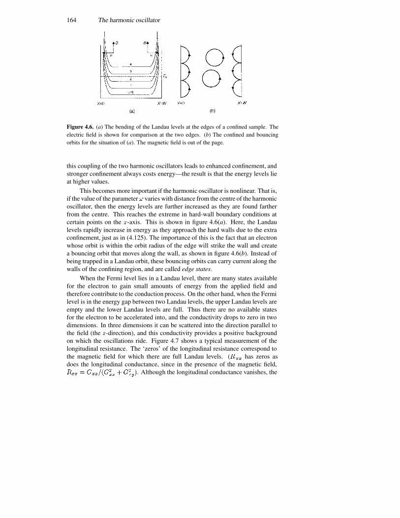
164 The harmonic oscillator
Figure 4.6. (a) The bending of the Landau levels at the edges of a confined sample. Theelectric field is shown for comparison at the two edges. (b) The confined and bouncingorbits for the situation of (a). The magnetic field is out of the page.
this coupling of the two harmonic oscillators leads to enhanced confinement, andstronger confinement always costs energy—the result is that the energy levels lieat higher values.
This becomes more important if the harmonic oscillator is nonlinear. That is,if the value of the parameter� varies with distance from the centre of the harmonicoscillator, then the energy levels are further increased as they are found fartherfrom the centre. This reaches the extreme in hard-wall boundary conditions atcertain points on the �-axis. This is shown in figure 4.6(a). Here, the Landaulevels rapidly increase in energy as they approach the hard walls due to the extraconfinement, just as in (4.125). The importance of this is the fact that an electronwhose orbit is within the orbit radius of the edge will strike the wall and createa bouncing orbit that moves along the wall, as shown in figure 4.6(b). Instead ofbeing trapped in a Landau orbit, these bouncing orbits can carry current along thewalls of the confining region, and are called edge states.
When the Fermi level lies in a Landau level, there are many states availablefor the electron to gain small amounts of energy from the applied field andtherefore contribute to the conduction process. On the other hand, when the Fermilevel is in the energy gap between two Landau levels, the upper Landau levels areempty and the lower Landau levels are full. Thus there are no available statesfor the electron to be accelerated into, and the conductivity drops to zero in twodimensions. In three dimensions it can be scattered into the direction parallel tothe field (the �-direction), and this conductivity provides a positive backgroundon which the oscillations ride. Figure 4.7 shows a typical measurement of thelongitudinal resistance. The ‘zeros’ of the longitudinal resistance correspond tothe magnetic field for which there are full Landau levels. (��� has zeros asdoes the longitudinal conductance, since in the presence of the magnetic field,��� � ������
�
�����
���. Although the longitudinal conductance vanishes, the
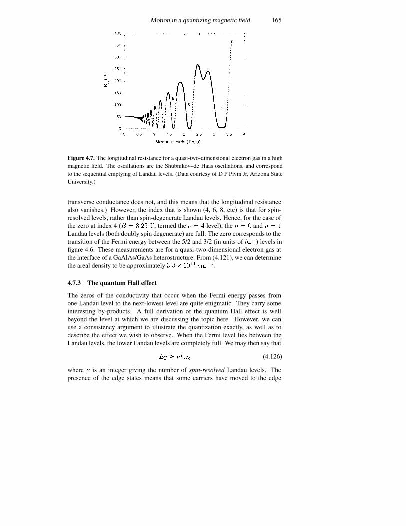
Motion in a quantizing magnetic field 165
Figure 4.7. The longitudinal resistance for a quasi-two-dimensional electron gas in a highmagnetic field. The oscillations are the Shubnikov–de Haas oscillations, and correspondto the sequential emptying of Landau levels. (Data courtesy of D P Pivin Jr, Arizona StateUniversity.)
transverse conductance does not, and this means that the longitudinal resistancealso vanishes.) However, the index that is shown (4, 6, 8, etc) is that for spin-resolved levels, rather than spin-degenerate Landau levels. Hence, for the case ofthe zero at index 4 (� � ���� �, termed the � � � level), the � � � and � � �
Landau levels (both doubly spin degenerate) are full. The zero corresponds to thetransition of the Fermi energy between the 5/2 and 3/2 (in units of �� �) levels infigure 4.6. These measurements are for a quasi-two-dimensional electron gas atthe interface of a GaAlAs/GaAs heterostructure. From (4.121), we can determinethe areal density to be approximately ���� ��
���
��.
4.7.3 The quantum Hall effect
The zeros of the conductivity that occur when the Fermi energy passes fromone Landau level to the next-lowest level are quite enigmatic. They carry someinteresting by-products. A full derivation of the quantum Hall effect is wellbeyond the level at which we are discussing the topic here. However, we canuse a consistency argument to illustrate the quantization exactly, as well as todescribe the effect we wish to observe. When the Fermi level lies between theLandau levels, the lower Landau levels are completely full. We may then say that
�� � ���� (4.126)
where � is an integer giving the number of spin-resolved Landau levels. Thepresence of the edge states means that some carriers have moved to the edge
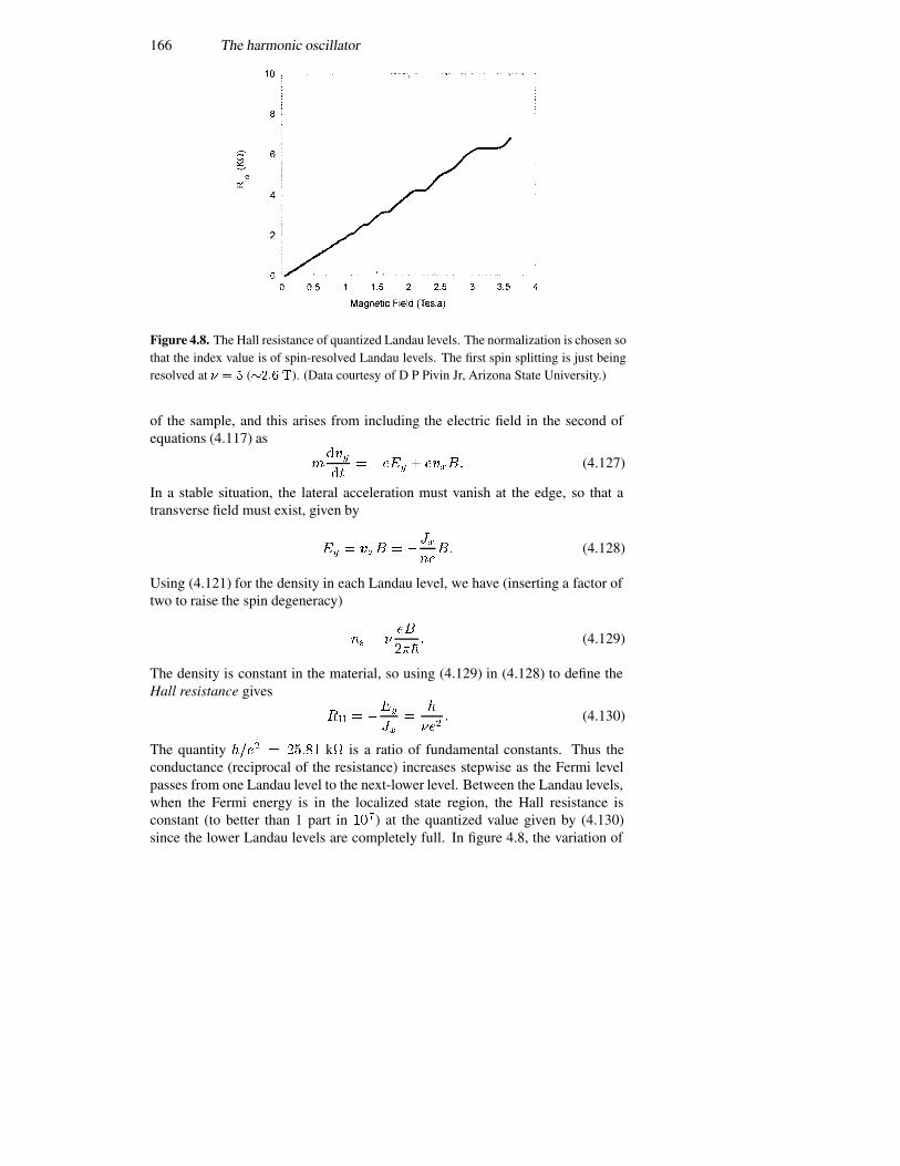
166 The harmonic oscillator
Figure 4.8. The Hall resistance of quantized Landau levels. The normalization is chosen sothat the index value is of spin-resolved Landau levels. The first spin splitting is just beingresolved at � � � (���� �). (Data courtesy of D P Pivin Jr, Arizona State University.)
of the sample, and this arises from including the electric field in the second ofequations (4.117) as
����
��� ���� � ����� (4.127)
In a stable situation, the lateral acceleration must vanish at the edge, so that atransverse field must exist, given by
�� � ��� � �����
�� (4.128)
Using (4.121) for the density in each Landau level, we have (inserting a factor oftwo to raise the spin degeneracy)
�� � ���
��� (4.129)
The density is constant in the material, so using (4.129) in (4.128) to define theHall resistance gives
� � ���
���
�
���� (4.130)
The quantity ���� � ����� k� is a ratio of fundamental constants. Thus theconductance (reciprocal of the resistance) increases stepwise as the Fermi levelpasses from one Landau level to the next-lower level. Between the Landau levels,when the Fermi energy is in the localized state region, the Hall resistance isconstant (to better than 1 part in ���) at the quantized value given by (4.130)since the lower Landau levels are completely full. In figure 4.8, the variation of
Motion in a quantizing magnetic field 167
the Hall resistance as a function of magnetic field for a typical sample is shown.These measurements were made in the same sample and geometry of figure 4.7,so that they can be easily compared.
The magnetic field could, of course, be swept to higher values in bothfigures 4.7 and 4.8. When this is done, new features appear, and these are notexplained by the above theory. Klaus von Klitzing received the Nobel prize forthe discovery of the quantum Hall effect (von Klitzing et al 1980). In fact, inhigh quality samples, once the Fermi energy is in the lowest Landau level, onebegins to see fractional filling and plateaus, in which the resistance is a fraction of���� (Tsui et al 1982). This fractional quantum Hall effect is theorized to arisefrom the condensation of the interacting electron system into a new many-bodystate characteristic of an incompressible fluid (Laughlin 1983). Tsui, Stormer,and Laughlin shared the Nobel prize for this discovery. However, the propertiesof this many-body ground state are clearly beyond the present level.
References
Ando T, Fowler A B and Stern F 1982 Rev. Mod. Phys. 54 437Born M and Huang K 1954 Dynamical Theory of Crystal Lattices (London: Oxford
University Press)Ferry D K 1991 Semiconductors (New York: Macmillan)Ferry D K and Goodnick S M 1997 Transport in Nanostructures (Cambridge: Cambridge
University Press)Hall J M 1967 Phys. Rev. 161 756Kroemer H 1994 Quantum Mechanics (Englewood Cliffs, NJ: Prentice-Hall)Landau L 1930 Z. Phys. 64 629Landau L and Lifshitz E M 1958 Quantum Mechanics (London: Pergamon)Laughlin R B 1983 Phys. Rev. Lett. 50 1395Merzbacher E 1970 Quantum Mechanics (New York: Wiley)Schiff L I 1955 Quantum Mechanics 2nd edn (New York: McGraw-Hill)Smith R A 1969 Wave Mechanics of Crystalline Solids (London: Chapman and Hall)Tsui D, Stormer H L and Gossard A C 1982 Phys. Rev. Lett. 48 1559von Klitzing K, Dorda G and Pepper M 1980 Phys. Rev. Lett. 45 494von Neumann J 1955 Mathematical Foundations of Quantum Mechanics (Princeton, NJ:
Princeton University Press)Ziman J 1964 Principles of the Theory of Solids (Cambridge: Cambridge University Press)
168 The harmonic oscillator
Problems
1. Using the WKB formula for the bound states of a potential well (3.71),compute the energy levels of a harmonic oscillator, whose potential is describedby (4.2).
2. Consider a simple, classical harmonic oscillator, whose amplitude ofoscillation is �. Show that this amplitude is related to the energy of the oscillatorthrough the formula
� �
���
���������� ��
where � is an arbitrary constant, which is unknown. If we consider that theprobability of finding the particle in the small increment �� is just the fractionof time spent in this interval during each period of oscillation, show that theprobability of finding the mass in a small region �� about � is 0 for ��� ��
������ and ��
������ � ���� for ��� ��
������.3. According to the previous problem, there is no chance classically for
a particle of energy ����� to be in the region ��� ��
�����. What is theprobability for a particle of this energy to be in this region quantum mechanically?
4. Using a series representation for the general Hermite polynomial of order�, which has been properly normalized, verify that (4.27) is valid. The series canbe developed from the coefficients in (4.22).
5. Using the generating function for the Hermite polynomials, compute � ��and ���. Can these results be obtained from a knowledge of the expectations ��and ��? What is the uncertainty in position and momentum?
6. Using the creation and annihilation operators, compute � �� and ���.How does the complexity of this approach compare with that in the previousproblem?
7. Determine the expectation values for the kinetic and potential energies ina harmonic oscillator.
8. Consider an electromagnetic resonator with a resonant frequency of� �� Hz. What is the energy separation of the oscillator levels? How does thiscompare with the thermal energy fluctuation?
9. If the velocity of sound ����� of a set of lattice vibrations is � � �� ���,and the lattice constant is � � �� nm, what is the phonon frequency at the zoneedge � � ���?
10. If one begins with the so-called symmetric gauge, where � ����������������, show that a more complicated harmonic oscillator solutionresults. Show that this still gives energy levels according to (4.113), and find theappropriate form of the wave functions that are the solutions.
11. Consider an electron moving in a �-directed magnetic field andconstrained in a quadratic potential �
����
��. In the simplest case, in which
the system is homogeneous in the �-direction, determine the energy levels of theelectron.
Problems 169
12. A semiconductor sample measures 1 cm by 0.5 cm and is 0.1 cm thick.For an applied electric field of 1 V cm��, 5 mA of current flows. If a 0.5 Tmagnetic field is applied normal to the broad surface, a Hall voltage of 5 mV isdeveloped. Determine the Hall mobility and the carrier density.
13. Consider a free-electron ‘gas’ with an areal density of � � ����
����.
What is the periodicity (in units of ���) expected for the Shubnikov–de Haasoscillation?
Chapter 5
Basis functions, operators, and quantumdynamics
In the past few chapters, we have developed the Schrodinger equation and appliedit to the solution of a number of quantum mechanical problems, mainly to developexperience with the results of simple and common systems. The results from theseexamples can be summarized relatively simply. In general, quantization entersthe problem through the non-commuting nature of conjugate operators such asposition and momentum. This has led to the Schrodinger equation itself as theprimary equation of motion for the wave function solution to the problem. Inessence, the system (e.g. the electron) is treated as a wave, rather than as a particle,and the wave equation of interest is the Schrodinger equation. When boundaryconditions are applied, either through potential barriers, or through the form ofthe potential (as in the harmonic oscillator), the time-independent Schrodingerequation yields solutions that are often special functions. Examples of this arethe sines and cosines in the rectangular-barrier case, the Airy functions in thetriangular-well case, and the Hermite polynomials in the harmonic oscillator case.
It is generally true that any time we examine a bounded system (even aclassical system), the allowed energy levels take on discrete values, each of whichcorresponds to a single one of the family of possible members of the specialfunctions. Thus, in the rectangular-well case, each energy level corresponds toone of the sinusoidal harmonics; in the harmonic oscillator, each energy levelcorresponds to one of the Hermite polynomials. In the set of levels, there isalways a lowest energy level, called the ground state. The higher energy levelsare referred to as the excited states, even when some are occupied in thermalequilibrium.
It should not be surprising that the set of all possible solutions to agiven problem formulation, for example the set of all sines and cosines forthe rectangular barriers, can be shown to form a complete set, and thus canserve as a basis for a many-dimensional linear-vector-space representation of theproblem. In the preceding chapters, we have not employed this terminology, but
170

Basis functions, operators, and quantum dynamics 171
rather treated the expansion in terms of these functions in a manner that had thetime variation appearing directly within the function itself. This is the normalSchrodinger picture, in which the so-called basis functions arise from solving theSchrodinger equation subject to the boundary conditions and these basis functionscontain any time variation. In this picture, the operators are not time varying, buttheir projection onto any of the basis functions is time varying. Here, the basisfunctions can be thought of as the unit vectors of a coordinate system, and theamplitudes such as those of (2.87) can be thought of as amplitudes along eachaxis of this coordinate system. In the Schrodinger picture, the coordinate systemrotates around the direction of the vector operator as a function of time. But thisis a relative view—it could as easily be that the coordinate system is fixed and thevector operator rotates in the coordinate frame in such a way that the projectionon any axis still varies with time in the prescribed manner. This picture, or view,is referred to as the Heisenberg picture of quantum mechanics (Heisenberg 1925).
We can think about this connection between the Heisenberg picture and theSchrodinger picture in a relatively simple manner. We have found that the wavefunction ���� �� evolves under the action of the Hamiltonian operator via thetime-dependent Schrodinger equation (2.8)
����
��� �� �
��
��
��
��
���� � ���
��� (5.1)
In a sense, this wave function evolves as described in (2.93), or
���� �� � ����������� ��� (5.2)
If we consider any arbitrary complete set of functions �������, such as the set ofbasis states for an infinite potential well lying in the range � �
����� �
��
�����
�(5.3)
we can expand the wave function as
���� �� ���
���������� (5.4)
The basis functions �� create a infinite set of coordinates, and the coefficients ���� are the projections of the wave function onto each of these coordinates.Hence, the basis states create an infinite-dimensional coordinate system, which isthe Hilbert space corresponding to these functions.
The rotation of the total wave function (5.2) in this new coordinate space,described by the basis states, can be found by inserting (5.4) into (5.2). This gives
���� �� � ���������
��������� ���
����������������
���
����������������� �
��
���������������� (5.5)
172 Basis functions, operators, and quantum dynamics
In this last form, the frequency �� � ���� has been introduced, and �� is theenergy corresponding to each of the time-independent basis functions. The resultis that
����� � ������������ (5.6)
The difference between the Heisenberg picture and the Schrodinger picture is oneof just where to assign the exponential factor. If we take the view that the basisstates are fixed and time independent, as indicated in (5.4), then the coordinateaxes are fixed and the wave function rotates in this fixed coordinate system withthe time-varying projections �����. This is the Heisenberg picture. On the otherhand, if we attach the time variation to the basis states, and allow them to varywith time as
����� �� � ����������� �� (5.7)
and take the various �� as time independent (and assign their projections at � � �),then the coordinates ‘rotate’ around the wave function. This is the Schrodingerpicture. In fact, we have used the latter in the previous chapters, although we willincreasingly use the former in subsequent chapters. The difference is only one ofdetail.
In this chapter, we want to achieve a number of things, not the least of whichis a review of many of the concepts introduced in chapter 1, but at the sametime put in some of the details and mathematical rigour omitted in the earliertreatment. However, we want to go further. For example, in sections 3.8 and4.5, we introduced pseudo-position and pseudo-momentum operators in orderto quantize some systems. In essence, this was the introduction of generalizedconjugate operators, and we want to examine here the rules that allow us to dothis. Finally, we want to formalize the connections between the Schrodingerand Heisenberg pictures, and the operator equations that govern the appropriatedynamics. For example, in the Schrodinger picture, we solved the Schrodingerequation for the wave functions themselves. In the Heisenberg picture, however,the basis functions will be specified by the boundary conditions and coordinates,and the time evolution of the operators themselves must be sought. This willallow us to introduce some general postulates of quantum mechanics that relateto the connection between classical dynamics and the evolution of the operatorsdescribing quantum dynamics.
5.1 Position and momentum representation
Already, in section 1.4, we have talked about the position and the momentum ofa wave function, or of a wave packet. In this earlier discussion, it was pointedout that one normally works with a wave function that is a function of positionand time only; or one works with the Fourier-transformed quantity, which is afunction of momentum and time alone. This led to the recognition that we could
Position and momentum representation 173
write down the expectation values of the position and momentum as
��� � ��� ��� �
������ ������� �� �� (5.8)
��� � ��� ��� �
������ ��
����
�
������ ��
���
�
������ ������� �� ��� (5.9)
Here, we have used both the differential form of the momentum operator andits parameter form in the momentum representation. This symbolic relationshipbetween the momentum as a simple operator in the momentum representation,and as a differential operator in the position representation, carries throughequally to its conjugate variable—the position. Let us take (5.8) and introducethe Fourier transforms of the wave functions from (1.26), as
��� �
������ ������� �� ��
��
��
���
������� �����
�� ����
����� ����� ��
� ��
���
����
������� �� ��
����� ��
��
�������
�� ��
� ��
������� ��
�
������ �� �� (5.10)
from which we may immediately recognize the position operator in themomentum representation as
� � ���
��� (5.11)
Thus, we have a full symmetry between the two operators—position andmomentum—which form the conjugate pair. In the position representation, themomentum becomes a differential operator. In the momentum representation,the position becomes a differential operator. This behaviour carries over to anyfunction of the position and momentum. Any normal function can be expandedas a Taylor series, and term by term the relationships used in (5.10) and (1.29) canbe invoked to lead to the relationship that in the position representation
��� ���
������
�
��
�(5.12)
and in the momentum representation
��� ���
���
�
��� �
�� (5.13)
174 Basis functions, operators, and quantum dynamics
The appropriate averages can be developed by using these functionalrelationships.
Let us now finish this short review by considering what the Schrodingerequation looks like in the momentum representation. We begin by forming thepartial derivative, with respect to time, of the inverse Fourier transform of (1.26),as
����
���
�����
���
������� ��
�����
������
����
��
��
���� � ��
����� � ��
��
��
������
��
��
��
��
���� � ��
���
������ ����
�� ���
�
��
��� �
���
�
�
������ � (5.14)
This latter form is the Schrodinger equation in the momentum representation. Itis clear that we have used the operator relationships as developed previously, butbrute force in the third line of (5.14) produces the same results if a Taylor seriesexpansion for the potential energy is introduced.
The equivalent relationships hold for any pair of conjugate operators. Wecan choose a representation that diagonalizes one of the pair. Then the otherappears as a differential operator in that representation. This is the essentialpoint. In the position representation, we can find the position from the wavefunction, but the momentum appears as a differential operator. On the other hand,in the momentum representation, the latter can be an eigenvalue, but the positionwill appear as a differential operator. Thus, we are confronted with a pair ofconjugate operators that are non-commuting operators. We will see that this non-commutativity is one of the fundamental postulates of quantum mechanics. Ingeneral, we can find a representation in which one of the operators is diagonal,but the second appears as a differential operator. This result is in essence theintroduction of the quantum effects that arise from the non-commutativity ofthe pair of operators. In the next section, we will show how the uncertaintyrelationship arises from these properties.
5.2 Some operator properties
The previous section reinforced the understanding of conjugate operators such asposition and momentum. However, it is not always clear that the desired operatoris easily developed in terms of a representation in which the various terms in theexpansion for the wave function yield simple eigenvalues. In fact, we generallydo not know just which basis (the set of basis functions with which to define ageneralized coordinate system) to choose to evaluate the expectation value of one
Some operator properties 175
or a group of operators. In a few cases, the Schrodinger equation appears in asufficiently simple form that we can recognize the appropriate special functions.In general, however, there are very few cases in which the basis functions areeasily determined from the Schrodinger equation. Thus, we need to understandthe dynamics that occurs for an operator in a general basis set. This is the aim ofthis, and the next, section. We first want to show that it is easy to change from theSchrodinger to the Heisenberg representation, and then to look at the propertiesof Hermitian operators and commutators. We begin with the first of these tasks.
5.2.1 Time-varying expectations
In (5.8) and (5.9), we developed the expectation value of the position and themomentum operators in their respective representations. We can do this quitegenerally for any operator, and the expectation value of such a general operator �is given by the generalization of the above as
��� � ��� ��� �
������ ������� �� ��� (5.15)
We do not write the dependence of the general operator � on position andmomentum, but in general it is a function of these generalized conjugate variables.Thus, � � ���� �� is some function of the position and of the momentum. Anexample of this is the quadratic harmonic oscillator potential energy, in which wecan write � � �������, so the expectation value (5.15) is the average of thepotential energy.
How does the average defined in (5.15) change with time in a system inwhich the wave function ���� �� evolves in time? We explored this briefly insection 2.8.1, where we discussed the Ehrenfest theorem, but there we werespecifically interested in the relationship with the accelerative force. Here, wewant to develop a general approach for an operator. We will, however, assumethat the operator � is not a specific function of time itself (time will not be oneof the explicit variables upon which it depends). Thus, we can develop the timevariation of (5.15) as
����
���
������ ��
������ �� �� �
������ ���
���� ��
���
��
�
������� ������� �� �� �
�
�
������ ������� �� ��
��
�
������ ���� �� ���� �� ��
��
������� (5.16)
This result is very important, and is the basis of the Heisenberg approach toquantum mechanics. Previously, we needed to solve directly for the wave function
176 Basis functions, operators, and quantum dynamics
and then develop the expectation value of specific operators. Here, however, wemay choose to construct the wave function with any convenient basis set. Thetime variation of the expectation values of the operators is entirely determined bythe commutator relation between the specific operator and the total Hamiltonian.Thus, the expectation value of any operator that commutes with the Hamiltonianremains constant in time. This is because in the conservative (non-dissipativesystems) that we have treated so far, the Hamiltonian is not a function of timeand the total energy is conserved. Therefore, any operator that commutes with theHamiltonian is similarly conserved, and can also be simultaneously measured.
In treating conjugate operators, such as position and momentum, it was notgenerally possible (with a potential term present) to write the Hamiltonian as afunction of only position or of only momentum. In general, the Hamiltoniancontains both position (in the potential energy term) and momentum (in the kineticenergy term). Thus, we cannot choose a basis in which both commute with theHamiltonian, so we cannot measure both simultaneously. Hence, non-commutingoperators generally appear in a manner such that they do not commute with theHamiltonian.
Equation (5.16) leads us to the general view that we can choose a basis set offunctions, in terms of which to expand the total wave function, that is convenient.Thus, we would choose a set that is the natural set of expansion functions for thecoordinate system and boundary conditions present. The choice is only importantin that we must be able to evaluate the integrals inherent in the averages expressedin (5.16), and as expansions of the wave functions in for example (2.93), to whichwe return in the next section. So far, we have disregarded the time variation in thewave functions, although (5.16) begins to transfer this to the operator itself. Letus continue this process.
The time-varying Schrodinger equation allows us to write directly the timevariation through a simple exponential term, as was done in section 2.3. Thus, wemay write the total wave function in the general form
���� �� � ��������� � � ���� (5.17)
Now, we know that the energy arises in the argument of the exponential as theeigenvalue for the Hamiltonian (which must be summed over in most cases), sowhen we introduce (5.17) into the averages in (5.16), we will retain use of theoperator form; for example, we will introduce the formal solution of the time-varying Schrodinger equation. Following (5.16), this leads to
����
���
�
�
������ ����� ��� ����� �� ��
��
�
� ��
��
�
���
�����
��
������ � �
��
�
���
����� ��
��
�
������������������ ������������ ��� (5.18)
Some operator properties 177
Now, consider the general operator � defined in terms of two operators � and �by the relationship
� � ��������� (5.19)
The time derivative of this operator is given by
��
��� ��������� � ��������� � ������������� (5.20)
We note in passing that, since � and � might well be non-commuting operators,the order of the terms in (5.20) is quite important and must be preserved.However, if we relate � and � both to the operator � in (5.18), and the factor� with ����, we can rewrite (5.18) as
����
���
������
�����
������ �� (5.21)
provided that � is not an explicit function of time, and the so-called Heisenbergrepresentation of � is given by
����� � ��������������� (5.22)
The subscript ‘H’ is often used to denote the Heisenberg representation of anoperator, which varies with time only through the effects that arise from the non-commuting of this operator with the Hamiltonian. However, this subscript is justas often not explicitly given.
From (5.21), we can work backwards toward our starting equation (5.15) bydropping the time derivatives, so we can write the expectation of an operator inthe Heisenberg picture as
��� �
��������������� ��� (5.23)
This is the basis for the Heisenberg picture (or representation) of quantummechanics. Here, the wave function is expanded in a convenient basis set offunctions, which corresponds to a fixed coordinate system. Then, instead of thewave function evolving or varying with time, the operators themselves evolvein time (if they do not commute with the Hamiltonian). The averages arenow computed using the arbitrary, fixed basis functions and the ‘time-varying’Heisenberg representation of the operators. In essence, if we expand the wavefunction in terms of the basis set, the above average is a matrix multiplication,which we will deal with below.
5.2.2 Hermitian operators
We recall from our earlier discussions in section 2.2 that �� is the Hermitianadjoint of the operator �. If � were represented by a matrix, then the Hermitian
178 Basis functions, operators, and quantum dynamics
adjoint would correspond to the transpose complex conjugate of that matrix. Here,we want to emphasize that all measurable quantities correspond to operators inwhich the Hermitian conjugate is equal to the operator itself; for example, theoperator is said to be a Hermitian operator. We will discuss some of the propertiesof these operators. We first note that the average value of the operator � is givenby (5.15). If the expectation value is a measurable quantity, then this averagevalue must be a real quantity. With this in mind, we rewrite (5.15) as
��� � ���� �
������� ������� �� ��
��
�
������� �������� �� ��
�
������ �������� �� ��� (5.24)
By comparison with (5.15), it is now obvious that for the expectation value to bea real quantity we must have � � ��. As mentioned, operators for which thisrelation holds are said to be Hermitian operators. The step from the first line tothe second has used the fact that ����� � ������, and ����� � ������.These are general properties of the complex conjugate and adjoint operations. Wecan demonstrate this with the momentum differential operator using the secondline of (5.24):
��� �
���������� �������� �� ��
� ��
�������� ������� �� ��
� ��
�������� ������ ��� �� � ��
������ �������� ��� ��
�
������ ����������� ��� �� (5.25)
which is the normal result. Thus, Hermitian operators correspond to dynamicalvariables for which the expectation values are real quantities.
Let us now consider the situation in which the wave function is describedin such a manner that the operator � produces the eigenvalue �, where � is a�-number (not an operator, but a scalar constant). Thus, we have the operatorrelation
����� �� � ����� ��� (5.26)
Then, the average value of this operator is given again by (5.15) as
��� �
������ ������� �� ��
�
������ ������� �� �� � �� (5.27)
Some operator properties 179
By the same token, we can compute the expectation value of the square of theoperator
���� �
������ �������� �� ��
�
������ �������� �� �� � ��� (5.28)
This leads to the interesting result that the operator, for which the wave functionleads to an exact eigenvalue, exhibits no variance, as ���� � ����. Thus, theuncertainty of measuring the expectation of this operator, with this wave function,is identically zero. Now suppose that we have two such wave functions for whichthe operator � produces eigenvalues, and so
������ �� � ������� �� ������ �� � ������� ��� (5.29)
Let us post-multiply the first of these equations by the complex conjugate of � �,take the complex conjugate of the second and post-multiply by � �, then subtractthe two and integrate the result. This leads to
��� � ����
���
���� ������� �� ��
�
���
���� �������� �� ���
�����
���� ������� �� ��
�
���
���� �������� �� ���
���
���� �������� �� �� � �� (5.30)
We thus have two options for the integral on the left. The first option is that�� � ��, which leads to �� � ��
�� ��
�. That is, if the two wave functions are
the same, then the eigenvalue must be the same, and it must be real! The secondoption is that the eigenvalues actually are different, for which we must have
���
���� ������� �� �� � � (5.31)
which means that the wave functions are orthogonal to each other.Thus, if an operator gives different eigenvalues when operating on different
wave functions, these wave functions must be mutually orthogonal. It is thislatter point that allows us to set up a ‘coordinate’ system with basis functions thatare orthonormal (orthogonal and normalized). This is the purpose of the linearvector space approach. We can choose a set of orthogonalized (and normalized)wave functions ����� (we write in now only the spatial variation, as we willpursue the Heisenberg picture). These can correspond to the infinite set of wavefunctions found in the potential well problems of chapter 2, or the set of Hermitepolynomials of chapter 4, as examples. Then, we expect that any operator � willgive a set of eigenvalues �� corresponding to each member of the set of wave
180 Basis functions, operators, and quantum dynamics
functions. To illustrate this, let us expand the total wave function in the set ofbasis functions, as
���� ��
�
�������� (5.32)
With this expansion, we can write the expectation value of the operator � as
��� �
� ��
�����
������
�������� ��
�
� ��
�����
� �����
��������� ��
���
���
��
������ ���
�������� (5.33)
In going from the second line to the third, we have used the fact that the integralis zero (orthogonality) unless � � �. This provides the Kronecker delta functionin the third line, which is then used in the summation over the index �. Thus,the coefficients provide the weight, or probability amplitude, for each of theindividual eigenvalues of the basis set. The set of eigenvalues � � is termed thespectrum of the operator�. (No comment has been made about all of the � � beingunique. This is not required, but can be achieved by techniques discussed below.)The connection with a normal spectrum is quite straightforward: in the normalcase, the strength of a component at frequency � is given by the correspondingFourier coefficient. Here, the eigenvalue � � is the generalized Fourier coefficientgiving the strength of the operator � in the particular basis coordinate � �. Thecoefficients �� give a normalization to the excitation of the particular mode � � bythe total wave function �.
If the operator is taken to be the unit scalar (non-operator) quantity, then eacheigenvalue is also unity, and we are led to
������ �
��
����� � �� (5.34)
If we know that the system is in one particular basis state, then we can say that�� � �, and all other �� � � �� �� �. This is said to be a pure state. All othercases are taken to be the so-called mixed states.
The individual eigenvalues �� of the operator � are taken to be the possibleoutcomes of measurements based upon the dynamic variable corresponding tothis operator. The magnitude-squared terms �� ��
� are the individual probabilitiescorresponding to each member of the selected basis set of wave functions. Ingeneral, any function of the operator � can be expanded in a Taylor series andevaluated term by term to lead to the form
����� � ��� ���
���������� (5.35)

Some operator properties 181
In many cases, the spectrum of the operator is a continuous function, such asthe momentum in plane waves where the waves are unbounded. In general, thetotal wave function can be expanded in a sum over the discrete states plus anintegral over the continuous states. The principles of orthonormality continueto be upheld. Thus, plane waves with different values of the momentum areorthogonal to each other and to any discrete (bounded) basis states.
We close this section by illustrating one final property of the basis states—the property of closure, which we used in the preceding chapters. The total wavefunction can easily be written as in (5.32) as an expansion in some arbitrary basisset of functions. These functions can be chosen for convenience, but should be acomplete orthonormal set of such basis functions. Then, for a given wave function����, we can evaluate the coefficients as
�� �
���
�������� ��� (5.36)
If we re-insert this result in (5.32), we obtain
���� ��
�
�����
���
���������� ���
�
� ��
�������
���������� ���� (5.37)
If the right-hand side is to yield the left-hand side as it should, since we are makinga completely circular argument, then we must have
��
�������
����� � ��� ���� (5.38)
This is the principle of closure: the summation over the complete set of theorthonormal basis states shown is zero unless the product of basis states isevaluated at the same position in space. This is another representation of thedelta function itself in a discrete linear vector space.
5.2.3 On commutation relations
In the above, it was stated that operators that are simultaneously measurable mustcommute. We want now to show that this is indeed the case. Suppose that we havetwo operators, � and �, for which the wave function ���� is an eigenfunction;for example, both operators produce simple eigenvalues with this wave function:
����� � ����� ����� � ����� (5.39)
which implies that ��� � �, ��� � �. Then, we can form the product operations
������ � ������ � ������ � ������
������ � ������ � ������ (5.40)
182 Basis functions, operators, and quantum dynamics
which immediately shows that
����� � �� ��� � �� (5.41)
In producing an eigenvalue according to (5.39), both operators leave the wavefunction unchanged. It is this property, of not changing the wave function, thatis the important aspect of eigenvalues. Normally, an operator will take a wavefunction and change the functional form. This is not the case in the eigenvalueequation (5.39), which means that when the average is taken, the two wavefunctions maintain their normalization. The result (5.41) means that if we havetwo operators that both have this eigenvalue property of leaving the wave functionunchanged, then the two operators by necessity must commute. This, in turn,implies that we can simultaneously determine their expectation values, and hencemeasure these average values. If the operators do not commute, they cannotbe simultaneously measured. This is the essence of the uncertainty principle(Heisenberg 1927).
We now want to close this section by showing that when two operators donot commute, they satisfy the uncertainty relation determined by the value ofthe commutator relation itself. Consider two operators � and � that satisfy thecommutator relation
�� ��� � ����� � ��� (5.42)
The uncertainty in measuring the value of the operator � is given by its variancewhich is found from (the variance is a �-number by construction)
����� �
�������� � ��������� �
�
���� ������������ � �������� �
�
����� ���������� �� (5.43)
Similarly, the uncertainty in measuring the expectation of � is given by
����� �
���� � ���������� �� (5.44)
We can now invoke the Schwarz inequality
���� �� �
������� �
��
�����
��� �
�����
� (5.45)
We now make the associations
� � ��� �������� � � �� � �������� (5.46)
Some operator properties 183
so the Schwarz inequality leads to
���������� �
����
�������� � ������ � �������� ��
�����
� (5.47)
Our task now is to put the operator product in this equation into a usable form. Todo this, we will call this product � and rewrite it as a symmetrized product plus adifference term in the following manner
� � ��� ������ � ����
���� ������ � ���� � �� � ������ � ����
�
���� ������ � ���� � �� � ������ � ����
�� (5.48)
The (numerator of the) symmetrized product will yield the average ���������������. Since both � and � are assumed to be Hermitian operators, whichyield real numbers upon measurement, this product is self-adjoint and thereforegives an expectation value that is a real quantity (the order of the averages isunimportant in the overall average). We will call this symmetrized product � forconvenience, and �� � is real. The second term yields just �����, which is ��.Since� is also Hermitian, and is usually a �-number, this latter term is completelyimaginary. Thus, we can write (5.48) as
� � �
��� � ��� (5.49)
and���������� � �
���� �� � ����� � �
������ (5.50)
In the last form, we have dropped �� �, since it does not invalidate the basicinequality. Using the last form, we arrive at the expression of the Heisenberguncertainty principle for non-commuting operators:
�������� � �
������ (5.51)
which we first used in (1.35). For position and momentum � � �, and this leadsto the normal form with which we familiar.
We note that in the previous paragraph the Heisenberg uncertainty relationholds only for non-commuting operators, such as position and momentum. Whatabout the often cited uncertainty in energy and time? In the non-relativisticquantum mechanics with which we are dealing, time is not an operator, andtherefore it commutes with the total-energy operator—the Hamiltonian itself.Thus, there is no Heisenberg uncertainty principle for energy and time! Wewill, however, see in a later chapter that an eigenstate that possesses a lifetimecan give rise to an uncertainty relation that greatly resembles the Heisenberguncertainty relation—but there is a basic difference. The Heisenberg uncertaintyrelation describes basic fundamental uncertainties, while this latter relationship isrelated to a measurement of the energy alone, and is not therefore a fundamentaluncertainty relation (Landau and Lifshitz 1958).

184 Basis functions, operators, and quantum dynamics
5.3 Linear vector spaces
When we talk about linear vector spaces, we are combining the concepts ofstate variables, used in linear-systems theory, and vector calculus, used inelectromagnetic fields. In vector calculus, we choose a set of basis vectors todefine a coordinate system; these can be for example the unit vectors along thethree Cartesian coordinate directions in a rectangular coordinate system. Then,any general vector can be written as the sum of components in each of thesedirections, as
� � ���� � ���� � ����� (5.52)
Here, the �� are the unit vectors and the �� are the components of the vector� ineach of the various directions defined by the unit vectors. The same ideas carryover to linear vector spaces of operators. We choose a basis set of functions thatdefine the coordinates, which are usually infinite in number. Then, we can expanda general function in terms of the components as
���� � ������� � ������� � ������� � � � � ��
�
�������� (5.53)
Again, the ����� are the unit vectors of this space and the �� are the componentsof the ‘vector’ in each of the various directions defined by the unit vectors. Thedifference between (5.52) and (5.53) is that the Cartesian coordinate system hasonly three unit vectors (is only three dimensional) while the linear vector spacegenerally has an infinite number of dimensions (von Neumann 1932).
In the rectangular coordinate system for vectors, the unit vectors satisfythe relationship �� � �� � �� , that is they satisfy an orthonormality condition.Similarly, we require the basis vectors in the linear vector space to be orthonormal(normally, but there are cases where this is not required). This is expressed as�
��
� �������� �� � �� � (5.54)
The basis set also satisfies closure as expressed in (5.38). The linear vector spacehas many standard properties associated with it being a linear vector space. Someof these are
����� � ����� � ����� � ����� (5.55a)
����� � ������ � ������ � ������ � ������ � ����� (5.55b)
��������� � ��������� �� � are �-numbers (5.55c)
������� � ������ � ������ � ������� (5.55d)
In addition, there exists a null element ����� � � such that ����� � ����� ������. Finally, the basis vectors are linearly independent of each other, so thestatement
������� � ������� � ������� � � � �� ������� � � (5.56)
Linear vector spaces 185
implies explicitly that �� � � for all values of � and �. This can be seen bytaking the inner product (5.54) of the expression with one of the basis vectors; atmost, only one term remains after the integration which requires that particularcoefficient to vanish.
This last expression raises a very important point. If we can write the wavefunction in terms of just one of the basis set, such as
���� � ������� (5.57)
then we say that the wave function is in a pure state. On the other hand, the generalexpression (5.56) is for a mixed state—the wave function has contributions frommany of the basis states. More importantly, the wave function (5.56) is said to bean entangled state, in that it cannot be separated into any of the basis vectors.
If we have two wave functions, we can expand them in terms of the samelinear vector space as
����� ��
�
�������
����� ��
�
�������� (5.58)
Then, the inner product of the two wave functions is
������� �
�����
�����
� �����
�������
���
���
��
���� ���
��� ��� (5.59)
Obviously, then,������� �
��
����� � �� (5.60)
In (5.37), we expanded the wave function in a linear vector space set of basisvectors. This can be re-expressed as
���� �
� ��
�������
� ��������� ���
���
������������ (5.61)
The inner product in the last line is recognized as merely being the coefficient � �.It is useful to write the individual terms in the summation as
����� � ��������� �� (5.62)
by which we define a projection operator � � onto the �th coordinate. Theprojection operator picks out that portion of the total wave function that has the
186 Basis functions, operators, and quantum dynamics
variation of this coordinate, much as we project a vector onto a preferred axis invector algebra. The projection operator has some interesting properties:
���� � �� ���� � ��
�
�� � �� (5.63)
The first property follows from the fact that the first projection operator picksout that part of the function that projects onto the desired coordinate, while thesecond one must yield unity as the entire result of the first projection is alreadyonto the desired axis. The second property follows from the fact that the firstprojects onto a desired coordinate, so there is no part left to project onto anyother coordinate. The first expression is a statement of normalization, the secondexpresses orthogonality, and the last expresses closure.
5.3.1 Some matrix properties
Once we have selected a basis set of functions, then it is no longer necessary tocontinue to restate these functions. Rather, we need only to keep track of theexpansion coefficients for the wave function. This leads to matrix operations.Consider, for example, a wave function expanded in the series given in the firstline of (5.58). If we operate on this wave function with the operator �, let usassume that it produces the new wave function given by the second line of (5.58),that is ��� � ��. Thus, we write
����� ��
�
�������� ��
�
�������� (5.64)
Let us pre-multiply the last two expressions by ��
� ���, and integrate this over allspace. This gives the results
�� ��
�
����� ��� �
���
� ��������� ��� (5.65)
The last expression defines the matrix elements of the operator �. This gives thematrix expression (we use the standard notation of only a single right bracket fora column matrix)
�� � ������ (5.66)
This leads to the expectation value of the operator � as
��� � ��� ��� � �������� (5.67)
where the superscript T implies the transpose operation (which here produces therow matrix). Since the operator is Hermitian, the matrix representation of theoperator is a Hermitian matrix, which implies that ��
�� � ���.Suppose that after carefully choosing a set of basis functions, we discover
that another choice would have been preferred. Just as one can do coordinate
Linear vector spaces 187
transformations in vector algebra, one can do coordinate transformations in thelinear vector spaces. Initially, the wave function is defined in terms of the basisset ������ as
���� ��
�
�������� (5.68)
which we want to write in terms of a ‘rotation’ matrix with new coordinatesdefined by
������ ��
�
���������� (5.69)
If the wave function is expanded in terms of the new coordinates as
���� ��
�
�������� (5.70)
the various coefficients are related by
�� ��
�
����� (5.71)
or�� � ������ (5.72)
We now use our operator � of (5.64) and operate on the various wave functions.Thus, we obtain
������ � ��������� (5.73)
by which we mean that the operator acts upon the individual basis functions, andhence will move through the matrix sum. Since the basis functions are changedon the right-hand side, the result is different and leads to there being differentmatrix elements, which have been denoted by the subscripts corresponding to theold and new sets of basis functions. By using the inverse of (5.72), we can relatethe two matrix representations (in the new and old basis sets) via
���� � ������������ (5.74)
where the last term is the inverse of the transformation matrix. Equation (5.74)defines a similarity transformation. The two basis sets are orthonormal, so
����� ��
�
����� ��
�
�����
��
����
��
����
���������� ���
��
���
��
����
������� (5.75)
188 Basis functions, operators, and quantum dynamics
By comparing the first term on the right of the first line and the last line, it isobvious that the similarity transformation must produce
�
�
��
����� � ��� (5.76)
We can rewrite this expression as
����������� � �� (5.77)
which means that the product of these two matrices must be a unit matrix (valuesof unity on the main diagonal and zeros off the diagonal), so
���� � ������ (5.78)
The last expression is the relationship defining a unitary matrix. The similaritytransformations from one coordinate (orthonormal basis) set to another must beunitary transformations, and thus are generalized rotations.
5.3.2 The eigenvalue problem
As the final part of this section, we want to address the transformations that applyto the eigenvalue problem, as it is often called. In previous chapters, and sections,it was assumed that one could find a basis set in which an operator returned thesame basis function multiplied by a �-number constant, as in (5.26). In general,we would have to be quite prescient to choose the basis set properly for this tooccur for all, or even a significant fraction, of the operators of interest. How thendo we find the eigenvalues of operators, which become importantly related to theexpectation values of the operators? We know from the arguments of section 5.2.2that, if an operator produces two different values when operating upon a set offunctions, these latter functions must be orthogonal to one another. This means, ingeneral, that a selected basis set can be found that will lead to a diagonal matrix forany selected operator, but it is unlikely to be diagonal for other operators unlessthe latter commute with the selected operator. This is a very special situation,which is not found in general.
On the other hand, we have asserted above that the choice of the basis set isnot particularly important to the physics, but is generally made based upon otherconsiderations such as the ease of solving the boundary condition problem. Thus,in general, we should expect that some linear combination of the chosen basisstates, much like a Fourier series representation, will describe the basis statesfor any operator. The connection between the selected basis states and thosethat yield the diagonal representation for an operator is given by the similaritytransformations described in the previous subsection. In this section, we show thatthis is the case, and that one can in fact diagonalize the basis set, or linear vectorspace, through a coordinate rotation defined by the similarity transformations.
Linear vector spaces 189
In order to describe any physical problem, the first step is to choose abasis set of wave functions ������� that describe the linear vector space. Thesefunctions are properly orthogonalized, so the inner product of any distinct pairis zero, but each is normalized. From this selection of a basis set, it is possibleto determine the expectation value of a general operator in such a way that theoperator lies in a space defined by these operators. It may be asserted that thereexists a proper choice of basis functions, which describes a vector space rotatedwith respect to the initial choice, in which the operator is directed solely alongone of the basis functions:
������ � ������� (5.79)
The rotated basis function can be expressed in terms of the original set by thesimilarity transformation (5.69), or
�
�
�������� � ��
�
������� (5.80)
where we have used the coefficients �� in the actual expansion of the new basisfunctions in terms of the old. If we now multiply by any one of the original basisfunctions and integrate, it gives one row of the matrix equation
����� � ���� (5.81)
This latter is the eigenvalue equation. Since any choice of the � � produces one ofthe �� , we do not expect the vector �] to be a null vector. Thus, the only solutionof (5.81) is the choice
��� ����� ����� � � (5.82)
In this last expression, ��� is the unit matrix which has the elements given by Æ �� .Solving this algebraic expression gives the allowed values of the eigenvalues ofthe operator �. If the space has � dimensions, there are then � values of theseeigenvalues. Once these values are found, � � � of these can be substituted, inturn, into (5.81) to find � � � equations for the various coefficients, which relatethe new basis states to the old (the last solution arises from normalization). Theseequations define the similarity transformation, since it is assumed that each valueof an eigenvalue determined from (5.82) corresponds to defining one basis stateof the rotated coordinate system.
The above also is dependent upon the values obtained for the eigenvaluesfrom (5.82) all being distinct. If two or more values of � are the same, then aproblem arises. This case is called degeneracy, as two (or more) different basisfunctions in the rotated coordinate system yield the same value of the eigenvalue.The solution to this is to consider as a new sub-coordinate system only thosedegenerate functions for which a linear combination (a second rotation) can beused to lift the degeneracy of the functions. That is, we form a linear combinationof the functions that lifts the degeneracy, proceeding precisely as above in asecond iteration. We will see an example of this in the next chapter.
190 Basis functions, operators, and quantum dynamics
The presence of eigenvalues raises an important issue with regard to theuncertainty discussed in section 5.2.3. Suppose the wave function is such thatit is an eigenvalue of the operator �, so that
����� � ������ (5.83)
Then, the uncertainty associated with this operator is identically zero. To see this,we note that
��� �
������� �
������� � �
���� �
�������� � �
������� � ��
(5.84)
so that����� � ���� � ���� � �� (5.85)
An operator which satisfies an eigenvalue equation has zero uncertainty. This isespecially important for the time-independent Schrodinger equation (2.23). Thisequation is an eigenvalue equation for the total energy. On the left-hand side isthe Hamiltonian, or energy operator, while the energy value is on the right-handside. Since this is an eigenvalue equation, there is no uncertainty in the energythat results from its solutions. Each energy value is well described and subject tono variation that can be connected to an uncertainty principle.
5.3.3 Dirac notation
A useful notation, which is very common, is called Dirac notation. Rather thanwrite out all of the various symbols for the basis function, its subscript, and itsvariational functionality, we use only the descriptor by which the set is labelled;for example, we use the subscript (or expansion parameter) as the identifier. Thus,any single basis state from the set ������� is defined as ���. This formulation iscalled the ket vector. Its complex conjugate is called a bra vector ���. Thus,
����� � ��� ��
���� � ���� (5.86)
The inner product is written as the product of a bra and a ket vector (a bracket!),as
���� ��� � ����� � �� � (5.87)
We note in the last expression that the double vertical bar is dropped in favour ofa single one, and that any time a bra and a ket are combined as shown, there is aninferred integration over the functional variable. Thus, the matrix elements of theoperator � would be given by
������� � �������� (5.88)
Linear vector spaces 191
The projection operator of (5.62) can be written in terms of the Dirac notation ina much simpler manner, as
�� � ������ (5.89)
and �
�
������ � � (5.90)
is said to be an expansion of unity in the linear vector space (or a resolution ofthe delta function). If we want to rotate the coordinate system to a new basis setdescribed by the set ����, we can use the projection operator quite effectively, as
������ � �����
���
������������ ��
���
���������������� (5.91)
Each bracket represents a similarity transformation matrix ���. This can be seenquite easily by letting � and �� be the same set of basis states, and replacing � in(5.91) by say � �, a member of the ��-set. The result is just
�
���
���������������� � ���� (5.92)
which is just (5.77) describing a basis property of the similarity transformations,in this case between the ��-set of basis functions and the ���-set of basis functions.
In the case of an infinite, continuous set of functions (the index is acontinuous rather than a discrete one), the sums become integrals, and theKronecker delta becomes a Dirac delta function:
������ � �������
�
������ �
������� ��� (5.93)
In the case of the position representation used in the earlier chapters, ��� is a wavepacket that is localized at the site �. Thus, we expect that
������ � ��� ���� (5.94)
If we have a discrete function defined at a position, we can write this function as
��� �
���� ������� (5.95)
where we have introduced the projection operator for projection onto thecoordinate (the resolution of the delta function) and we can recognize that
����� � ������ (5.96)
If we operate with the position operator, it can be seen that
�������� � �������� � ����� ���� (5.97)
192 Basis functions, operators, and quantum dynamics
In general, any function of position can be expanded in a Taylor series, and (5.97)used to show that
����������� � ����������� � �������� ���� (5.98)
These general operations can be continued almost infinitely. It is importantto remember that the Dirac notation is a shorthand, and should be usedaccordingly—that is, to simplify the equations, but not to obfuscate them.
5.4 Fundamental quantum postulates
One of the things that we would like to do is to show once again that the operatorand matrix approach is fully compatible with the Schrodinger equation. To thatend, we will consider here a number of operator functions and principles, allof which lead us to show that the Heisenberg picture is fully equivalent to theSchrodinger picture. At the end, we find a set of postulates that define thetransition from classical dynamics to quantum dynamics.
5.4.1 Translation operators
Consider an operator that translates a wave packet in position by an infinitesimalamount �. In other words, we define a translation operator � � in a manner thatproduces the result
����� � ��� ��� (5.99)
Now, this operator has the property of displacing the wave function in the positivedirection, and this can be checked by noting that
��������� � ������ �� � ��� � �� ��� (5.100)
In general ���� � ���� � ����, so the displacement operator preservesorthonormality and completeness of the entire basis set of functions. Thus, � �
is unitary. In general, then, we can write �� � ������, which ensures that theunitarity is preserved ���� � ��. The properties of �� can now be used todetermine just what value � must have. We note that
����� � ��� (5.101)
and so
����� � ������ � � � � ����� � ����� for any � (5.102)
and, by letting � � �, we see that
���� � ������ (5.103)
Fundamental quantum postulates 193
This, in turn, implies that ���� � �, or �� � ����� . We have chosen thecoefficient as the wave vector for the sake of units and taken the negative signrather arbitrarily, but both can be checked by expanding in a Taylor series, as
����� � ����� ��� � �� � ��� � �� �����
� � � � ������ �� � ��� �
� ����� � � � ������ �� � ������ �
� ������� � � � �����
� ��� ��� (5.104)
We have used the exponential expansion in the first line, expressed � in terms ofthe momentum operator in the second line, and recognized that the third lineis the Taylor series for the fourth line. Thus, the choice of the sign satisfiesthe original definition (5.99). It may also be recognized that the infinitesimaltranslation operator is a momentum wave function corresponding to the smalldisplacement.
We can expand the general idea that the translation operator is a momentumwave function by some simple arguments. First, we note that we can usethe general orthonormality of the basis sets and (5.96) to allow us write that������ � ��������
��, where ����� is a scalar function. This leads to
������ � �� � ��� �
������ ��������
� ����������
�����
����� ��
� �������������� � ��� (5.105)
from which we find that, within an arbitrary phase factor that will be ignored,
���� �����
������ � ����
������ (5.106)
Thus, we can expand the momentum wave function as
���� ��
��� �������� � ����
����
����� �� (5.107)
which, if we make the identifications ����� � �� �� and ��� � ���, is just theinverse of (1.26) (the first line of (1.37)). Hence, we are indeed back to momentumwave functions.
5.4.2 Discretization and superlattices
The displacement operators of the previous paragraphs point out an importantpoint in regard to finite difference discretization that is used for numerical
194 Basis functions, operators, and quantum dynamics
solutions of the Schrodinger equation. In (2.124), the finite difference versionof the time-independent equation is just
�
��
��������� ����� � ���� � ���� � ��� (5.108)
or
�
��
��������� �� � ���� ��� ������ � � ������� � ������ (5.109)
Using the displacement operator �� � ���� from (5.104), this may be written as
�
��
��������� � ����� � ������ � � ������� � ����� (5.110)
or
� � � ��� ����
������������� (5.111)
This is not the proper energy relationship. In the absence of the potential, theenergy should just be the free-electron dispersion relation
� �����
��� (5.112)
This can only be recovered from (5.111) if we insist that ���� � . That is,the discretization size � must be much smaller than the inverse of the smallestmomentum wave vector of interest
���
�� (5.113)
Alternatively, we must require that the energy range of interest be sufficientlysmall that
� ����
���� �������� (5.114)
where the last form introduces the nearest-neighbour hopping energy from(2.126). If this is not strictly maintained, then the artificial band structure of(5.111) that is due to the discretization of the equation rather than the intrinsicphysics will dominate the energy levels.
On the other hand, materials systems can be fabricated in which asuperlattice is formed, such as with alternating layers of GaAs and AlAs. In thiscase, the parameter � is the periodicity of this new superlattice, and the resultingband structure is quite real. The wide band gap material AlAs creates barriers tothe conduction band electrons (and the valence band holes) in the GaAs, just as inthe Kronig–Penney model of section 3.7. Translation from one GaAs layer to thenext, at a distance of �, brings the wave function back to that of the GaAs electrons(or holes). Hence, in this case, the periodic structure produces a real mini-band
Fundamental quantum postulates 195
system, in which the new allowed energy levels are described by (5.111). Theband width of the new mini-band is just twice the hopping energy (2.126). Itwas in these structures that Esaki and Tsu sought to find Bloch oscillations, asdiscussed in section 3.7.1.
Imposing a magnetic field creates new effects in this mini-band system.Here, we will ignore the potential � ��� by assuming that it has been taken careof in the superlattice structure that gives rise to the periodicity �. Then, we canrewrite (5.110) and (5.111) as
��
������������ ������ ������ (5.115)
With the presence of the magnetic field, however, we must also treat the transversedirection, assuming the magnetic field is in the �-direction. Thus, we can extend(5.115) to the two-dimensional case as
��
������������ ������������� � ����� � (5.116)
and the constant term has been absorbed into the energy as a shift of this energyby four times the hopping energy �
������. Since the energy is relative toan arbitrary reference level, this shift is not important to the overall discussion.At this point, the magnetic field is introduced in the Landau gauge of section 4.7as
��
���
��������� ���
�����
� ��
�
������ � ����� �� (5.117)
At this point, it is useful to return to the ‘displaced’ coordinates, and we mayrewrite (5.117) as
����� � ���� �� � ���� �� �
������������� �� ������������ � ���� (5.118)
Here, the wave function is connected to its four nearest neighbours, exactly as in afinite difference discretization for the Schrodinger equation (but that is where webegan). Indeed, this is the heart of the tight-binding method of band structure. Tosimplify this result, the fact that the wave functions are periodic in � and withperiod � suggests that we introduce the reduced coordinates
� �� �� �� � ������� � � � � (5.119)
In addition, the only remaining operator is in the �-direction, which is that of theinitial superlattice, so this suggests that the -variation be taken to be plane waves,and
���� � ����� ��� �������� � ���� (5.120)

196 Basis functions, operators, and quantum dynamics
With these substitutions, (5.118) becomes Harper’s equation (Harper 1955)
����� � �
���� � �� � ��� � �� � ���
�����
�� � �
�����
�
� ����� � �� � ��� � �� � ������ � ������ (5.121)
Here,
�����
��
�
��
(5.122)
is the flux (in terms of the quantum unit of flux ���) that is coupled througheach ‘unit cell’ of the superlattice structure. Hofstadter (1976) studied the energyspectrum of (5.121) extensively, and found that the energy is periodic in � � inmagnetic field and in � in energy. As a general rule, the energy spectrum isfractal, having solutions only when the parameter is a rational number (e.g., aratio of two integers). Otherwise, the orbits do not close upon themselves. Thisrationality means that the magnetic length � �
����� must be in a rational
relationship with the periodicity �—that is, a fixed number of cycle lengths �must correspond to a fixed number of factors of �. The fact that the energystructure, and also the conductivity, is periodic in magnetic field was first notedby Azbel (1963), who seems to have not continued his investigations when hecomputed the needed magnetic field if � corresponded to a regular inter-atomicspacing. However, with superlattices, it is now possible to study such effects(Ferry 1992).
5.4.3 Time as a translation operator
The results of the last subsection showed that we could describe the momentumwave function in a manner that produced a displacement, or translation, operatoron the wave function in the position representation. Here, we want to examinethe time evolution operator, an operator that differs somewhat from the Green’sfunction kernel introduced in chapter 2. In particular, we want to examine a linearoperator � that gives the time evolution of the wave packet, or of any averagesarrived at in the linear vector space. Then, we will turn to treating equations ofmotion that are obtained from the Heisenberg picture; for example, equations ofmotion obtained through forming commutators with the total Hamiltonian. Theselead to an equivalence principle which will form a basis for quantum mechanicsin the next section.
We recall that the Schrodinger equation is a linear first-order equation in itstime evolution, so the specification of the initial state at � � � fully determinesthe time evolution. Thus, we can specify the state vectors as
����� �� � ��� �� � � ��� ������ ��� (5.123)
where ��� ��� is the initial basis state and � is an independent linear operatorthat produces the time evolution. Note that in section 2.8.2, the Green’s function
Fundamental quantum postulates 197
kernel needed to be integrated over all values of the initial position. Here, onthe other hand, � is an operator that produces the time evolution, and refers to aparticular basis state ��� as one of the set of states forming the linear vector space.However, in the present context, the time variation remains with the basis statesand not with the operators, although we will remove this shortly, returning to theoperators as rotating functions.
Since the time evolution operator is a linear operator, it can be decomposedinto products of similar operators in a manner consistent with the property of localtime behaviour (Markovian behaviour, i.e., no memory). This may be stated as
��� �� � � ��� ������ ��� � � ��� ���� ���� ������ ��� (5.124)
or� ��� ��� � � ��� ���� ���� ���� (5.125)
It is also obvious that � ��� �� � �, so
� ��� �� � � ��� ���� ���� �� � � (5.126)
and so� ��� ��� � �� ���� ���
��� (5.127)
Now, let us define an operator � such that
� ��� �� �� � �����
�(5.128)
where � is a very small parameter which we will ultimately let tend to zero. Theleft-hand side of (5.128) can also be written as
� ��� �� ��� � � ��� �� ��� ��� ���� (5.129)
With these results, we can now write
�� ��� ���
��� �
���
� ��� �� ���� � ��� ���
�� �
��
�� ��� ��� (5.130)
and
���� ��� ���
��� �� ��� ���� (5.131)
Comparing this with the Schrodinger equation, it is immediately apparent that theoperator � is the Hamiltonian, the total-energy operator, and re-insertion of thebasis function leads to the Schrodinger equation
������
��� � ��� ��� (5.132)
Further, (5.131) is readily solved to give the time evolution operator as
� ��� ��� � ��
������� ���
�
�� (5.133)
198 Basis functions, operators, and quantum dynamics
Clearly, this also satisfies (5.127), and, in fact, � is a unitary (and Hermitian)operator.
Now, let us see how this gives the equivalence principle. We recall that thetime rate of change of the expectation value of an operator is given by
������
��� ��
�
����� ������ ��
�
����� � � ��
��
��
�� (5.134)
In general, � does not depend explicitly on time, so the last partial derivativein the bracket vanishes, and (5.18) is recovered. Thus, again, we are led to theconclusion that the time evolution of the average of an operator is determined bythe manner in which that operator commutes with the Hamiltonian.
How can we use these operator relationships to establish the principles ofquantum mechanics? The fact that we have established that a set of operators canlead to their respective average values, and that the time evolution is given by anoperator � , which is equivalent to the total-energy operator in the Schrodingerequation, does not establish this as quantum mechanics yet. We must still invokesome quantum conditions that establish the system as a quantum mechanicalone. In doing this, we invoke a correspondence principle: if a quantum systemhas a classical analogue, we must regain this classical analogue as � � �.Further, we need a set of quantization rules. Certainly, we have these rules fromearlier chapters—but suppose we did not. Can we proceed to show that they areconsistent with this correspondence principle? The answer is, of course, yes.Consider the application of (5.134) to the position operator
������
��� ����� ��� (5.135)
Classically, the same equivalent formula is (in one dimension)
��
���
��
��� (5.136)
Therefore, the correspondence principle requires that we have
������
��� ����
���
��
��� (5.137)
Similarly, we require that
��
��� ���
���
��� ����
��� �
��
��� (5.138)
We can achieve the quantization of the system by asserting two postulates,which are really all that are needed to introduce quantum mechanics. First, it

Fundamental quantum postulates 199
is postulated that the Hamiltonian operator � is a Hermitian operator that isidentical in form to the classical one; for example, it represents simply a sum ofthe various energies, particularly (and most commonly) the kinetic and potentialenergies. The second postulate is that operators for conjugate variables, such asposition and momentum, do not commute, but satisfy a commutator relationshipgiven by
��� �� � ��� (5.139)
This commutator relationship is compatible with now using (5.138) to express themomentum operator, in position space, as
� � ����
��(5.140)
and using (5.137) to express the position operator, in momentum space, as
� � ���
��� (5.141)
One problem that arises with the above is the ordering of products of non-commuting operators, such as terms like ��. Classically, the order of the termsis not important, but for non-commuting operators, the result of (5.134) dependscritically upon whether such a term in the Hamiltonian is written as �� or ��.Often, symmetrized products such as ��� � ����� will be used to avoid thisproblem, but it is only a problem when such cross products arise.
To illustrate the results from these postulates, we consider the classicalharmonic oscillator, in which the Hamiltonian is
� ���
���
�
������� (5.142)
By the first postulate, this carries over directly to the quantum mechanical case,but now the conjugate variables are operators. We can now use (5.134) to evaluatethe time evolution of the expectation values for these operators. First, the positionoperator gives
�����
� ����� �� �
�
������ ���� �
��
����� (5.143)
This result is just (2.96), but in a much more informative picture. Now, the timerate of change of the expectation value of the momentum is similarly given by
� ����
� ����� �� �
�
�������� ���� � ��������� (5.144)
which again is just (2.99) for this particular potential energy. Thus, (5.134) forthe momentum is equivalent to the Ehrenfest theorem as well. Here, however, theachievement of the relevant results is much more straightforward. We rely only
200 Basis functions, operators, and quantum dynamics
upon the two postulates, which were fully used in the earlier chapters. It shouldalso be noted that, in both of these cases, Planck’s (reduced) constant drops outof the equations, so the classical result is directly obtained, except of course thatwe are dealing with operators.
The fact that the Hamiltonian is the major function in quantum mechanicsraises an interesting issue that is important in terms of commutator relationships.We note that for non-commutating operators such as � and �, their time rateof change is given by the expectation value of a derivative of the Hamiltonianwith respect to their conjugate variable, according to (5.136) and (5.138). Moreimportantly, this time rate of change is found from the commutation relationshipwith the Hamiltonian. What about an energy operator, such as the Hamiltonian?One often wants to express an energy–time uncertainty principle, although wepointed out in section 5.2.3 that this does not make any sense. The time-evolutionoperator is the Hamiltonian, but this certainly commutes with itself. In thereversible Schrodinger equation, energy is conserved as a constant of the motion.Therefore, there is no uncertainty in this variable. Time is a parameter by whichthe progress of the system is measured, and therefore is not a dynamical variablewhich can be used to infer an uncertainty relationship. As we pointed out inchapter 1, there is a classical problem in measuring the energy within a fixedamount of time, and this leads to an indeterminism from the Fourier transformrelationship between time and frequency (energy). This classical problem is oftenconfused as a quantum mechanical relationship, but this is erroneous and suchusage should be avoided rigorously.
5.4.4 Canonical quantization
As a last consideration, we want to revisit the concepts that have been applied toa number of examples in previous chapters. In these examples, we arbitrarily (itseems) chose a set of conjugate operators, which were then used to introducequantization through a commutation relationship. Is there any rationale inselecting these operators, and can we be sure that a particular selection is thecorrect one? In short, when a particular problem is approached, are there a setof coordinates, other than the normal position and momentum, that are usefulin solving the problem? The answer is the same as is arrived at in classicalmechanics: if there is a set of canonically conjugate generalized coordinates thatsimplify the system Hamiltonian, then it is fruitful to use these coordinates in theproblem at hand. An example is to solve a problem with cylindrical symmetry incylindrical coordinates, where the coordinates might for example be the azimuthalangle and the angular momentum. In the ��-circuit, the variables were chargeand flux, and this pair forms another example.
We consider the position and momentum coordinates � and � to be a pair thatsatisfy the commutation relationship (5.139). However, let us assert that there is

Fundamental quantum postulates 201
a conjugate pair of operators � and �, which satisfy the transformations
� � �� ���
��� � �� �
��
��(5.145)
where � is a new (classical) function which generates a transformation of theoriginal Hamiltonian expressed in terms of � and �. In general, we take theparameter � as a small parameter so that linear variations can be assumed. Then,the Hamiltonian can be expressed in terms of the new parameters through a Taylorseries as
� ���� �� � ���� �� � �� � ����
��� ��� ��
��
��� � � �
� ���� �� � ���
��
��
��� �
��
��
��
��� � � � (5.146)
The second and third terms in the last line of (5.146) form the classicalPoisson bracket relationship, which goes over into the commutator relationship.In essence, the transformation between the two sides of (5.145) in quantummechanics must be a unitary transformation, because it is primarily a coordinatetransformation. The primary question is that of whether we can find a suitablefunction � that makes the quantum mechanical problem simpler.
In carrying the problem over to quantum mechanics, we note that (5.145) isprincipally a classical statement. When the problem is made one of quantummechanics, the partial derivative with respect to position is carried into themomentum operator, the partial derivative with respect to momentum is made theposition operator, and the overall partial derivatives become commutators. Thus,the quantum mechanical version of (5.145) is written as
� � ���
������� � � ��
�
������� (5.147)
and it is recognized now that � and � are operators as are � and �. Now, since �is a small parameter, and we are linearizing the results, this last expression can berewritten as
� �
�� �
��
��
��
���
��
��
�� � �
�
�
� �
�� �
��
��
��
���
��
��
�� ��
�
� (5.148)
Thus, each of the terms in large parentheses corresponds to an infinitesimal‘rotation’ defined by the unitary transformation �. These new conjugatecoordinates still satisfy the commutation relationship, since
��� �� � ���
���
�
�� ��
�
���
�
�
� ����
�� ���
�
�� ���� ��
�
�� �� (5.149)
202 Basis functions, operators, and quantum dynamics
While the transformation so far has been an infinitesimal transformation, it can becarried to higher orders. We note that if we apply the transformation repeatedly,we find that
� � ������
�� �
��
��
��� ������
�� �
��
���
��
� ���
���
��
�� (5.150)
Between the first and second lines, we have made the substitution of � � ���as the small parameter, where � is not necessarily small. If the substitutions� � � , � � � are made, then the unitary transformation is just the timeevolution operator. It is this relationship that led us to remark that the timeevolution operator is a generalized rotation in the linear vector space, since theunitary transformations dealt with above are generalized rotations. Indeed, and could be the time-varying forms of � and �, which implies that the time variationis a series of infinitesimal translations determined by unitary operators. In general,however, (5.150) is one class of important coordinate transformations. Thesetransformations produce useful operators like the raising and lowering operatorsof the harmonic oscillator.
The above treatment also leads us to the realization that numerical simulationof quantum mechanics by infinitesimal steps (time transformations) is a quiteviable procedure for finding solutions to complicated problems. This approach,which addresses the more general subject of computational quantum mechanics,allows us to attack much more difficult problems than can be solved with simpleoperators and coordinate systems.
We may summarize the above through the main principle in which we finda coordinate system in which there may be constants of the motion, such asenergy and momentum. Then we choose ‘natural’ variables in this system thatare conjugates of one another. From these, a coordinate transformation from morenormal position and momentum coordinates leads to the equivalent quantizationrelationships. Solutions then follow much more easily, even if they must beobtained numerically. Our example of the previous chapter was the use of theraising (creation) and lowering (annihilation) operators. These provided a mucheasier method of solution, and yielded the solutions much more quickly than thetroublesome determination of the Hermite polynomials.
References
Azbel M Ya 1963 J. Exp. Theor. Phys. 44 980Ferry D K 1992 Prog. Quantum Electron. 16 251Harper P G 1955 Proc. R. Soc. A 68 874Heisenberg W 1925 Z. Phys. 33 879Heisenberg W 1927 Z. Phys. 43 172

Fundamental quantum postulates 203
Hofstadter D R 1976 Phys. Rev. B 14 2239Kroemer H 1994 Quantum Mechanics (Englewood Cliffs, NJ: Prentice-Hall)Landau L D and Lifshitz E M 1958 Quantum Mechanics: Non-Relativistic Theory
(Reading, MA: Addison-Wesley) pp 150–3Merzbacher E 1970 Quantum Mechanics (New York: Wiley)Schiff L I 1955 Quantum Mechanics 2nd edn (New York: McGraw-Hill)von Neumann J 1932 Mathematische Grundlagen der Quantummechanik (Berlin:
Springer)

204 Basis functions, operators, and quantum dynamics
Problems
1. A dynamic system has � � �� � �� � ���. Calculate the equationsof motion for the operators �� �; that is, compute the time derivatives of theexpectation values for these operators.
2. A particular operator � has been used to evaluate a dynamical propertyin a orthonormal set containing only three basis functions. When its expectationvalue is found, the resulting matrix for the operator is given by
��� ��
�
������� �
����� �
� � �
�� �
Determine the eigenvalues of this operator.3. Compare the different dynamics that results from Hamiltonians that are
written as �����, ���� � ���� and ������. What can you conclude about theproper symmetrization of operators?
4. Two operators �, � satisfy ����� � �. Compute the difference���� � �����. Assume that � is a �-number and not an operator.
5. A particular projection operator � � ���� is defined on the basis set
����� �
��
��
� ��
�
�
for � � � � � ( � are integers). Expand the function � ��� in the basis set ��if � ��� � � for � � � � �, and � ��� � � elsewhere; that is, determine thecoefficients �� in the expansion
� ��� ���
�� ���
6. Consider a computational scheme in which the real axis (the positioncoordinate) is discretized to points � � ��, where � is a ‘lattice’ constant. Insteadof the continuous eigenvalue characteristics of (5.85), each lattice site must becharacterized by a function that allows the orthogonality of (5.85) to be retained.Determine a function localized at each lattice site that satisfies normalization andis orthogonal with all of its neighbours. (The functions will yield an integratedproduct that is one of the generalized distribution forms of the delta function.)
7. Numerically solve equation (5.121) for the allowed energy values for arange of magnetic fields (reproduce the Hofstadter butterfly) over the range of� � � � ����
�, � � � � ��.8. Consider a potential well which is described by the potential � ��� � ��
for � � � � �, and � ��� � � for � � � and � � �. Using the wave functionsof the infinite potential well
����� �
��
������
�
Problems 205
compute the Hamiltonian matrix for the lowest five energy levels. Take � �
���� �� ���� and � � � ��. Then, diagonalize the matix to determine the
energy eigenvalues and their wave functions. (While a proper approach woulduse an infinite set, approximate results can be found from these lowest five wavefunctions.) Compare the results with those of problem 15 of chapter 2.
Chapter 6
Stationary perturbation theory
It is generally nice to be able to solve a problem exactly. However, this is oftennot possible, and some approximation scheme must be applied. One example ofthis is the triangular potential well of section 2.6 or the finite potential well ofsection 2.5. In the former example, complicated special functions were requiredto solve Schrodinger’s equation. In the latter example, the solution could not beobtained in closed form, and graphical solutions were used to find the eigenvaluesof the energy. These are examples of more common problems. In the previouschapter, however, it was pointed out that one could choose an arbitrary basis setof functions that formed a complete orthonormal set as a defining linear vectorspace. The only requirement on these functions (other than their properties as aset) was that they made the problem easy to solve. In the two previous examplesmentioned, what choice would we have made for the set? One choice would havebeen to use the basis functions that arise from an infinitely deep potential well,but these are not really defined outside the range of the well itself. Nevertheless, itis usually found that it is difficult to find a proper basis set of functions for whichthe problem can be easily solved.
When the problem is not calculated easily with a direct method, one mustthen resort to approximate methods. One such method is perturbation theory.This approach is useful when the Hamiltonian can be split into two parts
� � �� ��� (6.1)
in which the first part�� can be solved directly, and the second part�� is small.When this can be done, then the second part can be initially ignored, and theproblem solved exactly in terms of a natural basis function set. After this isdone, the second term in (6.1) is treated as a perturbation, and the eigenvaluesand eigenfunctions are then developed in a perturbation series in terms of thenatural basis function set.
In this chapter, we will develop the general methodology of the perturbationtechnique. We will then consider several examples of the technique. Finally, atotally different approach, the variational method, will be introduced. The latter
206
The perturbation series 207
is useful when the split of the Hamiltonian into two parts, as in (6.1), does notlead to a small perturbing term.
6.1 The perturbation series
As was discussed above, the basic approach revolves around being able to solvethe quantum mechanical problem with only a portion of the total Hamiltonian,with the remainder being a small term. For this, we rewrite (6.1) as
� � �� � �� (6.2)
where � is a small parameter (if � is small compared with ��, we can eventuallylet � go to unity without introducing any inconsistency). The introduction ofthis parameter is solely to help us to develop the proper terms in the perturbationseries. The term � is the perturbing part of the Hamiltonian and contains all ofthe extra terms that have been removed from � to produce� �. Now, it is assertedthat the solutions to �� are easily obtained in terms of a set of basis functions forwhich
������ � �����
����� (6.3)
That is, we have a set of zero-order basis functions for which one can find theappropriate eigenvalues of ��. If the deviation of the actual basis functionsand eigenvalues from these zero-order ones is small, then we can write the basisfunctions as
��� � ���� � ����� � ������ � � � � (6.4)
and the eigenvalues as
� � �����
� ������
� ���
����
� � � � � (6.5)
To solve the overall problem, we insert the two series (6.4) and (6.5) into theSchrodinger equation
� ��� � ������ (6.6)
When this is done, all the terms with the same coefficient �� are grouped together,and must vanish together. The lowest three equalities are
��� ������ � �
����
���� (6.7)
��� ������ � � ���� � �
����
���� � �����
���� (6.8)
��� ������ � � ���� � �
����
���� � �����
���� � �����
����� (6.9)
The first equation (6.7) is obviously just the appropriate (6.3) for the unperturbedsolutions. The second equation (6.8) gives the basis for first-order perturbationtheory.
208 Stationary perturbation theory
The initial corrections to the basis functions and to the eigenvalues are foundby working with (6.8). This equation may be rearranged, to give a more directapproach to the solution, as
��� � ����� ����� � ��
���� � � ������ (6.10)
The basic assumption is that the perturbed basis functions are only smalldeviations from the unperturbed ones, so that it is fruitful to expand the deviationsin terms of the unperturbed functions as
���� ��
�
�� ����� (6.11)
Introducing this expansion into (6.10) gives us�
�
����� � ����� ����� � ��
���� � � ������ (6.12)
The left-hand side vanishes for the single term � � �, which will leave ��
undetermined. The first-order deviation of the wave function ��� � is made up ofsmall admixtures of the other members of the unperturbed basis set. Yet, we wantthe new wave function to remain normalized. To achieve this, we will require that�� � � by definition. Then, using (6.3), equation (6.12) can be rewritten as
�
� ���
�������� � �
���� ����� � ��
���� � � ������ (6.13)
In order to evaluate the change in the eigenvalue, let us multiply both sides of(6.13) by the adjoint function ����, and perform the implied integral. The resultingKronecker delta functions allow us to perform the summation, and rearrange(6.13) to give
����� �� � ��� �
�
�
�������� � �
���� ���
� ��� � �������� � �
���� � (6.14)
where��� � ����� ���� (6.15)
is the matrix element between states � and �. This single equation (6.14) producestwo sets of answers for us. If � � �, the last term on the right-hand side vanishes,and
����� � ��� (6.16)
is the shift of the energy level. Similarly, if � �� �, the left-hand side vanishes, andthe coefficient of the admixture of the different basis functions is given by
�� ����
����� � �
����
� (6.17)
The perturbation series 209
The choice �� � � is now seen also to avoid an inconvenient zero in thedenominator of this equation. Thus, to first order, the eigenvalues are (� � �)
�� � ����� � ��� (6.18)
and the perturbed basis functions are
��� � ���� ��
� ���
���
����� � �
����
����� (6.19)
Let us now proceed to consider the second-order corrections to the eigenvaluesand the basis functions. Equation (6.9) can be rearranged as
��� � ����� ����� � ���� � � ����� � �
���� ���� (6.20)
where (6.18) has been introduced for the first-order perturbation of the energylevels. Again, the second-order perturbation of the wave function is expanded interms of the unperturbed basis set as
���� ��
� ���
������ (6.21)
where again we omit the term �� �� ��. Now, (6.21) and the last term of (6.19)are inserted into (6.20) to give
�
� ���
����� � ����� ����� �
�
� ���
������� � � �
����� � �
����
���� � ����� ����� (6.22)
Again, in order to evaluate the change in the eigenvalue, let us multiply bothsides of (6.22) by the adjoint function ���, and perform the implied integral.The resulting Kronecker delta functions allow us to perform the summation, andrearrange (6.22) to give
�������� � �
���� � ��
� ���
��������� � ����
����� � �
����
� ����� ��� (6.23)
There are several possibilities in this equation, but again it will determine all thatwe need to know. First, consider the case for which � �. For this case, the left-hand side vanishes (particularly as we have directly omitted such a term from theleft-hand summation prior to the last step), but the term in ��� in the numeratorof the summation does not contribute (� �� �), and the second-order change in theenergy is just
����� ��
� ���
������
����� � �
����
� (6.24)
When �� �, the last term on the right-hand side of (6.23) does not contribute,and it is straightforward now to determine the expansion coefficient for the wave
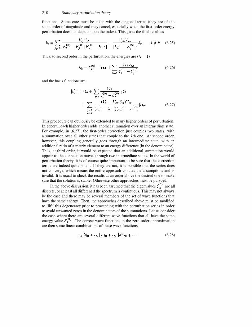
210 Stationary perturbation theory
functions. Some care must be taken with the diagonal terms (they are of thesame order of magnitude and may cancel, especially when the first-order energyperturbation does not depend upon the index). This gives the final result as
�� ��
� ���
������
������ ��
���� ���
���� ��
���� �
�
������
������ ��
���� ��
�� � �� �� (6.25)
Thus, to second order in the perturbation, the energies are (� � �)
�� � ����� � ��� �
�
� ���
������
����� � �
����
(6.26)
and the basis functions are
��� � ���� ��
� ���
���
����� � �
����
����
��
� ���� ���
���� � ��� ������
������ � �
���� ���
���� � �
���� �
����� (6.27)
This procedure can obviously be extended to many higher orders of perturbation.In general, each higher order adds another summation over an intermediate state.For example, in (6.27), the first-order correction just couples two states, witha summation over all other states that couple to the �th one. At second order,however, this coupling generally goes through an intermediate state, with anadditional ratio of a matrix element to an energy difference (in the denominator).Thus, at third order, it would be expected that an additional summation wouldappear as the connection moves through two intermediate states. In the world ofperturbation theory, it is of course quite important to be sure that the correctionterms are indeed quite small. If they are not, it is possible that the series doesnot converge, which means the entire approach violates the assumptions and isinvalid. It is usual to check the results at an order above the desired one to makesure that the solution is stable. Otherwise other approaches must be pursued.
In the above discussion, it has been assumed that the eigenvalues � ���� are all
discrete, or at least all different if the spectrum is continuous. This may not alwaysbe the case and there may be several members of the set of wave functions thathave the same energy. Then, the approaches described above must be modifiedto ‘lift’ this degeneracy prior to proceeding with the perturbation series in orderto avoid unwanted zeros in the denominators of the summations. Let us considerthe case where there are several different wave functions that all have the sameenergy value �
���� . The correct wave functions in the zero-order approximation
are then some linear combinations of these wave functions
������ � ��� ����� � ���� ������ � � � � � (6.28)
Some examples of perturbation theory 211
For the constants ��, it suffices to take their zero-order values as the solutions ofthe process. We now will write out a set of equations with � � �� � �� ���, etc andsubstitute in them, as the first approximation, �� � �
����
� �����
obtained from the� ���� term in (6.10), which then gives
�����
�� ��
��
���� ��� � (6.29)
Here, � and �� take on all the possible values that span the set of degenerate wavefunctions. This leads to a system of homogeneous equations
�
��
����� � �����
��� ���� � �� (6.30)
This system of homogeneous equations has solutions for the various values of thecoefficients �� if the determinant vanishes:
����� � �����
��� � � �� (6.31)
If there are � degenerate eigenvalues, then the equation (6.31) is of order �.The � roots of the equation then give the values of � ���
�. The equation (6.31) is
called the secular equation. We note that the sum of the various new eigenvaluecorrections is given by the sum of the diagonal matrix elements, a general resultin degenerate perturbation theory. This process can be continued to second orderif the degeneracy is not fully lifted by the first-order treatment.
6.2 Some examples of perturbation theory
In this section, we now want to consider a series of examples that will serve toillustrate the stationary perturbation technique. We will first consider a trapezoidalpotential well, one with a linear potential term. Then we turn to a shifted harmonicoscillator, again obtained as a result of adding a linear potential to the harmonicoscillator. Next, we consider two coupled quantum wells, a system that we firsttreated in section 2.7. Finally, we treat the scattering of a plane wave by aCoulomb potential, a problem important to impurity scattering in semiconductors.
6.2.1 The Stark effect in a potential well
The system that we consider is that shown in figure 6.1, where we have aninfinitely deep potential well (one with infinitely high barriers, corresponding tosection 2.4), but with a linear potential existing within the well. Here, we take theunperturbed Hamiltonian as the quantity
�� ���
�� �� (6.32)
212 Stationary perturbation theory
Figure 6.1. The trapezoidal well, in which a linear potential appears at the bottom.
where
�� � � for ��� � � and
�� elsewhere� (6.33)
For this value of the unperturbed Hamiltonian, the eigenvalues and eigenfunctionsare found from the solutions of section 2.4 to be
����� �
�������
�����
�� ���
��� � �
� elsewhere(6.34a)
�� �������
���� (6.34b)
The perturbing Hamiltonian is then the potential
� � �� (6.35)
and the entire problem is reduced to determining the matrix elements of thispotential between the various basis states. There are two sets to be determined,the diagonal ones and the off-diagonal ones. First, the diagonal matrix elementsare simply
��� � ���� ��� � ��������
Some examples of perturbation theory 213
���
�
��
��
� ���������
�� � �����
���
��
��
��
��� ��
������� ��
���� � �� (6.36)
This result is a particular result of choosing the potential to be symmetrical aboutthe centre of the well, so that the average under the perturbing potential is zero.Thus, there is no first-order shift in the energy levels themselves. In other words,the particular choice of the potential results in the centre of the well not moving,which means that, on average, the energy levels are not shifted to first order. Theoff-diagonal terms, however, are non-zero, and we find that
��� � ���� �� � ��������
���
�
� �
��
� ���
���
����� ��
����
��
����� ��
���
���
��
� �
��
�
���
���� ��
����� ��
�� ��
���� ��
���� � ��
����
�
�� ���
���
��� � ������ � odd
� ��� � even.(6.37)
The last result tells us that the odd potential must mix only those states that havedifferent parity. Thus, the odd potential produces matrix elements only betweenan even-parity state and an odd-parity state. (The plus/minus sign just reminds usthat the if the difference between two integers is odd, then the sum of these sametwo integers is also odd, and thus the two terms that result from the two integralsin (6.37) have been combined in the final result.)
Normally, the addition of an electric field produces a shift of the energylevels, an effect called the Stark effect. Here, because the potential has been takento be an anti-symmetric one, the linear shift in the energy levels vanishes, andthere is no first-order Stark effect. However, this is merely because of the choiceof the reference level for the potential. If we had taken the zero of energy to lie atthe point � � ��, then all the energy levels would have been pushed upward bythe value of the potential at the centre of the well. We can see this by taking thepotential as shown in figure 6.2. Now, the basis functions are given by
���� ������
������
�(6.38)
although the energy levels do not change (we are only moving the reference in theaxis, and the well does not change when the perturbation is not present). However,the symmetry of the perturbing potential has been changed. Now, the diagonalelements become
��� � ���� ��� � ���������
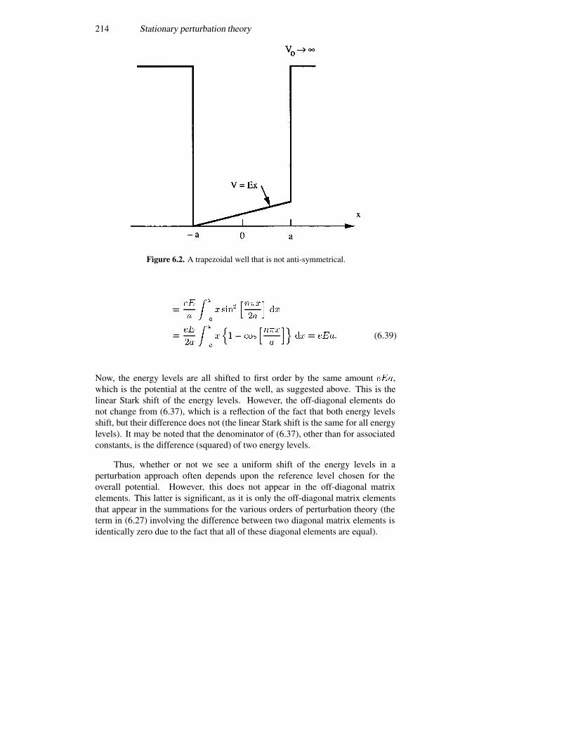
214 Stationary perturbation theory
Figure 6.2. A trapezoidal well that is not anti-symmetrical.
���
�
��
��
� ����
����
��
���
���
��
��
��
�
��� ���
����
�
���� � ���� (6.39)
Now, the energy levels are all shifted to first order by the same amount ���,which is the potential at the centre of the well, as suggested above. This is thelinear Stark shift of the energy levels. However, the off-diagonal elements donot change from (6.37), which is a reflection of the fact that both energy levelsshift, but their difference does not (the linear Stark shift is the same for all energylevels). It may be noted that the denominator of (6.37), other than for associatedconstants, is the difference (squared) of two energy levels.
Thus, whether or not we see a uniform shift of the energy levels in aperturbation approach often depends upon the reference level chosen for theoverall potential. However, this does not appear in the off-diagonal matrixelements. This latter is significant, as it is only the off-diagonal matrix elementsthat appear in the summations for the various orders of perturbation theory (theterm in (6.27) involving the difference between two diagonal matrix elements isidentically zero due to the fact that all of these diagonal elements are equal).
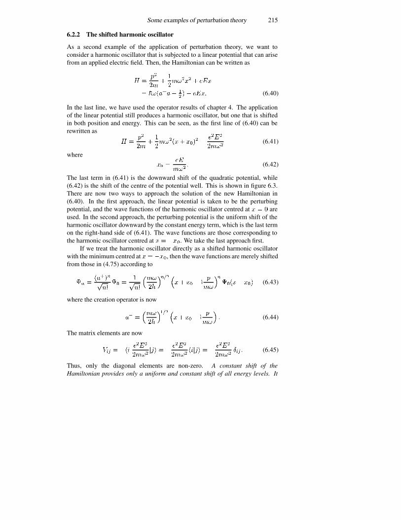
Some examples of perturbation theory 215
6.2.2 The shifted harmonic oscillator
As a second example of the application of perturbation theory, we want toconsider a harmonic oscillator that is subjected to a linear potential that can arisefrom an applied electric field. Then, the Hamiltonian can be written as
� ���
���
�
������ � ���
� ������� �
�� � ���� (6.40)
In the last line, we have used the operator results of chapter 4. The applicationof the linear potential still produces a harmonic oscillator, but one that is shiftedin both position and energy. This can be seen, as the first line of (6.40) can berewritten as
� ���
���
�
������� ���
��
����
����(6.41)
where
�� ���
���� (6.42)
The last term in (6.41) is the downward shift of the quadratic potential, while(6.42) is the shift of the centre of the potential well. This is shown in figure 6.3.There are now two ways to approach the solution of the new Hamiltonian in(6.40). In the first approach, the linear potential is taken to be the perturbingpotential, and the wave functions of the harmonic oscillator centred at � � � areused. In the second approach, the perturbing potential is the uniform shift of theharmonic oscillator downward by the constant energy term, which is the last termon the right-hand side of (6.41). The wave functions are those corresponding tothe harmonic oscillator centred at � � ���. We take the last approach first.
If we treat the harmonic oscillator directly as a shifted harmonic oscillatorwith the minimum centred at � � ���, then the wave functions are merely shiftedfrom those in (4.75) according to
�� �������
��� �
���
���
��
���� �
�� �� � �
��
������� ��� (6.43)
where the creation operator is now
�� ����
��
���� ��� �� �
�
��
�� (6.44)
The matrix elements are now
�� � ���� ����
������� � � ����
��������� � � ����
������ � (6.45)
Thus, only the diagonal elements are non-zero. A constant shift of theHamiltonian provides only a uniform and constant shift of all energy levels. It
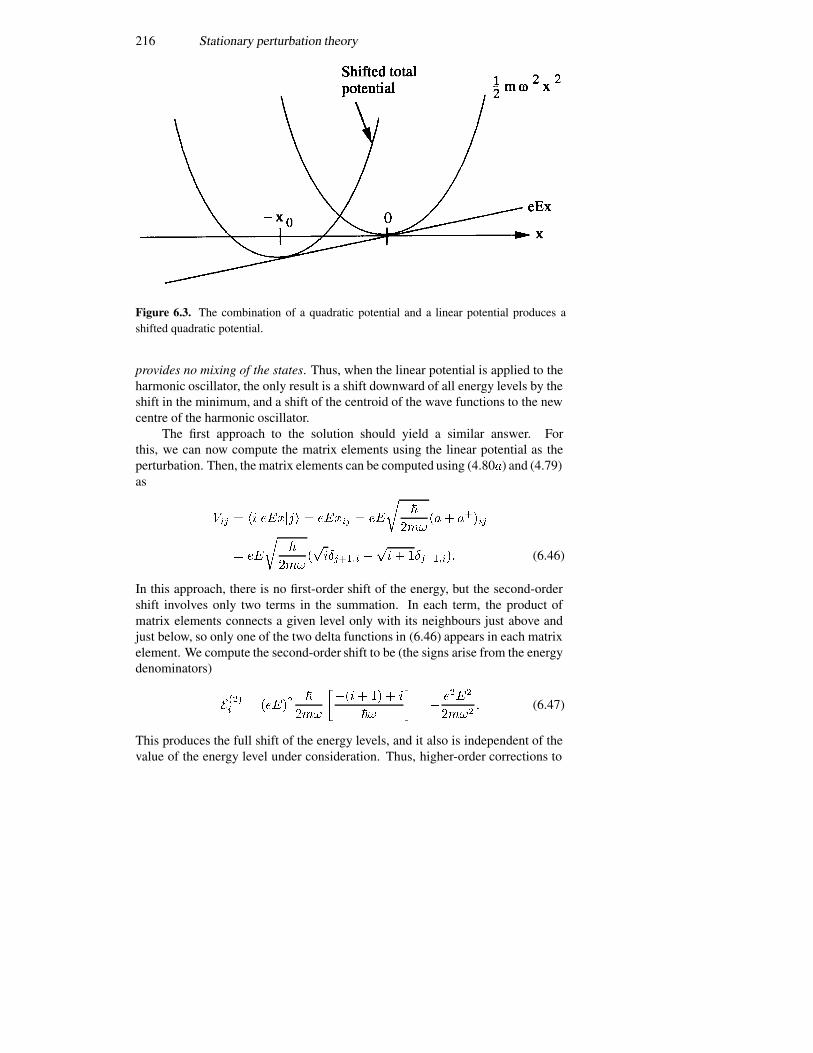
216 Stationary perturbation theory
Figure 6.3. The combination of a quadratic potential and a linear potential produces ashifted quadratic potential.
provides no mixing of the states. Thus, when the linear potential is applied to theharmonic oscillator, the only result is a shift downward of all energy levels by theshift in the minimum, and a shift of the centroid of the wave functions to the newcentre of the harmonic oscillator.
The first approach to the solution should yield a similar answer. Forthis, we can now compute the matrix elements using the linear potential as theperturbation. Then, the matrix elements can be computed using (4.80�) and (4.79)as
��� � ��������� � ����� � ��
��
������ �����
� ��
��
����������� �
��� ������� (6.46)
In this approach, there is no first-order shift of the energy, but the second-ordershift involves only two terms in the summation. In each term, the product ofmatrix elements connects a given level only with its neighbours just above andjust below, so only one of the two delta functions in (6.46) appears in each matrixelement. We compute the second-order shift to be (the signs arise from the energydenominators)
����� � �����
�
���
����� �� � �
��
�� � ����
���� (6.47)
This produces the full shift of the energy levels, and it also is independent of thevalue of the energy level under consideration. Thus, higher-order corrections to
Some examples of perturbation theory 217
the energy levels should vanish, and this can be checked by examining the fourth-order term, which is the next one expected. However, it cannot always be ensuredthat the higher-order terms vanish, but rational thinking for this problem suggeststhat they should sum to zero, when all orders are included. The corrections tothe wave functions are just those that try to move the centroid to the new centreof the harmonic potential. This is a perfect example of a case where low-orderperturbation theory does not produce a result that is close to the exact answer(at least for the wave functions), which we know from being able to solve theproblem exactly. The first-order shift in the wave functions can also be obtainedby using the matrix elements above. For the lowest energy level,
������ � ���
��
��
��������� (6.48)
and for the higher levels, we obtain
������ � ���
��
��
���
������ ����� ��
�� ���� ������
� � �� (6.49)
To obtain the exact wave functions, we will need to sum to higher orders.
6.2.3 Multiple quantum wells
We now want to turn to a consideration of coupled quantum wells, which wewill take each to be quadratic in nature. This treatment provides us with adiscussion of degenerate perturbation theory, a process in which we decide howtwo levels that otherwise would have the same energy interact to cause a smallsplitting. This was discussed at the end of section 6.1. Consider, for example,two harmonic wells that are displaced from one another by a distance �, as shownin figure 6.4. Here, the unperturbed wave functions in each well are at the sameenergy, so the degeneracy is between wave functions centred in each of the twowells. The interaction between the two causes only a small barrier between thetwo wells, so the wave function of an electron localized in one of the wellsactually extends somewhat into the other well (see, e.g., section 2.7). Thus, thetwo wave functions overlap with each other and there is an interaction betweenthem. It is this interaction that causes a modification of the two wave functions,lifts the degeneracy and leads to two new levels, which are then separated slightlyin energy. One of the levels has a wave function composed of the constructiveinterference of the two individual wave functions, while the second (the higherenergy state) has a wave function that is anti-symmetric in the combined wells andthus arises from the destructive interference of the two individual wave functions.
In each of the two wells, the unperturbed problem is just that of a harmonicoscillator, centred at the particular well, so the Hamiltonian and lowest wavefunction of the well at � � � are given by
��� ��
����
������

218 Stationary perturbation theory
Figure 6.4. The composite potential that arises from two overlapping harmonic potentialsthat are displaced slightly.
������������� � ������������ (6.50)
Similarly, those at the second well are given by
���� ���
����
������� ���
������������� � ��������
���� (6.51)
We note that both wave functions, one centred in each well, have the sameeigenvalues for the unperturbed energy. Thus, these two eigenvalues are said tobe degenerate. The task here is to use perturbation theory to lift this degeneracy.We are not so much interested in how the interaction with higher levels changesthe energy levels as we are with how these two wave functions interact with eachother to change the energy levels. While we work with the energy level that wehave indicated is the lowest isolated well level, this is not a limitation, and wecould work with any of the levels of the isolated well that lie below the centralpeak between the two wells (for those levels above this peak, perturbation theoryis not appropriate). Our interest then is in the matrix element
��� ����������� ��������� �
��
��
������� ������� � �� ��� (6.52)
Here, the potential is the actual total potential in the problem, but the main partis that part of the potential that lies between the two wells. Equation (6.52) is theoverlap integral defining the mixing of the two wave functions.
The composite wave functions should be able to be written as a sum of thetwo individual wave functions, as
��� � ���������� ����������� (6.53)
When we operate first with the conjugate of the wave function of the left-handwell, and then with the conjugate of the wave function of the right-hand well, we

Some examples of perturbation theory 219
produce two equations. This is done by neglecting the variation of the potentialdifference from the single well for the diagonal terms (wave functions on the samesites). The process produces the resulting matrix equation
��� ���
� �
����
��
�
�� �
�
�
�� (6.54)
If this is to have a solution, then we must arrange for the determinant���� ��� � �� ���
� �
����� � ��
���� � �� (6.55)
This leads to the new energy levels
� � �� � ������ (6.56)
Thus, the two individual energy levels ��, which were degenerate, are now splitby the amount ������. It is easy then to determine that the additive overlap of thetwo individual wave functions gives the lower energy level, while the subtractiveoverlap of the two individual wave functions gives the upper energy level. Thelower is said to be a bonding wave function, while the upper is an anti-symmetricanti-bonding wave function.
The above treatment can be extended to three potential wells, under theassumption that only the two nearest neighbours interact. This then leads to a��� matrix equation, for which the solution is given by the determinant equation
���������� � �� ��� �� �
����� � �� ���
� � �
����� � ��
������ � �� (6.57)
This leads to the equation
��� � ��� � ������
����� � �� � � (6.58)
which gives the eigenvalues
� � �� �� ��������� (6.59)
The lowest energy level has the additive sum of the three individual wavefunctions, while the other two levels are various other combinations. It isimportant to note that the resulting wave functions all have contributions in eachof the three potential wells and are no longer localized in a single well.
The result (6.59) illustrates another important point of the degenerateperturbation approach. The band widths in (6.59) and in (6.56) differ. Thedifference between the highest energy level and the next lowest is smaller,however. This is true in nearly all such near-neighbour systems. As the numberof wells builds up, the density of the energy levels increases, until it is almost a

220 Stationary perturbation theory
continuum—an energy band as it were. This is how the energy bands in solidsare formed. The width of the so-called energy band does not increase withoutlimit, but approaches a limiting value as the number of wells increases withoutlimit. In terms of the matrix element ���, the ‘band width’ for two, three, andfour potential wells is 2, 2.828, 3.236. In fact, the limiting value is �� ��, which isa property of the matrix rather than the physics.
6.2.4 Coulomb scattering
Here, we will discuss the scattering of an incoming plane wave, which variesas ���� , by a charged atom through the Coulomb potential. This atom can beconsidered to be an impurity atom in the host semiconductor. In any treatmentof electron scattering from a Coulomb potential, it is necessary to consider thelong-range nature of the potential. If the interaction is summed over all space, theintegral diverges and a cutoff mechanism must be invoked to limit the integral.One approach is just to cut off the integration at the mean impurity spacing, theso-called Conwell–Weisskopf (1950) approach. A second approach is to invokescreening of the Coulomb potential by the free carriers. In this case, the potentialis induced to fall off much more rapidly than a bare Coulomb interaction, dueto the Coulomb forces from surrounding carriers (such as the one creating theincident plane wave). The screening is effective over a distance on the order ofthe Debye screening length in non-degenerate materials. This screening of therepulsive Coulomb potential results in an integral for the scattering cross sectionwhich converges without further approximations (Brooks 1955).
For spherical symmetry about the scattering centre, or ion location, thepotential is screened in a manner that gives rise to the potential
���� ���
���������� (6.60)
where the Debye wave vector �� is the inverse of the screening length, and isgiven by
����
���
����� (6.61)
Here �� is the high-frequency permittivity and � is the density of charge carriersin the semiconductor of interest.
In treating the scattering from this screened Coulomb potential, we use awave scattering approach and compute the scattering cross section ���, whichgives the angular dependence of the scattering. This is the perturbation theory fora continuum of energy (or momentum) states as represented by the continuousvariable �. It is assumed the incident wave is a plane-wave, and the scatteredwave is also a plane-wave. The total wave function is written as
���� � ���� � ���������� (6.62)
Some examples of perturbation theory 221
Here, � � ��� orients the incident wave along the polar axis in a sphericalcoordinate system, and the second term represents the scattered wave. That is,the exponential represents the final state of the perturbation, and the coefficient���� represents the matrix element coupling this state to the initial state.Equation (6.62) is inserted into the Schrodinger equation, neglecting termsof second or higher order in the scattered wave, in keeping with first-orderperturbation theory, and
������ � ������� ����
��
��
�������������� � (6.63)
If the terms on the right-hand side are treated as a charge distribution, the normalresults from electromagnetic field theory can be used to write the solution as
���� � �����
�����
�����
���� � �������
������
����������� (6.64)
To proceed, it is assumed that � � � �, and the polar axis in real space is taken tobe aligned with �. Further, the scattering wave vector is taken to be � � � � � �,so that � �
�
� � �� ������
������
��(6.65)
the integration is simple and can be done quickly, while the remainingintegration becomes
���� �� �����
�������
� �
�
�����������
��� �����
��������� � ���� (6.66)
Now � � � � ��, but here we assume that � � � �, and � �� ������, where� is the angle between � and � �. The assumption is that the scattering does notchange the energy of the carrier, but only changes its direction. If we write thescattered wave function ���� as ������, then we recognize that the factor ���� isthe matrix element, and the cross section is defined as
��� � ������� �
�����
��������
���
������� � ��������
� (6.67)
The total scattering cross section (for the relaxation time) is found by integratingover �. Thus
� � ��
� �
�
��� �� � �� � ���
� ���
�
��
�
��
��
�
��
��
�
�
�
��
�
�����
��������
�� �����
������ � �
��
�� (6.68)
The cross section describes the fraction of each incoming carrier that is lost toother wave states, and has the units of area (such as ���). It can be connected
222 Stationary perturbation theory
to a scattering rate, which describes the number of scattering events per second,by multiplying by the number of scattering centres per unit volume and by thevelocity of the incoming carrier (which converts a loss per centimetre into a lossper second). First, the loss per unit length of the incoming carrier to scatteringevents is just
���� � ��� �������
���������
����
���� � �������
� (6.69)
The scattering rate is now the product of the attenuation per unit length and thevelocity of the carrier, or
���� � ���� ������
���������
����
���� � �������
� (6.70)
6.3 An alternative technique—the variational method
There are often times when the perturbation approach just does not work, becausethe basis set cannot be determined consistently with (6.3). An example isthe triangular potential well of section 2.6. The problem with this particularbarrier is that the solution of the Schrodinger equation is complicated and thewave functions are special functions that, in general, are evaluated numerically.Often, however, the exact eigenvalues and eigenfunctions are not required;rather, only good approximations to them are required. To accomplish this,another approximation technique is generally used—the Rayleigh–Ritz method,or variational method. Here, it may be assumed that we cannot begin with (6.3)or any equivalent form. Nevertheless, we may take an approximate wave functionas an expansion in a convenient basis set:
��� ��
�
������ (6.71)
It may be assumed then that, if this is an orthonormal basis set, the expectationvalue of the Hamiltonian is given by
� � ��
�
������� (6.72)
where we have constructed the expectation value by pre-multiplying bythe conjugate of (6.71), post-multiplied by (6.71), integrated and used theorthogonality properties of the basis set. An inequality can be created byassuming that only the lowest energy level is used in the expansion (using thelowest energy level for each of the eigenstates), and
� � � ���
�
����� � �� (6.73)
An alternative technique—the variational method 223
since the sum over all the basis states is unity to ensure the normalization of thewave function in (6.71).
The principle of the Rayleigh–Ritz method is that we can adopt a trial wavefunction, which may have some parameters in it, and then minimize the energycalculated with this wave function. This energy will still be above the actuallowest energy level ��. This gives a good approximation to the actual energylevel. The next higher state can be developed by using a second parametrizedbasis function, which is made orthogonal to the first. The energy level of thiswave function is then found by the same adjustment technique. Let us illustratethis with the actual triangular-potential-well problem of section 2.6.
To begin, we note that the wave function vanishes at the origin, as thepotential is typically defined by
� ��� � ��� for � � � ��� � ����� for � � �� (6.74)
Thus, we seek a trial function that vanishes at � � �, and also vanishes for large�, where the energy lies at a lower level than the potential. For this, we take
��� � ������ (6.75)
which satisfies both limiting requirements. The pre-factor coefficient isdetermined by normalization to be
����� � � �
��
�
��������� �� ���
��(6.76)
or� � ����� (6.77)
Then, the expectation value of the Hamiltonian is
��� � ����
�
�������
��
�
��� ���
������ ��
�����
�
���
�� (6.78)
This value is now above the actual lowest energy level, and we can minimize thisvalue by setting the derivative with respect to � to zero. This then leads to (we takethe first level as the lowest level in keeping with the general results of section 2.6)
� �
����
��
����(6.79a)
�� ����
����
��
����� (6.79b)
This result should be compared with (2.83). The present result differs from (2.83)only by a factor of ��������� � ��� , or about a 7% error, which is quite small
224 Stationary perturbation theory
considering the approximations. As expected, the right-hand side of (6.79�) liesabove the actual value, given by (2.83).
To compute the next level, we must assume a wave function that isorthogonal to (6.75). The wave function of (6.75) has a single maximum,decaying away to zero at the origin and for large values of �. The next levelshould have a wave function with two maxima, but also decaying away for largevalues of � and at the origin. For this purpose, we write the first-excited-statewave function as
��� � ���� ��������� (6.80)
To begin, we make this wave function orthogonal to ���, through
����� � ��������
�
��� � ������������ ��
� �������
�
��� ����
�
��� ���
�� � (6.81)
or
� ��� �
� (6.82)
With this new wave function, we can now compute the normalization:
����� � � ���
������ � �� � ��� (6.83)
or
�� �����
�� � �� � ��� (6.84)
so, once we have evaluated � by minimizing the energy level, we can computethe normalization as well. Actually, we will use the result in our evaluation of theenergy, which is
��� �����
�
�� �
����
�� � �� � ��
�
��
��
�� �
��
���� � �� � ���
�� (6.85)
This can now be minimized, to yield the value of � as above. While the tendencymight be to ignore the second terms in each of the large parentheses, this wouldbe a mistake, as it would lead to an energy level below the lowest level. Theseterms are actually the major terms. Unfortunately, this leads to a complicated,high-order algebraic equation for � in terms of �. This can be solved most easilyby numerical calculations, which lead to the result � � �� �, which in turn leadsto �� � �����.
A similar procedure can now be used to generate a variational wave functionfor the next higher eigenstate. A wave function, probably with a cubic term in the
An alternative technique—the variational method 225
pre-factor, is assumed and the coefficients are adjusted first to make it orthogonalto each of the two lower eigenfunctions. Then, the energy is minimized to providean estimate of the energy level. Of course, each successive higher level becomesmore complicated to determine, and most efforts using this method are addressedonly to the lowest energy level.
References
Ando T, Fowler A and Stern F 1982 Rev. Mod. Phys. 54 437Brooks H 1955 Adv. Electr. Electron Phys. 8 85Conwell E M and Weisskopf V 1950 Phys. Rev. 77 368Schiff L I 1955 Quantum Mechanics 2nd edn (New York: McGraw-Hill)Stern F and Howard W E 1967 Phys. Rev. 163 816
226 Stationary perturbation theory
Problems
1. In an infinite square well, in which � ��� � � for � � � and � � �,� ��� � � for � � � � �, the basis states are given by ��� �
���� ����������,
and �� � �������������. For the introduction of a perturbing potential of
�� � ��������, calculate the changes in the wave functions up to first order andin the energy levels up to second order.
2. Determine the third-order correction to the energy in perturbation theory.3. Determine the corrections to second order necessary to lift the degeneracy
of a set of states in an arbitrary perturbing potential.4. Except for certain accidents, degeneracy usually does not arise in a one-
dimensional problem. Degeneracy is usually found when the dimension is raised.Consider the two-dimensional infinite square well
� �� � �
�� for ��� � ��� and �� � ����� for ��� � ��� or �� � ���.
Using this potential, separate the Schrodinger equation into two one-dimensionalequations and solve for the allowed energy values using the fact that the potentialcan be written as the sum of two one-dimensional potentials. The solutions canthen be written down using the results of chapter 2. Consider the application ofthe simple perturbation ���� � � �� for ��� � ��� and �� � ���, and is zeroelsewhere (the perturbing potential exists only in the centre of the well). Computethe splitting of the lowest two unperturbed energy levels.
5. Using the harmonic oscillator raising and lowering operators, computedirectly the matrix element for ��������. Then, introducing a complete set ofstates (as a resolution of the delta function) break this into two products � ���,and compute the matrix element from
�������� ���
�����������������
6. A one-dimensional harmonic oscillator is perturbed by a term � �.Calculate the change in each energy level to second order.
7. Calculate the lowest energy level of a harmonic oscillator using theGaussian wave function as a variational wave function. Let the width of theGaussian be the parameter that is varied.
8. To compute a momentum relaxation time, a factor of � � �� �� isincluded in the integral (6.68). Plot the results with this inclusion versus theresults that result from (6.68) directly—plot the scattering rate versus the energy.
Chapter 7
Time-dependent perturbation theory
In many physical systems, we are interested in small time-dependent changes inthe state. The approach used in the last chapter cannot deal with this situation,and we must develop perturbation theory further. This will be done in the presentchapter. In fact, we will develop the approach twice, first for the Schrodingerrepresentation and then for the Heisenberg representation in a linear vectorspace. This double approach is followed for two reasons. First, it is importantto grasp the concept of the time-dependent perturbation approach in a directmethod, without the encumbrance of the mathematics that accompanies the latterapproach—the interaction representation. Second, it is important to learn themathematics of the interaction representation, but in doing so it is quite helpfulto understand just where we are heading. The double approach achieves bothobjectives.
In time-dependent perturbation theory, we continue to assume that theHamiltonian can be split into two parts
� � �� ��� (7.1)
in which the first part �� can be solved directly and the second part �� is small.When this can be done, then the second part can be initially ignored, and theproblem solved directly to give the wave function, or its expansion in a naturalbasis function set. After this is done, the second term in (7.1) is treated as aperturbation, and the eigenvalues and eigenfunctions are then developed in a time-dependent perturbation approach in terms of the natural basis function set.
In this chapter, we will first develop the approach in the Schrodingerrepresentation and consider an example due to a harmonic potential. Thenthe interaction representation will be developed and the perturbation theory re-developed in the Heisenberg representation. Our attention will then be turned toan extended approach in which the initial state of the system has an exponentialdecay. It is this latter approach that allows us to return once again to the idea of anenergy–time relationship as a result of the lifetime of the initial state. Finally, thescattering matrix approach (the � -matrix) is developed. One note of importance
227
228 Time-dependent perturbation theory
is that it will be assumed that the total Hamiltonian is a time-independent quantity,while the perturbation term�� will be allowed to have an oscillatory nature.
7.1 The perturbation series
If the Schrodinger equation is used with a time-independent and unperturbedHamiltonian (�� � �), for which it may readily be solved, the solution maybe written from (2.93) as (the position coordinate is suppressed)
������� ��
�
���������� (7.2)
where���� � ���� �� � ���� (7.3)
and�� � �����
�������� (7.4)
The determination of the coefficients has been done at � � � for ease of notation.In the presence of the perturbation ��, we seek a solution that has the same
general form as (7.2)–(7.4), and this can be achieved by making the assumptionthat the perturbation �� � � is small and produces a slow variation in thecoefficients ��. Then, we may write the new solution as
���� ��
�
�������������� (7.5)
The problem is now to determine the time variation of the coefficients. Toproceed, the assumed solution (7.5) is introduced into the Schrodinger equation
���
�� ��� � � ��� (7.6)
This leads to�
�
��������������� � ��
�
�
�����
��������
��
�
��������������� �
�
�
� �������������� (7.7)
Here, we shall assume that the potential � is time varying as
� � � ��� � �������� (7.8)
The first term on the left and the first term on the right drop out by virtue of (7.3).We now multiply through by an arbitrary basis function � �
�, and integrate over all
space, using the orthonormality of these functions. This leads to
�������
������ ��
�
������������������� (7.9)

The perturbation series 229
where��� � �������� (7.10)
is the matrix element. On introducing the difference frequency
��� ��� � ��
�(7.11)
equation (7.8) can be rewritten as
�������
��
�
�������������������� (7.12)
What we now have is a complicated set of equations for the coefficients and theirtime dependence. In general, this can be solved by matrix techniques when thematrix elements are known.
The approach that we want to follow, however, assumes that the perturbationis very small. Moreover, we will also assume that the system is in one singleeigenstate at the initial time, which will be taken as � � �:
����� � � ����� � � for all � �� �� (7.13)
To be consistent with this assumption, we also will assume that the perturbation� is zero for � � �. In (7.10), it has been assumed that the perturbing potential isconstant, but it would be easy to change this and to include a perturbing potentialvarying with a particular frequency. This frequency factor would then appearwith the matrix element. We will continue with the time-independent approach,but the reader should be aware that the inclusion of the time variation can easilybe incorporated, as has been done. With the above approximations, (7.12) nowbecomes a simple equation
�������
� ������������������� � ����
����������� (7.14)
This can now be easily solved to give
�� � ��
�
� �
�
���������
������
�
���
� ��
���� � ��������
���������� � ��� (7.15)
The change in the occupancy of the state is mainly determined by the change inthe magnitude squared of the wave function. Thus, the quantity of interest is themagnitude squared of (7.15), which becomes
����� �
������
������ � �������� �
����� � ���� � (7.16)
230 Time-dependent perturbation theory
This is now the probability that density moves from the initial state � to the state�. Our interest is in the rate at which this probability transfers, or the transitionrate
��� ������
�� (7.17)
For large values of time, we note that (Landau and Lifshitz 1958)
������
��������
���� ����� (7.18)
When � �� , the limit is zero and the transition rate vanishes (we associate �with ���� � ����). Thus, we note that the delta function serves to ensure thatthe transition rate is non-vanishing only for � � . Thus, the transition rate canbe written as
��� ��
������
����� � ��� ��
�����
������ � ���� (7.19)
The last form in (7.19) is often referred to as the Fermi golden rule. The transitionrate is given by a numerical factor times the squared magnitude of the matrixelement and a delta function that conserves the energy in the transition. The latteris important, as it ensures that time-dependent variations arise only from thosestates in which the transition can conserve energy.
7.2 Electron–phonon scattering
Scattering of the electrons, or the holes, from one state to another by thelattice vibrations is one of the most important processes in the transport of thecarriers through a semiconductor. In one sense, it is the scattering that limitsthe velocity of the charge carriers in the applied fields. Transport is seen as abalance between accelerative forces and dissipative forces (the scattering). Ingeneral, the electronic motion is separated from the lattice motion. It is theadiabatic principle, where the atomic motion is supposed to be slow relative tothe electronic motion, which allows separation of the electronic motion fromthe lattice motion. There remains one term in the total system Hamiltonianthat couples the electronic motion to the lattice motion. This term gives rise tothe electron–phonon interaction. However, this is not a single interaction term.Rather, the electron–phonon interaction can be expanded in a power series inthe scattered wave vector � � � � � �, and this process gives rise to a numberof terms, which correspond to the number of phonon branches and the varioustypes of interaction term. There can be acoustic phonon interactions with theelectrons, and the optical interactions can be either through the polar interaction(in compound semiconductors) or through the non-polar interaction. These arejust the terms up to the harmonic expansion of the lattice; higher-order terms giverise to higher-order interactions.
Electron–phonon scattering 231
In this section, the basic elastic electron–phonon (which may also be hole–phonon) interaction is treated in a general sense and we develop the acousticphonon scattering rate as an example of time-dependent perturbation theory.
The treatment followed here is based on the simple assumption thatvibrations of the lattice cause small shifts in the energy bands. These vibrationswere discussed in section 4.6, and the Fourier components are simple harmonicoscillators. Thus these oscillators induce periodic deviations in the bands fromtheir equilibrium positions. Deviations of the bands due to these small shiftsfrom the frozen lattice positions lead to an additional potential that causes thescattering process. The scattering potential is then used in time-dependent, first-order perturbation theory to find a rate at which electrons are scattered out of onestate � and into another state ��, while either absorbing or emitting a phonon ofwave vector �. Each of the different processes, or interactions, leads to a different‘matrix element’ in terms of its dependence on these three wave vectors and theircorresponding energy. These are discussed in the following sections, but here thetreatment will retain just the existence of the scattering potential Æ� which leadsto a matrix element
���� �������� � �������������� (7.20)
and the subscripts indicate that the wave function involves both the electronicand the lattice coordinates. Normally, the electronic wave functions are takento be Bloch functions that exhibit the periodicity of the lattice. In addition, thematrix element usually contains the momentum conservation condition. Here thisconservation condition leads to
� � �� � � �� (7.21)
where � is a vector of the reciprocal lattice. In essence, the presence of � is aresult of the Fourier transform from the real space lattice to the momentum spacelattice, and the fact that we can only define the crystal momentum � within asingle Brillouin zone. For the upper sign, the final state lies at a higher momentumthan the initial state, and therefore also at a higher energy. This upper sign mustcorrespond to the absorption of a phonon by the electron. The lower sign leads tothe final state being at a lower energy and momentum, hence corresponds to theemission of a phonon by the electrons.
Straightforward time-dependent, first-order perturbation theory then leads tothe equation for the scattering rate, in terms of the Fermi golden rule (7.19):
� ������ ���
��������������� ���� � ���� (7.22)
and the signs have the same meaning as in the preceding paragraph: for example,the upper sign corresponds to the absorption of a phonon and the lower signcorresponds to the emission of a phonon.
232 Time-dependent perturbation theory
The scattering rate out of the state defined by the wave vector � and theenergy �� is obtained by integrating (7.22) over all final states. Because of themomentum conservation condition (7.21), the integration can be carried out overeither �� or � with the same result (omitting the processes for which the reciprocallattice vector � �� �). For the moment, the integration will be carried out overthe final state wave vector ��, and (� � ��� is the scattering rate, whose inverseis the scattering time � used in previous paragraphs)
���� ���
�
�
��
������������� ���� � ����� (7.23)
In those cases in which the matrix element � is independent of the phonon wavevector, the matrix element can be removed from the summation, which leads tojust the density of final states
���� ���
������������ � ����� (7.24)
This has a very satisfying interpretation: the total scattering rate is just the productof the square of the matrix element and the total number of final states. For thesecases the scattering angle is a random variable that is uniformly distributed acrossthe energy surface of the final state. Thus any state lying on the final energysurface is equally likely, and the scattering is said to be isotropic.
One of the most common phonon-scattering processes is the interactionof the electrons (or holes) with the acoustic modes of the lattice through adeformation potential. Here, a long-wavelength acoustic wave moving throughthe lattice can cause a local strain in the crystal that perturbs the energy bandsdue to the lattice distortion. This change in the bands produces a weak scatteringpotential, which leads to a perturbing energy (Shockley and Bardeen 1950)
� � ��� � ��� � ��� (7.25)
Here, �� is the deformation potential for a particular band and� is the dilation ofthe lattice produced by a wave, whose Fourier coefficient is ��. We note here thatany static displacement of the lattice is a displacement of the crystal as a wholeand does not contribute, so that it is the wavelike variation of the amplitude withinthe crystal that produces the local strain in the bands. This variation is representedby the dilation, which is just the desired divergence of the wave. The amplitude�� is a relatively uniform Fourier coefficient for the overall lattice wave, and maybe expressed as (4.89) with �� taken from (4.80) as
�� �
��
��� ��
������
���� �� ��������
����� (7.26)
where �� is the mass density, is the volume, � and �� are the annihilationand creation operators of section 4.4 for phonons, � � is the polarization vector,
Electron–phonon scattering 233
and the plane-wave factors have been incorporated along with the normalizationfactor for completeness. Because the divergence produces a factor proportionalto the component of � in the polarization direction (along the direction ofpropagation), only the longitudinal acoustic modes couple to the carriers in aspherically symmetric band. The fact that the resulting interaction potential isnow proportional to � (i.e., to first order in the phonon wave vector) leads to thisterm being called a first-order interaction.
The matrix element may now be calculated by considering the proper sumover both the lattice and the electronic wave functions. The second term in (7.26),the term for the emission of a phonon by the carrier, leads to the matrix elementsquared, as
����� ���� ����
���
���� ����� � ������� (7.27)
where �� is the Bose–Einstein distribution function for the phonons, and
���� �
��
������� ��� (7.28)
is the overlap integral between the cell portions of the Bloch waves (unfortunately,similar symbols are used, but the �� in this equation is the cell periodic part of theBloch wave and not the phonon amplitude given earlier) for the initial and finalstates, and the integral is carried out over the cell volume�. For elastic processes,and for both states lying within the same ‘valley’ of the band, this integral is unity.Essentially, exactly the same result (7.27) is obtained for the case of the absorptionof phonons by the electrons, with the single exception that �� � � �� is replacedby ��.
One thing that should be recognized is that the acoustic modes have very lowenergy. If the velocity of sound is � �� �� ��, a wave vector correspondingto 25% of the zone edge yields an energy only of the order of 10 meV. This isa very large wave vector, so for most practical cases the acoustic mode energywill be less than a millivolt. Scattering processes in which the phonon energymay be ignored are termed elastic scattering events. Of more interest here isthe fact that these energies are much lower than the thermal energy except at thelowest temperatures, and the Bose–Einstein distribution can be expanded underthe equipartition approximation as
�� ��
����������
�� �
��
���� �� (7.29)
Since this distribution is so large and the energy exchange so small, it is quite easyto add the two terms for emission and absorption together, and use the fact that�� � ���, where �� is the velocity of sound, to achieve
������� �����
��� ���� (7.30)
234 Time-dependent perturbation theory
For electrons in a simple, spherical energy surface and parabolic bands, this leadsto
���� ���
�
��
����
��� ���
�
���
����
��
��������
������� ��������
�������������� (7.31)
It has been assumed that the interaction does not mix spin states, and this factoris accounted for in the density of states. Although most of the parameters mayeasily be obtained for a particular semiconductor, it is found that the deformationpotential itself is almost universally of the order of 7 to 10 eV for nearly allsemiconductors. Nevertheless, this result for the scattering rate of electrons byacoustic phonons is a straightforward example of the application of the Fermigolden rule.
7.3 The interaction representation
We now want to revisit the idea of time-dependent perturbation theory, but in anapproach that is based upon the Heisenberg representation introduced in chapter 5.To review, for this approach, the wave function is expanded in a linear vectorspace of basis functions, just as in the approach leading to (7.3), but now it isassumed that the basis set is not time varying, at least in the unperturbed state.Rather, the time variation is attached to the operators themselves, which rotate inthe fixed linear vector space (which forms our coordinate system) as a function oftime according to
�� � ��������������� (7.32)
with�
��
���� �� (7.33)
This is the basis of the Heisenberg representation.In the presence of a time-varying perturbation, however, it will now be
assumed that the perturbation introduces a slow variation in the basis set itself.Just as we earlier assumed that the coefficients of the expansion were now timevarying, we will assume that this slow variation is entirely due to the perturbingpotential � �� defined according to (7.32) as
� �� � �������� �������� (7.34)
except that we will also assume below that there is an explicit time variation tothis perturbation (such as might arise if the perturbation were due to an interactionwith a harmonic oscillator). Hence, there is a slow variation of the wave functionin the linear vector space that is introduced by � , while all other operators
The interaction representation 235
still respond to the unperturbed Hamiltonian according to (7.33). This mixedrepresentation is termed the interaction representation.
In keeping with the development leading to (5.124), it may be assumed thatthere is a unitary operator ���� ��� that describes the slow time evolution of thewave function according to
���� � ���� �������� (7.35)
from which we may write the equivalent Schrodinger equation as
����
��� � ������� ���� (7.36)
The approach now is to define the properties of the unitary operator���� � ��. First,we note that for � � ��,
����� ��� � � (7.37)
and, in general,����� ��� � ����� �������� ���� (7.38)
Using (7.37), we can directly integrate (7.36) to give
���� ��� � ���
�
��
��
� ��������� ��� ���� (7.39)
Obviously, this integral equation is not easily solved (because of the two-timebehaviour, it is not a simple convolution integral). Thus, the normal method isto develop a perturbation series of various orders of iteration. For example, inthe first iteration, it is assumed that only the first term of (7.39) is used inside theintegral; then this result is used within the integral to produce the next iterate, andso on. This procedure gives the sequence of approximations to ���� � �� as
����� ��� � � (7.40a)
����� ��� � ���
�
��
��
� ���������� ��� ��
� � ���
�
��
��
� ���� ��� (7.40b)
����� ��� � ���
�
��
��
� ���� ��� �
��
�
�� � �
��
� ����
���
��
� ����� ���� ��� (7.40c)
and so on. We leave it as a problem at the end of the chapter to show that theinfinite iterate is the exponential operator
����� ��� � �
��
�
�
��
��
� ���� ����� (7.40d)
In keeping with the approach begun in section 7.1, we will assume that the linearvector space is rotated so that the wave function initially is completely in state
236 Time-dependent perturbation theory
�. Then, we can take the inner product with state � to obtain the equivalentcoefficient:
��������� � ���� ���� ������
� ����� ��
�
� �
��
������� ���
�
��
�
�� � �
��
� ��
��
���� ����� �������� ���� ��� � � � � � (7.41)
Obviously, the first term on the right-hand side vanishes by the principle oforthogonality, while the second term is essentially the first line of (7.15) if werecognize that the exponential is buried in the time dependence of the perturbingpotential. We note that the left-hand side is the coefficient �� defined insection 7.1. The result here tells us that the result obtained earlier is just thefirst term in a perturbation series expansion, which may be terminated only solong as the terms decrease sufficiently rapidly in order.
Here, we would like to take into account the specific time variation of theperturbing potential according to the simple rule
� � �������� (7.42)
The matrix element is then
���� ������ � ����������������������������
� ���������������� (7.43)
This leads to the coefficient (�� � �)
����� � ��� ������ � ��
�
� �
�
��������������� ���
� ���� ��
�
���������� �
�� � (7.44)
and
�������� �
���������
� ���� ��� � ���
��� � ��� (7.45)
Using the result (7.18), we obtain the transition rate as
��� ��
��������
�Æ ���� � �� (7.46)
which is just (7.19). The delta function conserves energy in the transition rate, sowe have to interpret (7.46) as declaring that the states � and �, which are coupledby the perturbation, must have energies that differ from each other by the energy� of the photon associated with the oscillation in the potential. Thus, a single
Exponential decay and uncertainty 237
photon of energy �� is absorbed (or emitted) in moving the state from coordinate� (and energy ���) to the state with coordinate � (and energy ���). The initialand final states are no longer degenerate, but differ in energy by the energy of theperturbing potential. The second-order term in (7.41) is a two-photon transition,and each higher-order term includes another photon in the process. (We use theterm photon here, but the type of particle depends upon the perturbation and couldbe a photon, a phonon, or whatever.)
7.4 Exponential decay and uncertainty
In the preceding sections, it has been assumed that the initial state remains at unitamplitude. In fact, this is really unlikely, and it is now desirable to see how thedecay of the initial state affects the transition probability. Each approach yieldsthe same form for the transition rate, so we will use the direct form of (7.14)–(7.15); we rewrite this as
�� � ��
�
� �
�
�����������
�
��� (7.47)
where it is assumed that the perturbing potential is time invariant. The inclusionof any time variation of this potential is easily re-inserted using the results of(7.43). In a similar manner, (7.12) must also be written for the initial state as
�������
���
��������������� (7.48)
We need first to solve for the time variation of the initial state ��. Combining thelast two equations, we find that
�����
� ��
��
��
������
� �
�
�������������
���� ���� (7.49)
The last term is a convolution integral of the coefficient �� and the exponentialtime variation. This suggests that a transform approach is the best way to solve theequation for the time variation of this coefficient. For this purpose, the Laplacetransform will be used, but the transform variable will be taken to be �, as thetraditional � has been used for the state notation. Thus, using (7.13), the transformof (7.49) leads to the equation
�����
�� �
�
���� �
�
��
�� ���
���� �� �
� � ����
�� � (7.50)
where the term for � � � has been separated out from the rest of the sum. Toclarify this result, the last term in the square brackets will be rationalized, and
�����
���
�
��
�� ���
���� �� �
�� � ����
��
�
�����
�
�
�� ���
���������
�� � ����
��� �� (7.51)
238 Time-dependent perturbation theory
In the end, we will be taking the long-time limit, which corresponds to � � �(the multiplication by � is in the finished radical which will not affect theapproximations we are about to make). In this limit, the second term in the largebracket becomes just (7.19) summed over the states �, as the fraction becomes thedelta function; that is, the second term becomes just half of
�� ���
�
�
� ���
���� �������� (7.52)
which is the total out-scattering rate from state �. The term in the curly bracketsis just the energy shift in (6.25) found to second order in time-independentperturbation theory. Thus, we may re-transform (7.51) as
����� � ���
��
���
�
����
��
�� (7.53)
The out-scattering process causes a decay of the state amplitude, as expected, butthere is also a shift in the frequency of the state, which is often referred to as theself-energy correction. We note that the probability amplitude of the initial statedecays as
���� � �������� � ������ (7.54)
The result (7.53) can now be used in (7.47) to compute the rate of scattering intothe state �. This gives
�� � �
�
� �
�
��������
����������
��� (7.55)
where
�� � ��� �
���� �
�� � �� �����
(7.56)
is the shift in frequency due to the self-energy correction of the initial state.Equation (7.55) is readily integrated as
�� � �����
������������� � �
�� ���(7.57)
and
����� �
������
��
�� �������� ���� ���� �����
��� ������
� (7.58)
After a very long time compared with the lifetime ��� (we have previously takenthe long-time limit), we obtain the occupancy of the �th state as
����� �
������
��� ��� �������
(7.59)
Exponential decay and uncertainty 239
which exhibits the bell-shaped resonance behaviour with a peak height of ��� �
�at
the new resonance position ��� � � (which is shifted from the normal positionof the delta function by the self-energy of the state �).
One problem with the form of (7.59) is that the peaked shape of the function,which is a Lorentzian line shape, does not integrate out to be equivalent to (7.19).In the case of (7.19), the quantity ����� was divided by � in order to determinethe transition probability because it increased linearly with time. If (7.59) is‘integrated’ over all energies ����, it is found that the result is
��
��������� (7.60)
which differs from the result obtained from (7.19) by the quantity � �. It isclear from this that instead of dividing by the time, in this decaying case theeffective time is the reciprocal of the lifetime of the state �, which is ��. Thus,the probability of transition into state � is given by
��� � ������� ������
�
��
����
��� �������
� (7.61)
As the lifetime reduces toward zero, the Lorentzian lineshape becomes anapproximation to a delta function, which reproduces (7.19).
We now see that the decay of the initial state � gives rise to an effective‘uncertainty’ relationship between this lifetime and the energy. The half-amplitude points of the Lorentzian curve are the values of frequency such that��� � ����. Then it is possible to define an energy width � � ���
(corresponding to twice the frequency width defined in the previous sentence)or, for � � ���,
�� � � (7.62)
which is a factor of two larger than a true uncertainty principle would produce.One should not make the mistake of calling this an uncertainty principle, however(Landau and Lifshitz 1958). In arriving at (7.62), the limit � � � has beeninvoked. There is no uncertainty, or standard deviation, of the time parameter;it has been sent off to infinitely large values. Instead, the lifetime of the initialstate � has induced a measurement problem in the determination of the energycorresponding to this state (due to the self-energy shift of the initial state). Ourmeasurement time is limited by this lifetime; thus the accuracy with which theenergy can be measured is limited. However, this is not a fundamental uncertaintyprinciple, since these are not non-commuting operators. Rather, this result is morea property of Fourier transform pairs, or to be more strictly accurate, the problemof taking the Fourier transform in a finite time window. Here, the time window isset by the lifetime. Using a window function in the Fourier transform causes theactual transform to be convolved by the transform of the window function, whichlimits the resolution in the spectral domain. Here, the lifetime limits the resolutionof the energy scale. Again, this is not a fundamental uncertainty principle, but a
240 Time-dependent perturbation theory
limitation placed on the experiment by the finite measurement time, as defined bythe lifetime.
7.5 A scattering-state basis—the � -matrix
In treating the Fermi golden rule transition rate of the last few sections, it wasassumed that the perturbation was turned on at � � �. This was done simply toavoid facing the evaluation of the limit of the integrals at �� ��. The latter limitis problematic when the excitation is taken to be a simple sinusoid or a constantfunction. This has also allowed us to use the Laplace transforms where necessary.A somewhat different approach is often used, in which Fourier transforms areutilized as necessary. In order to avoid the problem of the limit at large negativetime, a different strategy is adopted. Here, let us assume that the perturbationis slowly turned on over a very long time period, but in such a manner that thematrix element can be written as
��� � ������ (7.63)
with � � � for � � � and � � � for � � �. In general, the factor � can be set tozero after the lower limit of the integrals is evaluated. With this approach, (7.15)becomes (we include a delta function for the case where � � �)
�� � ������
��
��
����������
�
��� �����
����������
�
��� ��� �� (7.64)
The last form is only valid for � � ���, so the growing exponential is not to beconsidered as a major factor. From this, we find that
����� �
������
��
����
�� � ���
(7.65)
and
��� � �����
������
��� ��
���
������
��
�����
�� � ���
�������
�
������ (7.66)
where we have assumed that � is small and taken only the derivative of theexponential term. This result is just (7.19), the Fermi golden rule.
7.5.1 The Lippmann–Schwinger equation
The matrix of quantities ��� is usually called the � -matrix, and it was introducedin the above discussion in a rather ad hoc manner. Here, we want to pursue it
A scattering-state basis—the � -matrix 241
a little more deeply and find out how it is related to the matrix elements ���.To proceed, let us insert the basic equation (7.64) into the earlier (7.12) for thecoefficients of the expansion series. This leads to
��������� �
�
�
�
�
���������������������
��� ���� ����
������ (7.67)
We note that the frequency term in the exponent reduces to � ��, which relates theinitial and final states described by the � -matrix term on the left-hand side of theequation. For all practical purposes, we can now set � � � in the exponent, andthe exponential factors drop out of the equation. The summation includes termsfor which � � �, which lead to singularities, that carry significant weight if theenergy spectrum is a set of discrete energy levels. On the other hand, if the energyspectrum is continuous, any single point in the spectrum does not carry muchweight, and the singularity is not serious. For this reason, we will assume that thefollowing is for a system in which the energy spectrum is continuous, such as afree-electron gas.
Let us now define a new total wave function ����� which describes an
outgoing, causal wave that arises from the scattering process. We will definethis new outgoing wave in terms of the � -matrix through the matrix elements
��� � ���� � �����
� ��
�
���� � ������� �����
� (7.68)
where an expansion of the delta function has been inserted in the last line. Usingthis definition, (7.67) can be rewritten as
���� � ����� � �
�
�
���� � ������� � ����� �
����� ����� ��� � � ���� (7.69)
If we now let � �, this becomes
���� � �����
� ��
�
���� � ������� � ����� �
���� �� � ��� ���� � ���� (7.70)
This can be recognized as just taking the product of the wave function withthe perturbing potential and the unperturbed wave function and integrating, forexample,
�����
��
�
������ � �
���� �
���� �� � ��� ��
� �� ��
�
�
����� � �������� � �
���� �� (7.71)
In the last line, we have recognized that (7.3) can be used to replace theenergy with the Hamiltonian operator (the new ordering is very important). The
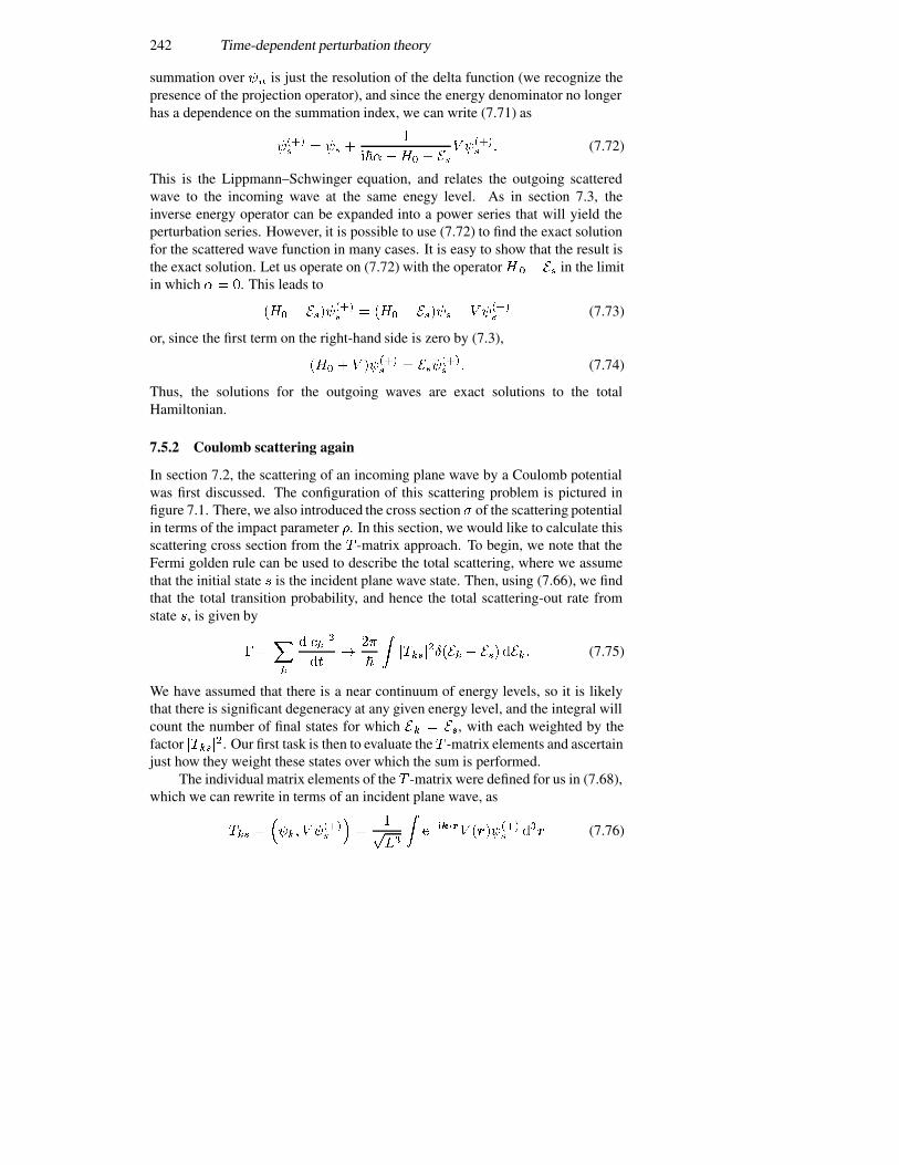
242 Time-dependent perturbation theory
summation over �� is just the resolution of the delta function (we recognize thepresence of the projection operator), and since the energy denominator no longerhas a dependence on the summation index, we can write (7.71) as
����� � �� �
�
������ � ��� ����� � (7.72)
This is the Lippmann–Schwinger equation, and relates the outgoing scatteredwave to the incoming wave at the same enegy level. As in section 7.3, theinverse energy operator can be expanded into a power series that will yield theperturbation series. However, it is possible to use (7.72) to find the exact solutionfor the scattered wave function in many cases. It is easy to show that the result isthe exact solution. Let us operate on (7.72) with the operator � � ��� in the limitin which � � �. This leads to
��� � ��������
� ��� � ����� � � �����
(7.73)
or, since the first term on the right-hand side is zero by (7.3),
��� � � ������
� �������
� (7.74)
Thus, the solutions for the outgoing waves are exact solutions to the totalHamiltonian.
7.5.2 Coulomb scattering again
In section 7.2, the scattering of an incoming plane wave by a Coulomb potentialwas first discussed. The configuration of this scattering problem is pictured infigure 7.1. There, we also introduced the cross section � of the scattering potentialin terms of the impact parameter �. In this section, we would like to calculate thisscattering cross section from the � -matrix approach. To begin, we note that theFermi golden rule can be used to describe the total scattering, where we assumethat the initial state � is the incident plane wave state. Then, using (7.66), we findthat the total transition probability, and hence the total scattering-out rate fromstate �, is given by
� ��
�
������
� �
�
���������� � ��� ���� (7.75)
We have assumed that there is a near continuum of energy levels, so it is likelythat there is significant degeneracy at any given energy level, and the integral willcount the number of final states for which �� � ��, with each weighted by thefactor ������. Our first task is then to evaluate the � -matrix elements and ascertainjust how they weight these states over which the sum is performed.
The individual matrix elements of the � -matrix were defined for us in (7.68),which we can rewrite in terms of an incident plane wave, as
��� ����� � ����
�
��
�� �
������� �������
���� (7.76)
A scattering-state basis—the � -matrix 243
Figure 7.1. The scattering geometry for the Coulomb scattering of a plane wave.
where �� is the volume normalization for the plane wave that is incident. Inaddition, it has been assumed that the incident plane wave is described by thewave vector � of energy ��. How are we to describe the scattered wave function����� ? It may be assumed that the scattering is small, so we can approximate this
wave function as a plane wave as well, but will take the scattering into a new wavevector ��, describing the energy ��. The delta function in (7.75) ensures that thesetwo energies are equal, which means that the two wave functions must have equalamplitudes (but not necessarily the same directions). Thus, we assume that
�����
� ����
������ (7.77)
and so
��� ��
��
������������� ��� ��� (7.78)
which is just the Fourier transform of the Coulomb potential. This can beevaluated by standard techniques (assuming a convergence factor to eliminate theproblem of � � ��, where the scattering is assumed to vanish), which leads to
��� ���
����� � ���� (7.79)
where � is the dielectric permittivity of the medium. Hence, there is a strongdependence upon the magnitude of the scattered wave vector in the matrix elementand we have to take care in evaluating the integral in (7.75).
While we have indicated an integration over the energy coordinate, the resultfor the matrix element of the � -matrix indicates that the integration should bemore carefully carried out in momentum space. For this purpose, the delta
244 Time-dependent perturbation theory
function and differential can be transformed to
��� � ��� ��
����� � �
�� (7.80)
and
��� �
��
��
���� �� ��� � �� ��� (7.81)
The direction of the scattering vector � � � � � � is found subject to the deltafunction which gives the scattering geometry shown in figure 7.1. This leads to
� ���
�
��
��
�� � ���
����� � ����
���
����� � ��� �� �� ��� � �� ��
����
���
��
��
�����
����
���
���� � ��
��������� (7.82)
The last integral has a problem with the lower limit of the �-integration, whereit diverges. This divergence is usually removed via the following argument:the transition rate of interest is really that at which the momentum of theincoming wave is reduced, which leads to the introduction of an additionalfactor of ( � �� �) into the argument of the integral. This factor arises fromprojecting �� onto �, so the change in the initial momentum is proportional to��� � � � �� �� � � �� � �� ��, which gives the factor of ( � �� �) to beincluded within the integral. Thus, each scattering process reduces the momentumby only a small amount, and it is the integrated sum of many scattering processesthat relaxes the momentum. It is really this momentum decay rate that is ofinterest. The result would then properly be called a momentum transition rate,or momentum scattering rate. We will pursue this approach to complete theillustration of the scattering cross section.
Using the convergence factor to describe the momentum scattering rate, thetransition rate becomes
� �����
���
��
��
�����
����
�� ��� �� �� ��� � ��
��������
� ����
���
��
��
�����
����
���
���
�������� (7.83)
This result is the scattering rate for a single Coulomb centre, and needs of courseto be modified if there are multiple scattering centres. Normally, one uses thedensity of these centres, which eliminates the volume term remaining in (7.83).We can now retreat from this to obtain the cross section through the definition
� ��
����
����
������� (7.84)
Generally, one goes in the opposite direction, and computes the scattering ratefrom the cross section through � � ��, where is the density of scatteringcentres.
A scattering-state basis—the � -matrix 245
7.5.3 Orthogonality of the scattering states
The Lippmann–Schwinger equation can now be used to show that the scatteringstates remain normalized and orthogonal. Before doing this, though, we divergeto illustrate another representation of the equation. If the resolvent operator, orGreen’s function (in this case a retarded Green’s function due to the sign on theimaginary part), is defined by
����� ��
�� ��� � ���(7.85)
then (7.72) can be rewritten as
�����
��
�������� ��
� (7.86)
This latter form is termed Dyson’s equation, and clearly illustrates how theperturbation series is obtained by expanding the denominator in a power series.In fact, the form (7.86) is often termed the re-summed perturbation series.
Let us now rewrite (7.72) to obtain another useful result. We pre-multiply allthe terms by the denominator of the last term to give
��� ��� � ���������
� ��� ��� � ������ � � �����
(7.87)
which can be rearranged to give
��� ��� � � � ���������
� ��� ��� � ������ (7.88)
or
��� �� � ���������
� ��� ��� � ������
� ��� �� � ������ � � ��� (7.89)
This can now be rearranged to give
�����
� �� ��
�� �� � ���� ��� (7.90)
With a little algebra, it is clear that this form is merely the Dyson equation, butrearranged slightly.
Finally, we want to show that the scattering states retain their orthogonalityand orthonormality. To begin, we will use (7.90) to describe just one of the statesaccording to
������
� �����
� �
��� �
�
�� �� � ���� ����
����
�
�
���� �
����
� ��
�� �� � ��������
�
�
���� �
����
� ��
�� � �� � ��������
�(7.91)
246 Time-dependent perturbation theory
where we have used (7.74) to replace the total Hamiltonian with the energy ofthe scattered state. We can now factor out the minus sign of the denominator,and since the fraction is now a �-number, we can reverse the order of the termsmultiplying the last scattering state. We then take the total operator back to theadjoint term, where the ��-term becomes the operator ��. Then, returning thisoperator to the position shown in (7.91), this latter equation can be written as
������
� �����
� �
���� �
����
��
�� ��� � ���� ����
�
�� (7.92)
Now, using (7.72), this finally becomes
������
� �����
� � ��� � ��� � �� (7.93)
which establishes the orthonormality of the scattering states.
References
Ferry D K 2000 Semiconductor Transport (London: Taylor and Francis)Landau L D and Lifshitz E M 1958 Quantum Mechanics (London: Pergamon) pp 146,
150–3Merzbacher E 1970 Quantum Mechanics (New York: Wiley)Shockley W and Bardeen J 1950 Phys. Rev. 77 407; 80 72
Problems 247
Problems
1. For the unperturbed wave functions and energies of section 6.2.1, estimatethe decay rate
�� ��
��
�
�
������
2. The propagator ���� ��� satisfies the integral equation (7.36). If � ��� ������ ���, show that
���� ��� ��
� � ����������� ���
where ���� is the Heaviside step function; ���� � � for � � , and ���� � for � . (Hint: break up the integral into segments � �� � Æ,�� � Æ � �� � Æ, �� � Æ � �, where Æ is a very small parameterthat is assumed to vanish, and use the property (7.35).)
3. Verify (7.37). (Hint: the multiple time integrals in each term must betransformed all to have the same limits of integration. This introduces a factorialin the pre-factor and also changes the multiple integrals from a nested set to aproduct of individual integrals. The series is then summed.)
4. At � , an electron is assumed to be in the � � eigenstate of aninfinite square potential well, which extends from ���� � ���. At � � ,an electric field is applied, with the potential � � �. The electric field is thenremoved at time � . Determine the probability that the electron is in any other stateat � � � . Do not make any assumptions about the relative size of ���� . What arethe differences for the cases in which this latter quantity is small or is large?
5. Assume that an incident electron in a solid, in a state characterized by thewave vector �, is scattered by the motion of the atoms of the solid. This scatteringfrom the acoustic waves in the solid is characterized by a perturbing potential thatis independent of the scattering wave vector �. Convert the sum over the finalstates into a sum over the final-state energies, and show that the scattering rate (thetotal transition rate ��) is directly proportional to the magnitude of the incidentwave vector.
6. Using only ionized impurity scattering (chapter 6) and acousticdeformation potential scattering, so that the average relaxation time can be easilycomputed, analyse the data of Tyler W W and Woodbury H H 1956 Phys. Rev. 102647, for n-type germanium. Treat the impurity concentration and the deformationpotential as adjustable parameters for each sample and tabulate the results (youshould have a single value for each of these two numbers for each sample and thedeformation potential should not vary from sample to sample).
7. A particular semiconductor has a zero-field mobility composed ofionized impurity scattering of � �� ��� ��� and of acoustic scattering of

248 Time-dependent perturbation theory
���� ��� ��� ���. Assume that the average energy of the carriers is givenapproximately by
�
������ � � � ��� ���
with �� ���� � (�� is an energy relaxation time). Plot � as a function of theelectric field at 22 K.
Chapter 8
Motion in centrally symmetric potentials
The problem of interacting particles can usually be reduced in quantum mechanicsto that of one particle, as can be done in classical mechanics. Normally, thisproblem is one of an electron orbiting around, or being affected by, a positiveatomic core or a scattering centre with the interaction governed by the Coulombpotential. In general, this is a multi-dimensional problem, and not one ofthe simpler one-dimensional problems with which we have been concerned inthe previous chapters. Once we begin to treat multiple dimensions, then statedegeneracy begins to arise more frequently, and the most common problemtreated is that of the hydrogen atom. These extra dimensions provide moredegrees of freedom and more complexity. In this chapter, we want to discussthe motion of a charged particle in a centrally symmetric potential, and so willdiscuss the hydrogen atom. First, however, we want to begin to understand howthe degeneracies arise and just what they mean. To facilitate this, we will treatfirst the harmonic oscillator for a two-dimensional motion and potential. We willthen consider the manner in which the degeneracies are split by a magnetic field.Following this, we will be ready to discuss the hydrogen atom with its three-dimensional potential. Finally, we will briefly discuss the energy levels that arisein atoms more complex than the hydrogen atom with real, but non-coulombicpotentials.
8.1 The two-dimensional harmonic oscillator
The harmonic oscillator in one dimension was discussed in chapter 4. This simpleproblem of a particle in a quadratic potential energy is one of the typical problemsof quantization. In two (or more) dimensions, the problem is more interesting,but not particularly more complicated. We want to treat only two dimensionshere in order to understand better just how the degeneracies arise. However, aswe will see, the two-dimensional problem is of particular interest for electrons insemiconductor interfaces. Here, this typical two-dimensional problem, similar tothe one that we will consider, can arise when electrons are confined in an inversion
249
250 Motion in centrally symmetric potentials
layer at the interface between, for example, silicon and silicon dioxide or at theinterface of a heterostructure or in a potential well in the direction normal to thatconsidered here (see section 2.6 for the first example). In any case, it is assumedthat there is no �-motion, due to confinement of the carriers in this dimension.Further, it will be assumed for simplicity that centrally symmetric properties ofthe potential require that the ‘spring’ constants of the harmonic potential are thesame in the two free coordinates.
8.1.1 Rectangular coordinates
We begin by treating the two dimensions as existing along two perpendicularaxes in a normal rectangular coordinate system. Thus, the Hamiltonian may beobtained by expanding (4.9) to two dimensions, and becomes
� � ���
��
���
����
��
���
��
�
������� � ���� (8.1)
In order to simplify the results, we will introduce the creation and annihilationoperators from (4.60), but with one set for the �-coordinates (denoted with asubscript �) and one set for the �-coordinates (with a subscript �). With theintroduction of these operators, equation (8.1) may simply be expressed as
� � �������� �
�
�� � �����
��� �
�
�� � ����� � �� � �� (8.2)
where we have introduced the number operator � � ���, introduced insection 4.4.
We note from (8.2) that the lowest energy level �� is just ��, which arisesfor �� � �� � �. This level arises from just the zero-point motion of theharmonic oscillators, and there is just one possible state that contributes to thislevel (the state where both number operators are identically zero). Thus, there isno degeneracy in this lowest energy level. On the other hand, the next highestenergy level
�� � ��� (8.3)
has a double degeneracy since it can arise from two combinations of numberoperators, �� � � and �� � �, as well as �� � � and �� � �. The third energylevel has the value
�� � ��� (8.4)
and is triply degenerate, since it arises from the three combinations of values thatyield �� � �� � �. This discussion can be continued to higher energy levels,from which it is found that the energy value of the �th level is
�� � ��� ���� (8.5)
and has an �� � ��-fold degeneracy from the multiple ways in which the twonumber operators can be combined to yield �� � �� � �.

The two-dimensional harmonic oscillator 251
How do we determine the �- and �-axes? The problem has no centralproperty that allows us to determine uniquely the orientation of either of theseaxes. Thus, the selection of some arbitrary direction for the �-axis is one ofconvenience, but not one of basic physics. This means that the basic propertiesof the harmonic oscillator are not those associated with these axes. Rather,we will find that the various degeneracies arise from the angular motion of theparticle, while the energy level is basically set by the radial motion (in cylindricalcoordinates). To illustrate this better, we will change variables and work theproblem in cylindrical coordinates, and this is done in the next section.
8.1.2 Polar coordinates
If we specify the oscillator merely by its energy Hamiltonian (8.5), wecannot specify a complete set of commuting observables; that is, there issome degeneracy in the specification. This is because there are a number ofcombinations of �- and �-oscillator states that can combine into any single valueof �. If we expand the total Hamiltonian into polar coordinates (cylindricalcoordinates with no �-variation), and separate the resulting Schrodinger equationinto the radial and the angular parts, we will find that the radial part generallydetermines the energy level, and the degeneracy goes into the various angularvariations that result. For example, if we consider the � � � level of (8.5), oneof the solutions arises for �� � �� � �. Thus, each of the two one-dimensionalharmonic oscillators is in the first excited state. How do we adjust the phasedifference between the two oscillations? This phase difference can make the totaloscillation actually rotate in the (�� �) plane as a phasor. The rotation of theoscillation amplitude corresponds to angular momentum, and it is this momentumoperator that arises from the angular parts of the Hamiltonian in polar coordinates.By treating this angular momentum, we can understand the overall motion of thetwo-dimensional harmonic oscillator in polar coordinates.
Angular momentum in classical mechanics arises from the motion of a bodyaround some centre of rotation. This is defined by the vector
� � � � �� (8.6)
In the two-dimensional harmonic oscillator in quantum mechanics, these variablesbecome operators, but the only component (there is no �-variation in eitherposition or momentum in our current approach) that arises is � �. This is given by
�� � ��� � ���� (8.7)
We want to put this into the operator notation used in the past section, and so weintroduce the operators defined in (4.60) for each coordinate as
�� � � ��
���� � ��
����� � ��
�� � �
�
���� � ��
����� � ��
��
� � �������� � ��
���� (8.8)

252 Motion in centrally symmetric potentials
where we have used the various commutation relations for these operators
����� ��
�� � ���
�� ��� � ���
�� ��� � ���� ��� � � (8.9)
and the commutators between operators with the same subscript satisfy (4.60).We note that these operators also satisfy
������� �
�
��� � ��
���� � � (8.10a)
������� �
�
��� � ��
���� � �� (8.10b)
Using the total Hamiltonian (8.2) and (8.8), this last result shows that the �-component of the angular momentum commutes with the Hamiltonian. Since theenergy (8.5) has a set of degeneracies, these must correspond to different valuesof the angular momentum. In the lowest level (� � �), there is only one statewhich must correspond to a single angular momentum value. Because there isautomatically a degeneracy between positive and negative angles of rotation (e.g.,for every state with positive angular momentum, there must be a state with theopposite negative value of angular momentum, as there is nothing in the problemto give a preferred rotation direction), this single level must have � � � �. In thenext energy level (� � �), there are two degenerate states, one for each of the �-and �-axes. These must also correspond, in polar coordinates, to a non-zero valueof angular momentum, with one state for each direction of rotation. This can becontinued to the higher energy levels. We shall therefore seek to find the basis ofthe eigenvalues for the total Hamiltonian � and the angular momentum � �. Wewill basically follow the treatment of Cohen-Tannoudji et al (1977).
In electromagnetic fields, it is useful to decompose linear polarized wavesinto left- and right-circularly polarized waves. These circularly polarized waveshave angular momentum just as we are discussing here. This suggests that weintroduce rotating creation and annihilation operators
� ������� � ��� (8.11a)
������� � ��� (8.11b)
and comparably for their adjoints
�� �������
�� ���
� (8.12a)
� �������
�� ���
�� (8.12b)
We note from these definitions that both � and will produce the result that
����� ��� � ���� � �� ���� ����� �� � �� (8.13)
The two-dimensional harmonic oscillator 253
where the �� are constants. This means that the operation of � or � producesa linear combination of states that are at the energy level one quantum (��)down, and so removes one quantum of energy from the system just as theisolated component of an annihilation operator in a single dimension does fromthat coordinate’s harmonic oscillator. Similarly, the adjoint operators (creationoperators) increase the energy of the state by one unit of energy ��. We will seebelow that this energy reduction is accompanied by a corresponding change in theangular momentum of the state.
The rotational operators satisfy a commutation relation that can be obtainedfrom those of the independent ones for each axis, and
��� ��� � ��� ��� � � (8.14)
��� �� � ��� ��� � ���� �� � ���� ��� � �� (8.15)
We also note that (8.11) and (8.12) can be used to give
��� � �
����� �� � ��� �� � ���� �� � ���� ��� (8.16a)
��� � �
����� �� � ��� �� � ���� �� � ���� ���� (8.16b)
Thus, we can write the Hamiltonian as
� � ����� ���� ���� � ��� � �� � ����� (8.17)
Here, we have introduced the equivalent number operators for each of therotational operator pairs. In addition, we can rewrite the angular momentum as
�� � ����� ����� � ��� � ����� (8.18)
Here, the Hamiltonian remains in a form as simple as that for rectangularcoordinates, and the angular momentum has been considerably simplified.
Using the operators � and �, we can go through the complete arguments ofsection 4.4 to determine the wave functions. This will lead to the definition of theorthonormal states
���� ��� ��
���������
������������ ��� �� (8.19)
and these states are eigenstates of both the Hamiltonian and the angularmomentum. The normal parameters, such as the energy index in (8.6), are givenby the integers
� � �� � �� � �� � ��� (8.20)
We note that if we act with the operator �� on (8.19), we not only raise theenergy by one unit (we increase �� by one unit), we also raise the value of by one unit, hence increasing the angular momentum by one unit of Planck’s(reduced) constant. Note that operating with �� raises the energy but reduces the
254 Motion in centrally symmetric potentials
angular momentum by decreasing � through increasing � �. This tells us that thisoperator corresponds to the positive (anti-clockwise) direction of rotation, whilethe other operator set refers to the negative (clockwise) direction of rotation. Theeigenvalues of the angular momentum are then ��. The eigenvalues with a givenvalue of � are ��� ��-fold degenerate, since we can have
�� � � �� � �
�� � �� � �� � �
�� � �� � �� � �
� � �
�� � � �� � �� �
�� � � �� � ��
(8.21)
Now, � can be a positive or negative integer, since it can range from � ����� to�������, or from � to ��. For � � �, there is only a single level that requires� � �. For the next energy level, � � � and there are two levels. Thus, � � ��.For the third level, � � � and there are three levels. Here, � takes on the values0 and ��. Hence, for a given energy level, the allowed values of � are
� � �� �� �� �� �� � � � ���� ����� (8.22)
Hence, any particular state is specified by the integers � and �, and the wavefunction is defined through
������ �
���
�� �� �
���
�
�� (8.23)
We now need to turn our attention to finding the lowest wave function, as thehigher wave functions can be obtained from this lowest level with (8.19).
In seeking the wave function for the ground state, we will now introduce thepolar coordinates, through the quantities
� � � �� � � �
� � � ��� � � � � ���(8.24)
Using (4.60) and (8.11), we find that
� ���
�
�� �
�
�
���
�
�
�
��
�(8.25)
and
� � ��
�
�� �
�
�
���
�
�
�
��
�� (8.26)
Similarly,
� � ��
�
�� �
�
�
���
�
�
�
��
�(8.27)
The two-dimensional harmonic oscillator 255
and
�� �����
�
��� �
�
�
�
���
�
��
�
��
�(8.28)
where
� ������� (8.29)
Note, that because of the rotating coordinates, the adjoint operators are not simplycomplex conjugates of the annihilation operators, but must be carefully calculatedfrom the definitions themselves. Now, either or � will attempt to lower theenergy and change the angular momentum. The lowest eigenstate should satisfyboth of these operators, as
�� �� � ��� �� � �� (8.30)
The two operators and � differ only by the sign of the imaginary part. Since(8.30) must satisfy both the real and imaginary parts simultaneously, it leads to
�
��
�
���� �� � � (8.31a)
�
�
�
���� �� � ����� ��� (8.31b)
Equation (8.31a) just leads to a function that is independent of the angle �. Thesecond of these equations leads to ���������� behaviour, just as for the linearharmonic oscillator. After normalization, the ground-state wave function is just
�� �� � ������
������ (8.32)
The higher-lying levels are now found by using (8.19). We note that angularvariation is introduced into the wave function by the operators � and ��
themselves through the exponential pre-factors. For example, the wave functionfor the � � � � � state is given by
�� �� � ��� �� � ��������
�������� (8.33)
while the state �� �� (� � �, � � ��) is given by the complex conjugate ofthis expression. Thus, the two angular momentum states have counter-rotatingproperties, but both are made up of linear combinations of the linear harmonicoscillators along the two axes. In the next section, an additional potential due to amagnetic field will be used to raise the degeneracy of the two angular momentumstates.
256 Motion in centrally symmetric potentials
8.1.3 Splitting the angular momentum states with a magnetic field
The motion of an electron in a magnetic field was discussed earlier in section 4.7,where it was shown that the magnetic motion also introduces a harmonic oscillatorpotential. Here, we want to examine the coupling of the magnetic harmonicoscillator potential with the two-dimensional harmonic oscillator potential of(8.1). The first people to study the two-dimensional harmonic oscillator in amagnetic field were apparently Fock (1928) and Darwin (1931), but the operatorapproach that we want to use follows the treatment of Rossler (1991). The totalHamiltonian can be found by coupling (8.1) with (4.107), and
� ��
����� ���� �
�
������� � ���� (8.34)
Because of the two-dimensional nature of the electrostatic harmonic oscillator,it is more convenient to take the vector potential in the symmetric gauge, ratherthan the Landau gauge used in section 4.7, with� � �������� ����, so that themagnetic field is oriented in the -direction, normal to the two-dimensional planeof the motion (� ���� � ���). The momentum term can now be expandedas
��� ���� � ����
�
���
�
��
�� ����
��
�� �
�
��
�
�������� � ����
(8.35)The last term can be combined with the electrostatic harmonic oscillator if wedefine the new oscillator ‘spring’ frequency
�
��� �
���
�
��(8.36)
where �� � ���� is the cyclotron frequency introduced near (4.112). Thesecond term in (8.35), which is linear in the magnetic field, can be rewritten using(8.7) as
����� (8.37)
With these definitions, the Hamiltonian, with the change in frequency in thedefinitions of the operators as � � , can then be rewritten as
� � � � � � � ���� �
����� � � � ���� �
����� (8.38)
where � � �� � is the angular momentum quantum number, and not the massthat appeared in the some of the early equations in this section. The reader shouldcheck that this new Hamiltonian still commutes with the angular momentum,and hence that both are simultaneously measurable. However, the energy nowhas a contribution from the angular momentum directly. This term raises thedegeneracy of the previous eigenvalues (energies).
For small values of the magnetic field, �� � , each energy level is splitinto � � levels as the degeneracy is raised by the magnetic field. Each pair
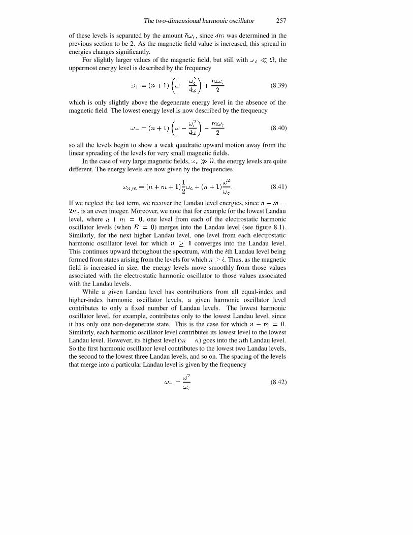
The two-dimensional harmonic oscillator 257
of these levels is separated by the amount ���, since � was determined in theprevious section to be 2. As the magnetic field value is increased, this spread inenergies changes significantly.
For slightly larger values of the magnetic field, but still with �� � �, theuppermost energy level is described by the frequency
�� � ��� ��
�� �
���
��
�����
�(8.39)
which is only slightly above the degenerate energy level in the absence of themagnetic field. The lowest energy level is now described by the frequency
��
� ��� ��
�� �
���
��
�����
�(8.40)
so all the levels begin to show a weak quadratic upward motion away from thelinear spreading of the levels for very small magnetic fields.
In the case of very large magnetic fields, �� � �, the energy levels are quitedifferent. The energy levels are now given by the frequencies
���� � ����� ���
��� � ��� ��
��
��� (8.41)
If we neglect the last term, we recover the Landau level energies, since ��� ���� is an even integer. Moreover, we note that for example for the lowest Landaulevel, where � � � � �, one level from each of the electrostatic harmonicoscillator levels (when � � �) merges into the Landau level (see figure 8.1).Similarly, for the next higher Landau level, one level from each electrostaticharmonic oscillator level for which � � � converges into the Landau level.This continues upward throughout the spectrum, with the �th Landau level beingformed from states arising from the levels for which � � �. Thus, as the magneticfield is increased in size, the energy levels move smoothly from those valuesassociated with the electrostatic harmonic oscillator to those values associatedwith the Landau levels.
While a given Landau level has contributions from all equal-index andhigher-index harmonic oscillator levels, a given harmonic oscillator levelcontributes to only a fixed number of Landau levels. The lowest harmonicoscillator level, for example, contributes only to the lowest Landau level, sinceit has only one non-degenerate state. This is the case for which � � � � �.Similarly, each harmonic oscillator level contributes its lowest level to the lowestLandau level. However, its highest level (� � �) goes into the �th Landau level.So the first harmonic oscillator level contributes to the lowest two Landau levels,the second to the lowest three Landau levels, and so on. The spacing of the levelsthat merge into a particular Landau level is given by the frequency
��
���
��(8.42)
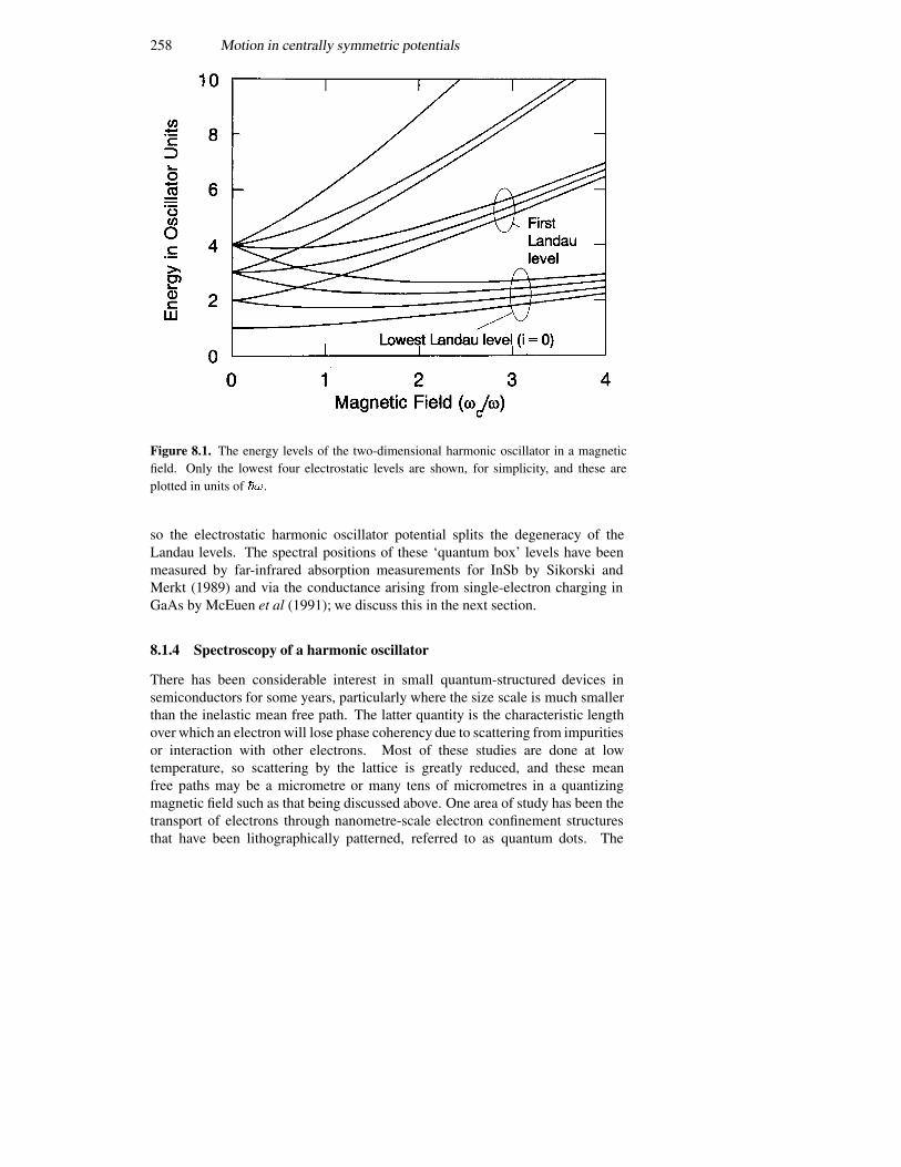
258 Motion in centrally symmetric potentials
Figure 8.1. The energy levels of the two-dimensional harmonic oscillator in a magneticfield. Only the lowest four electrostatic levels are shown, for simplicity, and these areplotted in units of ��.
so the electrostatic harmonic oscillator potential splits the degeneracy of theLandau levels. The spectral positions of these ‘quantum box’ levels have beenmeasured by far-infrared absorption measurements for InSb by Sikorski andMerkt (1989) and via the conductance arising from single-electron charging inGaAs by McEuen et al (1991); we discuss this in the next section.
8.1.4 Spectroscopy of a harmonic oscillator
There has been considerable interest in small quantum-structured devices insemiconductors for some years, particularly where the size scale is much smallerthan the inelastic mean free path. The latter quantity is the characteristic lengthover which an electron will lose phase coherency due to scattering from impuritiesor interaction with other electrons. Most of these studies are done at lowtemperature, so scattering by the lattice is greatly reduced, and these meanfree paths may be a micrometre or many tens of micrometres in a quantizingmagnetic field such as that being discussed above. One area of study has been thetransport of electrons through nanometre-scale electron confinement structuresthat have been lithographically patterned, referred to as quantum dots. The
The two-dimensional harmonic oscillator 259
structures are typically heterostructures between GaAs and AlGaAs, in whichelectrons move from donors in the AlGaAs to the GaAs and form an inversionlayer at the interface. This inversion layer has confinement quantization in thedirection normal to the heterostructure interface, just as discussed for Si–SiO �
in section 2.6. The transport is then allowed in the two dimensions in theplane of the heterostructure interface. The lithographically defined confinementpotential in two dimensions creates the equivalent of a two-dimensional harmonicoscillator, as shown in figure 8.2(a). A similar quantum dot was discussedin sections 1.3 and 3.3.3, where transport through a quantum dot was used tomodulate the Aharonov–Bohm interference (Yacoby et al 1994, 1995). In thatexample, transport through the quantum dot states was used to modulate thetunnelling phase of the particles. In the present case, the tunnelling is used toactually do spectroscopy of the quantum dot states. The so-called edge states arethe drift of the electrons in the strong magnetic field around the periphery of thequantum dot. The guiding centre orbit is formed by the cyclotron motion of theelectron being interrupted by the edge of the dot; that is, they specularly reflectfrom the confining potential, so they bounce along the interface. These guidingcentre orbits are called edge states (section 4.7.2).
The spectroscopy of the quantum dot arises from the motion of the Fermienergy in a magnetic field. The Fermi energy in a semiconductor, at lowtemperature (the experiments discussed here were performed with the sample atapproximately 0.3 K), is the energy level at which all states below this energy arefull and all states above this energy are empty. In figure 8.2(b), an enlarged sectionof figure 8.1 is shown. The heavy black line is the Fermi energy. The density ofelectrons is pre-set in the sample, so this defines precisely the number of filledstates in the quantum dot, which is two (for spin degeneracy) times the numberof energy levels below the Fermi energy. As the magnetic field is increased, anda state crosses the Fermi level from above—for example just above the point����� � ��� (our � is �� in this figure)—the Fermi energy must follow this statedownward allowing the upward-moving state to pass above the Fermi level so asto keep the number of levels below the Fermi energy fixed.
As the gate voltage applied to the confinement potential, or more exactlyto a uniform back metal contact, is changed the number of electrons in thequantum dot can be changed. As an electron enters or leaves the dot throughthe end couplings, a conductance peak along the channel is observed, which canbe followed while varying the magnetic field. This is shown in figure 8.3(a).The nearly constant Coulomb energy of the electrons in the dot can be subtractedout, and the gate voltage converted to energy to unfold the experimental energyspectrum, which is shown in figure 8.3(b). This should be compared with thetheoretical spectrum expected for a two-dimensional harmonic oscillator in amagnetic field shown in figure 8.1 and figure 8.2(b). The agreement as regardsthe shape of the spectrum is remarkable.
This experiment samples the spectra for rather large energy and magneticfield. More recent studies have actually looked at the spectra for small numbers
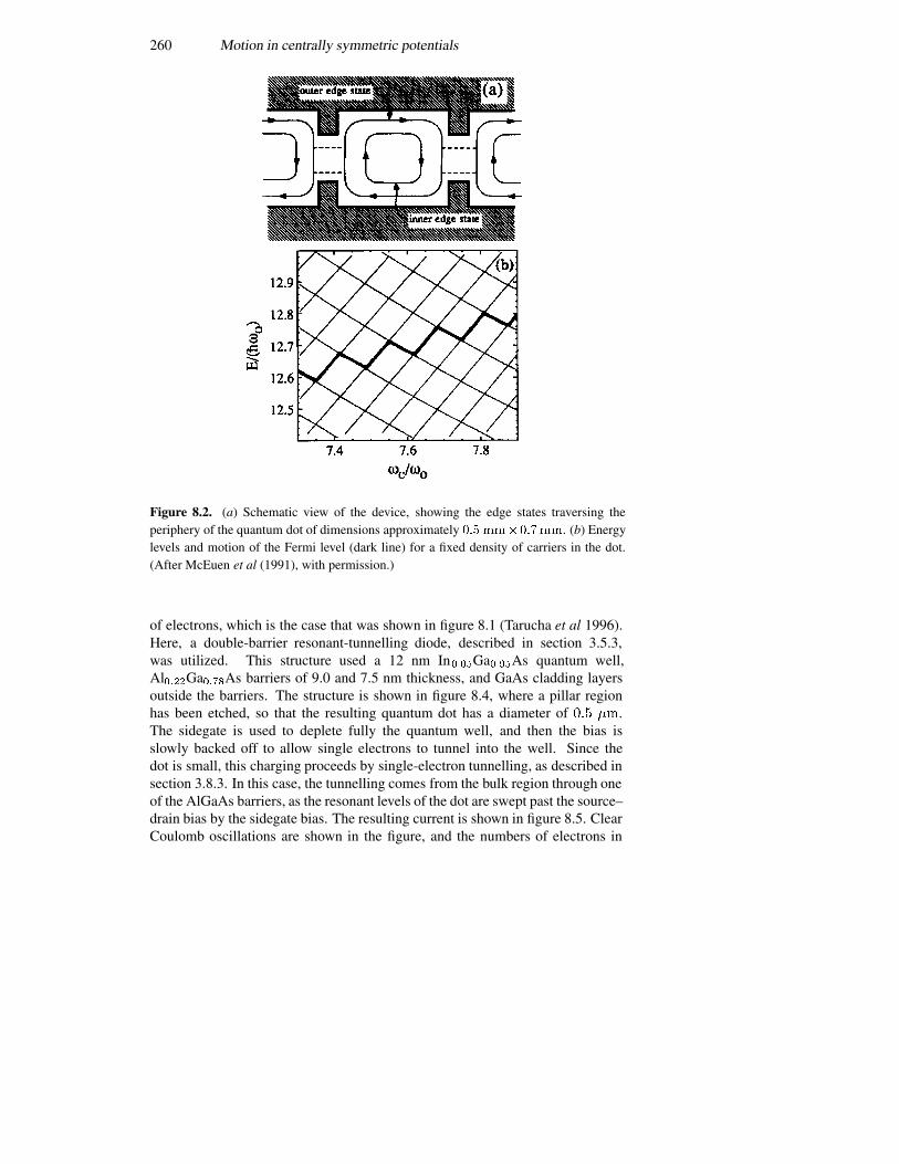
260 Motion in centrally symmetric potentials
Figure 8.2. (a) Schematic view of the device, showing the edge states traversing theperiphery of the quantum dot of dimensions approximately ��� ��������. (b) Energylevels and motion of the Fermi level (dark line) for a fixed density of carriers in the dot.(After McEuen et al (1991), with permission.)
of electrons, which is the case that was shown in figure 8.1 (Tarucha et al 1996).Here, a double-barrier resonant-tunnelling diode, described in section 3.5.3,was utilized. This structure used a 12 nm In����Ga����As quantum well,Al����Ga����As barriers of 9.0 and 7.5 nm thickness, and GaAs cladding layersoutside the barriers. The structure is shown in figure 8.4, where a pillar regionhas been etched, so that the resulting quantum dot has a diameter of ��� ��.The sidegate is used to deplete fully the quantum well, and then the bias isslowly backed off to allow single electrons to tunnel into the well. Since thedot is small, this charging proceeds by single-electron tunnelling, as described insection 3.8.3. In this case, the tunnelling comes from the bulk region through oneof the AlGaAs barriers, as the resonant levels of the dot are swept past the source–drain bias by the sidegate bias. The resulting current is shown in figure 8.5. ClearCoulomb oscillations are shown in the figure, and the numbers of electrons in
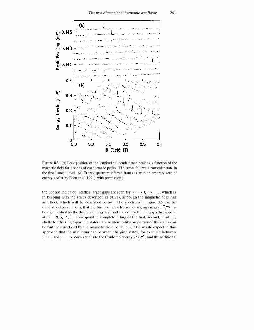
The two-dimensional harmonic oscillator 261
Figure 8.3. (a) Peak position of the longitudinal conductance peak as a function of themagnetic field for a series of conductance peaks. The arrow follows a particular state inthe first Landau level. (b) Energy spectrum inferred from (a), with an arbitrary zero ofenergy. (After McEuen et al (1991), with permission.)
the dot are indicated. Rather larger gaps are seen for � � �� �� ��� � � � , which isin keeping with the states described in (8.21), although the magnetic field hasan effect, which will be described below. The spectrum of figure 8.5 can beunderstood by realizing that the basic single-electron charging energy � ���� isbeing modified by the discrete energy levels of the dot itself. The gaps that appearat � � �� �� ��� � � � correspond to complete filling of the first, second, third, . . .shells for the single-particle states. These atomic-like properties of the states canbe further elucidated by the magnetic field behaviour. One would expect in thisapproach that the minimum gap between charging states, for example between� � � and � � ��, corresponds to the Coulomb energy �����, and the additional
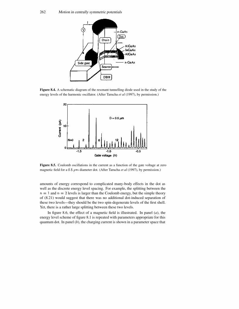
262 Motion in centrally symmetric potentials
Figure 8.4. A schematic diagram of the resonant tunnelling diode used in the study of theenergy levels of the harmonic oscillator. (After Tarucha et al (1997), by permission.)
Figure 8.5. Coulomb oscillations in the current as a function of the gate voltage at zeromagnetic field for a ��� �� diameter dot. (After Tarucha et al (1997), by permission.)
amounts of energy correspond to complicated many-body effects in the dot aswell as the discrete energy level spacing. For example, the splitting between the� � � and � � � levels is larger than the Coulomb energy, but the simple theoryof (8.21) would suggest that there was no additional dot-induced separation ofthese two levels—they should be the two spin-degenerate levels of the first shell.Yet, there is a rather large splitting between these two levels.
In figure 8.6, the effect of a magnetic field is illustrated. In panel (a), theenergy level scheme of figure 8.1 is repeated with parameters appropriate for thisquantum dot. In panel (b), the charging current is shown in a parameter space that

The two-dimensional harmonic oscillator 263
Figure 8.6. (a) Calculated single-particle energy levels in the Darwin–Fock spectrum as afunction of the magnetic field, with ��� � � meV. Each state is twofold degenerate, andthe broken line is discussed in the text. (b) Experimentally determined evolution of thefifth, sixth, and seventh tunnelling current peaks as a function of the magnetic field. (AfterTarucha et al (1997), by permission.)
plots gate voltage versus magnetic field (Tarucha et al 1997). Here, the magneticfield is held fixed at a value and the gate voltage swept, and there are some 41 ofthese sweeps in the figure. The Coulomb charging energy has not been subtractedfrom the gate voltage, so the movements of the peaks are kept some distance apartfrom one another (in gate voltage). The peaks for the fifth, sixth, and seventhelectrons are shown in these plots. The seventh electron is characterized by thebroken curve in panel (a), and it can be seen that this charging peak changescharacter as one raises the magnetic field. That is, the seventh electron goes intothe ��� �� � ��� �� state at low magnetic field, then begins to occupy the ������state for a field larger than the level crossing at 1.3 T. Finally, a second levelcrossing occurs at about 2 T, whereupon the seventh electron begins to fill the��� �� level arising from the fourth shell. At the same time, the spin-degeneratefifth and sixth electrons begin in the ������ level and transition to the ��� �� levelfor magnetic fields beyond the 1.3 T crossing. The splitting between these latter
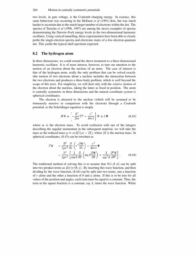
264 Motion in centrally symmetric potentials
two levels, in gate voltage, is the Coulomb charging energy. In essence, thissame behaviour was occurring in the McEuen et al (1991) dots, but was muchharder to ascertain due to the much larger number of electrons within the dot. Thespectra of Tarucha et al (1996, 1997) are among the nicest examples of spectrademonstrating the Darwin–Fock energy levels in the two-dimensional harmonicoscillator. Using vertical tunnelling, these experimenters have been able to clearlyprobe the single-electron spectra and electronic states of a few-electron quantumdot. This yields the typical shell spectrum expected.
8.2 The hydrogen atom
In three dimensions, we could extend the above treatment to a three-dimensionalharmonic oscillator. It is of more interest, however, to turn our attention to themotion of an electron about the nucleus of an atom. The case of interest isthat of the hydrogen atom, really the only problem that can be solved exactly(the motion of two electrons about a nucleus includes the interaction betweenthe two electrons and produces a three-body problem, which is well beyond thescope of this text). For simplicity, we will deal only with the relative motion ofthe electron about the nucleus, taking the latter as fixed in position. The atomis centrally symmetric in three dimensions and the natural coordinate system isspherical coordinates.
The electron is attracted to the nucleus (which will be assumed to beimmensely massive in comparison with the electron) through a Coulombpotential, so the Schrodinger equation is simply
�� �
��
��
���
��
��
����
�� � �� (8.43)
where � is the electron mass. To avoid confusion with one of the integersdescribing the angular momentum in the subsequent material, we will take themass as the reduced mass � � ��������, where � is the nuclear mass. Inspherical coordinates, (8.43) can be rewritten as
�� � ���
�����
��
�����
��
��
��
�����
���
����
��
�
�
�
��
��
�
��
�
��
���
��
� (8.44)
The traditional method of solving this is to assume that ���� � �� can be splitinto two product terms as ������ ��. By inserting this wave function, and thendividing by the wave function, (8.44) can be split into two terms, one a functionof � alone and the other a function of and � alone. If this is to be true for allvalues of the position and angles, each term must be equal to a constant. Thus, theterm in the square brackets is a constant, say �, times the wave function. While
The hydrogen atom 265
this constant is arbitrary, it is known from treatments of spherical harmonics thatit is more appropriate to set this separation constant equal to ��� � ��. It is easyto show that there is a one-to-one correspondence to any value of � and �, so longas � � �, so no generality is lost by making this latter substitution.
8.2.1 The radial equation
By eliminating the angular variables with the above constant interpretation, whichstill must be shown to be valid (and we do this below), the radial equation nowbecomes
�
���
��
�����
��
��
���� ��
����
��
��
�� �
��
���
�� � � (8.45)
To simplify the equation, we introduce the reduced units for energy and length
�� ����
��(8.46a)
and� � �� (8.46b)
respectively, and set
� ����
������
��
���
��
���� (8.46c)
Then, we can rewrite (8.45) as
�
���
��
�����
��
��
��
��
�
��
���� ��
��
�� � � (8.47)
The choice of the number �
�is arbitrary, but quite useful for the following
development.As in the treatment of the harmonic oscillator, we first seek the behaviour
for large values of �. For sufficiently large values of the normalized radius, it isclear that the behaviour of � is as ������. This follows by retaining just thesecond-order derivative and the term with �
�as the pre-factor. The factor will
have to be determined, though, but this suggests that we seek solutions of the form���� � � �������, where � ��� will be a polynomial of finite order in �. Usingthis substitution leads to
���
����
��
�� �
���
���
��� �
��
���� ��
��
�� � � (8.48)
We now will assume that � ��� varies as ������, so (8.48) becomes
�����
��������������
��
��������������������������� � � (8.49)
266 Motion in centrally symmetric potentials
If we evaluate this at � � � (we assume the derivatives are well behaved and arefinite at this point), we see clearly that � � � or ��� � ��. Since we require thefunctions to be finite at � � �, only the former value is allowed. Equation (8.49)then becomes
����
���� ����� ��� ��
��
��� ��� �� ��� � �� (8.50)
Finally, to proceed, we will assume that ���� is a power series in �, but onethat is finite and terminates at some order. This leads to the ratio of coefficientsof successive orders � and � � �:
���� � ��� � �� �� �
�� � ���� � ��� ��� (8.51)
For this to terminate, there must be a maximum value of � � such that
� � � � � �� �� (8.52)
Here, is the total quantum number (this and thereby � determines the totalenergy of the level), � is the radial quantum number and is the angularmomentum quantum number; all are integers. With this total quantum number,the energy levels are given by (8.46c) as
�� � ����
� ������� (8.53)
Thus, as in the two-dimensional harmonic oscillator, the energy levels arespecified by the total quantum number, except that there is no � � level here.This may be used in (8.46a) to show that the effective radius of the ground stateis given by ��� � �� � ������� � ������� cm. This quantity is called theBohr radius. Note, however, that the actual normalization radius, and the factor�, depend upon the index .
The coupling between the radial quantum number and the angularmomentum quantum number means that as the angular momentum increases, theradial variations decrease (the order of the polynomial decreases). Further, forthe lowest energy level ( � �), both the radial and angular momentum quantumnumbers are zero, so the only variation is in the exponential term. In this lowestlevel, the wave function is spherically symmetric, decaying exponentially awayfrom the centre of the atom. For the second level ( � �), � can be either 0(� � �) or 1 (� � �), so there is a spherically symmetric state and one thathas preferential directions due to the angular momentum. This continues, with �taking on values �� �� � � � � ��, so there are values for this variable. Let us nowturn to the angular momentum.
We can write out a few of the lower-level wave functions in terms of thecomponents written as �������, where and � are the two eigenvalue integers
The hydrogen atom 267
that we have discussed above. Thus, the lowest three energy levels have theunnormalized radial wave functions (� � ��)
������� � �����
������� � ��� �������
������� � ������
������� � ��� � ���� ��������
������� � ���� �������
������� � ��������
(8.54)
We see that the highest-order term is determined by the radial quantum number�, but that the number of lower-order terms is related to the angular momentumquantum number �. Note, again, that this is the normalized radius, and thisnormalization depends upon the level number �.
8.2.2 Angular solutions
The angular equation that arises from (8.44) is now the focus of our attention.This equation, separated for the angular parts, becomes
�
� �
�
��
�� �
�
��
��
�
�� �
��
��� ���� �� � �� (8.55)
This can be further separated by letting � ���� ��. Using this form for theangular wave function allows us to separate (8.55) into two equations for the twovariables:
���
��� �� � � (8.56a)
�
� �
�
��
��
�
��
��
����� ��� �
�� �
� � � (8.56b)
where we have let the separation constant be the square of an integer, so thevariation in the azimuthal angle is periodic in ��:
��� �����
���� � � � � (8.57)
and is a constant for � �. We note that can take on both positive and negativevalues, but that � must be continuous and have a continuous derivative for anyvalue of .
In addressing the last angular equation, it will be convenient to let � � ��� �.With this substitution, (8.56�) becomes
�
��
���� ���
� ���
��
��
����� ��� �
�� ��
� ��� � �� (8.58)

268 Motion in centrally symmetric potentials
Since the angle varies from 0 to �, the domain of � is 0 to 1. To begin, we let thewave function be assumed to vary as ��� ����� ���. With this substitution, wefind that
��� ������
���� ������ ��
��
��� ����� ��� ������ ���� � � (8.59)
with ��� � ��. This leads us to say that �� � ���. � is now a polynomialof finite order, and for this to be the case, we must have the order of thepolynomial equal to �� ��. The parity of the polynomial (even or odd) is that of� � �� � � � ���. These polynomials are the associated Legendre polynomials,and the ��� are the associated Legendre polynomials.
8.2.3 Angular momentum
In (8.6) and (8.7), we introduced the angular momentum, and particularly the�-component of this quantity. We want to consider now the overall angularmomentum of the particle orbiting the central potential in the hydrogen atom. Bycontinuation of (8.7), we can immediately write the three components of angularmomentum as
�� � ��
���
��� �
�
��
�(8.60a)
�� � ��
���
��
�
��
�(8.60b)
�� � ��
��
��� �
�
�
� (8.60c)
It is easily then shown using the normal commutation relations between positionand momentum that
���� ��� � ��� ���� ��� � ��� ���� ��� � ��� (8.61)
Finally, the square of the total angular momentum can be written as
�� � ��
�� ��
�� ��
�(8.62)
and, moreover, this total angular momentum commutes with each of thecomponents individually. Thus, we have four relatively independent quantities—the three components of the angular momentum and the total angularmomentum—that can all be measured simultaneously. Normally, we can onlyspecify two of these independently (we have only two parameters, � and �, thatarise in the treatment of the orbital motion).
Let us first examine ��, since the second of the parameters, �, is related tothe motion about the polar axis, the �-axis as it were. If we convert (8.60c) to
The hydrogen atom 269
spherical coordinates, with � � � ��� � ����, � � � ��� � ����, � � ��� �, thenwe find that
�� � ����
��� (8.63)
Obviously, this involves only the quantum number �, so � � is a good componentof the angular momentum to take as one of the independent quantities in theproblem. The eigenvalues of the �-component of the angular momentum are then����, with � an integer. From the discussion of (8.59), it is clear that ��� � ,so the values of � are
���� �� � � � ���� �� �� � � � � � �� � (8.64)
Thus, there are � � values for the �-component of angular momentum, for agiven value of .
We expect that the final independent quantity will be the total angularmomentum. Indeed, this will be the case. To see this, we begin by takingcombinations of the �- and �-components:
�� � �� � ��� � ����
�� �
��� � ��� �
�
��
�� (8.65)
Now,���� � ��� � ��� ��� � ��� � ��� � ��� � ���� (8.66)
Thus, we can write the total angular momentum as
�� � ��� � ��� ��� � ��� � ��� � ���
� � ��
��
��� �
�
��
���� �
�
��
��
�
���� �
��
���
�(8.67)
which is the angular part of the differential equation for the total wave function!We need only show now that the eigenvalue is indeed given by �� � . For this,we will suppress the factors of �.
For the first step, we note that we can rewrite the total angular momentum inthe form
�� � ��� � ��� � ��� � � (8.68)
which means that���� � �� �
���� (8.69)
Thus, the possible limits for � are set by the total angular momentum (this is whythe polynomial can be made to be finite in the associated Legendre polynomials).Now, we note that
����� � ��� � ��� � ��� ��� � � � (8.70)
270 Motion in centrally symmetric potentials
If we now operate on an arbitrary angular wave function, the last term produces�� �, or
����� � ������ � ��� ����� � ������� (8.71)
This tells us that the operator ��
reduces the angular momentum by one unitwhile �� raises it by one unit. If � � �, the raising operator must give a zeroresult, or
��� � ������ � �� (8.72)
If we now operate with the lowering operator��
, the same result is obtained, and
��� � ������� � ������ � ���� ��
� � ����� � � (8.73)
where we have used (8.67). Introducing the eigenvalues for the �-component ofangular momentum, with � � � in these results, we find
�� � �� � �� (8.74)
Thus, we find, upon re-inserting the Planck’s constant terms, that the eigenvaluesfor the total angular momentum are
�� � ���� ���� (8.75)
as we assumed in section 8.2.1 to solve the radial equation.
8.3 Atomic energy levels
In treating the hydrogen atom, the central potential was taken to be the Coulombpotential that existed between the atomic core and the single electron. It wouldbe desirable to continue to do this for the general atom, but there are problems.Certainly, we can continue to use the central-field approximation. However, thesimple Coulomb potential of (8.43) is only valid for the outermost electron whenthe core is shielded by the remaining electrons. For the innermost level, the chargeis ��, rather than �, where � is the atomic number of the atom. This meansthat the potential is not simply a � potential, but rather one whose amplitudevaries with the electron under consideration. The simple energy levels obtainedin (8.53) are no longer valid, in that the angular momentum states are no longerdegenerate with the states with no angular momentum—in essence, the energylevels now depend upon both � and �. This change can be found by treatingthe difference between the actual potential (for a given electron) and the Coulombpotential as a perturbation, and calculating the shift in energy for various values of� and �. In fact, this is not particularly accurate, because the inner-shell electronsalso interact with the outer electrons (and, in fact, each electron interacts witheach other electron) through an additional Coulomb (repulsive) potential. Manyschemes have been proposed for calculating the exact eigenvalues through variousapproximations, but usually some form of variational approach yields the best

Atomic energy levels 271
method. These approaches are, however, well beyond the level we want to treathere. The most important result is that, for a given level index �, the states oflowest � lie at a lower energy (are more tightly bound to the nucleus). This issufficient information to begin to construct the periodic table of the elements.
The lowest, and only exact, energy level is that for hydrogen, where there isa single electron and the atomic core of unit charge. The lowest energy level from(8.53) is the one for � � �. The allowed values of radial and angular momentumindices must satisfy �� � � � � from (8.52). Thus, the only occupied state has noangular momentum, and the radial wave function varies (in the asymptotic limitof a simple Coulomb potential) simply as �����, in reduced units. Because ofelectron spin, this energy level can hold two electrons, so this behaviour actuallyholds also for helium (although the energy level is shifted to lower energy due tothe non-Coulomb nature of the potential in helium). Because these wave functionsare spherically symmetric, they have come to be termed the 1s levels. The 1s(� � �� � � �) level can hold two electrons, which then fill the complete shell for� � �. This shell comprises the first row of the periodic table.
The next energy level, according to (8.53) has � � �. For this level,(8.52) would tell us that �� � � � �, so the lowest angular momentum statehas ���� �� � ��� ��. This lowest state gives rise to the pair of electrons inthe 2s state. For this state, the wave function is again spherically symmetricand has an asymptotic variation (for a simple Coulomb potential) proportionalto �� � �������. This wave function has two nodes (in the amplitude-squaredvalue), and this behaviour continues as the order of the s levels increases. Thetwo elements that are added via these two energy states are Li and Be. For moreelectrons, the angular momentum states begin to be filled. These levels arise for���� �� � ��� ��. There are �� � � � � values of � for these levels, and eachwill hold two electrons because of the electron spin angular momentum. Thismeans that there can be an additional six electrons accommodated by these levels.From the discussion of section 8.2.2, we know that the angular part of the wavefunction for � � � varies as � � only. This gives amplitude peaks along the�-axis, so this state is the p� state. Similarly, the � � �� states give rise to the�� states, which are combinations of the p� and p� states. These states have anangular variation as �� �����. In figure 8.7, we indicate the orientation of thesethree angular momentum wave functions. The filling of these six states, which aretermed the 2p states (we use the symbol p to signify the � � � states), is carriedout by progressing through the elements B, C, N, O, F, and Ne (� � �–10). Thus,the � � � level can hold eight electrons, and this shell is completely filled by theelement of atomic number ten (Ne). The elements Li through to Ne comprise rowtwo of the periodic table.
The states for � � � arise in a similar manner. Here, � � � � � �, so � cantake the values 0, 1, and 2. These give rise to the two 3s states and the six 3pstates, which do not differ in principle from those described above. However, theten possible states for � � � raise additional complications, and are described byquite complicated wave functions. These are the d levels, as we use the symbol
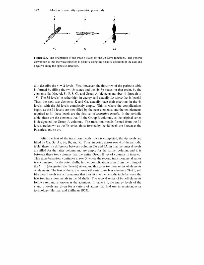
272 Motion in centrally symmetric potentials
Figure 8.7. The orientation of the three p states for the 2p wave functions. The generalconvention is that the wave function is positive along the positive direction of the axis andnegative along the opposite direction.
d to describe the � � � levels. First, however, the third row of the periodic tableis formed by filling the two 3s states and the six 3p states, in that order, by theelements Na, Mg, Al, Si, P, S, Cl, and Group A (elements number 11 through to18). The 3d levels lie rather high in energy, and actually lie above the 4s levels!Thus, the next two elements, K and Ca, actually have their electrons in the 4slevels, with the 3d levels completely empty. This is where the complicationsbegin, as the 3d levels are now filled by the next elements, and the ten elementsrequired to fill these levels are the first set of transition metals. In the periodictable, these are the elements that fill the Group B columns, as the original seriesis designated the Group A columns. The transition metals formed from the 3dlevels are known as the Pb series, those formed by the 4d levels are known as thePd series, and so on.
After the first of the transition metals rows is completed, the 4p levels arefilled by Ga, Ge, As, Se, Br, and Kr. Thus, in going across row 4 of the periodictable, there is a difference between columns 2A and 3A, in that the inner d levelsare filled for the latter column and are empty for the former column, and it isbetween these two columns that the entire Group B set of columns is inserted.This same behaviour continues in row 5, where the second transition metal seriesis encountered. In the outer shells, further complications arise from the filling ofthe � � � (designated the f levels) states, and this gives two new series of elementsof elements. The first of these, the rare-earth series, involves elements 58–71, andfills their f levels in such a manner that they fit into the periodic table between thefirst two transition metals in the 5d shells. The second series of f-shell elementsfollows Ac, and is known as the actinides. In table 8.1, the energy levels of thes and p levels are given for a variety of atoms that find use in semiconductortechnology (Herman and Skillman 1963).
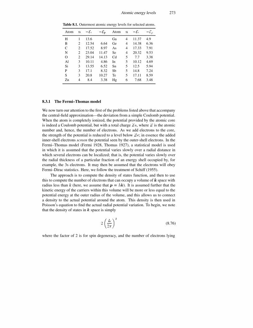
Atomic energy levels 273
Table 8.1. Outermost atomic energy levels for selected atoms.
Atom � ��� ��� Atom � ��� ���
H 1 13.6 Ga 4 11.37 4.9B 2 12.54 6.64 Ge 4 14.38 6.36C 2 17.52 8.97 As 4 17.33 7.91N 2 23.04 11.47 Se 4 20.32 9.53O 2 29.14 14.13 Cd 5 7.7 3.38Al 3 10.11 4.86 In 5 10.12 4.69Si 3 13.55 6.52 Sn 5 12.5 5.94P 3 17.1 8.32 Sb 5 14.8 7.24S 3 20.8 10.27 Te 5 17.11 8.59Zn 4 8.4 3.38 Hg 6 7.68 3.48
8.3.1 The Fermi–Thomas model
We now turn our attention to the first of the problems listed above that accompanythe central-field approximation—the deviation from a simple Coulomb potential.When the atom is completely ionized, the potential provided by the atomic coreis indeed a Coulomb potential, but with a total charge ��, where � is the atomicnumber and, hence, the number of electrons. As we add electrons to the core,the strength of the potential is reduced to a level below ��; in essence the addedinner-shell electrons screen the potential seen by the outer-shell electrons. In theFermi–Thomas model (Fermi 1928, Thomas 1927), a statistical model is usedin which it is assumed that the potential varies slowly over a radial distance inwhich several electrons can be localized; that is, the potential varies slowly overthe radial thickness of a particular fraction of an energy shell occupied by, forexample, the 3s electrons. It may then be assumed that the electrons will obeyFermi–Dirac statistics. Here, we follow the treatment of Schiff (1955).
The approach is to compute the density of states function, and then to usethis to compute the number of electrons that can occupy a volume of � space withradius less than � (here, we assume that � � ��). It is assumed further that thekinetic energy of the carriers within this volume will be more or less equal to thepotential energy at the outer radius of the volume, and this allows us to connecta density to the actual potential around the atom. This density is then used inPoisson’s equation to find the actual radial potential variation. To begin, we notethat the density of states in � space is simply
�
��
��
��
(8.76)
where the factor of 2 is for spin degeneracy, and the number of electrons lying
274 Motion in centrally symmetric potentials
within a volume of � space with radius � is just
���� � �
��
��
�� � �
�
�� ��
� �
�
��� � ��
���
�
�� �����
���� (8.77)
The electron density is just ����, and the kinetic energy is �������, so we canwrite the electron density as (recall that we are going to let the kinetic energybe equal to the potential energy by assuming that the potential energy describesthe outer limit of the electron orbit as in a classical motion, and we note that thepotential is negative)
�� � ����� ������
������ (8.78)
We can now write Poisson’s equation (which is for the voltage and not the energy,so an additional � is introduced) as
��� �� �
��
�
��
��
�
�� �
����
� � (8.79)
The boundary conditions on the potential must be set by the physical constraintsof the system. As � �, there is no charge due to the electrons, and the onlycharge is that on the atomic core. Thus, � � � �� � ����� . On the otherhand, as ��, there is no net charge within the sphere that we are considering.In this limit the potential must fall off faster than �, so � �� � �. In thissense, the potential found from the Fermi–Thomas approach is that experiencedby a test charge, and is not the one experienced by the electrons themselves. Inthis view, the potential is screened by the charge, so the actual potential in thislarge-radius limit goes as follows:
� �� � �
����� (8.80)
If we now combine the above equations, it is possible to compute an estimate forthe radial dependence of the actual potential around the atom. Combining (8.79)and (8.78) leads to
��
�
��
��
�
��
������ ������
��� ��� (8.81)
The potential, along with the boundary conditions discussed above, can beconveniently incorporated into a set of dimensionless constants. To achieve this,we define
� �� ����
� � � ��
� �
�
���
����� ��
��������
(8.82)

Atomic energy levels 275
With these substitutions, (8.81) becomes
���� �
��
���� ���� (8.83)
with� � � at � � � and � � � as ���� (8.84)
This is still a complicated equation, and the solution is usually obtainednumerically. One result of this is that the atomic radius of an atom is inverselyproportional to the cube root of its atomic number�. While this is not particularlyaccurate for small �, the accuracy of the Fermi–Thomas approximation increasesas the atomic number increases. If for no other reason, this is true since theincreasing number of electrons makes the statistical method more accurate.
8.3.2 The Hartree self-consistent potential
A second method for computing the potential for the atom is due to Hartree(1928). In this method, it is assumed that each electron moves in a central fieldthat can be calculated from the nuclear potential and the wave functions of allof the other electrons, where the charge density of each electron is given by thesquared magnitude of its wave function. The Schrodinger equation is solved foreach electron moving in its own central field in a self-consistent fashion. Wewill see in the next chapter that the Hartree potential is created by calculatingthe Coulomb interaction between the chosen electron and all other electrons, butthat the coordinates of the other electrons are integrated out of the problem, thusproviding an average potential seen by the electron due to the average distanceaway of the other electrons. Since the position of each electron changes as theother electrons move, iteration to self-consistency is required. In essence, wewant to solve the � equations for the � electrons (� � �� �� � � � � � )�
���
����
� ����
����� ���
��������
���
���� � �������
������ � ��������
(8.85)To begin, a potential that approximates that represented by the second and thirdterms in the square brackets is assumed and the charge distributions calculated.These are then inserted into Poisson’s equation to calculate the next iteration forthe potential. This is then used to calculate a new charge distribution and theprocess is repeated until consistency is achieved. In a sense, this is an iterativeapproach to the variational method introduced in section 6.3. There is one moreassumption that has been suppressed until now, and this is that the angular effectsin the third term are averaged to give a spherically symmetric potential, and it isoften assumed that the electrons in a given shell (all s, p, and so on) all move inthe same potential.
A further modification was introduced to include the exchange interaction asa modification to the third term within the square brackets, a form that is called
276 Motion in centrally symmetric potentials
the Hartree–Fock approximation. We will discuss the exchange energy term in thenext chapter as well. This gives a more complete potential variation, and ensuresthat the electrons satisfy the Pauli exclusion principle. The energy levels listed intable 8.1 were calculated within the Hartree–Fock approximation.
8.3.3 Corrections to the centrally symmetric potential
In both the Fermi–Thomas approximation and the Hartree self-consistentpotential, one must still deal with the difference between the actual potentialand the average potential that has been used to solve for the energy levels.Generally, this is small and does not make a big correction to the results. However,the interaction between the orbital angular momentum and the spin angularmomentum of the electron must also be included, and this effect leads to anobservable fine-structure splitting of the energy levels. If we take � � as theangular momentum of the �th electron in its orbit and � � as its spin angularmomentum about its own axis, then the spin–orbit interaction can be written interms of an additional energy
�
�
������ � �� (8.86)
where ���� is a function that depends upon the radial variation of the potentialthrough
���� ��
�����
�
��
��� (8.87)
The presence of the factor �� clearly signals that this correction is a relativisticone. This is why this term really does not appear in the Hamiltonians that havebeen treated until now. The semi-classical treatment that has been used to gatherthe appropriate terms for the Hamiltonian is a non-relativistic one, and this termmust be put in if it is to be a factor. That is, we add the term in an ad hocmanner, knowing that to derive it requires a complicated approach well beyond theinterest of the present treatment. Nevertheless, the spin–orbit coupling producesa splitting of those levels in which there exists an orbital angular momentum; thatis, it is important in the d, f, . . . levels, where � �� �. It is not too difficult torecognize that the contribution of the terms in (8.86) that arise from full shellsof electrons vanishes through the summation over completely opposite angularmomentum eigenvalues. The summation can therefore be limited to being onlyover those electrons that are in incomplete outer shells.
8.3.3.1 �-coupling
In a given energy level, say a p level for example, there are a number of statesthat are degenerate in that they have the same energy (six of them for the exampleused here). These states differ in their values of �� ��� � �� and �� �� �
��. The
theory of the actual spectra consists in introducing an interaction, such as (8.86),

Atomic energy levels 277
that can be used to diagonalize the portion of the Hamiltonian dealing with these(six) degenerate states, which will give a contribution to the diagonal energies thatis different (in principle) for each of these states. This splits the degenerate energylevel into a set of (six) states.
The case usually treated is one for which the electrostatic energy adjustmentdiscussed above (either the Fermi–Thomas one or the Hartree one) is largerthan the spin–orbit interaction, which is termed the Russell–Saunders (Russelland Saunders 1925) perturbation scheme. Thus, the spin–orbit interaction is asmall effect, and we can say that the states of the total Hamiltonian should beeigenfunctions of any dynamical variables that commute with the Hamiltonian.Then, we seek to put the spin–orbit interaction into a form in which we can utilizethese properties. Once these states are considered, with the total Hamiltonianincorporating all of the corrections, the only constants of the motion (for the levelsthat are of interest here, to raise the degeneracy) are the parity (even or odd, etc)and the total angular momentum. Now, we define the total angular momentum ofthe electrons as
� � �� � ��
�
��� � ���� (8.88)
This total angular momentum is conserved, because the relative angles of anymotion with an arbitrary axis are not observable. If one were to neglect the spin–orbit interaction, and treat only the electrostatic corrections, then � and � wouldbe separate constants of the motion, as it is the spin–orbit interaction that producesthe coupling.
As previously, the total angular momentum and the �-component of theangular moment, both for the orbital component and for the spin component, maybe specified. This leads to the expressions
�� �� � ��� � ���� �� � ���
���� � ���� ���� �� � ���
���� � ��� � ���� �� � ����
(8.89)
When the spin–orbit interaction is neglected, the electrostatic potential willseparate states of different � (� � for each electron). In some cases, onlyparticular values of � are permitted; for example, if � � � as in the s levels, � � �as it sums over two electrons of opposite spin. Because of the spherical symmetryof the Hamiltonian, the energy is independent of the �-components of the angularmomentum, and there are ��� � ����� � �� (�� for our p levels, as � � �
�)
degenerate states. The degenerate states can be composed of linear combinationsof the individual states specified by the pair (�����) of indices. This approach iscalled the ��-coupling scheme since the individual orbital angular momenta aregrouped to form the total �, and the individual spin angular momenta are groupedto form the total �.
When the spin–orbit interaction is now included in order to raise thedegeneracy, the individual � and � are no longer good quantum numbers, but
278 Motion in centrally symmetric potentials
Table 8.2. Allowed values for �, � for the p level.
State � �
p� 1 �
�, � �
�
p� 2 1, 0p� 3 �
�, �
�, � �
�, � �
�
p� 4 1, 0,��p� 5 �
�, � �
�
the total � and �� are. It must be assumed that the levels of different � aresufficiently far apart (i.e., the 2p and 2s are far apart) that degenerate perturbationtheory can be applied only to the degenerate set for each level. Now, let usconsider in more detail the p levels. A full p level has � � � and � � �. If wewrite the number� of electrons in the p level as p�, then the various combinationsare given in table 8.2. The entries for � are understandable if we realize that onlythree electrons may possess the same spin.
The various states in the p levels are named according to a conventionthat specifies a Russell–Saunders state. We write this as �X� , where � isthe multiplicity ����� � ��, X is S, P, D, F, G, H, . . . according to � ��� �� �� �� �� � � � � , respectively, and the subscript is the total-angular-momentumquantum number. The notation for � follows that for �, except that capital lettersare used instead of the lower-case ones. Thus, for example, the three states forp� are �G�, �G�, �G�. The first two are triplets (three degenerate levels) whilethe last is a singlet (one level). Similarly, the three states for p� are �D�, �D�,�D�. The three possible states are that � can take on the values � � �, �� � ��.If we take the maximum value of � for each row, then � can take values thatlie between these two limits and differ by integers. These various notations areimportant in atomic spectroscopy, where the absorption (or emission) spectra ofatoms are studied.
8.3.3.2 ��-coupling
In heavy atoms, it is often the case that the spin–orbit coupling is quite strong,and may even be stronger than the actual atomic potential. The orbital and spinangular momenta of all the various states are coupled together to determine thestates. Here, the problem is solved for the angular momentum states and theelectrostatic potential is used to split states of the same � from one another. Thetechnique is mainly of interest for the very heavy atoms, and is mentioned hereonly for completeness, as it is a very different approach to that of solving for theatomic structure.

Atomic energy levels 279
Figure 8.8. The bonding configuration of the tetrahedral coordination in the diamond andzinc-blende lattice common to most semiconductors. The inner atom of the two on thebasis located at ��� �� �� is bonded to its four nearest neighbours (on the adjacent faces ofthe cube) by highly directional orbitals. These sp� orbitals give highly directional bonds.
8.3.4 The covalent bond in semiconductors
The basic structure of the energy bands can be inferred from a knowledge of theatomic lattice and its periodicity. The semiconductors in which we are interestedare tetrahedrally coordinated, by which we mean that there are four electrons (onaverage) from each of two atoms in the basis of the diamond structure. (This isthe face-centred cubic structure with a basis of two atoms per lattice site.) Thesefour electrons are in the s and p levels of the outer shell. For example, the Sibonds are composed of 3s and 3p levels, while GaAs has bonds composed of 4sand 4p levels, as does germanium. In each case, the inner shells are not expectedto contribute anything at all to the bonding of the solid. This is not strictly true,as the inner d levels often lie quite close to the outer s and p levels when theformer are occupied. This would imply that there is some modification of theenergy levels in GaAs due to the filled 3d levels. This correction is small, and willnot be considered further. The p wave functions are quite directional in nature,and this leads to a very directional nature of the bonding electrons. Thus, theelectrons are not diffusely spread, as in a metal, but are quite localized into aset of hybrids which join nearest-neighbour atoms together. This hybrid orbitalbonding is shown in figure 8.8.
The bonds are composed of hybrids that are formed by composition of thevarious possible arrangements of the s and p wave functions. There are, of course,four hybrids for the tetrahedrally coordinated semiconductors. These four hybrids
280 Motion in centrally symmetric potentials
may be written as
���� ��
������ ����� ����� �����
���� �������� ���� � ���� � �����
���� ������� � ����� ���� � �����
���� ������� � ���� � ����� ������
(8.90)
The first of these hybrids points in the (111) direction, while the other threepoint in the �������, �������, and ������� directions, respectively (the bar over thetop indicates a negative coefficient). The factor of �
�is included to normalize the
hybrids properly so that ������� � �� . These hybrids are now directional andpoint in the proper directions for the tetrahedral bonding coordination of thesesemiconductors. Thus the bonds are directed at the nearest neighbours in thelattice. For Ga in GaAs, the four hybrids point directly at the four As neighbours,which lie at the points of the tetrahedron. The locations of the various atoms forthe tetrahedral bond are shown in figure 8.8.
Each of the atomic levels possesses a distinct energy level that describes theatomic energy in the isolated atom, and these were shown in table 8.1. Thusthe s levels possess an energy given by �� and the p levels have the energy��. In general, these levels are properties of the atoms, so that the levels aredifferent in the heteropolar compounds like GaAs. The levels will be marked witha superscript A or B, corresponding to the A–B compound that forms the basisof the lattice. In the following, the compound semiconductors will be treated, asthey form a more general case, and the single component semiconductors, such asSi or Ge, are a special case that is easily obtained in a limiting process of settingA � B.
The s and p energy levels are separated by an energy that has been termedthe metallic energy (Harrison 1980). In general, this energy may be defined fromthe basic atomic energy levels through
�� �� � ��
� ���� �� �
� � ��� ���
� � (8.91)
Here the A atom is the cation and the B atom is the anion in chemical terms. Thehybrids themselves possess an energy that arises from the nature of the way inwhich they are formed. Thus the hybrid energy is
�� ������ ����
��������
�
�
���� ���� ����� ����� ����� ����� ����� ����
�
� ����� � ��� (8.92)
for all values of the index �, where � is the Hamiltonian operator for theSchrodinger equation representing the crystal but neglecting any interactionbetween the atoms (without these interaction terms, the cross terms that wouldarise in (8.92) will vanish by orthonormality). In figure 8.9, the hybrid energy isderived from the atomic energies in a compound semiconductor.
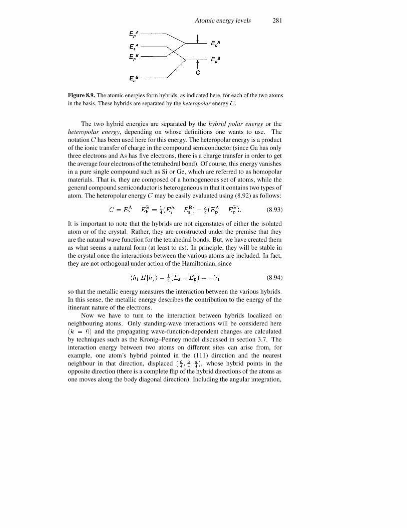
Atomic energy levels 281
Figure 8.9. The atomic energies form hybrids, as indicated here, for each of the two atomsin the basis. These hybrids are separated by the heteropolar energy �.
The two hybrid energies are separated by the hybrid polar energy or theheteropolar energy, depending on whose definitions one wants to use. Thenotation� has been used here for this energy. The heteropolar energy is a productof the ionic transfer of charge in the compound semiconductor (since Ga has onlythree electrons and As has five electrons, there is a charge transfer in order to getthe average four electrons of the tetrahedral bond). Of course, this energy vanishesin a pure single compound such as Si or Ge, which are referred to as homopolarmaterials. That is, they are composed of a homogeneous set of atoms, while thegeneral compound semiconductor is heterogeneous in that it contains two types ofatom. The heteropolar energy � may be easily evaluated using (8.92) as follows:
� � ��� � ��
� � �����
� ���� � �
�����
� ���� �� (8.93)
It is important to note that the hybrids are not eigenstates of either the isolatedatom or of the crystal. Rather, they are constructed under the premise that theyare the natural wave function for the tetrahedral bonds. But, we have created themas what seems a natural form (at least to us). In principle, they will be stable inthe crystal once the interactions between the various atoms are included. In fact,they are not orthogonal under action of the Hamiltonian, since
����� ���� ������ ���� � ��� (8.94)
so that the metallic energy measures the interaction between the various hybrids.In this sense, the metallic energy describes the contribution to the energy of theitinerant nature of the electrons.
Now we have to turn to the interaction between hybrids localized onneighbouring atoms. Only standing-wave interactions will be considered here�� � �� and the propagating wave-function-dependent changes are calculatedby techniques such as the Kronig–Penney model discussed in section 3.7. Theinteraction energy between two atoms on different sites can arise from, forexample, one atom’s hybrid pointed in the (111) direction and the nearestneighbour in that direction, displaced � �
�� ��� ���, whose hybrid points in the
opposite direction (there is a complete flip of the hybrid directions of the atoms asone moves along the body diagonal direction). Including the angular integration,
282 Motion in centrally symmetric potentials
the interaction energy between these nearest neighbour hybrids is
��� ��
������ �����
��
������� ����� ����� ����� � �
������ ����� (8.95)
Harrison (1980) has argued that these energies should depend only on theinteratomic spacing � ��
������, and that they should have the general form
�� �� �����
���� (8.96)
Phillips (1973) also argues that �� should be a function of the interatomic spacing,but that it should also satisfy another scaling rule. Since the atomic radii are thesame for each row of the periodic table, the value of � � should be the same in AlPas in Si, the same in GaAs and ZnTe as in Ge, and so on. In other words, the valuefor this quantity is set by the distance between the atoms, and this really does notchange as one moves across a row of the table. Thus this value is the same inheteropolar compounds as in homopolar compounds and Phillips has termed � �
the homopolar energy, �� � �� (this should not be confused with the hybridenergy �, which differs for the two atoms). The average energy gap betweenbonding and anti-bonding orbitals is thus composed of a contribution from thehomopolar energy �� and a contribution from the heteropolar energy .
The bonding orbital will be composed of hybrids based on the atoms at eachend of the bond, as suggested above. These bonding orbitals can be written as alinear combination of the two hybrids at each atom, as
����� � ��� ��� ��� �� (8.97)
where the �� are coefficients to be determined. This is achieved by minimizing theexpectation value of the energy determined by the Hamiltonian, which is given by
������� �������������� �
����
�� ������ � ���
�
�
���� ��
�
(8.98)
with respect to both �� and �� separately. This leads to two equations (from thepartial derivatives)
�� � ���
� � ���� �� � ���
� � ����� (8.99)
Introducing the average energy � � ���
� ����, the determinant of
coefficients for (8.99) may readily be solved to give the energies
� � � �
�
������ � � � � � �
��� (8.100)
The bonding (lower sign) and the anti-bonding (upper sign) energy levels aresymmetrically spaced about the average hybrid energy of the two atoms. Ofcourse, in a homopolar material, these two hybrid energies are the same and are
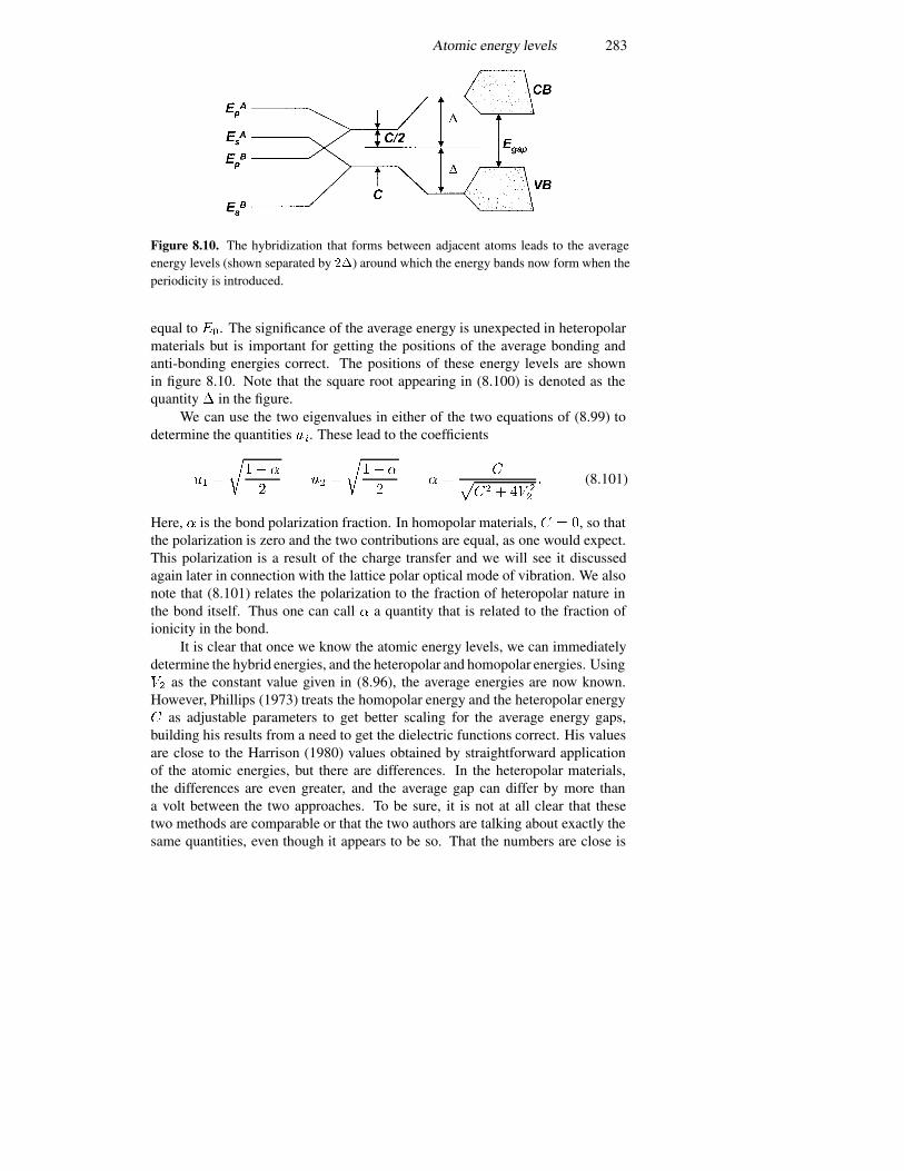
Atomic energy levels 283
Figure 8.10. The hybridization that forms between adjacent atoms leads to the averageenergy levels (shown separated by ��) around which the energy bands now form when theperiodicity is introduced.
equal to ��. The significance of the average energy is unexpected in heteropolarmaterials but is important for getting the positions of the average bonding andanti-bonding energies correct. The positions of these energy levels are shownin figure 8.10. Note that the square root appearing in (8.100) is denoted as thequantity � in the figure.
We can use the two eigenvalues in either of the two equations of (8.99) todetermine the quantities ��. These lead to the coefficients
�� �
�� � �
��� �
��� �
�� �
���� � �� �
�
� (8.101)
Here, � is the bond polarization fraction. In homopolar materials, � � �, so thatthe polarization is zero and the two contributions are equal, as one would expect.This polarization is a result of the charge transfer and we will see it discussedagain later in connection with the lattice polar optical mode of vibration. We alsonote that (8.101) relates the polarization to the fraction of heteropolar nature inthe bond itself. Thus one can call � a quantity that is related to the fraction ofionicity in the bond.
It is clear that once we know the atomic energy levels, we can immediatelydetermine the hybrid energies, and the heteropolar and homopolar energies. Using�� as the constant value given in (8.96), the average energies are now known.However, Phillips (1973) treats the homopolar energy and the heteropolar energy� as adjustable parameters to get better scaling for the average energy gaps,building his results from a need to get the dielectric functions correct. His valuesare close to the Harrison (1980) values obtained by straightforward applicationof the atomic energies, but there are differences. In the heteropolar materials,the differences are even greater, and the average gap can differ by more thana volt between the two approaches. To be sure, it is not at all clear that thesetwo methods are comparable or that the two authors are talking about exactly thesame quantities, even though it appears to be so. That the numbers are close is

284 Motion in centrally symmetric potentials
perhaps remarkable and points out the basic correctness of the overall picture ofthe composition of the energy bands in semiconductors.
The values that are obtained, as seen in figure 8.10, are not the actual energygaps one associates with the conduction and valence bands, but are average gapsaround which the energy bands form. That is, these are levels near mid-bandthat may be associated with the mean energy in the band. These levels are thenbroadened by the interaction with other atoms, and the periodicity that is invokedin the structure, and this broadening produces the conduction and valence bands,just as in the Kronig–Penney model. The number of states in each of these bandsis twice the number of lattice sites for the basis of two atoms per lattice site andanother factor of two for spin. Thus, the four electrons per atom are just sufficientto completely fill the valence band, and it is this full valence band, with a gap tothe conduction band, that provides most of the properties of the semiconductors.
8.4 Hydrogenic impurities in semiconductors
One can achieve in semiconductors a situation in which an impurity atom is placedin the host lattice, with the special case that the impurity may have an additionalelectron or be short of one electron. When the impurity atom has an additionalelectron over those (four) required for tetrahedral bonding in the covalent lattice,this extra electron can be ionized rather easily. In this case, the impurity atom hasa single positive charge, while the ionized electron has a single negative charge.In many ways this interaction is quite like that in the hydrogen atom. On theother hand, the impurity atom that is short of one electron allows for electrons tomove from other atoms to this one in order to complete the tetrahedral bondingrequirements. Here, we say that a ‘hole’ moves from the impurity to the otheratoms. This hole (the absence of an electron in the valence band) can be ionizedfrom the impurity, leaving a negatively charged impurity atom and a positivelycharged particle.
The energy required to ionize either the electron or the hole is generallymuch smaller than that required to lift an electron out of the valence band into theconduction band—the band gap energy. Thus, these impurities introduce defectlevels within the band gap region of the semiconductor. Because of the coulombicnature of the interaction between the ionized particle (electron or hole) and thecentral cell of the ionized impurity, the perturbing potential is simply a Coulombpotential:
� ��� � ���
����� (8.102)
Here, � is the dielectric constant (times the free-space permittivity) of thesemiconductor host crystal. It may generally be assumed that the carriers in thesemiconductor are characterized by a scalar effective mass �
�, which accountsfor the band structure nature of the electrons or the holes, as the case may be.Thus, we are concerned either with electrons near the minimum of the conduction
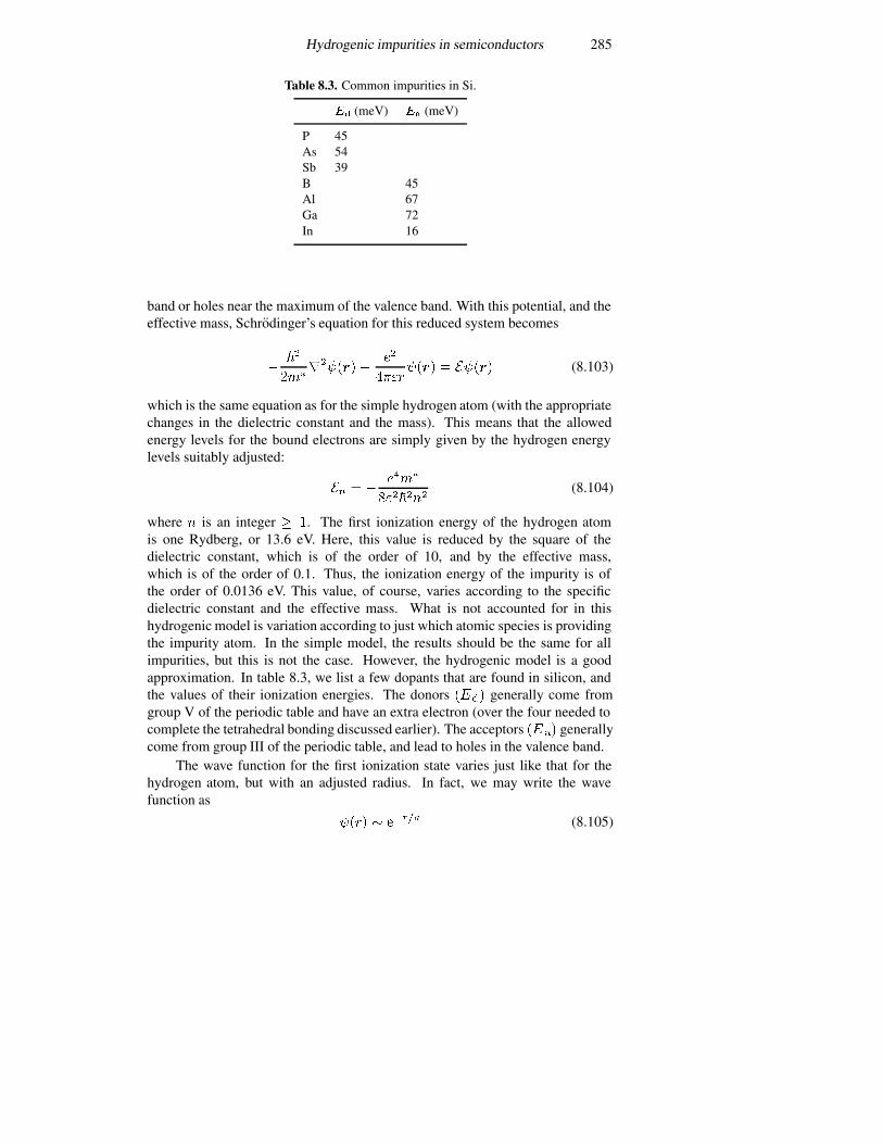
Hydrogenic impurities in semiconductors 285
Table 8.3. Common impurities in Si.
�� (meV) �� (meV)
P 45As 54Sb 39B 45Al 67Ga 72In 16
band or holes near the maximum of the valence band. With this potential, and theeffective mass, Schrodinger’s equation for this reduced system becomes
�
��
���
���������
�������� � ����� (8.103)
which is the same equation as for the simple hydrogen atom (with the appropriatechanges in the dielectric constant and the mass). This means that the allowedenergy levels for the bound electrons are simply given by the hydrogen energylevels suitably adjusted:
�� � �����
�������(8.104)
where � is an integer � �. The first ionization energy of the hydrogen atomis one Rydberg, or 13.6 eV. Here, this value is reduced by the square of thedielectric constant, which is of the order of 10, and by the effective mass,which is of the order of 0.1. Thus, the ionization energy of the impurity is ofthe order of 0.0136 eV. This value, of course, varies according to the specificdielectric constant and the effective mass. What is not accounted for in thishydrogenic model is variation according to just which atomic species is providingthe impurity atom. In the simple model, the results should be the same for allimpurities, but this is not the case. However, the hydrogenic model is a goodapproximation. In table 8.3, we list a few dopants that are found in silicon, andthe values of their ionization energies. The donors ���� generally come fromgroup V of the periodic table and have an extra electron (over the four needed tocomplete the tetrahedral bonding discussed earlier). The acceptors �� �� generallycome from group III of the periodic table, and lead to holes in the valence band.
The wave function for the first ionization state varies just like that for thehydrogen atom, but with an adjusted radius. In fact, we may write the wavefunction as
���� � ����� (8.105)
286 Motion in centrally symmetric potentials
where
� �����
�
���
�
� ��
�
��
��
��
(8.106)
where � is the Bohr radius discussed in section 8.2.1. For our hypotheticalsemiconductor, with a dielectric constant of 10 and an effective mass of 0.1,we find an effective radius of ��� � ��
�� cm, or 5.3 nm. This is about tenlattice constants, so the size of the orbit of the electron, when it is capturedby the impurity, actually samples a great many unit cells of the crystal. Thismeans that the effective-mass approximation is a fairly good approximation forthe hydrogenic impurity. Nevertheless, the potential probably deviates in realityfrom a coulombic one, and this difference is likely to account for the variation inionization energy seen for different impurities in the same semiconductor.
References
Cohen-Tannoudji C, Diu B and Laloe F 1977 Quantum Mechanics vol 1 (New York:Wiley) p 727
Darwin C G 1931 Proc. Cambridge Phil. Soc. 27 86–90Fermi E 1928 Z. Phys. 48 73Fock V 1928 Z. Phys. 47 446Harrison W A 1980 Electronic Structure and the Property of Solids (San Francisco, CA:
Freeman)Hartree D R 1928 Proc. Cambridge Phil. Soc. 24 111Herman F and Skillman S 1963 Atomic Structure Calculations (Englewood Cliffs, NJ:
Prentice-Hall)McEuen P L, Foxman E B, Meirav U, Kastner M A, Meir Y, Wingreen N S and Wind S J
1991 Phys. Rev. Lett. 66 1926–9Phillips J C 1973 Bonds and Bands in Semiconductors (New York: Academic)Rossler U 1991 Quantum Coherence in Mesoscopic Systems ed B Kramer (New York:
Plenum) pp 45–62Russell H N and Saunders F A 1925 Astrophys. J. 61 38Schiff L I 1955 Quantum Mechanics 2nd edn (New York: McGraw-Hill) pp 281–3Sikorski Ch and Merkt U 1989 Phys. Rev. Lett. 62 2164–6Tarucha S, Austing D G, Honda T, van der Hage R J and Kouwenhoven L P 1996 Phys.
Rev. Lett. 77 3613Tarucha S, Austing D G, Honda T, van der Hage R J and Kouwenhoven L P 1997 Japan.
J. Appl. Phys. B 36 3917Thomas L H 1927 Proc. Cambridge Phil. Soc. 23 542Yacoby A, Heiblum M, Umansky V, Shtrikman H and Mahalu D 1994 Phys. Rev. Lett. 73
3149Yacoby A, Heiblum M, Mahalu D and Shtrikman H 1995 Phys. Rev. Lett. 74 4047

Problems 287
Problems
1. Find the wave functions for the � � �, � � � level of the two-dimensional harmonic oscillator. Use the angular momentum operators and showthat this level is cylindrically symmetric.
2. Suppose that the �-axis harmonic oscillator is characterized by afrequency ��, which is slightly larger than that of the �-axis (�� � � � �).Compute the exact energy levels of the two-dimensional harmonic oscillator.Then, using the energy levels and wave functions for the symmetric two-dimensional harmonic oscillator, calculate the perturbation shift of these energylevels with the perturbation���������.
3. Let us consider the application of an electric field ���� to the two-dimensional harmonic oscillator in the presence of a magnetic field. Determinethe change in the energy levels introduced by this electric field.
4. What are the energy values of the lowest three energy levels in thehydrogen atom? (That of the lowest energy level, the ionization energy of thehydrogen atom, is termed one rydberg.)
5. Verify that (8.58) is the correct equation for the angular variation of thehydrogen atom.
6. Show that the solution of (8.58) is a polynomial of finite order, and thatthis order is given by �� ���.
7. Develop the full wave functions (the form, neglect normalization) for the3p states utilizing the angular momentum operators.
8. Show that �� in (8.62) commutes with each component of the angularmomentum.
9. Develop a computer program and solve (8.83) for the potential of an atomin the Fermi–Thomas approximation.
10. (a) Using the known lattice constants and atomic energy levels, computethe values of the parameters �, �, and �� for Si, Ge, GaAs, AlAs, InAs, InSb,and InP. (b) The bond polarizability is often related to the ionicity of a particularcompound. Using the values found in part (a), plot the bond polarizability as afunction of the average energy gap for these compounds. Is there a trend to thesedata?
11. From the known lattice constant and density of Si, compute the numberof atoms per cubic metre. Then, use this value of , and the known dielectricconstant of Si, to compute the valence plasma frequency from � �
�� �������.
What is the average energy gap required to satisfy the Penn dielectric function
�� � ��
�� �
������
����
How does this compare with the value of �� found in problem 10?
Chapter 9
Electrons and anti-symmetry
The treatment of particles that we have presented in the previous chapters isdeficient in a number of respects, mainly because of the many approximationsthat have been made in the various approaches. One of the most significant ofthese is constituted by the particular constraints that are introduced by the fact thatthe electrons are indistinguishable and identical particles. In addition, we haveonly paid lip service to the fact that each electron also possesses a spin angularmomentum about its own axis, although this became important at the end of thelast chapter. When we deal with single isolated electrons, these approximationsdo not get us into very much trouble. However, most atoms and solids are denselypopulated with electrons, and the neglected properties can introduce new effectsthat need to be considered. Even though the effects may be quite small, anunderstanding of them is necessary, if for no other reason than to be able toascertain when they may properly be ignored.
In classical mechanics, it is quite easy to follow the individual trajectories ofeach and every electron. However, the Heisenberg uncertainty principle preventsthis from being possible in quantum mechanics. If we completely understandthe position of a given particle, we can say nothing about its momentum andmost other dynamical variables. This principle of the indistinguishability ofidentical particles leads to other more complex forms of the wave functions. Thesemore complicated forms can lead to effects in quantum mechanics that have noanalogue in classical mechanics. We use the word identical to indicate particlesthat can be freely interchanged with one another with no change in the physicalsystem. While these particles may be distinguished from one another in situationsin which their individual wave functions do not overlap, the more usual case iswhere they have overlapping wave functions because of the high particle densityin the system. In this latter case, it is necessary to invoke a many-particle wavefunction. To describe properly the properties of the many-particle wave function,it is necessary to understand the properties of the interactions that occur amongand between these single particles. If the one-electron problem were our onlyinterest, this more powerful development that is used for the interacting system
288
Symmetric and anti-symmetric wave functions 289
would be worthless to us, for its complexity is not worth the extra effort. However,when we move to multi-electron problems, the power of the approach becomesapparent. In this chapter, we want to examine just the properties of these generalwave functions for the case of electrons, which also possess their own spin angularmomentum, and to introduce the interaction among the electrons.
9.1 Symmetric and anti-symmetric wave functions
We begin by considering just two electrons. Because these are indistinguishableparticles, the physical state that is obtained by merely interchanging the positionsof these two particles must be completely equivalent to the original one. This putscertain constraints upon the wave function. Let us consider the two-electron wavefunction ����� ���. Here, the parameter �� refers to the vector position �� and thespin orientation�� of the electron (which will be further explained below). Thus,we can refer to this as a four-vector �� � �������. Now, under exchange of thepositions and spins of the two particles, we must have
����� ��� � �������� ���� (9.1)
The phase � is some real constant. By repeating the interchange, we arrive at
����� ��� � �������� ��� � ��������� ���� (9.2)
But this requires ���� � �, or ��� � ��. Thus, the possible forms for the wavefunction are
����� ��� � ������ ���� (9.3)
The wave function that is found upon interchange of the two particles is going tobe either symmetrical or anti-symmetrical. By symmetrical, we mean that it isunchanged, while anti-symmetrical implies a change of sign. Which of these twoare we to choose?
The choice of either a symmetric or an anti-symmetric wave function lies inthe imposition of the Pauli exclusion principle (Pauli 1925). We have constantlyheld that each eigenstate determined by solving the Schrodinger equation couldhold two electrons, provided that they had opposite spin. In each situation, thepositional wave functions for the two electrons are the same, but the spin wavefunctions must yield a spin eigenvalue � that is oppositely directed. Now, thisspin eigenvalue is one of the vectors included above in the description of thetwo-particle wave function. Thus, the electrons, which obey the Pauli exclusionprinciple, must have an anti-symmetric wave function. We can summarize this bysaying that particles that do not obey the exclusion principle (phonons, photons,etc) are bosons, and are found to obey Bose–Einstein statistics. These bosonshave symmetric wave functions under interchange of the particles. On the otherhand, particles that obey the exclusion principle (electrons and some others, withwhich we will not be concerned) are fermions, and are found to obey Fermi–Dirac statistics. Fermions must have anti-symmetric wave functions under the

290 Electrons and anti-symmetry
interchange of particles. We will see below that the use of the anti-symmetricwave function actually ensures that the Pauli exclusion principle is obeyed.
Now, what do we really mean by bosons and fermions? In the previousparagraph, we stated that bosons do not obey the Pauli exclusion principle, anddo obey the Bose–Einstein distribution. On the other hand, fermions do obeythe Pauli exclusion principle—no more than two fermions, and these are ofopposite spin—can be accomodated in any quantum state. Bosons are particleswith integer spin, such as phonons (zero spin) and photons (integer spin givenby ��, corresponding to right- and left-circularly polarized plane waves forexample). Fermions are particles with half-integer spin, such as electrons. Thesetwo distributions are given by
������ ��
������ � �(9.4)
and
������ ��
����������� � �� (9.5)
There is a significant difference in the behaviour of these two distributions at lowenergy. The Bose–Einstein distribution diverges at � � �, as there is no limitto the number of bosons which can occupy the lowest energy state. On the otherhand, the Fermi–Dirac distribution approaches unity in this limit, as the state iscertainly occupied if it lies well below the Fermi energy ��. As pointed out, oneway of achieving the Pauli exclusion principle is to ensure that the wave functionfor a fermion is anti-symmetric.
Now, what do we mean by anti-symmetric? The fact is that if we havea two-electron system, which satisfies the Schrodinger equation, then we needa proper two-electron wave function ����� ���, where the first argument refersto the first electron and the second argument refers to the second electron. Byanti-symmetry, we mean that we require the wave function to have the property����� ��� � ������ ���. That is, if we interchange (exchange) the two particles,the wave function is multiplied by a numerical factor of ��.
If we insert our many-particle wave function into the Schrodinger equation,it is found that under the circumstances discussed above, it is possible to writethis equation as
������ ���� � ����� ��� � �� (9.6)
Here, we may assert that the Hamiltonian itself is invariant under the exchange ofthe particles, and the equivalence of the two physical states implies that the energyhas the same invariance. Hence, the imposition of the exclusion principle appearsonly in the wave function (unless some special spin-dependent interaction, suchas the spin–orbit interaction of the last chapter, is introduced in the Hamiltonian todistinguish one spin state from another). Whether the wave function is symmetricor anti-symmetric has no impact upon (9.6). The importance of this latter result isthat, for simple Hamiltonians with no interaction among the electrons, it is usually
Spin angular momentum 291
possible to separate (9.6) into two equations, one for each particle, with the totalenergy being the sum of the single-particle energies. This separation is carried outin exactly the same manner as that in which separation of coordinates is done in amany-dimensional partial differential equation. As a result, it is possible to writethe two-particle wave function as a product of the one-particle wave functions������ and ������. The subscripts on the wave functions themselves (as opposedto those on the variables) refer to the particle ‘number’. Carrying this out produces
����� ��� � ������������� (9.7)
However, this wave function does not possess the proper symmetry for electrons;for example, interchanging the positions of particles ‘1’ and ‘2’ does not producethe necessary anti-symmetry. However, we can achieve this with a somewhatcleverer summation; that is, we use
����� ��� ������������������ �������������� (9.8)
This wave function has the desired anti-symmetry under the interchange of thetwo electrons.
This method of forming a properly anti-symmetric many-electron wavefunction from the single-electron wave functions has been extended to anarbitrarily large number of electrons by Slater (1929). The resulting wave functionfor � electrons is given by the Slater determinant
����� ��� � � � � �� � ���� �
�������
������ ������ � � � ����� ������� ������ � � � ����� �� � � � � � � � � � � �
�� ���� �� ���� � � � �� ��� �
�������
� (9.9)
Equation (9.9) has the added usefulness that it has the property that it vanishesif two of the �� are the same. This implies that no two electrons can have thesame state (recall that we have included spin angular momentum explicitly in thevariables), and thus the Pauli exclusion principle is automatically satisfied. Thus,when we can separate the Hamiltonian into single-particle parts, and separate thewave function accordingly, the anti-symmetrized product of these wave functionsin a Slater determinant ensures that the Pauli exclusion principle is satisfied.
9.2 Spin angular momentum
The electrons that were treated in the last section can have two possible spinstates, which are generally referred to as ‘spin up’ and ‘spin down’. The fact thatthere are only two spin states arises from the Pauli exclusion principle, since eachstate (neglecting spin) can have only two electrons, which possess opposite spinproperties or ‘directions’. In this section, we would like to examine the properties
292 Electrons and anti-symmetry
of the spin states and ascertain the appropriate eigenvalues and wave functions ofthe operators. In section 8.2.3, we discussed the angular momentum of a particle(there it was the orbital angular momentum of an electron orbiting a nucleusin a centrally symmetric potential). It was clear that �� and �� could both bemade to commute with the Hamiltonian, and therefore could be simultaneouslydiagonalized. The �-component, ��, had eigenvalues of ����, while the totalangular momentum had eigenvalues of ��� � ���� (here, � is an integer andshould not be confused with the mass, which we will write as ��). In the presentcase, the only angular momentum is the spin of the electron about its own axis,which we shall take as the �-axis for convenience (hence, ‘up’ and ‘down’ arerelative to the normal �-axis, which is often used to convey altitude). The rangeof � is therefore from �� to �, and � thus takes �� � � values. Since we haveonly two values (‘up’ and ‘down’), it is clear that � � �
�, and � � � �
�. The
eigenvalue of the total momentum �� is then �����.In the matrix formulation of quantum mechanics, the total Hilbert space is
spanned by a set of eigenfunctions �����. If we now want to include the spincoordinates, an additional two-component space must be created for the twocomponents of the spin. We can take these as the two unit vectors
�
��
�
��
���
��
���
�
��
���
�(9.10)
where the first row refers to the ‘up’ state and the second row refers to the ‘down’state. Thus, the ‘up’ state has the � �
�eigenvalue (in units of the reduced Planck’s
constant), and the ‘down’ state has the� �
�eigenvalue. Whatever matrix describes
the positional variations of the wavefunction must be adjoined by the spin wavefunctions. This is a general result.
Because the spin angular momentum has been taken to be directed alongthe �-axis, we expect the matrix for the �-component of the spin operator to bediagonal, since it must simply produce the eigenvalues when operating on theabove spin wave functions. Thus, we have (we will use � now rather than � toindicate the spin angular momentum)
�� ��
��
�� �� ��
�(9.11)
so �����
�� � �������� �
�� and �����
�
�� � ��������� �
��. Similarly, the
operator for the total angular momentum must produce
���� � �
���
�� �� ��
�� (9.12)
How are we to find the other components of the spin angular momentum? Forthis, we can use the results of (8.66) for the rotating ��. We know that �� issimply ���. Now, (8.66) is simply re-expressed as
�� � ���� � ���� ���� (9.13)

Systems of identical particles 293
Similarly,�� � �
�
�� � ���� ���� (9.14)
These can be combined, using (9.11) and (9.12), to give
�� � ���� �
������ � �
�
��� ��
���� (9.15)
The individual matrices for the rotating components can easily be found,up to a normalizing constant. To begin, we recall from chapter 8 that the��-component raises the angular momentum by one unit. This must take the‘down’ state into the ‘up’ state and produce a zero from the ‘up’ state. This canbe satisfied by making the definition
�� � �
�� �� �
�� (9.16)
Similarly, the operator ��
must reduce the angular momentum by one unit, andhence it must take the ‘up’ state into the ‘down’ state and produce zero from the‘down’ state. Thus, we can now define
��
� �
�� �� �
�(9.17)
and equation (9.15) is satisfied quite easily. From these, we can now use (8.65) todefine the �- and �-components:
�� ��
���� � �
�
� ��
�
�� �� �
�(9.18a)
�� ��
���� � ��� �
�
�
�� � �
�� (9.18b)
It is normal to define the three components in terms of Pauli spin matrices (Pauli1927) as �� � �
���. The various �� are also called spinors.
9.3 Systems of identical particles
In section 9.1, the multi-particle wave function was introduced, and in particularwas connected with products of single-particle wave functions through the Slaterdeterminant to ensure the anti-symmetry of the wave function. In this section,we now want to explore some of the properties of the many-electron wavefunctions in further detail. Quite generally, we may introduce the � -particlewave function � ���� ��� � � � � �� �, which represents the probability (when themagnitude squared is computed) of finding particles at positions and spins��� ��� � � � � �� . This wave function must satisfy the condition
�� �� � �
���� ��� � � ���� �� ���� ��� � � � � �� ���� (9.19)
294 Electrons and anti-symmetry
As we have defined it to this point, the Hilbert space for the � -particle systemis simply the � th tensor product of the single-particle Hilbert spaces and thecorresponding spin spaces. The wave function of the � fermions is properlyanti-symmetric under the exchange of any two particles, and therefore for a largenumber of permutations must satisfy
�����
�� ��
�� � � � � ��
�� � ������� ���� ��� � � � � �� � (9.20)
where � is the total number of permutations required to reach the configurationof the wave function on the left from that on the right of (9.20). Thus, if we havefor example ������ ��� ��� ���, then to get to ������ ��� ��� ��� requires a totalof six permutations (three to get �� moved to the beginning, then two to bring�� adjacent to it, and finally one more to interchange �� and ��). Hence, thisnew example yields a symmetric product after the six interchanges. The generalpermuted wave function (9.20) then has the inner product with the original of
��� ���
�� ��
�� � � � � ��
����� ���� ��� � � � � �� �� � ����� � (9.21)
It is important to note that the normalization of the many-electron wavefunction arises from the normalization of the single-electron wave functions thatgo into the Slater determinant (9.9). The factor of ����� arises from the need toget these into the ‘right’ product order for taking the associated inner products ofthe single-electron wave functions. The normalization factor in (9.9) then goesto cancel the multiplicity of terms that arise from the determinantal form. Letus consider just the two-electron case of (9.8) as an example (remember that theadjoint operator on the left of the inner product reverses the order of terms):
������� ��
���������������� ���������������������������� ��������������
� �
������������������������������ ���������������������������
� ��������������������������� � ����������������������������
� �
������� � ����� � ������� ������� � � (9.22)
where the zeros arise because the wave functions at the same variables aredifferent and orthogonal to one another. Thus, one needs to be careful that the one-electron wave functions are orthonormal and that the permutations are properlycomputed.
Finally, we note that it is usually the case that the coordinates are the samefor all of the single-electron wave functions; only the spin coordinates differ.Thus, we can think of the differences between the single-particle states as theparticular member of the Hilbert space and the particular spin variable that isexcited for each electron. No two combinations can be occupied by more than oneelectron. With this realization, it is possible to think of a simple set of parametersto characterize each single-electron wave function—its index in the Hilbert spaceand its spin angular momentum. Thus, we may write the single-particle wavefunctions as ������. Here, the index � signifies the particular member of the basis
Fermion creation and annihilation operators 295
set, and � denotes the spin state. These may be combined for simplicity intothe index � � ��� ��. We will do this in the following discussion. However, weare making a major change of paradigm with this notational change. In the casetreated above, it was assumed that the coordinates (including spin) of a particledefined a particular localized wave function in the position representation, and theindex of the wave function described the type of wave function at that position.Thus, at the point � � ��� ��, there may be many types of wave function available,and the �� correspond to these types. In the latter description, however, it isassumed that there is only a single type of wave function at each site, or that thereis no localization and that there are a number of wave function types. An exampleof the first of these options is a Gaussian wave packet localized at �. This ischaracteristic of, for example, localized delta function wave packets, which satisfy������ � ��� �
��. The latter formulation is characteristic of, for example, thewave functions of an electron in a quantum well, where the ‘space’ is the regionthat lies within the well, and the various wave functions are those that arise fromthe different energy levels. A second example of the latter, and one that willbe heavily used, is that of momentum eigenfunctions, which are plane wavesextending over all space. The indices are then the momentum values and thespin indices. It is important in evaluating the anti-symmetrized wave functions tounderstand fully just which interpretation is being placed on the individual single-electron wave functions.
9.4 Fermion creation and annihilation operators
In the treatment of the harmonic oscillator, it was found to be useful to introducea set of commuting operators which described the creation or annihilation of oneunit of energy in the harmonic oscillator. This also changed the wave functionsaccordingly. Can we use a similar description to enhance our understanding ofthe many-electron picture? The answer is obviously yes, but we must carefullyexamine how the rules will be changed by the requirement of anti-symmetry andthe corresponding Pauli exclusion principle. New views that arise will be basedupon the fact that the energy of the harmonic oscillator could be continuouslyraised by pumping phonons into the system; the introduction of � phonons couldbe achieved by using the operator �����. Here, however, operation with a singlecreation operator (we use the notation � for fermions) ��
�creates one fermion in
state �. This state may be a momentum eigenstate, a state in a quantum well, orany other state in a system in which the wave functions span the entire allowedvariable space. If we try to create a second fermion in this state, the result mustbe forced to vanish because of the exclusion principle; for example,
����
����� � � (9.23)
where ��� is the so-called vacuum state in which no fermions exist. In fact,however, equation (9.23) must hold for any wave function in which the state �
296 Electrons and anti-symmetry
is empty (or even filled). Similarly,
���� � � �� � � (9.24)
where � � � � � is any state of the system (since there can be no more than a singleelectron in any state, there cannot be more than one annihilation).
This suggests that a different combination of products must be used for thesefermion operators. Consider, for example, the product
��� �� � ����
� � (9.25)
If the state ��� is empty, the first term immediately gives zero. The secondterm creates a fermion in the state, then destroys it, so the result is, by (4.67),�� � �� � �. Similarly, if the state ��� is occupied, the second term gives zero(another fermion cannot be created), while the first term is the number operatorand yields 1. Thus, the result in either case is the anti-commutator product
���� � ��� � ��� �� � ����
� � �� (9.26)
Here, we use the curly brackets to indicate that the positive sign is used in theanti-commutator, as opposed to the negative sign used in the commutator relation.This may be extended to operators on other states as
���� � ��� � �� (9.27a)
���� � ��� � � ���� ��� � �� (9.27b)
This leads to an interesting result for the number of fermions that can existin, or arise from, any state of the system. Since we can rewrite (9.26) as��� �� � �� ���
�
� , we have
���� ���� � ��� ����� ���
�
� � � ��� �� � ��� ������
� � ��� �� (9.28)
from (9.24). Thus, ��� � �� � � if the state is occupied (it is naturally zerootherwise, a result independent of the choice of whether to use boson operatorsor fermion operators). The representation in which the number operators arediagonal, along with the energy, is known as the number representation.
Note that the operators ��� and �� used here are fermion operators. Therelationship (9.23) ensures that no more than a single fermion can exist in thegiven state. The attempt to put a second particle in this state must yield zero,as given by (9.23). Similarly, only a single fermion can be removed from anoccupied state, as indicated by (9.24). These statistics differ markedly from theoperators used in chapters 4 and 8, which were for bosons. While the wavefunction differed for each state, we referred to a particular harmonic oscillatormode as being described by its occupation. In increasing the occupation, weraised the energy of the mode (given by the number of bosons in that particular
Fermion creation and annihilation operators 297
harmonic oscillator mode). In the boson harmonic oscillator, the energy of aparticular mode was given by
�� � ��� ��
����� �� � �� �� �� � � � � (9.29)
Thus, there could be a great many bosons occupying the mode, even though thedistinct mode wave function would change. In the case of fermions, however, welimit the range of the occupation factor � � to be only 0 or 1. This is imposed byusing the same generation properties of the creation and annihilation operators,but with the limitations for fermions that
����� � � (9.30a)
and���� �
� � �� (9.30b)
These properties are now carried over to the many-particle wave function.The general many-electron wave function is created by operating on the
empty state, or vacuum state, with the operators for positioning the electronswhere desired. For example, a three-electron state may be created as
����� � ��� ��� �
�
� ���� (9.31)
It should be noted that the order of creation of the particles is important, sincechanging the order results in a permutation of the indices, and
����� � ������� (9.32)
This may be generalized to an arbitrary many-electron wave function
����� � � � ��� � ����������
���� � � � ���
���� ���� (9.33)
Then,
��� � � � � �� � � �� �
�� � � � ��� � �� � � �� if �� � �� if �� � �
(9.34)
and
��� � � � �� � � �� �
�� � � � ��� � �� � � �� if �� � �� if �� � � .
(9.35)
It is possible to recognize that the creation and annihilation operators do notoperate in a simple Hilbert space. In general, the creation operator operates in aspace of � electrons and moves to a space with � � � electrons. Similarly, theannihilation operator moves to a space with � � � electrons. The general spacemay then be a product space of Hilbert spaces, and elements may be combinedwith a variety of partially occupied wave functions. This complicated structureis called a Fock space, but the details of this structure are beyond the simpletreatment that we desire here.

298 Electrons and anti-symmetry
9.5 Field operators
We have seen in the above sections that the fermion creation and annihilationoperators may be used to put electrons into and take electrons from particularstates in a complete Hilbert space. In (2.92) we expanded the arbitrary wavefunction solution to the time-independent Schrodinger equation in terms of thesevery same basis functions, which are the eigenfunctions of the equation itself.There, we used a set of expansion coefficients to provide the weights for each ofthe basis functions. Here, however, we cannot excite a fraction of an electron—abasis state either has an electron in it or it does not. This means that we can usethe creation operators and the annihilation operators to define the overall wavefunction for fermions as
���� ��
������� (9.36)
where the wave functions of the basis set include the appropriate spin functions,and the coordinates include both position and spin coordinates. Similarly, we canwrite
����� ��
���������� (9.37)
Here, the expansion functions satisfy
��
��
���
� � � ���
������ � ������� (9.38)
where there are no specific spin-dependent operators in the normal Hamiltonian.It should be remarked that these are single-electron wave functions even thoughthere are excitations into various states, since there are no products of wavefunctions for which to require proper anti-symmetry. Two-electron wavefunctions can only be created by products of creation operators, and similarly formore densely populated systems. This is a problem that we will have to addressbelow, where we will make the connection between this description of a many-electron system with one-electron wave functions and the many-electron wavefunctions introduced above.
The interpretation of (9.36) and (9.37) as wave functions is complicated asthey are now operators—the expansion coefficients are creation and annihilationoperators. These quantities are called field operators. The concept of fieldhere is precisely the one that is used in electromagnetic field theory. Normally,quantization is invoked via non-commuting operators such as position andmomentum. Here, however, these operators are buried in the creation andannihilation operators, and the normally simple wave functions have now becomeoperators in their own right. We have quantized the normally �-number wavefunctions. This process is usually referred to as second quantization, and we wantto examine this concept further here. In this approach, the Hamiltonian operatorappears in a totally different light (but does not invoke different physics).

Field operators 299
It is easy now to examine the behaviour of the field operators under the anti-commutation operations. For example,
������������� � ���������� � ����������
��
�
�����
�����
�
�������� ��
�
���������
�
��� ��
����
��
�
��
�����
�
���������� � ���
��
�
��
�����
�
��������
��
�
��
���������� � �� � ���� (9.39)
This last line is precisely the principle of closure of a complete set (5.38). In asense, the anti-commutation of the fermion operators ensures the orthonormalityof the basis functions in a way connected with the Pauli principle. Similarly,
�������������� � ������������ � �� (9.40)
We can now use these field operators to show how the Schrodinger equationappears in second quantization, and we can then relate these operators to theproper anti-symmetrized many-electron wave functions.
9.5.1 Connection with the many-electron formulation
Let us now look at how the energy levels and wave functions may be connectedbetween the field operator forms and the many-electron wave function forms.Here, we follow the approach of Haken (1976). We begin by assuming that aproper vacuum state ��� exists such that
����� � � for all �� (9.41)
We can then write an arbitrary many-electron wave function as (9.33), which werewrite as
����� ��
�
���� ��� ���� (9.42)
Since ���� �� � �, the allowed values for �� are only 0 or 1 (formally, we have set
���� �� � �). One possible set of values for the wave function is given by
��� � ��� �� �� �� �� �� � � ��� (9.43)
The energy for this wave function is given by the energy of the excited states, andmay be written as
� ��
�
����� (9.44)
300 Electrons and anti-symmetry
If the total number of electrons is � , then there are exactly this number of 1s inthe set (9.43). With this in mind, we can write an ordered representation for (9.42)as
����� � ������������� � � ��
����� (9.45)
where it is assumed that
�� � �� � �� � � � � � �� (9.46)
orders the creation of the electrons by some measure, which may be arrived atquite arbitrarily. This measure of ordering provides the ‘yardstick’ via which weenforce anti-symmetry through the exchange of any two creation operators.
In order to see how this formulation now compares with the field operatorapproach, we will look specifically at a simple one-electron form of this wavefunction. We shall assume that the correct (in some measure) single-electronwave function may be written as a weighted summation over the possible one-electron states that can occur from (9.42) (there are almost an infinity of these,of course). We write this weighted sum in exactly the same manner as used inprevious chapters; for example,
��� ��
�
����
� ��� (9.47)
where the �� are �-number coefficients. The creation operator can be eliminatedby multiplying (9.37) by ����� and integrating over the coordinates (including asummation over the spin coordinates), so
��� �
� ��
������������ �� ��� �
��������� �� ��� (9.48)
in which we have defined a spatially varying weight function (which will becomea wave function in the manner of previous chapters)
��� ���
�������� (9.49)
It will be shown below that the weight function ��� satisfies the Schrodingerequation (for one particle). Equation (9.48) may now be interpreted as � ����creating a single particle at the position � and for spin (recall that � is the set ofa position vector and a spin index), with the probability of any particular value of� given by the weight function.
The above interpretation that ����� creates a particle at � can be verified byoperating on this function with the particle density operator �����������:
������������������� � ���������� � �����������������
� ��������� � ������������������������
� ��������� � ������ (9.50)
Field operators 301
Similarly, the result can also be written (we note that the density operator producesa zero when operating on the vacuum state) as
������������������� � ��� � ������������ (9.50a)
This shows that the state �������� is an eigenstate of the density operator, withthe value 0 if the created particle’s position and spin � do not correspond with thatof the density operator.
9.5.2 Quantization of the Hamiltonian
The one-electron wave function is now a function of the field operator. Toproceed, we will now need to quantize the Schrodinger equation itself, whichreally means that we want to work out how to write the Hamiltonian in a second-quantized form in terms of the field operators. Quantization of a field is the usualmethod by which classical (electromagnetic) fields are quantized to produce thequantum mechanical equivalent fields. Here, however, our ‘field’ is described bythe Schrodinger equation. The normal manner in which the quantization proceedsis through the use of Lagrange’s equations, which is an approach beyond the levelto be maintained here. Therefore, we will proceed with a heuristic approach.The idea is as follows: the field operators are expansions in terms of the basisset of functions in our Hilbert space, so each operator is a ‘vector position’ inthe Hilbert space, which we will term a pseudo-position. Similarly, the motionof this field operator is a pseudo-momentum. We want to generate the second-quantized Hamiltonian by writing it in terms of these dynamic pseudo-variables,remembering that the spatial operators will really operate on the density operator.We reach the operator form by integrating over all space (and summing over allspins), so the second-quantized Hamiltonian operator is expressed as
� �
� ��
���
���� � � ��� � � ������������
���
�
� �������������� � ����� � � ������������
���
�
������
����������� � � ���
����� �� (9.51)
where the first term on the right-hand side has been integrated by parts. Now, theHamiltonian is an operator written in terms of the field operators, and is said tobe second quantized.
Let us now use this Hamiltonian operator to examine the one-electron wavefunction (9.48). This becomes
� ��� �
������
����
���� � � ���
����� ��
������������ ��� ���� (9.52)
302 Electrons and anti-symmetry
Using the anti-commutation relations of the field operators, this can be rewrittenin the form (the second term arising from the anti-commutator vanishes as usual)
� ��� �
� ������
��
��
���� � � ���
��� � ����������� �� ���� (9.53)
Since the Laplacian operator produces the same result when operating on the deltafunction, regardless of whether the primed or unprimed coordinates are used, andthe Hamiltonian is Hermitian, equation (9.53) can be rewritten as
� ��� �
���������
��
��
���� � � ���
����� ��� (9.54)
Since � ��� � ����, and �������� is linearly independent of the weight function,the conclusion to be drawn is that the weight function must satisfy the Schrodingerequation �
���
���� � � ���
����� � ������ (9.55)
Thus, we have transferred the need to satisfy the Schrodinger equation from thebasis functions, which are assumed to provide the coordinate system in the Hilbertspace, to the weight function that describes the one-electron wave function interms of the field operators.
The fact that the weight function now satisfies the Schrodinger equationtells us that the field operator approach, based upon the use of creation andannihilation operators, produces a proper treatment of at least the one-electronproblem in quantum mechanics. The weight function is a proper wave functionitself, and satisfies the Schrodinger equation. As stated earlier, if the one-electron problem were our only interest, this more powerful development wouldbe worthless to us, for its complexity is not worth the extra effort. However,when we move to multi-electron problems, the power of the approach becomesapparent. The many-electron wave function is expressed equivalently in terms ofthe field operators or the creation and annihilation operators that make up the fieldoperators. Consequently, complicated quantum mechanical calculations may beexpressed in terms of the simple anti-commutator algebra of the anti-commutingoperators for fermions. Let us continue to the two-electron problem, and showthat this approach is quite general.
9.5.3 The two-electron wave function
We now turn to a general two-particle treatment. In addition to the normalSchrodinger equation with two electrons excited into the system, we will alsointroduce the Coulomb interaction between the pair of particles. This will nowproduce an interacting system, since there is now a force between each pair ofparticles due to this potential term. Once we begin to treat the many-electronsystem, particularly with interacting particles, the second-quantized approach
Field operators 303
begins to show its value, as there are many processes that can only be treatedadequately once this approach is adopted. Let us begin with the most generaltwo-particle state, which is written as above as a summation over all possibletwo-particle states, as
��� ��
��
�����
� ��
� ���� (9.56)
The procedure to be followed is exactly that used in the previous paragraphs. Wewill first replace the creation operators and find a general function that will berequired to satisfy the Schrodinger equation. Thus, we use (9.48) twice, so wehave
��� ��
��
���
�������
���� ��
�����
�������� ������
�
� ����� �������������� �� ������ (9.57)
where���� ��� �
���
��������������� (9.58)
It must now be shown that the function ���� � �� is properly anti-symmetric withrespect to its two coordinates. To do so, we take the last expression from (9.57)and interchange the two coordinates:
��� �
� ����� �������������� �� ��� ���
� �
� ����� �������������� �� ��� ���� (9.59)
In the last line, the two field operators were interchanged using the anti-commutation relation (9.40). Now, these operations really do not change (9.57),since the coordinates are true dummy variables which are being integrated out ofthe problem. Thus, expression (9.59) must be equivalent to (9.57) which is onlypossible if
����� �� � ����� ��� (9.60)
and it is in this function that the anti-symmetry is imposed directly (it is stillimposed on the field operators by the appropriate anti-commutation relations).
We can now use the Hamiltonian operator (9.53) to determine the equationfor the two-electron wave function ��� �� ��. This leads to, for the simple one-particle operators,
����� �
������
��
��
���� � ���
����� ��
�
� ������� ���������������� ���� ��� ���� (9.61)
304 Electrons and anti-symmetry
Now,
����������������� � �� � �������������������� � ��� (9.62)
so, with (9.60), equation (9.61) becomes
����� �
� ��������������
��
��
������ � � �����
������� ��� ���� ������
�
� ��������������
��
��
����� � � ����
������� ��� ���� �������
(9.63)
Using the anti-commutator relations for the field operators, the sign between thetwo terms will be changed, and they can be combined. Thus, the one-particleHamiltonian leads to the Schrodinger equation for the function ���� � ��, if weinclude the energy term as in the previous section,
��
��
����� ����� � � ��� � � ����
����� ��� � ����� ���� (9.64)
Let us now turn to the two-electron interaction potential.The Coulomb interaction arises between two charge densities. This can be
expressed as
�� ��
�
� �����
�
���� �������� �� ��� (9.65)
where the spin index is summed over. This can be extended by the introductionof the field operators through the particle density operator used in (9.50) and
�� ��
�
� ����������
�
���� �������������� �� ���
��
�
� ������������
�
���� ������������ �� ��� (9.66)
and, using (9.59) and the commutator relations, we have
����� �
� ������������
�
���� ������� ��� �� ��� ���� (9.67)
Thus, the full two-electron Schrodinger equation for the two-electron function isgiven by
����
����� ����� � � ��� � � ���� �
�
���� ���
����� ��� � ����� ����
(9.68)
Field operators 305
This is easily extended to an arbitrary � -electron wave function, which yields
���
��
��
����
� � � ����
������
��
������ � ��������� ��� � �� �
� ������ ��� � �� � (9.69)
Even with this multi-electron wave function, the Hamiltonian is still expressiblein terms of the field operators as
�
������
�� �
�
���� � � ���
����� ��
��
�
� ������������
��
������ ������
������ �� ��� (9.70)
9.5.4 The homogeneous electron gas
In the case of a homogeneous electron gas, the function ��� �� ��� � �� � canbe expected to be a combination of plane waves; that is, each of the basisstates from which this function is made up is itself a plane wave (in momentumrepresentation). In fact, there are several modifications to this, which we willexamine in a subsequent section, but for now we assume that the basis states aresimply
����� ���������� (9.71)
where �� is the spin function, which can be represented by the matrices of (9.10).These basis functions can now be used in the representations for the field operatorsto rewrite the Hamiltonian. The first term (we neglect the potential term for thehomogeneous gas) can be written as
� ��
�
���
�����
� ���
��������
�� �
�
��
��� ������
������ ��
��
�
���
�����
����
�� ��� ����� �� � �
�� ���
����
����
�� ��� �� (9.72)
where the delta function in position arises from the integration over the positionvariable and that in the spin index arises from the spin operators. The latter arisesfrom the fact that the adjoint spin operator is a row matrix, and the product of therow matrix and the column matrix is zero unless the spin states are the same. Inthis latter case, the product is unity.

306 Electrons and anti-symmetry
For the interaction term, we must introduce the Fourier transform of theinteraction potential in order to proceed. When this is done, this term becomes
�� ��
�� �
�
��������������������
������
��������
��������
�������
����
�
��
������ �����������
�������
�������������������
����� ��� ��
��
�� �
���������������������
������
��������
��������
�������
����
���
��
���������������������
������
�
�������������������
�������� ��� (9.73)
Now, the integrations can be carried out over � and � � separately. These givedelta functions that provide � ��� � � � �, and ��� � �� � �. Moreover, the spinfunctions are similarly combined, and we can now write
� ���
��������
����������
��
�������������������
���
��������
��
������������
����
������������� (9.74)
where we have shifted the axes of the momentum vectors in the last line to amore usual notation. The interpretation is that the � momentum component ofthe Coulomb interaction potential scatters one electron from � to � � � whilescattering the second of the interacting pair from � � to �� � �, all the whilepreserving the spin of the two electrons. When � � �, a problem arises andone must resort to using a convergence factor, which can be set to zero after thesummations are taken. However, this latter term is precisely the component thatcancels the uniform background charge (the neutralizing charge that we have saidnothing about). Thus, in (9.74), the term for � � � must be omitted from thesummation.
The total Hamiltonian can now be written by combining (9.72) and (9.74)into a single term, which becomes
����
���
��������� �
��
��������
��
������������
����
������������� � (9.75)
This form of the Hamiltonian is often found in introductory texts on quantumeffects in solids, and is sometimes referred to as the number representation, sincethe number operator appears in the first term. However, it should be noted that thisrepresentation is only for the homogeneous electron gas, and it has been obtainedwith single-electron wave functions for the basis functions. In the next section,
The Green’s function 307
we will begin to examine how the general many-electron wave function can beexpressed in single-electron functions.
Let us now recap on the introduction of the field operators. These functionsallow us to talk about the excitation of an electron into the system, with a weightfunction describing the amount of each basis state included in the description.The advantage of this is that it allows us to talk about a quantized Hamiltonian,and to have a weight function for 1, 2, � � � , � electrons that satisfies the one-,two-, � � � � � -electron Schrodinger equation. Instead of now having to solve thisequation, we work on the basic algebra of the anti-commuting field operators. Wewill see, in the next section, that the need to solve the � -electron Schrodingerequation remains with us, and in the end we develop an approximation schemethat is essentially just the time-dependent perturbation theory of chapter 7. Whatthe field operators then give us is a methodology for approaching complicatedinteractions in a simplified manner, in which the work is going to be in the carefulevaluation of the proper terms in the perturbation series. The next section will giveus a formal procedure for evaluating these terms without having to work throughthe multiple integrals and complications that can arise in such involved problems.
9.6 The Green’s function
In the previous section, the Hamiltonian was written in terms of field operatorsdefined in a Hilbert space of basis functions. Products of the form ����������arise in this expression. We can show this in the first term by inserting theexpansion of a delta function, and (9.70) becomes
� �
���
����
��
��
���� � ���������������
� �
������������
��
������ ������������
�� (9.76)
Let us assume that there is a ground state ��� of the system, in which all states upto the Fermi energy are filled and all states above the Fermi energy are empty at � � K. We assume that this ground state has the lowest energy for the system,and that
� ��� � ������ (9.77)
Similarly, we can introduce the time variation of the field operators by goingover to the time-dependent Schrodinger equation (which introduces the timevariation of each of the basis states that may arise through perturbation theoryin the interaction representation, as the basis states do not vary with time inthe simpler Heisenberg representation). Nevertheless, we may introduce a timevariation in the definition of the field operators. Simultaneously, we can alsointroduce the idea of the ensemble average of the Hamiltonian through the innerproduct ��� � ���� �� � (at present, we shall assume that the normalizing
308 Electrons and anti-symmetry
denominator ���� � � �, but we will reconsider this normalization term later).From these simple ideas, we can define the time-ordered Green’s function throughthe definition
����� ��� ����� ��� � ���� ����� �������� ������� (9.78)
where � is the time-ordering operator. That is,
����� ��� ����� ��� � ������ ����
������ ���� � � �� (9.79a)
����� ��� ����� ��� � ��������
�� �������� ��� � � ��� (9.79b)
The subscripts in (9.78) and (9.79) are the spin indices for the two field operators,and represent a summation that appears in the Hamiltonian term (9.76). Thesefunctions have quite simple interpretations, and describe the response of thedegenerate Fermi gas to perturbations. In general, these functions may be writtenas
������� ��� ����� ��� � ��� ���������� �����
������ ����� (9.80a)
������� ��� ����� ��� � ���� � ������
������ ��������� ���� (9.80b)
for the retarded and advanced Green’s functions, respectively, in keeping withthe definitions of chapter 2. The retarded Green’s function defines the responseof the Fermi gas when an additional electron is introduced at (� �� ��), propagatesto ��� ��, and then is annihilated. The advanced function describes the reverseprocess, or as more commonly described, the destruction of an electron throughthe creation of a hole in the gas at ��� ��, the propagation of this hole to �� �� ���,and consequent re-excitation of an electron (destruction of the hole). We canexamine these properties through some simple examples.
Let us first consider the case of a single free electron (for which �� � ).Here, we will take �� � , �� � , and will note that the spin is conserved, so thisindex can be ignored. Then, we can write the retarded Green’s function, using(9.36), (9.37), and (9.71), as
������ �� � ������� �����
������ �����
�
������
�������� ��
��
������
�������
�
���� �
���
��
�������
��������������� � ��
������
��
�������
����������������
��
���
���������� (9.81)
The Green’s function 309
where curly brackets denote the anti-commutator, and the second term in the anti-commutator vanishes as we require the state � � to be empty, and
�� �����
�(9.82)
is the frequency (or energy) of the state and this term re-introduces the timevariation. The form of (9.81) is highly suggestive of a Fourier transform, andwe can actually write this transform as
����� �� ��
�
�
�
���������� �� (9.83)
for which����� �� � ����������� � � � (9.84)
where � is a convergence factor (that will be set to zero after any calculation).This can be further Fourier transformed in frequency to give
����� �� ��
� � �� � ��� (9.85)
While the particular form that we have assumed begins with the vacuum stateand a single electron, it should not be surprising that the same result is obtainedfor the Fermi ground state, provided that the initial electron is created in anempty state. For this case, the advanced function no longer vanishes, but thedouble Fourier transform for the advanced function differs from (9.85) only in achange of the sign of the convergence factor (moving the closure of the inversetransform integral from the lower complex frequency half-plane to the upper half-plane). The same result for the retarded function could have been obtained, ifwe had defined ����� �� in terms of the creation and annihilation operators in theinteraction representation as
����� �� � ����������� �
��������� (9.86)
The Green’s function provides a fundamental difference from classicalstatistics, and the most important aspect of this is given by the spectral density. Inclassical mechanics, the energy is given by a specific function of the momentum;for example, in parabolic energy bands,
�� � � � ��� �����
�(9.87)
as discussed above. Here, the last term is the ���� used above. Quantummechanically, however, this is no longer the case. Now, the energy � andmomentum � are separate dynamic variables, which are not given by a simplerelationship. In fact, if we take the imaginary part of (9.85), we find that
����� �� � ��
�� � ��� � ��� (9.88)
310 Electrons and anti-symmetry
In the limit of � � �, we can recover a delta function between the energy and����. However, the spectral density ������ provides the quantum relationshipbetween the energy �� and the momentum function ���� through
������ � �� ��������� (9.89a)
with ��
��
������ �� � �� (9.89b)
The last expression provides the conservation of area of the spectral density, byproviding that the integral is the same as integrating over �� � �������, theclassical form.
Before proceeding, it is worthwhile to consider just why we would want touse Green’s functions. The answer to this lies in their use in many other fieldsof mathematics and physics (including engineering). In electromagnetics, weuse the response to (the fields generated by) a single point charge by summingthis response over the entire charge distribution. The response to the singlepoint charge is the Green’s function for the wave equation that is obtained fromMaxwell’s equation (whether in the the electrostatic or dynamic limit, dependingupon the exact response used for the single point charge). In circuit theory, itis usual to use the impulse response for a circuit to generate the response for acomplicated input function. Again, the impulse reponse is the Green’s functionfor the differential equation describing the circuit response. In each of these twoexamples, the Green’s function is used to build up the linear response throughthe use of the superposition principle. The purpose of Green’s functions inquantum mechanics is precisely the same. We use them where they are of benefitto find the more complicated solutions more easily. We have written them interms of field operators for a similarly easier understanding. The field operatorsgive a wave-function-like form to the operators, while the operators provide uswith a simple algebra for analysing complicated interaction terms. The fieldoperators have a series expansion in terms of the basis functions providing theHilbert space (our coordinate system). Thus, while the approach seems morecomplicated than solving the Schrodinger equation directly, the result providesan easier methodology for analysing the complicated situations that can arise inreal physical systems. Of course, this is true only when the work of solving theSchrodinger equation in the real system would be more than we have expended insetting up our Green’s functions for their own ease of use.
9.6.1 The equations of motion
To proceed to discuss the manner in which the Green’s functions can beused to solve the many-electron problem, we need to obtain the appropriateequations of motion for these functions. Certainly, this can be done directlyfrom the Hamiltonian (9.70), but we need to be careful with the two-electron
The Green’s function 311
interaction term ��. If we were to drop the integrations and one of the fieldoperators, ��
������ ���, the remainder would be the time-independent terms of the
Schrodinger equation for���� ��, except that the integration within the interactionterm is over the variables �� and �� (a summation in the latter case). Theremaining terms are related to the interaction of the charge density with the fieldoperator of interest. To expedite achieving an understanding, we will repeat thetrick used in the previous chapter; that is, we will insert a �� �
� �� with anintegration over the first variable (using a double prime for the previous primed setof variables). Then ignoring the integrations over � and � � (and their consequentspin summations), we can write the time-independent terms as (again, for thehomogeneous case we will neglect the potential terms)
������ �������� �� �
��
��
�������� ��������� �� �
������� ���������� ��
���
������ ���������� ������ ��
������ (9.90)
If we now construct the ensemble average by taking the inner product with theFermi ground state ���, and sum over the spin indices (noting that the spin statesare orthogonal), as above, we can construct the Green’s function equation. Thereare two problems that must be faced. The first is in replacing the terms on theleft-hand side of (9.90) with the time derivative of the Green’s function, andthe second in that the averaging of the interaction term produces a two-particleGreen’s function involving four field operators instead of two. Approximationsmust be made to this last term. Let us first deal with the time-varying term.
The left-hand side of (9.90) is the term that is normally set equal to the timevariation of the wave function and then averaged as follows:
������� �������� ��� � ��
������� ���
����� ��
�� (9.91)
However, the term on the right-hand side is not the time derivative of the Green’sfunction because of the discontinuity at � � � � that is given by the definition(9.79). To see this, we will take the derivative of (9.79):
����� ����� ��� �
����� ��������� ���
�
����
�� ����
���� � �����
����
�� �������� ����
�
��
�
������ ���
�
����
�� ���
��
� ��� ��� ������ ����
����
�� ����
� ��� ��� ���
����
�� �������� ���
�
��
���
����
�� ���
������ ��
��� ������ ��� ��� �
���
(9.92)
312 Electrons and anti-symmetry
We recognize that the first term on the right-hand side of this last equation is theterm we need in (9.92). Thus, we can now insert these results into (9.91), andwrite the equation for the Green’s function as
���
������ ����� ��� � � ��� ������ ������
�
��
����
����� ����� ���
� �
���
������ ���������� ������ ����� ����� ��� ����
(9.93)
where the minus sign of the interaction term arises from re-ordering the fieldoperators to fit the definition of the two-particle Green’s function, which is givenby:
����� ������ ������ ������ ���
� ��� ������� �������� �������� ��������� ���� (9.94)
and the sign arises from the ubiquitous set of factors of � necessary to match tosingle-particle Green’s functions (�� � �). The choice of the time factor for thesecond set of variables in the interaction term in (9.93) ensures that the interactionoccurs prior to the time of measurement �. We now turn to approximations for thislatter term.
9.6.2 The Hartree approximation
The general problem of the two-particle Green’s function that arises in (9.90)and (9.94) is that it is part of an infinite hierarchy. For example, if we decidedto develop an equation for the two-particle Green’s function, the interaction termwould couple it to a three-particle Green’s function, and so on. It is this interactionterm that ‘fouls up’ any possible separation of the Hamiltonian into a sum ofsingle-electron Hamiltonians, which would allow us to solve the one-electronproblem and use the Slater determinant. We cannot do this if the interaction termis present. This is because any projection from the many-particle Green’s functiononto an equivalent equation for the single-particle function always involves someaveraging. The interaction terms always couple any reduced function to thehigher-order functions and provide a correlation of the typical one-particle motionwith that of all other particles. Thus, if we are to solve for a simple equation ofmotion for the one-particle Green’s function, it is necessary to terminate this setof coupled equations at some order. This termination is made by approximatingthe two-particle Green’s function as a product of single-particle functions. Thesimplest approximation is to write this product as (the sign is that appropriate forfermions)
����� ������ ������ ������ ��� � ����� ������ �������� ������ ��� (9.95)
The Green’s function 313
This simple approximation is termed the Hartree approximation. We will see thatthis approximation completely uncouples the interaction term and allows us towrite a single simple equation of motion for the Green’s function. Indeed, usingthis approximation in the two-particle Green’s function in (9.94) leads to one ofthe Green’s functions being
����� ������ ��� � ������ ������� �� � ��������� �������� ��� � ������� ��(9.96)
which is the particle density of the electron gas. This now leads to the followingequation for the Green’s function:
� ��
������ ����� ��� �
��
��
������
������� ����
������ ��������
����� ����� ���
� ���� ������ ������ (9.97)
The second term in the square brackets is often called the Hartree energy. If weFourier transform in space and time for our plane-wave homogeneous states, theGreen’s function can be solved (with the convergence factor) as
���� � �
� � � �������� � ��� (9.98)
where ����� is the Fourier transform of the Hartree energy, and we have assumedthat �� � �, �� � , and the upper sign is for the retarded Green’s function whilethe lower sign is for the advanced function. This should be compared with (9.85)for the one-electron case. The correction that the interaction term has introducedis to ‘renormalize’ the energy with the Hartree energy.
The form of the Green’s function has been seen previously, in particular as(7.51) for the decay of the initial state in perturbation theory. There, the extrapotential, represented here as the Hartree potential, was termed the self-energycorrection to the initial state. Indeed, that is the normal terminology. In the presentcase, the Hartree potential is usually real so the only effect is a self-energy shiftof the initial energy represented by � � ������. Note that since the Hartreepotential has the sign opposite to that of �, it serves to lower the energy of thestate. In the next subsection, this connection with perturbation theory will beexplored further.
Another approximation to the two-particle Green’s function is given by theso-called Hartree–Fock approximation, where the two-particle function is definedin terms of one-particle functions according to
����� ������ ������ ������ ��� � ����� ������ �������� ������ ���
������ ������ �������� ������ ��� (9.99)
This leads, for the interaction term in (9.93), to
������ ������ ����� ����� ��� � ������ ������� ������ ����� ���
����� ������ �������� ������ ��� (9.100)
314 Electrons and anti-symmetry
Whereas the Hartree approximation represented an interaction between thebackground density and the Green’s function test particle that occurred at �� �, thesecond term in (9.100) represents a distributed interaction. This cannot be handledso simply, and leads to a more complicated interaction. In fact, this second termis called the exchange energy, and arises from the interchange of positions � ��
and � (interchange of �� and ��) in the two-particle Green’s function. In theHartree energy, one of the Green’s functions reduced to the simple density and asolvable equation was obtained. This is not the case for the exchange energy.Even though the integral over � �� can be separated by Fourier transformation(it becomes a convolution integral, so the transform is simpler), the result stillinvolves a product of two Green’s functions. Thus, no simple equation for thedesired Green’s function is obtained, and some form of approximation approachmust be used. Here, we now turn to perturbation theory.
9.6.3 Connection with perturbation theory
In perturbation theory, it was supposed that we could work with the knownsolutions to a particular Hamiltonian and treat the more complicated terms asa perturbation that modified these known solutions. While perturbation theorycan be used for any small interaction term, we shall pursue it here for theparticular case of the electron–electron interaction, which is the process that wehave referred to as the interaction term in this section. It could as easily be usedfor the electron–phonon interaction.
In the present case, we know that in the absence of the interaction term, thesolutions would be normal plane waves for the homogeneous electron gas. TheGreen’s function that we are interested in is just
����� ��� ����� ��� � ���� ��������� ���
�
����
�� ����
����� � �����
����
�� �������� ���� (9.101)
The ensemble averages are evaluated over the Fermi gas at some particular time.However, when we revert to perturbation theory, we must be somewhat carefulabout this time of evaluation. The Green’s function is evaluated from � � to �,which means that the perturbation has already been initiated into the Fermi gasprior to the onset of the time for the Green’s function. This process can beincorporated by noting that the perturbing interaction can be treated using theinteraction representation, in which the effect is governed by the unitary operatordefined in (7.40d):
���� ��� � ��
��
�
�
��
��
� ���� ���
(9.102)
where here the perturbing potential is
� ��� �
���
����
����� �������� ��
��
������ � �������� ������� ���
(9.103)
The Green’s function 315
Thus, the Fermi gas state can be described as being derived from the zero-orderstate in which there is no interaction, through
��� � ����������� (9.104)
where the time scale has been set by that desired for the Green’s function (9.101).Similarly, the adjoint state is
�� � � �������� ��� (9.105)
In the following, we will only use the retarded function for which � � � �, althoughthe method can easily be extended to the general case. We can now write thegeneral Green’s function in terms of the interaction propagators as (we have re-introduced the time-ordering operator in the final result)
����� ����� ��� � �������� ������� ������ ������ �������� ��
������� �������� �������������
� ����� ������������������������ (9.106)
This suggests that we can call
������ ����� ��� � ����� ����� �������� �������� (9.107)
the unperturbed Green’s function, or the Green’s function for a single (free)electron. The solutions for these two (the retarded and the advanced functions)are given by (9.85) and (9.86), with the proper sign of the convergence factor, forthe Fourier-transformed version.
Let us consider the Fourier-transformed version (9.86), which is a functionof the momentum � and the time �. We note that this version suggests that theGreen’s function is properly a function only of the difference��� � and ����, andthis is a general property of a homogeneous system, particularly in equilibrium.This is an important point, but we will return to using the position representation.The Green’s function that we must evaluate is then one in which a number ofperturbation terms appear, and we can write the first-order term, in the positionrepresentation, as
���� ����� ��� � ����� ����� ���
�
�
��
��
���� �� �������� �������� ������� �� (9.108)
where, the interaction potential is just (9.103). In this case, the integration over�� ensures conservation of energy in the interaction process, but care needs tobe exercised. The problem is that there are now six operators in (9.108), threecreation operators and three annihilation operators. How are we to organize theseoperators into Green’s functions?
316 Electrons and anti-symmetry
It is a relatively arduous task to organize the operators in (9.108) as thereare many possible pairings that can be made. By pairings, we mean the puttingtogether of a creation operator and an annihilation operator in a form that will leadto a Green’s function of some type. For example, we can bring together ���� ��and ������ �� to form a Green’s function. The second of these two terms puts anelectron into a state, while the first operator removes the electron from this stateat a later time, so if this is to be a Green’s function in the sense described above,the electron must be taken from the state into which it is initially placed. This isalso true for the advanced function in which the particle is first removed and thenreplaced at a later time. Thus, the various pairings are actually the various waysin which three electrons can be created and three electrons annihilated by the sixoperators, in any order. There are a set of rules for the breaking of the operatorsinto pairs that taken together are termed Wick’s theorem.
The first rule is that in making the pairings, each pair of operators must beput into their time-ordered positioning, but with the creation operator to the rightas is done in the unperturbed Green’s function. One must keep track of the signchanges that must be incorporated for the various exchanges of operators. Thesecond rule says that the time ordering of different excitation terms should bemaintained. The third rule states that when the two paired operators operate at the‘same’ time, the creation operator should be placed to the right. The time-orderedproduct of interest now is
� � � � � ������� ��������� �������� �������� ������� �������� ����
� � ������ ��������� ����� ����� �������� ����� ������ ����
����� ����
� � ������ ��������� ����� ������ ����
����� ����� ����� �������� ����
� � ������ ��������� ����� ������ ����
����� ����� ����� �������� ����
� � ������ ��������� ����� ����� �������� ����� ������ ����
����� ����
� � ����� �������� ����� ������ ��������� ����� ������ ����
����� ����
�� ����� �������� ����� ������ ��������� ����� ������ ����
����� �����
(9.109)
These six terms are the six possible combinations of the three creation operatorsand three annihilation operators, with the ordering and signs satisfying the aboverules. This now leads to the first-order correction to the Green’s function (we mustremember to incorporate the needed factors of � in going from each time-orderedproduct to the Green’s function):
� � �
�
�
��
��
���
����
����
��
����� � ���
�������� ����� ����
���� ���� ��������� ���
�� ���
������� ����� ��������� ����� ����
���� ���� ���
������� ����� ��������� ����� ����
���� ���� ���
The Green’s function 317
������� ������ �������� ����� ����
����� ������ ���
������ ����� ��������� ������ ����
����� ������ ���
������ ����� ��������� ������ ����
����� ������ ���
�� (9.110)
We can understand these various terms by making a series of diagrams, calledFeynman diagrams. Each of the six terms in the square brackets leads to onediagram. Each Green’s function is represented by a solid line with an arrowpointing in the direction of the time flow (time is taken to flow from the bottomof a diagram to the top), and each end of a line segment, termed a vertex, isat one of the position–time values of the two arguments. The interaction (theCoulomb potential in this case) connects two vertices by a wavy (or zigzag) lineadjoining the two vertices for �� and ��. Six products in (9.110), together withthe interaction term, are shown by parts (a)–(f ) of figure 9.1, respectively. Eachvertex is identified with its position and time coordinates.
We note that the diagrams (a) and (f ) are identical except for the interchangeof �� and ��. Since these are dummy variables which will be integrated out ofthe final result, they may be interchanged, so these two terms may be combinedwith a pre-factor of 2. Similarly, diagrams (d) and (e) are the same except for theinterchange of these two variables, and these two terms can similarly be combinedwith the resultant factor of 2. This suggests that the result should contain onlythose diagrams that truly differ in their topology. Diagrams (b) and (c), however,are more complicated. These disconnected diagrams will drop out of the finalresult, by consideration of the denominator. Above, in (9.78), we set ����� � �,but this will no longer be the case with the introduction of the pertubation from theunperturbed ground state, which we have neglected up to now. We now reconsiderthis denominator term.
We have assumed that the Fermi ground state was normalized, butin computing the expectation value (9.106) we switched to considering theunperturbed Fermi ground state. To be consistent we must do the same for thedenominator which has, until now, been ignored as a normalized factor of unity.We could continue in this, except that the perturbation series imposed upon thenumerator may distort the normalization, and we must treat the denominator tomake sure that normalization is maintained. Thus, the denominator is
���� � � ����� �������������� (9.111)
Here, we can now expand the interaction term to yield the zero- and first-orderterms as
����� � ������� ��
�
���
�
���
��
���
��
����� � ���
� � ������� �������� ������� ������� ���� (9.112)
This time-ordered product has only four terms and can be decomposed somewhat

318 Electrons and anti-symmetry
Figure 9.1. Diagrams for the triple products of unperturbed Green’s functions appearingin (9.103).
more easily than the result above. This leads to the terms
����� � ������� ��
�
���
�
����
���
����
��
������ � ���
�������� ������ ����
����� ������ ���
������� ������ ��������� ������ ���
�� (9.113)
The three terms in this series (the leading unity factor plus the two products ofGreen’s functions with their interaction term) are shown in figure 9.2 by diagrams(a) to (c) respectively.
The three terms of figure 9.2 are quite similar to diagrams (b) and (c) infigure 9.1. In fact, if we take the three diagrams of figure 9.2 and multiply themby the unperturbed Green’s function, we arrive at the first term of the expansionfor the numerator plus diagrams (b) and (c) of figure 9.1. This suggests that thedenominator will cancel all such disconnected diagrams. While this is quite aleap of faith, it turns out to be the truth (Abrikosov et al 1963). This meansthat we need to treat only those factors of the Wick’s theorem expansion thatlead to connected diagrams. Thus, the denominator remains normalized and the
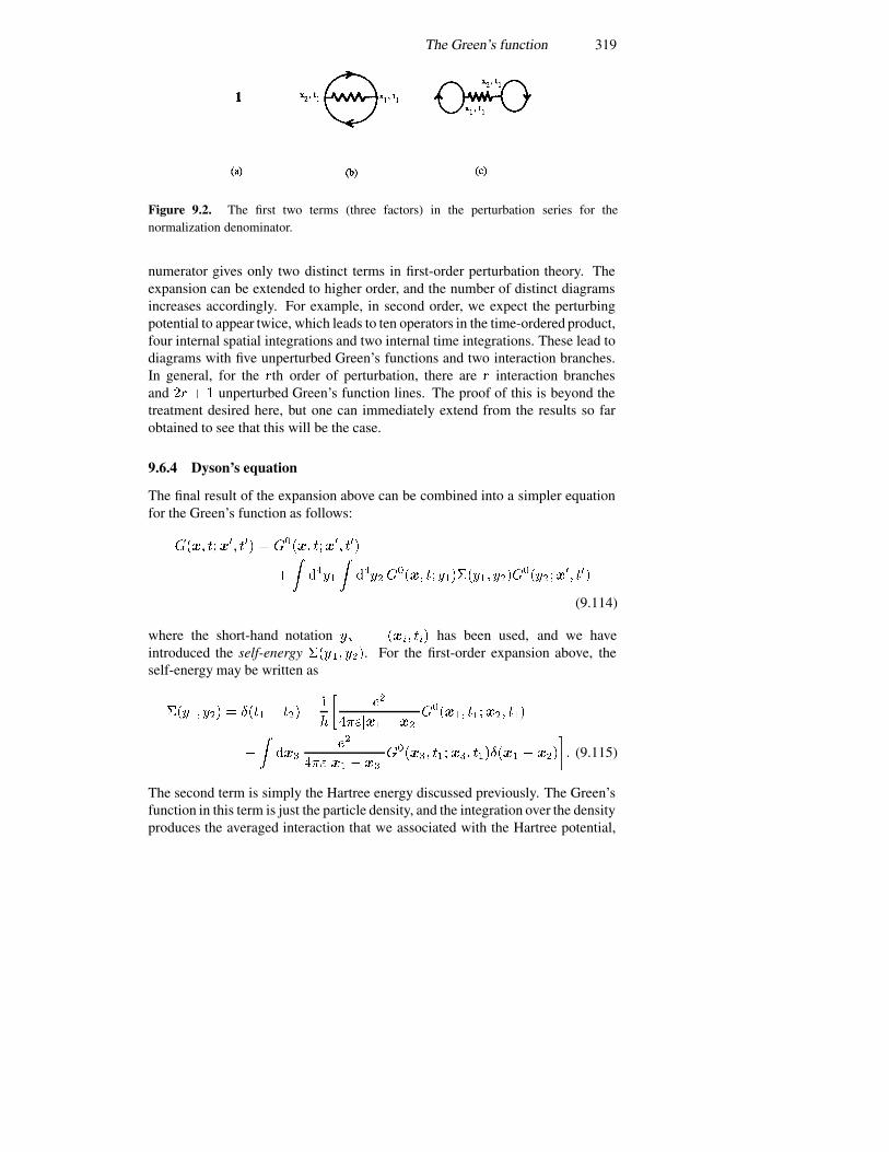
The Green’s function 319
Figure 9.2. The first two terms (three factors) in the perturbation series for thenormalization denominator.
numerator gives only two distinct terms in first-order perturbation theory. Theexpansion can be extended to higher order, and the number of distinct diagramsincreases accordingly. For example, in second order, we expect the perturbingpotential to appear twice, which leads to ten operators in the time-ordered product,four internal spatial integrations and two internal time integrations. These lead todiagrams with five unperturbed Green’s functions and two interaction branches.In general, for the �th order of perturbation, there are � interaction branchesand �� � � unperturbed Green’s function lines. The proof of this is beyond thetreatment desired here, but one can immediately extend from the results so farobtained to see that this will be the case.
9.6.4 Dyson’s equation
The final result of the expansion above can be combined into a simpler equationfor the Green’s function as follows:
���� ����� ��� � ����� ����� ���
�
�����
����� �
���� �� �������� ����������
�� ���
(9.114)
where the short-hand notation �� � ���� ��� has been used, and we haveintroduced the self-energy ����� ���. For the first-order expansion above, theself-energy may be written as
����� ��� � ��� � ����
�
���
����� � ��������� ������ ���
�
����
��
����� � ��������� ������ ������ � ���
�� (9.115)
The second term is simply the Hartree energy discussed previously. The Green’sfunction in this term is just the particle density, and the integration over the densityproduces the averaged interaction that we associated with the Hartree potential,
320 Electrons and anti-symmetry
although the formulation is different here. On the other hand, the first term is theleading term in the exchange energy since it involves the interaction between theelectron at different points at the same time.
The integral in (9.114) is a multiple convolution integral. We want toexamine the structure of this equation for a moment, and for this purpose willsuppress the integrations and the internal variables, but recalling that all internalvariables must be integrated in keeping with the concept of the convolutionproduct. Thus, we can rewrite (9.114) in this reduced notation as
� � ����
���
�� (9.116)
Now, consider the product� � �
���
��� (9.117)
in which the unperturbed Green’s function at the end of the last term is replacedby the full interacting Green’s function, calculated to all orders of perturbationtheory. Let us follow the spirit of perturbation theory, discussed in chapter 7,where we first assume that the lowest-order approximation to � is found by takingonly the first term in (9.117), so that
�� � ��� (9.118)
The next approximation, the first-order approximation, is found by using this lastresult for � on the right-hand side of (9.117):
�� � ����
���
�� (9.119)
This is just our result (9.116) obtained the hard way. If we continue, the nextorder in the approximate expansion is
�� � ����
���
���
���
���
�� (9.120)
In fact, this argument is to convince ourselves that the form (9.117) is the properlyre-summed perturbation expansion. The first intuitive step is to assume that allhigher-order terms in the perturbation expansion will go into the change from �
�
to �, but this would be wrong. Certain of the terms in fact do contribute to thischange. On the other hand, in particular, terms that expand the ‘bubble’ on theend of the interaction line (the combination of the interaction line and the bubbleare often referred to as a ‘tadpole diagram’ for reasons that are too obvious toexplain) in figure 9.1(d) or that expand the interaction line in figure 9.1(a) actuallycontribute to an expansion for the self-energy. In addition, when the problem isworked through self-consistently, the electrons can modify the strength of theinteraction, which leads to a correction called a vertex correction. Most of this isjust too complicated to worry about at this point, and we will limit ourselves tothe corrections that arise in the lowest order of perturbation theory. However, we
The Green’s function 321
can immediately jump from (9.114) to the re-summed equation for the interactingGreen’s function
���� ����� ��� � ����� ����� ���
�
�����
������
���� �� �������� ����������� ����
(9.121)
This is still a complicated integral equation for the Green’s function. However,because this is a convolution product, it is possible to rid ourselves of theintegrations by Fourier transforming in both space and time, using the results thatthe self-energy acts at a single time and that the Green’s functions are functionsonly of the differences in the arguments. This result is just
���� �� � ����� �� ������ ���������� �� (9.122)
for which
���� �� ��
������� ��� �����
�
� � �� ������ ��(9.123)
where we have used (9.85). This is, of course, a result quite similar to thatobtained in the Hartree approximation, except that now the self-energy is a morecomplicated function. Moreover, the self-energy usually has an imaginary partand so the convergence factor can be ignored; for the retarded Green’s function,we use the retarded self-energy with its negative imaginary part to produce theproper positive imaginary term in the denominator. The converse is taken for theadvanced functions.
Equation (9.122) is termed Dyson’s equation, and it should be comparedwith the equivalent formulation found in (7.85) and (7.86) (the latter differ by afactor of the reduced Planck constant). This equation is generally considered to bethe basic starting point of any treatment of Green’s functions. What we have donehere is to develop just the starting point for these calculations. From this point,real results incorporate a number of further approximations, necessary becausethe interacting electron system, with its vast number of contributing particles inany real system, is a complicated beast. Only the beginnings have been exploredbut, with this opening to the unsolved, we are brought to a suitable point to stop.Before we do this, however, we need to finish our discussion of the self-energy inits lowest order.
9.6.5 The self-energy
Before completing this chapter, we want to examine in some more detail the self-energy that arises for the Coulomb interaction between electrons, at least to thelowest order encompassed in (9.114) and (9.115). For this purpose, we will want
322 Electrons and anti-symmetry
to work in the momentum space description of the Green’s functions and the self-energy. We define the transforms as
���� ��� �� ��� �
���
�����
���
������ �������������������
�� (9.124)
and similarly for the self-energy and interaction terms (which form part of the self-energy). We will take the two terms that make up (9.114) and (9.115) separately.Let us first consider the leading term, which is composed of diagrams (a) and (f )of figure 9.1, as
�� �
�����
�����
���
�����
���
������� ���������������������
�
����
�����
����
������� ������
�������
���������������� � ���
�
�
�
���
�������
�������������
�����
������������ �����
���������� (9.125)
The first step is to notice that the integration over �� (part of ��) produces thefactor �� �� � ���, which can then be used in the integration over � �. Similarly,the integration over �� (part of ��) incorporates the delta function on the two timesand yields unity. The integrations over �� and �� produce ������� � ��� � ��and �������� ��� � ���, respectively, which also lead to ��� � ��. We can usethese delta functions to integrate out � � and ���. This leads to the result
�� �
���
�����
���
������� ������ �������������������
��
�
�
�
���
�������
������ � �� �� (9.126)
from which we can recognize the self-energy contribution by comparing with(9.114):
� ��
�
���
�������
������ � �� �� (9.127)
Now, the second term in (9.115) leads to
�� � �
�����
�����
���
�����
���
������� ���������������������
�
����
�����
����
������� ������
�������
���������������� � ���
�
�
�
����
���
�������
�������������
�
�����
������������ �����
������������� � ��� (9.128)
The Green’s function 323
Again, integrating over �� leads to a delta function for the two frequencies thatcan be absorbed in the integration over � �. Integration over �� involves the time-conserving delta function in the fourth line. Similarly, the integration over � �
involves the delta function and leads to a factor of unity. Integration over � �
leads to a factor of ������� � ����, which is absorbed in the integration over���. Finally, the next integration over �� leads to ������� � ���, which is thenabsorbed in the integration over � �. With these changes, the result is then
�� � �
���
�����
���
������� ������ ���������������������
�
�
�
���
�������
�������� �� (9.129)
from which we can see that
� � ��
�
���
�������
�������� ��� (9.130)
The transform of the unperturbed Green’s function in the last term is the valueat zero wave vector and zero frequency, which is normally written as the averagedensity, and this term is recognized as the Hartree term. The problem is thatthe assignment of a non-zero wave vector to the interaction line normally meansthat the Green’s functions on the input and output lines must have wave vectorsthat differ by this amount, but they have the same wave vector. This must beinterpreted as meaning that we must seek the value for the interaction as � � �.Since (9.130) is normally interpreted as a convolution integral, it is often seenin a form in which the dependence on � is transferred from the interaction tothe Green’s function in order to keep this consistency of notation. In any case,the expression (9.130) has no spatial variation and is an average potential—theHartree potential. The final form of the self-energy is then
�� � ��
���
�������
������� � �� �������� ���� (9.131)
This form can now be evaluated, but with care taken because of the problem withthe second term and the Hartree energy.
References
Abrikosov A A, Gorkov L P and Dzyaloshinskii I E 1963 Methods of Quantum FieldTheory in Statistical Physics (Englewood Cliffs, NJ: Prentice-Hall) section 7
Haken H 1976 Quantum Field Theory of Solids (Amsterdam: North-Holland)Pauli W 1925 Z. Phys. 31 765Pauli W 1927 Z. Phys. 43 601Slater J C 1929 Phys. Rev. 34 1293
324 Electrons and anti-symmetry
Problems
1. Consider two electrons in a state in which the radius (around some orbitcentre) is set normalized to unity, and the angular wave function is ���� �� ��������. If these two electrons have opposite spins and are located at � ��������and � ������ � ���, discuss the anti-symmetric properties of these electrons. Canyou infer the nature of the function describing the angular variations?
2. Show that the number operator
� �
�������� �
commutes with the Hamiltonian (9.47).3. Using the Hamiltonian (9.71), determine the dynamical equations of
motion for the creation and annihilation operators for the electrons.4. Expand the perturbation series to the second-order terms and draw the
ten distinct connected diagrams. Explain how these can be separated into sixdiagrams for the second-order terms of the self-energy and the four second-orderterms for �.
5. Consider a perturbation that scatters an electron from state � to state�
� while creating or annihilating one unit of lattice vibration. In section 4.6, itwas shown how the vibrating lattice could be represented in Fourier space as asummation of a set of harmonic oscillators. Devise a perturbing potential thataccounts for the scattering of the above electron by the lattice (it will take threeoperators, two for the electrons and one for the boson). Carry out lowest-orderperturbation and sketch the diagrams and Green’s functions that will result.
Solutions to selected problems
Chapter 1
2. We use de Broglie’s wave expression � � ��� � ������. The
frequency is always given by � � ��, so � � ����� ���� Hz. The wavelengthsare
�� � ����� ����� � �� � ����� ����� ��
The group velocity is ���� �� ���� and the phase velocity is half of this value.This leads to
�� ���
electron ���� � ���
����� ��� m s��
proton ���� � ���
����� ��� m s��.
3. We work in momentum space, with
� ����
��
��
������� ���
The expectation value is then
�� ���
��
��� �
��
�
��
��
���
��
����������� ���
�
���
��
������� ��
��
which then is manipulated as
�� � �
�
��
��
����� �����
��
� ������
��
��
�� ���
�� �
������
�
��
�
��
��
����� �����
��
� ������
��
��
�� ����� �
�����
�
�
��
��
����� �����
��
��
� �
�����
���� � �
325
326 Solutions to selected problems
�
��
��
�������
���
������
�
�
���
��
��
���
�
��
��
4. Using (1.52), with � � ��, gives
�� � �
�� �
���
����
���
For �� to equal ��, we require that the term in parentheses take the value�.
Thus,
� ������
��
Now, the average energy � ������, but ���� � ���� � ������� ��������. Thus, ��� �
��� to within 0.01%, so
� ������
���
��
������� �
���
���� � ����
� ����� ���� �
Chapter 2
1. We can summarize the picture, by defining the momentum wave functionas
���� � ��
���
������ ������
This, however, is not normalized properly, and we must check the propernormalization:�
���
����
������� �� � ���� ���
����
���
������ ������
�� �� �
�
The normalized wave function is then
���� �
�
� ��
���
������ ������
��
�
���
������ ������
This is now Fourier transformed into real space to give the wave function as
���� ����
��
��
�������� �� �
���
�
� ���
����
���
������ ��������� ��
�
�
�
�
�� ��� ��
��
� �
Solutions to selected problems 327
We note first that this wave function is symmetrical about � � �, so ��� � �.Thus, we then find that ����� � ����, and
����� ����
��
��
��
�
��
��� ��
����
���� �
���
���
Using the momentum wave function, we similarly find
����� �
����
����
�����
��
���
�������������
� ���
����
so the uncertainty relation is found to be
���� �
��
���
2. In general, one thinks that the kinetic energy is reduced once the wavepasses over the barrier, and this leads to a smaller value of � �, and hence alonger wavelength (����). However, how does this appear in a wave packet?The important point is that anything that narrows the momentum distribution willbroaden the spatial distribution just due to the properties of the Fourier transform.Hence, we consider a Gaussian wave packet, centred at ��, as in (following (1.33))
���� �
�
�
����� �������� � ���
���
For this wave packet, ��� � ��, and �� � ���� from (1.34). We note that �� isa function only of the width of the packet and not the centroid. If we now pass thiswave packet over the barrier (��� �� �
�������), then not much happens
until the barrier begins to eat away part of the Gaussian distribution. This narrowsthe distribution, which means that the real space wave function (obtained fromthe Fourier transform) must become broader.
6. For this problem, we note that �� � � �� � (which is true for any oscillatingsystem, where the energy oscillates between being purely potential energy andpurely kinetic energy), and this leads to (since we assume that ��� � ��� � �)
����� ��
� ������ �
�
� �
�
���
�
and
���� �
��
� ���� �
� �
�
for which
� � ��� � �
������ �
�
������ �
�
��

328 Solutions to selected problems
7. First, one determines the value of
� �
������
����������
from which it may be determined that solutions can be found only for ���� � ���.This means that there is only one root from each of the two solution sets (e.g.,one even-symmetry function and one odd-symmetry function). These two energylevels are (measured from the bottom of the well) 0.053 eV and 0.197 eV. Whenwe shift to measuring the levels from the top of the well, the energy levels are at������ eV and������ eV. From this, the values of � and � are easily determinedand the wave functions plotted.
8. Here, it is easiest if an integral representation for the Airy function is used,e.g.
�����
��
�
��
��
�
����
�� �
�
�
���
with
�
���
���
�����
The wave function that we begin with is for the �th energy level:
�� �� � ����
��� ����
��
�
��
��
�
����
�� �
��� ����
��
���
with
���� �
��
� ��� ��
�����
The Airy functions with different values of ���� are orthogonal to one another.Thus, we need only show that this property is maintained in the transforming tomomentum space. Thus, we start with the latter, as
�� �� ����
��
�
�� ������ �� �
����
��
�
��
��� ����
����� ��
�����
�
��
�
���� ��
��
��
�
����
�� �
�� �����
�
���
�����
�
��
��
�
����
�� �
����
�
���
��
�
�
��
��
� �
��
���
�����
�
��
��
�
����
�� �
����
�
����Æ � � ��
� ��
��
�
��
��
�
��� ������
Solutions to selected problems 329
and we check the orthogonality through
��� ������
�
�
��
��
����
��
���
�
��� ������
���
�����
��
���
�
��� ������
����
� ������
�
��
��
��� �������� � ���� �� � ������� ����� � ����
which clearly establishes the orthogonality, as the integral is zero unless the twozeros of the Airy functions coincide. Further, this may be used to show that�� � ��
��.
Chapter 3
1–3. For a linear axis, these may be plotted as
330 Solutions to selected problems
For a logarithmic transmission, the results are
For problem 1, the single bound-state resonance is at 0.1166 eV, althoughthere is a resonance at about 0.36 eV.
4. The resonant peak is now at 0.124 eV, and the transmission at this pointis 0.029. The values from problem 1 and problem 2 at this energy are 0.0156 and0.000 116 85, respectively, so ���������� is 0.0299, which is about as close asone can get on such a problem.
Solutions to selected problems 331
5. This problem is solved using the ‘general’ result:
��
�
���� �� �
��
�
���
����� �� � ���� �� � ���� ��
�
�
which leads to the result (with the energy � in eV)
��� ����� � ��� ������ ����
����
���
������ ��
This leads to a single level in the well, given by �� � ����� eV.6. For this problem, we cannot use the normal formula, because of the sharp
potential at � � . At the energy of the bound states, each energy � � can be relatedto a turning point �� via �� � ����. For � ��, the decaying wave function isgiven by
�������
��� �
��
���� ��
�
and this must be connected to the cosine function
�������
�� ��
�
���� �� ��
��
Now, this latter wave function must vanish at � � , so the bound states are foundfrom
���
�� ��
�
���� �� ��
�� �
Using the above energy relation, we can write this as
� ��
�
���� �� �
�����
��
� ��
�
��� � � �� � �� � ��
�
��
�
which leads to
�� � ���� �
�������
��
���� ���
�� �
�
�
������
It turns out that these are precisely the values found from solving the Airyequation (once we adjust the latter for � � �� �� � � � , and not � � �� �� � � �).
8. For this problem, we can return to our ‘general’ formula. Again, notingthat the energy eigenvalues will have corresponding turning points � � through�� � �����
�, we have
���� ���
��
� ��
���
���� �� �
����
��
� ��
���
���� � �� ��
� ����
����
��
332 Solutions to selected problems
and the energy eigenvalues are given by
�� � �
����
���
���
�
�
��
�
�����
Chapter 4
1. The potential is given by �������. We seek energy levels given by ��,with the turning points
�� ��
������ � � �
�������
�
Via the basic approach we now seek solutions to the phase integral
� �
��
��� �� �
� �
��
���
��
�� � �
������
���
���
�
� �
��
��� � �� �� � ���� ��
�
�
which leads to
���
�
�
�� ���� ��
�
�� � �
���� ���
��� �� �
���
�
�
���
which is the exact answer. We conclude that a quadratic potential is a ‘soft’potential.
3. The energy ����� corresponds to the energy level � � �. Using thecreation operators, we find
����� ����
�����
�������
���
����
��� � �
��
Then,
� ��� � ��� ������
��� � ���
����
��� � �
�����
��� ��
which leads to
� ��� � ��� ����
� ���� �
��
�����
���
��
6. This may be carried out with the operator algebra. However, to understandthe result, we must define wave functions. Since we do not know which state isoccupied, we will take an arbitrary occupation of each state via the definition
���� ��
�� ����
Solutions to selected problems 333
where the �� are the harmonic oscillator wave functions for state �. Then, theexpectation values are found from (�� is used as the example)
���� �
���
����
���� ���
����
�����
���� � ��� � ��� � ����
�
� ����
��������� ��� ����� ������
for which the �� matrix element is
������ ����
�
����� ���� �
���� ����� �������
������ �������
�
Similarly,
������ ��
���
����� ���� �
���� ����� �������
������ �������
�
Thus, in both cases, only states either equal in index or separated by 2 in indexcan contribute to the expectation values.
7. Using the results of problem 6, we have
�� ��
��������
���
�
����� ���� �
���� ����� ������� �
����� �������
�� �
���
�������
���
�
����� ���� �
���� ����� ������� �
����� �������
�
11. We take � � ����, which we can get from the vector potential� � ��� ��� ��. This will give a harmonic oscillator in the �-direction, andfor homogeneity in the -direction, we take ���� � � ���� ���� �. Then, theSchrodinger equation becomes
�
����� � �����
� ���
��
��
���������
������� � �����
which with the change of variables
�� ���
�
��
��� � ����� �
���
� � � ��� � ���
334 Solutions to selected problems
gives
�
��
��
���
����
�
������� ���
�� �
�� �
����
���
�
������
�
��
which is a shifted harmonic oscillator and leads to the energy levels
�� �
���
�
�
����
����
���
�
������
��
Chapter 5
1. The Hamiltonian is given as � � �� �����. From (5.16)
������
��
���� �� � �
����� � ��� � ���� ��
��
��� � �������� ����� � �
��� � �������� ����
� �����������
��
���� �� � �
����� � ��� � ���� ��
��
������ ��� � � ����� � �����
��
������� ���� ���� ����� ����
� ���������
2. The eigenvalues are found from
�
�
���������� ���
�� �
��� ���� ��� �
� � ��� ���
������ � �
(the factor of 2 multiplying the� is due to the pre-factor) and this leads to� � � �,with the other two roots being given by
���� ���� � � � �
���� ������
�
�� � �
�� ���
3. (i) � � �����
������
��
�������� �� � ������
������
��
�������� �� � �������
Solutions to selected problems 335
(ii)� � ���� � ����
����
��� ��������
�
������ � ������ � �������
����
��� ��������
�
�������� ����� � �������
(iii) � � ������
����
���
�
��������� �� � ������ � ������
����
���
�
��������� �� � �������� ������
4. ���� � �, in which � is a �-number. Thus,
���� � ����� � ���� �������
� ���� ����� � ����� � ���
� ���� ������� � ������ � ����
� ���� ������ � ���� � ������ � ����
� ����� � ���� � ����� � ������
Chapter 6
1. We have ��� � � for � � � � �, and � � elsewhere. The perturbingpotential is given by � � �� � ��� �. The unperturbed wave functions andenergies are then given by
����� �
��
��� ����
�
�� � � � �
�� �������
����
For the effect of the perturbation, we find the matrix elements
�� ��
�
��
�
�� ����
�
���� ��� ��
�����
���
�
�������
��
��
��
�������
�
������
�� �� �
��
�
���
�����
�� � �.
The first term can be simplified, but the perturbed wave function can be written as
����� �
�
��� ����
�
�
336 Solutions to selected problems
��
����
��
�����
��� � ����
�����
������� � ���
�����
����
����
�
�
�
��
��������
�
��
����
����
��
�
�� ���
���
��� � �������
����
�
��
The energy levels are now given by
�� � ����� �����
� ������
�������
�����
��
��
�
�����
�
���
��
������
����
�� ���
����
��� � �����
2. The third-order correction to the energy is given by
����� �
�� ���
��������� � �������
������ ��
���� ��
��� �����
���������
������ ��
���� ���
���� ��
���� �
���
4. The lowest energy level is for � � � � ,
��� �����
������ � �� �
����
���
since the wave functions are
������ �
��
��������
��
��
�
������ �
��
�������
��
��
�
��
The lowest degenerate energy level occurs for the sets of ����� � ��� �� �� ��,which both give the energy level of
��� � ��� �����
������� � �� �
�����
�����
If we call the (�� ) set � and the (� �) set �, then the matrix element which couplesthese two wave functions is
��� � ��
� ��
���
�
� ��
���
������ ������ �
������
� ��
���
� ���
����
�
��������
�� ��
���
������
����
���
�
�
������
�
�
� ��
���
�
����
����
�
�� ���
����
��� ��
Hence this potential does not split the degeneracy. The reason for this is that thepotential is still a separable potential (it can be split into � and parts). Since the
Solutions to selected problems 337
potential is an even function around the centre of the well, it can only couple twoeven or two odd wave functions, hence it does not split the lowest level which iscomposed of even and odd functions.
5. We use the fact that ��� ��� � ��� � ��� � � to get
� �
��
���
������� ���
�� ��
������ ���� �
�
������ � ����� � ��� ��
�� �
��
���
����� ����
�
��
���
����� � ����� � ����� ����� � ������ � ��� � ��� ���
This leads to the matrix elements
�������� � ���������� ����� ����� �
����������� � ������
��� ����� ����� ���� ��
�������� � ���������� ��
����������� � ������
��� ����� ���
The matrix has elements on the main diagonal ����������, and elements giventwo and four units off the main diagonal, given by the above matrix elements (plusthe pre-factor listed above).
6. By the same procedures as the previous problem, the perturbation can bewritten as
�� � �� �
��
���
������� ����
�
��
���
������� � ����� � ��� ���� ��� ������
We note that the ��-term is zero, so there is no first-order correction to theenergy. Thus, we need only calculate the second-order correction using the matrixelements
������ �
��
���
���� ������
����� ����� �� � �������� ��
��
�������
��� ����� ����� � � �������� ����� �
�
which leads to
���� �
�� ���
������������
���� �
����
338 Solutions to selected problems
� ��
��
���
�� ����� ����� ��
����
��� ����� ����� ��
���
��
������� ���� � ���� ������ ���
�
�����
����
��
��� � ���� �
�
�� ������ ���� �
��
Chapter 7
4. From (7.40d), we may write the general propagator as
���� �� � ���
��
��
�
�
for � � . Thus, the total wave function is given by
���� � ���� ������ �
��
�������� ���
���
��
�
��
and the connection to an arbitrary state ��� becomes
��� ������ ��
���
����
���
���
��
�
������
��
�
�� � ���
��
�
��
� ���
���
��
�
���
These integrals may be computed with some care. It should be noted, however,that the field term does not have the periodicity of the quantum well, but doeshave symmetry properties. Thus, for example, the initial state has even symmetryin the well. Thus, the cosine term in the field will only couple to states that haveeven symmetry. On the other hand, the sine term will only couple to states thathave odd symmetry since it is odd. In general, all states are coupled to the � � �state by this perturbation.
Chapter 8
1. This zero-angular-momentum state requires �� � �� � �. Thus, the stateis excited as
��� �� � ��� ��� �� �The various quantities are given by
� ����
�
��� � �
�
�
��� �
��
�
��
�
�� � � ��� ��� �� � ������
������
�
�� �
���
��
Solutions to selected problems 339
This leads to
��� �� � �������� � �� ���
������
�
��
2. The perturbation may be found by expanding the frequency in the form�� � ���� � �����. The operator � may be expressed in terms of thevarious creation and annihilation operators as
� �
��
����� �
� �
�
�
��
��� � � ���
This leads to the crucial part, which is the ��-operator:
�� ��
���
�� �� ��� ����
��� �� �� ��� ���� �� ���
We now define the matrix elements between the state � � �� and the state ���� ���to be
��������and the various terms in �� can be evaluated as
�������� �������������� ��������� �
�������������
��������� �������������� ��������� �
�������������
�������� � ������������ ���������� � ������������
��������� � ������������ ��������� � �������������
The term in the number operators is diagonal. Thus, there are a variety of shiftingoperations in the perturbation, which generally mixes a number of modes.
3. We write the Schrodinger equation with the potential � � ���� as�� �
�
��
���
���
��
���
�
�����
��� ��� ���
����� � � ����� ��
Introducing the parameter
�� ���
����
this may be written as a shifted harmonic oscillator in the form�� �
�
��
���
���
��
���
�
�����
���� ��� ���
����� �
�
�� ����
����
����� �

340 Solutions to selected problems
so the new energies are given by
����� � ��� � �� � ����� ����
�
����
�
�

Index
Absorption 231Acceptors 285Actinides 272Action 27Adiabatic principle 230Adjoint 30
Operators 150Advanced behavior 62
Green’s function 308Aharonov–Bohm effect 7Airy equation 52Allowed states 115Alloy 43Angular momentum 251Anion 280Annihilation operator 151Anti-bonding 219Anti-commutator 296Anti-symmetric part 98
Wave function 289Artificial band structure 194Attenuation 85Average energy gap 282
Band gap 116Width 117
Bands 113Basis 170Black-body radiation 1Bloch frequency 118, 122
Function 114, 231Oscillation 118, 195
Bohm potential 28, 97Bohr model 2
Radius 266, 286Bond polarization 283Bonding 219Bose–Einstein statistics 142, 158,
233, 289Boson 142, 153, 289Bound states 57Box normalization 10Bra vector 190Bragg reflection 123Brillouin zone 116
�-number 150Capacitance 54Cation 280Cavity 155Central-field approximation 270Centripetal force 159Charge 139, 154
Neutrality 108Closure 157, 181, 299Coherent tunnelling 95Commutator bracket 15
Relation 176Complementarity 2Conductance quantization 110Conjugate operators 174Connected diagrams 318Connection formulas 91Conservative system 176Contact resistance 112Continuity equation 28Convolution 63Correspondence principle 2
341

342 Index
Coulomb blockade 122, 131Interaction 306
Crank–Nicholson 69Creation operator 151Current 29, 59Cyclotron frequency 161, 256Cylindrical coordinates 251
Darwin–Foch levels 263De Broglie wavelength 2Debye wave vector 220Defect levels 284Deformation potential 232Degeneracy 189, 210, 249Degenerate perturbation theory 217Delta function 14Density 219
Operator 301Depletion 51Diffusive effect 21Dilation 232Dirac notation 190Disconnected diagrams 317Dispersion 18
Relation 116Displacement operator 192Dissipation 109Donors 285Duality 2Dyson’s equation 245
Edge states 164, 259Effective mass 284Ehrenfest’s theorem 60, 175Eigenfunctions 57Eigenstate 301Eigenvalue 12, 181
Equation 189Elastic scattering 49, 231Emission 231Energy band 116
Conservation 94Levels 38Relaxation time 248
Representation 58Shift 238
Energy-time uncertainty 183, 227Ensemble average 311Entangled state 185Equivalence principle 198Evanescent wave 73Exchange energy 314Excited states 170, 224Expectation 11
Value 59, 176
Face-centered-cubic lattice 279Fermi–Dirac statistics 289Fermi energy 290
Golden rule 230Fermi–Thomas approximation 274Fermion 153, 289
Operator 295Feynman diagrams 317Field operators 298
Theory 298Fine structure 276Flux 154
Linkage 139Quantum 7
Fock space 297Forbidden gap 115
States 100Fractal 196Fractional quantum Hall effect 167
Gaussian function 226General basis set 175Generalized coordinates 155Generating function 143Green’s function 245Ground state 151, 252, 307Group velocity 19, 117Guiding centre 259
Half-integer spin 290Hall resistance 166Harper’s equation 196
Index 343
Hartree energy 313Hartree–Fock approximation 276,
313Heaviside function 32Heisenberg picture 171
Representation 177, 307Uncertainty relation 183
Hermite polynomials 139Hermitian adjoint 177
Operator 30, 178Heteropolar compound 280
Energy 281Heterostructure 49, 87High-electron-mobility transistor 51Hilbert space 171, 292Hofstadter butterfly 204Homopolar energy 281Hybrid-polar energy 281Hydrogenic model 285
Identical particles 288Indistinguishable 288Inelastic mean free path 8, 258In-plane gates 87Interaction potential 315
Representation 227, 307Interference 3, 77, 217Inversion layer 50, 250Ionicity 283Ionized acceptor 51
Impurity scattering 247
Ket vector 190Kronecker delta 146
Lagrange’s equations 301Landau gauge 160, 256
Level 163, 257Landauer formula 109Lattice 155
Constant 113Distortion 232Vibrations 230
Leakage 127
Legendre polynomials 269Lifetime 239Linear vector space 170, 184Lippmann–Schwinger equation 242Localization 118Logarithmic derivative 40Lorentz force 160Lorentzian line 239Lowering operator 151
Magnetic length 162Many-body effects 262Many-particle wave function 288Matrix 76
Element 147, 186, 207, 231Mesoscopic systems 109Metallic energy 280Mixed state 180Mixing 218Molecular-beam epitaxy 49Momentum 124
Conservation 95, 231Eigenfunctions 295Operator 14Relaxation time 226Representation 173Wave function 13
MOS transistor 49Multi-electron problem 289
Negative differential conductance99
Non-commuting operators 182Normalization 207Number operator 150, 250
Representation 296
Operators 1, 8Orbitals 279Ordered operators 299Orthogonal 10Orthonormal polynomials 139Orthonormality 145, 179Out-scattering rate 238

344 Index
Overlap integral 218, 233
Parity 141, 213Pauli exclusion principle 153, 289
Matrices 293Peak-to-valley ratio 105Peierls substitution 160Pendulum 137Penn dielectric function 287Periodic array 113
Potential 113Table 271
Periodicity 113Permutations 294Perturbation theory 206Phase 124
Shifts 85Phasor 251Phonons 142, 156Photoemission 4Photon 4, 142Planck’s constant 1
Law 1Plane waves 305Plunger gate 87Poisson’s equation 107Polarization charge 128Position representation 173Potential well 37Predictor-corrector algorithm 69Probability wave 6Projection operator 185Propagator 61Pseudo-momentum 301Pseudo-position 301Pure state 38, 180
Quanta 1Quantized conductance 110Quantum capacitance 54
Dot 87, 127Point contacts 87
Raising operator 151
Rare-earth elements 272Rayleigh–Ritz method 222Reciprocity 80Reduced zone 116Relaxation time 221Representation 11Resolution of unity 191Resonances 46, 83Response function 63Retarded behavior 62
Green’s function 308Rotating operators 252Russell–Saunders perturbation 277Rydberg 285
Scalar potential 160Scattered wave 221Scattering 48
Cross section 220Potential 231Rate 222, 232
Schrodinger equation 27Picture 171
Schwarz inequality 182Screening length 220, 273Second quantization 298Secular equation 211Self-energy 319
Correction 238, 313Sequential tunnelling 120Shell 271Shubnikov–de Haas effect 163Sidegate 260Similarity transform 187Singular 66Slater determinant 291Spectral density 63, 309Spectroscopy 259Spectrum of operator 180Spherical coordinates 264Spin angular momentum 288Spin–orbit coupling 276, 290Spinors 293Spring constant 136

Index 345
Stark effect 213Ladder 120
Stationary phase 91Sturm–Liouville problem 139Superlattice 118, 194Superposition 75, 310Symmetric gauge 251
Part 98Wave function 289
Symmetrized product 199Symmetry 39
Tadpole diagrams 320Tetrahedral coordination 279Tight-binding method 195Time-evolution operator 197
-Ordered Green’s function 308-Ordering operator 308
� -matrix 241Transit time 87Transition metals 272
Probability 230Rate 230
Translation operator 193Transmission 75Transparency 80Transpose 186Transverse energy 101
Truncation error 65Tunnel diode 94Tunnelling 73Turning point 89Two-particle Green’s function 312
Uncertainty 16Unit vectors 184Unitary matrix 76, 188
Operator 235
Vacuum state 295Valence plasma frequency 287Variational method 206Vector potential 160Velocity 28Vertex 317
Correction 320
Wave mechanics 26Packet 18Vector 13
Wick’s theorem 316Work function 4
Zener breakdown 73Zero-point motion 250
Copyright © 2022 FDOKUMEN