I. QUANTUM MECHANICS OF ONE-DIMENSIONAL

TWO-PARTICLE MODELS

II. A QUANTUM MECHANICAL TREATMENT OF

INELASTIC COLLISIONS

Thesis by

Dennis J. Diestler

In Partial Fulfillment of the Requirements

For the Degree of

Doctor of Philosophy

California Institute of Technology

Pasadena, California

1968

(Submitted August 7 ,. 1967)

,.

ii

ACKNOWLEDGMENTS

I express my sincere gratitude to Dr. Vincent McKoy,

my advisor, for his patient interest in my research, for the

many lengthy and fruitful discussions we have had, and for the

attention he has given to the many matters, both trivial and

important, incidental to my education as a graduate student.

Of course, I am thankful that my life has been enriched

by myriads of discussions of all types with faculty and students.

I feel particularly indebted to my office-mates (all 11 of them) in

212 Church and to Dr. Vlilliam A. Goddard, Dr. William E. Palke,

and Dr. Russell M. Pitzer. I have also received much assistance

from and enjoyed many enlightening discussions with members of

Professor Kuppermann's group, in particular Merle E. Riley.

I am grateful to the National Science Foundation for three

years of graduate fellowships and to the California Institute of

Technology for two part-time teaching assistantships, which have

given me invaluable experience.

Finally, albeit not least of all, I should like to thank

Marcia Kelly for her speedy and meticulous typing of numerous

business letters and for her alacritous assistance in all manner

of other secretarial matters with which I have plagued her since

the inception of our acquaintance.

iii

ABSTRACT

Part I

Solutions of Schrtldinger 's equation for systems of two

particles bound in various stationary one-dimensional potential

wells and repelling each other with a Coulomb force are obtained

by the method of finite differences. The general properties of

such systems are worked out in detail for the case of two electrons

in an infinite square well. For small well widths (1-10 a. u.) the

energy levels lie above those of the noninteracting particle model

by as much as a factor of 4, although excitation energies are only

half again as great. The analytical form of the solutions is obtained

and it is shown that every eigenstate is doubly degenerate due to the

"pathological" nature of the one-dimensional Coulomb potential.

This degeneracy is verified numerically by the finite-difference

method. The properties of the square-well system are compared

with those of the free- electron and hard- sphere models; perturbation

and variational treatments are also carried out using the hard- sphere

Hamiltonian as a zeroth-order approximation. The lowest several

finite-difference eigenvalues converge from below with decreasing

mesh size to energies below those of the "best" linear variational

function consisting of hard- sphere eigenfunctions. The finite­

difference solutions in general yield expectation values and matrix

. elements as accurate as those obtained using the "best" variational

function.

The system of two electrons in a para bolic well is also

treated by finite differences. In this system it is possible to

separate the center-of-mass motion and hence to effect a con-

iv

siderable numerical simplification. It is shown that the pathological

one-dimensional Coulomb potential gives rise to doubly degenerate

eigenstates for the parabolic well in exactly the same manner as for

the infinite square well.

v

Part II

A general method of treating inelastic collisions quantum

m.echanically is developed and applied to several one-dimensional

models. The formalism is first developed for nonreactive

"vibrational" excitations of a bound system by an incident free

particle. It is then eh'tended to treat simple exchange reactions of

the form A + BC .... AB + C. The method consists essentially of

finding a set of linearly independent solutions of the Schrtldinger

equation such that each solution of the set satisfies a distinct, yet

arbitrary boundary condition specified in the asymptotic region.

These linearly independent solutions are then combined to form a

total scattering wavefunction having the correct asymptotic form.

The method of finite differences is used to determine the linearly

independent functions.

The theory is applied to the impulsive collision of a free

particle with a particle bound in (1) an infinite square well and (2)

a parabolic well. Calculated transition probabilities agree well

with previously obtained values.

Several models for the exchange reaction involving three

identical particles are also treated: (1) infinite-square-well

potential surface, in which all three particles interact as hard

spheres and each two- particle subsystem (i. e . , BC and AB) is

bound by an attractive infinite-square-well potential; (2) truncated

parabolic potential surface, in which the two- particle subsystems

are bound by a harmonic oscillator potential which becomes infinite

for interparticle separations greater than a certain value ; (3) para­

bolic (untruncated) surface. Although there are no published values

with which to compare our reaction probabilities, several inde­

pendent checks on internal consistency indicate that the results are

reliable.

vi

P REFACE

All of Part I of this work is concerned exclusively with the

treatment and properties of one-dimensional (1-D) model systems.

Also in Part II we have chosen 1-D models to illustrate the

application of a quite general theory. Because of their mathematical

tractability, 1-D analogues of real physical systems have long been

studied with the hope of gaining insight into the real systems.

Indeed, there has been published recently a book entitled

"Mathematical Physics in One Dimension"*, in which are collected

reprints of one-dimensional model studies.

On one hand, we must question the value of investigating

models which indubitably suffer from a lack of three-dimensional

effects. On the other hand, we may in particular cases adduce

much evidence, perhaps empirical, that a one-dimensional model

faithfully reflects the properties of interest in the real physical

system under scrutiny. Whatever the case may be, it is clear that

the study of one-dimensional models indirectly makes a significant

contribution to our understanding of real systems. First, the

appealing feature of 1-D models, i.e., their susceptibility to

rigorous mathematical analysis, makes us wary of simplistic

theories contrived merely to circumvent mathematical complexities

inherent in the three-dimensional problem. Second, specific results

of the 1-D treatment may suggest interpretations of confounding 3-D

results or modifications in the theory which lead to a more satis­

factory "picture". In this respect the study of one-dimensional

models serves to sharpen our concept of reality.

* "Mathematical Physics in One Dimension", ed. E. Lieb and D. Wmttis (Academic Press, Inc., New York, 1966).

vii

TABLE OF CONTENTS

PART TITLE PAGE

I QUANTUM MECHANICS OF ONE-DIMENSIONAL

TWO-PARTICLE MODELS 1

A. Introduction 1

B. Wmthematical Treatment of the IFEM 4

1. General Considerations 4

2. The Finite-Difference Method 17

a. Uniqueness and convergence 19

b. Method of solution of finite-

difference equations 24

c. Results 25

d. Numerical verification of

degeneracies 28

3. Comparison of Results with Other

Approximations 29

c. Two Electrons in a Parabolic Well 35

1. Results 38

D. Discussion 39

E. Appendix 43

REFERENCES 47

TABLES 50

FIGURES 58

II QUANTUM MECHANICAL TREATMENT OF

ThfELASTIC COLLISIONS 74

A. Introduction 74

viii

PART TITLE PAGE ---B. General Theory 78

c. Determination of the X· 87 J

1. Uniqueness and Convergence 90

2. Solution of the Finite-Difference

Equations 94

3. .A.nalysis of the X· 97 J

D. Application of the Theory to Vibrational

Excitations 98

1. Infinite- Square-Well Binding Potential 98

2. Parabolic Binding Potential 100

E. Extension of the Theory to Exchange

Re ::wtions of the Type A + BC ..... AB + C 103

F. Application of the Theory to Exchange

Reactions 112

1. Infinite- Square-Well Potential Surface 113

2. Truncated Parabolic Potential Surface 114

3. Untruncated Parabolic Surface 117

G. Discussion 120

H. App,~ndix 124

REFERENCES 127 TABLES 129 FIGURES 135

m PROPOSITIONS 157

1

I. QUANTUM MECHANICS OF ONE-DIMENSIONAL TWO­

PARTIC LE MODELS

A. Introduction

A classic example of a valuable one-dimensional (1-D)

model is the simple free-electron model (FEM), in which the

electrons move independently in a 1-D infinite square well. In

spite of the relative success of this model, e. g. , in its application

to pi-electron spectra of conjugated molecules, a first obvious

"improvement" is the inclusion of the 1-D Coulomb interaction

among the electrons. The solution of our model gives wave­

functions, energies, and other properties for the two-electron

case of this improved FEM and furthermore demonstrates how

"physics" may get distorted in one-dimension.

In this part we solve, by the method of finite differences

(FD), the Schrtldinger wave equation for systems of two particles

bound in various types of one-dimensional potentials and inter­

acting with each other via a 1-D Coulomb potential I x1 - x2 I""1.

For the case of two electrons in an infinite square well, 1 which

we shall treat in detail, the energy levels lie higher than those

of the noninteracting-particle model (FEM) by as much as a

factor of 4; excitation energies are 50 to 70% greater. Most

important, however, every eigenstate is doubly degenerate. This

is a non-group-theoretically required degeneracy and is due to the

"pathological" nature of the 1-D Coulomb potential which requires

that the wavefun.ction vanish when the coordinates of the electrons

are equal.

2

A central problem in the quantum theory of many- electron

systems is to find approximate wavefunctions which accurately

predict the properties of the system. Traditionally, one uses the

variational principle to determine the "best" trial function of a

given form. Often, however, this "best" trial function does not

successfully predict other properties of the system more important

to the chemist than total energy. To discover directly why this

function fails it is necessary to examine the exact solution. For

example, to study the effects of electron correlation in two­

electron atoms, Kestner and Sinanoglu 2 and Tredgold and Evans3

independently investigated the "exactly" soluble 3-D model con­

sisting of two electrons bound in a parabolic well, but repelling

eacn other with a Coulomb force. Although the model is not

exactly soluble in the sense that the wavefunction may be written

in closed form, the presence in the Hamiltonian of the attractive

(nuclear-electron) parabolic terms allowed them to separate the

Schrtsdinger equation in the center-of-mass coordinate system.

As we shall see, the one-dimensional problem may be treated

similarly. In fact, the solution of the 1-D relative equation is

identical to the 3-D relative solution multiplied by the interelectron

coordinate r 12. It is clear, however, that the FD method has the

advantage of enabling one to study the effects of a wide variety of

attractive (nuclear- electron) potentials on electron correlation,

since it does not rely on the presence of a separable potential in

the Hamiltonian.

A great deal of study has been given to the problem of

electronic interaction in the FEM. Several authors have

investigated the effect of including explicit interelectronic inter­

action (Coulomb) terms in the model Hamiltonian. Araki and

3

Araki4 used a 2-D average over the 3-D Coulomb potential in a 1-D

treatment of the cya.nine dyes. In a similar manner, . Huzinaga 5

re- exar.a.ined the Platt model for the naphthalene molecule, including

electron repulsion terms as 1-D averages over the 3-D potentials .

. Also, Ham and Ruedenberg6 modified the free-electron network

model by introducing the electron interaction terms as 2-D

averages over the cross-section of the bond path. Finally,

Olszewski 7

attempted a configuration interaction treatment of

linear conjugated molecules using antisymmetrized 1-D free­

electron molecular orbitals (ASFEMO). 8 The solution of our

model suggests several alternative methods of treating linear

conjugated molceules which do not involve taking averages over

arbitrary cross sections or limits of 3-D expressions.

Bolton and Scoins, 9

concerned primarily with the solution

of eigenvalue problems by the finite-difference method, have

reviewed attempts to solve various two-variahi.e Schrtldinger

equations. Although not particularly interested in electron corre­

lation, they obtained for the "S-limit1110 of the ground state of the

helium atom a value of -2. 65 a. u. (best value -2. 879)~ lO, 11

In the remaining sections of Part I we have two main

purposes: first to obtain accurate energies, wavefunctions, and

selected properties for the model system (IFE M) discussed above

and then to consider the relevance of our results to more com­

plicated and interesting systems. In Section II the !FEM is

treated quantitatively. The analytical propert ies of the wave­

functions, including the "accidental" double degeneracies, in

part 1; the FD method, uniqueness and convergence properties

of FD eigenfunctions, eigenvalues, and matrix elements in part 2.

4

We also discuss numerical verification of the degeneracies in

part 2. In part 3 the FD results are compared with approximate

solutions obtained by the perturbation and variational methods. In

Section C we apply the FD method to the problem of two electrons

in a parabolic ·well, discussing how the accidental degeneracies

arise analogously to those of the IFEM. Finally, in Section D we

discuss the results and how they apply to more complicated one­

dimensional models and also indicate how the FD method may be

used to solve differential equations arising in the treatment of

more 11chemically" interesting three-dimensional problems such

as the He atom.

B. Wiathematical Treatment of the IFEM

1. General Considerations

The time-independent Schrt)dinger equation for the one­

dimensional system of two electrons in an infinite square well is

written in atomic units (a. u.) in the coordinate system [xJ.,. x2] 12

where 0 ~ x11

, x2 1

:::;. a and x1' and x2 ' denote the electron

coordinates; a is the well width. Since the wavefunction must

vanish outside the well, the boundary conditions on v,; in

[x11

, x21 J are:

(la)

(lb)

5

l,(;(xl I' 0) - 0

l,(;(xl '' a) = 0 -

(2) l,(1(0, x ') 2 - 0

l,V(a, x2 ') :: 0

These conditions require that ~(x1 ', x2 1

) vanish on the boundary

of a square of edge a (see Fig. Ia). The Schrtldinger equation

(la) is invariant under transformation to the system [x1, x2J, defined by

However, the boundary conditions in [x1, x2J are:

cp(x1

, - a/2) _ 0

cp(x1, a/2) - 0

(3)

cp(- a/2, x2) = - 0

cp(a/2, x2) - 0 .

In the center-of-mass coordinate system [X1, X2J, where

G

X~ + x 2 X - _1-=--

1 - 2

the Schrt5dinger equation becomes

2 Cl '1' --· +

aX2 2

= E'l' '

with the corresponding boundary conditions

'1' (X 1'

2X1

+a) = 0

'1' (Xl, 2X1 - a) = 0

'1' (Xl, -2X1

- a) = 0

'1' (X -2X +a) 1' 1 = 0 .

These conditions specify that the wavefunction vanish on the

bour.ldary of a rhombus, the edges of which are not coincident

with coordinate surfaces in [X1, X2J (see Fig. lb).

In each of the coordinate systems there is a group of

(4)

(5)

operators IE , ri. , fR 1 , IR 2 defining coordinate transformations

which leave the Hamil~onian invariant. It is simplest to define

thesa operators in [x1, x2J, although we shall express them

later in the other systems. Thus IE is the identity which takes

7

the point (x1

, x2) into itself, Ii is the inversion about (0, 0)

taking (x1, x2) into (-x1, - x2), lf\ is the reflection about the

diagon~l x2 = x1 which transforms (x1, x2) into (x2, x1) and IR2

is the reflection about the other diagonal which carries (x1, x 2)

into (-x2, -x1). This group is isomorphic with the Vierergruppe, 13

in which all the elements are mutually commuting. Thus the group

of the Schrtldinger equation is Abelian and has only one-dimensional

irreducible representations (i. r. ). These are listed in Table I.

Furthermore, since the exact eigenfunctions of the Hamiltonian

must transform according to these i. r. 's, we conclude that all the

eigenstates of our system are nondegenerate, i.e., there is no

group-theoretically-required degeneracy.

Now consider the solution of the Schr<:Sdinger equation in the

system [ x1

, x2J by the method of separation of variables. To

study the form of the components of the required solution, we

substitute 'i' (X1, x 2) = ¢(X1)x(X2) into Eq. (4). A sum of such

components will, of course, have to be used to satisfy the boundary

conditions, Eq. (5). We obtain

and

1 d2

¢ Li: ... - 2 + En-¢ = 0

dX 'P

1

~+ dX2

2

_ X_ - E X = 0' IX2l x

where E = E¢ +EX. The general solution of Eq. (6a) may be

written

(6a)

(6b)

8

2 where k¢ = 4E¢ and A1 and A2 are arbitrary constants.

In the region x2

> 0, Eq. (6b) may be transformed into

Kummer's equation

2 z d v + (2 - z) dv - (1 - - 1- ) v = 0

dz2 dz 2kx '

k x2

(7)

(8)

by the substitutions x = x2e X v( z), z = -2kXX2, where

k 2 = -E . 14 Since b in the general form of Kummer's equation x x is an integer in this case, namely 2, the two independent solutions

are, in the notation of Slater14

where

co

v 1

= 1F

1 (a, b ;z) :;;: l

m:;;:O

n-l (a-n) r-n co

v2:;;: l (1-n{zr! +l r=O r r=O

(a)m

~ m

m z m!

(a-n) r-1 n+r z

(l-n)n-1 (l)n+r rT x

r-1 1 r 1 \

-r-(a-+-s--n-1) - l (s+n-1) - L s:;;:l s=l

(9)

9

1 a= 1--2k ' x

b=n+1=2

(s) = s(s + 1) ••.. (s+p-1) . p

Thus for x2 > 0 the general solution of the relative equation (6b)

is

Similarly for x 2 < 0 the general solution takes the form

-k x . x<(X2) = CX2e x

2 {Bl vl (2kxX2) + B2 v2(2kxX2)} ' (lOb)

where the B's and C are arbitrary constants. vVe note that with

the substitutions

. 1 Tl = 2()..

A. = E , Eq. (6b) becomes x

10

ct2 2 ~ + (1 - ~) x ::: 0 '

dp2 p (11)

the Coulomb wave equation for states of zero angular momentum. 15

The general solution of the relative equation may thus be expressed

as a sum of the regular and irregular Coulomb wavefunctions of

order zero, F 0 and G0 , respectively

The solution of the relative equation in the regions x2

< 0

and x2

> 0 is thus reasonably straightforward but, on account of

the singularity in the Coulomb potential, it is not clear how the

solutions should be joined at x2 = 0. In order to ascertain the

appropriate boundary conditions in the case of an infinite potential

it is necessary to start with a finite potential V requiring

continuity of the wavefunction and its gradient, and then to take

the limit as V goes to infinity. 16 To resolve the joining problem

at x2

= 0 we consider a related simplified problem in which the

"physics" is identical except that the boundary conditions arising

from the stationary potential (the infinite square well) pose no

difficulty. A suitable system is that of a particle of mass 1/2

which is repelled by a "truncated" Coulomb potential symmetric

about the origin, but which is confined in an infinite square well.

The Schrtidinger equation is

- d2tf; + 1/.1

dx2 I xi + e: = Etj;, (12)

11

where -a/2 .s: x ,:::; a/2, a is the well width. We require that

'lf.,{-a/2) = 'lf.,{+a/2) = 0. Equation (12) is identical in form with

Eq. (Gb) and thus the general solution may be expressed

(13)

where y = x + e: for x > 0 and y = -x + e: for x < 0. Since the

potential V = 1/( I xi + e: ) is even under :inversion of the coordinate

x, the solutions I/; must be either even or odd under inversion.

Hence, for the states of odd parity I/; must vanish at y = e: and

e: ± a/2,

(14a)

I ( /2) F ( e: + a/2 ) + b G ( e: ~~/2 ) = 0 • 'l.f.I o e: + a = ao 0 11 ' 211 o 0 11 ' (14b)

On the other hand, for the even states the first derivative must

vanish at y = e:. Since IJ;(e: + a/2) = 0 for the even states also, we

have

I/; '(e:) =a F 01 (11, e:/211) + b G0

1 (11, e:/211) = o e e e (15a)

( I ) ( e: + a/2) ( e: + a/2) 1fJ e: +a 2 = a F 0 11, . 2 + b G0 11, 2 = o . e e 11 e 11

(15b)

The eigenvalues E = 1/ 4112

are found for each e: from the

requirement that the determinant of coefficients of the unknowns

12

a , b , a , b in the above equations vanish. V./ e now consider o o e e the behavior of the solutions as e becomes arbitrarily small, in

the limit restoring the Coulomb potential. For the odd states b0

must be zero in the limit since F 0(ri, 0) = 0 and G0(ri, 0) I- O.

Thus, for the odd states

where ri is chosen such that F 0 vanishes at y = a/2 and a0

so

that tll is normalized. ·o For the even states, if Eq. (15a) is to be satisfied, b

e must become very small as e approaches zero since G0

1 diverges

while F 01 remains finite. In the limit e = 0, we thus obtain for

· the even states

x>O

x < 0'

where ri and a are chosen as before. e Apparently, the odd and even states are degenerate in pairs

as are the one-dimensional hydrogen-atom eigenstates (except the

ground state). 17 Also there is a required node for all states

(actually the coalescing of two nodes for even states) at x = 0.

13

This result is equivalent to that obtained by initially eliminating

G0 on the basis of "physical" considerations. We suppose that

if; contains G0

• Then the expectation value of the Hamiltonian is

where (if; IV I if; ) contains a term

+a/2 2 1 J G0 - dx. -a/2 I xj

Since G0 is approximately constant in the neighborhood of the

origin, the integrand diverges. We have

.. a/2 2 1 I G -dx~lim

.1 o I I o -a/ 2 x a. ....

:= 2 a lim ln 2a. •

a.-+ 0

Hence ( if; IV I if; ) diverges logarithmically and since

~ dx}

(lf;j K0

pjlf;) > 0, we find that the eigenvalue is infinite. Hence

we eliminate G0.

The discontinuity of the first derivative for the even .wave­

functions is tolerable since the potential is singular there. The

same sort of discontinuity is observed in the solutions of other

one-dimensional problems which involve singular potentials, e.g.,

the particle in the box, hard spheres in a box, and the hydrogen atom ..

14

Applying the results of this simplified problem [Eq. (12)]

to the solution of the relative equation (6b), we set B2, the

coefficient of the irregular function v 2 in the general solution,

equal to zero, thus obtaining

Finally, we have the complete general solution of the Schr(}dinger

equation in [X1, X2J

for the states symmetric under reflection about the line x2

= 0,

i. e. , operation IR 1 of the symmetry group, and

for the states antisymmetric under this operation. Here

1/4, k .. 2

- k .2 = E, the A1 .1 and A2 .1 are arbitrary cons~ts,

9 J XJ J J and the S . indicates a sum over the discrete spectrum of k and

]

an integral over the continuum. In order to find the allowed

15

eigenvalues and eigenfunctions we must impose the boundary

conditions (5) in [ x1, x2J. To simplify the discussion we

consider only the totally symmetric eigenfunctions, i. e. , those

which transform according to the i. r. r 1, and therefore set

A2 j1 :::: 0 for all j. Thus, from Eqs. (16a) and (5)

(17)

for all x1

for 0 '5. x1

.::;;: a/2. To further simplify the discussion

we rewrite Eq. (17) as

'i' (Xl, -2Xl +a):;; s .A. ¢. (k.;Xl)x .(E,k.;Xl) . (18) J J ' J J J J

The ¢ . and x. may be expanded in power series as J J

00

¢ . :::: \ a . (k.) x1

11

J L Jn J (19a)

n::::O

(19b)

Now from Eqs. (18) and (19), we have

16

co n \ \ S .A.a.

9 (k.)b.

9 (E, k.)X

1n. (20)

L L . J J J"- J J, n-"' J n~O t=O

Since the sum must vanish identically in the range 0:;; x1

:::; a/2,

the coefficient of each power of x 1 in the right member of Eq. (20)

must vanish. Vie have thus

n \ S .A.a.

9 (k.)b.

9 (E, k.) = 0, n = 0, 1, 2,... (21)

L J J J"- J J, n-"' J .t=O

In fact, sh-ice the spectrum of k is continuousj Eq. (21) represents

an infinite set of coupled integral equations found to be highly

intractable mathematically. Employing a discrete set of k and

truncating the expansions in n and j, we obtain a finite set of

equat ions in the unknowns A., which has a nontrivial solution only J

if the determinant of the coefficients of the A . vanishes. This J

requirement allows one to determine the approximate eigenvalues

E. \Ve have investigated this method, but have encountered

difficulties in choo.sing an appropriate set of k. 's and also in solving J

a rather unmanageable determinantal equation in E. We shall

therefore defer further consideration of this approach until a later

date and go on to discuss the more generally applicable and highly

tractable finite-difference method.

17

2. The Finite-Difference Method

In the FD method the approximate solution of the

Schrtldinger equation (la) is expressed as a set of numbers 1.f; i

which are the approximate values of the wavefunction of a finite

set of grid (mesh) points in [ x1', x21

] • The set of grid points

is divided into boundary points, at which the values of 1.f;.. are 1

k nown, and interior points, at which the values of 1.f;.. are to be 1

determined by solving the difference equation analogue of the

Schrtidinger equation

H. iµ, ;;;: ei.J;,., i ;;;: 1, 2, . . • M, 1 1 1

where H. is the discretized Hamiltonian, e is the discretized 1

eigenvalue, and M is the number of interior points. A square

(22)

mesh of size h is conveniently constructed as shown in Fig. Ila,

wher2 the boundary points are denoted by circles 0 and the

interior points by dots 0 . It is not necessary to construct a

mesh over the whole square since, as we have shown above, all

of the exact eigenfunctions vanish along the diagonal, being either

symmetric or antisymmetric with respect to IR 1. The explicit

form of the difference equation analogue (22) is f ow1d at each

point of the mesh by expressing the partial derivatives in H in

terms of 1.f;. at neighboring points. Thus we consider mesh 1

point i .:::; M and denote the neighboring points as i1, i 2, i3

, and

i 4 (Fig. Ilb). The values 'If; i. at neighboring points may be·

expanded in a Taylor's serie~ as18 ·

18

2 2 3 3 .1. L1. I I , ,1, , • I , • _ ( otf.1 ) ( o '<f.I ) n , ( o '+' ) n o '<f.I n

1./J - - if/ . + -...,-, h + --2 -21 .,. --3 -3 T + (--.1_) 4-1 + •. • 11 l 0Xl 1. 0X1' l. • 0X1' l. • 0 I • • xl i, i

1

,3 4 , ,4 ~+ (~) n 3 1 4 41.+ ••••

• '::>. I

i oXl i, i3

Adding these equations and rearranging, we obtain

2 ll;. + w - - 2ij;. 2 L1. .,, . l . 1 1 •

( ~) = _1_-=3 __ - ~ [(~) "' ,2 , 2 4 ! ~ A ox1 1

. n ox1 . . 1, 11

A s Lnilar expression may be obtained for (o 21.f;/ ox2

12)i. For h

small enough the bracketed terms may be neglected19 so that the

difference equation analqgue becomes

i = 1, 2, •.. M, (23)

, /2' 2 wn2re e = -A. n . The set of equations (23) may be expressed

more conveniently in matrix form as

(24)

where H is a real symmetric (Hermitian) matrix order M, "± is

a colur.c.1.n vector of the 1.fl.., and A. is the modified eigenvalue. The 1

19

structure of !:! is, of course, determined by the mesh labeling

shown in Fig. Ila. All the diagonal elements are negative and

the off-diagonal elements are either 1 or O. Since ~ is Hermitian,

its eigenvectors, which are approximations to the exact eigen­

functions, are orthogonal. Furthermore, the matrix ~2 which

reflects '1!, across the diagonal x2' == -x

1' + a commutes with !!

so that the FD eigenvectors have the same symmetry required of

the exact eigenfunctions. Thus, the eigenvectors 1/1 , formed X-ws over the whole square by joining the discretized solutions in the

two half-squares such that tJ; is of either even or odd parity, ~- ~ws

must transform according to the i. r. 's of the Vierergruppe.

a. Uniqueness and convergence

A symmetric nxn matrix always has n distinct

(i. e. , linearly independent) eigenvectors. 2° Furthermore, a

Hermitian matrix can be diagonalized by a similarity transfor­

mation with a unitary matrix whose columns are the eigenvectors

determined up to a phase factor. 21 Hence, we may conclude that

for every mesh size h there is a set of distinct eigenvectors

determined up to a constant factor, which we set by normalization.

Following the procedure of Bolton and Scoins9 we

consider whether the discretized eigenvalues, eigenfrmctions, and

matrix elements converge to the exact values in the limit as the

mesh size h approaches zero. We assume that there exists a

continuous function l./J c (x1', x2' ;h) which satisfies the difference

equation analogue (23) for all values of h and that l./J c (x1', x21 ;h)

and A. (h), the discretized eigenvalue, may be expanded as follows

in the intervals 0 ;:::; x1', x21 .$ a, 0 .$ h < h

0

20

(25)

or

where the ¢ 1 may be expanded in the complete orthonormal set .. {:

of exact eigenfunctions. If the expansions (25) are substituted

into E q. (23), the value of lfJ at neighboring grid points expanded c in Taylor's series, and the coefficients of equal powers of h

equated, one obtains

(26a)

(26c)

21

Since Eq. (2Ga) is just the Schre5dinger equation, we see that ¢0

is the exact eigenfunction and E = - c /2 foe exact eigenvalue. . 0

Multiplying Eq. (26b) by ¢ and integrating over the range 0

0 ~ x1 ', x2 ' .:::; a, we. obtain

a a a a c1 a J J ¢0H¢1dx1'dx2' = E J J ¢0¢1dx1'dx2' - 2 J 0 0 0 0 0

Since H is Hermitian and the ¢k real, the left member of Eq.

(27) equals the first term of the right member and

a a

I I 0 0

Fience c1 = O. Thus from Eq. (26b) ¢1

:: 0 or is a multiple of

¢0

• Vle set ¢1

:: 0, thus obtaining c3

== 0 in a ma:r1ner similar

to that above. If we multiply Eq. (26c) by ¢0

and integrate as

before, we obtain eventually

c = 2

L1.

+ 0 ... ") ¢ dx

11dx

21

• ':::. ,... 0 oX2

Thus we see that the error in the leading term of the discretized

energy e(h) is of order h2 .

e(h)

22

It can be shown that, under rather general

conditions, as h tends to zero, the solutions of the difference

equation approach the solution of the differential equation, i.e.,

the discretization error usually decreases as the mesh size is

reduced. A small value of h will minimize the truncation error

inherent in Eq. (23) but will increase the size of the matrix to be

diagonalized. Although the eigenvalues of fairly large matrices

of this type can be obtained quite accurately and economically, 11

it would be advantageous to avoid such large matrices. Since the

difference between the eigenvalue at a given mesh size and the

exact eigenvalue is a polynomial in h2, one may use the Richardson

extrapolation technique 22 : put a polynomial through the values

obtained at various not-too-large mesh sizes and extrapolate to

"zero" mesh size. Of course, this extrapolation process may be

somewhat dangerous since it is necessary to employ mesh sizes

sufficiently small to be certain that the extrapolant lies close to

the true eigenvalue. Exactly how small a mesh size is required

must be ascertained by investigation of specific cases. As we

show below, there are several cogent reasons why our solutions

should be reliable, e.g., agreement with variation and perturbation

treatments, small differences between FD eigenvectors for mesh

sizes differing by a factor of 2, and results obtained for the "S­

limit" of the He atom using much smaller mesh sizes and including

fourth-difference terms in the discretized Schrtsdinger equation.

Consider the matrix element of an operator M

connecting states k and .i. We write

23

a a J . J l/J ck (x1', x2'; h) Ml/Jc .f-(x1

1, x 2

1; h)dx1

1 dx21

• (28a)

0 0

Substituting the expansion of E q. (25) for l/J c (x11

, x21

; h), we obtain

Hence as h approaches zero, the discretized matrix element

approaches the exact value with error of order h2, since

¢ . = 0 for all j. J1

(28b)

24

b. Method of solution of the finite difference equations

In order for the set of homogeneous equations (23)

to have a nontrivial solution, the determinantal equation

I!:!- t..,!,I =o

must hold, where I is the M x M unit matrix. The eigenvalues

t.. are determined by solving this Mth degree equation. For large

mesh sizes (M .::; 4), the roots may be found analytically. For

M > 4 the problem is solved by diagonalization of ~ by the

Householder method on a computer. Symmetry serves as a

useful check on the accuracy of eigenvectors for a given mesh

size. Various approximations, e (h) = - 1/2h2 · t.. (h), to a n . n particular eigenvalue E are obtained for a series of values of

n h corresponding to M = 10, 15, 21, 28, 36, 45, 55, 66, and 78.

To obtain an accurate estimate of the true eigenvalue E for a given n

state, we extrapolate to zero mesh size using the method of

Richardson and Gaunt22

as discussed above, which depends on

the fact that the discretized eigenvalue is expressible as a series

in even powers of h.

IY.fatrix elements of operators M(x11

, x21), e.g.,

expectation values and transition moments, are approximated for

a given mesh size h by

M_(h) (ij Ml j) ::: l \/lik~(xlk' x2k)\[ljk ' (29)

k=l

25

where i and j denote the eig·enstates connected by M, 1\ (x1_k, x2k 1 ) is the FD analogue of the operator M at point k of the

mesh; ij;'s now have two subscripts, the first indicating the

eigenstate and the second the mesh point. i.J;. 1s are normalized l

M 2 so that l tf;ik = 1. Of course, the matrix elements may be

k=l

evaluated by more accurate numerical quadrature methods. 23

In a few cases examined these methods yielded values very little

different from those calculated from the simpler expression (29).

We note that if one wishes to compare eigenvectors corresponding

to different mesh sizes, it is necessary to normalize the approxi­

mate eigenfunction over the half- square x11 .2: x2'. We do this

below.

c. Results

Results of calculations performed for the case of a

square well of width 4. 00 a. u. are shown in Table II.

The eigenvectors corresponding to the eigenvalues

e:l' e: 2, etc. are, of course, approximations to the exact eigen­

functions tJ;1 , i.J.;2 , etc. in the half- square x11 > x2

1• Since ex ex --

the exact eigenstates are all doubly degenerate, we form the FD

approximations over the whole square by joining the reflection of

"}, (or -Y!) in the half-square x11 < x2

1 with Y!, in the half-square

x11 > x2

1• Thus we have doubly degenerate eigenstates whose

approximate eigenfunctions are either symmetric or antisymmetric

with respect to IR 1 and transform according to the i. r. 's listed in

Table I. The symmetric states are denoted by a superscript + and

26

the antisymmetric states by - . Figure Ill shows probability

amplitude contours (obtained by linear interpolation) for h = • 50

for the first three symmetric eigenstates of the 4. 00 - a. u. well.

A three-dimensional plot of the approximate symmetric FD ground­

s tate eigenfunction is shown in Fig. N. An indication of the

relative accuracy of eigenvectors corresponding to different mesh

sizes may be obtained by comparing eigenvectors generated from

meshes whose sizes differ by a factor of 2, such that each point

of the coarser mesh coincides with alternate points of the finer

mesh. Such a comparison is made in Table ill for the ground- and

first excited- state eigenvectors (normalized over the half- square)

and shows that the eigenfunction changes very little when the mesh

size is halved. This is a commonly used method24

of estimating

the accuracy of a finite-difference solution. Usually if the

difference between two solutions with quite different mesh sizes

is small, one may feel justified in assuming that the error is

small. Our results certainly indicate this. _, --+ _,

In [x1, x2J the matrix elements of x = x1 e1 + x2e2,

where el and e2 are unit vectors, may be written

(ijijj ) = (ilx1lj) el+ (ilx2lj) e2, ws ws ws (30)

where the subscript ·ws denotes that the integral is over the whole

square. Each of these integrals may be broken up into two

integrals, one over the lower half-square (lhs) where x1 > x2 and

over the upper half-square (uhs). Thus

(31)

27

Now if both '<{; . and '<{;. are either symmetric or antisymmetric, l J .

'<{Ji · '<{;j is symmetric about x1 == x2, whereas if only one is

antisymmetric '<{; i · '<{; j is antisymmetric. Further, since x1 in

uhs at (x2, x1) is equal to x2 in lhs at the reflected point (x1, x2),

we can rewrite Eq. (31) as

where the + sign holds if both i and j are symmetric or anti­

symmetric and the - if only one is antisymmetric. From Eq.

(32) we deduce

In a similar manner,

with the same sign convention. If '<{;. and '<{;. transform l J

a ccording to the same i. r., then '<{;. • '<{;. transforms totally l J

s ymmetrically (r 1). Then, since (x1 + x2) transforms as r 3,

the total integrand transforms as r 3. We conclude that

(33)

(34)

( ii x1 ! j) == 0 in [xl'x2J or 2.0 in [x11,x2

1 J. Table II confirms

these group theoretical results. Furthermore, since x12 + x2

2

and V == 1/ I x1 - x2 I both tr an sf orm according to r 1, their .

expectation values do not vanish in general. However, all matrix

elements of these operators connecting eigenstates of different

symmetry must vanish.

28

Ground- state energies, extrapolated by Richardson's

method from mesh sizes corresponding to M = 10, 15, 21, and 28,

are plotted as a function of well width in Figure V. In particular

we verify that the FD eigenfunctions satisfy the virial theorem

approximately. For any system of particles interacting by Coulomb

potentials the virial theorem is given by

. oE 2 (K ) + (V) = 2E - (V) = -a( -)

op 11=a 11=a a 11=a 011 11=a ' (34a)

where E is the total energy, 11 is a scale factor, in our case the a

well width, and a is a particular value of 11. 25 The quantity

-a(oE/011)11

=a' calculated using values of (aE/011) obtained by five­

point interpolation, is tabulated in Table IV along with 2Ea - (V) 11

=a·

The increasing percentage error with well width is due to the fact

that extrapolations for larger well widths are approximately as

inaccurate as for smaller, yet the virial is decreasing with

increasing well width.

d. Numerical verification of degeneracies

When the boundary condition along the diagonal

x1

' = x2 ' is relaxed and a rectangular mesh with n(n + 1) interior

points (arranged n + 1 horizontal by n vertical) constructed over

the whole square such that no mesh point lies on the diagonal,

near degeneracies occur in pairs, the eigenvector associated with

the lesser of the two eigenvalues (see Table V) being symmetric

with respect to ~l and that associated with the greater being anti­

symmetric. The eigenvalues of the lowest four eigenstates (two

29

lowest nearly dege1~erate pairs) of the 4. 00 -a. u. well are listed

in Table V as a function of n along with the Richardson extra­

polants. We note that the eigenvalue for the lower state of the

1-2 pair converges less rapidly than the eigenvalue of the higher

state, thus indicating that in the limit n = ClO ex.act degeneracy

would occur. We also note that the higher-state eigenvalue of

neither pair is greater than the corresponding eigenvalue obtained

from the half-square treatment. Probability amplitude contours

(normalized over the whole- square) for the lowest nearly

degenerate pair are pictured in Fig. VI. The heavy dark lines

represent the approximate nodes. Note that the inversion d. is

the only operator transforming mesh points in lhs into mesh

points in uhs, although the contours indicate that the other

required symmetry is present.

3. Comparison of Results with Other Approximate

Treatments

In order to compare the accuracy of the approximate

eigenvalues and functions found by the FD method and also to

assess the effects of inter-electronic interaction on the properties

of the system, it is advantageous to consider some other perhaps

less accurate approximations.

FEM. As a zeroth-order approximation we neglect

the electronic interaction entirely. The Hamiltonian for the

model system becomes simply that of two independent particles

in an infinite square well, whose eigenvalues and associated

eigenfunctions may be written in [x11

, x21 J

30

• , 1

_ 2 . nrrx1' . mrrx2' . mrrx1' . nrrx2' ) ¢FEM(n, m, x1 , x2 ) - a (sm -a Sill a ± Sill -a- sm -a

n2 2 2

EFEM(n,m) = 2 (n + m), 2a

where the + and - signs hold when n -f m. If one attempts to

improve the FEM approximation by using the FEM Hamiltonian

(35)

as an unperturbed Hamiltonian and including the 1-D Coulomb

interaction as a perturbation, one finds that the integrals involved

in the first..: order corrections to the energies and wavefunctions

diverge, since the integrand in . J lf/0

*H'lf;0

dT behaves as 1/ I x1- x2' I in the region of x1 ' = x2 '. This suggests that we do perturbation

theory on a system whose wavefunctions are required to vanish on

x1' = x2 ', i. e. , a system in which a large part of interelectronic

interaction has been accounted for. Such a system is that of two

point hard spheres (HSM) in an infinite square well.

HSM. The HSM Hamiltonian is identical to the FEM

Hamiltonian, except that the hard- sphere condition requires that

the wavefunctions vanish on x1 ' = x21

, where the potential becomes

infinite. Because of the singularity in the potential, every state is

at least doubly degenerate (for the reasons discussed above in part 1 of

section B.) . Further degeneracies occur for states ¢HSM(n, m)

and ¢HSM(n', m') for which n2

+ m2

= n 12 + m 12• These

degeneracies are all "accidental" in the sense that they are .not

group-theoretically required. Thus the energy levels and wave­

functions (normalized over the half square) are:

31

2 2 2 EHSM(n, m) = TT 2 (n + m )

2a (36a)

n I I I I + .

1 , _ 2 . rrx1 . mnx2 . mnx1 . nnx2 1 1 ¢HSM> (n,m,x1, x2)- a(sm a-sm-a- -sm -a- sm -a-), x1 > x2

(36b)

+ . 1

, __ 2 . nnxi_ . mnx2 . mnxl . nnx2 1

,

¢HSM<(n,m,x1, x2)--a(sm a- sm -a- -sm -a- sm -a-), x1 < x2

(36c)

(36d)

all x11 and x2 ', where n 'f m. From expressions (36) it is clear

that

Using the HSM Hamiltonian as an unperturbed

~-Iamiltonian, we calculate corrections to first- and second-order

in the ener gies and to first-order in the wavefunctions for the

first two symmetric eigenstates of the 4. 00 - a. u. well (see

Tables VI and VII). The first- and second-order corrections

to the energy are given by the expressions

32

En<.2m) = ~ \ (¢F.+ISM(n,m) 1 ¢+ (9 k)) (¢+ (9 k) 1 . L L HSM ""' HSM ""' t k >t I x1-x2 I I x1-x2 I

Although these integrals may be evaluated analytically (see

Appendix), for the purposes of the present calculation they

were done numerically by a Simpson's rule routine on a

computer. The numerical and analytical results for selected

integrals agree closely, as demonstrated by the small errors

in integrals which vanish by group theory (see Table VII). Tbe

energies corrected to second-order in Table VI were calculated

including the first ten terms of the sum (37b); matrix elements

were evaluated from the first-order wavefunctions given by

N-1 N

-.p = ¢+ (n m) + \ \ 1 · nm HSM ' L L (EHSM(n, m) - EHSM(.i, k))

t=l k>-l

(37a)

(37b)

33

where N = 5. Properties involving the third eigenstate were not

included since this state is of the same symmetry as the ground

state.

We note that the double degeneracies due to the

singularity in the hard sphere potential are not split since the

perturbation operator 1/ I x1' - x2 ' I does not connect symmetric

and antisymmetric states.

The Ritz linear variation treatment employing an

expansion in N HSM eigenfunctions is also carried out for the

4. 00 - a. u. well. vVe express the variational function as

¢v = l cnm ¢~SM (n, m;x1', x2') • nm

Since the ¢~SM form a complete orthonormal set, the requirement

that ( ¢ I HI ¢ ) be stationary for first- order variations in the c v v nm leads to the equations

m-1 N

l l cnm { (¢~sM(n, m) I HI ¢~sM(k, .i)) ·- e:onk6m.e.J ::: O

n:::l m>n

k = 1, 2, .•• l-1

.f,>k.

To find the eigenvalues e:, which are approximations to the true

eigenvalues, we have diagonalized the H matrix by the Householder

method on a computer. This is done for N = 1, 2, and 5 and the

results are collected in Tables VI and VIL· The energy (¢vl I _HI li\i> for the variational function

34

¢ :; x '(x ' - a)x '(x ' - a) (x ' - x ') vl 1 1 2 2 1 2

is also included in Table VI for comparison.

In order to compare the wavefunctions calculated by

these various approximations, we expand the FD eigenfunctions

in the complete orthonormal set of HSM eigenfunctions. The

expansion coefficients for the ground state eigenfunction are

. listed in Table VII along with those of the HSM and the HSM

perturbation and variational treatments. All of the wavefunctions

are normalized over the half- square in [ x11

, x21]. We also

compare some average properties predicted by these various

.approximations in Table VL All matrix elements and expectation

· values are calculated for the states symmetric with respect to !R 1•

From Table VI we note that no variational function

gives an energy less than the ground state FD eigenvalue. Further­

more, the "best" trial function, the 10-term HSM function, yields

an energy about. 5% above that of the extrapolated FD eigenvalue

for the ground state. We conclude that the FD method is converging

to the exact eigenvalue from below and gives a very good lower

bound to the true eigenvalue. The energies determined by first­

order perturbation theory on the HSM are very inaccurate, in

general. It is clear that the first- order corrections to the energy

are not small and hence we should not be surprised that first- order

theory is inaccurate in this instance. However, the second- order

corrections lower the energies nearly to those of the variational

values, and higher- order corrections appear to be progressively

less important. We note further that since the unperturbed energy

is proportional to 1/a2 and the first-order correction to 1/a (see

35

Appendix), we would expect the accuracy of the first-order treat­

ment to improve for smaller well widths.

Table VII indicates that, for the coefficients that do

not vanish by group theory, i.e., c12, c14

, c23

, c25

, and c34

,

the 10-term HSM variational ground-state function agrees

remarkably well with the M = 78 (h = . 285) FD eigenfunction;

matrix elements are also in close agreement. The HSM ground-

. state eigenfunction corrected to first-order by perturbation theory

also agrees well with the FD treatment, although matrix elements

do not compare as favorably.

C. Two Electrons in a Parabolic Well

The Schrtidinger equation governing two electrons in· a

parabolic well is, in [x1, x2J

(39)

where x1 and x2 are the electron coordinates with respect to the

center of force and x. is the force constant which determines how

tightly the electrons are bound. In the center-of-mass system

Eq. (39) is separable into the two ordinary differential equations

(40a)

(40b)

36

where

We note that the group of the SchrUdinger equation (39)

is identical to that of Eq. (la) for the infinite square well and hence

we should be tempted to conclude, as before, that there are no

·degeneracies in the eigenstates of this system. However, comparing

Eqs. (6b) and (40b) near x2 = 0, we observe that the behavior of qi

is similar to that of x and that similar arguments about joining the

solutions for regions x2 < 0 and x2 > 0 at x2 = 0 may be made.

Hence we again have accidental double degeneracies.

To solve Eqs. (40) we note that l/; = r(x1)tll(X2) mustvanish

rapidly enough for large values of x1 and x2 such that l/; is square

integrable. Hence the boundary conditions in [X1, x 2J are

lim r = o (41a)

X1-+=

lim qi = 0 (41b)

x -+Cl) 2

such that r and ell are separately square integrable. Eq. (40a)

describes the motion of a harmonic oscillator of mass 2 and force

constant 2x., the eigenfunctions and eigenvalues of which are. given

by

37

r;:;-L 1/2 2 r (~) = (-" P_1/n) H (?;)e ... ; /2

n 2n , n n.

Er(n);; .f2x_(n + 1/2) ,

, E:r (~) . H ·t 1 · 1 26 wnere J. '=> is a erm1 e po ynom1a. n

Eq. (40b) cannot be

solved by the power series method since it gives rise to an

irreducible three-term recursion relation. Hence we use the

method of finite differences.

The FD analogue of Eq. (40b) is easily obtained by a

procedure similar to that followed in section B2 above. We

divide the interval of interest, say [ 0, a], into M + 1 equal

subintervals as shown in Fig. VIL The value of d2(f}/d.X2

2 at

point i is then found by using appropriate Taylor's series

expansions about the neighboring points, of which there are ·

only two now. Upon substituting the discretized expressions

into Eq. (40b), we obtain

1 2 2 1 2 -[- 2 ~ (-4 x. x. + -)h ]w. + <ll. 1 + «P. 1 = t...<I>. , l x. l 1- l+ l

1

i ;; 1, 2, • • • , M,

(42a)

(42b)

(43)

where f... ~ - e cJ? h 2

, h is the mesh size, and e: <I> is the discretized

energy eigenvalue. We note that in Eq. (43) x2 has been replaced

by x., where the subscript i denotes the mesh point. In matrix l

38

form, Eq. (43) becomes

(44)

where H is a M x M real symmetric tridiagonal matrix and ~ is

the M- component column vector of approximate values of <I? at the

mesh points. The eigenvectors and eigenvalues of !! are found by

diagonalization by the Householder or Jacobi method. We note

that in the FD treatment of Eq. (40b) much finer meshes may be

used than in the treatment of Eq. (23). This is, of course, because

Eq. (40b) involves only one independent variable whereas Eq. (23)

involves two. Hence, for the same number of mesh points M and ·

the same interval for each variable, the mesh size h is inversely

proportional to M + 1 in Eq. (43) rather than to 1 + /M as in Eq.

(23). As we shall see below, it is possible to obviate Richardson

extrapolation by using fine enough meshes.

Uniqueness and convergence properties of the solutions of

Eq. (44) may be proved in analogy to the proofs of section .B2.

1. Results

We have solved Eq. (44) for x. = • 320224 and a= 10. O.

This value of a is large enough that the value of the wavefunction

at a is negligible compared to its maximum value. The ·eigen­

values as a function of mesh size are given in Table VIII for the

first several eigensolutions of Eq. (44). Kestner and Sinanoglu2

obtained the ground state energy and wavefunction for the three­

dimensional problem also using x. = • 320224. They too separated

variables in the center-of-mass system, obtaining equations

analogous to Eqs. (40).

related to ours by

39

Their relative wavefunction <Ii1 is . {S

where 0 1 is a solution to their relative equation (6). The L{-S

corresponding relative eigenvalue E1 is identical to ours. {-S

Solving their relative equation by the Hartree method, they

obtained an eigenvalue Ek-s = 1. 384168, which agrees well

with the 1. 384 which we estimate from Table VIII. Plots of our

lowest several relative wavefunctions are shown in Fig. vm.

D . . Discussion

Consideration of two examples has demonstrated that the

FD method can yield (1) accurate lower bounds to the true eigen­

values of a system of two particles interacting by a Coulomb

potential, and also (2) discretized wavefunctions which give .

expectation values of accuracy comparable to that obtained using

the "best" variational functions. In the solution of single-variable

relative ordinary differential equations resulting from a separation

of variables it is relatively easy to obtain convergence to 4 or 5

significant figures by using a fine enough mesh (see Table VIII).

The "accidental" double degeneracies found for the !FEM

seem to be characteristic of linear one-dimensional systems of

particles interacting by the Coulomb potential. For exa.mple, we

have solved the problem of two electrons bound in a parabolic well

and have observed the same double degeneracies arising. By

40

arguments similar to those of section Bl we can show for the

general case of an arbitrary binding potential that if the energy

is to be finite, the wavefunctions must vanish at least as rapidly

as (x1 - x 2) near x1 =: x2. Hence, the general solutions in the

region x 2 > 0 and x 2 < 0 can be joined to form either symmetric

or antisymmetric wavefunctions by satisfying appropriate boundary

conditions. An interesting corollary to this result is that for

one-dimensional systems of two fermions interacting by Coulomb

potentials, S =: 0 and S:: 1 states are degenerate, a conclusion

in accord with Lieb and Mattis• 27 result: "If S > S', the E(S) > E(S')

unless V is pathologic, in which case E(S) 2: E(S')," where E(S) is

the ground-state energy, S is the spin. The Coulomb potential is ·

an example of a pathologic potential.

The pathological nature of the 1-D Coulomb potential has

certainly "distorted" physics, since we know that in three­

dimensional systems of two fermions, the S = 0 state is of lower

energy than the S - 1 state. The Coulomb potential is too "strong"

in one dimension. Hence, in order to apply our model to real

systems, some modifications, or at least conventions, will have

to be made. For example, our treatment above of the IFEM

suggests at least two ways of handling the pi-electron system of

linear conjugated molecules. One way is to expand a trial wave­

function as a linear combination of hard- sphere eigenfunctions and

use the Ritz method to find the approximate eigenvalues and

functions. This does not get rid of the degeneracies, but at least

allows us to calculate the integrals in the Hamiltonian matrix. An

alternative method is to assume that the electrons move on parallel

lines so that the Coulomb potential 1/jx . . j is replaced by

1//d2 + x ..

2: where d is distance betwe~n the lines. This lJ

41

modified potential corresponds to a 2·D average over a 3~D

Coulomb potential. 28

The latter method has the advantage of no

degeneracy, but the disadvantage that d cannot be known~ priori.

Although we have been concerned in this part with the

treatment of several examples of one-dimensional two-particle

models, further work (yet in progress) has demonstrated the

general utility of the FD method in the solution of real three­

dimensional problems .of more direct interest to chemists. As we

. mentioned above, it has been possible to obtain an accurate

value for the "S-limit" of helium-like atoms. 11 Another appli­

cation is the solution of second-order, inhomogeneous, partial

differential equations resulting from the reduction of the N-electron

first- order perturbation equation

(Ho - e:)!/J(l) = (e: (1) ..: V).i/J o (45)

to a series of pair equations. Each of these pair equations corre­

spond· to a description of the motion of that pair in the field of the .

remaining electrons and is not coupled to other pair equations.

Each pair function is associated with a pair energy and the second

order correction to the energy is a sum over the various pair -energies. The first order equation is obtained by varying 1.f;1 in

the expression

(46)

Hence, we can use Eq. (46) to determine an upper bound for the

42

contribution of each pair energy to the secmd order correction.

We solve the pair equations by expanding the pair functions

in a series of partial waves and then solving the resulting un-

coupled partial-wave equations by the FD method. The discretized

partial-wave solutions are fit to a convenient analytical expansion

and the analytical expansion plugged back into Eq. (46) to obtain an

upper bound for the contribution of each partial wave. This

procedure has been applied to the He atom with encouraging results:

using a mesh size of . 25 a. u. we have obtained -0. 12386, -0. 02554,

and-. 00323 a. u. for the contributions to the second-order energy of the

the t =: 0, 1, and 2 partial waves, respectively. These are to be

compared to the t =: 0, 1, and 2 contributions of -0. 12532, -0. 02648,

and -0. 09389 obtained by Byron and Joachain29 using a variational

expansion of the form

t ,m,n

We are presently extending this method to more complicated

atoms.

Acknowledgment. We thank Dr. David Cartwright for supplying the

programs necessary to generate the three-dimensional graphs of

Fig. IV.

43

E. Appendix

The first-order correction to the energy of hard-sphere + state ¢HSM(n, m) is given by

a x' 1 E ( 1) - I - I d I j" d I Ii\+ ( . I I) 1 Ii\+ { . I ') (A 1)

nm - - o xl o x2 ""HSM"n,m,xl, x2 I x1-x2 I ""HSM"n,m,xl, x2 ' -

since the integrand is symmetric with respect to 1R 1 and ¢~SM is normalized over the half- square. Making the changes of

variables

and

TIX I 1 x =-­a

TI~' y=-·

a

Y = (x - y),

we obtain from Eq. (A-1)

TI/2 .

(A-2a)

(A-2b)

2 2 rr - I - { . n< - - . m < - -I - 4 · a • TI j dy dx sm 2 2x + y) sin 2 2x - y) -

. o y/2 . (A-3) . 2

sin ~ (2x + y) sin ~ (2x - y)} 1

y

44

Hence, we see that E(l) is proportional to 1/a, the reciprocal of nm

the well width. The integrand in Eq. (A-3) is expanded to obtain

· a sum of three terms, each term consisting of a product of four

sines of arguments involving the sum of x and y. These three

terms may be further broken down by trigonometric identities into

sums of products of sines and cosines. Thus

where

n n/2

1 = ~ • ~ I ctY f dx er 1 + 12 + I3),

0 y/2

- ) 1 1{ - - - -I (n m = - • - 1 - cos ny cos 2nx + sin ny sin 2nx 1 ' 4 -y

- cos mY cos 2mx - sin my sin 2mx

+ 4 cos (n-m)y cos 2(n+m)x - 4 sin (n-m)y sin 2(n+m)x

(A-4a)

1 - - · 1 - -} + 2 cos (n+m)y cos 2(n-m)x - 2 sin (n+m)y sin 2(n-m)x . (A-4b)

12 (n, m) . = - 41: {cos 2:n.X cos 2mx - cos my cos 2:n.X - cos ny cos 2mx y .

+cos ny cos my}

I 3 (n, m) = 11

(m, n) .

Carrying out the integrations over x, we have

45

n l - l cos (n+m)y _! - _! cos (n-m)y I = ~ • 21 J dy {n ( 2 2 ) + n( 2 __ 2 ____ )

a n - -y y 0

1 ( 1 1 1 ) sin 2ny - + 2n - 4(n+m) - 4(n-m) -

y

( 1 1 1 ) sin 2my + 2m - 4(n+m) + 4(n-m) -

y

( 1 _ _!__ _ _!_ ) sin (n+m)y + 2(n+m) 2n 2m -

y

+ ( 1 _ _!__ + _!_ ) sin (n-m)y 2(n-m) 2n 2m - .

y

+ cos ny cos my } •

The first two terms of Eq. (A- 5) may be written in the form

a . 2 1 . J s~ x dx = 2 (ln y + log a. - Ci(2a) ) ,

0

(A-5)

(A-6)

where y is Euler's constant and Ci is the cosine integral. 30 The

last term of Eq. A- 5 vanishes since n -f m. Thus we obtaiil ·

finally

46

4 { IT (n+ m)IT . ( ) I = ITa 2 [ ln y + ln 2 - Ci n+ m IT ]

+ ] [ln y + 1n (n-;i)IT - Ci (n-m)IT] -IT

1 1 1 + ( 2n - 4(n+m) - 4(n-m) ) Si (2nIT)

1 1 1 + ( 2m - 4(n_!m) + 4(n-m) ) Si (2mIT)

+ ( 1 1 2ml ) Si (n+m)IT 2(n+m) - 2n -

+ ( 2(;-m) - in + 2~ ) Si (n-m)IT} ' (A-7)

where Si is the sine integral.

47

REFERENCES

1. Vie refer to this interacting-particle model as the IFEM,

i.e., the "interacting"-free-electron model.

2. N. Kestner and O. Sinanoglu, Phys. Rev. 128, 2687 (1962).

3. R. Tredgold and J. Evans, Technical Report No. 55

(Physics Department, University of Maryland, 1956).

4. G. Araki and H. Araki, Prog. Theor. Phys . .!_!, 20 (1954).

5. S. Huzinaga, Prog. Theor. Phys. ~' 495 (1956).

6. N. Ham and K. Ruedenberg, J. Chem. Phys. 25, 1 (1956) • .

7. S. Olszewski, Acta Phys. Polon. 14, 419 (1955).

8. However, later noting that the electron repulsion integrals

in his energy expression diverged, Olszewski modified the

treatment by first evaluating the 3-D repulsion integrals in

a cylinder and then allowing the cylinder radius to go to

zero. See S. Olszewski, Acta Phys. Polon. 16, 369 (1957).

9. H. Bolton and H. Scoins, Proc. Camb. Phil. Soc. 53, 150

(1957).

10. R. Parr, "Quantum Theory of Molecular Electronic

Structure"(W. A. Benjamin, Inc., New York, 1964), p. 10.

11. We have obtained a considerably better value for the "S­

limit" with little labor by employing finer meshes in. setting

up the FD equations.

48

12. The symbol "[ s, TJ]" denotes a particular coordinate

system, s and TJ specifying the unit vectors for each

dimension. Thus [x1 ', x2 '] denotes the system in which

the coordinates are just the distances of each electron

from the origin at the left end of the well.

13. M. Tinkham, "Group Theory and Quantum Mechanics"

(McGraw-Hill Book Company, Inc., New York, 1964)

first edition, p. 11.

14. L. Slater, "Confluent Hyper geometric Functions"( Cambridge

University Press, Cambridge, 1960), p. 2.

15. M. Abramowitz and I. Stegun, "Handbook of Mathematical

Functions'XNBS Appl. Math. Ser. 55, 1964), p. 538.

16. L. Schiff, "Quantum Mechanics"(McGraw-Hill Book Company,

Inc., New York, 1955) 2nd edition, p. 29.

17. R. Loudon, Am. J. Phys. 27, 649 (1959).

18. See, for example, J. Todd,"Survey of Numerical Analysis''

(McGraw-Hill Book Company, Inc., New Yairk, 1962), p. 384.

19. In a paper to be published (see reference 11) we show that this

is a good approximation for similar mesh sizes in the He

atom "S-limit" wavefunction. There we will also include the

effect of fourth-order differences by the method discussed

in L. Fox, Proc. Roy. Soc. (London) 190, 31 (1947).

20. L. Fox, ''An Introduction to Numerical Linear Algebra;'

(Clarendon Press, Oxford, 1964), p. 42.

49

21. E. Wig11er, "Group Theory''(Academic Press, Inc., New

York, 1959), p. 26.

22. L. Richardson and J. Gaunt, Trans. Roy. Soc. (London)

A.226, 299 (1927).

23. See, for example, Reference 15, p. 885.

24. See, for example, Reference 18, p. 389.

25. See, for example, P. -0. Ltiwdin, J. Mol. Spectr., ~' 46

(1959).

26. H. Eyring, J. Walter, and G. Kimball, "Quantum

Chemistry" (John Wiley & Sons, New York, 1963), p. 77.

27. E. Lieb and D. Mattis, Phys. Rev., 125, 146 (1962).

28. E. Niki.tin, "Methods of Quantum Chemistry" (Academic

Press, Inc., New York, 1965), p. 127.

29. F. Byron and C. Joachain, Phys. Rev., 157, 1 (1967) •.

30. W. Grtibner and N. Hofreiter, "Integraltafel'\Springer­

Verlag, Vienna, 1961), p. 129.

50

TABLE I.

The Irreducible Representations of the. Vierergruppe

IE Ii. Rl R2

11 1 1 l 1

12 1 -1 -1 1

13 1 -1 1 -1

14 1 1 -1 -1

52

TABLE ID

Comparison of FD Ground- and First-Excited-State

Eigenvectors for the 4. 00-a. u. Well

State Ground state First excited state

Mesh Size • 571 • 286 • 571 • 286

Mesh :Point

1 • 03821 • 03751 • 12456 • 12663

2 • 14178 • 14177 .34840 • 35116

3 • 27866 • 27775 • 42171 • 41246

4 • 34600 • 34196 • 21740 • 21612

5 . 24750 • 24260 o.o o. 0

6 • 12818 • 13129 • 22911 • 24444

7 • 33380 • 33811 • 29243 • 29746

8 • 46116 • 46084 o.o 0. 0

9 • 34602 • 34196 - .21740 - .20612

10 • 17995 • 18162 o. 0 o. 0

11 . 33380 • 33810 - • 29243 - • 29746

12 • 27866 • 27775 - .42171 - • 41246

13 • 12818 . 13129 • 22911 • 24444

14 • 14178 • 14177 - .34840 - . 35116

15 • 03821 • 03751 - .12456 - • 12663

3.00

4.00

5.00

53

TABLE IV

Verification of Virial Theorem for the IFEM

(2E - (V) ) a ri==a

- a(oE/ori) _ · ri-a

6.42 6.72

3.82 3.56

2.55 2. 90

bBased on a(oE/o ri)ri==a· See Eq. (34a).

% Error b

4. 5

7. 3

12.1

54

TABLE V

Eigenvalues of the Lowest 4 Eigenstates for

the 4. 00-a. u. Vvell Obtained by the FD Treat­

ment Over the Whole Square

Eigenstate 1 2 3

n

6 2.03624 2.21361 3.37296

7 2.06110 2.23207 3.44395

8 2.08029 2.24502 3.49775

9 2.09554 2.25446 3.53989

10 2.10795 2.26154 3.57379

11 2.11824 2.26699 3.60162

Extrapolated 2. 18 2.28 3.76

4

3.65420

3.73663

3.79488

3.83759

3.86983

3. 89.476

3.96

55

TABLE VI

Comparison of FD Results with Other Approximations for the

4. 0-a. u. Well

Expec-Matrix Matrix Matrix ta ti on

Eigen- Eigen- Element Element Element Value of

Approximation state value (ij x1' j 1) (ij x1• j 2) (ij x1• J 3) x'2+x'2 1 2

Finite Difference (FD) 1 2. 281 1. 999 • 364 4. x 10-7t 9. 86

(extrapolated to h=_==O) 2 3.9G4 1. 999 • 335 9.85

3 4.798 1. 999 10.40

Frea-Electron Model 1 • 61684 2.000 o.oo o.o 8. 90

(FEM) 2 1. 5421 2.000 0.0 10.16

3 2.4674 2.00 10.26

Hard-Sphere Model 1 1.5421 2.000 • 389 3. x 10- 5t 9.65

(HSM) 2 3.0842 2.000 • 397 9. '77

3 4. 0095 2.000 9. 81

HSM Perturbation 1 2. 291 2.043 • 368 10.08

Treatment 2 4.036 2.034 10.01

3

HSM Variational Treatment a) 1 function 1 2.353 2.000 9.65

(n=l, m=2) b) 2 functions 1 2.353a

(n=l, m=2; n=l, m=3) 2 4.097

c) 10 functions 1 2.298 2.000 • 364 3. x 10-4t 9. 85 (n=l, m=2, ••• 5; n=2, m=3, .•• 5; 2 4.040 2.000 .336 9.849 n=3, m=4 5; n=4, m=5~ 3 4. 887 2.000 10.40

Variational Function

x '(x '-a)x '(x '-a)(x '-x ') 1 1 2 2 1 2 1 2.382

aThese values are identical with energies corrected to first-order.

t These elements vanish by group theory.

/

TABLE VII

Coefficients of Hard-Sphere Ejgenfunctions in Expansions of Various Approximate Ground State Wavefunctions for the 4. 00-a. u. Well

Coefficients

Approximation I c12 c13 t

c14 cl5 t

c23 c24 t

Finite Difference I • 991 -6 -2 -6 .124 ~. 06 x 10 3. 67 x 10 1. 04 x 10 - 7. 70x10

(M = 78)

I-ISM I 1. 000 o. 0 0,0 o.o o.o 0.0

HSM Perturbation 1. 000 -5 -2 -6 • 135 -1. 49x10 3. 57 x 10 -7.6l x 10 - -5.87 x 10

treatment

RSM Variational -5 -2 -6 treatment • 991 -1. 44 x 10 3. 48 x 10 -6. 97 x 10 - • 123 1. 41 x 10

(10 functions)

Approximation I c25 c34 c35 t

c45

Finite Di.ff erence I 7. 24 x 10 -3

-2. 62 x 10 -2

2. 86 x 10 -8 - 1. 01 x 10

-2

(M=78)

RSM I o. 0 o.o o.o o.o HSM Perturbation J 1. 00x10

-2 -3.72xl0

-2 1.74x10

-6 - 1. 56 x 10 -2

treatment

HSM Variational I -3 -2 -6 -2 treatment 7. 32 x 10 -2. 64 x 10 1. 91x10 - 1. 05 x 10

(10 functions)

t These coefficients should vanish by group theory.

-7

-7 01 CJ')

-6

57

TABLE VIII

Eigenvalues as a Function of Mesh Size for the

First Three Eigenstates of the Relative Eq. (40b)

for Two Electrons in a Parabolic Well (x. = • 320224,

a = 10. 0)

Eigenstate 1 2 3

Mesh size

1. 250 1. 34210 2.24398 2.94878

. 500 1. 37784 2.42160 3.46717

• 333 1. 38135 2.43785 3.50787

• 250 1.38258 2.44347 3.52185

• 200 1. 38314 2.44606 3.52828

• 167 1. 38344 2.44746 3.53175

58

Figure I

Boundary conditions on the wa vefunctions in various co­

ordinate systems. (a) Coordinate systems [x1 ', x2'] and

[x1, x2J, in which the wavefunctions vanish on the edges of

a s quare. (b) Center-of-mass coordinate system [X1, X2J, in which wavefunctions vanish on the edges of a rhombus.

59a

( 0, a) .- --------------/ (a,a) /

/ /

/

/ /

j v

//(~,~)

/ /

/ /

/ /

x,

.v (0 ,0) 0-----------------' (a,O) I x,

{a)

59b

(0,a}

(0,-a)

(b)

60

Figure II

Finite-difference mesh. (a) Square mesh of size h = a/6

(a is well width). (b) Enlargement of mesh of size h

around point i.

61a

28 r----------------------------0(010)

llu·----o----o----0----0----0----o (010) 12 13 14

x' 1

la)

15 16

6lb

-'1

O i4 (Xj ,yi -h)

(b)

62

Figure ID

Probability amplitude contours (normalized over the half­

squara) for the three lowest symmetric eigenstates of the

4. 00-a. u. well determined by the FD method over the half­

square. (a) Ground state lf;1+(r1). (b) First excited state

lf;2+(r

3). (c) Second excited state lf;

3+(r1).

4.0

3 .0

0 2.0

e .0401

°' w

XI I / / / ./ '- \ I I r.> 2

1.0 • • .7134 .7930

. ~ . . 33'82~3480

.o 1.0 2.0 3.0 4.0

x~

4 .0

3.0

-CT 2.0 I I / "- - \u~ -ibb"" -bJ I II C>

X2 w v

1.0 I- // /•c . ~0~:66

.3520 .6644 .s ilo 0.0~6

( . . 60.) .2i7~ o.o .4 458 .69 00

~ --- ~I "'1 I

0 .0 1.0 2.0 3.0 4.0 I x,

-n I

X2

4 .0

3.0

2 .0

1.0

0.0

• -.1394

1.0

0 - .139 4

/ - .3366 -.385 6

/o r:f o.5 )-o.3

r -:-3572 _ 519 o . 4 5 4 - . 3972

28 - .144 2 ° ;j

.0971

• 0.5

(

.3366 - .~54 0 -,1442 . I

I. .5884

0 .3 (

- .38°56 - • • --.:_39 72 1971 o • I /0.3

2 .0 3.0 4.0

x~

c w (")

64

Figure IV

Three- dimensional plots of symmetric FD ground state

eigenvector for the 4. 00-a. u. well (interpolated from M = 78).

65a

(a)

65b

( b)

66

Figt1.re V

Ground- state eigenvalue as a function of well width for two

electrons with (a) no interaction (FEM) (b) one­

dimensional Coulomb potential (IFEM).

67

30

. D FEM

o I FEM

- 20 :J

0 -w ~ _J

<( > z w <..?

w 10

8.0

6.0

4.0

2.0

I

10 20 WELL WIDTH (a .u.)

68

Fig-1.1re VI

Probability amplitude contours (normalized over the whole

square) for the lowest pair of nearly degenerate states of

the 4. 00-a. u. well. (a) Ground state (symmetric). (b)

First excited state (antisymmetric).

4.0

I o~o .1~\

C)

.1742 .2741-.2746 .2038 .0453

3.0 I- /Olt2 0.3

0 () I /c 0 0 .2526 .3873 .1287 .0574 .0496

\8 0 0 OA 0 0

.3197 .2801 .174~1725\3 \

p 2.0 I \. I Ol

x' o~ o o o

CD Pl

2 0

.12~1363 .1748 .2801 .3197 . 2192

002\ 01 .. ~ 0 • 0

1.0 I- .0496 .0574 .1287 .2547 .3702 .3873 .2526

./. G .20~. 2:46 .~ .00875 .0453 . -1139 .2741 .1742

· lL: I I I 0 .0 1.0 2.0 3.0 4.0

x~

0-

4.0

3.0

2.0 I

X2 .

1.0

o.o

~---..__ o o ·o o /o

O.I .20 97 .302J9 .2033 ~.0941 L.OL2466 - .0001 7

0 0 0 G ~ 0 .2913 .4297 .3786 .2182 .0663 -: 0740 - .0301 2

2~~1~aoi'L~ 0

.(165 ·7 ..

. 03~12 .ooZ/,~2 -.3~86 - .• ~97 -.2~3 /.

(_0. 1 -o.3 . J • ~ • 0 .~ 0

.00017 -.02466 - .0941

1.0 2.0 x;

- .3029----:::3197 -.2092

3.0 4 .0

CTl c:.D r:;-

70

Figure VII

Illustration of finite-difference mesh (M = 19) used in the

treatment of the relative equation (40b) for two electrons

in a parabolic well.

71

~~-0..--~-.o~~-o---

i - 1 L i +1

2 3 4 5 6 7 8 9 10 II 12 13 14 15 16 17 18 19 ~ • ~ Q ~ Cl ll Cl c, 0 • 0 ~

o.o 2.0 4 .0 6 .0 8 .0 10.0

X2

72

Figure Vill

Plots of the lowest three FD eigenfunctions (normalized

over half-space x2

> 0) of the relative equation (40b) for

two electrons in a parabolic well (rt = • 320224; a = 10. O).

w 0 :::::> 1-::J CL ~ <!

>­I­_J

CD <! CD 0 a:: CL

LOt 0.9

0.8

0.7

0 .6

0 .5

0.4

0.3 -

0.2

0 .1

o.o '

-0. 1

- 0 .2

- 0.3

- 0.4

- 0.5

- 0 .6

- 0.7

- 0 .8

-0.9

- 1.0

1.0

\ \ \ \ \ \ \ \ \ \ ..._/

I I I I I I

\ I I I

\ J

I \ I J

2.0 3.0 \ I . I \ I

v 1\ I . I \

73

/ ..... , ., I \ / . . \

I y . !\ \ .

\

I

I 4.0

I I

I

I I

\ \ \ \ \ \

\ \ \

\ \

\ \.

'

I \ I I \ I I

\ .i I

'h ... 1

q) · 2

<P 3

\ \

\

' ' ' ...... ..... ..... ·-9 .0 10.0

74

IT. A QUANTUM IvIBCHA.NICAL TREATMENT OF INE LASTIC

COLLISIONS

A. Introduction

There exists a large volume of literature devoted to the

theoretical study of energy transfer in the inelastic collision of

composite particles. In particular, the problem of energy

transfer between translational and vibrational and rotational

degrees of freedom has received a great deal of attention.

Takayanagi1 has written a stellar review of the work done in

this field.

A great proportion of the theoretical work has been done

on coli.near (one-dimensional) models representing the collision

between an atom and a diatomic molecule or a solid sarface or

between two diatomic molecules. .foJthough these models

undoubtedly suffer from a neglect of three-dimensional effects

of real space, it may be reasonably argued that the configuration

allowing the most efficient transfer of energy is that in which the

atoms are · coli.near. The model of a diatomic molecule,

repr esented by a harmonic oscillator, being struck by an atom

has been treated classically~' 3 semi.classically,

4 and quantum

mechanically by the method of distorted waves. 5' 6

Shuler and Zwanzig 7 have calculated numerically the

quantum mechanical transition probabilities for the impulsive

collision (coli.near) of a free particle with a particle bound

harmonically to a fixed equilibrium position, a problem

mathematically equivalent to the atom-diatomic collision.

Their method consists of expanding the total scattering wave-

75

flmction '±' (R, r) as a linear combination of products of the bound­

state eigenfunctions of the oscillator and free-particle wave­

functions such that '±' satisfies the Schrtlding·er equation describing

the system. Now since the SchrUdinge r equation is separable, '±'

as expressed above automatically has the correct asymptotic form.

The impulsive condition now requires that the '±' (R, r = R) :: 0, i.e.,

that the wavefunction vanish whenever the particle coordinates are

identical. Shuler and Zwanzig satisfied this requirement in a

least-squares sense by expanding the '±' (R, R) in the complete

orthonormal set of harmonic oscillator eigenfunctions, thereby

obtaining an infinite set of simultaneous linear equations for the

unknown expansion coefficients. Although the matrix corresponding

to this set of equations is inherently ill-condit ioned, Shuler and

Zwanzig found that they could obtain transition probabilities which

had converged to several sig11ificant figures by using successively

larger finite matrices, i.e. , by successively increasing the

num ber of virtual channels in the expansion of '1' . Vl e have

attempted to apply this method to the impulsive collision between

two diatomic molecules. Hmvever, the number of equations in

the truncated set increases as the s quare of the number of

channels included in the expansion so that numerical instability

sets in before the probabilities converge.

The Shuler- Zwanzig method has the clear disadvantage

(in addition to numerical instability) that it is applicable only to

impulsive collisions. Secrest and Jolmson B, 9

have r ecently

developed an approximate method of treating inelastic collisions

which is more generally applicable. Essentially their method

involves a stepwise matching of the total scattering solutions for

a portion of the interaction potential and an additional "slab 11 to

76

obtain fi.J.i.ally the total scattering vv-avefunction having the correct

asymptotic form. To clarify this procedure, we look at the

scattering of a one-dimensional plane wave i.J.1cident upon a

potential barrier. We can find the reflection and transmission

coefficients by splitti.J.1g up the barrier into "slabs". Suppose that

we know the solutions !,l;1 and !,l;2 of the Schrt5dinger equations

for slabs 1 and 2. \Ve can then form a "partial" solution if.! for

both slabs by requiring continuity of l,L; and grad l,L; at the point

where the slabs join. This procedure is continued by matching

this partial solution for slabs 1 and 2 with that for the ne}i..1: slab

3, and so on until the total scattering wavefunction l' is obtained.

An analogous procedure may be employed to treat inelastic

scattering except that in this case the matching is complicated

somewhat by the fact that it is necessary to invert two matrices

of order equal to the number of channels in the state expansion

(or Green's function expansion) for 'f.

Secrest and Jolmson applied their method to the atom­

diatomic collision problem, using various types of i.J.1teraction

potentials between the incident particle and the diatomic. In

particular they were able to duplicate the results of Shuler and

Zwanzig by approximating the hard- sphere interaction by a step

potential +25 oscillator units high.

Chemical reactions constitute a special case of inelastic

collisions. w· e wish to restrict our consideration to reactions

which involve the collision of two composite particles to produce

two new composite particles, e.g., exchange reactions.

Furthermore, we shall consider only electronically adiabatic

constrained linear encounters primarily because such a model

77

is mathematically tractable (in coritradistinction to the non­

linear case). Also a vast amount of previous theoretical work

in this a r ea has been devoted to this model , presumably for the

same reasons. It has been t r eated both classicallylO, 11 and

quantum mechanically. 12, 13 Mazur and Rubin12

solved the

time-dependent Schrodinger equation for a linear model exchange

reaction using a specially prepared wave packet giving directly

a momentum averaged reaction probability.

Mortensen and Pitzer13 have treated the H2, H exchange

reaction by solviri.g the time-independent Schr()dinger equation

using the Sato14 potential surface and including "bending" corre­

ctions to take into account the effects of nonlinearity. They use

the finite - difference method to solve the Schrt>dinger equation in

the inseparable region, assuming a set of amplitudes and phases

which determine the asymptotic form of the wa vefunction. In the

intermediate region between the inseparable and asymptotic

regions they analyze the solution to obtain a new set of amplitudes

and phases apparently differing little from the assumed set.

These are then "corrected to the boundary using the WKB approxi­

mation". These corrected values a.re next u sed to obtain an

improved finite - difference solution and the above process is

repeated until convergence is obtained.

The principal purport of the present work i s to develop

a general method of treating the problem of energy transfer

occurring in the inelastic collision of composite particles.

Essentially the theory consists of constructing the total scattering

wavefunction from a set of linearly independent solutions of the

relevant Schrt>dinger equation, each solution of the set satisfying

78

a different arbitrary boundary condition specified in the asymptotic

region. We shall see that the method is capable of handling both

nonreactive (e.g. , vibrational excitation) and reactive (e.g.,

exchange reaction) collisions. After presenting the formalism

for one-dimensional colinear models, we shall consider several

specific examples of each type (i.e., nonreactive and reactive) of

collision which demonstrate the utility of the method.

In section B -sve develop the general theory for vibrational

excitations, using the atom-diatomic collision as an example.

The determination of the set of linearly independent functions (x .) ]

by the method of finite differences is the subject of section C ., in

which we also consider the "analysis'' of the X· 's into their ]

separable components in the asymptotic region and also the

convergence of the x. ' s and transition probabilities as a function ]

of the mesh size. In section D we apply the theory to i-wo

problems in vibrational excitation: the impulsive collision of a

free particle with a particle bound in (1) an infinite square well

and (2) a parabolic well. In section E the general theory is

e::h.i:ended to exchange reactions and then applied in section F to

several models for exchange reactions involving three identical

particles, of which the H2, H · exchange reaction is the simplest

physical realizable example. Finally in section G we shall discuss

our results and indicate how the general theory might be modified

to treat three-dimensional collisions.

B. General Theory

In order to clarify the presentation of the theory we shall

consider the colinear atom-diatomic collision, which is depicted

79

in Fig. I. If we let m 1, m 2, m 3 and xl' x2, x3 denote the

masses and coordinates of the three particles, respectively,

we may write the time-independent Schrtldinger equation for

the system

(1)

where we have assumed that particles 1 and 2 are bound by

the potential V 12 ' and that the incident particle (atom) 3 inter­

acts only with particle 2 of the bound pair (diatomic).

In the center-of-mass coordinate system, defined by

the following transformation,

x = (m1x 1 + m 2x2 + m3x3)/M

x' = x - (m1 x1 + m2x2)/m 3

y' = x2 - xl

M = ml+ m2 + m3

m = ml+ m2

the Schrtldinger equation (1) becomes

80

2 :::.2 2 2 2 2 m {

t1 _v_ _ ti _o __ _ f, __ o __ + V, (y') + V' (x' _ -1y')}'l.'=E'i' - 2M 0x2 2µ 12,3 ox'2 2µ 12 oy'2 12 I m '

where

m • m 3 µ12, 3 = -rvr-

=

(2)

Since the potential energy does not depend on the center-of-mass

coordinate X, we can separate variables in the Schrt>dinger

equation (2) by making the substitution 'l' = XcM(X) • i.j;(x', y') .

The equation for the relative motion is then found to be

112 a2w ri

2 a2 t

{ - -2' 2 - 2-~ + v12(y) + VI(x - y)} i.J; = E i./;' (3) µ ~ µ12 :::. r oX oY

where

x'

y'

µ

=y+yo'

mm2 3 1 = Mm

v12(y) = v 12 '(y' - Yo) '

81

E = E + E CM r'

and y denotes the equilibrium separation of particles 1 and 2. 0

We see from Eq. (3) that our problem is equivalent to that of a

particle of mass µ 12 oscillating about an equilibrium position y 0

being struck by a particle of mass µ. Hence, we now can

simplify our treatment by adopting this point of view.

In Fig. Ila is drawn the coordinate system for the

system described by the SchrtJdinger equation (3). We shall

assume that the bound particle has a discrete spectrum and that

it is bound tightly enough that i{;(x, y) :: 0 for I yj ~a. Further­

more, we assume that the interaction potential is weak enough

that

V=Oifx>x, x<x ' I o o

The "cutoffs'' x , x 1 thus specify the extent. of what we shall 0 0

refer to as the inseparable (or interaction) region (see Fig. Ilb).

Outside the interaction region, where the Schrodinger equation

is separable, we seek a total scattering wavefunction of the form

+ik x m -A.x R e ¢ (y) + 0 (e ) , x > x m in o

m=l

N -ik x

if; = \ T e m ¢ (y) + 0 ( e + A.x), x < L m m

m=l

x' 0 '

(4a)

(4b)

82

where the 0 are ei2:enfunctions of the bound particle which · rn ~

satisfy

V· (y) ¢ = e: ¢ 12 m m m'

(4c)

and the exponentials are the corresponding free -particle wave­

functions , such that

8 + . 111 2µ

= E r

(4d)

From Eqs. (4) we see that there are N open channels, i.e., the

incoming particle has sufficient energy to excite the bound

particle to any of the lowest N eigenstates. In the asymptotic

region x > x ti11e total scattering wavefunction i.f; consists of 0

an incoming wave of tmit amplitude in channel I plus reflected

waves of amplitudes R in the various open channels. In the m . other asymptotic region "</; given by Eq. (4b) consists of

transmitted waves of amplih1des R in the various open · in channels. The terms O(e- A.x) in Eq. (4a) and O(e +A.x) in

Eq. (4b) i11dicate contributions to i.f; from virtual states, which

are included for mathematical completeness as we shall see

below. Physically, Eq. (4a) describes a free particle of

momentum tik:r impinging on a particle initially in state I,

exciting the bound particle to state m with a certain probability

given by

83

k P (R) - m jR 12 --- 1 I-. m k1 m '

and then reflecting back in the direction from which it came.

Eq. (4b) corresponds to the incident particle's exciting the

bound particle to state m with probability

(5a)

(5b)

and continuing on its path in the same direction. Relations (5a)

and (5b) are obtained by identifying the transition probability

P1

_, m with the ratio of current scattered into channel m to

incident current tikr!m in channel I.

Conservation of current (flux) requires that

N k ?

N k

I m jR , ... l m IT 12 = 1 kI m + kI m ' m~l m=l

(6)

a relation which serves as a useful chec.k on numerical calcu­

lations of the transition probabilities. Another check is provided

by time-reversal invariance, which, stated classically, means

that a system executes its motion in reverse if time is allowed

to rw1 backward. In quantum scattering processes this means

that P . . = P. . , i. e. , the probability of a transition for 1->J 3-•1

state i to state j is equal to that for transition for state j to i .

We now turn to the central problem - determination of the R m

84

The crux of the method, which has already been stated

in the Introduction, is to find a set of linea rly independent

solutions x. of the Schr(}dinger equation, each solution of t he J

set satisfying a distinct arbitrary bounda ry condition specified

in the a symptotic regions x < x ', x > x . For example, we 0 0

might set x .(x ' , y) = ¢1

(y), x .(x , y) = ¢2

(y). These conditions, J 0 J 0

along with those that x/x, I YI ~ a) = 0, are sufficient to determine

a unique solution of Schrl5dinger 's equation. Although none of the

s olutions X· will have the correct asymptotic form, each may be J

expresse d in the regions x < x ' x > x as ~ 0 ' 0

where

N

x/x, y) = l (.) -iktx (") +iktx [A J e + A J e ] ¢ (y)

t t t

t>N

-e->N

t =1

(") - 1\X (") +k X [B J e + BJ e t ]¢

9 (y), x > x

t t ~ 0

( •) -k-e, x (") +k-l x [~tJ e + ~-lJ e ] ¢.e, (y),

E r

X< X T

0 '

(7a)

(7b)

85

\Ve note that xj satisfies the wave equation (3). The first sum in

en.ch of Eqs. (7) i s over the; open channels, i. e., k-i is pure real;

the second is over all virb.ial (i. e., energetically inaccessible)

channel s for which k-e, i s pure imaginar y. Vlc can regard xj as

being expanded in the "complete" (for energy E ) orthonormal set r

of eigenflmctions .of the Hamiltonian without the interaction term

V 1 and this set must include t?e virt:ials. .

The coefficients A (J) A (J) B (j) etc may be found {, ' {, ' t ' . ,

by taking the appropriate inner product with ¢ t (y) and solving the

resulting sets of simultaneous equations (see Appendix). Now the

total scattering wavefunction ij; is constructed as a linear

combination of the independent x. as J

co (I) \ C . X· ' L J J

(8)

j=l

such that ij; is everywher e a solution of the SchrCJdi.nger equation

(3) and also satisfie s the correct a symptotic conditions (4). Thus

we must r equire

~ (I) (j) Cj A1

::: olt ' (9a)

j

\' c/I) Bt (j) 0 . l :::

' (9b)

j

)' C j (I) (i-t (j) ::: 0 ' '-'

(9c)

j

86

'\' (I) (j) = L cj f3.e, o, t>N, (9d)

j

where the superscript (I) on the C . (I) denotes the incident state. J

Physically, Eq. (9a) states that there is only a single incoming

wave incident from the right and Eq. (9c) that there are no waves

:incident from the left. Eqs. (9b) and (9d) require that there be

no rising virtual components in either asymptotic region.

In practice we anticipate solving Eqs. (9) by truncating

the expansions in -t and j to obtain a finite system of simultaneous

linear equations. Suppose we retain a total of M states, N open

and M-N virtual, in the t expansion of Eq. (7). Then there are

2M Eqs. (9) so that we must determine 2M linearly independent

X· 's. If this is done, Eqs. (9) may be expressed more compactly J

in matrix form as

AC = I' (10)

where A is a 2M x 2M matrix of the coefficients A.e, (j), etc.,

C is a 2M x N matrix of unknow11 coefficients C. (I), and I' is a ~ J ~

2M x N matrh:: consisting of a N x N unit matrix spanning the

first N rows and a ( 2M- N) x N null matrix spcuming the

remaining. The column vectors of£ correspond to the various

possible incident states I= 1, 2, . .. N. Having obtained £ by

solving Eq. (10), we can find the reflection and transmission

coefficients by taking the product

A C = A A-l I' (11)

87

where A is a N x 2M matrix of the coefficients A (j) a (j) ,{'., ' t

corresponding to the relations

I - (j) CjAt = R,e,

j

I c j Ct_e, (j) = Tt t < N.

j

C. Determination of the x. J

(12a)

(12b)

Having developed the formalism of the method, we now

turn to the central problem - determination of the set of

linearly independent solutions X·· For this purpose we choose J

the method of finite differences, which has been discussed

already in Part I. In this case, however, our task is considerably

simpler since we do not have an eigenvalue problem. We have

only to find the solution (discretized x .) of the simultaneous set J

of linear equations resulting from the discretization of the

Schr()dinger equation for a fixed energy Er.

Substituting the expressions for the discretized partial

derivatives derived in Part I, we obtain for the finite-difference

analogue of the Schrl5dinger equation (3)

1 1 '2 1 [2(- +-) + 2n (V12 +VI - E).Jx. - - (x. + X· )

µ µ12 1 1 µ 11 13

i = 1, 2, ... Q ' (13)

88

where the points are mun be red as shown in Fig. ID and the sub­

scripts on x have the same sig11ificance as in Part I, i.e., the

subscript j denoting the particular member of the linearly

independent set has been suppressed. The set of equations (13)

may be rewritten in matrix form as

H v = b. ~ ,.(J ~

(14)

H is a real symmetric band matrix of order Q (the number of

interior mesh points). The bandwidth, defined by the expression

bandwidth _ 2B - 1 ,

where Hij = 0 if· Ii - j I .::: B, is determined by the number of

poi11ts across the well (i. e. , the number of points which divide

the range of the y variable :in the finite-difference mesh), for

the particular 5-point difference analogue which we are using.

x is the column vector of approximate values of x. at the grid J

points. b is the column vector of the form

89

lx(x <x ' ~ )/µ l o ' n + 1

X(x<x' ~ )/µ o' n + 1

•

0

•

0

x(x > xo, n ~ 1)/µ

2a x(x > xo, n + 1)/µ

where n is the number of p0ints across the well. The form of

E corresponds to the non-zero boundary conditions at either

end of the interaction region which occur as "off-diagonal" terms

in the left member of Eq. (13).

90

1. Uniqueness and Convergence

The uniqueness of the solution of the finite-difference

equations resulting from elliptic partial differential equations with

Dirichlet boundary conditions has been discussed elsewhere. 15

\Ve wish to consider further the explicit dependence of the

convergence of the solutions x. and the transition probabilities J

upon the mesh size h. Employing the procedure of Part I, we

assume that there exists a continuous function x (x, y; h) such c that x satisfies the difference equation for all values of h and

c that x may be expanded in a power series of the form

c

Xe (x, y; h) ;::; I sk(x, y) hk '

k

where the sk may in turn be expanded in~ complete set of

linearly independent functions which are the exact solutions

of Eq. (3). 16

Then x must satisfy the difference equation c analogue

- _! x (x+h y· h) - _! x (x-h y· h) - - 1-x (x y+h· h) µ c ' ' µc '' µ c'' 12

where

(15)

(16)

91

2 <:: = 2h E

r

Substituting Taylor's series expansions for Xe into Eq. (16) gives

[2(1+-1-) + 2h2 (v12 +V

1)J x (x,y;h)

µ µ12 . e

~ .._2 2 ..._3 3 "' 4 L1 1 uXe , o Xe h o Xe h o Xe h. I - ~ fx (x, y;h) + (-, -)n + (-2-)2' + ( -3-)31 + <-a-hrr j µ l e ox ax · ox · ox· • ·

= e x (x, y; h) • c

Re placing x with its expansion Eq. (15), making appropriate c cancellations, and equating coefficients of equal powers of h,

we obtain

(17)

(18a)

92

{ - 21µ 2 1 02 0

+ V 12 +VI} sl Ersl 2 - 2µ 12 2 = ox Cly

( 1 ,2 1 ,2

+ V 12. + VI } S 2 0 0 + l - 2µ oX2 - 2µ 12 ay2

{ - 2!µ 04 1 0

4

ox4 - 24µ12 ay4} so = Ers2.

Since s 0

satisfies the Schrlldinger equation and the boundary

conditions we have that

the exact solution of the problem. Hence, the approximate

finite difference function may be expressed as

2 xc = x + hs 1 + h s 2 ,

and x approaches the exact solution as h approaches zero. c Now the asymptotic form of x may be written in analogy to

c Eq. (7) as

(18b)

(18c)

(19)

N -ik.e,x _ _ +ik.e,x Xe= l [(A.e,0 + A-llh + · · · )e +(A-lo+ A-t lh + .•• )e ] ¢-e,

-t,~1

93

where the various channel coefficients have been expanded in

powers of h. This is possible since the asymptotic form of

each sk can be expanded in the complete set of eigenfunctions

of the Hamiltonian without the interaction term Vr Corre­

sponding to this approximate expansion of the x. our matrix ]

equation (10) becomes

Identifying coefficients of equal powers of h on either side of

Eq. (20), we find

c ::: A -1 I I

..-vO ..-vO

-1

-S1 ::: -A A c

..-vO '°'"' 1..-vO '

etc. From Eq. (11) we see that the matrix of approximate

amplitudes may be written

A. c + (A c 1 + A.1 c ) h + • • • • ..-vO ..-vO ,.,..,0 ,.,_, '"'-' ,.,..,0

(21a)

(2lb)

(21c)

Thus the approximate transition probabilities determined by the

finite-difference method approach the exact values as the mesh

size tends to zero

94

P. .(h) = (P. .) + (P. .)1h + (P . .. )

2h2+· • •. (22)

1-+J 1-+JO 1-+] 1-+J

This equation may be used to extrapolate to the exact transition

probability (P. .) analogously to the Richardson procedure 1-+ J 0

used in Part I. We obtain values P. .(h1), P. .(h2), 1-+J 1->J

Pi__. j(h3

), ... at various not-too-large mesh sizes h1, h2,

113

· · · and then fit a polynomial of the form of Eq. (22) through

these points. We shall do this in several examples considered

below. Alternatively, we may regard P. .(h) as a "mathematical 1 _, J

transient" and apply the so-called e 1 m transform to enhance

the convergence of the sequence. 17

We shall also use this

procedure.

2. Solution of Finite-Difference Equations

Depending on the eA'tent of the interaction region

and on the accuracy we demand of the transition probabilities,

it may be necessary to .solve very large systems of simultaneous

equations (14). It turns out that for the examples we shall

consider below it is necessary to solve up to 1500 simultaneous

equations, the corresponding matrix !:! having a bandwidth of

81. To accomplish this we have employed a highly accurate and

efficient computer subroutine capable of handling large band

matrices. 18

Originally devised by C. W. 1\J.IcC ormick for treating

large distributed elastic systems, the method is based on tri­

angular resolution without interchanges.

95

The matrix !! is put into upper triangular form

(i. e. , zeros below the diagonal) by Gaussian elimination, taking

the successive pivots along the principal diagonal. The upper

triangular matrL"I{ is called £. If the successive multipliers

are arranged in columns to form the matrix

1 0 0 0

0 0

L =

1

where the first column is composed of the multipliers - aj 1/a11,

j :::; 2 · · · n used to eliminate the first variable from the last

n - 1 equations, and so on, the following relation holds

(23)

Hence, we can find the solution _x to Eq. (14) by solving

~ l = b (24a)

u x = J, (24b)

96

sequentially by back substitution. The method fails if the ith

leading minor of !:! is singular or nearly so, since the element

{,.. of L depends on the reciprocal of this minor. Usually such Jl ~

a difficulty may be avoided by interchanging the rows or columns

of H.

A great computational advantage of the triangular

resolution scheme for band matrices is realized as reduced

storage requirements and running times compared with con­

ventional matrix inversion routines. This is so because at each

stage o~ -elimination only B rows of H need be contained in core, 2 so B locations are required for an unsymmetric matrix and

about half as many for a symmetric matrix. McCormick

has made provision for large matrices by using magnetic tapes

to store H and b. They are read into core in successive "blocks"

and the resulting triangular matrices written on special magnetic

tapes. Once the triangular resolution has been effected, the ~

and U _matrices may be used to operate on as many right-hand

side vectors b as desired.

The solution may be improved iteratively to specified

accuracy. This is done by solving Eqs. (24) to find a first approxi_.

mation x . Then a residual vector ob = b - b is calculated o ~ ~ ~o

using b = H x . A correction o x to x is calculated using ~o ~ o ~o ~o

Eqs. (24) with b replaced by 6 b. This process is repeated until

j 6X I is less th~1 a specified nu~ber e or until a specified x

maximum number of iterations have been carried out. For the

FD equations one iteration is sufficient to obtain an accuracy of

1 part in 10 7.

97

3. Analysis of the x. J

The integrals necessary in the determination of the

expansion coefficients At (j), At (j), etc. in Eq. (7) are of the

form

+co

I ¢ * x. dy = f (j) (x) k J k

where xj vanishes for j yj ~ a (see Appendix). These integrals

are evaluated approximately using ai1 extended Simpson's rule;

the general form of which is

n-1 Y2n I p (y) dy == ~ [fo + 4 I f2j + 1

j=O

n-1

+ 2 \ f2. + f2 J L. J n j=O

- nh5

p (4)(s) 90

where h is the mesh size, 2n is the number of mesh points

(including the end points) in the interval, and s is some value

of y such that y 0

,:::; s < y 2n. 19

For selected x j' this method

has yielded integrals accurate to 1 part in 108.

(25)

98

D. Application of the Theory to Vibrational Excitations

In this section we apply the theory to two one-dimensional

(two- particle) models for vibrational excitations. Vv e consider

the impulsive (hard- sphere) collision of a free particle with a

particle bound to a fixed center of force. A diagram of the

coordinate system and appropriate boundary conditions is shown

in Fig. N. Note that transmission is not allowed in this case.

1. Infinite-Square-Well Binding Potential

The Schrtsdinger equation for this system is simply

E if; ' r (26)

where x 2: y and o .s y .s a, ~ being the width of the square well.

Ma.king the substitutions x = a/11 x', y = a/11 y', and dividing

through by ti 2

112 /mBa.

2, we obtain

2 2 2 where E' = mBa /ti 11 E. The bound states of the well are

described by eigenfunctions

¢ = 12/rr sin nx' , n

(27)

99

and eigenvalues

Hence, we express energy conservation by the equation

2 k 2 a n 22 for all n, (28) IT

where k is the wavenumber of the free particle. Transition n

probabilities have been obtained for two different total energies

and the following parameters: a= rr; x0

=a; m A/mB = 1. 0.

Fig. V shows a graph of transition probability v. s. (a/h - 1),

the number of mesh points across the well, for a total energy

of 2. 25 units, i.e. , two open channels. It was found necessary

to include only one virtual channel in the state expansion for the

range of mesh sizes considered. Adding one or two more virtuals

did not change the transition probabilities before the fifth decimal

place. Table I lists transition probabilities as a function of the

mesh size together with e1m -extrapolated probabilities, which

differ by ± • 005 to ± • 01 from values obtained for the finest

mesh. For a total energy of 4. 75 units (corresponding to three

open channels) lists of transition probabilities are contained in

Table II. Again it was necessary to retain only one virtual

channel in the state expansion.

N \ P .. L i .... J j=l

We observe from the tables that the sum check, i. e. '

= 1, improves as we decrease the mesh size; also

that the sum check for e2d:rapolated values

100

is better than that for the finest mesh. The same appears to be true of the check afforded by the time reversal requirement

P .. = P ... i-3 3-1

2. Parabolic Binding Potential

For the collision of a free hard sphere with a hard­

sphere oscillator we may write the Schrl:5dinger equation as

1i 2 02 h2 02 1 2 . [ - 2m -2 .- 2M -2+- tt(y - Y) ]lj;=E lfl. (29)

ox oY 2 o r

In the coordinate system defined by

- - (Mw)l/2( ) i; - T Y "."' Yo

SI = ( ~W ) 1/2 X '

Eq. (29) becomes

1 1 a2 1 a2

1 2 ' [-2 - -2-2 +-2s ]lj;=Elj;,

( m) os '2 as M

(30)

)-1 2 where E' = (ti w E, x. = Mw , w being the classical frequency

of the oscillator. In these w1its the eigenstates of the oscillator

are described by

101

1 1;2 -s2/2 9\1 =( n 1/2 ) Hn (s)e

2 n!rr

e: = (n + 1/2) , n

where H is a Hermite polynomial. The energy conservation n

(3la)

(3lb)

relation determining k , the free particle wavenumber, is given n

by

EK. E. + (n + 1/2) = E'. (32)

The x-'s are determined by solving the Schrtldinger J

equation (30) with the harmonic· oscillator equilibrium position

with s = a/2 and taking a large enough that the x. 's are in 0 J

fact small compared to their maximum value for s > a/2.

Transition probabilities were determined for several total

energies using the following set of parameters: a = 10; s 0

'

(cutoff in asymptotic region) = 10; m/M = 1/2. Table ID contains

the e_ m-extrapolated transition probabilities for E' = 1. 75. In 1

this case there are two open channels and it was sufficient to

include two virtuals in the state expansion. Table IV lists e1

m _

e}...'trapolated transition probabilities for E' = 2. 75, in which case

there were three open and two virtual channels in the state

expansion. In. general we find that the sum and time-reversal

checks improve as the mesh size decreal?es~ the extrapolated

102

values satisfying these requirements better than finest-mesh

values. These results also agree with Shuler and Zwanzig's 7

to ± • 02.

Observing that extrapolated values seem to differ

from finest-mesh values by approximately ± • 006, we have

calculated transition probabilities in the range E' = 1. 50 ..., 2. 50

(two open and two virtual channels) using a mesh size h = . 3125

(number of points across well = 31). The transition probability

v. s. total incident energy curves (see Fig. VI) agree to ± • 02

with previously calculated 7 curves, taking into· account the

extrapolation error and the error in reading the Shuler- Zwanzig

curves.

From the preceding examples we see that transition

probabilities for impulsive collisions may be obtained quite

accurately using relatively crude me3hes. Also, computing

times for the solution of FD equations, which is really the rate

determining step in the calculation, are relatively low. For

example, for the impulsive free-particle-harmonic-oscillator

collision the execution time is approximately linear in the band­

width as shown by the curves in Fig. VIL These curves were

obtained specifying a maximum of three iterations. However,

it is possible to obtain solutions x. agreeing with the three­

iteration solution s to 1 part in 10 7J requiring only one iteration,

which consumes approximately one-third as much time. We

note that these time estimates are independent of the nature of

the interaction potential V 1 or the total energy Er.

103

E. Eh.i:ension of the Theory to Exchange Reactions of the Type

A + BC .... AB + C

Although the extension of the theory to exchange reactions

is perhaps straightforward in principle (as most insoluble

problems seem to be), some simplifications can be effected by

choosing an appropriate coordinate system in which to determine

the x. and to analyze them into their separable components in the ]

asymptotic regions. To keep the presentation clear and simple

we consider a colinear electronically adiabatic reaction (see Fig.

VIII), for which the time-independent Schrt5dinger equation may

be written as

{- (33)

where x1

, x2, x3 and m 1, m 2, m3

are, respectively, the

coordinates and masses of the three particles (atoms or molecular

fragments) involved in the reaction. The potential V 123 is a

three- body potential, i. e . , the total potential cannot be expressed

simply as a sum of two-body potentials. This is so because, in

the adiabatic approximation, the electron "clouds" of the three

atoms interact with one another in a complicated fashion to

produce an effective potential surface upon which the nuclei of

the atoms move. Our task is to develop a quantum mechanical

description of the motion of these nuclei on the potential surface

which will allow us to predict the probability that for a given

incident state (e. g. , atom A impinging with a given relative

104

kinetic energy upon pair BC bound in a given eigenstate) a

reaction yielding products AB and C will occur.

In the following treatment we shall employ four distinct

coordinate systems, which are labeled as in Part I. The three

systems other than [x1, x2, x3] are defined by the following

transformations:

(a) [X, x12' x23]'

(34a)

(b) [X, x, x12J,

3 X = \. m.x_/M

L i i

i=l

(34b)

(c) [X, x', x23 J,

3 X = \ m.x./M

.Ll l l i=

105

(34c)

In these equations the symbols have their usual significance,

i.e., xl' x2, x3

· are the particle coordinates in an arbitrary

space-fixed reference frame, X is the coordinate of the center

of mass in this frame, x12 and x23 are the interparticle

separations, and x and x' are the coordinates of particles 3

and 1, respectively, with respect to the center of mass of the

bound pair.

Since the potential is independent of X, we can separate

the center-of-mass motion in each of the three coordinate

systems defined above. Thus in [X, x12, x23 ] the SchrUdinger

equation for the relative motion becomes

{ -2

0 + V }111 = E il1 ax ox 123 -r r.,.' 12 23 (35)

where

The coordinate system showing the interaction region and

boundary conditions is sketched in Fig. IXa. We assume that

106

each bound pair has a discrete spectrum and that V 123

= V 12

when x23

> x23

(O), V 123

= V 23

when x12

> x12

(O). These

"cutoff" parameters define the inseparable region for the reaction

in a manner analogous to x , x 1 for the case of non1·eactive 0 0

scattering. We. also sketch the boundary conditions and

inseparable region in the systems [X, x, x12J and [X, x 1, x23 J

(see Fig. IXb) since the asymptotic forms of -.p assume a simpler,

more physically aesthetic appearance than in [X, . x12, x23 ].

We now wish to find a total wa vefunction -.p satisfying

the wave equation everywhere and having the following form in

the asymptotic regions:

+ik x Rme m ¢m (x12),

m=l

- (0) X > XO - a.x12 + X23

N' -.p(xr' x23) = l +ik 1 x'

T e m -;;.. (x ) x' > x 1 = ci x + x (O) m ""m 23 ' o "' 23 12

m=l

where

(36a)

(36b)

where the ¢ and ¢ are the bound- state eigenfunctions of the in m BC and AB subsystem, respectively, and the exponentials are

the corresponding free-particle eigenfunctions. The energy

conservation condition may be expressed as

107

21 2 21 2 .> 21 ,2 (I) tz ,:I (m) ti · .;:m (m) r1 .;:m

€ + = € + = € +---12 2µ12 3 . 12 2µ12 3 23 2µ23 1

' ' ' (37)

where

3 l /µ12 3 = ( l mi)/(ml + m2) · m3

' i=l

3

l/µ23 1 = ( l mi)/(m2 + m3) • ml • ' i=l

We may interpret the asymptotic behavior of lj/ as given in Eqs.

(36) analogously to that described by Eq. (4), i.e., the total

stationary scattering wavefunction consists of an incident wave

of unit amplitude in channel I plus scattered waves of various

amplitudes in channels corresponding to reaction and reflection

without reaction.. Thus R is the amplitude for excitation of m

the BC subsystem to state m and reflection of A with relative

momentum f'zk . T is the amplitude for reaction to occur, m m

producing AB in state m and ejecting C with relative momentum

tzk ' . The transition probabilities are expressed as m

p (R) k

IR 12 In =

kl I-+ In m (38a)

k I

p (T) In !Tm! 2' =

kI I_, m (38b)

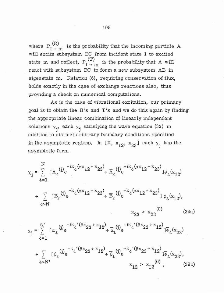
108

where PI (~)m is the probability that the incoming particle A

will excite subsystem BC from incident state I to excited

state m and reflect, P1(T) is the probability that A will -+ n1

react with subsystem BC to form a new subsystem AB in

eigenstate m. Relation (6), requiring conservation of flux,

holds exactly in the case of exchange reactions also, thus

providing a check on numerical computations.

As in the case of vibrational excitation, our primary

goal is to obtain the R 1 s and T 1 s and we do this again by finding

the appropriate linear combination of linearly independent

solutions x ., each x. satisfying the wave equation (33) in J ]

addition to distinct arbitrary boundary conditions specified

in the asymptotic regions. In [X, x12, x23

J each X· has the . J

asymptotic form

+ I -G>N

(0) x23 > x23 (39a)

(j) -ikt'(!3X23+X12), - (j) +ikt'(!3X23+X12)-:-[at e -rat e ] qit (x23)

109

where N and N' are the number of open channels for subsystems

BC and AB, respectively. The coefficients in the above expansions

A-t (j), A-l (j), etc. are found by tnincating the expansion, i:..t..ki.ng

inner products with the bound-state eigenfunctions, and solving

the resultant set of simultaneous equations (see Appendix). The

total wavefunction for the reaction may now be written

l./J = \ c . (I) X. ' L J J

(40)

j

such that i.f; everywhere satisfies Eq. (33) and has the correct

asymptotic forms [Eqs. (36)]. As before, we must have

l cj (I) At (j) = 6r {, ' j

I c. (I) B (j) = 0 --' J {, j

l c. (I) a (j) = 0 ' J )..., j

l c/I) ~ -t (j) = 0 ' ,e, > N' '

j

where the superscript I denotes the particular incident state.

The physical interpretation of these equat ions is as follows :

Eq. (41a) corresponds to the requirement that we have a

(41a)

(41b)

(4lc)

(41d)

110

monoenergetic beam of particles A from the right, Eq. (41c) to

the fact that there are no particles C incident from the left;

Eqs. (4lb) and (4ld) eliminate the rising virh1al components in

reo-ions x > x (O) and x > x (O) respectively Truncatino-:::. 23 • 23 12 12 ' . ::::>

the expansions in t and j, we may obtain a finite system of

simultaneous linear equations expressed in matrix form as

A c = I' ,,-....,,J r-..J ~ '

(42)

where A is the (IvI + M') x (M + M') matrix of coefficients A (j),

etc. , c is the (M + M') x N matrix of c. (I), and I' is a (M +~' )xN ~ J ~

matrix consisting of the N x N unit matrix occupying the first N

rows and a (M + M' - N) null matrix the rest. M is the total

number of BC channels and M' the total number of AB channels

retained in the truncated state expansion (39). The amplitudes

R and T are determined from 111 lll

where - (j) a.t

A- -- A- A-l I' 'T - c (43) ~ ~ ~

A is the (N + N') x (M + M ')

c is the matrix of . c . (I) ]

matrix of coefficients At (j),

determined from ( 42), and

T is the NN' x N matrix, the first N rows of which are the R 111'

the next N' the T . in The x. may be determined most easily by the finite­

J difference method in the coordinate system [X, x12, x23J.

Making the substitutions20

111

(44a)

2 ( a x2) = 12 (x. 1 . - 2x . . + x. 1 .) + O(h2)

oX12 . . h l+ ' J 1, J 1- ' J 1, J

(44b)

2 ( 0 x )

..._ 2 oX23 . .

1, ]

1 2 = - 2 (x. . 1 - 2x. . + x . . 1) + o (h ) ,

, 1, J+ i, ] 1, J-n (44c)

we obtain for the discretized Schrtidinger equation (Eq. (33))

1 1 - -µ (xi 3·-1 +xi 3·+1) - -µ Cxi-1 3· + xi+l J.)

12 ' ' 23 ' '

1 . 1 -2 { } 2 + 2 [ - + - + 1i ( v123 - E )h Jx. . = o, µ12 µ23 i, j r l, 3

(45)

where the indices i and j denote the point of the mesh as shown

in Fig. X. Again the subscript j of x., denoting a particular )

member of the linearly independent set, has been dropped. We

note that even though the Hamiltonian contains a mixed partial

derivative in the kinetic term, this is not difficult to incorporate

in the FD equations and does not ruin the symmetry or "bandedness"

of the FD matrix, although the bandwidth increases. Furthermore,

112

the boundary conditions are separable and it is easy to construct

a uniform mesh, as we have seen in Fig. X.

It is possible to make arguments about uniqueness and

convergence analogous to those given above in section C. We

shall not review those here.

F. Application of the Theory to Exchange Reactions

V.l e consider in this section two models for the exchange

reaction involving three equivalent particles. Though the

particles are equivalent, they are not indistinguishable since

they cannot penetrate one another. We solve for the X · in J

[X, x12, x23 J. Since V 123 is symmetric about x12 = x23 , it

is necessary to solve for only half as many x. 's as usual. - J

Suppose we include M cha1mels in the truncated state expansion.

Then, according to the development in section E, we need 2M

linearly independent X· 's. We find M of these using the following

set of boundary conditions: xj(x12, x23 (O)) = ¢j(x12), x/x23 ,

x12

(O)) ::: 0, j = 1, 2, · · · M. For the remaining M we simply

th " d" t f d •t• . ( ' (O)) - 0 ( ' use e reverse se o con i 10ns. X· x12, x23 = , X. x23, (0) J J

x12 ) = ¢j' j = 1, 2, · · • M. But the xj 's corresponding to the

reversed conditions are identical to the first M x. 's reflected . J

through the line x12 - x 23 = O. Hence, it is necessary to

determine only M: X· 's, i.e., to solve the FD equations only M . ] times. We have done this for several model potential surfaces.

113

1. Infinite Square-\Vell Potential Surface

V./ e consider first the simplest possible potential

surface, i.e., V 123 :: 0 inside the L- shaped reaction path and

V 123

= O:l outside. Thus, each subsystem is bound by an infinite

square well potential. Making the substitutions

a I

x12 ::: - x12 TI

a f

X23 = - x23 TI

in Eq. (32) and then multiplying both members by (ti 2

TI2/µ12a

2r 1, we obtain

where

E' =

The spectra of the two subsystems are discrete, the eigen­

functions and eigenvalues being given by

e:i~ = n2 /2 , respectively.

114

Energy conservation requires, as usual,

2 k a n 2

22 TT

where

k is the free-particle wavenumber. Since the particles are n

identical, we have m 2/ µ12 = 2, µ 12/ µ12, 3 = 3/ 4. Transition

probabilities have been determined for E 1 = 2. 125 (two open

channels), a= TT, x12

(O) = x23

(O) =TT. It was necessary to retain

only two virtuals in the state expansion and five for the analysis

of x. (see Appendix). Probabilities as a function of mesh size J

are given in Table V along with extrapolated values obtained

using Eq. (22). Since probabilities for only four different mesh

sizes were obtained, an accurate e1

m extrapolation was not

possible.

From Table V we observe that sum and time-reversal

checks are good not only for individual mesh values but also for

the extrapolated values~ For examples, y1 (~)2 and P 2 (~\ differ by less than 2%, or . 0006, and Pi

12 2 and P~T~ 1 by

less than 3% (. 0028).

2. Truncated Parabolic Potential Surface

A more realistic potential surface is described by

the expressions

1 2 V 123 = 2 x. (r 12 - r 120)

115

r 12' r23 < O (47b)

1 2 V 123 = 2 ]{.(r23 - r230)

. (0) r 12 > r 12 ' 0 .$; r 23 S a

(0) r12>rl2 .r23<0, r23>a, (47c)

where r 120 = r 230 , the equilibrium separation of the two atoms

of the equivalent subsystems. The potential surface described

by Eqs. (47) is sketched in Fig. XI. In the asymptotic regions

the potential is a truncated parabola. In the interaction region,

it is generated by rotating a parabola centered at r 120 about an

axis at (r12 = 2r120, r 23 = 2r230) perpendicular to the r 12 - r 23 plane. With the substitutions

(48a)

(48b)

the Schrodinger equation (32) becomes

{-4

where

o2 1 ---,,,.+-

:;,. r 1 2 2y uX23

116

r _ 2 2 2 -1 V 123 - ( h TT / µ12a ) V 123

1 _ 2 2 2 -1

E - (ti TT /µ12a ) Er '

(49)

and a is the well width, i. e. , truncation point. The eigenvalues

and eigenfunctions of the truncated parabolic binding potential

are determined using the Ritz linear variational method,

expressing the trial wavefunction as a linear combination

of particle-in- box eigenstates as

11 max

¢1/x12) = J2far l ckn sin n xl2' . 11=1

Energy conservation requires, as usual,

(E ) + e: = E' K. E. n n '

(50)

(51)

where e: is the approximate eigenvalue associated with the nth 11

eigenstate and (EK. E. )n is the corresponding energy of the free

117

particle, either A or C. Since we are dealing with identical

particles, the mass ratios are fixed as follows: µ 12 :;::; 1/2;

y :;::; 1. Reaction probabilities are given in Table VI for other

system parameters arbitrarily fixed as follows= rt:;::; 10. O;

a :;::; n ; E ' :;::; 5. 00; n :;::; 10. For this particular energy there r in ax

are two open channels; it was found sufficient to retain three

virtuals in the asymptotic state expansions. The probabilities

were calculated by analyzing the xj with values of x121 or x23 '

as far apart as possible in the asymptotic regions (see Appendix).

As we can see from Table VI, the values seem to converge in a

reasonable fashion, with sum and time-reversal checks improving

as the mesh size dec1·eases. Probabilities obtained by doing the

xj analyzes at x121 (x

23 ') values closer together differ little

( < 1 %) from the values of Table VI. Also, including more

functions in the variational trial function Eq. (50), i.e., taking

n > 10, induces an insig11ificant change in the probabilities. max

3. U ntruncated Parabolic Surface

Certainly a more realistic potential surface is that

described by Eqs. · (47) without the truncation. In this case the

binding potentials become ''pure'' parabolic in the asymptotic

regions. In order to determine the x. we take the interaction J

region to be large enough that x. are negligibly small outside J

the L- shaped reaction path, requiring that xj :: 0 outside this

region (except, of course, in the asymptotic regions). :W.!aking

the substitutions

118

. the Schrtld:inger equation (32) becomes

where

E' = E / t1 w r

The eigenfunctions and eigenvalues of the bound states of the

subsystem are given, with minor modifications, by Eqs. (31).

Energy conservation may be expressed by

(EK. E.) + (n + 1/2) = E' 11

(53)

119

where, as usual, (E1r E ) is the kinetic energy of the free )... . n particle, A or C. As before, since we are dealing with identical

particles, the mass ratios are fixed as follows: µ 12 == 1/2, y ::: 1.

When we attempted to treat the reaction using the parameters

a == 10. 0, E' == 1. 75 (two open channels), difficulties were

encountered. The problem is summarized in Table VII, which

lists probabilities obtained using a mesh size of • 4165 (23 points

across the well) and two virtual states. For this mesh size

there are four pairs of values of ~ (or ~' ) for which the

analysis of x . may be carried out. Probabilities obtained using . J

these various possible pairs are listed in the columns of Table

VII. The first column corresponds to the ~ , values farthest

apart, the second column to ~ values next closest, etc.

Clearly the various sets of probabilities disagree markedly.

Column 2 seems to best satisfy sum and time reversal checks,

although there is no obvious reason. We attribute this ":instability"

to the fact that the mesh is too coarse. For example, the finest

mesh size attainable ·for a == 10. 0 is h == • 325 compared with

h == • 157 for the coarsest mesh used in the treatment of the

trw1cated parabolic surface. One might reasonably expect an

improvement using finer meshes. Addition of more virtuals in

either the state expansion or x. analysis did not alter the columns J

of Table VII appreciably. Although there is no really sound reason

to favor column 2, we would expect columns 3 and 4 to be more in

error since the analysis matrix (see Appendix) may be i.11-

conditioned for ~ values too near one another.

120

G. Discussion

We have presented a quite general method for the quantum

mechanical. treatment of the inelastic collision of composite

particles. The essential feature of the method consists of forming

the complete stationary wavefunction describing the collision by

taking a linear combination of members of a set of linearly inde­

pendent functions, each member of the set satisfying the relevant

Schrt>dinger equation in addition to an arbitrary boundary condition

specified in the asymptotic region. vVe have shown that the

functions of the linearly independent set may be found using the

finite-difference method; that the finite-difference equations may

be quickly and accurately solved by the McCormick subroutine.

Two examples of one-dimensional impulsive collisions

have been treated and in one case, the free-particle-harmonic­

oscillator collision, the results agree well with previously

published results.

By a simple extension of the theory we have been able

to treat an important special class of chemical reactions -

exchange reactions. We have obtained very reasonable results

for the reaction probabilities on several model potential surfaces

for constrained linear electronically adiabatic encounters. As

far as we know, this is the first direct quantum mechanical

treatment of exchange reactions. The crucial feature of our

method is that it avoids the difficulty of the usual state expansion

.,.-,l

j

¢. f. ' J J

(54)

121

where ¢ . are eigenfunctions of the initially bound pair BC and J

f. are arbitrary functions of the coordinate of the incoming J

particle A relative to the center of mass of the bound pair. The

difficulty is that the ¢ . do not form a complete set over the whole J

reaction space and hence tfJ caru10t be everywhere expressed as

in Eq. (54). In our method it is not necessary to expand the

fw1ctions x. in any particular set, except in either asymptotic J

region where expansions (39) are valid.

The success -of our method in the treatment of impulsive

collisions indicates that it should be generally useful, although

there are several diffic-µlties. For long-range interaction

potentials the FD equations must be solved over a large inter­

action region. For vibrational excitations, this may pose no

problem, since, as we found for the free-particle-harmonic­

oscillator collision, it may be possible to obtain convergence of

transition probabilities using relatively crude meshes. However,

from our results on the parabolic potential surface, it is clear

that large interaction regions may lead to a type of "instability"

or, at least, inconsistency in the treatment of exchange reactions.

It may be possible to circumvent this difficulty by using a small

interaction region, specifying the boundary condition in the "near

asymptotic" region and then extending the solution into the

asymptotic region by the WKB method (assuming the potential

is essentially separable in the "near asymptotic" region).

A possibly · very useful application of our method would

be an investigation of a parametrized potential surface to determine

which regions most influence reaction probabilities for a given

incident total energy. Such a parametrized surface has been

122

studied classically by Wall and Porter. 21 It would be interesting

to compare our results with quantum mechanical approximations

and with the classical results. This should give us an idea of the

importance of quantum effects and conditions under which these

other approximations are reliable.

It does not appear to be practical to apply our method

directly to three-dimensional problems, since the number of FD

equations increases as (a/h - l)n, where a is the range of each

variable, h is the mesh size, and n is the number of variables.

Thus, for a three-dimensional two-particle problem, one would

be required to solve 106 simultaneous equations for a ::; 10. 0

and h ::; 10/11, a very crude mesh. This is a formidable task

even if the FD matrix is banded. However, it may be possible

to solve the problem indirectly by using a state expansion of the

form of Eq. (54). For instance, suppose we are interested in

the collision of two diatomic molecules. Following Takayanagi's1

formal treatment, we expand the total scattering wavefunction 'l'

as

'l' = I f(j, \)'A I~' R)R-l s(j, v, A J8, ¢, rl, 81' ¢1' xl' r2, 82, ¢2, x2)

jvt.. (55)

where R is the distance between centers-of-mass of the molecules,

s are vibrational- rotational functions for the free molecules,

characterized by quantum numbers j, v, and t... We obtain an

infinite set of coupled equations for the f's by making use of the

orthonormality of the various factors in 'l'. These equations may

be expressed as

123

t1 2

{ a2

j(j + 1) 2} . I 2M - 2 - 2 + 1\ f(J, v, A. 1)_, R) =

dR R

J., v' A.' ' '

V., ., ,, , f(j',v',A. 1 /k.. "R). JV11.J V 11. A.

(56)

Our approach to the solution of this set of coupled equations

would be as follows. Having truncated the expansion in j ', v',

and A.', we would solve the FD equations to obtain sets of f's

corresponding to independent boundary conditions specified in

the asymptotic region. Then we would take an appropriate

linear combination of these sets to satisfy the asymptotic

condition on the total wavefunction '±'. Unfortunately, the FD

matrix is symmetric but unbanded. However, the total number

of FD equations should be given by the product of the number of

states retained in Eq. (56) by the number of mesh points, there

being only one variable R. If one can tolerate a paucity of both

mesh points and expansion states, it may be relatively easy to

solve the coupled FD equations.

124

H. Appendix

If we multiply Eq. (7a) by ¢ 1 * and integrate with respect , (

to y from - 00 to 00 , we obtain (for k .=:;; N)

(Al)

A similar equation involving the virtual coefficients B (j) and B (j) k k may be obtained if k > N. Choosing two different values of x, say

· x1

and x2, in the asymptotic region (x > x0

) gives us two .

simultaneous linear equations from which to determine A1

(J) and

~ (j). We have, dropping the subscript k and superscrip~ j,

(A2a)

(A2b)

where the integrals f are evaluated using the eA.'i:ended Simpson's

rule as discussed in section C. Eqs. (A2) can be solved trivially

using Cramer's rule:

+ib::2 +ib::1 -ik(x1-x2) +ik(x1-x2)

A= (f(x1)e - f(x2)e )/(e - e )

(A3a)

125

Clearly from Eqs. (A3),

A* = A. (A4)

Repeated evaluations of A and A using different pairs of values

of x agree to 1 or 2% (depending on the mesh size) for the cases

of vibrational excitation treated in section D.

We now consider the more complicated analysis of the

x. for the case of exchange reactions. Upon multiplying E q. J

(36a) by ¢k * and integrating with respect to x12 over all space,

we arrive at the following equation

N

l [~.e, (x23)At (j) + 1k.i*(x23)A-e, (j)] + I CH}z;:.e, (x23)Bt (j)

.i=l -t>N

( ) - (j) - (j)( ) + Gkt x2 3 B -t ] - gk x 2 3 , k = 1, 2, 3, ••. , (A5)

where

(A6a)

' (A6b)

(A6c)

126

and

co

gk <n <x23) = I ¢1/ <x12) x/x12' x23) dx12 • (A6d)

We note that Eq. (A5) is, in fact, a set of simultaneous equations

involving all the unknown coefficients. We solve this set of

equations by trwicating the expansions in .f- and k and then adding

successively more terms until convergence of the coefficients is

achieved. If we retain n terms in the .f- expansion, then we have

n equations (obtained by taking inner products with ¢k' k = 1, 2,

· .• .. n) in 2n unknown, there being an "unbarred" and "barred"

unknown for each of the n terms. Hence, we secure two equations

per k by choosing two different values of x23 , as we did above.

A similar analysis of x j for the cx,.f- (j), etc. , may be carried out.

For the model exchange reactions discussed in section D

we have found it necessary to take n equal to 5 or 6 (using a

computer subroutine CSLECD which solves systems of equations

with complex coefficients) for a four- channel (two open, two virtual)

state expansion of Xj. Analyses using different pairs of x23

(or

x12 ) values vary considerably depending on mesh size, as the

examples treated in section F demonstrate.

127

REFERENCES

1. K. Takayanagi, Progr. Theoret. Phys., Suppl. 25, 1

(1963).

2. L. Landau and E. Teller, Physik Z. Sowjetunion, 10,

34 (1936).

3. J. Kelley and M. Wolfsberg, J. Chem. Phys., 44, 324

(1966).

4. D. Rapp and T. Sharp, J. Chem. Phys., 38, 2641 (1963).

5. C. Zener, Phys. Rev., 37, 556 (1931).

6. J. Jackson and N. Mott, Proc. Cambridge Phil. Soc.,

29, 136 (1936).

7. K. Shuler and R. Zwanzig, J. Chem. Phys., 33, 1778

(1960)~

8. . B. Johnson and D. Secrest, J. Math. Phys. J_, 2187

(1966).

9. D. Secrest and B. Johnson, J. Chem. Phys. 45, 1515

(1966).

10. R. DeVogelaire and M. Boudart, J. Chem. Phys., 23,

1236 (1955).

11. F. Wall, L. Hiller and J. Mazur, J. Chem. Phys., 29,

255 (1958).

12. J. Mazur and R. Rubin, J. Chem. Phys., ..9_!, 1395 (1959).

13. E. Mortensen and K. Pitzer, "Transition State", Chem.

Soc. Special Publication No. 16, p. 57.

128

14. 'S. Sato, J. Chem. Phys. , 23, 592, 2465 (1955).

15. P. Morse and H. Feshbach, "Methods of Theoretical

Physics", (McGraw-Hill Book Co., Inc., New York,

1953), Vol. I, p. 698.

16. Let {¢/Er)} be the set of exact solutions of the

SchrUdinger equation corresponding to linearly inde­

pendent boundary conditions (labeled by index i) specified

in the asymptotic region. Then this set {¢i(Er)} is

complete in the sense that any "well- behaved" function,

e.g., s1, may be expanded as a linear combination of {

the ¢.(E ). . . i r

17. D. Shanks, Journal of Math. and Phys., 34, 1 (1955).

18. C. McCormick and K. Hebert, "Solution of Linear

Equations with Digital Computers", (California Institute

of Technology, 1965).

19. M. Abramowitz and I. Stegun, "Handbook of Mathematical

Functions" (NBS Appl. Math. Ser. 55, 1964), p. 886.

20. Ibid, p. 884.

21. F. Wall and R. Porter, J. Chem. Phys., 36, 3256 (1962);

39, 3112 (1963).

129

TABLE I

Transition Probabilities as a Function of Mesh Size for Impulsive

Collision of Free Particle with Particle Bound in Infinite Square

Well (E' = 2. 25; Number of Virtuals = l; a= n; mA/mB = 1)

Mesh size pl-+ 1 pl-+ 2 p 1-+l + p 1-+2

. 1745 • 5468 • 4463 • 9931

. 1571 • 5498 • 4446 . 9944

. 1428 • 5521 • 4433 . • 9954

• 1309 • 5538 • 4423 • 9961

• 1208 • 5552 • 4415 • 9967

Extrapolated • 5606 • 4387 • 9993 value

p2-+ 1 p2-+ 2 p 2-+l + p 2-+2

• 1745 • 4602 • 5468 1. 0070

• 1571 • 4557 . 5499 1. 0056

• 1428 • 4524 • 5522 1. 0046

• 1309 • 4500 • 5539 1. 0039

• 1208 • 4480 • 5552 1. 0032

Extrapolated • 4399 • 5607 1. 0007 value

130

TABLE II

Transition Probabilities as a Function of Mesh Size for Impulsive

Collision of a Free Particle with a Particle Bound in an Infinite

Square Well (E' ::: 4. 75; Number of Virtuals ::: l; a::: rr; m A/mB:::l)

Mesh

I size Pl ... 1 Pl_, 2 Pl ... 3 p

1 ->i

• 1745 • 6126 • 1281 • 2470 . 9877 • 1571 • 6121 • 1304 • 2475 . 9900 • 1428 .6115 . 1325 • 2477 . 9917 • 1309 • 6108 • 1345 . 2477 • 9930 • 1208 • 6103 • 1362 • 2477 • 9942

Extrapolated .6072 • 1466 • 2477 1. 0015 value

l p 2->i P2 ... 1 P2 .... 2 P2 ... 3

• 1745 • 1321 • 6069 . 2564 • 9954 • 1571 • 1337 • 6050 . 2576 . 9963 . 1428 . 1353 • 6034 • 2583 . 9970 . 1309 . 1368 • 6019 • 2587 • 9974 • 1208 • 1382 • 6008 • 2588 • 9978

Extrapolated • 1473 • 5965 • 2588 1. 0026 value

l p 3->i P3_, 1 P3 .... 2 p3 _, 3

• 1745 • 2681 • 2698 • 4796 1. 0175 • 1571 • 2645 • 2684 ·• 4812 1. 0141 • 1428 • 2617 • 2673 . 4827 1. 0117 • 1309 • 2594 • 2662 . 4841 1. 0097 • 1208 . 2575 • 2652 • 4855 1. 0082

Extrapolated • 2461 • 2529 • 5010a 1. 0000 value

a.This value is obtained by difference from P 3... , P 3_,2, since extrapolation on such rapidly varying values gave faulty results.

131

TABLE III

Extrapolated Trahsition Probabilities for Hard-Sphere-Harmonic

Oscillator Collision (E = 1. 75; Number of Virtuals = 2; a= 10. O;

m/M = 1/2)

Final State

Incident State

1

2

1

• 4941

.5084

TABLE IV

2

• 5044

• 4941

Extrapolated Transition Probabilities for Hard-Sphere-Harmonic

Oscillator Collision (E = 2. 75; Number of Virtuals = 2; a= 10. O;

m/M = 1/2)

Final State 1 2 3

Incident State

1 • 0014 . 5903 • 3981

2 • 5.988 • 1595 • 2414

3 • 4059 • 2480 • 3506

132

TABLE V

Reaction Probabilities as a Fw1ction of Mesh Size for Square-Well

Binding Potentials (a = rr; E' = 2. 125; Number of Virtual Channels

= 2)

p(R) p(R) (T) p(T) 2

Mesh I pl . size

1-+ 1 1-+ 2 pl-+1 1-+ 2 -+1 T,R,i=l

• 1571 • 7673 • 0249 . 1178 • 0859 • 9959

• 1308 • 7590 • 0267 • 1208 • 0911 • 9976

• 1122 • 7539 • 0279 • 1225 • 0943 • 9986

• 0982 • 7509 • 0286 • 1237 • 0965 • 9997

Extrapolated . 7404 • 0306 .1264 • 1042 1. 0016 value

p(R) p(R) p(T) p(T) 2

I p2 . 2-+ 1 2-+ 2 2-+ 1 2--+ 2 -+1 T,R,i=l

• 1571 • 0251 • 4398 • 0942 • 4453 1. 0054

• 1308 • 0268 • 4429 • 0960 • 4369 1. 0026

• 1122 • 0278 • 4451 • 0971 • 4314 1. 0014

• 0982 • 0284 • 4466 • 0978 • 4277 1. 0005

Extrapolated .• 0300 • 4562 .1014 • 4116 • 9992 value

133

TABLE VI

Reaction Probabilities as a Function of Mesh Size for Truncated

Parabolic Surface (x. = 10. 0; E' = 5. 0; a = rr; Number of Virtual

Channels = 3)

. Mesh p(R) p(R) p(T) p(T) I pl . size 1--1 1--2 1--1 1--2 --1

T,R,i

• 1571 • 0455 • 1134 • 6489 • 1774 • 9852

• 1308 • 0538 .1196 • 6327 • 1832 • 9893

• 1122 • 0595 • 1233 . 6224 • 1865 • 9917

• 0982 . 0635 • 1256 • 6156 • 1885 • 9932

Extrapolated • 0779 • 1326 • 5932 • 1939 • 9976 value

p(R) 2--1

p(R) 2--2

p(T) 2--1

p(T) 2-- 2 I P2 ... i

T,R,i

• 1571 • 1178 • 4271 • 2048 • 2673 1. 0170

• 1308 • 1230 • 4177 • 2022 • 2688 1. 0117

• 1122 • 1262 • 4118 • 2007 • 2701 1. 0088

.• 0982 • 1282 • 4079 • 1997 • 2712 1. 0070

Extrapolated • 1347 • 3958 • 1958 . 2753 1. 0016 value

134

TABLE VII

Transition Probabilities for the Untruncated Parabolic Surface

(a= 10. O; E ' = 1. 75; h = • 4165; Number of Virtual Channels r = 2). The Columns Correspond to Various Analyses of X· as . J

Discussed in Text

Transition 1 2 3 4 Probability

p(R) 1 -+ 1 • 000667 • 000611 • 000915 . 00103

p(R) 1-+ 2 • 003135 • 002430 • 001429 • 00840

p(T) 1 -t 1 • 724909 • 712349 • 698335 . 68557

p(T) 1 -t 2 • 256870 • 283050 • 314947 . 34546

· l pl--i • 995581 • 998440 1. 015626 1. 04146

R,T,i

p(R) 2 -t 1 • 000306 . 001567 • 002316 • 00268

p(R) 2 -t 2 • 005751 • 005947 • 004405 • 00277

p(T) 2--> 1 . 292969 • 287198 • 283838 • 28214

p(T) 2 -t 2 • 719046 • 707013 • 694846 •. 68384

~

l p2 . -t l

1. 018072 1. 001725 • 985405 • 97143

R,T,i

135

Figure I

Diagram of the colinear collision of an atom (m3) with a

diatomic molecule (m1 - m 2) showing relation between ·

coordinate systems.

136

137

Figure II

(a) Diagram of a collision of a free particle with a particle

bound to a fixed center of force. (b) Schematic showing

boW1dary conditions and interaction (inseparable) region

for collision diagrammed in (a).

138a

x_

. (x-y)

(a)

138b

y

(O, a) .:' : 1 '' ' '·! '' ·

( 0 ' 0) : ,: ' ~ : ': : . ;:".:·:· ': . . ' ·· . .

(b)

; , >'.· r · ,

·' .. ·~·· ·.-·· · . .. , .

~ ....

Asymptotic region

(x , 0) 0

x

139

Figure ill

Finite-difference mesh used in the solution of the atom­

diatomic collision problem.

t y

(x~, a) (O, a) (x0 ,o)

0 0 • (' 0 0 0 0 0 0 0 0 f) 0 • 0 0 5 10 15 20 25 90 95 e 0 0 Q 0 0 0 0 0 0 0 0 0 0 0 0 4 9 14 19 24 29 94 .......

0 0 0 0 0 0 0 0 0 0 0 (t 0 H:>-0

3 8 13 18 23 28 93 0 6 0 0 0 0 e 0 0 0 0 0 0 0

2 7 12 17 22 27 92 0 0 0 0 0 0 Q 0

(x~,-o) (o, -a> (x~,-o) X->

141

Figure IV

Schematic of the coordinate system and boundary conditions

for the impulsive collision of a free particle with a particle

bound to a fixed equilibrium position.

(O,a)

y

(0,0)

142

(a,0) (2a,0) . x

"'= 0

143

Figure V

Transition probability v. s. number of mesh points across

the well (y' coordinate) for the impulsive collision of a

particle bound in an infinite square well with a free

particle (incident energy E' = 2. 25; number of virtuals

in state expansion (N - M) = 1; well width a = rr; mA/mB = 1).

>-I--_J .58 -CD <t .56 CD 0 0:: .54 Cl.

z .52 0 -I- 50 - . CJ)

z .48 <t

0:: f- .46

.44

.42

.40 7 9 11 13 15 17 19 21 23 25

NUMBER OF POINTS ACROSS THE WELL, a/h-1

~ ~ ~

145

Figure VI

Transition probability v. s. total incident energy for the

impulsive harmonic- oscillator-free- particle collision.

D Po-o} VALUES OBTAINED IN THIS WORK (h=.3125; a=IO;

O Po-1 NUMBER OF VIRTUALS = 2)

>- 1.0 t II Po-o} VALUES OBTAINED o p BY SHULER AND

0-1 ZWANZIG (REFERENCE 7) t- 0.9 _J

co o.a <{ en 0 0.7 0: a.. 0.6

~ 0.51 ""'/ ..... if:>. m

t--~ 0.4 <t 0: 0.3 t-

0.2

0.1

0.0 1.60 1.70 1.80 1.90 2.00 2.10 2.20 2.30

TOTAL ENERGY IN OSCILLATOR UNITS, E1

147

Figure VII

Execution time v. s. number of mesh points across the well

for the computation of transition probabilities in the

impulsive harmonic-oscillator-free-particle collision.

6.0

c 5.0 -E -w ~ 4.0 -I-

~ 3.01 / ..... ~ CX>

:::> u w

/o ~ 2.ol . e E1= 2.75; NUMBER OF OPEN CHANNELS= 3; NU MBER OF VIRTUAL CHANNELS= 2

0 E1=1.75; NUMBER OF OPEN

1.0 I- / CH ANNELS=2; NU MBER OF VIRTUAL CHANNELS=2

17 19 21 23 25 27

NU MBER OF MESH POINTS ACROSS WE LL

149

Figure Vill

Diagram of exchange reaction A + BC -+ AB + C.

150

~--x--1~

151

Figure IX

Coordinate systems used in the treatment of exchange

reactions showing boundary conditions and the interaction

region: (a) [X, x12, x23]; (b) [X, x, x12].

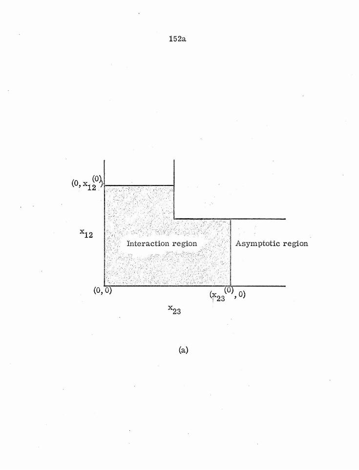
152a

(a)

Asymptotic region

. :•· , ..

0 (f 23 'O)

152b

(O, 0) x

(b)

= Q x + x (O) ~ 23 12

Asymptotic region

x

153

Figure X

Finite-difference mesh used in the treatment of exchange

reactions in the coordinate system [X, x12, x23 J.

154

9 0 0 0 0 0 9 18 27 36 45

8 0 0 ® 0 0 8 17 26 35 44

7 0 0 0 0 0 7 16 25 34 43

6 0 0 0 0 0 6 15 24 33 42

5 0 0 0 0 0 0 c 0 0 5 14 23 32 41 50 55 60 65

4 0 0 0 0 0 0 0 0 0 4 13 22 31 40 49 54 59 64

Xl2 3 0 0 0 0 0 0 0 0 0 3 12 21 30 39 48 53 58 63

2 0 0 c 0 0 0 0 0 0 2 11 20 29 38 47 52 57 62

I 0 0 0 0 0 0 0 0

t 10 19 28 37 46 51 56 61

j --1 2 3 4 5 6 7 8 9 X23

155

Figure XI

Sketch of trw1cated parabolic surface for model exchange

reaction.

156

157

Abstract of Propositions

I. An improved model for physical adsorption on metal surfaces is presented and discussed. It is proposed that · the model be tested by calculating heats of adsorption of nitrogen on three different copper crystal faces for which reliable experimental data are available.

II. An initial-value method of calculating quantum-mechanical transition probabilities for inelastic collisions is presented. A perturbation method for solving the coupled equations to various orders in a "cutoff" parameter is proposed. ·

ill. A semiclassical theory of radiationless transitions is proposed. The theory views the relaxation of an electronically excited solute molecule as a transition between zero- order nonstationary states induced by a time-dependent perturbation caused by solute- solvent Coulomb interactions. The translational motion of the molecules is treated classically and the internal degrees of freedom quantum mechanically. Two model studies designed to compare the effect of various parameters of the classical motion on the transition probability are proposed.

IV. A method for treating the collisional transfer of ener gy between vibrational and electr onic degrees of freedom is proposed. The central feature of the method,

.- Which remedies several defects of a previous treatment, is that it treats only the electronic motion of the vibrator adiabatically. This is believed to be a reasona ble approxi­mation since the vibrator is not undergoing a change of electronic state. It is proposed that the transition proba­bilities be found by the initial-value method outlined in Proposition IL

158

V. · · It is proposed that the relaxation (including r eaction) of an initial distribution of reactant molecules among various quantum levels be investigated. The transition rates W depend explicitly on concentration so that the mn relaxation equations are nonlinear. After outlining the general theory, we derive the relaxation equations for a displacement reaction and briefly discuss methods of solution.

159

Proposition I

An improved model for physical adsorption on metal surfaces is presented and discussed. It is proposed that the model be tested by calculating heats of adsorption of nitrogen on three different copper crystal faces for which reliable experimental data are available.

It seems apparent that not a great deal is understood about

forces between isolated pairs of atoms and molecules and even less

about the interaction of atoms and molecules with surfaces, wherein

the interaction among large collections of particles complicates the

problem. The particular case of physical adsorption on metal

·surfaces is of great interest. Gurney1 has discussed the theory of

electrical double layers in terms of one-dimensional systems of

potential wells representing the metal and adsorbate. Gomer and

Swanson2 have recently elaborated on this model in conjunction with

a theory of field desorption.

Lennard-Jones3

had earlier viewed the van der Waals

attraction of a molecule to a metal surface in terms of the inter­

action of instantaneous dipoles formed between the electrons and 4 . 5

their images in the metal. Bardeen and Margenau and Pollard

objecting that Lennard-Jones 1 model assumed instantaneous

relaxation of the metal electrons and that it neglected their quantum­

mechanical behavior, developed their respective models. Bardeen

presented a general method for the approximate calculation of

dispersion forces between two arbitrary systems. The method

of Margenau and Pollard regards the metal as composed of

160

polarizable volume elements and the total interaction of metal and

molecule is expressed as a sum of dipole-dipole induced inter­

actions over the volume of the metal.

All of the theories discussed above seem to suffer from

the disadvantage of not considering the internal structure of the

metal in detail, a factor which may be of considerable importance

in the process of physical adsorption. It is therefore proposed

that a new approach, which is based on an extant model for metals

and which also explicitly takes into account the structure of the

metal, be investigated. In the following paragraphs the general

model will be discussed and then a specific proposal made to test

the worth of the model.

As a zeroth-order approximation the Sommerfeld theory

of metals will be assumed, in which one valence electron from

each atom is in a non-localized state belonging to the metal as a

whole and the remaining electrons are localized. It is further

assumed that for the delocalized electrons the potential is zero

inside the metal and infinite outside. Thus, for a metal in the

shape of a cube of edge a, the wave function for the free- electron

gas is given by

n.nx. t.ny. m.nz. , 1, _A{ rr . i i . i 1 . i i} 'r'FE - 9 Sm -- SID Sln • n.'"'.m. a a a

(1) . 1 1 1

Hence, the metal appears as a lattice of positive ions in a uniformly

dense electron gas. This hp.plies that an electric field will exist

outside the metal which is non-uniform and depends on the structure

of the lattice.

161

Consider an arbitrary array of lattice points in the half­

space z > 0. For points z < - e: < 0, the electric field is given by

- - + - - ..-. N e( r - r ) - - J. p(r') (r - r') dv' l j E(r) = + , I- - ,3 ,- -+13 r-r' . 1 r-r.

J~ J

-where p is the electron density, r is the radius vector to the

field point, and r. + is the radius vector locating the ith lattice 1 .

point. Note that since p is constant the integral E- ( ~) will be

constant for a very large volume of metal. The ref ore the

variations in the surface electric field w~ll be determined only

by the positive lattice. For example, for a simple cubic lattice

(2a)

(2b)

3 of 8n atoms, the z-component of the electric field will be given

by

n f· ~ (z - ma) Ez +(r) = e l L l (3)

k=-n t =-n m=O { (x- ka)2 + (y - t a)2 + (z - ma)} 3/2 '

where a. is the lattice spacing. Hence, it is seen that the field

component perpendicular to the metal surface will vary as a

function of the coordinates (x, y, z) of the field point in a manner

that reflects the structure of the lattice. An atom or molecule

in the vicinity of the surface will thus be polarized and the resulting

dipole attracted toward the surface where it will reside in a region

162

of lower energy. The properties of the adsorbed species and of

the adsorption process may then be calculated using quantum and

statistical mechanics.

It is suggested that this theory be applied to a specific

case for which reasonably reliable experimental data are available.

Rhodin 6 has reported results for the adsorption of nitrogen on very

clean, regular copper crystal faces at coverages low enough that

lateral interactions among the adsorbed molecules are negligible.

He found that the heats of adsorption are -1800, -2000, -2200

cal/mole on the (100), (110), and (111) faces, respectively. As a

zeroth- order approxima~ion, the potential energy of a nitrogen

molecule near the metal surface can be expressed as

V FI( r) is given by

.... 1 .... .... 2 V FI( r) = - 2 a,' I E ( r) I '

and is the energy of interaction of the induced dipole with the

electric field, VD is the van der Waals attraction energy, and

(4)

(5)

V R is the repulsive interaction energy. V FI can be broken down

into the contribution of the lattice v;I and that of the electron

gas VFT The dispersion and repulsive interactions of the

molecule with the lattice may be approximated by the Lennard-

J ones 6-12 potential.

163

Other applications of this model to the problem of the

interactions of molecules with metal surfaces may be envisioned. 7

Also, there are several obvious (albeit perhaps difficultly

incorporable) improvements, among which are, for example ,

(1) the requirement that there be fewer than one delocalized

electron per 1'l18tal atom, (2) the employment of a periodic, lattice­

dependent potential, and (3) allowance for repulsion among the

free electrons. Each of these "improvements" will affect the

negative charge distribution in the metal and consequently the

negative component of the surface electric field.

References

1. R. W. Gurney, Phys. Rev., 47, 479 (1935).

2. R. Gomer and L. Swanson, J. Chem. Phys., 38, 1613

(1960).

3. J. Lennard-Jones, Trans. Faraday Soc., 28, 333 (1932).

4. J. Bardeen, Phys. Rev., 58, 727 (1934).

5. H. Margenau and W. Pollard, Phys. Rev., 60, 128 (1941).

6. T. Rhodin, Jr., J. Am. Chem. Soc., 72, 4343, 5691

(1950).

7. Dr. James King of the Jet Propulsion Laboratory, California

Institute of Technology, from discussions with whom inspir­

ation for this proposition was largely derived, has used a

model to explain the chromatographic separation of hydrogen

isotopes on an alumina column (see J. King, Jr. and S. Benson,

J. Chem. Phys. 41 1007 (1966} ) . .,..._,...

164

Proposition II

An initial-value method of calculating quanium­mechanical transition probabilities for inelastic collisions is presented. A perturbation method for solving the coupled equations to various orders in a "cutoff" parameter is proposed.

Reconsider the one-dimensional problem of the inelastic

collision of a free particle with a particle bound to a fixed equi­

librium position. Assume that the interaction potential V 1

is

slowly varying and that the interaction region is well localized (for

reasons which will become clear below). We wish to solve the

Schrl:Jdinger equation

H '±' = E '±' , (1)

where

tz 2 02 . 112 02 H = - 2-- --2 - 2- ~ + VB(y) + VI(x, y)' (2)

mA ox mB oy

and 'l' satisfies the asymptotic conditions

-il~x N +ik x 'l' = e . ¢I(y) + l Rme m ¢m (y) + O(e -A.x),

m=l

.N '±' = I x < o,

m=l

x > x ' 0 (3a)

(3b)

and

165

2 2 fl k

Ill = E: +

m 2mA (4)

where we have assumed that the interaction region extends from

x = 0 to x = x • The symbols in Eqs. (2) - (4) have the same 0

significance as in Part II, i.e., A labels free-particle parameters,

B labels bound-particle parameters, Rm is the amplitude for

reflection in channel m, T the amplitude for transmission in m . channel m, N is the number of open channels, e: is the mth

~~ m discrete eigenvalue of the bound particle, and k is the corre­

m sponding free-particle wavenumber.

The method of solution of the Schr(jdinger equation (1) is

essentially that described in Part II. There is one important

modification, however, and that involves the method of deter­

mination of the x. 's. 1 We express the total scattering wa vefunction J

'i' as a linear combination of functions of a set, each member of

the set satisfying linearly independent initial conditions in the

asymptotic region x < O. Denoting the members of this set by

x-, we have J

Now each X· is expressed as ]

C-X· • J J

(5)

166

f. (j) (x) ¢ . (y) ' l l

(6)

whe1•e the ¢. are the bound- state eigenfunctions and f. (j) (x) are 1 1

arbitrary fw1ctions of x to be determined. The x. are found by ]

solving the initial-value problem created by specifying the values

and slopes of the f. (j) corresponding to arbitrary initial conditions l

on X·· Now since each X· must satisfy the Schrl1dinger equation ] ]

(1), we substitute Eq. (6) into Eq. (1) and take the inner product

of both sides with ¢ t to obtain

up .(x) f. (j)(x) = 0, t = 1, 2, ..• M (7) '\/l l

where

= 2mA r·ai 7

We find the f. (j) by solving the set of coupled equations (7), which 1 "k -1 ~ .x

we note has been truncated. If x .(x < 0, y) ·=- e J ¢.(y), then we J J

167

have the following initial conditions on f. (j): 1

f.(j)(O) = 0 . . 1 lJ

f_(j)(O) = ~ik . 0 .. , j ~ N 1 J lJ

or f. (j) (0) = 0 . .

1 lJ

f_(j)(O) = k. 0 .. ' j > N. 1 J lJ

Inside the interaction region the various channels "couple" so

that in the asymptotic region x > x , X· is expressible as 0 J

(j) -il\X _ (j) +ikiX (A. e + A. e ) ¢. (y)

1 1 1

( .) -1\X _ (j) +kiX) .( ) + \ (B. J e + B. e ¢1 Y ' L i i

i>N

where the coefficients A. (j), A. (j), B. (j), B. (j) are determined . 1 1 1 1

by requiring continuity of x. and grad x. at x = x0

• Thus for J J

i _::s N

(8a)

(8b)

(9a)

(9b)

(10)

(lla)

168

( .) -ik .x (j) +ik.x = "k A J l 0 "k A l 0

-1 i i e + l i i e '

from which the A. (j) and A. (j) can be determined. Similar l l

equations may be written for the virtual-channel coefficients.

Since we choose only outgoing waves in the open channels and

decaying virtual channels for our initial conditions, we need

solve for only M (the total number of states retained in the

state expansion of each x .) x. 1 s. The equations determining J J

c. in Eq. (5) are ]

M

I c . (I) A. (j) = 6Ii ] l j < N

j=l

M

I c. (I) B. (j) :::; 0, ] l

j > N

j=l

These may be written more compactly as

where I denotes the incident state.

T (I) are given by m

M

I I

,...., '

The amplitudes R (I) and lU

R (I) = \ c . (I) A (j) L J m m j=l

(llb)

(12a)

(12b)

(13)

(14a)

T (I) = m

169

c m

(I) (14b)

It now remains to solve the coupled set Eq. (7). If u -li (x)

is a smooth, slowly varying function and the interaction region is

not too large, i. e. , the interaction is of the nature of a perturbation,

we may be able to obtain a rapidly convergent power series

representation of fi (j) in the interaction region. We expand ft (j)

and u -li in a Taylor Is series about x = 0 as follows

f (j) -l

co

= l n=O

a (j) (-l) x11

n

d (-t, i) xn . n

Substituting these expansions into Eq. (7), we obtain

OJ

l { (n + 2)(n + 1) a~j~ 2 (-l) ± yk-l 2 an (j) (t)} xn

n=O

(15a)

(15b)

. M OJ OJ

- l ( l an(j\i)xn)( l dm(t ,i)xm) = 0, j = 1,2, •.. M, (16)

i= 1 n=O m=O

170

where the + holds for t .:s N and the - for t > N. Equating

coefficients of equal powers of x gives

m M

(m+2)(m+l) a (j) (-l) ± yk 2a (j) (t) - \ m+2 t m L { \ a. (j) d (t i)} = 0 •

L K m-k ' i=l k=O (17)

The initial conditions (8) and (9) determine a0

(j) (-i) and a1

(j) (t).

Thus

a (j) (t) = 0 tj 0

al O\t) = -ikt ot j, j < N

or a (j) (t) = 0 ,f, j 0

a (j) (-e,) 1 = kt 0 tj ' j > N .

From Eqs. (18) and (19) we can use the recursion relation (17)

to find all the coefficients a (j) (t) successively. m

(18a)

(18b)

(19a)

(19b)

Now we treat x as a parameter to obtain a "perturbation" 0

expansion for the c.'s and transition probabilities. To see how this J

is possible, we solve Eqs. (11) to obtain

171

A (j) -.e..

[ik f (j) (x ) - f ,(j) (x )] +ik9

x0 t .e.. 0 -e, 0 'V

~~~---,,~~~~~- e 2ik-e,

Substituting the expansions

f (j\x ) - f a (j) (t ) x 11

t o . L n o

f ,(j) (x ) t 0

into Eq. (20) gives

Similarly, we obtain

n-0

• c:::>

= I n-0

n=O

q=O

(n + l)a (j) (t)x 11

n+l o

[ ik a (j) (t ) - (q + 1) a (j)~ (.e..) J t q q+l

(ik9

)11-q

-v ·} n --.(-n--q)-c--=-! x o •

(20)

(21a)

172

co 11

B (j) (x ) = - 1- \ { .\ [k a (j) (-i) + (q + l)a (j) (t ) J • t o 2k-e, L L t q ·q + 1

n=O q:==O

(2lb)

co n B (j)(x ) = - 1 \ { \ [k a (j)(t) - (q+ l)a (j) (t)J .

t o 2kt L L t q q+ 1 n=O q=O

( )n-q +kt n

(n-q) ! } XO ' (21c)

and

co n A (j)(x ) = --J:- \ { \ [ik a (j)(-e,) + (q+ l)a (j) (t)J ·

-e, o 21k-e, L L -i q q + 1 n=O q=O

(-ik )n-q t } n

(n-q) ! XO • (2ld)

Thus, we have the matrix elements of .f:: expressed as explicit

functions of the "cutoff" parameter x . The matrix equation (13)

for the c (I) may now be expressed as0

(A + A x + A x 2 . · · )(c (I) + c (I) x + c(I)x 2 •.• ) = I' (22) ""0 "" 1 0 ""2 0 ""0 ""1 0 "" 2 0 ""

173

The various "orders" of c (I) may be determined by identifying

coefficients of equal powers of the "cutoff" parameter. Hence,

we obtain the matrix equations

A c (I) =I I ""'0 ""'0 ""'

n1

\ A. c . (I) = 0 • L ""'J ""'m- J

j=O

We note from the expansions (21) that

A (j) = -.1- [ik a (j)(t) - a (j)(t)J = o . -lo 21k-e.. t o 1 tJ

B (j) = - 1- [k a (j)(t) +a (j\t)] = o . t 0 2k t t 0 1 l J '

(23a)

(23b)

and thus A is the M x M unit matrix. From Eqs. (23) we then ""'O

obtain

c (I) = I I

"-'O (24a)

C (I) = - A c (I) -·1 1 ·- ""' ,....,0

(24b)

(24c)

174

Expressing Eqs. (14) as a matrix equation, we can obtain the

reflection and transmission amplitudes to various orders as

follows:

(A + Al x + A2x 2 + ... ) ( c (I) + c 1 (I) x + c.2 (I) x 2 + ••• ) = '"'"'0 '"'"' 0 '"'"' 0 '"'"'0 '"'"' 0 ~ 0

R (I) + R (I)x + R (I)x 2 + · · · (25a) ~o ~1 o ""'2 o

T(I) = c (I) + c (I)x + c (I)x 2 + · · • • (25b) "-'O ~1 0 ~2 0

In particular, if x0

= 0, i.e., there is no interaction, we observe

that

- (I) A c ""'O "-'O

= R (I) = 0 ~o

T(I) = c (I) ""'O

which means that there is only a wave of unit amplitude

transmitted in channel I and nothing reflected. Evidently,

our formalism is correct in the limit x0

== O. The hopa is

·that we may obtain reasonably accurate approximations to the

amplitudes for weak interactions VI by including only a few

powers of x0

in the expansions (24) and (25). The method has

two possible advantages over the distorted wave method. The

first is that it is possible to obtain analytic expressions for the

(26a)

(26b)

175

amplitudes for arbitra r y potentials. Second, each order of

correction couples all the cha.ilnels, both open and virtual,

included in the state expansion for '±'.

References

1. This initial-value method has been independently

developed by Barnes et al., (see L. Barnes, N. Lane,

and C. Lin, Phys. Rev., 137, 388 (1965)) and by

Merle Riley at California. Institute of Technology.

176

Proposition ID

A semiclassical theory of radiationless transitions is proposed. The theory views the relaxation of an electronically excited solute molecule as a transition between zero-order nonstationary states induced by a time-dependent perturbation caused by solute-solvent Coulomb interactions. The translational motion of the molecules is treated classically and the internal degrees of freedom quantum mechanically. Two model siudies designed to compare the effect of various parameters of the classical motion on the transition probability are proposed.

Several theories of radiationless transitions have been

proposed. l, 2' 3 Among those which consider explicitly the relation

of solute molecules (guest) to environment (host, lattice), Robinson

and Frosch 1s 2 and Gouterman1s 3 are probably most prominent.

Essentially Robinson and Frosch determine the rate of a radiationless

transition by following the "decay" and "build-up" of the nonstationary

initial and final states which are coupled by stationary perturbations.

The most important of these stationary perturbations arise in the

free molecule. Solute-solvent perturbations are not important

except in special cases. Hence, the major role of the solvent is to

serve as a collection of coupled oscillators into which the excitation

energy ultimately flows as phonons.

Gouterman 3

, in contrast to Robinson and Frosch, assumes

that the solute-environment interaction is wholly responsible for

inducing transitions between stationary electronic states of molecules.

He develops a Hi.ickel-type theory based on the analogy of the "phonon

field" of the solvent to the photon field used in the semiclassical

177

theory of radiative transitions. Expressing the time-dependent

perturbation as

H" = \ ri x F cos (wt + ~ • r ) , L a. a. a. a. Ct.

where F is a force field set up by "phonon waves" (analogous Ct.

to E ) and ri is a "coupling constant", he obtains expressions x a.

for the induced and spontaneous radiationless transition rates.

These expressions involve Htlckel-type constants, e.g., the

coupling constants ri • a.

(1)

It is proposed that a more realistic semiclassical model

for radiationless transitions be investigated. Gouterman admits

that his perturbation (1) is wrong, but he hopes to compensate for

this error after the manner of Htickel theory by introduction of

empirical parameters. The model we propose to investigate here

takes full account of the proper solute-solvent interaction

Hamiltonian in the same fashion as the semi.classical theory of

radiative transitions. vVe now suppose that we have a solution of

excited solute molecules which exist in any of a complete set of

"stationary" excited states at time t = O. The translational motion

of the molecules is treated classically and the internal degrees of

freedom quantum mechanically. We now look at a particular excited

solute molecule. It is constantly colliding with solvent molecules

which are creating an effective time-dependent perturbation through

the Coulomb interactions of their charges with the electrons of the

excited solute molecule. It is this time-dependent perturbation

which we wish to consider causing radiationless transitions between

178

the "stationary" states of the free-molecule. In a way, it appears

that this is an eA.'tension of the Robinson-Frosch theory which

:involves transitions between nonstationary states induced by a

stationary perturbation switched on at time t = O. In fact, there

exist no true stationary states of molecules in condensed media,

although this approximation may not be unreasonable for gases.

An alternative way of looking at the present theory is as follows.

It takes into account the full Hamiltonian of the free molecule to

calculate a complete set of zero- order nonstat:ionary states. The

states are nonstat:ionary by virtue of solute-solvent time-dependent

interactions. These time-dependent interactions which couple the

initial and final nonstat:ionary states are determined by the classical

motion of individual molecules.

Of course, the time-dependent field which any particular

molecule experiences is an incredibly complex function of time

which depends on the velocities, impact parameters, and phases

·of many successive collisions. In condensed media the inter-

molecular correlations are important in determining the detailed

nature of the time dependence. Hence, we should expect the

radiationless transition rate to depend on the pressure and

temperature as well as the molecular structure. In order to

study the effects of these variables, it is proposed that several

simplified models be investigated: (1) the binary collision of

two hydrogen-like atoms; (2) the system of monatomic solute

molecules imbedded in a monatomic solvent.

In Fig. 1 is depicted the collision of an excited hydrogen­

like atom A (nuclear charge Z A) and a ground-state hydrogen-like

atom B (nuclear charge ZB). Initially B is travelling toward A

179

_, with velocity v and impact parameter b. For the present, we

assume that the trajectory of B, calculated classically using an

appropriate adiabatic ir1termolecular potential such as the

Lennard-Jones 6-12, is such that we may neglect relativistic

and exchange effects. The set of zero-order states is denoted

by {¢ (i! ) · '<// (i!b)}. The perturbation may be written n a m

+ 2 e

+

where RAB is the radius vector from nucleus A (regarded as

fixed in the x - y frame) to nucleus B, I! is the radius vector _,a

from A to the electron on atom A, and rb the radius vector

from nucleus B to its electron. The time dependence enters

in RAB = RAB (t). Since the perturbation acts for only a finite

time, i.e. , the time of duration of the collision, the transition

probability P , , is given by4 n1n-+ nm

2 1 CO 0 +iUJ I ,t

pnm-+n'm' = 2 2 J ot (V nm n'm')e nm, nm dt 1i w -(X) '

nm n'm' . ' ' '

where

(2)

(3)

180

and

E is the eigenvalue associated with the stationary state nm

. ¢ (J; ) '</; (J; b). This model could be used to study the dependence m a n of the transition rate on relative velocity and impact parameter.

Now for a system of molecules we have seen that the

time-dependent perturbation is a much more complicated function.

For dense media, especially, it is not a good approximation to

assume that only binary collisions are important and that the

interval between collisions is long compared to molecular rotation

and vibration. We thus propose a model which allows for the

complex correlations in a dense medium such as a liquid. We

adopt a simplified model which consists of a dilute solution of

excited monatomic solute molecules in a monatomic solvent. We

assume that only the valence electrons of the solute need be

considered. Also, the solvent molecules are not excited during

solute-solvent collisions so that the electronic motion of the

solvent can be treated adiabatically in calculating the perturbation.

The complicated motion of the nuclei is found classically by

integrating Newton1 s equations using an adiabatic intermolecular

potential. Thus a single solute molecule A experiences a time­

dependent perturbation of the form

N

VA (I! a' t) = l j=l

181

VA.(~ 'RA.(t)) ' J a J

where VA. is the time-dependent perturbation due to solvent J -+

molecule j, R Aj (t) being its trajectory relative to the solute

molecule. The radiationless transition probability P for n-+ lTI

the solute molecule to be deexcited from state n to state m is

then given by5

p 1 n-+m=~

·where

t +iw t J V mn (t) e mn dt 0

2

This model should allow us to study the effect solvent-solvent

and solvent-solute correlations on the transition probabilities

in addition to the effects of temperature and pressure.

(4)

(5)

182

y

• v(t)

b

x

Figure I. The collision of two hydrogen-like atoms.

183

References

1. G. Htmt, E. McCoy, and I. Ross, Australian J. Chem.,

15, 591 (1962).

2. G. Robinson and R. Frosch, J. Chem. Phys., 37, 1962

(1962); ~~' 1187 (1963).

3. M. Gouterman, J. Chem. Phys. , 36, 2846 (1962).

4. L. Landau and E. Lifshitz, "Quantum Mechanics ,

Nonrelativistic The ory11(Addison-Wesley Publishing

Co., Inc., London, 1965), p. 141.

5. Ibid., p. 137.

184

Proposition IV

A method for treating the collisional tr an sf er of energy between vibrational and electronic degrees of freedom is proposed. The central feature of the method, which remedies several defects of a previous treatment, is that it treats only the electronic motion of the vibrator adiabatically. This is believed to be a reasonable approximation since the vibrator is not w1dergoing a change of electronic state. It is proposed that the transition probabilities be found by the initial-value method outlined in Proposition II.

The treatment of collisional energy transfer between

electronic and vibrational degrees of freedom is complicated by

the fact that the interaction potential cannot be calculated in the

adiabatic approximation, i. e. , by assuming that electronic motion

adjusts itself instantaneously to provide a surface upon which the

nuclei move. Effectively, the surface changes discontinuously

during the collision. We consider the coli.near collision of a

diatomic molecule BC with an atom A and desire to find the

cross sections for the following reactions

A* + BC A+ BC* (1)

A + BC* A*+ BC (2)

A +BC ..... A*+ BC* . (3)

185

Reaction (2) is a transfer of electronic excitation of at om A to

vibrational excitation of molecule BC and reaction (2) vice

versa. Reaction (3) is a collision in which translational energy

is converted into electronic and/ or vibrational energy. Dickens,

Linnett, and Sovers1

have calculated cross sections for electronic­

vibrational transfer reactions of type (1) above using the Born

and distorted-wave approximations. Unfortunately, they used a

very approximate interaction potenti~ of the form v = v 1 ( r) . V2(q) · V3(r1

), where r is the vector distance between the ->

centers of mass, q is the vibrational coordinate, and r 1 the

electronic coordinate. Apparently this form was chosen to

simplify the integrals necessary in the calculation. For the

various potential factors they used

v 1<r) = V " e -a.r 0

= e +a.q

(4a)

(4b)

(4c)

where V ", a., and ~ are empirical constants. This corresponds 0

to an exponential interaction between the incident atom A and

the nearest atom of the diatomic, modulated by the electronic

charge of A concentrated at r 1. They found that the cross sections

were very sensitive to the empirical parameters. Furthermore,

one would expect that the interaction potential would not be entirely

repulsive and actually might be attractive similar to a Lem1ard-

186

Jones 6-12 potential. Also, with all the approximations, both

mathematical (Born or distorted-wave) and physical (p::>tential)

it is not clear why the cross sections do not agree with experi­

ment. For these several reasons it is proposed that reactions

of type (1), (2), and (3) be treated rigorously within the frame­

work of theinitial..,.value method of Proposition II using a more

physically realistic form for the interaction potential.

We consider the "colinear" collision of atom A with

diatomic molecule BC (see Fig. I). The motion of the nuclei

is restricted to a straight line, although each of the electrons

has three-degrees of freedom. To illustrate the nature of the

intei'action potential, we choose A to be very simple, say a

hydrogen atom. Then we wish to solve the following wave

equation, expressed in the center-of-mass (of nuclei) system

> 2 {

rl

- 2µA BC '

2 v + H r o

where

187

H0

is the Hamiltonian of the electron a in the field of nucleus

A, V BC is the adiabatic binding potential of the diatomic BC, _,

v1

the interaction potential, r the radius vector from the a nucleus of A to its electron, and E the total energy. Hence,

the interaction potential depends explicitly on the electronic and

nuclear coordinates of A only and may be expressed as

p (y; j'.!BC) di!BC

ji! + j'.!BCI

(6)

where the first two terms are the nuclear repulsion terms, the

third term is the interaction of nucleus A with the charge cloud

about the diatomic, and the last term is the interaction of the

electron about .A with the diatomic charge cloud. If one wishes,

he may take into account polarization of the diatomic by making

P (r BC), the electronic density of BC, a function of r.

Note that we have assumed that the diatomic behaves adiabatically

and this does not seem unreasonable in view of the fact that its

electronic state does not change during the collision. If the

diatomic is not highly vibrationally excited, the approximation

may be expected to be good.

188

To find the transition probabilities for the various

reactions (1), (2), and (3), we expand the total scattering wave·

as

'l.' = l l fnm (r) xn (y) lflm (r a)

n .m

(7)

where x is the nth vibrational eigenfunction of BC, If; the mth n m electronic eigenfunction of atom A, and f the corresponding nm arbitrary function of r, the asymptotic behavior of which is

lim f00 r-+c:o

lim f = R e r-+c:o nm nm

+ik r nm

(8a)

(8b)

where f is the incident cham1el function. Since the interaction 00

v1 becomes infinite for r .:::;; 0, f (0) = 0. The transition nm probability P is given as usual by

00-+ n1n

where

k p = n1n I

12

oo --+ nm ~ . Rnm ' 00

h2 2

----k +e: +e. =E. 2µA BC nm n m

'

(9)

(10)

189

In Eq. (10), which is an expression of energy conservation, E: 11

and e are, respectively, the vibrational and electronic eigen­m

values and k is the corresponding free-particle wavenumber. n1n Substituting expansion (7) into SchrUdinger equation (5) and taking

the inner product with x , (y) lj; , ( i! ) , we obtain the set of coupled n _ 111 - a equations for the f , nm

2 2 2µA BC -( 'V + k )f = ' \ V (r)f (r)

r n1n n 1m 1 2 L n'1n'nrn n1n ' fl

(11)

nm

where

The coupled set (11) may be solved by the method outlined in

Proposition II or, if only a rough approximation is needed, the

Born approximation or distorted wave method may be used. The

integrals V , , will probably have to be calculated numerically. n 111 n111

For atoms A with more than one electron, we may wish

to express the interaction potential and zero- order electronic

eigenfunctions as functions involving all the electronic coordinates

explicitly. .P.J.ternatively, we may treat just the valence electrons.

In summary, the salient feature of the proposed method

is that it treats adiabatically those electrons whose motion is not

greatly affected by the collision, i. e. , the electrons associated

with the diatomic and possibly with the core of a many electron

atom A.

190

c B A

r

Figure I. Collision of an atom A with a diatomic molecule BC.

191

References

1. P. Dickens, J. Linnett, and O. Sovers, Discussions

Faraday Soc., 33, 52 (1962).

192

Proposition V

It is proposed that the relaxation (including reaction) of an initial distribution of reactant molecules among various quantum levels be investigated. The transition rates vV depend explicitly on concentration so that thent1haxation equations are nonlinear. After outlining the general theory, we derive the relaxation equations for a displacement reaction and briefly discuss methods of solution.

The standard theories of chemical kinetics, i.e. , the

collision theory and Eyring's absolute rate theory, assume that

the velocities of the reactants are distributed according to the

Maxwell-Boltzmann law throughout the course of the reaction.

Montroll and Shuler1 have reviewed various models of chemical

reactions which allow for the disturbance of the initial equilibrium

velocity distribution. Curtiss2, Prigogine 3, and Takayanagi4 have

investigated the pertur!)ation of an initial Maxwell velocity distri­

bution by a chemical reaction. They developed a generalized

Boltzmann equation which took account of (1) the energy change

during reaction and (2) the loss of highly energetic molecules by

reaction. Zwolinski and Eyring5 described chemical reactions as

occurring by collision-induced transitions from one set of quantum

levels representing the reactant to another set representing the

product. Equations governing the concentration of reactants and

products in the various quantum levels as a function of time were

derived and applied to test the validity of the equilibrium postulate

of absolute rate theory . . Kramers6 postulated a Brownian-motion

193

model in which reactant molecules gain sufficient energy by

successive collisions to surmount a potential barrier (react).

Montroll and Schuler1 have generalized the Zwolinski­

Eyring approach to a stochastic model and have derived general

mathematical expressions describing the relaxation of non­

equilibrium initial distributions. They consider a large number

of reactant molecules with quantized energy l evels to be dilutely

dispersed in a constant-temperature heat bath. By successive

collision with heat bath molecules the reactants are stepwise

excited to higher levels. Reaction is defined to occur when a

molecule is excited into the (N + 1) "level 11, where it is in an

unbound state. The model corresponds to unimolecular de­

composition following activation. The equation governing the

relaxation of some initial distribution is

dx n

dt =

N

l { W nmxm - W mnxn} ' n = 1, 2, ••• N '

m.fn

(1)

where x is the concentration of reactant molecules in level n, n

W is the transition probability per unit time per molecule. nm The first term corresponds to transitions from various levels

m to level n, the second to transitions from level n to the other

levels. The transition rates W can be calculated quantum nm mechanically.

vVidom 7, using classical mechanics, has derived a

"continuous" version of the relaxation equations (1) in which the

194

transition rate matrix W is replaced by a kernel k(x, y) and the

summation by an integration.

A great deal of attention has been devoted to the relaxa.tion

of non-equilibrium distributions of harmonic oscillators diluted

dispersed in a constant-temperature bath. Under these conditions,

the W are constant and the relaxation equations thus are linear. nm It is possible to obtain analytical expressions for the solutions of

Eqs. (1). 1 However, for more general relaxation processes, e.g.,

reactions and nonconstant-temperature relaxations, the explicit

dependence of W on concentration, temperature and time must nm be ta.ken into account. It is proposed that a model for reactions

which incorporates these various dependencies be investigated.

Below we shall derive the relaxation equations and consider the

specific manner in which the transition rates depend on concen­

trations. Then we shall consider briefly the method of solution of

the relaxation equations.

Since most complex reactions occur by a series of bi­

molecular reactions, we restrict our consideration here to such

a reaction, realizing that we . obtain the overall relaxation equation

by "coupling" the bimolecular relaxation equations. Consider the

displacement reaction

M AB+ C BC + A,

in which, for simplicity, we assume that AB is a diatomic

molecule with internal quantum levels 1, 2, ... N, BC is a

diatomic molecule with levels 1, 2, · · • N', and C and A are

atoms possessing only translational kinetic energy. M denotes

(2)

195

an "inert"low density g·as solvent. It is inert in the sense tha t it cannot react

with any of the reactants or products, although it can undergo

inelastic collisions witll any of them. The equations describing

the relaxation (reaction) may be written

N' + l {unq xBC(q, t) - U qn xAB(n, t)}

q;;l

N' dxBC (n, t) ~ \

dt - L { w nin XBC (m, t) . - w mn XBC (n, t)}

N

min

N

+ l {unq XAB(q, t) - u qn XBC(n, t)} ' q::::l

N' N N'

(3a)

(3b)

Eqs. (3a) and (3b) relate the rates of change of concentrations of

var ious quantum levels of the ·reactants and products, while Eq.

(3c) expresses conservation of matter. xAB(n, t) and xBC(n, t)

are the concentrations of AB and BC in quantum level n at time

196

t; W is the transition probability per unit time per rnolecule nn1 from level m to level n of molecule AB and VI is the transition n1n rate similarly defined for molecule BC; U is the transition

nq probability per unit time per molecule for transition from level q

of BC to level n of AB and, similarly, U is the transition rate nq for AB in level q going to BC in level n. Thus, the contribution

of the first term of Eq. (3a) arises from nonreactive transitions

among the levels of AB, while the second term correspm1ds to

reactive transitions from levels of BC to levels of AB. Eq. (3b)

has a similar interpretation.

Before considering solutions of Eqs. (3), we discuss the

behavior of the transition rates W , W , U , U in which nm nm nq · nq the various consequences of our assumptions about the reaction

conditions are manifested. A general expression for the transition

rate T.. is given by l]

a:>

T .. =-v'8/7Tc(kT/µ )112 J CY •• (E)(E/kT)112 e-E/kT dE , lJ lJ

0

where T is the absolute temperature, µ is the reduced mass of

the "collision complex" leading to the transition i - j, CY •• (E) is lJ

the cross section for transition i _.. j at relative l:inetic energy

E, and c is the concentration of molecules capable of for ming

a complex leading to the transition. 7

The derivation of Eq. (4)

assumes that the relative translational motion of the molecules

forming the complex is determined by an equilibrium velocity

distribution at temperature T.

(4)

197

Now let us consider reaction (2) in which we begin with

equal concentrations of AB and C in a dilute solution. Since

AB - M and BC - M collisions are primarily responsible for

nonreactive transitions among the quantum levels of AB and BC,

W and W shm1ld remain constant if T remains constant. nm n1n However, reactive transitions can occur only via collision

complexes of the form AB - C or BC - A. Hence, from Eq. (4)

we see that U decreases in proportion to the concentration of nq C as the reaction (2) proceeds to the right. At the same time, the

increasing concentration of A causes U to increase. Thus, nq since the initial concentrations of AB and C are equal

N xJt) = nZi x AB (n, t) (5a)

N' xA (t) ;::: l xBC(n, t) (5b)

n=l

Thus

u ;::: kn (T) . [I' "Bc(m, t)J (6a) nq q rn=l

u = k (T) · hI xAB(m, t)l (6b) qn qn m=l

u = kn (T) • ~I xAB(m, t)J (6c) nq q m=l

u qn

198

[N' J :::: k (T) • \ xuc<m, t) ,

qn 11f.::::1 .o (6d)

where k .. (T) is the temperature dependent factor which depends l]

implicitly on the cross section also. Substitution of Eqs. (6) into

Eq. (3a) for example, gives

+

which, together with the similar equations for dxBC/ dt, form a

set of coupled, nonlinear first-order ordinary differential equations.

In most cases of interest, it will probably not be possible

· to obtain analytical expressions for the solutions of Eqs. (7). For

initial distributions { XAB(l, 0), XAB(2, 0), •.• ' XBC(N'' o)} . close

to equilibrium, it is possible to use the equilibrium transition rates

and obtain analytical expressions for the xAB and xBC" For

initial distributions far from equilibrium, such as the one discussed

above, it is necessary to solve Eqs. (7) numerically. For this

199

purpose there are numero:1s computer subroutines available which

are based on the Runge-Kutta method or various modifications.

References

1. E. Montroll and K. Shuler, Advan. Chem. Phys. , _!,

361 (1958).

2. C. Curtiss, University of Wisconsin, Report CM-476,

Jw1e, 1948.

3. I. Prigogine and E. Xhrouet, Physica 15, 913 (1949).

4. K. Takayanagi, Progr. Theoret. Phys., ~' 486 (1951).

5. B. Zwolinski and H. Eyring, J. Am. Chem. Soc., 69,

2702 (1947).

6. H. Kramers, Physica, J_, 284 (1940).

7. B. Widom, Advan. Chem. Phys., ~' 353 (1963).