arX

iv:q

uant

-ph/

0309

063v

1 7

Sep

200

3

One dimensional quantum walk with unitary noise

Daniel Shapira and Ofer Biham

Racah Institute of Physics, The Hebrew University, Jerusalem,91904,Israel

A.J. Bracken and Michelle Hackett

Department of Mathematics, University of Queensland,

Brisbane, Queensland 4072, Australia

Abstract

The effect of unitary noise on the discrete one-dimensional quantum walk is studied using com-

puter simulations. For the noiseless quantum walk, starting at the origin (n = 0) at time t = 0, the

position distribution Pt(n) at time t is very different from the Gaussian distribution obtained for

the classical random walk. Furthermore, its standard deviation, σ(t) scales as σ(t) ∼ t, unlike the

classical random walk for which σ(t) ∼√

t. It is shown that when the quantum walk is exposed

to unitary noise, it exhibits a crossover from quantum behavior for short times to classical-like

behavior for long times. The crossover time is found to be T ∼ α−2 where α is the standard

deviation of the noise.

PACS numbers: PACS: 03.67.Lx,05.40.Fb

1

I. INTRODUCTION

Random walk models describe a great variety of diffusion phenomena in physical systems.

Such phenomena include the diffusion of particles in a fluid (Brownian motion), the motion

of vacancies in a crystal and of atoms on a crystalline surface. Related models are also used

to describe the spatial structure of systems such as polymer chains.

A random walker on a lattice hops at each time step from its present site to one of

its nearest neighbors. The hopping direction is picked randomly, with, for example, the

probability to hop to each of c nearest neighbors given by 1/c. Random walk models on

discrete lattices as well as in the continuum have been studied extensively.

Consider a random walker on a one dimensional lattice. Denote the probability to find

it at site n at time t by Pt(n). The time evolution of Pt(n) is described by the recursion

equation

Pt+1(n) =1

2[Pt(n− 1) + Pt(n+ 1)], n = 0,±1,±2, . . . (1)

For a walker starting from the origin at t = 0, the probabilities, Pt(n), of the walker to be

at site n at time t, are given by the components of the Pascal triangle, namely

Pt(n) =

t!

2t( t−n

2 )!( t+n

2 )!: n = −t,−t+ 2, . . . , t

0 : n = −t+ 1,−t+ 3, . . . , t− 1,(2)

and Pt(n) = 0 for |n| > t. Note that at even times only the even sites can be occupied, while

at odd times only the odd sites can be occupied. A continuum description of the random

walk can be obtained when the lattice constant ∆n → 0 and the time step ∆t → 0, such

that D = ∆n2/(2∆t) converges to a finite value. The parameter D is called the diffusion

coefficient and it quantifies the rate in which the random walker moves. In this limit the

random walk can be described by the diffusion equation

dPt(n)

dt−D

d2Pt(n)

dn2= 0, (3)

where n and t are continuous variables. The solution of this equation, approached by Eq.

(2) in this limit, is the Gaussian probability distribution

Pt(n) =1√

4πDte−

n2

4Dt (4)

2

with D = 1/2. The standard deviation of this distribution, σ(t) =√

2Dt, thus takes the

form σ(t) =√t.

Recently, quantum analogues of the classical random walk model have been studied on

the one dimensional lattice [1, 2, 3, 4, 5] as well as on more general graphs [6, 7]. Consider

the quantum walk on the one dimensional lattice. Unlike the classical random walker that

occupies a single site at a time, the quantum walker can be in an extended state. This

state is a superposition of all the basis states |n〉, n = 0,±1,±2, . . . , where |n〉 is the state

in which the walker is located at site n. In addition to the spatial degree of freedom the

walker has a chirality qubit, which can be in a superposition of the states |R〉 and |L〉, and

determines the direction of the next hop. Each move of the walker consists of two unitary

operations. The first one is a unitary transform, taken here to be the Hadamard transform,

on the chirality qubit (expressed in the standard basis). The second one is the actual move,

in which a walker with chirality |R〉 moves to the right and a walker with chirality |L〉 moves

to the left. This definition resembles the classical walk in the sense that a walker in a basis

state |n〉|s〉 (s = R or L) at time t, will have equal probabilities to be found in the n + 1

and n− 1 sites if a measurement is performed at time t+ 1. However, the coherent motion

of the state gives rise to constructive and destructive interference that strongly modifies the

emerging probability distribution. As a result, a quantum walk starting from the origin at

time t = 0 moves away faster than the classical random walk. The standard deviation σ(t)

of the probability distribution Pt(n) for the quantum walk increases with time according to

σ(t) ∼ t, while for the classical random walk σ(t) ∼√t.

One of the main difficulties in the experimental implementation of quantum algorithms

is the sensitivity of the quantum systems to noise [8, 9, 10] and decoherence [11]. The

problem of decoherence can be tackled by using quantum error correction methods [12, 13,

14, 15, 16] as well as decoherence free sub-spaces [17, 18, 19, 20]. However, these methods

require significant overhead, making the quantum circuits more complicated. It is thus

useful to examine the effect of decoherence on various quantum algorithms, implemented

on unprotected quantum circuits [21]. The quantum walk model is particularly suitable for

this task since its behavior is qualitatively different from the classical random walk. The

effect of decoherence on the quantum walk has been studied recently [22, 23, 24, 25, 26].

It was found that the quantum walk is highly sensitive to decoherence, namely, even weak

decoherence gives rise to classical-like behavior in the long time limit. Decoherence is a

3

fundamental problem because it is a result of the unavoidable interaction of the system with

the environment, that makes the two of them entangled. This interaction can be described

by a variety of noise models, bringing the system into a mixed state, by essentially tracing

out the environment degrees of freedom.

A related problem is the effect of unitary noise, which appears as a result of fluctuations

and drifts in the generating Hamiltonian of any given unitary operation [27]. This noise

tends to reduce the performance of quantum devices, but does not cause an entanglement

with the environment, namely the system remains in a pure state.

In this paper we analyze the effect of unitary noise on the discrete one-dimensional

quantum walk model, using computer simulations. We find that even a tiny noise level

will eventually induce a crossover from the quantum walk into a classical-like behavior,

characterized by σ(t) ∼√t. The crossover time T is calculated numerically. It is found that

T ∼ α−2, where α is the standard deviation of the noise distribution.

The paper is organized as follows. The quantum walk model on the one-dimensional

lattice is described in Sec. II. The noisy quantum walk is introduced in Sec. III. Simulations

and results are presented in Sec. IV, followed by a summary in Sec. V.

II. THE QUANTUM WALK MODEL

Consider a quantum walker on a one-dimensional lattice. The state of the system at time

t is

|ψ(t)〉 =∞

∑

n=−∞

R∑

s=L

an,s(t)|n〉|s〉, (5)

where the amplitudes an,s are complex numbers that satisfy∑

n,s |an,s|2 = 1. The state

vector |n〉, where n = 0,±1,±2, . . ., represents the position of the walker on the lattice.

The state vector |s〉 = |R〉 or |L〉 represents the chirality degree of freedom. The chirality

consists of a single qubit, and its state determines the coefficients an,s(t+ 1). Operations in

the chirality space in the quantum model, replace the randomized decision that appears in

the classical walk model and determines the hopping direction. When measuring the walker

4

position at a certain time t, the probability to find the walker at site n is given by:

Pt(n) = |an,R(t)|2 + |an,L(t)|2. (6)

The time evolution of the quantum walk is expressed by

|ψ(t+ 1)〉 = Q0|ψ(t)〉, (7)

where |ψ(t)〉 is the quantum state at time t. The quantum walker’s step is defined by

Q0 = T U0, (8)

where U0 is a unitary operator that applies only in the chirality space and takes the role of

the “coin” in the classical random walk. Here we focus the case of the Hadamard walk, in

which U0 = I ⊗ w0, where

w0 =1√2

1 1

1 −1

(9)

is the Hadamard operator. The states of the chirality qubit are expressed in the standard

basis

|R〉 =

1

0

; |L〉 =

0

1

, (10)

and I is the spatial identity operator. The computational basis state vectors are transformed

by the Hadamard operator according to

U0|n〉|R〉 =1√2|n〉(|R〉 + |L〉)

U0|n〉|L〉 =1√2|n〉(|R〉 − |L〉). (11)

The translation operator T then performs the walker’s move according to the chirality state

such that:

T |n〉|R〉 = |n+ 1〉|R〉

T |n〉|L〉 = |n− 1〉|L〉. (12)

5

These operators yield the following recursion equations for the amplitudes of the quantum

state

an,R(t+ 1) =1√2[an−1,R(t) + an−1,L(t)]

an,L(t+ 1) =1√2[an+1,R(t) − an+1,L(t)]. (13)

For a given initial state, the recursion equations provide the probability of finding the walker

at any site n at time t. Here we focus on the case that at t = 0 the walker is located at the

origin, namely, an,s(0) = 0 for all n 6= 0 (and s = L,R).

III. THE NOISY QUANTUM WALK

The quantum walk, like other quantum computing systems, may be affected by unitary

noise. This noise is due to fluctuations and drifts in the parameters of the quantum Hamil-

tonian of the system. The perturbed Hamiltonian is still Hermitian and therefore generates

time evolution operators that are unitary, but now include a stochastic part. Formally, one

can write a noisy unitary operator as

U = U0eiA, (14)

where A is a stochastic Hermitian operator determined by the perturbation and U0 is the

time evolution operator of the original quantum process without the perturbation.

The Hadamard walk model consists of Hadamard gates that act in the chirality space at

each time step of the walker. Here we consider the effect of unitary noise in the Hadamard

operator on the quantum walker. To this end we describe a move of the noisy walker at

time t as:

|ψ(t+ 1)〉 = Q(t)|ψ(t)〉. (15)

where

Q(t) = T (I ⊗ w0eia(t)). (16)

6

The operator a(t) is a stochastic and Hermitian operator that applies in the single-qubit

chirality space at time t. It can be expanded in the basis of the Pauli operators such that

a(t) = α1(t)σ1 + α2(t)σ2 + α3(t)σ3, (17)

where αk(t), k = 1, 2, 3 are real stochastic variables, and the σ’s are the Pauli operators,

represented in the spin basis as:

σ1 =

0 1

1 0

; σ2 =

0 −ii 0

; σ3 =

1 0

0 −1

. (18)

Although, in principle, the 2× 2 identity operator should also be included in the expansion

(17), it is omitted because it can only change the overall phase in the quantum walk process,

and does not have any effect on the walker’s measurement probabilities.

We will now analyze the properties of the noisy Hadamard walk according to the charac-

teristics of the real stochastic variables αk(t), k = 1, 2 and 3. In the analysis we assume that

there is no correlation between different noise components k and k′ 6= k as well as between

different walker steps at times t and t′ 6= t, namely

〈αk(t)αk′(t′)〉 = δk,k′δt,t′α2, (19)

where δk,k′ is the Kronecker delta function. Furthermore, we focus on the isotropic case in

which α1, α2 and α3 are taken from the same distribution p(α), which is unbiased, namely

〈αk(t)〉 = 0, k = 1, 2, 3, (20)

with standard deviation α.

To analyze the time evolution of the Hadamard walk in the presence of unbiased and

isotropic unitary noise, we have performed computer simulations of the model. In these

simulations the Hadamard gate is replaced by a noisy one, so the walker step at time t is

given by Eq. (16). The Pauli coefficients α1(t), α2(t) and α3(t) are taken from a Gaussian

distribution with zero average and a standard deviation α. The magnitude of the isotropic

noise is characterized by the values of α. To obtain proper statistics the results were averaged

over a sufficient number of runs. For each value of α, we have applied 10, 000 steps of the

noisy Hadamard walk for at least 200 runs in the case of weak noise (α < 0.07) and more

7

than 4, 000 runs in case of strong noise (α ≥ 0.07). The distribution Pt(n) of the walker’s

position was then examined and its moments are calculated.

The probability to measure the noisy Hadamard walker in site n at time t is given by:

〈Pt(n)〉α = 〈|an,R(t)|2〉α + 〈|an,L(t)|2〉α, (21)

where an,R(t) and an,L(t) are amplitudes of the walker’s state |ψ(t)〉 [see Eq. (5)]. Here 〈〉αdenotes the averaging over the noise, taken from a Gaussian distribution with a zero average

and standard deviation α.

Here we consider only initial conditions for which at t = 0, the walker is located at the

origin, namely an,s(0) = 0 for all n 6= 0. For these initial states it is guaranteed that Pt(n) = 0

for all |n| > t. Therefore the first and the second moments of the spatial distribution at

time t (which are both averaged over the noise) are given by:

〈n(t)〉α =

t∑

n=−t

n〈Pt(n)〉α (22)

and

〈n2(t)〉α =

t∑

n=−t

n2〈Pt(n)〉α. (23)

The standard deviation σα(t) of the spatial distribution of the noisy Hadamard walk at time

t is given by

σ2α(t) ≡ 〈n2(t)〉α − 〈n(t)〉α

2. (24)

IV. SIMULATIONS AND RESULTS

To analyze the effect of noise on the Hadamard walk we have performed direct computer

simulations of the system, using Eq. (16). The initial condition used in the simulations is

|ψ(0)〉 =1√2(|0〉|R〉+ i|0〉|L〉). (25)

For this state the probability distribution Pt(n) of the Hadamard walk without noise turns

out to be symmetric around the origin [5], namely Pt(−n) = Pt(n). In Fig. 1 we present the

8

probability distribution Pt(n), n = −t,−t + 2, . . . , t, for t = 250 (a), 1000 (b), and 10, 000

(c) steps. The distribution exhibits two main peaks, on opposite sides of the origin, that

move away from each other as time evolves. In the central part it forms a plateau, in which

Pt(n) ∼ 1/t. It also exhibits wild oscillations under the envelope, that decays towards the

origin and rises towards the two peaks. This distribution is clearly very different from the

Gaussian distribution obtained for the classical random walk. The formation of Pt(n) can

be understood as a result of constructive interference in the front of the propagating wave

function, while the center is dominated by destructive interference.

When unitary noise is added, it perturbs the structure produced by constructive and

destructive interference. The distribution Pt(n) for a weak noise level (α = 0.025) is shown

in Fig. 2 for t = 250 (a), 1000 (b), and 10, 000 (c) steps. The effects of the competition

between the behavior of the original Hadamard walk and the unitary noise are clearly shown.

First, alongside the oscillating wings on the edges, an incoherent component is generated

around the center [Fig. 2(a)]. Gradually, the central peak increases absorbing weight from

the two oscillating wings [Fig. 2(b)], which later disappear completely, [Fig. 2(c)]. However,

the probability distribution does not converge to a Gaussian even at much longer times, since

at any time step the quantum effects continue to be dominant. The incoherent component

becomes more dominant as time evolves, due to the accumulation of noise effects. However,

the coherent features of the quantum walk appear in every time step and the probability

distribution does not seem to converge to a Gaussian.

In Fig. 3 we present the probability distribution Pt(n) for the case of strong noise (α = 0.8)

at t = 1000. At this noise level the quantum effects are completely suppressed by the noise.

The oscillations are smoothed and the probability distribution converges towards a Gaussian

distribution with a zero mean, that expands with time. It thus approaches the behavior of

the classical random walk.

In Fig. 4 we present the time dependence of the standard deviation σα(t) of Pt(n) for the

noisy Hadamard walk with symmetric, unbiased noise. The standard deviation σα(t), given

by Eq. (24), is shown for different noise levels α. The top curve is for the noiseless quantum

walk, the next four curves, from top to bottom, are for α = 0.025, 0.05, 0.1 and 0.2, and

the last curve at the bottom is for the classical random walk. The initial state used in these

9

simulations is

|ψ(0)〉 = |0〉|R〉. (26)

We observe that as the noise level α increases, the standard deviation curves for the noisy

quantum walk move down from the top curve of the noiseless quantum walk and approach

the bottom curve describing the classical random walk.

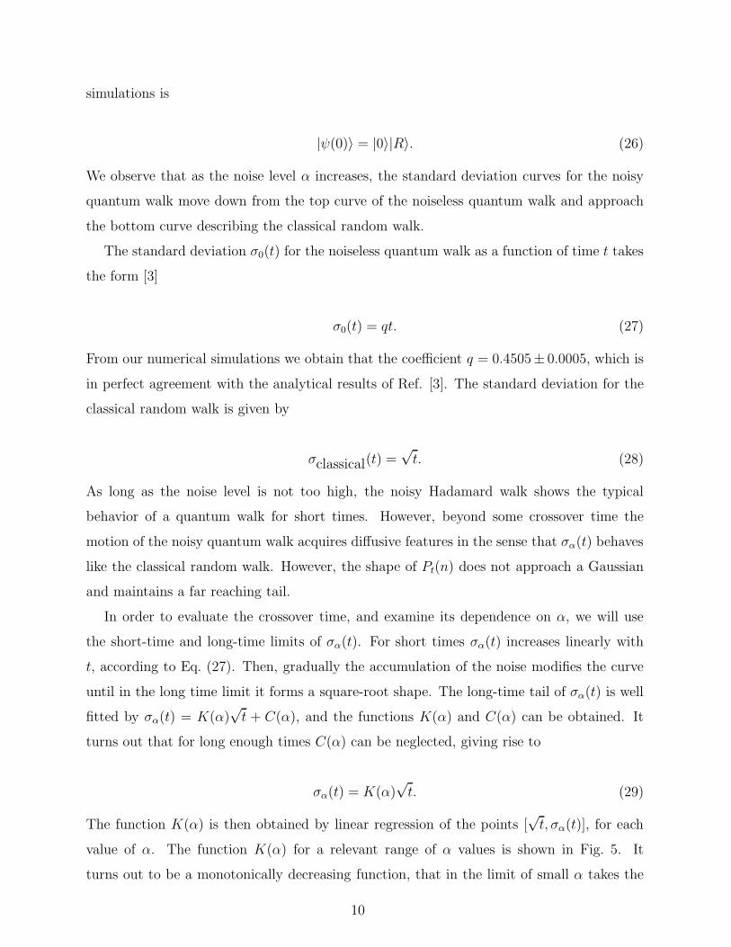
The standard deviation σ0(t) for the noiseless quantum walk as a function of time t takes

the form [3]

σ0(t) = qt. (27)

From our numerical simulations we obtain that the coefficient q = 0.4505± 0.0005, which is

in perfect agreement with the analytical results of Ref. [3]. The standard deviation for the

classical random walk is given by

σclassical(t) =√t. (28)

As long as the noise level is not too high, the noisy Hadamard walk shows the typical

behavior of a quantum walk for short times. However, beyond some crossover time the

motion of the noisy quantum walk acquires diffusive features in the sense that σα(t) behaves

like the classical random walk. However, the shape of Pt(n) does not approach a Gaussian

and maintains a far reaching tail.

In order to evaluate the crossover time, and examine its dependence on α, we will use

the short-time and long-time limits of σα(t). For short times σα(t) increases linearly with

t, according to Eq. (27). Then, gradually the accumulation of the noise modifies the curve

until in the long time limit it forms a square-root shape. The long-time tail of σα(t) is well

fitted by σα(t) = K(α)√t + C(α), and the functions K(α) and C(α) can be obtained. It

turns out that for long enough times C(α) can be neglected, giving rise to

σα(t) = K(α)√t. (29)

The function K(α) is then obtained by linear regression of the points [√t, σα(t)], for each

value of α. The function K(α) for a relevant range of α values is shown in Fig. 5. It

turns out to be a monotonically decreasing function, that in the limit of small α takes the

10

form K(α) ∼ 1/α. In the limit of very large α, K(α) → 1, and the noisy quantum walk

coincides with the classical random walk, for which K = 1 (dashed line). The monotonically

decreasing behavior of K(α) means that as the noise level increases, the broadening of the

distribution Pt(n) in the long time limit becomes slower. This is due to an earlier suppression

of the quantum coherence, that broadens the distribution much faster than the noise.

We will now consider the crossover time T2(α), which is based on the behavior of σα(t). It

is defined as the time at which the long time asymptote of the noisy Hadamard walk [given

by Eq. (29)] intersects with the short time asymptote, namely the ideal noiseless linear curve

[Eq. (27)]. This crossover time is given by

K(α)√

T2(α) = qT2(α), (30)

and therefore

T2(α) =

[

K(α)

q

]2

. (31)

The crossover time T2(α), obtained from Eq. (31), is shown in Fig. 6 as a function of α, on

a log-log scale. It is found that

T2 = c2 α−η, (32)

where c2 = 0.62 ± 0.01 and η = 2.05 ± 0.08. The crossover time can be interpreted as the

time required for the noise to scramble the phases and thus eliminate the structure of the

constructive and destructive interference that characterize the Hadamard walk. This time

can be estimated by

α√

T2 ∼ 1 (33)

namely,

T2 ∼1

α2, (34)

in agreement with the simulation results. Unlike the classical random walk that produces a

symmetric probability distribution for a particle that starts from the origin, the Hadamard

walk exhibits an inherent asymmetry. For example, the initial state of Eq. (26) produces a

11

distribution Pt(n) with much more weight on the right vs. the left hand side. Moreover, the

average position of the walker moves to the right at a constant speed, namely

n(t) = vt. (35)

where v = 0.293 ± 0.003, in perfect agreement with the analytical results of Ref. [3]. In

Fig. 7 we show the evolution in time of the average position 〈n(t)〉α [given by Eq. (22)] for

the noisy Hadamard walk with different values of the noise α. The dashed linear line at the

top is the result for the noiseless Hadamard walk, given by Eq. (35). Below it, from top to

bottom are the simulation results for α = 0.025, 0.03, 0.04, 0.07 and 0.1. For short times,

the average 〈n(t)〉α of the noisy Hadamard walk tends to follow the straight line of Eq. (35),

up to some crossover time, T1(α), at which it saturates and approaches a constant value:

〈n(t)〉α → nα. (36)

The asymptotic value, nα, decreases as the noise level α is increased. This is due to the fact

that at higher noise levels, the buildup of the asymmetric pattern, which is a quantum effect,

is suppressed more quickly. We define the crossover time T1(α) as the time t at which the line

of Eq. (35), describing the noiseless Hadamard walk, intersects the asymptotic horizontal

line 〈n(t)〉α = nα, namely vT1 = nα. Therefore

T1 =nα

v. (37)

In Fig. 8 we present the crossover time T1(α) vs. α on a log-log scale. It is well fitted by a

power-law function of the form

T1 = c1 α−ρ, (38)

where c1 = 0.20±0.01 and ρ = 2.06±0.08, which is consistent with the expected asymptotic

result of ρ = 2, based on an argument similar to Eq. (33). We thus find that both T1(α)

and T2(α) exhibit similar dependence on the noise level α, up to a constant factor.

We will now discuss the connection between our results for the effect of unitary noise on

the quantum walk and earlier results on decoherence effects [22, 23, 24, 25, 26]. Decoherence

can be described by an additional quantum operation that applies on the chirality qubit at

12

each step of the quantum walk. In a particular choice of the noise model, this operation is

given by the completely positive map that consists of the operators [25]

A0 =√p|R〉〈R|

A1 =√p|L〉〈L|

A2 =√

1 − pI, (39)

where I is the identity operator. This set of operators satisfies

2∑

n=0

A†nAn = I . (40)

It can be interpreted as a measurement of the chirality qubit that is performed with prob-

ability p. Analytical calculations show that in the long time limit, the first moment of the

decohered quantum walk, starting in the state |0〉|R〉, saturates and approaches the value:

〈n(t)〉p → np =(1 − p)2

p(2 − p). (41)

For weak decoherence, or p ≪ 1, np ∼ 1/p, which resembles our result nα ∼ 1/α2, if p is

replaced by α2. This is a sensible connection since α represents some matrix elements that

multiply the amplitudes while p is a probability.

The results of Ref. [25] for the second moment of the spatial distribution of the decohered

quantum walk can be expressed by

σp(t) = K(p)√t, (42)

where

K(p) =

√

1 +2(1 − p)2

p(2 − p). (43)

Like K(α), this is a monotonically decreasing function, that in the limit of small p takes

the form K(p) ∼ 1/√p, while K(p) → 1 for p → 1. Therefore, associating p with α2, one

obtains the same scaling behavior of the noise effects in the two noise models for both the

first and second moments of the distribution.

13

V. SUMMARY

We have studied the effect of unitary noise on the discrete one dimensional quantum

walk. We have shown that when the quantum walk is exposed to unitary noise it exhibits

a crossover from the quantum behavior for short times to classical-like behavior for long

times. For times shorter than the crossover time, the standard deviation σα(t) of the spatial

distribution of the noisy Hadamard walk, scales linearly with t, like the noiseless Hadamard

walk. Beyond the crossover time, σα(t) scales like√t, namely it acquires diffusive behavior,

like the classical random walk. The crossover time was also characterized using the average

position of the random walker, namely the first moment, 〈n(t)〉α, of the spatial distribution,

which scales like t for short times and saturates to a constant value for long times. In both

cases the crossover time was found to scale as α−2 where α is the standard deviation of the

random noise.

Acknowledgments

OB thanks the Center for Quantum Computer Technology and the Department of Physics

at the University of Queensland for hospitality during a sabbatical leave when this work was

initiated. The work at the Hebrew University was supported by the EU Grant No. IST-

1999-11234.

[1] Y. Aharonov, L. Davidovich and N. Zagury, Phys. Rev. A 48, 1687 (1993).

[2] D. Meyer, J. Stat. Phys. 85, 551 (1996).

[3] A. Amabainis, E. Bach, A. Nayak, A. Vishwanath and J. Watrous, One-dimensional quantum

walks, Proceedings of the 33th Ann. ACM Symposium on the Theory of Computing, New-York

(2001) p. 37.

[4] T.D. Mackay, S.D. Bartlett, L. Stephanson and B.C. Sanders, J. of Phys. A 35, 2745 (2002).

[5] C. Travaglione and G.J. Milburn, Phys. Rev. A 65, 032310 (2002).

[6] D. Aharonov and A. Ambainis, J. Kempe and U. Vazirani, Quantum walks on graphs, Pro-

ceedings of the 33th Ann. ACM Symposium on theTheory of Computing, New-York (2001)

p. 50.

14

[7] A.M. Childs, E. Farhi and S. Gutmann, An example of differnce between quantum and classical

random walks, LANL preprint quant-ph/0103020 (2001).

[8] E. Bernstein and U. Vazirani, SIAM J. Comp 26, 1411 (1997).

[9] J. Preskill, Lectures notes for physics 229: Quantum Information and Computation, available

from www.theory.caltech.edu/people/preskill/ph299/.

[10] M. A. Nielsen and I. L. Chuang , Quantum computation and quantum information (Cambridge

University Press, Cambridge, 2000).

[11] W.H. Zurek, e-print quant-ph/0105127.

[12] P. Shor, Phys. Rev. A 52, 2493 (1995).

[13] P. Shor, Phys. Rev. A 54, 1098 (1996).

[14] A. Steane, Proc. R. Soc. London, Ser. A 452, 2551 (1996).

[15] A. Steane, Phys. Rev. Lett. 77, 793 (1996).

[16] E. Knill and R. Laflamme, Phys. Rev. A 55, 900 (1997).

[17] P. Zanardi, Phys. Rev. A 56, 4445 (1997).

[18] D.A. Lidar, I.L. Chuang and K.B. Whaley, Phys. Rev. Lett. 81, 2594 (1998).

[19] D. Bacon, D.A. Lidar and K.B. Whaley, Phys. Rev. A 60, 1944 (1999).

[20] J. Kempe, D. Bacon, D.A. Lidar and K.B. Whaley, Phys. Rev. A 63, 042307 (2001).

[21] H. Azuma, Phys. Rev. A 65, 042311 (2002).

[22] T.A. Brun, H.A. Carteret and A. Ambainis, The quantum to classical transition for random

walks, eprint quant-ph/0208195.

[23] V. Kendon and B. Tregenna, Decoherence in a quantum walk on the line, eprint

quant-ph/0210047.

[24] V. Kendon and B. Tregenna, Phys. Rev. A 67, 042315 (2003).

[25] T.A. Brun, H.A. Carteret and A. Ambainis, Phys. Rev. A 67, 032304 (2003).

[26] V. Kendon and B. Tregenna, Decoherence in discrete quantum walks, Proceedings of the

DICE2002 workshop, Piombino (Tuscany), September 2-6, 2002 on Decoherence, Information,

Complexity and Entropy, to appear in Lecture Notes in Physics, Springer-Verlag (2003); eprint

quant-ph/0301182.

[27] D. Shapira, S. Mozes and O. Biham, Phys. Rev. A 67, 042301 (2003).

15

FIG. 1: The probability distribution Pt(n) of the noiseless Hadamard walk on the one dimensional

lattice at time t, vs. the spatial coordinate n. This probability distribution is given for different

times: t = 250(a), t = 1000 (b) and t = 10000 (c). The initial state of the quantum walk is given

by Eq. (25).

FIG. 2: The probability distribution 〈Pt(n)〉α of the noisy Hadamard walk at low noise level

α = 0.025, as a function of n for t = 250 (a), t = 1000 (b) and t = 10000 (c). The initial state of

the walk is given by Eq. (25).

FIG. 3: The probability distribution 〈Pt(n)〉α of the noisy Hadamard walk for high noise level

α = 0.8, as a function of n, for t = 1000. The initial state of the walk is given by Eq. (25).

FIG. 4: The standard deviation σα(t) for the noisy Hadamard walk as a function of the time t,

for several noise levels α. The top curve (dashed line) is for the noiseless Hadamard walk. Below

it (from top to bottom) are the results for the noisy Hadamard walk with α = 0.025, 0.05, 0.1 and

0.2, respectively (solid lines). The bottom curve (dashed line) is for the classical random walk.

Each data point was averaged over 200 runs for weak noise (α < 0.07) and over 4000 runs in case

of strong noise (α ≥ 0.07).

FIG. 5: The coefficient K(α) as a function of the noise level α. In the limit of small α it takes the

form K(α) ∼ 1/α. In the limit of very large α, K(α) → 1, namely, it coincides with the result of

the classical random walk.

FIG. 6: The crossover time T2 as a function of the noise level α, on a log-log scale. It follows a

power-law behavior T2 ∼ α−η where η = 2.05 ± 0.08.

FIG. 7: The average position 〈n(t)〉α of noisy Hadamard walk as a function of the time t. The

top curve is for the noiseless Hadamard walk and below it, from top to bottom are the curves for

α = 0.025, 0.03, 0.04, 0.07 and 0.1.

FIG. 8: The crossover time T1 as a function of α, on a log-log scale. It follows a power-law of the

form T1 ∼ α−ρ where ρ = 2.06 ± 0.08

16

Fig. 1(a)-1000 -500 0 500 10000

0.01

0.02

0.03

0.04

0.05

n

P t(n)

17

Fig. 1(b)-1000 -500 0 500 10000

0.005

0.01

0.015

0.02

0.025

0.03

n

P t(n)

18

Fig. 1( )-10000 -5000 0 5000 10000

0

0.001

0.002

0.003

0.004

n

P t(n)

19

Fig. 2(a)-1000 -500 0 500 10000

0.01

0.02

0.03

0.04

0.05

n

hP t(n)i�

20

Fig. 2(b)-1000 -500 0 500 10000

0.005

0.01

0.015

0.02

0.025

0.03

n

hP t(n)i�

21

Fig. 2( )-10000 -5000 0 5000 10000

0

0.001

0.002

0.003

0.004

n

hP t(n)i�

22

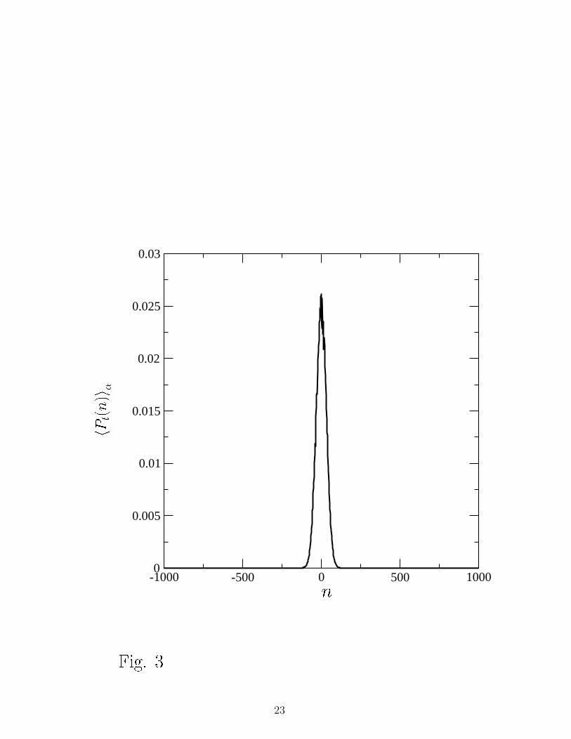
Fig. 3-1000 -500 0 500 10000

0.005

0.01

0.015

0.02

0.025

0.03

n

hP t(n)i�

23

Fig. 40 200 400 600 800 1000

0

100

200

300

400

500

t

� �(t)

24

Fig. 50 0.05 0.1 0.15 0.2 0.25

0

1

5

10

15

�

K(�)

25

Fig. 60.05 0.1 0.2

10

100

1000

�

T 2

26

Fig. 70 200 400 600 800 1000

0

50

100

150

200

250

300

t

hn(t)i �

27

Fig. 80.03 0.05 0.1

50

100

200

300

400

�

T 1

28