Lecture Notes on Quantum Mechanics

A.N. Njah,Department of Physics,

University of Agriculture,Abeokuta, NIGERIA

PHS 411: Symmetry in quantum mechanics. Fundamentals of quantum me-chanics - okperations in Hilbert space. Matrix formulation of quantum me-

chanics. Angular momentum in quantum mechanics; approximation methodsin collision theory. Many electron systems. Scattering theory.

Suggested reading.

1. Quantum Mechanics by L. I. Schiff

2. Quantum Mechanics by E. Merzbacher

3. Schaum’s Outline of Theory and Problems of Quantum Mechanics byY. Peleg, R. Pnini and E. Zaatur

1

Contents

2

Chapter 1

APPROXIMATION METHODS

1.1 VARIATIONAL METHOD

This method is applicable to conservative systems. Consider a physical sys-tem with time-independent Hamiltonian H. We assume for simplicity that

the entire spectrum of H is discrete and non degenerate

(H|φn〉 = En|φn〉), n = 1, 2, 3... (1.1)

Let Eo be the smallest eigenvalue of H (i.e, the smallest energy of the system).An arbitrary state |ψ〉 can be written in the form

|ψ〉 =∑ncn|φn〉 (1.2)

Then

〈ψ|H|ψ〉 =∑n|cn|2En ≥ Eo

∑n|cn|2 (1.3)

On the other hand,〈ψ|ψ〉 =

∑n|cn|2 (1.4)

Thus, we can conclude that for every ket,

〈H〉 =〈ψ|H|ψ〉〈ψ|ψ〉 ≥ Eo (1.5)

Eq.(6.5) is the basis of the variational method. A family of kets |ψ(α)〉 is

chosen, the so called trial kets. The mean value of H in the states |ψ(α)〉is calculated, and the expression 〈H〉(α) is minimized with respect to the

parameter α. The minimum value obtained is an approximation of the groundstate energy Eo.

3

Equation (6.5) is actually a part of a more general result called the Ritztheorem. The mean value of the Hamiltonian H is stationary in the neigh-

borhood of its discrete eigenvalues.The variational problem can therefore be generalized to provide an esti-

mation for other energy levels based on the ground state. If the function〈H〉(α) obtained from the trial kets |ψ(α)〉 has several extrema, they giveapproximate values of some of its energies En.

Examples 1. Consider a 1D harmonic oscillator

H =−h2

2m

d2

dx2 +1

2mw2x2

(a) For the one-parameter family of wave functions ψα(x) = e−αx2

(α > 0),find a wave function that minimizes 〈H〉. What is the value of 〈H〉 min?

(b) For another one parameter family of wave functions ψβ(x) = xe−βx2

(β >0), find a wave function that minimizes 〈H〉 and compute the value of 〈H〉min.(c) Repeat the same procedure for

ψγ(x) =1

x2 + γ(γ > 0)

Solution

(a) We begin by considering 〈H〉.

〈H〉 =

∫∞−∞ ψ∗

α

[−h2

2md2

dx2 + 12mw

2x2]ψα(x)dx∫∞

−∞ ψ∗α(x)ψα(x)dx

=h2

2mα +

1

8

mw2

αWe differentiate 〈H〉 with respect to α

d〈H〉dα

=h2

2m− 1

8

mw2

α2

From the condition d〈H〉dα α=αo

= 0, we have

h2

2m− mw2

8α2o

= 0 ⇒ αo =mw

2h;

4

thus αo gives the minimum value of 〈H〉. The wave function that minimizes

〈H〉 is ψαo(x) = e−

mwx2

2h and

〈H〉min =h2

2mαo +

mw2

8αo=

1

2hw

Thus 〈H〉min coincides with the energy of the n=0 level of a 1D harmonicoscillator. Note that the family of functions we are studying coincides with

the ground state wave function of the harmonic oscillator.

(b) We proceed with the same method as in part (a).

〈H〉 =

∫∞−∞ ψ∗

β

[−h2

2md2

dx2 + 12mw

2x2]ψβ(x)dx∫∞

−∞ ψ∗β(x)ψβ(x)dx

= 3h2

mβ +

3

8

mw2

β

andd〈H〉dβ

=3h2

2m− 3mω2

8

1

β2 = 0

We obtain βo = 12

mωh and ψβo

(x) = xe−mωx2/2h; so 〈H〉min equals the energyof the n = 1 level of the one-dimensional harmonic oscillator.

(c) Applying the procedures of parts (a) and (b), we obtain

〈H〉 =

∫∞−∞ ψ∗

γ

[−h2

2md2

dx2 + 12mw

2x2]ψγ(x)dx∫∞

−∞ ψ∗γ(x)ψγ(x)dx

=h2

2m

1

γ+

1

2mw2γ

and

ψγo(x) =

1

x2 + h2/√

2mωγo =

1√2

h

mω

2. Consider a particle in a one-dimensional potential V(x) - λx4. Using the

variational method, find an approximate value for the energy of the groundstate. Compare it to the exact value Eo = 1.06 h2

2mk13 where k= 2mλ/h2.

Choose as a trial function ψ = (2α/π)14e−αx2

.

5

Solution: First note that the trial function ψ = (2α/π)14e−αx2

is normal-

ized to unity; that is∫∞−∞ |ψ|2dx=1. The Hamiltonian is H = −h2

2md2

dx2 + λx4;thus

〈H〉 =

∫∞−∞ ψ∗

[−h2

2md2

dx2 + λx4]ψ(x)dx∫∞

−∞ ψ∗(x)ψ(x)dx

The denominator equals one since ψ(x) is normalized; thus

〈H〉 =∫ ∞−∞

(2α

π

)14e−αx2

(− h2

2m

) d2

dx2

(2α

π

) 14e−αx2

dx+∫ ∞−∞

(2α

π

)14e−αx2

λx4(2α

π

)14e−αx2

dx

= − h2

2m

√√√√2α

π

∫ ∞−∞ e−2αx2

2α[2αx2 − 1]dx+ λ

√√√√2α

π

∫ ∞−∞ x4e−2αx2

dx

= −h2(4α2)

2m

√√√√2α

π

∫ ∞−∞ x2e−2αx2

dx+h2(2α)

2m

√√√√2α

π

∫ ∞−∞ e−2αx2

dx+λ

√√√√2α

π

∫ ∞−∞ x4e−2αx2

dx

The first integral is

I1 ≡ −h2(4α2)

2m

√√√√2α

π

∫ ∞−∞ e−2αx2

x2dx = −h2(4α2)

2m

√√√√2α

π

1

4α

√π

2α= −h

2α

2m

The second integral is:

I2 ≡ h2(2α)

2m

√√√√2α

π

∫ ∞−∞ e−2αx2

dx =h2(2α)

2m

√√√√2α

π

√π

2α=h2α

m

and the third integral is:

I3 ≡ λ

√√√√2α

π

∫ ∞−∞ x4e−2αx2

dx = λ

√√√√2α

π

3

4(2α)2

√π

2α=

3λ

16α2

Substituting these integrals we obtain

〈H〉 = −h2α

2m+h2α

m+

3λ

16α2 =h2

2mα +

3

16

λ

α2 †

Hence, d〈H〉dα = h2

2m − 38

λα3

o. Since d〈H〉

dα

∣∣∣∣α=α0

= 0, we obtain h2

2m − 38

λα3

o= 0 →

αo =(

3mλ4h2

)13. In terms of k =2mλ/h2, we have αo = (3/8)

13k

13 . Substituting

this value in †, we obtain

〈H〉min =3

43

13h2

2mk

13 = 1.082

h2

2mk

13

6

Comparing the last result to the exact value of Eo we see that we have quitea good approximation. The error is approximately 2 percent.

3.(a) Taking a trial wave function proportional to exp(−βr) , where β is avariable parameter, use the variational method to obtain an upper limit for

the energy of the ground state of the hydrogen atom in terms of atomic con-stants.(a) The upper limit of the ground state is the minimum value of the ex-

pectation value of the energy as β varies. Denote the trial wave functionby

ψ = A exp(−βr)where A is a constant. Its value is obtained from the normalizing condition.Since ψ depends only on r, we put d3r = 4πr2dr. Therefore, the normalizationcondition yields,

4πA2∫ ∞0r2 exp(−2βr)dr =

8πA2

(2β)3)= 1

Thus

A2 =β3

π(1)

The Hamiltonian for the hydrogen atom is

H = − h2

2m∇2 − e2

4πεo

1

r(2)

The expectation value of the energy for the function ψ is

〈E〉 = 4πA2∫ ∞0

exp(−βr)(− h2

2m∇2 − e2

4πεo

1

r

)exp(−βr)r2dr (3)

Since exp(−βr) depends only on r, we need only the r- dependent part of theoperator

∇2 exp(−βr) =( ∂2

∂r2 +2

r

∂

∂r

)exp(−βr (4)

Inserting (1) and (4) in (3) gives

〈E〉 = 4β3

h2

2mβ2 ∫∞

0 r2 exp(−2βr)dr

+(

βh2

m − e2

4πεo

) ∫∞0 r exp(−2βr)dr

= − h2

2mβ2 + h2

mβ2 − e2

4πεoβ

= h2

2mβ2 − e2

4πεoβ

7

Thend〈E〉dβ

=h2β

m− e2

4πεo

which is

0, when β =me2

4πεoh2

Inserting this in the expression for 〈E〉 gives

〈E〉min = −me

2h2

( e2

4πεo

)2

= − e2

8πεo

1

ao

Where ao is the Bohr radius.(b) The expression obtained above is the correct value of the ground-stateenergy of the hydrogen atom. The expression is correct because the rtrial

function is the correct form of the ground-state wave function.

8

1.2 THE WKB APPROXIMATION (or Semiclassical

Approximation)

WKB stands for the names of the proponents: Wentzel, Kramer and Bril-

louin. The method is suitable for obtaining solutions of the one-dimensionalSchr

..odinder equation as well as the 3-dimensional problems, if the potential

is spherically symmetric and a radial defferential equation can be separated.That is, it is applicable to situations in which the wave can be separatedinto one or more total differential equations each of which involves a single

independent variable.Consider the Schr

..odinger equation in one-dimention:

d2ψ

dx2 +2m

h2 [E − V (x)]ψ(x) = 0 (1)

Let ⎧⎪⎪⎪⎨⎪⎪⎪⎩k(x) = 1

h

√2m[E − V (x)] for E〉V (x)

κ(x) = −ih

√2m[E − V (x)] for E〈V (x)

(2)

If V (x) is constant eq.(1) has solution ψ ∼ e±ikx

However if V (x) varies slowly with x we assume a solution of the form

ψ = Aeiu(x)/h (3)

Subsituting this solution in eq.(1) we find that u(x) satisfies the equation

ihd2u

dx2 −(du

dx

)2

+ [hk(x)]2 = 0 (4)

In the WKB approximation we expand u(x) in power series of h as follows:

u(x) = u0 + hu1 + h2u2 + . . . (5)

where un, n = 0, 1, 2, . . . are approximate solutions of eq.(4). Neglectingexpansion terms of order h2 and putting eq.(5) in eq.(4) we have

h

⎧⎨⎩id2u0

dx2 + 2

(du0

dx

) (du1

dx

)⎫⎬⎭−

(du0

dx

)2

+ [hk(x)]2 = 0 (6)

where again the expansion terms of order h2 are neglected and the terms ineq.(6) are grouped in powers of h. Now equating equal powers of h we have

−u′20 + [hk(x)]2 = 0 (7)

9

iu′′0 − 2u′0u′1 = 0 (8)

Integrating eqs.(7) and (8) we have

u0(x) = ±h∫ x

k(x′)dx′ + c1 (9)

u1(x) =1

2i ln k(x) + c2 (10)

where c1 and c2 are arbitrary constants of integration. Substituting eqs.(9)and (10) into eq.(5) and sustituting eq.(5) in eq.(3) one gets

ψ(x) = Ak−12 (x) exp(±i

∫ xk(x′)dx′) for E > V (11)

where c1 and c2 are absorbed into A. In a similar fashion, the case E〈V gives

ψ(x) = Bκ−12 (x) exp(±

∫ xκ(x′)dx′) for E〈V (12)

The region in which E > V (x) is called a classically allowed region of motion,while a region in which E〈V (x) is called classically inaccessible. The points

in the boundary between these 2 kinds of regions are called turning points[where E = V (x)].

Applicability condition: The WKB approximation is based on the condi-tion

1

2

∣∣∣∣∣dk

dx

∣∣∣∣∣ |k2(x)| (13)

(i.e. V(x)varies very slowly with x). k(x) is the wave number so k(x) = 2πλ ,

where λ is the wavelength. We can then write eq.(13) as

1

2

∣∣∣∣∣dk

dx

∣∣∣∣∣ 2π

λk(x)

orλ

4π

∣∣∣∣∣dk

dx

∣∣∣∣∣ k(x) (14)

Solution near a turning point: Adjacent to the turning points for whichk(x0), we have k ≈ dk

dx|x0(x−x0). Thus the WKB approximation is applicable

for a distance from the turning point satisfying the condition

|x− x0| λ

4π(15)

The connection formulas

The connection formulas at the turning point depends on whether the clas-sical region is to the left (p1) or to the right (p2) of it.

10

In the first case we have x > a:

ψ1(x) =A1√k

cos(∫ x

ak(x′)dx′ − B1π) (16)

while in the second case, for x〈b

ψ2(x) =A2√k

cos(∫ b

xk(x′)dx′ − B2π) (17)

(The results in eqs.(16 and 17) are quoted)

Application to the bound state: The WKB approximation can be applied

to derive an equation for the energies of a bound state. Since the wave func-tion is zero at the boundaries the argument of the cosine in the connection

formulas eqs.(16 and 17) is given by

∫ b

ak(x)dx−Bπ = (n+

1

2)π n = 0, 1, 2 . . . (18)

or∫ b

ak(x)dx = (n+

1

2)π n = 0, 1, 2 . . . (19)

if the initial phase is chosen to be zero, i.e. B = 0.

∫p(x)dx = 2πh(n+

1

2) n = 0, 1, 2 . . . (20)

where p(x) = hk(x) Eq.(20) is called the Bohr-Sommerfeld quantization rule.Barrier potential: For a potential barrier V(x) between x = a and x =

11

b and a particle of energy E, the transmission coefficient T in the WKBapproximation is (quoted)

T = exp

−2

h

∫ b

a

√2m[V (x) − E]dx

(21)

Solved examples:

1. Using the WKB approximation find the bounded states for a one-dimensionalinfinite potential well. Compare your result with the exact solution.

Suppose that the boundaries of the potential well are at x = ±a. At theboundaries the wave function has value zero and k(a) = 0. From eqs.(16)

and (17) we have ⎧⎪⎪⎪⎨⎪⎪⎪⎩

0 = cos(−B1π)

0 = cos(−B2π)

and therefore B1 = B2 = 12. Thus we get, according to eq.(18)∫ a

−aKndx− 1

2π = (n+

1

2)π

i.e. 2akn = (n+ 1)π ⇒ kn =(n+ 1)π

2a

From eq.(2) we get En =1

2

h2k2n

m=π2h2(n+ 1)2

8ma2

Recall that the exact solution is π2h2n2

8ma2

2.Use the WKB approximation to obtain the energy levels of a harmonic os-

cillator.Consider the Bohr-Sommerfeld quantization rule:

∫ b

ap(x)dx = hπ(n+

1

2) (n = 0, 1, 2, . . .) (i)

where p(x) =√

2m[E − V (x)] is the momentum of the oscillator, V (x) =12mω

2x2. Since∫pdx = 2

∫ ba pdx holds for a linear harmonic oscillator we can

use eq.(i). The points a and b are the turning points that are determined bythe condition p(a) = p(b) = 0 or E − V = 0; thus E − 1

2mω2x2 = 0 so we

havea = −

√2E

mω2 , b =√

2Emω2 . We introduce the new variable z = x

√mω2

2E , and

obtain ∫ b

ap(x)dx =

2E

ω

∫ 1

−1

√1 − z2dz =

πE

ω(ii)

12

Comparing eqs.(ii) and (i) we obtain En = hω(n + 12) which is the exact

solution.

13

1.3 TIME-INDEPENDENT PERTURBATION THE-

ORY

(FOR BOUND STATES) OR STATIONARY PERTURBATION THEORY

(SPT)Time-independent perturbation theory is widely used in Physics. Perturba-

tion theory is appropriate when the Hamiltonian H of the system can be putin the form

H = H0 + λh (1)

where λ is a small parameter such that the perturbation (or disturbance)λh H0, i.e., λ 1; and the matrix elements of the operator h are com-

parable in magnitude to those of H0. The eigenstates un and eigenvalues En

of the unperturbed Hamiltonian, H0 must be known. The SPT is concernedwith finding the changes in discrete energy levels and eigenfunctions of a sys-

tem when a small disturbance (perturbation) is applied.In the unperturbed state

H0un = Enun (2)

or H0|n〉 = En|n〉 (2)

where un or |n〉 form an orthonormal basis of the state space.

(i.e., 〈m|n〉 = δmn and∑

n |n〉〈n| = 1).In the perturbed state H = H(λ) as in eq.(1) and its nth eigenstate ψn(λ)

and the corresponding eigenvalue En(λ) are also functions of λ. Therefore

H(λ)ψn(λ) = En(λ)ψn(λ) (3)

We assume that En(λ) and ψn(λ) can be expanded as a power series of λ in

the formEn(λ) = ε0 + λε1 + λ2ε2 + . . . (4)

ψn(λ) = φ0 + λφ1 + λ2φ2 + . . . (5)

Substituting eqs.(4) and (5) into eq.(3) we obtain

(H0+λh)(φ0 +λφ1 +λ2φ2 + . . .) = (ε0 +λε1 +λ2ε2 + . . .)(φ0+λφ1 +λ2φ2 + . . .)

(6)Expanding eq.(6) and equating equal powers of λ we have for

λ0 : (H0 − ε0)φ0 = 0 (7)

14

λ1 : (H0 − ε0)φ1 = (ε1 − h)φ0 (8)

λ2 : (H0 − ε0)φ2 = (ε1 − h)φ1 + ε2φ0 (9)

. . . . . . . . . . . . . . . . . . . . . . . . . . . . . . . . .

Note the following:

1. As λ → 0, we have ε0 = En (the unperturbed eigenvalue of the nth level)and eq.(7) means that φ0 is the corresponding unperturbed eigenfunction.

We, therefore putφ0 = un, ε0 = En (10)

2. any arbitrary multiple of φ0 can be added to any of the functions φs

without affecting the RHS of eqs.(7) to (9) and the determination of φs interms of lower order functions. Hence we choose the arbitrary multiple such

that(φ0, φs) = 0 s > 0 (11)

3. Using the result

Ωαβ =∫φ∗α(r)Ωφβ(r)d

3r =∫

[Ω†φα(r)]∗φβ(r)d3r = 〈α|Ω|β〉 (12)

(where Ωαβ is the matrix element of Ω in the states α, β) the inner productof φ0 and the LHS of eqs.(7) to (9) is zero in each case, and it follows, withthe help of eqs.(10) and (11) that

εs =(φ0, hφs−1)

(φ0, φ0)= (un, φs−1) (13)

First-order perturbation theory: Eq.(13) with s = 1 shows that

ε1 = (un, hun) or 〈n|h|n〉 (14)

which is the expectation value of h for the unperturbed state un or |n〉. Any

function can be written as a linear combination of the orthonormal basisfunctions um so

φ1 =∑ma(1)

m um (15)

Substituting eq.(15) into eq.(8) we have

∑ma(1)

m (H0 −En)um = (ε1 − h)un

15

where a(1)n = 0 because of eq.(11) (free choice). Now replace H0um by Emum,

multiply by u∗k and sum over all m making use of the orthonormality of the

u′s (only terms k = m survive) to have

a(1)k =

(uk, hun)

En −Ekor

〈k|h|n〉En − Ek

k = n (16)

i.e. a(1)m =

〈m|h|n〉En − Em

m = n (17)

Hence φ1 =∑m

〈m|h|n〉En −Em

|m〉 m = n (18)

The first-order solutions are

En(λ) = ε0 + λε1 = En + λ〈n|h|n〉 (19)

ψn(λ) = φ0 + λφ1 = un + λ∑m

〈m|h|n〉En − Em

|m〉 m = n (20)

Usually we set λ = 1

Second-order perturbationWhen s = 2 eq.(13) gives

ε2 = (un, hφ1) = (un, h∑ma(1)

m um) =∑ma(1)

m (un, hum) =∑ma(1)

m 〈n|h|n〉

=∑m

〈m|h|n〉En − Em

〈n|h|m〉 =∑m

|〈n|h|m〉|2En −Em

m = n (21)

since h is assumed to be hermitian. Eq.(21) is the second-order approxima-tion of the eigenvalue.

The second-order approximation of the eigenfunction φ2 is calculated by ex-panding it in terms of um:

φ2 =∑ma(2)

m um, a(2)n = 0 (22)

Substituting eq.(22) into eq.(9) we obtain∑ma(2)

m (H0 −En)um =∑ma(1)

m (ε1 − h)um + ε2un

Again, replace H0um by Emum, multiply by u∗k and sum over all m makinguse of the orthonormality of the u′s (only terms k = m survive) to have

a(2)k (Ek −En) = a

(1)k ε1 −

∑ma(1)

m (uk, hum) or a(1)k ε1 −

∑ma(1)

m 〈k|h|m〉 k = n

16

This gives, with the help of eqs.(14) and (17),

a(2)k = −〈k|h|n〉〈n|h|n〉

(En − Ek)2 +∑m

〈k|h|m〉〈m|h|n〉(En − Ek)(En −Em)

m =nn =k (23)

Inserting eq.(23) into eq.(22) we have

φ2 =∑k

⎡⎣−〈k|h|n〉〈n|h|n〉

(En −Ek)2 +∑m

〈k|h|m〉〈m|h|n〉(En − Ek)(En − Em)

⎤⎦ |m〉 m =n

n =k (24)

The second-order solutions are:

En(λ) = ε0 + λε1 + λ2ε2 = En + λ〈n|h|n〉 + λ2 ∑m

|〈n|h|m〉|2En − Em

m =n (25)

ψn(λ) = φ0 + λφ1 + λ2φ2 = un + λ∑m

〈m|h|n〉En −Em

|m〉

+λ2 ∑k

⎡⎣−〈k|h|n〉〈n|h|n〉

(En − Ek)2 +∑m

〈k|h|m〉〈m|h|n〉(En − Ek)(En −Em)

⎤⎦ |m〉 m =n

n =k (26)

Example 1: The effect of the finite size of the nucleus is to raise the energiesof the electronic states from the theoretical values based on a point nucleus.

Show from first-order perturbation theory that, if the proton is regarded (forsimplicity) as a thin uniform spherical shell of charge of radius b, the frac-

tional change in the energy of the ground state is 4b2

3a20

where the ground state

eigenfunction for Hydrogen is us = ( 1πa3

0)

12 exp(−r/a0) and b/a0 = 10−5.

Solution: For a point nucleus the potential is

V0 = − e2

4πε0r(i)

For this uniform spherical shell the potential is

V =

⎧⎪⎪⎪⎨⎪⎪⎪⎩

e2

4πε0rr > b

− e2

4πε0br〈b

(ii)

The perturbation potential is therefore

V1 = V − V0 =

⎧⎪⎪⎪⎨⎪⎪⎪⎩

e2

4πε0(1

r − 1b) r〈b

0 r > b

(iii)

17

The first order correction to the energies of the ground state is

ε1 =∫u∗0V1u0dτ (iv)

where dτ = 4πr2dr is the volume element and u0 = ( 1πa3

0)

12 exp(−r/a0)

Thus4

a30

e2

4πε0

∫ b

0r2(

1

r− 1

b) exp(−2r/a0)dr (v)

Since b/a0 ≈ 10−5, the exponential term may be replaced by unity over the

range of integration, and the integral becomes

∫ b

0(r − r2

b)dr =

1

6b2 (vi)

The ground-state energy for a point nucleus is

E0 = − e2

8πε0a0(vii)

From eqs.(v), (vi) and (vii)E1

E0= −4b2

3a20

Example 2: Consider a 3 dimensional problem. In a given orthonormal

basis, the Hamiltonian is represented by the matrix

H =

⎛⎜⎜⎜⎝

1 0 00 3 00 0 −2

⎞⎟⎟⎟⎠ +

⎛⎜⎜⎜⎝

0 c 0c 0 00 0 c

⎞⎟⎟⎟⎠

Here, H = Ho +H ′ and c is a constant, c 1.

1. Find the exact eigenvalues of H.

2. Use second order perturbation to determine the eigenvalues.

3. Compare the results of 1 and 2.

Solution 1. The eigenvalue of H are roots of the equation det(H-λI) =0.∣∣∣∣∣∣∣∣∣1 − λ c 0c 3 − λ 0

0 0 c− 2 − λ

∣∣∣∣∣∣∣∣∣= (c−2−λ)

∣∣∣∣∣∣1 − λ c

c 3 − λ

∣∣∣∣∣∣ = (c−2−λ)[λ2−4λ+3−c2]

18

Therefore, λ = c− 2, 2 ±√1 + c2.

2. The second order correction to the energy may be written as: En =

E(0)n + E(1)

n +E(2)n or

(E)i = (Ho)ii + (H ′)ii +∑k =i

H ′ikH

′ki

E(0)i −E

(0)k

It can be seen that (Ho)ii = 1, 3 and -2. The first order energy correction isgiven by H ′

11 = 0, H ′22 = 0 and H ′

33 = c. For the second correction, we have

E(2)1 =

H ′12H

′21

E(0)1 − E

(0)2

+H ′

13H′31

E(0)1 − E

(0)3

=c2

−2+

0

3= −c

2

2

E(2)2 =

H ′21H

′12

E(0)2 − E

(0)1

+H ′

23H′32

E(0)2 − E

(0)3

=c2

3 − 1+

0.0

3=c2

2

and

E(2)3 =

H ′31H

′13

E(0)3 −E

(0)1

+H ′

32H′23

E(0)3 −E

(0)2

= 0 + 0 = 0

Thus E1 = 1 − c2

2 , E2 = 3 + c2

2 ;E3 = −2 + c.

3. Expand 2 ±√1 + c2 in a binomial series

2 ±√

1 + c2 = 2 ± (1 +1

2c2 + ...) = 3 +

c2

2, 1 − c2

2(c2 1).

This gives the same result as the second order corrections.Example 3: Consider a perturbation of the form 1

2bx2 to the linear har-

monic oscillator problem. Thus,

Ho =−h2

2m

d2

dx2 +1

2kx2

and H ′ = 12bx

2. The eigenvalues and eigenfunctions of Ho are well known

Houn = Enun

where

En =(n+

1

2)hω; n = 0, 1, 2, 3...

un = NnHn(ξ) exp(−1

2ξ2)

19

ω =

√√√√ k

m, Nn =

[ γ√π2nn!

] 12

ξ = γx, γ =

√mω

h=

[mkh2

]1/4

Notice that the exact solution can easily be obtained; all that one has to do

is replace k by k+b. Thus if we write

Hψn = Enψn

where H = Ho +H ′

then En =(n+

1

2)h

√√√√ k

m

[1 +

b

k

]1/2

or En =(n+

1

2)h

√√√√ k

m

[1 +

1

2

b

k− 1

8

b2

k2 + ...]... ∗ ∗

the binomial expansion been valid when bk〈1. If we compare (**) with equa-

tion (4), we obtain

εo =(n+

1

2

)h

√√√√ k

m...............(∗)

ε1 =1

2

(n+

1

2

)h

√√√√ k

m

b

k...............(∗∗)

ε2 = −1

8

(n+

1

2

)h

√√√√ k

m

b2

k2 ...............(∗ ∗ ∗)where εo represents the unperturbed eigenvalue, and ε1 and ε2 represent the

first and second order perturbations respectively. We can now apply pertur-bation theory to compute ε1 and ε2 etc. Now,

ε1 =1

2b∫ ∞−∞ u∗n(x)x

2un(x)dx =1

2b〈n|x2|n〉

=1

2

(n+

1

2

)h

√√√√ k

m

b

k...............(i∗)

Equation (i*) agrees with eqn. (**). In order to calculate ε2, we note that

H ′mn = 〈m|H ′|n〉 =

1

2b〈m|x2|n〉

20

and this is non zero , only when m=n-2, m=n or m=n+2. Thus

ε2 =′∑m

|H ′mn|2

En − Em=

(1

2b)2[ |〈n− 2|x2|n〉|2

En − En−2+

|〈n+ 2|x2|n〉|2En −En+2

]

= −1

8b2

h

m2ω2

(n+

1

2

)

which agrees with eqn (***).

21

1.4 TIME-DEPENDENT PERTURBATION THEORY

The time-dependent perturbation theory, which is sometimes called the methodof variation of constants, assumes as in the last section that

H(t) = H0 + λh(t) (1)

H0uk = Ekuk (2)

where H0 is the unperturbed Hamiltonian with known eigenvalues Ek andeigenstates uk, and h (the perturbation) is small, (i.e., λ 1) and depends

on time t. h has the effect of causing transitions between eigenstates of H0

that would be stationary in the absence of h. We use the adiabatic approx-imation which assumes that H(t) contains parameters which change very

slowly with time. For time-dependent perturbation we work with the time-dependent Schr

..odinger equation. The time-dependent Schr

..odinger equation

for the unperturbed state is

ih∂uk(t)

∂t= H0uk(t) = Ekuk(t)

i.e.∂uk(t)

∂t= − i

hEkuk(t)

⇒ uk(t) = uk(0)e−iEkt

h (3)

uk(0) is the solution of the unperturbed time-independent Schr..odinger eq.(2).

The time-dependent Schr..odinger equation for the perturbed state is

ih∂ψ

∂t= H(t)ψ (4)

We express ψ as an expansion in the eigenfunctions uke− iEkt

h with coefficientsak(t) that depend on time.

ψ =∑nan(t)une

− iEnth (5)

⇒ ak(t) = u∗kψ (6)

ak(t) is the probability amplitude for state uk, |ak(t)|2 is the probability that

the system is in the state uk. Substituting eq.(5) into eq.(4) we have

∑nih

.an une

− iEnth +

∑nanEnune

− iEnth =

∑nan(H0 + λh(t))une

− iEnth

22

where.an=

dan

dt . We replace H0un by Enun on the RHS, multiply through on

the left by uk, and sum over all k, making use of the orthonormality of theu’s to have

ih.ak e

− iEkth = λ

∑nan(t)e

− iEnth 〈k|h(t)|n〉 (7)

where 〈k|h(t)|n〉 =∫

allspace

u∗kh(t)undτ . We define the Bohr (angular) frequency

ωkn =Ek −En

h(8)

and eq.(7) becomes

.ak=

λ

ih

∑n〈k|h(t)|n〉an(t)e

iωknt (9)

First-order Perturbation

We express the an(t) in eq.(9) as a power series in λ:

an(t) = a(0)n (t) + λa(1)

n (t) + λ2a(2)n (t) + . . . (10)

Substitute eq.(10) into eq.(9), equate the coefficients of corresponding powersof λ, and set λ = 1 in final result to have the set of equations

.a(0)

k (t) = 0 (11a)

.a(s+1)

k (t) =1

ih

∑n〈k|h(t)|n〉a(s)

n (t)eiωknt (11b)

Eq.(11) can be integrated successively to obtain approximate solutions to anydesired order in the perturbation. For first-order perturbation s = 0 and

.a(1)

k (t) =1

ih

∑n〈k|h(t)|n〉a(0)

n (t)eiωknt (12)

where a(0)n (t) are the solution of eq.(11a), the zero-order coefficients a

(0)k , which

are constant with time. The a(0)k are the initial conditions of the system before

the perturbation is applied.Assuming, for simplicity, that all except one of the a

(0)k are zero, so that the

system is initially in a definite unperturbed energy state |m〉.

We thus put a(0)k = 〈k|m〉 = δkm (13)

23

Put eq.(13) into eq.(12) to have

.a(1)

k (t) =1

ih〈k|h(t)|m〉eiωkmt

⇒ a(1)k (t) =

1

ih

∫ t

−∞or 0

〈k|h(t′)|m〉eiωkmt′dt′

a(1)k (t) is the first-order probability amplitude at any time t > 0 for state |k〉,

|a(1)k (t)|2 is the first-order probability of finding the system in the state |k〉

i.e. the transition probability from state |m〉 to |k〉 after time t > 0.Examples1. A system of hydrogen atoms in the ground state is contained between the

plates of a parallel-plate capacitor. A voltage pulse is applied to the capacitorso as to produce a homogeneous electric field

E =

⎧⎨⎩ 0 t〈0eε0 exp(−t/τ) t > 0

Show that, after a long time, the fraction of atoms in the 2p (m = 0) stateis, to first order

215

310

a20e

2ε20h2(ω2 + 1

τ2 )

where a0 is the Bohr radius, and hω is the energy difference between the 2pand the ground state.

Solution: First-order time-dependent perturbation theory gives the resultthat if a Hamiltonian h(t) is applied at t = 0 to a system in an initial state|m〉 with energy Em, the probability that a transition has occurred to a state

|k〉, with energy Ek at time t is |ak|2, where

ak =1

ih

∫ t

0〈k|h(t′)|m〉 exp(iωt′)dt′, hω = Ek − Em (i)

In this problem h(t′) is the potential of the electron in the applied field, whosedirection we take as the z-axis, i.e.

h(t′) = eε0z exp(−t′/τ), t′ > 0 (ii)

For t = ∞, eq.(i) becomes

ak =eε0ih

〈k|z|m〉∫ ∞0

exp(iω − 1/τ)t′dt′ (iii)

24

The time integral is

∫ ∞0

exp(iω − 1/τ)t′dt′ =1

iω − 1/τ[exp(iω − 1/τ)t′]∞0 =

1

iω − 1/τ(iv)

Therefore, ak =eε0

h(ω + i/τ)〈k|z|m〉 (v)

The initial state is the ground state of the hydrogen atom, i.e., the quantum

numbers are n = 1, l = 0, m = 0 and the final state has n = 2, l = 1 m =0. We evaluate the matrix element in spherical polar coordinates r, θ, φ using

the relation z = r cos θ. Then

〈k|z|m〉 =∫

allspace

u∗210r cos θu100dv (vi)

where dv = r2dr sin θdθdφ (vii)

u100 = R10Y00 =2√4π

1

a3/20

exp(−r/a0) (viii)

u210 = R21Y10 =1√4π

1

(2a0)3/2

r

a0exp(−r/2a0) cos θ (ix)

Thus 〈k|z|m〉 =1

23/2

1

a40

∫ ∞0r4 exp(− 3r

2a0)dr

∫ π

0cos2 θ sin θdθ (x)

=4!

23/2

(2

3

)6a0 (xi)

(We have used the result∫∞0 r4 exp(−βr)dr = 4!

β5 ). From eqs.(v) and (xi) theprobability of a transition is

|ak|2 =215

310

a20e

2ε20h2(ω2 + 1

τ2 )

2. A time-varying Hamiltonian h(t′) brings about transition of a system froma state |k〉 at t′ = 0 to |j〉 at t′ = t with probability pkj(t). Use first-order

time-dependent perturbation theory to show that, if pjk(t) is the probabilitythat the same Hamiltonian brings about the transition j → k in the same

time interval, then pjk(t) = pkj(t).Solution: The probability of a transition from |k〉 (at time zero) to |j〉 (at

time t) ispkj(t) = |akj(t)|2 (i)

25

where the first-order expression for akj(t) is

akj(t) =1

ih

∫ t

0〈j|h(t′)|k〉 exp(iωjkt

′)dt′ (ii)

Similarly, ajk(t) =1

ih

∫ t

0〈k|h(t′)|j〉 exp(iωkjt

′)dt′ (iii)

Now h(t′) is a Hermitian operator. Therefore

〈k|h(t′)|j〉 = 〈j|h(t′)|k〉∗ (iv)

Also hωkj = Ek −Ej = −hωjk (v)

Therefore the integral in eq.(iii) is the complex conjugate of the one in eq.(ii).

Thusajk(t) = −akj(t)∗

giving pjk(t) = |akj(t)|2 = pkj(t)

Comment: It is in general true that the probability of transition betweentwo states, due to an external stimulus represented by h(t), is the same for

transition in either direction. The result is known as the principle of detailedbalancing

3. Consider a one-dimensional harmonic oscillator with angular frequecy ω0

and electric charge q. At time t = 0 the oscillator is in ground state. Anelectric field is applied for time τ , so the perturbation is

h(t) =

⎧⎨⎩ −qεx 0 ≤ t ≤ τ

0 otherwise

where ε is a field strength and x is a position operator. Using first-order

perturbation theory, calculate the probability of transition to the state n = 1.

26

Chapter 2

SCATTERING THEORY

Introduction: Much of what we know about the forces and interactions inatoms and nuclei has been learnt from scattering experiments, in which atoms

in a target are bombarded with beams of particles whose nature are known.Theoretically, the most significant aspect of scattering processes is that ofthe continuous part of energy spectrum. Here intensities are the objects of

measurement and prediction. These intensities, being measures of the likeli-hood of finding a particle at certain places, are related to the eigenfunctions.

Establishing this relation is the first problem of scattering theory.In an idealized scattering experiment a single fixed scattering center is bom-

barded by particles (projectiles) incident along the z-axis. In the classicallimit each particle can be assigned an impact parameter, ρ and an azimuthangle, φ, which together with z define its position in cylindrical coordinates.

Let dσ/dΩ be the area which, when placed at right angles to the incidentbeam, would be traversed by as many particles as are scattered into the

unit solid angle around a direction characterized by the angles θ and φ (fig.

27

above). If the scattering potential is spherically symmetric, V = V (r) thescattering becomes independent of φ. Therefore, classically it can be shown

that the differential cross-section is

dσ

dΩ=

ρ

sin θ

∣∣∣∣∣dρ

dθ

∣∣∣∣∣ (1)

The impact parameter ρ is a function of θ. To determine this function fromNewton’s second law is the problem of classical scattering theory. Eq.(1) isvalid if the de Broglie wavelength of the projectile is much smaller than the

dimension of the scattering region. As the wavelength increases quantumfeatures appear. Quantum Mechanics represents the particles in the beam by

wave packets. That is, the particles do not have sharp boundaries. Therefore,in Quantum Mechanics particles need not actually touch each other as they

can do in Classical Mechanics. When two particles are near each other theyfeel the influence of each other by the degree of freedom which is common to

both. E.g., an electron has the degrees of freedom (mass, charge, spin) whilea neutron has (mass, spin). So an electron and a neutron can feel or relatewith each other by (mass, spin) which is common to both.

Elastic ScatteringIt is scattering without energy loss or gain by the projectile, i.e. kinetic en-

ergy of projectile is conserved. In elastic scattering the scattering center onthe particles can be represented by a potential energy V (r) of finite range d

such that V (r) = 0, if r > d. The disc of radius d is called the scatteringcross-section. Scattering cross-section is a measure of the probability of scat-tering of the projectile by the target.

Definition of differential cross-section: A beam of particles of mass m trav-elling along the z-direction with velocity v is scattered by a short-range po-

tential V (r) centred on the origin O (fig. below). We use spherical polarcoordinates r, θ, φ taking z as the polar axis. The Schr

..odinger equation is

used to calculate the probability of a particle being scattered into a smallsolid angle dΩ in the direction θ, φ. The probability is expressed in terms of

a differential cross-section, dσ/dΩ, which is defined as the ratio of the num-ber of scattered particles dn(θ, φ) per unit time within the solid angle dΩ tothe incident flux F ;

dσ/dΩ = dn(θ, φ)/FdΩ (2)

where dσ/dΩ has dimension of surface. We assume:1. Any interaction between the scattered particles themselves is negligible

28

2. Possible multiple scattering processes are negligible. (A multiple scatter-ing process is a process in which a scattered particle can be scattered multiple

times in the same target range)3. The incident beam width is much larger than a typical range of the scat-

tering potential, so that the particle will have a well-defined momentum.The total scattering cross-section σsc =(total number of particles scatteredper second)/F =

∫ dσdΩdΩ. Absorption cross-section σab = (total number of

particles absorbed per second)/F .

The Schr..odinger equation for scattering

1. Ignore the center of mass motion

2. Consider only the motion in the center of mass frame i.e. relative motionwhich is important for collision.

⎡⎣− h2

2µ∇2 + V (r)

⎤⎦ψ(r) = Eψ(r) (3)

where µ = reduced mass. This is the equation for the projectile; it is not an

eigenvalue equation. E is positive and is the energy given to the projectileby the experimenter. Therefore, it is arbitrary. Divide (3) through by h2/2µto obtain [

−∇2 +2µV

h2 − 2µE

h2

]ψ

or [∇2 + k2]ψ = Uψ (4)

where E = h2k2

2µ and U = 2µVh2

Green’s function method: We seek solution ψ(r) = Φ(r) exp(−iωt) that

satisfies the boundary conditions that

29

ψ(r) is finite at r = 0 and ψ(r) → 0 as r → ∞. In that case

Φ(r) = exp(ikz) +f(θ, φ)

rexp(ikr) (5)

This result is obtained by Green’s function method applied to (4) (details

deferred). Therefore,

ψ(r) = exp i(kz − ωt) +f(θ, φ)

rexp i(kr − ωt) (6)

The first term represents the incident particles moving along the z-axis, andthe second term, which is a spherical wave travelling outwards from the origin,

represents the scattered particles. We are confining the dicussion to elasticscattering hence the value of k is the same in the incident and scattered

terms in (6). The function f(θ, φ) is known as the scattering amplitude. Thedifferential cross-section is related to f(θ, φ) by

dσ/dΩ = |f(θ, φ)|2 (7)

Proof: The area dA subtends a solid angle dΩ at the origin, where

dΩ = dA/r2 (i)

The term ui = exp(ikz) in the wave function (6) represents the incident

particles with densityGi = |ui|2 = 1 (ii)

While the term us = 1rf(θ, φ) exp(ikr) represents the scattered particles with

densityGs = |us|2 = |f(θ, φ)|2/r2 (iii)

The number of scattered particles passing through dA in unit time = (density

of particles at r)×v × dA = |f(θ,φ)|2r2 = |f(θ, φ)|2vdΩ (iv)

where v is the velocity of the incident and scattered particles. The incidentflux is F = Gi × v = v (v).Inserting (iv) and (v) into the definition of dσ/dΩ, eq.(2) we have (7)

Born ApproximationThis is a first-order perturbation calculation, valid for fast particles and a

weak potential, which means that the incident wave function is only slightlyperturbed by the potential. The approximation gives

f(θ, φ) = − m

2πh2

∫allspace

V (r) exp(iκ.r)dv (8)

30

where the quantity κ, known as the scattering vector, is defined by κ = k−k′,where k is the wave vector of the incident particles, and k′ that of the scattered

particles. The angle between k and k′ is the scattering angle θ. For elasticscattering

|k| = |k′|, and κ = 2k sinθ

2(9)

Example 1: Show that for a spherically symmetric potential

∫ ∞−∞ V (r) exp(ik.r) =

4π

k

∫ ∞0V (r) sin krdr

Solution: Since the potential is spherically symmetric, it depends only onthe magnitude of r, thus we have

∫V (r) exp( k.r)d3r = 2π

∫ ∞0V (r)r2dr

∫ π

0exp(ikrcosθ) sin θdθ (i)

where θ is the angle between r and the polar axis. Put u = cos θ. Then

du = − sin θ

and ∫ π

0exp(ikr cos θ) sin θdθ =

∫ 1

−1exp(ikru)du =

2

krsin kr (ii)

Inserting (ii) in (i), we have the expected result.Example 2: a) Particles are incident on a spherically symmetric poten-

tial V (r) = βrexp(−γr), where β and γ are constants. Show that, in the Born

approximation, the differential scattering cross-section for the scattering vec-

tor κ is given by dσ/dΩ =

2mβh2(κ2+γ2)

2

b) Use this result to derive the Rutherford formula for the scattering of α-particles, namely, that for α-particles of energy E incident on nuclei of atomic

number Z, the differential scattering cross-section for scattering at an angle

θ to the incident direction is dσ/dΩ =

Ze2

8πε0E sin2( θ2 )

Solution: a) The Born approximation gives the amplitude

f(θ) = − mI

2πh2 (i)

where I =∫

allspace

V (r) exp(iκ.r)dv (ii)

31

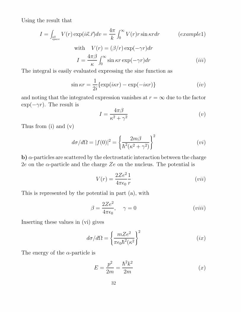
Using the result that

I =∫

allspace

V (r) exp(iκ.r)dv =4π

k

∫ ∞0V (r)r sinκrdr (example1)

with V (r) = (β/r) exp(−γr)drI =

4πβ

κ

∫ ∞0

sinκr exp(−γr)dr (iii)

The integral is easily evaluated expressing the sine function as

sinκr =1

2iexp(iκr) − exp(−iκr) (iv)

and noting that the integrated expression vanishes at r = ∞ due to the factor

exp(−γr). The result is

I =4πβ

κ2 + γ2 (v)

Thus from (i) and (v)

dσ/dΩ = |f(0)|2 =

⎧⎨⎩

2mβ

h2(κ2 + γ2)

⎫⎬⎭

2

(vi)

b) α-particles are scattered by the electrostatic interaction between the charge2e on the α-particle and the charge Ze on the nucleus. The potential is

V (r) =2Ze2

4πε0

1

r(vii)

This is represented by the potential in part (a), with

β =2Ze2

4πε0, γ = 0 (viii)

Inserting these values in (vi) gives

dσ/dΩ =

⎧⎨⎩

mZe2

πε0h2(κ2

⎫⎬⎭

2

(ix)

The energy of the α-particle is

E =p2

2m=h2k2

2m(x)

32

where p is the momentum. Since κ = 2k sin(θ2)

h2κ2 = 8mE sin2(θ

2

)(xi)

Inserting (xi) in (ix) gives the required result

Partial waves and phase shiftsWe look for solutions of the Schr

..odinger equation

− h2

2µ∇2ψ + V (r)ψ =

h2k2

2µψ (10)

(where ∇2 is the Laplacian in spherical polar coordinates and V (r) is a spher-ically symmetric potential ⇒ elastic scattering) which have the asymptotic

form

ψ(+)k = eikrcosθ + fk(θ)

eikr

r(11)

We establish the connection between these solutions and

ψ(r, θ, φ) = Rl,k(r)Yml (θ, φ) =

ul,k(r)

rY m

l (θ, φ) (12)

which are simultaneous (common) eigenfunctions ofH, L2 and Lz. The radial

functions Rl,k and ul,k satisfy the differential equations⎡⎣− 1

r2

d

dr(r2 d

dr) +

l(l + 1)

r2 +2µ

h2 V (r) − k2

⎤⎦Rl,k(r) = 0 (13)

⎡⎣− d2

dr2 +l(l + 1)

r2 +2µ

h2 V (r) − k2

⎤⎦ul,k(r) = 0 (14)

respectively as well as the boundary condition that Rl,k be finite at the origin⇒ ul,k = 0 (15)

For the region r > d, V (r) = 0⎡⎣− 1

r2

d

dr(r2 d

dr) +

l(l + 1)

r2 − k2⎤⎦Rl,k(r) = 0 (16)

The asymptotic solution of (16) for large kr is (quoted)

Rl,k(r) =ul,k(r)

r∼ Al

sin(kr − lπ/2)

kr− Bl

cos(kr − lπ/2)

kr(17)

33

The first term of (17) is called the regular solution while the second term isthe irregular solution. The magnitude of Bl/Al is a measure of the intensity

scattering.Bl/Al = − tan δl (18)

where δl is called scattering phase shift. Hence (17) can be written as

ul,k(r)

r∼ Cl

sin(kr − lπ/2 + δl)

kr

orul,k(r)

r∼ sin(kr − lπ/2 + δl)

kr(19)

(where Cl = 1 in order to fix the normalization). If we expand ψ(+)k in terms

of the separable solution of (12) (i.e. Legendre polynomials) we get

ψ(+)k (r, θ) =

∞∑l=0al(k)pl(cos θ)

ul,k(r)

r(20)

where ψ(+)k depends only on the angle between k and r but not on their

directions. The asymptotic expansion of the plane wave eikz gives

eikz = eikrcosθ ∼∞∑l=0

(2l + 1)ilsin(kr − lπ/2)

krpl(cos θ) (21)

Substituting (21) into (11), and (19) into (20) and comparing coefficients of

the terms of the form pl(cos θ)exp(−ikr+ilπ/2)kr we have

al =(2l + 1)il

(2π)3/2 eiδl (22)

Hence asymptotically, (i.e. using (22) and (19) in (20))

ψ(+)k (r, θ) ∼

∞∑l=0

(2l + 1)ileiδlsin(kr − lπ/2 + δl)

(2π)3/2krpl(cosθ) (23)

Eq.(23) differs from a plane wave by the presence of δ and is called distorted

plane waves. Put (21) into (11) and compare the coefficients of eikr

r in (11)and (23) to have

fk(θ) =∞∑l=0

(2l + 1)e2iδl − 1

2ikpl(cos θ) (24)

34

or fk(θ) =1

k

∞∑l=0

(2l + 1)eiδl(k) sin δl(k)pl(cos θ) (25)

Each l term in (24) or (25) is known as a partial wave. The l = 0 wave is

termed an s-wave, the l = 1 a p-wave, the l = 2 a d-wave and so on (samenomenclature as for atomic states). The lth wave, being an eigenfunction ofthe operator L2, is a state in which the particle has orbital angular momentum

about the origin of magnitude√l(l + 1)h ≈ lh. Since the linear momentum

of the particle is hk, a classical picture of the lth wave is that it corresponds

to the particle passing the potential at a distance ρl from its centre, wherehkρl = lh, i.e.

ρl = l/k (26)

Eq.(25) shows that, if δl = 0, that partial wave gives no contribution to f(θ).If ρl, the distance of closest approach, is much larger than d, the range of the

potential, the particle passes outside the potential and is not scattered, soδl = 0 for that partial wave. It follows from (26) that only those partial waves

with l ≤ dk have non-zero values of δl, and contribute to the scattering.If dk 1, as in the case for nuclear scattering at low energy all the δl = 0,

except δ0. Since k = 2π/λ the condition dk 1 ⇒ 2πd/λ 1 ⇒ λd i.e. the wavelength λ of the particle is large compared to the range of thepotential. In this situation, when only the s-wave is disturbed, the angular

dependence of f(θ) is given by the Legendre polynomial p0(cos θ) = 1 so thescattering is spherically symmetric. As k → 0, tan δ0 is proportional to k,

i.e. δ0 → 0 or nπ and the limiting value of − tan δ0/k, is termed scatteringlength. the concept is most commonly applied to the scattering of thermal

neutrons.Example: 1. a) Verify that, outside the range of a short-range potential,the wave function

ψ(r, θ) =1

r

(1 +

i

kr

)exp(ikr) cos θ

represents an outgoing p-wave.

b) A beam of particles represented by the plane wave e(ikz) is scattered by animpenetrable sphere of radius d, where kd 1. By considering only s and p

components in the scattered wave, show that, to order (kd)2, the differentialscattering cross-section for scattering at an angle θ is

dσ/dΩ = d21 − 1

3(kd)2 + 2(kd)2 cos θ

35

[The value of cos2 θ averaged over all directions is 1/3]Solution: a) The dependence on θ for a p-wave (l = 1) is given by the

Legendre polynomial p1(θ) = cos θ. So the angular part of the given functionψ(r, θ) has the required form for a p-wave. It remains to show that the radial

part R(r) has the correct form. Put R(r) = u(r)/r. From (14), outside therange of the potential, u(r) satisfies

d2u

dr2 +

⎧⎨⎩k2 − l(l + 1)

r2

⎫⎬⎭u = 0, (i)

with l = 1. For the given ψ(r, θ),

u(r) =

(1 +

i

kr

)exp(ikr). (ii)

Differentiating this twice with respect to r and substituting in (i) shows thatthe equation is satisfied with l = 1.

b) Outside the range of the potential, the wave function for s and p waveshas the form

ψ = exp(ikz) +A

rexp(ikr) +

B

r

(1 +

i

kr

)exp(ikr) cos θ, (iii)

where A and B are constants. The term in A is the spherically symmetric

s-wave, and the term in B is the p-wave. As r → ∞

ψ = exp(ikz) +f(θ)

rexp(ikr) (iv)

Equating terms in (1/r) exp(ikr) in (iii) and (iv) gives

f(θ) = A+ B cos θ (v)

Since the scattering object is an impenetrable sphere, the wave function van-ishes on the surface r = d. Thus

exp(ikd cos θ) +A

dexp(ikd) +

B

d

(1 +

i

kd

)exp(ikd) cos θ = 0. (vi)

The terms on the RHS that are independent of θ must sum to zero, andsimilarly the terms proportional to cos θ. Expanding exp(ikd cos θ) in powers

of kd we have

exp(ikd cos θ) = 1 + ikd cos θ − 1

2(kd)2 cos2 θ + 0(k3d3). (vii)

36

We cannot make the terms in cos2 θ sum to zero in (vi), because that wouldrequire the contribution from d-waves, which are excluded. However, we need

to take into account the average value of cos2 θ, which is 1/3. Summing theterms in (6) which are independent of θ gives

1 − 1

6(kd)2 +

A

dexp(ikd) = 0 (viii)

whence A = −d1 − 1

6(kd)2 exp(−ikd). (ix)

Summing the terms in cos θ gives

ikd+B

d

(1 +

i

kd

)exp(ikd) = 0. (x)

Since kd 1, i/kd 1. Therefore to terms in (kd)2

B = −d(kd)2. (xi)

From (v),(ix), and (xi), the differential scattering cross-section is

dσ

dΩ= |f(θ)|2 = |A+ B cos θ|2 = d21 − 1

3(kd)2 + 2(kd)2 cos θ, (xii)

to terms in (kd)2

Example 2 A particle of mass µ and momentum P = hk is scattered bythe potential V (r) = e−r/a

r Voa, where Vo and a>0 are real constants (Yukawa

potential).(a) Using the Born approximation, calculate the differential cross section (b)obtain the total cross section.

Solution(a) The range of the Yukawa potential is characterized by the distance a. We

assume that Voa2 h2/µ, so that the Born approximation is valid for all

values of ka. The scattering amplitude is then given by:

f(θ, φ) = − 1

4π

2µVoa

h2

∫e−iq.r e

−r/ro

rd3r

Since the potential has spherical symmetry V(r) = V(r), we can carry outthe integration using the relation

∫r2e−iq.rV (r)drdΩ =

4π

q

∫ ∞0

sin(qr)V (r)rdr

37

where r =|r| and dΩ = sin θdθdφ. Therefore,

f(θ) = −2µVoah2k

∫∞0 r sin(kr)e−r/adr = −2µVoa

3

h21

1+q2a2

= −2µVoa3

h21

1+[2ka sin θ2 ]2

Finally, the differential cross section dσdΩ = |f(θ)|2 is:

dσ(θ)

dΩ=

4µ2V 2o a

6

h41

[1 + 4k2a2 sin2 θ2 ]

2∗

Note that due to spherical symmetry, the cross section does not depend onthe azimuthal angle.

(b) The total cross section is obtained by integration

σ =∫ dσ(θ)

dΩdΩ =

4µ2V 2o a

6

h44π

1 + 4k2a2

Note that the infinite range limit ( a→ ∞, Vo → 0 and Voa = Z1Z2e2=constant

of the Yukawa potential corresponds to the Coulomb interaction between two

ions of charges Z1e and Z2e. At this point (*) reduces to the well -knownRutherford formula

dσ

dΩ=

4µ2

h4Z2

1Z22e

4

16K4 sin4 θ2

=Z2

1Z22e

4

16E2 sin4 θ2

where E = h2k2

2µ is the energy of the particle in the center of mass frame andµ is their reduced mass.

Example 3: A point particle is scattered by a second particle with rigidcore; that is, the scattering potential is V(r) = 0 for r> a and V(r) = ∞for r < a. The energy of the scattered particle satisfies ka = 1. (a) Find theexpression for δl. Complete the table below (express δl in radians).

tan δl δl sin δll = 0

l = 1

l = 2

(b) Calculate the differential cross section dσ/dΩ for angles 0 and π, takinginto account only the waves l =0 and l =1. (c) Compute the total cross

38

section σT taking into account only the waves l =0 and l =1. (d) What is theaccuracy of part (c)?

Solution(a) The phase shifts for a rigid sphere is given by the equation:

tan δl =jl(ka)

nl(ka)

Using the known expressions for the Spherical Bessel functions:

jo(x) =sin x

xno(x)= − cosx

x

j1(x) =sin x

x2 − cosx

xn1(x) = −cosx

x2 − sin xx

j2(x) =( 3

x2 − 1

x

)sinx− 3

cosx

x2 n2(x) = −(

3x2 − 1

x

)cosx− 3 sinx

x2

and substituting x=ka =1, we find tan δo = -1.56, tan δ1= -0.22 and tan δ2 =-0.02. Therefore

tan δl δl sin δll = 0 -1.56 -1.00 -0.84

l = 1 -0.22 -0.22 -0.22

l = 2 -0.02 -0.02 -0.02

(b) The differential cross section is given by:

dσ

dΩ=

1

k2 |∞∑l=0

(2l + 1)eiδl sin δlPl(cos θ)|2

For l =0, 1 and k =a−1

dσ

dΩ= a2| sin δoeiδo + 3 sin δ1e

iδ1 cos θ|2

= a2[sin2 δo + 6 sin δo sin δ1 cos(δo − δ1) cos θ

+9 sin2 δ1 cos2 θ]

Substituting θ = 0, π, we obtain:

dσ

dΩ|0,π = a2| sin2 δo ± 6 sin δo sin δ1 cos(δ0 − δ1) + 9 sin2 δ1|

with δ1 and δ0 given in the table above.

39

(c) The total cross section is given by:

σT =4π

k2

∞∑l=0

(2l + 1) sin2 δl

for l =0, 1 and k =1/a

σT = 4πa2[sin2 δo + 3 sin2 δ1] ≈ 0.854πa2.

(d) A rough estimate on the accuracy of the calculation in part (c) is givenby calculating the additional term l =2.

σT ≈ (0.85 + 0.002)4πa2

Example 4: (a) Consider scattering from a spherical symmetric potential.The solution of the Schrodinger equation is given by the expansion φ(r, θ) =

Σ∞l=0Rl(r)Pl(cos θ)), where R(r) is the solution of the radial wave equation

and Pl(cos θ) is the Legendre polynomial of order l. In the limit r → ∞ the

asymptotic form of the wave function is:

φ(r, θ)r→∞ ≈ eikz +1

rf(θ)eikr (1)

where f(θ) is the scattering amplitude. Similarly, the asymptotic form of R(r)

is

R(r)r→∞ ≈Alsin

(kr − π

2 l + δl)

kr(2)

where δl are phase shifts. (i) use expressions (1) and (2) to obtain the Leg-endre expansion of f(θ)

(b) Show that the total cross section is given by

σT =4π

k2

∞∑l=0

(2l + 1) sin2 δl

Solution (a) The asymptotic form of the wave function is as given above:

φ(r, θ)r→∞ ≈∞∑l=0Al

sin(kr − π

2 l + δl)

krPl(cos θ) = eikr +

1

rf(θ)eikr

Using the Legendre expansion of eikz,

eikz = eikr cos θ =∞∑l=0

(2l + 1)iljl(kr)Pl(cos θ)

40

we find that

∞∑l=0Al

sin(kr − π

2 l + δl)

krPl(cos θ) = eikr +

1

rf(θ)eikr

=∞∑l=0

[(2l + 1)il

sin(kr − π

2 l + δl)

kr+

1

rfl(θ)e

ikr]Pl(cos θ)

where f(θ) =∑∞

l=0 flPl(cos θ). Now, we write sin x = eix−e−ix

2i , and obtain

I Alei((

kr−π2 l+δl

)− (2l + 1)ile

i

(kr−π l

2

)= 2ikfle

ikr

II Ale−ikr−π l

2+δl − 2l + ile−ikr−π l2 = 0

Therefore from (II), we obtain Al = (2l + 1)ileiδl and then by subst back in

(II), we have

f(θ) = (2ik)−1∞∑l=0

(2l + 1)(e2iδl − 1)Pl(cos θ)

(b) The total cross section is

σT =∫|f(θ)|2dΩ = 2π

∫ 1

−1

d(cos θ)

4k2 |∞∑l=0

(2l + 1)(e2iδ1 − 1)Pl(cos θ)|2

=π

2k2

∫ 1

−1d(cos θ)

∞∑l,l′=0

(2l′ + 1)(2l+ 1)(e2iδl′ − 1)(e2iδl − 1)Pl′(cos θ)Pl(cos θ)

Now, ∫ 1

−1d(cos θ)Pl′(cos θ)Pl(cos θ) =

2

(2l + 1)δll′.

Therefore

σT =π

k2

∞∑l=0

(2l + 1)(2 − e2iδl − e−2iδl) =4π

k2

∞∑l=0

(2l + 1) sin2 δl

41