
ELEMENTARY QUANTUM MECHANICS - FAU Digital Library
438
ELEMENTARY QUANTUM MECHANICS
-
Upload
khangminh22 -
Category
Documents
-
view
0 -
download
0
Transcript of ELEMENTARY QUANTUM MECHANICS - FAU Digital Library

ELEMENTARYQUANTUMMECHANICS

ELEMENTARYQUANTUM
MECHANICS
David S. SaxonUniversity o/California, Los Angeles
noHOLDEN-DAY
San Francisco, Cambridge. London, Amsterdam

© Copyright 1968 by Holden-Day, Inc., 500 SansomeStreet, San Francisco, California. All rights reserved. Nopart of this book may be reproduced in any form, bymimeograph or any other means, without permission inwriting from the publisher.
Library of Congress Catalog Card Number 68-16996.Printed in the United States of America.

Preface
This book is based on lectures given by the author in an intensiveundergraduate course in quantum mechanics which occupies a centralrole in the physics curriculum at UCLA. It is a required course for allthird-year physics and astrophysics students, but it is taken by someseniors and many graduate students, both in physics and in related fields.
Students enrolling in the course are expected to have had an introduction to elementary Hamiltonian mechanics, to the extent of knowing,for simple systems, what the Hamiltonian function is and what theHamiltonian equations are. Students are also expected to have hadtraining in mathematics through differential equations and Fourier senesand to have at least seen many of the special functions of mathematicalphysics. In an effort to keep the mathematics as simple as possible,however, the first two-thirds of the book is largely confined to the consideration of one-dimensional systems.
The stress throughout is on the formulation of quantum mechanicsand not on its applications. At UCLA the applications follow in immediately subsequent courses selected from atomic, nuclear, solid state andelementary particle physics. The last chapter is intended to pave the wayfor these applications; in it a number of relatively advanced topics aresomewhat briefly presented.
The coverage is rather broad and not everything is treated in depth.Wherever the text is frankly introductory, however, references to acomplete treatment are given. In all other respects the book is selfcontained. Experience with a preliminary edition has shown that it isaccessible to students and that they can learn from it largely by themselves. To a considerable degree the teacher is thus left free to illuminatethe subject in his own way.
One hundred and fifty problems are presented, and these play an im-

vi PREFACE
portant pedagogical role. The problems are not exclusively illustrativeof material presented in the text; they also amplify it. A significantnumber are intended to broaden the scope of the course by pointing theway to new topics and new points of view. Many problems are too difficult for the student to master in his first attempt. He is encouraged toreturn to them again and again as his understanding grows. Eventuallyhe should be able to handle any and all of them. Answers or completesolutions to some fifty representative problems are given in Appendix Ill.About forty exercises are scattered throughout the text. These are mostlyconcerned with the working out of details, but not all of them are trivial.
At UCLA the material in the text is presented in a sequence coveringtwo quarters. However, the text is also intended for use in a one-semestercourse; any, or all, of the starred sections in the table of contentS canbe omitted without harm to the logical development. If it is desired, onthe other hand, to use the text for a one-year course, some supplementation would be desirable. The Heisenberg and interaction representations,and transformation theory in general, are topics which at once come tomind. At the applied level, the Zeeman and Stark effects, Bloch waves,the Hartree-Fock and Fermi-Thomas methods, simple molecules andisotopic spin are a suitable list from which to choose.
The author has benefited from numerous criticisms and suggestionsfrom a host of colleagues and students. To each of them, he expresseshis deep gratitude and especially to Dr. Ronald Blum for his meticulousreading of both the preliminary edition and the final manuscript. Theauthor wi11 be equally grateful for additional comments and for thecorrection of misprints and errors.
David S. Saxon
November, 1967

Contents
I. THE DUAL NATURE OF MATTER AND RADIATION
I. The breakdown of classical physics .2. Quantum mechanical concepts. . . . . . .3. The wave aspects of particles. . . . . . .4. Numerical magnitudes and the quantum domain5. The particle aspects of waves .6. Complementarity . . . . .7. The correspondence principle.
II. STATE FUNCTIONS AND THEIR INTERPRETATION
I. The idea of a state function; superposition of states2. Expectation values. . . . . . . . . . .3. Comparison between the classical and quantum
descriptions of a state; wave packets . . . .
Ill. LINEAR MOMENTUM
I35
12131616
1823
25
I. State functions corresponding to a definite momentum 292. Construction of wave packets by superposition 313. Fourier transforms: the Dirac delta function. 344. Momentum and configuration space. . 385. The momentum and position operators. 396. Commutation relations . 457. The uncertainty principle . . . . . 47
IV. MOTION OF A FREE PARTICLE
I. Motion of a wave packet; group velocity 56

viii CONTENTS
2. The correspondence principle requirement 593. Propagation of a free particle wave packet in
configuration space. 604. Propagation of a free particle wave packet in momentum
space; the energy operator . 625. Time development of a Gaussian wave packet 646. The free particle Schrodinger equation . 667. Conservation of probability. 688. Dirac bracket notation 729. Stationary states 73
10. A particle in a box. 75II. Summary 81
V. SCHRODINGER'S EQUATION
I. The requirement of conservation of probability. 842. Hermitian operators 853. The correspondence principle requirement 9\4. Schrodinger's equation in configuration and
momentum space 955. Stationary states 976. Eigenfunctions and eigenvalues of Hermitian operators 1017. Simultaneous observables and complete sets of operators 1048. The uncertainty principle 106
* 9. Wave packets and their motion 11010. Summary: The postulates of quantum mechanics III
VI. STATES OF A PARTICLE IN ONE DIMENSION
I. General features 1172. Classification by symmetry; the parity operator. 1193. Bound states in a square well 1214. The harmonic oscillator . 127
* 5. The creation operator representation 139* 6. Motion of a wave packet in the harmonic oscillator
potential 1457. Continuum states in a square well potential 1478. Continuum states in general; the probability flux 153
* 9. Passage of a wave packet through a potential 155* 10. Numerical solution of Schrodinger's equation 159
VII. APPROXIMATION METHODS
I. The WKB approximation 1752. The Rayleigh-Ritz approximation 1853. Stationary state perturbation theory. 189
* For a one-semester course, any or all of the starred sections can be omitted withoutharm to the logical development (see Preface).

CONTENTS
4. Matrices . . . . . . . .5. Degenerate or close-lying states6. Time dependent perturbation theory
VIII. SYSTEMS OF PARTICLES IN ONE DIMENSION
I. Formulation. . . . . . . . . . . . .2. Two particles: Center-of-mass coordinates3. Interacting particles in the presence of uniform
external forces . . . . . . . . . . . .* 4. Coupled harmonic oscillators . . . . . .
5. Weakly interacting particles in the presence ofgeneral external forces . . . . . . . .
6. Identical particles and exchange degeneracy.7. Systems of two identical particles. . . . .8. Many-particle systems; symmetrization and the
Pauli exclusion principle. . . . . . .* 9. Systems of three identical particles. . .10. Weakly interacting identical particles in the
presence of general external forces
IX. MOTION IN THREE DIMENSIONS
I. Formulation: Motion of a free particle.* 2. Potentials separable in rectangular coordinates
3. Central potentials; angular momentum states.4. Some examples. . .5. The hydrogenic atom. . . . . . . . .
X. ANGULAR MOMENTUM AND SPIN
I. Orbital angular momentum operators andcommutation relations . . . . . . .
2. Angular momentum eigenfunctions and eigenvalues* 3. Rotation and translation operators
4. Spin: The Pauli operators . .* 5. Addition of angular momentum .
ix
201205209
227229
233237
239241243
245249
255
263265269279287
299303313317327
XI. SOME APPLICATIONS AND FURTHER GENERALIZATIONS
* I. The helium atom; the periodic table. . . . . . .. 345* 2. Theory of scattering . . . . . . . . . . . .. 351* 3. Green's function for scattering; the Born approximation. 361* 4. Motion in an electromagnetic field . 373* 5. Dirac theory of the electron 377* 6. Mixed states and the density matrix. 387

x
APPENDICES
CONTENTS
I. Evaluation of integrals containing Gaussian functions.II. Selected references. . . . . . . . .
III. Answers and solutions to selected problems . . . .
397401403

"A nd now reader, - bestir thyself-forthough we will always lend thee properassistance in difficult places, as we donot, like some others, expect thee to usethe arts of divination to discover ourmeaning, yet we shall not indulge thylaziness where nothing but thy ownattention is required; for thou art highlymistaken if thou dost imagine that weintended when we begun this great workto leave thy sagacity nothing to do, orthat without sometimes exercising thistalent thou wilt be able to travel throughour pages with any pleasure or profitto thyself."
HENRY FIELDING

IThe dual nature of
matter and radiation
1. THE BREAKDOWN OF CLASSICAL PHYSICS*
In the latter part of the 19th century, most physicists believed that theultimate description of nature had already been achieved and that onlythe details remained to be worked out. This belief was based on thespectacular and uniform success of Newtonian mechanics, combinedwith Newtonian gravitation and Maxwellian electrodynamics, in describing and predicting the properties of macroscopic systems whichranged in size from the scale of the laboratory to that of the cosmos. However, as soon as experimental techniques were developed to the stagewhere atomic systems could be studied, difficulties appeared which couldnot be resolved within the laws, and even concepts, of classical physics.The necessary new laws and new concepts, developed over the firstquarter of the 20th century, are those of quantum mechanics.
The difficulties encountered were of several kinds. First, there weredifficulties with some of the predictions of the beautiful and generalclassical equipartition theorem. Straightforward applications of thistheorem gave the wrong, and even a nonsensical, black-body radiationspectrum and gave wrong results for the specific heats of material systems. In both cases, the empirical result implies that only certain of thedegrees of freedom participate fully in the energy exchanges leading tostatistical equilibrium, while others participate little or not at all.
Second, there were difficulties in explaining the structure, and indeedthe very existence, of atoms as systems of charged particles. For anysuch system, static equilibrium is impossible under purely electro-
• For a detailed discussion of the experimental and historical background of quantummechanics, see references [I J through [5) in the selected list of references given in Appendix II.

2 THE DUAL NATURE OF MArrER AND RADIATION
magnetic forces, while dynamic equilibrium, for example, in the form ofa miniature solar system, is equally impossible. Particles in dynamicequilibrium are accelerated and, classically, accelerated charges mustradiate, thus causing rapid collapse of the orbits, whatever their precisenature might be. Accepting the fact that atoms somehow do manage toexist, there is still the problem of explaining atomic spectra, the characteristic radiation caused by the acceleration of the charged constituentsof an atom when it is disturbed from its equilibrium configuration. Classically, one would expect such spectra to consist of the harmonics of afew fundamental frequencies. The observed spectra instead satisfy theRitz combination law, which states that the frequencies are expressibleas differences between a relatively few basic frequencies, or terms, andnot as multiples.
A third, and more special, class of difficulties is illustrated by thephoto-electric effect. Photo-emission of electrons from an illuminatedsurface takes place under circumstances which permit no classicalexplanation. The essential difficulty is this: the number of emitted electrons is proportional to the intensity of the incident light and thus to theelectromagnetic energy falling on the surface, but the energy transferredto the individual photo-electrons does not depend at all upon the intensityof the illumination. Instead this energy depends upon the frequency ofthe light, increasing linearly with frequency above a certain thresholdvalue, characteristic of the surface material. For frequencies below thisthreshold, photo-emission simply does not occur. Otherwise stated, atfrequencies below threshold, no photo-electrons are emitted even if arelatively large amount of electromagnetic energy is being transmittedinto the surface. On the other hand, at frequencies above threshold, nomatter how weak the light source, some photo-electrons are alwaysemitted and always with the full energy appropriate to the frequency.
The explanation of these various difficulties began in 190 I, whenPlanck assumed the existence of energy quanta in order to obtain thedesired modification of the equipartition theorem. The implication thatelectromagnetic radiation therefore had corpuscular aspects was emphasized, and indeed first recognized, in 1905 in Einstein's direct and simplepredictions of the characteristics of photo-electric emission. It was alsoEinstein who first realized, two years later, that the low-temperature behavior of the specific heats of solids could be explained by quantizing thevibrational modes of internal motion of a material object according toPlanck's rules. The first understanding of atomic structure and spectracame in 1913, when Bohr introduced the revolutionary idea of stationarystates and gave quantum conditions for their determination. These conditions were subsequently generalized by Sommerfeld and Wilson, andthe resultant theory accounted almost perfectly for the spectrum and

QUANTUM MECHANICAL CONCEPTS 3
structure of atomic hydrogen. But the Bohr theory encountered increasingly serious difficulties a5 attempts were made to apply it to morecomplex problems and to more complex systems. The helium atom, forexample, proved to be completely intractable. The first indication ofthe ultimate solution to these problems came in 1924, when de Brogliesuggested that, just as light waves exhibit particle-like behavior, so doparticles exhibit wave-like behavior. Following up this suggestion,Schrodinger developed, in 1926, the famous wave equation which bearshis name. Slightly earlier, and from a very different point of view, Heisenberg had arrived at a mathematically equivalent statement in terms ofmatrices. At about the same time, Uhlenbeck and Goudsmit introducedthe idea of electron spin, Pauli enunciated the exclusion principle, andthe formulation of nonrelativistic quantum mechanics was substantiallycompleted.
2. QUANTUM MECHANICAL CONCEPTS
The laws of quantum mechanics cannot be derived, any more than canNewton's laws or Maxwell's equations. Ideally, however, one might hopethat these laws could be deduced, more or less directly, as the simplestlogical consequence of some well-selected set of experiments. U nfortunately, the quantum mechanical description of nature is too abstractto make this possible; the basic constructs of quantum theory are onelevel removed from everyday experience. These constructs are thefollowing:
State Functions. The description of a system proceeds through thespecification of a special function, called the state function of the system,which cannot itself be directly observed. The information contained inthe state function is inherently statistical or probabilistic.
Observables. Specification of a state function implies a set of observations, or measurements, of the physical properties, or attributes, ofthe system in question. Properties susceptible of measurement, such asenergy, momentum, angular momentum, and other dynamical variables,are called observables. Observations or observables are represented byabstract mathematical objects called operators.
The process of observation requires that some interaction take placebetween the measuring apparatus and the system being observed. Classically, such interactions may be imagined to be as small as one pleases.Normally they are taken to be infinitesimal, in which case the system isleft undisturbed by an observation. On the quantum level, however, theinteraction is discrete in character, and it cannot be decreased beyond adefinite limit. The act of observation thus introduces certain irreducibleand uncontrollable disturbances into the system. The observation of

4 THE DUAL NATURE OF MATTER AND RADIATION
some property A, say, will produce unpredictable changes in some otherrelated observable B. The existence of an absolute limit to an interactionor a disturbance permits an absolute meaning to be given to the idea ofsize. A system may be thought of as large or small, and treated as classicalor quantum mechanical, to the extent that a given irreducible interactioncan be safely regarded as negligible or not.
The notion that precise observation of one property makes a secondproperty (called complementary to the first) unobservable is a completelyquantum mechanical idea with no counterpart in classical physics. Theattributes of being wave-like or particle-like furnish one example of apair of complementary properties. The wave-particle duality of quantummechanical systems is a statement of the fact that such a system canexhibit either property, depending upon the observations to which it hasbeen subjected. A second and more quantitative example of a pair of complementary observables is furnished by the dynamical variables, positionand momentum. Observing the position of a particle, say by looking atit, which means by shining light on it, will necessarily produce a finitedisturbance in its momentum. This follows because of the corpuscularnature of light; a measurement of position requires at least one photonto strike the particle, and it is this collision which produces the disturbance. One immediate consequence of this relationship between measurement and disturbance is that precise particle trajectories cannot be definedat the quantum level. The existence of a precise trajectory implies preciseknowledge of both position and momentum at the same time. But simultaneous knowledge of both is not possible if measurement of one produces a significant and uncontrollable disturbance in the other, as is thecase for quantum mechanical systems. We emphasize that these mutualdisturbances or uncertainties are not a matter of experimental technique·they follow instead as an inevitable consequence of measurement orobservation. The necessary existence of such effects in a pair of complementary variables was first enunciated by Heisenberg in his statement ofthe famous uncertainty principle.
We shall return to these questions later, but now we want to begin ourdevelopment of the laws of quantum mechanics. Our approach, whichis not the historical one, will proceed in the following way. First, in theremainder of this chapter, we shall try to make plausible some of theideas of quantum mechanics,' and particularly the ideas of complementarity and uncertainty. We shall do this by considering some experimentsand observations which emphasize that matter is dual in nature and that,as one immediate consequence, the precise particle trajectories of Newtonian mechanics do not exist. This at once poses the problem of howthe state of motion of a quantum mechanical system is to be characterized and how such systems are to be described. In Chapter II we answer

THE WAVE ASPECTS OF PARTICLES 5
this question by introducing the state function of a system, and we thendiscuss its probabilistic interpretation. In Chapter III we consider thegeneral properties of observables and dynamical variables in quantummechanics and give rules for obtaining their abstract operator representations. Next, in Chapters IV and V, we complete the first stage ofour formulation by introducing Schrodinger's equation, which governsthe time development of quantum systems. Methods of solving Schrodinger's equation for the simplest possible system, the motion of a singleparticle in one dimension, are discussed in Chapters V I and V I I. Onlyin the final four chapters are we ready to treat the general problem ofsystems of interacting particles in three dimensions, thus making contactwith the real world. Throughout our development we shall continuallyuse the principle that the predictions of the quantum laws must correspond to the predictions of classical physics in the appropriate limit.As we shall see, this principle of correspondence plays a key role indetermining the form of the quantum mechanical equations.
The emphasis throughout will be on the quantum mechanical propertiesof material systems. Because of its complexity, no corresponding systematic development of the quantum properties of electromagnetic fieldswill be presented, although relevant quantum properties will occasionallybe asserted and perhaps even made plausible. I
3. THE WAVE ASPECTS OF PARTICLES
The experiment which most nearly isolates the basic elements of thequantum mechanical description of nature is the scattering of a beamof electrons by a metallic crystal, first performed by Davisson andGermer in 1927. Their experiment was designed to test the predictionof de Broglie that, by analogy with the already well-established corpuscular properties of light, there is associated with a particle of momentump a wave of wavelength A, now called the de Broglie wavelength, givenin terms of the momentum by
A = hlp.
The universal constant h is Planck's constant or the quantum of action.Motivating de Broglie was the desire to provide a basis for understanding, in terms of fitting an integral number of half-wavelengths into a Bohrorbit, Bohr's apparently arbitrary quantization condition. In any case,
I Specifically, in Section 5 of the present chapter, the corpuscular nature of light is invokedto account for the nature of black-body radiation and of Compton scattering. We shall notrefer to radiation again until Section 6, Chapter VII, when its emission and absorption ispresented heuristically and semiclassically. Finally, in Section 4, Chapter XI, we brieflydiscuss the motion of a charged particle in a classical, externally prescribed electromagneticfield.

6 THE DUAL NATURE OF MATTER AND RADIATION
Davisson and Germer observed that the electrons of momentum p scattered by the crystal were indeed distributed in a diffraction pattern,exactly as would be x-rays of the same wavelength scattered by the samecrystal; and thus they directly, conclusively and quantitatively verifiedde Broglie's hypothesis.
The quantum of action is seen to have the dimensions of momentumlength or, equivalently, of energy-time, and its numerical value is
h = 6.625 X 10⁻²⁷ erg-sec.
In most quantum mechanical applications it turns out to be more convenient to use the quantity h/27T, which is abbreviated as h and is called"h bar." It has the numerical value
h == h/27T = 1.054 X 10⁻²⁷ erg-sec.
In terms of h, the de Broglie relation can be rewritten in the form
A == A/27T = hlp,
where we have introduced the reduced wavelength'" (called "lambdabar"), which is physically a more significant length characterizing thewave than is the wavelength itself. It is also convenient to define thewave number k (strictly speaking, the reduced wave number) as thereciprocal of;\. Thus we can also write the de Broglie relation in the form
p= hk.
To collect these relations in a single expression let us write, finally,
p = h/A = 27Th/A = h/'A = hk. (I)
The de Broglie hypothesis, and the Davisson-Germer experiment,are in sharp conflict with classical physics in that both particle and waveproperties are assigned to the same entity. Tht: nature and implicationsof the conflict can be made much clearer by imagining the experimentto be performed with a beam of electrons so limited in intensity that onlya single electron is scattered by the crystal and recorded at a time. Inthat event, no diffraction pattern at all would be observed at first; a givenelectron would be scattered in some direction or other in an apparentlyrandom way. However, as time went on and the slowly accumulatingnumber of scattered electrons mounted into the thousands and millions,it would become increasingly clear that more elel.:trons are scattered insome directions than in others, and thus the diffraction pattern wouldgradually emerge.
The following conclusions can be drawn from the results of the Davisson-Germer experiment:

THE WAVE ASPECTS OF PARTICLES 7
(a) Electrons exhibit both particle and wave properties. The quantitative connection between these is expressed by the de Broglierelation, equation (I).
(b) The exact behavior of a given electron cannot be predicted, onlyits probable behavior.
(c) Precisely defined trajectories do not exist at the quantum level.(d) The probability that an electron is observed to be in a given region
is proportional to the intensity of its associated wave field.(e) The superposition principle applies to de Broglie waves, just as
it does to electromagnetic waves. •Conclusions (a) and (b) require no further comment. Conclusion (c)follows from (b), because classically a particle moves along a uniquetrajectory under the influence of specified forces for given initial conditions. Conclusion (d) is inferred from the parallelism between the x-rayand electron diffraction patterns from a given crystal. Finally, conclusion(e) follows from the fact that the diffraction pattern is produced by interference of secondary waves generated at each atomic site in the crystal,that is, by a linear combination or superposition of these scattered waves.
These conclusIOns are the starting point for our whole developmentof quantum mechanics. They have been reached without reference tothe specific character of the interaction between electrons (or x-rayseither, for that matter) with the atoms in the cryst~1 and without referenceto the details of the diffraction pattern formed as a result of that interaction. This is no oversight, however, for our argument is based entirelyon the behavior of a crystal as a three-dimensional diffraction grating,calibrated by observation of its effects upon x-rays of known properties.Nonetheless, it is a little unsatisfying, pedagogically speaking, to havereached such significant conclusions without exploring all the details.Unfortunately, these details require an understanding of the interactionof an electron with the atoms in a crystalline solid, and this interactioncannot be understood before we understand quantum mechanics itself.For that reason we shall now consider two highly idealized "crucial"experiments which will force us to essentially the same conclusions in amore or less transparent way. These experiments are one-dimensionalversions of scattering and diffraction, and they involve nothing but thesimplest kinds of systems. However, as will shortly become apparent,our experiments are actually performable only in principle and not inpractice.
In the first experiment, as shown in Figure I(a), a particle of positivecharge e and mass m is sent with momentum p down the axis of a longdrift tube, the walls of which are at ground potential. Aligned with thefirst drift tube, and infinitesimally separated from it is a second drift tubeat a higher potential Vo.

8 THE DUAL NATURE OF MATTER AND RADIATION
First drift lube
--P
(a)
UE" __ - - - - - _
Second drift tube
eV" --+-----------E, ------------
(b)
FIGURE t. (a) The drift tube system. (b) The potential energy U as a functionof distance along the axis of the drift tube system. For simplicity, we have takenU to change discontinuously. A classical particle is reflected if its energy is £"transmitted if its energy is £2'
Suppose first that the energy of the particle is £, = p,2/2m and that£, is less than eVo, as shown in Figure I(b). Classically, the resultingmotion is such that the particle is reflected at the interface and returnsalong the axis of the first drift tube with its momentum unchanged inmagnitude. Next suppose the energy is increased to a value £2' whichexceeds eVo., as is also shown in Figure I(b). The classical predictionis that the electron will be decelerated at the interface and will proceedinto the second drift tube with momentum j5 such that
j52/2m = £2 - eVo.
The results of such an experiment agree with the classical predictionin the first instance, but not in the second. For £2 somewhat greater thaneVo, the particle is not always transmitted as predicted but is sometimes reflected. However, as £2 increases, the likelihood of reflectiondecreases until, eventually, the particle is almost never reflected and theclassical prediction becomes correct. If we define the transmission co-
FIGURE 2. Transmission and reflection coefficients as a function of energy forthe drift tube of Figure I. The dotted lines are the classical predictions.

THE WAVE ASPECTS OF PARTICLES 9
efficient T as the relative number of times the particle is transmitted, andthe reflection coefficient R as the relative number of times it is reflected,with T + R = 1, the results are shown in Figure 2. The classical prediction is the dotted line, and the experimental result is the solid curve,which is clearly impossible to explain on classical grounds. Note that,over the energy region where either reflection or transmission can occur,there is no way of predicting the precise behavior of, or assigning a precise trajectory to, a given incident particle. The best one can do is to saythat a particle will be reflected with probability R or, equivalently,transmitted with probability T = 1 - R.
We now go on to a second idealized and still more revealing experiment in which a third drift tube at ground potential is aligned with thesecond. The potential U then is as shown in Figure 3. The length of the
u
E2 - - - - - - - - - - - - - - - - - - - - - - - - - - - - - - - - - -
~--------- -------~------
20
FIGURE 3. The repulsive square well potential.
middle drift tube is 2a, and the origin has been taken halfway along themiddle tube. A potential such as that in Figure 3 is called a repulsivesquare well potential; if Va were negative, it would be attractive.
The classical prediction is, of course, that the particle will be reflectedif its energy is less than eVa, say £) in Figure 3, and will be transmittedpast the barrier if its energy exceeds eVa, say £2 in the figure. Again thisclassical prediction is wrong, but now it is wrong in both instances, if thebarrier is sufficiently thin. Whatever the sign of £ - eVa, provided thisdifference is not too large, some fraction of the particles is transmitted and

10 THE DUAL NATURE OF MATTER AND RADIATION
some fraction reflected. Defining reflection and transmission coefficientsas before, the experimental transmission coefficient as a function ofenergy is plotted in Figure 4. For comparison, the classical predictionis also shown.
9"
T
1.0
4,
.--,....."",-- - -- - - --
experimental result
- - - - - classical prediction
eVo E
FIGURE 4. Transmission coefficient for the repulsive square well potential.
The results are quite remarkable and -unexpected. Particularly astonishing is the fact that the particle is sometimes transmitied through thebarrier when its energy is too small for the particle to cross over it, thatis, when its kinetic energy would be negative if the particle were insidethe barrier. Classically, no meaning can be assigned to a negative kineticenergy, and motion in such a region is impossible. We thus have theparadox that the particle somehow appears on the other side of a regionthrough which it cannot pass. This is commonly called the tunnel effect,because the particle appears to have tunneled through the potentialbarrier. For the moment, we merely remark that this is further evidencethat the idea of a classical trajectory loses its meaning where quantumeffects are important.
We now focus our attention on the oscillations in the transmissioncoefficient. If the fir!)t maximum occurs at an energy € above the barrierheight, the second is observed to occur at 4€, the third at 9€ and so on.If the experiment is repeated for different barrier widths, the value of €
is found to vary inversely with the square of the barrier width. We thusdeduce that the energy En of the nth maximum is such that YEn - eVois proportional to n/a. Introducing the momentum I' of the particle whilepassing over the barrier, we see that the momentum 1'" of the nth maximum satisfies the simple relation

THE WAVE ASPECTS OF PARTICLES
- h nPII= -;j'
11
where the constant of proportionality turns out to be just Planck's constant. Otherwise stated, when the width of the barrier, 2a, i a half-integral multiple of hlp, the transmission achieves its maximum value ofunity (and the reflection coefficient becomes zero), so that the barrierbecomes perfectly transparent only for these special values.
This behavior is exactly analogous to that for the transmission of lightthrough a thin dielectric slab or film, where the reflection coefficientvanishes whenever the thickness of the film is a half-integral number ofwavelengths. This makes clear that what is being observed is a wavephenomenon and, more explicitly, that associated with a particle ofmomentum P is a wave of wavelength A, in precise agreement with deBroglie's prediction and the results of the Davisson-Germer experiment.
Our explanation of the observations is then something like this. Weassociate with the incident particle in the first drift tube a wave, which weshall henceforth call a de Broglie wave,
(2)
When this wave impinges on the first face of the potential barrier, partof it is transmitted into the barrier, part of it is reflected. The transmittedwave inside the barrier has the form
ljJ = eiPx/A•
This wave is, in turn, partially transmitted out of the barrier and partially reflected at the second interface. The reflected wave travels backtoward the first interface where part is again reflected and part transmitted, and so on. The wave eventually transmitted to the right is thusa superposition of a multiply reflected set of waves. The condition forthese to interfere constructively to give a maximum in the transmi sionis that the barrier be a half-integral number of wavelengths thick. Implicitin this explanation is the idea that the intensity of the final transmittedand reflected waves is to be associated with the probabilities for transmission and reflection of the particle.
On the basis of this interpretation, note that negative kinetic energy,or imaginary momentum, is no longer nonsensical. For imaginary momentum the de Broglie wavelength is also imaginary. and hence thecorresponding wave are attenuated rather than propagating waves.But such waves exist and make sense. Indeed, the tunnel effect can bequalitatively explained on this basis. That portion of the incident wavewhich is transmitted into the barrier becomes an attenuated wave. Itreaches the second interface diminished in amplitude, but upon transmission through the second interface becomes a propagating wave again.
12 THE DUAL NATURE OF MATTER AND RADIATION
If the barrier is thick, the attenuation becomes very great and the transmission drops exponentiaily to zero, in agreement with observation. 2
4. NUMERICAL MAGNITUDES AND THE QUANTUM DOMAIN
It is quite instructive to examine the magnitudes of the de Broglie wavelength for some representative cases:
(a) Electron of energy £ (electron volts)
~ = !!:. = Ii = 10-8 £-1/2 cmp Y2m£
(b) Proton of energy £ (electron volts)
A = 5 X 10⁻¹⁰ £-1/2 cm
(c) One gm mass moving at one cm/sec
'" = 10-27 cm.
These numbers tell us at once why quantum effects manifest themselves only at the atomic level. On the macroscopic level all dimensionsare so enormous, compared to the de Broglie wavelength, that waveaspects are undetectable. In the atomic and subatomic domain, thedimensions become comparable to the de Broglie wavelength and thewave aspects dominate.
These numbers also make clear the difficulty of actually performingour idealized drift tube experiments in the laboratory. For simplicity,we assumed the potentials to change discontinuously. In actuality thepotentials will change over some distance, say b. This complicates theanalysis but does not change the qualitative features of the results.However, the magnitude of the quantum effects are crucially dependenton the size of b. Only if b is rather smaller than, or at most comparablewith, the wavelength, will the effects be appreciable. Looking at themost favorable case, that of the electron, we see that the gap betweendrift tubes would have to be at most a few angstroms, that is, a few atomdiameters.
There are, however, analogs of our experiment on the atomic scale.Thus thermonic emission of electrons from a metal corresponds to ourfirst experiment. Field emission, where tunneling plays a dominantrole, corresponds to the second. So does nuclear alpha decay. The passage of an externally incident electron through an atom also correspondsroughly to our second experiment. Resonances in the transmission areindeed observed, as in our experiment, and are known as the Ramsauer
2 A detailed treatment is presented in Section 7 of Chapter VI.

THE PARTI lE ASPECTS OF WAVES 13
effect. Unfortunately, all of the e involve complex phy ical y ternwho e relevant properties cannot be fully under tood before we understand quantum mechanic it elf.
s. THE PARTICLE ASPECTS OF WAVES
In the preceding, we have demon trated that classical particles have adual nature in that they al 0 exhibit wave properties. We now brieflyde cribe orne experiments which, conver ely, demon trate that electromagnetic wave have particle propertie . The fir t indication of this aro ein connection with the spectral propertie of the radiation from a perfectly absorbing, or a black, body. An approximation to such a body iobtained as follows. Imagine a container to be co.nstructed with wallopaque to electromagnetic radiation and uppose it to have an infinite imal hole in it urface. Radiation which enters the hole will not, withappreciable probability, find it way out again, and the hole is thus a blackbody. The radiation field in the interior of the container, and in thermalequilibrium with it at a given temperature T, i then black-body radiation.It can be studied experimentally by examining the radiation which leakout through the infinite imal hole. It spectral distribution and volumeden ity turn out to depend only upon the temperature and not upon thedetailed properties of the wall or of anything else. We note that it ijust this freedom from dependence upon detail which makes black-bodyradiation such an important testing ground for our under tanding of theenergy interchange between matter and radiation in thermal equilibrium.Classical phy ic gives an unambiguou and almost totally wrong answerto the question of what the pectrum of thi radiation ought to be. Theargument i a follows.
The electromagnetic field in the interior of a cavity can be completelyde cribed a a uperposition of the characteri tic mode of harmonicvibration of the field in the given cavity. The amplitude of each mode iindependent and may, in principle, be arbitrarily assigned. Thus eachmode repre ent a degree of freedom of the radiation field, and the edegrees of freedom are vibrational in character. According to the equipartition theorem of clas ical statistical mechanics, each vibrationaldegree of freedom has the same mean energy kT in thermal equilibrium.Now it is not hard to show that the number of mode in the frequencyinterval between II and (II + dll) is given by (87T/C3 ) V1I2dll, where Vithe volume of the cavity. Thu we obtain the paradoxical result that theenergy den ity pectrum of the black-body radiation is given by (87T/C:I )
kTlI 2dll, which means that the density of radiation with frequency between II and II + dll increa e indefinitely with the quare of the frequencyand that the total electromagnetic energy in the cavity i infinite.

14 THE DUAL NATURE OF MATI'ER AND RADIATION
Exercise 1. Consider a cubical box of volume V with perfectly conductingwalls.
(a) Show that the number of modes with frequency between v andv + dv is given by (87T/C 3 ) Vv 2 dv (reference [3]).
(b) Would such a box, even with the proverbial speck of dust in it,actually behave like a black body at all frequencies? In particular, whatare its properties at very low frequencies?
We have described the classical result, which is known as the Rayleigh-Jeans Law, as almost totally wrong; however, the low frequencypart of the spectrum is, in fact, accurately predicted by this relation. Athigh~r frequencies, the observed spectrum is less intense than that predicted classically, and eventually 'it falls exponentially to zero. To put itanother way, the degrees of freedom associated with the higher frequencies do not participate fully in the sharing of energy, and the highestnot at all.
The mystery of the non-participation of some degrees of freedom wasfirst penetrated by Planck when he proposed that the energy of a vibrational mode of frequency v could take on only discrete values, and couldnot vary continuously as it would classically.a In particular, he assumedthat the energy could increase from zero only in equal steps or jumps ofmagnitude proportional to the frequency. The proportionality constantis just Planck's constant, of course, so that the energy of a quantum offrequency v, or angular frequency w , is
E = hv = fiw (3)
and the energy of an oscillator would then have as its only permissiblevalues 0, fiw, 2fiw, ....
It is easy to see that Planck's idea is at least qualitatively correct. Forsufficiently low frequency modes, the energy steps are very small compared to thermal energies, and the classical equipartition theorem isunaffected. For sufficiently high frequency modes, on the other hand,the energy steps are very large compared to thermal energies, and thesemodes do not participate in the energy sharing process. Specifically, itturns out that the mean energy of a vibrational degree of freedom offrequency v at temperature T is
- hv fiwE = ehvlkT _ I e"wlkT _ I ' (4)
3 We present the argument from a modern point of view. Planck actually ascribed quantumcharacteristics only to the material oscillators, which he introduced to represent the properties of the walls of the enclosure, and not to the modes of the electromagnetic field. Itwas Einstein who first realized that the radiation field is also necessarily quantized.

THE PARTICLE ASPECTS OF WAVES _ 15
(5)
which is seen to take on the classical value kT when hw/kT ~ I and tobe exponentially small for liw/kT ~ I. The corresponding energy densityof black-body radiation of frequency between v and v + dv is then
87T hv3
£(v) dV=-:3 ehvlkT_1 dv,L •
which is the Planck radiation law. It is in excellent agreement withexperiment and historically it furnished the first, and quite accurate,determination of Ii.
Exercise 2. (See reference (3].)(a) Derive equation (4) and the Planck radiation law, equation (5).(b) Denoting the wavelength at the maximum of the black-body
spectrum by Am, show that AmT = constant (Wien's displacement law).(c) Show that the total energy radiated by a black body at temper
ature T is proportional to T4 (Stefan's Law).
Although Planck gave a completely successful solution to the difficulties of black-body radiation, his work attracted little attention.4 Indeed, it was not even taken very seriously before 1905, when Einsteinapplied the quantum idea to the explanation of the phenomenon ofphotoelectric emission by explicitly introducing the corpuscular properties of electromagnetic radiation. These corpuscular properties are evenmore explicitly demonstrated in the Compton effect. When x-ray of agiven frequency are scattered from (essentially) free electrons at rest,the frequency of the scattered x-rays is not unaltered but decreases in adefinite way with increasing scattering angle. This effect is preciselydescribed by treating the x-rays as rclativis~ic particles of energy liwand momentum liw/e, and applying the usual energy and momentumconservation laws to the collision.
Exercise 3. Show that for Compton scattering
1.. I - 1.. = 2~ sin2 1!.c 2 '
where 'A c = Ii/me is the so-called Compton wavelength, m is the massof the electron, 1\ is the wavelength of the incident x-rays and ~ I is thewavelength of x-rays scattered through the angle cP. The Compton wavelength plays the role of a fundamental length associated with a particle
• E. U. Condon, in Physics Today, Vol. IS, No. 10, p. 37, Oct. 1962.

16 THE DUAL NATURE OF MATTER AND RADIATION
of mass m. What is its approximate numerical value for an electron?For a proton? For a 7T-meson? For a billiard ball? (See reference [3].)
6. COMPLEMENTARITY
We have now established a certain symmetry in nature between particles and waves which is totally lacking in classical physics, where agiven entity must be exclusively one or the other. But this has come atthe price of great conceptual difficulty. We must somehow accommodate the classically irreconcilable wave and particle concepts. Thisaccommodation involves what is known as the principle of complementarity, first enunciated by Bohr. The wave-particle duality is justone of many examples of complementarity.
The idea is the following: Objects in nature are neither particles norwaves; a given experiment or measurement which emphasizes one ofthese properties necessarily does so at the expense of the other. Anexperiment properly designed to isolate the particle properties, such asCompton scattering or the observation of cloud chamber tracks, providesno information on the wave aspects. Conversely, an experiment properlydesigned to isolate the wave properties, for example, diffraction, providesno information about the particle properties. The conflict is thus resolvedin the sense that irreconcilable aspects are not simultaneously observablein principle. Other examples of complementary aspects are the positionand linear momentum of a particle, the energy of a given state and thelength of time for which that state exists, the angular orientation of asystem and its angular momentum, and so on. We shall elaborate onthese various aspects in due course. We are now, however, in a positionto give a reasonably general statement of the principle of complementarity. The quantum mechanical description of the properties of a physicalsystem is expressed in terms of pairs of mutually complementary variables or properties. Increasing precision in the determination of one suchvariable necessarily implies decreasing precision in the determinationof the other.
7. THE CORRESPONDENCE PRINCIPLE
Thus far we have been concentrating our attention on experiments whichdefy explanation in terms of classical mechanics and which, at the sametime, isolate certain aspects of the laws of quantum mechanics. We mustnot lo~e sight, however, of the fact that there exists an enormous domain,the domain of macroscopic physics, for which classical physics worksand works extremely well. There is thus an obvious requirement whichquantum mechanics must satisfy - namely, that in the appropriate or
II
State functions andtheir interpretation
1. THE IDEA OF A STATE FUNCTION;SUPERPOSITION OF STATES
We have been led to the idea that the description of the behavior of aparticle requires the introduction of de Broglie waves. These wavesexhibit characteristic interference, and the intensity of these waves in agiven region is associated with the probability of finding the particle inthat region.
We now seek to generalize these ideas, and at the same time to makethem more definite. To simplify the mathematical features, we shallconsider the motion of a single particle in one dimension under the influence of some arbitrary, but prescribed, external force. As a first stepwe ask how the state of motion of such a particle is to be described atsome given instant. In classical mechanics, a description is normallygiven by specifying the position and momentum of the particle at theinstant in question. Newton's laws then furnish a prescription for determining the development of the state of motion in time. But we haveemphasized that such a description will not do in quantum mechanics,since particle trajectories are not well defined. We must start somewhere, however, and we shall make the minimum assumption that thestate of a particle at time t is completely describable, at least as completely as possible, by some function l/J which we shall call the statefunction of the particle or system.
We must then address ourselves to the following questions:(I) How is l/J to be specified? That is, what variables does it depend
on?

PROBLEMS 17
classical limit, it must lead to the same predictions as does classicalmechanics. Mathematically, this limit is that in which Ii. may be regardedas small. For the electromagnetic field, for example, this means that thenumber of quanta in the field must be very large. For particles it meansthat the de Broglie wavelength must be very small compared to allrelevant lengths. Of course, the statements of quantum mechanics areprobabilistic in nature, we have argued, while those of classical mechanicsare completely deterministic. Thus, in the classical limit, the quantummechanical probabilities must become practical certainties; fluctuationsmust become negligible.
This principle, that in the classical limit the predictions of the lawsof quantum mechanics must be in one-to-one correspondence with thepredictions of classical mechanics, is called the correspondence principle.Its requirements are sufficiently stringent that, starting with the idea ofde Broglie waves and their probabilistic interpretation, the laws of quantum mechanics can be more or less completely determined from thecorrespondence principle, as we shall eventually demonstrate.
Problem 1. Calculate, to two significant figures, the de Broglie wavelengths of the following:
(a) An electron moving at 107 cm/sec.(b) A thermal neutron at room temperature, that is, a neutron in
thermal equilibrium at 3000 K and moving with mean thermal energy.(c) A 50 MeV proton.(d) A 100 gm golf ball moving at 30 meters/sec.
Problem 2. Consider an electron and proton each with the same kineticenergy, T. Calculate the de Broglie wavelength of each, to one significantfigure, in the following cases:
(a) T = 30 eV.(b) T = 30 keV.(c) T = 30 MeV.(d) T = 30 G eV = 30,000 MeV.
NOTE: To sufficient accuracy, the rest energy of an electron is 0.5Me V, and of a proton it is one G eV. Note also that the relation betweenki netic energy, momentum and rest mass can be expressed as
E = T + mc2= Y(mc 2)2 + (pC)2.

IDEA OF A STATE FUNCTION; SUPERPOSITION OF STATES 19
(2) How i t/J to be interpreted? That is, how are the observableproperties of a system to be inferred from t/J?
(3) How does t/J develop in time? That is, what is the equation ofmotion for the system?
As a tentative an wer to the first question we shall make the simplestpossible a sumption, namely, that the state function of a structureless I
one-dimensional particle at a given time t can be expressed in terms ofspace coordinates alone, t/J = t/J, (x), where the subscript t denote theinstant at which the description applies. Putting this in more conventional notation, we write
t/J=t/J(x,t), ( I)
whe.e t plays the role of a parameter. Our assumption that t/J can be soexpressed for a structureless particle turns out to be correct. This meansthat any physical state can be specified in terms of an appropriate t/J ofthe form of equation (I). What about the converse? Does every arbitrarily chosen t/J correspond to some physical state? The answer is no.Only a certain class of state functions, which we shall call physicallyadmissible, correspond in fact to realizable physical states. For example,it turns out that t/J must be single-valued and bounded, in a sense to bedefined later, if it is to be physically admissible.
Proceeding now to the second question, which is the main businessof the present chapter, we first give a precise meaning to the probabilistica pects of the quantum mechanical state function. We shall make theplausible and physically necessary assumption that the probability offinding a particle in a given region of space is large where t/J is relativelylarge and small where t/J is relatively small. Since probabilities can neverbe negative, and since t/J itself takes on both positive and negative values(and indeed turns out to be a complex function), the simplest associationwe can make is to take the relative probability proportional to the absolute value squared of t/J, which is analogous to the intensity of an ordinarywave field. More precisely, if P(x, t) dx is the relative probability offinding the particle at time t in a volume element dx centered about x,we write
P(x, t) dx = It/J(x, t)12 dx = t/J*(x, t)t/J(x, t) dx;;;. 0,
where t/J* denote the complex conjugate of t/J. We can convert to absolute probabilities p(x, t) dx by writing
P(x, t) dxp (x, t) dx = I P (x, t) dx
or
I By a structureless panicle we mean a conventional ma s point. The description must bemodified for a panicle with internal degrees of freedom. such as spin. as we shall see.
20 STATE FUNCTIONS AND THEIR INTERPRETATION
I/J* (X, t)l/J(x, t)p(x, t) = fl/J*(x, t)l/J(x, t) dx' (2)
where the integral extends over all space. That p dx is indeed an ab oluteprobability follows from the fact that, evidently,
fpdx=1.
This means that the probability of finding the particle somewhere inspace, anywhere, correctly has the value unity. The quantity p is calledthe probability density. If the probability density is not to lose its meaning, the integral in the denominator must be bounded. Hence all physically admissible state functions must be square integrable.2
Note that, according to equation (2), p is unchanged if I/J is multipliedby any arbitrary space-independent factor, that is to say, by an arbitraryfactor c(t), which may be complex. In that sense, I/J is undeterminedup to such a factor. It is generally convenient to choose this multiplicative factor in such a way that
fl/J*l/Jdx=l, (3)
which can always be done for physically admissible state functions. Thiscondition is called the normalization condition and state functions whichsatisfy it are called normalized. For normalized state functions I/J*I/J isitself the probability density,
p(x, t) = I/J*(x, t)l/J(x, t), (4)
and I/J can then be interpreted as a probability amplitude.The actual normalization procedure is the following: Suppose I/J to
be some given physically admissible state function. Evaluate f I/J*I/J dxand denote the result by M, a real number. Then
I/J == \1M ei6 1/J'
defines the normalized state function I/J' for arbitrary 8. We emphasizethat normalization is a matter of convenience and that no physical significance is to be attributed to the absolute numerical magnitude of atate function. Only relative magnitudes are important. Otherwise stated,
a state function which is everywhere increased by an order of magnitudeis physically unchanged. This is in sharp contrast to the situation in classical physics. An increase by a similar factor in the amplitude of the
"While lhis statement is correct. physicislS frequently find it convenient to work withidealized state functions which satisfy the weaker condition, or others equivalent to it,
N*(x,t)ojJ(X,t) e-u1rl dx = M(o:,t),
where M is finite for arbitrarily small but non-zero 0:. We shall shortly ee ome examples.

IDEA OF A STATE FUNCTION; SUPERPOSITION OF STATES 21
pressure in an acoustical wave, for example, results in a significantlyaltered physical situation, readily apparent to even the most casualobserver.
It is important to understand the precise nature of the probabilisticquantities we have introduced. We are discussing a system which consists of a one-dimensional particle moving under the influence of someprescribed external force. Imagine now an ensemble of such systems,identical to one another and satisfying identical initial conditions. Suppose that at some instant t the coordinates of the particle in each systemin the ensemble are measured. The measured values will not all be thesame, as would be the case classically, but instead will be distributedover some range of coordinate values. The quantity p(x, t) dx then givesthe fraction of the systems in the ensemble for which the measuredcoordinates lie between x and x + dx.
One important property of state functions must still be emphasized.The existence of interference, the observation of which led us to associate wave properties with particles in the first place, implies that if lfJ)describes one possible state of the system and if lfJ2 describes a secondpossible state, then
lfJ3 = a1lfJ. + a2lfJ2'
with a. and a2 arbitrary, also describes a possible state of the system.By extension, we see that an arbitrary superposition of any set of possible state functions is also a possible state function. This is called theprinciple of superposition. That this principle applies is one of our basicassumptions; its applicability sharply differentiates the probablisticaspects of quantum mechanics from those of classical statistical mechanics.
To make the relationship between interference and the superpositionprinciple clear, consider the probability density corresponding to theparticular superposition lfJ3 defined above. We have
lfJ3*lfJ3 = la.l2lfJt*lfJ) + la21 2lfJ2*lfJ2 + a 1a2*lfJ.lfJ2* + a.*a2lfJ.*lfJ2·
The first two terms give ju t the sum of the individual probabilities foreach tate, weighted by the extent to which each is pre ent in the uperposition, exactly as would be the case classically. The last two termsare the interference terms. These terms are not expressible solely interms of the individual probabilities associated with each state, but aresimultaneously and mutually a property of both states. Their sign isdetermined by the relative phase of a1lfJI and a2lfJ2' and it can be eitherpositive or negative corre ponding to constructive or destructive interference in the probabilities. The radical nature of thi behavior must notbe overlooked. It mean that a set of states, each of which independently

22 STATE FUNCTIONS AND THEIR INTERPRETATION
describes the occurrence of orne event with finite probability, can becombined in such a way that the given event cannot occur at all!
An interesting example is the famous double slit experiment, in whichthe interference pattern of a beam of particles incident upon a doubleslit system in an opaque screen is studied. The experiment is shownschematically in Figure I(a). The first screen contains identical slits at
x
incident beam
of particles
A ____
I ..B ____
transmittedparticles
o
screen withslits at A and B
P.\=PII
recording screen C
(a)
P.\U
---.......oL----'---"''''--'---xslit A or slit B open slits A and B open
(b)
FIGURE I. The double lit experiment. (a) Schematic experimental arrangement.(b) Distribution of particles recorded on the screen C.
A and at B, either of which can be opened or closed. Any electrons pa ing through the slit ystem are recorded on the di tant screen C. InFigure I(b), the distribution of particles recorded when either A or B isopen i shown on the left, that when both A and B are open is shown onthe right. In the former case, the result i the typical Fraunhofer pattern,in the latter this pattern i modulated by interference and is clearly notthe uperposition of the probability for transmission through either slitalone. To relate this to the superposition principle, let l/JA denote the statefunction of an electron for A open and B closed, l/JIJ that for B open andA closed, and l/J.4/J that for both A and B open. Let PA, plJ and PA/J denotethe corresponding probability densities. Then, to good approximation,we have

whence
EXPECTATION VALUES 23
PAn == Il/JABI2 = Il/JAI2 + 1l/J812+ l/JA *l/Jn + l/J8*l/JA·
Since PA = PB, we thus have, in harp contrast .to the classical resultPAB = PA + P8 = 2PA,
PAB = 2PA[1 + cos 8(x)],
where 8(x) is the phase ofl/JB relative to l/JA,
l/JB = l/JAe iIJ•
The phase factor 8 increases linearly with distance from 0 along therecording screen, and interference minima occur whenever 8 is an oddmultiple of 7T. We here see quite explicitly how superposition leads tointerference. Note, in particular, that when both slits are open the probability of an electron arriving at the screen at an interference minimumis zero, even though its probability of reaching the same point on thescreen is quite finite when only one slit is open!
One further aspect of this experiment deserves comment. The electron's particle nature manifests itself in the fact that an electron is, afterall, a localizable entity. When detected or recorded in any way, it isalways observed as just that; one never sees only a part of an electron.Thus an electron passing through the first screen must pass through oneslit or the other. If it pa ses through A, how can it know about Bandthus somehow adjust its behavior to give the experimental re ult? Theanswer is that, in just this respect, the electron is not localized; it alsohas attributes which are distributed in space like a wave. In short, itexhibits both particle and wave properties. The complementary aspectsof this duality are emphasized by introducing an additional detectorthat permits one to observe through which of the two slits a givenelectron actually passes. This can be done, and sure enough, each electron is always observed to pass through one slit or the other. However,the act of observation necessarily involves an interaction of some kindbetween the measuring apparatus and the electron, and this interactionproduces an uncontrollable disturbance which destroys the phase relationship necessary for interference. In other words, as one observeswhich slit the electron passes through, one forces it to act entirely likea particle, and thus the wave-generated interference pattern disappearsand the cia sical result appropriate to classical particles is observed.
2. EXPECTATION VALUES
Given our probabilistic interpretation of the state function l/J (x, t), we

24 STATE FUNCTIONS AND THEIR INTERPRETATION
now show how to extract information from it concerning the behaviorof a particle. Specifically, recalling that p (x, t) refers to the distributionof measured values of the particle coordinate for an ensemble of systems,we see that the (ensemble) average, or expectation value, of the position,written (x), is simply
(x) = J x p (x, t) dx, (5)
where the integral extends over all space. We emphasize that this followsjust because p (x, t) dx is that fraction of the measured values of positionwhich lies between x and x + dx. Suppose now that we are concernedabout some function of the position of the particle, f(x). Then p(x, t) dxis the fraction of the times the measured value of f(x) would lie betweenf(x) andf(x + dx). Hence we have, for the (ensemble) average or expectation value of f(x), in the same notation,
(f(x» = J f(x)p(x, t) dx. (6)
(7)
As an example, if a particle is moving in a potential V(x), and its probability density function is p(x, t), then its mean potential energy can becomputed according to equation (6), with f(x) = V(x).
Let us express these expectation values in terms of the state functionl/J(x, t). We have at once
(f( » = f l/J*(x, t)f(x) l/J (x, t) dxx J l/J*l/Jdx
or, if the state function is normalized,
(I(x» = f l/J *(x, t)f(x)l/J(x, t) dx. (8)
Of course, the order of the factors in the integrand of these expressionsis a matter of indifference. We could equally well have written fl/J*l/J orl/J*l/Jf, both of which are less complicated-looking than the form obtainedby insertingf between l/J* and l/J. We have chosen this last, however, forreasons of future convenience.
We have seen how to calculate the quantum analog of the position ofa particle (or any function of its position). What about the remainingone-dimensional dynamical variable, the momentum? One way ofproceeding might be thought to be the following. In general, sincel/J=l/J(x,t), the expectation value of x is a function of time, (x) =f(t).Hence the quantity md(x)jdt can certainly be calculated if the timedependence of l/J is known. This quantity ought then to correspond tothe momentum, at least in the classical limit. There are two difficultieswith this approach. The first is a fundamental one having to do with thenature of the momentum as a dynamical variable. Classically, the existence of a trajectory gives a precise meaning to the mathematical opera-
CLASSICAL AND QUANTUM DESCRIPTIONS; WAVE PACKETS 25
tions involved in evaluating the Quantity m dx/dt. In quantum mechanics,no precise trajectories exist and the quantity dx/dt mu t presently beregarded as undefined. It thus makes no sen e at this stage to talk aboutp, if it i merely defined as m dx/dt, that is, as a purely kinematicalquantity. On the other hand, p must certainly have a dynamical meaning, quite independently of trajectories. Regarded a a dynamical variable, on the same footing as the po ition variable, we must make en eout of the momentum and out of such related Quantities as its expectationvalue (p), and indeed this is our next ta k.3
The second difficulty referred to above is more of a practical kind.To compute a quantity like d(x)/dt, we must know the answer to thethird question asked at the beginning of this chapter: How do state functions develop in time? We are not yet prepared to answer that question.Indeed, once we understand the momentum as a quantum mechanicaldynamical variable, we shall make use of the correspondence principlerequirements
() =md(x)p dt
and
cjJpl = _/dV(x))dt \ dx
in order to establish the time dependence of state functions.
3. COMPARISON BETWEEN THE QUANTUM AND CLASSICALDESCRIPTIONS OF A STATE; WAVE PACKETS
Our discussion has been rather far removed from classical physics, inwhich we are accustomed to pre cribing the precise position and velocityof a particle at some instant and not a probability distribution, muchless an intrinsically unobservable probability amplitude. Since quantummechanics is intended to be more general than classical mechanics,which it must contain as a limiting case, we now discuss the sense inwhich we can, in fact, recover the cla ical description, starting from theconcept of a quantum mechanical state function. Our task is not a difficult one. A classical trajectory is nothing more than some curve in spacewhich evolves in time in some definite way. The quantum mechanicalstate function has all of space and time as its domain. Although it thus
3 CIa ically, the de cription which places po ition and momentum on an equal footing adynamical variable i the Hamiltonian de cription. We thus anticipate that the Hamiltonian function will bear closely on the formulation of quantum mechanical laws.

26 STATE FUNCTIONS AND THEIR INTERPRETATION
appears to be an inherently non-localized entity, it can certainly be u edto de cribe a trajectory if it is simply cho en to be a very pecial andlocalized space-time function-namely one which vani he everywhereexcept in the infinite imal neighborhood of the trajectory in que tion.
Such localized, or harply peaked, tate function are called wavepackets. They playa key role in the i olation of many physical effects,and particularly, of cour e, in under tanding the relationship betweenetas ical and quantum mechanic. An example of a wave packet at somegiven in tant is the Gaus ian function,
I/J = A exp [-(x - xo)2/2L 2] .
Noting that the relative probability distribution is then
I/J*I/J = IA 12 exp [-(x - XO)2/U],
(9)
(10)
we see that we have here a state localized about the point x = Xo withina neighborhood of dimen ion L. The mailer L i , the more localizedthe state function; the clas ical limit of ab olute preci ion corre pondsto the limit in which L approaches zero.
Specification of the tate function at a given in tant i entirely analogou to the cIa ical pecification of the initial po ition of a particle. Ifone eems more vague and my teriou than the other, it i only beeau e,at the cia ical level, we are accustomed to the establishment of initialconditions through our own direct and per onal involvement, at lea t inimagination, as when we throw a piece of chalk or et into motion amechani m that fires a atellite. At both level , the detail by whichinitial condition are e tabli hed are irrelevant to the subsequent developments; all we need to know i what the initial condition in fact are.That we are not yet able to di cus hOI\! a well-defined quantum mechanical initial state i actually prepared thu need not be a source ofdifficulty. To repeat, we need to know only what the initial tate i , notwhere it came from.
Given orne initial state, it time development is, of course, determinedby the equation of motion, both cia ically and quantum mechanically.4Suppo e the classical equation of motion upon integration yield thetrajectory
x = !(t).
It i then tempting to gue that a uitable form for the corre pondingquantum mechanical probability function in the classical limit is
4 The initial po ilion and momentum mu t both be specified. of course. in the cia sical ca e.In the quantum mechanical case. both ClIllllot be pre cribed with arbitrary preci ion.Information aboul the momentum i imp/icity contained in the tate function. How to extract that information i the ubject of the following chapter.

PROBLEMS
t/J*t/J = IA 12 exp {-[x - J(t) FlU}
27
for sufficiently small L. Thi expression repre ent a wave packet ofwidth L moving along the cia ical trajectory in accordance with thec1as ical equation of motion. This intuitive supposition can be explicitlytested for the special case of the motion of a free particle. For such aparticle, of mass m, say, starting from the origin with initial momentumPo, we have classically,
X = po/1m,
and we thu are upposing that the quantum mechanical probabilitydistribution might be given by the moving wave packet
t/J*t/J = IAI2 exp [-(x - potlm)2/U]. (I I)
The actual re ult, obtained in Chapter IV (equation IV-22) by integration of the quantum mechanical equations of motion, is precisely thi ,except that the constant width L i replaced by the time dependent width
L(t) = YU + (h2/2Im2U) .
Thus the correct re ult reveals that, in actuality, the wave packet growsin size from it initial width L. However, for macroscopic particle thesecond term under the square root sign is readily seen to remain negligibleover cosmological time interval ,5 hence equation (II) deviates undetectably from the correct result and our intuitive expectations are ubstantially correct. We hall return to thi ubject again in Chapter IV.
Problem 1. Consider a particle described by a Gau ian wave packet,
t/J = A exp[-(x - xo)2/2a2].
(a) Calculate A if t/J is normalized.(b) Calculate (x) .(c) Calculate the mean square deviation in the particle's po ition,
«x - (x) )2).(d) Suppose the particle is moving in a potential V(x). Calculate
(V) for V = mgx; for V = ! kx2 • See Appendix I for the evaluation ofGaussian Integrals.
Problem 2.(a) The ame as Problem I, except for the state function
t/JI = A exp[i(x - xo)la] exp[-(x - xo)2/2a2].
(b) Consider the superpo ition state
• This follows because" is so small in macroscopic term.
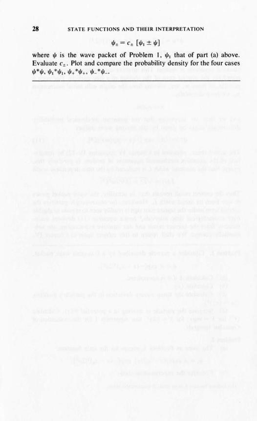
28 STATE FUNCTIONS AND THEIR INTERPRETATION
1/1± = c± [1/1\ ± 1/1]
where 1/1 is the wave packet of Problem I. 1/1\ that of part (a) above.Evaluate c±. Plot and compare the probability density for the four cases
1/1*1/1. 1/1. *1/1., 1/1+ *1/1+. 1/1- *1/1_.

IIILinear momentum
1. STATE FUNCTIONS CORRESPONDING TO ADEFINITE MOMENTUM
We have now come to understand some of the properties of state functions and have seen that our next task is to understand linear momentumas a quantum mechanical dynamical variable. The essential clue isprovided by the de Broglie description of a free particle of definite momentum p. Associated in some way with such a particle, we have argued,is a wave of reduced wavelength 1. = hlp. We now make this vaguerelationship explicit by assuming that the de Broglie wave itself is thestate function of the particle. Specifically, we write
t/J(x, t) = exp[i(xli\) - iwt]
or, expressing f... in terms of p,
t/Jp(x, t) = exp[i(pxlh) - iw(p)t], (I)
where we have attached a subscript p to t/J to denote that this state function describes a particle which is moving with definite, fixed linearmomentum p. The frequency w of de Broglie waves has not yet receivedany special attention, and in writing equation (I) we have therefore takenw to be some characteristic, but as yet unknown, function of p.
The identification of that particular state function which describes aparticle with definite momentum is an absolutely crucial step in ourmethod of development. It i offered here as a reasonably direct, buthardly unambiguous, deduction from the Davisson-Germer experiment.So there will be no misunderstanding, we state as emphatically as possible that the quantum mechanical rabbit is already in the hat, once equation(I) is accepted and under tood. Except for spin and the exclusion principle, all else follows from the correspondence principle alone.
Because of the importance of this result, we shall comment on it in

30 LINEAR MOMENTUM
some detail. Note first that we have written l/Jp as a complex exponentialfunction. This choice requires elaboration because a traveling wave cancertainly be represented by a real trigonometric function as easily asby an exponential. Indeed, all classical wave fields are actually represented by such real functions, even if complex notation is used for convenience. That this striking property is essential for quantum mechanicalstate functions can be made plausible by the following argument: Fora free particle, all points in space are physically equivalent. 10 particular,the choice of origin is irrelevant; the state of the system cannot dependin any essential way on thi choice. Suppose, now, that the origin isshifted to the left through some arbitrary distance b, by which we meanthat x i replaced by x + b. Then, as defined by equation (I), l/Jp is merelymultiplied by the physically undetectable constant phase factor eipb/h.
As required, the description of th~ state is seen to contain no physicallysignificant 'reference to the origin. This would not be the ca e were a realtrigonometric function used to represent l/Jp. In fact, if we had startedwith the most general possible traveling wave,
l/J = A cos (px/h - wt) + B sin (px/h - wt)
the demand that l/J reduce to a multiple of itself under an arbitrary translation then would at once have led u to the exponential form of equation (I ).1
Exercise 1. Prove this la t as ertion.
Still another feature of l/Jp requires comment. It is a state functioncorresponding to a total absence of localization in space. The relativeprobability density is
which means that the particle is just as likely to be found in anyonevolume element a in any other. As an immediate consequence, the statefunction l/Jp is not physically admissible, except in the weak sense referredto in the footnote following equation (11-3). Nonethele s, because l/Jp doescorrespond to a preci e value of the momentum p it is a useful idealization, as we shall at once show.
I A more conventional, and perhaps more convincing, argument can be given in terms ofthe requirement that the probability of finding the particle somewhere in space must beunity for all rimes. We shall return to the subject in Section 7 of Chapter IY.

(3)
CONSTRUCTION OF WAVE PACKETS BY SUPERPOSITION 31
2. CONSTRUCTION OF WAVE PACKETSBY SUPERPOSITION
We now give an important and instructive example of the utility of theseidealized non-physical states by combining them to form a wave packet,the most intuitively physical kind of state function. We do this by constructing a general superposition of momentum states .pp. Since thereis a continuum of possible values of p, the superposition takes the formof an integral rather than a sum and we write
.p(x, t) = • ~Jco cf>(p) exp[i(px/h) - iw(p)t] dp (2)V21Th -co
where the factor I/V21Th has been introduced for reasons of future convenience. In this superposition, ,the amplitude of the state function .ppcorresponding to momentum p is denoted by cf>(p). For the present weshall not be concerned with the time dependence of state functions orwith the relationship between wand p. We shall consider instead onlythe description at some fixed instant, which we take to be t = 0 for simplicity. We thus write, in place of equation (2),
I Jco.p(x) = -- cf>(p) eip.r'fl dp,V21Th -co
where now
.p(x) == .p(x, t = 0).
It is perhaps helpful at this stage to give an example, even if a purelymathematical one, of how a physically admissible normalizable state.p(x) can in fact be obtained by superposition of the idealized inadmissiblemomentum states exp [ipx/h]. To particularize to a very simple case,
<pCp)
c
p" Po+.).P P
FIGURE I. The momentum distribution of equation (4).

32 LINEAR MOMENTUM
let us suppose that q, (p) is constant in some interval of width 6.p on eachside of some fixed momentum Po, and is identically zero outside of thatinterval. In other words, we choose q, (p) to be a square distribution,
q,(p) = {c,0,
Ip - Pol",,;; 6.pIp - Pol > 6.p,
(4)
where c is an arbitrary constant. This means that the state we are considering is one in which the momentum does not have some preciselydetermined numerical value but is instead distributed uniformly over aband of width 26.p centered about Po, as illustrated in Figure I.
With this choice for q, (p), equation (3) becomes
1 JPO+6Pl/J(x) =-- c eiPx/fI dp
V2Trh Po-6p
or, factoring out the term e lPoX/fI and simplifying,
l/J(x) = cV2h/Tr sin 6.px/h eIPox/fI.x
(5)
This example has thus yielded a state function which is a de Brogliewave corresponding to the momentum Po, but modulated by the factor(l/x) sin (6.px/h). This factor makes l/J(x) normalizable and thusphysically admissible. To carry the example one step further, let usfix the constant c in equation (4) and equation (5) by actually normalizing l/J. We have
1 = J:", l/J*(x)l/J(x) dx = 2h;:-12 J:", sin2~px/h dx
whence, introducing the new integration variable u = 6.px/h, we obtain
lei = I/V2~p,
where we have made use of the known result
f'" sin2u-2- dU=Tr.
_'" U
(6)
(7)
To summarize, the particular momentum distribution of equation (4)yields by superposition the normalized wave packet of equation (5),provided c satisfies equation (6).
Observe that in the limit as 6.p approaches 0, we recover a pure deBroglie wave of momentum Po, that is to say
lim l/J(x) = V6.p/Trh eipoxlfl.6p-O

CONSTRUCTION OF WAVE PACKETS BY SUPERPOSITION 33
The appearance of the factor "'Vt1P, which means that the amplitude of'" becomes infinitesimal, is a consequence of the fact that the state function is not normalizable in this limit. We thus cannot proceed to the limitin the usual way. If, however, the relevant physical dimensions of ourphysical system are say L, then the state function need be consideredonly over a domain of that dimension. Hence, if I1pLlh ~ I, the normalizable wave packet state deviates undetectably from the pure deBroglie state. This means that the above limit is in fact physically achievable, which is to say that I1p can be regarded as effectively zero, providedit is much smaller than hlL. We have here an illustration of the way inwhich the non-physical and non-normalizable pure momentum statescan nonetheless serve as useful idealizations of true physical states.
Returning now to the general case, we seek to interpret the amplitude</> (p) which appears in the superposition integral defined in equation(3). Suppose we had been less ambitious and had considered the superposition of only two momentum state functions,
Evidently, this combination corresponds to a state in which the momentum is either PI or P2' with relative probability amplitudes al and a2,respectively. The more general state of equation (3) is a state in whichall possible momenta are present with probability determined by </> (p) .It is natural to assume that </> (p) is proportional to the momentum probability amplitude or the probability amplitude in momentum space. Ifp (p) denotes the corresponding probability density, we thus take theprobability that the particle has momentum between p and p + dp to be
p(p)dp= CD </>*</>dp ,
LCD </>*(p)cb(p) dp
where, as indicated, the integral extends over all momentum space.If </>(p) is normalized so that
J </>*(p)</>(p) dp= I,
then we have simply
p(p) = </>*</>, (9)
and </> (p) gives the probability amplitude directly.Accepting this interpretation, we now have a first answer to our ques
tion about the momentum as a dynamical variable. If </> (p) is given orknown, we have, in exact analogy to our procedure in x-space, or configuration space,

34 LINEAR MOMENTUM
(p ) = f pp (p) dp
= f ep*(p)pep(p) dp,
where (p) is to be interpreted as the average momentum for an ensembleof identical systems identically prepared. More generally, for anyfunction of the momentum f(p), we have
(f(p) ) = f ep* (p )f(p )ep(p) dp.
As a particular example, the expectation value of the kinetic energy is
/L)= f ep*(p) L ep(p) dp.\2m 2m
We now see how to handle the linear momentum p in a manner analogous to that used for the coordinate x. Some questions still remain,however. If ep (p) is given, we know that the corresponding I/J(x) isuniquely determined by equation (3). What about the converse - how isep(p) to be determined if I/J(x) is given? Note, moreover, that the uniquerelationship between ep(p) and I/J(x) implied by equation (3) means thatif one of these functions is normalized, there is no freedom left to normalize the other. Hence as a test of the consistency of our formulationand its interpretation, we must demand that if ep(p) is normalized somust I/J(x) be, and conversely. In the particular example of equations(4) and (5), it is readily verified that this consistency requirement isindeed satisfied. Recall that I/J(x) is normalized if lei = I/V2tip andhence, from equation (4),
JI JPO+6P
ep*ep dp = - dp = I ,2tip Po-6p
so that ep is also normalized. Of course, we must demonstrate that thisis true in general and not merely for such special examples.
To answer these and similar questions, we now make a brief mathematical digression into the properties of Fourier integrals, a integralsof the form of equation (3) are called.
3. FOURIER TRANSFORMS; THE DIRAC DELTA FUNCTION2
Recall that a function f(O), piecewise continuous in the interval-7T :s:; 0 :s:; 7T, can be represented by a Fourier series. Writing such aseries in exponential form we have
2 See items [6] through [13] in the elected list of references given in Appendix 11.

FOURIER TRANSFORMS; THE DIRAC DELTA FUNCTION 35
0:>
f(O) = LA" ei"e,
where
A" = _I J'" f( 0) e-i"e dO2rr _'"
Now replace 0 by rrx/L. We then obtain
0:>
f(x) = L A" ei"",xlL
-0:>
I JLA = - f(x) e- I'l1rxlL dx" 2L -I. •
We next want to consider the limit of these expressions when L tends toinfinity. To prepare the way, we write
kn == mr/L
11k == k"+J - k" = rr/L
whence, also,
k" = nl1k.
We next write
A" == (I/L) 'Vrr/2 g(k,,) = (I/L) v;j2 g(nl1k).
Then, putting this aJl together,
0:> v:;j2 . . 0:>
f(x) = L -- g(nl1k) e"ll1kX = YI/(2rr) L g(nl1k) e i "l1kx 11k_0:> L _0:>
g(nl1k) = YI/(2rr) fl. f(x) e-i"l1kX dx
and letting L ~ 00, so that 11k ~ 0 while nl1k ~ k, we have, finally,utilizing the elementary definition of the integral as the limit of a sum,
I JO:>f(x) = - g(k) e ikx dk\/2; -0:>
I JO:>g(k) = 4 r,;- f(x) e-ikx dx.v2rr -0:>
(II)
The symmetrically related pair of functions f(x) and g(k) are calledFourier transforms. one of the other, and the expressions of equation(II) are called Fourier integral representations.

36 LINEAR MOMENTUM
Equation (11) tells us how to calculatef(x), given g(k), and conversely. One interesting aspect of these relations is the following. Considersome arbitrary f(x) and suppose g(k) to be determined from the secondof the equations in (II). Substituting the resulting expression for g(k)in terms of f(x) back into the first equation, we then have the identity
f(x) = _I fa:> dk eikx fa:> f(x ' ) e-ikx' dx',27T _a:> -a:>
where we have introduced x I as the dummy integration variable in theintegral representation of g(k). Now take the mathematically riskystep of interchanging the order of integration. The result can be writtenin the form
f(x) = J:a:> dx' f(x ' )8(x - x') ,
where we have introduced the abbreviation
8(x - x') == _1_ fa:> eikIX-X') dk.27T _a:>
(12)
(13)
The function 8 (x - x'), first introduced by Dirac, is called the Diracdelta functioll. 3 Since f(x) is arbi'trary within wide bounds, the deltafunction evidently has very strange properties. These properties arereadily identified from the form of equation (12), which, after all, simplystates that the product of an arbitrary function f and the 8-function,when integrated over all space, yields as an answer the value assumedby f at that particular isolated point where the argument of the 8-functionvanishes. In other words, 8(z), say, singles out in the integration onlythe value of f(z) at the point z = O. The behavior of f(z) everywhereelse is irrelevant. This implies that 8(z) vanishes everywhere except atthe point z = O. At z = 0, it becomes indefinitely large, but in such a waythat it remains integrable. This last is easily made explicit by observingthat, if f(x) is chosen to be a constant, then equation (12) at once yields
3 Replacing x - x' by z, and k by y, our definition can be restated in the form
This means, for example, that in analogy to equation (13) we also have
,s(k - k') = J.... f~ ellk-k'l¥ dx.27T _~

FOURIER TRANSFORMS; THE DIRAC DELTA FUNCTION 37
J:a> 8(x - x') dx' = I, (14)
SO that the integral of a 8-function is normalized to unity.4To summarize, the significant properties of the Dirac 8-function are
defined by equations (14) and (12), respectively, and equation (13) isits Fourier integral representation. A list of additional useful propertiesare the following:
8(-x) = 8(x)
a8(±ax) = 8(x), a>O
(15)
(16)
I8(x2-a2)=- [8(x-a)+8(x+a)]
2a
fa> I(x) d8(x - a) dx = _ dfl .-a> dx dxlx=a
( 17)
( 18)
The proof of these relations is left to the problems.As a final mathematical point we now mention the convolution theorem.
Suppose II (x) and 12 (x) are given arbitrary functions with Fourier transforms gl (k) and g2(k), respectively. This theorem states that
The proof is not difficult, but it provides an instructive exercise in themanipulation of Fourier integrals. Substitution of the Fourier integralrepresentations for II (x) and 12(X) gives
Jdx e-ikx II (X)/2(X) = 2~ Jdx e-ikx Jdk' gl (k') eik'x
x Jdk" g2(k") eik"X.
Noting that the dependence on x of the right side is explicit, we interchange the order of integration and evaluate the integral over x first.Specifically, we write
• An alternative version of our argument can be constructed as follows. Consider equation(12) for fixed x, say x = b. Suppose f(x) to be altered by some arbitrary amount 'I)(x) inthe infinitesimal neighborhood of any point a ~ b. The left side of equation (12) is unchanged; it remains f(b), and hence the additional contribution on the right must yieldzero. This at once implies lj (a - b) = 0, b ~ a, in agreement with our conclusion above.Incidentally, it may help the student to visualize the properties of the lj·function if heconsiders it to be the limit of a sharply peaked but perfectly well·behaved function, forexample, a Gaussian, as discussed in the problems.

38 LINEAR MOMENTUM
J dx e-i4".r I. (X)j;(X) = J J:", dk' dk" g. (k')g2(k")
X _I Jd i(4""+4"'-4")x271' x e .
The la t factor is now recognized as 8(k" - k + k') according to equation (13). Finally, evaluation of the integral over kIf gives the statedresult. As a special ca e we note that
J:J*(x)/(x) dx= J:", g*(k)g(k) dk.
Exercise 2. Prove equation (20).
4. MOMENTUM AND CONFIGURATION SPACE
(20)
We are now in a position to provide a precise relationship between wavefunctions in configuration space, t/J(x), and in momentum space, cf>(p).We had as equation (3)
I f'"t/J(x) = -- cf>(p) e ipx/f1 dpY27Th -'"
whence, according to equation (I I),
I f'"cf>(p) =-- t/J(x) e- iPX/fi dx.Y27Th -'"
(21)
Note that only in a system of units in which h = I, often used by physicists, is cf> the Fourier transform of t/J. More generally,
~(plh) == Vi" cf>(p)
is its transform, the transform variable being plh = 271'1>" == k, where kis recalled to be the (reduced) wave number. With this identification,equation (20) becomes, with/= t/J, g = Vi" cf>,
f t/J*t/J dx = f cf>*cf> dp
and the condition that t/J and cf> be imultaneously normalizable is indeedsatisfied.
We have now established two completely equivalent representationsof, or ways of writing, a given state function, one in configuration space,one in momentum space. Neither contains more information than theother, neither has special claims to distinction. Together, they permitus to treat position and linear momentum on an equal footing as dynamical variables.

THE MOMENTUM AND POSITION OPERATORS
5. THE MOMENTUM AND POSITION OPERATORS
39
Given some state function, t/J(x) , we now know how to calculate expectation values of any function of position, or of any function of momentum.In the latter case, we must calculate the state function in momentumspace, or briefly, we must transform to momentum space. This procedureis clearly rather roundabout and inefficient. Can we not instead calculateexpectation values of momentum from t/J(x) directly? More than amatter of convenience is actually involved, since our present techniquewill not permit us to calculate expectation values of mixed functions ofposition and momentum, such as angular momentum, for example.
To answer our question, consider first
(p) = I cP* (p)PcP(p) dp.
Using equation (17) to express cP(p) in terms of t/J(x) and similarly forcP* (p) in terms of t/J* (x), we obtain
(p) = 2:m I I I dp dx dx' t/J* (x') eiPx'lft p t/J(x) e-ipJ'lft. (22)
Now the dependence on p is explicit and we therefore seek to performthe p integration first. This integration becomes very simple if the factorp in the integrand is eliminated. To do so use the fact that
(23)
as is readily verified by performing the indicated differentiation on theright-hand side. Introducing this result into equation (22), we obtain
(p) = _1- I I I dp dx dx' t/J* (x') eip-r'lft t/J(x) (-~ .!!-. e-IIJXlft).27Th I dx
Next integrate with respect to x by parts. The integrated part i~ proportional to the value of t/J(x) at infinity and hence is zero for physicallyadmissible state functions because all such functions necessarily vanishat infinity. Thus the result of the integration by parts is
(p) = _1- I I I dp dx dx' t/J*(x')[eiP<X'-xl/ll] ~ dt/J(x).27Th I dx
The p integration is now easily performed and we obtain
() III d d ' .,.*( ') _fi.l d·I,(x) ~(.yl - x)p= xx'/'x '/'V"I dx
whence, finally.
h d(p) = I dx t/J*(x) -:- -d t/J(x).
I x(24)

40 LINEAR MOMENTUM
Next consider the expectation value of p" for arbitrary n. We have,using the same technique,
(p") = I ep*(p)p"ep(p) dp
= _1- I I I dp dx' dx l/J*(x') e,px'/A p" l/J(x) e-iPxlA27Th
or
(p") = _1- I I I dp dx' dx l/J* (x') eiPX'/A l/J(x) (-~ ~)" e-ivxlA (25)27Th I dx
where, in the last step, we have used the following generalization ofequation (23):
_. (h d)" _. (h)" d"(e-iVxIA )p" e IPxlA = -j dx e ,pxlA == -j dx'" (26)
Integration of equation (25) by parts with respect to x, n times repeated,then yields, since the integrated part always vanishes,
(p") = _1- I I I dp dx' dx l/J*(x') eiP(X'-X)/A(~~)" l/J(x).27Th I dx
Again the p integration yields 27Th 8(x' - x) and hence, after the integration over x' is performed, we obtain as the final result
(h d)" (h)"d"l/J(X)(p")=Idxl/J*(x) -;-- l/J(x)==Idxl/J*(x) -;- '(27)I dx I dx"
To generalize still further, consider any function f(p) which can beexpanded as a power series in p. By an obvious extension ofthe argumentwe then have
(f(p» = f l/J*(x)f(~ fx)l/J(x) dx. (28)
We intend to draw a deep and important conclusion from this result,so let us first make sure we understand precisely what it says. By hypothesis, f(p) is expressible as a power series in p. Imagine f to be soexpressed,
f(p) = 2: G" p".
"Then equation (28) can be written in the form
(f(p» = 2: G" (p"),/I
each term of which can be evaluated using equation (27). Evidentlythis is not a very useful or practical way to deal with complicated func-

THE MOMENTUM AND POSITION OPERATORS 41
tions of the momentum; it is much simpler to do so by transforming tomomentum space. Indeed, we remark parenthetically, for functionswhich cannot be expanded in a power series, no alternative to this latterprocedure is possible.
Our concern at present, however, is more formal than practical. Specifically, we observe that we can rewrite equation (28) in the followingway,
(f(p» = J:", l/J*(x)f(p)l/J(x) dx, (29)
provided we understand that the momentum p in the integrand is to bereplaced by the differential operator (h/i)d/dx which acts on the functionl/J (x) standing to its right. This replacement can be restated as follows:In configuration space, the linear momentum is represented by theoperation of space differentiation multiplied by hli,
by which we mean that
h d ll,pl/J(x) ="7 ~
I dx
or, more generally, that
(hd)" (h)"p"l/J(x) = i dx l/J(x) = i d".p(x)dx"
(30)
(31)
(32)
/
Strictly viewed, our argument appears to admit this interpretation ofthe momentum as a differential operator in configuration space onlyinsofar as the calculation of expectation values is concerned, that is tosay, only in an expression such as that of equation (29). We now extendthis interpretation by accepting equation (30) as a general statement,the operational content of which is expressed by equations (31) and (32)as they stand, quite independently of the calculation of expectationvalues. This generalization is a conceptual one, and an unusually usefulone as we shall abundantly show, but we emphasize that no additionalphysical assumptions are implied by it. This follows because every observable or measurable consequence of quantum mechanics is ultimatelyexpressed in terms of expectation values, and hence in terms of integralsover quadratic functionals of the state function, as equation (29) illustrates.
We have thus far confined our attention to the properties of the momentum in configuration space. What can we say about the properties of the
, position in momentum space? By exactly parallel arguments, which are
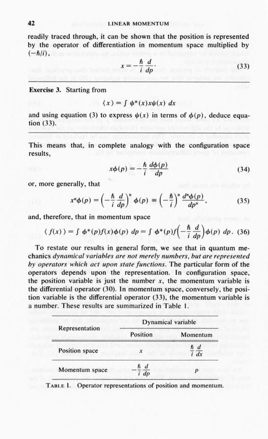
42 LINEAR MOMENTUM
readily traced through, it can be shown that the position is representedby the operator of differentiation in momentum space multiplied by(-fili) ,
Exercise 3. Starting from
fi dx=---'
i dp(33)
(x) = I l/J*(x)xl/J(x) dx
and using equation (3) to express l/J(x) in terms of cfJ (p), deduce equation (33).
This means that, in complete analogy with the configuration spaceresults,
or, more generally, that
xcfJ(p) = -~ dcfJ(p)I dp
(34)
(35)x"cfJ(p) = (_~~)" cfJ(p) == (-~)" d"cfJ(p) ,I dp I dp"
and, therefore, that in momentum space
(f(x» = I cfJ*(p)f(x)cfJ(p) dp = I cfJ*(p)f(-~ ~)cfJ(p) dp. (36)
To restate our results in general form, we ee that in quantum mechanics dynamical variables are not merely numbers, but are representedby operators which act upon state functions. The particular form of theoperators depends upon the representation. In configuration space,the position variable is just the number x, the momentum variable isthe differential operator (30). In momentum space, conversely, the position variable is the differential operator (33), the momentum variable isa number. These results are summarized in Table I.
Dynamical variableRepresentation
Position Momentum
Position spaceft d
x j dx
Momentum spaceft d
-j dp P
T ABLE I. Operator representations of position and momentum.

THE MOMENTUM AND POSITION OPERATORS 43
Our characterization of dynamical variables at the quantum level hasled us to introduce the concept of an operator. We shall encounter suchentities with increasing frequency as our development continues. Beforegoing on, therefore, let LIS briefly summarize their relevant properties.
Any unambiguous rule by which one function is changed to some otherfunction is called an operation, and the ab tract representation of thisprocess is called an operator. Symbolically, we thus write
Af(x) =g(x), (37)
where the operator A is defined over a given class of functions if g isdetermined for every f in that class. This may sound complicated, butit is actually a mere formalization of what we are already thoroughlyaccustomed to doing. This is perhaps made clearer by the examplesgiven in Table II. Observe first that although the left side of equation
Operation
Multiplication by 2Multiplication by e1d>(x)DifferentiationSquaringComplex conjugation
Equation (37)
AJ= 2JAJ= efd>JAJ= dJldxAJ=j2AJ=f*
Symbolic representation
A =2A =e1d>(x)A = dldxA =?A=?
T ABLE II. Examples of operalions and operators.
(37) has the appearance of a product (and indeed is a product when A isa number or some given function of x, real or complex), there is generallynothing very much like an ordinary product involved. Observe also thatoperators exist, and are perfectly well defined, which have no conventional or simple symbolic representation, as indicated by the questionmarks in the right-hand column of Table II for the last two examples.
The operators we shall meet in quantum mechanics are linear operators. that is to say, operators such that
(38)
All of the operators in Table II are linear except the squaring operator.That the quaring operator is non-linear follows at once from the factthat
which i clearly different than
Afl+Af2 =f, 2 +f/·
We shall frequently be concerned with equences of operations,

44 LINEAR MOMENTUM
carried out one after the next. Thus, for example, we shall encountersituations in which an operator B acts on some function and an operatorA then acts on the result. The net result defines a new operator, say C.Then we can write
Cfa A(Bf). (39)
It is customary to omit the parenthesis on the right and to express thisrelation in the form
Cf=ABf,
which then implies the purely operator statement
C=AB,
whereby C is called the product of A and B. We emphasize that themeaning of such a product is precisely that expressed by equation (39),The square of an operator is to be regarded as a special case of a product.Products of more than two operators, or higher powers of a given operator, are defined by successive application of the rule for products. Thus,for example,
C=A.A 2 ,'·A/I
means the result of successive operation~ by A /I first, then A /I-I, and soon down to A •.
To give some specific examples, let A denote mUltiplication by eid>(X)
and B denote differentiation with respect to x. Then
A Bf= eil/>(x) dfdx'
ABAf= ei<l>(X) ix [ei<b(.rlf(x)] ,
B2f= d2fdx 2 '
and so on.Observe that the order of the operators in a product uniquely deter
mines the order in which these operators act. The result, in general,depends on this order, which is to say that, in general,
AB ¥- BA
and the algebra of operators is nOll-commutative, in contra t to thealgebra of ordinary numbers. For the particular operators A and B above,we see that

COMMUTATION RELATIONS
BAf= :x [ei~x) f],
45
which is clearly different than ABf, as given above. Similarly, if C isthe operator of complex conjugation, then
ACf= e icb f*(x)
but
CAf= e-icb f*(x).
On the other hand, for the particular operators Band C defined above,the results obtained are easily seen to be indifferent to the order ofoperation, whence
BC=CB,
and these operators are then said to commute with each other, or to bemutually commutative.
6. COMMUTATION RELATIONS
An obvious aspect of the fact that dynamical variables must be regardedas operators is that dynamical quantities which are indistinguishableclassically may become quite different in the quantum domain. An important example is the product xp compared to px. Classically these areidentical, but that they are not identical in quantum mechanics followsby letting each operate on some arbitrary state function. Thus, in configuration space, we have
Ii d Ii d.pxp.p(x) = x-;- -.p = -;- x-
Idx I dx
and
-!!:!!.. -!!: !!: ~px.p(x) - . d (x.p) - . .p + . x fix'I X I I
whence
Ii(px - xp).p = -;- .p.
I(40)
Since .p is arbitrary, this implies that the difference between px and xpis the purely numerical operator hli,
Ii(px-xp) == (p,x) =-;-.
I
The difference between the products of two operators in the two possible

46 LINEAR MOMENTUM
orders is called the commutator, and we have introduced a specialnotation to represent this important quantity. Thus, if A and B are arbitrary operators,
(A, B) == AB - BA =- (B,A). (41)
In contrast to ordinary multiplication, multiplication of dynamicalvariables in quantum mechanics is noncommutative.
It is also instructive to examine the commutator of p and x in momentum space. We have
fi d fi fi debxPcb(p) = --;- - (pcb) = --;- cb - -;- p-
1 dp 1 1 dp
and
(h d) fi debpxcb(p) =p --;-- cb=--;-p-,1 dp 1 dp
whence
fi(p, x)cb = (px - xp)cb = -;- cb·
1
Since cb is arbitrary, we again conclude that
(p, x) = fiji.
We thus see that although the particular form taken by p and x dependson the representation, their commutator does not. The commutationrelation (40) can thus be regarded as the fundamental statement of theproperties of the quantum mechanical dynamical variables representingmomentum and position. Note that h enters as the quantitative measureof noncommutativity. In the classical limit, where fi can be regarded asvanishingly small, the classical commutivity is seen to be recovered.
It is easy to generalize the commutation relation (40) to functions ofthe dynamical variables. Thus, for example, consider [p, f(x)] forarbitrary f(x). We have at once
[ f()] =!!:. df(x)p, x i dx '
which is most easily verified in configuration space. Similarly,
(42)
(43)[f(p) , x] = ~ dfd(p) ,1 P
as is easily verified in momentum space. On the other hand, of course,
[p,f(p)] = [x,f(x)] = 0 (44)

THE UNCERTAINTY PRINCIPLE
whence it also follows that, if f(x, p) is a well-defined operator,S
[f( )] =!!:. af(x, p)p, x, P i ax
while
[f(x,p),x] = ~ af~,p).I p
These latter are equivalent to
f(x, p) = f(x, ~ :Jin configuration space and to
f(x,p) =f(-~ ~,p)
in momentum space.
7. THE UNCERTAINTY PRINCIPLE
47
(45)
(46)
(47)
(48)
The noncommutativity of quantum mechanical operators, some specialexamples of which we have just been studying, has direct physicalsignificance in terms of measurements or observations. The specification of a particular state function implies that the system in questionhas been prepared by a sequence of observations. Measuring the valueof a given dynamical variable is equivalent to operating upon the statefunction with the operator representing that variable, as we shall elaborate upon later. In general, measurement produces a disturbance of thesystem at the quantum level. Consequently, measurement of propertyA need not yield the same result if carried out after property B is measured than if carried out before, since the disturbance produced bymeasuring B may well cause changes in the value of A. If that is the case,then A and B do not commute. If, on the other hand, there is no interference, then A and B do commute.
The uncertainty principle is concerned precisely with the questionof the interference produced by observation. Later we shall establishan exact general relationship between the mutual uncertainty in a pairof observables and their commutator. We now give a somewhat qualitative discussion in terms of the simultaneous determination of theparticular variables position and momentum.
At the beginning of thi chapter we saw that the state function .pI} of
• By a well-defined operator. we mean one for which the order of the non-commutingelements is unambiguously specified in every term of it power series development.

48 LINEAR MOMENTUM
equation (1), which describes a particle with precisely defined momentum, contains no information at all about the location of the particle. Todescribe a localized particle, it was necessary to construct a wave packet.From the form of equation (3), representing such a packet, we see thatthe momentum is then no longer precisely fixed but is distributed overa range of values, determined by the structure of <f>(p). This behavior,in' which one of the variables p or x becomes Jess sharpLy fixed as theother becomes more so, is a significant general feature that we nowbriefly examine.
As a starting point, we discuss two particular wave packets as examples.
(a) Square-Wave Packet. Consider first a normalized square-wavepacket defined by
=0 Ixl > L,(49)
which is seen to consist simply of a piece of a plane wave, correspondingto momentum Po, of length 2L and centered at the origin. According toequation (21) we then have
I fL ei(/?o-p)x/fl
<f>(p) = Y2'TTn -L V2L dx
or
and
<f>(p) = Yh/'TTL sin [(Po - p)Lln]Po-P
(50)
(51 )<f>*<f> =!!:.- sin 2 [(Po - p) Lin] ,'TTL (Po - p)2
which is plotted in Figure 2. As indicated in the figure, the height of the
---------r-----
p" p
FIGURE 2. Distribution of momenta for a square-wave packet.

THE UNCERTAINTY PRINCIPLE 49
main peak, centered at Po, is proportional to L and its width is inverselyproportional to L. 6 The area under it is thus seen to be independent ofL and close to unity. In other words a wave packet which localizes aparticle within a distance !:u = 2L is localized in momentum within arange 6.p = fmlL. Hence 6.x6.p is of the order of Ii and is independentof L. For large L, the momentum becomes well defined, the space location poorly defined, and conversely for small L, and always in such away that the product of the uncertainty in x and that in p is of the orderof ~.
(b) Gaussian Wave Packet. As a second example, we consider a normalized Gaussian wave packet
"'(x) = vIILV"7r exp [iP()X -~]'I' Ii 2V' (52)
which describes a particle localized about the origin within a distanceL and with mean momentum Po. In momentum space it turns out, usingthe techniques of Appendix I, that this packet is given by
(53)
which is again a Gaussian, of width inversely proportional to L. Moreprecisely, it is seen that the momentum is localized within a range fi/L,centered about Po. Thus once again, the product of the uncertainties isof the order of Ii .
Exercise 4. Calculate (x) and (p) in both the configuration and momentum space representations for the square wave packet [equations (49)and (50)] and the Gaussian packet [equations (52) and (53)].
The relationship between the width of a wave packet in configurationspace and its width in momentum space has been shown to be approximately the same for both square and Gaussian wave packets. We nowverify that this is a general feature by examining a general wave packet,which we write in the form
(54)
We shall take f(x) to be a real, relatively smooth function of x, of width
6 The height of the peak is obtained by taking the limit as (p - Po) approaches zero inequation (5 I). The width is measured by the location of the first zero of the sine function,which occurs when its argument is 7T.

50 LINEAR MOMENTUM
L, centered about the origin. We shall also assume'" to be normalized,which means that
f:", J2(x) dx = I.
It is easily verified that for such a wave packet, the expectation valueof the momentum is Po.
Exercise 5. Verify that (p) = Po for the wave packet of equation (54).
For this wave packet, the state function in momentum space is givenby, according to equation (21),
c/>(p) = _1- f f(x) ei(P......P)Xlfl dx.Y2'TTfi -'"
By hypothesis, f(x) is a relatively smooth function peaked about theorigin and of width L. This means that the principal contribution to theintegral comes from the domain Ixl ~ L. Hence if
the argument of the exponential factor is negligible over the effectivedomain of integration and c/>(p) is roughly constant and proportional tothe area under the function f(x). As (Po - p) increases, the exponentialbegins to oscillate and eventually it oscillates very rapidly over theeffective domain of integration, so that the integral, and thus c/>(p) ,becomes very small. The dividing line between these two regions ofbehavior comes for
(Po - p) L/fi = I,
which is when the oscillations begin to occur. In other words, when thiscondition is satisfied, c/>(p) begins to significantly decrease from itsmaximum value at p = Po. Thus the width of the wave packet in momentum space is approximately
t::.p = filL.
But the width in configuration space, t::.x, is just L and hence
t::.pt::.x = fi, (55)
providedf(x) is smooth.Supposef(x) is not smooth but contains some structure. Then (Po - p)

THE UNCERTAINTY PRINCIPLE 51
must become larger than before if the oscillations of the exponentialare to become rapid compared to the distance characterizing this structure and cf>(p) is to begin to decrease significantly. Thus the width t::.pof the wave packet in momentum space becomes correspondingly larger,and equation (55) represents the best we can do in the sense that, moregenerally,
t::.pt::.x ~ Ii. (56)
Later we shall define precisely what we mean by t::.x and t::.p and hallobtain a correspondingly precise inequality. For now, we simply regardeach of these quantities as some reasonable measure of the width of awave packet in configuration and momentum space, respectively.
The physical interpretation of this mathematically trivial relation isthe following. If a particle is localized in some region t::.x, no matter themeans, then its momentum will necessa!"ily be localized at most withint::.p and conversely. In other words, the position and momentum of aparticle cannot be simultaneously known (or determined or measured)with arbitrary precision, but only within the limits of the relation, equation (56), which is a mathematical, if not yet very accurate, version ofthe uncertainty principle, first enunciated by Heisenberg. The uncertainty principle convincingly demonstrates that clas ical trajectorieshave no precise meaning in the quantum mechanical domain.
More generally, the uncertainty relation holds between any pair ofcanonically conjugate, or complementary, dynamical variables. As asecond example, if the energy of a system is mea ured within t::.E, thetime to which the measurement refers is uncertain within an interval t::.tsuch that
t::.Et::.t > Ii. (57)
It takes increa ingly longer to measure the energy of a system to increasing accuracy. An important aspect of this result is the informationit provides about the decay of excited state. In particular, the meanlifetime and the energy width of such states are related by equation(57). For an example, ee Section 3 of Chapter V II.
From our discussion, we see that the uncertainty relation are automatically built into quantum mechanics. In term of measurement,the e relations are a consequence of uncontrollable transfers of energyand momentum which necessarily take place, during the proce s of measurement, between the measuring apparatus and the system whose properties are being measured. As an example, consider localization of they-coordinate of a particle by a slit (Figure 3). If the lit has aperture L,

52 LINEAR MOMENTUM
p,,------~~
FtGURE 3. Localization of a particle by a slit.
as indicated, so that .iy = L, the diffraction pattern produced will haveangular width 0 = A/L = h/PoL = h/po.iy. The uncertainty of the y component of momentum is .ip" = Po sinO = PoO. Hence .ip".iy = h, inagreement with the uncertainty principle. A second standard exampleis the use of a microscope to locate a particle. To localize a particlewithin a distance .ix, the wavelength of the light in which it is viewedmust be of order ~ < .ix. The momentum of the photon is then of orderp ;::: h/.ix. The particle is seen- because of the photon it scatters orabsorbs, and the momentum transferred to it in the scattering processis seen to be of the order h/.ix, as the uncertainty principle demands. 7
As implied earlier, it is important to recognize that the uncertaintyprincipal is an integral part of quantum mechanics, as well as a naturaland direct consequence of it. In a purely quantum mechanical treatmentof a problem, the question of violating the uncertainty principle neverarises. To the extent that quantum mechanics in its present form iscorrect, then the uncertainty principle necessarily follows. This is notto say, of course, that even within the framework of quantum mechanicsthe uncertainty principle is in any sense empty. On the contrary, it isan extremely useful guide to the understanding of the quantum mechanical properties of a system. Indeed, for ystems too complicated to permitcomplete or exact solutions, it often provides a basi for deciding whethergiven effect exist or not.
As an example of where it provides very significant qualitative, andeven semi-quantitative, understanding, consider a particle confined to
7 For a detailed di cu ion of this and other examples, see Reference [18].
THE UNCERTAINTY PRJNCIPLE 53
some region of radius a by an attractive potential V(r). For each of itscoordinates, the uncertainty in position is of the order a, and hencet::.p = Ma. The mean momentum being zero, this is of the order of themomentum itself and hence the mean kinetic energy (T) of the particlecannot be less than Ii 2/2ma2. The mean potential energy (V) is of theorder V(a). Hence the total energy £ is approximately given by
li2£(a) = (T) + (V) = 2 2 + V(a).
ma(58)
We observe in this expression a clear competition between kinetic andpotential energies which is strictly quantum mechanical in origin. Asa becomes smaller, the potential energy decreases for attractive interactions, but the kinetic energy always increases. A rough estimate ofthe minimum possible energy of the system, or ground state energy,is obtained by differentiating equation (58) with respect to a and settingthe result equal to zero. As a specific example, consider the hydrogenatom where the confining potential is the Coulomb potential, (-e2/r).The total energy is thus approximately
li2 e2£(0) = ----.
2ma2 a
This expression is easily found to assume its minImum value whena = Ii2/me2 , which is recognized to be just the Bohr radius, and theminimum energy is (-me4/2h 2 ), which is recognized to be the correctenergy of the ground state.8 The mere existence of a ground state alreadycompletely explains why atoms do not collapse, as the classical prediction would have it. Because the energy is an absolute minimum, the atomsimply cannot lose energy, by radiation or any other means, and thesystem is stable.
This example is a most instructive one. The uncertainty principle hasbeen used to explain the existence of a ground state, and thus to accountfor the existence and stability of atoms, and it has provided us with asimple method for estimating what that energy is, at least for the hydrogenatom. With reference to the hydrogen atom, in particular, the uncertaintyprinciple has enabled us to identify the essential characteristics of a relatively complex system, ufficiently complex that we shall not be in a position even to formulate the problem. let alone solve it, until Chapter IX.
" Our apparently casual choice of numerical factors in estimating (T) and ( V). each ofwhich is actually uncertain by a factor of two or more. was in fact designed to provideus with the correct answers for the hydrogen atom. This minor swindle in no way affectsthe essential nature of the results.

54 LINEAR MOMENTUM
Problem 1.(a) Consider the function 11 (x) defined as
l1(x) = _I ft eik:r dk.27T _I.
Evaluate the integral and show that l1(x) has the properties of 8(x) whenL --+ 00.
(b) Consider the function
11 (x) = _1- foo eik:r-nlk'l dk.27T -00
Show that l1(x) behaves like 8(x) in the limit a --+ O.(c) Consider the function 11 (x) = A e-x2
/b2
• Show that if A i properly chosen, l1(x) behaves like 8(x) when b --+ O.
(d) Show the following:(I) 8(-x) = 8(x).(2) a8(±ax) = 8(x), a> O.(3) 8(x2
- (2
) = ~ a[8(x - a) + 8(x + a)].(4) J~oof(x)8'(X-a) dx=-f'(a), where the prime denotes
differentiation.
Problem 2. Find the Fourier series representation of the followingfunctions in the interval - L < x < L:
(a) f(x) = x.(b) f(x) = Ixl.(c) f(x) = I.(d) f(x) = e-n1xl .
For case (d), compare the behavior of the Fourier series amplitudesin the limit aL ~ I with the behavior of the Fourier transform of e-nl:rl.
Problem 3. Find the Fourier transforms of the following functions:
(a) f(x) = {x ,Ixl < Io ,Ixl ;;;. I.
(b) f(x) = {ixi ,Ixl < Io ,Ixl ;;;. I.
(c) f( r) = { I - lxi, Ixl < I. 0 ,Ixl ;;;. I.
Problem 4. Consider the wave packet IjJ = A exp[-( Ixll L) + ipoXlli] .(a) ormalize 1jJ.(b) Calculate cf>(p) and verify that it is properly normalized.(c) Examine the width of the wave packets in configuration pace
and momentum space and verify that the uncertainty relations aresati fied.

PROBLEMS 55
Problem 5. Calculate the following commutators, using whicheverrepresentation is most convenient.
(a) (p, x 2 ).
(b) (p3,X).(c) (p2, x 2).(d) [p2,J(X)].
Problem 6. The operators A I, A 2 , ••• , A 6 are defined to act as followsupon an arbitrary function tjJ(x): AI multiplies tjJ(x) by x 2 , A 2 squarestjJ, A 3 averages tjJ(x) over an interval 2L centered about x, A 4 replacesx by x + a, A 5 replaces x by -x, and A 6 differentiates tjJ twice.
(a) Write out an explicit expression for A itjJ(X) in each case.(b) Which of the A I are linear operators?(c) Which pairs of the A I commute?
Problem 7. Use the uncertainty relation to estimate the ground stateenergy of the following systems:
(a) A particle in a box of length L.(b) A harmonic oscillator of classical frequency w.(c) A particle sitting on a table under the influence of gravity.
Problem 8. Let Xo and Po denote the expectation values of x and p forthe state tjJo (x). Consider the state tjJ (x) defined by
tjJ(x) = e-fPoJlh tjJo(xo+ x).
Show that both (x) and (p) vanish for this state. Does this violate theuncertainty principle? Explain.
Problem 9. A particle of mass m moving in a potential V(x) is in itsground state tjJo(x). Suppose tjJo to be known, but not necessarily normalized.
(a) Write an expression for the probability that a measurement ofthe particle's momentum would yield a value between p and p + dp.
(b) Write an expression for the probability that a measurement ofthe particle's kinetic energy T would yield a value between T and T + dT.Check your result by verifying that you get the correct expression forthe expectation value of T.
Problem 10. Consider a state function which is real, tjJ(x) = tjJ*(x).(a) Show that (p) = O. What about (p2)? (x)?(b) Under what conditions on tjJ(x) is cP(p) real, and what then
is (x)?

IVMotion of a free particle
1. MOTION OF A WAVE PACKET; GROUP VELOCITY
We have thus far been concerned with the state function of a system atsome fixed instant. We now begin our discussion of how such statesdevelop in time. In the present chapter we shall consider the simplestpossible problem, namely that of the motion of a particle free fromexternal influences. As a starting point, we return to equation (2) ofChapter Ill, which provides a general description of a free particle wavepacket
I fOCl [iPX ]l/J(x, t) = V27Th -0Cl c/>(p) exp h - iw(p)t dp, (I)
where w(p) is as yet unknown. We shall assume that l/J is prescribedat t = 0, and we shall denote its initial value by l/Jo(X) ,
I f'"l/Jo(X) = l/J(x, t = 0) =~ c/>(p) e IPz,,, dp.V27Tfi -'"
(2)
Our problem then is, given an initial wave packet l/Jo (x), how does itdevelop in time? That is, what is l/J(x, t)?
As a preliminary step, and as an example, we first consider dispersionless propagation (as in the propagation of light in free space) wherew is proportional to p/fi. The constant of proportionality has the dimensions of a velocity and we denote it by c. Thus, in this example,
w = cp/fi = 27TC/"A
and (I) becomes
I fOCll/J(x, t) =-- c/>(p) eiP(z-cm" dp.V27Th '"

MOTION OF A WAVE PACKET; GROUP VELOCITY 57
Comparison with equation (2) then shows that ljJ(x, t) is exactly the samefunction of (x - ct) as ljJo is of x. In other words,
ljJ(x, t) = ljJo(x - ct),
and the wave packet simply travels to the right with velocity c, withoutdistortion, whatever its initial shape. I
We now go back to the general case where w(p) is unknown. Wecannot, of course, calculate anything for arbitrary w(p) and for a completely arbitrary wave packet. However, we do not need to particularizetoo much in order to determine the essential features. The first assumption we shall make is that c/> (p) is a smooth wave packet in momentumspace, centered about Po, say, and of width li.p. To emphasize thisbehavior we rewrite c/>(p) in the form
c/>(p) = g(p - Po),
where g is a smooth function which falls rapidly to zero when its argument exceeds t:.p in magnitude. This means that the main contributionto the integral in equation (I) comes from a region of width t:.p about thepoint Po.
Secondly, we assume that w(p) is a smooth function of p. If so, wecan expand w in a Taylor series about Po.
dw (p ) d 2ww(p) = w(Po) + (p-Po) dpo 0 +t (p_pO)2 d
p02 + ..
== wo + (p - Po) ~ + (p - Po)2 a + .. "
where
wo = w(Po)
dwv =h-g dpo
d 2wa = t dp02'
Introducing also the new variable s = p - Po. we can now rewrite equation (I) as
ljJ(x, t) = f(x, t) exp [ ip;x - iwot] ,
'Our treatment of this problem in optical propagation is considerably over implified.The case where wand p have opposite sign, w = -cp/". must al~o he considered. The motion of a wave packet in optics accordingly is /lot determined if only l/Jo(x) is given. Inaddition, it turns out that al/J/at (x. t = 0) must be prescribed. This is a consequence of thefact that the electromagnetic wave equation is of second order in the time.

58 MOTION OF A FREE PARTICLE
where f(x, t), which determines the envelope of the wave packet, isgiven by
I foo [is ]f(x, t) = •~ ds g(s) exp ""i: (x - vot) - ias2t + . .. .v 27Th -00' fL
At the same time, equation (2) becomes
l/Jo(x) = fo(x) eiPoxll,
where fo(x), the initial envelope function, is given by
I foofo(x) = f(x, t = 0) = -- ds g(s) eisx"I.Y27Th -00
(3)
(4)
Now the main contribution to these integrals comes when s is lessthan 6.p in magnitude, because of the assumed behavior of g (s). Hence,if t is small enough that
the term in the exponent of equation (3) which is quadratic in s can beneglected and the envelope function is approximately
I foo .f(x, t) = -- ds g(s) e'·...x-l.'of)J~.Y27Th -00
Comparison with equation (4) then shows that, to this approximation,f(x, t) is the same function of (x - vot) as isfo of x, that is to say,
f(x, t) = fo(x - Vgt).
We have thus demonstrated that for t ~ to, where
I 2t - ~.,..----,-: - ...,....,---,--=-:-:,..--,--,----:0- a(6.p)2 - (6.p)2d2w/dp02
the wave packet travels undistorted with velocity Vg , where
Vo = hdw/dpo·
(5)
(6)
(7)
The quantity Vo is called the group velocity of the waves, since it represents the velocity of propagation of a group of waves, namely those whichmake up the wave packet. It should be contrasted with the phase velocity,which is the velocity with which the phase of a given pure harmonicwave advances and which is given by Vp = hw/po. For dispersionlesspropagation, where w is proportional to p, .these two velocities are equal,but in general they are quite different.
We emphasize that our result holds only for times short compared toto, defined in equation (6). Eventually, when t exceeds to, the exponential begins to oscillate very rapidly for s smaller than 6.p. When that

THE CORRESPONDENCE PRINCIPLE REQUIREMENT 59
happens, the effective domain of integration in p is reduced in size andthis produces a corresponding increase in the width of the wave packetin configuration space. This means that, in general, a wave packetinitially travels undistorted with the group velocity vg, but eventuallybegins to spread out in space. We shall give some examples later.
2. THE CORRESPONDENCE PRINCIPLE REQUIREMENT
We now use the following argument to deduce the form of w(p) forquantum mechanical waves. If we have a well-defined wave packet inconfiguration space, we have seen that it travels with the group velocityV g , at least for short enough times. In the classical limit, this limitationon the time must become unimportant, that is, to must become very largecompared to all relevant times. Assuming this to be so, we accordinglydemand that
v - v - Po9 - classical - m .
Hence, from equation (5)
Ii dw =Podpo m
and, dropping the subscript on Po,
2
liw=L=E2m '
(8)
which is the Planck relation. In a sense, we have thus deduced the Planckrelation as a consequence of our formulation and its interpretafion.2
Note that equation (8) is arbitrary up to a constant of integration,which we have simply set equal to zero. This is related to the freedom ofchoice of the zero of energy and implies a similar freedom in the choiceof quantum mechanical frequency. Only differences in energy, and alsotherefore in frequency, are physically significant.3
We next examine the time to at which a quantum mechanical wavepacket begins to spread out significantly. We have, from equations (6)and (8),
2 Our argument demonstrates that equation (8) must hold in the classical domain. At thequantum level, one might suppose that additional terms could logically enter, providedthey contribute negligibly in the classical limit. However, it is not hard to show by dimensional arguments that for free particles no such terms can exist and that equation (8) istherefore unique, up to an additive constant.
3 We saw earlier that the absolute amplitude of quantum mechanical waves has no physicalsignificance and we now see that the absolute frequency has none either. The contrastwith classical waves is remarkable and complete.
60 MOTION OF A FREE PARTICLE
2mhto = (ap)2' (9)
An instructive way to rewrite this is to use the uncertainty relation toexpress 6.p as h/ax, where ax is the spatial extent of the initial wavepacket. Thus
2m(6.x)2to = h .
For a macroscopic particle, say of mass one gram, whose position isdefined to even 10-4 cms (I micron), we have
to = 1019 sec.
The age of the universe is about 3 x 10¹⁰ years or about 1018 sec. Hence,a wave packet for a macroscopic particle holds together without spreading for a period comparable to the age of the universe. This establishesthat classical trajectories for macroscopic systems are not in conflictwith quantum mechanics. On the other hand, for an electron whose position is defined to say 10-8 cm,
to = 10-16 sec,
and a classical description is meaningless.It is possible to give a simple physical interpretation of the time to
along the following lines. The group velocity of propagation of de Brogliewaves is p/m. In a time t, two segments of a wave packet differing inmomentum by 6.p/2, say, will differ in distance traveled by an amountapt/2m. When this distance becomes comparable with the width 6.x ofthe initial packet, the width of the packet will begin to increase significantly. Hence the packet begins to spread at a time 10 defined by
ap 1 = ax = .!!:.-2m 0 ap'
which is equation (9). This argument implies that once wave packetsstart spreading they do so at a rate linear in the time. We shall shortlyverify that this is indeed the case.
3. PROPAGATION OF A FREE PARTICLE WAVE PACKET INCONFIGURATION SPACE
With our identification of w(p), we can now rewrite equation (I) as
I foo [iPX ip2/]l/J(x, I) = .~ cf>(p) exp - - - dp,v 27Th -00 h 2mh
( 10)
which is a general representation of a time-dependent state function for

(II)
FREE PARTICLE WAVE PACKET IN CONFIGURATION SPACE 61
a free particle. If ljJo(x) = ljJ(x, 0) is prescribed, c/>(p) is given, accordingto equation (111-21), by
I foo .c/> (p) = -- ljJo (x) e-IPrln dx.v'21Th -00
We can now express ljJ(x, t) in terms of its initial value by substitutingthis expression back into equation (10). The result is
- I JJoo , , [iP(X-X') ip2t]ljJ(x, t) - 21Th _00 dp dx ljJo(x) exp h - 2mh .
Noting that the dependence upon p is explicit, we invert the order ofintegration and rewrite the result in the form
ljJ(x, t) = J~oo ljJ(x', 0) K(x', x; t) dx' ,
where K is given by
I foo [iP(X - x') ip2t ]K(x',x; t) == - dp exp - - .21Th _00 h 2mh
This integral is readily evaluated by the methods cf Appendix I, and weobtain, finally,
K (x', x; t) = v'm/ (21Tiht) exp [i(x - x' )2m/2ht]. (13)
Equation (II) is an important result and we now analyze it in somedetail. The initial state function ljJ(x', 0) specifies the probability amplitude that a measurement of the particle's position will reveal it to bex' at t = O. The state function ljJ(x, t) specifies the corresponding amplitude at x at time t. Equation (II) shows how the latter is to be compounded from the former through the intermediary function K. Thisimplies that K can be interpreted as the probability amplitude that aparticle originally at x' will propagate to the point x in the time interval t.The function K is thus called the propagator, in this particular case, thefree particle propagator. With this interpretation, the entire process canbe described in the following way: The initial amplitude for finding theparticle at x' multiplied by the amplitude for propagation from x' to xduring the time interval t yields, when summed over all x', the amplitudefor finding the particle at x, just as it should. This, then, is the physicalcontent of equation (II).
The general properties of the free particle propagator are not hard todiscern. Note from either equation (12) or equation (13) that
K(x', x; 0) = 8(x - x'),
which simply means that for infinitesimal time intervals, the amplitude

62 MOTION OF A FREE PARTICLE
for propagation to any point x is negligible except from points in theimmediate neighborhood of x. As time goes on, however, K is seen tospread out more and more, and contributions come from an increasingrange of values of (x - x'). 4
Equation (II) and (13) provide a complete, general and explicitsolution to the problem of the quantum mechanical motion of a freeparticle. It is precisely analogous to the solution of the correspondingclassical problem,
x = Xo + pot/m.
Were our only intere t the study of free particle motion, nothing morewould have to be said. However, our actual aim is to pave the way foreventual generalization to the motion of a particle under external influences; we must still take the step from the quantum analog of Newton's first law to the second.
4. PROPAGATION OF A FREE PARTICLE WAVE PACKETIN MOMENTUM SPACE; THE ENERGY OPERATOR
We now discuss the time development of a free particle wave packet inmomentum space. For this purpose, we first define time-dependentmomentum space state functions cf>(p,1) by writing the obvious generalization
I foocf>(p, t) =~ t/J(x, t) e-iIJ-cill dx.Y21Th -00 •
( 14)
Of cour e t here simply plays the role of a parameter, which was takento be zero for convenience in our earlier discu sion. Otherwise stated,the quantity we previously denoted by cf>(p) i merely cf>(p, t = 0). Bythe Fourier integral theorem, we then have
I foot/J(x, t) = -- cf>(p, t) eiJ)xIII dp.21Th -00
( 15)
Comparing this expres ion with equation (10), we see at once that
cf> (p t) = cf> (p) e-iJ)21/211111 = cf> (p, t = 0) e-iJ!21/2111I' ( 16)
while
p(p,t) = 1cf>(p,t)!2= 1cf>(p)12=p(p,t=0).
In other words, only the phase of an arbitrary free particle wave packet
4 Note that the amplitude from remote point i finite, though small. for even very shorttime intervals. This reflects the non-relativistic character of our treatment. The relatil'isticpropagator, on the other hand, properly vanishes outside the light cone.

(18)
WAVE PACKET IN MOMENTUM SPACE; THE ENERGY OPERATOR 63
in momentum space changes in time. The probability density is independent of time or is stationary and therefore the expectation value ofany function of momentum is also independent of time. This result is nosurprise. We are talking about the states of a free particle and the momentum classically is a constant of the motion. In view of our use of thecorrespondence principle, the momentum of a free particle must be aconstant of the motion in quantum mechanics, as well, and so it hasturned out.
We have emphasized that the expectation value of any function ofthe momentum is simple for free particles. As a particular and importantexample, consider the energy E which is just p2j2m. We have
f'" p2(E) = -00 cP*(p,t) 2m cP(p,t) dp.
Now, according to equation (16),
p2 cP(p t) = _!!:. acP(p, t)2m ' i at
and hence this expression can be rewritten as
(E) = foo cP*(p, t) [-~ ap(p, t)] dp.-00 I at
Indeed, for any function f(E), we have, by an obvious extension of theargument,
(f(E» = J:oo cP* (p, t)f(-~ :J cP(p, t) dp. (17)
Since cP(p, t) is an arbitrary free particle state function, we concludethat in momentum space the energy E can be represented by the operation of time differentiation multiplied by (-fiji), that is,
fi aE=-; at'
What about E in configuration space? Since t enters only as a parameter with respect to the transformation between momentum and configuration space, it is clear that E must have exactly the same representationin both spaces. That this is correct follows upon expressing cP(p, t) andcP * (p, t) from equation (17) in terms of l/J and l/J*, using equation (14),and evaluating the integral over p. As asserted, one obtains almost atonce
(f(E» = J:oo l/J*(x,t)f(-~ :t) l/J(x,t) dx. (19)

64 MOTION OF A FREE PARTICLE
Exercise 1. Deduce equation (19) in the way indicated.
5. TIME DEVELOPMENT OF A GAUSSIAN WAVE PACKET
Before continuing with the general discussion, it is helpful to work outa specific example in some detail. We shall now do so for the case of awave packet which, initially, is Gaussian in form. In particular we consider the wave packet of equation (II I-52),
20)
and the probability density is
which describes a particle initially localized about the origin within adistance L and whose momentum ha!> the expectation value Po. Usingequations (II) and (13), we then obtain, upon evaluating the integral bythe methods of Appendix I,
_ [~ I ( ifit) TI /2 [L(-x2/2V + ipoX/h - iPo2t/2mh) ]
I/J(x, t) - V7T L + mL exp L + iht/mL '
(21)
Exercise 2. Consider the Gaussian initial wave packet, equation (20).(a) Derive equation (21).(b) Derive equation (22) from (21).(c) Write out <!>(p, t) .(d) Calculate (E) and its fluctuation «E- (E»2).
Comparing equation (22) to p(x, t = 0), which is simply
Ip(x t = 0) = -- e-:r2
/L2, v:iiL '
we see that p(x, t) involves only two changes. First, the center of thewave packet moves with the group velocity po/m. Second, the width ofthe wave packet increases with time. Calling this width L(t), we have
L(t) = VV + h 2t2/m 2V.
The result is seen to be entirely in agreement with our earlier predictionsconcerning the propagation of wave packets. In particular, it is seenthat the wave packet is initially undistorted and begins to spread appre-

TIME DEVELOPMENT OF A GAUSSIAN WAVE PACKET 6S
ciably only when fit/rnL2 is of the order of unity, in agreement with equation (9). Further, when t becomes very large, the width of the packetgrows linearly at the rate
also as predicted.The behavior of p(x, t) for a Gaussian wave packet is sketched in
Figure I below. The area under the curve, of course, remains the same.
Y;Lp (x, I)
xX=pOI,/m
-------L VI + (h'I'/III·L·)
1-_0 ---------- --- --- - ---
x=o
1.0
FIGURE 1. Spreading of a Gaussian wave packet with time.
This example is particularly well-suited to a discussion of the classicallimit. All quantum effects must disappear, of course, if we let fi ~ O.That this is indeed so in our example follows at once, since in that limitequation (22) becomes
1p(x, t) = -:r--:- exp [-(x - pot/m)2/V],
v'TT'L
which describes the classical motion of a free particle, the initial momentum of which is precisely Po but the initial position of which is distributedabout the origin according to a Gaussian of width L. The conventionalclassical initial condition, in which the position and momentum are bothprecisely defined, is achieved by letting L ~ 0, and we then obtain
p(x, t) = ()(x - pot/m) ,
which is the classical trajectory expressed in the language of probabilitydensities. This last expression simply means that the probability offinding the particle anywhere except on the classical trajectory is precisely zero, as it ought to be.
There are two comments we would like to add. First, observe that twolimiting processes were involved in recovering the conventional classicalresult and that the order in which they are made to occur is crucial.;
• The student will find it instructive to examine the result obtained if this order is reversedand first L and then h are allowed to go to zero.

66 MOTION OF A FREE PARTICLE
In this example, and in general, it is essential in obtaining the classicallimit to let Ii vanish before prescribing the precise initial conditions ofthe classical description. Second, observe that although the limit ofvanishing Ii has a meaning for the probability density, it has no meaningfor the state function, or at least no readily discernible one at this stageof our understanding. Otherwise stated, the amplitude of the state function is well-defined in the classical limit; at present the phase is not.This should be no surprise, because only the former is a directly observable quantity. In Chapter V II, Section I, we shall present a more systematic analysis of the classical limit and of its meaning for the phase,as well as the amplitude, of the state function.
6. THE FREE PARTICLE SCHRODINGER EQUATION
We return now to a discussion of the time development of an arbitraryfree particle state function. We have derived several equivalent integralrepresentations for the state function I/J(x, t), and we now seek a differential description. This desire is motivated by the following consideration. An integral representation is a global characterization; it requiresthe specification of a function, the initial state, over all of space at somegiven instant. With this information, the solution at some later time canbe found. We are more accustomed, however, to a local characterizationin which information about the properties of the system in an infinitesimalspace-time neighborhood is sufficient to define the solution. Such a localdescription is achieved through the intermediary of differential equations. More than custom is involved, of cour e because differentialequations provide a powerful and largely independent approach whichturns out to be indispensable in treating problems more complicatedthan that of the free particle.
The local characterization we seek is most easily obtained fromequation (10). We need merely note that, differentiating under theintegral sign,
_!!: al/J(x, t) = I foo,l,.() ~ ex [iPX _ ip2t] di at "\127T1i -00 'I' P 2m p Ii 2ml'" p ,
and that the same result is obtained upon evaluating - (Ii 212m) rPI/J/ax2,again by differentiating under the integral sign. We thus conclude thatany function I/J (x, t) defined by equation (10), and therefore any freeparticle state function, satisfies the partial differential equation
(23)

THE FREE PARTICLE SCHRODINGER'S EQUATIO 67
Otherwise stated, equation (10) is simply a way of writing the generalsolution of equation (23), which is Schrodinger's equation in configurationspace for a free particle in one dimension. Note that it i explicitlycomplex and that it is of the first order in time, and not of second orderas in optics.6
The interpretation of this equation is quite simple and direct if werecall that, in configuration space, the momentum operator is
according to equation (111-30), while the energy operator is
Ii aE=--
i at'
according to equation (18). Hence, Schrodinger's equation is the operatorequation
p22m l/J(x, t) = El/J(x, t) . (24)
Classically, of course, for a free particle
E= p2/2m,
and we see that the corresponding quantum mechanical equation requires the state function for a free particle to be such that it yields thesame result when operated upon by the total energy operator E as whenoperated upon by the kinetic energy operator p2/2m. This condition ensures that the expectation value of any function of total energy is exactlythe same as the expectation value of the same function of the kineticenergy,
(f(E» = (f(p2/2m)) ,
which, in turn, ensures that the requirements of the correspondenceprinciple are satisfied.
Of course, Schrodinger's equation can also be written in momentumspace as
p2 Ii a</>2m </>(p, t) = E</>(p, t) = -j at' (25)
which is actually much simpler than equation (24) because p is now apurely numerical operator. Since equations (24) and (25) have exactlythe same form, it is not necessary to explicitly identify the representation
6 These aspects are discussed in the next section.

68 MOTION OF A FREE PARTICLE
and we can write symbolically
L 'I' = £'I12m '
26)
which is intended to convey the idea that the representation is unspecified. In configuration space 'I' = ljJ(x, t), in momentum space 'I' = cP(p, t).
Because of its simple form, the solution to equation (25) is trivial andimmediate. We can rewrite that equation in the form
whence
cP(p, t) = cP(p, to) exp [-ip2(t - to)j2mh] ,
where cP(p, to) is arbitrary. This is recognized as an obvious generalization of our earlier result to arbitrary initial times, to' The solution ofSchrodinger's equation in configuration space, where it is a partial andnot an ordinary differential equation, is more complicated, and we deferthis question for the moment.
7. CONSERVATION OF PROBABILITY
In our development of the quantum mechanical laws, we have identified1jJ*1jJ as a probability density and have assumed that IjJ is normalizable.In particular, we have assumed that, at any arbitrarily chosen instant t,we can choose IjJ in such a way that
J:"" 1jJ*(x,t)ljJ(x,t) dx= I,
and similarly in momentum space. Now the time dependence of the statefunctions appearing in the integrand is not at our disposal but is prescribedby Schrodinger's equation. Hence, we must verify that this condition,if imposed at one instant, will continue to be satisfied as time goes on.Given our interpretation of IjJ as the probability amplitude, the normalization condition is simply the statement that the probability of finding theparticle somewhere is unity. We are thus seeking to verify that thisprobability remains unity as time goes on, which is to say that, as it mustbe, probability is conserved.
The proof of this is straightforward. Writing
P(t) == J:"" 1jJ* (x, t)ljJ(x, t) dx,
we want to show that dPjdt is zero for any arbitrary solution of Schrod-

CONSERVATION OF PROBABILITY 69
inger's equation. We have
dP Joo a(fi = _00 at [l/J*(x, t)l/J(x, t)) dx
=Joo [~l/J+l/J*!!!k] dx._00 at at
Now according to Schrodinger's equation in configuration space, equation (23),
al/J ih a2l/Jat = 2m ax2 '
while, upon taking the complex conjugate,
at/J* -ih a2l/J*iit= 2m ax2 '
Thus,
dP ih Joo [l/J* a2
l/J -l/J a2l/J*] dx{fi = 2m _00 ax2 ax2
=~ Joo ~ [l/J* al/J - l/J al/J*] dx2m _00 ax ax ax
=~[l/J*~-t/Jal/J*] 1
00
2m ax ax_ooBecause the normalizability of l/J requires that it vanish at ±oo, we seethat the right side vanishes and dP/dt is indeed zero.
This is a crucial point for our whole interpretation and we want toemphasize that the proof would have failed had Schrodinger's equationbeen other than first order in the time derivative. This is even moreapparent in momentum space, where we have
=0.
If, instead of (25), Schrodinger's equation were, for example,
the proof fails, as is readily verified.

70 MOTION OF A FREE PARTICLE
Exercise 3. If .p*.p is interpreted as a probability density, verify thatprobability is not necessarily conserved for an equation of the type
(L)2 'I' = £2 'I'2m .
Try to isolate the specific origin of the difficulty, bearing in mind thatevery solution of Schrodinger's equation is also a solution of the aboveequation.
We have emphasized both the importance of probability conservationand the fact that it holds only because of the particular form assumedby Schrodinger's equation. When we generalize from the free particlecase to that of a particle under the influence of external forces, we shallturn the argument around by starting from the requirement that thegeneralized Schrodinger's equation we seek be so constructed thatprobability conservation is guaranteed. As we shall see, this is a stringentcondition indeed, and therefore a very useful and informative O·le.
From this point of view, one might well ask how we have been solucky in our development of the free particle equations that we havearrived at just the right result. Where, in short, was the essential steptaken? The answer is, as we remarked at that time, when we definedmomentum states at the very beginning as complex exponentials andnot as the real trigonometric functions appropriate to classical fields.If the arguments are traced through, it is readily seen that this definitionled us first to the identification of the momentum and energy operators,and then to Schrodinger's equation as a first-order differential equationin the time and, therefore, as an explicitly complex equation.
The fact that quantum mechanics involves complex numbers in suchan essential way is often regarded as a rather mysterious manifestationof the difference between the classical and quantum descriptions. Perhaps it is worth emphasizing, however, that in quantum mechanics, asin classical mechanics, the introduction of complex numbers is a matterof convenience and economy, not of necessity. Quantum mechanics canreadily be reformulated, in terms of real functions only, in the followingway. Let .pI denote the real part of.p and .p2 denote its imaginary part;that is, write
where .pI and .p2 are both real. Using this expression, Schrodinger'sequation (23) then becomes, upon separation of its real and imaginaryparts,

CONSERVATION OF PROBABILITY
_~ a2.p. = -Ii a.p22m ax2 at
71
which are seen to be a pair of coupled equations in .pI and .p2' Evidently,every relation we have derived and used can be laboriously rewrittenin this notation. Thus, we obtain as the normalization condition
I = f (.p.2 + .pl) dx
and, as the expectation value of the momentum,
(p) = Ii f (a.p2 .p -.p. a.p.) dxax I 2 ax '
and so on. In short, quantum mechanics can be completely transcribedinto the language of real two-component states.'
For comparison, a similar decomposition of any cia sical field into itsreal and imaginary parts yield a pair of identical uncoupled differentialequations, one for each part. The real and imaginary parts of classicalfields are thus equivalent and either can be used to completely characterize the field. In contrast, as we have seen, the quantum mechanicalstate requires two interrelated functions for its specification. This i
7 Those familiar with matrix notation will have already perceived that this transcription inot quite so awkward or inconvenient as we have made it appear. Introduction of the twocomponent column and row matrices
and the two-by-two matrix
permit an immediate transcription of all our result according to the simple rule: replacei everywhere it appears by y. Specifically,
p=-hy (a/ax)
x = f,y (a/ap)
E = hy (atill).
and the operator form of Schrodinger's equation is unaltered in appearance. one of thisis surprising since it is easily verified that
y2=_I,
and we have simply provided an alternative to the conventional designation of v=T as animaginary number. It is instructive to compare Ihis two-component theory with the twocomponent Pauli theory of spin presented in Chapter X.

72 MOTION OF A FREE PARTICLE
the essential content of the statement that Schrodinger's equation isintrinsically complex.
8. DIRAC BRACKET NOTAnON
We have consistently developed our formulation in both momentum andconfiguration space and have attempted to present the basic laws in aform independent of the particular representation under consideration.We now introduce a notation, originated by Dirac, which Will permit usto write our equations in a representation-independent way. Dirac'snotation is actually far more general than we require at present, or areprepared to understand. We shall merely introduce one or two definitions and will generalize these, and add others, as the need arises.
First, we introduce a representation-independent way of writing theexpectation value. Let 'I' denote some arbitrary, but definite, statefunction, in whatever representation. Let A be some arbitrary operator.The expectation value of A in the state 'I' is written as the bracketexpression
(A) == ('I' IA 1'1' ).In the position representation, say,
('I'IAI'I') = I .p*(x, t)A.p(x, t) dx.
while in the momentum representation
('ltIA I'It ) = I cf>* (p, t)Acf>(p, t) dp.
Suppose A is the numerical operator unity. We then introduce, asour second definition,
('ltl'lt) == ('ltlll'l')·
In configuration space, we have
('I'I 'It ) = I 1/1* (x, t).p(x, t) dx
and similarly in momentum space. In this notation, the normalizationcondition is simply
('I'I'It) = I.
If it is desirable, or nece sary, to specify the representation in thisbracket notation, this is easily accomplished by explicitly giving the argument of the state function. Thus, in the position repre entation, we canwrite (.p(x, t) IA l.p (x, t) and so on. One note of caution i in order.Ob erve that as a matter of definition 'It i written as the left factor, not'It*. The operation of complex conjugation i implicit, not explicit, in

STATIONARY STATES 73
Dirac notation. Thus, in writing out the expectation value as an integral,the complex conjugate of the left-hand state function in the bracket mustalways be used.
9. STATIONARY STATES
We now return to the question of solving Schrodinger's equation (23)in configuration space. For this purpose we use the conventional methodof separation of variables. Thus we seek a special solution in the form ofa product
t/J(x, t) = t/J(x) T(t) .
Substitution into equation (23) yields
h2 d2 t/J h dT- 2m dx 2 T = - T t/J di
or, rearranging,
(28)
h2 I d2t/J h I dT- 2m ;j; dx2 = - T T dt'
The left side depends only upon x, the right side only upon t, but the twomust be equal to each other for all x and t. Hence each must equal thesame constant, say a, which is called the separation constant,
h I dT-- - -=a
i T. di
and, also,
h 2 I d2 t/J----=a2m t/J dx 2 •
The solution to equation (29) is immediate:
T(t) = e-fal/ft •
Hence, from equation (28),
t/Ja(x, t) = t/Ja (x) e-ial/ft,
(29)
(30)
(31)
where t/Ja(x) must satisfy equation (30) and where the subscript denotesthat we are diSCUSSing the solution corresponding to the particularseparation constant a.
The interpretation of a is the following. Consider the state function (31)and suppose it to be normalized. Then no matter what the particulars oft/Ja(x) , we have

74 MOTION OF A FREE PARTICLE
(E) = (l/Jo(x, t)!EIl/Jo(x, t» = Jl/Jo*[-~ a~o] dx= a.
Similarly, for any function of energy ,J(E) , which can be expanded in apower series,
(l/Jolf(E) Il/Jo) = f(a) ,
which means that l/Jo is a state in which the energy E has the precise anddefinite numerical value a. 8 To remind ourselves of this fact, we shallreplace ex by the number E, which is simply the numerical value of theenergy for the state in question. Compare this notation with that for thestates l/Jp defined earlier. It will be recalled that these were states in whichthe linear momentum had the precise numerical value p. In either casethis notation is somewhat unfortunate, since the symbol which is beingused to denote a numerical value is the same as that used to denote anoperator in other contexts. However, it is standard practice to do this,and the literature can hardly be read without keeping this ambiguity inmind. The reader cannot proceed blindly, but must distinguish which ismeant from the context. Fortunately, this is relatively easy to do.
In any case, we now write our solution in the form
l/JE(X, t) = l/JE(X) e-iEI/~,
while equation (30) can be rewritten as
Ii 2 d2l/JE- 2m dx2 = El/JE(X).
(32)
(33)
Equation (33), which no longer contains the time, is called the timeindependent Schrodinger's equation, in this case, for a free particle.
The states l/JE(X, t) have one very important property. The expectationvalue of any operator A is independent of time provided A does not itselfexplicitly depend on t. For example, if A =f(p,x), then (l/JEIAIl/JE) doesnot change with time. For this reason, the states l/JE are called stationarystates. Stationary states are solutions of the time dependent Schrodinger's equation; they are states of definite energy. Accordingly, they areparticularly simple states quantum mechanically. On the other hand, theyare very complicated states, or at least singularly inappropriate ones, fromthe classical point of view.. This follows because the expectation valuesof x and p are independent of time and hence bear no discernible relationto a classical state of motion. Classical states are necessarily superpositions of many stationary states.
8 This is certainly a sufficient condition on .po. It can also be shown to be necessary asfollow : Any statistical distribution is uniquely defined by a complete set of appropriatemoments. Ours has the property (£") = a" = (E)". for all n. All fluctuations of E abouta = (E) accordingly vanish and the conclusion follows.

A PARTICLE IN A BOX 75
We now complete our discussion by exhibiting the solutions to equation (31). We have at once
a i ea ily verified. Hence
[iY2mEx iEtJ
t/JE(x,r) =exp ± Ii -Y'
Note that E must be positive if t/JE is not to increase exponentially in onedirection or the other. Now, since
p = Y2mE,
where p is the numerical value of the momentum corresponding to theenergy E, we can equally well write
[ipx ip
2t J
t/JE(X, t) = exp ± y - 2mli '
where the two signs in the exponent make explicit the two possible valueof linear momentum corre ponding to a given energy E. This is then asolution of Schrodinger' equation (23) for any positive value of E or,equally, for any value of p, po itive or negative. The general solutionof equation (23) is a uperpo ition of these stationary states with arbitrary amplitudes. Our original representation, equation (10), is recognized a just such a superposition. We have thus demonstrated thatequation (10) is a repre entation of the general solution of equation (23),as claimed.
10. A PARTICLE IN A BOX
A an example of the u e of Schrodinger's equation, we now examinethe stationary tate of a particle which is constrained to move in theinterior of a (one-dimensional) box, but which is otherwise free. Thiscon traint is intended to mean that outside of the box the probability offinding the particle is zero, and hence that t/J must vanish. If t/J i not tobe discontinuou . then it behavior in the interior mu t be such that itis zero at the constraining wall Y Taking the walls of the box to be at
"We are not in a position to !Jrol'C' that tiJ must indeed be continuou,. as assumed. Theprollcm under consiueration is not in actuality a free particle problem. since the wall ofthe container exert impulsive forces on the particle. In the next two chapters we discussmotion under the influence of external forces. The case of a particle in a box can be considered as the limiting case of motion in a square well potential as the potential becomesin.finitely deep. When so considered. the stated continuity and boundary conditions can beverified.

76 MOTION OF A FREE PARTICLE
x- = 0 and x = L, we thus seek those solutions of the free particle Schrodinger's equation (33) which are such that
t/JE(X = 0) = t/JE(X = L) = O.
We saw earlier that for a fixed energy E,
t/JE = e:iV2iiIExl" .
(34)
The most general solution for a given E is thus the linear combination
Applying the boundary conditions, equation (34), we obtain
A+B=O
A eiV2iiIE Lin + B e-iV2iiIE 1./" = 0,
or, from the first,
B=-A
and, from the second,
sin Y2mE Lift = O.
This latter condition is not satisfied for arbitrary values of E, but onlyif E has particular, discrete values En such that
n=O, 1,2, ...
or
(35)
The corresponding stationary state functions are, after normalization,
t/JEn= v'2ii sin (nzx) , (36)
whence it is seen that solutions are obtained only if a half-integralnumber of de Broglie waves can exactly fit into the box. Note, however,that for n = 0, the state function vanishes identicaIly. Hence the stateof lowest energy is that for n = I,
t/JE. = v'2ii sin (~)

A PARTICLE IN A BOX 77
In terms of E, we can conveniently express En as
En =n2 E,.
We have thus found that, in contrast to classical physics, a particle ina box can exist only in a discrete set of states.'o Further, we note that nostate of zero energy exists, in agreement with the requirements of theuncertainty principle. A particle in a box cannot simply sit on the floor;it must always be in at least some minimal state of motion.
The spectrum of allowed energies and the corresponding wave functions are shown in Figure 2. In spite of the fact that the spacing of theseenergy levels increases with n, for a macroscopic particle this spacingis infinitesimal for all achievable energies.
£
£.= 16£,
£, - - - ~~-------"";;:::o.j
o x L
FIGURE 2. Energy spectrum and state functions for a particle in a square well.In exhibiting the state functions, the following convention is used, here andthroughout. The spatial axis x for the nth state is drawn at a height representingthe energy E,.. The ordinate, measured from that x-axis, represents the probability amplitude l/In .
For example, consider a one-gram particle in a box one cm in length.Its ground state energy is about 5 X 10-54 ergs. For the n = 1030 stateits energy will be about 107 erg = one joule and for the n = 1033 stateits energy will be about one million joules. The distance between adjacentstates is about 10-24 ergs in the former case and 10-2 ' ergs in the latter.These are enormously larger than the 10-53 erg spacing in the neighbor-
to 11 lurns out that the spectrum of states is discrete whenever the motion of a particle isbounded. that is, confined to a finite domain. The reason is essentially the same as in thepresent example, the necessity of fitting an appropriate number of de Broglie wavelengthsinto the domain in question.

78 MOTION OF A FREE PARTICLE
hood of the ground state, but both are still undetectably small on themacroscopic energy scale. On the other hand, for an electron in a boxtwo angstroms in size, E 1 = 10-11 ergs = 6 eV, which is roughly of theorder of the spacing actually observed in atoms.
We conclude with a di cussion of the properties of a wave packet, ortime dependent state, for a particle in a box. The most general possiblesuch state is an arbitrary superposition of the discrete set of stationarystates,
l/JEIl (x, t) = l/JEn(x) e- iE.·ll l/fl,
where Ell and l/JEIl are given by equations (35) and (36). We thus write
l/J(x, t) = L AIll/JEn(X) e-iE"l/fl,II
(37)
which evidently describes a state in which the energy of the particle isnot precisely fixed but can take on any of the values En with probabilitydetermined by the extent to which the nth state is represented in thesuperposition. More precisely, if l/J(x, t) is normalized, we expect thata measurement of the energy will yield the value Ell with a likelihoodwhich is just IA n I2. This is an important result and we now show thatour interpretation is indeed correct.
As a preliminary step, note that the stationary state functions l/JEn,which are simple sinusoids according to equation (36), are such that
fL {I m=nl/J~m(x)l/JE..(x)dx= 0' .J. =amll ·
o 11 ,m r n(38)
For brevity, we have introduced the Kronecker delta symbol amn , whichis defined to be unity when m is equal to n and to be zero when m and ndiffer from one another. Any set of functions satisfying an equation ofthe type of equation (38), that is, such that each function in the set isnormalized and such that different functions in the set are orthogonal toone another, is called an orthonormaL set.
Supposing l/J(x, t) to be normalized,
f l/J* (x, t)l/J(x, t) dx = I,
we obtain from equation (37)
f (~ A :l/J;n(x) e iE"I/fl ) (~ A ml/JEm(X) e-iE.'ml/fl ) dx = I,
where we have used n as the summation index in the expression forl/J* (x, t) and m in the expression for l/J(x, t). Interchanging the order ofsummation and integration, we now have

A PARTICLE IN A BOX
~ A*A ei(EII-EIII)I/~ fL .1.* (x)·/' (x) dx = I£.J n m 'I' Ell 'I' Em .m,n 0
79
Hence, using the orthonormality condition of equation (38), this becomes
~ A*A e'(EII-Em)l/~ (j = I~ Ii m 11111m,ll
and, finally, the normalization condition is seen to require that
(39)III
Next we calculate the expectation value of the energy. We have
(ljJIElljJ)= (I' ljJ*(x,t) [-~ aljJ(x,t)] dx,Jo I at
whence, using equation (37),
(ljJIElljJ) = L(f.: A,iljJflll (x) eiEIII/~)(L A mE",ljJEm (x) e-it;,"I/~) dx.
Thus, again using the orthonormality of the ljJn, we obtain
(ljJIElljJ) = L E III IA III 12.
I ndeed, by the same argument, it follows that for every s
(ljJl£"lljJ) = L EmS IA ",1 2
111
and hence that, for any function f(E) ,
(40)
(41)
Since f(E) is arbitrary, we thus see that, as asserted, ljJ is a state in whicha measurement of the energy yields the value Em with probability IA",12.Otherwise stated, A 111 is the probability amplitude and IA 11I1 2 the probability that the system will be found upon observation to be in its mth tationary state, with energy Em.
Suppose now that the state function of a particle in a box is prescribedat some instant, which we take to be t = 0 for simplicity. Denoting thisinitial state by ljJo(x) we thus have
ljJ(x,t=O) = ljJoCr) ,
where ljJo(x) is assumed to be known. The behavior of the system cannow be readily determined, at least formally. From equation (37), settingt = 0, we have
II

80 MOTION OF A FREE PARTICLE
(42)
Multiplying this expression by t/lEm(x) and integrating over the box, weobtain
LL t/ltm(x)t/loCr) dx = ~ A" J J t/lim(X)t/lEII (x) dx.
By virtue of the orthonormality of the t/lEn, the right side reduces to thesingle term A m and hence we find
Am = f t/llm(x)t/lo(x) dx = (t/lEmlt/lo).
For the given initial state t/lo(x) , equation (42) then gives the probabilityamplitude that the system is the mth stationary state.
The evolution of the system in time can be studied in the followingway. Substitution of equation (42) back into equation (37) yields theexpression
t/I(x, t) = f.: (f t/li,,(x')t/lo(x') dx') t/lEn(X) e-1t:"l/n,
where we have used x' to denote the dummy variable of integrationin the expression for the amplitudes A ". Rearranging this result, we thushave
t/I(x, t) = JoL
t/lo(x')K(x',x; t) dx',
where the propagator K for a particle in a box is given by00
K(x', x; t) = L t/ltll(X')t/lE,,(X) e-iE"tln.n=1
(43)
(44)
These results should be compared with those for a free particle, equations (II) and (12).
The specific form of K is of some interest. From equations (35) and(36), we have
2 00 ,
K (x', x; t) = L Lsin n~x sin n~x exp [-in 27T
2ht/2mU] . (45),,=1
In the limit in which L - 00, the sum can be replaced by an integral andthe resemblance of the result to that for a free particle is not hard todiscern.
Unfortunately, it is not possible to obtain K in closed form for a particle in a box. However, in the classical limit, it is possible to show thata wave packet propagates without distortion and bounces successivelyoff the walls of the container, just as it should. The algebra involved isquite tedious, however, and we shall not work out the details.

11. SUMMARY
SUMMARY 81
It may be helpful to briefly recapitulate our progress to this point, especially because we have been working more or less simultaneously ontwo reasonably distinct conceptual levels. On the surface, our primaryconcern has been with the behavior of a free particle. This we formulated the equation of motion, Schrodinger's equation, for such a particle,and gave its complete and general solution in terms of the free particlepropagator. The result was then applied to an elucidation of the relationship between the quantum and classical solutions. The technique ofseparation of variables was introduced and applied to the motion of aparticle in a box. Again, a complete solution was obtained.
At a deeper level, however, our primary concern was with the underlying general features of the quantum mechanical description of nature,features which recur again and again in subsequent developments. Firstamong these in importance were the identification of the energy operatorand the understanding we achieved of the essential parts played byprobability conservation and the correspondence principle in fixing theform of the quantum mechanical equations. In the course of our analysiswe were led to the notion of a stationary state, the simplest possiblequantum state function. Finally, we saw that for a bound particle, thestationary states form a discrete and ortho-normal set.
Problem 1.(a) In deep water, the phase velocity of water waves of wavelength
lI. is vp = V gll./27T. What is the group velocity of such waves?(b) The phase velocity of a typical electromagnetic wave in a wave
guide has the form
cvp = VI - (WO/W)2'
where c is the velocity of light in free space and where Wo is a certaincharacteristic frequency. What is the group velocity of such waves?Note that the phase velocity exceeds c. Does this violate special relativity? What about the group velocity?
Problem 2. Consider a wave packet which at t = 0 has the form
1/J(x,O) = A eiPoXlft e-1xIl1••
(a) Normalize 1/J(x, 0).(b) Calculate <f>(p, 0) and <f>(p, t). Verify that each is normalized.(c) Calculate (p) and discuss its time dependence. Do the same
for (E >.(d) Plot I<f>(p, t) 12 against p, assuming that L ~ h/po and that

82 MOTION OF A FREE PARTICLE
L ~ fi/po. Explain the difference in the two cases using the uncertaintyprinciple.
(e) Calculate (x) at t = O. At any time t > O. [Hint: Do this inmomentum space.]
Problem 3. A particle is confined in a box of length L.
(a) Calculate
Discuss your results in each case.(b) The motion of a classical particle in a box is periodic with
period T = 2Lfv, where v is the particle's speed. The quantum mechanicalmotion exhibits no such periodicity. Explain how the classical periodicmotion is attained in its appropriate limit. (This is a non-trivial problem.It requires more thought than algebra for its solution.)
Problem 4. A particle is in its ground state in a box of length L. Thewall of the box at x = L is suddenly moved outward to
(a) x = 2L,(b) x = IOL,(c) x = looL.
In each case, calculate the probability that the article will be found in theground state of the expanded box. In each case, find the state of theexpanded box most likely to be occupied by the particle. Explain. [Hint:What is the initial, prescribed state function of the particle in each case?]
Problem 5. A particle is in its ground state in a box of length L. Thewalls of the box are suddenly dissolved so that the particle can movefreely.
(a) What is the probability that, after the walls are dissolved, theparticle's momentum will be between p and p + dp?
(b) Plot the momentum probability density against p and discussthe qualitative nature of your result. What would you expect classically?[Hint: What is the initial state function of the particle?]
(c) Calculate (x) at t = 0 and at any time t > O. [Hint: Do this inmomentum space.]
(d) The same assuming the particle to have been in the IOOth stateof the box initially.
Problem 6. A particle in a box is in the state
ItP (x, t) = V2 [tPo(x, t) + tP. (x, t)],
where tPo is the normalized ground state, tPI the normalized first excited
PROBLEMS 83
state. Calculate (E), (x), (p). Di cu the time dependence of eachof the e quantities.
Problem 7. Show that, for an arbitrary free particle wave packet,
(x) / = (x) /=/0 +(p) (1 - 10 ) ,m
in agreement with the corre pondence principle. Do this(a) In momentum space, using equation (16).(b) In configuration pace, u ing equations (I 1) and (12); using
equation (I I) and (13).

(I)
vSchrodinger's equation
In the preceding we have obtained the quantum mechanical equationsof motion for a free particle. These results will now be generalized tothe case of a particle moving under the influence of an external force.Only forces which are conservative, and thus derivable from a potentialV(x), will be considered. We shall show that the combined requirementsof probability conservation and the correspondence principle essentiallydetermine the result. We begin by considering the conservation ofprobability.
1. THE REQUIREMENT OF CONSERVAnONOF PROBABILITY
In our analysis of free particle motion, we saw that the appearance ofno higher than a first-order time derivative in Schrodinger's equationis essential if probability is to be conserved. We shall therefore assumethat, in the generalized equation we seek, the time derivative again entersto the first order only. Specifically, we shall assume that Schrodinger'sequation has the form, in configuration pace,
Ii al/JHI/J(x, t) = -i at'
where H is some as yet unknown operator. Of cour e, if the particle isfree, H must reduce to the kinetic energy operator p2/2m. We shallalso assume that H is linear, 0 that the superposition postulate ismaintained.
Probability conservation now requires that for any phy ically admis 1
ble state function I/J, sati fying equation (I), we must have
dP d foo-d == -d I/J*(x, t)l/J(x, t) dx = O.t t_oo
Carrying out the differentiations, we obtain

HERMITIAN OPERATORS
dP = Joo (at/J* t/J + t/J* at/J) dxdt -00 at at
or, using equation (I) to eliminate the time derivative,
dP Joo-= (i/f~) [(H*t/J*)t/J-t/J*Ht/J] dx.dt -00
8S
The parentheses in the first term are used to indicate that the operatorH *, the complex conjugate of H, act only upon the function t/J* and notupon t/J. If this expre sion is to vanish then we must have
or, alternatively,
(2)
Since this equation must hold for all times, it must equally hold forarbitrary admissible t/J and hence is a restriction on the operator H. Thiscondition i called the H ermiticity condition and any operator satisfyingit is called an Hermitian operator (after the mathematician Hermite).We have thus proved that H must be Hermitian.
2. HERMITIAN OPERATORS
Before proceeding, we pause briefly to discus the properties of Hermiticity and to give some examples. Consider some arbitrary operator A.If A represents a physically observable quantity, then its expectationvalue must always be real. Now
(A) = f-oooo t/J*At/J dx
while
If (A) is to be real, these two expressions mu t be equal, and this requirement is seen to be precisely the definition of Hermiticity.' We have thus
I The reader must be careful not to confuse (A) * and (A *). The former is wrillen above.The Jailer, by definition, is
(A*)= f ojI*A*ojI dx.
which generally is seen to be entirely different.

86 SCHRODINGER'S EQUATION
shown that any operator which represents a physical observoble must beHermitian.
Next we generalize our definition of Hermiticity by showing that ifA is Hermitian, and if t/J. and t/J2 are any two admis ible state functions,not necessarily the same, then
(3)
The proof follows by considering the state function
t/J = a.tPI + a2t/J2,
which is an arbitrary superpo ition of t/JI and t/J2' By the definition ofHermiticity, we have
J(At/J) *t/J dx = JtP*At/J dx
or, substituting for t/J and carrying out the multiplication,
10 1 12 I (At/JI)*t/J1 dx+ 10212 I (AtP2)*t/J2 dX+O.*02 I (AtP.)*t/J2 dx
+ 0.02* I (At/J2)*t/J. dx
= la.l2 I t/J. *AtPI dx + 10212 I tP2*At/J2 dx + 0.*02 I tPl*AtP2 dx
+ 0.02* I t/J2*AtP. dx.
Since A is Hermitian, the first term on the left is equal to the first termon the right, and similarly for the second term . Hence, after rearrangement, we are left with
0.*a2 [I (AtPl)*tP2 dx- I tPl*AtP2 dx] =
0.Q2*[J tP2*At/J. dx - I (At/J2)*t/J. dx].
Now o. and O2 are arbitrary, and, in particular, their relative phase isarbitrary. But thi equality must hold no matter what the relative phaseand hence we conclude that eoch bracketed expression vanishes.2 Thiscompletes the proof. Henceforth, we shall take equation (3) as the general definition of Hermiticity.
We can rewrite equation (3) in Dirac bracket notation as follows.First, we generalize the notation by writing
Next, since AtPj and AtP2 are themselves state function, we can write,
2To put it another way, the right side is the complex conjugate of the left. But the pha eof each side is arbitrary because a, and lI 2 are arbitrary. The equality can thu hold if, andonly if, each side is identically zero.

HERMITIAN OPERATORS
using the same notational definition,
(l/JIIAl/J2) = f l/JI *Al/J2 dx
and
Hence, if A is Hermitian, from equation (3) we obtain
87
(4)
as the definition of Hermiticity in Dirac bracket notation.Again, it should be observed that the complex conjugate of the left
hand function is always understood when the Dirac bracket expressionare translated into the language of integrals.
The fact that only operators which are Hermitian have real expectation values is an important one. It means that the opera to!", representingany physically observable dynamical variable must be Hermitian. It iseasily verified that the linear momentum and the position of a particleeach satisfy this requirement: The former is a real number in momentumspace, the latter in configuration space, and real numbers are triviallyHermitian.
Exercise 1.(a) Prove that p and x are Hermitian. In each case carry your proof
out in both configuration and momentum space. (Hint: Integrate by partsin the nontrivial cases.)
(b) Prove as simply as you can that any arbitrary real function ofp alone is Hermitian, of x alone.
(c) I px Hermitian? Is xp? Is (p,x)? Is (px+xp)? Based onyour results, by what quantum mechanical operator might you expect torepresent the product of linear momentum and position?
The dynamical variables we are typically concerned with at this stageof our development are some function or other of the Hermitian operators, position and momentum. What can we say about the propertiesof such operator functions, that is, those con tructed from operatorsknown to be Hermitian? We approach the problem by looking at someexamples. It follows trivially from the definition of Hermiticity thatthe sum of Hermitian operators is Hermitian, but if we con ider the moregeneral case of an arbitrary linear combination of Hermitian operatorsA and B,
C = aA + f3B, (5)

88 SCHRODINGER'S EQUATION
then C is not Hermitian unless a and f3 happen to be real numbers. Tosee this, note that
(t/1IICt/12) = (t/1II(aA + f3B)t/12) ,
while on the other hand
(6)
(7)
which are evidently different. This last equation follows by observingthat, because A is Hermitian,
(aAt/1IIt/12) = a* (At/111 t/12) = a*(t/1IIAt/12) = (t/1da*At/12)
and similarly for the term in B.As a second example consider the product AB of two Hermitian oper
ators. Writing
we have
D=AB (8)
The effect of operating upon t/12 with B is to produce some new functionwhich we temporarily abbreviate as 1>2' Thus we write
where, in the last step, we have used the fact that A is Hermitian. Reexpressing 1>2 as BljJ2' we then obtain
Thinking of At/11 as some new function 1>1' we thus write
where we have now used the fact that B is also Hermitian. Finally, reexpressing 1>1 as At/11 and putting all of this together, we see that
(9)
On the other hand, we have
(10)
and hence D is not Hermitian unless A and B happen to commute.These apparently random results can be put into a systematic and
unified framework by introducing the concept of the adjoint, or Hermitian conjugate, of an operator. Let E denote some operator, not necessarily Hermitian. Its adjoint, written Et, and called "E adjoint" or "Edagger," is defined by

or, equivalently,
HERMITIAN OPERATORS 89
(II a)
( lIb)
for arbitrary admissible ljJl and ljJ2' Note that it follows from this definitionthat the adjoint of the adjoint of an operator is the operator itself,
(Et)t = E.
That equations (II a) and (II b) are equivalent is easily seen by goingto a specific representation in either configuration or momentum space.Equation (II a) assumes the form
f ljJl *EtljJ2 dx = f (EljJI) *ljJ2 dx,
while equation (II b) states that
f ljJI*EljJ2 dx= f (EtljJ.)*ljJ2 dx,
and similarly in momentum space. The second is merely the complexconjugate of the first, provided the arbitrary functions ljJl and ljJ2 are relabeled. To put all of this into words, we see that the adjoint of an operator acting on one function in a Dirac bracket expression is equivalentto the operator itself acting on the other function. In the language ofintegrals, the definition is basically a generalization of the concept ofintegration by parts in which the adjoint symbol attached to an operatormeans that the complex conjugate of that operator is transferred fromone function to the other.
The fact that equations (II a) and (II b) must hold for arbitrary admissible ljJ. and ljJ2 guarantees that these equations indeed provide atleast a formally complete definition of the adjoint of an operator. However, the definition may seem so formal as to appear useless, becauseit contains no clear prescription for actually constructing an explicitrepresentation of Et when E is regarded as known. We now show thatsuch a prescription can, in fact, be readily given for the class of operatorsof interest, namely those constructed from Hermitian operators. Inaddition, the notion of the adjoint permits us to give a purely operatorcharacterization of the properties of operator so constructed and ofHermiticity itself. For this latter, we see at once from equation (4) thatevery Hermitian operator is its own adjoint. In other word,
A =At (12)
if A is Hermitian. For this reason, Hermitian operators are often calledself-adjoint or self-conjugate.
Next consider an operator such as C in equation (5). Recalling that,according to our definition,
90 SCHRODINGER'S EQUATION
we see from equation (7) that
Ct = a*A + {3*B,
which is to say that
(aA + {3B)t = a*A + {3*B.
More generally, if A i are a set of Hermitian operators and ai a set ofnumber,
( 13)
As a pecial case, we ee that the adjoint of a numerical operator is justit complex conjugate,
at = a *,
so that Hermitian conjugation can be regarded as the operator analogof complex conjugation for ordinary complex numbers. As a furtherexpression of this idea, observe that R + Rt is Hermitian and so is(R - Rt)/i. Hence an arbitrary operator R can always be expre sed interms of two Hermitian operator by writing
R = [(R + Rt)/2] + i[(R - Rt)/2i], ( 14)
in analogy with the familiar way of writing complex numbers in termsof two real numbers.
Finally, considering products of operators, equation (9) shows that
Dt = BA,
which is to ay that
(AB)t = BA.
More generally, the adjoint of a product of any number of Hermitianoperator i simply that product written in rever e order,
(ABC' .. QR)t = RQ ... CHA. ( 15)
Equations (13) and (15) are the prescription we seek. They tell ushow to construct the adjoints of arbitrary sums and products of operatorsand thus of arbitrary functions of operators expre ible in power seriesform.
Exercise 2. Suppose A, B, C, ... , R are arbitrary operator , not necessarily Hermitian.
(a) Show that (ABC, .. QR)t = RtQt ... CtBtAt.

THE CORRESPONDENCE PRINCIPLE REQUIREMENT 91
(b) Show that (aA + f3B)t = a*At + f3*Bt.(c) Show that if A and B are Hermitian, 0 are i(A, B) ; AB + BA ;
ABA.(d) Show that if A is Hermitian, 0 i A".
With thi under tanding of how to con truct the adjoints of operators,equation (II b) now mean that (t/J.JAt/J2) and (A' t/Jllt/J2) can be regardedas two completely equivalent expressions for the same quantity. Toexpress this equivalence, we now introduce the ingle ymmetricalbracket symbol (t/J.JA 1t/J2) to denote both, by writing, as a notationaldefinition,
( 16)
This notation makes explicit the complete freedom we have gained totransfer operators from one state function to another at will, or to integrate by parts, using the rules of equations (13) and (15). In essence,then, the symbol (t/JIIAIt/J2) implies no prior commitment as to whichfunction is to be operated upon. Of course, in actually evaluating such anexpression, some choice must ultimately be made, but we are alwaysfree to do this as it suits our convenience.
3. THE CORRESPONDENCE PRINCIPLE REQUIREMENT
Returning now to our main task, that of determining the Hermitianoperator H of equation (I), we examine the correspondence principlerequirements that
and
d(t/Jlplt/J) = m dt (t/Jlxlt/J) ( 17)
(18)
where t/J is any solution of equation (I). The first of these expresses theclassical relation between momentum and velocity, the other is justNewton's second law of motion.
As a preliminary step, we examine dldt (t/JIA It/J) for an arbitrary operator A (p, x, t). We have
d d J'"d- (t/JIAIt/J) =d- t/J*(x,t)A(p,x,t)t/J(x,t) dx
t t _'"

92 SCHROOINGER'S EQUATION
=f'" [a1/1* A1/1 + 1/1* aA 1/1+1/1*A a1/1] dx._'" at at at
Separating out the middle term, which is recognized as the expectationvalue of aA fat, and using equation (I) to eliminate the time derivativesin the remaining terms, we obtain
Looking now at the first term in the integral, we see that, as a consequence of the Hermiticity of H,
f (H 1/1 )*A 1/1 dx = f 1/1 *H A 1/1 dx,
whence
In this form the integral is recognized as the expectation value of thecommutator of H and A, and we thus obtain the very important result
It is worthy of note that if A does not explicitly depend upon the time,the first term vanishes and the time rate of change is determined solelyby the commutator of H and A. The first term involves the rate at whichthe operator A itself varies with time; the second term is generated entirely by the change of the state function with time.
We have just emphasized that it is the explicit time dependence of Awhich is relevant in these considerations. Now we are accustomed tothinking of dynamical variables such as position and momentum asfunctions of the time because they indeed are in the classical domain.At the quantum level, however, the symbols x and p refer to operatorswhich do not alter in form with time; in short, they are time independentoperators. This means precisely and explicitly that
ax =0at
and
ap = 0at '

THE CORRESPONDENCE PRINCIPLE REQUIREMENT 93
and similarly for any other operators whose specification contains noreference to the time. 3
The particular application of equation (19) we have in mind involvesjust these time independent position and momentum operators. Thus,considering first x, we obtain at once
(20)
The right-hand side can be rewritten using the commutation relationsderived in Chapter III. Recall that
(f ) =~ af(x,p),x i ap , (111-46)
where f is any operator function of x and p. Hence, equation (20) becomes
(21 )
In this form, all reference to h having disappeared, the passage to theclassical limit may be taken at once. Comparison with the correspondence principle requirement expressed by equation (17) then shows that,at least in the classical limit, we must have
Now at any given instant, l/J is a perfectly arbitrary (admissible) statefunction and hence this result implies the operator equation
p aHm = ap' (22)
(23)
Next, consider the momentum operator p. Equation (19) at once gives
d idt (l/J!pll/J) =-,; (l/JI(H,p)Il/J)·
This time, using the alternative commutation relation
3 Our version of quantum mechanics i one in which all of the time dependence of the observable represented by such operators is carried by the state function. It was introducedby Schrodinger and is usually called the Schriidinger I"l'presentlllion. An alternative, introduced by Heisenberg, is also possible. In the Heisenberg represenwtion. the state functionis time independent and all of the time dependence is carried by the dynamical operators.through the equations of motion. Thi representation thus bears a close resemblance to theclassical description. Versions intermediate between these extreme are also possible.All of these are completely equivalent and each has its own domain of simplicity and utility.We have chosen the Schrodinger representation because it is the easiest to work with atthe elementary level.

94
we obtain
SCHROOINGER'S EQUATION
Ii, af(p, f) = i ax'
d !aHIdt (1/IIpll/l) =-(1/1 dx 1/1).
(111-45)
(24)
Comparison with the correspondence principle requirement expressedby equation (18) then shows that, again at least in the classical limit, wemust have
which implies the operator equation
aH dV-=-. (25)ax dx
Equations (22) and (25) thus express conditions on the quantity Hwhich must hold in the classical limit. It is easily verified that theseconditions on H are satisfied, provided that
H = :; + V (x) . (26)
The operator H, which is the total energy of the system expressed interms of momentum and position variables, is recognized as the Hamiltonian function and equations (21) and (24) as the classical equations ofmotion in Hamiltonian form. 4 We thus conclude that the correspondenceprinciple will be satisfied provided that the quantum mechanical operatorH is the same function of the quantum mechanical dynamical variablesp and x as is the classical Hamiltonian of the corresponding classicaldynamical variables. The operator H is seen to be Hermitian and toreduce to p2/2m for a free particle, as required.
Our argument, of course, does not rule out the possibility that H couldcontain terms which vanish in the classical limit, because their effectswould be significant only on the quantum level. It turns out, however,that no such terms occur and that equation (26), which merely gives Hits simplest form consistent with the correspondence principle, is correctas it stands.5
• See any of References [14]-[17].
• More precisely, equation (26) is correct for particles without spin. For particles with spin,some modifications are in fact required, as we shall eventually see.

SCHRODINGER'S EQUATION
4. SCHRODINGER'S EQUATION IN CONFIGURATIONAND MOMENTUM SPACE
95
We have shown that the state function of a particle in one dimensionmust satisfy Schrodinger's equation (I), where H, the Hamiltonianoperator, is given by equation (26). In configuration space this equationtakes the form
h 2 a2l/J h al/J-- --+ V(x)l/J=---'2m ax2 i at
(27)
What about in momentum space? If V(x) can be expanded as a powerseries in x, then according to our general prescription, we have
p2 ( h a) h a</>- </>(p, t) + V --:- - </>(p, t) = --:- _.2m I ap I at
(28)
Since, in general, V(x) will contain terms of all orders in x, this represents a differential equation of infinite order and hence is hardly useful.A better procedure is to start with equation (27) and transform it directlyto momentum space, using the convolution theorem to evaluate thetransform of the product V(x)l/J(x, t). In this way we obtain the integralequation
L </>(p, t) + I J W(p')</>(p - p', t) dp' = _~ a</>(p, t) , (29)2m Y27Th I at
where W is the transform of V (x) ,
I 100
W(p') =~ V(x) e-iP'xlfl dx.Y27Th -00
(30)
The connection between the forms of equations (28) and (29) can beestablished by expanding </> (p - p', t) in a power series in p' and identifying the coefficient of the nth derivative of </>(p, t) with the nth termin the power series expansion of V(x). In any case, unless the potentialis a very special function, the momentum space equation is considerablymore complicated than that in configuration space. Hence we shallconcentrate mainly on the latter. The reason for the complications inmomentum space, compared to the utter simplicity of the momentumspace equations for a free particle, is that the momentum is no longera constant of the motion. The presence of external forces means thatthe state function necessarily contains a broad mixture of pure ~omen
tum states and this mixing is explicitly represented by the integral inequation (29).

96 SCHRODINGER'S EQUATION
Exercise 3. Verify the equivalence of equations (28) and (29) in the waysuggested above.
It is easy to see that the operator identification
h aE=--i at'
(31 )
which we obtained earlier, retains its validity for a particle which is notnecessarily free. This follows since, evidently,
( E) == (f~) + (V) = (H) .
Hence, using equation (I),
(E) = f t/J*Ht/J dx= f t/J*(-~ a~)t/J dx,
where t/J is any admissible solution of Schrodinger's equation, andsimilarly for any function of E, which verifies our assertion. Note, too,that the requirement that the energy be a constant of the motion (if itdoes not contain the time) is automatically satisfied. This follows uponsetting the operator A in equation (19) equal to an arbitrary functionof H. We obtain at once
d(J(H» = 0dt '
since [H, f(H)] = 0, for arbitrary f.Schrodinger's equation (I) can thus be written as the operator equation
Ht/J=Et/J, (32)
where the Hamiltonian operator H is the classical Hamiltonian functionof the dynamical variables p and x, regarded as quantum mechanicaloperators, and where E is the operator (3 I). Classically, of course,
2
H =L+ V(x) = E2m '
and we thus see that Schrodinger's equation requires that the statefunction t/J be such that it yield the same result when operated upon bythe Hamiltonian operator H as when operated upon by the total energyoperator E. This then ensures that the expectation value of any functionof the total energy is exactly the same as the expectation value of the samefunction of the Hamiltonian, as required by the correspondence principle. Explicitly,

STATIONARY STATES
(t/Jlf(H)It/J) = (t/Jlf(E)It/J) ,
97
where t/J is any solution of Schrodinger's equation.Our formulation of quantum mechanics is now more or less completed.
We must still generalize it to three dimensions and to systems of particles. Neither of these is difficult to do, although we shall postpone thesegeneralizations for now. We must also eventually introduce the ideaof spin.
The particular procedure we have followed in our development isonly one of many possible schemes. At this point, it might be instructiveto outline a rather more direct procedure which is a rough approximationto the historical development. Starting with the Planck relation and thede Broglie relation, the free particle Schrodinger equation (which is theequation of a de Broglie wave, exp [27Tix/A]) can be quickly writtendown as
For a particle moving in a potential V(x),
L=E-V(x)2m '
and hence it may plausibly be argued that, more generally,
h2 a2t/J-2m ax2 + V(x)t/J = Et/J.
Now, according to the Planck relation, the time dependence is e-jEllh
whence, finally, the result can be rewritten in the time dependent form
h2 a2t/J h at/J-2m ax2+ V(x)t/J=-j at'
which is recognized as Schrodinger' equation (27) in configuration space.One can then use this result to examine the time dependence of expectation values and hence to consider the classical limit. A proof that thecorrespondence principle is satisfied is required under this scheme ofdevelopment. Such a proof was first given by Ehrenfest and is known asEhrenfest's theorem. We have more or less reversed this entire line ofreasoning in our approach.
5. STATIONARY STATES
Just as in the free particle case, a basic set of solutions of Schrodinger'sequation can be constructed by using the method of separation of varia-

98 SCHRODINGER'S EQUATION
(34)
bles to isolate the time dependence. In this way we obtain, as is readilyverified, the set of stationary states
l/JE(X, t) = l/JE (x) e-iEl/fl,
where l/JE (x) is the solution of the time independent Schrodinger's equation for energy E,
[p2 ] fi2 d 2 l/JE
Hl/JE == -2 + V(x) l/JE = - -2 dx2 + V(X)IfJE(X) = El/JE(X),m m (33)
The general solution of the time dependent Schrodinger's equation isan arbitrary superposition of stationary states. Depending upon V(x),these states may exist for only a discrete set of energies, for a continuousset or for a mixture. We shall nonetheless write this superposition in theform of a summation
l/J(X, t) = L CEl/JE(X) e-iEl/fl,E
but it must be understood that equation (34) is symbolic. If the spectrumof energy values is continuous, the superposition sum must be replacedby an integral. If the spectrum contains both discrete and continuousstates, a general superposition involves a sum over the discrete statesand an integral over continuum states, as they are called. No conceptualdifficulties are involved, but these aspects are best explained by considering specific examples, as we shall later do. For now, we shall simplytreat the general superposition as if it were a simple summation, becauseit is algebraically simpler to do so.
The general state described by equation (34) is one in which the energyof the system is not precisely fixed but can take on any of the values Ewith a likelihood determined by the amplitude, CE , of the Eth state inthe superposition. More precisely, if l/J(x, t) is normalized, a measurement of the energy yields the value E with probability IC£12, whenceIC£12 is the probability that a measurement of the energy of the systemwill reveal it to be in the Eth state. We shall shortly give a proof of theseassertions in a rather general context.
We now make the fundamental assumption that whatever the characterof the energy spectrum, it represents the totality of physically realizableenergies for the system under consideration. This assumption meansthat the set of functions 1fJ£ forms a complete set in the sense that anyphysical realizable state function must be expressible as a superpositionof stationary states.
It is' convenient to choose the stationary states to be normalized, andwe shall generally do so,

STATIONARY STATES 99
We now show that these states are also orthogonal, so that the l/J E forma complete, orthonormal set,
where 8 EE' is the Kronecker 8-symbol
{I E=E'
8EE , = 0: E # E' .
The proof proceeds as folIows. We have
Hl/JE= El/JE
and hence, multiplying by l/J E'* and integrating,
J l/JE'* Hl/JE dx = EJ l/JE'*l/JE dx.
Similarly, since
or
(Hl/JE') * = E'l/JE'*
we have, upon multiplying by l/JE and integrating,
Because H is Hermitian, this can be rewritten as
(35)
(36)
J l/JE,*Hl/JE dx= E' J l/JE,*l/JE dx.
Comparison with equation (36) then shows that
(E - E') J l/JE' *l/JE dx = 0
and hence the integral vanishes if E' # E, as was to be proved.It is instructive to carry out the proof in Dirac notation, as an illus
tration of its use. We have at once, using equation (16) and the fact thatH is Hermitian,
whence, from Schrodinger's equation,
and hence, as before,
E' # E.
It may turn out, and in three dimensions it generally does, that therecan be more than one stationary state corresponding to a given energy E.

100 SCHRODINGER'S EQUATION
The states are then called degenerate. Suppose the set of degeneratestates, however many they may be, are denoted by l/Jt:( I), l/J/:..l2J, ....6
Our proof, then, furnishes no information on whether the degeneratestates are orthogonal to each other, and in general they are not. However, these degenerate tates can alway be cho en in uch a way thattt}ey become orthogonal. One procedure for doing this, known as theSchmidt orthogonalization procedure, is the following. Suppose thenormalized degenerate state functions l/Jt:{\), l/J/:..(2) , ... to be given, butsuppose they are not orthogonal. Define a new et 1fJt:{\), 1/i/2), ... bywriting
lii/:."(I) = l/Jt:(I)
1fJt:(2) = a ll/JE{\) + (/2l/Jt:(2)
IjiE( 3l = b1l/J t: (\) + b2l/JE(2) + b3 l/J E( 3) ,
where the coefficients are as yet unknown. These coefficients are nowdetermined successively by requiring that the set lJit: be orthonormal.Thus, we demand first that
(lJit:(2 lllJit:( I) = 0
(lJi E(2l llfJt:(2» = 1,
and these two equations then determine al and a2 and hence IjiE(2). Next,we demand that
( lJiE( 3)liiiE( I) = (iJIE(3)llJiE(2l) = 0
(lJiE(3l llJi E(3» = I ,
which furnishes three equations for the determination of b l , b2 and b3.This process is continued until all the functions are found.
Note that because the initial ordering of the degenerate states is arbitrary, the set of orthogonalized states is far from unique. Indeed, thereare infinitely many possible sets, even in the simplest case. In practice,one takes advantage of this freedom to choose a set convenient to theproblem at hand. In the future we shall assume that, if there are degenerate states, these have been orthogonalized in one way or another.
We next demonstrate another important property of the set of stationary states, namely that of closure. Closure is a mathematical statement of the completeness of the set. Let l/J denote some arbitrary admissible function and expand it in the complete set l/JE,
6 The notation i intended to emphasize the fact that we are dealing with a group of states,each member of which has the same energy E. The different members of this group ofdegenerate states are specified by the superscripts (I), (2) and 0 on.

EIGENFUNCTIONS AND EIGENVALUES
I/J(x) = L C/::I/JECr) .f:
101
(37)
(39)
From equation (35),
CE= f I/JE*(X)I/J(x) dx= (I/J/,·II/J)· (38)
Substituting this expression back into equation (37), we obtain, afterinterchanging the order of summation and integration,
I/J(x) = f I/J(x') dx' (t: I/JE*(X')I/JE(X)).
Since I/J(x) is arbitrary, this implies that
L I/JE *(x')l/Jdx) = 8(x - x'),
which is the desired result. Any complete set of functions satisfies theclosure condition (39). Conversely, any set of functions which satisfiesthe closure condition is complete.
6. EIGENFUNCTIONS AND EIGENVALUES OFHERMITIAN OPERATORS
Stationary states are those for which the energy has a definite, precisevalue E. It is also of great interest and importance to discuss states inwhich other physically observable quantities, such as linear momentumor angular momentum, have a definite, precise value. Let the observablein question be represented by the Hermitian operator A, and let I/Ja denotethe normalized state in which the observable has the precise (real) valuea. This means that for any n,
(l/JaIA"ll/Ja) = a"
or that, for all n,
f l/Ja*(x)[A"-a"]l/Ja(x) dx=O, (40)
which implies that operating upon I/Ja with A is equivalent to multiplication by a, that is,
AI/Ja = al/Jn· (41)
This is clearly a sufficient condition that equation (40) be satisfied; itcan be shown to be a necessary condition as well.
The quantity a is called an eigenvalue of the operator A and I/Ja is calledthe eigenfunction of A corresponding to the eigenvalue a. Equation (41)is called an eigenvalue equation. In this language, the stationary statefunction I/JE(X) is the eigenfunction of the Hamiltonian operator corresponding to the energy eigenvalue E.
The eigenvalues of A represent possible values of the observablerepresented by A. Whatever the character of the eigenvalue spectrum

102 SCHRODINGER'S EQUATION
of a given observable may be, we shall assume it to contain the totalityof physically realizable values of the observable in question. Statedmathematically, we shall assume the ljJa to form a complete set. Repeatingthe arguments of the last section, with H replaced by A and ljJe by ljJa,we find at once that, corresponding to equation (35),
( ljJa·lljJa) = oaa'
and, corresponding to equation (39),
~ ljJa*(x')ljJa(x) = o(x - x').a
(42)
(43)
Indeed, equations (35) and (39) are now to be regarded as special casesof equation (42) and equation (43).
According to our assumptions, any arbitrary admissible state function ljJ(x) can be expressed in terms of the ljJa by the general superposition
where
C,,= J ljJa*(x)ljJ(x) dx= (ljJalljJ)·
(44)
(45)
Equations (44) and (45) are thus seen to be generalizations of Fourierseries (or integrals).
The physical significance of the expansion coefficients Ca can be seenas follows. Assuming ljJ(x) to be normalized, we have
1= (ljJlljJ) = (~c,,·ljJa.l~ c"ljJa)a' "
= ~ c",*ca (ljJ,,·lljJl/) 'a.a'
and hence, using the orthonormality condition, equation (42),
~lc(l12= I.
Next consider the expectation value of A. We have
(ljJIAlljJ) = ~ cl/.*ca (ljJa·IAlljJa)a~a '
whence, since ljJ" is an eigenfunction of A with eigenvalue a,
(ljJIAlljJ) = ~ aca,*c/l (ljJ,,·lljJ,,)·a,a'
Once again using the orthnormality condition, we finally obtain
By exactly the same argument we see that, more generally,

EIGENFUNCTIONS AND EIGENVALUES 103
We thus conclude that lcal 2 is the probability that in the state t/J, theobservable represented by the operator A has the numerical value CI.
This is then the proof, and the generalization, of our assertions aboutthe meaning of the analogous coefficients which are obtained when anarbitrary state function is expressed as a superposition of stationarystates.
As a specific example, suppose that A is the momentum operator,
Equation (41) becomes
!!: dt/Jp(x) = t/J ( )i dx P p x ,
whence
,I, (x) =_1- eipx/f1",p Y27Th '
in agreement with our earlier discussion of state functions corresponding to a definite momentum p. Since these states exist for all real valuesof p, the spectrum is continuous and the superposition sum must bereplaced by an integral. The momentum eigenfunctions are not normalizable, and the multiplicative factor I/Y27Th has been chosen to maintain the closure relation (43), which takes the form
I t/Jp*(x')t/Jp(x) dp=8(x-x')
or
2~h f eilxx-x'l/f1 dp = 8(x - x').
The orthonormality condition (42) is
2~h f ei(/J-p')x/f1 dx = 8(p - p'),
the Kronecker 8 being replaced by a Dirac 8-function, since p is continuous.
The expansion of an arbitrary wave function as a superposition ofmomentum eigenfunctions is expressed as an integral, as we have said,and we rewrite equation (44) as
t/J(x) = I cpt/Jp(x) dp

104 SCHRODINGER'S EQUATION
where the expansion coefficient cp must now be considered as a functionof the continuous variable p. Writing cp = cf> (p) to make this apparent,and inserting the explicit form of .pp, we obtain the familiar result
.p(x) =Y~7Th Jcf>(p) e ipx'f1 dp,
while equation (45) becomes the equally familiar expression
cf>(p) =_I_J e-iPx'f1 .p(x) dx.Y27Th
Finally Icf>(p) 12 is to be interpreted as the probability density that the
momentum have the value p for a system in the state .p. Thus we haveagain derived the features of momentum space representations, physicallyspeaking, or of Fourier transforms, mathematically speaking, from thisgeneral point of view.
7. SIMULTANEOUS OBSERVABLES AND COMPLETE SETSOF OPERATORS
We have seen that if an observation is performed on some system it willlead to a definite and precise result only if the system is in a special state,namely, an eigenstate of the observable in question. If, as before, theoperator representing the observable is denoted by A, then its eigenstate.p" corresponding to the eigenvalue a is defined by equation (41), whichwe rewrite here for reference,
A.p" == a.p".
Thus far, our understanding of such an equation has mainly been something as follows. If the operator A, representing some observable, istaken as known, that is, if the effect it produces when acting upon anyarbitrary admissible function is given, then equation (41) is a mathematically precise recipe for constructing the abstract states .p" in whichthe observable in question has the definite value a. Our appreciation of thephysical content of such quantum mechanical equations can be greatlyenhanced, however, if we also regard these equations as abstract representations of the physical process of measurement itself. More specifically, operation upon some state function with an operator A can bethought of as equivalent to actually measuring the observable to whichA corresponds. In this view, equation (41) is directly and simply astatement that .p" is that state for which measurement of the observablerepresented by A always yields the value a.
The complete specification of a quantum mechanical state, just as ofa classical state, requires some number of measurements or observations, this number being determined by the degrees of freedom of the

SIMULTANEOUS OBSERVABLES 105
system. As an immediate generalization of our previous results, itfollows that simultaneous measurement of two or more observables willlead to a definite result for each only if the system is, at one and the sametime, an eigenfunction of each. This implies that such simultaneousobservations are mutually independent or do not interfere with oneanother. If that is the case, the order in which the measurements aremade is irrelevant and the operators representing the observables (orobservations) must mutually commute. We now give a formal proof thatthis is so.
Consider first the situation in which there are only two observables.Denote the corresponding operators by A and B and let I/JUb be a state inwhich the observables represented by A and B have the precise valuesa and b. Such a state is called a simultaneous eigenfunction of A and Band is defined by
AI/JUb = al/Jab
BI/Jab = bl/Jab'
Now, evidently, we have
BA I/JUb = abl/Jub
ABI/Jab = abl/Jab
whence
(A, B) I/Jab = O.
If the set I/Jab is complete, then any arbitrary state I/J can be expressed asa superposition of the I/Jab' This means that (A, B) gives zero whenacting upon an arbitrary state and hence, as was to be proved, (A, B) = O.
Note that the state I/Jab is degenerate with respect to a or b alone. Forgiven a the eigenfunctions of B, with differing values of b, are all degenerate with respect to A, and conversely.
By an obvious extension of the argument, we see that a complete setof simultaneous eigenfunctions of a set of operators can exist only if theoperators mutually commute. Bearing in mind the degeneracy associatedwith such simultaneous eigenfunctions, we say that a set of mutuallycommuting operators is complete if that set uniquely defines a completeset of states. For a structureless particle, for example, the momentumoperator by itself forms such a complete set. So does the position operator. The Hamiltonian operator H generally does not. Along with H, thecomplete set of operators which commute with H defines the quantummechanical constants of the motion. As we shall see, most but not all ofthese are analogous to classical constants of motion.
It is important to note that if, say, A and B commute, then our analysisin no way implies that an eigenfunction of A is necessarily an eigen-

106 SCHRODINGER'S EQUATION
function of B or vice versa. What we have demonstrated is that it ispossible to define a set of simultaneous eigenfunctions of operators ifthey mutually commute. All this is obvious when expressed in terms ofmeasurements. Commutivity means that independent, noninterferingobservatiuns are possible, but not, of course, that such observationshave necessarily been carried out.
8. THE UNCERTAINTY PRINCIPLE
Observables take on definite and precise values only in their eigenstates.For more general states, observation yields values which fluctuate aboutthe average or expectation value from one measurement to the next. Forsome given admissible state t/J and some given observable A, we nowintroduce the uncertainty 6A as a quantitative measure of these fl'uctuations. The uncertainty is defined as the root mean quare deviation ofthe observed values of A from the expected value. Thus we write7
(48)
where all expectation values are taken with respect to the state t/J, whichwe shall assume to be normalized as a matter of convenience.
Con ider now a pair of observables represented by the Hermitianoperators A and B. If A and B commute, and thus are noninterferingobservations, we have seen that states exist for which each has a definitevalue. However, if A and B do not commute, so that measurement ofone introduces a disturbance into the measurement of the other, then bothcannot be simultaneously known with arbitrary precision. This mutualuncertainty is not a matter of experimental technique but is a questionof principle, the uncertainty principle. As a precise statement of thatprinciple, we now prove that for any admissible state t/J,
(49)
7 The equivalence of the two expressions given in equation (48) is established by squaringout the first. Thus
«A - (A )2) = «A2_2A (A) + (A)2)).
Now (A) is some. ordinary number and the expectation value of any number i. just thenumber itself. Hence. for all II,
( ( (A)") ) = (A )" .
Proceeding term by term,
«A- (A))2) = (A 2)-2(A)2+ (A)2
= (A2) - (A)2.
as was to be proved.

THE UNCERTAINTY PRINCIPLE 107
where again all expectation values are taken with respect to l/J. We shallshow further that the equality sign in equation (49), which indicates theminimum possible uncertainty, holds only for states such that, with csome constant,
[A - (A)]l/J=c[B- (B)]l/J
and such that, at the same time,
(50)
([A - (A)][B - (B)] + [B - (B)][A - (A)]) = O. (51)
The starting point of the proof is the observation that for any arbitrarypair of functions J and g,
Because the integrand can never be negative, the equality sign holdsonly if the integrand is identically zero, that is, if
J= cg, (53)
where c is an arbitrary constant.Squaring out the integrand of equation (52) and combining terms, we
obtain, after some algebra,
f JJ* dx f gg* dx ~ f Jg* dx f J*g dx, (54)
which is the famous Schwartz inequality. Now replace J by Fl/J and g byGl/J, where
F=A-(l/JIAIl/J)
G = B - (l/JIBIl/J). (55)
Since A and B are Hermitian, and thus have real expectation values,F and G are also Hermitian. Consequently, referring back to equation(48), equation (54) becomes
(~A)2(~B)2 ~ f Fl/JG *l/J* dx f F*l/J*Gl/J dx
= f l/JF*G *l/J* dx f l/J*FGl/J dx
or
(~A)2(~B)2 ~ I f l/J*FGl/J dxl 2= 1(l/JIFGIl/J)I2·
Now the quantity (l/J IFGIl/J) is complex,because FG is not Hermitian.To separate it into its real and imaginary parts, we introduce the identity 8
8 See Section 2. particularly equation (14), and also Exercise 2. part (c). page 91.

108
whence we obtain
SCHRODINGER'S EQUATION
Because the first term under the absolute value squared sign in equation(56) is real and the second imaginary, the right side of that equation isjust the sum of the squares, and we thus obtain
The first term involves the expectation value of the quantum analog ofthe classical dynamical variable which is the product of A and B. Thisexpectation value is certainly state dependent and at any instant can bemade to vanish. The right side, involving the commutator, often may havea state independent character because, as we have seen, the commutatorof operators representing dynamical variables is, in at least some cases,a pure number. Hence the essential content of equation (57) is that thereis a fundamental limitation on the simultaneous determination of A andB which is beyond our control because, no matter what, we must alwayshave
(58)
or, using equation (55),
(~A)2(~B)2;;:;.t l(ljIl(A,B)lljI)12,
which is equation (49). Further, the equality holds if, and only if, thefirst term of equation (57) vanishes, which is recognized as equation (51),and if, in addition, equation (53) is simultaneously satisfied. Recallingthatfand g are FljI and GljI, respectively, this condition is imply
FljI=cGljI,
which is recognized as equation (50).As a particular example, consider the position and momentum,
A =p, B=x.
Equation (49) then states thatfi2
(~p)2(~X)2 ;;:;'4'which is the precise inequality promised in our earlier discussion inSection 7 of Chapter III. Further,(~p)2(~x)2 takes on its minimumpo sible value, fi 2/4, only if the state ljI is such that
(59)
and

THE UNCERTAINTY PRINCIPLE 109
where we have used the abbreviations
(t/Jlplt/J)=po
(t/Jlxlt/J) = Xo'
The state function defined by equations (59) and (60) is called the wavepacket of minimum uncertainty. We now determine this state.
Equation (59) is equivalent to
h dt/J-;--d =[Po+c(x-xo)]t/JI x
whence
"'=A [iPOX+ic(x-xo)2]'I' exp h 2h .
Next consider equation (60). Perhaps the simplest procedure is thefollowing: The commutation relation between p and x permits us to write
whence equation (60) becomes
Using equation (59), this expression can be rewritten in the form
whence
ih (t/Jlt/J )c=2' (t/JI(X-XO)21t/J)'
This shows c to be a positive, purely imaginary number. Writing therefore
c == ih/U,
we finally obtain, upon putting all of this together,
f (x - X )2 e-<x-xo)2/V dxL 2 = 2 0f e - (X-XOP/L2 dx '
which is identically satisfied for all L. The minimum wave packet is .therefore simply a general Gaussian

no SCHROOINGER'S EQUATION
,f, = A [iPOX _ (x - XO)2]'i' exp fi 2U '
which can be normalized by proper choice of A.
9. WAVE PACKETS AND THEIR MOnO
We have assumed that the eigenfunctions of any Hermitian operator,say A, form a complete set and have seen that these functions can always be chosen to be orthonormal. This means that any arbitrary statefunction, lfJ(x, t) can be expressed as the superposition
lfJ(x, t) = L Ca (t)lfJa(x) ,a
where the lfJa are eigenfunctions of A with eigenvalue a, and wherelea (t) 12 is the probability that the particle will be found in the state aat time t. If lfJ(x, I) is prescribed at some initial instant, say to, then invirtue of the orthonormality of the lfJa, we have
Ca(to) = I lfJa *(x)lfJ(x, to) dx
and the ca(t) can thus be presumed known initially. What about thesubsequent development of the Ca with time? This development is determined by Schrodinger's equation, and no useful general prescriptioncan be given. Only if A = H and a = E is the description simple. In thatcase,
and
whence
CE(t) = e-lEtt-tol/fl I lfJE* (x)lfJ (x, to) dx.
Substitution into the superposition
lfJ(x, t) = LCE(t)lfJE (x)E
then gives, as the generalization of our earlier results for a free particle,
lfJ(x, t) = I lfJ(x' , 10)K(x', x; t - to) dx', (61)
where the propagator K is given by
K(x',X;I-lo) = L lfJe*(x')lfJe(x) e-IEtt-tol/fl. (62)e
Of course, as before,

SUMMARY: POSTULATES OF QUANTUM MECHANICS III
K(x',x; 0) =cS(x-x'),
so' that K is initially sharply localized, but as time goes on, K spreadsout over a broader and broader region.
Equations (61) and (62) provide a complete formal solution to theproblem of a particle's motion under the influence of external forces, asolution expressed in terms of the complete set of eigenfunctions of theHamiltonian. We emphasize that the solution is a formal one because,even if these eigenfunctions are explicitly known, the infinite summationin equation (62) cannot be evaluated in closed form except in specialcases. Thus we were able earlier to find the free particle propagator,equation (IV-13), and we shall eventually obtain K for a uniformly accelerated particle and for the harmonic oscillator.9 These special casestogether furnish at least a reasonable qualitative guide to the generalcharacteristics of propagators. We remark, finally, that, as might beexpected, K can generally be constructed, and is very useful, in theclassical limit.
10. SUMMARY: THE POSTULATES OFQUANTUM MECHANICS
We now give a brief summary in the form of a list of basic postulates.These are:
(I) Every physically realizable state of motion of a system is described by a state function lfJ. Physically admissible state functions arenormalizable and single-valued. Any superposition of state functionsis also a state function.
(2) Dynamical variables are represented by Hermitian operatorswhich act on state functions. The spectrum of eigenvalues of a givenoperator comprises the totality of physically realizable values for theobservable in question. The simultaneous eigenfunctions of any completeset of mutually commuting operators is a uniquely determined completeset of state functions. For a structureless particle in one dimension, theposition variable is itself such a complete set. So is the linear momentumvariable. These two operators are characterized by the commutationrelation (p, x) = hli.
(3) The time development of a state function is given by Schrodinger'sequation, HlfJ = ElfJ, where H = p2/2m + V(x) is the Hamiltonian operator and where
Ii aE=--
i at
• For the former, see Problem VI-8; the latter is derived in Chapter VI, Section 6.
112 SCHRODINGER'S EQUATION
is the energy operator.(4) The expectation value of any dynamical variable A when the
system is in a state l/J is (l/JIA Il/J). The expectation value is to be interpreted as the average of a series of measurements of A performed uponan ensemble of identical systems each of which is in the same state l/J.
Problem l. Consider an operator A and its eigenfunctions l/Ja, definedover the interval 0 ~ x ~ L and satisfying the boundary conditionsl/Ja(x = 0) = l/Ja(x = L). [These are called periodic boundary conditions.] Determine the eigenvalues and eigenfunctions of A, if any, forthe fOllowing cases:
d(a) A = dx'
(b) A = i : + k, k is real, positive and fixed.
(c) A = th: integral operator defined by Al/J == i J: l/J(y) dy.
In each case, prove whether or not A is Hermitian. Is the set of l/Ja complete in each case?
Problem 2. Consider the eigenvalue'equation
defined over the interval - L ~ x ~ L and subject to the boundary conditions
(a) If A = (d/dx)/I, for what values of tI, if any, is A Hermitian?Explain.
(b) Find the eigenfunctions of A corresponding to a = 0 for eachof the cases n = 3,4,5. If there are any degeneracies for a given n, usethe Schmidt procedure to orthogonalize the degenerate states.
Problem 3. Give the time dependence of the state function for(a) a system which is in an eigenstate of its Hamiltonian with
eigenvalue {3 ..(b) a system which is an unspecified mixture of an n-fold degen
erate set of eigenstates of its Hamiltonian with eigenvalue {3.
Problem 4. Find the smallest interval in x over which sin 1TX/Xo andcos 1TX/XO are orthogonal. Over this same interval are sin 1TX/Xo and sin21T x/xo orthogonal? sin 1TX/Xo and exp [i1TX/Xo]? sin 1TX/Xo and sin 1TX/2xO?
Problem 5. Let </>/1 denote the ortho-normal stationary states of a system

PROBLEMS 113
corresponding to energy E". At time t = 0, the normalized state functionof the system is l/J = ~ c"cP". Assuming the cP" and c" to be given,
(a) write the state function of the system for t > o.(b) what is the probability that a measurement of the energy at
time t will yield the value E" ?(c) what is the expectation value of the energy at any time t?
Pr~!llem 6. A and B are two arbitrary Hermitian operators. Work outwhich, if any, of the following operators (i) A B, (ii) A 2, (iii) A B - BA,(iv) AB + BA, (v) ABA
(a) are Hermitian.(b) have real non-negative expectation values.(c) have pure imaginary expectation values.(d) are purely numerical operators.
Problem 7.(a) A and B are Hermitian operators and are such thatA 2 = B2 = 2.
Deduce the eigenvalues of each.(b) Let l/JIJ denote the eigenfunctions of B corresponding to the
eigenvalues b. Suppose A to be such that (l/JIJIAIl/JIJ) = O. From the definition of uncertainty, calculate the uncertainty in A for a state of definite B.
(c) Use your result and the uncertainty principle to deduce thevalue of (l/JIJI (A, B) Il/JIJ). Verify your answer by direct evaluation of theexpectation value of the commutator.
Problem 8.(a) If A, Band C are arbitrary operators, prove that
(A,BC) = (A,B)C+B(A,C).
(b) Use your result to show that
d aA aB; ;dt (AB) = (at B) + (A at) +h «H,A)B) + h (A(H, B».
Problem 9. For a system described by the Hamiltonian H = p2/2m+ V (x), obtain an expression for d (p2/2m) /dt. Discuss the relation ofyour result to the classical work-energy theorem.
Problem 10. We have asserted that the commutation relation (p, x) = hi;is fundamental. In configuration space, where x is a numerical operator,we have represented p as the differential operator
fi dP =7 dx'
which is consistent with the commutation relation. More generally, onecould equally well write

114 SCHRODINGER'S EQUATION
Ii ap = -;- -a + f(x) ,
I X
where f(x) is arbitrary, without violating this commutation relation.Suppose this is done.
(a) Find the new momentum eigenfunctions .pp.(b) Express an arbitrary state function .p(x) as a superposition
of these momentum eigenfunctions.(c) Verify that no physically observable properties of the system
depend on f(x) and hence that the most convenient choice, f(x) = 0generally, is always permissible.
Problem 11. Consider the propagator K of equation (62).(a) Show that K satisfies the integral equation
K(x',x;t- to) = J K(x',x",t- t,)K(x:',x;t , - to) dx".
(b) rnterpret this equation in terms of the time development of astate function first from to to t. and then from t. to t.
(c) Equation (61) was derived from the time dependent Schrodinger's equation and is entirely equivalent to it. Verify this by derivingSchrodinger's equation from equation (61). Assume the .pdx) are knownto be solutions of H.pE(X) = E.pE(X) with H given.
Problem 12. Let .p1l(X) denote the orthonormal stationary states of asystem corresponding to energy Ell' Let .p(x, 0) denote the normalizedstate function of the system at time t = O. Suppose .p(x,O) to be suchthat a measurement of the energy of the system would yield the valueE. with probability t, E2 with probability t, and E3 with probability t·
(a) Write the most general expression you can for .p(x, 0) in termsof the .pn (x), consistent with the given data.
(b) Write an expression for the state function .p(x, t) at time t > O.(c) Which of the following quantities have expectation values
which are independent of the time for this system when it is in the state.p(x, t) of part (b)?
(i) position, (x). (iv) Hamiltonian, (H).
(ii) kinetic energy, (p2/2m). (v)' I ( dV)(iii) potential energy, V(x) . Impu se, - t dx .
(d) The same as (c) when the system is in one of its stationarystates .pll'
Problem 13. Let C denote the operator which changes a function intoits complex conjugate,
C.p == .p*.
(a) Determine whether or not C is Hermitian.(b) Find the eigenvalues of C.
PROBLEMS 115
(c) Do the eigenfunctions of C form a complete set? Are theyorthogonal? Briefly explain your answers.
Problem 14. Show that if the potential energy V(x) is changed by aconstant amount everywhere, the stationary state wave functions areunaltered. What about the energy eigenvalues?
Problem 15. Show that the expectation value of the square of an Hermitian operator can never be negative.
Problem 16.(a) Using the result given in problem 8, part (b), find an expression
for did! (t/Jlpxlt/J) and then, by considering a stationary state t/JE, provethe so-called virial theorem
(b) Find the corresponding virial theorem for classical mechanicsby translating your proof into classical language.
Problem 17.(a) Find an expression for (~X)2(~T)2 where T = p2/2m is the
kinetic energy operator.(b) Find an expression for (~p)2(~H)2; for (~x)2(~H)2.
(c) Why are the results so much less useful and interesting thanthose obtained in the text for the mutual uncertainties in x and p?

VIStates of a particle
one dimension
1. GENERAL FEATURES
.In
(I)
We now consider the stationary states 1JJE(X) of a particle moving in apotential V(x). Such states are solutions of the time independent Schrodinger equation H1JJE = E1JJE' which. when written out in configurationspace, is the ordinary second-order differential equation
fi2 d21JJE _- 2m dx2 + V(X)1JJE - E1JJE'
Before going on to consider the solutions of this equation for particularpotentials, we discuss the character of its solutions for some more or lessgeneral potential, which we suppose to have the form sketched in FigureI. In drawing the figure, the zero of energy has been chosen in such a
£~
-----------+-------,#--------x
£, -------------------
FIGURE I. States of motion in a potential V(x) for various energies.

GENERAL FEATURES 117
way that V(x) vanishes for x -+-00. As x increases, we have taken V(x)to become increasingly negative until it attains some minimum valueV2 , after which it is taken to increa e and eventually to attain the valueVI when x -+ +00. A potential uch a this is quite general enough forour purposes.
The character of the state of motion, both classically and quantummechanically, is completely determined by the energy. We di tinguishfour regions of energy as follows:
(I) £ > V., for example £. in the figure.(2) °< £ < V., for example £2 in the figure.(3) V2 < £ < 0, for example £3 in the figure.(4) £ < V2 , for example £4 in the figure.
We now take these up in order.(I) £ > VI' In this region the kinetic energy £- V(x) is every
where positive. Classically there are two independent states of motion,one in which the particle moves toward the right, the other in which itmoves toward the left. Quantum mechanically there are also two independent, if more complicated, states of motion which are just the twoindependent solutions of the second-order differential equation (I).Since the kinetic energy is everywhere positive, we see from equation( I) that d2tPE/dx2 and tPE have opposite sign everywhere. Hence tPE ialways concave toward the x-axis or, in other words, oscillatory. Consequently tPE is bounded but extends to infinity in both directions.· Theseproperties it shares with the eigenfunctions of momentum tPP' and, likethem, it is not strictly physically admissible. Also like the tPP' the estatesrepresent very useful idealizations from which the true physical states,wave packets, can be constructed. The two independent quantum mechanical states do not corre pond to motion solely to the left or right; aparticle incident from the left, for example, does not necessarily continueindefinitely; it is sometimes reflected. The states are thu rather complicated. Nonetheless, these state occur for any energy £ which exceedsV., and we thus conclude that the energy spectrum is continuous anddoubly degenerate in this region.
(2) °< £ < V.. In this region the kinetic energy is positive to theleft of the intersection of £ and V(x), negative to the right. The point ofintersection, where £ = V(x) and the kinetic energy vanishes, is theclassical turning point of the motion. Classically, a particle moving tothe right is reflected at the turning point and returns to the left; this isthe only general type of motion. Quantum mechanically there are stilltwo independent solutions of Schrodinger' equation, but only one isadmi ible (even as an idealized state), a we now show. To the left ofthe classical turning point, the solutions of equation (I) are oscillatory.
1 The olution labeled o/lt·, in Figure I illu trate this behavior.

118 STATES OF A PARTICLE IN ONE DIMENSION
To the right, however, where d2tJJ,Jdx2 has the same sign as tJJE, the solutions are convex with respect to the x-axis and hence either increasewithout limit or decrease strongly to zero as x increases. The generalsolution to equation (1) contains an arbitrary superposition of these twotypes of terms, but only the particular solution which decrea es to zerois permitted by the requirements of physical admissibility. One suchsolution, labeled tJJE., is illustrated in Figure !. We thus conclude thatthe spectrum is continuous and nondegenerate in this region. The solutions resemble the classical ones in the sense that a particle is alwaysreflected.
(3) V 2 < E < O. In this region there are two classical turning pointsand the kinetic energy is positive between them, negative elsewhere.Classically, the motion is periodic. with the period uniquely determinedby the energy. There is thus only one type of motion for a given energy.Quantum mechanically, no motion is possible at all unless the energyhas exactly the right value, one of a set of proper values which comprisesa discrete, nondegenerate spectrum. The argument is the following. Thegeneral solution of equation (I) contains both increasing and decreasingterms in the region to the right of the right-hand turning point. The samebehavior occurs in the region to the left of the left-hand turning point.A physically admissible solution, however, must decrease to zero inboth these domains. Suppose we choose that solution which has thedesired property on the right. Call this particular solution, which isuniquely specified, tJJE. right. Now suppose we choose instead that solutionwhich decreases to zero on the left. Call it tJJE, left. It is also unique. BothtJJE. right and tJJE. left oscillate in the region between turning points, and ingeneral they will not join smoothly together in their common domain ofexistence. As E is varied, however, the curvature of these functions,and therefore their rate of oscillation, is altered and hence, if E hasexactly the right value, tJJE. left and tJJ E. right can be made to join smoothlytogether. In a rough sense, this corresponds to choosing E in such a waythat a definite member of de Broglie wavelengths will fit between theturning points. (See the solution labeled tJJE'3' Figure I.) The particulardiscrete values of E for which this happens are the allowed energies.Because the particle is confined to a finite domain, these states are calledbound tates. We thus conclude that the bound state spectrum in onedimension is discrete and nondegenerate.
(4) E < V2 • In this region the kinetic energy is everywhere negativeand no classical motion is po sible. No quantum mechanical states existeither, becau e the solutions of equation (1) are everywhere convexwith respect to the x-axis and hence must increase without limit in onedirection or the other.

CLASSIFICATION BY SYMMETRY; THE PARITY OPERATOR 119
2. CLASSIFICATION BY SYMMETRY; THE PARITY OPERATOR
Most of the potentials of interest in the microscopic domain describe theinteractions between pairs of particles. Such potentials are usually symmetric functions of position and this feature permits a considerable simplification of the analysis. We thus consider now the special case inwhich V(x) is symmetric,
V(x) = V(-x). (2)
The simplification we refer to is a consequence of the fact that whenV is symmetric, so is the Hamiltonian H. Hence, when Hoperatesupon any function it does not change the symmetry properties of thatfunction. This means that Schrodinger's equation can be separated intotwo independent equations, one involving only symmetric state functions,the other only antisymmetric state functions, as we now proceed todemonstrate.
For this purpose we introduce a new operator P, called the parityoperator, which is defined by
Pf(x) = f(-x), (3)
where f(x) is arbitrary. Thus, the parity operator simply changes thesign of the space coordinates in any function upon which it operates.
Note that P is Hermitian since we have, for arbitrary admissible I/JIand 1/J2'
r.. 1/J.*(X)PI/J2(X) dx= L.... 1/J.*(X)1/J2(-X) dx
=r.. I/J.*(-X)1/J2(X) dx=r.. (PI/J.)*1/J2 dx,
where we have changed integration variables from x to - x in going tothe second line.
Let us now find the eigenvalues and eigenfunctions of this Hermitianoperator. We seek, that is, the solutions of
PI/Ja= al/Ja'
Now, operating on this equation with P, we obtain
p2I/Ja = aPl/Ja = a2I/Ja
but, for any function f(x) ,
P2f(x) == P[Pf(x)] =Pf(-x) =f(x).
Hence upon comparison we see that a 2= I and the eigenvalues of theparity operator are plus or minus unity. Denoting the correspondingeigenstates by I/J+ and I/J _, we then have

120 STATES OF A PARTICLE IN ONE DIMENSION
Pl/J- =-l/J-, (4)
which is to say that
l/J+(-x) = l/J+(x)
l/J-(-x) = -l/J-(x).
Accordingly, l/J+ is any even function, l/J- is any odd function. Note thatl/J+ and l/J- are properly orthogonal. We thus have the curious spectacleof an Hermitian operator with only two eigenvalues, each of which isinfinitely degenerate.
The eigenfunctions of P are obviously complete, that is to say, anyfunction can always be expressed as a sum of its symmetric and antisymmetric parts. Specifically, we write
f(x) = f+(x) + f-(x) ,
where f+ is defined as
f ( ) :=f(x) + f(-x)+ x 2'
and is obviously symmetric, while f- is defined as
f-(x) := f(x) ~f(-x) ,
and is obviously antisymmetric.An interesting way of rewriting these expressions is to replace f( - x)
by Pf(x). We then obtain
1 + Pf+ (x) = -2-f(x)
I-Pf-(x) = -2- f (x).
The quantities
= I ±PP~ - 2 (5)
(6)
are called projection operators; P+ projects out of a general state itssymmetric or even part, P _ its antisymmetric or odd part. Note that
P +P_ = P _P+ = 0
P++P_=I,
which exemplify the general properties of such projection operators. Inany case, we have, succinctly,

BOUND STATES IN A SQUARE WELL 121
(7)
Exercise 1. Verify the expressions in equation (6) by substitution ofequation (5).
To proceed, we need only remark that P commutes with the Hamiltonian if V(x) is symmetric. This is so because
P(H.p) = H(-x).p(-x) = H(x).p(-x) = HP.p.
Of course, the P:t also commute with H and hence, operating on Schrodinger's equation with P:t, we finally obtain the independent pair ofequations
H.pE.+ = E.pE. + (8)H.pE. - = E.pE. _.
This then tells us that the stationary states in a symmetric potential canalways be classified according to their parity, that is, they can alwaysbe chosen to have definite symmetry, without loss of generality. Moreparticularly, since bound states in one dimension are non-degenerate,each bound state in a symmetric potential must either be even or odd.
3. BOUND STATES IN A SQUARE WELL
As a specific example, we now consider bound states in one of the simplest possible potentials, the square well. This potential is defined by
V(x) = {-Vo, -a < x < a (9)0, Ixl > a,
and is sketched in Figure 2. Note that V(x) is symmetric, so that thebound states must have a definite symmetry, which greatly simplifiesthe algebra, as we shall see.
Region III :I
x = -G
IRegion II
X=G
Region I
-----r----+----r-----xV=o
1.-__...... ... V = - Vo
FIGURE 2. The square well potential.

122 STATES OF A PARTICLE IN ONE DIMENSION
Since we are seeking bound states, the energy E must be negative.It is therefore convenient to introduce the binding energy E, defined as
E=-E, (10)
whence SchrOdinger's equation becomes
h 2 ti _-2m dx2 + V(X)l/JE--El/JE' (II)
In the region to the right of x = a, which we call region I (see Figure 2),V (x) vanishes and equation (I I) reduces to
d2
l/JE _ 2mE .f. = 0 (12)dx2 h2 'l'E ,
which has the general solution l/JE - e:±v"Eiilxl". However, only the negative exponential is permitted if l/JE is not to increase without limit as xapproaches infinity. Hence, in this region
l/JE = C( e-v"Eiil XI". (13)
Similarly, in the region to the left of x = -a, region III, l/JE also satisfiesequation (12), and hence has the form
l/J E = Cm ev"Eiil xl" , (14)
where now only the positive exponential appears since otherwise l/Jwould increase without limit as x approaches minus infinity.
Finally, in the central region between x = -a and x = a, region II,where Vex) = - Vo, equation (11) becomes
~ 2m _dx2+¥ (Vo-E)l/JE-O.
Hence l/JE is oscillatory in this region, and we express its general solutionin the form
l/JE = Cu(+l cos eY2m(Vo - E)xlh) + Cul-lsin (Y2m(V0 - E)xlh). (15)
We thus see that the state function l/JE has a different form in each ofthe three regions. Since Vex) is discontinuous in crossing from one regionto the next, equation (11) tells us that the second derivative of l/JE mustalso be discontinuous, but that l/JE itself and its slope are continuous.Hence we have two continuity conditions which must be satisfied ateach boundary between regions, and these yield four linear and homogeneous equations in the coefficients C" Cu(+l, Cu(-l and Cm. If theseequations are to have a solution, then the determinant of the coefficientsmust vanish. The condition that this be so then determines the allowedvalue or values of E.
To reduce the algebra, we now make explicit use of our prior knowledge that the bound states in a symmetric potential have a definite symmetry; they must be either even or odd. We take up these two possibilitiesin order.
Even States: l/JE(X) = l/JE(-X). For the even states, we have at once

BOUND STATES I A SQUARE WELL 123
that C III = C. and that, in equation (15), CIII-) = O. Further, any continuity condition imposed at x = a is automatically satisfied at x = -a,by ymmetry. We thus need apply these conditions only at, say, x = a.Doing so, we obtain:
continuity of ljJ
c. e-V2nIEll/~ = CIII+l cos CV2m(Vo - E) a/h)
continuity of dljJ/dx
-~ C -V2nIEll/~ - - v'2m(Vo - E) C l+l . (,12 (V _ ) /~)hie - h II Sin v moE a T£ •
Taking the ratio of the second equation to the first, we see that
~=v'Vo-Etan (v'2m(Vo-E) a/h) , (16)
and this is the equation which determines the energy spectrum of theeven states. It is a transcendental equation and its roots cannot be determined algebraically. A straightforward graphical procedure, which givesa complete characterization, is to simply plot the left-hand and righthand sides of equation (16) as a function of E; the roots are then thepoints of intersection of the two curves. This is illustrated in Figure 3.Since the left side becomes imaginary for negative E, while the right sideis real, roots exist only for positive E. This is entirely consistent withour expectations, of course, since negative E, or negative binding energy,means that the state is, in fact, not bound. On the other hand, the rightside becomes and remains negative for E > Vo, as shown in the figure,
,; (3.".)2 r/E = Vo - 2' 2ma2
,.-, = V.,( )
2 r/Vo - ~ -'-
2 2ma'
,II,II _-
--r- IIII,I,• ."."fi1
Vo --·2ma'IIIII
E =
I,,III,'--....-~
FIGURE 3. Graphical solution of equation (16) for the allowed energies of theeven states of a particle in a quare well. The solid curve is the right side ofequation (16), the dot-dash curve is the left side. The intersections give theallowed energies. For the particular Vo chosen, there are two such energies. Theenergy of the ground state is labeled E1, that of the next higher even state Ea.

124 STATES OF A PARTICLE IN ONE DIMENSION
and hence there are no states with binding energy which exceeds thedepth Vo of the well, also in agreement with expectation. Taken together,we see that these two limitations mean that the even bound state energiesare confined to the interval 0 ". E < Vo. The number of roots and, therefore, the number of even bound states, are seen from the figure to dependonly upon the number of zeros of the right side of equation (16) forE ". O. As indicated, the zeros of the right side occur when
1'1=0,1,2, ... ,
that is, when E = Vo, E = Vo- 1T2fi2/2ma 2, and so on. In the illustrationthere are two zeros and therefore two such states. The energy of the mosttightly bound even state is labeled E" the energy of the other state islabeled E3. The reason for this choice of numerical subscripts will shortlybecome clear. As Vo is decreased, the curve representing the right sideof equation (16) is translated to the left, and when Vo < 1T2fi2/2ma 2,there is only one zero and one even bound state. Similarly, when Vo increases, the curve is translated to the right and when Vo ;;. (21T )2fi2/2ma2,there are three zeros and three even bound states, and so on. To summarize, when
( 17)
there are 1'1 + I even bound states. Note that so long as Vo is positive,there is always at least one such state.
Odd States: tPE(X) = -tPE(-X). For the odd states, Cm = -C( whileC n(+) in equation (15) must vanish. Again, any continuity condition imposed at x = a is automatically satisfied at x = -a by symmetry. Proceeding in the same way as before, we find that for the odd states, E isdetermined by the equation
Vi. = - YVo- E ctn (Y2m(Vo - E) a/fi),
which we again solve graphically, as illustrated in Figure 4. We haveused the same Vo as in Figure 3, and it turns out that there are again twoallowed states. We have labeled their energies E2 and E4. Comparisonwith Figure 3 shows that E( > E2 > E3 > E4. Turning to general valuesof Vo, we see, by the same arguments as before, that the number of oddbound states equals the number of zeros of the right side of equation(18) for E ;;. 0 and that, more specifically, there are exactly (1'1 + I) oddbound states for
Note, however, that there are no bound odd states at all for
(1T)2 fi2V < - --.
o 2 2ma 2 (20)

I111
:...-- E = Vo1I1(
E =
I 'If'1i,2
Vo - -2ma2E =
(3)2 r/Vo - ..:!.. -.!-.2 2ma-
BOUND STATES tN A SQUARE WELL 125
, I I
1 I 11 I 11 I 11 I 1I I 1 11 1 _ ... ...L-
1 1 - I, - -, I1 - I 1I.- 1 1
/"1 I11 1, 1 1
I11II1,1I
~'E =
( )
2 1/Vo - ?:. --.
2 2ma-
FIGURE 4. Graphical solution of equation (18) for the allowed energies of theodd state of a particle in a quare well. The olid curve is the right side of equation (18), the dot-da h curve is the left side. The intersections give the allowedenergie . The energy of the lowe t odd tate is labeled £2, that of the next highestodd tate £4.
This i quite an important result, as we shall see when we come to thedi cus ion of three-dimensional problems.
We can sum up our results in the following way. Suppose we considerwhat happen as we gradually increase Vo from zero. At first, we haveonly one bound state, an even state. As soon as the point is reached atwhich
(7T)2 ft2V - - -
0- 2 2ma 2 '
the fir t odd state appears. Then, when
the second even state appears. When
the second odd state appears, and so on. For any given Vo, the pectrumcon i ts of an interlacing of even and odd states, the lowest or groundtate always being even, the next odd, and 0 on, with the total number
of state depending on the magnitude of Vo. In Figure 5 we ketch thespectrum and state functions for the particular case illustrated in Figures3 and 4, where Vo is such that there are two even and two odd tates.

126 STATES OF A PARTICLE IN ONE DIMENSION
From this figure we can sense that as Vo is decreased, that is, as the wellis made gradually shallower, the highest state, labeled £4' is pushed out,then the next state, and so on, just as our previous analysis indicated.Note, however, that equations (17), (19) and (20) are really restrictionson the quantity Vo a2
, and not on Vo alone, as we have assumed for implicity in our discussion. Thus a decrease in a2 is indistinguishable in itseffect on the energy (but not on the state functions) from a decrease inVo. If a2 is gradually decreased, thereby making the well narrower, weagain successively squeeze out the higher states.
....--.....odd
-~ ~ 1/;,£, E.
1/;3 -even --- - ....... ...... £3 = -E"--"'"1/;2
odd £2 = -E
even .--- --.l.1£1 = -E
v=ox = -a
v = - vo
x=av=o
FIGURE 5. Bound state energies and wave functions in a square well. Notethat each higher energy state has one more node than the preceding one.
Note also that the state functions extend into the classically forbiddenregion beyond the walls of the potential well. According to equations(13) and (14), the wave functions fall off exponentially in this region, ase-v'2iiiElxI/A. Hence the distance extended, say b, is roughly given by
hb = V2m£'
which is the distance over which the exponential decreases by lIe. Forthe lowest states, where £ is large, this distance is very small and thestate function is correspondingly small at the boundary. In the limit ofan infinitely deep potential, these states actually vanish at the boundaries,and their energies, measured with respect to the bottom of the well, can·easily be shown to increase as 11 2, in agreement with our previous analysisof the states of a free particle in a box.
On the other hand, when £ is small, as for example £4 in Figure 5, thedistance b becomes very large and the particle is by no means confinedto the interior of the potential, as would be required classically.
4. THE HARMONIC OSCILLATOR
We next consider the most important single problem in quantum mechan-

THE HARMONIC OSCILLATOR 127
(21)
ics, the harmonic oscillator. Not unrelated to its importance is its simplicity; it is one of the two or three non-trivial examples which can beexplicitly solved in complete generality. We shall devote to it the fullattention it thereby merits.
The potential energy of an harmonic oscillator, of classical frequencyw, is most conveniently written in the form
V(x) = t mw2x 2,
whence the time independent Schrodinger's equation is
h2 d 2 ,'t I--~ + - mw2x2.p = £.p.2m dx 2 2
From the general discussion of Section I, we thus see that the states ofthe harmonic oscillator have positive energy and that they are discreteand nondegenerate. We now proceed to find these states by two quitedifferent methods. The first is the power series method, the second is them~thod of factorization.
The Method of Power Series. We introduce the dimensionless variableY by writing
(22)
in terms of which Schrodinger's equation becomes
d2.pdY) + (2£ _y2).p (y) = 0dy 2 hw E •
For y approaching infinity, the term in £ is negligible compared to theterm in y2 and it is easy to verify that .pE(y) behaves like e±1I
2/2, multiplied by some algebraic factor. The physically admissible solution mustcontain only the minus sign and we thus write, without loss of generality,
(23)
(24)
Substitution into Schrodinger's equation then gives, after some manipulation,
d2u du (2£ )--2y-+ --I u=O.
dy 2 dy hw
We shall solve this equation by expanding u in a power series in y.Since the harmonic oscillator potential is symmetrical, we know in advance that the states must have definite parity. We thus consider separately the even and odd states.
Even States: u(y) = u(-y). We seek a solution in the form ofa powerseries. Since II is symmetrical, only even powers of y enter and we therefore write

128 STATES OF A PARTICLE IN ONE DIMENSION
'"u(y) = L asY2S .
o(25)
Substitution into equation (24) then gives
'" '" (2£ )L 2s(2s - I) asY2(o-!l + L hw - 1 - 4s asY2S = O.
o 0
Replacing s by s + 1 in the first summation, this can be rewritten as
:i [2(S + 1)(2s + l)as+1+ (~~ - 1- 4S) as]y2S= O.o
The coefficient of each power of y must separately vanish and hence weobtain the recursion relation,
4s + I - (2£/hw)a8+ 1 = 2(s+ 1)(2s+ I) as' (26)
Given ao, all of the expansion coefficients can be successively determined.2 Thus,
1( 2£)al = '2 1 - hw ao
1(2£) 1( 2£)( 2£)a2 = T2 5 - hw a\ = 24 5 - hw 1- hw ao
and we have now obtained a series representation of the general symmetrical solution of equation (24). Let us next examine the form of thissolution for large y. Its behavior is determined by the character of asfor large s. From equation (26), we see that
as+ 1 I-=-,as s
S ---4 (Xl •
This ratio is exactly the same as that of the coefficients in the powerseries expansion of the exponential function. We thus conclude that,for y2 approaching infinity, u (y) diverges like ell', whence, from equation (23), l/Je(Y) diverges like eJ/'/2. This is no surprise, since we havealready argued that the general solution of Schrodinger's equationbehaves like e±J/'/2 for large y. Because the general solution must contain
2 The e ential role of the transformation of equation (23) can now be made clear. Thereader will readily verify that if l/J,;, rather than II, is expanded in a power series, the recursion formula obtained connect t!tree expan ion coefficients and not two, as in equation(26). Such three-term recursion relation are, in general. extremely difficult to olve.

THE HARMONIC OSCILLATOR 129
1'= 0,1,2, ... ,
terms of both signs, the positive exponential necessarily dominates, andso we have found. This catastrophe can be avoided only if the seriesrepresentation terminates after, say, I' terms. From equation (26), wesee that this will be so if, and only if, E has one of the discrete values
fiwE = T (41' + 1) = (21' + i) fiw,
since ar+J , and therefore all subsequent as, then vanish. We have thus,finally, obtained an infinite set of solutions, one for each value of the integer r. These symmetrical states, still unnormalized, are given explicitly by
1'=0, E = fiw/2, .pE = ao e- y2/2
I' = 1, E = 5hw/2, .pE = Go(J - 2y 2) e-y2/2 (27)
1'= 2, E = 9hw/2, .pe = ao( 1 - 4y2+ f y4) e- y2/2.
Before discussing these solutions further, we go on to consider the oddstates.
Odd States: u(y) = -u( -y). For this case we express u as a seriesin odd powers of y,
ClO
u(y) = L asy2S+J.o
Substitution into equation (24) then yields, after the same kind of manipulation as before, the recursion relation
4S + 3 - 2E/fiwas+1 = 2(s + 1) (2s + 3) as·
Again the solution diverges unless the series terminates after I' terms,say, and hence E can only take on the discrete values
E= (2r+i)hw; 1'= 0, 1,2, ... ,
and the corresponding unnormalized solutions are
1'=0,
1'= I,
E = 3fiw/2,
E = 7fiw/2,(28)
Putting this all together, we see that the lowest state is even and itsenergy is fiw/2, the next state is odd with energy 3fiw/2, the next even withenergy 5fiw/2, and so on. The complete spectrum i thus expre ible as
E" = (11 + -4-) fiw; 11 = 0,1,2 ... , (29)

130 STATES OF A PARTICLE IN ONE DIMENSION
and the states are even or odd, according to whether n is even or odd.This spectrum is just that adduced by Planck, except for the additiveconstant, fiw/2. The necessity for such a term in the spectrum, the famouszero point energy, is quite clear from the uncertainty principle.
Exercise 2. Use the uncertainty principle to deduce the order of magnitude of the zero point energy.
The most convenient and customary way to write the normalizedstate functions3 is the following. Letting t/Jn denote the state with energyEn' we write
.1. ( ) = -.SL h ( ) -y212'f'n X - 2"/2 n y e ,
= (v'mW/fi7T)112en I .n.
(30)
The h" (y) are polynomials of degree n, in even or odd powers of y according to whether n is even or odd. These polynomials are called Hermitepolynomials, and the first few are4
ho(y) = I
h1(y) = 2y
h2 (y) = 4y 2 - 2
h3= 8y3 - 12y
h4 = 16y 4 - 48y 2 + 12
hs = 32ys - 160y3 + 120y.
(31 )
The first four states of the harmonic oscillator are sketched in Figure 6.Note that, as usual, the number of nodes in the wave function increasesby one as we go from one energy level to the next higher one.
odd --¥==:::::::........=--:::::;;~==::::::.."""===-=,I..--n = 3, E3 = 71iw/2
even ---~t=::=::::::~:::::=="""':::::::=~"''''-- n = 2, E. = 51iw/2
odd .....=-__-:....c:::.._--.,;::::..,.t.- n = I, E1 = 31iw/2
even-----~~;::::==::::;i-'----- n = 0, Eo = ftc42
FIGURE 6. Energy states and wave functions for the harmonic oscillator.
3 The normalization of the state functions will be discussed in Sections 4 and 5.
4 See Reference [7] for a more extensive list.

THE HARMONIC OSCILLATOR 131
One curious feature of the harmonic oscillator is its complete symmetrywith respect to configuration and momentum space. Since the Hamiltonian operator is simply
(32)
we see that Schrodinger's equation in momentum pace i identical tothat in configuration space, provided m is everywhere replaced by l/mw2•
It is then easy to verify that the normalized state functions in momentumspace are given by
,/,. () d)/ I ( ) -q'/2'PII P = 2)//2 1)/ q e , q= p
Ymwh(33)
(I )1/2
d)/=.~ .v mwfl1T n!
A plot of these functions, superposed on a plot of the kinetic energyp2/2m, has exactly the same appearance as Figure 6.
The Method of Factorization. The second method, which we now present, is a purely operator method for obtaining the eigenstates of theharmonic oscillator. This scheme, introduced by Dirac, is called themethod of factorization.
We introduce two new operators, which we define in the followingway. The first, denoted by a, is expressed in the form
a == Ymw/2h x + i YI/2mwh p, (34)
while the second is defined as the adjoint of the first. 1t is thus the operatoranalog of the complex conjugate. According to equation (V-13), it isgiven by
at = Y mw/2h x - i YI/2mwh p, (35)
where, as in Chapter V, we have used the dagger to denote the adjoint.For future reference we note that in configuration space a and at are
simply expressed, in terms of the dimensionless variable y of equation(30), by
a = _I (y + .E.-)Vi dy
at = _1 (y _.E.-)Vi dy'
(36)
and similarly, in momentum space, in terms of the variable q of equation (33), by
132 STATE OF A PARTICLE 1 0 E DIME SIO
i ( d)at = - V2 q - dq .
ext, we ob erve that
I (2 I ).aat = fiw f,n + 2 mw
2x
2 + 21fi (p x),
(37)
as is easily verified by using equation (34) and (35) to expres the leftside in terms of x and p and carrying out the indicated multiplication.Recognizing the term in parent he e a the Hamiltonian and evaluatingthe commutator, we then obtain
I Iaat = fiw H + 2' (38)
where H is the Hamiltonian operator.5 In exactly the same way we alsofind
I Iata=-H--'
fiw 2 (39)
Subtracting equation (39) from equation (38), we see that a and at satisfythe commutation rule
(a,at)=I,
while adding these two equations we see that
2aat + ata = fiw H.
(40)
(41)
Schrodinger's equation can thus be written in three different butcompletely equivalent ways, corresponding to equations (38), (39)and (41):
(aat -4) ~E =,: ~E
( ata + ~) ~E = fi: ~E
2£(aat + ata) ~E = fiw ~E'
(42a)
(42b)
(42c)
• Giving the method its name i the fact that. except for an additive constant. the Hamiltonian ha now been faclored into a product or the new operators a and lit.

THE HARMONIC OSCILLATOR 133
A the essential step in actually solving Schrodinger's equation, wenow show that if we know t/JE for some given E, we can successively construct an infinite set of solutions from it. To do this, we operate on equation (42a) from the left with at, that is, we write
at (aat - 4) t/JE = h: aNE
or
( ata - 4) aNE = ~ aNE'
Next, adding aNE to each side, we obtain
Cumparison with equation (42b) then shows that aNE is also a solutionof Schrodinger's equation, but with energy eigenvalue E + hw, that is,
(43)
where C+ is a constant. Repeating this procedure, we thus generate fromthe given state an infinite ladder of equally spaced states of energiesE + hw, E + 2hw, E + 3hw, and so on. Since operating with at raisesthe energy by one step, at is called the raising operator, or more commonly, the creation operator.
We next show that from the given t/JE we can also successively constructstates of lower energy. To do this, we operate on Schrodinger's equationin the form equation (42b) with a. We then find, in exactly the same wayas before,
( I) E - hwaat - 2 at/JE = hw at/JE,
whence we can write
(44)
(45)
For obvious reasons the operator a is called the lowering operator, orthe annihilation operator.
Repeated operation with a thus extends the ladder downward from E,again in steps of hw. However, the energy of an harmonic oscillatorstate can never be negative,6 and hence the ladder must have a bottom
6 This i clear from our discussion in Section I. It also follows from the fact that the harmonic oscillator Hamiltonian is positive definite and hence so must be its expectationvalue in any state.

134 STATES OF A PARTICLE IN ONE DIMENSION
rung. Call the energy of this lowe t state Eo, the corresponding eigenfunction tjJo.
For E= Eo, equation (44) becomes
( I) Eo - nwaat - 2" atjJo = nw atjJo·
Unless atjJo vanishes, this equation states that atjJo is an eigenstate witheigenvalue Eo - nw, in contradiction to the fact that Eo is the loweststate. We thus conclude that tjJo must be such that
atjJo= 0, (46)
(47)
(48)
whence, from equation (42b), we see that Eo is uniquely determined to be
Eo = nw/2.
Assuming tjJo known for the moment, we also see that the remainingstates of the harmonic oscillator can be constructed by successive application of at to tjJo, the energy increasing at each step by nw. For the nthstate, we thus have
tjJ" = ~: (at)" tjJo,
where CIt is a normalizing constant, and where, as before,
E,,= (n+i) fiw.
To explicitly construct tjJo in configuration space, we use equation (36)to rewrite equation (46) in the form
which is easily solved to give
in agreement with our earlier result. Again using equation (36), equation (47) becomes
_SL( _L)" -y'/2tjJ" - 2"/2 Y dye.
It turns out, as we show later, that Cn is the same normalizing constantas in equation (30). Comparison of our result with that equation thenshows that
( d)"h,,(y) = ey2
/2 y - dy e-
y2/2 , (49)

THE HARMONIC OSCILLATOR 13S
which is a very compact and convenient representation of the Hermitep~lynomials. We shall shortly give an even simpler and more convenientrepresentation.
Equations (43) and (45) are very useful in a number of applications,and we now evaluate the proportionality constants contained in theserelations. From equation (48) we have
C CattP" = -.!! (at) "+1 tPo =-"- tP"+I'
Co C"+I(50)
whence, from the explicit expression for the c" given in equation (30),
aNII = Vii+I tP"+I' (51)
Next consider the more difficult case of operation upon tPlI with theannihilation operator a. We shall obtain the result in two different ways,just to illustrate how manipulations can be carried out entirely in thelanguage of these operators. The first is straightforward. It starts withequation (47), from which we obtain, upon operating with a,
It follows from the fundamental commutation relation, equation (40),that
(52)
Exercise 3. Prove this result using the commutation relation, equation(40). (We remark that the proof can also be carried out, and trivially,by the methods of the next section.)
Because a annihilates tPo, the first term gives no contribution and wethus obtain
.1. - C" t II-I .f. - .-£!L .1.a'l'lI-n a 'I'o-n 'I'll_I,Co C"_I
whence, finally, again using equation (30),
atP" = \In tPlI-I' (53)
The second method is less direct. Consider equation (42a) for the(n - I)st state, that is, for E = (n - i) fiw. We have, rearranging terms,
aattPlI_1 = ntPlI-1 .
However, from equation (51),
136 STATES OF A PARTICLE IN ONE DIMENSION
aNn-t = vn l/Jn'
and the result follows at once.
Exercise 4. Verify the commutation relation, equation (40), by operatingwith the commutator on l/Jn and using equations (51) and (53) to evaluatethe result.
The reader may be tempted, at this stage, to regard the algebraicoperator techniques of the factorization approach as merely a devicefor circumventing the inelegant power series method of solution. Itshould be recognized, however, that it has also furnished us with arepresentation independent solution of the harmonic oscillator problemwhich is complete in every way. Not only is it complete, it is, in fact,generally much more convenient than the explicit configuration spacerepresentation involving, as it does, the unwieldly Hermite polynomials.The essential feature here is that the state functions are very simpleexpressions in terms of a and at, and so are the dynamical variables,according to equations (34) and (35). Hence expectation values can bereadily computed in the language of these operators. As an example,we briefly discuss the normalization of the harmonic oscillator eigenfunctions.
Consider then, for arbitrary n,
Transferring at" from the second factor to the first, we obtain, by thedefinition of the adjoint,
To evaluate this expression, we observe that, according to equation (52),and because al/Jo = 0,
Similarly, u ing this result, we find
a2at"l/Jo = naat'l-Il/Jo = n(n - I )at'l-2l/Jo.
Repeating this process n times, we then obtain
a"at"l/Jo = n !l/Jo,

. whence
THE HARMONIC OSCILLATOR 137
Thus, if t/Jo is normalized, so will the t/J" be normalized, provided that
Ie 12 = lcol2" n! '
in agreement with equation (30).As a second example, consider the expectation value of the kinetic
energy for the nth state. Inverting equations (34) and (35) we have
v'2mwftp = 2i (a - at) ,
whence
(t/J"I;;It/Jn) = - ft: (t/Jnl (a - at)21t/J,,)
ftw= -4 (t/Jnl a2 - aat - ata + at21t/Jn)'
Now a2operating on t/J" yields the state t/J"-2' whence that term vanishesbecause the states form an orthonormal set. Similarly, at2 operating ont/J" yields t/J"+2' and again there is no contribution. We thus obtain, retaining only the contributing terms,
which is one-half the expectation value of the Hamiltonian accordingto equation (42c). Thus we find
( t/J" I;~ It/Jn) = ~n = 4(n+ 4) ftw,
in agreement with the classical relation between the mean kinetic energyand the total energy of an oscillator.
Even if one fails to recognize the particular combination of operatorsabove as the Hamiltonian, the calculation can easily be worked outdirectly using equations (51) and (53). Thus we have
atat/J" = Y;; att/JII-I = nt/J"
and
aatt/J" = v;:+T at/Jn+1 = (n + I)t/J,,,

138 STATES OF A PARTICLE IN ONE DIMENSION
whence the result follows at once.7
These examples illustrate the kind of manipulations of the creationand annihilation operators which must be carried out when quantitiesof physical interest are to be calculated. In the next section we developa new representation in which the algebra becomes entirely trivial.
5. THE CREATION OPERATOR REPRESENTATION
In the preceding we introduced a transformation from the dynamicalvariables p and x to a new set of dynamical variables a and at, satisfyingthe commutation relation (40). We now introduce a new representation,the creation operator representation, in which at is a purely numericaloperator and a is the operator of differentiation in at space.s Of course,a and at are somewhat peculiar dynamical variables classically, sinceeach is complex. Although some complications are encountered as aresult, these turn out not to be very serious.
To develop the representation we seek, we first obtain the eigenfunctions !/Jat of the creation operator in configuration space. In terms ofthe dimensionless variable Y, using equation (36), we seek the solutions of
(54)
where at is a (complex) number. The states !/Ja t are thus states in whichthe creation operator has the definite numerical value at. Such statesare nonphysical because at is not a physical observable, but we cannonetheless use them to construct physical states, as we shall see. Inany case, the solution of equation (54) is easily seen to be
!/Jat(Y) - eU2/2-V2uat.
Note that !/Ja t is a strongly divergent function of Y, so that these statesare clearly unnormalizable. We are, of course, free to multiply this solution by an arbitrary factor, independent of Y, and it turns out to be convenient to do so. Specifically, we introduce the factor eatz/2 , in whichcase the solution to equation (54) is written as
!/Jat(Y) = exp [y 2/2 - V2 yat + at 2/2].
7 It may help the reader to appreciate the remarkable simplicity of the operator methods ifhe attempts to work out either of these examples in the configuration pace repre entationof equation (49), or of equations (30) and (3 I).
8 We are motivated here by the observation that the commutator of a and at is the same asthat of p and x up to the factor hli. That this factor is imaginary has important r::onsequences,as we shall see. However, our procedure is quite analogous to that followed in treatingmomentum and configuration space repre entations.

THE CREATION OPERATOR REPRESENTATION 139
With thi choice, the annihilation operator a assumes its simplest formin at space consistent with the commutation relation (40), namely
(55)
as we shall shortly verify.9We now want to represent an arbitrary state function ljJ(x) as a super
position of the eigenfunctions of at, just as we earlier represented arbitrary state functions as superpositions of momentum eigenfunctions orof energy eigenfunctions (stationary states). Since at is complex, we arefree to specify a convenient path of integration in the complex at-planewhen making this superposition. We choose it to lie along the axis ofimaginaries and thus write
I JiOOljJ(y) = " ~ f(at) exp [y2/2 - V2 yat + at2/2] dat.I V 27T -;00
(56)
To make the meaning of this expression clear, we introduce a new realvariable a by writing
at = ia,
whence ljJ(y) assumes the more comfortable form
ljJ(y) = .~ foo f(a) exp [y2/2 - iV2 ya - a2/2] dav 27T -00
or
(57)
(58)
which is simply a Fourier integral representation of ljJ(y) e-y2/2 in terms
of f(a) e-a2/2. This relation can be inverted to give
f(a) e-a2 /2 = _1- Joo ljJ(y) e- y2 /2 eiV2ya dyV; -00
or, reintroducing at,
I Joof(at) = V; _00 ljJ(y) exp [-y2/2 + V2 yat - at2/2] dy. (59)
These expressions demonstrate the completeness of the eigenfunctionsof at in view of the known propertie of Fourier integral representations.
The pair of functions IjJ (y) and f(a t) provide completely equivalentdescriptions of any state of the harmonic oscillator system, the former,
9 See Problem 10. Chapter V. for a discu sion of the same que tion with respect to therepre entation of the momenum operator in configuration pace.
140 STATES OF A PARTICLE IN ONE DIMENSION
of course, in configuration space and the latter in creation operator space.According to equation (46) and (59) each i uniquely defined if the otheris given, and each therefore contains precisely the same information.We can thus speak of f(at) as the creation space representation of astate function. Note, however, that normalization in configuration pacedoe not lead to normalization, in the usual sen e, in creation pace, amay be seen from equations (57) and (58) with the aid of the convolutiontheorem, equation (111-19), Indeed, a direct meaning cannot even beassigned to normalization integrals of the standard form in creationspace, This feature, which is a consequence of the unphysical characterof that space, causes no c:fficulty provided that all questions of normalization are simply referred to configuration space, and that is what weshall do. IO
We next verify that in creation space the annihilation operator is justthe operator of differentiation, as given by equation (55). To do so, recallthat, according to equation (36),
aljJ(y) = ~(y + Jy)ljJ(y).
Hence, from equation (56), differentiating under the integral sign,
I JiOO
aljJ(y) = '.~ J(at)( V2 y - at) exp [y2/2 - V2 ya + at 2/2] datI v 271' -ioo
I Ji OO (d)= '. j- . J(at) d- t exp [y2/2 - V2yat + at2/2] dat.I v 271' -,00 a
Integrating by parts, we then obtain, because the integrated part vanishes,
I Ji OO
[ d ]aljJ(y) = '. j- . -dtJ(at) exp [y2/2 - V2yat + aF/2] dat.I v 271' -,00 a
In other words, this states that if J(at) is equivalent in creation spaceto ljJ(y) in configuration space, then dj7dat is equivalent to aljJ. In hort,the creation space representation of aljJ(y) is seen to be dJ(at)/dat. Inthe same way, it can be seen that, for an arbitrary function g, the creationstate representation of g(a)ljJ(y) is g(d/dat)J(at). Hence it followsthat, in creation space, the operator a is indeed represented by d/da t ,as was to be proved,
We are now in a position to trivially construct the harmonic oscillatoreigenfunctions in at space. Recall that, according to equation (47),
10 Normalization integral can be defined by introducing a second set of functions, .pa, theeigenfunctions of the annihilation operator a, It can be shown that the .pat and .p. form whatis called a bi-orlhogol/al set of function . The mathematical properties of bi-orthogonalsets are well known. and, in fact, are only a little more complicated than the familiar properties of ordinary orthonormal sets,

THE CREATION OPERATOR REPRESENTATION
these are expressible in terms of the ground tate l/Jo(Y) by
141
l/J,,(Y) = ~: (at) "l/Jo(Y) ,
where the C" are normalizing constants and where l/Jo(Y) is such that
Hence in at space,
I,,(at) = c"at'1o(at) ,Co
where !,.(at) is the creation space representation of l/J,,(Y) and where,therefore,fo (at) is such that
aIo(at) = o.Because a is the operator of differentiation with respect to· at, this tellsus that 10 is a constant, namely Co, and the harmonic oscillator statefunction in creation space, corresponding to the energy
E" = (n + i) hw,
is the monomial
(60)
which is incomparably simpler than the Gaussian multiplied by Hermitepolynomials which we found in configuration (or momentum) space.
Using equation (56), we can now write a very useful and elegant representation of the harmonic oscillator eigenfunctions. Specifically, thisrepresentation is
C Iiool/J,,(Y) =.,~ at" exp [y2/2 - Y2yat + at2/2] dat.I v 27T -joo
(61)
As a first demonstration of the utility of these results, we again calculate the normalization constant C". As an exercise, we also verify that,as they must be, the l/J" are orthogonal to each other. In the light of ourearlier discussion we must normalize in configuration space, and we consider therefore
J l/J",*(Y)l/J,,(Y) dy = C(~:r" J (at"'l/Jo) * at"l/Jo dy.
Recalling that at" operating under the complex conjugation sign on thefirst function in such an integral can be replaced by a" operating on thesecond function, according to the definition of the adjoint, we then obtain

142 STATES OF A PARTICLE IN ONE DIMENSION
Jl/Jm*(Y)l/J,,(Y) dy= C(~:I~"Jl/Jo*amat"l/Jo dy.
Next we express the factor amat"l/Jo(Y) in the integrand in terms of itscreation space representation. Using equation (55) and equation (61)we have
a1l/at"l/JoCv) =~ JiOO
[(~)mat"] exp [y2/2 - Y2 yat + at2/2] dat,"\!2; -ioo' dat
which clearly vanishes for m > n. On the other hand, for m < n, weobtain the same result by carrying out the procedure in the oppositesense, transferring at, operating on the second function in the integrand,to a operating on the first. We thus see that the integrand vanishes form ~ n and the ~/" are indeed orthogonal. Now finally, for m = n, we have,performing the differentiations,
n' JiOO
a"at"l/Jo(y) = ., /' Co exp [y2/2 - Y2 yat + at2/2] datI v 277" -ioo
and thus,
Hence if the l/J" are to be normalized, we find as before,
Ic 12 = ICol2.
" n!
We must still determine Co, but this is easily done. We require normalization in x-space,
f l/Jo*(x)l/Jo(x) dx = I.
Recalling that x = Yh!mw y, we thus obtain the normalization requirement in the form
According to equation (48), we had, with n = 0,
so that, upon evaluating the integral, we find at once,
Co = (mw/'m) 1/4
and, finally, in agreement with equation (30),

THE CREATION OPERATOR REPRESENTATION
= (vimw/fm) 1/2e,l I .n.
143
As a second example of the utility of the integral representation, equation(61), we now construct the so-called generating function for the Hermitepolynomials h,. (y). From equation (30), we have
hn (y) = 2"/2 e1l2/2 t/JIIC(y) ,II
whence, from equation (61), we obtain the integral representation
I Ii'"h,.(y) = ~ r-:- (v'2 at)" exp [y2 - v'2 aty + at2/2] dat.,v27T' -;00
(62)
Multiplying this expression by s"/n! and summing over n, we obtain
'" h,.( ) I '" II'" (v'2 ats)nL -~- t' = .~ ~ L ,exp [y2 - v'2 aty + at2/2] dat.n=O n. ,v27T'n=0 -/'" n.
Interchanging the order of summation and integration on the right, thesummation is easily carried out, and it then follows that
To evaluate the integral, write at = ia, whence we obtain, after completing the square in the exponent,
~ h,.~) s" = _1- e-S2+2SII J'" exp [--}EO' - iv'2(s - y»)2] dO'n=O n . "\/h -'"
or, finally, upon evaluating the Gaussian integral,
e-32+2311 = ~ hll (~) s".n=O n.
(63)
The quantity on the left is called the generating function for the Hermitepolynomials because these polynomials are generated as the coefficientsin an expansion of that function in powers of s, that is,
hll (y) = [d n
n(e-S2+2SII)]
ds 3=0'
Exercise s. For n = 0, 1,2,3, verify that the hn(y) given in equation(31) are actually obtained from equation (62); from equation (63); fromequation (49).
144 STATES OF A PARTICLE IN ONE DIMENSION
6. MOTION OF A WAVE PACKET IN THE HARMONICOSCILLATOR POTENTIAL
We now consider the motion of an arbitrary wave packet in an harmonicoscillator potential. To obtain the general solution we must evaluate thepropagator of equation (V-62),
K (x', x; 1- (0) = L I/IE* (x')l/Ie(x) e-iE(t-/olfl,e
in terms of which
I/I(x, t) = J:oo I/I(x', (0)K(x',x; 1- (0) dx'. (64)
For the harmonic oscillator specifically, we must thus find
K(x',x;7") = L 1/1"* (x')I/I"(x) e-i<"+1I2lwT, (65)
"where for brevity we have introduced the elapsed time 7", given by
7" = 1 - 10 • (66)
Before going on, we note one remarkable feature, peculiar to the harmonic oscillator alone among quantum mechanical systems. Becausethe energy states are equally spaced, the motion of a wave packet isperiodic. The period is seen to be twice the classical period for 1/1, andexactly the classical period for 11/11 2. Thus, no matter the initial conditions,wave packets do not spread indefinitely, but alternately spread and shrink.We shall exhibit this behavior in an example shortly.
The expression, equation (65), for the propagator is not too difficultto evaluate in closed form using the creation state representation.Working in y-space, we have from equation (61)
K (y' , y; 7") =~ e(II'+J/"-iwTl/2
fi OO I-ioo (atat')" e-i"wT
x ~ -100 dat 100 da t' ~':"""";'-n"'----!'-----
X exp [-v'2(yat + y'at') + (at2+ at'2)/2].
Recognizing that
(atat')" e-i"wT = [atat' e- IWT]"
and performing the summation over n, we then obtain
K(y', y; 7") = Vmw/h7T e(II'+II"-lwTl/2 fioo dat 1-;00 dat'27T -~ ~
x exp [-v'2 (yat + y'at') + (aP + at'2)/2 + atat' e- IWT].
(67)

WAVE PACKET IN THE HARMONIC OSCILLATOR POTENTIAL 145
Replacing at by a new variable ia, and replacing at' by -i{3, the integralsare seen to be of the standard Gaussian type. After the usual manipulations (see Appendix I) we eventually find, re-expressing y and y' in termsof x and x',
K(x',x;r) = v'mw/(1Th 2i sin wr) exp [i~w (x2+ X'2) cos wr - 2xx'J2 sin wr '
(68)
(69)
which is the desired closed-form resultYIn this expression, the multiplicative factor (2i sin wr)-1/2 is to be
interpreted as
(2i sin wr) -1/2 = e-iWT/2 (I - e-2iwT )-1/2,
so that K is seen to exhibit the predicted periodicity. Specifically, weobserve that, as was already obvious from equation (65),
(2m1T)K x',x;r+--;- = (-1)mK(x',x;r).
Additionally, it also follows from equation (65) that
(2m + 1)1T) .K(x',x;r+ w = (-I)2m+IK(x',-x;r). (70)
That this last follows equally from equation (65) may be seen directly.We have
K(x', x; r + (2m + 1)1T/W)
= 2:,l/Jn*(x')l/Jn(X) exp [-i(n+t)[wr+ (2m+ 1)1T]]n
= (_i)2m+1 2:, l/Jn *(x')l/Jn(x) (_1)n e-iln+I/2)wT.n
Recalling that l/J" (x) is even for even n and odd for odd n, and hence that
l/Jn(-x) = (-I)"l/J,,(x),
we thus can write
K (x' ,x; r + (2m + I )1T/W) = (_i)2m+1 2:, l/Jn *(x') l/Jn (-x) e-i(,,+1/2)WTn
= (-i)2m+1 K (x', -x; r),
II Observing that, in the limit w -> 0, the harmonic oscillator becomes a free particle, wecan check our algebra by examining the form assumed by the propagator in that limit. Weobtain at once
K(X',X;T)=J m.. exp[im(x-x')2/2hT],271"1"T
in precise agreement with equation (IV-I3).

146 STATES OF A PARTICLE IN ONE DIMENSION
(71)
in agreement with equation (70).The meaning of equations (69) and (70) can be understood as follows.
Using equation (64), we see that equation (69) gives
l/J(x, to + 2nm/w) = (-I ) Inl/J (x, to),
while equation (70) gives
l/J(x, to + (2m + l)7T/W) = (_I)2m+1l/J(_x, to). (72)
Suppose now that l/J(x, to) describes a particle centered at Xo and movingwith mean momentum Po. An example of such a wave packet is theexpression
l/J(x, to) = eiPoxtft f(x - xo) ,
where f is real and attains its maximum when its argument is zero. Aftera time interval 7T/W, equal to one-half of the classical period, equation(72) tells us that
l/J(X,tO +7T/W) =-i e-iPox/ft f(-x-xo),
so that the wave packet is centered at x = _·xo, is unaltered in shapeand is moving with mean momentum -Po' After one period, 21T/W,equation (71) shows that
l/J(x, to + 27T/W) = _eiPoxtft f(x - xo),
so that the wave packet has returned to its original position, unaltered inshape, and with its original mean momentum Po. Thus the motion proceeds indefinitely, and in this respect the wave packet moves exactlyas would a classical particle. 12
As a particular example, we consider a Gaussian wave packet initiallycentered at the origin and with initial mean momentum Po,
Substituting this expression into equation (64), and evaluating the usualGaussian integrals, we eventually find
!l/J(x,t)12=,jl -exp[-[x- (po/mw) sin WT]2/V(T») , (73)v7TL(T)
where T = t - to, and
L(T) = \Iv cos2 WT + (h/mwLF sin2(J.IT. (74)
12 These conclusions do no! depend on the particular form chosen for l/J(x, to); they applyto an arbitrary wave packet.

CONTINUUM STATES IN A SQUARE WELL POTENTIAL 147
In agreement with our prediction, the particle is seen to oscillate precisely as would a classical particle which starts from the origin withinitial momentum Po. The width of the wave packet L(T) also oscillates,with twice the classical frequency, w, between its two extreme valuesL, at the origin, and himwL, at the classical turning point. Note that ifthe initial width L is larger than Yhlmw, the wave packet actuallydiminishes in size as it moves away from its initial position. No violationof the uncertainty principle is involved, of course, since the width of thewave packet in momentum space always changes in such a way as toexactly compensate for the change in width of the wave packet in configuration space. The wave packet in this example is always Gaussianand therefore always a minimum uncertainty wave packet.
Even more remarkable, perhaps, is the fact that if the initial Gaussianpacket is such that
L= Yhlmw
then, according to equation (74),
L(T) = L = Yhlmw
and is constant. In other words, the shape of such a wave packet isindependent of time! Note that with this choice of L, the shape of thewave packet is exactly that of the ground state eigenfunction. In effectthen, if a particle in the ground state of an harmonic oscillator could begiven some initial momentum Po, it would oscillate indefinitely with theclassical frequency and amplitude, and the shape of its state functionwould be unaltered with time.
Exercise 6.(a) Obtain equation (68) from equation (67).(b) Derive equation (73).
7. CONTINUUM STATES OF A SQUARE WELL POTENTIAL
So far we have considered only bound states, first in a square well, andthen in the harmonic oscillator. In the harmonic oscillator, bound statesconstitute the entire spectrum. However, for the square well potential,there also exist a continuous set of states of positive energy, which wenow examine.
Using the same notation as in Section 3, and referring to Figure 2, weseek solutions of

148 STATES OF A PARTICLE IN ONE DIMENSION
where
E > 0, (75)
V(x)={-Vo,o ,-a < x < a
Ixl >a.
(76)
The square well potential has bound states only for Vo > 0 (attractivepotentials), but of course continuum states exist for Vo < 0 (repulsivepotentials) as well, and we shall consider both cases.
There is no difficulty in constructing the solutions we seek, only adifficulty in interpreting them once we have them. The nature of thisdifficulty is the following. For Ixl > a, that is, in regions I and III ofFigure 2, equation (75) takes the form
d 2ljJE+ 2mE ljJ = 0
dx2 h 2 E ,
and hence the solutions are oscillatory. They can be expressed as linearcombinations of the de Broglie waves exp [±i Y2mE x/h]. These solutions thus extend to infinity and are not normalizable. Accordingly, thestationary states are not physically admissible. To obtain a true physicalstate one must construct a wave packet as a superposition of such states.As an example, let us consider a wave packet centered at some largenegative value of x and traveling toward the potential with mean momentum p = Y2mE. Such a wave'packet will travel very nearly as a freeparticle wave packet until it reaches the region of the potential. As aresult of its interaction with the potential, some fraction of the wavepacket will be transmitted through the potential well and some fractionwill be reflected. In other words, a particle incident upon the potentialwill sometimes be transmitted and somtimes reflected. 13 Note that inregion III, x < -a, there appears in the course of time a wave packettraveling to the left, in addition to the incident wave packet travelingto the right. On the other hand, in region I, x > a, only a wave packettraveling to the right is encountered.
Now suppose we let the initial wave packet become broader andbroader. As it does so, its width in momentum space, and therefore alsoits energy spread, becomes narrower and narrower. Indeed, by makingthe wave packet broad enough, the energy spread can be made infinitesimal. Further, the time required for the incident wave packet to completeits interaction with the potential becomes longer and longer. Hence, inthe limit of an enormously broad wave packet, the description reduces to
13 See Section 10, particularly Figures 8-13, for a description of the numerical solution tothe problem of a wave packet incident upon a square well potential.
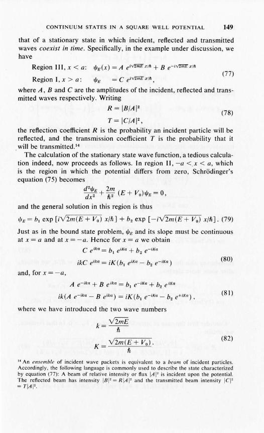
CONTINUUM STATES IN A SQUARE WELL POTENTIAL 149
that of a stationary state in which incident, reflected and transmittedwaves coexist in time. Specifically, in the example under discussion, wehave
(77)
(78)
Region III, x < a:
Region I, x> a: IjJE = C eiV2mEXlft,
where A, Band C are the amplitudes of the incident, reflected and transmitted waves respectively. Writing
R = IB/AI2
T=!C/AI2,the reflection coefficient R is the probability an incident particle will bereflected, and the transmission coefficient T is the probability that itwill be transmitted. 14
The calculation of the stationary state wave function, a tedious calculation indeed, now proceeds as follows. In region II, -a <,x < a, whichis the region in which the potential differs from zero, Schrodinger'sequation (75) becomes
d 2ljJE 2m (dx2 + h2 E + Vo) IjJE = 0,
and the general solution in this region is thus
IjJE = b l exp [iY2m(E + Vo) x/h] + b2 exp [-iY2m(E + Vo) x/h]. (79)
Just as in the bound state problem, IjJE and its slope must be continuousat x = a and at x = -a. Hence for x = a we obtain
C e ika = b l eiKa + b2 e- iKa
(80)
and, for x = -a,
ik(A e- ika - B eika ) = iK(b l e- iKa - b2 e+ iKa ),
where we have introduced the two wave numbers
(81 )
k= Y2mEh
K= Y2m(E+ Vo)·h
(82)
14 An ensemble of incident wave packets is equivalent to a beam of incident particles,Accordingly, the following language is commonly used to describe the state characterizedby equation (77): A beam of relative intensity or flux IA 1
2 is incident upon the potential.The reflected beam has intensity 181 2 = RIA 12 and the transmitted beam intensity lel 2
= TIAI2,

150 STATES OF A PARTICLE IN ONE DIMENSION
From equation (80), we can express b l and b 2 in terms of C,
b =.! (I +!) Cei<k-Kla12K
b2 = ~ ( 1 - ;) C ei<k+Kla.
Equation (81) then becomes
A e-ika + B e ik'a = [ ~ ( 1+ ;) e i(k-2Kla + ~ ( 1- ;) e i (k+2Kla ] C
k(A e- ika - B e ika = K [~( 1 + ;) ei<k-2Kla - ~( 1- ;) e i(k+2Kla] C.
Introducing the amplitude transmission coefficient T = CIA, we then obtain, after some elementary algebra,
C 2e- ikaT=-=
A (I +~+~) i<k-2Kla+ (I_~_ K) i<k+2Kla2K 2k e 2K 2k e
cos 2Ka - ~ (; + ~) sin 2Ka
or, finally,
T= cos (2\lzm(£+ Vo) a/h) _i(~+~) sin (2V2m(£+ Vo) a/h)2 £ + Vo £
(83)
Introducing also the amplitude reflection coefficient p = B/A, we' obtain,after some more algebra,
i e-2iV2m,· 0/11 ( 1£ + Vo _ I £ ) sin (2V2m (£ + V ) a/h2 Y £ Y£+~ 0
p = . ( I £ 1£ + V ) .cos (2V2m(£ + Vo) a/h) - i Y £ + V
o+Y~ sin (2V2m(£ + Vo) a/h)
(84)
Consider first the case of attractive potentials, Vo > O. In that instance,we obtain
R = I 12 = [Vo2/4E(E + Vo)] sin2 (2Y2m(E + Vo) a/h) (85)p 1+ [Vo2/4E(E + Vo)] sin2 (2Y2m(E + Vo) a/h)
and

CONTINUUM STATES IN A SQUARE WELL POTENTIAL 151
where we have used the fact that2 V 2
CVE/(E+Vo)+v'(E+Vo)/E) =4+ E(E~Vo)
to simplify these expressions for the reflection and transmission coefficient. Observe that, as it must according to our interpretation,
R+T=I. (87)
Also observe that transmission resonances occur, in which T = 1 andR = 0, whenever
2v'2m(E + Vo) a/h = n7T.
Now the momentum of the particle in the interior of the potential is givenby
Hence, these resonances occur when the width 2a of the potential is ahalf-integral number times the de Broglie wave length hlp in the interiorof the potential, just as we claimed intuitively in our discussion in Chapter I.
From equations (85) and (86), it can be seen that when E is sufficientlylarge compared to Vo, the reflection coefficient approaches zero and thetransmission coefficient unity, this being the expected result in theclassical limit. Actually, the approach to this limit is surprisingly slow.Even if E is as large as Vo in magnitude, the probability that an incidentparticle will be reflected can exceed 10 per cent. It must be mentioned,however, that for more realistic potentials than a square well, with itsunphysical discontinuities, the approach to the classical result is muchmore rapid.
E-------------
v=ox = -a x=a
v=o
FIGURE 7. The tunnel effect or penetration through a barrier.
We next turn to the more interesting case of repulsive potentials,Vo < O. As long as E + Vo > 0, the results are as given above and

152 STATES OF A PARTICLE IN ONE DIMENSION
equations (85) and (86) are both applicable as they stand. Suppose,however, that E + Vo < o. Write Vo = - V, so that V represents theheight of the potential barrier. The case under consideration is thus thatfor which E < V, as illustrated in Figure 7. From equations (83) and(84), we then find
R = Ipl2 = [V2/4EW - E)] sinh2(2V2m(V: E) a/h) (88)1+ [V2/4E(V-E)] sinh2 (2V2m(V-E) a/h)
and
1T = 1'T12 = (89)
1+ [V2/4E(V-E)] sinh2 (2V2m(V-E) a/h)'
and, of course, equation (87) is still satisfied, as it must be. Here we havean explicit example of the tunnel effect, which was also discussed inChapter I. There is a finite probability that a particle will be transmittedthrough a classically forbidden region, that is, one in which its kineticenergy is negative. Note that if the barrier is wide enough, or the kineticenergy is negative enough, that
2V2m(V - E) a/h ~ 1.
Then, to good approximation,
sinh (2V2m (V - E) a/Ii) = ~ exp [2V2m (V - E) a/n] .
In that case the transmission coefficient is the exponentially smallquantity
16EW - E)T = V2 exp [-4V2m(V - E) a/n] , (90)
so that the deviation from the classical result is negligible. Otherwisestated, only if the potential barrier is very thin, and the potential energybarely negative, will there be significant tunneling through a barrier.
One final remark must be added. We have derived a solution of Schrodinger's equation which corresponds to a particle incident on the potentialwell from the left. We could equally well have chosen to describe aparticle incident from the right, of course. This freedom is simply areflection of the existence of two linearly independent solutions to thesecond-order Schrodinger's equation, in agreement with our earlierprediction of the twofold degeneracy of continuum states of the type wehave just been discussing.
8. CONTINUUM STATES IN GENERAL; THE PROBABILITY FLUX
The most important potentials on the microscopic level describe the

CONTINUUM STATES; THE PROBABILITY FLUX 153
interaction between particles and thus have the property that
VeX) ~ 0, Ixi ~ 00.
It is accordingly of interest to discuss the continuum states of suchpotentials. For simplicity, we restrict our attention to the case in whichVex) vanishes more rapidly than [I as Ixl tends to infinity.15 Underthese circumstances, it is not hard to see that, for sufficiently large lxi,the state function is expressible as a linear combination of the de Brogliewaves exp[±iV2mE x/Ii], just as for the square well case. Indeed, ourinterpretation of the solutions can be taken over unaltered, and we writeat once
x ~ -00, t/JE (x) = A (eiv2ii!E xl" + p e-iv2mE XI") , (91)
and
(92)
where we have explicitly introduced the amplitude reflection and transmission coefficients p and 7. Of course, the precise form of p and 7
depends on the detailed nature of the potential, but in any case, R = Ipl2is the probability that a particle incident from infinity will be reflected,and T = 171 2 is the probability that it will be transmitted. As before, wemust demand that equation (87), R + T = I, be satisfied, no matter whatthe detailed form of the potential, if our interpretation is to be correct.We now verify that this is indeed the case. To do so we must temporarilyrevert to the wave packet description, of which the stationary state solutions are the limiting case. Denote the state function'by t/J(x, t), as usual,and consider the probability that the particle is to be found at some instantt in the fixed but arbitrary region of space between x = XI and x = x2,where for definiteness we take Xl < x 2 • This probability is
JX'
P(XI ,X2; t) = t/J*(x,t)t/J(x,t) dxx,
(93)
and, as we have indicated, it is a function of time. Specifically, as the wavepacket sweeps across the region of space under examination, we expectP(x], x 2 ; t) to increase from an initially negligible value to somethingclose to unity and then to decrease practically to zero again. In any case,we have
ap(xt>x2; t) =fx, (at/J* t/J+t/J* at/J) dxat x, at at
or, since t/J is a solution of Schrodinger's equation,
15 The case in which V (x) falls off exactly as l/x is of great importance, but requires specialtreatment which is, at present, beyond our capabilities.

154
we see that
STATES OF A PARTICLE IN ONE DIMENSION
nZ aZl/J n al/J-- --. + V(x)l/J=--;--2m ax z l at'
in IX2 a ( al/J al/J*)=- - l/J*--l/J- dx.2m XI ax ax ax
The right side is thus a perfect differential and we obtain finally
ap(xl,xz; t) _.( ) .( )at - J XI' t - J Xz, t ,
where
(94)
(95)j(x, t) =~(l/J* al/J_l/J al/J*).2ml ax ax
The interpretation of the result is the following. The change per unit timeof the probability of finding the particle in the interval between XI andXz, ap/at, is the difference between the probability per unit time thatthe particle entered at xl,j(xl,t) and that it emerged at xz,j(xz,t).Thus j (x, t) has the significance of a probability flux or current, directedtoward positive x ,16
Equation (94) is simply a general statement of probability conservation,applied to a finite domain rather than to all of space. The particularapplication we have in mind is to the stationary state limit of a wavepacket. In that limit, we have
l/J (x, t) = l/J E (x, t) = l/J E (x) e-iEl/f"
and hence it follows from its definition, equation (93), that P(xt.xz;t)
16 It may be helpful to compare this result and its interpretation to that expressing conservation of charge. Suppose Q(xI,x,; I) represents the net charge between the points XI andx, on a long wire, and suppose that / (x, I) is the electric current flowing in the wire at agiven point x, the positive direction of flow being toward positive x. Then in a time interval8 I, the net charge flowing into the wire at XI is / (x" I) 8 I, and that flowing out at x, is/(X"I) 81. Hence the net increase in charge, 8Q, is [J(X"I) -/(X"I)] 81, or
aQ(x"x,; t)al =/(XI,I)-/(X"t),
which has the same form as equation (94) and thus supports our interpretation of j as a(probability) current.

PASSAGE OF A WAVE PACKET THROUGH A POTENTIAL 155
is independent of time. The left side of equation (94) therefore vanishes,and we conclude that, for arbitrary XI and X2, j (x I) = j (X2) , which meansthat j(x) is a constant, say Jo. For Ixl ~ 00, I/JE(X) is given by (91) or(92) and it is easily verified that
x ~ -oo,Jo = IAI2v(l-lpI2) = IAI2v (l- R)
x~+oo,Jo= IA12V 17 12= IAI2V T
where v = Y2rnE/h is the classical velocity of the particle. Since thesemust be equal, we thus see that R + T = 1, as required.
The form ofJo in each region is not unexpected, as the following argument shows. Consider first the region x ~ 00, where I/JE is given by equation (92). We have
p(x) = I/JE*I/JE = IA 121712= IA 12T,
where p(x) is the probability density. Thus the probability flux j issimply pv, just as in hydrodynamics. Similarly for x ~ -00, the netprobability flux is the difference between the flux to the right IA 1
2v andthe independent flux to the left IA 1
2vR. Note that the interference termsbetween incident and reflected waves have completely cancelled out,as they must (why?).
9. PASSAGE OF A WAVE PACKET THROUGH A POTENTIAL
We have considered nonphysical stationary state solutions as the limiting case of very broad wave packets. Our arguments concerning thislimiting process were crucial to our interpretation of the solutions, butthey are essentially irrelevant as far as the mathematical properties ofthese solutions are concerned. Quite independently of this interpretation,we are at liberty to view the stationary states simply as idealized statesfrom which physical states can be constructed by superposition. Wenow show how to do this. Since the I/JE form a complete set, we canexpress an arbitrary solution of the time dependent Schrodinger's equation in the form
I/J(x, t) = f I/JE(X) e-iEl/fl feE) dE, (96)
where the integral extends over the continuum states and must also beregarded as including the discrete states, if any. Now suppose we wantto construct a wave packet which at time t = 0 is centered at large negative x, say at x = -Xo, and is moving to the right with mean momentum,Po = V2rnEo. For x large and negative, I/JE is given by (91). Hence,absorbing the arbitrary amplitude A into f(E), we have, as x ~ -00,
I/J(x, t) = f f(E)[e iV2rilE'X/f! + peE) e-iv2niEX/f!] e-iEl/fl dE. (97)
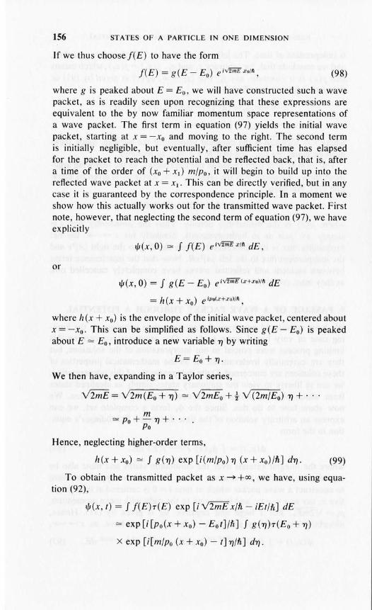
156 STATES OF A PARTICLE IN ONE DIMENSION
If we thus choose f(E) to have the form
f(E) = g(E - Eo) e i v'2mE xu,ft, (98)
where g is peaked about E = Eo, we will have constructed such a wavepacket, as is readily seen upon recognizing that these expressions areequivalent to the by now familiar momentum space representations ofa wave packet. The first term in equation (97) yields the initial wavepacket, starting at x = - Xo and moving to the right. The second termis initially negligible, but eventually, after sufficient time has elapsedfor the packet to reach the potential and be reflected back, that is, aftera time of the order of (xo + Xl) m/po, it will begin to build up into thereflected wave packet at X = Xl. This can be directly verified, but in anycase it is guaranteed by the correspondence principle. In a moment weshow how this actually works out for the transmitted wave packet. Firstnote, however, that neglecting the second term of equation (97), we haveexplicitly
l/J(x,O) = f f(E) e iv2n1EX'ft dE,
or
l/J(x,O) = f g(E - Eo) e iv'2mE(x+xo),ft dE
= h(x + xo) eiVo(x+xo),ft,
where h (x + xo) is the envelope of the initial wave packet, centered aboutx = -xo. This can be simplified as follows. Since g(E - Eo) is peakedabout E = Eo, introduce a new variable 'Yj by writing
E= Eo+ 'Yj.
We then have, expanding in a Taylor series,
Y2mE = Y2m(Eo+ 'Yj) = Y2mEo+ i Y (2m/Eo) 'Yj + ...
m= Po+-'Yj+··· .
Po
Hence, neglecting higher-order terms,
h(x+xo) = f g(r}) exp[i(m/po)'Yj (x + xo)/h] d'Yj. (99)
To obtain the transmitted packet as x - +00, we have, using equation (92),
l/J(x, t) = f f(E)7(E) exp [i V2mE x/h - iEt/h] dE
= exp[i[po(x+xo) -Eot]/h] f g('Yj)7(Eo+'Yj)
x exp [i[m/po (x + xo) - t] 'Yj/h] d'Yj.

PASSAGE OF A WAVE PACKET THROUGH A POTENTIAL 157
Recalling that /712 = T, we write
r(Eo+ 1)) = VT(Eo+ 1)) e i8<Eo+T/),
and we now assume that T(E) is a rather slowly varying function of E,but that 8(E) need not be. In other words, we make the plausible assumption that the magnitude of the transmission coefficient does not changemuch when E is changed a little, but that its phase may change significantly. With this assumption,
r(Eo+ 1)) = VT(Eo) exp [i8(Eo) + i1) d8/dEo] = r(Eo) eiT/ a5fdE
and
ljJ(x, t) = r(Eo) exp [i[po(x + xo) - Eot]/Ii]J g(n)
x exp [i[m/po(x + xo) - t + Iid8/dEoh/li] d1).
Comparison with equation (91) then shows that, for x ~ +00,
ljJ(x, t) = r(Eo) h [ x + Xo - ~o (t - Ii d8/dEo) ]
x exp [i[po(x + xo) - Eot]/Ii]. (100)
Thus, to this approximation, the transmitted packet appears undistortedbut reduced in amplitude by the transmission coefficient r(Eo). Thepacket appears at the position x at a time t given by
m d8t = - (x + xo) + Ii dE .
Po 0
The first term is recognized as the time for a free particle with momentumPo to travel from - Xo to x. The second term is the increment of timeintroduced by the forces which act on the particle during its passagethrough the potential. Calling this increment ~ t, we thus have
d8~t = Ii-·
dE(101)
Perhaps it should be emphasized that these last results are onlyapproximate in nature. Specifically, two rather different assumptionswere made in deriving equations (100) and (101). The first was that inthe various Taylor series expansions about Eo the quadratic (and higher)terms in 1) could be neglected. These terms lead to a spreading of thewave packet, in just about the same way as for a free-particle wavepacket. Reference to the discussion of Chapter IV shows that thisspreading is negligible if the wave packet is sufficiently broad. Thesecond assumption was that the magnitude of the transmission coefficient r does not change significantly over the energy width of the wave

158 STATES OF A PARTICLE IN ONE DIMENSION
packet. The neglected terms in this case lead to a distortion of the wavepacket, and again this is negligible for sufficiently broad wave packets.Even if some spreading and distortion occur, however, the qualitativefeatures of the results are not strikingly affected. A transmitted wavepacket ultimately does appear and its time delay is expressed throughthe dependence of I:) on energy. These features comprise the essentialcontents of equations (100) and (10 I).
-.10. NUMERICAL SOLUTION OF SCHRODINGER'S EQUATION
Our remarks thus far have been exclusively directed to the solutions ofSchrodinger's equation by analytic methods. However, the availabilityof modern high-speed computers has made it a relatively simple androutine matter to obtain such solutions numerically. In particular, theordinary differential equations which define the stationary states are readily integrated numerically, in a matter of seconds or fractions of a second,for both bound states and continuum states, and for quite complicatedpotential energy functions. On the other hand, the partial differentialtime dependent Schrodinger's equation is a great deal more complicated, and its solution, while feasible, is a significant task for even thefastest and largest computers. As a result, the time dependent problemof the motion of wave packets has not yet been very extensively studiedby numerical methods and our knowledge of the details of their behavioris largely semi-quantitative. Tl:te discussion in the last section is rathertypical in this respect.
This situation has recently been improved to a considerable degreeby the construction of exact numerical solutions for a Gaussian wavepacket incident upon a square well potential. 17 The results are shownfor a number of different circumstances in Figures 8 through 13. 18 ] nFigures 8, 9 and 10, a wave packet is incident upon an attractive potential of fixed width and depth, and its behavior is studied as the meanenergy of the wave packet state is varied. The figures are largely selfexplanatory, consisting of a sequence of "snapshots" which show thepacket approaching the well and then .interacting with it to generate reflected and transmitted packets. In Figure 8 the mean energy of the
J7 A. Goldberg, H. M. Schey, and J. 'L. Schwartz, "Computer-Generated Motion Picturesof One-Dimensional Quantum Mechanical Transmission and Reflection Phenomena,"American Journal of Physics, 35, 177 (1967).
I" Note that in these figures the envelope of the wave packets is displayed on an arbitraryordinate scale of probability density, while the potential well is displayed on an independently arbitrary energy scale. The height of the packet relative to the magnitude of thepotential has 'no significance whatsoever. Thus the well could have been drawn one-tenthas large or ten times as large, without affecting in any way the depicted behavior of thewave packet.

NUMERICAL SOLUTION OF SCHRODINGER'S EQUATION 159
packet state is one-half the depth of the attractive potential, in Figure 9the mean energy is equal to the well depth and in Figure IO it is twicethe well depth. In agreement with expectations, the reflected packetdecreases rapidly in magnitude with increasing energy, and at the highestenergy the classical limit of no discernible reflection is seen to be achieved.
0 200 240
1\ 1\(\., \
/ "I
/i ~
I
'- '- L280 360 440
II
JV:! Ilil
/ ~l~ ,I~:'::i\\ ! /-\t \11 ',,)\,;j::;\ I: '~;"j '.
'.' _J~~ii1\I\l
L U U520 640 680
f\ jf"\~
I \
.-/""\ ~/ \/ \
~ ---~ j \
'- '- '--
FIGURE 8. Gaussian wave-packet scattering from a square well. The averageenergy is one-half the well depth. Numbers denote the time of each configurationin arbitrary units.

160 STATES OF A PARTICLE IN ONE DIMENSION
Figure 11, 12 and 13 show the behavior of packets for this same set ofenergies, but incident upon a repulsive potential, or barrier. Here one goesfrom practically total reflection at low energies to practically total transmission at high, both in agreement with the classical behavior. The intermediate energy case, in which both reflected and transmitted packets are
o 300 350
u L'-,------i(\
)\{'I \
i \) \
ui\I \
! \
400 500 600
.!j~"~' J .
1"1 " \
)1 \ /ljfll~ J;;P \\
l \ ..AW \.t---.-L-....,.....r-----+---'--'l "..----t----~Ur--~----i
700 800 950
-
FIGURE 9. Gaussian wave-packet scattering from a square well. The averageenergy is equal to the well depth. Numbers denote the time of each configurationin arbitrary units.

NUMERICAL SOLUTION OF SCHRODINGER'S EQUATION 161
formed, is particularly interesting, especialIy in view of the rather unexpected trapping of a portion of the wave packets within the potential, asshown in Figure 12(b).
These exact results demonstrate very clearly and explicitly our earlierassertions about the qualitative behavior of wave packets. The gradualformation of the reflected and transmitted packets is clearly visible, as
0 480 560
J\ r\ I' \
) \,
U ........
720 880 960
.~d11
\ l\I \ jf
j \ )' \
L...- L...- U1040 1200 1520
,r·.. \ / " t\I '
~/ \ ,/ \) \
'-- L -
FIGURE 10. Gaussian wave-packet scattering from a square well. The averageenergy is twice the well depth. Numbers denote the time of each configurationin arbitrary units.

162 STATES OF A PARTICLE IN ONE DIMENSION
is the gradual spreading of the wave packet with the passage of time. Asexpected, this spreading is noticeably less for higher than for lowerenergy packets (why?). Note, however, that the wave packets suffernegligible distortion, at least visually. This is rather remarkable, considering the highly complicated and easily visible structure which developsduring the actual period of interaction between the packet and the poten-
o
280
480
200
320
560
240
440
800
FIGURE II. Gaussian wave-packet scattering from a square barrier. Theaverage energy is one-half the barrier height. Numbers denote the time of eachconfiguration in arbitrary units.

NUMERICAL SOLUTION OF SCHRODINGER'S EQUATION 163
tiaI. The time increment associated with the passage of the packet throughthe potential, although certainly present, unfortunately is too small to beapparent on the time scale in the figures.
We conclude with some brief remarks on the methods commonly usedto numerically integrate differential equations, such as Schrodinger's.19Consider first the matter of stationary states. Here we seek to solve thetime independent Schrodinger's equation, which we write in the form
l/J+f(x)l/J=O (102)
where each dot over a symbol denotes differentiation with respect to xand where
2mf(x) ={;2 (E- V). (103)
We assume f(x) to be an exactly known function.By a numerical solution to equation (102) we mean the set of values,
to some assigned level of accuracy, of both l/J and tb at a discrete set ofpoints, X n , called mesh points. 20 We shall take these points to be equidistant from each other, and of spacing E, whence we write
Xn = nE, n = 0, ±I, ±2, .... (104)
Since we are seeking the solution of a second-order differential equation,two integration constants must be fixed to uniquely specify the solution;we shall take these to be the values of l/J and tb at some given point, which,for convenience, we choose to be the origin. Our problem may now bestated as follows: Given l/J(O) and tb(O), how do we construct l/J(x n )
and tb(x n ) over whatever domain of mesh points may be of interesp21We now answer this question by constructing a pair of simple differenceequations for these quantities.
Consider first
19 See Reference [7], Chapter 13, and Reference [9], Chapter 10, for a general discussion.For the application to Schrodinger's equation for bound states, see R. S. Caswell, "Improved Fortran Program for Single Particle Energy Levels and Wavefunctions in NuclearStructure Calculations," National Bureau of Standards Technical Note 410, Superintendent of Documents, U. S. Government Printing Office (1966). For continuum states,see M. A. Melkanoff, J. S. Nodvik, D. Cantor and D. S. Saxon, A Fortran Program forElastic Scattering Analyses with the Nuclear Optical Model, University of CaliforniaPress (1961), especially pp. 24-29, and M. A. Melkanoff, T. Sawada arid J. Raynal,"Nuclear Optical Model Calculations," in Methods of Computational Physics, Vol. 6,Academic Press (1966). This latter gives a particularly complete and up-to-date account.
20 Only 1/1 and ~ need be considered because all higher derivatives are at once expressiblein terms of these two using equation (102).
2\ If the normalization of the state function is taken to be arbitrary, only the ratio of 1/1(0)to ~(O) need be specified in actuality.

164 STATES OF A PARTICLE IN ONE DIMENSION
ljJ(X n+1 ) = ljJ(X n + t:)
and expand the right side in a Taylor series. We obtain
o
600
300
650
400
700
800 1050 1450
FIGURE .\ 2(a). Gaussian wave packet scattering from a square barrier. Theaverage energy is equal to the barrier height. Numbers denote the time of eachconfiguration in arbitrary units. Note the resonance effect in which a part of theprobability distribution remains for a long time in the region of the potential.

NUMERICAL SOLUTION OF SCHRODINGER'S EQUATION 165
1600 ~ 1850 ,.--
V\ /\
2100 ,.-- 2450 r--
I/'\.
FIGURE 12(b). Details of the decay of the resonant slate seen in Figure 12(a).
whence, using equation (102),
. e2 •
ljJ(X n+l) = ljJ(x n ) + eljJ(x n ) - 2 !(XIl)ljJ(X Il ) + O(e3). (105)
This equation permits us to calculate ljJ (x 11+1), provided ljJ (x II) and~(xn) are known. We now need a similar equation for ~(x11+1)' This iseasily obtained from the identity
~(XII+I) = ~(XII) + fXII+
E~(x) dx
XII
= ~(XII) - JXII+E !(x)ljJ(x) dx,XII
whence. .
ljJ(x ll+ l ) = ljJ(x ll ) - e!(x ll )ljJ(x ll ) + O(e 2). (106)
This completes the formalism because, given ljJ (0) and ljJ(O) , we use (105)and (106) to. compute ljJ (e) and ljJ (e). The result permits us to calculateljJ(2e) and ljJ(2e) , and so we march through the set of .mesh points.Evidently the minimum error in ljJ is of order e3 and in ljJ of order e2
•
This scheme is simple enough to make the basic idea clear, but muchtoo crude to be useful. The scheme commonly used, called the RungeKutta method, effectively uses Simpson's rule for the numerical integrations leading to equations (105) and (106),22 The resulting expressions
22 Equation (105) is equivalent to a trapezoidal rule of integration.
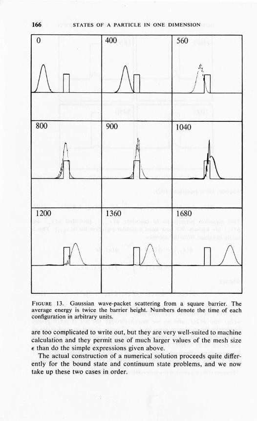
166 STATES OF A PARTICLE IN ONE DIMENSION
o
800
1200
400
900
1360
560
1040
1680
FIGURE 13. Gaussian wave-packet scattering from a square barrier. Theaverage energy is twice the barrier height. Numbers denote the time of eachconfiguration in arbitrary units.
are too complicated to write out, but they are very well-suited to machinecalculation and they permit use of much larger values of the mesh sizeE than do the simple expressions given above.
The actual construction of a numerical solution proceeds quite differently for the bound state and continuum state problems, and we nowtake up these two cases in order.

NUMERICAL SOLUTION OF SCHRODINGER'S EQUATION 167
Bound States.23 Here the unknown discrete energy eigenvalues mustbe determined, and this is usually done in the following way. Suppose thetrue energy eigenvalues in increasing order are En' n = 0, 1,2, .... Themathematical solution to Schrodinger's equation then has the propertythat if E < Eo, t/J has no nodes, if Eo < E < E" t/J has one node,and so on.The eigenvalues are thus marked by the appearance (or disappearance)of a node at infinite values of x , and this in turn is signaled by a changein sign of the sense in which t/J diverges as E passes across an eigenvalue.Thus one simply guesses a value of E and numerically integrates out fromthe origin until this solution begins to diverge. An increase in E increases the curvature of t/J and tends to increase the number of nodes, andconversely for a decrease in E. By appropriate adjustments in theassumed values of the energy, the eigenvalues can thus be readilybracketed. This behavior is illustrated in Figure 14 for the ground stateof a symmetrical potential. In the figure, the 'numerical solutions areschematically shown for several assumed values of E. It.is clear fromthe figure that the true ground state energy lies between E b and Ec , andis already quite closely bracketed by these two values.
FIGURE 14. Schematic behavior of the solution of Schrodinger's equation forseveral trial values of E in the neighborhood of the ground state energy Eo. Thebehavior of these solutions shows that E b < Eo < Ec.
Continuum States.2•4 Here solutions are desired for some given value
of E in the continuum. These are obtained very simply by integratingoutward from the origin and joining the numerical solution smoothly tothe known pure de Broglie wave asymptotic state functions of equations
2:' Caswell, op. cit.
24 Melkanoff, et al., op. cit.

168 STATES OF A PARTICLE IN ONE DIMENSION
(91) and (92). The analysis is complicated considerably by the fact thatthe state function is complex and not real.
Finally, we remark on the numerical solution of the time-dependentequation. 25 Here one must introduce a mesh in the time coordinate aswell as the space coordinate. The numerical problem is then the following. Given t/J at every spatial mesh point at some time tIl' calculate 1/Jat every spatial mesh point t ,,+1> starting, of course, from the initial valueof t/J at t = 0, say. Note that here we must specify a complete functionto define a solution in contrast to the time-independent case where onlythe two numbers t/J(O) and tb(O) were required. The problem is furthercomplicated by the fact that special care must be taken to avoid numericalinstabilities26 and to ensure probability conservation. The resultingequations, which turn out to be second-order difference equations in thespatial coordinate and first-order in the time, are lengthy and complex,and we shall not bother to write them out.
Problem 1. Obtain the energy spectrum and eigenstates of a particle ina box from those for a particle in a square well potential of depth Vo bypassing to the limit in which Vo~ 00. Verify that your results are thesame as those obtained directly in Chapter IV. Hint: Measure all energiesfrom the bottom of the well, before going to the limit.
Problem 2. If t/J" is the nth harmonic oscillator eigenstate, evaluate:(a) (t/J"latslt/J,,), (t/J"laslt/J,,)(b) (t/J"lxlt/J,,), (t/J"lx 2 1t/J,,), (t/J"lx 4 1t/J,,)(c) (t/J"lplt/J,,), (t/J"lp 2 1t/J,,), (t/J"lp 4 1t/J,,)(d) (t/Jmlatslt/J,,), (t/Jmlaslt/J,,)(e) (t/Jmlxlt/J,,), (t/Jmlx21t/J,,)(f) (t/JmIPIt/J,,), (t/Jmlp 2 1t/J,,)·
Hints: (I) Work in the creation space representation and use the knownortho-normality of the harmonic oscillator states. (2) Express x in termsof a and at, and similarly for p. Remarks: This problem is not hard ifyou know and understand what you are doing. By brute force methods,it's a mess!
Problem 3. A simple harmonic oscillator of frequency Wo is in its groundstate. The force constant is suddenly diminished at t = 0 to such a valuethat the oscillator frequency becomes (I) w = wo/2; (2) w = wo/lO. Forboth cases:
25 Goldberg, Schey and Schwartz, op. cit.
26 A numerical scheme is called unstable if truncation and round-off errors accumulate insuch a way that the numerical solution diverges uncontrollably from the true solution.

PROBLEMS 169
(a) What is l/J(x, t = 0) ?(b) Calculate l/J(x, t). Sketch the behavior of 1l/J12 over one period.(c) If the momentum of the particle is measured at some time t > 0,
what is the probability that it will lie in the interval between p andp+ dp?
(d) If, instead, the energy of the particle is measured, what is theprobability that it will have the value En = (n + 1/2)hw? (Use the integralrepresentation of equation (61) to work this out.) For what value of nwill this probability be a maximum? Discuss your results briefly.
Problem 4. A particle moves in a square well potential of width 2a anddepth Vo. Consider the limit in which 2a tends to zero and Vo to infinityin such a way that their product approaches the finite value g. By considering the square well solutions discussed in the text, show that such apotential has exactly one bound state and that
(a) its binding energy is E = g2m/2h 2 .
(b) its normalized eigenstate is (2mE/h 2 )1/4 e-v2ni<)xl/li.
Next consider continuum states. From the solutions given in the text,(c) find the amplitude reflection and transmission coefficients and
verify that probability is conserved.(d) Finally, noting that such a potential can be expressed as a delta
function, V (x) = - g 8 (x) [why?], see if you can deduce that the slopeof l/J must be discontinuous across such a potential. Specifically, showthat l/J is such that
dl/JI _ dl/J!_=_2m2
g l/J(O).dx 0+ dx 0_ h
Use this result to obtain the answers to parts (a), (b) and (c) directly.
Problem 5. Consider a bouncing ball of mass m. Assume (1) that themotion is exactly vertical, (2) that collisions with the floor are perfectlyelastic and (3) that the force of gravity is uniform.
(a) Sketch the potential in which the ball moves. Write Schr6dinger's equation and give the boundary conditions satisfied by l/J.
(b) Show that the stationary states of the system can be expressedin terms of Bessel functions of order one-third.
(c) Find, if you can, the transcendental equation which determinesthe allowed energies.
Problem 6. A particle of mass m moves in an attractive potential V (x)= - Vo e-1xlll,.
(a) By making the substitution z = e-X/2L show that the stationarystates can be expressed in terms of Bessel functions.
(b) Noting that the stationary states can be classified according to

170 STATES OF A PARTICLE IN ONE DIMENSION
their parity, find the transcendental equation which determines theenergy of the bound states of the system.
(c) Consider next continuum states, E > O. Find expressions forthe amplitude reflection and transmission coefficients. Verify that probability is conserved.
(d) Find an expression for the time increment 6. t associated withpassage of a wave packet through the potential. Compare your resultwith that to be expected classically.
Problem 7. A particle moves in a square well potential of depth Voand width 2a. Considering only continuum states in the limit E ~ Vo,and using the solutions obtained in the text:
(a) Show that the amplitude transmission coefficient 7 is given by
7(E) = exp[iVo v'm/2E 2a/li]
and calculate the time increment associated with the passage of a wavepacket through the potential. Explain your results.
(b) Show that for the reflected waves
p(E) = ~~ [exp [2i(v'2mE + 2 Vo v'm/2E'V'Q7h]- exp[2i v'2mE a/Ii]].
(c) Using the same rough method used in obtaining equations (100)and (10 I), show that there are two contributions to the reflected wavepacket and calculate the time of arrival of each at x = - XI' say. Explainyour results.
Problem 8. A particle moves in the uniform field of force F.(a) Write Schrodinger's equation in momentum space.(b) Find the stationary states 4>E(P).(c) Given an initial wave packet 4>(p, t = 0), find 4>(p, t). Do this
by constructing the momentum space propagator K (p I , p; t) .(d) Use your results to obtain an integral representation for 1./1 (x, t) ,
given 1./1 (x, 0). See if you can verify that the wave packet accelerates inthe expected way.
Problem 9. A harmonic oscillator is in the state
1l./1(x, t) = v'2 [1./10 (x, t) + 1./11 (x, t)],
where 1./10 and 1./11 are the normalized ground and first excited harmonicoscillator states. Calculate (E >, (x> and (p > and discuss the timedependence of each.
Problem 10. Calculate the probability flux j(x, t) for the state given inproblem 9.

PROBLEMS 171
Problem 11.(a) Show that bound stationary state wave functions can always be
chosen to be real functions with no loss of generality.(b) Show that the probability currentj(x, t) is zero for any bound
stationary state.
Problem 12. A 10 gm particle undergoes simple harmonic motion withfrequency 2 cycles per second. If it is in its lowest state, what is theuncertainty in its position? in its momentum? Suppose it is set in motionwith an amplitude of 10 cm. What is its energy? What is the order ofmagnitude of the quantum numbers appropriate to states of this energy?
Problem 13. Show that a state function of definite parity in configurationspace has the same parity in momentum space. What are the explicitproperties of the parity operator in momentum space?
Problem 14. A harmonic oscillator of mass m, charge e and classicalfrequency w is in its ground state in a uniform electric field. At timet = 0, the electric field is suddenly turned off.
(a) Using the known properties of the propagator, find an exact,closed form expression for the state of the system at any time t > 0.Compare your result with that for a classical oscillator.
(b) If a measurement is made at any time t > 0, what is the probability that the oscillator will be found in its nth state?Hint: Introduce a shift of origin to find the exact initial state.
Problem 15.(a) A particle moves in a potential V (x). The stationary states
t/JE of the system have the following properties:(i) The spectrum is discrete for E < 0, continuous for E ~ 0.
(ii) There are a denumberably infinite number of bound states.(iii) For each bound state and for every integer q,
\t/JElx2<1+IIt/JE1=0.
Sketch a simple smooth potential V (x) consistent with all of these properties. Briefly explain your reasoning.
(b) The same except that, instead of (ii), only a (small) finite numberof bound states exist.
(c) The same as (b), except that property (iii) is replaced by:(iiia) The expectation value of x is zero for the ground state
but increases monotonically with excitation energy (boundstates only).
(d) Suppose that in case (b), the ground state energy of the systemis Eo = - 2 eV. Suppose also that \ t/Jt'olx 2 1t/Jf:o 1= 4 X IO- IH cm2
. If themass of the particle is 10-27 gm, estimate the strength of VEx) in electron

172 STATES OF A PARTICLE IN ONE DIMENSION
volts and its spatial extent in angstroms, that is, affix a rough numericalscale to your sketch for part (b). Hint: Use the uncertainty principle tomake your estimate.
Problem 16. The Hamiltonian of a particle can be expressed in the form
(a,a+) = I,
where £) and £2 are constants.(a) Find the energies of the stationary states. (You are not required
to find the corresponding state functions.)(b) The same except that the commutator of a and a+ is
(a, a+) = q2,
where q is a pure number.Hint: Keeping the harmonic oscillator in mind, introduce new annihilation and creation operators band b+ by writing
b = exa + f3,
and choose the constants ex and f3 wisely.
Problem 17. Let t/J (x, t) denote an arbitrary, time dependent harmonicoscillator state function. Prove that
(x)t=(x>ocoswt+ (P>osinwtmw
(p >t = (p >0 cosw t - mw (x >0 sinw t,
in complete correspondence with the classical equations.Do this in the following two ways:
(a) By finding expressions for d (p >/dt and d (x> /dt and integratingthe resulting coupled equations.
(b) By direct evaluation of (x> t and (p >to using the propagatorfor the harmonic oscillator to express t/J(x, t) in terms of t/J(x, 0).
Problem 18.(a) Let t/J (x, t) denote an arbitrary, time dependent harmonic
oscillator state function. Prove that
( at >I = (at> 0e iw1•
Do this in the following three ways.i) By finding expressions for d (a> /dt and d (at> /dt and inte
grating the resulting equations.ii) By direct evaluation of (a> I and (at> I using the propagator,
as given in closed form in equation (68), to express t/J (x, t)in terms of t/J(x, 0).

PROBLEMS 173
iii) By direct evaluation using equation (65) for the propagator..(b) Solve the classical oscillator problem using as classical dynami
cal variables a and at instead of x and p.
Problem 19. U sing the numerical integration prescription of equations(105) and (106), integrate the differential equation
d 21/1dx 2 + 1/1 = 0
from x = zero to one for the following two cases:(a) 1/1(0) = 0, ~(o) = I(b) 1/1(0) = I, ~(o) = o.
In both cases use a mesh size E = 0.2. Compare your results with theexact answers.

VIIApproximation methods
1. THE WKB APPROXIMAnON
In the last chapter we studied the solutions of Schrodinger's equationfor the harmonic oscillator and for a square well potential. These are twoimportant examples of potentials for which exact solutions of the quantummechanical equations can be found. While there are many such onedimensional examples, more generally we must deal with potentials forwhich exact solutions cannot be found. I To enable us to handle thislarger class of problems, we now take up a variety of approximationmethods, each with its own domain of validity.
We first discuss a method for treating potentials which change veryslowly in a de Broglie wavelength. For classical systems the wavelength approaches zero, so that this restriction is always satisfied forphysically realizable potentials. This method thus gives essentially theclassical limit and is therefore frequently called the semiclassical approximation. More often, however, it is called the WKB approximation, afterWentzel, Kramers and Brillouin, who first applied the method to quantummechanical problems and are commonly credited by physicists withinventing it. Actually, the subject is an old one to mathematicians, underthe heading of asymptotic solutions to differential equations, and datesback to Stokes, who originated the techniques in the middle of the 19thcentury. These were rediscovered by Wentzel, Kramers and Brillouin,and also, independently, by Jeffries. Therefore, the method is sometimescalled the WKBJ approximation.
To proceed, consider a particle moving in a potential V (x) so thatSchrodinger's equation for the stationary states has the usual form,
I This is even more the case in three dimensions and in the study of systems of interactingparticles. In both cases the class of exactly soluble problems is very limited indeed, as weshall see.

THE WKB APPROXIMATION 175
(I)
We now want to study the limit in which h can be regarded as tending tozero. However, we cannot do so in equation (I) as it stands, since t/JEoscillates so rapidly in this limit that the first term gives a finite contribution and not zero, as might at first be thought. To make this behaviorexplicit, we write t/JE(X) in the form
(2)
which is seen to be a generalized kind of de Broglie wave with amplitudeA (x) and phase S (x), both of which are, as yet, unknown functions ofposition.2 Upon differentiation twice, equation (2) becomes
d2
t/JE = [d2A + 2i dA dS + i A d
2S _.:! (dS)2] eiS/fl
dx2 dx2 dx dx h dx 2 h 2 dx '
whence we obtain, upon substituting into Schrodinger's equation, cancelling the common factor eiS/
fl and regrouping the terms, the exactnon-linear equation
A [_I (dS)2 + V(x) -E] _ ~[2 dA dS + A d2S] _ ~ d
2A = O. (3)
2m dx 2m dx dx dx 2 2m dx2
Regarding h as a parameter of smallness, it is noted that the first termis of order unity, the second of order h and the last of order h2 • We provisionally neglect the term in h 2 and set the other two separately equalto zero, thus determining S and A. From the first we have at once
dSdx =±V2m(E- V) =±p(x)
or
S(x) =± f p(x) dx.
Using this result,3 the second becomes
2 dA (x) + A dp = 0dx p dx
or, multiplying through by A and combining terms,
(4)
2 This form may appear quite special, but no loss of generality is incurred by writing it. Onthe contrary, we have introduced two unknown functions to replace a single such function.We shall shortly take advantage of this redundancy by choosing S and A in a particularlyconvenient way.
3 Equation (4) will be recognized by those familiar with the Hamilton-Jacobi formulationof classical mechanics (Reference [14]).

176 APPROXIMATION METHODS
(5)
(6)
Note that, from equation (2), I./JE*I./JE = .4 2, for real A and S. We thus see
that this last equation is merely a statement of conservation of probability, since it is equivalent to dj/dx = 0, where the probability flux j isgiven, in the approximation to which we are working, by
j = pv = I./JE*I./JE p/m = A 2p/m .
In any case, we have from equation (5)
A = c/vP,
where c is an arbitrary constant. Our approximate solution thus has theform
where
p = V2m [E - V (x) ] .
Note that the answer is expressed in terms of an indefinite integral.However, it can easily be re-expressed in terms of a definite integralby referring I./JE(X) to its value at some given pointxo. Doing so, we obtainat once
I./JE±(X) = I./JE±(XO) ~~~:oi exp [ ±i 1:0 p dx/h J.The structure of the WKB result is easy to understand. We have
already seen that the amplitude function is determined by the requirement that probability be conserved. The phase factor is interpreted inthe following way. Consider the change in phase ocp of a de Broglie waveof wavelength A when it advances a distance ox. Evidently
If the wavelength is not constant, but changes with position, then theaccumulated phase shift cp for a finite advance is
J277"
cp = T dx = f p dx/h,
in agreement with our result. Now this argument is based on the notionof a position dependent wavelength. But the very concept of wavelengthloses its meaning if the wavelength is not practically constant over a

THE WKB APPROXIMATION 177
distance of the order of the reduced wavelength in size. Hence, roughlyspeaking, we expect our approximation to be valid only if the wavelengthchanges by a sufficiently small fraction of itself over such a distance.That is, we expect that (iA./if... «i 1, where &'A. = (dif.../dx) if... , or that, puttingall this together,
I~~I «i 1 (7)
(9)
(8)
for the WKB approximation to hold. Expressing "A in terms of p, this isequivalent to
I~ dPI = 11. dp if...I «i 1p2 dx p dx
or, also, expressing p in terms ofE and V,
_h_ I 1 dV I «i 1zV2m (E - V)3/2 dx .
Equation (8) states that the fractional change in the momentum in awavelength must be small, while equation (9) states that, in a wavelength, the change in the potential energy, relative to the kinetic energy,must be small. An alternative way to put these conditions is that thewavelength must be small compared to the distance over which themomentum changes appreciably or over which the potential changesappreciably. Of course, equations (7), (8) and (9) are completely equivalent to each other and are merely different ways of stating the samecondition.
Even though we have been guided by classical arguments in obtaipingthe WKB approximation, we note from equation (9) that, as a kind ofbonus, the approximation is also valid in classically forbidden regionsof negative kinetic energy, provided only that this negative kinetic energyis sufficiently large and that it changes slowly enough. On the otherhand, we observe that in the neighborhood of a classical turning pointwhere E = V, p = 0 and if... = 00, the approximation breaks down completely. [We shall have more to say on both these points later.]
It still remains for us to give a more precise statement of the condition for the validity of the WKB approximation than that deduced bythe rough arguments used above. To do so, we return to the exact equation (3), which was our starting point, and take into account the neglectedterm 4 in h 2
• With this term included, the phase function S is determined
4 We shall'treat the ft2 term as a correction term in the expression for S. However, it couldequally well have been treated as a correction to A. We have chosen the former because itsimplifies the subsequ.ent analysis, but the final result is independent of which choice ismade.

178
by the exact equation
APPROXIMATION METHODS
[1 (dS)2 J h
2d
2AA - - + V(x) -E -- --=0
2m dx 2m dx2
or
dS I h2 d2AdX=± yp2(X)+A dx2'
To first approximation, the effect of the small term in h2 is obtained byexpanding the square root to give
dS h2 d2Adx = ± [p (x) + 2pA dx2 + ... ] ,
while, to this order, A may still be taken as proportional to p-lI2. Thuswe have
or, integrating,
S = ± (J:/. dx + t1S) ,
where
With this choice for the limits of integration, we then have in place ofequation (6),
IjJE±(X) = IjJE±(XO) V~~:o; exp [±{Do p dx/h + t1S/hJ].Consequently, we conclude that the WKB approximation will be validprovided that
(10)
which is the precise condition we seek. Note that this condition involvesmore than the local behavior of p(x) ; it takes into account the accumulated error in the phase function S over the entire interval from the reference point Xo to the point x at which the state function is being calculated.
Unfortunately, equation (10) is somewhat complicated and difficultto interpret. We shall therefore give a rough, but adequate, upper boundto t1S/h which is much easier to understand. We have by inspection

THE WKB APPROXIMATION 179
where Pmin is the minimum value of P over the domain of integration.For simplicity, suppose first that d2p-112(dx2 is monotonic over the interval from Xo to x. The integration can then be performed at once, and weobtain
IIlSI ~ Ii I(d
p-
112) _ (dP-
112) I.
Ii 2YPmin dx x dx Xo
Since, evidently,
l(dP-
1'2) _ (dP-
1/2) I ~ 2I dP-
11?1 '
dx x dx xo dx max
where Idp-1/2(dxlmax is the largest value attained by Idp- 1/2(dxl over theinterval from Xo to x, we thus find
Suppose now that (d2p-1/2(dx2) is not actually monotonic but thatit changes sign q times over the integration interval. The contributionto IllS(iii over each subinterval in which d2p-1/2(dx2 is monotonic isbounded by twice the maximum value attained by Idp- 112(dxl and hence,since there are q + 1 such subintervals,
IIlSI ~ (q + I )Ii IdP-1121 'Ii YPmin dx max
where Idp- I /2(dxl max still denotes the largest value of Idp- 1/2(dxl over theentire domain of integration. Since
IdP-1121 I II dPI I I IdPI-- = - 3i2 - ~ - ----:ii2 - ,
dx max 2 P dx max 2 Pmin dx max
we have, finally,
and, therefore, the WKB approximation is guaranteed to be valid, provided that
(8a)
Up to numerical factors of order unity, this is the same as the roughcondition, equation (8), except that the minimum value of P and the maxi-

180 APPROXIMATION METHODS
mum value of (dp/dx) over the relevant interval must be used. Note thatif the interval is small enough, this distinction becomes unimportantand equation (8) is thus essentially the correct local condition as it stands.
We now give some examples of the application of the WKB approximation. We first discuss continuum states and then the more interestingcase of discrete states. In the latter, we obtain essentially the Bohr quantization rules, as we shall see.
In our treatment of continuum states we shall restrict our attentionto the case in which the potential vanishes at infinity at least as rapidlyas rl. We shall also assume that the particle has energy E which everywhere exceeds the potential energy so that there are no classical turningpoints. In that case, the two independent solutions of Schrodinger'sequation are given by equation (6), and correspond to a particle traveling either toward the right or toward the left, without reflection. Thislatter feature is a consequence of the assumption that the potentialchanges very slowly. In general, the more slowly the potential changes,the smaller is the reflection coefficient, and in the WKB limit the reflection becomes negligibly small, in agreement with the classical behavior.The amplitude transmission coefficient T then has magnitude unity, ofcourse, but it contains a phase factor 0 which is related to the time increment associated with the passage of a particle through the potential.We now obtain an explicit expression for T and for this time increment.Considering a particle moving to the right, we have, from equation (6),
t/JE(X) = t/JE(XO) ~~~:o} exp [i to p dx/h J.We now fix the reference point Xo by taking it to be infinitely far to theleft; this choice permits us to prescribe the form of the incident wave atonce. In view of the assumed behavior of the potential at infinity, V(xo)is negligible for Xo sufficiently remote and the momentum assumes theconstant value
The state function in this region is thus a pure de Broglie wave and wewrite
t/JE(XO} = f(E) eiV211lE xolft,
where f(E) is the (arbitrary) all'l1'litude of the incident wave. Our expression for t/JE(X) can now be written in the form
t/JE(X) = x!~~., [f(E)(Y~mEr2 exp [i(J:o p dx + Y2mE xo)/hJ).In order to pass to the limit, observe that

THE WKB APPROXIMATION 181
Y2mE XO+ JX P dx = Y2mE x + JX (p - Y2mE) dx.XO XO
Because (p - Y2mE) vanishes more rapidly than Xo-1, the limit cannow be taken, and we thus obtain as our WKB state function
I/JE(X) = f(E) (~r2 exp [i( roo (p - Y2mE) dx + Y2mE x)/h].
Finally, letting x approach infinity on the right, we have
I/JE(X) = f(E) exp [i J:oo (p - Y2mE) dx/h] eiv'2mE xl"
= r f(E) eiV?:mE xl" ,
where, as anticipated, the transmission coefficient r has the form
r = ei6(El
with
foo ~fOO -
&(E) = _oo (p- Y2mE) dx/h = -h- _oo (YE - V - VE) dx.
Recall now that, according to equation (VI-IO 1), the time incrementlit associated with the passage of a particle across a potential is given by
lit = h d&/dE
whence, in WKB approximation, we obtain, upon performing the indicated differentiation,
I fOO (I I )lit=-~ -- dx2 -oo YE- V VE
= J:oo c/x) - ~J dx,
where v(x) = Y2(E - V)/m is the classical velocity of a particle oftotal energy E in a potential V(x) and where vo = V2E/m is the velocityof a free particle of the same energy. We thus see that we obtain exactlythe classical result for the difference in arrival time of a free particle ofenergy E and a particle of the same energy which has traversed a potential V.
We next consider the bound states of a particle in a potential V (x).Suppose that for given energy E, the classical turning points occur atXI and x 2 , where for definiteness we take XI < X2. In the interior of thepotential, but not too close to the turning points, the WKB approximation to the solutions can be written as a linear combination of waves

182 APPROXIMATION METHODS
traveling to left and right. It is convenient to choose this linear combination to have the form
l/JE(X) =.../p sin [(f p(x) dxlh) + a]. (11)
Since l/JE contains two arbitrary constants c and a, this is still a perfectlygeneral expression. Now, to the right of X 2 , and not too close to it, thesolution can also be treated in WKB approximation and is an exponentially damped function; similarly, to the left of Xl' None of these WKBsolutions, however, are valid near the turning points, and the basic mathematical problem is to join together, or to connect, solutions on one sideof a turning point with those on the other. This problem can be solvedin a variety of ways and a general answer can be given. That answer iseasy to understand, but the details of the derivation are complicatedand we omit them.s To understand the answer, we first point out that,if the classically forbidden region were also forbidden quantum mechanically, the wave function would have to vanish at each turning point,and this could be accomplished by exactly fitting a half-integral numberof de Broglie waves between the turning points, that is, by making thesinusoidal function of equation (11) vanish at each turning point. However, since the true wave function actually extends into the forbiddenregion a little, one finds instead that slightly less than an integral numberof half-wavelengths must be fitted between the turning points. Specifically, at each extreme, it turns out that the wave function behaves as ifit vanished exactly 1/8 of a wavelength into the forbidden region. Thus,the condition for a bound state is that there be an integral number ofhalf-wavelengths diminished by 1/4 of a wavelength, or by 1/2 of a halfwavelength. Since the number of half-wavelengths in the interval betweenXl and X2 is
we thus have, according to our rule,
1 2 fX'm--=- p dx2 h XI '
or equally well, replacing m by n + 1,
m= 1,2,3, ...
5 The standaq:l procedure is the following: Suppose the WKB solution to be valid except insome interval of length L about the turning point. If the potential changes slowly enough,it can be treated as linear over this interval and Schrodinger's equation can then be solvedexactly in terms of Bessel functions of order one-third. This solution can then be joinedsmoothly to the WKB form at the extremities of the interval. For a detailed derivation seeReference [19].

THE WKB APPROXIMATION 183
( 12)n = 0,1,2, ... ,f p dx = 2 J:: p dx = (n +~)h ,where the integral on the left is the conventional integral over one periodof the classical motion and is thus twice the integral between turningpoints, as indicated.6
This result is recognized as a modified version of the Bohr quantization condition, modified by the inclusion of the zero point energy, whicharises from the extra h/2 on the right. It is an obvious improvement onthe Bohr rule, and in addition some estimate of its domain of applicabilitycan be given. Specifically, since the WKB approximation requires thatthe wavelength be short compared to the distance over which the potential changes appreciably, equation (12) is seen to be increasingly applicable as the quantum number n increases and the wavelength correspondingly decreases.
In applying equation (12), we have, of course, that
p = v'2m(E - V) = p(E, x),
while the turning points also depend on the unknown energy E. Theleft-hand side is thus a function of E and the solutions of equation (12)then give the allowed energies in WKB approximation.
As an example, we briefly work out the energy eigenvalues for theharmonic oscillator, where equation (12) happens to give the exactanswers for all states. We have
and the turning points are seen to occur at
x=±v'2E/mw2•
Thus equation (12) becomes
2 J~ v'2m(E - mw2x 2/2) dx = (n + -21)h.
-v2Elmw2
Introducing a new variable 0 by writing
x = v'2E/mw2 cos 0
we obtain
( 1) 4E f1Tn +"2 h = --;;; 0 sin2 0 dO = 27rE/w,
whence
6 Note that equation (12) is expressed in terms of h and not h.

184 APPROXIMATION METHODS
in fortunate agreement with the correct result for all n. Although theWKB approximation gives the correct energy, it does not, of course,yield the correct wave function. For a comparison between exact andWKB harmonic oscillator state functions, see Problem VII-l7.
2. THE RAYLEIGH-RITZ APPROXIMATION
There is a distinct and significant difference in the problem of obtainingapproximate solutions to Schrodinger's equation for bound states ascompared to continuum states. In the latter case, the problem is findingthe stationary state functions for some preassigned energy in the continuum. In the former, the discrete, allowed energies must also be determined. We now present a variational method which optimizes the approximate determination of the allowed energies of discrete states, at leastfor the lowest few of these states. The technique involved was originatedby Rayleigh and by Ritz toward the end of the 19th century in the analysisof classical boundary value problems.
Consider the time independent Schrodinger's equation
(13)
(14)
for a system described by some Hamiltonian H. Now multiply throughby t/JE* and integrate over all space. The result can be written in the form
£ = I t/JE* Ht/JE dxI t/JE*t/JE dx '
where it is convenient to assume that t/JE is not necessarily normalized.For the correct eigenfunctions of H, this equation is just an identity, ofcourse. Our problem, for the bound states under consideration, is thatneither £ nor t/JE is known. Suppose, however, we consider some approximation to t/J E, say t/J. Replacement of t/JE by t/J in equation (14) then givessome approximation to £, say £'. In other words, £' is defined, for anyphysically admissible t/J and t/J* , by
£' == I t/J*Ht/J dx.I t/J*t/J dx
(15)
Evidently, £' can be interpreted as the expectation value of the Hamiltonian for the approximate state t/J.
We now show that the error in £' is of second order in the errors inthe state functions or, equivalently, that the energy is stationary withrespect to arbitrary, independent variations of t/J and t/J* about their

THE RAYLEIGH-RITZ APPROXIMAnON 185
true values. To carry this out we need to define a class of arbitrary functions t/J which includes the true functions. A general way to do this issimply to introduce the one-parameter family
which merely expresses the deviation of t/J from the true value t/JE as aep.The parameter a then serves as a convenient measure of this deviation.Similarly, we write
where normally, of course, f3 = a* and X = ep *. However, it turns out,and we might as well make it explicit, that the stationary properties holdeven if t/J* is not the complex conjugate of t/J, but is an entirely independently chosen function. In any case, equation (15) can now be rewritten, after clearing of fractions, in the form
E'(a,f3) f (t/JE*+f3xHt/JE+aep) dx
= f (t/JE* + f3X)H(t/JE + aep) dx, (16)
where, of course, E' (a = 0, f3 = 0) = E. Differentiating with respect tof3, and then setting a = f3 = 0, we obtain
or
Hence, since t/JE satisfies equation (13) by definition, we have finally
aE'1-----;3 = 0.a a.I3~O
Similarly, using the Hermitian character of H, we find that
(17)
(18)aE'1-a- = 0.a a.I3=O
Equations (17) and (18) together mean that E' has the form E' (a, (3)= E + terms quadratic and higher in a and f3 and thus that, as asserted,the errors in the approximate energy are of second order in the errorsin the approximate wave function when the energy is computed fromequation (15).

186 APPROXIMATION METHODS
Exercise 1. Derive equation (18).
Conversely, if we start from equation (15) and demand that l/J and l/J*be such that E' is stationary with respect to independent variations inthese functions, it can be shown that l/J and l/J* must be eigenfunctions ofH. In other words, equation (15), regarded as a stationary expression,is entirely equivalent to Schrodinger's equation or, in the language of thecalculus of variations, Schrodinger's equation is the Euler's equationof the variational problem.
How can this be used as an approximation method? The simplestprocedure is simply to introduce some physically reasonable l/J as a trialfunction. The calculation of E' then gives an optimum estimate of thecorrect energy E. To proceed more systematically, introduce a, trialfunction which explicitly depends upon some set of free parameters.Then calculate E' as a function of these parameters using equation (15).Finally, make E' stationary by differentiating with respect to each parameter in turn and setting the result of each differentiation equal to zero. Thesolution of the resulting set of simultaneous equations in the unknownparameters then yields an approximate value of the energy. This valueis the best that can be attained with a trial function of the initially chosenform. In a moment we shall give an illustrative example.
The actual utility of this scheme in practice is greatly enhanced bythe fact that the ground state r;nergy calculated in this way provides anupper bound to the true ground state energy. Thus, while equation (15)provides a variational principle for any eigenstate of the Hamiltonian,it provides a minimum principle for the ground state. The proof is simple.Any trial function l/J can be expressed as a superposition of the completeset of eigenstates of H. Thus we can write
and hence, upon substitution into equation (15),
E' = L EIcEI2.LlcEI2
If Eo denotes the ground state energy, then for each term in the summation E ~ Eo, and hence
Furthermore, the equality holds only for l/J = l/JEo' assuming the groundstate to be nondegenerate.
Obviously, the minimum principle does not hold for higher states unless

THE RAYLEIGH-RITZ APPROXIMAnON 187
the trial function is orthogonal to all the exact lower-lying states. Tosee this, consider the nth state with exact energy En. Suppose t/J is orthogonal to all t/JE for E < En. Then, if t/J is expressed as a superposition ofthe exact states, no terms for E < En enter by hypothesis. Hence, wehave
and, as claimed,
This condition of orthogonality is obviously difficult to achieve, in general, because it requires knowledge of all the exact state functions forE < En. Fortunately, symmetry properties can often be used in practiceto ensure such exact orthogonality for some low-lying states. For example, in a symmetrical potential even states and odd states are automatically orthogonal to each other. Hence the lowest even state andlowest odd state each satisfy a minimum principle. More generally, thebest one can do is to make the trial function orthogonal to the approximately known lower states, but the method quickly loses reliability asthe quantum number of the state increases. Since the WKB method worksbest for large quantum numbers, the variational and WKB methods arethus seen to complement each other to some degree.
The variational method requires that some specific function or o!herbe introduced as a trial function, and we have suggested thatthis functionshould be physically reasonable. How should one actually construct orchoose such a function, and what do we mean by "physically reasonable"? It is difficult to give a precise answer, but perhaps the followingremarks will help. Suppose, first, that we are considering the ground stateof a particle in a symmetrical potential. Ground state wave functions haveno nodes and, like all bound state functions, they vanish rapidly at largedistances. The simplest trial function is thus a smooth function centeredat the origin, because it must be symmetrical, which falls off over somecharacteristic distance. This latter can be treated as a parameter to bedetermined variationally. A specific and frequently used example is aGaussian,
Other examples, which have similar properties, are csch x/a, (x 2 + a2 )-m,and so on. More general functions can be constructed by multiplying any

188 APPROXIMATION METHODS
of the above by polynomials, with coefficients which are to be determinedvariationally. Unless one has access to a computing machine, one usuallyseeks functions for which the requisite integrals can be readily performed,provided that these trial functions have the general features indicatedby the above examples.
Considering excited .states, one again builds into the trial function thecorrect (and known) number of nodes, the correct symmetry and theexpected overall behavior. For the first excited state in a symmetricalpotential, which is odd and thus has a node at the origin, any of the abovementioned functions multiplied by x would be a suitable trial function.For the second excited state, which is even and has two nodes, any ofthe above functions could be multiplied by the polynomial (b2 - x 2 ).
The location of the nodes at x = ±b could then be determined variationally by treating b as a variational parameter.
In summary, then, one constructs trial functions which are reasonablysimple to work with and which contain all of the known specific andgeneral features of the exact functions, or at least as many as possible.
As an example, we now use the variational method to estimate theground state energy of the harmonic oscillator. Use of a Gaussian yieldsthe exact result, of course, because the exact ground state is Gaussian.We shall thus use a polynomial over the region Ixl :s; a which has the rightgeneral shape and which smoothly vanishes at the extremities. ForIxl > a, we khall take the trial function to be zero and, of course, weshall determine a variationally. Specifically, we choose the function
=0,
Ixl :s; a,
Ixl ;;. a.(19)
Recalling that the harmonic oscillator Hamiltonian is
p2 IH= -+- mw2x 2
2m 2 '
equation (15) becomes
h2 J d
2lfJ 1 J-- lfJ* -2 dx+- mw2 x21fJ*lfJ dx
E'(a2 ) = 2m dx 2
JlfJ*lfJ dx
We now evaluate the various integrals involved. Considering first thedenominator, we have
fa lfJ*lfJdx=2 fa (x2-a2)4dx=2a9(!_~+~-~+ 1)= 256a9
.-a Jo 9 7 5 3 9·7·5
In the same way, the potential energy term gives

STATIONARY STATE PERTURBATION THEORY
fa 256011_
ax2 t/J*t/J dx = 11 ·9·7· 5'
The kinetic energy term is most easily evaluated as follows:
fa t/J* d2f = fa ~ (t/J* dt/J) dx - fa dt/J* dt/J dx-a dx -a dx dx -a dx dx
or, since the first term vanishes,
189
fa d2t/J fa dt/J* dt/J fa 25607
t/J*-=-2 - -dx=-2 [4x(x2-a2))2dx=---'-a dx2
0 dx dx 0 7 . 5 . 3
Putting these results together, we find
h 2 25607 I 2560 11- --- +.- m w2 -,--,------=-----=----:::c
£ ' ( 2) _ 2m 7·5·3 2 II ·9·7·5 _ ~ ~ + -.L 2 2o - 25609/9.7. 5 - 2 m02 22 mw 0 .
Note the standard competition between the kinetic and potential energyterms which we referred to in our earlier qualitative discussion of thecharacteristics of bound states, using the uncertainty principle as a guide.The smaller 0 2 is, the lower the potential energy, but the larger the kineticenergy because of the increased localization of the wave function. Thevariational procedure makes this competition quite explicit in the presentinstance. In any case, we obtain, upon differentiating £' with respect tothe variational parameter 0 2 and setting the result equal to zero,
whence
and
in error by only 5 percent and larger than the true ground state energy, asit must be.
We leave further examples to the problems.
3. STATIONARY STATE PERTURBATION THEORY
We now come to the most important method for obtaining approximatesolutions to Schrodinger's equation, a method based on the theory ofperturbations. This method is applicable to any situation in which theHamiltonian H describing the system under consideration is not too

190 APPROXIMATION METHODS
different from the Hamiltonian H 0, say, describing some similar butsimpler system, simple enough that the full set of eigenfunctions andeigenvalues of H o are known exactly. Such circumstances may seem toospecial to be of consequence, but in fact they occur very commonly, aslater applications make clear, and it is this fact which gives the methodits practical importance. In the present section, we discuss the simplestcase, namely that in which the states are nondegenerate, stationary anddiscrete.
We start by expressing the perturbed Hamiltonian H in terms of theunperturbed Hamiltonian H 0 by writing, in complete generality,
H=Ho+AH'. (20)
The quantity H' is called the perturbation term in the Hamiltonian. Thedimensionless parameter A, which is redundant, may be taken to have thevalue unity for the actual physical problem. It is introduced for convenience as a visible parameter of smallness and also to permit us togradually pass from the physical problem to the unperturbed problem, in
. a well-defined way, simply by letting A tend to zero.We seek the eigenfunctions and eigenvalues of H, which we define by
E,,1JJ1I = H1JJ" = (H o+ AH') 1JJ". (2\ )
The known, unperturbed eigenfunctions and eigenvalues are similarlydefined by
(22)
We assume that the cPlI and 1JJ." are both nondegenerate. We now make thefundamental assumption that, as A approaches zero, the set of energiesEn approaches the set 8 II" In view of the nondegeneracy of the states,each 1JJ1I thus approaches some particular cP" and we now make this one-toone correspondence explicit by labeling the states in such a way that, foreach n,
lim En = 8",1.-0
lim 1JJ1I = cP,,·1.-0
(23)
We next express the unknown perturbed states 1JJ" as a superpositionof the complete set of unperturbed states. Thus we write
1JJ1I = L c ill cP;,;
and we note for future reference that, according to equation (23),
lim C;n = o;n"1.-0
(24)
(25)
Now substitute the superposition equation (24) into equation (2\), giving

STATIONARY STATE PERTURBATION THEORY
Ell L Cj"cPi = (Ho+ AH ' ) L CincPj = L Cin6 icPi+ A L cjnH'cP;,iii i
191
and then multiply through by cP j * and integrate. Using the orthonormalityof the cP '" we obtain,for each value ofj,
Cj" (E" -6j ) = A L Hij Cjn,i
(26)
where the numbers H 'jj , called the matrix elements of H I, are defined by
(27)
Note thatHj j = H' ij *, since H' is Hermitian.For a given n, we must now solve the exact set of equations (26),
one for each j, where 6 j , H~j and Aare to be regarded as known. If thisinfinite set of homogeneous equations is to have a solution, its determinant must vanish, and this yields, in principle, the exact eigenvaluesand eigenfunctions of the problem. In practice, it is not possible to carrythrough this procedure, and we thus seek an approximate solution forsmall enough A. Now equations (23) and (25) tell us that, as Aapproacheszero, En ~ 6 n, while Cmt ~ I and all other Cjn approach zero. Thus weseparate out the dominant terms by rewriting equation (26) in the form
j = n: cnn(En-6,,) = Acll"Hm,' + A L' H;tj Cilli
j 'I' n: Cjll(En-6j) = Acm.H jll' + AL' H 'jj Cin,i
where the prime on the summation symbol means that the term i = n isomitted, since that term has already been explicitly separated out. Dividing through by Cnn and rearranging, we finally obtain
, c·j= n: En =6 n+ AH'nn+A L H'ni---ill.
i C nn(28)
and
j'l' n: £ill = AH 'jn + A L I H'ji Cin. (29)Cm• En-6 j EIl-§j i Clln
If the perturbed state function is to be normalized, then these equationsmust be supplemented by the condition, 2 ICi,,12 = lor, equivalently,
t
Icllnl 2 = ------;-,----I + L ICin/C "nI 2
i
(30)
Now equation (29) tells us that Ci"/C,," is of order A, and hence that thesummation terms contribute, in all three equations, (28), (29) and (30),terms of order 1..2 and higher. We can thus develop a power series in A

192 APPROXIMATION METHODS
for the eigenvalues En and for the state function t/ln by a scheme of successive approximations, as follows. In zeroth order, obtained by settingA = 0, we obtain just the unperturbed solution, En = 8 n, C in = 8 in and,of course, t/ln = ¢". Substitution of this zero-order result into the rightsides of equations (28), (29) and (30) then gives the solution to first orderin A, or in brief, the first-order solution. Thus,
and
En = 8 n + AH' nn
Cnn = I
AH'jnCin = Q. _ Q. .'
CYn C.9J
j # n,
(31)
(32)
whence, using these expressions for the expansion coefficients, we obtainthe first-order state function from equation (24),
, H'·t/ln = c/>n + A L 8 ~n8. ¢j.
j n J
(33)
Note that the first-order expression for En actually involves only thezeroth-order wave function since H' nn = (¢nl H 'I ¢n)' This is easilyunderstood from the variational principle, because equation (3 I) is simplythe Rayleigh-Ritz approximation to En for the trial function t/ln = ¢".From equation (32), we see that a necessary condition for the applicability of the perturbation method for the nth state is that
for all values of j # n or, in other words, that the energy differencesbetween the unperturbed energies be much larger than the correspondingmatrix elements of the perturbation term in the Hamiltonian.
To carry the process one step further, the second-order approximationcan now be obtained by substituting the first-order results, equations (3 I)and (32), into the right sides of equations (27), (28) and (29). We shallwrite explicitly only the second-order approximation to the energy, whichis seen to be
'H' H'E = 8 + AH' + A2 "'" ni in.
n n l1n L.- 8n
- 8 i(34)
Because H' is Hermitian, H' ni = H' in *, and the result can be rewrittenin the form
E - Q. + 'H' + '2'" IH'inl2
n - CY n I\. nn I\..L.J a _ .'i C9n 8.
(35)
whence the energy is manifestly real, as it must be. Note that only the

STATIONARY STATE PERTURBATION THEORY 193
first-order approximation to the Cin, and hence to t/Jn' is required for thecomputation of this second-order expression for the energy. Clearly thisis a general feature; knowledge of the wave function to a given orderalways permits calculation of the energy to one higher order. 7
Still higher-order corrections can be obtained by systematically continuing this procedure, but the algebra becomes increasingly tedious andthe results increasingly difficult to actually evaluate. As a result, theperturbation method is not very useful unless it converges rapidly enoughthat terms of higher order than the second are negligible. Indeed, eventhe second-order correction is usually omitted in practice unless the firstorder result happens to vanish identically. 8
A physical description of the perturbation corrections is the following:The perturbation term in the Hamiltonian is generated by forces whichact on the unperturbed system and which tend to distort it from itsunperturbed configuration. Because it is calculated from the unperturbedstate function, the first-order energy is obtained by ignoring this distortionand thus treating the system as if it were rigid. The computation is entirelyanalogous to the classical calculation of the interaction energy of aprescribed charge distribution in an external electric field or of a prescribed mass distribution in an external gravitational field. Because itutilizes perturbed state functions, the second-order caiculation takesinto account, at least to first approximation, the distortion of the systemby the perturbing forces. The matrix elements H'jn are a measure of thestrength of the distorting forces, and the energy demonimator, [} n - [} j,
measures the resistance to distortion, or the rigidity, of the system. Thesedistortions are analogous to the classical polarization of a charge distribution by an external electric field or to the strain d£?Jormation producedin a material object by an external gravitational field.
The algebraic signs of the terms in the perturbation theory expressionfor the energy determine whether the energy of the system is increased ordecreased as a result of the perturbation. The first-order correction canhave either sign, depending simply upon whether the perturbation termis attractive or repulsive on the average; it is negative in the former case,positive in the latter. What about the second-order terms? We have justargued that these terms arise because of distortion effects, that is to say,because of the adjustment of the system to the influence of the perturbingforces. Now the response of any system to a perturbing force is to deformat the expense of that force and hence to decrease the potential energy
7 This is most directly seen from equation (28). Because A multiplies the summation term,we observe at once that if Cj,,!c "" is given to order A·, the energy is given to order A0+'.
• To put it more generally, perturbation theory corrections are normally calculated onlyto the lowest non-vanishing order. It is rather uncommon that both the first- and second·order terms vanish and that higher-order terms are thus required.
194 APPROXIMATION METHODS
of interaction. Consequently, we expect the second-order correction tolower the energy compared to its first-order value. Unfortunately, we areunable to specify the general conditions under which these expectationsare realized, except for the special case of the ground- state. For thatcase, the second-order correction indeed always decreases the energy,no matter the character of the perturbation. This is readily seen fromequation (35). The ground state energy 60' say, is less than 6Jor everyj '" 0, hence every term in the summation, and therefore the entire 'A2
term in that equation, is negative. To summarize, on physical grounds weexpect the second-order correction to lower the energy in general buthave proved this to be the case only for the ground state.
The behavior of the matrix elements appearing in equation (35) istoo dependent upon details to permit any very broad generalizations.However, the symmetry properties of the system do have a profoundinfluence which is relatively easy to discern. Suppose, in particular, thatthe unperturbed Hamiltonian, Ho, is symmetrical, as is generally the case,and that the perturbation term H' has a definite symmetry, either evenor odd. It is then easy to see that half of the matrix elements of H' areidentically zero. The argument is based on the fact that the unperturbedstates necessarily have a definite symmetry when the unperturbed Hamiltonian is symmetrical. If H' is even, all matrix elements between statesof opposite parity then automatically vanish,
<<PevenIH'evenl<Podd> = <<PoddIH'evenl<Peven> = 0, (36)
and, conversely, if H I is odd, all matrix elements between states of thesame parity automatically vanish,
,(37)
Such general and pervasive rules are special examples of what are calledselection rules in spectroscopy. Observe that the selection rules forodd H I have the immediate consequence that the first-order correctionto the energy vanishes identically for every state.9
We conclude this general discussion with some remarks on the convergence of the perturbation results. We have already remarked that themethod breaks down for a given state, n, unless 'AH ' jn ~ 6 n - 6 j forall values ofj '" n. This is clearly a necessary condition for convergence,but hardly a sufficient one in view of the infinite summations appearing in
9 The importance of this result may be judged from the example of an atomic or nuclearsystem perturbed by a uniform external electric field. In that example, H 0 is even and H'is odd, so that equation (37) applies and the first-order correction to the energy of theground state vanishes. There is thus no term in the energy linear in the applied' electricfield, which means that such systems exhibit no permanent electric dipole moment. This atonce accounts for the observed fact that atoms and nuclei indeed do not possess suchmoments. For a somewhat more detailed discussion, see Section 3 of Chapter VIII.

STATIONARY STATE PERTURBATION THEORY 195
(38), IH' .1 2L n1..
i I§,,-§;j
equations (33) and (34). We now provide a rather crude, but more or lesssufficient, condition for convergence by finding an upper bound to themagnitude of the second-order correction. We start by writing the inequality, obtained by replacing each term in the summation of equation(35) by its absolute value,
IL' IH~iI2 .1 ~
i §" §,
Next, introduce 1::1§", the difference in energy between §" and its nearestneighbor. Replacing each denominator on the right in equation (38) by11::1§"I, which only increases the inequality, we then obtain
IL' IH'"d
2 I~_I- L IH'"d2,i §"-§i I1::1 §"I i"'"
where we have made explicit our convention that a prime on the summation symbol means that the term with i = n is omitted. Adding and subtracting this omitted term, we then obtain
I '" I IH' "i12 I "c _1_ {'" IH ' 1
2- IH' 12}'LJ §"-§i ~ 11::1§" 1 LJ"i ""
1 ,
Next, we observe that the summation on the right can be evaluated inthe following way. From the definition of the matrix elements we have
L IH'"iI 2 =L H'''i H'i"i i
=L f <f>,,*(x')H'(x')<f>;(x /) dx' f <f>i*(x)H'(x)<f>,,(x) dx.i
Performing the summation over i and using the closure property of the<f>i' we obtain
L IH',,;j2 = f f <f>,,*(x') H'(x') S(x - x') H'(x) <f>,,*(x) dx dx',;
whence, performing the integration over x', we find 10
L IH"liI 2= (<f>"IH'21<f>,,)·
;
Finally then, using 1H",,'12 == (<f>,,1 H 'I<f>" )2, we obtain
IL' IH~d2 I~ (<f>"IH'21<f>,,) - (<f>"IH'I<f>,,)2, (39)i §" §; 11::1§,,1
which states that the second-order correction to the energy of a givenstate is less in magnitude than the ratio of the mean square deviationof the perturbation Hamiltonian, about its average for the state in ques-
10 See the next section, equation (47) with A = B, for a derivation of this result using themethods of matrix algebra.

196 APPROXIMATION METHODS
tion, to the energy separation of that state from its nearest neighbor.Admittedly, this is not a very refined estimate, but it is a simple and usefulone, as we shall shortly demonstrate.
As a first example of the use of perturbation theory, we consider anharmonic oscillator with a flattened bottom, produced by a Gaussianperturbation. Specifically, we write
p2 IH = - + - mw2x 2 + V e-exx 2
2m 2
so that, with A = I ,
The first-order correction to the ground state energy, which is just theground state expectation value of H', is easily evaluated and we obtainalmost at once
h w (mw/h )1/2
E O =2+ V a+mw/h .
Observe that for a ~ mw/ h, when the perturbation term is practicallyconstant over the domain of the ground state, the energy is shifted upward by V, which is just what should happen when a constant potentialof that magnitude is added to the Hamiltonian. Observe also that whena :t> mw/h, so that the Gaussian is narrow, the correction is small evenwhen V is comparable to hw in magnitude. Hence the first-order resultappears to be satisfactory in the limits of small and large a, for values ofV which are not necessarily small, and it thus appears to be similarlysatisfactory for all values of a. One way to test these conjectures is tocalculate the second-order corrections, but this turns out to be verydifficult to carry through. Instead, therefore, we shall use the simple upperbound to these corrections provided by equation (39). Because we arehere dealing with the ground state, the second-order term must be negative (why?) and hence, after an elementary calculation, we can write ourresult in the form
E =hw+ v( mw/h )1/2 (I-E)o 2 a+mw/h
where E, the ratio of the second- to first-order correction, is such that
E,,;;;~{(a+mw/h)1/2_( mw/h )1/2}.hw 2a + mw/h a + mw/h
When a is small, the case of a nearly constant perturbing potential, theright side is of the order of a 2V/hw and hence is indeed negligible, as weexpected, even for appreciable values of V/hw. On the other hand, for

STATIONARY STATE PERTURBATION THEORY 197
a :P mw/Ii, the right side is of the order of V/ hw and hence convergenceof the perturbation series is not assured unless V/ liw <l1 I, contrary toour earlier guess. The true situation for large a is then the following: Thecorrection to the energy is small, as we indeed found it to be, but thefirst-order estimate for this small correction is unreliable unless V/ Ii w
is also small.As our second, and final, example, we consider the physically much
more interesting case of an anharmonic oscillator described by theHamiltonian
(40)
For the unperturbed Hamiltonian we write
2 1H =L+- mw2x 2
o 2m 2
so that, with A. = I,
H ' -.! mw2
4- 2 b2 X
To obtain the energy to first order we must calculate (<Pnlx41<P n), where<P n is the nth harmonic oscillator state function, which, from equationVI-47, is given by
Now from equations (VI-34) and (VI-35), we can write
x = YIi/2mw (a + at) ,
so that x 4 is a quartic in the annihilation and creation operators. Recalling that at operating on a harmonic oscillator state produces the nexthigher state and a the next lower state, we note that operating q times on<P .. with a and 4 - q times with at, in any sequence, gives the state<PnH-2q. In view of the orthogonality of the <P,,, we thus see that a nonvanishing contribution to the matrix element is obtained only for q = 2.In other words, only those terms in the quartic contribute which containa twice and at twice. Explicitly,
x4= (2;w )2[a 2a t 2 + aataat + aaFa + ata2at + ataata + aFa2
+ noncontributing terms] .
Consider a typical term, say the first. We have

198 APPROXIMATION METHODS
(<t>"la 2aPI<t>,,) = (<t>"I~:la2at"+2<t>o) = (n+2)(n+ I) (<t>"I<t>,,)
= (n + 2) (n + 1) ,
where we have used the fact that, in the creation operator representation,a = djdat, which is to say that the effect of operating with a is equivalentto differentiation with respect to at. Thus we have at once, using thesame technique on the remaining terms,
(<t>"lx4 1<t>,,) = (2:J2[(n + 2)(n + 1) + (n + 1)2 + n(n + I) +
+n(n+ 1) +n2+n(n-I)]
= 3(2:J2[I + 2n(n + 1)].
Finally, since
E" = 8" + (<t>"IH'I<t>,,) = (n +~) hw + ;~2 (<t>"lx 4 1<t>,,),
we obtain
(1 3h )E,,=hw n+2"+8mwb2 [I+2n(n+I)]· (41)
The validity of this approximation requires that the correction term besmall compared to the spacing between states or, explicitly, that
31i8mwb2 [1 + 2n(n + 1)] ~ 1.
The result is thus valid for sufficiently large b, but no matter how largeb is, the approximation is seen to become steadily worse as n increases.This is not unexpected, because the higher states extend to larger andlarger values of x and, for sufficiently large x, the perturbation clearlybecomes enormous, however large b may be.
Although equation (41) provides an entirely unambiguous relationbetween the perturbation term in the Hamiltonian and the corrections tothe energy states, the experimental detection of the presence of suchanharmonic terms is possible only because of the term quadratic inn 2• This can be made clearer by rewriting the result in the completelyequivalent form,
where
E,,=h(w+ow) (n+t)+n 2how, (42)

STATIONARY STATE PERTURBATION THEORY 199
Hence, the anharmonic perturbation is seen to have two distinct effects:first, it increases the frequency by 8w,11 and second, it makes the spacingbetween levels increase with increasing energy. The spacing betweenlevels is what the spectroscopist observes, of course, and it is just thissystematic increase which tells him that he is dealing with an anharmonicoscillator. The experimentalist's problem of unraveling his data is actuallymore complicated than we have indicated, because it so happens that acubic perturbation produces exactly the same qualitative behavior as thequartic. It should be remarked that a cubic perturbation contributes onlyin second order; the first-order contribution is zero (why?).12 It turns out,incidentally, that this correction is always negative, for all states, as weargued on physical grounds that such second-order terms should be.
We next turn our attention to the remarkably interesting case in whichthe quadratic perturbation has a negative sign. In a certain sense, to bedefined shortly, all of our results can be taken over by merely replacingb2 by its negative everywhere, and thus, for example, equation (42)applies with
8w = - 3h/41Tmb 2 •
We must now explain the sense in which our perturbation results areapplicable, and it is these considerations which will lead us to the remarkable features of the problem. In Figure I, we plot the potential energy
(43)
and it is seen at once that the exact energy spectrum is continuous, thatthis spectrum is unbounded in either direction, and that therefore thesystem does not even have a ground state. These remarks apply, nomatter how small the perturbation in the neighborhood of the origin.Among other things, this means that we have violated our fundamentalassumption that the exact and unperturbed states can be placed in one-toone correspondence and that these states approach each other as theperturbation tends to zero. It is clear that this is simply not true forE < 0 or for E > Vm, where Vm is the maximum value attained by thepotential, as shown in Figure I.
What about the situation when 0 ~ E < VlIl ? There are two sharplydifferent kinds of states:
(I) Continuum states in which the particle is almost exclusively out-
II This frequency shift has nothing to do with the amplitude dependent alteration of theclassical period of the oscillator, as the presence of h in the expression for I5w makesabundantly clear. The classical period can be shown to be related to the spacing betweenlevels, but we shall not pursue the subject further.
12 For a discussion of cubic and quartic anharmonicities, see page 136 of Reference [24].

200 APPROXIMATION METHODS
V(x)
---f--------....::::!lo"'t""~-------+--x
FIGURE I. The potential energy function V(x) for the anharmonic oscillator ofequation (43). The maximum value of the potential is denoted by Vm .
side of the potential well and which therefore cannot be placed in one-toone correspondence with the unperturbed states.
(2) States in which the particle is almost exclusively inside of thepotential well.It is these states which correspond to the discrete unperturbed states,and it is for these states alone that our perturbation approximation holds.We shall call these states quasi-bound or metastable.
Classically, these two kinds of states are absolutely distinct, butquantum mechanically they are not. Because of the tunnel effect, a partic1eoutside of the well has a very small but non-zero part of its wavefunction extending into the well. Conversely, the stationary state functionof a particle inside the well has a very small but non-zero amplitude in theexternal region. This means that the probability of finding the particle inthis region is finite. Hence, given a sufficiently large ensemble of suchsystems, or a sufficiently long time, particles will occasionally be observedemerging from the interior region. We have here, in short, just an analogof the process of a-radioactivity.
Although the stationary state description of the above system revealsits main features, it is instructive to re-examine it in terms of time dependent states. Let us thus consider a very special wave packet, one which ismade up of a superposition of states in the immediate neighborhood of oneof the quasi-bound states and 'which is so constructed that the particle isinitially inside the well with absolute certainty. Such a superposition ofcontinuum states is required in order to cancel the tail of the quasi-boundstate, which otherwise would extend into the external region. This superposition has some characteristic width !i.E and the rate at which the wavepacket, because of tunneling, gradually emerges into the exterior domainis entirely governed by this width. More precisely, one sees that in a

MATRICES 201
time T such that TliE/1i is of the order of unity, the very special phaserelations which were built into the initial packet will have been significantly altered and the packet will thus have begun to emerge from thecentral region. The time T is just the mean life of the state and it is given by
T = ii/liE.
This relation between mean life time and the energy width of a wavepacket is very general; it is, as we have stated before, another manifestation of the uncertainty principle. The feature which makes the presentcase so special is that, unlike the situation in free space, the presence ofthe potential well makes it possible to construct a wave packet which isconfined to a very small domain, and is thus well localized in space, andwhich simultaneously has an extremely small energy spread. From thispoint of view, a true bound stationary state is the limiting case in whichthe spatial domain is small and the energy spread is exactly zero. Anysuch state thus has an infinite mean life. Note that the momentum spreadin these wave packets is always very large because of the presence of thepotential, so that no violation of the uncertainty relation between positionand momentum is encountered.
Coming back, finally, to the applicability of perturbation theory, wesee that it is only these quasi-bound or quasi-stationary states for whichthe theory can be used. If the correction to some particular unperturbedstate is small, then the width of that state is guaranteed to be narrow. Itis in this sense that our perturbation theory analysis goes through withoutmodification and that equation (41) applies with b2 negative.
4. MATRICES
In our development of perturbation theory, we saw that the matrix elements of the perturbation term in the Hamiltonian played an essentialrole. We now briefly discuss the matrix representation of operators generally and give some elements of matrix algebra.
Consider some operator A and let it operate upon one of a completeorthonormal set of functions cPn- The result is that some new functionis produced which can be expressed as a superposition of the completeset. That is, we can write
AcP" = L A",,,cP,,,,'"
(44)
where the notation is intended to make explicit the fact that the coefficientof cP '" in the superposition depends on the operator A and on the statecPn upon which it operates. Given the orthonormality of the cPm' we seethat

202 APPROXIMATION METHODS
(45)
The array of numbers thus defined is called a matrix, and any particularnumber is called an element of the matrix, or a matrix element. This arrayis entireLy equivaLent to the operator A in the sense that these numberscompLeteLy define the effect ofoperating with A upon any arbitrary function. This follows, since such a function can always be expanded in thecomplete set cPn, and equation (44) describes the precise result of operating on each cPn. The matrix, with elements A mn , thus is a specific realization or representation of the operator A. A convenient way of visualizingthis array is to arrange the numbers in rows and columns with A mn theentry in the mth row and nth column. Thus we write
All A 12 A ln
A 21 A 22 A 2nA=
(46)
Ami A m2 A mn
We emphasize that any particular matrix representation of a given operator depends upon the particular set of functions cPn, or basis functions,which are used to construct the A mn' If one uses a different set, say $ n,a new set of matrix elements will be obtained, but the new matrix stillrepresents the same operator. Transformations from one representationto another form an important subject of study in quantum mechanics,but we shall not pursue it here.13
Suppose, we consider the product C of two operators A and B,
C=AB.
We have
Cmn = f cPm*CcPn dx = f cPm*ABcPn dx.
But now,
and
ABcPn = L BsnAcPs = L BsnAkscPk's s.k
13 See Reference [19] or any of References [22]-[28].

MATRICES
whence
C mn = f cPm* LA ksBs"cPh's,k
and, finally, since the cPm are orthonormal,
C m" == (AB)mll = L AmsBsII ·s
203
(47)
This rule for multiplying matrices is easy to remember. The matrixelements are written in the same order as the operators, the first index ofthe first factor and the second of the last factor label the matrix elementof the product, and the summation is taken over the common interiorindex. Pictorially, the mth, nth matrix element of the product is obtainedby multiplying the mth row of the first matrix by the nth column of thesecond, element by element. Note that multiplication is defined only ifthe number of elements in the rows of the first and the columns of thesecond are equal.
The generalization to a product of more than two matrices is trivial.By successive application of equation (47) we obtain at once
(ABC, .. R)mn = L AmiBikCkl'" R sn · (48)i,k, I, ... ,S
The noncommutativity of operator multiplication is quite explicitusing these matrix representations. Indeed, from our general rule we have
(BA)mn = L BlIlsA sn ,s
which is clearly different from (AB)",n, as comparison with equation (47)demonstrates.
From the definitions, it follows trivially that
(A + B)lIln = (B + A)mn = A 11111 + B mll
and, further, that if two matrices are equal, then each element of thefirst equals the corresponding element of the second.
With this understanding of matrix algebra, we see that all relationswhich hold between operators also hold between their matrix representations. For example, if
(A, B) = C,
then
(A, B) III II == (ABLnll - (BA)1I111 = Cmll'
whence matrices representing commuting operators commute.The matrix representation of the adjoint of an operator is related very
simply to the matrix representation of the operator itself. Recalling the

204 APPROXIMATION METHODS
definition of the adjoint, equations (V-I Ia, II b), it follows almost atonce that
(A t ) mn = A nm* .
Introducing the symbol A to denote the transposed matrix
(A)mn == A mn ,
(49)
we see that equation (49) can be written in the representation-independentform
At=A*.
Exercise 2. Deduce equation (49).
Observe that for an Hermitian operator, A = At, equation (49) yieldsthe result found earlier for the particular case of the Hamiltonian operator,
A mn =A nm*·
Thus the diagonal elements, Ann' of an Hermitian matrix are real. Thismust be so, of course, since A nn is simply the expectation value of A inthe state cPn.
A particularly simple representation of an operator is obtained whenits own complete set of eigenfunctions is used as a basis. Thus, if cPnare the eigenfunctions of A ,
we have at once
A mn = amomn · (50)
In words, in the basisformed by its eigenfunctions, the matrix representation ofan operator is diagonal and its matrix elements are just the eigenvalues of the operator. From this point of view, the problem of findingthe eigenvalues and eigenfunctions of an operator is equivalent to thatof transforming to a basis in -.yhich its matrix representation is diagonal.
5. DEGENERATE OR CLOSE-LYING STATES
The perturbation theory approximation method developed in Section 3required for its applicability that the matrix element H' nj connectingthe nth and jth states be small compared to the energy separation,8 n - 8 j , between these states, for all values of j. We now discuss the

DEGENERATE OR CLOSE-LYING STATES 205
modification required when this condition is violated for some one state,say the Ith. A particular example of great importance is that for whichthe nth and 1th states are degenerate, CP n = CPL' In any case, if CP " - CP I
is not necessarily large compared to H'nbwe can no longer safely assumethat CI", the amplitude of the Ith state, is small. In analyzing equation(26), which is exact, of course, we must therefore treat c"" and Cl" on anequal footing. All the remaining C j" may still be regarded as small, andwe thus rewrite equation (26) in the form
j = n: (En -CP" - 'AH'",,) Cnn - 'AH~1 Cln = 'A L H' ni C'"#n,l
j = I: -'AH'ln C",,+ (En - (h - 'AH'll) Cl" = 'A L H'UCi" (51),>,,,,1
j '" I, n: (E,,-- §j) Cj" = 'AH'jn cn,,+ 'AH'jl Cl"+ 'A L H'ji C,,,,i#n,l
From the last of these equations we see that the right side of each of thefirst two equations is of order 'A2, and hence can be neglected to firstorder. We thus obtain to this approximation,
(E" - §n -'AH'",,) c",,-'AH'nlCI" = 0
-'AH'lnCnn+ (En-CPI-'AH'u) Cl"=O,
whence the determinant of this pair of homogeneous equations in theunknown Cn" and Cl" must vanish,
(E" - §n - 'AH'nn) (En -§l- 'AH'll) -'A2H'lnH'nl = O.
After some elementary algebra, we thus find
E ± = §n + §I + 'A(H' nn + H'll)" 2
+ ~[ §n - §I + 'A(H' nn - H'U)]2 + 'A2[-{' H'- 2 In nl, (53)
while from equation (43),
(Cln )± = 'AH'ln = Ei;:- §n - 'AH'nn (54)Cn" Ei;:- §l- 'AH'u 'AH'nl
Note first that we obtain two perturbed energies and states, corresponding to the plus and minus sign in equation (53). The reason is thatwe have treated two unperturbed states, the Ith and the nth, on an equalbasis, and have thus simultaneously determined the first-order energy ofeach. Supposing that the states are not actually degenerate, the correctness of this interpretation can be seen by going to the limit of vanishinglysmall 'A. In that limit, the term in 'A2 under the square root sign in equation

206 APPROXIMATION METHODS
(53) can be treated as small. We then obtain, using the plus sign in equation (53),
(Cln )<+l =C""
(55)
while, using the minus sign,
En<-) = 8>1 + AH'll
(Cln)H = 8>1 - 8>n .Cn" AH'nl
Thus the former is the proper first-order perturbation theory result forthe nth state, and the latter is the same for the lth.
The qualitative features of equation (53) can be made clearer by rewriting it in the following way. Introduce first the average of the firstorder energies of the two levels,
E==t (8n+AH'nn+ 8>1+AH'll)'
Next, introduce the relative first-order separation of the energies,
d == [( 8 n + AH'",,) :: (8)1 + AH'll)] .E
Equation (53) can now be expressed in the form
En±/E= 1± Y(d2/4) +A2H I
I"H '"dE\which shows the levels to be equally spaced about their first-orderaverage. Note that the second-order terms always increase the relativeseparation of the levels and this by an amount which is larger the morenearly degenerate the states are to first order, or otherwise stated, thesmaller is d. This general tendency of close-lying levels to repel eachother is illustrated in Figure 2, where En±/E is plotted as a function ofd. Observe, in particular, that the second-order contribution is alwayssuch as to prevent exact degeneracy and thus to make it impossible fora pair of close-lying levels to cross-over as the strength of the perturbation term is altered.
We turn next to the situation in which the unperturbed states areexactly degenerate, 8" = 8>1' In that case, equations (53) and (54)become
E ± = 8> +A(H'nn + H'll) + A I(H'",,- H'll)2 + H' H'II n 2 -"V 2 In III
and
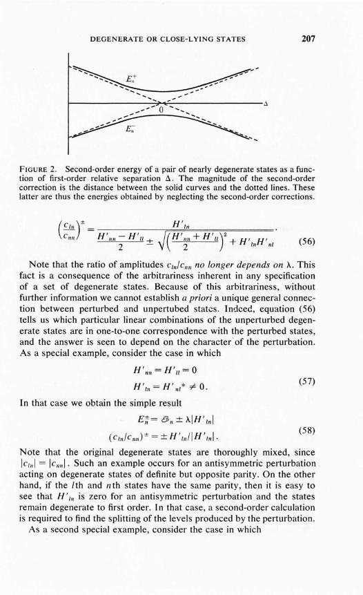
DEGENERATE OR CLOSE-LYING STATES 207
FIGURE 2. Second-order energy of a pair of nearly degenerate states as a function of first-order relative separation ~. The magnitude of the second-ordercorrection is the distance between the solid curves and the dotted lines. Theselatter are thus the energies obtained by neglecting the second-order corrections.
(CIII )± H'I"c"n = H'nn - H'll-+- I(H'n" + H'Il)2 + H' H' (56)
2 - \/ 2 In nl
Note that the ratio of amplitudes CI"/C",, no longer depends on "-. Thisfact is a consequence of the arbitrariness inherent in any specificationof a set of degenerate states. Because of this arbitrariness, withoutfurther information we cannot establish a priori a unique general connection between perturbed and unpertubed states. Indeed, equation (56)tells us which particular linear combinations of the unperturbed degenerate states are in one-to-one correspondence with the perturbed states,and the answer is seen to depend on the character' of the perturbation.As a special example, consider the case in which
H'nn = H'll = 0
H'III = H' 111* =;6 O.(57)
(58)
In that case we obtain the simple result
E~= 8" ± ,,-iH'lni
(CI"/C,,n) ± = ± H '11l/IH 'I"i·Note that the original degenerate states are thoroughly mixed, sincelelni = ICnnl· Such an example occurs for an antisymmetric perturbationacting on degenerate states of definite but opposite parity. On the otherhand, if the lth and nth states have the same parity, then it is easy tosee that H' In is zero for an antisymmetric perturbation and the statesremain degenerate to first order. In that case, a second-order calculationis required to find the splitting of the levels produced by the perturbation.
As a second special example, consider the case in which

208 APPROXIMATION METHODS
H 'In = !-I I nl* = 0,
so that the states are not connected to first order. In that case, the twostates are described by
and
En = 3 n + 'AH'"" ,
E,,= §,,+'AH'l/'
C"n = I
Cln = I,
and the degeneracy plays no role in the analysis. Examples of this sortoccur whenever the perturbation commutes with the set of operatorsused to define the unperturbed states. Otherwise stated, the analysisreduces to that of conventional perturbation theory whenever the unperturbed states can be uniquely specified by a set of operators, each ofwhich commutes with the perturbation term.
6. TIME DEPENDENT PERTURBATION THEORY
As a final approximation method, we now consider the case in whicha system, in some definite initial state, is subjected to some externalforce which depends on the time. An example would be the oscillatingforce exerted on an atom by a light wave passing through it. We shallassume the external force to be weak enQugh that a perturbation methodcan be applied. We write the Hamiltonian in the form
H=Ho+H'(t), (59)
without bothering to introduce a parameter of smallness 'A. We nowseek approximate solutions of the time dependent Schrodinger's equation
HljJ == [Ho+HI(t)]ljJ=_~ ~~.
Again denoting the eigenfunctions and eigenvalues of the unperturbedHamiltonian by cPn and 3 n, we express ljJ as the superposition,
ljJ(x, t) = Lan (t) cPn(X) ,n
where the expansion coefficients must now be regarded as functionsof time. If H' were zero, the a" would be proportional to e-i9"l/~, andit is accordingly convenient to write, without loss of generality,
a,,(t) =c,,(t) e-iCJ,,,l/~,
so that
(60)
We thus have

TIME DEPENDENT PERTURBATION THEORY
and
whence Schrodinger's equation becomes
209
(61)
Multiplying through by cPm* and integrating, we finally obtain, for each m,
dc i----!!!= ---" H' (t) e-i(,5n-6mltlh c (t)dt Ii L.J m" n .
This simultaneous set of coupled first-order differential equations isexact and is completely equivalent to the time dependent Schrodinger'sequation. Of course, the initial conditions must still be specified. We shallconsider only the case in which ljJ(t = 0) = cPk' that is, in which thesystem is in the kth unperturbed state initially. Thus we have
(',,(t=O) =8nk .
We now assume that the perturbation is weak enough, or that werestrict our attention to short enough times, that all c" except Ck remainsmall. To first order, we then have
where we have retained only the kth term in the summation on the rightside of equation (61). The first of these equations then gives at once
ck=exp [-i LH'kk(t) dt/Ii] = 1-*J: H'kk(t) dt.
Neglecting the deviation of Ck from unity, since this deviation contributes only terms of higher order than the first, the second equation gives
. (tm "'" k: Cm =-* Jo H'mk(t) e-iWk-6m)/lh dt. (62)
As a first exa:npie, suppose that H' is independent of time, except forsuddenly having been "switched on" at t = 0, and just as suddenly"switched off" at time t. We then obtain
210 APPROXIMATION METHODS
which corresponds to an energy shift H'kb in agreement with our firstorder stationary perturbation theory result. For the Cm we have
e-i( () k- () m)//ft - ICm(t) = H'mk
(63)
or
1 () 12= 41H' 12 sin
2( 6 k - 6 m )t/2fi .
cmt mk (6k -6m)2
For non-degenerate states, we thus see that if H'mk is small enough,then Icml2 remains small for all t. For larger H' mk, however, our approximation is valid only for small enough t. In either case, the interpretationof our result is the following. The probability that the system, initiallyin the kth unperturbed state, will be found in the rnth unperturbed stateafter the interaction has occurred is Icm(t) 12 • From this point of view, therole of the perturbation, acting over the time interval from 0 to t, is toproduce transitions between the unperturbed states.
Consider next the case of degenerate, or nearly degenerate, states.For 6 m = 6 k , we see that
Icml 2 = IH' mk/2t2/fi2, (64)
and hence that the transition probability grows rapidly with time andeventually becomes of order unity. This follows no matter how small isH'mk' just so long as it is not identically zero. The reason for this behavioris easy to understand from our previous stationary perturbation theoryresults. As we saw, when the rnth and kth states are degenerate and H'mkdiffers from zero, the perturbed states are particular linear combinationsof the degenerate unperturbed states with relative magnitudes of orderunity. The growth of Icml 2 thus reflects the frantic (but unsuccessful)attempt of the system to achieve just the right linear combination inresponse to the perturbation. Since C m eventually becomes comparableto Ck, our approximation evidently holds only for short enough times.However, results valid for arbitrary times can be obtained by treatingCm and Ck simultaneously and on equal basis in equation (61). The resulting coupled equations are easy to solve, but the details are left to theproblems.
One aspect of equation (63), which is rather surprising, is that Icml 2
initially grows as t 2• We would instead expect the probability of transitions to grow linearly with time, that is, the effect of the perturbationshould be describable in terms of a rate at which it induces transitions.Clearly this is not the case for transitions to a single degenerate finalstate, but our expectation is realized for transitions to a dense group offinal states, as in the continuum. To understand this important case, wenow consider the transition probability P to such a group of states,

TIME DEPENDENT PERTURBATION THEORY 211
The structure of this summation is already very interesting. For t largeand fixed, the matrix element H' mk can be regarded as varying ratherslowly from term to term compared to the remaining factor. Hence,regarded as a function of 8 m , the quantity Icm l2 is sharply peaked about8 m = 8k> as shown in Figure 3 below. From the figure it is clear that,for t approaching infinity, transitions occur with appreciable probabilityonly to a narrower and narrower band of states, with energy E centeredabout the initial state energy 8 k • This expresses the fact of conservationof energy, since only those final states are appreciably populated whose
FIGURE 3. Transition probability against energy.
energy differs infinitesimally from that of the initial state. The nonconservative effects of switching the interaction on and off thus becomenegligible if the time interval between these acts is long enough.
From the figure we note that the width of the peak in the transitionprobability curve is inversely proportional to t, while the height of thecurve is proportional to t 2
• Thus P, which is proportional to the areaunder the curve, increases linearly with t, as asserted. To make thisexplicit, recalling that the final states are assumed to be dense, we convertthe summation in equation (65) to an integral over an interval 6..£ surrounding 8 k , by expressing the number of states in the energy intervalbetween E and E + dE as p (E) dE. Thus pee) is the density of statesat E. In this way we obtain
P = 4J °k+Ii
E/2 (E) dE IH ' 12 sin2[( 8 k - E) t/2h]P mk ( to. E)2 '
0k-IiE/2 CPk -
where now H' ml, means the matrix element between the initial stateand a typical final state in the interval 6.E. Neglecting the variation ofp (E) and of IH 'mk 12 over this small interval, we then obtain

212 APPROXIMATION METHODS
Letting x = (E - 8 k ) t/2h, we next have
P = 2ht p(E) IH'mkl2jl"'£/4" sixn: x dx.
-1"'£/4'.
For t ~ 00, the integral can be shown to equal 7T, and hence we find
(66)
(67)
and P is proportional to t, as predicted. Introducing the transition rateW = dP/dt, we finally obtain
W = 2; p(E) IH'mk1 2 •
This is an extremely important and useful result. It is usually called,after Fermi, the golden rule of quantum mechanics. In words, it statesthat the number oftransitions per unit time from an initial state to a densegroup of final states which conserve energy is 27T/h times the density offinal states times the absolute square of the matrix element connectinginitial and final states.
The domain of validity of this result is determined by the followingconsiderations. In the first place, the total probability P that the systemhas undergone some transition from the initial state must be small,P ~ I. Hence, from equation (66), we must have
(68)
which serves to restrict the time interval over which the results apply.On the other hand, the details of our derivation make clear that thisinterval cannot be too short. To see this, recall that the width of the peakin Figure 3 is inversely proportional to t. If we denote this width by E,
we have specifically
Et/2h = I. (69)
Recall also that our evaluation of the sum over final states in equation(64) in effect assumes that E is small enough that both the density ofstates and the matrix elements can be treated as constant. If Eo is a measure of the maximum width over which this assumption is justified, thenwe must have
Eot/2h 2: I. (70)

TIME DEPENDENT PERTURBATION THEORY 213
(72)
The only way that equations (68) and (70) can be simultaneously satisfied, in general, is for H '/Ilk to be small. In summary, then, we are notsurprised to see that the golden rule applies only for weak perturbations.
One other aspect of equation (69) is worthy of comment. The quantity€ is a measure of the uncertainty in the energy of those final states whichare reached by the system because of the perturbation. The product ofthis uncertainty and of the time for which the perturbation acts is thusof the order of fi, in agreement with the uncertainty principle.
So far, we have considered only perturbations which are independentof time, except for being switched on or off. We now generalize to thecase of harmonic time dependence by considering a perturbation of theform
H' (x, t) = H' (x)e±iwt, (71)
which is of the type describing the effects of the electromagnetic radiation field. 14 It then follows at once from equation (53) that all of our previous results apply, except that 6" - 6/11 is replaced by 6 •. - 6/11 =+= fiw.In particular, equation (63) becomes
I . ( )1 2 = 41H' 12 sin2[(6 •. - 6/11 =+= fiw)t/2fi].
(/II t /Ilk (a _ a _ L )2u.. U'1Il + nW
To make the notation clear, we remark that the upper sign in equation(72) goes with the upper sign in the exponent of equation (71), and similarly for the lower signs.
We now see that transitions from the kth to the mth state take placewith appreciable probability only when
(73)
which means that transitions are preferentially induced in which aquantum of energy fiw is either absorbed or emitted by the system.The former is called resonance absorption, the latter is called stimulatedor induced emission. If w is such that equation (73) is satisfied, and ifk and 111 refer to discrete, non-degenerate states, the transition probabilityis given by equation (64) as before, and hence is still seen to grow quadratically with the time. The result is thus valid only for short enoughtimes, no matter how weak the perturbation. However, just as in thecase ()f a time-independent perturbation, results valid for arbitrary timescan be obtained by treating C/II and c•. on an equal footing in equation(61). The resulting equations are again easy to solve, but the details areleft to the problems.
14 Strictly speaking, the harmonic time dependence is trigonometric, say cos(w{ + Il). Asa consequence, interference occurs between the positive and negative frequency components of the perturbation, but its contribution is negligible for those transitions which takeplace with appreciable probability, namely those near resonance.

214 APPROXIMATION METHODS
Considering next transitions to (or from) a dense set of degeneratestates in the continuum, the derivation of equation (67) is unaltered except that the initial and final state energies are related by equation (73).One can still speak of the process as conserving energy if it is understoodthat the energy referred to is that of the total system, the material partand the radiation field together. Thus in absorption, the material systemabsorbs a quantum hw at the expense of the radiation field. In emission,the radiation field gains a quantum at the expense of the material system.15
With this understanding, the golden rule and our interpretation of it bothstand without modification.
It must be emphasized that, in our development, the electromagneticfield has been treated as a strictly classical entity. The fact that absorption and emission are quantized is an automatic consequence of thequantum properties of the material system; it is not directly related tothe quantum properties of the field, although it is clearly consistent withthose properties. To take these latter into account, the field amplitudesmust be regarded as operators acting upon the state function describingthe field. These amplitudes can be expressed in terms of harmonic oscillator variables for each mode, and the state of the field is characterizedby the number of quanta in each. The zero point energy of these harmonicoscillators plays a crucial role in the interaction of material systems withthe electromagnetic field. These vacuum fluctuations, as they are called,are responsible for spontaneous emission, the emission of radiation bya system when, as is usually the case, no externally imposed radiationfield is present. Our classical treatment, valid only for large quantumnumbers, contains no reference to vacuum fluctuations and does not,therefore, account for spontaneous emission. 16
We remark without proof that the golden rule also applies to the description of induced transitions to a definite, discrete final state from aninitial state which is a dense mixture of degenerate states in the continuum. This process is thus the inverse of that described above.
As a specific example of the application of the golQen rule, we now consider a particle of charge e in its ground state 1/10 in a potential V(x),which is irradiated by light of frequency wand thereby ejected into thecontinuum. The process is thus essentially that of photo-ionization. Weshall make two simplifying assumptio05 in carrying out the calculation.The first of these is that the wavelength of the light is very great comparedto the size of the system. This is a very common and generally validassumption since, except in the x-ray region and below, the wavelength
15 Multiple emission and absorption processes, where two or more photons are involved,are described by second- and higher-order perturbation theory calculations.
16 For a semiclassical discussion of spontaneous emission, see Reference [23].

PROBLEMS 215
of light is certainly very much greater than atomic dimensions. Withthis assumption, the electric field {} which acts on the particle can betaken to be uniform in space, but harmonic in time, and the perturbationterm then has the form
H' (x, t) = H' (x) e- iwl = -e §x e- iwl , (74)
which is just the instantaneous potential energy of the particle in such afield. 17 The second simplifying assumption we shall make is that thefrequency w is large enough that the energy of the final state E is verylarge compared to V(x). This assumption allows us to treat the finalstate of the particle as a free particle state, that is, as a state of definitemomentum as well as energy.
The only points of difficulty in the calculation arise in evaluating thedensity of final states, since these lie in the continuum, and in the relatedproblem of properly normalizing such states. Both can be solved by thetrick of supposing the system to be enclosed in a large box of length L,and then eventually letting L approach infinity. A discrete, normalizableset of states is easily obtained, by imposing appropriate boundary conditions, when the system is in such a box. For example, for a physical box,the wave function would have to vanish at the walls. However, the statefunctions so defined would not be states of definite momentum, even inthe limit L ~ 00, because states of definite momentum never vanish.Thus we introduce, as a purely· mathematical device, the nonphysicalperiodicity condition that l/J(xo + L) = l/J(xo) , where the walls are assumed to lie at Xo and x 0+ L. For obvious reasons, this requirement iscalled a periodic boundary condition.
Since the free-particle simultaneous eigenfunctions of momentum andenergy are pure de Broglie waves, ei V'ImE xlft, we thus require that
exp [iY2mE (xo + L) /h] = exp [tV2mE xo/h ]
and hence that
Y2mE L/h= 2mr, n = 0, ±I, ±2, ....
The normalized states are then seen to be
•" - _I e iV2mE xlftyE - \II '
where
(75)
17 We have neglected magnetic forces because these are of order vic smaller than the electric forces, where v is the particle velocity. We have also omitted the positive frequencyterm because we are interested only in absorption.

216 APPROXIMATION METHODS
Y2mE = p = 2mrnL '
n = O,±I,±2,±.... (76)
As L becomes larger and larger, we see that the spectrum becomes moreand more closely spaced, and in the limit the states indeed become theusual free particle continuum states of definite momentum. It is just thisfact which both motivates and justifies the introduction of periodicboundary conditions.
We now evaluate the density of states peE). Recall that this densityis defined as the number of states with energy between E and E + il E.Now from equation (76), the total number of states N (E) with energyless than or equal to E is 2n + I, or equivalently, expressing n in termsof E,
N(E) = ~n Y2mE + l.
Consequently,
N(E+ ilE) = Ln
Y2m(E+ ilE) + I = N(E) + L~ ilE.~ 2~n E
Hence, neglecting higher-order terms,
ilN = N(E + ilE) - N(E) = 2~n Y2m/E ilE,
but by definition, ilN = p(E)ilE, and thus,
peE) = 2~n Y2m/E. (77)
Next we write the form of the matrix element of the perturbationH' (x) defined in equation (74). To make explicit the fact that this matrixelement is taken between the initial and final states, we denote it by H' if'
The initial state for our problem is the normalized ground state t/Jo(x)with energy Eo = -E, where E is the binding energy. The final state isthe normalized free-particle state defined by equation (75), with energyE r given by
Er= Eo + nw = nw - E.
The matrix element is then
H'ir= I t/Jo(x)H'(x)t/JEr(x) dx
or, explicitly, using (74) and (75),
H'· =-8 J,I, (x)ex-1- eiV2nlEr x 'fl dxIf '1'0 n .
(78)

PROBLEMS 217
The factor multiplying the electric field strength § is seen to be thematrix element of the dipole moment operator ex, and H'ifis a quantummechanical average of the energy of a dipole in a uniform field §.
In any case, the transition probability per unit time is now given by
W = 2; p(E f ) IH'ifI2
= ~2 V2m/Ef e2§21 f t/Jo(x) x e iV2niEfxlfl dxl 2. (79)
Note that the normalization length L, as it must not, does not enter intothe final result. The density of states is proportional to L but, through thenormalization of the continuum states, the square of the matrix elementis inversely proportional to L and their product is thus independent ofnormalization length. Hence equation (61) as it stands is the limit attainedas L becomes infinite.
It is of some interest to actually evaluate the matrix element for somespecific example. We shall do so for a particle in its ground state in asquare well potential. To simplify the calculation, we shall assume thewidth of the potential to be narrow enough that the ground state is theonly bound state, and further, that this state is so slightly bound that thewave function extends far beyond the walls of the potential. Indeed, weshall take the limit in which the wave function inside the square wellcontributes negligibly to the integral in equation (61) and can be ignored.Specifically, we thus write, extrapolating the exterior wave function tothe origin,
(80)
where € is the binding energy. This function, which is normalized, isillustrated in Figure 4, and is schematically compared with the trueground state wavefunction for a narrow potential. 18
equation (80)
true wave function
,------'=----x
- --2a
Vu
FIGURE 4. The wave function of equation (80) compared to the true wave function in the weakly bound ground state of a narrow square well potential.
.8 The wave function of equation (80) can be shown to be that obtained when 2a tends tozero and Vo to infinity in such a way that 2aVo approaches a constant, say g, that is, thelimit in which the square well potential approaches go(x). The binding energy is given interms of g by E = mg 2f2h 2 , as may be verified by taking the limit of equation (VI-16). Seealso Problem 4 of Chapter VI.

218 APPROXIMATION METHODS
With this final simplification, we then have
J:oo ljJo(x)x eivzmEfxlfl dx
(2me )1/4 JOO
= h2 -00 x exp [-V2mcv~lxl-tv'EfX)/h] dx
-_ (2:'ze )1/4 { Jooo xn exp [-~ (\!; - iV"E;)x/h] dx
+ foo x exp ['\I2in('\IE + i~)x/h] dX}
(2me)1/4 hZ {I I}
= f;2 2m (~-- iVEf)Z- (~+ iVEf)Z
= (2me)1/4 ~ 4i "\/E;i.h Z 2m E/+ez
Hence, equation (79) yields, for this example,
8hez§z e3/ZE liZw- f- m (Ei + €Z)2'
where
E f = hw - e.
Since we have assumed from the outset that hw P E, this can be reducedto
8ez§z e3IZw=----·mh5/Z W 71Z (81)
Subject to all the simplifying assumptions we have made, this resultmeans that if an electromagnetic wave of frequency wand electric vector§ irradiates an ensemble of N particles of charge e and mass m each inits ground state of binding energy e, in a square well potential, then thenumber of photoelectrons produced per second with energy hw - e isNW, where W is given above.
The example we have worked out is entirely analogous to the calculation of the photo-ionization of atoms or of the photo (electric)-disintegration of nuclei. Of course, our calculation, nontrivial as it may be, isonly one-dimensional, but the three-dimensional calculation is littlemore difficult. The differences between three dimensions and one aremerely characteristic differences in the density of states. Other differences may also arise if the structure of the ground state wave function isdifferent. The photo (electric)-disintegration of the deuteron isolates theeffects of the change in density of states, since the deuteron ground statewave function is essentially the one we have used in our calculation. The

PROBLEMS 219
result is that the transition probability per second turns out to be proportional to e112/w512 at high energies instead of to e312/w7/2. The photoionization of the hydrogen atom, on the other hand, also involves a changein the character of the ground state wave function, which is that appropriate to a Coulomb potential rather than to a square well, with the resultthat the transition probability falls off much more rapidly with frequency,being proportional to e 5/2 /(lJ912.
As a final remark, we note that it is customary to describe these processes in terms of the probability of disintegration or ionization perincident photon, rather than in terms of the probability per unit time. Thenumber of photons per cm2 per second in a light beam of intensity I isproportional to I/hw, and I in turn is proportional to the square of theelectric field, 8 2
• Hence the probability per incident photon per cm2 ,
or cross-section as it is called, is proportional to e1/2/w3/2 for photo (electric)-disintegration of the deuteron, and to e512/w7/2 for photo-ionizationof the hydrogen atom.
Problem 1. If the classical turning point occurs at an infinite potentialwall, the wave function actually vanishes at the turning point; it doesnot extend an effective one-eighth wavelength beyond the turning point.The quantum condition equation (12) must then be modified.
(a) What is the correct quantum condition for a particle in a box(infinite potential walls)?
(b) Use the WKB approximation to find the stationary states andcompare with the exact results. Explain.
Problem 2. Consider the motion of a bouncing ball. Take the motionto be perfectly vertical and the collisions of the ball with the ground tobe perfectly elastic. The potential is given in Figure 5, below.
(a) What are the correct quantum conditions?(b) Use the WKB approximation to find the stationary state
energies.(c) What is the order of magnitude of the quantum number appro
priate to the stationary state of a ball of mass 100 gm dropped fromone meter?
IV=CO ~~v~xmgx
FIGURE 5. Potential energy of a bouncing ball.
Problem 3. Apply the Rayleigh-Ritz variational method to the harmonicoscillator to find:

220 APPROXIMATION METHODS
(a) The ground state energy using a Gaussian of variationallydetermined width as a trial function.
(b) The energy of the first excited state using the trial wave function, with a2 as variational parameter,
1/J={x(x2 -a2 )2, Ixl~a0, Ixl ~ a.
Does the minimum principle apply? Explain.
Problem 4. Apply the Rayleigh-Ritz variational method to a particlein a box of width L to find:
(a) The ground state energy using a second-degree polynomial astrial function.
(b) The ground state energy using a fourth-degree polynomial.(c) The energy of the first excited state using the simplest appro
priate polynomial as a trial function.Note: In each case choose your trial function to satisfy the correctboundary conditions at the walls.
Problem 5. In nuclear physics, a frequently used potential is a harmonicoscillator cut off at x = ± b, that is,
V(x) = {t mw2 (x 2- b2
), Ixl ~ b0, Ixl ~ b.
(a) Use the Rayleigh-Ritz method to estimate the energies of theground state and first excited state. As trial functions use the polynomialin the example in the text, equation (19), and that in Problem 3(b), ineach case with a2 as variational parameter. Choose b such that b > a.
(b) The same, for the case b < a.(c) Estimate the energies of the same two states using the WKB
approximation (modified Bohr quantization condition).(d) From your variational results and your WKB results, estimate
the maximum value of b for which the potential contains only one boundstate.
(e) Compare your WKB and variational results in each case aboveand state which you think more reliable. Explain your reasoning.
Problem 6. A particle is described by the Hamiltonian H = H 0 - Fx,where H 0 is the harmonic oscillator Hamiltonian. The system is thusthat of a harmonic oscillator in a uniform gravitational field (F = -mg)or in a uniform electric field (F = - e 6).
(a) Show that to first order the energy eigenvalues are unchanged.(b) Show that
X II ,n+l = X II +1,1I = V(n + l) 1i/2mw
x n,1II = 0, m -# n ± 1.

PROBLEMS 221
(c) Calculate the energy eigenvalues to second order.(d) Find the exact solution to the problem. Hint: Introduce a shift
of origin. Compare with the results of part (c).
Problem 7.(a) What is the matrix representing the operation of multiplication
by unity? This matrix is called the unit matrix. What about multiplication by a constant c?
(b) Verify by the rules of matrix multiplication that the unit matrixmultiplying any matrix gives the expected result.
(c) Given the two-by-two matrices
-I)I '
B = ( 2-IA=G D,
find A 2 , B 2, A + B, AB and BA.
Problem 8.(a) The matrix elements x"", of x for the harmonic oscillator are
given in Problem 6(b). Using the rules of matrix multiplication find thematrix elements of x 2 • Verify your results by direct computation ofX 2'"I1. (See Problem 2(b) of Chapter VI).
(b) The same for p and p2. (See Problem 2(c) of Chapter VI.)(c) Use your results to verify that
(p,x) = Il/i.
Problem 9. A particle moves with energy E in a potential
VV(x) - 0- cosh2 x/b
(a) Assuming E > 1Vol, find as precisely as you can the conditionson Vo and b under which the WKB approximation is valid.
(b) Under the conditions obtained in (a), calculate the WKB transmission coefficient T( E) and the time increment associated with thepassage of a particle of energy E through the potential.
Problem 10. Consider a perturbation H' which is independent of timeexcept for being switched on at t = 0 and switched off at time t. Supposethe mth and nth unperturbed states to be exactly degenerate, 6", = 6".
(a) Assuming that initially the system is in the mth unperturbedstate, find its subsequent behavior. Start with equation (61) and neglectall states but the degenerate pair, but treat these without further approximation.
(b) For what initial conditions will the system be in a stationarystate, with no (first-order) transitions being induced by the perturbation?
(c) Discuss the connection of your results with those obtained instationary perturbation theory.

222 APPROXIMATION METHODS
Problem 11. A particle of mass m is placed in a one-dimensional box ofwidth 2L, centered at the origin, in the presence of a uniform gravitational field. Thus the Hamiltonian of the system is
2
H=L+ mgx2m '
Ixl :,;::; L.
Estimate the allowed energies of the system using:(a) WKB approximation.(b) Second-order perturbation theory (why not first-order?).(c) The Rayleigh-Ritz method (ground state only). Use the trial
function (I - ax) cos 1Tx/2L. Explain why this is a reasonable trialfunction. Why is any function of definite symmetry inferior to the onesuggested?
Problem 12. A particle of mass m is confined inside the triangular potential well shown in Figure 6. Its Hamiltonian is thus H = (p2/2m) + V(x),where
V(x) = 00,
= kx,
x<O
x> O.
v = kx
"----------.. xoFIGURE 6. Triangular potential well.
(a) Estimate the ground state energy using the uncertainty principle.(b) Estimate the ground state energy using the Rayleigh-Ritz
variational method. As triai function choose
x ~ a,
and treat a as a variational parameter.(c) Suggest a suitable trial function for the first excited states but do
not carry out any calculations. Briefly justify your choice. Does the firstexcited state satisfy a minimum principle? Why?

PROBLEMS 223
Problem 13. The ground state energy of a system is estimated both bythe Rayleigh-Ritz method and by a second-order perturbation theorycalculation. The Rayleigh-Ritz result is found to be -27.1 eV and theperturbation theory result - 26.0 eV. Which lies closer to the true groundstate energy? Suppose the numbers had been reversed. Would it still bepossible to decide which estimate is better? Explain your reasoning.
Problem 14. A particle of mass m moves in a potential Vex) = Vo(x/L)2s,where s is a positive integer. (N .B. The problem is that of the harmonicoscillator for s = 1, of a square well for s ~ 00.)
(a) Estimate the magnitude of its ground state energy using theuncertainty principle.
(b) Estimate its ground state energy by the Rayleigh-Ritz methodusing as trial functions
(i) t/J = exp [- x2/2a 2]
(ii) t/J = {sin 7Txla, x ~ ao , x> a.
Treat a as a variational parameter in both cases. Which trial functiongives better results for differing values of s? Discuss your result.
(c) Show that in WKB approximation the energy of the nth statecan be expressed in the form
E =k(' [(n+t)2sfi,2S Vo]s:hn s) mSL2S ,
where k(s) is a dimensionless quantity which is of order of magnitudeunity for all s. Find an explicit expression for k(s).
Problem 15. A harmonic oscillator of mass m, charge e and classicalfrequency w is in its ground state.
(a) A uniform electric field eJ is turned on at t = 0' and is thenturned off at t = 'T. Use first-order time dependent perturbation theoryto estimate the probability that the system is excited to its nth state.
(b) The same for a uniform but sinusoidally oscillating electricfield, eJ = eJo sin wot.
Problem 16. Let t/J Iand t/J2 be a pair of degenerate orthonormal states ofsome system. At time t = 0, a perturbation H' is turned on and at timet = 'T it is turned off. If the system is initially in the state t/JI'
(a) Find t/J(x, t) for t > 'T and find the probability that a transitionhas occurred from t/J 1 to t/J2' Neglect all other states except the degeneratepair. For simplicity, assume
(t/JI!H'liJJ2) = (t/J2IH ' lt/Jl) = E
(t/J2IH'It/J2)= (t/JIIH'!t/JI) =0.

224 APPROXIMATION METHODS
(b) Compare your result for the transition probability with thatobtained using first-order time dependent theory and then find preciseconditions for the validity of the latter in the present instance.
Problem 17. The harmonic oscillator reduces to a free particle systemwhen its frequency tends to zero. It is easily verified that the harmonicoscillator propagator properly becomes that for a free particle in thislimit. It is not so easy, however, to verify that the harmonic oscillatorstate functions reduce to free particle state functions.
(a) Do so by letting w ~ 0 and n ~ 00 in such a way that
En=(n+t)hw~E
and examining the oscillator state function !/Ill in this limit. [Hint: Usethe integral representation of equation (VI-61) and eval.uate the integralby a saddle point method.]
(b) Consider the WKB approximation to the harmonic oscillatorstate functions (but not too close to the turning points). Show that, forlarge enough n, the state function is quite close to a free particle stateover the central region.
(c) Show that the WKB states reduce to the correct free particlestates in the zero frequency limit described in part (a). Note that theturning points become infinitely remote in that limit.
Problem 18. A system with unperturbed eigenstates and energies <Pnand En, respectively, is subjected to a time dependent perturbation
H'(t) =~ e- t2/T
"
V7TT
where A is a time independent operator.(a) If initially (t = -00) the system is in its ground state <Po, show
that, to first order, the probability amplitude that at t = 00 the system willbe in its mth state (m "# 0) is
where
Amo = (<PmIAI<P o)·
(b) The limit T2(E 1 - E O)2/4h2 ~ I is called the adiabatic limit.
Discuss the behavior of the system as t progresses from minus to plusinfinity in the adiabatic limit. Why do all transition probabilities tend tozero in this limit?
(c) Next consider the limit of an impulsive perturbation, T = O.Show that the probability P that the system makes any transition whatsoever out of the ground state is

PROBLEMS
Ip= h2 [(A2) 00- (A OO )2]
I= h2 [(<pOIA21<P0) - (<PoI A I<P0)2].
225
Hint: Find the transition probability to the mth state and sum over allexcited states using the methods of matrix algebra.
(d) Show that the impulsive perturbation of part (c) is equivalent to
H'(t) =A8(t).
(e) Integrate the time dependent Schrodinger's equation over aninfinitesimal interval about t = 0 to show that 1/1(x, t) is discontinuousat t = O. Show specifically that 19
and hence that the exact solution of the time dependent Schrodinger'sequation is
t < 0:
t> 0:
1/1 = <Po e-iEollfl
1/1 = ~ em <Pm e-iEmtlfl
Show that this reduces to the first-order perturbation theory result ifthe perturbation is weak enough.
(0 Verify that ~ Icml 2 = 1.
Problem 19. Let 1/1" denote the stationary bound states of a system corresponding to energy EI/' Choosing the 1/111 to be real for convenience (seeproblem VI-II),
(a) Show that
(1/1"lpx!1/1,,) = hl2i
(tP"lxP!1/1,,) =?
(b) Show that
2: {(1/1"lxHI1/1q) (1/1 qlxltPlI) - (.tP"l x l1/1q) (1/1qlxH!1/1,,)}q
=2: (Eq-E,.)lx"qI2.q
19 If B denotes some operator, its inverse B-I is defined. when it exists. by
B-IB= BB- 1 = I.

226 APPRoxIMATION METHODS
(c) Using the results of (a) and (b), and the methods of matrixalgebra, show, finally, that
L (Eq -En)lxnqI2=h2/2m.q
[This is an extremely important example of what is called a sum rule.Its importance comes from the fact that the probability for a dipoleradiative transition between the qth and nth states is proportional toIXnq 1
2• Thus these matrix elements are directly measurable quantities.]
(d) Verify the sum rule for the harmonic oscillator by actual evaluation of the sum.
Problem 20. In Chapter VI we showed that an attractive square well hasat least one bound state no matter how weak the potential. Use the Rayleigh-Ritz variational method to prove that this is a general property ofany potential which is purely attractive. Do this by using the trial function
and showing that a can always be so chosen that E' (a) is negative. (Whydoes this constitute a proof?)

VIII~Systems of particles
one dimension
1. FORMULATION
.zn
We now come to the first major generalization of our formulation of thelaws of quantum mechanics. We have seen that the requirements of thecorrespondence principle led us to the Hamiltonian as the operator whichdetermines the time development of a system consisting of a single particle moving in an external field of force. By similar arguments, it followsthat the Hamiltonian operator for a system of particles plays exactly thesame role, as we now show.
We consider a system of A interacting particles, each of which may alsobe under the influence of some external force. The classical Hamiltonianfor such a system is then
A p.2 A
H(PI," "PA, XI,···, X A) =L"2-:+ L Vi(Xi) + L VU(xi-xJ,i=1 m, i=1 pairs (I)
where plj2m i is the kinetic energy of the ith particle of mass mi andVi(xJ is any externally imposed potential (such as gravity) in which theith particle is moving. Finally,
Vij(xi-Xj) == Vj;(Xj-x i)
is the mutual potential energy of interaction between the ith particle atXi and the jth at Xj' As the notation shows, we take this interaction todepend only upon the coordinate difference Xi - X j' The total energy ofinteraction is obtained by summing the two particle terms over all pairsof particles, as indicated. An explicit way of writing this term is
L Vij (Xi - Xj) == LVii'pain i.i
i< j

228 SYSTEMS OF PARTICLES IN ONE DIMENSION
In summing over i and}, the condition that i is always less than} insuresthat each pair is counted only once.
We now make the following assumptions about the quantum mechanical description of such a system, all of which are more or less obviousgeneralizations of the one particle description.
(a) In configuration space, the state function of the system depends onthe coordinate of each particle and on the time,
(b) Assuming 1/1 to be normalized,
J dx dx 2 ' .. dXAII/I12 = 1, (2)
the absolute probability density in configuration space is 11/11 2 • Moreexplicitly, 11/11 2 dXI dx 2' •• dx A is the probability that, at one and thesame instant t, particle one is to be found in the interval between x I
and XI + dxl , particle two between X2 and X2+ dX2' and so on for all Aparticles. From this it follows that
(3)
is the probability density for particle one alone, independent of the details of the behavior of the remaining particles. Thus p(x l ) has the samemeaning and the same properties as the familiar probability density for asingle particle; in particular, the usual probability conservation laws mustbe satisfied.
(c) The dynamical variables of each particle are operators satisfying the normal commutation law. However, since the dynamical variablesof different particles represent totally different degrees of freedom, andthus noninterfering observables, the dynamical variables of differentparticles commute with each other. In brief, we thus write
[Pi' Pi] = [x·i,Xj] =0
Ii[pi.xd=--;-Oij.
I(4)
Specifically, in configuration space the Xi are numbers and the Pi are givenby
(5)
In momentum space, conversely, the Pi are numbers and the X i aregiven ~y
Ii ax·=-- -.I i api
(6)

TWO PARTICLES: CENTER-OF-MASS COORDINATES 229
From these assumptions it follows that the state function in momentumspacecP(PhP2," "PA.t) is the A-fold Fourier transform 1 of ljJ, thatexpectation values are computed in the usual way,
(h a h a )(f(Xi,' . . ,XA; Ph' . "PA» = (ljJlf x;, . . . ,X.A;-:- -, ... ,-:- - IljJ)I aXi I aX A
(h a h a )= (cPlf--:--a ""'--;--a-;Pl"",PA IcP),I Pi I PA
and that Schrodinger's equation must have the general form
H,I. = E"'=-!!:. aljJ'I' 'I' i at' (7)
where H is some linear Hermitian operator. The first-order time derivative is required for probability conservation just as before. Using thefact that, from equations (4), (5) and (6),
h af[Pi,f(X1 , • • • ,X A;Pl,' .. ,PA)] =-:- -a
I Xi
h af[f(x!> . . "XA,Pl" . ',PA),XJ =-;--,
I api
we then find that, by arguments exactly paralleling those used in thesingle-particle case (see Section 3 of Chapter V),
d aHdt (Xi) = (api)
d aHdt (Pi)=-(OXi)'
Associating expectation values with the classical variables in the senseof the correspondence principle, we see that these are the classical equations of motion in Hamiltonian form, provided that H in equation (7)is the Hamiltonian operator, that is, the Hamiltonian of equation (1)regarded as a function of the quantum mechanical dynamical variablesdefined by (4), (5) and (6).
2. TWO PARTICLES: CENTER-OF-MASS COORDINATES
As a first application of our generalized formulation we consider two
, Specifically, this means that ljJ and c/J are related by
ljJ = (21Th) -A/2 f dp, ... dp A c/J(PI> .. " P A) exp [i(p,x, + P 2X2 + ... + PAx.)/h]
and

230 SYSTEMS OF PARTICLES IN ONE DIMENSION
particles, of mass mt and m 2 , respectively, which interact through apotential V(x t - X2) in the absence of external forces. The Hamiltonianof the system is thus
(8)
and Schrodinger's equation in configuration space is then
(9)
The form of V suggests the introduction of the distance between theparticles as a new coordinate, and we therefore introduce the transformation
X=X t -X2
where a and f3 are parameters of our choice. Of course X will turn outto be the center-of-mass coordinate, but it is instructive to see how thisworks out. We now have
a a a----+f3-aX2 - ax ax'
whence
where p., the reduced mass of the system, is given by
1 1 I-=-+_.P. m t m2 '
(10)
To eliminate the cross-term, we choose f3 such that
and hence
1 a2 1 a2 1 a2 a 2 a2m
tax
t2+ m2 ax22 =;, ax2 + m
t(mt + m2) aX2·
The choice of a is still quite arbitrary; it merely serves to fix the scale of

TWO PARTICLES: CENTER-OF-MASS COORDINATES 231
the X coordinate. The most convenient choice is clearly that for which
f f dx 1 dx 2~ f f dx dX,
and this requires that the Jacobian of the transformation be unity. Thus
ax ax- - -1
1= aX l aX 2= ex (::+ 1),
ax ax m2- ex -exaX l ax 2 ml
and hence
where M = ml + m2 is the total mass. Thus finally
(11)
and, conversely,
(12)
(13)
whence Schrodinger's equation becomes
[h2 a2 h2 a2
] h a'lr-- ----+V(x) 'Jr(x X t)=--_·2JL ax2 2M aX2 "i at
We now give an alternative method for deriving Schrodinger's equationin the center-of-mass coordinate system, as the coordinates defined byequations (11) and (12) are called. The classical Hamiltonian, equation(8), can at once be written in center-of-mass coordinates in the familiarform 2
(14)
where
dX dXI dX 2P= Mdt = m l dt + m2 dt = P 1+ P2
P = J.L dx = J.L (!!.L _l!.1...) .dt m l m2
Consider now the quantum mechanical operators corresponding tothese new coordinates and momenta. We have
2 See References [14] through [17].

232 SYSTEMS OF PARTICLES IN ONE DIMENSION
[ p X]-[( ) mIXI+m2x2]_ml [ ] m2 [ ]_h, - PI + P2 , M - M PbX. + M P2,X2 -j'
while, in the same way, it is easy to see that
[p,X] = [P,x] = O.
The transformation from PhXhP2,X2 to P,x,P,X thus leaves thecommutation rules unchanged; such a transformation is called a canonicaltransformation.3 From these commutation rules we can write, in configuration space,
h aP = j ax'
h aP= j ax' (15)
and hence Schrodinger's equation in the form of equation (13) followsat once from the Hamiltonian in center-of-mass coordinates, equation(14). Note that the center-of-mass momentum P commutes with Handhence is a constant of the motion. Just as in classical physics, the totalmomentum of an isolated system is conserved.
Schrodinger's equation in center-of-mass coordinates is clearly separable, which is the main point of the transformation. Thus, writing
we have
'I'(X, X, t) = X(X, t)l/J(x, t) (16)
(17)
! [_!!!... a2
1/J + V(x)1/J + ~ al/J] = _1. [_~ a2X + ~ ax].I/J 21-'- ax2 i at x 2M aX2 i at
The separation constant is merely an additive constant in the total energyand hence can be set equal to zero without loss of generality.4 With thischoice, the state function of the center of mass of the system satisfiesthe free-particle Schrodinger's equation
h2 a2X h aX-2M aX2=-j at'
and can thus be taken to be a free-particle wave packet at rest or in uni-
3 Such a transformation is the quantum analog of a classical canonical transformation, thatis, a transformation which leaves the Hamiltonian equations unaltered in form. See, forexample. Reference [14].
4 More generally, the separation "constant" could be regarded as an arbitrary functionof the time. This merely reflects the invariance of the total wave function 'i'(x, X, T) tothe transformation t/Jf= t/J e ifW, Xf= X e- ifW , by which we mean the simultaneous replacement of t/J by t/J eifW and X by X e- ifW. No physical result depends on f and no loss of generality is incurred in choosing it to be zero.

(18)
INTERACTING PARTICLES AND UNIFORM EXTERNAL FORCES 233
form motion; it can also be taken to be an eigenstate of the total momentum, as circumstances warrant.
Exercise 1. From equations (14) and (16) verify that
(Etotal) = (Ecm ) + (Erel ),
where Ecm and Erel respectively refer to the energy of the center of massand of the relative motion.
The relative motion is governed by the equivalent single-particleSchrodinger's equation
Ii 2 a21jJ Ii aljJ- 2JL ax2 + V(x)1jJ = - i at'
the solutions of which have already been thoroughly investigated. Forexample, for a quadratic interaction V(x) = JLW2x 2 j2, the states of relativemotion are just those of the harmonic oscillator. Such a system is a kindof one-dimensional diatomic molecule, and the states in question arevibrational in character. As a second example, continuum states of thekind discussed earlier can be interpreted as describing the collision of twoparticles (in one dimension). The reflection and transmission coefficientsgive the probability that the particles bounce back from or pass throughone another in the course of the collision. This transmission process mayseem strange classically, since classical particles are normally regardedas impenetrable. However, even on the classical level, impenetrabilityimplies an interaction potential which becomes infinitely repulsive atsmall distances of separation. For such a potential, the quantum mechanical transmission coefficient is easily seen to vanish, in agreement withthe classical result.
Our discussion thus far has been concerned with only a pair of interacting particles. What about isolated systems of three or more particles?It is easy to demonstrate,just as in classical mechanics, that the center-ofmass motion can be separated out and that this motion is governed by theequations for a free particle. However, again just as in classical mechanics, the internal motion is extremely complicated. Even in the roughestapproximation, the techniques involved in analyzing the states of such asystem are too sophisticated and too special to make it profitable for usto pursue the subject further at this time.
3. INTERACTING PARTICLES IN THE PRESENCE OF UNIFORMEXTERNAL FORCES
We now generalize our considerations to the case in which external forces

234 SYSTEMS OF PARTICLES iN ONE DIMENSION
are present. In these circumstances, no particular simplification is guaranteed by a transformation to center-of-mass coordinates. Of course, themotion of the center of mass is governed by the net external force onthe system, quantum mechanically as well as classically, but this netforce depends in general upon the configuration of the system. Thus thecenter-of-mass motion and the internal motion are coupled or, to put itanother way, Schrodinger's equation is not separable in the presence ofarbitrary external forces. However, as the above argument implies, thereis one exceptional situation in which separability is always possible,namely that in which the external forces are uniform, because the netforce is then independent of configuration. We now take up this specialcase.
Specifically, we consider two particles, each of which is subject to aconstant external force, say F I and F2 respectively, and which interactwith each other through a potential V (XI - X2)' The Hamiltonian of thesystem is thus
Transforming to center-of-mass coordinates, using equation (12), wethen have at once
H = [f;+ V(x) - (Flm2~F2ml) X] + [{~- (FI + F2) x].
Schrodinger's equation is now easily seen to separate, and we obtainfor the center-of-mass motion
(19)
and, for the internal motion,
[_!!!- L + V(x) - (F l m2 - F2ml.) x]l/J(x t) = - 4al/J. (20)
2/L ax2 M 'I at
As expected, equation (19) is the equation governing the motion of thecenter of mass under the influence of the net external force. Its solutionsare, unfortunately, rather complicated, but they are merely the quantummechanical transcription of motion under uniform acceleration.5
The additional term in equation (20) represents the differential effectof the external force on the motion of the particles relative to each other.If this term is small compared to the interaction potential, it can be treatedas a perturbation in the usual way. Thus, for example, to first order theenergy is shifted by the expectation value of the external force term. Of
5 See Problem VI-S.

INTERACTING PARTICLES AND UNIFORM EXTERNAL FORCES 235
course, if V(x) is symmetrical so that the unperturbed states havedefinite parity, this expectation value vanishes and the energy shift isof second order, that is, proportional to the square of the effective external forces.
The special case in which the interaction potential V(x) is quadraticin x is particularly simple, since the perturbing term can then be transformed away by a change of origin (see Chapter VII, Problem 6). Thestates are thus harmonic-oscillator states in which the minimum of thepotential energy is shifted away from the origin and in which the energyof each state is decreased by a constant amount, proportional to thesquare of the eftective external force. To give this example a physicalcast, let us call the two-particle system a diatomic molecule. Further,let us particularize the external forces by considering first the case of sucha molecule in a uniform gravitational field. In that case FI = - mig, F2
= - m2 g and the external force term in equation (20) is seen to vanish,while in equation (19) it is (m l + mz)g = MgKThus, the internal motionis unaffected by the gravitational field and the center of mass acceleratesin the expected way.
Consider next the case in which the external force is produced by auniform electric field 8. If the particles have equal and opposite charge,of magnitude e, then F I = -e 8 and F2 = e8. The net external force thusvanishes, as it must since the molecule has no net charge, and the centerof-mass motion is that of a free particle. The additive term in equation(20) is 8 ex, which is just the energy of an electric dipole of momentex in a uniform field 8. Recalling that the energy shift is quadratic inthe external force, the ground state energy of the diatomic moleculehas the form
(21)
where a is expressible in terms of the parameters of the harmonic oscillator potential. This energy shift is the energy of an induced dipole, ofmoment a 8, in the field 8; the quantity a is called the electric polarizabilily of the molecule. Note, for comparison, that if the ground state ofthe system had not had a definite parity, then the energy shift would havebeen linear, rather than quadratic in 8. That is, the ground state energywould have had the form
E = Eo - J-te 8,
which is the energy of a permanent electric dipole, of moment J-te, in anexternal field. From this example, we see that if the ground state of asystem has a definite parity, it has no permanent electric dipole moment.This is, overwhelmingly, the most common case in nature. For suchsystems, the action of an external electric field distorts the system,

236 SYSTEMS OF PARTICLES IN ONE DIMENSION
(22)
thereby producing a separation of charge proportional to the strength ofthe electric field which is expressed in terms of polarizability. We remarkthat the polarizability is a more or less directly measurable quantity,since the electric susceptibility of a gas can be simply expressed in termsof the electric polarizability of its constituent molecules.
4. COUPLED HARMONIC OSCILLATORS
Before going on to consider general external forces, we now briefly takeup a second exactly soluble example, that of a pair of coupled harmonicoscillators. Specifically, we consider a two-particle Hamiltonian of theform 6
H - Pl2
P22
I 2 2 + I 2 2 + I k( )2- 2m, + 2m2 +:2 mlw Xl "2 m2w X2 "2 Xl - X2 .
It is readily verified that the normal coordinates for this problem are justthe familiar center-of-mass and relative coordinates of equation (11).7
Introduction of these coordinates transforms the Hamiltonian into theseparable form
where
and
H = Hem + H ret ,
H - p2 1 M 2X2em - 2M +"2 w
(23)
(24)
(25)H - p2 + I -2X2
reI - 2p. "2 p.w
and where we have introduced the new frequency w, defined by
w= ~W2+~. (26)
Observe that if the interaction term is attractive, k > 0, we have w > w,and conversely, for repulsive interactions, k < 0, we have w < w.
Denoting the respective harmonic oscillator eigenfunctions of Hemand H rel by <PN(X) and cPn(x), with energies (N + i) hw and (n + i) hw,we then have as the exact stationary states
with energies
'l'Nn=<PN(X) cPn(x), N,n=0,1,2, ... , (27)
6For simplicity, we have chosen the somewhat special case in which the uncoupled oscillators each have the same frequency w.
7 This and subsequent details are left to the problems.

COUPLED HARMONIC OSCILLATORS
ENn = (N + t) nw + (n + t) nw .
237
(28)
The spectrum, which is seen to be non-degenerate if wand warenoncommensurate, is a simple composition of two harmonic oscillatorspectra. Its appearance, however, is strongly dependent on the relativemagnitude of wand w. In Figure l(a) the spectrum is shown for weaklyattractive interactions, by which we mean 0 < kIp., ~ w2
• For this case,w only slightly exceeds wand we obtain well-separated sets of states:an isolated ground state, a close-lying pair of first excited states, a c1oselying triplet of second excited states, and so on. For weakly repulsive
Nn
03122130
021120
0110
00
Nn
(a) (b)
FIGURE I. (a) Coupled oscillator spectrum for weak attractive forces. Allclose-lying states have the common spacing Ii (w - w). (b) Coupled oscillatorspectrum for dominantly strong attractive forces. Each infinite ladder of statesstarting on a given n has equal spacing liw.

238 SYSTEMS OF PARTICLES IN ONE DIMENSION
states, the same structure appears, except that the order of the close-lyingstates is reversed. In Figure I(b), the spectrum is shown for the oppositelimit kIlL ~ w2
, when the interaction term dominates. Here, the spectrumis seen to consist of a set of overlapping infinite ladders of closely-spacedstates, the first ladder starting on the ground state, the next on the staten = I, the next on n = 2, and so on.
The state function, although a reasonably simple function of the normalcoordinates, is a rather complicated function of the particle coordinatesXl and X2, except for the ground state, which, properly normalized, canbe expressed as
(29)
The excited states then consist of the same Gaussian factor multiplied byunwieldy polynomials of degree (n + N) in Xl and X2'
The coupled oscillator problem has some intrinsic interest.· For example, in the strong interaction limit it is a crude model of the states of atightly bound diatomic molecule in a crystal. However, its main interestis that it serves as a guide to applying approximation methods to the studyof properties of a system of particles (see Problem 9). In this connection,we remark that the utility of the coupled oscillator problem is not limitedto the two-particle system we have been analyzing. Exact solutions canbe found for any number of particles8 and we shall, in fact, eventuallydiscuss the three-particle case.
5. WEAKLY INTERACTING PARTICLES IN THE PRESENCEOF GENERAL EXTERNAL FORCES
We now return to the general case of nonuniform external forces where,as we emphasized at the outset, the center-of-mass motion cannot beseparated out. Even for a two-particle system, this problem is a verydifficult one, and we restrict our attention to the limit in which theexternal forces dominate over the internal forces, so that the latter canbe treated as a perturbation. As a starting point we must thus discuss theunperturbed states, which are those of a set of noninteracting particlesmoving under the influence of external forces. We shall consider onlytwo-particle systems in detail, but we will also briefly mention manyparticle systems.
8 For the classical case, see References [14] through [17]. For the quantum case, seeI. Bloch and Y. Hsieh, Physical Review 96, 382 (1954); 101, 205 (1956).

WEAKLY INTERACTING PARTICLES AND EXTERNAL FORCES 239
We start with the two-particle Hamiltonian
H = [f~I + VI(XI)] + [f~2 + V2(X2)] = HI (Ph Xl) + H2(P2,X2)' (31)
Center-of-mass coordinates are clearly irrelevant for this system, whichclassically consists simply of two particles moving independently. Writing
(32)
Schrodinger's equation is seen to separate, and we obtain the two singleparticle equations
[PI2 ] h a.pIHI.pI (Xl' t) = 2m
I+ VI (Xl) .pI = - i at
H ( ) - [ P22
V ( ) ] _ h a.p2. 2.p2 X2, t - -2 + 2 X2 .p2 - -"7 - •m2 I at
The stationary states of the system are simply the product states
.pnm = .pIn(XI).p2m(X2)
with energy
where .pIn and .p2m are the orthonormal eigenfunctions of HI and Hz witheigenvalues E ln and E2m. An arbitrary general state can then be constructed as a superposition of such independent particle states. Inparticular, solutions of the product form of equation (32) are obtained asthe product of an arbitrary superposition of the states of particle one andof a similar superposition of those of particle two. For such a product, wehave from equation (32)
1'1'12= 1.pI!21.p212,so that the particles are entirely uncorrelated and the time developmentof each proceeds just as independently as in the classical case.
We note, however, that it is possible to have states for which this complete independence does not hold. To see this, consider some arbitraryinitial state .p(Xh X2, t = 0). The most general state function is expressibleas
'I'(X I , X2, t) = L Cmn.pIn (Xl) .p2m (X 2) exp [- i(E In + E 2,,)t/h] ,
and hence, in virtue of the orthonormality of the .pIn and .p2m, we obtain,setting t = 0 and inverting,
Cnlll = JJ 'I'(X I,X2, t = 0) .pl"* (XI).p2m* (X2) dXI dX2'
240 SYSTEMS OF PARTICLES IN ONE DIMENSION
Now if the initial state is uncorrelated, that is, if it has the formIJJI(X I)IJJ2(X2), then Cnm can be expressed as a product CI "C2m , and thestate function remains uncorrelated for all time. However, if the initialstate is correlated, for whatever reason, then these correlations, whichhave no classical counterpart, persist in the state function for all time.Such correlations playa fundamental role in determining the propertiesof systems of identical particles, as we later show.
We are now ready to consider the effects of interactions upon thestationary states, supposing these to be weak compared to the externalforces. Denoting the interaction term by V(XI - X2), the Hamiltonian hasthe form
Treating V(x i - x2 ) as a perturbation, the unperturbed states are justproduct states IJJnm = IJJln(XI)1JJ2m(X2) with energy 6 nm = E I" + E2"" asdiscussed previously. To first order, we then have at once
(33)
while to second order,
(34)
where the matrix elements are explicitly given by
(IJJnmIVIIJJ lk) = f f dXI dX2 IJJln* (XI) IJJ2m * (X2) V(XI - X2) IJJH (XI) IJJ2d x 2) .
The generalization to more than two particles is immediate. Considerfirst a three-particle system. The unperturbed states are products of threeindependent particle states, and in the same notation as before, we havefor these states
If the mutual interaction perturbation term is written
V= VI2 (X 1 -X2) + VdXI-X3) + V23(X2-X3),
then the first-order result is
E"ml = 6 111"1 + (IJJ"mllVllJJ"ml).
The last term in this expression simplifies to a sum of two-body terms,exactly like those in equation (33). To see this, consider the contributionof, say, VI2 (XI - X2). We have

IDENTICAL PARTICLES AND EXCHANGE DEGENERACY 241
(t/JnmIIV121 t/Jnml)
= f dX 1dX2 dX31t/Jln(x1) 12 1t/J2m(X2) 1
2 !t/J31(X3) 12 V 12 (X1- X2)'
The X3 integration can be performed at once, and because t/J31 is normalized, the result is, as we claimed,
(t/JnmIIV121t/Jnml) = (t/JnmlVdt/Jnm) ,
and it is independent of I. In the same way, the other two terms yieldsimilar purely two-particle contributions.
For A particles we have products of A independent particle states andthe perturbation corrections again take the form of a sum of two-particlecontributions.
6. IDENTICAL PARTICLES AND EXCHANGE DEGENERACY
We now consider the extremely important case of a system of identicaLparticles. By identical particles, we always mean particles which arecompletely and absoluteLy indistinguishable: No physical significanceattaches to the labeling of such particles and no observable effects areproduced when any two of them are interchanged. In particular, thismeans that the coordinates of all identical particles must appear in theHamiltonian in exactly the same way. As a specific and simple example,consider two noninteracting identical particles under the influence ofsome external force. Each particle must feel exactly the same potential,and hence the Hamiltonian has the form
(35)
The stationary state solutions are thus
(36)
with energy
where t/Js(x) is an eigenfunction, with eigenvalue Es, of the commonsingle-particle Hamiltonian
Observe now that if q and n are different, this state is degenerate withrespect to interchange of the particles, that is, the state
(37)

242 SYSTEMS OF PARTICLES IN ONE DIMENSION
has the same energy as !J;nq. This degeneracy is called exchange degeneracy, and it is a consequence of the evident invariance of the Hamiltonian,equation (35), to an exchange of the coordinates of the two particles.
We now generalize this very important result. Specifically, we showthat exchange degeneracy is a property of the solutions of Schrodinger'sequation for any system of identical particles, no matter what their mutualinteractions, no matter what the external forces to which they are subjected, and no matter how many particles in the system. For this purposewe introduce the so-called exchange operator Pl2 == P2lo which exchangesthe coordinates of particles one and two when it acts upon any functionof those coordinates.9 Thus Pl2 is defined by
PI2f(XloX2,XS,' . . ,XA) = f(X2'X I,XS" . . ,XA) (38)
for arbitrary f Similarly Pij exchanges the coordinates of the ith andjth particles. As further examples, we have
PIS f(Xlo X2'XS" . . ,XA) = f(XS,X2,XI" . . ,XA)
and
Pl2 P lS f(Xt. X2,XS,' .. , XA) = Pl2 f(XS,X2,XI" .. ,XA)
= f(xs, Xl' X2, ... , XA) ,
and so on. Note carefully that, as this last example demonstrates, thesubscript on a coordinate labels the particle to which that coordinaterefers, and not the order in which a coordinate happens to appear in thestate function.
Now Pij commutes with the Hamiltonian by the definition of indistinguishability. Hence, if !J;E (xt. X2, ... , XN) is an eigenfunction of Hwith eigenvalue E, so is Pij!J;E, inasmuch as
H Pij !J;E= Pij H !J; E= E Pij !J;E'
We thus see that these states are degenerate with respect to the interchange of the ith andjth particles, unless Pij!J;E happens to be a multipleof !J;E, as for example the independent particle state of equation (36) withn = q. Of course, the labels i and j can refer to any pair of particles andhence exchange degeneracy occurs when any two identical particles areexchanged. For a system of A particles the solutions of Schrodinger'sequation may thus be as much as A !-foLd degenerate, corresponding tothe A ! permutations of the order in which the A particles can be labeledin writing the state function. Any linear combination of the linearlyindependent states formed from the complete set of A! permutations isan eigenfunction of the Hamiltonian, and the matter of classifying thesestates is generally not an easy one, as we shall see. However, for two
9 The algebraic properties of exchange operators are elaborated upon in Problem 1.

SYSTEMS OF TWO IDENTICAL PARTICLES 243
particles the problem is trivial and we now take up this simple, butimportant, special case.
7. SYSTEMS OF TWO IDENTICAL PARTICLES
For a two-particle state, we obviously need to consider only {he singleexchange operator P12' Now P122 is evidently unity and hence, just asfor the parity operator, the eigenvalues of Pl2 are ±l, corresponding tostates which are symmetrical or antisymmetrical under exchange. Thus,two-particle states can always be classified according to their symmetryunder exchange. As a particular example, for the independent particlestates of equation (36), we obtain the (normalized) correlated states
n y6 q;
and it is easily seen that, as it must,
More generally, if IjIE(XI> X2) is an eigenfunction of some two-particleHamiltonian with energy E, then the (unnormalized) symmetrized states,as they are called, are
(40)
provided that IjIE(XI> X2) does not happen to be symmetrized or antisymmetrized to start with.
The existence of such built-in symmetry might seem to be the exception, judging from the independent particle example where it occursonly in the special case n = q of equation (36). We now show, how~ver,that for real physical systems, that is, those containing interactions, wemust expect the true two-particle bound states to automatically exhibitsuch definite symmetry properties. The argument is a simple one. Theantisymmetric state function necessarily vanishes when Xl = X2, andhence the likelihood of finding the two particles in the immediate neighborhood of each other is reduced, compared to the similar likelihood fora symmetric state. The contribution of the interaction term in the Hamiltonian, whatever its sign, is thus numerically larger for symmetricalthan for antisymmetrical states. We accordingly expect that symmetricand antisymmetric states do not form degenerate pairs, except perhapsby accident, and hence that the bound state spectrum consists of a setof discrete and nondegenerate states. Now we simply turn the argumentaround. If the spectrum is indeed nondegenerate, barring accidents, thenwe conclude, knowing that all states are classifiable by their symmetryunder exchange, that the true states must have a definite symmetry, and

244 SYSTEMS OF PARTICLES IN ONE DIMENSION
(41 )
hence will automatically turn out to be symmetrized. 10
Our discussion of these properties of the states of two identical particles will be made clearer, perhaps, by consideration of the followingsimple and exactly soluble examples, first treated in Sections 3 and 4for the case of distinguishable particles. We now take these up in order.
(a) Uniform external forces. Here the particles can interact arbitrarily with each other, but the external force is restricted to be uniform.The Hamiltonian has the form
Pl2 P22
H = 2m + 2m + V(x i - X2) + F XI + F X2·
Because the particles are identical, the external force F acting on eachparticle is the same. Further, the interaction potential is necessarily asymmetrical function of its argument (why?). As a result, the states ofrelative motion are readily seen, from equation (20), with m l = m2 = mand F I = F2 = F, to have definite symmetry with respect to the relativecoordinate x = XI - X2' Since the center-of-mass states are necessarilysymmetrical under exchange (why?), the states of the system are seen tobe automatically symmetrized, in agreement with our expectations.
Exercise 2. Work out the details of the arguments leading to the aboveconclusion.
(b) Coupled Harmonic Oscillators. This is a more interesting example, and we work it out in some detail. For identical particles, theHamiltonian of equation (22) for coupled oscillators becomes
P 2 P 2 I 1 1H = _I + _2 + - mw2X 2 + - mw2X 2 + - k (X - X ) 22m 2m 2 1 2 2 2 I 2'
The center-of-mass transformation now takes the simple form
X =x I + X22 ' (42)
and under this transformation H becomes
10 This argument is rather similar to our discussion in Chapter VI of the parity of statesin a symmetrical potential. In that case, however, we were able to prove that the boundstate spectrum in one dimension is always nondegenerate and hence that the bound statesare always classifiable according to their symmetry with respect to parity. Here the argument is necessarily more tentative. Degeneracies can occur, after all, as they indeed dofor almost all states in the independent particle case, or accidentally for the more realisticcase of interacting particles. It should be noted that even for the realistic case we havegiven no proofs, but have merely presented some plausibility arguments.

MANY-PARTICLE SYSTEMS; THE PAULI EXCLUSION PRINCIPLE 245
H = ~+! Mw2X 2 +Ii:...- +! IIW2X2 (43)2M 2 2J.L 2 r-
just as before, with M = 2m and J.L = m12. Also, as before,
The stationary states are given by
(44)
whence
(45)
and hence these states are automatically symmetrized in agreement withexpectations. The spectrum for weak interactions is that of Figure I(a),and for dominantly strong interactions, that of Figure I(b).
At this stage it might appear that, in spite of our earlier claims, no realcomplications result when identical particles are considered. On thecontrary, the description is simplified, if anything, because of the moreor less built-in symmetry properties. This conclusion is, in fact, a validone for two-particle systems. Significant complications enter only forsystems of three or more particles, as we show next.
8. MANY-PARTICLE SYSTEMS, SYMMETRIZATION AND THEPAULI EXCLUSION PRINCIPLE
We return now to the consideration of the properties of a system of Aidentical particles. Such a system is described by the Hamiltonian
A Pi2 A _
H=:L 2 +:L V (xd+ L V(x;-Xj),;=1 m i=l pairs
(46)
where V(x) is the common external potential in which each and everyparticle moves and V(x; - Xj) = V(Xj - Xi) is the common mutualinteraction potential of each and every pair of particles. To determinethe symmetry characteristics of the states of such a system we mustexamine the properties of the exchange operators P;j. Now as we havesaid before, Pij necessarily commutes with H for every pair of particles,and hence the states of the system may be as much as A !-fold degenerateunder exchange, corresponding to the A! permutations of the order inwhich the A particles can be labeled in writing the state function. Thatthe classification of these states is a complicated matter follows at once

246 SYSTEMS OF PARTICLES IN ONE DIMENSION
from the observation that P I2 and P13, say, or more generally P jj andPjk> do not mutually commute. The symmetry of the state function withrespect to exchange. of the ith and jth particles and of the ith and kthparticles cannot therefore be simultaneously and arbitrarily specified. Wethus reach the important conclusion that, in general, the solutions ofSchrodinger's equation for a system of three or more identical particlesdo not have definite symmetry with respect to the exchange ofeach andevery pair of particles.
There are, however, two exceptional states, both of paramount importance in what follows, which do possess definite symmetry. One ofthese is symmetrical with respect to the exchange of each pair of particlesand is called a tOially symmetric state. The other is antisymmetric withrespect to each particle interchange and is called totally antisymmetric.Both are very simply constructed from the unsymmetrized statesIfJE(X\> X2,· .. , XA)' Denoting the former by 'ItE+ and the latter by 'It E-,these states can be symbolically exhibited as
and
.Tr +_'t'E - L
permutations
(47)
'lt E-= L (-IYIfJE(x\>X2," "XA)'permutations
(48)
In each case the sum runs over the complete set of permutations. Anyadditional exchange merely shuffles these permutations and hence leavesthe symmetric state unaltered, as it must. The index r on the factor(-1) T in the antisymmetric state is the number oftwo-particle exchangesrequired to achieve a given permutation. The important point is that thesign of each term in the summation depends on whether this number iseven or odd. Exchanging any pair of particles in the totally antisymmetricstate function changes each even r to an odd r and vice versa, and hencechanges the sign of 'ItE-, as it must. The fundamental symmetry propertyof these two states is now summarized by the statement that, for everyparticle pair i and j,
(49)
Our discussion of the symmetry properties of many-particle systemshas shown that the exchange degenerate states, which may be as much asA !-fold degenerate, possess no definite symmetry, with the exception ofthe very special totally symmetric and totally antisymmetric states. ll
II In contrast to the two-particle case, even these highly symmetrized states do not appearautomati'cally. They must be constructed according to the recipes of equations (47) and(48).

MANY-PARTICLE SYSTEMS; THE PAULI EXCLUSION PRINCIPLE 247
Fortunately, nature has enormously simplified the problem for us in thatnot all of these A! solutions of Schr6dinger's equation are, in fact,physically realizable. This is a feature of overriding importance for thestructure of matter and of the very universe itself.
In order to make a precise statement of the restrictions imposed bynature, we need to mention that the elementary particles are not reallystructureless , but require certain internal coordinates for their completespecification. The relevant internal coordinate in the present discussionis the internal angular momentum, or spin, of a particle, which we shalldenote by s. We shall take up this subject in some detail later; for now wemerely remark that the spin angular momentum has a definite magnitudefor a given kind of particle. These magnitudes are quantized and, in unitsof h, can take on only half-integer or integer values. For example, electrons, protons and neutrons have spin one-half, the photon has spin one,the 7T-meson has spin zero. In any case, if we now agree that by exchangeof coordinates we mean exchange of internal (spin) as well as externalcoordinates, then all of our arguments about exchange degeneracy areunaffected by the presence of spin, and the A !-fold degeneracy may stilloccur. Nature's simplification is then that for a given type of particleonly one of these A ! states is ever observed. Specifically, the state function for a system of integral spin particles must always be totally symmetric, while the state function for a system of half-odd-integral spinparticles must always be totally antisymmetric. The former is thusuniquely described by the special state of equation (47), the latter by thatof equation (48).
The postulate that the state function for half-odd-integral particles istotally antisymmetric is nothing more than a precise and general versionof the famous Pauli exclusion principle, as we shall make clear in amoment. Such particles satisfy the Fermi-Dirac statistics and are nowcommonly given the generic namefermions. On the other hand, particlesof integral spin satisfy the Bose-Einstein statistics and are called bosons.These connections between spin and statistics, and the symmetry postulates themselves, were first discovered empirically, but they have sincebeen deduced as a necessary consequence of the restrictions imposedupon the form of quantum mechanical laws by the requirements of relativistic invariance.
A better understanding of the structure of the state functions in equations (47) and (48) can be obtained by observing that, for a system without interactions, a stationary state solution of the A-particle system issimply a product of A single-particle state functions. The totally antisymmetric state is then seen to be expressible as a determinant, calledthe Slater determinant, of these single-particle functions. Specifically,the normalized antisymmetric state is given by

248 SYSTEMS OF PARTICLES IN ONE DIMENSION
where the argument of the single-particle functions is written as (XiS;)to indicate that both space and spin coordinates enter. The product ofthe diagonal elements gives the original unsymmetrized state and theother terms generate the complete set of permutations, each with itsappropriate sign. In this independent-particle case we thus see that anantisymmetrized wave function vanishes if any two particles are in thesame spatial and spin state, since two rows of the determinant are thenidentical. The familiar and elementary version of the Pauli principle,stating that no two particles can be in the same quantum state, is thereforeseen to be a special case of the general antisymmetrization requirement.
The symmetric state cannot be written in such an elegant way, but itcan be very simply pictured as a determinantal wave function in which thesign of every term is taken to be positive.
Note that symmetrized wave functions, such as that of equation (50),are correlated states, even though built out of uncorrelated products.Thus the probability is zero that any two particles will have identical coordinates, space and spin, in an antisymmetric state. Such correlationsproduce substantial effects, and they are responsible, for example, forthe phenomenon of ferromagnetism.
The reduction from A! to a single state is the end of the story forparticles without spin. To give a very simple and specific example, consider the two-particle system described by the coupled oscillator Hamiltonian of equation (41). For spinless particles, the state function must besymmetric under exchange and hence, according to equation (45), onlystates with even n are physically achievable. This means that only halfof the mathematical (and perfectly well behaved) solutions of Schrodinger's equation are physical solutions and thus appear in the spectrum ofFigure l(a) (or of Figure l(b». For three or more particle systems, thisreduction in the number of states is much greater. Because the states arenot automatically symmetrized, the analysis of many-particle systems isconsiderably more difficult, as we illustrate shortly in the three-particlecase.
For particles with spin one-half, such as electrons, the situation ismore difficult still. The nature of these additional complications can bemade quite explicit by noting that, except for relativistic effects, theHamiltonian is typically independent of the spin coordinates. If so, thespin of each particle commutes with H and hence each spin is separately

SYSTEMS OF THREE IDENTICAL PARTICLES 249
a constant of the motion. This introduces into the state functions a newdegeneracy, which may be expressed by the fact that any solution of thespin-independent Schrodinger's equation remains a solution when multiplied by an arbitrary function of spin coordinates. Now the symmetryrequirements are conditions on the total wave function and not on thespace or spin coordinates alone. Hence there are many ways in whichsymmetrization can be achieved. In the simplest case, that of a twoelectron system, one can construct a totally antisymmetric state functionin two ways, as a product of a symmetric space function and an antisymmetric spin function, or as a product of an antisymmetric space function and a symmetric spin function. As discussed in Chapter X, the formeris a state of total spin zero, the latter of total spin one.12 Again using thecoupled oscillator as an example, this means that for spin one-half particles all of the states are physically realizable and the spectrum is that ofFigure l(a) (or Figure l(b» in its entirety. States with even n are spin zerostates (antisymmetric in the spins), those with odd n are spin one states(symmetric in the spins).
Considering next a three-electron system, we find that there are threeways to construct a totally antisymmetric state function. The first isrelatively simple. It is a state of total spin 3/2, which is symmetric inthe spins and antisymmetric in the space coordinates. The other two arerather unpleasant. They are states of total spin 1/2, neither of which hasdefinite symmetry with respect to space exchange or spin exchangeseparately.
To summarize, we have studied the states of a system of A identicalparticles and have found that the most general of the stationary statesolutions of Schrodinger's equation are A !-fold degenerate. However,depending on the spin of the particle, only certain combinations of thesedegenerate states are observed to occur. In particular, for particles without spin, the states must be totally symmetric with respect to exchange ofany pair of particles. For particles with spin one-half, the state functionmust be totally antisymmetric with respect to interchange of the spaceand spin coordinates of any pair of particles.
9. SYSTEMS OF THREE IDENTICAL PARTICLES
In our discussion of the behavior of identical particles we have so farconcentrated, at least for illustrative purposes, upon two-particle systems. The two-particle case is, however, deceptively simple because ofthe more or less automatic appearance of precisely the proper spatiallysymmetrized states, which, in fact, are the only states possible. To illustrate the new features which enter when more than two particles are in-
12 The atomic states of helium are of this type. See Chapter XI.

250 SYSTEMS OF PARTICLES IN ONE DIMENSION
volved, we now briefly discuss the properties of many-particle systems.The essential question is the following: Given some particular many
particle system, how do we identify its physically realizable states? Quitegenerally, we do so, at least in principle, by first finding the solutions ofSchrodinger's equation, without regard to symmetrization, and thensymmetrizing the result according to the prescription of equation (47)for spin zero particles, or of equation (48) for spin one-half particles. Wenow demonstrate this procedure for a system of three identical particles,which we shallfirst take to be spinless for simplicity. We remark that thethree-particle system is general enough to exhibit the relevant features ofmany-particle systems and yet simple enough to permit us to work out thedetails explicitly, as we shall see.
We begin by considering the simplest possible three-particle system,namely that in which the particles do not interact with each other.13 TheHamiltonian is thus given by equation (46) with V= o. It can be expressed in the independent particle form,
3
H= L H sp (Xi),i=1
where the common single-particle Hamiltonian is
p2H sp =2m+ V(x).
(51)
(52)
Denoting the eigenfunctions and corresponding eigenvalues of Hsp bycPn and En' the stationary states can then be expressed as a product
(53)
with energy
(54)
Consider now an exchange degenerate state, say P12 tjJ nqs. We have
P 12 t/Jnqs(XI,X2,X3) = tjJ"qS(X2,XIo X3) = cPq(x1)cPn(X2)cPs(X3)
= tjJ qns(Xl' X2, X3) ,
and similarly for all the others. Because of the product form of the statefunction, we thus see that a permutation of the particle coordinates simplypermutes the indices on the state function. Henceforth, for simplicity inwriting, we shall omit the argument of the states whenever that argumentis to be taken in the normal order Xlo X2, X3. The 3! = 6 exchange degenerate states are thus simply expressed as t/Jnqs, tjJnsq, t/Jqsn, t/Jqns, tjJsnq, tjJsqn'Obserye now that whether or not these states are linearly independent is
13 This is an important case because it typically serves as the starting point for perturbationcalculations. See Section 10.

SYSTEMS OF THREE IDENTICAL PARTICLES 251
(56)
determined by whether or not n, q and s refer to different single-particlestates. To complete the description, we thus distinguish three cases, asfollows:
(a) n = q = s. The state function is automatically symmetric and thephysically realizable normalized states are
!Jinnn+ = cPn(x1 )cPn(X2)cPn(X3) (55)
with energy
8 nnn =3En·
The ground state of the system is necessarily included in this class.(b) n = q oF- s. Only three of the six permuted states are distinct. The
normalized totally symmetrical states, and thus the only physicallyrealizable states of this type, are
!Ji nn/ = ~ (!Jinns + !Jinsn + !Jisnn)
with energy
8 nns = 2En + Es·
The first excited state of the system is necessarily included in this class.(c) n oF- q oF- s. Here the full set of six exchange degenerate states
enters. The normalized totally symmetrical states, the only physicallyrealizable states, are
!Jinq/ =~ (!JinQs + !JinsQ + !JiQsn + !/JQns + !/JsnQ + ifJsQn) (57)
with energy
8 nQs = En + EQ+ Es ·
Observe that in all three cases, the ordering of the indices for thesymmetrized states carries no significance, that is,
tjlnqs+ == 1/Jnsq+ ,
and similarly for every other permutation. Observe also that the degeneracy of the physical states now depends only upon the structure of thesingle-particle spectrum. If more than one distinct combination (11, q, s)yields the same energy, the state are degenerate, otherwise not.
This completes the description for spinless particles. What modifications occur for spin one-half? Here an additional degeneracy is introducedbecause there are two possible orientations of the spin of the particle.Let Xi denote the spin coordinate as well as the space coordinate and letcPn:!: denote the two possible single particle spin states.14 If the Hamil-
14 These may be thought of as corresponding to spin up or down with respect to some givenreference axis, as discussed in Chapter X.

252 SYSTEMS OF PARTICLES IN ONE DIMENSION
tonian is independent of spin, then the states cP,,+ and cP,,- both have thesame energy En. The solutions of Schrodinger's equation correspondingto energy 8"qs can now be expressed in the form
(58)
where a, band c can each be eith~r plus or minus symbols. The fact thata, band c cannot possibly all be different has profound consequencesfor the system, as we now show. The totally antisymmetric state functioncan be expressed as the Slater determinant, equation (50),
cPnU (X2)
cPqb(X2)
cP.c (X2)
cP"U (X3)
cPqb(X3)
cP.c (X3)
(59)
Again, we distinguish the three cases discussed before.(a) n = q = s. Because a, band c cannot all be different, two rows
of the determinant are necessarily identical and the determinant vanishes. There is thus no physically achievable state of this class in thespectrum, in agreement with the Pauli principle.
(b) n = q ~ s. If the determinant is not to vanish, we must haveb = -a, whence a typical physically achievable state is, expanding outthe determinant,
+_+ __ 1(.pnns ) - V6 [.pnns+-+ - .p"sn++-
+ ,I, -++ ,I, -++ + ,I, ++- ,I, +-+]'Pnsn - 'Pnns 't'snn - 't'snn
with energy
(60)
The ground state of the system is included in this class of states, eachof which is seen to be doubly degenerate. Note that these states have nodefinite symmetry with respect to space exchange alone or to spin exchange alone; they are antisymmetric only under the simultaneousexchange of both.
(c) n ~ q ~ s. Here, physically achievable states exist for anycombination of a, band c. The states are thus eight-fold degenerate,corresponding to the eight possible assignments of (a, b, C).15 The simplest state of this type is totally symmetrical in the spins and antisymmetrical in the space coordinates. An example is
IS This degeneracy is reduced if the Hamiltonian contains spin dependent terms. Specifically,the eight-fold state splits into a quartet and two doublets.

SYSTEMS OF THREE IDENTICAL PARTICLES
( ,I, +++)- __1_ (,I, +++ _ ,I, +++ + ,I, +++ _ ,I, +++'I'nqs - \/6 'I'nqs 'I'llSq 'I'qSll 'I'qns
253
Exercise 3. Find the degenerate companion state to that given in equation(60).
We now consider, as a second example, an exactly soluble three particle system with interactions. Specifically, we discuss a system of threecoupled oscillators, described by the Hamiltonian
3 .2 3 I IH = ~ £!... + ~ - mw2x·2 + - k (x - x ) 2
.~ 2m ~ 2 '2 I 2t=1 1=1
It is readily verified that the following 16 constitutes a set of normal coordinates for this problem:
(63)
XI + X2Y=X3 ---2-
and, conversely,
x =X-~-~2 2 3
x3 = X + i y.
(64)
The physical significance of the normal coordinates is apparent; X is thecenter-of-mass coordinate, x is the relative coordinate of particles oneand two, and y is the coordinate of particle three relative to the centerof mass of particles one and two. In any case, the introduction of thesecoordinates transforms the Hamiltonian into the separable form
II; Subsequent details are left to the problems.

254
where
SYSTEMS OF PARTICLES IN ONE DIMENSION
and
M=3m, (66)
(67)
(68)
and where the new momenta are given by
P = PI + P2 + P3
PX=t(PI-P2)
py = t (P3 _l!1 ~ P2 ) .
It is not difficult to show that the canonical commutation relations aresatisfied, whence the exact solutions of Schrodinger's equation are seento be product states of the form
with energies
hENnXny ="2 (w + 2w) + Nhw + (nx + ny) hw. (70)
Of course, <PN(X), cPnx(x) and <Pny (y) are the respective harmonic oscillator eigenfunctions for the X, x and y normal coordinates. We leave theidentification of the physically realizable states and of the energy spectrum to the problems, but we make the following observations as a guide:
(1) The states associated with the center-of·mass motion are symmetrical under exchange and hence appear as a common factor in allsymmetrized state functions. These states thus play no role in the symmetrization process.
(2) The maximum number of exchange degenerate states is three,and not six. 17
(3) Totally symmetric states cannot be formed when nx is odd. Hencesuch states do not appear in the spectrum for spinless particles.
(4) In contrast to the independent particle example, the exchangedegenerate solutions are not necessarily orthogonal.
17 There are, however, additional degeneracies because the x and y normal modes have thesame frequency.

IDENTICAL PARTICLES AND GENERAL EXTERNAL FORCES 255
Exercise 4. Verify the above assertions.
We bring this section to a close with a few remarks about the propertiesof three-particle systems in general. Let lfJE(X" X2, X3) denote an eigenfunction with energy E of some three-particle Hamiltonian. The maximum possible number of linearly independent exchange degenerate statesis 3! = 6, but we have seen that this number is often reduced. This reduction is related to any symmetry properties which may be built into lfJEfrom the start. In particular, if an eigenstate is symmetric with respect tothe exchange of one pair of particles, it exhibits only three-fold degeneracy under exchange. Further, if a state has definite symmetry withrespect to two different pairs of particles, it is automatically a totallysymmetrized state, and thus exhibits no exchange degeneracy.
Exercise 5. Prove the above statements.
10. WEAKLY INTERACTING IDENTICAL PARTICLES IN THEPRESENCE OF GENERAL EXTERNAL FORCES
In our discussion of identical particle systems we have concentrated uponthe requirements of symmetrization and its consequences for the statesof the system. In doing so, we have more or less taken the solution of themany-particle Schrodinger equation for granted. We now turn our attention to the matter of actually constructing such solutions, at least approximately, for interacting particles in the presence of some general externalforce. The problem is an extremely difficult one, of course, and we therefore restrict our attention to the simple situation in which the externalforces dominate over the internal forces, so that the latter can be treatedas a perturbation. We shall also restrict our considerations to two-particlesystems.
Specifically, then, we consider the Hamiltonian
(71)
where the unperturbed Hamiltonian has the independent particle formof equation (35),
H = p,2 + P22
+ V(x ) + V(x )o 2m 2m ' 2
with the unperturbed solutions of equation (36),
lfJnm = lfJn(x,)lfJm(X2) '

256 SYSTEMS OF PARTICLES IN ONE DIMENSION
corresponding to the unperturbed energies
CP nm = En + Em·
We must, of course, take into account the possible degeneracy of theunperturbed states. However, this is easy to work out in the two-particlecase because, as we have already proved, the states can be classified bytheir symmetry under exchange. We now distinguish two cases:
(a) Perturbation of a Nondegenerate State. In this case we considerthe effect of the interaction on a nondegenerate unperturbed state, thatis, a state in which both particles are in the same single-particle state,such as the ground state. The unperturbed state function has the form
lfJnn(Xt> X2) = lfJn(XI)l/Jn(X2)
and is automatically symmetric. To first order, we have at once
E nn = 6 nn + (lfJnnIVllfJnn)'
(72)
(73)
(b) Perturbation of a Degenerate State. Here we consider an unperturbed state involving two distinct single-particle states. We nowchoose the symmetrized combinations
(74)
and
the first of which is symmetric, the second antisymmetric. The matrixelement of the perturbation connecting these states necessarily vanishes,since the perturbing interaction commutes with P12 • Hence we can usethe methods of nondegenerate perturbation theory to obtain at once, forthe symmetric state,
E nm(+) = CP nm + (lfJnm(+) IVllfJnm(+»
and, for the antisymmetric state,
E nm(-) = 6 nm + (lfJnm(-> IVllfJnm (-» .
(76)
(77)
As we have argued earlier, the matrix elements in equations (76) and(77) are generally quite different, and the states are thus split by theinteraction. Specifically, since lfJnm<-> is zero when XI = X2, and since weexpect the interaction to be strongest when the particles are close together, the matrix element for the antisymmetric state is numericallysmaller than for the symmetric state. Of course, the sign of the matrixelement depends upon whether V is attractive or repulsive.

IDENTICAL PARTICLES AND GENERAL EXTERNAL FORCES 257
It is very instructive to examine the structure of the matrix elementsin equations (76) and (77) in detail. Substituting the unperturbed functions of equations (74) and (75), we obtain, after rearranging and collecting like terms,
and
Emn<-> = 6 mn + J nm - K nm ,
(78)
(79)
where J n1/!' the so-called direct interaction energy, is given by
J nm = J J dXl dX2 t/ln*(Xl)t/lm*(X2)V(Xl -X2)t/l,,(xl )t/lm(X2) (80)
and Knm, the exchange interaction energy, is given by
where we have assumed the phases of t/ln and t/lm to be chosen in such away that K nm is real, as we can always do without loss of generality.
The meaning of J /!In is clear; the quantity It/ln(x l ) 121t/lm(x2) 1
2 is just thejoint probability that particle one is at Xl and particle two is at X2, andhence that their interaction energy is V(x l - X2)' The integral thus givesthe mean interaction energy, as expected intuitively. The quantity K nm,on the other hand, has no similar simple interpretation. It appears as aconsequence of the correlations required by invariance under exchange,and it has no classical ~ounterpart.
It is instructive to rederive these results using the methods of degenerate state perturbation theory, starting from the unsymmetrized unperturbed states t/ln(xl )t/lm(X2) and t/lm(xl )t/ln(X2), However, we leave thisas an exercise.
Exercise 6. Taking the unperturbed states to be t/l" (XI) t/lm (X2) andt/lm(xI)t/ln(X2) ' derive equations (78) and (79). Why must degeneratestate perturbation theory be used?
What now of the effect of the spin and statistics of the particles? Aswe have already established, for spin zero particles, only spatially symmetric states can occur, and hence only the state function of equation(74), with first-order energy given by equation (78), is permitted. Thespectrum thus contains about half the states which are obtained as mathematical, well-behaved solutions of Schrodinger's equation. For spinone-half particles, on the other hand, both kinds of states are representedin the spectrum. The symmetric space state is associated with an anti-

258 SYSTEMS OF PARTICLES IN ONE DIMENSION
symmetric spin state (spin zero, the spins of the particle are opposed)while the antisymmetric space state is associated with a symmetric spinstate (spin one, the spins are aligned). The atomic states of helium furnishan excellent example of a system of this type.
Problem 1. Let Po denote the exchange operator for the ith and jthparticles. Verify each of the following statements:
(a) Pij is Hermitian.(b) Pi / = 1.(c) The projection operators Pi/ for exchange are
I ± PijP;/= 2
and have the properties
(Pi/)2 = Pi /
Pij+ Pij- = Pij - Pjj+ = 0
Pij+ + Pij - = I.
(d) Pij and Pkl commute if (i,j) and (k, t) refer to two differentpairs of particles, but Pij and Pil, j "" t, do not commute.
Problem 2.(a) Consider a system of A = 2N identical particles. Show that
there are N (2N - I) independent exchange operators but that only Nof these mutually commute. Exhibit one specific complete set of thesemutually commuting operators.
(b) Suppose A = 2N + I. How many independent exchange operators are there, and how many of these mutually commute?
Problem 3.(a) Two noninteracting particles of mass O.98m and 1.02m, respec
tively, are placed in a box of width L. Draw an energy level diagramshowing the first half-dozen or so states of the system.
(b) Suppose the particles have a weak, attractive interaction. Showqualitatively what happens to the states of the system.
Problem 4.(a) Two identical noninteracting particles of mass m are placed in
a box of width L. Draw an energy level diagram (to the same scale as inProblem 3) showing the first half-dozen or so states of the system. Indicate the exchange degeneracy, if any, of each level.
(b) Same as part (b) of Problem 3.

PROBLEMS 259
(c) What states would be observed for spin zero particles? Forspin one-half particles?
Problem 5. A system consists of a neutral particle and a particle ofcharge e. The interaction of the particles is described by the potential
Vex! - x 2 ) = i I-tW2 (x! - x 2 )2,
where I-t is the reduced mass.(a) Find the ground state energy of the system when it is in a uni
form electric field 3, directed along the x-axis.(b) What is the polarizability of the system?(c) Describe the motion of the center of mass of the system.
Problem 6. A two-particle system is described by the Hamiltonian
H = Pi- + P22 +.! m w2x 2 + .! m w2x 2 + V e-<Xt-x2)2/a2
2m! 2m2
2 ! ! 2 2 2 0 •
(a) Treating the Gaussian interaction term as a perturbation, obtainthe energy of the ground state and first excited state to first order.
(b) The same, but first transform to center-of-mass coordinates.(c) Use equation (VIl-39) to find an upper bound to the second
order correction to the ground state energy. Use your result to determine the conditions under which the first-order result is valid.
(d) Suppose the interaction term is strong enough to dominate overthe oscillator terms, at least for low-lying states. Discuss qualitatively,but in as much detail as you can, the behavior of the system.
Problem 7. The same as Problem 6, but for identical spinless particles.
Problem 8. Consider the two identical particle, coupled harmonic oscillator Hamiltonian of equation (41).
(a) Show that a transformation to center-of-mass coordinates leadsto equation (43), and thus to the solutions given in equation (44).
(b) Find the classical solutions to the problem and describe thenormal modes in both the weak and strong interaction limits.
(c) For spinless particles, sketch the spectrum corresponding firstto Figure I(a), then to Figure I(b).
Problem 9. A system of two spinless identical particles is described bythe coupled oscillator Hamiltonian of equation (41).
(a) Considering the interaction term to be small, use first-orderperturbation theory to estimate the energy of the ground state, and of thefirst excited state.
(b) The same, except treat the Hamiltonian as follows: Square outthe interaction term and collect like terms. The Hamiltonian then becomes

260
where
SYSTEMS OF PARTICLES IN ONE DIMENSION
Now take the perturbation term to be (-kx tx 2 ).
(c) Use equation (VII-39) to find an upper bound on the secondorder correction to your first-order results for the ground state. Do thisfor the perturbation method of either part (a) or part (b), whichever seemseasier.
(d) Use the Rayleigh-Ritz method to estimate the ground stateenergy, using a product of Gaussians, of variationally determined width,as a trial function. In all cases, compare your results with the exactresults given in the text.
Problem 10. Consider three identical particles described by the coupledharmonic oscillator Hamiltonian of equation (62).
(a) Show that the normal coordinate transformation of equation(63) yields the Hamiltonian of equation (65).
(b) Find the classical solutions to the problem and describe thenormal modes in both the weak and strong interaction limits.
(c) Show that the momentaof equation (68) and the coordinates ofequation (63) satisfy the canonical commutation relations.
(d) Sketch the energy spectrum in both the weak and strong interaction limits, without regard to symmetrization. Give the degeneraciesof the first few states.
(e) Which of these states are physically achievable for spinlessparticles?
Problem 11. A system of three spinless identical particles is describedby the coupled harmonic oscillator Hamiltonian of equation (62).
(a) Considering the interaction terms to be small, estimate the energy of the ground state, and of the first excited state.
(b) The same, except square out the interaction terms, collect liketerms, and treat the quantity (-k) (X1X2 + X 2X 3 + X 1X3 ) as the perturbation term. [See Problem 9(b).]
(c) Use equation (VII-39) to find an upper bound on the secondorder correction to your first-order results. Do this for the perturbationmethod of either part (a) or part (b), whichever seems easier.
(d) Use the Rayleigh-Ritz method to estimate the ground stateenergy, using a product of Gaussians, of variationally determined width,as a trial function. In all cases, compare your results with the exactresults given in the text.

PROBLEMS 261
Problem 12. Four identical particles are described by the Hamiltonian
4
H = L H sp (Xi) ,i=l
where
-L .! 22H SP - 2m + 2 mw X •
(a) Find the eigenfunctions and energies of the system, withoutregard to symmetrization.
(b) Give the degeneracy of the lowest four states, including exchange degeneracy.
(c) The same, but for the physically realizable states of spinlessparticles.
(d) What is the ground state for spin one-half particles? What isits degeneracy?

Motion.In
IXthree dimensions
1. FORMULATION: MOTION OF A FREE PARTICLE
For simplicity, we have thus far considered only one-dimensional motion.We now generalize our treatment to three dimensions. No conceptualdifficulties are encountered, but the mathematical aspects are considerably more complicated, as we shall see.
We consider the motion of a particle of mass m in an external potentialV(r), where r is the position vector of the particle referred to some conveniently chosen origin. The Hamiltonian for this system is then
H=~+ V(r)2m ' (I)
(2)
(3)
where p is the vector momentum of the particle. Introducing a set ofunit vectors ex, ey and ez , along the axes of rectangular coordinates, wehave
r = xe.r: + ye y + zez
p = Pxex + pyey + pzez·
It is often convenient to use numerical indices to identify the componentsof vectors, and we shall therefore also write equation (2) in the equivalentform
p = plel + pzez + P3e3,
where the subscripts I, 2 and 3 are intended to represent the x, y and 7.
components respectively.Different spatial components of the motion represent different degrees
of freedom and hence commute with each other. The general commuta-

FORMULATION: MOTION OF A FREE PARTICLE 263
tion relations can thus be compactly written
(p;'pj) = (x;,Xj) =0
h(p;, Xj) = --;- 8;j.
I
In particular, in configuration space, the X; are numbers and
(4)
whence, introducing(5)
we have, in brief,
hp= -vi . (6)
The state function tjJ(r, t) = tjJ(x, y, z, 1) satisfies the time dependentSchrodinger's equation
where
HtjJ=EtjJ, (7)
E=-~ -i.I at
and where the Hamiltonian operator, in configuration space, is given by
or, using (5),
(8)
The operator V2 is called the Laplacian operator or simply the Laplacian.In any case, Schrodinger's equation in configuration space is the partialdifferential equation
[h2 ] h atjJ__ \72+ V(r) tjJ(r t) =---.2m 'i at (9)
As usual, the stationary state solutions can be separated out by writing
(10)
264 MOTION IN THREE DIMENSIONS
and we obtain at once the time independent Schrodinger's equation
(11)
The fact that this is a partial, rather than an ordinary, differential equation, as it was in one dimension, accounts for the greatly increased mathematical complexity of the three-dimensional problem.
Before going on to consider the solutions of equation (II), we remarkthat for normalized state functions, t/J*t/J is the probability density inordinary three space and that expectation values are defined by
(t/JIAIt/J) = J t/J*(r, t)At/J(r, t) d 3 r,
where the symbol d3r means the three-dimensional volume element. Weremark also that the probability flux or current density is given by
j = 2:i (t/J*Vt/J - t/JVt/J*)' (12)
which is an obvious generalization of equation (VI-95). It is not difficultto verify that probability is properly conserved.
Finally, we remark that the above equations apply not only to themotion of a particle in an external potential, but equally to the relativemotion of a pair of isolated interacting particles (after the uninterestingcenter-of-mass motion has been separated out). In the latter case, thecoordinate r is the distance between the particles, V(r) is their interaction potential, p their relative momentum and m their reduced mass.
The solutions of equation (II) are rather complicated in general andcan only be obtained exactly and explicitly for a few simple cases. Thesimplest case of all, of course, is that of a free particle, when V(r) vanishes. The free-particle solutions are just de Broglie waves traveling insome given direction, and are easily verified to be
t/Jp(r) = ejp'rlfl =exp [i(p"x+pyY+Pzz)/h]
E=p2/2m,(13)
where, as our notation indicates, these are states of definite vectormomentum p. Note that such states are infinitely degenerate becausethere are infinitely many possible orientations of the momentum vectorfor a fixed energy E.
The momentum states form a complete set, and hence any state function can be expressed as a superposition of these functions. We thushave the three-fold Fourier integral representation
(I )3/2
t/J(r, t) = 21Th J J J dpx dpy dpz </>( p, t) exp [i(pxx + pyy + pzz)/h]

POTENTIALS SEPARABLE IN RECTANGULAR COORDINATES 265
or, in brief,
(I )3/2
tjJ(r, t) = 21r1i J d3 p eJ>(p, t) eip·r/fl. (14)
Here eJ> ( p, t), the probability amplitude in momentum space, can beexpressed in terms of tjJ(r, t) by the inversion
(I )3/2
eJ>(p, t) = 2Tr1i J d3 r tjJ(r, t) e-ip·rlf>. (15)
Equations (14) and (15) are thus seen to be three-dimensional generalizations of our earlier results in one dimension.
Just as in the one-dimensional case discussed in Chapter IV, the freeparticle Schrodinger's equation is trivially soluble in momentum space.The state function eJ> (p, t) satisfies the ordinary differential equation
p2 Ii aeJ>2meJ>(p,t)=-iai
with the general solution
eJ>(p, t) = eJ>(p, to) exp [-ip2(t -' to)j2mli].
This result constitutes the complete momentum space solution to theproblem of the motion of an arbitrary free-particle wave packet. Thecorresponding solution in configuration space is expressible in terms ofthe three-dimensional free-particle propagator, which is easily seen tobe a straightforward generalization of the one-dimensional expression,equation (IV-13). The details are left to the problems.
2. POTENTIALS SEPARABLE IN RECTANGULAR COORDINATES
The simplest three-dimensional problem is that in which the potentialhas the very special form
(16)
since in that case Schr6dinger's equation separates in rectangular coordinates, as we now show. The stationary state Schr6dinger's equationfor such a potential has the form
and hence, writing

266 MOTION IN THREE DIMENSIONS
i = 1,2,3
nj = 1,2,3 ..
we obtain, for each factor,
[_~ a2 ]2m aXi2 + Vj(Xj) l/JEj(Xj) = Ejl/JEj(Xj) ,
E=E1 +E2+E3.
Thus, the states are expressible as a simple composition of familiar onedimensional states. 1
As a first example, consider the states in a rectangular box of sidesL 1 , L 2 and L 3 respectively. Taking the origin to be at one corrier of thebox we see that if l/JE is required to vanish at each of the walls, then thestationary state solutions are
I -' r;:;-;;-;8/V . nl7TX . n27TY . n37TZlfIE - v l'J1 v sm L
1sm L
2sm L
3'
where V = L 1L 2L 3 is the volume of the box and where
1i2 [(n7T)2 (n7T)2 (n7T)2]E = 2m L
1+ i
2+ I3 = EII111.n3·
The spectrum is thus fairly complicated and has no particular regularitiesfor general L 1 , L 2 and L 3 •
For a cubical box of side L the situation is somewhat simpler, since inthat case
The lowest state is that for which nl = n2= n3= 1, and its energy isEo = 31i 2
1T2 /2mU. The next state is that for which one of the nj is two
and each of the remaining is unity. This state is thus three-fold degenerate,and its energy is 61i27T 2/2mU = 2Eo. The third state is that for which anytwo of the nj are two and the remaining one is unity. It is also three-folddegenerate, and its energy is 3Eo. This regular pattern is broken with thefourth state, which occurs when one of the nj is equal to three and theother two are each equal to unity. This state has energy llIi 27T 2/2mU= lIEo/3, and it is three-fold degenerate. The fifth state, which is nondegenerate and has energy 4Eo, occurs for nl = n2= n3= 2, while thesixth state has energy 14Eo/3 and is six-fold degenerate correspondingto the permutations of its quantum numbers 1, 2 and 3. The spectrumobtained by continuing in this way is shown in Figure I.
1 The motion of a free particle can be regarded as a special case in which the potentialsVi are identically zero. Observe that the free-particle stationary states of equation (13) arejust such a composition of one-dimensional states.

POTENTIALS SEPARABLE IN RECTANGULAR COORDINATES 267
Energy Quantum numbers (n,n2!l3) Degeneracy
6Eo
17Eo/3
14Eo/3
4£0
11Eo/3
3Eo
2Eo
Eo
o -
411,414,144 3322,232,223 3
321,312,231,213,123,132 6
222 I
311,131,113 3
221,212,122 3
211,121,112 3
111
FIGU RE I. Energies, quantum numbers and degeneracies of the states of a particle in a cubical box of side L. The energy Eo of the ground state is 3fi 27T 2/2mV.
It is also of interest to consider periodic boundary conditions for thecubical box, that is, boundary conditions which require that t/JE assume thesame value on any pair of opposite walls of the box. For this case,
where
ni = 0, ± 1, ±2, .... (17)
By computing the total number of states N (E) of energy less than or equalto E, we can find the density of states p(E), just as we did in one dimension. It is not hard to show in this way that
(18)
which is a very useful and important result.
Exercise 1.(a) Derive equation (18).

268 MOTION IN THREE DIMENSIONS
(b) Construct the analog of Figure I for the states of equation (17).
As a second example, we discuss the three-dimensional isotropicharmonic oscillator, described by the potential
VCr) = t mw2r2 = t mw2 (x 2 + y2 + Z2).
This potential is of the form of equation (16), and the stationary statesolutions of Schrodinger's equation can be expressed as
t/Jn,n2n3 = t/Jn,(X)t/Jn2(y)t/Jn3(Z)
(19)
ni = 0, 1, '2, ... ,
where t/Jni (Xi) is the one-dimensional harmonic oscillator stationary statefunction. The ground state, with energy 3Iiw/2, is not degenerate, but allthe remaining states are, and increasingly so as their energy increases.For example, the first excited state has energy 51iw/2 and is three-folddegenerate (anyone of the ni can be unity, the other two are zero), thesecond excited state has energy 7/2fiw and is six-fold degenerate (anynj can be two, the others zero, or any two can be unity, the remainingone zero). It can be shown that the state of energy (n + 3/2)liw is[(n+ 1)(n+2)/2]-fold degenerate, this being the number of ways ncan be expressed as the sum of three non-negative integers.
Exercise 2. Prove the three-dimensional harmonic oscillator state ofenergy (n + 3/2) liw is [(n + 1) (n + 2)/2]-fold degenerate.
3. CENTRAL POTENTIALS; ANGULAR MOMENTUM STATES
We now consider the important case of motion in a spherically symmetricpotential, such as the Coulomb potential between point charges, or thegravitational potential between point masses. Such a potential depends,of course, only upon the magnitude, and not upon the orientation, of theradius vector from a fixed point, which we shall take to be the origin. Todescribe motion in a potential of this kind, it is convenient to introducespherical coordinates, r, 8, </>, which are defined as follows. Considera point P with coordinates X, y, Z in some right-handed rectangular system.The displacement vector of P relative to the origin is then

CENTRAL POTENTIALS; ANGULAR MOMENTUM STATES 269
where ex, ey and ez are unit vectors along the x, yand zaxes respectively.As illustrated in Figure 2, (} is then defined as the angle between r and thez-axis, while 1> is defined as the angle between the projection of r in thex-y plane and the x-axis measured clockwise when looking toward positive z. The range of 1> is taken as zero to 27T, and the range of eis taken aszero to 7T. The radial coordinate r is, of course, the magnitude of r, andits range is zero to infinity. From Figure 2, the relationship between the
z
P(x, y, z) = per, e, et»
r = Irl
*,-----4----__ Y, , , ," ,
'-.I
x
FIGURE 2. Spherical coordinate system.
spherical and rectangular coordinates of P is seen to be
x = r sin (} cos 1>
y = r sin (} sin 1>
z = r cos e
I' = Vx 2 + y2 + Z2
tan 1> = y/x
cos e = z/Vx 2 + y2 + Z2.
(20)
The coordinate system thus defined is clearly orthogonal, and the volumeelement can be shown to be
The element of area on a unit sphere, or element of solid angle, is commonly denoted by d n and is given by
dn = sin e de d1>,
whence also
We now seek to write Schrodinger's equation
(21 )
(22)

270 MOTION IN THREE DIMENSIONS
- ;~ \72t/JE + V(r)t/JE = Et/JE (23)
in spherical coordinates. This requires that we express the Laplacianoperator \72 in these coordinates. Now, from equation (20), we have
l... = ar ~ + ao l... + a1>~ = ~ ~ + xz l... _ L cos2 1>~ax ax ar ax ao ax a1> r ar r3sin 0 ao x2 a1>
= sin 0 cos cf> ~ + cos 0 cos 1> l... _ si~ 1> ~,ar r ao r Sin 0 a1>
with similar expressions for ajay and ajaz. Recalling that
\72 = L-+ _~+~ax2 ay2 az2'
we eventually find, upon putting all this together, that equation (23)becomes
_~ [1 ~ (r2 at/JE) + 1 l... (sin oat/JE) + __1_ a2
t/JE ]2m r2 ar ar r2sin 0 ao ao r2sin2 0 aqi
+ Vt/JE = Et/JE' (24)
which is the desired expression of Schrodinger's equation in sphericalcoordinates. 2 In spite of its complicated appearance, this equation isseparable, as we now proceed to show.
We first separate the angular and radial coordinates by writing
t/JE(r, 6, 1» = R(r)Y(O, 1». (25)
After multiplying through by -2mr2jli2, we then obtain in the usual way
1[1 a (. ay) 1 a2Y]y sin 0 ao \Sin 0 ae + sin20 a1>2 = - {3
1 [d ( dR) 2m ]- - 1'2 -- + 1'2 - [E - V (r)] R = {3,R dr dr li2
(26)
(27)
(28)
where (3 is the separation constant. The first of these equations can nowin turn be separated by writing
YeO, 1» = 8(0)<1>(1».
Multiplying through by sin2 0, we then obtain, again in the usual way,
1 d 2<1>;p d1>2 =- a
2
2 For a derivation of expressions for the Laplacian operator in spherical and other curvilinear coordinate systems. see Reference [7].

CENTRAL POTENTIALS; ANGULAR MOMENTUM STATES 271
and
1 [sin ()!!.- (sin () de ) + f3 sin2 0 e] = a 2 (29)e dO dO '
where a 2 is a second separation constant. Observe the striking fact thatthe angular equations are independent of the potential Very and of theenergy E. The angular functions are thus un~versal functions whichappear for any central potential. Now it turns out, as we show in amoment, that equation (26) defines states of definite angular momentum.If we temporarily accept this assertion, and if we recall that angularmomentum is a constant of the motion for a central potential, this behavior is not too surprising. It simply expresses the fact that the statesin a central potential involve a universal set of functions characterizingthe equally universal angular momentum states of the system.
We now show that equation (26) indeed defines states of definiteangular momentum, as asserted. Recall that, with respect to some fixedpoint which we take to be the origin, the classical angular momentumvector L is given by
L = r X p. (30)
Quantum mechanically, L is taken to be the same function of thequantum mechanical dynamical variables, and hence is a vector operator.In configuration space its rectangular components are, explicitly,
h (a a)L = (yp - zp ) = - y - - z -x Z Y i az ay
h (a a)L = (xp - yp ) = - x - - y - .Z Y x i ay ax
(31)
(32)
(33)
It is not hard to show that in spherical coordinates these rectangularcomponents become
L = - !!:- (sin A.. ~ + ctn 0 cos A.. ~)x i 'I' ao 'I' a,p
L =!!:- (cos,p.i. - ctn 0 sin ,p~-)Y i ao a,p
L =!!:-~Z i a,p
and hence that, after more algebra,
(34)
(35)
(36)

272 MOTION IN THREE DIMENSIONS
L 2 = L 2 + L 2 + L 2 - _.l: 2 [_1_ ~ st'n f} ~ + _1- ~] (37)- x y z - n sin f} iJf} iJf} sin2 f} aep2 .
We thus see that equation (26) is equivalent to
(38)
and hence that, as was to be proved, Y defines a state in which the magnitude of the angular momentum has a definite value, namely v'iifi. Wedefer a detailed discussion of angular momentum and its properties toChapter X. Before going on, however, we remark briefly on the orientation of the angular momentum vector. Note that, since L z = (fili) a/aep,equation (28) is equivalent to
(39)
(40)
(42)
This means that Y = 8<1> is also an eigenfunction of Lz, with eigenvalueodi. Thus the angular momentum states Yare states in which the magnitude of the angular momentum vector and its projection on the z-axisare both fixed, with {3 determining the magnitude and ex the projection.3
Observe that the form of the Laplacian in spherical coordinates, andtherefore of the kinetic energy operator, has been established by thepreceding analysis to be
p2 fi2 fi2 [I a ( a)] U2m = - 2m V 2 = - 2m r2 ar r
26r + 2mr2'
where U is given by equation (37). We now give a direct and instructivealternative derivation of this important result, a derivation in whieh theangular momentum enters from the outset instead of appearing in rathermysterious fashion at the end. We start with the classical vector identity
(A x B) • (C x D) = (A· C) (B· D) - (A· D) (B· C), (41)
which is readily verified by expressing each of the four vectors in rectangular components and writing each side out explicitly.
We use this vector identity by making the identification
A=C=r,
B=D=p.
For the classical case, this at once gives
(43)
which, when mUltiplied through by (1/2mr2 ), already resembles the
3 It turns out, as we shall see, that the orientation of the angular momentum vector cannotbe specified more precisely on the quantum mechanical level, and that this lack of precisionis nothing more than a manifestation of the uncertainty principle.

CENTRAL POTENTIALS; ANGULAR MOMENTUM STATES 273
sought-after equation (40). Equation (42) can be applied in the quantummechanical case as well, provided that the ordering of the non-commutingvectors rand p is maintained in every term. Choosing the order ABeD,so that the left side is just (r X p)2 = U, we thus can write this vectoridentity as
U = L XiPjXiPj- L XiPjXjPioi,j i,j
where the terms on the right have been written out in rectangular component form, with every factor appearing in its proper order. U sing thecommutation relation
the first summation gives
~XiPjXiPj = ~ X;2p/ -:- T~ X;pj 8ut.1 t,1 1.1
while the second gives3hL XiPjXjPi = L XiXjPjPi + i r • p
i.i i.i
Hence
(44)
(45)
which differs from the classical result only by the term proportional toh. As the final step, observe that
(r.p)2+~ (r·p) =-h2 [(r~)2+r~]I iJr iJr
= - h2~ (r2~),iJr iJr
whence equation (44) can be rewritten, upon multiplying from the leftby l/r2 and solving for p 2
, in the form
p2=_h2 ~ (r2~)+Ur2 iJr iJr r2'

274 MOTION IN THREE DIMENSIONS
which is recognized as equation (40) except for the common factor of112m. From this derivation, the first term in equation (45) is recognizedas the quantum analog of the square of the radial momentum, or, upondivision by 2m, as the kinetic energy associated with the radial motion.
We now turn to the specific angular functions defined by the differentialequations (28) and (29). Unfortunately, the latter of these functions israther complicated. However, its detailed structure is not particularlyrelevant for our present purposes, and we shall therefore simply writedown the answer.4 It turns out that single-valued well-behaved solutionsof equations (28) and (29) are obtained only if {3 and a are such that
(3=I(I+ I),
a=m
I = 0,1,2, ...
m = O,±I,±2, ... ,±l.(46)
Note that I must be a non-negative integer and that, for a given I, m cantake on only those integral values which range from -I to I.
The normalized solution YeO, ¢) = e(o)<p(¢), which we denote byYt"'(O, ¢) for a particular value of I and of m, is usually expressed as
Y"'(O A..) = (_1)"'+/"1 /2/+ 1 (I-Iml)! P"'(O) ei"'<bI , 'f' V 47T (I + 1m!)! I , (47)
where the function P1"'(0) == p/-"'(O) is known as an associated Legendrefunction. It is a product of sin1ml 0 and a polynomial of degree (I-1m!)in cos 0, in even powers if (I-Iml) is even, in odd powers if (1- Iml) isodd. For reference, the first few Yt'" are given in Table I.
m=O
m=±1
m=±2
{= 0 /= I {= 2
y 0 = f5 3 cos2 8 - I2 V4; 2
y ±\ =:::;::: 15 3 sin 8 cos 8 e±i-b2 V24;
y ±2 = 15 3 sin2 8 e±2i-b2 V96;
TABLE I. Normalized angular momentum eigenfunctions.
The normalized angular momentum eigenfunctions are known mathematically as spherical harmonics. They form a complete orthonormalset on a unit sphere. By orthonormality for these functions, we mean that
, A complete derivation is given in Chapter X. See also References [1] through [5].

CENTRAL POTENTIALS; ANGULAR MOMENTUM STATES 275
as may readily be verified for any of the particular examples in Table I.Although, as we have said, we shall defer a derivation of any of the
above features until Chapter X, where we will use a factorization methodto construct the solutions, it is instructive to at least indicate how equations (28) and (29) can be handled directly. The first is trivial; it yieldsat once <I> (<t» = eiacl>. Since <t> = 0 and <t> = 27T refer to the same pointin space, a must be an integer, say m, if <I> is to be a single-valued function.Equation (29) is more complicated, but it can be solved by a power seriesmethod in which e is expressed in the form
e = sinl"'l () 2: Cp cos p().
p
It turns out that this series diverges at () = 0 and 7T, unless it is forced toterminate. The condition that it do so for given m is that f3 = 1(I + I)with (1- Im/) restricted to nonnegative integral values. The resultingpolynomials are the associated Legendre polynomials, and the conditions on a and f3 are those of equation (46).
Thus far we have considered only the angular dependence of thestationary state solutions of Schrodinger's equation. We must next takeup equation (27) for the radial function. Expressing f3 in terms of I, andrearranging slightly, this equation becomes
-~ -l_ri (r 2 dR EI ) + [v(r) -+- h21(1 ~ 1) lR" = ER (49)
2m r2 dr, dr 2mr" J ul El,
where we have now introduced the subscripts E and 1 to denote thedependence of R on these quantities. Of course, the entire stationarystate wave function is expressed as the product
(50)
where we have again introduced appropriate subscripts to make explicitthe fact that these are simultaneously states of definite energy (E),angular momentum (I) and z-component of angular momentum (m).
Before going on to consider the solutions of equation (49) for particular potentials, we point out some general properties of the stationarystates. Our first remark has to do with the degeneracy of the states. Notethat REI does not depend on m, but only on I. Hence we obtain an eigenfunction corresponding to the same energy for each permissible valueof m for a given I. Since m can take on any integral value running from

276 MOTION IN THREE DIMENSIONS
-I to I, there are (21 + I) such values, and thus the states in a centralpotential are intrinsically (21 + I )-fold degenerate. As we have seen,m measures the projection of L on the z-axis and hence it is essentiallydetermined by the orientation of the angular momentum vector. Thedegeneracy in question is a consequence of the fact that the Hamiltonianis independent of this orientation when the potential is sphericallysymmetric.
Our second remark has to do with the parity of the states. The parityoperator, it is recalled, changes the sign of all coordinates. Thus, bydefinition, for arbitrary f,
Pf(x,Y,x) =f(-x,-Y,-z).
Reference to equation (20), or to Figure I, then shows that in sphericalcoordinates
Pf(r, e, cf» = fer, 11"-e, cf> ± 11").
In particular, therefore,
Pl/JElm(r, e, cf» = REI(r) yr(11" - e, cf> ± 11").
Recalling that pr(e) is an even or odd function of cos e, depending uponwhether (I - Im I) is even or odd, we see that Pr (e) has parity (- 1) /-Iml,
while the remaining factor, eim<t> , in y/n, has parity (- I) m. Hence
(51)
and the states thus have definite parity. The parity is even or odd, depending only upon whether I is even or odd, and not at all upon m.
Finally, we remark on the relation between the radial equation (49)and the equation, familiar by now, for the stationary states in one rectilinear dimension. If we think of the combination V (r) plus the centrifugalterms 1(1+ l)h 2/2mr 2 as equivalent to an effective potential
(52)
(53)
then the radial equation is already seen to bear a close resemblance toone-dimensional motion. Just how close this connection is becomesapparent if we write the radial part of the wave function REI in the form
RE1(r) = uE/(r)r
Substitution into equation (49) then gives, almost at once,
h2 d 2uEI [ h 2/(1+ I)] _- 2m dr 2 + VCr) + 2mr2 UEI - EUEl> (54)
which is seen to be rather simpler than equation (49) and, more important,

CENTRAL POTENTIALS: ANGULAR MOMENTUM STATES 277
identical in form to the stationary state Schrodinger equation in one rectilinear dimension for motion in the effective potential V. However, equation (54) has meaning only for positive values of the coordinate r. Further,if REi (r) is bounded at the origin, then, according to equation (53),
lIEl(r=O) =0. (55)
From this we see that the solutions of the radial equations are exactlythe same as the odd state solutions in the one-dimensional problem ofmotion in the symmetrical potential V= V(lx[) +h2/(L+ 1)fx2
, sincethese odd states automatically vanish at the origin. The even one-dimensional states do not satisfy equation (55) and hence do not appear inthe spectrum. All of the one-dimensional techniques we have learnedare thus seen to be applicable to the study of motion in three dimensions.Note, moreover, that for given L, the radial states are unique; there is oneand only one simultaneous radial eigenfunction of E and L, for continuumstates as well as for bound states. However, eigenstates of any givenenergy in the continuum can always be found for every value of L; andthe continuum states in three dimensions are thus infinitely degeneratecorresponding to the infinite set of possible I values. Furthermore, itmay happen that even in the discrete part of the spectrum states ofdifferent I occur which have the same energy. The degeneracy thus introduced, which is an addition to the intrinsic (21 + I)-fold degeneracydiscussed earlier for each state of given L, is commonly called an accidentaL degeneracy. This nomenclature is sometimes inappropriate, since,in fact, such degeneracies are not always accidental but instead may bea consequence of additional symmetries in the Hamiltonian ueyond thespherical symmetry we have assumed for V (r). We shall shortly present
\---;,----\--\---------£
oFIGURE 3. Plot of the effective radial potential V= V (r) + I (l + I) h2/2mr 2
for the first few values of I, for a repulsive potential. Only continuum statesof positive energy E appear. For given E one such state occurs for each valueof I.

278 MOTION IN THREE DIMENSIONS
some examples which illustrate this behavior.The above remarks are perhaps made clearer by reference to the
figures. Thus Figure 3 shows the effect of the centrifugal potential whenV(r) is everywhere repulsive. As l increases, the effective potential isseen to become increasingly repulsive and the spectrum thus consistsentirely of continuum states of positive energy. For any given positiveenergy, one radial state exists for each value of l. In Figure 4, the morecomplicated and more interesting case of an attractive potential is presented. For positive energies the situation is the same as for repulsivepotentials; the spectrum is continuous for every l. The spectrum of discrete, negative energy bound states depends, of course, upon the detailedbehavior of V(r). In the example shown, such states could exist forthe particular l values 0, 1 and 2, but evidently for l ~ 3 no boundstates· exist because V is repulsive for every such state. The lowestbound state for a given l has no radial nodes, the first excited statehas one such node, and so on.
Hf--~,__~,__----- £, > a
VCr) + l(l + I )fi'/2mr'
+--+--;---.----:::...:::IF------ r
t-----It-------;''- /-'--- £, < a
FIGURE 4. Plot of the effective radial potential V = VCr) + 1(1 + I) fi2f2mr2
for the first few values of 1 for an attractive potential. For positive energy, suchas £" the spectrum is continuous for every I. For those values of I for whichbound states of negative energy, such as £2' exist, the spectrum is discrete.
This behavior is illustrated in Figure 5, where the spectrum is shownfor l = °and l = I. In the example chosen, which is that of a rathershallow short-range potential, it so happens that there are three stateswith l = °and two with I = I. At the other extreme, when the potential is

SOME EXAMPLES 279
deep and long-range, as for the Coulomb potential, it turns out that thereare infinitely many discrete bound states for every value of I, as we shallsee.
E
1=0
01---------:::;--r
v
E
Ot---+-=------~r
v
FIGURE 5. Discrete states for / = °and / = I in the attractive potential ofFigure 4. In the example shown there are three bound states for / = 0, two forI = I. The radial functions UEI = rREI are also shown for each state. If oneof the allowed energies Enl for / = I happened to coincide with one of the energiesfor / = 0, this would be an example of an accidental degeneracy. As pointedout in the text, such degeneracies are sometimes a consequence of the symmetryproperties of the Hamiltonian.
4. SOME EXAMPLES
We now consider a few special examples of motion in spherically symmetric potentials.
(a) Spherically symmetric states (l = 0). For spherically symmetricstates, that is, states with 1= 0, and hence with zero angular momentum,equation (54) reduces to
where UEO (r) satisfies the boundary condition
UEO(r=O) =0.
Thus the problem is exactly equivalent to that of finding the odd statescharacterizing one-dimensional motion in the symmetrical potential
V(lxl) = V(r).
The situation is particularly simple because of the absence of the invariably serious complications associated with the centrifugal potential.
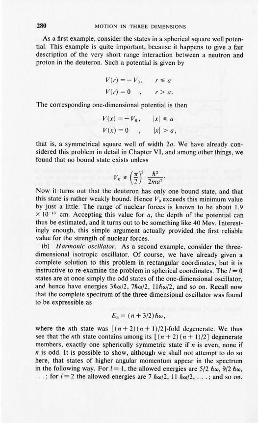
280 MOTION IN THREE DIMENSIONS
As a first example, consider the states in a spherical square well potential. This example is quite important, because it happens to give a fairdescription of the very short range interaction between a neutron andproton in the deuteron. Such a potential is given by
V(r)=-Vo,
V(r) = 0
r.s;a
r> a.
The corresponding one-dimensional potential is then
V(x) = - Vo,
V(x) = 0
Ixl .s; a
Ixl > a,
that is, a symmetrical square well of width 2a. We have already considered this problem in detail in Chapter VI, and among other things, wefound that no bound state exists unless
. (7T)2 h2
/I 0;;'"2 2ma2'
Now it turns out that the deuteron has only one bound state, and thatthis state is rather weakly bound. Hence Vo exceeds this minimum valueby just a little. The range of nuclear forces is known to be about 1.9x 10⁻¹³ em. Accepting this value for a, the depth of the potential canthus be estimated, and it turns out to be something like 40 Mev. Interestingly enough, this simple argument actually provided the first reliablevalue for the strength of nuclear forces.
(b) Harmonic oscillator. As a second example, consider the threedimensional isotropic oscillator. Of course, we have already given acomplete solution to this problem in rectangular coordinates, but it isinstructive to re-examine the problem in spherical coordinates. The I = 0states are at once simply the odd states of the one-dimensional oscillator,and hence have energies 3hw/2, 7hw/2, 11 hw/2, and so on. Recall nowthat the complete spectrum of the three-dimensional oscillator was foundto be expressible as
En = (n + 3/2)h<o,
where the nth state was [(n + 2)(n + 1)/2]-fold degenerate. We thussee that the nth state contains among its [( n + 2) (n + 1) /2] degeneratemembers, exactly one spherically symmetric state if n is even, none ifn is odd. I t is possible to show, although we shall not attempt to do sohere, that states of higher angular momentum appear in the spectrumin the following way. For I = I, the allowed energies are 5/2 hw, 9/2 hw,... ; for 1=2 the allowed energies are 7 hw/2, II hw/2, ... ; and so on.

SOME EXAMPLES 281
In general, for angular momentum I, the allowed energies are (l + 3/2)fiw,(l + 2 + 3/2) nw, (l + 4 + 3/2) fiw, .... Otherwise stated, the degenerate members of the nth energy state are those states of angular momentum I = n, n - 2, n - 4, ... , and so on down to I = 0, for even n, or toI = 1 for odd n.
The spectrum, classified according to angular momentum, is shown inFigure 6. The degeneracy of each state in this scheme can be obtainedupon noting that a state of angular momentum I is (21 + I)-fold degenerate. Thus the ground state, which is I = 0, is not degenerate, the firstexcited state which contains only an I = I state is three-fold degenerate,the second excited state contains a nondegenerate 1= °state and a fivefold-degenerate 1=2 state so that the total degeneracy is six-fold, andso on, in agreement with our earlier rule. The pervasive occurrence ofdegeneracies between states of different I values is an excellent exampleof "accidental" degeneracies which are not accidental at all. Thesedegeneracies occur because of the special structure of the potential forthe isotropic harmonic oscillator which makes Schrodinger's equationseparable in both rectangular and spherical coordinates.
Exercise 3. Verify that the oscillator states corresponding to energy£1 = 5fiw/2 are indeed I = I states, as we claimed above. Do this byshowing that
t/lIOO ± it/lolo = f(r) y l±I(8, cf»
t/lOOI = f(r) y IO(6, cf»,
where t/ln,n2n3(X, y, z) is defined by equation (19). Identify f(r) and bysubstitution verify that it actually satisfies the correct radial Schrodinger's equation.
Degeneracy
£, = Il/2flw
£3 = 9/2/iw
£, = 7/2/iw
£1 = 5/2/iw
£0 = 3/2/iw
1=0 I = I 1= 2 1= 3 1=4
15
10
6
3
FIGURE 6. States of the three-dimensional harmonic oscillator classified according to angular momentum. The degeneracy of each state is also indicated.

282 MOTION IN THREE DIMENSIONS
(c) Motion of a free particle. We have already discussed the statesof a free particle in rectangular coordinates. The states so obtained weresimultaneous eigenfunctions of the Hamiltonian and of the linear momentum. In spherical coordinates we obtain states which are, instead, simultaneous eigenfunctions of H and of the angular momentum, that is, theyhave definite values of E, I and m. The radial functions are solutions ofequation (49) with V (r) set equal to zero. They thus satisfy
where
1 ~ (r2 dR E1 ) + [k2 _I(l + 1)] R =0r2 dr dr r2 El , (56)
(57)
Alternatively, these solutions may be obtained from equation (54),which, for a free particle, can be written in the form
(58)
where, it is recalled, UEI = rR EI •
Consider first the case 1= O. From equation (58), recalling also thatUEI (r) must vanish at the origin, we have at once
UEO - sin kr
and hence
R _ sin kr.EO r
For I different from zero the situation is more complicated. However,it turns out that the solutions of equation (56) are a well-studied set offunctions which can be compactly defined as follows:
j(kr) == (_1)1 (!.-)I (I ~)I sinkr.I k r dr kr (59)
The function }l(kr) is called a spherical Bessel function of order I. Interms of these functions, and up to a multiplicative constant, the radialfree particle states are given by
k = V2mE/h, (60)
which clearly reduce to the correct solution for 1= O. The proof thatthe functions defined by equation (59) are, for general I values, actually
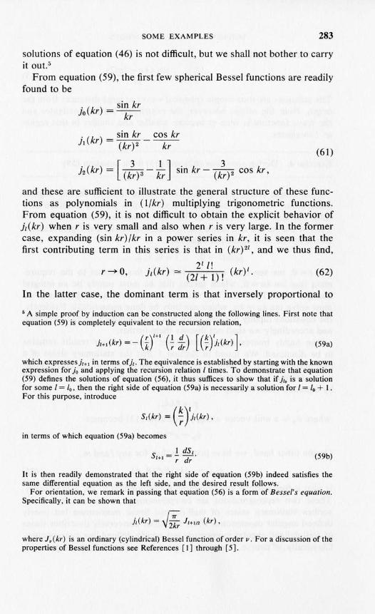
SOME EXAMPLES 283
(61)
solutions of equation (46) is not difficult, but we shall not bother to carryit out. 5
From equation (59), the first few spherical Bessel functions are readilyfound to be
. (k ) - sin krJo r - kr
. (kr) = sin kr _ cos kr11 (kr)2 kr
j2(kr) = [(~)3 - ir] sin kr - (~)2 cos kr,
and these are sufficient to illustrate the general structure of these functions as polynomials in (Ilkr) multiplying trigonometric functions.From equation (59), it is not difficult to obtain the explicit behavior ofjl(kr) when r is very small and also when r is very large. In the formercase, expanding (sin kr)lkr in a power series in kr, it is seen that thefirst contributing term in this series is that in (kr)21, and we thus find,
r~O, (62)
In the latter case, the dominant term is that inversely proportional to
5 A simple proof by induction can be constructed along the following lines. First note thatequation (59) is completely equivalent to the recursion relation,
. (r)I+l (I d) [(k)l. ]JI+l(kr)=- k -; dr -; JI(kr) , (59a)
which expressesjl+1 in terms ofk The equivalence is established by starting with the knownexpression for jo and applying the recursion relation 1 times. To demonstrate that equation(59) defines the solutions of equation (56), it thus suffices to show that if jlo is a solutionfor some 1= 10 , then the right side of equation (59a) is necessarily a solution for 1= 10 + I.For this purpose, introduce
SI(kr) == (~Yjl(kr),
in terms of which equation (59a) becomes
S _! dS I •1+1 - r dr (59b)
It is then readily demonstrated that the right side of equation (59b) indeed satisfies thesame differential equation as the left side, and the desired result follows.
For orientation, we remark in passing that equation (56) is a form of Bessel's equation.Specifically, it can be shown that
jl(kr) = ~2~r JI+ 1/2 (kr),
where J.(kr) is an ordinary (cylindrical) Bessel function of order IJ. For a discussion of theproperties of Bessel functions see References [1] through [5].

284 MOTION IN THREE DIMENSIONS
r, and we eventually find,
. (k) sin (kr-17T/2)Jl r = kr . (63)
The solutions are thus simple spherical waves at large distances from theorigin. Near the origin, however, the centrifugal barrier dominates andthe wave function is seen to become smaller and smaller in that regionas I increases.
Exercise 4. Derive equations (62) and (63) from equation (59).
As a simple example involving free particle states of definite angularmomentum, we briefly consider the states of a particle confined in aspherical container of radius a. The wave function must vanish at thewalls of the sphere and hence the spectrum of allowed energies is determined by the transcendental equations,
Jl(ka) = 0, 1= 0, 1,2, ....
For 1=0, we see from equation (61) that this reduces to the requirement that sin ka = 0, which means that ka must simply be an integralmultiple of 1T. For 1= 1, the situation is not quite so simple, since wemust solve tan ka = ka, which can only be done numerically. Evidently,the equations rapidly become more and more complicated as I increases,and accordingly we shall not discuss them further.
One highly interesting and important aspect of our results remainsto be discussed. We found in Section I that the stationary states of afree particle could be written as ordinary de Broglie waves corresponding to definite, but arbitrarily oriented, vector momentum p, as expressedby equation (13). Writing
p = hknp ,
where lip is a unit vector along p, equation (13) becomes
On the other hand, we have just seen that, for any I and m,
l/JBlm = Jl(kr) nn(o, cP)
(64)
(65)
is also a free particle state function corresponding to the same energy.These two representations are complementary in that the former describes stationary states of well-defined linear momentum but poorlydefined angular momentum, while the latter conversely describes statesof well-defined angular momentum but poorly defined linear momentum.Classically, of course, free particle states are such that both are precisely

SOME EXAMPLES 285
defined. This is not so in quantum mechanics - not by accident but asa direct consequence of the easily verifiable noncommutativity of thelinear and angular momentum operators.
The representations of equations (64) and (65) are both complete inthat an arbitrary free particle state of energy E can be expressed as asuperposition of either. In particular, then, each must be expressiblein terms of the other. Using standard properties of the spherical harmonics and spherical Bessel functions, it can be shown6 after someeffort that
tJ;p(r) = 47T 2: ilyr* (Op, cfJp)tJ;Elrr.(r, 0, cfJ), (66)I,m
where Op and cfJp define the angular orientation of p in the same way thato and cfJ define the angular orientation of r. Conversely, in view of theorthonormality of the spherical harmonics,
tJ;Elm(r, 0, cfJ) = 4~il JYt (Op, cfJp)tJ;p(r) dH p, (67)
where dH p= sin Op dOp dcfJp is the element of solid angle about the unitvector np defining the direction of p. For a given energy, equation (66)is seen to express a state of linear momentum p as a superposition overall angular momentum states, while equation (67) expresses a state ofdefinite angular momentum as a superposition over all orientations ofthe linear momentum.
An important special case of equation [66] is that in which np liesalong the z-axis, the polar axis of the spherical coordinate system, sothat Op = O. Since
Y m(O -1-.) = /21 + I 81 ''f' V 47T mO,
we obtain, upon inserting the explicit forms of tJ;p and tJ;Elm,.,
tJ;p = e ik,· cos 9 = 2: i/(2/ + I) jl(kr) PI (cos 0), (68)1=0
where we have also used the fact that, according to equation (47),
Yt=o (0, cfJ) = V2/4: I PI (cos 0),
"with PI (cos 0) denoting the ordinary Legendre polynomial. Now,because the linear momentum has been chosen to lie along the z-axis,the z-component of angular momentum must be zero, and so we havefound; the superposition of equation (51) involves only states with mequal to zero.
6 For a derivation of equation (66) see, for ex,ample, Reference [22], Chapter IX, Section 9.
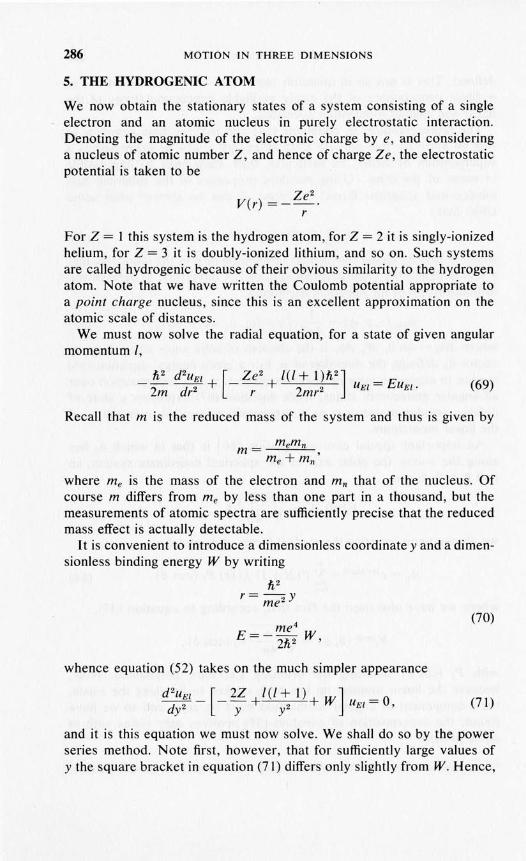
286 MOTION IN THREE DIMENSIONS
5. THE HYDROGENIC ATOM
We now obtain the stationary states of a system consisting of a singleelectron and an atomic nucleus in purely electrostatic interaction.Denoting the magnitude of the electronic charge bye, and consideringa nucleus of atomic number Z, and hence of charge Ze, the electrostaticpotential is taken to be
Ze 2
V(r) =--.r
For Z = 1 this system is the hydrogen atom, for Z = 2 it is singly-ionizedhelium, for Z = 3 it is doubly-ionized lithium, and so on. Such systemsare called hydrogenic because of their obvious similarity to the hydrogenatom. Note that we have written the Coulomb potential appropriate toa point charge nucleus, since this is an excellent approximation on theatomic scale of distances.
We must now solve the radial equation, for a state of given angularmomentum I,
(69)
Recall that m is the reduced mass of the system and thus is given by
where me is the mass of the electron and mn that of the nucleus. Ofcourse m differs from me by less than one part in a thousand, but themeasurements of atomic spectra are sufficiently precise that the reducedmass effect is actually detectable.
It is convenient to introduce a dimensionless coordinate y and a dimensionless binding energy W by writing
li2r = me 2 Y
(70)
(71)
whence equation (52) takes on the much simpler appearance
d2uEI _ [- 2Z +l(l + I) + wJ u = 0
dy 2 Y y2 El,
and it is this equation we must now solve. We shall do so by the powerseries method. Note first, however, that for sufficiently large values ofy the square bracket in equation (71) differs only slightly from W. Hence,

THE HYDROGENIC ATOM 287
(72)
asymptotically the behavior of UEI is dominated by the exponential factore±v'WY. Physical admissibility demands the negative sign and hence wewrite
UEI = VEI(Y) e-v'WY.
Substitution into equation (71) then yields
d2vEI_ 2VW dVEI_[I(I + 1) 2
yZ] VEL = O. (73)
dy2 dy y2
Next we determine the behavior of VEL near the origin. For this purpose,write
VEL-YO'·
Substitution into equation (73) then gives
s(s - 1)yS-2 - 2VW syS-1 -1(1 + 1) yS-2 + 2ZyS-1 = 0
or
s(s - 1) -1(1 + 1) + 2y(Z - VW) = O.
The last term is negligible for sufficiently small y and hence s must besuch that
s(s-1)=I(I+1)
or
s=l+ 1, -l.
Since VEL must be bounded at the origin, only the former is permitted andwe thus see that .
y~O,
Consequently, we now seek a power series solution of the form00
VEl = yl+1 2: cqyq.q=O
Substitution into equation (73) then gives002: cq(q + 1+ 1) (q + l)yQ+I-I
q=O
- 2VW ±cq(q + 1+ 1)yQ+1q=O
(74)
00 00
- 2: cql (I + 1)yq+l-I + 2Z 2: CqyQ+1 = 0q=O q=O
or, collecting terms, we can write
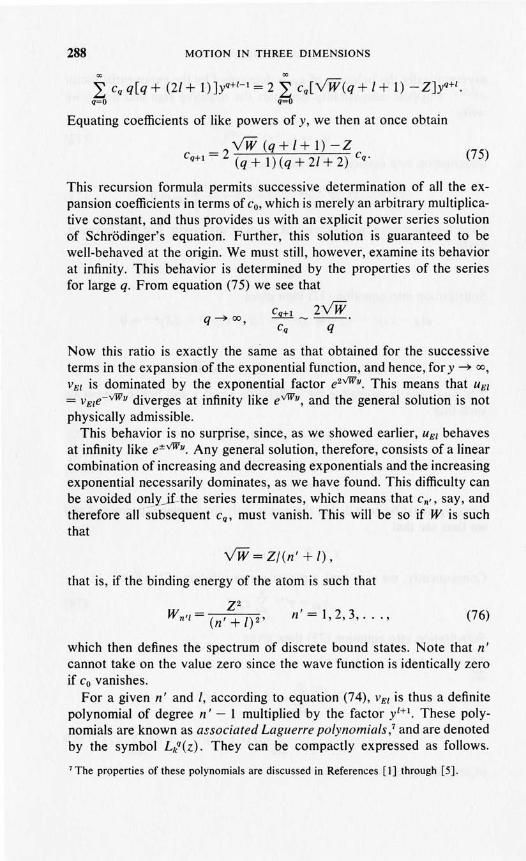
288 MOTION IN THREE DIMENSIONS
00 00
L cqq[q+ (2/+ 1)]yq+l-l=2 L cq[VW(q+l+ I) -Z]yQ+l.q=o q=O
Equating coefficients of like powers of y, we then at once obtain
VW(q+I+1)-ZCq+1 = 2 (q + 1) (q + 21 + 2) cq
•(75)
q~ 00,
This recursion formula permits successive determination of all the expansion coefficients in terms of Co, which is merely an arbitrary multiplicative constant, and thus provides us with an explicit power series solutionof Schrodinger's equation. Further, this solution is guaranteed to bewell-behaved at the origin. We must still, however, examine its behaviorat infinity. This behavior is determined by the properties of the seriesfor large q. From equation (75) we see that
Cq+l _ 2VW.Cq q
Now this ratio is exactly the same as that obtained for the successiveterms in the expansion of the exponential function, and hence, for y ~ 00,
VEL is dominated by the exponential factor e2v'Wv. This means that UEI
= vEle-v'Wv diverges at infinity like ev'Wv, and the general solution is notphysically admissible.
This behavior is no surprise, since, as we showed earlier, UEI behavesat infinity like e±v'Wv. Any general solution, therefore, consists of a linearcombination of increasing and decreasing exponentials and the increasingexponential necessarily dominates, as we have found. This difficulty canbe avoided onlyjLthe series terminates, which means that Cn" say, andtherefore alls"i:Ibsequent Cq , must vanish. This will be so if W is suchthat
VW=Z/(n'+l),
n'=1,2,3, ... ,
that is, if the binding energy of the atom is such that
Z2Wnl l = (n'+l)2' (76)
which then defines the spectrum of discrete bound states. Note that n'cannot take on the value zero since the wave function is identically zeroif Co vanishes.
For a given n' and I, according to equation (74), VEL is thus a definitepolynomial of degree n' - 1 multiplied by the factor yl+l. These polynomials are known as associated Laguerre polynomials,7 and are denotedby the symbol Lkq(z). They can be compactly expressed as follows.
7 The pn;>perties of these polynomials are discussed in References [I] through [5].

THE HYDROGENIC ATOM
First introduce the ordinary Laguerre polynomial Lk(z), defined by
(d)kLk(z) = eZ dz (Zke-z) .
Then the associated Laguerre polynomials are given by
289
(77)
(78)
From these expressions, Lk(z) is seen to be a polynomial of degree kin z, Lkq a polynomial of degree k - q in z. An alternative expression forthese polynomials can be obtained in terms of an appropriate generatingfunction; specifically it can be shown that
e-zsl(l-s) 00 Sk
I-s = ~OLk(Z)k!'
whenc,e, from equation (78),
(
S)q e-zs/(I-s) 00 Sk- -- = ~ Lkq(z) -.
I-s I-s £.J k!k=q
Finally, it can also be shown that
In terms of these polynomials, it then turns out that
1+1 L 21+1 (2' r;;-;--W )VEl = Y n'+21 Y V W n'l ,
(79)
(80)
and it is not too hard to verify, by direct substitution, that this expressionis indeed a solution of equation (68). Next, from equation (72), the radialwave function is given by
- UEI _ I L 21+1 (2 • ~W ) ~REI - - - Y n'+21 Y V W n'l e- n'IY.r
(81)
Using equation (80), the normalized stationary states are found to be
,I, _ [ 2Zr ]1 L 21+1 ( 2Zr ) -ZrJ(n'+llaoy m(o,l,.) (82)'l'Elm - Cn'l (n' + l)ao n'+21 (n' + I)ao e I, 'I' ,
where
= [2Z(n' + I) ]3/2 [ (n' - I)! ]1/2Cn'l Go 2(n'+/)[(n'+2l)!]3 (83)
and where, in re-expressing Y in terms of r, we have introduced the Bohrradius ao, defined by

290 MOTION IN THREE DIMENSIONS
h2
ao = - = 0.53 X 10⁻⁸ em.me2 (84)
The energy E of these states, according to equations (70) and (76), is
Z2e2 1E=-------
2ao (n' + /)2' {n'=1,2, ...I = 0,1,2,. ..
(85)
Observe now that the energy depends only upon the sum of the radialquantum nlimber n' and of the angular momentum quantum number I.It is convenient and customary to introduce at this stage the principalquantum number n, defined by
in terms of which
n=n'+I, (86)
(87)
which is seen to be the familiar Bohr formula. 8 The state function canalso be expressed in terms of the principal quantum number, of course,and we obtain at once
where
.r. = D (2Zr)1 L2l+ 1 (2Zr) -Zrlnao ym({) ,/,,)'f'nlm nl n+1 e I, 'I' ,n~ n~ .
= (2zn)3/2 [ (n -1- I)! JII2.D nl ao 2n[(n+/)!]3
(88)
(89)
It is important to keep in mind that, according to equation (86), n can takeon, for given I, only the values 1+ 1, 1+ 2, ... , while for given n, I cantake on only the values n - 1, n - 2, ... , O. The first few normalizedstationary state functions are given below:
0/100 =2 (~r2 e-zrlaoyoo; E 1 =_~::2
(90)
8 Observe that the energy is proportional to Z2, even though the strength of the interactionis proportional to Z. The explanation is that the mean radius of the atom for a state of givenn is inversely proportional to the strength of interaction and hence inversely proportionalalso to Z. Because the energy, being electrostatic in origin, is proportional to the strengthdivided by the radius, the Z2 dependence follows.

THE HYDROGENIC ATOM 291
The degeneracy of the hydrogenic states can be found in the followingway. For a given principal quantum number n, and thus for a given boundstate energy En, / can take on all values ranging from zero to n - I, aswe have seen. For each / value, there is a (2/ + I )-fold degeneracy andhence N, the total number of states with energy En, is
"-1N = L (2/ + I) = n 2
•
1=0
Again we have an excellent example of pervasive "accidental" degeneracies which are not accidental. They arise in this case because Schrodinger's equation for a Coulomb potential happens to be separable inparabolic as well as spherical coordinates.
The spectrum of the hydrogenic atom is shown in Figure 7. As a matterof nomenclature, dating back to the early days of spectroscopy, stateswith / = 0 are called s-states; with / = I, p-states; with l = 2, d-states;with / = 3, f-states; with l = 4, g-states; and so on in alphabetical orderfor states of still higher /. From the figure it is readily seen how the statescrowd together as E approaches zero, in contrast to the behavior of thestates in a square well. This is a consequence of the long range of theCoulomb interaction, as is the fact that there are infinitely many discretebound states for each value of l.
We have now obtained a complete and exact solution for the boundstates of a (nonrelativistic) hydrogenic atom. Unfortunately, these states
s1=0
PI = I
d
1= 2
f1= 3
E = 0----------------n = 3
n = 2
n=\
FIGURE 7. The hydrogenic spectrum.
have turned out to be rather complicated in general, and their qualitativebehavior is not very readily apparent. The simplest states are those ofmaximum angular momentum and of maximum z-component of angularmomentum, for a given n, that is, the states lfIn.l=n-l;m=n-I' The state
292 MOTION IN THREE DIMENSIONS
functions in this case have the simple form, omitting normalizationfactors,
I/In,n-I,n-I = ,"-I e-Zr/nao sinn-I e.
For large quantum numbers n, these states are quite well localized inangle and in radius. In particular, the wave function has a relativelysharp maximum about the equatorial plane and about the Bohr radiusn2ao/Z. Thus such states actually exhibit the behavior predicted by theoriginal Bohr theory, in the sense that they are centered about the circularorbits of that theory, and rather precisely so for sufficiently large quantumnumbers.
Exercise 5. Verify the above assertions for the state I/In, n-I, n-I •
Problem 1.(a) Find the propagator K (r, r '; t - to) for a free particle in three
dimensions.(b) Consider a wave packet which at t = 0 is a Gaussian,
I/I(r, t = 0) = A eiPo ·(r-rol/fi e-(r-rol2 /2L2.
Find A if the wave packet is normalized.(c) Show that I/I(r, t = 0) is a minimum uncertainty wave packet.(d) Findl/l(r,t).(e) Find cP(p, t = 0), cP(p, t).(f) Find (x) at t = 0 and for any t > O.(g) Find (p), (p2) at t = 0 and for any t > O.
Note: All integrals can be factored into products of one-dimensionalintegrals, familiar from our earlier work. The problem can, however, bemore easily worked directly in three dimensions. Either procedure isacceptable.
Problem 2. Using the results of Chapter VI for a one-dimensional oscillator,
(a) Find the propagator for a three-dimensional oscillator.(b) Discuss the motion of an arbitrary wave packet in a three
dimensional oscillator.
Problem 3.(a) Calculate the polarizability of a three-dimensional isotropic
harmonic oscillator.(b) What is the degeneracy of the states of a three-dimensional
oscillator in a uniform external field E = 8 ex?

PROBLEMS 293
Problem 4. To good approximation, the nucleus can be regarded as auniformly charged sphere of radius Ro ~ Go.
(a) What is the electrostatic potential between an electron and anucleus so regarded?
(b) Find an expression for the first-order correction to the groundstate energy of a hydrogenic atom arising from the finite nuclear size.What is the order of magnitude of this correction, assuming that R o= (2Z)l/3 X 10-13 cm? How does it depend upon Z?
(c) The same for a J-L-mesonic atom, that is, a system consisting ofa nucleus and a negative J-L-meson. (The mass of the J-L-meson is approximately 207 electron masses.) For what value of Z, if any, does first-orderperturbation theory become inadequate? [The earliest accurate estimates of nuclear sizes were obtained by analysis of a J-L-mesonic atomicspectra.]
Problem S. Consider an anisotropic harmonic oscillator described bythe potential
V(x, y, z) = i mWI2 (x2+ y2) + i mW22Z2.
(a) Find the stationary states using rectangular coordinates. Whatare the degeneracies of the states, assuming WI and W2 are incommensurate?
(b) Can the stationary states be eigenstates of U? of Lz? Explainin each case.
y
----t-----~---'--t_---x
FIGURE 8. Motion of a particle on a circular track.

294 MOTION IN THREE DIMENSIONS
Problem 6. A particle of mass M is constrained to move on a frictionless,vertical circular track of radius R. Neglecting gravity, the Hamiltonianof the system is H = Lz2/2MR2. Since Lz = (fi/i) (a/a4» , Schrodinger'sequation is
fi a21fJ _ fi alfJ .- 2MR2 a4>2 - - Tat'
where, as shown in Figure 8, 4> is the angular coordinate of the particle.(a) Solve Schrodinger's equation to find the allowed energies 8>m
and the energy eigenstates IfJm' What are the degeneracies of these states,if any?
(b) Suppose the gravitational field is now included. The Hamiltionian is then
H = L//2MR2 + MgR sin 4>.
Treating the gravitational term as a perturbation, show that the firstorder correction to the energies 8>m vanishes. Calculate the secondorder correction to the energy.
(c) Suppose the gravitational term is much too large to be treatedgenerally as a perturbation. (For what combination of the parameterswill that be true?) Estimate the ground state energy using the RayleighRitz method and then using the WKB approximation.
(d) Discuss the transition between states bounded in 4> and statesunbounded in 4>, using the WKB approximation. For what states, if any,will the perturbation results of part (b) apply?
Problem 7. Suppose two identical spinless particles are moving on thecircular track described in Problem 6. Neglect gravity.
(a) Assuming the particles do not interact with each other, solveSchrodinger's equation to find the allowed energies and the energy eigenstates. What are the degeneracies of these states, if any?
(b) Suppose the particles interact weakly according to the potentialV(4)h 4>2) = Vo[1 + COS(4)1 - 4>2)]' Use perturbation theory to findthe corrections to the unperturbed ground state energy.
Problem 8. A particle of mass M is constrained to move on the surfaceof a sphere of radius R, but is otherwise free.
(a) Solve Schrodinger's equation for the allowed energies and theenergy eigenstates.
(b) Classically, the orbit of such a particle lies in a plane and isthus kinematically equivalent to motion on a circular track, as in Problem6, part (a). Show that, to good approximation, this equivalence is alsoattained quantum mechanically by considering, for large quantum numbers, states of maximum L z •

PROBLEMS 295
Problem 9. A hydrogen atom is placed in a uniform electric field directedalong the z-axis. Neglecting spin, the relative motion of electron andproton is then described by the Hamiltonian
p2 e2H=---+e6z.
2m r
(a) Is U a constant of the motion? Is L z? Do the states have definiteparity? Explain briefly.
(b) Treating the term in the electric field as a perturbation, writedown an expression for the second-order correction to the ground stateenergy (why second-order?). Include only non-vanishing matrix elementsin your answer. Do not actually evaluate the integrals or perform thesummations.
(c) Suggest some explicit trial function suitable for a variationalcalculation. Allow, as best you can, for the distortion of the atom causedby the electric field. Do not actually carry out any calculation, but justifyyour choice of trial function.
Problem 10. Consider the bound states of a particle in a spherically symmetric potential. Show that if there are no "accidental" degeneracies,(x> and (p > vanish for any stationary state. Why does the proof failif there are accidental degeneracies? [Hint: What can you say about theparity of the stationary states?]
Problem 11. The nucleus H3 (the triton) consisting of one proton and twoneutrons is unstable. By beta emission it decays to He3, consisting of twoprotons and one neutron. Assume that when this process takes place itdoes so instantaneously. Thus there occurs a sudden doubling of theCoulomb interaction between the atomic electron and the nucleus whentritium (the H3 atom) decays by beta emission to He+ (singly ionizedHe3). If the tritium atom is in its ground state when it decays, what isthe probability that the He+ ion in its ground state immediately after thedecay? In the 2s-state? In the 2p-state? In any state other than an s-state?
Problem 12. The weakness of gravitational compared to electrostaticinteractions is dramatically illustrated by considering a system of twoneutrons under the sole influence of their mutual gravitational attraction.
(a) Write expressions for the bound state energies and for the "Bohrradius" for such a system.
(b) Estimate, to the nearest power of ten, the numerical value ofthe ground state energy (in electron volts) and of the Bohr radius (incm, in light years).
Problem 13. Three identical non-interacting particles are described bythe following Hamiltonian,

296 MOTION IN THREE DIMENSIONS
3
H = L H SP (ri) ;i=1
H () _L+! 22SP r - 2m 2 mw r .
(a) Find the eigenfunctions and energies of the system, withoutregard to symmetrization.
(b) Give the degeneracy of the lowest three states, including ex-change degeneracy. .
(c) The same for the physically realizable states of spinless particles.
(d) What is the ground state energy for spin one-half particles?What is the degeneracy of the ground state?
Problem 14. A two-particle system is described by the Hamiltonian
H = PI2 + pl +! m w2r 2 +! m w2r 2 + V e-(n-r2)2/a2
2ml 2m2 2 1 1 2 2 2 0 •
Treating the Gaussian interaction term as a perturbation and transforming to center of mass coordinates,
(a) Find the energy of the ground state and first excited state tofirst order.
(b) Use equation (VIl-39) to find an upper bound to the secondorder correction to the ground state energy.
(c) Use a Gaussian of variationally determined width as a trialfunction in the Rayleigh-Ritz method to estimate the ground state energy.
Problem 15. The same as Problem 14, but for identical spinless particles.
Problem 16. A two-particle system is described by the Hamiltonian
H _. PI2 + P2
2 + 1 2 2 1 2 2 + 1 k( )2- 2m
l2m2 "2 m1w rl +"2 m2w r2 "2 r l - r 2 •
(a) Find the exact solutions by transforming to center-of-masscoordinates.
(b) Sketch the spectrum in the weak and strong coupling limits,k «; I-tW2 and k ~ I-tW2, respectively, where I-t is the reduced mass.
(c) The same for identical spinless particles.
Problem 17. Consider the hydrogen atom in its ground state. Suppose bysome magic that the Coulomb interaction is suddenly turned off at t = 0and the electron moves off as a free particle. Treating the proton asinfinitely massive for simplicity,
(a) Find the probability p (p, t) d 3p that a measurement of theelectron's momentum at any time t > 0 will yield a value in the volumeelement d 3 p at p. How does the result depend upon t? Upon the direction of p? Explain.

PROBLEMS 297
(b) What is the probability that a measurement of the electron'senergy will yield a value between E and E + dE?
(c) Find the probability that a measurement of the electron's position at any time t > 0 will yield a value in the volume element d 3r at r.[Hint: Use the free particle propagator.] Without working out all thedetails, show qualitatively how this probability changes with time, starting at t = O. Explain briefly.
(d) In contrast to the distributions in parts (a), (b) and (c), a measurement of the electron's angular momentum must always yield a uniqueand precise value. What is this unique value?
Problem 18. Obtain an expression for dldt (t/Jlp • rlt/J) and then, byconsidering a stationary state t/JE' prove the virial theorem,
where T is the kinetic energy, V the potential energy. Use the virialtheorem to show that E = 2 (t/JEI Vlt/JE) for the harmonic oscillator andE = f (t/JEI V!t/JE) for the hydrogen atom.
Problem 19. The neutron and proton interact through a strong shortrange force. Reasonable approximations to such a force are:
VR(i) Yukawa type: V(r) = - _0- e-r/Rr
(ii) Exponential: V(r) = - Vo e-r/R
(iii) Square well: V(r) = {- Vo, r < R0, r> R.
(a) Use the Rayleigh-Ritz method to find an expression for theground state binding energy E for each of the three cases. Use e-r/2R
as a trial function. 9
(b) Taking E = 2.2 MeV and R = 2 X 10-13 em, find Vo in each case.Draw the three interactions on the 'same graph.
(c) As a check on the accuracy of the Rayleigh-Ritz method, solvethe square well case exactly, using graphical methods to find E, for theparticular value of Vo found in part (b).
9 One can do considerably better by introducing a trial function containing a variationalparameter, such as e-arI2R. Unfortunately, however, the resulting equations are complicated and must be solved numerically in all three cases. We remark that case (ii) canactually be solved exactly in terms of Bessel functions. See Reference l29], pp. 218-220.The variational method is discussed in these pages as well.

xAngular momentum and spin
1. ORBITAL ANGULAR MOMENTUM OPERATORS ANDCOMMUTATION RELATIONS
If at some instant a structureless particle passes with momentum pthrough a point whose displacement from an arbitrarily chosen originis r, then its angular momentum L with respect to that origin is
or, in component form,
L=rXp (1)
(2)
L x = ypz - ZPlI
L lI = ZPx - Xpz
Lz = XPlI- YPx'
The corresponding quantum mechanical dynamical variable, called theorbital angular momentum operator, is given by these relations with,of course, rand p interpreted as quantum mechanical dynamical variables. Since the commutator of Xi and Pi vanishes for i ¥ j, it is easilyverified that L is Hermitian.
Exercise 1. Prove that L is Hermitian.
The commutation relations between the rectangular components ofL are obtained as follows. We have, for example,
(Lx, L lI ) = ([ypz - ZPlI], [zPx - xpz])
= (YPz, zPx) - (YPz, xpz) - (zPlI' zPx) + (zPlI' xpz) .

ORBITAL ANGULAR MOMENTUM OPERATORS 299
Consider the first term,
(YPz, zPx) = YPzzPx- zPxypz·
Because y and Px commute with each other and with z and Pz, this becomes
Similarly, the last term becomes
On the other hand, since Y, x and pz mutually commute, the second termvanishes, and because z, Py and Px mutually commute, so does the third.Thus we obtain
(Lx, L y) = ifi(xpy - YPx)
or, recognizing the term in parentheses as L z , simply
(3)
From the structure of L, the remaining commutation relations are obtained at once by cyclic permutation of the coordinates, and we thushave
(4)
and
(5)
These three relations are equivalent to the single vector commutationrelation
Lx L = ifiL, (6)
as is easily verified by writing out the rectangular components. Theoperator nature of L is made quite explicit by equation (6), since thevector product of a purely numerical vector with itself vanishes.
It is recalled that simultaneous. eigenfunctions or a collection of operators exist only if the operators in question mutually commute. Hence, thenoncommutativity of the rectangular components of angular momentumat once means that a complete set of states cannot be defined for whicheach component of the angular momentum vector has a precise anddefinite value. Instead, only a single component of L can be preciselyspecified; the remaining two components perpendicular to it are neces-

300 ANGULAR MOMENTUM AND SPIN
sarily uncertain. l Noting that the orientation of the coordinate axes isopen to choice, we see that we may choose angular momentum states insuch a way that the projection of L on any arbitrary axis has a definitevalue. Normally this axis of quantization (for angular momentum), asit is called, is taken to be the z-axis, in which case L z has a definite value,but Lx and L y do not.
Although we have shown that the orientation of the angular momentumvector cannot be completely specified on the quantum level, the questionof its magnitude has not been discussed. We now take up this question.To do so, we introduce the square of the angular momentum operator,
U = L • L = L/ + L/ + L/. (7)
We must now examine the commutation properties of L2 with respectto its rectangular components. Let us look first at (Lx, L2). Since thecommutator of Lx with itself vanishes, we have
(Lx, L2) = (L.r:, L y2) + (Lx, Lz2).
Now, it is easily verified by expanding both sides that
(Lx, L/) = (Lx, L y) L y + Ly(Lx, L y)
and hence, from equation (3),
(L.r:, Ly2) = ih(LzLy + LyLz).
Similarly, using equation (5),
(Lx, Lz2) = (Lx, Lz)Lz + Lz(Lx, Lz) = -iii (LyLz + LzLy).
Combining these results we thus see that
(Lx, P) = O.
In the same way, we find at once
or, in brief,
(L,L2)=O. (8)
It then follows that L2 and anyone of its rectangular components, sayLz , can be simultaneously specified and, further, that L 2 and Lz form acomplete set of commuting operators for the specification of angularmomentum states. These states are characterized by the magnitude of
1 Observe, however, that states with angular momentum identically zero are not ruled out,even though all three components of L have definite values for such states. The commutation relations are not violated, because each side of equation (6) vanishes when operatingon a state of zero angular momentum.

ORBITAL ANGULAR MOMENTUM OPERATORS 301
the angular momentum and by its projection on the arbitrarily orientedz-axis, both of which have definite values.
Before going on to explicitly construct the angular momentum eigenfunctions, we briefly consider the properties of angular momentum for asystem of particles. For such a system, the total angular momentum is
(9)
where L; is the angular momentum of the ith particle, and is given by
Evidently, since dynamical variables referring to different particlescommute, we have
i-,t.j,
and it follows after some elementary algebra that
Lx L = ihL,
just as for a single particle. Our conclusions about the general characterof angular momentum states for a single particle thus apply, withoutmodification, to the angular momentum of a system of particles.
Exercise 2. Verify the vector commutation relation for the total angularmomentum of a system of particles.
An important feature of many-particle systems is that the angularmomentum associated with the center-of-mass motion is not the totalangular momentum of the system. This is in contrast to linear momentum; the total linear momentum of a system and the linear momentumof its center of mass are, of course, identical. As an example, we specifically consider only the simplest case, that of a two-particle system.Transforming to center-of-mass and relative coordinates, we have forthe center-of-mass angular momentum
L cm = R X P,
and for the angular momentum of the relative motion
where
(10)
(II)

302 ANGULAR MOMENTUM AND SPIN
It is then easily verified, by direct substi.tution, that the total angularmomentum of the system is the sum of the relative and center-of-massangular momentum vectors. Further, in view of the fact that the centerof-mass and relative coordinates satisfy the usual (canonical) commutation relations, it follows at once that
L cm X Lcm = ihLcm
(12)
(13)
Consequently, the states of a two-particle system can be simultaneouslyclassified with respect to the angular momentum of its center of massand of its relative motion, and each is formally identical to the orbitalangular momentum states of a single particle.
2. ANGULAR MOMENTUM EIGENFUNCTIONSAND EIGENVA,LUES
We now construct the simultaneous eigenfunctions, and the corresponding eigenvalues, of L2 and Lz. We shall do so by a factorization methodutilizing only the algebraic properties of the operators. The analysis isanalogous to but somewhat more complicated than that encountered inour treatment of the harmonic oscillator. The operators which play arole similar to that of a and at, turn out to be, as we shall see in a moment,2
L+ = Lx + iLy
L_ = Lx - iLy.
Denoting the eigenvalue of V by h2f3 and of Lz by hex. and denotingtheir simultaneous eigenfunctions, not necessarily normalized, by ylJa,we have
( 14)
(15)
Because L2 - Lz2= Lx2+ L/, and is thus a nonnegative operator, wemust have
(16)
2 For reasons which will become clear, L+ is called the raising operator for angular momentum and L_ is called the lowering operator. Note that L = (L+lt.

ANGULAR MOMENTUM EIGENFUNCTIONS AND EIGENVALUES 303
Now, Lx and L y commute with L2 and hence so do L+ and L_. Consequently,
(17)
that is, if Y{3/l is an eigenfunction of U with eigenvalue h2{3, then so arethe new functions L±Y{3/l.
Next, consider the commutator of L± and Lz. We have,
(L±, Lz) = (Lx ± iLy , Lz)
= - ihLy ± i (ihLx)
= =+= hL±
or, equally well,
Operating on Y{3/l with this operator equation, we then obtain
LzL±Y{3/l = L±(Lz ± h) Y{3/l
or, using equation (15),
LzL±Y{3/l = h(a ± I) L±Y{3/l.
(18)
(19)
Together, equations (17) and (19) tell us that L±Y{3/l is a simultaneouseigenfunction of U and Lz with eigenvalues h2{3 and h(a ± 1). Hencewe write, according to our notation,
(20)
where the normalization is again left unspecified.Starting from a given state Y{3/l, an eigenstate of Lz with eigenvalue
ha, we now see that by repeated operation with L+ we can successivelyconstruct eigenstates of L z with eigenvalues h (a + I), h (a + 2), andso on, each of which is also an eigenstate of U with eigenvalue h2{3.Similarly, by repeated operation with L_, we can construct a sequenceof eigenstates of Lz with eigenvalues h(a - 1), h(a - 2), and so on,and again each is an eigenstate of U with the same eigenvalue h2{3 .However, since U - L z2 is a nonnegative operator, this ladder of statescannot continue indefinitely in either direction, but must terminate ateach end. Call the eigenvalue of the top rung ha I , and that of the bottomrung (-ha2)' We must then have, according to equation (16),
al2 ,;;; {3
al ,;;; {3.
Further, since the ladder must necessarily contain an integral numberof intervals between rungs, say n, we have

304 ANGULAR MOMENTUM AND SPIN
n=O,I,2, .... (21)
The termination of the ladder at its upper end requires that
L+ YI3'" = 0
and its termination at the lower end requires that
(22)
(23)
(24)
and we now use these conditions to determine the allowed values ofaI, a2 and {3.
To do so, we must first express U in terms of L+, L_ and Lz . Now
L+L_ = (Lx + iLy ) (Lx - iLy ) = L/ + L/ - i(Lx , Ly )
= L/ + Ly2+ hLz ,
and consequently
U = Lx2 + L/ + L/ = L+L_ - hLz + L/ .
Similarly,
L_L+ = L/ + L/ - hLz ,
whence we obtain the alternative but equivalent expression
U = L_L+ + hLz + Lz2
• (25)
To proceed, operate on YI301 with U in the form of equation (25), whence
L2 Yl3o, = L_L+YI301 + (hLz + L/) Y1301•
Now the first term on the right vanishes according to equation (22)and Y13°:' is a simultaneous eigenfunction of U and of Lz with eigenvaluesh2{3 and hal, according to equations (14) and (15). Hence, canceling acommon factor of h2 , we must have
(26)
In the same way, operating on Y13 -02 with U in the form of equation(24), we find
(27)
whence a l (a1 + I) = a2(a2 + 1). The only solution of this equationconsistent with equation (21) is al = a2, and hence we have
(28)
where l is integral or half-integral, depending on whether n is even orodd. In either case,

-----m=1
ANGULAR MOMENTUM EIGENFUNCTIONS AND EIGENVALUES 305
(3=I(l+l), (29)
and the eigenvalues of Lz range from hi to -iii in integral steps in Ii.Denoting now the eigenvalues of L z by lim instead of by liex, we thus seethat m is integral or half-integral, depending on I, and takes on all valuesfrom I to -I in integral steps, as shown in Figure 1. It is easy to see thatthere are (21 + 1) eigenstates for L z for a given value of I.
----m=l
----m=l-l -----m = I-I
m = 2m = 3/2
m= I1/2m=
m = a-1/2m=
m= -I m= -3/2
m= -2
----m = -1+ I
-----m= -I
Integrall
----m= -1+1
----- m =-1
Half-integral I
(30)
FIGURE I. Values of m for states of given angular momentum I.
From now on we shall denote an angular momentum eigenstate withsimultaneous eigenvalues Ii2/ (l + 1) and lim by y1m, whence its eigenvalue equations take the form
U y1m = 1i2/(l + 1) y1m
Lz y1m = limyr.
For brevity, such states are called states of angular momentum I withz-component m. These states can be constructed quite simply by startingwith the top state on the ladder, y/, and then operating successivelywith the lowering operator L_. Thus, we write specifically,
ym= cr (L )l-mylI c/ - I, (31)

306 ANGULAR MOMENTUM AND SPIN
where the elm are normalizing constants and where, it is recalled, Y/ isdefined by
(32)
Of course, the angular momentum states can equally well be obtainedby starting with the bottom state yl-1 and operating successively withL+. In either case, using the already established properties of the raisingand lowering operators, these states can be explicitly constructed andtheir relevant properties can be determined. Leaving the details toExercise 3, below, we simply state the results: 3
Y m = lim-I ~ (l + m) ! (L )I-m Y I }I (2/) ! (l- m) ! - I
m _ -m-I (l- m) ! l+m-IY 1 -Ii ~(2l)!(l+m)! (L+) YI
L±yr = Ii VI(l + 1) - m(m ± 1) y 1m±1.
(33a)
(33b)
Exercise 3.(a) Show that equation (33b) follows from equation (33a) and hence
that these two equations are equivalent.(b) Derive equation (33b) by directly evaluating (L±y1mjL±yr),
assuming the yr to be normalized. Hint: Start by establishing that
(L±yrIL±yr) = (YrIL:;:L±ylm),
and then use equations (24) and (25).(c) Verify that the yr are orthogonal.
It is important to observe that all our results to this stage have followed simply and directly as consequences of the angular momentumcommutation relation, equation (6). We have used the specific realization of Las the dynamical variable corresponding to orbital angularmomentum, and thus defined by equation (I), only in establishing thiscommutation relation. Our results accordingly hold for any operatorsatisfying equation (6), whether or not it represents orbital angularmomentum.
Even with this generality in mind, there is one unexpected featurein our results, namely the appearance of half-integral angular momentum
3 See Reference [22], especially Chapter XIII and Appendix B, for a particularly completeand careful presentation.

ANGULAR MOMENTUM EIGENFUNCTIONS AND EIGENVALUES 307
states as possible states in the spectrum. Recall that, in our treatmentof orbital angular momentum states for a particle moving in a centralpotential, we deduced that these states should have integral angularmomentum from the requirement that the state function be single-valued.Actually, this requirement was too stringently applied since, in fact,only physically observable quantities need be single-valued. Now suchquantities are always expressed in terms of expectation values and arethus second-degree functionals of the state function of the system.This means that there can be no a priori objection to a state functionmerely because it can assume two different signs at a given point in space,for the square of such a function is single-valued.
To put it another way, no physical significance can be attached to theabsolute sign of the state function. Recall also that the question of singlevaluedness arose specifically in connection with the eigenfunctions eim<l>
of L z , and also with the fact that 1> = 0 and 4> = 27T refer to the same pointin space. We thus see that half-integral angular momentum, and therefore half-integral m, corresponds precisely to the previously ignoredpossibility of an ambiguity of sign. Note, however, that the relativesign of any two state functions is physically significant, since interferenceterms depend on the relative phase. As a consequence, the single-valuedness requirement would be violated if some of the states of a given systemcould have integral angular momentum and some half-integral. To makethis explicit, suppose t/JI is an integral angular momentum state, t/J2 ahalf-integral angular momentum state, and consider the superpositionstate
Then
whence 1t/J12 is not single-valued and such combinations are accordinglyforbidden.
On the basis of this general and purely formal discussion, we thusconclude that, in principle, the states of a given system can have integralor half-integral angular momentum, but only one or the other exclusively,and never a mixture. In particular, this means that while the orbitalangular momentum states could indeed have integral angular momentum,as we earlier assumed, the alternative possibility of half-integral angularmomentum exists and must be examined. Which is correct is then a matterfor experiment to determine. The hydrogen atom can readily be usedfor this test, and it turns out that the spectrum computed assuming halfintegral values of orbital angular momentum is not in agreement withexperiment. Half-integral values of orbital angular momentum are thus

308 ANGULAR MOMENTUM AND SPIN
ruled out.4 As we shall see shortly, this is not the case for the intrinsicangular momentum or spin of a particle. Both possibilities for the spinare, in fact, observed in nature.
Because we shall be concerned with more than one kind of angularmomentum, as the discussion above implies, we now introduce an appropriate and more or less standard notation to permit us to distinguishamong them. We shall continue to denote the orbital angular momentumoperator by L and its eigenstates by ytm. The spin angular momentumoperator will be denoted by S and its eigenstates by X/', which is to saythat Xsm is defined by
(34)
(35)
Finally, we shall use the symbol J as a generic symbol for the angularmomentum operator, referring to either orbital or spin angular momentum, as the case may be. Its eigenstates will be denoted by Y/", whence
j2 Y/" = Ii2j(j + 1) Y/"
1.yr = limyjm.
For ease in writing, in all three cases we have used m as the quantumnumber associated with the z-component of angular momentum. Whenever it becomes necessary to make a distinction, we shall simply introduce appropriate subscripts and write ml or ms or mj, depending oncircumstances.
The point of these notational matters is that all angular momentumoperators satisfy the same vector commutation relations, namely,equation (6) for L,
for S, and, for J,
S x S = ih S
J x J = ihJ.
(36)
(37)
Nonetheless, there are some distinct differences between orbital andspin angular momentum, as is made clear by the fact that only the lattercan assume half-integral values. We shall use J to write those generalrelations which are valid for either. In other words, all expressionswritten in terms of J apply equally to both orbital and spin angularmomentum. On the other hand, expressions written in terms of L or S,
4 Arguments other than the simple empirical one we have given are available for ruling outha!f-integral orbital angular momentum. In particular, difficulties are encountered with theprobability flux for such states, according to J. M. Blatt and V. F. Weisskopf, TheoreticalNuclear Physics, Wiley (1952), Appendix A.

(3-8a)
(38b)
ANGULAR MOMENTUM EIGENFUNCTIONS AND EIGENVALUES 309
depending on the context, either will be particular cases of the generalrelations or wilI refer to some special property of one which is not sharedby the other. An example of the latter is the representation of orbitalangular momentum in terms of spherical harmonics; no such representation exists for spin. Equations (6) and (36) are examples of the former;both are particular cases of the general angular momentum commutationrule, equation (37).
We shall also ultimately be concerned with the total angular momentum of composite systems. In general, the total angular momentum iscompounded from both spin and orbital contributions and hence exhibitsonly the properties they share in common. It was precisely to exhibitthese common properties that J was introduced, and hence we shallalso denote the total angular momentum of a general system by J.
As we have already emphasized, all of our results to this stage havebeen derived using only the vector commutation relation for angularmomentum, and they thus hold for any kind of angular momentum. Forfuture reference, as well as to make their generality explicit, we nowrewrite at least the principal results in terms of J :
Y/" = hm
-j ~(2A~ ~j~)~)! (L)j-m Y/ }
ym = h-m-j I (j - m) ! (J )i+m y.-j) '/(2j)!(j+m)! + )
l:,;Y/"=hVj(j+I) -m(m± I) yjm:';l,
where, of course,
(39a)
(39b)
and
l_l+ =]2 - hlz -l/
1+ 1_ = ]2 + hlz - 1z2•
One interesting feature of the angular momentum operator is that itsprojection on the z-axis is always less than its absolute magnitude;thus, as we have mentioned before, its orientation is not preciselydefined. It is ilIuminating to discuss this behavior in terms of the uncertainty principle. Recall that, according to equation (V-49), we have, forany pair of Hermitian operators A and B,
(LiA)2(LiB)2;;': t 1«(A,B))i2.
We now use this relation to examine the effects of the noncommutativityof the rectangular components of J. First observe, however, that for anystate Y/"
310 ANGULAR MOMENTUM AND SPIN
(Y/"IJ;:IY/") - (Y/"IY/"±I) = 0,
and hence, since Jx and Jyare linear combinations of J+ and J_ ,
(Y/"1 Jxl Y/") = (Y/"1 Jyl Y/") = O.
Consequently, for such a state,
(D.JxF = (Jx2)
and
whence
(D.JxF + (D.J y)2 = Ux2+ Jy2) = (j2 - Jn.On the other hand, according to the uncertainty principle,
1 h2
(D.JxF(D.J.v)2 ~41«(Jx,Jy))12=4 Uz)2.
Now the orientation of the x- and y-axes is arbitrary, and hence we inferthat
whence the first relation becomes
(D.JxF=4(p-J/),
while the second becomes
Comparing these expressions, then, we must have
(]2-J/) ~ hIUz)l,
so that ( P) must always be greater than (J/). Specifically,
(P) ~ U/) + hlUJI = IUJI(IUJI + Ii),
and hence, for a state of given j2, say h2j(j + I), we have
It then follows that the maximum possible value of (JJ is correctlyhj, and not Ii Vj(j + I) as it would be if the angular momentum wereoriented precisely along the z-axis.
These quantum mechanical features of the angular momentum can begiven an oversimplified but helpful geometrical interpretation. For the

ANGULAR MOMENTUM EIGENFUNCTIONS AND EIGENVALUES 311
state y/n, the angular momentum J can be visualized as a vector oflength Y j(j + I) h lying on the surface of a cone with altitude mhcentered about the z-axis, as illustrated in Figure 2. In this picture,
z
x
FIGURE 2. Geometrical interpretation of the properties of the angular momentum for the state Y/".
all orientations of J on the surface of the cone are to be regarded asequally likely. Hence, as should be the case,
Further, by the Pythagorean theorem,
(Jx2) = (J/) = (Yj (j + 1)h)2 - (mh)2 = [j(j + 1) - m 2] h2,
which is also the correct result, as we have, in effect, just demonstratedabove. States of different m for a given j then correspond to cones ofdifferent altitude and angular opening. The angular momentum conecan never close completely, its smallest aperture coming for m = j,when the angular opening is cos-1 (j/Yj (j + 1». The precise orientationof classical angular momentum vectors is recovered, however, in theclassical limit j :P 1, as it must be.
These features are further illustrated in Figure 3, where the angularmomentum cones are drawn to scale for the particular angular momentumstates j = 1 and j = 2.
It still remains for us to exhibit the orbital angular momentum states inconfiguration space, and thereby to establish the relationship betweenour present results and those given in Chapter IX. We start with equation(32). Referring back to equations (34) and (35) of Chapter IX, we seethat, in configuration space,
L ~ ict> [ a . 0 a ]+ = /£ e ao + I ctn act>

312 ANGULAR MOMENTUM AND SPIN
m = 1
m = 0
m = -1
(a) j = I
(b) j = 2
m = 2
m = I
m = 0
m = -I
m = -2
FIGURE 3. Geometrical representation of angular momentum states for j = 1and j= 2.
and
L = -h e-icl> [.i- - i ctn 8-.L] .- a8 act>
Writing Y/(8, ct» = fl(8) eilcl>, equation (32) then becomes
~~ = (l ctn 8)fl'
whence, as is easily verified,
and hence

ROTATION AND TRANSLATION OPERATORS 313
It follows just as readily that y1-l has exactly the same form. Evaluationof the normalization integral then leads, finally, to the result
Y Zl(8 A..) = (-)1 /(2/+ I)! sin18 ±il</>I , 'P + Y 47T 21l! e .
Observe that the phase of the normalization constant is not determinedby the normalization condition. Our choice of this arbitrary phase, whichis that of most authors, is already embodied in equations (33). For furtherdiscussion see reference [22].
Exercise 4. By performing the angular integration, verify that yl±1 asgiven above is indeed normalized to unity.
States with m =F- ±I can be obtained by successive operation withL+ on y/l and, after some manipulation, the results can be summarizedin the form
(21 + I) ! (I + m)! elm</> sin-m 847T(2l) ! (1- m) ! 21 I! d(cos 8)I-m
X (I - cos' (J)!
or, equivalently,
m . __ m+l /(2/+ I)! (I-m)! elm</> sin rn 8. dl+ rn
YI (8, ¢) - (1) Y 47T(2/)! (I + m) ! 21 l! d(cos 8)Hm
X (I - cos 2 8)1.
Exercise s. By carrying out the indicated differentiations, find y1o,y1±1, y 2±2, Y2±1, Yzo, and compare with Table I, Chapter IX.
3. ROTAnON AND TRANSLAnON OPERATORS
We now establish an interesting and informative relationship betweenrotational transformations of the space coordinates and the orbitalangular momentum operator. Consider an infinitesimal rotation of thecoordinates through an angle 8¢ about the z-axis. Denote the operatorwhich induces this transformation by 8R z ; that is, 8R z , acting on anyscalar functionf(r, 8, ¢), is defined by
8R z f(r, e, ¢) == fer, 8, ¢ + 8¢). (40)
314 ANGULAR MOMENTUM AND SPIN
Because 0cP is infinitesimal, we expand the right-hand side in a Taylorseries,
affer, e, cP + ocP) = fer, e, cP) + °cP acP + .. "
or, retaining only first-order terms,
f( r, e, cP + 0cP) = (I + 0cP a~) f( r, e, cP) .
Thus upon comparison of equations (40) and (41), we see that
aoR z = I + °cP acP'
Now
and thus
(41)
(42)
which establishes a deep and fundamental connection between spacerotations and the angular momentum operators.
Next, we use this result to generate a rotation about the z-axis throughsome finite angle, say f3. We do this by repeatedly operating with oR z .
Denote such a finite rotation operator by R z (f3), which, operating uponan arbitrary scalar function f, is explicitly defined by
Rz(f3) fer, e, cP) == fer, e, cP + f3).
Now
and hence, writing n0cP = f3,
_. ( . 0cP )13/6et>RzCf3) - hm I + I T L z .6et>-0 n
Proceeding to the limit, we thus obtain, from the definition of the exponential function,
1 (if3L)"RzCf3) = ei13Lz/rt == L n! h"
That this result is correct may be directly verified by operating with Rz (f3)

ROTATION AND TRANSLATION OPERATORS 315
in power series form on an arbitrary functionJ(r, 8, </» and then comparing the result with the Taylor series representation of J(r, 8, </> + f3) .More generally, the operator R" (f3) , which induces a rotation throughan angle /3 about an axis oriented along an arbitrary unit vector n, isseen to be
R n(/3) = eil3n'L/~ ,
while the corresponding infinitesimal rotation operator oR" is
(43)
?iRa = I + io</>n . Lin.From these results we see that if, for any system, the Hamiltonian Hcommutes with the angular momentum operator L then H is necessarilyinvariant under an arbitrary rotation of the coordinate axes. From thispoint of view, then, conservation of angular momentum, which is aconsequence of the. commutativity of Land H, implies that there is nopreferred set of coordinate axes for the system in question. Hence thedynamical requirement that the total angular momentum be conservedfor any isolated system is equivalent to the much deeper and purelygeometrical requirement that space be intrinsically isotropic.
The relation between space rotations and angular momentum alsoprovides us with a geometrical interpretation of the noncommutativityof different components of angular momentum. Explicitly, we see thatthis property is a direct and immediate consequence of the noncommutativity of finite rotations in space about different axes. For example, itis easily verified that rotation about the x-axis followed by rotation aboutthe y-axis gives an entirely different result from that obtained when theserotations are carried out in the opposite order.
Another'important result of these considerations is that they providea basis for a better understanding of the intrinsic (2/ + I )-fold degeneracy of states of angular momentum / in a central potential. This degeneracy occurs whenever the Hamiltonian is rotationally invariant, andit is merely a reflection of the fact that the choice of z-axis is entirelyarbitrary, in which circumstance no physical significance attaches tothe eigenvalues of Lz . We remark, however, that if for the system inquestion, the isotropy of space is destroyed in some way, then this degeneracy is removed. An important example is the Zeeman splitting of atomicstates in the presence of an external magnetic field. The direction ofthe magnetic field singles out a particular spatial axis, and the actualsplitting is produced by the interaction of the external field with themagnetic moments generated by the orbital motion of the charged constituents of the atomic system and with whatever intrinsic magneticmoments these constituents may have.
As an interesting addendum to these observations, we note that if

316 ANGULAR MOMENTUM AND SPIN
space is homogeneous as well as isotropic, that is, if there is no preferredorigin of coordinates, then we expect invariance with respect to translations of the coordinates. To make this explicit, introduce the.infinitesimal translation operator Tar> defined by
Tarf(r) == f(r + «Sr). (44)
Thus Tar is seen to translate the coordinates through «Sr. Since «Sr isinfinitesimal, we expand f(r + «Sr) in a Taylor series,
f(r + «Sr) = f(r) + «Sr . \I f(r)
or, using p = h \I/i,
f(r + «Sr) = (l + i«Sr . p/h)f(r).
Comparing equations (44) and (45), we then see that
Tar = I + i«Sr . p/h,
(45)
(46)
(47)
which thus relates space translations to the linear momentum. By arguments analogous to those used for rotations, it follows that the operatorT a which induces translation through a finite distance a is given by
T a = eia·p!fl = 2 ~ (ia . p/h)"." n.
The requirement that the total linear momentum of an isolated systembe conserved is now seen to be equivalent to the geometrical requirement that space be intrinsically homogeneous. Further, the mutualcommutativity of different components of the linear momentum is seento follow from the indifference of the final results of a sequence of translations to the order in which they are carried out. A net translation canalways be expressed as a sum of any set of its components taken in anyorder.
4. SPIN: THE PAULI OPERATORS
To the present we have been primarily concerned with the properties oforbital angular momentum, that is, with angular momentum which depends only upon the state of motion of a particle and not at all upon thespecific characteristics of the particle itself. We now take up a secondkind of angular momentum which occurs in nature and whi.ch is an intrinsic attribute of certain elementary particles. This intrinsic angularmomentum, or spin as it is called, satisfies the usual angular momentumcommutation rules, but it differs sharply from orbital angular momentumin the following ways:
(a) Spin is a specific property of specific types of particles and is

SPIN: THE PAULI OPERATORS 317
independent of their state of motion. Accordingly, the spin of a particlemay be regarded as an internal degree of freedom which is in some senseassociated with the internal structure of these particles.
(b) The spin angular momentum can take on half-integral as well asintegral values, but exclusively one or the other for a given type ofparticle.
(c) For a given type of particle, the spin has a fixed and immutablemagnitude. For example, the common constituents of matter, the electron, neutron and proton, all have spin one-half in units of h, so doneutrinos and muons, and so do the anti-particles of all of these. Photonshave spin one. Some particles, such as pions and kaons, carry no intrinsicangular momentum and thus have spin zero.
(d) Spin angular momentum is a purely quantum mechanical quantity. In the sense of the correspondence principle, there is no classicallimit for spin. Otherwise stated, no classical description can be suppliedfor the internal degrees of freedom associated with spin.
Although spin is an internal property of the elementary particles, itmust be coupled in some way to the external world if it is to have anyphysical significance. This coupling occurs in several domains. Thestrong interactions, which are those which predominate in nuclearphysics, are very much dependent upon spin. So are the weak interactions, which describe beta decay processes. On the more familiar levelof electromagnetic interactions, any charged particle carrying spin alsocarries an associated magnetic moment, with the magnetic moment vectorbeing proportional to the spin vector.
Whatever the nature of these couplings, there are certain generalconsequences of the existence of spin. For one thing, the connectionbetween spin and statistics discussed in Chapter VIII plays a dominantrole in the thermodynamical-statistical properties of matter. For asecond, at the quantum level, spin angular momentum enters cruciallyinto the profoundly significant angular momentum conservation laws,just as crucially as does orbital angular momentum. Historically, however, the existence of spin was not inferred from such general features,but rather from the special effects of the electron's magnetic momentupon atomic states. The simplest of these effects involves the splittingof atomic states in an external magnetic field. Since the degeneracy of astate of total angular momentum j is (2j + 1), it follows that the valueof j for a given state is unambiguously determined by the number ofstates into which it is split.
A detailed and systematjc analysis of these Zeeman splittings, asthey are called, was shown by Goudsmit and Uhlenbeck in 1925 to implythat the electron carries an intrinsic angular momentum, of fixed magnitude one-half in units of h, which must be added to the orbital angular

318 ANGULAR MOMENTUM AND SPIN
momentum to give the total angular momentum j. Thus, for example,an s-state (I = 0) of a hydrogenic atom is split into two components,since j = 1/2 for such a state. A p-state (l = I) can combine with thespin in two ways. In one, the orbital and spin angular momentum areparallel (j= 3/2), in the other anti-parallel (j = 1/2). The former thussplits into four components, the latter into two, giving a total of sixcomponents instead of three, as there would be if the electron werespinless. And so it goes for the states of higher angular momentum; for agiven [ there occur two states, j = [+ 1/2 and j = [- 1/2, and the totalnumber of states in the spectrum is seen to be doubled. Note that all ofthis refers only to a hydrogenic atom, since the description is far morecomplicated for an atom containing more than one electron.
We now want to develop a formalism for handling spin. We shallrestrict our attention to the most important case, that of spin one-half.As we have stated, the existence of electron spin produces a doublingof the single-particle electronic states corresponding to the two, and onlytwo, possible orientations of the spin one-half angular momentum vectorwith respect to some arbitrarily chosen axis. We shall denote this axisas the z-axis. We now want to write a general expression for an arbitrarysingle particle spin dependent wave function l/1(r, spin). This can only bea linear combination of the two possible spin states, that in which thez-component of spin is +fi/2 and that in which it is -fi/2. We thus writethe superposition
(48)
where 1/1± (r) are the space dependent parts of the state function andwhere x+ and x- are eigenfunctions of the spin angular momentumcorresponding, respectively, to spin up or down.5 These functions thuscarryall the information about spin. The probability density for findingthe particle at r with spin up is 1/1+ * (r) 1/1+ (r), and with spin down it is1/1- * (r)I/1_(r) , whence the probability density for finding the particle atr, independently of its spin, is 1/1+ *1/1+ + 1/1- *1/1-. I t thus follows that thenormalization integral for such a function is to be understood as
(l/1(r, spin)/I/1(r, spin» = (1/1+(r)II/1+(r)) + (1/1-(r)II/1-(r)), (49)
where each of the terms on the right has its conventional meaning as aconfiguration space integral. Equation (49) follows from equation (48),provided we understand that
(50)
5 In the notation of equation (34), these functions are simply X1i2 1/2 and XI12 -1i2, respectively.
To save writing, we have abbreviated them in a way which has become standard in theliterature.

SPIN: THE PAULI OPERATORS 319
(51)
and that the x'" are orthonormal,
<x+lx+> = <x-Ix-> = 1
<x+lx-> = <x-Ix+> =0.
It may be helpful to compare this way of writing the state function withthe way in which an ordinary vector A, say, is written in componentform,
A = Axex + Ayey+ Azez ,
where ex, ey and ez are orthonormal unit vectors. In correspondencewith equation (49), we have
A2=A/+A/+A/.
A spin dependent state function may thus be regarded as a two-component function, one component for each possible spin orientation, withthe spin states x'" playing the role of unit vectors.
We next develop the properties of the spin states and of the spin angularmomentum operator, S, which acts upon these states. Of course, S mustsatisfy the usual commutation rules for angular momentum, equation (36),
S x S = diS,
and, from their definition as eigenstates corresponding to z-componentsof spin+ h/2 and - h/2, respectively, X+ and X_ must satisfy the relations
hSzX+ ="2 x+
hSzX-=-"2X-'
(52)
Further, because both are states of total spin h/2, we must have
S2 X",=t (t+ I) h2X",=ih2X",·
Reference to equation (48) then shows that, for a perfectly arbitrarystate function, l/J (r, spin),
S2l/J(r, spin) = i h2l/J(r, spin),
which is to say that, in contrast to the case for orbital angular momentum,S2 is a purely numerical operator,
(53)
Note also that

320 ANGULAR MOMENTUM AND SPIN
(54)
and hence S / is also a purely numerical operator by the same argument.Now Sx2, Sy2 and Sz2 are entirely equivalent dynamical variables, andthey must thus all share this last property, whence
S 2 = S 2 = S 2 = h2
x y z 4 '
which is clearly consistent with equation (53).Equations (53) and (54) mean that no differential operator characteriza
tion exists, in any representation, for the spin angular momentum. Thisposes no problem, of course, since an operator is completely defined bythe results it yields when it operates upon an arbitrary state. These results have already been given for S2 and Sz, and it remains only tosimilarly specify S x and S y. Instead of working with these latter operatorsdirectly, it is more' convenient to work with the raising and loweringoperators S+ and S_, which are defined, as usual, by
(55)
Applying the completely general relation, equation (38b), we at onceobtain for the special case under consideration, j = ~ and m = ± ~,
S+x+ = 0
S-x+ = hX
and, inverting equation (55),
hSxX+="2 X-
ihSyX+ =2 x-
S+x- = hx+
S-x- = 0
hSxX- ="2 x+
ihSyX-=-2 x +.
(56)
(57)
It is easily verified that Sx 2 and Sy2 are numerical operators satisfyingequation (54) and that the proper commutation relations are satisfied.
Exercise 6.(a) Obtain equation (57) starting with equation (38b).(b) Taking Sx, Sy and Sz to be defined by equations (52) and (57),
show that equation (54) and the vector commutation relation, equation(36), are both satisfied. Do this by letting the spin operators act upon theperfectly arbitrary spin state of equation (48).
The algebra of the spin one-half operators is quite unusual, as we havealready seen, primarily as a consequence of equation (54). We nowdevelop this algebra a little further. From equation (56), it follows at

SPIN: THE PAULI OPERATORS
once that S-z2 = O. Hence, using equation (55),
0= (Sx ± iS u)2 = Sx2 - S/ ± i(SxSu + SuSx)
or, since S x 2 = S / = h 2/4,
321
SxSu + SuSx = O.
The same relation must hold between any different pair of components,of course, since all components of S are dynamically equivalent. Thiskind of expression, which is like the commutator except for a plus signinstead of a minus sign, is called an anticommutator, and the anficommutator bracket is defined by, for any pair of operators,
(A, B)+ == AB + BA = (B, A)+. (58)
(60)
Denoting the x, y and z components of S by numerical subscripts, wecan thus write the anticommutation relations for spin one-half,
li2(SI> Sj)+ = 2" 6jj . (59)
Using this important result, the commutation relations can now be somewhat simplified. We have, with i, j and k in cyclic order,
SjSj - SjSj = ihSk
and hence, since Sj and Sj anticommute,
iiiSjSj =2" Sk>
or alternatively, multiplying by S k from either left or right,
SiSjSk = SkSjSj = ih 3/8, (61)
where, we repeat for emphasis, i, j and k are to be taken in cyclic order.Equation (60) is particularly useful for the following reason. Con
sider some completely arbitrary spin dependent operator. Suppose itto involve a term in the nth power of the components of S, in some order.Equations (54) and (60) then assure that such a term can always bereduced either to a spin independent term or to term linear in the spinoperators. To see how this works, consider the following examples:

322 ANGULAR MOMENTUM AND SPIN
In the first line we replaced SZSII by (-ihj2)Sx, in the second, Sx2 byh2j4 and in the third, SxSy by (ihj2)Sz'
In the first line we replaced SZSXSII by ih 3 j8, according to equation(61), and in the second, S/ by h2j4. Since any power of the spin operatorscan be reduced in the above way, we see that the most general possiblespin dependent operator A must be expressible as a linear function ofthe spin, that is, as
(62)
where the Ai are arbitrary spin independent oi'erators of the type wehave worked with all along.
We are now in a position to show that the spin operator is indeedcompletely specified by equations (52) and (57). We do this by computingthe result of operating with the arbitrary operator A, equation (62),on an arbitrary state t/J, equation (48). We have at once
h ihAt/J = Ao (t/J+X+ + t/J-X-) + 2Al (t/J+X- + t/J-X+) + 2" A 2 (t/J+X- - t/J-X+)
h+2 A3(t/J+x+ - t/J-x-)
or, collecting terms,
At/J = [(Ao+ ~ A3)t/J+ + ~ (AI - iA 2 )t/J- ] x+
+[(Ao-~A3)t/J-+~ (A I +iA 2 )t/J+]X-.
Thus, for example, the expectation value of A is
(t/JIA It/J >= (t/J+IAo+ ~ A 31t/J+ >+ ~ (t/J+IA I - iA 2 1t/J- >
+ (t/J-IAo-~A31t/J-> +~ (t/J-IA t + iA 2 1t/J+>·
(63)
(64)
We now give some specific applications of these results.(1) Let the operator A of equation (62) be given by
A =0' S,
where ri is an arbitrary unit vector with rectangular components n x'

SPIN: THE PAULI OPERATORS 323
(67)
ny and nz • The expectation value of the component of the spin angularmomentum along the n-axis is then, according to equation (64),
h(t/Jln' Sit/J) = nz2 [(t/J+lt/J+) - (t/J-It/J-)]
+~(nx+iny) (t/J-It/J+)+~(nx-iny) (t/J+lt/J-). (65)
Observe that the last term is the complex conjugate of the second, sothat the result is properly real. The special case in which either t/J+ ort/J- is zero, so that the state t/J is a state of spin up or down with respectto the z-axis, respectively, gives the expected result
(2) As a similar but more important and more complicated example,let
A = L· S,
where L is the orbital angular momentum operator. We then obtain
h h(t/JIL' Sit/J) =2 (t/J+ILzlt/J+) -2 (t/J-ILzlt/J-)
h h+2 (t/J-IL+It/J+) +2 (t/J+ILIt/J-)· (66)
If t/J+ is a state of z-component of orbital angular momentum mh, we seethat the last two terms give a contribution only if t/J- contains states withz-component of angular momentum (m + 1) h.
(3) As a final example, consider a state of the special, but important,form
t/J(r, spin) = 1>(r) (ax+ + f3x-),
lal 2 + 1f31 2 = 1, (1)11>) = 1.
We then obtain, for the general operator A ,
(t/JIAIt/J) =(1)I{A o+ (af3* +a*f3) ~Al +i(af3* -a*f3) ~A2
+ (laI 2 -1f31 2) ~A3}11»' (68)
The special operator of the first example, A = n . S, gives the simpleresult
(t/Jln' Sit/J) = {n x (af3* + a*f3) + iny(af3* - a*f3)
+nz (laI 2 -1f31 2 )}!!:.2
(69)
324 ANGULAR MOMENTUM AND SPIN
Further applications are left to the problems.Although it is clearly unnecessary to do so, as the above examples
demonstrate, it is frequently helpful to give an explicit realization of thespin operators. This is readily done using a matrix representation, notingthat, becal,lse there are just two spin states, only two-by-two matricesare required. From the definition of the matrix elements of an operator,we thus write, for the ith component of S,
The matrix elements are easily calculated using equations (52) and (57).For example,
<x+ISxlx+> =0= <x-ISxlx->Ii
<x+ISxlx-> =2= <x-ISxlx+>,
and similarly for S y and Sz; whence we find
1i(0 ~)Sx = 2 1
Sy = ~ (~ -i I0;
Ii ( 1 -~)Sz =2 0
(70)
U sing the laws of matrix multiplication, it is not hard to verify that thecomponents of S satisfy the various relations derived earlier.
Exercise 7. Use the laws of matrix multiplication to show that the Sx'
Sy and Sz defined by equation (70) satisfy equations (54), (59) and (60).
Although we have worked with S itself throughout, it is customary andconvenient to eliminate the all-pervasive factors of nl2 which appearin our analysis. We thus introduce the dimensionless Pauli operator(T = (Jxex + (JyC y+ (Jzezby writing
(71)
Taking over our previous results, we have at once

SPIN: THE PAULI OPERATORS
U"2 = 3
U" X U" = 2iU"
while the matrix representation of U" is
325
(72)
(0 -i)
U"y= i 0 (73)
It is easily seen that u"x, U"y, u"z and the unit matrix form a complete setof two-by-two matrices in the sense that any arbitrary two-by-two matrixcan be expressed in terms of them (why?). This statement is an alternativeand more transparent version of our earlier statement that an arbitraryspin dependent operator can always be expressed as a linear function ofthe spin. (Why are these two statements equivalent?)
This matrix representation for the spin operators suggests a similarrepresentation for the two-component state functions of the theory.Specifically, the spin functions X+ and X_ can be represented by columnmatrices6 defined by
That these definitions are consistent follows upon verification of the factthat equations (52) and (57) hold, as they must, when regarded as purelymatrix equations. The details are left to the exercises.
Next, we introduce the adjoints of these matrices, these being therow matrices
x+t=(l 0), x-t=(O I),
in agreement with the general definition of the adjoint of a matrix, equation (VII-49). Observing that, according to the usual rules of matrixmultiplication,
and
6 Such column matrices are also often called column vectors, or simply vectors.

326 ANGULAR MOMENTUM AND SPIN
we see that these relations are precisely equivalent to the Dirac bracketexpressions defined in equation (51). Specifically, upon comparison, wehave
We have thus provided a picturization of Dirac brackets for spin states,lacking in our earlier definition, which is rather useful and convenienteven though it contains no new information.
A general column matrix is now defined as an arbitrary linear combination of X+ and X_ and hence, for example, the general spin dependentstate of equation (48) is expressed in matrix language as
Note, however, that Dirac bracket expressions involving both space andspin functions are still to be assigned the meaning of equation (50).7
Exercise 8. Verify that equations (52) and (57) hold when regarded aspurely matrix equations.
Some final remarks are in order. We have introduced the spin in apurely ad hoc way as an empirical necessity, more or less as was donehistorically. The two-component theory was originated on just this empirical basis by Pauli. We want to mention, however, that all of thesefeatures were derived, without any ad hoc assumptions at all, by Diracin 1930. Starting with a completely structureless electron, Dirac constructed a relativistic version of Schrodinger's equation which yieldedthe spin properties of the electron as one of its consequences. It alsopredicted the existence of the positron. We shall briefly discuss the Diracequation in the next chapter to see how this comes about.
We have given a relatively complete discussion of spin one-half, andwe know how to handle spinless particles, but what about other spins,for example unity? Since three orientations exist for unit spin, the statefunction describing a spin one particle must have three components. Thealgebra, although still straightforward, becomes much more complicated
7 We remark that these ideas can equally well be applied to the representation of conventional state functions, t/J(r). Consider t/J to be expressed as a superposition of some completeset of orthonormal basis functions eJ>m. The coefficients in this superposition, say Cm, completely define t/J, which can thus be represented as an infinite-dimensional column matrixwith Cm as the mth element. Expressing operators as matrices in the same basis, any relations which hold in the conventional description also hold when regarded as purely matrixstatements.

ADDITION OF ANGULAR MOMENTUM
as a consequence, and we shall not attempt to develop it.
s. ADDITION OF ANGULAR MOMENTUM
327
Consider some isolated many-particle system. Its total angular momentum operator can be expressed as
(74)
where L; is the orbital angular momentum and S; the spin angular momentum, if any, of the ith particle. Since the angular momentum of an isolatedsystem is conserved, the states of such a system can always be writtenas simultaneous eigenfunctions of j2 and J z' with eigenvalues j (j + 1) h2
and mho However, it frequently happens that the system can be decomposed into subsystems which do not interact with each other to someapproximation. To this approximation, we can discuss the system in termsof the angular momentum of each of these parts. Such ideas are quitefamiliar in classical physics. Thus the angular momentum of the solarsystem can be regarded as a composition of a number of quite distinctelements - the orbital angular momentum of each planet as it moves aboutthe sun, the angular momenta of the various planetary moons as eachmoves about its planet and, finally, the angular momenta of all of theseobjects, and the sun, arising from the spinning motion of each about itsaxis. To first approximation all of these are uncoupled and separatelyconserved, and this provides an adequate description of the short-termbehavior of the solar system. The long-term behavior requires a moreprecise treatment in which mutual interactions between the variousangular momenta are taken into account. The individual angular momentaare no longer separately conserved, but only the total for the entiresystem.
We now seek a quantum mechanical description of the total angularmomentum of a system as a composition of the angular momenta of someassembly of subsystems. We assume these to be sufficiently weakly interacting that the effects of interactions can be handled by the methods ofperturbation theory. We thus seek an appropriate set of unperturbedstates, states of definite angular momentum for each subsystem and ofdefinite total angular momentum for the whole. The process of combiningangular momenta is completely trivial classically; one simply takes thevector sum in the usual way. Quantum mechanically, however, even thisprocess is complicated, because none of the angular momentum vectorsare precisely oriented. In effect, we must add together vectors, lying oncones, such as those illustrated in Figures 2 and 3, of varying angularopenings, altitudes and orientations, to form a resultant which also lieson such a cone. We shall not attempt to give a complete answer, but will

328 ANGULAR MOMENTUM AND SPIN
content ourselves with merely enumerating those states of total angularmomentum which are actually achievable as a composition of states ofdefinite angular momentum. Except for one or two special cases, we shallnot explicitly construct these composite states.s
The question of enumerating the achievable composite angular momentum states, so simple and obvious it never enters one's head for classicalsystems, is not quite trivial quantum mechanically. As we shall shortlysee, the answer, which is called the vector addition theorem for angularmomenta, is the following: When a system of angular momentum il iscombined with a system of angular momentum i2' the resulting totalangular momentumi has as its maximum possible valueil + i2 and as itsminimum IiI - i21. The other achievable values of i lie at integral stepsbetween these two extremes. The complete set of possibilities is thus(JI +i2), (JI + J2 - 1), (JI +i2 ~ 2), ... , IiI - i2j.9 Further, for'eachachievable value of i, the composite state with definite z-component mis unique. However, these unique states are such that, in general, thez-components of il and i2 do not separately have definite values. Thisaspect is a direct manifestation of the quantum mechanical uncertaintyin the orientation of angular momentum vectors, and it is precise-ly herethat the complication of actually constructing the states arises.
To verify these assertions, let us now consider a composite systemconsisting of two non-interacting subsystems. Denote the angularmomentum operator of the first by J I and its angular momentum statesby cf> itm.· Similarly, let J 2 and Xhm2 denote the same quantities for thesecond. According to these definitions we then have
J l2cf>ilm, = il (JI + 1) fj,2cf>ilm,(75)
and
(76)
The states of the complete system can, of course, be expressed interms of products of these functions. We now seek composite stateswhich are simultaneous eigenfunctions of J 2 == (J I + J2) 2 and J z' and
8 For a complete discussion see Reference [22]. For a briefer treatment see References[24] and [25].
9 In short, we have
(j,+j,) ;;"j;;" Ij,-j,I,in analogy with the familiar triangle rule for classical vectors A and B,
A+B;;"IA+BI;;,,!A-BI·

ADDITION OF ANGULAR MOMENTUM 329
also of J 12 and J 22, that is, we seek states in which the angular momentajl andj2 of the two subsystems add together to give a state of total angularmomentum j with z-component m. Denoting such a composite statefunction by I/JJmJd2' we have
l/JimJd2 = 2: CJmmlm2 cPiJml Xi2m2'ml~m2
(77)
since this is the most general superposition of product functions whichis a simultaneous eigenfunction of J 1
2 and of J 22. The C immlm2' calledClebsch-Gordan coefficients, can be determined from the requirementthat I/J imilh also be a simultaneous eigenfunction of j2 and J %. In orderto verify the vector addition theorem, we now seek to enumerate the permissible values of j and m.
With respect to m, the answer is immediate since J % = J 1% + J 2%'
whence we see by operating with J % on equation (77) that we must have
(78)
This means that the double sum of equation (77) reduces at once to asingle sum. It also tells us that the maximum possible value of m, whichis attained when ml and m2 take their maximum values of jl and j2,respectively, is simply j 1 + j 2. 10 This in turn tells us that the maximumpossible value of j is jmax = jl + j2' Consider next a state in which misjl + j2 - 1. This state can be formed in two linearly independent ways,in one of which ml is j 1 and m2 is j2 - 1, while in the other ml is j 1 - 1and m2 is j2. 11 One combination of these states must belong to the j max
= jl + j2 state already identified, but a second (orthogonal) combinationalso exists and it must therefore be associated with a state in whichj = jl + j2 - 1. Proceeding next to states with m = jl + j2 - 2, we seethat now three linearly independent states exist. Two of these mustbe associated with the total angular momentum states previously identified, while the third tells us that a state exists with j = jl + j2 - 2. Andso it goes, with j decreasing in integral steps until all of the combinationsare exhausted, which occurs when j achieves its minimum value, j min
=UI-j21·It is not difficult to verify that all possible states have indeed been
10 Because there is only one such term in the superposition of equation (77), this particularstate is at once uniquely determined to be
(79)
It, and its companion state, m = - (jt + j2),
(80)
are the only composite states which can always be trivially constructed.
11 Specifically, these two linearly independent states are q,h,h-t X!2!2 and q, JodI X12.;'-t.

330 ANGULAR MOMENTUM AND SPIN
included in this enumeration. The argument is the following. The degeneracy of the first subsystem is (2j, + 1) , that of the second is (2j2 + 1),and hence there must be (2j, + I) (2j2 + 1) linearly independent statesin any representation. We now also calculate the total number of statesin the (j, m) representation. The degeneracy of a state of total angularmomentum j is 2j + I and hence, assuming j, ;;,: j2 for definiteness, wemust have, if all states are to be accounted for,
j=it+i2
(2j, + 1) (2j2 + 1) = L (2j + 1) .i=;'-i2
The sum can be evaluated by writing it in reverse order, adding it to theoriginal and dividing by two. The first term of each sum taken together is2(2j, + I), and so is the sum of every corresponding pair of terms.There are (2j2 + 1) terms in all and hence the desired result follows.
We have thus verified the previously stated rules, according to whichangular momentum is to be added together. As claimed, these rules areequivalent to the rules for the addition of ordinary vectors, but supplemented by the usual quantum conditions for angular momentum states.The same rules can also be applied to the addition of more than twoangular momenta. To do so, add any two together, then add the result toa third, and so on.
There are many important examples involving the addition of angularmomentum. In one class of these the Hamiltonian is approximatelyindependent of spin, so that the total orbital angular momentum of allthe particles and their total spin angular momentum form two non-interacting systems. The first of these is described in terms of states of definiteL, the second by states of definite 8. These are then coupled together bythe weak spin dependent forces to form states of definite total angularmomentum. This scheme is called either L-S or Russell-Saunderscoupling and is applicable to the atomic states in the first portion of theperiodic table. At the other extreme is the class of problems in whichthe interaction between individual particles can be neglected, but not thespin dependence of the forces. In that case, each particle is described bya state of definite total angular momentum j and the system as a wholeby the sum of these single particle states. This scheme is called thej-jcoupling scheme and it is applicable to atomic states in the latter portionof the periodic table and to nuclear states in the shell model approximation.
We now work out an example of the addition of angular momenta.Specifically, we shall obtain the states of definite total spin for two spinone-half particles. This is the simplest possible example, sufficientlysimple that all of the details can be presented. Let 8, denote the spinoperator for the first particle and 8 2 that for the second. Let X I± and

ADDITION OF ANGULAR MOMENTUM 331
X2± denote the corresponding spin states. According to equation (77),the most general spin state of the two-particle system, tfismH, can bewritten as the superposition of (2 . t + 1) (2 . t + I) = 4 composite spinstates
== Xsm· (81)
Because we are here talking about pure spin states, we have denotedthe spin angular momentum eigenvalues by s rather than by j and we haveabbreviated the composite spin states by Xsm. Also, as a notational convenience, the subscripts m l and m2 in the summand of equation (77)have been replaced by plus and minus signs. Finally, the superpositionsum has been written out explicitly since it contains only four terms.
We now seek those four particular linear combinations which are simultaneous eigenstates of the total spin and of its z-component. The totalspin operator is, of course,
and the states we seek are thus those for which
S2 Xsm = s(s + l)h2Xsm
SzXsm = mhXsm
or, in terms of the more convenient Pauli operators,
(T2 Xsm = 4s (s + 1) Xsm
(TzXsm = 2mXsm.
(82)
(83)
(84)
These states are readily identified with the aid of the vector additiontheorem. According to that theorem, two spin one-half particles cancombine only in such a way as to form a system of total spin unity ortotal spin zero. Now the states of maximum possible angular momentumand maximum ImJ are always trivially constructed, being given by equations (79) and (80). For the present case these are the states s = 1,m = ± 1, and we thus have at once for these states,
XII = XI+X2+(85)
XI,-I = XI-X2-·
The remaining two states of the system both have m = 0, and each isthus some linear combination of X1+ X2- and X1- X2+. What linear combination of these two states corresponds to s = I, m = 0, the missingmember of the threefold set of s = I substates? Observing that each of

332 ANGULAR MOMENTUM AND SPIN
(86)
the s = 1 states already identified in equation (85) is symmetrical withrespect to the interchange of the spins of particles one and two, it followsthat the state we seek must also be symmetrical. Hence, properly normalized, it is
IXIO = V2 (X1+X2- + XI-X2+)'
Evidently the remaining state of the system, that with both j and m = 0,must be a similar linear combination, but orthogonal to that of equation(86), and hence is the antisymmetric state,
(87)
(88)
(89)
Exercise 9. Verify the assertion that the j = I, m = 0 state must besymmetrical because the j = 1, m = ± I states are. Do this by considering a rotation of the axis of quantization and showing that the relevantrotation operator is symmetric in the spins of the two particles.
That the states we have found are indeed simultaneous eigenfunctionsof 52 and Sz (or equivalently of (J"2 and (J"z) is not hard to verify. Specifically, according to equation (84), we must show that, for the s = 1 states,
(J"2 X1m = 8Xlm } m = 1,0,-1(J"zXlm = 2mXlm
and, for the s = 0 state,
(J"2 XOO = 0
(J"zXoo=O.
The equations in (J"z are transparently correct, bilt those in (J"2 are notentirely trivial. They can be simplified by observing that
or, because (J"12 = ai = 3,
(90)
Comparison with equations (88) and (89) then shows that (J"I . (J"2 mustyield unity when it operates on a state with s = 1 and minus three whenit operates on a state of s = O. That this is actually the case now followsreadily, but we leave the details to the problems.
To recapitulate, with the help of the vector addition theorem we

ADDITION OF ANGULAR MOMENTUM 333
have explicitly constructed the so-called triplet spin state, with s = 1and m = 1,0, -1, and the singlet spin state with s = m = 0. The formerwas found to be symmetric under exchange of spins, the latter antisymmetric. 12 The normalized state functions and their properties aresummarized in Table I.
Triplet
s = 1(J"2 = 8, (J"I . (J"2 = 1
m = 1 : /(1,1 = /(1+/(2+
Im = 0: /(1,0 = V2 (XI+X2- + Xl-X2+)
m = -I : /(1,-1 = /(1-/(2-
/(I.m is symmetricunder exchange
Singlet
s=O(J"2 = O,(J"I • (J"2=-3
m = 0: /(0,0
I= v2 (/(1+/(2- - /(1-/(2+)
/(0,0 is antisymmetricunder exchange
TABLE I. Normalized spin states of two spin one-half particles.
As a second and very important example, we consider the additionof spin and orbital angular momentum for the case of spin one-half.Leaving the details to Exercise 10, below, we merely state the results.For a given orbital angular momentum 1# 0, there are two states oftotal angular momentum j = I ± t, in agreement with the vector addition theorem. These states, which we denote by l/Jjmjl are defined by
J2l/Jjmjl = /i.2j(j + l)l/Jjmjl
(89)
Ul/Jjmjl = /i, 21(l + l)l/Jjmjl'
They are given in terms of the eigenfunctions l/Jlm of U and L z and of thespin states X:!: by
l/Jjmjl =~ [VI + m + 1 l/JlmX+ + VI- m l/J1,m+1 X-] (90)
12 This verifies our assertion in Chapter VIII that the totally antisymmetric states of twoidentical particles can be classified as either the product of an antisymmetric (singlet)spin state and a symmetric space state or as the product of a symmetric (triplet) spin stateand an antisymmetric space state.

334 ANGULAR MOMENTUM AND SPIN
and by
J. = I _I m· = m + I2') 2
In equation (90), m takes on all integral values between - (I + I) andI, and in equation (91) all integral values between -I and 1- 1.
The importance of this particular example is a consequence of theexistence of the so-called spin-orbit force. For an electron moving in acentral potential V(r), this interaction is represented in the Hamiltonianby the term
1 1 dVHsPin-orbit = -22 2 - -d L· S,mer r
(92)
where L is the orbital angular momentum operator of the electron andS is its spin operator. This term, which is relativistic in origin, arises asa consequence of the fact that the magnetic field produced by the motionof a charged particle interacts with its spin magnetic moment. A Hamiltonian containing such a term commutes with ]2, J z and U but not withL z. Hence its angular momentum states are just those of equations (90)and (91). This connection can be made quite explicit by observing that,since
we have for a spin one-half particle
and the simultaneous eigenfunctions of J 2 and U are therefore also eigenfunctions of L . S. Specifically
(L· S) t/Jjm.!=i [j(j+ I) -1(1+ 1) -iJ li2t/Jjm.!') )
More specifically still, for j = 1+ i, L . S has the eigenvalue Iii 2/2, andfor j = 1- i it has the eigenvalue - (I + I) li2/2.
Exercise 10. The t/Jjmj! of equations (90) and (91) are obviously eigenfunctions of U and J z' as claimed. Use equation (66) to verify that theyare simultaneously eigenfunctions of L . S, and therefore of J2, also asclaimed.

ADDITION OF ANGULAR MOMENTUM 335
Consider now some system, such as the hydrogenic atom, describedby the Hamiltonian
p2H = 2m + V(r) + HsPin-orbit·
This Hamiltonian is separable into a product of radial and angular functions, as the substitution
tfi(r, spin) = Rjl tfijmjl
makes clear. Using the results obtained above for the eigenvalues ofL . S, the radial wave function Rjl is seen to satisfy the equation
(93)
where the upper line in the braces refers to the state j = 1+i, the lowerto the state j = 1- i. Of course the spin-orbit term is absent for s-states(/ = 0), so that equation (93), which is exact, applies only for 1 ¥- O.The perturbation produced by this term is responsible for the fine structure of atomic states, while in the nuclear domain the existence of astrong spin-orbit interaction is an essential ingredient in the explanationof the observed shell structure of nuclei. In the atomic case, where thisterm is usually small, its contribution to the energy is given, to adequateapproximation, by first-order perturbation theory. A one-electron stateof given 1 is split into a doublet, the energy shifts being
j= I+~:
j=I-~: AE=_~/!dV) (/+ I).4mc2
\ r dr
Thus the energy separation of the two states is simply
fi2 II dV)4mc2 \-;: d;: (21 + l).
The separation of the famous sodium D-lines is an example of the splitting produced by the spin-orbit interaction.
Problem 1.(a) Compute the ground state energy of the hydrogen atom, assum
ing half-integral angular momentum. Compare the ionization energyobtained with the experimental value.
(b) What are the ground state eigenfunctions?

336 ANGULAR MOMENTUM AND SPIN
Problem 2. Find the ground state energy and eigenfunction for the threedimensional isotropic harmonic oscillator, assuming half-integral orbitalangular momentum.
Problem 3. Work out the commutation relations of Lx, Ly, Lz, U withPx, py, P., p 2
, and with x, y, Z, r2•
Problem 4. Consider the motion of a particle in central potential V (r).Let I/JElm(r) be an eigenfunction of the Hamiltonian corresponding tototal angular momentum land z-component m in units of fi. Show that
I/J' == ei/3n'L/h I/JElm (r)
is an eigenfunction of H corresponding to the same energy E and the sametotal angular momentum l, no matter what the value of {3 or the orientationof n. Is I/J' also an eigenfunction of Lz? Explain.
Problem S.(a) Suppose 0 to be an arbitrarily oriented unit vector. Denote
by l, m, n its direction cosines with respect to the x, y, z axes, respectively. Show that
• (n l-im)n . (T = l + im - n '
where (T is the Pauli (vector) operator. Verify that (0 . (T)2 = 1, no matterwhat the orientation of o.
(b) The most general spin one-half state is the superposition
where X± are the eigenfunctions of (Tz with eigenvalues ± 1. Use the resultof part (a) to find the values of a+ and a_ if Xis to be an eigenfunction ofo. fT. [Hint: The eigenvalues of (0 . (T) are ± 1. Why?]
(c) The result of part (b) gives the spin states referred to an arbitrary axis rather than to the z-axis. Suppose an electron has its spinoriented along the positive x-axis. What is its spin function? What isthe probability that a measurement of its z-component of spin will yieldthe value + 1/2?
Problem 6.(a) Noting that (L z , ¢) = fili and that, because 0",;; ¢",;; 271', (Ll¢F
is necessarily finite, for any state, how is it possible to have states ofdefinite L z = mfi without violating the uncertainty principle, equation(V-49)? [Hint: Equation (V-49) holds for Hermitian operators only.For what class of functions u(¢) is L z Hermitian?]
(b) Consider the angular wave packet

PROBLEMS
00
u(cP) = eimo<!> L exp [- (cP - cPo + 2S7T)z/2"Z].S=-CD
Show that for any periodic function f (cP)
337
I:7T f( cP) u (cP) dcP = roo f (cP) eimo<t>-<<!>-<!>o)2J2y2 dcP·
(c) What is the probability Pm that a measurement of L z for the wavepacket u (cP) will yield mh?
(d) By plotting IU(cP)IZ against cP and Pm against m, discuss themutual uncertainties in cP and in L z .
Problem 7. Let Ta denote the translation operator, Rn(f3) the rotationoperator, P the parity operator, and Pij the exchange operator. Which,if any, of the following pairs commute:
(i) Ta,T b ; (ii) R;.(f3),R;.(,,); (iii) Rn(f3),Rn,(f3);(iv) P, Ta ; (v) P, Pij'
What must be the relation between ii and a if Ta and Rn(f3) commute?
Problem 8. Consider a system of two spinless identical particles. Showthat the orbital angular momentum of their relative motion can only beeven (l = 0, 2, 4, ... ).
Problem 9. Show by direct calculation that for the triplet spin states oftwo spin one-half particles
(TI • (Tz Xlm = Xlm;
while, for the singlet state,
m = 1,0, -1,
(TI' (TzXoo=-3Xoo·
Problem 10. Find lZcPilm,Xi2m2 where cPitml and Xi2m2 are given by equations (75) and (76) and where J = J I + J 2 • Hint:
j2 = liz + lzz + 2JI . Jz
JI' Jz=-} (ll+lz-+ll_lz+) +llzlzz·
Problem 11. The state function of an electron is given by
t/J= R(r) {~YIO (8, cP)X+ +..f3 Y11 (8, cP)x-}·
(a) Show directly that the z-component of the electron's totalangular momentum is 1/2 and that the electron has orbital angularmomentum unity.
(b) What is the probability density for finding the electron with spinup at r, 8, cP? With spin down?

338 ANGULAR MOMENTUM AND SPIN
(c) Show that the probability density for finding the electron atr, 8, </>, no matter what its spin, is spherically symmetric, that is, independent of 8 and </>.
Problem 12. Write the most general configuration space state functionconsistent with the stated conditions for:
(a) A particle in one dimension with definite linear momentum p.(b) A particle in one dimension with linear momentum p of un
specified sign.(c) A particle in three dimensions with definite linear momentum
vector p.(d) A particle in three dimensions with linear momentum of mag
nitude p but unspecified direction.(e) A particle of definite angular momentum I and z-component m.(f) A particle of definite angular momentum / but with unspecified
z-component.(g) A particle with unspecified total angular momentum but with
definite z-component m.
Problem 13. Write down the constants of the motion for each of the following cases (consider only the dynamical variables: energy, the components of linear momentum, the components of angular momentum,the square of the angular momentum, and the parity):
(a) A free particle.(b) A particle in a central potential.(c) A particle in a cubical container.(d) A particle in a spherical container.(e) A particle in a cylindrical container with axis oriented along the
z-axis.(f) A particle in a container of irregular shape.(g) A charged particle in a uniform electric field in the z-direction.(h) A charged particle in a time-varying but spatially uniform elec-
tric field in the z-direction.
Problem 14.(a) Show that an operator A which commutes with Lx and L y must
also commute with U.(b) Suppose instead that A commuted with L/ and L/. Could one
draw similar conclusions about its commutator with U?
Problem 15.(a) Let A be a spin-independent vector operator. Prove that
(a'A)2=A2+ia' (A,xA).
(b) With n an arbitrary unit vector and </>(r) an arbitrary spin-

PROBLEMS 339
independent function of position, prove that
eia.n<b = cos c/> + icr . nsin c/>.
Problem 16. The most general spin one-half dependent operator beinglinear in the spin, reduce the following to linear functions:
(a) (I + crx )I/2 (b) (I + crx + icry )t/2
(c) (crx + cry) n (d) (I + crx) 11
(e) (acr x + f3cr y) 11
Problem 17. Taking the inverse of an operator A to be defined by
A-IA =AA-1 = I,
reduce the following to linear form:(a) crx- t (b) (2+cr x )-t(c) (I + crx + icry)-t (d) (2 +crx)-t (2 + cry)(e) (2 + cr y)(2 + crx)-I ([) Does (I + crx ) have an inverse?
Problem 18.(a) Show that, for arbitrary f(r),
eia'P/~ f(r) = f(r + a).
(b) Let IjJ (r, t) be a solution of Schrodinger's equation for a particlemoving in a potential V(r). Show that eia'P/~ ljJ(r, t) is a solution ofSchrodinger's equation for motion in the potential V (r + a) .
Problem 19. Consider a transformation from a coordinate system 5 toa coordinate system 5', corresponding to a simple change of origin
r'=r-a.
N ate that rand r I are simply different coordinate labels for the samephysical point in space, as shown in Figure 4. Let the state function inS be denoted by ljJ(r,t) and in 5' by IjJI(r ' ,t). Show that this transformation can be induced by the translation operator Tn of equation(47) according to
1jJ' (r', t) = Ta ljJ(r ' , t)
and that, as must be the case (why?),
(ljJ(r, t)lrlljJ(r, tn = (1jJ'(r',t)lr' +alljJ'(r',t)).
Show, further, that p' = p, and that, as it must (why?),
Ic/>' (p, t)i2 = Ic/>(p, t)12.
Is c/>'(p, t) = c/>(p, t)?

340 ANGULAR MOMENTUM AND SPIN
p
s
FIGURE 4. Coordinate transformation corresponding to a change of origin.The coordinates of Pare r in Sand r' in S'.
Problem 20. Consider a transformation in which an isolated physicalsystem is displaced through a constant distance a, the origin of coordinates being held fixed. A portion of the system originally at r' is thustranslated to the point at r where
r=r'+a.
FIGURE 5. Transformation of r' into r, corresponding to a uniform translationa of an isolated physical system with respect to a fixed origin.
Note that, as illustrated in Figure 5, and in contrast to the change oforigin discussed in Problem 19, each point in space retains its uniquelabeling under this transformation. Let 1.jJ' (r' ,t) denote the state function
PROBLEMS 341
before this uniform translation is applied and t/J(r, t) the state functionafter. Show that all of the conclusions of Problem 19 hold, and thus thatit is a matter of indifference whether the physical system is translatedrelative to the origin or the origin translated (in the opposite direction)relative to the system.
Problem 21. Show that the operator which induces a translation Po inmomentum space is given by
(94)
Problem 22. Consider a Galilean transformation 13 between a coordinatesystem S and a coordinate system S' moving relative to each other withuniform velocity v. Classically,
r' =r-vt
p'=p-mv,
(95a)
(95b)
but the form of the classical equations of motion is exactly the samewhen expressed in terms of either coordinates. Neither coordinate system is preferred, and the concept of absolute rest therefore has no meaning in a system governed by Newtonian mechanics. The same must betrue quantum mechanically as well (why?). How can one show that thisis indeed the case? Let the state function in S be denoted by t/J(r, t) andin S' by t/J' (r', t). Then, if t/J is a solution of Schrodinger's equation
{h 2
• } h at/J- - V 2 + V(r) t/J(r t) = - - -2m r ' i at'
we must have the following conditions satisfied:(i) t/J' (r', t) must be a solution of Schrodinger's equation,
{-;; Vr,2+ v(r'+vt)} t/J'(r',t) =(-7 :t+ c ) t/J'(r',t), (96)
where we have allowed for the possibility of an additive constant in the energy, c, which cannot be ruled out because sucha term is undetectable and hence has no physically significantconsequences.
(ii) The expectation value of any function of the coordinates musttransform, in accord with equation (95a),
(t/J(r, t)lf(r)It/J(r, t) = (t/J'(r', t)lf(r' + vt)It/J'(r', t». (97)
(iii) The expectation value of any function of the momentum must
13 A detailed treatment, from a different point of view than that developed here, is givenin Reference [29], pp. 174-177. See also References [21], [22] and [28].

342 ANGULAR MOMENTUM AND SPIN
transform in accord with equation (95b),
<tjJ(r, t) If(p) ItjJ(r, t)) = <tjJ(r', t) If(p' + mv) ItjJ(r', I)). (98)
(a) One might be tempted to assume that, in accord with equation(95a),
tjJ'(r', I) = tjJ(r' + vI, I). (99)
Show, however, that this expression does not satisfy either condition(i) or condition (iii), equations (96) and (98).
(b) To see what is wrong with equation (99), observe that it corresponds to
tjJ'(r', t) =eip·vt/h tjJ(r',/),
which is to say that tjJ' is generated only by the space translation partof the Galilean transformation, the accompanying momentum translationbeing omitted. Referring to equation (94), this suggests the combinedtransformation
tjJ' (r', I) = e-imv·r"fl eip ,v t/h tjJ (r' , I)
= e-imv.r'/fl tjJ(r' + VI, I). (100)
Show that this expression does indeed satisfy all three conditions andevaluate the additive constant in the energy.
(c) Translations in momentum space and in configuration space arenot commutative. Show, however, that if the pair of transformationsleading to equation (100) had been carried out in the opposite order, thenew function obtained would still satisfy all three conditions, only theadditive constant in the energy being altered.
(d) Neither (b) nor (c) is entirely satisfying, because each imposesan arbitrary and unnatural ordering of the two simultaneous and inseparable translations which make up the Galilean transformation ofequation (95). To see how to solve this problem, consider the full transformation to be achieved by a sequence of infinitesimal transformationsgenerated by velocity increments Ov. Show that infinitesimal transformations in momentum and configuration space are commutative, and then,by "integrating" these combined infinitesimal transformations, show thatone obtains the desired simultaneous and symmetrical combined transformation
tjJ' (r', t) = eiv·(pt-mr')/fl tjJ (r', I)
= e-iv.(mr'-pO/f, tjJ (r' , t) . (lOl)
(e) To evaluate equation (10 I) use the following theorem, which

PROBLEMS 343
we offer without proof: 16 If A and B are two operators, and.if theircommutator (A,B) is some number a, then exp [A + B] = exp A expB exp (- i a). Using this result, show that
[ i ( mv2
)]t/J'(r',t)=exp -r;, mV'r'+-2- t t/J(r'+vt,t), (102)
and that the additive constant in the energy now is zero.(f) Show that, for a system of particles, the Galilean transforma
tion is just what we have found but with m replaced by the total massof the system, and with rand p replaced by the center-of-mass dynamicalvariables Rand P.
(g) For an isolated system, where the center of mass moves as afree particle, examine the specific form assumed by the state functionunder the various transformations discussed above.
Problem 23. A hydrogen atom in its ground state is moving with velocityv along the z-axis in the laboratory system of coordinates. If the protonin the atom is suddenly brought to rest, say by some kind of collision,what is the probability that the hydrogen atom will remain in its groundstate? (For simplicity, take the electron mass to be negligible comparedto the proton mass.) Use the results of Problem 22 to obtain the initialstate of the system.
'6 The proof is given in Reference [29], p. 145.

XISome applications andfurther generalizations
1. THE HELIUM ATOM; THE PERIODIC TABLE
Studying the states of helium-like atoms provides an excellent exampleof the application of a variety of quantum mechanical ideas and techniques. By a helium-like atom, we mean a system consisting of two electrons and a nucleus of charge Ze in mutual interaction. For simplicity,we shall neglect the motion of the nucleus, in effect treating it as if itwere infinitely massive. At least at first, we shall also neglect all spindependent interactions. Our system thus reduces to a pair of electronsmoving in the Coulomb potential of the nucleus and interacting electrostatically with each other. Taking the nucleus to lie at the origin ofcoordinates, the Hamiltonian is thus
PI 2P2
2 Ze2 Ze2 e2
H=-+-----+ (1)2m 2m '1 '2 If I - f21'
where fl and f 2 are the coordinates of the two electrons, as indicated inFigure I, while PI and P2 denote their respective momenta. The last termin the expression for H, which describes the electron-electron interaction, is responsible for all the complications in the problem. Although
-e
Ze
FIGURE I. Coordinate system for helium-like atom.

THE HELIUM ATOM; THE PERIODIC TABLE 345
(3)
(4)
its relative effects clearly decrease steadily with increasing Z, this termis not particularly small in general. Nonetheless, we shall begin by treating it as a perturbation. Later we shall use the Rayleigh-Ritz variationalmethod to obtain an improved result.
The unperturbed Hamiltonian, obtained by neglecting the electronelectron interaction, is separable and hence the unperturbed groundstate wave fun~tion is simply a product of hydrogenic wave functions.Specifically, we have
cPo(rl , r2) = cPIOO(rl )cPIOO (r2) , (2)
where, with ao the Bohr radius,
cPIOO(r) = .J; (~r2 e-Zr/ao
•
The unperturbed ground state energy is then just twice the hydrogenicground state energy
Z2e26 0 =-2' --,
2ao
while the first-order correction to the energy, !:lEo, is given by
!:lEo = / e2
\ = e2JJcPI002(rl )cPI00
2(r2) d3rl d3r2' (5)
\ Irl - r21 / Irl - r21
This last is recognized as precisely the interaction energy of two superposed spherically symmetric charge clouds of charge density
p = e cPI002(r) ,
and it is thus easy to give a reasonable estimate of the magnitude of!:lEo. Each charge cloud contains a total charge e and each extends overa spatial region approximately ao/Z in radius, according to equation (3).Hence, up to a numerical factor of order unity, their mutual interactionenergy, !:lEo, is simply e2/(ao/Z) = Ze2/ao. The important feature ofthis result is that it is linear in Z and not quadratic, as is the unperturbedenergy. This makes explicit the decreasing relative importance of theelectron-electron interaction with increasing Z.
The actual value of the numerical factor in the expression for !:lEocan readily be obtained using elementary electrostatic techniques. Asomewhat more general procedure is to make use of the following expansion, familiar from potential theory, which we shall not prove,
(6)

346 APPLICATIONS AND FURTHER GENERALIZATIONS
where (J is the angle between f 1 and f2' Only the spherically symmetricterm (I = 0) is seen to contribute, in view of the orthogonality of theLegendre polynomials, and the resulting integral is not difficult to evaluate. By either method, the result turns out to be
6.E = ~ Ze2
o 8 Go'
so that the numerical factor by which our rough estimate must be multiplied is just 5/8. The first-order expression for the energy is then
(7)
Both this result and the unperturbed energy are presented in Table Ifor the elements from helium (Z = 2) to four times ionized carbon(Z = 6). The observed energies are also tabulated. The first-orderperturbation theory results are seen to be remarkably good, consideringthe crudeness of the calculation.
Next we consider a much improved, if still crude, calculation using avariational approach. A basic error in the first-order perturbation theorycalculation arises because neither electron actually moves in the fieldof the bare nucleus, but each is shielded to some degree by the other.We can take this into account in a rough way by choosing as a trialfunction for each electron a hydrogenic wave function appropriate to anucleus of charge Z'e, say, instead of Ze, and then determining Z'variationally. Specifically, we write for the first electron
I (Z' )3/2cPtrial = -v;.~' e-Z'rlao (8)
and similarly, for the second. We then find, after some straightforwardbut tedious calculations, that
Eo(Z') =_ ~2 (2ZZ'-Z'2_ 5i'),o .
which reduces, of course, to equation (7) for Z' = Z (why?). SettingdEoldZ' equal to zero, we obtain
whence
Z'=Z-5/16, (9)
(10)Eo = - ( Z - (6Y=: 'which is seen to be lower, and hence more accurate, than the first-orderperturbation theory result, equation (7). Note that the result is exactly

THE HELIUM ATOM; THE PERIODIC TABLE 347
what would be obtained if each electron moved independently in the fieldof a nucleus of charge (2 - 5/16) e. The variational results are also givenin Table I and are seen to be quite close to the observed values.
IGround state energies (eV)
-------
Element l==u=n=p=er=tu=r=b=ed==F=ir=st=o=rd=c=r==V=ar=ia=t=io=n=,,=I==E=x=p=e=ri=m=e=nt=a=1
He ~ 108.24 74.42 77.09 78.62
Li+ 243.54 192.80 195.47 197.14f------------------------
Be++ 432.96 365.31 367.98 369.96
B+++
C++++
676.50
974.16
591.94
872.69
594.6
875.4
596.4
876.2
T ABLE I. Calculated and observed binding energies of helium-like atoms (afterPauling and Wilson, Reference [20]).
Now we come to the much harder problem of the excited states ofhelium-like atoms, which we shall discuss only in perturbation theory.From the unperturbed result we see at once that, except for very highlyexcited states, we need concern ourselves only with cases in which oneelectron remains in its lowest state (why?). A general unperturbed,symmetrized, not too highly excited state thus has the form
<Pn1m(r l , r2) = ~ [<PlOo(rl)<Pnlm(r2) ± <P100(r2)<Pnlm (r1)], (11)
where we now label the states by the quantum numbers of the excitedelectron only, since only these change from one state to the next. Moreimportant, since the ground state electron carries no orbital angularmomentum, the total orbital angular momentum of the state <P n1m is Iand its z-component is m. Now for the spin-independent Hamiltonianwe are considering, the total orbital angular momentum and its z-component are exact constants of the motion. Hence our classification ofstates will be exact within our spin-independent approximation, evenif estimates of the energies are rather rough.
Note that states of different I or of different m are not coupled togetherby the perturbation and hence ordinary nondegenerate perturbationtheory can be used directly to calculate the first-order correction to theenergy of the states of equation (11). From our previous work in ChapterVIII, we know that the perturbed energies to this order have the form,independent of m,
(12)

348 APPLICATIONS AND FURTHER GENERALIZATIONS
where the plus sign appears for space symmetric states and the minussign for space antisymmetric states. The Coulomb energy Jill is given by
and Kilt. the exchange energy, by
Kill = JJcP\Oo(r\)cP·1l10 (r2) Ir1~ r
21cPIOO(r2)cPnIO(r1) d3r\ d3r2'
These integrals can be evaluated, but we shall not bother to do so. Evidently each is just the familiar quantity Ze 2/ao, up to numerical factors(which decrease with increasing n).
Finally, we must include the spin to complete our description. Sincethe electrons are identical spin one-half particles, they must satisfy theexclusion principle. Hence the space symmetric states must be multipliedby antisymmetric or singlet spin states, the space anti symmetric statesby symmetric or triplet spin states. As one consequence we see that thespin of one electron or the other must be altered or "flipped" if a transition occurs between any state in the singlet series and any in the tripletseries, as these sets of states are called. Such transitions almost neveroccur under normal conditions, and these series are practically independent. Historically, they were given quite separate names and origins,the singlet states being ascribed to something called para-helium and thetriplet to something different called ortho-helium.
Although we have not attempted to evaluate the integrals for J and forK, we note thatJ is clearly positive and that K must therefore be positive,too. This last follows, since the mean electrostatic interaction of theelectrons in the space anti symmetric state must be smaller than in thespace symmetric states because of the correlations imposed by symmetry.This will indeed be so, provided that K has the same sign as J. Thus thetriplet states lie lower than the corresponding singlet states and thisis an example of a general rule, known as Hund's rule, that states of thehighest spin normally lie lowest.
Putting all this together, we are now in a position to exhibit the spectrum of helium in its main features. This is done, rather schematically,in Figure 2. In the figure, the unperturbed configuration is given, as isthe common spectroscopic designation of the states 28+\ LJ and of theelectronic configuration.
The difference in the sign of the contribution of the exchange energyKill in singlet and triplet states can be expressed in the following interesting and suggestive way. Recall that the operator (T\ • (T2 = - 3 whenacting upon singlet spin states and that (T\ • (T2 = I when acting upontriplet spin states. The first-order energy can thus be symbolically written

THE HELIUM ATOM; THE PERIODIC TABLE 349
III _
:;E'I = 021 + J 21 - K'I
Is2p--...L-- 'p'.,.o
Is2s ---.,-_- 'S,
E20 = 820 + J20 - K,o
Triplet states (artha-helium)
(ls)2 --r----'So\Eo
Singlet states (para-helium)
FIGURE 2. Spectrum of helium.
in the form
(I + tTl • tT2)
E"I= 6"1+ 1"1- 2 K"I'
because the factor in parentheses is +1 for triplet spin states, -1 forsinglet. In this special sense, the energy depends explicitly upon therelative spins of the electrons, even though the Hamiltonian does notcontain the spin. Because the electrons carry magnetic moments alignedwith their spin angular momentum, we here discern the basis of ferromagnetism, including the purely electrostatic nature of the forces responsible for it.
Thus far we have neglected all spin-dependent interactions, and particularly the spin-orbit interaction, which is the dominant one of these.When such a term is included in the Hamiltonian, the following modifications result:
(l) U, L z , S 2, S z are no longer exact constants of the motion, although1 2 and 1 z are, of course. Thus the states are no longer strictly singletor triplet spin states, and weak transitions between the (approximately)"singlet" and "triplet" series occur. These are called intercombinationlines.
(2) "Triplet" states are split into three components corresponding,for given I, to j = I + I, I, I - 1. This classification of the states is onlyapproximate, but the spin-orbit interaction is weak, the splitting is smalland the approximation is good.
We conclude this section with some brief remarks about the periodictable.! We consider a highly approximate independent particle descrip-
1 For a detailed treatment, see J. C. Slater, Quantum Theory of Atomic Structure, Vols.I and 2, McGraw-Hili (1960). See also, for a more elementary discussion, G. P. Harnwelland w. E. Stephens, Atomic Physics, McGraw-Hill (1955).

350 APPLICATIONS AND FURTHER GENERALIZATIONS
tion of an atom in which each electron is assumed to move in the Coulombpotential of the nucleus and in the average electrostatic field of all theother electrons. Further, this average field is assumed to be sphericallysymmetric. Neglecting spin-orbit forces, each electron can be assigned aprincipal quantum number n and angular momentum quantum numbersI and m, in analogy to hydrogenic states. The energy does not depend onm, of course, and hence each level of given i is (21 + I )-fold degenerate.Also taking into account the two possible orientations of electron spin,the total degeneracy is 2(2l + 1). For hydrogenic states, the energy depends only on n and not on I, as a consequence of the special propertiesof the Coulomb potential. However, the average electrostatic interactionbetween the electrons alters the radial dependence of the potential energyin which each electron moves, and hence introduces a dependence uponI. Specifically, states of smallest I for a given n have the lowest energy.
This follows because the smaller the angular momentum, the less effective is the centrifugal barrier and the more likely is an electron to be foundclose to the nucleus, where the attractive nuclear Coulomb potential isstrong. The energy of states of given n and I depend upon the nuclearcharge Ze, of course, and gradually shift downward as Z increases fromone element to the next.
The ground state of a given element is that in which its Z electronsoccupy the lowest possible set of independent particle states consistentwith the Pauli exclusion principle. Generally speaking, the states areoccupied in order of increasing principle quantum number n and of increasing I for each n. A state of given n and I can contain 2 (21 + I)electrons, each of which has the same energy. Such states are called shellsand electrons in the same shell are called equivalent electrons. In largepart the ground state configurations of atoms can be inferred from aknowledge of the ordering of these shells with energy. Using the standardspectroscopic notation in which the principle quantum number is givenits proper numerical value and the I value is denoted by a letter, theempirically observed order of the states is
Is,2s,2p,3s,3p, [4s,3d],4p, [5s,4d],
5p, [6s, 4f, 5dJ, 6p, [7s, 5f, 6d].
As we have said, these states generally appear in order of increasingn and of increasing I. Note, however, that for larger I values the increasein energy with I more than compensates the increase with n and the statesappear in reverse order. Thus, for example, the 5s(n = 5, 1=0) and5p (n = 5, I = I) shells have lower energies than the 4f( n = 4, 1= 3) .Similarly the 6s and 6p shells have lower energies than the 5f. Thebrackets enclose shells where this compensation is almost exact, so thattwo or more shells have very nearly the same energy. The filling of such

THEORY OF SCATTERING 351
states is rather complicated, since it involves a detailed competitionbetween the shells in question. The filling of the 3d shell is responsiblefor the first transition elements, the iron group, while the filling of the4d shell produces the palladium group. The filling of the fourteen 4fstates produces the rare earths and of the 5f states the actinide group.
The ground state electronic configuration for a given atom is specifiedby the number of electrons in each shell. This number is conventionallyattached as a superscript to the shell designation. Thus, using the shellordering scheme above, we can write the following examples:
Z=I,
Z=2,
Z=3,
Z=4,
Z=5,
Z= II,
Z=36,
H : Is
He: Is2
To make the meaning clear, Kr has two electrons in its Is shell, two inits 2s shell, 6 in its 2p shell, and so on up to 6 in its 4p shell. This notation is clearly redundant, since the filled shells need not be explicitlywritten out; only the last partially filled shell is required to uniquelyspecify the configuration. Thus one uses the abbreviation 3s for Na,4p 6 for Kr, 5d1o for Hg (Z = 80), 5s4d8 for Rh (Z = 45) or 5so4d lO
for Pd (Z = 46). This last pair illustrates the complicated nature of thecompetition between the 5s and 4d states in the Pd group.
The chemical properties of atoms are determined primarily by the mostloosely bound, or valence, electrons. The dominant factors are the number of such valence electrons and the energy interval to the next higherunfilled shell. The recurrence of similar sequences of shells produces asimilar recurrence in chemical properties and hence is responsible for theperiodic character of the table of elements.
2. THEORY OF SCATTERING
In our discussion of the stationary states characterizing the motion ofa pair of particles interacting through a potential V(r) we have thus far

352 APPLICATIONS AND FURTHER GENERALIZATIONS
emphasized only discrete, bound states. We now consider states in thecontinuum. We shall assume that V(r) vanishes at infinity sufficientlyrapidly that
lim rV(r) = 0, (14)
so that continuum states exist for all positive energies, E ~ O. Note thatcondition (14) rules out the Coulomb potential. We shall return to thatspecial case later.
One immediate consequence of equation (14) is that for sufficientlylarge values of r, V(r) becomes negligible and Schrodinger's equationreduces to that for a free particle. The state function at large r is thus composed of familiar free particle states. In Chapter IX we obtained twoalternative descriptions of such states, one in terms of eigenfunctions ofthe linear momentum, the other in terms of eigenfunctions of the orbitalangular momentum. Both are involved in the description of the states wenow seek if these states are to be physically significant.
In order to understand the question of pbysical significance, we turnfor a moment to a time dependent description. Imagine a wave packet inwhich the particles are far apart initially, but are approaching each otherwith mean relative momentum p. As time goes on the particles comeclose together, eventually interact and then finally separate with altereddirection but with the magnitude of their mean relative momentum unchanged from its original value, as is required if energy is to be conserved.We have thus given a description of a collision or scattering process. Nowimagine the initial wave packet to become broader and broader. As itdoes so its width in momentum space, and therefore also its energyspread, becomes narrower and narrower. Indeed, if the packet is madebroad enough, the energy spread can be made infinitesimal. Further, thetime required for the incident wave packet to complete its interaction withthe potential becomes longer and longer. Hence, in the limit of an infinitely broad wave packet, the momentum (and energy) become preciselydefined and the incident and scattered wave packets all coexist in time.In this limit, which corresponds to a stationary state description, theincident wave l/linc becomes an eigenstate of the linear momentum,
l/llnc = eip·r/h = eik·r , (15)
where we have introduced the wave vector k = p/h.On the other hand, the scattered wave l/lsc' which emanates from the
neighborhood of the origin, since that is where the interaction whichproduces it occurs, must have the form of an outward traveling generalized spherical wave. That is, at large distances, as r approachesinfinity along some given direction n, we must have

THEORY OF SCATTERING
eiprlfl e ikr
t/Jsc (itr) = /(0) -r-= /(0) -r-'
353
(16)
Note that 0 is simply a unit vector along the direction of the radiusvector r. Putting equations (15) and (16) together, the complete field forlarge r has the form
• e ikr
t/J(n r) = eik .nr + /(0) _., r (17)
The coordinates used in this expression are shown in Figure 3, whichalso depicts the incident plane wave and the scattered spherical wave.
FIGURE 3. The incident and scattered waves of equation (17).
The language of our subsequent analysis is considerably simplifiedif we temporarily imagine one of the particles to be infinitely massiveand at rest. We shall call this particle the target particle. The states theninvolve only the motion of a single particle which is incident upon andscattered by the target particle. For now, we shall assume this to be thecase.
The quantity /(0) is called the scattering amplitude. It is the probability amplitude that the incident particle will emerge along the directiono as a result of the collision. To put this idea into more quantitativeterms, note that the probability flux in the incident wave, normalized tounit amplitude, is
J' -~I'" 12 -~.inc - m 'i'inc - m
With the same normalization the probability flux in the outgoing sphericalwave is

(18)
354 APPLICATIONS AND FURTHER GENERALIZATIONS
Now the probability per second that the particle will emerge after thecollision through some surface element dS is j se . dS. If dS lies at a distance r from the origin, then
since n. dS = r2dO, where dO is the solid angle subtended at the originby dS. Finally, the relative probability dcr that the particle will emergeinto the solid angle dO is given by
jse . dS I Idcr = -.- = f(n) 2 dO.IJinel
The quantity dcr has the dimensions of an area, and it is called the differential cross section for scattering into the element of solid angle dOat n. The quantity If(o)l2, which may be symbolically written as dcr/dO,is usually simply called the differential cross section. 2
The reason for calling these relative probabilities "cross sections" isthe following. Think of the uniform flux of probability j inc in the incidentwave. Then dcr is the effective cross-sectional area of the interactionregion for intercepting probability flux from the incident wave and transferring it into the solid angle dO. This will perhaps be clearer if we thinknot of a single incident particle and a single target particle but rather ofa beam of particles incident upon an ensemble of target par!icles. Then,if the flux of incident particles is J per cm2 per second, and if the numberof target particles irradiated by the beam is N, the number of particlesdN emerging per second into dO is
dN = J Ndcr =JNlf(n) 12 dO, (19)
and each target particle has an effective area dcr for intercepting an incident particle and scattering it into dO. The quantity dN is an experimentally observable quantity, and indeed, the observation of crosssections and of their dependence on energy and direction is the mainsource of information about the elementary particles and their inter-
2 It is instructive to compare this quantum mechanical description, involving incident andscattered probability waves, with the classical description in terms of trajectories. Recallthat the classical cross section is defined in terms of the number of particles deflected intodO per unit time and per unit incident flux, in complete analogy to the quantum definition.Recall also that for a given spherically symmetrical potential, the angle through which aclassical particle of given energy is deflected depEnds only upon its impact parameter andhence only upon its angular momentum. The classical analysis thus conveniently proceedsthrough the isolation of states of definite angular momentum. As we shall see in a moment,the quantum analysis for such potentials is also conveniently treated in the same way,although the simple direct and precise connection between angular momentum and deflection angles is lost. A detailed presentation of classical scattering theory is given inReference [15]; the subject is also treated, but more briefly, in Reference [14].

THEORY OF SCATTERING 355
actions. The information is somewhat tenuous, of course, since one mustessentially work backwards in order to draw inferences about the natureof the interactions from the observed cross sections.
For most of the discussion above we have treated the target particleas if it were infinitely massive. However, no serious complications occurwhen the mass of the target particle is taken into account. In fact all ofour results apply as written, provided only that the center-of-mass andnot laboratory coordinates are understood in all of the equations.
We must still supply a method for calculating scattering amplitudesand cross sections. We restrict our attention to spherically symmetricpotentials, considering states of definite angular momentum I. The radialpart of the wave function REI then satisfies equation (lX-49), which werewrite here for reference,
_!!Z... 1 !i ( 2 dR El ) + [V( ) + l(l + l)h2]R = ER
2m r2 dr r dr r 2mr2 EI El' (20)
Now if V(r) were zero, these radial functions would be the free particlefunctions jl (kr) which, according to equation (lX-63), take the form,for large r,
r~ 00,. (k ) sin (kr - 17T/2)
Ji r = kr .
Since V(r) becomes negligible at large r, the presence of the potentialcannot change this functional form but can, at most, alter the phase ofthe sinusoidal function. We thus write,
r~ 00,R _ sin (kr - 17T/2 + ad .
EI - kr (21)
The quantity al = al (E) is called the phase shift of the Ith partial wave.It can be calculated by solving the radial equation for REI and examiningthe asymptotic form of the solution for large r.
Let us suppose that this has been done and that the a1 have been determined. Our final task is then to express the scattering amplitude and crosssection in terms of the phase shifts. This is achieved by forming a generalsuperposition of partial waves,
ljJ = L C lm R E1 (r) Y!"l (8,1» ,I.m
and then choosing the expansion coefficients C 1m in such a way thatljJ has precisely the form of equation (17) as r becomes very large. Choosing the z-axis to coincide with the direction of incidence for simplicity,the incident plane wave term in equation (17) can be expressed in termsof spherical waves using equation (lX-68),
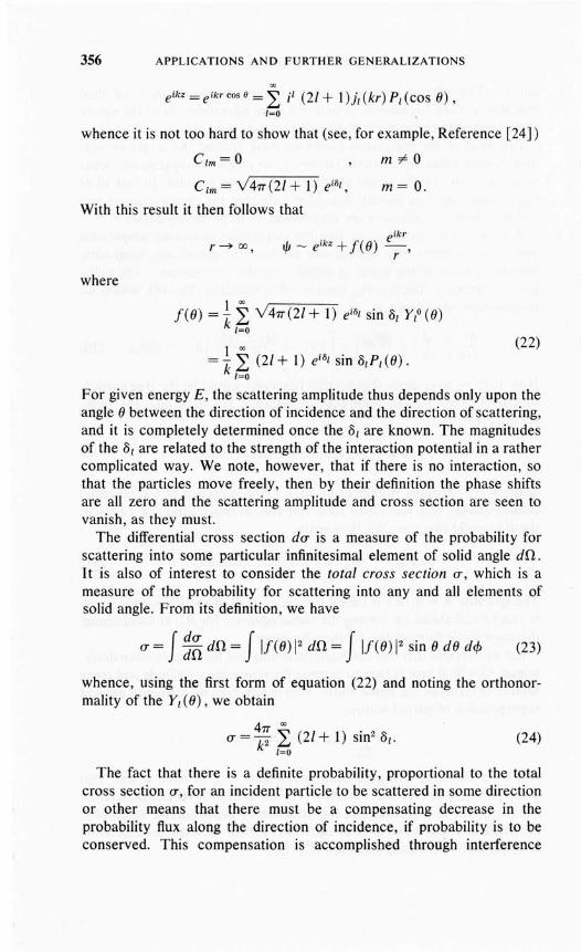
356 APPLICATIONS AND FURTHER GENERALIZATIONS
00
eikz =eikr cos 8 = L i/ (21 + IH(kr) p/(cos e),/=0
whence it is not too hard to show that (see, for example, Reference [24])
C1m=O
C/m =V47T(21+ I) ei8/,
With this result it then follows that
m ¥ 0
m= O.
. eikr
t/J - e'kz + fee) -r-'
(22)
where
fee) = i f V47T(21 + I) eiS/ sin (j/ y/o (e)/=0
= if (21 + I) ei8/ sin (j/p/(e).
/=0
For given energy E, the scattering amplitude thus depends only upon theangle ebetween the direction of incidence and the direction of scattering,and it is completely determined once the (j/ are known. The magnitudesof the (j/ are related to the strength of the interaction potential in a rathercomplicated way. We note, however, that if there is no interaction, sothat the particles move freely, then by their definition the phase shiftsare all zero and the scattering amplitude and cross section are seen tovanish, as they must.
The differential cross section d(J" is a measure of the probability forscattering into some particular infinitesimal element of solid angle dO.It is also of interest to consider the total cross section (J", which is ameasure of the probability for scattering into any and all elements ofsolid angle. From its definition, we have
(J" = f ~~ dO = f If(e) 12 dO = f If(e) 1
2 sin e de d¢ (23)
whence, using the first form of equation (22) and noting the orthonormality of the Y/ (e) , we obtain
(J" = ~~ f (21 + I) sin2 (j/. (24)1=0
The fact that there is a definite probability, proportional to the totalcross section (J", for an incident particle to be scattered in some directionor other means that there must be a compensating decrease in theprobability flux along the direction of incidence, if probability is to beconserved. This compensation is accomplished through interference

THEORY OF SCATTERING 357
(25)
between the incident state function and the scattering amplitude in theforward direction. This argument implies the existence of a generalrelationship between the total cross section and the forward scatteringamplitude. We now establish this relationship. To do so, we examine theforward scattering amplitudefCO = 0). Recalling that for alll
P1CO=0)=I,
we have, from equation (22),
fCO = 0) = ±~ C2l + I) ei81 sin 811=0
I 00 i 00
= k L C2l + I) cos 81sin 81 + - L C2l + I) sin2 81 ,
1=0 k 1=0
The second term is seen to be porportional to the total cross section,and hence the relation we seek may be expressed in the form
47T(T=T ImfCO=O).
In words, the total cross section (T is 47T divided by the reduced wavenumber k times the imaginary part of the scattering amplitude in theforward direction. This important result is known as the optical theoremor as the cross section theorem. For emphasis, we repeat that it expressesthe probability conservation requirement that the amplitude of theincident wave must ultimately be reduced in proportion to the totalprobability that the particle is scattered in any way. We also emphasizethat it is a far more general result than our method of derivation wouldseem to indicate; it holds for arbitrary potentials, spherical or not, andfor arbitrary scattering processes.
The expressions we have obtained for the scattering amplitude andcross section involve summations over the partial wave phase shifts.Questions of the convergence of these infinite series expressions deservesome attention at this point. The role of the centrifugal barrier in keepingthe particles apart plays the dominant role in these considerations. Forsufficiently large l values the particles do not approach each other closelyenough to interact and the phase shifts corresponding to such l valuesmust vanish. To become a bit more quantitative, the distance of closestapproach ro of two particles with relative energy E and relative angularmomentum l is roughly that point at which the centrifugal barrier heightis equal to the total energy E,
l(l + I)1i2 = E2mr
02 •
If we neglect unity In comparison with l we obtain the somewhat
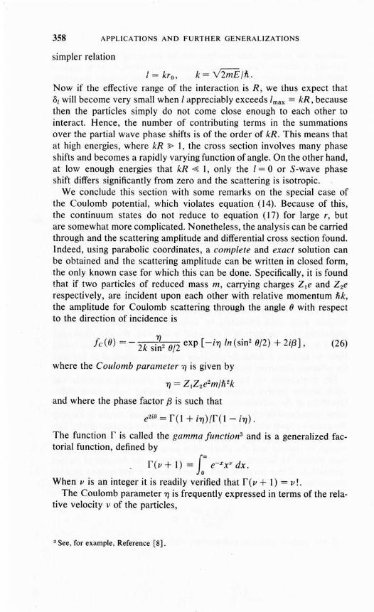
358 APPLICATIONS AND FURTHER GENERALIZATIONS
simpler relation
l=kro, k=V2mE/h.
Now if the effective range of the interaction is R, we thus expect that0/ will become very small when I appreciably exceeds Imax == kR, becausethen the particles simply do not come close enough to each other tointeract. Hence, the number of contributing terms in the summationsover the partial wave phase shifts is of the order of kR. This means thatat high energies, where kR ;;> I, the cross section involves many phaseshifts and becomes a rapidly varying function of angle. On the other hand,at low enough energies that kR <;g I, only the I = 0 or S-wave phaseshift differs significantly from zero and the scattering is isotropic.
We conclude this section with some remarks on the special case ofthe Coulomb potential, which violates equation (14). Because of this,the continuum states do not reduce to equation (17) for large r, butare somewhat more complicated. Nonetheless, the analysis can be carriedthrough and the scattering amplitude and differential cross section found.Indeed, using parabolic coordinates, a complete and exact solution canbe obtained and the scattering amplitude can be written in closed form,the only known case for which this can be done. Specifically, it is foundthat if two particles of reduced mass m, carrying charges Zle and Z2erespectively, are incident upon each other with relative momentum hk,the amplitude for Coulomb scattering through the angle 8 with respectto the direction of incidence is
fd8) = - 2k si~2 8/2 exp [-i7) In (sin2 8/2) + 2i/3] , (26)
where the Coulomb parameter ''I is given by
7) = ZIZ2e2m/h2k
and where the phase factor /3 is such that
e2iIJ = f(l + i7)/f(l - i7).
The function f is called the gamma function3 and is a generalized factorial function, defined by
f(v+ I) == 10'" e-Xx" dx.
When v is an integer it is readily verified that f(v + I) = v!.The Coulomb parameter 7) is frequently expressed in terms of the rela
tive velocity v of the particles,
3 See, for example, Reference [8].

THEORY OF SCATTERING
where the dimensionless fine structure constant a is given by
359
e2
a= he = 1/137.
It should be remarked that the expression we have given for theCoulomb scattering amplitude is that corresponding to the repulsiveinteraction of two like charges. For two unlike charges Tj changes sign,which simply means that fe is replaced by the negative of its complexconjugate.
The differential cross section for Coulomb scattering is obtained inthe usual way from the scattering amplitude and is thus given by
dcr _ 2 _ Tj2 _ (ZJZ2e2/2mv2)2 .dO - Ifel - 4k2 sin4 e/2 - sin4 8/2
This expression is in exact agreement with the classicaL result for thescattering of point charges, first obtained by Rutherford in 1911, and iscommonly called the Rutherford cross section. No explanation can beoffered for this unique and strange correspondence between the classicaland quantum mechanical cross sections. It is important to observe, however, that this exact agreement occurs because the magnitude of thescattering amplitude happens not to contain h and hence neither doesdcr/dO, which must necessarily assume its classical value as a consequence. On the other hand, the phase of the scattering amplitude is anentirely quantum mechanical quantity so that any processes whichdepend upon that phase will exhibit quantum effects. An important andinteresting example in which this is so is the scattering of identicalparticles, as we now show.
If two particles interact and if one of them emerges at angle e in thecenter-of-mass system of coordinates, the other must emerge at angle1T - e. On the other hand, if the first emerges at 1T - e the second mustemerge at e. If the particles are identical these two possibilities cannotbe distinguished from each other in any way whatsoever. Classically,therefore, the cross sections for both processes must be added so thatthe classical result for identical particles is
(dcr) = dcr(e) + dcr(1T - 8).dO classical dO dO
Quantum mechanically, on the other hand, the scattering amplitudes,and not the cross sections, must be combined, with relative sign determined by the symmetry of the state function. For spinless particles

360 APPLICATIONS AND FURTHER GENERALIZATIONS
(a-particles, for example) the total wave function must be symmetricand the scattering amplitudes add with the same sign,
For spin one-half particles (electrons or protons, for example) the wavefunction must be antisymmetric in the space and spin coordinates together. The spatially symmetric state combines with a singlet spin state,the spatially antisymmetric state with a triplet spin state. The formerhas statistical weight one, the latter three. Hence for unpolarized spinone-half particles
du 1 3dO = 4 If (0) + f(7T - oW + 4If(0) - f(7T - 0) 12 •
In both cases, the results contain interference terms which depend onthe relative phase of the scattering amplitude at 0 and at 7T - 0 and whichare clearly quantum mechanical in structure.4 Specifically, for Coulombscattering of identical particles these expressions become, upon substitution for fe from equation (26):
spin zero
du = (ZtZ2e2)2 [ 1 + 1 + 2 cos (TJln tan2 0/2)]dO 2mv2 sin4 0/2 cos4 0/2 sin2 0/2 cos2 0/2
spin one-half
du = (ZtZ2e2)2 r 1 + I _ cos (TJln tan2 0/2)].dO 2mv2 l sin4 0/2 cos4 0/2 sin2 0/2 cos2 0/2
The first two terms in each case give the classical result; the last is thequantum mechanical interference term. In the classical limit the interference term must disappear, of course, and it is interesting to see howthis comes about. As h tends toward zero l TJ increases without limit andthe interference term oscillates more and more rapidly. An infinitesimalspread in energy, or in angle of observation, thus causes this term toaverage to zero and hence to become unobservable.
3. GREEN'S FUNCTIONS FOR SCATTERING;THE BORN APPROXIMATION
In the preceding section we have given a rather formal treatment of thetheory of scattering. The scattering amplitude was introduced, and in
4 Note that these effects are far from small. At 90°, for example, dajdfl. is twice the classicalresult for spinless particles and half the classical result for spin one-half particles.

GREEN'S FUNCTION; THE BORN APPROXIMATION 361
terms of it was defined the experimentally measurable quantity, the crosssection. For the special case of spherically symmetrical potentials amethod was given for evaluating this quantity, the method of partialwaves. The actual calculation requires the solution of the set of radialequations (20). These are so complicated, even for the simplest interaction, that no attempt was made to even discuss their properties.s
As a result we were unable to present, to any significant degree, aqualitative description of the general character of quantum mechanicalscattering processes.
In the present section we correct this defect by presenting an approximation method first introduced by Born. The Born approximation isnothing more than perturbation theory applied to continuum states, aswe shall see, and it is therefore restricted to sufficiently weak interactions. 6 Even so, it is the physicist's absolutely indispensable qualitative guide to scattering and it effectively serves as the norm to which allis referred.
We shall derive the Born approximation by two quite distinct methods.In the first, we obtain an exact integral equation for the state functionthrough the intermediary of the free particle Green's function. In thesecond we regard the scattering process as a transition, induced by theinteraction potential, between states of definite initial and final momenta,and we thus use the methods of time dependent perturbation theory.
(a) Green's Function Method. 7 We seek a solution of the time independent Schrodinger equation, which we write in the form
Here
2m(V2 + k2 )tjJ(r) = ¥ V(r)tjJ(r). (27)
k2 = 2mE/h 2 ,
so that k is the free particle wave number for energy E. We assumeE > 0 and that rV(r) vanishes at infinity, in accord with equation (14).The solution we seek is subject to the asymptotic boundary conditionsfor large r, given in equation (17), which we repeat here for convenience:
• A eikr
tjJ(r) = e'k.r + f(o) ----;-,
S In practice, these equations are almost exclusively solved numerically with the aid of ahigh-speed digital computer. See Section 10, Chapter VI.
61t is not, however, restricted to spherically symmetrical interactions. This is in contrastto the method of partial waves, which becomes completely intractable for non-sphericalinteractions, except in rather special cases.
7 For a general discussion of Green's functions, see References [6) through [13).

362 APPLICATIONS AND FURTHER GENERALIZATIONS
where r = Dr.We now obtain an integral equation for l/J(r), which incorporates
these boundary conditions, by introducing the Green's function G (r, r')= G (r', r), defined as the purely outgoing wave solution of the inhomogeneous equation
(28)
Here 8(r - r') is the three-dimensional Dirac 8-function, which may bethought of as the product of three one-dimensional 8-functions,
8(r - r') == 8(x - x') 8(y - y') 8(z - z')
and which therefore is such that
J 8(r - r') d3r' = 1.
The Green's function is thus seen to be the wave function at the pointr generated by a pointsource at r' .
Deferring the actual construction of G for a moment, we observe thatany function l/J which satisfies the integral equation
l/J(r) = eikor- 2n: f G (r, r') V(r') l/J(r') d3r' (29)
h all space
is a solution of Schrodinger's equation (27) and that this solution automatically satisfies the boundary conditions of equation (17). That l/J isa solution follows by operating on equation (29) with (V 2 + k2). Thisoperator annihilates the first term on the right and, when taken under theintegral sign to operate on G, the only quantity dependent upon r, ityields the Dirac 8-function according to equation (28). Hence we obtain
('\7 2 + k2 )l/J = - ~n: J(V 2 + k2) G(r, r') V(r') l/J(r') d3r',
2mJ= ¥ 8(r - r') V(r') l/J(r') d3r' ,
2m= ¥ V(r) l/J(r),
which is indeed equation (27). That equation (17) is satisfied followsbecause G contains only outgoing waves at r generated by a point sourceat r', whence the integral on the right of equation (29) is simply a superposition of such outgoing waves, and therefore assumes the required formfor r sufficiently large. We shall shortly demonstrate this aspect quiteexplicitly.
The next step is the construction of G itself. We start with the relation,
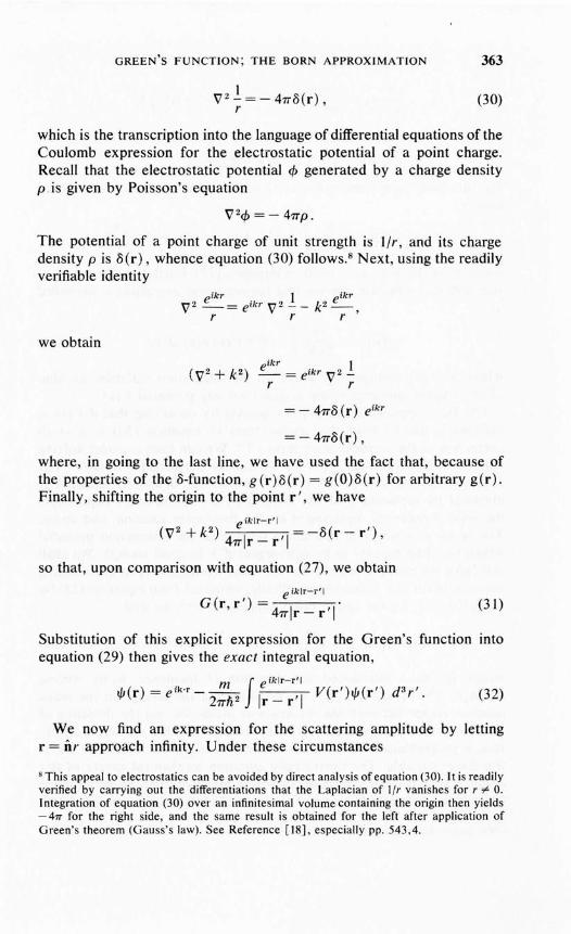
GREEN'S FUNCTION; THE BORN APPROXIMATION 363
IV2 -=-47T8(r) (30)
r '
which is the transcription into the language of differential equations of theCoulomb expression for the electrostatic potential of a point charge.Recall that the electrostatic potential </J generated by a charge densityp is given by Poisson's equation
V2</J = - 47Tp.
The potential of a point charge of unit strength is I/r, and its chargedensity pis 8(r), whence equation (30) follows. s Next, using the readilyverifiable identity
eikr I e ikr
V 2 -= eikr V 2 -- k2-,r r r
we obtain
= - 47T8 (r) eikr
= - 47T8(r),
where, in going to the last line, we have used the fact that, because ofthe properties of the 8-function, g(r)8(r) = g(0)8(r) for arbitrary g(r).Finally, shifting the origin to the point r I, we have
iklr-r'l
(V 2 + P) 4 el
'I = -8(r - r / ),7Tr-r
so that, upon comparison with equation (27), we obtain
iklr-r'l
G(r,r/)=4
el 'I'7Tr-r
(31 )
Substitution of this explicit expression for the Green's function intoequation (29) then gives the exact integral equation,
m Jeiklr-r'l
lJJ(r) = e ik·r
- 27T1i2 Ir _ r'l V(r')lJJ(r/) d 3 r ' . (32)
We now find an expression for the scattering amplitude by lettingr = Dr approach infinity. Under these circumstances
8 This appeal to electrostatics can be avoided by direct analysis of equation (30). It is readilyverified by carrying out the differentiations that the Laplacian of l/r vanishes for r # O.Integration of equation (30) over an infinitesimal volume containing the origin then yields- 417 for the right side, and the same result is obtained for the left after application ofGreen's theorem (Gauss's law). See Reference [18], especially pp. 543,4.

364 APPLICATIONS AND FURTHER GENERALIZATIONS
e iklr-r'l
Ir- r'leiklnr-r'l
Inr - r'le
ikr• ( I )-- e-ikn ·r ' + 0 - ,
r r 2
where we have expanded Ir - r'l in a Taylor series according to
h(r - r') = h(r) - r' . Vh(r) + .. '.
We thus find, upon substitution of this result into equation (32), that forlarge r,
m J . eikr
tJ;(r) = e ik 'n,' - -- e- ikn .r ' V(r')tJ;(r') d 3 r' . - ,2~h2 r
which is of the form demanded by equation (17). Further, upon comparison with that equation, we see that the scattering amplitude is identifiedas
(33)
where we have dropped the prime on the integration variables for simplicity. Again, this expression is exact for any potential V(r).
The Born approximation follows quickly by observing that if V(r) issufficiently small,9 then the second term of equation (32) is a smallcorrection to the incident wave term e ik·r. We can thus consider solvingequation (32) iteratively, just as we did in perturbation theory. Thezeroth-order solution is the incident wave, the first-order solution isobtained by replacing tJ; in the integral by its zeroth-order expression,the second-order by replacing it by the first-order solution, and so on.The result is a series in increasing powers of the interaction potentialwhich we shall assume to be convergent if V is small enough. We shallnot carry the process beyond the first step. Looking only at the resultingexpression for the scattering amplitude, obtained from equation (33) byreplacing tJ;(r) by the zeroth-order expression e ik ' r , we find
m J "f(o) =-2~h2 eik(no-n)'r V(r) d 3 r, (34)
where we have introduced the direction of incidence 00 by wrItmgk = fiok. The quantity k(no - n) == Llk is just the change in the wavenumber vector between the direction of incidence and the direction ofscattering, and we see that, to this approximation, the scattering amplitude is proportional to the Fourier transform of the potential with Ll k astransform variable. The intrinsically quantum mechanical nature of thisresult is readily apparent; contributing to the scattering through a givenangle is the potential function at every point in space, not just the poten-
9 We discuss the meaning of this condition later.

GREEN'S FUNCTION; THE BORN APPROXIMATION 365
tial along a localized trajectory, as would be the case classically.It is instructive to rewrite equation (34) in terms of momenta rather
than wave number. We have, rearranging the terms slightly,
(35)
where we have introduced the initial and final momenta Pi and PI bywriting
Pi = likiio = pOo
PI = hkn = poand where
p = Y2mE.
We thus observe that f(o) is proportional to the matrix element of Vbetween unperturbed (free particle) final and initial momentum states.The differential cross section, given by
is then proportional to the square of this matrix element and hence hasthe form of atransition probability. We next show how this result canbe obtained directly, using the conventional methods of time dependentperturbation theory.
(b) Perturbation Theory Method. Consider now the interaction potential as a perturbation which induces transitions between a state ofdefinite initial momentum Pi and a dense set of energy conserving finalstates, namely those with momentum PI = pD.. According to the goldenrule of time dependent perturbation theory, equation (VII-37), the transition rate is given by
where p(E) is the density of final states and Vii is the matrix elementconnecting the initial state and a typical final state. to We are here dealingwith idealized, nonphysical continuum states of definite momentum,and we therefore adopt the conventional artifice of periodic boundary
10 The precise meaning of typical with reference to the final states will be made clear in amoment.

366 APPLICATIONS AND FURTHER GENERALIZATIONS
conditions in a cube of side L to permit us to properly normalize thesestates and to calculate their density. With this convention, the momentum states are written as
,I. = _1- e ip·rm'l'P L3/2 (37)
and are evidently correctly normalized over the periodicity volume L3.
We thus have at once
(38)
Observe now that Vfi is not necessarily slowly varying, as assumed inthe derivation of the golden rule, if Pr is permitted to range freely overall final states which conserve energy. Otherwise stated, the requirementthat Vfi represent the matrix element to a typical final state has nomeaning if Pr is permitted to vary over all directions. Accordingly, PImust be restricted to an infinitesimal range of orientations about somegiven direction it, which is to say that it must lie in an infinitesimal solidangle dO. about n. This means that p (E) is to be interpreted as the density of that particular fraction of all the states with energy between Eand E + dE which have momenta in dD. To symbolize this fact, wedenote the relative density by dp(E) and the corresponding transitionrate by dW, whence, using equation (38),
(39)
Because the distribution of momentum states for a free particle isisotropic in momentum space, dp is easily expressed in terms of thedensity p of all states; it is just p itself multiplied by the ratio of dD to47T, the total solid angle encompassing all directions,
dDdp=p-'
47T
Now, according to equation (IX-18),
(2m )3/2 • r;:; mpp(E) = 47T 2h 3 LJ V E = 27T 2h 3 LJ,
whence
and equation (39) yields

(41)
GREEN'S FUNCTION; THE BORN APPROXIMATION 367
dW = mp l(eiPrr IVI e iP;-r)12 dO47T 2h4L3 .
This, then, is the probabiiity per unit time of a transition from the initialstate to any final state with momentum oriented in the solid angle dO.Otherwise stated, dW is the probability per unit time that scattering intodfl has occurred. Ry the definition of the differential cross section drr,equation (18), this is nothing more than drrljinel, where Ijinel is the magnitude of the incident probability flux,
I · I - £ 1'"
12 - -.l!..-Jine - m 'l'lne - mL3'
in virtue of the normalization of equation (36). Hence, finally,
mL3 m 2
drr = -- dW = --I( e iprr IVI e iPi 'r)12 dOp 47T 2h '
in agreement with equation (37).The utility and simplicity of the Born approximation is best illustrated
by considering some examples. As the first case, which we shall workthrough in some detail because of its importance, we examine scatteringby the so-called Yukawa pontential,ll
e-rlRV(r) = VoR -' (40)
r
The constant Vo is usually called the strength of the Yukawa potential,and R is called the range. Substitution into equation (34) gives
V R J -riRf(n) =-~ eik(rio-n)·r _e_ d3r.27Th 2 r
The integration is easily performed by choosing the polar axis to liealong (no - n) , as illustrated in Figure 4. Denoting the angle between(no - it) and r by w, as indicated, we thus pave
V R foo J1T J21T ., e-r/RfUi) = -~ r2 dr sin w dw de/> eiklno-nlreosw --.27Th 2 0 0 0 r
The integrand is independent of azimuthal angle so that integration overazimuth simply gives a factor of 27T. The integration over w is also readilycarried out to give
f( ~) m VoR {OOO dr e-r/R (eiklno-rilr _ e-iklno-nlr)n = - Wkloo - 01 JI
II The Yukawa potential is an essential ingredient in nucleon-nucleon interactions. It alsois frequently used to describe a screened Coulomb potential (see Problem 8).
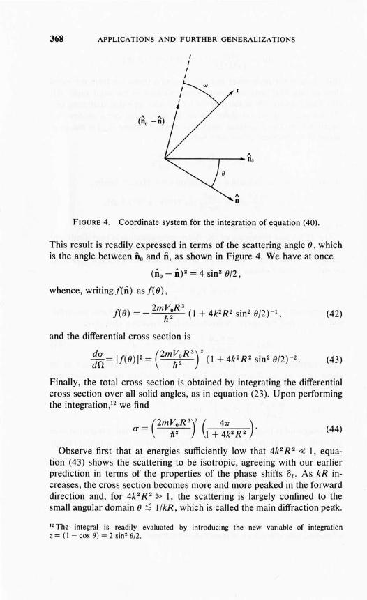
(42)
(44)
368 APPLICATIONS AND FURTHER GENERALIZATIONS
III
I
w
1\~----,...--.. no
1\n
FIGURE 4. Coordinate system for the integration of equation (40).
This result is readily expressed in terms of the scattering angle 6, whichis the angle between Do and n, as shown in Figure 4. We have at once
(no - 0)2 = 4 sin2 6/2,
whence, writing f(n) as f( 6),
f(6) = - 2m~~R3 (1 + 4k2R2 sin2 6/2)-1,
and the differential cross section is
~~ = If(6) 12 = cm~~R3r (1 + 4k 2R2 sin2 6/2)-2. (43)
Finally, the total cross section is obtained by integrating the differentialcross section over all solid angles, as in equation (23). Upon performingthe integration,12 we find
(F= cm~~R7 (I +::2R2)'
Observe first that at energies sufficiently low that 4k 2 R 2 ~ I, equation (43) shows the scattering to be isotropic, agreeing with our earlierprediction in terms of the properties of the phase shifts iii' As kR increases, the cross section becomes more and more peaked in the forwarddirection and, for 4k 2 R 2 ~ I, the scattering is largely confined to thesmall angular domain 6 :S l/kR, which is called the main diffraction peak
12 The integral is readily evaluated by introducing the new variable of integrationz = (I - cos 0) = 2 sin 2 012.

GREEN'S FUNCTION; THE BORN APPROXIMATION 369
This behavior is illustrated in Figure 5. As shown in the figure, the forward scattering turns out to be independent of energy in Born approximation, whereas the total cross section decreases with increasing energy,ultimately inversely as the energy according to equation (44).
drr
o e o e o e
FIGURE 5. Differential scattering for the Yukawa potential at different valuesof kR, according to the Born approximation, equation (43).
All of these features are quite general ones, with only the details differing from one interaction potential to the next. To make this explicit,let us consider as a second example a Gaussian potential,
V(r) = Vo e-(r/R)2.
Omitting details, we obtain
f( () = - ( m ~~ 3) y;. e-k2R2 sin2 9/2
da/dfl = (m~h~3r 7T e-2k2R2s1n29/2
and
Exercise 1. Derive equations (46), (47), and (48).
(45)
(46)
(47)
(48)
Again we find that the scattering in the forward direction, () = 0, isindependent of energy, that the cross section is independent of angleat low energies but as the energy increases a diffraction peak developswhich is of angular width () = l/kR and, finally, that the total cross section decreases inversely as the energy at high energies. The explanationof these common general features follows:

370 APPLICATIONS AND FURTHER GENERALIZATIONS
Forward Scattering. According to equation (34), the scattering amplitude in the forward direction, 0 = 00' is simply proportional to thevolume integral of the potential. Specifically, denoting the forward scattering amplitude by 1(0), we have
(49)
(50)
Up to numerical factors of order unity, this can be expressed, in agreement with equations (42) and (46), as
1(0) = - m~02R3,
where Vo is the strength of the potential and R is its range.Angular Dependence. At energies low enough that kR ~ I, the
exponential factor in the integrand of equation (34) never deviates significantly from unity over the effective domain of integration, which issimply a sphere of radius approximately R. Consequently, for all angles,
1(8) = 1(0) ,
whence the cross section is isotropic at low energies and the total crosssection is
(51)
Comparison with equations (44) and (48) in the low energy limit showsthat we have again obtained the correct result, up to numerical factorsof order unity.
We next consider the opposite limit in which the energy is high enoughthat kR ~ 1. Here the oscillations of the exponential factor in the integrand of equation (34) must be taken into account. Evidently this factoroscillates more and more rapidly as the scattering angle increases, thuscausing the scattering amplitude to diminish sharply as one moves awayfrom the forward direction. This diminution sets in at scattering anglessuch that
kRloo- 01 = 2kR sin 0/2 = 1,
because at smaller angles than this the exponential deviates little fromunity. Since kR ~ 1, this relation can be written in the simpler form
8 = l/kR,
and we have thus demonstrated that the width of the high energy diffraction peak is of the order l/kR, as claimed.

GREEN'S FUNCTION; THE BORN APPROXIMATION 371
Total Cross Section at High Energies. This last result permits us toquickly estimate the high energy total cross section. The essential feature is that only the main diffraction peak contributes significantly tothe scattering, whence we have
0- = JI!(O) 12 sin 0 de d¢ = 27T J:1kRI!(O) 12 sin 0 dO
= 27T J:'kR I!(O) 12 0 dO = 7T1!(O) 12/k2 R 2
and, finally, using equation (48),
(mVR3)2 7T
0- = h~ k2R2' (52)
in agreement with the high energy limit of equations (44) and (48), up tothe usual numerical factors.
We conclude our discussion of the Born approximation with some remarks about its domain of validity. Most treatments of this subject arebased on a consideration, which turns out to be rather complicated,of the magnitude of the first-order correction to the zero-order planewave state function. 13 However, we give here a much simpler analysisin which the total cross section 0- plays the key role. The essence of theargument is that, in the spirit of time dependent perturbation theory, thecross section directly measures the effective rate for transitions out of theinitial state. Now this rate must be small if the perturbation treatment isto be valid. To put this on a quantitative basis, we shall take the effectiverate to be the ratio of the scattered probability flux to the maximum possible scattered flux, namely that incident on the geometrical cross se~tion
of the scatterer,14 7TR2. The ratio in question is simply 0-/7TR2 and henceour condition for the validity of the Born approximation is that this ratiobe small,
(53)
At low energies, using equation (51), the validity condition is thus
(54)
and at high energies, using equation (52), it is
'" A particularly complete treatment is presented in Reference [18].
" Strictly speaking, this is the maximum only at high energies. At low energies the maximumis considerably larger because of diffraction. As a result, our estimate is on the conservative side.

372 APPLICATIONS AND FURTHER GENERALIZATIONS
1 (mV R2)2PR2 Ii~ «; 1. (55)
(56)
(57)
Observe that the low energy condition is much more stringent than thehigh energy one; whenever equation (54) is satisfied, equation (55) isautomatically, and much more strongly, satisfied, because it containsthe extra factor (kR)-2, which is small at high energies. Moreover, atsufficiently high energies, equation (55) can always be satisfied, even ifequation (54) is not. For this reason, the Born approximation is primarilyregarded as a high energy approximation and it thus nicely supplementsthe phase shift method which, it is recalled, becomes quite unwieldy inthe high energy domain.
Equations (54) and (55) cannot be thought of as particularly preciseor rigorous conditions, as is evid~nt from our mode of derivation. Thefollowing argument, however, may perhaps serve to increase our confidence in their reliability. Recall that the exact solution to any scatteringproblem satisfies the optical theorem of equation (25),
47T(J' = T 1m 1(0) .
Now the Born approximation can never satisfy this theorem because,as equation (49) makes clear, the forward scattering amplitude in Bornapproximation is always real. This implies that the Born approximationis not reliable unless the imaginary part of the true forward scatteringamplitude is negligibly small compared to the entire forward scatteringamplitude. In brief, we must have as a kind of self-consistency condition
1m 1(0) «; 1/(0) Ior, multiplying through by 47T/k and using the optical theorem,
47T(J' «; k 1/(0) I·
At low energies this gives, using the estimates of equations (50) and (51),
kR (m V~~2) «; 1.
This is seen to be a generally weaker condition than equation (54) because it contains the factor kR, which becomes vanishingly small in thelow energy limit. On the other hand, at high energies we obtain
1 (mVoR2)4kR 1i2 «; 1,
which is the square root of equation (55) up to numerical factors, and

MOTION IN AN ELECTROMAGNETIC FIELD 373
hence is a generally somewhat stronger condition.In summary, then, the self-consistency requirement and the require
ment that the total transition rate be small lead roughly, but not precisely,to equivalent conditions for the validity of the Born approximation. Thismay be taken as rather strong evidence that we have indeed identifiedthe relevant features. As far as the application of these conditions inpractice is concerned, the safest guide is to use whichever of the twosets of conditions is more restrictive in the energy domain under consideration.
4. MOTION IN AN ELECTROMAGNETIC FIELD
Consider a particle of positive charge e moving in a given externallyimposed electromagnetic field described by the vector potential A(r, t)and scalar potential cf>(r, t). It is recalled that in Gaussian units theelectromagnetic field strengths 8 and 96 are given in terms of thesepotentials by
96=v x A
I aA8=-vcf>---c at'
and the classical Hamiltonian is
IH = 2m (p - eAIc)2 + ecf> + V,
(58)
(59a)
(59b)
where V is any additional potential which may be present. 15 It is notdifficult to verify that Hamilton's equations
dXi= aHdt api
dpi aH----cit = - ax i
then yield the correct equations of motion
d 2r em dt 2 = e8+~ (v x %) - VV.
Note however, that from the first of equations (59b)
(60)
(61)
15 See, for example, Reference [14], especially Chapter I, Section 5, and Chapter VII,Section 3. See also Problem II.

374 APPLICATIONS AND FURTHER GEJI;ERALIZATIONS
so that p is not the kinetic momentum. It is nonetheless the canonicalmomentum, that is, the formal momentum variable in the sense of Hamilton's equations.
Note also that the electromagnetic potentials have no direct physicalsignificance; only the field strengths do. Indeed A and cP are not uniquelydefined by equation (58). The class of tranJiormations which leave §and 96 unchanged are called gauge transformations and are generatedby arbitrary scalar functions X according to
(62)A'=A-VX, cP' = cP + ! ax.c at
The choice of X determines the gauge, but no physical result dependsupon this choice. Otherwise stated, the potentials A' , cP' yield the samefield strengths, equations of motion, and so forth, as do A, cPo Note thatwhile the canonical momentum does depend upon the gauge, the particlevelocity does not, as may be seen from equation (60), which makes noreference to gauge dependent quantities.
As usual, the Hamiltonian operator is obtained by replacing the classical dynamical variables in the classical Hamiltonian by the quantummechanical operators which represent them. Thus Schrodinger's equationbecomes
(63)_I (p_ eA)2 1/1+ (ecP+ V)I/I=-~ al/l.2m c I at
The commutation rules between p and r are unaltered by the presenceof the field and thus assume their usual form
Ii(Pi, X j) = -:- Oij.
I
In configuration space we still have, therefore,
fiP=-:-V·
I
(64)
Note that p and A(r, t) do not commute in general and hence that themeaning of the first term of equation (63) must be spelled out. Specifically, this term is to be understood as having the symmetrized form,
(eA ')2 e e2
p-c =p2- C(p. A+A· p) + c2 A2,
in which case it is not hard to see that it is properly Hermitian.We have argued that the vector and scalar potentials are not uniquely
defined but may be altered at will by a gauge transformation. Classically,no physical results are affected by such a transformation, and the same

MOTION IN AN ELECTROMAGNETIC FIELD 375
conclusion must hold in the quantum mechanical case as well. To seehow this comes about, consider \he gauge transformation of equation (62).Let 1./1' (x, t) denote the transformed state function, which is to say, letit be the solution to Schrodinger's equation in the new gauge,
-1- (p _eA')2 1./1' + (e¢' + VH' = _ ~ a1./1 , .2m c I at
Substitution of equation (62) then yields
_1 ( +~ 'i7 _~A)2 tfJ'+ (e¢+ VH' =-~ al./l' -~ aX 1./1'. (65)2m P c X C I at c at
Comparison of equations (63) and (65) now shows that 1./1 and 1./1' are related by the expression
1./1' (x, t) = 1./1 (x , t) e-ieX/flc, (66)
as is readily verified by direct substitution. Otherwise stated, the gaugetransformation of equation (62) is generated by replacing 1./1 by t/J eiexW
in equation (63). We thus conclude that the arbitrariness in the definition of the electromagnetic potentials is reflected in a correspondingarbitrariness in the phase of the state function. The phase is actuallydetermined only within an undetectable scalar function ex /lic, and thisis the meaning of gauge invariance for Schrodinger's equation. 16
As an illustrative example, consider a charged particle in a uniformmagnetic field 96. For this case the vector potential can be written inthe form
1A="2(96Xr).
It may readily be verified that equation (58) is satisfied with this choice.Since p commutes with this particular vector potential, we can writeA . P + P . A = 2A . p and hence
e e2
(p-eA/c)2=p2_-(9bxr) ·p+-(96xr)2.C 4c2
Now
(96 X r) . p = 96 . (r X p) = 96· L,
where L is the orbital angular momentum operator, and hence Schrodinger's equation becomes
p2 [e e2 2J Ii al./l-1./1+ V--96·L+-.-(96xr) 1./1=--;--'
2m .2mc 8mc2 I at (67)
16 See Problem 10. Chapter V, for a discussion of the undetectability of a phase factor suchas that referred to above.

(68)
376 APPLICATIONS AND FURTHER GENERALIZATIONS
The term quadratic in 9G is most easily understood by considering themotion of a free particle in a magnetic field. Classically, this motion proceeds along a helical orbit and is bounded in the plane perpendicular to9G. The quadratic term in 9G in Schrodinger's equation is responsible fora similar confinement of the state function with respect to motion in thetransverse plane. Indeed, it is not hard to show, although we shall notdo so, that the motion in this plane is equivalent to that of a two-dimensional harmonic oscillator.1 7 The quadratic term is thus clearly essentialfor the description of such states. On the other hand, in discussing thebound states of a particle in some confining potential V, the contributionof the quadratic term is generally quite small and it can often be neglectedentirely.
The term linear in 9G in Schrodinger's equation is at once seen to describe the interaction of a magnetic dipole of magnetic moment
- e LIJ-- 2mc
with the magnetic field. If the quadratic term is neglected, if V(r) isspherically symmetrical and if the z-axis is chosen to coincide with 9G,then the stationary states can be classified as simultaneous eigenfunctionsof U and of L z , as usual. However, the energy now depends upon theeigenvalues mlh of L z . Specifically, if we have a state tfilllmi with energyEnl in the absence of a magnetic field, then in the presence of the fieldwe have
and the intrinsic (2/ + I)-fold degenerate state is split into 2/ + I stateswith equal energy separations
~E=~9G.2mc
The quantity eh/2mc is called a Bohr magneton; it is the magnetic momentof a particle with unit orbital angular momentum. Because of the role ofthe quantum number ml in the above, ml is frequently called the magneticquantum number. It is well to remark at this point that all of our equations have been written for a particle of positive charge e. For an electron,e must be replaced by - e everywhere.
We now briefly mention the effect of spin. Associated with the spin isa magnetic moment, which we write in the form
ehIJ-spin = g -2- S/h.
mc
17 See References [19] or [24].

DIRAC THEORY OF THE ELECTRON 377
The dimensionless quantity g measures the ratio of the magnetic moment,in units ek(2mc, to the angular momentum in units ofk. For orbital motiong was seen to be unity. For the intrinsic magnetic moment ofthe electrong turns out to have the value two. In a sense, the spin angular momentumis thus twice as effective as the orbital angular momentum in generatinga magnetic moment. IS
The existence of the spin magnetic moment means that the Hamiltonianmust be supplemented by an additional magnetic energy term /Lspin ·96,Thus, for example, for an electron in a uniform magnetic field the termlinear in 96 in the Hamiltonian has the form
e e(/L+/LsPin) '96=-2- (L+2S) '96=-2- (J+S)'96,
mc mc
where J is the total angular momentum. The analysis of this term, leadingto the so-called anomalous Zeeman effect, is considerably more complicated than for the case of a particle without spin, and we shall not carryit OUt. 19
5. DIRAC THEORY OF THE ELECTRON
We now want to develop a relativistic version of Schrodinger's equationfor the motion of an electron. We shall consider primarily the case inwhich no external forces act so that the electron can be treated as free.In that case, the classical relativistic Hamiltonian is
H = V (pc)2 + (mc 2 ) 2 ,
where m is the rest mass of the electron and p is its momentum. We nowsee at once that if p is the usual quantum mechanical operator, H is notwell-defined because of the square root sign. 20 One way out of this difficulty was suggested by Klein and Gordon, who considered
18 It is of interest to remark on the g-values for other particles, measuring magnetic momentsalways in the natural units eh/2mc, where m is the mass of the particle. For the JL-meson,g is again two, as for the electron. Both cases are in agreement with the predictions ofthe Dirac theory. On the other hand, the intrinsic magnetic moment of the proton is not onenuclear magneton, as it is called, (g = 2), but 2.79 nuclear magnetons (g = 5.59), whilethe neutron's magnetic moment is not zero (as for the neutrino) but is - 1.91 nuclear magneton, the minus sign meaning that it is directed opposite to the spin. These anomalousmagnetic moments clearly indicate the existence of some kind of charge structure for theproton and neutron. These are subjects of great current interest in the physics of elementaryparticles.
19 See, for example, Reference [22].
20 In configuration space the square root must be expanded in a power series, whence His equivalent to a differential operator of infinite order. This can be circumvented by working in momentum space, but the resulting equations are completely intractable except forthe special case of a free particle.

(69)
(70)
378 APPLICATIONS AND FURTHER GENERALIZATIONS
rather than
This is a perfectly good relativistic wave equation but, because of thesecond time derivative, probability is not conserved if I/J is interpretedas a probability amplitude. It turns out that this equation, the KleinGordon equation, can be interpreted in the quantum theory of fields,but it cannot be applied to the motion of a single particle.
The dilemma was resolved by Dirac using the following argument. Ift/J is to be a probability amplitude, then only a first-order time derivativecan appear in Schrodinger's equation. Since time and space coordinatesenter on an essentially equal footing relativistically, the space derivativesin Schrodinger's equation must also appear only linearly. Thus he wrote
Ii al/JHI/J=-j at'
where H is now constrained to be linear in the momentum,
H = [a . pc + ,Bmc2] ,
and where a and ,B are to be determined by the requirement that
H2 = (pcF + (mc2)2.
Thus Dirac forced the issue by imposing the condition that
H = V(pcP + (mc2)2
be a well-defined linear function of p. It is clear, of course, that a and ,Bcannot be ordinary numbers if equations (69) and (70) are to be satisfiedbut must be (space and time independent) operators.
Keeping in mind the operator nature of a and ,B we thus require
[a . pc + ,Bmc2J2 = (pC)2 + (mc2)2
or, preserving the order of all relevant factors,
2: alp/c2+ ~ L (a;aj + aja;) P;PjC2+ L (a;,B + ,Ba;)mc2p;ci i~ i
+ ,B2(mc2)2 = p2C2 -t- (mc2 )2.
Comparing terms we thus see that a/ = ,B2 = 1 or
(71)
and
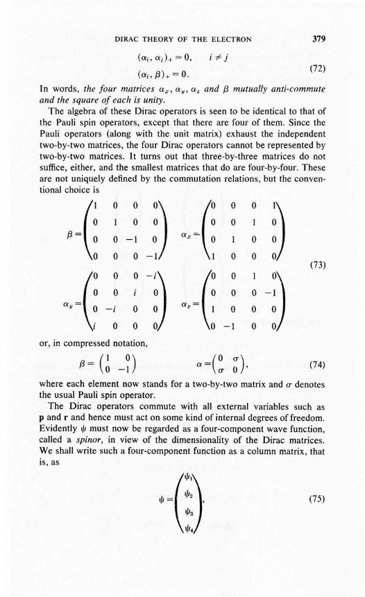
DIRAC THEORY OF THE ELECTRON 379
i~j
(72)
In words, the four matrices ax, ay, az and 13 mutually anti-commuteand the square of each is unity.
The algebra of these Dirac operators is seen to be identical to that ofthe Pauli spin operators, except that there are four of them. Since thePauli operators (along with the unit matrix) exhaust the independenttwo-by-two matrices, the four Dirac operators cannot be represented bytwo-by-two matrices. It turns out that three-by-three matrices do notsuffice, either, and the smallest matrices that do are four-by-four. Theseare not uniquely defined by the commutation relations, but the conventional choice is
0 0 0 0
0 0 0
13= 0 0a =-
00 -1 x
0 0 0 -1 0 0(73)
0 0 0 -i 0 0
0 0 0 0 -1a =
0a =
0 0y 0 -i z
0 0 -1 0
or, in compressed notation,
13 = (~ -n a=(~ ~), (74)
where each element now stands for a two-by-two matrix and (J denotesthe usual Pauli spin operator.
The Dirac operators commute with all external variables such asp and r and hence must act on some kind of internal degrees of freedom.Evidently l/J must now be regarded as a four-component wave function,called a spinor, in view of the dimensionality of the Dirac matrices.We shall write such a four-component function as a column matrix, thatis, as
(75)

380 APPLICATIONS AND FURTHER GENERALIZATIONS
with the understanding that when an arbitrary four-by-four matrix A,with elements Ai;, acts on l/J it does so according to the rules of matrixmultiplication to produce an altered column matrix. Explicitly writtenout, this means that
Al/J=
Thus, specifically,
f3l/J =
(76)
(77)
The Dirac equation
c [a . p + f3mc] l/J = - ~ al/J = El/JI at
is now to be understood as an equation in these column matrices. Notethat E is the operator for the total energy, including the rest energy ofthe particle.
Recall now that if two matrices are equal, each element of the firstmust equal the corresponding element of the second. We thus see thatthe Dirac equation is a compact way to write a set of four coupled lineardifferential equations in the four components of l/J. Writing these outexplicitly, using equation (76), we have
(_. ) 2,1. __ !!:. al/JI
c Px Ipy l/J4+ cPzl/J3+ mc O/l- . aI t
(78)

DIRAC THEORY OF THE ELECTRON 381
(.) .1, 2.1, _ Ii at/J4c PX+1Py t/JI-CPZ'¥2- mC '¥4---:- -a .
I t
We now consider a stationary state of definite linear momentum pand energy E. For simplicity, we shall take p to be directed along thez-axis. Writing
(81)
(80)
(79)
V=
t/J = VeiPzlft
where V is a spinor with constant components,
VI
V 2
V 3
V4
equation (78) then reduces to the algebraic equations
cPV 3 - (E - mc2 ) V I = 0
-cpV4 - (E - mc2 ) V 2 = 0
cpVI - (E + mc2 )V3 = 0
-cpV2 - (E + mc2) V 4 = o.
It is then easily verified that we obtain a solution, provided that
E = ± V (pcF + (mc2)2.
With either choice of sign, we then have
VI E + mc2 pcV 3 pc E - mc2
(82)pc
E-mc2
Note first that equation (81) gives the correct relativistic relation between energy and momentum, but that states of both positive and negative energy are possible. For now we restrict our attention to positiveenergy states. We shall return later to the question of negative energies.
Next note that VI and V 3 are entirely independent of V 2 and V 4 .
This means that our solution can be expressed as an arbitrary linearcombination of two independent states. Let us exhibit these states bywriting
(83)
where

382 APPLICATIONS AND FURTHER GENERALIZATIONS
X+ = X-= (84)
The coefficients Q+ and Q_ are arbitrary and, of course, VI and V 3 arerelated to each other by equation (82), as are U2 and V4'
We thus see that states of given energy E and given linear momentumvector (which is directed along the z-axis in the case under consideration)are not unique but are doubly degenerate. This means Hand p do notform a complete set of commuting operators but must be supplementedby an additional operator which can be associated only with some kindof internal coordinate. This internal coordinate turns out to be the spinand the missing operator to be the component of the spin along thedirection of p, as we now demonstrate.
First define the four-component analog of the Pauli spin operator bywriting
(85)
The notation means, for example, that
o• _ (crz 0)_cr -- -z 0 crz
o 0
-I
oo 0-1
(86)
and similarly for the remaining components. It is now seen at once that
where X± are given by equation (84). Since the Dirac operator fr hasexactly the same algebraic properties as the Pauli operator cr, we thustentatively conclude that X+ describes a state in which the spin is orientedalong the positive z-axis and X_ a state in which it is oriented along thenegative z-axis. As our notation indicates, these states are the spinoranalogs of the two-component nonrelativistic states discussed in ChapterX. This relationship can be made clearer by passing to the nonrelativisticlimit, which can be defined by
In that limit, it follows from equation (82) that V 3 and V 4 become neg-

DIRAC THEORY OF THE ELECTRON 383
ligible compared to VI and V 2 . If these small components are neglected,the Dirac spinors X± can be collapsed to two-component states which areprecisely the usual representations of nonrelativistic spin states X+
and X_, and the Dirac operator &- collapses to the Pauli (T.
The argument above makes it plausible that &- is related to the internalangular momentum of the electron, but it is by no means a proof. Indeed,it should be observed that whell relativistic effects are important, a statefunction which is an eigenstate of Hand p can be simultaneously made aneigenfunction only of that component of &- which is directed along p,and not of either perpendicular component. Otherwise stated, only theparallel component of &- commutes with H. Thus, relativistically, thereis a coupling between the internal and external degrees of freedom andthe separation into "internal" and "external" is no longer quite so sharp.
A genuine proof, instead of a plausibility argument, can be constructedin the following way. We first ask whether orbital angular momentum is aconstant of the motion. To answer this, let us examine the commutationrelations between Land H. After some algebra,21 we find
(L, H) = ific(a x p) ,
so that orbital angular momentum is not conserved. This is no surprise;a glance at the Dirac Hamiltonian shows that it is not invariant underspace rotations alone. Next examine the commutator of &- and H. Aftersome more algebra we obtain
(&-,H)=-2ic (aXp),
whence it follows that J = L + (fiI2)&- is a constant of the motion,
[(L+~&-),H] = (J, H) =0.
Hence the quantity J, which satisfies the requisite commutation relationsfor angular momentum, must be interpreted as the total angular momentum and (fiI2)&- as the operator representing intrinsic angular momentum.The Dirac equation thus has the automatic consequence that the electron,or any other particle it describes, has spin angular momentum one-half.
Since spinor wave functions have four components, we must extendour definition of expectation values and matrix elements. The meaningof an expression like (t/JI<p) is
4
(t/JI<p) = L (l/Jd<Pi),i=1
where t/Ji and <Pi are the ith components of the spinor states t/J and .p.The quantities (t/Jd<Pi) have their normal meaning. Thus, for example,in configuration space
21 The details are left to the problems.

384 APPLICATIONS AND FURTHER GENERALIZATIONS
Note that this rule is all that is required for the evaluation of the matrixelements of an arbitrary operator A, arbitrary in both spinor and ordinaryspace, since we can always write (t/JIA 1<1> >= (t/JI<1> / >, where <1> I is simplythe new spinor obtained by operating upon <1> with A.
We turn now to the question of the negative energy states. Accordingto equation (81), the free particle energy spectrum is a continuumranging from plus infinity down to the rest energy mc 2
• Below this energythere is a gap containing no states, and this gap extends to the negativeenergy -mc 2 • At more negative energies still the spectrum again becomes continuous and extends to minus infinity. This spectrum is shownin Figure 6. In a certain sense it is no different than the classical spectrum,since the same negative energy solutions are formally possible in theclassical- case as well. Classically, however, no communication whatsoever is possible between the positive and negative energy portions of thespectrum. A particle cannot change from a state of motion with positiveenergy to one with negative energy, for to do so it would have to passthrough an energy interval in which motion is impossible. The existenceof such states thus causes no difficulty on the classical level; such statesare simply inaccessible and therefore unobservable.
E
Positive energy continuum
No free
particle states
Negative energy continuum
FIGURE 6. Spectrum of allowed energies for a free Dirac particle.
On the quantum level, all is changed; discontinuous changes are thenile. Hence, transitions from positive to negative energy states wouldcertainly be expected to occur, and with the release of an enormousamount of energy - in excess of 2mc 2
• Indeed, since the negative energyspectrum extends to indefinitely large values it would appear that noDirac particle could ever be observed in a positive energy state. Inother words, all of the electrons in the universe would quickly fall into

DIRAC THEORY OF THE ELECTRON 385
the negative energy "sea," a sea more than deep enough to accept them.It might appear that one way out of this difficulty would be to rule out
negative energy states as physically inadmissible. It turns out, however,that if this is done the Dirac states do not form a complete set.22 Diracgave a brilliant solution to this problem by postulating that in the normalstate of the universe all of these negative energy states are completelyoccupied. Under these conditions the exclusion principle then forbidsany transitions of an electron from a state of positive to a state of negative energy. Furthermore, this vast, infinitely dense ensemble of negativeenergy state electrons would be electrically and mechanically inert,except for transitions a particle in the filled negative sea might make tothe relatively empty states of positive energy. Such a transition wouldrequire an energy in excess of 2mc 2
• This huge energy is not availableunder normal conditions and the negative energy particles are not observable, in agreement with experience.
Suppose, however, that enough energy were supplied to produce atransition from the negative sea to a positive energy state. We wouldthen observe the sudden appearance of an ordinary electron, originallyunobservable as an occupant of a negative energy state. We would alsoobserve a correspondingly sudden change in the properties of the negative energy sea. This sea would no longer be electrically and mechanically inert, and therefore unobservable, because it would no longer becompletely filled; one state would be unoccupied. This hole state, as itis called, is associated with the removal of a negative charge of negativeenergy from the inert normal state of the universe, which we might callthe vacuum. The removal of a negative charge of negative energy fromthe vacuum can be interpreted as the appearance of a positive chargeof positive energy, called the positron, completely equivalent to anelectron except for its opposite charge.
That thi~ interpretation is reasonable can be seen by considering theeffects of an applied electromagnetic force on the negative energy seawhen the sea contains a hole state. The electrons would tend to movein the direction of the applied force, and transitions to the hole state,the only available state within the sea, would be favored if they supportedthis tendency. The hole would then tend to move oppositely to the electrons, and indeed to do so as freely as if it were an isolated object.
22 This is one example, and a very important one, in which the mathematics initially forcedthe physical picture, rather than the other way around. We have given a physical interpretation of completeness by arguing, correctly, that the totality of physically admissiblestates must be complete. This leaves the question of how we are to identify all of thephysically admissible states. In the past we have more or less taken this identification forgranted and have then asserted completeness as a necessary consequence. In the presentinstance, even if our intuition about physical admissibility is inadequate, the completenessrequirement forces us to admit negative energy states.

386 APPLICATIONS AND FURTHER GENERALIZATIONS
It is now seen that the transition of an electron from a negative to apositive energy state corresponds to the sudden appearance of an electron and positron at the same point in space and time and requires aminimum energy ex.penditure of 2mc 2
• This is the famous phenomenonof pair production. The reverse of this process also occurs, of course,when an electron happens to fall from a positive energy state into a holestate. This is the phenomenon of electron-positron annihilation, and theenergy appears as electromagnetic energy, normally as a pair of photons.
So far we have considered only the free particle Dirac Hamiltonian.Suppose now that the electron moves in an external electromagneticfield or other potential. The Dirac Hamiltonian is then modified in thecanonical way by writing
H=c[a' (p-eAfc)]+f3mc 2 +e<fJ+V,
where A and <fJ are the electromagnetic vector and scalar potentials andwhere V is any other independent interaction which may exist. If onesolves this equation for an electron in a uniform magnetic field, forexample, the magnetic interaction energy turns out to be precisely thatof a spin one-half particle carrying a magnetic moment of one Bohrmagneton, just as required by observation. To mention a second example, the solution of the Dirac equation for the states of the hydrogenatom gives almost perfect agreement with experiment, including all finestructure corrections.23
Starting with only its mass and charge, the Dirac theory of the electron is thus seen to account for all of its intrinsic properties as well asfor the existence of the positron and the phenomena of pair productionand annihilation.
We have emphasized the electron in our discussion. However, everyspin one-half particle is described by the Dirac equation. Muons andneutrinos, for example, are described by precisely the same equation,with appropriate rest mass, as that for electrons. On the other hand,protons and neutrons, as a consequence of their anomalous magneticmoments, are described by a Dirac Hamiltonian supplemented by anextra term, empirically adjusted to give: the observed magnetic moment.Pair production and annihilation involving all of these particles and theiranti-particles, as they are called, have been observed, in full agreementwith the predictions of the theory.
23 However, the Dirac equation as we have considered it does not give the so-called Lambshift. This very small shift is generated by interactions with the fluctuating vacuum electromagnetic fields. Such field fluctuations, like the zero point motion of the harmonicoscillator, are entirely quantum mechanical in nature and do not appear in any treatment,such as ours, in which the electromagnetic field is taken to be classical.

MIXED STATES AND THE DENSITY MATRIX
6. MIXED STATES AND THE DENSITY MATRIX
387
Every uniquely defined state of a quantum mechanical system must bea simultaneous eigenfunction of some complete set of operators. Expressed in terms of observations, this means that some complete sei ofnoninterfering measurements must be performed if a state is to beuniquely specified. Such a uniquely specified state is called a pure state.The evolution of a pure state with time is governed by Schrodinger'sequation, and this evolution proceeds in a perfectly definite predictableway. The intrinsic statistical nature of quantum mechanics manifestsitself in the distributions of observed values which are obtained whenmeasurements are performed upon an ensemble of identically preparedsystems, each in the same pure state. Only pure states have concernedU8 to the present. More often than not, however, our knowledge ofcomplicated systems is not complete and a description in terms of purestates is impossible. This lack of knowledge introduces a second statistical element, which is not quantum mechanical in origin and which isfamiliar from classical statistical mechanics. We now briefly show how incompletely defined or mixed states can be treated quantum mechanically.
The description of a mixed state requires a statistical mixture of allthose pure states which happen to be consistent with our incompleteknowledge, whatever it may be. Alternatively, we can think of an ensemble of systems, each of which is in one or another of such purestates. Consider now one such system of the ensemble described by thepure state t/J, and suppose l/J to be expressed in terms of some completeorthonormal set,
(87)n
Let A be an operator representing some arbitrary observable. Then
(88)
where the A nm are the matrix elements of A ,
Averaging over the ensemble, in the usual sense of statistical mechanics,we then obtain
(89)n~m
where a bar over a quantity denotes that an ensemble average has beentaken. Note that the A nm are fixed known numbers so that the ensembleaverage on the right involves only the en, which play the role of statistical variables. Since A is arbitrary, we thus see that the ensemble

388 APPLICATIONS AND FURTHER GENERALIZATIONS
average for any physical operator whatsoever is uniquely specified by aknowledge of the quantity
IPmnl ::;;: I. (90)
The operator P, with matrix elements Pmn, is called the density matrix.It contains all of the available information about the system, since if Pis known, so is the distribution of measured values for every measurement which might conceivably be performed upon the ensemble.
Expressing equation (89) in terms of P, we now obtain
(A) = L PmnAnm.n,m
Since the right-hand side can be interpreted as a matrix product, thisreduces to
(91)m
The sum of the diagonal elements of a matrix is called the trace of thematrix and is written as
Tr B == L B mm ,m
whence equation (91) can be expressed in the representation independent form
(A ) = Tr (pA) . (92)
We have now achieved our main objective, namely, to develop asuitable characterization of mixed states. The density matrix for suchstates is seen to play the same role as does the state function for purestates. In particular, all of the information available is contained in each,and each defines the state it characterizes.
We next develop some of the properties of the density matrix. Notefirst, from equation (90), that P is Hermitian,
Pmn = Pnm*' (93)
This follows because of the independence of ensemble averaging andcomplex conjugation. Next observe, setting A equal to unity in equation(92), that
Tr P = I. (94)
In words, the diagonal elements of the density matrix sum to unity. Thisresult can be verified from equation (90), since we have
Tr P = L em em* = L em em* = 1.m m

MIXED STATES AND THE DENSITY MATRIX 389
Observe also that the diagonal element Pmm directly gives the probabilitythat the system is in the state cl>m. Hence Pmm can never be negative, butmust lie between zero and unity. Considering a representation in whichP is diagonal, the diagonal elements are then the eigenvalues of P, andwe see that the eigenvalues of the density matrix all lie between zero andunity, so that P is a positive definite, bounded operator.
Suppose now that P is prescribed initially. What can we say about itsdevelopment in time? Let H denote the Hamiltonian of the system andconsider the Cn in equation (87) to be functions of time,
Since t/J satisfies
H"'=-~ at/J'I' i at'
we find in the usual way that the Cm satisfy the set of equations
- ~ d;tm = L HmiCi ,
I
whence also,
(95)
(96)
where we have used the fact that H is Hermitian in taking the last step.Multiplying equation (95) by Cn* and equation (96) by Cm and subtracting, this gives
Ii d- -:- -d (CmCn*) = L (HmiC;Cn* - CmCi*Hin ).
I t i
The operations of time differentiation and ensemble averaging are independent, and hence, upon averaging over the ensemble, we obtain
= (H, P)mn.
Thus finally, the time development of P is given by
Ii dp-idi=(H,p), (97)
whence we observe that P is stationary if it commutes with the Hamiltonian.
To illustrate some of these properties of P we now give some simpleexamples. Consider a system in a state of definite energy E and angular

390 APPLICATIONS AND FURTHER GENERALIZATIONS
momentum L, but suppose its angular momentum to be oriented atrandom. Then each of its 2L + 1 degenerate states of the given E and Iare equally probable. These 2L + 1 states are complete for the system,and in a representation using these states P is simply the unit matrixdivided by (2L + I). A similar example is that of an unpolarized particleof spin one-half. Then, in the usual representation in which cr. is diagonal,
(1/2 0 )
P = 0 1/2'
which describes a mixed state in which the spin is equally likely to be upor down with respect to any axis. Note that in both cases the trace of Pis properly unity and that P is stationary.
A final and extremely important example is that of a system in thermalequilibrium at some temperature· T. The probability that the system isin a given state is determined by the Boltzmann factor and hence
P = 1. e-H/kTZ '
where Z, the partition function, is given by
Z = Tr e-H/kT
so that the trace of P is unity. Note that since p is a function only ofH it commutes with H and hence is stationary, as it must be for equilibrium. All thermodynamic properties of the system are determined inthe usual way in terms of the partition function.
We conclude by remarking that the density matrix formalism is applicable to the description of pure states as well as to mixed. If a state ispure, all systems of the ensemble are in the same state and the ensembleaverage has no effect. Thus Pmn has the product form
(98)
It is precisely this product form that identifies P as describing a purestate. To obtain a representation-independent characterization, observethat
(p2) mn = L PmiPin
i
= L CmC;* CiCn* ,i
whence, since the ICY sum to unity,
(p2)mn = Pmn'
that is to say, p2 = P for a pure state. As a consequence
Tr p2 = 1, (99)

PROBLEMS 391
which can be shown to be a necessary and)iufficient condition that thestate is pure. 24
Problem 1. Evaluate the integral of equation (5) to find the first·orderperturbation theory correction to the energy of helium-like atoms.
Problem 2. Starting with the trial function of equation (8) for the heliumlike atom, derive equation (10).
Problem 3. Consider the helium-like atom with Z = I, the negativehydrogen ion. Show that according to the variational estimate of equation(10) the system is unstable against dissociation by a little less than oneeV. [The H- system is actually stabLe, but it requires a considerablymore refined calculation to show this than that leading to equation (10).]
Problem 4.(a) Treating the protons as infinitely massive, and neglecting spin
dependent terms, show that the Hamiltonian for the hydrogen moLecuLe is
Pl2 P22 e2 e2 e2 e2H = - +-_. - - - - + - + .,..-~.-.,..-
2m 2m r l r2 R Ir t - r2 - RIusing the coordinate system shown in Figure 7.
e2 e2
Irt - RI 11"2 + RI'
-e•-e
J'•
Ie R e
FIGURE 7. Coordinate system for the hydrogen molecule.
(b) A reasonable trial function for a Rayleigh-Ritz calculation isone in which each electron is assumed to be in a hydrogenic ground state¢o with respect to its "own" nucleus. Show that a properLy symmetrizedtrial function based on this idea is
tJ;(r t , r2) = ¢0(r1)¢0(r2) ± ¢0(r2 + R)¢o(r l - R).
(c) Using this trial function show that
J±KE± (R) = 1 ± a'
where J and K are direct and exchange integrals of the total HamiltonianH, and where
2. See Reference [22].

392 APPLICATIONS AND FURTHER GENERALIZATIONS
Q' = f 4>0 (1'1)4>0 (r2 )4>0(r2 + R)4>0(r 1 - R) d 3r, d 3r2 •
This result, when the integrals are evaluated, shows that only the symmetrical case leads to a bound state, E+ (R) having a minimum of aboutthe right value at about the right value of R. See reference [20].
Pr-oblem 5. Plot the ratio of quantum mechanical to classical differentialcross sections for Coulomb scattering of electrons by electrons at acenter-of-mass energy of 100 electron volts; for alpha particles on alphaparticles at 5 MeV.
Problem 6. Use Born approximation to find the scattering amplitudeplus the differential and total cross sections for the exponential potential
Compare the low and high energy behavior with that predicted in the text.
Problem 7. The same as problem 6 for a square well potential,
V= {- Vo,o ,
I' < R,.~R.
Problem 8. The screening effect of the electrons in a neutral atom modifies the electrostatic interaction between an atom and an incident chargedparticle. A reasonable approximation to this screened Coulomb potential, as it is called, is
Zze2
V(r) = -1'- e-rlR ,
which is seen to be the same as the Yukawa potential in form. Here Zis the atomic number of the atom, ze is the charge of the incident particle,and R is the effective atomic radius.
(a) Show that the Born approximation gives the exact result forthe Rutherford cross section in the limit R ~ 00.
(b) Use Born approximation to estimate the angular domain overwhich the differential scattering cross section from a screened Coulombpotential differs from Rutherford scattering in the following cases:
(i) a 5 MeV alpha particle scattered by gold;(ii) a 1 MeV proton scattered by carbon;(iii) a 100 eV electron scattered by carbon.
oFor simplicity take R = IA in all cases and assume all energies to be inthe center-of-mass system.
Problem 9.(a) At a center-of-mass energy of 5 MeV, the phase shifts describ
ing the elastic scattering of a neutron by a certain nucleus have thefollowing values:

PROBLEMS 393
Assuming all other phase shifts to be negligible, plot du/dO as a functionof scattering angle. What is the total cross section u? For simplicity takethe reduced mass of the system to be that of the neutron.
(b) The same if the algebraic sign of all three phase shifts is reversed.
(c) The same if the sign of only 00 is reversed.(d) Using the results of part (a), calculate the total number of neu
trons scattered per second out of a beam of 1010 neutrons per cm2 per sec,of cross-sectional area 2 cm2 , incident upon a foil containing 1021 nucleiper cm2
• How many neutrons per second would be scattered into a counter at 90° to the incident beam and subtending a solid angle of 2 x 10⁻⁵
ster-radians?
Problem 10. Find the states of the hydrogen atom in a magnetic fieldof strength 104 gauss. For simplicity, take the efectron tc be spinlessand neglect the quadratic terms in the magnetic field. Is the latter justified?
Problem 11. Show that the classical Hamiltonian, equation (59a), yieldsthe correct classical equations of motion, equation (60). Note that
dA(r, t) = aA + (v . V')Adt at
aA=-+V'(v·A)-vX (V'XA)
at
and that, for any vector B,
V' (B2) =2(B'V' )B+2B x (V' x B).
Problem 12. Show that, for the Dirac equation just as for Schrodinger'sequation,
where A is an arbitrary (spinor) operator.
Problem 13. A particle satisfying the free particle Dirac equation is inan arbitrary state. Find explicit expressions for
(a) (x), (p)
(b) d ( x ) d ( p) .dt' dt
Problem 14. Show by direct calculation that J = L + fi&/2 commuteswith the Dirac Hamiltonian.

394 APPLICATIONS AND FURTHER GENERALIZATIONS
Problem 15.(a) Starting with equation (80), derive equation (83).(b) Find the free particle Dirac state function for a particle of rest
mass m moving along the x-axis with momentum p.
Problem 16.(a) A system is known to be in one of three states. Its probability
of being in the first is 1/2 and of being in the second is 1/3. What is thedensity matrix for the system?
(b) Which, if any, of the following density matrices describe purestates?
I ( 2 i)4 -i 2
Problem 17. The state of a certain system is described by the densitymatrix
10.4 0.2 ei7T/4
)
P=~x y .
(a) x = ?, y = ?(b) Verify whether or not the system is in a pure state.
Problem 18.(a) A system is known to be in one of two states. Show that the
most general possible density matrix has the form
_ (a (3eidJ
). {? < a < ?P - {3e- idJ I - a ' 1{31 < ?
(b) Show that {3 = ± yO' (L - a) if the system is in a pure state.(c) Show that 0'= -}, {3 = 0 for an unpolarized beam of particles of
spin one-half.(d) Find a and {3 (in a representation in which U-z is diagonal) for
a partially polarized beam of particles such that spin parallel to thez-axis occurs twice as often as spin anti-parallel to the z-axis.
Problem 19. The state of polarization of a beam of spin one-half particlesis described by the polarization vector P defined in terms of the densitymatrix p as follows:
P = (u-) = Tr (pu- ) .
Supposing P to be determined experimentally, show that
p=i(l+P·u-).
Problem 20. Recalling that the spin-dependent part of the Hamiltonianfor an electron in a magnetic field % is

PROBLEMS
enH sPin = - -2- (J ·96,
me
395
(a) show that the polarization vector P (see Problem 19) of abeam of electrons in such a field satisfies the equation of motion
dP edi = - ~e 96 x P.
(b) Assuming the magnetic field to be uniform, solve this equationof motion and discuss your results.

APPENDIX I
Evaluation of integralscontaining Gaussian functions
1. THE BASIC INTEGRAL
We seek to evaluate the integral
To do so we consider the square of this expression, which we write inthe product form
and which is then equivalent to the double integral00
10
2 = JJdx dy e-(a+ib)(x2+y2) ,
If x and yare regarded as rectangular coordinates in a plane, this doubleintegral is readily evaluated by transforming to polar coordinates r, e/>,We have at once
f21T foo 1T102 = de/> r dr e-(a+iblr
2 = --.o 0 a + Ib
and, therefore,
10=)a:ib'
Note that, in the limit a -- 0,
10 = Y1T/ib = v;ji; e- i1T/4 •

398 APPENDICES
For a = 0, the Gaussian integral can be given a meaning in the sense ofthis limit.
2. GAUSSIAN MOMENT INTEGRALS
We next generalize our result by considering the integral, for integer n,
In == J"" x n e-(u+iblx2 dx.
, -00
Observe first that
12m+1= 0,
because the integrand is odd, Next observe that
12m = (_l)m (!!...)m f"" e-<u+iblx2 dxda -00
= (-l)m dm/odam'
whence
As an example,
12=~ y:;;. (a + ib)-312 = 2(a lib) 10 ,
3. GENERALIZED GAUSSIAN INTEGRALS
Finally we consider an integral of the form
where both 0: and {3 may be complex but where the real part of 0: must begreater than zero. To evaluate the integral we complete the square inthe exponent, writing
o:x2 + {3x = 0: ( X + fo:r-{32/40:.
Replacing x + {3/20: by a new integration variable, say y, the integralreduces to the standard form considered in Section I, and we obtain atonce

EVALUATION OF INTEGRALS WITH GAUSSIAN FUNCTIONS 399
Jo= ~ e132/4a
•
Again, this result holds for a pure imaginary, if it is regarded as a limit.Specifically, if a = a + ib, a > 0, it is the limit attained as a ~ O.
Moment integrals are again readily evaluated by the method of Section2. If we define
then we obtain at once, as perhaps the simplest of many possible expressions,
(iJ )2m+l
= (- l)2m+J iJ{3
and
J = (-l)m iJmJo2m iJam
As examples,
J =_JlJ1 2a 0
and
Exercise 1. J3 can be evaluated by the prescription given above, but itcan also be evaluated from the relation
J=_oJ2 •3 iJ{3
Verify that both methods give the same result. Show that, in general,
oJnI n+1 = - 0{3 .

APPENDIX II
Selected references
A. HISTORICAL AND EXPERIMENTAL BACKGROUND
1. G. Holton and D. H. D. Roller, Foundations of Modern Physical Science, Addison-Wesley (1958). An interesting but exclusivelyelementary and descriptive introduction.
2. F. K. Richtmyer, E. H. Kennard and T. Lauritsen, Introductionto Modern Physics, fifth edition, McGraw-Hill (1955).
3. R. M. Eisberg, Fundamentals ofModern Physics, Wiley (1962).4. M. Born, A tomic Physics, seventh edition, Blackie, Glasgow
(1962). A classic book on the background and origins of quantummechanics.
5. R. B. Leighton, Principles of Modern Physics, McGraw-Hill( 1959).
B. MATHEMATICAL BACKGROUND
6. E. A. Kraut, Fundamentals of Mathematical Physics, McGraw-Hill (1967).
7. H. Margenau and G. M. Murphy, The Mathematics of Physicsand Chemistry, second edition, Van Nostrand (1956).
8. P. Dennery and A. Krzywicki, Mathematics for Physicists,Harper and Row (1967).
9. J. S. Sokolnikoff and R. M. Redheffer, Mathematics of Physicsand Modern Engineering, McGraw-Hill (1966).
10. J. D. Jackson, Mathematicsfor Quantum Mechanics, Benjamin( 1962).
11. G. Arfken, Mathematical Methods for Physicists, AcademicPress (1966).
12. A. Sommerfeld, Partial Differential Equations in Physics(translated by E. G. Straus), Academic Press (1949). A classic book forphysicists on differential equations and related topics.

SELECTED REFERENCES 401
13. P. W. Berg and J. L. McGregor, Elementary Partial DifferentialEquations, Holden-Day (1966).
C. CLASSICAL MECHANICS
14. H. Goldstein, Classical Mechanics , Addison-Wesley (1950).Emphasizes those aspects of classical mechanics of particular importancefor quantum mechanics. A standard reference, if somewhat advancedfor undergraduates.
15. J. B. Marion, Classical Dynamics of Particles and Systems,Academic Press (1965).
16. R. A. Becker, Introduction to Theoretical Mechanics, McGraw-Hili (1954).
17. J. C. Slater and N. H. Frank, Mechanics, McGraw-Hili (1947).
D. QUANTUM MECHANICS (UNDERGRADUATE LEVEL)
18. D. Bohm, Quantum Theory, Prentice-Hall (1951). A physicallymotivated, discursive treatment, with emphasis on the relations betweenclassical and quantum concepts.
19. R. H. Dicke and J. P. Wittke, Introduction to Quantum Mechanics . Addison-Wesley (1960).
20. L. Pauling and E. B. Wilson, Introduction to Quantum Mechanics, McGraw-Hili (1935).
21. D. Park, Introduction to the Quantum Theory, McGraw-Hili(1964).
E. QUANTUM MECHANICS (GRADUATE LEVEL)
22. A. Messiah, Quantum Mechanics (in two volumes), NorthHolland, Amsterdam (1961). A remarkably careful and readable text.
23. L. I. Schiff, Quantum Mechanics, McGraw-Hili (1955).24. L. D. Landau and E. M. Lifshitz, Quantum Mechanics, Non
relativistic Theory (translated by J. B. Sykes and J. S. Bell), AddisonWesley (1958).
25. A. S. Davydov, Quantum Mechanics (translated by D. terHaar), Addison-Wesley (1965).
26. G. L. Trigg, Quantum Mechanics, Van Nostrand (1964).27. P. A. M. Dirac, Quantum Mechanics, fourth edition, Oxford
(1958). An absolutely classic book. No student should be satisfied untilhe has read and understood it.
28. P. Stehle, Quantum Mechanics, Holden-Day (1966).

402 APPENDICES
29. O. ter Haar, editor, Selected Problems in Quantum Mechanics,Academic Press (19(i4). A collection ofexcellent problems. The solutionsto most are fully worked out.
30. J. O. Bjorken and S. o. Orell, Relativistic Quantum Mechanics,McGraw-Hill (1964).

APPENDIX III
Answers and solutions toselected problems
CHAPTER I
Problem 2. Perhaps the simplest procedure is to write, after solving forp in terms of (T/mc2
) ,
'A = 'Ac [ (T/mc2 )2 + 2T/mc2 ]-1/2,
where Xc = h/mc is the reduced Compton wavelength of the particle. Wefind in this way,
'A (cm)T
electron proton
30 eV 4 x 10⁻⁹ 10-10
30 keV 10-10 4 X 10-12
30 MeV 7 x 10-13 10-[3
30 GeV 7 x 10-16 7 X 10-16
Note that at ultra-relativistic energies, T p mc2 , the de Broglie wave:length is approximately hc/T and is independent of the mass of theparticle.
Problem 1.
Problem 2.
CHAPTER II
(a) IA I = 7T- 1/4 a-1/2 ; (b) (x) = X o
(b) Ic±1 = [2(1 ± e-1/4 )]-1/2

404
Problem 2.
APPENDICES
CHAPTER III
(a) - 2L ~ (_ 1)" sin (n7Tx/L)7T ) n
Problem 3.
(c)· g(k) = If (Si~/;/2rProblem 4.
(a) A = L -1/2
(b) ep(p) = (2 h3/7TU)1/2 [(p - PO)2 + h2/UJ-l
Problem 7. The ground state energies are roughly
(a) h2/mU
(b) hw
(c) (h 2mg 2 )1/3.
CHAPTER IV
Problem 1.
10-(a) Vg = 2 Yr;;. = vp /2
(b) Vg = C VI - (WO/W)2 ~ C
Problem 3.
L(a) (t/JElllxlt/JEIl)=2
(t/JE ll lx2 1t/JE) = ;2 (1 - 2n~7T2)
(t/JElllplt/JE) = 0
p2 1 (n7Th)2(t/JE II 12m It/JE II ) = 2m L = Ell
(b) Consider a wave packet initially centered about x = xo withmean momentum Po and described by

(2)
ANSWERS AND SOLUTIONS TO SELECTED PROBLEMS 405
ljJ(x, t=O) =f(x-xo) eiPo(x-xo)/n. (I)
According to equations (I V-43) and (I V-45), the development of sucha state with time is given by
ljJ(x, t) = I (I- dx' f f(x' - xo) eiPo(X'-xo)/ft sin n~x' sin nzxJo 11=1
x exp [- in 27T 2ht/2mU] .
Note that any such state is exactly periodic, with period
4mUT = ----;r;- ,
but that this period obviously has nothing to do with the classical period(why?). In fact, it is of the order of 1027 seconds for a macroscopic objectin a macroscopic box!
We now consider the classical limit of equations (I) and (2). To settleorders of magnitude, think of a particle with mass a gram or so, in a boxa few centimeters in length. Suppose its initial momentum to be onegm-cm/sec and its initial position to be defined within one micron(10-4 em). This last means that the amplitude function f is sharplypeaked about the point x = Xo for which its argument is zero, with awidth of about 10-4 em. Because Po/h is of the order of 1027
, this in turnmeans that the exponential factor in equation (I) oscillates about 1023
times over the width of the wave packet. Accordingly, for the nth termin the summation of equation (2), the integral yields a negligible contribution unless n is such that the oscillations of sin n7Tx' /L are almostexactly in phase with the oscillations of the exponential factor. To makethis explicit, introduce a new summation index s by writing
n = PoL + s7Th
(3)
= 1027 + s.
That the main contribution to the summation comes for values of swhich are relatively small is now readily established. The relevant factorin tte nth term of equation (2) now becomes
f(x' - xo) eiPo(X'-Xo)!n sin (po;' + 7Tl' s)
= - ~if(x' - xo) e-ipoxolft [e- i7TX 'sID - exp (2iPox'/h + i7Tx's/L)].
The second term in the bracket oscillates so rapidly over the wave packetthat it yields a negligible contribution for all values of s. The first term

406 APPENDICES
oscillates approximately SAX7T/L times over the one micron width, Ax,of the packet. Hence, the effective domain for the summation is
Llsi < - = 104
•~ 7TAx (4)
(5)
To establish the classical periodicity of the motion, we now needexamine the consequences of these results only for the time dependentexponential factor in each term of equation (2). Upon substitution ofequation (3), this factor for the nth term becomes
. . [. P02 t . S7TPot . S27T2ht]exp [- m27T2ht/2mU] = exp -/ 2mh - / mL - / 2mU .
Now according to equation (4), the term quadratic in s does not exceedht/m(AxF = 10-19 t in magnitude, and hence it is negligible over timeintervals comparable to the age of the universe. [Compare this analysiswith that leading to equation (IV-9).] Omitting the quadratic term,therefore, we have
exp [- in 27T2ht/2mU] = exp [- Po2t - i 7Tpot s]. (6)2mh mL
Hence, except for the phase factor exp [- i ( po2t/2mh) ], which multiplies the entire wave packet and thus plays no significant role (why?),we see that the solution is indeed periodic with just the classical period
T =2mL = 2L.Po v
We conclude by remarking without proof that, using equation (6),first the summation and then the integration in equation (2) can beevaluated in closed form without further approximation, the result beingthat the wave packet travels without distortion and alternately bouncesoff the walls at x = 0 and x = L. In short, the center of the undistortedwave packet displays a periodic saw-toothed form when plotted againstt, in exact agreement with the classical solution. The details, which arenot entirely trivial, are left as an exercise.
Problem 5. Suppose, for generality, the particle to be in the nth stateof the box when the walls are dissolved. We thus have, as the initialstate,
t/J(x, 0) = {V27L Si~ n7Tx/L: O~x~L
otherwise.
After the walls are dissolved, we have, in momentum space,
¢(p, t) = ¢(p) e-ip2tlm~,
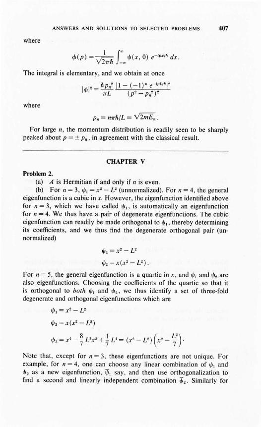
ANSWERS AND SOLUTIONS TO SELECTED PROBLEMS 407
where
I JOO .1>(p) =-- lfi(x, 0) e-1Pxtfl dx.Y2TTh -00
The integral is elementary, and we obtain at once
2_ hPn2 11- (_I)" e-iPLtfl!211>1 - TTL (p2 - p,,2)2
where
p" = nTTh/L = Y2mEn .
For large n, the momentum distribution is readily seen to be sharplypeaked about p = ± Pn' in agreement with the classical result.
CHAPTER V
Problem 2.(a) A is Hermitian if and only if n is even.(b) For n = 3, lfil = x 2 - U (unnormalized). For n = 4, the general
eigenfunction is a cubic in x. However, the eigenfunction identified abovefor n = 3, which we have called lfil' is automatically an eigenfunctionfor n = 4. We thus have a pair of degenerate eigenfunctions. The cubiceigenfunction can readily be made orthogonal to lfil , thereby determiningits coefficients, and we thus find the degenerate orthogonal pair (unnormalized)
lfil =x2-U
lfi2=X(X2-U).
For n = 5, the general eigenfunction is a quartic in x, and t/JI and lfi2 arealso eigenfunctions. Choosing the coefficients of the quartic so that itis orthogonal to both lfil and lfi2' we thus identify a set of three-folddegenerate and orthogonal eigenfunctions which are
lfi. =x2-U
lfi2 = x(x2 - U)
lfi:l = x 4 - ~ Ux2+ ~ V = (x 2_ U) (x2 _ ~2).
Note that, except for n = 3, these eigenfunctions are not unique. Forexample, for n = 4, one can choose any linear combination of lfil andlfi2 as a new eigenfunction, lfil say, and then use orthogonalization tofind a second and linearly independent combination lfi2' Similarly for

408 APPENDICES
(d) none(c) iii;(b) 11;
n = 5. The particular orthogonal eigenfunctions given above are merelythe easiest to construct.
Problem 6.(a) ii, iv, v;
Problem 10.(a) The new momentum eigenfunctions are defined by
and hence are given by
,t, = _1_ eilpx-y(x)J/fl'f'p Y27Th '
where
g(x)=rf(x) dx.
These states thus differ by a phase factor from the conventional momentum states; which we denote by ijjp to make the distinction clear, andwhich are given by
- I . ~t/Jp = Y27Th e'px/".
(b) t/J(x) = I cf>(p)t/Jp(x) dp
= e-iY(Xl/fl I cf> (p ) ijjp dp
= e-iY(Xl{fl iJi(x) ,
where ijj(x) is the state function in the conventional representation.We emphasize that t/J and lfj represent the same physical state, namelythat corresponding to the particular momentum state function cf> (p).
(c) Observe first that
(t/Jlxlt/J) = (lfj Ix Ilfj ) ,
because the phase factor e-iy(x){fl plays no role in the evaluation of theleft side. Next, observe that
Iha I -Ihal-)(t/J i ax + f(x) t/J) = (t/J i ax t/J
because
[ ~ .i- + f(X)] t/J = e-iY(Xl/fl ~ alfjI ax I ax
and the phase factors on the left then cancel. Finally, taking into ac-

ANSWERS AND SOLUTIONS TO SELECTED PROBLEMS 409
count the fact that the commutation relation is unaltered, it follows that(f(x, p) yields the same result in either representation. Hence theexpectation values of any and all observables are independent of j, aswas to be proved.
Problem 12.
where the (j, are arbitrary constants.
eifh-iEltifl ei62-iE211fl ei63-iE311fl
(b) t/J(X,t)=t/JI v'2 +t/J2 2 +t/J3 2
(c) iv(d) all but v
(c) zero;
Problem 2.(a) (jos
CHAPTER VI
( I) (mwh)2.mwh 11 + 2"; 3 -2- (2n 2 + 2n + I)
~ n' (j(n - s)! lIl,n-s~(n+s)!
n! (jlll.n+s;(d)
Problem 3.
(a) t/J(x, 0) = (~:of4 e-lIlwox2/2"
(b) Taking w to be arbitrary, we treat both cases together. We thenhave
t/J(x, t) = I t/J(x', O)K(x', x; t) dx',
where the propagator K is given by equation (68). The integral is of standard Gaussian form and, after some algebra, yields
_ (mwo/h7T) 1/4
t/J(x, t) - [cos wt + (iwo/w) sin wtJ1/2
{mwx2 [wo cos wt + iw sin wt]}X exp ---
2h w cos wt + iwo sin wt '
which is seen to reduce to the correct result when w = Wo' It also yields,for 1t/J12, the expression to which equation (73) reduces for the particularGaussian initial packet of part (a).
(c) We have

410 APPENDICES
cf>(p, t) = '\~7Th Jl/J(X, t) e- iPX/ft dx,
which is seen to be of standard Gaussian form. After evaluation of theintegral one finds the momentum space probability density to be
(7Tmw h)-liZIcf>(p, t)IZ = [COSZ wt + (wz/WOZ) sinz W/]lIZ
[pZJmhwo ]x exp
cosz wI + (wz/WOZ) sinz wI
which yields, using the indicated representation for l/Jn'
p _ 2~ (25)! (wo - W)Z8Z8 - wo+w 228 (5!)Z wo+w
PZS+1 = O.
Although it is not a trivial exercise, it can be verified that, as it must,
Problem 4.(d) Schrodinger's equation is
hZ dZl/JE ' _- 2m dx2 - g 8(X)l/JE - El/JE'
Thinking of the 8-function as the limit of a sharply peaked function, itis not hard to see that l/JE is continuous but that dl/JEJdx changes dramatically over the width of the potential, by an amount proportional to thearea under the potential. In the limit, dl/JEJdx actually becomes discontinuous. To display this discontinuity quantitatively, first integrateSchrodinger's equation from a point just to the left of the origin (0_)to a point just to the right (0+), and then consider the limit as each ofthese points approaches the origin (and thus each approaches the otherfrom its respective domain). We find
- ~ {dl/JEI _ dl/JE I } - gl/JE(O) = 0,2m dx 0+ dx 0-
where the right side vanishes, as indicated, because l/JE is continuous.The discontinuity in dl/JEJdx is thus
dl/JE I - dl/JE I = - 2~g l/JE (0) .dx 0+ dx 0_ h

ANSWERS AND SOLUTIONS TO SELECTED PROBLEMS 411
The prescription for solving Schrodinger's equation is now the following:Call the region to the left of the origin, x < 0, region I, to the right,x > 0, region II. Noting that the origin is excluded from each region,we see that in both regions Schrodinger's equation becomes that for afree particle. Hence, writing a general solution which satisfies the correctboundary condition at infinity on the right, say, the solution on the leftis then fixed by requiring that !JJE be continuous and that d~JE/dx havethe correct discontinuity. We now construct solutions for bound and continuous states.
(i) Bound States, E < O. Writing E = - E, we have in region II,
!JJEiI = A exp (- V2mE/fi2x) ,
the posItive exponential being inadmissible, of course. Similarly, inregion I,
!JJE1 = B exp (V2mE/h2x)
the negative exponential now being inadmissible. The condition that!JJE be continuous at the origin then yields A = B. The discontinuitycondition on d!JJE/dx can now only be satisfied if E has the unique value,
E = mg 2/2fi2,
. which is the binding energy of the single bound state of a a-functionpotential, in agreement with the result quoted in part (a). The normalizedbound state function is readily seen to be that given in part (b).
(ii) Continuum States, E > O. To construct a solution corresponding to the conventional case of a wave incident only from the left withamplitude, say, A, we take the free particle solutions in each region to be
!JJE1 ~ A ei v'2mE xlft + B e-iV2mE xlft
!JJEII = C eiYrniF xlft •
Application of both boundary conditions at the origin then gives, almostat once,
C IA == r = -=-1-----:i-g-:-Y7=m=:/'="2E=fi:=::'2
B igYm/2Efi2-==p=- .A 1 - igYm/2Efi2
Note that Ipl2 + Irl2= 1, as demanded by probability conservation.
Problem 6.(a) Region I, x < O. Letting z = eXI2J, we obtain a form of Bessel's
equation, and the general solution, for energy E, can be expressed inthe form

412
where
APPENDICES
y = i'\/2mE (2L/h)
a = V2mVo (2L/h).
Region II, x > O. Letting z = e-x /n , in the same way we find thegeneral solution
l/JEIl = CJy(ae-x /n ) + DJ_y(ae- X /2L ).
Boundary Conditions at x = 0: Both l/Jt: and dl/Jeldx must be continuous.
(b) Bound States, E < O. Writing E = - E, we see that y is real,
y = V2mE (2L/h) ,
where we have arbitrarily chosen the sign of the square root to makey positive (why do we have the freedom to do this?). Observe now, looking at l/JE1, that for x ~ 00, the argument of the Bessel functions approacheszero. Because
J (z) = (z/2)" + ..." r(v+l)
for z~ 0 (see references [6] - [13]), we see that only the J y term isphysically admissible. Similarly, in region II we see that again only theJ y term is physically admissible. Hence, we have
l/JE1 = AJy (aeX/2L
)
l/JEIl = BJ y (ae- x /2L ).
Both l/JE and dl/Jt:/dx must be continuous at the origin and hence werequire
AJy(a) = BJy(a),
but also
A dJy(a) = _ B dJy(a).da da
The solutions are thus given by either A = B, dJy/da = 0 or by A = -B,J y(a) = O. The former are seen to be even, the latter odd.
Problem 8.
Problem 18.
(c) K(p', p; t) = ei(p'3-p3l/6fB"F o(p - p' - Ft)
(a) Writing a = b -~, at = bt - E2, we find H = E1btb - E//El;E1 EI

ANSWERS AND SOLUTIONS TO SELECTED PROBLEMS 413
(bt, b) = I. Comparison with the harmonic oscillator Hamiltonian thenshows Ell = nE j - E22/Ej , n = 0, 1,2, ....
CHAPTER VII
Problem 3.(a) £0 = fiwl2 (exact! why?)(b) £j = ~~ fiw = 1.6 fiw
Problem 4.
fi2 7T 2 fi2(a) £ = 5 -L?' about I% greater than the correct value -2 -LoJm - m -
Problem 7.
(c) A2 = (~ I~)
A+B=n ~) AB = ( ~ :) =BA
Problem 9.(a) b ~ 2mfi Vol [2m (£ - VoHlI2(b) T=e iB(/:;), 0(£) =-2VobmlfiY2m£
Problem 15.
=0, n7"o1
Problem 16.·
(a) ljJ(t) = [ cos (~) ljJj - i sin (~) ljJ2] e- iEr",
CHAPTER VIIl
Problem 5.
I e28>2(a) -2 fiw - 2 oJ ~, where m is the mass of the charged constituent.
m-w-(b) 0' = J.le21m 2w 2
(c) uniform acceleration under the force e 8>
Problem 6.(a) 11£= <<PIO(X j )<P20(x2)1H'1<pIO(X j )<P20(X2», where <PIO and <P20

414 APPENDICES
are the harmonic oscillator ground state eigenfunctions of particles Iand 2, respectively. Thus
boE = vim 1m2 ~~o JdX1 JdX2
exp (- K(m1xJ2 + m2x 22) - (XI - x 2)2/a2)
= Vo ( J-Lwa2
)1/2J-L(lJa2 + Ii '
where J-L is the reduced mass ml m2/ (m l + m2) .(b) The result is unchanged, but the analysis is much simpler. In
center of mass coordinates, the Hamiltonian becomes
2/ I 2 IH = L- +- Mw2X 2+ L + - J-Lw 2 x 2+ V e-x2
/a2
2M 2 2J-L 2 0,
and hence is separable. The problem thus reduces to an equivalent singleparticle problem which, in fact, is just one of the examples discussed indetail in Section 3 of Chapter VII.
Problem 12.(a) ljJpqrs = cPp(x1 )cPq(X2)cPr(x3 )cPs(X4 )
Epqrs = (2 + P + q + r + s) liw,
where p, q, r, s can take on all integral values starting with zero andwhere cPn (x) is the nth harmonic oscillator eigenfunction.
(b) Writing p + q + r + s = N, we see that
E pqrs = (N + 2)liw.
The degeneracy of the Nth state is thus the number of ways four nonnegative integers can be chosen so that their sum is N. It can be shownthat this number is (N + I) (N + 2) (N + 3) /6. The first four states thenhave degeneracies 1,4, 10,20, respectively. Table I gives the quantumnumbers of these degenerate states.
(c) For spinless particles, only those states totally symmetric underexchange are physically realizable. The ground state is automaticallysymmetrical. The four states for N = I are an exchange degenerate setand a symmetric combination of them is the only realizable state. ForN = 2, the states in the grout' (a) are an exchange degenerate set, as areseparately those in group (b). Because these two groups of states are independent, there are two physically realizable states of N = 2, the symmetric combination of the states of type (a) and of the states of type (b).For N = 3, by the same argument, there are three physically realizablestates, namely the symmetric combinations of the exchange degeneratestates of types (a), (b) and (c), respectively.

ANSWERS AND SOLUTIONS TO SELECTED PROBLEMS 415
N Degeneracy pqrs
0 0000
4 1000, 0100, 0010, 0001
(a) 2000, 0200, 0020, 00022 10
(b){l1oo, 1010, 1001, 0110
0101, 0011
(a) 3000, 0300, 0030, 0003(b) 1110, 1101, 1011,0111
3 20 rlOO, 2010, 2001, 1200,(c) 0210, 0201, 1020, 0120,
0021, 1002, 0102, 0012
TABLE I. Quantum numbers and degeneracies of lowest four states
(d) The ground state for spin 1/2 particles is easy to identify usingthe Pauli exclusion principle. It is the state N = 2 and is the totally antisymmetric combination of single-particle states in which two particleswith opposite spin are in the ground state and two with opposite spinare in the first excited state. It is not degenerate.
CHAPTER IX
Problem 3.(a) a = e2/mw2
(b) same as with zero field
Problem 4.
(a)Ze2
V(r) = - 2Ro
[3 - (r/R o)2],
Ze2
r(b) 6.£ = ~ Z4e2Ro2/ao3
= 7 x 10⁻⁹ ZI4/3 eV
Problem 6.
I . ~(a) tflm = yz; e,m~, m = O,±I,±2, ....

416 APPENDICES
(b) IJ.Em(I) = 0
IJ.Em(2) = g2M3R4/(4m2- l)h 2
(c) WKB: Eo = ~ Vi/ii - MgR
Problem 8.(a) tPlm=y1m(o,ep)
El = h2[(l + l)/2MR2
Problem 11. Probability for Is state = 0.70, for 2s state = 0.25, for anystate other than an s-state = O. (See Reference [29], pp. 250-2.)
Problem 17.
- 1 f e- r/ao
[. p . r . p2t 1 3
(a) ep(p, t) - (27Thp/2 (7Ta03) 1/2 exp - I -h--/ 2mh d r
=; C~or2
[I :-(i;~:';~)2F8a 3
p(p, t) = ep*ep = 7T2~3 [I + (pao/h)2]-4 = p(p)
(b) PE(E) = 27T(2mp/2 VE p(p = V2mE)
Problem 19.
(a) Yukawa:
Exponential: E = same (coincidence!)
( 5) h2
Square Well' E = 1 - - e- 1 V ---. 2 0 8p,R2
CHAPTER X
Problem 1.
(a) Eo (l = -}) = ~ Eo (l = I)
(b) ,I, I ~ +~ = Vr sinO e±i<l>/2 e-21'/3ao'I' '2'-2
Problem 3. Some typical commutators are the following:
(Lx,x)=O; (Lx, y) = ihz; (Lx, py) = ihpz
Problem 7. The pairs (i), (ii) and (v) commute; the other pairs do not.Ta and R" (f3) commute if and only if nand a are co-linear.

ANSWERS AND SOLUTIONS TO SELECTED PROBLEMS 417
Problem 11.
(a) Jz = (Lz + Sz)
Lzl/J= hR(r) v2i3 YII X-
Szl/J = I R (r) {v'ill Y lO X+ - v2i3 Y II X- }
and hence
(b) Probability density for spin-up:
P+ = llR (r) 12
1y l ol2.
Probability for spin down:
p_=j IR(r)12IY/12.
(c) p++p_=1IR(r)12 (IYIOI2+2IYllj2)
=.! IR (r)\2 (~COS2e+~ sin2 e)3 47T 47T
1=-IR(r)\2
47T
Problem 13.(a) All are constants of the motion.(b) All but the components of linear momentum are constants of
the motion.(c) the energy and the parity(d) same as (b)(e) E and Lz(f) only E(g) E,Lz,Px,PY(h) Lz,Px,PY.
Problem 22. The probability that the hydrogen atom will remain in itsground state is [I + (mvGo/2hF]-4. (See Reference [29], pp. 310-14.)
CHAPTER XI
Problem 3. According to the variational estimate of equation (10), thebinding energy of H- is
E __ ll! e2•
°- 256 Go

418 APPENDICES
This must be compared with the energy of the dissociated system, aneutral hydrogen atom plus a free electron at infinity. The ground stateenergy of the dissociated system is just the binding energy of the hydrogenatom, -e2j2ao. Accordingly, the H- system is unstable to dissociationin this approximation by ri-B- e2jao, or by about 0.7 eV. Of course, thefact that the H- system is actually stable does not violate the minimumprinciple for ground state energies (why?).
Problem 7. After a straightforward evaluation of the integral, the Bornapproximation scattering amplitude for a square well can be expressedin the form
2mVoR3 jl(2kR sin ~)f(O) = h 2 0'
2kR sin "2
where jl denotes the spherical Bessel function of order unity [see equation (lX-61)] and is thus given by
j (z) = sin z _ cos Z.1 Z2 Z
The differential cross section is then du-jdO = If(0) 12 and the total crosssection is
That the low and high energy behavior is in agreement with expectationscan now be shown with relative ease. (See Reference [23], pp. 168-9,for a detailed discussion.)
Problem 9.(a) u = 2 X 10-25 cm2
(b) Both u and dujdO are unaltered.(c) u is unchanged but dujdO is altered.(d) Total number scattered per second = 4 X 10⁶ ; the number
scattered into the counter at 90° is about six per second.
Problem 10. Taking the z-axis along the magnetic field direction, theenergy En1ml of a state of principal quantum number n, total angularmomentum I and z-componeni ml is
e2 eh9&E -------m
nlml- 2n2ao 2mc I

ANSWERS AND SOLUTIONS TO SELECTED PROBLEMS 419
Thus s-states are unaffected and states of / ~ 0 are split into 2/ + 1components of equal spacing, this spacing being about 5 x 10⁻⁵ eV inmagnitude.
We now consider the neglected (quadratic) term in %, which wedenote by A. According to equation (67),
Because r is of the order of n2ao, where n is the principal quantum number, we thus have
2 2Q/2( A) = e ao-:/U 4
8mc2 n.
Comparing this to the first-order splitting, we then have
(A) _ eao2% 4 _ 10-6 4
(eh%/2mc) - 4lic n - n ,
whence this term is seen to be negligible for almost all principal quantumnumbers of interest.
Problem 13.4
(a) (x) = (l/Jlxll/J) = L (l/J;lxll/J;) ,;=1
(b) d~~) =k(l/JIH,xll/J)
d~) = k(l/JIH, pll/J)
For a free particle, (H, p) = 0 and (H, x) = ~ ca x ' whence, as expected,I
d(p) = 0dt '
but, surprisingly,
d(x)--;jf=c (ax).
Noting that this last result also holds when the electron is not free butmoves in a static potential, we see that ca plays the role of a velocityoperator in Dirac theory. Because the eigenvalues of each component ofa are ± I, the eigenvalues of the velocity operator are ± c, which is tosay that a measurement of velocity can yield only the magnitude c. Thisseemingly paradoxical result can be understood intuitively in the following way. A measurement of instantaneous velocity implies an absolutely
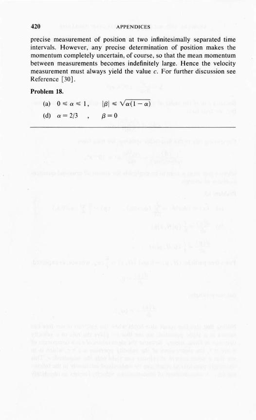
420 APPENDICES
precise measurement of position at two infinitesimally separated timeintervals. However, any precise determination of position makes themomentum completely uncertain, of course, so that the mean momentumbetween measurements becomes indefinitely large. Hence the velocitymeasurement must always yield the value c. For further discussion seeReference [30].
Problem 18.
(a) 0 ~ 0' ~ I,
(d) 0' = 2/3
I.BI ~ \/0'(1-0')
.B=O

Index
Absorption of light, 213-214Accidental degeneracy (see Degeneracy)Addition of angular momentum, 327-335Adiabatic perturbation, 224Adjoint of an operator, 88-90Adjoint of a matrix, 203-204Admissable state functions, 19Amplitude (see Probability amplitude,
Scattering amplitude)Angular momentum, 271-274, 298-333
addition of, 327-335commutation relations for, 298-300, 308conservation of, 315eigenvalues of, 271-274, 302, 309intrinsic or spin, 316-327operator, 271-272, 298-300orbital, 271-274, 298-302parity of eigenstates of, 276rotations and, 313, 315tot~,301, 309,327-335uncertainty relations for, 309-3 10
Anharmonic oscillator, 197-201Annihilation and production of pairs, 386Annihilation and creation operators,
131-133Anticommutation relations, 321, 325, 379Anticommutator, 321Antisymmetric states and exclusion
principle, 245-249Arfken, G., 400Associated Laguerre polynomials, 288-289Associated Legendre functions, 274-275Atoms, helium-like, 344-349
hydrogenic,286-292mu-mesonic, 293
Barrier penetration (see Tunnel effect)Basis, 202
Becker, R. A., 401Berg, P. W., 401Bessel functions, 283n
spherical, 282-284Bjorken, J. D., 402Black body radiation, 13-15Bloch, I., 238nBohr magneton, 376Bohr radius, 289-290Bohm, D., 401Born, M., 400Born approximation, 360-373
validity of, 371-373Bose-Einstein statistics, 247Bosons,247Bound states, 77, .118
numerical methods, 158, 163-167in Rayleigh- Ritz approximation,
184-189in WKB approximation, 182-184
Canonical transformation, 232Cantor, D., 163nCaswell, R. S., 163n, 167nCenter-of-mass coordinates, 229-233Central potentials, 268-279
scattering from, 355-358Centrifugal potential (see Effective radial
potential)Classical limit, 17, 174Classical turning point, 117-118Classical vs quantum theory, 1-4,8-13,
25-27,65-66,359-360(See also Correspondence principle,
WKB approximation)Clebsch-Gordon coefficients, 329Closure, 100-102

422 INDEX
Commutation relations, angularmomentum, 299-300, 308
linear momentum and coordinate, 45-47,228, 263
Commutator, 46Complementarity, 16Complete set of commuting operators,
104-i05,111Complete set of eigenfunctions, 98,
100-102,111Complex conjugation, operation of,
114-115Compton effect, 15Compton wavelength, 15Configuration space, 38,228-229Conservation, of angular momentum, 315
of energy, 96of linear momentum, 63, 232, 316of probability, 68-70, 153-154
restriction imposed by, 84-85Constants of motion, 63, 96, 232, 3 15-3 16Continuous spectrum, 117Continuum states, free particle, 29, 60-64,
264, 282-284one-dimensional, 117-118, 147-155and scattering, 351
Coordinate systems, center of mass,229-233
spherical, 268-270Correlations in quantum mechanics,
239-240, 248Correspondence principle, 16-17
restriction imposed by, 59-60, 91-94Coulomb scattering, 358-360Coupled harmonic oscillators, 236-238,
244-245, 253-255, 259-260Creation and annihilation operators,
131-133Creation operator representation, 138-143Cross section, differential, 354
Rutherford, 359theorem, 357total, 356
Crossing of energy levels, 206-207
Davisson and Germer experiment, 5-7Davydov, A. S., 401de Broglie wave, 11, 264de Broglie wavelength, 5Degeneracy, 99-100, 117-118
accidental, 277, 279,281,291exchange, 242for hydrogenic atom, 291for isotropic harmonic oscillator, 268,
280-281for particle in a box, 266-267
Degeneracy (continued)for central potential, 275-276
Degenerate perturbation theory (seeStationary state perturbation theory,Time dependent perturbation theory)
Delta function potential, 169, 410-411Dennary, P., 400Density matrix, 387-391
equation of motion for, 389for pure states, 390
Density of states, 211, 215-216, 267Deuteron, 280, 297Diatomic molecule, 235, 238, 391Dicke, R. H., 401Differential cross section, 354Dipole moment, electric, 194n, 226, 235
magnetic, 376--377Dirac, P. A. M., 401Dirac bracket notation, 72, 86-87, 91Dirac delta function, 36-37, 54
in three dimensions, 362Dirac equation, 377-386Discrete spectrum, 76, 118Double slit interference, 22-23Drell, S. D., 402Dynamical variables as operators, 3,
41-42, 63, 85-86, III
Effective radial potential, 276-279Ehrenfest's theorem, 97Eigenfunctions and eigenvalues, 10 I-I 04Eisberg, R. M., 400Electric dipole moment, 194n, 226, 235Electromagnetic field, gauge transforma-
tion of, 374motion of particle in, 373-377
Emission of light, induced, 213-214spontaneous, 214
Energy eigenvalues, for coupled oscillators,237,254
for delta function potential, 169,411for exponential well, 169-170,412for free particle, 73-75for harmonic oscillator, 129,268for helium atom, 345-349for hydrogenic atom, 290-291for particle in a box, 75-78, 266-267in Rayleigh-Ritz approximation,
184-189for square well, 121-126in WKB approximation, 183
Energy operator, 63, 96Equation of motion, for density matrix, 389
for expectation values, 92, 113for state functions (see Schrodinger's
equation)

INDEX 423
Exchange of identical particles, 241-243degeneracy under, 242operators for, 242, 258symmetry under, 243-249
Exchange integral, 257, 348Exclusion principle, 247-248Expectation values, 23-25, 112,264
equation of motion for, 92, 113of position and momentum, 40, 42in spin space, 322-323of spinors, 383
Factorization, method of, for angularmomentum, 302-309
for harmonic oscillator, 131-138Fermi-Dirac statistics, 247Fermion, 247Fine structure constant, 359Fourier integrals, 34-38Fourier series, 34-35Frank, N. H., 401Free particle states, in one dimension,
56-75for definite angular momentum, 282-284for definite linear momentum, 264relation between, for definite angular and
linear momentum, 285
g-value, 376-377, 377nGalilean transformation, 341-343Gauge transformations, and the electro-
magnetic field, 374and Schrodinger's equation, 375
Gaussian function, integrals of, 397-399Gaussian potential, 369Gaussian wave packet, 49
motion of, for free particle, 64-65for harmonic oscillator, 146-147for square well, 158-166
Goldberg, A., 158n, 168£1Golden rule, 212, 214Goldstein, H., 401Green's function, 362-363Ground state, 53Group velocity, 58Gyromagnetic ratio (see g-value)
Hamiltonian operator, 94, 229, 262-263in center-of-mass coordinates, 231-232in external electromagnetic field,
373-374,386for identical particle systems, 241, 245relativistic, 377, 386
Harmonic oscillator, 127-147eigenfunctions for, in configuration
space, 130
Harmonic oscillator (continued)in creation operator space, 141in momentum space, 131
propagator, 145three-dimensional isotropic, 268,
280-281wave packet motion in, 144-147(See also Anharmonic oscillator,
Coupled oscillators)Hamwell, G. P., 349£1Heisenberg representation, 93nHeisenberg uncertainty principle (see
Uncertainty principle)Helium-like atom, 344-349Hermite polynomials, 130, 134
generating function, 143integral representation for, 143
Hermitian matrix, 204Hermitian operators, 85-86
as observables, 85-86orthogonal eigenfunctions of, 101-103
Holton, G., 400Hsieh, Y., 238nHydrogen molecule, 391Hydrogenic atom, 286-292
degeneracy, 291eigenfunctions, 290energy levels, 290-291
Identical particles, 241-258and exchange degeneracy, 241-243scattering of, 359-360spin and statistics of, 247and symmetry of state function, 243-249
Indistinguishability of identical particles,241
Induced electric dipole moment, 235Infinitesimal rotations, 313-314Infinitesimal translations, 316Integral equation for scattering states, 363Interference and the superposition prin-
ciple,21Intrinsic angular momentum (see Spin)Invariance, under rotations, 315
under translations, 316(See also Galilean invariance, Gauge
invariance)Inverse of operator, 225£1, 339
Jackson, J. D., 400
Kennard, E. H., 400Klein-Gordon equation, 377-378Kraut, E. A., 400Kronecker delta symbol, 78, 99Krzywicki, A., 400

424 INDEX
Ladder method (see Factorization)Laguerre polynomials, 289Lamb shift, 386nLandau, L. D., 401Lauritsen, T., 400Legendre polynomial expansion, of plane
wave, 285for scattering, 355-356
Legendre polynomials, 274-275Leighton, R. B., 400Lifetime of metastable state, 20 ILifshitz, E. M., 401Linear operators, 43Lowering and raising operators, for
angular momentum, 302, 311-312for harmonic oscillator, 131-133
McGregor, J. L., 401Magnetic moment, 376-377, 377nMagnetic quantum number, 376Margenau, H., 400Marion, J. B., 40 IMass, reduced, 230Matrix algebra, 202-204Matrix elements, 191, 202
of spin operators, 322-323of spinor operators, 383
Matrix representation, of operators,201-202
of spin, 324Measurement of observables, 104Melkanoff, M. A., 163n, 167nMessiah, A., 40 IMetastable states, 199-201Minimum uncertainty wave packet,
109-110Momentum states, 29, 264
as superposition of angular momentumstates, 285
and wave packets, 31-33Momentum operator, 39-42, 228,262-263Momentum space, 33, 38, 228-229, 265
harmonic oscillator in, 13 Ipropagator for uniform acceleration,
170,412representation, 38, 229Schrodinger's equation in, 67,95, 170
Murphy, G. M., 400
Negative energy Dirac states, 381,384-386
Nodvik, J. S., 163nNormalization condition, 20
and physical admissability, 20
Observables, 3complete set of, 104-105, IIIas Hermitian operators, 85-87
Observations, 3as Hermitian operators, 47, 104mutual interference of, 4(See also Uncertainty principle)
Operators, algebra of, 43-45as dynamical variables, 39-42, 85-87,
III(See also Matrix representation of
operators)Optical theorem, 357Orbital angular momentum (see Angular
momentum)Orthogonality of eigenfunctions, 10 I-I 02Orthonormal set, 78, 99Oscillator (see Anharmonic oscillator,
Harmonic oscillator, Coupledoscillators)
Pair production and annihilation, 386Parity, 119-121
of angular momentum states, 276and selection rules, 194
Park, D., 40 IPartial waves, 285, 355-356Particle in a box, 75-81, 266-267, 284Pauli exclusion principle, 247-248Pauli operators, 324-325Pauli two component theory, 325-326Pauling, L., 40 IPeriodic boundary conditions, 112,
215-216,267Periodic table, 349-351Perturbation theory (see Stationary state
perturbation theory, Time dependentperturbation theory)
Phase shift, scattering, 355in transmission through a barrier, time
increment associated with, 157WKB approximation to, 181
Planck's constant, 4, 5Polarizability, 235
of hydrogen atom, 295of isotropic oscillator, 292, 415
Polarization vector, and density matrix, 394equation of motion for, 395
Position operator, 39-42, 228Potential barrier (see Square well potential,
Tunneling effect)Power series, method of, for hydrogenic
atom, 286-288for harmonic oscillator, 126-130

INDEX 425
Principal quantum number, 290Probability amplitude, 20, 103,228, 264
in momentum space, 33, 229, 265for stationary states, 79-80, 98
Probability conservation, 68-70,153-154restriction imposed by, 84-85
Probability density, 20, 228, 264in momentum space, 33, 229
Probability flux, 154, 264Probability interpretation, 19,21, 78-80,
112,228-229·Projection operator, for parity, 120
for exchange, 258Propagator, 60-62, 110-111, 114
free particle, 6\, 292harmonic oscillator, 144- 145,292particle in a box, 80for uniform acceleration, 170, 412
Quantum of action, 5Quasi-bound or quasi-stationary states,
199-201
Radial eigenfunction, 275-279Radial Schrodinger's equation, 275-279Radiation, absorption and emission of,
213-214black body, 13-15
Raising and lowering operators, for angularmomentum, 302, 311-312
for harmonic oscillator, 131-133Ramsauer effect, 12Rayleigh- Ritz approximation, 184-189
and harmonic oscillator, 188-189and helium-like atom, 346-347and perturbation theory, 192upper bounds in, 186-187trial functions for, 187-188
Raynal, J., 163nRedheffer, R. M., 400Reflection coefficient, 8-9, 149, 153Relative motion, 233Richtmyer, F. K., 400Roller, D. H. D., 400Rotation operator, 3 I 3-315Rutherford cross section, 359
Saxon, D. S., 163nSawada, T., 163nScattering, 351-373
in Born approximation, 360-373of identical particles, 359-360phase shift analysis of, 355-358of wave packets, 152-158, 352
numerical solution, 158-166
Scattering amplitude, 353, 364in Born approximation, 364Coulomb, 358partial wave expansion of, 356
Scattering cross section (see Cross section)Scattering phase shift (see Phase shift)Schey, H. M., 158n, 168nSchiff, L. I., 401Schmidt orthogonalizaiion method, 100,
112Schrodinger's equation, for free particle,
66-67in momentum space, 67, 95for motion in electromagnetic field, 374for a system of particles, 229in three dimensions, 263
Schwartz, J. L., 158n, 168nSchwartz inequality, 107Screened Coulomb potential, 392Selection rules, 194Self-adjoint operator (see Hermitian
operator)Separation of variables, 73, 232Simultaneous observables, 104-106Single valuedness of state functions, 275,
307Singlet state, 333, 348-349Slater, J. c., 349n, 401Slater determinant, 247-248Sokolnikoff, J. S., 400Sommerfeld, A., 400Spectrum, energy, 77, 98, 116-118
for free Dirac particle, 384Spherical Bessel fu'nctions, 282-284Spherical coordinates, 268-270Spherical harmonics, 274-275Spin, 316-327
and Dirac theory, 382-383and statistics, 247
Spin-orbit interaction, 334-335, 349Spinors, 379-380
expectation values for, 383Spins, addition of, 330-333Spontaneous emission, 214Square well, bound states of, 121-126
continuum states of, 147-152in three dimensions, 280
State functions, 3, 18-19, 111complex nature of, 30, 70-72for definite energy, 74, 76-77for definite momentum, 29-30as eigenfunctions, \0 1-1 02as superposition of stationary states, 78,
98

426 INDEX
Stationary state perturbation theory,189-201,204-208
for degenerate or close lying states,204-208
for non-degenerate states, to first order,192
to second order, 192-193physical interpretation of, 193-194and selection rules, 194for system of particles, 240-241,
255-258upper bound to second order correction
in, 195Stationary states, 73-75, 97-98
as complete orthonormal set, 98-101Statistical ensemble, density matrix for,
387-391Stehle, P., 401Stephens, W. E., 349nStimulated emission, 213-214Sum rule, 225-226Superposition principle, 21Superposition of states, and interference,
7,21to form wave packets, 31-33, II 0-111
Symmetrization of identical particle states,249-255, 261
Symmetry, classification of states by,119-121,243,247
Symmetry properties of identical particlestates, 243-258
ter Haar, D., 402Time dependent perturbation theory,
208-219for degenerate or close lying states,
210-214golden rule for, 212, 214for impulsive perturbation, 224, 225for non-degenerate states, 210for scattering, 365-367validity of, 210, 212-213
Time dependent Schrodinger's equation(see Schrodinger's equation)
Time development, of density matrix, 389of expectation values, 92, 112of state functions (see Schrodinger's
equation)Time independent Schrodinger's equation,
74,98
Total angular momentum (see Angularmomentum)
Trace of a matrix, 388Transformations, Galilean, 341-343
of gauge, 374-375as operators, 313-316, 339-341
Transition rate, 212Translation operator, 315-316Transmission coefficient, 8-9, 149, 153Transposed matrix, 204Trial wave function, 187-188Triangle rule, 328nTrigg, G. L., 401Triplet states, 333, 348-349Tunnel effect, 10, 151-152Turning points, 117-118
Uncertainties, 4, 106Uncertainty principle, 47-53, 106-110
for angular momentum, 309-310for coordinates and momenta, 51, 108for energy and time, 5 I, 20 I, 213
Variational method (see Rayleigh-Ritzapproximation)
Virial theorem, 115,297
Wave functions (see State functions)Wave packets, 32, 48-50
and classical limit, 25-27, 65-66and group velocity, 56-59minimum uncertainty, 109-1 10motion of, I 10-111
for free particle 60-65for harmonic oscillator, 144-147
scattering of, 152-166, 352spreading of, 27,59-60,64-65,
157-158,162as superposition, 31-33
Wilson, E. B., 401Witke, J. P" 401WKB approximation, 174-184
for bound states, 182-184for continuum states, 180-181validity of, 177-180
¥ukawa potential, 367
Zeeman effect, 317, 376-377Zero point energy, DO, 183

ELEMENTARY QUANTUM MECHANICS

Holden-Day Series in Physics

Topics in Several Particle Dynamics
By K. M. Watson, University of California atBerkeley and J. Nuttall, Texas A and M University. With a chapter by J. S. R. Chisholm,Texas A and M University and University ofKent, Canterbury.
This monograph provides an introduction tocurrent research ,in several particle dynamics.Based on non-relativistic quantum mechanics.some of the techniques covered are also usefuiwhen considering the relativistic problem. Itbegins with a survey of relative topics from thetheory of integral equations. These are appliedfirst to the two-body problem. Next the three·body problem is discussed, with some com·ments on the many-body problem. A review ofthe use of variational methods in several bodyinteraction is also included. The description ofintegral equations, as used in scattering theory,can provide an easily read introduction to moreadvanced treatises on this subject. Intended forresearch seminars for professionals and forstudents who have had a course in quantummechanics, it is also well suited for self·study,
Vector Analysisand Cartesian Tensorswith Selected Applications
By Krishnamurty Karamcheti, Stanford University.
This text clearly and systematically explainsall the important elements of vector analysisand cartesian tensors, together with their physical applications, for students of engineeringand the physical sciences who have only aknowledge of elementary calculus, The authorfirst gives a thorough explanation of vector algebra and calculus. Cartesian tensors andtensor notation are then explained so as to introduce the reader to a convenient way ofmathematically handling physical problemsthat involve scalars, vectors, and quantities ofa more general character. The application ofthe various concepts to the mathematical formulation of physical problems and to the derivation of some general results relating to suchproblems are amply illustrated.
Problems and Solutions inMathematical Physics
By Y. Choquet.Bruhat, Faculte des Sciences deParis. TraliJ. i'y C. Peltzer. Ed. by J. J. Brandstatter.
Divided into two parts, this text containsproblems and worked out solutions for linearalgebra and analysis in the first; for functionspaces and differential and integral operatorsin the second. The problems in both parts aredrawn from classical and modern physics, andeach is introduced in a manner which orientsthe reader to a rapid understanding of it. Themethod of solution immediately follows theproblem and utilizes the modern methods oflinear space theory. Linear algebra, matrices,tensors, exterior differential forms, differentialgeometry, Hilbert space, integral equations,and ordinary and partial differential equationsare all covered in a novel. pedagogical methodwhich reflects Professor Choquet-Bruhat'sunique teaching approach. The book will beespecially valuable to physicists, engineers,and mathematicians who are seeking modernmethods of approach to the solutions of non·trivial problems of physics. It is an ideal textfor teachers in need of examples to supplementtheir courses and especially well suited forself study as well.
The translation of Linear Algebra and Analy.sis by A. Lichnerowicz (Holden-Day) is recom'mended for simultaneous reading,
Classical and Quantum Theories ofSpinning Particles
By H. C. Corben, TRW Systems.
This monograph provides an integrated dis·cussion of the basic equations of motion of aspinning particle according to non·relativisticand relativistic classical and quantum mechanics, emphasizing the correspondence be'.tween these various levels of approximation.This approach is intended to convey a deeperconcept of the unity of all physics and tostimulate teacher and student with unusualapproaches and methods which shed new lighton traditional thinking. Presupposing only themathematical tools of algebra and vector andtensor analysis, the book is well suited for selfstudy as well as supplementary use in senior·graduate courses in physics, engineering, andchemistry.
HOLDEN-DAY.500 Sansome Stre~t San Francisco, Calif. 94111
7582