Classical Mechanics
665
-
Upload
khangminh22 -
Category
Documents
-
view
1 -
download
0
Transcript of Classical Mechanics

“M00 Goldstein 9788131758915 FM” — 2011/2/15 — page i — #1
CLASSICAL MECHANICSTHIRD EDITION
Herbert GoldsteinColumbia University
Charles P. PooleUniversity of South Carolina
John L. SafkoUniversity of South Carolina
“M00 Goldstein 9788131758915 FM” — 2011/2/15 — page ii — #2
Many of the designations used by manufacturers and sellers to distinguish their products are claimed astrademarks. Where those designations appear in this book, and the publisher was aware of a trademark claim, thedesignations have been printed in initial caps or all caps.
Authorized adaptation from the United States edition, entitled Classical Mechanics, 3rd Edition, ISBN:9788131758915 by Goldstein, Herbert; Poole, Charles; Safko, John; published by Pearson Education, Inc.,publishing as Addison-Wesley, Copyright c© 2002
Indian Subcontinent AdaptationCopyright c© 2011 Dorling Kindersley (India) Pvt. Ltd
This book is sold subject to the condition that it shall not, by way of trade or otherwise, be lent, resold, hired outor otherwise circulated without the publisher’s prior written consent in any form of binding or cover other thanthat in which it is published without a similar condition including this condition being imposed on subsequentpurchaser and without limiting the rights under copyright reserved above, no part of this publication may bereproduced, stored in or introduced into a retrieval system, or transmitted in any form or by any means(electronic, mechanical, photocopying, recording or otherwise), without the prior written permission of both thecopyright owner and above-mentioned publisher of this book.
First Impression
This edition is manufactured in India and is authorized for sale only in India, Bangladesh, Bhutan, Pakistan,Nepal, Sri Lanka and the Maldives.
Published by Dorling Kindersley (India) Pvt. Ltd, licensees of Pearson Education in South Asia.
No part of this eBook may be used or reproduced in any manner whatsoever without the publisher’s prior written consent.
This eBook may or may not include all assets that were part of the print version. The publisher reserves the right to remove any material in this eBook at any time.
ISBN 978-81-317-5891-5
eISBN 978-93-325-7618-6
Head Office: 15th Floor, Tower-B, World Trade Tower, Plot No. 1, Block-C, Sector-16, Noida 201 301, Uttar Pradesh, India.Registered Office: 4th Floor, Software Block, Elnet Software City, TS-140, Block 2 & 9,Rajiv Gandhi Salai, Taramani, Chennai 600 113, Tamil Nadu, India.Fax: 080-30461003, Phone: 080-30461060www.pearson.co.in, Email: [email protected]
“M00 Goldstein 9788131758915 FM” — 2011/2/15 — page iii — #3
Contents
Preface to the Third Edition ix
Preface to the Second Edition xii
Preface to the First Edition xvi
1 Survey of the Elementary Principles 11.1 Mechanics of a Particle 11.2 Mechanics of a System of Particles 51.3 Constraints 121.4 D’Alembert’s Principle and Lagrange’s Equations 161.5 Velocity-Dependent Potentials and the Dissipation Function 211.6 Simple Applications of the Lagrangian Formulation 24
Derivations 29Exercises 31
2 Variational Principles and Lagrange’s Equations 342.1 Hamilton’s Principle 342.2 Some Techniques of the Calculus of Variations 362.3 Derivation of Lagrange’s Equations from Hamilton’s Principle 442.4 Extending Hamilton’s Principle to Systems with Constraints 452.5 Advantages of a Variational Principle Formulation 512.6 Conservation Theorems and Symmetry Properties 552.7 Energy Function and the Conservation of Energy 61
Derivations 64Exercises 64
3 The Central Force Problem 703.1 Reduction to the Equivalent One-Body Problem 703.2 The Equations of Motion and First Integrals 723.3 The Equivalent One-Dimensional Problem, and
Classification of Orbits 763.4 The Virial Theorem 833.5 The Differential Equation for the Orbit, and Integrable
Power-Law Potentials 863.6 Conditions for Closed Orbits (Bertrand’s Theorem) 893.7 The Kepler Problem: Inverse-Square Law of Force 92
iii
“M00 Goldstein 9788131758915 FM” — 2011/2/15 — page iv — #4
iv Contents
3.8 The Motion in Time in the Kepler Problem 983.9 The Laplace–Runge–Lenz Vector 1023.10 Scattering in a Central Force Field 1063.11 Transformation of the Scattering Problem to Laboratory
Coordinates 1143.12 The Three-Body Problem 121
Derivations 126Exercises 128
4 The Kinematics of Rigid Body Motion 1344.1 The Independent Coordinates of a Rigid Body 1344.2 Orthogonal Transformations 1394.3 Formal Properties of the Transformation Matrix 1444.4 The Euler Angles 1504.5 The Cayley–Klein Parameters and Related Quantities 1544.6 Euler’s Theorem on the Motion of a Rigid Body 1554.7 Finite Rotations 1614.8 Infinitesimal Rotations 1634.9 Rate of Change of a Vector 1714.10 The Coriolis Effect 174
Derivations 180Exercises 182
5 The Rigid Body Equations of Motion 1845.1 Angular Momentum and Kinetic Energy of Motion
about a Point 1845.2 Tensors 1885.3 The Inertia Tensor and the Moment of Inertia 1915.4 The Eigenvalues of the Inertia Tensor and the Principal
Axis Transformation 1945.5 Solving Rigid Body Problems and the Euler Equations of
Motion 1985.6 Torque-Free Motion of a Rigid Body 2005.7 The Heavy Symmetrical Top with One Point Fixed 2085.8 Precession of the Equinoxes and of Satellite Orbits 2235.9 Precession of Systems of Charges in a Magnetic Field 230
Derivations 232Exercises 234
6 Oscillations 2386.1 Formulation of the Problem 2386.2 The Eigenvalue Equation and the Principal Axis Transformation 241
“M00 Goldstein 9788131758915 FM” — 2011/2/15 — page v — #5
Contents v
6.3 Frequencies of Free Vibration, and Normal Coordinates 2506.4 Free Vibrations of a Linear Triatomic Molecule 2536.5 Forced Vibrations and the Effect of Dissipative Forces 2586.6 Beyond Small Oscillations: The Damped Driven Pendulum and the
Josephson Junction 265Derivations 272Exercises 272
7 The Classical Mechanics of theSpecial Theory of Relativity 2767.1 Basic Postulates of the Special Theory 2777.2 Lorentz Transformations 2807.3 Velocity Addition and Thomas Precession 2827.4 Vectors and the Metric Tensor 2867.5 1-Forms and Tensors 2897.6 Forces in the Special Theory; Electromagnetism 2977.7 Relativistic Kinematics of Collisions and Many-Particle
Systems 3007.8 Relativistic Angular Momentum 3097.9 The Lagrangian Formulation of Relativistic Mechanics 3127.10 Covariant Lagrangian Formulations 3187.11 Introduction to the General Theory of Relativity 324
Derivations 328Exercises 330
8 The Hamilton Equations of Motion 3348.1 Legendre Transformations and the Hamilton Equations
of Motion 3348.2 Cyclic Coordinates and Conservation Theorems 3438.3 Routh’s Procedure 3478.4 The Hamiltonian Formulation of Relativistic Mechanics 3498.5 Derivation of Hamilton’s Equations from a
Variational Principle 3538.6 The Principle of Least Action 356
Derivations 361Exercises 363
9 Canonical Transformations 3689.1 The Equations of Canonical Transformation 3689.2 Examples of Canonical Transformations 3759.3 The Harmonic Oscillator 377
“M00 Goldstein 9788131758915 FM” — 2011/2/15 — page vi — #6
vi Contents
9.4 The Symplectic Approach to Canonical Transformations 3819.5 Poisson Brackets and Other Canonical Invariants 3889.6 Equations of Motion, Infinitesimal Canonical Transformations, and
Conservation Theorems in the Poisson Bracket Formulation 3969.7 The Angular Momentum Poisson Bracket Relations 4089.8 Symmetry Groups of Mechanical Systems 4129.9 Liouville’s Theorem 419
Derivations 421Exercises 424
10 Hamilton–Jacobi Theory and Action-Angle Variables 43010.1 The Hamilton–Jacobi Equation for Hamilton’s Principal
Function 43010.2 The Harmonic Oscillator Problem as an Example of the
Hamilton–Jacobi Method 43410.3 The Hamilton–Jacobi Equation for Hamilton’s Characteristic
Function 44010.4 Separation of Variables in the Hamilton–Jacobi Equation 44410.5 Ignorable Coordinates and the Kepler Problem 44510.6 Action-Angle Variables in Systems of One Degree of Freedom 45210.7 Action-Angle Variables for Completely Separable Systems 45710.8 The Kepler Problem in Action-Angle Variables 466
Derivations 478Exercises 478
11 Classical Chaos 48311.1 Periodic Motion 48411.2 Perturbations and the Kolmogorov–Arnold–Moser Theorem 48711.3 Attractors 48911.4 Chaotic Trajectories and Liapunov Exponents 49111.5 Poincare Maps 49411.6 Henon–Heiles Hamiltonian 49611.7 Bifurcations, Driven-Damped Harmonic Oscillator, and Parametric
Resonance 50511.8 The Logistic Equation 50911.9 Fractals and Dimensionality 516
Derivations 522Exercises 523
12 Canonical Perturbation Theory 52612.1 Introduction 52612.2 Time-Dependent Perturbation Theory 527
“M00 Goldstein 9788131758915 FM” — 2011/2/15 — page vii — #7
Contents vii
12.3 Illustrations of Time-Dependent Perturbation Theory 53312.4 Time-Independent Perturbation Theory 54112.5 Adiabatic Invariants 549
Exercises 555
13 Introduction to the Lagrangian and HamiltonianFormulations for Continuous Systems and Fields 55813.1 The Transition from a Discrete to a Continuous System 55813.2 The Lagrangian Formulation for Continuous Systems 56113.3 The Stress-Energy Tensor and Conservation Theorems 56613.4 Hamiltonian Formulation 57213.5 Relativistic Field Theory 57713.6 Examples of Relativistic Field Theories 58313.7 Noether’s Theorem 589
Exercises 598
Appendix A Euler Angles in Alternate Conventionsand Cayley–Klein Parameters 601
Appendix B Groups and Algebras 605
Appendix C Solutions to Select Exercises 617
Selected Bibliography 626
Author Index 631
Subject Index 633

“M00 Goldstein 9788131758915 FM” — 2011/2/15 — page viii — #8
This page is intentionally left blank.
“M00 Goldstein 9788131758915 FM” — 2011/2/15 — page ix — #9
Preface to the Third Edition
The first edition of this text appeared in 1950, and it was so well received thatit went through a second printing the very next year. Throughout the next threedecades it maintained its position as the acknowledged standard text for theintroductory Classical Mechanics course in graduate level physics curriculathroughout the United States, and in many other countries around the world.Some major institutions also used it for senior level undergraduate Mechanics.Thirty years later, in 1980, a second edition appeared which was “a through-goingrevision of the first edition.” The preface to the second edition contains the fol-lowing statement: “I have tried to retain, as much as possible, the advantages ofthe first edition while taking into account the developments of the subject itself,its position in the curriculum, and its applications to other fields.” This is thephilosophy which has guided the preparation of this third edition twenty moreyears later.
The second edition introduced one additional chapter on Perturbation The-ory, and changed the ordering of the chapter on Small Oscillations. In addition itadded a significant amount of new material which increased the number of pagesby about 68%. This third edition adds still one more new chapter on NonlinearDynamics or Chaos, but counterbalances this by reducing the amount of materialin several of the other chapters, by shortening the space allocated to appendices,by considerably reducing the bibliography, and by omitting the long lists of sym-bols. Thus the third edition is comparable in size to the second.
In the chapter on relativity we have abandoned the complex Minkowski spacein favor of the now standard real metric. Two of the authors prefer the complexmetric because of its pedagogical advantages (HG) and because it fits in well withClifford Algebra formulations of Physics (CPP), but the desire to prepare studentswho can easily move forward into other areas of theory such as field theory andgeneral relativity dominated over personal preferences. Some modern notationsuch as 1-forms, mapping and the wedge product is introduced in this chapter.
The chapter on Chaos is a necessary addition because of the current interestin nonlinear dynamics which has begun to play a significant role in applicationsof classical dynamics. The majority of classical mechanics problems and appli-cations in the real world include nonlinearities, and it is important for the studentto have a grasp of the complexities involved, and of the new properties that canemerge. It is also important to realize the role of fractal dimensionality in chaos.
New sections have been added and others combined or eliminated here andthere throughout the book, with the omissions to a great extent motivated by thedesire not to extend the overall length beyond that of the second edition. A section
ix
“M00 Goldstein 9788131758915 FM” — 2011/2/15 — page x — #10
x Preface to the Third Edition
was added on the Euler and Lagrange exact solutions to the three body problem.In several places phase space plots and Lissajous figures were appended to illus-trate solutions. The damped-driven pendulum was discussed as an example thatexplains the workings of Josephson junctions. The symplectic approach was clar-ified by writing out some of the matrices. The harmonic oscillator was treatedwith anisotropy, and also in polar coordinates. The last chapter on continua andfields was formulated in the modern notation introduced in the relativity chap-ter. The significances of the special unitary group in two dimensions SU(2) andthe special orthogonal group in three dimensions SO(3) were presented in moreup-to-date notation, and an appendix was added on groups and algebras. Specialtables were introduced to clarify properties of ellipses, vectors, vector fields and1-forms, canonical transformations, and the relationships between the spacetimeand symplectic approaches.
Several of the new features and approaches in this third edition had been men-tioned as possibilities in the preface to the second edition, such as properties ofgroup theory, tensors in non-Euclidean spaces, and “new mathematics” of theoret-ical physics such as manifolds. The reference to “One area omitted that deservesspecial attention—nonlinear oscillation and associated stability questions” nowconstitutes the subject matter of our new Chapter 11 “Classical Chaos.” We de-bated whether to place this new chapter after Perturbation theory where it fitsmore logically, or before Perturbation theory where it is more likely to be coveredin class, and we chose the latter. The referees who reviewed our manuscript wereevenly divided on this question.
The mathematical level of the present edition is about the same as that of thefirst two editions. Some of the mathematical physics, such as the discussions ofhermitean and unitary matrices, was omitted because it pertains much more toquantum mechanics than it does to classical mechanics, and little used notationslike dyadics were curtailed. Space devoted to power law potentials, Cayley-Kleinparameters, Routh’s procedure, time independent perturbation theory, and thestress-energy tensor was reduced. In some cases reference was made to the secondedition for more details. The problems at the end of the chapters were divided into“derivations” and “exercises,” and some new ones were added.
The authors are especially indebted to Michael A. Unseren and Forrest M.Hoffman of the Oak Ridge National laboratory for their 1993 compilation oferrata in the second edition that they made available on the Internet. It is hopedthat not too many new errors have slipped into this present revision. We wish tothank the students who used this text in courses with us, and made a number ofuseful suggestions that were incorporated into the manuscript. Professors ThomasSayetta and the late Mike Schuette made helpful comments on the Chaos chapter,and Professors Joseph Johnson and James Knight helped to clarify our ideason Lie Algebras. The following professors reviewed the manuscript and mademany helpful suggestions for improvements: Yoram Alhassid, Yale University;Dave Ellis, University of Toledo; John Gruber, San Jose State; Thomas Handler,University of Tennessee; Daniel Hong, Lehigh University; Kara Keeter, IdahoState University; Carolyn Lee; Yannick Meurice, University of Iowa; DanielMarlow, Princeton University; Julian Noble, University of Virginia; Muham-
“M00 Goldstein 9788131758915 FM” — 2011/2/15 — page xi — #11
Preface to the Third Edition xi
mad Numan, Indiana University of Pennsylvania; Steve Ruden, University ofCalifornia, Irvine; Jack Semura, Portland State University; Tammy Ann Smecker-Hane, University of California, Irvine; Daniel Stump, Michigan State University;Robert Wald, University of Chicago; Doug Wells, Idaho State University.
We thank E. Barreto, P. M. Brown, C. Chien, C. Chou, F. Du, R. F. Gans,I. R. Gatland, C. G. Gray, E. J. Guala, Jr, S. Gutti, D. H. Hartmann, M. Horbatsch,J. Howard, K. Jagannathan, R. Kissmann, L. Kramer, O. Lehtonen, N. A.Lemos, J. Palacios, R. E. Reynolds, D. V. Sathe, G. T. Seidler, J. Suzuki,A. Tenne-Sens, J. Williams, and T. Yu for providing us with corrections inprevious printings. We also thank Martin Tiersten for pointing out the errors inFigures 3.7 and 3.13 that occurred in the earlier editions and the first few printingsof this edition.
A list of corrections for all printings are on the Web at 〈http://astro.physics.sc.edu/goldstein/goldstein.html〉. Additions to this listing may be emailed to theaddress given on that page.
It has indeed been an honor for two of us (CPP and JLS) to collaborate asco-authors of this third edition of such a classic book fifty years after its firstappearance. We have admired this text since we first studied Classical Mechan-ics from the first edition in our graduate student days (CPP in 1953 and JLS in1960), and each of us used the first and second editions in our teaching through-out the years. Professor Goldstein is to be commended for having written and laterenhanced such an outstanding contribution to the classic Physics literature.
Above all we register our appreciation and acknolwedgement in the words ofPsalms (19:1):
O ‘ι o ’vρανoι διηγ ovνται δoξαν �εov
Flushing, New York HERBERT GOLDSTEIN
Columbia, South Carolina CHARLES P. POOLE, JR.Columbia, South Carolina JOHN L. SAFKO
July, 2002
The publishers would like to thank Dr R. Jagannathan, Deputy Registrar(Education), Vinayaka Missions University, Chennai, for his valuable sugges-tions and inputs in enhancing the content of this book to suit the requirementsof Indian and other Asian universities.
“M00 Goldstein 9788131758915 FM” — 2011/2/15 — page xii — #12
Preface to the Second Edition
The prospect of a second edition of Classical Mechanics, almost thirty years afterinitial publication, has given rise to two nearly contradictory sets of reactions.On the one hand it is claimed that the adjective “classical” implies the field iscomplete, closed, far outside the mainstream of physics research. Further, thefirst edition has been paid the compliment of continuous use as a text since itfirst appeared. Why then the need for a second edition? The contrary reactionhas been that a second edition is long overdue. More important than changes inthe subject matter (which have been considerable) has been the revolution in theattitude towards classical mechanics in relation to other areas of science and tech-nology. When it appeared, the first edition was part of a movement breaking witholder ways of teaching physics. But what were bold new ventures in 1950 are thecommonplaces of today, exhibiting to the present generation a slightly musty andold-fashioned air. Radical changes need to be made in the presentation of classicalmechanics.
In preparing this second edition, I have attempted to steer a course some-where between these two attitudes. I have tried to retain, as much as possible,the advantages of the first edition (as I perceive them) while taking some accountof the developments in the subject itself, its position in the curriculum, and itsapplications to other fields. What has emerged is a thorough-going revision of thefirst edition. Hardly a page of the text has been left untouched. The changes havebeen of various kinds:
Errors (some egregious) that I have caught, or which have been pointed out tome, have of course been corrected. It is hoped that not too many new ones havebeen introduced in the revised material.
The chapter on small oscillations has been moved from its former positionas the penultimate chapter and placed immediately after Chapter 5 on rigid bodymotion. This location seems more appropriate to the usual way mechanics coursesare now being given. Some material relating to the Hamiltonian formulation hastherefore had to be removed and inserted later in (the present) Chapter 8.
A new chapter on perturbation theory has been added (Chapter 11). The lastchapter, on continuous systems and fields, has been greatly expanded, in keepingwith the implicit promise made in the Preface to the first edition.
New sections have been added throughout the book, ranging from one in Chap-ter 3 on Bertrand’s theorem for the central-force potentials giving rise to closedorbits, to the final section of Chapter 12 on Noether’s theorem. For the most partthese sections contain completely new material.
xii
“M00 Goldstein 9788131758915 FM” — 2011/2/15 — page xiii — #13
Preface to the Second Edition xiii
In various sections arguments and proofs have been replaced by new ones thatseem simpler and more understandable, e.g., the proof of Euler’s theorem in Chap-ter 4. Occasionally, a line of reasoning presented in the first edition has beensupplemented by a different way of looking at the problem. The most importantexample is the introduction of the symplectic approach to canonical transforma-tions, in parallel with the older technique of generating functions. Again, while theoriginal convention for the Euler angles has been retained, alternate conventions,including the one common in quantum mechanics, are mentioned and detailedformulas are given in an appendix.
As part of the fruits of long experience in teaching courses based on the book,the body of exercises at the end of each chapter has been expanded by more thana factor of two and a half. The bibliography has undergone similar expansion,reflecting the appearance of many valuable texts and monographs in the yearssince the first edition. In deference to—but not in agreement with—the presentneglect of foreign languages in graduate education in the United States, referencesto foreign-language books have been kept down to a minimum.
The choices of topics retained and of the new material added reflect to somedegree my personal opinions and interests, and the reader might prefer a differentselection. While it would require too much space (and be too boring) to discussthe motivating reasons relative to each topic, comment should be made on somegeneral principles governing my decisions. The question of the choice of math-ematical techniques to be employed is a vexing one. The first edition attemptedto act as a vehicle for introducing mathematical tools of wide usefulness thatmight be unfamiliar to the student. In the present edition the attitude is more oneof caution. It is much more likely now than it was 30 years ago that the studentwill come to mechanics with a thorough background in matrix manipulation.The section on matrix properties in Chapter 4 has nonetheless been retained,and even expanded, so as to provide a convenient reference of needed formu-las and techniques. The cognoscenti can, if they wish, simply skip the section.On the other hand, very little in the way of newer mathematical tools has beenintroduced. Elementary properties of group theory are given scattered mentionthroughout the book. Brief attention is paid in Chapters 6 and 7 to the manip-ulation of tensors in non-Euclidean spaces. Otherwise, the mathematical levelin this edition is pretty much the same as in the first. It is more than adequatefor the physics content of the book, and alternate means exist in the curriculumfor acquiring the mathematics needed in other branches of physics. In particularthe “new mathematics” of theoretical physics has been deliberately excluded. Nomention is made of manifolds or diffeomorphisms, of tangent fibre bundles orinvariant tori. There are certain highly specialized areas of classical mechanicswhere the powerful tools of global analysis and differential topology are use-ful, probably essential. However, it is not clear to me that they contribute tothe understanding of the physics of classical mechanics at the level sought inthis edition. To introduce these mathematical concepts, and their applications,would swell the book beyond bursting, and serve, probably, only to obscurethe physics. Theoretical physics, current trends to the contrary, is not merelymathematics.
“M00 Goldstein 9788131758915 FM” — 2011/2/15 — page xiv — #14
xiv Preface to the Second Edition
In line with this attitude, the complex Minkowski space has been retained formost of the discussion of special relativity in order to simplify the mathematics.The bases for this decision (which it is realized goes against the present fashion)are given in detail on pages 292–293.
It is certainly true that classical mechanics today is far from being a closedsubject. The last three decades have seen an efflorescence of new developmentsin classical mechanics, the tackling of new problems, and the application of thetechniques of classical mechanics to far-flung reaches of physics and chemistry. Itwould clearly not be possible to include discussions of all of these developmentshere. The reasons are varied. Space limitations are obviously important. Also,popular fads of current research often prove ephemeral and have a short lifetime.And some applications require too extensive a background in other fields, suchas solid-state physics or physical chemistry. The selection made here representssomething of a personal compromise. Applications that allow simple descriptionsand provide new insights are included in some detail. Others are only briefly men-tioned, with enough references to enable the student to follow up his awakenedcuriosity. In some instances I have tried to describe the current state of researchin a field almost entirely in words, without mathematics, to provide the studentwith an overall view to guide further exploration. One area omitted deservesspecial mention—nonlinear oscillation and associated stability questions. Theimportance of the field is unquestioned, but it was felt that an adequate treatmentdeserves a book to itself.
With all the restrictions and careful selection, the book has grown to a sizeprobably too large to be covered in a single course. A number of sections havebeen written so that they may be omitted without affecting later developmentsand have been so marked. It was felt however that there was little need to markspecial “tracks” through the book. Individual instructors, familiar with their ownspecial needs, are better equipped to pick and choose what they feel should beincluded in the courses they give.
I am grateful to many individuals who have contributed to my education inclassical mechanics over the past thirty years. To my colleagues Professors FrankL. DiMaggio, Richard W. Longman, and Dean Peter W. Likins I am indebted formany valuable comments and discussions. My thanks go to Sir Edward Bullardfor correcting a serious error in the first edition, especially for the gentle and gra-cious way he did so. Professor Boris Garfinkel of Yale University very kindlyread and commented on several of the chapters and did his best to initiate meinto the mysteries of celestial mechanics. Over the years I have been the gratefulrecipient of valuable corrections and suggestions from many friends and strangers,among whom particular mention should be made of Drs. Eric Ericsen (of OsloUniversity), K. Kalikstein, J. Neuberger, A. Radkowsky, and Mr. W. S. Pajes.Their contributions have certainly enriched the book, but of course I alone amresponsible for errors and misinterpretations. I should like to add a collectiveacknowledgment and thanks to the authors of papers on classical mechanics thathave appeared during the last three decades in the American Journal of Physics,whose pages I hope I have perused with profit.
“M00 Goldstein 9788131758915 FM” — 2011/2/15 — page xv — #15
Preface to the Second Edition xv
The staff at Addison-Wesley have been uniformly helpful and encouraging.I want especially to thank Mrs. Laura R. Finney for her patience with what musthave seemed a never-ending process, and Mrs. Marion Howe for her gentle butpersistent cooperation in the fight to achieve an acceptable printed page.
To my father, Harry Goldstein , I owe more than words can describe forhis lifelong devotion and guidance. But I wish at least now to do what he wouldnot permit in his lifetime—to acknowledge the assistance of his incisive criticismand careful editing in the preparation of the first edition. I can only hope thatthe present edition still reflects something of his insistence on lucid and concisewriting.
I wish to dedicate this edition to those I treasure above all else on this earth,and who have given meaning to my life—to my wife, Channa, and our children,Penina Perl, Aaron Meir, and Shoshanna.
And above all I want to register the thanks and acknowledgment of my heart,in the words of Daniel (2:23):
Kew Gardens Hills, New York HERBERT GOLDSTEIN
January 1980
“M00 Goldstein 9788131758915 FM” — 2011/2/15 — page xvi — #16
Preface to the First Edition
An advanced course in classical mechanics has long been a time-honored partof the graduate physics curriculum. The present-day function of such a course,however, might well be questioned. It introduces no new physical concepts tothe graduate student. It does not lead him directly into current physics research.Nor does it aid him, to any appreciable extent, in solving the practical mechanicsproblems he encounters in the laboratory.
Despite this arraignment, classical mechanics remains an indispensable partof the physicist’s education. It has a twofold role in preparing the student forthe study of modern physics. First, classical mechanics, in one or another ofits advanced formulations, serves as the springboard for the various branchesof modern physics. Thus, the technique of action-angle variables is needed forthe older quantum mechanics, the Hamilton-Jacobi equation and the principleof least action provide the transition to wave mechanics, while Poisson bracketsand canonical transformations are invaluable in formulating the newer quantummechanics. Secondly, classical mechanics affords the student an opportunity tomaster many of the mathematical techniques necessary for quantum mechanicswhile still working in terms of the familiar concepts of classical physics.
Of course, with these objectives in mind, the traditional treatment of the sub-ject, which was in large measure fixed some fifty years ago, is no longer adequate.The present book is an attempt at an exposition of classical mechanics whichdoes fulfill the new requirements. Those formulations which are of importancefor modern physics have received emphasis, and mathematical techniques usuallyassociated with quantum mechanics have been introduced wherever they resultin increased elegance and compactness. For example, the discussion of centralforce motion has been broadened to include the kinematics of scattering and theclassical solution of scattering problems. Considerable space has been devoted tocanonical transformations, Poisson bracket formulations, Hamilton-Jacobi theory,and action-angle variables. An introduction has been provided to the variationalprinciple formulation of continuous systems and fields. As an illustration of theapplication of new mathematical techniques, rigid body rotations are treated fromthe standpoint of matrix transformations. The familiar Euler’s theorem on themotion of a rigid body can then be presented in terms of the eigenvalue problemfor an orthogonal matrix. As a consequence, such diverse topics as the inertiatensor, Lorentz transformations in Minkowski space, and resonant frequencies ofsmall oscillations become capable of a unified mathematical treatment. Also, bythis technique it becomes possible to include at an early stage the difficult con-
xvi
“M00 Goldstein 9788131758915 FM” — 2011/2/15 — page xvii — #17
Preface to the First Edition xvii
cepts of reflection operations and pseudotensor quantities, so important in modernquantum mechanics. A further advantage of matrix methods is that “spinors” canbe introduced in connection with the properties of Cayley-Klein parameters.
Several additional departures have been unhesitatingly made. All too often,special relativity receives no connected development except as part of a highlyspecialized course which also covers general relativity. However, its vital impor-tance in modern physics requires that the student be exposed to special relativ-ity at an early stage in his education. Accordingly, Chapter 6 has been devotedto the subject. Another innovation has been the inclusion of velocity-dependentforces. Historically, classical mechanics developed with the emphasis on staticforces dependent on position only, such as gravitational forces. On the other hand,the velocity-dependent electromagnetic force is constantly encountered in modernphysics. To enable the student to handle such forces as early as possible, velocity-dependent potentials have been included in the structure of mechanics from theoutset, and have been consistently developed throughout the text.
Still another new element has been the treatment of the mechanics of continu-ous systems and fields in Chapter 11, and some comment on the choice of materialis in order. Strictly interpreted, the subject could include all of elasticity, hydro-dynamics, and acoustics, but these topics lie outside the prescribed scope of thebook, and adequate treatises have been written for most of them. In contrast, noconnected account is available on the classical foundations of the variational prin-ciple formulation of continuous systems, despite its growing importance in thefield theory of elementary particles. The theory of fields can be carried to consid-erable length and complexity before it is necessary to introduce quantization. Forexample, it is perfectly feasible to discuss the stress-energy tensor, microscopicequations of continuity, momentum space representations, etc., entirely withinthe domain of classical physics. It was felt, however, that an adequate discussionof these subjects would require a sophistication beyond what could naturally beexpected of the student. Hence it was decided, for this edition at least, to limitChapter 11 to an elementary description of the Lagrangian and Hamiltonian for-mulation of fields.
The course for which this text is designed normally carries with it a prerequisiteof an intermediate course in mechanics. For both the inadequately prepared grad-uate student (an all too frequent occurrence) and the ambitious senior who desiresto omit the intermediate step, an effort was made to keep the book self-contained.Much of Chapters 1 and 3 is therefore devoted to material usually covered in thepreliminary courses.
With few exceptions, no more mathematical background is required of thestudent than the customary undergraduate courses in advanced calculus andvector analysis. Hence considerable space is given to developing the morecomplicated mathematical tools as they are needed. An elementary acquaintancewith Maxwell’s equations and their simpler consequences is necessary forunderstanding the sections on electromagnetic forces. Most entering graduatestudents have had at least one term’s exposure to modern physics, and frequentadvantage has been taken of this circumstance to indicate briefly the relationbetween a classical development and its quantum continuation.
“M00 Goldstein 9788131758915 FM” — 2011/2/15 — page xviii — #18
xviii Preface to the First Edition
A large store of exercises is available in the literature on mechanics, easilyaccessible to all, and there consequently seemed little point to reproducing anextensive collection of such problems. The exercises appended to each chaptertherefore have been limited, in the main, to those which serve as extensions ofthe text, illustrating some particular point or proving variant theorems. Pedanticmuseum pieces have been studiously avoided.
The question of notation is always a vexing one. It is impossible to achievea completely consistent and unambiguous system of notation that is not at thesame time impracticable and cumbersome. The customary convention has beenfollowed by indicating vectors by bold face Roman letters. In addition, matrixquantities of whatever rank, and tensors other than vectors, are designated bybold face sans serif characters, thus: A. An index of symbols is appended at theend of the book, listing the initial appearance of each meaning of the importantsymbols. Minor characters, appearing only once, are not included.
References have been listed at the end of each chapter, for elaboration of thematerial discussed or for treatment of points not touched on. The evaluationsaccompanying these references are purely personal, of course, but it was felt nec-essary to provide the student with some guide to the bewildering maze of literatureon mechanics. These references, along with many more, are also listed at the endof the book. The list is not intended to be in any way complete, many of the olderbooks being deliberately omitted. By and large, the list contains the referencesused in writing this book, and must therefore serve also as an acknowledgementof my debt to these sources.
The present text has evolved from a course of lectures on classical mechanicsthat I gave at Harvard University, and I am grateful to Professor J. H. Van Vleck,then Chairman of the Physics Department, for many personal and official encour-agements. To Professor J. Schwinger, and other colleagues I am indebted for manyvaluable suggestions. I also wish to record my deep gratitude to the students inmy courses, whose favorable reaction and active interest provided the continuingimpetus for this work.
Cambridge, Mass. HERBERT GOLDSTEIN
March 1950
“M01 Goldstein ISBN C01” — 2011/2/15 — page 1 — #1
C H A P T E R
1 Survey of theElementary Principles
The motion of material bodies formed the subject of some of the earliest researchpursued by the pioneers of physics. From their efforts there has evolved a vastfield known as analytical mechanics or dynamics, or simply, mechanics. In thepresent century the term “classical mechanics” has come into wide use to denotethis branch of physics in contradistinction to the newer physical theories, espe-cially quantum mechanics. We shall follow this usage, interpreting the name toinclude the type of mechanics arising out of the special theory of relativity. It isthe purpose of this book to develop the structure of classical mechanics and tooutline some of its applications of present-day interest in pure physics. Basic toany presentation of mechanics are a number of fundamental physical concepts,such as space, time, simultaneity, mass, and force. For the most part, however,these concepts will not be analyzed critically here; rather, they will be assumed asundefined terms whose meanings are familiar to the reader.
1.1 MECHANICS OF A PARTICLE
Let r be the radius vector of a particle from some given origin and v its vectorvelocity:
v = drdt. (1.1)
The linear momentum p of the particle is defined as the product of the particlemass and its velocity:
p = mv. (1.2)
In consequence of interactions with external objects and fields, the particle mayexperience forces of various types, e.g., gravitational or electrodynamic; the vec-tor sum of these forces exerted on the particle is the total force F. The mechanicsof the particle is contained in Newton’s second law of motion, which states thatthere exist frames of reference in which the motion of the particle is described bythe differential equation
F = dpdt
≡ p, (1.3)
1
“M01 Goldstein ISBN C01” — 2011/2/15 — page 2 — #2
2 Chapter 1 Survey of the Elementary Principles
or
F = d
dt(mv). (1.4)
In most instances, the mass of the particle is constant and Eq. (1.4) reduces to
F = mdvdt
= ma, (1.5)
where a is the vector acceleration of the particle defined by
a = d2rdt2
. (1.6)
The equation of motion is thus a differential equation of second order, assumingF does not depend on higher-order derivatives.
A reference frame in which Eq. (1.3) is valid is called an inertial or Galileansystem. Even within classical mechanics the notion of an inertial system is some-thing of an idealization. In practice, however, it is usually feasible to set up a co-ordinate system that comes as close to the desired properties as may be required.For many purposes, a reference frame fixed in Earth (the “laboratory system”)is a sufficient approximation to an inertial system, while for some astronomicalpurposes it may be necessary to construct an inertial system (or inertial frame) byreference to distant galaxies.
Many of the important conclusions of mechanics can be expressed in the formof conservation theorems, which indicate under what conditions various mechan-ical quantities are constant in time. Equation (1.3) directly furnishes the first ofthese, the
Conservation Theorem for the Linear Momentum of a Particle: If the total force,F, is zero, then p = 0 and the linear momentum, p, is conserved.
The angular momentum of the particle about point O , denoted by L, is definedas
L = r3 p, (1.7)
where r is the radius vector from O to the particle. Notice that the order of thefactors is important. We now define the moment of force or torque about O as
N = r3F. (1.8)
The equation analogous to (1.3) for N is obtained by forming the cross product ofr with Eq. (1.4):
r3F = N = r3d
dt(mv). (1.9)

“M01 Goldstein ISBN C01” — 2011/2/15 — page 3 — #3
1.1 Mechanics of a Particle 3
Equation (1.9) can be written in a different form by using the vector identity:
d
dt(r3mv) = v3mv + r3
d
dt(mv), (1.10)
where the first term on the right obviously vanishes. In consequence of this iden-tity, Eq. (1.9) takes the form
N = d
dt(r3mv) = dL
dt≡ L. (1.11)
Note that both N and L depend on the point O , about which the moments aretaken.
As was the case for Eq. (1.3), the torque equation, (1.11), also yields an imme-diate conservation theorem, this time the
Conservation Theorem for the Angular Momentum of a Particle: If the totaltorque, N, is zero then L = 0, and the angular momentum L is conserved.
Next consider the work done by the external force F upon the particle in goingfrom point 1 to point 2. By definition, this work is
W12 =∫ 2
1F ? ds. (1.12)
For constant mass (as will be assumed from now on unless otherwise specified),the integral in Eq. (1.12) reduces to
∫F ? ds = m
∫dvdt
? v dt = m
2
∫d
dt(v2) dt,
and therefore
W12 = m
2(v2
2 − v21). (1.13)
The scalar quantity mv2/2 is called the kinetic energy of the particle and isdenoted by T , so that the work done is equal to the change in the kinetic energy:
W12 = T2 − T1. (1.14)
If the force field is such that the work W12 is the same for any physicallypossible path between points 1 and 2, then the force (and the system) is said to beconservative. An alternative description of a conservative system is obtained byimagining the particle being taken from point 1 to point 2 by one possible pathand then being returned to point 1 by another path. The independence of W12 onthe particular path implies that the work done around such a closed circuit is zero,

“M01 Goldstein ISBN C01” — 2011/2/15 — page 4 — #4
4 Chapter 1 Survey of the Elementary Principles
i.e.: ∮F ? ds = 0. (1.15)
Physically it is clear that a system cannot be conservative if friction or other dis-sipation forces are present, because F ? ds due to friction is always positive andthe integral cannot vanish.
By a well-known theorem of vector analysis, a necessary and sufficient condi-tion that the work, W12, be independent of the physical path taken by the particleis that F be the gradient of some scalar function of position:
F = −∇V (r), (1.16)
where V is called the potential, or potential energy. The existence of V can beinferred intuitively by a simple argument. If W12 is independent of the path ofintegration between the end points 1 and 2, it should be possible to express W12as the change in a quantity that depends only upon the positions of the end points.This quantity may be designated by −V , so that for a differential path length wehave the relation
F ? ds = −dV
or
Fs = −∂V
∂s,
which is equivalent to Eq. (1.16). Note that in Eq. (1.16) we can add to V anyquantity constant in space, without affecting the results. Hence the zero level of Vis arbitrary.
For a conservative system, the work done by the forces is
W12 = V1 − V2. (1.17)
Combining Eq. (1.17) with Eq. (1.14), we have the result
T1 + V1 = T2 + V2, (1.18)
which states in symbols the
Energy Conservation Theorem for a Particle: If the forces acting on a particleare conservative, then the total energy of the particle, T + V , is conserved.
The force applied to a particle may in some circumstances be given by thegradient of a scalar function that depends explicitly on both the position of theparticle and the time. However, the work done on the particle when it travels adistance ds,
F ? ds = −∂V
∂sds,
“M01 Goldstein ISBN C01” — 2011/2/15 — page 5 — #5
1.2 Mechanics of a System of Particles 5
is then no longer the total change in −V during the displacement, since V alsochanges explicitly with time as the particle moves. Hence, the work done as theparticle goes from point 1 to point 2 is no longer the difference in the function Vbetween those points. While a total energy T + V may still be defined, it is notconserved during the course of the particle’s motion.
1.2 MECHANICS OF A SYSTEM OF PARTICLES
In generalizing the ideas of the previous section to systems of many particles,we must distinguish between the external forces acting on the particles due tosources outside the system, and internal forces on, say, some particle i due to allother particles in the system. Thus, the equation of motion (Newton’s second law)for the i th particle is written as
∑j
F j i + F(e)i = pi , (1.19)
where F(e)i stands for an external force, and F j i is the internal force on the i thparticle due to the j th particle (Fi i , naturally, is zero). We shall assume that theFi j (like the F(e)i ) obey Newton’s third law of motion in its original form: that theforces two particles exert on each other are equal and opposite. This assumption(which does not hold for all types of forces) is sometimes referred to as the weaklaw of action and reaction.
Summed over all particles, Eq. (1.19) takes the form
d2
dt2
∑i
mi ri =∑
i
F(e)i +∑
i, ji �= j
F j i . (1.20)
The first sum on the right is simply the total external force F(e), while the secondterm vanishes, since the law of action and reaction states that each pair Fi j + F j i
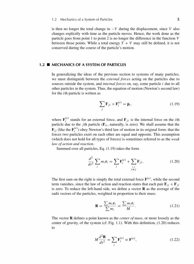
is zero. To reduce the left-hand side, we define a vector R as the average of theradii vectors of the particles, weighted in proportion to their mass:
R =∑
mi ri∑mi
=∑
mi ri
M. (1.21)
The vector R defines a point known as the center of mass, or more loosely as thecenter of gravity, of the system (cf. Fig. 1.1). With this definition, (1.20) reducesto
Md2Rdt2
=∑
i
F(e)i ≡ F(e), (1.22)
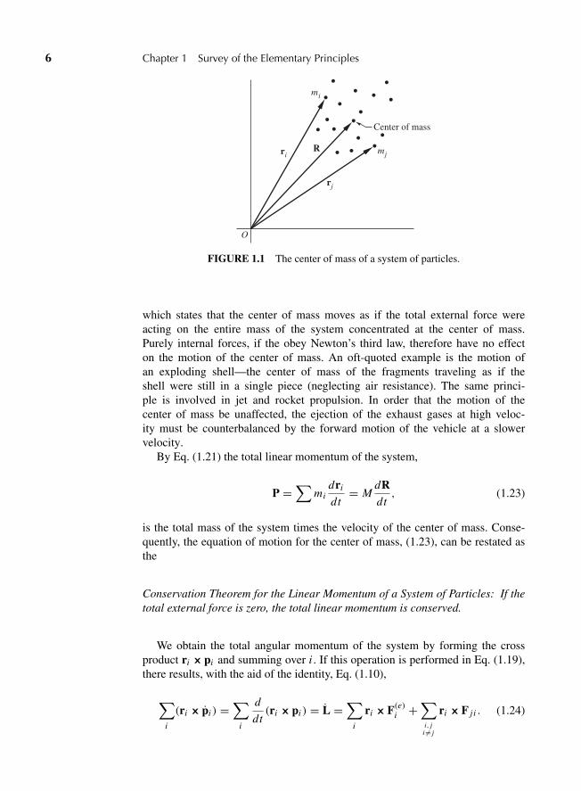
“M01 Goldstein ISBN C01” — 2011/2/15 — page 6 — #6
6 Chapter 1 Survey of the Elementary Principles
O
mj
rj
R
mi
ri
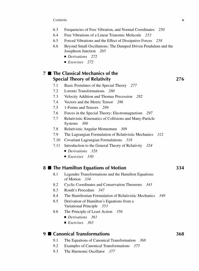
Center of mass
FIGURE 1.1 The center of mass of a system of particles.
which states that the center of mass moves as if the total external force wereacting on the entire mass of the system concentrated at the center of mass.Purely internal forces, if the obey Newton’s third law, therefore have no effecton the motion of the center of mass. An oft-quoted example is the motion ofan exploding shell—the center of mass of the fragments traveling as if theshell were still in a single piece (neglecting air resistance). The same princi-ple is involved in jet and rocket propulsion. In order that the motion of thecenter of mass be unaffected, the ejection of the exhaust gases at high veloc-ity must be counterbalanced by the forward motion of the vehicle at a slowervelocity.
By Eq. (1.21) the total linear momentum of the system,
P =∑
midri
dt= M
dRdt, (1.23)
is the total mass of the system times the velocity of the center of mass. Conse-quently, the equation of motion for the center of mass, (1.23), can be restated asthe
Conservation Theorem for the Linear Momentum of a System of Particles: If thetotal external force is zero, the total linear momentum is conserved.
We obtain the total angular momentum of the system by forming the crossproduct ri 3 pi and summing over i . If this operation is performed in Eq. (1.19),there results, with the aid of the identity, Eq. (1.10),
∑i
(ri 3 pi ) =∑
i
d
dt(ri 3pi ) = L =
∑i
ri 3F(e)i +∑
i, ji �= j
ri 3F j i . (1.24)
“M01 Goldstein ISBN C01” — 2011/2/15 — page 7 — #7
1.2 Mechanics of a System of Particles 7
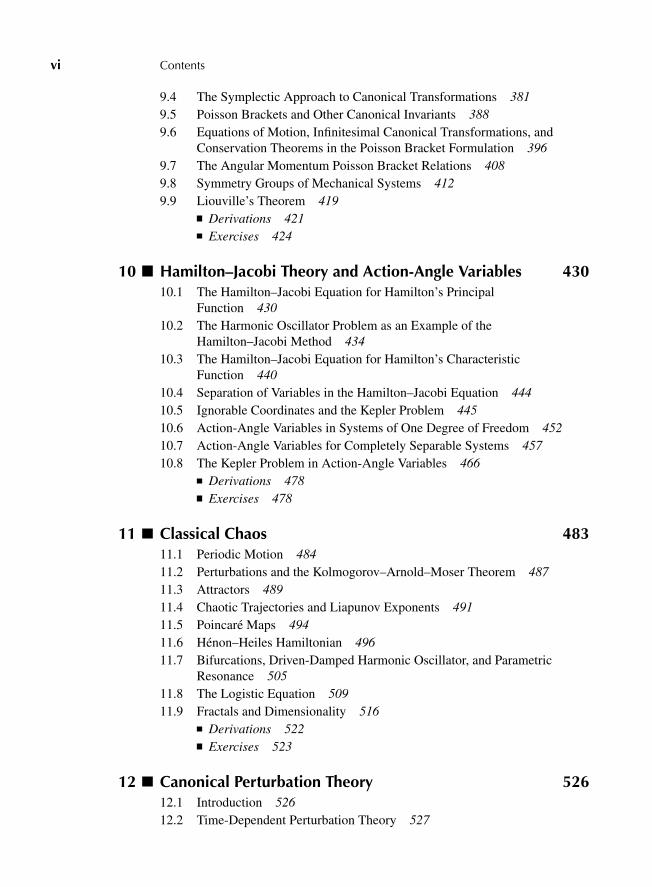
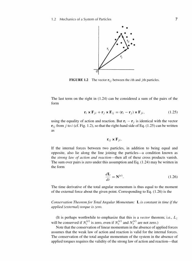
FIGURE 1.2 The vector ri j between the i th and j th particles.
The last term on the right in (1.24) can be considered a sum of the pairs of theform
ri 3F j i + r j 3Fi j = (ri − r j )3F j i , (1.25)
using the equality of action and reaction. But ri − r j is identical with the vectorri j from j to i (cf. Fig. 1.2), so that the right-hand side of Eq. (1.25) can be writtenas
ri j 3F j i .
If the internal forces between two particles, in addition to being equal andopposite, also lie along the line joining the particles—a condition known asthe strong law of action and reaction—then all of these cross products vanish.The sum over pairs is zero under this assumption and Eq. (1.24) may be written inthe form
dLdt
= N(e). (1.26)
The time derivative of the total angular momentum is thus equal to the momentof the external force about the given point. Corresponding to Eq. (1.26) is the
Conservation Theorem for Total Angular Momentum: L is constant in time if theapplied (external) torque is zero.
(It is perhaps worthwhile to emphasize that this is a vector theorem; i.e., Lz
will be conserved if N (e)z is zero, even if N (e)
x and N (e)y are not zero.)
Note that the conservation of linear momentum in the absence of applied forcesassumes that the weak law of action and reaction is valid for the internal forces.The conservation of the total angular momentum of the system in the absence ofapplied torques requires the validity of the strong law of action and reaction—that
“M01 Goldstein ISBN C01” — 2011/2/15 — page 8 — #8
8 Chapter 1 Survey of the Elementary Principles
the internal forces in addition be central. Many of the familiar physical forces,such as that of gravity, satisfy the strong form of the law. But it is possible tofind forces for which action and reaction are equal even though the forces are notcentral (see below). In a system involving moving charges, the forces betweenthe charges predicted by the Biot-Savart law may indeed violate both forms ofthe action and reaction law.* Equations (1.23) and (1.26), and their correspondingconservation theorems, are not applicable in such cases, at least in the form givenhere. Usually it is then possible to find some generalization of P or L that isconserved. Thus, in an isolated system of moving charges it is the sum of themechanical angular momentum and the electromagnetic “angular momentum” ofthe field that is conserved.
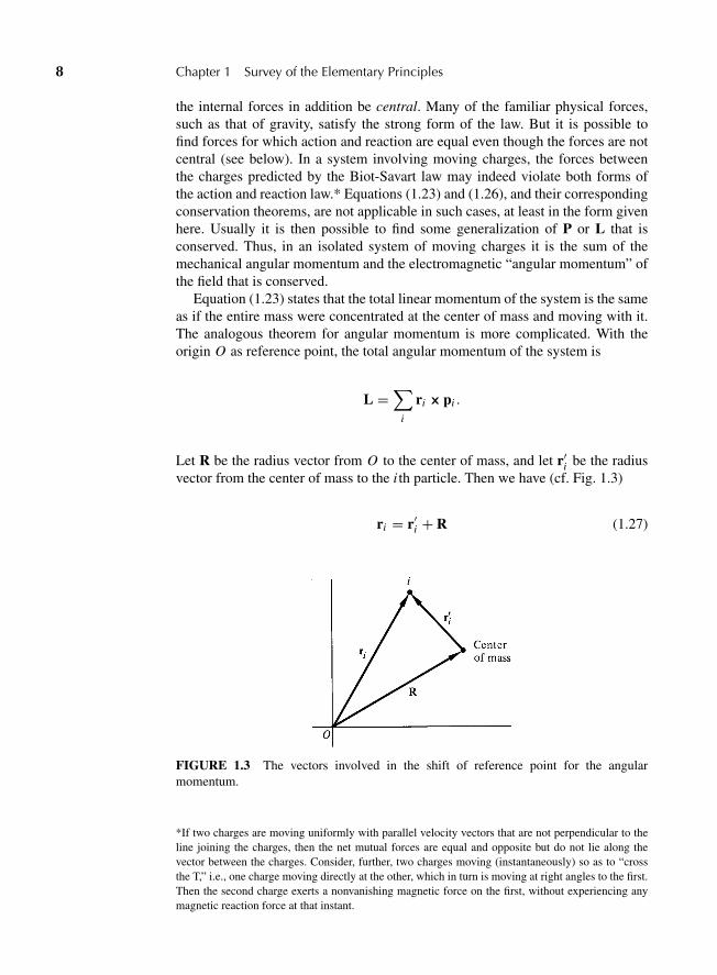
Equation (1.23) states that the total linear momentum of the system is the sameas if the entire mass were concentrated at the center of mass and moving with it.The analogous theorem for angular momentum is more complicated. With theorigin O as reference point, the total angular momentum of the system is
L =∑
i
ri 3 pi .
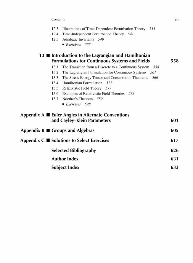
Let R be the radius vector from O to the center of mass, and let r′i be the radiusvector from the center of mass to the i th particle. Then we have (cf. Fig. 1.3)
ri = r′i + R (1.27)
FIGURE 1.3 The vectors involved in the shift of reference point for the angularmomentum.
*If two charges are moving uniformly with parallel velocity vectors that are not perpendicular to theline joining the charges, then the net mutual forces are equal and opposite but do not lie along thevector between the charges. Consider, further, two charges moving (instantaneously) so as to “crossthe T,” i.e., one charge moving directly at the other, which in turn is moving at right angles to the first.Then the second charge exerts a nonvanishing magnetic force on the first, without experiencing anymagnetic reaction force at that instant.
“M01 Goldstein ISBN C01” — 2011/2/15 — page 9 — #9
1.2 Mechanics of a System of Particles 9
and
vi = v′i + v
where
v = dRdt
is the velocity of the center of mass relative to O , and
v′i =dr′idt
is the velocity of the i th particle relative to the center of mass of the system. UsingEq. (1.27), the total angular momentum takes on the form
L =∑
i
R3mi v +∑
i
r′i 3mi v′i +(∑
i
mi r′i
)3 v + R3
d
dt
∑i
mi r′i .
The last two terms in this expression vanish, for both contain the factor∑
mi r′i ,which, it will be recognized, defines the radius vector of the center of mass in thevery coordinate system whose origin is the center of mass and is therefore a nullvector. Rewriting the remaining terms, the total angular momentum about O is
L = R3 Mv +∑
i
r′i 3 p′i . (1.28)
In words, Eq. (1.28) says that the total angular momentum about a point O isthe angular momentum of motion concentrated at the center of mass, plus theangular momentum of motion about the center of mass. The form of Eq. (1.28)emphasizes that in general L depends on the origin O , through the vector R. Onlyif the center of mass is at rest with respect to O will the angular momentum beindependent of the point of reference. In this case, the first term in (1.28) vanishes,and L always reduces to the angular momentum taken about the center of mass.
Finally, let us consider the energy equation. As in the case of a single particle,we calculate the work done by all forces in moving the system from an initialconfiguration 1, to a final configuration 2:
W12 =∑
i
∫ 2
1Fi ? dsi =
∑i
∫ 2
1F(e)i ? dsi +
∑i, j
i �= j
∫ 2
1F j i ? dsi . (1.29)
Again, the equations of motion can be used to reduce the integrals to
∑i
∫ 2
1Fi ? dsi =
∑i
∫ 2
1mi vi ? vi dt =
∑i
∫ 2
1d
(1
2miv
2i
).
“M01 Goldstein ISBN C01” — 2011/2/15 — page 10 — #10
10 Chapter 1 Survey of the Elementary Principles
Hence, the work done can still be written as the difference of the final and initialkinetic energies:
W12 = T2 − T1,
where T , the total kinetic energy of the system, is
T = 1
2
∑i
miv2i . (1.30)
Making use of the transformations to center-of-mass coordinates, given inEq. (1.27), we may also write T as
T = 1
2
∑i
mi (v + v′i ) ? (v + v′i )
= 1
2
∑i
miv2 + 1
2
∑i
miv′2i + v ?
d
dt
(∑i
mi r′i
),
and by the reasoning already employed in calculating the angular momentum, thelast term vanishes, leaving
T = 1
2Mv2 + 1
2
∑i
miv′2i (1.31)
The kinetic energy, like the angular momentum, thus also consists of two parts:the kinetic energy obtained if all the mass were concentrated at the center of mass,plus the kinetic energy of motion about the center of mass.
Consider now the right-hand side of Eq. (1.29). In the special case that theexternal forces are derivable in terms of the gradient of a potential, the first termcan be written as
∑i
∫ 2
1F(e)i ? dsi = −
∑i
∫ 2
1∇i Vi ? dsi = −
∑i
Vi
∣∣∣∣2
1,
where the subscript i on the del operator indicates that the derivatives are withrespect to the components of ri . If the internal forces are also conservative, thenthe mutual forces between the i th and j th particles, Fi j and F j i , can be obtainedfrom a potential function Vi j . To satisfy the strong law of action and reaction, Vi j
can be a function only of the distance between the particles:
Vi j = Vi j (| ri − r j |). (1.32)
The two forces are then automatically equal and opposite,
F j i = −∇i Vi j = +∇ j Vi j = −Fi j , (1.33)

“M01 Goldstein ISBN C01” — 2011/2/15 — page 11 — #11
1.2 Mechanics of a System of Particles 11
and lie along the line joining the two particles,
∇Vi j (| ri − r j |) = (ri − r j ) f, (1.34)
where f is some scalar function. If Vi j were also a function of the difference ofsome other pair of vectors associated with the particles, such as their velocitiesor (to step into the domain of modern physics) their intrinsic “spin” angular mo-menta, then the forces would still be equal and opposite, but would not necessarilylie along the direction between the particles.
When the forces are all conservative, the second term in Eq. (1.29) can berewritten as a sum over pairs of particles, the terms for each pair being of theform
−∫ 2
1(∇i Vi j ? dsi + ∇ j Vi j ? ds j ).
If the difference vector ri − r j is denoted by ri j , and if ∇i j stands for the gradientwith respect to ri j , then
∇i Vi j = ∇i j Vi j = −∇ j Vi j ,
and
dsi − ds j = dri − dr j = dri j ,
so that the term for the ij pair has the form
−∫
∇i j Vi j ? dri j .
The total work arising from internal forces then reduces to
−1
2
∑i, j
i �= j
∫ 2
1∇i j Vi j ? dri j = −1
2
∑i, j
i �= j
Vi j
∣∣∣∣2
1. (1.35)
The factor 12 appears in Eq. (1.35) because in summing over both i and j each
member of a given pair is included twice, first in the i summation and then in thej summation.
From these considerations, it is clear that if the external and internal forces areboth derivable from potentials it is possible to define a total potential energy, V ,of the system,
V =∑
i
Vi + 1
2
∑i, j
i �= j
Vi j , (1.36)
such that the total energy T + V is conserved, the analog of the conservationtheorem (1.18) for a single particle.
“M01 Goldstein ISBN C01” — 2011/2/15 — page 12 — #12
12 Chapter 1 Survey of the Elementary Principles
The second term on the right in Eq. (1.36) will be called the internal potentialenergy of the system. In general, it need not be zero and, more important, it mayvary as the system changes with time. Only for the particular class of systemsknown as rigid bodies will the internal potential always be constant. Formally,a rigid body can be defined as a system of particles in which the distances ri j
are fixed and cannot vary with time. In such case, the vectors dri j can only beperpendicular to the corresponding ri j , and therefore to the Fi j . Therefore, in arigid body the internal forces do no work, and the internal potential must remainconstant. Since the total potential is in any case uncertain to within an additiveconstant, an unvarying internal potential can be completely disregarded in dis-cussing the motion of the system.
1.3 CONSTRAINTS
From the previous sections one might obtain the impression that all problems inmechanics have been reduced to solving the set of differential equations (1.19):
mi ri = F(e)i +∑
j
F j i .
One merely substitutes the various forces acting upon the particles of the system,turns the mathematical crank, and grinds out the answers! Even from a purelyphysical standpoint, however, this view is oversimplified. For example, it may benecessary to take into account the constraints that limit the motion of the system.We have already met one type of system involving constraints, namely rigid bod-ies, where the constraints on the motions of the particles keep the distances ri j
unchanged. Other examples of constrained systems can easily be furnished. Thebeads of an abacus are constrained to one-dimensional motion by the supportingwires. Gas molecules within a container are constrained by the walls of the ves-sel to move only inside the container. A particle placed on the surface of a solidsphere is subject to the constraint that it can move only on the surface or in theregion exterior to the sphere.
Constraints may be classified in various ways, and we shall use the followingsystem. If the conditions of constraint can be expressed as equations connectingthe coordinates of the particles (and possibly the time) having the form
f (r1, r2, r3, . . . , t) = 0, (1.37)
then the constraints are said to be holonomic. Perhaps the simplest example ofholonomic constraints is the rigid body, where the constraints are expressed byequations of the form
(ri − r j )2 − c2
i j = 0.
A particle constrained to move along any curve or on a given surface is anotherobvious example of a holonomic constraint, with the equations defining the curveor surface acting as the equations of a constraint.
“M01 Goldstein ISBN C01” — 2011/2/15 — page 13 — #13
1.3 Constraints 13
Constraints not expressible in this fashion are called nonholonomic. The wallsof a gas container constitute a nonholonomic constraint. The constraint involvedin the example of a particle placed on the surface of a sphere is also nonholo-nomic, for it can be expressed as an inequality
r2 − a2 ≥ 0
(where a is the radius of the sphere), which is not in the form of (1.37). Thus, ina gravitational field a particle placed on the top of the sphere will slide down thesurface part of the way but will eventually fall off.
Constraints are further classified according to whether the equations of con-straint contain the time as an explicit variable (rheonomous) or are not explicitlydependent on time (scleronomous). A bead sliding on a rigid curved wire fixedin space is obviously subject to a scleronomous constraint; if the wire is movingin some prescribed fashion, the constraint is rheonomous. Note that if the wiremoves, say, as a reaction to the bead’s motion, then the time dependence of theconstraint enters in the equation of the constraint only through the coordinatesof the curved wire (which are now part of the system coordinates). The overallconstraint is then scleronomous.
Constraints introduce two types of difficulties in the solution of mechanicalproblems. First, the coordinates ri are no longer all independent, since they areconnected by the equations of constraint; hence the equations of motion (1.19)are not all independent. Second, the forces of constraint, e.g., the force that thewire exerts on the bead (or the wall on the gas particle), is not furnished a pri-ori. They are among the unknowns of the problem and must be obtained from thesolution we seek. Indeed, imposing constraints on the system is simply anothermethod of stating that there are forces present in the problem that cannot be spec-ified directly but are known rather in terms of their effect on the motion of thesystem.
In the case of holonomic constraints, the first difficulty is solved by the intro-duction of generalized coordinates. So far we have been thinking implicitly interms of Cartesian coordinates. A system of N particles, free from constraints,has 3N independent coordinates or degrees of freedom. If there exist holonomicconstraints, expressed in k equations in the form (1.37), then we may use theseequations to eliminate k of the 3N coordinates, and we are left with 3N − k inde-pendent coordinates, and the system is said to have 3N − k degrees of freedom.This elimination of the dependent coordinates can be expressed in another way,by the introduction of new, 3N − k, independent variables q1, q2, . . . , q3N−k interms of which the old coordinates r1, r2, . . . , rN are expressed by equations ofthe form
r1 = r1(q1, q2, . . . , q3N−k, t)
... (1.38)
rN = rN (q1, q2, . . . , q3N−k, t)
“M01 Goldstein ISBN C01” — 2011/2/15 — page 14 — #14
14 Chapter 1 Survey of the Elementary Principles
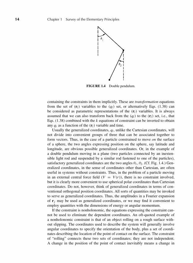
FIGURE 1.4 Double pendulum.
containing the constraints in them implicitly. These are transformation equationsfrom the set of (rl) variables to the (ql) set, or alternatively Eqs. (1.38) canbe considered as parametric representations of the (rl) variables. It is alwaysassumed that we can also transform back from the (ql) to the (rl) set, i.e., thatEqs. (1.38) combined with the k equations of constraint can be inverted to obtainany qi as a function of the (rl) variable and time.
Usually the generalized coordinates, ql , unlike the Cartesian coordinates, willnot divide into convenient groups of three that can be associated together toform vectors. Thus, in the case of a particle constrained to move on the surfaceof a sphere, the two angles expressing position on the sphere, say latitude andlongitude, are obvious possible generalized coordinates. Or, in the example ofa double pendulum moving in a plane (two particles connected by an inexten-sible light rod and suspended by a similar rod fastened to one of the particles),satisfactory generalized coordinates are the two angles θ1, θ2. (Cf. Fig. 1.4.) Gen-eralized coordinates, in the sense of coordinates other than Cartesian, are oftenuseful in systems without constraints. Thus, in the problem of a particle movingin an external central force field (V = V (r)), there is no constraint involved,but it is clearly more convenient to use spherical polar coordinates than Cartesiancoordinates. Do not, however, think of generalized coordinates in terms of con-ventional orthogonal position coordinates. All sorts of quantities may be invokedto serve as generalized coordinates. Thus, the amplitudes in a Fourier expansionof r j may be used as generalized coordinates, or we may find it convenient toemploy quantities with the dimensions of energy or angular momentum.
If the constraint is nonholonomic, the equations expressing the constraint can-not be used to eliminate the dependent coordinates. An oft-quoted example ofa nonholonomic constraint is that of an object rolling on a rough surface with-out slipping. The coordinates used to describe the system will generally involveangular coordinates to specify the orientation of the body, plus a set of coordi-nates describing the location of the point of contact on the surface. The constraintof “rolling” connects these two sets of coordinates; they are not independent.A change in the position of the point of contact inevitably means a change in
“M01 Goldstein ISBN C01” — 2011/2/15 — page 15 — #15
1.3 Constraints 15
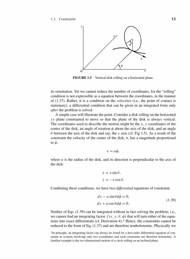
FIGURE 1.5 Vertical disk rolling on a horizontal plane.
its orientation. Yet we cannot reduce the number of coordinates, for the “rolling”condition is not expressible as a equation between the coordinates, in the mannerof (1.37). Rather, it is a condition on the velocities (i.e., the point of contact isstationary), a differential condition that can be given in an integrated form onlyafter the problem is solved.
A simple case will illustrate the point. Consider a disk rolling on the horizontalxy plane constrained to move so that the plane of the disk is always vertical.The coordinates used to describe the motion might be the x , y coordinates of thecenter of the disk, an angle of rotation φ about the axis of the disk, and an angleθ between the axis of the disk and say, the x axis (cf. Fig 1.5). As a result of theconstraint the velocity of the center of the disk, v, has a magnitude proportionalto φ,
v = aφ,
where a is the radius of the disk, and its direction is perpendicular to the axis ofthe disk:
x = v sin θ,
y = −v cos θ.
Combining these conditions, we have two differential equations of constraint:
dx − a sin θdφ = 0,
dy + a cos θdφ = 0.(1.39)
Neither of Eqs. (1.39) can be integrated without in fact solving the problem; i.e.,we cannot find an integrating factor f (x, y, θ, φ) that will turn either of the equa-tions into exact differentials (cf. Derivation 4).* Hence, the constraints cannot bereduced to the form of Eq. (1.37) and are therefore nonholonomic. Physically we
*In principle, an integrating factor can always be found for a first-order differential equation of con-straint in systems involving only two coordinates and such constraints are therefore holonomic. Afamiliar example is the two-dimensional motion of a circle rolling on an inclined plane.
“M01 Goldstein ISBN C01” — 2011/2/15 — page 16 — #16
16 Chapter 1 Survey of the Elementary Principles
can see that there can be no direct functional relation between φ and the othercoordinates x , y, and θ by noting that at any point on its path the disk can bemade to roll around in a circle tangent to the path and of arbitrary radius. At theend of the process, x , y, and θ have been returned to their original values, but φhas changed by an amount depending on the radius of the circle.
Nonintegrable differential constraints of the form of Eqs. (1.39) are of coursenot the only type of nonholonomic constraints. The constraint conditions mayinvolve higher-order derivatives, or may appear in the form of inequalities, as wehave seen.
Partly because the dependent coordinates can be eliminated, problems involv-ing holonomic constraints are always amenable to a formal solution. But there isno general way to attack nonholonomic examples. True, if the constraint is nonin-tegrable, the differential equations of constraint can be introduced into the prob-lem along with the differential equations of motion, and the dependent equationseliminated, in effect, by the method of Lagrange multipliers.
We shall return to this method at a later point. However, the more vicious casesof nonholonomic constraint must be tackled individually, and consequently in thedevelopment of the more formal aspects of classical mechanics, it is almost invari-ably assumed that any constraint, if present, is holonomic. This restriction doesnot greatly limit the applicability of the theory, despite the fact that many of theconstraints encountered in everyday life are nonholonomic. The reason is that theentire concept of constraints imposed in the system through the medium of wiresor surfaces or walls is particularly appropriate only in macroscopic or large-scaleproblems. But today physicists are more interested in atomic and nuclear prob-lems. On this scale all objects, both in and out of the system, consist alike ofmolecules, atoms, or smaller particles, exerting definite forces, and the notion ofconstraint becomes artificial and rarely appears. Constraints are then used onlyas mathematical idealizations to the actual physical case or as classical approxi-mations to a quantum-mechanical property, e.g., rigid body rotations for “spin.”Such constraints are always holonomic and fit smoothly into the framework of thetheory.
To surmount the second difficulty, namely, that the forces of constraint areunknown a priori, we should like to so formulate the mechanics that the forcesof constraint disappear. We need then deal only with the known applied forces.A hint as to the procedure to be followed is provided by the fact that in a particularsystem with constraints, i.e., a rigid body, the work done by internal forces (whichare here the forces of constraint) vanishes. We shall follow up this clue in theensuing sections and generalize the ideas contained in it.
1.4 D’ALEMBERT’S PRINCIPLE AND LAGRANGE’S EQUATIONS
A virtual (infinitesimal) displacement of a system refers to a change in the con-figuration of the system as the result of any arbitrary infinitesimal change of thecoordinates δri , consistent with the forces and constraints imposed on the systemat the given instant t . The displacement is called virtual to distinguish it from anactual displacement of the system occurring in a time interval dt , during which
“M01 Goldstein ISBN C01” — 2011/2/15 — page 17 — #17
1.4 D’Alembert’s Principle and Lagrange’s Equations 17
the forces and constraints may be changing. Suppose the system is in equilibrium;i.e., the total force on each particle vanishes, Fi = 0. Then clearly the dot productFi ? δri , which is the virtual work of the force Fi in the displacement δri , alsovanishes. The sum of these vanishing products over all particles must likewise bezero: ∑
i
Fi ? δri = 0. (1.40)
As yet nothing has been said that has any new physical content. Decompose Fi
into the applied force, F(a)i , and the force of constraint, fi ,
Fi = F(a)i + fi , (1.41)
so that Eq. (1.40) becomes
∑i
F(a)i ? δri +∑
i
fi ? δri = 0. (1.42)
We now restrict ourselves to systems for which the net virtual work of theforces of constraint is zero. We have seen that this condition holds true for rigidbodies and it is valid for a large number of other constraints. Thus, if a particle isconstrained to move on a surface, the force of constraint is perpendicular to thesurface, while the virtual displacement must be tangent to it, and hence the virtualwork vanishes. This is no longer true if sliding friction forces are present, and wemust exclude such systems from our formulation. The restriction is not undulyhampering, since the friction is essentially a macroscopic phenomenon. On theother hand, the forces of rolling friction do not violate this condition, since theforces act on a point that is momentarily at rest and can do no work in an infinites-imal displacement consistent with the rolling constraint. Note that if a particle isconstrained to a surface that is itself moving in time, the force of constraint isinstantaneously perpendicular to the surface and the work during a virtual dis-placement is still zero even though the work during an actual displacement in thetime dt does not necessarily vanish.
We therefore have as the condition for equilibrium of a system that the virtualwork of the applied forces vanishes:
∑i
F(a)i ? δri = 0. (1.43)
Equation (1.43) is often called the principle of virtual work. Note that the coef-ficients of δri can no longer be set equal to zero; i.e., in general F(a)i �= 0, sincethe δri are not completely independent but are connected by the constraints. Inorder to equate the coefficients to zero, we must transform the principle into aform involving the virtual displacements of the qi , which are independent. Equa-tion (1.43) satisfies our needs in that it does not contain the fi , but it deals onlywith statics; we want a condition involving the general motion of the system.
“M01 Goldstein ISBN C01” — 2011/2/15 — page 18 — #18
18 Chapter 1 Survey of the Elementary Principles
To obtain such a principle, we use a device first thought of by James Bernoulliand developed by D’Alembert. The equation of motion,
Fi = pi ,
can be written as
Fi − pi = 0,
which states that the particles in the system will be in equilibrium under a forceequal to the actual force plus a “reversed effective force” −pi . Instead of (1.40),we can immediately write ∑
i
(Fi − pi ) ? δri = 0, (1.44)
and, making the same resolution into applied forces and forces of constraint, thereresults ∑
i
(F(a)i − pi ) ? δri +∑
i
fi ? δri = 0.
We again restrict ourselves to systems for which the virtual work of the forces ofconstraint vanishes and therefore obtain∑
i
(F(a)i − pi ) ? δri = 0, (1.45)
which is often called D’Alembert’s principle. We have achieved our aim, in thatthe forces of constraint no longer appear, and the superscript (a) can now bedropped without ambiguity. It is still not in a useful form to furnish equationsof motion for the system. We must now transform the principle into an expressioninvolving virtual displacements of the generalized coordinates, which are thenindependent of each other (for holonomic constraints), so that the coefficients ofthe δqi can be set separately equal to zero.
The translation from ri to q j language starts from the transformation equations(1.38),
ri = ri (q1, q2, . . . , qn, t) (1.45′)
(assuming n independent coordinates), and is carried out by means of the usual“chain rules” of the calculus of partial differentiation. Thus, vi is expressed interms of the qk by the formula
vi ≡ dri
dt=∑
k
∂ri
∂qkqk + ∂ri
∂t. (1.46)
Similarly, the arbitrary virtual displacement δri can be connected with the virtualdisplacements δqi by
δri =∑
j
∂ri
∂q jδq j . (1.47)
“M01 Goldstein ISBN C01” — 2011/2/15 — page 19 — #19
1.4 D’Alembert’s Principle and Lagrange’s Equations 19
Note that no variation of time, δt , is involved here, since a virtual displacementby definition considers only displacements of the coordinates. (Only then is thevirtual displacement perpendicular to the force of constraint if the constraint itselfis changing in time.)
In terms of the generalized coordinates, the virtual work of the Fi becomes
∑i
Fi ? δri =∑i, j
Fi ?∂ri
∂q jδq j
=∑
j
Q jδq j , (1.48)
where the Q j are called the components of the generalized force, defined as
Q j =∑
i
Fi ?∂ri
∂q j. (1.49)
Note that just as the q’s need not have the dimensions of length, so the Q’s donot necessarily have the dimensions of force, but Q jδq j must always have thedimensions of work. For example, Q j might be a torque N j and dq j a differentialangle dθ j , which makes N j dθ j a differential of work.
We turn now to the other other term involved in Eq. (1.45), which may bewritten as ∑
i
pi ? δri =∑
i
mi ri ? δri .
Expressing δri by (1.47), this becomes
∑i, j
mi ri ?∂ri
∂q jδq j .
Consider now the relation∑i
mi ri ?∂ri
∂q j=∑
i
[d
dt
(mi ri ?
∂ri
∂q j
)− mi ri ?
d
dt
(∂ri
∂q j
)]. (1.50)
In the last term of Eq. (1.50) we can interchange the differentiation with respectto t and q j , for, in analogy to (1.46),
d
dt
(∂ri
∂q j
)= ∂ ri
∂q j=∑
k
∂2ri
∂q j∂qkqk + ∂2ri
∂q j∂t,
= ∂vi
∂q j,
by Eq. (1.46). Further, we also see from Eq. (1.46) that
∂vi
∂q j= ∂ri
∂q j. (1.51)
“M01 Goldstein ISBN C01” — 2011/2/15 — page 20 — #20
20 Chapter 1 Survey of the Elementary Principles
Substitution of these changes in (1.50) leads to the result that
∑i
mi ri ?∂ri
∂q j=∑
i
[d
dt
(mi vi ?
∂vi
∂ q j
)− mi vi ?
∂vi
∂q j
],
and the second term on the left-hand side of Eq. (1.45) can be expanded into
∑j
{d
dt
[∂
∂q j
(∑i
1
2miv
2i
)]− ∂
∂q j
(∑i
1
2miv
2i
)− Q j
}δq j .
Identifying∑
i12 miv
2i with the system kinetic energy T , D’Alembert’s principle
(cf. Eq. (1.45)) becomes
∑j
{[d
dt
(∂T
∂ q j
)− ∂T
∂q j
]− Q j
}δq j = 0. (1.52)
Note that in a system of Cartesian coordinates the partial derivative of T withrespect to q j vanishes. Thus, speaking in the language of differential geometry,this term arises from the curvature of the coordinates q j . In polar coordinates,e.g., it is in the partial derivative of T with respect to the angle coordinate that thecentripetal acceleration term appears.
Thus far, no restriction has been made on the nature of the constraints otherthan that they be workless in a virtual displacement. The variables q j can be anyset of coordinates used to describe the motion of the system. If, however, the con-straints are holonomic, then it is possible to find sets of independent coordinatesq j that contain the constraint conditions implicitly in the transformation equations(1.38). Any virtual displacement δq j is then independent of δqk , and therefore theonly way for (1.52) to hold is for the individual coefficients to vanish:
d
dt
(∂T
∂ q j
)− ∂T
∂q j= Q j . (1.53)
There are n such equations in all.When the forces are derivable from a scalar potential function V ,
Fi = −∇i V .
Then the generalized forces can be written as
Q j =∑
i
Fi ?∂ri
∂q j= −
∑i
∇i V ?∂ri
∂q j,
which is exactly the same expression for the partial derivative of a function−V (r1, r2, . . . , rN , t) with respect to q j :
Q j ≡ − ∂V
∂q j. (1.54)
“M01 Goldstein ISBN C01” — 2011/2/15 — page 21 — #21
1.5 Velocity-Dependent Potentials and the Dissipation Function 21
See Eq. (1.47). Equations (1.53) can then be rewritten as
d
dt
(∂T
∂q j
)− ∂(T − V )
∂q j= 0. (1.55)
The equations of motion in the form (1.55) are not necessarily restricted to conser-vative systems; only if V is not an explicit function of time is the system conserva-tive (cf. p. 4). As here defined, the potential V does not depend on the generalizedvelocities. Hence, we can include a term in V in the partial derivative with respectto q j :
d
dt
(∂(T − V )
∂q j
)− ∂(T − V )
∂q j= 0.
Or, defining a new function, the Lagrangian L, as
L = T − V, (1.56)
the Eqs. (1.53) become
d
dt
(∂L
∂ q j
)− ∂L
∂q j= 0, (1.57)
expressions referred to as “Lagrange’s equations.”Note that for a particular set of equations of motion there is no unique choice
of Lagrangian such that Eqs. (1.57) lead to the equations of motion in the givengeneralized coordinates. Thus, in Derivations 8 and 10 it is shown that if L(q, q, t)is an approximate Lagrangian and F(q, t) is any differentiable function of thegeneralized coordinates and time, then
L ′(q, q, t) = L(q, q, t)+ d F
dt(1.57′)
is a Lagrangian also resulting in the same equations of motion. It is also oftenpossible to find alternative Lagrangians beside those constructed by this prescrip-tion (see Exercise 20). While Eq. (1.56) is always a suitable way to construct aLagrangian for a conservative system, it does not provide the only Lagrangiansuitable for the given system.
1.5 VELOCITY-DEPENDENT POTENTIALSAND THE DISSIPATION FUNCTION
Lagrange’s equations can be put in the form (1.57) even if there is no potentialfunction, V , in the usual sense, providing the generalized forces are obtained froma function U (q j , q j ) by the prescription
Q j = − ∂U
∂q j+ d
dt
(∂U
∂ q j
). (1.58)
“M01 Goldstein ISBN C01” — 2011/2/15 — page 22 — #22
22 Chapter 1 Survey of the Elementary Principles
In such case, Eqs. (1.57) still follow from Eqs. (1.53) with the Lagrangian givenby
L = T − U. (1.59)
Here U may be called a “generalized potential,” or “velocity-dependent poten-tial.” The possibility of using such a “potential” is not academic; it applies to onevery important type of force field, namely, the electromagnetic forces on movingcharges. Considering its importance, a digression on this subject is well worth-while.
Consider an electric charge, q, of mass m moving at a velocity, v, in an other-wise charge-free region containing both an electric field, E, and a magnetic field,B, which may depend upon time and position. The charge experiences a force,called the Lorentz force, given by
F = q [E + (v × B)] . (1.60)
Both E(x, y, z, t) and B(x, y, z, t) are continuous functions of time and positionderivable from a scalar potential φ(x, y, z, t) and a vector potential A(x, y, z, t)by
E = −∇φ − ∂A∂t
(1.61a)
and
B = ∇ × A. (1.61b)
The force on the charge can be derived from the following velocity-dependentpotential energy
U = qφ − qA ? v, (1.62)
so the Lagrangian, L = T − U , is
L = 12 mv2 − qφ + qA ? v. (1.63)
Considering just the x-component of Lagrange’s equations gives
mx = q
(vx∂Ax
∂x+ vy
∂Ay
∂x+ vz
∂Az
∂x
)− q
(∂φ
∂x+ d Ax
dt
). (1.64)
The total time derivative of Ax is related to the partial time derivative through
d Ax
dt= ∂Ax
∂t+ v ?∇Ax
= ∂Ax
∂t+ vx
∂Ax
∂x+ vy
∂Ax
∂y+ vz
∂Ax
∂z. (1.65)
“M01 Goldstein ISBN C01” — 2011/2/15 — page 23 — #23
1.5 Velocity-Dependent Potentials and the Dissipation Function 23
Equation (1.61b) gives
(v × B)x = vy
(∂Ay
∂x− ∂Ax
∂y
)+ vz
(∂Az
∂x− ∂Ax
∂z
).
Combining these expressions gives the equation of motion in the x-direction
mx = q [Ex + (v × B)x ] . (1.66)
On a component-by-component comparison, Eqs. (1.66) and (1.60) are identical,showing that the Lorentz force equation is derivable from Eqs. (1.61) and (1.62).
Note that if not all the forces acting on the system are derivable from a poten-tial, then Lagrange’s equations can always be written in the form
d
dt
(∂L
∂q j
)− ∂L
∂q j= Q j ,
where L contains the potential of the conservative forces as before, and Q j rep-resents the forces not arising from a potential. Such a situation often occurs whenfrictional forces are present. It frequently happens that the frictional force is pro-portional to the velocity of the particle, so that its x-component has the form
F f x = −kxvx .
Frictional forces of this type may be derived in terms of a function F , known asRayleigh’s dissipation function, and defined as
F = 1
2
∑i
(kxv
2i x + kyv
2iy + kzv
2i z
), (1.67)
where the summation is over the particles of the system. From this definition it isclear that
F fxi= − ∂F
∂vxi
,
or, symbolically,
F f = −∇vF . (1.68)
We can also give a physical interpretation to the dissipation function. The workdone by the system against friction is
dW f = −F f ? dr = −F f ? v dt =(
kxv2x + kyv
2y + kzv
2z
)dt.
Hence, 2F is the rate of energy dissipation due to friction. The component of thegeneralized force resulting from the force of friction is then given by
Q j =∑
i
F fi ?∂ri
∂q j= −
∑∇vF ?
∂ri
∂q j
“M01 Goldstein ISBN C01” — 2011/2/15 — page 24 — #24
24 Chapter 1 Survey of the Elementary Principles
= −∑
∇vF ?∂ ri
∂q j, by (1.51),
= − ∂F∂q j
. (1.69)
An example is Stokes’ law, whereby a sphere of radius a moving at a speed v,in a medium of viscosity η experiences the frictional drag force F f = −6πηav.The Lagrange equations with dissipation become
d
dt
(∂L
∂q j
)− ∂L
∂q j+ ∂F∂ q j
= 0, (1.70)
so that two scalar functions, L and F , must be specified to obtain the equationsof motion.
1.6 SIMPLE APPLICATIONS OF THE LAGRANGIAN FORMULATION
The previous sections show that for systems where we can define a Lagrangian,i.e., holonomic systems with applied forces derivable from an ordinary or gen-eralized potential and workless constraints, we have a very convenient way ofsetting up the equations of motion. We were led to the Lagrangian formulationby the desire to eliminate the forces of constraint from the equations of motion,and in achieving this goal we have obtained many other benefits. In setting up theoriginal form of the equations of motion, Eqs. (1.19), it is necessary to work withmany vector forces and accelerations. With the Lagrangian method we only dealwith two scalar functions, T and V , which greatly simplifies the problem.
A straightforward routine procedure can now be established for all problemsof mechanics to which the Lagrangian formulation is applicable. We have only towrite T and V in generalized coordinates, form L from them, and substitute in(1.57) to obtain the equations of motion. The needed transformation of T and Vfrom Cartesian coordinates to generalized coordinates is obtained by applying thetransformation equations (1.38) and (1.45′). Thus, T is given in general by
T =∑
i
1
2miv
2i =
∑i
1
2mi
⎛⎝∑
j
∂ri
∂q jq j + ∂ri
∂t
⎞⎠
2
.
It is clear that on carrying out the expansion, the expression for T in generalizedcoordinates will have the form
T = M0 +∑
j
M j q j + 1
2
∑j,k
M jkq j qk, (1.71)
where M0, M j , M jk are definite functions of the r’s and t and hence of the q’sand t . In fact, a comparison shows that
M0 =∑
i
1
2mi
(∂ri
∂t
)2
,
“M01 Goldstein ISBN C01” — 2011/2/15 — page 25 — #25
1.6 Simple Applications of the Lagrangian Formulation 25
M j =∑
i
mi∂ri
∂t?∂ri
∂q j, (1.72)
and
M jk =∑
i
mi∂ri
∂q j?∂ri
∂qk.
Thus, the kinetic energy of a system can always be written as the sum of threehomogeneous functions of the generalized velocities,
T = T0 + T1 + T2, (1.73)
where T0 is independent of the generalized velocities, T1 is linear in the velocities,and T2 is quadratic in the velocities. If the transformation equations do not containthe time explicitly, as may occur when the constraints are independent of time(scleronomous), then only the last term in Eq. (1.71) is nonvanishing, and T isalways a homogeneous quadratic form in the generalized velocities.
Let us now consider simple examples of this procedure:
1. Single particle in space
(a) Cartesian coordinates
(b) Plane polar coordinates
2. Atwood’s machine3. Time-dependent constraint—bead sliding on rotating wire
1. (a) Motion of one particle: using Cartesian coordinates. The generalizedforces needed in Eq. (1.53) are obviously Fx , Fy , and Fz . Then
T = 12 m(x2 + y2 + z2),
∂T
∂x= ∂T
∂y= ∂T
∂z= 0,
∂T
∂ x= mx,
∂T
∂ y= my,
∂T
∂ z= mz,
and the equations of motion are
d
dt(mx) = Fx ,
d
dt(my) = Fy,
d
dt(mz) = Fz . (1.74)
We are thus led back to the original Newton’s equations of motion.
(b) Motion of one particle: using plane polar coordinates. Here we mustexpress T in terms of r and θ . The transformation equations, Eqs. (1.38), are
x = r cos θ
y = r sin θ.
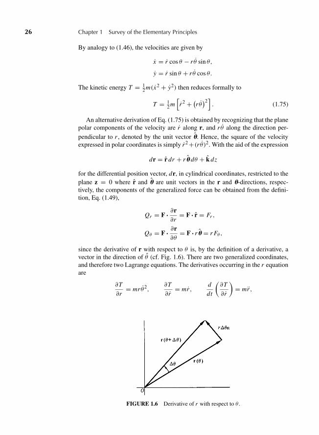
“M01 Goldstein ISBN C01” — 2011/2/15 — page 26 — #26
26 Chapter 1 Survey of the Elementary Principles
By analogy to (1.46), the velocities are given by
x = r cos θ − r θ sin θ,
y = r sin θ + r θ cos θ.
The kinetic energy T = 12 m(x2 + y2) then reduces formally to
T = 12 m
[r2 + (
r θ)2]
. (1.75)
An alternative derivation of Eq. (1.75) is obtained by recognizing that the planepolar components of the velocity are r along r, and r θ along the direction per-
pendicular to r , denoted by the unit vector u. Hence, the square of the velocityexpressed in polar coordinates is simply r2+(r θ )2. With the aid of the expression
dr = r dr + r u dθ + k dz
for the differential position vector, dr, in cylindrical coordinates, restricted to theplane z = 0 where r and u are unit vectors in the r and u-directions, respec-tively, the components of the generalized force can be obtained from the defini-tion, Eq. (1.49),
Qr = F ?∂r∂r
= F ? r = Fr ,
Qθ = F ?∂r∂θ
= F ? r u = r Fθ ,
since the derivative of r with respect to θ is, by the definition of a derivative, avector in the direction of θ (cf. Fig. 1.6). There are two generalized coordinates,and therefore two Lagrange equations. The derivatives occurring in the r equationare
∂T
∂r= mr θ2,
∂T
∂ r= mr ,
d
dt
(∂T
∂ r
)= mr ,
FIGURE 1.6 Derivative of r with respect to θ .
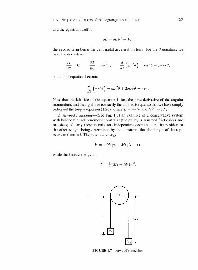
“M01 Goldstein ISBN C01” — 2011/2/15 — page 27 — #27
1.6 Simple Applications of the Lagrangian Formulation 27
and the equation itself is
mr − mr θ2 = Fr ,
the second term being the centripetal acceleration term. For the θ equation, wehave the derivatives
∂T
∂θ= 0,
∂T
∂θ= mr2θ ,
d
dt
(mr2θ
)= mr2θ + 2mrr θ ,
so that the equation becomes
d
dt
(mr2θ
)= mr2θ + 2mrr θ = r Fθ .
Note that the left side of the equation is just the time derivative of the angularmomentum, and the right side is exactly the applied torque, so that we have simplyrederived the torque equation (1.26), where L = mr2θ and N (e) = r Fθ .
2. Atwood’s machine—(See Fig. 1.7) an example of a conservative systemwith holonomic, scleronomous constraint (the pulley is assumed frictionless andmassless). Clearly there is only one independent coordinate x , the position ofthe other weight being determined by the constraint that the length of the ropebetween them is l. The potential energy is
V = −M1gx − M2g(l − x),
while the kinetic energy is
T = 12 (M1 + M2) x2.
FIGURE 1.7 Atwood’s machine.
“M01 Goldstein ISBN C01” — 2011/2/15 — page 28 — #28
28 Chapter 1 Survey of the Elementary Principles
Combining the two, the Lagrangian has the form
L = T − V = 12 (M1 + M2) x2 + M1gx + M2g(l − x).
There is only one equation of motion, involving the derivatives
∂L
∂x= (M1 − M2) g,
∂L
∂ x= (M1 + M2) x,
so that we have
(M1 + M2) x = (M1 − M2) g,
or
x = M1 − M2
M1 + M2g,
which is the familiar result obtained by more elementary means. This trivial prob-lem emphasizes that the forces of constraint—here the tension in the rope—appear nowhere in the Lagrangian formulation. By the same token, neither canthe tension in the rope be found directly by the Lagrangian method.
3. A bead (or ring) sliding on a uniformly rotating wire in a force-free space.The wire is straight, and is rotated uniformly about some fixed axis perpendicularto the wire. This example has been chosen as a simple illustration of a constraintbeing time dependent, with the rotation axis along z and the wire in the xy plane.The transformation equations explicitly contain the time.
x = r cosωt, (ω = angular velocity of rotation)
y = r sinωt. (r = distance along wire from rotation axis)
While we could then find T (here the same as L) by the same procedure used toobtain (1.71), it is simpler to take over (1.75) directly, expressing the constraintby the relation θ = ω:
T = 12 m(r2 + r2ω2).
Note that T is not a homogeneous quadratic function of the generalized velocities,since there is now a term not involving r . The equation of motion is then
mr − mrω2 = 0
or
r = rω2,
which is the familiar simple harmonic oscillator equation with a change of sign.The solution r = eωt for a bead initially at rest on the wire shows that the
“M01 Goldstein ISBN C01” — 2011/2/15 — page 29 — #29
Derivations 29
bead moves exponentially outwards. Again, the method cannot furnish the forceof constraint that keeps the bead on the wire. Equation (1.26) with the angularmomentum, L = mr2ω = mωr2
0 e2ωt , provides the force F = N/r , which pro-duces the constraint force, F = 2mr0ω
2eωt , acting perpendicular to the wire andthe axis of rotation.
DERIVATIONS
1. Show that for a single particle with constant mass the equation of motion implies thefollowing differential equation for the kinetic energy:
dT
dt= F ? v,
while if the mass varies with time the corresponding equation is
d(mT )
dt= F ? p.
2. Prove that the magnitude R of the position vector for the center of mass from anarbitrary origin is given by the equation
M2 R2 = M∑
i
mi r2i − 1
2
∑i �= j
mi m j r2i j .
3. Suppose a system of two particles is known to obey the equations of motion,Eqs. (1.22) and (1.26). From the equations of the motion of the individual parti-cles show that the internal forces between particles satisfy both the weak and thestrong laws of action and reaction. The argument may be generalized to a system witharbitrary number of particles, thus proving the converse of the arguments leading toEqs. (1.22) and (1.26).
4. The equations of constraint for the rolling disk, Eqs. (1.39), are special cases ofgeneral linear differential equations of constraint of the form
n∑i=1
gi (x1, . . . , xn)dxi = 0.
A constraint condition of this type is holonomic only if an integrating functionf (x1, . . . , xn) can be found that turns it into an exact differential. Clearly the func-tion must be such that
∂ ( f gi )
∂x j= ∂
(f g j
)∂xi
for all i �= j . Show that no such integrating factor can be found for either ofEqs. (1.39).
5. Two wheels of radius a are mounted on the ends of a common axle of length b suchthat the wheels rotate independently. The whole combination rolls without slipping ona plane. Show that there are two nonholonomic equations of constraint,
cos θdx + sin θdy = 0
sin θdx − cos θdy = 12 a(dφ + dφ′
),
“M01 Goldstein ISBN C01” — 2011/2/15 — page 30 — #30
30 Chapter 1 Survey of the Elementary Principles
(where θ , φ, and φ′ have meanings similar to those in the problem of a single verticaldisk, and (x, y) are the coordinates of a point on the axle midway between the twowheels) and one holonomic equation of constraint,
θ = C − a
b(φ − φ′),
where C is a constant.
6. A particle moves in the xy plane under the constraint that its velocity vector is alwaysdirected towards a point on the x axis whose abscissa is some given function of timef (t). Show that for f (t) differentiable, but otherwise arbitrary, the constraint is non-holonomic.
7. Show that Lagrange’s equations in the form of Eqs. (1.53) can also be written as
∂ T
∂ q j− 2
∂T
∂q j= Q j .
These are sometimes known as the Nielsen form of the Lagrange equations.
8. If L is a Lagrangian for a system of n degrees of freedom satisfying Lagrange’s equa-tions, show by direct substitution that
L ′ = L + d F(q1, . . . , qn, t)
dt
also satisfies Lagrange’s equations where F is any arbitrary, but differentiable, func-tion of its arguments.
9. The electromagnetic field is invariant under a gauge transformation of the scalar andvector potential given by
A → A + �ψ(r, t),
φ → φ − 1
c
∂ψ
∂t,
where ψ is arbitrary (but differentiable). What effect does this gauge transformationhave on the Lagrangian of a particle moving in the electromagnetic field? Is the motionaffected?
10. Let q1, . . . , qn be a set of independent generalized coordinates for a system of ndegrees of freedom, with a Lagrangian L(q, q, t). Suppose we transform to anotherset of independent coordinates s1, . . . , sn by means of transformation equations
qi = qi (s1, . . . , sn, t), i = 1, . . . , n.
(Such a transformation is called a point transformation.) Show that if the Lagrangianfunction is expressed as a function of s j , s j , and t through the equations of transfor-mation, then L satisfies Lagrange’s equations with respect to the s coordinates:
d
dt
(∂L
∂ s j
)− ∂L
∂s j= 0.
In other words, the form of Lagrange’s equations is invariant under a point transfor-mation.
“M01 Goldstein ISBN C01” — 2011/2/15 — page 31 — #31
Exercises 31
EXERCISES
11. Check whether the force �F = yzi + zx j + xyk is conservative or not.
12. Compute the orbital period and orbital angular velocity of a satellite revolving aroundthe Earth at an altitude of 720 km. [Given: radius of Earth R = 6000 km andg = 9.83 m/s2.]
13. Rockets are propelled by the momentum reaction of the exhaust gases expelled fromthe tail. Since these gases arise from the reaction of the fuels carried in the rocket, themass of the rocket is not constant, but decreases as the fuel is expended. Show that theequation of motion for a rocket projected vertically upward in a uniform gravitationalfield, neglecting atmospheric friction, is
mdv
dt= −v′ dm
dt− mg,
where m is the mass of the rocket and v′ is the velocity of the escaping gases relative tothe rocket. Integrate this equation to obtain v as a function of m, assuming a constanttime rate of loss of mass. Show, for a rocket starting initially from rest, with v′ equalto 2.1 km/s and a mass loss per second equal to 1/60th of the initial mass, that inorder to reach the escape velocity the ratio of the weight of the fuel to the weight ofthe empty rocket must be almost 300!
14. Two points of mass m are joined by a rigid weightless rod of length l, the center ofwhich is constrained to move on a circle of radius a. Express the kinetic energy ingeneralized coordinates.
15. A point particle moves in space under the influence of a force derivable from a gener-alized potential of the form
U (r, v) = V (r)+ s ?L,
where r is the radius vector from a fixed point, L is the angular momentum about thatpoint, and s is a fixed vector in space.
(a) Find the components of the force on the particle in both Cartesian and sphericalpolar coordinates, on the basis of Eq. (1.58).
(b) Show that the components in the two coordinate systems are related to each otheras in Eq. (1.49).
(c) Obtain the equations of motion in spherical polar coordinates.
16. A particle moves in a plane under the influence of a force, acting toward a center offorce, whose magnitude is
F = 1
r2
(1 − r2 − 2rr
c2
),
where r is the distance of the particle to the center of force. Find the generalizedpotential that will result in such a force, and from that the Lagrangian for the motionin a plane. (The expression for F represents the force between two charges in Weber’selectrodynamics.)
17. A nucleus, originally at rest, decays radioactively by emitting an electron of momen-tum 1.73 MeV/c, and at right angles to the direction of the electron a neutrino with
“M01 Goldstein ISBN C01” — 2011/2/15 — page 32 — #32
32 Chapter 1 Survey of the Elementary Principles
momentum 1.00 MeV/c. (The MeV, million electron volt, is a unit of energy used inmodern physics, equal to 1.60 × 10⁻¹³ J. Correspondingly, MeV/c is a unit of lin-ear momentum equal to 5.34 × 10⁻²² kg ?m/s.) In what direction does the nucleusrecoil? What is its momentum in MeV/c? If the mass of the residual nucleus is3.90 × 10−25 kg what is its kinetic energy, in electron volts?
18. A Lagrangian for a particular physical system can be written as
L ′ = m
2
(ax2 + 2bx y + cy2 )− K
2
(ax2 + 2bxy + cy2 ) ,
where a, b, and c are arbitrary constants but subject to the condition that b2 −ac �= 0.What are the equations of motion? Examine particularly the two cases a = 0 = cand b = 0, c = −a. What is the physical system described by the above Lagrangian?Show that the usual Lagrangian for this system as defined by Eq. (1.56) is related to L ′by a point transformation (cf. Derivation 10). What is the significance of the conditionon the value of b2 − ac?
19. Obtain the Lagrange equations of motion for a spherical pendulum, i.e., a mass pointsuspended by a rigid weightless rod.
20. A particle of mass m moves in one dimension such that it has the Lagrangian
L = m2 x4
12+ mx2V (x)− V 2(x),
where V is some differentiable function of x . Find the equation of motion for x(t) anddescribe the physical nature of the system on the basis of this equation.
21. Two mass points of mass m1 and m2 are connected by a string passing through ahole in a smooth table so that m1 rests on the table surface and m2 hangs suspended.Assuming m2 moves only in a vertical line, what are the generalized coordinates forthe system? Write the Lagrange equations for the system and, if possible, discussthe physical significance any of them might have. Reduce the problem to a singlesecond-order differential equation and obtain a first integral of the equation. What isits physical significance? (Consider the motion only until m1 reaches the hole.)
22. Obtain the Lagrangian and equations of motion for the double pendulum illustrated inFig. 1.4, where the lengths of the pendula are l1 and l2 with corresponding masses m1and m2.
23. Two masses 2 kg and 3 kg, respectively, are tied to the two ends of a massless,inextensible string passing over a smooth pulley. When the system is released,calculate the acceleration of the masses and the tension in the string.
24. A spring of rest length La (no tension) is connected to a support at one end and hasa mass M attached at the other. Neglect the mass of the spring, the dimension of themass M , and assume that the motion is confined to a vertical plane. Also, assume thatthe spring only stretches without bending but it can swing in the plane.
(a) Using the angular displacement of the mass from the vertical and the lengththat the string has stretched from its rest length (hanging with the mass m), findLagrange’s equations.
(b) Solve these equations for small stretching and angular displacements.(c) Solve the equations in part (a) to the next order in both stretching and angular
displacement. This part is amenable to hand calculations. Using some reasonable
“M01 Goldstein ISBN C01” — 2011/2/15 — page 33 — #33
Exercises 33
assumptions about the spring constant, the mass, and the rest length, discuss themotion. Is a resonance likely under the assumptions stated in the problem?
(d) (For analytic computer programs.) Consider the spring to have a total massm M . Neglecting the bending of the spring, set up Lagrange’s equationscorrectly to first order in m and the angular and linear displacements.
(e) (For numerical computer analysis.) Make sets of reasonable assumptions of theconstants in part (a) and make a single plot of the two coordinates as functions oftime.

“M02 Goldstein ISBN C02” — 2011/2/15 — page 34 — #1
C H A P T E R
2 Variational Principles andLagrange’s Equations
2.1 HAMILTON’S PRINCIPLE
The derivation of Lagrange’s equations presented in Chapter 1 started from aconsideration of the instantaneous state of the system and small virtualdisplacements about the instantaneous state, i.e., from a “differential principle”such as D’Alembert’s principle. It is also possible to obtain Lagrange’s equationsfrom a principle that considers the entire motion of the system between timest1 and t2, and small virtual variations of this motion from the actual motion.A principle of this nature is known as an “integral principle.”
Before presenting the integral principle, the meaning attached to the phrase“motion of the system between times t1 and t2” must first be stated in moreprecise language. The instantaneous configuration of a system is described by thevalues of the n generalized coordinates q1, . . . , qn , and corresponds to a particularpoint in a Cartesian hyperspace where the q’s form the n coordinate axes. Thisn-dimensional space is therefore known as configuration space. As time goeson, the state of the system changes and the system point moves in configurationspace tracing out a curve, described as “the path of motion of the system.” The“motion of the system,” as used above, then refers to the motion of the systempoint along this path in configuration space. Time can be considered formally asa parameter of the curve; to each point on the path there is associated one or morevalues of the time. Note that configuration space has no necessary connectionwith the physical three-dimensional space, just as the generalized coordinatesare not necessarily position coordinates. The path of motion in configurationspace has no resemblance to the path in space of any actual particle; each pointon the path represents the entire system configuration at some given instantof time.
The integral Hamilton’s principle describes the motion of those mechanicalsystems for which all forces (except the forces of constraint) are derivable from ageneralized scalar potential that may be a function of the coordinates, velocities,and time. Such systems will be denoted as monogenic. Where the potential is anexplicit function of position coordinates only, then a monogenic system is alsoconservative (cf. Section 1.2).
For monogenic systems, Hamilton’s principle can be stated as
The motion of the system from time t1 to time t2 is such that the lineintegral (called the action or the action integral),
34
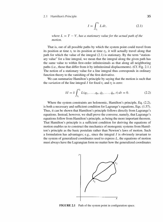
“M02 Goldstein ISBN C02” — 2011/2/15 — page 35 — #2
2.1 Hamilton’s Principle 35
I =∫ t2
t1L dt, (2.1)
where L = T − V , has a stationary value for the actual path of themotion.
That is, out of all possible paths by which the system point could travel fromits position at time t1 to its position at time t2, it will actually travel along thatpath for which the value of the integral (2.1) is stationary. By the term “station-ary value” for a line integral, we mean that the integral along the given path hasthe same value to within first-order infinitesimals as that along all neighboringpaths (i.e., those that differ from it by infinitesimal displacements). (Cf. Fig. 2.1.)The notion of a stationary value for a line integral thus corresponds in ordinaryfunction theory to the vanishing of the first derivative.
We can summarize Hamilton’s principle by saying that the motion is such thatthe variation of the line integral I for fixed t1 and t2 is zero:
δ I = δ
∫ t2
t1L(q1, . . . , qn, q1, . . . , qn, t) dt = 0. (2.2)
Where the system constraints are holonomic, Hamilton’s principle, Eq. (2.2),is both a necessary and sufficient condition for Lagrange’s equations, Eqs. (1.57).Thus, it can be shown that Hamilton’s principle follows directly from Lagrange’sequations. Instead, however, we shall prove the converse, namely, that Lagrange’sequations follow from Hamilton’s principle, as being the more important theorem.That Hamilton’s principle is a sufficient condition for deriving the equations ofmotion enables us to construct the mechanics of monogenic systems from Hamil-ton’s principle as the basic postulate rather than Newton’s laws of motion. Sucha formulation has advantages; e.g., since the integral I is obviously invariant tothe system of generalized coordinates used to express L , the equations of motionmust always have the Lagrangian form no matter how the generalized coordinates
FIGURE 2.1 Path of the system point in configuration space.

“M02 Goldstein ISBN C02” — 2011/2/15 — page 36 — #3
36 Chapter 2 Variational Principles and Lagrange’s Equations
are transformed. More important, the formulation in terms of a variational prin-ciple is the route that is generally followed when we try to describe apparentlynonmechanical systems in the mathematical clothes of classical mechanics, as inthe theory of fields.
2.2 SOME TECHNIQUES OF THE CALCULUS OF VARIATIONS
Before demonstrating that Lagrange’s equations do follow from (2.2), we mustfirst examine the methods of the calculus of variations, for a chief problem of thiscalculus is to find the curve for which some given line integral has a stationaryvalue. (See website for necessary comments.)
Consider first the problem in an essentially one-dimensional form: We have afunction f (y, y, x) defined on a path y = y(x) between two values x1 and x2,where y is the derivative of y with respect to x . We wish to find a particular pathy(x) such that the line integral J of the function f between x1 and x2,
y ≡ dy
dx,
J =∫ x2
x1
f (y, y, x) dx, (2.3)
has a stationary value relative to paths differing infinitesimally from the correctfunction y(x). The variable x here plays the role of the parameter t , and we con-sider only such varied paths for which y(x1) = y1, y(x2) = y2. (Cf. Fig. 2.2.)Note that Fig. 2.2 does not represent configuration space. In the one-dimensionalconfiguration space, both the correct and varied paths are the segment of thestraight line connecting y1 and y2; the paths differ only in the functional rela-tion between y and x . The problem is one-dimensional, y is not a coordinate, it isa function of x .
FIGURE 2.2 Varied paths of the function of y(x) in the one-dimensional extremumproblem.
“M02 Goldstein ISBN C02” — 2011/2/15 — page 37 — #4
2.2 Some Techniques of the Calculus of Variations 37
We put the problem in a form that enables us to use the familiar apparatus ofthe differential calculus for finding the stationary points of a function. Since Jmust have a stationary value for the correct path relative to any neighboring path,the variation must be zero relative to some particular set of neighboring pathslabeled by an infinitesimal parameter α. Such a set of paths might be denoted byy(x, α), with y(x, 0) representing the correct path. For example, if we select anyfunction η(x) that vanishes at x = x1 and x = x2, then a possible set of variedpaths is given by
y(x, α) = y(x, 0)+ αη(x). (2.4)
For simplicity, it is assumed that both the correct path y(x) and the auxiliaryfunction η(x) are well-behaved functions—continuous and nonsingular betweenx1 and x2, with continuous first and second derivatives in the same interval. Forany such parametric family of curves, J in Eq. (2.3) is also a function of α:
J (α) =∫ x2
x1
f (y(x, α), y(x, α), x) dx, (2.5)
and the condition for obtaining a stationary point is the familiar one that(d J
dα
)α=0
= 0. (2.6)
By the usual methods of differentiating under the integral sign, we find that
d J
dα=∫ x2
x1
(∂ f
∂y
∂y
∂α+ ∂ f
∂ y
∂ y
∂α
)dx . (2.7)
Consider the second of these integrals:
∫ x2
x1
∂ f
∂ y
∂ y
∂αdx =
∫ x2
x1
∂ f
∂ y
∂2 y
∂x ∂αdx .
Integrating by parts, the integral becomes
∫ x2
x1
∂ f
∂ y
∂2 y
∂x ∂αdx = ∂ f
∂ y
∂y
∂α
∣∣∣∣x2
x1
−∫ x2
x1
d
dx
(∂ f
∂ y
)∂y
∂αdx . (2.8)
The conditions on all the varied curves are that they pass through the points(x1, y1), (x2, y2), and hence the partial derivative of y with respect to α at x1 andx2 must vanish. Therefore, the first term of (2.8) vanishes and Eq. (2.7) reduces to
d J
dα=∫ x2
x1
(∂ f
∂y− d
dx
∂ f
∂ y
)∂y
∂αdx .
The condition for a stationary value, Eq. (2.6), is therefore equivalent to the equa-tion
“M02 Goldstein ISBN C02” — 2011/2/15 — page 38 — #5
38 Chapter 2 Variational Principles and Lagrange’s Equations∫ x2
x1
(∂ f
∂y− d
dx
∂ f
∂ y
)(∂y
∂α
)0
dx = 0. (2.9)
Now, the partial derivative of y with respect to α occurring in Eq. (2.9) is afunction of x that is arbitrary except for continuity and end point conditions. Forexample, for the particular parametric family of varied paths given by Eq. (2.4),it is the arbitrary function η(x). We can therefore apply to Eq (2.9) the so-called“fundamental lemma” of the calculus of variations, which says if
∫ x2
x1
M(x)η(x) dx = 0 (2.10)
for all arbitrary functions η(x) continuous through the second derivative, thenM(x) must identically vanish in the interval (x1, x2). While a formal mathemat-ical proof of the lemma can be found in texts on the calculus of variations, thevalidity of the lemma is easily seen intuitively. We can imagine constructing afunction η that is positive in the immediate vicinity of any chosen point in theinterval and zero everywhere else. Equation (2.10) can then hold only if M(x)vanishes at that (arbitrarily) chosen point, which shows M must be zero through-out the interval. From Eq. (2.9) and the fundamental lemma, it therefore followsthat J can have a stationary value only if
∂ f
∂y− d
dx
(∂ f
∂ y
)= 0. (2.11)
The differential quantity,
(∂y
∂α
)0
dα ≡ δy, (2.12)
represents the infinitesimal departure of the varied path from the correct pathy(x) at the point x and thus corresponds to the virtual displacement introduced inChapter 1 (hence the notation δy). Similarly, the infinitesimal variation of J aboutthe correct path can be designated
(d J
dα
)0
dα ≡ δ J. (2.13)
The assertion that J is stationary for the correct path can thus be written
δ J =∫ x2
x1
(∂ f
∂y− d
dx
∂ f
∂ y
)δy dx = 0,
requiring that y(x) satisfy the differential equation (2.11). The δ-notation, intro-duced through Eqs. (2.12) and (2.13), may be used as a convenient shorthandfor treating the variation of integrals, remembering always that it stands for themanipulation of parametric families of varied paths such as Eq. (2.4).
“M02 Goldstein ISBN C02” — 2011/2/15 — page 39 — #6
2.2 Some Techniques of the Calculus of Variations 39
Some simple examples of the application of Eq. (2.11) (which clearlyresembles a Lagrange equation) may now be considered:
1. Shortest distance between two points in a plane. An element of length in aplane is
ds =√
dx2 + dy2
and the total length of any curve going between points 1 and 2 is
I =∫ 2
1ds =
∫ x2
x1
√1 +
(dy
dx
)2
dx .
The condition that the curve be the shortest path is that I be a minimum. This isan example of the extremum problem as expressed by Eq. (2.3), with
f =√
1 + y2.
Substituting in (2.11) with
∂ f
∂y= 0,
∂ f
∂ y= y√
1 + y2,
we have
d
dx
(y√
1 + y2
)= 0
or
y√1 + y2
= c,
where c is constant. This solution can be valid only if
y = a,
where a is a constant related to c by
a = c√1 − c2
.
But this is clearly the equation of a straight line,
y = ax + b,

“M02 Goldstein ISBN C02” — 2011/2/15 — page 40 — #7
40 Chapter 2 Variational Principles and Lagrange’s Equations
where b is another constant of integration. Strictly speaking, the straight line hasonly been proved to be an extremum path, but for this problem it is obviously alsoa minimum. The constants of integration, a and b, are determined by the conditionthat the curve pass through the two end points, (x1, y1), (x2, y2).
In a similar fashion we can obtain the shortest distance between two pointson a sphere, by setting up the arc length on the surface of the sphere in terms ofthe angle coordinates of position on the sphere. In general, curves that give theshortest distance between two points on a given surface are called the geodesicsof the surface. (See website about part 2 below.)
2. Minimum surface of revolution. Suppose we form a surface of revolutionby taking some curve passing between two fixed end points (x1, y1) and (x2, y2)
defining the xy plane, and revolving it about the y axis (cf. Fig. 2.3a). The problemthen is to find that curve for which the surface area is a minimum. The area of astrip of the surface is 2πx ds = 2πx
√1 + y2 dx , and the total area is
2π∫ 2
1x√
1 + y2 dx .
The extremum of this integral is again given by (2.11) where
f = x√
1 + y2
and
∂ f
∂y= 0,
∂ f
∂ y= x y√
1 + y2.
Equation (2.11) becomes in this case
FIGURE 2.3a Minimum surface of revolution. Note that this figure is drawn for y1 andy2 having the same sign relative to the rotation axis. This is not assumed in the generalsolution.
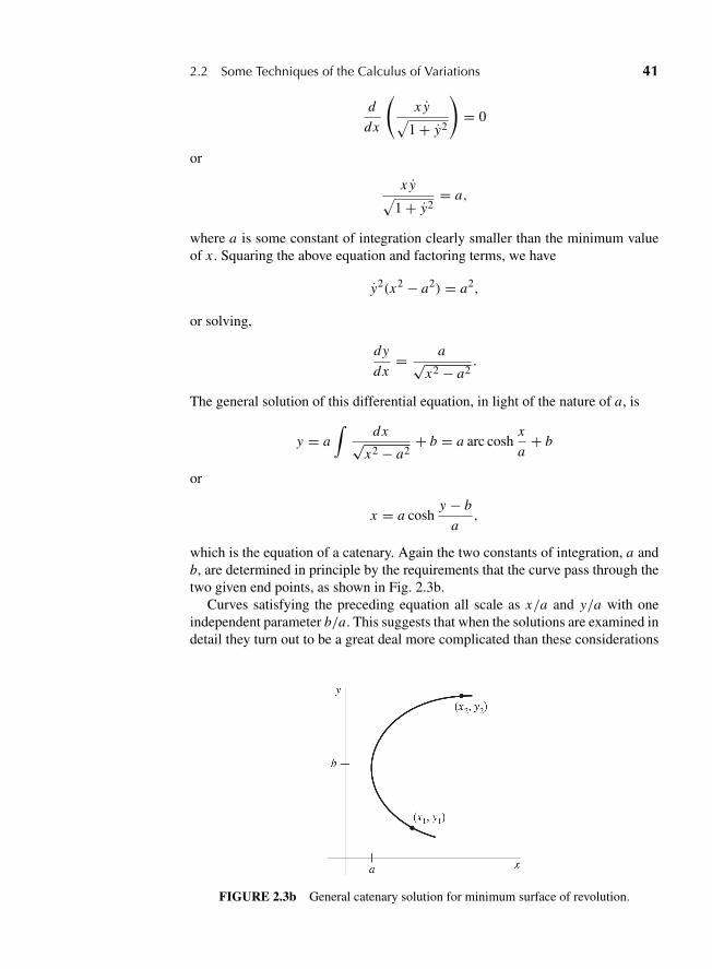
“M02 Goldstein ISBN C02” — 2011/2/15 — page 41 — #8
2.2 Some Techniques of the Calculus of Variations 41
d
dx
(x y√
1 + y2
)= 0
or
x y√1 + y2
= a,
where a is some constant of integration clearly smaller than the minimum valueof x . Squaring the above equation and factoring terms, we have
y2(x2 − a2) = a2,
or solving,
dy
dx= a√
x2 − a2.
The general solution of this differential equation, in light of the nature of a, is
y = a∫
dx√x2 − a2
+ b = a arc coshx
a+ b
or
x = a coshy − b
a,
which is the equation of a catenary. Again the two constants of integration, a andb, are determined in principle by the requirements that the curve pass through thetwo given end points, as shown in Fig. 2.3b.
Curves satisfying the preceding equation all scale as x/a and y/a with oneindependent parameter b/a. This suggests that when the solutions are examined indetail they turn out to be a great deal more complicated than these considerations
FIGURE 2.3b General catenary solution for minimum surface of revolution.
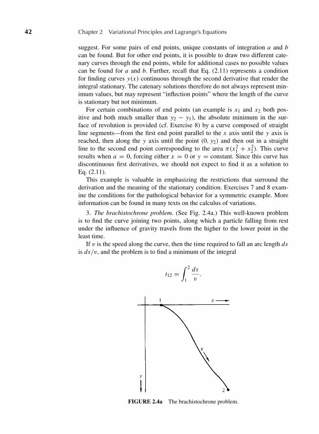
“M02 Goldstein ISBN C02” — 2011/2/15 — page 42 — #9
42 Chapter 2 Variational Principles and Lagrange’s Equations
suggest. For some pairs of end points, unique constants of integration a and bcan be found. But for other end points, it is possible to draw two different cate-nary curves through the end points, while for additional cases no possible valuescan be found for a and b. Further, recall that Eq. (2.11) represents a conditionfor finding curves y(x) continuous through the second derivative that render theintegral stationary. The catenary solutions therefore do not always represent min-imum values, but may represent “inflection points” where the length of the curveis stationary but not minimum.
For certain combinations of end points (an example is x1 and x2 both pos-itive and both much smaller than y2 − y1), the absolute minimum in the sur-face of revolution is provided (cf. Exercise 8) by a curve composed of straightline segments—from the first end point parallel to the x axis until the y axis isreached, then along the y axis until the point (0, y2) and then out in a straightline to the second end point corresponding to the area π(x2
1 + x22). This curve
results when a = 0, forcing either x = 0 or y = constant. Since this curve hasdiscontinuous first derivatives, we should not expect to find it as a solution toEq. (2.11).
This example is valuable in emphasizing the restrictions that surround thederivation and the meaning of the stationary condition. Exercises 7 and 8 exam-ine the conditions for the pathological behavior for a symmetric example. Moreinformation can be found in many texts on the calculus of variations.
3. The brachistochrone problem. (See Fig. 2.4a.) This well-known problemis to find the curve joining two points, along which a particle falling from restunder the influence of gravity travels from the higher to the lower point in theleast time.
If v is the speed along the curve, then the time required to fall an arc length dsis ds/v, and the problem is to find a minimum of the integral
t12 =∫ 2
1
ds
v.
FIGURE 2.4a The brachistochrone problem.
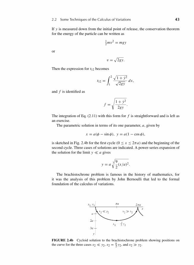
“M02 Goldstein ISBN C02” — 2011/2/15 — page 43 — #10
2.2 Some Techniques of the Calculus of Variations 43
If y is measured down from the initial point of release, the conservation theoremfor the energy of the particle can be written as
12 mv2 = mgy
or
v =√
2gy.
Then the expression for t12 becomes
t12 =∫ 2
1
√1 + y2√
2gydx,
and f is identified as
f =√
1 + y2
2gy.
The integration of Eq. (2.11) with this form for f is straightforward and is left asan exercise.
The parametric solution in terms of its one parameter, a, given by
x = a(φ − sinφ), y = a(1 − cosφ),
is sketched in Fig. 2.4b for the first cycle (0 ≤ x ≤ 2πa) and the beginning of thesecond cycle. Three cases of solutions are indicated. A power-series expansion ofthe solution for the limit y � a gives
y = a3
√9
2(x/a)2.
The brachistochrone problem is famous in the history of mathematics, forit was the analysis of this problem by John Bernoulli that led to the formalfoundation of the calculus of variations.
FIGURE 2.4b Cycloid solution to the brachistochrone problem showing positions onthe curve for the three cases x2 � y2, x2 = π
2 y2, and x2 � y2.
“M02 Goldstein ISBN C02” — 2011/2/15 — page 44 — #11
44 Chapter 2 Variational Principles and Lagrange’s Equations
2.3 DERIVATION OF LAGRANGE’S EQUATIONSFROM HAMILTON’S PRINCIPLE
The fundamental problem of the calculus of variations is easily generalized to thecase where f is a function of many independent variables yi , and their derivativesyi . (Of course, all these quantities are considered as functions of the parametricvariable x .) Then a variation of the integral J ,
δ J = δ
∫ 2
1f (y1(x); y2(x), . . . , y1(x); y2(x), . . . , x) dx, (2.14)
is obtained, as before, by considering J as a function of parameter α that labels apossible set of curves y1(x, α). Thus, we may introduce α by setting
y1(x, α) = y1(x, 0)+ αη1(x),y2(x, α) = y2(x, 0)+ αη2(x),
......
...
(2.15)
where y1(x, 0), y2(x, 0), etc., are the solutions of the extremum problem (to beobtained) and η1, η2, etc., are independent functions of x that vanish at the endpoints and that are continuous through the second derivative, but otherwise arecompletely arbitrary.
The calculation proceeds as before. The variation of J is given in terms of
∂ J
∂αdα =
∫ 2
1
∑i
(∂ f
∂yi
∂yi
∂αdα + ∂ f
∂ yi
∂ yi
∂αdα
)dx . (2.16)
Again we integrate by parts the integral involved in the second sum of Eq. (2.16):
∫ 2
1
δ f
∂ yi
∂2 yi
∂α ∂xdx = ∂ f
∂ yi
∂yi
∂α
∣∣∣∣2
1−∫ 2
1
∂yi
∂α
d
dx
(∂ f
∂ yi
)dx,
where the first term vanishes because all curves pass through the fixed end points.Substituting in (2.16), δ J becomes
δ J =∫ 2
1
∑i
(∂ f
∂yi− d
dx
∂ f
∂ yi
)δyi dx, (2.17)
where, in analogy with (2.12), the variation δyi is
δyi =(∂yi
∂α
)0
dα.
Since the y variables are independent, the variations δyi are independent (e.g.,the functions ηi (x) will be independent of each other). Hence, by an obviousextension of the fundamental lemma (cf. Eq. (2.10)), the condition that δ J is zero
“M02 Goldstein ISBN C02” — 2011/2/15 — page 45 — #12
2.4 Extending Hamilton’s Principle to Systems with Constraints 45
requires that the coefficients of the δyi separately vanish:
∂ f
∂yi− d
dx
∂ f
∂ yi= 0, i = 1, 2, . . . , n. (2.18)
Equations (2.18) represent the appropriate generalization of (2.11) to sev-eral variables and are known as the Euler-Lagrange differential equations. Theirsolutions represent curves for which the variation of an integral of the form givenin (2.14) vanishes. Further generalizations of the fundamental variational prob-lem are easily possible. Thus, we can take f as a function of higher derivativesy,...y , etc., leading to equations different from (2.18). Or we can extend it to cases
where there are several parameters x j and the integral is then multiple, with falso involving as variables derivatives of yi with respect to each of the parametersx j . Finally, it is possible to consider variations in which the end points are notheld fixed.
For present purposes, what we have derived here suffices, for the integral inHamilton’s principle,
I =∫ 2
1L(qi , qi , t) dt, (2.19)
has just the form stipulated in (2.14) with the transformation
x → t
yi → qi
f (yi , yi , x)→ L(qi , qi , t).
In deriving Eqs. (2.18), we assumed that the yi variables are independent. Thecorresponding condition in connection with Hamilton’s principle is that the gen-eralized coordinates qi be independent, which requires that the constraints beholonomic. The Euler-Lagrange equations corresponding to the integral I thenbecome the Lagrange equations of motion,
d
dt
∂L
∂ qi− ∂L
∂qi= 0, i = 1, 2, . . . , n,
and we have accomplished our original aim, to show that Lagrange’s equa-tions follow from Hamilton’s principle—for monogenic systems with holonomicconstraints.
2.4 EXTENDING HAMILTON’S PRINCIPLETO SYSTEMS WITH CONSTRAINTS
In Section 1.3 we solved problems with holonomic constraints by choosingcoordinates such that the constraint equations (1.37) become a trivial 0 = 0 set of
“M02 Goldstein ISBN C02” — 2011/2/15 — page 46 — #13
46 Chapter 2 Variational Principles and Lagrange’s Equations
equations. In this section we show that Hamilton’s principle can be used to solvesystems with holonomic constraints as well as certain types of non-holonomicsystems.
First consider holonomic constraints. When we derive Lagrange’s equationsfrom either Hamilton’s or D’Alembert’s principle, the holonomic constraintsappear in the last step when the variations in the qi were considered independentof each other. However, the virtual displacements in the δqI ’s may not be consis-tent with the constraints. If there are n variables and m constraint equations fαof the form of Eq. (1.37), the extra virtual displacements are eliminated by themethod of Lagrange undetermined multipliers.
We modify the integral in Eq. (2.19) to be
I =∫ 2
1
(L +
m∑α=1
λα fa
)dt, (2.20)
and allow the qα and the λα to vary independently to obtain n +m equations. Thevariations of the λα’s give the m constraint equations. The variations of the qi ’sgive
δ I =∫ 2
1dt
(n∑
i=1
(d
dt
∂L
∂qi− ∂L
∂qi+
m∑α=1
λa∂ fa
∂qi
)δqi
)= 0. (2.21)
However, the δqi ’s are not independent. We choose the λα’s so that m of theequations are satisfied for arbitrary δqi , and then choose the variations of the δqi
in the remaining n − m equations independently. Thus we obtain m equations ofthe form
d
dt
∂L
∂ qk− ∂L
∂qk+
m∑α=1
λa∂ fa
∂qk= 0, (2.22)
for k = 1, . . . ,m. The equality follows from the choice of the λα’s. We also havethe same expressions as Eq. (2.22) for k = m + 1, . . . , n, where the equalityfollows from the virtual variations of the δqi ’s.
This solves the system at the expense of introducing m functions λα . We canunderstand this by considering that Eqs. (2.22), for k = 1, . . . , n, can be writtenas
d
dt
∂L
∂qk− ∂L
∂qk= −
m∑α=1
λa∂ fa
∂qk= Qk, (2.23)
where the Qk are generalized forces. The functions, Qκ , have the magnitudes ofthe forces needed to produce the individual constraints; however, since the choiceof the “+” in the third term of Eq. (2.22) is arbitrary, we can mathematicallydetermine only the magnitudes of these generalized forces. You need to under-stand the physics to determine their directions.
“M02 Goldstein ISBN C02” — 2011/2/15 — page 47 — #14
2.4 Extending Hamilton’s Principle to Systems with Constraints 47
As an example, consider a smooth solid hemisphere of radius a placed withits flat side down and fastened to the Earth whose gravitational acceleration is g.Place a small mass M at the top of the hemisphere with an infinitesimal displace-ment off center so the mass slides down without friction. Choose coordinatesx , y, z centered on the base of the hemisphere with z vertical and the x-z planecontaining the initial motion of the mass.
Let θ be the angle from the top of the sphere to the mass. The Lagrangian isL = 1
2 M(x2 + y2 + z2) − mgz. The initial conditions allow us to ignore the
y coordinate, so the constraint equation is a − √x2 + z2 = 0. Expressing the
problem in terms of r2 = x2 + z2 and x/z = cos θ , Lagrange’s equations areMaθ2 − Mg cos θ + λ = 0, and Ma2θ + Mga sin θ = 0. Solve the secondequation and then the first to obtain
θ2 = −2g
acos θ + 2g
aand λ = Mg(3 cos θ − 2).
So λ is the magnitude of the force keeping the particle on the sphere and sinceλ = 0 when θ = cos−1( 2
3 ), the mass leaves the sphere at that angle.In general, nonholonomic constraints cannot be expressed by a variational
principle. One of the exceptions is semi-holonomic constraints where the con-straints can be written as a set of functions of the form
fα(q1, . . . , qn; q1, . . . , qn; t) = 0, (2.24)
where α = 1, 2, . . . ,m. Equation (2.24) commonly appears in the restricted form
fα =n∑
k=1
aakqk + a0 = 0, (2.25)
where the fα are a set of nonintegrable differential expressions and the aαk anda0 are functions of the qι and t . In these cases, since we cannot integrate theconstraints, there are more variables than equations. However, we can treat thevariations in the same fashion as before by writing*
δ
∫ t2
t1
(L +
m∑α=1
μa fa
)dt = 0, (2.26)
where the symbol μ is used to distinguish these multipliers from the holonomicLagrange multipliers. If we assume that μα = μα(t), the equations resulting fromthe virtual displacements are
d
dt
∂L
∂ qk− ∂L
∂qk= Qk = −
m∑α=1
μa∂ fa
∂ qk, (2.27)
*J. Ray, Amer. J. Phys. 34 (1202), 1969; E. J. Saletan & A. H. Comer, Amer. J. Phys. 38 (892–897),1970.
“M02 Goldstein ISBN C02” — 2011/2/15 — page 48 — #15
48 Chapter 2 Variational Principles and Lagrange’s Equations
and the δμα give the equations of constraint (2.23). These two sets (Eq. (2.26)and (2.27)) together constitute n + m equations for the n + m unknowns. Hencethey can be interpreted as equivalent to an n + m holonomic system with gen-eralized forces Qk . The generalization to μα = μα(q1, . . . , qn; q1, . . . , qn; t) isstraightforward.
As an example, consider a particle with the Lagrangian
L = 1
2m(x2 + y2 + z2)− V (x, y, z) (2.28)
subject to the nonholonomic constraint
f (x, x, y, y, z) = x y2 + x y + kz = 0, (2.29)
with k a constant. The resulting equations of motion are
mx + μy2 − ∂V
∂x= 0, (2.30a)
my + μx − ∂V
∂y= 0, (2.30b)
and
mz − ∂V
∂z= 0. (2.30c)
We now solve the four equations ((2.29) and (3.30)) to find x(t), y(t), z(t), andthe multiplier μ(t).
In this process we have obtained more information than was originally sought.Not only do we get the qk’s we set out to find, but we also get mλl ’s. Whatis the physical significance of the λl ’s? Suppose we remove the constraintson the system, but instead apply external forces Q′
k in such a manner as tokeep the motion of the system unchanged. The equations of motion likewiseremain the same. Clearly these extra applied forces must be equal to the forcesof constraint, for they are the forces applied to the system so as to satisfy thecondition of constraint. Under the influence of these forces Q′
k , the equations ofmotion are
d
dt
∂L
∂qk− ∂L
∂qk= Q′
k . (2.31)
But these must be identical with Eqs. (2.24). Hence, we can identify (2.25) withQ′
k , the generalized forces of constraint. In this type of problem we really do noteliminate the forces of constraint from the formulation. They are supplied as partof the answer.
Although it is not obvious, the version of Hamilton’s principle adopted herefor semiholonomic systems also requires that the constraints do no work in virtualdisplacements. This can be most easily seen by rewriting Hamilton’s principle in
“M02 Goldstein ISBN C02” — 2011/2/15 — page 49 — #16
2.4 Extending Hamilton’s Principle to Systems with Constraints 49
the form
δ
∫ t2
t1L dt = δ
∫ t2
t1T dt − δ
∫ t2
t1U dt = 0. (2.32)
If the variation of the integral over the generalized potential is carried out by theprocedures of Section 2.3, the principle takes the form
δ
∫ t2
t1T dt =
∫ t2
t1
∑k
[∂U
∂qk− d
dt
(∂U
∂qk
)]δqkdt; (2.33)
or, by Eq. (1.58),
δ
∫ t2
t1T dt = −
∫ t2
t1
∑k
Qkδqkdt. (2.34)
In this dress, Hamilton’s principle says that the difference in the time integral ofthe kinetic energy between two neighboring paths is equal to the negative of thetime integral of the work done in the virtual displacements between the paths.The work involved is that done only by the forces derivable from the generalizedpotential. The same Hamilton’s principle holds for both holonomic and semi-holonomic systems, it must be required that the additional forces of semiholo-nomic constraints do no work in the displacements δqk . This restriction parallelsthe earlier condition that the virtual work of the forces of holonomic constraintalso be zero (cf. Section 1.4). In practice, the restriction presents little handi-cap to the applications, as many problems in which the semiholonomic formal-ism is used relate to rolling without slipping, where the constraints are obviouslyworkless.
Note that Eq. (2.20) is not the most general type of nonholonomic constraint;e.g., it does not include equations of constraint in the form of inequalities. Onthe other hand, it does include holonomic constraints. A holonomic equation ofconstraint,
f (q1, q2, q3, . . . , qn, t) = 0, (2.35)
is equivalent to (2.20) with no dependence on qk . Thus, the Lagrange multipliermethod can be used also for holonomic constraints when (1) it is inconvenient toreduce all the q’s to independent coordinates or (2) we might wish to obtain theforces of constraint.
As another example of the method, let us consider the following somewhattrivial illustration—a hoop rolling, without slipping, down an inclined plane. Inthis example, the constraint of “rolling” is actually holonomic, but this fact willbe immaterial to our discussion. On the other hand, the holonomic constraint thatthe hoop be on the inclined plane will be contained implicitly in our choice ofgeneralized coordinates.

“M02 Goldstein ISBN C02” — 2011/2/15 — page 50 — #17
50 Chapter 2 Variational Principles and Lagrange’s Equations
FIGURE 2.5 A hoop rolling down an inclined plane.
The two generalized coordinates are x , θ , as in Fig. 2.5, and the equation ofrolling constraint is
r dθ = dx .
The kinetic energy can be resolved into kinetic energy of motion of the centerof mass plus the kinetic energy of motion about the center of mass:
T = 12 Mx2 + 1
2 Mr2θ2.
The potential energy is
V = Mg(l − x) sinφ,
where l is the length of the inclined plane and the Lagrangian is
L = T − V
= Mx2
2+ Mr2θ2
2− Mg(l − x) sinφ. (2.36)
Since there is one equation of constraint, only one Lagrange multiplier λ isneeded. The coefficients appearing in the constraint equation are:
aθ = r, ax = −1.
The two Lagrange equations therefore are
Mx − Mg sinφ + λ = 0, (2.37)
Mr2θ − λr = 0, (2.38)
which along with the equation of constraint,
r θ = x, (2.39)
constitutes three equations for three unknowns, θ , x , λ.
“M02 Goldstein ISBN C02” — 2011/2/15 — page 51 — #18
2.5 Advantages of a Variational Principle Formulation 51
Differentiating (2.39) with respect to time, we have
r θ = x .
Hence, from (2.38)
Mx = λ,
and (2.37) becomes
x = g sinφ
2
along with
λ = Mg sinφ
2
and
θ = g sinφ
2r.
Thus, the hoop rolls down the incline with only one-half the acceleration it wouldhave slipping down a frictionless plane, and the friction force of constraint isλ = Mg sinφ/2.
2.5 ADVANTAGES OF A VARIATIONAL PRINCIPLE FORMULATION
Although we can extend the original formulation of Hamilton’s principle (2.2) toinclude some nonholonomic constraints, in practice this formulation of mechanicsis most useful when a Lagrangian of independent coordinates can be set upfor the system. The variational principle formulation has been justly describedas “elegant,” for in the compact Hamilton’s principle is contained all of themechanics of holonomic systems with forces derivable from potentials. Theprinciple has the further merit that it involves only physical quantities thatcan be defined without reference to a particular set of generalized coordi-nates, namely, the kinetic and potential energies. The formulation is there-fore automatically invariant with respect to the choice of coordinates for thesystem.
From the variational Hamilton’s principle, it is also obvious why the Lagrangianis always uncertain to a total time derivative of any function of the coordinatesand time, as mentioned at the end of Section 1.4. The time integral of such a totalderivative between points 1 and 2 depends only on the values of the arbitraryfunction at the end points. As the variation at the end points is zero, the additionof the arbitrary time derivative to the Lagrangian does not affect the variationalbehavior of the integral.
“M02 Goldstein ISBN C02” — 2011/2/15 — page 52 — #19
52 Chapter 2 Variational Principles and Lagrange’s Equations
Another advantage is that the Lagrangian formulation can be easily extendedto describe systems that are not normally considered in dynamics—such asthe elastic field, the electromagnetic field, and field properties of elementaryparticles. Some of these generalizations will be considered later, but as threesimple examples of its application outside the usual framework of mechanics, letus consider the cases of an RL circuit, an LC circuit, and coupled circuits.
We consider the physical system of a battery of voltage V in series with aninductance L and a resistance of value R and choose the electric charge q asthe dynamical variable. The inductor acts as the kinetic energy term since theinductive effect depends upon the time rate of change of the charge. The resistorprovides a dissipative term and the potential energy is qV . The dynamic terms inLagrange’s equation with dissipation (1.70) are
T = 12 Lq2, F = 1
2 Rq2,
and potential energy = qV . The equation of motion is
V = Lq + Rq = L I + RI, (2.40)
where I = q is the electric current. A solution for a battery connected to thecircuit at time t = 0 is
I = I0(1 − e−Rt/L),
where I0 = V/R is the final steady-state current flow.The mechanical analog for this is a sphere of radius a and effective mass m′
falling in a viscous fluid of constant density and viscosity η under the force ofgravity. The effective mass is the difference between the actual mass and the massof the displaced fluid, and the direction of motion is along the y axis. For thissystem,
T = 12 m′ y2, F = 3πηa y2,
and potential energy = m′gy, where the frictional drag force, F f = 6πηa y,called Stokes’ law, was given at the end of Section 1.5.
The equation of motion is given by Lagrange’s equations (1.70) as
m′g = m′ y + 6πηa y.
Using v = y, the solution (if the motion starts from rest at t = 0), is
v = vo(1 − e−t/τ )
where τ = m′/(6πηa) is a measure of the time it takes for the sphere to reach1/e of its terminal speed of v0 = m′g/6πηa.
Another example from electrical circuits is an inductance, L , in series witha capacitance, C . The capacitor acts as a source of potential energy given by
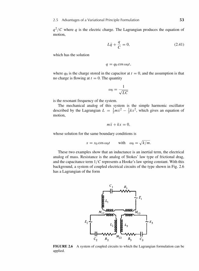
“M02 Goldstein ISBN C02” — 2011/2/15 — page 53 — #20
2.5 Advantages of a Variational Principle Formulation 53
q2/C where q is the electric charge. The Lagrangian produces the equation ofmotion,
Lq + q
C= 0, (2.41)
which has the solution
q = q0 cosω0t,
where q0 is the charge stored in the capacitor at t = 0, and the assumption is thatno charge is flowing at t = 0. The quantity
ω0 = 1√LC
is the resonant frequency of the system.The mechanical analog of this system is the simple harmonic oscillator
described by the Lagrangian L = 12 mx2 − 1
2 kx2, which gives an equation ofmotion,
mx + kx = 0,
whose solution for the same boundary conditions is
x = x0 cosω0t with ω0 =√
k/m.
These two examples show that an inductance is an inertial term, the electricalanalog of mass. Resistance is the analog of Stokes’ law type of frictional drag,and the capacitance term 1/C represents a Hooke’s law spring constant. With thisbackground, a system of coupled electrical circuits of the type shown in Fig. 2.6has a Lagrangian of the form
FIGURE 2.6 A system of coupled circuits to which the Lagrangian formulation can beapplied.

“M02 Goldstein ISBN C02” — 2011/2/15 — page 54 — #21
54 Chapter 2 Variational Principles and Lagrange’s Equations
L = 1
2
∑j
L j q2j +
1
2
∑jk
j =k
M jkq j qk −∑
j
q2j
2C j+∑
j
e j (t)q j ,
and a dissipation function
F = 1
2
∑j
R j q2j .
where the mutual inductance terms, M jkq j qk , are added to take into account thecoupling between inductors. The Lagrange equations are
L jd2q j
dt2+∑
kj =k
M jkd2qk
dt2+ R j
dq j
dt+ q j
C j= E j (t). (2.42)
where the E j (t) terms are the external emf’s.This description of two different physical systems by Lagrangians of the same
form means that all the results and techniques devised for investigating one of thesystems can be taken over immediately and applied to the other. In this particularcase, the study of the behavior of electrical circuits has been pursued intenselyand some special techniques have been developed; these can be directly appliedto the corresponding mechanical systems. Much work has been done in formulat-ing equivalent electrical problems for mechanical or acoustical systems, and viceversa. Terms hitherto reserved for electrical circuits (reactance, susceptance, etc.)are now commonly found in treatises on the theory of vibrations of mechanicalsystems.
Additionally, one type of generalization of mechanics is due to a subtlerform of equivalence. We have seen that the Lagrangian and Hamilton’s principletogether form a compact invariant way of obtaining the mechanical equations ofmotion. This possibility is not reserved for mechanics only; in almost every fieldof physics variational principles can be used to express the “equations of motion,”whether they be Newton’s equations, Maxwell’s equations, or the Schrodingerequation. Consequently, when a variational principle is used as the basis of theformulation, all such fields will exhibit, at least to some degree, a structural anal-ogy. When the results of experiments show the need for alterating the physicalcontent in the theory of one field, this degree of analogy has often indicatedhow similar alterations may be carried out in other fields. Thus, the experimentsperformed early in this century showed the need for quantization of both elec-tromagnetic radiation and elementary particles. The methods of quantization,however, were first developed for particle mechanics, starting essentially from theLagrangian formulation of classical mechanics. By describing the electromag-netic field by a Lagrangian and corresponding Hamilton’s variational principle,it is possible to carry over the methods of particle quantization to construct aquantum electrodynamics (cf. Sections 13.5 and 13.6).
“M02 Goldstein ISBN C02” — 2011/2/15 — page 55 — #22
2.6 Conservation Theorems and Symmetry Properties 55
2.6 CONSERVATION THEOREMS AND SYMMETRY PROPERTIES
Thus far, we have been concerned primarily with obtaining the equations ofmotion, but little has been said about how to solve them for a particular problemonce they are obtained. In general, this is a question of mathematics. A systemof n degrees of freedom will have n differential equations that are second orderin time. The solution of each equation will require two integrations resulting, alltold, in 2n constants of integration. In a specific problem these constants will bedetermined by the initial conditions, i.e., the initial values of the nq j ’s and thenq j ’s. Sometimes the equations of motion will be integrable in terms of knownfunctions, but not always. In fact, the majority of problems are not completelyintegrable. However, even when complete solutions cannot be obtained, it is oftenpossible to extract a large amount of information about the physical nature ofthe system motion. Indeed, such information may be of greater interest to thephysicist than the complete solution for the generalized coordinates as a functionof time. It is important, therefore, to see how much can be stated about the motionof a given system without requiring a complete integration of the problem.*
In many problems a number of first integrals of the equations of motion can beobtained immediately; by this we mean relations of the type
f (q1, q2, . . . , q1, q2, . . . , t) = constant, (2.43)
which are first-order differential equations. These first integrals are of interestbecause they tell us something physically about the system. They include, in fact,the conservation laws obtained in Chapter 1.
Let us consider as an example a system of mass points under the influence offorces derived from potentials dependent on position only. Then
∂L
∂ xi≡ ∂T
∂ xi− ∂V
∂ xi= ∂T
∂ xi= ∂
∂ xi
∑ 1
2mi(x2
i + y2i + z2
i
)= mi xi = pix ,
which is the x component of the linear momentum associated with the i thparticle. This result suggests an obvious extension to the concept of momentum.The generalized momentum associated with the coordinate q j shall be defined as
p j = ∂L
∂q j. (2.44)
The terms canonical momentum and conjugate momentum are often also used forp j . Notice that if q j is not a Cartesian coordinate, p j does not necessarily havethe dimensions of a linear momentum. Further, if there is a velocity-dependentpotential, then even with a Cartesian coordinate q j the associated generalized
*In this and succeeding sections it will be assumed, unless otherwise specified, the system is such thatits motion is completely described by a Hamilton’s principle of the form (2.2).
“M02 Goldstein ISBN C02” — 2011/2/15 — page 56 — #23
56 Chapter 2 Variational Principles and Lagrange’s Equations
momentum will not be identical with the usual mechanical momentum. Thus,in the case of a group of particles in an electromagnetic field, the Lagrangian is(cf. 1.63)
L =∑
i
1
2mi r
2i −
∑i
qiφ(xi )+∑
i
qi A(xi ) ? ri
(qi here denotes charge) and the generalized momentum conjugate to xi is
pix = ∂L
∂ xi= mi xi + qi Ax , (2.45)
i.e., mechanical momentum plus an additional term.If the Lagrangian of a system does not contain a given coordinate q j (although
it may contain the corresponding velocity q j ), then the coordinate is said to becyclic or ignorable. This definition is not universal, but it is the customary oneand will be used here. The Lagrange equation of motion,
d
dt
∂L
∂q j− ∂L
∂q j= 0,
reduces, for a cyclic coordinate, to
d
dt
∂L
∂ q j= 0
or
dp j
dt= 0,
which mean that
p j = constant. (2.46)
Hence, we can state as a general conservation theorem that the generalizedmomentum conjugate to a cyclic coordinate is conserved.
Note that the derivation of Eq. (2.46) assumes that q j is a generalized coordi-nate; one that is linearly independent of all the other coordinates. When equationsof constraint exist, all the coordinates are not linearly independent. For exam-ple, the angular coordinate θ is not present in the Lagrangian of a hoop rollingwithout slipping in a horizontal plane that was previously discussed, but the angleappears in the constraint equations rdθ = dx . As a result, the angular momentum,pθ = mr2θ , is not a constant of the motion.
Equation (2.46) constitutes a first integral of the form (2.43) for the equa-tions of motion. It can be used formally to eliminate the cyclic coordinatefrom the problem, which can then be solved entirely in terms of the remain-ing generalized coordinates. Briefly, the procedure, originated by Routh, consistsin modifying the Lagrangian so that it is no longer a function of the general-ized velocity corresponding to the cyclic coordinate, but instead involves only
“M02 Goldstein ISBN C02” — 2011/2/15 — page 57 — #24
2.6 Conservation Theorems and Symmetry Properties 57
its conjugate momentum. The advantage in so doing is that p j can then beconsidered one of the constants of integration, and the remaining integrationsinvolve only the noncyclic coordinates. We shall defer a detailed discussion ofRouth’s method until the Hamiltonian formulation (to which it is closely related)is treated.
Note that the conditions for the conservation of generalized momenta are moregeneral than the two momentum conservation theorems previously derived. Forexample, they furnish a conservation theorem for a case in which the law of actionand reaction is violated, namely, when electromagnetic forces are present. Sup-pose we have a single particle in a field in which neither φ nor A depends on x .Then x nowhere appears in L and is therefore cyclic. The corresponding canoni-cal momentum px must therefore be conserved. From (1.63) this momentum nowhas the form
px = mx + q Ax = constant. (2.47)
In this case, it is not the mechanical linear momentum mx that is conserved butrather its sum with q Ax .* Nevertheless, it should still be true that the conser-vation theorems of Chapter 1 are contained within the general rule for cycliccoordinates; with proper restrictions (2.46) should reduce to the theorems ofSection 1.2.
We first consider a generalized coordinate q j , for which a change dq j repre-sents a translation of the system as a whole in some given direction. An examplewould be one of the Cartesian coordinates of the center of mass of the system.Then clearly q j cannot appear in T , for velocities are not affected by a shift in theorigin, and therefore the partial derivative of T with respect to q j must be zero.Further, we will assume conservative systems for which V is not a function of thevelocities, so as to eliminate such complications as electromagnetic forces. TheLagrange equation of motion for a coordinate so defined then reduces to
d
dt
∂T
∂ q j≡ p j = − ∂V
∂q j≡ Q j . (2.48)
We will now show that (2.48) is the equation of motion for the total linearmomentum, i.e., that Q j represents the component of the total force alongthe direction of translation of q j , and p j is the component of the total linearmomentum along this direction. In general, the generalized force Q j is given byEq. (1.49):
Q j =∑
i
Fi ?∂ri
∂q j.
Since dq j corresponds to a translation of the system along some axis, the vectorsri (q j ) and ri (q j + dq j ) are related as shown in Fig. 2.7. By the definition of a
*It can be shown from classical electrodynamics that under these conditions, i.e., neither A nor φdepending on x , that q Ax is exactly the x-component of the electromagnetic linear momentum of thefield associated with the charge q.
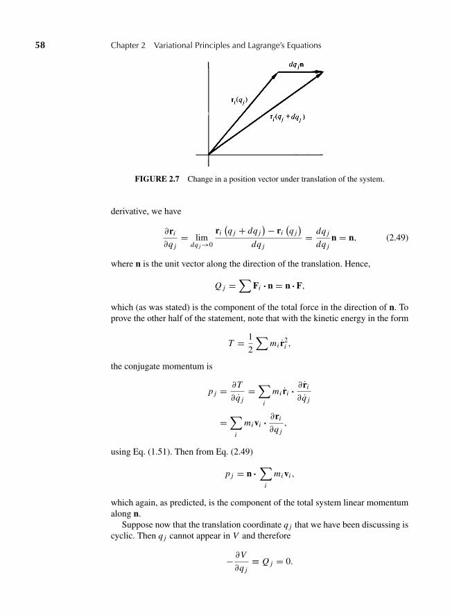
“M02 Goldstein ISBN C02” — 2011/2/15 — page 58 — #25
58 Chapter 2 Variational Principles and Lagrange’s Equations
FIGURE 2.7 Change in a position vector under translation of the system.
derivative, we have
∂ri
∂q j= lim
dq j→0
ri(q j + dq j
)− ri(q j)
dq j= dq j
dq jn = n, (2.49)
where n is the unit vector along the direction of the translation. Hence,
Q j =∑
Fi ?n = n ?F,
which (as was stated) is the component of the total force in the direction of n. Toprove the other half of the statement, note that with the kinetic energy in the form
T = 1
2
∑mi r2
i ,
the conjugate momentum is
p j = ∂T
∂q j=∑
i
mi ri ?∂ ri
∂q j
=∑
i
mi vi ?∂ri
∂q j,
using Eq. (1.51). Then from Eq. (2.49)
p j = n ?∑
i
mi vi ,
which again, as predicted, is the component of the total system linear momentumalong n.
Suppose now that the translation coordinate q j that we have been discussing iscyclic. Then q j cannot appear in V and therefore
− ∂V
∂q j≡ Q j = 0.

“M02 Goldstein ISBN C02” — 2011/2/15 — page 59 — #26
2.6 Conservation Theorems and Symmetry Properties 59
But this is simply the familiar conservation theorem for linear momentum—thatif a given component of the total applied force vanishes, the corresponding com-ponent of the linear momentum is conserved.
In a similar fashion, it can be shown that if a cyclic coordinate q j is such thatdq j corresponds to a rotation of the system of particles around some axis, thenthe conservation of its conjugate momentum corresponds to conservation of anangular momentum. By the same argument used above, T cannot contain q j , fora rotation of the coordinate system cannot affect the magnitude of the velocities.Hence, the partial derivative of T with respect to q j must again be zero, and sinceV is independent of q j , we once more get Eq. (2.48). But now we wish to showthat with q j a rotation coordinate the generalized force is the component of thetotal applied torque about the axis of rotation, and p j is the component of the totalangular momentum along the same axis.
The generalized force Q j is again given by
Q j =∑
i
Fi ?∂ri
∂q j,
only the derivative now has a different meaning. Here the change in q j mustcorrespond to an infinitesimal rotation of the vector ri , keeping the magnitudeof the vector constant. From Fig. 2.8, the magnitude of the derivative can easilybe obtained:
|dri | = ri sin θ dq j and
∣∣∣∣ ∂ri
∂q j
∣∣∣∣ = ri sin θ,
FIGURE 2.8 Change of a position vector under rotation of the system.
“M02 Goldstein ISBN C02” — 2011/2/15 — page 60 — #27
60 Chapter 2 Variational Principles and Lagrange’s Equations
and its direction is perpendicular to both ri and n. Clearly, the derivative can bewritten in vector form as
∂ri
∂q j= n3 ri . (2.50)
With this result, the generalized force becomes
Q j =∑
i
Fi ? n3 ri
=∑
i
n ? ri 3Fi ,
reducing to
Q j = n ?∑
i
Ni = n ?N,
which proves the first part. A similar manipulation of p j with the aid of Eq. (2.50)provides proof of the second part of the statement:
p j = ∂T
∂q j=∑
i
mi vi ?∂ri
∂q j=∑
i
n ? ri 3mi vi = n ?∑
i
Li = n ?L.
Summarizing these results, we see that if the rotation coordinate q j is cyclic,then Q j , which is the component of the applied torque along n, vanishes, andthe component of L along n is constant. Here we have recovered the angularmomentum conservation theorem out of the general conservation theorem relatingto cyclic coordinates.
The significance of cyclic translation or rotation coordinates in relation to theproperties of the system deserves some comment at this point. If a generalizedcoordinate corresponding to a displacement is cyclic, it means that a translationof the system, as if rigid, has no effect on the problem. In other words, if the sys-tem is invariant under translation along a given direction, the corresponding linearmomentum is conserved. Similarly, the fact that a generalized rotation coordinateis cyclic (and therefore the conjugate angular momentum conserved) indicatesthat the system is invariant under rotation about the given axis. Thus, the momen-tum conservation theorems are closely connected with the symmetry propertiesof the system. If the system is spherically symmetric, we can say without furtherado that all components of angular momentum are conserved. Or, if the system issymmetric only about the z axis, then only Lz will be conserved, and so on forthe other axes. These symmetry considerations can often be used with relativelycomplicated problems to determine by inspection whether certain constants of themotion exist. (cf. Noether’s theorem—Sec. 13.7.)
Suppose, for example, the system consists of a set of mass points moving ina potential field generated by fixed sources uniformly distributed on an infiniteplane, say, the z = 0 plane. (The sources might be a mass distribution if the forces
“M02 Goldstein ISBN C02” — 2011/2/15 — page 61 — #28
2.7 Energy Function and the Conservation of Energy 61
were gravitational, or a charge distribution for electrostatic forces.) Then the sym-metry of the problem is such that the Lagrangian is invariant under a translationof the system of particles in the x- or y-directions (but not in the z-direction) andalso under a rotation about the z axis. It immediately follows that the x- andy-components of the total linear momentum, Px and Py , are constants of themotion along with Lz , the z-component of the total angular momentum. However,if the sources were restricted only to the half plane, x ≥ 0, then the symmetry fortranslation along the x axis and for rotation about the z axis would be destroyed.In that case, Px and Lz could not be conserved, but Py would remain a constant ofthe motion. We will encounter the connections between the constants of motionand the symmetry properties of the system several times in the following chapters.
2.7 ENERGY FUNCTION AND THE CONSERVATION OF ENERGY
Another conservation theorem we should expect to obtain in the Lagrangianformulation is the conservation of total energy for systems where the forces arederivable from potentials dependent only upon position. Indeed, it is possible todemonstrate a conservation theorem for which conservation of total energy repre-sents only a special case. Consider a general Lagrangian, which will be a functionof the coordinates q j and the velocities q j and may also depend explicitly on thetime. (The explicit time dependence may arise from the time variation of externalpotentials, or from time-dependent constraints.) Then the total time derivative ofL is
d L
dt=∑
j
∂L
∂q j
dq j
dt+∑
j
∂L
∂ q j
dq j
dt+ ∂L
∂t. (2.51)
From Lagrange’s equations,
∂L
∂q j= d
dt
(∂L
∂ q j
),
and (2.51) can be rewritten as
d L
dt=∑
j
d
dt
(∂L
∂q j
)q j +
∑j
∂L
∂ q j
dq j
dt+ ∂L
∂t
or
d L
dt=∑
j
d
dt
(q j∂L
∂q j
)+ ∂L
∂t.
It therefore follows that
d
dt
⎛⎝∑
j
q j∂L
∂ q j− L
⎞⎠+ ∂L
∂t= 0. (2.52)
“M02 Goldstein ISBN C02” — 2011/2/15 — page 62 — #29
62 Chapter 2 Variational Principles and Lagrange’s Equations
The quantity in parentheses is oftentimes called the energy function* and will bedenoted by h:
h(q1, . . . , qn; q1, . . . , qn; t) =∑
j
q j∂L
∂ q j− L , (2.53)
and Eq. (2.52) can be looked on as giving the total time derivative of h:
dh
dt= −∂L
∂t. (2.54)
If the Lagrangian is not an explicit function of time, i.e., if t does not appearin L explicitly but only implicitly through the time variation of q and q , thenEq. (2.54) says that h is conserved. It is one of the first integrals of the motion andis sometimes referred to as Jacobi’s integral.†
Under certain circumstances, the function h is the total energy of the system.To determine what these circumstances are, we recall that the total kinetic energyof a system can always be written as
T = T0 + T1 + T2, (1.73)
where T0 is a function of the generalized coordinates only, T1(q, q) is linear in thegeneralized velocities, and T2(q, q) is a quadratic function of the q’s. For a verywide range of systems and sets of generalized coordinates, the Lagrangian can besimilarly decomposed as regards its functional behavior in the q variables:
L(q, q, t) = L0(q, t)+ L1(q, q, t)+ L2(q, q, t). (2.55)
Here L2 is a homogeneous function of the second degree (not merely quadratic)in q , while L1 is homogeneous of the first degree in q . There is no reason intrinsicto mechanics that requires the Lagrangian to conform to Eq. (2.55), but in fact itdoes for most problems of interest. The Lagrangian clearly has this form whenthe forces are derivable from a potential not involving the velocities. Even withthe velocity-dependent potentials, we note that the Lagrangian for a charged par-ticle in an electromagnetic field, Eq. (1.63), satisfies Eq. (2.55). Now, recall thatEuler’s theorem states that if f is a homogeneous function of degree n in thevariables xi , then
∑i
xi∂ f
∂xi= n f. (2.56)
*The energy function h is identical in value with the Hamiltonian H (See Chapter 8). It is givena different name and symbol here to emphasize that h is considered a function of n independentvariables q j and their time derivatives q j (along with the time), whereas the Hamiltonian will betreated as a function of 2n independent variables, q j , p j (and possibly the time).†This designation is most often confined to a first integral in the restricted three-body problem. How-ever, the integral there is merely a special case of the energy function h, and there is some historicalprecedent to apply the name Jacobi integral to the more general situation.
“M02 Goldstein ISBN C02” — 2011/2/15 — page 63 — #30
2.7 Energy Function and the Conservation of Energy 63
Applied to the function h, Eq. (2.53), for the Lagrangians of the form (2.55), thistheorem implies that
h = 2L2 + L1 − L = L2 − L0. (2.57)
If the transformation equations defining the generalized coordinates, Eqs. (1.38),do not involve the time explicitly, then by Eqs. (1.73) T = T2. If, further,the potential does not depend on the generalized velocities, then L2 = T andL0 = −V , so that
h = T + V = E, (2.58)
and the energy function is indeed the total energy. Under these circumstances,if V does not involve the time explicitly, neither will L . Thus, by Eq. (2.54), h(which is here the total energy), will be conserved.
Note that the conditions for conservation of h are in principle quite distinctfrom those that identify h as the total energy. We can have a set of generalizedcoordinates such that in a particular problem h is conserved but is not the totalenergy. On the other hand, h can be the total energy, in the form T + V , but notbe conserved. Also note that whereas the Lagrangian is uniquely fixed for eachsystem by the prescription L = T − U independent of the choice of generalizedcoordinates, the energy function h depends in magnitude and functional form onthe specific set of generalized coordinates. For one and the same system, variousenergy functions h of different physical content can be generated depending onhow the generalized coordinates are chosen.
The most common case that occurs in classical mechanics is one in which thekinetic energy terms are all of the form mq2
i /2 or p2i /2m and the potential energy
depends only upon the coordinates. For these conditions, the energy function isboth conserved and is also the total energy.
Finally, note that where the system is not conservative, but there are frictionalforces derivable from a dissipation function F , it can be easily shown that Fis related to the decay rate of h. When the equations of motion are given byEq. (1.70), including dissipation, then Eq. (2.52) has the form
dh
dt+ ∂L
∂t=∑
j
∂F∂ q j
q j .
By the definition of F , Eq. (1.67), it is a homogeneous function of the q’s ofdegree 2. Hence, applying Euler’s theorem again, we have
dh
dt= −2F − ∂L
∂t. (2.59)
If L is not an explicit function of time, and the system is such that h is the sameas the energy, then Eq. (2.59) says that 2F is the rate of energy dissipation,
d E
dt= −2F , (2.60)
a statement proved above (cf. Sec. 1.5) in less general circumstances.
“M02 Goldstein ISBN C02” — 2011/2/15 — page 64 — #31
64 Chapter 2 Variational Principles and Lagrange’s Equations
DERIVATIONS
1. Complete the solution of the brachistochrone problem begun in Section 2.2 and showthat the desired curve is a cycloid with a cusp at the initial point at which the particleis released. Show also that if the particle is projected with an initial kinetic energy12 mv2
0 that the brachistochrone is still a cycloid passing through the two points with a
cusp at a height z above the initial point given by v20 = 2gz.
2. Show that if the potential in the Lagrangian contains velocity-dependent terms, thecanonical momentum corresponding to a coordinate of rotation θ of the entire systemis no longer the mechanical angular momentum Lθ but is given by
pθ = Lθ −∑
i
n ? ri 3∇vi U,
where ∇v is the gradient operator in which the derivatives are with respect to thevelocity components and n is a unit vector in the direction of rotation. If the forces areelectromagnetic in character, the canonical momentum is therefore
pθ = Lθ +∑
i
n ? ri 3qi
cAi .
3. Prove that the shortest distance between two points in space is a straight line.
4. Show that the geodesics of a spherical surface are great circles, i.e., circles whosecenters lie at the center of the sphere.
EXERCISES
5. A particle is subjected to the potential V (x) = −Fx , where F is a constant. Theparticle travels from x = 0 to x = a in a time interval t0. Assume the motion of theparticle can be expressed in the form x(t) = A + B t +C t2. Find the values of A, B,and C such that the action is a minimum.
6. Find the Euler–Lagrange equation describing the brachistochrone curve for a particlemoving inside a spherical Earth of uniform mass density. Obtain a first integral forthis differential equation by analogy to the Jacobi integral h. With the help of thisintegral, show that the desired curve is a hypocycloid (the curve described by a pointon a circle rolling on the inside of a larger circle). Obtain an expression for the timeof travel along the brachistochrone between two points on Earth’s surface. How longwould it take to go from New York to Los Angeles (assumed to be 4800 km apart onthe surface) along a brachistochrone tunnel (assuming no friction) and how far belowthe surface would the deepest point of the tunnel be?
7. In Example 2 of Section 2.1 we considered the problem of the minimum surface ofrevolution. Examine the symmetric case x1 = x2, y2 = −y1 > 0, and express thecondition for the parameter a as a transcendental equation in terms of the dimension-less quantities k = x2/a, and α = y2/x2. Show that for α greater than a certain valueα0 two values of k are possible, for α = α0 only one value of k is possible, while ifα < α0 no real value of k (or a) can be found, so that no catenary solution exists inthis region. Find the value of α0, numerically if necessary.
“M02 Goldstein ISBN C02” — 2011/2/15 — page 65 — #32
Exercises 65
8. The broken-segment solution described in the text (cf. p. 42), in which the area ofrevolution is only that of the end circles of radius y1 and y2, respectively, is knownas the Goldschmidt solution. For the symmetric situation discussed in Exercise 7,obtain an expression for the ratio of the area generated by the catenary solutionsto that given by the Goldschmidt solution. Your result should be a function only ofthe parameters k and α. Show that for sufficiently large values of α at least one ofthe catenaries gives an area below that of the Goldschmidt solution. On the otherhand, show that if α = α0, the Goldschmidt solution gives a lower area than thecatenary.
9. A chain or rope of indefinite length passes freely over pulleys at heights y1 and y2above the plane surface of Earth, with a horizontal distance x2 − x1 between them.If the chain or rope has a uniform linear mass density, show that the problem offinding the curve assumed between the pulleys is identical with that of the prob-lem of minimum surface of revolution. (The transition to the Goldschmidt solutionas the heights y1 and y2 are changed makes for a striking lecture demonstration. SeeExercise 8.)
10. Suppose it is known experimentally that a particle fell a given distance y0 in a timet0 = √
2y0/g. The times of fall for distances other than y0 are not known. Sup-pose further that the Lagrangian for the problem is known, but that instead of solv-ing the equation of motion for y as a function of t , it is guessed that the functionalform is
y = at + bt2.
If the constants a and b are adjusted always so that the time to fall y0 is correctlygiven by t0, show directly that the integral∫ t0
0L dt
is an extremum for real values of the coefficients only when a = 0 and b = g/2.
11. When two billiard balls collide, the instantaneous forces between them are very largebut act only in an infinitesimal time �t , in such a manner that the quantity∫
�tF dt
remains finite. Such forces are described as impulsive forces, and the integral over�t is known as the impulse of the force. Show that if impulsive forces are presentLagrange’s equations may be transformed into(
∂L
∂q j
)f−(∂L
∂ q j
)i= S j ,
where the subscripts i and f refer to the state of the system before and after theimpulse, S j is the impulse of the generalized impulsive force corresponding to q j ,and L is the Lagrangian including all the nonimpulsive forces.
12. The term generalized mechanics has come to designate a variety of classical mechan-ics in which the Lagrangian contains time derivatives of qi higher than the first. Prob-lems for which
...x = f (x, x, x, t) have been referred to as “jerky” mechanics. Such
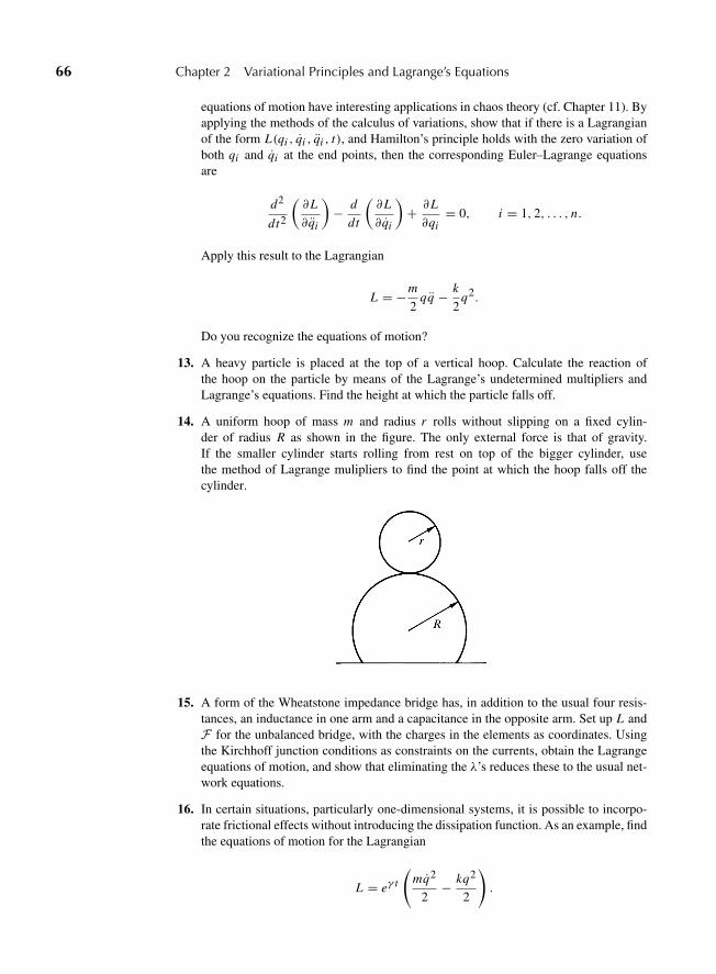
“M02 Goldstein ISBN C02” — 2011/2/15 — page 66 — #33
66 Chapter 2 Variational Principles and Lagrange’s Equations
equations of motion have interesting applications in chaos theory (cf. Chapter 11). Byapplying the methods of the calculus of variations, show that if there is a Lagrangianof the form L(qi , qi , qi , t), and Hamilton’s principle holds with the zero variation ofboth qi and qi at the end points, then the corresponding Euler–Lagrange equationsare
d2
dt2
(∂L
∂qi
)− d
dt
(∂L
∂qi
)+ ∂L
∂qi= 0, i = 1, 2, . . . , n.
Apply this result to the Lagrangian
L = −m
2qq − k
2q2.
Do you recognize the equations of motion?
13. A heavy particle is placed at the top of a vertical hoop. Calculate the reaction ofthe hoop on the particle by means of the Lagrange’s undetermined multipliers andLagrange’s equations. Find the height at which the particle falls off.
14. A uniform hoop of mass m and radius r rolls without slipping on a fixed cylin-der of radius R as shown in the figure. The only external force is that of gravity.If the smaller cylinder starts rolling from rest on top of the bigger cylinder, usethe method of Lagrange mulipliers to find the point at which the hoop falls off thecylinder.
15. A form of the Wheatstone impedance bridge has, in addition to the usual four resis-tances, an inductance in one arm and a capacitance in the opposite arm. Set up L andF for the unbalanced bridge, with the charges in the elements as coordinates. Usingthe Kirchhoff junction conditions as constraints on the currents, obtain the Lagrangeequations of motion, and show that eliminating the λ’s reduces these to the usual net-work equations.
16. In certain situations, particularly one-dimensional systems, it is possible to incorpo-rate frictional effects without introducing the dissipation function. As an example, findthe equations of motion for the Lagrangian
L = eγ t
(mq2
2− kq2
2
).
“M02 Goldstein ISBN C02” — 2011/2/15 — page 67 — #34
Exercises 67
How would you describe the system? Are there any constants of motion? Suppose apoint transformation is made of the form
s = eγ t/2q.
What is the effective Lagrangian in terms of s? Find the equation of motion for s.What do these results say about the conserved quantities for the system?
17. It sometimes occurs that the generalized coordinates appear separately in the kineticenergy and the potential energy in such a manner that T and V may be written in theform
T =∑
i
fi (qi )q2i and V =
∑i
Vi (qi ).
Show that Lagrange’s equations then separate, and that the problem can always bereduced to quadratures.
18. A point mass is constrained to move on a massless hoop of radius a fixed in a verticalplane that rotates about its vertical symmetry axis with constant angular speed ω.Obtain the Lagrange equations of motion assuming the only external forces arise fromgravity. What are the constants of motion? Show that if ω is greater than a criticalvalue ω0, there can be a solution in which the particle remains stationary on the hoopat a point other than at the bottom, but that if ω < ω0, the only stationary point for theparticle is at the bottom of the hoop. What is the value of ω0?
19. A particle moves without friction in a conservative field of force produced by variousmass distributions. In each instance, the force generated by a volume element of thedistribution is derived from a potential that is proportional to the mass of the volumeelement and is a function only of the scalar distance from the volume element. For thefollowing fixed, homogeneous mass distributions, state the conserved quantities in themotion of the particle:
(a) The mass is uniformly distributed in the plane z = 0.
(b) The mass is uniformly distributed in the half-plane z = 0, y > 0.
(c) The mass is uniformly distributed in a circular cylinder of infinite length, withaxis along the z axis.
(d) The mass is uniformly distributed in a circular cylinder of finite length, with axisalong the z axis.
(e) The mass is uniformly distributed in a right cylinder of elliptical cross section andinfinite length, with axis along the z axis.
(f) The mass is uniformly distributed in a dumbbell whose axis is oriented along thez axis.
(g) The mass is in the form of a uniform wire wound in the geometry of an infinitehelical solenoid, with axis along the z axis.
20. A particle of mass m slides without friction on a wedge of angle α and mass M that canmove without friction on a smooth horizontal surface, as shown in the figure. Treatingthe constraint of the particle on the wedge by the method of Lagrange multipliers,find the equations of motion for the particle and wedge. Also obtain an expression forthe forces of constraint. Calculate the work done in time t by the forces of constraintacting on the particle and on the wedge. What are the constants of motion for thesystem? Contrast the results you have found with the situation when the wedge is

“M02 Goldstein ISBN C02” — 2011/2/15 — page 68 — #35
68 Chapter 2 Variational Principles and Lagrange’s Equations
fixed. [Suggestion: For the particle you may either use a Cartesian coordinate systemwith y vertical, or one with y normal to the wedge or, even more instructively, do it inboth systems.]
21. A carriage runs along rails on a rigid beam, as shown in the figure below. The carriageis attached to one end of a spring of equilibrium length r0 and force constant k, whoseother end is fixed on the beam. On the carriage, another set of rails is perpendicular tothe first along which a particle of mass m moves, held by a spring fixed on the beam,of force constant k and zero equilibrium length. Beam, rails, springs, and carriage areassumed to have zero mass. The whole system is forced to move in a plane about thepoint of attachment of the first spring, with a constant angular speed ω. The length ofthe second spring is at all times considered small compared to r0.
(a) What is the energy of the system? Is it conserved?
(b) Using generalized coordinates in the laboratory system, what is the Jacobi integralfor the system? Is it conserved?
(c) In terms of the generalized coordinates relative to a system rotating with the angu-lar speed ω, what is the Lagrangian? What is the Jacobi integral? Is it conserved?Discuss the relationship between the two Jacobi integrals.
22. Suppose a particle moves in space subject to a conservative potential V (r) butis constrained to always move on a surface whose equation is σ(r, t) = 0. (Theexplicit dependence on t indicates that the surface may be moving.) The instan-taneous force of constraint is taken as always perpendicular to the surface. Showanalytically that the energy of the particle is not conserved if the surface moves intime. What physically is the reason for nonconservation of the energy under thiscircumstance?
23. Consider two particles of masses m1 and m2. Let m1 be confined to move on a circleof radius a in the z = 0 plane, centered at x = y = 0. Let m2 be confined to moveon a circle of radius b in the z = c plane, centered at x = y = 0. A light (massless)spring of spring constant k is attached between the two particles.
“M02 Goldstein ISBN C02” — 2011/2/15 — page 69 — #36
Exercises 69
(a) Find the Lagrangian for the system.
(b) Solve the problem using Lagrange multipliers and give a physical interpretationfor each multiplier.
24. The one-dimensional harmonic oscillator has the Lagrangian L = mx2/2 − kx2/2.Suppose you did not know the solution to the motion, but realized that the motionmust be periodic and therefore could be described by a Fourier series of the form
x(t) =∑j=0
a j cos jωt,
(taking t = 0 at a turning point) where ω is the (unknown) angular frequency of themotion. This representation for x(t) defines a many-parameter path for the systempoint in configuration space. Consider the action integral I for two points, t1 and t2separated by the period T = 2π/ω. Show that with this form for the system path, I isan extremum for nonvanishing x only if a j = 0, for j = 1, and only if ω2 = k/m.
25. A disk of radius R rolls without slipping inside the stationary parabola y = ax2. Findthe equations of constraint. What condition allows the disk to roll so that it touchesthe parabola at one and only one point independent of its position?
26. A particle of mass m is suspended by a massless spring of length L . It hangs, withoutinitial motion, in a gravitational field of strength g. It is struck by an impulsive hor-izontal blow, which introduces an angular velocity ω. If ω is sufficiently small, it isobvious that the mass moves as a simple pendulum. If ω is sufficiently large, the masswill rotate about the support. Use a Lagrange multiplier to determine the conditionsunder which the string becomes slack at some point in the motion.
27. (a) Show that the constraint Eq. (2.29) is truly nonholonomic by showing that it can-not be integrated to a homonomic form.
(b) Show that the corresponding constraint forces do no virtual work.
(c) Find one or more solutions to (2.29)–(2.30) for V = 0 and show that theyconserve energy.
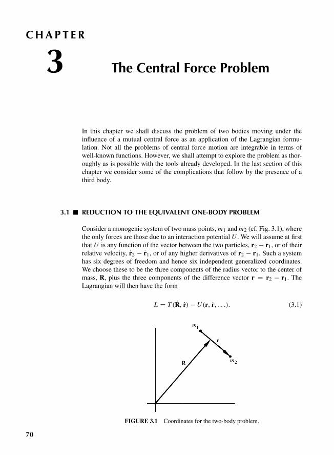
“M03 Goldstein ISBN C03” — 2011/2/15 — page 70 — #1
C H A P T E R
3 The Central Force Problem
In this chapter we shall discuss the problem of two bodies moving under theinfluence of a mutual central force as an application of the Lagrangian formu-lation. Not all the problems of central force motion are integrable in terms ofwell-known functions. However, we shall attempt to explore the problem as thor-oughly as is possible with the tools already developed. In the last section of thischapter we consider some of the complications that follow by the presence of athird body.
3.1 REDUCTION TO THE EQUIVALENT ONE-BODY PROBLEM
Consider a monogenic system of two mass points, m1 and m2 (cf. Fig. 3.1), wherethe only forces are those due to an interaction potential U . We will assume at firstthat U is any function of the vector between the two particles, r2 − r1, or of theirrelative velocity, r2 − r1, or of any higher derivatives of r2 − r1. Such a systemhas six degrees of freedom and hence six independent generalized coordinates.We choose these to be the three components of the radius vector to the center ofmass, R, plus the three components of the difference vector r = r2 − r1. TheLagrangian will then have the form
L = T (R, r)− U (r, r, . . .). (3.1)
FIGURE 3.1 Coordinates for the two-body problem.
70
“M03 Goldstein ISBN C03” — 2011/2/15 — page 71 — #2
3.1 Reduction to the Equivalent One-Body Problem 71
The kinetic energy T can be written as the sum of the kinetic energy of themotion of the center of mass, plus the kinetic energy of motion about the centerof mass, T ′:
T = 12 (m1 + m2) R2 + T ′
with
T ′ = 12 m1r′21 + 1
2 m2r′22 .
Here r′1 and r′2 are the radii vectors of the two particles relative to the center ofmass and are related to r by
r′1 = − m2
m1 + m2r,
r′2 = m1
m1 + m2r (3.2)
Expressed in terms of r by means of Eq. (3.2), T ′ takes on the form
T ′ = 1
2
m1m2
m1 + m2r2
and the total Lagrangian (3.1) is
L = m1 + m2
2R2 + 1
2
m1m2
m1 + m2r2 − U (r, r, . . .). (3.3)
It is seen that the three coordinates R are cyclic, so that the center of massis either at rest or moving uniformly. None of the equations of motion for r willcontain terms involving R or R. Consequently, the process of integration is par-ticularly simple here. We merely drop the first term from the Lagrangian in allsubsequent discussion.
The rest of the Lagrangian is exactly what would be expected if we had a fixedcenter of force with a single particle at a distance r from it, having a mass
μ = m1m2
m1 + m2, (3.4)
where μ is known as the reduced mass. Frequently, Eq. (3.4) is written in the form
1
μ= 1
m1+ 1
m2. (3.5)
Thus, the central force motion of two bodies about their center of mass can alwaysbe reduced to an equivalent one-body problem.
“M03 Goldstein ISBN C03” — 2011/2/15 — page 72 — #3
72 Chapter 3 The Central Force Problem
3.2 THE EQUATIONS OF MOTION AND FIRST INTEGRALS
We now restrict ourselves to conservative central forces, where the potential isV (r), a function of r only, so that the force is always along r. By the results ofthe preceding section, we need only consider the problem of a single particle ofreduced mass m moving about a fixed center of force, which will be taken as theorigin of the coordinate system. Since potential energy involves only the radialdistance, the problem has spherical symmetry; i.e., any rotation, about any fixedaxis, can have no effect on the solution. Hence, an angle coordinate representingrotation about a fixed axis must be cyclic. These symmetry properties result in aconsiderable simplification in the problem.
Since the problem is spherically symmetric, the total angular momentumvector,
L = r3 p,
is conserved. It therefore follows that r is always perpendicular to the fixed direc-tion of L in space. This can be true only if r always lies in a plane whose normalis parallel to L. While this reasoning breaks down if L is zero, the motion in thatcase must be along a straight line going through the center of force, for L = 0requires r to be parallel to r, which can be satisfied only in straight-line motion.*Thus, central force motion is always motion in a plane.
Now, the motion of a single particle in space is described by three coordi-nates; in spherical polar coordinates these are the azimuth angle θ , the zenithangle (or colatitude) ψ , and the radial distance r . By choosing the polar axis to bein the direction of L, the motion is always in the plane perpendicular to the polaraxis. The coordinate ψ then has only the constant value π/2 and can be droppedfrom the subsequent discussion. The conservation of the angular momentum vec-tor furnishes three independent constants of motion (corresponding to the threeCartesian components). In effect, two of these, expressing the constant directionof the angular momentum, have been used to reduce the problem from three totwo degrees of freedom. The third of these constants, corresponding to the con-servation of the magnitude of L, remains still at our disposal in completing thesolution.
Expressed now in plane polar coordinates, the Lagrangian is
L = T − V
= 12 m(r2 + r2θ2)− V (r). (3.6)
As was forseen, θ is a cyclic coordinate, whose corresponding canonical momen-tum is the angular momentum of the system:
pθ = ∂L
∂θ= mr2θ .
*Formally: r = rnr + r θnθ , hence r3 r = 0 requires θ = 0.
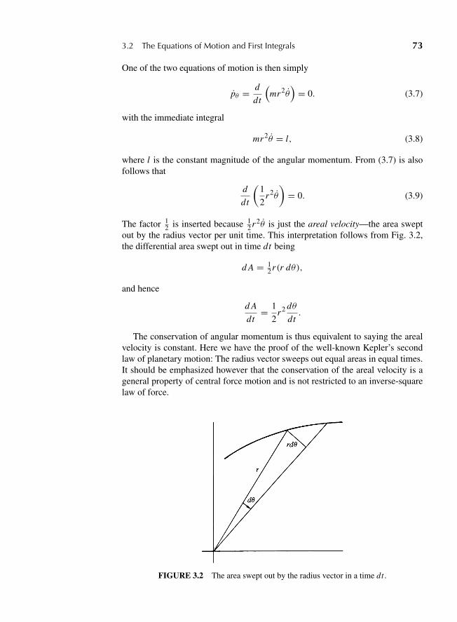
“M03 Goldstein ISBN C03” — 2011/2/15 — page 73 — #4
3.2 The Equations of Motion and First Integrals 73
One of the two equations of motion is then simply
pθ = d
dt
(mr2θ
)= 0. (3.7)
with the immediate integral
mr2θ = l, (3.8)
where l is the constant magnitude of the angular momentum. From (3.7) is alsofollows that
d
dt
(1
2r2θ
)= 0. (3.9)
The factor 12 is inserted because 1
2r2θ is just the areal velocity—the area sweptout by the radius vector per unit time. This interpretation follows from Fig. 3.2,the differential area swept out in time dt being
d A = 12r(r dθ),
and hence
d A
dt= 1
2r2 dθ
dt.
The conservation of angular momentum is thus equivalent to saying the arealvelocity is constant. Here we have the proof of the well-known Kepler’s secondlaw of planetary motion: The radius vector sweeps out equal areas in equal times.It should be emphasized however that the conservation of the areal velocity is ageneral property of central force motion and is not restricted to an inverse-squarelaw of force.
FIGURE 3.2 The area swept out by the radius vector in a time dt .
“M03 Goldstein ISBN C03” — 2011/2/15 — page 74 — #5
74 Chapter 3 The Central Force Problem
The remaining Lagrange equation, for the coordinate r , is
d
dt(mr)− mr θ2 + ∂V
∂r= 0. (3.10)
Designating the value of the force along r, −∂V/∂r , by f (r) the equation can berewritten as
mr − mr θ2 = f (r). (3.11)
By making use of the first integral, Eq. (3.8), θ can be eliminated from the equa-tion of motion, yielding a second-order differential equation involving r only:
mr − l2
mr3= f (r). (3.12)
There is another first integral of motion available, namely the total energy,since the forces are conservative. On the basis of the general energy conservationtheorem, we can immediately state that a constant of the motion is
E = 12 m(r2 + r2θ2)+ V (r), (3.13)
where E is the energy of the system. Alternatively, this first integral could bederived again directly from the equations of motion (3.7) and (3.12). The lattercan be written as
mr = − d
dr
(V + 1
2
l2
mr2
). (3.14)
If both sides of Eq. (3.14) are multiplied by r the left side becomes
mrr = d
dt
(1
2mr2
).
The right side similarly can be written as a total time derivative, for if g(r) is anyfunction of r , then the total time derivative of g has the form
d
dtg(r) = dg
dr
dr
dt.
Hence, Eq. (3.14) is equivalent to
d
dt
(1
2mr2
)= − d
dt
(V + 1
2
l2
mr2
)
or
d
dt
(1
2mr2 + 1
2
l2
mr2+ V
)= 0,
“M03 Goldstein ISBN C03” — 2011/2/15 — page 75 — #6
3.2 The Equations of Motion and First Integrals 75
and therefore
1
2mr2 + 1
2
l2
mr2+ V = constant. (3.15)
Equation (3.15) is the statement of the conservation of total energy, for byusing (3.8) for l, the middle term can be written
1
2
l2
mr2= 1
2mr2m2r4θ2 = mr2θ2
2,
and (3.15) reduces to (3.13).These first two integrals give us in effect two of the quadratures necessary to
complete the problem. As there are two variables, r and θ , a total of four inte-grations are needed to solve the equations of motion. The first two integrationshave left the Lagrange equations as two first-order equations (3.8) and (3.15); thetwo remaining integrations can be accomplished (formally) in a variety of ways.Perhaps the simplest procedure starts from Eq. (3.15). Solving for r , we have
r =√
2
m
(E − V − l2
2mr2
), (3.16)
or
dt = dr√2m
(E − V − l2
2mr2
) . (3.17)
At time t = 0, let r have the initial value r0. Then the integral of both sides of theequation from the initial state to the state at time t takes the form
t =∫ r
r0
dr√2m
(E − V − l2
2mr2
) . (3.18)
As it stands, Eq. (3.18) gives t as a function of r and the constants of integrationE , l, and r0. However, it may be inverted, at least formally, to give r as a functionof t and the constants. Once the solution for r is found, the solution θ followsimmediately from Eq. (3.8), which can be written as
dθ = l dt
mr2. (3.19)
If the initial value of θ is θ0, then the integral of (3.19) is simply
θ = l∫ t
0
dt
mr2(t)+ θ0. (3.20)
“M03 Goldstein ISBN C03” — 2011/2/15 — page 76 — #7
76 Chapter 3 The Central Force Problem
Equations (3.18) and (3.20) are the two remaining integrations, and formallythe problem has been reduced to quadratures (evaluating integrals), with fourconstants of integration E , l, r0, θ0. These constants are not the only ones thatcan be considered. We might equally as well have taken r0, θ0, r0, θ0, but ofcourse E and l can always be determined in terms of this set. For many appli-cations, however, the set containing the energy and angular momentum is thenatural one. In quantum mechanics, such constants as the initial values of r andθ , or of r and θ , become meaningless, but we can still talk in terms of the sys-tem energy or of the system angular momentum. Indeed, two salient differencesbetween classical and quantum mechanics appear in the properties of E and lin the two theories. To discuss the transition to quantum theories it is importantthat the classical description of the system be in terms of its energy and angularmomentum.
3.3 THE EQUIVALENT ONE-DIMENSIONAL PROBLEM,AND CLASSIFICATION OF ORBITS
Although we have solved the one-dimensional problem formally, practicallyspeaking the integrals (3.18) and (3.20) are usually quite unmanageable, and inany specific case it is often more convenient to perform the integration in someother fashion. But before obtaining the solution for any specific force laws, letus see what can be learned about the motion in the general case, using only theequations of motion and the conservation theorems, without requiring explicitsolutions.
For example, with a system of known energy and angular momentum, the mag-nitude and direction of the velocity of the particle can be immediately determinedin terms of the distance r . The magnitude v follows at once from the conservationof energy in the form
E = 12 mv2 + V (r)
or
v =√
2
m(E − V (r)). (3.21)
The radial velocity—the component of r along the radius vector—has been givenin Eq. (3.16). Combined with the magnitude v, this is sufficient information tofurnish the direction of the velocity.* These results, and much more, can also beobtained from consideration of an equivalent one-dimensional problem.
The equation of motion in r , with θ expressed in terms of l, Eq. (3.12), involvesonly r and its derivatives. It is the same equation as would be obtained for a
*Alternatively, the conservation of angular momentum furnishes θ , the angular velocity, and thistogether with r gives both the magnitude and direction of r.
“M03 Goldstein ISBN C03” — 2011/2/15 — page 77 — #8
3.3 The Equivalent One-Dimensional Problem 77
fictitious one-dimensional problem in which a particle of mass m is subject to aforce
f ′ = f + l2
mr3. (3.22)
The significance of the additional term is clear if it is written as mr θ2 = mv2θ /r ,
which is the familiar centrifugal force. An equivalent statement can be obtainedfrom the conservation theorem for energy. By Eq. (3.15) the motion of theparticle in r is that of a one-dimensional problem with a fictitious potentialenergy:
V ′ = V + 1
2
l2
mr2. (3.22′)
As a check, note that
f ′ = −∂V ′
∂r= f (r)+ l2
mr3,
which agrees with Eq. (3.22). The energy conservation theorem (3.15) can thusalso be written as
E = V ′ + 12 mr2. (3.15′)
As an illustration of this method of examining the motion, consider a plot ofV ′ against r for the specific case of an attractive inverse-square law of force:
f = − k
r2.
(For positive k, the minus sign ensures that the force is toward the center of force.)The potential energy for this force is
V = −k
r,
and the corresponding fictitious potential is
V ′ = −k
r+ l2
2mr2.
Such a plot is shown in Fig. 3.3; the two dashed lines represent the separate com-ponents
−k
rand
l2
2mr2,
and the solid line is the sum V ′.
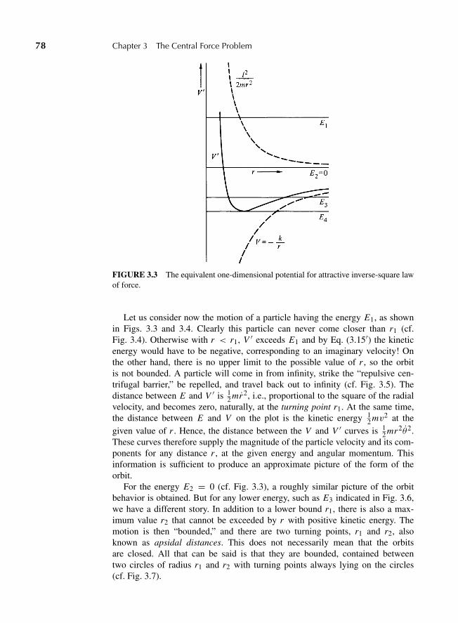
“M03 Goldstein ISBN C03” — 2011/2/15 — page 78 — #9
78 Chapter 3 The Central Force Problem
FIGURE 3.3 The equivalent one-dimensional potential for attractive inverse-square lawof force.
Let us consider now the motion of a particle having the energy E1, as shownin Figs. 3.3 and 3.4. Clearly this particle can never come closer than r1 (cf.Fig. 3.4). Otherwise with r < r1, V ′ exceeds E1 and by Eq. (3.15′) the kineticenergy would have to be negative, corresponding to an imaginary velocity! Onthe other hand, there is no upper limit to the possible value of r , so the orbitis not bounded. A particle will come in from infinity, strike the “repulsive cen-trifugal barrier,” be repelled, and travel back out to infinity (cf. Fig. 3.5). Thedistance between E and V ′ is 1
2 mr2, i.e., proportional to the square of the radialvelocity, and becomes zero, naturally, at the turning point r1. At the same time,the distance between E and V on the plot is the kinetic energy 1
2 mv2 at thegiven value of r . Hence, the distance between the V and V ′ curves is 1
2 mr2θ2.These curves therefore supply the magnitude of the particle velocity and its com-ponents for any distance r , at the given energy and angular momentum. Thisinformation is sufficient to produce an approximate picture of the form of theorbit.
For the energy E2 = 0 (cf. Fig. 3.3), a roughly similar picture of the orbitbehavior is obtained. But for any lower energy, such as E3 indicated in Fig. 3.6,we have a different story. In addition to a lower bound r1, there is also a max-imum value r2 that cannot be exceeded by r with positive kinetic energy. Themotion is then “bounded,” and there are two turning points, r1 and r2, alsoknown as apsidal distances. This does not necessarily mean that the orbitsare closed. All that can be said is that they are bounded, contained betweentwo circles of radius r1 and r2 with turning points always lying on the circles(cf. Fig. 3.7).
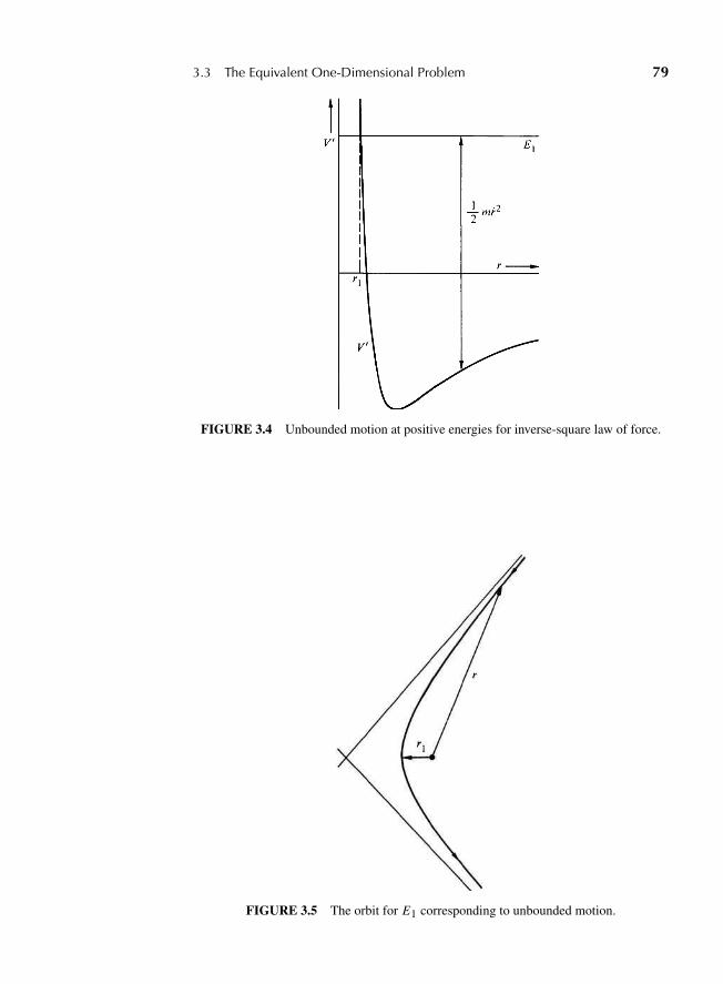
“M03 Goldstein ISBN C03” — 2011/2/15 — page 79 — #10
3.3 The Equivalent One-Dimensional Problem 79
FIGURE 3.4 Unbounded motion at positive energies for inverse-square law of force.
FIGURE 3.5 The orbit for E1 corresponding to unbounded motion.
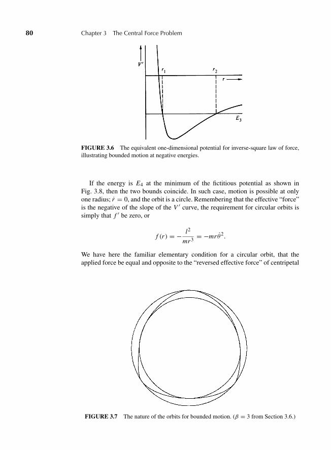
“M03 Goldstein ISBN C03” — 2011/2/15 — page 80 — #11
80 Chapter 3 The Central Force Problem
FIGURE 3.6 The equivalent one-dimensional potential for inverse-square law of force,illustrating bounded motion at negative energies.
If the energy is E4 at the minimum of the fictitious potential as shown inFig. 3.8, then the two bounds coincide. In such case, motion is possible at onlyone radius; r = 0, and the orbit is a circle. Remembering that the effective “force”is the negative of the slope of the V ′ curve, the requirement for circular orbits issimply that f ′ be zero, or
f (r) = − l2
mr3= −mr θ2.
We have here the familiar elementary condition for a circular orbit, that theapplied force be equal and opposite to the “reversed effective force” of centripetal
FIGURE 3.7 The nature of the orbits for bounded motion. (β = 3 from Section 3.6.)
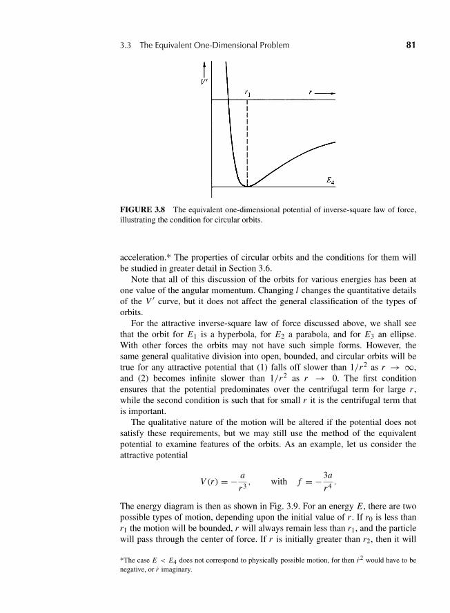
“M03 Goldstein ISBN C03” — 2011/2/15 — page 81 — #12
3.3 The Equivalent One-Dimensional Problem 81
FIGURE 3.8 The equivalent one-dimensional potential of inverse-square law of force,illustrating the condition for circular orbits.
acceleration.* The properties of circular orbits and the conditions for them willbe studied in greater detail in Section 3.6.
Note that all of this discussion of the orbits for various energies has been atone value of the angular momentum. Changing l changes the quantitative detailsof the V ′ curve, but it does not affect the general classification of the types oforbits.
For the attractive inverse-square law of force discussed above, we shall seethat the orbit for E1 is a hyperbola, for E2 a parabola, and for E3 an ellipse.With other forces the orbits may not have such simple forms. However, thesame general qualitative division into open, bounded, and circular orbits will betrue for any attractive potential that (1) falls off slower than 1/r2 as r → ∞,and (2) becomes infinite slower than 1/r2 as r → 0. The first conditionensures that the potential predominates over the centrifugal term for large r ,while the second condition is such that for small r it is the centrifugal term thatis important.
The qualitative nature of the motion will be altered if the potential does notsatisfy these requirements, but we may still use the method of the equivalentpotential to examine features of the orbits. As an example, let us consider theattractive potential
V (r) = − a
r3, with f = −3a
r4.
The energy diagram is then as shown in Fig. 3.9. For an energy E , there are twopossible types of motion, depending upon the initial value of r . If r0 is less thanr1 the motion will be bounded, r will always remain less than r1, and the particlewill pass through the center of force. If r is initially greater than r2, then it will
*The case E < E4 does not correspond to physically possible motion, for then r2 would have to benegative, or r imaginary.
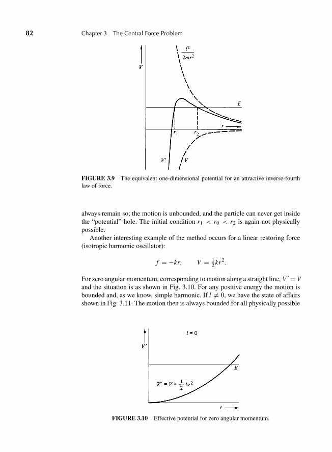
“M03 Goldstein ISBN C03” — 2011/2/15 — page 82 — #13
82 Chapter 3 The Central Force Problem
FIGURE 3.9 The equivalent one-dimensional potential for an attractive inverse-fourthlaw of force.
always remain so; the motion is unbounded, and the particle can never get insidethe “potential” hole. The initial condition r1 < r0 < r2 is again not physicallypossible.
Another interesting example of the method occurs for a linear restoring force(isotropic harmonic oscillator):
f = −kr, V = 12 kr2.
For zero angular momentum, corresponding to motion along a straight line, V ′ = Vand the situation is as shown in Fig. 3.10. For any positive energy the motion isbounded and, as we know, simple harmonic. If l �= 0, we have the state of affairsshown in Fig. 3.11. The motion then is always bounded for all physically possible
FIGURE 3.10 Effective potential for zero angular momentum.
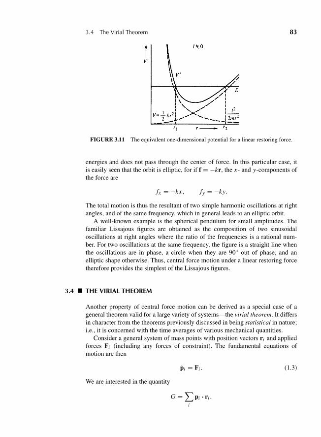
“M03 Goldstein ISBN C03” — 2011/2/15 — page 83 — #14
3.4 The Virial Theorem 83
FIGURE 3.11 The equivalent one-dimensional potential for a linear restoring force.
energies and does not pass through the center of force. In this particular case, itis easily seen that the orbit is elliptic, for if f = −kr, the x- and y-components ofthe force are
fx = −kx, fy = −ky.
The total motion is thus the resultant of two simple harmonic oscillations at rightangles, and of the same frequency, which in general leads to an elliptic orbit.
A well-known example is the spherical pendulum for small amplitudes. Thefamiliar Lissajous figures are obtained as the composition of two sinusoidaloscillations at right angles where the ratio of the frequencies is a rational num-ber. For two oscillations at the same frequency, the figure is a straight line whenthe oscillations are in phase, a circle when they are 90◦ out of phase, and anelliptic shape otherwise. Thus, central force motion under a linear restoring forcetherefore provides the simplest of the Lissajous figures.
3.4 THE VIRIAL THEOREM
Another property of central force motion can be derived as a special case of ageneral theorem valid for a large variety of systems—the virial theorem. It differsin character from the theorems previously discussed in being statistical in nature;i.e., it is concerned with the time averages of various mechanical quantities.
Consider a general system of mass points with position vectors ri and appliedforces Fi (including any forces of constraint). The fundamental equations ofmotion are then
pi = Fi . (1.3)
We are interested in the quantity
G =∑
i
pi ? ri ,
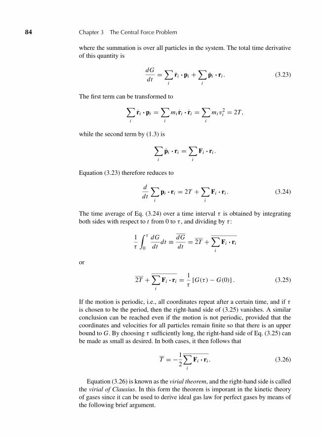
“M03 Goldstein ISBN C03” — 2011/2/15 — page 84 — #15
84 Chapter 3 The Central Force Problem
where the summation is over all particles in the system. The total time derivativeof this quantity is
dG
dt=∑
i
ri ? pi +∑
i
pi ? ri . (3.23)
The first term can be transformed to∑i
ri ? pi =∑
i
mi ri ? ri =∑
i
miv2i = 2T,
while the second term by (1.3) is
∑i
pi ? ri =∑
i
Fi ? ri .
Equation (3.23) therefore reduces to
d
dt
∑i
pi ? ri = 2T +∑
i
Fi ? ri . (3.24)
The time average of Eq. (3.24) over a time interval τ is obtained by integratingboth sides with respect to t from 0 to τ , and dividing by τ :
1
τ
∫ τ
0
dG
dtdt ≡ dG
dt= 2T +
∑i
Fi ? ri
or
2T +∑
i
Fi ? ri = 1
τ[G(τ )− G(0)] . (3.25)
If the motion is periodic, i.e., all coordinates repeat after a certain time, and if τis chosen to be the period, then the right-hand side of (3.25) vanishes. A similarconclusion can be reached even if the motion is not periodic, provided that thecoordinates and velocities for all particles remain finite so that there is an upperbound to G. By choosing τ sufficiently long, the right-hand side of Eq. (3.25) canbe made as small as desired. In both cases, it then follows that
T = −1
2
∑i
Fi ? ri . (3.26)
Equation (3.26) is known as the virial theorem, and the right-hand side is calledthe virial of Clausius. In this form the theorem is imporant in the kinetic theoryof gases since it can be used to derive ideal gas law for perfect gases by means ofthe following brief argument.
“M03 Goldstein ISBN C03” — 2011/2/15 — page 85 — #16
3.4 The Virial Theorem 85
We consider a gas consisting of N atoms confined within a container ofvolume V . The gas is further assumed to be at a Kelvin temperature T (notto be confused with the symbol for kinetic energy). Then by the equipartitiontheorem of kinetic theory, the average kinetic energy of each atom is given by32 kB T , kB being the Boltzmann constant, a relation that in effect is the definitionof temperature. The left-hand side of Eq. (3.26) is therefore
32 NkB T .
On the right-hand side of Eq. (3.26), the forces Fi include both the forces ofinteraction between atoms and the forces of constraint on the system. A perfectgas is defined as one for which the forces of interaction contribute negligibly tothe virial. This occurs, e.g., if the gas is so tenuous that collisions between atomsoccur rarely, compared to collisions with the walls of the container. It is thesewalls that constitute the constraint on the system, and the forces of constraint,Fc, are localized at the wall and come into existence whenever a gas atom col-lides with the wall. The sum on the right-hand side of Eq. (3.26) can therefore bereplaced in the average by an integral over the surface of the container. The forceof constraint represents the reaction of the wall to the collision forces exerted bythe atoms on the wall, i.e., to the pressure P . With the usual outward conventionfor the unit vector n in the direction of the normal to the surface, we can thereforewrite
dFi = −Pn d A,
or
1
2
∑i
Fi ? ri = − P
2
∫n ? r d A.
But, by Gauss’s theorem,∫n ? r d A =
∫� ? r dV = 3V .
The virial theorem, Eq. (3.26), for the system representing a perfect gas can there-fore be written
32 NkB T = 3
2 PV,
which, cancelling the common factor of 32 on both sides, is the familiar ideal
gas law. Where the interparticle forces contribute to the virial, the perfect gaslaw of course no longer holds. The virial theorem is then the principal tool, inclassical kinetic theory, for calculating the equation of state corresponding to suchimperfect gases.
We can further show that if the forces Fi are the sum of nonfrictional forcesF′
i and frictional forces fi proportional to the velocity, then the virial depends
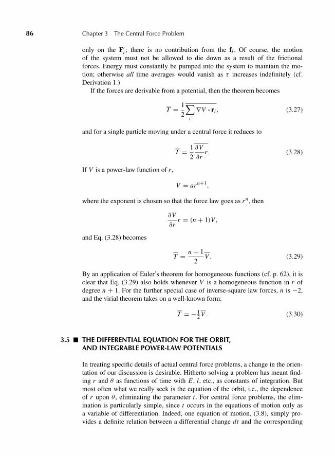
“M03 Goldstein ISBN C03” — 2011/2/15 — page 86 — #17
86 Chapter 3 The Central Force Problem
only on the F′i ; there is no contribution from the fi . Of course, the motion
of the system must not be allowed to die down as a result of the frictionalforces. Energy must constantly be pumped into the system to maintain the mo-tion; otherwise all time averages would vanish as τ increases indefinitely (cf.Derivation 1.)
If the forces are derivable from a potential, then the theorem becomes
T = 1
2
∑i
∇V ? ri , (3.27)
and for a single particle moving under a central force it reduces to
T = 1
2
∂V
∂rr . (3.28)
If V is a power-law function of r ,
V = arn+1,
where the exponent is chosen so that the force law goes as rn , then
∂V
∂rr = (n + 1)V,
and Eq. (3.28) becomes
T = n + 1
2V . (3.29)
By an application of Euler’s theorem for homogeneous functions (cf. p. 62), it isclear that Eq. (3.29) also holds whenever V is a homogeneous function in r ofdegree n + 1. For the further special case of inverse-square law forces, n is −2,and the virial theorem takes on a well-known form:
T = − 12 V . (3.30)
3.5 THE DIFFERENTIAL EQUATION FOR THE ORBIT,AND INTEGRABLE POWER-LAW POTENTIALS
In treating specific details of actual central force problems, a change in the orien-tation of our discussion is desirable. Hitherto solving a problem has meant find-ing r and θ as functions of time with E , l, etc., as constants of integration. Butmost often what we really seek is the equation of the orbit, i.e., the dependenceof r upon θ , eliminating the parameter t . For central force problems, the elim-ination is particularly simple, since t occurs in the equations of motion only asa variable of differentiation. Indeed, one equation of motion, (3.8), simply pro-vides a definite relation between a differential change dt and the corresponding
“M03 Goldstein ISBN C03” — 2011/2/15 — page 87 — #18
3.5 The Differential Equation for the Orbit 87
change dθ :
l dt = mr2 dθ. (3.31)
The corresponding relation between derivatives with respect to t and θ is
d
dt= l
mr2
d
dθ. (3.32)
These relations may be used to convert the equation of motion (3.12) or (3.16) toa differential equation for the orbit. A substitution into Eq. (3.12) gives a second-order differential equation, while a substitution into Eq. (3.17) gives a simplerfirst-order differential equation.
The substitution into Eq. (3.12) yields
l
r2
d
dθ
(l
mr2
dr
dθ
)− l2
mr3= f (r), (3.33)
which upon substituting u = 1/r and expressing the results in terms of the poten-tial gives
d2u
dθ2+ u = −m
l2
d
duV
(1
u
). (3.34)
The preceding equation is such that the resulting orbit is symmetric about twoadjacent turning points. To prove this statement, note that if the orbit is symmet-rical it should be possible to reflect it about the direction of the turning anglewithout producing any change. If the coordinates are chosen so that the turningpoint occurs for θ = 0, then the reflection can be effected mathematically bysubstituting −θ for θ . The differential equation for the orbit, (3.34), is obviouslyinvariant under such a substitution. Further the initial conditions, here
u = u(0),
(du
dθ
)0= 0, for θ = 0,
will likewise be unaffected. Hence, the orbit equation must be the same whetherexpressed in terms of θ or −θ , which is the desired conclusion. The orbit is there-fore invariant under reflection about the apsidal vectors. In effect, this means thatthe complete orbit can be traced if the portion of the orbit between any two turningpoints is known. Reflection of the given portion about one of the apsidal vectorsproduces a neighboring stretch of the orbit, and this process can be repeated in-definitely until the rest of the orbit is completed, as illustrated in Fig. 3.12.
For any particular force law, the actual equation of the orbit can be obtained byeliminating t from the solution (3.17) by means of (3.31), resulting in
dθ = l dr
mr2
√2m
(E − V (r)− l2
2mr2
) . (3.35)
“M03 Goldstein ISBN C03” — 2011/2/15 — page 88 — #19
88 Chapter 3 The Central Force Problem
FIGURE 3.12 Extension of the orbit by reflection of a portion about the apsidal vectors.
With slight rearrangements, the integral of (3.35) is
θ =∫ r
r0
dr
r2√
2m El2 − 2mV
l2 − 1r2
+ θ0, (3.36)
or, if the variable of integration is changed to u = 1/r ,
θ = θ0 −∫ u
u0
du√2m E
l2 − 2mVl2 − u2
. (3.37)
As in the case of the equation of motion, Eq. (3.37), while solving the problemformally, is not always a practicable solution, because the integral often cannot beexpressed in terms of well-known functions. In fact, only certain types of forcelaws have been investigated. The most important are the power-law functions of r ,
V = arn+1 (3.38)
so that the force varies at the nth power of r .* With this potential, (3.37) becomes
θ = θ0 −∫ u
u0
du√2m E
l2 − 2mal2 u−n−1 − u2
. (3.39)
This again is integrable in terms of simple functions only in certain cases. Theparticular power-law exponents for which the results can be expressed in terms oftrigonometric functions are
n = 1,−2,−3.
*The case n = −1 is to be excluded from the discussion. In the potential (3.38), it corresponds to aconstant potential, i.e., no force at all. It is an equally anomalous case if the exponent is used in theforce law directly, since a force varying as r−1 corresponds to a logarithmic potential, which is not apower law at all. A logarithmic potential is unusual for motion about a point; it is more characteristicof a line source. Further details of these cases are given in the second edition of this text.
“M03 Goldstein ISBN C03” — 2011/2/15 — page 89 — #20
3.6 Conditions for Closed Orbits (Bertrand’s Theorem) 89
The results of the integral for
n = 5, 3, 0,−4,−5,−7
can be expressed in terms of elliptic functions. These are all the possibilities for aninteger exponent where the formal integrations are expressed in terms of simplewell-known functions. Some fractional exponents can be shown to lead to ellipticfunctions, and many other exponents can be expressed in terms of the hyperge-ometric function. The trigonometric and elliptical functions are special cases ofgeneralized hypergeometric function integrals. Equation (3.39) can of course benumerically integrated for any nonpathological potential, but this is beyond thescope of the text.
3.6 CONDITIONS FOR CLOSED ORBITS (BERTRAND’S THEOREM)
We have not yet extracted all the information that can be obtained from theequivalent one-dimensional problem or from the orbit equation without explic-itly solving for the motion. In particular, it is possible to derive a powerful andthought-provoking theorem on the types of attractive central forces that leadto closed orbits, i.e., orbits in which the particle eventually retraces its ownfootsteps.
Conditions have already been described for one kind of closed orbit, namely acircle about the center of force. For any given l, this will occur if the equivalentpotential V ′(r) has a minimum or maximum at some distance r0 and if the energyE is just equal to V ′(r0). The requirement that V ′ have an extremum is equiva-lent to the vanishing of f ′ at r0, leading to the condition derived previously (cf.Section 3.3).
f (r0) = − l2
mr30
, (3.40)
which says the force must be attractive for circular orbits to be possible. In addi-tion, the energy of the particle must be given by
E = V (r0)+ l2
2mr20
, (3.41)
which, by Eq. (3.15), corresponds to the requirement that for a circular orbit r iszero. Equations (3.40) and (3.41) are both elementary and familiar. Between themthey imply that for any attractive central force it is possible to have a circularorbit at some arbitrary radius r0, provided the angular momentum l is given byEq. (3.40) and the particle energy by Eq. (3.41).
The character of the circular orbit depends on whether the extremum of V ′is a minimum, as in Fig. 3.8, or a maximum, as if Fig. 3.9. If the energy isslightly above that required for a circular orbit at the given value of l, then fora minimum in V ′ the motion, though no longer circular, will still be bounded.
“M03 Goldstein ISBN C03” — 2011/2/15 — page 90 — #21
90 Chapter 3 The Central Force Problem
However, if V ′ exhibits a maximum, then the slightest raising of E above thecircular value, Eq. (3.34), results in motion that is unbounded, with the parti-cle moving both through the center of force and out to infinity for the potentialshown in Fig. 3.9. Borrowing the terminology from the case of static equilibrium,the circular orbit arising in Fig. 3.8 is said to be stable; that in Fig. 3.9 is unsta-ble. The stability of the circular orbit is thus determined by the sign of the secondderivative of V ′ at the radius of the circle, being stable for positive second deriva-tive (V ′ concave up) and unstable for V ′ concave down. A stable orbit thereforeoccurs if
∂2V ′
∂r2
∣∣∣∣r=r0
= −∂ f
∂r
∣∣∣∣r=r0
+ 3l2
mr40
> 0. (3.42)
Using Eq. (3.40), this condition can be written
∂ f
∂r
∣∣∣∣r=r0
< −3 f (r0)
r0, (3.43)
or
d ln f
d ln r
∣∣∣∣r=r0
> −3 (3.43′)
where f (r0)/r0 is assumed to be negative and given by dividing Eq. (3.40) by r0.If the force behaves like a power law of r in the vicinity of the circular radius r0,
f = −krn,
then the stability condition, Eq. (3.43), becomes
−knrn−1 < 3krn−1
or
n > −3, (3.44)
where k is assumed to be positive. A power-law attractive potential varying moreslowly than 1/r2 is thus capable of stable circular orbits for all values of r0.
If the circular orbit is stable, then a small increase in the particle energy abovethe value for a circular orbit results in only a slight variation of r about r0. Itcan be easily shown from (3.34) that for such small deviations from the circu-larity conditions, the particle executes a simple harmonic motion in u(≡ 1/r)about u0:
u = u0 + a cosβθ. (3.45)
Here a is an amplitude that depends upon the deviation of the energy from thevalue for circular orbits, and β is a quantity arising from a Taylor series expansion
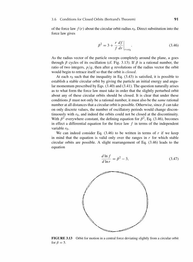
“M03 Goldstein ISBN C03” — 2011/2/15 — page 91 — #22
3.6 Conditions for Closed Orbits (Bertrand’s Theorem) 91
of the force law f (r) about the circular orbit radius r0. Direct substitution into theforce law gives
β2 = 3 + r
f
d f
dr
∣∣∣∣r=r0
. (3.46)
As the radius vector of the particle sweeps completely around the plane, u goesthrough β cycles of its oscillation (cf. Fig. 3.13). If β is a rational number, theratio of two integers, p/q, then after q revolutions of the radius vector the orbitwould begin to retrace itself so that the orbit is closed.
At each r0 such that the inequality in Eq. (3.43) is satisfied, it is possible toestablish a stable circular orbit by giving the particle an initial energy and angu-lar momentum prescribed by Eqs. (3.40) and (3.41). The question naturally arisesas to what form the force law must take in order that the slightly perturbed orbitabout any of these circular orbits should be closed. It is clear that under theseconditions β must not only be a rational number, it must also be the same rationalnumber at all distances that a circular orbit is possible. Otherwise, since β can takeon only discrete values, the number of oscillatory periods would change discon-tinuously with r0, and indeed the orbits could not be closed at the discontinuity.With β2 everywhere constant, the defining equation for β2, Eq. (3.46), becomesin effect a differential equation for the force law f in terms of the independentvariable r0.
We can indeed consider Eq. (3.46) to be written in terms of r if we keepin mind that the equation is valid only over the ranges in r for which stablecircular orbits are possible. A slight rearrangement of Eq. (3.46) leads to theequation
d ln f
d ln r= β2 − 3, (3.47)
FIGURE 3.13 Orbit for motion in a central force deviating slightly from a circular orbitfor β = 5.
“M03 Goldstein ISBN C03” — 2011/2/15 — page 92 — #23
92 Chapter 3 The Central Force Problem
which can be immediately integrated to give a force law:
f (r) = − k
r3−β2 . (3.48)
All force laws of this form, with β a rational number, lead to closed stable orbitsfor initial conditions that differ only slightly from conditions defining a circularorbit. Included within the possibilities allowed by Eq. (3.48) are some familiarforces such as the inverse-square law (β ≡ 1), but of course many other behaviors,such as f = −kr−2/9(β = 5
3 ), are also permitted.Suppose the initial conditions deviate more than slightly from the requirements
for circular orbits; will these same force laws still give circular orbits? The ques-tion can be answered directly by keeping an additional term in the Taylor seriesexpansion of the force law and solving the resultant orbit equation.
J. Bertrand solved this problem in 1873 and found that for more than first-order deviations from circularity, the orbits are closed only for β2 = 1 andβ2 = 4. The first of these values of β2, by Eq. (3.48), leads to the familiarattractive inverse-square law; the second is an attractive force proportional tothe radial distance—Hooke’s law! These force laws, and only these, could pos-sibly produce closed orbits for any arbitrary combination of l and E(E < 0),and in fact we know from direct solution of the orbit equation that they do.Hence, we have Bertrand’s theorem: The only central forces that result inclosed orbits for all bound particles are the inverse-square law and Hooke’slaw.
This is a remarkable result, well worth the tedious algebra required. It is a com-monplace astronomical observation that bound celestial objects move in orbitsthat are in first approximation closed. For the most part, the small deviationsfrom a closed orbit are traceable to perturbations such as the presence of otherbodies. The prevalence of closed orbits holds true whether we consider only thesolar system, or look to the many examples of true binary stars that have beenobserved. Now, Hooke’s law is a most unrealistic force law to hold at all dis-tances, for it implies a force increasing indefinitely to infinity. Thus, the exis-tence of closed orbits for a wide range of initial conditions by itself leads tothe conclusion that the gravitational force varies as the inverse-square of thedistance.
We can phrase this conclusion in a slightly different manner, one that is ofsomewhat more significance in modern physics. The orbital motion in a planecan be looked on as compounded of two oscillatory motions, one in r and onein θ with the same period. The character of orbits in a gravitational field fixesthe form of the force law. Later on we shall encounter other formulations of therelation between degeneracy and the nature of the potential.
3.7 THE KEPLER PROBLEM: INVERSE-SQUARE LAW OF FORCE
The inverse-square law is the most important of all the central force laws, and itdeserves detailed treatment. For this case, the force and potential can be written
“M03 Goldstein ISBN C03” — 2011/2/15 — page 93 — #24
3.7 The Kepler Problem: Inverse-Square Law of Force 93
as
f = − k
r2V = −k
r. (3.49)
There are several ways to integrate the equation for the orbit, the simplest being tosubstitute (3.49) in the differential equation for the orbit (3.33). Another approachis to start with Eq. (3.39) with n set equal to −2 for the gravitational force
θ = θ ′ −∫
du√2m E
l2 + 2mkul2 − u2
, (3.50)
where the integral is now taken as indefinite. The quantity θ ′ appearing in (3.50)is a constant of integration determined by the initial conditions and will not nec-essarily be the same as the initial angle θ0 at time t = 0. The indefinite integral isof the standard form,∫
dx√α + βx + γ x2
= 1√−γ arc cos−β + 2γ x√q
, (3.51)
where
q = β2 − 4αγ.
To apply this to (3.50), we must set
α = 2m E
l2, β = 2mk
l2γ = −1, (3.52)
and the discriminant q is therefore
q =(
2mk
l2
)2(
1 + 2El2
mk2
). (3.53)
With these substitutes, Eq. (3.50) becomes
θ = θ ′ − arc cosl2umk − 1√1 + 2El2
mk2
. (3.54)
Finally, by solving for u, ≡ 1/r , the equation of the orbit is found to be
1
r= mk
l2
⎛⎝1 +
√1 + 2El2
mk2cos(θ − θ ′)
⎞⎠ . (3.55)
The constant of integration θ ′ can now be identified from Eq. (3.55) as one of theturning angles of the orbit. Note that only three of the four constants of integrationappear in the orbit equation; this is always a characteristic property of the orbit. In
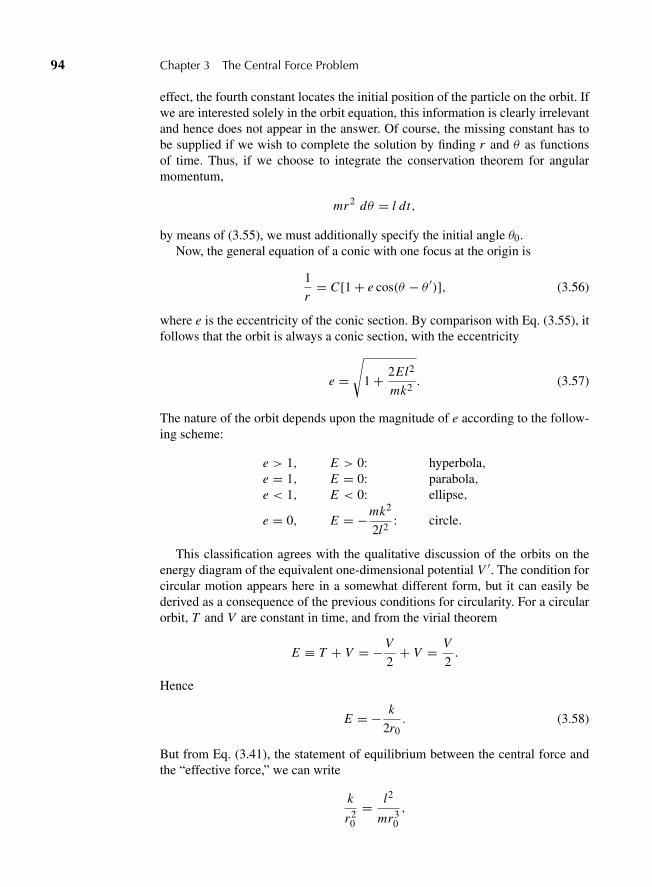
“M03 Goldstein ISBN C03” — 2011/2/15 — page 94 — #25
94 Chapter 3 The Central Force Problem
effect, the fourth constant locates the initial position of the particle on the orbit. Ifwe are interested solely in the orbit equation, this information is clearly irrelevantand hence does not appear in the answer. Of course, the missing constant has tobe supplied if we wish to complete the solution by finding r and θ as functionsof time. Thus, if we choose to integrate the conservation theorem for angularmomentum,
mr2 dθ = l dt,
by means of (3.55), we must additionally specify the initial angle θ0.Now, the general equation of a conic with one focus at the origin is
1
r= C[1 + e cos(θ − θ ′)], (3.56)
where e is the eccentricity of the conic section. By comparison with Eq. (3.55), itfollows that the orbit is always a conic section, with the eccentricity
e =√
1 + 2El2
mk2. (3.57)
The nature of the orbit depends upon the magnitude of e according to the follow-ing scheme:
e > 1, E > 0: hyperbola,e = 1, E = 0: parabola,e < 1, E < 0: ellipse,
e = 0, E = −mk2
2l2: circle.
This classification agrees with the qualitative discussion of the orbits on theenergy diagram of the equivalent one-dimensional potential V ′. The condition forcircular motion appears here in a somewhat different form, but it can easily bederived as a consequence of the previous conditions for circularity. For a circularorbit, T and V are constant in time, and from the virial theorem
E ≡ T + V = −V
2+ V = V
2.
Hence
E = − k
2r0. (3.58)
But from Eq. (3.41), the statement of equilibrium between the central force andthe “effective force,” we can write
k
r20
= l2
mr30
,

“M03 Goldstein ISBN C03” — 2011/2/15 — page 95 — #26
3.7 The Kepler Problem: Inverse-Square Law of Force 95
or
r0 = l2
mk. (3.59)
With this formula for the orbital radius, Eq. (3.58) becomes
E = −mk2
2l2,
the above condition for circular motion.In the case of elliptic orbits, it can be shown the major axis depends solely
upon the energy, a theorem of considerable importance in the Bohr theory of theatom. The semimajor axis is one-half the sum of the two apsidal distances r1 andr2 (cf. Fig. 3.6). By definition, the radial velocity is zero at these points, and theconservation of energy implies that the apsidal distances are therefore the roots ofthe equation (cf. Eq. (3.15))
E − l2
2mr2+ k
r= 0,
or
r2 + k
Er − l2
2m E= 0. (3.60)
The coefficient of the linear term in this particular quadratic equation is the nega-tive of the sum of the roots. Hence, the semimajor axis is given by
a = r1 + r2
2= − k
2E. (3.61)
Note that in the circular limit, Eq. (3.61) agrees with Eq. (3.58). In terms of thesemimajor axis, the eccentricity of the ellipse can be written
e =√
1 − l2
mka, (3.62)
(a relation we will have use for in a later chapter). Further, from Eq. (3.62) wehave the expression
l2
mk= a(1 − e2), (3.63)
in terms of which the elliptical orbit equation (3.55) can be written
r = a(1 − e2)
1 + e cos(θ − θ ′) . (3.64)
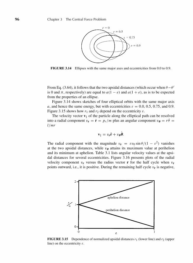
“M03 Goldstein ISBN C03” — 2011/2/15 — page 96 — #27
96 Chapter 3 The Central Force Problem
FIGURE 3.14 Ellipses with the same major axes and eccentricities from 0.0 to 0.9.
From Eq. (3.64), it follows that the two apsidal distances (which occur when θ−θ ′is 0 and π , respectively) are equal to a(1 − e) and a(1 + e), as is to be expectedfrom the properties of an ellipse.
Figure 3.14 shows sketches of four elliptical orbits with the same major axisa, and hence the same energy, but with eccentricities ε = 0.0, 0.5, 0.75, and 0.9.Figure 3.15 shows how r1 and r2 depend on the eccentricity ε.
The velocity vector v‖ of the particle along the elliptical path can be resolvedinto a radial component vr = r = pr/m plus an angular component vu = r θ =l/mr
v‖ = vrr + vuu.
The radial component with the magnitude vr = εv0 sin θ/(1 − ε2) vanishesat the two apsidal distances, while vu attains its maximum value at perihelionand its minimum at aphelion. Table 3.1 lists angular velocity values at the apsi-dal distances for several eccentricities. Figure 3.16 presents plots of the radialvelocity component vr versus the radius vector r for the half cycle when vrpoints outward, i.e., it is positive. During the remaining half cycle vr is negative,
FIGURE 3.15 Dependence of normalized apsidal distances r1 (lower line) and r2 (upperline) on the eccentricity ε.
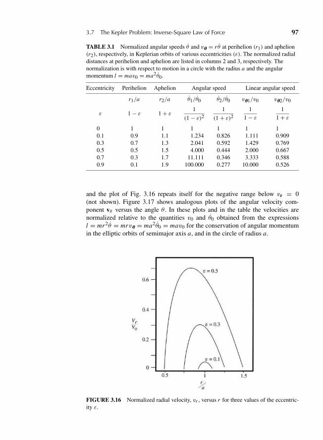
“M03 Goldstein ISBN C03” — 2011/2/15 — page 97 — #28
3.7 The Kepler Problem: Inverse-Square Law of Force 97
TABLE 3.1 Normalized angular speeds θ and vu = r θ at perihelion (r1) and aphelion(r2), respectively, in Keplerian orbits of various eccentricities (ε). The normalized radialdistances at perihelion and aphelion are listed in columns 2 and 3, respectively. Thenormalization is with respect to motion in a circle with the radius a and the angularmomentum l = mav0 = ma2θ0.
Eccentricity Perihelion Aphelion Angular speed Linear angular speed
r1/a r2/a θ1/θ0 θ2/θ0 vu1/v0 vu2/v0
ε 1 − ε 1 + ε 1
(1 − ε)21
(1 + ε)21
1 − ε1
1 + ε0 1 1 1 1 1 10.1 0.9 1.1 1.234 0.826 1.111 0.9090.3 0.7 1.3 2.041 0.592 1.429 0.7690.5 0.5 1.5 4.000 0.444 2.000 0.6670.7 0.3 1.7 11.111 0.346 3.333 0.5880.9 0.1 1.9 100.000 0.277 10.000 0.526
and the plot of Fig. 3.16 repeats itself for the negative range below vr = 0(not shown). Figure 3.17 shows analogous plots of the angular velocity com-ponent vθ versus the angle θ . In these plots and in the table the velocities arenormalized relative to the quantities v0 and θ0 obtained from the expressionsl = mr2θ = mrvu = ma2θ0 = mav0 for the conservation of angular momentumin the elliptic orbits of semimajor axis a, and in the circle of radius a.
FIGURE 3.16 Normalized radial velocity, vr , versus r for three values of the eccentric-ity ε.

“M03 Goldstein ISBN C03” — 2011/2/15 — page 98 — #29
98 Chapter 3 The Central Force Problem
FIGURE 3.17 Normalized orbital velocity, vθ , versus θ for three values of the eccen-tricity ε.
3.8 THE MOTION IN TIME IN THE KEPLER PROBLEM
The orbital equation for motion in a central inverse-square force law can thus besolved in a fairly straightforward manner with results that can be stated in simpleclosed expressions. Describing the motion of the particle in time as it traverses theorbit is however a much more involved matter. In principle, the relation betweenthe radial distance of the particle r and the time (relative to some starting point)is given by Eq. (3.18), which here takes on the form
t =√
m
2
∫ r
r0
dr√kr − l2
2mr2 + E. (3.65)
Similarly, the polar angle θ and the time are connected through the conserva-tion of angular momentum,
dt = mr2
ldθ,
which combined with the orbit equation (3.55) leads to
t = l3
mk2
∫ θ
θ0
dθ
[1 + e cos(θ − θ ′)]2. (3.66)
Either of these integrals can be carried out in terms of elementary functions. How-ever, the relations are very complex, and their inversions to give r or θ as func-tions of t pose formidable problems, especially when one wants the high precisionneeded for astronomical observations.
To illustrate some of these involvements, let us consider the situation forparabolic motion (e = 1), where the integrations can be most simply carriedout. It is customary to measure the plane polar angle from the radius vector at

“M03 Goldstein ISBN C03” — 2011/2/15 — page 99 — #30
3.8 The Motion in Time in the Kepler Problem 99
the point of closest approach—a point most usually designated as the perihe-lion.* This convention corresponds to setting θ ′ in the orbit equation (3.56) equalto zero. Correspondingly, time is measured from the moment, T , of perihelionpassage. Using the trigonometric identity
1 + cos θ = 2 cos2 θ
2,
Eq. (3.66) then reduces for parabolic motion to the form
t = l3
4mk2
∫ θ
0sec4 θ
2dθ.
The integration is easily performed by a change of variable to x = tan(θ/2),leading to the integral
t = l3
2mk2
∫ tan(θ/2)
0(1 + x2) dx,
or
t = l3
2mk2
(tan
θ
2+ 1
3tan3 θ
2
). (3.67)
In this equation, −π < θ < π , where for t → −∞ the particle startsapproaching from infinitely far away located at θ = −π . The time t = 0 corre-sponds to θ = 0, where the particle is at perihelion. Finally t → +∞ correspondsto θ → π as the particle moves infinitely far away. This is a straightforward rela-tion for t as a function of θ ; inversion to obtain θ at a given time requires solvinga cubic equation for tan(θ/2), then finding the corresponding arctan. The radialdistance at a given time is given through the orbital equation.
For elliptical motion, Eq. (3.65) is most conveniently integrated through anauxiliary variable ψ , denoted as the eccentric anomaly,* and defined by therelation
r = a(1 − e cosψ). (3.68)
By comparison with the orbit equation, (3.64), it is clear that ψ also covers theinterval 0 to 2π as θ goes through a complete revolution, and that the perihelionoccurs at ψ = 0 (where θ = 0 by convention) and the aphelion at ψ = π = θ .
*Literally, the term should be restricted to orbits around the Sun, while the more general term shouldbe periapsis. However, it has become customary to use perihelion no matter where the center of forceis. Even for space craft orbiting the Moon, official descriptions of the orbital parameters refer toperihelion where pericynthion would be the pedantic term.*Medieval astronomers expected the angular motion to be constant. The angle calculated by multi-plying this average angular velocity (2π /period) by the time since the last perihelion passage wascalled the mean anomaly. From the mean anomaly the eccentric anomaly could be calculated and thenused to calculate the true anomaly. The angle θ is called the true anomaly just as it was in medievalastronomy.
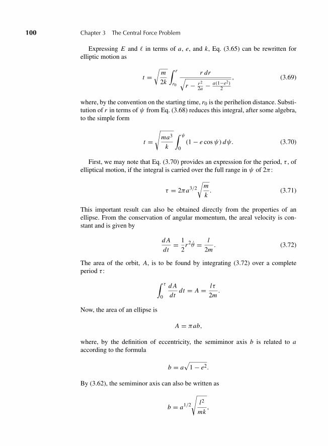
“M03 Goldstein ISBN C03” — 2011/2/15 — page 100 — #31
100 Chapter 3 The Central Force Problem
Expressing E and � in terms of a, e, and k, Eq. (3.65) can be rewritten forelliptic motion as
t =√
m
2k
∫ r
r0
r dr√r − r2
2a − a(1−e2)2
, (3.69)
where, by the convention on the starting time, r0 is the perihelion distance. Substi-tution of r in terms of ψ from Eq. (3.68) reduces this integral, after some algebra,to the simple form
t =√
ma3
k
∫ ψ
0(1 − e cosψ) dψ. (3.70)
First, we may note that Eq. (3.70) provides an expression for the period, τ , ofelliptical motion, if the integral is carried over the full range in ψ of 2π :
τ = 2πa3/2
√m
k. (3.71)
This important result can also be obtained directly from the properties of anellipse. From the conservation of angular momentum, the areal velocity is con-stant and is given by
d A
dt= 1
2r2θ = l
2m. (3.72)
The area of the orbit, A, is to be found by integrating (3.72) over a completeperiod τ :
∫ τ
0
d A
dtdt = A = lτ
2m.
Now, the area of an ellipse is
A = πab,
where, by the definition of eccentricity, the semiminor axis b is related to aaccording to the formula
b = a√
1 − e2.
By (3.62), the semiminor axis can also be written as
b = a1/2
√l2
mk,
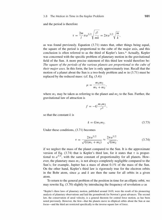
“M03 Goldstein ISBN C03” — 2011/2/15 — page 101 — #32
3.8 The Motion in Time in the Kepler Problem 101
and the period is therefore
τ = 2m
lπa3/2
√l2
mk= 2πa3/2
√m
k,
as was found previously. Equation (3.71) states that, other things being equal,the square of the period is proportional to the cube of the major axis, and thisconclusion is often referred to as the third of Kepler’s laws.* Actually, Keplerwas concerned with the specific problem of planetary motion in the gravitationalfield of the Sun. A more precise statement of this third law would therefore be:The square of the periods of the various planets are proportional to the cube oftheir major axes. In this form, the law is only approximately true. Recall that themotion of a planet about the Sun is a two-body problem and m in (3.71) must bereplaced by the reduced mass: (cf. Eq. (3.4))
μ = m1m2
m1 + m2,
where m1 may be taken as referring to the planet and m2 to the Sun. Further, thegravitational law of attraction is
f = −Gm1m2
r2,
so that the constant k is
k = Gm1m2. (3.73)
Under these conditions, (3.71) becomes
τ = 2πa3/2
√G(m1 + m2)
≈ 2πa3/2
√Gm2
, (3.74)
if we neglect the mass of the planet compared to the Sun. It is the approximateversion of Eq. (3.74) that is Kepler’s third law, for it states that τ is propor-tional to a3/2, with the same constant of proportionality for all planets. How-ever, the planetary mass m1 is not always completely negligible compared to theSun’s; for example, Jupiter has a mass of about 0.1% of the mass of the Sun.On the other hand, Kepler’s third law is rigorously true for the electron orbitsin the Bohr atom, since μ and k are then the same for all orbits in a givenatom.
To return to the general problem of the position in time for an elliptic orbit, wemay rewrite Eq. (3.70) slightly by introducing the frequency of revolution ω as
*Kepler’s three laws of planetary motion, published around 1610, were the result of his pioneeringanalysis of planetary observations and laid the groundwork for Newton’s great advances. The secondlaw, the conservation of areal velocity, is a general theorem for central force motion, as has beennoted previously. However, the first—that the planets move in elliptical orbits about the Sun at onefocus—and the third are restricted specifically to the inverse-square law of force.
“M03 Goldstein ISBN C03” — 2011/2/15 — page 102 — #33
102 Chapter 3 The Central Force Problem
ω = 2π
τ=√
k
ma3. (3.75)
The integration in Eq. (3.70) is of course easily performed, resulting in the relation
ωt = ψ − e sinψ, (3.76)
known as Kepler’s equation. The quantity ωt goes through the range 0 to 2π ,along with ψ and θ , in the course of a complete orbital revolution and is thereforealso denoted as an anomaly, specifically the mean anomaly.
To find the position in orbit at a given time t , Kepler’s equation, (3.76), wouldfirst be inverted to obtain the corresponding eccentric anomaly ψ . Equation (3.68)then yields the radial distance, while the polar angle θ can be expressed in termsof ψ by comparing the defining equation (3.68) with the orbit equation (3.64):
1 + e cos θ = 1 − e2
1 − e cosψ.
With a little algebraic manipulation, this can be simplified, to
cos θ = cosψ − e
1 − e cosψ. (3.77)
By successively adding and subtracting both sides of Eq. (3.77) from unity andtaking the ratio of the resulting two equations, we are led to the alternative form
tanθ
2=√
1 + e
1 − etan
ψ
2. (3.78)
Either Eq. (3.77) or (3.78) thus provides θ , once ψ is known. The solution ofthe transcendental Kepler’s equation (3.76) to give the value of ψ correspondingto a given time is a problem that has attracted the attention of many famous math-ematicians ever since Kepler posed the question early in the seventeenth century.Newton, for example, contributed what today would be called an analog solution.Indeed, it can be claimed that the practical need to solve Kepler’s equation toaccuracies of a second of arc over the whole range of eccentricity fathered manyof the developments in numerical mathematics in the eighteenth and nineteenthcenturies. A few of the more than 100 methods of solution developed in the pre-computer era are considered in the exercises to this chapter.
3.9 THE LAPLACE–RUNGE–LENZ VECTOR
The Kepler problem is also distinguished by the existence of an additionalconserved vector besides the angular momentum. For a general central force,Newton’s second law of motion can be written vectorially as
p = f (r)rr. (3.79)
“M03 Goldstein ISBN C03” — 2011/2/15 — page 103 — #34
3.9 The Laplace–Runge–Lenz Vector 103
The cross product of p with the constant angular momentum vector L thereforecan be expanded as
p3L = m f (r)
r[r3 (r3 r)]
= m f (r)
r
[r(r ? r)− r2r
]. (3.80)
Equation (3.80) can be further simplified by noting that
r ? r = 1
2
d
dt(r ? r) = rr
(or, in less formal terms, the component of the velocity in the radial direction is r ).As L is constant, Eq. (3.80) can then be rewritten, after a little manipulation, as
d
dt(p3L) = −m f (r)r2
(rr− rr
r2
).
or
d
dt(p3L) = −m f (r)r2 d
dt
(rr
). (3.81)
Without specifying the form of f (r), we can go no further. But Eq. (3.81) canbe immediately integrated if f (r) is inversely proportional to r2—the Keplerproblem. Writing f (r) in the form prescribed by Eq. (3.49), Eq. (3.81) thenbecomes
d
dt(p3L) = d
dt
(mkr
r
),
which says that for the Kepler problem there exists a conserved vector A definedby
A = p3L − mkrr. (3.82)
The relationships between the three vectors in Eq. (3.82) and the conservation ofA are illustrated in Fig. 3.18, which shows the three vectors at different positionsin the orbit. In recent times, the vector A has become known amongst physicistsas the Runge–Lenz vector, but priority belongs to Laplace.
From the definition of A, we can easily see that
A ?L = 0, (3.83)
since L is perpendicular to p3L and r is perpendicular to L = r3 p. It followsfrom this orthogonality of A to L that A must be some fixed vector in the plane ofthe orbit. If θ is used to denote the angle between r and the fixed direction of A,
“M03 Goldstein ISBN C03” — 2011/2/15 — page 104 — #35
104 Chapter 3 The Central Force Problem
FIGURE 3.18 The vectors p, L, and A at three positions in a Keplerian orbit. At perihe-lion (extreme left) |p×L| = mk(1+e) and at aphelion (extreme right) |p×L| = mk(1−e).The vector A always points in the same direction with a magnitude mke.
then the dot product of r and A is given by
A ? r = Ar cos θ = r ? (p3L)− mkr. (3.84)
Now, by permutation of the terms in the triple dot product, we have
r ? (p3L) = L ? (r3 p) = l2,
so that Eq. (3.84) becomes
Ar cos θ = l2 − mkr,
or
1
r= mk
l2
(1 + A
mkcos θ
). (3.85)
The Laplace–Runge–Lenz vector thus provides still another way of deriving theorbit equation for the Kepler problem! Comparing Eq. (3.85) with the orbit equa-tion in the form of Eq. (3.55) shows that A is in the direction of the radius vectorto the perihelion point on the orbit, and has a magnitude
A = mke. (3.86)
For the Kepler problem we have thus identified two vector constants of themotion L and A, and a scalar E . Since a vector must have all three independentcomponents, this corresponds to seven conserved quantities in all. Now, a systemsuch as this with three degrees of freedom has six independent constants of themotion, corresponding, say to the three components of both the initial positionand the initial velocity of the particle. Further, the constants of the motion we
“M03 Goldstein ISBN C03” — 2011/2/15 — page 105 — #36
3.9 The Laplace–Runge–Lenz Vector 105
have found are all algebraic functions of r and p that describe the orbit as a whole(orientation in space, eccentricity, etc.); none of these seven conserved quantitiesrelate to where the particle is located in the orbit at the initial time. Since oneconstant of the motion must relate to this information, say in the form of T , thetime of the perihelion passage, there can be only five independent constants of themotion describing the size, shape, and orientation of the orbit. We can thereforeconclude that not all of the quantities making up L, A, and E can be independent;there must in fact be two relations connecting these quantities. One such relationhas already been obtained as the orthogonality of A and L, Eq. (3.83). The otherfollows from Eq. (3.86) when the eccentricity is expressed in terms of E and lfrom Eq. (3.57), leading to
A2 = m2k2 + 2m El2, (3.87)
thus confirming that there are only five independent constants out of the seven.The angular momentum vector and the energy alone contain only four inde-
pendent constants of the motion: The Laplace–Runge–Lenz vector thus adds onemore. It is natural to ask why there should not exist for any general central forcelaw some conserved quantity that together with L and E serves to define theorbit in a manner similar to the Laplace–Runge–Lenz vector for the special caseof the Kepler problem. The answer seems to be that such conserved quantitiescan in fact be constructed, but that they are in general rather peculiar functionsof the motion. The constants of the motion relating to the orbit between themdefine the orbit, i.e., lead to the orbit equation giving r as a function of θ . Wehave seen that in general orbits for central force motion are not closed; the argu-ments of Section 3.6 show that closed orbits imply rather stringent conditions onthe form of the force law. It is a property of nonclosed orbits that the curve willeventually pass through any arbitrary (r, θ ) point that lies between the bounds ofthe turning points of r . Intuitively this can be seen from the nonclosed nature ofthe orbit; as θ goes around a full cycle, the particle must never retrace its foot-steps on any previous orbit. Thus, the orbit equation is such that r is a multi-valued function of θ (modulo 2π ); in fact, it is an infinite-valued function of θ .The corresponding conserved quantity additional to L and E defining the orbitmust similarly involve an infinite-valued function of the particle motion. Supposethe r variable is periodic with angular frequency ωr and the angular coordinateθ is periodic with angular frequency ωθ . If these two frequencies have a ratio(ωr/ωθ ) that is an integer or integer fraction, periods are said to be commensu-rate. Commensurate orbits are closed with the orbiting mass continually retracingits path. When ωθ > ωr the orbit will spiral about the origin as the distancevaries between the apsidal (maximum and minimum) values, closing only if thefrequencies are commensurate. If, as in the Kepler problem, ωr = ωθ , the periodsare said to be degenerate. If the orbits are degenerate there exists an additionalconserved quantity that is an algebraic function of r and p, such as the Runge–Lenz vector.
From these arguments we would expect a simple analog of such a vector toexist for the case of a Hooke’s law force, where, as we have seen, the orbits are
“M03 Goldstein ISBN C03” — 2011/2/15 — page 106 — #37
106 Chapter 3 The Central Force Problem
also degenerate. This is indeed the case, except that the natural way to formulatethe constant of the motion leads not to a vector but to a tensor of the secondrank (cf. Section 7.5). Thus, the existence of an additional constant or integral ofthe motion, beyond E and L, that is a simple algebraic function of the motionis sufficient to indicate that the motion is degenerate and the bounded orbits areclosed.
3.10 SCATTERING IN A CENTRAL FORCE FIELD
Historically, the interest in central forces arose out of the astronomical problemsof planetary motion. There is no reason, however, why central force motion mustbe thought of only in terms of such problems; mention has already been madeof the orbits in the Bohr atom. Another field that can be investigated in terms ofclassical mechanics is the scattering of particles by central force fields. Of course,if the particles are on the atomic scale, it must be expected that the specific resultsof a classical treatment will often be incorrect physically, for quantum effectsare usually large in such regions. Nevertheless, many classical predictions remainvalid to a good approximation. More important, the procedures for describingscattering phenomena are the same whether the mechanics is classical or quan-tum; we can learn to speak the language equally as well on the basis of classicalphysics.
In its one-body formulation, the scattering problem is concerned with thescattering of particles by a center of force. We consider a uniform beam ofparticles—whether electrons, or α-particles, or planets is irrelevant—all of thesame mass and energy incident upon a center of force. It will be assumed thatthe force falls off to zero for very large distances. The incident beam is charac-terized by specifying its intensity I (also called flux density), which gives thenumber of particles crossing unit area normal to the beam in unit time. As aparticle approaches the center of force, it will be either attracted or repelled,and its orbit will deviate from the incident straight-line trajectory. After passingthe center of force, the force acting on the particle will eventually diminish sothat the orbit once again approaches a straight line. In general, the final direc-tion of motion is not the same as the incident direction, and the particle is saidto be scattered. The cross section for scattering in a given direction, σ(�), isdefined by
σ(�) d� = number of particles scattered into solid angle d� per unit time
incident intensity,
(3.88)where d� is an element of solid angle in the direction �. Often σ(�) is also des-ignated as the differential scattering cross section. With central forces there mustbe complete symmetry around the axis of the incident beam; hence the elementof solid angle can be written
d� = 2π sin� d�, (3.89)
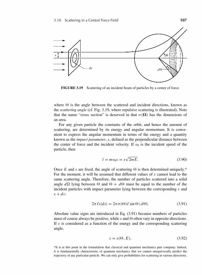
“M03 Goldstein ISBN C03” — 2011/2/15 — page 107 — #38
3.10 Scattering in a Central Force Field 107
FIGURE 3.19 Scattering of an incident beam of particles by a center of force.
where � is the angle between the scattered and incident directions, known asthe scattering angle (cf. Fig. 3.19, where repulsive scattering is illustrated). Notethat the name “cross section” is deserved in that σ(�) has the dimensions ofan area.
For any given particle the constants of the orbit, and hence the amount ofscattering, are determined by its energy and angular momentum. It is conve-nient to express the angular momentum in terms of the energy and a quantityknown as the impact parameter, s, defined as the perpendicular distance betweenthe center of force and the incident velocity. If v0 is the incident speed of theparticle, then
l = mv0s = s√
2m E . (3.90)
Once E and s are fixed, the angle of scattering � is then determined uniquely.*For the moment, it will be assumed that different values of s cannot lead to thesame scattering angle. Therefore, the number of particles scattered into a solidangle d� lying between � and � + d� must be equal to the number of theincident particles with impact parameter lying between the corresponding s ands + ds:
2π I s|ds| = 2πσ(�)I sin� | d�|. (3.91)
Absolute value signs are introduced in Eq. (3.91) because numbers of particlesmust of course always be positive, while s and� often vary in opposite directions.If s is considered as a function of the energy and the corresponding scatteringangle,
s = s(�, E), (3.92)
*It is at this point in the formulation that classical and quantum mechanics part company. Indeed,it is fundamentally characteristic of quantum mechanics that we cannot unequivocally predict thetrajectory of any particular particle. We can only give probabilities for scattering in various directions.
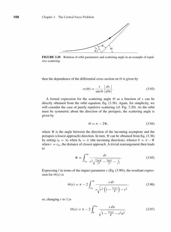
“M03 Goldstein ISBN C03” — 2011/2/15 — page 108 — #39
108 Chapter 3 The Central Force Problem
FIGURE 3.20 Relation of orbit parameters and scattering angle in an example of repul-sive scattering.
then the dependence of the differential cross section on � is given by
σ(�) = s
sin�
∣∣∣∣ ds
d�
∣∣∣∣ . (3.93)
A formal expression for the scattering angle � as a function of s can bedirectly obtained from the orbit equation, Eq. (3.36). Again, for simplicity, wewill consider the case of purely repulsive scattering (cf. Fig. 3.20). As the orbitmust be symmetric about the direction of the periapsis, the scattering angle isgiven by
� = π − 2�, (3.94)
where � is the angle between the direction of the incoming asymptote and theperiapsis (closest approach) direction. In turn, � can be obtained from Eq. (3.36)by setting r0 = ∞ when θ0 = π (the incoming direction), whence θ = π −�when r = rm , the distance of closest approach. A trivial rearrangement then leadsto
� =∫ ∞
rm
dr
r2√
2m El2 − 2mV
l2 − 1r2
. (3.95)
Expressing l in terms of the impact parameter s (Eq. (3.90)), the resultant expres-sion for �(s) is
�(s) = π − 2∫ ∞
rm
s dr
r
√r2(
1 − V (r)E
)− s2
, (3.96)
or, changing r to 1/u
�(s) = π − 2∫ um
0
s du√1 − V (u)
E − s2u2. (3.97)
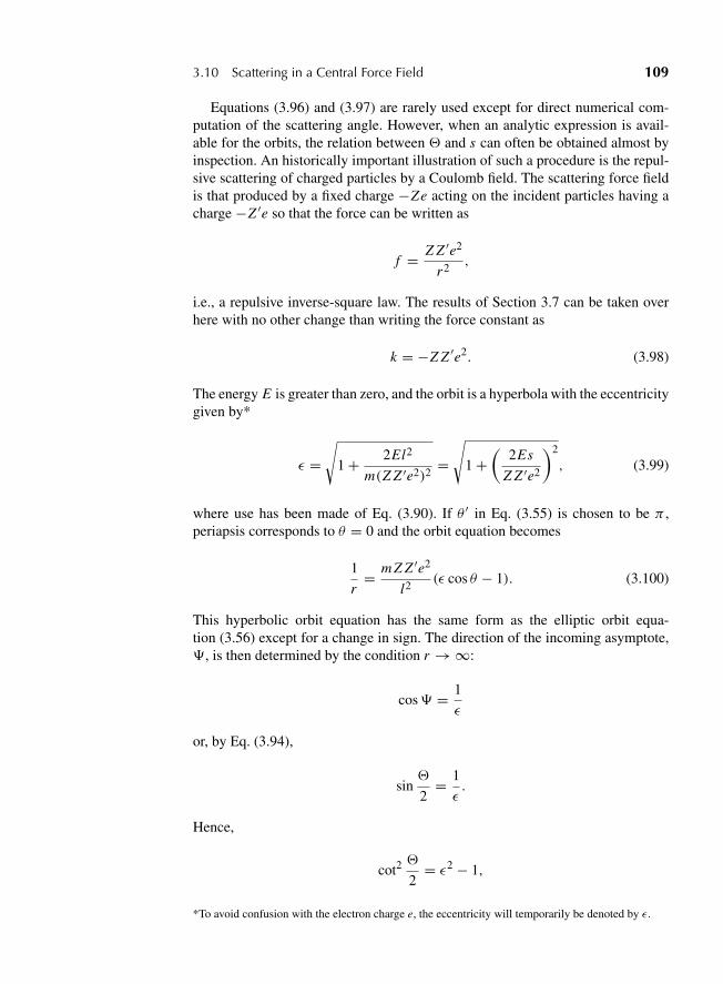
“M03 Goldstein ISBN C03” — 2011/2/15 — page 109 — #40
3.10 Scattering in a Central Force Field 109
Equations (3.96) and (3.97) are rarely used except for direct numerical com-putation of the scattering angle. However, when an analytic expression is avail-able for the orbits, the relation between � and s can often be obtained almost byinspection. An historically important illustration of such a procedure is the repul-sive scattering of charged particles by a Coulomb field. The scattering force fieldis that produced by a fixed charge −Ze acting on the incident particles having acharge −Z ′e so that the force can be written as
f = Z Z ′e2
r2,
i.e., a repulsive inverse-square law. The results of Section 3.7 can be taken overhere with no other change than writing the force constant as
k = −Z Z ′e2. (3.98)
The energy E is greater than zero, and the orbit is a hyperbola with the eccentricitygiven by*
ε =√
1 + 2El2
m(Z Z ′e2)2=√
1 +(
2Es
Z Z ′e2
)2
, (3.99)
where use has been made of Eq. (3.90). If θ ′ in Eq. (3.55) is chosen to be π ,periapsis corresponds to θ = 0 and the orbit equation becomes
1
r= m Z Z ′e2
l2(ε cos θ − 1). (3.100)
This hyperbolic orbit equation has the same form as the elliptic orbit equa-tion (3.56) except for a change in sign. The direction of the incoming asymptote,�, is then determined by the condition r → ∞:
cos� = 1
ε
or, by Eq. (3.94),
sin�
2= 1
ε.
Hence,
cot2�
2= ε2 − 1,
*To avoid confusion with the electron charge e, the eccentricity will temporarily be denoted by ε.
“M03 Goldstein ISBN C03” — 2011/2/15 — page 110 — #41
110 Chapter 3 The Central Force Problem
and using Eq. (3.99)
cot�
2= 2Es
Z Z ′e2.
The desired functional relationship between the impact parameter and the scatter-ing angle is therefore
s = Z Z ′e2
2Ecot
�
2, (3.101)
so that on carrying through the manipulation required by Eq. (3.93), we find thatσ(�) is given by
σ(�) = 1
4
(Z Z ′e2
2E
)2
csc4 �
2. (3.102)
Equation (3.102) gives the famous Rutherford scattering cross section, orig-inally derived by Rutherford for the scattering of α particles by atomic nuclei.Quantum mechanics in the nonrelativistic limit yields a cross section identicalwith this classical result.
In atomic physics, the concept of a total scattering cross section σT , definedas
σT =∫
4πσ(�) d� = 2π
∫ π
0σ(�) sin� d�,
is of considerable importance. However, if we attempt to calculate the total crosssection for Coulomb scattering by substituting Eq. (3.102) in this definition, weobtain an infinite result! The physical reason behind this behavior is not diffi-cult to discern. From its definition the total cross section is the number of parti-cles scattered in all directions per unit time for unit incident intensity. Now, theCoulomb field is an example of a “long-range” force; its effects extend to infinity.The very small deflections occur only for particles with very large impact param-eters. Hence, all particles in an incident beam of infinite lateral extent will bescattered to some extent and must be included in the total scattering cross section.It is therefore clear that the infinite value for σT is not peculiar to the Coulombfield; it occurs in classical mechanics whenever the scattering field is differentfrom zero at all distances, no matter how large.* Only if the force field “cuts off,”i.e., is zero beyond a certain distance, will the scattering cross section be finite.Physically, such a cut-off occurs for the Coulomb field of a nucleus as a result ofthe presence of the atomic electrons, which “screen” the nucleus and effectivelycancel its charge outside the atom.
*σT is also infinite for the Coulomb field in quantum mechanics, since it has been stated thatEq. (3.102) remains valid there. However, not all “long-range” forces give rise to infinite total crosssections in quantum mechanics. It turns out that all potentials that fall off faster at larger distancesthan 1/r2 produce a finite quantum-mechanical total scattering cross section.
“M03 Goldstein ISBN C03” — 2011/2/15 — page 111 — #42
3.10 Scattering in a Central Force Field 111
In Rutherford scattering, the scattering angle � is a smooth monotonic func-tion of the impact parameter s. From Eq. (3.101) we see that as s decreases frominfinity, � increases monotonically from zero, reaching the value π as s goes tozero. However, other types of behavior are possible in classical systems, requiringsome modification in the prescription, Eq. (3.93), for the classical cross section.For example, with a repulsive potential and particle energy qualitatively of thenature shown in Fig. 3.21(a), it is easy to see physically that the curve of � ver-sus s may behave as indicated in Fig. 3.21(b). Thus, with very large values ofthe impact parameter, as noted above, the particle always remains at large radialdistances from the center of force and suffers only minor deflection. At the otherextreme, for s = 0, the particle travels in a straight line into the center of force,and if the energy is greater than the maximum of the potential, it will continueon through the center without being scattered at all. Hence, for both limits in s,the scattering angle goes to zero. For some intermediate value of s, the scatter-ing angle must pass through a maximum �m . When � < �m , there will be twovalues of s that can give rise to the same scattering angle. Each will contributeto the scattering cross section at that angle, and Eq. (3.93) should accordingly bemodified to the form
σ(�) =∑
i
si
sin�
∣∣∣∣ ds
d�
∣∣∣∣i, (3.103)
where for � �= �m the index i takes on the values 1 and 2. Here the subscript idistinguishes the various values of s giving rise to the same value of �.
Of particular interest is the cross section at the maximum angle of scattering�m . As the derivative of� with respect to s vanishes at this angle, it follows fromEq. (3.93) or (3.103) that the cross section must become infinite at�→ �m . Butfor all larger angles the cross section is zero, since the scattering angle cannotexceed �m . The phenomenon of the infinite rise of the cross section followed byabrupt disappearance is very similar to what occurs in the geometrical optics of thescattering of sunlight by raindrops. On the basis of this similarity, the phenomenonis called rainbow scattering.
FIGURE 3.21 Repulsive nonsingular scattering potential and double-valued curve ofscattering angle � versus impact parameter s0 for sufficiently high energy.
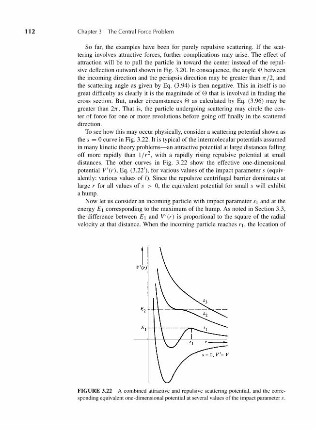
“M03 Goldstein ISBN C03” — 2011/2/15 — page 112 — #43
112 Chapter 3 The Central Force Problem
So far, the examples have been for purely repulsive scattering. If the scat-tering involves attractive forces, further complications may arise. The effect ofattraction will be to pull the particle in toward the center instead of the repul-sive deflection outward shown in Fig. 3.20. In consequence, the angle � betweenthe incoming direction and the periapsis direction may be greater than π/2, andthe scattering angle as given by Eq. (3.94) is then negative. This in itself is nogreat difficulty as clearly it is the magnitude of � that is involved in finding thecross section. But, under circumstances � as calculated by Eq. (3.96) may begreater than 2π . That is, the particle undergoing scattering may circle the cen-ter of force for one or more revolutions before going off finally in the scattereddirection.
To see how this may occur physically, consider a scattering potential shown asthe s = 0 curve in Fig. 3.22. It is typical of the intermolecular potentials assumedin many kinetic theory problems—an attractive potential at large distances fallingoff more rapidly than 1/r2, with a rapidly rising repulsive potential at smalldistances. The other curves in Fig. 3.22 show the effective one-dimensionalpotential V ′(r), Eq. (3.22′), for various values of the impact parameter s (equiv-alently: various values of l). Since the repulsive centrifugal barrier dominates atlarge r for all values of s > 0, the equivalent potential for small s will exhibita hump.
Now let us consider an incoming particle with impact parameter s1 and at theenergy E1 corresponding to the maximum of the hump. As noted in Section 3.3,the difference between E1 and V ′(r) is proportional to the square of the radialvelocity at that distance. When the incoming particle reaches r1, the location of
FIGURE 3.22 A combined attractive and repulsive scattering potential, and the corre-sponding equivalent one-dimensional potential at several values of the impact parameter s.
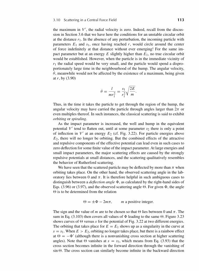
“M03 Goldstein ISBN C03” — 2011/2/15 — page 113 — #44
3.10 Scattering in a Central Force Field 113
the maximum in V ′, the radial velocity is zero. Indeed, recall from the discus-sion in Section 3.6 that we have here the conditions for an unstable circular orbitat the distance r1. In the absence of any perturbation, the incoming particle withparameters E1 and s1, once having reached r , would circle around the centerof force indefinitely at that distance without ever emerging! For the same im-pact parameter but at an energy E slightly higher than E1, no true circular orbitwould be established. However, when the particle is in the immediate vicinity ofr1 the radial speed would be very small, and the particle would spend a dispro-portionately large time in the neighbourhood of the hump. The angular velocity,θ , meanwhile would not be affected by the existence of a maximum, being givenat r , by (3.90)
θ = l
mr21
= s1
r21
√2E
m.
Thus, in the time it takes the particle to get through the region of the hump, theangular velocity may have carried the particle through angles larger than 2π oreven multiples thereof. In such instances, the classical scattering is said to exhibitorbiting or spiraling.
As the impact parameter is increased, the well and hump in the equivalentpotential V ′ tend to flatten out, until at some parameter s2 there is only a pointof inflection in V ′ at an energy E2 (cf. Fig. 3.22). For particle energies aboveE2, there will no longer be orbiting. But the combined effects of the attractiveand repulsive components of the effective potential can lead even in such cases tozero deflection for some finite value of the impact parameter. At large energies andsmall impact parameters, the major scattering effects are caused by the stronglyrepulsive potentials at small distances, and the scattering qualitatively resemblesthe behavior of Rutherford scattering.
We have seen that the scattered particle may be deflected by more than π whenorbiting takes place. On the other hand, the observed scattering angle in the lab-oratory lies between 0 and π . It is therefore helpful in such ambiguous cases todistinguish between a deflection angle �, as calculated by the right-hand sides ofEqs. (3.96) or (3.97), and the observed scattering angle �. For given �, the angle� is to be determined from the relation
� = ±�− 2mπ, m a positive integer.
The sign and the value of m are to be chosen so that � lies between 0 and π . Thesum in Eq. (3.103) then covers all values of � leading to the same�. Figure 3.23shows curves of� versus s for the potential of Fig. 3.22 at two different energies.The orbiting that takes place for E = E1 shows up as a singularity in the curve ats = s1. When E > E2, orbiting no longer takes place, but there is a rainbow effectat � = −�′ (although there is a nonvanishing cross section at higher scatteringangles). Note that � vanishes at s = s3, which means from Eq. (3.93) that thecross section becomes infinite in the forward direction through the vanishing ofsin�. The cross section can similarly become infinite in the backward direction
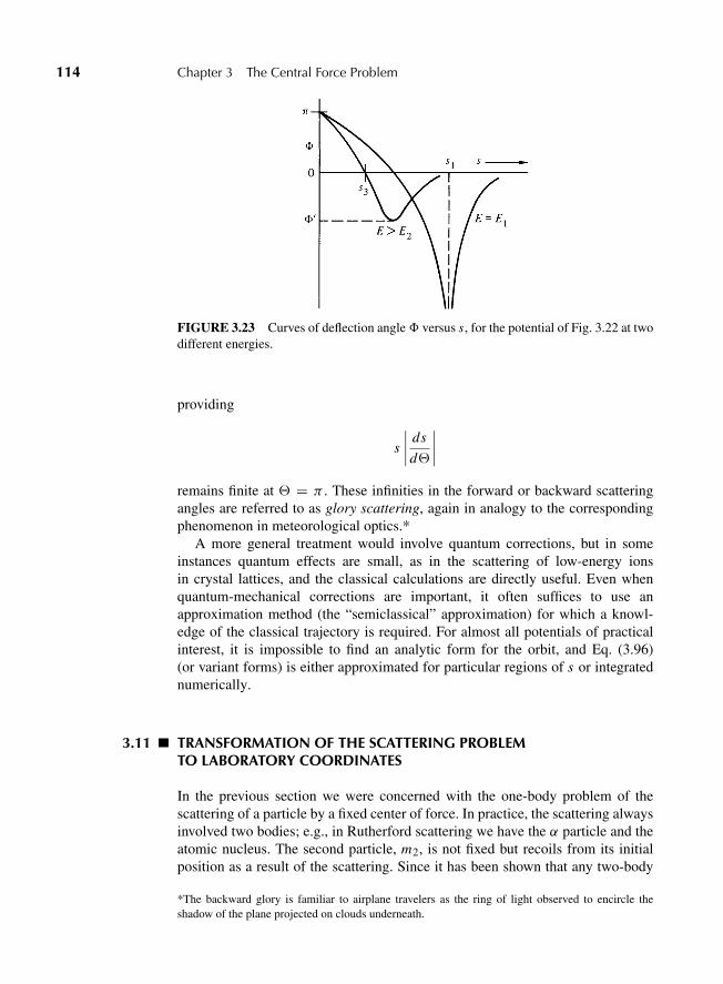
“M03 Goldstein ISBN C03” — 2011/2/15 — page 114 — #45
114 Chapter 3 The Central Force Problem
FIGURE 3.23 Curves of deflection angle� versus s, for the potential of Fig. 3.22 at twodifferent energies.
providing
s
∣∣∣∣ ds
d�
∣∣∣∣remains finite at � = π . These infinities in the forward or backward scatteringangles are referred to as glory scattering, again in analogy to the correspondingphenomenon in meteorological optics.*
A more general treatment would involve quantum corrections, but in someinstances quantum effects are small, as in the scattering of low-energy ionsin crystal lattices, and the classical calculations are directly useful. Even whenquantum-mechanical corrections are important, it often suffices to use anapproximation method (the “semiclassical” approximation) for which a knowl-edge of the classical trajectory is required. For almost all potentials of practicalinterest, it is impossible to find an analytic form for the orbit, and Eq. (3.96)(or variant forms) is either approximated for particular regions of s or integratednumerically.
3.11 TRANSFORMATION OF THE SCATTERING PROBLEMTO LABORATORY COORDINATES
In the previous section we were concerned with the one-body problem of thescattering of a particle by a fixed center of force. In practice, the scattering alwaysinvolved two bodies; e.g., in Rutherford scattering we have the α particle and theatomic nucleus. The second particle, m2, is not fixed but recoils from its initialposition as a result of the scattering. Since it has been shown that any two-body
*The backward glory is familiar to airplane travelers as the ring of light observed to encircle theshadow of the plane projected on clouds underneath.

“M03 Goldstein ISBN C03” — 2011/2/15 — page 115 — #46
3.11 Transformation of the Scattering Problem 115
FIGURE 3.24 Scattering of two particles as viewed in the laboratory system.
central force problem can be reduced to a one-body problem, it might be thoughtthat the only change is to replace m by the reduced mass μ. However, the matteris not quite that simple. The scattering angle actually measured in the laboratory,which we shall denote by ϑ , is the angle between the final and incident directionsof the scattered particle in laboratory coordinates.† On the other hand, the angle� calculated from the equivalent one-body problem is the angle between the finaland initial directions of the relative vector between the two particles in the cen-ter of mass coordinates. These two angles, θ and �, would be the same only ifthe second particle remains stationary through the scattering process. In general,however, the second particle, though initially at rest, is itself set in motion by themutual force between the two particles, and, as is indicated in Fig. 3.24, the twoangles then have different values. The equivalent one-body problem thus doesnot directly furnish the scattering angle as measured in the laboratory coordinatesystem.
The relationship between the scattering angles � and ϑ can be determinedby examining how the scattering takes place in a coordinate system moving withthe center of mass of both particles. In such a system the total linear momentumis zero, of course, and the two particles always move with equal and oppositemomenta. Figure 3.25 illustrates the appearance of the scattering process to anobserver in the center of mass system. Before the scattering, the particles aremoving directly toward each other; after, they are moving directly away fromeach other. The angle between the initial and final directions of the relative vec-tor, �, must therefore be the same as the scattering angle of either particle inthe center-of-mass system. The connection between the two scattering angles� and ϑ can thus be obtained by considering the transformation between thecenter-of-mass system and the laboratory system.
†The scattering angle ϑ must not be confused with the angle coordinate θ of the relative vector, r,between the two particles.
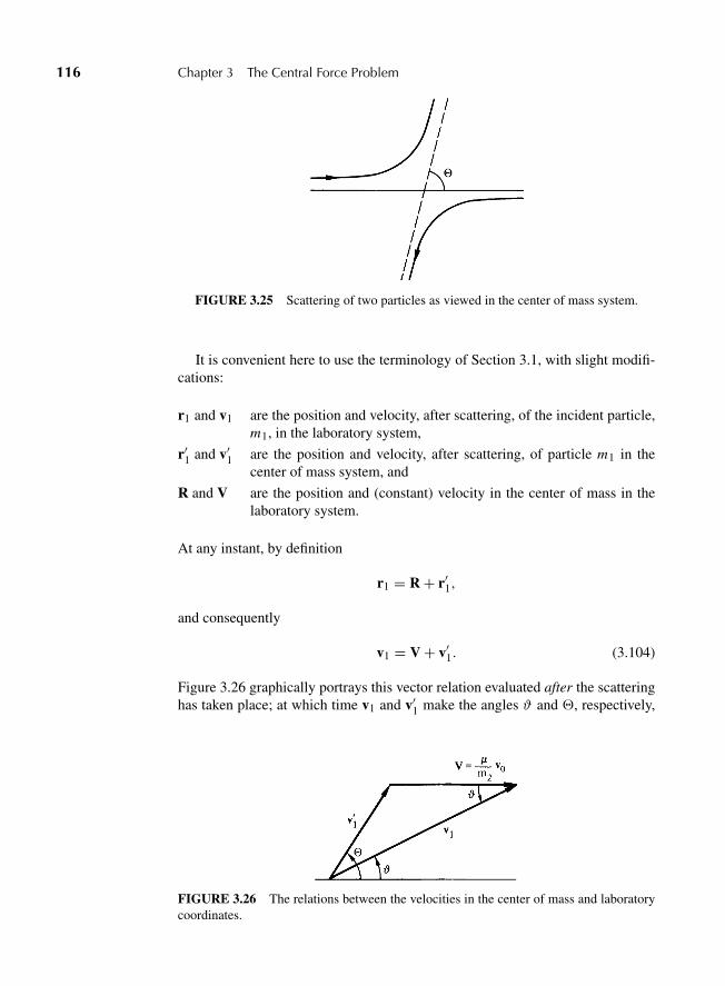
“M03 Goldstein ISBN C03” — 2011/2/15 — page 116 — #47
116 Chapter 3 The Central Force Problem
FIGURE 3.25 Scattering of two particles as viewed in the center of mass system.
It is convenient here to use the terminology of Section 3.1, with slight modifi-cations:
r1 and v1 are the position and velocity, after scattering, of the incident particle,m1, in the laboratory system,
r′1 and v′1 are the position and velocity, after scattering, of particle m1 in thecenter of mass system, and
R and V are the position and (constant) velocity in the center of mass in thelaboratory system.
At any instant, by definition
r1 = R + r′1,
and consequently
v1 = V + v′1. (3.104)
Figure 3.26 graphically portrays this vector relation evaluated after the scatteringhas taken place; at which time v1 and v′1 make the angles ϑ and �, respectively,
FIGURE 3.26 The relations between the velocities in the center of mass and laboratorycoordinates.
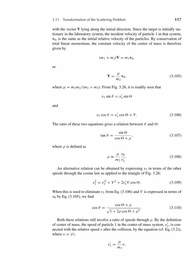
“M03 Goldstein ISBN C03” — 2011/2/15 — page 117 — #48
3.11 Transformation of the Scattering Problem 117
with the vector V lying along the initial direction. Since the target is initially sta-tionary in the laboratory system, the incident velocity of particle 1 in that system,v0, is the same as the initial relative velocity of the particles. By conservation oftotal linear momentum, the constant velocity of the center of mass is thereforegiven by
(m1 + m2)V = m1v0,
or
V = μ
m2v0, (3.105)
where μ = m1m2/(m1 + m2). From Fig. 3.26, it is readily seen that
v1 sinϑ = v′1 sin�
and
v1 cosϑ = v′1 cos�+ V . (3.106)
The ratio of these two equations gives a relation between ϑ and �:
tanϑ = sin�
cos�+ ρ , (3.107)
where ρ is defined as
ρ ≡ μ
m2
v0
v′1. (3.108)
An alternative relation can be obtained by expressing v1 in terms of the otherspeeds through the cosine law as applied to the triangle of Fig. 3.26:
v21 = v′21 + V 2 + 2v′1V cos�. (3.109)
When this is used to eliminate v1 from Eq. (3.106) and V is expressed in terms ofv0 by Eq. (3.105), we find
cosϑ = cos�+ ρ√1 + 2ρ cos�+ ρ2
. (3.110)
Both these relations still involve a ratio of speeds through ρ. By the definitionof center of mass, the speed of particle 1 in the center-of-mass system, v′1, is con-nected with the relative speed v after the collision, by the equation (cf. Eq. (3.2)),where v = |r |:
v′1 = μ
m1v.
“M03 Goldstein ISBN C03” — 2011/2/15 — page 118 — #49
118 Chapter 3 The Central Force Problem
Hence, ρ can also be written as
ρ = m1
m2
v0
v, (3.108′)
where v, it should be emphasized, is the relative speed after the collision. Whenthe collision is elastic, the total kinetic energy of the two particles remains unal-tered and v must equal v0 so that ρ is simply
ρ = m1
m2, (elastic collision) (3.111)
independent of energies or speeds. If the collision is inelastic, the total kineticenergy of the two particles is altered (e.g., some of the kinetic energy goes intothe form of internal excitation energy of the target). Since the total energy is con-served and momentum is conserved, the energy change resulting from the colli-sion can be expressed as
μv2
2= μv2
0
2+ Q. (3.112)
The so-called Q value of the inelastic collision is clearly negative in magnitude,but the sign convention is chosen to conform to that used in general for atomicand nuclear reactions. From Eq. (3.112) the ratio of relative speeds before andafter collision can be written
v
v0=√
1 + m1 + m2
m2
Q
E, (3.113)
where E = 12 m1v
20 is the energy of the incoming particle (in the laboratory
system). Thus, for inelastic scattering ρ becomes
ρ = m1
m2
√1 + m1+m2
m2
QE
. (inelastic scattering) (3.114)
Not only are the scattering angles ϑ and � in general different in magnitude,but the values of the differential scattering cross section depend upon which ofthe two angles is used as the argument of σ . The connection between the twofunctional forms is obtained from the observation that in a particular experimentthe number of particles scattered into a given element of solid angle must be thesame whether we measure the event in terms of ϑ or �. As an equation, thisstatement can be written
2π Iσ(�) sin�| d�| = 2π Iσ ′(ϑ) sinϑ | dϑ |,
“M03 Goldstein ISBN C03” — 2011/2/15 — page 119 — #50
3.11 Transformation of the Scattering Problem 119
or
σ ′(ϑ) = σ(�)sin�
sinϑ
∣∣∣∣d�dϑ
∣∣∣∣ = σ(�)
∣∣∣∣d(cos�)
d(cosϑ)
∣∣∣∣ , (3.115)
where σ ′(ϑ) is the differential scattering cross section expressed in terms of thescattering angle in the laboratory system. The derivative can easily be evaluatedfrom Eq. (3.110), leading to the result
σ ′(ϑ) = σ(�)(1 + 2ρ cos�+ ρ2)3/2
1 + ρ cos�. (3.116)
Note that σ(�) is not the cross section an observer would measure in thecenter-of-mass system. Both σ(�) and σ ′(ϑ) are cross sections measured in thelaboratory system; they are merely expressed in terms of different coordinates. Anobserver fixed in the center-of-mass system would see a different flux density ofincident particles from that measured in the laboratory system, and this transfor-mation of flux density would have to be included if (for some reason) we wantedto relate the cross sections as measured in the two different systems.
The two scattering angles have a particularly simple relation for elastic scat-tering when the two masses of particles are equal. It then follows that ρ = 1, andfrom Eq. (3.110) we have
cosϑ =√
1 + cos�
2= cos
�
2,
or
ϑ = �
2, (ρ = 1).
Thus, with equal masses, scattering angles greater than 90◦ cannot occur in thelaboratory system; all the scattering is in the forward hemisphere. Correspond-ingly, the scattering cross section is given in terms of � from Eq. (3.116) as
σ ′(ϑ) = 4 cosϑ · σ(�), ϑ ≤ π
2, (ρ = 1).
Even when the scattering is isotropic in terms of �, i.e., σ(�) is constant,independent of �, then the cross section in terms of ϑ varies as the cosine of theangle! When, however, the scattering mass m2 is very large compared to the inci-dent particle mass m1 and the scattering is elastic, then from Eq. (3.111) ρ ≈ 0,so σ ′(ϑ) ≈ σ(�) from Eq. (3.116).
We have seen that even in elastic collisions, where the total kinetic energyremains constant, a collision with an initially stationary target results in a transferof kinetic energy to the target with a corresponding decrease in the kinetic energyof the incident particle. In other words, the collision slows down the incident
“M03 Goldstein ISBN C03” — 2011/2/15 — page 120 — #51
120 Chapter 3 The Central Force Problem
particle. The degree of slowing down can be obtained from Eq. (3.109) if v′1 andV are expressed in terms of v0 by Eqs. (3.108) and (3.105), respectively:
v21
v20
=(μ
m2ρ
)2
(1 + 2ρ cos�+ ρ2). (3.117)
For elastic collisions ρ = m1/m2, and Eq. (3.117) can be simplified to
E1
E0= 1 + 2ρ cos�+ ρ2
(1 + ρ)2 , (elastic collision) (3.117′)
where E0 is the initial kinetic energy of the incident particle in the laboratorysystem and E1 the corresponding energy after scattering. When the particles areof equal mass, this relation becomes
E1
E0= 1 + cos�
2= cos2 ϑ.
Thus, at the maximum scattering angle (� = π , ϑ = π/2), the incident particleloses all its energy and is completely stopped in the laboratory system.
This transfer of kinetic energy by scattering is, of course, the principle behindthe “moderator” in a thermal neutron reactor. Fast neutrons produced by fissionmake successive elastic scatterings until their kinetic energy is reduced to thermalenergies, where they are more liable to cause fission than to be captured. Clearlythe best moderators will be the light elements, ideally hydrogen (ρ = 1). For anuclear reactor, hydrogen is practical only when contained as part of a mixtureor compound, such as water. Other light elements useful for their moderatingproperties include deuterium, of mass 2, and carbon, of mass 12. Hydrogen, aspresent in paraffin, water, or plastics, is frequently used in the laboratory to slowdown neutrons.
Despite their current useful applications, these calculations of the transforma-tion from laboratory to center of mass coordinates, and of the transfer of kineticenergy, are not particularly “modern” or “quantum” in nature. Nor is the classi-cal mechanics involved particularly advanced or difficult. All that has been used,essentially, is the conservation of momentum and energy. Indeed, similar calcula-tions may be found in freshman textbooks, usually in terms of elastic collisionsbetween, say, billiard balls. But it is their elementary nature that results in thewidespread validity of these calculations. So long as momentum is conversed (andthis will be true in quantum mechanics) and the Q value is known, the details ofthe scattering process are irrelevant. In effect, the vicinity of the scattering par-ticle is a “black box,” and we are concerned only with what goes in and whatcomes out. It matters not at all whether the phenomena occurring inside the boxare “classical” or “quantum.” Consequently, the formulae of this section may beused in the experimental analysis of phenomena essentially quantum in nature,as for example, neutron-proton scattering, so long as the energies are low enoughthat relativistic effects may be neglected. (See Section 7.7 for a discussion of therelativistic treatment of the kinematics of collisions.)
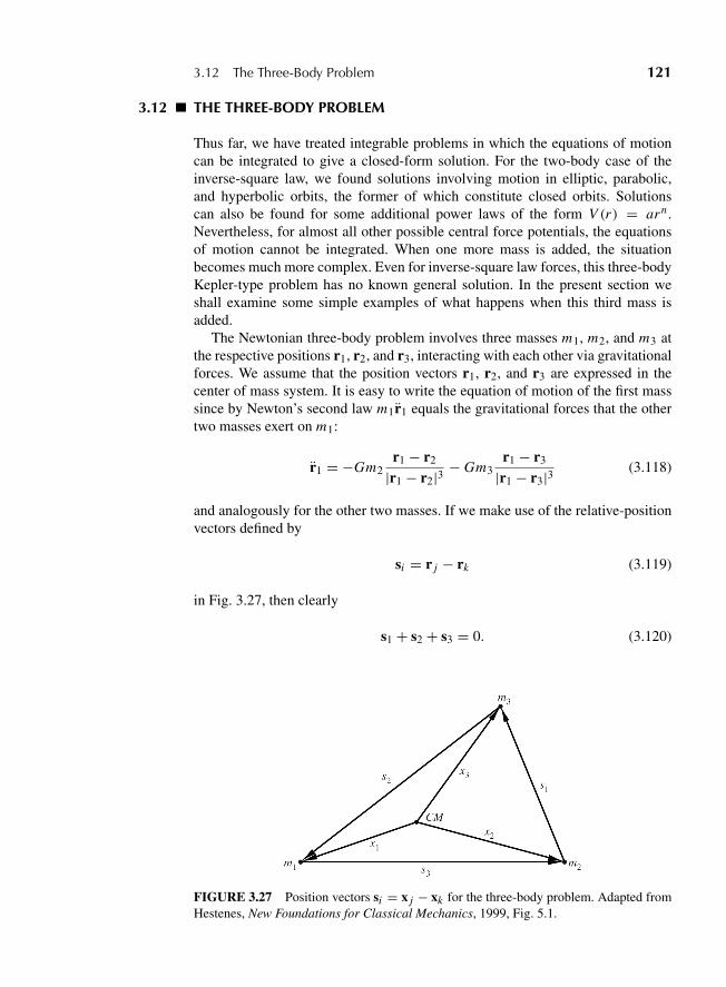
“M03 Goldstein ISBN C03” — 2011/2/15 — page 121 — #52
3.12 The Three-Body Problem 121
3.12 THE THREE-BODY PROBLEM
Thus far, we have treated integrable problems in which the equations of motioncan be integrated to give a closed-form solution. For the two-body case of theinverse-square law, we found solutions involving motion in elliptic, parabolic,and hyperbolic orbits, the former of which constitute closed orbits. Solutionscan also be found for some additional power laws of the form V (r) = arn .Nevertheless, for almost all other possible central force potentials, the equationsof motion cannot be integrated. When one more mass is added, the situationbecomes much more complex. Even for inverse-square law forces, this three-bodyKepler-type problem has no known general solution. In the present section weshall examine some simple examples of what happens when this third mass isadded.
The Newtonian three-body problem involves three masses m1, m2, and m3 atthe respective positions r1, r2, and r3, interacting with each other via gravitationalforces. We assume that the position vectors r1, r2, and r3 are expressed in thecenter of mass system. It is easy to write the equation of motion of the first masssince by Newton’s second law m1r1 equals the gravitational forces that the othertwo masses exert on m1:
r1 = −Gm2r1 − r2
|r1 − r2|3 − Gm3r1 − r3
|r1 − r3|3 (3.118)
and analogously for the other two masses. If we make use of the relative-positionvectors defined by
si = r j − rk (3.119)
in Fig. 3.27, then clearly
s1 + s2 + s3 = 0. (3.120)
FIGURE 3.27 Position vectors si = x j − xk for the three-body problem. Adapted fromHestenes, New Foundations for Classical Mechanics, 1999, Fig. 5.1.
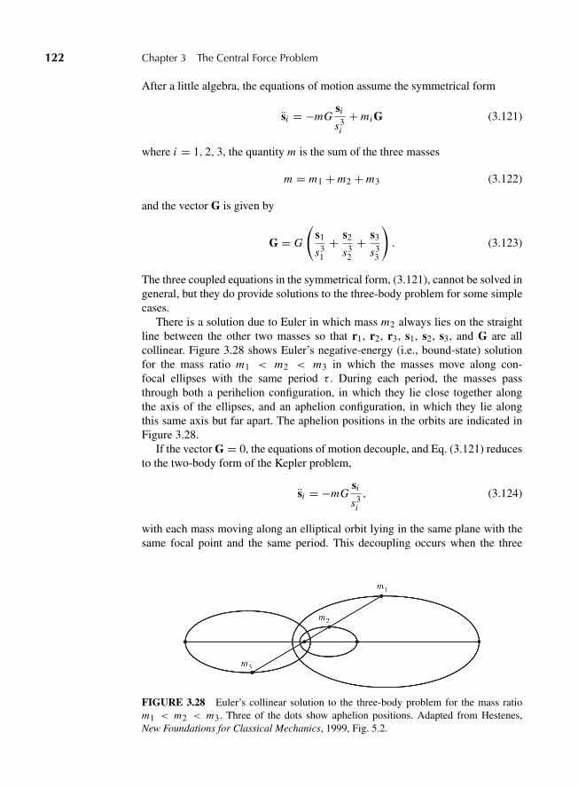
“M03 Goldstein ISBN C03” — 2011/2/15 — page 122 — #53
122 Chapter 3 The Central Force Problem
After a little algebra, the equations of motion assume the symmetrical form
si = −mGsi
s3i
+ mi G (3.121)
where i = 1, 2, 3, the quantity m is the sum of the three masses
m = m1 + m2 + m3 (3.122)
and the vector G is given by
G = G
(s1
s31
+ s2
s32
+ s3
s33
). (3.123)
The three coupled equations in the symmetrical form, (3.121), cannot be solved ingeneral, but they do provide solutions to the three-body problem for some simplecases.
There is a solution due to Euler in which mass m2 always lies on the straightline between the other two masses so that r1, r2, r3, s1, s2, s3, and G are allcollinear. Figure 3.28 shows Euler’s negative-energy (i.e., bound-state) solutionfor the mass ratio m1 < m2 < m3 in which the masses move along con-focal ellipses with the same period τ . During each period, the masses passthrough both a perihelion configuration, in which they lie close together alongthe axis of the ellipses, and an aphelion configuration, in which they lie alongthis same axis but far apart. The aphelion positions in the orbits are indicated inFigure 3.28.
If the vector G = 0, the equations of motion decouple, and Eq. (3.121) reducesto the two-body form of the Kepler problem,
si = −mGsi
s3i
, (3.124)
with each mass moving along an elliptical orbit lying in the same plane with thesame focal point and the same period. This decoupling occurs when the three
FIGURE 3.28 Euler’s collinear solution to the three-body problem for the mass ratiom1 < m2 < m3. Three of the dots show aphelion positions. Adapted from Hestenes,New Foundations for Classical Mechanics, 1999, Fig. 5.2.
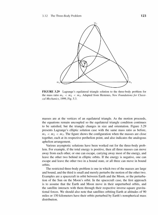
“M03 Goldstein ISBN C03” — 2011/2/15 — page 123 — #54
3.12 The Three-Body Problem 123
FIGURE 3.29 Lagrange’s equilateral triangle solution to the three-body problem forthe mass ratio m1 < m2 < m3. Adapted from Hestenes, New Foundations for Classi-cal Mechanics, 1999, Fig. 5.3.
masses are at the vertices of an equilateral triangle. As the motion proceeds,the equations remain uncoupled so the equilateral triangle condition continuesto be satisfied, but the triangle changes in size and orientation. Figure 3.29presents Lagrange’s elliptic solution case with the same mass ratio as before,m1 < m2 < m3. The figure shows the configuration when the masses are closetogether, each at its respective perihelion point, and also indicates the analogousaphelion arrangement.
Various asymptotic solutions have been worked out for the three-body prob-lem. For example, if the total energy is positive, then all three masses can moveaway from each other, or one can escape, carrying away most of the energy, andleave the other two behind in elliptic orbits. If the energy is negative, one canescape and leave the other two in a bound state, or all three can move in boundorbits.
The restricted three-body problem is one in which two of the masses are largeand bound, and the third is small and merely perturbs the motion of the other two.Examples are a spacecraft in orbit between Earth and the Moon, or the perturba-tion of the Sun on the Moon’s orbit. In the spacecraft case, the first approachis to assume that the Earth and Moon move in their unperturbed orbits, andthe satellite interacts with them through their respective inverse-square gravita-tional forces. We should also note that satellites orbiting Earth at altitudes of 90miles or 150 kilometers have their orbits perturbed by Earth’s nonspherical massdistribution.
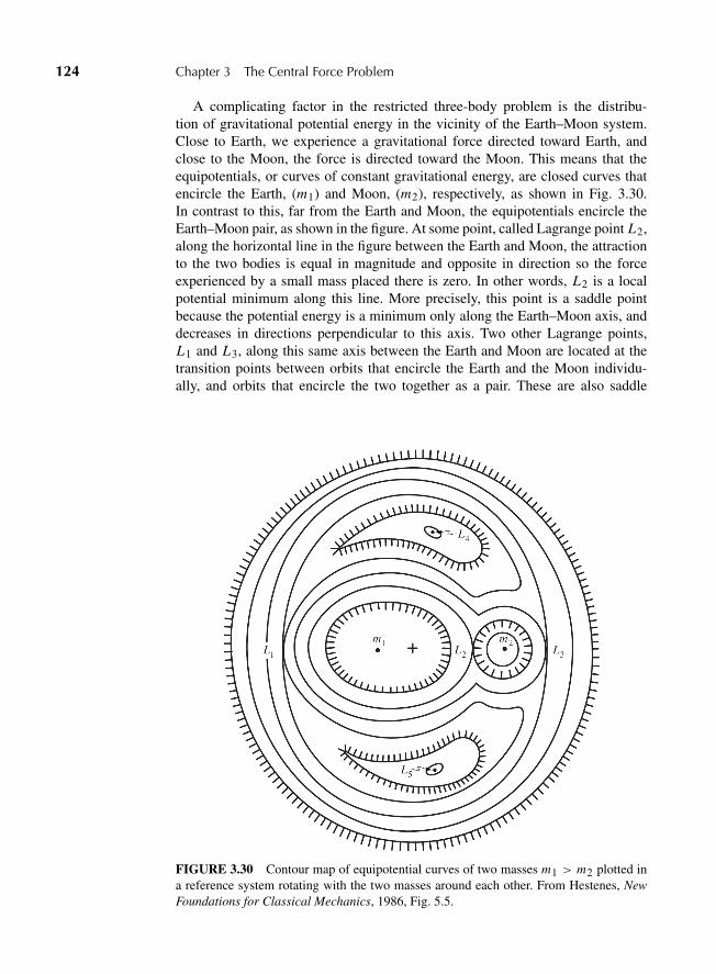
“M03 Goldstein ISBN C03” — 2011/2/15 — page 124 — #55
124 Chapter 3 The Central Force Problem
A complicating factor in the restricted three-body problem is the distribu-tion of gravitational potential energy in the vicinity of the Earth–Moon system.Close to Earth, we experience a gravitational force directed toward Earth, andclose to the Moon, the force is directed toward the Moon. This means that theequipotentials, or curves of constant gravitational energy, are closed curves thatencircle the Earth, (m1) and Moon, (m2), respectively, as shown in Fig. 3.30.In contrast to this, far from the Earth and Moon, the equipotentials encircle theEarth–Moon pair, as shown in the figure. At some point, called Lagrange point L2,along the horizontal line in the figure between the Earth and Moon, the attractionto the two bodies is equal in magnitude and opposite in direction so the forceexperienced by a small mass placed there is zero. In other words, L2 is a localpotential minimum along this line. More precisely, this point is a saddle pointbecause the potential energy is a minimum only along the Earth–Moon axis, anddecreases in directions perpendicular to this axis. Two other Lagrange points,L1 and L3, along this same axis between the Earth and Moon are located at thetransition points between orbits that encircle the Earth and the Moon individu-ally, and orbits that encircle the two together as a pair. These are also saddle
FIGURE 3.30 Contour map of equipotential curves of two masses m1 > m2 plotted ina reference system rotating with the two masses around each other. From Hestenes, NewFoundations for Classical Mechanics, 1986, Fig. 5.5.
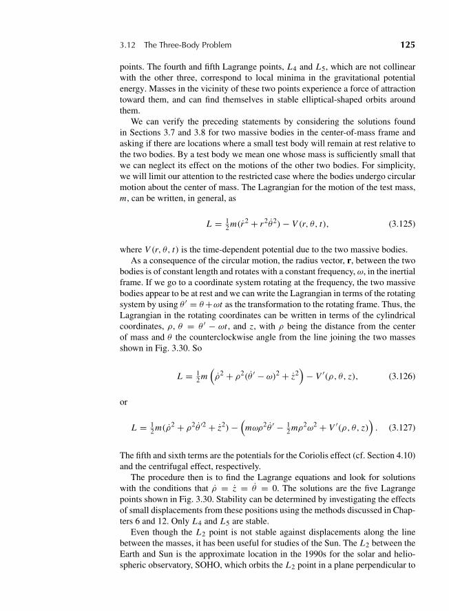
“M03 Goldstein ISBN C03” — 2011/2/15 — page 125 — #56
3.12 The Three-Body Problem 125
points. The fourth and fifth Lagrange points, L4 and L5, which are not collinearwith the other three, correspond to local minima in the gravitational potentialenergy. Masses in the vicinity of these two points experience a force of attractiontoward them, and can find themselves in stable elliptical-shaped orbits aroundthem.
We can verify the preceding statements by considering the solutions foundin Sections 3.7 and 3.8 for two massive bodies in the center-of-mass frame andasking if there are locations where a small test body will remain at rest relative tothe two bodies. By a test body we mean one whose mass is sufficiently small thatwe can neglect its effect on the motions of the other two bodies. For simplicity,we will limit our attention to the restricted case where the bodies undergo circularmotion about the center of mass. The Lagrangian for the motion of the test mass,m, can be written, in general, as
L = 12 m(r2 + r2θ2)− V (r, θ, t), (3.125)
where V (r, θ, t) is the time-dependent potential due to the two massive bodies.As a consequence of the circular motion, the radius vector, r, between the two
bodies is of constant length and rotates with a constant frequency, ω, in the inertialframe. If we go to a coordinate system rotating at the frequency, the two massivebodies appear to be at rest and we can write the Lagrangian in terms of the rotatingsystem by using θ ′ = θ+ωt as the transformation to the rotating frame. Thus, theLagrangian in the rotating coordinates can be written in terms of the cylindricalcoordinates, ρ, θ = θ ′ − ωt , and z, with ρ being the distance from the centerof mass and θ the counterclockwise angle from the line joining the two massesshown in Fig. 3.30. So
L = 12 m
(ρ2 + ρ2(θ ′ − ω)2 + z2
)− V ′(ρ, θ, z), (3.126)
or
L = 12 m(ρ2 + ρ2θ ′2 + z2)−
(mωρ2θ ′ − 1
2 mρ2ω2 + V ′(ρ, θ, z)). (3.127)
The fifth and sixth terms are the potentials for the Coriolis effect (cf. Section 4.10)and the centrifugal effect, respectively.
The procedure then is to find the Lagrange equations and look for solutionswith the conditions that ρ = z = θ = 0. The solutions are the five Lagrangepoints shown in Fig. 3.30. Stability can be determined by investigating the effectsof small displacements from these positions using the methods discussed in Chap-ters 6 and 12. Only L4 and L5 are stable.
Even though the L2 point is not stable against displacements along the linebetween the masses, it has been useful for studies of the Sun. The L2 between theEarth and Sun is the approximate location in the 1990s for the solar and helio-spheric observatory, SOHO, which orbits the L2 point in a plane perpendicular to
“M03 Goldstein ISBN C03” — 2011/2/15 — page 126 — #57
126 Chapter 3 The Central Force Problem
the Earth–Sun line. The satellite cannot be exactly at the L2 point, or we couldnot receive its transmissions against the bright Sun. Small steering rockets correctfor the slow drift toward, or away from, L2.
DERIVATIONS
1. Consider a system in which the total forces acting on the particles consist of conserva-tive forces F′
i and frictional forces fi proportional to the velocity. Show that for sucha system the virial theorem holds in the form
T = −1
2
∑i
F′i ? ri ,
providing the motion reaches a steady state and is not allowed to die down as a resultof the frictional forces.
2. By expanding e sinψ in a Fourier series in ωt , show that Kepler’s equation has theformal solution
ψ = ωt +∞∑
n=1
2
nJn(ne) sin nωt,
where Jn is the Bessel function of order n. For small argument, the Bessel functioncan be approximated in a power series of the argument. Accordingly, from this resultderive the first few terms in the expansion of ψ in powers of e.
3. If the difference ψ − ωt is represented by ρ, Kepler’s equation can be written
ρ = e sin(ωt + ρ).
Successive approximations to ρ can be obtained by expanding sin ρ in a Taylor seriesin ρ, and then replacing ρ by its expression given by Kepler’s equation. Show that thefirst approximation by ρ is ρ1, given by
tan ρ1 = e sinωt
1 − e cosωt,
and that the next approximation is found from
sin3(ρ2 − ρ1) = − 16 e3 sin(ωt + ρ1)(1 + e cosωt),
an expression that is accurate through terms of order e4.
4. Show that for repulsive scattering, Eq. (3.96) for the angle of scattering as a functionof the impact parameter, s, can be rewritten as
� = π − 4s∫ 1
0
ρ dρ√r2m
(1 − V
E
)2 − s2(1 − ρ2)
,

“M03 Goldstein ISBN C03” — 2011/2/15 — page 127 — #58
Derivations 127
or
� = π − 4s∫ 1
0
dρ√r2
mρ2 E
(V (rm)− V (r))+ s2(2 − ρ2)
,
by changing the variable of integration to some function ρ(r). Show that for arepulsive potential the integrand is never singular in the limit r → rm . Because ofthe definite limits of integration, these formulations have advantages for numericalcalculations of �(s) and allow naturally for the use of Gauss–Legendre quadratureschemes.
5. Apply the formulation of the preceding exercise to compute numerically�(s) and thedifferential cross section of σ(�) for the repulsive potential
V = V0
1 + r
and for a total energy E = 1.2V0. It is suggested that 16-point Gauss–Legendrequadrature will give adequate accuracy. Does the scattering exhibit a rainbow?
6. If a repulsive potential drops of monotonically with r , then for energies high com-pared to V (rm) the angle of scattering will be small. Under these conditions show thatEq. (3.97) can be manipulated so that the deflection angle is given approximately by
� = 1
E
∫ 1
0
(V (um)− V (u)) dy
(1 − y2)3/2,
where y, obviously, is u/um .Show further, that if V (u) is of the form Cun , where n is a positive integer, then inthe high-energy limit the cross section is proportional to �−2(1+1/n).
7. (a) Show that the angle of recoil of the target particle relative to the incident directionof the scattered particle is simply � = 1
2 (π −�).(b) It is observed that in elastic scattering the scattering cross section is isotropic in
terms of �. What are the corresponding probability distributions for the scatteredenergy of the incident particle, E1, and for the recoil energy of the target parti-cle, E2?
8. Show that the angle of scattering in the laboratory system, ϑ , is related to the energybefore scattering, E0, and the energy after scattering E1, according to the equation
cosϑ = m2 + m1
2m1
√E1
E0− m2 − m1
2m1
√E0
E1− m2 Q
2m1√
E0 E1.
9. Show that the central force problem is soluble in terms of elliptic functions when theforce is a power-law function of the distance with the following fractional exponents:
n = −3
2,−5
2,−1
3,−5
3,−7
3.
“M03 Goldstein ISBN C03” — 2011/2/15 — page 128 — #59
128 Chapter 3 The Central Force Problem
EXERCISES
10. A planet of mass M is in an orbit of eccentricity e = 1 − α where α 1, about theSun. Assume the motion of the Sun can be neglected and that only gravitational forcesact. When the planet is at its greatest distance from the Sun, it is struck by a comet ofmass m, where m M traveling in a tangential direction. Assuming the collision iscompletely inelastic, find the minimum kinetic energy the comet must have to changethe new orbit to a parabola.
11. Two particles move about each other in circular orbits under the influence of gravita-tional forces, with a period τ . Their motion is suddenly stopped at a given instant oftime, and they are then released and allowed to fall into each other. Prove that theycollide after a time τ/4
√2.
12. Suppose that there are long-range interactions between atoms in a gas in the form ofcentral forces derivable from a potential
U (r) = k
rm ,
where r is the distance between any pair of atoms and m is a positive integer. Assumefurther that relative to any given atom the other atoms are distributed in space suchthat their volume density is given by the Boltzmann factor:
ρ(r) = N
Ve−U (r)/kT ,
where N is the total number of atoms in a volume V . Find the addition to the virial ofClausius resulting from these forces between pairs of atoms, and compute the resultingcorrection to Boyle’s law. Take N so large that sums may be replaced by integrals.While closed results can be found for any positive m, if desired, the mathematics canbe simplified by taking m = +1.
13. (a) Show that if a particle describes a circular orbit under the influence of an attractivecentral force directed toward a point on the circle, then the force varies as theinverse-fifth power of the distance.
(b) Show that for the orbit described the total energy of the particle is zero.
(c) Find the period of the motion.
(d) Find x , y, and v as a function of angle around the circle and show that all threequantities are infinite as the particle goes through the center of force.
14. (a) For circular and parabolic orbits in an attractive 1/r potential having the sameangular momentum, show that the perihelion distance of the parabola is one-halfthe radius of the circle.
(b) Prove that in the same central force as in part (a) the speed of a particle at anypoint in a parabolic orbit is
√2 times the speed in a circular orbit passing through
the same point.
15. A meteor is observed to strike Earth with a speed v, making an angle φ with thezenith. Suppose that far from Earth the meteor’s speed was v′ and it was proceedingin a direction making a zenith angle φ′, the effect of Earth’s gravity being to pull it into
“M03 Goldstein ISBN C03” — 2011/2/15 — page 129 — #60
Exercises 129
a hyperbolic orbit intersecting Earth’s surface. Show how v′ and φ′ can be determinedfrom v and φ in terms of known constants.
16. Prove that in a Kepler elliptic orbit with small eccentricity e the angular motion ofa particle as viewed from the empty focus of the ellipse is uniform (the empty focusis the focus that is not the center of attraction) to first order in e. It is this theoremthat enables the Ptolemaic picture of planetary motion to be a reasonably accurateapproximation. On this picture the Sun is assumed to move uniformly on a circlewhose center is shifted from Earth by a distance called the equant. If the equant istaken as the distance between the two foci of the correct elliptical orbit, then theangular motion is thus described by the Ptolemaic picture accurately to first orderin e.
17. One classic theme in science fiction is a twin planet (“Planet X”) to Earth that isidentical in mass, energy, and momentum but is located on the orbit 180◦ out of phasewith Earth so that it is hidden from the Sun. However, because of the elliptical natureof the orbit, it is not always completely hidden. Assume this twin planet is in thesame Keplerian orbit as Earth in such a manner than it is in aphelion when Earthis in perihelion. Calculate to first order in the eccentricity e the maximum angularseparation of the twin and the Sun as viewed from the Earth. Could such a twin bevisible from Earth? Suppose the twin planet is in an elliptical orbit having the samesize and shape as that of Earth, but rotated 180◦ from Earth’s orbit, so that Earth andthe twin are in perihelion at the same time. Repeat your calculation and compare thevisibility in the two situations.
18. Find the ratio of maximum and minimum speeds of Earth, taking the eccentricity ofthe Earth’s orbit to be 0.023.
19. A particle moves in a force field described by the Yukowa potential
V (r) = − k
rexp
(− r
a
),
where k and a are positive.
(a) Write the equations of motion and reduce them to the equivalent one-dimensionalproblem. Use the effective potential to discuss the qualitative nature of the orbitsfor different values of the energy and the angular momentum.
(b) Show that if the orbit is nearly circular, the apsides will advance approximatelyby πρ/a per revolution, where ρ is the radius of the circular orbit.
20. A uniform distribution of dust in the solar system adds to the gravitational attractionof the Sun on a planet an additional force
F = −mCr,
where m is the mass of the planet, C is a constant proportional to the gravitationalconstant and the density of the dust, and r is the radius vector from the Sun to theplanet (both considered as points). This additional force is very small compared to thedirect Sun–planet gravitational force.
“M03 Goldstein ISBN C03” — 2011/2/15 — page 130 — #61
130 Chapter 3 The Central Force Problem
(a) Calculate the period for a circular orbit of radius r0 of the planet in this combinedfield.
(b) Calculate the period of radial oscillations for slight disturbances from this circularorbit.
(c) Show that nearly circular orbits can be approximated by a precessing ellipse andfind the precession frequency. Is the precession in the same or opposite directionto the orbital angular velocity?
21. Show that the motion of a particle in the potential field
V (r) = − k
r+ h
r2
is the same as that of the motion under the Kepler potential alone when expressed interms of a coordinate system rotating or precessing around the center of force.
For negative total energy, show that if the additional potential term is very smallcompared to the Kepler potential, then the angular speed of precession of the ellipticalorbit is
� = 2πmh
l2τ.
The perihelion of Mercury is observed to precess (after correction for known planetaryperturbations) at the rate of about 40′′ of arc per century. Show that this precessioncould be accounted for classically if the dimensionless quantity
η = h
ka
(which is a measure of the perturbing inverse-square potential relative to the gravita-tional potential) were as small as 7 × 10⁻⁸. (The eccentricity of Mercury’s orbit is0.206, and its period is 0.24 year.)
22. The additional term in the potential behaving as r−2 in Exercise 21 looks very muchlike the centrifugal barrier term in the equivalent one-dimensional potential. Why is itthen that the additional force term causes a precession of the orbit, while an additionto the barrier, through a change in l, does not?
23. Evaluate approximately the ratio of mass of the Sun to that of Earth, using only thelengths of the year and of the lunar month (27.3 days), and the mean radii of Earth’sorbit (1.49 × 10⁸ km) and of the Moon’s orbit (3.8 × 10⁵ km).
24. Show that for elliptical motion in a gravitational field the radial speed can be written as
r = ωa
r
√a2e2 − (r − a)2.
Introduce the eccentric anomaly variable ψ in place of r and show that the resultingdifferential equation in ψ can be integrated immediately to give Kepler’s equation.
25. If the eccentricity e is small, Kepler’s equation for the eccentric anomaly ψ as a func-tion of ωt , Eq. (3.76), is easily solved on a computer by an iterative technique that
“M03 Goldstein ISBN C03” — 2011/2/15 — page 131 — #62
Exercises 131
treats the e sinψ term as of lower order than ψ . Denoting ψn by the nth iterativesolution, the obvious iteration relation is
ψn = ωt + e sinψn−1.
Using this iteration procedure, find the analytic form for an expansion of ψ in powersof e at least through terms in e3.
26. Earth’s period between successive perihelion transits (the “anomalistic year”) is365.2596 mean solar days, and the eccentricity of its orbit is 0.0167504. Assumingmotion in a Keplerian elliptical orbit, how far does the Earth move in angle in theorbit, starting from perihelion, in a time equal to one-quarter of the anomalistic year?Give your result in degrees to an accuracy of one second of arc or better. Any methodmay be used, including numerical computation with a calculator or computer.
27. Determine the Earth’s surface potential taking the radius of Earth as 6.1 × 108 cm.The mean density of the material of Earth can be taken as 5 gm/cc. The universalgravitation constant is 6.6 × 10⁻⁶ cgs units.
28. A magnetic monopole is defined (if one exists) by a magnetic field singularity of theform B = br/r3, where b is a constant (a measure of the magnetic charge, as it were).Suppose a particle of mass m moves in the field of a magnetic monopole and a centralforce field derived from the potential V (r) = −k/r .
(a) Find the form of Newton’s equation of motion, using the Lorentz force givenby Eq. (1.60). By looking at the product r3 p show that while the mechanicalangular momentum is not conserved (the field of force is noncentral) there is aconserved vector
D = L − qb
c
rr.
(b) By paralleling the steps leading from Eq. (3.79) to Eq. (3.82), show that for somef (r) there is a conserved vector analogous to the Laplace–Runge–Lenz vector inwhich D plays the same role as L in the pure Kepler force problem.
29. If all the momentum vectors of a particle along its trajectory are translated so as tostart from the center of force, then the heads of the vectors trace out the particle’shodograph, a locus curve of considerable antiquity in the history of mechanics, withsomething of a revival in connection with space vehicle dynamics. By taking the crossproduct of L with the Laplace–Runge–Lenz vector A, show that the hodograph forelliptical Kepler motion is a circle of radius mk/ l with origin on the y axis displaceda distance A/ l from the center of force.
30. In a scattering experiment, 106 α particles are scattered at an angle of 4◦. Find thenumber of α particles scattered at an angle of 6◦.
31. Examine the scattering produced by a repulsive central force f = kr−3. Show thatthe differential cross section is given by
σ(�) d� = k
2E
(1 − x) dx
x2(2 − x)2 sinπx,
where x is the ratio of �/π and E is the energy.
“M03 Goldstein ISBN C03” — 2011/2/15 — page 132 — #63
132 Chapter 3 The Central Force Problem
32. A central force potential frequently encountered in nuclear physics is the rectangularwell, defined by the potential
V = 0 r > a
= −V0 r ≤ a.
Show that the scattering produced by such a potential in classical mechanics is iden-tical with the refraction of light rays by a sphere of radius a and relative index ofrefraction
n =√
E + V0
E.
(This equivalence demonstrates why it was possible to explain refraction phenomenaboth by Huygen’s waves and by Newton’s mechanical corpuscles.) Show also that thedifferential cross section is
σ(�) = n2a2
4 cos �2
(n cos �2 − 1
) (n − cos �2
)(
1 + n2 − 2n cos �2
)2.
What is the total cross section?
33. A particle of mass m is constrained to move under gravity without friction on theinside of a paraboloid of revolution whose axis is vertical. Find the one-dimensionalproblem equivalent to its motion. What is the condition on the particle’s initial velocityto produce circular motion? Find the period of small oscillations about this circularmotion.
34. Consider a truncated repulsive Coulomb potential defined as
V = k
rr > a
= k
ar ≤ a.
For a particle of total energy E > k/a, obtain expressions for the scattering angle �as a function of s/s0, where s0 is the impact parameter for which the periapsis occursat the point r = a. (The formulas can be given in closed form but they are not simple!)Make a numerical plot of� versus s/s0 for the special case E = 2k/a. What can youdeduce about the angular scattering cross section from the dependence of � on s/s0for this particular case?
35. Another version of the truncated repulsive Coulomb potential has the form
V = k
r− k
ar < a
= 0 r > a.
Obtain closed-form expressions for the scattering angle and the differential scatter-ing cross section. These are most conveniently expressed in terms of a parametermeasuring the distance of closest approach in units of a. What is the total crosssection?
“M03 Goldstein ISBN C03” — 2011/2/15 — page 133 — #64
Exercises 133
36. The restricted three-body problem consists of two masses in circular orbits about eachother and a third body of much smaller mass whose effect on the two larger bodiescan be neglected.
(a) Define an effective potential V (x, y) for this problem where the x axis is the lineof the two larger masses. Sketch the function V (x, 0) and show that there are two“valleys” (points of stable equilibrium) corresponding to the two masses. Alsoshow that there are three “hills” (three points of unstable equilibrium).
(b) Using a computer program, calculate some orbits for the restricted three-bodyproblem. Many orbits will end with ejection of the smaller mass. Start by assum-ing a position and a vector velocity for the small mass.
“M04 Goldstein ISBN C04” — 2011/2/15 — page 134 — #1
C H A P T E R
4 The Kinematics ofRigid Body Motion
A rigid body was defined previously as a system of mass points subject to theholonomic constraints that the distances between all pairs of points remain con-stant throughout the motion. Although something of an idealization, the conceptis quite useful, and the mechanics of rigid body motion deserves a full expo-sition. In this chapter we shall discuss principally the kinematics of rigid bod-ies, i.e., the nature and characteristics of their motions. We devote some timeto developing the mathematical techniques involved, which are of considerableinterest in themselves, and have many important applications to other fields ofphysics.
Of essential importance is the rotational motion of a rigid body. These consid-erations lead directly to the relation between the time rate of change of a vectorin an inertial frame and the time rate of change of the same vector in a rotatingframe. Since it is appropriate at that point, we leave kinematics and develop thedescription of the dynamics of motion in a rotating frame. In the next chapter wediscuss, using the Lagrangian formulation, how the motion of extended objects isgenerated by applied forces and torques.
4.1 THE INDEPENDENT COORDINATES OF A RIGID BODY
Before discussing the motion of a rigid body, we must first establish how manyindependent coordinates are necessary to specify its configuration. From ex-perience, we expect that there should be six independent coordinates. Threeexternal coordinates are needed to specify the position of some reference pointin the body and three more to specify how the body is oriented with respect tothe external coordinates. In this section we show that these intuitive expectationsare correct.
A rigid body with N particles can at most have 3N degrees of freedom, butthese are greatly reduced by the constraints, which can be expressed as equationsof the form
ri j = ci j . (4.1)
Here ri j is the distance between the i th and j th particles and the c’s are constants.The actual number of degrees of freedom cannot be obtained simply by subtract-ing the number of constraint equations from 3N , for there are 1
2 N (N −1) possible
134
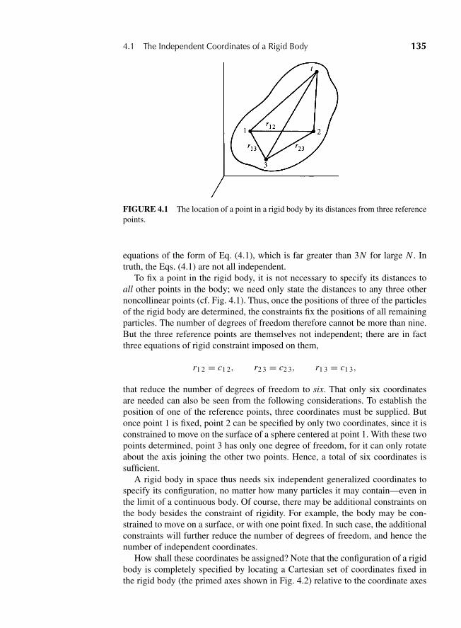
“M04 Goldstein ISBN C04” — 2011/2/15 — page 135 — #2
4.1 The Independent Coordinates of a Rigid Body 135
FIGURE 4.1 The location of a point in a rigid body by its distances from three referencepoints.
equations of the form of Eq. (4.1), which is far greater than 3N for large N . Intruth, the Eqs. (4.1) are not all independent.
To fix a point in the rigid body, it is not necessary to specify its distances toall other points in the body; we need only state the distances to any three othernoncollinear points (cf. Fig. 4.1). Thus, once the positions of three of the particlesof the rigid body are determined, the constraints fix the positions of all remainingparticles. The number of degrees of freedom therefore cannot be more than nine.But the three reference points are themselves not independent; there are in factthree equations of rigid constraint imposed on them,
r1 2 = c1 2, r2 3 = c2 3, r1 3 = c1 3,
that reduce the number of degrees of freedom to six. That only six coordinatesare needed can also be seen from the following considerations. To establish theposition of one of the reference points, three coordinates must be supplied. Butonce point 1 is fixed, point 2 can be specified by only two coordinates, since it isconstrained to move on the surface of a sphere centered at point 1. With these twopoints determined, point 3 has only one degree of freedom, for it can only rotateabout the axis joining the other two points. Hence, a total of six coordinates issufficient.
A rigid body in space thus needs six independent generalized coordinates tospecify its configuration, no matter how many particles it may contain—even inthe limit of a continuous body. Of course, there may be additional constraints onthe body besides the constraint of rigidity. For example, the body may be con-strained to move on a surface, or with one point fixed. In such case, the additionalconstraints will further reduce the number of degrees of freedom, and hence thenumber of independent coordinates.
How shall these coordinates be assigned? Note that the configuration of a rigidbody is completely specified by locating a Cartesian set of coordinates fixed inthe rigid body (the primed axes shown in Fig. 4.2) relative to the coordinate axes
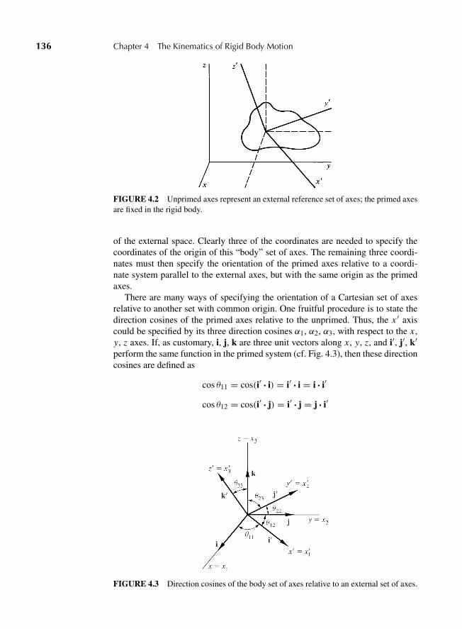
“M04 Goldstein ISBN C04” — 2011/2/15 — page 136 — #3
136 Chapter 4 The Kinematics of Rigid Body Motion
FIGURE 4.2 Unprimed axes represent an external reference set of axes; the primed axesare fixed in the rigid body.
of the external space. Clearly three of the coordinates are needed to specify thecoordinates of the origin of this “body” set of axes. The remaining three coordi-nates must then specify the orientation of the primed axes relative to a coordi-nate system parallel to the external axes, but with the same origin as the primedaxes.
There are many ways of specifying the orientation of a Cartesian set of axesrelative to another set with common origin. One fruitful procedure is to state thedirection cosines of the primed axes relative to the unprimed. Thus, the x ′ axiscould be specified by its three direction cosines α1, α2, α3, with respect to the x ,y, z axes. If, as customary, i, j, k are three unit vectors along x , y, z, and i′, j′, k′perform the same function in the primed system (cf. Fig. 4.3), then these directioncosines are defined as
cos θ11 = cos(i′ ? i) = i′ ? i = i ? i′
cos θ12 = cos(i′ ? j) = i′ ? j = j ? i′
FIGURE 4.3 Direction cosines of the body set of axes relative to an external set of axes.
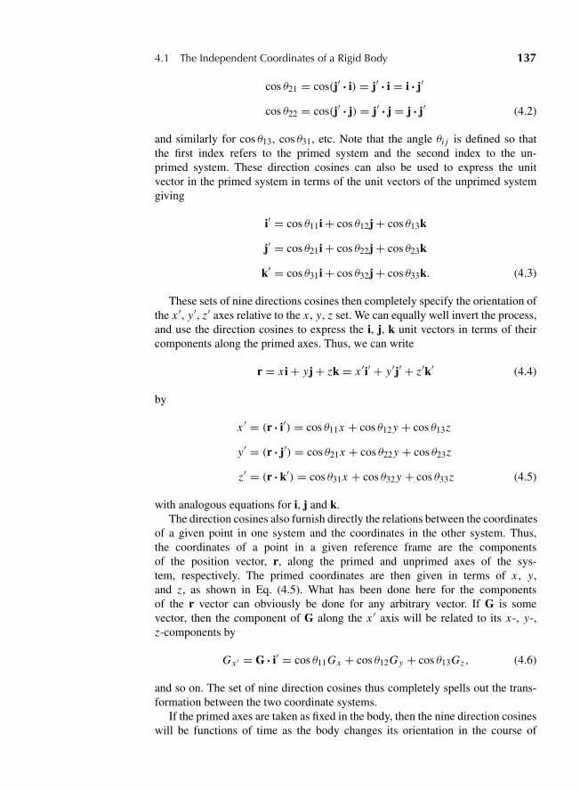
“M04 Goldstein ISBN C04” — 2011/2/15 — page 137 — #4
4.1 The Independent Coordinates of a Rigid Body 137
cos θ21 = cos(j′ ? i) = j′ ? i = i ? j′
cos θ22 = cos(j′ ? j) = j′ ? j = j ? j′ (4.2)
and similarly for cos θ13, cos θ31, etc. Note that the angle θi j is defined so thatthe first index refers to the primed system and the second index to the un-primed system. These direction cosines can also be used to express the unitvector in the primed system in terms of the unit vectors of the unprimed systemgiving
i′ = cos θ11i + cos θ12j + cos θ13k
j′ = cos θ21i + cos θ22j + cos θ23k
k′ = cos θ31i + cos θ32j + cos θ33k. (4.3)
These sets of nine directions cosines then completely specify the orientation ofthe x ′, y′, z′ axes relative to the x , y, z set. We can equally well invert the process,and use the direction cosines to express the i, j, k unit vectors in terms of theircomponents along the primed axes. Thus, we can write
r = x i + yj + zk = x ′i′ + y′j′ + z′k′ (4.4)
by
x ′ = (r ? i′) = cos θ11x + cos θ12 y + cos θ13z
y′ = (r ? j′) = cos θ21x + cos θ22 y + cos θ23z
z′ = (r ? k′) = cos θ31x + cos θ32 y + cos θ33z (4.5)
with analogous equations for i, j and k.The direction cosines also furnish directly the relations between the coordinates
of a given point in one system and the coordinates in the other system. Thus,the coordinates of a point in a given reference frame are the componentsof the position vector, r, along the primed and unprimed axes of the sys-tem, respectively. The primed coordinates are then given in terms of x , y,and z, as shown in Eq. (4.5). What has been done here for the componentsof the r vector can obviously be done for any arbitrary vector. If G is somevector, then the component of G along the x ′ axis will be related to its x-, y-,z-components by
Gx ′ = G ? i′ = cos θ11Gx + cos θ12G y + cos θ13Gz, (4.6)
and so on. The set of nine direction cosines thus completely spells out the trans-formation between the two coordinate systems.
If the primed axes are taken as fixed in the body, then the nine direction cosineswill be functions of time as the body changes its orientation in the course of
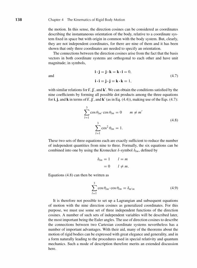
“M04 Goldstein ISBN C04” — 2011/2/15 — page 138 — #5
138 Chapter 4 The Kinematics of Rigid Body Motion
the motion. In this sense, the direction cosines can be considered as coordinatesdescribing the instantaneous orientation of the body, relative to a coordinate sys-tem fixed in space but with origin in common with the body system. But, clearly,they are not independent coordinates, for there are nine of them and it has beenshown that only three coordinates are needed to specify an orientation.
The connections between the direction cosines arise from the fact that the basisvectors in both coordinate systems are orthogonal to each other and have unitmagnitude; in symbols,
i ? j = j ? k = k ? i = 0,and (4.7)
i ? i = j ? j = k ? k = 1,
with similar relations for i′, j′, and k′. We can obtain the conditions satisfied by thenine coefficients by forming all possible dot products among the three equationsfor i, j, and k in terms of i′, j′, and k′ (as in Eq. (4.4)), making use of the Eqs. (4.7):
3∑l=1
cos θlm′ cos θlm = 0 m �= m′
(4.8)3∑
l=1
cos2 θlm = 1.
These two sets of three equations each are exactly sufficient to reduce the numberof independent quantities from nine to three. Formally, the six equations can becombined into one by using the Kronecker δ-symbol δlm , defined by
δlm = 1 l = m
= 0 l �= m.
Equations (4.8) can then be written as
3∑l=1
cos θlm′ cos θlm = δm′m (4.9)
It is therefore not possible to set up a Lagrangian and subsequent equationsof motion with the nine direction cosines as generalized coordinates. For thispurpose, we must use some set of three independent functions of the directioncosines. A number of such sets of independent variables will be described later,the most important being the Euler angles. The use of direction cosines to describethe connections between two Cartesian coordinate systems nevertheless has anumber of important advantages. With their aid, many of the theorems about themotion of rigid bodies can be expressed with great elegance and generality, and ina form naturally leading to the procedures used in special relativity and quantummechanics. Such a mode of description therefore merits an extended discussionhere.
“M04 Goldstein ISBN C04” — 2011/2/15 — page 139 — #6
4.2 Orthogonal Transformations 139
4.2 ORTHOGONAL TRANSFORMATIONS
To study the properties of the nine direction cosines with greater ease, it is con-venient to change the notation and denote all coordinates by x , distinguishing theaxes by subscripts:
x → x1
y → x2 (4.10)
z → x3
as shown in Fig. 4.3. We also change the notation for the direction cosines to
ai j = cos θi j (4.11)
Equations (4.5) and (4.6) constitute a group of transformation equations froma set of coordinates x1, x2, x3 to a new set x ′1, x ′2, x ′3. In particular, they form anexample of a linear or vector transformation, defined by transformation equationsof the form
x ′1 = a1 1x1 + a1 2x2 + a1 3x3
x ′2 = a2 1x1 + a2 2x2 + a2 3x3 (4.12)
x ′3 = a3 1x1 + a3 2x2 + a3 3x3,
where the a1 1, a1 2, . . ., are any set of constant (independent of x , x ′) coeffi-cients.* To simplify the appearance of many of the expressions, we will also makeuse of the summation convention first introduced by Einstein: Whenever an indexoccurs two or more times in a term, it is implied, without any further symbols, thatthe terms are to be summed over all possible values of the index. Thus, Eqs. (4.12)can be written most compactly in accordance with this convention as
x ′i = ai j x j , i = 1, 2, 3. (4.12′)
The repeated appearance of the index j indicates that the left-hand side ofEq. (4.12′) is a sum over the dummy index j for all possible values (here, j = 1,2, 3). Some ambiguity is possible where powers of an indexed quantity occur, andfor that reason, an expression such as
∑i
x2i
appears under the summation convention as
xi xi .
*Equations (4.12) of course are not the most general set of transformation equations, cf., for example,those from the r’s to the q’s (1–38).
“M04 Goldstein ISBN C04” — 2011/2/15 — page 140 — #7
140 Chapter 4 The Kinematics of Rigid Body Motion
For the rest of the book the summation convention should be automaticallyassumed in reading the equations unless otherwise explicitly indicated. Whereconvenient, or to remove ambiguity, the summation sign may be occasionallydisplayed explicitly, e.g., when certain values of the index are to be excludedfrom the summation.
The transformation represented by Eqs. (4.11) is only a special case of the gen-eral linear transformation, Eqs. (4.12), since the direction cosines are not all inde-pendent. The connections between the coefficients, Eqs. (4.8) are rederived herein terms of the newer notation. Since both coordinate systems are Cartesian, themagnitude of a vector is given in terms of the sum of squares of the components.Further, since the actual vector remains unchanged no matter which coordinatesystem is used, the magnitude of the vector must be the same in both systems. Insymbols, we can state the invariance of the magnitude as
x ′i x ′i = xi xi . (4.13)
The left-hand side of Eq. (4.13) is therefore
ai j aik x j xk,
and it will reduce to the right-hand side of Eq. (4.13), if, and only if
ai j aik = 1 j = k
= 0 j �= k, (4.14)
or, in a more compact form, if
ai j aik = δ jk, j, k = 1, 2, 3. (4.15)
When the ai j coefficients are expressed in terms of the direction cosines, the sixequations contained in Eq. (4.15) become identical with the Eqs. (4.9).
Any linear transformation, Eq. (4.12), that has the properties required byEq. (4.15) is called an orthogonal transformation, and Eq. (4.15) itself is knownas the orthogonality condition. Thus, the transition from coordinates fixed inspace to coordinates fixed in the rigid body (with common origin) is accom-plished by means of an orthogonal transformation. The array of transformationquantities (the direction cosines), written as
⎡⎢⎣
a11 a12 a13
a21 a22 a23
a31 a32 a33
⎤⎥⎦ , (4.16)
is called the matrix of transformation, and will be denoted by a capital letter A.The quantities ai j are correspondingly known as the matrix elements of the trans-formation.
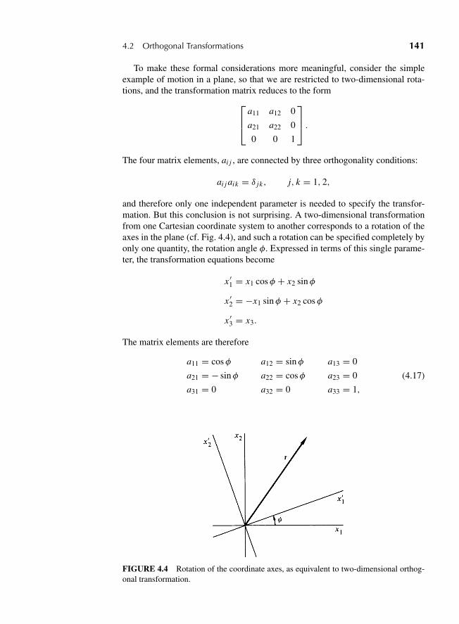
“M04 Goldstein ISBN C04” — 2011/2/15 — page 141 — #8
4.2 Orthogonal Transformations 141
To make these formal considerations more meaningful, consider the simpleexample of motion in a plane, so that we are restricted to two-dimensional rota-tions, and the transformation matrix reduces to the form⎡
⎢⎣a11 a12 0
a21 a22 0
0 0 1
⎤⎥⎦ .
The four matrix elements, ai j , are connected by three orthogonality conditions:
ai j aik = δ jk, j, k = 1, 2,
and therefore only one independent parameter is needed to specify the transfor-mation. But this conclusion is not surprising. A two-dimensional transformationfrom one Cartesian coordinate system to another corresponds to a rotation of theaxes in the plane (cf. Fig. 4.4), and such a rotation can be specified completely byonly one quantity, the rotation angle φ. Expressed in terms of this single parame-ter, the transformation equations become
x ′1 = x1 cosφ + x2 sinφ
x ′2 = −x1 sinφ + x2 cosφ
x ′3 = x3.
The matrix elements are therefore
a11 = cosφ a12 = sinφ a13 = 0
a21 = − sinφ a22 = cosφ a23 = 0
a31 = 0 a32 = 0 a33 = 1,
(4.17)
FIGURE 4.4 Rotation of the coordinate axes, as equivalent to two-dimensional orthog-onal transformation.
“M04 Goldstein ISBN C04” — 2011/2/15 — page 142 — #9
142 Chapter 4 The Kinematics of Rigid Body Motion
so that the matrix A can be written
A =⎡⎣ cosφ sinφ 0− sinφ cosφ 0
0 0 1
⎤⎦ (4.17′)
The three nontrivial orthogonality conditions expand into the equations
a11a11 + a21a21 = 1
a12a12 + a22a22 = 1
a11a12 + a21a22 = 0.
These conditions are obviously satisfied by the matrix (4-17′), for in terms of thematrix elements (4.17) they reduce to the identities
cos2 φ + sin2 φ = 1
sin2 φ + cos2 φ = 1
cosφ sinφ − sinφ cosφ = 0.
The transformation matrix A can be thought of as an operator that, actingon the unprimed system, transforms it into the primed system. Symbolically, theprocess might be written
(r)′ = Ar, (4.18)
which is to be read: The matrix A operating on the components of a vector in theunprimed system yields the components of the vector in the primed system. Notethat in the development of the subject so far, A acts on the coordinate system only,the vector is unchanged, and we ask merely for its components in two differentcoordinate frames. Parentheses have therefore been placed around r on the left inEq. (4.18) to make clear that the same vector is involved on both sides on the equa-tion. Only the components have changed. In three dimensions, the transformationof coordinates, as shown earlier, is simply a rotation, and A is then identical withthe rotation operator in a plane.
Despite this, note that without changing the formal mathematics, A can also bethought of as an operator acting on the vector r, changing it to a different vector r′:
r′ = Ar, (4.19)
with both vectors expressed in the same coordinate system. Thus, in two dimen-sions, instead of rotating the coordinate system counterclockwise, we can rotatethe vector r clockwise by an angle φ to a new vector r′, as shown in Fig. 4.5. Thecomponents of the new vector will then be related to the components of the oldby the same Eqs. (4.12) that describe the transformation of coordinates. From aformal standpoint, it is therefore not necessary to use parentheses in Eq. (4.18);rather, it can be written as in Eq. (4.19) and interpreted equally as an operation on
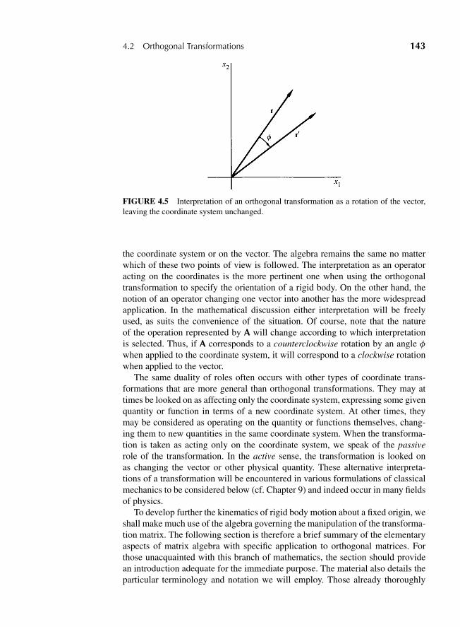
“M04 Goldstein ISBN C04” — 2011/2/15 — page 143 — #10
4.2 Orthogonal Transformations 143
FIGURE 4.5 Interpretation of an orthogonal transformation as a rotation of the vector,leaving the coordinate system unchanged.
the coordinate system or on the vector. The algebra remains the same no matterwhich of these two points of view is followed. The interpretation as an operatoracting on the coordinates is the more pertinent one when using the orthogonaltransformation to specify the orientation of a rigid body. On the other hand, thenotion of an operator changing one vector into another has the more widespreadapplication. In the mathematical discussion either interpretation will be freelyused, as suits the convenience of the situation. Of course, note that the natureof the operation represented by A will change according to which interpretationis selected. Thus, if A corresponds to a counterclockwise rotation by an angle φwhen applied to the coordinate system, it will correspond to a clockwise rotationwhen applied to the vector.
The same duality of roles often occurs with other types of coordinate trans-formations that are more general than orthogonal transformations. They may attimes be looked on as affecting only the coordinate system, expressing some givenquantity or function in terms of a new coordinate system. At other times, theymay be considered as operating on the quantity or functions themselves, chang-ing them to new quantities in the same coordinate system. When the transforma-tion is taken as acting only on the coordinate system, we speak of the passiverole of the transformation. In the active sense, the transformation is looked onas changing the vector or other physical quantity. These alternative interpreta-tions of a transformation will be encountered in various formulations of classicalmechanics to be considered below (cf. Chapter 9) and indeed occur in many fieldsof physics.
To develop further the kinematics of rigid body motion about a fixed origin, weshall make much use of the algebra governing the manipulation of the transforma-tion matrix. The following section is therefore a brief summary of the elementaryaspects of matrix algebra with specific application to orthogonal matrices. Forthose unacquainted with this branch of mathematics, the section should providean introduction adequate for the immediate purpose. The material also details theparticular terminology and notation we will employ. Those already thoroughly
“M04 Goldstein ISBN C04” — 2011/2/15 — page 144 — #11
144 Chapter 4 The Kinematics of Rigid Body Motion
familiar with matrix algebra may however omit the section and proceed directlyto Section 4.4.
4.3 FORMAL PROPERTIES OF THE TRANSFORMATION MATRIX
Let us consider what happens when two successive transformations are made—corresponding to two successive displacements of the rigid body. Let the firsttransformation from r to r′ be denoted by B:
x ′k = bkj x j , (4.20)
and the succeeding transformation from r′ to a third coordinate set r′′ by A:
x ′′i = aik x ′k . (4.21)
The relation between x ′′i and x j can then be obtained by combining the twoEqs. (4.20) and (4.21):
x ′′i = aikbk j x j .
This may also be written as
x ′′i = ci j x j , (4.22)
where
ci j = aikbk j . (4.23)
The successive application of two orthogonal transformations A, B is thusequivalent to a third linear transformation C. It can be shown that C is also anorthogonal transformation in consequence of the orthogonality of A and B. Thedetailed proof will be left for the exercises. Symbolically, the resultant operator Ccan be considered as the product of the two operators A and B:
C = AB,
and the matrix elements ci j are by definition the elements of the square matrixobtained by multiplying the two square matrices A and B.
Note that this “matrix” or operator multiplication is not commutative,
BA �= AB,
for, by definition, the elements of the transformation D = BA are
di j = bikak j , (4.24)
“M04 Goldstein ISBN C04” — 2011/2/15 — page 145 — #12
4.3 Formal Properties of the Transformation Matrix 145
which generally do not agree with the matrix elements of C, Eq. (4.23). Thus, thefinal coordinate system depends upon the order of application of the operators Aand B, i.e., whether first A then B, or first B and then A. However, matrix mul-tiplication is associative; in a product of three or more matrices the order of themultiplications is unimportant:
(AB)C = A(BC). (4.25)
In Eq. (4.19) the juxtaposition of A and r, to indicate the operation of A onthe coordinate system (or on the vector), was said to be merely symbolic. But, byextending our concept of matrices, it may also be taken as indicating an actualmatrix multiplication. Thus far, the matrices used have been square, i.e., withequal number of rows and columns. However, we may also have one-columnmatrices, such as x and x′ defined by
x =⎡⎣ x1
x2x3
⎤⎦ , x′ =
⎡⎣ x ′1
x ′2x ′3
⎤⎦ . (4.26)
The product Ax, by definition, shall be taken as a one-column matrix, with theelements
(Ax)i = ai j x j = x ′i .
Hence, Eq. (4.19) can also be written as the matrix equation
x′ = Ax.
The addition of two matrices, while not as important a concept as multiplica-tion, is a frequently used operation. The sum A+ B is a matrix C whose elementsare the sum of the corresponding elements of A and B:
ci j = ai j + bi j .
Of greater importance is the transformation inverse to A, the operation thatchanges r ′ back to r . This transformation will be called A−1 and its matrix ele-ments designated by a′
i j . We then have the set of equations
xi = a′i j x ′j , (4.27)
which must be consistent with
x ′k = aki xi . (4.28)
Substituting xi from (4.27), Eq. (4.28) becomes
x ′k = aki a′i j x ′j . (4.29)
“M04 Goldstein ISBN C04” — 2011/2/15 — page 146 — #13
146 Chapter 4 The Kinematics of Rigid Body Motion
Since the components of r′ are independent, Eq. (4.29) is correct only if the sum-mation reduces identically to x ′k . The coefficient of x ′j must therefore be 1 forj = k and 0 for j �= k; in symbols,
aki a′i j = δk j . (4.30)
The left-hand side of Eq. (4.30) is easily recognized as the matrix element for theproduct AA−1, while the right-hand side is the element of the matrix known asthe unit matrix 1:
1 =⎡⎣ 1 0 0
0 1 00 0 1
⎤⎦ . (4.31)
Equation (4.30) can therefore be written as
AA−1 = 1, (4.32)
which indicates the reason for the designation of the inverse matrix by A−1. Thetransformation corresponding to 1 is known as the identity transformation, pro-ducing no change in the coordinate system:
x = 1x.
Similarly multiplying any matrix A by 1, in any order, leaves A unaffected:
1A = A1 = A.
By slightly changing the order of the proof of Eq. (4.28), it can be shown that Aand A−1 commute. Instead of substituting xi in Eq. (4.29) in terms of x ′, we couldequally as well demand consistency by eliminating x ′ from the two equations,leading in analogous fashion to
a′i j a jk = δik .
In matrix notation, this reads
A−1A = 1, (4.33)
which proves the statement.Now let us consider the double sum
aklaki a′i j ,
which can be written either as
cli a′i j with cli = aklaki
“M04 Goldstein ISBN C04” — 2011/2/15 — page 147 — #14
4.3 Formal Properties of the Transformation Matrix 147
or as
akldk j with dkj = aki a′i j .
Applying the orthogonality conditions, Eq. (4.15), the sum in the first form re-duces to
δli a′i j = a′
l j .
On the other hand, the same sum from the second point of view, and with the helpof Eq. (4.30), can be written
aklδk j = a jl .
Thus, the elements of the direct matrix A and the reciprocal A−1 are related by
a′l j = a jl . (4.34)
In general, the matrix obtained from A by interchanging rows and columns isknown as the transposed matrix, indicated by the tilde thus: A. Equation (4.34)therefore states that for orthogonal matrices the reciprocal matrix is to be identi-fied as the transposed matrix; symbolically,
A−1 = A. (4.35)
If this result is substituted in Eq. (4.33), we obtain
AA = 1, (4.36)
which is identical with the set of orthogonality conditions, Eq. (4.15), written inabbreviated form, as can be verified by direct expansion. Similarly, an alternativeform of the orthogonality conditions can be obtained from Eq. (4.30) by substi-tuting (4.34):
aki a ji = δk j . (4.37)
In symbolic form, (4.37) can be written
AA = 1
and may be derived directly from (4.36) by multiplying it from the left by A andfrom the right by A−1.
A rectangular matrix is said to be of dimension m × n if it has m rows and ncolumns; i.e., if the matrix element is ai j , then i runs from 1 to m, and j from 1to n. Clearly the transpose of such a matrix has the dimension n × m. If a vectorcolumn matrix is considered as a rectangular matrix of dimension m × 1, thetranspose of a vector is of dimension 1 × m, i.e., a one-row matrix. The product
“M04 Goldstein ISBN C04” — 2011/2/15 — page 148 — #15
148 Chapter 4 The Kinematics of Rigid Body Motion
AB of two rectangular matrices exists only if the number of columns of A is thesame as the number of rows of B. This is an obvious consequence of the definitionof the multiplication operation leading to a matrix element:
ci j = aikbk j .
From this viewpoint, the product of a vector column matrix with a square matrixdoes not exist. The only product between these quantities that can be formed isthat of a square matrix with a single column matrix. But note that a single rowmatrix, i.e., a vector transpose, can indeed pre-multiply a square matrix. For avector, however, the distinction between the column matrix and its transpose isoften of no consequence. The symbol x may therefore be used to denote eithera column or a row matrix, as the situation warrants.* Thus in the expression Ax,where A is a square matrix, the symbol x stands for a column matrix, whereas inthe expression xA it represents the same elements arranged in a single row. Notethat the i th component of Ax can be written as
Ai j x j = x j (A) j i .
Hence, we have a useful commutation property of the product of a vector and asquare matrix that
Ax = xA.
A square matrix that is the same as its transpose,
Ai j = A ji , (4.38)
is said (for obvious reasons) to be symmetric. When the transpose is the negativeof the original matrix,
Ai j = −A ji , (4.39)
the matrix is antisymmetric or skew symmetric. Clearly in an antisymmetricmatrix, the diagonal elements are always zero.
The two interpretations of an operator as transforming the vector, or alterna-tively the coordinate system, are both involved if we find the transformation of anoperator under a change of coordinates. Let A be considered an operator actingupon a vector F (or a single-column matrix F) to produce a vector G:
G = AF.
If the coordinate system is transformed by a matrix B, the components of thevector G in the new system will be given by
BG = BAF,
*The transpose sign on vector matrices will occasionally be retained where it is useful to emphasizethe distinction between column and row matrices.
“M04 Goldstein ISBN C04” — 2011/2/15 — page 149 — #16
4.3 Formal Properties of the Transformation Matrix 149
which can also be written
BG = BAB−1BF. (4.40)
Equation (4.40) can be stated as the operator BAB−1 acting upon the vector F,expressed in the new system, produces the vector G, likewise expressed in thenew coordinates. We may therefore consider BAB−1 to be the form taken by theoperator A when transformed to a new set of axes:
A′ = BAB−1. (4.41)
Any transformation of a matrix having the form of Eq. (4.41) is known as a simi-larity transformation.
It is appropriate at this point to consider the properties of the determinantformed from the elements of a square matrix. As is customary, we shall denotesuch a determinant by vertical bars, thus: |A|. Note that the definition of matrixmultiplication is identical with that for the multiplication of determinants
|AB| = |A| ? |B|. (4.41′)
Since the determinant of the unit matrix is 1, the determinantal form of theorthogonality conditions, Eq. (4.36), can be written
|A| ? |A| = 1.
Further, as the value of a determinant is unaffected by interchanging rows andcolumns, we can write
|A|2 = 1, (4.42)
which implies that the determinant of an orthogonal matrix can only be +1 or −1.(The geometrical significance of these two values will be considered in the nextsection.)
When the matrix is not orthogonal, the determinant does not have these simplevalues, of course. It can be shown however that the value of the determinant isinvariant under a similarity transformation. Multiplying Eq. (4.41) for the trans-formed matrix from the right by B, we obtain the relation
A′B = BA,
or in determinantal form
|A′| ? |B| = |B| ? |A|.
Since the determinant of B is merely a number, and not zero,* we can divide by
*If it were zero, there could be no inverse operator B−1 (by Cramer’s rule), which is required forEq. (4.41) to make sense.
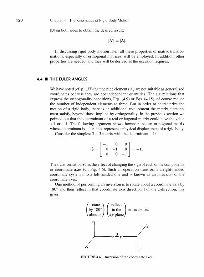
“M04 Goldstein ISBN C04” — 2011/2/15 — page 150 — #17
150 Chapter 4 The Kinematics of Rigid Body Motion
|B| on both sides to obtain the desired result:
|A′| = |A|.
In discussing rigid body motion later, all these properties of matrix transfor-mations, especially of orthogonal matrices, will be employed. In addition, otherproperties are needed, and they will be derived as the occasion requires.
4.4 THE EULER ANGLES
We have noted (cf. p. 137) that the nine elements ai j are not suitable as generalizedcoordinates because they are not independent quantities. The six relations thatexpress the orthogonality conditions, Eqs. (4.9) or Eqs. (4.15), of course reducethe number of independent elements to three. But in order to characterize themotion of a rigid body, there is an additional requirement the matrix elementsmust satisfy, beyond those implied by orthogonality. In the previous section wepointed out that the determinant of a real orthogonal matrix could have the value+1 or −1. The following argument shows however that an orthogonal matrixwhose determinant is −1 cannot represent a physical displacement of a rigid body.
Consider the simplest 3 × 3 matrix with the determinant −1:
S =⎡⎣−1 0 0
0 −1 00 0 −1
⎤⎦ = −1.
The transformation S has the effect of changing the sign of each of the componentsor coordinate axes (cf. Fig. 4.6). Such an operation transforms a right-handedcoordinate system into a left-handed one and is known as an inversion of thecoordinate axes.
One method of performing an inversion is to rotate about a coordinate axis by180◦ and then reflect in that coordinate axis direction. For the z-direction, thisgives
⎛⎝ rotate
by 180◦about z
⎞⎠⎛⎝ reflect
in thexy plane
⎞⎠ = inversion.
FIGURE 4.6 Inversion of the coordinate axes.
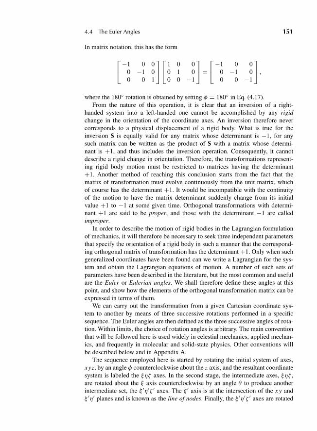
“M04 Goldstein ISBN C04” — 2011/2/15 — page 151 — #18
4.4 The Euler Angles 151
In matrix notation, this has the form
⎡⎣−1 0 0
0 −1 00 0 1
⎤⎦⎡⎣ 1 0 0
0 1 00 0 −1
⎤⎦ =
⎡⎣−1 0 0
0 −1 00 0 −1
⎤⎦ ,
where the 180◦ rotation is obtained by setting φ = 180◦ in Eq. (4.17).From the nature of this operation, it is clear that an inversion of a right-
handed system into a left-handed one cannot be accomplished by any rigidchange in the orientation of the coordinate axes. An inversion therefore nevercorresponds to a physical displacement of a rigid body. What is true for theinversion S is equally valid for any matrix whose determinant is −1, for anysuch matrix can be written as the product of S with a matrix whose determi-nant is +1, and thus includes the inversion operation. Consequently, it cannotdescribe a rigid change in orientation. Therefore, the transformations represent-ing rigid body motion must be restricted to matrices having the determinant+1. Another method of reaching this conclusion starts from the fact that thematrix of transformation must evolve continuously from the unit matrix, whichof course has the determinant +1. It would be incompatible with the continuityof the motion to have the matrix determinant suddenly change from its initialvalue +1 to −1 at some given time. Orthogonal transformations with determi-nant +1 are said to be proper, and those with the determinant −1 are calledimproper.
In order to describe the motion of rigid bodies in the Lagrangian formulationof mechanics, it will therefore be necessary to seek three independent parametersthat specify the orientation of a rigid body in such a manner that the correspond-ing orthogonal matrix of transformation has the determinant +1. Only when suchgeneralized coordinates have been found can we write a Lagrangian for the sys-tem and obtain the Lagrangian equations of motion. A number of such sets ofparameters have been described in the literature, but the most common and usefulare the Euler or Eulerian angles. We shall therefore define these angles at thispoint, and show how the elements of the orthogonal transformation matrix can beexpressed in terms of them.
We can carry out the transformation from a given Cartesian coordinate sys-tem to another by means of three successive rotations performed in a specificsequence. The Euler angles are then defined as the three successive angles of rota-tion. Within limits, the choice of rotation angles is arbitrary. The main conventionthat will be followed here is used widely in celestial mechanics, applied mechan-ics, and frequently in molecular and solid-state physics. Other conventions willbe described below and in Appendix A.
The sequence employed here is started by rotating the initial system of axes,xyz, by an angle φ counterclockwise about the z axis, and the resultant coordinatesystem is labeled the ξηζ axes. In the second stage, the intermediate axes, ξηζ ,are rotated about the ξ axis counterclockwise by an angle θ to produce anotherintermediate set, the ξ ′η′ζ ′ axes. The ξ ′ axis is at the intersection of the xy andξ ′η′ planes and is known as the line of nodes. Finally, the ξ ′η′ζ ′ axes are rotated

“M04 Goldstein ISBN C04” — 2011/2/15 — page 152 — #19
152 Chapter 4 The Kinematics of Rigid Body Motion
FIGURE 4.7 The rotations defining the Eulerian angles.
counterclockwise by an angle ψ about the ζ ′ axis to produce the desired x ′y′z′system of axes. Figure 4.7 illustrates the various stages of the sequence. The Eulerangles θ , φ, andψ thus completely specify the orientation of the x ′y′z′ system rel-ative to the xyz and can therefore act as the three needed generalized coordinates.*
The elements of the complete transformation A can be obtained by writingthe matrix as the triple product of the separate rotations, each of which has arelatively simple matrix form. Thus, the initial rotation about z can be describedby a matrix D:
j = Dx,
where j and x stand for column matrices. Similarly, the transformation from ξηζ
to ξ ′η′ζ ′ can be described by a matrix C,
j ′ = Cj,
*A number of minor variations will be found in the literature even within this convention. The differ-ences are not very great, but they are often sufficient to frustrate easy comparison of the end formulae,such as the matrix elements. Greatest confusion, perhaps, arises from the occasional use of left-handedcoordinate systems.

“M04 Goldstein ISBN C04” — 2011/2/15 — page 153 — #20
4.4 The Euler Angles 153
and the last rotation to x ′y′z′ by a matrix B,
x′ = Bj ′.
Hence, the matrix of the complete transformation,
x′ = Ax,
is the product of the successive matrices,
A = BCD.
Now the D transformation is a rotation about z, and hence has a matrix of theform (cf. Eq. (4.17))
D =⎡⎣ cosφ sinφ 0− sinφ cosφ 0
0 0 1
⎤⎦ . (4.43)
The C transformation corresponds to a rotation about ξ , with the matrix
C =⎡⎣ 1 0 0
0 cos θ sin θ0 − sin θ cos θ
⎤⎦ , (4.44)
and finally B is a rotation about ζ ′ and therefore has the same form as D:
B =⎡⎣ cosψ sinψ 0− sinψ cosψ 0
0 0 1
⎤⎦ . (4.45)
The product matrix A = BCD then follows as
A =[
cosψ cosφ − cos θ sinφ sinψ cosψ sinφ + cos θ cosφ sinψ sinψ sin θ− sinψ cosφ − cos θ sinφ cosψ − sinψ sinφ + cos θ cosφ cosψ cosψ sin θ
sin θ sinφ − sin θ cosφ cos θ
].
(4.46)
The inverse transformation from body coordinates to space axes
x = A−1x′
is then given immediately by the transposed matrix A:
A−1 =
A =[
cosψ cosφ − cos θ sinφ sinψ − sinψ cosφ − cos θ sinφ cosψ sin θ sinφcosψ sinφ + cos θ cosφ sinψ − sinψ sinφ + cos θ cosφ cosψ − sin θ cosφ
sin θ sinψ sin θ cosψ cos θ
].
(4.47)
“M04 Goldstein ISBN C04” — 2011/2/15 — page 154 — #21
154 Chapter 4 The Kinematics of Rigid Body Motion
Verification of the multiplication, and demonstration that A represents a proper,orthogonal matrix will be left to the exercises.
Note that the sequence of rotations used to define the final orientation of thecoordinate system is to some extent arbitrary. The initial rotation could be takenabout any of the three Cartesian axes. In the subsequent two rotations, the onlylimitation is that no two successive rotations can be about the same axis. A totalof 12 conventions is therefore possible in defining the Euler angles (in a right-handed coordinate system). The two most frequently used conventions differ onlyin the choice of axis for the second rotation. In the Euler’s angle definitionsdescribed above, and used throughout the book, the second rotation is about theintermediate x axis. We will refer to this choice as the x-convention. In quan-tum mechanics, nuclear physics, and particle physics, we often take the seconddefining rotation about the intermediate y axis; this form will be denoted as they-convention.
A third convention is commonly used in engineering applications relating tothe orientation of moving vehicles such as aircraft and satellites. Both the x- andy-conventions have the drawback that when the primed coordinate system is onlyslightly different from the unprimed system, the angles φ and ψ become indis-tinguishable, as their respective axes of rotation, z and z′ are then nearly coin-cident. To get around this problem, all three rotations are taken around differentaxes. The first rotation is about the vertical axis and gives the heading or yawangle. The second is around a perpendicular axis fixed in the vehicle and nor-mal to the figure axis; it is measured by the pitch or attitude angle. Finally, thethird angle is one of rotation about the figure axis of the vehicle and is the rollor bank angle. Because all three axes are involved in the rotations, it will bedesignated as the xyz-convention (although the order of axes chosen may actu-ally be different). This last convention is sometimes referred to as the Tait–Bryanangles.
While only the x-convention will be used in the text, for reference purposesAppendix A lists formulae involving Euler’s angles, such as rotation matrices, inboth the y- and xyz-conventions.
4.5 THE CAYLEY–KLEIN PARAMETERS AND RELATED QUANTITIES
We have seen that only three independent quantities are needed to specify theorientation of a rigid body. Nonetheless, there are occasions when it is desirableto use sets of variables containing more than the minimum number of quan-tities to describe a rotation, even though they are not suitable as generalizedcoordinates. Thus, Felix Klein introduced the set of four parameters bearinghis name to facilitate the integration of complicated gyroscopic problems. TheEuler angles are difficult to use in numerical computation because of the largenumber of trigonometric functions involved, and the four-parameter representa-tions are much better adapted for use on computers. Further, the four-parametersets are of great theoretical interest in branches of physics beyond the scope ofthis book, wherever rotations or rotational symmetry are involved. It therefore
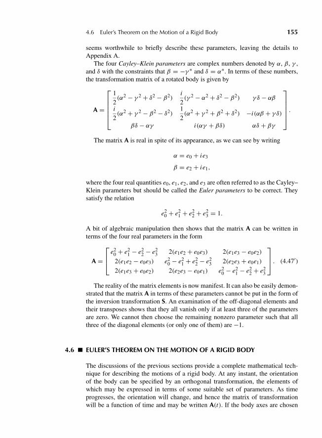
“M04 Goldstein ISBN C04” — 2011/2/15 — page 155 — #22
4.6 Euler’s Theorem on the Motion of a Rigid Body 155
seems worthwhile to briefly describe these parameters, leaving the details toAppendix A.
The four Cayley–Klein parameters are complex numbers denoted by α, β, γ ,and δ with the constraints that β = −γ ∗ and δ = α∗. In terms of these numbers,the transformation matrix of a rotated body is given by
A =
⎡⎢⎢⎢⎢⎣
1
2(α2 − γ 2 + δ2 − β2)
i
2(γ 2 − α2 + δ2 − β2) γ δ − αβ
i
2(α2 + γ 2 − β2 − δ2)
1
2(α2 + γ 2 + β2 + δ2) −i(αβ + γ δ)
βδ − αγ i(αγ + βδ) αδ + βγ
⎤⎥⎥⎥⎥⎦ .
The matrix A is real in spite of its appearance, as we can see by writing
α = e0 + ie3
β = e2 + ie1,
where the four real quantities e0, e1, e2, and e3 are often referred to as the Cayley–Klein parameters but should be called the Euler parameters to be correct. Theysatisfy the relation
e20 + e2
1 + e22 + e2
3 = 1.
A bit of algebraic manipulation then shows that the matrix A can be written interms of the four real parameters in the form
A =
⎡⎢⎣
e20 + e2
1 − e22 − e2
3 2(e1e2 + e0e3) 2(e1e3 − e0e2)
2(e1e2 − e0e3) e20 − e2
1 + e22 − e2
3 2(e2e3 + e0e1)
2(e1e3 + e0e2) 2(e2e3 − e0e1) e20 − e2
1 − e22 + e2
3
⎤⎥⎦ . (4.47′)
The reality of the matrix elements is now manifest. It can also be easily demon-strated that the matrix A in terms of these parameters cannot be put in the form ofthe inversion transformation S. An examination of the off-diagonal elements andtheir transposes shows that they all vanish only if at least three of the parametersare zero. We cannot then choose the remaining nonzero parameter such that allthree of the diagonal elements (or only one of them) are −1.
4.6 EULER’S THEOREM ON THE MOTION OF A RIGID BODY
The discussions of the previous sections provide a complete mathematical tech-nique for describing the motions of a rigid body. At any instant, the orientationof the body can be specified by an orthogonal transformation, the elements ofwhich may be expressed in terms of some suitable set of parameters. As timeprogresses, the orientation will change, and hence the matrix of transformationwill be a function of time and may be written A(t). If the body axes are chosen
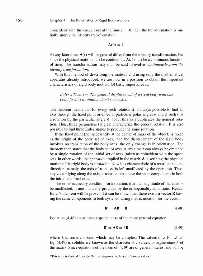
“M04 Goldstein ISBN C04” — 2011/2/15 — page 156 — #23
156 Chapter 4 The Kinematics of Rigid Body Motion
coincident with the space axes at the time t = 0, then the transformation is ini-tially simply the identity transformation:
A(0) = 1.
At any later time, A(t) will in general differ from the identity transformation, butsince the physical motion must be continuous, A(t)must be a continuous functionof time. The transformation may thus be said to evolve continuously from theidentity transformation.
With this method of describing the motion, and using only the mathematicalapparatus already introduced, we are now in a position to obtain the importantcharacteristics of rigid body motion. Of basic importance is:
Euler’s Theorem: The general displacement of a rigid body with onepoint fixed is a rotation about some axis.
The theorem means that for every such rotation it is always possible to find anaxis through the fixed point oriented at particular polar angles θ and φ such thata rotation by the particular angle ψ about this axis duplicates the general rota-tion. Thus, three parameters (angles) characterize the general rotation. It is alsopossible to find three Euler angles to produce the same rotation.
If the fixed point (not necessarily at the center of mass of the object) is takenas the origin of the body set of axes, then the displacement of the rigid bodyinvolves no translation of the body axes; the only change is in orientation. Thetheorem then states that the body set of axes at any time t can always be obtainedby a single rotation of the initial set of axes (taken as coincident with the spaceset). In other words, the operation implied in the matrix A describing the physicalmotion of the rigid body is a rotation. Now it is characteristic of a rotation that onedirection, namely, the axis of rotation, is left unaffected by the operation. Thus,any vector lying along the axis of rotation must have the same components in boththe initial and final axes.
The other necessary condition for a rotation, that the magnitude of the vectorsbe unaffected, is automatically provided by the orthogonality conditions. Hence,Euler’s theorem will be proven if it can be shown that there exists a vector R hav-ing the same components in both systems. Using matrix notation for the vector,
R′ = AR = R. (4.48)
Equation (4.48) constitutes a special case of the more general equation:
R′ = AR = λR, (4.49)
where λ is some constant, which may be complex. The values of λ for whichEq. (4.49) is soluble are known as the characteristic values, or eigenvalues,* ofthe matrix. Since equations of the form of (4.49) are of general interest and will be
*This term is derived from the German Eigenwerte, literally “proper values.”
“M04 Goldstein ISBN C04” — 2011/2/15 — page 157 — #24
4.6 Euler’s Theorem on the Motion of a Rigid Body 157
used in Chapter 6, we shall examine Eq. (4.49) and then specialize the discussionto Eq. (4.48).
The problem of finding vectors that satisfy Eq. (4.49) is therefore called theeigenvalue problem for the given matrix, and Eq. (4.49) itself is referred to as theeigenvalue equation. Correspondingly, the vector solutions are the eigenvectorsof A. Euler’s theorem can now be restated in the following language:
The real orthogonal matrix specifying the physical motion of a rigidbody with one point fixed always has the eigenvalue +1.
The eigenvalue equations (4.49) may be written
(A − λ1)R = 0, (4.50)
or, in expanded form,
(a11 − λ)X + a12Y + a13 Z = 0
a21 X + (a22 − λ)Y + a23 Z = 0 (4.51)
a31 X + a32Y + (a33 − λ)Z = 0.
Equations (4.51) comprise a set of three homogeneous simultaneous equationsfor the components X , Y , Z of the eigenvector R. As such, they can never fur-nish definite values for the three components, but only ratios of components.Physically, this corresponds to the circumstance that only the direction of theeigenvector can be fixed; the magnitude remains undetermined. The product of aconstant with an eigenvector is also an eigenvector. In any case, being homoge-neous, Eqs. (4.51) can have a nontrivial solution only when the determinant of thecoefficients vanishes:
|A − λ1| =∣∣∣∣∣∣a11 − λ a12 a13
a21 a22 − λ a23a31 a32 a33 − λ
∣∣∣∣∣∣ = 0. (4.52)
Equation (4.52) is known as the characteristic or secular equation of the matrix,and the values of λ for which the equation is satisfied are the desired eigenvalues.Euler’s theorem reduces to the statement that, for the real orthogonal matricesunder consideration, the secular equation must have the root λ = +1.
In general, the secular equation will have three roots with three correspondingeigenvectors. For convenience, the notation X1, X2, X3 will often be used insteadof X , Y , Z . In such a notation, the components of the eigenvectors might belabeled as Xik , the first subscript indicating the particular component, the seconddenoting which of the three eigenvectors in involved. A typical member of thegroup of Eqs. (4.51) would then be written (with explicit summation) as
∑j
ai j X jk = λk Xik
“M04 Goldstein ISBN C04” — 2011/2/15 — page 158 — #25
158 Chapter 4 The Kinematics of Rigid Body Motion
or, alternatively, as
∑j
ai j X jk =∑
j
Xi jδ jkλk . (4.53)
Both sides of Eq. (4.53) then have the form of a matrix product element; the leftside as the product of A with a matrix X having the elements X jk , the right sideas the product of X with a matrix whose jkth element is δ jkλk . The last matrix isdiagonal, and its diagonal elements are the eigenvalues of A. We shall thereforedesignate the matrix by l:
l =⎡⎣ λ1 0 0
0 λ2 00 0 λ3
⎤⎦ . (4.54)
Equation (4.53) thus implies the matrix equation
AX = Xl,
or, multiplying from the left by X−1,
X−1AX = l. (4.55)
Now, the left side is in the form of a similarity transformation operating on A.(We have only to denote X−1 by the symbol Y to reduce it to the form Eq. (4.41).)Thus, Eq. (4.55) provides the following alternative approach to the eigenvalueproblem: We seek to diagonalize A by a similarity transformation. Each columnof the matrix used to carry out the similarity transformation consists of the com-ponents of an eigenvector. The elements of the diagonalized form of A are thecorresponding eigenvalues.
Euler’s theorem can be proven directly by using the orthogonality property ofA. Consider the expression
(A − 1)A = 1 − A.
If we take the determinant of the matrices forming both sides (cf. Eq. (4.41′)), wecan write the equality
|A − 1‖A| = |1 − A|. (4.56)
To describe the motion of a rigid body, the matrix A(t) must correspond to aproper rotation; therefore the determinant of A, and of its transpose, must be +1.Further, since in general the determinant of the transpose of a matrix is the sameas that of the matrix, the transpose signs in Eq. (4.56) can be removed:
|A − 1| = |1 − A|. (4.57)
“M04 Goldstein ISBN C04” — 2011/2/15 — page 159 — #26
4.6 Euler’s Theorem on the Motion of a Rigid Body 159
Equation (4.57) says that the determinant of a particular matrix is the same as thedeterminant of the negative of the matrix. Suppose B is some n × n matrix. Thenit is a well-known property of determinants that
| − B| = (−1)n|B|.
Since we are working in a three-dimensional space (n = 3), it is clear thatEq. (4.57) can hold for any arbitrary proper rotation only if
|A − 1| = 0. (4.58)
Comparing Eq. (4.58) with the secular equation (4.52), we can see that one of theeigenvalues satisfying Eq. (4.52) must always be λ = +1, which is the desiredresult of Euler’s theorem.
Note how the proof of Euler’s theorem emphasizes the importance of the num-ber of dimensions in the space considered. In spaces with an even number ofdimensions, Eq. (4.57) is an identity for all matrices and Euler’s theorem doesn’thold. Thus, for two dimensions there is no vector in the space that is left unalteredby a rotation—the axis of rotation is perpendicular to the plane and therefore outof the space.
It is now a simple matter to determine the properties of the other eigenvaluesin three dimensions. Designate the +1 eigenvalue as λ3. The determinant of anymatrix is unaffected by a similarity transformation (cf. Section 4.3). Hence, byEqs. (4.54) and (4.55) and the properties of A as a proper rotation,
|A| = λ1λ2λ3 = λ1λ2 = 1. (4.59)
Further, since A is a real matrix, then if λ is a solution of the secular equa-tion (4.52), the complex conjugate λ∗ must also be a solution.
If a given eigenvalue λi is complex, then the corresponding eigenvector, Ri ,that satisfies Eq. (4.59) will in general also be complex. We have not previouslydealt with the properties of complex vectors under (real) orthogonal transforma-tions, and there are some modifications to previous definitions. The square of thelength or magnitude of a complex vector R is R ?R∗, or in matrix notation RR∗,where the transpose sign on the left-hand vector indicates it is represented by arow matrix. Under a real orthogonal transformation, the square of the magnitudeis invariant:
R′R′∗ = (AR)AR∗ = RAAR∗ = RR∗.
Suppose now that R is a complex eigenvector corresponding to a complex eigen-value λ. Hence, by Eq. (4.49), we have
R′R′∗ = λλ∗RR∗,
which leads to the conclusion that all eigenvalues have unit magnitude:
λλ∗ = 1. (4.60)
“M04 Goldstein ISBN C04” — 2011/2/15 — page 160 — #27
160 Chapter 4 The Kinematics of Rigid Body Motion
From these properties it may be concluded that there are three possible distri-butions of eigenvalues. If all of the eigenvalues are real, then only two situationsare possible:
1. All eigenvalues are +1. The transformation matrix is then just 1, a case wemay justly call trivial.
2. One eigenvalue is +1 and the other two are both −1. Such a transformationmay be characterized as an inversion in two coordinate axes with the thirdunchanged. Equally it is a rotation through the angle π about the directionof the unchanged axis.
If not all of the eigenvalues are real, there is only one additional possibility:
3. One eigenvalue is +1, and the other two are complex conjugates of eachother of the form ei� and e−i�.
A more complete statement of Euler’s theorem thus is that any nontrivial realorthogonal matrix has one, and only one, eigenvalue +1.
The direction cosines of the axis of rotation can then be obtained by settingλ = 1 in the eigenvalue equations (4.51) and solving for X , Y , and Z .* Theangle of rotation can likewise be obtained without difficulty. By means of somesimilarity transformation, it is always possible to transform the matrix A to asystem of coordinates where the z axis lies along the axis of rotation. In such asystem of coordinates, A′ represents a rotation about the z axis through an angle�, and therefore has the form
A′ =⎡⎣ cos� sin� 0− sin� cos� 0
0 0 1
⎤⎦ .
The trace of A′ is simply
1 + 2 cos�.
Since the trace is always invariant under a similarity transformation, the trace ofA with respect to any initial coordinate system must have the same form,
TrA = aii = 1 + 2 cos�, (4.61)
which gives the value of � in terms of the matrix elements. The rotation angle �is to be identified also with the phase angle of the complex eigenvalues λ, as the
*If there are multiple roots to the secular equation, then the corresponding eigenvectors cannot befound as simply (cf. Sections 5.4 and 6.2). Indeed, it is not always possible to completely diagonalizea general matrix if the eigenvalues are not all distinct. These exceptions are of no importance for thepresent considerations, as Euler’s theorem shows that for all nontrivial orthogonal matrices +1 is asingle root.
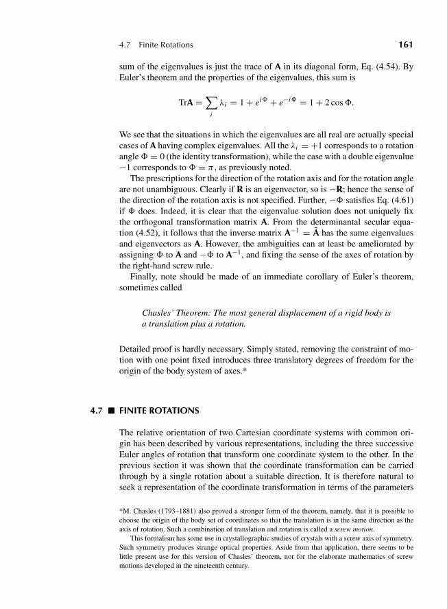
“M04 Goldstein ISBN C04” — 2011/2/15 — page 161 — #28
4.7 Finite Rotations 161
sum of the eigenvalues is just the trace of A in its diagonal form, Eq. (4.54). ByEuler’s theorem and the properties of the eigenvalues, this sum is
TrA =∑
i
λi = 1 + ei� + e−i� = 1 + 2 cos�.
We see that the situations in which the eigenvalues are all real are actually specialcases of A having complex eigenvalues. All the λi = +1 corresponds to a rotationangle� = 0 (the identity transformation), while the case with a double eigenvalue−1 corresponds to � = π , as previously noted.
The prescriptions for the direction of the rotation axis and for the rotation angleare not unambiguous. Clearly if R is an eigenvector, so is −R; hence the sense ofthe direction of the rotation axis is not specified. Further, −� satisfies Eq. (4.61)if � does. Indeed, it is clear that the eigenvalue solution does not uniquely fixthe orthogonal transformation matrix A. From the determinantal secular equa-tion (4.52), it follows that the inverse matrix A−1 = A has the same eigenvaluesand eigenvectors as A. However, the ambiguities can at least be ameliorated byassigning � to A and −� to A−1, and fixing the sense of the axes of rotation bythe right-hand screw rule.
Finally, note should be made of an immediate corollary of Euler’s theorem,sometimes called
Chasles’ Theorem: The most general displacement of a rigid body isa translation plus a rotation.
Detailed proof is hardly necessary. Simply stated, removing the constraint of mo-tion with one point fixed introduces three translatory degrees of freedom for theorigin of the body system of axes.*
4.7 FINITE ROTATIONS
The relative orientation of two Cartesian coordinate systems with common ori-gin has been described by various representations, including the three successiveEuler angles of rotation that transform one coordinate system to the other. In theprevious section it was shown that the coordinate transformation can be carriedthrough by a single rotation about a suitable direction. It is therefore natural toseek a representation of the coordinate transformation in terms of the parameters
*M. Chasles (1793–1881) also proved a stronger form of the theorem, namely, that it is possible tochoose the origin of the body set of coordinates so that the translation is in the same direction as theaxis of rotation. Such a combination of translation and rotation is called a screw motion.
This formalism has some use in crystallographic studies of crystals with a screw axis of symmetry.Such symmetry produces strange optical properties. Aside from that application, there seems to belittle present use for this version of Chasles’ theorem, nor for the elaborate mathematics of screwmotions developed in the nineteenth century.
“M04 Goldstein ISBN C04” — 2011/2/15 — page 162 — #29
162 Chapter 4 The Kinematics of Rigid Body Motion
of the rotation—the angle of rotation and the direction cosines of the axis ofrotation.
With the help of some simple vector algebra, we can derive such a repre-sentation. For this purpose, it is convenient to treat the transformation in itsactive sense, i.e., as one that rotates the vector in a fixed coordinate system (cf.Section 4.2 ). Recall that a counterclockwise rotation of the coordinate systemthen appears as a clockwise rotation of the vector. In Fig. 4.8(a) the initial posi-tion of the vector r is denoted by
−→O P and the final position r′ by
−−→O Q, while the
unit vector along the axis of rotation is denoted by n. The distance between Oand N has the magnitude n ? r, so that the vector
−−→O N can be written as n(n ? r).
Figure 4.8(b) sketches the vectors in the plane normal to the axis of rotation. Thevector
−→N P can be described also as r − n(n ? r), but its magnitude is the same as
that of the vectors−−→N Q and r× n. To obtain the desired relation between r′ and r,
we construct r′ as the sum of three vectors:
r′ = −−→O N +−→
N V +−→V Q
or
r′ = n(n ? r)+ [r − n(n ? r)] cos�+ (r3 n) sin�.
A slight rearrangement of terms leads to the final result:
r′ = r cos�+ n(n ? r)(1 − cos�)+ (r3 n) sin�. (4.62)
Equation (4.62) will be referred to as the rotation formula. Note that Eq. (4.62)holds for any rotation, no matter what its magnitude, and thus is a finite-rotationversion (in a clockwise sense) of the description given in Section 2.6, for thechange of a vector under infinitesimal rotation. (cf. also Section 4.8.)
FIGURE 4.8 Vector diagrams for derivation of the rotation formula.
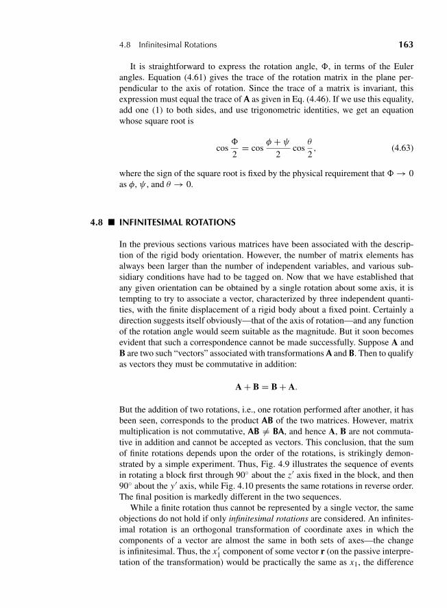
“M04 Goldstein ISBN C04” — 2011/2/15 — page 163 — #30
4.8 Infinitesimal Rotations 163
It is straightforward to express the rotation angle, �, in terms of the Eulerangles. Equation (4.61) gives the trace of the rotation matrix in the plane per-pendicular to the axis of rotation. Since the trace of a matrix is invariant, thisexpression must equal the trace of A as given in Eq. (4.46). If we use this equality,add one (1) to both sides, and use trigonometric identities, we get an equationwhose square root is
cos�
2= cos
φ + ψ2
cosθ
2, (4.63)
where the sign of the square root is fixed by the physical requirement that�→ 0as φ, ψ , and θ → 0.
4.8 INFINITESIMAL ROTATIONS
In the previous sections various matrices have been associated with the descrip-tion of the rigid body orientation. However, the number of matrix elements hasalways been larger than the number of independent variables, and various sub-sidiary conditions have had to be tagged on. Now that we have established thatany given orientation can be obtained by a single rotation about some axis, it istempting to try to associate a vector, characterized by three independent quanti-ties, with the finite displacement of a rigid body about a fixed point. Certainly adirection suggests itself obviously—that of the axis of rotation—and any functionof the rotation angle would seem suitable as the magnitude. But it soon becomesevident that such a correspondence cannot be made successfully. Suppose A andB are two such “vectors” associated with transformations A and B. Then to qualifyas vectors they must be commutative in addition:
A + B = B + A.
But the addition of two rotations, i.e., one rotation performed after another, it hasbeen seen, corresponds to the product AB of the two matrices. However, matrixmultiplication is not commutative, AB �= BA, and hence A, B are not commuta-tive in addition and cannot be accepted as vectors. This conclusion, that the sumof finite rotations depends upon the order of the rotations, is strikingly demon-strated by a simple experiment. Thus, Fig. 4.9 illustrates the sequence of eventsin rotating a block first through 90◦ about the z′ axis fixed in the block, and then90◦ about the y′ axis, while Fig. 4.10 presents the same rotations in reverse order.The final position is markedly different in the two sequences.
While a finite rotation thus cannot be represented by a single vector, the sameobjections do not hold if only infinitesimal rotations are considered. An infinites-imal rotation is an orthogonal transformation of coordinate axes in which thecomponents of a vector are almost the same in both sets of axes—the changeis infinitesimal. Thus, the x ′1 component of some vector r (on the passive interpre-tation of the transformation) would be practically the same as x1, the difference
“M04 Goldstein ISBN C04” — 2011/2/15 — page 164 — #31
164 Chapter 4 The Kinematics of Rigid Body Motion
FIGURE 4.9 The effect of two rotations performed in a given order.
FIGURE 4.10 The two rotations shown in Fig. 4.9, but performed in reverse order.
being extremely small:
x ′1 = x1 + ε11x1 + ε12x2 + ε13x3. (4.64)
The matrix elements ε11, ε12, etc., are to be considered as infinitesimals, so that insubsequent calculations only the first nonvanishing order in εi j need be retained.For any general component x ′i , the equations of infinitesimal transformation canbe written as
x ′i = xi + εi j x j
or
x ′i = (δi j + εi j )x j . (4.65)
The quantity δi j will be recognized as the element of the unit matrix, andEq. (4.65) appears in matrix notation as
x′ = (1 + e)x. (4.66)
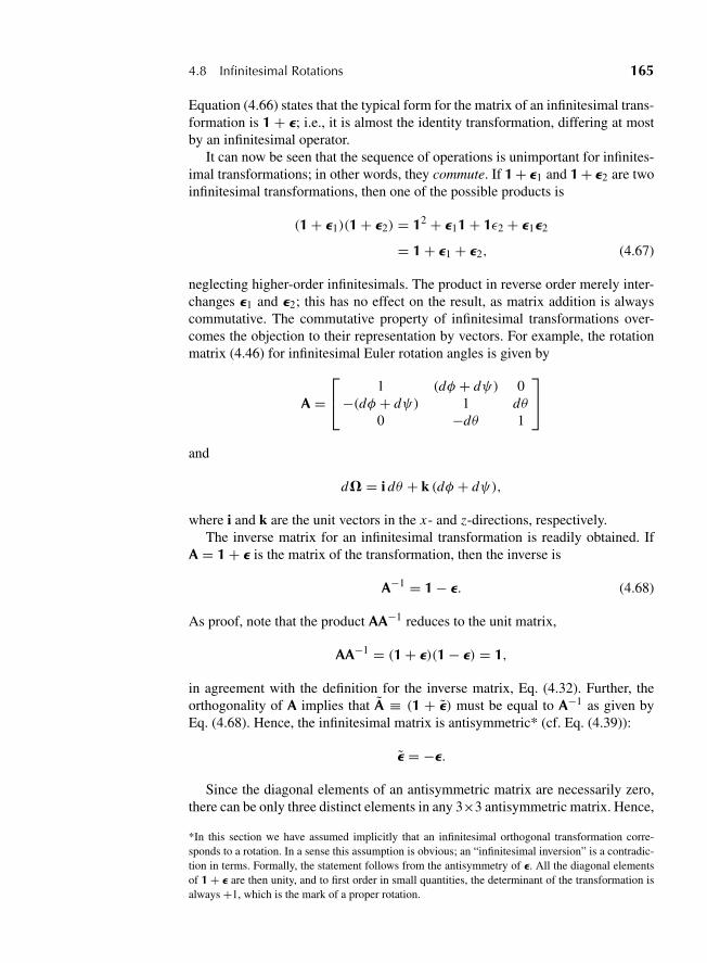
“M04 Goldstein ISBN C04” — 2011/2/15 — page 165 — #32
4.8 Infinitesimal Rotations 165
Equation (4.66) states that the typical form for the matrix of an infinitesimal trans-formation is 1 + e; i.e., it is almost the identity transformation, differing at mostby an infinitesimal operator.
It can now be seen that the sequence of operations is unimportant for infinites-imal transformations; in other words, they commute. If 1+ e1 and 1+ e2 are twoinfinitesimal transformations, then one of the possible products is
(1 + e1)(1 + e2) = 12 + e11 + 1ε2 + e1e2
= 1 + e1 + e2, (4.67)
neglecting higher-order infinitesimals. The product in reverse order merely inter-changes e1 and e2; this has no effect on the result, as matrix addition is alwayscommutative. The commutative property of infinitesimal transformations over-comes the objection to their representation by vectors. For example, the rotationmatrix (4.46) for infinitesimal Euler rotation angles is given by
A =⎡⎣ 1 (dφ + dψ) 0−(dφ + dψ) 1 dθ
0 −dθ 1
⎤⎦
and
d� = i dθ + k (dφ + dψ),
where i and k are the unit vectors in the x- and z-directions, respectively.The inverse matrix for an infinitesimal transformation is readily obtained. If
A = 1 + e is the matrix of the transformation, then the inverse is
A−1 = 1 − e. (4.68)
As proof, note that the product AA−1 reduces to the unit matrix,
AA−1 = (1 + e)(1 − e) = 1,
in agreement with the definition for the inverse matrix, Eq. (4.32). Further, theorthogonality of A implies that A ≡ (1 + e) must be equal to A−1 as given byEq. (4.68). Hence, the infinitesimal matrix is antisymmetric* (cf. Eq. (4.39)):
e = −e.
Since the diagonal elements of an antisymmetric matrix are necessarily zero,there can be only three distinct elements in any 3×3 antisymmetric matrix. Hence,
*In this section we have assumed implicitly that an infinitesimal orthogonal transformation corre-sponds to a rotation. In a sense this assumption is obvious; an “infinitesimal inversion” is a contradic-tion in terms. Formally, the statement follows from the antisymmetry of e. All the diagonal elementsof 1 + e are then unity, and to first order in small quantities, the determinant of the transformation isalways +1, which is the mark of a proper rotation.
“M04 Goldstein ISBN C04” — 2011/2/15 — page 166 — #33
166 Chapter 4 The Kinematics of Rigid Body Motion
there is no loss of generality in writing e in the form
e =⎡⎣ 0 d�3 −d�2−d�3 0 d�1d�2 −d�1 0
⎤⎦ . (4.69)
The three quantities d�1, d�2, d�3 are clearly to be identified with the threeindependent parameters specifying the rotation. We will now show that these threequantities also form the components of a particular kind of vector. By Eq. (4.66)the change in the components of a vector under the infinitesimal transformationof the coordinate system can be expressed by the matrix equation
r′ − r ≡ dr′ = er, (4.70)
which in expanded form, with e given by (4.69), becomes
dx1 = x2 d�3 − x3 d�2
dx2 = x3 d�1 − x1 d�3 (4.71)
dx3 = x1 d�2 − x2 d�1.
The right-hand side of each of Eqs. (4.71) is in the form of a component ofthe cross product of two vectors, namely, the cross product of r with a vectord� having components* d�1, d�2, d�3. We can therefore write Eq. (4.71)equivalently as
dr = r3 d�. (4.72)
The vector r transforms under an orthogonal matrix B according to the relations(cf. Eq. (4.20))
x ′i = bi j x j . (4.73)
If d� is to be a vector in the same sense as r, it must transform under B in thesame way. As we shall see, d� passes most of this test for a vector, although inone respect it fails to make the grade. One way of examining the transformationproperties of d� is to find how the matrix e transforms under a coordinate trans-formation. As was shown in Section 4.3, the transformed matrix e′ is obtained bya similarity transformation:
e′ = BeB−1.
*It cannot be emphasized too strongly that d� is not the differential of a vector. The combination d�stands for a differential vector, that is, a vector of differential magnitude. Unfortunately, notationalconvention results in having the vector characteristic applied only to �, but it should be clear to thereader there is no vector of which d� represents a differential. As we have seen, a finite rotationcannot be represented by a single vector.
“M04 Goldstein ISBN C04” — 2011/2/15 — page 167 — #34
4.8 Infinitesimal Rotations 167
As the antisymmetry property of a matrix is preserved under an orthogonal simi-larity transformation (see Derivation 3), e′ can also be put in the form of Eq. (4.69)with nonvanishing elements d�′
i . A detailed study of these elements shows thate transforms under the similarity transformation such that
d�′i = |B|bi j d� j . (4.74)
The transformation of d� is thus almost the same as for r, but differs by the factor|B|, the determinant of the transformation matrix.
There is however a simpler way to uncover the vector characteristics of d�,and indeed to verify its transformation properties as given by Eq. (4.74). In theprevious section a vector formula was derived for the change in the componentsof r under a finite rotation � of the coordinate system. By letting � go to thelimit of an infinitesimal angle d�, the corresponding formula for an infinitesimalrotation can be obtained. In this limit, cos� in Eq. (4.62) approaches unity, andsin� goes to �; the resultant expression for the infinitesimal change in r is then
r′ − r ≡ dr = r3 n d�. (4.75)
Comparison with Eq. (4.72) indicates that d� is indeed a vector and is determinedby
d� = n d�. (4.76)
Equation (4.75) can of course be derived directly without recourse to the finiterotation formula. Considered in its active sense, the infinitesimal coordinate trans-formation corresponds to a rotation of a vector r clockwise through an angle d�about the axis of rotation, a situation that is depicted in Fig. 4.11.* The magnitudeof dr, to first order in d� is, from the figure,
dr = r sin θ d�,
and the direction dr is, in this limit, perpendicular to both r and d� = n d�.Finally, the sense of dr is in the direction a right-hand screw advances as r isturned into d�. Figure 4.11 thus shows that in magnitude, direction, and sense dris the same as that predicted by Eq. (4.75).
The transformation properties of d�, as defined by Eq. (4.76), are still to bediscussed. As is well known from elementary vector algebra, there are two kindsof vectors in regard to transformation properties under an inversion. Vectors thattransform according to Eq. (4.72) are known as polar vectors. Under a three-dimensional inversion,
S =⎡⎣−1 0 0
0 −1 00 0 −1
⎤⎦
*Figure 4.11 is the clockwise-rotation version of Fig. 2.8.
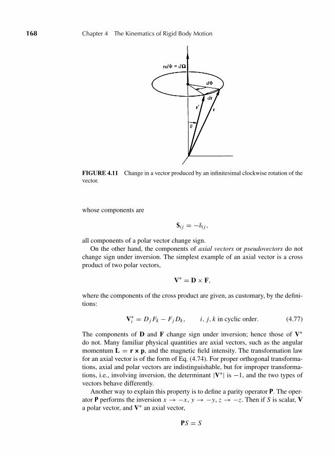
“M04 Goldstein ISBN C04” — 2011/2/15 — page 168 — #35
168 Chapter 4 The Kinematics of Rigid Body Motion
FIGURE 4.11 Change in a vector produced by an infinitesimal clockwise rotation of thevector.
whose components are
Si j = −δi j ,
all components of a polar vector change sign.On the other hand, the components of axial vectors or pseudovectors do not
change sign under inversion. The simplest example of an axial vector is a crossproduct of two polar vectors,
V∗ = D × F,
where the components of the cross product are given, as customary, by the defini-tions:
V∗i = D j Fk − Fj Dk, i, j, k in cyclic order. (4.77)
The components of D and F change sign under inversion; hence those of V∗do not. Many familiar physical quantities are axial vectors, such as the angularmomentum L = r3 p, and the magnetic field intensity. The transformation lawfor an axial vector is of the form of Eq. (4.74). For proper orthogonal transforma-tions, axial and polar vectors are indistinguishable, but for improper transforma-tions, i.e., involving inversion, the determinant |V∗| is −1, and the two types ofvectors behave differently.
Another way to explain this property is to define a parity operator P. The oper-ator P performs the inversion x → −x , y → −y, z → −z. Then if S is scalar, Va polar vector, and V∗ an axial vector,
PS = S
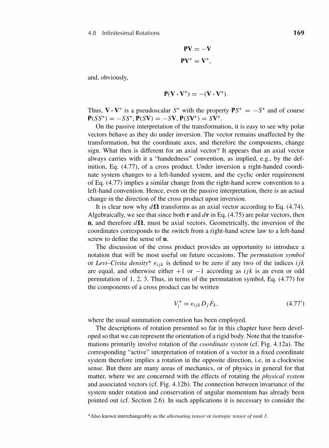
“M04 Goldstein ISBN C04” — 2011/2/15 — page 169 — #36
4.8 Infinitesimal Rotations 169
PV = −V
PV∗ = V∗,
and, obviously,
P(V ?V∗) = −(V ?V∗).
Thus, V ?V∗ is a pseudoscalar S∗ with the property PS∗ = −S∗ and of courseP(SS∗) = −SS∗, P(SV) = −SV, P(SV∗) = SV∗.
On the passive interpretation of the transformation, it is easy to see why polarvectors behave as they do under inversion. The vector remains unaffected by thetransformation, but the coordinate axes, and therefore the components, changesign. What then is different for an axial vector? It appears that an axial vectoralways carries with it a “handedness” convention, as implied, e.g., by the def-inition, Eq. (4.77), of a cross product. Under inversion a right-handed coordi-nate system changes to a left-handed system, and the cyclic order requirementof Eq. (4.77) implies a similar change from the right-hand screw convention to aleft-hand convention. Hence, even on the passive interpretation, there is an actualchange in the direction of the cross product upon inversion.
It is clear now why d� transforms as an axial vector according to Eq. (4.74).Algebraically, we see that since both r and dr in Eq. (4.75) are polar vectors, thenn, and therefore d�, must be axial vectors. Geometrically, the inversion of thecoordinates corresponds to the switch from a right-hand screw law to a left-handscrew to define the sense of n.
The discussion of the cross product provides an opportunity to introduce anotation that will be most useful on future occasions. The permutation symbolor Levi–Civita density* εi jk is defined to be zero if any two of the indices i jkare equal, and otherwise either +1 or −1 according as i jk is an even or oddpermutation of 1, 2, 3. Thus, in terms of the permutation symbol, Eq. (4.77) forthe components of a cross product can be written
V ∗i = εi jk D j Fk, (4.77′)
where the usual summation convention has been employed.The descriptions of rotation presented so far in this chapter have been devel-
oped so that we can represent the orientation of a rigid body. Note that the transfor-mations primarily involve rotation of the coordinate system (cf. Fig. 4.12a). Thecorresponding “active” interpretation of rotation of a vector in a fixed coordinatesystem therefore implies a rotation in the opposite direction, i.e, in a clockwisesense. But there are many areas of mechanics, or of physics in general for thatmatter, where we are concerned with the effects of rotating the physical systemand associated vectors (cf. Fig. 4.12b). The connection between invariance of thesystem under rotation and conservation of angular momentum has already beenpointed out (cf. Section 2.6). In such applications it is necessary to consider the
*Also known interchangeably as the alternating tensor or isotropic tensor of rank 3.
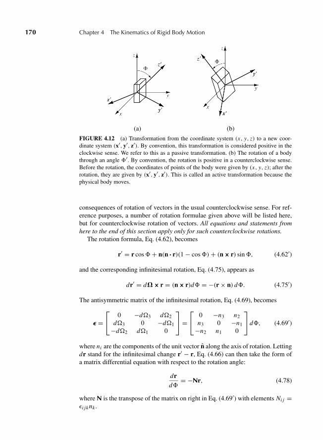
“M04 Goldstein ISBN C04” — 2011/2/15 — page 170 — #37
170 Chapter 4 The Kinematics of Rigid Body Motion
(a) (b)
FIGURE 4.12 (a) Transformation from the coordinate system (x, y, z) to a new coor-dinate system (x′, y′, z′). By convention, this transformation is considered positive in theclockwise sense. We refer to this as a passive transformation. (b) The rotation of a bodythrough an angle �′. By convention, the rotation is positive in a counterclockwise sense.Before the rotation, the coordinates of points of the body were given by (x, y, z); after therotation, they are given by (x′, y′, z′). This is called an active transformation because thephysical body moves.
consequences of rotation of vectors in the usual counterclockwise sense. For ref-erence purposes, a number of rotation formulae given above will be listed here,but for counterclockwise rotation of vectors. All equations and statements fromhere to the end of this section apply only for such counterclockwise rotations.
The rotation formula, Eq. (4.62), becomes
r′ = r cos�+ n(n ? r)(1 − cos�)+ (n3 r) sin�, (4.62′)
and the corresponding infinitesimal rotation, Eq. (4.75), appears as
dr′ = d�3 r = (n3 r)d� = −(r × n) d�. (4.75′)
The antisymmetric matrix of the infinitesimal rotation, Eq. (4.69), becomes
e =⎡⎣ 0 −d�3 d�2
d�3 0 −d�1−d�2 d�1 0
⎤⎦ =
⎡⎣ 0 −n3 n2
n3 0 −n1−n2 n1 0
⎤⎦ d�, (4.69′)
where ni are the components of the unit vector n along the axis of rotation. Lettingdr stand for the infinitesimal change r′ − r, Eq. (4.66) can then take the form ofa matrix differential equation with respect to the rotation angle:
drd�
= −Nr, (4.78)
where N is the transpose of the matrix on right in Eq. (4.69′) with elements Ni j =εi jknk .
“M04 Goldstein ISBN C04” — 2011/2/15 — page 171 — #38
4.9 Rate of Change of a Vector 171
Another useful representation is to write e in Eq. (4.69′) as
e = ni Mi d�
where Mi are the three matrices:
M1 =⎡⎣ 0 0 0
0 0 −10 1 0
⎤⎦ , M2 =
⎡⎣ 0 0 1
0 0 0−1 0 0
⎤⎦ , M3 =
⎡⎣ 0 −1 0
1 0 00 0 0
⎤⎦ .(4.79)
The matrices Mi are known as the infinitesimal rotation generators and have theproperty that their products are
Mi M j − M j Mi ≡[Mi ,M j
] = εi jkMk . (4.80)
The difference between the two matrix products, or commutator, is also called theLie bracket or Mi , and Eq. (4.80) defines the Lie algebra of the rotation groupparametrized in terms of the rotation angle. To go further into the group theory ofrotation would take us too far afield, but we shall have occasion to refer to theseproperties of the rotation operation. (cf. Section 9.5 and Appendix B)
4.9 RATE OF CHANGE OF A VECTOR
The concept of an infinitesimal rotation provides a powerful tool for describingthe motion of a rigid body in time. Let us consider some arbitrary vector or pseu-dovector G involved in the mechanical problem, such as the position vector of apoint in the body, or the total angular momentum. Usually such a vector will varyin time as the body moves, but the change will often depend upon the coordinatesystem to which the observations are referred. For example, if the vector happensto be the radius vector from the origin of the body set of axes to a point in the rigidbody, then clearly such a vector appears constant when measured by the body setof axes. However, to an observer fixed in the space set of axes, the componentsof the vector (as measured on the space axes) will vary in time if the body is inmotion.
The change in a time dt of the components of a general vector G as seen by anobserver in the body system of axes will differ from the corresponding change asseen by an observer in the space system. A relation between the two differentialchanges in G can be derived on the basis of physical arguments. We can write thatthe only difference between the two is the effect of rotation of the body axes:
(dG)space = (dG)body + (dG)rot.
Now consider a vector fixed in the rigid body. As the body rotates, there is ofcourse no change in the components of this vector as seen by the body observer,
“M04 Goldstein ISBN C04” — 2011/2/15 — page 172 — #39
172 Chapter 4 The Kinematics of Rigid Body Motion
i.e., relative to body axes. The only contribution to (dG)space is then the effect ofthe rotation of the body. But since the vector is fixed in the body system, it rotateswith it counterclockwise, and the change in the vector as observed in space is thatgiven by Eq. (4.75′), and hence (dG)rot is given by
(dG)rot = d�3G.
For an arbitrary vector, the change relative to the space axes is the sum of the twoeffects:
(dG)space = (dG)body + d�3G. (4.81)
The time rate of change of the vector G as seen by the two observers is thenobtained by dividing the terms in Eq. (4.81) by the differential time element dtunder consideration; (
dGdt
)space
=(
dGdt
)body
+v3G. (4.82)
Here v is the instantaneous angular velocity of the body defined by the relation*
v dt = d�. (4.83)
The vector v lies along the axis of the infinitesimal rotation occurring between tand t + dt , a direction known as the instantaneous axis of rotation. In magnitude,v measures the instantaneous rate of rotation of the body.
A more formal derivation of the basic Eq. (4.82) can be given in terms ofthe orthogonal matrix of transformation between the space and body coordi-nates. The component of G along the i th space axis is related to the componentsalong the body axes:
Gi = ai j G′j = a ji G
′j .
As the body moves in time, the components G ′j will change as will the elements
ai j of the transformation matrix. Hence, the change in Gi in a differential timeelement dt is
dGi = a ji dG ′j + da ji G
′j . (4.84)
It is no loss of generality to take the space and body axes as instantaneouslycoincident at the time t . Components in the two systems will then be the sameinstantaneously, but differentials will not be the same, since the two systems aremoving relative to each other. Thus, G ′
j = G j but a ji dG ′j = dG ′
i , the primeemphasizing the differential is measured in the body axis system. The change inthe matrix A in the time dt is thus a change from the unit matrix and therefore
*Note that v is not the derivative of any vector.
“M04 Goldstein ISBN C04” — 2011/2/15 — page 173 — #40
4.9 Rate of Change of a Vector 173
corresponds to the matrix e of the infinitesimal rotation. Hence,
da ji = (e)i j = −ei j ,
using the antisymmetry property of e. In terms of the permutation symbol ei jk ,the elements of e are such that (cf. Eq. (4.69))
−εi j = −εi jkd�k = εik j d�k .
Equation (4.84) can now be written
dGi = dG ′i + εik j d�k G j .
The last term on the right will be recognized as the expression for the i th com-ponent of a cross product, so that the final expression for the relation betweendifferentials in the two systems is
dGi = dG ′i + (d�3G)i , (4.85)
which is the same as the i th component of Eq. (4.81).Equation (4.81) is not so much an equation about a particular vector G as it is a
statement of the transformation of the time derivative between the two coordinatesystems. The arbitrary nature of the vector G made use of in the derivation can beemphasized by writing Eq. (4.82) as an operator equation acting on some givenvector: (
d
dt
)s=(
d
dt
)r+v3. (4.86)
Here the subscripts s and r indicate the time derivatives observed in the spaceand body (rotating) system of axes, respectively. The resultant vector equationcan then of course be resolved along any desired set of axes, fixed or moving. Butagain note that the time rate of change is only relative to the specified coordinatesystem. When a time derivative of a vector is with respect to one coordinate sys-tem, components may be taken along another set of coordinate axes only after thedifferentiation has been carried out.
It is often convenient to express the angular velocity vector in terms of theEuler angles and their time derivatives. The general infinitesimal rotation asso-ciated with v can be considered as consisting of three successive infinitesimalrotations with angular velocities ωφ = φ, ωθ = θ , ωψ = ψ . In consequence ofthe vector property of infinitesimal rotations, the vector v can be obtained as thesum of the three separate angular velocity vectors. Unfortunately, the directionsvφ , vθ , and vψ are not symmetrically placed: vφ is along the space z axis, vθis along the line of nodes, while vψ alone is along the body z′ axis. However,the orthogonal transformations B, C, D of Section 4.4 may be used to furnish thecomponents of these vectors along any desired set of axes.
“M04 Goldstein ISBN C04” — 2011/2/15 — page 174 — #41
174 Chapter 4 The Kinematics of Rigid Body Motion
The body set of axes proves most useful for discussing the equations of motion,and we shall therefore obtain the components of v for such a coordinate system.Since vφ is parallel to the space z axis, its components along the body axes aregiven by applying the complete orthogonal transformation A = BCD, Eq. (4.46):
(vφ)x ′ = φ sin θ sinψ, (vφ)y′ = φ sin θ cosψ, (vφ)z′ = φ cos θ.
Note that φ has the projection φ sin θ in the x ′, y′ plane, and it is perpendicular tothe line of nodes.
The line of nodes, which is the direction of vθ , coincides with the ξ ′ axis, sothat the components of vθ with respect to the body axes are furnished by applyingonly the final orthogonal transformation B, Eq. (4.45):
(vθ )x ′ = θ cosψ, (vθ )y′ = −θ sinψ, (vθ )z′ = 0.
No transformation is necessary for the components of vψ , which lies along the z′axis (ωψ = ψ). Adding these components of the separate angular velocities, thecomponents of v with respect to the body axes are
ωx ′ = φ sin θ sinψ + θ cosψ,
ωy′ = φ sin θ cosψ − θ sinψ,
ωz′ = φ cos θ + ψ. (4.87)
Similar techniques may be used to express the components of v along the spaceset of axes in terms of the Euler angles.
4.10 THE CORIOLIS EFFECT
Equation (4.86) is the basic kinematical law upon which the dynamical equationsof motion for a rigid body are founded. But its validity is not restricted solely torigid body motion. It may be used whenever we wish to discuss the motion of aparticle, or system of particles, relative to a rotating coordinate system.
A particularly important problem in this latter category is the description ofparticle motion relative to coordinate axes rotating with Earth. Recall that inSection 1.1 an inertial system was defined as one in which Newton’s laws ofmotion are valid. For many purposes, a system of coordinates fixed in the rotatingEarth is a sufficient approximation to an inertial system. However, the system ofcoordinates in which the local stars are fixed comes still closer to the ideal iner-tial system. Detailed examination shows there are observable effects arising fromEarth’s rotation relative to this nearly inertial system. Equation (4.86) providesthe needed modifications of the equations of motion relative to the noninertialsystem fixed in the rotating Earth.
The initial step is to apply Eq. (4.86) to the radius vector, r, from the origin ofthe terrestrial system to the given particle:
vs = vr +v3 r, (4.88)
“M04 Goldstein ISBN C04” — 2011/2/15 — page 175 — #42
4.10 The Coriolis Effect 175
where vs and vr are the velocities of the particle relative to the space and rotatingset of axes, respectively, and v is the (constant) angular velocity of Earth relativeto the inertial system. In the second step, Eq. (4.86) is used to obtain the time rateof change of vs :
(dvs
dt
)s= as =
(dvs
dt
)r+v3 vs
= ar + 2(v3 vr )+v3 (v3 r), (4.89)
where vs has been substituted from Eq. (4.88), and where as and ar are the accel-erations of the particle in the two systems. Finally, the equation of motion, whichin the inertial system is simply
F = mas,
expands, when expressed in the rotating coordinates, into the equation
F − 2m(v3 vr )− mv3 (v3 r) = mar . (4.90)
To an observer in the rotating system, it therefore appears as if the particle ismoving under the influence of an effective force Feff:
Feff = F − 2m(v3 vr )− mv3 (v3 r). (4.91)
Let us examine the nature of the terms appearing in Eq. (4.91). The last term isa vector normal to v and pointing outward. Further, its magnitude is mω2r sin θ .It will therefore be recognized that this term provides the familiar centrifugalforce. When the particle is stationary in the moving system, the centrifugal forceis the only added term in the effective force. However, when the particle is mov-ing, the middle term known as the Coriolis effect* comes into play. The orderof magnitude of both of these quantities may easily be calculated for a particleon Earth’s surface. Earth rotates counterclockwise about the north pole with anangular velocity relative to the fixed stars:
ω =(
2π
24 × 3600
)(366.25
365.25
)= 7.292 × 10⁻⁵s−1.
Here the first set of parentheses gives the angular velocity relative to the radiusvector to the Sun. The quantity in the second parentheses, the ratio of the numberof sidereal days in a year to the corresponding number of solar days, is the correc-tion factor to give the angular velocity relative to the fixed stars. With this value
*The term Coriolis effect is used instead of the older term, Coriolis force, to remind us that this effectexists because we are using a noninertial frame. In a proper inertial frame, the effect does not exist.You can always visualize the Coriolis effect by asking what is happening in an inertial frame.
“M04 Goldstein ISBN C04” — 2011/2/15 — page 176 — #43
176 Chapter 4 The Kinematics of Rigid Body Motion
for ω, and with r equal to Earth’s equatorial radius, the maximum centripetalacceleration is
ω2r = 3.38 cm/s2,
or about 0.3% of the acceleration of gravity. While small, this acceleration isby no means negligible. However, the measured effects of gravity representthe combination of the gravitational field of the mass distribution of Earth andthe effects of centripetal acceleration. It has become customary to speak of thesum of the two as Earth’s gravity field, as distinguished from its gravitationalfield.
The situation is further complicated by the effect of the centripetal accelerationin flattening the rotating Earth. If Earth were completely fluid, the effect of rota-tion would be to deform it into the shape of an ellipsoid whose surface would bean equipotential surface of the combined gravity field. The mean level of Earth’sseas conforms very closely to this equilibrium ellipsoid (except for local varia-tions of wind and tide) and defines what is called the geoid.
Except for effects of local perturbations, the force of gravity will be perpen-dicular to the equipotential surface of the geoid. Accordingly, the local vertical isdefined as the direction perpendicular to the geoid at the given point on the sur-face. For phenomena that occur in the vicinity of a particular spot on Earth, thecentripetal acceleration terms in Eq. (4.91) can be considered as swallowed up inthe gravitational acceleration g, which will be oriented in the local vertical direc-tion. The magnitude of g of course varies with the latitude on Earth. The effectsof centripetal acceleration and the flattening of Earth combine to make g about0.53% less at the equator than at the poles.
Incidentally, the centrifugal force on a particle arising from Earth’s revolu-tion around the Sun is appreciable compared to gravity, but it is almost exactlybalanced by the gravitational attraction to the Sun. If we analyze the motion ofthe Sun–Earth system from a frame rotating with Earth, it is of course just thebalance between the centrifugal effect and the gravitational attraction that keepsthe Earth (and all that are on it) and Sun separated. An analysis in a Newtonianinertial frame gives a different picture. As was described in Section 3.3, theangular momentum contributes to the effective potential energy to keep the Earthin orbit.
The Coriolis effect on a moving particle is perpendicular to both v and v.*In the northern hemisphere, where v points out of the ground, the Coriolis effect2m(v3v) tends to deflect a projective shot along Earth’s surface, to the right ofits direction of travel (cf. Fig. 4.13). The Coriolis deflection reverses direction inthe southern hemisphere and is zero at the equator, where v is horizontal. Themagnitude of the Coriolis acceleration is always less than
2ωv 1.5 × 10⁻⁴v,
*From here on, the subscript r will be dropped from v as all velocities will be taken with respect tothe rotating coordinate axes only.
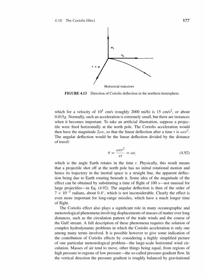
“M04 Goldstein ISBN C04” — 2011/2/15 — page 177 — #44
4.10 The Coriolis Effect 177
FIGURE 4.13 Direction of Coriolis deflection in the northern hemisphere.
which for a velocity of 105 cm/s (roughly 2000 mi/h) is 15 cm/s2, or about0.015g. Normally, such an acceleration is extremely small, but there are instanceswhen it becomes important. To take an artificial illustration, suppose a projec-tile were fired horizontally at the north pole. The Coriolis acceleration wouldthen have the magnitude 2ωv, so that the linear deflection after a time t is ωvt2.The angular deflection would be the linear deflection divided by the distanceof travel:
θ = ωvt2
vt= ωt, (4.92)
which is the angle Earth rotates in the time t . Physically, this result meansthat a projectile shot off at the north pole has no initial rotational motion andhence its trajectory in the inertial space is a straight line, the apparent deflec-tion being due to Earth rotating beneath it. Some idea of the magnitude of theeffect can be obtained by substituting a time of flight of 100 s—not unusual forlarge projectiles—in Eq. (4.92). The angular deflection is then of the order of7 × 10−3 radians, about 0.4◦, which is not inconsiderable. Clearly the effect iseven more important for long-range missiles, which have a much longer timeof flight.
The Coriolis effect also plays a significant role in many oceanographic andmeteorological phenomena involving displacements of masses of matter over longdistances, such as the circulation pattern of the trade winds and the course ofthe Gulf stream. A full description of these phenomena requires the solution ofcomplex hydrodynamic problems in which the Coriolis acceleration is only oneamong many terms involved. It is possible however to give some indication ofthe contribution of Coriolis effects by considering a highly simplified pictureof one particular meteorological problem—the large-scale horizontal wind cir-culation. Masses of air tend to move, other things being equal, from regions ofhigh pressure to regions of low pressure—the so-called pressure-gradient flow. Inthe vertical direction the pressure gradient is roughly balanced by gravitational
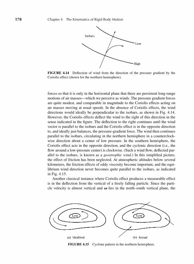
“M04 Goldstein ISBN C04” — 2011/2/15 — page 178 — #45
178 Chapter 4 The Kinematics of Rigid Body Motion
FIGURE 4.14 Deflection of wind from the direction of the pressure gradient by theCoriolis effect (shown for the northern hemisphere).
forces so that it is only in the horizontal plane that there are persistent long-rangemotions of air masses—which we perceive as winds. The pressure gradient forcesare quite modest, and comparable in magnitude to the Coriolis effects acting onair masses moving at usual speeds. In the absence of Coriolis effects, the winddirections would ideally be perpendicular to the isobars, as shown in Fig. 4.14.However, the Coriolis effects deflect the wind to the right of this direction in thesense indicated in the figure. The deflection to the right continues until the windvector is parallel to the isobars and the Coriolis effect is in the opposite directionto, and ideally just balances, the pressure-gradient force. The wind then continuesparallel to the isobars, circulating in the northern hemisphere in a counterclock-wise direction about a center of low pressure. In the southern hemisphere, theCoriolis effect acts in the opposite direction, and the cyclonic direction (i.e., theflow around a low-pressure center) is clockwise. (Such a wind flow, deflected par-allel to the isobars, is known as a geostrophic wind.) In this simplified picture,the effect of friction has been neglected. At atmospheric altitudes below severalkilometers, the friction effects of eddy viscosity become important, and the equi-librium wind direction never becomes quite parallel to the isobars, as indicatedin Fig. 4.15.
Another classical instance where Coriolis effect produces a measurable effectis in the deflection from the vertical of a freely falling particle. Since the parti-cle velocity is almost vertical and v lies in the north–south vertical plane, the
FIGURE 4.15 Cyclone pattern in the northern hemisphere.
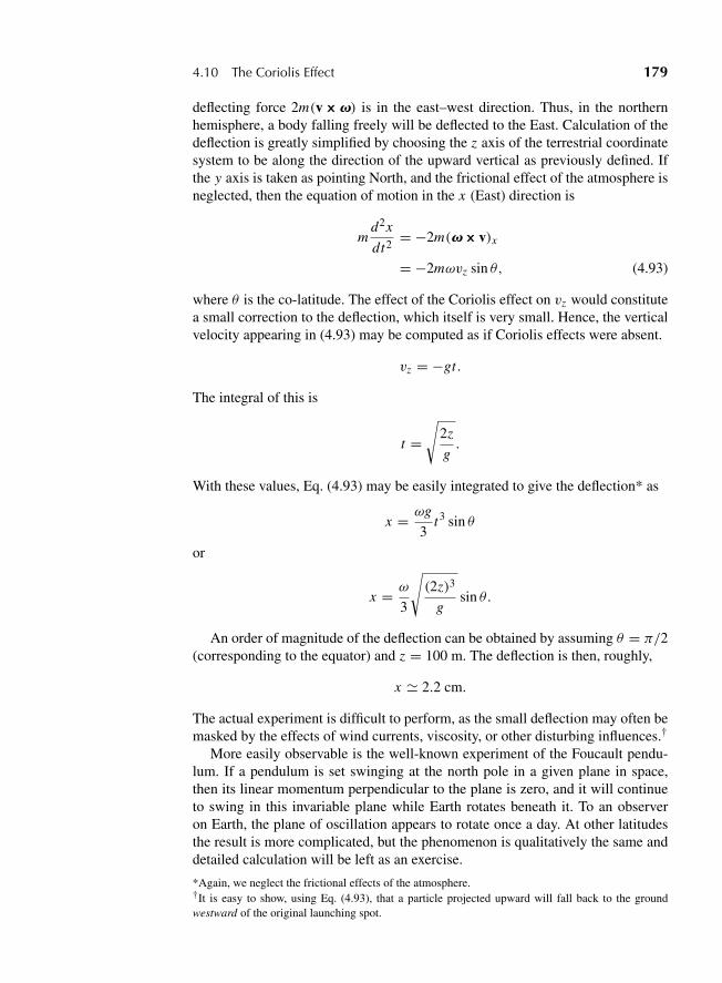
“M04 Goldstein ISBN C04” — 2011/2/15 — page 179 — #46
4.10 The Coriolis Effect 179
deflecting force 2m(v3v) is in the east–west direction. Thus, in the northernhemisphere, a body falling freely will be deflected to the East. Calculation of thedeflection is greatly simplified by choosing the z axis of the terrestrial coordinatesystem to be along the direction of the upward vertical as previously defined. Ifthe y axis is taken as pointing North, and the frictional effect of the atmosphere isneglected, then the equation of motion in the x (East) direction is
md2x
dt2= −2m(v3 v)x
= −2mωvz sin θ, (4.93)
where θ is the co-latitude. The effect of the Coriolis effect on vz would constitutea small correction to the deflection, which itself is very small. Hence, the verticalvelocity appearing in (4.93) may be computed as if Coriolis effects were absent.
vz = −gt.
The integral of this is
t =√
2z
g.
With these values, Eq. (4.93) may be easily integrated to give the deflection* as
x = ωg
3t3 sin θ
or
x = ω
3
√(2z)3
gsin θ.
An order of magnitude of the deflection can be obtained by assuming θ = π/2(corresponding to the equator) and z = 100 m. The deflection is then, roughly,
x 2.2 cm.
The actual experiment is difficult to perform, as the small deflection may often bemasked by the effects of wind currents, viscosity, or other disturbing influences.†
More easily observable is the well-known experiment of the Foucault pendu-lum. If a pendulum is set swinging at the north pole in a given plane in space,then its linear momentum perpendicular to the plane is zero, and it will continueto swing in this invariable plane while Earth rotates beneath it. To an observeron Earth, the plane of oscillation appears to rotate once a day. At other latitudesthe result is more complicated, but the phenomenon is qualitatively the same anddetailed calculation will be left as an exercise.
*Again, we neglect the frictional effects of the atmosphere.†It is easy to show, using Eq. (4.93), that a particle projected upward will fall back to the groundwestward of the original launching spot.
“M04 Goldstein ISBN C04” — 2011/2/15 — page 180 — #47
180 Chapter 4 The Kinematics of Rigid Body Motion
Effects due to the Coriolis terms also appear in atomic physics. Thus, two typesof motion may occur simultaneously in polyatomic molecules: The moleculerotates as a rigid whole, and the atoms vibrate about their equilibrium positions.As a result of the vibrations, the atoms are in motion relative to the rotatingcoordinate system of the molecule. The Coriolis term will then be differentfrom zero and will cause the atoms to move in a direction perpendicular to theoriginal oscillations. Perturbations in molecular spectra due to Coriolis effectsthus appear as interactions between the rotational and vibrational motions ofthe molecule.
DERIVATIONS
1. Prove that matrix multiplication is associative. Show that the product of two orthogo-nal matrices is also orthogonal.
2. Prove the following properties of the transposed and adjoint matrices:
AB = BA,
(AB)† = B†A†.
3. Show that the trace of a matrix is invariant under any similarity transformation. Showalso that the antisymmetry property of a matrix is preserved under an orthogonal sim-ilarity transformation.
4. (a) By examining the eigenvalues of an antisymmetric 3× 3 real matrix A, show that1 ± A is nonsingular.
(b) Show then that under the same conditions the matrix
B = (1 + A)(1 − A)−1
is orthogonal.
5. Obtain the matrix elements of the general rotation matrix in terms of the Eulerangles, Eq. (4.46), by performing the multiplications of the successive componentrotation matrices. Verify directly that the matrix elements obey the orthogonalityconditions.
6. The body set of axes can be related to the space set in terms of Euler’s angles by thefollowing set of rotations:
(a) Rotation about the x axis by an angle θ .
(b) Rotation about the z′ axis by an angle ψ .
(c) Rotation about the old z axis by an angle φ.
Show that this sequence leads to the same elements of the matrix of transformation asthe sequence of rotations given in the book. [Hint: It is not necessary to carry out theexplicit multiplication of the rotation matrices.]
7. If A is the matrix of a rotation through 180◦ about any axis, show that if
P± = 12 (1 ± A),
“M04 Goldstein ISBN C04” — 2011/2/15 — page 181 — #48
Derivations 181
then P2± = P±. Obtain the elements of P± in any suitable system, and find a geometricinterpretation of the operation P+ and P− on any vector F.
8. (a) Show that the rotation matrix in the form of Eq. (4.47′) cannot be put in the formof the matrix of the inversion transformation S.
(b) Verify by direct multiplication that the matrix in Eq. (4.47′) is orthogonal.
9. Show that any rotation can be represented by successive reflection in two planes, bothpassing through the axis of rotation with the planar angle �/2 between them.
10. If B is a square matrix and A is the exponential of B, defined by the infinite seriesexpansion of the exponential,
A ≡ eB = 1 + B + 1
2B2 + · · · + Bn
n+ · · · ,
then prove the following properties:
(a) eBeC = eB+C, providing B and C commute.(b) A−1 = e−B
(c) eCBC−1 = CAC−1
(d) A is orthogonal if B is antisymmetric.
11. Verify the relation
| − B| = (−1)n |B|for the determinant of an n × n matrix B.
12. In a set of axes where the z axis is the axis of rotation of a finite rotation, the rotationmatrix is given by Eq. (4.43) with φ replaced by the angle of finite rotation �. Derivethe rotation formula, Eq. (4.62), by transforming to an arbitrary coordinate system,expressing the orthogonal matrix of transformation in terms of the direction cosinesof the axis of the finite rotation.
13. (a) Suppose two successive coordinate rotations through angles �1 and �2 are car-ried out, equivalent to a single rotation through an angle�. Show that�1,�2, and� can be considered as the sides of a spherical triangle with the angle opposite to� given by the angle between the two axes of rotation.
(b) Show that a rotation about any given axis can be obtained as the product of twosuccessive rotations, each through 180◦.
14. (a) Verify that the permutation symbol satisfies the following identity in terms ofKronecker delta symbols:
εi j pεrmp = δir δ jm − δimδ jr .
(b) Show that
εi j pεi jk = 2δpk .
15. Show that the components of the angular velocity along the space set of axes are givenin terms of the Euler angles by
ωx = θ cosφ + ψ sin θ sinφ,
ωy = θ sinφ − ψ sin θ cosφ,
ωz = ψ cos θ + φ.
“M04 Goldstein ISBN C04” — 2011/2/15 — page 182 — #49
182 Chapter 4 The Kinematics of Rigid Body Motion
16. Show that the Euler parameter e0 has the equation of motion
−2e0 = e1ωx ′ + e2ωy′ + e3ωz′ ,
where the prime denotes the body set of axes. Find the corresponding equations for theother three Euler parameters and for the complex Cayley–Klein parameters α and β.
17. Verify directly that the matrix generators of infinitesimal rotation, Mi , as given byEq. (4.79) obey the commutation relations
[Mi ,M j ] = εi jkMk .
18. (a) Find the vector equation describing the reflection of r in a plane whose unitnormal is n.
(b) Show that if li , i = 1, 2, 3, are the direction cosines of n, then the matrix oftransformation has the elements
Ai j = δi j − 2li l j ,
and verify that A is an improper orthogonal matrix.
19. Figures 4.9 and 4.10 show that the order of finite rotations leads to different results.Use the notation that A(α, 1n) where A is a rotation in the direction of 1n through anangle α. Let n1 and n2 be two orthogonal directions.
(a) If x is the position vector of a point on a rigid body, which is then rotated by anangle θ around the origin, show that the new value of x is
x′ = (1n ? x)1n + [x − 1n(1n ? x)] cos θ − 1n × x sin θ.
From this, obtain the formula for A(π/2, 1n) and derive the two rotations in thefigures.
(b) Discuss these two rotations. [Hint: The answer will involve a rotation by the angle23π in a direction (1/
√3)(1, 1, 1).]
20. Express the “rolling” constraint of a sphere on a plane surface in terms of the Eulerangles. Show that the conditions are nonintegrable and that the constraint is thereforenonholonomic.
EXERCISES
21. A particle is thrown up vertically with initial speed v0, reaches a maximum heightand falls back to ground. Show that the Coriolis deflection when it again reaches theground is opposite in direction, and four times greater in magnitude, than the Coriolisdeflection when it is dropped at rest from the same maximum height.
22. A projectile is fired horizontally along Earth’s surface. Show that to a first approxima-tion the angular deviation from the direction of fire resulting from the Coriolis effectvaries linearly with time at a rate
ω cos θ,
where ω is the angular frequency of Earth’s rotation and θ is the co-latitude, thedirection of deviation being to the right in the northern hemisphere.
“M04 Goldstein ISBN C04” — 2011/2/15 — page 183 — #50
Exercises 183
23. The Foucault pendulum experiment consists in setting a long pendulum in motion ata point on the surface of the rotating Earth with its momentum originally in the ver-tical plane containing the pendulum bob and the point of suspension. Show that thependulum’s subsequent motion may be described by saying that the plane of oscilla-tion rotates uniformly 2π cos θ radians per day, where θ is the co-latitude. What is thedirection of rotation? The approximation of small oscillations may be used, if desired.
24. A wagon wheel with spokes is mounted on a vertical axis so it is free to rotate in thehorizontal plane. The wheel is rotating with an angular speed of ω = 3.0 radian/s. Abug crawls out on one of the spokes of the wheel with a velocity of 0.5 cm/s holdingon to the spoke with a coefficient of friction μ = 0.30. How far can the bug crawlalong the spoke before it starts to slip?
25. A carousel (counter-clockwise merry-go-round) starts from rest and accelerates at aconstant angular accleration of 0.02 revolutions/s2. A girl sitting on a bench on theplatform 7.0 m from the center is holding a 3.0 kg ball. Calculate the magnitude anddirection of the force she must exert to hold the ball 6.0 s after the carousel starts tomove. Give the direction with respect to the line from the center of rotation to the girl.

“M05 Goldstein ISBN C05” — 2011/2/15 — page 184 — #1
C H A P T E R
5 The Rigid Body Equationsof Motion
Chapter 4 presents all the kinematical tools needed in the discussion of rigid bodymotion. In the Euler angles we have a set of three coordinates, defined ratherunsymmetrically it is true, yet suitable for use as the generalized coordinatesdescribing the orientation of the rigid body. In addition, the method of orthog-onal transformations, and the associated matrix algebra, furnish a powerful andelegant technique for investigating the characteristics of rigid body motion. Wehave already had one application of the technique in deriving Eq. (4.86), the rela-tion between the states of change of a vector as viewed in the space system and inthe body system. These tools will now be applied to obtain the Euler dynamicalequations of motion of the rigid body in their most convenient form. With the helpof the equations of motion, some simple but highly important problems of rigidbody motion can be discussed.
5.1 ANGULAR MOMENTUM AND KINETIC ENERGYOF MOTION ABOUT A POINT
Chasles’ theorem states that any general displacement of a rigid body can be rep-resented by a translation plus a rotation. The theorem suggests that it ought tobe possible to split the problem of rigid body motion into two separate phases,one concerned solely with the translational motion of the body, the other, withits rotational motion. Of course, if one point of the body is fixed, the separa-tion is obvious, for then there is only a rotational motion about the fixed point,without any translation. But even for a general type of motion such a separa-tion is often possible. The six coordinates needed to describe the motion havealready been formed into two sets in accordance with such a division: the threeCartesian coordinates of a point fixed in the rigid body to describe the transla-tional motion and, say, the three Euler angles for the motion about the point.If, further, the origin of the body system is chosen to be the center of mass,then by Eq. (1.28) the total angular momentum divides naturally into contribu-tions from the translation of the center of mass and from the rotation about thecenter of mass. The former term will involve only the Cartesian coordinates ofthe center of mass, the latter only the angle coordinates. By Eq. (1.31), a sim-ilar division holds for the total kinetic energy T , which can be written in theform
T = 12 Mv2 + T ′(φ, θ, ψ),
184
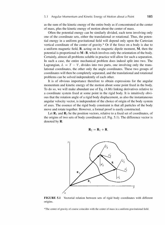
“M05 Goldstein ISBN C05” — 2011/2/15 — page 185 — #2
5.1 Angular Momentum and Kinetic Energy of Motion about a Point 185
as the sum of the kinetic energy of the entire body as if concentrated at the centerof mass, plus the kinetic energy of motion about the center of mass.
Often the potential energy can be similarly divided, each term involving onlyone of the coordinate sets, either the translational or rotational. Thus, the poten-tial energy in a uniform gravitational field will depend only upon the Cartesianvertical coordinate of the center of gravity.* Or if the force on a body is due toa uniform magnetic field, B, acting on its magnetic dipole moment, M, then thepotential is proportional to M ?B, which involves only the orientation of the body.Certainly, almost all problems soluble in practice will allow for such a separation.In such a case, the entire mechanical problem does indeed split into two. TheLagrangian, L = T − V , divides into two parts, one involving only the trans-lational coordinates, the other only the angle coordinates. These two groups ofcoordinates will then be completely separated, and the translational and rotationalproblems can be solved independently of each other.
It is of obvious importance therefore to obtain expressions for the angularmomentum and kinetic energy of the motion about some point fixed in the body.To do so, we will make abundant use of Eq. (4.86) linking derivatives relative toa coordinate system fixed at some point in the rigid body. It is intuitively obvi-ous that the rotation angle of a rigid body displacement, as also the instantaneousangular velocity vector, is independent of the choice of origin of the body systemof axes. The essence of the rigid body constraint is that all particles of the bodymove and rotate together. However, a formal proof is easily constructed.
Let R1 and R2 be the position vectors, relative to a fixed set of coordinates, ofthe origins of two sets of body coordinates (cf. Fig. 5.1). The difference vector isdenoted by R:
R2 = R1 + R.
FIGURE 5.1 Vectorial relation between sets of rigid body coordinates with differentorigins.
*The center of gravity of course coincides with the center of mass in a uniform gravitational field.
“M05 Goldstein ISBN C05” — 2011/2/15 — page 186 — #3
186 Chapter 5 The Rigid Body Equations of Motion
If the origin of the second set of axes is considered as a point defined relative tothe first, then the time derivative of R2 relative to the space axes is given by
(dR2
dt
)s=(
dR1
dt
)s+(
dRdt
)s=(
dR1
dt
)s+v1 3R.
The last step follows from Eq. (4.86), recalling that the derivatives of R rel-ative to any rigid body axes must vanish, and with v1 as being the angularvelocity vector appropriate to the first coordinate system. Alternatively, theorigin of the first coordinate system can be considered as fixed in the secondsystem with the position vector −R. In the same manner, then, the derivativeof the position vector R1 to this origin relative to the fixed-space axes can bewritten as
(dR1
dt
)s=(
dR2
dt
)s−(
dRdt
)s=(
dR2
dt
)s−v2 3R.
A comparison of these two expressions shows (v1 − v2)3R = 0. Any differ-ence in the angular velocity vectors at two arbitrary points must lie along the linejoining the two points. Assuming the v vector field is continuous, the only possi-ble solution for all pairs of points is that the two angular velocity vectors must beequal:
v1 = v2.*
The angular velocity vector is the same for all coordinate systems fixed in therigid body.
When a rigid body moves with one point stationary, the total angular momen-tum about that point is
L = mi (ri 3 vi ), (5.1)
(employing the summation convention) where ri and vi are the radius vector andvelocity, respectively, of the i th particle relative to the given point. Since ri is afixed vector relative to the body, the velocity vi with respect to the space set ofaxes arises solely from the rotational motion of the rigid body about the fixedpoint. From Eq. (4.86), vi is then
vi = v3 ri . (5.2)
Hence, Eq. (5.1) can be written as
L = mi [ri 3 (v3 ri )] ,
*See also N. A. Lemos, Am. Jr. Phys., 68(7) 2000, pp. 668–669.
“M05 Goldstein ISBN C05” — 2011/2/15 — page 187 — #4
5.1 Angular Momentum and Kinetic Energy of Motion about a Point 187
or, expanding the triple cross product,
L = mi
[vr2
i − ri (ri ?v)]. (5.3)
Again expanding, the x-component of the angular momentum becomes
Lx = ωx mi (r2i − x2
i )− ωymi xi yi − ωzmi xi zi , (5.4)
with similar equations for the other components of L. Thus, each component ofthe angular momentum is a linear function of all the components of the angularvelocity. The angular momentum vector is related to the angular velocity by alinear transformation. To emphasize the similarity of (5.4) with the equations ofa linear transformation, (4.12), we may write Lx as
Lx = Ixxωx + Ixyωy + Ixzωz .
Analogously, for L y and Lz we have
L y = Iyxωx + Iyyωy + Iyzωz, (5.5)
Lz = Izxωx + Izyωy + Izzωz .
The nine coefficients Ixx , Ixy , etc., are the nine elements of the transformationmatrix. The diagonal elements are known as moment of inertia coefficients, andhave the following form
Ixx = mi (r2i − x2
i ), (5.6)
while the off-diagonal elements are designated as products of inertia, a typicalone being
Ixy = −mi xi yi . (5.7)
In Eqs. (5.6) and (5.7), the matrix elements appear in the form suitable if therigid body is composed of discrete particles. For continuous bodies the summa-tion is replaced by a volume integration, with the particle mass becoming a massdensity. Thus, the diagonal element Ixx appears as
Ixx =∫
Vρ(r)(r2 − x2) dV . (5.6′)
With a slight change in notation, an expression for all matrix elements can bestated for continuous bodies. If the coordinate axes are denoted by x j , j = 1, 2, 3,then the matrix element I jk can be written
I jk =∫
Vρ(r)(r2δ jk − x j xk) dV . (5.8)
“M05 Goldstein ISBN C05” — 2011/2/15 — page 188 — #5
188 Chapter 5 The Rigid Body Equations of Motion
Thus far, the coordinate system used in resolving the components of L hasnot been specified. From now on, we will take it to be a system fixed in thebody.* The various distances xi , yi , zi are then constant in time, so that the matrixelements are likewise constants, peculiar to the body involved, and dependent onthe origin and orientation of the particular body set of axes in which they areexpressed.
Equations (5.5) relating the components of L and v can be summarized by asingle operator equation,
L = Iv, (5.9)
where the symbol I stands for the operator whose matrix elements are theinertia coefficients appearing in (5.5), and v and L are column matrices. Ofthe two interpretations that have been given to the operator of a linear trans-formation (cf. Section 4.2), it is clear that here I must be thought of as actingupon the vector v, and not upon the coordinate system. The vectors L and vare two physically different vectors, having different dimensions, and are notmerely the same vector expressed in two different coordinate systems. Unlikethe operator of rotation, I will have dimensions—mass times length squared—and it is not restricted by any orthogonality conditions. Equation (5.9) is to beread as the operator I acting upon the vector v results in the physically newvector L.
While full use will be made of the matrix algebra techniques developed inthe discussion of the rotation operator, more attention must be paid here to thenature and physical character of the operator per se. However, a certain amountof preliminary mathematical formalism needs first to be discussed. Those alreadyfamiliar with tensors can proceed immediately to Section 5.3.
5.2 TENSORS
The quantity I may be considered as defining the quotient of L and v for theproduct of I and v gives L. Now, the quotient of two quantities is often nota member of the same class as the dividing factors, but may belong to a morecomplicated class. Thus, the quotient of two integers is in general not an inte-ger but rather a rational number. Similarly, the quotient of two vectors, as is wellknown, cannot be defined consistently within the class of vectors. It is not sur-prising, therefore to find that I is a new type of quantity, a tensor of the secondrank.
In a Cartesian three-dimensional space, a tensor T of the N th rank may bedefined for our purposes as a quantity having 3N components Ti jk... (with Nindices) that transform under an orthogonal transformation of coordinates, A,
*In Chapter 4, such a system was denoted by primes. As components along spatial axes are rarelyused here, this convention will be dropped from now on to simplify the notation. Unless other-wise specified, all coordinates used for the rest of the chapter refer to systems fixed in the rigidbody.
“M05 Goldstein ISBN C05” — 2011/2/15 — page 189 — #6
5.2 Tensors 189
according to the following scheme:*
T ′i jk...(x
′) = aila jmakn . . . Tlmn...(x). (5.10)
By this definition, a tensor of the zero rank has one component, which is invariantunder an orthogonal transformation. Hence, a scalar is a tensor of zero rank.A tensor of the first rank has three components transforming as
T ′i = ai j Tj .
Comparison with the transformation equations for a vector, (4.12′), shows thata tensor of the first rank is completely equivalent to a vector.† Finally, the ninecomponents of a tensor of the second rank transform as
T ′i j = aika jl Tkl . (5.11)
Rigorously speaking, we must distinguish between a second-rank tensor T andthe square matrix formed from its components. A tensor is defined only in terms ofits transformation properties under orthogonal coordinate transformations. On theother hand, a matrix is in no way restricted in the types of transformations it mayundergo and indeed may be considered entirely independently of its propertiesunder some particular class of transformations. Nevertheless, the distinction mustnot be stressed unduly. Within the restricted domain of orthogonal transforma-tions, there is a practical identity. The tensor components and the matrix elementsare manipulated in the same fashion; for every tensor equation there will be acorresponding matrix equation, and vice versa. By Eq. (4.41), the components ofa square matrix T transform under a linear change of coordinates defined by thematrix A according to a similarity transformation:
T′ = ATA−1.
For an orthogonal transformation, we therefore have
T′ = ATA (5.12)
*In a Cartesian space (that is, with orthogonal straight-line axes) there is no distinction between “co-variant” and “contravariant” indices, and the terminology will not be needed. Indeed, strictly speakingthe tensors defined here should be denoted as “Cartesian tensors.” As this is the only type of tensorthat will be used in this book (except in Chapters 7 and 13), the adjective will be omitted in subsequentdiscussions.†A pseudotensor in three dimensions transforms as a tensor except under inversion. In general, thetransformation equation for a pseudotensor T∗ of the N th rank is (cf. Eq. (4.74))
T ∗′i jk... = |A|ail a jmakn . . . T
∗lmn...,
and the parity operation P gives
PT∗ = (−1)N+1T∗
As rigid body motion involves only proper rotations, no further use will be made here of the generalpseudotensor.
“M05 Goldstein ISBN C05” — 2011/2/15 — page 190 — #7
190 Chapter 5 The Rigid Body Equations of Motion
or
T ′i j = aik Tkla jl . (5.13)
Comparison with Eq. (5.11) thus shows that the matrix components transformidentically, under an orthogonal transformation, with the components of a ten-sor of the second rank. All the terminology and operations of matrix algebra,such as “transpose” and “antisymmetrical” can be applied to tensors withoutchange. The equivalence between the tensor and the matrix is not restricted totensors of the second rank. For example, we already know that the componentsof a vector, which is a tensor of the first rank, form a column or row matrixand vector manipulation may be treated completely in terms of these associatedmatrices.
Two vectors can be used to construct a second-rank tensor, T. Let A and B bevectors with components Ai and Bi and construct the tensor T, by
Ti j = Ai B j . (5.14)
For example, if A and B are two-dimensional vectors,*
T =(
Txx Txy
Tyx Tyy
)=(
Ax Bx Ax By
Ay Bx Ay By
).
Since each individual vector transforms as a vector under a Cartesian trans-formation, each component of T will transform as required by Eq. (5.10). Forexample,
T′xy =
3∑i=1
3∑j=1
axi ay j Ti j = axi ay j Ai B j = axi Ai ayj B j = A′x B ′
y,
so T is a tensor.The types of operations performed with vectors can be combined with tensors
in an obvious way. There is a unit tensor, 1, whose components are
1i j = δi j (5.15)
where δi j is the delta function (also called the Kronecker delta), δi j = 1 if i = j ,and zero otherwise. The dot product on the right of a tensor T with a vector C isdefined as the vector D by
D = T ?C where Di =3∑
j=1
Ti j C j = Ti j C j ,
*To distinguish between matrices which are transformations and tensors which are physical quantitieswe use [ ] for matrices and ( ) for tensors.
“M05 Goldstein ISBN C05” — 2011/2/15 — page 191 — #8
5.3 The Inertia Tensor and the Moment of Inertia 191
and the dot product on the left with a vector F is defined as the vector E by
E = F ? T where Ei =3∑
j=1
Fj Tji = Fj Tji .
A scalar S can be constructed by a double dot product
S = F ? T ?C where S =3∑
i=1
3∑j=1
Fi Ti j C j = Fi Ti j C j .
These processes are termed contraction. If the tensor T is constructed of twovectors A and B as in Eq. (5.14), then
T ?C = A(B ?C) = (B ?C)A, and F ? T = (F ?A)B = (A ?F)B.
5.3 THE INERTIA TENSOR AND THE MOMENT OF INERTIA
Considered as a linear operator that transforms v into L, the matrix I has elementsthat behave as the elements of a second-rank tensor. The quantity I is thereforeidentified as a second-rank tensor and is usually called the moment of inertiatensor or briefly the inertia tensor.
The kinetic energy of motion about a point is
T = 12 miv
2i ,
where vi is the velocity of the i th particle relative to the fixed point as measuredin the space axes. By Eq. (5.2), T may also be written as
T = 12 mi vi ? (v3 ri ),
which, upon permuting the vectors in the triple dot product, becomes
T = v2?mi (ri 3 vi ).
The quantity summed over i will be recognized as the angular momentum of thebody about the origin, and in consequence the kinetic energy can be written inthe form
T = v?L2
= v? I ?v2
. (5.16)
Let n be a unit vector in the direction of v so that v = ωn. Then an alternativeform for the kinetic energy is
T = ω2
2n ? I ?n = 1
2Iω2, (5.17)
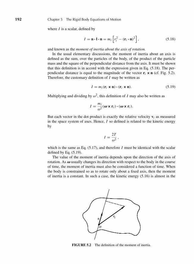
“M05 Goldstein ISBN C05” — 2011/2/15 — page 192 — #9
192 Chapter 5 The Rigid Body Equations of Motion
where I is a scalar, defined by
I = n ? I ?n = mi
[r2
i − (ri ?n)2], (5.18)
and known as the moment of inertia about the axis of rotation.In the usual elementary discussions, the moment of inertia about an axis is
defined as the sum, over the particles of the body, of the product of the particlemass and the square of the perpendicular distance from the axis. It must be shownthat this definition is in accord with the expression given in Eq. (5.18). The per-pendicular distance is equal to the magnitude of the vector ri 3n (cf. Fig. 5.2).Therefore, the customary definition of I may be written as
I = mi (ri 3n) ? (ri 3 n). (5.19)
Multiplying and dividing by ω2, this definition of I may also be written as
I = mi
ω2(v3 ri ) ? (v3 ri ).
But each vector in the dot product is exactly the relative velocity vi as measuredin the space system of axes. Hence, I so defined is related to the kinetic energyby
I = 2T
ω2,
which is the same as Eq. (5.17), and therefore I must be identical with the scalardefined by Eq. (5.19).
The value of the moment of inertia depends upon the direction of the axis ofrotation. As v usually changes its direction with respect to the body in the courseof time, the moment of inertia must also be considered a function of time. Whenthe body is constrained so as to rotate only about a fixed axis, then the momentof inertia is a constant. In such a case, the kinetic energy (5.16) is almost in the
FIGURE 5.2 The definition of the moment of inertia.
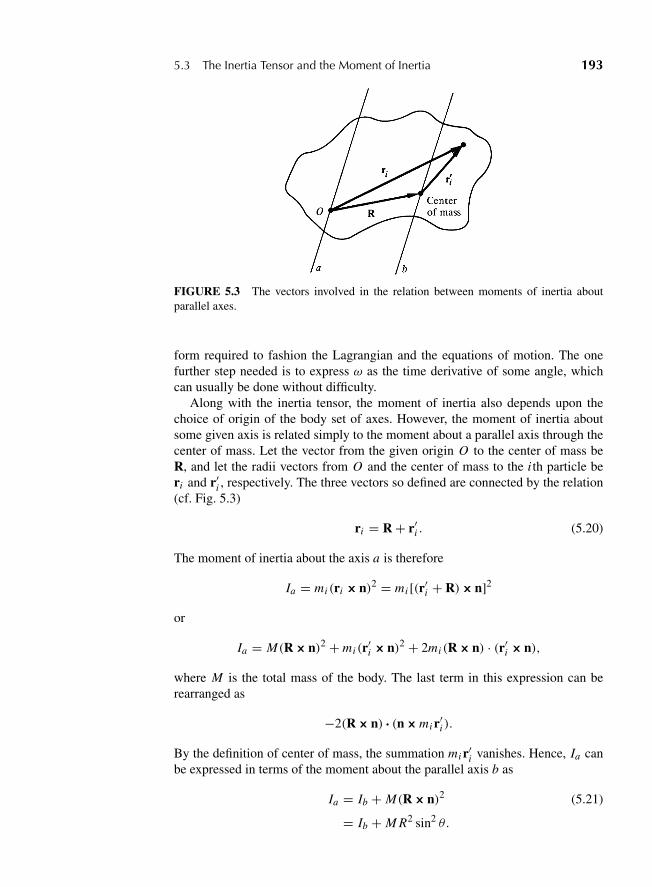
“M05 Goldstein ISBN C05” — 2011/2/15 — page 193 — #10
5.3 The Inertia Tensor and the Moment of Inertia 193
FIGURE 5.3 The vectors involved in the relation between moments of inertia aboutparallel axes.
form required to fashion the Lagrangian and the equations of motion. The onefurther step needed is to express ω as the time derivative of some angle, whichcan usually be done without difficulty.
Along with the inertia tensor, the moment of inertia also depends upon thechoice of origin of the body set of axes. However, the moment of inertia aboutsome given axis is related simply to the moment about a parallel axis through thecenter of mass. Let the vector from the given origin O to the center of mass beR, and let the radii vectors from O and the center of mass to the i th particle beri and r′i , respectively. The three vectors so defined are connected by the relation(cf. Fig. 5.3)
ri = R + r′i . (5.20)
The moment of inertia about the axis a is therefore
Ia = mi (ri 3n)2 = mi [(r′i + R)3 n]2
or
Ia = M(R3n)2 + mi (r′i 3 n)2 + 2mi (R3 n) · (r′i 3n),
where M is the total mass of the body. The last term in this expression can berearranged as
−2(R3 n) ? (n3mi r′i ).
By the definition of center of mass, the summation mi r′i vanishes. Hence, Ia canbe expressed in terms of the moment about the parallel axis b as
Ia = Ib + M(R3 n)2 (5.21)
= Ib + M R2 sin2 θ.
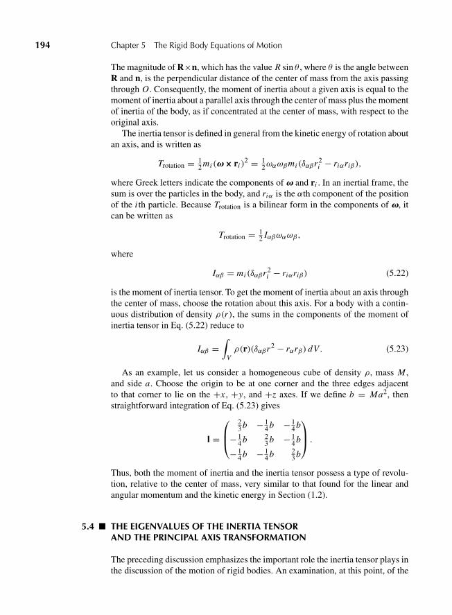
“M05 Goldstein ISBN C05” — 2011/2/15 — page 194 — #11
194 Chapter 5 The Rigid Body Equations of Motion
The magnitude of R×n, which has the value R sin θ , where θ is the angle betweenR and n, is the perpendicular distance of the center of mass from the axis passingthrough O . Consequently, the moment of inertia about a given axis is equal to themoment of inertia about a parallel axis through the center of mass plus the momentof inertia of the body, as if concentrated at the center of mass, with respect to theoriginal axis.
The inertia tensor is defined in general from the kinetic energy of rotation aboutan axis, and is written as
Trotation = 12 mi (v3 ri )
2 = 12ωαωβmi (δαβr2
i − riαriβ),
where Greek letters indicate the components of v and ri . In an inertial frame, thesum is over the particles in the body, and riα is the αth component of the positionof the i th particle. Because Trotation is a bilinear form in the components of v, itcan be written as
Trotation = 12 Iαβωαωβ,
where
Iαβ = mi (δαβr2i − riαriβ) (5.22)
is the moment of inertia tensor. To get the moment of inertia about an axis throughthe center of mass, choose the rotation about this axis. For a body with a contin-uous distribution of density ρ(r), the sums in the components of the moment ofinertia tensor in Eq. (5.22) reduce to
Iαβ =∫
Vρ(r)(δαβr2 − rαrβ) dV . (5.23)
As an example, let us consider a homogeneous cube of density ρ, mass M ,and side a. Choose the origin to be at one corner and the three edges adjacentto that corner to lie on the +x , +y, and +z axes. If we define b = Ma2, thenstraightforward integration of Eq. (5.23) gives
I =
⎛⎜⎝
23 b − 1
4 b − 14 b
− 14 b 2
3 b − 14 b
− 14 b − 1
4 b 23 b
⎞⎟⎠ .
Thus, both the moment of inertia and the inertia tensor possess a type of revolu-tion, relative to the center of mass, very similar to that found for the linear andangular momentum and the kinetic energy in Section (1.2).
5.4 THE EIGENVALUES OF THE INERTIA TENSORAND THE PRINCIPAL AXIS TRANSFORMATION
The preceding discussion emphasizes the important role the inertia tensor plays inthe discussion of the motion of rigid bodies. An examination, at this point, of the
“M05 Goldstein ISBN C05” — 2011/2/15 — page 195 — #12
5.4 The Eigenvalues of the Inertia Tensor 195
properties of this tensor and its associated matrix will therefore prove of consid-erable interest. From the defining equation, (5.7), it is seen that the componentsof the tensor are symmetrical; that is
Ixy = Iyx . (5.24)
This means that, while the inertia tensor will in general have nine components,only six of them will be independent—the three along the diagonal plus three ofthe off-diagonal elements.
The inertia coefficients depend both upon the location of the origin of thebody set of axes and upon the orientation of these axes with respect to the body.This symmetry suggests that there exists a set of coordinates in which the ten-sor is diagonal with the three principal values I1, I2, and I3. In this system,the components of L would involve only the corresponding component of v,thus*
L1 = I1ω1, L2 = I2ω2, L3 = I3ω3. (5.25)
A similar simplification would also occur in the form of the kinetic energy:
T = v? I ?v2
= 1
2I1ω
21 +
1
2I2ω
22 + 1
2I3ω
23. (5.26)
We can show that it is always possible to find such axes, and the proof is basedessentially on the symmetric nature of the inertia tensor.
There are several ways to understand vectors and tensors. For example, a vectoris a quantity defined by its transformation properties. In any set of coordinates, avector is specified by its three components, e.g.,
V = Vx i + Vyj + Vzk, (5.27)
or by its magnitude and direction. In any frame, the magnitude is given by√V 2
x + V 2y + V 2
z , and the direction is given by the polar angles θ and φ. An
alternative is to use the first two Euler angles to specify a new z axis chosen suchthat the vector’s direction is along that axis. Since the vector lies along that z axis,the third Euler angle is not needed.
An approach similar to this latter method can be used for the symmetricmoment of inertia tensor. Consider the moment of inertia of a body about anaxis passing through the center of mass of the body. A similarity transformationperformed by a rotation matrix R can be chosen such that
ID = RIR. (5.28)
*With an eye to future applications, components relative to these axes will be denoted by subscripts1, 2, 3.
“M05 Goldstein ISBN C05” — 2011/2/15 — page 196 — #13
196 Chapter 5 The Rigid Body Equations of Motion
This rotation can be expressed in terms of the Euler angles φ, θ , and ψ as shownin Eqs. (4.46) and (4.47). A proper choice of these angles will transform I into itsdiagonal form
ID =⎛⎝I1 0 0
0 I2 00 0 I3
⎞⎠ (5.29)
where I1, I2, and I3, which are the eigenvalues of I, are referred to as the com-ponents of the principal moment of inertia tensor. The directions of x ′, y′, andz′ defined by the rotation matrix in Eq. (5.28) are called the principal axes, oreigenvectors of the inertia tensor. These eigenvectors lie along the directions x ′,y′, and z′.
Once the principal moments and their directions relative to the surface ofa body are known, the inertia tensor relative to any other set of axis throughthe center of mass can be found by a similarity transformation defined by theEuler angles relating the two coordinate systems. If S is that transformation,then
I = SID S, (5.30)
gives the moment of inertia in that frame. Equation (5.21) can then be used totransform the rotation center to any desired location. The principal values of I canbe determined by the methods of matrix algebra.
The three principal values of the moment of inertia tensor in Eq. (5.29) can befound by solving the cubic equation for I that arises from the determinant∣∣∣∣∣∣
Ixx − I Ixy Izx
Ixy Iyy − I Iyz
Izx Iyz Izz − I
∣∣∣∣∣∣ = 0, (5.31)
where the symmetry of I has been displayed explicitly. Equation (5.31) is thesecular equation, whose three roots are the desired principal moments. Foreach of these roots, Eqs. (5.28) can be solved to obtain the direction of thecorresponding principal axis. In most of the easily soluble problems in rigiddynamics, the principal axes can be determined by inspection. For example, weoften have to deal with rigid bodies that are solids of revolution about someaxis, with the origin of the body system on the symmetry axis. All directionsperpendicular to the axis of symmetry are then alike, which is the mark of adouble root to the secular equation. The principal axes are then the symme-try axis and any two perpendicular axes in the plane normal to the symmetryaxis.
The principal moments of inertia cannot be negative, because as the diagonalelements in the principal axes system they have the form of sums of squares. Thus,Ixx is given by (cf. Eq. (5.6))
Ixx = mi (y2i + z2
i ).
“M05 Goldstein ISBN C05” — 2011/2/15 — page 197 — #14
5.4 The Eigenvalues of the Inertia Tensor 197
For one of the principal moments to vanish, all points of the body must be suchthat two coordinates of each particle are zero. Clearly this can happen only if allpoints of the body are collinear with the principal axis corresponding to the zeroprincipal moment. Any two axes perpendicular to the line of the body will thenbe the other principal axes. Indeed, this is clearly a limiting case of a body withan axis of symmetry passing through the origin.
We can also understand the concept of principal axes through some geometri-cal considerations that historically formed the first approach to the subject. Themoment of inertia about a given axis has been defined as I = n ? I ?n. Let thedirection cosines of the axis be α, β, and γ so that
n = αi + βj + γk;
I then can be written as
I = Ixxα2 + Iyyβ
2 + Izzγ2 + 2Ixyαβ + 2Iyzβγ + 2Izxγα, (5.32)
using the symmetry of I explicitly. It is convenient to define a vector r by theequation
r = n√I. (5.33)
The magnitude of r is thus related to the moment of inertia about the axis whosedirection is given by n. In terms of the components of this new vector, Eq. (5.32)takes on the form
1 = Ixxρ21 + Iyyρ
22 + Izzρ
23 + 2Ixyρ1ρ2 + 2Iyzρ2ρ3 + 2Izxρ3ρ1. (5.34)
Considered as a function of the three variables ρ1, ρ2, ρ3, Eq. (5.34) is theequation of some surface in ρ space. In particular, Eq. (5.34) is the equation ofan ellipsoid designated as the inertial ellipsoid. We can always transform to aset of Cartesian axes in which the equation of an ellipsoid takes on its normalform:
1 = I1ρ′21 + I2ρ
′22 + I3ρ
′23, (5.35)
with the principal axes of the ellipsoid along the new coordinate axes. But (5.35)is simply the form Eq. (5.34) has in a system of coordinates in which the inertiatensor I is diagonal. Hence, the coordinate transformation that puts the equationof ellipsoid into its normal form is exactly the principal axis transformationpreviously discussed. The principal moments of inertia determine the lengthsof the axes of the inertia ellipsoid. If two of the roots of the secular equationare equal, the inertia ellipsoid thus has two equal axes and is an ellipsoid ofrevolution. If all three principal moments are equal, the inertia ellipsoid is asphere.

“M05 Goldstein ISBN C05” — 2011/2/15 — page 198 — #15
198 Chapter 5 The Rigid Body Equations of Motion
A quantity closely related to the moment of inertia is the radius of gyration,R0, defined by the equation
I = M R20 . (5.36)
In terms of the radius of gyration, the vector r can be written as
r = n
R0√
M.
The radius vector to a point on the inertia ellipsoid is thus inversely proportionalto the radius of gyration about the direction of the vector.
It is worth reemphasizing that the inertia tensor I and all the quantitiesassociated with it—principal axes, principal moments, inertia ellipsoid, etc.—areonly relative to some particular point fixed in the body. If the point is shiftedelsewhere in the body, all the quantities will in general be changed. Thus,Eq. (5.21) gives the effect of moving the reference point from the center ofmass to some other point. The principal axis transformation that diagonalizesI′ at the center of mass will not necessarily diagonalize I about another axis,and hence is not in general the principal axis transformation for the shifted ten-sor I. Only if the shift vector R is along one of the principal axes relative tothe center of mass will the difference tensor be diagonal in that system. Thenew inertia tensor I will in that special case have the same principal axes asat the center of mass. However, the principal moments of inertia are changed,except for that corresponding to the shift axis, where the diagonal element ofthe difference tensor is clearly zero. The “parallel axis” theorem for the diag-onalized form of the inertia tensor thus has a rather specialized and restrictedform.
5.5 SOLVING RIGID BODY PROBLEMSAND THE EULER EQUATIONS OF MOTION
Practically all the tools necessary for setting up and solving problems in rigidbody dynamics have by now been assembled. If nonholonomic constraints arepresent, then special means must be taken to include the effects of these con-straints in the equations of motion. For example, if there are “rolling constraints,”these must be introduced into the equations of motion by the method of Lagrangeundetermined multipliers, as in Section 2.4. As discussed in Section 5.1, we usu-ally seek a particular reference point in the body such that the problem can besplit into two separate parts, one purely translational and the other purely rota-tional about the reference point. Of course, if one point of the rigid body is fixedin an inertial system, then that is the obvious reference point. All that has to beconsidered then is the rotational problem about the fixed point.
For bodies without a fixed point, the most useful reference point is almostalways the center of mass. We have already seen that the total kinetic energy andangular momentum then split neatly into one term relating to the translational
“M05 Goldstein ISBN C05” — 2011/2/15 — page 199 — #16
5.5 Solving Rigid Body Problems and the Euler Equations of Motion 199
motion of the center of mass and another involving rotation about the center ofmass. Thus, Eq. (1.31) can now be written
T = 12 Mv2 + 1
2 Iω2.
For many problems (certainly all those that will be considered here), a similarsort of division can be made for the potential energy. We can then solve individu-ally for the translational motion of the center of mass and for the rotational motionabout the center of mass. For example, the Newtonian equations of motion can beused directly: Eq. (1.22) for the motion of the center of mass and Eq. (1.26) forthe motion about that point.
With holonomic conservative systems, the Lagrangian formulation is available,with the Lagrangian taking the form
L(q, q) = Lc(qc, qc)+ Lb(qb, qb).
Here Lc is that part of the Lagrangian involving the generalized coordinates qc
(and velocities qc) of the center of mass, and Lb the part relating to the ori-entation of the body about the center of mass, as described by qb, qb. In effectthen, there are two distinct problems, one with Lagrangian Lc and the other withLagrangian Lb.
In both the Newtonian and Lagrangian formulations, it is convenient to workin terms of the principal axes system of the point of reference, so that the kineticenergy of rotation takes the simple form given in Eq. (5.26). So far, the onlysuitable generalized coordinates we have for the rotational motion of the rigidbody are the Euler angles. Of course, the motion is often effectively confined totwo dimensions, as in the motion of a rigid lamina in a plane. The axis of rotationis then fixed in the direction perpendicular to the plane; only one angle of rotationis necessary and we may dispense with the cumbersome machinery of the Eulerangles.
For the rotational motion about a fixed point or the center of mass, the directNewtonian approach leads to a set of equations known as Euler’s equations ofmotion. We consider either an inertial frame whose origin is at the fixed point ofthe rigid body, or a system of space axes with origin at the center of mass. In thesetwo situations, Eq. (1.26) holds, which here appears simply as
(dLdt
)s= N.
The subscript s is used because the time derivative is with respect to axes that donot share the rotation of the body. However, Eq. (4.86) can be used to obtain thederivatives with respect to axes fixed in the body:
(dLdt
)s=(
dLdt
)b+v3L,
“M05 Goldstein ISBN C05” — 2011/2/15 — page 200 — #17
200 Chapter 5 The Rigid Body Equations of Motion
or, by dropping the “body” subscript:
dLdt
+v3L = N. (5.37)
Equation (5.37) is thus the appropriate form of the Newtonian equation of motionrelative to body axes. The i th component of Eq. (5.37) can be written
d Li
dt+ εi jkω j Lk = Ni . (5.38)
If now the body axes are taken as the principal axes relative to the referencepoint, then the angular momentum components are Li = Iiωi . By Eq. (5.25),Eq. (5.38) takes the form (no summation on i*)
Iidωi
dt+ εi jkω jωk Ik = Ni , (5.39)
since the principal moments of inertia are of course time independent. In expandedform, the three equations making up Eq. (5.39) look like
I1ω1 − ω2ω3(I2 − I3) = N1
I2ω2 − ω3ω1(I3 − I1) = N2 (5.39′)
I3ω3 − ω1ω2(I1 − I2) = N3.
Equations (5.39) or (5.39′) are Euler’s equations of motion for a rigid bodywith one point fixed. They can also be derived from Lagrange’s equations inthe form of Eq. (1.53) where the generalized forces Q j are the torques, N j ,corresponding to the Euler angles of rotation. However, only one of the Eulerangles has its associated torque along one of the body axes, and the remainingtwo Euler’s equations must be obtained by cyclic permutation (cf. Derivation 4).
Consider the case where I1 = I2 �= I3. A torque with components N1 or N2will cause both ω1 and ω2 to change without affecting ω3. We shall return to adiscussion of this in Section 5.7 when we consider the heavy symmetric top withone point fixed. Let us first consider the torque-free motion of a rigid body.
5.6 TORQUE-FREE MOTION OF A RIGID BODY
One problem in rigid dynamics where Euler’s equations are applicable is in themotion of a rigid body not subject to any net forces or torques. The center of massis then either at rest of moving uniformly, and it does not decrease the generalityof the solution to discuss the rotational motion in a reference frame in which thecenter of mass is stationary. In such a case, the angular momentum arises onlyfrom rotation about the center of mass, and Euler’s equations are the equations of
*It should be obvious that Eq. (5.39), as the i th component of a vector equation, does not involve asummation over i , although summation is implied over the repeated indices j and k.
“M05 Goldstein ISBN C05” — 2011/2/15 — page 201 — #18
5.6 Torque-Free Motion of a Rigid Body 201
motion for the complete system. In the absence of any net torques, they reduce to
I1ω1 = ω2ω3(I2 − I3)
I2ω2 = ω3ω1(I3 − I1) (5.40)
I3ω3 = ω1ω2(I1 − I2).
The same equations, of course, will also describe the motion of a rigid bodywhen one point is fixed and there are no net applied torques. We know twoimmediate integrals of the motion, for both the kinetic energy and the total angularmomentum vector must be constant in time. With these two integrals it is possibleto integrate (5.40) completely in terms of elliptic functions, but such a treatment isnot very illuminating. However, it is also possible to derive an elegant geometri-cal description of the motion, known as Poinsot’s construction, without requiringa complete solution to the problem.
Let us consider a coordinate system oriented along the principal axes of thebody but whose axes measure the components of a vector r along the instanta-neous axis of rotation as defined by Eq. (5.33). For our purposes, it is convenientto make use of Eq. (5.17) for the kinetic energy (here constant) and write thedefinition of r in the form
r = v
ω√
I= v√
2T. (5.41)
In this r space, we define a function
F(ρ) = r ? I ? r = ρ2i Ii , (5.42)
where the surfaces of constant F are ellipsoids, the particular surface F = 1 beingthe inertia ellipsoid. As the direction of the axis of rotation changes in time, theparallel vector r moves accordingly, its tip always defining a point on the inertiaellipsoid. The gradient of F , evaluated at this point, furnishes the direction ofthe corresponding normal to the inertia ellipsoid. From Eq. (5.42) for F(ρ), thegradient of F with respect to ρ has the form
∇ρF = 2I ? r = 2I ?v√2T
,
or
∇ρF =√
2
TL. (5.43)
Thus, the v vector will always move such that the corresponding normal to theinertia ellipsoid is in the direction of the angular momentum. In the particular caseunder discussion, the direction of L is fixed in space, and it is the inertia ellipsoid(fixed with respect to the body) that must move in space in order to preserve thisconnection between v and L (cf. Fig. 5.4).
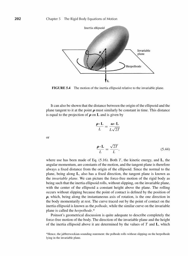
“M05 Goldstein ISBN C05” — 2011/2/15 — page 202 — #19
202 Chapter 5 The Rigid Body Equations of Motion
FIGURE 5.4 The motion of the inertia ellipsoid relative to the invariable plane.
It can also be shown that the distance between the origin of the ellipsoid and theplane tangent to it at the point r must similarly be constant in time. This distanceis equal to the projection of r on L and is given by
r ?LL
= v?L
L√
2T
or
r ?LL
=√
2T
L, (5.44)
where use has been made of Eq. (5.16). Both T , the kinetic energy, and L, theangular momentum, are constants of the motion, and the tangent plane is thereforealways a fixed distance from the origin of the ellipsoid. Since the normal to theplane, being along L, also has a fixed direction, the tangent plane is known asthe invariable plane. We can picture the force-free motion of the rigid body asbeing such that the inertia ellipsoid rolls, without slipping, on the invariable plane,with the center of the ellipsoid a constant height above the plane. The rollingoccurs without slipping because the point of contact is defined by the position ofr, which, being along the instantaneous axis of rotation, is the one direction inthe body momentarily at rest. The curve traced out by the point of contact on theinertia ellipsoid is known as the polhode, while the similar curve on the invariableplane is called the herpolhode.*
Poinsot’s geometrical discussion is quite adequate to describe completely theforce-free motion of the body. The direction of the invariable plane and the heightof the inertia ellipsoid above it are determined by the values of T and L, which
*Hence, the jabberwockian-sounding statement: the polhode rolls without slipping on the herpolhodelying in the invariable plane.
“M05 Goldstein ISBN C05” — 2011/2/15 — page 203 — #20
5.6 Torque-Free Motion of a Rigid Body 203
are among the initial conditions of the problem. It is then a matter of geometry totrace out the polhode and the herpolhode.* The direction of the angular velocityin space is given by the direction of r, while the instantaneous orientation of thebody is provided by the orientation of the inertia ellipsoid, which is fixed in thebody. Many elaborate descriptions of force-free motion obtained in this fashioncan be found in the literature.
In the special case of a symmetrical body, the inertia ellipsoid is an ellip-soid of revolution, so that the polhode on the ellipsoid is clearly a circle aboutthe symmetry axis. The herpolhode on the invariable plane is likewise a cir-cle. An observer fixed in the body sees the angular velocity vector v moveon the surface of a cone—called the body cone—whose intersection with theinertia ellipsoid is the polhode. Correspondingly, an observer fixed in the spaceaxes sees v move on the surface of a space cone whose intersection with theinvariable plane is the herpolhode. Thus, the free motion of the symmetricalrigid body is sometimes described as the rolling of the body cone on the spacecone. If the moment of inertia about the symmetry axis is less than that aboutthe other two principal axes, then from Eq. (5.35) the inertia ellipsoid is prolate,i.e., football shaped—somewhat as is shown in Fig. 5.4. In that case, the bodycone is outside the space cone. When the moment of inertia about the symmetryaxis is the greater, the ellipsoid is oblate and the body cone rolls around theinside of the space cone. In either case, the physical description of the motionis that the direction of v precesses in time about the axis of symmetry of thebody.
The Poinsot construction shows how v moves, but gives no information as tohow the L vector appears to move in the body system of axes. Another geomet-rical description is available however to describe the path of the L vector as seenby an observer in the principal axes system. Equations (5.25) and (5.26) implythat in this system the kinetic energy is related to the components of the angularmomentum by the equation
T = L2x
2I1+ L2
y
2I2+ L2
z
2I3. (5.45)
Since T is constant, this relation defines an ellipsoid, referred to as the Binetellipsoid, also fixed in the body axes but not the same as the inertia ellipsoid.
If we adopt the convention
I3 ≤ I2 ≤ I1,
and write the equations for the ellipsoid in the standard form
L2x
2T I1+ L2
y
2T I2+ L2
z
2T I3= 1 (5.45′)
*The herpolhode is always concave to the origin, belying its name, which suggests “snakelike.”

“M05 Goldstein ISBN C05” — 2011/2/15 — page 204 — #21
204 Chapter 5 The Rigid Body Equations of Motion
then we see that the ellipsoid sketched on Fig. 5.5a has semimajor axes, in orderof decreasing size, of
√2T I1,
√2T I2, and
√2T I3. The conservation of the total
angular momentum, L , gives us
L2x + L2
y + L2z
L2= 1, (5.46)
the equation for a sphere in Lx L y Lz space. The vector L moves in such a way thatit describes a path on both the ellipsoid of Eq. (5.45) and the sphere of Eq. (5.46).In other words, the path of L is the intersection of the ellipsoid and the sphere.The components L satisfy the equation
L2x
2T I1+ L2
y
2T I2+ L2
z
2T I3= L2
x + L2y + L2
z
L2.
It is easy to show that these two surfaces will intersect for values of L largerthan the ellipsoid semiminor axis and less than the semimajor axis, that is,
√2T I3 < L <
√2T I1.
The sphere is outside the ellipsoid on the Lz axis and inside the ellipsoid alongLx . Figure 5.5 depicts curves where the sphere intersects the ellipsoid for variousvalues of L . Fig. 5.5a shows a perspective view and Fig. 5.5b shows the viewas seen from the L y axis. The curves that appear as straight lines on Fig 5.5bcorrespond to the case where L = √
2T I2.
FIGURE 5.5 (a) The kinetic energy, or Binet, ellipsoid fixed in the body axes, and somepossible paths of the L vector in its surface. (b) Side view of Binet ellipsoid.
“M05 Goldstein ISBN C05” — 2011/2/15 — page 205 — #22
5.6 Torque-Free Motion of a Rigid Body 205
With the help of this geometrical construction, something can be said about thepossible motions of a free asymmetric body. It is easy to see that a steady rotationof such a body is possible only about one of the principal axes. From the Eulerequations (5.40), all the components of ω can be constant only if
ω1ω2(I1 − I2) = ω2ω3(I2 − I3) = ω3ω1(I3 − I1) = 0,
which requires that at least two of the components ωi be zero; i.e., v is alongonly one of the principal axes. However, not all of these possible motions arestable—that is, not moving far from the principal axis under small perturbation.For example, steady motion about the Lz axis will occur when L2 = 2T I3. Whenthere are slight deviations from this condition, the radius of the angular momen-tum sphere is just slightly smaller than this value, and the intersection with thekinetic energy ellipsoid is a small circle about the Lz axis. The motion is thusstable, the L vector never being far from the axis.
Similarly, at the other extreme, when the motion about the axis of smallest I isperturbed, the radius of the angular momentum sphere is just slightly larger thanthe smallest semimajor axis. The intersection is again a small closed figure aroundthe principal axis, and the motion is stable. However, the motion about the inter-mediate axis is unstable. This is clearly shown in Fig. 5.5. For the intermediate(L y) axis, the kinetic energy has two orbits that encircle the ellipsoid and crosseach other where the ±L y pass through the ellipsoid. Hence, there are two differ-ent orbits with values slightly less than
√2T I2 and two other distinctly different
orbits with values slightly exceeding√
2T I2, all four of which have quite longpaths on the surface.
This behavior can be best understood by recognizing that at the intermediateaxis the radius of curvature of the ellipsoid in one direction is greater than thatof the contact sphere, and less in the perpendicular direction. At the other twoextremes, the radii of curvature are either greater or smaller than the sphere radiusin all directions. These conclusions on the stability of free-body motion have beenknown for a long time, but applications, e.g., to the stability of spinning space-craft, have brought them out of the obscurity of old monographs on rigid bodydynamics.*
For a symmetrical rigid body, the analytical solution for the force-free motionis not difficult to obtain, and we can directly confirm the precessing motion pre-dicted by the Poinsot construction. Let the symmetry axis be taken as the Lz
*If there are dissipative mechanisms present, these stability arguments have to be modified. It is easyto see that for a body with constant L , but slowly decreasing T , the only stable rotation is about theprincipal axis with the largest moment of inertia. The kinetic energy of rotation about the i th principalaxis for given L is T = L2/2Ii , which is least for the axis with the largest Ii . If a body is set spinningabout any other principal axis, the effect of a slowly decreasing kinetic energy is to cause the angularvelocity vector to shift until the spinning is about the axis requiring the least value of T for the givenL . Such dissipative effects are present in spacecraft because of the flexing of various members in thecourse of the motion, especially of the long booms carried by many of them. These facts were learnedthe hard way by the early designers of spacecraft!
“M05 Goldstein ISBN C05” — 2011/2/15 — page 206 — #23
206 Chapter 5 The Rigid Body Equations of Motion
principal axis so that I1 = I2. Euler’s equations (5.40) reduce then to
I1ω1 = (I1 − I3)ω3ω2
I1ω2 = (I3 − I1)ω3ω1 (5.47)
I3ω3 = 0.
The last of these equations states that ω3 is a constant, and it can therefore betreated as one of the known initial conditions of the problem. The remaining twoequations can now be written
ω1 = −�ω2, ω2 = �ω1, (5.48)
where � is an angular frequency
� = I3 − I1
I1ω3. (5.49)
Elimination of ω2 between Eqs. (5.48) leads to the standard differential equationfor simple harmonic motion
ω1 = −�2ω1,
with the typical solution
ω1 = A cos�t.
The corresponding solution for ω2 can be found by substituting this expressionfor ω1, back in the first of Eqs. (5.48):
ω2 = A sin�t.
The solutions for ω1 and ω2 show that the vector ω1i + ω2j has a constant mag-nitude and rotates uniformly about the z axis of the body with the angular fre-quency � (cf. Fig. 5.6). Hence, the total angular velocity v is also constant inmagnitude and precesses about the z axis with the same frequency, exactly as pre-dicted by the Poinsot construction. * Recall that the precession described here isrelative to the body axes, which are themselves rotating in space with the largerfrequency v. From Eq. (5.49), it is seen that the closer I1 is to I3, the slower willbe the precession frequency � compared to the rotation frequency ω. The con-stants A (the amplitude of the precession) and ω3 can be evaluated in terms ofthe more usual constants of the motion, namely, the kinetic energy and the mag-nitude of the angular momentum. Both T and L2 can be written as functions of A
*The precession can be demonstrated in another fashion by defining a vector � lying along the z axiswith magnitude given by (5.49). Equations (5.47) are then essentially equivalent to the vector equation
v = v3�,
which immediately reveals the precession of v with the frequency �.
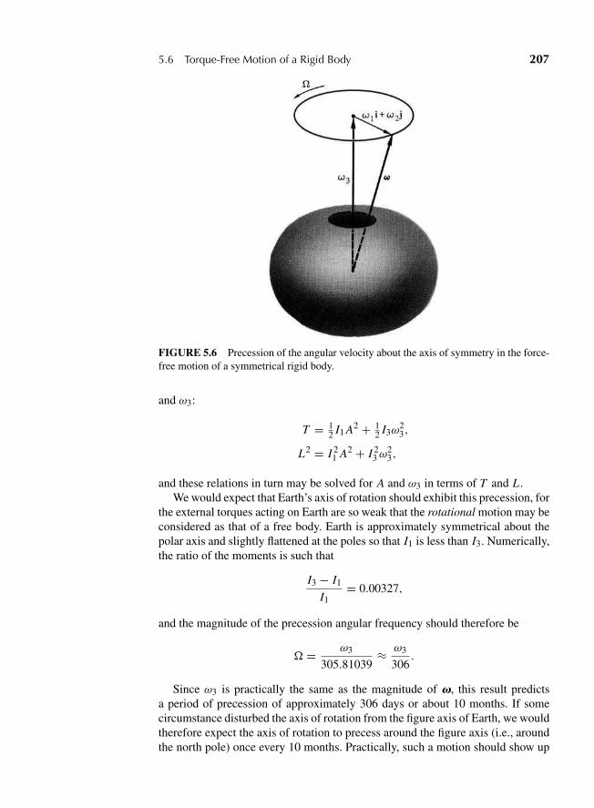
“M05 Goldstein ISBN C05” — 2011/2/15 — page 207 — #24
5.6 Torque-Free Motion of a Rigid Body 207
FIGURE 5.6 Precession of the angular velocity about the axis of symmetry in the force-free motion of a symmetrical rigid body.
and ω3:
T = 12 I1 A2 + 1
2 I3ω23,
L2 = I 21 A2 + I 2
3ω23,
and these relations in turn may be solved for A and ω3 in terms of T and L .We would expect that Earth’s axis of rotation should exhibit this precession, for
the external torques acting on Earth are so weak that the rotational motion may beconsidered as that of a free body. Earth is approximately symmetrical about thepolar axis and slightly flattened at the poles so that I1 is less than I3. Numerically,the ratio of the moments is such that
I3 − I1
I1= 0.00327,
and the magnitude of the precession angular frequency should therefore be
� = ω3
305.81039≈ ω3
306.
Since ω3 is practically the same as the magnitude of v, this result predictsa period of precession of approximately 306 days or about 10 months. If somecircumstance disturbed the axis of rotation from the figure axis of Earth, we wouldtherefore expect the axis of rotation to precess around the figure axis (i.e., aroundthe north pole) once every 10 months. Practically, such a motion should show up
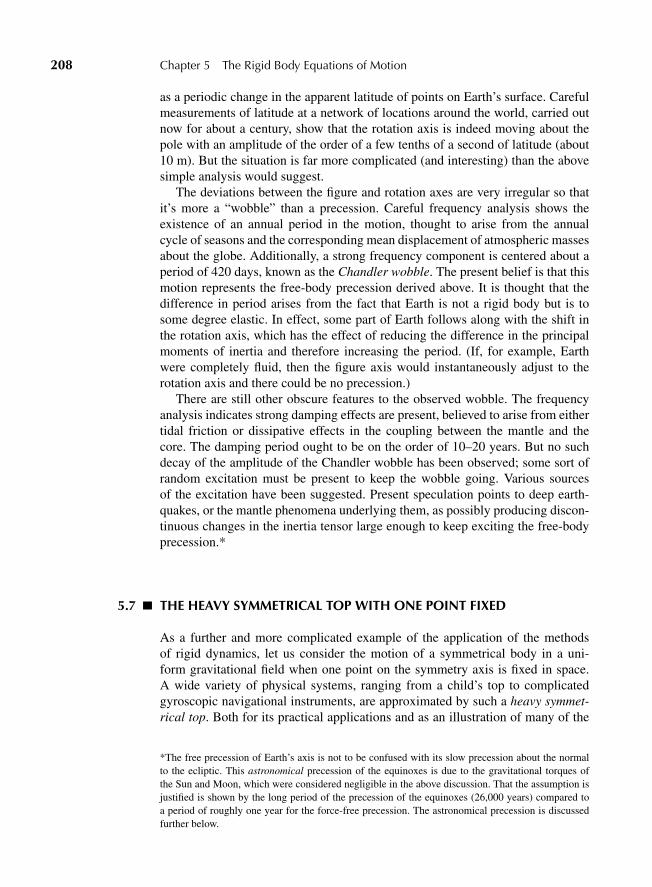
“M05 Goldstein ISBN C05” — 2011/2/15 — page 208 — #25
208 Chapter 5 The Rigid Body Equations of Motion
as a periodic change in the apparent latitude of points on Earth’s surface. Carefulmeasurements of latitude at a network of locations around the world, carried outnow for about a century, show that the rotation axis is indeed moving about thepole with an amplitude of the order of a few tenths of a second of latitude (about10 m). But the situation is far more complicated (and interesting) than the abovesimple analysis would suggest.
The deviations between the figure and rotation axes are very irregular so thatit’s more a “wobble” than a precession. Careful frequency analysis shows theexistence of an annual period in the motion, thought to arise from the annualcycle of seasons and the corresponding mean displacement of atmospheric massesabout the globe. Additionally, a strong frequency component is centered about aperiod of 420 days, known as the Chandler wobble. The present belief is that thismotion represents the free-body precession derived above. It is thought that thedifference in period arises from the fact that Earth is not a rigid body but is tosome degree elastic. In effect, some part of Earth follows along with the shift inthe rotation axis, which has the effect of reducing the difference in the principalmoments of inertia and therefore increasing the period. (If, for example, Earthwere completely fluid, then the figure axis would instantaneously adjust to therotation axis and there could be no precession.)
There are still other obscure features to the observed wobble. The frequencyanalysis indicates strong damping effects are present, believed to arise from eithertidal friction or dissipative effects in the coupling between the mantle and thecore. The damping period ought to be on the order of 10–20 years. But no suchdecay of the amplitude of the Chandler wobble has been observed; some sort ofrandom excitation must be present to keep the wobble going. Various sourcesof the excitation have been suggested. Present speculation points to deep earth-quakes, or the mantle phenomena underlying them, as possibly producing discon-tinuous changes in the inertia tensor large enough to keep exciting the free-bodyprecession.*
5.7 THE HEAVY SYMMETRICAL TOP WITH ONE POINT FIXED
As a further and more complicated example of the application of the methodsof rigid dynamics, let us consider the motion of a symmetrical body in a uni-form gravitational field when one point on the symmetry axis is fixed in space.A wide variety of physical systems, ranging from a child’s top to complicatedgyroscopic navigational instruments, are approximated by such a heavy symmet-rical top. Both for its practical applications and as an illustration of many of the
*The free precession of Earth’s axis is not to be confused with its slow precession about the normalto the ecliptic. This astronomical precession of the equinoxes is due to the gravitational torques ofthe Sun and Moon, which were considered negligible in the above discussion. That the assumption isjustified is shown by the long period of the precession of the equinoxes (26,000 years) compared toa period of roughly one year for the force-free precession. The astronomical precession is discussedfurther below.
“M05 Goldstein ISBN C05” — 2011/2/15 — page 209 — #26
5.7 The Heavy Symmetrical Top with One Point Fixed 209
FIGURE 5.7 Euler’s angles specifying the orientation of a symmetrical top.
techniques previously developed, the motion of the heavy symmetrical top de-serves a detailed exposition.
The symmetry axis is of course one of the principal axes and will be chosen asthe z axis of the coordinate system fixed in the body.* Since one point is stationary,the configuration of the top is completely specified by the three Euler angles: θgives the inclination of the z axis from the vertical, φ measures the azimuth of thetop about the vertical, while ψ is the rotation angle of the top about its own z axis(cf. Fig. 5.7). The distance of the center of gravity (located on the symmetry axis)from the fixed point will be denoted by I .
The rates of change of these three angles give the characteristic motions of thetop as
ψ = rotation or spinning of the top about its own figure axis, z
φ = precession or rotation of the figure axis z about the vertical axis z′
θ = nutation or bobbing up and down of the z figure axis relative to the verti-cal space axis z′.
For many cases of interest such as the top and the gyroscope, we have ψ θ φ. Since I1 = I2 �= I3, Euler’s equations (5.39′) become
I1ω1 + ω2ω3(I3 − I2) = N1,
I2ω2 + ω1ω3(I1 − I3) = N2,
*Only the body axes need specific identification here; it will therefore be convenient to designatethem in this section as the xyz axes, without fear of confusing them with the space axes, which willbe designated by the x ′y′z′ axes.
“M05 Goldstein ISBN C05” — 2011/2/15 — page 210 — #27
210 Chapter 5 The Rigid Body Equations of Motion
andI3ω3 = N3.
Let us consider the case where initially N3 = 0 = N2, N1 �= 0, and ω1 =ω2 = 0, ω3 �= 0, then ω3 will be constant. The torque N1 will cause ω1 to changesince ω1 �= 0. Since ω1 is no longer zero, the second equation requires that ω2begin to change also. What this means in terms of an observation is not obvious.We observe the changes in the Euler angles ψ , φ, θ and their associated anglesin the x ′, y′, z′ laboratory frame rather than the ω1, ω2, ω3 and their associatedangles in the principal axis system. This suggests that the Euler equations maynot provide the most useful description of the motion.
The Lagrangian procedure, rather than Euler’s equations, will be used to obtaina solution for the motion of the top. Since the body is symmetrical, the kineticenergy can be written as
T = 12 I1(ω
21 + ω2
2)+ 12 I3ω
23,
or, in terms of Euler’s angles, and using Eqs. (4.87), as
T = I1
2(θ2 + φ2 sin2 θ)+ I3
2(ψ + φ cos θ)2, (5.50)
where the φ, θ cross terms in ω21 and ω2
2 cancel.It is a well-known elementary theorem that in a constant gravitational field the
potential energy is the same as if the body were concentrated at the center of mass.We will however give a brief formal proof here. The potential energy of the bodyis the sum over all the particles:
V = −mi ri ? g,
where g is the constant vector for the acceleration of gravity. By Eq. (1.21), defin-ing the center of mass, this is equivalent to
V = −MR ? g, (5.51)
which proves the theorem. In terms of the Euler angles,
V = Mgl cos θ, (5.51′)
so that the Lagrangian is
L = I1
2(θ2 + φ2 sin2 θ)+ I3
2(ψ + φ cos θ)2 − Mgl cos θ. (5.52)
Note that φ andψ do not appear explicitly in the Lagrangian; they are thereforecyclic coordinates, indicating that the corresponding generalized momenta are
“M05 Goldstein ISBN C05” — 2011/2/15 — page 211 — #28
5.7 The Heavy Symmetrical Top with One Point Fixed 211
constant in time. Now, we have seen that the momentum conjugate to a rotationangle is the component of the total angular momentum along the axis of rotation,which for φ is the vertical axis, and for ψ , the z axis in the body. We can in factshow from elementary principles that these components of the angular momentummust be constant in time. Since the torque of gravity is along the line of nodes,there is no component of the torque along either the vertical or the body z axis,for by definition both of these axes are perpendicular to the line of nodes. Hence,the components of the angular momentum along these two axes must be constantin time.
We therefore have two immediate first integrals of the motion:
pψ = ∂L
∂ψ= I3(ψ + φ cos θ) = I3ω3 = I1a (5.53)
and
pφ = ∂L
∂φ= (I1 sin2 θ + I3 cos2 θ)φ + I3ψ cos θ = I1b. (5.54)
Here the two constants of the motion are expressed in terms of new constants aand b. There is one further first integral available; since the system is conservative,the total energy E is constant in time:
E = T + V = I1
2(θ2 + φ2 sin2 θ)+ I3
2ω2
3 + Mgl cos θ. (5.55)
Only three additional quadratures are needed to solve the problem, and they areeasily obtained from these three first integrals without directly using the Lagrangeequations. From Eq. (5.53), ψ is given in terms of φ by
I3ψ = I1a − I3φ cos θ, (5.56)
and this result can be substituted in (5.54) to eliminate ψ :
I1φ sin2 θ + I1a cos θ = I1b,
or
φ = b − a cos θ
sin2 θ. (5.57)
Thus, if θ were known as a function of time, Eq. (5.57) could be integrated tofurnish the dependence of φ on time. Substituting Eq. (5.57) back in Eq. (5.56)results in a corresponding expression for ψ :
ψ = I1a
I3− cos θ
b − a cos θ
sin2 θ, (5.58)
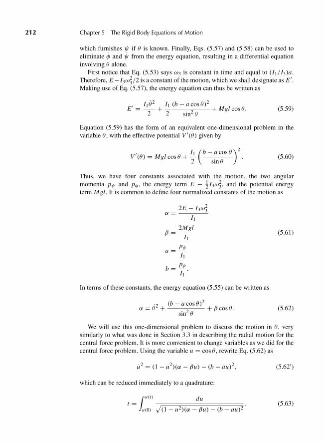
“M05 Goldstein ISBN C05” — 2011/2/15 — page 212 — #29
212 Chapter 5 The Rigid Body Equations of Motion
which furnishes ψ if θ is known. Finally, Eqs. (5.57) and (5.58) can be used toeliminate φ and ψ from the energy equation, resulting in a differential equationinvolving θ alone.
First notice that Eq. (5.53) says ω3 is constant in time and equal to (I1/I3)a.Therefore, E− I3ω
23/2 is a constant of the motion, which we shall designate as E ′.
Making use of Eq. (5.57), the energy equation can thus be written as
E ′ = I1θ2
2+ I1
2
(b − a cos θ)2
sin2 θ+ Mgl cos θ. (5.59)
Equation (5.59) has the form of an equivalent one-dimensional problem in thevariable θ , with the effective potential V ′(θ) given by
V ′(θ) = Mgl cos θ + I1
2
(b − a cos θ
sin θ
)2
. (5.60)
Thus, we have four constants associated with the motion, the two angularmomenta pψ and pφ , the energy term E − 1
2 I3ω23, and the potential energy
term Mgl. It is common to define four normalized constants of the motion as
α = 2E − I3ω23
I1
β = 2Mgl
I1(5.61)
a = pψI1
b = pφI1.
In terms of these constants, the energy equation (5.55) can be written as
α = θ2 + (b − a cos θ)2
sin2 θ+ β cos θ. (5.62)
We will use this one-dimensional problem to discuss the motion in θ , verysimilarly to what was done in Section 3.3 in describing the radial motion for thecentral force problem. It is more convenient to change variables as we did for thecentral force problem. Using the variable u = cos θ , rewrite Eq. (5.62) as
u2 = (1 − u2)(α − βu)− (b − au)2, (5.62′)
which can be reduced immediately to a quadrature:
t =∫ u(t)
u(0)
du√(1 − u2)(α − βu)− (b − au)2
. (5.63)
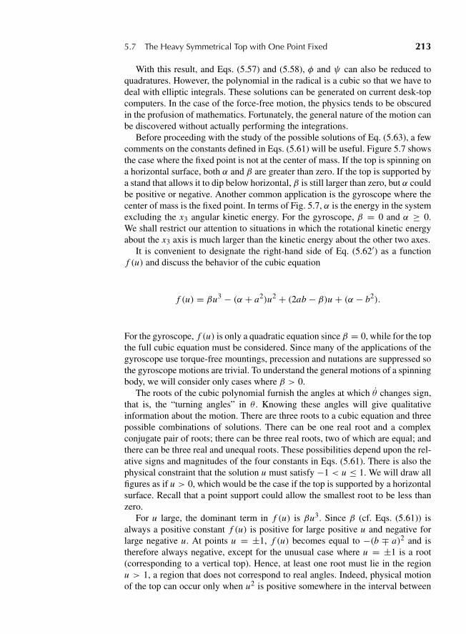
“M05 Goldstein ISBN C05” — 2011/2/15 — page 213 — #30
5.7 The Heavy Symmetrical Top with One Point Fixed 213
With this result, and Eqs. (5.57) and (5.58), φ and ψ can also be reduced toquadratures. However, the polynomial in the radical is a cubic so that we have todeal with elliptic integrals. These solutions can be generated on current desk-topcomputers. In the case of the force-free motion, the physics tends to be obscuredin the profusion of mathematics. Fortunately, the general nature of the motion canbe discovered without actually performing the integrations.
Before proceeding with the study of the possible solutions of Eq. (5.63), a fewcomments on the constants defined in Eqs. (5.61) will be useful. Figure 5.7 showsthe case where the fixed point is not at the center of mass. If the top is spinning ona horizontal surface, both α and β are greater than zero. If the top is supported bya stand that allows it to dip below horizontal, β is still larger than zero, but α couldbe positive or negative. Another common application is the gyroscope where thecenter of mass is the fixed point. In terms of Fig. 5.7, α is the energy in the systemexcluding the x3 angular kinetic energy. For the gyroscope, β = 0 and α ≥ 0.We shall restrict our attention to situations in which the rotational kinetic energyabout the x3 axis is much larger than the kinetic energy about the other two axes.
It is convenient to designate the right-hand side of Eq. (5.62′) as a functionf (u) and discuss the behavior of the cubic equation
f (u) = βu3 − (α + a2)u2 + (2ab − β)u + (α − b2).
For the gyroscope, f (u) is only a quadratic equation since β = 0, while for the topthe full cubic equation must be considered. Since many of the applications of thegyroscope use torque-free mountings, precession and nutations are suppressed sothe gyroscope motions are trivial. To understand the general motions of a spinningbody, we will consider only cases where β > 0.
The roots of the cubic polynomial furnish the angles at which θ changes sign,that is, the “turning angles” in θ . Knowing these angles will give qualitativeinformation about the motion. There are three roots to a cubic equation and threepossible combinations of solutions. There can be one real root and a complexconjugate pair of roots; there can be three real roots, two of which are equal; andthere can be three real and unequal roots. These possibilities depend upon the rel-ative signs and magnitudes of the four constants in Eqs. (5.61). There is also thephysical constraint that the solution u must satisfy −1 < u ≤ 1. We will draw allfigures as if u > 0, which would be the case if the top is supported by a horizontalsurface. Recall that a point support could allow the smallest root to be less thanzero.
For u large, the dominant term in f (u) is βu3. Since β (cf. Eqs. (5.61)) isalways a positive constant f (u) is positive for large positive u and negative forlarge negative u. At points u = ±1, f (u) becomes equal to −(b ∓ a)2 and istherefore always negative, except for the unusual case where u = ±1 is a root(corresponding to a vertical top). Hence, at least one root must lie in the regionu > 1, a region that does not correspond to real angles. Indeed, physical motionof the top can occur only when u2 is positive somewhere in the interval between
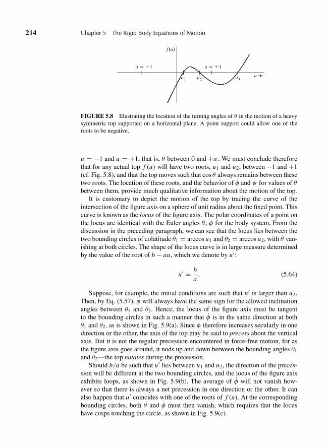
“M05 Goldstein ISBN C05” — 2011/2/15 — page 214 — #31
214 Chapter 5 The Rigid Body Equations of Motion
FIGURE 5.8 Illustrating the location of the turning angles of θ in the motion of a heavysymmetric top supported on a horizontal plane. A point support could allow one of theroots to be negative.
u = −1 and u = +1, that is, θ between 0 and +π . We must conclude thereforethat for any actual top f (u) will have two roots, u1 and u2, between −1 and +1(cf. Fig. 5.8), and that the top moves such that cos θ always remains between thesetwo roots. The location of these roots, and the behavior of φ and ψ for values of θbetween them, provide much qualitative information about the motion of the top.
It is customary to depict the motion of the top by tracing the curve of theintersection of the figure axis on a sphere of unit radius about the fixed point. Thiscurve is known as the locus of the figure axis. The polar coordinates of a point onthe locus are identical with the Euler angles θ , φ for the body system. From thediscussion in the preceding paragraph, we can see that the locus lies between thetwo bounding circles of colatitude θ1 = arccos u1 and θ2 = arccos u2, with θ van-ishing at both circles. The shape of the locus curve is in large measure determinedby the value of the root of b − au, which we denote by u′:
u′ = b
a. (5.64)
Suppose, for example, the initial conditions are such that u′ is larger than u2.Then, by Eq. (5.57), φ will always have the same sign for the allowed inclinationangles between θ1 and θ2. Hence, the locus of the figure axis must be tangentto the bounding circles in such a manner that φ is in the same direction at bothθ1 and θ2, as is shown in Fig. 5.9(a). Since φ therefore increases secularly in onedirection or the other, the axis of the top may be said to precess about the verticalaxis. But it is not the regular precession encountered in force-free motion, for asthe figure axis goes around, it nods up and down between the bounding angles θ1and θ2—the top nutates during the precession.
Should b/a be such that u′ lies between u1 and u2, the direction of the preces-sion will be different at the two bounding circles, and the locus of the figure axisexhibits loops, as shown in Fig. 5.9(b). The average of φ will not vanish how-ever so that there is always a net precession in one direction or the other. It canalso happen that u′ coincides with one of the roots of f (u). At the correspondingbounding circles, both θ and φ must then vanish, which requires that the locushave cusps touching the circle, as shown in Fig. 5.9(c).
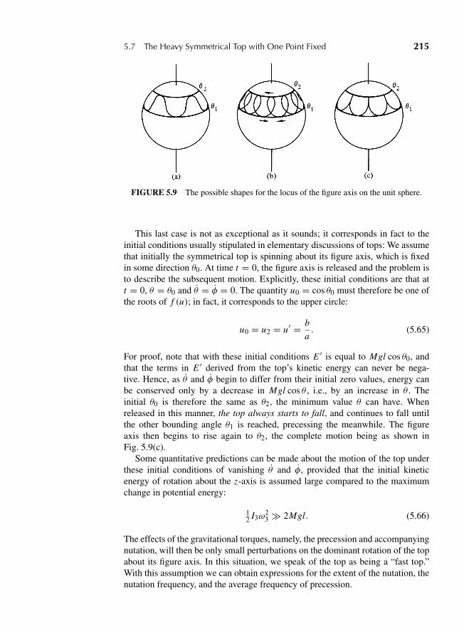
“M05 Goldstein ISBN C05” — 2011/2/15 — page 215 — #32
5.7 The Heavy Symmetrical Top with One Point Fixed 215
FIGURE 5.9 The possible shapes for the locus of the figure axis on the unit sphere.
This last case is not as exceptional as it sounds; it corresponds in fact to theinitial conditions usually stipulated in elementary discussions of tops: We assumethat initially the symmetrical top is spinning about its figure axis, which is fixedin some direction θ0. At time t = 0, the figure axis is released and the problem isto describe the subsequent motion. Explicitly, these initial conditions are that att = 0, θ = θ0 and θ = φ = 0. The quantity u0 = cos θ0 must therefore be one ofthe roots of f (u); in fact, it corresponds to the upper circle:
u0 = u2 = u′ = b
a. (5.65)
For proof, note that with these initial conditions E ′ is equal to Mgl cos θ0, andthat the terms in E ′ derived from the top’s kinetic energy can never be nega-tive. Hence, as θ and φ begin to differ from their initial zero values, energy canbe conserved only by a decrease in Mgl cos θ , i.e., by an increase in θ . Theinitial θ0 is therefore the same as θ2, the minimum value θ can have. Whenreleased in this manner, the top always starts to fall, and continues to fall untilthe other bounding angle θ1 is reached, precessing the meanwhile. The figureaxis then begins to rise again to θ2, the complete motion being as shown inFig. 5.9(c).
Some quantitative predictions can be made about the motion of the top underthese initial conditions of vanishing θ and φ, provided that the initial kineticenergy of rotation about the z-axis is assumed large compared to the maximumchange in potential energy:
12 I3ω
23 2Mgl. (5.66)
The effects of the gravitational torques, namely, the precession and accompanyingnutation, will then be only small perturbations on the dominant rotation of the topabout its figure axis. In this situation, we speak of the top as being a “fast top.”With this assumption we can obtain expressions for the extent of the nutation, thenutation frequency, and the average frequency of precession.
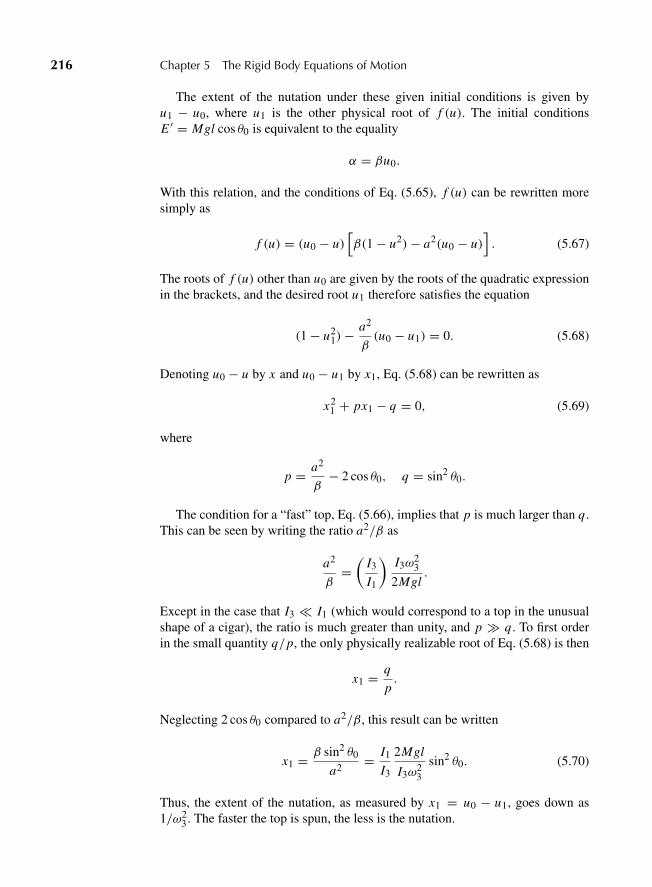
“M05 Goldstein ISBN C05” — 2011/2/15 — page 216 — #33
216 Chapter 5 The Rigid Body Equations of Motion
The extent of the nutation under these given initial conditions is given byu1 − u0, where u1 is the other physical root of f (u). The initial conditionsE ′ = Mgl cos θ0 is equivalent to the equality
α = βu0.
With this relation, and the conditions of Eq. (5.65), f (u) can be rewritten moresimply as
f (u) = (u0 − u)[β(1 − u2)− a2(u0 − u)
]. (5.67)
The roots of f (u) other than u0 are given by the roots of the quadratic expressionin the brackets, and the desired root u1 therefore satisfies the equation
(1 − u21)−
a2
β(u0 − u1) = 0. (5.68)
Denoting u0 − u by x and u0 − u1 by x1, Eq. (5.68) can be rewritten as
x21 + px1 − q = 0, (5.69)
where
p = a2
β− 2 cos θ0, q = sin2 θ0.
The condition for a “fast” top, Eq. (5.66), implies that p is much larger than q.This can be seen by writing the ratio a2/β as
a2
β=(
I3
I1
)I3ω
23
2Mgl.
Except in the case that I3 � I1 (which would correspond to a top in the unusualshape of a cigar), the ratio is much greater than unity, and p q. To first orderin the small quantity q/p, the only physically realizable root of Eq. (5.68) is then
x1 = q
p.
Neglecting 2 cos θ0 compared to a2/β, this result can be written
x1 = β sin2 θ0
a2= I1
I3
2Mgl
I3ω23
sin2 θ0. (5.70)
Thus, the extent of the nutation, as measured by x1 = u0 − u1, goes down as1/ω2
3. The faster the top is spun, the less is the nutation.
“M05 Goldstein ISBN C05” — 2011/2/15 — page 217 — #34
5.7 The Heavy Symmetrical Top with One Point Fixed 217
The frequency of nutation likewise can easily be found for the “fast” top. Sincethe amount of nutation is small, the term (1−u2) in Eq. (5.67) can be replaced byits initial value, sin2 θ0. Equation (5.67) then reads, with the help of Eq. (5.70),
f (u) = x2 = a2x(x1 − x).
If we shift the origin of x to the midpoint of its range, by changing variable to
y = x − x1
2,
then the differential equation becomes
y2 = a2
(x2
1
4− y2
),
which on differentiation again reduces to the familiar equation for simple har-monic motion
y = −a2 y.
In view of the initial condition x = 0 at t = 0, the complete solution is
x = x1
2(1 − cos at), (5.71)
where x1 is given by (5.70). The angular frequency of nutation of the figure axisbetween θ0 and θ1 is therefore
a = I3
I1ω3, (5.72)
which increases the faster the top is spun initially.Finally, the angular velocity of precession, from (5.57), is given by
φ = a(u0 − u)
sin2 θ≈ ax
sin2 θ0,
or, substituting Eqs. (5.70) and (5.71),
φ = β
2a(1 − cos at). (5.73)
The rate of precession is therefore not uniform but varies harmonically with time,with the same frequency as the nutation. The average precession frequency how-ever is
φ = β
2a= Mgl
I3ω3, (5.74)
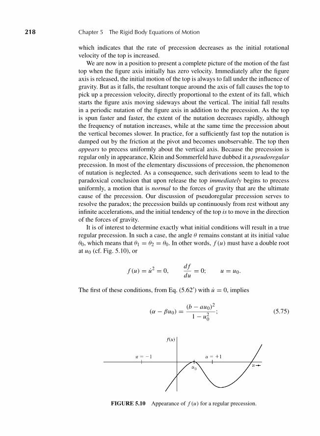
“M05 Goldstein ISBN C05” — 2011/2/15 — page 218 — #35
218 Chapter 5 The Rigid Body Equations of Motion
which indicates that the rate of precession decreases as the initial rotationalvelocity of the top is increased.
We are now in a position to present a complete picture of the motion of the fasttop when the figure axis initially has zero velocity. Immediately after the figureaxis is released, the initial motion of the top is always to fall under the influence ofgravity. But as it falls, the resultant torque around the axis of fall causes the top topick up a precession velocity, directly proportional to the extent of its fall, whichstarts the figure axis moving sideways about the vertical. The initial fall resultsin a periodic nutation of the figure axis in addition to the precession. As the topis spun faster and faster, the extent of the nutation decreases rapidly, althoughthe frequency of nutation increases, while at the same time the precession aboutthe vertical becomes slower. In practice, for a sufficiently fast top the nutation isdamped out by the friction at the pivot and becomes unobservable. The top thenappears to precess uniformly about the vertical axis. Because the precession isregular only in appearance, Klein and Sommerfeld have dubbed it a pseudoregularprecession. In most of the elementary discussions of precession, the phenomenonof nutation is neglected. As a consequence, such derivations seem to lead to theparadoxical conclusion that upon release the top immediately begins to precessuniformly, a motion that is normal to the forces of gravity that are the ultimatecause of the precession. Our discussion of pseudoregular precession serves toresolve the paradox; the precession builds up continuously from rest without anyinfinite accelerations, and the initial tendency of the top is to move in the directionof the forces of gravity.
It is of interest to determine exactly what initial conditions will result in a trueregular precession. In such a case, the angle θ remains constant at its initial valueθ0, which means that θ1 = θ2 = θ0. In other words, f (u) must have a double rootat u0 (cf. Fig. 5.10), or
f (u) = u2 = 0,d f
du= 0; u = u0.
The first of these conditions, from Eq. (5.62′) with u = 0, implies
(α − βu0) = (b − au0)2
1 − u20
; (5.75)
FIGURE 5.10 Appearance of f (u) for a regular precession.
“M05 Goldstein ISBN C05” — 2011/2/15 — page 219 — #36
5.7 The Heavy Symmetrical Top with One Point Fixed 219
the second corresponds to
β
2= a(b − au0)
1 − u20
− u0(α − βu0)
1 − u20
. (5.76)
Substitution of Eq. (5.75) in Eq. (5.76) leads, in view of Eq. (5.57) for φ, to aquadratic equation for φ:
β
2= aφ − φ2 cos θ0. (5.76′)
With the definitions of β and a, Eq. (5.61), this can be written in two alternativeforms, depending on whether a is expressed in terms of ω3 or the (constant) ψand φ:
Mgl = φ(I3ω3 − I1φ cos θ0), (5.77)
or
Mgl = φ(I3ψ − (I1 − I3)φ cos θ0). (5.77′)
The initial conditions for the problem of the heavy top require the specificationof θ , φ,ψ , θ , φ, and, say, either ψ or ω3 at the time t = 0. Because they are cyclic,the initial values of φ and ψ are largely irrelevant, and in general we can chooseany desired value for each of the four others. But if in addition we require that themotion of the figure axis be one of uniform precession without nutation, then ourchoice of these four initial values is no longer completely unrestricted. Instead,they must satisfy either of Eqs. (5.77). For θ = 0, we may still choose initialvalues of θ and ω3, almost arbitrarily, but the value of φ is then determined. Thephrase “almost arbitrarily” is used because Eqs. (5.77) are quadratic, and for φ tobe real, the discriminant of Eq. (5.77) must be positive:
I 23ω
23 > 4Mgl I1 cos θ0. (5.78)
For θ0 > π/2 (a top mounted so its center of mass is below the fixed point), thenany value of ω3 can lead to uniform precession. But for θ0 < π/2, ω3 must bechosen to be above a minimum value ω′
3,
ω3 > ω′3 = 2
I3
√Mgl I1 cos θ0 (5.79)
to achieve the same situation. Similar conditions can be obtained from Eq. (5.77′)for the allowable values of ψ . As a result of the quadratic nature of Eq. (5.77),there will in general be two solutions for φ, known as the “fast” and “slow” pre-cession. Also note that (5.77) can never be satisfied by φ = 0 for finite ψ or ω3;to obtain uniform precession, we must always give the top a shove to start it on its
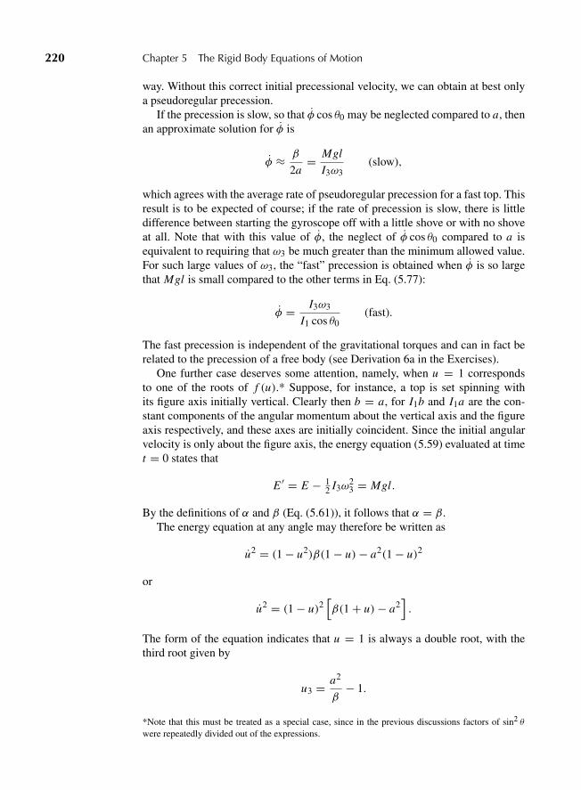
“M05 Goldstein ISBN C05” — 2011/2/15 — page 220 — #37
220 Chapter 5 The Rigid Body Equations of Motion
way. Without this correct initial precessional velocity, we can obtain at best onlya pseudoregular precession.
If the precession is slow, so that φ cos θ0 may be neglected compared to a, thenan approximate solution for φ is
φ ≈ β
2a= Mgl
I3ω3(slow),
which agrees with the average rate of pseudoregular precession for a fast top. Thisresult is to be expected of course; if the rate of precession is slow, there is littledifference between starting the gyroscope off with a little shove or with no shoveat all. Note that with this value of φ, the neglect of φ cos θ0 compared to a isequivalent to requiring that ω3 be much greater than the minimum allowed value.For such large values of ω3, the “fast” precession is obtained when φ is so largethat Mgl is small compared to the other terms in Eq. (5.77):
φ = I3ω3
I1 cos θ0(fast).
The fast precession is independent of the gravitational torques and can in fact berelated to the precession of a free body (see Derivation 6a in the Exercises).
One further case deserves some attention, namely, when u = 1 correspondsto one of the roots of f (u).* Suppose, for instance, a top is set spinning withits figure axis initially vertical. Clearly then b = a, for I1b and I1a are the con-stant components of the angular momentum about the vertical axis and the figureaxis respectively, and these axes are initially coincident. Since the initial angularvelocity is only about the figure axis, the energy equation (5.59) evaluated at timet = 0 states that
E ′ = E − 12 I3ω
23 = Mgl.
By the definitions of α and β (Eq. (5.61)), it follows that α = β.The energy equation at any angle may therefore be written as
u2 = (1 − u2)β(1 − u)− a2(1 − u)2
or
u2 = (1 − u)2[β(1 + u)− a2
].
The form of the equation indicates that u = 1 is always a double root, with thethird root given by
u3 = a2
β− 1.
*Note that this must be treated as a special case, since in the previous discussions factors of sin2 θ
were repeatedly divided out of the expressions.
“M05 Goldstein ISBN C05” — 2011/2/15 — page 221 — #38
5.7 The Heavy Symmetrical Top with One Point Fixed 221
FIGURE 5.11 Plot of f (u) when the figure axis is initially vertical.
If a2/β > 2 (which corresponds to the condition for a “fast” top), u3 is largerthan 1 and the only possible motion is for u = 1; the top merely continues to spinabout the vertical. For this state of affairs, the plot of f (u) appears as shown inFig. 5.11(a). On the other hand, if a2/β < 2, the third root u1 is then less than1, f (u) takes on the form shown in Fig. 5.11(b), and the top will nutate betweenθ = 0 and θ = θ3. There is thus a critical angular velocity, ω′, above which onlyvertical motion is possible, whose value is given by
a2
β=(
I3
I1
)I3ω
′2
2Mgl= 2
or
ω′2 = 4Mgl I1
I 23
, (5.80)
which is identical with Eq. (5.79) for the minimum frequency for uniform preces-sion with θ0 = 0.
In practice, if a top is started spinning with its axis vertical and with ω3 greaterthan the critical angular velocity, it will continue to spin quietly for a while aboutthe vertical (hence the designation as a “sleeping” top). However, friction grad-ually reduces the frequency of rotation below the critical value, and the top thenbegins to wobble in ever larger amounts as it slows down.
The effects of friction (which of course cannot be directly included in theLagrangian framework) can give rise to unexpected phenomena in the behaviorof tops. A notable example is the “tippie-top,” which consists basically of some-what more than half a sphere with a stem added on the flat surface. When setrotating with the spherical surface downwards on a hard surface, it proceeds toskid and nutate until it eventually turns upside down, pivoting on the stem, whereit then behaves as a normal “sleeping” top. The complete reversal of the angularmomentum vector is the result of frictional torque occurring as the top skids onits spherical surface.
“M05 Goldstein ISBN C05” — 2011/2/15 — page 222 — #39
222 Chapter 5 The Rigid Body Equations of Motion
A large and influential technology is based on the applications of rapidly spin-ning rigid bodies, particularly through the use of what are called “gyroscopes.”Basically, a three-frame gyroscope is a symmetrical top rotated very rapidly byexternal means about the figure axis and mounted in gimbals so that the motion ofthe figure axis is unrestricted about three perpendicular spatial axes while the cen-ter of gravity remains stationary. The figure axis maintains the same direction inspace no matter how the mounting is reoriented, a phenomenon called gyroscopicinertia. Such an instrument can indicate the roll, pitch, and attitude directions ofan airplane flying “blind” by using the xyz Euler angle convention described inSection 4.4 and Appendix A.
If external torques are suitably exerted on the gyroscope, it will undergo theprecession and nutation motions described earlier for the heavy top. However,the condition for the “fast” top is abundantly satisfied, so that the extent of thenutation is always very small, and moreover is deliberately damped out by themethod of mounting. The only gyroscopic phenomenon then observed is preces-sion, and the mathematical treatment required to describe this precession can begreatly simplified. We can see how to do this by generalization from the case ofthe heavy symmetrical top.
If R is the radius vector along the figure axis from the fixed point to the centerof gravity, then the gravitational torque exerted on the top is
N = R3 Mg, (5.81)
where g is the downward vector of the acceleration of gravity. If L3 is the vec-tor along the figure axis, describing the angular momentum of rotation about thefigure axis, and vp, known as the precession vector, is aligned along the vertical
with magnitude equal to the mean precession angular velocity φ, Eq. (5.74), thenthe sense and magnitude of the (pseudoregular) precession is given by
vp 3L3 = N. (5.82)
Since any torque about the fixed point or center of mass can be put in the formR × F, similar to Eq. (5.81), the resulting average precession rate for a “fast” topcan always be derived from Eq. (5.82), with the direction of the force F definingthe precession axis. Almost all engineering applications of gyroscopes involvethe equilibrium behavior (i.e., neglecting transients) which can be derived fromEq. (5.82).
Free from any torques, a gyroscope spin axis will always preserve its originaldirection relative to an inertial system. Gyros can therefore be used to indicateor maintain specific directions, e.g., provide stabilized platforms. As indicated byEq. (5.82), through the precession phenomena they can sense and measure angularrotation rates and applied torques. Note from Eq. (5.82) that the precession rateis proportional to the torque, whereas in a nonspinning body it is the angularacceleration that is given by the torque. Once the torque is removed, a nonspinningbody will continue to move; under similar conditions a gyro simply continuesspinning without precessing.
“M05 Goldstein ISBN C05” — 2011/2/15 — page 223 — #40
5.8 Precession of the Equinoxes and of Satellite Orbits 223
The gyrocompass involves more complicated considerations because herewe are dealing with the behavior of a gyroscope fixed in a noninertial system,while Earth rotates underneath it. In a gyrocompass, an additional precessionis automatically applied by an external torque at a rate just enough to balanceEarth’s rotation rate. Once set in the direction of Earth’s rotation, i.e., the northdirection, the gyrocompass then preserves this direction, at least in slowly mov-ing vehicles. What has been presented here is admittedly an oversimplified,highly compressed view of the fascinating technological uses of fast spinningbodies. To continue further in this direction would regrettably lead us too farafield.
There are however two examples of precession phenomena in nature for whicha somewhat fuller discussion would be valuable, both for the great interest inthe phenomena themselves and as examples of the techniques derived in thischapter. The first concerns the types of precession that arise from the torquesinduced by Earth’s equatorial “bulge,” and the second is the precession of mov-ing charges in a magnetic field. The next two sections are concerned with theseexamples.
5.8 PRECESSION OF THE EQUINOXES AND OF SATELLITE ORBITS
It has been mentioned previously that Earth is a top whose figure axis is pre-cessing about the normal to the ecliptic, the plane of Earth’s orbit, a motionknown astronomically as the precession of the equinoxes. Were Earth completelyspherical, none of the other members of the solar system could exert a gravi-tational torque on it. But, as has been pointed out, Earth deviates slightly froma sphere, being closely approximated by an oblate spheroid of revolution. It isjust the net torque on the resultant equatorial “bulge” arising from gravitationalattraction, chiefly of the Sun and Moon, that sets Earth’s axis precessing inspace.
To calculate the rate of this precession, a slight excursion into potential theoryis needed to find the mutual gravitational potential of a mass point (representingthe sun or the moon) and a nonspherical distribution of matter. We will find theproperties of the inertia tensor as obtained above very useful in the derivation ofthis potential.
Consider a distribution of mass points forming one body, and a single masspoint, mass M , representing the other (cf. Fig. 5.12). If ri is the distance betweenthe i th point in the distribution and the mass point M , then the mutual gravitationalpotential between the two bodies is*
V = −G Mmi
ri= − G Mmi
r
√1 +
(r ′ir
)2− 2
r ′ir cosψi
. (5.83)
*It may be worth a reminder that summation is implied over repeated subscripts.

“M05 Goldstein ISBN C05” — 2011/2/15 — page 224 — #41
224 Chapter 5 The Rigid Body Equations of Motion
FIGURE 5.12 Geometry involved in gravitational potential between an extended bodyand a mass point.
In this last expression the terminology of Fig. 5.12 is used: r′i is the radius vectorto the i th particle from a particular point, which will later be taken to be the centerof mass of the first body, r is the corresponding radius vector to the mass pointM , and ψi is the angle between the two vectors. It is well known that a simpleexpansion in terms of Legendre polynomials can be given for Eq. (5.83); in fact,the reciprocal of the square root in Eq. (5.83) is known as the generating functionfor Legendre polynomials, so that
V = −G M
r
∑n=0
mi
(r ′ir
)n
Pn(cosψi ), (5.84)
providing r , the distance from the origin to M , is much greater than any r ′i . Weshall make use of only the first three Legendre polynomials that, for reference, are
P0(x) = 1, P1(x) = x, P2(x) = 12 (3x2 − 1). (5.85)
For a continuous spherical body, with only a radial variation of density, allterms except the first in Eq. (5.84) can easily be shown to vanish. Thus, the nthterm inside the summation, for a body with spherical symmetry and mass densityρ(r ′), can be written
∫ ∫ ∫d3 R′ρ(r ′)
(r ′
r
)n
Pn(cosψ).
Using spherical polar coordinates, with the polar axis along r, this becomes
2π∫
r ′2 dr ′ ρ(r ′)(
r ′
r
)n ∫ +1
−1d(cosψ)Pn(cosψ).
From the orthonormal properties of Pn with respect to P0, the integral over cosψvanishes except for n = 0, which proves the statement.
If the body deviates only slightly from spherical symmetry, as is the case withEarth, we would expect the terms in Eq. (5.84) beyond n = 0 to decrease rapidly
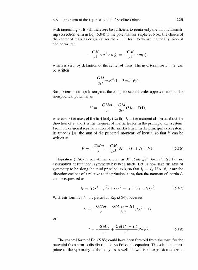
“M05 Goldstein ISBN C05” — 2011/2/15 — page 225 — #42
5.8 Precession of the Equinoxes and of Satellite Orbits 225
with increasing n. It will therefore be sufficient to retain only the first nonvanish-ing correction term in Eq. (5.84) to the potential for a sphere. Now, the choice ofthe center of mass as origin causes the n = 1 term to vanish identically, since itcan be written
−G M
r2mir
′i cosψi = −G M
r3r ?mi r′i ,
which is zero, by definition of the center of mass. The next term, for n = 2, canbe written
G M
2r3mir
′i2(1 − 3 cos2 ψi ).
Simple tensor manipulation gives the complete second-order approximation to thenonspherical potential as
V = −G Mm
r+ G M
2r3(3Ir − Tr I),
where m is the mass of the first body (Earth), Ir is the moment of inertia about thedirection of r, and I is the moment of inertia tensor in the principal axis system.From the diagonal representation of the inertia tensor in the principal axis system,its trace is just the sum of the principal moments of inertia, so that V can bewritten as
V = −G Mm
r+ G M
2r3[3Ir − (I1 + I2 + I3)]. (5.86)
Equation (5.86) is sometimes known as MacCullagh’s formula. So far, noassumption of rotational symmetry has been made. Let us now take the axis ofsymmetry to be along the third principal axis, so that I1 = I2. If α, β, γ are thedirection cosines of r relative to the principal axes, then the moment of inertia Ir
can be expressed as
Ir = I1(α2 + β2)+ I3γ
2 = I1 + (I3 − I1)γ2. (5.87)
With this form for Ir , the potential, Eq. (5.86), becomes
V = −G Mm
r+ G M(I3 − I1)
2r3(3γ 2 − 1),
or
V = −G Mm
r+ G M(I3 − I1)
r3P2(γ ). (5.88)
The general form of Eq. (5.88) could have been foretold from the start, for thepotential from a mass distribution obeys Poisson’s equation. The solution appro-priate to the symmetry of the body, as is well known, is an expansion of terms
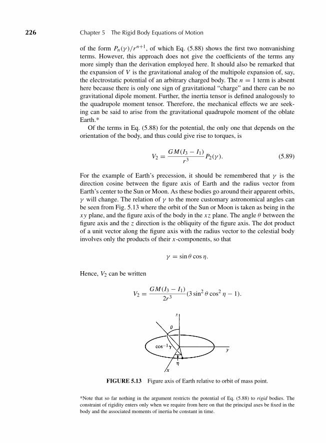
“M05 Goldstein ISBN C05” — 2011/2/15 — page 226 — #43
226 Chapter 5 The Rigid Body Equations of Motion
of the form Pn(γ )/rn+1, of which Eq. (5.88) shows the first two nonvanishingterms. However, this approach does not give the coefficients of the terms anymore simply than the derivation employed here. It should also be remarked thatthe expansion of V is the gravitational analog of the multipole expansion of, say,the electrostatic potential of an arbitrary charged body. The n = 1 term is absenthere because there is only one sign of gravitational “charge” and there can be nogravitational dipole moment. Further, the inertia tensor is defined analogously tothe quadrupole moment tensor. Therefore, the mechanical effects we are seek-ing can be said to arise from the gravitational quadrupole moment of the oblateEarth.*
Of the terms in Eq. (5.88) for the potential, the only one that depends on theorientation of the body, and thus could give rise to torques, is
V2 = G M(I3 − I1)
r3P2(γ ). (5.89)
For the example of Earth’s precession, it should be remembered that γ is thedirection cosine between the figure axis of Earth and the radius vector fromEarth’s center to the Sun or Moon. As these bodies go around their apparent orbits,γ will change. The relation of γ to the more customary astronomical angles canbe seen from Fig. 5.13 where the orbit of the Sun or Moon is taken as being in thexy plane, and the figure axis of the body in the xz plane. The angle θ between thefigure axis and the z direction is the obliquity of the figure axis. The dot productof a unit vector along the figure axis with the radius vector to the celestial bodyinvolves only the products of their x-components, so that
γ = sin θ cos η.
Hence, V2 can be written
V2 = G M(I3 − I1)
2r3(3 sin2 θ cos2 η − 1).
FIGURE 5.13 Figure axis of Earth relative to orbit of mass point.
*Note that so far nothing in the argument restricts the potential of Eq. (5.88) to rigid bodies. Theconstraint of rigidity enters only when we require from here on that the principal axes be fixed in thebody and the associated moments of inertia be constant in time.
“M05 Goldstein ISBN C05” — 2011/2/15 — page 227 — #44
5.8 Precession of the Equinoxes and of Satellite Orbits 227
As we shall see, the orbital motion is very rapid compared to the precessionalmotion, and for the purpose of obtaining the mean precession rate, it will beadequate to average V2 over a complete orbital period of the celestial body con-sidered. Since the apparent orbits of the Sun and Moon have low eccentricities, rcan be assumed constant and the only variation is in cos η. The average of cos2 η
over a complete period is 12 , and the averaged potential is then
V 2 = G M(I3 − I1)
2r3
(3
2sin2 θ − 1
)= G M(I3 − I1)
2r3
(1
2− 3
2cos2 θ
),
or, finally,
V 2 = −G M(I3 − I1)
2r3P2(cos θ). (5.90)
The torque derived from Eq. (5.90) is perpendicular to both the figure axis andthe normal to the orbit (which plays the same role as the vertical axis for the heavytop). Hence, the precession is about the direction of the orbit normal vector. Themagnitude of the precession rate can be obtained from Eq. (5.82), but because thepotential differs in form from that for the heavy top, it may be more satisfying toobtain a more formal derivation. For any symmetric body in which the potentialis a function of cos θ only, the Lagrangian can be written, following Eq. (5.52), as
L = I1
2(θ2 + φ2 sin2 θ)+ I3
2(ψ + φ cos θ)2 − V (cos θ). (5.91)
If we are to assume only uniform precession and are not concerned about thenecessary initial conditions, we can simply take θ and θ to be zero in the equationsof motion. The Lagrange equation corresponding to θ is then
∂L
∂θ= I1φ
2 sin θ cos θ − I3φ sin θ(ψ + φ cos θ)− ∂V
∂θ= 0
or
I3ω3φ − I1φ2 cos θ = ∂V
∂(cos θ), (5.92)
which is the analog of Eq. (5.76′) for a more general potential. For slow pre-cession, which means basically that φ � ω3, the φ2 terms in Eq. (5.92) can beneglected, and the rate of uniform precession is given by
φ = 1
I3ω3
∂V
∂(cos θ). (5.93)
From Eq. (5.51′) we see that for the heavy top Eq. (5.93) agrees with the averageresult of Eq. (5.74). With the potential of Eq. (5.90), the precession rate is
φ = − 3G M
2ω3r3
I3 − I1
I3cos θ. (5.94)
“M05 Goldstein ISBN C05” — 2011/2/15 — page 228 — #45
228 Chapter 5 The Rigid Body Equations of Motion
For the case of the precession due to the Sun, this formula can be put in asimpler form, by taking r as the semimajor axis of Earth’s orbit and using Kepler’slaw, Eq. (3.71), in the form
ω20 =
(2π
τ
)2
= G M
r3.
The precession rate, relative to the orbital angular velocity, ω0, is then
φ
ω0= −3
2
ω0
ω3
I3 − I1
I3cos θ. (5.95)
With the value of (I3 − I1)/I3 as given in Section 5.6, and θ = 23◦27′, Eq. (5.95)says that the solar-induced precession would be such as to cause a complete rota-tion of the figure axis about the normal to the ecliptic (plane of Earth’s orbit) inabout 81,000 years.
The Moon is far less massive than the Sun, but it is also much closer; thenet result is that the lunar-induced precession rate is over twice that caused bythe Sun. Since the lunar orbit is close to the ecliptic and has the same sense asthe apparent solar orbit, the two precessions nearly add together arithmetically,and the combined lunisolar precession rate is 50.25′′/year, or one complete rota-tion in about 26,000 years. Note that this rate of precession is so slow that theapproximation of neglecting φ compared to ω3 is abundantly satisfied. Becausethe Sun, Moon, and Earth are in constant relative motion, and the Moon’s orbitis inclined about 5◦ to the ecliptic, the precession exhibits irregularities desig-nated as astronomical nutation. The extent of these periodic irregularities is notlarge—about 9′′ of arc in θ and about 18′′ in φ. Even so, they are far larger thanthe true nutation that, as Klein and Sommerfeld have shown, is manifested bythe Chandler wobble whose amplitude is never more than a few tenths of an arcsecond.
One further application can be made of the potential, Eq. (5.88), and associ-ated uniform precession rate, Eq. (5.93). It has been stressed that the potentialrepresents a mutual gravitational interaction; if it results in torques acting on thespinning Earth, it also gives rise to (noncentral) forces acting on the mass point M .The effect of these small forces appears as a precession of the plane of the orbitof the mass point, relative to an inertial frame. It is possible to obtain an approx-imate formula for this precession by an argument again based on the behavior ofspinning rigid bodies.
Since the precession rates are small compared to the orbital angular veloc-ity, we can again average over the orbit. The averaging in effect replaces theparticle by a rigid ring of mass M with the same radius as the (assumed circu-lar) orbit, spinning about the figure axis of the ring with the orbital frequency.Equation (5.90) gives the potential field in which this ring is located, with θthe angle between the figure axes of the ring and Earth. The average preces-sion rate is still given by Eq. (5.93), but now I3 and ω3 refer to the spinningring and not Earth. It would therefore be better to rewrite Eq. (5.93) for this
“M05 Goldstein ISBN C05” — 2011/2/15 — page 229 — #46
5.8 Precession of the Equinoxes and of Satellite Orbits 229
application as
φ = τ
2πMr2
∂V
∂(cos θ), (5.93′)
and Eq. (5.94) appears as
φ = − τ
2π
3
2
G(I3 − I1)
r5cos θ. (5.94′)
Equation (5.94′) could be used, for example, to find the precession of the orbitof the Moon due to Earth’s oblateness. A more current application would beto the precession of nearly circular orbits of artificial satellites revolving aboutEarth. The fraction of a complete precession rotation in one period of the satel-lite is
φτ
2π= −
( τ2π
)2 3
2
G(I3 − I1)
r5cos θ.
An application of Kepler’s law, this time for the period of the satellite, reducesthis result to
φτ
2π= −3
2
I3 − I1
mr2cos θ, (5.96)
where m is Earth’s mass. If Earth were a uniform sphere, then the principalmoments of inertia would be
I3 ∼ I1 = 25 m R2,
with R Earth’s radius. Because the core is much more dense than the outer layers,the moment of inertia is smaller, such that in fact*
I3 = 0.331m R2 ≈ 13 m R2.
The approximate precession is thus given by
φτ
2π= −1
2
I3 − I1
I3
(R
r
)2
cos θ. (5.97)
For a “close” satellite where r is very close to R, and the inclination of the satelliteorbit to the equator is, say, 30◦, Eq. (5.97) says that the plane of the orbit precessescompletely around 2π in about 700 orbits of the satellite. Since the period of aclose satellite is about 1 1
2 hours, complete rotation of the orbital plane occursin a little over six weeks time. Clearly the effect is quite significant. We shallrederive the precession of the satellite orbit later on, when we discuss the subjectof perturbation theory (cf. Section 12.3).
*The best values of I3 are now obtained from observation of just such effects on satellite orbits.
“M05 Goldstein ISBN C05” — 2011/2/15 — page 230 — #47
230 Chapter 5 The Rigid Body Equations of Motion
5.9 PRECESSION OF SYSTEMS OF CHARGES IN A MAGNETIC FIELD
The motion of systems of charged particles in magnetic fields does not normallyinvolve rigid body motion. In a number of particular instances, the motion is how-ever most elegantly discussed using the techniques developed here for rigid bodymotion. For this reason, and because of their importance in atomic and nuclearphysics, a few examples will be given here.
The magnetic moment of a system of moving charges (relative to a particularorigin) is defined as
M = 1
2qi (ri 3 vi )→ 1
2
∫dV ρe(r)(r3 v). (5.98)
Here the first expression is a sum over discrete particles with charge qi , while thesecond is the corresponding generalization to a continuous distribution of chargedensity ρe(r). The angular momentum of the system under corresponding con-ventions is
L = mi (ri 3 vi )→∫
dV ρm(r)(r3 v).
Both the magnetic moment and the angular momentum have a similar form.We shall restrict the discussion to situations in which M is directly proportionalto L:
M = γL, (5.99)
most naturally by having a uniform q/m ratio for all particles or at all points inthe continuous system. In such cases, the gyromagnetic ratio γ is given by
γ = q
2m, (5.100)
but, with an eye to models of particle and atomic spin, γ will often be left unspec-ified. The forces and torques on a magnetic dipole may be considered as derivedfrom a potential
V = −(M ?B). (5.101)
It is implied along with Eq. (5.101) that the magnetic field is substantiallyconstant over the system. Indeed, the picture applies best to a pointlike magneticmoment whose magnitude is not affected by the motion it undergoes—a pictureappropriate to permanent magnets or systems on an atomic or small scale. Withuniform B, the potential depends only on the orientation of M relative to B; noforces are exerted on the magnetic moment, but there is a torque
N = M3B. (5.102)
“M05 Goldstein ISBN C05” — 2011/2/15 — page 231 — #48
5.9 Precession of Systems of Charges in a Magnetic Field 231
(Compare with Eq. (5.81).) The time rate of change of the total angular momen-tum is equal to this torque, so that in view of Eq. (5.99) we can write
dLdt
= γL3B. (5.103)
But this is exactly the equation of motion for a vector of constant magnituderotating in space about the direction of B with an angular velocity v = −γB.The effect of a uniform magnetic field on a permanent magnetic dipole is to causethe angular momentum vector (and the magnetic moment) to precess uniformly.
For the classical gyromagnetic ratio, Eq. (5.100), the precession angularvelocity is
vi = −qB2m, (5.104)
known as the Larmor frequency. For electrons q is negative, and the Larmorprecession is counterclockwise around the direction of B.
As a second example, consider a collection of moving charged particles, with-out restrictions on the nature of their motion, but assumed to all have the sameq/m ratio, and to be in a region of uniform constant magnetic field. It will alsobe assumed that any interaction potential between particles depends only on thescalar distance between the particles. The Lagrangian for the system can be writ-ten (cf. Eq. (1.63)). L is a system quantity so sum over repeated i’s and all j’s �= ifor the rest of this chapter.
L = 1
2miv
2i + q
mmi vi ?A(ri )− V (|ri − r j |), (5.105)
where the constant magnetic field B is generated by a vector potential A:
A = 12 B3 r. (5.106)
In terms of B, the Lagrangian has the form (permuting dot and cross products)
L = 1
2miv
2i + qB
2m? (ri × mi vi )− V (|ri − r j |). (5.107)
The interaction term with the magnetic field can be variously written (cf.Eqs. (5.101) and (5.104))
qB · L2m
= M ?B = −vi ? (ri 3mi vi ). (5.108)
Suppose now we express the Lagrangian in terms of coordinates relative to“primed” axes having a common origin with the original set, but rotating uni-formly about the direction of B with angular velocity vl . Distance vectors fromthe origin are unchanged as are scalar distances such as |ri − r j |. However,velocities relative to the new axes differ from the original velocities by the relation
vi = v′i +vl 3 ri .
“M05 Goldstein ISBN C05” — 2011/2/15 — page 232 — #49
232 Chapter 5 The Rigid Body Equations of Motion
The two terms in the Lagrangian affected by the transformation are
miv2i
2= miv
′i2
2+ mi v′i ? (vl 3 ri )+ mi
2(vl 3 ri ) ? (vl 3 ri ),
−vl ? ri 3mi vi = −vl ? (ri 3mi v′i )−vl ? (ri 3mi (vl 3 ri )).
By permuting dot and cross product, we can see that the terms linear in vl andv′i are just equal and opposite and therefore cancel in the Lagrangian. A similarpermutation in the terms quadratic in ωl show that they are of the same form andare related to the moment of inertia of the system about the axis defined by vl (cf.Section 5.3). The quadratic term in the Lagrangian can in fact be written as
−mi
2(vl 3 ri ) ? (vl 3 ri ) = −1
2vl ? I ?vl = −1
2Ilω
2l , (5.109)
where Il denotes the moment of inertia about the axis of vl . In terms of coordi-nates in the rotating system, the Lagrangian thus has the simple form
L = 12 miv
′i2 − V (|ri − r j |)− 1
2 Ilω2l , (5.110)
from which all linear terms in the magnetic field have disappeared.We can get an idea of the relative magnitude of the quadratic term by con-
sidering a situation in which the motion of the system consists of a rotation withsome frequency ω, e.g., an electron revolving around the atomic nucleus. Then forsystems not too far from spherical symmetry, the kinetic energy is approximately12 Iω2 (without subscripts on the moment of inertia) and the linear term in ωl ison the order of vl ?L ≈ Iωlω. Hence, the quadratic term in Eq. (5.110) is onthe order of (ωl/ω)
2 compared to the kinetic energy, and on the order of (ωl/ω)
relative to the linear term.In most systems on the atomic or smaller scale, the natural frequencies are
much larger than the Larmor frequency. Compare, for example, the frequency ofa spectral line (which is a difference of natural frequencies) to the frequency shiftin the simple Zeeman effect, which is proportional to the Larmor frequency. Thus,for such systems the motion in the rotating system is the same as in the laboratorysystem when there is no magnetic field. What we have is Larmor’s theorem, whichstates that to first order in B, the effect of a constant magnetic field on a classicalsystem is to superimpose on its normal motion a uniform precession with angularfrequency vl .
DERIVATIONS
1. If Ri is an antisymmetric matrix associated with the coordinates of the i th mass pointof a system, with elements Rmn = εmnl xl show that the matrix of the inertia tensorcan be written as
I = −mi (Ri )2.
“M05 Goldstein ISBN C05” — 2011/2/15 — page 233 — #50
Derivations 233
2. Show directly by vector manipulation that the definition of the moment of inertia as
I = mi (ri 3 n) ? (ri 3n)
reduces to Eq. (5.18).
3. Prove that for a general rigid body motion about a fixed point, the time variation ofthe kinetic energy T is given by
dT
dt= v?N.
4. Derive Euler’s equations of motion, Eq. (5.39′), from the Lagrange equation ofmotion, in the form of Eq. (1.53), for the generalized coordinate ψ .
5. Equation (5.38) holds for the motions of systems that are not rigid, relative to a chosenrotating set of coordinates. For general nonrigid motion, if the rotating axes are chosento coincide with the (instantaneous) principal axes of the continuous system, show thatEqs. (5.39) are to be replaced by
d(Iiωi )
dt+ εi jkω jωk Ik − ωi
d Ii
dt= Ni , i = 1, 2, 3,
where
Ii =∫
dV ρ(r)εi jk x jv′k
with ρ(r) the mass density at point r, and v′ the velocity of the system point at rrelative to the rotating axes. These equations are sometimes known as the Liouvilleequations and have applications for discussing almost-rigid motion, such as that ofEarth including the atmosphere and oceans.
6. (a) Show that the angular momentum of the torque-free symmetrical top rotates inthe body coordinates about the symmetry axis with an angular frequency�. Showalso that the symmetry axis rotates in space about the fixed direction of the angularmomentum with the angular frequency
φ = I3ω3
I1 cos θ,
where φ is the Euler angle of the line of nodes with respect to the angularmomentum as the space z axis.
(b) Using the results of Exercise 15, Chapter 4, show that v rotates in space aboutthe angular momentum with the same frequency φ, but that the angle θ ′ betweenv and L is given by
sin θ ′ = �
φsin θ ′′,
where θ ′′ is the inclination of v to the symmetry axis. Using the data givenin Section 5.6, show therefore that Earth’s rotation axis and the axis of angularmomentum are never more than 1.5 cm apart on Earth’s surface.
(c) Show from parts (a) and (b) that the motion of the force-free symmetrical topcan be described in terms of the rotation of a cone fixed in the body whose axisis the symmetry axis, rolling on a fixed cone in space whose axis is along the
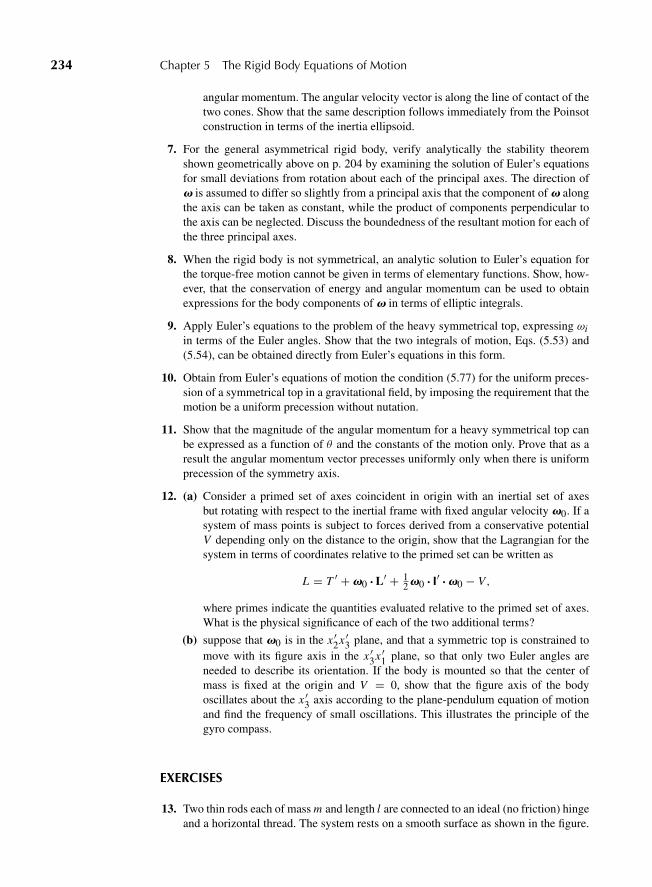
“M05 Goldstein ISBN C05” — 2011/2/15 — page 234 — #51
234 Chapter 5 The Rigid Body Equations of Motion
angular momentum. The angular velocity vector is along the line of contact of thetwo cones. Show that the same description follows immediately from the Poinsotconstruction in terms of the inertia ellipsoid.
7. For the general asymmetrical rigid body, verify analytically the stability theoremshown geometrically above on p. 204 by examining the solution of Euler’s equationsfor small deviations from rotation about each of the principal axes. The direction ofv is assumed to differ so slightly from a principal axis that the component of v alongthe axis can be taken as constant, while the product of components perpendicular tothe axis can be neglected. Discuss the boundedness of the resultant motion for each ofthe three principal axes.
8. When the rigid body is not symmetrical, an analytic solution to Euler’s equation forthe torque-free motion cannot be given in terms of elementary functions. Show, how-ever, that the conservation of energy and angular momentum can be used to obtainexpressions for the body components of v in terms of elliptic integrals.
9. Apply Euler’s equations to the problem of the heavy symmetrical top, expressing ωiin terms of the Euler angles. Show that the two integrals of motion, Eqs. (5.53) and(5.54), can be obtained directly from Euler’s equations in this form.
10. Obtain from Euler’s equations of motion the condition (5.77) for the uniform preces-sion of a symmetrical top in a gravitational field, by imposing the requirement that themotion be a uniform precession without nutation.
11. Show that the magnitude of the angular momentum for a heavy symmetrical top canbe expressed as a function of θ and the constants of the motion only. Prove that as aresult the angular momentum vector precesses uniformly only when there is uniformprecession of the symmetry axis.
12. (a) Consider a primed set of axes coincident in origin with an inertial set of axesbut rotating with respect to the inertial frame with fixed angular velocity v0. If asystem of mass points is subject to forces derived from a conservative potentialV depending only on the distance to the origin, show that the Lagrangian for thesystem in terms of coordinates relative to the primed set can be written as
L = T ′ +v0 ?L′ + 12v0 ? I′ ?v0 − V,
where primes indicate the quantities evaluated relative to the primed set of axes.What is the physical significance of each of the two additional terms?
(b) suppose that v0 is in the x ′2x ′3 plane, and that a symmetric top is constrained tomove with its figure axis in the x ′3x ′1 plane, so that only two Euler angles areneeded to describe its orientation. If the body is mounted so that the center ofmass is fixed at the origin and V = 0, show that the figure axis of the bodyoscillates about the x ′3 axis according to the plane-pendulum equation of motionand find the frequency of small oscillations. This illustrates the principle of thegyro compass.
EXERCISES
13. Two thin rods each of mass m and length l are connected to an ideal (no friction) hingeand a horizontal thread. The system rests on a smooth surface as shown in the figure.
“M05 Goldstein ISBN C05” — 2011/2/15 — page 235 — #52
Exercises 235
At time t = 0, the thread is cut. Neglecting the mass of the hinge and the thread, andconsidering only motion in the xy plane
(a) Find the speed at which the hinge hits the floor.
(b) Find the time it takes for the hinge to hit the floor.
14. What is the height-to-diameter ratio of a right cylinder such that the inertia ellipsoidat the center of the cylinder is a sphere?
15. Find the principal moments of inertia about the center of mass of a flat rigid body inthe shape of a 45◦ right triangle with uniform mass density. What are the principalaxes?
16. A system of three particles of masses 40, 50 and 60 gm has the center of mass at (2,2, 2). Where can a fourth particle of mass 70 gm be placed so that the position of thenew center of mass will be at (0, 0, 0)?
17. A uniform right circular cone of height h, half-angle α, and density ρ rolls on itsside without slipping on a uniform horizontal plane in such a manner that it returnsto its original position in a time τ . Find expressions for the kinetic energy and thecomponents of the angular momentum of the cone.
18. (a) A bar of negligible weight and length l has equal mass points m at the two ends.The bar is made to rotate uniformly about an axis passing through the centerof the bar and making an angle θ with the bar. From Euler’s equations find thecomponents along the principal axes of the bar of the torque driving the bar.
(b) From the fundamental torque equation (1.26) find the components of the torquealong axes fixed in space. Show that these components are consistent with thosefound in part (a).
19. A uniform bar of mass M and length 2l is suspended from one end by a spring offorce constant k. The bar can swing freely only in one vertical plane, and the spring isconstrained to move only in the vertical direction. Set up the equations of motion inthe Lagrangian formulation.
“M05 Goldstein ISBN C05” — 2011/2/15 — page 236 — #53
236 Chapter 5 The Rigid Body Equations of Motion
20. A plane pendulum consists of a uniform rod of length l and negligible thickness withmass m, suspended in a vertical plane by one end. At the other end a uniform disk ofradius a and mass M is attached so it can rotate freely in its own plane, which is thevertical plane. Set up the equations of motion in the Lagrangian formulation.
21. A compound pendulum consists of a rigid body in the shape of a lamina suspendedin the vertical plane at a point other than the center of gravity. Compute the periodfor small oscillations in terms of the radius of gyration about the center of gravityand the separation of the point of suspension from the center of gravity. Show that ifthe pendulum has the same period for two points of suspension at unequal distancesfrom the center of gravity, then the sum of these distances is equal to the length of theequivalent simple pendulum.
22. A uniform rod slides with its ends inside a smooth vertical circle. If the rod subtendsan angle of 120◦ at the center of the circle, show that the equivalent simple pendulumhas a length equal to the radius of the circle.
23. An automobile is started from rest with one of its doors initially at right angles. Ifthe hinges of the door are toward the front of the car, the door will slam shut as theautomobile picks up speed. Obtain a formula for the time needed for the door to closeif the acceleration f is constant, the radius of gyration of the door about the axis ofrotation is r0, and the center of mass is at a distance a from the hinges. Show thatif f is 0.3 m/s2 and the door is a uniform rectangle 1.2 m wide, the time will beapproximately 3.04 s.
24. A wheel rolls down a flat inclined surface that makes an angle α with the horizontal.The wheel is constrained so that its plane is always perpendicular to the inclinedplane, but it may rotate about the axis normal to the surface. Obtain the solution forthe two-dimensional motion of the wheel, using Lagrange’s equations and the methodof undetermined multipliers.
25. (a) Express in terms of Euler’s angles the constraint conditions for a uniform sphererolling without slipping on a flat horizontal surface. Show that they are nonholo-nomic.
(b) Set up the Lagrangian equations for this problem by the method of Lagrangemultipliers. Show that the translational and rotational parts of the kinetic energyare separately conserved. Are there any other constants of motion?
26. For the axially symmetric body precessing uniformly in the absence of torques, findanalytical solutions for the Euler angles as a function of time.
27. In Section 5.6, the precession of Earth’s axis of rotation about the pole was calculatedon the basis that there were no torques acting on Earth. Section 5.8, on the other hand,showed that Earth is undergoing a forced precession due to the torques of the Sunand Moon. Actually, both results are valid: The motion of the axis of rotation aboutthe symmetry axis appears as the nutation of the Earth in the course of its forcedprecession. To prove this statement, calculate θ and φ as a function of time for aheavy symmetrical top that is given an initial velocity φ0, which is large comparedwith the net precession velocity β/2a, but which is small compared with ω3. Underthese conditions, the bounding circles for the figure axis still lie close together, butthe orbit of the figure axis appears as in Fig. 5.9(b), that is, shows large loops thatmove only slowly around the vertical. Show for this case that (5.71) remains valid but
“M05 Goldstein ISBN C05” — 2011/2/15 — page 237 — #54
Exercises 237
now
x1 =(β
a2− 2φ0
a
)sin2 θ0.
From these values of θ and φ, obtain ω1 and ω2, and show that for β/2a small com-pared with φ0, the vector v precesses around the figure axis with an angular velocity
� = I3 − I1
I1v3
in agreement with Eq. (5.49). Verify from the numbers given in Section 5.6 that φ0corresponds to a period of about 1600 years, so that φ0 is certainly small comparedwith the daily rotation and is sufficiently large compared with β/2a, which corre-sponds to the precession period of 26,000 years.
28. Suppose that in a symmetrical top each element of mass has a proportionate chargeassociated with it, so that the e/m ratio is constant—the so-called charged symmetrictop. If such a body rotates in a uniform magnetic field the Lagrangian, from (5.108), is
L = T −vl ?L.
Show that T is a constant (which is a manifestation of the property of the Lorentzforce that a magnetic field does no work on a moving charge) and find the otherconstants of motion. Under the assumption that ωl is much smaller than the initialrotational velocity about the figure axis, obtain expressions for the frequencies andamplitudes of nutation and precession. From where do the kinetic energies of nutationand precession come?
29. A homogeneous cube of sides l is initially at rest in unstable equilibrium with one edgein contact with a horizontal plane. The cube is given a small angular displacement andallowed to fall. What is the angular velocity of the cube when one face contacts theplane if:
(a) the edge in contact with the plane cannot slide?
(b) the plane is frictionless so the edge can slide?
30. A door is constructed of a thin homogeneous material. It has a height of 2 m and awidth of 0.9 m. If the door is opened by 90◦ and released from rest, it is observed thatthe door closes itself in 3 s. Assuming that the hinges are frictionless, what angle dothese hinges make with the vertical?
“M06 Goldstein ISBN C06” — 2011/2/15 — page 238 — #1
C H A P T E R
6 Oscillations
A class of mechanical motions that can best be treated in the Lagrangianformulation is that of the oscillations of a system about positions of equilib-rium. The theory of small oscillations finds widespread physical applicationsin acoustics, molecular spectra, vibrations of mechanisms, and coupled electri-cal circuits. If the deviations of the system from stable equilibrium conditionsare small enough, the motion can generally be described as that of a system ofcoupled linear harmonic oscillators. It will be assumed the reader is familiarwith the properties of a simple harmonic oscillator of one degree of freedom,both in free and forced oscillation, with and without damping. Here the emphasiswill be on methods appropriate to discrete systems with more than one degreeof freedom. As will be seen, the mathematical techniques required turn outto be very similar to those employed in studying rigid body motion, althoughthe mechanical systems considered need not involve rigid bodies at all. Anal-ogous treatments of oscillations about stable motions can also be developed,but these are most easily done in the Hamiltonian formulation presented inChapter 8.
6.1 FORMULATION OF THE PROBLEM
We consider conservative systems in which the potential energy is a function ofposition only. It will be assumed that the transformation equations defining thegeneralized coordinates of the system, q1, . . . , qn , do not involve the time explic-itly. Thus, time-dependent constraints are to be excluded. The system is said to bein equilibrium when the generalized forces acting on the system vanish:
Qi = −(∂V
∂qi
)0= 0. (6.1)
The potential energy therefore has an extremum at the equilibrium configurationof the system, q01, q02, . . . , q0n . If the configuration is initially at the equilib-rium position, with zero initial velocities qn , then the system will continue inequilibrium indefinitely. Examples of the equilibrium of mechanical systems arelegion—a pendulum at rest, a suspension galvanometer at its zero position, an eggstanding on end.
An equilibrium position is classified as stable if a small disturbance of thesystem from equilibrium results only in small bounded motion about the rest
238
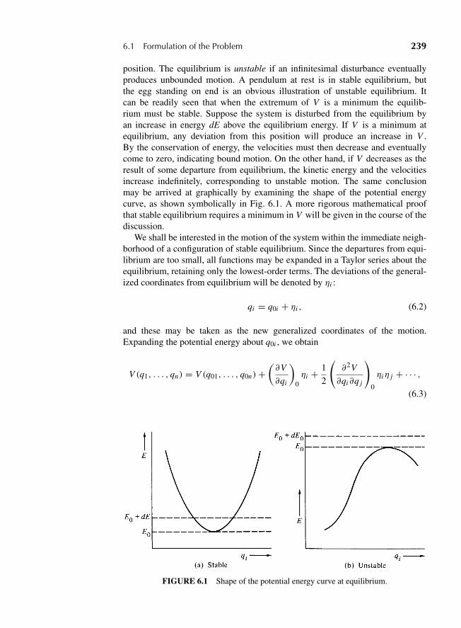
“M06 Goldstein ISBN C06” — 2011/2/15 — page 239 — #2
6.1 Formulation of the Problem 239
position. The equilibrium is unstable if an infinitesimal disturbance eventuallyproduces unbounded motion. A pendulum at rest is in stable equilibrium, butthe egg standing on end is an obvious illustration of unstable equilibrium. Itcan be readily seen that when the extremum of V is a minimum the equilib-rium must be stable. Suppose the system is disturbed from the equilibrium byan increase in energy dE above the equilibrium energy. If V is a minimum atequilibrium, any deviation from this position will produce an increase in V .By the conservation of energy, the velocities must then decrease and eventuallycome to zero, indicating bound motion. On the other hand, if V decreases as theresult of some departure from equilibrium, the kinetic energy and the velocitiesincrease indefinitely, corresponding to unstable motion. The same conclusionmay be arrived at graphically by examining the shape of the potential energycurve, as shown symbolically in Fig. 6.1. A more rigorous mathematical proofthat stable equilibrium requires a minimum in V will be given in the course of thediscussion.
We shall be interested in the motion of the system within the immediate neigh-borhood of a configuration of stable equilibrium. Since the departures from equi-librium are too small, all functions may be expanded in a Taylor series about theequilibrium, retaining only the lowest-order terms. The deviations of the general-ized coordinates from equilibrium will be denoted by ηi :
qi = q0i + ηi , (6.2)
and these may be taken as the new generalized coordinates of the motion.Expanding the potential energy about q0i , we obtain
V (q1, . . . , qn) = V (q01, . . . , q0n)+(∂V
∂qi
)0ηi + 1
2
(∂2V
∂qi∂q j
)0
ηiη j + · · · ,(6.3)
FIGURE 6.1 Shape of the potential energy curve at equilibrium.
“M06 Goldstein ISBN C06” — 2011/2/15 — page 240 — #3
240 Chapter 6 Oscillations
where the summation convention has been invoked, as usual. The terms linear inηi vanish automatically in consequence of the equilibrium conditions (6.1). Thefirst term in the series is the potential energy of the equilibrium position, and byshifting the arbitrary zero of potential to coincide with the equilibrium potential,this term may also be made to vanish. We are therefore left with the quadraticterms as the first approximation to V :
V = 1
2
(∂2V
∂qi∂q j
)0
ηiη j = 1
2Vi jηiη j , (6.4)
where the second derivatives of V have been designated by the constants Vi j
depending only upon the equilibrium values of the qi ’s. It is obvious fromtheir definition that the Vi j ’s are symmetrical, that is, that Vi j = Vji . The Vi j
coefficients can vanish under a variety of circumstances. Thus, the potential cansimply be independent of a particular coordinate, so that equilibrium occursat any arbitrary value of that coordinate. We speak of such cases as neutralor indifferent equilibrium. It may also happen, for example, that the potentialbehaves like a quadratic at that point, again causing one or more of the Vi j ’s tovanish. Either situation calls for special treatment in the mathematical discussionthat follows.
A similar series expansion can be obtained for the kinetic energy. Since thegeneralized coordinates do not involve the time explicitly, the kinetic energy is ahomogeneous quadratic function of the velocities (cf. Eq. (1.71)):
T = 12 mi j qi q j = 1
2 mi j ηi η j . (6.5)
The coefficients mi j are in general functions of the coordinates qk , but they maybe expanded in a Taylor series about the equilibrium configuration:
mi j (q1, . . . , qn) = mi j (q01, . . . , q0n)+(∂mi j
∂qk
)0ηk + · · · .
As Eq. (6.5) is already quadratic in the ηi ’s, the lowest nonvanishing approxima-tion to T is obtained by dropping all but the first term in the expansions of mi j .Denoting the constant values of the mi j functions at equilibrium by Ti j , we cantherefore write the kinetic energy as
T = 12 Ti j ηi η j . (6.6)
It is again obvious that the constants Ti j must be symmetric, since the individ-ual terms in Eq. (6.6) are unaffected by an interchange of indices. From Eqs. (6.4)and (6.6), the Lagrangian is given by
L = 12 (Ti j ηi η j − Vi jηiη j ). (6.7)
“M06 Goldstein ISBN C06” — 2011/2/15 — page 241 — #4
6.2 The Eigenvalue Equation and the Principal Axis Transformation 241
Taking the η’s as the general coordinates, the Lagrangian of Eq. (6.7) leads to thefollowing n equations of motion:
Ti j η j + Vi jη j = 0, (6.8)
where explicit use has been made of the symmetry property of the Vi j and Ti j
coefficients. Each of Eqs. (6.8) will involve, in general, all of the coordinates ηi ,and it is this set of simultaneous differential equations that must be solved toobtain the motion near the equilibrium.
In almost all cases of interest, the kinetic energy term can be easily written soas to have no cross terms.* This corresponds to the Lagrangian
L = 12 (Ti η
2i − Vi jηiη j ), (6.9)
which generates the following equations of motion
Ti ηi + Vi jη j = 0. (no sum over i) (6.10)
6.2 THE EIGENVALUE EQUATIONAND THE PRINCIPAL AXIS TRANSFORMATION
The equations of motion (6.8) are linear differential equations with constantcoefficients, of a form familiar from electrical circuit theory. We are therefore ledto try an oscillatory solution of the form
ηi = Cai e−iωt . (6.11)
Here Cai gives the complex amplitude of the oscillation for each coordinate ηi ,the factor C being introduced for convenience as a scale factor, the same for allcoordinates. It is understood of course that it is the real part of Eq. (6.11) thatis to correspond to the actual motion. Substitution of the trial solution (6.11)into the equations of motion leads to the following equations for the amplitudefactors:
(Vi j a j − ω2Ti j a j ) = 0. (6.12)
Equations (6.12) constitute n linear homogeneous equations for the ai ’s,and consequently can have a nontrivial solution only if the determinant of the
*Mathematically, we could go even further when the coordinates are Cartesian and making the Ti j =δi j by rescaling the coordinates. Such coordinates are called mass-weighted coordinates since theyare generated by dividing the coordinates by the square root of the mass. This transforms the kineticenergy to the form
T = ηi ηi
2.
This reduces the problem to the eigenvalue problem of Chapters 4 and 5, only in n dimensions insteadof three; however, the mathematical simplification can obscure the physics, since each coordinate canhave a different characteristic scale.
“M06 Goldstein ISBN C06” — 2011/2/15 — page 242 — #5
242 Chapter 6 Oscillations
coefficients vanishes:∣∣∣∣∣∣∣∣∣
V11 − ω2T11 V12 − ω2T12 . . .
V21 − ω2T21 V22 − ω2T22
V31 − ω2T31...
∣∣∣∣∣∣∣∣∣= 0. (6.13)
This determinantal condition is in effect an algebraic equation of the nth degreefor ω2, and the roots of the determinant provide the frequencies for whichEq. (6.11) represents a correct solution to the equations of motion. For eachof these values of ω2, Eqs. (6.12) may be solved for the amplitudes of ai , or moreprecisely, for n − 1 of the amplitudes in terms of the remaining ai .
Equations (6.12) represent a type of eigenvalue equation, for writing Ti j as anelement of the matrix T, the equations may be written
Va = λTa. (6.14)
Here the effect of V on the eigenvector a is not merely to reproduce the vectortimes the factor λ, as in the ordinary eigenvalue problem. Instead, the eigenvectoris such that V acting on a produces a multiple of the result of T acting on a. Weshall show that the eigenvalues λ for which Eq. (6.14) can be satisfied are all realin consequence of the symmetric and reality properties of T and V, and, in fact,must be positive. It will also be shown that the eigenvectors a are orthogonal—ina sense. In addition, the matrix of the eigenvectors, A, diagonalizes both T and V,the former to the unit matrix 1 and the latter to a matrix whose diagonal elementsare the eigenvalues λ. Most importantly it is necessary to show that a and λ arereal.
Proceeding as in Section 5.4, let ak be a column matrix representing the ktheigenvector, satisfying the eigenvalue equation*
Vak = λkTak . (6.15)
Assume now that the only solution to Eq. (6.15) involves complex λ and ak . Theadjoint equation, i.e., the transposed complex conjugate equation, for λl has theform
a†l V = λ∗l a†
l T. (6.16)
Here a†l stands for the adjoint vector—the complex conjugate row matrix—and
explicit use has been made of the fact that the V and T matrices are real andsymmetric. Multiply Eq. (6.16) from the right by ak and subtract the result ofthe similar product of Eq. (6.15) from the left with a†
l . The left-hand side of the
*It hardly need be added that there is no summation over k in Eq. (6.15). Indeed, in this chapter thesummation convention will apply only to the components of matrices or tensors (of any rank) and notto the matrices and tensors themselves.
“M06 Goldstein ISBN C06” — 2011/2/15 — page 243 — #6
6.2 The Eigenvalue Equation and the Principal Axis Transformation 243
difference equation vanishes, leaving only
0 = (λk − λ∗l )a†l Tak . (6.17)
When l = k, Eq. (6.17) becomes
(λk − λ∗k)a†kTak = 0. (6.18)
That the matrix product in Eq. (6.18) is real can be shown immediately by takingits complex conjugate and using the symmetry property of T. However, we wantto prove that the matrix product is not only real but is positive definite. For thispurpose, separate ak into its real and imaginary components:
ak = ak + ibk .
The matrix product can then be written as
a†kTak = akTak + bkTbk + i(akTbk − bkTak). (6.19)
The imaginary term vanishes by virtue of the symmetry of T and therefore, asnoted earlier, the matrix product is real. Further, the kinetic energy in Eq. (6.6)can be rewritten in terms of a column matrix h as
T = 12˜hTh. (6.20)
Hence, the first two terms in Eq. (6.18) are twice the kinetic energies when thevelocity matrix hk has the values ak and bk , respectively. Now, a kinetic energyby its physical nature must be positive definite for real velocities, and thereforethe matrix product in Eq. (6.18) cannot be zero. It follows that the eigenvalues λk
must be real.Since the eigenvalues are real, the ratios of the eigenvector components a jk
determined by Eqs. (6.15) must all be real. There is still some indeterminatenessof course since the value of a particular one of the a jk’s can still be chosen at willwithout violating Eqs. (6.15). We can require however that this component shallbe real, and the reality of λk then ensures the reality of all the other components.(Any complex phase factor in the amplitude of the oscillation will be thrown intothe factor C , Eq. (6.11).) Multiply now Eq. (6.15) by ak from the left and solvefor λk :
λk = akVak
akTak. (6.21)
The denominator of this expression is equal to twice the kinetic energy for veloc-ities aik and since the eigenvectors are all real, the sum must be positive definite.Similarly, the numerator is the potential energy for coordinates aik , and the con-dition that V be a minimum at equilibrium requires that the sum must be positiveor zero. Neither numerator nor denominator can be negative, and the denominatorcannot be zero, hence λ is always finite and positive. (It may however be zero.)

“M06 Goldstein ISBN C06” — 2011/2/15 — page 244 — #7
244 Chapter 6 Oscillations
Recall that λ stands for ω2, so that positive λ corresponds to real frequencies ofoscillation. Were the potential not a local minimum, the numerator in Eq. (6.21)might be negative, giving rise to imaginary frequencies that would produce anunbounded exponential increase of the ηi with time. Such motion would obvi-ously be unstable, and we have here the promised mathematical proof that a min-imum of the potential is required for stable motion.
Let us return for the moment to Eq. (6.17) which, in view of the reality of theeigenvalues and eigenvectors, can be written
(λk − λl)alTak = 0. (6.17′)
If all the roots of the secular equation are distinct, then Eq. (6.17′) can hold onlyif the matrix product vanishes for l not equal to k:
alTak = 0, l �= k. (6.22a)
It has been remarked several times that the values of the a jk’s are not completelyfixed by the eigenvalue equations (6.12). We can remove this indeterminacy byrequiring further that
akTak = 1. (6.22b)
There are n such equations (6.22), and they uniquely fix the one arbitrary compo-nent of each of the n eigenvectors ak .* If we form all the eigenvectors ak intoa square matrix A with components a jk (cf. Section 4.6), then the two equa-tions (6.22a and b) can be combined into one matrix equation:
ATA = 1. (6.23)
When two or more of the roots are repeated, the argument leading to Eq. (6.22a)falls through for λl = λk . We shall reserve a discussion of this exceptional caseof degeneracy for a later time. For the present, suffice it to state that a set ofa jk coefficients can always be found that satisfies both the eigenvalue conditionsEqs. (6.10), and Eq. (6.22a), so that Eq. (6.23) always holds.
In Chapter 4, the similarity transformation of a matrix C by a matrix B wasdefined by the equation (cf. Eq. (4.41):
C′ = BCB−1.
*Equation (6.22b) may be put in a form that explicitly shows that it suffices to remove the indetermi-nacy in the a jk ’s. Suppose it is the magnitude of a1k that is to be evaluated; the ratio of all the othera jk ’s to a1k is obtained from Eqs. (6.12). Then Eq. (6.22b) can be written as
∑i. j
Ti jaik
a1k
a jk
a1k= 1
a21k
.
The left-hand side is completely determined from the eigenvalue equations and may be evaluateddirectly to provide a1k .
“M06 Goldstein ISBN C06” — 2011/2/15 — page 245 — #8
6.2 The Eigenvalue Equation and the Principal Axis Transformation 245
We now introduce the related concept of the congruence transformation of C byA according to the relation
C′ = ACA. (6.24)
If A is orthogonal, so that A = A−1, there is no essential difference betweenthe two types of transformation (as may be seen by denoting A−1 by the matrixB). Equation (6.23) can therefore be read as the statement that A transforms Tby a congruence transformation into a diagonal matrix, in particular into the unitmatrix.
If a diagonal matrix l with elements λik = λkδik is introduced, the eigenvalueequations (6.15) may be written
Vi j a jk = Ti j a jlλlk,
which becomes in matrix notation
VA = TAl. (6.25)
Multiplying by A from the left, Eq. (6.25) takes the form
AVA = ATAl,
which by Eq. (6.23) reduces to
AVA = l. (6.26)
Our final equation (6.26) states that a congruence transformation of V byA changes it into a diagonal matrix whose elements are the eigenvalues λk .Eq. (6.26) has solutions
|V − l1| = 0. (6.26′)
In summary we can use normalized Cartesian coordinates so that Ti j = δi j whichreduces the physics to solving
AA = 1 (4.36) and AVA = Vdiagonal (6.26),
or we may choose more general goordinates where Ti j �= δi j , even allowingTi j = Tji �= 0 for i �= j , and use
ATA = 1 (6.23) and AVA = Vdiagonal (6.26),
to solve the general problem.As an example, we consider a particle of mass m with two degrees of freedom
(x1, x2) that obeys the Lagrangian (cf. Eq. (6.9))
L = 12 m(x2
1 + x22)− 1
2 Vi j xi x j
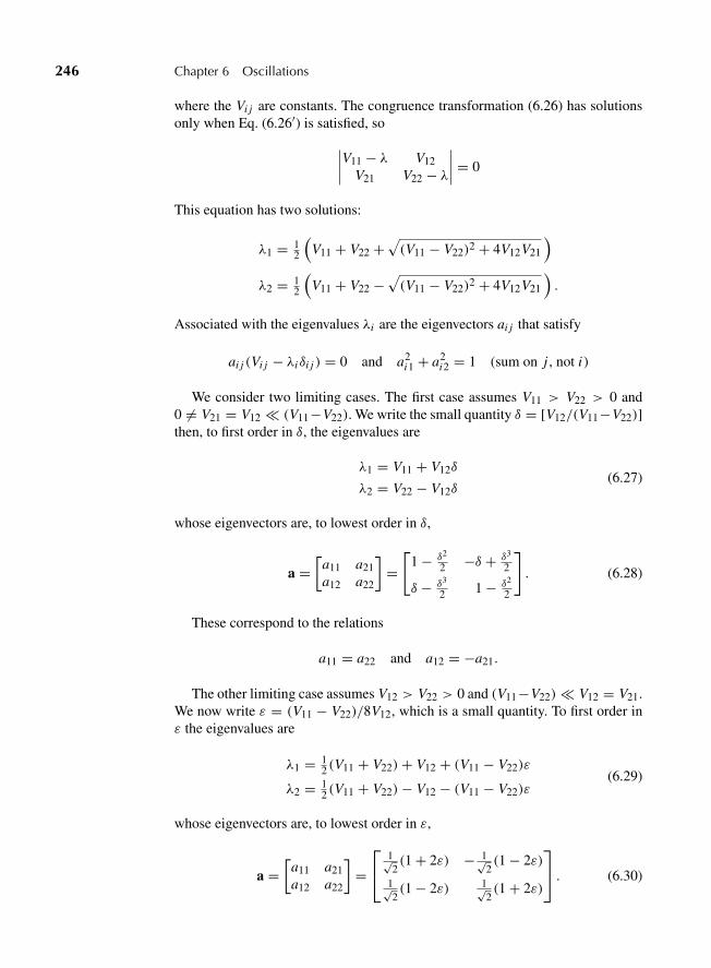
“M06 Goldstein ISBN C06” — 2011/2/15 — page 246 — #9
246 Chapter 6 Oscillations
where the Vi j are constants. The congruence transformation (6.26) has solutionsonly when Eq. (6.26′) is satisfied, so
∣∣∣∣V11 − λ V12V21 V22 − λ
∣∣∣∣ = 0
This equation has two solutions:
λ1 = 12
(V11 + V22 +
√(V11 − V22)2 + 4V12V21
)λ2 = 1
2
(V11 + V22 −
√(V11 − V22)2 + 4V12V21
).
Associated with the eigenvalues λi are the eigenvectors ai j that satisfy
ai j (Vi j − λiδi j ) = 0 and a2i1 + a2
i2 = 1 (sum on j , not i)
We consider two limiting cases. The first case assumes V11 > V22 > 0 and0 �= V21 = V12 � (V11−V22). We write the small quantity δ = [V12/(V11−V22)]then, to first order in δ, the eigenvalues are
λ1 = V11 + V12δ
λ2 = V22 − V12δ(6.27)
whose eigenvectors are, to lowest order in δ,
a =[
a11 a21a12 a22
]=
[1 − δ2
2 −δ + δ3
2
δ − δ3
2 1 − δ2
2
]. (6.28)
These correspond to the relations
a11 = a22 and a12 = −a21.
The other limiting case assumes V12 > V22 > 0 and (V11−V22)� V12 = V21.We now write ε = (V11 − V22)/8V12, which is a small quantity. To first order inε the eigenvalues are
λ1 = 12 (V11 + V22)+ V12 + (V11 − V22)ε
λ2 = 12 (V11 + V22)− V12 − (V11 − V22)ε
(6.29)
whose eigenvectors are, to lowest order in ε,
a =[
a11 a21a12 a22
]=
⎡⎣ 1√
2(1 + 2ε) − 1√
2(1 − 2ε)
1√2(1 − 2ε) 1√
2(1 + 2ε)
⎤⎦ . (6.30)
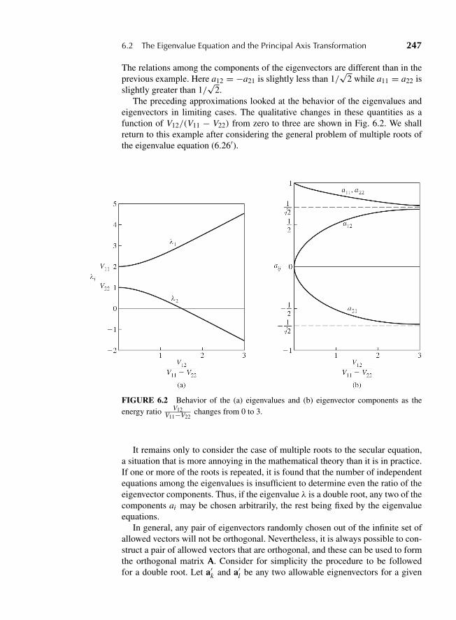
“M06 Goldstein ISBN C06” — 2011/2/15 — page 247 — #10
6.2 The Eigenvalue Equation and the Principal Axis Transformation 247
The relations among the components of the eigenvectors are different than in theprevious example. Here a12 = −a21 is slightly less than 1/
√2 while a11 = a22 is
slightly greater than 1/√
2.The preceding approximations looked at the behavior of the eigenvalues and
eigenvectors in limiting cases. The qualitative changes in these quantities as afunction of V12/(V11 − V22) from zero to three are shown in Fig. 6.2. We shallreturn to this example after considering the general problem of multiple roots ofthe eigenvalue equation (6.26′).
FIGURE 6.2 Behavior of the (a) eigenvalues and (b) eigenvector components as theenergy ratio V12
V11−V22changes from 0 to 3.
It remains only to consider the case of multiple roots to the secular equation,a situation that is more annoying in the mathematical theory than it is in practice.If one or more of the roots is repeated, it is found that the number of independentequations among the eigenvalues is insufficient to determine even the ratio of theeigenvector components. Thus, if the eigenvalue λ is a double root, any two of thecomponents ai may be chosen arbitrarily, the rest being fixed by the eigenvalueequations.
In general, any pair of eigenvectors randomly chosen out of the infinite set ofallowed vectors will not be orthogonal. Nevertheless, it is always possible to con-struct a pair of allowed vectors that are orthogonal, and these can be used to formthe orthogonal matrix A. Consider for simplicity the procedure to be followedfor a double root. Let a′k and a′l be any two allowable eignenvectors for a given
“M06 Goldstein ISBN C06” — 2011/2/15 — page 248 — #11
248 Chapter 6 Oscillations
double root λ, which have been normalized so as to satisfy Eq. (6.22b). Any linearcombination of a′k and a′l will also be an eigenvector for the root λ. We thereforeseek to construct a vector al ,
al = c1a′k + c2a′l , (6.31)
where c1 and c2 are constants such that al is orthogonal to a′k . The orthogonalitycondition, Eq. (6.22a), then requires that
alTa′k = c1 + c2a′lTa′k = 0,
where use has been made of the normalization of a′k . It therefore follows that theratio of c1 to c2 must be given by
c1
c2= −a′lTa′k ≡ −τl . (6.32)
We can illustrate these ideas by again considering our two-dimensionalexample given by Eqs. (6.27) through (6.30). The two limiting cases of theoff-diagonal potential term V12, being much less than and much greater thanthe difference factor (V11 − V22), provide an excellent example of the problemsintroduced by degeneracy. When
V11 = V22 = V0, V12 = 0,
the two eigenvalues become the same, λ1 = λ2 = V0.If the limit is taken by letting V12 → 0 first and then taking the limit
(V11 → V22), the eigenvectors in Eqs. (6.28) become
a1 =(
10
)and a2 =
(01
). (6.33)
If the limit is taken in the reverse order, Eqs. (6.30) give
b1 =⎛⎝ 1√
21√2
⎞⎠ and b2 =
⎛⎝− 1√
21√2
⎞⎠ , (6.34)
where b is used for the eigenvectors in Eqs. (6.34) to avoid confusion with theeigenvectors in Eqs. (6.33). Each of the eigenvectors in (6.33) and (6.34) are linearcombinations of the other set of eigenvectors. For example,
b1 = 1√2(a1 + a2), and b2 = 1√
2(a2 − a1),
so either set of eigenvectors is a linear combination of the other, as was discussedin this section. These results obviously generalize to the infinite set
a1 =(
ab
)and a2 =
(−ba
),
“M06 Goldstein ISBN C06” — 2011/2/15 — page 249 — #12
6.2 The Eigenvalue Equation and the Principal Axis Transformation 249
where a and b are any pairs of numbers that satisfy
a2 + b2 = 1.
This shows that there is an infinite set of possible eigenvectors in the case ofdegeneracy.
There is another way to consider the significance of these results. The approx-imate eigenvectors in Eqs. (6.28) are for the case where the main potential energyterms are V11 and V22, which are at diagonal positions, and the V12 are in the off-diagonal positions. If we take the eigenvectors of Eq. (6.30) in the limit ε → 0and let the eigenvectors of Eqs. (6.30) transform V as V′ = AVA, we obtain thetransformed potential energy tensor
V′ =(
12 (V11 + V22)+ V12
12 (V11 − V22)
12 (V11 − V22)
12 (V11 + V22)− V12
)
in which the difference term (V11−V22) is off-diagonal. Thus, the set of eigenvec-tors given by Eqs. (6.30) are for the physical situation in which the small energyterm (V11 − V22) is off-diagonal.
Returning to the main discussion, the requirement that al of Eq. (6.32) be nor-malized provides another condition on the two coefficients, which in terms of τl
defined by Eq. (6.32) takes the form
alTal = 1 = c21 + c2
2 + 2c1c2τl .
Together the two equations fix the coefficients c1 and c2, and therefore the vectoral . Both al and ak ≡ a′k are automatically orthogonal to the eigenvectors of theother distinct eigenvalues, for then the argument based on Eq. (6.17′) remainsvalid. Hence, we have a set of n eigenvectors a j whose components form thematrix A satisfying Eq. (6.23).
A similar procedure is followed for a root of higher multiplicity. If λ is anm-fold root, then orthogonal normalized eigenvectors are formed out of linearcombinations of any of the m corresponding eigenvectors a′1, . . . , a′m . The first ofthe “orthonormal” eigenvectors a1 is then chosen as a multiple of a′1; a2 is takenas a linear combination of a′1 and a′2; and so on. In this manner, the number ofconstants to be determined is equal to the sum of the first m integers, or 1
2 m(m+1).The normalization requirements provide m conditions, while there are 1
2 m(m−1)orthogonality conditions, and together these are just enough to fix the constantsuniquely.
This processes of constructing orthogonalized eigenvectors in the case of mul-tiple roots is completely analogous to the Gram-Schmidt method of constructinga sequence of orthogonal functions out of any arbitrary set of functions. Phrasedin geometrical language, it is also seen to be identical with the procedure followedin Chapter 5 for multiple eigenvalues of the inertia tensor. For example, the addedindeterminacy in the eigenvector components for a double root means that all ofthe vectors in a plane are eigenvectors. We merely choose any two perpendicular
“M06 Goldstein ISBN C06” — 2011/2/15 — page 250 — #13
250 Chapter 6 Oscillations
directions in the plane as being the new principal axes, with the eigenvectors in Aas unit vectors along these axes.
6.3 FREQUENCIES OF FREE VIBRATION, AND NORMAL COORDINATES
The somewhat lengthy arguments of the preceding section demonstrate that theequations of motion will be satisfied by an oscillatory solution of the form (6.11),not merely for one frequency but in general for a set of n frequencies ωk . A com-plete solution of the equations of motion therefore involves a superposition ofoscillations with all the allowed frequencies. Thus, if the system is displacedslightly from equilibrium and then released, the system performs small oscilla-tions about the equilibrium with the frequencies ω1, . . . , ωn . The solutions of thesecular equation are therefore often designated as the frequencies of free vibrationor as the resonant frequencies of the system.
The general solution of the equations of motion may now be written as a sum-mation over an index k:
ηi = Ckaike−iωk t , (6.35)
there being a complex scale factor Ck for each resonant frequency. It might beobjected that for each solution λk of the secular equation there are two resonantfrequencies +ωk and −ωk . The eigenvector ak would be the same for the twofrequencies, but the scale factors C+
k and C−K could conceivably be different. On
this basis, the general solution should appear as
ηi = aik(C+k e+iωk t + C−
k e−iωk t ). (6.35′)
Recall however that the actual motion is the real part of the complex solution, andthe real part of either (6.35) or (6.35′) can be written in the form
ηi = fkaik cos(ωk t + δk), (6.36)
where the amplitude fk and the phase δk are determined form the initial condi-tions. Either of the solutions ((6.35) and (6.36)) will therefore represent the actualmotion, and the former of course is the more convenient.
The orthogonality properties of A greatly facilitate the determination of thescale factors Ck in terms of the initial conditions. At t = 0, the real part ofEq. (6.35) reduces to
ηi (0) = Re Ckaik, (6.37)
where Re stands for “real part of.” Similarly, the initial value of the velocities isobtained as
ηi (0) = Im Ckaikωk, (6.38)
“M06 Goldstein ISBN C06” — 2011/2/15 — page 251 — #14
6.3 Frequencies of Free Vibration, and Normal Coordinates 251
where Im Ck denotes the imaginary part of Ck . From these 2n equations, the realand imaginary parts of the n constants Ck may be evaluated. To solve Eq. (6.37),for example, let us first write it in terms of column matrices h(0) and C:
h(0) = A Re C. (6.37′)
If we multiply by AT from the left and use Eq. (6.23), we immediately obtain asolution for Re C:
Re C = ATh(0),
or, taking the lth component,
Re Cl = a jl Tjkηk(0). (6.39)
A similar procedure leads to the imaginary part of the scale factors as*
Im Cl = 1
ωl
∑j,k
a jl Tjk ηk(0). (6.40)
Equations (6.39) and (6.40) thus permit the direct computation of the complexfactors Cl (and therefore the amplitudes and phases) in terms of the initial condi-tions and the matrices T and A.
The solution for each coordinate, Eq. (6.35), is in general a sum of simpleharmonic oscillations in all of the frequencies ωk satisfying the secular equation.Unless it happens that all of the frequencies are commensurable, that is, rationalfractions of each other, ηi never repeats its initial value and is therefore not itself aperiodic function of time. However, it is possible to transform from the ηi to a newset of generalized coordinates that are all simple periodic functions of time—a setof variables known as the normal coordinates.
We define a new set of coordinates ζ j
ηi = ai jζ j , (6.41)
or, in terms of single-column matrices h and z,
h = Az. (6.41′)
The potential energy, Eq. (6.4), is written in matrix notation as
V = 12 hVh. (6.42)
Now, the single-row transpose matrix h is related to z by the equation
h = Az = zA,
*The summation over j and k is shown explicitly because there is no summation over the repeatedsubscript l.
“M06 Goldstein ISBN C06” — 2011/2/15 — page 252 — #15
252 Chapter 6 Oscillations
so that the potential energy can be written also as
V = 12 zAVAz.
But A diagonalizes V by a congruence transformation (cf. Eq. (6.26)), and thepotential energy therefore reduces simply to
V = 12 zlz = 1
2ω2kζ
2k . (6.43)
The kinetic energy has an even simpler form in the new coordinates. Since thevelocities transform as the coordinates, T as given in Eq. (6.20) transforms to
T = 12˜zATAz
which by virtue of Eq. (6.23) reduces to
T = 12˜zz = 1
2 ζi ζi . (6.44)
Equations (6.43) and (6.44) state that in the new coordinates both the potentialand kinetic energies are sums of squares only, without any cross terms. Of course,this result is simply another way of saying that A produces a principal axis trans-formation. Recall that the principal axis transformation of the inertia tensor wasspecifically designed to reduce the moment of inertia to a sum of squares; the newaxes being the principal axes of the inertia ellipsoid. Here the kinetic and poten-tial energies are also quadratic forms (as was the moment of inertia) and both arediagonalized by A. For this reason, the principal axis transformation employedhere is a particular example of the well-known algebraic process of the simulta-neous diagonalization of two quadratic forms.
The equations of motion share in the simplification resulting from their use.The new Lagrangian is
L = 12 (ζk ζk − ω2
kζ2k ) (6.45)
so that the Lagrange equations for ζk are
ζk + ω2kζk = 0. (6.46)
Equations (6.47) have the immediate solutions
ζk = Cke−iωk t , (6.47)
which could have been seen of course directly from Eqs. (6.35) and (6.41). Eachof the new coordinates is thus a simply periodic function involving only one ofthe resonant frequencies. As mentioned earlier, it is therefore customary to callthe ζ ’s the normal coordinates of the system.
Each normal coordinate corresponds to a vibration of the system with only onefrequency, and these component oscillations are spoken of as the normal modesof vibration. All of the particles in each mode vibrate with the same frequencyand with the same phase;* the relative amplitudes being determined by the matrix
*Particles may be exactly out of phase if the a’s have opposite sign.

“M06 Goldstein ISBN C06” — 2011/2/15 — page 253 — #16
6.4 Free Vibrations of a Linear Triatomic Molecule 253
elements a jk . The complete motion is then built up out of the sum of the normalmodes weighted with appropriate amplitude and phase factors contained in theCk’s.
Harmonics of the fundamental frequencies are absent in the complete motionessentially because of the stipulation that the amplitude of oscillation be small.We are then allowed to represent the potential as a quadratic form, which ischaracteristic of simple harmonic motion. The normal coordinate transforma-tion emphasizes this point, for the Lagrangian in the normal coordinates (6.45)is seen to be the sum of the Lagrangians for harmonic oscillators of frequenciesωk . We can thus consider the complete motion for small oscillations as beingobtained by exciting the various harmonic oscillators with different intensitiesand phases.*
6.4 FREE VIBRATIONS OF A LINEAR TRIATOMIC MOLECULE
To illustrate the technique for obtaining the resonant frequencies and normalmodes, we shall consider in detail a model based on a linear symmetrical tri-atomic molecule. In the equilibrium configuration of the molecule, two atomsof mass m are symmetrically located on each side of an atom of mass M (cf.Fig. 6.3). All three atoms are on one straight line, the equilibrium distances apartbeing denoted by b. For simplicity, we shall first consider only vibrations alongthe line of the molecule, and the actual complicated interatomic potential will beapproximated by two springs of force constant k joining the three atoms. Thereare three obvious coordinates marking the position of the three atoms on the line.In these coordinates, the potential energy is
V = k
2(x2 − x1 − b)2 + k
2(x3 − x2 − b)2. (6.48)
We now introduce coordinates relative to the equilibrium positions:
ηi = xi − x0i ,
where
x02 − x01 = b = x03 − x02.
FIGURE 6.3 Model of a linear symmetrical triatomic molecule.
*Note for future reference that the same sort of picture appears in the quantization of the electromag-netic field. The frequencies of the harmonic oscillators are identified with the photon frequencies, andthe amplitudes of excitation become the discrete quantized “occupation numbers”—the number ofphotons of each frequency.
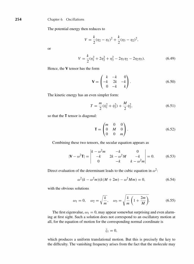
“M06 Goldstein ISBN C06” — 2011/2/15 — page 254 — #17
254 Chapter 6 Oscillations
The potential energy then reduces to
V = k
2(η2 − η1)
2 + k
2(η3 − η2)
2,
or
V = k
2(η2
1 + 2η22 + η2
3 − 2η1η2 − 2η2η3). (6.49)
Hence, the V tensor has the form
V =⎛⎝ k −k 0−k 2k −k
0 −k k
⎞⎠ . (6.50)
The kinetic energy has an even simpler form:
T = m
2(η2
1 + η23)+
M
2η2
2, (6.51)
so that the T tensor is diagonal:
T =⎛⎝m 0 0
0 M 00 0 m
⎞⎠ . (6.52)
Combining these two tensors, the secular equation appears as
|V − ω2T| =∣∣∣∣∣∣k − ω2m −k 0
−k 2k − ω2 M −k0 −k k − ω2m
∣∣∣∣∣∣ = 0. (6.53)
Direct evaluation of the determinant leads to the cubic equation in ω2:
ω2(k − ω2m)(k(M + 2m)− ω2 Mm) = 0, (6.54)
with the obvious solutions
ω1 = 0, ω2 =√
k
m, ω3 =
√k
m
(1 + 2m
M
). (6.55)
The first eigenvalue, ω1 = 0, may appear somewhat surprising and even alarm-ing at first sight. Such a solution does not correspond to an oscillatory motion atall, for the equation of motion for the corresponding normal coordinate is
ζ1 = 0,
which produces a uniform translational motion. But this is precisely the key tothe difficulty. The vanishing frequency arises from the fact that the molecule may

“M06 Goldstein ISBN C06” — 2011/2/15 — page 255 — #18
6.4 Free Vibrations of a Linear Triatomic Molecule 255
be translated rigidly along its axis without any change in the potential energy,an example of neutral equilibrium mentioned previously. Since the restoringforce against such motion is zero, the effective “frequency” must also vanish.We have made the assumption that the molecule has three degrees of freedomfor vibrational motion, whereas in reality one of them is a rigid body degree offreedom.
A number of interesting points can be discussed in connection with a vanishingresonant frequency. It is seen from Eq. (6.21) that a zero value of ω can occuronly when the potential energy is positive but is not positive definite; that is, itcan vanish even when not all the ηi ’s are zero. An examination of V , Eq. (6.49),shows that it is not positive definite and that V does in fact vanish when all theη’s are equal (uniform translation).
Since the zero frequency found here is of no consequence for the vibrationfrequencies of interest, it is often desirable to phrase the problem so that the rootis eliminated from the outset. We can do this here most simply by imposing thecondition or constraint that the center of mass remain stationary at the origin:
m(x1 + x3)+ Mx2 = 0. (6.56)
Equation (6.56) can then be used to eliminate one of the coordinates from V andT , reducing the problem to one of two degrees of freedom (cf. Derivation 1, thischapter).
The restriction of the motion to be along the molecular axis allows onlyone possible type of uniform rigid body motion. However, if the more gen-eral problem of vibrations in all three directions is considered, the number ofrigid body degrees of freedom will be increased to six. The molecule may thentranslate uniformly along the three axes or perform uniform rotations aboutthe axes. Hence, in any general system of n degrees of freedom, there will besix vanishing frequencies and only n − 6 true vibration frequencies. Again,the reduction in the number of degrees of freedom can be performed before-hand by imposing the conservation of linear and angular momentum upon thecoordinates.
In addition to rigid body motion, it has been pointed out that zero resonantfrequencies may also arise when the potential is such that both the first and secondderivatives of V vanish at equilibrium. Small oscillations may still be possible inthis case if the fourth derivatives do not also vanish (the third derivatives mustvanish for a stable equilibrium), but the vibrations will not be simple harmonic.Such a situation therefore constitutes a breakdown of the customary method ofsmall oscillations, but fortunately it is not of frequent occurrence.
Returning now to the examination of the resonant frequencies, ω2 will be rec-ognized as the well-known frequency of oscillation for a mass m suspended bya spring of force constant k. We are therefore led to expect that only the endatoms partake in this vibration; the center molecule remains stationary. It is onlyin the third mode of vibration, ω3, that the mass M can participate in the oscilla-tory motion. These predictions are verified by examining the eigenvectors for thethree normal modes.
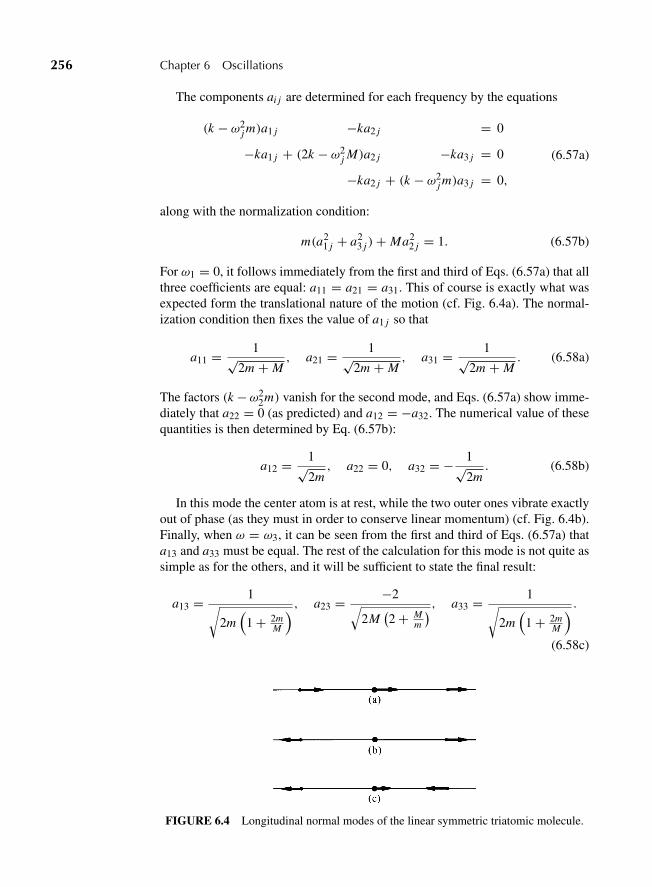
“M06 Goldstein ISBN C06” — 2011/2/15 — page 256 — #19
256 Chapter 6 Oscillations
The components ai j are determined for each frequency by the equations
(k − ω2j m)a1 j −ka2 j = 0
−ka1 j + (2k − ω2j M)a2 j −ka3 j = 0
−ka2 j + (k − ω2j m)a3 j = 0,
(6.57a)
along with the normalization condition:
m(a21 j + a2
3 j )+ Ma22 j = 1. (6.57b)
For ω1 = 0, it follows immediately from the first and third of Eqs. (6.57a) that allthree coefficients are equal: a11 = a21 = a31. This of course is exactly what wasexpected form the translational nature of the motion (cf. Fig. 6.4a). The normal-ization condition then fixes the value of a1 j so that
a11 = 1√2m + M
, a21 = 1√2m + M
, a31 = 1√2m + M
. (6.58a)
The factors (k −ω22m) vanish for the second mode, and Eqs. (6.57a) show imme-
diately that a22 = 0 (as predicted) and a12 = −a32. The numerical value of thesequantities is then determined by Eq. (6.57b):
a12 = 1√2m, a22 = 0, a32 = − 1√
2m. (6.58b)
In this mode the center atom is at rest, while the two outer ones vibrate exactlyout of phase (as they must in order to conserve linear momentum) (cf. Fig. 6.4b).Finally, when ω = ω3, it can be seen from the first and third of Eqs. (6.57a) thata13 and a33 must be equal. The rest of the calculation for this mode is not quite assimple as for the others, and it will be sufficient to state the final result:
a13 = 1√2m
(1 + 2m
M
) , a23 = −2√2M
(2 + M
m
) , a33 = 1√2m
(1 + 2m
M
) .(6.58c)
FIGURE 6.4 Longitudinal normal modes of the linear symmetric triatomic molecule.
“M06 Goldstein ISBN C06” — 2011/2/15 — page 257 — #20
6.4 Free Vibrations of a Linear Triatomic Molecule 257
Here the two outer atoms vibrate with the same amplitude, while the inner oneoscillates out of phase with them and has a different amplitude, (cf. Fig. 6.4c.)
The normal coordinates may be found by inverting Eq. (6.41) as
ζ1 = 1√2m + M
(mη1 + Mη2 + mη3)
ζ2 =√
m
2(η1 − η3) (6.59)
ζ3 =√
m M
2(2m + M)[(η1 + η3)− 2η2] .
These normal modes describe each of the behaviors shown on Fig. 6.4. Any gen-eral longitudinal vibration of the molecule that does not involve a rigid translationwill be some linear combination of the normal modes ω2 and ω3. The amplitudesof the normal modes, and their phases relative to each other, will of course bedetermined by the initial conditions (cf. Exercise 5).
We have spoken so far only of vibrations along the axis; in the actual moleculethere will also be normal modes of vibration perpendicular to the axis. The com-plete set of normal modes is naturally more difficult to determine than merely thelongitudinal modes, for the general motion in all directions corresponds to ninedegrees of freedom. While the procedure is straightforward, the algebra rapidlybecomes quite complicated, and it is not feasible to present the detailed calcula-tion here. However, it is possible to give a qualitative discussion on the basis ofgeneral principles, and most of the conclusions of the complete solution can bepredicted beforehand.
The general problem will have a number of zero resonant frequencies cor-responding to the possibility of rigid body motion. For a molecule with n atomsthere are 3n degrees of freedom. Subtracting the three translational and three rigidrotational degrees of freedom, there will be in general 3n − 6 vibrational modes.For the linear molecule, there will be three degrees of freedom for rigid trans-lation, but rigid rotation can account for only two degrees of freedom. Rotationabout the axis of the molecule is obviously meaningless and will not appear as amode of rigid body motion. We are therefore left with four true modes of vibra-tion. Two of these are the longitudinal modes, which have already been examinedso that there can only be two modes of vibration perpendicular to the axis. How-ever, the symmetry of the molecule about its axis shows that these two modesof perpendicular vibration must be degenerate. There is nothing to distinguish avibration in the y direction from a vibration in the z direction, and the two fre-quencies must be equal.
The additional indeterminacy of the eigenvectors of a degenerate mode appearshere, in that all directions perpendicular to the molecular axis are alike. Any twoorthogonal axes in the plane normal to the molecule may be chosen as the direc-tions of the degenerate modes of vibration. The complete motion of the atoms nor-mal to the molecular axis will depend upon the amplitudes and relative phases of
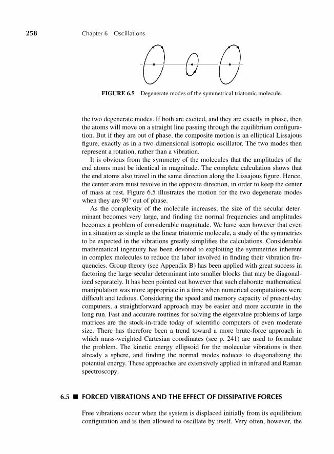
“M06 Goldstein ISBN C06” — 2011/2/15 — page 258 — #21
258 Chapter 6 Oscillations
FIGURE 6.5 Degenerate modes of the symmetrical triatomic molecule.
the two degenerate modes. If both are excited, and they are exactly in phase, thenthe atoms will move on a straight line passing through the equilibrium configura-tion. But if they are out of phase, the composite motion is an elliptical Lissajousfigure, exactly as in a two-dimensional isotropic oscillator. The two modes thenrepresent a rotation, rather than a vibration.
It is obvious from the symmetry of the molecules that the amplitudes of theend atoms must be identical in magnitude. The complete calculation shows thatthe end atoms also travel in the same direction along the Lissajous figure. Hence,the center atom must revolve in the opposite direction, in order to keep the centerof mass at rest. Figure 6.5 illustrates the motion for the two degenerate modeswhen they are 90◦ out of phase.
As the complexity of the molecule increases, the size of the secular deter-minant becomes very large, and finding the normal frequencies and amplitudesbecomes a problem of considerable magnitude. We have seen however that evenin a situation as simple as the linear triatomic molecule, a study of the symmetriesto be expected in the vibrations greatly simplifies the calculations. Considerablemathematical ingenuity has been devoted to exploiting the symmetries inherentin complex molecules to reduce the labor involved in finding their vibration fre-quencies. Group theory (see Appendix B) has been applied with great success infactoring the large secular determinant into smaller blocks that may be diagonal-ized separately. It has been pointed out however that such elaborate mathematicalmanipulation was more appropriate in a time when numerical computations weredifficult and tedious. Considering the speed and memory capacity of present-daycomputers, a straightforward approach may be easier and more accurate in thelong run. Fast and accurate routines for solving the eigenvalue problems of largematrices are the stock-in-trade today of scientific computers of even moderatesize. There has therefore been a trend toward a more brute-force approach inwhich mass-weighted Cartesian coordinates (see p. 241) are used to formulatethe problem. The kinetic energy ellipsoid for the molecular vibrations is thenalready a sphere, and finding the normal modes reduces to diagonalizing thepotential energy. These approaches are extensively applied in infrared and Ramanspectroscopy.
6.5 FORCED VIBRATIONS AND THE EFFECT OF DISSIPATIVE FORCES
Free vibrations occur when the system is displaced initially from its equilibriumconfiguration and is then allowed to oscillate by itself. Very often, however, the
“M06 Goldstein ISBN C06” — 2011/2/15 — page 259 — #22
6.5 Forced Vibrations and the Effect of Dissipative Forces 259
system is set into oscillation by an external driving force that continues to act onthe system after t = 0. The frequency of such a forced oscillation is then deter-mined by the frequency of the driving force and not by the resonant frequencies.Nevertheless, the normal modes are of great importance in obtaining the ampli-tudes of the forced vibration, and the problem is greatly simplified by use of thenormal coordinates obtained from the free modes.
If Fj is the generalized force corresponding to the coordinate η j , then byEq. (1.49) the generalized force Qi for the normal coordinate ζi is
Qi = a ji Fj . (6.60)
The equations of motion when expressed in normal coordinates now become
ζi + ω2i ζi = Qi . (6.61)
Equations (6.61) are a set of n inhomogeneous differential equations that can besolved only when we know the dependence of Qi on time. While the solutionwill not be as simple as in the free case, note that the normal coordinates preservetheir advantage of separating the variables, and each equation involves only asingle coordinate.
Frequently, the driving force varies sinusoidally with time. In an acoustic prob-lem, for example, the driving force might arise from the pressure of a sound waveimpinging on the system, and Qi then has the same frequency as the sound wave.Or, if the system is a polyatomic molecule, a sinusoidal driving force is presentif the molecule is illuminated by a monochromatic light beam. Each atom in themolecule is then subject to an electromagnetic force whose frequency is that ofthe incident light. Even where the driving force is not sinusoidal with a single fre-quency, it can often be considered as built up as a superposition of such sinusoidalterms. Thus, if the driving force is periodic, it can be represented by a Fourierseries; other times, a Fourier integral representation is suitable. Since Eqs. (6.61)are linear equations, its solutions for particular frequencies can be superposed tofind the complete solution for given Qi .
It is therefore of general interest to study the nature of the oscillations whenthe force Qi can be written as
Qi = Q0i cos(ωt + δi ), (6.62)
where ω is the angular frequency of an external force. The equations of motionnow appear as
ζi + ω2i ζi = Q0i cos(ωt + δi ). (6.63)
A complete solution of Eq. (6.63) consists of the general solution to the homoge-neous equation (that is, the free modes of vibration) plus a particular solutionto the inhomogeneous equation. By a proper choice of initial conditions, the
“M06 Goldstein ISBN C06” — 2011/2/15 — page 260 — #23
260 Chapter 6 Oscillations
superimposed free vibrations can be made to vanish,* centering our interest onthe particular solution of Eqs. (6.63) that will obviously have the form
ζi = Bi cos(ωt + δi ). (6.64)
Here the amplitudes Bi are determined by substituting the solution in Eqs. (6.63):
Bi = Q0i
ω2i − ω2
. (6.65)
The complete motion is then
η j = a jiζi = a ji Q0i cos(ωt + δi )
ω2i − ω2
. (6.66)
Thus, the vibration of each particle is again composed of linear combinations ofthe normal modes, but now each normal oscillation occurs at the frequency of thedriving force.
Two factors determine the extent to which each normal mode is excited. Oneis the amplitude of the generalized driving force, Q0i . If the force on each particlehas no component in the direction of vibration of some particular normal mode,then obviously the generalized force corresponding to the mode will vanish andQ0i will be zero. An external force can excite a normal mode only if it tends tomove the particles in the same direction as in the given mode. The second fac-tor is the closeness of the driving frequency to the free frequency of the mode.As a consequence of the denominators in Eq. (6.66), the closer ω approachesto any ωi , the stronger will that mode be excited relative to the other modes.Indeed, Eq. (6.66) apparently predicts infinite amplitude when the driving fre-quency agrees exactly with one of the ωi ’s— the familiar phenomenon of res-onance. Actually, of course, the theory behind Eq. (6.66) presumes only smalloscillations about equilibrium positions; when the amplitude predicted by the for-mula becomes large, this assumption breaks down and Eq. (6.66) is then no longervalid. Note that the oscillations are in phase with the driving force when the fre-quency is less than the resonant frequency, but that there is a phase change of πin going through the resonance.
Our discussion has been unrealistic in that the absence of dissipative or fric-tional forces has been assumed. In many physical systems, these forces, whenpresent, are proportional to the particle velocities and can therefore be derivedfrom a dissipation function F (cf. Section 1.5). Let us first consider the effects offrictional forces on the free modes of vibration.
From its definition, F must be a homogeneous quadratic function of thevelocities:
F = 12Fi j ηi η j . (6.67)
*The free vibrations are essentially the transients generated by the application of the driving forces.If we consider the system to be initially in an equilibrium configuration, and then slowly build upthe driving forces from zero, these transients will not appear. Alternatively, dissipative forces can beassumed present (see pages following) that will damp out the free vibrations.
“M06 Goldstein ISBN C06” — 2011/2/15 — page 261 — #24
6.5 Forced Vibrations and the Effect of Dissipative Forces 261
The coefficients Fi j are clearly symmetric, Fi j = F j i , and in general will befunctions of the coordinates. Since we are concerned with only small vibrationsabout equilibrium, it is sufficient to expand the coefficients about equilibrium andretain only the first, constant term, exactly as was done for the kinetic energy.In future applications of Eq. (6.67), we shall take Fi j as denoting these con-stant factors. Recall that 2F is the rate of energy dissipation due to the fric-tional forces (cf. Eq. (2.60)). The dissipation function F therefore can neverbe negative. The complete set of Lagrange equations of motion now become(cf. Section 1.5)
Ti j η j + Fi j η j + Vi jη j = 0. (6.68)
Clearly in order to find normal coordinates for which the equations of motionwould be decoupled, it is necessary to find a principal axis transformation thatsimultaneously diagonalizes the three quadratic forms T , V , and F . As was shownabove, this is not in general possible; normal modes cannot usually be found forany arbitrary dissipation function.
There are however some exceptional cases when simultaneous diagonalizationis possible. For example, if the frictional force is proportional both to the particle’svelocity and its mass, then F will be diagonal whenever T is. When such simul-taneous diagonalization is feasible, then the equations of motion are decoupled inthe normal coordinates with the form
ζi + Fi ζi + ω2i ζi = 0. (no summation) (6.69)
Here the Fi ’s are the nonnegative coefficients in the diagonalized form of F whenexpressed in terms of ζi . Being a set of linear differential equations with constantcoefficients, Eqs. (6.69) may be solved by functions of the form
ζi = Ci e−iω′
i t ,
where ω′i satisfies the quadratic equation
ω′i2 + iω′
iFi − ω2i = 0. (no summation) (6.70)
Equation (6.70) has the two solutions
ω′i = ±
√ω2
i − F2i
4− i
Fi
2. (6.71)
The motion is therefore not a pure oscillation, for ω′ is complex. It is seen fromEq. (6.71) that the imaginary part of ω′
i results in a factor exp(−Fi t/2), and byreason of the nonnegative nature of of the Fi ’s, this is always an exponentially
“M06 Goldstein ISBN C06” — 2011/2/15 — page 262 — #25
262 Chapter 6 Oscillations
decreasing function of time.* The presence of a damping factor due to the frictionis hardly unexpected. As the particles vibrate, they do work against the frictionalforces, and the energy of the system (and hence the vibration amplitudes) mustdecrease with time. The real part of Eq. (6.71) corresponds to the oscillatory factorin the motion; note that the presence of friction also affects the frequency of thevibration. However, if the dissipation is small, the squared term in Fi may beneglected, and the frequency of oscillation reduces to the friction-free value. Thecomplete motion is then simply an exponential damping of the free modes ofvibration:
ζi = Ci e−Fi t/2e−iωi t . (6.72)
If the dissipation function cannot be diagonalized along with T and V , thesolution is much more difficult to obtain. The general nature of the solutionremains pretty much the same, however: an exponential damping factor times anoscillatory exponential function. Suppose we seek a solution to Eqs. (6.68) of theform
η j = Ca j e−iωt = Ca j e
−κt e−2π ivt . (6.73)
With this solution, Eqs. (6.68) become a set of simultaneous linear equations
Vi j a j − iωFi j a j − ω2Ti j a j = 0. (6.74)
It is convenient to write ω as iγ , so that
γ = −iω = −κ − 2π iv, (6.75)
and thus −κ is the real part of γ . In terms of the square tensors of V , T , and F ,the set of equations (6.74) become a column matrix equation involving γ :
Va + γ Fa + γ 2Ta = 0. (6.76)
The set of homogeneous equations (6.74) or (6.76) can be solved for the a j onlyfor certain values of ω or γ .
Without actually evaluating the corresponding secular equation, we can showthat κ must always be nonnegative. Convert the matrix equation (6.76) into ascalar equation for γ by multiplying from the left with a†:
a†Va + γ a†Fa + γ 2a†Ta = 0. (6.77)
Equation (6.77) is a quadratic equation for γ with coefficients that are matrixproducts of the same general type as those encountered in Eq. (6.19). By virtueof the symmetry of V, F, and T, the matrix products are all real, as can be seen by
*Some (but not all) Fi ’s may be zero, which simply means there are no frictional effects in the corre-sponding normal modes. The important point is that the Fi ’s cannot be negative.
“M06 Goldstein ISBN C06” — 2011/2/15 — page 263 — #26
6.5 Forced Vibrations and the Effect of Dissipative Forces 263
expanding a as a + ib (cf. Eq. (6.19)). Hence, if γ is a solution of the quadraticequation, its complex conjugate γ ∗ must also be a solution. Now, the sum of thetwo roots of a quadratic equation is the negative of the coefficient of the linearterm divided by the coefficient of the square term
γ + γ ∗ = −2κ = −a†Faa†Ta
. (6.78)
Hence, κ can be expressed in terms of the real and imaginary parts of a j as
κ = 1
2
Fi j (αiα j + βiβ j )
Tkl(αkαl + βkβl). (6.79)
The dissipation function F must always be positive, and T is positive defi-nite; hence κ cannot be negative. The oscillations of the system may decreaseexponentially with time, but they can never increase with time. Note that if Fis positive definite, κ must be different from zero (and positive), and all modeswill have an exponential damping factor. The frequencies of oscillation, givenby the real part of ω, will of course be affected by the dissipative forces, butthe change will be small if the damping is not very large during a period ofoscillation.
Finally, we may consider forced sinusoidal oscillations in the presence ofdissipative forces. Representing the variation of the driving force with time by
Fj = F0 j e−iωt ,
where F0 j may be complex, the equations of motion are
Vi jη j + Fi j η j + Ti j η j = F0i e−iωt . (6.80)
If we seek a particular solution to these equations of the form
η j = A j e−iωt ,
we obtain the following set of inhomogeneous linear equations for the amplitudesA j :
(Vi j − iωFi j − ω2Ti j )A j − F0i = 0. (6.81)
The solution to these equations* may easily be obtained from Cramer’s rule:
A j = D j (ω)
D(ω), (6.82)
where D(ω) is the determinant of the coefficients of A j in Eq. (6.81) andD j (ω) is the modification in D(ω) resulting when the j th column is replaced
*They are of course merely the inhomogeneous version of Eqs. (6.74).
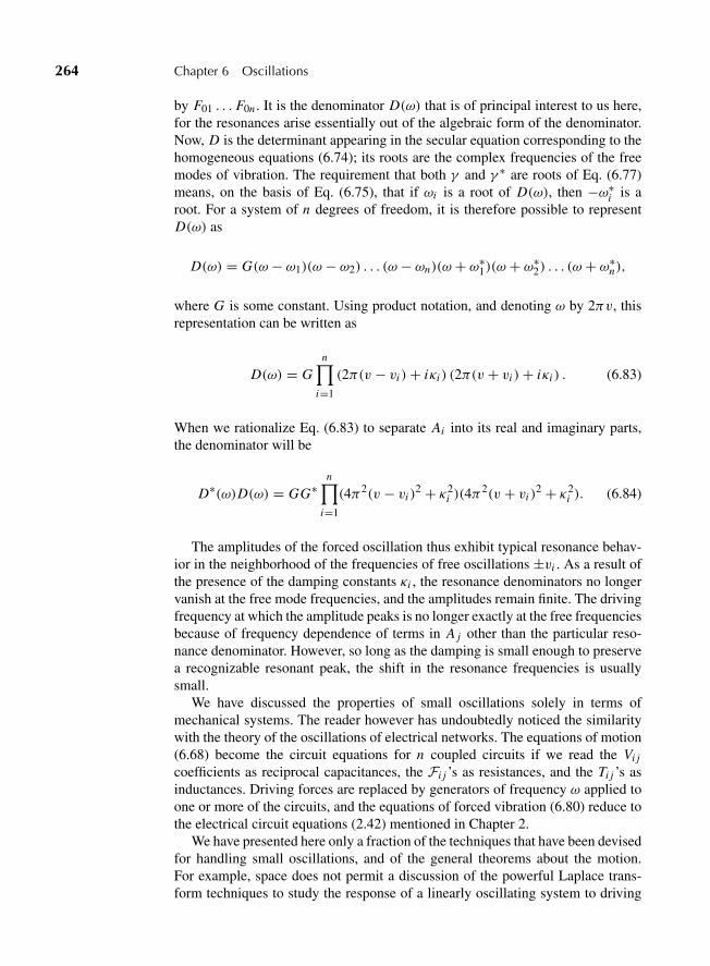
“M06 Goldstein ISBN C06” — 2011/2/15 — page 264 — #27
264 Chapter 6 Oscillations
by F01 . . . F0n . It is the denominator D(ω) that is of principal interest to us here,for the resonances arise essentially out of the algebraic form of the denominator.Now, D is the determinant appearing in the secular equation corresponding to thehomogeneous equations (6.74); its roots are the complex frequencies of the freemodes of vibration. The requirement that both γ and γ ∗ are roots of Eq. (6.77)means, on the basis of Eq. (6.75), that if ωi is a root of D(ω), then −ω∗
i is aroot. For a system of n degrees of freedom, it is therefore possible to representD(ω) as
D(ω) = G(ω − ω1)(ω − ω2) . . . (ω − ωn)(ω + ω∗1)(ω + ω∗
2) . . . (ω + ω∗n),
where G is some constant. Using product notation, and denoting ω by 2πv, thisrepresentation can be written as
D(ω) = Gn∏
i=1
(2π(v − vi )+ iκi ) (2π(v + vi )+ iκi ) . (6.83)
When we rationalize Eq. (6.83) to separate Ai into its real and imaginary parts,the denominator will be
D∗(ω)D(ω) = GG∗n∏
i=1
(4π2(v − vi )2 + κ2
i )(4π2(v + vi )
2 + κ2i ). (6.84)
The amplitudes of the forced oscillation thus exhibit typical resonance behav-ior in the neighborhood of the frequencies of free oscillations ±vi . As a result ofthe presence of the damping constants κi , the resonance denominators no longervanish at the free mode frequencies, and the amplitudes remain finite. The drivingfrequency at which the amplitude peaks is no longer exactly at the free frequenciesbecause of frequency dependence of terms in A j other than the particular reso-nance denominator. However, so long as the damping is small enough to preservea recognizable resonant peak, the shift in the resonance frequencies is usuallysmall.
We have discussed the properties of small oscillations solely in terms ofmechanical systems. The reader however has undoubtedly noticed the similaritywith the theory of the oscillations of electrical networks. The equations of motion(6.68) become the circuit equations for n coupled circuits if we read the Vi j
coefficients as reciprocal capacitances, the Fi j ’s as resistances, and the Ti j ’s asinductances. Driving forces are replaced by generators of frequency ω applied toone or more of the circuits, and the equations of forced vibration (6.80) reduce tothe electrical circuit equations (2.42) mentioned in Chapter 2.
We have presented here only a fraction of the techniques that have been devisedfor handling small oscillations, and of the general theorems about the motion.For example, space does not permit a discussion of the powerful Laplace trans-form techniques to study the response of a linearly oscillating system to driving
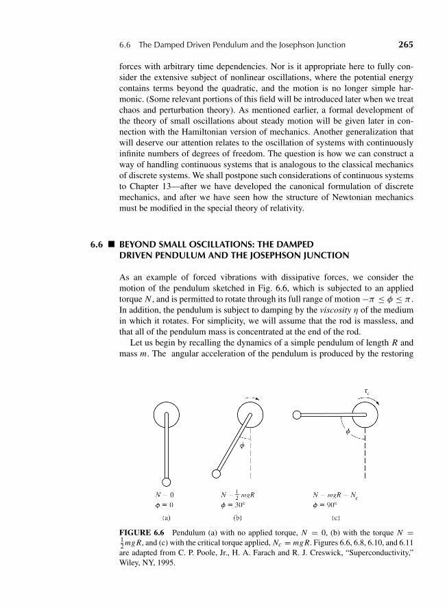
“M06 Goldstein ISBN C06” — 2011/2/15 — page 265 — #28
6.6 The Damped Driven Pendulum and the Josephson Junction 265
forces with arbitrary time dependencies. Nor is it appropriate here to fully con-sider the extensive subject of nonlinear oscillations, where the potential energycontains terms beyond the quadratic, and the motion is no longer simple har-monic. (Some relevant portions of this field will be introduced later when we treatchaos and perturbation theory). As mentioned earlier, a formal development ofthe theory of small oscillations about steady motion will be given later in con-nection with the Hamiltonian version of mechanics. Another generalization thatwill deserve our attention relates to the oscillation of systems with continuouslyinfinite numbers of degrees of freedom. The question is how we can construct away of handling continuous systems that is analogous to the classical mechanicsof discrete systems. We shall postpone such considerations of continuous systemsto Chapter 13—after we have developed the canonical formulation of discretemechanics, and after we have seen how the structure of Newtonian mechanicsmust be modified in the special theory of relativity.
6.6 BEYOND SMALL OSCILLATIONS: THE DAMPEDDRIVEN PENDULUM AND THE JOSEPHSON JUNCTION
As an example of forced vibrations with dissipative forces, we consider themotion of the pendulum sketched in Fig. 6.6, which is subjected to an appliedtorque N , and is permitted to rotate through its full range of motion −π ≤ φ ≤ π .In addition, the pendulum is subject to damping by the viscosity η of the mediumin which it rotates. For simplicity, we will assume that the rod is massless, andthat all of the pendulum mass is concentrated at the end of the rod.
Let us begin by recalling the dynamics of a simple pendulum of length R andmass m. The angular acceleration of the pendulum is produced by the restoring
FIGURE 6.6 Pendulum (a) with no applied torque, N = 0, (b) with the torque N =12 mgR, and (c) with the critical torque applied, Nc = mgR. Figures 6.6, 6.8, 6.10, and 6.11are adapted from C. P. Poole, Jr., H. A. Farach and R. J. Creswick, “Superconductivity,”Wiley, NY, 1995.

“M06 Goldstein ISBN C06” — 2011/2/15 — page 266 — #29
266 Chapter 6 Oscillations
gravitational torque mgR sinφ corresponding to the equation of motion
m R2 d2φ
dt2+ mgR sinφ = 0, (6.85)
where I = m R2 is the moment of inertia. For small angular displacements, theapproximation sinφ ≈ φ linearizes the problem by making the torque propor-tional to the displacement, and the motion is simple harmonic, φ = φ0 sinωt withthe characteristic frequency ω0
ω0 =( g
R
)1/2(6.86)
If a torque N is applied to a stationary pendulum, it will swing out through anangle φ. The force of gravity acting on the mass m provides the restoring torquemgR sinφ, as we noted above, and the pendulum assumes an equilibrium positionat the angle φ given by
N = mgR sinφ
(dφ
dt= 0
), (6.87)
as indicated in Fig. 6.6b. The greater the torque, the larger the angle φ. There isa critical torque Nc indicated on Fig. 6.6(c) for which the angle φ assumes thevalue π/2:
Nc = mgR. (6.88)
If N exceeds this critical value, then the applied torque becomes larger than therestoring torque, N > mgR sinφ, for all angles φ. As a result, the pendulum willbegin to rotate beyond φ = π/2, and it will continue to rotate as long as the torqueN > Nc is applied. The motion will take place at a variable angular speed ω
ω = dφ
dt, (6.89)
and it can persist if the torque is later removed.With these facts in mind, let us proceed to examine the case of the damped
pendulum assuming that the damping force Fdamp = ηω is proportional to theangular velocity ω. To write the differential equation of its motion, we add therestoring and damping torques mgR sinφ and η dφ/dt , respectively, to Eq. (6.85):
N = m R2 d2φ
dt2+ ηdφ
dt+ mgR sinφ. (6.90)
If we define a critical frequency ωc corresponding to the angular speed at whichthe damping torque ηω equals the critical torque mgR,
ωc = mgR
η= Nc
η, (6.91)
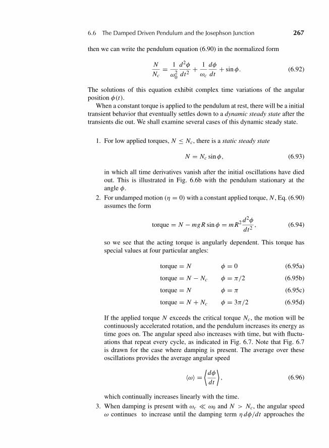
“M06 Goldstein ISBN C06” — 2011/2/15 — page 267 — #30
6.6 The Damped Driven Pendulum and the Josephson Junction 267
then we can write the pendulum equation (6.90) in the normalized form
N
Nc= 1
ω20
d2φ
dt2+ 1
ωc
dφ
dt+ sinφ. (6.92)
The solutions of this equation exhibit complex time variations of the angularposition φ(t).
When a constant torque is applied to the pendulum at rest, there will be a initialtransient behavior that eventually settles down to a dynamic steady state after thetransients die out. We shall examine several cases of this dynamic steady state.
1. For low applied torques, N ≤ Nc, there is a static steady state
N = Nc sinφ, (6.93)
in which all time derivatives vanish after the initial oscillations have diedout. This is illustrated in Fig. 6.6b with the pendulum stationary at theangle φ.
2. For undamped motion (η = 0)with a constant applied torque, N , Eq. (6.90)assumes the form
torque = N − mgR sinφ = m R2 d2φ
dt2, (6.94)
so we see that the acting torque is angularly dependent. This torque hasspecial values at four particular angles:
torque = N φ = 0 (6.95a)
torque = N − Nc φ = π/2 (6.95b)
torque = N φ = π (6.95c)
torque = N + Nc φ = 3π/2 (6.95d)
If the applied torque N exceeds the critical torque Nc, the motion will becontinuously accelerated rotation, and the pendulum increases its energy astime goes on. The angular speed also increases with time, but with fluctu-ations that repeat every cycle, as indicated in Fig. 6.7. Note that Fig. 6.7is drawn for the case where damping is present. The average over theseoscillations provides the average angular speed
〈ω〉 =⟨
dφ
dt
⟩, (6.96)
which continually increases linearly with the time.
3. When damping is present with ωc � ω0 and N > Nc, the angular speedω continues to increase until the damping term η dφ/dt approaches the
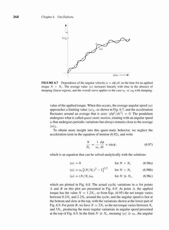
“M06 Goldstein ISBN C06” — 2011/2/15 — page 268 — #31
268 Chapter 6 Oscillations
FIGURE 6.7 Dependence of the angular velocity ω = dφ/dt on the time for an appliedtorque N > Nc. The average value 〈ω〉 increases linearly with time in the absence ofdamping (linear region), and the overall curve applies to the case ωe � ω0 with damping.
value of the applied torque. When this occurs, the average angular speed 〈ω〉approaches a limiting value 〈ω〉L , as shown in Fig. 6.7, and the accelerationfluctuates around an average that is zero: 〈dφ2/dt2〉 = 0. The pendulumundergoes what is called quasi-static motion, rotating with an angular speedω that undergoes periodic variations but always remains close to the average〈ω〉L .
To obtain more insight into this quasi-static behavior, we neglect theacceleration term in the equation of motion (6.92), and write
N
Nc= 1
ωc
dφ
dt+ sinφ, (6.97)
which is an equation that can be solved analytically with the solutions
〈ω〉 = 0 for N < Nc (6.98a)
〈ω〉 = ωc[(N/Nc)
2 − 1]1/2 for N > Nc (6.98b)
〈ω〉 = (N/Nc)ωc for N � Nc, (6.98c)
which are plotted in Fig. 6.8. The actual cyclic variations in ω for pointsA and B on this plot are presented in Fig. 6.9. At point A, the appliedtorque has the value N = 1.2Nc, so from Eqs. (6.95) the net torque variesbetween 0.2Nc and 2.2Nc around the cycle, and the angular speed is fast atthe bottom and slow at the top, with the variations shown at the lower part ofFig. 6.9. For point B, we have N = 2Nc so the net torque varies between Nc
and 3Nc, producing the more regular variations in angular speed presentedat the top of Fig. 6.9. In the limit N � Nc, meaning 〈ω〉 � ωc, the angular

“M06 Goldstein ISBN C06” — 2011/2/15 — page 269 — #32
6.6 The Damped Driven Pendulum and the Josephson Junction 269
FIGURE 6.8 Relationship between the applied torque N and the average angular veloc-ity 〈ω〉 for ωc � ω0. We see that 〈ω〉 = 0 for N < Nc and 〈ω〉 increases with increasingN > Nc.
FIGURE 6.9 Oscillations at points A (N = 1.2Nc) and B (2Nc) for ωc � ω0 indicatedon Fig. 6.8 for the damped harmonic oscillator. Adapted from A. Barone and G. Paterno,“Physics and Applications of the Josephson Effect,” Wiley, NY, 1982.

“M06 Goldstein ISBN C06” — 2011/2/15 — page 270 — #33
270 Chapter 6 Oscillations
speed begins to approximate a sinusoidal variation with time
ω(t) ≈ 〈ω〉 + α sin�t, (6.99)
which approximates point B in Fig. 6.8.
4. For the negligible damping case (η → 0 and ωc � ω0), the steady-statesolution (6.98a) can still occur for N < Nc with the pendulum held fixedat the angle φ defined by Eq. (6.93), which means that ω = 〈ω〉 = 0.In addition, the solution, (6.98c), in which the torque balances the timeaveraged damping force, now applies for all values of N , both less than andgreater than Nc, and so we have
ω = 0 for N ≤ Nc (6.100a)
〈ω〉 = (N/Nc)ωc for 0 ≤ N (6.100b)
These solutions are plotted in Fig. 6.10. Note from the figure that the sys-tem exhibits hysteresis, meaning that the behavior differs for increasing anddecreasing torques. When the torque is increased for N < Nc, the pen-dulum is stabilized at the angle φ satisfying the relation N = Nc sinφof Eq. (6.87), so ω = 0 via Eq. (6.100a). When N reaches the criticaltorque Nc, the angular speed jumps to the value ωc, and then rises linearlywith further increases in N , as shown in the figure. For decreasing torques,Eq. (6.100b) applies, and 〈ω〉 remains proportional to N all the way to theorigin, as shown.
5. Figure 6.8 shows the response for ωc � ω0, Fig. 6.10 presents it forωc � ω0, and the question arises as to what is the behavior for an inter-mediate condition such as ωc ≈ ω0? This requires solving the general
FIGURE 6.10 Relationship between the applied torque N and the average angularvelocity 〈ω〉 for ωc � ω0. There is hysteresis for the behavior when 〈ω〉 < ωc.
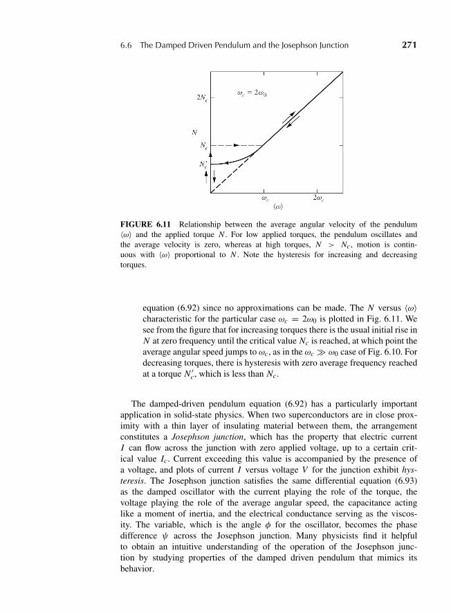
“M06 Goldstein ISBN C06” — 2011/2/15 — page 271 — #34
6.6 The Damped Driven Pendulum and the Josephson Junction 271
FIGURE 6.11 Relationship between the average angular velocity of the pendulum〈ω〉 and the applied torque N . For low applied torques, the pendulum oscillates andthe average velocity is zero, whereas at high torques, N > Nc, motion is contin-uous with 〈ω〉 proportional to N . Note the hysteresis for increasing and decreasingtorques.
equation (6.92) since no approximations can be made. The N versus 〈ω〉characteristic for the particular case ωc = 2ω0 is plotted in Fig. 6.11. Wesee from the figure that for increasing torques there is the usual initial rise inN at zero frequency until the critical value Nc is reached, at which point theaverage angular speed jumps to ωc, as in the ωc � ω0 case of Fig. 6.10. Fordecreasing torques, there is hysteresis with zero average frequency reachedat a torque N ′
c, which is less than Nc.
The damped-driven pendulum equation (6.92) has a particularly importantapplication in solid-state physics. When two superconductors are in close prox-imity with a thin layer of insulating material between them, the arrangementconstitutes a Josephson junction, which has the property that electric currentI can flow across the junction with zero applied voltage, up to a certain crit-ical value Ic. Current exceeding this value is accompanied by the presence ofa voltage, and plots of current I versus voltage V for the junction exhibit hys-teresis. The Josephson junction satisfies the same differential equation (6.93)as the damped oscillator with the current playing the role of the torque, thevoltage playing the role of the average angular speed, the capacitance actinglike a moment of inertia, and the electrical conductance serving as the viscos-ity. The variable, which is the angle φ for the oscillator, becomes the phasedifference ψ across the Josephson junction. Many physicists find it helpfulto obtain an intuitive understanding of the operation of the Josephson junc-tion by studying properties of the damped driven pendulum that mimics itsbehavior.

“M06 Goldstein ISBN C06” — 2011/2/15 — page 272 — #35
272 Chapter 6 Oscillations
DERIVATIONS
1. The problem of the linear triatomic molecule can be reduced to one of two degrees offreedom by introducing coordinates y1 = x2−x1, y2 = x3−x2, and eliminating x2 byrequiring that the center of mass remain at rest. Obtain the frequencies of the normalmodes in these coordinates and show that they agree with the results of Section 6.4.The distances between the atoms, y1 and y2, are known as internal coordinates.
2. Obtain the frequencies of longitudinal vibration of the molecule discussed in Sec-tion 6.4, except that now the center atom is to be considered bound to the origin by aspring of force constant k. Show that the translational mode disappears.
EXERCISES
3. A bead of mass m is constrained to move on a hoop of radius R. The hoop rotateswith constant angular velocity ω around a diameter of the hoop, which is a verticalaxis (line along which gravity acts).
(a) set up the Lagrangian and obtain the equations of motion of the bead.
(b) Find the critical angular velocity � below which the bottom of the hoop providesa stable equilibrium for the bead.
(c) Find the stable equilibrium position for ω > �.
4. Obtain the normal modes of vibration for the double pendulum shown in Fig. 1.4,assuming equal lengths, but not equal masses. Show that when the lower mass issmall compared to the upper one, the two resonant frequencies are almost equal. If thependula are set in motion by pulling the upper mass slightly away from the verticaland then releasing it, show that subsequent motion is such that at regular intervals onependulum is at rest while the other has its maximum amplitude. This is the familiarphenomenon of “beats.”
5. (a) In the linear triatomic molecule, suppose the initial condition is that the centeratom is at rest but displaced by an amount a0 from equilibrium, the other twobeing at their equilibrium points. Find the amplitudes of the longitudinal smalloscillations about the center of mass. Give the amplitudes of the normal modes.
(b) Repeat part (a) but with the center atom initially at its equilibrium position butwith an initial speed v0.
6. A spring of force constant 3 Nm−1 is connected between two identical simple pen-dulums, each of length 0.8 m. Calculate the period of the other pendulum if one isdamped taking the mass of each bob as 0.23 kg (g = 10 m/s2).
7. In the linear triatomic molecule, suppose that motion in the y and z directions isgoverned by the potentials
Vy = k
2(y2 − y1)
2 + k
2(y3 − y2)
2,
Vz = k
2(z2 − z1)
2 + k
2(z3 − z2)
2.
Find the eigenfrequencies for small vibrations in three dimensions and describe thenormal modes. What symmetries do the zero frequencies represent? You may want touse the kind of intermediate coordinates suggested in Exercise 6.
“M06 Goldstein ISBN C06” — 2011/2/15 — page 273 — #36
Exercises 273
8. The equilibrium configuration of a molecule is represented by three atoms of equalmass at the vertices of a 45◦ right triangle connected by springs of equal force con-stant. Obtain the secular determinant for the modes of vibration in the plane and showby rearrangement of the columns that the secular equation has a triple root ω = 0.Reduce the determinant to one of third rank and obtain the nonvanishing frequenciesof free vibration.
9. Calculate the force constant of a harmonic oscillator if its resting position potentialenergy is 8 joule and the total energy is 13 joule. [Given: the amplitude as 1 m.]
10. (a) Three equal mass points have equilibrium positions at the vertices of an equi-lateral triangle. They are connected by equal springs that lie along the arcs ofthe circle circumscribing the triangle. Mass points and springs are constrained tomove only on the circle, so that, for example, the potential energy of a spring isdetermined by the arc length covered. Determine the eigenfrequencies and normalmodes of small oscillations in the plane. Identify physically any zero frequencies.
(b) Suppose one of the springs has a change in force constant δk, the others remainingunchanged. To first order in δk, what are the changes in the eigenfrequencies andnormal modes?
(c) Suppose what is changed is the mass of one of the particles by an amount δm.Now how do the normal eigenfrequencies and normal modes change?
11. A uniform bar of length l and mass m is suspended by two equal springs of equilibriumlength b and force constant k, as shown in the diagram.
Find the normal modes of small oscillation in the plane.
12. Two particles move in one dimension at the junction of three springs, as shown in thefigure. The springs all have unstretched lengths equal to a, and the force constants andmasses are shown.
Find the eigenfrequencies and normal modes of the system.
13. Two mass points of equal mass m are connected to each other and to fixed points bythree equal springs of force constant k, as shown in the diagram.

“M06 Goldstein ISBN C06” — 2011/2/15 — page 274 — #37
274 Chapter 6 Oscillations
The equilibrium length of each spring is a. Each mass point has a positive charge +q ,and they repel each other according to the Coulomb law. Set up the secular equationfor the eigenfrequencies.
14. Find expressions for the eigenfrequencies of the following electrical coupled circuit:
15. If the generalized driving forces Qi are not sinusoidal, show that the forced vibrationsof the normal coordinates in the absence of damping are given by
ζi =1√2π
∫ +∞
−∞Gi (ω)
ω2i − ω2
e−iωt dω,
where Gi (ω) is the Fourier transform of Qi defined by
Qi (t) =1√2π
∫ +∞
−∞Gi (ω)e
−iωt dω.
If the dissipation function is simultaneously diagonalized along with T and V , showthat the forced vibrations are given by
ζi =1√2π
∫ +∞
−∞Gi (ω)(ω
2i − ω2 + iωFi )
(ω2i − ω2)2 + ω2F2
i
e−iωt dt,
which has the typical resonance denominator form. These results are simple illus-trations of the powerful technique of the operational calculus for handling transientvibrations.
16. A mass particle moves in a constant vertical gravitational field along the curve definedby y = ax4, where y is the vertical direction. Find the equation of motion for smalloscillations about the position of equilibrium.
17. A plane triatomic molecule consists of equal masses m at vertices of an equilateraltriangle of sides a. Assume the molecule is held together by forces that are harmonicfor small oscillations and that the force constants are identical and equal to k. Allowmotion only in the plane of the molecule.
(a) Without writing the equations of motion, justify your reasoning on the number ofnormal modes of the system and how many of these modes have zero frequency.
(b) One of the normal modes corresponds to a symmetrical stretching of all threevertices of the molecule. Find the frequency of this mode.
18. A particle in an isotropic three-dimensional harmonic oscillator potential has a naturalfrequency of ω0. Assume the particle is charged and that crossed static electric andmagnetic fields are applied. Find the vibration frequencies with these electromagneticfields present. Discuss the results for the limits of strong and weak fields.
“M06 Goldstein ISBN C06” — 2011/2/15 — page 275 — #38
Exercises 275
19. Show for the case V11 > V22 > 0 and V12 = V21 = 0 in Eq. (6.27) that there are twonormal modes with frequencies ω1 = (V11)
1/2 and ω2 = (V22)1/2. Reintroduce the
mass factor m and describe a physical system that would show this behavior for smalloscillations.
20. Write the Lagrangian for the case V11 = V22 = 0 and V12 = V21 > 0 for the examplediscussed in Eqs. (6.27) to (6.30). Show there is one normal mode of simple harmonicmotion with the frequency ω1 = (V12)
1/2, and a second mode in which the particleis unbound, receding exponentially to infinity for long time t > τ in accordance withthe expression e−t/τ , where the parameter τ is given by τ = (V12)
−1/2. For thisunbounded mode, how does the distance depend upon time when t < τ? What is thenature of the point x1 = x2 = 0? Restate your results with the mass parameter mincluded explicitly.
21. Write the Lagrangian discussed in Eqs. (6.27) to (6.30) in polar coordinates for thecase V11 = V22 > 0 and V12 = V21 = 0. Show that there is a radial normal mode r =r0 cos(ωt) with frequency ω = (V11)
1/2 when the angular momentum is zero. Showthat in the case of nonzero angular momentum, the angular momentum is conservedand the particle can no longer reach r = 0. Write the fictitious potential energy V ′(r)(Chapter 3) for nonzero angular momentum. When finished, reintroduce the massparameter, m, into all equations.
22. Repeat Exercise 21 with the conditions V11 > V22 > 0 and V12 = V21 = 0 anddiscuss your results in terms of the effective potential energy of Chapter 3.
23. Make a full analysis of the example discussed in Eqs. (6.27) to (6.30).
“M07 Goldstein ISBN C07” — 2011/2/15 — page 276 — #1
C H A P T E R
7 The Classical Mechanics of theSpecial Theory of Relativity
At the end of the nineteenth century, the physics community had two incom-patible descriptions of phenomena, Newtonian mechanics and Maxwellian elec-tromagnetic theory. Newtonian mechanics assumed that all inertial frames wereequivalent, while Maxwell’s wave equations gave a universal speed of light thatimplied a preferred inertial frame. Albert Einstein developed the special theory ofrelativity to replace Newtonian mechanics with a theory that was consistent withelectromagnetic theory without this implication. After a brief historical survey,we shall review the assumptions of the special theory and the consequences ofthese assumptions. We shall then examine the formalism of the geometric pictureof spacetime that results. Lastly, we develop a Lagrangian formalism and studyattempts to express the results in a proper relativistic form.
In Newtonian mechanics, a set of well-verified laws applies in an inertial frameof reference defined by the first law. Any frame moving at constant velocitywith respect to an inertial frame is also an inertial frame. Consider two framesdenoted by S and S′ with (t, x, y, z) and (t ′, x ′, y′, z′) the coordinates in S andS′, respectively. Without loss of generality, we assume the coordinate axes arealigned, x along x ′, and so on. Let S′ be moving relative to S in the +x-directionat a speed v, as shown in Figure 7.1.
Newtonian mechanics assumes the spacetime coordinates in S are related tothose in S′ by the simple expressions
t ′ = t,
x ′ = x − vt,
y′ = y, (7.1)
z′ = z.
Transformations of this type are called Galilean transformations. Under thisassumption, it follows that Newton’s second law,
F = d
dtp,
relating the applied force (F) and the momentum (p) remains invariant, and
F′ = d
dt ′p′ and t ′ = t. (7.2)
276
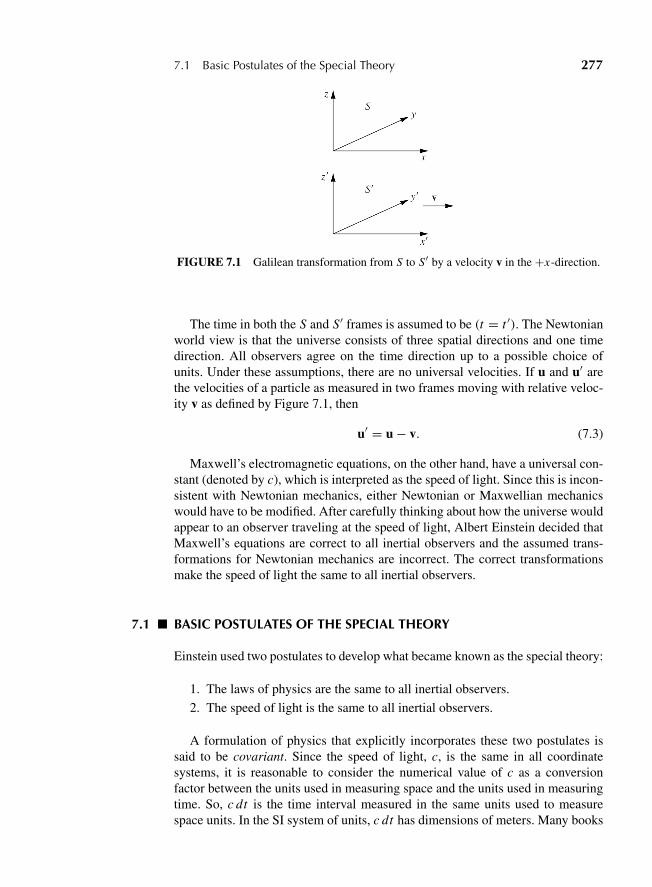
“M07 Goldstein ISBN C07” — 2011/2/15 — page 277 — #2
7.1 Basic Postulates of the Special Theory 277
FIGURE 7.1 Galilean transformation from S to S′ by a velocity v in the +x-direction.
The time in both the S and S′ frames is assumed to be (t = t ′). The Newtonianworld view is that the universe consists of three spatial directions and one timedirection. All observers agree on the time direction up to a possible choice ofunits. Under these assumptions, there are no universal velocities. If u and u′ arethe velocities of a particle as measured in two frames moving with relative veloc-ity v as defined by Figure 7.1, then
u′ = u − v. (7.3)
Maxwell’s electromagnetic equations, on the other hand, have a universal con-stant (denoted by c), which is interpreted as the speed of light. Since this is incon-sistent with Newtonian mechanics, either Newtonian or Maxwellian mechanicswould have to be modified. After carefully thinking about how the universe wouldappear to an observer traveling at the speed of light, Albert Einstein decided thatMaxwell’s equations are correct to all inertial observers and the assumed trans-formations for Newtonian mechanics are incorrect. The correct transformationsmake the speed of light the same to all inertial observers.
7.1 BASIC POSTULATES OF THE SPECIAL THEORY
Einstein used two postulates to develop what became known as the special theory:
1. The laws of physics are the same to all inertial observers.
2. The speed of light is the same to all inertial observers.
A formulation of physics that explicitly incorporates these two postulates issaid to be covariant. Since the speed of light, c, is the same in all coordinatesystems, it is reasonable to consider the numerical value of c as a conversionfactor between the units used in measuring space and the units used in measuringtime. So, c dt is the time interval measured in the same units used to measurespace units. In the SI system of units, c dt has dimensions of meters. Many books
“M07 Goldstein ISBN C07” — 2011/2/15 — page 278 — #3
278 Chapter 7 The Classical Mechanics of the Special Theory of Relativity
and articles on relativity set c = 1 and measure time and space in meters. In thematerial that follows, we shall show the explicit dependence upon c.
To satisfy the two postulates, the space and time of the special theory consistof a single entity that we refer to as spacetime. This spacetime is the geometricframework within which we perform physics. We cannot assume that all observersmake the same division into time and space in the same way. The separation isunique to each inertial frame. The square of the distance in that spacetime, �s2,between two points A and B is given by
(�s)2 = c2(time interval)2 − (space interval)2, (7.4)
where the interval is between the two points A and B. If the separation of theinterval is assumed to be infinitesimal, the� is replaced by the differential symbold. Since a point in spacetime consists of a specification of three spatial coordinatevalues and one time value, the usual convention is to refer to a point in spacetimeas an event. The term event is used because such a point has a definite locationand a definite time in any frame.
The choice of opposite signs for the time and space intervals is intrinsic tothe theory; however, the choice of a positive sign for (c dt)2 is arbitrary. Someauthors define a (ds)2, which is the negative of the choice given in Eq. (7.4). Allsign choices makes (ds)2 = 0 according to the definition in Eq. (7.4) for light,since the space interval is ±(c × time interval). The choice made here for therelative signs used for space and time is such that real bodies moving at a velocityless than light have (ds)2 > 0. This makes ds real for bodies moving slower thanlight speed. If (ds)2 > 0, the interval is called timelike. If (ds)2 < 0, the intervalis called spacelike. Intervals for which (ds)2 = 0 are called lightlike or null.
Since, to all inertial observers, objects that travel on timelike paths move lessthan the speed of light, they are called tardyons. Hypothetical bodies that alwaysmove faster than light are called tachyons, but such bodies will not concern ushere. Objects moving at the speed of light are called null or lightlike.
In the limit of small displacements (differential displacements), Eq. (7.4)becomes, in a Cartesian coordinate system,
(ds)2 = (c dt)2 − (dx2 + dy2 + dz2). (7.4′)
The four-dimensional space with an interval defined by Eqs. (7.4) or (7.4′), isoften called Minkowski space to distinguish it from a four-dimensional Euclideanspace for which there would be no minus sign in Eqs. (7.4) or (7.4′). The ideaof using ict for the time coordinate to make the space Euclidean is no longeruseful since it obscures the non-Euclidean nature of spacetime and makes thegeneralization to noninertial frames more difficult.
Since the interval between two events of spacetime is a geometric quantity,all inertial observers measure coordinates that preserve the value of the intervalsquared, (ds)2. If S and S′ are two different inertial frames, then
ds′2 = ds2. (7.5)
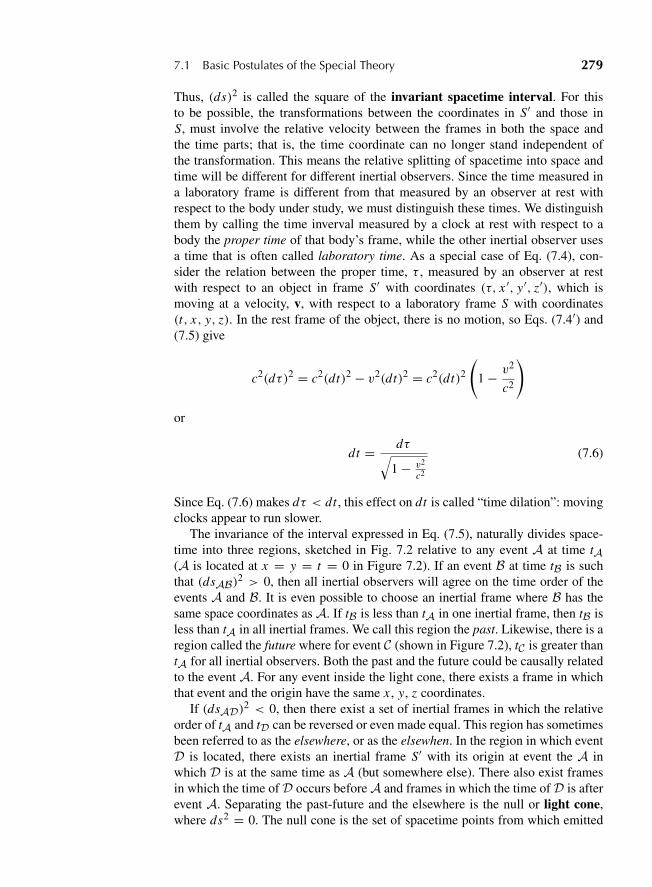
“M07 Goldstein ISBN C07” — 2011/2/15 — page 279 — #4
7.1 Basic Postulates of the Special Theory 279
Thus, (ds)2 is called the square of the invariant spacetime interval. For thisto be possible, the transformations between the coordinates in S′ and those inS, must involve the relative velocity between the frames in both the space andthe time parts; that is, the time coordinate can no longer stand independent ofthe transformation. This means the relative splitting of spacetime into space andtime will be different for different inertial observers. Since the time measured ina laboratory frame is different from that measured by an observer at rest withrespect to the body under study, we must distinguish these times. We distinguishthem by calling the time inverval measured by a clock at rest with respect to abody the proper time of that body’s frame, while the other inertial observer usesa time that is often called laboratory time. As a special case of Eq. (7.4), con-sider the relation between the proper time, τ , measured by an observer at restwith respect to an object in frame S′ with coordinates (τ, x ′, y′, z′), which ismoving at a velocity, v, with respect to a laboratory frame S with coordinates(t, x, y, z). In the rest frame of the object, there is no motion, so Eqs. (7.4′) and(7.5) give
c2(dτ)2 = c2(dt)2 − v2(dt)2 = c2(dt)2(
1 − v2
c2
)
or
dt = dτ√1 − v2
c2
(7.6)
Since Eq. (7.6) makes dτ < dt , this effect on dt is called “time dilation”: movingclocks appear to run slower.
The invariance of the interval expressed in Eq. (7.5), naturally divides space-time into three regions, sketched in Fig. 7.2 relative to any event A at time tA(A is located at x = y = t = 0 in Figure 7.2). If an event B at time tB is suchthat (dsAB)2 > 0, then all inertial observers will agree on the time order of theevents A and B. It is even possible to choose an inertial frame where B has thesame space coordinates as A. If tB is less than tA in one inertial frame, then tB isless than tA in all inertial frames. We call this region the past. Likewise, there is aregion called the future where for event C (shown in Figure 7.2), tC is greater thantA for all inertial observers. Both the past and the future could be causally relatedto the event A. For any event inside the light cone, there exists a frame in whichthat event and the origin have the same x , y, z coordinates.
If (dsAD)2 < 0, then there exist a set of inertial frames in which the relativeorder of tA and tD can be reversed or even made equal. This region has sometimesbeen referred to as the elsewhere, or as the elsewhen. In the region in which eventD is located, there exists an inertial frame S′ with its origin at event the A inwhich D is at the same time as A (but somewhere else). There also exist framesin which the time of D occurs before A and frames in which the time of D is afterevent A. Separating the past-future and the elsewhere is the null or light cone,where ds2 = 0. The null cone is the set of spacetime points from which emitted
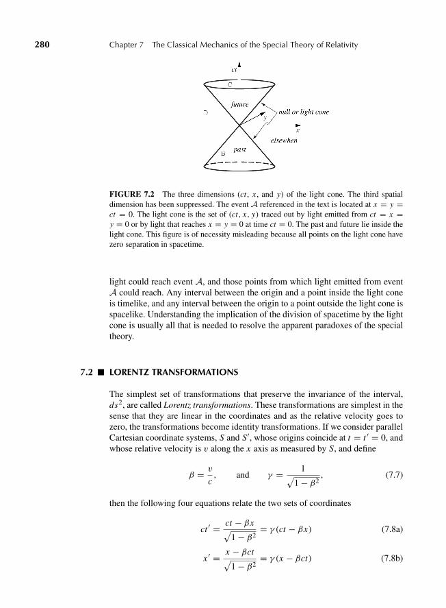
“M07 Goldstein ISBN C07” — 2011/2/15 — page 280 — #5
280 Chapter 7 The Classical Mechanics of the Special Theory of Relativity
FIGURE 7.2 The three dimensions (ct , x , and y) of the light cone. The third spatialdimension has been suppressed. The event A referenced in the text is located at x = y =ct = 0. The light cone is the set of (ct, x, y) traced out by light emitted from ct = x =y = 0 or by light that reaches x = y = 0 at time ct = 0. The past and future lie inside thelight cone. This figure is of necessity misleading because all points on the light cone havezero separation in spacetime.
light could reach event A, and those points from which light emitted from eventA could reach. Any interval between the origin and a point inside the light coneis timelike, and any interval between the origin to a point outside the light cone isspacelike. Understanding the implication of the division of spacetime by the lightcone is usually all that is needed to resolve the apparent paradoxes of the specialtheory.
7.2 LORENTZ TRANSFORMATIONS
The simplest set of transformations that preserve the invariance of the interval,ds2, are called Lorentz transformations. These transformations are simplest in thesense that they are linear in the coordinates and as the relative velocity goes tozero, the transformations become identity transformations. If we consider parallelCartesian coordinate systems, S and S′, whose origins coincide at t = t ′ = 0, andwhose relative velocity is v along the x axis as measured by S, and define
β = v
c, and γ = 1√
1 − β2, (7.7)
then the following four equations relate the two sets of coordinates
ct ′ = ct − βx√1 − β2
= γ (ct − βx) (7.8a)
x ′ = x − βct√1 − β2
= γ (x − βct) (7.8b)
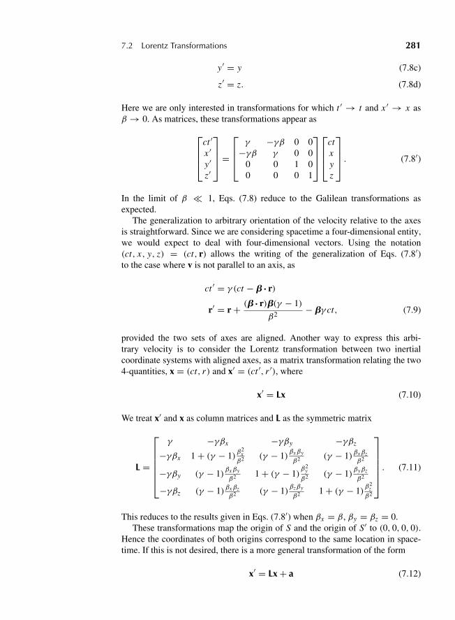
“M07 Goldstein ISBN C07” — 2011/2/15 — page 281 — #6
7.2 Lorentz Transformations 281
y′ = y (7.8c)
z′ = z. (7.8d)
Here we are only interested in transformations for which t ′ → t and x ′ → x asβ → 0. As matrices, these transformations appear as
⎡⎢⎢⎣
ct ′x ′y′z′
⎤⎥⎥⎦ =
⎡⎢⎢⎣γ −γβ 0 0
−γβ γ 0 00 0 1 00 0 0 1
⎤⎥⎥⎦⎡⎢⎢⎣
ctxyz
⎤⎥⎥⎦ . (7.8′)
In the limit of β � 1, Eqs. (7.8) reduce to the Galilean transformations asexpected.
The generalization to arbitrary orientation of the velocity relative to the axesis straightforward. Since we are considering spacetime a four-dimensional entity,we would expect to deal with four-dimensional vectors. Using the notation(ct, x, y, z) = (ct, r) allows the writing of the generalization of Eqs. (7.8′)to the case where v is not parallel to an axis, as
ct ′ = γ (ct − b ? r)
r′ = r + (b ? r)b(γ − 1)
β2− bγ ct, (7.9)
provided the two sets of axes are aligned. Another way to express this arbi-trary velocity is to consider the Lorentz transformation between two inertialcoordinate systems with aligned axes, as a matrix transformation relating the two4-quantities, x = (ct, r) and x′ = (ct ′, r ′), where
x′ = Lx (7.10)
We treat x′ and x as column matrices and L as the symmetric matrix
L =
⎡⎢⎢⎢⎢⎢⎣
γ −γβx −γβy −γβz
−γβx 1 + (γ − 1)β2xβ2 (γ − 1)βxβy
β2 (γ − 1)βxβzβ2
−γβy (γ − 1)βxβy
β2 1 + (γ − 1)β2
y
β2 (γ − 1)βyβz
β2
−γβz (γ − 1)βxβzβ2 (γ − 1)βzβy
β2 1 + (γ − 1)β2
zβ2
⎤⎥⎥⎥⎥⎥⎦ . (7.11)
This reduces to the results given in Eqs. (7.8′) when βx = β, βy = βz = 0.These transformations map the origin of S and the origin of S′ to (0, 0, 0, 0).
Hence the coordinates of both origins correspond to the same location in space-time. If this is not desired, there is a more general transformation of the form
x′ = Lx + a (7.12)
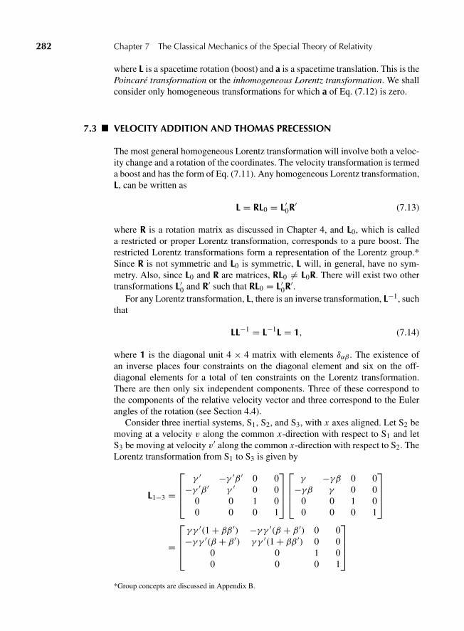
“M07 Goldstein ISBN C07” — 2011/2/15 — page 282 — #7
282 Chapter 7 The Classical Mechanics of the Special Theory of Relativity
where L is a spacetime rotation (boost) and a is a spacetime translation. This is thePoincare transformation or the inhomogeneous Lorentz transformation. We shallconsider only homogeneous transformations for which a of Eq. (7.12) is zero.
7.3 VELOCITY ADDITION AND THOMAS PRECESSION
The most general homogeneous Lorentz transformation will involve both a veloc-ity change and a rotation of the coordinates. The velocity transformation is termeda boost and has the form of Eq. (7.11). Any homogeneous Lorentz transformation,L, can be written as
L = RL0 = L′0R′ (7.13)
where R is a rotation matrix as discussed in Chapter 4, and L0, which is calleda restricted or proper Lorentz transformation, corresponds to a pure boost. Therestricted Lorentz transformations form a representation of the Lorentz group.*Since R is not symmetric and L0 is symmetric, L will, in general, have no sym-metry. Also, since L0 and R are matrices, RL0 �= L0R. There will exist two othertransformations L′0 and R′ such that RL0 = L′0R′.
For any Lorentz transformation, L, there is an inverse transformation, L−1, suchthat
LL−1 = L−1L = 1, (7.14)
where 1 is the diagonal unit 4 × 4 matrix with elements δαβ . The existence ofan inverse places four constraints on the diagonal element and six on the off-diagonal elements for a total of ten constraints on the Lorentz transformation.There are then only six independent components. Three of these correspond tothe components of the relative velocity vector and three correspond to the Eulerangles of the rotation (see Section 4.4).
Consider three inertial systems, S1, S2, and S3, with x axes aligned. Let S2 bemoving at a velocity v along the common x-direction with respect to S1 and letS3 be moving at velocity v′ along the common x-direction with respect to S2. TheLorentz transformation from S1 to S3 is given by
L1−3 =
⎡⎢⎢⎣
γ ′ −γ ′β ′ 0 0−γ ′β ′ γ ′ 0 0
0 0 1 00 0 0 1
⎤⎥⎥⎦⎡⎢⎢⎣γ −γβ 0 0
−γβ γ 0 00 0 1 00 0 0 1
⎤⎥⎥⎦
=
⎡⎢⎢⎣γ γ ′(1 + ββ ′) −γ γ ′(β + β ′) 0 0−γ γ ′(β + β ′) γ γ ′(1 + ββ ′) 0 0
0 0 1 00 0 0 1
⎤⎥⎥⎦
*Group concepts are discussed in Appendix B.
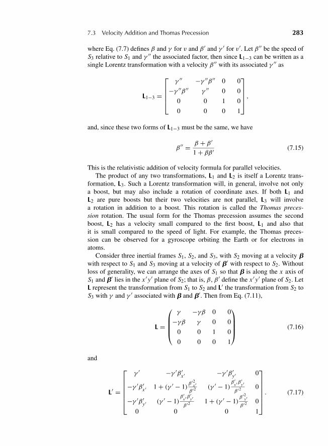
“M07 Goldstein ISBN C07” — 2011/2/15 — page 283 — #8
7.3 Velocity Addition and Thomas Precession 283
where Eq. (7.7) defines β and γ for v and β ′ and γ ′ for v′. Let β ′′ be the speed ofS3 relative to S1 and γ ′′ the associated factor, then since L1−3 can be written as asingle Lorentz transformation with a velocity β ′′ with its associated γ ′′ as
L1−3 =
⎡⎢⎢⎢⎣
γ ′′ −γ ′′β ′′ 0 0
−γ ′′β ′′ γ ′′ 0 0
0 0 1 0
0 0 0 1
⎤⎥⎥⎥⎦ ,
and, since these two forms of L1−3 must be the same, we have
β ′′ = β + β ′1 + ββ ′ (7.15)
This is the relativistic addition of velocity formula for parallel velocities.The product of any two transformations, L1 and L2 is itself a Lorentz trans-
formation, L3. Such a Lorentz transformation will, in general, involve not onlya boost, but may also include a rotation of coordinate axes. If both L1 andL2 are pure boosts but their two velocities are not parallel, L3 will involvea rotation in addition to a boost. This rotation is called the Thomas preces-sion rotation. The usual form for the Thomas precession assumes the secondboost, L2 has a velocity small compared to the first boost, L1 and also thatit is small compared to the speed of light. For example, the Thomas preces-sion can be observed for a gyroscope orbiting the Earth or for electrons inatoms.
Consider three inertial frames S1, S2, and S3, with S2 moving at a velocity bwith respect to S1 and S3 moving at a velocity of b′ with respect to S2. Withoutloss of generality, we can arrange the axes of S1 so that b is along the x axis ofS1 and b′ lies in the x ′y′ plane of S2; that is, β, β ′ define the x ′y′ plane of S2. LetL represent the transformation from S1 to S2 and L′ the transformation from S2 toS3 with γ and γ ′ associated with b and b′. Then from Eq. (7.11),
L =
⎛⎜⎜⎜⎝
γ −γβ 0 0
−γβ γ 0 0
0 0 1 0
0 0 0 1
⎞⎟⎟⎟⎠ (7.16)
and
L′ =
⎡⎢⎢⎢⎢⎢⎣
γ ′ −γ ′β ′x ′ −γ ′β ′y′ 0
−γ ′β ′x ′ 1 + (γ ′ − 1)β ′2x ′β ′2
(γ ′ − 1)β ′
x ′β′y′
β ′20
−γ ′β ′y′ (γ ′ − 1)β ′
x ′β′y′
β ′21 + (γ ′ − 1)
β ′2y′β ′2
0
0 0 0 1
⎤⎥⎥⎥⎥⎥⎦ . (7.17)
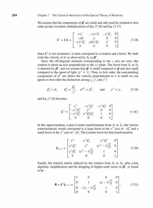
“M07 Goldstein ISBN C07” — 2011/2/15 — page 284 — #9
284 Chapter 7 The Classical Mechanics of the Special Theory of Relativity
We assume that the components of b′ are small and only need be retained to firstorder giving via matrix multiplications of Eq. (7.16) and Eq. (7.17)
L′′ = L′L =
⎡⎢⎢⎣
γ γ ′ −γ γ ′β −γ ′β ′y′ 0−γβ γ 0 0
−γ γ ′β ′y′ γβγ ′β ′y′ γ ′ 00 0 0 1
⎤⎥⎥⎦ (7.18)
Since L′′ is not symmetric, it must correspond to a rotation and a boost. We shallwrite the velocity of S3 as observed by S1 as b′′.
Since the off-diagonal elements corresponding to the z axis are zero, thisrotation is about an axis perpendicular to the xy plane. The boost from S1 to S3is denoted by b′′, and we assume that b′ is small compared to b and also smallcompared to the speed of light (γ ′ ≈ 1). Then, to first order, the nonvanishingcomponents of β ′′ are (Since the velocity perpendicular to x is small we canignore to first order the distinction among y, y′, and y′′)
β ′′x = β, β ′′y = β ′yγ, β ′′2 = β2, and γ ′′ = γ, (7.19)
and Eq. (7.18) becomes
L′′ ≈
⎡⎢⎢⎣
γ ′′ −γ ′′β ′′x −γ ′′β ′′y 0−γ ′′β ′′x γ ′′ 0 0−γ ′′β ′′y γ ′′β ′′x β ′′y 1 0
0 0 0 1
⎤⎥⎥⎦ . (7.18′)
In this approximation, a pure Lorentz transformation from S3 to S1 (the inversetransformation) would correspond to a large boost in the x ′′ axis of −β ′′x and asmall boost in the y′′ axis of −β ′′y . The Lorentz boost for that transformation
L3−1 =
⎡⎢⎢⎢⎢⎣γ ′′ γ ′′β ′′x γ ′′β ′′y 0
γ ′′β ′′x γ ′′ (γ ′′ − 1)β ′′yβ ′′x
0
γ ′′β ′′y (γ ′′ − 1)β ′′yβ ′′x
1 0
0 0 0 1
⎤⎥⎥⎥⎥⎦ . (7.20)
Finally, the rotation matrix induced by the rotation from S1 to S3, after somealgebraic simplification and the dropping of higher-order terms in b′′, is foundto be
R = L′′L3−1 =
⎡⎢⎢⎢⎣
1 0 0 0
0 1 (γ − 1)β ′′yβ
0
0 −(γ − 1)β ′′yβ
1 00 0 0 1
⎤⎥⎥⎥⎦ . (7.21)
“M07 Goldstein ISBN C07” — 2011/2/15 — page 285 — #10
7.3 Velocity Addition and Thomas Precession 285
Comparison with Eq. (4.44) shows that R implies S3 is rotated with respect to S1about the z axis through an infinitesimal angle:
�� = (γ − 1)β ′′yβ
= β ′′yβ(γ − 1
β2
). (7.22)
The spatial rotation resulting from the successive application of two nonparallelLorentz transformations has been declared every bit as paradoxical as the morefrequently discussed apparent violations of common sense, such as the so-called“twin paradox.” But the present apparent paradox has important applications,especially in atomic physics, and therefore has been abundantly verified exper-imentally.
Consider a particle moving in the laboratory system with a velocity v that isnot constant. Since the system in which the particle is at rest is accelerated withrespect to the laboratory, the two systems should not be connected by a Lorentztransformation. We can circumvent this difficulty by a frequently used stratagem(elevated by some to the status of an additional postulate of relativity). We imaginean infinite number of inertial systems moving uniformly relative to the laboratorysystem, one of which instantaneously matches the velocity of the particle. Theparticle is thus instantaneously at rest in an inertial system that can be connected tothe laboratory system by a Lorentz transformation. It is assumed that this Lorentztransformation will also describe the properties of the particle and its true restsystem as seen from the laboratory system.
Suppose now that S1 is the laboratory system, while S2 and S3 are two of theinstantaneous rest systems a time�t apart in the particle’s motion. By Eq. (7.22),the laboratory observer will see a change in the particle’s velocity in this time,�v, which has only a y-component β ′′y c = �v. Since the initial x axis has beenchosen along the direction of v = βc, the vector of the infinitesimal rotation inthis time can be written as
�� = −(γ − 1)v3�vv2
(7.23)
Hence, if the particle has some specific direction attached to it (such as a spinvector), it will be observed from the laboratory system that this direction precesseswith an angular velocity
v = d�
dt= −(γ − 1)
v3 av2
(7.24)
where a is the particle’s acceleration as seen from S1. Equation (7.24) is frequencyencountered in the form it takes when v is small enough that γ can be approxi-mated (using γ ≈ 1 + 1
2β2) as
v = 1
2c2(a3 v). (7.25)
In either form, v is known as the Thomas precession frequency.
“M07 Goldstein ISBN C07” — 2011/2/15 — page 286 — #11
286 Chapter 7 The Classical Mechanics of the Special Theory of Relativity
7.4 VECTORS AND THE METRIC TENSOR
We will use the notation that the coordinates, which need not be Cartesian, arewritten as xμ where x0 = ct is the time coordinate, and x1, x2, x3 are the spacecoordinates. This change in notation is needed to be consistent with the develop-ments in the following sections.
Consider an arbitrary one-dimensional curve in 4-dimensional spacetime, P ,described by a parameter λ, where for a given λ the coordinates of a point ofthe curve can be written as x0(λ), x1(λ), x2(λ), x3(λ). In introductory texts a4-vector, v, is defined by this curve as an arrow whose tail is located at an event Aon the curve and whose head is at an event B on the curve where vAB = PB−PA.However, instead of defining the vector at two points, we can use the parameterλ, which is a measure of the length along the curve from A to B, by writing
vAB =(
dPdλ
)λ=0
. (7.26)
Such a 4-vector is a tangent vector to the curve. We adopt the notation that thecomponents of vectors are written with superscripts such as v0, v1, v2, v3. In spiteof the way we draw tangent vectors, they do not have any extension in spacetime.The arrows we draw simply help us visualize the vector. At each point along thecurve, the tangent vector has a direction and a magnitude. For curves that aretimelike, the proper time, τ , is usually chosen as the parameter λ. The laboratorycoordinates are then x0 = ct (τ ), x1 = x(τ ), x2 = y(τ ), x3 = z(τ ), and thetangent to the curve is the four-velocity, u, of a particle traveling along the curveP . Equation (7.26) becomes
u0 = dct
dτ= γ c, ui = dxi
dτ= γ vi (7.27)
where vi = dxi/dt is the normal three-velocity with v2 = (vx )2 + (vy)2 + (vz)2.We shall assume that Greek letters can take on the values 0–3 and Latin lettersthe values 1–3. Repeated indices are summed. Since the 4-velocity of a particle isdefined over a range of the parameter λ, there is an infinite set of 4-velocities forthe particle, one for each value of λ. Such a set of vectors is termed a vector field.Some common examples of vector fields are given in Table 7.1.
We assume that the components of any 4-vector can be expressed by the val-ues of the vector’s projections along a set of basis vectors, e0, e1, e2, e3, andthat the coordinates are measured along the direction given by the basis vectors.Such a system is called a coordinates basis.* Cartesian, spherical, and cylindricalcoordinate systems, among many possible systems, can have such a basis set. Theposition of a point on the curve P(τ ) can be written as
P(τ ) = xμ(τ)eμ, (7.28)
*The choice of a coordinate basis is arbitrary but avoids some complications. For this introductorychapter we will assume that each basis vector lies in the direction of its increasing coordinate.
“M07 Goldstein ISBN C07” — 2011/2/15 — page 287 — #12
7.4 Vectors and the Metric Tensor 287
TABLE 7.1 Examples of Vector Fields
Time SpaceName Portion Portion (Magnitude)2 Type
Coordinate ct r c2t2 − r2 spacelike, null, or timelike
Velocity γ c γ v c2 timelike
Momentum Ec p m2c2 timelike
Force γc
d Edt γ
dpdt = γF −(FNewtonian)
2 spacelike
Current density γρc γ J ρ2c2 timelike
where repeated Greek indices, one raised and one lowered, are summed from 0to 3. In particular, the 4-velocity given in Eq. (7.27) becomes
u = dPdτ
= dxμ
dτeμ = uμeμ. (7.29)
The magnitude of the 4-velocity is a scalar whose values can vary as wechange λ. This set of magnitudes is an example of a scalar field. To convert a4-vector field to a scalar field, we need what is called a functional,* which canconvert a pair of vectors into a scalar function at each point in spacetime. In otherwords, we wish to define the scalar product of two vectors or vector fields. Thisconversion of a 4-vector field (or two different vector fields) to a scalar field isan example of a mapping. If both the vectors are the same, then this scalar wouldbe the square of the length of the vector, and when the vectors are different, itis called the scalar product of the vectors. Such a functional is called the metrictensor, g.† The metric tensor functional can be considered as a machine with twoslots (both of which are linear) into which you can insert two vectors to producea scalar (real-valued function). That is,
g(u, v) = g(v, u) = u · v, (7.30)
is the scalar product. In particular if the basis vectors are inserted into the metric,
gαβ = g(eα, eβ) = eα · eβ. (7.31)
The gαβ are the components of the metric tensor associated with the basis vec-tors eα . For example, consider a two-dimensional Minkowski space with coordi-nates ct and x and a vector v = (a, b). Then g(v, v) = a2 − b2 and g00 = 1,g11 = −1.
The form of the gαβ is defined by the form for the interval. This suggests thatwe consider small displacements. If the relative displacement vector between two
*A functional is a function whose arguments are themselves functions.†We use the same notation for tensors in 4-space as we do for 4-vectors.
“M07 Goldstein ISBN C07” — 2011/2/15 — page 288 — #13
288 Chapter 7 The Classical Mechanics of the Special Theory of Relativity
points is small, it can be written as
dζ = �xαeα. (7.32)
Recasting Eq. (7.32) in the language of Eq. (7.4′), we see for Minkowskicoordinates
(�s)2 = dζ ? dζ = �xα�xβeα ? eβ = gαβ�xα�xβ
= (c�t)2 − (�x)2 − (�y)2 − (�z)2.
In the limit of infinitesimal displacements this can be written as
ds2 = gαβdxαdxβ, (7.32′)
which holds for any metric tensor. The metric tensor for a Minkowski coordinatesystem, using the +−−− sign convention, has the following tensor representa-tion*
g =
⎛⎜⎜⎝
1 0 0 00 −1 0 00 0 −1 00 0 0 −1
⎞⎟⎟⎠ . (7.33)
The scalar product of two vectors in this coordinate system is
u ? v = uαvβgαβ = u0v0 − u1v1 − u2v2 − u3v3. (7.34)
It is straightforward to show that in any coordinate system, the square of themagnitude of the four-velocity is
u ? u = c2. (7.35)
The 4-momentum can be defined from Eq. (7.27)
p = mu, (7.36)
where the mass, m, is a scalar. So the length squared of the four-momentum is
p ? p = m2c2, (7.37)
or from Eqs. (7.27) and (7.34),
p ? p = m2c2 = m2c2γ 2 − m2v2γ 2 = E2
c2− p2 (7.38)
*The notation used for the display of a matrix is [ ], while for tensors ( ) will be used as it wasin Chapter 5. Matrices are used for relating different coordinate frames while tensors are physicalgeometric objects.
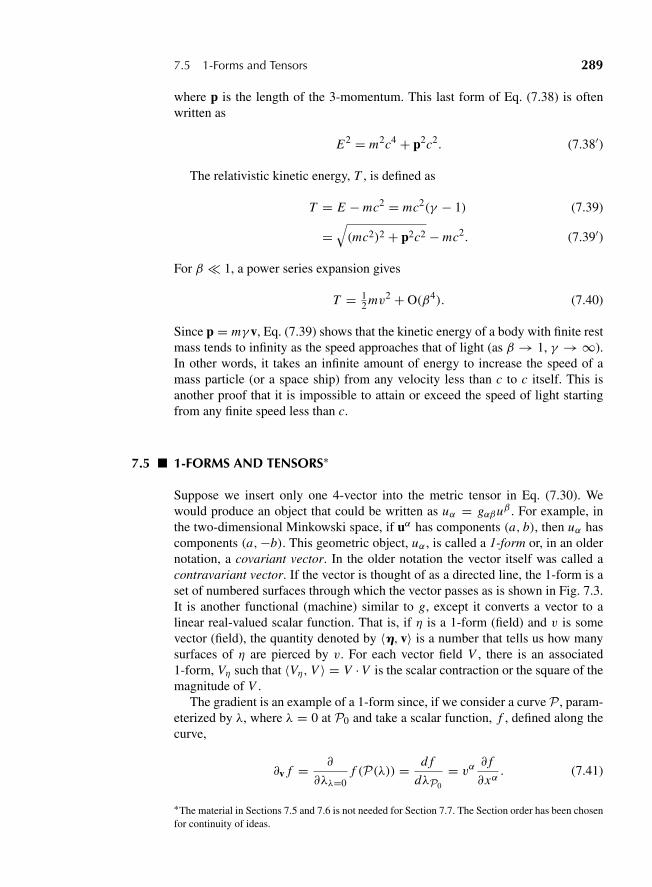
“M07 Goldstein ISBN C07” — 2011/2/15 — page 289 — #14
7.5 1-Forms and Tensors 289
where p is the length of the 3-momentum. This last form of Eq. (7.38) is oftenwritten as
E2 = m2c4 + p2c2. (7.38′)
The relativistic kinetic energy, T , is defined as
T = E − mc2 = mc2(γ − 1) (7.39)
=√(mc2)2 + p2c2 − mc2. (7.39′)
For β � 1, a power series expansion gives
T = 12 mv2 + O(β4). (7.40)
Since p = mγ v, Eq. (7.39) shows that the kinetic energy of a body with finite restmass tends to infinity as the speed approaches that of light (as β → 1, γ → ∞).In other words, it takes an infinite amount of energy to increase the speed of amass particle (or a space ship) from any velocity less than c to c itself. This isanother proof that it is impossible to attain or exceed the speed of light startingfrom any finite speed less than c.
7.5 1-FORMS AND TENSORS∗
Suppose we insert only one 4-vector into the metric tensor in Eq. (7.30). Wewould produce an object that could be written as uα = gαβuβ . For example, inthe two-dimensional Minkowski space, if uα has components (a, b), then uα hascomponents (a,−b). This geometric object, uα , is called a 1-form or, in an oldernotation, a covariant vector. In the older notation the vector itself was called acontravariant vector. If the vector is thought of as a directed line, the 1-form is aset of numbered surfaces through which the vector passes as is shown in Fig. 7.3.It is another functional (machine) similar to g, except it converts a vector to alinear real-valued scalar function. That is, if η is a 1-form (field) and v is somevector (field), the quantity denoted by 〈h, v〉 is a number that tells us how manysurfaces of η are pierced by v. For each vector field V , there is an associated1-form, Vη such that 〈Vη, V 〉 = V ·V is the scalar contraction or the square of themagnitude of V .
The gradient is an example of a 1-form since, if we consider a curve P , param-eterized by λ, where λ = 0 at P0 and take a scalar function, f , defined along thecurve,
∂v f = ∂
∂λλ=0f (P(λ)) = d f
dλP0
= vα∂ f
∂xα. (7.41)
∗The material in Sections 7.5 and 7.6 is not needed for Section 7.7. The Section order has been chosenfor continuity of ideas.
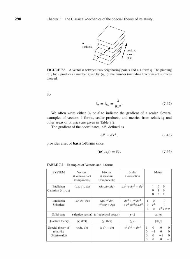
“M07 Goldstein ISBN C07” — 2011/2/15 — page 290 — #15
290 Chapter 7 The Classical Mechanics of the Special Theory of Relativity
FIGURE 7.3 A vector v between two neighboring points and a 1-form η. The piercingof η by v produces a number given by 〈η, v〉, the number (including fractions) of surfacespierced.
So
∂α = ∂eα = ∂
∂xα. (7.42)
We often write either ∂v or d to indicate the gradient of a scalar. Severalexamples of vectors, 1-forms, scalar products, and metrics from relativity andother areas of physics are given in Table 7.2.
The gradient of the coordinates, vα , defined as
vα = dxα, (7.43)
provides a set of basis 1-forms since
〈vα, eβ〉 = δαβ , (7.44)
TABLE 7.2 Examples of Vectors and 1-forms
SYSTEM Vectors: 1-forms: Scalar Metric(Contravariant (Covariant ContractionComponents) Components)
Euclidean (dx, dy, dz) (dx, dy, dz) dx2 + dy2 + dz2 1 0 0Cartesian (x, y, z) 0 1 0
0 0 1
EuclideanSpherical
(dr, dθ, dφ) (dr, r2 dθ,r2 sin2 θ dφ)
dr2 + r2 dθ2
+ r2 sin2 θ dφ21 0 00 r2 00 0 r2 sin2 θ
Solid-state r (lattice vector) k (reciprocal vector) r · k varies
Quantum theory |i〉 (ket) 〈 j | (bra) 〈 j |i〉 |i〉〈 j |Special theory of
relativity(Minkowski)
(c dt, dr) (c dt,−dr) c2 dt2 − dr2 1 0 0 00 −1 0 00 0 −1 00 0 0 −1
“M07 Goldstein ISBN C07” — 2011/2/15 — page 291 — #16
7.5 1-Forms and Tensors 291
and any 1-form η can be written as
η = ηαvα. (7.45)
It follows that
〈η, eα〉 = ηα (7.46)
and for any vector, v
〈η, v〉 = ηαvα. (7.47)
This gives us two ways to calculate the scalar product of two vectors v and u.If we define the inverse metric by
gαβgβγ
= δαγ (7.48)
or in index-free notation by
g−1g = gg−1 = 1, (7.48′)
we can convert vectors (uα) to 1-forms (ua) and conversely as
uα = gαβuβ and uα = gαβuβ. (7.49)
We can therefore write for two 4-vectors u and v (or they could be two 1-forms),
u ? v = g(u, v) = gαβuαvβ = uαvα = uαvβgαβ. (7.34′)
Since each 1-form has a unique associated vector, we could use the same symbolfor both. The difference is important only when considering components.
In terms of the two-dimensional example that we previously considered(Minkowski spacetime) with ct and x as the coordinates), if the vector u hascomponents (a, b) and the vector v has components (c, d), the last three terms ofthe preceding equation can be written as
gαβuαvβ = (1)(a)(c)+ (−1)(b)(d) = ac − bd,
uαvα = (a)(c)+ (b)(−d) = ac − bd,
and
uαvβgαβ = (a)(c)(1)+ (b)(d)(−1) = ac − bd.
It may help to consider the relationship between a vector and a 1-form from amore general point of view using the Minkowski two-dimensional space as an
“M07 Goldstein ISBN C07” — 2011/2/15 — page 292 — #17
292 Chapter 7 The Classical Mechanics of the Special Theory of Relativity
example. A vector V in two-dimensional space with basis vectors e1 and e2 canbe written as
V = V 1e1 + V 2e2
In general, it is not necessary that any of the basis vectors be normalized (e1 ? e1 �=1, e2 ? e2 �= 1) or that they be orthogonal (e1 ? e2 �= 0). This means that themagnitude of the scalar product is not conveniently obtained from a simple sumof squares
V ? V =2∑
i, j=1
V i V j = (V 1)2e1 ? e1 + V 1V 2(e1 ? e2 + e2 ? e1)+ (V 2)2e2 ? e2
�=2∑
i=1
V i V i ,
and it does not have the value√(V 1)2 + (V 2)2. One way to obtain the magni-
tude of the vector is to define the dual space with basis vectors v1 and v2 (cf.Eq. (7.43)), which have the properties
e1 ?v1 = v1 ? e1 = e2 ?v2 = v2 ? e2 = 1and e1 ?v2 = v2 ? e1 = e2 ?v1 = v1 ? e2 = 0.
We say that the vector basis, ei , is orthonormal to the 1-form basis vi . The 1-form,v, corresponding to the vector V may be written as
v = v1v1 + v2v2.
This vector has a (magnitude)2 of
(magnitude)2 = v ? V = V ? v = V 1v1 + V 2v2.
When we want to require an object to be expressed in terms of its coordinate basisvectors we will write with a Roman letter (e.g., u) and use Greek letters when itis to be expressed in terms of the basis 1-forms (e.g., η). This same approachprovides the scalar product of two vectors V and U in terms of their associated1-forms v and u as
scalar product = V ? u = v ?U = u ? V = U ? v = V 1u1+V 2u2 = v1U 1+v2U 2.
These results are easily generalized to more dimensions, to spaces that havean indefinite metric, and even to more general spaces, such as those discussed inSection 7.11. For example, in a four-dimensional Minkowski space, the 1-form,v, associated with the vector V , is v0 = V 0, v1 = −V 1, v2 = −V 2, v3 = −V 3,
“M07 Goldstein ISBN C07” — 2011/2/15 — page 293 — #18
7.5 1-Forms and Tensors 293
so the squared length of the vector V is
V 0v0 + V 1v1 + V 2v2 + V 3v3 = V 0V 0 − V 1V 1 − V 2V 2 − V 3V 3.
The Lorentz transformations can be expressed in terms of the basis vectors. Ifwe let x0, x1, x2, x3 be the coordinates in a frame S and xα
′ = xα′(x0, x1, x2, x3)
be the transformed coordinates in the frame S′, then the Lorentz transformationcan be written as
xα′ = Lα
′βxβ and xα = Lαβ ′xβ
′, (7.50)
where Lαβ ′ is the inverse transformation of Lα′β . The basis vectors transform as
eα′ = Lβα′eβ and eα = Lβ′αeβ ′ . (7.51)
Any vector transforms as v = vαeα = vβ′eβ ′ , so 〈η, v〉 = ηαv
α = ηα′vα′ . This
means that 1-forms transform as η = ηαvα = ηα′vα′, and it follows that
vα′ = Lα
′βvβ and vα = Lαβ ′vβ
′, (7.52)
so
vα′ = Lα
′βvβ and vα = Lαβ ′vβ
′, (7.53)
and
ηα′ = Lβα′ηβ and ηα = Lβ′αηβ ′ . (7.54)
To convert vectors, sum on the second (lowered) index of the transformationmatrix. To convert 1-forms, sum on the first (raised) index. In tensor notation,vectors are columns, while 1-forms are rows.
Scalars, vectors and 1-forms are simple examples of geometric objects calledtensors. A tensor is a functional into which we insert p vectors and n 1-formsto produce a mapping onto a scalar. We describe a tensor by saying that it has arank given by the numbers n and p, where n is the number of 1-forms insertionspossible and p is the number of possible vector insertions. A tensor, Q, with n1-form slots and p vector slots is written as Q of rank
(np
). A tensor H of rank(n
p
)is a functional into which we can insert n 1-forms σ, λ, . . . , β and p vec-
tors u, v, . . . , w to produce a scalar. For example, the energy momentum vector(E/c,p) is a tensor of rank
(10
), since contracting it with a 1-form produces a
scalar. An example of an ordinary second-rank tensor is the quadrupole tensor ofrank
(20
).
Although the components of 1-forms are written with their indices down, thenumber of 1-form slots is written as the upper of the two numbers used to give therank of a tensor. This is because in component notation the object generated willhave that number of indices to be contracted with 1-forms. For example, if S is a
“M07 Goldstein ISBN C07” — 2011/2/15 — page 294 — #19
294 Chapter 7 The Classical Mechanics of the Special Theory of Relativity
tensor of rank(2
1
),
S(σαωα, λβω
β, vγ eγ ) = σαλβvγ S(ωα, ωβ, eγ ) = Sαβγ σαλβv
γ , (7.55)
where the Sαβγ are called the components of the tensor S in the chosen coordinateframe. The output of S is a scalar (see Eq. (7.55)), so if we repeat this calcula-tion in another Lorentz frame, we obtain the transformation law for the tensorcomponents under a coordinate transformation,
Sα′β ′γ ′ = Sαβγ Lα
′αLβ
′βLγ γ ′ . (7.56)
The metric tensor can be used to convert indices from vector to 1-form or 1-formto vector; for example,
Sαβγ = gβσ Sασ γ . (7.57)
Hence, any tensor of rank(n
p
)can be converted by the metric tensor, without
loss of information, to any arrangement of tensor and 1-form indices desired aslong as the total number of indices (n + p) is conserved. All of these objects aredifferent coordinate forms of the same geometric object (tensor).
Consider our two-dimensional example with a vector, u, whose componentsare (a, b) and a 1-form, σ , with components (c, d). If we examine a tensor W ofrank
(11
), then, from Eq. (7.55),
W (σ, u) = Wαβσαuβ = W 0
0ca + W 01cb + W 1
0da + W 11db.
Physically, by using sets of vectors, u’s, and 1-forms, σ ’s, and measuring thevalue of the scalar field W (σ, u), the values of the components of Wα
β can bedetermined in one frame. And from Eq. (7.56), specialized to the number andtype of components, the values in all inertial frames are known. In a Minkowskispace with pseudo-Cartesian coordinates, the components of the tensor W of rank(1
1
)can be converted to a corresponding tensor of rank
(02
)using the metric tensor
in Eq. (7.33) {g00 = 1, g11 = g22 = g33 = −1} and the expression in Eq. (7.57)to give the following relations:
W00 = g00W 00 = W 0
0, W01 = g00W 01 = W 0
1,
W10 = g11W 10 = −W 1
0, and W11 = g11W 11 = −W 1
1.
Given any two vectors, we can construct a second-rank tensor by the operationcalled tensor product, T = u ⊗ v. The tensor product is a machine whose outputis a number when the two vectors and the two 1-forms are inserted
(u ⊗ v)(s,l) = 〈s,u〉〈λ, v〉. (7.58)
The components of the tensor product are
T αβ = uαvβ. (7.59)
“M07 Goldstein ISBN C07” — 2011/2/15 — page 295 — #20
7.5 1-Forms and Tensors 295
In our two-dimensional example of vector u with components (a, b) and vectorv with components (c, d), Eq. (7.59) becomes written in tensor form
(T αβ) =(
ac adbc bd
).
This process can be continued and could include 1-forms as well as vectors; forexample, two vectors (u, v) and a 1-form (s) would be written as u ⊗ v ⊗ s.
Other useful operations include the gradient, contraction, the divergence, andthe wedge product. First, let us consider the gradient operation. We used d forthe gradient operation on scalars. For a higher-rank tensor, the gradient is oftendenoted by =. In three-dimensional Cartesian space, � is the operator
� = i∂
∂x+ j
∂
∂y+ k
∂
∂z,
which may also be written as
∂r = e1∂
∂x1+ e2
∂
∂x2+ e3
∂
∂x3.
Returning to 4-dimensions, an example of a more general case, let S be a(0
3
)rank
tensor, then by definition, =S(u, v,w, j) = ∂jS(u, v,w) with the vectors u, v, wheld fixed, and
=S(u, v,w, j) = ∂ξ (Sαβγ uαvβwγ ) = ∂Sαβγ∂xδ
ξ δuαvβwγ = Sαβγ,δξδuαvβwγ .
(7.60)That is, the gradient operates only on the coefficients in the definition of the tensor,not on the included vector fields. Since the vectors and 1-forms in Eq. (7.60) arearbitrary and constant, we can rewrite the preceding as
∂ξ (Sαβγ ) = ∂Sαβγ∂xδ
ξ δ = Sαβγ,δξδ, (7.60′)
where the ξδ define the direction of the gradient, and the last equality showsclearly that the derivative does not operate on the vector given by ξδ .
In Minkowski spacetime, contracting the energy momentum vector (E/c, p)with the charge-current 1-form (rc,−J) produces the scalar (Eρ − p ? J). Thisidea can be extended to reduce the rank of a tensor by a process called contraction.The contraction operation can be performed on any tensor whose total rank (sumof vector and 1-form indices) is equal to or greater than 2. To do this, enter a basisvector in one slot and the corresponding 1-form basis in another slot and sumover the basis, thereby producing a lower-rank tensor. For example, consider the4-index tensor whose components are Rαμβν . We can form a two-index tensorby the inserting a basis 1-form into the first slot of the tensor definition, and the
“M07 Goldstein ISBN C07” — 2011/2/15 — page 296 — #21
296 Chapter 7 The Classical Mechanics of the Special Theory of Relativity
related basis vector in the third slot, and summing over the basis set. Formally,
R(eα, u,wα, v) = M(u, v), (7.61)
or in component form
Mμvuμvν = Rαμανuμvν, (7.62)
which can be written as
Mμν = Rαμαν. (7.62′)
In three-dimensional Cartesian space, the divergence of a vector V is the scalarquantity = ?V = ∂Vx
∂x + ∂Vy∂y + ∂Vz
∂z , while in 4-dimensional space the 4-divergence
is ∂Vμ
∂xμ . In Minkowski spacetime the 4-divergence operator is often denoted by thesame symbol, =, in italics, or by � whose components are
�μ = =μ = vαμ1
∂xα,
with vαμ the 1-form basic components. For example, the continuity equation inelectromagnetic theory is
∂ jμ
∂xμ= � ? J = = ? J = ∂(ρc)
∂ct+ � ? j = ∂ρ
∂t+ � ? j = 0.
The operator =2 (sometimes written as �2) is called the d’Alembertian and is
�2 = =2 = = ?= = gμv∂
∂xμ∂
∂xv= 1
c2
∂2
∂t2−(∂2
∂x2+ ∂2
∂y2+ ∂2
∂z2
)
where the last equality is the expression in Minkowski space with Cartesiancoordinates. The 4-divergence operator on tensors reduces the rank of the tensorby 1. For spacetime tensors, the divergence is written as = ? S and, considering asan example a tensor S with a slot for a 1-form and three vector slots,
� ? S(u, v) = = ? S(u, v) = = ? S(vα, u, v, eα) = Sαβγ,αuβvγ . (7.63)
That is, the gradient of Eq. (7.60) is taken along a basis direction, and then acontraction is formed between this direction and one of the 1-form slots in thetensor. In component form, this reduces to
∇αSαβγ = Sαβγ,α. (7.63′)
The final tensor operator we need is the wedge product, also called the bivectoror biform, which is
u ∧ v = u ⊗ v − v ⊗ u, (7.64)
“M07 Goldstein ISBN C07” — 2011/2/15 — page 297 — #22
7.6 Forces in the Special Theory; Electromagnetism 297
where the tensor product, ⊗, was defined in Eq. (7.58). The wedge product is anantisymmetric vector product. In component form, Eq. (7.64) becomes
(u ∧ v)αβ = uαvβ − vαuβ. (7.64′)
Successive ∧ operations can be strung together just like the ⊗ operator. Thewedge product is useful whenever we deal with antisymmetric expressions. Inparticular, when we look at the electromagnetic field in the next section, we willdiscover that the fundamental field tensor, called Faraday, can be expressed interms of the wedge product.
Consider the two-dimensional example used previously, where u = u1e1 +u2e2 and v = v1e1 + v2e2. The wedge product in Eq. (7.64′) has componentsW = u ∧ v given by
W =(
u1v1 − v1u1 u1v2 − u2v1
u2v1 − v2u1 u2v2 − v2u2
)=(
0 u1v2 − v1u2
u2v1 − v2u1 0
).
Although the examples given above assumed a certain combination of 1-formslots and vector slots, we must stress that the metric tensor can be used to producea tensor with indices in any desired position.
7.6 FORCES IN THE SPECIAL THEORY; ELECTROMAGNETISM
The preceding material has been concerned with the kinematics of the specialtheory. The dynamics of the theory follows from the assumption that Newton’slaws are correct for objects at rest in the rest frame of the observer, nearly correctfor objects moving slowly relative to the speed of light, and require generaliza-tions to covariant equations. The correct generalization of the three-velocity to thefour-velocity was given in Eq. (7.27). So we must generalize the force law,
Fi = d(mvi )
dt, (7.65)
to a covariant form.Since Maxwell’s equations are assumed to be a correct description, we shall
briefly consider a covariant reformulation of electromagnetic theory as a guidefor the correct form of the force laws of mechanics. The vector and scalar elec-tromagnetic potentials form a four-vector Aμ = (φ/c,A). If the potentials satisfythe Lorenz condition (in SI units), which is the vanishing of the four-divergenceof the electromagnetic potential 4-vector,
� ? A = = ? A = ∂Aμ
∂xμ= � ?A + μ0ε0
∂φ
∂t= 0, (7.66)
they separately satisfy the wave equations of the form (where μ0ε0 = 1/c2)
�2A = =2A = 1
c2
∂2A∂t2
− ∇2A = μ0j (7.67a)
“M07 Goldstein ISBN C07” — 2011/2/15 — page 298 — #23
298 Chapter 7 The Classical Mechanics of the Special Theory of Relativity
for the space components and for the time component
�2φ = =2φ = 1
c2
∂2φ
∂t2− �2φ = ρ
ε0. (7.67b)
In terms of φ and A, the Lorentz force is F = q{−�φ + 1c∂A∂t + 1[v × (� × A)]}.
This suggests that we should generalize the Lorentz force law to
dpμdτ
= q
(∂(uvAv)
∂xμ− d Aμ
dτ
). (7.68)
For the three-momentum, p3, and three-velocity, v, Eq. (7.68) becomes
dp3
dt= q(E + v3B), (7.68′)
with E the electric field, B the magnetic field, and e the electric charge. The geo-metric approach is to define a tensor F , named Faraday, whose components willbe the electromagnetic field tensor and write, with u the 4-velocity,
dp
dτ= q F(u). (7.69)
In component notation, this becomes
dpμ
dτ= q Fμβuβ. (7.70)
This produces Maxwell’s equations, provided (according to Eq. (7.68)) Fαβ isgiven by
cFαβ =
⎛⎜⎜⎝
0 Ex Ey Ez
Ex 0 cBz −cBy
Ey −cBz 0 cBx
Ez cBy −cBx 0
⎞⎟⎟⎠ . (7.71)
In Minkowski space, the indices are raised and lowered by the metric tensor(Eq. (7.33)), so
cFαβ =
⎛⎜⎜⎝
0 −Ex −Ey −Ez
Ex 0 −cBz cBy
Ey cBz 0 −cBx
Ez −cBy cBx 0
⎞⎟⎟⎠ , (7.71′)
and
cFαβ =
⎛⎜⎜⎝
0 Ex Ey Ez
−Ex 0 −cBz cBy
−Ey cBz 0 −cBx
−Ez −cBy cBx 0
⎞⎟⎟⎠ . (7.71′′)
“M07 Goldstein ISBN C07” — 2011/2/15 — page 299 — #24
7.6 Forces in the Special Theory; Electromagnetism 299
The Faraday tensor can be written in at least two different ways using either thetensor product, Eq. (7.58), or the wedge product, Eq. (7.64), as
F = Fαβ dxα ⊗ dxβ = 12 Fαβ dxα ∧ dxβ.
The latter expression explicitly shows the antisymmetry.We can write Maxwell’s equation in their normal component form using
geometric notation:
=F = 0 and = ? F = J, (7.72)
where J is the 4-current density with components (ρc, j), where ρ is the chargedensity and j is the three-current density. The first of these equations produces(using three-dimensional notation) � ?B = 0 and ∂B/∂t + �3E = 0, while thesecond gives � ?E = ρ/ε0 and (1/c2) ∂E/∂t − �3B = −μ0j.
Following the guide provided by the covariant formulation of electromagnetictheory, the proper generalization of Newton’s second law, Eq. (7.65), is
dpμ
dτ= Kμ, (7.73)
where Kμ is a 4-vector force, known as the Minkowski force. The spatial compo-nents of Kμ are not the components of the force in Eq. (7.65), but rather they arequantities that reduce to the Fi as β → 0. The exact form clearly results fromthe Lorentz transformation properties of the forces present. Some aspects of the4-force are listed in Table 7.1.
The general question (which cannot be uniquely resolved) is, How do we findthe proper relativistic expression for force? Electromagnetism is used to justify thespecial theory, so we should expect no problem with it. As we saw in the previousparagraphs, this is trivial for electromagnetic forces because the special theory andthe Lorentz transformations are constructed to make Maxwell’s electromagnetictheory covariant. For example, the electromagnetic force is given by Eq. (7.68) as
Kμ = −q
(∂uvAv
∂xμ− d Aμ
dτ
), (7.74)
with q the charge on the particles and Aμ the components of the four-potentialgiven by (φ/c,A). Note that φ is the scalar potential and A is the three-dimensional electromagnetic vector potential. So the ordinary force, Fi , andthe spatial component of the Minkowski electromagnetic force, Ki , are related by
Fi = Ki
√1 − β2. (7.75)
What about other forces? Two methods are commonly used to deduce acceptabletransformation properties of forces and hence the correct relativistic form of theforces.
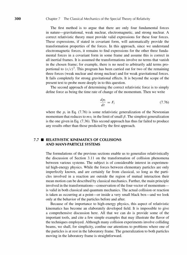
“M07 Goldstein ISBN C07” — 2011/2/15 — page 300 — #25
300 Chapter 7 The Classical Mechanics of the Special Theory of Relativity
The first method is to argue that there are only four fundamental forcesin nature—gravitational, weak nuclear, electromagnetic, and strong nuclear. Acorrect relativistic theory must provide valid expressions for these four forces.These expressions, if stated in covariant form, will automatically provide thetransformation properties of the forces. In this approach, since we understandelectromagnetic forces, it remains to find expressions for the other three funda-mental forces in a covariant form in some frame and assume this is correct inall inertial frames. It is assumed the transformations involve no terms that vanishin the chosen frame; for example, there is no need to arbitrarily add terms pro-portional to (v/c)3. This program has been carried out for two of the remainingthree forces (weak nuclear and strong nuclear) and for weak gravitational forces.It fails completely for strong gravitational effects. It is beyond the scope of thepresent text to probe more deeply in to this question.
The second approach of determining the correct relativistic force is to simplydefine force as being the time rate of change of the momentum. Then we write
dpi
dt= Fi (7.76)
where the pi in Eq. (7.76) is some relativistic generalization of the Newtonianmomentum that reduces to mvi in the limit of small β. The simplest generalizationis the one given in Eq. (7.36). This second approach has thus far failed to produceany results other than those predicted by the first approach.
7.7 RELATIVISTIC KINEMATICS OF COLLISIONSAND MANY-PARTICLE SYSTEMS
The formulations of the previous sections enable us to generalize relativisticallythe discussion of Section 3.11 on the transformation of collision phenomenabetween various systems. The subject is of considerable interest in experimen-tal high-energy physics. While the forces between elementary particles are onlyimperfectly known, and are certainly far from classical, so long as the parti-cles involved in a reaction are outside the region of mutual interaction theirmean motion can be described by classical mechanics. Further, the main principleinvolved in the transformations—conservation of the four-vector of momentum—is valid in both classical and quantum mechanics. The actual collision or reactionis taken as occurring at a point—or inside a very small black box—and we lookonly at the behavior of the particles before and after.
Because of the importance to high-energy physics, this aspect of relativistickinematics has become an elaborately developed field. It is impossible to givea comprehensive discussion here. All that we can do is provide some of theimportant tools, and cite a few simple examples that may illustrate the flavor ofthe techniques employed. Although many collision experiments involve collidingbeams, we shall, for simplicity, confine our attentions to problems where one ofthe particles is at rest in the laboratory frame. The generalization to both particlesmoving in the laboratory frame is straightforward.
“M07 Goldstein ISBN C07” — 2011/2/15 — page 301 — #26
7.7 Relativistic Kinematics of Collisions and Many-Particle Systems 301
The notion of a point designated as the center of mass obviously presentsdifficulties in a Lorentz-invariant theory. But the center-of-mass system can besuitably generalized as the Lorentz frame of reference in which the total spatiallinear momentum of all particles is zero. That such a Lorentz frame can alwaysbe found follows from the theorem that the total momentum 4-vector is timelikefor a system of mass points.
One such frame is the center-of-momentum frame. This is a frame in whichthe components of the spatial momentum of the initial particles add to zero. Sucha frame obviously exists. Let us define E and p in Eq. (7.36) to be
E =n∑
i=1
Ei and p =n∑
i=1
pi (7.77)
where the sum is over the particles involved. The left-hand side of Eq. (7.38)becomes
∑r,s
mr msc2 −∑r,s
mr msγrγs(vr ? vs). (7.78)
This clearly is positive (hint: separate the negative terms in which r = s), soit is possible to find a frame in which the three-momentum, p, equals zero. TheLorentz system, in which the spatial components of the total momentum are zero,is termed the center-of-momentum system, or more loosely, and somewhat incor-rectly, as the center-of-mass system, and will be designated by the abbreviation“C-O-M system.”
As an example, let us consider a particle of mass m1 and momentum p1 in thex-direction, which suffers a head-on collision with a particle of mass m2 at rest inan experimenter’s frame (called the laboratory frame). The initial 4-momentum is
pμ = ([m1γ + m2]c,m1γ v1, 0, 0). (7.79)
The length squared of momentum has the magnitude
pμ pμ = (m21 + m2
2 + 2m1γm2)c2. (7.79′)
When components are given, we shall follow the practice of denoting the primedframe by primes on the indices. The two particles are denoted by subscripts1 and 2 respectively.
In the C-O-M system, the total momentum is
([m1γ
′1 + m2γ
′2]c, 0, 0, 0
), (7.80)
since by definition the space part of the momentum vanishes,
m1γ′1b
′1c + m2γ
′2b
′2c = 0, (7.81)
“M07 Goldstein ISBN C07” — 2011/2/15 — page 302 — #27
302 Chapter 7 The Classical Mechanics of the Special Theory of Relativity
where b′1 and b′
2 are the velocities of m1 and m2, respectively, in the C-O-Mframe.
The boost, b′, needed to go from the laboratory to the C-O-M frame, has thevalue
b′2 = −b′. (7.81′)
Since all velocities are parallel, the velocity addition formula Eq. (7.15) givesthe velocity b′
1 of mass m1 in the C-O-M system in terms of b′ and its velocityb = v/c in the laboratory frame,
β ′1 = β − β ′1 − ββ ′ . (7.82)
The total squared momentum in the C-O-M frame given in Eq. (7.80) can berewritten using the results of Eqs. (7.81) and (7.82) as
pμ pμ = m22β
2(1 − β ′2)c2
β − β ′ . (7.83)
Equating Eqs. (7.79′) and (7.83) gives a single equation that can be solved forthe boost velocity β ′. There are two real roots, one of which corresponds to thephysically meaningful case of β ′ < 1.
Since the spatial momentum in the C-O-M frame is zero, there is clearly moreenergy, p0, in this frame than in the laboratory frame.* The excess energy in theC-O-M frame, �E , is obtained by subtracting the time component of Eq. (7.79)from the time component of Eq. (7.80).
The total momentum four vector is conserved, which automatically impliesboth conservation of spatial linear momentum and conservation of total energy(including rest mass energy). Our major tools for making use of the conserva-tion principle are Lorentz transformations to and from the C-O-M system, andthe formation of Lorentz invariants (world scalars) having the same value in allLorentz frames. Since energy and momentum are combined into one conservationlaw, the relativistic results are more easily obtained than the nonrelativistic resultsof previous chapters. The transformations between laboratory system and C-O-Msystem are merely special cases of the Lorentz transformation.
As an example of the use of Lorentz invariants, let us consider a reaction ini-tiated by two particles that produces another set of particles with masses mr ,r = 3, 4, 5, . . .. In the C-O-M system, the transformed total momentum is
Pμ′ = (E ′/c, 0, 0, 0). (7.84)
It is often convenient to look on the C-O-M system as the proper (or rest) systemof a composite mass particle of mass M = E ′/c2.† The square of the magnitude of
*For a single particle, the energy has a minimum value, mc2, in the rest frame. The C-O-M frame isnot the rest frame of either particle.†Although it is customary in high-energy physics to use units in which c = 1, it seems more helpfulin an introductory exposition such as this to retain the powers of c throughout.
“M07 Goldstein ISBN C07” — 2011/2/15 — page 303 — #28
7.7 Relativistic Kinematics of Collisions and Many-Particle Systems 303
P must be invariant in all Lorentz systems and conserved in the reaction. Hence,we have
PμPμ = Pμ′ Pμ′ = E ′2
c2= M2c2. (7.85)
But for the initial particles, PμPμ can be evaluated as
PμPμ = (m21 + m2
2)c2 − 2p1μ pμ2 . (7.86)
The energy in the C-O-M system, or equivalent mass M , is therefore given interms of the incident particles as
E ′2 ≡ M2c4 = (m21 + m2
2)c4 + 2(E1 E2 − c2p1 ? p2). (7.87)
Suppose now that, one particle, say 2, was initially stationary in the laboratorysystem. Since then p2 = 0 and E2 = m2c2, the C-O-M energy becomes
E ′2 ≡ M2c4 = (m21 + m2
2)c4 + 2m2c2 E ′
1. (7.88)
If the excess of E1 over the rest mass energy be denoted by T1, [cf. Eq. (7.39)]that is, the kinetic energy, this can be written
E ′2 ≡ M2c4 = (m1 + m2)2c4 + 2m2c2T1. (7.89)
It is clear that the available energy in the C-O-M system increases only slowlywith incident kinetic energy. Even in the “ultrarelativistic” region, where thekinetic energy of motion is very large compared to the rest mass energy, E ′increases only as the square root of T1.
The effect of the proportionally small amount of incident energy available inthe C-O-M system is shown dramatically in terms of the threshold energies. It isobvious that the lowest energy at which a reaction (other than elastic scattering) ispossible is when the reaction products are at rest in the C-O-M system. Any finitekinetic energy requires a higher E ′ or equivalently higher incident energy. Thetotal four-momentum in the C-O-M system after the reaction, denoted by Pμ
′′
has the magnitude at threshold given by
Pμ′′ Pμ′′ = c2
(∑r
mr
)2
, (7.90)
which, by conservation of momentum, must be the same as Eq. (7.85). For astationary target, the incident energy of motion as threshold is then given as aconsequence of Eq. (7.89) by
T1
m1c2=
(∑r
mr
)2
− (m1 + m2)2
2m1m2.
“M07 Goldstein ISBN C07” — 2011/2/15 — page 304 — #29
304 Chapter 7 The Classical Mechanics of the Special Theory of Relativity
If the Q value of the reaction is defined as*
Q =[∑
r
mr − (m1 + m2)
]c2, (7.91)
this threshold energy becomes
T1
m1c2= Q2 + 2Q(m1 + m2)c2
2m1m2c4. (7.92)
A common illustration of the application of Eq. (7.92) is the historic productionof an antiproton, p, by the reaction, involving a proton p,
p + n → p + n + p + p,
where n is a nucleon, either neutron or proton. The masses of all particles involvedare nearly equal at 938 MeV equivalent rest mass energy and we select Q = 2mc2.Equation (7.92) then says that the incident particle kinetic energy at thresholdmust be
T1 = 6mc2 = 5.63 GeV,
which is 3 times the energy represented by Q! If, however, the reaction wasinitiated by two nucleons incident on each other with equal and opposite velocity,then the laboratory system is the same as the C-O-M system. All of the kineticenergy is available in this case to go into production of the proton–antiprotonpair, and each of the incident particles at threshold need have a kinetic energy ofmotion equivalent to only the mass of one proton, 938 MeV. It is no wonder somuch effort has been put into constructing colliding beam machines!
Another instructive example of a threshold calculation is photomeson produc-tion, say, by the reaction
γ + p = �0 + K+, (7.93)
where γ stands for an incoming photon. For the purposes of classical mechanics,a photon is a zero-mass particle with spatial momentum 0p and energy 0pc.† Incalculating Q, the mass m1 of the photon is zero:
Q = (m�0 + mK+ − mp)c2 = 749 MeV.
*Q here has the opposite sign to the convention adopted in Eq. (3.112).†The square of the magnitude of the photon momentum four-vector is zero, so the vector can bedescribed as “lightlike.” The C-O-M theorem is imperiled only if all of the particles are photons, andeven then only if the photons are going in the same direction.
“M07 Goldstein ISBN C07” — 2011/2/15 — page 305 — #30
7.7 Relativistic Kinematics of Collisions and Many-Particle Systems 305
Equation (7.92) is rewritten for a reaction involving an incident photon as
T1 = 0 pc = Q2 + 2Qm2c2
2m2c2.
From the value of Q and the rest mass energy m2 of the proton, the thresholdenergy for the reaction Eq. (7.93) is then
T1 = 1.05 GeV,
which is only slightly higher than Q.We can also easily find the energy of the reaction products in the laboratory
system at threshold. The C-O-M system is the rest system for the mass M , withP0′ = Mc. In any other system, the zeroth component of the 4-vector is P0 =Mcγ . But in the laboratory system
P0 = 1
c(E1 + E2) = 1
c(E1 + m2c2),
where the last form holds only for a stationary target particle. Hence, the C-O-Msystem moves relative to the laboratory system such that
γ = E1 + m2c2
Mc2. (7.94)
But at threshold all the reaction products are at rest in the C-O-M system so thatM = ∑
rmr , and therefore
γ = T1 + (m1 + m2)c2∑r
mr c2(threshold). (7.95)
The kinetic energy of the sth reaction product in the laboratory system is then
Ts = msc2(γ − 1). (7.96)
Thus, the antiproton at threshold has a kinetic energy Tp = mc2 = 938 MeV. Incontrast, the K+ meson emerges at threshold with 494 MeV.
In Section 3.11, the kinematic transformations of a two-body nonrelativisticcollision were investigated. Eq. (3.117′) gives the reduction in energy of an inci-dent particle after elastic scattering from a stationary target, as a function of thescattering angle in the C-O-M system. The derivation of the relativistic analogprovides another interesting example of the methods of relativistic kinematics.Use of Lorentz invariants here is not particularly helpful; instead direct Lorentztransformations are made between the laboratory and C-O-M systems. Figure 7.4illustrates the relations of the incident and scattered spatial momentum vectorsin both systems. The incident and scattered momentum vectors define a plane,
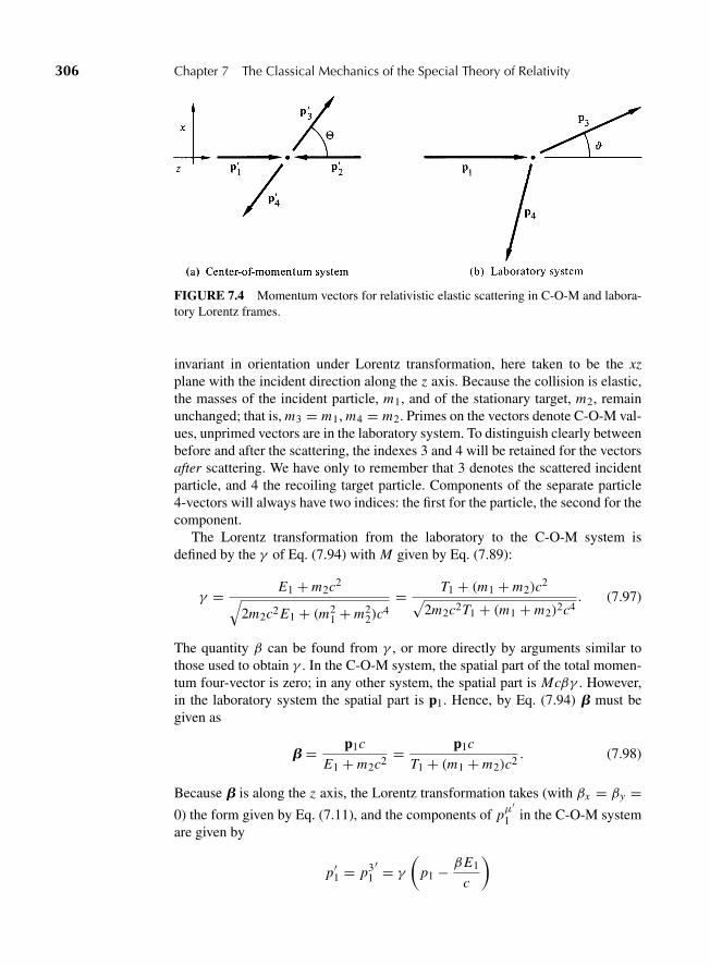
“M07 Goldstein ISBN C07” — 2011/2/15 — page 306 — #31
306 Chapter 7 The Classical Mechanics of the Special Theory of Relativity
FIGURE 7.4 Momentum vectors for relativistic elastic scattering in C-O-M and labora-tory Lorentz frames.
invariant in orientation under Lorentz transformation, here taken to be the xzplane with the incident direction along the z axis. Because the collision is elastic,the masses of the incident particle, m1, and of the stationary target, m2, remainunchanged; that is, m3 = m1, m4 = m2. Primes on the vectors denote C-O-M val-ues, unprimed vectors are in the laboratory system. To distinguish clearly betweenbefore and after the scattering, the indexes 3 and 4 will be retained for the vectorsafter scattering. We have only to remember that 3 denotes the scattered incidentparticle, and 4 the recoiling target particle. Components of the separate particle4-vectors will always have two indices: the first for the particle, the second for thecomponent.
The Lorentz transformation from the laboratory to the C-O-M system isdefined by the γ of Eq. (7.94) with M given by Eq. (7.89):
γ = E1 + m2c2√2m2c2 E1 + (m2
1 + m22)c
4= T1 + (m1 + m2)c2√
2m2c2T1 + (m1 + m2)2c4. (7.97)
The quantity β can be found from γ , or more directly by arguments similar tothose used to obtain γ . In the C-O-M system, the spatial part of the total momen-tum four-vector is zero; in any other system, the spatial part is Mcβγ . However,in the laboratory system the spatial part is p1. Hence, by Eq. (7.94) b must begiven as
b = p1c
E1 + m2c2= p1c
T1 + (m1 + m2)c2. (7.98)
Because b is along the z axis, the Lorentz transformation takes (with βx = βy =0) the form given by Eq. (7.11), and the components of pμ
′1 in the C-O-M system
are given by
p′1 = p31′ = γ
(p1 − βE1
c
)
“M07 Goldstein ISBN C07” — 2011/2/15 — page 307 — #32
7.7 Relativistic Kinematics of Collisions and Many-Particle Systems 307
E ′1
c= p0
1′ = γ
(E1
c− βp1
). (7.99)
After the collision, p′3 is no longer along the z axis, but since the collision is
elastic, its magnitude is the same as that of p′1. If � is the angle between p′
3 andthe incident direction, as in Section 3.11, then the components of p′3 in the C-O-Msystem are
p1′3 = p′1 sin�, p3
3′ = p′1 cos�, p0
3′ = p0
1′ = E ′
1
c. (7.100)
The transformation back to the laboratory system is the same Lorentz transfor-mation but with relative velocity −b. Hence, the components of p3 are
p13 = p1
3′ = p′1 sin�
p33 = γ (p3
3′ − β p0
3′) = γ
(p′1 cos�+ βE ′
1
c
)
p03 = γ (p0
3′ + β p3
3′) = γ
(E ′
1
c+ βp′1 cos�
). (7.101)
If E ′1 and p′1 are substituted in the last of Eqs. (7.101), from Eqs. (7.99) we obtain,
after a little simplification, an expression for the energy of the scattered particlein terms of its incident properties:
E3 = E1 − γ 2β(1 − cos�)(p1c − βE1). (7.102)
In Eq. (7.102), γ and β must be expressed terms of the incident quantities throughEqs. (7.97) and (7.98), resulting in the relation
γ 2β(p1c − βE1) =m2 p2
1c2
2m2 E1 + (m21 + m2
2)c2. (7.103)
With the help of the relation between p1 and E1, Eq. (7.38′), this can be written
γ 2β(p1c − βE1) = m2T1(T1 + 2m1c2)
2m2T1 + (m1 + m2)2c2. (7.104)
Some further algebraic manipulation then enables us to rewrite Eq. (7.102) as
T3
T1= 1 − 2ρ(1 − E1/2)
(1 + ρ)2 + 2ρE1(1 − cos�), (7.105)
“M07 Goldstein ISBN C07” — 2011/2/15 — page 308 — #33
308 Chapter 7 The Classical Mechanics of the Special Theory of Relativity
where ρ = m1/m2, as in Section 3.11 for elastic scattering, and E1 is the kineticenergy of the incident particle in units of the rest mass energy,
E1 = T1
m1c2. (7.106)
Equation (7.105) is the relativistic counterpart of Eq. (3.117′). It is easy to seethat Eq. (7.105) reduces to the nonrelativistic case as E1 → 0, and that if ρ = 1(equal masses), the relativistic corrections cancel completely. Equation (7.105)implies that the minimum energy after scattering, in units of m1c2, is given by
(E3)min = E1(1 − ρ)2
(1 + ρ)2 + 2ρE1. (7.107)
In the nonrelativistic limit, the minimum fractional energy after scattering is
(E3)min
E1=(
1 − ρ1 + ρ
)2
; E1 � 1, (7.108)
which is a well-known result, easily obtained from Eq. (3.117′). Equation (7.108)says that in the nonrelativistic region a particle of mass m1 cannot lose muchkinetic energy through scattering from a much heavier particle, that is, whenρ � 1, which clearly agrees with common sense. However, in the ultrarelativisticregion, when ρE1 � 1, the minimum energy after scattering is independent of E1:
(T3)min = (m2 − m1)2c2
2m2; ρE1 � 1. (7.109)
Since the condition on E1 is equivalent to requiring T1 � m2c2, it follows fromEq. (7.109) that such a particle can lose a large fraction of its energy even whenscattered by a much heavier particle. This behavior is unexpected, but it should beremembered that for particles at these energies, traveling very close to the speedof light, even a slight change in velocity corresponds to a large change in energy.
Finally, we may easily obtain the relation between the scattering angles in theC-O-M and laboratory system by noting that (first index particle, second compo-nent)
tanϑ = p31
p33= sin�
γ(
cos�+ βE ′1
p′1c
) . (7.110)
By Eq. (7.36),
p′1c
E ′1
= v′1c
≡ β ′1, (7.111)

“M07 Goldstein ISBN C07” — 2011/2/15 — page 309 — #34
7.8 Relativistic Angular Momentum 309
so that tanϑ can also be written
tanϑ = sin�
γ (cos�+ β/β ′1). (7.112)
In terms of initial quantities, Eqs. (7.99) show that
βE ′1
p′1c=β(
E1c − βp1
)p1 − βE1
c
. (7.113)
This can be further reduced by employing the relations (cf. Eq. (7.98))
β
p1 − βE1c
= 1
m2c, (7.114)
E1 − βp1 = m1(m1 + m2)c4 + m2c2T1
(m1 + m2)c2 + T1. (7.115)
The final expression for tanϑ can then be written as
tanϑ = sin�
γ [cos�+ ρg(ρ, E1)], (7.116)
where g(ρ, E1) is the function
g(ρ, E1) = 1 + ρ(1 + E1)
(1 + E1)+ ρ , (7.117)
and γ , by Eq. (7.97), takes the form
γ (ρ, E1) = 1 + E1 + ρ√(1 + ρ)2 + 2ρE1
. (7.118)
Again, in the nonrelativistic region, γ and g tend to unity, and Eq. (7.116)reduces to Eq. (3.107). The correction function g(ρ, E1) never really amounts tomuch, approaching the constant limit ρ as E1 becomes very large. The importantfactor affecting the transformed angle is γ , which of course increases indefinitelyas E1 increases. It does not affect the bounds of the angular distribution, when� = 0 or π , but its presence means that at other angles ϑ is always smaller than itwould be nonrelativistically. The Lorentz transformation from C-O-M to the labo-ratory system, which does not affect the transverse component of the momentum,thus always tends to distort the scattered angular distribution into the forwarddirection.
7.8 RELATIVISTIC ANGULAR MOMENTUM
In Chapter 1, it was proven that the nonrelativistic angular momentum obeys anequation of motion much like that for the linear momentum, but with torques
“M07 Goldstein ISBN C07” — 2011/2/15 — page 310 — #35
310 Chapter 7 The Classical Mechanics of the Special Theory of Relativity
replacing forces. It was shown that for an isolated system obeying the law ofaction and reaction the total angular momentum is conserved, and that in theC-O-M system it is independent of the point of reference. All of these statementshave their relativistic counterparts, at times involving some additional restrictions.
For a single particle, let us define an antisymmetric tensor of rank(2
0
)in
Minkowski space using the formalism of Eq. (7.64)
m = x ∧ p (7.119)
whose elements would be
mμν = xμ pv − xν pμ. (7.120)
The 3 × 3 subtensor mi j clearly corresponds, as was seen in Section 5.1, withthe spatial angular momentum of the particle. An equation of motion for mμν canbe found by taking its derivative with respect to the particle’s proper time andmaking use of Eq. (7.73) giving
dm
dτ= u ∧ p + x ∧ K = x ∧ K , (7.121)
where the first term vanishes by the antisymmetry of the wedge product and K isthe Minkowski force. In component notation, Eq. (7.121) becomes
dmμν
dτ= xμK ν − xνKμ. (7.122)
This suggests we define the relativistic generalization of the torque by
N = x ∧ K , (7.123)
whose components are
Nμν = xμK ν − xνKμ. (7.124)
Thus, m obeys the equations of motion
dm
dτ= N , (7.125)
whose component form is
dmμν
dτ= Nμν, (7.126)
with Eq. (1.11) as the nonrelativistic limiting form.For a system involving a collection of particles, a total angular momentum
4-tensor can be defined (analogously to the total linear momentum 4-vector) as
M =∑
s
ms (7.127)
“M07 Goldstein ISBN C07” — 2011/2/15 — page 311 — #36
7.8 Relativistic Angular Momentum 311
or in component form
Mμν =∑
s
mμνs , (7.128)
where the index s denotes the sth particle. It is more difficult to form an equationof motion for M because each particle has its own proper time. (For the same rea-son, we did not attempt it even for P .) Nevertheless, plausible arguments can begiven for the conservation of M under certain circumstances. If the system is com-pletely isolated and the particles do not interact with each other or with the outsideworld (including fields), then m for each particle is conserved by Eq. (7.126), andtherefore M is also conserved. Even if the particles interact, but the interactiontakes place only through binary collisions at a point, there still could be conser-vation as can be seen from the following argument. Instantaneously when the twoparticles collide they are traveling together and have the same proper time. Inother words, their world lines cross and they share the same event. One can there-fore write an equation of motion of the form of Eq. (7.126) for the sum of theirangular momenta. If the impulsive forces of contact are equal and opposite—aswe would expect from conservation of linear momentum in the collision—thenthe sum of the impulsive torques cancel. Hence relativistic angular momentum isalso conserved through such collisions. Note that unlike the nonrelativistic casecovariance requires that the interactions are assumed to be instantaneous pointcollisions.
The relativistic angular momentum obeys the same kind of theorem regardingtranslation of the reference point as does its nonrelativistic counterpart. In the def-inition, Eq. (7.120) or Eq. (7.128), the reference point (really reference “event”)is the arbitrary origin of the Lorentz system. With respect to some other referenceevent aλ, the total angular momentum is
M(aλ) =∑
s
(xs − aλ) ∧ ps (7.129)
= M(0)− aλ ∧ P (7.130)
As in the nonrelativistic case, the change in the angular momentum componentsis equal to the angular momentum, relative to the origin, that the whole systemwould have if it were located at aλ.
In Chapter 1, one particular reference point played an important role—the cen-ter of mass. We can find something similar here, at least in one Lorentz frame, byexamining the nature of the mixed time and space components of Mμν , namely,M0 j = −M j0. By definition, in some particular Lorentz frame, these componentsare given by
M0 j =∑
s
(x0s p j
s − x js p0
s ) (7.131)
= c∑
s
(tp j
s − x js Es
c2
). (7.132)
“M07 Goldstein ISBN C07” — 2011/2/15 — page 312 — #37
312 Chapter 7 The Classical Mechanics of the Special Theory of Relativity
In the C-O-M frame, the total linear momentum p = ∑ps vanishes, and M0 j in
this frame has the form
M0 j = −c∑
s
xs Es
c2. (7.133)
If the system is such that the total angular momentum is conserved, as describedabove, then along with other components M is conserved and hence
∑s
x js Es = constant.
Conservation of total linear momentum means that E = ∑Es is also conserved.
It is therefore possible to define a spatial point R j ,
R j =∑s
x js Es∑
sEs
, (7.134)
associated with the system, which is stationary in the C-O-M coordinate frame.In the nonrelativistic limit, where to first approximation Es = msc2, Eq. (7.134)reduces to the usual definition, Eq. (1.21). Thus, a meaningful center of mass(sometimes called center of energy) can be defined in special relativity only interms of the angular-momentum tensor, and only for a particular frame of refer-ence. Finally, it should be noted that by Eq. (7.130) the spatial part of the angularmomentum tensor, M , is independent of reference point in the C-O-M system,exactly as in the nonrelativistic case.
Except for the special case of point collisions, we have so far carefully skirtedthe problem of finding the motion of a relativistic particle given the Minkowskiforces. To this more general problem we address ourselves in the next section,within the nominal framework of the Lagrangian formulation.
7.9 THE LAGRANGIAN FORMULATION OF RELATIVISTIC MECHANICS
Having established the appropriate generalization of Newton’s equation of motionfor special relativity, we can now seek to establish a Lagrangian formulation of theresulting relativistic mechanics. Generally speaking, there are two ways in whichthis has been attempted. One method makes no pretense at a manifestly covariantformulation and instead concentrates on reproducing, for some particular Lorentzframe, the spatial part of the equation of motion, Eq. (7.76). The forces Fi mayor may not be suitably related to a covariant Minkowski force. The other methodsets out to obtain a covariant Hamilton’s principle and ensuing Lagrange’s equa-tions in which space and time are treated in common fashion as coordinates in afour-dimensional configuration space. The basis for the first method is at timesquite shaky, especially when the forces are not relativistically well formulated.
“M07 Goldstein ISBN C07” — 2011/2/15 — page 313 — #38
7.9 The Lagrangian Formulation of Relativistic Mechanics 313
Most of the time, however, the equations of motion so obtained, while not man-ifestly covariant, are relativistically correct for some particular Lorentz frame.The second method, on the other hand, seems clearly to be the proper approach,but it quickly runs into difficulties that require skillful handling if they are to besolvable, even for a single particle. For a system of more than one particle, itbreaks down almost from the start. No satisfactory formulation for an interactingmultiparticle system exists in classical relativistic mechanics except for some fewspecial cases.
This section follows the first method, seeking to find a Lagrangian that leadsto the relativistic equations of motion in terms of the coordinates of some par-ticular inertial system. Within these limitations there is no great difficulty inconstructing a suitable Lagrangian. It is true that the method of Section (1.4),deriving the Lagrangian from D’Alembert’s principle, will not work here. Whilethe principle itself remains valid in any given Lorentz frame, the derivation thereis based on pi = mi vi , which is no longer valid relativistically. But we mayalso approach the Lagrangian formulation from the alternative route of Hamil-ton’s principle (Section 2.1) and attempt simply to find a function L for which theEuler–Lagrange equations, as obtained from the variational principle
δ I = δ
∫ t2
t1L dt = 0, (7.135)
agree with the known relativistic equations of motion, Eq. (7.76).A suitable relativistic Lagrangian for a single particle acted on by conservative
forces independent of velocity would be*
L = −mc2√
1 − β2 − V, (7.136)
where V is the potential, depending only upon position, and β2 = v2/c2, with vthe speed of the particle in the Lorentz frame under consideration. That this is thecorrect Lagrangian can be shown by demonstrating that the resultant Lagrangeequations,
d
dt
(∂L
∂vi
)− ∂L
∂xi= 0,
agree with Eq. (7.76). Since the potential is velocity independent vi occurs onlyin the first term of (7.136) and therefore
∂L
∂vi= mvi√
1 − β2= P i . (7.137)
*We do not choose L = mc2√
1 −√
1 − β2 − V because we want h in Eq. (7.139) to be the totalenergy.

“M07 Goldstein ISBN C07” — 2011/2/15 — page 314 — #39
314 Chapter 7 The Classical Mechanics of the Special Theory of Relativity
The equations of motion derived from the Lagrangian (7.136) are then
d
dt
mvi√1 − β2
= − ∂V
∂xi= Fi ,
which agree with (7.76). Note that the Lagrangian is no longer L = T −V but thatthe partial derivative of L with velocity is still the momentum. Indeed, it is thislast fact that ensures the correctness of the Lagrange equations, and we could haveworked backward from Eq. (7.137) to supply at least the velocity dependence ofthe Lagrangian.
We can readily extend the Lagrangian (7.136) to systems of many particlesand change from Cartesian to any desired set of generalized coordinates q. Thecanonical momenta, P , will still be defined by
Pi = ∂L
∂ qi, (7.138)
so that the connection between cyclic coordinates and conservation of the corre-sponding momenta remains just as in the nonrelativistic theory. Further, just as inSection (2.7), if L does not contain the time explicitly, there exists a constant ofthe motion
h = qiPi − L . (7.139)
However, the identification of h with the energy for, say, a Lagrangian of the formof Eq. (7.136) cannot proceed along the same route as in Section (2.7). Note thatL in Eq. (7.136) is not at all a homogeneous function of the velocity components.Nonetheless, direct evaluation of Eq. (7.139) from Eq. (7.136) shows that in thiscase h is indeed the total energy:
h = mvivi√
1 − β2+ mc2
√1 − β2 + V,
which, on collecting terms, reduces to
h = mc2√1 − β2
+ V = T + V + mc2 = E . (7.140)
The quantity h is thus again seen to be the total energy E , which is therefore aconstant of the motion under these conditions.
The introduction of velocity-dependent potentials produces no particular diffi-culty here and can be performed in exactly the same manner as in Section 1.5 fornonrelativistic mechanics. Thus, the Lagrangian for a single particle of charge, q,in an electromagnetic field is
L = −mc2√
1 − β2 − qφ + qA ? v. (7.141)
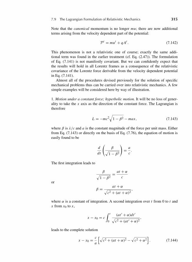
“M07 Goldstein ISBN C07” — 2011/2/15 — page 315 — #40
7.9 The Lagrangian Formulation of Relativistic Mechanics 315
Note that the canonical momentum is no longer mu; there are now additionalterms arising from the velocity dependent part of the potential:
P i = mui + q Ai . (7.142)
This phenomenon is not a relativistic one of course; exactly the same addi-tional term was found in the earlier treatment (cf. Eq. (2.47)). The formulationof Eq. (7.141) is not manifestly covariant. But we can confidently expect thatthe results will hold in all Lorentz frames as a consequence of the relativisticcovariance of the Lorentz force derivable from the velocity dependent potentialin Eq. (7.141).
Almost all of the procedures devised previously for the solution of specificmechanical problems thus can be carried over into relativistic mechanics. A fewsimple examples will be considered here by way of illustration.
1. Motion under a constant force; hyperbolic motion. It will be no loss of gener-ality to take the x axis as the direction of the constant force. The Lagrangian istherefore
L = −mc2√
1 − β2 − max, (7.143)
where β is x/c and a is the constant magnitude of the force per unit mass. Eitherfrom Eq. (7.143) or directly on the basis of Eq. (7.76), the equation of motion iseasily found to be
d
dt
(β√
1 − β2
)= a
c.
The first integration leads to
β√1 − β2
= at + αc
or
β = at + α√c2 + (at + α)2
,
where α is a constant of integration. A second integration over t from 0 to t andx from x0 to x ,
x − x0 = c∫ t
0
(at ′ + α)dt ′√c2 + (at ′ + α)2
,
leads to the complete solution
x − x0 = c
a
[√c2 + (at + α)2 −
√c2 + α2
]. (7.144)
“M07 Goldstein ISBN C07” — 2011/2/15 — page 316 — #41
316 Chapter 7 The Classical Mechanics of the Special Theory of Relativity
If the particle starts at rest from the origin so that x0 = 0 and v0 = 0 = α, thenEq. (7.144) can be written as
(x + c2
a
)2
− c2t2 = c4
a2,
which is the equation of a hyperbola in the x, t plane. (Under the same conditionsthe nonrelativistic motion is of course a parabola in the x, t plane). The nonrela-tivistic limit is obtained from Eq. (7.144) by considering (at +α) small comparedto c; the usual freshman-physics formula for x as a function of t is then easilyobtained, recognizing that in this limit α → v0.
The motion described in this example arises in reasonably realistic situations.It corresponds, for example, to the acceleration of electrons to relativistic speedsin the laboratory system by means of a constant and uniform electric field. Theillustration considered next is more academic, but is of interest as an example ofthe techniques employed.2. The relativistic one-dimensional harmonic oscillator. The Lagrangian in thiscase is of the form of Eq. (7.136) with
V (x) = 12 kx2. (7.145)
Since L is then not explicitly a function of time and V is not velocity depen-dent, the total energy E is constant. Equation (7.140) may now be solved for thevelocity x as
1
c2
(dx
dt
)2
= 1 − m2c4
(E − V )2. (7.146)
For the moment, we shall postpone substituting in the particular form of V (x)and generalize the problem slightly to include any potential sharing the qualita-tive characteristics of Eq. (7.145). Thus, let us suppose that V (x) is any poten-tial function symmetric about the origin and possessing a minimum at that point.Then providing E lies between V (0) and the maximum of V , the motion will beoscillatory between limits x = −b and x = +b, determined by
V (±b) = E .
The period of the oscillatory motion is, by Eq. (7.146), to be obtained from
τ = 4
c
∫ b
0
dx√1 − m2c4
(E−V (x))2
. (7.147)
Equation (7.147), when specialized to the particular Hooke’s law form (7.145)for V (x), can be expressed in terms of elliptic integrals. We shall instead examine
“M07 Goldstein ISBN C07” — 2011/2/15 — page 317 — #42
7.9 The Lagrangian Formulation of Relativistic Mechanics 317
the first-order relativistic corrections when the potential energy is always smallcompared to the rest mass energy mc2. A change of notation is helpful. The energyE can be written as
E = mc2(1 + E)
so that here
E − V (x)
mc2= 1 + E − κx2 = 1 + κ(b2 − x2), (7.148)
where
κ = k
2mc2. (7.149)
To the order (κb2)2, the period, Eq. (7.147) then reduces to
τ � 4
c
∫ b
0
dx√2κ(b2 − x2)
[1 − 3κ
4(b2 − x2)
]. (7.150)
The intergral in Eq. (7.150) can be evaluated by elementary means, most simplyby changing variable through x = b sinφ; the final result is
τ � 2π
c
1√2κ
(1 − 3
8κb2
)= 2π
√m
k
(1 − 3
16
kb2
mc2
).
Note that the expression in front of the bracket is τ0, the nonrelativistic period ofthe harmonic oscillator. In special relativity, the period of the harmonic oscillatoris thus not independent of the amplitude; instead, there is an amplitude dependentcorrection given approximately by
�v
v0= −�τ
τ0� 3
16
kb2
mc2= 3
8E . (7.151)
3. Motion of a charged particle in a constant magnetic field. In principle, weshould start from a Lagrangian of the form of Eq. (7.141) with the scalar potentialφ = 0 and A appropriate to a constant magnetic field (Eq. 5.106). But we knowsuch a Lagrangian corresponds to the Lorentz force on the charged particle ofcharge q, given by
F = q(v3B) (7.152)
(cf. Eq. 1.60). Hence, the equation of motion must be
dpdt
= q(v3B) = q
mγ(p3B). (7.153)
“M07 Goldstein ISBN C07” — 2011/2/15 — page 318 — #43
318 Chapter 7 The Classical Mechanics of the Special Theory of Relativity
The nature of the force, Eq. (7.152), is clearly such that the magnetic field doesno work on the particle: F ? v = 0. Hence, E must be a constant, as also p andγ by Eq. (7.38′). Further, by Eq. (7.152), there is no component of the forceparallel to B, and the momentum component along that direction must remainconstant. It is therefore no loss of generality to consider the motion only in theplane perpendicular to B and to let p represent the projection of the total linearmomentum on to that plane. Equation (7.153) then says that the vector p (whosemagnitude is constant) is precessing around the direction of the magnetic fieldwith a frequency
� = q B
mγ(7.154)
referred to as the cyclotron frequency. In the nonrelativistic limit γ → 1. Thisagrees with the cyclotron resonance expression found in solid state physics texts.Because γ is constant, the velocity vector in the plane is also of constant mag-nitude and rotating with the same frequency. The particle must therefore moveuniformly in a circular orbit in the plane with angular speed�. Since the centrifu-gal force, F , equals mu2/r , it follows that the magnitude of the linear momentumin the plane must be given by
p = mγ r�.
Combining this expression with Eq. (7.154) leads to the relation between thecircle radius and the momentum:
r = p
q B. (7.155)
The radius of curvature into which the particle motion is bent depends only uponthe particle properties through the ratio p/q (= Br), which is sometimes calledthe magnetic rigidity of the particle. Note that while � (Eq. (7.154)) shows rela-tivistic corrections through the presence of γ , the relation between r and p is thesame both relativistically and nonrelativistically. Recall that in both Eqs. (7.154)and (7.155) p is the magnitude of the momentum perpendicular to B, but in calcu-lating γ we must use both the perpendicular and parallel components to find β.*
7.10 COVARIANT LAGRANGIAN FORMULATIONS
The Lagrangian procedure as given above certainly predicts the correct relativisticequations of motion. Yet it is a relativistic formulation only “in a certain sense.”No effort has been made to keep to the ideal of a covariant four-dimensional form
*The Larmor precession frequency vL of Eq. (5.104) has an extra factor of 2, and corresponds to theprecession of a magnetic moment in a constant magnetic field. This is a physically different case fromthat of the cyclotron resonance of a charged particle moving at a constant speed in a magnetic field.
“M07 Goldstein ISBN C07” — 2011/2/15 — page 319 — #44
7.10 Covariant Lagrangian Formulations 319
for all the laws of mechanics. Thus, the time t has been treated as a parame-ter entirely distinct from the spatial coordinates, while a covariant formulationwould require that space and time be considered as entirely similar coordinatesin world space. Clearly some invariant parameter should be used, instead of t , totrace the progress of the system point in configuration space. Further, the exam-ples of Lagrangian functions discussed in the previous section do not have anyparticular Lorentz transformation properties. Hamilton’s principle must itself bemanifestly covariant, which can only mean in this case that the action integralmust be a world scalar. If the parameter of integration is a Lorentz invariant, thenthe Lagrangian function itself must be a world scalar in any covariant formula-tion. Finally, instead of being a function of xi and xi , the Lagrangian should bea function of the coordinates in Minkowski space and of their derivatives withrespect to the invariant parameter.
We shall consider primarily a system of only one particle. The natural choiceof the invariant parameter in such a system would seem to be the particle’s propertime τ . But the various components of the generalized velocity, uν , must thenobey the relation
u · u = uνuν = c2, (7.35)
which shows they are not independent. Therefore, we shall instead assume thechoice of some Lorentz-invariant quantity θ with no further specification than thatit be a monotonic function of the progress of the world point along the particle’sworld line. For the purpose of this discussion, a superscript prime will be used todenote differentiation with respect to θ :
x ′ν ≡ dxν
dθ,
while a dot over the letter indicates differentiation with respect to t . A suitablycovariant Hamilton’s principle must therefore appear as
δ I = δ
∫ θ2
θ1
�(xμ, x ′μ) dθ, (7.156)
where the Lagrangian function � must be a world scalar and the (xμ, x ′μ) meansa function of all or any of these. Note that this formulation includes what wouldhave ordinarily been called “time-dependent Lagrangians,” because � is consid-ered a function of x0. The Euler–Lagrange equations corresponding to Eq. (7.156)are
d
dθ
(∂�
∂x ′μ
)− ∂�
∂xμ= 0. (7.157)
The problem is to find the form of � such that Eqs. (7.157) are equivalent to theequations of motion, Eq. (7.73).
One way of seeking� is to transform the action integral from the usual integralover t to one over θ , and to treat the time t appearing explicitly in the Lagrangian
“M07 Goldstein ISBN C07” — 2011/2/15 — page 320 — #45
320 Chapter 7 The Classical Mechanics of the Special Theory of Relativity
not as a parameter but as an additional generalized coordinate. Since θ must be amonotonic function of t as measured in some Lorentz frame, we have
dxi
dt= dxi
dθ
dθ
dt= c
x ′i
x ′0. (7.158)
Hence, the action integral is transformed as
I =∫ t2
t1L(x j , t, x j ) dt = 1
c
∫ θ2
θ1
L
(x j , c
x ′ j
x ′0
)x ′0 dθ.
It would seem therefore that a recipe for a suitable � is given by the relation
�(xμ, x ′μ) = x ′0
cL
(xμ, c
x ′ j
x ′0
). (7.159)
The Lagrangian obtained this way is however a strange creature, unlike anyLagrangian we have so far met. Note that no matter what the functional form ofL , the new Lagrangian� is a homogeneous function of the generalized velocitiesin the first degree:
�(xμ, ax ′μ) = a�(xμ, x ′μ). (7.160)
This is not a phenomenon of relativistic physics per se; it is a mathematical conse-quence of enlarging configuration space to include t as a dynamical variable andusing some other parameter to mark the system-point’s travel through the space.A Lagrangian obeying Eq. (7.160) is often called (somewhat misleadingly) ahomogeneous Lagrangian and the corresponding “homogeneous” problem of thecalculus of variations requires special treatment. The most serious of the resultingdifficulties will arise in the Hamiltonian formulation, but we can glimpse some ofthem by noting that in consequence the energy function h, according to Eq. (2.53),is identically zero. It follows from Euler’s theorem on homogeneous functions thatif � is homogeneous to first degree in x ′μ, then
� = x ′μ∂�
∂x ′μ.
We can then show (cf. Derivation 10 at the end of this chapter) that as a result thefunction � identically satisfies the relation[
d
dθ
(∂�
∂x ′μ
)− ∂�
∂xμ
]x ′μ = 0. (7.161)
Thus, if any three of the Lagrangian Eqs. (7.157) are satisfied, it will follow, solelyas a consequence of the homogeneous property of �, that the fourth is satisfiedidentically.
Being thus forewarned to tread carefully, so to speak, let us carry out this trans-formation for a free particle. From Eq. (7.136), the “relativistic” but “noncovariant”
“M07 Goldstein ISBN C07” — 2011/2/15 — page 321 — #46
7.10 Covariant Lagrangian Formulations 321
Lagrangian for the free particle is
L = −mc√
c2 − x i xi .
By the transformation of Eq. (7.159), a possible covariant Lagrangian is then
� = −mc√
x ′μx ′μ. (7.162)
With this Lagrangian, the Euler–Lagrange equations are equivalent to
d
dθ
⎛⎝ mcx ′√
x ′μx ′μ
⎞⎠ = 0.
The parameter θ must be a monotonic function of the proper time τ so that deriva-tives with respect to θ are related to those in terms of τ according to
x ′ ≡ dx
dθ= dτ
dθu.
Hence, the Lagrangian equations correspond to
d
dτ
(mcu√uvuv
)= d(mu)
dτ= 0,
which are Eqs. (7.73) for a free particle. As we have seen above, the fourth ofthese equations says that the kinetic energy T is conserved, which is indeed notnew but can be derived from the other three equations.
We have thus been led to a covariant Lagrangian procedure that works, at leastfor a single free particle, but only in a tortuous fashion. The elaborate superstruc-ture can be greatly simplified however by a few bold pragmatic steps. First ofall, we can avoid using θ and work in terms of the proper time τ directly by aprocedure introduced in a slightly different context by Dirac. The constraint onthe generalized velocities in terms of τ , Eq. (7.35), is not a true dynamical con-straint on the motion; rather it is a geometric consequence of the way in whichτ is defined. Equation (7.35) says in effect that we cannot roam over the fullfour-dimensional u space; we are confined to a particular three-dimensional sur-face in the space. Dirac calls relations such as Eq. (7.35) weak equations. Wecan with impunity treat uν as unconstrained quantities, and only after all differ-entiation operations have been carried out, need the condition of Eq. (7.35) beimposed. Certainly the procedure would have worked above for the free particleLagrangian. There would have been no difference if θ were set equal to τ from thestart and Eq. (7.35) applied only in the last step. The covariant Lagrange equationscan with this proviso therefore be written directly in terms of τ :
d
dτ
(∂�
∂uν
)− ∂�
∂xν= 0. (7.163)
“M07 Goldstein ISBN C07” — 2011/2/15 — page 322 — #47
322 Chapter 7 The Classical Mechanics of the Special Theory of Relativity
Secondly, it is not a sacrosanct physical law that the action integral in Hamil-ton’s principle must have the same value whether expressed in terms of t or interms of θ (or τ ). It needn’t be given by the prescription of Eq. (7.159). All thatis required is that � be a world scalar (or function of a world scalar) that leads tothe correct equations of motion. It doesn’t have to be homogeneous to first degreein the generalized velocities. For example, a suitable � for a free particle wouldclearly be the quadratic expression
� = 12 muνuν . (7.164)
Many other possibilities are available.* We shall use Eq. (7.162) for the “kineticenergy” part of the Lagrangian in all subsequent discussions; many present andfuture headaches will thereby be avoided.
If the particle is not free, but is acted on by external forces, then interactionterms have to be added to the Lagrangian of Eq. (7.164) that would lead tothe corresponding Minkowski forces. Very little can be said at this time aboutthe additional terms, other than they must be Lorentz-invariant. For example, ifGμ were some (external) four-vector, then Gμxμ would be suitable interactionterm. If in some particular Lorentz frame G1 = ma and all other componentsvanish, then we would have an example of a constant force such as discussedin the previous section. In general, these terms will represent the interactionof the particle with some external field. The specific form will depend uponthe covariant formulation of the field theory. We have only one example of afield already expressed in a covariant way—the electromagnetic field—and it isinstructive therefore to examine the Lagrangian for a particle in an electromag-netic field.
A suitable Lagrangian can easily be seen to be
�(xμ, uμ) = 12 muμuμ + quμAμ(x
λ). (7.165)
The corresponding Lagrange’s equations are then
d
dτ(muν) = −q d Aν
dτ+ ∂
∂xν(quμAμ
),
which are exactly the generalized equations of motion Eq. (7.73), with theMinkowski force Kν on a charged particle, Eq. (7.74). Note that again the“mechanical momentum” four-vector pμ differs from the canonical momentum
*In general, � can have the form m f (uνuν), where f (y) is any function of y such that
∂ f
∂y
∣∣∣∣y=c2
= 1
2.
In Eq. (7.164), we have used f (uνuν) = 12 uνuν . The choice
f (uνuν) = −c√
uνuν
corresponds to Eq. (7.162).
“M07 Goldstein ISBN C07” — 2011/2/15 — page 323 — #48
7.10 Covariant Lagrangian Formulations 323
Pμ:
Pμ = gμν∂�
∂uν= muμ + q Aμ = pμ + q Aμ (7.166)
by a term linear in the electromagnetic potential. The canonical momentum, P ,conjugate to x0 is now
P0 = E
c+ q
φ
c= 1
cE,
where E is the mechanical energy and E is the total energy of the particle, E +qφ. Thus, the momentum conjugate to the time coordinate is proportional to thetotal energy. A similar conjugate connection between these two quantities willrecur later in nonrelativistic theory. The connection between the magnitude of thespatial “mechanical” momentum and the energy E is still given by Eq. (7.38′).From Eq. (7.166), it is seen that the canonical momenta conjugate to x form thecomponents of a spatial Cartesian vector P related to p by
P = p + qA. (7.167)
In terms of P , Eq. (7.100) can be rewritten as
E2 = (P − qA)2 + m2c4, (7.168)
which is a useful relation between the energy E and the canonical momentumvector P .
The interaction term in the Lagrangian of Eq. (7.165) is an example of a vec-tor field interaction (as is also a term of the form Gμxμ). We could also have asimple scalar field interaction where the term added to the Lagrangian would besome world scalar ψ(xμ). Or more complicated invariant interaction terms can becreated involving an external tensor field. The nature of such Lagrangians prop-erly stems from the physical field theory involved and cannot concern us furtherhere.
So far we have spoken only of systems comprising a single mass particle.Multiparticle systems introduce new complications. One obvious problem is find-ing an invariant parameter to describe the evolution of the system—each particlein the system has its own proper time. With a little thought, however, we couldimagine ways of solving this difficulty. For example, the proper time associatedwith the C-O-M system involves a symmetric treatment of all the particles andmight prove suitable. We could also include in the picture interactions of theparticles with external fields very much as was done for a single particle. Thegreat stumbling block however is the treatment of the type of interaction that isso natural and common in nonrelativistic mechanics—direct interaction betweenparticles.
At first sight, it would seem indeed that such interactions are impossiblein relativistic mechanics. To say that the force on a particle depends upon thepositions or velocities of other particles at the same time implies propagation of
“M07 Goldstein ISBN C07” — 2011/2/15 — page 324 — #49
324 Chapter 7 The Classical Mechanics of the Special Theory of Relativity
effects with infinite velocity from one particle to another—“action at a distance.”In special relativity, where signals cannot travel faster than the speed of light,action-at-a-distance seems outlawed. And in a certain sense this seems to be thecorrect picture. It has been proven that if we require certain properties of thesystem to behave in the normal way (such as conservation of total linear momen-tum), then there can be no covariant direct interaction between particles exceptthrough contact forces.
There have been many attempts in recent years to get around this “no-interaction” theorem. After all, we have seen that electromagnetic forces canbe expressed covariantly, and a static electric field gives rise to the Coulomblaw of attraction, which has the same form as the supposedly banned Newtoniangravitational attraction. Some of these attempts have led to approximately covari-ant Lagrangians, correct through orders of v2/c2. Others involve formulations ofmechanics at variance with our normal structures; most for example cannot bestated in terms of a simple Hamilton’s principle.
7.11 INTRODUCTION TO THE GENERAL THEORY OF RELATIVITY
Thus far we have been careful to use the term “special theory of relativity” andnot to introduce the term “special relativity,” by which we endeavored to makeclear that it is the theory that is special, not the relativity. The special theory usesideal inertial frames that are assumed to exist over all of spacetime. The gen-eral theory not only removes that requirement, but also has a spacetime whosenature is part of the solution to the question of motion. To paraphrase John A.Wheeler: “Matter tells space how to bend, and space returns the complimentby telling matter how to move.” The general theory is often interpreted in termsof non-Euclidean geometry, so terms like geodesic (paths of extremal distance)and curvature of spacetime are often used. In this brief section we can only out-line the formalism of the general theory to show how the full tensor notation isused.
Five principles guided Einstein in the development of the general theory:
1. Mach’s principle—the special theory used inertial frames. E. Mach observedthat Newtonian inertial frames were not rotating with respect to the fixedstars. This suggests Mach’s principle, whereby inertial properties are deter-mined by the presence of other bodies in the universe.
2. Principle of equivalence—whereby the gravitational mass for each body inthe universe can be consistently and universally chosen to equal its inertialmass. To the best accuracy of all experiments performed to date, the ratioof the gravitational mass (the mass that appears in Newton’s force law forgravity) to the inertial mass (the mass that appears in the second law) ofany object is independent of both the total mass and of the compositionof the object. This means that no local experiments can distinguish nonro-tating free fall in a gravitational field from uniform motion in the absenceof any gravitational fields. Likewise, local experiments cannot distinguish

“M07 Goldstein ISBN C07” — 2011/2/15 — page 325 — #50
7.11 Introduction to the General Theory of Relativity 325
between being at rest in a uniform gravitational field and undergoinguniform acceleration in the absence of any gravitational field (that is, in arocket).
3. Principle of covariance—in the special theory, all inertial observers areequivalent. The general theory extends this idea by postulating the princi-ple of covariance. This principle is that all observers, inertial or not, observethe same laws of physics. That means the laws of physics can be expressedin terms of tensors, since tensors are geometric objects defined independentof any coordinate system.
4. Correspondence principle—in weak gravitational fields with velocitiessmall compared to light, the general theory should make predictionsthat approximate the predictions of gravitational behavior in Newtonianmechanics. As gravitational fields go to zero, the correspondence principlestates the predictions of the general theory should approach those of thespecial theory.
5. Principle of minimal gravitational coupling—this principle postulates thatno terms explicitly containing the curvature should be added in making thetransition from the special theory to the general theory.
Newton’s first law tells us that in the absence of external force bodies movealong straight lines without acceleration. The preceding guiding principles sug-gest that in the general theory, objects will move along the geodesics of space-time. For example, let us consider a family of geodesics that start out parallel. Ifgravitational effects in the region under consideration are uniform, the geodesicswill remain parallel. If there is a nonuniform gravitational field, the geodesicsshould start to approach or recede. The change in separation, or geodesic devia-tion, is the proper measure of the gravitational field. Near Earth’s surface, we oftenassume the gravitational field is uniform over small regions. Thus, we assume twofalling bodies released side by side fall parallel. An experiment for larger sepa-rations or longer fall times measures the nonuniformity of Earth’s gravitationalfield.
To illustrate this, let us consider an example of two balls separated horizon-tally by a distance, d, which are dropped at the same time from the same heighthigh above Earth. Very close to either ball, and neglecting the gravitational massof the balls, local experiments will give results that allow us to treat the localregion as an inertial frame. Locally, gravity can be made to vanish by a choiceof coordinate frame. Let us choose this local free-fall frame for our observa-tions. Locally this satisfies the conditions for an inertial frame. However, as theballs fall toward Earth, their separation, d, decreases. This change in separation,rather than the fall toward Earth, is the local measure of the gravitational effect ofEarth since it can not be eliminated by a choice of frame. This is reflected by thegeneral theory statement that only the tides (differential effects) are real gravita-tional effects. Any other gravitational effects can be locally eliminated by freelyfalling.
Now consider two geodesics as shown in Figure 7.5. We can define two vectorfields at any point. One field, denoted by u, gives the 4-velocity of motion along
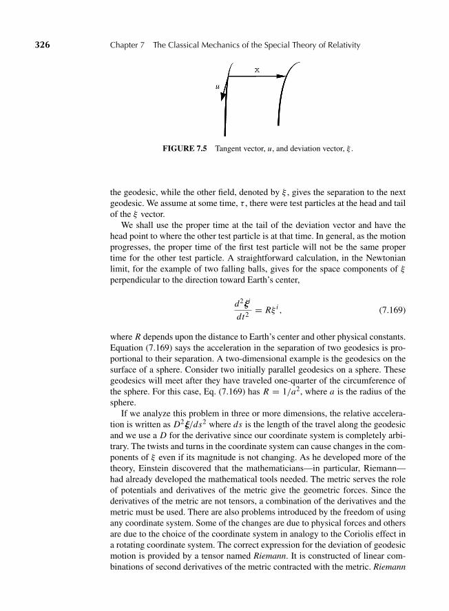
“M07 Goldstein ISBN C07” — 2011/2/15 — page 326 — #51
326 Chapter 7 The Classical Mechanics of the Special Theory of Relativity
FIGURE 7.5 Tangent vector, u, and deviation vector, ξ .
the geodesic, while the other field, denoted by ξ , gives the separation to the nextgeodesic. We assume at some time, τ , there were test particles at the head and tailof the ξ vector.
We shall use the proper time at the tail of the deviation vector and have thehead point to where the other test particle is at that time. In general, as the motionprogresses, the proper time of the first test particle will not be the same propertime for the other test particle. A straightforward calculation, in the Newtonianlimit, for the example of two falling balls, gives for the space components of ξperpendicular to the direction toward Earth’s center,
d2ji
dt2= Rξ i , (7.169)
where R depends upon the distance to Earth’s center and other physical constants.Equation (7.169) says the acceleration in the separation of two geodesics is pro-portional to their separation. A two-dimensional example is the geodesics on thesurface of a sphere. Consider two initially parallel geodesics on a sphere. Thesegeodesics will meet after they have traveled one-quarter of the circumference ofthe sphere. For this case, Eq. (7.169) has R = 1/a2, where a is the radius of thesphere.
If we analyze this problem in three or more dimensions, the relative accelera-tion is written as D2j/ds2 where ds is the length of the travel along the geodesicand we use a D for the derivative since our coordinate system is completely arbi-trary. The twists and turns in the coordinate system can cause changes in the com-ponents of ξ even if its magnitude is not changing. As he developed more of thetheory, Einstein discovered that the mathematicians—in particular, Riemann—had already developed the mathematical tools needed. The metric serves the roleof potentials and derivatives of the metric give the geometric forces. Since thederivatives of the metric are not tensors, a combination of the derivatives and themetric must be used. There are also problems introduced by the freedom of usingany coordinate system. Some of the changes are due to physical forces and othersare due to the choice of the coordinate system in analogy to the Coriolis effect ina rotating coordinate system. The correct expression for the deviation of geodesicmotion is provided by a tensor named Riemann. It is constructed of linear com-binations of second derivatives of the metric contracted with the metric. Riemann
“M07 Goldstein ISBN C07” — 2011/2/15 — page 327 — #52
7.11 Introduction to the General Theory of Relativity 327
has slots for three vectors and one slot for a single one-form. If we put the tangentvector into the second and fourth slots and the deviation vector into the third slot,Riemann produces
=u=uj+ Riemann(. . . , u, ξ, u) = 0, (7.170)
where =u=u = D2
ds2 . In component notation, Eq. (7.170) is
d2ξα
ds2+ Rαβγ δ
dxβ
dτξγ
dxδ
dτ= 0. (7.171)
If we contract Riemann on slots 1 and 3, we produce a tensor called Ricci,defined as
Ricci(u, ν) = Riemann(wα, u, eα, v), (7.172)
whose components are
Rμν = Rαμαv. (7.173)
Another critical contraction produces the curvature scalar, called R
R = Ricci(wα, eα) = Rαα. (7.174)
Of all these possible contractions of Riemann, only one tensor of rank(2
0
)retains
all the differential symmetries of Riemann. That tensor is called Einstein (denotedby G) and is defined as
G = Ricci − 12 gR, (7.175)
with components
Gμν = Rμν − 12 gμνR. (7.176)
Using T to denote the stress-energy tensor, Einstein’s field equations makeEinstein proportional to T .
G = kT . (7.177)
These equations for weak gravitational fields and for speeds much less thanlight approach Newtonian gravitational theory, and for no gravitational fieldsproduce the results of the special theory. They also correctly predict all themeasured first- and second-order corrections to the special theory of relativityin experiments thus far performed. In addition, the theory predicts the exis-tence of gravitational waves from moving masses. Although these waves havenot, at this writing, been directly observed, measured changes in the periods of
“M07 Goldstein ISBN C07” — 2011/2/15 — page 328 — #53
328 Chapter 7 The Classical Mechanics of the Special Theory of Relativity
several binary star systems are consistent with the existence of such radiationexisting.
Soon after Einstein proposed Eqs. (7.177), astronomers pointed out that thesolutions of these equations were not consistent with their observation of astatic universe that was neither expanding nor contracting. Einstein modifiedthe equations by adding a term that was proportional to the metric tensor. Theconstant of proportionality, called the cosmological constant, was denoted by �giving
G +�g = kT . (7.178)
Soon after that, astronomers decided that the observational data showed thatthe universe was expanding and the cosmological constant was not needed, andmost physicists dropped the term. Einstein said that the cosmological constantwas his greatest mistake. However, the early 21st century observational data ondistant galaxies suggests that the universe is accelerating as it expands. This wouldre-introduce the cosmological constant into the field equations. The current ter-minology, since this would be a � < 0, is to refer to the cosmological con-stant as “dark energy,” since it is a positive contribution to the right-hand side ofEq. (7.178).
DERIVATIONS
1. Consider a mechanical system of n particles, with a conservative potential consist-ing of terms dependent only upon the scalar distance between pairs of particles.Show explicitly that the Lagrangian for the system when expressed in coordinatesderived by a Galilean transformation differs in form from the original Lagrangianonly by a term that is a total time derivative of a function of the position vectors.This is a special case of invariance under a point transformation (cf. Derivation 10,Chapter 1).
2. Obtain the Lorentz transformation in which the velocity is at an infinitesimal angle dθcounterclockwise from the x axis, by means of a similarity transformation applied toEq. (7.16). Show directly that the resulting matrix is orthogonal and that the inversematrix is obtained by substituting −v for v.
3. The Einstein addition law can also be obtained by remembering that the secondvelocity is related directly to the space components of a four-velocity, which maythen be transformed back to the initial system by a Lorentz transformation. If thesecond system is moving with a speed v′ relative to the first in the direction of their zaxes, while a third system is moving relative to the second with an arbitrarily orientedvelocity v′′, show by this procedure that the magnitude of the velocity v between thefirst and third system is given by
√1 − β2 =
√1 − β ′2
√1 − β ′′2
1 + β ′β ′′z,

“M07 Goldstein ISBN C07” — 2011/2/15 — page 329 — #54
Derivations 329
and that the components of v are
βx = β ′′x√
1 − β ′21 + β ′β ′′z
, βy = β ′′y√
1 − β ′21 + β ′β ′′z
, βz = β ′ + β ′′z1 + β ′β ′′z
Here β ′′x = v′′x /c, and so forth.
4. Show that the magnitude of the velocity of the preceding exercise between the firstand the third systems can be given in general by
β2 = (b′ + b′′)2 − (b′3b′′)2(1 + b′ ? b′′)2
.
5. Show that the matrix R defined by Eq. (7.21) has the form of a spatial rotation by doingthe matrix multiplication, and by examining the properties of the 3×3 submatrix withelements Ri j . Prove that there cannot be two rotation matrices such that Eq. (7.21) issatisfied; that is, R is unique. Finally, show that L can similarly be uniquely factoredinto a rotation and a pure Lorentz transformation in the form
L = P′R′.
6. Show that to each plane wave there is associated a covariant four-vector involving thefrequency and the wave number. From the consequent transformation equations of thecomponents of the four-vector, derive the Doppler-effect equations.
7. From the transformation properties of the world acceleration, show that the compo-nents of the acceleration a are given in terms of the transformed acceleration a′ in asystem momentarily at rest with respect to the particle by the formulas
a′x = ax
(1 − β2)3/2, a′y = ay
1 − β2, a′z = az
1 − β2,
the x axis being chosen in the direction of the relative velocity.
8. By expanding the equation of motion, Eq. (7.73), with Eq. (7.36) for the momentumshow that the force is parallel to the acceleration only when the velocity is eitherparallel or perpendicular to the acceleration. Obtain expressions for the coefficientsof the acceleration in these two cases. In the older literature, these coefficients wereknown as the longitudinal and transverse masses, respectively.
9. A generalized potential suitable for use in a covariant Lagrangian for a single particle
U = −Aλν(xμ)uλuν
where Aλν stands for a symmetric world tensor of the second rank and uν are thecomponents of the world velocity. If the Lagrangian is made up of Eq. (7.164) minusU , obtain the Lagrange equations of motion. What is the Minkowski force? Give thecomponents of the force as observed in some Lorentz frame.
10. Show that if � satisfies the Lagrange equations, it identically satisfies Eq. (7.161)on the basis of the homogeneity of �, by explicitly forming the total derivative withrespect to θ that occurs in the equation.
“M07 Goldstein ISBN C07” — 2011/2/15 — page 330 — #55
330 Chapter 7 The Classical Mechanics of the Special Theory of Relativity
11. In special relativity, it is not necessarily obvious that the velocity of system B asobserved in system A is the negative of the velocity vector of system A observed insystem B. From the orthogonality properties of L, prove that the two vectors havethe same magnitude and are in fact the negative of each other. For simplicity, a pureLorentz transformation may be assumed, although this condition is not necessary forthe proof.
12. A set of transformations are said to form the group (see Appendix B) if they possessthe following four characteristics:
• The transformation equivalent to two successive transformations (“product” oftransformations) is a member of the set.
• The product operation obeys the associative law.
• The identity transformation is a member of the set.
• The inverse of each transformation in the set is also a member of the set.
Prove that the sets of full Lorentz transformations and of restricted Lorentz transfor-mation have (separately) the group property.
EXERCISES
13. Show by direct multiplication of the vector form of the Lorentz transformation,Eqs. (7.9), that
r ′2 − c2t ′2 = r2 − c2t2.
14. Calculate the length of a rod of rest length 2 m, moving at 0.73c as observed by anobserver at rest. Also, compute at what speed the length in motion of the rod will behalf the rest length?
15. A beam of particles moving with uniform velocity collides with a collection of targetparticles that are at rest in a particular system. Let σ0 be the collision cross sectionobserved in this system. In another system, the incident particles have a normalizedvelocity b1 and the target particles a normalized velocity b2. If σ is the observedcross section in this system, show that
σ = σ0
√1 − (b1 3b2)
2
(b1 − b2)2.
Remember that collision rate must be invariant under a Lorentz transformation.
16. For a “close” satellite of Earth (semimajor axis approximately the radius of Earth)calculate numerically the value of the Thomas precession rate. Compare the resultwith the precession rate induced in the orbit because of the oblate figure of Earth.Assume the satellite orbital plane is inclined at 30◦ to the equator.
“M07 Goldstein ISBN C07” — 2011/2/15 — page 331 — #56
Exercises 331
17. Two particles with rest masses m1 and m2 are observed to move along the observer’sz axis toward each other with speeds v1 and v2, respectively. Upon collision, they areobserved to coalesce into one particle of rest mass m3 moving with speed v3 relativeto the observer. Find m3 and v3 in terms of m1, m2, v1, and v2. Would it be possiblefor the resultant particle to be a photon, that is, m3 = 0, if neither m1 nor m2 arezero?
18. Calculate the mass of an electron moving at 0.84c. Also, comment whether theelectron can be accelerated to the velocity of light. (Rest mass of an electron is9.1× 10−31 kg.)
19. A meson of mass mπ at rest disintegrates into a meson of mass mμ and a neutrino ofeffectively zero mass. Show that the kinetic energy of motion of the μ meson is
T = (mπ − mμ)2
2mπc2.
20. Calculate the mean life of a pion travelling at 0.8c. (Proper mean lifetime for the pionis 28 nano second.)
21. A photon may be described classically as a particle of zero mass possessing never-theless a momentum h/λ = hν/c, and therefore a kinetic energy hν. If the photoncollides with an electron of mass m at rest, it will be scattered at some angle θ with anew energy hν′. Show that the change in energy is related to the scattering angle bythe formula
λ′ − λ = 2λc sin2 θ
2,
where λc = h/mc, is known as the Compton wavelength. Show also that the kineticenergy of the recoil motion of the electron is
T = hν2(λcλ
)sin2 θ
2
1 + 2(λcλ
)sin2 θ
2
.
22. Calculate the relativistic mass of the photon of wavelength 6600 A. Sketch the varia-tion of the relativistic mass of the photon as a function of its wavelength.
23. The theory of rocket motion developed in Exercise 13, Chapter 1, no longer applies inthe relativistic region, in part because there is no longer conservation of mass. Instead,all the conservation laws are combined into the conservation of the world momentum;the change in each component of the rocket’s world momentum in an infinitesimaltime dt must be matched by the value of the same component of pv for the gasesejected by the rocket in that time interval. Show that if there are no external forcesacting on the rocket, the differential equation for its velocity as a function of themass is
mdv
dm+ a
(1 − v2
c2
)= 0,
“M07 Goldstein ISBN C07” — 2011/2/15 — page 332 — #57
332 Chapter 7 The Classical Mechanics of the Special Theory of Relativity
where a is the constant velocity of the exhaust gases relative to the rocket. Verify thatthe solution can be put in the form
β =1 −
(mm0
)2a/c
1 +(
mm0
)2a/c,
m0 being the initial mass of the rocket. Since mass is not conserved, what happens tothe mass that is lost?
24. In a Michelson–Morley experiment, taking the distance between the two mirrors fromthe plate to be 12 m and the velocity of Earth as 35 km/s, calculate the fringe shift fora light of wavelength 5 × 10⁻⁵ cm.
25. A particle of rest mass m, charge q , and initial velocity v0 enters a uniform electricfield E perpendicular to v0. Find the subsequent trajectory of the particle and showthat it reduces to a parabola as the limit c becomes infinite.
26. Show that the relativistic motion of a particle in an attractive inverse-square law offorce is a precessing ellipse. Compute the precession of the perihelion of Mercuryresulting from this effect. (The answer, about 7′′ per century, is much smaller thanthe actual precession of 43′′ per century that can be accounted for correctly only bygeneral relativity. The other planets produce a precession greater than 5,000′′ percentury.)
27. Starting from the equation of motion (7.73), derive the relativistic analog of the virialtheorem, which states that for motions bounded in space and such that the velocitiesinvolved do not approach indefinitely close to c, then
L0 + T = −F ? r,
where L0 is the form the Lagrangian takes in the absence of external forces. Note thatalthough neither L0 nor T corresponds exactly to the kinetic energy in nonrelativisticmechanics, their sum, L + T , plays the same role as twice the kinetic energy in thenonrelativistic virial theorem, Eq. (3.26).
28. Let e1 and e2 be the basis vectors for a Cartesian coordinate system in a two-dimensional Euclidean space that contains a crystal whose lattice vectors are a = e1and b = e1 + e2. Use the underlying Euclidean geometry to determine that the recip-rocal lattice vectors are A = e1 − e2 and B = e2. Using the a, b pair as basis vectors,determine the metric tensor g necessary for A and B to be the 1-forms as defined byEqs. (7.34′) and (7.49).
29. An electron has a kinetic energy of 3 MeV. Calculate its speed. The rest mass of theelectron is 9.1 × 10⁻³¹ kg.
30. The red-shifted spectral line of 5100 A from a star is observed at 5435 A. Calculatethe velocity on the star.
31. To show that the word “relativity” in the special theory of relativity does not have itsordinary meaning, consider a disk rotating in an inertial frame about an axis fixed atits center and perpendicular to the disk. Mounted on the edge of the disk are mirrorsarranged so that light emitted tangentially from a point on the disk is reflected tan-gentially around the disk back to the starting location. Compare the behavior of light
“M07 Goldstein ISBN C07” — 2011/2/15 — page 333 — #58
Exercises 333
emitted in the direction of rotation (assumed clockwise) to the behavior of light emit-ted in the opposite direction. Now consider a pulse of light emitted by a source on theaxis and used to synchronize the clocks on the perimeter. Since clocks are commonlysynchronized by light and distance in the special theory (elapsed time = distance/c),what does this say about the absolute sense of rotation in the special theory?
32. Show that the space components of Eq. (7.68) are identical to the components in theequation on the preceding line.
“M08 Goldstein ISBN C08” — 2011/2/15 — page 334 — #1
C H A P T E R
8 The Hamilton Equationsof Motion
The Lagrangian formulation of mechanics was developed largely in the firsttwo chapters, and most of the subsequent discussion has been in the nature ofapplication, but still within the framework of the Lagrangian procedure. In thischapter we resume the formal development of mechanics, turning our attentionto an alternative statement of the structure of the theory known as the Hamilto-nian formulation. Nothing new is added to the physics involved; we simply gainanother (and more powerful) method of working with the physical principlesalready established. The Hamiltonian methods are not particularly superior toLagrangian techniques for the direct solution of mechanical problems. Rather, theusefulness of the Hamiltonian viewpoint lies in providing a framework for theo-retical extensions in many areas of physics. Within classical mechanics it formsthe basis for further developments, such as Hamilton–Jacobi theory, perturbationapproaches and chaos. Outside classical mechanics, the Hamiltonian formulationprovides much of the language with which present-day statistical mechanics andquantum mechanics is constructed. We shall assume in the following chaptersthat the mechanical systems are holonomic and that the forces are monogenic,that is, derived either from a potential dependent upon position only, or fromvelocity-dependent generalized potentials of the type discussed in Section 1.5.
8.1 LEGENDRE TRANSFORMATIONSAND THE HAMILTON EQUATIONS OF MOTION
In the Lagrangian formulation (nonrelativistic), a system with n degrees of free-dom possesses n equations of motion of the form
d
dt
(∂L
∂ qi
)− ∂L
∂qi= 0. (8.1)
As the equations are of second order, the motion of the system is determined forall time only when 2n initial values are specified, for example, the n qi ’s andn qi ’s at a particular time t1, or the n qi ’s at two times, t1 and t2. We representthe state of the system by a point in an n-dimensional configuration space whosecoordinates are the n generalized coordinates qi and follow the motion of the sys-tem point in time as it traverses its path in configuration space. Physically, in theLagrangian viewpoint a system with n independent degrees of freedom is a prob-lem in n independent variables qi (t), and qi appears only as a shorthand for the
334
“M08 Goldstein ISBN C08” — 2011/2/15 — page 335 — #2
8.1 Legendre Transformations and the Hamilton Equations of Motion 335
time derivative of qi . All n coordinates must be independent. In the Hamiltonianformulation there can be no constraint equations among the coordinates. If the ncoordinates are not independent, a reduced set of m coordinates, with m < n, mustbe used for the formulation of the problem before proceeding with the followingsteps.
The Hamiltonian formulation is based on a fundamentally different picture.We seek to describe the motion in terms of first-order equations of motion. Sincethe number of initial conditions determining the motion must of course still be 2n,there must be 2n independent first-order equations expressed in terms of 2n inde-pendent variables. Hence, the 2n equations of the motion describe the behaviorof the system point in a phase space whose coordinates are the 2n independentvariables. In thus doubling our set of independent quantities, it is natural (thoughnot inevitable) to choose half of them to be the n generalized coordinates qi . Aswe shall see, the formulation is nearly symmetric if we choose the other half ofthe set to be the generalized or conjugate momenta pi already introduced by thedefinition (cf. Eq. (2.44)):
pi = ∂L(q j , q j , t)
∂ qi(no sum on j) (8.2)
where the j index shows the set of q’s and q’s. The quantities (q, p) are knownas the canonical variables.*
From the mathematical viewpoint, it can however be claimed that the q’s andq’s have been treated as distinct variables. In Lagrange’s equations, Eq. (8.1), thepartial derivative of L with respect to qi means a derivative taken with all other q’sand all q’s constant. Similarly, in the partial derivatives with respect to q , the q’sare kept constant. Treated strictly as a mathematical problem, the transition fromLagrangian to Hamiltonian formulation corresponds to changing the variables inour mechanical functions from (q, q, t) to (q, p, t), where p is related to q andq by Eqs. (8.2). The procedure for switching variables in this manner is providedby the Legendre transformation, which is tailored for just this type of change ofvariable.
Consider a function of only two variables f (x, y), so that a differential of fhas the form
d f = u dx + v dy, (8.3)
where
u = ∂ f
∂x, v = ∂ f
∂y. (8.4)
We wish now to change the basis of description from x, y to a new distinct setof variables u, y, so that differential quantities are expressed in terms of the
*Unless otherwise specified, in this and subsequent chapters the symbol p will be used only for theconjugate or canonical momentum. When the forces are velocity dependent, the canonical momentumwill differ from the corresponding mechanical momentum (cf. Eq. (2.47)).

“M08 Goldstein ISBN C08” — 2011/2/15 — page 336 — #3
336 Chapter 8 The Hamilton Equations of Motion
differentials du and dy. Let g be a function of u and y defined by the equation
g = f − ux . (8.5)
A differential of g is then given as
dg = d f − u dx − x du,
or, by (8.3), as
dg = v dy − x du,
which is exactly in the form desired. The quantities x and v are now functions ofthe variables u and y given by the relations
x = −∂g
∂u, v = ∂g
∂y, (8.6)
which are the analogues of Eqs. (8.4).The Legendre transformation so defined is used frequently in thermodynamics.
The first law of thermodynamics relates the differential change in energy, dU , tothe corresponding change in heat content, dQ, and the work done, dW:
dU = d Q − dW. (8.7)
For a gas undergoing a reversible process, Eq. (8.7) can be written as
dU = T d S − P dV, (8.8)
where U (S, V ) is written as a function of the entropy, S, and the volume, V ,where the temperature, T , and the gas pressure, P , are given by
T = ∂U
∂Sand P = −∂U
∂V. (8.9)
The enthalpy, H(S, P) is generated by the Legendre transformation
H = U + PV, (8.10)
which gives
d H = T d S + V d P, (8.11)
where
T = ∂H
∂Sand V = ∂H
∂P.
“M08 Goldstein ISBN C08” — 2011/2/15 — page 337 — #4
8.1 Legendre Transformations and the Hamilton Equations of Motion 337
Additional Legendre transformations,
F = U − T S(8.12)
G = H − T S,
generate the Helmholtz free energy, F(T, V ), and the Gibbs free energy, G(T, P).The transformation from (q, q, t) to (q, p, t) differs from the type considered
in Eqs. (8.3) to (8.12) only in that more than one variable is to be transformed.We begin by writing the differential of the Lagrangian, L(q, q, t), as
d L = ∂L
∂qidqi + ∂L
∂qidqi + ∂L
∂tdt. (8.13)
The canonical momentum was defined in Eq. (2.44) as pi = ∂L/∂qi ; substitutingthis into the Lagrange equation (8.1), we obtain
pi = ∂L
∂qi, (8.14)
so Eq. (8.13) can be written as
d L = pi dqi + pi dqi + ∂L
∂tdt. (8.13′)
The Hamiltonian H(q, p, t) is generated by the Legendre transformation
H(q, p, t) = qi pi − L(q, q, t), (8.15)
which has the differential
d H = qi dpi − pi dqi − ∂L
∂tdt, (8.16)
where the term pi dqi is removed by the Legendre transformation. Since d H canalso be written as
d H = ∂H
∂qidqi + ∂H
∂pidpi + ∂H
∂tdt, (8.17)
we obtain the 2n + 1 relations
qi = ∂H
∂pi
− pi = ∂H
∂qi
⎫⎪⎪⎬⎪⎪⎭ (8.18)
−∂L
∂t= ∂H
∂t. (8.19)
“M08 Goldstein ISBN C08” — 2011/2/15 — page 338 — #5
338 Chapter 8 The Hamilton Equations of Motion
Equations (8.18) are known as the canonical equations of Hamilton; they consti-tute the desired set of 2n first-order equations of motion replacing the n second-order Lagrange equations.*
The first half of Hamilton’s equations give the qi ’s as functions of (q, p, t).They form therefore the inverse of the constitutive equations (8.2), which definethe momenta pi as functions of (q, q, t). It may therefore be said that they provideno new information. In terms of solving mechanical problems by means of thecanonical equations, the statement is correct. But within the framework of theHamiltonian picture, where H(q, p, t) is some given function obtained no matterhow, the two halves of the set of Hamiltonian equations are equally independentand meaningful. The first half says how q depends on q, p, and t ; the second saysthe same thing for p.
Of course, the Hamiltonian H is constructed in the same manner, and has iden-tically the same value, as h, the energy function defined in Eq. (2.53). But theyare functions of different variables: Like the Lagrangian, h is a function of q, q(and possibly t), while H must always be expressed as a function of q, p (andpossibly t). It is to emphasize this difference in functional behavior that differ-ent symbols have been given to the quantities even though they have the samenumerical values.
Nominally, the Hamiltonian for each problem must be constructed via theLagrangian formulation. The formal procedure calls for a lengthy sequence ofsteps:
1. With a chosen set of generalized coordinates, qi , the Lagrangian L(qi , qi , t)= T − V is constructed.
2. The conjugate momenta are defined as functions of qi , qi , and t byEqs. (8.2).
3. Equation (8.15) is used to form the Hamiltonian. At this stage we have somemixed function of qi , qi , pi , and t .
4. Equations (8.2) are then inverted to obtain qi as functions of (q, p, t). Pos-sible difficulties in the inversion will be discussed below.
5. The results of the previous step are then applied to eliminate q from H soas to express it solely as a function of (q, p, t).
Now we are ready to use the Hamiltonian in the canonical equations of motion.For many physical systems it is possible to shorten this drawn-out sequence
quite appreciably. As has been described in Section 2.7, in many problems the La-grangian is the sum of functions each homogeneous in the generalized velocities
*Canonical is used here presumably in the sense of designating a simple, general set of standardequations. It appears that the term was first introduced by C. G. J. Jacobi in 1837 (Comptes rendus del’Academie des Sciences de Paris, 5, p. 61) but in a slightly different context referring to an applicationof Hamilton’s equations of motion to perturbation theory. Although the term rapidly gained commonusage, the reason for its introduction apparently remained obscure even to contemporaries. By 1879,only 45 years after Hamilton explicitly introduced his equations, Thomson (Lord Kelvin) and Taitwere moved by the adjective “canonical” to exclaim: “Why it has been so called would be hard tosay.”
“M08 Goldstein ISBN C08” — 2011/2/15 — page 339 — #6
8.1 Legendre Transformations and the Hamilton Equations of Motion 339
of degree 0, 1, and 2, respectively. In that case, H by the prescription of Eq. (8.15)is given by (cf. Eqs. (2.53) and (2.55))
H = qi pi − L = qi pi − [L0(qi , t)+ L1(qi , t)qk + L2(qi , t)qk qm] (8.20)
(no sum on i in the square brackets) where L0 is the part of the Lagrangian that isindependent of the generalized velocities, L1 represents the coefficients of the partof the Lagrangian that is homogeneous in qi in the first degree, and L2 is the partthat is homogeneous in qi in the second degree. Further, if the equations definingthe generalized coordinates don’t depend on time explicitly, then L2qk qm = T(the kinetic energy), and if the forces are derivable from a conservative potentialV (that is, work is independent of the path), then L0 = −V . When both theseconditions are satisfied, the Hamiltonian is automatically the total energy:
H = T + V = E . (8.21)
If either Eq. (8.20) or (8.21) holds, then much of the algebra in steps 3 and 4 aboveis eliminated.
We can at times go further. In large classes of problems, it happens that L2 is aquadratic function of the generalized velocities and L1 is a linear function of thesame variables with the following specific functional dependencies:
L(qi , qi , t) = L0(q, t)+ qi ai (q, t)+ q2i Ti (q, t), (8.22)
where the ai ’s and the Ti ’s are functions of the q’s and t .The algebraic manipulations required in steps 2–5 can then be carried out, at
least formally, once and for all. To show this, let us form the qi ’s into a singlecolumn matrix q. Under the given assumptions the Lagrangian can be written as
L(q, q, t) = L0(q, t)+ ˜qa + 12˜qTq, (8.23)
where the single row matrix ˜q has been written explicitly as the transpose of asingle column matrix, q. Here a is a column matrix, and T is a square n×n matrix(much like the corresponding matrix introduced in Section 6.2). The elements ofboth are in general functions of q and t . To illustrate this formalism, let us considerthe special case where qi = {x, y, z} and T is diagonal. We would then write
1
2˜qTq = 1
2(x y z)
⎡⎣m 0 0
0 m 00 0 m
⎤⎦⎡⎣x
yz
⎤⎦ = m
2(x2 + y2 + z2) (8.24a)
and
˜qa = (x y z)
⎡⎣ax
ay
az
⎤⎦ = ax x + ay y + az z = a · r. (8.24b)
“M08 Goldstein ISBN C08” — 2011/2/15 — page 340 — #7
340 Chapter 8 The Hamilton Equations of Motion
In this notation the Hamiltonian, H = ˜qp − L , becomes
H = ˜q(p − a)− 12˜qTq − L0. (8.24c)
Since T is symmetric, the conjugate momenta, considered as a column matrix p,is given by Eq. (8.2)
p = Tq + a, (8.25)
which can be inverted (step 4) to the column vector q
q = T−1(p − a). (8.26a)
This step presupposes that T−1 exists, which it normally does by virtue of thepositive definite property of kinetic energy.
The corresponding equation for ˜q is
˜q = (p − a)T−1. (8.26b)
To obtain the correct functional form for the Hamiltonian, Eqs. (8.26) must beused to replace q and ˜q, yielding the final form for the Hamiltonian:
H(q, p, t) = 12 (p − a)T−1(p − a)− L0(q, t). (8.27)
If the Lagrangian can be written in the form of Eq. (8.23), then we can imme-diately skip the intervening steps and write the Hamiltonian as Eq. (8.27). Theinverse matrix T−1 can usually most easily be obtained straightforwardly as
T−1 = Tc
|T| , (8.28)
where Tc is the cofactor matrix whose elements (Tc) jk are (−1) j+k times thedeterminant of the matrix obtained by striking out the j th row and the kth columnof T.
In the example Eq. (8.24a), these three matrices are given explicitly by
T =⎡⎣m 0 0
0 m 00 0 m
⎤⎦ , T−1 =
⎡⎣ 1
m 0 00 1
m 00 0 1
m
⎤⎦ , and
Tc =⎡⎣m2 0 0
0 m2 00 0 m2
⎤⎦ ,
and the determinant |T| = m3. It is easy to see that for the usual case when T isdiagonal, then T−1 is also diagonal with elements that are just the reciprocals ofthe corresponding elements of T.
“M08 Goldstein ISBN C08” — 2011/2/15 — page 341 — #8
8.1 Legendre Transformations and the Hamilton Equations of Motion 341
A number of exercises in applying this formalism to various mechanical sys-tems will be found in the problems at the end of the chapter. Two very simpleexamples are considered here because they illustrate some important aspects ofthe technique. First consider the spatial motion of a particle in a central forcefield, using spherical polar coordinates (r, θ, φ) for the generalized coordinates.The potential energy is some function V (r) and the kinetic energy is
T = mv2
2= m
2(r2 + r2 sin2 θφ2 + r2θ2). (8.28′)
Clearly the Hamiltonian has the form of Eq. (8.21) and corresponds to the totalenergy T + V . Since T is diagonal the form of H is, by inspection,
H(r, θ, pr , pθ , pφ) = 1
2m
(p2
r + p2θ
r2+
p2φ
r2 sin2 θ
)+ V (r). (8.29)
Note that the Hamiltonian would have a different functional form if the gener-alized coordinates were chosen to be the Cartesian coordinates xi of the particle.If we make that choice, then the kinetic energy has the form
T = mv2
2= mxi xi
2,
so that the Hamiltonian is now
H(xi , pi ) = pi pi
2m+ V (r). (8.30)
It is sometimes convenient to form the canonical momenta pi conjugate to xi intoa vector p such that the Hamiltonian can be written as
H(xi , pi ) = p ? p2m
+ V (√
xi xi ). (8.31)
We can of course take the components of p relative to any coordinate systemwe desire, curvilinear spherical coordinates, for example. But it is important not toconfuse, say, pθ with the θ component of p, designated as (p)θ . The former is thecanonical momentum conjugate to the coordinate θ ; the latter is the θ componentof the momentum vector conjugate to the Cartesian coordinates. Dimensionally,it is clear they are quite separate quantities; pθ is an angular momentum, (p)θ is alinear momentum. Whenever a vector is used from here on to represent canonicalmomenta it will refer to the momenta conjugate to Cartesian position coordinates.
For a second example, let us consider a single (nonrelativistic) particle of massm and charge q moving in an electromagnetic field. By Eq. (1.63), the Lagrangianfor this system is
L = T − V = 12 mv2 − qφ + qA · v,
where the scalar potential term, −qφ, is the L0 term of the Lagrangian as ex-pressed in Eq. (8.22) and the vector potential term, qA ? v, is the L1 term.
“M08 Goldstein ISBN C08” — 2011/2/15 — page 342 — #9
342 Chapter 8 The Hamilton Equations of Motion
Using Cartesian position coordinates as generalized coordinates, the Lagrangiancan also be written as
L = mxi xi
2+ q Ai xi − qφ, (8.32)
where the potentials φ and A are in general functions of xi and the time.There is now a linear term in the generalized velocities such that the matrix
a has the elements q Ai . Because of this linear term in V , the Hamiltonian is notT +V . However, it is still in this case the total energy since the “potential” energyin an electromagnetic field is determined by φ alone. The canonical momenta,either by Eq. (8.2) or Eq. (8.25), are
pi = mxi + q Ai , (8.33)
and the Hamiltonian (cf. Eq. (8.27)) is
H = (pi − q Ai )(pi − q Ai )
2m+ qφ, (8.34)
which is the total energy of the particle. Again, the momenta pi can be formedinto a vector p and H written as
H = 1
2m(p − qA)2 + qφ, (8.35)
and remembering that p refers only to momenta conjugate to xi .It is clear that Hamilton’s equations of motion do not treat the coordinates and
momenta in a completely symmetric fashion. The equation for p has a minus signthat is absent in the equation for q . Considerable ingenuity has been exercisedin devising nomenclature schemes that result in entirely symmetric equations,or combine the two sets into one. Most of these schemes have only curiosityvalue, but one has proved to be an elegant and powerful tool for manipulating thecanonical equations and allied expressions.
For a system of n degrees of freedom, we construct a column matrix h with 2nelements such that
ηi = qi , ηi+n = pi ; i ≤ n. (8.36)
Similarly, the column matrix ∂H/∂h has the elements(∂H
∂h
)i= ∂H
∂qi,
(∂H
∂h
)i+n
= ∂H
∂pi; i ≤ n. (8.37)
Finally, let J be the 2n × 2n square matrix composed of four n × n zero and unitmatrices according to the scheme
J =[
0 1−1 0
](8.38a)
“M08 Goldstein ISBN C08” — 2011/2/15 — page 343 — #10
8.2 Cyclic Coordinates and Conservation Theorems 343
with the following transpose matrix, which is its inverse
J =[
0 −11 0
], (8.38b)
which means
JJ = JJ = 1 =[1 00 1
], (8.38c)
so
J = −J = J−1 (8.38d)
and
J2 = −1, (8.38e)
and the determinant is
|J| = +1. (8.38f)
Here 0 is the n × n matrix all of whose elements is zero, and 1 is the standardn × n unit matrix. Hamilton’s equations of motion can then be written in compactform as
h = J∂H
∂h. (8.39)
For two coordinate variables, this has the expanded form⎡⎢⎢⎣
q1q2p1p2
⎤⎥⎥⎦ =
⎡⎢⎢⎣
0 0 1 00 0 0 1−1 0 0 00 −1 0 0
⎤⎥⎥⎦⎡⎢⎢⎣− p1− p2q1q2
⎤⎥⎥⎦ , (8.40)
where use was made of Eqs. (8.37) and (8.18). This method of displaying thecanonical equations of motion will be referred to as Hamilton’s equations inmatrix or symplectic* notation. In subsequent chapters we shall frequently em-ploy this matrix form of the equations.
8.2 CYCLIC COORDINATES AND CONSERVATION THEOREMS
According to the definition given in Section 2.6, a cyclic coordinate q j is one thatdoes not appear explicitly in the Lagrangian; by virtue of Lagrange’s equations
*The term symplectic comes from the Greek for “intertwined,” particularly appropriate for Hamilton’sequations where q is matched with a derivative with respect to p and p similarly with the negative ofa q derivative. H. Weyl first introduced the term in 1939 in his book The Classical Groups.
“M08 Goldstein ISBN C08” — 2011/2/15 — page 344 — #11
344 Chapter 8 The Hamilton Equations of Motion
its conjugate momentum p j is then a constant. But comparison of Eq. (8.14) withEq. (8.16) has already told us that
p j = ∂L
∂q j= − ∂H
∂q j.
A coordinate that is cyclic will thus also be absent from the Hamiltonian.* Con-versely if a generalized coordinate does not occur in H , the conjugate momentumis conserved. The momentum conservation theorems of Section 2.6 can thus betransferred to the Hamiltonian formulation with no more than a substitution of Hfor L . In particular, the connection between the invariance or symmetry proper-ties of the physical system and the constants of the motion can also be derived interms of the Hamiltonian. For example, if a system is completely self-contained,with only internal forces between the particles, then the system can be moved asa rigid ensemble without affecting the forces or subsequent motion. The systemis said to be invariant under a rigid displacement. Hence, a generalized coordinatedescribing such a rigid motion will not appear explicitly in the Hamiltonian, andthe corresponding conjugate momentum will be conserved. If the rigid motion isa translation along some particular direction, then the conserved momentum isthe corresponding Cartesian component of the total linear (canonical) momentumof the system. Since the direction is arbitrary, the total vector linear momentumis conserved. The rigid displacement may be a rotation, from whence it followsthat the total angular momentum vector is conserved. Even if the system inter-acts with external forces, there may be a symmetry in the situation that leads toa conserved canonical momentum. Suppose the system is symmetrical about agiven axis so that H is invariant under rotation about that axis. Then H obviouslycannot involve the rotation angle about the axis and the particular angle variablemust be a cyclic coordinate. It follows, as in Section 2.6, that the component ofthe angular momentum about that axis is conserved.†
The considerations concerning h in Section 2.7 have already shown that if L(and in consequence of Eq. (8.15), also H ) is not an explicit function of t , thenH is a constant of motion. This can also be seen directly from the equations ofmotion (8.18) by writing the total time derivative of the Hamiltonian as
d H
dt= ∂H
∂qiqi + ∂H
∂pipi + ∂H
∂t.
In consequence of the equations of motion (8.18), the first two sums on the rightcancel each other, and it therefore follows that
d H
dt= ∂H
∂t= −∂L
∂t. (8.41)
*This conclusion also follows from the definition of Eq. (8.15), for H differs from −L only by pi qi ,which does not involve qi explicitly.†The relation between conservation laws, symmetry of the Lagrangian, (and the Hamiltonian) of thesystem is called Noether’s theorem. The formal proof is given in Section 13.7.
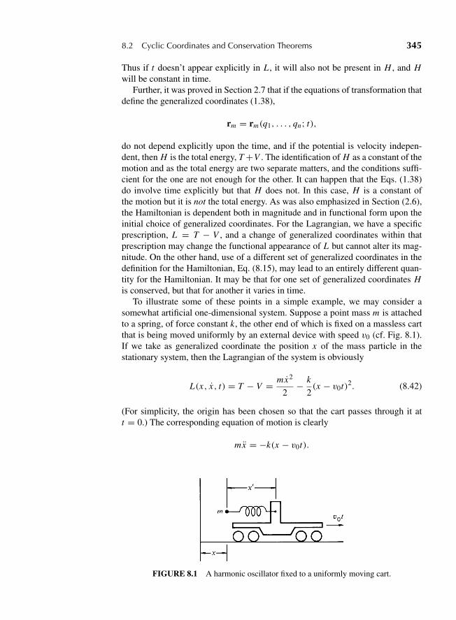
“M08 Goldstein ISBN C08” — 2011/2/15 — page 345 — #12
8.2 Cyclic Coordinates and Conservation Theorems 345
Thus if t doesn’t appear explicitly in L , it will also not be present in H , and Hwill be constant in time.
Further, it was proved in Section 2.7 that if the equations of transformation thatdefine the generalized coordinates (1.38),
rm = rm(q1, . . . , qn; t),
do not depend explicitly upon the time, and if the potential is velocity indepen-dent, then H is the total energy, T +V . The identification of H as a constant of themotion and as the total energy are two separate matters, and the conditions suffi-cient for the one are not enough for the other. It can happen that the Eqs. (1.38)do involve time explicitly but that H does not. In this case, H is a constant ofthe motion but it is not the total energy. As was also emphasized in Section (2.6),the Hamiltonian is dependent both in magnitude and in functional form upon theinitial choice of generalized coordinates. For the Lagrangian, we have a specificprescription, L = T − V , and a change of generalized coordinates within thatprescription may change the functional appearance of L but cannot alter its mag-nitude. On the other hand, use of a different set of generalized coordinates in thedefinition for the Hamiltonian, Eq. (8.15), may lead to an entirely different quan-tity for the Hamiltonian. It may be that for one set of generalized coordinates His conserved, but that for another it varies in time.
To illustrate some of these points in a simple example, we may consider asomewhat artificial one-dimensional system. Suppose a point mass m is attachedto a spring, of force constant k, the other end of which is fixed on a massless cartthat is being moved uniformly by an external device with speed v0 (cf. Fig. 8.1).If we take as generalized coordinate the position x of the mass particle in thestationary system, then the Lagrangian of the system is obviously
L(x, x, t) = T − V = mx2
2− k
2(x − v0t)2. (8.42)
(For simplicity, the origin has been chosen so that the cart passes through it att = 0.) The corresponding equation of motion is clearly
mx = −k(x − v0t).
FIGURE 8.1 A harmonic oscillator fixed to a uniformly moving cart.
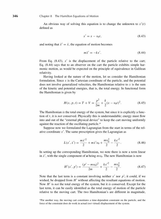
“M08 Goldstein ISBN C08” — 2011/2/15 — page 346 — #13
346 Chapter 8 The Hamilton Equations of Motion
An obvious way of solving this equation is to change the unknown to x ′(t)defined as
x ′ = x − v0t, (8.43)
and noting that x ′ = x , the equation of motion becomes
mx ′ = −kx ′. (8.44)
From Eq. (8.43), x ′ is the displacement of the particle relative to the cart;Eq. (8.44) says that to an observer on the cart the particle exhibits simple har-monic motion, as would be expected on the principle of equivalence in Galileanrelativity.
Having looked at the nature of the motion, let us consider the Hamiltonianformulation. Since x is the Cartesian coordinate of the particle, and the potentialdoes not involve generalized velocities, the Hamiltonian relative to x is the sumof the kinetic and potential energies, that is, the total energy. In functional formthe Hamiltonian is given by
H(x, p, t) = T + V = p2
2m+ k
2(x − v0t)2. (8.45)
The Hamiltonian is the total energy of the system, but since it is explicitly a func-tion of t , it is not conserved. Physically this is understandable; energy must flowinto and out of the “external physical device” to keep the cart moving uniformlyagainst the reaction of the oscillating particle.*
Suppose now we formulated the Lagrangian from the start in terms of the rel-ative coordinate x ′. The same prescription gives the Lagrangian as
L(x ′, x ′) = mx ′2
2+ mx ′v0 +
mv20
2− kx ′2
2. (8.46)
In setting up the corresponding Hamiltonian, we note there is now a term linearin x ′, with the single component of a being mv0. The new Hamiltonian is now
H ′(x ′, p′) = (p′ − mv0)2
2m+ kx ′2
2− mv2
0
2. (8.47)
Note that the last term is a constant involving neither x ′ nor p′; it could, if wewished, be dropped from H ′ without affecting the resultant equations of motion.Now H ′ is not the total energy of the system, but it is conserved. Except for thelast term, it can be easily identified as the total energy of motion of the particlerelative to the moving cart. The two Hamiltonian’s are different in magnitude,
*Put another way, the moving cart constitutes a time-dependent constraint on the particle, and theforce of the constraint does do work in actual (not virtual) displacement of the system.
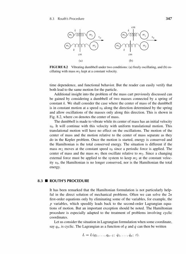
“M08 Goldstein ISBN C08” — 2011/2/15 — page 347 — #14
8.3 Routh’s Procedure 347
FIGURE 8.2 Vibrating dumbbell under two conditions: (a) freely oscillating, and (b) os-cillating with mass m2 kept at a constant velocity.
time dependence, and functional behavior. But the reader can easily verify thatboth lead to the same motion for the particle.
Additional insight into the problem of the mass cart previously discussed canbe gained by considering a dumbbell of two masses connected by a spring ofconstant k. We shall consider the case where the center of mass of the dumbbellis in constant motion at a speed v0 along the direction determined by the springand allow oscillations of the masses only along this direction. This is shown inFig. 8.2, where cm denotes the center of mass.
The dumbbell is made to vibrate while its center of mass has an initial velocityv0. It will continue with this velocity with uniform translational motion. Thistranslational motion will have no effect on the oscillations. The motion of thecenter of mass and the motion relative to the center of mass separate as theydo in the Kepler problem. Once the motion is started, energy is conserved andthe Hamiltonian is the total conserved energy. The situation is different if themass m2 moves at the constant speed v0 since a periodic force is applied. Thecenter of mass and the mass m1 then oscillate relative to m2. Since a changingexternal force must be applied to the system to keep m2 at the constant veloc-ity v0, the Hamiltonian is no longer conserved, nor is the Hamiltonian the totalenergy.
8.3 ROUTH’S PROCEDURE
It has been remarked that the Hamiltonian formulation is not particularly help-ful in the direct solution of mechanical problems. Often we can solve the 2nfirst-order equations only by eliminating some of the variables, for example, thep variables, which speedily leads back to the second-order Lagrangian equa-tions of motion. But an important exception should be noted. The Hamiltonianprocedure is especially adapted to the treatment of problems involving cycliccoordinates.
Let us consider the situation in Lagrangian formulation when some coordinate,say qn , is cyclic. The Lagrangian as a function of q and q can then be written
L = L(q1, . . . , qn−1; q1, . . . , qn; t).
“M08 Goldstein ISBN C08” — 2011/2/15 — page 348 — #15
348 Chapter 8 The Hamilton Equations of Motion
All the generalized velocities still occur in the Lagrangian and in general will befunctions of the time. We still have to solve a problem of n degrees of freedom,even though one degree of freedom corresponds to a cyclic coordinate. A cycliccoordinate in the Hamiltonian formulation, on the other hand, truly deserves itsalternative description as “ignorable,” for in the same situation pn is some con-stant α, and H has the form
H = H(q1, . . . , qn−1; p1, . . . , pn−1; α; t).
In effect, the Hamiltonian now describes a problem involving only n − 1 coordi-nates, which may be solved completely ignoring the cyclic coordinate except asit is manifested in the constant of integration α, to be determined from the initialconditions. The behavior of the cyclic coordinate itself with time is then found byintegrating the equation of motion
qn = ∂H
∂α.
The advantages of the Hamiltonian formulation in handling cyclic coordinatesmay be combined with the Lagrangian conveniences for noncyclic coordinates bya method devised by Routh. Essentially, we carry out a mathematical transforma-tion from the q, q basis to the q, p basis only for those coordinates that are cyclic,obtaining their equations of motion in the Hamiltonian form, while the remain-ing coordinates are governed by Lagrange equations. If the cyclic coordinates arelabeled qs+1, . . . , qn , then a new function R (known as the Routhian) may beintroduced, defined as
R(q1, . . . , qn; q1, . . . , qs; ps+1, . . . , pn; t) =n∑
i=s+1
pi qi − L , (8.48)
which is equivalent to writing
R(q1, . . . , qn; q1, . . . , qs; ps+1, . . . , pn; t) =Hcycl(ps+1, . . . , pn)− Lnoncycl(q1, . . . , qs; q1, . . . , qs). (8.49)
It is easy to show for the s nonignorable coordinates, the Lagrange equations
d
dt
(∂R
∂ qi
)− ∂R
∂qi= 0, i = 1, . . . , s, (8.50)
are satisfied, while for the n−s ignorable coordinates, Hamilton’s equations applyas
∂R
∂qi= − pi = 0, and
∂R
∂pi= qi , i = s + 1, . . . , n. (8.51)
A simple, almost trivial, example may clarify Routh’s procedure and thephysical significance of the quantities involved. Consider the Kepler problem
“M08 Goldstein ISBN C08” — 2011/2/15 — page 349 — #16
8.4 The Hamiltonian Formulation of Relativistic Mechanics 349
investigated in Section 3.7, that of a single particle moving in a plane underthe influence of the inverse-square central force f (r) derived from the potentialV (r) = −k/rn . The Lagrangian is then
L = m
2(r2 + r2θ2)+ k
rn.
As noted before, the ignorable coordinate is θ , and if the constant conjugatemomentum is denoted by pθ , the corresponding Routhian (8.49) is
R(r, r , pθ ) =p2θ
2mr2− 1
2mr2 − k
rn.
Physically we see that the Routhian is the equivalent one-dimensional potentialV ′(r) minus the kinetic energy of radial motion.
Applying the Lagrange equation (8.50) to the noncyclic radial coordinate r ,we obtain the equation of motion (3.11)
r − p2θ
mr3+ nk
rn+1= 0. (8.52)
Applying Hamilton’s equation (8.51) to the cyclic variable θ , we obtain the pairof equations
pθ = 0 andpθ
mr2= θ , (8.53)
whose solution is the same as Eq. (3.8),
pθ = mr2θ = l = constant.
Typically, Routh’s procedure does not add to the physics of the analysis pre-sented earlier in Chapter 3, but it makes the analysis more automatic. In compli-cated problems with many degrees of freedom, this feature can be a considerableadvantage. it is not surprising therefore that Routh’s procedure finds its greatestusefulness in the direct solution of problems relating to engineering applications.But as a fundamental entity, the Routhian is a sterile hybrid, combining some ofthe features of both the Lagrangian and the Hamiltonian pictures. For the devel-opment of various formalisms of classical mechanics, the complete Hamiltonianformulation is more fruitful.
8.4 THE HAMILTONIAN FORMULATION OF RELATIVISTIC MECHANICS
As with the Lagrangian picture in special relativity, two attitudes can be takento the Hamiltonian formulation of relativistic mechanics. The first makes nopretense at a covariant description but instead works in some specific Lorentzor inertial frame. Time as measured in the particular Lorentz frame is then nottreated on a common basis with other coordinates but serves, as in nonrelativisticmechanics, as a parameter describing the evolution of the system. Nonetheless,
“M08 Goldstein ISBN C08” — 2011/2/15 — page 350 — #17
350 Chapter 8 The Hamilton Equations of Motion
if the Lagrangian that leads to the Hamiltonian is itself based on a relativisticallyinvariant physical theory (for example, Maxwell’s equations and the Lorentzforce), then the resultant Hamiltonian picture will be relativistically correct. Thesecond approach of course attempts a fully covariant description of the Hamil-tonian picture, but the difficulties that plagued the corresponding Lagrangianapproach (cf. Section 7.9) are even fiercer here. We shall consider the noncovari-ant method first.
For a single-particle Lagrangian of the form of Eq. (7.136),
L = −mc2√
1 − β2 − V,
we have already shown that the Hamiltonian (in the guise of the energy functionh) is the total energy of the system:
H = T + V .
The energy T can be expressed in terms of the canonical momenta pi (Eq. 7.139)through Eq. (7.38):*
T 2 = p2c2 + m2c4,
so that a suitable form for the Hamiltonian is
H =√
p2c2 + m2c4 + V . (8.54)
When the system consists of a single particle moving in an electromagneticfield, the Lagrangian has been given as (cf. Eq. (7.141))
L = −mc2√
1 − β2 + qA ? v − qφ.
The term in L linear in the velocities does not appear explicitly in the Hamiltonian(cf. Eq. (8.54)), as we have seen, whereas the first term leads to the appearance ofT in the Hamiltonian. Thus, the Hamiltonian is again the total particle energy:
H = T + qφ. (8.55)
For this system, the canonical momenta conjugate to the Cartesian coordinates ofthe particle are defined by (cf. Eq. (7.142))
pi = mui + q Ai ,
so that the relation between T and pi is given by Eq. (7.168), and the Hamiltonianhas the final form
H =√(p − qA)2c2 + m2c4 + qφ. (8.56)
*In this section we use T for the motion energy (pc) plus the rest energy (mc2) to avoid confusing itwith the total energy T + V .
“M08 Goldstein ISBN C08” — 2011/2/15 — page 351 — #18
8.4 The Hamiltonian Formulation of Relativistic Mechanics 351
It should be emphasized again that p here is the vector of the canonical momentaconjugate to the Cartesian position coordinates of the particle. We may also notethat (H − qφ)/c is the zeroth component of the 4-vector
muν + q Aν
(cf. Eqs. (7.27), (7.38′), and (7.166)). While the Hamiltonian (8.56) is not ex-pressed in covariant fashion, it does have a definite transformation behavior undera Lorentz transformation as being, in some Lorentz form, the zeroth componentof a 4-vector.
In a covariant approach to the Hamiltonian formulation, time must be treated inthe same fashion as the space coordinates; that is, time must be taken as one of thecanonical coordinates having an associated conjugate momentum. The founda-tions of such an extension of the dimensionality of phase space can in fact be con-structed even in nonrelativistic mechanics. Following the pattern of Section 7.10,the progress of the system point along its trajectory in phase space can be markedby some parameter θ , and t “released,” so to speak, to serve as an additionalcoordinate. If derivatives with respect to θ are denoted by a superscript prime, theLagrangian in the (q1, . . . , qn; t) configuration space is (cf. Eq. (7.159))
(q, q ′, t, t ′) = t ′L(
q,q ′
t ′, t
). (8.57)
The momentum conjugate to t is then
pt = ∂
∂t ′= L + t ′
∂L
∂t ′.
If we make explicit use of the connection q = q ′/t ′, this relation becomes
pt = L − q ′i
t ′∂L
∂ qi= L − qi
∂L
∂ qi= −H. (8.58)
The momentum conjugate to the time “coordinate” is therefore the negative of theordinary Hamiltonian.* While the framework of this derivation is completely non-relativistic, the result is consistent with the identification of the time component ofthe 4-vector momentum with E/c. As can be seen from the definition, Eq. (8.2),if q is multiplied by a constant α, then the conjugate momentum is divided by α.Hence, the canonical momentum conjugate to ct is H/c.
Thus, there seems to be a natural route available for constructing a relativis-tically covariant Hamiltonian. But the route turns out to be mined with boobytraps. It will be recalled that the covariant Lagrangian used to start the process,Eq. (7.159) or Eq. (8.57), is homogeneous in first degree in the generalized
*The remaining momenta are unchanged by the shift from t to θ , as can be seen by evaluating thecorresponding derivative:
∂
∂q ′i= t ′ ∂L
∂q ′i= t ′
(∂L
∂ q
1
t ′)= pi .
“M08 Goldstein ISBN C08” — 2011/2/15 — page 352 — #19
352 Chapter 8 The Hamilton Equations of Motion
velocities q ′, and for such a Lagrangian the recipe described above for construct-ing the Hamiltonian formulation breaks down irreparably. If L is of type L1, thecorresponding Hamiltonian, call it Hc(q, t, p, pt ), is identically zero!
Fortunately, there does not seem to be any compelling reason why the covari-ant Lagrangian has to be homogeneous in the first degree, at least for classicalrelativistic mechanics. It has already been seen that for a single free particle thecovariant Lagrangian
(xμ, uμ) = 12 muμuμ
leads to the correct equations of motion. Of course the four-velocity components,uμ, are still not all independent, but the constraint can be treated as a “weak con-dition” to be imposed only after all the differentiations have been carried through.There is now no difficulty in obtaining a Hamiltonian from this Lagrangian, bythe same route as in nonrelativistic mechanics; the result is clearly
Hc = pμ pμ
2m. (8.59)
For a single particle in an electromagnetic field, a covariant Lagrangian has beenfound previously: (cf. Eq. (7.165))*
(xμ, uμ) = 12 muμuμ + quμAμ(xλ), (7.147)
with the canonical momenta (cf. Eq. (7.167)),
pμ = muμ + q Aμ. (7.149)
In the corresponding Hamiltonian, the term linear in uμ does not appearexplicitly in the Hamiltonian, and the remaining L2 part in terms of the canonicalmomenta is
H′c =
(pμ − q Aμ
)(pμ − q Aμ)
2m. (8.60)
Both Hamiltonians, Eqs. (8.59) and (8.60), are constant, with the same value,−mc2/2, but to obtain the equations of motion it is the functional dependence onthe 4-vectors of position and momenta that is important. With a system of oneparticle, the covariant Hamiltonian leads to eight first-order equations of motion
dxμ
dτ= ∂H′
cgμν
∂pν,
dpμ
dτ= −∂Hcgμν
∂xν. (8.61)
We know that these equations cannot be all independent. The space parts ofEqs. (8.61) obviously lead to the spatial equations of motion. We should expect
*The Legendre transformation process is reversible: Given a Hamiltonian we can obtain the corre-sponding Lagrangian (cf. Derivation 1). But the difficulties also arise in either direction. If a givenHamiltonian is postulated to be homogeneous in first degree in the momenta, then it is not possible tofind an equivalent Lagrangian.
“M08 Goldstein ISBN C08” — 2011/2/15 — page 353 — #20
8.5 Derivation of Hamilton’s Equations from a Variational Principle 353
therefore that the remaining two equations tell us nothing new, exactly as in theLagrangian case. This can be verified by examining the ν = 0 equations in someparticular Lorentz frame. One of them is the constitutive equation for p0:
u0 = ∂H′c
∂p0= 1
m
(p0 − q A0
)or
p0 = 1
c(T + qφ) = H′
c
c, (8.62)
a general conclusion that has been noted before. The other can be written as
1√1 − β2
dp0
dt= −1
c
∂Hc
∂t
or
d H
dt=√
1 − β2 ∂Hc
∂t. (8.63)
As with the covariant Lagrangian formulation, we have the problem of find-ing suitable covariant potential terms in the Lagrangian to describe the forcesother than electromagnetic. In multiparticle systems we are confronted in fullmeasure with the critical difficulties of including interactions other than withfields. In Hamiltonian language, the “no-interaction” theorem already referredto in Section 7.10 says that only in the absence of direct particle interactions canLorentz invariant systems be described in terms of the usual position coordinatesand corresponding canonical momenta. The scope of the relativistic Hamiltonianframework is therefore quite limited and so for the most part we shall confineourselves to nonrelativistic mechanics.
8.5 DERIVATION OF HAMILTON’S EQUATIONSFROM A VARIATIONAL PRINCIPLE
Lagrange’s equations have been shown to be the consequence of a variationalprinciple, namely, the Hamilton’s principle of Section 2.1. Indeed, the variationalmethod is often the preferable one for deriving Lagrange’s equations, for it isapplicable to types of systems not usually included within the scope of mechanics.It would be similarly advantageous if a variational principle could be found thatleads directly to the Hamilton’s equations of motion. Hamilton’s principle,
δ I ≡ δ
∫ t2
t1L dt = 0, (8.64)
lends itself to this purpose, but as formulated originally it refers to paths in con-figuration space. The first modification therefore is that the integral must be eval-uated over the trajectory of the system point in phase space, and the varied paths
“M08 Goldstein ISBN C08” — 2011/2/15 — page 354 — #21
354 Chapter 8 The Hamilton Equations of Motion
must be in the neighborhood of this phase space trajectory. In the spirit of theHamiltonian formulation, both q and p must be treated as independent coordi-nates of phase space, to be varied independently. To this end the integrand in theaction integral, Eq. (8.64), must be expressed as a function of both q and p, andtheir time derivatives, through Eq. (8.15). Equation (8.64) then appears as
δ I = δ
∫ t2
t1
(pi qi − H(q, p, t)
)dt = 0. (8.65)
As a variational principle in phase space, Eq. (8.65) is sometimes referred to asthe modified Hamilton’s principle. Although it will be used most frequently inconnection with transformation theory (see Chapter 9), the main interest in it hereis to show that the principle leads to Hamilton’s canonical equations of motion.
The modified Hamilton’s principle is exactly of the form of the variationalproblem in a space of 2n dimensions considered in Section 2.3 (cf. Eq. (2.14)):
δ I = δ
∫ t2
t1f (q, q, p, p, t) dt = 0, (8.66)
for which the 2n Euler–Lagrange equations are
d
dt
(∂ f
∂q j
)− ∂ f
∂q j= 0 j = 1, . . . , n (8.67)
d
dt
(∂ f
∂ p j
)− ∂ f
∂p j= 0 j = 1, . . . , n. (8.68)
The integrand f as given in Eq. (8.65) contains q j only through the pi qi term,and q j only in H . Hence, Eqs. (8.67) lead to
p j + ∂H
∂q j= 0. (8.69)
On the other hand, there is no explicit dependence of the integrand in Eq. (8.65)on p j . Equations (8.68) therefore reduce simply to
q j − ∂H
∂p j= 0. (8.70)
Equations (8.69) and (8.70) are exactly Hamilton’s equations of motion, Eqs.(8.18). The Euler–Lagrange equations of the modified Hamilton’s principle arethus the desired canonical equations of motion.
This derivation of Hamilton’s equations from the variational principle is sobrief as to give the appearance of a sleight-of-hand trick. One wonders whethersomething extra has been sneaked in while we were being misdirected by themagician’s patter. Is the modified Hamilton’s principle equivalent to Hamilton’sprinciple, or does it contain some additional physics? The question is largelyirrelevant; the primary justification for the modified Hamilton’s principle is thatit leads to the canonical equations of motion in phase space. After all, no further
“M08 Goldstein ISBN C08” — 2011/2/15 — page 355 — #22
8.5 Derivation of Hamilton’s Equations from a Variational Principle 355
argument was given for the validity of Hamilton’s principle than that it corre-sponded to the Lagrangian equations of motion. So long as Hamiltonian can beconstructed, the Legendre transformation procedure shows that the Lagrangianand Hamiltonian formulations, and therefore their respective variational princi-ples, have the same physical content.
One question that can be raised however is whether the derivation puts limita-tions on the variation of the trajectory that are not present in Hamilton’s principle.The variational principle leading to the Euler–Lagrange equations is formulated,as in Section 2.2, such that the variations of the independent variables vanish atthe end points. In phase space, that would require δqi = 0 and δpi = 0 at theend points, whereas Hamilton’s principle requires only the vanishing of δqi underthe same circumstances. A look at the derivation as spelled out in Section 2.2will show however that the variation is required to be zero at the end points onlyin order to get rid of the integrated terms arising from the variations in the timederivatives of the independent variables. While the f function in Eq. (8.66) thatcorresponds to the modified Hamilton’s principle, Eq. (8.65), is indeed a func-tion of q j , there is no explicit appearance of p j . Equations (8.68) and therefore(8.70) follow from Eq. (8.65) without stipulating the variations of p j at the endpoints. The modified Hamilton’s principle, with the integrand L defined in termsof the Hamiltonian by Eq. (8.19), leads to Hamilton’s equations under the samevariation conditions as those in Hamilton’s principle.*
Nonetheless, there are advantages to requiring that the varied paths in the mod-ified Hamilton’s principle return to the same end points in both q and p, for wethen have a more generalized condition for Hamilton’s equations of motion. Aswith Hamilton’s principle, if there is no variation at the end points we can add atotal time derivative of any arbitrary (twice-differentiable) function F(q, p, t) tothe integrand without affecting the validity of the variational principle. Suppose,for example, we subtract from the integrand of Eq. (8.65) the quantity
d
dt(qi pi ).
The modified Hamilton’s principle would then read
δ
∫ t2
t1(− pi qi − H(q, p, t)) dt = 0. (8.71)
Here the f integrand of Eq. (8.66) is a function of p, and it is easily verified thatthe Euler–Lagrange equations (8.67) and (8.68) with this f again correspond toHamilton’s equations of motion, Eqs. (8.18). Yet the integrand in Eq. (8.71) isnot the Lagrangian nor can it in general be simply related to the Lagrangian by a
*It may be objected that q and p cannot be varied independently, because the defining Eqs. (8.2) linkp with q and q. We could not then have a variation of q (and q) without a corresponding variation ofp. But this entire objection is completely at variance with the intent and the spirit of the Hamiltonianpicture. Once the Hamiltonian formulation has been set up, Eqs. (8.2) form no part of it. The momentahave been elevated to the status of independent variables, on an equal basis with the coordinates andconnected with them and the time only through the medium of the equations of motion themselves andnot by any a priori defining relationship.
“M08 Goldstein ISBN C08” — 2011/2/15 — page 356 — #23
356 Chapter 8 The Hamilton Equations of Motion
point transformation in configuration space. By restricting the variation of both qand p to be zero at the end points, the modified Hamilton’s principle provides anindependent and general way of setting up Hamilton’s equations of motion with-out a prior Lagrangian formulation. If you will, it does away with the necessityof a linkage between the Hamiltonian canonical variables and a correspondingLagrangian set of generalized coordinates and velocities. This will be very impor-tant to us in the next chapter where we examine transformations of phase spacevariables that preserve the Hamiltonian form of the equations of motion.
The requirement of independent variation of q and p, so essential for the abovederivation, highlights the fundamental difference between the Lagrangian andHamiltonian formulations. Neither the coordinates qi nor the momenta pi areto be considered there as the more fundamental set of variables; both are equallyindependent. Only by broadening the field of independent variables from n to 2nquantities are we enabled to obtain equations of motion that are of first order. Ina sense, the names “coordinates” and “momenta” are unfortunate, for they bringto mind pictures of spatial coordinates and linear, or at most, angular momenta. Awider meaning must now be given to the terms. The division into coordinates andmomenta corresponds to no more than a separation of the independent variablesdescribing the motion into two groups having an almost symmetrical relationshipto each other through Hamilton’s equations.
8.6 THE PRINCIPLE OF LEAST ACTION
Another variational principle associated with the Hamiltonian formulation isknown as the principle of least action. It involves a new type of variation, whichwe shall call the -variation, requiring detailed explanation. In the δ-variationprocess used in the discussion of Hamilton’s principle in Chapter 2, the variedpath in configuration space always terminated at end points representing thesystem configuration at the same time t1 and t2 as the correct path. To obtainLagrange’s equations of motion, we also required that the varied path return tothe same end points in configuration space, that is, δqi (t1) = δqi (t2) = 0. The -variation is less constrained; in general, the varied path over which an integralis evaluated may end at different times than the correct path, and there may bea variation in the coordinates at the end points. We can however use the sameparameterization of the varied path as in the δ-variation. In the notation of Sec-tion 2.3, a family of possible varied paths is defined by functions (cf. Eq. (2.15))
qi (t, α) = qi (t, 0)+ αηi (t), (8.72)
where α is an infinitesimal parameter that goes to zero for the correct path. Herethe functions ηi do not necessarily have to vanish at the end points, either the orig-inal or the varied. All that is required is that they be continuous and differentiable.Figure 8.3 illustrates the correct and varied path for a -variation in configurationspace.
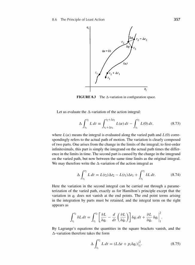
“M08 Goldstein ISBN C08” — 2011/2/15 — page 357 — #24
8.6 The Principle of Least Action 357
FIGURE 8.3 The -variation in configuration space.
Let us evaluate the -variation of the action integral:
∫ t2
t1L dt ≡
∫ t2+ t2
t1+ t1L(α) dt −
∫ t2
t1L(0) dt, (8.73)
where L(α) means the integral is evaluated along the varied path and L(0) corre-spondingly refers to the actual path of motion. The variation is clearly composedof two parts. One arises from the change in the limits of the integral; to first-orderinfinitesimals, this part is simply the integrand on the actual path times the differ-ence in the limits in time. The second part is caused by the change in the integrandon the varied path, but now between the same time limits as the original integral.We may therefore write the -variation of the action integral as
∫ t2
t1L dt = L(t2) t2 − L(t1) t1 +
∫ t2
t1δL dt. (8.74)
Here the variation in the second integral can be carried out through a parame-terization of the varied path, exactly as for Hamilton’s principle except that thevariation in qi does not vanish at the end points. The end point terms arisingin the integration by parts must be retained, and the integral term on the rightappears as
∫ t2
t1δL dt =
∫ t2
t1
[∂L
∂qi− d
dt
(∂L
∂qi
)]δqi dt + ∂L
∂qiδqi
∣∣∣∣2
1.
By Lagrange’s equations the quantities in the square brackets vanish, and the -variation therefore takes the form
∫ t2
t1L dt = (L t + piδqi )
∣∣21. (8.75)
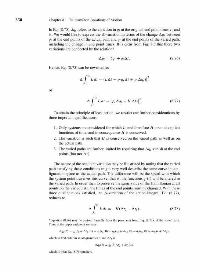
“M08 Goldstein ISBN C08” — 2011/2/15 — page 358 — #25
358 Chapter 8 The Hamilton Equations of Motion
In Eq. (8.75), δqi refers to the variation in qi at the original end point times t1 andt2. We would like to express the -variation in terms of the change qi betweenqi at the end points of the actual path and qi at the end points of the varied path,including the change in end point times. It is clear from Fig. 8.3 that these twovariations are connected by the relation*
qi = δqi + qi t. (8.76)
Hence, Eq. (8.75) can be rewritten as
∫ t2
t1L dt = (L t − pi qi t + pi qi )
∣∣21
or
∫ t2
t1L dt = (pi qi − H t)
∣∣21. (8.77)
To obtain the principle of least action, we restrict our further considerations bythree important qualifications:
1. Only systems are considered for which L , and therefore H , are not explicitfunctions of time, and in consequence H is conserved.
2. The variation is such that H is conserved on the varied path as well as onthe actual path.
3. The varied paths are further limited by requiring that qi vanish at the endpoints (but not t).
The nature of the resultant variation may be illustrated by noting that the variedpath satisfying these conditions might very well describe the same curve in con-figuration space as the actual path. The difference will be the speed with whichthe system point traverses this curve; that is, the functions qi (t) will be altered inthe varied path. In order then to preserve the same value of the Hamiltonian at allpoints on the varied path, the times of the end points must be changed. With thesethree qualifications satisfied, the -variation of the action integral, Eq. (8.77),reduces to
∫ t2
t1L dt = −H( t2 − t1). (8.78)
*Equation (8.76) may be derived formally from the parameter form, Eq. (8.72), of the varied path.Thus, at the upper end point we have
qi (2) = qi (t2 + t2, α)− qi (t2, 0) = qi (t2 + t2, 0)− qi (t2, 0)+ αηi (t + t2),
which to first order in small quantities α and t2 is
qi (2) = qi (2) t2 + δqi (2),
which is what Eq. (8.76) predicts.
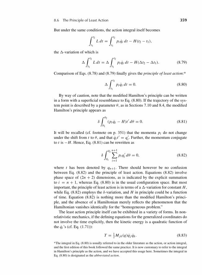
“M08 Goldstein ISBN C08” — 2011/2/15 — page 359 — #26
8.6 The Principle of Least Action 359
But under the same conditions, the action integral itself becomes∫ t2
t1L dt =
∫ t2
t1pi qi dt − H(t2 − t1),
the -variation of which is
∫ t2
t1L dt =
∫ t2
t1pi qi dt − H( t2 − t1). (8.79)
Comparison of Eqs. (8.78) and (8.79) finally gives the principle of least action:*
∫ t2
t1pi qi dt = 0. (8.80)
By way of caution, note that the modified Hamilton’s principle can be writtenin a form with a superficial resemblance to Eq. (8.80). If the trajectory of the sys-tem point is described by a parameter θ , as in Sections 7.10 and 8.4, the modifiedHamilton’s principle appears as
δ
∫ θ2
θ1
(pi qi − H)t ′ dθ = 0. (8.81)
It will be recalled (cf. footnote on p. 351) that the momenta pi do not changeunder the shift from t to θ , and that qi t ′ = q ′
i . Further, the momentum conjugateto t is −H . Hence, Eq. (8.81) can be rewritten as
δ
∫ θ2
θ1
n+1∑i=1
pi q′i dθ = 0, (8.82)
where t has been denoted by qn+1. There should however be no confusionbetween Eq. (8.82) and the principle of least action. Equations (8.82) involvephase space of (2n + 2) dimensions, as is indicated by the explicit summationto i = n + 1, whereas Eq. (8.80) is in the usual configuration space. But mostimportant, the principle of least action is in terms of a -variation for constant H ,while Eq. (8.82) employs the δ-variation, and H in principle could be a functionof time. Equation (8.82) is nothing more than the modified Hamilton’s princi-ple, and the absence of a Hamiltonian merely reflects the phenomenon that theHamiltonian vanishes identically for the “homogeneous problem.”
The least action principle itself can be exhibited in a variety of forms. In non-relativistic mechanics, if the defining equations for the generalized coordinates donot involve the time explicitly, then the kinetic energy is a quadratic function ofthe qi ’s (cf. Eq. (1.71)):
T = 12 M jk(q)q j qk . (8.83)
*The integral in Eq. (8.80) is usually referred to in the older literature as the action, or action integral,and the first edition of this book followed the same practice. It is now customary to refer to the integralin Hamilton’s principle as the action, and we have accepted this usage here. Sometimes the integral inEq. (8.80) is designated as the abbreviated action.
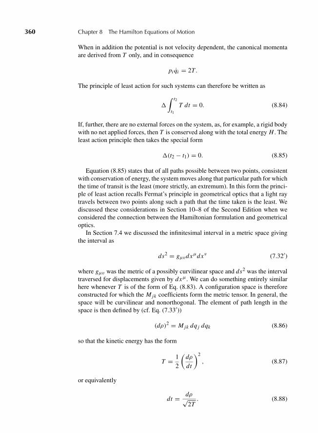
“M08 Goldstein ISBN C08” — 2011/2/15 — page 360 — #27
360 Chapter 8 The Hamilton Equations of Motion
When in addition the potential is not velocity dependent, the canonical momentaare derived from T only, and in consequence
pi qi = 2T .
The principle of least action for such systems can therefore be written as
∫ t2
t1T dt = 0. (8.84)
If, further, there are no external forces on the system, as, for example, a rigid bodywith no net applied forces, then T is conserved along with the total energy H . Theleast action principle then takes the special form
(t2 − t1) = 0. (8.85)
Equation (8.85) states that of all paths possible between two points, consistentwith conservation of energy, the system moves along that particular path for whichthe time of transit is the least (more strictly, an extremum). In this form the princi-ple of least action recalls Fermat’s principle in geometrical optics that a light raytravels between two points along such a path that the time taken is the least. Wediscussed these considerations in Section 10–8 of the Second Edition when weconsidered the connection between the Hamiltonian formulation and geometricaloptics.
In Section 7.4 we discussed the infinitesimal interval in a metric space givingthe interval as
ds2 = gμvdxμdxv (7.32′)
where gμv was the metric of a possibly curvilinear space and ds2 was the intervaltraversed for displacements given by dxμ. We can do something entirely similarhere whenever T is of the form of Eq. (8.83). A configuration space is thereforeconstructed for which the M jk coefficients form the metric tensor. In general, thespace will be curvilinear and nonorthogonal. The element of path length in thespace is then defined by (cf. Eq. (7.33′))
(dρ)2 = M jk dq j dqk (8.86)
so that the kinetic energy has the form
T = 1
2
(dρ
dt
)2
, (8.87)
or equivalently
dt = dρ√2T. (8.88)
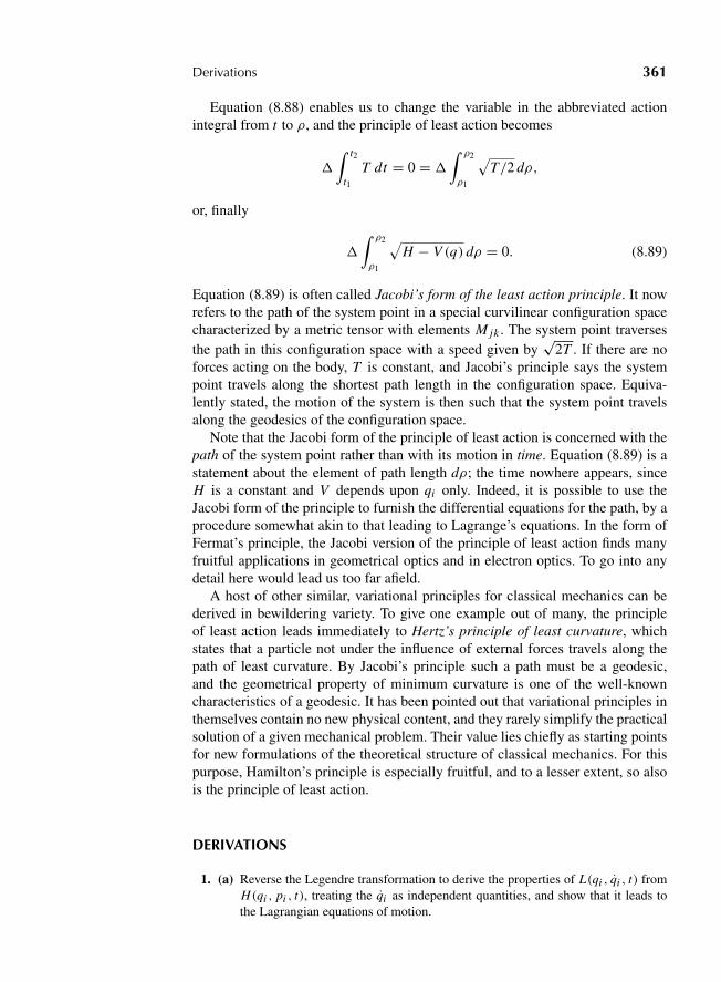
“M08 Goldstein ISBN C08” — 2011/2/15 — page 361 — #28
Derivations 361
Equation (8.88) enables us to change the variable in the abbreviated actionintegral from t to ρ, and the principle of least action becomes
∫ t2
t1T dt = 0 =
∫ ρ2
ρ1
√T/2 dρ,
or, finally
∫ ρ2
ρ1
√H − V (q) dρ = 0. (8.89)
Equation (8.89) is often called Jacobi’s form of the least action principle. It nowrefers to the path of the system point in a special curvilinear configuration spacecharacterized by a metric tensor with elements M jk . The system point traversesthe path in this configuration space with a speed given by
√2T . If there are no
forces acting on the body, T is constant, and Jacobi’s principle says the systempoint travels along the shortest path length in the configuration space. Equiva-lently stated, the motion of the system is then such that the system point travelsalong the geodesics of the configuration space.
Note that the Jacobi form of the principle of least action is concerned with thepath of the system point rather than with its motion in time. Equation (8.89) is astatement about the element of path length dρ; the time nowhere appears, sinceH is a constant and V depends upon qi only. Indeed, it is possible to use theJacobi form of the principle to furnish the differential equations for the path, by aprocedure somewhat akin to that leading to Lagrange’s equations. In the form ofFermat’s principle, the Jacobi version of the principle of least action finds manyfruitful applications in geometrical optics and in electron optics. To go into anydetail here would lead us too far afield.
A host of other similar, variational principles for classical mechanics can bederived in bewildering variety. To give one example out of many, the principleof least action leads immediately to Hertz’s principle of least curvature, whichstates that a particle not under the influence of external forces travels along thepath of least curvature. By Jacobi’s principle such a path must be a geodesic,and the geometrical property of minimum curvature is one of the well-knowncharacteristics of a geodesic. It has been pointed out that variational principles inthemselves contain no new physical content, and they rarely simplify the practicalsolution of a given mechanical problem. Their value lies chiefly as starting pointsfor new formulations of the theoretical structure of classical mechanics. For thispurpose, Hamilton’s principle is especially fruitful, and to a lesser extent, so alsois the principle of least action.
DERIVATIONS
1. (a) Reverse the Legendre transformation to derive the properties of L(qi , qi , t) fromH(qi , pi , t), treating the qi as independent quantities, and show that it leads tothe Lagrangian equations of motion.
“M08 Goldstein ISBN C08” — 2011/2/15 — page 362 — #29
362 Chapter 8 The Hamilton Equations of Motion
(b) By the same procedure find the equations of motion in terms of the function
L ′(p, p, t) = − pi qi − H(q, p, t).
2. It has been previously noted that the total time derivative of a function of qi and tcan be added to the Lagrangian without changing the equations of motion. What doessuch an addition do to the canonical momenta and the Hamiltonian? Show that theequations of motion in terms of the new Hamiltonian reduce to the original Hamilton’sequations of motion.
3. A Hamiltonian-like formulation can be set up in which qi and pi are the independentvariables with a “Hamiltonian” G(qi , pi , t). [Here pi is defined in terms of qi , qi inthe usual manner.] Starting from the Lagrangian formulation, show in detail how toconstruct G(qi , pi , t), and derive the corresponding “Hamilton’s equation of motion.”
4. Show that if λi are the eigenvalues of a square matrix, then if the reciprocal matrixexists it has the eigenvalues λ−1
i .
5. Verify that the matrix J has the properties given in Eqs. (8.38c) and (8.38e) and thatits determinant has the value +1.
6. Show that Hamilton’s principle can be written as
δ
∫ 2
1[2H(h, t)+ hJh] dt = 0.
7. Verify that both Hamiltonians, Eq. (8.45) and Eq. (8.47), lead to the same motion asdescribed by Eq. (8.44).
8. Show that the modified Hamilton’s principle, in the form of Eq. (8.71), leads to Hamil-ton’s equations of motion.
9. If the canonical variables are not all independent, but are connected by auxiliary con-ditions of the form
ψk(qi , pi , t) = 0,
show that the canonical equations of motion can be written
∂H
∂pi+∑
k
λk∂ψk
∂pi= qi ,
∂H
∂qi+∑
k
λk∂ψk
∂qi= − pi ,
where the λk are the undetermined Lagrange multipliers. The formulation of theHamiltonian equations in which t is a canonical variable is a case in point, since arelation exists between pn+1 and the other canonical variables:
H(q1, . . . , qn+1; p1, . . . , pn)+ pn+1 = 0.
Show that as a result of these circumstances the 2n + 2 Hamilton’s equations of thisformulation can be reduced to the 2n ordinary Hamilton’s equations plus Eq. (8.41)and the relation
λ = dt
dθ.
Note that while these results are reminiscent of the relativistic covariant Hamiltonianformulation, they have been arrived at entirely within the framework of nonrelativisticmechanics.
“M08 Goldstein ISBN C08” — 2011/2/15 — page 363 — #30
Exercises 363
10. Assume that the Lagrangian is a polynomial in q of no higher order than quadratic.Convert the 2n equations (8.2) and (8.14)
pi =∂L
∂ qi, pi =
∂L
∂qi,
into 2n equations for qi and pi in terms of q and p, using the matrix form of theLagrangian. Show that these are the same equations as would be obtained fromHamilton’s equations of motion.
EXERCISES
11. A particle is confined to a one-dimensional box. The ends of the box move slowlytowards the middle. By slowly we mean the speed of the ends is small when comparedto the speed of the particle. Solve the following using Lagrangian formulation and thenusing the Hamiltonian.
(a) if the momentum of the particle is p0 when the walls are a distance x0 apart, findthe momentum of the particle at any later time assuming the collisions with thewall are perfectly elastic. Also assume the motion is nonrelativistic at all times.
(b) When the walls are a distance x apart, what average external force must be appliedto each wall in order to move it at a constant speed?
12. Write the problem of central force motion of two mass points in Hamiltonian formu-lation, eliminating the cyclic variables, and reducing the problem to quadratures.
13. Formulate the double-pendulum problem illustrated by Fig. 1.4, in terms of theHamiltonian and Hamilton’s equations of motion. It is suggested that you find theHamiltonian both directly from L and by Eq. (8.27).
14. The Lagrangian for a system can be written as
L = ax2 + by
x+ cx y + f y2 x z + gy2 − k
√x2 + y2,
where a, b, c, f , g, and k are constants. What is the Hamiltonian? What quantities areconserved?
15. A dynamical system has the Lagrangian
L = q21 + q2
2
a + bq21
+ k1q21 + k2q1q2,
where a, b, k1, and k2 are constants. Find the equations of motion in the Hamiltonianformulation.
16. A Hamiltonian of one degree of freedom has the form
H = p2
2α− bqpe−αt + ba
2q2e−αt (α + be−αt )+ kq2
2,
where a, b, α, and k are constants.
(a) Find a Lagrangian corresponding to this Hamiltonian.
(b) Find an equivalent Lagrangian that is not explicitly dependent on time.
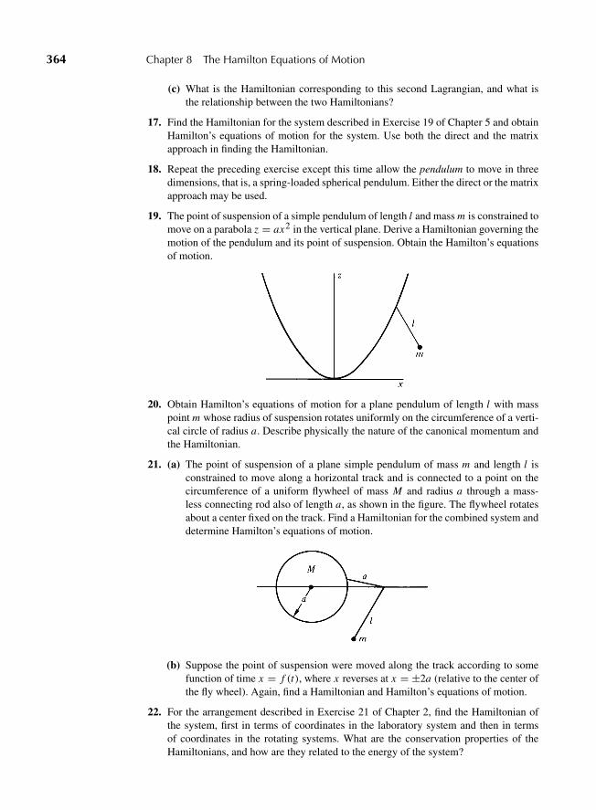
“M08 Goldstein ISBN C08” — 2011/2/15 — page 364 — #31
364 Chapter 8 The Hamilton Equations of Motion
(c) What is the Hamiltonian corresponding to this second Lagrangian, and what isthe relationship between the two Hamiltonians?
17. Find the Hamiltonian for the system described in Exercise 19 of Chapter 5 and obtainHamilton’s equations of motion for the system. Use both the direct and the matrixapproach in finding the Hamiltonian.
18. Repeat the preceding exercise except this time allow the pendulum to move in threedimensions, that is, a spring-loaded spherical pendulum. Either the direct or the matrixapproach may be used.
19. The point of suspension of a simple pendulum of length l and mass m is constrained tomove on a parabola z = ax2 in the vertical plane. Derive a Hamiltonian governing themotion of the pendulum and its point of suspension. Obtain the Hamilton’s equationsof motion.
20. Obtain Hamilton’s equations of motion for a plane pendulum of length l with masspoint m whose radius of suspension rotates uniformly on the circumference of a verti-cal circle of radius a. Describe physically the nature of the canonical momentum andthe Hamiltonian.
21. (a) The point of suspension of a plane simple pendulum of mass m and length l isconstrained to move along a horizontal track and is connected to a point on thecircumference of a uniform flywheel of mass M and radius a through a mass-less connecting rod also of length a, as shown in the figure. The flywheel rotatesabout a center fixed on the track. Find a Hamiltonian for the combined system anddetermine Hamilton’s equations of motion.
(b) Suppose the point of suspension were moved along the track according to somefunction of time x = f (t), where x reverses at x = ±2a (relative to the center ofthe fly wheel). Again, find a Hamiltonian and Hamilton’s equations of motion.
22. For the arrangement described in Exercise 21 of Chapter 2, find the Hamiltonian ofthe system, first in terms of coordinates in the laboratory system and then in termsof coordinates in the rotating systems. What are the conservation properties of theHamiltonians, and how are they related to the energy of the system?
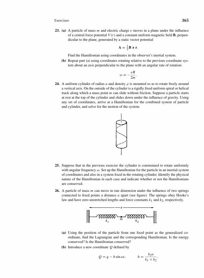
“M08 Goldstein ISBN C08” — 2011/2/15 — page 365 — #32
Exercises 365
23. (a) A particle of mass m and electric charge e moves in a plane under the influenceof a central force potential V (r) and a constant uniform magnetic field B, perpen-dicular to the plane, generated by a static vector potential
A = 12 B3 r.
Find the Hamiltonian using coordinates in the observer’s inertial system.
(b) Repeat part (a) using coordinates rotating relative to the previous coordinate sys-tem about an axis perpendicular to the plane with an angular rate of rotation:
ω = − eB
2m.
24. A uniform cylinder of radius a and density ρ is mounted so as to rotate freely arounda vertical axis. On the outside of the cylinder is a rigidly fixed uniform spiral or helicaltrack along which a mass point m can slide without friction. Suppose a particle startsat rest at the top of the cylinder and slides down under the influence of gravity. Usingany set of coordinates, arrive at a Hamiltonian for the combined system of particleand cylinder, and solve for the motion of the system.
25. Suppose that in the previous exercise the cylinder is constrained to rotate uniformlywith angular frequency ω. Set up the Hamiltonian for the particle in an inertial systemof coordinates and also in a system fixed in the rotating cylinder. Identify the physicalnature of the Hamiltonian in each case and indicate whether or not the Hamiltoniansare conserved.
26. A particle of mass m can move in one dimension under the influence of two springsconnected to fixed points a distance a apart (see figure). The springs obey Hooke’slaw and have zero unstretched lengths and force constants k1 and k2, respectively.
(a) Using the position of the particle from one fixed point as the generalized co-ordinate, find the Lagrangian and the corresponding Hamiltonian. Is the energyconserved? Is the Hamiltonian conserved?
(b) Introduce a new coordinate Q defined by
Q = q − b sinωt, b = k2a
k1 + k2.

“M08 Goldstein ISBN C08” — 2011/2/15 — page 366 — #33
366 Chapter 8 The Hamilton Equations of Motion
What is the Lagrangian in terms of Q? What is the corresponding Hamiltonian?Is the energy conserved? Is the Hamiltonian conserved?
27. (a) The Lagrangian for a system of one degree of freedom can be written as
L = m
2(q2 sin2 ωt + qqω sin 2ωt + q2ω2).
What is the corresponding Hamiltonian? Is it conserved?
(b) Introduce a new coordinate defined by
Q = q sinωt.
Find the Lagrangian in terms of the new coordinate and the correspondingHamiltonian. Is H conserved?
28. Consider a system of particles interacting with each other through potentials depend-ing only on the scalar distances between them and acted upon by conservative centralforces from a fixed point. Obtain the Hamiltonian of the particle with respect to aset of axes, with origin at the center of force, which is rotating around some axis inan inertial system with angular velocity ω. What is the physical significance of theHamiltonian in this case? Is it a constant of the motion?
29. Obtain the Hamiltonian of a heavy symmetrical top with one point fixed, and from itthe Hamilton’s equations of motion. Relate these to the equations of motion discussedin Section 5.7 and, in particular, show how the solution may be reduced to quadratures.Also use the Routhian procedure to eliminate the cyclic coordinates.
30. In Exercise 16 of Chapter 1, there is given the velocity-dependent potential assumed inWeber’s electrodynamics. What is the Hamiltonian for a single particle moving underthe influence of such a potential?
31. Treat the nutation of a “fast” top as an example of small oscillations about steadymotion, here precession at constant θ . Find the frequency of nutation.
32. A symmetrical top is mounted so that it pivots about its center of mass. The pivot inturn is fixed a distance r from the center of a horizontal disk free to rotate about avertical axis. The top is started with an initial rotation about its figure axis, which isinitially at an angle θ0 to the vertical. Analyze the possible nutation of the top as acase of small oscillations about steady motion.
33. Two mass points, m1 and m2, are connected by a string that acts as a Hooke’s-lawspring with force constant k. One particle is free to move without friction on a smoothhorizontal plane surface, the other hangs vertically down from the string through ahole in the surface. Find the condition for steady motion in which the mass point onthe plane rotates uniformly at constant distance from the hole. Investigate the smalloscillations in the radial distance from the hole, and in the vertical height of the secondparticle.
34. A possible covariant Lagrangian for a system of one particle interacting with a field is
= 12 muλuλ + Dλν(xμ)mλν,
where Dxν(xμ) is an antisymmetric field tensor and mλν is the antisymmetric angularmomentum tensor,
“M08 Goldstein ISBN C08” — 2011/2/15 — page 367 — #34
Exercises 367
mλν = m(xλuν − xνuλ).
What are the canonical momenta? What is the corresponding covariant Hamiltonian?
35. Consider a Lagrangian of the form
L = 12 m(x2 − ω2x2)eγ t ,
where the particle of mass m moves in one direction. Assume all constants arepositive.
(a) Find the equations of motion.
(b) Interpret the equations by giving a physical interpretation of the forces acting onthe particle.
(c) Find the canonical momentum and construct the Hamiltonian. Is this Hamiltoniana constant of the motion?
(d) If initially x(0) = 0 and dx/dt = 0, what is x(t) as t approaches large values?
“M09 Goldstein ISBN C09” — 2011/2/15 — page 368 — #1
C H A P T E R
9 Canonical Transformations
When applied in a straightforward manner, the Hamiltonian formulation usu-ally does not materially decrease the difficulty of solving any given problem inmechanics. We wind up with practically the same differential equations to besolved as are provided by the Lagrangian procedure. The advantages of the Hamil-tonian formulation lie not in its use as a calculational tool, but rather in the deeperinsight it affords into the formal structure of mechanics. The equal status accordedto coordinates and momenta as independent variables encourages a greater free-dom in selecting the physical quantities to be designated as “coordinates” and“momenta.” As a result we are led to newer, more abstract ways of presentingthe physical content of mechanics. While often of considerable help in practicalapplications to mechanical problems, these more abstract formulations are primar-ily of interest to us today because of their essential role in constructing the moremodern theories of matter. Thus, one or another of these formulations of classicalmechanics serves as a point of departure for both statistical mechanics and quan-tum theory. It is to such formulations, arising as outgrowths of the Hamiltonianprocedure, that this and the next chapter are devoted.
9.1 THE EQUATIONS OF CANONICAL TRANSFORMATION
There is one type of problem for which the solution of the Hamilton’s equations istrivial. Consider a situation in which the Hamiltonian is a constant of the motion,and where all coordinates qi are cyclic. Under these conditions, the conjugatemomenta pi are all constant:
pi = αi ,
and since the Hamiltonian cannot be an explicit function of either the time or thecyclic coordinates, it may be written as
H = H(α1, . . . , αn).
Consequently, the Hamilton’s equations for qi are simply
qi = ∂H
∂αi= ωi , (9.1)
368
“M09 Goldstein ISBN C09” — 2011/2/15 — page 369 — #2
9.1 The Equations of Canonical Transformation 369
where the ωi ’s are functions of the αi ’s only and therefore are also constant intime. Equations (9.1) have the immediate solutions
qi = ωi t + βi , (9.2)
where the βi ’s are constants of integration, determined by the initial conditions.It would seem that the solution to this type of problem, easy as it is, can only
be of academic interest, for it rarely happens that all the generalized coordinatesare cyclic. But a given system can be described by more than one set of general-ized coordinates. Thus, to discuss motion of a particle in a plane, we may use asgeneralized coordinates either the Cartesian coordinates
q1 = x, q2 = y,
or the plane polar coordinates
q1 = r, q2 = θ.
Both choices are equally valid, but one of the other set may be more convenientfor the problem under consideration. Note that for central forces neither x nor yis cyclic, while the second set does contain a cyclic coordinate in the angle θ .The number of cyclic coordinates can thus depend upon the choice of generalizedcoordinates, and for each problem there may be one particular choice for whichall coordinates are cyclic. If we can find this set, the remainder of the job is trivial.Since the obvious generalized coordinates suggested by the problem will not nor-mally be cyclic, we must first derive a specific procedure for transforming fromone set of variables to some other set that may be more suitable.
The transformations considered in the previous chapters have involved goingfrom one set of coordinates qi to a new set Qi by transformation equations of theform
Qi = Qi (q, t). (9.3)
For example, the equations of an orthogonal transformation, or of the changefrom Cartesian to plane polar coordinates, have the general form of Eqs. (9.3).As has been previously noted in Derivation 10 of Chapter 1, such transforma-tions are known as point transformations. But in the Hamiltonian formulationthe momenta are also independent variables on the same level as the general-ized coordinates. The concept of transformation of coordinates must therefore bewidened to include the simultaneous transformation of the independent coordi-nates and momenta, qi , pi , to a new set Qi , Pi , with (invertible) equations oftransformation:
Qi = Qi (q, p, t),
Pi = Pi (q, p, t). (9.4)
Thus, the new coordinates will be defined not only in terms of the old coordi-nates but also in terms of the old momenta. Equations (9.3) may be said to define
“M09 Goldstein ISBN C09” — 2011/2/15 — page 370 — #3
370 Chapter 9 Canonical Transformations
a point transformation of configuration space; correspondingly Eqs. (9.4) definea point transformation of phase space.
In developing Hamiltonian mechanics, only those transformations can be ofinterest for which the new Q, P are canonical coordinates. This requirement willbe satisfied provided there exists some function K (Q, P, t) such that the equa-tions of motion in the new set are in the Hamiltonian form
Qi = ∂K
∂Pi, Pi = − ∂K
∂Qi. (9.5)
The function K plays the role of the Hamiltonian in the new coordinate set.*It is important for future considerations that the transformations considered beproblem-independent. That is to say, (Q, P) must be canonical coordinates notonly for some specific mechanical systems, but for all systems of the same num-ber of degrees of freedom. Equations (9.5) must be the form of the equations ofmotion in the new coordinates and momenta no matter what the particular initialform of H . We may indeed be incited to develop a particular transformation from(q, p) to (Q, P) to handle, say, a plane harmonic oscillator. But the same trans-formation must then also lead to Hamilton’s equations of motion when applied,for example, to the two-dimensional Kepler problem.
As was seen in Section 8.5, if Qi and Pi are to be canonical coordinates, theymust satisfy a modified Hamilton’s principle that can be put in the form
δ
∫ t2
t1(Pi Qi − K (Q, P, t)) dt = 0, (9.6)
(where summation over the repeated index i is implied). At the same time the oldcanonical coordinates of course satisfy a similar principle:
δ
∫ t2
t1(pi qi − H(q, p, t)) dt = 0. (9.7)
The simultaneous validity of Eqs. (9.6) and (9.7) does not mean of course that theintegrands in both expressions are equal. Since the general form of the modifiedHamilton’s principle has zero variation at the end points, both statements will besatisfied if the integrands are connected by a relation of the form
λ(pi qi − H) = Pi Qi − K + d F
dt. (9.8)
Here F is any function of the phase space coordinates with continuous secondderivatives, and λ is a constant independent of the canonical coordinates and thetime. The multiplicative constant λ is related to a particularly simple type of trans-formation of canonical coordinates known as a scale transformation.
*It has been remarked in a jocular vein that if H stands for the Hamiltonian, K must stand for theKamiltonian! Of course, K is every bit as much a Hamiltonian as H , but the designation is occasionallya convenient substitute for the longer term “transformed Hamiltonian.”
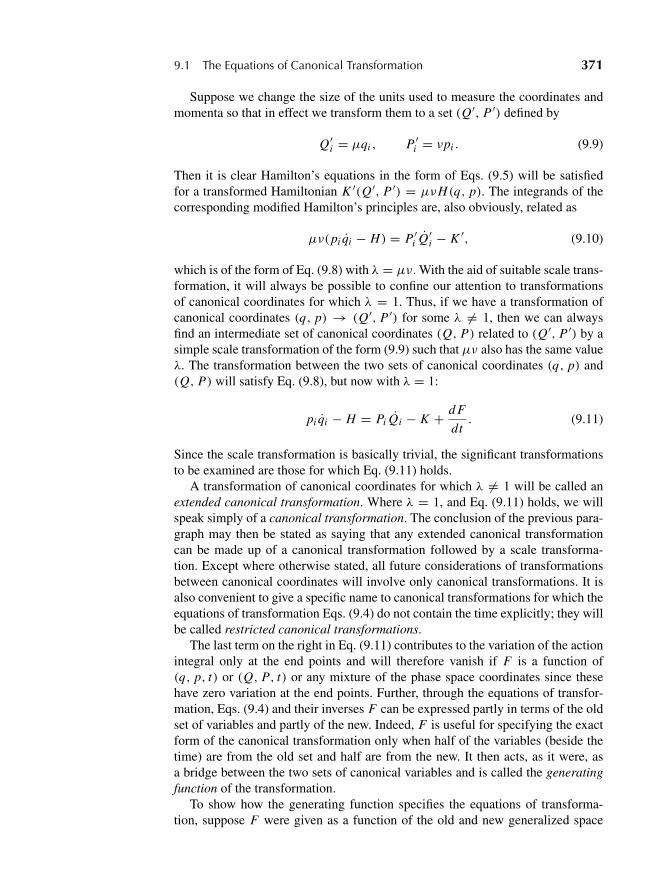
“M09 Goldstein ISBN C09” — 2011/2/15 — page 371 — #4
9.1 The Equations of Canonical Transformation 371
Suppose we change the size of the units used to measure the coordinates andmomenta so that in effect we transform them to a set (Q′, P ′) defined by
Q′i = μqi , P ′
i = νpi . (9.9)
Then it is clear Hamilton’s equations in the form of Eqs. (9.5) will be satisfiedfor a transformed Hamiltonian K ′(Q′, P ′) = μνH(q, p). The integrands of thecorresponding modified Hamilton’s principles are, also obviously, related as
μν(pi qi − H) = P ′i Q′
i − K ′, (9.10)
which is of the form of Eq. (9.8) with λ = μν. With the aid of suitable scale trans-formation, it will always be possible to confine our attention to transformationsof canonical coordinates for which λ = 1. Thus, if we have a transformation ofcanonical coordinates (q, p) → (Q′, P ′) for some λ �= 1, then we can alwaysfind an intermediate set of canonical coordinates (Q, P) related to (Q′, P ′) by asimple scale transformation of the form (9.9) such that μν also has the same valueλ. The transformation between the two sets of canonical coordinates (q, p) and(Q, P) will satisfy Eq. (9.8), but now with λ = 1:
pi qi − H = Pi Qi − K + d F
dt. (9.11)
Since the scale transformation is basically trivial, the significant transformationsto be examined are those for which Eq. (9.11) holds.
A transformation of canonical coordinates for which λ �= 1 will be called anextended canonical transformation. Where λ = 1, and Eq. (9.11) holds, we willspeak simply of a canonical transformation. The conclusion of the previous para-graph may then be stated as saying that any extended canonical transformationcan be made up of a canonical transformation followed by a scale transforma-tion. Except where otherwise stated, all future considerations of transformationsbetween canonical coordinates will involve only canonical transformations. It isalso convenient to give a specific name to canonical transformations for which theequations of transformation Eqs. (9.4) do not contain the time explicitly; they willbe called restricted canonical transformations.
The last term on the right in Eq. (9.11) contributes to the variation of the actionintegral only at the end points and will therefore vanish if F is a function of(q, p, t) or (Q, P, t) or any mixture of the phase space coordinates since thesehave zero variation at the end points. Further, through the equations of transfor-mation, Eqs. (9.4) and their inverses F can be expressed partly in terms of the oldset of variables and partly of the new. Indeed, F is useful for specifying the exactform of the canonical transformation only when half of the variables (beside thetime) are from the old set and half are from the new. It then acts, as it were, asa bridge between the two sets of canonical variables and is called the generatingfunction of the transformation.
To show how the generating function specifies the equations of transforma-tion, suppose F were given as a function of the old and new generalized space
“M09 Goldstein ISBN C09” — 2011/2/15 — page 372 — #5
372 Chapter 9 Canonical Transformations
coordinates:
F = F1(q, Q, t). (9.12)
Equation (9.11) then takes the form
pi qi − H = Pi Qi − K + d F1
dt
= Pi Qi − K + ∂F1
∂t+ ∂F1
∂qiqi + ∂F1
∂QiQi . (9.13)
Since the old and the new coordinates, qi and Qi , are separately independent,Eq. (9.13) can hold identically only if the coefficients of qi and Qi each vanish:
pi = ∂F1
∂qi, (9.14a)
Pi = − ∂F1
∂Qi, (9.14b)
leaving finally
K = H + ∂F1
∂t. (9.14c)
Equations (9.14a) are n relations defining the pi as functions of q j , Q j , and t .Assuming they can be inverted, they could then be solved for the n Qi ’s in termsof q j , p j , and t , thus yielding the first half of the transformation equations (9.4).Once the relations between the Qi ’s and the old canonical variables (q, p) havebeen established, they can be substituted into Eqs. (9.14b) so that they give then Pi ’s as functions of q j , p j , and t , that is, the second half of the transforma-tion equations (9.4). To complete the story, Eq. (9.14c) provides the connectionbetween the new Hamiltonian, K , and the old one, H . We must be careful to readEq. (9.14c) properly. First q and p in H are expressed as functions of Q and Pthrough the inverses of Eqs. (9.4). Then the qi in ∂F1/∂t are expressed in termsof Q, P in a similar manner and the two functions are added to yield K (Q, P, t).
The procedure described shows how, starting from a given generating functionF1, the equations of the canonical transformation can be obtained. We can usu-ally reverse the process: Given the equations of transformation (9.4), an appro-priate generating function F1 may be derived. Equations (9.4) are first inverted toexpress pi and Pi as functions of q, Q, and t . Equations (9.14a, b) then constitutea coupled set of partial differential equations than can be integrated, in principle,to find F1 providing the transformation is indeed canonical. Thus, F1 is alwaysuncertain to within an additive arbitrary function of t alone (which doesn’t affectthe equations of transformation), and there may at times be other ambiguities.
It sometimes happens that it is not suitable to describe the canonical transfor-mation by a generating function of the type F1(q, Q, t). For example, the trans-formation may be such that pi cannot be written as functions of q, Q, and t , but
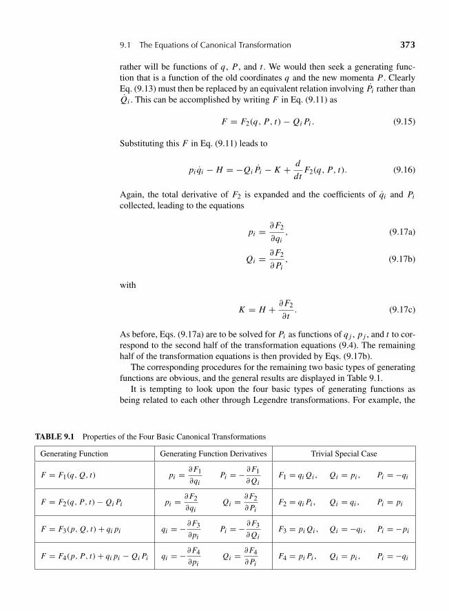
“M09 Goldstein ISBN C09” — 2011/2/15 — page 373 — #6
9.1 The Equations of Canonical Transformation 373
rather will be functions of q, P , and t . We would then seek a generating func-tion that is a function of the old coordinates q and the new momenta P . ClearlyEq. (9.13) must then be replaced by an equivalent relation involving Pi rather thanQi . This can be accomplished by writing F in Eq. (9.11) as
F = F2(q, P, t)− Qi Pi . (9.15)
Substituting this F in Eq. (9.11) leads to
pi qi − H = −Qi Pi − K + d
dtF2(q, P, t). (9.16)
Again, the total derivative of F2 is expanded and the coefficients of qi and Pi
collected, leading to the equations
pi = ∂F2
∂qi, (9.17a)
Qi = ∂F2
∂Pi, (9.17b)
with
K = H + ∂F2
∂t. (9.17c)
As before, Eqs. (9.17a) are to be solved for Pi as functions of q j , p j , and t to cor-respond to the second half of the transformation equations (9.4). The remaininghalf of the transformation equations is then provided by Eqs. (9.17b).
The corresponding procedures for the remaining two basic types of generatingfunctions are obvious, and the general results are displayed in Table 9.1.
It is tempting to look upon the four basic types of generating functions asbeing related to each other through Legendre transformations. For example, the
TABLE 9.1 Properties of the Four Basic Canonical Transformations
Generating Function Generating Function Derivatives Trivial Special Case
F = F1(q, Q, t) pi =∂F1
∂qiPi = − ∂F1
∂QiF1 = qi Qi , Qi = pi , Pi = −qi
F = F2(q, P, t)− Qi Pi pi =∂F2
∂qiQi =
∂F2
∂PiF2 = qi Pi , Qi = qi , Pi = pi
F = F3(p, Q, t)+ qi pi qi = −∂F3
∂piPi = − ∂F3
∂QiF3 = pi Qi , Qi = −qi , Pi = −pi
F = F4(p, P, t)+ qi pi − Qi Pi qi = −∂F4
∂piQi =
∂F4
∂PiF4 = pi Pi , Qi = pi , Pi = −qi
“M09 Goldstein ISBN C09” — 2011/2/15 — page 374 — #7
374 Chapter 9 Canonical Transformations
transition from F1 to F2 is equivalent to going from the variables q, Q to q, Pwith the relation
−Pi = ∂F1
∂Qi. (9.18)
This is just the form required for a Legendre transformation of the basis variables,as described in Section 8.1, and in analogy to Eq. (8.5) we would set
F2(q, P, t) = F1(q, Q, t)+ Pi Qi , (9.19)
which is equivalent to Eq. (9.15) combined with Eq. (9.12). All the other definingequations for the generating functions can similarly be looked on, in combina-tion with Eq. (9.12) as Legendre transformations from F1, with the last entry inTable 9.1 describing a double Legendre transformation. The only drawback tothis picture is that it might erroneously lead us to believe that any given canoni-cal transformation can be expressed in terms of the four basic types of Legendretransformations listed in Table 9.1. This is not always possible. Some transfor-mations are just not suitable for description in terms of these or other elementaryforms of generating functions, as has been noted above and as will be illustratedin the next section with specific examples. If we try to apply the Legendre trans-formation process, we are then led to generating functions that are identicallyzero or are indeterminate. For this reason, we have preferred to define each typeof generating function relative to F , which is some unspecified function of 2nindependent coordinates and momenta.
Finally, note that a suitable generating function doesn’t have to conform toone of the four basic types for all the degrees of freedom of the system. It ispossible, and for some canonical transformations necessary, to use a generatingfunction that is a mixture of the four types. To take a simple example, it may bedesirable for a particular canonical transformation with two degrees of freedomto be defined by a generating function of the form
F ′(q1, p2, P1, Q2, t). (9.20)
This generating function would be related to F in Eq. (9.11) by the equation
F = F ′(q1, p2, P1, Q2, t)− Q1 P1 + q2 p2, (9.21)
and the equations of transformation would be obtained from the relations
p1 = ∂F ′
∂q1, Q1 = ∂F ′
∂P1,
q2 = −∂F ′
∂p2, P2 = − ∂F ′
∂Q2, (9.22)
“M09 Goldstein ISBN C09” — 2011/2/15 — page 375 — #8
9.2 Examples of Canonical Transformations 375
with
K = H + ∂F ′
∂t. (9.23)
Specific illustrations are given in the next section and in the exercises.
9.2 EXAMPLES OF CANONICAL TRANSFORMATIONS
The nature of canonical transformations and the role played by the generatingfunction can best be illustrated by some simple yet important examples. Let usconsider, first, a generating function of the second type with the particular form
F2 = qi Pi (9.24)
found in column 3 of Table 9.1. From Eqs. (9.17), the transformation equationsare
pi = ∂F2
∂qi= Pi ,
Qi = ∂F2
∂Pi= qi ,
K = H. (9.25)
The new and old coordinates are the same; hence F2 merely generates the identitytransformation (cf. Table 9.1). We also note, referring to Table 9.1, that the par-ticular generating function F3 = pi Qi generates an identity transformation withnegative signs; that is, Qi = −qi , Pi = −pi .
A more general type of transformation is described by the generating function
F2 = fi (q1, . . . , qn; t)Pi , (9.26)
where the fi may be any desired set of independent functions. By Eqs. (9.17b),the new coordinates Qi are given by
Qi = ∂F2
∂Pi= fi (qi , . . . , qn; t) (9.27)
Thus, with this generating function the new coordinates depend only upon theold coordinates and the time and do not involve the old momenta. Such a trans-formation is therefore an example of the class of point transformations definedby Eqs. (9.3). In order to define a point transformation, the functions fi must beindependent and invertible, so that the q j can be expressed in terms of the Qi .Since the fi are otherwise completely arbitrary, we may conclude that all pointtransformations are canonical. Equation (9.17c) furnishes the new Hamiltonianin terms of the old and of the time derivatives of the fi functions.
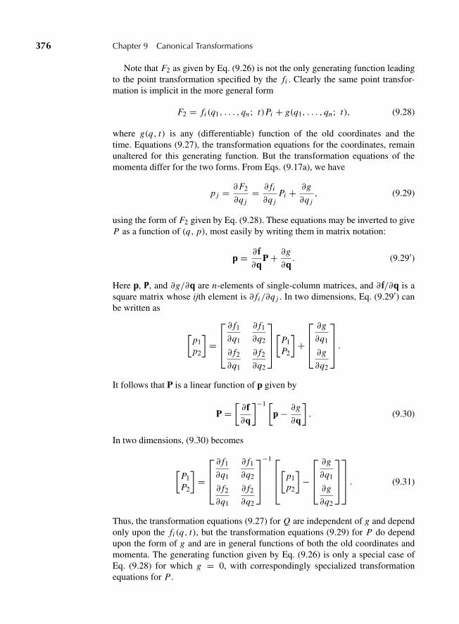
“M09 Goldstein ISBN C09” — 2011/2/15 — page 376 — #9
376 Chapter 9 Canonical Transformations
Note that F2 as given by Eq. (9.26) is not the only generating function leadingto the point transformation specified by the fi . Clearly the same point transfor-mation is implicit in the more general form
F2 = fi (q1, . . . , qn; t)Pi + g(q1, . . . , qn; t), (9.28)
where g(q, t) is any (differentiable) function of the old coordinates and thetime. Equations (9.27), the transformation equations for the coordinates, remainunaltered for this generating function. But the transformation equations of themomenta differ for the two forms. From Eqs. (9.17a), we have
p j = ∂F2
∂q j= ∂ fi
∂q jPi + ∂g
∂q j, (9.29)
using the form of F2 given by Eq. (9.28). These equations may be inverted to giveP as a function of (q, p), most easily by writing them in matrix notation:
p = ∂f∂q
P + ∂g
∂q. (9.29′)
Here p, P, and ∂g/∂q are n-elements of single-column matrices, and ∂f/∂q is asquare matrix whose ijth element is ∂ fi/∂q j . In two dimensions, Eq. (9.29′) canbe written as
[p1p2
]=
⎡⎢⎢⎣∂ f1
∂q1
∂ f1
∂q2
∂ f2
∂q1
∂ f2
∂q2
⎤⎥⎥⎦[
P1P2
]+
⎡⎢⎢⎣∂g
∂q1
∂g
∂q2
⎤⎥⎥⎦ .
It follows that P is a linear function of p given by
P =[∂f∂q
]−1 [p − ∂g
∂q
]. (9.30)
In two dimensions, (9.30) becomes
[P1P2
]=
⎡⎢⎢⎣∂ f1
∂q1
∂ f1
∂q2
∂ f2
∂q1
∂ f2
∂q2
⎤⎥⎥⎦−1⎡⎢⎢⎣[
p1p2
]−
⎡⎢⎢⎣∂g
∂q1
∂g
∂q2
⎤⎥⎥⎦⎤⎥⎥⎦ . (9.31)
Thus, the transformation equations (9.27) for Q are independent of g and dependonly upon the fi (q, t), but the transformation equations (9.29) for P do dependupon the form of g and are in general functions of both the old coordinates andmomenta. The generating function given by Eq. (9.26) is only a special case ofEq. (9.28) for which g = 0, with correspondingly specialized transformationequations for P .
“M09 Goldstein ISBN C09” — 2011/2/15 — page 377 — #10
9.3 The Harmonic Oscillator 377
An instructive transformation is provided by the generating function of the firstkind, F1(q, Q, t), of the form
F1 = qk Qk .
The corresponding transformation equations, from (9.14a, b) are
pi = ∂Fi
∂qi= Qi , (9.32a)
Pi = − ∂F1
∂Qi= −qi . (9.32b)
In effect, the transformation interchanges the momenta and the coordinates; thenew coordinates are the old momenta and the new momenta are essentially the oldcoordinates. Table 9.1 shows that the particular generating function of type F4 =pi Pi produces the same transformation. These simple examples should emphasizethe independent status of generalized coordinates and momenta. They are bothneeded to describe the motion of the system in the Hamiltonian formulation. Thedistinction between them is basically one of nomenclature. We can shift the namesaround with at most no more than a change in sign. There is no longer present inthe theory any lingering remnant of the concept of qi as a spatial coordinate andpi as a mass times a velocity. Incidentally, we may see directly from Hamilton’sequations,
pi = −∂H
∂qi, qi = ∂H
∂pi,
that this exchange transformation is canonical. If qi is substituted for pi , the equa-tions remain in the canonical form only if −pi is substituted for qi .
A transformation that leaves some of the (q, p) pairs unchanged, and inter-changes the rest (with a sign change), is obviously a canonical transformation ofa “mixed” form. Thus, in a system of two degrees of freedom, the transformation
Q1 = q1, P1 = p1,
Q2 = p2, P2 = −q2,
is generated by the function
F = q1 P1 + q2 Q2, (9.33)
which is a mixture of the F1 and F2 types.
9.3 THE HARMONIC OSCILLATOR
As a final example, let us consider a canonical transformation that can be used tosolve the problem of the simple harmonic oscillator in one dimension. If the force
“M09 Goldstein ISBN C09” — 2011/2/15 — page 378 — #11
378 Chapter 9 Canonical Transformations
constant is k, the Hamiltonian for this problem in terms of the usual coordinates is
H = p2
2m+ kq2
2. (9.34a)
Designating the ratio k/m by ω2, H can also be written as
H = 1
2m(p2 + m2ω2q2). (9.34b)
This form of the Hamiltonian, as the sum of two squares, suggests a transfor-mation in which H is cyclic in the new coordinate. If we could find a canonicaltransformation of the form
p = f (P) cos Q, (9.35a)
q = f (P)
mωsin Q, (9.35b)
then the Hamiltonian as a function of Q and P would be simply
K = H = f 2(P)
2m(cos2 Q + sin2 Q) = f 2(P)
2m, (9.36)
so that Q is cyclic. The problem is to find the form of the yet unspecified functionf (P) that makes the transformation canonical. If we use a generating function ofthe first kind given by
F1 = mωq2
2cot Q, (9.37)
Eqs. (9.14) then provide the equations of transformation,
p = ∂F1
∂q= mωq cot Q, (9.38a)
P = −∂F1
∂Q= mωq2
2 sin2 Q. (9.38b)
Solving for q and p, we have*
q =√
2P
mωsin Q, (9.39a)
*It can be argued that F1 does not unambiguously specify the canonical transformation, because insolving Eq. (9.38b) for q we could have taken the negative square root instead of the positive root as(implied) in Eqs. (9-39). However, the two canonical transformations thus derived from F1 differ onlytrivially; a shift in α by π corresponds to going from one transformation to the other. Nonetheless, itshould be kept in mind that the transformations derived from a generating function may at times bedouble-valued or even have local singularities.
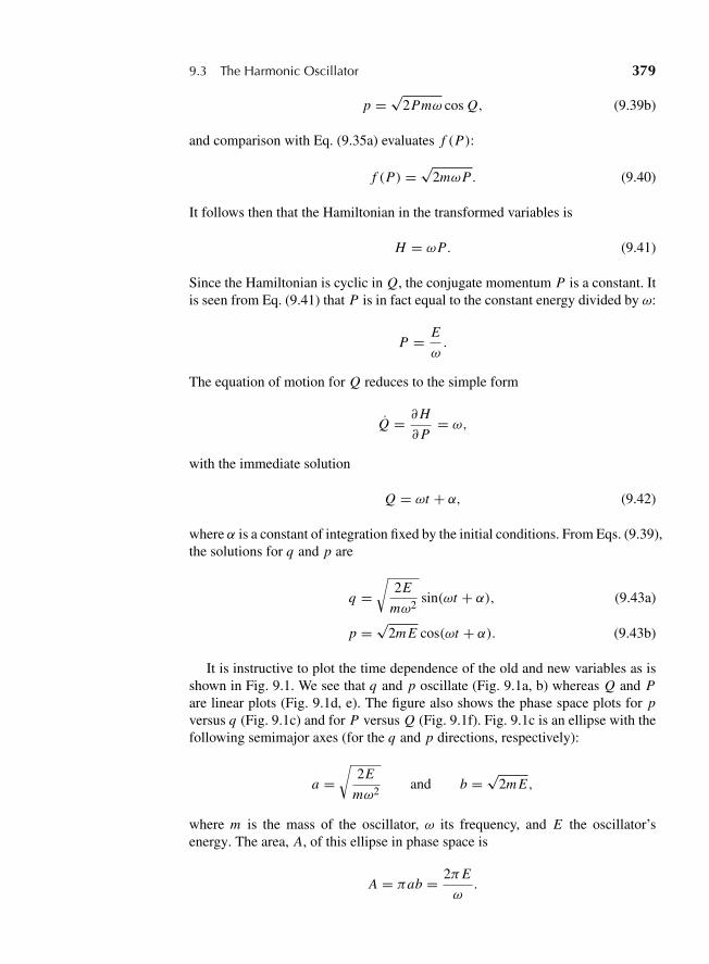
“M09 Goldstein ISBN C09” — 2011/2/15 — page 379 — #12
9.3 The Harmonic Oscillator 379
p =√
2Pmω cos Q, (9.39b)
and comparison with Eq. (9.35a) evaluates f (P):
f (P) =√
2mωP . (9.40)
It follows then that the Hamiltonian in the transformed variables is
H = ωP. (9.41)
Since the Hamiltonian is cyclic in Q, the conjugate momentum P is a constant. Itis seen from Eq. (9.41) that P is in fact equal to the constant energy divided by ω:
P = E
ω.
The equation of motion for Q reduces to the simple form
Q = ∂H
∂P= ω,
with the immediate solution
Q = ωt + α, (9.42)
where α is a constant of integration fixed by the initial conditions. From Eqs. (9.39),the solutions for q and p are
q =√
2E
mω2sin(ωt + α), (9.43a)
p =√
2m E cos(ωt + α). (9.43b)
It is instructive to plot the time dependence of the old and new variables as isshown in Fig. 9.1. We see that q and p oscillate (Fig. 9.1a, b) whereas Q and Pare linear plots (Fig. 9.1d, e). The figure also shows the phase space plots for pversus q (Fig. 9.1c) and for P versus Q (Fig. 9.1f). Fig. 9.1c is an ellipse with thefollowing semimajor axes (for the q and p directions, respectively):
a =√
2E
mω2and b =
√2m E,
where m is the mass of the oscillator, ω its frequency, and E the oscillator’senergy. The area, A, of this ellipse in phase space is
A = πab = 2πE
ω.
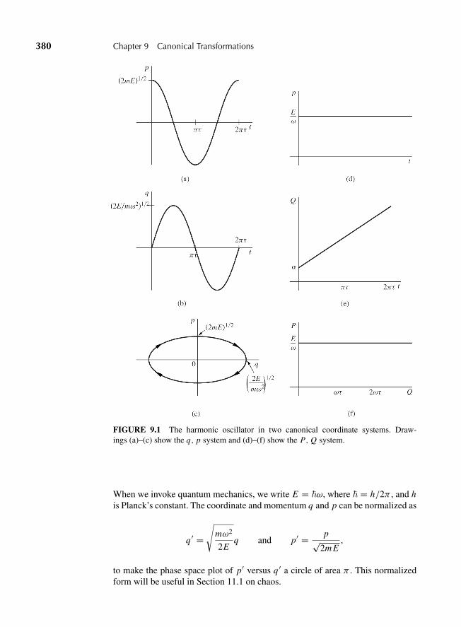
“M09 Goldstein ISBN C09” — 2011/2/15 — page 380 — #13
380 Chapter 9 Canonical Transformations
FIGURE 9.1 The harmonic oscillator in two canonical coordinate systems. Draw-ings (a)–(c) show the q, p system and (d)–(f) show the P, Q system.
When we invoke quantum mechanics, we write E = �ω, where � = h/2π , and his Planck’s constant. The coordinate and momentum q and p can be normalized as
q ′ =√
mω2
2Eq and p′ = p√
2m E,
to make the phase space plot of p′ versus q ′ a circle of area π . This normalizedform will be useful in Section 11.1 on chaos.
“M09 Goldstein ISBN C09” — 2011/2/15 — page 381 — #14
9.4 The Symplectic Approach to Canonical Transformations 381
It would seem that the use of canonical transformations to solve the harmonicoscillator problem is similar to “cracking a peanut with a sledge hammer.” Wehave here however a simple example of how the Hamiltonian can be reduced to aform cyclic in all coordinates by means of canonical transformations. Discussionof general schemes for the solution of mechanical problems by this technique willbe reserved for the next chapter. For the present, we shall continue to examine theformal properties of canonical transformations.
9.4 THE SYMPLECTIC APPROACH TO CANONICAL TRANSFORMATIONS
Another method of treating canonical transformations, seemingly unrelated to thegenerator formalism, can be expressed in terms of the matrix or symplectic for-mulation of Hamilton’s equations. By way of introduction to this approach, let usconsider a restricted canonical transformation, that is, one in which time does notappear in the equations of transformation:
Qi = Qi (q, p),
Pi = Pi (q, p). (9.44)
We know that the Hamiltonian function does not change in such a transformation.The time derivative of Qi , on the basis of Eqs. (9.44), is to be found as
Qi = ∂Qi
∂q jq j + ∂Qi
∂p jp j = ∂Qi
∂q j
∂H
∂p j− ∂Qi
∂p j
∂H
∂q j. (9.45)
On the other hand, the inverses of Eqs. (9.44),
q j = q j (Q, P),
p j = p j (Q, P), (9.46)
enables us to consider H(q, p, t) as a function of Q and P and to form the partialderivative
∂H
∂Pi= ∂H
∂p j
∂p j
∂Pi+ ∂H
∂q j
∂q j
∂Pi. (9.47)
Comparing Eqs. (9.45) and (9.47), it can be concluded that
Qi = ∂H
∂Pi;
that is, the transformation is canonical, only if
(∂Qi
∂q j
)q,p
=(∂p j
∂Pi
)Q,P
,
(∂Qi
∂p j
)q,p
= −(∂q j
∂Pi
)Q,P
. (9.48a)
“M09 Goldstein ISBN C09” — 2011/2/15 — page 382 — #15
382 Chapter 9 Canonical Transformations
The subscripts on the derivatives are to remind us that on the left-hand side ofthese equations Qi is considered as a function of (q, p) (cf. Eqs. (9.44)), whileon the right-hand side the derivatives are for q j and p j as functions of (Q, P) (cf.Eqs. (9.46)). A similar comparison of Pi with the partial of H with respect to Q j
leads to the conditions(∂Pi
∂q j
)q,p
= −(∂p j
∂Qi
)Q,P
,
(∂Pi
∂p j
)q,p
=(∂q j
∂Qi
)Q,P
. (9.48b)
The sets of Eqs. (9.48) together are sometimes known as the “direct conditions”for a (restricted) canonical transformation.
The algebraic manipulation that leads to Eqs. (9.48) can be performed in acompact and elegant manner if we make use of the symplectic notation for theHamiltonian formulation introduced above at the end of Section 8.1. If h is acolumn matrix with the 2n elements qi , pi , then Hamilton’s equations can bewritten, it will be remembered, as Eq. (8.39)
h = J∂H
∂h,
where J is the antisymmetric matrix defined in Eq. (8.38a). Similarly the new setof coordinates Qi , Pi define a 2n-element column matrix z, and for a restrictedcanonical transformation the equations of transformation (9.44) take the form
z = z(h). (9.49)
Analogously to Eq. (9.45) we can seek the equations of motion for the new vari-ables by looking at the time derivative of a typical element of z:
ζi = ∂ζi
∂η jη j , i, j = 1, . . . , 2n.
In matrix notation, this time derivative can be written as
z = Mh, (9.50)
where M is the Jacobian matrix of the transformation with elements
Mi j = ∂ζi
∂η j. (9.51)
Making use of the equations of motion for h, Eq. (9.50) becomes
z = MJ∂H
∂h. (9.52)
Now, by the inverse transformation H can be considered as a function of z, andthe derivative with respect to ηi evaluated as
∂H
∂ηi= ∂H
∂ζ j
∂ζ j
∂ηi,
“M09 Goldstein ISBN C09” — 2011/2/15 — page 383 — #16
9.4 The Symplectic Approach to Canonical Transformations 383
or, in matrix notation*
∂H
∂h= M
∂H
∂z. (9.53)
The combination of Eqs. (9.52) and (9.53) leads to the form of the equationsof motion for any set of variables z transforming, independently of time, from thecanonical set h:
z = MJM∂H
∂z. (9.54)
We have the advantage of knowing from the generator formalism that for arestricted canonical transformation the old Hamiltonian expressed in terms of thenew variables serves as the new Hamiltonian:
z = J∂H
∂z. (9.54′)
The transformation, Eq. (9.49), will therefore be canonical if M satisfies thecondition
MJM = J. (9.55)
That Eq. (9.55) is also a necessary condition for a restricted canonical transforma-tion is easily shown directly by reversing the order of the steps of the proof. Notethat for an extended time-independent canonical transformation, where K = λH ,the condition of Eq. (9.55) would be replaced by
MJM = λJ. (9.56)
Equation (9.55) may be expressed in various forms. Multiplying from the rightby the matrix inverse to M leads to
MJ = JM−1, (9.57)
(since the transpose of the inverse is the inverse of the transpose). The elementsof the matrix equation (9.57) will be found to be identical with Eqs. (9.48a) and(9.48b). If Eq. (9.57) is multiplied by J from the left and −J from the right, thenby virtue of Eq. (8.38e) we have
JM = M−1J,
*Readers of Section 7.5 will have recognized that Eq. (9.50) is the statement that h transforms con-travariantly (as a vector) under the transformation, and Eq. (9.53) says that the partial derivative of Hwith respect to the elements of h transforms covariantly (or as a 1-form) (cf. Eqs. (7.50) and (7.54)).
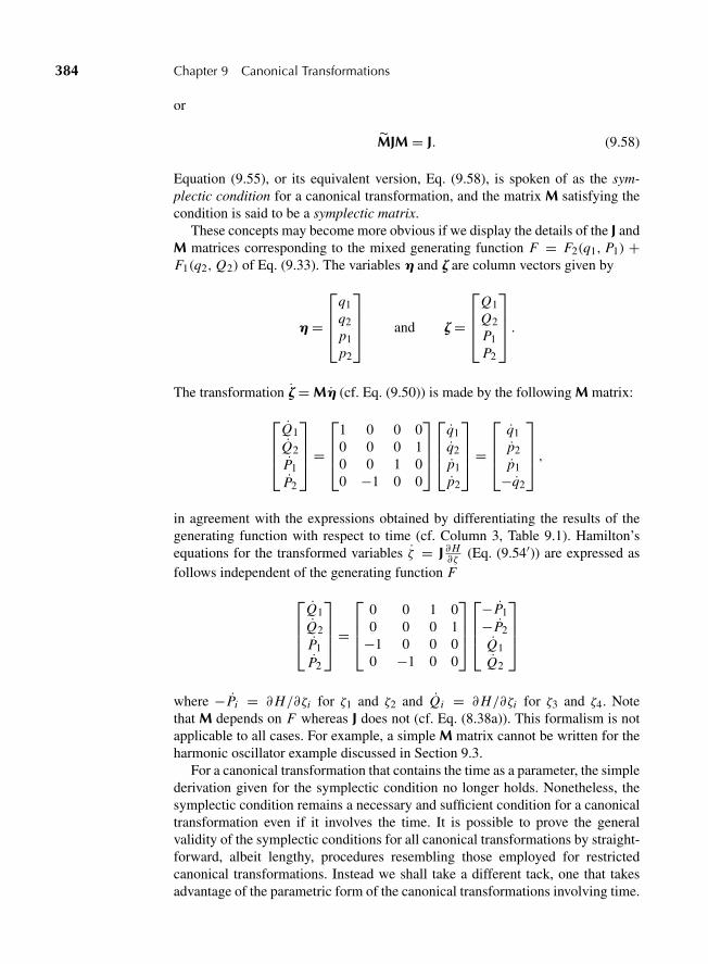
“M09 Goldstein ISBN C09” — 2011/2/15 — page 384 — #17
384 Chapter 9 Canonical Transformations
or
MJM = J. (9.58)
Equation (9.55), or its equivalent version, Eq. (9.58), is spoken of as the sym-plectic condition for a canonical transformation, and the matrix M satisfying thecondition is said to be a symplectic matrix.
These concepts may become more obvious if we display the details of the J andM matrices corresponding to the mixed generating function F = F2(q1, P1) +F1(q2, Q2) of Eq. (9.33). The variables h and z are column vectors given by
h =
⎡⎢⎢⎣
q1q2p1p2
⎤⎥⎥⎦ and z =
⎡⎢⎢⎣
Q1Q2P1P2
⎤⎥⎥⎦ .
The transformation z = Mh (cf. Eq. (9.50)) is made by the following M matrix:
⎡⎢⎢⎣
Q1
Q2
P1
P2
⎤⎥⎥⎦ =
⎡⎢⎢⎣
1 0 0 00 0 0 10 0 1 00 −1 0 0
⎤⎥⎥⎦⎡⎢⎢⎣
q1q2p1p2
⎤⎥⎥⎦ =
⎡⎢⎢⎣
q1p2p1−q2
⎤⎥⎥⎦ ,
in agreement with the expressions obtained by differentiating the results of thegenerating function with respect to time (cf. Column 3, Table 9.1). Hamilton’sequations for the transformed variables ζ = J ∂H
∂ζ(Eq. (9.54′)) are expressed as
follows independent of the generating function F
⎡⎢⎢⎣
Q1
Q2
P1
P2
⎤⎥⎥⎦ =
⎡⎢⎢⎣
0 0 1 00 0 0 1−1 0 0 00 −1 0 0
⎤⎥⎥⎦⎡⎢⎢⎣−P1
−P2
Q1
Q2
⎤⎥⎥⎦
where −Pi = ∂H/∂ζi for ζ1 and ζ2 and Qi = ∂H/∂ζi for ζ3 and ζ4. Notethat M depends on F whereas J does not (cf. Eq. (8.38a)). This formalism is notapplicable to all cases. For example, a simple M matrix cannot be written for theharmonic oscillator example discussed in Section 9.3.
For a canonical transformation that contains the time as a parameter, the simplederivation given for the symplectic condition no longer holds. Nonetheless, thesymplectic condition remains a necessary and sufficient condition for a canonicaltransformation even if it involves the time. It is possible to prove the generalvalidity of the symplectic conditions for all canonical transformations by straight-forward, albeit lengthy, procedures resembling those employed for restrictedcanonical transformations. Instead we shall take a different tack, one that takesadvantage of the parametric form of the canonical transformations involving time.
“M09 Goldstein ISBN C09” — 2011/2/15 — page 385 — #18
9.4 The Symplectic Approach to Canonical Transformations 385
A canonical transformation of the form
z = z(h, t) (9.59)
evolves continuously as time increases from some initial value t0. It is a single-parameter instance of the family of continuous transformations first studied sys-tematically by the mathematician Sophus Lie and as such plays a distinctive rolein the transformation theory of classical mechanics.
If the transformation
h → z(t) (9.60a)
is canonical, then so obviously is the transformation
h → z(t0). (9.60b)
It follows then from the definition of canonical transformation that the transfor-mation characterized by
z(t0)→ z(t) (9.60c)
is also canonical. Since t0 in Eq. (9.60b) is a fixed constant, this canonical trans-formation satisfies the symplectic condition (9.58). If now the transformation ofEq. (9.60c) obeys the symplectic condition, it is easy to show (cf. Derivation 13)that the general transformation Eq. (9.60a) will also.
To demonstrate that the symplectic condition does indeed hold for canonicaltransformations of the type of Eq. (9.60c), we introduce the notion of an infinites-imal canonical transformation (abbreviated I.C.T.), a concept that will prove tobe widely useful. As in the case of infinitesimal rotations, such a transformationis one in which the new variables differ from the old only by infinitesimals. Onlyfirst-order terms in these infinitesimals are to be retained in all calculations. Thetransformation equations can then be written as
Qi = qi + δqi , (9.61a)
Pi = pi + δpi , (9.61b)
or in matrix form
z = h+ δh. (9.61c)
(Here δqi and δpi do not represent virtual displacements but are simply the in-finitesimal changes in the coordinates and momenta.) An infinitesimal canonicaltransformation thus differs only infinitesimally from the identity transformationdiscussed in Section 9.1. In the generator formalism, a suitable generating func-tion for an I.C.T. would therefore be
F2 = qi Pi + εG(q, P, t), (9.62)
“M09 Goldstein ISBN C09” — 2011/2/15 — page 386 — #19
386 Chapter 9 Canonical Transformations
where ε is some infinitesimal parameter of the transformation, and G is any (dif-ferentiable) function of its 2n + 1 arguments. By Eq. (9.17a), the transformationequations for the momenta are to be found from
p j = ∂F2
∂q j= Pj + ε ∂G
∂q j
or
δp j ≡ Pj − p j = −ε ∂G
∂q j. (9.63a)
Similarly, by Eq. (9.17b), the transformation equations for Q j are determined bythe relations
Q j = ∂F2
∂Pj= q j + ε ∂G
∂Pj.
Since the second term is already linear in ε, and P differs from p only by aninfinitesimal, it is consistent to first order to replace Pj in the derivative functionby p j . We may then consider G as a function of q, p only (and possibly t). Fol-lowing the usual practice, we will refer to G(q, p) as the generating function ofthe infinitesimal canonical transformation, although strictly speaking that desig-nation belongs only to F . The transformation equation for Qi can therefore bewritten as
δq j = ε∂G
∂p j. (9.63b)
Both transformation equations can be combined into one matrix equation
δh = ε J∂G
∂h. (9.63c)
An obvious example of an infinitesimal canonical transformation would be thetransformation of Eq. (9.60c) when t differs from t0 by an infinitesimal t :
z(t0)→ z(t0 + dt), (9.64)
with dt as the infinitesimal parameter ε. The continuous evolution of the trans-formation z(η, t) from z(η, t0) means that the transformation z(t0) → z(t) canbe built up as a succession of such I.C.T.’s in steps of dt . It will therefore sufficeto show that the infinitesimal transformation, Eq. (9.64), satisfies the symplecticcondition (9.58). But it follows from the transformation equations (9.63) that theJacobian matrix of any I.C.T. is a symplectic matrix. By definition the Jacobianmatrix (9.51) for an infinitesimal transformation is
M ≡ ∂z∂h
= 1 + ∂δh∂h
,
“M09 Goldstein ISBN C09” — 2011/2/15 — page 387 — #20
9.4 The Symplectic Approach to Canonical Transformations 387
or by Eq. (9.63c)
M = 1 + εJ ∂2G
∂h ∂h. (9.65)
The second derivative in Eq. (9.65) is a square, symmetric matrix with elements(∂2G
∂h ∂h
)i j
= ∂2G
∂ηi ∂η j.
Because of the antisymmetrical property of J, the transpose of M is
M = 1 − ε ∂2G
∂h ∂hJ. (9.66)
The symplectic condition involves the value of the matrix product
MJM =(
1 + εJ ∂2G
∂h ∂h
)J
(1 − ε ∂2G
∂h ∂hJ
).
Consistent to first order in this product is
MJM = J + εJ ∂2G
∂h ∂hJ − Jε
∂2G
∂h ∂hJ
= J,
thus demonstrating that the symplectic condition holds for any infinitesimalcanonical transformation. By the chain of reasoning we have spun out, it there-fore follows that any canonical transformation, whether or not it involves time asa parameter, obeys the symplectic conditions, Eqs. (9.55) and (9.58).
The symplectic approach, for the most part, has been developed independentlyof the generating function method, except in the treatment of infinitesimal canon-ical transformations. They are of course connected. We shall sketch later, forexample, a proof that the symplectic condition implies the existence of a gen-erating function. But the connection is largely irrelevant. Both are valid ways oflooking at canonical transformations, and both encompass all of the needed prop-erties of the transformations. For example, either the symplectic or the generatorformalisms can be used to prove that canonical transformations have the fourproperties that characterize a group (cf. Appendix B).
1. The identity transformation is canonical.
2. If a transformation is canonical, so is its inverse.
3. Two successive canonical transformations (the group “product” operation)define a transformation that is also canonical.
4. The product operation is associative.
“M09 Goldstein ISBN C09” — 2011/2/15 — page 388 — #21
388 Chapter 9 Canonical Transformations
We shall therefore be free to use either the generator or the symplectic approachat will, depending on which leads to the simplest treatment at the moment.
9.5 POISSON BRACKETS AND OTHER CANONICAL INVARIANTS
The Poisson bracket of two functions u, v with respect to the canonical variables(q, p) is defined as
[u, v]q,p = ∂u
∂qi
∂v
∂pi− ∂u
∂pi
∂v
∂qi. (9.67)
In this bilinear expression we have a typical symplectic structure, as in Hamilton’sequations, where q is coupled with p, and p with −q. The Poisson bracket thuslends itself readily to being written in matrix form, where it appears as
[u, v]h = ∂u
∂hJ∂v
∂h. (9.68)
The transpose sign is used on the first matrix on the right-hand side to indicateexplicitly that this matrix must be treated as a single-row matrix in the multi-plication. On most occasions this specific reminder will not be needed and thetranspose sign may be omitted.
Suppose we choose the functions u, v out of the set of canonical variables(q, p) themselves. Then it follows trivially from the definition, either as Eq. (9.67)or (9.68), that these Poisson brackets have the values
[q j , qk]q,p = 0 = [p j , pk]q,p, (9.69a)
and
[q j , pk]q,p = δ jk = −[p j , qk]q,p. (9.69b)
We can summarize the relations of Eqs. (9.69) in one equation by introducinga square matrix Poisson bracket, [h,h], whose lm element is [ηl , ηm]. Equa-tions (9.69) can then be written as
[h,h]h = J. (9.70)
Now let us take for u, v the members of the transformed variables (Q, P), orz, defined in terms of (q, p) by the transformation equations (9.59). The set ofall the Poisson brackets that can be formed out of (Q, P) comprise the matrixPoisson bracket defined as
[z, z]h = ∂z∂h
J∂z∂h.
“M09 Goldstein ISBN C09” — 2011/2/15 — page 389 — #22
9.5 Poisson Brackets and Other Canonical Invariants 389
But we recognize the partial derivatives as defining the square Jacobian matrix ofthe transformation, so that the Poisson bracket relation is equivalent to
[z, z]h = MJM. (9.71)
If the transformation h → z is canonical, then the symplectic condition holds andEq. (9.71) reduces to (cf. Eq. (9.58))
[z, z]h = J, (9.72)
and conversely, if Eq. (9.72) is valid, then the transformation is canonical.Poisson brackets of the canonical variables themselves, such as Eqs. (9.70)
or (9.72), are referred to as the fundamental Poisson brackets. Since we havefrom Eq. (9.70) that
[z, z]z = J, (9.73)
Eq. (9.72) states that the fundamental Poisson brackets of the ζ variables have thesame value when evaluated with respect to any canonical coordinate set. In otherwords, the fundamental Poisson brackets are invariant under canonical transfor-mation. We have seen from Eq. (9.71) that the invariance is a necessary and suffi-cient condition for the transformation matrix to be symplectic. The invariance ofthe fundamental Poisson brackets is thus in all ways equivalent to the symplecticcondition for a canonical transformation.
It does not take many more steps to show that all Poisson brackets are invariantunder canonical transformation. Consider the Poisson bracket of two functionsu, v with respect to the h set of coordinates, Eq. (9.68). In analogy to Eq. (9.53),the partial derivative of v with respect to h can be expressed in terms of partialderivatives with respect to z as
∂v
∂h= M
∂v
∂z
(that is, the partial derivative transforms as a 1-form). In a similar fashion,
∂u
∂h=
˜M∂u
∂z= ∂u
∂zM.
Hence the Poisson bracket Eq. (9.68) can be written
[u, v]h = ∂u
∂hJ∂v
∂h= ∂u
∂zMJM
∂u
∂z.
If the transformation is canonical, the symplectic condition in the form ofEq. (9.55) holds, and we then have
[u, v]h = ∂u
∂zJ∂v
∂z≡ [u, v]z. (9.74)
“M09 Goldstein ISBN C09” — 2011/2/15 — page 390 — #23
390 Chapter 9 Canonical Transformations
Thus, the Poisson bracket has the same value when evaluated with respect to anycanonical set of variables—all Poisson brackets are canonical invariants. In writ-ing the symbol for the Poisson bracket, we have so far been careful to indicate bythe subscript the set of variables in terms of which the brackets are defined. Solong as we use only canonical variables that practice is now seen to be unneces-sary, and we shall in general drop the subscript.*
The hallmark of the canonical transformation is that Hamilton’s equations ofmotion are invariant in form under the transformation. Similarly, the canonical in-variance of Poisson brackets implies that equations expressed in terms of Poissonbrackets are invariant in form under canonical transformation. As we shall see, wecan develop a structure of classical mechanics, paralleling the Hamiltonian for-mulation, expressed solely in terms of Poisson brackets. Historically this Poissonbracket formulation, which has the same form in all canonical coordinates, wasespecially useful for carrying out the original transition from classical to quantummechanics. There is a simple “correspondence principle” that says that the clas-sical Poisson bracket is to be replaced by a suitably defined commutator of thecorresponding quantum operators.
The algebraic properties of the Poisson bracket are therefore of considerableinterest. We have already used the obvious properties
[u, u] = 0, (9.75a)
[u, v] = −[v, u]. (antisymmetry) (9.75b)
Almost equally obvious are the characteristics
[au + bv,w] = a[u, w] + b[v,w], (linearity) (9.75c)
where a and b are constants, and
[uv,w] = [u, w]v + u[v,w]. (9.75d)
One other property is far from obvious, but is very important in defining thenature of the Poisson bracket. It is usually given in the form of Jacobi’s iden-tity, which states that if u, v, and w are three functions with continuous secondderivatives, then
[u, [v,w]] + [v, [w, u]] + [w, [u, v]] = 0; (9.75e)
that is, the sum of the cyclic permutations of the double Poisson bracket of threefunctions is zero. There seems to be no simple way of proving Jacobi’s identity forthe Poisson bracket without lengthy algebra. However, it is possible to mitigatethe complexity of the manipulations by introducing a special nomenclature. We
*Note that for a scale transformation, or an extended canonical transformation, where the symplecticcondition takes on the form of Eq. (9.56), then Poisson brackets do not have the same values in allcoordinate systems. That is one of the reasons scale transformations are excluded from the class ofcanonical transformations that are useful to consider.
“M09 Goldstein ISBN C09” — 2011/2/15 — page 391 — #24
9.5 Poisson Brackets and Other Canonical Invariants 391
shall use subscripts on u, v, w (or functions of them) to denote partial derivativesby the corresponding canonical variable. Thus,
ui ≡ ∂u
∂ηi, and vi j ≡ ∂v
∂ηi ∂η j.
In this notation the Poisson bracket of u and v can be expressed as
[u, v] = ui Ji jv j .
Here Ji j , as usual, is simply the ijth element of J. In the proof, the only propertyof J that we shall need is its antisymmetry.
Now let us consider the first double Poisson bracket in Eq. (9.75e):
[u, [v,w]] = ui Ji j [v,w] j = ui Ji j (vk Jklwl) j .
Because the elements Jkl are constants, the derivative with resect to η doesn’t acton them, and we have
[u, [v,w]] = ui Ji j (vk Jklwl j + vk j Jklwl). (9.76)
The other double Poisson brackets can be obtained from Eq. (9.76) by cyclicpermutation of u, v, w. There are thus six terms in all, each being a fourfold sumover dummy indices i , j , k, and l. Consider the term in Eq. (9.76) involving asecond derivative of w:
Ji j Jkluivkwl j .
The only other second derivative of w will appear in evaluating the second doublePoisson bracket in (Eq. 9.75e):
[v, [w, u]] = vk Jkl(w j J ji ui )l .
Here the term in the second derivative in w is
J ji Jkluivkw jl .
Since the order of differentiation is immaterial, wl j = w jl , and the sum of thetwo terms is given by
(Ji j + J ji )Jkluivkwl j = 0,
by virtue of the antisymmetry of J . The remaining four terms are cyclic permuta-tions and can similarly be divided in two pairs, one involving second derivativesof u and the other of v. By the same reasoning, each of these pairs sums to zero,and Jacobi’s identity is thus verified.
If the Poisson bracket of u, v is looked on as defining a “product” operation ofthe two functions, then Jacobi’s identity is the replacement for the associative law
“M09 Goldstein ISBN C09” — 2011/2/15 — page 392 — #25
392 Chapter 9 Canonical Transformations
of multiplication. Recall that the ordinary multiplication of arithmetic is associa-tive; that is, the order of a sequence of multiplications is immaterial:
a(bc) = (ab)c.
Jacobi’s identity says that the bracket “product” is not associative and givesthe effect of changing the sequence of “multiplications.” Brackets that satisfyEqs. (9.75), together with the expression
[ui , u j ] =∑
k
cki j uk, (9.77)
constitute a generally noncommunitive algebra called a Lie algebra. For Poissonbrackets in three-dimensional space, either the structure constants ck
i j are all zeroor only one term in the right-hand side of Eq. (9.77) exists for any pair of indices.Examples of this will be given later, and a more detailed discussion of Lie algebrasis given in Appendix B.
The Poisson bracket operation is not the only type of “product” familiar tophysicists that satisfies the conditions for a Lie algebra. It will be left to the exer-cises to show that that vector product of two vectors,
V[A,B] → A × B, (9.78a)
and the commutator of two matrices,
M[A,B] → AB − BA, (9.78b)
satisfy the same Lie algebra conditions as the Poisson bracket. It is this last thatmakes it feasible to replace the classical Poisson bracket by the commutator of thequantum mechanical operators. In other words, the “correspondence principle”can work only because both the Poisson bracket and commutator are representa-tions of a Lie algebra “product.”*
There are other canonical invariants besides the Poisson bracket. One, mainlyof historical interest now, is the Lagrange bracket, denoted by {u, v}. Suppose uand v are two functions out of a set of 2n independent functions of the canonicalvariables. By inversion, the canonical variables can then be considered as func-tions of the set of 2n functions. On this basis, the Lagrange bracket of u and vwith respect to the (q, p) variables is defined as
*Of course, we must not mistake the mathematical acceptability of this version of the correspondenceprinciple with its physical necessity. The introduction of the quantum commutation relations was agreat act of physical discovery by the pioneers of quantum mechanics. All we show here is that thereis a similarity in the mathematical structure of the Poisson bracket formulation of classical mechanicsand the commutation relation version of quantum mechanics. The formal correspondence is that
[u, v] → 1
ih(uv − vu)
where on the left u, v are classical functions and on the right they are quantum operators.
“M09 Goldstein ISBN C09” — 2011/2/15 — page 393 — #26
9.5 Poisson Brackets and Other Canonical Invariants 393
{u, v}q,p = ∂qi
∂u
∂pi
∂v− ∂pi
∂u
∂qi
∂v, (9.79)
or, in matrix notation,
{u, v}h = ∂h∂u
J∂h∂v. (9.80)
Proof of the canonical invariance of the Lagrange bracket parallels that for thePoisson bracket.
If for u and v we take two members of the set of canonical variables, then weobtain the fundamental Lagrange brackets:
{qi , q j }qp = 0 = {pi , p j }qp {qi , p j }qp = δi j , (9.81)
or, in matrix notation,
{h,h} = J. (9.82)
The Lagrange and Poisson brackets clearly stand in some kind of inverse rela-tionship to each other, but the precise form of this relation is somewhat compli-cated to express. Let ui , i = 1, . . . , 2n, be a set of 2n independent functions ofthe canonical variables, to be represented by a column (or row) matrix u. Then{u,u} is the 2n × 2n matrix whose ijth element is {ui , u j }, with a similar descrip-tion for [u,u]. The reciprocal character of the two brackets manifests itself in therelation
{u,u}[u,u] = −1. (9.83)
If for u we choose the canonical set itself, h, then Eq. (9.83) obviously fol-lows from the fundamental bracket formulas, Eqs. (9.70) and (9.82), and theproperties of J. The proof for arbitrary u is not difficult if written in terms ofthe matrix definitions of the brackets and is reserved for the exercises. Whilethe properties of the Lagrange and Poisson brackets parallel each other inmany aspects, note that the Lagrange brackets do not obey Jacobi’s identity.Lagrange brackets therefore do not qualify as a “product” operation in a Liealgebra.
Another important canonical invariant is the magnitude of a volume element inphase space. A canonical transformation h → z transforms the 2n-dimensionalphase space with coordinates ηi to another phase space with coordinates ζi . Thevolume element
(dη) = dq1dq2 . . . dqndp1 . . . dpn
transforms to a new volume element
(dζ ) = d Q1d Q2 . . . d Qnd P1 . . . d Pn .

“M09 Goldstein ISBN C09” — 2011/2/15 — page 394 — #27
394 Chapter 9 Canonical Transformations
As is well known, the sizes of the two volume elements are related by theabsolute value of the Jacobian determinant ‖M‖;
(dζ ) = ‖M‖(dη).
For example, in the two-dimensional transformation from ηi = q, p to ζi = Q, P ,this expression becomes
d Q d P =
∣∣∣∣∣∣∣∣∂q
∂Q
∂q
∂P
∂p
∂Q
∂p
∂P
∣∣∣∣∣∣∣∣dq dp = [q, p]ζ dq dp. (9.84)
But, by taking the determinant of both sides of the symplectic condition, Eq. (9.58),we have
|M|2|J| = |J|. (9.85)
Thus, in a real canonical transformation the Jacobian determinant is ±1, and theabsolute value is always unity, proving the canonical invariance of the volumeelement in phase space. It follows, also, that the volume of any arbitrary region inphase space,
Jn =∫
· · ·∫(dη), (9.86)
is a canonical invariant. In our two-dimensional example, the invariant is dη =dq dp and J1 = ∫
dq dp.The volume integral in Eq. (9.86) is the final member of a sequence of canon-
ical invariants known as the integral invariants of Poincare, comprising integralsover subspaces of phase space of different dimensions. The other members of thesequence cannot be stated as simply as Jn , and because they are not needed forthe further development of the theory, they will not be discussed here.
Finally, the invariance of the fundamental Poisson brackets now enables us tooutline a proof that the symplectic condition implies the existence of a generatingfunction, as mentioned at the conclusion of the previous section. To simplify con-siderations, we shall examine only a system with one degree of freedom; the gen-eral method of the proof can be directly extended to systems with many degreesof freedom.* We suppose that the first of the equations of transformation,
Q = Q(q, p), P = P(q, p),
*In the literature, the connection between the symplectic approach and the generator formalism issometimes referred to as the Caratheodory theorem.
“M09 Goldstein ISBN C09” — 2011/2/15 — page 395 — #28
9.5 Poisson Brackets and Other Canonical Invariants 395
is invertable so as to give p as a function q and Q, say
p = φ(q, Q). (9.87)
Substitution in the second equation of transformation gives P as some functionof q and Q, say
P = ψ(q, Q). (9.88)
In such a case, we would expect the transformation to be generated by a generatingfunction of the first kind,* F1, with Eqs. (9.87) and (9.88) appearing as
p = ∂F1(q, Q)
∂q, P = −∂F1
∂Q(q, Q). (9.89)
If Eq. (9.89) holds, then it must be true that
∂φ
∂Q= −∂ψ
∂q. (9.90)
Conversely, if we can show that Eq. (9.90) is valid, then there must exist a functionF1 such that p and P are given by Eqs. (9.89).
To demonstrate the validity of Eq. (9.90), we try to look on all quantities asfunctions of q and Q. Thus, we of course have the identity
∂Q
∂Q= 1,
but if Eq. (9.87) be substituted in the first transformation equation,
Q = Q(q, φ(q, Q)), (9.91)
the partial derivative can also be written
∂Q
∂Q= ∂Q
∂p
∂φ
∂Q,
so that we have the relation
∂Q
∂p
∂φ
∂Q= 1. (9.92)
In the same spirit we evaluate the Poisson bracket
[Q, P] ≡ ∂Q
∂q
∂P
∂p− ∂P
∂q
∂Q
∂p= 1.
*Of course, if the Q transformation equation is not invertable, as in the identity transformation, thenwe would invert the P equation and be led to a generating function of the second kind.
“M09 Goldstein ISBN C09” — 2011/2/15 — page 396 — #29
396 Chapter 9 Canonical Transformations
The derivatives of P are derivatives of ψ from Eq. (9.88) considered as a functionof q and Q(q, p). Hence, the Poisson bracket can be written
[Q, P] = ∂Q
∂q
∂ψ
∂Q
∂Q
∂p− ∂Q
∂p
(∂ψ
∂q+ ∂ψ
∂Q
∂Q
∂q
),
or, consolidating terms, as
[Q, P] = ∂ψ
∂Q
(∂Q
∂q
∂Q
∂p− ∂Q
∂p
∂Q
∂q
)− ∂Q
∂p
∂ψ
∂q,
and therefore
1 = −∂Q
∂p
∂ψ
∂q. (9.93)
Combining Eqs. (9.92) and (9.93), we have
∂Q
∂p
∂φ
∂Q= −∂Q
∂p
∂ψ
∂q.
Since the partial derivative of Q with respect to p is the same on both sides of theequation, that is, the other variable being held constant is q in both cases, and sincethe derivative doesn’t vanish (else the Q equation could not be inverted), it followsthat Eq. (9.90) must be true. Thus, from the value of the fundamental Poissonbracket [Q, P], which we have seen is equivalent to the symplectic condition, weare led to the existence of a generating function. The two approaches to canonicaltransformations, though arrived at independently, are fully equivalent.
9.6 EQUATIONS OF MOTION, INFINITESIMAL CANONICALTRANSFORMATIONS, AND CONSERVATION THEOREMSIN THE POISSON BRACKET FORMULATION
Almost the entire framework of Hamiltonian mechanics can be restated in termsof Poisson brackets. As a result of the canonical invariance of the Poisson brack-ets, the relations so obtained will also be invariant in form under a canonicaltransformation. Suppose, for example, we look for the total time derivative ofsome function of the canonical variables and time, u(q, p, t), by use of Hamil-ton’s equations of motion:
du
dt= ∂u
∂qiqi + ∂u
∂pipi + ∂u
∂t= ∂u
∂qi
∂H
∂pi− ∂u
∂pi
∂H
∂qi+ ∂u
∂t,
or
du
dt= [u, H ] + ∂u
∂t. (9.94)
“M09 Goldstein ISBN C09” — 2011/2/15 — page 397 — #30
9.6 Equations of Motion 397
In terms of the symplectic notation, the derivation of Eq. (9.94) would run
du
dt= ∂u
∂hh+ ∂u
∂t= ∂u
∂hJ∂H
∂h+ ∂u
∂t,
from whence Eq. (9.94) follows, by virtue of (9.68). Equation (9.94) may belooked on as the generalized equation of motion for an arbitrary function u inthe Poisson bracket formulation. It contains Hamilton’s equations as a specialcase when for u we substitute one of the canonical variables
qi = [qi , H ], pi = [pi , H ], (9.95a)
or, in symplectic notation,
h = [h, H ]. (9.95b)
That Eq. (9.95b) is identical with Hamilton’s equations of motion may be seendirectly from the observation that by the definition of the Poisson bracket,Eq. (8.39), we have
[h, H ] = J∂H
∂h, (9.96)
so that Eq. (9.95b) is simply another way of writing Eq. (8.31). Another familiarproperty may be obtained from Eq. (9.94) by taking u as H itself. Equation (9.94)then says that
d H
dt= ∂H
∂t,
as was obtained previously in Eq. (8.41).Note that the generalized equation of motion is canonically invariant; it is valid
in whatever set of canonical variables q, p is used to express the function u or toevaluate the Poisson bracket. However, the Hamiltonian used must be appropriateto the particular set of canonical variables. Upon transforming to another set ofvariables by a time-dependent canonical transformation, we must also change tothe transformed Hamiltonian K .
If u is a constant of the motion, then Eq. (9.94) says it must have the property
[H, u] = ∂u
∂t. (9.97)
All functions that obey Eq. (9.97) are constants of the motion, and conversely thePoisson bracket of H with any constant of the motion must be equal to the explicittime derivative of the constant function. We thus have a general test for seekingand identifying the constants of the system. For those constants of the motion not
“M09 Goldstein ISBN C09” — 2011/2/15 — page 398 — #31
398 Chapter 9 Canonical Transformations
involving the time explicitly, the test of Eq. (9.97) reduces to requiring that theirPoisson brackets with the Hamiltonian vanish, that is, [H, u] = 0.*
If two constants of the motion are known, the Jacobi identity provides a possi-ble way for obtaining further constants. Suppose u and v are two constants of themotion not explicitly functions of time. Then if w in Eq. (9.75e) is taken to be H ,the Jacobi identity says
[H, [u, v]] = 0;
that is, the Poisson bracket of u and v is also a constant in time. Even whenthe conserved quantities depend upon time explicitly, it can be shown with a bitmore algebra (cf. Exercise 30) that the Poisson bracket of any two constants of themotion is also a constant of the motion (Poisson’s theorem). Repeated applicationof the Jacobi identity in this manner can in principle lead to a complete sequenceof constants of the motion. Quite often, however, the process is disappointing.The Poisson bracket of u and v frequently turns out to be a trivial function of uand v themselves, or even identically zero. Still, the possibility of generating newindependent constants of motion by Poisson’s theorem should be kept in mind.
The Poisson bracket notation can also be used to reformulate the basic equa-tions of an infinitesimal canonical transformation. As discussed above (Sec-tion 9.4), such a transformation is a special case of a transformation that is acontinuous function of a parameter, starting from the identity transformation atsome initial value of the parameter (which may, for convenience, be set equalto zero). If the parameter is small enough to be treated as a first-order infinitesi-mal, then the transformed canonical variables differ only infinitesimally from theinitial coordinates:
z = h+ δh (9.98)
with the change being given in terms of the generator G through Eq. (9.63c):
δh = εJ∂G(h)∂h
.
Now, by the definition (9.68) of the Poisson bracket, it follows that
[h, u] = J∂u
∂h(9.99)
(cf. Eq. (9.96)), a relation that remains valid when the Poisson bracket is evaluatedin terms of any other canonical variables. If u is taken to be G, it is seen that theequations of transformation for an infinitesimal canonical transformation can be
*In view of the “correspondence principle” between the classical Poisson bracket and the quantumcommutator, it is seen that this statement corresponds to the well-known quantum theorem that con-served quantities commute with the Hamiltonian.
“M09 Goldstein ISBN C09” — 2011/2/15 — page 399 — #32
9.6 Equations of Motion 399
written as
δh = ε[h,G]. (9.100)
Consider now an infinitesimal canonical transformation in which the contin-uous parameter is t (as was done in proving the symplectic condition) so thatε = dt , and let the generating function G be the Hamiltonian. Then the equationsof transformation for this I.C.T. become, by Eq. (9.100),
δh = dt[h, H ] = h dt = dh. (9.101)
These equations state that the transformation changes the coordinates andmomenta at the time t to the values they have at the time t + dt . Thus, themotion of the system in a time interval dt can be described by an infinitesimalcontact transformation generated by the Hamiltonian. Correspondingly, the sys-tem motion in a finite time interval from t0 to t is represented by a succession ofinfinitesimal contact transformations, which, as we have seen, is equivalent to asingle finite canonical transformation. Thus, the values of q and p at any timet can be obtained from their initial values by a canonical transformation that is acontinuous function of time. According to this view, the motion of a mechanicalsystem corresponds to the continuous evolution or unfolding of a canonical trans-formation. In a very literal sense, the Hamiltonian is the generator of the systemmotion with time.
Conversely, there must exist a canonical transformation from the values ofthe coordinates and momenta at any time t to their constant initial values.Obtaining such a transformation is obviously equivalent to solving the prob-lem of the system motion. At the beginning of the chapter it was pointed outthat a mechanical problem could be reduced to finding the canonical transfor-mation for which all momenta are constants of the motion. The present con-siderations indicate the possibility of an alternative solution by means of thecanonical transformation for which both the momenta and coordinates are con-stants of the motion. These two suggestions will be elaborated in the next chapterin order to show how formal solutions may be obtained for any mechanicalproblem.
Implicit to this discussion has been an altered way of looking at a canonicaltransformation and the effect it produces. The notion of a canonical transforma-tion was introduced as a change of the coordinates used to characterize phasespace. In effect, we switched from one phase space η with coordinates (q, p) toanother, ζ , with coordinates (Q, P). If the state of the system at a given timewas described by a point A in one system, it could also be described equallywell by the transformed point A′ (cf. Fig. 9.2). Any function of the system vari-ables would have the same value for a given system configuration whether it wasdescribed by the (q, p) set or by the (Q, P) set. In other words, the function wouldhave the same value at A′ as at A. In analogy to the corresponding descriptionof orthogonal transformations, we may call this the passive view of a canonicaltransformation.
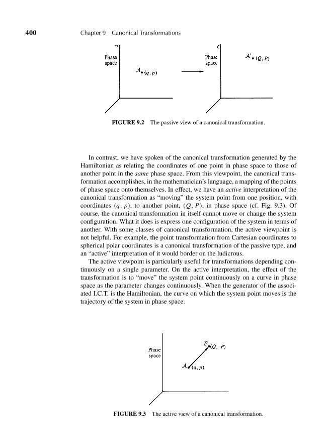
“M09 Goldstein ISBN C09” — 2011/2/15 — page 400 — #33
400 Chapter 9 Canonical Transformations
FIGURE 9.2 The passive view of a canonical transformation.
In contrast, we have spoken of the canonical transformation generated by theHamiltonian as relating the coordinates of one point in phase space to those ofanother point in the same phase space. From this viewpoint, the canonical trans-formation accomplishes, in the mathematician’s language, a mapping of the pointsof phase space onto themselves. In effect, we have an active interpretation of thecanonical transformation as “moving” the system point from one position, withcoordinates (q, p), to another point, (Q, P), in phase space (cf. Fig. 9.3). Ofcourse, the canonical transformation in itself cannot move or change the systemconfiguration. What it does is express one configuration of the system in terms ofanother. With some classes of canonical transformation, the active viewpoint isnot helpful. For example, the point transformation from Cartesian coordinates tospherical polar coordinates is a canonical transformation of the passive type, andan “active” interpretation of it would border on the ludicrous.
The active viewpoint is particularly useful for transformations depending con-tinuously on a single parameter. On the active interpretation, the effect of thetransformation is to “move” the system point continuously on a curve in phasespace as the parameter changes continuously. When the generator of the associ-ated I.C.T. is the Hamiltonian, the curve on which the system point moves is thetrajectory of the system in phase space.
FIGURE 9.3 The active view of a canonical transformation.
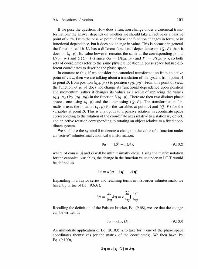
“M09 Goldstein ISBN C09” — 2011/2/15 — page 401 — #34
9.6 Equations of Motion 401
If we pose the question, How does a function change under a canonical trans-formation? the answer depends on whether we should take an active or a passivepoint of view. From the passive point of view, the function changes in form, or infunctional dependence, but it does not change in value. This is because in generalthe function, call it U , has a different functional dependence on (Q, P) than itdoes on (q, p). Its value however remains the same at the corresponding pointsU (q0, p0) and U (Q0, P0) since Q0 = Q(q0, p0) and P0 = P(q0, p0), so bothsets of coordinates refer to the same physical location in phase space but use dif-ferent coordinates to describe the phase space.
In contrast to this, if we consider the canonical transformation from an activepoint of view, then we are talking about a translation of the system from point Ato point B, from position (qA, pA) to position (qB, pB). From this point of view,the function U (q, p) does not change its functional dependence upon positionand momentum, rather it changes its values as a result of replacing the values(qA, pA) by (qB, pB) in the function U (q, p), There are then two distinct phasespaces, one using (q, p) and the other using (Q, P). The transformation for-malism uses the notation (q, p) for the variables at point A and (Q, P) for thevariables at point B. This is analogous to a passive rotation in coordinate spacecorresponding to the rotation of the coordinate axes relative to a stationary object,and an active rotation corresponding to rotating an object relative to a fixed coor-dinate system.
We shall use the symbol ∂ to denote a change in the value of a function underan “active” infinitesimal canonical transformation:
∂u = u(B)− u(A), (9.102)
where of course A and B will be infinitesimally close. Using the matrix notationfor the canonical variables, the change in the function value under an I.C.T. wouldbe defined as
∂u = u(h+ δh)− u(h).
Expanding in a Taylor series and retaining terms in first-order infinitesimals, wehave, by virtue of Eq. (9.63c),
∂u = ∂u
∂hδh = ε
∂u
∂hJ∂G
∂h.
Recalling the definition of the Poisson bracket, Eq. (9.68), we see that the changecan be written as
∂u = ε[u,G]. (9.103)
An immediate application of Eq. (9.103) is to take for u one of the phase spacecoordinates themselves (or the matrix of the coordinates). We then have, byEq. (9.100),
∂h = ε[h,G] = δh.
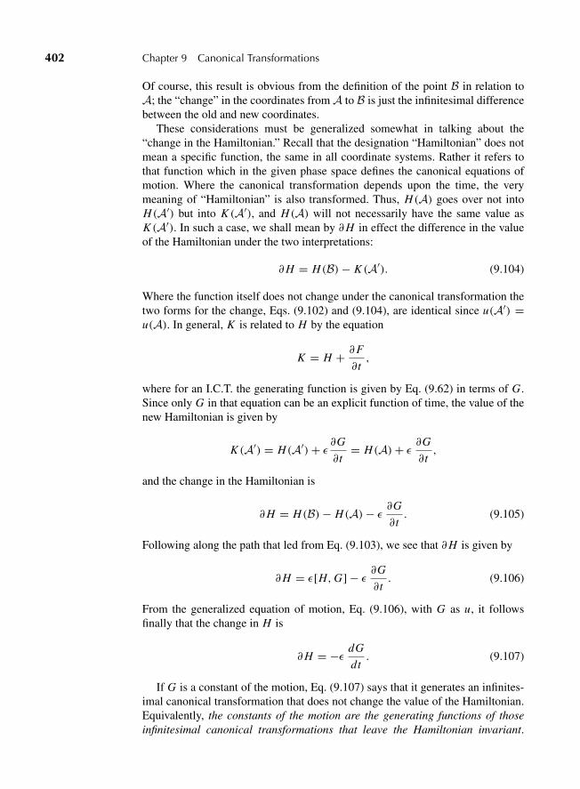
“M09 Goldstein ISBN C09” — 2011/2/15 — page 402 — #35
402 Chapter 9 Canonical Transformations
Of course, this result is obvious from the definition of the point B in relation toA; the “change” in the coordinates from A to B is just the infinitesimal differencebetween the old and new coordinates.
These considerations must be generalized somewhat in talking about the“change in the Hamiltonian.” Recall that the designation “Hamiltonian” does notmean a specific function, the same in all coordinate systems. Rather it refers tothat function which in the given phase space defines the canonical equations ofmotion. Where the canonical transformation depends upon the time, the verymeaning of “Hamiltonian” is also transformed. Thus, H(A) goes over not intoH(A′) but into K (A′), and H(A) will not necessarily have the same value asK (A′). In such a case, we shall mean by ∂H in effect the difference in the valueof the Hamiltonian under the two interpretations:
∂H = H(B)− K (A′). (9.104)
Where the function itself does not change under the canonical transformation thetwo forms for the change, Eqs. (9.102) and (9.104), are identical since u(A′) =u(A). In general, K is related to H by the equation
K = H + ∂F
∂t,
where for an I.C.T. the generating function is given by Eq. (9.62) in terms of G.Since only G in that equation can be an explicit function of time, the value of thenew Hamiltonian is given by
K (A′) = H(A′)+ ε ∂G
∂t= H(A)+ ε ∂G
∂t,
and the change in the Hamiltonian is
∂H = H(B)− H(A)− ε ∂G
∂t. (9.105)
Following along the path that led from Eq. (9.103), we see that ∂H is given by
∂H = ε[H,G] − ε ∂G
∂t. (9.106)
From the generalized equation of motion, Eq. (9.106), with G as u, it followsfinally that the change in H is
∂H = −ε dG
dt. (9.107)
If G is a constant of the motion, Eq. (9.107) says that it generates an infinites-imal canonical transformation that does not change the value of the Hamiltonian.Equivalently, the constants of the motion are the generating functions of thoseinfinitesimal canonical transformations that leave the Hamiltonian invariant.
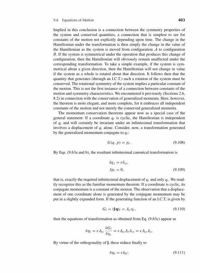
“M09 Goldstein ISBN C09” — 2011/2/15 — page 403 — #36
9.6 Equations of Motion 403
Implied in this conclusion is a connection between the symmetry properties ofthe system and conserved quantities, a connection that is simplest to see forconstants of the motion not explicitly depending upon time. The change in theHamiltonian under the transformation is then simply the change in the value ofthe Hamiltonian as the system is moved from configuration A to configurationB. If the system is symmetrical under the operation that produces this change ofconfiguration, then the Hamiltonian will obviously remain unaffected under thecorresponding transformation. To take a simple example, if the system is sym-metrical about a given direction, then the Hamiltonian will not change in valueif the system as a whole is rotated about that direction. It follows then that thequantity that generates (through an I.C.T.) such a rotation of the system must beconserved. The rotational symmetry of the system implies a particular constant ofthe motion. This is not the first instance of a connection between constants of themotion and symmetry characteristics. We encountered it previously (Sections 2.6,8.2) in connection with the conservation of generalized momenta. Here, however,the theorem is more elegant, and more complete, for it embraces all independentconstants of the motion and not merely the conserved generalized momenta.
The momentum conservation theorems appear now as a special case of thegeneral statement: If a coordinate qi is cyclic, the Hamiltonian is independentof qi and will certainly be invariant under an infinitesimal transformation thatinvolves a displacement of qi alone. Consider, now, a transformation generatedby the generalized momentum conjugate to qi :
G(q, p) = pi . (9.108)
By Eqs. (9.63a and b), the resultant infinitesimal canonical transformation is
δq j = εδi j ,
δpi = 0, (9.109)
that is, exactly the required infinitesimal displacement of qi and only qi . We read-ily recognize this as the familiar momentum theorem: If a coordinate is cyclic, itsconjugate momentum is a constant of the motion. The observation that a displace-ment of one coordinate alone is generated by the conjugate momentum may beput in a slightly expanded form. If the generating function of an I.C.T. is given by
Gl = (Jh)l = Jlrηr , (9.110)
then the equations of transformation as obtained from Eq. (9.63c) appear as
δηk = ε Jks∂Gl
∂ηs= ε Jks Jlrδrs = ε Jks Jls .
By virtue of the orthogonality of J, these reduce finally to
δηk = εδkl; (9.111)
“M09 Goldstein ISBN C09” — 2011/2/15 — page 404 — #37
404 Chapter 9 Canonical Transformations
that is, a displacement of any canonical variables ηl alone is generated in terms ofthe conjugate variable in the form given by Eq. (9.110). Of course, if ηl is qi , Gfrom Eq. (9.110) is just pi , and if ηl is pi , G is then −qi .
As a specific illustration of these concepts, let us consider again the infinites-imal contact transformation of the dynamical variables that produces a rotationof the system as a whole by an angle dθ . The physical significance of the corre-sponding generating function cannot depend upon the choice of initial canonicalcoordinates,* and it is convenient to use for this purpose the Cartesian coordinatesof all particles in the system. Nor will there be any loss in generality if the axes areso oriented that the infinitesimal rotation is along the z axis. For an infinitesimalcounterclockwise rotation of each particle, the change in the position vectors is tobe found from the infinitesimal rotation matrix of Eq. (4.69). With a rotation onlyabout the z axis, the changes in the particle coordinates are
δxi = −yi dθ, δyi = xi dθ, δzi = 0. (9.112a)
The effect of the transformation on the components of the Cartesian vectorsformed by the momenta conjugate to the particle coordinates is similarly givenby
δpix = −piy dθ, δpiy = pix dθ, δpiz = 0. (9.112b)
Comparing these transformation equations with Eqs. (9.63a and b), it is seen thatthe corresponding generating function is
G = xi piy − yi pix , (9.113)
with dθ as the infinitesimal parameter ε. For a direct check, note that
δxi = dθ∂G
∂pix= −yi dθ, δpix = −dθ
∂G
∂xi= −piy dθ,
δyi = dθ∂G
∂piy= xi dθ, δpiy = −dθ
∂G
∂yi= pix dθ,
agreeing with Eqs. (9.112). The generating function (9.113) in addition has thephysical significance of being the z-component of the total canonical angularmomentum:
G = Lz ≡ (ri × pi )z . (9.114)
Since the z axis was arbitrarily chosen, we can state that the generating functioncorresponding to an infinitesimal rotation about an axis denoted by the unit vector
*This can most easily be seen from the canonically invariant Eq. (9.100). The change in the canonicalvariable ηi remains the same no matter in what set of canonical variables G is expressed.
“M09 Goldstein ISBN C09” — 2011/2/15 — page 405 — #38
9.6 Equations of Motion 405
n is
G = L ? n. (9.115)
Note that the canonical angular momentum as defined here may differ fromthe mechanical angular momentum. If the forces on the system are derivable fromvelocity-dependent potentials, then the canonical momentum vectors pi are notnecessarily the same as the linear momentum vectors, and L in Eqs. (9.114) and(9.115) may not be the same as the mechanical angular momentum. The resultobtained here is therefore a generalization of the conclusion given in Section 2.6that the momentum conjugate to a rotation coordinate is the corresponding com-ponent of the total angular momentum. The proof presented there was restrictedto systems with velocity-independent potentials. By virtue of Eqs. (9.108) and(9.109), we can now conclude that the momentum conjugate to a generalizedcoordinate that measures the rotation of the system as a whole about an axis n isthe component of the total canonical angular momentum along the same axis. Justas the Hamiltonian is the generator of a displacement of the system in time, so theangular momentum is the generator of the spatial rotations of the system.
It has already been noted that on the “active” interpretation a canonical trans-formation depending upon a parameter “moves” the system point along a con-tinuous trajectory in phase space. Since the finite transformation can be lookedon as the sum of an infinite succession of infinitesimal canonical transformations,each corresponding to an infinitesimal displacement along the curve, it shouldtherefore be possible formally to obtain the finite transformation by integratingthe expression for the infinitesimal displacements. We can do this by noting thateach point on the trajectory in phase space corresponds to a particular value ofthe parameter, which we shall call α, starting from the initial system configura-tion denoted by α = 0. If u is some function of the system configuration, then uwill be a continuous function of α along the trajectory , u(α), with initial valueu0 = u(0). (For simplicity, we shall consider u as not depending explicitly upontime.) Equation (9.103) for the infinitesimal change of u on the trajectory can bewritten as
∂u = dα[u,G],
or as a differential equation in the variable α:
du
dα= [u,G]. (9.116)
We can get u(α), and therefore the effect of the finite canonical transformation,by integrating this differential equation. A formal solution may be obtained byexpanding u(α) in a Taylor series about the initial conditions:
u(α) = u0 + α du
dα
∣∣∣0+ α2
2
d2u
dα2
∣∣∣0+ α3
3
d3u
dα3
∣∣∣0+ · · · .
“M09 Goldstein ISBN C09” — 2011/2/15 — page 406 — #39
406 Chapter 9 Canonical Transformations
By Eq. (9.116), we have
du
dα
∣∣∣0= [u,G]0,
the zero subscript meaning that the value of the Poisson bracket is to be taken atthe initial point, α = 0. Repeated application of Eq. (9.116), taking [u,G] itselfas a function of the system configuration, gives
d2u
dα2= [[u,G],G],
and the process can be repeated to give the third derivative of u and so on. TheTaylor series for u(α) thus leads to the formal series solution
u(α) = u0 + α[u,G]0 +α2
2[[u,G],G]0 +
α3
3[[[u,G],G],G]0 + · · · . (9.117)
If for u we take any of the canonical variables ζi , with u0 the starting set of vari-ables ηi , then Eq. (9.115) is a prescription for finding the transformation equationsof the finite canonical transformation generated by G.
It is not difficult to find specific examples showing that this procedure actu-ally works. Suppose for G we take Lz , so that the final canonical transformationshould correspond to a finite rotation about the z axis. The natural parameter touse for α is the rotation angle. For u, let us take the x-coordinate of the i th particlein the system. Either by direct evaluation of the Poisson brackets or by inferencefrom Eqs. (9.112a), it is easy to see that
[Xi , Lz] = −Yi , [Yi , Lz] = Xi , (9.118)
where capital letters have been used to denote the coordinates after some rotationθ , that is, the final coordinate. The initial coordinates, that is, before rotation, areas usual represented by lowercase letters. It follows then that
[Xi , Lz]0 = −yi ,
[[Xi , Lz], Lz]0 = −[Yi , Lz]0 = −xi ,
[[[Xi , Lz], Lz], Lz]0 = −[Xi , Lz]0 = yi ,
and so on. The series representation for Xi thus becomes
Xi = xi − yiθ − xiθ2
2+ yi
θ3
3+ xi
θ4
4− · · ·
= xi
(1 − θ2
2+ θ4
4− · · ·
)− yi
(θ − θ3
3+ · · ·
).
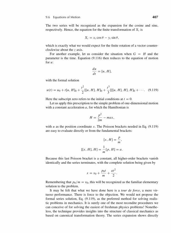
“M09 Goldstein ISBN C09” — 2011/2/15 — page 407 — #40
9.6 Equations of Motion 407
The two series will be recognized as the expansion for the cosine and sine,respectively. Hence, the equation for the finite transformation of Xi is
Xi = xi cos θ − yi sin θ,
which is exactly what we would expect for the finite rotation of a vector counter-clockwise about the z axis.
For another example, let us consider the situation when G = H and theparameter is the time. Equation (9.116) then reduces to the equation of motionfor u:
du
dt= [u, H ],
with the formal solution
u(t) = u0 + t[u, H ]0 +t2
2[[u, H ], H ]0 +
t3
3[[[u, H ], H ], H ]0 + · · · . (9.119)
Here the subscript zero refers to the initial conditions at t = 0.Let us apply this prescription to the simple problem of one-dimensional motion
with a constant acceleration a, for which the Hamiltonian is
H = p2
2m− max,
with u as the position coordinate x . The Poisson brackets needed in Eq. (9.119)are easy to evaluate directly or from the fundamental brackets:
[x, H ] = p
m,
[[x, H ], H ] = 1
m[p, H ] = a.
Because this last Poisson bracket is a constant, all higher-order brackets vanishidentically and the series terminates, with the complete solution being given by
x = x0 + p0t
m+ at2
2.
Remembering that p0/m = v0, this will be recognized as the familiar elementarysolution to the problem.
It may be felt that what we have done here is a tour de force, a mere vir-tuoso performance. There is force to the objection. We would not propose theformal series solution, Eq. (9.119), as the preferred method for solving realis-tic problems in mechanics. It is surely one of the most recondite procedures wecan conceive of for solving the easiest of freshman physics problems! Nonethe-less, the technique provides insights into the structure of classical mechanics asbased on canonical transformation theory. The series expansion shows directly

“M09 Goldstein ISBN C09” — 2011/2/15 — page 408 — #41
408 Chapter 9 Canonical Transformations
that infinitesimal canonical transformations can generate finite canonical trans-formations, depending on a parameter, and thus lead to solutions to the equationsof motion. Of particular interest for the relation between classical and quantummechanics is the observation that the series in Eqs. (9.117) or (9.119) bear a fam-ily resemblance to the series for an exponential. The nest of Poisson brackets inthe nth term can be considered as the nth repeated application (from the right!)of the operator [ ,G], or the nth power of the operator. Equation (9.119), forexample, could symbolically be written as
u(t) = ueHt∣∣∣0. (9.120)
The exponential here means no more than its series representations and thesymbol H is used to indicate the operator [ , H ]. What we have here is very rem-iniscent of the Heisenberg picture in quantum mechanics where the u(t) becometime-varying operators, whose time dependence is given in terms of exp[i Ht/�]in such a manner as to lead to the same equation of motion, Eq. (9.94). (Theadditional factor i/� arises out of the correspondence between the classical Pois-son bracket and the quantum commutator.) The Poisson bracket formulation ofmechanics is thus the classical analog of the Heisenberg picture of quantummechanics.
9.7 THE ANGULAR MOMENTUM POISSON BRACKET RELATIONS
The identification of the canonical angular momentum as the generator of arigid rotation of the system leads to a number of interesting and importantPoisson bracket relations. Equations (9.103) for the change of a function uunder an infinitesimal canonical transformation (on the “active” view) is alsovalid if u is taken as the component of a vector along a fixed axis in ordinaryspace. Thus, if F is a vector function of the system configuration, then (cf. Eq.(9.116))
∂Fi = dα[Fi ,G].
Note that the direction along which the component is taken must be fixed, that is,not affected by the canonical transformation. If the direction itself is determinedin terms of the system variables, then the transformation changes not only thevalue of the function but the nature of the function, just as with the Hamiltonian.With this understanding the change in a vector F under a rotation of the systemabout a fixed axis n, generated by L ? n, can be written in vector notation (cf. Eq.(9.115))
∂F = dθ [F,L ? n]. (9.121)
To put it in other words, Eq. (9.121) implies that the unit vectors i, j, k that formthe basis set for F are not themselves rotated by L ? n.
“M09 Goldstein ISBN C09” — 2011/2/15 — page 409 — #42
9.7 The Angular Momentum Poisson Bracket Relations 409
The words describing what is meant by Eq. (9.121) must be chosen carefullyfor another reason. What is spoken of is the rotation of the system under theI.C.T., not necessarily the rotation of the vector F. The generator L ? n induces aspatial rotation of the system variables, not for example of some external vectorsuch as a magnetic field or the vector of the acceleration of gravity. Under whatconditions then does L ? n generate a spatial rotation of F? The answer is clear—when F is a function only of the system variables (q, p) and does not involve anyexternal quantities or vectors not affected by the I.C.T. Only under these condi-tions does a spatial rotation imply a corresponding rotation of F. We shall des-ignate such vectors as system vectors. The change in a vector under infinitesimalrotation about an axis n has been given several times before (cf. Eq. (2.50) andEq. (4.75)):
dF = n dθ 3F.
For a system vector F, the change induced under an I.C.T. generated by L ? n cantherefore be written as
∂F = dθ [F,L ? n] = n dθ 3F. (9.122)
Equation (9.122) implies an important Poisson bracket identity obeyed by all sys-tem vectors:
[F,L ? n] = n3F. (9.123)
Note that in Eq. (9.123) there is no longer any reference to a canonical transfor-mation or even to a spatial rotation. It is simply a statement about the value ofcertain Poisson brackets for a specific class of vectors and, as such, can be veri-fied by direct evaluation in any given case. Suppose, for example, we had a systemof an unconstrained particle and used the Cartesian coordinates as the canonicalspace coordinates. Then the Cartesian vector p is certainly a suitable system vec-tor. If n is taken as a unit vector in the z direction, then by direct evaluation wehave
[px , xpy − ypx ] = −py,
[py, xpy − ypx ] = px ,
[pz, xpy − ypx ] = 0.
The right-hand sides of these identities is clearly the same as the components ofn3 p, as predicted by Eq. (9.123).
On the other hand, suppose that in the same problem we tried to use for Fthe vector A = 1
2 (r3B) where B = Bi is a fixed vector along the x axis.The vector A will be recognized as the vector potential corresponding to a uni-form magnetic field B in the x-direction. As A depends upon a vector externalto the system, we would expect it not to fit the characteristics of a system vectorand Eq. (9.123) should not hold for it. Indeed, we see that the Poisson brackets
“M09 Goldstein ISBN C09” — 2011/2/15 — page 410 — #43
410 Chapter 9 Canonical Transformations
involved are here
[0, xpy − ypx ] = 0,[12 zB, xpy − ypx
]= 0,[
− 12 y B, xpy − ypx
]= − 1
2 Bx,
whereas the vector n3A has instead the components (− 12 Bz, 0, 0).
The relation (9.123) may be expressed in various notations. Perhaps the mostadvantageous is a form using the Levi–Civita density to express the cross product(cf. Eq. (4.77′)). The i th component of Eq. (9.123) for arbitrary n then can bewritten
[Fi , L j n j ] = εi jkn j Fk, (9.124)
which implies the simple result
[Fi , L j ] = εi jk Fk . (9.125)
An alternative statement of Eq. (9.125) is to note that if l, m, n are three indicesin cyclic order, then
[Fl , Lm] = Fn, l,m, n in cyclic order. (9.125′)
Another consequence of Eq. (9.123) relates to the dot product of two systemvectors: F ?G. Being a scalar, such a dot product should be invariant under rota-tion, and indeed the Poisson bracket of the dot product with L ? n is easily shownto vanish:
[F ?G,L ? n] = F ? [G,L ? n] + G ? [F,L ? n]
= F ? n3G + G ? n3F
= F ? n3G + F ?G3 n
= 0. (9.126)
The magnitude of any system vector therefore has a vanishing Poisson bracketwith any component of L.
Perhaps the most frequent application of these results arises from taking F tobe the vector L itself. We then have
[L,L ? n] = n3L, (9.127)
[Li , L j ] = εi jk Lk, (9.128)
and
[L2,L ? n] = 0. (9.129)
“M09 Goldstein ISBN C09” — 2011/2/15 — page 411 — #44
9.7 The Angular Momentum Poisson Bracket Relations 411
A number of interesting consequences follow from Eqs. (9.127)
[p,L ? n] = n3 p
[pi , L j ] = εi jk pk .
If Lx and L y are constants of the motion, Poisson’s theorem then states that[Lx , L y] = Lz is also a constant of the motion. Thus, if any two components ofthe angular momentum are constant, the total angular momentum vector is con-served. As a further instance, let us assume that in addition to Lx and L y beingconserved there is a Cartesian vector of canonical momentum p with pz a con-stant of the motion. Not only is Lz conserved but we have two further constantsof the motion:
[pz, Lx ] = py
and
[pz, L y] = −px ,
that is, both L and p are conserved. We have here an instance in which Poisson’stheorem does yield new constants of the motion. Note, however, that if px , py ,and Lz were the given constants of the motion, then their Poisson brackets are
[px , py] = 0,
[px , Lz] = −py,
[py, Lz] = px .
Here no new constants can be obtained from Poisson’s theorem.Recall from the fundamental Poisson brackets, Eqs. (9.69), that the Pois-
son bracket of any two canonical momenta must always be zero. But, fromEq. (9.128), Li does not have a vanishing Poisson bracket with any of the othercomponents of L. Thus, while we have described L as the total canonical angu-lar momentum by virtue of its definition as ri 3 pi (summed over all particles),no two components of L can simultaneously be canonical variables. However,Eq. (9.129) shows that any one of the components of L, and its magnitude L , canbe chosen to be canonical variables at the same time.*
*It has been remarked previously that the correspondence between quantum and classical mechanics issuch that the quantum mechanical commutator goes over essentially into the classical Poisson bracketas h → 0. Much of the formal structure of quantum mechanics appears as a close copy of the Poissonbracket formulation of classical mechanics. All the results of this section therefore have close quantumanalogs. For example, the fact that two components of L cannot be simultaneous canonical momentaappears as the well-known statement that Li and L j cannot have simultaneous eigenvalues. But L2
and any Li can be quantized together. Indeed, most of these relations are known far better in theirquantum form than as classical theorems.
“M09 Goldstein ISBN C09” — 2011/2/15 — page 412 — #45
412 Chapter 9 Canonical Transformations
9.8 SYMMETRY GROUPS OF MECHANICAL SYSTEMS
It has already been pointed out that canonical transformations form a group.Canonical transformations that are analytic functions of continuous parametersform groups that are Lie groups. A Lie group with continuous parameters, θi ,has associated with it a flat vector space whose basis vectors, ui , constitute a Liealgebra satisfying the previously given condition on the Poisson bracket
[ui , u j ] =∑
k
ci jkuk . (9.77)
The elements, Q(θi ), of the associated Lie group are related to the elements ofthe Lie algebra by
Q(θi ) = exp
(i
2
∑θi ui
). (9.130)
The definitions of Lie groups and Lie algebras are considered in more detail inAppendix B.
In Chapter 4 of the first two editions of this text, an extensive discussion wasgiven of the Pauli matrix representation of the rotational group in three dimensionswhere the Pauli matrices that form the basis,
σx =(
0 11 0
), σy =
(0 −ii 0
), σz =
(1 00 −1
)
are both hermitian (the matrix is equal to its own transpose complex conjugate)and unitary (the transpose complex conjugate of the matrix is the inverse). Thesematrices have the properties*
[σi , σ j ] = 2iσk
for i , j , and k a cyclic permutation of x , y, and z. The structure constants are thusci j
k = 2iεi jk and σ 2i = 1, the unit 2 × 2 matrix. The Euler angles can be used
as the parameters that generate the group elements. For a rotation in the y-z planewe have, for example,
Q(θ) = 1 cosθ
2+ iσx sin
θ
2=
⎛⎜⎜⎝
cosθ
2i sin
θ
2
i sinθ
2cos
θ
2
⎞⎟⎟⎠ .
*Some physicists define a Lie algebra with the expression [ul , u j ] = i∑
k cl jkuk instead of
Eq. (9.77). This makes the structure constants in the following discussion real. Many mathematiciansomit the i = √−1 in the definition. The present text follows the latter convention.
“M09 Goldstein ISBN C09” — 2011/2/15 — page 413 — #46
9.8 Symmetry Groups of Mechanical Systems 413
In this formalism, vectors are represented by 2 × 2 matrices of the form
V(x,y,z) =(
Vz Vx − iVy
Vx + iVy −Vz
),
and a rotation is performed by a similarity transformation
V(x ′,y′,z′) = Q(θ)V(x,y,z)Q†(θ),
where Q† is the adjoint, or complex conjugate transpose of the matrix Q.The 2 × 2 matrices Q are unitary with determinant +1, so they constitute a
representation of the special unitary group in two dimensions, SU(2). The setof unitary 2 × 2 matrices with determinant either +1 or −1 has twice as manyelements (both infinite in number), which form the full unitary group U(2) in twodimensions. This group of 2 × 2 rotatation matrices has the same properties asthe group of the associated infinitesimal canonical transformations (I.C.T.). It iscustomary to work primarily with the I.C.T.’s as they are easier to handle. TheLie groups of I.C.T.’s whose generators are the constants of the motion of thesystem are known as the symmetry groups of the system for, as we have seen, suchtransformations leave the Hamiltonian invariant. Finding the symmetry groups ofa system goes a long way toward solving the problem of its classical motion andis even closer to a solution of the quantum-mechanical problem.
A system with spherical symmetry is invariant under rotation about any axis, soit can be represented by the group SU(2) as discussed above. Of more practical useis the set of the usual 3×3 rotation matrices with determinant +1, which representthe special rotation group in three dimensions R(3) ≡ SO(3). The vector L isconserved in such a system in accord with our identification of the components ofL as the generators of spatial rotations. For the group of transformations generatedby Li , Eq. (9.128) shows that the structure constants are ci j
k = εi jk , and it is thisrelationship that stamps the group as being the rotation group in three dimensions.Thus, the matrix generators Mi of infinitesimal rotations, Eqs. (4.79), have beenseen to obey the commutation relations, Eq. (4.80),
[Mi ,M j ] = εi jkMk, (4.80)
that is, with the same structure constants as for Li . The quantities Li and Mi
are different physically; the brackets in Eqs. (9.125) and (4.80) refer to differentoperations (although they share the same significant algebraic properties). Butthe identity of the structure constants for Li and Mi (cf. Eqs. (9.128) and (4.80))shows that they have the same group structure, that of SO(3).
For the bound Kepler problem, we have seen (Section 3.9) that there existsin addition to L another conserved vector quantity, A, the Laplace-Runge–Lenzvector defined by Eq. (3.82)
A = p3L − mkrr. (3.82)
“M09 Goldstein ISBN C09” — 2011/2/15 — page 414 — #47
414 Chapter 9 Canonical Transformations
The Poisson bracket relations of the components of A with themselves and withthe components of L can be obtained in a straightforward manner. Since A clearlyqualifies as a system vector, we immediately have the bracket relations
[Ai , L j ] = εi jk Ak . (9.131)
The Poisson brackets of the components of A among themselves cannot beobtained by any such simple stratagem, but after a fair amount of tedious manip-ulation it is found that*
[A1, A2] = −(
p2 − 2mk
r
)L3. (9.132)
The quantity on the right in the parentheses will be recognized as 2m H , whichhas the conserved value 2m E . If we therefore introduce a new constant vector Ddefined as
D = A√−2m E≡ A√
2m|E | (9.133)
(note that E is negative for bound motion!), then the components of D satisfy thePoisson bracket relation
[D1, D2] = L3.
By cyclically permuting the indices, the complete set of Poisson brackets followsimmediately. Thus, the components of L and D together form a Lie algebra for thebound Kepler problem, with structure constants to be obtained from the identities.
[Li , L j ] = εi jk Lk, (9.128)
[Di , L j ] = εi jk Dk, (9.134)
and
[Di , D j ] = εi jk Lk . (9.135)
An examination of the fundamental matrices for rotation will show that thesymmetry group for the bound Kepler problem is to be identified with the groupof four-dimensional real proper rotations, called the special orthogonal group ofdimension 4, which is usually designated as SO(4) or R(4). Such a transforma-tion preserves the value of the scalar quadratic form xμxμ, where all the xμ arereal. An orthogonal transformation in four dimensions has 10 conditions on the16 elements of the matrix with determinant ±1, so only 6 are independent. By
*Some reduction in the length of the derivation is obtained by identifying p3L as a system vector C,and first evaluating the Poisson brackets [C1, (p3L)2] and [C1, r/r ] making use of the fundamentalPoisson brackets and Eqs. (9.125) to the utmost.
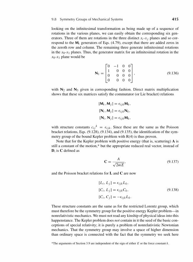
“M09 Goldstein ISBN C09” — 2011/2/15 — page 415 — #48
9.8 Symmetry Groups of Mechanical Systems 415
looking on the infinitesimal transformation as being made up of a sequence ofrotations in the various planes, we can easily obtain the corresponding six gen-erators. Three of them are rotations in the three distinct xi -x j planes and so cor-respond to the Mi generators of Eqs. (4.79), except that there are added zeros inthe zeroth row and column. The remaining three generate infinitesimal rotationsin the x0-x1 planes. Thus, the generator matrix for an infinitesimal rotation in thex0-x1 plane would be
N1 =
⎡⎢⎢⎣
0 −1 0 01 0 0 00 0 0 00 0 0 0
⎤⎥⎥⎦ , (9.136)
with N2 and N3 given in corresponding fashion. Direct matrix multiplicationshows that these six matrices satisfy the commutator (or Lie bracket) relations
[Mi ,M j ] = εi jkMk,
[Ni ,M j ] = εi jkNk,
[Ni ,N j ] = εi jkMk,
with structure constants ci jk = εi jk . Since these are the same as the Poisson
bracket relations, Eqs. (9.128), (9.134), and (9.135), the identification of the sym-metry group of the bound Kepler problem with R(4) is thus proven.
Note that for the Kepler problem with positive energy (that is, scattering) A isstill a constant of the motion,* but the appropriate reduced real vector, instead ofD, is C defined as
C = A√2m E
, (9.137)
and the Poisson bracket relations for L and C are now
[Li , L j ] = εi jk Lk,
[Ci , L j ] = εi jkCk, (9.138)
[Ci ,C j ] = −εi jk Lk .
These structure constants are the same as for the restricted Lorentz group, whichmust therefore be the symmetry group for the positive energy Kepler problem—innonrelativistic mechanics. We must not read any kinship of physical ideas into thishappenstance. The Kepler problem does not contain in it the seed of the basic con-ceptions of special relativity; it is purely a problem of nonrelativistic Newtonianmechanics. That the symmetry group may involve a space of higher dimensionthan ordinary space is connected with the fact that the symmetry we seek here
*The arguments of Section 3.9 are independent of the sign of either E or the force constant k.
“M09 Goldstein ISBN C09” — 2011/2/15 — page 416 — #49
416 Chapter 9 Canonical Transformations
is one in the six-dimensional phase space. The symmetry group consists of thecanonical transformations in this space that leave the Hamiltonian unchanged. Itshould not be surprising therefore that the group can be interpreted in terms oftransformations of spaces of more than three dimensions.
The two-dimensional isotropic harmonic oscillator is another mechanical sys-tem for which a symmetry group is easily identified. In Cartesian coordinates, theHamiltonian for this system may be written as
H = 1
2m(p2
x + m2ω2x2)+ 1
2m(p2
y + m2ω2 y2). (9.139)
As it doesn’t depend on time explicitly, the Hamiltonian is constant and is equalto the total energy of the system. The z axis is an axis of symmetry for the system,and hence the angular momentum along that axis (which is in fact the total angularmomentum) is also a constant of motion:
L = xpy − ypx . (9.140)
Further constants of the motion exist for this problem that can be written as com-ponents of a symmetrical two-dimensional tensor A defined as
Ai j = 1
2m(pi p j + m2ω2xi x j ). (9.141)
Of the three distinct elements of the tensor, the diagonal terms may be identifiedas the energies associated with the separate one-dimensional motions along thex and y axes, respectively. Physically, as there is no coupling between the twomotions, the two energies must separately be constant. A little more formally, itis obvious from the way in which H has been written in Eq. (9.139) that A11and A22 each have a vanishing Poisson bracket with H . The off-diagonal elementof A,
A12 = A21 = 1
2m(px py + m2ω2xy), (9.142)
is a little more difficult to recognize. That it is a constant of the motion may easilybe seen by evaluating the Poisson bracket with H . In relation to the separate x andy motions, A11 and A22 are related to the amplitudes of the oscillations, whereasA12 is determined by the phase difference between the two vibrations. Thus, thesolutions for the motion can be written as
x =√
2A11
mω2sin(ωt + θ1),
y =√
2A22
mω2sin(ωt + θ2),
“M09 Goldstein ISBN C09” — 2011/2/15 — page 417 — #50
9.8 Symmetry Groups of Mechanical Systems 417
and it then follows from Eq. (9.142) that
A12 =√
A11 A22 cos(θ2 − θ1). (9.143)
The trace of the A tensor is the total energy of the harmonic oscillator. Out ofthe elements of the matrix, we can form two other distinct constants of the motion,which it is convenient to write in the form
S1 = A12 + A21
2ω= 1
2mω(px py + m2ω2xy), (9.144)
S2 = A22 − A11
2ω= 1
4mω
[p2
y − p2x + m2ω2(y2 − x2)
]. (9.145)
To these we may add a third constant of the motion from Eq. (9.140):
S3 = L
2= 1
2(xpy − ypx ). (9.146)
The quantities Si plus the total energy H form four algebraic constants of themotion not involving time explicitly. It is clear that not all of them can be inde-pendent, because in a system of two degrees of freedom there can at most be onlythree such constants. We know that the orbit for the isotropic harmonic oscillatoris an ellipse and three constants of the motion are needed to describe the param-eters of the orbit in the plane—say, the semimajor axis, the eccentricity, and theorientation of the ellipse. The fourth constant of motion relates to the passage ofthe particle through a specific point at a given time and would therefore be explic-itly time dependent. Hence, there must exist a single relation connecting Si andH . By direct evaluation it is easy to show that*
S21 + S2
2 + S23 = H2
4ω2. (9.147)
By straight forward manipulation of the Poisson brackets, we can verify thatthe three Si quantities satisfy the relations
[Si , S j ] = εi jk Sk . (9.148)
These are the same relations as for the three-dimensional angular momentum vec-tor, or for the generators of rotation in a three-dimensional space. The group oftransformations generated by Si may therefore be identified with R(3) or SO(3).Actually, there is some ambiguity in the identification.
*An equivalent form of the condition Eq. (9.147) is that the determinant of A is L2ω2/4. It will berecalled that similarly in the case of the Kepler problem, the components of the new vector constantof motion A were not all independent of the other constants of the motion. There exist indeed tworelations linking A, L, and H , Eqs. (3.83) and (3.87).
“M09 Goldstein ISBN C09” — 2011/2/15 — page 418 — #51
418 Chapter 9 Canonical Transformations
There is a homomorphism (in this case, a 2 to 1 mapping) between theorthogonal unimodular group SO(3) also called the rotation group R(3) in threedimensions and the unitary unimodular group* SU(2) in two dimensions. It turnsout that SU(2) is here more appropriate. To glimpse at the circumstances jus-tifying this choice, note that Eq. (9.147) suggests there is a three-dimensionalspace, each point of which corresponds to a particular set of orbital parameters.For a given system energy, Eq. (9.147) says the orbit “points” in this space lie ona sphere. The constants Si generate three-dimensional rotations on this sphere;that is, they change one orbit into another orbit having the same energy. It maybe shown that S1 generates a transformation that changes the eccentricity of theorbit and that for any given final eccentricity we can find two transformationsleading to it. It is this double-valued quality of the transformation that indicatesSU(2) rather than SO(3) is the correct symmetry group for the two-dimensionalharmonic oscillator.
For higher dimensions, the structure constants of the Lie algebras of the SO(n)rotation groups and the SU(n) unitary groups are no longer identical, and a clear-cut separation between the two can be made. For the three-dimensional isotropicharmonic oscillator, there is again a tensor constant of the motion defined byEq. (9.141), except that the indices now run from 1 to 3. The distinct componentsof this tensor, together with the components of L now satisfy Poisson bracket rela-tions with the rather complicated structure constants that belong to SU(3). Indeed,it is possible to show that for the n-dimensional isotropic harmonic oscillator thesymmetry group is SU(n).
It has previously been pointed out in Section 3.9 that there exists a connectionbetween the existence of additional algebraic constants of the motion—and there-fore of higher-symmetry groups—and degeneracy in the motions of the system.In the case of the Kepler and isotropic harmonic oscillator problems, the addi-tional constants of the motion are related to parameters of the orbit. Unless theorbit is closed, that is, the motion is confined to a single curve, we can hardlytalk of such orbital parameters. Only when the various components of the motionhave commensurate periods will the orbit be closed. The classic example is thetwo-dimensional anisotropic oscillator. When the frequencies in the x and y direc-tions are rational fractions of each other, the particle traverses a closed Lissajousfigure. But if the frequencies are incommensurate, the motion of the particle isspace-filling or ergodic, eventually coming as close as desired to any specific pointin the rectangle defined by the energies of motion in the two directions (ergotichypothesis). Attempts at finding complicated (and perhaps complex) symmetrygroups for incommensurate systems, applicable to all problems of the same num-ber of degrees of freedom, have not yet proved fruitful. We shall have occasionin Section 13.7 to consider further the relation between symmetry and invariancewhen we discuss Noether’s theorem which gives a formal proof of the relationbetween invariance and conserved quantities.
*A matrix is unitary if its inverse is its transpose complex conjugate, and a unimodular matrix is onewhose determinant is +1.
“M09 Goldstein ISBN C09” — 2011/2/15 — page 419 — #52
9.9 Liouville’s Theorem 419
9.9 LIOUVILLE’S THEOREM
As a final application of the Poisson bracket formalism, we shall briefly discussa fundamental theorem of statistical mechanics known as Liouville’s theorem.While the exact motion of any system is completely determined in classicalmechanics by the initial conditions, it is often impracticable to calculate an exactsolution for complex systems. It would be obviously hopeless, for example, tocalculate completely the motion of some 1023 molecules in a volume of gas.In addition, the initial conditions are often only incompletely known. We maybe able to state that at time t0 a given mass of gas has a certain energy, butwe cannot determine the initial coordinates and velocities of each molecule.Statistical mechanics therefore makes no attempt to obtain a complete solutionfor systems containing many particles. Its aim, instead, is to make predictionsabout certain average properties by examining the motion of a large numberof identical systems. The values of the desired quantities are then computedby forming averages over all the systems in the ensemble. All the membersof the ensemble are as like the actual systems as our imperfect knowledgepermits, but they may have any of the initial conditions that are consistentwith this incomplete information. Since each system is represented by a sin-gle point in phase space, the ensemble of systems corresponds to a swarm ofpoints in phase space. Liouville’s theorem states that the density of systemsin the neighborhood of some given system in phase space remains constant intime.
The density, D, as defined above can vary with time through two separatemechanisms. Since it is the density in the neighborhood of a given system point,there will be an implicit dependence as the coordinates of the system (qi , pi ) varywith time, and the system point wanders through phase space. There may also bean explicit dependence upon time. The density may still vary with time even whenevaluated at a fixed point in phase space. By Eq. (9.94), the total time derivativeof D, due to both types of variation with time, can be written as
d D
dt= [D, H ] + ∂D
∂t, (9.149)
where the Poisson bracket arises from the implicit dependence, and the last termfrom the explicit dependence.
The ensemble of system points moving through phase space behaves much likea fluid in a multidimensional space, and there are numerous similarities betweenour discussion of the ensemble and the well-known notions of fluid dynamics.In Eq. (9.149), the total derivative is a derivative of the density as we followthe motion of a particular bit of the ensemble “fluid” in time. It is sometimesreferred to as the material or hydrodynamic derivative. On the other hand, thepartial derivative is at fixed (q, p); it is as if we station ourselves at a partic-ular spot in phase space and measure the time variation of the density as theensemble of system points flows by us. These two derivatives correspond to twoviewpoints frequently used in considering fluid flow. The partial derivative at afixed point in phase space is in line with the Eulerian viewpoint that looks on
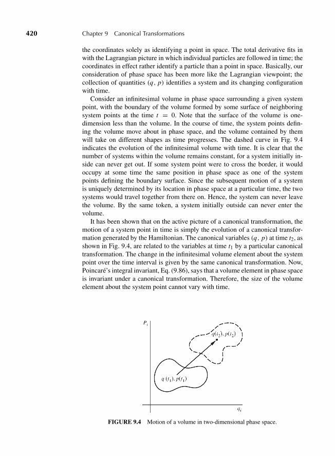
“M09 Goldstein ISBN C09” — 2011/2/15 — page 420 — #53
420 Chapter 9 Canonical Transformations
the coordinates solely as identifying a point in space. The total derivative fits inwith the Lagrangian picture in which individual particles are followed in time; thecoordinates in effect rather identify a particle than a point in space. Basically, ourconsideration of phase space has been more like the Lagrangian viewpoint; thecollection of quantities (q, p) identifies a system and its changing configurationwith time.
Consider an infinitesimal volume in phase space surrounding a given systempoint, with the boundary of the volume formed by some surface of neighboringsystem points at the time t = 0. Note that the surface of the volume is one-dimension less than the volume. In the course of time, the system points defin-ing the volume move about in phase space, and the volume contained by themwill take on different shapes as time progresses. The dashed curve in Fig. 9.4indicates the evolution of the infinitesimal volume with time. It is clear that thenumber of systems within the volume remains constant, for a system initially in-side can never get out. If some system point were to cross the border, it wouldoccupy at some time the same position in phase space as one of the systempoints defining the boundary surface. Since the subsequent motion of a systemis uniquely determined by its location in phase space at a particular time, the twosystems would travel together from there on. Hence, the system can never leavethe volume. By the same token, a system initially outside can never enter thevolume.
It has been shown that on the active picture of a canonical transformation, themotion of a system point in time is simply the evolution of a canonical transfor-mation generated by the Hamiltonian. The canonical variables (q, p) at time t2, asshown in Fig. 9.4, are related to the variables at time t1 by a particular canonicaltransformation. The change in the infinitesimal volume element about the systempoint over the time interval is given by the same canonical transformation. Now,Poincare’s integral invariant, Eq. (9.86), says that a volume element in phase spaceis invariant under a canonical transformation. Therefore, the size of the volumeelement about the system point cannot vary with time.
FIGURE 9.4 Motion of a volume in two-dimensional phase space.
“M09 Goldstein ISBN C09” — 2011/2/15 — page 421 — #54
Derivations 421
Thus, both the number of systems in the infinitesimal region, d N , and thevolume, dV , are constants, and consequently the density
D = d N
dV
must also be constant in time, that is,
d D
dt= 0,
which proves Liouville’s theorem. An alternative statement of the theorem followsfrom Eq. (9.149) as
∂D
∂t= −[D, H ]. (9.150)
When the ensemble of systems is in statistical equilibrium, the number of sys-tems in a given state must be constant in time, which is to say that the densityof system points at a given spot in phase space does not change with time. Thevariation of D with time at a fixed point corresponds to the partial derivative withrespect to t , which therefore must vanish in statistical equilibrium. By Eq. (9.150),it follows that the equilibrium condition can be expressed as
[D, H ] = 0.
We can ensure equilibrium therefore by choosing the density D to be a functionof those constants of the motion of the system not involving time explicitly, forthen the Poisson bracket with H must vanish. Thus, for conservative systems Dcan be any function of the energy, and the equilibrium condition is automaticallysatisfied. The characteristics of the ensemble will be determined by the choice offunction for D. As an example, one well-known ensemble, the microcanonicalensemble, occurs if D is constant for systems having a given narrow energy rangeand zero outside the range.
The considerations have been presented here to illustrate the usefulness of thePoisson bracket formulation in classical statistical mechanics. Further discussionof these points would carry us far outside our field.
DERIVATIONS
1. One of the attempts at combining the two sets of Hamilton’s equations into one tries totake q and p as forming a complex quantity. Show directly from Hamilton’s equationsof motion that for a system of one degree of freedom the transformation
Q = q + i p, P = Q∗
is not canonical if the Hamiltonian is left unaltered. Can you find another set of coordi-nates Q′, P ′ that are related to Q, P by a change of scale only, and that are canonical?
“M09 Goldstein ISBN C09” — 2011/2/15 — page 422 — #55
422 Chapter 9 Canonical Transformations
2. Show that the transformation for a system of one degree of freedom,
Q = q cosα − p sinα,
P = q sinα + p cosα,
satisfies the symplectic condition for any value of the parameter α. Find a generatingfunction for the transformation. What is the physical significance of the transformationfor α = 0? For α = π/2? Does your generating function work for both of these cases.
3. In Section 8.4 some of the problems of treating time as one of the canonical variablesare discussed. If we are able to sidestep these difficulties, show that the equations oftransformation in which t is considered a canonical variable reduce to Eqs. (9.14) ifin fact the transformation does not affect the time scale.
4. Show directly that the transformation
Q = log
(1
qsin p
), P = q cot p
is canonical.
5. Show directly that for a system of one degree of freedom the transformation
Q = arc tanαq
p, P = αq2
2
(1 + p2
α2q2
)
is canonical, where α is an arbitrary constant of suitable dimensions.
6. The transformation equations between two sets of coordinates are
Q = log(1 + q1/2 cos p),
P = 2(1 + q1/2 cos p)q1/2 sin p.
(a) Show directly from these transformation equations that Q, P are canonical vari-ables if q and p are.
(b) Show that the function that generates this transformation is
F3 = −(eQ − 1)2 tan p.
7. (a) If each of the four types of generating functions exist for a given canonical trans-formation, use the Legendre transformation to derive relations between them.
(b) Find a generating function of the F4 type for the identify transformation and ofthe F3 type for the exchange transformation.
(c) For an orthogonal point transformation of q in a system of n degrees of freedom,show that the new momenta are likewise given by the orthogonal transformationof an n-dimensional vector whose components are the old momenta plus a gradi-ent in configuration space.
8. Prove directly that the transformation
Q1 = q1, P1 = p1 − 2p2,
Q2 = p2, P2 = −2qi − q2
is canonical and find a generating function.
“M09 Goldstein ISBN C09” — 2011/2/15 — page 423 — #56
Derivations 423
9. (a) For a single particle show directly (that is, by direct evaluation of the Poissonbrackets), that if u is a scalar function only of r2, p2, and r ? p, then
[u,L] = 0.
(b) Similarly show directly that if F is a vector function,
F = ur + vp + w(r3p),
where u, v, and w are scalar functions of the same type as in part (a), then
[Fi , L j ] = εi jk Fk .
10. Find under what conditions
Q = αp
x, P = βx2,
where α and β are constants, represents a canonical transformation for a system ofone degree of freedom, and obtain a suitable generating function. Apply the transfor-mation to the solution of the linear harmonic oscillator.
11. Determine whether the transformation
Q1 = q1q2, P1 = p1 − p2
q2 − q1+ 1,
Q2 = q1 + q2, P2 = q2 p2 − q1 p1
q2 − q1− (q2 + q1)
is canonical.
12. Show that the direct conditions for a canonical condition are given immediately bythe symplectic condition expressed in the form
JM = M−1J.
13. The set of restricted canonical transformations forms a group (Appendix B). Ver-ify this statement once using the invariance of Hamilton’s principle under canonicaltransformation (cf. Eq. (9.11)), and again using the symplectic condition.
14. Prove that the transformation
Q1 = q21 , Q2 = q2 sec p2,
P1 = p1 cos p2 − 2q2
2q1 cos p2, P2 = sin p2 − 2q1
is canonical, by any method you choose. Find a suitable generating function that willlead to this transformation.
15. (a) Using the fundamental Poisson brackets find the values of α and β for which theequations
Q = qα cosβp, P = qα sinβp
represent a canonical transformation.
“M09 Goldstein ISBN C09” — 2011/2/15 — page 424 — #57
424 Chapter 9 Canonical Transformations
(b) For what values of α and β do these equations represent an extended canonicaltransformation? Find a generating function of the F3 form for the transformation.
(c) On the basis of part (b), can the transformation equations be modified so that theydescribe a canonical transformation for all values of β?
16. For a symmetric rigid body, obtain formulas for evaluating the Poisson brackets
[φ, f (θ, φ, ψ)], [ψ, f (θ, φ,ψ)]
where θ , φ, and ψ are the Euler angles, and f is any arbitrary function of the Eulerangles.
17. Show that the Jacobi identity is satisfied if the Poisson bracket sign stands for thecommutator of two square matrices:
[A,B] = AB − BA.
Show also that for the same representation of the Poisson bracket that
[A,BC] = [A,B]C + B[A,C].
18. Prove Eq. (9.83) using the symplectic matrix notation for the Lagrange and Poissonbrackets.
19. Verify the analog of the Jacobi identity for Lagrange brackets,
∂{u, v}∂w
+ ∂{v,w}∂u
+ ∂{w, u}∂v
= 0,
where u, v, andw are three functions in terms of which the (q, p) set can be specified.
20. (a) Verify that the components of the two-dimensional matrix A, defined by Eq.(9.141), are constants of the motion for the two-dimensional isotropic harmonicoscillator problem.
(b) Verify that the quantities Si , i = 1, 2, 3, defined by Eqs. (9.144), (9.145), (9.146),have the properties stated in Eqs. (9.147) and (9.148).
EXERCISES
21. (a) For a one-dimensional system with the Hamiltonian
H = p2
2− 1
2q2,
show that there is a constant of the motion
D = pq
2− Ht.
(b) As a generalization of part (a), for motion in a plane with the Hamiltonian
H = |p|n − ar−n,
“M09 Goldstein ISBN C09” — 2011/2/15 — page 425 — #58
Exercises 425
where p is the vector of the momenta conjugate to the Cartesian coordinates, showthat there is a constant of the motion
D = p ? rn
− Ht.
(c) The transformation Q = λq, p = λP is obviously canonical. However, the sametransformation with t time dilatation, Q = λq , p = λP , t ′ = λ2t , is not. Showthat, however, the equations of motion for q and p for the Hamiltonian in part (a)are invariant under this transformation. The constant of the motion D is said to beassociated with this invariance.
22. Show that the following transformation is canonical by using Poisson bracket:
Q =√
2qeα cos p and P =√
2qe−α sin p.
23. Prove that the following transformation from (q, p) to (Q, P) basis is canonical usingPoisson bracket
Q =√
2 · q · tan p and P =√
2 · log(sin p).
24. Show that the transformation defined by Q = 1/p and P = qp2 is canonical usingPoisson bracket.
25. (a) The Hamiltonian for a system has the form
H = 1
2
(1
q2+ p2q4
).
Find the equation of motion for q .
(b) Find a canonical transformation that reduces H to the form of a harmonic oscilla-tor. Show that the solution for the transformed variables is such that the equationof motion found in part (a) is satisfied.
26. A system of n particles moves in a plane under the influence of interaction forcesderived from potential terms depending only upon the scalar distances betweenparticles.
(a) Using plane polar coordinates for each particle (relative to a common origin),identify the form of the Hamiltonian for the system.
(b) Find a generating function for the canonical transformation that corresponds to atransformation to coordinates rotating in the plane counterclockwise with a uni-form angular rate ω (the same for all particles). What are the transformation equa-tions for the momenta?
(c) What is the new Hamiltonian? What physical significance can you give to thedifference between the old and the new Hamiltonians?
27. (a) In the problem of small oscillations about steady motion, show that at the pointof steady motion all the Hamiltonian variables h are constant. If the valuesfor steady motion are h0 so that h = h0 + j, show that to the lowest non-vanishing approximation the effective Hamiltonian for small oscillation can be
“M09 Goldstein ISBN C09” — 2011/2/15 — page 426 — #59
426 Chapter 9 Canonical Transformations
expressed as
H(h0, z) = 12jSj,
where S is a square matrix with components that are functions of h0 only.
(b) Assuming all frequencies of small oscillation are distinct, let M be a square2n × 2n matrix formed by the components of a possible set of eigenvectors (forboth positive and negative frequencies). Only the directions of the eigenvectorsare fixed, not their magnitudes. Show that it is possible to apply conditions to theeigenvectors (in effect fixing their magnitudes) that make M the Jacobian matrixof a canonical transformation.
(c) Show that the canonical transformation so found transforms the effective Hamil-tonian to the form
H = iω j q j p j ,
where ω j is the magnitude of the normal frequencies. What are the equations ofmotion in this set of canonical coordinates?
(d) Finally, show that
F2 = q j Pj +i
2
P2j
ω j− i
4ω j q2
j
leads to a canonical transformation that decomposes H into the Hamiltoniansfor a set of uncoupled linear harmonic oscillators that oscillate in the normalmodes.
28. A charged particle moves in space with a constant magnetic field B such that thevector potential, A, is
A = 12 (B3 r)
(a) If v j are the Cartesian components of the velocity of the particle, evaluate thePoisson brackets
[vi , v j ], i �= j = 1, 2, 3.
(b) If pi is the canonical momentum conjugate to xi , also evaluate the Poissonbrackets
[xi , v j ], [pi , v j ],
[xi , p j ], [pi , p j ].
29. The semimajor axis a of the elliptical Kepler orbit and the eccentricity e are functionsof first integrals of the motion, and therefore of the canonical variables. Similarly, themean anomaly
φ ≡ ω(t − T ) = ψ − e sinψ
is a function of r , θ , and the conjugate momenta. Here T is the time of periapsispassage and is a constant of the motion. Evaluate the Poisson brackets that can be
“M09 Goldstein ISBN C09” — 2011/2/15 — page 427 — #60
Exercises 427
formed of a, e, φ, ω, and T . There are in fact only nine nonvanishing distinct Poissonbrackets out of these quantities.
30. (a) Prove that the Poisson bracket of two constants of the motion is itself a constantof the motion even when the constants depend upon time explicitly.
(b) Show that if the Hamiltonian and a quantity F are constants of the motion, thenthe nth partial derivative of F with respect to t must also be a constant of themotion.
(c) As an illustration of this result, consider the uniform motion of a free particle ofmass m. The Hamiltonian is certainly conserved, and there exists a constant of themotion
F = x − pt
m.
Show by direct computation that the partial derivative of F with t , which is aconstant of the motion, agrees with [H, F].
31. Show by the use of Poisson brackets that for a one-dimensional harmonic oscillatorthere is a constant of the motion u defined as
u(q, p, t) = ln(p + im ωq)− iωt, ω =√
k
m.
What is the physical significance of this constant of the motion?
32. A system of two degrees of freedom is described by the Hamiltonian
H = q1 p1 − q2 p2 − aq21 + bq2
2 .
Show that
F1 = p1 − aq1
q2and F2 = q1q2
are constants of the motion. Are there any other independent algebraic constants ofthe motion? Can any be constructed from Jacobi’s identity?
33. Set up the magnetic monopole described in Exercise 28 (Chapter 3) in Hamilto-nian formulation (you may want to use spherical polar coordinates). By means ofthe Poisson bracket formulation, show that the quantity D defined in that exercise isconserved.
34. Obtain the motion in time of a linear harmonic oscillator by means of the formalsolution for the Poisson bracket version of the equation of motion as derived fromEq. (9.116). Assume that at time t = 0 the initial values are x0 and p0.
35. A particle moves in one dimension under a potential
V = mk
x2.
Find x as a function of time, by using the symbolic solution of the Poisson bracketform for the equation of motion for the quantity y = x2. Initial conditions are that att = 0, x = x0, and v = 0.
“M09 Goldstein ISBN C09” — 2011/2/15 — page 428 — #61
428 Chapter 9 Canonical Transformations
36. (a) Using the theorem concerning Poisson brackets of vector functions and compo-nents of the angular momentum, show that if F and G are two vector functions ofthe coordinates and momenta only, then
[F ?L,G ?L] = L ? (G3F)+ Li L j [Fi ,G j ].
(b) Let L be the total angular momentum of a rigid body with one point fixed andlet Lμ be its component along a set of Cartesian axes fixed in the rigid body. Bymeans of part (a) find a general expression for
[Lμ, Lν ], μ, ν = 1, 2, 3.
(Hint: Choose for F and G unit vectors along the μ and ν axes.)
(c) From the Poisson bracket equations of motion for Lμ derive Euler’s equations ofmotion for a rigid body.
37. Set up the problem of the spherical pendulum in the Hamiltonian formulation, usingspherical polar coordinates for the qi . Evaluate directly in terms of these canonicalvariables the following Poisson brackets:
[Lx , L y], [L y , Lz], [Lz, Lx ],
showing that they have the values predicted by Eq. (9.128). Why is it that pθ and pψcan be used as canonical momenta, although they are perpendicular components ofthe angular momentum?
38. In Section 9.7, it is shown that if any two components of the angular momentumare conserved, then the total angular momentum is conserved. If two of the compo-nents are identically zero, the third must be conserved. From this it would appear tofollow that in any motion confined to a plane, so that the components of the angu-lar momentum in the plane are zero, the total angular momentum is constant. Thereappear to be a number of obvious contradictions to this prediction; for example, theangular momentum of an oscillating spring in a watch, or the angular momentum ofa plane disk rolling down an inclined plane all in the same vertical plane. Discussthe force of these objections and whether the statement of the theorem requires anyrestrictions.
39. (a) Show from the Poisson bracket condition for conserved quantities that theLaplace–Runge–Lenz vector A,
A = p3L − mkrr,
is a constant of the motion for the Kepler problem.
(b) Verify the Poisson bracket relations for the components of A as given byEq. (9.131).
40. Consider a system that consists of a rigid body in three-space with one point fixed.Using cylindrical coordinates find the canonical transformation corresponding to newaxes rotating about the z-axis with an arbitrary time-dependent angular velocity. Ver-ify that your proposed solution is canonical.
41. We start with a time independent Hamiltonian Ho(q, p) and impose an external oscil-lating field making the Hamiltonian
H = Ho(q, p)− ε sinωt

“M09 Goldstein ISBN C09” — 2011/2/15 — page 429 — #62
Exercises 429
where ε and ω are given constants.
(a) How are the canonical equations modified?
(b) Find a canonical transformation that restores the canonical form of the equationsof motion and determine the “new” Hamiltonian.
(c) Give a possible physical interpretation of the imposed field.
“M10 Goldstein ISBN C10” — 2011/2/15 — page 430 — #1
C H A P T E R
10 Hamilton–Jacobi Theory andAction-Angle Variables
It has already been mentioned that canonical transformations may be used to pro-vide a general procedure for solving mechanical problems. Two methods havebeen suggested. If the Hamiltonian is conserved, then a solution could be obtainedby transforming to new canonical coordinates that are all cyclic, thereby provid-ing new equations of motion with trivial solutions. An alternative technique is toseek a canonical transformation from the coordinates and momenta, (q, p), at thetime t , to a new set of constant quantities, which may be the 2n initial values,(q0, p0), at t = 0. With such a transformation, the equations of transformationrelating the old and new canonical variables are exactly the desired solution of themechanical problem:
q = q(q0, p0, t),
p = p(q0, p0, t).
They give the coordinates and momenta as a function of their initial values and thetime. This last procedure is the more general one, especially as it is applicable, inprinciple at least, even when the Hamiltonian involves the time. We shall thereforebegin our discussion by considering how such a transformation may be found.
10.1 THE HAMILTON–JACOBI EQUATIONFOR HAMILTON’S PRINCIPAL FUNCTION
We can automatically ensure that the new variables are constant in time by requir-ing that the transformed Hamiltonian, K , shall be identically zero, for then theequations of motion are
∂K
∂Pi= Qi = 0,
− ∂K
∂Qi= Pi = 0. (10.1)
As we have seen, K must be related to the old Hamiltonian and to the generatingfunction by the equation
K = H + ∂F
∂t,
430
“M10 Goldstein ISBN C10” — 2011/2/15 — page 431 — #2
10.1 The Hamilton–Jacobi Equation for Hamilton’s Principal Function 431
and hence will be zero if F satisfies the equation
H(q, p, t)+ ∂F
∂t= 0. (10.2)
It is convenient to take F as a function of the old coordinates qi , the new constantmomenta Pi , and the time; in the notation of the previous chapter we would desig-nate the generating function as F2(q, P, t). To write the Hamiltonian in Eq. (10.2)as a function of the same variables, use may be made of the equations of transfor-mation (cf. Eq. (9.17a)),
pi = ∂F2
∂qi,
so that Eq. (10.2) becomes
H
(q1, . . . , qn; ∂F2
∂qi, . . . ,
∂F2
∂qn; t
)+ ∂F2
∂t= 0. (10.3)
Equation (10.3), known as the Hamilton–Jacobi equation, constitutes a partialdifferential equation in (n+1) variables, q1, . . . , qn; t , for the desired generatingfunction. It is customary to denote the solution F2 of Eq. (10.3) by S and to callit Hamilton’s principal function.
Of course, the integration of Eq. (10.3) only provides the dependence on theold coordinates and time; it would not appear to tell how the new momenta arecontained in S. Indeed, the new momenta have not yet been specified except thatwe know they must be constants. However, the nature of the solution indicateshow the new Pi ’s are to be selected.
Mathematically Eq. (10.3) has the form of a first-order partial differential equa-tion in n + 1 variables. Suppose there exists a solution to Eq. (10.3) of the form
F2 ≡ S = S(q1, . . . , qn; α1, . . . , αn+1; t), (10.4)
where the quantities α1, . . . , αn+1 are n + 1 independent constants of integration.Such solutions are known as complete solutions of the first-order partial differen-tial equation.* One of the constants of integration, however, is in fact irrelevant tothe solution, for it will be noted that S itself does not appear in Eq. (10.3); only itspartial derivatives with respect to q or t are involved. Hence, if S is some solutionof the differential equation, then S + α, where α is any constant, must also bea solution. One of the n + 1 constants of integration in Eq. (10.4) must there-fore appear only as an additive constant tacked on to S. But by the same token,an additive constant has no importance in a generating function, since only par-tial derivatives of the generating function occur in the transformation equations.
*Equation (10.4) is not the only type of solution possible for Eq. (10.3). The most general formof the solution involves one or more arbitrary functions rather than arbitrary constants. Nor is therenecessarily a unique solution of the form (10.4). There may be several complete solutions for the givenequation. But all that is important for the subsequent argument is that there exist a complete solution.
“M10 Goldstein ISBN C10” — 2011/2/15 — page 432 — #3
432 Chapter 10 Hamilton–Jacobi Theory and Action-Angle Variables
Hence, for our purposes a complete solution to Eq. (10.3) can be written in theform
S = S(q1, . . . , qn; α1, . . . , αn; t), (10.5)
where none of the n independent constants is solely additive. In this mathematicalgarb, S tallies exactly with the desired form for an F2 type of generating func-tion, for Eq. (10.5) presents S as a function of N coordinates, the time t , and nindependent quantities αi . We are therefore at liberty to take the n constants ofintegration to be the new (constant) momenta:
Pi = αi . (10.6)
Such a choice does not contradict the original assertion that the new momentaare connected with the initial values of q and p at time t0. The n transformationequations (9.17a) can now be written as
pi = ∂S(q, α, t)
∂qi, (10.7)
where q, α stand for the complete set of quantities. At the time t0, these constituten equations relating the n α’s with the initial q and p values, thus enabling us toevaluate the constants of integration in terms of the specific initial conditions ofthe problem. The other half of the equations of transformation, which provide thenew constant coordinates, appear as
Qi = βi = ∂S(q, α, t)
∂αi. (10.8)
The constant β’s can be similarly obtained from the initial conditions, simply bycalculating the value of the right side of Eq. (10.8) at t = t0 with the known initialvalues of qi . Equations (10.8) can then be “turned inside out” to furnish q j interms of α, β, and t :
q j = q j (α, β, t), (10.9)
which solves the problem of giving the coordinates as functions of time and theinitial conditions.* After the differentiation in Eqs. (10.7) has been performed,
*As a mathematical point, it may be questioned whether the process of “turning inside out” is feasiblefor Eqs. (10.7) and (10.8), that is, whether they can be solved for αi and qi , respectively. The questionhinges on whether the equations in each set are independent, for otherwise they are obviously notsufficient to determine the n independent quantities αi or qi as the case may be. To simplify thenotation, let Sα symbolize members of the set of partial derivatives of S with respect to αi , so thatEq. (10.8) is represented by β = Sα . That the derivatives Sα in (10.8) form independent functionsof the q’s follows directly from the nature of a complete solution to the Hamilton–Jacobi equation;indeed this is what we mean by saying the n constants of integration are independent. Consequently,the Jacobian of Sα with respect to qi cannot vanish. Since the order of differentiation is immaterial,this is equivalent to saying that the Jacobian of Sq with respect to αi cannot vanish, which proves theindependence of Eqs. (10.7).
“M10 Goldstein ISBN C10” — 2011/2/15 — page 433 — #4
10.1 The Hamilton–Jacobi Equation for Hamilton’s Principal Function 433
Eqs. (10.9) may be substituted for the q’s, thus giving the momenta pi as functionsof the α, β, and t :
pi = pi (α, β, t). (10.10)
Equations (10.9) and (10.10) thus constitute the desired complete solution ofHamilton’s equations of motion.
Hamilton’s principal function is thus the generator of a canonical transforma-tion to constant coordinates and momenta; when solving the Hamilton–Jacobiequation, we are at the same time obtaining a solution to the mechanical prob-lem. Mathematically speaking, we have established an equivalence between the2n canonical equations of motion, which are first-order differential equations,to the first-order partial differential Hamilton–Jacobi equation. This correspon-dence is not restricted to equations governed by the Hamiltonian; indeed, the gen-eral theory of first-order partial differential equations is largely concerned withthe properties of the equivalent set of first-order ordinary differential equations.Essentially, the connection can be traced to the fact that both the partial differen-tial equation and its canonical equations stem from a common variational princi-ple, in this case Hamilton’s modified principle.
To a certain extent, the choice of the αi ’s as the new momenta is arbitrary. Wecould just as well choose any n quantities, γi , which are independent functions ofthe αi constants of integration:
γi = γi (αi , . . . , αn). (10.11)
By means of these defining relations, Hamilton’s principal function can be writtenas a function of qi , γi , and t , and the rest of the derivation then goes throughunchanged. It often proves convenient to take some particular set of γi ’s as thenew momenta, rather than the constants of integration that appear naturally inintegrating the Hamilton–Jacobi equation.
Further insight into the physical significance of Hamilton’s principal functionS is furnished by an examination of its total time derivative, which can be com-puted from the formula
d S
dt= ∂S
∂qiqi + ∂S
∂t,
since the Pi ’s are constant in time. By Eqs. (10.7) and (10.3), this relation can alsobe written
d S
dt= pi qi − H = L , (10.12)
so that Hamilton’s principal function differs at most from the indefinite time inte-gral of the Lagrangian only by a constant:
S =∫
L dt + constant. (10.13)
“M10 Goldstein ISBN C10” — 2011/2/15 — page 434 — #5
434 Chapter 10 Hamilton–Jacobi Theory and Action-Angle Variables
Now, Hamilton’s principle is a statement about the definite integral of L , and fromit we obtained the solution of the problem via the Lagrange equations. Here thesame action integral, in an indefinite form, furnishes another way of solving theproblem. In actual calculations, the result expressed by Eq. (10.13) is of no help,because we cannot integrate the Lagrangian with respect to time until qi and pi
are known as functions of time, that is, until the problem is solved.When the Hamiltonian does not depend explicitly upon the time, Hamilton’s
principal function can be written in the form
S(q, α, t) = W (q, α)− at, (10.14)
where W (q, α) is called Hamilton’s characteristic function. The physical signifi-cance of W can be understood by writing its total time derivative
dW
dt= ∂W
∂qiqi .
Comparing this expression to the results of substituting Eq. (10.14) into Eq. (10.7),it is clear that
pi = ∂W
∂qi, (10.15)
and hence,
dW
dt= pi qi . (10.16)
This can be integrated to give
W =∫
pi qi dt =∫
pi dqi , (10.17)
which is just the abbreviated action defined by Eq. (8.80).
10.2 THE HARMONIC OSCILLATOR PROBLEM AS AN EXAMPLEOF THE HAMILTON–JACOBI METHOD
To illustrate the Hamilton–Jacobi technique for solving the motion of mechanicalsystems, we shall work out in detail the simple problem of a one-dimensionalharmonic oscillator. The Hamiltonian is
H = 1
2m(p2 + m2ω2q2) ≡ E, (10.18)
where
ω =√
k
m, (10.19)
“M10 Goldstein ISBN C10” — 2011/2/15 — page 435 — #6
10.2 The Harmonic Oscillator Problem as an Example 435
k being the force constant. We obtain the Hamilton–Jacobi equations for S bysetting p equal to ∂S/∂q and substituting in the Hamiltonian; the requirementthat the new Hamiltonian vanishes becomes
1
2m
[(∂S
∂q
)2
+ m2ω2q2
]+ ∂S
∂t= 0. (10.20)
Since the explicit dependence of S on t is present only in the last term, Eq. (10.14)can be used to eliminate the time from the Hamilton–Jacobi equation (10.20)
1
2m
[(∂W
∂q
)2
+ m2ω2q2
]= α. (10.21)
The integration constant α is thus to be identified with the total energy E . Thiscan also be recognized directly from Eq. (10.14) and the relation (cf. Eq. (10.3))
∂S
∂t+ H = 0,
which then reduces to
H = α.
Equation (10.21) can be integrated immediately to
W =√
2mα∫
dq
√1 − mω2q2
2α, (10.22)
so that
S =√
2mα∫
dq
√1 − mω2q2
2α− αt. (10.23)
While the integration involved in Eq. (10.23) is not particularly difficult, thereis no reason to carry it out at this stage, for what is desired is not S but its partialderivatives. The solution for q arises out of the transformation equation (10.8):
β ′ = ∂S
∂α=√
m
2α
∫dq√
1 − mω2q2
2α
− t,
which can be integrated without trouble to give
t + β ′ = 1
ωarcsin q
√mω2
2α. (10.24)

“M10 Goldstein ISBN C10” — 2011/2/15 — page 436 — #7
436 Chapter 10 Hamilton–Jacobi Theory and Action-Angle Variables
Equation (10.24) can be immediately “turned inside out” to furnish q as afunction of t and the two constants of integration α and β = β ′ω:
q =√
2α
mω2sin(ωt + β), (10.25)
which is the familiar solution for a harmonic oscillator. Formally, the solutionfor the momentum comes from the transformation equation (10.7), which, usingEq. (10.22), can be written
p = ∂S
∂q= ∂W
∂q=√
2mα − m2ω2q2. (10.26)
In conjunction with the solution for q, Eq. (10.25), this becomes
p =√
2mα(1 − sin2(ωt + β)),
or
p =√
2mα cos(ωt + β). (10.27)
Of course, this result checks with the simple identification of p as mq .To complete the story, the constants α and β must be connected with the initial
conditions q0 and p0 at time t = 0. By squaring Eqs. (10.25) and (10.27), it isclearly seen that α is given in terms of q0 and p0 by the equation
2mα = p20 + m2ω2q2
0 . (10.28)
The same result follows immediately of course from the previous identification ofα as the conserved total energy E . Finally, the phase constant β is related to q0and p0 by
tanβ = mωq0
p0. (10.29)
The choice q0 = 0 and hence β = 0 corresponds to starting the motion with theoscillator at its equilibrium position q = 0.
Thus, Hamilton’s principle function is the generator of a canonical transforma-tion to a new coordinate that measures the phase angle of the oscillation and to anew canonical momentum identified as the total energy.
If the solution for q is substituted into Eq. (10.23), Hamilton’s principal func-tion can be written as
S = 2α∫
cos2(ωt + β) dt − αt = 2α∫(cos2(ωt + β)− 1
2 ) dt. (10.30)
“M10 Goldstein ISBN C10” — 2011/2/15 — page 437 — #8
10.2 The Harmonic Oscillator Problem as an Example 437
Now, the Lagrangian is
L = 1
2m(p2 − m2ω2q2)
= α(cos2(ωt + β)− sin2(ωt + β))= 2α(cos2(ωt + β)− 1
2 ),
so that S is the time integral of the Lagrangian, in agreement with the generalrelation (10.13). Note that the identity could not be proved until after the solutionto the problem had been obtained.
As another illustration for the Hamilton–Jacobi method, it is instructive toconsider the two-dimensional anisotropic harmonic oscillator. If we let m be themass of the oscillating body and kx and ky be the spring constants in the x- andy-directions, respectively, the Hamiltonian is
E = 1
2m(p2
x + p2y + m2ω2
x x2 + m2ω2y y2),
where
ωx =√
kx
mand ωy =
√ky
m.
Since the coordinates and momenta separate into two distinct sets, the princi-pal function can be written as a sum of the characteristic function for each pair.Assuming that we solve the y-functional dependency first, this means
S(x, y, α, αy, t) = Fx (x, α)+ Fy(y, αy)− αt, (10.31)
and the Hamilton–Jacobi equation assumes the form
1
2m
[(∂W
∂x
)2
+ m2ω2x x2 +
(∂W
∂y
)2
+ m2ω2y y2
]= α (10.32)
in analogy with Eq. (10.18). Since the variables are separated, the y-part of theEq. (10.32) must be equal to a constant, which we call αy , so
1
2m
(∂W
∂y
)2
+ 1
2mω2
y y2 = αy, (10.33)
and we replace the y-term in (10.32) with αy from (10.33), yielding
1
2m
(∂W
∂x
)2
+ 1
2mω2
x x2 = αx , (10.34)
where we write α − αy = αx showing the symmetry of Eqs. (10.33) and (10.34).
“M10 Goldstein ISBN C10” — 2011/2/15 — page 438 — #9
438 Chapter 10 Hamilton–Jacobi Theory and Action-Angle Variables
Each equation has a solution analogous to Eqs. (10.25) and (10.27), so
x =√
2αx
mω2x
sin(ωx t + βx ),
px =√
2mαx cos(ωx t + βx ),(10.35)
y =√
2αy
mω2y
sin(ωyt + βy),
py = √2mαy cos(ωyt + βy),
where the βi ’s are phase constants and the total energy is given by
E = αx + αy = α.
As a third example of Hamilton–Jacobi theory, we again consider the two-dimensional harmonic oscillator; only we will assume the oscillator is isotropic,so
kx = ky = k and ωx = ωy = ω,
and use polar coordinates to write
x = r cos θ, r =√
x2 + y2,
y = r sin θ, θ = tan−1 y
x,
(10.36)px = mx, pr = mr ,
py = my, pθ = mr2θ .
The Hamiltonian now written as
E = 1
2m
(p2
r + p2θ
r2+ m2ω2r2
)(10.37)
is cyclic in the angular coordinate θ . The principal function can then be written as
S(r, θ, α, αθ ) = Wr (r, α)+ Wθ (θ, αθ )− αt
= Wr (r, α)+ θαθ − αt, (10.38)
where, as we show later, a cyclic coordinate qi always has the characteristic func-tion component Wqi = qiαi . The canonical momentum pθ associated with thecyclic coordinate, θ , is calculated from the generating function
pθ = ∂Fθ∂θ
= αθ
and has its expected constant value.
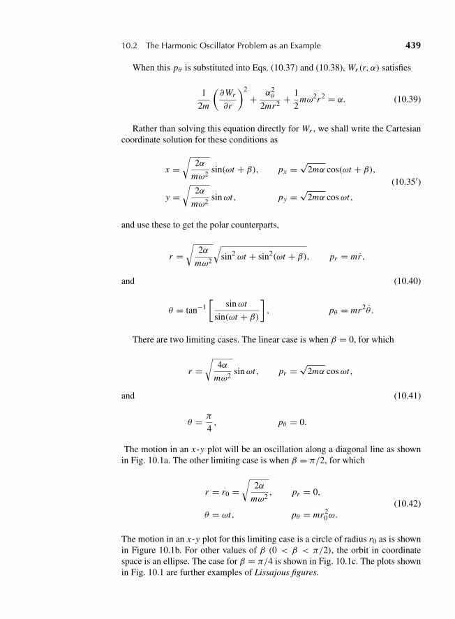
“M10 Goldstein ISBN C10” — 2011/2/15 — page 439 — #10
10.2 The Harmonic Oscillator Problem as an Example 439
When this pθ is substituted into Eqs. (10.37) and (10.38), Wr (r, α) satisfies
1
2m
(∂Wr
∂r
)2
+ α2θ
2mr2+ 1
2mω2r2 = α. (10.39)
Rather than solving this equation directly for Wr , we shall write the Cartesiancoordinate solution for these conditions as
x =√
2α
mω2sin(ωt + β), px =
√2mα cos(ωt + β),
(10.35′)y =
√2α
mω2sinωt, py =
√2mα cosωt,
and use these to get the polar counterparts,
r =√
2α
mω2
√sin2 ωt + sin2(ωt + β), pr = mr ,
and (10.40)
θ = tan−1[
sinωt
sin(ωt + β)], pθ = mr2θ .
There are two limiting cases. The linear case is when β = 0, for which
r =√
4α
mω2sinωt, pr =
√2mα cosωt,
and (10.41)
θ = π
4, pθ = 0.
The motion in an x-y plot will be an oscillation along a diagonal line as shownin Fig. 10.1a. The other limiting case is when β = π/2, for which
r = r0 =√
2α
mω2, pr = 0,
(10.42)θ = ωt, pθ = mr2
0ω.
The motion in an x-y plot for this limiting case is a circle of radius r0 as is shownin Figure 10.1b. For other values of β (0 < β < π/2), the orbit in coordinatespace is an ellipse. The case for β = π/4 is shown in Fig. 10.1c. The plots shownin Fig. 10.1 are further examples of Lissajous figures.
“M10 Goldstein ISBN C10” — 2011/2/15 — page 440 — #11
440 Chapter 10 Hamilton–Jacobi Theory and Action-Angle Variables
FIGURE 10.1 The two limiting cases (a) and (b) for the harmonic oscillator and anintermediate example (c).
10.3 THE HAMILTON–JACOBI EQUATION FORHAMILTON’S CHARACTERISTIC FUNCTION
It was possible to integrate the Hamilton–Jacobi equation for the simple harmonicoscillator primarily because S could be separated into two parts, one involving qonly and the other only time. Such a separation of variables using Hamilton’scharacteristic function W (q, α) (Eq. (10.14)) is always possible whenever the oldHamiltonian does not involve time explicitly. This provides us with the restrictedHamilton–Jacobi equation
H
(qi ,
∂W
∂qi
)= α1, (10.43)
which no longer involves the time. One of the constants of integration, namelyα1, is thus equal to the constant value of H . (Normally H will be the energy, butremember that this need not always be the case, cf. Section 8.2.)
The time-independent function, Hamilton’s characteristic function W , appearshere merely as a part of the generating function S when H is constant. It canalso be shown that W separately generates its own contact transformation withproperties quite different from that generated by S. Let us consider a canonicaltransformation in which the new momenta are all constants of the motion αi , andwhere α1 in particular is the constant of motion H . If the generating functionfor this transformation be denoted by W (q, P), then the equations of transforma-tion are
pi = ∂W
∂qi, Qi = ∂W
∂Pi= ∂W
∂αi. (10.44)
While these equations resemble Eqs. (10.7) and (10.8) respectively for Hamil-ton’s principal function S, the condition now determining W is that H is the newcanonical momentum α1:
H(qi , pi ) = α1.
“M10 Goldstein ISBN C10” — 2011/2/15 — page 441 — #12
10.3 Hamilton’s Characteristic Function 441
Using Eqs. (10.44), this requirement becomes the partial differential equation:
H
(qi ,
∂W
∂qi
)= α1,
which is seen to be identical with Eq. (10.43). Since W does not involve the time,the new and old Hamiltonians are equal, and it follows that K = α1.
Hamilton’s characteristic function W thus generates a canonical transforma-tion in which all the new coordinates are cyclic. It was noted in the introductionto this chapter that when H is a constant of the motion, a transformation of thisnature in effect solves the mechanical problem involved, for the integration of thenew equations of motion is then trivial. The canonical equations for Pi , in fact,merely repeat the statement that the momenta conjugate to the cyclic coordinatesare all constant:
Pi = − ∂K
∂Qi= 0, Pi = αi . (10.45)
Because the new Hamiltonian depends upon only one of the momenta αi , theequations of motion for Qi are
Qi = ∂K
∂αi= 1, i = 1,
= 0, i �= 1,
with the immediate solutions
Q1 = t + β1 ≡ ∂W
∂α1,
(10.46)
Qi = βi ≡ ∂W
∂αii �= 1.
The only coordinate that is not simply a constant of the motion is Q1, which isequal to the time plus a constant. We have here another instance of the conjugaterelationship between the time as a coordinate and the Hamiltonian as its conjugatemomentum.
The dependence of W on the old coordinates qi is determined by the par-tial differential equation (10.43), which, like Eq. (10.3), is also referred to as theHamilton–Jacobi equation. There will now be n constants of integration in a com-plete solution, but again one of them must be merely an additive constant. Then − 1 remaining independent constants, α2, . . . , αn , together with α1 may then betaken as the new constant canonical momenta. When evaluated at t0 the first halfof Eqs. (10.44) serve to relate the n constants αi with the initial values of qi andpi . Finally, Eqs. (10.45) and (10.46) can be solved for the qi as a function of αi ,βi , and the time t , thus completing the solution of the problem. It will be noted
“M10 Goldstein ISBN C10” — 2011/2/15 — page 442 — #13
442 Chapter 10 Hamilton–Jacobi Theory and Action-Angle Variables
that (n − 1) of the Eqs. (10.46) do not involve the time at all. One of the qi ’s canbe chosen as an independent variable, and the remaining coordinates can then beexpressed in terms of it by solving only these time-independent equations. We arethus led directly to the orbit equations of the motion. In central force motion, forexample, this technique would furnish r as a function of θ , without the need forseparately finding r and θ as functions of time.
It is not always necessary to take α1 and the constants of integration in W asthe new constant canonical momenta. Occasionally it is desirable rather to usesome particular set of n independent functions of the αi ’s as the transformedmomenta. Designating these constants by γi the characteristic function W canthen be expressed in terms of qi and γi as the independent variables. The Hamil-tonian will in general depend upon more than one of the γi ’s and the equations ofmotion for Qi become
Qi = ∂K
∂γi= vi ,
where the vi ’s are functions of γi . In this case, all the new coordinates are linearfunctions of time:
Qi = vi t + βi . (10.47)
The form of W cannot be found a priori without obtaining a complete integral ofthe Hamilton–Jacobi equation. The procedures involved in solving a mechanicalproblem by either Hamilton’s principal or characteristic function may now bysummarized in the following tabular form:
The two methods of solution are applicable when the Hamiltonian
is any general function of q, p, t :H(q, p, t).
is conserved:H(q, p) = constant.
We seek canonical transformations to new variables such that
all the coordinates and momentaQi , Pi are constants of the motion.
all the momenta Pi are constants.
To meet these requirements it is sufficient to demand that the new Hamiltonian
shall vanish identically:K = 0.
shall be cyclic in all the coordi-nates:
K = H(Pi ) = α1.
Under these conditions, the new equations of motion become
Qi = ∂K
∂Pi= 0,
Pi = − ∂K
∂Qi= 0,
Qi = ∂K
∂Pi= vi ,
Pi = − ∂K
∂Qi= 0,
“M10 Goldstein ISBN C10” — 2011/2/15 — page 443 — #14
10.3 Hamilton’s Characteristic Function 443
with the immediate solutions
Qi = βi ,Pi = γi ,
Qi = vi t + βi
Pi = γi
which satisfy the stipulated requirements.The generating function producing the desired transformation is Hamilton’s
Principal Function:S(q, P, t),
Characteristic Function:W (q, P),
satisfying the Hamilton–Jacobi partial differential equation:
H
(q,∂S
∂q, t
)+ ∂S
∂t= 0. H
(q,∂W
∂q
)− α1 = 0.
A complete solution to the equation contains
n nontrivial constants of integra-tion α1, . . . , αn .
n − 1 nontrivial constants of in-tegration, which together with α1form a set of n independent con-stants α1, . . . , αn .
The new constant momenta, Pi = γi , can be chosen as any n independent func-tions of the n constants of integration:
Pi = γi (α1, . . . , αn), Pi = γi (α1, . . . , αn),
so that the complete solutions to the Hamilton–Jacobi equation may be consideredas functions of the new momenta:
S = S(qi , γi , t). W = W (qi , γi ).
In particular, the γi ’s may be chosen to be the αi ’s themselves. One-half of thetransformations equations,
pi = ∂S
∂qi, pi = ∂W
∂qi,
are fulfilled automatically, since they have been used in constructing the Hamilton–Jacobi equation. The other half,
Qi = ∂S
∂γi= βi , Qi = ∂W
∂γi= vi (γ j )t + βi ,
can be solved for qi in terms of t and the 2n constants βi , γi . The solution to theproblem is then completed by evaluating these 2n constants in terms of the initialvalues, (qi0, pi0), of the coordinates and momenta.
“M10 Goldstein ISBN C10” — 2011/2/15 — page 444 — #15
444 Chapter 10 Hamilton–Jacobi Theory and Action-Angle Variables
When the Hamiltonian does not involve time explicitly, both methods are suit-able, and the generating functions are then related to each other according to theformula
S(q, P, t) = W (q, P)− α1t.
10.4 SEPARATION OF VARIABLES IN THE HAMILTON–JACOBI EQUATION
It might appear from the preceding section that little practical advantage has beengained through the introduction of the Hamilton–Jacobi procedure. Instead ofsolving the 2n ordinary differential equations that make up the canonical equa-tions of motion, we now must solve the partial differential Hamilton–Jacobi equa-tion, and partial differential equations can be notoriously complicated to solve.Under certain conditions, however, it is possible to separate the variables in theHamilton–Jacobi equation, and the solution can then always be reduced to quadra-tures. In practice, the Hamilton–Jacobi technique becomes a useful computationaltool only when such a separation can be effected.
A coordinate q j is said to be separable in the Hamilton–Jacobi equation when(say) Hamilton’s principal function can be split into two additive parts, one ofwhich depends only on the coordinate q j and the other is entirely independent ofq j . Thus, if q1 is taken as a separable coordinate, then the Hamiltonian must besuch that one can write
S(q1, . . . , qn; α1, . . . , αn; t) = S1(q1; α1, . . . , αn; t)
+ S′(q2, . . . , qn; α1, . . . , αn; t), (10.48)
and the Hamilton–Jacobi equation can be split into two equations—one separatelyfor S1 and the other for S′. Similarly the Hamilton–Jacobi equation is described ascompletely separable (or simply, separable) if all the coordinates in the problemare separable. A solution for Hamilton’s principal function of the form
S =∑
i
Si (qi ; α1, . . . , αn; t) (10.49)
will then split the Hamilton–Jacobi equation into n equations of the type
Hi
(q j ; ∂S j
∂q j;α1, . . . , αn; t
)+ ∂S j
∂t= 0. (10.50)
If the Hamiltonian does not explicitly depend upon the time, then, for each Si wehave
Si (q j ; α1, . . . , αn; t) = Wi (q j ; α1, . . . , αn; t)− αi t, (10.51)
“M10 Goldstein ISBN C10” — 2011/2/15 — page 445 — #16
10.5 Ignorable Coordinates and the Kepler Problem 445
which provide n restricted Hamilton–Jacobi equations,
Hi
(qi ; ∂Wi
∂qi;α1, . . . , αn
)= αi . (10.52)
(No summation in Eqs. (10.50) to (10.52)!)The functions Hi in Eqs. (10.50) and (10.52) may or may not be Hamiltonians,
and the αi may be an energy, an angular momentum squared, or some other quan-tity depending on the nature of qi . We shall show this by example in the Keplerproblem in the next section.
The constants αi are referred to now as the separation constants. Each of theEqs. (10.52) involves only one of the coordinates qi and the corresponding partialderivative of Wi with respect to qi . They are therefore a set of ordinary differentialequations of a particularly simple form. Since the equations are only of first order,it is always possible to reduce them to quadratures; we have only to solve for thepartial derivative of Wi with respect to qi and then integrate over qi . In practice,each Hi will only contain one or at most a few of the α’s. There will also becases where a subset of r variables can be separated in this fashion, leaving n − rvariables, which will not separate. We shall also examine this eventuality in thenext section.
It is possible to find examples in which the Hamilton–Jacobi equation can besolved without separating the time variable (cf. Exercise 8). Nonetheless, almostall useful applications of the Hamilton–Jacobi method involve Hamiltonians notexplicitly dependent upon time, for which t is therefore a separable variable. Thesubsequent discussion on separability is thus restricted to such systems where His a constant of motion, and Hamilton’s characteristic function W will be usedexclusively.
10.5 IGNORABLE COORDINATES AND THE KEPLER PROBLEM
We can easily show that any cyclic or ignorable coordinate is separable. Supposethat the cyclic coordinate is q1; the conjugate momentum p1 is a constant, say γ .The Hamilton–Jacobi equation for W is then
H
(q2, . . . , qn; γ ; ∂W
∂q2, . . . ,
∂W
∂qn
)= α1. (10.53)
If we try a separated solution of the form
W = W1(q1, α)+ W ′(q2, . . . , qn;α), (10.54)
then it is obvious that Eq. (10.53) involves only the separate function W ′, whileW1 is the solution of the equation
p1 = γ = ∂W1
∂q1. (10.55)
“M10 Goldstein ISBN C10” — 2011/2/15 — page 446 — #17
446 Chapter 10 Hamilton–Jacobi Theory and Action-Angle Variables
The constant γ is thus the separation constant, and the obvious solution for W1(to within a trivial additive constant) is
W1 = γ q1,
and W is given by
W = W ′ + γ q1. (10.56)
There is an obvious resemblance between Eq. (10.56) and the form S assumeswhen H is not an explicit function of time, Eq. (10.43). Indeed, both equationscan be considered as arising under similar circumstances. We have seen that t maybe considered in some sense as a generalized coordinate with −H as its canonicalmomentum (cf. Eq. (8.58)). If H is conserved, then t may be treated as a cycliccoordinate.
If s of the n coordinates are noncyclic (that is, they appear explicitly in theHamiltonian), then the Hamiltonian is of the form H(q1, . . . , qs;α1, . . . , αn; t).The characteristic function can then be written as
W (q1, . . . , qs;α1, . . . , αn) =s∑
i=1
Wi (qi ; α1, . . . , αn)+n∑
i=s+1
qiαi , (10.56′)
and there are s Hamilton–Jacobi equations to be solved:
H
(q1; ∂W1
∂q1;α2, . . . , αn
)= α1. (10.57)
Since these are ordinary first-order differential equations in the independent vari-able q1, they can be immediately reduced to quadratures, and the complete solu-tions for W can be obtained.
In general, a coordinate q j is separable if q j and the conjugate momentum p j
can be segregated in the Hamiltonian into some function f (q j , p j ) that does notcontain any of the other variables. If we then seek a trial solution of the form
W = W j (q j , α)+ W ′(qi , α),
where qi represents the set of all q’s except q j , then the Hamilton–Jacobi equationappears as
H
(qi ,
∂W ′
∂qi, f
(q j ,
∂W j
∂q j
))= α1. (10.58)
In principle, at least, Eq. (10.58) can be inverted so as to solve for f :
f
(q j ,
∂W j
∂q j
)= g
(qi ,
∂W ′
∂qi, α1
). (10.59)
“M10 Goldstein ISBN C10” — 2011/2/15 — page 447 — #18
10.5 Ignorable Coordinates and the Kepler Problem 447
The argument used previously in connection with Eq. (10.51) holds here inslightly varied guise; f is not a function of any of the q’s except q j ; g on theother hand is independent of q j . Hence, Eq. (10.59) can hold only if both sidesare equal to the same constant, independent of all q’s:
f
(q j ,
∂W j
∂q j
)= α j ,
g
(qi ,
∂W ′
∂qi
)= α j , (10.60)
and the separation of the variable has been accomplished.Note that the separability of the Hamilton–Jacobi equation depends not only
on the physical problem involved but also on the choice of the system of general-ized coordinates employed. Thus, the one-body central force problem is separablein polar coordinates, but not in Cartesian coordinates. For some problems, it is notpossible to completely separate the Hamilton–Jacobi equation, the famous three-body problem being one illustration. On the other hand, in many of the basic prob-lems of mechanics and atomic physics, separation is possible in more than one setof coordinates. In general, it is feasible to solve the Hamilton–Jacobi equation inclosed form only when the variables are completely separable. Considerable inge-nuity has therefore been devoted to finding the separable systems of coordinatesappropriate to each problem.
No simple criterion can be given to indicate what coordinate systems lead toseparable Hamilton–Jacobi equations for any particular problem. In the case oforthogonal coordinate systems, the so-called Staeckel conditions have proved use-ful. They provide necessary and sufficient conditions for separability under certaincircumstances. A proof of the sufficiency of the conditions and references will befound in Appendix D of the second edition of this text.
The Staeckel conditions for the separation of the Hamilton–Jacobi equationsare:
1. The Hamiltonian is conserved.
2. The Lagrangian is no more than a quadratic function of the generalizedvelocities, so the Hamiltonian takes the form:
H = 12 (p − a)T−1(p − a)+ V (q). (8.27)
3. The vector a has elements ai that are functions only of the correspondingcoordinate, that is ai = ai (qi ).
4. the potential function can be written as a sum of the form
V (q) =∑
i
Vi (qi )
Tii. (10.61)
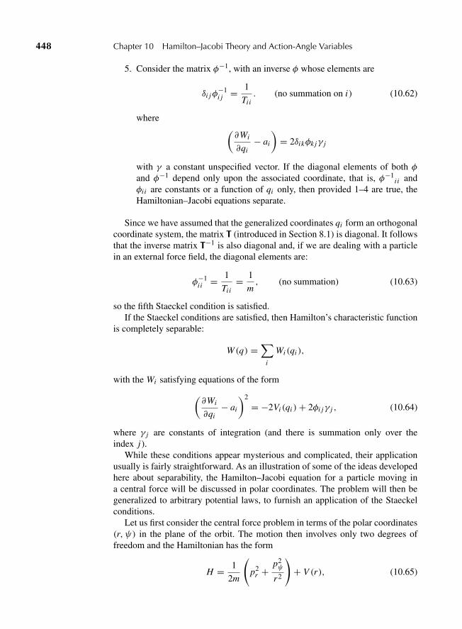
“M10 Goldstein ISBN C10” — 2011/2/15 — page 448 — #19
448 Chapter 10 Hamilton–Jacobi Theory and Action-Angle Variables
5. Consider the matrix φ−1, with an inverse φ whose elements are
δi jφ−1i j = 1
Tii. (no summation on i) (10.62)
where (∂Wi
∂qi− ai
)= 2δikφk jγ j
with γ a constant unspecified vector. If the diagonal elements of both φand φ−1 depend only upon the associated coordinate, that is, φ−1
i i andφi i are constants or a function of qi only, then provided 1–4 are true, theHamiltonian–Jacobi equations separate.
Since we have assumed that the generalized coordinates qi form an orthogonalcoordinate system, the matrix T (introduced in Section 8.1) is diagonal. It followsthat the inverse matrix T−1 is also diagonal and, if we are dealing with a particlein an external force field, the diagonal elements are:
φ−1i i = 1
Tii= 1
m, (no summation) (10.63)
so the fifth Staeckel condition is satisfied.If the Staeckel conditions are satisfied, then Hamilton’s characteristic function
is completely separable:
W (q) =∑
i
Wi (qi ),
with the Wi satisfying equations of the form
(∂Wi
∂qi− ai
)2
= −2Vi (qi )+ 2φi jγ j , (10.64)
where γ j are constants of integration (and there is summation only over theindex j).
While these conditions appear mysterious and complicated, their applicationusually is fairly straightforward. As an illustration of some of the ideas developedhere about separability, the Hamilton–Jacobi equation for a particle moving ina central force will be discussed in polar coordinates. The problem will then begeneralized to arbitrary potential laws, to furnish an application of the Staeckelconditions.
Let us first consider the central force problem in terms of the polar coordinates(r, ψ) in the plane of the orbit. The motion then involves only two degrees offreedom and the Hamiltonian has the form
H = 1
2m
(p2
r +p2ψ
r2
)+ V (r), (10.65)
“M10 Goldstein ISBN C10” — 2011/2/15 — page 449 — #20
10.5 Ignorable Coordinates and the Kepler Problem 449
which is cyclic in ψ . Consequently, Hamilton’s characteristic function appears as
W = W1(r)+ αψψ, (10.66)
where αψ is the constant angular momentum pψ conjugate to ψ . The Hamilton–Jacobi equation then becomes
(∂W1
∂r
)2
+α2ψ
r2+ 2mV (r) = 2mα1, (10.67)
where α1 is the constant identified physically as the total energy of the system.Solving Eq. (10.66) for the partial derivative of W1 we obtain
∂W1
∂r=√
2m(α1 − V )−α2ψ
r2,
so that W is
W =∫
dr
√2m(α1 − V )−
α2ψ
r2+ αψψ. (10.68)
With this form for the characteristic function, the transformation equations(10.46) appear as
t + β1 = ∂W
∂α1=∫
m dr√2m(α1 − V )− α2
ψ
r2
, (10.69a)
and
β2 = ∂W
∂αψ= −
∫αψdr
r2
√2m(α1 − V )− α2
ψ
r2
+ ψ. (10.69b)
Equation (10.69a) furnishes r as a function of t and agreees with the correspond-ing solution, Eq. (3.18), found in Chapter 3, with α1 and αψ written explicitly as Eand l, respectively. It has been remarked previously that the remaining transforma-tion equations for Qi , here only Eq. (10.69b), should provide the orbit equation.If the variable of integration in Eq. (10.69b) is changed to u = 1/r , the equationreduces to
ψ = β2 −∫
du√2mα2ψ
(α1 − V )− u2
which agrees with Eq. (3.37) previously found for the orbit, identifying ψ as θand β2 as θ0.
“M10 Goldstein ISBN C10” — 2011/2/15 — page 450 — #21
450 Chapter 10 Hamilton–Jacobi Theory and Action-Angle Variables
As a further example of separation of variables, we shall examine the samecentral force problem, but in spherical polar coordinates, that is, ignoring oura priori knowledge that the orbit lies in a plane. The appropriate Hamiltonian hasbeen shown to be (cf. Eq. (8.29)):
H = 1
2m
(p2
r + p2θ
r2+ p2
φ
r2 sin2 θ
)+ V (r). (10.70)
If the variables in the corresponding Hamilton–Jacobi equation are separable, thenHamilton’s characteristic function must have the form
W = Wr (r)+ Wθ (θ)+ Wφ(φ). (10.71)
The coordinate φ is cyclic in the Hamiltonian and hence
Wφ = αφφ (10.72)
where αφ is a constant of integration. In terms of this form for W , the Hamilton–Jacobi equation reduces to
(∂Wr
∂r
)2
+ 1
r2
[(∂Wθ
∂θ
)2
+ α2φ
sin2 θ
]+ 2mV (r) = 2m E, (10.73)
where we have explicitly identified the constant Hamiltonian with the totalenergy E . Note that all dependence on θ , and on θ alone, has been segregated intothe expression within the square brackets. The Hamilton–Jacobi equation thenconforms to the appearance of Eq. (10.58), and following the argument giventhere we see that the quantity in the square brackets must be a constant:
(∂Wθ
∂θ
)2
+α2φ
sin2 θ= α2
θ . (10.74)
Finally the dependence of W on r is given by the remainder of the Hamilton–Jacobi equation:
(∂Wr
∂r
)2
+ α2θ
r2= 2m(E − V (r)). (10.75)
The variables in the Hamilton–Jacobi equation are thus completely separated.Equations (10.74) and (10.75) may be easily reduced to quadratures providingat least a formal solution for Wθ (θ) and Wr (r), respectively.
Note that the constants of integration αφ , αθ , α1 all have directly recognizablephysical meanings. The quantity αφ is of course the constant value of the angularmomentum about the polar axis (cf. Eq. (10.44)):
αφ = pφ = ∂Wφ
∂φ. (10.76)
“M10 Goldstein ISBN C10” — 2011/2/15 — page 451 — #22
10.5 Ignorable Coordinates and the Kepler Problem 451
To identify αθ we use Eq. (10.44) to rewrite Eq. (10.74) as
p2θ +
p2θ
sin2 θ= α2
θ , (10.74′)
so that the Hamiltonian, Eq. (10.70) appears as
H = 1
2m
(p2
r + α2θ
r2
)+ V (r). (10.70′)
Comparison with Eq. (10.65) for the Hamiltonian as expressed in terms of polarcoordinates in the plane of the orbit shows that αθ is the same as pψ , the magni-tude of the total angular momentum:
αθ = pψ ≡ l. (10.77)
Lastly, α1 is of course the total energy E . Indeed, the three differential equationsfor the component parts of W can be looked on as statements of conservation the-orems. Equation (10.75) says the z-component of the angular momentum vector,L, is conserved, while Eq. (10.74) states the conservation of the magnitude, l,of the angular momentum. And Eq. (10.75) is a form of the energy conservationtheorem.
In this simple example, some of the power and elegance of the Hamilton–Jacobi method begins to be apparent. A few short steps suffice to obtain thedependence of r on t and the orbit equation, Eqs. (10.69a and b), results derivedearlier only with considerable labor. The conserved quantities of the central forceproblem also appear automatically. Separation of variables for the purely centralforce problem can also be performed in other coordinate systems, for example,parabolic coordinates, and the conserved quantities appear there in forms appro-priate to the particular coordinates.
Finally, we can employ the Staeckel conditions to find the most general form ofa scalar potential V for a single particle for which the Hamilton–Jacobi equationis separable in spherical polar coordinates. The matrix f of the Staeckel condi-tions depends only on the coordinate system and not on the potential. Since theHamilton–Jacobi equation is separable in spherical polar coordinates for at leastone potential, that is, the central force potential, it follows that the matrix f doesexist. The specific form of f is not needed to answer our question. Further, since aby hypothesis is zero, all we need do is apply Eq. (10.62) to find the most generalseparable form of V . From the kinetic energy (Eq. 8.28′), the diagonal elementsof T are
Trr = m, Tθθ = mr2, Tφφ = mr2 sin2 θ.
By Eq. (10.62) it follows that the desired potential must have the form
V (q) = Vr (r)+ Vθ (θ)
r2+ Vφ(φ)
r2 sin2 θ. (10.78)
“M10 Goldstein ISBN C10” — 2011/2/15 — page 452 — #23
452 Chapter 10 Hamilton–Jacobi Theory and Action-Angle Variables
It is easy to verify directly that with this potential the Hamilton–Jacobi equationis still completely separable in spherical polar coordinates.
10.6 ACTION-ANGLE VARIABLES INSYSTEMS OF ONE DEGREE OF FREEDOM
Of especial importance in many branches of physics are systems in which themotion is periodic. Very often we are interested not so much in the details of theorbit as in the frequencies of the motion. An elegant and powerful method of han-dling such systems is provided by a variation of the Hamilton–Jacobi procedure.In this technique, the integration constants αi appearing directly in the solution ofthe Hamilton–Jacobi equation are not themselves chosen to be the new momenta.Instead, we use suitably defined constants Ji , which form a set of n independentfunctions of the αi ’s, and which are known as the action variables.
For simplicity, we shall first consider in this section systems of one degree offreedom. It is assumed the system is conservative so that the Hamiltonian can bewritten as
H(q, p) = α1.
Solving for the momentum, we have that
p = p(q, α1), (10.79)
which can be looked on as the equation of the orbit traced out by the systempoint in the two-dimensional phase space, p, q when the Hamiltonian has theconstant value α1. What is meant by the term “periodic motion” is determined bythe characteristics of the phase space orbit. Two types of periodic motion may bedistinguished:
1. In the first type, the orbit is closed, as shown in Fig. 10.2(a), and the systempoint retraces its steps periodically. Both q and p are then periodic functionsof the time with the same frequency. Periodic motion of this nature will befound when the initial position lies between two zeros of the kinetic energy.It is often designated by the astronomical name libration, although to aphysicist it is more likely to call to mind the common oscillatory systems,such as the one-dimensional harmonic oscillator.
2. In the second type of periodic motion, the orbit in phase space is such that pis some periodic function of q, with period q0, as illustrated in Fig. 10.2(b).Equivalently, this kind of motion implies that when a is increased by q0,the configuration of the system remains essentially unchanged. The mostfamiliar example is that of a rigid body constrained to rotate about a givenaxis, with q as the angle of rotation. Increasing q by 2π then produces noessential change in the state of the system. Indeed, the position coordinatein this type of periodicity is invariably an angle of rotation, and the motion

“M10 Goldstein ISBN C10” — 2011/2/15 — page 453 — #24
10.6 Action-Angle Variables in Systems of One Degree of Freedom 453
FIGURE 10.2 Orbit of the system point in phase space for periodic motion of one-dimensional systems.
will be referred to simply as rotation, in contrast to libration. The values ofq are no longer bounded but can increase indefinitely.
It may serve to clarify these ideas to note that both types of periodicity mayoccur in the same physical system. The classic example is the simple pendulumwhere q is the angle of deflection θ . If the length of the pendulum is l and thepotential energy is taken as zero at the point of suspension, then the constantenergy of the system is given by
E = p2θ
2ml2− mgl cos θ. (10.80)
Solving Eq. (10.64) for pθ , the equation of the path of the system point in phasespace is
pθ = ±√
2ml2(E + mgl cos θ). (10.81)
If E is less than mgl, then physical motion of the system can only occur for |θ |less than a bound, θ ′, defined by the equation
cos θ ′ = − E
mgl.
Under these conditions, the pendulum oscillates between −θ ′ and +θ ′, which is aperiodic motion of the libration type. The system point then traverses some suchpath in phase space as the curve 1 of Fig. 10.3. However, if E > mgl, all valuesof θ correspond to physical motion and θ can increase without limit to produce aperiodic motion of the rotation type. What happens physically in this case is thatthe pendulum has so much energy that it can swing through the vertical position
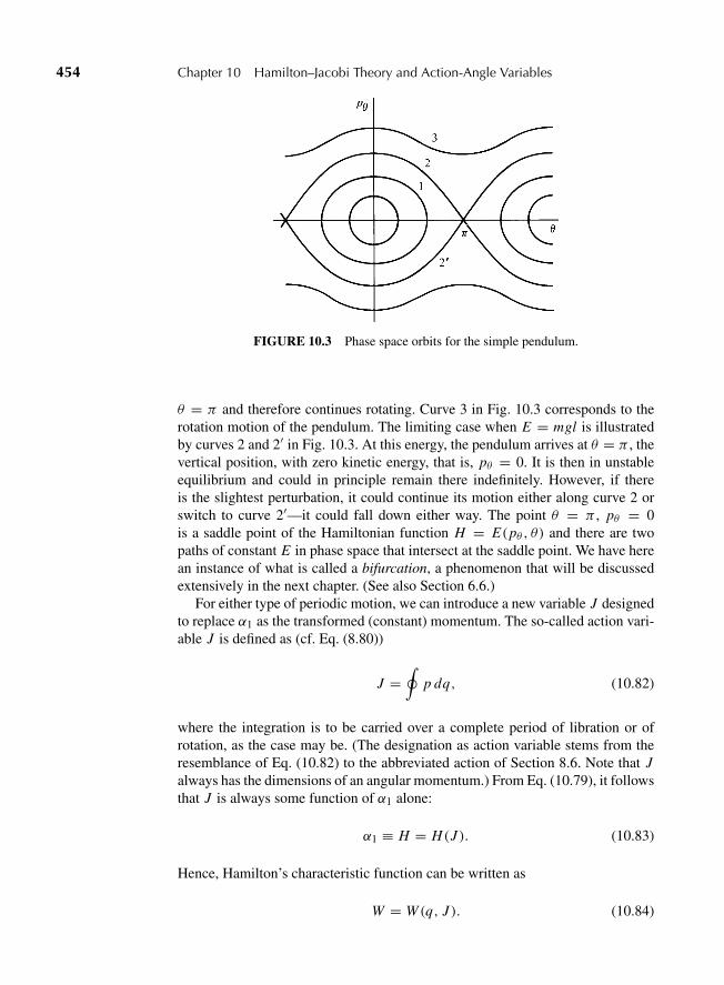
“M10 Goldstein ISBN C10” — 2011/2/15 — page 454 — #25
454 Chapter 10 Hamilton–Jacobi Theory and Action-Angle Variables
FIGURE 10.3 Phase space orbits for the simple pendulum.
θ = π and therefore continues rotating. Curve 3 in Fig. 10.3 corresponds to therotation motion of the pendulum. The limiting case when E = mgl is illustratedby curves 2 and 2′ in Fig. 10.3. At this energy, the pendulum arrives at θ = π , thevertical position, with zero kinetic energy, that is, pθ = 0. It is then in unstableequilibrium and could in principle remain there indefinitely. However, if thereis the slightest perturbation, it could continue its motion either along curve 2 orswitch to curve 2′—it could fall down either way. The point θ = π , pθ = 0is a saddle point of the Hamiltonian function H = E(pθ , θ) and there are twopaths of constant E in phase space that intersect at the saddle point. We have herean instance of what is called a bifurcation, a phenomenon that will be discussedextensively in the next chapter. (See also Section 6.6.)
For either type of periodic motion, we can introduce a new variable J designedto replace α1 as the transformed (constant) momentum. The so-called action vari-able J is defined as (cf. Eq. (8.80))
J =∮
p dq, (10.82)
where the integration is to be carried over a complete period of libration or ofrotation, as the case may be. (The designation as action variable stems from theresemblance of Eq. (10.82) to the abbreviated action of Section 8.6. Note that Jalways has the dimensions of an angular momentum.) From Eq. (10.79), it followsthat J is always some function of α1 alone:
α1 ≡ H = H(J ). (10.83)
Hence, Hamilton’s characteristic function can be written as
W = W (q, J ). (10.84)
“M10 Goldstein ISBN C10” — 2011/2/15 — page 455 — #26
10.6 Action-Angle Variables in Systems of One Degree of Freedom 455
The generalized coordinate conjugate to J , known as the angle variable w, isdefined by the transformation equation:
w = ∂W
∂ J. (10.85)
Correspondingly, the equation of motion for w is
w = ∂H(J )
∂ J= v(J ), (10.86)
where v is a constant function of J only. Equation (10.86) has the immediatesolution
w = vt + β, (10.87)
so that w is a linear function of time, exactly as in Eq. (10.47).So far the action-angle variables appear as no more than a particular set of the
general class of transformed coordinates to which the Hamilton–Jacobi equationleads. Equation (10.85) could be solved for q as a function of w and J , which,in combination with Eq. (10.87), would give the desired solution for q as a func-tion of time. But when employed in this fashion the variables have no signifi-cant advantage over any other set of coordinates generated by W . Their particularmerit rises rather from the physical interpretation that can be given to v. Considerthe change in w as q goes through a complete cycle of libration or rotation, asgiven by
�w =∮∂w
∂qdq. (10.88)
By Eq. (10.85), this can also be written
�w =∮
∂2W
∂q∂ Jdq. (10.89)
Because J is a constant, the derivative with respect to J can be taken outside theintegral sign:
�w = d
d J
∮∂W
∂qdq = d
d J
∮p dq = 1, (10.90)
where the last step follows from the definition for J , Eq. (10.82).Equation (10.90) states that w changes by unity as q goes through a complete
period. But from Eq. (10.87), it follows that if τ is the period for a complete cycleof q, then
�w = 1 = vτ.
“M10 Goldstein ISBN C10” — 2011/2/15 — page 456 — #27
456 Chapter 10 Hamilton–Jacobi Theory and Action-Angle Variables
Hence, the constant v can be identified as the reciprocal of the period,
v = 1
τ, (10.91)
and is therefore the frequency associated with the periodic motion of q. The useof action-angle variables thus provides a powerful technique for obtaining the fre-quency of periodic motion without finding a complete solution to the motion of thesystem. If it is known a priori that a system of one degree of freedom is periodicaccording to the definitions given above, then the frequency can be found onceH is determined as a function of J . The derivative of H with respect to J , byEq. (10.86), then directly gives the frequency v of the motion. The designation ofw as an angle variable becomes obvious from the identification of v in Eq. (10.87)as a frequency. Since J has the dimensions of an angular momentum, the coordi-nate w conjugate to it is an angle.*
As an illustration of the application of action-angle variables to find frequen-cies, let us again consider the familiar linear harmonic oscillator problem. FromEqs. (10.26) and the defining equation (10.82), the constant action variable J isgiven by
J =∮
p dq =∮ √
2mα − m2ω2q2 dq, (10.92)
where α is the constant total energy and ω2 = k/m. The substitution (10.25)
q =√
2α
mω2sin θ
reduces the integral to
J = 2α
ω
∫ 2π
0cos2 θ dθ, (10.93)
where the limits are such as to correspond to a complete cycle in q. This integratesto
J = 2πα
ω
or, solving for α,
α ≡ H = Jω
2π. (10.94)
*For some applications the action variable is defined in the literature of celestial mechanics as (2π)−1
times the value given in Eq. (10.82). By Eq. (10.90), the corresponding angle variable is 2π times ourdefinition and in place of v we have ω, the angular frequency. However, we shall stick throughout tothe familiar definitions used in physics, as given above.
“M10 Goldstein ISBN C10” — 2011/2/15 — page 457 — #28
10.7 Action-Angle Variables for Completely Separable Systems 457
The frequency of oscillation is therefore
∂H
∂ J= v = ω
2π= 1
2π
√k
m, (10.95)
which is the customary formula for the frequency of a linear harmonic oscillator.Although it is entirely unnecessary for obtaining the frequencies, it is neverthelessinstructive (and useful for future applications) to write the solutions, Eqs. (10.25)and (10.27), in terms of J and w. It will be recognized first that the combination(ωt + β) is by Eqs. (10.95) and (10.87) the same as 2πw, with the constantof integration suitably redefined. Hence, the solutions for q, Eq. (10.25), and p,Eq. (10.27), take on the form
q =√
J
πmωsin 2πw, (10.96)
p =√
m Jω
πcos 2πw. (10.97)
Note that Eqs. (10.96) and (10.97) can also be looked on as the transformationequations from the (w, J ) set of canonical variables to the (q, p) canonical set.
10.7 ACTION-ANGLE VARIABLES FOR COMPLETELYSEPARABLE SYSTEMS*
Action-angle variables can also be introduced for certain types of motion of sys-tems with many degrees of freedom, providing there exists one or more sets ofcoordinates in which the Hamilton–Jacobi equation is completely separable. Asbefore, only conservative systems will be considered, so that Hamilton’s charac-teristic function will be used. Complete separability means that the equations ofcanonical transformation have the form
pi = ∂Wi (qi ; α1, . . . , αn)
∂qi, (10.98)
which provides each pi as a function of the qi and the n integration constants α j :
pi = pi (qi ; α1, . . . , αn). (10.99)
Equation (10.99) is the counterpart of Eq. (10.79), which applied to systems ofone degree of freedom. It will be recognized that Eq. (10.99) here representsthe orbit equation of the projection of the system point on the (qi , pi ) plane inphase space. We can define action-angle variables for the system when the orbitequations for all of the (qi , pi ) pairs describe either closed orbits (libration, as inFig. 10.2(a)) or periodic functions of qi (rotation, as in Fig. 10.2(b)).
Note that this characterization of the motion does not mean that each qi andpi will necessarily be periodic functions of the time, that is, that they repeat their
*Unless otherwise stated, the summation convention will not be used in this section.
“M10 Goldstein ISBN C10” — 2011/2/15 — page 458 — #29
458 Chapter 10 Hamilton–Jacobi Theory and Action-Angle Variables
values at fixed time intervals. Even when each of the separated (qi , pi ) sets areindeed periodic in this sense, the overall system motion need not be periodic.Thus, in a three-dimensional harmonic oscillator the frequencies of motion alongthe three Cartesian axes may all be different. In such an example, it is clear thecomplete motion of the particle may not be periodic. If the separate frequenciesare not rational fractions of each other, the particle will not traverse a closedcurve in space but will describe an open “Lissajous figure.” Such motion willbe described as multiply periodic. It is the advantage of the action-angle variablesthat they lead to an evaluation of all the frequencies involved in multiply periodicmotion without requiring a complete solution of the motion.
In analogy to Eq. (10.82), the action variables Ji are defined in terms of lineintegrals over complete periods of the orbit in the (qi , pi ) plane:
Ji =∮
pi dqi . (10.100)
If one of the separation coordinates is cyclic, its conjugate momentum is constant.The corresponding orbit in the (qi , pi ) plane of phase space is then a horizontalstraight line, which would not appear to be in the nature of a periodic motion.Actually the motion can be considered as a limiting case of the rotation type ofperiodicity, in which qi may be assigned any arbitrary period. Since the coordinatein a rotation periodicity is invariably an angle, such a cyclic qi always has a naturalperiod of 2π . Accordingly, the integral in the definition of the action variablecorresponding to a cyclic angle coordinate is to be evaluated from 0 to 2π , andhence
Ji = 2πpi (10.101)
for all cyclic variables.By Eq. (10.98), Ji can also be written as
J =∮∂Wi (qi ; α1, . . . , αn)
∂qidqi . (10.102)
Since qi is here merely a variable of integration, each action variable Ji is afunction only of the n constants of integration appearing in the solution of theHamilton–Jacobi equation. Further, it follows from the independence of the sep-arate variable pairs (qi , pi ) that the Ji ’s form n independent functions of the αi ’sand hence are suitable for use as a set of new constant momenta. Expressing theαi ’s as functions of the action variables, the characteristic function W can be writ-ten in the form
W = W (q1, . . . , qn; J1, . . . , Jn) =∑
j
W j (q j ; J1, . . . , Jn),
while the Hamiltonian appears as a function of the Ji ’s only:
H = α1 = H(J1, . . . , Jn). (10.103)
“M10 Goldstein ISBN C10” — 2011/2/15 — page 459 — #30
10.7 Action-Angle Variables for Completely Separable Systems 459
As in the system of one degree of freedom, we can define conjugate anglevariables wi by the equations of transformation that here appear as
wi = ∂W
∂ Ji=
n∑j=1
∂W j (q j ; J1, . . . , Jn)
∂ Ji. (10.104)
Note in general wi could be a function of several or all of the qi ; that is, wi =wi (qi , . . . , qn; Ji , . . . , Jn). The wi ’s satisfy equations of motion given by
wi = ∂H(J1, . . . , Jn)
∂ Ji= vi (J1, . . . , Jn). (10.105)
Because the vi ’s are constants, functions of the action variables only, the anglevariables are all linear functions of time
wi = vi t + βi . (10.106)
Note that in general the separate wi ’s increase in time at different rates.The constants vi can be identified with the frequencies of the multiply peri-
odic motion, but the argument to demonstrate the relation is more subtle than forperiodic systems of one degree of freedom. The transformation equations to the(w, J ) set of variables implies that each q j (and p j ) is a function of the constantsJi and the variables wi . What we want to find is what sort of mathematical func-tion the q’s are of the w’s. To do this, we examine the change in a particular wi
when each of the variables q j is taken through an integral number, m j , of cyclesof libration or rotation. In carrying out this purely mathematical procedure, weare clearly not following the motion of the system in time. It is as if the flowof time were suspended and each of the q’s were moved, manually as it were,independently through a number of cycles of their motion. In effect, we are deal-ing with analogues of the virtual displacements of Chapter 1, and accordingly theinfinitesimal change in wi as the q j ’s are changed infinitesimally will be denotedby δwi and is given by
δwi =∑
j
∂wi
∂q jdq j =
∑ ∂2W
∂ Ji∂q jdq j ,
where use has been made of Eq. (10.104). The derivative with respect to qi van-ishes except for the W j constituent of W , so that by Eq. (10.98) δwi reduces to
δwi = ∂
∂ Ji
∑j
p j (q j , J ) dq j . (10.107)
Equation (10.107) represents δwi as the sum of independent contributionseach involving the q j motion. The total change in wi as a result of the specified

“M10 Goldstein ISBN C10” — 2011/2/15 — page 460 — #31
460 Chapter 10 Hamilton–Jacobi Theory and Action-Angle Variables
maneuver is therefore
�wi =∑
j
∂
∂ Ji
∮m j
p j (q j , J ) dq j . (10.108)
The differential operator with respect to Ji can be kept outside the integral signsbecause throughout the cyclic motion of qi all the J ’s are of course constant. Be-low each integral sign, the symbol m j indicates the integration is over m j cyclesof q j . But each of the integrals is, by the definition of the action variables, exactlym j J j . Since the J ’s are independent, it follows that
�wi = mi . (10.109)
Further, note that if any q j does not go through a complete number of cycles, thenin the integration over q j there will be a remainder of an integral over a fractionof a cycle and �wi will not have an integral value. If the sets of w’s and m’s aretreated as vectors w and m, respectively, Eq. (10.109) can be written as
�w = m. (10.109′)
Suppose, first, that the separable motions are all of the libration type so thateach q j , as well as p j , returns to its initial value on completion of a completecycle. The result described by Eq. (10.109′) could now be expressed somewhatas follows: h (the vector of q’s and p’s) is such a function of w that a change�h = 0 corresponds to a change �w = m, a vector of integer values. Since thenumber of cycles in the chosen motions of q j are arbitrary, m can be taken as zeroexcept for mi = 1, and all the components of h remain unchanged or return totheir original values. Hence, in the most general case the components of h mustbe periodic functions of each wi with period unity; that is, the q’s and p’s aremultiply periodic functions of the w’s with unit periods. Such a multiply periodicfunction can always be represented by a multiple Fourier expansion, which for qk ,say, would appear as
qk =∞∑
j1=−∞
∞∑j2=−∞
, . . . ,
∞∑jn=−∞
a(k)j1,..., jn·e2π i( j1wi+ j2w2+ j3w3+···+ jnwn), (libration)
(10.110)where the j’s are n integer indices running from −∞ to ∞. By treating the set ofj’s also as a vector in the same n-dimensional space with w, the expansion can bewritten more compactly as
qk =∑
j
a(k)j a2π ij·w, (libration). (10.110′)
If we similarly write Eq. (10.109′) as a vector equation,
w = vt + b, (10.106′)
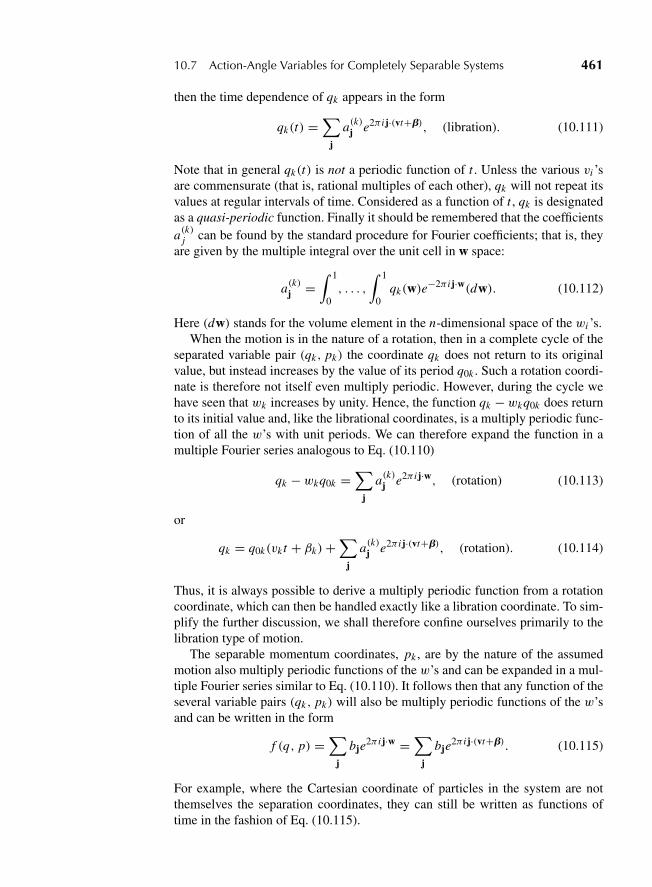
“M10 Goldstein ISBN C10” — 2011/2/15 — page 461 — #32
10.7 Action-Angle Variables for Completely Separable Systems 461
then the time dependence of qk appears in the form
qk(t) =∑
j
a(k)j e2π ij·(vt+b), (libration). (10.111)
Note that in general qk(t) is not a periodic function of t . Unless the various vi ’sare commensurate (that is, rational multiples of each other), qk will not repeat itsvalues at regular intervals of time. Considered as a function of t , qk is designatedas a quasi-periodic function. Finally it should be remembered that the coefficientsa(k)j can be found by the standard procedure for Fourier coefficients; that is, theyare given by the multiple integral over the unit cell in w space:
a(k)j =∫ 1
0, . . . ,
∫ 1
0qk(w)e−2π ij·w(dw). (10.112)
Here (dw) stands for the volume element in the n-dimensional space of the wi ’s.When the motion is in the nature of a rotation, then in a complete cycle of the
separated variable pair (qk, pk) the coordinate qk does not return to its originalvalue, but instead increases by the value of its period q0k . Such a rotation coordi-nate is therefore not itself even multiply periodic. However, during the cycle wehave seen that wk increases by unity. Hence, the function qk −wkq0k does returnto its initial value and, like the librational coordinates, is a multiply periodic func-tion of all the w’s with unit periods. We can therefore expand the function in amultiple Fourier series analogous to Eq. (10.110)
qk − wkq0k =∑
j
a(k)j e2π ij·w, (rotation) (10.113)
or
qk = q0k(vk t + βk)+∑
j
a(k)j e2π ij·(vt+b), (rotation). (10.114)
Thus, it is always possible to derive a multiply periodic function from a rotationcoordinate, which can then be handled exactly like a libration coordinate. To sim-plify the further discussion, we shall therefore confine ourselves primarily to thelibration type of motion.
The separable momentum coordinates, pk , are by the nature of the assumedmotion also multiply periodic functions of the w’s and can be expanded in a mul-tiple Fourier series similar to Eq. (10.110). It follows then that any function of theseveral variable pairs (qk, pk) will also be multiply periodic functions of the w’sand can be written in the form
f (q, p) =∑
j
bje2π ij·w =
∑j
bje2π ij·(vt+b). (10.115)
For example, where the Cartesian coordinate of particles in the system are notthemselves the separation coordinates, they can still be written as functions oftime in the fashion of Eq. (10.115).
“M10 Goldstein ISBN C10” — 2011/2/15 — page 462 — #33
462 Chapter 10 Hamilton–Jacobi Theory and Action-Angle Variables
While Eqs. (10.110) and (10.111) represent the most general type of motionconsistent with the assumed nature of the problem, not all systems will exhibitthis full generality. In particular, for most problems simple enough to be used asillustrations of the application of action-angle variables, Eq. (10.104) simplifies to
wi = ∂wi
∂ Ji(qi ; J1, . . . , Jn) (10.116)
and each separation coordinate qi is a function only of its corresponding wk .When this happens, qk is then a periodic function of wk (and therefore of time),and the multiple Fourier series reduces to a single Fourier series:
qk =∑
j
a(k)j e2π i jwk =∑
j
a(k)j e2π i j (vk t+βk ). (10.117)
In the language of Chapter 6, in such problems the qk’s are in effect thenormal coordinates of the system. However, even when the motion in the q’scan be so simplified, it frequently happens that functions of all the q’s, such asCartesian coordinates, remain multiply periodic functions of the w’s and must berepresented as in Eq. (10.115). If the various frequencies vk are incommensurate,then such functions are not periodic functions of time. The motion of a two-dimensional anisotropic harmonic oscillator provides a convenient and familiarexample of these considerations.
Suppose that in a particular set of Cartesian coordinates the Hamiltonian isgiven by
H = 1
2m[(p2
x + 4π2m2v2x x2)+ (p2
y + 4π2m2v2y y2)].
These Cartesian coordinates are therefore suitable separation variables, and eachwill exhibit simple harmonic motion with frequencies vx and vy , respectively.Thus, the solutions for x and y are particularly simple forms of the single Fourierexpansions of Eq. (10.117). Suppose now that the coordinates are rotated 45◦about the z axis; the components of the motion along the new x ′, y′ axes will be
x ′ = 1√2
[x0 cos 2π(vx t + βx )+ y0 cos 2π(vyt + βy)],
y′ = 1√2
[y0 cos 2π(vyt + βy)− x0 cos 2π(vx t + βx )]. (10.118)
If vx/vy is a rational number, these two expressions will be commensurate, corre-sponding to closed Lissajous figures of the type shown in Fig. 10.4. But if vx andvy are incommensurable, the Lissajous figure never exactly retraces its steps andEqs. (10.118) provide simple examples of multiply periodic series expansions ofthe form (10.117).
Even when qk is a multiply periodic function of all the w’s, we intuitively feelthere must be a special relationship between qk and its corresponding wk (and
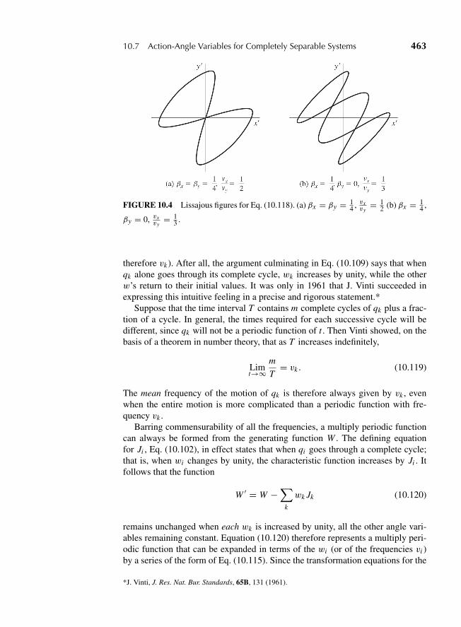
“M10 Goldstein ISBN C10” — 2011/2/15 — page 463 — #34
10.7 Action-Angle Variables for Completely Separable Systems 463
FIGURE 10.4 Lissajous figures for Eq. (10.118). (a) βx = βy = 14 , vxvy
= 12 (b) βx = 1
4 ,
βy = 0, vxvy
= 13 .
therefore vk). After all, the argument culminating in Eq. (10.109) says that whenqk alone goes through its complete cycle, wk increases by unity, while the otherw’s return to their initial values. It was only in 1961 that J. Vinti succeeded inexpressing this intuitive feeling in a precise and rigorous statement.*
Suppose that the time interval T contains m complete cycles of qk plus a frac-tion of a cycle. In general, the times required for each successive cycle will bedifferent, since qk will not be a periodic function of t . Then Vinti showed, on thebasis of a theorem in number theory, that as T increases indefinitely,
Limt→∞
m
T= vk . (10.119)
The mean frequency of the motion of qk is therefore always given by vk , evenwhen the entire motion is more complicated than a periodic function with fre-quency vk .
Barring commensurability of all the frequencies, a multiply periodic functioncan always be formed from the generating function W . The defining equationfor Ji , Eq. (10.102), in effect states that when qi goes through a complete cycle;that is, when wi changes by unity, the characteristic function increases by Ji . Itfollows that the function
W ′ = W −∑
k
wk Jk (10.120)
remains unchanged when each wk is increased by unity, all the other angle vari-ables remaining constant. Equation (10.120) therefore represents a multiply peri-odic function that can be expanded in terms of the wi (or of the frequencies vi )by a series of the form of Eq. (10.115). Since the transformation equations for the
*J. Vinti, J. Res. Nat. Bur. Standards, 65B, 131 (1961).
“M10 Goldstein ISBN C10” — 2011/2/15 — page 464 — #35
464 Chapter 10 Hamilton–Jacobi Theory and Action-Angle Variables
angle variables are
wk = ∂W
∂ Jk,
it will be recognized that Eq. (10.120) defines a Legendre transformation fromthe q, J basis to the q, w basis. Indeed, comparison with Eq. (9.15) in combina-tion with Eq. (9.12) shows that if W (q, J ) is a generating function of the formF2(q, P), then W ′(q, w) is the corresponding generating function of the typeF1(q, Q), transforming in both cases from the (q, p) variables to the (w, J ) vari-ables. While W ′ thus generates the same transformation as W , it is of course nota solution of the Hamilton-Jacobi equation.
It has been emphasized that the system configuration is multiply periodic onlyif the frequencies vi are not rational fractions of each other. Otherwise, the con-figuration repeats after a sufficiently long time and would therefore be simplyperiodic. The formal condition for the commensurability of two frequencies vi
and v j is that they satisfy the relation jivi = j jv j (no sum) where ji and j j arenonzero positive integers. For complete commensurability, all pairs of frequenciesmust satisfy relations of the form
jivi = jkvk, (no sum) (10.121)
where the ji and jk are nonzero positive integers.When we can express any vi as a rational fraction of any of the other frequen-
cies, the system is said to be completely commensurate. If only m + 1 of the nfrequencies satisfy Eq. (10.121), the system is said to be m-fold commensurate.For example, consider the set of seven frequencies v1 = 3 MHz, v2 = 5 MHz,v3 = 7 MHz, v4 = 2
√2 MHz, v5 = 3
√2 MHz, v6 = √
3 MHz, v7 = √7 MHz.
The first three v1, v2, and v3 are triply commensurate, the next two v4 and v5 aredoubly commensurate.
There is an interesting connection between commensurability and the coordi-nates in which the Hamilton–Jacobi equation is separable. It can be shown that thepath of the system point for a noncommensurate system completely fills a limitedregion of both configuration and phase space. This can be seen in the Lissajousfigures of incommensurate frequencies.
Suppose the problem is such that the motion in any one of the separation coor-dinates is simply periodic and has therefore been shown to be independent of themotion of the other coordinates. Hence, the path of the system point as a wholemust be limited by the surfaces of constant qi and pi that mark the bounds of theoscillatory motion of the separation variables. (The argument is easily extendedto rotation by limiting all angles to the region 0 to 2π .) These surfaces there-fore define the volume in space that is densely filled by the system point orbit.It follows that the separation of variables in noncommensurate systems must beunique; the Hamilton–Jacobi equation cannot be separated in two different coor-dinate systems (aside from trivial variations such as change of scale). The possi-bility of separating the motion in more than one set of coordinates thus normallyprovides evidence that the system is commensurate.

“M10 Goldstein ISBN C10” — 2011/2/15 — page 465 — #36
10.7 Action-Angle Variables for Completely Separable Systems 465
The simplest example of being commensurate is degeneracy which occurswhen two or more of the frequencies are equal. If two of the force constantsin a three-dimensional harmonic oscillator are equal, then the corresponding fre-quencies are identical and the system is singly degenerate. In an isotropic linearoscillator, the force constants are the same along all directions, all frequencies areequal, and the system is completely degenerate.
Whenever this simple degeneracy is present, the fundamental frequencies areno longer independent, and the periodic motion of the system can be describedby less than the full complement of n frequencies. Indeed, the m conditions ofdegeneracy can be used to reduce the number of frequencies to n − m + 1. Thereduction of the frequencies may be most elegantly performed by means of a pointtransformation of the action-angle variables. The m degeneracy conditions may bewritten (where jki are positive or negative integers)
n∑i=1
jkivi = 0, k = 1, . . . ,m. (10.122)
Consider now a point transformation from (w, J ) to (w′, J ′) defined by thegenerating function (cf. Eq. (9.26) where the summation convention is used):
F2 =m∑
k=1
n∑i=1
J ′k jkiwi +
n∑k=m+1
J ′kwk . (10.123)
The transformed coordinates are
w′k =
n∑i=1
jki , k = 1, . . . ,m,
= wk, k = m + 1, . . . , n. (10.124)
Correspondingly, the new frequencies are
v′k = w′k =
n∑i=1
jkivi = 0 k = 1, . . . ,m,
= vk k = m + 1, . . . , n. (10.125)
Thus in the transformed coordinates, m of the frequencies are zero, and we are leftwith a set of n −m independent frequencies plus the zero frequency. It is obviousthat the new w′
k may also be termed as angle variables in the sense that the systemconfiguration is multiply periodic in the w′
k coordinates with the fundamentalperiod unity. The corresponding constant action variables are given as the solutionof the n equations of transformation
Ji =m∑
k=1
J ′k jki +
n∑k=m+1
J ′kδki . (10.126)
“M10 Goldstein ISBN C10” — 2011/2/15 — page 466 — #37
466 Chapter 10 Hamilton–Jacobi Theory and Action-Angle Variables
The zero frequencies correspond to constant factors in the Fourier expansion.These are of course also present in the original Fourier series in terms of thev’s, Eq. (10.110), occurring whenever the indices ji are such that degeneracyconditions are satisfied. Since
v′i =∂H
∂ J ′i,
the Hamiltonian must be independent of the action variables J ′i whose corre-
sponding frequencies vanish. In a completely degenerate system, the Hamiltoniancan therefore be made to depend upon only one of the action variables.
Note that Hamilton’s characteristic function W also serves as the generatingfunction for the transformation from the (q, p) set to the (w′, J ′) set. Since the J ′quantities are n independent constants, the original constants of integration maybe expressed in terms of the J ′ set, and W given as W (q, J ′). In this form, it is agenerating function to a new set of canonical variables for which the J ′ quantitiesare the canonical momenta. But by virtue of the point transformation generatedby the F2 of Eq. (10.123), we know that w′ is conjugate to J ′. Hence, it followsthat the new coordinates generated by W (q, J ′)must be the angle variable w′ set,with equations of transformation given by
w′i =
∂W
∂ J ′i. (10.127)
(For a more formal proof of Eq. (10.127) based on the algebraic structure ofEq. (10.123), see Derivation 3.)
The problem of the bound motion of a particle in an inverse-square law centralforce illustrates many of the phenomena involved in degeneracy. A discussion ofthis problem also affords an opportunity to show how the action-angle technique isapplied to specific systems, and to indicate the connections with Bohr’s quantummechanics and with celestial mechanics. Accordingly, the next section is devotedto a detailed treatment of the Kepler problem in terms of action-angle variables.
10.8 THE KEPLER PROBLEM IN ACTION-ANGLE VARIABLES*
To exhibit all of the properties of the solution, we shall examine the motion inthree dimensional space, rather than make use of our a priori knowledge that theorbit lies in a plane. In terms of spherical polar coordinates, the Kepler problembecomes a special case of the general treatment given above in Section 10.5 forcentral force motion in space. Equations (10.70) through (10.77) can be takenover here immediately, replacing V (r) wherever it occurs by its specific form
V (r) = −k
r. (10.128)
*The summation convention will be resumed from here on.
“M10 Goldstein ISBN C10” — 2011/2/15 — page 467 — #38
10.8 The Kepler Problem in Action-Angle Variables 467
Since the potential V (r) depends only upon one of the three coordinates, it fol-lows that the Hamilton–Jacobi equation is completely separable in spherical polarcoordinates. We shall confine our discussion to the bound case, that is, E < 0.Hence, the motion in each of the coordinates will be periodic—libration in r andθ , and rotation in φ. The conditions for the application of action-angle variablesare thus satisfied, and we can proceed to construct the action variables on the basisof the defining equation (10.102). From Eq. (10.72), it follows that
Jφ =∮∂W
∂φdφ =
∮αφ dφ. (10.129a)
Similarly, on the basis of Eq. (10.74), Jθ is given by
Jθ =∮∂W
∂θdθ =
∮ √α2θ −
α2φ
sin2 θdθ. (10.129b)
Finally the integral for Jr from Eq. (10.75), is
Jr =∮∂W
∂rdr =
∮ √2m E + 2mk
r− α2
θ
r2dr. (10.129c)
The first integral is trivial; φ goes through 2π radians in a complete revolutionand therefore
Jφ = 2παφ = 2πpφ. (10.130)
This result could have been predicted beforehand, for φ is a cyclic coordinatein H , and Eq. (10.130) is merely a special case of Eq. (10.101) for the actionvariables corresponding to cyclic coordinates. Integration of Eq. (10.129b) canbe performed in various ways; a procedure involving only elementary rules ofintegration will be sketched here. If the polar angle of the total angular momentumvector is denoted by i , so that
cos i = αφ
αθ, (10.131)
then Eq. (10.129b) can also be written as
Jθ = αθ
∮ √1 − cos2 i csc2 θ dθ. (10.132)
The complete circuital path of integration is for θ going from a limit −θ0 to +θ0and back again, where sin θ0 = cos i , or θ0 = (π/2) − i . Hence, the circuitalintegral can be written as 4 times the integral over from 0 to θ0, or after somemanipulation,
Jθ = 4αθ
∫ θ0
0csc θ
√sin2 i − cos2 θ dθ.
“M10 Goldstein ISBN C10” — 2011/2/15 — page 468 — #39
468 Chapter 10 Hamilton–Jacobi Theory and Action-Angle Variables
The substitution
cos θ = sin i sinψ
transforms the integral to
Jθ = 4αθ sin2 i∫ π/2
0
cos2 ψ dψ
1 − sin2 i sin2 ψ. (10.133)
Finally, with the substitution
u = tanψ,
the integral becomes
Jθ = 4αθ sin2 i∫ ∞
0
du
(1 + u2)(1 + u2 cos2 i)
= 4αθ
∫ ∞
0du
(1
1 + u2− cos2 i
1 + u2 cos2 i
). (10.134)
This last form involves only well-known integrals, and the final result* is
Jθ = 2παθ (1 − cos i) = 2π(αθ − αφ). (10.135)
The last integral (Eq. (10.129c)), for Jr , can now be written as
Jr =∮ √
2m E + 2mk
r− (Jθ + Jφ)2
4π2r2dr. (10.136)
After performing the integration, this equation can be solved for the energy E ≡H in terms of the three action variables Jφ , Jθ , Jr . Note that Jφ and Jθ can occurin E only in the combination Jθ + Jφ , and hence the corresponding frequenciesvφ and vθ must be equal, indicating a degeneracy. This result has not involved theinverse-square law nature of the central force; any motion produced by a centralforce is at least singly degenerate. The degeneracy is of course a consequenceof the fact that the motion is confined to a plane normal to the constant angularmomentum vector L. Motion in this plane implies that θ and φ are related toeach other such that as φ goes through a complete 2π period, θ varies through acomplete cycle between the limits (π/2) ± i . Hence, the frequencies in θ and φare necessarily equal.
*In evaluating the integral of the second term in the final integrand of Eq. (10.134), it has been assumedthat cos i is positive. This is always possible, since there is no preferred direction for the z axis in theproblem and it may be chosen at will. If cos i were negative, the sign of αφ in Eq. (10.135) would bepositive. For changes in the subsequent formulas, see Exercise 23.
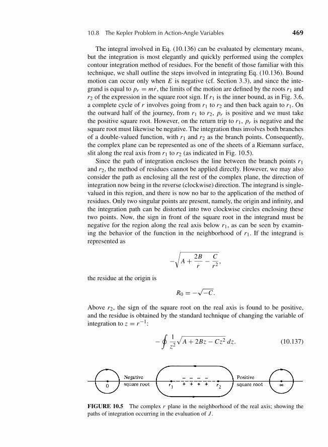
“M10 Goldstein ISBN C10” — 2011/2/15 — page 469 — #40
10.8 The Kepler Problem in Action-Angle Variables 469
The integral involved in Eq. (10.136) can be evaluated by elementary means,but the integration is most elegantly and quickly performed using the complexcontour integration method of residues. For the benefit of those familiar with thistechnique, we shall outline the steps involved in integrating Eq. (10.136). Boundmotion can occur only when E is negative (cf. Section 3.3), and since the inte-grand is equal to pr = mr , the limits of the motion are defined by the roots r1 andr2 of the expression in the square root sign. If r1 is the inner bound, as in Fig. 3.6,a complete cycle of r involves going from r1 to r2 and then back again to r1. Onthe outward half of the journey, from r1 to r2, pr is positive and we must takethe positive square root. However, on the return trip to r1, pr is negative and thesquare root must likewise be negative. The integration thus involves both branchesof a double-valued function, with r1 and r2 as the branch points. Consequently,the complex plane can be represented as one of the sheets of a Riemann surface,slit along the real axis from r1 to r2 (as indicated in Fig. 10.5).
Since the path of integration encloses the line between the branch points r1and r2, the method of residues cannot be applied directly. However, we may alsoconsider the path as enclosing all the rest of the complex plane, the direction ofintegration now being in the reverse (clockwise) direction. The integrand is single-valued in this region, and there is now no bar to the application of the method ofresidues. Only two singular points are present, namely, the origin and infinity, andthe integration path can be distorted into two clockwise circles enclosing thesetwo points. Now, the sign in front of the square root in the integrand must benegative for the region along the real axis below r1, as can be seen by examin-ing the behavior of the function in the neighborhood of r1. If the integrand isrepresented as
−√
A + 2B
r− C
r2,
the residue at the origin is
R0 = −√−C .
Above r2, the sign of the square root on the real axis is found to be positive,and the residue is obtained by the standard technique of changing the variable ofintegration to z = r−1:
−∮
1
z2
√A + 2Bz − Cz2 dz. (10.137)
FIGURE 10.5 The complex r plane in the neighborhood of the real axis; showing thepaths of integration occurring in the evaluation of J .
“M10 Goldstein ISBN C10” — 2011/2/15 — page 470 — #41
470 Chapter 10 Hamilton–Jacobi Theory and Action-Angle Variables
Expansion about z = 0 now furnishes the residue
R∞ = − B√A.
The total integral is −2π i times the sum of the residues:
Jr = 2π i
(√−C + B√A
), (10.138)
or, upon substituting the coefficients A, B, and C :
Jr = −(Jθ + Jφ)+ πk
√2m
−E. (10.139)
Equation (10.139) supplies the functional dependence of H upon the actionvariables; for solving for E , we have
H ≡ E = − 2π2mk2
(Jr + Jθ + Jφ)2. (10.140)
Note that, as predicted, Jθ and Jφ occur only in the combination Jθ + Jφ . Morethan that, all three of the action variables appear only in the form Jr + Jθ +Jφ . Hence, all of the frequencies are equal; the motion is completely degenerate.This result could also have been predicted beforehand, for we know that withan inverse-square law of force the orbit is closed for negative energies. With aclosed orbit, the motion is simply periodic and therefore, in this case, completelydegenerate. If the central force contained an r−3 term, such as is provided by first-order relativistic corrections, then the orbit is no longer closed but is in the formof a precessing ellipse. One of the degeneracies will be removed in this case, butthe motion is still singly degenerate, since vθ = vφ for all central forces. The onefrequency for the motion here is given by
v = ∂H
∂ Jr= ∂H
∂ Jθ= ∂H
∂ Jφ= 4π2mk2
(Jr + Jθ + Jφ)3. (10.141)
If we evaluate the sum of the J ’s in terms of the energy from Eq. (10.140) theperiod of the orbit is
τ = πk
√m
−2E3. (10.142)
This formula for the period agrees with Kepler’s third law, Eq. (3.71), if it isremembered that the semimajor axis a is equal to −k/2E .
The degenerate frequencies may be eliminated by canonical transformationto a new set of action-angle variables, following the procedure outlined in theprevious section. Expressing the degeneracy conditions as
vφ − vθ = 0, vθ − vr = 0,
“M10 Goldstein ISBN C10” — 2011/2/15 — page 471 — #42
10.8 The Kepler Problem in Action-Angle Variables 471
the appropriate generating function is
F = (wφ − wθ)J1 + (wθ − wr )J2 + wr J3. (10.143)
The new angle variables are
w1 = wφ − wθ,w2 = wθ − wr ,
w3 = wr , (10.144)
and, as planned, two of the new frequencies, v1 and v2, are zero. We can obtainthe new action variables from the transformation equations
Jφ = J1,
Jθ = J2 − J1,
Jr = J3 − J2,
which yields the relations
J1 = Jφ,
J2 = Jφ + Jθ , (10.145)
J3 = Jφ + Jθ + Jr .
In terms of these transformed variables the Hamiltonian appears as
H = −2π2mk2
J 23
, (10.146)
a form involving only that action variable for which the corresponding frequencyis different from zero.
If we are willing to use, from the start, our a priori knowledge that the motionfor the bound Kepler problem is a particular closed orbit in a plane, then the inte-grals for Jθ and Jr can be evaluated very quickly and simply. For the Jθ integral,we can apply the following procedure. It will be recalled that when the definingequations for the generalized coordinates do not involve time explicitly, then (cf.Eq. (8.20) and the material following (8.20))
pi qi = 2L2qi qi = 2T .
Knowing that the motion is confined to a plane, we can express the kinetic energyT either in spherical polar coordinates or in the plane polar coordinates (r, ψ). Itfollows, then, that
2T = pr r + pθ θ + pφφ = pr r + pψ, (10.147)
“M10 Goldstein ISBN C10” — 2011/2/15 — page 472 — #43
472 Chapter 10 Hamilton–Jacobi Theory and Action-Angle Variables
where p (≡ l) is the magnitude of the total angular momentum. Hence, the defi-nition for Jθ can also be written as
Jθ ≡∮
pθ dθ =∮
p dψ −∮
pφ dφ. (10.148)
Because the frequencies for θ and φ are equal, both φ and ψ vary by 2π as θ goesthrough a complete cycle of libration, and the integrals defining Jθ reduce to
Jθ = 2π(p − pφ) = 2π(αθ − αφ),
in agreement with Eq. (10.135).The integral for Jr , Eq. (10.136), was evaluated in order to obtain H ≡ E in
terms of the three action variables. If we use the fact that the closed elliptical orbitin the bound Kepler problem is such that the frequency for r is the same as thatfor θ and φ, then the functional dependence of H on J can also be obtained fromEq. (10.147). In effect then we are evaluating Jr in a different way. The virialtheorem for the bound orbits in the Kepler problem says that (cf. Eq. (3.30))
V = −2T ,
where the bar denotes an average over a single complete period of the motion. Itfollows that
H ≡ E = T + V = −T . (10.149)
Integrating Eq. (10.147) with respect to time over a complete period of motionwe have
2T
v3= Jr + Jθ + Jφ = J3, (10.150)
where v3 is the frequency of the motion, that is, the reciprocal of the period.Combining Eqs. (10.149) and (10.150) leads to the relation
− 2
J3= v3
H= 1
H
d H
d J3, (10.151)
where use has been made of Eq. (10.105). Equation (10.151) is in effect a differ-ential equation for the functional behavior of H on J3. Integration of the equationimmediately leads to the solution
H = D
J 23
, (10.152)
where D is a constant that cannot involve any of the J ’s, and must thereforedepend only upon m and k. Hence, we can evaluate D by considering the ele-mentary case of a circular orbit, of radius r0, for which Jr = 0 and J3 = 2πp.
“M10 Goldstein ISBN C10” — 2011/2/15 — page 473 — #44
10.8 The Kepler Problem in Action-Angle Variables 473
The total energy is here
H = − k
2r0(10.153)
(as can most immediately been seen from the virial theorem). Further, the condi-tion for circularity, Eq. (3.40), can be written for the inverse-square force law as
k
r20
= p2
mr30
= J3
4π2mr30
. (10.154)
Eliminating r0 between Eqs. (10.153) and (10.154) leads to
H = −2π2mk2
J 23
. (10.155)
This result has been derived only for circular orbits. But Eq. (10.152) says it mustalso be correct for all bound orbits of the Kepler problem, and indeed it is identicalwith Eq. (10.146). Thus, if the existence of a single period for all coordinates istaken as known beforehand, it is possible to obtain H(J )without direct evaluationof the circuital integrals.
In any problem with three degrees of freedom, there must of course be sixconstants of motion. It has previously been pointed out that in the Kepler problemfive of these are algebraic functions of the coordinates and momenta and describethe nature of the orbit in space, and only the last refers to the position of theparticle in the orbit at a given time (cf. Sections 3.7 to 3.9). It is easy to see thatfive parameters are needed to completely specify, say, the elliptical orbit of thebound Kepler problem in space. Since the motion is in a plane, two constants areneeded to describe the orientation of that plane in space. One constant is requiredto give the scale of the ellipse, for example, the semimajor axis a, and the otherthe shape of the ellipse, say, through the eccentricity e. Finally, the fifth parametermust specify the orientation of the ellipse relative to some arbitrary direction inthe orbital plane.
The classical astronomical elements of the orbit provide the orbital parametersalmost directly in the form given above. Two of the angles appearing in theseelements have unfamiliar but time-honored names. Their definitions, and func-tions as orbital parameters, can best be seen from a diagram, such as is given inFig. 10.6. Here xyz defines the chosen set of axes fixed in space, and the unitvector n characterizes the normal to the orbital plane. The intersection betweenthe xy plane and the orbital plane is called the line of nodes. There are two pointson the line of nodes at which the elliptical orbit intersects the xy plane; the pointat which the particle enters from below into the upper hemisphere (or goes fromthe “southern” to the “northern” hemispheres) is known as the ascending node. InFig. 10.6, the portion of the orbit in the southern hemisphere is shown, for clarity,as a dashed line. The dot-dashed line ON is a portion of the line of nodes contain-ing the ascending node. We can measure the direction of ON in the xy plane bythe angle xON, which is customarily denoted by�, and is known as the longitude
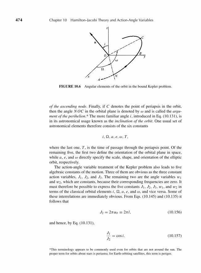
“M10 Goldstein ISBN C10” — 2011/2/15 — page 474 — #45
474 Chapter 10 Hamilton–Jacobi Theory and Action-Angle Variables
FIGURE 10.6 Angular elements of the orbit in the bound Kepler problem.
of the ascending node. Finally, if C denotes the point of periapsis in the orbit,then the angle N OC in the orbital plane is denoted by ω and is called the argu-ment of the perihelion.* The more familiar angle i , introduced in Eq. (10.131), isin its astronomical usage known as the inclination of the orbit. One usual set ofastronomical elements therefore consists of the six constants
i,�, a, e, ω, T,
where the last one, T , is the time of passage through the periapsis point. Of theremaining five, the first two define the orientation of the orbital plane in space,while a, e, and ω directly specify the scale, shape, and orientation of the ellipticorbit, respectively.
The action-angle variable treatment of the Kepler problem also leads to fivealgebraic constants of the motion. Three of them are obvious as the three constantaction variables, J1, J2, and J3. The remaining two are the angle variables w1and w2, which are constants, because their corresponding frequencies are zero. Itmust therefore be possible to express the five constants J1, J2, J3, w1, and w2 interms of the classical orbital elements i , �, a, e, and ω, and vice versa. Some ofthese interrelations are immediately obvious. From Eqs. (10.145) and (10.135) itfollows that
J2 = 2παθ ≡ 2πl, (10.156)
and hence, by Eq. (10.131),
J1
J2= cos i. (10.157)
*This terminology appears to be commonly used even for orbits that are not around the sun. Theproper term for orbits about stars is periastra; for Earth-orbiting satellites, this term is perigee.
“M10 Goldstein ISBN C10” — 2011/2/15 — page 475 — #46
10.8 The Kepler Problem in Action-Angle Variables 475
As is well known, the semimajor axis a is a function only of the total energy E(cf. Eq. (3.61)) and therefore, by Eq. (10.146), a is given directly in terms of J3:
a = − k
2E= J 2
3
4π2mk. (10.158)
In terms of J2, Eq. (3.62) for the eccentricities can be written as
e =√
1 − J 22
4π2mka,
or
e =√
1 −(
J2
J3
)2
. (10.159)
It remains only to relate the angle variables w1 and w2 to the classic orbitalelements. Obviously, they must involve � and ω. In fact, it can be shown that forsuitable choice of additive constants of integration they are indeed proportional to� and ω, respectively. This will be demonstrated for w1; the identification of w2will be left as an exercise.
The equation of transformation defining w1 is, by Eq. (10.127),
w1 = ∂W
∂ J1.
It can be seen from the separated form of W , Eq. (10.71), that W can be writtenas the sum of indefinite integrals:
W =∫
pφ dφ +∫
pθ dθ +∫
pr dr. (10.160)
As we have seen from the discussion on Jr , the radial momentum pr does notinvolve J1, but only J3 (through E) and the combination Jθ + Jφ = J2. Only thefirst two integrals are therefore involved in the derivative with respect to J1. ByEq. (10.130),
pφ = αφ = J1
2π, (10.161)
and by Eq. (10.74), with the help of Eqs. (10.156) and (10.161),
pθ = ±√α2θ −
α2φ
sin2 θ= ± 1
2π
√J 2
2 − J 21
sin2 θ. (10.162)
It turns out that in order to relate w1 to the ascending node, it is necessary tochoose the negative sign of the square root.* The angular variable w1 is therefore
*Note that when the particle passes through the ascending node (cf. Fig. 10.6) θ is decreasing andthe corresponding momentum is negative. In calculating Jθ , it was not necessary to worry about thechoice of sign because in going through a complete cycle both signs are encountered.
“M10 Goldstein ISBN C10” — 2011/2/15 — page 476 — #47
476 Chapter 10 Hamilton–Jacobi Theory and Action-Angle Variables
determined by
w1 = φ
2π+ J1
2π
∫dθ
sin2 θ
√J 2
2 − J 21 csc2 θ
,
or
2πw1 = φ + cos i∫
dθ
sin2 θ√
1 − cos2 i csc2 θ
= φ +∫
cot i csc2 θ dθ√1 − cot2 i cot2 θ
.
By a change of variable to u, defined through
sin u = cot i cot θ, (10.163)
the integration can be performed trivially, and the expression for w1 reduces to
2πw1 = φ − u. (10.164)
The angle coordinate φ is the azimuthal angle of the projection on the xy planemeasured relative to the x axis. Clearly, from Eq. (10.163) u is a function of thepolar angle θ of the particle. But what is its geometrical significance? We cansee what u is by reference to Napier’s rules* as applied to the spherical triangledefined by the line of nodes, the radius vector, and the projection of the radiusvector on the xy plane. However, it may be more satisfying to indulge in a littletrigonometric manipulation and derive the relation ab initio. In Fig. 10.7, the lineON is the line of nodes, O R is the line of the radius vector at some time, and thedotted line O P is the projection of the radius vector on the xy plane. The anglethat O P makes with the x axis is the azimuth angle φ. We contend that u is theangle O P makes with the line of nodes. To prove this, imagine a plane normalboth to the xy plane and to the line of nodes, which intersects the radius vectorat unit distance O B from the origin O . The points of intersection A, B, and C ofthis plane, with the three lines from the origin, define with the origin four righttriangles. Since O B has unit length, it follows that BC = cos θ and thereforeAC = cos θ cot i . On the other hand, OC = sin θ and therefore it is also true thatAC = sin θ sin u. Hence, sin u = cot i cot θ , which is identical with Eq. (10.163)and proves the stipulated identification of the angle u. Figure 10.7 shows clearlythat the difference between φ and u must be �, so that
2πw1 = �. (10.165)
*For an explanation of Napier’s rules for spherical triangles, see handbooks such as the Handbook ofMathematical Tables (Chemical Rubber Publishing Co.) or Handbook of Applied Mathematics (VanNostrand-Reinhold).
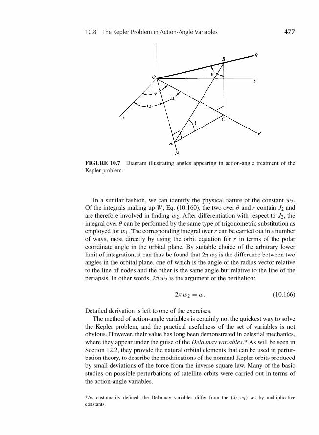
“M10 Goldstein ISBN C10” — 2011/2/15 — page 477 — #48
10.8 The Kepler Problem in Action-Angle Variables 477
FIGURE 10.7 Diagram illustrating angles appearing in action-angle treatment of theKepler problem.
In a similar fashion, we can identify the physical nature of the constant w2.Of the integrals making up W , Eq. (10.160), the two over θ and r contain J2 andare therefore involved in finding w2. After differentiation with respect to J2, theintegral over θ can be performed by the same type of trigonometric substitution asemployed forw1. The corresponding integral over r can be carried out in a numberof ways, most directly by using the orbit equation for r in terms of the polarcoordinate angle in the orbital plane. By suitable choice of the arbitrary lowerlimit of integration, it can thus be found that 2πw2 is the difference between twoangles in the orbital plane, one of which is the angle of the radius vector relativeto the line of nodes and the other is the same angle but relative to the line of theperiapsis. In other words, 2πw2 is the argument of the perihelion:
2πw2 = ω. (10.166)
Detailed derivation is left to one of the exercises.The method of action-angle variables is certainly not the quickest way to solve
the Kepler problem, and the practical usefulness of the set of variables is notobvious. However, their value has long been demonstrated in celestial mechanics,where they appear under the guise of the Delaunay variables.* As will be seen inSection 12.2, they provide the natural orbital elements that can be used in pertur-bation theory, to describe the modifications of the nominal Kepler orbits producedby small deviations of the force from the inverse-square law. Many of the basicstudies on possible perturbations of satellite orbits were carried out in terms ofthe action-angle variables.
*As customarily defined, the Delaunay variables differ from the (Ji , wi ) set by multiplicativeconstants.
“M10 Goldstein ISBN C10” — 2011/2/15 — page 478 — #49
478 Chapter 10 Hamilton–Jacobi Theory and Action-Angle Variables
DERIVATIONS
1. For a conservative system show that by solving an appropriate partial differentialequation we can construct a canonical transformation such that the new Hamiltonianis a function of the new coordinates only. (Do not use the exchange transformation,F1.) Show how a formal solution to the motion of the system is given in terms of thenew coordinates and momenta.
2. In the text, the Hamilton–Jacobi equation for S was obtained by seeking a con-tact transformation from the canonical coordinates (q, p) to the constants (α, β).Conversely, if S(qi , αi , t) is any complete solution of the Hamilton–Jacobi equa-tion (10.3), show that the set of variables (Qi , pi ) defined by Eqs. (10.7) and (10.8)are canonical variables, that is, that they satisfy Hamilton’s equations.
3. In the action-angle formalism, the arguments of Hamilton’s characteristic functionare the original coordinates qk and the action variables Jk . In the case of degener-acy, a subsequent canonical transformation is made to new variables (w′
i , J ′i ) from(wk , Jk), in order to replace the degeneracies by zero frequencies. By consideringeach Jk a function of the J ′i quantities as defined by Eq. (10.126), show that it remainstrue that
∂W
∂ J ′i= w′
i .
4. The so-called Poincare elements of the Kepler orbits can be written as
w1 + w2 + w3, Jφ,
Jr
πcos 2π(w2 + w1),
Jr
πsin 2π(w2 + w1),
Jθπ
cos 2πw1,Jθπ
sin 2πw1.
Show that they form a canonical set of coordinates, with the new coordinates formingthe left-hand column, their conjugate momenta being given on the right-hand side.
EXERCISES
5. Show that the function
S = mω
2(q2 + α2) cotωt − mωqα cscωt
is a solution of the Hamilton–Jacobi for Hamilton’s principal function for the linearharmonic oscillator with
H = 1
2m(p2 + m2ω2q2).
Show that this function generates a correct solution to the motion of the harmonicoscillator.
“M10 Goldstein ISBN C10” — 2011/2/15 — page 479 — #50
Exercises 479
6. A charged particle is constrained to move in a plane under the influence of a centralforce potential (nonelectromagnetic) V = 1
2 kr2, and a constant magnetic field Bperpendicular to the plane, so that
A = 12 B3 r
Set up the Hamilton–Jacobi equation for Hamilton’s characteristic function in planepolar coordinates. Separate the equation and reduce it to quadratures. Discuss themotion if the canonical momentum pθ is zero at time t = 0.
7. (a) A single particle moves in space under a conservative potential. Set up theHamilton–Jacobi equation in ellipsoidal coordinates u, v, φ defined in terms ofthe usual cylindrical coordinates r , z, φ by the equations
r = a sinh v sin u, z = a cosh v cos u.
For what forms of V (u, v, φ) is the equation separable?
(b) Use the results of part (a) to reduce to quadratures the problem of a point particleof mass m moving in the gravitational field of two unequal mass points fixed onthe z axis a distance 2a apart.
8. Suppose the potential in a problem of one degree of freedom is linearly dependentupon time, such that the Hamiltonian has the form
H = p2
2m− m Atx,
where A is a constant. Solve the dynamical problem by means of Hamilton’s principalfunction, under the initial conditions t = 0, x = 0, p = mv0.
9. Set up the plane Kepler problem in terms of the generalized coordinates
u = r + x,
v = r − x .
Obtain the Hamilton–Jacobi equation in terms of these coordinates, and reduce it toquadratures (at least).
10. One end of a uniform rod of length 2l amd mass m rests against a smooth hori-zontal floor and the other against a smooth vertical surface. Assuming that the rodis constrained to move under gravity with its ends always in contact with the sur-faces, use the Hamilton–Jacobi equations to reduce the solution of the problem toquadratures.
11. A particle is constrained to move on a roller coaster, the equation of whose curve is
z = A cos2 2πx
λ.
There is the usual constant downward force of gravity. Discuss the system trajectoriesin phase space under all possible initial conditions, describing the phase space orbitsin as much detail as you can, paying special attention to turning points and transitionsbetween different types of motion.
“M10 Goldstein ISBN C10” — 2011/2/15 — page 480 — #51
480 Chapter 10 Hamilton–Jacobi Theory and Action-Angle Variables
12. A particle of mass m moves in a plane in a square well potential:
V (r) = −V0 0 < r < r0,
= 0 r > r0.
(a) Under what initial conditions can the method of action-angle variables be applied?
(b) Assuming these conditions hold, use the method of action-angle variables to findthe frequencies of the motion.
13. A particle moves in periodic motion in one dimension under the influence of a poten-tial V (x) = F |x |, where F is a constant. Using action-angle variables, find the periodof the motion as a function of the particle’s energy.
14. A particle of mass m moves in one dimension under a potential V = −k/|x |. Forenergies that are negative, the motion is bounded and oscillatory. By the method ofaction-angle variables, find an expression for the period of motion as a function of theparticle’s energy.
15. A particle of mass m moves in one dimension subject to the potential
V = a
sin2(
xx0
) .Obtain an integral expression for Hamilton’s characteristic function. Under what con-ditions can action-angle variables be used? Assuming these are met, find the frequencyof oscillation by the action-angle method. (The integral for J can be evaluated bymanipulating the integrand so that the square root appears in the denominator.) Checkyour result in the limit of oscillations of small amplitude.
16. A particle of mass m is constrained to move on a curve in the vertical plane definedby the parametric equations
y = l(1 − cos 2φ),
x = l(2φ + sin 2φ).
There is the usual constant gravitational force acting in the vertical y direction. Bythe method of action-angle variables, find the frequency of oscillation for all initialconditions such that the maximum of φ is less than or equal to π/4.
17. Solve the problem of the motion of a point projectile in a vertical plane, using theHamilton–Jacobi method. Find both the equation of the trajectory and the dependenceof the coordinates on time, assuming the projectile is fired off at time t = 0 from theorigin with the velocity v0, making an angle α with the horizontal.
18. For the system described in Exercise 12 of Chapter 6, find a linear point transformationto variables in which the Hamilton–Jacobi equation is separable. By use of the action-angle variables, find the eigenfrequencies of the system.
19. A three-dimensional harmonic oscillator has the force constant k1 in the x- andy-directions and k3 in the z-direction. Using cylindrical coordinates (with the axisof the cylinder in the z direction), describe the motion in terms of the correspondingaction-angle variables, showing how the frequencies can be obtained. Transform tothe “proper” action-angle variables to eliminate degenerate frequencies.
“M10 Goldstein ISBN C10” — 2011/2/15 — page 481 — #52
Exercises 481
20. Find the frequencies of a three-dimensional harmonic oscillator with unequal forceconstants using the method of action-angle variables. Obtain the solution for eachCartesian coordinate and conjugate momentum as functions of the action-anglevariables.
21. (a) In the harmonic oscillator of Exercise 20, allow all the frequencies to becomeequal (isotropic oscillator) so that the motion is completely degenerate. Transformto the “proper” action-angle variables, expressing the energy in terms of only oneof the action variables.
(b) Solve the problem of the isotropic oscillator in action-angle variables using spher-ical polar coordinates. Transform again to proper action-angle variables and com-pare with the result of part (a). Are the two sets of proper variables the same?What are their physical significances? This problem illustrates the feasibility ofseparating a degenerate motion in more than one set of coordinates. The nonde-generate oscillator can be separated only in Cartesian coordinates, not in polarcoordinates.
22. The motion of a degenerate plane harmonic oscillator can be separated in any Carte-sian coordinate system. Obtain the relations between the two sets of action-angle vari-ables corresponding to two Cartesian systems of axes making an angle θ with eachother. Note that the transformation between the two sets is not the orthogonal trans-formation of the rotation.
23. (a) Evaluate the Jθ integral in the Kepler problem by the method of complex con-tour integration. To get the integral into a useful form, it is suggested that thesubstitution cos θ = x sin i might be made.
(b) Verify the integration procedure used for Jθ in the text, carrying out the finalintegrations in Eq. (10.134).
(c) Follow the consequences of the inclination being greater than 90◦, that is, cos inegative. In particular, what are the changes in Eq. (10.135), in the canonicaltransformations to zero frequencies and therefore in Eqs. (10.145)? Can you writethese equations in such a form that they are valid whether cos i is positive ornegative? Justify your answer.
24. Evaluate the integral for Jr in the Kepler problem by elementary means. This includesusing tables of integrals, but if so, explicit and detailed references should be given tothe tables used.
25. Show, by the method outlined in the text (or any other), that 2πw2 is ω, the argumentof the periapsis, in the three-dimensional Kepler problem.
26. Set up the problem of the heavy symmetrical top, with one point fixed, in theHamilton–Jacobi method, and obtain the formal solution to the motion as givenby Eq. (5.63).
27. Describe the phenomenon of small radial oscillations about steady circular motion ina central force potential as a one-dimensional problem in the action-angle formalism.With a suitable Taylor series expansion of the potential, find the period of the smalloscillations. Express the motion in terms of J and its conjugate angle variable.
28. Set up the problem of the relativistic Kepler motion in action-angle variables, usingthe Hamiltonian in the form given by Eq. (8.54). Show in particular that the total
“M10 Goldstein ISBN C10” — 2011/2/15 — page 482 — #53
482 Chapter 10 Hamilton–Jacobi Theory and Action-Angle Variables
energy (including rest mass) is given by
E
mc2= 1√
1 + 4π2k2
[(J ′3−J ′
2)c+√
J ′2
2c2−4π2k2]2
.
Note that the degeneracy has been partly lifted, because the orbit is no longer closed,but is still confined to a plane. In the limit as c approaches infinity, show that thisreduces to Eq. (10.146).
“M11 Goldstein ISBN C11” — 2011/2/15 — page 483 — #1
C H A P T E R
11 Classical Chaos
We have in the previous chapters devoted most of our attention to integrableproblems, that is, problems in which the equations of motion can be integratedto provide solutions in closed form. For example, in Sections 3.7 and 3.8 wefound exact solutions for the two-body, inverse-square force law problem by inte-grations of the equations of motion. For many physical situations exact solutionscannot be found. In the next chapter we shall examine problems with potentialsthat can be broken into a main integrable part and a weaker additional part thatrenders the problem nonintegrable, but that can be taken into account by apply-ing classical perturbation theory. A weak interaction term might, for example,couple together two equations of motion so the variables are no longer separa-ble. The present chapter deals with some situations involving perturbations andlack of integrability that cannot be conveniently handled by classical perturbationtheory.
If the interaction term is no longer “small” in the sense of classical pertur-bation theory (cf. Section 12.1), the solutions may become complex and differconsiderably from those of the uncoupled equations. In some cases new solutionsappear that cannot be generated from the uncoupled equations. These solutionsare often well behaved in the sense that a small change in the initial condi-tions brings about only a small change in the motion. When this is the case, thesolutions are referred to as regular or normal. There also exist cases in whichthe motion evolves in entirely different ways even for nearly identical startingcircumstances. Solutions of this type are referred to as chaotic. It is importantto point out that this chaos still involves deterministic solutions to deterministicequations. They are called chaotic because, although deterministic, they are notpredictable because they are highly sensitive to initial conditions. If we considertwo bounded solutions in the nonchaotic regime that start nearby within a smallregion of phase space, the phase space region covered by the solutions at a latertime will still be relatively small and compact as expected from Liouville’s the-orem (cf. Section 9.9). In the chaotic regime, the sector of phase space coveredby these solutions will continually disperse in one or more directions with thepassage of time.
Chaos is a type of motion that lies between the regular deterministic tra-jectories arising from solutions of integrable equations and a state of noise orunpredictable stochastic behavior characterized by complete randomness. Chaosexhibits extensive randomness tempered by some regularity. Chaotic trajecto-ries arise from the motion of nonlinear systems, which is nonperiodic, but still
483
“M11 Goldstein ISBN C11” — 2011/2/15 — page 484 — #2
484 Chapter 11 Classical Chaos
somewhat predictable. Specific solutions change exponentially in response tosmall changes in the initial conditions. In this chapter we shall examine some ofthe properties of this chaotic motion, and give examples of it.
This chapter is only an introduction to the subject of chaos; it presents thegeneral principles that underlie chaotic motion. We begin with a discussionof periodic motion in general, and we discuss ways to transform it to circu-lar motions in phase space. Then we add perturbations that disturb the regularmotion, and examine the Kolmogorov–Arnold–Moser (KAM) theorem, whichprovides conditions for the breakdown of regularity. We introduce the Liapunovexponent as a quantitative measure of chaos through dispersion in phase space,and use it to summarize some predictions concerning the stability of the solarsystem. The role played by attractors in nonchaotic motion is explained, aswell as the characteristics of the strange attractor involved in chaos. Our nexttask is to show how to conveniently display the regularities and irregularitiesof motion with the aid of Poincare sections. We then examine the motions ofindependent oscillators and, using the Henon–Heiles Hamiltonian as an exam-ple, we introduce the effect of a perturbation interaction, and demonstrate thatorbits that are initially regular will, when subject to a continual increase in themagnitude of the perturbing coupling potential, gradually transform to a stateof chaos. The logistic equation is treated in detail and used to explain bifur-cations and invariants, including a universal constant associated with chaos.Some brief comments are made on nonintegral dimensionality and fractals beforeclosing.
11.1 PERIODIC MOTION
In Chapter 3, we discussed bounded motion with an emphasis on motion in whichthe orbits are closed; that is, the trajectory repeats itself every period. The sim-ple harmonic oscillator and the Kepler problem are examples of closed periodicmotion. In the latter case there are two periodicities, the radial coordinate r variesfrom its minimum value r1 at perihelion to its maximum r2 at aphelion and thenback to perihelion during the time that the angular motion goes from θ = 0 toθ = 2π . Hence, the periods for the radial and the angular motions are the same.These periods exemplify two types of motion that are degenerate. We know fromSection 3.2 that the rate of change, θ , depends upon the radial distance r
θ (t) = �
mr2, (3.8)
and the rate of change of r is a complicated analytical closed-form expression.The angular speed vθ = r θ depends upon the angle θ in the manner sketched inFig. 3.17. In Chapter 3, we showed how to integrate the equations of motion toobtain the polar coordinate equation for the orbit
r = a(1 − e2)
1 + e cos θ, (3.64)
“M11 Goldstein ISBN C11” — 2011/2/15 — page 485 — #3
11.1 Periodic Motion 485
where the origin of the angular coordinate, θ = 0, is chosen at perihelion. Fig-ures 3.16 and 3.17 present phase space plots in the vr versus r and vθ versus θplanes, respectively, for Kepler orbits with the same energy and different eccen-tricities.
In Section 10.6, we found that a convenient way to represent periodic motionis to carry out a variant of the Hamilton–Jacobi procedure and transform theHamiltonian to action-angle variables. The new momentum, called the actionvariable J = ∮
p dq is a constant of the motion, and the new conjugatecoordinate w depends linearly upon the time: w = ωt + β. We are inter-ested in a Hamiltonian H(q1, q2, . . . , qn; p1, p2, . . . , pn; t) of a conservativesystem containing several variables pi , qi , which exhibits bounded motion. Ifthis Hamiltonian H is transformed to a new set of canonical variables Pi , Qi
in which all of the Qi ’s are cyclic, that is, H = H(P1, P2, . . . , Pn; t), thenHamilton’s equations (8.18) can be readily integrated to provide thesolution
Qi (t) = w(t) = ωi t + βi Pi (t) = Pi (0)− αi , (11.1)
where the 2n constants of integration βi and αi are invariants of the motion.When canonical transformations exist that provide this type of solution, then theHamiltonian is said to be integrable. This solution is similar to the action-anglevariables discussed in Chapter 10. For the motion to remain bounded, that is,confined to a finite region of phase space, the coordinates w(t), which are grow-ing linearly with the time, must be arguments of bounded functions, and in manycases, they will be arguments of periodic functions, as is the case with the radialvariable r of Eq. (3.64) quoted above.
In Sections 10.2 and 10.7, we showed that the Hamiltonian of a harmonicoscillator can undergo a canonical transformation to conjugate coordinates andmomenta with the time dependencies of Eqs. (11.1). It follows that a Hamiltonianwith the coordinates Qi (t) and Pi (t) can be transformed to that of a harmonicoscillator in standard form, with the coordinates q ′
i , p′i . For the case n = 2, thisgives
H = p′21
2m1+ 1
2m1ω
21q
′21 + p
′22
2m2+ 1
2m2ω
22q
′22 , (11.2)
which corresponds to a system of two uncoupled harmonic oscillators with aHamiltonian that equals the total energy
H = H1 +H2 = ET , (11.3)
where we have, in action variable notation (cf. (10.94))
H1 = J1ω1
2π= E1 and H2 = J2ω2
2π= E2. (11.4)
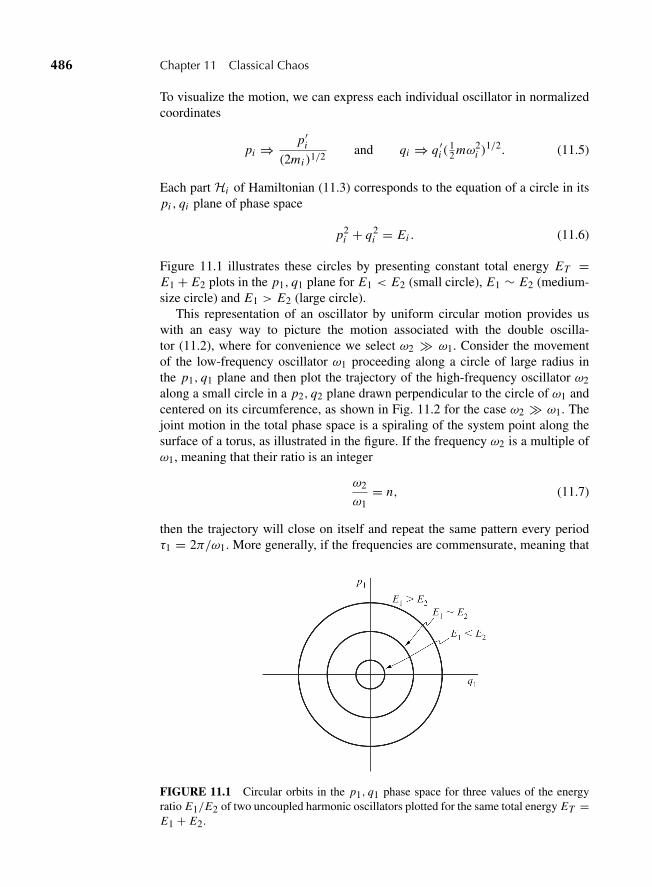
“M11 Goldstein ISBN C11” — 2011/2/15 — page 486 — #4
486 Chapter 11 Classical Chaos
To visualize the motion, we can express each individual oscillator in normalizedcoordinates
pi ⇒p′i
(2mi )1/2and qi ⇒ q ′
i (12 mω2
i )1/2. (11.5)
Each part Hi of Hamiltonian (11.3) corresponds to the equation of a circle in itspi , qi plane of phase space
p2i + q2
i = Ei . (11.6)
Figure 11.1 illustrates these circles by presenting constant total energy ET =E1 + E2 plots in the p1, q1 plane for E1 < E2 (small circle), E1 ∼ E2 (medium-size circle) and E1 > E2 (large circle).
This representation of an oscillator by uniform circular motion provides uswith an easy way to picture the motion associated with the double oscilla-tor (11.2), where for convenience we select ω2 � ω1. Consider the movementof the low-frequency oscillator ω1 proceeding along a circle of large radius inthe p1, q1 plane and then plot the trajectory of the high-frequency oscillator ω2along a small circle in a p2, q2 plane drawn perpendicular to the circle of ω1 andcentered on its circumference, as shown in Fig. 11.2 for the case ω2 � ω1. Thejoint motion in the total phase space is a spiraling of the system point along thesurface of a torus, as illustrated in the figure. If the frequency ω2 is a multiple ofω1, meaning that their ratio is an integer
ω2
ω1= n, (11.7)
then the trajectory will close on itself and repeat the same pattern every periodτ1 = 2π/ω1. More generally, if the frequencies are commensurate, meaning that
FIGURE 11.1 Circular orbits in the p1, q1 phase space for three values of the energyratio E1/E2 of two uncoupled harmonic oscillators plotted for the same total energy ET =E1 + E2.

“M11 Goldstein ISBN C11” — 2011/2/15 — page 487 — #5
11.2 Perturbations and the Kolmogorov–Arnold–Moser Theorem 487
FIGURE 11.2 Circular motions of a low-frequency (ω1) harmonic oscillator in thehorizontal p1, q1 plane and of a high-frequency (ω2 > ω1) harmonic oscillator in theuniformly moving p2, q2 vertical plane. The oscillators are uncoupled, and the resultantspiraling motion of the second oscillator generates a torus, as shown.
n in this Eq. (11.7) is a rational number like 23 , then the orbit will still be closed,
but it will trace out more than one path around the p1, q1 circle before closingon itself. If, however, the frequencies are incommensurate, meaning that n inEq. (11.7) is an irrational number, then the trajectory will never close, but willgradually cover the surface of the torus, without ever passing through exactly thesame point twice. Eventually, however, it will pass arbitrarily close to every pointon the surface. This is called a dense periodic orbit. Such an orbit is bounded andconfined to a surface, but it is not closed.
This approach can be generalized to more than two oscillators. If there arethree such oscillators with the frequencies ω1, ω2, and ω3, then the motion willbe confined to a three-dimensional surface called a 3-torus in the six-dimensionalp1, p2, p3, q1, q2, q3 phase space. For N oscillators, there will be an N -torus in a2N-dimensional phase space. It is not easy to visualize the N -tori for N > 2.
11.2 PERTURBATIONS AND THE KOLMOGOROV–ARNOLD–MOSER THEOREM
In the real world we can often express the dynamics of a system in terms of anintegrable Hamiltonian perturbed by a small interaction that makes it noninte-grable. An example is the motion of Earth in a Keplerian orbit around the Sunprimarily perturbed by the presence of the planets Mars and Jupiter. This inter-action is so weak that there is very little disturbance of Earth’s orbit. Weak in-teractions of this type are most conveniently treated with the aid of canonicalperturbation theory, which is explained in detail in Chapter 12. The followingoutline of the method discussed in Section 12.2 is sufficient for the considera-tion of chaos. References are given to the equations in Chapter 12 but reading thechapter is not necessary to follow the arguments, so we have placed this chapterfirst.

“M11 Goldstein ISBN C11” — 2011/2/15 — page 488 — #6
488 Chapter 11 Classical Chaos
We assume a Hamiltonian H involving a dominant interaction arising from anintegrable Hamiltonian H0 for which the solution is known, plus an additionalinteraction arising from a small perturbation term H
H = H0 +H. (11.8)
It is convenient to use the generating function S(q, P, t) = F2(q, P, t) intro-duced in Section 9.1 to transform the dominant Hamiltonian term H0 from thephase space coordinates p, q to new coordinates P, Q of a transformed Hamilto-nian K0(Q, P), that is identically zero, as was illustrated in the Hamilton–Jacobiapproach of Chapter 10. Hamilton’s equations (10.1) for K0 = 0 provide newcoordinates and momenta, Q0 and P0, which are constants of the motion. Thesame transformation carried out for the total Hamiltonian, H = H0 + H0,provides a transformed HamiltonianK0, which can be used to obtain first-ordercorrections P1, Q1 to the time derivatives of the coordinates and momenta viaHamilton’s equations (cf. Equation (12.4))
∂
∂PK0(P, Q) = Q1,
∂
∂QK0(P, Q) = −P1. (11.9)
After differentiation, Q and P are replaced in K0 by their unperturbed forms,that is, by q = Q0 and p = P0. These expressions (11.9) can be integratedover time to give the first-order determination of Q = Q1 and P = P1. Theprocedure provides us with a new generating function S(Q1, P1, t), and hence anew perturbed Hamiltonian K1, which can be iterated to give the next higher-order terms Q2 and P2, and so on. Further cycles of perturbation are obtained byiteration with the aid of the following relations (cf. Eq. (12.6)) with no summationintended:
∂
∂P1Ki (Pi , Qi ) = Qi+1,
∂
∂QiKi (Pi , Qi ) = −Pi+1. (11.10)
Thus, we have a systematic canonical iteration technique for obtaining better andbetter approximations to the solution when the perturbation H is present. Thismethod can be continued to higher order, as discussed in Chapter 12.
We have seen that perturbation theory provides us with a solution when His small relative to H0, but the question arises as to whether the perturbed solu-tion is stable, and whether or not the orbits will remain close to the unperturbedones over long periods of time. Large perturbations can clearly disturb the reg-ular motion. A theorem known as the Kolmogorov–Arnold–Moser (KAM) theo-rem provides the conditions for the breakdown of regularity. This theorem tellsus that
If the bounded motion of an integrable Hamiltonian H0 is disturbed by a smallperturbation, H, that makes the total Hamiltonian, H = H0 + H, noninte-grable and if two conditions are satisfied:
“M11 Goldstein ISBN C11” — 2011/2/15 — page 489 — #7
11.3 Attractors 489
(a) the perturbation H is small, and
(b) the frequencies ωi of H0 are incommensurate,
then the motion remains confined to an N-torus, except for a negligible set ofinitial conditions that result in a meandering trajectory on the energy surface.
Thus, the perturbed orbits will be stable, only slightly altered in shape, andlocalized in the same region as the unperturbed ones. Another way to say thisis to observe that for a perturbation of the Hamiltonian that is sufficiently small,most quasi-periodic orbits will only experience minimal changes. The methodof proof for this theorem was originally suggested by Kolmogorov in 1954, andthe proofs themselves, approached from different viewpoints, were worked outindependently by Arnold and by Moser a decade later. A great deal of mathemat-ical sophistication is needed for the proof, and references can be consulted fordetails.* For example, the second condition (b) of the theorem is mathematicallymore complex than simple incommensurability.
The caveat “except for a negligible set of initial conditions” introduces the pos-sibility of initial conditions for which the theorem does not hold. This is analogousto the case of a differential equation with well-behaved solutions over an entiredomain except for one or more singular points where the solutions blow up toinfinity. The exceptions are so few that they have very little effect on applications.Chaos can occur when KAM does not hold.
11.3 ATTRACTORS
The previous section was concerned with an integrable Hamiltonian H0 beingdisturbed by a small perturbation H. We found that stable orbits of H0 persistas slightly modified but still stable orbits of the total Hamiltonian, H = H0+H.Another case to consider is that of a system in which the initial conditions start themotion on a trajectory that does not lie on a stable path but that evolves toward aparticular fixed point in phase space, or toward a stable orbit in phase space calleda limit cycle. A fixed point of this type as well as a limit cycle are examples ofattractors.
In general, an attractor is a set of points in phase space to which the solutionof an equation evolves long after transients have died out. It might be a point withdimension dA = 0, a trajectory or limit cycle orbit (cf. Fig. 11.1) with dimensiondA = 1, or perhaps a toroidal surface or torus with dimension dA = 2. For aregular attractor, the attractor dimension, dA, is an integer that is less than theoverall dimensions of the phase space. In higher dimensions, the attractors canbe N -dimensional tori, where dA = 2 for the torus generated by the orbit in
*See, for example, H. Bai-Lin, Chaos, Singapore: World Science, 1984; E. A. Jackson, Perspectivesof Nonlinear Dynamics, Cambridge, England: Cambridge University Press, 1989; L. E. Reichl, TheTransition to Chaos, Berlin: Springer-Verlag, 1992.
“M11 Goldstein ISBN C11” — 2011/2/15 — page 490 — #8
490 Chapter 11 Classical Chaos
Fig. 11.2. There also exist somewhat bizarre types of attractors called strangeattractors, associated with chaos, which tend to be widely dispersed rather thanlocalized in phase space. In addition, they have fractal dimensions—in otherwords, dimensions that are fractions or irrational numbers rather than wholenumbers. These properties, as well as the term fractal dimension, are counterin-tuitive. We shall clarify the meanings of strange attractors and fractal dimensionslater in the chapter.
An example of a fixed-point attractor is the equilibrium position of a pendu-lum at rest. If the pendulum is oscillating while subject to the action of a weakfrictional drag force, then successive oscillations will decrease in amplitude untilthe pendulum finally comes to a stop at its equilibrium position. We say that themotion is drawn to the attractor. If the drag force is a perturbation on the mainHamiltonian, then the motion is underdamped and the pendulum undergoes manyoscillations before stopping at the attractor point. If the damping term exceeds themain Hamiltonian term, then the motion is overdamped and the pendulum falls torest without undergoing any oscillations. Either way, the motion of the pendulumfinds its way to the attractor. Being a point, it is clear that the dimensionality ofthis attractor is zero; dA = 0.
An example of a limit cycle type of attractor is provided by the van der Polequation,
md2x
dt2− ε(1 − x2)
dx
dt+ mω2
0x = F cos ωDt, (11.11)
which has been employed to describe oscillations in mechanical and electricalsystems, as well as cardiac rhythms. If we set ε = 0, then we have a drivensimple harmonic oscillator with a resonant frequency ω0 and a driving frequencyωD . If ωD is close to ω0, then the motion repeats itself at the frequency ωD ofthe applied force. If F = 0, then the motion will be simple harmonic at theresonant frequency ω0. If the small damping term ε(1 − x2) dx/dt is includedin the equation, then the motion will be drawn toward the limit cycle, which inthis case is a circle of unit radius. If x2 > 1, the damping is positive and themotion spirals inward toward the limit cycle, while for x2 < 1, the dampingis negative and the motion spirals outward toward the limit cycle. Both casesare shown in Fig. 11.3a. The final state of motion has long-term stability sincethe damping vanishes for x = 1, and the system point moves along the cir-cular path, which by its nature has dimension dA = 1. If ε is large enough,the damping term becomes comparable in magnitude to the other terms in theequation of motion, and the damping still draws the trajectories toward the limitcycle, but the cycle itself becomes distorted from a circular shape, as shown inFig. 11.3b. The distortion in shape does not change the dimension of the path,which remains dA = 1. In addition, the strong damping causes the previouslysimple harmonic oscillations x = sinω0t to decrease in frequency and becomedistorted, as shown in Fig. 11.3c. For very large damping, the shape approximatesa square wave.
“M11 Goldstein ISBN C11” — 2011/2/15 — page 491 — #9
11.4 Chaotic Trajectories and Liapunov Exponents 491
FIGURE 11.3 Limit cycles (darkened curves) of the van der Pol equation in the x, xphase space showing (a) circular motion for a small damping coefficient ε, and (b) distortedcurve for large damping. Approaches to the limit cycles via orbits outside and inside themare shown. Part (c) sketches the distorted sine wave obtained for the case of appreciabledamping (large ε).
11.4 CHAOTIC TRAJECTORIES AND LIAPUNOV EXPONENTS
The orbits that we have discussed thus far have been well behaved, and confinedto a relatively small region of phase space. Examples are the ellipses of the Keplerproblem, the circles of the simple harmonic oscillator, and the limit cycle of thevan der Pol equation (11.11). Under certain conditions, trajectories, called chaotictrajectories, will be encountered in which the motion wanders around an extensiveand perhaps irregularly shaped region of phase space in a manner that appearsto be random, but that in fact is tempered by constraints. This path or regionwhere the meandering takes place is an example of a strange attractor. It is calledstrange because of its (fractal) geometry and chaotic because of its dynamics.*The chaotic trajectory roams here and there, back and forth through this strangeattractor region seeming to fill the space, but without ever actually passing throughthe same point twice. In short, chaotic motion has affinities with ergotic motion(cf. Section 9.8), with characteristics between regular deterministic trajectoriesand totally random roaming.
The motion involved in chaos has the properties of mixing, dense quasi-periodic orbits, and sensitivity to initial conditions. The properties are as fol-lows. Mixing means that if we choose two arbitrarily small but nonzero regions,I1 and I2, of the domain of the motion and we follow an orbit that passesthrough region I1, then it will eventually pass through region I2. The orbits arequasi-periodic in the sense that they repeatedly and irregularly pass through thewhole range of the domain without ever closing on themselves, and without
*See A. B. Cambel, Applied Chaos Theory, New York: Academic Press, 1993, p. 70.
“M11 Goldstein ISBN C11” — 2011/2/15 — page 492 — #10
492 Chapter 11 Classical Chaos
any particular time period associated with successive transits. They are densebecause they pass through or arbitrarily close to every point of the domain, aproperty that conforms with the ergotic hypothesis (cf. Section 9.8). A chaoticorbit that visits and revisits (that is, mixes with) all regions of the availablephase space is identified with what is called a strange attractor. Its associa-tion is not with a localized attractor such as a fixed point or a limit cycle, butrather with a very extended region of phase space, hence the designation strange.The property of ergodicity, which involves covering all accessible regions ofa domain, is shared by incommensurate nonchaotic orbits with respect to anordinary attractor (for example, a torus), and by chaotic orbits with respect to astrange attractor.
Sensitivity to initial conditions means that a small change in the initial con-ditions can result in a large change in position and velocity many transits oriterations later. For example, a small change can convert a parabolic orbitof the Kepler problem to either a weakly bound elliptic orbit or to a hyper-bolic orbit that extends to infinity. In the Henon–Heiles Hamiltonian, (cf. Sec-tion 11.6), a small increase in the energy can induce the onset of chaos withthe Liapunov exponent (defined below) giving the time scale for this breakdownof order.
The KAM theorem of the previous section is valid for small perturbations.As the perturbation increases, the effect on the motion of the system becomesmore and more pronounced. If the perturbation becomes sufficiently large, thebehavior may become chaotic. Then successively calculated orbits move far-ther and farther away from each other. Even if the first few orbits of a chaoticsequence lie relatively close to the original one, each iteration involves a greaterrecession than the previous one, so the extent to which they move apart canincrease exponentially with the number of iterations. An example is a spaceshipin an Earth orbit. A small rocket boost will move it to a nearby orbit whereasa strong boost could throw it out of orbit, heading for outer space. Anothercommon example of how linear and chaotic motions differ when periodicity isnot present is turbulence in water. While there is streamline flow, two nearbypoints in the water stay close together as they move along; after the onset ofturbulence the same two points, on average, keep moving farther and fartherapart.
A quantitative measure of this exponential divergence is a coefficient, λ, calleda Liapunov exponent, (sometimes spelled Lyapunov or Ljapunov). In the chaoticregion of many systems, if two orbits are separated by the small distance s0 at thetime t = 0, then at a later time t their separation is given by
s(t) ∼ s0eλt . (11.12)
If λ > 0 the motion is chaotic, and the Liapunov exponent λ quantifies the averagegrowth of an infinitesimally small deviation of a regular orbit arising from a per-turbation. It sets a time scale τ ∼ 1/λ for the growth of divergences brought aboutby sufficiently large perturbations. The chaos becomes appreciable for t � τ
when the trajectory winds its way around the extensive, but bounded, phase space
“M11 Goldstein ISBN C11” — 2011/2/15 — page 493 — #11
11.4 Chaotic Trajectories and Liapunov Exponents 493
of the strange attractor. Eventually the separation s(t) becomes comparable to thedimensions of the accessible coordinate space so it can no longer increase further,and from that point on the separations s(t) vary randomly in time.
If the system evolves by an iterative process rather than by a temporal processthen Eq. (11.12) assumes the form
s(n) ∼ s0enλ, (11.13)
where n is the number of iterations, and the exponent λ is now dimensionless.Moreover, this divergence of orbits is not reversible. In a chaotic region it isimpossible to reconstruct the distant past history of a system from its present state.This means that current trajectories can no longer be projected back to determinethe initial configuration.
If the Liapunov exponent is negative it measures the rate at which a systempoint approaches a regular attractor. In other words, in the nonchaotic region λ< 0and the distance s(t) from an attractor at time t is given by the expression
s(t) ∼ s0e−|λ|t (11.14)
where s0 is the initial distance at time t = 0. For an iterative process we have theanalogous expression
s(n) ∼ s0e−n|λ| (11.15)
for the distance s(n) after n iterations. A negative exponent characterizes the rateat which the orbit spirals into the circle on Fig. 11.3a. In the previously consid-ered damped pendulum case the time constant τ of the damping process is thereciprocal of the associated negative Liapunov exponent, τ ∼ 1/|λ|.
As an example, consider the elliptic orbit of a planet in the solar system thatis perturbed by the gravitational interaction with another planet. The perturbationis nonlinear, and it is also small since the gravitational interactions of the twoplanets with the much larger Sun are dominant. We might expect that the KAMtheorem would predict that any perturbed orbit is stable, but this is not correctfor two reasons. First, many natural frequencies in the solar system correspondto resonances involving individual planets and asteroids. Second, many of theobjects in the solar system are asteroids, and perturbations resulting from theirpresence no longer remain small. Both of these effects lead to chaotic results.Some of this chaos simply means that we cannot make exact predictions aboutthe future. Other effects may lead to the eventual ejection of one or more bodiesfrom bound orbits, a possibility that was mentioned in Section 3.12 on the three-body problem.
When we consider natural frequencies, it is not only the orbital periods thatare important. The rotation, obliquity (axial tilt), rotational plane, orbital plane,and eccentricity provide some of the other frequencies that may interact in sur-prising ways. The massive planets of the outer solar system have apparentlysettled into quasi-periodic orbits of marginal stability. Marginal stability meansthat their orbital motion is stable on a time scale comparable with the age of

“M11 Goldstein ISBN C11” — 2011/2/15 — page 494 — #12
494 Chapter 11 Classical Chaos
the solar system. Other orbital parameters occasionally change. The obliquity ofEarth’s axis is apparently stabilized by the presence of the Moon. Both Venusand Earth interact in a bounded chaotic fashion with little change in their peri-ods. Mercury, Mars, Pluto, and many asteroids may undergo much more chaoticmotion.
Calculations, projecting motions for the next 100 Gyr, show that there is afinite probability that Mercury will be ejected or collide with Venus some timeduring the next 3.5 Gyr. Using the approximation τ ∼ 1/|λ| with τ = 3.5 Gyrprovides a Liapunov exponent λ ∼ 3 × 10⁻¹⁰ per year as the time scale forplanetary chaos. The eccentricity of the orbit of Mars could increase to 0.2,while its axial tilt can vary by 60◦, perhaps sufficient to release water on thesurface through the possible melting of its ice caps. Pluto also has chaoticmotions, but they seem to be bounded. Thus, chaos has been a mechanismfor the reorganization of the planetary bodies since the formation of the solarsystem.
Motions in both the outer (> 2.8 AU) and inner (< 2.5 AU) asteroid beltsare chaotic. The outer belt chaos is dominated by Jupiter and the Jupiter–Saturn–asteroid interactions, while the inner belt chaos involves Mars and Mars–Jupiter–asteroid resonances. These interactions provide a steady impetus for Marscrossing asteroids. Once established along such a path, the Liapunov exponent ismuch larger, leading to changes in orbit.
We must note that these conclusions are based upon the results of numericalcalculations. Every effort has been made to ensure that current limits of numericalaccuracy, as well as the inclusion or exclusion of members of the solar family, donot affect the conclusions. Although there is evidence of past chaos in the solarsystem, we must remember that our future predictions are based upon our modelof the solar system, not the system itself. Stability could be better or worse thanthe model predicts, but the chaos itself is definitely present.
11.5 POINCARE MAPS
In Section 11.1, we discussed the periodic motion of uncoupled oscillators. Whentwo one-dimensional oscillators become coupled by adding a term such as x2 y tothe Hamiltonian, then the motion becomes rather complex in the four-dimensionalpx xpy y phase space, and it is no longer feasible to follow the trajectories. It ismore convenient to sample the motion at regular intervals and use the resultinginformation to deduce some of its general characteristics. A convenient way tosample the motion is to map it on a cross section of phase space.
When the total energy, ET , of a double oscillator is fixed, the dimensionalityof the space is lowered by one, and the motion is confined to a three-dimensionalregion in this phase space called an energy hypersurface. Some authors refer toit as a “three-dimensional energy surface.” To avoid the complications of tracingout orbits wandering around this three-dimensional region, it is more advanta-geous to study a two-dimensional slice or section through the hypersurface. Theslice is called a Poincare section. We calculate the positions of points where
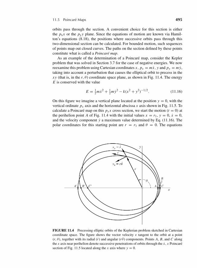
“M11 Goldstein ISBN C11” — 2011/2/15 — page 495 — #13
11.5 Poincare Maps 495
orbits pass through the section. A convenient choice for this section is eitherthe pxx or the py y plane. Since the equations of motion are known via Hamil-ton’s equations (8.18), the positions where successive orbits pass through thistwo-dimensional section can be calculated. For bounded motion, such sequencesof points map out closed curves. The paths on the section defined by these pointsconstitute what is called a Poincare map.
As an example of the determination of a Poincare map, consider the Keplerproblem that was solved in Section 3.7 for the case of negative energies. We nowreexamine this problem using Cartesian coordinates x, px = mx, y and py = my,taking into account a perturbation that causes the elliptical orbit to precess in thexy (that is, in the r, θ ) coordinate space plane, as shown in Fig. 11.4. The energyE is conserved with the value
E = 12 mx2 + 1
2 my2 − k(x2 + y2)−1/2. (11.16)
On this figure we imagine a vertical plane located at the position y = 0, with thevertical ordinate px axis and the horizontal abscissa x axis shown in Fig. 11.5. Tocalculate a Poincare map on this px x cross section, we start the motion (t = 0) atthe perihelion point A of Fig. 11.4 with the initial values x = r1, y = 0, x = 0,and the velocity component y a maximum value determined by Eq. (11.16). Thepolar coordinates for this starting point are r = r1 and θ = 0. The equations
FIGURE 11.4 Precessing elliptic orbits of the Keplerian problem sketched in Cartesiancoordinate space. The figure shows the vector velocity v tangent to the orbit at a point(r, θ), together with its radial (r ) and angular (r θ) components. Points A, B, and C alongthe x axis near perihelion denote successive penetrations of orbits through the x, x Poincaresection of Fig. 11.5 located along the x axis where y = 0.
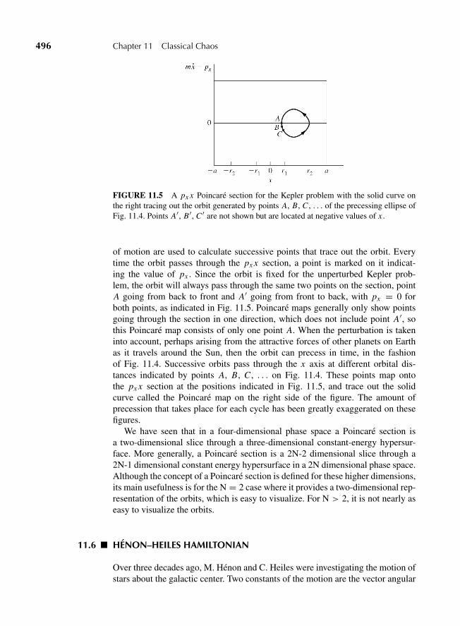
“M11 Goldstein ISBN C11” — 2011/2/15 — page 496 — #14
496 Chapter 11 Classical Chaos
FIGURE 11.5 A px x Poincare section for the Kepler problem with the solid curve onthe right tracing out the orbit generated by points A, B, C , . . . of the precessing ellipse ofFig. 11.4. Points A′, B′, C ′ are not shown but are located at negative values of x .
of motion are used to calculate successive points that trace out the orbit. Everytime the orbit passes through the px x section, a point is marked on it indicat-ing the value of px . Since the orbit is fixed for the unperturbed Kepler prob-lem, the orbit will always pass through the same two points on the section, pointA going from back to front and A′ going from front to back, with px = 0 forboth points, as indicated in Fig. 11.5. Poincare maps generally only show pointsgoing through the section in one direction, which does not include point A′, sothis Poincare map consists of only one point A. When the perturbation is takeninto account, perhaps arising from the attractive forces of other planets on Earthas it travels around the Sun, then the orbit can precess in time, in the fashionof Fig. 11.4. Successive orbits pass through the x axis at different orbital dis-tances indicated by points A, B, C , . . . on Fig. 11.4. These points map ontothe px x section at the positions indicated in Fig. 11.5, and trace out the solidcurve called the Poincare map on the right side of the figure. The amount ofprecession that takes place for each cycle has been greatly exaggerated on thesefigures.
We have seen that in a four-dimensional phase space a Poincare section isa two-dimensional slice through a three-dimensional constant-energy hypersur-face. More generally, a Poincare section is a 2N-2 dimensional slice through a2N-1 dimensional constant energy hypersurface in a 2N dimensional phase space.Although the concept of a Poincare section is defined for these higher dimensions,its main usefulness is for the N = 2 case where it provides a two-dimensional rep-resentation of the orbits, which is easy to visualize. For N > 2, it is not nearly aseasy to visualize the orbits.
11.6 HENON–HEILES HAMILTONIAN
Over three decades ago, M. Henon and C. Heiles were investigating the motion ofstars about the galactic center. Two constants of the motion are the vector angular
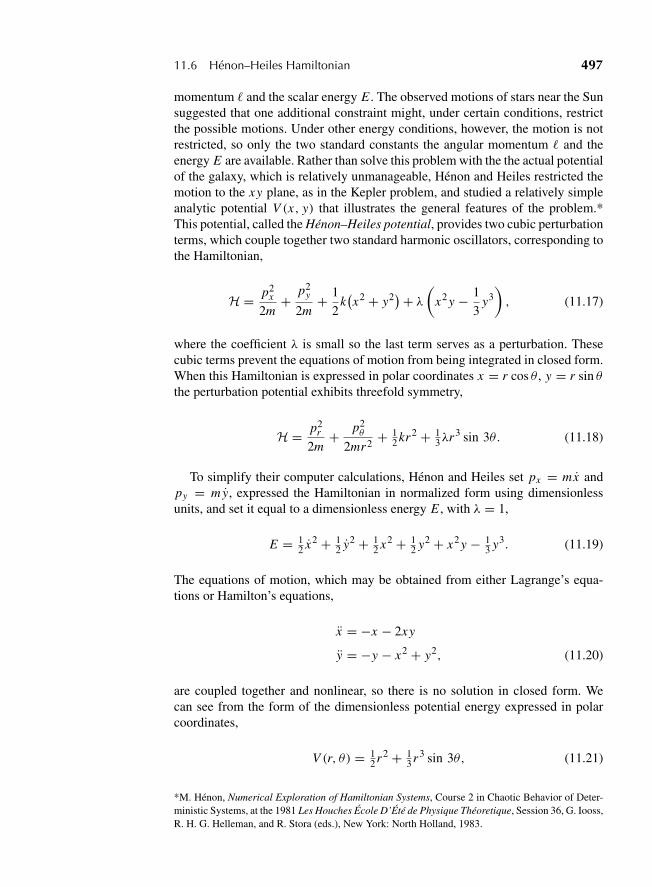
“M11 Goldstein ISBN C11” — 2011/2/15 — page 497 — #15
11.6 Henon–Heiles Hamiltonian 497
momentum � and the scalar energy E . The observed motions of stars near the Sunsuggested that one additional constraint might, under certain conditions, restrictthe possible motions. Under other energy conditions, however, the motion is notrestricted, so only the two standard constants the angular momentum � and theenergy E are available. Rather than solve this problem with the the actual potentialof the galaxy, which is relatively unmanageable, Henon and Heiles restricted themotion to the xy plane, as in the Kepler problem, and studied a relatively simpleanalytic potential V (x, y) that illustrates the general features of the problem.*This potential, called the Henon–Heiles potential, provides two cubic perturbationterms, which couple together two standard harmonic oscillators, corresponding tothe Hamiltonian,
H = p2x
2m+ p2
y
2m+ 1
2k(x2 + y2)+ λ(x2 y − 1
3y3), (11.17)
where the coefficient λ is small so the last term serves as a perturbation. Thesecubic terms prevent the equations of motion from being integrated in closed form.When this Hamiltonian is expressed in polar coordinates x = r cos θ , y = r sin θthe perturbation potential exhibits threefold symmetry,
H = p2r
2m+ p2
θ
2mr2+ 1
2 kr2 + 13λr3 sin 3θ. (11.18)
To simplify their computer calculations, Henon and Heiles set px = mx andpy = my, expressed the Hamiltonian in normalized form using dimensionlessunits, and set it equal to a dimensionless energy E , with λ = 1,
E = 12 x2 + 1
2 y2 + 12 x2 + 1
2 y2 + x2 y − 13 y3. (11.19)
The equations of motion, which may be obtained from either Lagrange’s equa-tions or Hamilton’s equations,
x = −x − 2xy
y = −y − x2 + y2, (11.20)
are coupled together and nonlinear, so there is no solution in closed form. Wecan see from the form of the dimensionless potential energy expressed in polarcoordinates,
V (r, θ) = 12r2 + 1
3r3 sin 3θ, (11.21)
*M. Henon, Numerical Exploration of Hamiltonian Systems, Course 2 in Chaotic Behavior of Deter-ministic Systems, at the 1981 Les Houches Ecole D’Ete de Physique Theoretique, Session 36, G. Iooss,R. H. G. Helleman, and R. Stora (eds.), New York: North Holland, 1983.
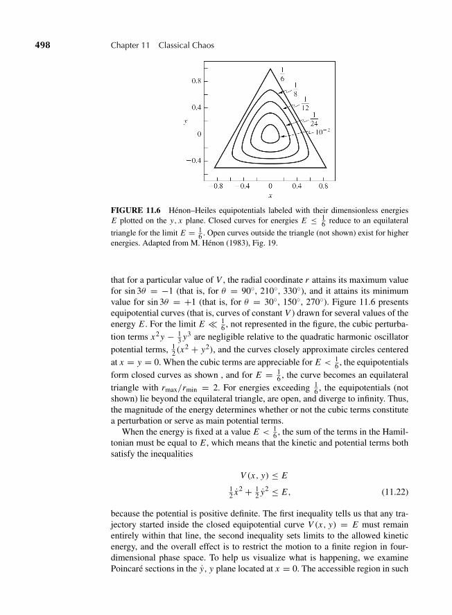
“M11 Goldstein ISBN C11” — 2011/2/15 — page 498 — #16
498 Chapter 11 Classical Chaos
FIGURE 11.6 Henon–Heiles equipotentials labeled with their dimensionless energiesE plotted on the y, x plane. Closed curves for energies E ≤ 1
6 reduce to an equilateral
triangle for the limit E = 16 . Open curves outside the triangle (not shown) exist for higher
energies. Adapted from M. Henon (1983), Fig. 19.
that for a particular value of V , the radial coordinate r attains its maximum valuefor sin 3θ = −1 (that is, for θ = 90◦, 210◦, 330◦), and it attains its minimumvalue for sin 3θ = +1 (that is, for θ = 30◦, 150◦, 270◦). Figure 11.6 presentsequipotential curves (that is, curves of constant V ) drawn for several values of theenergy E . For the limit E � 1
6 , not represented in the figure, the cubic perturba-tion terms x2 y − 1
3 y3 are negligible relative to the quadratic harmonic oscillatorpotential terms, 1
2 (x2 + y2), and the curves closely approximate circles centered
at x = y = 0. When the cubic terms are appreciable for E < 16 , the equipotentials
form closed curves as shown , and for E = 16 , the curve becomes an equilateral
triangle with rmax/rmin = 2. For energies exceeding 16 , the equipotentials (not
shown) lie beyond the equilateral triangle, are open, and diverge to infinity. Thus,the magnitude of the energy determines whether or not the cubic terms constitutea perturbation or serve as main potential terms.
When the energy is fixed at a value E < 16 , the sum of the terms in the Hamil-
tonian must be equal to E , which means that the kinetic and potential terms bothsatisfy the inequalities
V (x, y) ≤ E
12 x2 + 1
2 y2 ≤ E, (11.22)
because the potential is positive definite. The first inequality tells us that any tra-jectory started inside the closed equipotential curve V (x, y) = E must remainentirely within that line, the second inequality sets limits to the allowed kineticenergy, and the overall effect is to restrict the motion to a finite region in four-dimensional phase space. To help us visualize what is happening, we examinePoincare sections in the y, y plane located at x = 0. The accessible region in such
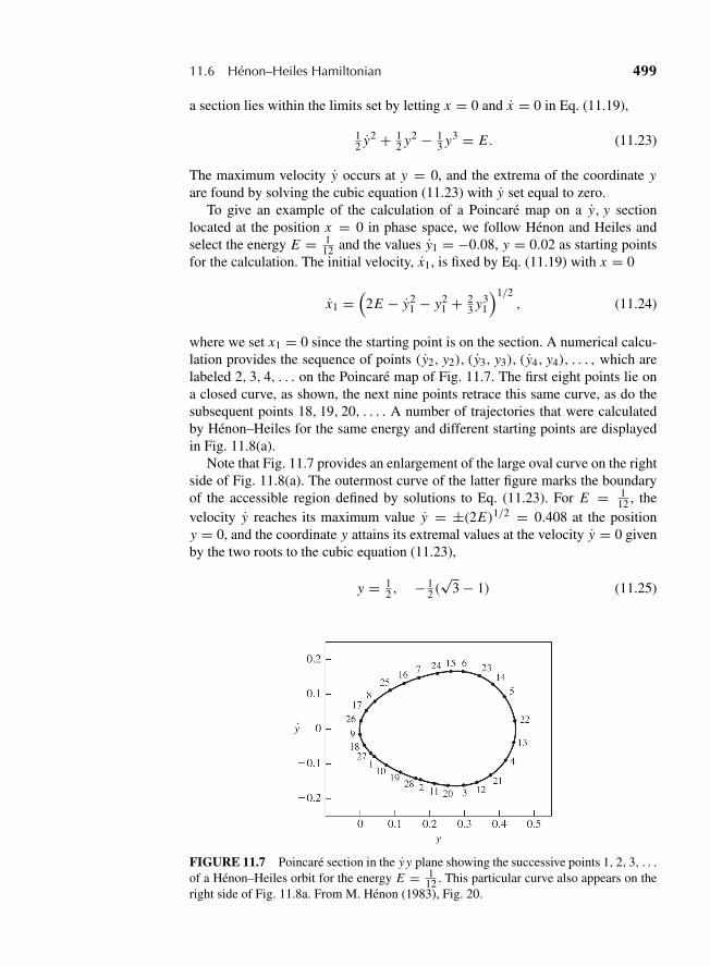
“M11 Goldstein ISBN C11” — 2011/2/15 — page 499 — #17
11.6 Henon–Heiles Hamiltonian 499
a section lies within the limits set by letting x = 0 and x = 0 in Eq. (11.19),
12 y2 + 1
2 y2 − 13 y3 = E . (11.23)
The maximum velocity y occurs at y = 0, and the extrema of the coordinate yare found by solving the cubic equation (11.23) with y set equal to zero.
To give an example of the calculation of a Poincare map on a y, y sectionlocated at the position x = 0 in phase space, we follow Henon and Heiles andselect the energy E = 1
12 and the values y1 = −0.08, y = 0.02 as starting pointsfor the calculation. The initial velocity, x1, is fixed by Eq. (11.19) with x = 0
x1 =(
2E − y21 − y2
1 + 23 y3
1
)1/2, (11.24)
where we set x1 = 0 since the starting point is on the section. A numerical calcu-lation provides the sequence of points (y2, y2), (y3, y3), (y4, y4), . . . , which arelabeled 2, 3, 4, . . . on the Poincare map of Fig. 11.7. The first eight points lie ona closed curve, as shown, the next nine points retrace this same curve, as do thesubsequent points 18, 19, 20, . . . . A number of trajectories that were calculatedby Henon–Heiles for the same energy and different starting points are displayedin Fig. 11.8(a).
Note that Fig. 11.7 provides an enlargement of the large oval curve on the rightside of Fig. 11.8(a). The outermost curve of the latter figure marks the boundaryof the accessible region defined by solutions to Eq. (11.23). For E = 1
12 , thevelocity y reaches its maximum value y = ±(2E)1/2 = 0.408 at the positiony = 0, and the coordinate y attains its extremal values at the velocity y = 0 givenby the two roots to the cubic equation (11.23),
y = 12 , − 1
2 (√
3 − 1) (11.25)
FIGURE 11.7 Poincare section in the y y plane showing the successive points 1, 2, 3, . . .of a Henon–Heiles orbit for the energy E = 1
12 . This particular curve also appears on theright side of Fig. 11.8a. From M. Henon (1983), Fig. 20.
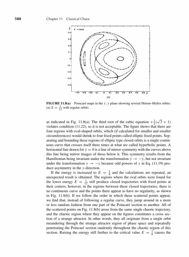
“M11 Goldstein ISBN C11” — 2011/2/15 — page 500 — #18
500 Chapter 11 Classical Chaos
FIGURE 11.8(a) Poincare maps in the y, y plane showing several Henon–Heiles orbits:(a) E = 1
12 with regular orbits.
as indicated in Fig. 11.8(a). The third root of the cubic equation + 12 (√
3 + 1)violates condition (11.22), so it is not acceptable. The figure shows that there arefour regions with oval-shaped orbits, which (if calculated for smaller and smallercircumferences) would shrink to four fixed points called elliptic fixed points. Sep-arating and bounding these regions of elliptic type closed orbits is a single contin-uous curve that crosses itself three times at what are called hyperbolic points. Ahorizontal line drawn for y = 0 is a line of mirror symmetry with the curves abovethis line being mirror images of those below it. This symmetry results from theHamiltonian being invariant under the transformation y → −y, but not invariantunder the transformation y → −y because odd powers of y in Eq. (11.19) pro-duce asymmetry in the y-direction.
If the energy is increased to E = 18 and the calculations are repeated, an
unexpected result is obtained. The regions where the oval orbits were found forthe lower energy E = 1
12 still produce closed trajectories with fixed points attheir centers; however, in the regions between these closed trajectories, there isno continuous curve and the points there appear to have no regularity, as shownin Fig. 11.8(b). If we follow the order in which these scattered points appear,we find that, instead of following a regular curve, they jump around in a moreor less random fashion from one part of the Poincare section to another. All ofthe scattered points on Fig. 11.8(b) arose from the same single chaotic trajectory,and the chaotic region where they appear on the figures constitutes a cross sec-tion of a strange attractor. In other words, they all originate from a single orbitmeandering through the strange attractor region of phase space and repeatedlypenetrating the Poincare section randomly throughout the chaotic region of thissection. Raising the energy still further to the critical value E = 1
6 causes the
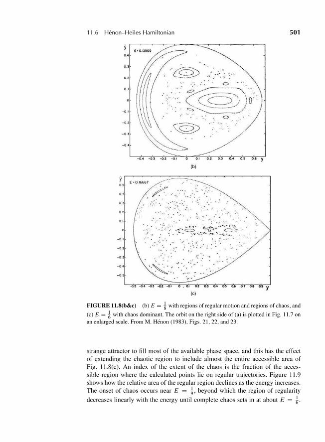
“M11 Goldstein ISBN C11” — 2011/2/15 — page 501 — #19
11.6 Henon–Heiles Hamiltonian 501
FIGURE 11.8(b&c) (b) E = 18 with regions of regular motion and regions of chaos, and
(c) E = 16 with chaos dominant. The orbit on the right side of (a) is plotted in Fig. 11.7 on
an enlarged scale. From M. Henon (1983), Figs. 21, 22, and 23.
strange attractor to fill most of the available phase space, and this has the effectof extending the chaotic region to include almost the entire accessible area ofFig. 11.8(c). An index of the extent of the chaos is the fraction of the acces-sible region where the calculated points lie on regular trajectories. Figure 11.9shows how the relative area of the regular region declines as the energy increases.The onset of chaos occurs near E = 1
9 , beyond which the region of regularitydecreases linearly with the energy until complete chaos sets in at about E = 1
6 .
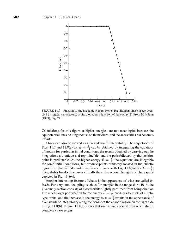
“M11 Goldstein ISBN C11” — 2011/2/15 — page 502 — #20
502 Chapter 11 Classical Chaos
FIGURE 11.9 Fraction of the available Henon–Heiles Hamiltonian phase space occu-pied by regular (nonchaotic) orbits plotted as a function of the energy E . From M. Henon(1983), Fig. 24.
Calculations for this figure at higher energies are not meaningful because theequipotential lines no longer close on themselves, and the accessible area becomesinfinite.
Chaos can also be viewed as a breakdown of integrability. The trajectories ofFigs. 11.7 and 11.8(a) for E = 1
12 can be obtained by integrating the equationsof motion for particular initial conditions; the results obtained by carrying out theintegrations are unique and reproducible, and the path followed by the positionpoint is predictable. At the higher energy E = 1
8 , the equations are integrablefor some initial conditions, but produce points randomly located in the chaoticregion for other initial conditions, in accordance with Fig. 11.8(b). For E = 1
6 ,integrability breaks down over virtually the entire accessible region of phase spacedepicted in Fig. 11.8(c).
Another interesting feature of chaos is the appearance of what are called is-lands. For very small coupling, such as for energies in the range E ∼ 10−3, they versus y section consists of closed orbits slightly perturbed from being circular.The much larger perturbation for the energy E = 1
12 produces four sets of elliptictype orbits, and the increase in the energy to E = 1
8 results in the appearance offive islands of integrability along the border of the chaotic region on the right sideof Fig. 11.8(b). Figure 11.8(c) shows that such islands persist even when almostcomplete chaos reigns.
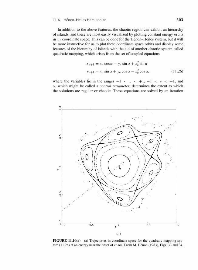
“M11 Goldstein ISBN C11” — 2011/2/15 — page 503 — #21
11.6 Henon–Heiles Hamiltonian 503
In addition to the above features, the chaotic region can exhibit an hierarchyof islands, and these are most easily visualized by plotting constant energy orbitsin xy coordinate space. This can be done for the Henon–Heiles system, but it willbe more instructive for us to plot these coordinate space orbits and display somefeatures of the hierarchy of islands with the aid of another chaotic system calledquadratic mapping, which arises from the set of coupled equations
xn+1 = xn cosα − yn sinα + x2n sinα
yn+1 = xn sinα + yn cosα − x2n cosα, (11.26)
where the variables lie in the ranges −1 < x < +1, −1 < y < +1, andα, which might be called a control parameter, determines the extent to whichthe solutions are regular or chaotic. These equations are solved by an iteration
FIGURE 11.10(a) (a) Trajectories in coordinate space for the quadratic mapping sys-tem (11.26) at an energy near the onset of chaos. From M. Henon (1983), Figs. 33 and 34.
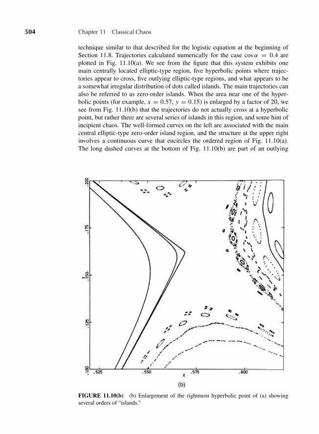
“M11 Goldstein ISBN C11” — 2011/2/15 — page 504 — #22
504 Chapter 11 Classical Chaos
technique similar to that described for the logistic equation at the beginning ofSection 11.8. Trajectories calculated numerically for the case cosα = 0.4 areplotted in Fig. 11.10(a). We see from the figure that this system exhibits onemain centrally located elliptic-type region, five hyperbolic points where trajec-tories appear to cross, five outlying elliptic-type regions, and what appears to bea somewhat irregular distribution of dots called islands. The main trajectories canalso be referred to as zero-order islands. When the area near one of the hyper-bolic points (for example, x = 0.57, y = 0.15) is enlarged by a factor of 20, wesee from Fig. 11.10(b) that the trajectories do not actually cross at a hyperbolicpoint, but rather there are several series of islands in this region, and some hint ofincipient chaos. The well-formed curves on the left are associated with the maincentral elliptic-type zero-order island region, and the structure at the upper rightinvolves a continuous curve that encircles the ordered region of Fig. 11.10(a).The long dashed curves at the bottom of Fig. 11.10(b) are part of an outlying
FIGURE 11.10(b) (b) Enlargement of the rightmost hyperbolic point of (a) showingseveral orders of “islands.”
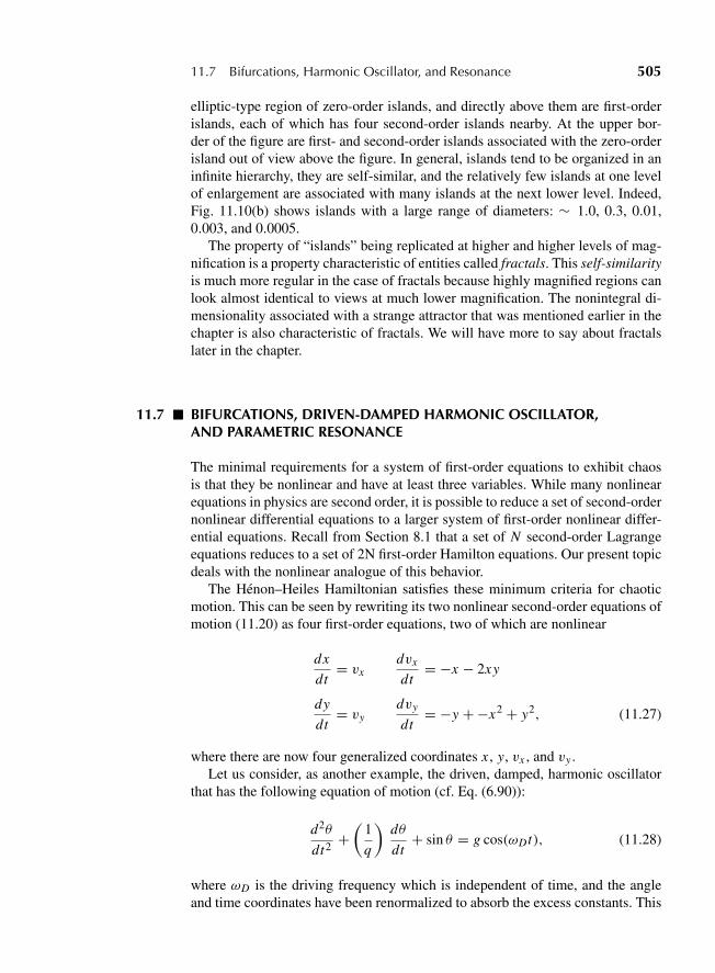
“M11 Goldstein ISBN C11” — 2011/2/15 — page 505 — #23
11.7 Bifurcations, Harmonic Oscillator, and Resonance 505
elliptic-type region of zero-order islands, and directly above them are first-orderislands, each of which has four second-order islands nearby. At the upper bor-der of the figure are first- and second-order islands associated with the zero-orderisland out of view above the figure. In general, islands tend to be organized in aninfinite hierarchy, they are self-similar, and the relatively few islands at one levelof enlargement are associated with many islands at the next lower level. Indeed,Fig. 11.10(b) shows islands with a large range of diameters: ∼ 1.0, 0.3, 0.01,0.003, and 0.0005.
The property of “islands” being replicated at higher and higher levels of mag-nification is a property characteristic of entities called fractals. This self-similarityis much more regular in the case of fractals because highly magnified regions canlook almost identical to views at much lower magnification. The nonintegral di-mensionality associated with a strange attractor that was mentioned earlier in thechapter is also characteristic of fractals. We will have more to say about fractalslater in the chapter.
11.7 BIFURCATIONS, DRIVEN-DAMPED HARMONIC OSCILLATOR,AND PARAMETRIC RESONANCE
The minimal requirements for a system of first-order equations to exhibit chaosis that they be nonlinear and have at least three variables. While many nonlinearequations in physics are second order, it is possible to reduce a set of second-ordernonlinear differential equations to a larger system of first-order nonlinear differ-ential equations. Recall from Section 8.1 that a set of N second-order Lagrangeequations reduces to a set of 2N first-order Hamilton equations. Our present topicdeals with the nonlinear analogue of this behavior.
The Henon–Heiles Hamiltonian satisfies these minimum criteria for chaoticmotion. This can be seen by rewriting its two nonlinear second-order equations ofmotion (11.20) as four first-order equations, two of which are nonlinear
dx
dt= vx
dvx
dt= −x − 2xy
dy
dt= vy
dvy
dt= −y +−x2 + y2, (11.27)
where there are now four generalized coordinates x , y, vx , and vy .Let us consider, as another example, the driven, damped, harmonic oscillator
that has the following equation of motion (cf. Eq. (6.90)):
d2θ
dt2+(
1
q
)dθ
dt+ sin θ = g cos(ωDt), (11.28)
where ωD is the driving frequency which is independent of time, and the angleand time coordinates have been renormalized to absorb the excess constants. This
“M11 Goldstein ISBN C11” — 2011/2/15 — page 506 — #24
506 Chapter 11 Classical Chaos
nonlinear second-order differential equation can be converted to a system of threefirst-order differential equations by writing
dφ
dt= ωD,
dθ
dt= ω, (11.29)
dω
dt= − 1
qω − sin θ + g cosφ
where φ is the phase of the driving term. There are now three dependent variables,φ(t), θ(t), ω(t), and one independent variable t . Since the third of these equationsis nonlinear, we expect that particular values of the parameters q, g, and ωD mightproduce chaotic motion. One physical way to justify this expectation is to notethat the motion of the pendulum should depend upon the interplay between the“natural” frequency ω and the driving frequency ωD .
To obtain quantitative results, we choose q = 2 and let the amplitude g ofthe forcing function play the role of what is called a control parameter. Such aparameter is an index that delineates regions of normal and chaotic behavior. InFig. 11.11(a), we show the ω = θ versus θ Poincare section for the control param-eter g = 0.9. We see from this figure that the motion is regular, while Fig. 11.11(b)constructed for g = 1.15 displays chaotic motion, that is, randomness in the dis-tribution of points. The periodic nature of the differential equations (11.29) pro-duces regions of stability, and then regions of chaos as the control parameter g isincreased.
If we examine how the frequency of oscillation, ω, depends upon this forc-ing function amplitude g for a fixed choice of phase, φ, we find that the sys-tem undergoes a number of bifurcations in the measured frequency of theoscillator. At each bifurcation, the number of allowed frequencies doubles. Aplot of this is shown in Fig. 11.12. The bifurcations are associated with nor-mal or nonchaotic behavior. The figure also shows shaded regions where theoscillator exhibits chaos. Fig. 11.12(b), which is a factor of ten enlargementof a region of (a), shows that bifurcations and chaos have a complex depen-dence upon the control parameter. Figures of this type are called bifurcationdiagrams or Feigenbaum plots. A comparison of the two Feigenbaum plots ofFig. 11.12 makes it clear that this system exhibits the property of self-similaritywhereby the behavior of ω(t) in the neighborhood of one bifurcation resemblesthat in the neighborhood of other bifurcations, even though the scale or lineardimensions are so much different. It is also evident that the quantity g seems to“control” the extent to which the system bifurcates and displays chaos. In theHenon–Heiles system discussed in the previous section, the control parameteris the magnitude of the perturbation H = x2 y − 1
3 y3. In the dimensionlessunits being used there, the effective magnitude of H was set by the choice ofenergy.
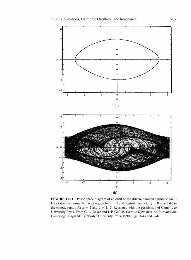
“M11 Goldstein ISBN C11” — 2011/2/15 — page 507 — #25
11.7 Bifurcations, Harmonic Oscillator, and Resonance 507
FIGURE 11.11 Phase space diagram of an orbit of the driven, damped harmonic oscil-lator (a) in the normal behavior region for q = 2 and control parameter g = 0.9, and (b) inthe chaotic region for q = 2 and g = 1.15. Reprinted with the permission of CambridgeUniversity Press. From G. L. Baker and J. P. Gollub, Chaotic Dynamics, An Introduction,Cambridge, England: Cambridge University Press, 1990, Figs. 3–4a and 3–4c.
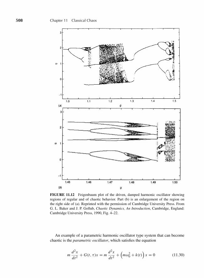
“M11 Goldstein ISBN C11” — 2011/2/15 — page 508 — #26
508 Chapter 11 Classical Chaos
FIGURE 11.12 Feigenbaum plot of the driven, damped harmonic oscillator showingregions of regular and of chaotic behavior. Part (b) is an enlargement of the region onthe right side of (a). Reprinted with the permission of Cambridge University Press. FromG. L. Baker and J. P. Gollub, Chaotic Dynamics, An Introduction, Cambridge, England:Cambridge University Press, 1990, Fig. 4–22.
An example of a parametric harmonic oscillator type system that can becomechaotic is the parametric oscillator, which satisfies the equation
md2x
dt2+ G(t, τ )x = m
d2x
dt2+(
mω20 + k(t)
)x = 0 (11.30)
“M11 Goldstein ISBN C11” — 2011/2/15 — page 509 — #27
11.8 The Logistic Equation 509
where G(t, τ ) is the parameter of the oscillator, and the term k(t) = k(t + τ)
is a perturbation periodic in the time τ . Many functions k(t) produce what iscalled parametric resonance, and we give an example of one. Recall that for asimple rigid rod pendulum of length L , corresponding to k = 0 in Eq. (11.30),the resonant frequency ω0 = (g/L)1/2 and the oscillations can be perturbed bychanging the length of the bob. Parametric resonance can be induced in a simplependulum by shortening the length L by a small amount L when the mass is atits lowest point with the maximum kinetic energy, and increasing the length bythe same amount L at the top of the motion where the mass is instantaneouslyat rest, with the kinetic energy zero and the potential energy a maximum. Moreenergy is added at the bottom than is subtracted at the top, so there is a continualincrease in energy every cycle.
In general, the evolution in time of the solution of Eq. (11.30) can be highlysensitive to small changes in the initial conditions and the nature of k(t). This isa condition for chaos.
11.8 THE LOGISTIC EQUATION
Since the driven-damped harmonic oscillator and the parametric resonanceoscillator solutions can only be calculated with the aid of sophisticated numericaltechniques, we shall consider the detailed analysis of a much simpler mathemati-cal equation called the logistic equation or quadratic iterator, which lends itselfto elementary calculations, and exemplifies most of the characteristics of chaos.Its solutions exhibit regularities as well as chaotic behavior. The properties of thisequation, using successive iterations, are easy to carry out on a small calculator,and the description of chaos that the calculations provide has much in com-mon with many realistic physical situations. This ubiquitous equation describesbehavior in various disciplines such as physics, engineering and economics. Forexample, in biology it describes population dynamics, or the rise and declineof populations interacting with each other through predator–prey relationships.Other simple functions with a quadratic term also give qualitative and quantitativeresults similar to those of the quadratic iterator.
The logistic equation is defined by the expression
xn+1 = axn(1 − xn), (11.31)
where a is the control parameter, with the variable x restricted to the domain
0 ≤ x ≤ 1. (11.32)
Successive iterations of this equation are expected to bring xn+1 closer and closerto a limiting value, x∞, so that further iterations produce no additional change inxn . This limiting value x∞ is called a fixed point, and it is obtained by settingxn+1 = xn in the logistic equation (11.31), which gives
x∞ = a − 1
a. (11.33)
“M11 Goldstein ISBN C11” — 2011/2/15 — page 510 — #28
510 Chapter 11 Classical Chaos
Since xn is limited to the range given by Eq. (11.32), the control parameter mustbe positive with the limit 1 ≤ a. Equation (11.33) does not set any upper limit onthe control parameter, and ordinarily the range 1 ≤ a ≤ 4 is studied.
It is of interest to know the conditions for the fixed point to be stable. Forstability, a value of xn near the fixed point will iterate to a value xn+1, which iscloser to x∞ than xn was. To check this, we can select a value of xn that is closeto the fixed-point value by writing
xn = a − 1
a± δ, (11.34a)
where δ � 1. We shall show in Derivation 4 that this gives, to first order in δ
xn+1 = a − 1
a± δ(2 − a). (11.34b)
For convergence to x∞, we require the coefficient (2−a) of δ to have an absolutevalue less than 1, meaning that this stable fixed point satisfies the condition
1 < a < 3. (11.35)
Such a fixed point constitutes an attractor since values of xn are attracted to it; thatis, they iterate toward it. We see from a left-hand column of Table 11.1 that forthe choice a = 2 and the initial value x0 = 0.3, less than half a dozen iterationsare needed to reach the fixed point x∞ = 1
2 obtained from Eq. (11.33).It is of interest to find out what happens when we iterate the logistic equation
for control parameters beyond the value a = 3. For a = 3.2 then, we find thatafter two dozen iterations the value of xn alternates between two final values orattractors as follows:
xn = 0.51304
xn+1 = 0.79946, (11.36)
as shown in the center columns of Table 11.1, and for the control parametera = 3.5, a double bifurcation corresponds to a fourfold cycle involving the fourattractors
xn = 0.501
xn+1 = 0.875
xn+2 = 0.383
xn+3 = 0.827. (11.37)
There is an eightfold cycle for a = 3.55, a sixteenfold cycle for a = 3.566, . . . .Figures 11.13(a) and Fig. 11.14 illustrate the bifurcations. These Feigenbaumdiagrams, which plot x∞ against a, show how the number of values of x∞
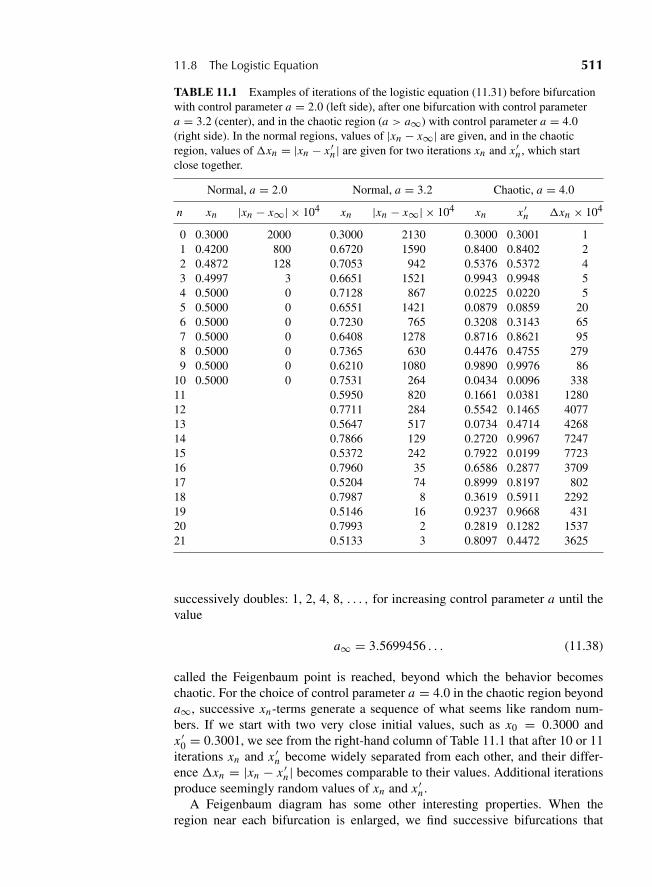
“M11 Goldstein ISBN C11” — 2011/2/15 — page 511 — #29
11.8 The Logistic Equation 511
TABLE 11.1 Examples of iterations of the logistic equation (11.31) before bifurcationwith control parameter a = 2.0 (left side), after one bifurcation with control parametera = 3.2 (center), and in the chaotic region (a > a∞) with control parameter a = 4.0(right side). In the normal regions, values of |xn − x∞| are given, and in the chaoticregion, values of xn = |xn − x ′n | are given for two iterations xn and x ′n , which startclose together.
Normal, a = 2.0 Normal, a = 3.2 Chaotic, a = 4.0
n xn |xn − x∞| × 104 xn |xn − x∞| × 104 xn x ′n xn × 104
0 0.3000 2000 0.3000 2130 0.3000 0.3001 11 0.4200 800 0.6720 1590 0.8400 0.8402 22 0.4872 128 0.7053 942 0.5376 0.5372 43 0.4997 3 0.6651 1521 0.9943 0.9948 54 0.5000 0 0.7128 867 0.0225 0.0220 55 0.5000 0 0.6551 1421 0.0879 0.0859 206 0.5000 0 0.7230 765 0.3208 0.3143 657 0.5000 0 0.6408 1278 0.8716 0.8621 958 0.5000 0 0.7365 630 0.4476 0.4755 2799 0.5000 0 0.6210 1080 0.9890 0.9976 86
10 0.5000 0 0.7531 264 0.0434 0.0096 33811 0.5950 820 0.1661 0.0381 128012 0.7711 284 0.5542 0.1465 407713 0.5647 517 0.0734 0.4714 426814 0.7866 129 0.2720 0.9967 724715 0.5372 242 0.7922 0.0199 772316 0.7960 35 0.6586 0.2877 370917 0.5204 74 0.8999 0.8197 80218 0.7987 8 0.3619 0.5911 229219 0.5146 16 0.9237 0.9668 43120 0.7993 2 0.2819 0.1282 153721 0.5133 3 0.8097 0.4472 3625
successively doubles: 1, 2, 4, 8, . . . , for increasing control parameter a until thevalue
a∞ = 3.5699456 . . . (11.38)
called the Feigenbaum point is reached, beyond which the behavior becomeschaotic. For the choice of control parameter a = 4.0 in the chaotic region beyonda∞, successive xn-terms generate a sequence of what seems like random num-bers. If we start with two very close initial values, such as x0 = 0.3000 andx ′0 = 0.3001, we see from the right-hand column of Table 11.1 that after 10 or 11iterations xn and x ′n become widely separated from each other, and their differ-ence xn = |xn − x ′n| becomes comparable to their values. Additional iterationsproduce seemingly random values of xn and x ′n .
A Feigenbaum diagram has some other interesting properties. When theregion near each bifurcation is enlarged, we find successive bifurcations that
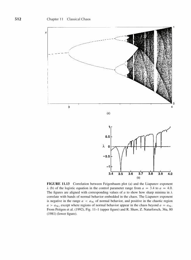
“M11 Goldstein ISBN C11” — 2011/2/15 — page 512 — #30
512 Chapter 11 Classical Chaos
FIGURE 11.13 Correlation between Feigenbaum plot (a) and the Liapunov exponentλ (b) of the logistic equation in the control parameter range from a = 3.4 to a = 4.0.The figures are aligned with corresponding values of a to show how sharp minima in λcorrelate with bands of normal behavior embedded in the chaos. The Liapunov exponentis negative in the range a < a∞ of normal behavior, and positive in the chaotic regiona > a∞, except where regions of normal behavior appear in the chaos beyond a = a∞.From Peitgen et al. (1992), Fig. 11–1 (upper figure) and R. Shaw, Z. Naturforsch, 36a, 80(1981) (lower figure).
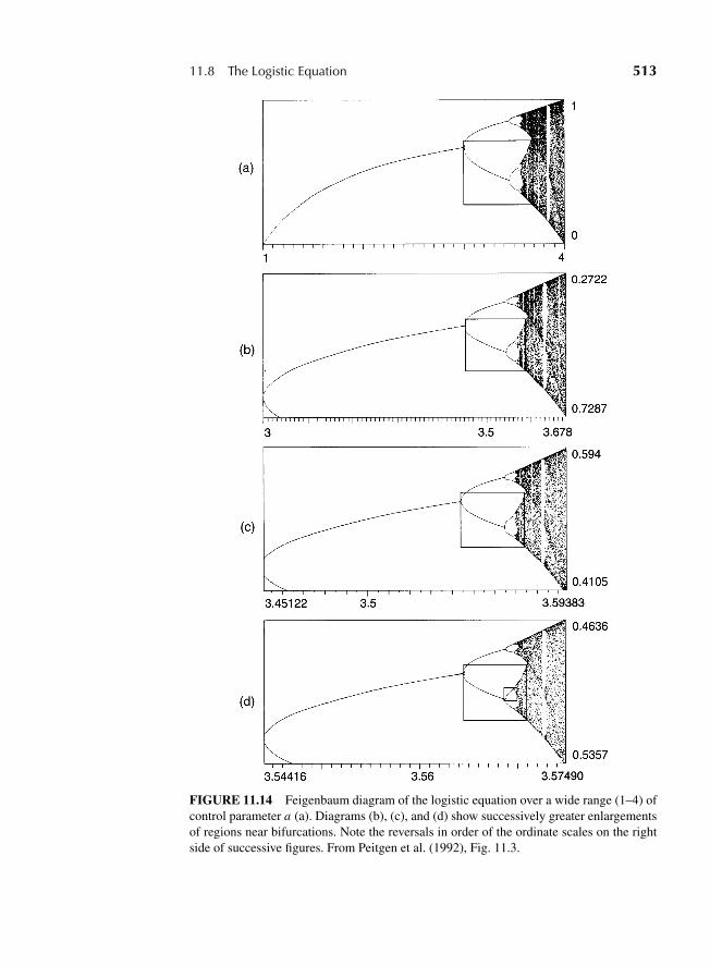
“M11 Goldstein ISBN C11” — 2011/2/15 — page 513 — #31
11.8 The Logistic Equation 513
FIGURE 11.14 Feigenbaum diagram of the logistic equation over a wide range (1–4) ofcontrol parameter a (a). Diagrams (b), (c), and (d) show successively greater enlargementsof regions near bifurcations. Note the reversals in order of the ordinate scales on the rightside of successive figures. From Peitgen et al. (1992), Fig. 11.3.
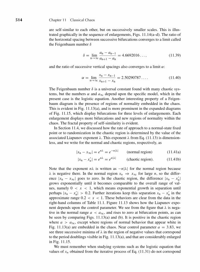
“M11 Goldstein ISBN C11” — 2011/2/15 — page 514 — #32
514 Chapter 11 Classical Chaos
are self-similar to each other, but on successively smaller scales. This is illus-trated graphically in the sequence of enlargements, Figs. 11.14(a–d). The ratio ofthe horizontal spacing between successive bifurcations converges to a limit calledthe Feigenbaum number δ
δ = limn→∞
an − an−1
an+1 − an= 4.6692016 . . . , (11.39)
and the ratio of successive vertical spacings also converges to a limit α:
α = limn→∞
xn − xn−1
xn+1 − xn= 2.50290787 . . . . (11.40)
The Feigenbaum number δ is a universal constant found with many chaotic sys-tems, but the numbers α and a∞ depend upon the specific model, which in thepresent case is the logistic equation. Another interesting property of a Feigen-baum diagram is the presence of regions of normality embedded in the chaos.This is evident in Fig. 11.13(a), and is more prominent in the expanded diagramsof Fig. 11.15, which display bifurcations for three levels of enlargements. Eachenlargement displays more bifurcations and new regions of normality within thechaos. The fractal property of self-similarity is evident.
In Section 11.4, we discussed how the rate of approach to a normal-state fixedpoint or to randomization in the chaotic region is determined by the value of theassociated Liapunov exponent λ. This exponent λ from Eq. (11.13) is dimension-less, and we write for the normal and chaotic regions, respectively, as
|xn − x∞| = enλ = e−n|λ| (normal region) (11.41a)
|xn − x ′n| = enλ = en|λ| (chaotic region). (11.41b)
Note that the exponent nλ is written as −n|λ| for the normal region becauseλ is negative there. In the normal region xn ⇒ x∞ for large n, so the differ-ence |xn − x∞| goes to zero. In the chaotic region, the difference |xn − x ′n|grows exponentially until it becomes comparable to the overall range of val-ues, namely 0 < x < 1, which means exponential growth in separation untilperhaps |xn − x ′n| > 0.2. Further iterations keep this separation xn − x ′n in theapproximate range 0.2 < x < 1. These behaviors are clear from the data in theright-hand columns of Table 11.1. Figure 11.13 shows how the Liapunov expo-nent depends upon the control parameter. We see from the figure that λ is nega-tive in the normal range a < a∞, and rises to zero at bifurcation points, as canbe seen by comparing Figs. 11.13(a) and (b). It is positive in the chaotic regionwhere a > a∞, except where regions of normal behavior that appear white inFig. 11.13(a) are embedded in the chaos. Near control parameter a = 3.83, wesee three successive minima of λ in the region of negative values that correspondto the period doublings visible in Fig. 11.13(a), and that are considerably enlargedin Fig. 11.15.
We must remember when studying systems such as the logistic equation thatvalues of xn obtained from the iterative process of Eq. (11.31) do not correspond
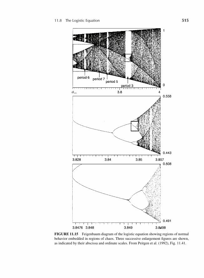
“M11 Goldstein ISBN C11” — 2011/2/15 — page 515 — #33
11.8 The Logistic Equation 515
FIGURE 11.15 Feigenbaum diagram of the logistic equation showing regions of normalbehavior embedded in regions of chaos. Three successive enlargement figures are shown,as indicated by their abscissa and ordinate scales. From Peitgen et al. (1992), Fig. 11.41.
“M11 Goldstein ISBN C11” — 2011/2/15 — page 516 — #34
516 Chapter 11 Classical Chaos
to a particle moving in space. Successive iterations merely illustrate some ofthe properties of chaos. We must maintain a clear distinction between the chaosthat results from simplified models such as that of Henon–Heiles, and the actualmotion of real stars in the galaxy. These simplified models display many ofthe features that are found in numerical solutions that more closely approxi-mate the real world, but they cannot make reasonable quantitative predictionsabout the onset of chaos in real physical situations.
By way of summary, we have seen that where the logistic equation behavesin a normal manner, the solutions occur at values of x called attractors, stablefixed points that constitute one-dimensional analogues of limit cycles. Beyondthis, successive bifurcations are found. In the chaotic region the equation gen-erates numbers in a random manner so that if we start with a value of x in onesmall interval, the iteration will eventually produce a number in another previ-ously designated small interval, corresponding to the property of mixing. We alsosaw that in the chaotic region two points that are initially very close generatesuccessive sequences that do not remain near each other, corresponding to theproperty of sensitivity to initial conditions. There are also regions of order withattractors, period doublings, and negative Liapunov exponents imbedded in thechaos.
11.9 FRACTALS AND DIMENSIONALITY
The phenomenon of “islands” being replicated at higher and higher levels of mag-nification, as described in Section 11.6, is characteristic of many chaotic systems,and also of entities called fractals. A fractal is an object or set with nonintegraldimensions that exhibits the property of self-similarity. For example, consider aline segment, remove its middle third to produce two line segments, remove themiddle third of these latter line segments to produce a total of four, and so on,as indicated in Fig. 11.16(a). If this process of removing the middle third of suc-cessively smaller line segments is continued indefinitely, we end up with a seriesof dots with characteristic spacings called a Cantor set. The Cantor set at variousstages in its generation is self-similar in the sense that magnifications of the setat later stages of generation have the same appearance as the set itself at earlierstages of formation. The dimensionality of the Cantor set is a little more subtle todeduce because the recursion process of its generation continually increases thenumber and reduces the size of the residual “dots.”
Before discussing the dimensionality of the Cantor set it will be helpful to saya few words about dimensionality d in ordinary Cartesian or Euclidian space. Inone dimension consider a line segment of length a0 divided into a large numberof equal subdivisions each of length a � a0. In two dimensions we have a squareof side a0 subdivided into many equal subdivisions each of side a � a0. In threedimensions the same type tiny squares are made of a cube of side a0. In each casethe total number of subdivisions, which we denote by N (a), is given by
N (a) = (a0/a)d
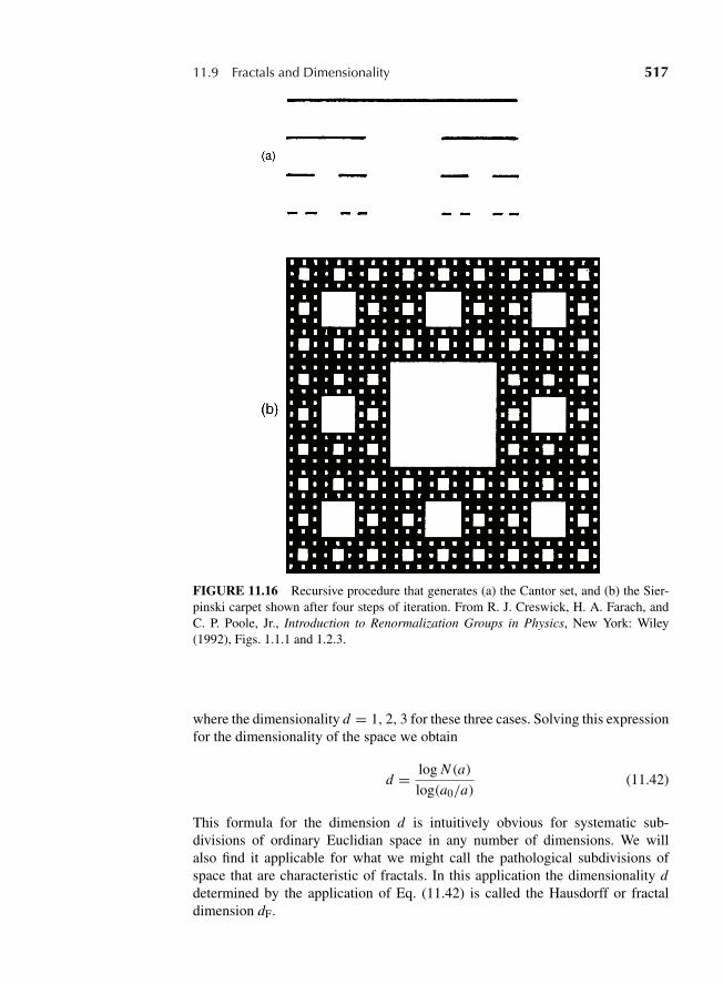
“M11 Goldstein ISBN C11” — 2011/2/15 — page 517 — #35
11.9 Fractals and Dimensionality 517
FIGURE 11.16 Recursive procedure that generates (a) the Cantor set, and (b) the Sier-pinski carpet shown after four steps of iteration. From R. J. Creswick, H. A. Farach, andC. P. Poole, Jr., Introduction to Renormalization Groups in Physics, New York: Wiley(1992), Figs. 1.1.1 and 1.2.3.
where the dimensionality d = 1, 2, 3 for these three cases. Solving this expressionfor the dimensionality of the space we obtain
d = log N (a)
log(a0/a)(11.42)
This formula for the dimension d is intuitively obvious for systematic sub-divisions of ordinary Euclidian space in any number of dimensions. We willalso find it applicable for what we might call the pathological subdivisions ofspace that are characteristic of fractals. In this application the dimensionality ddetermined by the application of Eq. (11.42) is called the Hausdorff or fractaldimension dF.
“M11 Goldstein ISBN C11” — 2011/2/15 — page 518 — #36
518 Chapter 11 Classical Chaos
Returning to the Cantor set, it involves subdividing a line originally of lengtha0, which is one-dimensional; that is, its Euclidean dimensionality dE = 1. Even-tually we feel by intuition that after an infinity of splittings the lines diminishto points that have a dimensionality of zero, and we say that the topologicaldimensionality of the Cantor set dT = 0. Further consideration, however, leadsus to think that the limit is never really reached, and that any large but finite num-ber of splittings still leaves an enormous number of infinitesimal one-dimensionalline segments present. This suggests that we need another way to assign dimen-sionality. This can be done by noting that at the nth level of subdivision the linesegments are of length a = a0/3n , and the number of them N (a) is 2n . Thus, wehave
a = 3−na0
N (a) = 2n . (11.43)
The fractal dimension or Hausdorff dimension dF is defined by the expression
dF = log N (a)
log(a0/a). (11.44)
This definition is chosen to be consistent with the results of Eq. (11.42). InsertingEqs. (11.43) into Eq. (11.44) to get for the Cantor set
dF = log 2
log 3= 0.6309. (11.45)
In the following discussion, we shall use dE for the initial Euclidean dimen-sion, dT , for the final limiting Euclidean (called topological) dimension, anddF for the counterintuitive non-integer dimension characteristic of fractals andstrange attractors. The fractal dimension dF is always between the two limitingvalues dT and dE ,
dT < dF < dE , (11.46)
and we see that this relation is satisfied for the Cantor set
0 < 0.6309 < 1. (11.47)
It will be instructive to determine the fractal dimensions of an initially two-dimensional (dE = 2) self-similar figure called the Sierpinski carpet of lineardimension a0 and area A0 = a2
0 illustrated in Fig. 11.16(b). To start, a square isdivided into nine squares of length a = a0/3 and area A = a2 = (a0/3)2, andthe middle square removed. Then each of the remaining eight squares is dividedinto nine smaller squares, and the middle one of each is removed. The figureshows the fourth step in this iteration process. At the nth level of subdivision, thesquares are of length a = a03−n and the number of them N (a) is 8n . Thus, wehave
“M11 Goldstein ISBN C11” — 2011/2/15 — page 519 — #37
11.9 Fractals and Dimensionality 519
a = a03−n
N (a) = 8n . (11.48)
The appropriate limit is a set of edges of squares delineating intersecting jaggedfilamentary lines, which become progressively thinner and thinner with succes-sive iterations, appearing to approach dT = 1. The fractal dimension dF is againgiven by Eq. (11.44),
dF = ln 8
ln 3= 1.8928, (11.49)
and Eq. (11.46) is satisfied by the Sierpinski carpet, as expected,
1 < 1.8928 < 2. (11.50)
In the general case of a fractal object in a dE -dimensional Euclidean space, wedefine the fractal dimensionality dF , also referred to as the capacity dimension,by a covering of the region occupied by the object by dE -dimensional spheres inaccordance with the expression
dF = limr→0
log N (r)
log (r0/r), (11.51)
where r is the radius of the dE -dimensional spheres. This definition is clearly in-dependent of the value of r0. If dE = 2, the sphere is a 2-sphere or circle of radiusr , and if dE = 1, the “sphere” is a 1-sphere or line segment of length 2r . In the caseof the Cantor set the object being covered by line segments or one dimensionalspheres of radius r = a/2 is the multitude of residual line segments after manysubdivisions. In the Sierpinski carpet case the covering is by circles of radiusr = a/
√2, where a circle of radius r = a0/
√2 covers the initial square before
any subdivisions. Fractal dimensions have been evaluated for many chaotic sys-tems.* For example, the logistic equation was quoted as having a strange attractordimension of 0.538, which is between the topological dimension dT = 0 corre-sponding to the individual points xn and the Euclidean dimension dE = 1 corre-sponding to the range of x given by Eq. (11.32). The driven-damped pendulumwith the equation of motion (11.25) exists in two-dimensional (x, y) Euclideanspace, and has one-dimensional orbits of the type shown in Fig. 11.11(a). Its frac-tal dimensionality determined from Liapunov exponents ranges from 1.2 to 1.4for various damping factors, which is between the values of dT = 1 and dE = 2that we just mentioned.
We saw in the previous section that chaotic systems exhibit a type of self-similarity, but less regular than in the case of systematically constructed fractalssuch as those in Fig. 11.16. This does, however, suggest that chaotic systemscould have a fractal-type nature, and that nonintegral dimensionality might be acharacteristic of chaos. This suggestion is correct. The fractal dimensionality dF
*See A. B. Cambel, Applied Chaos Theory, New York: Academic Press, 1993, p. 70; G. L Baker andJ. P. Gollub, Chaotic Dynamics, An Introduction, Cambridge, England: Cambridge University Press,1990.
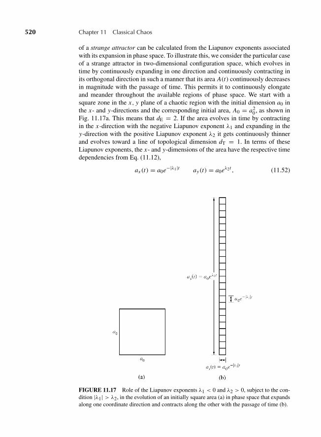
“M11 Goldstein ISBN C11” — 2011/2/15 — page 520 — #38
520 Chapter 11 Classical Chaos
of a strange attractor can be calculated from the Liapunov exponents associatedwith its expansion in phase space. To illustrate this, we consider the particular caseof a strange attractor in two-dimensional configuration space, which evolves intime by continuously expanding in one direction and continuously contracting inits orthogonal direction in such a manner that its area A(t) continuously decreasesin magnitude with the passage of time. This permits it to continuously elongateand meander throughout the available regions of phase space. We start with asquare zone in the x, y plane of a chaotic region with the initial dimension a0 inthe x- and y-directions and the corresponding initial area, A0 = a2
0 , as shown inFig. 11.17a. This means that dE = 2. If the area evolves in time by contractingin the x-direction with the negative Liapunov exponent λ1 and expanding in they-direction with the positive Liapunov exponent λ2 it gets continuously thinnerand evolves toward a line of topological dimension dT = 1. In terms of theseLiapunov exponents, the x- and y-dimensions of the area have the respective timedependencies from Eq. (11.12),
ax (t) = a0e−|λ1|t ay(t) = a0eλ2t , (11.52)
FIGURE 11.17 Role of the Liapunov exponents λ1 < 0 and λ2 > 0, subject to the con-dition |λ1| > λ2, in the evolution of an initially square area (a) in phase space that expandsalong one coordinate direction and contracts along the other with the passage of time (b).
“M11 Goldstein ISBN C11” — 2011/2/15 — page 521 — #39
11.9 Fractals and Dimensionality 521
and the area A(t) evolves in time as
A(t) = A0e(λ2−|λ1|)t , (11.53)
where A0 = a20 . Since λ1 is negative and λ2 is positive, it is necessary to have
|λ1| > λ2 so that the area (11.50) will continually decrease with time. The featureof a continuous decrease in the fractal area A(t) of Eq. (11.50) is analogous to thecontinuous decrease in overall length of the line segments in the Cantor set, andof the continuous decrease in the net remaining area in the Sierpinski carpet case,as the iterations progress to the limit n ⇒ ∞.
If we consider the evolved elongated area A(t) as containing a number N (t)of small squares of individual area A(t) = a2
x , as indicated in Fig. 11.17b thenwe have
A(t) = a20e−2|λ1|t , (11.54)
where λ1 is negative, and
N (t) = A(t)
A(t)= a2
0e(λ2−|λ1|)t
a20e−2|λ1|t = e(λ2+|λ1|)t . (11.55)
By analogy with Eq. (11.44), the strange attractor dimension dF , is given by
dF = log N (t)
log(a0/ax (t))= 1 + λ2
|λ1| , (11.56)
which has a nonintegral or fractal value. For the present case, λ2 < |λ1|, soEq. (11.46) is satisfied with 1 < dF < 2. Thus, a strange attractor is relatedto a fractal in the sense that its dimension is “strange”; that is, it is not aninteger.
There is a fundamental difference between the time evolution and the space-filling effect of regular trajectories and chaotic trajectories. We saw in Sec-tion 11.1 how the orbits of incommensurate oscillators can “fill” the space of atorus by ranging over the entire domain. However, technically speaking, theseregular orbits do not occupy any of the area of the toroidal surface because theyare one-dimensional curves without any width, meaning that the actual area takenup by them is zero. Chaotic orbits also range over their entire domain of phasespace, but they do so by occupying area in this space. What is strange is that themore the chaotic orbits “fill” phase space, the smaller the area that they actuallyoccupy (cf Eq. (11.53)). This makes it appropriate to refer to the domain overwhich the chaotic orbits roam as a strange attractor. The onset of chaos may belooked upon as the increase in the dimension of a regular orbit from its topolog-ical value dT = 1 to its fractal value 1 < dF < 2 as it begins to occupy spacein an area of Euclidean dimension dE = 2. The fractal dimension may be lookedupon as an index of how much space is occupied by the fractal orbit. We shouldof course continue to bear in mind the fact that the main difference between the
“M11 Goldstein ISBN C11” — 2011/2/15 — page 522 — #40
522 Chapter 11 Classical Chaos
space-“filling” aspects of regular and chaotic orbits is that in the regular incom-mensurate case the space is “filled” in a systematic manner by the predeterminedspiraling motion around the torus, while in the chaotic case the orbit “fills” spacein a random, meandering, manner.
This nonintuitive manner in which chaotic orbits in a sense spread out moreand more, and in another sense become more attenuated, as they develop in timeis very analogous to the behavior of fractals. We saw above how the Cantor setand the Sierpinski carpet illustrated in Fig. 11.16 both become more disperseand more attenuated as they go through successive iterations, always remainingfinite throughout the process. There is an analogue of the Sierpinski carpet inthree-dimensional Euclidian space called a Sierpinski sponge, which evolves inan analogous manner through an iterative process, dispersing through space whilelosing volume in accordance with a fractal dimension. Chaotic trajectories areindeed closely related to fractals.
In our treatment of the quantitative aspects of chaos, we have placed moreemphasis on the fractal property of nonintegral dimensionality than we have onits property of self-similarity. In the applications of fractals outside the domainof classical mechanics, the emphasis is often more on the self-similarity aspect.Many books display beautiful pictures of precisely drawn figures that illustrateself-similarity down to infinite levels of subdivision, such as the Sierpinski carpetsketched in Fig. 11.16. There are also examples from nature, such as the dendriticgrowth of the branches of a tree, in which the self-similarity is more approximateand irregular.
DERIVATIONS
1. Show that the system yn+1 = 1 − γ y2n with −1 < y < 1 and 0 < γ ≤ 2 can be
transformed to the logistic equation (11.31) by the substitution y = cx + d . Find γ ,c, and d in terms of the control parameter a of the logistic equation.
2. Show that the Henon–Heiles Hamiltonian (11.17) can be written in polar coordinatesas
H = p2r
2m+ p2
θ
2mr2+ 1
2kr2 + 1
3λr3 sin 3θ.
This form explicitly exhibits the threefold symmetry.
3. Show that for the energy E = 16 , the bounding equipotential (V (r, θ) = 1
6 ) for thedimensionless Henon–Heiles potential
V (r, θ) = 12r2 + 1
3r3 sin 3θ,
forms an equilateral triangle in the x, y plane (cf. Fig. 11.6).
4. Show that Eq. (11.34b) follows from inserting Eq. (11.34a) into Eq. (11.31). In addi-tion, show that the stability range given in the text (cf. Eq. (11.35)) also follows.
“M11 Goldstein ISBN C11” — 2011/2/15 — page 523 — #41
Exercises 523
EXERCISES
Most of the following exercises are best completed using a personal computerable to run programs such as MapleTM, MathematicaTM, or MaximaTM. In theseexercises the notation dz/dt = z is used.
5. Find the first three bifurcations for the system yn+1 = 1 − by2n , where −1 < y < 1
and 0 < b ≤ 2.
6. In an attempt to predict weather patterns, Edward N. Lorenz developed a model in1969 with the following three coupled equations (Lorenz model) in x(t), y(t), andz(t):
dx
dt= σ(y − x),
dy
dt= r x − y − xz,
dz
dt= xy − bz,
where σ , r , and b are positive constants and x , y, and z are real. Lorenz chose, forphysical reasons, σ = 10 and b = 8
3 , and the parameter r is increased from 0. Letx(0) = 2, y(0) = 5, and z(0) = 5. Investigate the behavior for
(a) r = 0, 10, and 20, 0 ≤ t < 20.
(b) r = 28, 0 ≤ t < 20, where chaotic behavior sets in for t ≈ 7.
In both cases, investigate the trajectories by using either three-dimensional plots ofthe coordinates x(t), y(t), z(t) for different time steps or, if your numeric programsdo not generate such plots, plot x(t) versus t .
7. A system of equations simpler than the Lorenz equations of Exercise 6 were proposedby O. E. Rossler in 1976, with only one nonlinear system coupling term. This systemhad no physical intent except to show chaos.
dx
dt= −(y + z),
dy
dt= x + ay,
dz
dt= b + z(x − c),
with a, b, and c positive constants and x(t), y(t), and z(t) real.
(a) Take a = b = 0.2, and initial conditions x(0) = −1, y(0) = z(0) = 0. Investigatethe effects of changing c around c = 5.7, holding a and b fixed.
(b) Take a = b = 0.2, c = 5.7 and investigate the effects of changing the initialconditions starting with x(0) = −1, y(0) = z(0) = 0.
8. The general forced damped oscillator equation studied by F. Duffing in 1918 (Duffingoscillator) can be written as
d2x
dt2+ 2γ
dx
dt+ αx + βx3 = F cosωt.
(a) Take α = 1, β = 0.2, γ = 0, F = 4.0, [dx/dt]t=0 = 0 and choose a setof values of xt=0 and ω to show that the amplitude (absolute magnitude of themaximum x) of the steady-state oscillation shows hysteresis. This is best done byplotting the behavior for increasing ω until there is a jump in the amplitude andthen continuing the plot for slowly decreasing ω from a value slightly larger thanwhere the jump occurred.
(b) Having solved part (a), pick a value of ω in the range of the jump and slightlyvary F to determine how the amplitude varies for a fixed ω as F is changed.
“M11 Goldstein ISBN C11” — 2011/2/15 — page 524 — #42
524 Chapter 11 Classical Chaos
9. Study the van der Pol equation (11.11),
md2x
dt2− ε(1 − x2)
dx
dt+ mω2
0x = F cosωDt
(a) For the initial conditions near x = 0.5 and dx/dt = 0 for the values of ε = 0,0.1, 0.2, and 0.3. Plot x(t) as a function of time to determine empirically the rateat which the orbit approaches the attractor at x = 1.
(b) Repeat for the initial conditions x = 1.5, dx/dt = 0.
10. Construct the Poincare section xp for the particular Duffing oscillator
d2x
dt2+ 0.7
dx
dt+ x3 = 0.75 cos t,
where p = x = dxdt , with initial conditions x(0) = dx
dt (0) = 0.
11. Construct the Poincare section, as in Exercise 10, for the inverted Duffing oscillator,
d2x
dt2+ 0.5
dx
dt− x + x3 = F cos t,
for values of F in the range 0.24 to 0.35. This oscillator is said to be inverted becausethe coefficient of the linear term is negative.
12. The diffusion equation is ∂u/∂t = η∇2u where u(x, t) is the density and η is thediffusion constant. The model of diffusion by Witten and Sadler can be approximatedfor numerical integration in two dimensions by considering a two-dimensional squarelattice and defining the size of a cluster as the minimum radius that includes all of itsparticles. Mathematically perform the following:
(a) Place a particle at the center of a 25 × 25 lattice of spacing a.
(b) Place a particle at a random position away from the center but not adjacent tothe center and allow this particle to randomly move one location at a time until iteither leaves the lattice or becomes adjacent to the original particle. For the lattereventuality, draw a circle centered on the center of the cluster that just includesthese two particles. Call this radius Rmin. After completing this step Rmin = a/2.
(c) Repeat this process by adding additional particles at random, increasing Rmin ifnecessary to include all adjacent particles.
(d) After a reasonable number of particles, N , are aggregated, calculate the fractaldimension, D, by the rule
D = ln N
ln Rmin.
13. Construct a Poincare section for the Henon–Heiles potential. It is suggested that youmake the plot in the y y plane so that you can compare your results with Figs. 11.7and 11.8. Choose an energy, E , and initial conditions, x = 0 and x = 0, and initialconditions on y and y to satisfy the energy condition and find the boundary curve.Relax the condition on x and choose conditions on x , y, and y that satisfy the energycondition for x = 0. Integrate the equations of motion to find the crossings.
(a) Choose E = 112 , y0 = 0.01, y0 = 0.02, and x0 = 0. Use the energy equation to
determine x0. Integrate the equations to find the values of t where x(t) ≈ 0 saving
“M11 Goldstein ISBN C11” — 2011/2/15 — page 525 — #43
Exercises 525
the values t , x(t) ≈ 0, x(t), y(t), y(t). Find the first 27 crossings and comparewith Fig. 11.7.
(b) Repeat this process for E = 18 and plot the chaotic behavior.
14. Construct the entries in Table 11.1 for a = 3.55 and a = 3.60.
15. Refer to Figs. 11.13 and 11.15 for the logistic equation. Find the values of the threecycle attractors embedded in the region of chaos. Use the control parameter a = 3.83.Also find the values of the next higher cycle obtained for a larger control parameter inthis same embedded region of normality.
16. Show that in the control parameter range between the first and second bifurcations ofthe logistic equation the two final values of the attractors, xn and xn+1, such as thosegiven by Eq. (11.36) satisfy the cubic equation
a3x2(2 − x)− a2(a + 1)x + (a2 − 1) = 0.
“M12 Goldstein ISBN C12” — 2011/2/15 — page 526 — #1
C H A P T E R
12 Canonical Perturbation Theory
12.1 INTRODUCTION
Almost all of the problems in classical mechanics discussed in Chapters 1–10,whether in the text or in the exercises, have had exact solutions. Nevertheless,it should be clear from Chapter 11 on chaos that the great majority of problemsin classical mechanics cannot be solved exactly. We have found solutions for thetwo-body Kepler problem, but with the exception of a few special cases the clas-sical motion of three-point bodies acted upon only by their mutual gravitationalforces has proved intractable (see Section 3.12). Even for two bodies the solutionsare implicit; no closed explicit formula can be found for the coordinates as a func-tion of time (cf. Section 3.8). There is thus considerable incentive for developingapproximate methods of solution.
It often happens, fortunately, that in a physical problem that cannot be solveddirectly the Hamiltonian differs only slightly from the Hamiltonian for a prob-lem that can be solved rigorously. The more complicated problem is then saidto be a perturbation of the soluble problem, and the difference between the twoHamiltonians is called the perturbation Hamiltonian. Perturbation theory consistsof techniques for obtaining approximate solutions based on the smallness of theperturbation Hamiltonian and on the assumed smallness of the changes in the so-lutions. We know from the discussion in Chapter 11 that even when the change inthe Hamiltonian is small, the eventual effect of the perturbation on the motion canbe large. This suggests that any perturbation solution must be carefully analyzedto be sure that it is physically correct.
The development of perturbation theory goes back to the earliest days of ce-lestial mechanics. Newton realized, for example, that most of the oscillations inthe Moon’s motion were the result of small changes in the attraction to the Sunas the Moon revolves about Earth. His initial attempts at a lunar theory includingthese effects corresponded roughly to a form of perturbation theory. Many ofthe subsequent developments in the formal structure of classical mechanics, suchas Hamilton’s canonical theory, stemmed in large measure from the desire toperfect perturbation techniques in celestial mechanics. The need for predictinghighly accurate orbits for space vehicles and the enormously increased capacityfor numerical computations have spurred further improvements in perturbationtheory.
Classical perturbation theory can be divided into two approaches: time-dependent and time-independent perturbations. The terminology is chosen with
526
“M12 Goldstein ISBN C12” — 2011/2/15 — page 527 — #2
12.2 Time-Dependent Perturbation Theory 527
an eye to perturbation theory as developed for quantum mechanics, and indeedthere are many points of analogy between the classical perturbation techniquesand their quantum counterparts. Generally speaking, classical perturbation theoryis considerably more complicated than the corresponding quantum mechanicalversion. We shall treat time-dependent perturbation first as being the easier formto understand. While perturbation theory can be developed for all versions ofclassical mechanics, it is simplest to use the Hamilton–Jacobi formulation.
12.2 TIME-DEPENDENT PERTURBATION THEORY
Let H0(q, p, t) represent the Hamiltonian for the soluble, unperturbed problem.We imagine the solution has been obtained through Hamilton’s principal functionS(q, α, t), which generates a canonical transformation in which the new Hamilto-nian, K0, for the unperturbed problem is identically zero. The transformed canon-ical variables, (α, β), are then all constant in the unperturbed situation. Now letus consider the perturbed problem for which we write the Hamiltonian as (cf.Eq. (11.8))
H(q, p, t) = H0(q, p, t)+�H(q, p, t). (12.1)
As has been emphasized before, the canonical property of a given coordinatetransformation is independent of the particular form of the Hamiltonian. There-fore, the transformation
(p, q)→ (α, β)
generated by S(q, α, t) remains a canonical transformation for the perturbedproblem. Only now the new Hamiltonian will not vanish and the transformedvariables may not be constant. For the perturbed problem, the transformed Hamil-tonian will be
K (α, β, t) = H0 +�H + ∂S
∂t= �H(α, β, t). (12.2)
Hence, the equations of motion satisfied by the transformed variables are now
αi = −∂�H(α, β, t)
∂βi, βi = ∂�H(α, β, t)
∂αi. (12.3)
Equations (12.3) are rigorous; no approximation has yet been made. If the set of2n equations can be solved for αi and βi as functions of time, then the equationsof transformation between (p, q) and (α, β) give q j and p j as functions of time,that is, solve the problem. However, the exact solution of Eqs. (12.3) is usuallyno less difficult to obtain than for the original equations of motion. The use ofEqs. (12.3) as an alternative approach to the rigorous solution is therefore notparticularly fruitful.

“M12 Goldstein ISBN C12” — 2011/2/15 — page 528 — #3
528 Chapter 12 Canonical Perturbation Theory
In the perturbation technique, however, advantage is taken of the fact that �His small. The quantities (α, β), while no longer constant, therefore do not changerapidly, at least compared to the explicit dependence of�H on time. A first-orderapproximation to the time variation of (α, β) is obtained by replacing α and β onthe right-hand side of Eqs. (12.3) by their constant unperturbed values:
α1i = −∂�H(α, β, t)
∂βi
∣∣∣∣0, β1i = ∂�H(α, β, t)
∂αi
∣∣∣∣0. (12.4)
Here α1i and β1i stand for the first-order perturbation solutions for αi and βi ,respectively, and the vertical lines with subscript 0 indicate that after differentia-tion α and β are to be replaced by their unperturbed forms; that is, the constants(α0, β0). Equations (12.4) can be placed in matrix form by designating g as thecolumn matrix of the β and α canonical variables, so that
gi = J∂�H(g, t)
∂g
∣∣∣∣0, (12.5)
where J is the matrix given by Eq. (8.38a). Equations (12.4) can now be integrateddirectly to yield the α1 and β1 as functions of time. Through the transformationequations, we then obtain (q, p) as functions of time to first order in the pertur-bation. Clearly, the second-order perturbation is obtained by using the first-orderdependence of α and β on time in the right-hand sides of Eqs. (12.4), and soon. In general, the nth-order perturbation solution is obtained by integrating theequations (in matrix form) for gn given by
gn = J∂�H(g, t)
∂g
∣∣∣∣n−1
. (12.6)
As a trivial example of these procedures, let us consider as the unperturbedsystem the force-free motion in one dimension of a particle of mass m. Theunperturbed Hamiltonian is
H0 = p2
2m.
The momentum p is clearly conserved; call its constant value α. For this systemthe Hamilton–Jacobi equation is
1
2m
(∂S
∂x
)2
+ ∂S
∂t= 0. (12.7)
Because the system is conservative and x is cyclic, we know immediately that thesolution for Hamilton’s principal function is
S = αx − α2t
2m. (12.8)

“M12 Goldstein ISBN C12” — 2011/2/15 — page 529 — #4
12.2 Time-Dependent Perturbation Theory 529
The transformed momentum is α; the transformed constant coordinate is
Q ≡ β = ∂S
∂α= x − αt
m
or
x = αt
m+ β, (12.9)
the expected solution for the force-free motion. While Eq. (12.9) is obviousa priori, this formal derivation via the Hamilton–Jacobi equation at least showsthat α and β, so defined, form a canonical set.
Now suppose the perturbation Hamiltonian is
�H = mω2x2
2, (12.10)
where ω is some constant. The total Hamiltonian is
H = H0 +�H = 1
2m(p2 + m2ω2x2). (12.11)
We are thus considering the harmonic oscillator potential as a perturbation onforce-free motion! In terms of the α, β variables, the perturbation Hamiltonian,by Eq. (12.9), is
�H = mω2
2
(αt
m+ β
)2
. (12.12)
In the perturbed system, the equations of motion for α, β are (cf. Eqs. (12.3))
α = −mω2(αt
m+ β
), (12.13a)
β = ω2t
(αt
m+ β
). (12.13b)
Note that
β + t
mα = 0. (12.14)
A rigorous solution of Eqs. (12.13) can be obtained by taking the time derivativeof Eq. (12.13a):
α = −ω2α − mω2(β − αt
m
)= −ω2α. (12.15)
“M12 Goldstein ISBN C12” — 2011/2/15 — page 530 — #5
530 Chapter 12 Canonical Perturbation Theory
Thus, α in the perturbed system rigorously has a simple harmonic variation withtime. From Eqs. (12.13a) and (12.9), it follows x = −α/(mω2), and hence thesolution for x is also simple harmonic motion. Considered as rigorous equationsof motion, Eqs. (12.13) therefore lead properly to the correct and well-knownsolution.
But now let us treat mω2 (≡ k, the force constant) as a small parameter andseek perturbation solutions. The first-order perturbation is obtained by replacingα and β on the right by their unperturbed values α0 and β0. For simplicity, weshall take x = 0 initially, so that β0 = 0; the initial value of p is then α0. Thefirst-order equations of motion are then
α1 = −ω2α0t, β1 = α0ω2t2
m, (12.16)
with immediate solutions
α1 = α0 − ω2α0t2
2, β1 = α0ω
2t3
3m. (12.17)
Solutions for x and p to first order are then
x = α1t
m+ β1 = α0
mω
(ωt − ω3t3
6
), (12.18a)
and
p = α1 = α0
(1 − ω2t2
2
). (12.18b)
Substituting Eqs. (12.17) for α and β on the right-hand side of Eqs. (12.13), thesecond-order equations of motion become
α2 = −α0ω2
(t − ω2t3
6
),
β2 = α0ω2
m
(t2 − ω2t4
6
), (12.19)
with solutions
α2 = α0 − ω2α0t2
2+ ω2α0t4
24,
β2 = α0ω2
m
(t3
3− ω2t5
30
). (12.20)
“M12 Goldstein ISBN C12” — 2011/2/15 — page 531 — #6
12.2 Time-Dependent Perturbation Theory 531
The corresponding second-order solutions for x and p are
x = α0
mω
(ωt − ω3t3
3+ ω2t5
5
),
p = α0
(1 − ω2t2
2+ ω4t4
4
). (12.21)
By now we have enough to see where the nth-order solution is going. The quan-tities in the parentheses in Eqs. (12.21) are the first three terms in the expansionof the sine and cosine, respectively. In the limit of infinite order of perturbation,clearly
x → α0
mωsinωt, p → α0 cosωt,
which are the standard solutions consistent with the initial conditions.The constant transformed variables (α, β) incorporate information on the pa-
rameters of the unperturbed orbit. Thus, if the Kepler problem in three dimensionsdescribes the unperturbed system, then a suitable set of (α, β) are the Delaunayvariables, that is, the constant action variables J1 and the constant terms in the cor-responding angle variables wi . We have seen in Section 10.8 that the Delaunayvariables are simply related to the orbital parameters—semimajor axis, eccentric-ity, inclination, and so on. The effect of the perturbation is to cause these parame-ters to vary with time. If the perturbation is small, the variation of the parameterswithin one period of the unperturbed motion will also be small. Time-dependentperturbation theory thus implies a picture in which the perturbed system movesduring small intervals of time in an orbit of the same functional form as the unper-turbed system, an orbit whose parameters however will be changing in time. Theunperturbed orbit along which the system is momentarily traveling is sometimesdescribed as the “osculating orbit.” In position and tangent direction, it matchesinstantaneously the true trajectory.
As determined by a perturbation treatment, the parameters of the osculatingorbit may vary with time in two ways. There may be a periodic variation, inwhich a parameter comes back to an initial value in a time interval that to firstorder is usually the period of the unperturbed motion. Or there may remain anet increment in the value of the parameter at the end of each successive orbitalperiod—and the perturbed parameters are said to exhibit secular change. Peri-odic effects of perturbation do not change the average parameters of the orbit;on the whole, the trajectory remains looking much like the unperturbed orbit. Asecular change, no matter how small per orbital period, means that eventually,after many periods, the instantaneous perturbed parameters may be quite differ-ent from their unperturbed values. Therefore, the major interest in a perturbationcalculation will often be in the secular terms only, and the periodic effects may beeliminated early in the game by averaging the perturbation over the unperturbedperiod. Effectively, this is what was done in Section 5.8 when the perturbing
“M12 Goldstein ISBN C12” — 2011/2/15 — page 532 — #7
532 Chapter 12 Canonical Perturbation Theory
gravitational potential of the oblate Earth was averaged over the satellite period(cf. Eq. (5.90)).*
Often we would like to determine the time dependence of the orbital “con-stants”—for example, eccentricity, or inclination—directly, rather than throughthe intermediary of the canonical set (α, β). This can be done easily through thePoisson bracket formalism. Let ci be any set of 2n independent functions of the(α, β) constants of the unperturbed system:
ci = ci (α, β). (12.22)
One or more of the ci may be the desired orbital parameters. Then in the perturbedsystem the time dependence of the ci quantities is determined by the equations ofmotion
ci = [ci , K ] = [ci ,�H ]. (12.23)
But �H(α, β, t) may equally well, by the inverse of Eqs. (12.22), be considereda function of the c’s and t , so that (cf. Eq (9.68))
[ci ,�H ] ≡ ∂ci
∂hJ∂�H
∂h= ∂ci
∂hJ∂�H
∂c j
∂c j
∂h
= [ci , c j ]∂�H
∂c j.
Hence,
ci = [ci , c j ]∂�H
∂c j. (12.24)
As with Eqs. (12.3), Eqs. (12.24) are rigorous equations of motion for theci ’s. They become first-order perturbation equations when the right-hand sides,including the Poisson brackets, are evaluated for the unperturbed motion. In gen-eral the nth-order perturbation is obtained when the right-hand sides are evaluatedin terms of the (n−1)st order of perturbation. Equations (12.24) thus correspond,in generalized form, to Eqs. (12.6).
*The circumstances are often be more complicated than as described in this paragraph. For example,the periodic variation of orbital parameters can exhibit more than one period. This would obviouslyoccur when the perturbing potential has its own intrinsic periodicity, for example, the varying pertur-bation of the Sun’s gravity on Earth–Moon orbit as Earth revolves around the Sun. Multiply periodicbehavior can also appear through interactions between perturbations. Thus, the periodic perturbationof satellite parameters can show both short and long periods, and it is necessary to average over bothkinds of periods to find the secular perturbation effects. Sometimes the dividing line between periodicand secular perturbations becomes a bit vague. What may appear as a secular perturbation in first orderwill at times on closer examination turn out to be a periodic perturbation with a very long period, aswe discovered in Section 11.1 with the harmonic oscillator perturbation calculation. Depending on thepurpose of the calculation, it may still be advisable to treat it as a secular perturbation term. Nonethe-less, the distinction between periodic and secular terms remains useful and normally straightforward,especially in first-order perturbation theory.

“M12 Goldstein ISBN C12” — 2011/2/15 — page 533 — #8
12.3 Illustrations of Time-Dependent Perturbation Theory 533
A version of Eqs. (12.24) expressed in Lagrange brackets (cf. Eq. (9.79)) isoften found in the literature of celestial mechanics. Multiply the equation for ci ,by the Lagrange bracket {ck, ci } and sum over i :
{ck, ci }ci = {ck, ci }{ci , c j } ∂�H
∂c j.
By the theorem expressed in Eq. (9.83), this reduces to
−∂�H
∂c j= {c j , ci }ci . (12.25)
Historically, the perturbation equations of celestial mechanics are expressed interms of the disturbing function R, defined as −�H , so that Eqs. (12.25) appear as
∂R
∂c j= {c j , ci }ci . (12.25′)
Equations (12.24) or (12.25) are frequently denoted as the Lagrange perturbationequations.
12.3 ILLUSTRATIONS OF TIME-DEPENDENT PERTURBATION THEORY
A. Period of the plane pendulum with finite amplitude. In the limit of small oscil-lations a plane pendulum behaves like a harmonic oscillator and is isochronous;that is, the frequency is independent of the amplitude. As the amplitude increases,however, the correct potential energy deviates from the harmonic oscillator form,and the frequency shows a small dependence on the amplitude. The small differ-ence between the potential energy and the harmonic oscillator limit can be con-sidered as the perturbation Hamiltonian, and the shift in frequency derived fromthe time variation of the perturbed phase angle.
The Hamiltonian for a plane pendulum, consisting of a mass point m at the endof a weightless rod of length l, is
H = p2
2ml2+ mgl(1 − cos θ), (12.26)
where, for simplicity, the momentum conjugate to θ is denoted by p. Expandingthe cos θ term in a Taylor series, the Hamiltonian can be written as
H = p2
2ml2+ mglθ2
2
(1 − θ2
12+ θ4
360− · · ·
). (12.27)
The small amplitude limit consists of dropping all but the first term in the paren-theses. We can get an idea of the magnitude of the correction terms by introducing
“M12 Goldstein ISBN C12” — 2011/2/15 — page 534 — #9
534 Chapter 12 Canonical Perturbation Theory
artificially a parameter
θ21 = 2E
mgl(12.28)
and the related parameter
λ = θ21
6= E
3mgl
The series in the parentheses (cf. (12.27)) then looks like
1 − λ
2
(θ
θ1
)2
+ λ2
10
(θ
θ1
)2
− · · · .
Now, the ratio θ/θ1 rises to the order of unity at the maximum amplitude. Indeed,θ1 is the maximum amplitude of oscillation when E , and therefore the amplitude,is small. Hence, the rate of convergence of the expansion is determined by themagnitude of λ.
If only one correction term is retained, first-order perturbation introduces termsof the order λ in the motion. Second-order perturbation with the same perturbationHamiltonian introduces λ2 terms. Thus, to obtain modifications of the motionconsistently correct to λ2, we would have to compute second-order perturbationon the λ term in the Hamiltonian, and first-order perturbation on the λ2 term inthe Hamiltonian. We shall here content ourselves with a consistent treatment toorder λ; that is, retain only the first correction term in the Hamiltonian and carryout a first-order perturbation solution.
The unperturbed Hamiltonian derived from Eq. (12.27) can be put in the formof a harmonic oscillator by writing it as (cf. Eq. (10.18))
H = 1
2I(p2 + I 2ω2θ2), (12.29)
where I = ml2, the moment of inertia of the pendulum, and
ω2 = mgl
I= g
l. (12.30)
A suitable set of canonical variables corresponding to a vanishing K for theunperturbed system are the action variable J and the phase angle β in the anglevariable:
w = νt + β, ν = ω
2π. (12.31)
The effect of the perturbation is to cause both J and β to vary with time. Theequations of transformation relating p and θ to J and β, respectively, have alreadybeen given in Eqs. (10.96) and (10.97), which here take the form
θ =√
J
π Iωsin 2π(νt + β),
“M12 Goldstein ISBN C12” — 2011/2/15 — page 535 — #10
12.3 Illustrations of Time-Dependent Perturbation Theory 535
p =√
I Jω
πcos 2π(νt + β). (12.32)
In the unperturbed system J and β are constant and Eqs. (12.32) constitute thecomplete solutions for the motion. But the equations remain valid for the per-turbed case, only J and β have time dependencies to be determined.
The unperturbed Hamiltonian is H0 = Jν, but the perturbation Hamiltoniantakes the form
�H = −mgl
24θ4 = − J 2
24π2ml2sin4 2π(νt + β). (12.33)
The first-order time dependence of β and J are to be obtained from
β = ∂�H
∂ J, J = −∂�H
∂β, (12.34)
where on the right-hand side of each equation the unperturbed solutions for J andβ are to be used; that is, J and β are considered constant. Thus,
β = − J
12π2ml2sin4 2π(νt + β). (12.35)
Equation (12.35) says that to first order, β varies over the cycle of the unperturbedoscillation. But there is a net value for β when averaged over a complete cycle,for the average of sin4 is 3
8 . Hence, β exhibits a secular perturbation at a constantrate given by
β = − J
32π2ml2. (12.36)
Viewed over times long compared to the unperturbed period, β has a time depen-dence
β = βt + β0. (12.37)
Such a variation, when inserted in Eq. (12.32), says that, on average, the first-ordersolution is still simple-harmonic with a frequency
ν′ = ν + β.
Now, in the unperturbed motion
J = 2πE
ω= 2πω
El
g,
“M12 Goldstein ISBN C12” — 2011/2/15 — page 536 — #11
536 Chapter 12 Canonical Perturbation Theory
so that β, Eq. (12.36), becomes
β = − ωE
16πmgl= −νθ
21
16. (12.38)
The first-order fractional change in the frequency at a finite amplitude θ1 istherefore
�ν
ν= β
ν= − θ
21
16, (12.39)
a well-known result that can also be obtained by approximating the elliptic-function representation of the motion.
From Eqs. (12.33) and (12.34), it is seen that to first order the time variation ofJ is
J = − J 2
3πml2sin3 2π(νt + β) cos 2π(νt + β).
The average of sin3 φ cosφ over even a half period of φ is zero; hence, J showsno secular perturbation. We would expect this result physically, as J is a measureof the amplitude of the oscillations (cf. Eqs. (12.32)), and the perturbation wouldnot be such as to cause the amplitude to grow or decay with time.
B. A central force perturbation of the bound Kepler problem. In Exercise 21,Chapter 3, it was shown rigorously that if a potential with a 1/r2 form is addedto the Coulomb potential, the orbit in the bound problem is an ellipse in a rotat-ing coordinate system. In effect, the ellipse rotates, and the periapsis appears toprecess. Here we will find the precession rate by first-order perturbation theory,considering a somewhat more general form for the perturbing potential.
Suppose the total potential is
V = −k
r− h
rn, (12.40)
where n is an integer greater than or equal to +2. The constant h will be assumedto be such that the second term is a small perturbation on the first for the range ofr considered. The perturbation Hamiltonian is thus
�H = − h
rn, n ≥ 2. (12.41)
In the unperturbed problem the angular position of the periapsis in the plane of theorbit is given by the constant ω = 2πw2 (cf. Eq. (10.166)). With the perturbation,ω has a time dependence determined by
ω = 2π∂�H
∂ J2= ∂�H
∂l, (12.42)
“M12 Goldstein ISBN C12” — 2011/2/15 — page 537 — #12
12.3 Illustrations of Time-Dependent Perturbation Theory 537
using the relation J2 = 2πl (Eq. (10.156)). First-order perturbation results areobtained by evaluating �H , and the derivative, in terms of the unperturbedmotion. Further, the instantaneous change in ω is rarely of interest. In most situa-tions where the perturbation formalism is of value, ω is so small the change in ωis difficult or impossible to perceive within a single orbital period, and it is suffi-cient to measure only the secular change in ω after many orbits. Therefore, whatis wanted is ω averaged over a time interval τ , the period of the unperturbed orbit:
ω ≡ 1
τ
∫ τ
0
∂�H
∂ldt.
The derivative can be taken outside the integral sign, since τ is a function of J3only (Eq. (10.142) combined with Eq. (10.146)), whereas the derivative is withrespect to l = J2/2π . Hence,
ω = ∂
∂l
(1
τ
∫ τ
0�H dt
)= ∂�H
∂l. (12.43)
But the time average of the perturbation Hamiltonian is here
�H = −h
(1
rn
)= −h
τ
∫ τ
0
dt
rn. (12.44)
By using the conservation of angular momentum in the form l dt = mr2 dψ , theintegral can be converted into one over ψ :
�H = −mh
lτ
∫ 2π
0
dψ
rn−2(12.45)
= −mh
lτ
(mk
l2
)n−2 ∫ 2π
0
[1 + e cos(ψ − ψ ′)
]n−2dψ, (12.45′)
where r has been expressed in terms of ψ through the orbit equation, Eq. (3.56)(with ψ used in place of θ ). In general, only terms involving even powers of theeccentricity e will give nonvanishing contributions to the integral. The derivativewith respect to l also involves e and its powers, since, by Eq. (10.159), e is afunction only of J2 and J3.
Two special cases are of particular interest. One occurs when n = 2, mentionedbriefly at the start of this illustration. The average perturbation Hamiltonian is thensimply
�H = −2πmh
lτ,
and the secular precession rate is
ω = 2πmh
l2τ, (12.46)
which agrees with Exercise 21 of Chapter 3.
“M12 Goldstein ISBN C12” — 2011/2/15 — page 538 — #13
538 Chapter 12 Canonical Perturbation Theory
The other case of interest is for n = 3 (a perturbation potential of 1/r3), forwhich Eq. (12.45′) reduces to
�H = −2πm2hk
l3τ
and
ω = 6πm2hk
l4τ. (12.47)
What makes this choice of n of particular significance is that general relativitytheory predicts a correction to Newtonian motion that can be construed as anr−3 potential. The so-called Schwarzschild spherically symmetric solution of theEinstein field equations corresponds for weak fields to an additional Hamiltonianterm in the Kepler problem of the form of Eq. (12.41), with n = 3 and
h = kl2
m2c2, (12.48)
so that Eq. (12.47) becomes
ω = 6πk2
τ l2c2. (12.49)
To apply Eq. (12.49) to the secular precession rate for the precession of a bodyrevolving around the Sun, k is set equal to G Mm and Eq. (3.63), valid for theunperturbed ellipse, is used
l2 = mka(1 − e2). (12.50)
Equation (12.49) can then be put in the form
ω = 6π
τ(1 − e2)
(R
a
), (12.51)
where R is the so-called gravitational radius of the Sun is
R = G M
c2= 1.4766 km. (12.52)
For the planet Mercury, τ = 0.2409 sidereal years, e = 0.2056, and a =5.790 × 10⁷ km; Eq. (12.51) then predicts a precession of the perihelion ofMercury arising from general relativity at an average rate of
ω = 42.98′′/century.
“M12 Goldstein ISBN C12” — 2011/2/15 — page 539 — #14
12.3 Illustrations of Time-Dependent Perturbation Theory 539
The observed secular precession of the perihelion of Mercury is over 100 timeslarger than this value, namely 5599.74± 0.41′′/century. Most of this is due to theprecession of the equinoxes, of the remainder, about 531.54′′/century arises fromperturbations of the orbit of Mercury by other planets. Only after these two sets ofeffects are subtracted from the observed precession does the small general relativ-ity effect of approximately 43′′/century become visible. The currently acceptedobservational value is stated to be 43.1′′ ± 0.5′′/century; the deviation from thetheoretical prediction is not considered significant.
One point remains to be made. In the application to relativistic effects, theconstant h, Eq. (12.48), is a function of the value of l. It might be asked thereforethat in finding ω, why doesn’t the derivative with respect to l act also on h? Thekey here is that h is not functionally dependent on l as a canonical momentum,Equation (12.48) says only how the value of the constant h is determined in termsof the value of the orbit parameter l. In other words, the perturbation potential isa function of the dynamical variables only through r ; it is not to be construed asvelocity dependent.
C. Precession of the equinoxes and of satellite orbits. The family of problems tobe considered here was discussed previously in Section 5.8, which bears the sametitle. We wish to describe the relative motion of two bodies interacting throughtheir gravitational attraction, one a spherically symmetric or point body, the otherbeing slightly oblate with a resultant gravitational quadrupole moment. The effectof the slight oblate shape of Earth is physically that the torques exerted by theSun and Moon on the equatorial bulge cause Earth’s rotation axis to precess veryslowly. Reciprocally, the effect on an object orbiting around Earth, such as theMoon or an artificial satellite, is to cause the plane of the orbit to precess aboutthe figure axis of Earth. The small magnitude of the gravitational quadrupole term,manifested by the very slow rate of precession, suggests that a perturbation treat-ment should be an extremely good approximation. We shall actually examine hereonly the case of the perturbation of a satellite’s orbit; the reciprocal phenomenonof the precession of the equinoxes proceeds very similarly (though with differentnotation) from the same perturbation Hamiltonian, and will be left for the exer-cises.
Since the emphasis here will be on a point satellite moving about a much moremassive Earth, the notation of Section (5.8) will be reversed here and m usedto denote the mass of the satellite while M stands for Earth’s mass. The totalpotential acting on the satellite, by Eq. (5.88), is then
V = −k
r+ k
M
(I3 − I1)
r3P2(γ ), (12.53)
where k = G Mm, P2(γ ) is the second-order Legendre polynomial, and γ is thecosine of the angle θ between the radius vector to the satellite and Earth’s figureaxis. For the perturbation Hamiltonian, we therefore have
�H = kI3 − I1
2Mr3(3 cos2 θ − 1). (12.54)
“M12 Goldstein ISBN C12” — 2011/2/15 — page 540 — #15
540 Chapter 12 Canonical Perturbation Theory
The polar angle θ can be expressed in terms of the inclination angle of the orbit,i , and the angle of the radius vector in the orbital plane relative to the periapsis,ψ , (the so-called true anomaly) by the relation*
cos θ = sin i sin(ψ + ω), (12.55)
where ω is the argument of the periapsis. A small amount of manipulation enablesus to rewrite the angular dependence of �H as
3 cos2 θ − 1 = ( 12 − 3
2 cos2 i)− 32 sin2 i cos 2(ψ + ω). (12.56)
Now, because of the small size of the perturbation, the chief interest is in thecumulative effects of the secular portion. Thus, the precession of the orbital planeshows up as a secular change in �, the angle of the line of nodes (or longitude ofthe ascending node). By the same argument used in the previous illustration wecan obtain the secular effects by averaging �H prior to taking derivatives:
�H ≡ 1
τ
∫ τ
0�H dt = m
lτ
∫ 2π
0r2�H dψ
= m2k2(I3 − I1)
2Ml3τ
∫ 2π
0(1 + e cosψ)(3 cos2 θ − 1) dψ. (12.57)
The term in cos 2(ψ + ω) in Eq. (12.56) gives zero contribution to the integralbecause it is orthogonal, in the interval of integration, to both l and cosψ . Hencethe averaged perturbation Hamiltonian is
�H = πm2k2(I3 − I1)
2Ml3τ(1 − 3 cos2 i). (12.58)
In view of Eqs. (10.157) and (10.165) linking � and i with the action-angle vari-
ables, the first-order perturbation value for � is to be found from
� = 2πw1 = 2π∂�H
∂ J1= 1
l
∂�H
∂ cos i
or
� = −3πm2k2(I3 − I1) cos i
Ml4τ.
*Equation (12.55) can be obtained in many ways, for example, by matrix rotation of the plane ofthe orbit into the xy plane. It is given, most simply perhaps, by some old-fashioned trigonometricreasoning based on Fig. 10.7. As O B = 1, BC = cos θ , but AB = sin(ψ + ω) and therefore BC isalso sin i sin(ψ + ω).
“M12 Goldstein ISBN C12” — 2011/2/15 — page 541 — #16
12.4 Time-Independent Perturbation Theory 541
Finally, using Eq. (12.50), the average fractional change in � per unperturbedrevolution is
�τ
2π= −3
2
I3 − I1
Ma2
cos i
(1 − e2)2, (12.59)
which is the appropriate generalization of Eq. (5.96) to an elliptic satellite orbit.Once the average perturbation Hamiltonian is known, the effect of the pertur-
bation on other average parameters of the orbit can be found. Thus, the secularprecession of the periapsis in the plane of the orbit is immediately given by
ω = 2πw2 = 2π∂�H
∂ J2= ∂�H
∂l.
The canonical variable J2 occurs in �H as given by Eq. (12.58) in two forms: inthe l3 term in the denominator and in the term containing cos i = J1/J2. Uponcarrying out the derivative, it is found that
ωτ
2π= 3
4
I3 − I1
Ma2(1 − e2)(5 cos2 i − 1). (12.60)
The maximum value of ω is thus about the same as that of �, but the dependenceupon i is quite different. At critical inclinations of 63◦26′ and 116◦34′, the pre-cession of the periapsis vanishes (at least to first order) and changes sign aboveand below these points. It is clear that, to first order, there is no secular changein either a or e, since �H does not contain the constant parts of any of the anglevariables. The shape and size of the osculating ellipse, when averaged over theorbital period, thus does not change with time.
It may be noted from the last two illustrations that the general relativity cor-rection and the gravitational quadrupole field both give rise to a precession of theperiapsis of an orbiting body. The former is believed to be the more dominantfactor contributing to the observed precession of the perihelion of Mercury, sincethe measured quadrupole component of the Sun’s mass is too small.
12.4 TIME-INDEPENDENT PERTURBATION THEORY
Consider conservative periodic separable systems of arbitrary number of degreesof freedom with a perturbation parameter ε. For the unperturbed problem, we as-sume a set of action-angle variables (J0i , w0i ) such that the unperturbed Hamil-tonian, H0, is a function only of the action variables J0i , and correspondingly, thew0i are then linear functions of time. In the notation of Eq. (10.110′), the relationbetween, say, qk and the w0i can be written compactly as
qk =∑
j
A(k)j (J0)e2π ij·w0 , (12.61)
where j, w0, and J0 are n-dimensional vectors of the integer indices, angle vari-ables, and action variables, respectively.
“M12 Goldstein ISBN C12” — 2011/2/15 — page 542 — #17
542 Chapter 12 Canonical Perturbation Theory
In the perturbed system, (w0, J0) remain a valid canonical set of variables.When expressed in terms of the set (w0, J0), the perturbed Hamiltonian can beexpanded in powers of a small perturbation parameter ε:
H(w0, J0, ε) = H0(J0)+ εH1(w0, J0)+ ε2 H2(w0, J0)+ · · · . (12.62)
We seek a canonical transformation from (w0, J0) to a new set (w, J), such thatthe J are all constants and the w therefore linear functions of time. In this set, His a function only of J (and ε) and, in its functional form with respect to J, will bewritten as
α(J, ε) = α0(J)+ εα1(J)+ ε2α2(J)+ · · · . (12.63)
To obtain the perturbed frequencies through a given order in ε, it suffices to findthe appropriate functions α0, α1, . . . , for then the vector representing the frequen-cies is
n = n0 + ε ∂α1
∂J+ ε2
∂α2
∂J+ · · · . (12.64)
The generator of the canonical transformation from (w0, J0) to (w, J) isY (w0, J, ε), with a corresponding expansion in ε:
Y (w0, J, ε) = w0 ? J + εY1(w0, J)+ ε2Y2(w0, J)+ · · · . (12.65)
We seek to find Y as the solution of the appropriate Hamilton–Jacobi equation:
H
(w0,
∂Y
∂w0, ε
)= α(J, ε). (12.66)
As before, the terms in a to a given order in ε are found by expanding both sides inpowers of ε and collecting coefficients of the same order on both sides. We shallillustrate the process for a second-order calculation, where the Hamilton–Jacobiequation reduces to
H0
(∂Y
∂w0
)+εH1
(w0,
∂Y
∂w0
)+ε2 H2
(w0,
∂Y
∂w0
)= α0(J)+εα1(J)+ε2α2(J).
(12.67)Each of the terms on the left are functions of ε through the derivative of Y :
J0 = ∂Y
∂w0= J + ε ∂Y1
∂w0+ ε2 ∂Y2
∂w0. (12.68)
We again expand the terms Hi in a Taylor series around J0 = J, retaining termsof order ε2 in H0 and of order ε in Hi , with J0 replaced directly by J in H2. The
“M12 Goldstein ISBN C12” — 2011/2/15 — page 543 — #18
12.4 Time-Independent Perturbation Theory 543
expansions for H0 and H1, in matrix notation, are then
H0
(∂Y
∂w0
)= H0(J)+
(ε∂Y1
∂w0+ ε2 ∂Y2
∂w0
)∂H0
∂J
+ 1
2
(ε∂Y1
∂w0
)∂2 H0
∂J∂J
(ε∂Y1
∂w0
), (12.69)
H1
(w0,
∂Y
∂w0
)= H1(w0, J)+ ε ∂Y1
∂w0
∂H1
∂J. (12.70)
Collecting powers of ε in Eq. (12.67) then leads to the following expressions forthe first three terms in α:
α0 = H0(J), (12.71a)
α1 = v0∂Y1
∂w0+ H1(w0, J), (12.71b)
α2 = v0∂Y2
∂w0+�2(w0, J), (12.71c)
where
�2(w0, J) = H2(w0, J)+ ∂Y1
∂w0
∂H1
∂J+ 1
2
∂Y1
∂w0
∂2 H0
∂J ∂J∂Y1
∂w0. (12.72)
Again, the equation of transformation linking w and w0 is given by
w = ∂Y
∂J= w0 + ε ∂Y1
∂J+ ε2 ∂Y2
∂J+ · · · . (12.73)
In order for the (q, p) set to be periodic in both w0 and w with period 1, all of theYk terms must be periodic functions of w0, that is, of the form
Yk(w0, J) =∑
j
B(k)j (J)e2π ij·w0 . (12.74)
Hence, all derivatives of Yk with respect to w0 have no constant term, and thefirst terms on the right of Eqs. (12.71b,c) do not contribute to the J dependence.Equations (12.71) can therefore also be written as
α0(J) = H0(J), (12.75a)
α1(J) = H1(w0, J), (12.75b)
α2(J) = �2(w0, J), (12.75c)
where the bar denotes an average over the periods of all w0. We can convenientlyexpress all of Eqs. (12.75) in a common format by
αi (J) = �i (w0, J), (12.75′)
“M12 Goldstein ISBN C12” — 2011/2/15 — page 544 — #19
544 Chapter 12 Canonical Perturbation Theory
where �0 = H0 and �1 = H1. In addition, Eqs. (12.71) have counterpartsperiodic in w0 with zero mean:
n0∂Yi
∂w0= �i −�i . (12.76)
Note that in second-order perturbation the terms in Y1 do not necessarily vanishin the mean. It is true that the derivatives of Y1 themselves have zero mean, butthey are multiplied by other functions that will be periodic in w0, and there isno guarantee that the average of the product vanishes. Hence, to find the second-order correction to the frequencies, we need to know the first-order canonicaltransformation. (Analogously in quantum mechanics, a second-order eigenvalueinvolves first-order corrections of the wave function.) In principle, the coefficientsB(1)J defining Y1 through Eq. (12.74) can be found directly from Eq. (12.76) fori = 1. Subtraction of the average means that H1 − H1 can be expanded in aFourier series analogous to Eqs. (12.61) or (12.74) but without any constant term:
H1 − H1 =∑j�=0
Cj(J)e2π ij·w0 . (12.77)
Using the derivative of Y1 in Eq. (12.76) with respect to one of the w0, say w0k ,will bring down a factor 2π i jk . Hence, the matrix product on the left-hand side ofEq. (12.76) can be written
n0∂Y1
∂w0=∑j�=0
B(1)j (J)2π i(j ? n0)e2π ij·w0 . (12.78)
From Eqs. (12.76) and (12.77), the coefficients in the series for Y1 can be obtainedas
B(1)j (J) = Cj(J)2π i(j ? n0)
, j �= 0. (12.79)
It is true the constant terms in Y1 are not determined in this way, but it is only thederivatives of Y1 that enter into the expressions for αi and these do not involve theconstant terms (cf. Eqs (12.71)).
While we have carried out the procedure in detail only for second-order per-turbation, it is easy to see that the general form of the higher-order calculationsmust be similar; only the details of the algebra will be more complex. For the i thorder perturbation, we will again be able to write αi in the form
αi (J) = v0∂Yi
∂w0+�i (w0, J). (12.71d)
The first term on the right will come from the first-derivative term in the Taylorexpansion of H(J0) about J0 = J, where all terms in the difference J0 − J arekept through order εi . Only in this term will Yi appear; hence,�i can contain only
“M12 Goldstein ISBN C12” — 2011/2/15 — page 545 — #20
12.4 Time-Independent Perturbation Theory 545
the generators Yk for order less than i . By virtue of the arguments already usedfor first- and second-order perturbations, the first term on the right in the previousequation (12.71d) has zero mean when averaged over complete cycles in w0, andhence, Eqs. (12.75) and (12.76) are valid in all orders. Of course, for i > 2, �i
becomes increasingly more complicated than Eq. (12.72), but it always containsonly such functions as have already been found in lower order calculations. Thus,step by step, we could in principle work up to any order perturbation.
There are practical problems in such a series of calculations of course, but themost serious and obvious conceptual difficulty occurs if the unperturbed systemis degenerate. As we see from Eq. (10.122), the existence of a degeneracy meansthere will be at least one vector of indices j such that j ? n0 = 0. The correspondingcoefficient B(1)j in the Fourier series for Y1 will therefore, by Eq. (12.79), blow up.Indeed, something similar takes place even when the unperturbed system is notdegenerate. Even if the frequencies are not exactly equal, as we go to higher andhigher values of the integer indices in j, eventually there will be found a vector jfor which j ? n0 is very small even if not zero, and the corresponding coefficientsB become very large (the so-called problem of “small divisors”).* This crudelyqualitative observation is the basis of the elegant proof by Poincare at the end ofthe last century that the Fourier series for Y1, and therefore for the motion, areonly semiconvergent. Nonetheless, the series can be truncated at some reasonablevalues of the indices and still give extremely precise results, at least for times thatare not too long.
We shall discuss later what can be done in the presence of degeneracy, but atthis point it may be well to illustrate a second-order calculation with a specificexample of a system with one degree of freedom.
Consider a one-dimensional anharmonic oscillator, that is, one with a q3 termin the potential energy. The Hamiltonian can be written as
H = 1
2m
[p2 + m2ω2
0q2(
1 + ε q
q0
)], (12.80)
where ω0 is the unperturbed angular frequency:
ω0 = 2πν0 = 2π
√k
m,
q0 is a reference amplitude that can be left unspecified for the moment, and ε is asmall dimensionless parameter. Taken as an expansion in powers of ε, H consistsof the terms
H0 = 1
2m(p2 + m2ω2
0q2), (12.81a)
*Similar phenomena, it will be recalled, are found in quantum mechanics, where degeneracy meansthat there are several states with the same energy E . Denominators of the form Ei − E j will thenvanish, or become small even if there is no exact degeneracy.

“M12 Goldstein ISBN C12” — 2011/2/15 — page 546 — #21
546 Chapter 12 Canonical Perturbation Theory
H1 = mω20q3
2q0, (12.81b)
and(12.81c)
Hi = 0, i ≥ 2. (12.81d)
Using the unperturbed action-angle variables (J0, w0) as canonical variables thenonvanishing parts of H can, by Eqs. (10.96) and (10.97), be written as
H0 = J0ν0 (12.82a)
and
H1 = mω20
2q0
(J0
πmω0
)3/2
sin3 2πw0. (12.82b)
The recipes of Eqs. (12.75a,b) then give as the lowest two terms in α(J )
α0(J ) = Hν0; α1(J ) = 0.
To obtain the second-order term α2(J ), we note that since H0 is linear in J , andH2 vanishes, then �2 (cf. Eq. (12.72)) reduces to
�2 = ∂Y1
∂w0
∂H1
∂ J.
But the vanishing of H1 means that Eq. (12.76) for i = 1 has the simple form
∂Y1
∂w0= − H1
ν0.
Combining these two results leads to
�2 = − 1
2ν0
∂H21
∂ J. (12.83)
Now from Eq. (12.82b),
H21 (w0, J ) = ν0 J 3
2π2mq20
sin6 2πw0,
leading to
�2(w0, J ) = − 3J 2
4π2mq20
sin6 2πw0. (12.84)
“M12 Goldstein ISBN C12” — 2011/2/15 — page 547 — #22
12.4 Time-Independent Perturbation Theory 547
Since the average of sin6 over one period is 1548 , α2(J ) is simply
α2(J ) = − 15J 2
64π2mq20 ,
(12.85)
and to second order in ε the perturbed frequency is
ν = ∂α
∂ J= ν0 − ε2 15J
32π2mq20
. (12.86)
It is convenient to use for q0 the maximum amplitude the oscillator would havefor the given energy in its unperturbed form, so that to lowest order
mω20q2
0
2= E,
or, since E = Jω0/(2π),
mq20 = J
πω0. (12.87)
In terms of this reference amplitude, Eq. (12.86) is equivalent to saying that thesecond-order fractional shift in the frequency is simply
�ν
ν0= −15
16ε2. (12.88)
Mention has already been made of the difficulties that appear in perturbationtheory arising out of the existence of degeneracy, for example, the vanishing (ornear vanishing) of j ? n0 in the denominators of Eq. (12.79). Treatment of degen-eracies in classical perturbation theory is much more complicated than in quantummechanics. The mathematics that has been brought to bear on the problem is bothsubtle and complicated, and a full exposition would be out of place here. Onlysome brief and introductory remarks can be made at this point.
We speak of exact (or “proper”) degeneracy, as in Section 10.7, when theunperturbed frequencies n0 are such that there are one or more sets of integersj for which j ? n0 = 0. As has been pointed out in Section 10.7, we can thentransform to a new set of variables (J0, w0) for which the degeneracies appearas zero frequencies and the remaining nonzero unperturbed frequencies are notdegenerate. The effect of the perturbation is to lift the degeneracy so that thecorresponding frequencies are not exactly zero but have small values. In conse-quence, there appear in the solution terms that have small frequencies, that is, longperiods. The corresponding angle variables are known as “slow” variables, in con-trast to the angle variables with nondegenerate frequencies, which are thereforecalled the “fast” variables. Long-period terms may appear as secular terms overrestricted time intervals; for example, sin 2πνt can be taken as a linear functionof t so long as νt � 1.
When there is exact degeneracy, a transformation is first made to the (w0, J0)set. The unperturbed Hamiltonian will be a function only of the nondegenerate
“M12 Goldstein ISBN C12” — 2011/2/15 — page 548 — #23
548 Chapter 12 Canonical Perturbation Theory
J0 variables; in all other respects Eq. (12.82) still represents the complete Hamil-tonian. We now carry through the canonical transformation of the perturbationcalculation, but only for the nonperturbed variables, leaving the degenerate vari-ables unchanged. The new Hamiltonian, Eq. (12.62), now has the form
α(J, J′0,w′0, ε) = α0(J)+ εα1(J, J′0, w
′0)+ ε2α2(J, J′0,w′
0)+ · · · .
Here w′0 stands for the m (degenerate) variables that in the unperturbed problem
have zero values and J′0 for their conjugate momenta. The transformed nondegen-erate momenta are represented by J. The result of the canonical transformationis thus to eliminate the “fast” variables, but to leave in terms with the “slow”variables. Note that since α is cyclic in w, the transformed J momenta are trueconstants of the motion, and α(J, J′0,w′
0, ε) can be considered as a Hamiltonianof a system with m degrees of freedom. Further, since α0(J) is a constant, inde-pendent of the remaining variables, it doesn’t matter for the equations of motionof (J′0,w′
0) and can be dropped from α. Thus, the new effective Hamiltonian isnow of order ε; in effect, the “unperturbed Hamiltonian” is εα1(J, J′0,w′
0), and inthis unperturbed problemw′
0 no longer consists of zero values. If there is only onedegeneracy condition, the effective problem is of only one degree of freedom andis in principle immediately integrable. With more degeneracy conditions, we canseek a second canonical transformation to eliminate the “slow” variable terms justas was done for the “fast” variables. In practice, the procedure obviously becomesquite complicated.
It has already been pointed out, in connection with Eq. (12.79), that even withnondegenerate frequencies, small values of the divisor j ? n0 will inevitably occuras the indices j become larger and larger. This phenomenon is referred to asresonance, implying that the amplitude of some particular term in the Fourierexpansions becomes very large. It would seem therefore that the problems ofdegeneracy will always be with us, no matter what the unperturbed frequenciesare! The situation is not all as bad as that, in part because of the nature of theperturbation Hamiltonians encountered in practice. From Eq. (12.79), it will benoted that what counts is not so much the value of j ? n0 as the ratio
Cj
j ? n0,
where Cj is the Fourier series expansion of the perturbation Hamiltonian H1, cf.Eq. (12.77). It turns out that in celestial mechanics, at least, most perturbationHamiltonians have what is called the D’Alembert characteristic. While the formalmathematical definition of the property is complicated, what it says, roughly, isthat when the values of the integers in the j indices are larger than the exponent ofε in the Hamiltonian, the magnitudes of Cj fall rapidly (generally exponentially)with increasing values of the indices. The ratios in Eq. (12.79) then do not becometoo large, and the expansion process actually can be proved to converge when thefrequencies ν0 are incommensurate.
“M12 Goldstein ISBN C12” — 2011/2/15 — page 549 — #24
12.5 Adiabatic Invariants 549
Resonant behavior in the presence of the D’Alembert characteristic, or gener-ally when Cj/(j ? n0) < O(ε1/2), is described as a shallow resonance. In princi-ple, at least, shallow resonances may not upset the perturbation expansion processand can be tolerated without introducing new methods. There are situations wherethe ratio Cj/(j ? n0) becomes large, at least larger than order ε1/2, and these arereferred to as deep resonances. Special methods have to be devised to handle deepresonances, such as the so-called Bohlin expansion in powers of ε1/2 rather thanin powers of ε.
12.5 ADIABATIC INVARIANTS
At the first Solvay Conference in 1911, which grappled with the problems of in-troducing quantum notions into physics, a deceptively simple problem in classicalmechanics was raised. Consider a bob on a string oscillating as a plane pendulum,with the string passing through a small hole in the ceiling. Now imagine that thestring is either pulled up or let down slowly, so slowly that there is little changein the length of the pendulum during one period of oscillation. What happens tothe frequency of oscillation during this process? Note that the energy of the pen-dulum is not conserved, for work is done on the system (or extracted from it) asthe length of the string is altered. By elementary means it was demonstrated thatfor very slow change of the ratio E/ν would be constant. It will be recognizedthat this ratio is precisely the action variable J . The adiabatic invariance of theaction variables under slow change of parameters was a very satisfying property tophysicists developing quantum mechanics. For simplicity, we shall examine onlyperiodic systems with one degree of freedom, although the extension to manydegrees of freedom normally is not difficult in the absence of degeneracy. Weconsider a system that initially has no dependence on the time, and that involvesa parameter a. Implicit in the method is a picture of the system as initially con-servative with a constant. Time dependence of a is then “switched on,” and avaries slowly over a long time, eventually reaching a constant value. When a isconstant, the motion is periodic, and the slow change in the parameter does notalter the periodic nature of the motion. Although the changes in the motion aresmall in any one period, over a long interval of time the properties of the motioncan accumulate large quantitative changes. The switching on of the time depen-dence is thus in the nature of a small perturbation, and we are looking for secularchanges in the motion.
When the parameter a is constant, the system will be described by action-anglevariables (J0, w0) such that the Hamiltonian is H = H(J0, a). It will be usefulto consider these variables as derived from an original canonical set (q, p) viaan F1 generating function W ∗(q, w0, a). The usual Hamilton–Jacobi equation ofcourse leads to an F2 generating function of the form W (q, J0, a), but these twogenerating functions are normally connected by a Legendre transformation (cf.Eq. (9.19)):
W ∗(q, w0, a) = W (q, J0, a)− J0w0. (12.89)
“M12 Goldstein ISBN C12” — 2011/2/15 — page 550 — #25
550 Chapter 12 Canonical Perturbation Theory
When a is allowed to vary with time, (w0, J0) of course remain as valid canonicalvariables, but the generating function is now an explicit function of time throughthe time dependence of a. Hence, the appropriate Hamiltonian for the (w0, J ) setis now
K (ω0, J0, a) = H(J0, a)+ ∂W ∗
∂t
= H(J0, a)+ a∂W ∗
∂a. (12.90)
Since J0 is no longer a constant and w0 does not vary linearly with time, thesecond term in the Hamiltonian is a perturbation. The time dependence of J0 isgoverned by the equation of motion
J0 = − ∂K
∂w0= −a
∂
∂w0
(∂W ∗
∂a
), (12.91)
where of course the derivative in parenthesis is expressed, as is K , in terms ofJ0, w0, and a. In the spirit of a first-order perturbation theory, we look for asecular term, the average of J0 over the period of the unperturbed motion for theappropriate a. Since a varies slowly, a can be taken as constant during this timeinterval, and the average can be written as
J0 = −1
τ
∫τ
a∂
∂w0
(∂W ∗
∂a
)dt
= − a
τ
∫τ
∂
∂w0
(∂W ∗
∂a
)dt + O
(a2, a
). (12.92)
It will be remembered from Eq. (10.17) that W is given by the indefinite integral
W =∫
p dq.
In one period of w0, the generating function, W , therefore increases by J0. Atthe same time, J0w0 also increases by J0, since w0 increases by unity. Hence, byEq. (12.89), W ∗ is a periodic function of w0, and both it and the derivative withrespect to a can be expressed as a Fourier series:
∂W ∗
∂a=∑
k
Ak(J0, a)e2π ikw0 . (12.93)
The average, J0, therefore has the form
J0 = − a
τ
∫τ
∑k �=0
2π ik Ak(J0, a)e2πikw0 dt + O(a2, a
).
“M12 Goldstein ISBN C12” — 2011/2/15 — page 551 — #26
12.5 Adiabatic Invariants 551
Since the integrand has no constant term, the integral vanishes,
J0 = 0 + O(a2, a), (12.94)
and J0 has no secular variation to first order in a, proving the desired property ofadiabatic invariance.
Let us see how this derivation would work in detail for the problem of theharmonic oscillator:
H = 1
2m(p2 + m2ω2q2),
where ω may be an explicit function of time. The equations of the canonicaltransformation from the (q, p) set to the (J0, w0) set are given by Eqs. (10.21)and (10.97), which can be written so as to facilitate the evaluation of W ∗:
J0 = πmωq2 csc2 2πw0 = −∂W ∗
∂w0,
(12.95)
p = mωq cot 2πw0 = ∂W ∗
∂q.
To within constant (and therefore irrelevant) terms, W ∗ is found by integration ofEqs. (12.95) to be
W ∗(q, w0, ω) = mωq2
2cot 2πw0. (12.96)
The derivative with respect to ω is
∂W ∗
∂ω= mq2
2cot 2πw0,
or, using Eq. (10.96) as a function of w0, J0, and ω,
∂W ∗
∂ω= J0
4πωsin 4πw0. (12.97)
Thus, J0 is given by the one-term Fourier expansion
J0 = − ωω
J0 cos 4πw0, (12.98)
which, as predicted, has no constant term. So far, Eq. (12.98) is rigorous. Similarlythe rigorous connection between w0 and time is determined by the w0 equationof motion
w0 = ∂K
∂ J0= ∂H
∂ J0+ ω ∂
∂ J0
(∂W ∗
∂ω
)= ω
2π+ ω
4πωsin 4πw0. (12.99)
“M12 Goldstein ISBN C12” — 2011/2/15 — page 552 — #27
552 Chapter 12 Canonical Perturbation Theory
In order to calculate an average of J0 over a period, including at least the firstcorrection term, we begin to make approximations. First we shall assume that overa particular period of the perturbed motion the ratio
ω
ω≡ ε (12.100)
is a constant, and one such that εt ≤ 1. Equation (12.100) corresponds to avariation
ω = ω0eεt ≈ ω0(1 + εt), (12.101)
where t is measured from the start of the period interval, at which timeω(0) = ω0.Equation (12.99) now looks like
w0 = ω
2π+ ε
4πsin 4πw0. (12.99′)
The zeroth-order solution is
2πw(0)0 = ω0t,
where the constant term has been set zero by suitable choice of the initial phase.To first order in ε, Eq. (12.99′) becomes
w(1)0 = ω0(1 + εt)
2π+ ε
4πsin 2ω0t, (12.102)
with the solution
2πw(1)0 = ω0t + ε
2
(ω0t2 + 1 − cos 2ω0t
2ω0
). (12.103)
Correspondingly the equation for J0 correct to second order in ε can be writtenas
d ln J0
dt= −ε cos
[2ω0t + ε
(ω0t2 + 1 − cos 2ω0t
2ω0
)].
Expanding the cosine, treating the term in ε as a small quantity to first order, thederivative reduces to
d ln J0
dt= −ε cos 2ω0t + ε2
(ω0t2 + 1 − cos 2ω0t
2ω0
)sin 2ω0t.
To find the secular behavior, this equation can be averaged over the period of themotion as it is at t = 0, that is, over an interval τ = 2π/ω0. In the averaging,almost all terms on the right drop out, except the first inside the parentheses,
“M12 Goldstein ISBN C12” — 2011/2/15 — page 553 — #28
12.5 Adiabatic Invariants 553
involving t2. The final result is
d ln J
dt= πε2
ω0= ω0δ
2
4π, (12.104)
where δ = ετ , that is, fractional change in ω over the period τ . Correspondingly,the fractional secular change in J over the period is
�J
J= δ2
2. (12.105)
As expected from the more general considerations, the secular change in theaction variable has no term in first order in ε. Only by retaining quantities ofthe order ε2 = (ω/ω)2 do we find any nonvanishing long-term change in J .
The adiabatic invariance of the action variables has proven to be especiallyuseful in applications involving the motion of charged particles in electromag-netic fields. One of the simplest instances, and one with important practical con-sequences, concerns the motion of electrons in a uniform (or nearly uniform)constant magnetic field. As is well known, the charged particle in such a situationcircles around the magnetic field lines. At the most basic level, this can be shownfrom Newton’s equations of motion. The Lorentz force in a constant magneticfield B is (v3 qB); hence, the equation of motion, Eq. (1.4), is
dvdt
= v3qBm. (12.106)
Equation (12.106) says the velocity vector v rotates, without change of magnitude,about the direction of the magnetic field, with an angular frequency
ωc = −q B
m. (12.107)
The frequency, called the cyclotron frequency, has a value twice the Larmorfrequency of Eq. (5.104) (cf. Eq. (7.154)).
An equivalent derivation can be formulated in terms of Lagrangian mechanics.It was shown, in Section 5.9, that the Lagrangian in this case can be written as
L = mv2
2+ M ?B, (12.108)
where M is magnetic moment of the moving particle defined in terms of its angu-lar momentum L by
M = qL2m. (12.109)
“M12 Goldstein ISBN C12” — 2011/2/15 — page 554 — #29
554 Chapter 12 Canonical Perturbation Theory
(Cf. Eq. (5.108).) In cylindrical coordinates with the z axis along the direction ofB, the component of M parallel to B is
Mz = qr2θ
2, (12.110)
and the Lagrangian is
L = m
2(r2 + r2θ2 + z2)+ q
2Br2θ . (12.111)
Since θ is cyclic in the Lagrangian, the corresponding canonical momentum pθ ,
pθ = mr2θ + q Br2
2, (12.112)
is a constant of the motion. Further, the radial equation of motion is
mr − r θ (mθ + q B) = 0. (12.113)
A steady-motion solution to Eqs. (12.112) and (12.113) corresponds to r and θconstant, with θ having the cyclotron value
θ = ωc ≡ −q B
m, (12.114)
in agreement with Eq. (12.107). In this case, pθ = −(q Br2/2) and the actionvariable corresponding to θ is
Jθ =∮
pθ dθ = −πq Br2. (12.115)
By (12.110), we can write
qr2 = 2M
ωc
(as Mz is equal to M for this motion), and therefore Jθ can also be written as
Jθ = −2πM B
ωc= 2πm
qM. (12.116)
The adiabatic invariance theorem implies that under sufficiently slow variation ofthe magnetic field Jθ remains constant. Equation (12.116) says that the magneticmoment is similarly invariant adiabatically. An alternative statement, on the basisof Eq. (12.115), is that B times the area πr2 of the orbit (that is, the number oflines of force threading through the orbit) remains constant.
An adiabatic variation of B might arise if the magnetic field configurationremained static but was slightly nonuniform. If then the particle had a small zcomponent of velocity, the resultant drift would move the particle slowly intoregions of different B values. From Eqs. (12.114), (12.115), and (12.116), it
“M12 Goldstein ISBN C12” — 2011/2/15 — page 555 — #30
Exercises 555
follows simply that the kinetic energy of motion around the lines of B is
T(θ) = mr2θ2
2= M B. (12.117)
Suppose a charged particle drifts in the direction of increasing B; by Eq. (12.117),the kinetic energy of rotation increases. As the total kinetic energy is conserved,the kinetic energy of longitudinal drift mz2/2 along the lines of force mustdecrease. Eventually, the drift velocity z goes to zero and the motion reverses indirection. If it can be arranged that B eventually increases in the other direction,the charged particle will remain confined, drifting back and forth between thetwo ends—the principle of the so-called mirror confinement. The mirror principleis used to contain hot plasmas for thermonuclear energy generation. The com-plete story is of course more complicated, but the significance of the adiabaticinvariance of M is clearly demonstrated.
We have seen that almost all phenomena of small oscillations about steady-state or steady motion can be described in terms of harmonic oscillators. In con-sequence, there is a good deal of practical interest in questions of the invariance ofJ for a harmonic oscillator under slow, and not so slow, variations of a parameter.The study of oscillations in charged particle accelerators, for example, has led toa number of new insights.
It has been possible to sketch here only the highlights of the subject of adia-batic invariants. The ramifications of the field go into many areas of classical andquantum physics and of mathematics.
EXERCISES
1. By the method of time-dependent perturbation theory, carry the solution for the lin-ear harmonic oscillator (in which the potential is considered a perturbation on thefree particle motion) out through third-order terms, assuming the initial conditionβ0 = 0. Find expressions for both x and p as functions of time and show thatthey agree with the corresponding terms in the expansion of the usual harmonicsolutions.
2. A mass point m hangs at one end of a vertically hung Hooke’s-law spring of forceconstant k. The other end of the spring is oscillated up and down according to z1 =a cosω1t . By treating a as a small quantity, obtain a first-order solution to the mo-tion of m in time, using time dependent perturbation theory. What happens as ω1approaches the unperturbed frequency ω0?
3. (a) A linear harmonic oscillator of force constant k has its mass suddenly increasedby a fractional amount ε. Use first-order time-independent perturbation theory,to find the resultant shift in the frequency of the oscillator to first order in ε.Compare your results with the exact solution and discuss.
(b) Repeat part (a), for the effect of increasing k by a fractional amount ε.
4. Carry out a consistent second-order perturbation calculation (using whichever methodyou choose) of the correction to the frequency of a plane pendulum as the result of afinite amplitude of oscillation. All terms of order λ2 should be retained in the Hamil-tonian and in the perturbation treatment.
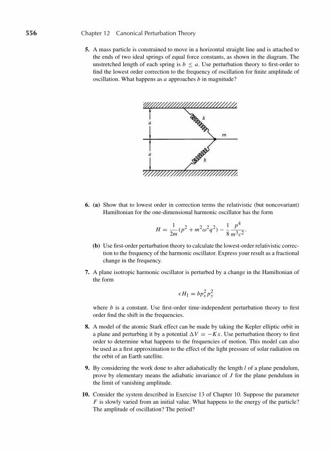
“M12 Goldstein ISBN C12” — 2011/2/15 — page 556 — #31
556 Chapter 12 Canonical Perturbation Theory
5. A mass particle is constrained to move in a horizontal straight line and is attached tothe ends of two ideal springs of equal force constants, as shown in the diagram. Theunstretched length of each spring is b ≤ a. Use perturbation theory to first-order tofind the lowest order correction to the frequency of oscillation for finite amplitude ofoscillation. What happens as a approaches b in magnitude?
6. (a) Show that to lowest order in correction terms the relativistic (but noncovariant)Hamiltonian for the one-dimensional harmonic oscillator has the form
H = 1
2m(p2 + m2ω2q2)− 1
8
p4
m3c2.
(b) Use first-order perturbation theory to calculate the lowest-order relativistic correc-tion to the frequency of the harmonic oscillator. Express your result as a fractionalchange in the frequency.
7. A plane isotropic harmonic oscillator is perturbed by a change in the Hamiltonian ofthe form
εH1 = bp2x p2
y
where b is a constant. Use first-order time-independent perturbation theory to firstorder find the shift in the frequencies.
8. A model of the atomic Stark effect can be made by taking the Kepler elliptic orbit ina plane and perturbing it by a potential �V = −K x . Use perturbation theory to firstorder to determine what happens to the frequencies of motion. This model can alsobe used as a first approximation to the effect of the light pressure of solar radiation onthe orbit of an Earth satellite.
9. By considering the work done to alter adiabatically the length l of a plane pendulum,prove by elementary means the adiabatic invariance of J for the plane pendulum inthe limit of vanishing amplitude.
10. Consider the system described in Exercise 13 of Chapter 10. Suppose the parameterF is slowly varied from an initial value. What happens to the energy of the particle?The amplitude of oscillation? The period?

“M12 Goldstein ISBN C12” — 2011/2/15 — page 557 — #32
Exercises 557
11. A plane pendulum of small amplitude is constrained to move on an inclined plane, asshown in the accompanying figure. How does its amplitude change when the inclina-tion angle α of the plane is changed slowly?
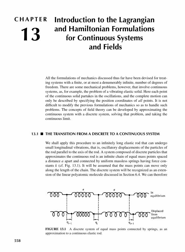
“M13 Goldstein ISBN C13” — 2011/2/15 — page 558 — #1
C H A P T E R
13Introduction to the Lagrangianand Hamiltonian Formulations
for Continuous Systemsand Fields
All the formulations of mechanics discussed thus far have been devised for treat-ing systems with a finite, or at most a denumerably infinite, number of degrees offreedom. There are some mechanical problems, however, that involve continuoussystems, as, for example, the problem of a vibrating elastic solid. Here each pointof the continuous solid partakes in the oscillations, and the complete motion canonly be described by specifying the position coordinates of all points. It is notdifficult to modify the previous formulations of mechanics so as to handle suchproblems. The concepts of field theory can be developed by approximating thecontinuous system with a discrete system, solving that problem, and taking thecontinuous limit.
13.1 THE TRANSITION FROM A DISCRETE TO A CONTINUOUS SYSTEM
We shall apply this procedure to an infinitely long elastic rod that can undergosmall longitudinal vibrations, that is, oscillatory displacements of the particles ofthe rod parallel to the axis of the rod. A system composed of discrete particles thatapproximates the continuous rod is an infinite chain of equal mass points spaceda distance a apart and connected by uniform massless springs having force con-stants k (cf. Fig. 13.1). It will be assumed that the mass points can move onlyalong the length of the chain. The discrete system will be recognized as an exten-sion of the linear polyatomic molecule discussed in Section 6.4. We can therefore
FIGURE 13.1 A discrete system of equal mass points connected by springs, as anapproximation to a continuous elastic rod.
558
“M13 Goldstein ISBN C13” — 2011/2/15 — page 559 — #2
13.1 The Transition from a Discrete to a Continuous System 559
obtain the equations describing the motion by the customary techniques for smalloscillations. Denoting the displacement of the i th particle from its equilibriumposition by ηi , the kinetic energy is
T = 1
2
∑i
mη2i , (13.1)
where m is the mass of each particle. The corresponding potential energy is thesum of the potential energies of each spring as the result of being stretched orcompressed from its equilibrium length (cf. Section 6.4):
V = 1
2
∑i
k(ηi+1 − ηi )2. (13.2)
Combining Eqs. (13.1) and (13.2), the Lagrangian for the system is
L = T − V = 1
2
∑i
[mη2i − k(ηi+1 − ηi )
2], (13.3)
which can also be written as
L = 1
2
∑i
a
[m
aη2
i − ka
(ηi+1 − ηi
a
)2]=∑
i
aLi , (13.4)
where a is the equilibrium separation between the points (cf. Fig. 13.1). Theresulting Lagrange equations of motion for the coordinates ηi are
m
aηi − ka
(ηi+1 − ηi
a2
)+ ka
(ηi − ηi−1
a2
)= 0. (13.5)
The particular form of L in Eq. (13.4), and of the corresponding equations ofmotion, has been chosen for convenience in going to the limit of a continuous rodas a approaches zero. It is clear that m/a reduces to μ, the mass per unit length ofthe continuous system, but the limiting value of ka may not be so obvious. For anelastic rod obeying Hooke’s law, it will be remembered that the extension of therod per unit length is directly proportional to the force or tension exerted on therod, a relation that can be written as
F = Y ξ,
where ξ is the elongation per unit length and Y is Young’s modulus. Now theextension of a length a of a discrete system, per unit length, will be ξ = (ηi+1 −ηi )/a. The force necessary to stretch the spring by this amount is
F = k(ηi+1 − ηi ) = ka
(ηi+1 − ηi
a
),
“M13 Goldstein ISBN C13” — 2011/2/15 — page 560 — #3
560 Chapter 13 Formulations for Continuous Systems and Fields
so that ka must correspond to the Young’s modulus of the continuous rod. Ingoing from the discrete to the continuous case, the integer index i identifying theparticular mass point becomes the continuous position coordinate x ; instead of thediscrete variable ηi we have a continuous field variable η(x). Further, the quantity
ηi+1 − ηi
a= η(x + a)− η(x)
a
occurring in Li obviously approaches the limit
dη
dx,
as a, playing the role of dx , approaches zero. Finally, the summation over a dis-crete number of particles becomes an integral over x , the length of the rod, andthe Lagrangian (13.4) appears as
L = 1
2
∫ [μη2 − Y
(dη
dx
)2]
dx . (13.6)
In the limit as a → 0, the last two terms in the equation of motion (13.5) become
Lima→0
−Y
a
[(dη
dx
)x−(
dη
dx
)x−a
],
which clearly defines a second derivative of η. Hence, the equation of motion forthe continuous elastic rod is
μd2η
dt2− Y
d2η
dx2= 0, (13.7)
the familiar wave equation in one dimension with the propagation velocity
v =√
Y
μ. (13.8)
Equation (13.8) is the well-known formula for the velocity of longitudinal elasticwaves.
This simple example is sufficient to illustrate the salient features of the tran-sition from a discrete to a continuous system. The most important fact to graspis the role played by the position coordinate x . It is not a generalized coordi-nate; it serves merely as a continuous index replacing the discrete i . Just as eachvalue of i corresponds to a different one of the generalized coordinates, ηi , ofthe system, so here for each value of x there is a generalized coordinate η(x).Since η depends also upon the continuous variable t , we should perhaps writemore accurately η(x, t), indicating that x , like t , can be considered as a parameterentering into the Lagrangian. If the continuous system were three-dimensional,
“M13 Goldstein ISBN C13” — 2011/2/15 — page 561 — #4
13.2 The Lagrangian Formulation for Continuous Systems 561
rather than one-dimensional as here, the generalized coordinates would be distin-guished by three continuous indices x , y, z, and would be written as η(x, y, z, t).Note that the quantities x , y, z, and t are completely independent of each other,and appear only as explicit variables in η. Derivatives of η with respect to any ofthem can therefore always be written as total derivatives without any ambiguity.Equation (13.6) also shows that the Lagrangian appears as an integral over thecontinuous index x ; in the corresponding three-dimensional case the Lagrangianwould have the form
L =∫ ∫ ∫
L dx dy dz, (13.9)
where L is known as the Lagrangian density. For the longitudinal vibrations ofthe continuous rod the Lagrangian density is
L = 1
2
[μ
(dη
dt
)2
− Y
(dη
dx
)2], (13.10)
corresponding to the continuous limit of the quantity Li , appearing in Eq. (13.4).It is the Lagrangian density, rather than the Lagrangian itself, that will be used todescribe the motion of the system.
13.2 THE LAGRANGIAN FORMULATION FOR CONTINUOUS SYSTEMS
It will be noted from Eq. (13.9) that L for the elastic rod, besides being a functionof η ≡ ∂η/∂t , also involves a spatial derivative of η, namely, ∂η/∂x ; x and t thusplay a similar role as parameters of the Lagrangian density. If there were localforces present in addition to the nearest neighbor interactions, then L would be afunction of η itself as well as of the spatial gradient of η. Of course, in the generalcase L might well be an explicit function of x and t also. So the Lagrangiandensity for any one-dimensional continuous system would appear as a function ofthe field quantity η in the form
L = L(η,
dη
dx,
dη
dt, x, t
). (13.11)
The total Lagrangian, following Eq. (13.10), is then the integral of L over therange of x defining the system, and Hamilton’s principle, Eq. (2.2), in the limit ofthe continuous system appears as
δ I = δ
∫ 2
1
∫L dx dt = 0. (13.12)
If Hamilton’s principle for the continuous system is to have any usefulness,it must be possible to derive the continuous limit of the equation of motion,
“M13 Goldstein ISBN C13” — 2011/2/15 — page 562 — #5
562 Chapter 13 Formulations for Continuous Systems and Fields
for example, Eq. (13.7), directly by variation of the double integral of L inEq. (13.12). We can carry out this variation by methods that differ only slightlyfrom those used in Chapter 2 for a discrete system. The variation is only on ηand its derivatives; the parameters x and t are not affected by the variation eitherdirectly or in the ranges of integration. Just as the variation of η is taken to bezero at the end points t1 and t2, so the variation of η at the limits x1 and x2 ofthe integration in x is also to be zero. As in Section 2.2, a suitable varied pathof integration in the η space can be obtained, for example, by choosing η from aone-parameter family of possible η functions:
η(x, t;α) = η(x, t; 0)+ αζ(x, t). (13.13)
Here η(x, t; 0) stands for the correct function that will satisfy Hamilton’s princi-ple, and ζ is any well-behaved function that vanishes at the end points in t and x .If I is considered as a function of α, to be an extremum for η(x, t; 0) the derivativeof I with respect to α vanishes at α = 0. By straightforward differentiation,
d I
da=∫ t2
t1
∫ x2
x1
dx dt
[∂L∂η
∂η
∂α+ ∂L∂
dηdt
∂
∂α
(dη
dt
)+ ∂L∂
dηdx
∂
∂α
(dη
dx
)]. (13.14)
Because the variation of η, that is, αζ , vanishes at the end points, integration byparts in x and t yields the relations
∫ t2
t1
∂L∂
dηdt
∂
∂α
(dη
dt
)dt = −
∫ t2
t1
d
dt
(∂L∂
dηdt
)∂η
∂αdt,
and
∫ x2
x1
∂L∂
dηdx
∂
∂α
(dη
dx
)dx = −
∫ x2
x1
d
dx
(∂L∂
dηdx
)∂η
∂αdx .
Hamilton’s principle can therefore be written as
∫ t2
t1
∫ x2
x1
dx dt
[∂L∂η
− d
dt
(∂L∂
dηdt
)− d
dx
(∂L∂
dηdx
)](∂η
∂α
)0= 0, (13.15)
and by the same arguments as in Section 2.2 the arbitrary nature of the varied pathimplies the vanishing of the expression in the brackets:
d
dt
(∂L∂
dηdt
)+ d
dx
(∂L∂
dηdx
)− ∂L∂η
= 0. (13.16)
The Euler-Lagrange equations (13.16) (cf. Eq. (2.18)) is the appropriate form ofthe equation of motion as derived from Hamilton’s principle, Eq. (13.12).
“M13 Goldstein ISBN C13” — 2011/2/15 — page 563 — #6
13.2 The Lagrangian Formulation for Continuous Systems 563
A system of n discrete degrees of freedom will have n Lagrange equationsof motion; for the continuous system with an infinite number of degrees of free-dom we seem to obtain only one Lagrange equation! It must be remembered,however, that the equation of motion for η is a differential equation involvingthe time only, and in that sense Eq. (13.15) furnishes a separate equation ofmotion for each value of x . The continuous nature of the indices x appears inthat Eq. (13.15) is a partial differential equation in the two variables x and t ,yielding η as η(x, t).
For the specific instance of longitudinal vibrations in an elastic rod, it is seenfrom the form of the Lagrangian density, Eq. (13.10), that
∂L∂
dηdt
= μdη
dt,
∂L∂
dηdx
= −Ydη
dx,
∂L∂η
= 0.
Thus, as desired, Eq. (13.16), reduces properly to the equation of motion,Eq. (13.7).
The Lagrangian formulation developed here for one-dimensional continuoussystems needs obviously to be extended to two- and three-dimensional situations,for example, a general elastic solid. Further, instead of one field quantity η theremay be several; for example, displacement from an equilibrium position wouldbe described by a spatial vector h with three components. There is no difficultyin carrying out the mathematical steps for the more general situation in closeparallelism to the one-component one-dimensional case. However, the formulasbecome lengthy and cumbersome if written in the same manner, especially inview of the two tiers of derivatives. Considerable gain in notational simplicitycan be achieved by noticing that time t and the spatial coordinates x, y, z playthe same type of mathematical role in Hamilton’s principle. The field quantitiesare functions of the coordinates of both time and space that are to be treated asindependent variables. No variation of the field quantities occurs at the limits ofintegration in Hamilton’s principle over both time and space.
It is mathematically convenient to think in terms of a four-dimensional spacewith coordinates x0 = ct , x1 = x , x2 = y, x3 = z. No physical significance isimplied for this space. The c in x0 is the speed of light used only to convert theunits of x0 to the same as those used for xi . The entire tensor formalism developedin Chapter 7 applies. The metric tensor g will have a Euclidean metric with theGalilean transformation group as the allowed coordinate transformations on thespace components of the metric tensor restricted by gi0 = g0i = 0. A Romanletter superscript refers only to the three coordinates of the physical space, a Greekletter superscript or subscript refers to all four coordinates. Use of the summationconvention with respect to repeated indices will be resumed for the rest of thechapter. The various components of the field quantities will be symbolized by asubscript ρ, which may cover a multitude of forms. At times, it will stand for asingle index having two, three, four, or more values. Or it may stand for multipleindices. Thus, if the field quantity is a spatial tensor of second rank, then ρ reallyrefers to two subscript indices. Finally, a derivative of the field quantities withrespect to any one of the four coordinates xμ will be denoted by the subscript ν
“M13 Goldstein ISBN C13” — 2011/2/15 — page 564 — #7
564 Chapter 13 Formulations for Continuous Systems and Fields
separated from ρ by a comma. Where there is only one field quantity the indexdoes not appear. Examples are
ηρ,ν ≡ dηρdxν
; η, j ≡ dη
dx j; ηi,μν = d2ηi
dxμdxν. (13.17)
Only the derivatives of the field quantities will be symbolized in this manner.In this notation, the most general form of the Lagrangian density to be consid-
ered here is written as
L = L(ηρ, ηρ,ν, xν). (13.18)
The total Lagrangian is then an integral over three-space:
L =∫
L(dxi ), (13.19)
but it rarely occurs explicitly. Hamilton’s principle appears as an integral over aregion in 4-space:
δ I = δ
∫L(dxμ) = 0, (13.20)
where the variation of the ηρ vanishes at the bounding surface S of the regionof integration. The derivation of the corresponding Euler–Lagrange equations ofmotion proceeds symbolically as before. We consider a one-parameter set of var-ied functions that reduce to ηρ(xν) as the parameter α goes to zero. As previously,a possible suitable set can be constructed, for example, by adding to ηρ the productαζρ , where ζρ(xν) are convenient arbitrary functions vanishing on the boundingsurface. The vanishing of the variation of I is equivalent to setting the derivativeof I with respect to α equal to zero:*
d I
dα=∫ (
∂L∂ηρ
∂ηρ
∂α+ ∂L∂ηρ,ν
∂ηρ,ν
∂α
)(dxμ).
Integration by parts yields
d I
dα=∫ [
∂L∂ηρ
− d
dxν
(∂L∂ηρ,ν
)]∂ηρ
∂α(dxμ)
+∫(dxμ)
d
dxν
(∂L∂ηρ,ν
∂ηρ
∂α
). (13.21)
The second integral vanishes in the limit as α goes to zero, as can be seen invarious ways. We can examine it term by term: carrying out the integrationfor the particular xν of each derivative term, which then vanishes because thederivative with respect to α is zero at the end points. Or the integral can be
*Unless otherwise noted, the summation convention will be used in the remainder of this chapter, forall types of subscript-superscript pairs.

“M13 Goldstein ISBN C13” — 2011/2/15 — page 565 — #8
13.2 The Lagrangian Formulation for Continuous Systems 565
transformed by a four-dimensional divergence theorem into an integral over thesurface bounding the region of integration in 4-space. The surface integral againvanishes because the variation of ηρ in the vicinity of the correct field functionsis zero on the surface. Equation (13.21) in the limit as α goes to zero thereforereduces to(
d I
dα
)0=∫(dxμ)
[∂L∂ηρ
− d
dxν
(∂L∂ηρ,ν
)](∂ηρ
∂α
)0. (13.22)
Again, the arbitrary nature of the variation of each ηρ means that Eq. (13.22) issatisfied only when each of the square brackets vanishes:
d
dxν
(∂L∂ηρ,ν
)− ∂L∂ηρ
= 0. (13.23)
Equations (13.23) represent a set of partial differential equations for the fieldquantities, with as many equations as there are different values of ρ. It maybe worth repeating that since the space coordinates xi are indices for the fieldquantities, each of Eqs. (13.23) in effect corresponds to an entire set of Lagrangedifferential equations of motion in the discrete case.
For a one-dimensional continuous system, where ν takes on only the values0 and 1, Eq. (13.23) expands to the same form as Eq. (13.16). The compactnessof the notation is evident even in so simple an example. Although we have usedcovariant notation, the use of a four-dimensional space for symbolic conveniencein no way requires covariant behavior (in the physicist’s sense of the word) of anyof the quantities in that space.
For discrete systems, the Lagrangian is uncertain to a total time derivative ofan arbitrary function of the generalized coordinates and time. With continuoussystems, the corresponding statement is that L is uncertain to any “4-divergence,”that is, to a term of the form
d Fν(ηρ, xμ)
dxν(13.24)
where the Fν are any four (differentiable) functions of the field quantities ηρ andthe coordinates xμ. That such a term makes no contribution to the variation ofthe action integral is obvious. Application of the divergence theorem in 4-spaceconverts the volume integral into an integral over the bounding surface where thevariation of Fν is zero. In symbols, the relevant variation can be written
δ
∫(dxμ)
d Fν(ηρ, xμ)
dxν= δ
∫Fν(ηρ, xμ) dσν = 0, (13.25)
where dσν represents the components of an element of surface (in Euclidean4-space) oriented along the direction of the outward normal.
The Lagrangian formulation for a continuous set of generalized coordinateshas been developed in order to treat continuous mechanical systems such as an
“M13 Goldstein ISBN C13” — 2011/2/15 — page 566 — #9
566 Chapter 13 Formulations for Continuous Systems and Fields
elastic solid in longitudinal oscillation, or a gas vibrating in such a manner as toset up acoustic waves. As has been implied, the formulation may also be used,even in the absence of a mechanical system, to describe the equations governinga field. Mathematically, a field is no more than a set of one or more independentfunctions of space and time, and the generalized coordinates fit this definition.There is no requirement that the field be related to some underlying mechanicalsystem. In thus breaking the connection between the Lagrangian field descrip-tion and purely mechanical motion, we are merely recapitulating the history ofphysics. For example, the electromagnetic field was long thought of in terms ofthe elastic vibrations of a mysterious ether. Only in recent times was it generallyrealized that the ether had no other role than being the subject of the verb “toundulate.” We recognize equally well that the variational procedures developedhere also stand independent of the notion of a continuous mechanical system, andthat they serve to furnish the equations describing any spacetime field. Hamilton’sprinciple then becomes in effect a convenient and compact description of the field,one that upon expansion leads to the field equations.
In addition to implying the field equations, the Lagrangian density has more totell us about the physical nature of the field. As with systems of a discrete numberof degrees of freedom, the structure of the Lagrangian also contains informationon conserved properties of the system. One such set of conservation theorems isdiscussed in the next section.*
13.3 THE STRESS-ENERGY TENSOR AND CONSERVATION THEOREMS
An analog to the conservation of Jacobi’s integral in point mechanics found inSection 2.6, can be derived here, and in much the same manner. All we have toremember is that the treatment of time must be extended in parallel fashion tothe xi since they are all independent parameters in L. Thus, instead of the timederivative of L , we seek to evaluate the total derivative of L with respect to xμ:
dLdxμ
= ∂L∂ηρ
ηρ,μ + ∂L∂ηρ,ν
ηρ,μν + ∂L∂xμ
. (13.26)
By the equations of motion, Eq. (13.23), this becomes (with a slight change innotation),
dLdxμ
= d
dxν
(∂L∂ηρ,ν
)ηρ,μ + ∂L
∂ηρ,ν
dηρ,μdxν
+ ∂L∂xμ
= d
dxν
(∂L∂ηρ,ν
ηρ,μ
)+ ∂L∂xμ
. (13.27)
*A more general attack on the conservation properties inherent in the Lagrangian will be found inSection 13.7 on Noether’s theorem.
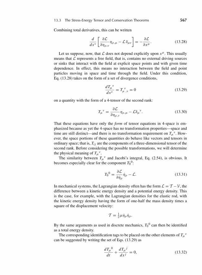
“M13 Goldstein ISBN C13” — 2011/2/15 — page 567 — #10
13.3 The Stress-Energy Tensor and Conservation Theorems 567
Combining total derivatives, this can be written
d
dxν
[∂L∂ηρ,ν
ηρ,μ − L δμν]= − ∂L
∂xμ. (13.28)
Let us suppose, now, that L does not depend explicitly upon xμ. This usuallymeans that L represents a free field, that is, contains no external driving sourcesor sinks that interact with the field at explicit space points and with given timedependence. In effect, this means no interaction between the field and pointparticles moving in space and time through the field. Under this condition,Eq. (13.28) takes on the form of a set of divergence conditions,
dTμν
dxν= T ν
μ ,ν = 0 (13.29)
on a quantity with the form of a 4-tensor of the second rank:
Tμν = ∂L
∂ηρ,νηρ,μ − Lδμν. (13.30)
That these equations have only the form of tensor equations in 4-space is em-phasized because as yet the 4-space has no transformation properties—space andtime are still distinct—and there is no transformation requirement on Tμν . How-ever, the space portions of these quantities do behave like vectors and tensors inordinary space; that is, Ti j are the components of a three-dimensional tensor of thesecond rank. Before considering the possible transformations, we will determinethe physical meaning of Tμν .
The similarity between Tμν and Jacobi’s integral, Eq. (2.54), is obvious. Itbecomes especially clear for the component T0
0:
T00 = ∂L
∂ηρηρ − L. (13.31)
In mechanical systems, the Lagrangian density often has the form L = T −V , thedifference between a kinetic energy density and a potential energy density. Thisis the case, for example, with the Lagrangian densities for the elastic rod, withthe kinetic energy density having the form of one-half the mass density times asquare of the displacement velocity:
T = 12μηρηρ.
By the same arguments as used in discrete mechanics, T00 can then be identified
as a total energy density.The corresponding identification tags to be placed on the other elements of Tμν
can be suggested by writing the set of Eqs. (13.29) as
dTμ0
dt+ dTμ j
dx j= 0, (13.32)
“M13 Goldstein ISBN C13” — 2011/2/15 — page 568 — #11
568 Chapter 13 Formulations for Continuous Systems and Fields
or
T νμ,ν =dT 0
μ
cdt+ dT i
μ
dxi= dT 0
μ
cdt+∇ · Tμ = 0 (13.33)
where Tμ, whose components are Tμν , are a set of 4-space vectors. In either form,Eqs. (13.32) or (13.33) appear as equations of continuity, which is to say that thetime rate of change of some density plus the divergence of some correspondingflux or current density vanishes. In turn, the equations of continuity imply theconservation of some integral quantities providing the field volume is finite; thatis, the field can be contained within a volume beyond which the field quantitiesare zero, defined, in such a case, integral quantities Rμ by
Rμ =∫
Tμ0 dV, (13.34)
where the volume integral extends beyond the region containing the field. Then,by Eqs. (13.33),
dRμdt
=∫
∇ ?Tμ dV =∫
Tμ · dA = 0. (13.35)
It is because of these conservation theorems, derived from Eq. (13.29), that thefour arrays Tμν, μ = 0, 1, 2, 3 are known as conserved currents, in analogy withthe conservation equations for electromagnetic current.
We should therefore expect T0 to play the role of the components of an energycurrent density. That this is reasonable can be seen again from considerations ofthe longitudinal vibration field in an elastic rod. Imagine the rod divided by animaginary cut at point x (cf. Fig. 13.2). From the considerations that led to theLagrangian, Eq. (13.6), the force exerted by the part of the rod on the right toextend the part that is to the left of the cut is
Ydη
dx. (13.36)
FIGURE 13.2 Diagram illustrating calculation of energy current density in elastic rod.
“M13 Goldstein ISBN C13” — 2011/2/15 — page 569 — #12
13.3 The Stress-Energy Tensor and Conservation Theorems 569
Hence, there is a tension at x in the left-hand portion of equal magnitude but ofopposite direction. Further, the left-hand portion is being stretched by an amountthat at x is η, and the rate at which this extension changes in time is η. Hence, therate of work being done by the tension at the cut is
−ηYdη
dx, (13.37)
which is thus the rate at which energy is being transferred to the right per unit time.Comparison shows that this is exactly T0
1 for the appropriate Lagrangian densityof Eq. (13.10). If T0
0 is an energy density then the quantity, R0, of Eq. (13.34)can be identified as the total energy in the field. The fourth component of the con-servation equation (13.35) therefore says that the total field energy is conserved ifT0
i vanishes on the bounding surface, that is, if the system does not radiate energyto the outside.
Physical meaning for the Ti0 components can be suggested similarly by turning
once more to the vibrations of the elastic rod. If the particles in the rod move bythe same amount all along the rod, the motion will be that of a rigid body, thatis, no oscillatory disturbances. The net change of mass in a length dx of the rodas a result of the motion would clearly be zero, since as much mass moves pastx + dx as past x . There would still be a net momentum density μη for this caseof rigid-body motion. When wave motion takes place, a net mass change in thelength dx exists, amounting at any given time to (cf. Fig. 13.2)
μ[η(x)− η(x + dx)] = −μdη
dxdx . (13.38)
The additional momentum in the interval resulting from the wave motion istherefore
−μη dη
dxdx .
Thus, an additional momentum density, above and beyond that of the steady-statemotion, can be identified as the wave or field momentum density:
−μη dη
dx. (13.39)
This quantity is just −T10 for the Lagrangian density given by Eq. (13.10). Thus,
we are led to identify −Ti0 as the components of field momentum density and
−Ri , as the total (linear) momentum of the field, at least in this four-dimensionalconvention.
The equations of continuity, Eqs. (13.33), then suggest that −Ti must representthe vector flux density for the i th component of the field momentum density. Weascribe a vector property to Ti because there can be, for example, a flow in they-direction of the x-component of the momentum density, as measured by −Tx
y .An alternative interpretation of Ti
j comes from considering the displacement field
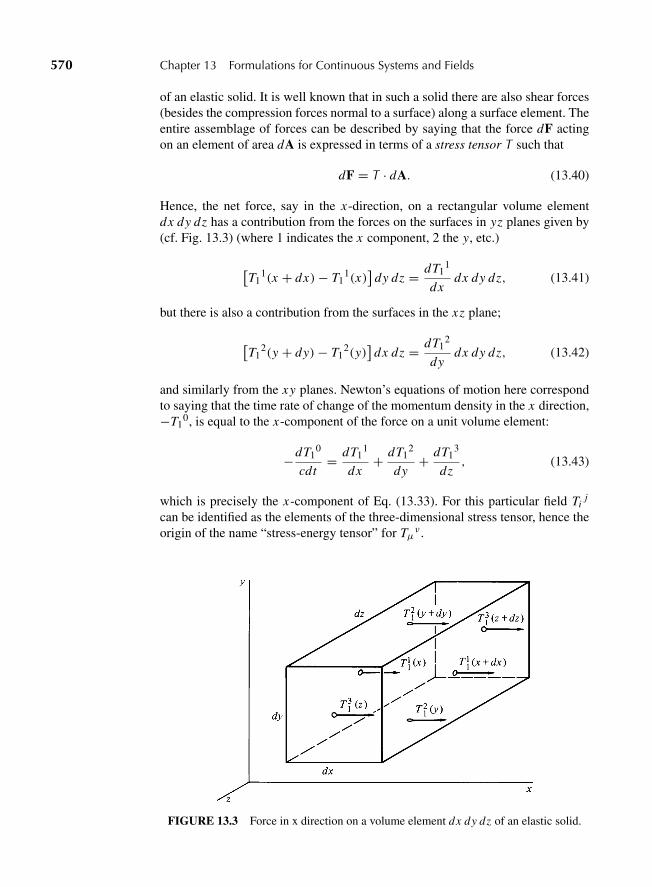
“M13 Goldstein ISBN C13” — 2011/2/15 — page 570 — #13
570 Chapter 13 Formulations for Continuous Systems and Fields
of an elastic solid. It is well known that in such a solid there are also shear forces(besides the compression forces normal to a surface) along a surface element. Theentire assemblage of forces can be described by saying that the force dF actingon an element of area dA is expressed in terms of a stress tensor T such that
dF = T · dA. (13.40)
Hence, the net force, say in the x-direction, on a rectangular volume elementdx dy dz has a contribution from the forces on the surfaces in yz planes given by(cf. Fig. 13.3) (where 1 indicates the x component, 2 the y, etc.)
[T1
1(x + dx)− T11(x)
]dy dz = dT1
1
dxdx dy dz, (13.41)
but there is also a contribution from the surfaces in the xz plane;
[T1
2(y + dy)− T12(y)
]dx dz = dT1
2
dydx dy dz, (13.42)
and similarly from the xy planes. Newton’s equations of motion here correspondto saying that the time rate of change of the momentum density in the x direction,−T1
0, is equal to the x-component of the force on a unit volume element:
−dT10
cdt= dT1
1
dx+ dT1
2
dy+ dT1
3
dz, (13.43)
which is precisely the x-component of Eq. (13.33). For this particular field Tij
can be identified as the elements of the three-dimensional stress tensor, hence theorigin of the name “stress-energy tensor” for Tμν .
FIGURE 13.3 Force in x direction on a volume element dx dy dz of an elastic solid.
“M13 Goldstein ISBN C13” — 2011/2/15 — page 571 — #14
13.3 The Stress-Energy Tensor and Conservation Theorems 571
By considerations of a continuous mechanical system, we have thus been ableto attach physical identifications, or associations, to each of the components ofthe stress-energy tensor. Thus, the components are
T00 field energy density divided by c,
T0, with components T0j field energy current density,
−Ti0 field momentum density, i th component,
−Ti , with components Ti0 current density for the i th component of the field
momentum density,
Tij three-dimensional stress tensor
where, as we saw discussed following Eqs. (13.33) and (13.35), T0 and Ti form4-space vectors each of which is conserved and thus identified, in analogy withthe charge-current vector of electromagnetic theory as a “4-current”. All suchconserved objects are called currents in field theory.
In almost all cases the three-dimensional tensor T is symmetric. This is notonly physically desirable, but almost necessarily a characteristic for the spatialportion of the stress-energy tensor.
It must be remembered that although the example of mechanical systems gavebirth to the procedures and nomenclature, the formalism can be applied to anyfield irrespective of its nature or origin. A classical theory of fields can be con-structed not only for vibrations of an elastic solid, but also for the electromag-netic field, for the “field” of the Schrodinger wave function, or for the relativisticfield describing a “scalar” meson, among others. We shall examine some of theseexamples in more detail later on.
Recalling the identification of Ri , the conservation equations, Eq. (13.35), saythat for a closed noninteracting system the total linear momentum of the field isconserved. We would expect no less. But there should be a corresponding con-servation theorem for the total angular momentum of the field. It is simple toconstruct a quantity that should act as an angular momentum density. Since angu-lar momentum is an axial vector. We expect that the components of the angularmomentum density are the elements of an antisymmetric tensor of the secondrank. A suitable form for this tensor is
Mi j = −(xi T j0 − x j T i0), (13.44)
with the total angular momentum of the field given by
Mi j =∫
Mi j dV . (13.45)
In as much as t and xi are completely independent variables, the time rate ofchange of Mi j is
d Mi j
dt= −
∫ (xi dT j0
dt− x j dT i0
dt
)dV, (13.46)
“M13 Goldstein ISBN C13” — 2011/2/15 — page 572 — #15
572 Chapter 13 Formulations for Continuous Systems and Fields
or, from the continuity conditions, Eqs. (13.32),
d Mi j
dt= −
∫ (xi dT jk
dxk− x j dT ik
dxk
)dV . (13.47)
Integration by parts converts this expression to
d Mi j
dt= −
∫d
dxk(xi T jk − x j T ik) dV +
∫(T i j − T ji ) dV . (13.48)
The first integral on the right is in the form of a volume integral of a divergence.It is therefore equal to an integral over the bounding surface, which vanishes for aclosed nonradiating system. Finally, if T i j = T ji , the second integral is also zero.Thus, the total angular momentum of the field is conserved if T is symmetric.
If the stress tensor is not symmetric, we can often make use of the ambiguityin defining the stress tensor to restore this symmetry. Just as for the Lagrangian,the form of the stress-energy tensor, Eq. (13.30), was chosen to satisfy diver-gence conditions (cf. Eq. (13.29)). Therefore Tμν is indeterminate by any func-tion whose 4-divergence vanishes. Usually it is possible to find such a quantity to“symmetrize” the stress-energy tensor.
13.4 HAMILTONIAN FORMULATION
It is possible to obtain a Hamiltonian formulation for systems with a continuousset of coordinates much as was done in Chapter 8 for discrete systems. To indicatethe method of approach, we return briefly to the linear chain of mass points dis-cussed in Section 13.1. Conjugate to each field component, ηi , there is a canonicalmomentum
pi = ∂L
∂ηi= a
∂Li
∂ηi. (13.49)
The Hamiltonian for the system is therefore
H ≡ pi ηi − L = a∂Li
∂ηiηi − L ,
or
H = a
(∂Li
∂ηiηi − Li
). (13.50)
It will be remembered that in the limit of the continuous rod, when a goes to zero,Li → L and the summation in Eq. (13.50) becomes an integral:
H =∫
dx
(∂L∂ηη − L
). (13.51)

“M13 Goldstein ISBN C13” — 2011/2/15 — page 573 — #16
13.4 Hamiltonian Formulation 573
The individual canonical momenta pi , as given by Eq. (13.49), vanish in the con-tinuous limit, but we can define a momentum density, π , that remains finite:
Lima→0
pi
a≡ π = ∂L
∂η. (13.52)
Equation (13.51) is in the form of a space integral over a Hamiltonian density, H,defined by
H = πη − L. (13.53)
While a Hamiltonian formulation can thus be introduced in a straightforwardmanner for classical fields, note that the procedure singles out the time variablefor special treatment. It is therefore in contrast to the development we have givenfor the Lagrangian formulation where the independent variables of time and spacewere handled symmetrically. For this reason the Hamiltonian approach, at least asintroduced here, lends itself less easily to incorporation in a relativistically covari-ant description of fields. The Hamiltonian way of looking at fields has thereforenot proved as useful as the Lagrangian method, and a rather brief descriptionshould suffice here.
The obvious route for generalizing to a three-dimensional field described byfield quantities ηρ is to define, analogously to Eq. (13.52), the canonical momen-tum densities
πρ(xμ) = ∂L∂ηρ
. (13.54)
The quantities ηρ(xi , t), πρ(xi , t) together define the infinite-dimensional phasespace describing the classical field and its time development. A conservationtheorem can be found for πρ that is roughly similar to that for the canonicalmomentum in discrete systems. If a given field quantity ηρ is cyclic in the sensethat L does not contain ηρ explicitly (as in the case of Eq. (13.10)), then theLagrange field equation looks like an existence statement for a conserved current:
d
dxμ∂L∂ηρ,μ
= 0, (13.55)
or
dπρ
dt+ d
dxi
∂L∂ηρ,i
= 0. (13.56)
It follows that if ηρ is cyclic, there is an integral conserved quantity
�ρ =∫
dV πρ(xi , t).
The obvious generalization of Eq. (13.53) for a Hamiltonian density is
H(ηρ, ηρ,i , πρ, xi ) = πρηρ − L, (13.57)
“M13 Goldstein ISBN C13” — 2011/2/15 — page 574 — #17
574 Chapter 13 Formulations for Continuous Systems and Fields
where it is assumed that functional dependence upon ηρ can be eliminated byinversion of the defining equations (13.49). From this definition it follows that
∂H∂πρ
= ηρ + πλ ∂ηλ∂πρ
− ∂L∂ηλ
∂ηλ
∂πρ= ηρ, (13.58)
by Eq. (13.51). The other half of the canonical field equation is more cumbersome.When expressed in terms of the canonical variables, H is a function of ηρ throughthe explicit dependence of L, and through ηρ . Hence,
∂H∂ηρ
= πλ∂ηλ
∂ηρ− ∂L∂ηλ
∂ηλ
∂ηρ− ∂L∂ηρ
= − ∂L∂ηρ
. (13.59)
Using the Lagrange equations, this can be written
∂H∂ηρ
= − d
dxμ
(∂L∂ηρ,μ
)= −πρ − d
dxi
(∂L∂ηρ,i
). (13.60)
Because of the appearance of L, we still do not have a useful form. By an exactlyparallel derivation, however, we find that
∂H∂ηρ,i
= πλ∂ηλ
∂ηρ,i− ∂L∂ηλ
∂ηλ
∂ηρ,i− ∂L∂ηρ,i
= − ∂L∂ηρ,i
. (13.61)
Hence, we can write as the second half of the canonical equations
∂H∂ηρ
− d
dxi
(∂H∂ηρ,i
)= −πρ . (13.62)
Equations (13.58) and (13.62) can be put in a notation more closely approachingHamilton’s equations for a discrete system by introducing the notion of a func-tional derivative defined as
δ
δψ= ∂
∂ψ− d
dxi
∂
∂ψ, i. (13.63)
Since H is not a function of πρ,i , Eqs. (13.58) and (13.62) can be written as
ηρ = δHδπρ
, πρ = − δHδηρ
. (13.64)
Note that in the same symbolism the Lagrange equations, Eqs. (13.23), take theform
d
dt
(∂L∂ηρ
)− δLδηρ
= 0. (13.65)
“M13 Goldstein ISBN C13” — 2011/2/15 — page 575 — #18
13.4 Hamiltonian Formulation 575
About the only advantage of the functional derivative, however, is that of theresultant similarity with discrete system. It suppresses, on the other hand, theparallel treatment of time and space variables.
There is a way to treat classical fields that provides almost all of the Hamil-tonian formulation of discrete mechanics. The main idea behind this treatmentis to replace the continuous space variable or index by a denumerable discreteindex. We can see how to do this by referring again to the longitudinal oscilla-tions of the elastic rod. Let us suppose the rod is of finite length L = x2 − x1. Therequirement that η vanish at the extremities is a boundary condition that could beachieved physically by placing the rod between two perfectly rigid walls. Thenthe amplitude of oscillation can be represented by a Fourier series:
η(x) =∞∑
n=0
qn sin2πn(x − x1)
2L. (13.66)
Instead of the continuous index x , we have the discrete index n. We are allowed touse this representation for all x only when η(x) is a well-behaved function, whichmost physical field quantities are.
For simplicity in illustrating how the scheme may be carried out, it willbe assumed that only one real field quantity, η, can be expanded in a three-dimensional Fourier series of the form
η(r, t) = 1
V 1/2
∑k
qk(t)eik ? r. (13.67)
Here k is a wave vector that can take on only discrete magnitudes and directions,such that only an integral (or sometimes, half-integral) number of wavelengths fitinto a given linear dimension. We say that k has a discrete spectrum. The scalarindex k stands for some ordering of the set of integer indices used to denumer-ate the discrete values of k, and V is the volume of the system, appearing in anormalization factor. Because η is real, we must have q∗
k = q−k .The orthogonality of the exponentials over the volume can be stated as the
relation
1
V
∫ei(k−k′) ? r dV = δkk′ . (13.68)
In effect, the allowed values of k are those for which the condition (13.68) issatisfied (as can be seen by looking at the one-dimensional Fourier series). Itfollows that the coefficients of expansion, qk(t), are given by
qk(t) = 1
V 1/2
∫e−ik ? rη(r, t) dV . (13.69)
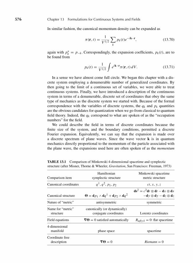
“M13 Goldstein ISBN C13” — 2011/2/15 — page 576 — #19
576 Chapter 13 Formulations for Continuous Systems and Fields
In similar fashion, the canonical momentum density can be expanded as
π(r, t) = 1
V 1/2
∑k
pk(t)e−ik ? r, (13.70)
again with p∗k = p−k . Correspondingly, the expansion coefficients, pk(t), are tobe found from
pk(t) = 1
V 1/2
∫eik ? rπ(r, t) dV . (13.71)
In a sense we have almost come full circle. We began this chapter with a dis-crete system employing a denumerable number of generalized coordinates. Bythen going to the limit of a continuous set of variables, we were able to treatcontinuous systems. Finally, we have introduced a description of the continuoussystem in terms of a denumerable, discrete set of coordinates that obey the sametype of mechanics as the discrete system we started with. Because of the formalcorrespondence with the variables of discrete systems, the qk and pk quantitiesare the obvious candidates for quantization when we go from classical to quantumfield theory. Indeed, the qk correspond to what are spoken of as the “occupationnumbers” for the field.
We could describe the field in terms of discrete coordinates because thefinite size of the system, and the boundary conditions, permitted a discreteFourier expansion. Equivalently, we can say that the expansion is made overa discrete spectrum of plane waves. Since the wave vector k is in quantummechanics directly proportional to the momentum of the particle associated withthe plane wave, the expansions used here are often spoken of as the momentum
TABLE 13.1 Comparison of Minkowski 4-dimensional spacetime and symplecticstructure (after Misner, Thorne & Wheeler, Gravitation, San Francisco: Freeman, 1973)
Hamiltonian Minkowski spacetimeComparison item symplectic structure metric structure
Canonical coordinates q1, q2, p1, p2 ct , x , y, z
ds2 = c2dt ⊗ dt − dx ⊗ dxCanonical structure � = dp1 ∧ dq1 + dp2 ∧ dq2 −dy ⊗ dy − dz ⊗ dz
Nature of “metric” antisymmetric symmetric
Name for “metric” canonically (or dynamically)structure conjugate coordinates Lorentz coordinates
Field equations �� = 0 satisfied automatically Rαβγ δ = 0: flat spacetime
4-dimensionalmanifold phase space spacetime
Coordinate freedescription �� = 0 Riemann = 0
“M13 Goldstein ISBN C13” — 2011/2/15 — page 577 — #20
13.5 Relativistic Field Theory 577
representation. We need not be restricted to plane wave expansions. A denumer-able set of coordinates can be found whenever the field functions can be expandedin terms of a discrete set of orthonormal eigenfunctions.
One final comment. The Hamiltonian or symplectic structure can be expressedin tensor notation. Table 13.1 compares the metric structure of 4-dimensionalMinkowski spacetime with the symplectic structure of a Hamiltonian withcoordinates q1, q2, p1, and p2.
13.5 RELATIVISTIC FIELD THEORY
We saw in Chapter 7 that there is considerable difficulty in constructing relativis-tically covariant Lagrangian and Hamiltonian descriptions of particle mechanics.Part of the problem can be traced to the separate roles played by space and timecoordinates. For point particles, the space coordinates are mechanical variableswhile time is a monotonic parameter. But in classical field theory there is a nat-ural similarity in handling space and time coordinates. They are all parameters,together defining a point in the spacetime continuum at which the field variablesare to be determined. While the four-dimensional spacetime system has been usedso far only for reasons of notational simplicity, the easy and natural way it fits intothe formulation suggests that a relativistically covariant description is quite fea-sible for classical fields. Indeed, only relatively minor tinkering has to be doneto the formulation already presented so that it can handle relativistic fields in amanner that is manifestly Lorentz covariant.
Three points require specific attention: (1) the nature (and metric) of thefour-dimensional space used; (2) the Lorentz transformation properties of thefield quantities, Lagrangian densities, and related functions; and (3) the covari-ant description of the limits of integration. The simple Cartesian, 4-space withcoordinates t, x, y, z that we have implicitly used so far in this chapter is notconvenient for exhibiting Lorentz invariance. We will use the notation and con-ventions adopted in Chapter 7 as well as the results of that chapter. Accordingly,the Greek letter indices will still run from 0 to 3, with x0 = ct . Note that theLagrange equations (13.23) are unaffected by this change. Indeed, the term
d
dxν
(∂L∂ηρ,ν
)
remains unaltered by a scale change of any of the xν , and the other term in theLagrange equation does not involve the coordinates at all. Further, the change inspace does not affect the formulation of Hamilton’s principle in Eq. (13.20), sinceit only introduces a multiplicative constant.
All of the quantities related to the field and associated equations must now havesome definite Lorentz covariant properties. The field quantities must thereforeconsist of 4-tensors of some given rank—scalar, 4-vector, and so on. In principle,ηρ need not be restricted to any one of these categories but may stand for a set ofsuch, for example, two scalars. The Lagrangian and Hamiltonian densities must
“M13 Goldstein ISBN C13” — 2011/2/15 — page 578 — #21
578 Chapter 13 Formulations for Continuous Systems and Fields
also be covariant. In Hamilton’s principle, the volume element (dxν) of 4-space isinvariant under Lorentz transformation. Since we usually think of the action I as ascalar, this means that the Lagrangian density (and therefore H) should be scalars.That is to say, they must be functions of the field quantities (possibly along withexternal covariant quantities) in such manner as to form scalars under Lorentztransformations. It then follows that the stress-energy tensor Tμν , as defined byEq. (13.30) is automatically a 4-tensor of the second rank. The change in the4-space however means that the components of Tμν may be altered in value.
In tensor notation, the stress-energy tensor, T, is a linear, symmetric “func-tional” with slots for two vectors. It has the following properties:
1. If we insert the 4-velocity u of the observer into one of the slots and leavethe other slot empty, the output is
T(u, . . .) = T(. . . , u) = −(
density of 4-momentum,dpdV
)(13.72)
The right-hand side is the negative of the 4-momentum per unit three-dimensional volume as measured in the observer’s frame at the event whereT is measured. In component notation,
T αβuα = Tβαuβ = −
(dpα
dV
)(13.73)
2. If we insert the 4-velocity u of the observer into one of the slots and anarbitrary unit vector n into the other slot, the output is
T (u, n) = T (n, u) = −(
n ?dpdV
)(13.74)
The right-hand side is the negative of the component of the 4-momentumdensity along the n direction. In component notation
Tαβuαnβ = Tβαuβnα = −nμdpμ
dV. (13.75)
3. If we insert the 4-velocity of the observer into both slots, the output is
T (u, u) = (mass energy per unit volume) (13.76)
as measured in the frame with 4-velocity u.In component notation,
Tαβuαuβ = Tβαuβuα = uμdpμ
dV. (13.75′)
4. If we pick a frame and insert two spacelike basis vectors ei and ek in thatframe, the output is
Tik = Tki = T(ei , ek) = T(ek, ei )
“M13 Goldstein ISBN C13” — 2011/2/15 — page 579 — #22
13.5 Relativistic Field Theory 579
= i-component of force acting from side xk − δ to side xk + δ acrossa unit surface area perpendicular to direction ek
= k-component of force acting from side xi − δ to side xi + δ acrossa unit surface area perpendicular to direction ei (13.77)
For example, if we assume the Lorentz transformations apply and consider aperfect fluid moving with a 4-velocity u, which may vary in spacetime, we candescribe the fluid in terms of its mass density, ρ, and an isotropic pressure, p, bothin the rest frame of the fluid element. The stress-energy tensor is given by
T = (ρ + p)u ⊗ u + pg (13.78)
or in component form
Tαβ = (ρ + p)uαuβ + pgαβ. (13.79)
Insert the 4-velocity into one slot giving
T αβuβ = [(ρ + p)uαuβ + pδαβ ]uβ = ρuα. (13.80)
In the rest frame of the fluid, this becomes
T 0βuβ = ρc (13.81)
and
T iβuβ = dpi
dV= momentum density = 0, (13.82)
where the last equality follows from the choice of the rest frame. Finally
Tik = T(ei , ek) = pδik . (13.83)
The Lagrangian density is of course uncertain to a multiplicative constant fac-tor. It is customary to choose the factor such that T00 (or its symmetrized form)directly represents the energy density in the field. In the chosen 4-space the quan-tities Rμ, Eq. (13.34), are now defined as
Rμ =∫
Tμ0 dV . (13.84)
Let us consider a related set Pμ defined as
Pμ = 1
cRμ. (13.85)
It follows then, from Eqs. (13.72) to (13.76) and the interpretation given above forTi0, that Pi represents the components of the total linear momentum of the field,
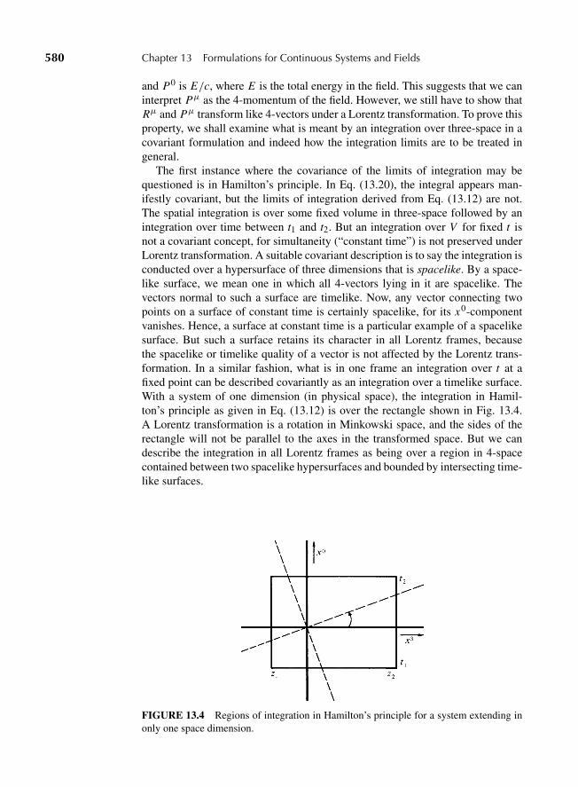
“M13 Goldstein ISBN C13” — 2011/2/15 — page 580 — #23
580 Chapter 13 Formulations for Continuous Systems and Fields
and P0 is E/c, where E is the total energy in the field. This suggests that we caninterpret Pμ as the 4-momentum of the field. However, we still have to show thatRμ and Pμ transform like 4-vectors under a Lorentz transformation. To prove thisproperty, we shall examine what is meant by an integration over three-space in acovariant formulation and indeed how the integration limits are to be treated ingeneral.
The first instance where the covariance of the limits of integration may bequestioned is in Hamilton’s principle. In Eq. (13.20), the integral appears man-ifestly covariant, but the limits of integration derived from Eq. (13.12) are not.The spatial integration is over some fixed volume in three-space followed by anintegration over time between t1 and t2. But an integration over V for fixed t isnot a covariant concept, for simultaneity (“constant time”) is not preserved underLorentz transformation. A suitable covariant description is to say the integration isconducted over a hypersurface of three dimensions that is spacelike. By a space-like surface, we mean one in which all 4-vectors lying in it are spacelike. Thevectors normal to such a surface are timelike. Now, any vector connecting twopoints on a surface of constant time is certainly spacelike, for its x0-componentvanishes. Hence, a surface at constant time is a particular example of a spacelikesurface. But such a surface retains its character in all Lorentz frames, becausethe spacelike or timelike quality of a vector is not affected by the Lorentz trans-formation. In a similar fashion, what is in one frame an integration over t at afixed point can be described covariantly as an integration over a timelike surface.With a system of one dimension (in physical space), the integration in Hamil-ton’s principle as given in Eq. (13.12) is over the rectangle shown in Fig. 13.4.A Lorentz transformation is a rotation in Minkowski space, and the sides of therectangle will not be parallel to the axes in the transformed space. But we candescribe the integration in all Lorentz frames as being over a region in 4-spacecontained between two spacelike hypersurfaces and bounded by intersecting time-like surfaces.
FIGURE 13.4 Regions of integration in Hamilton’s principle for a system extending inonly one space dimension.
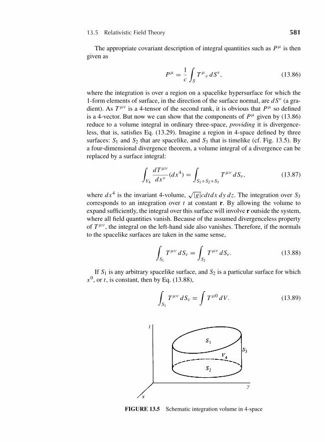
“M13 Goldstein ISBN C13” — 2011/2/15 — page 581 — #24
13.5 Relativistic Field Theory 581
The appropriate covariant description of integral quantities such as Pμ is thengiven as
Pμ = 1
c
∫S
Tμν d Sν, (13.86)
where the integration is over a region on a spacelike hypersurface for which the1-form elements of surface, in the direction of the surface normal, are d Sν (a gra-dient). As Tμν is a 4-tensor of the second rank, it is obvious that Pμ so definedis a 4-vector. But now we can show that the components of Pμ given by (13.86)reduce to a volume integral in ordinary three-space, providing it is divergence-less, that is, satisfies Eq. (13.29). Imagine a region in 4-space defined by threesurfaces: S1 and S2 that are spacelike, and S3 that is timelike (cf. Fig. 13.5). Bya four-dimensional divergence theorem, a volume integral of a divergence can bereplaced by a surface integral:∫
V4
dTμν
dxν(dx4) =
∫S1+S2+S3
Tμν d Sν, (13.87)
where dx4 is the invariant 4-volume,√|g|cdtdx dy dz. The integration over S3
corresponds to an integration over t at constant r. By allowing the volume toexpand sufficiently, the integral over this surface will involve r outside the system,where all field quantities vanish. Because of the assumed divergenceless propertyof Tμν , the integral on the left-hand side also vanishes. Therefore, if the normalsto the spacelike surfaces are taken in the same sense,∫
S1
Tμν d Sν =∫
S2
Tμν d Sν . (13.88)
If S1 is any arbitrary spacelike surface, and S2 is a particular surface for whichx0, or t , is constant, then by Eq. (13.88),∫
S1
Tμν d Sν =∫
Tμ0 dV . (13.89)
FIGURE 13.5 Schematic integration volume in 4-space
“M13 Goldstein ISBN C13” — 2011/2/15 — page 582 — #25
582 Chapter 13 Formulations for Continuous Systems and Fields
The 4-vector transformation property of the left-hand side is obvious; hence,the right-hand side, i.e., Rμ according to Eq. (13.84), also transforms as a4-vector. Further, if both S1 and S2 are surfaces at constant t , say t1 and t2,respectively, then Eq. (13.88) is equivalent to
Rμ(t1) = Rμ(t2), (13.90)
which is thus the covariant way proving that Rμ is conserved in time.With some care, therefore, the conserved integral quantities can still be used
within the framework of a relativistic theory of classical fields. We shall notalways carry through the detailed correspondence but will let it suffice in mostinstances that the volume integration refers to a particular Lorentz frame in whichthe spacelike hypersurface is a region in three-space at constant t . For the angu-lar momentum density, note that the covariant analog of Mi j , Eq. (13.44), is a4-tensor of third rank:
Mμνλ = 1
c(xμT νλ − xνTμλ), (13.91)
which is antisymmetric in μ and ν. The corresponding global or integral quantityis
Mμν =∫
Mμνλ d Sλ, (13.92)
where the integration is over a spacelike hypersurface. If the Lorentz frame ischosen such that the surface is one at constant t , then
Mμν →∫
Mμν0 dV, (13.93)
which corresponds to the previous definition. The rest of the argument on theconservation of Mi j for symmetrical stress-energy tensors then can be carried outas before by considering this particular Lorentz frame. All of this follows fromChapter 7.
As constructed in the previous section, the Hamiltonian formulation sharplydistinguishes between the time coordinate and the space coordinates. This is notto say that it is necessarily nonrelativistic, merely that the formulation is not man-ifestly covariant. We must imagine the Hamiltonian framework as constructed interms of the time as seen by each particular observer. Providing the field quantitiesand derived functions have suitable transformation properties, this constructionfor each Lorentz frame is not in violation of special relativity.
One further point needs to be made here. By allowing ηρ to stand for a set ofcovariant field quantities, we allow for the possibility that the system consists oftwo or more fields that interact with each other. The complete Lagrangian den-sity may consist of a sum of Lagrangian densities representing the free fields plusterms that describe the interactions between the fields. It will be remembered that
“M13 Goldstein ISBN C13” — 2011/2/15 — page 583 — #26
13.6 Examples of Relativistic Field Theories 583
one of the difficulties of relativistic point mechanics was the problem of consid-ering interactions between particles that necessarily implied action-at-a-distance.However, interactions between fields can be at a point and, therefore, consistentwith special relativity. We can often go further and treat the interaction betweena field and a particle at a given point in spacetime. There is thus the possibilityof considering relativistically a system consisting of a continuous field, a discreteparticle, and the interaction between them. How this can be done in a specific casewill be shown in the next section, which provides illustrations of relativistic fieldtheories.
13.6 EXAMPLES OF RELATIVISTIC FIELD THEORIES
We shall consider three examples, of increasing complexity.
A. Complex scalar field. Any complex field will be described by two independentparts, which can be expressed either as the real and imaginary part of the fieldor as the complex field itself and its complex conjugate. We shall follow the lat-ter alternative. Accordingly, the Lagrangian density and associated functions willhere be given in terms of two independent field variables, φ and φ∗, each of whichare 4-scalars.* For this particular example, we choose the Lagrangian density
L = c2φ,λφ∗,λ − μ2
0c2φφ∗ (13.94)
where μ0 is a constant φ,λ= ∂φ
∂xλ, and φ,λ= gλν ∂φ
∂xν as given in Eq. (13.17).Notice, that as required, L is a world scalar. Expressed in terms of space and timevariables, L is written as (where φ = ∂φ/∂t)
L = φφ∗ − c2∇φ · ∇φ∗ − μ20c2φφ∗. (13.95)
To obtain the field equation for which ηρ = φ∗, note that
∂L∂φ∗, ν
= c2φ,ν ,∂L∂φ∗
= −μ20c2φ. (13.96)
Hence, the Lagrange-Euler field equation is
φ,νν + μ2
0φ = 0, (13.97)
or, in equivalent form,
∑ν
d2φ
(dxν)2+ μ2
0φ = 0 (13.98)
*As shall be seen in the next section, complex fields lead naturally to an associated charge and currentdensity, and this is the main reason for their introduction in physical theories.
“M13 Goldstein ISBN C13” — 2011/2/15 — page 584 — #27
584 Chapter 13 Formulations for Continuous Systems and Fields
and
−∇2φ + 1
c2
d2φ
dt2+ μ2
0φ = 0. (13.97′)
In terms of the D’Alembertian (cf. Section 7.5), the field equation can also bewritten covariantly as
(�2 + μ20)φ = (=2 + μ2
0)φ = 0. (13.99)
Similarly, from the symmetry of L, the field equation obtained when ηρ = φ∗ is
(�2 + μ20)φ
∗ = (=2 + μ20)φ
∗ = 0. (13.100)
This basic field equation satisfied by both φ and φ∗ is known as the Klein–Gordonequation and, as given here, represents the relativistic analog of the Schrodingerequation for a charged zero-spin particle of rest mass energy μ0.
The stress-energy tensor defined by Eq. (13.30) has components
Tμν = c2φ,μ φ∗, ν + c2φ∗,μ φν + c2(φ,λ φ
∗,λ+μ20φφ
∗)gμν (13.101)
and is clearly symmetrical. As the Lagrangian density describes a free field,without interactions with the outside world, L does not contain x explicitly andthe conservation theorem (13.29) holds for Tμν , as can be verified directly. Tointroduce the Hamiltonian formulation, we must distinguish between the timeand space coordinates in some particular Lorentz frame. The conjugate momenta,according to Eq. (13.54), are then (cf. Eq. (13.95))
π = ∂L∂φ
= φ∗, π∗ = ∂L∂φ∗
= φ. (13.102)
It follows that the Hamiltonian density (which has the same magnitude as T00)takes the form
H ≡ πφ + π∗φ∗ − L,= ππ∗ + c2∇φ · ∇φ∗ + μ2
0c2φφ∗. (13.103)
For the moment, all that we shall do here is illustrate the transformation to themomentum representation. The expansions (13.67) and (13.70) can be introducedinto the Hamiltonian density. Since the field is not real, we do not have thatq∗
k = q−k . In effect, qk and q∗k now stand for two independent sets of discrete
coordinates, one representing φ and the other φ∗. The total Hamiltonian is a sumof volume integrals over the three terms in Eq. (13.103). As a typical example, letus consider
μ20
∫φφ∗ dV = μ2
0
V
∑k,k′
∫qkq∗
k′ei(k−k′)·r dV, (13.104)
“M13 Goldstein ISBN C13” — 2011/2/15 — page 585 — #28
13.6 Examples of Relativistic Field Theories 585
which by Eq. (13.68) reduces to
μ20qkq∗
k .
The only other term requiring any special note at all is that involving the diver-gences, which introduce a factor (ik) ? (−ik′) in the integrand. The final form forH can be written as
H = pk p∗k + ω2kqkq∗
k , (13.105)
where ωk is related to k through the dispersion relation
ω2k = c2(k2 + μ2
0). (13.106)
Each term of the summation in Eq. (13.105) is in the form of a harmonic oscil-lator of unit mass with frequency ωk . This can be seen explicitly by evaluatingHamilton’s equations of motion. In the momentum or plane wave representations,the fields φ and φ∗ are thus replaced by discrete systems of harmonic oscillators,much in the same manner that the sound field in a solid is looked on as a collectionof “phonons.” The discrete spectrum of “vibrations” of our scalar charged fieldis given by Eq. (13.106). Quantization of the field (that is, the so-called secondquantization) is done most simply via the momentum representation. In effect, themotion of each harmonic oscillator is quantized as would be done for an actualharmonic oscillator. But this subject certainly lies outside our province.
B. The Sine–Gordon equation and associated field. If the scalar field in the previ-ous example were taken as real (that is, φ∗ = φ) and to exist in only one spatialdimension, then the obvious corresponding Lagrangian density along the modelof Eq. (13.95) would be
L = c2
2
[φ2
c2−(∂φ
∂x
)2
− μ20φ
2
]. (13.107)
(The factor of 12 is introduced for convenience; it clearly does not affect the form
of the equations of motion.) The associated field equation (cf. Eq. (13.16))
∂2φ
∂x2− 1
c2
∂2φ
∂t2= μ2
0φ, (13.108)
is the one-dimensional Klein–Gordon equation. Note that it is linear in the fieldφ(x, t).
We can look upon the Lagrangian density of Eq. (13.107) as a small-fieldapproximation to a Lagrangian density of the form
L = c2
2
[φ2
c2−(∂φ
∂x
)2]− μ2
0c2(1 − cosφ), (13.109)
“M13 Goldstein ISBN C13” — 2011/2/15 — page 586 — #29
586 Chapter 13 Formulations for Continuous Systems and Fields
which has the corresponding field equation
∂2φ
∂x2− 1
c2
∂2φ
∂t2= μ2
0 sinφ. (13.110)
Inevitably, if perhaps frivolously, Eq. (13.110) has come to be known as the sine–Gordon equation. If the Klein–Gordon equation, Eq. (13.99), is reminiscent of theharmonic oscillator, then the “potential” term in the Lagrangian equation (13.109)recalls the potential term of the linear pendulum. Indeed, Eq. (13.110) has alsobeen called, perhaps more appropriately, the pendulum equation.
In this one-dimensional world, the stress-energy tensor has only four compo-nents. As x and t again do not appear explicitly in L, the elements of the tensorsatisfy conservation equations, which are here two in number. Details will be leftto the exercises, but of particular interest is the energy density T00:
T00 = 1
2
[φ2 + c2
(∂φ
∂x
)2]+ μ2
0c2(1 − cosφ), (13.111)
which is of course the same in magnitude as the Hamiltonian density
H = 1
2
[π2 + c2
(∂φ
∂x
)2]+ μ2
0c2(1 − cosφ), (13.112)
where the conjugate momentum is
π(x, t) = φ. (13.113)
The momentum representation for the Klein–Gordon field as the sum overharmonic oscillators means that in the one-dimensional case the field can be builtup as a superposition of plane waves of the form
qk(t)eikr = A0(k)e
i(kr−ωk t), (13.114)
where k and ωk are related by the dispersion relation, Eq. (13.106). For the fieldobeying the sine-Gordon equation, it is much more difficult to apply a momentumrepresentation, because of the presence of the cosφ term in H. But we can stillsolve the sine–Gordon equation by something resembling a traveling wave. Asolution for φ in Eq. (13.110) that has the form of a disturbance traveling with aspeed v, but otherwise keeping its shape, must be a function only of τ = t − x/v.In that case, Eq. (13.110) reduces to
d2φ
dτ 2− A sinφ = 0, (13.115)
where
A = μ20c2v2
c2 − v2. (13.116)
“M13 Goldstein ISBN C13” — 2011/2/15 — page 587 — #30
13.6 Examples of Relativistic Field Theories 587
In terms of the variable τ , the equation of motion is indeed that for a simplependulum of finite amplitude. For very small amplitude, we know that φ is asimple harmonic motion in τ with ω given by Eq. (13.106) for a wave numberk = ω/v, independent of the amplitude. With finite amplitude, we also knowfrom our study of the pendulum, that while φ will still be periodic, the frequencyω will also depend upon the amplitude. That is to say, the dispersion relation willbe amplitude dependent. This is a characteristic of course of nonlinear equations,of which the sine–Gordon equation is one example. The Klein–Gordon equationis linear, but the dispersion equation, Eq. (13.106), is said to be nonlinear; that is,ωk is not a linear function of k. It becomes linear only when μ0 → 0, reducingthe Klein–Gordon equation the usual linear wave equation.
We can thus describe the sine–Gordon equation as being nonlinear, with a non-linear amplitude-dependent dispersion relation. Further examination reveals thatit can have solutions with properties shared by only a few other nonlinear equa-tions. These solutions are traveling wave disturbances that can interact with eachother—pass through each other—and emerge with unchanged shape except per-haps for a phase shift. Such solutions are also found, for example, for the nonlinearKorteweg–deVries equation,
∂φ
∂t+ αφ ∂φ
∂x+ ν ∂
3φ
∂x3= 0, (13.117)
where α and ν are constants. These solitary waves that preserve their shape eventhrough interactions have been termed “solitons” and have found many applica-tions throughout physics, from elementary particles through solid-state physics.The pendulum sine–Gordon equation, for example, has been used to describe fam-ilies of elementary particles, and it also shows up in connection with the theory ofthe Josephson junction.
C. The Electromagnetic Field.* The formalism and field equations for the electro-magnetic field were developed in Section 7.5. It remains to express these ideas interms of the Lagrangian formalism. If the components Aμ of the electromagneticpotential are treated as the field quantities, then a suitable Lagrangian density forthe electromagnetic field is
L = − FλρFλρ
4+ jλAλ. (13.118)
To obtain the Euler–Lagrange equations, we note that
∂L∂Aμ
= jμ; ∂L∂Aμ,ν
= − Fλρ2
∂Fλρ
∂Aμ,ν
*Part of the difficulty in handling the electromagnetic field arises from the fact that the components Aμ
are not entirely independent; to be unique, they must be connected through some gauge condition, suchas Eq. (7.66). However, it will be sufficient for our present purposes if we treat the gauge condition asa “weak” constraint.
“M13 Goldstein ISBN C13” — 2011/2/15 — page 588 — #31
588 Chapter 13 Formulations for Continuous Systems and Fields
Now, from the defining equations (7.71), the derivative of Fλρ vanishes exceptwhen λ = μ, ρ = ν and λ = ν, ρ = μ. Hence,
∂L∂Aμ,ν
= Fμν2
− Fνμ2
= Fμν, (13.119)
and the Euler–Lagrange equations are
d Fμν
dxν−√μ0
ε0jμ = 0. (13.120)
Finally, it has already been noted that L for an electromagnetic field consistsof a free-field Lagrangian density plus a term describing the interaction of a con-tinuous charge and current density with the field. It is tempting to see how farwe can go toward introducing field–particle interactions, by localizing the chargeto a point. This is most easily done by considering the physical situation in someparticular Lorentz frame, that is, as seen by a particular observer. Manifest covari-ance is thereby abandoned, but the result still conforms to special relativity, as itderives from a clearly relativistic theory. The current density is a measure of themotion of the charges, and in any given system j is defined in terms of the chargedensity ρ by the relation
j(r, t) = ρ(r, t)v(r, t).
Here v is the velocity “field” of the continuous charge distribution. The localiza-tion can be carried out through the use of the well-known Dirac δ-function. Inthree-dimensional form, the δ-function has the property that if f (r) is any func-tion of space, then
∫dV f (r)δ(r − s(t)) = f (s), (13.121)
where s(t) is the spatial position, say, of a particle at time t (so long as s is insidethe volume of integration). Thus, the spatial charge and current density corre-sponding to a particle of charge q at point s is
ρ = qδ(r − s) (13.122)
and
j = qδ(r − s)v(r). (13.123)
If we write L of Eq. (13.118) as the sum of a free-field term L0 and an interactionterm, the Lagrangian as seen in the given Lorentz frame is
L =∫
dVL0 −∫
dVρφ +∫
dV A ? j =∫
dVL0 − qφ + qA ? v. (13.124)
“M13 Goldstein ISBN C13” — 2011/2/15 — page 589 — #32
13.7 Noether’s Theorem 589
The interaction terms in Eq. (13.124) are exactly the same as those in Eq. (7.141)for the Lagrangian of a single particle in an electromagnetic field. This suggeststhat a single Lagrangian can be formed for the complete system of particle andfield that, analogous to Eq. (7.141), would look like
L = −mc2√
1 − β2 − qφ + qv ?A +∫
dVL0. (13.125)
Considered as a function of the field tensor or potentials, this Lagrangian impliesthe field equations; considered as a function of the particle coordinates, L leads tothe particle equations of motion. The mechanical descriptions of the continuousfield and the discrete particle have in effect been put under one wing, expressedin a common formalism!
An important branch of modern physics is concerned with the constructionof fields to represent various types of elementary particles. Of course, all suchtheories are quantum-mechanical, but many features of quantum field theorieswill have concomitant or nearly corresponding classical analogs. There is littlea priori physical guidance in the construction of possible Lagrangian densitiesand interaction terms for the various particles. Some constraint on the form ofthese functions comes from covariance limitations. For example, the terms in Lmust be combinations of field and other quantities in such a manner as to pro-duce a 4-scalar. Usually, L is also restricted to the field quantities or their firstderivatives, although Lagrangian densities with higher derivatives have also beenexplored. Additional requirements on the form of the terms are also provided, orsuggested, by conservation and invariance properties, implicit in the Lagrangians.These properties go beyond the conservation conditions contained in the stress-energy tensor and are usually to be found by the application of a powerful pro-cedure known as Noether’s theorem, which forms the subject of the next and lastsection.
13.7 NOETHER’S THEOREM
A recurring theme throughout this text has been that symmetry properties of theLagrangian (or Hamiltonian) imply the existence of conserved quantities. Thus,if the Lagrangian does not contain explicitly a particular coordinate of displace-ment, then the corresponding canonical momentum is conserved. The absenceof explicit dependence on the coordinate means the Lagrangian is unaffected bya transformation that alters the value of that coordinate; it is said to be invari-ant, or symmetric, under the given transformation. Similarly, invariance of theLagrangian under time displacement implies conservation of energy. The formaldescription of the connection between invariance or symmetry properties and con-served quantities is contained in Noether’s theorem. It is in the 4-space of classi-cal field theory that the theorem attains its most sophisticated and fertile form. Forthat reason, explicit discussion of the theorem has been reserved for the treatmentof fields, although a discrete-system version can also be derived.
“M13 Goldstein ISBN C13” — 2011/2/15 — page 590 — #33
590 Chapter 13 Formulations for Continuous Systems and Fields
Symmetry under coordinate transformation refers to the effects of an infinites-imal transformation of the form
xμ → x ′μ = xμ + δxμ, (13.126)
where the infinitesimal change δxμ may be a function of all the other xν .Noether’s theorem also considers the effect of a transformation in the field quan-tities themselves, which may be described by
ηρ(xμ)→ η′ρ(x
′μ) = ηρ(xμ)+ δηρ(xμ). (13.127)
Here δηρ(xμ) measures the effect of both the changes in xμ and in ηρ and maybe a function of all the other field quantities ηλ. Note that the change in one of thefield variables at a particular point in xμ space is a different quantity δηρ :
η′ρ(xμ) = ηρ(x
μ)+ δηρ(xμ). (13.128)
The description of the transformations in terms of infinitesimal changes from theuntransformed quantities indicates we are dealing only with continuous transfor-mations. Thus, symmetry under inversion in three dimensions (parity symmetry)is not one of the symmetries for which Noether’s theorem can be applied. As aconsequence of the transformations of both the coordinates and the field quanti-ties the Lagrangian appears, in general, as a different function of both the fieldvariables and the spacetime coordinates:
L(ηρ(xμ), ηρ,ν(xμ), xμ)→ L′(η′μ(x ′μ), η′ρ,ν(x ′μ), x ′μ
). (13.129)
The version of Noether’s theorem that we shall present here is not the mostgeneral form possible, but is such as to facilitate the derivation without signifi-cantly restricting the scope of the theorem or the usefulness of the conclusions.Three conditions will be assumed to hold. The first two are
1. The 4-space is flat; that is, either it is Euclidean, or in the form ofEq. (7.171), Rαβγσ = 0.
2. The Lagrangian density displays the same functional form in terms of thetransformed quantities as it does of the original quantities, that is,
L′(η′ρ(x ′μ), η′ρ,ν(x ′μ), x ′μ) = L(η′ρ(x ′μ), η′ρ,ν(x ′μ), x ′μ
). (13.130)
This type of condition has not previously entered our discussions of con-served quantities, mainly because it has been automatically satisfied under thetransformations considered. When cyclic coordinates are transformed by dis-placement, the functional dependence of the Lagrangian on the variables isunaltered by the implied shift in origin. But in our present extended typesof transformation, it becomes a symmetry property that needs study. Thus,the free-field version of the Lagrangian density for the electromagnetic field,
“M13 Goldstein ISBN C13” — 2011/2/15 — page 591 — #34
13.7 Noether’s Theorem 591
Eq. (13.118), retains its functional form when Aμ is subject to a gauge trans-formation, while other forms may not. Note also that Eq. (13.130) ensuresthat the equations of motion have the same form whether expressed in termsof the old or the new variables (form invariance). The condition of form-invariance is not the most general circumstance under which this is true; theoriginal and transformed Lagrangian densities may also differ by a 4-divergencewithout modifying the equations of motion. Indeed, it is possible to carry outthe derivation of Noether’s theorem with such an extended version of form-invariance because the volume integral of the 4-divergence term vanishes.But for simplicity we shall restrict ourselves to Eq. (13.130). The third con-dition is
3. The magnitude of the action integral is invariant under the transformation,that is to say, (cf. Hamilton’s principle Eq. (2.1))
I ′ =∫�′(dx ′4)L′(η′ρ(x ′μ), η′ρ,ν(x ′μ), x ′μ
)
=∫�
(dx4)L(ηρ(xμ), ηρ,ν(xμ), xμ), (13.131)
where dx4 is the invariant volume element is equal to√|g| dx0 dx1 dx2 dx3
and√|g| = √| det(g)| is the square root absolute value of the determinant
of g.
Again, Eq. (13.131) represents an extension of, and includes, our previoussymmetry properties such as cyclic coordinates. The Lagrangian does not changenumerically under translation of a cyclic coordinate, nor does the value of theaction integral. Equation (13.131) will be called the condition of scale-invariance.Our second and third conditions thus represent generalizations of the symmetry orinvariance conditions that led to the existence of conserved quantities for discretesystems.
Combining Eqs. (13.130) and (13.131) gives the requirement
∫�′
L(η′ρ(x ′μ), η′ρ,ν(x ′μ), x ′μ)
dx ′4 −∫�
L(ηρ(xμ), ηρ,ν(xμ), xμ)
dx4 = 0.
(13.132)In the first integral, x ′μ now represents merely a dummy variable of integrationand can therefore be relabeled xμ. But of course there remains a change in thedomain of integration, so the condition becomes
∫�′
L(η′ρ(xμ), η′ρ,ν(xμ), xμ)
dx4 −∫�
L(ηρ(xμ), ηρ,ν(xμ), xμ)
dx4 = 0.
(13.133)The sequence of transformations of space and of integration region is illustratedin Fig. 13.6 for a space of two dimensions. Equation (13.133) says that if inthe action integral over (xμ) space we replace the original field variables by the
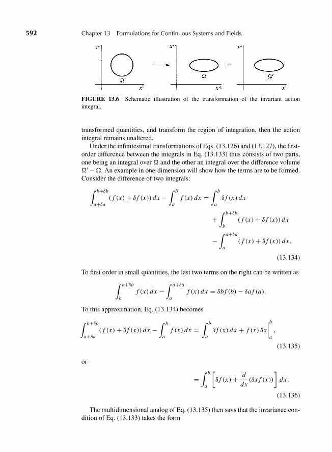
“M13 Goldstein ISBN C13” — 2011/2/15 — page 592 — #35
592 Chapter 13 Formulations for Continuous Systems and Fields
FIGURE 13.6 Schematic illustration of the transformation of the invariant actionintegral.
transformed quantities, and transform the region of integration, then the actionintegral remains unaltered.
Under the infinitesimal transformations of Eqs. (13.126) and (13.127), the first-order difference between the integrals in Eq. (13.133) thus consists of two parts,one being an integral over � and the other an integral over the difference volume�′ −�. An example in one-dimension will show how the terms are to be formed.Consider the difference of two integrals:∫ b+δb
a+δa( f (x)+ δ f (x)) dx −
∫ b
af (x) dx =
∫ b
aδ f (x) dx
+∫ b+δb
b( f (x)+ δ f (x)) dx
−∫ a+δa
a( f (x)+ δ f (x)) dx .
(13.134)
To first order in small quantities, the last two terms on the right can be written as∫ b+δb
bf (x) dx −
∫ a+δa
af (x) dx = δb f (b)− δa f (a).
To this approximation, Eq. (13.134) becomes
∫ b+δb
a+δa( f (x)+ δ f (x)) dx −
∫ b
af (x) dx =
∫ b
aδ f (x) dx + f (x) δx
∣∣∣∣b
a,
(13.135)
or
=∫ b
a
[δ f (x)+ d
dx(δx f (x))
]dx .
(13.136)
The multidimensional analog of Eq. (13.135) then says that the invariance con-dition of Eq. (13.133) takes the form
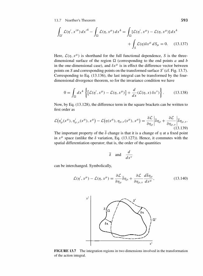
“M13 Goldstein ISBN C13” — 2011/2/15 — page 593 — #36
13.7 Noether’s Theorem 593∫�′
L(η′, x ′μ) dx ′4 −∫�
L(η, xμ) dx4 =∫�
[L(η′, xμ)− L(η, xμ)] dx4
+∫
SL(η)δxμ d Sμ = 0. (13.137)
Here, L(η, xμ) is shorthand for the full functional dependence, S is the three-dimensional surface of the region � (corresponding to the end points a and bin the one-dimensional case), and δxμ is in effect the difference vector betweenpoints on S and corresponding points on the transformed surface S′ (cf. Fig. 13.7).Corresponding to Eq. (13.136), the last integral can be transformed by the four-dimensional divergence theorem, so for the invariance condition we have
0 =∫�
dx4{[L(η′, xμ)− L(η, xμ)
]+ d
dx(L(η, x) δxν)
}. (13.138)
Now, by Eq. (13.128), the difference term in the square brackets can be written tofirst order as
L(η′ρ(xμ), η′ρ,ν(xμ), xμ)− L(η(xμ), ηρ,ν(xμ), xμ
) = ∂L∂ηρ
∣∣∣∣δηρ + ∂L∂ηρ,ν
∣∣∣∣δηρ,ν .(13.139)
The important property of the δ change is that it is a change of η at a fixed pointin xμ space (unlike the δ variation, Eq. (13.127)). Hence, it commutes with thespatial differentiation operator; that is, the order of the quantities
δ andd
dxν
can be interchanged. Symbolically,
L(η′, xμ)− L(η, xμ) = ∂L∂ηρ
δηρ + ∂L∂ηρ,ν
dδηρdxμ
, (13.140)
FIGURE 13.7 The integration regions in two dimensions involved in the transformationof the action integral.
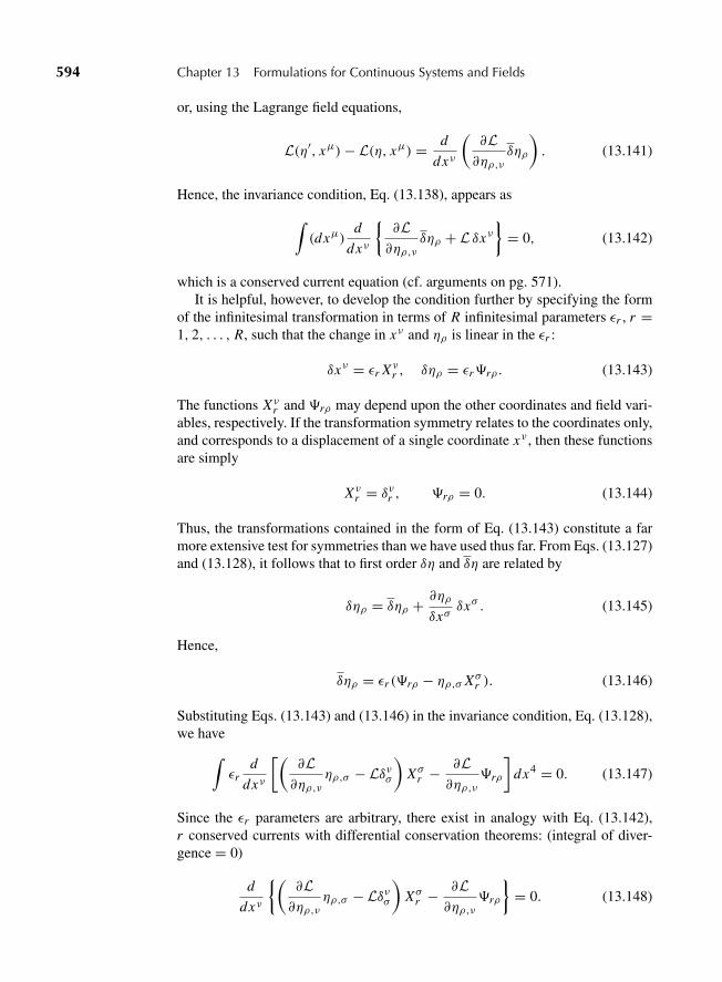
“M13 Goldstein ISBN C13” — 2011/2/15 — page 594 — #37
594 Chapter 13 Formulations for Continuous Systems and Fields
or, using the Lagrange field equations,
L(η′, xμ)− L(η, xμ) = d
dxν
(∂L∂ηρ,ν
δηρ
). (13.141)
Hence, the invariance condition, Eq. (13.138), appears as
∫(dxμ)
d
dxν
{∂L∂ηρ,ν
δηρ + L δxν}= 0, (13.142)
which is a conserved current equation (cf. arguments on pg. 571).It is helpful, however, to develop the condition further by specifying the form
of the infinitesimal transformation in terms of R infinitesimal parameters εr , r =1, 2, . . . , R, such that the change in xν and ηρ is linear in the εr :
δxν = εr Xνr , δηρ = εr�rρ. (13.143)
The functions Xνr and �rρ may depend upon the other coordinates and field vari-ables, respectively. If the transformation symmetry relates to the coordinates only,and corresponds to a displacement of a single coordinate xν , then these functionsare simply
Xνr = δνr , �rρ = 0. (13.144)
Thus, the transformations contained in the form of Eq. (13.143) constitute a farmore extensive test for symmetries than we have used thus far. From Eqs. (13.127)and (13.128), it follows that to first order δη and δη are related by
δηρ = δηρ + ∂ηρ
δxσδxσ . (13.145)
Hence,
δηρ = εr (�rρ − ηρ,σ Xσr ). (13.146)
Substituting Eqs. (13.143) and (13.146) in the invariance condition, Eq. (13.128),we have∫
εrd
dxν
[(∂L∂ηρ,ν
ηρ,σ − Lδνσ)
Xσr − ∂L∂ηρ,ν
�rρ
]dx4 = 0. (13.147)
Since the εr parameters are arbitrary, there exist in analogy with Eq. (13.142),r conserved currents with differential conservation theorems: (integral of diver-gence = 0)
d
dxν
{(∂L∂ηρ,ν
ηρ,σ − Lδνσ)
Xσr − ∂L∂ηρ,ν
�rρ
}= 0. (13.148)
“M13 Goldstein ISBN C13” — 2011/2/15 — page 595 — #38
13.7 Noether’s Theorem 595
Equations (13.148) form the main conclusion of Noether’s theorem, whichthus says that if the system (or the Lagrangian density) has symmetry prop-erties such that conditions (2) and (3) above hold for transformations of thetype of Eqs. (13.143), then there exist r conserved quantities.
The conservation of the stress-energy tensor is easily recovered as a specialcase of Eq. (13.142). If L does not contain any of the xμ, then it, and thereforethe action integral, will be invariant under transformations such as Eq. (13.144),where λ takes on all the values μ. Equation (13.148) then reduces to
d
dxν
[(∂L∂ηρ,ν
ηρ,σ − Lδνσ)δσμ
]= d
dxν
(∂L∂ηρ,ν
ηρ,μ − Lδνμ), (13.149)
which is identical with Eqs. (13.29) with Tμν given by Eq. (13.30).A large number of other symmetries are covered by transformations of the
form of Eq. (13.142). One of the most interesting is a family of transformationsof the field variables only, called gauge transformations of the first kind,* suchthat
δx = 0, δηρ = εcρηρ (no summation on ρ), (13.150)
where the cρ are constants. If the Lagrangian density, and therefore the actionintegral, is invariant under this transformation, then there is a conservation equa-tion of the form
d�ν
dxν= 0, (13.151)
where
�ν = cρ∂L∂ηρ,ν
ηρ. (13.152)
Equation (13.151) is in the form of an equation of continuity with �ν in the roleof a current density jν . Hence, invariance under a gauge transformation of the firstkind leads to the identification of a conserved current that would be appropriatefor an electric charge and current density to be associated with the field.
As an illustration, let us consider the first example of Section 13.6, the complexscalar field. A transformation of the type
φ′ = φeiε, φ∗′ = φ∗e−iε (13.153)
corresponds in infinitesimal form to a gauge transformation of the first type,Eq. (13.150), with
c = i, c∗ = −i.
*The familiar gauge transformation of the electromagnetic field, which adds a 4-gradient �,μ to Aμ,is part of a gauge transformation of the second kind and is not considered here.
“M13 Goldstein ISBN C13” — 2011/2/15 — page 596 — #39
596 Chapter 13 Formulations for Continuous Systems and Fields
It is obvious that the Lagrangian density of Eq. (13.94) is invariant under thetransformation (13.153). Hence, there is an associated current density for theKlein–Gordon field that can be given as
jμ = iq
(dφ
dxμφ∗ − φ dφ∗
dxμ
), (13.154)
which is in agreement with the conventional quantum-mechanical current density.Note that the entire derivation of the conserved charge current density dependsupon the fact that the field is complex. Thus, as mentioned above, a real field doesnot lead to a charge or current density associated with the field. To describe fieldsassociated with charged particles, we must use a pair of complex fields such asφ and φ∗ for the (spinless) Klein–Gordon particle.
Note that while Noether’s theorem proves that a continuous symmetry prop-erty of the Lagrangian density leads to a conservation condition, the converseis not true. There appear to be conservation conditions that cannot correspondto any symmetry property. The most prominent examples at the moment are thefields that have soliton solutions, for example, are described by the sine–Gordonequation or the Korteweg–deVries equation.
Consider, for example, the Lagrangian density for the sine–Gordon equation,Eq. (13.107). As x and t do not appear explicitly, the Lagrangian density is invari-ant under translations of space and time in the manner fulfilling the conditions ofNoether’s theorem. In addition, there is a symmetry under a Lorentz transforma-tion (in xt space). No other symmetry is apparent. We would therefore expect nomore than three conserved quantities from the application of Noether’s theorem.Yet it has been demonstrated, by methods lying outside the Lagrangian descrip-tion of fields, that there exists an infinite number of conserved quantities. That isto say, an infinite number of distinct functions Fi and Gi that are polynomials ofφ, and derivatives can be found for which
d Fi
dt+ dGi
dx= 0, (13.155)
so that the volume integrals of the Fi are constant in time. It appears that thepresence of such an infinite set of conserved quantities is a necessary condition inorder for the field to describe solitons.
Finally, we can easily deduce the version of Noether’s theorem that shouldapply to discrete systems. Here the four coordinates of spacetime are no longerparametric variables on equal footing—the space coordinates revert to their sta-tus as mechanical variables (or functions thereof), and only time remains to fillthe role of a parameter. The action integral, instead of being a four-dimensionalvolume integral,
I =∫
L dx4,

“M13 Goldstein ISBN C13” — 2011/2/15 — page 597 — #40
13.7 Noether’s Theorem 597
is a one-dimensional integral in t as in Eq. (2.1) which is Hamilton’s principle:
I =∫
L dt.
Instead of the continuously indexed field variables ηρ(xν), we have the discretegeneralized coordinates qk(t). It is straightforward enough to recapitulate withthese translations the steps that led to Noether’s theorem. We could repeat in thismanner the arguments contained in Eqs. (13.126) through (13.148) as applied todiscrete systems. But the effect of the conversion is sufficiently obvious and clear,that we can readily see the translation need be done directly only on the finalresult, Eq. (13.148).
The rules for the translation can be summarized as
L → L ,
xμ or xν → t,
ηρ → qk,
ηρ,ν → qk . (13.156)
Further, all sums over 4-valued Greek indices reduce to one term, in t . As a result,the transformations, Eq. (13.143), under which the Lagrangian is to exhibit formand scale invariance become
δt = εr Xr , δqk = εr�rk . (13.157)
Equation (13.148), the statement of the conservation theorems resulting from theinvariance, now becomes
d
dt
[(∂L
∂ qkqk − L
)Xr − ∂L
∂qk�rk
]= 0. (13.158)
Equation (13.158) is the statement of the conclusions of Noether’s theoremfor a discrete mechanical system.
The expression in the parentheses in Eq. (13.158) is our old friend the Jacobiintegral h of Eq. (2.53), or equivalently in terms of (q, p), the Hamiltonian.Indeed, we can recover the conservation of h by considering a transformationthat involves a displacement of time only:
Xr = δr1, �rk = 0. (13.159)
If the Lagrangian is not an explicit function of time, then clearly the form of theLagrangian and the value of the action integral are unaffected by this transfor-mation. But Noether’s theorem, Eq. (13.148), then says that as a result there is aconservation theorem
d
dt
(∂L
∂ qkqk − L
)= 0,
which is identical with the familiar conclusion of Section 2.6.
“M13 Goldstein ISBN C13” — 2011/2/15 — page 598 — #41
598 Chapter 13 Formulations for Continuous Systems and Fields
Let us suppose further that a particular coordinate ql is cyclic. Then theLagrangian and the action are invariant under a transformation for which
Xr = 0, �rk = δklδrl (13.160)
and Eq. (13.158) immediately implies the single conservation statement
d
dt
(∂L
∂ ql
)= 0,
or
pl = 0.
so the canonical momentum is conserved. Thus, the theorems on the conservationboth of Jacobi’s integral and of the generalized momentum conjugate to a cycliccoordinate are subsumed under Noether’s theorem as stated in Eq. (13.158).
The connection between symmetry properties of a mechanical system and con-served quantities has run as a thread throughout formulations of mechanics aspresented here. Having come full circle, as it were, and rederived by sophisticatedtechniques symmetry theorems found in the first chapters, it seems an appropriatepoint at which to end our discussions.
EXERCISES
1. (a) The transverse vibrations of a stretched string can be approximated by a discretesystem consisting of equally spaced mass points located on a weightless string.Show that if the spacing is allowed to go to zero, the Lagrangian approaches thelimit
L = 1
2
∫ [μη2 − T
(∂η
∂x
)2]
dx
for the continuous string, where T is the fixed tension. What is the equation ofmotion if the density μ is a function of position?
(b) Obtain the Lagrangian for the continuous string by finding the kinetic andpotential energies corresponding to transverse motion. The potential energycan be obtained from the work done by the tension force in stretching the stringin the course of the transverse vibration.
2. (a) Describe the field of sound vibrations in a gas in the Hamiltonian formalism andobtain the corresponding Hamilton equations of motion.
(b) Generalizing the momentum expansion to a vector field, express the Hamiltonianfor the acoustic modes of a gas in the momentum representation.
3. Obtain Hamilton’s equations of motion for a continuous system from the modifiedHamilton’s principle, following the procedure of Section 8.5.
“M13 Goldstein ISBN C13” — 2011/2/15 — page 599 — #42
Exercises 599
4. Show that if ψ and ψ∗ are taken as two independent field variables, the Lagrangiandensity
L = h2
8π2m�ψ ?�ψ∗ + Vψ∗ψ + h
4π i(ψ∗ψ − ψψ∗)
leads to the Schrodinger equation
− h2
8π2m∇2ψ + Vψ = ih
2π
∂ψ
∂t,
and its complex conjugate. What are the canonical momenta? Obtain the Hamiltoniandensity corresponding to L.
5. Show that
Gi = −∫πk ∂ηk
∂xidV
is a constant of the motion if the Hamiltonian density is not an explicit function ofposition. The quantity Gi can be identified as the total linear momentum of the fieldalong the xi direction. The similarity of this theorem with the usual conservationtheorem for linear momentum of discrete systems should be obvious.
6. (a) In a 4-space that is not Euclidean, the D’Alembertian is defined as
�2 = =2 = gμν∂2
∂xμ∂xν.
Here gμν is the contravariant metric tensor, which in the flat space of specialrelativity is indeed the same as gμν . For the metric tensor of trace +2 instead of−2 used in Eq. (7.33), find the explicit form of the D’Alembertian so defined.
(b) A suitable Lagrangian for the charged scalar meson field in this metric is
L = 1
2
(gμν
∂φ
∂xμ∂φ∗∂xν
− μ20φφ
∗).
Show that one of the corresponding field equations is
(�2 − μ20)φ = (=2 − μ2
0)φ = 0.
Show also that in light of part (a) this equation is actually identical withEq. (13.99).
7. To the Lagrangian density for the scalar charged meson, Eq. (13.94), add the followingterm to represent the interaction with an electromagnetic field:
jλAλ
where
jλ = i(φφ∗,λ − φ,λφ∗).
What are the field equations for φ and φ∗? What happens to the conserved currentsand associated conservation theorems?
“M13 Goldstein ISBN C13” — 2011/2/15 — page 600 — #43
600 Chapter 13 Formulations for Continuous Systems and Fields
8. Suppose the Lagrangian density in Hamilton’s principle is a function of higher deriva-tives of the field quantities ηρ :
L = L(ηρ; ηρ,μ; ηρ,μν ; xλ).
Assuming the vanishing of the variation at the end points, what is the form of the fieldequations corresponding to such a Lagrangian density?
9. Consider a scalar field quantity η that, for simplicity, is a function only of x and t .Suppose now that the Hamiltonian density is a function of higher spatial derivativesof η and π , that is,
H = H(η, η,x , π, π,x , π,xx ).
What are the corresponding Hamilton equations of motion?
10. Show that the Korteweg-deVries equation corresponds to the field equation for a scalarfield ψ with Lagrangian density
L = 1
2ψxψt + α
6ψ3
x − ν
2ψ2
xx ,
where the subscripts indicate derivatives with respect to the variables indicated, pro-vided ψ is a potential function for the quantity φ of Eq. (13.117):
φ = ∂ψ
∂x.
11. Consider a Hamiltonian density in (x, t) space:
H = η3 + 12η
2,x + π3
,x + 12π
2,xx .
Show that the Hamilton equations of motion correspond to a form of the Korteweg-deVries equation, Eq. (13.117), if
η = φ(x, t)
π =∫ ∞
−∞φ(x ′, t) dx ′.
12. Evaluate explicitly T 0j /c and Ti j for the symmetrized stress-energy tensor of the free
electromagnetic field as given by
Tμν sym = Tμν −Aμ,λFλν
4π= − FλμFλν
4π+ Lgμν
What can be said about the physical meaning of these components?
13. In a 4-space with metric gμν of trace +2, evaluate explicitly the elements of thecovariant (mathematically speaking) tensor Fμν of the electromagnetic field. Alsogive the elements of the matrix with one index lifted and with two indices lifted:
Fλρ = gλμFμν; Fλρ = gλμFμνgρν .
“Z01 Goldstein ISBN AppA” — 2011/2/11 — page 601 — #1
APPENDIX
AEuler Angles in Alternate
Conventions andCayley–Klein Parameters
The Euler angles as defined in Section 4.4 are specified by an initial rotation aboutthe original z axis through an angle φ, a second rotation about the intermediate xaxis through an angle θ , and a third roation about the final z axis through an angleψ . This sequence is here denoted as the “x convention,” referring to the choice ofthe second rotation. For the x convention the Cayley–Klein parameters in termsof the Euler angles are
α = ei(ψ+φ)/2 cosθ
2, β = iei(ψ−φ)/2 sin
θ
2,
γ = ie−i(ψ−φ)/2 sinθ
2, δ = e−i(ψ−φ)/2 cos
θ
2,
Other conventions are possible, and two in particular have found frequent appli-cations in particular fields. Formulas will be given here for properties of a generalrotation in terms of the Euler angles of these two alternate conventions.
y CONVENTION
The y convention differs from the x convention only in that the second rotationis about the intermediate y axis. Transcription from the x to the y conventionis particularly simple because θ retains its meaning in both conventions and thechanges for the other angles are easily obtained. In the x convention, φ is theangle between the line of nodes and the x axis; in the y convention, it is the sameangle measure to the y axis. Similarly in the x convention, ψ is the angle betweenthe line of nodes and the x ′ axis; while in the y convention, it is the same anglerelative to the y′ axis. Temporarily using subscripts to indicate the conventionused, these relations imply the connection (cf. Fig. 4.7)
φx = φy + π
2
ψx = ψy − π
2, (A.1y)
or
sinφx = cosφy sinψx = − cosψy
cosφx = − sinφy cosψx = sinψy . (A.2y)
With this recipe we obtain the following formulas in terms of the Euler angles inthe y convention:
601
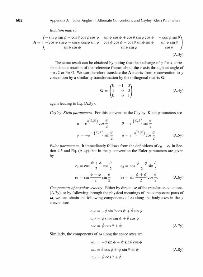
“Z01 Goldstein ISBN AppA” — 2011/2/11 — page 602 — #2
602 Appendix A Euler Angles in Alternate Conventions and Cayley–Klein Parameters
Rotation matrix.
A =⎛⎝− sinψ sinφ + cos θ cosφ cosψ sinψ cosφ + cos θ sinφ cosψ − cosψ sin θ− cosψ sinφ − cos θ cosφ sinψ cosψ cosφ − cos θ sinφ sinψ sinψ sin θ
sin θ cosφ sin θ sinφ cos θ
⎞⎠
(A.3y)
The same result can be obtained by noting that the exchange of y for x corre-sponds to a rotation of the reference frames about the z axis through an angle of−π/2 or 3π/2. We can therefore translate the A matrix from x convention to yconvention by a similarity transformation by the orthogonal matrix G:
G =⎛⎝0 −1 0
1 0 00 0 1
⎞⎠ (A.4y)
again leading to Eq. (A.3y).
Cayley–Klein parameters. For this convention the Cayley–Klein parameters are
α = ei(ψ+φ
2
)cos
θ
2β = e
i(ψ−φ
2
)sin
θ
2
γ = −e−i(ψ−φ
2
)sin
θ
2δ = e
−i(ψ+φ
2
)cos
θ
2. (A.5y)
Euler parameters. It immediately follows from the definitions of e0 − ex in Sec-tion 4.5 and Eq. (A.4y) that in the y convention the Euler parameters are givenby
e0 = cosψ + φ
2cos
θ
2e2 = cos
ψ − φ2
sinθ
2
e1 = sinψ − φ
2sin
θ
2e3 = sin
ψ + φ2
cosθ
2. (A.6y)
Components of angular velocity. Either by direct use of the translation equations,(A.2y), or by following through the physical meanings of the component parts ofv, we can obtain the following components of v along the body axes in the yconvention:
ωx ′ = −φ sin θ cosψ + θ sinψ
ωy′ = φ sin θ sinψ + θ cosψ
ωz′ = ψ cos θ + ψ. (A.7y)
Similarly, the components of v along the space axes are
ωx = −θ sinφ + ψ sin θ cosφ
ωy = θ cosφ + ψ sin θ sinφ (A.8y)
ωz = ψ cos θ + φ.
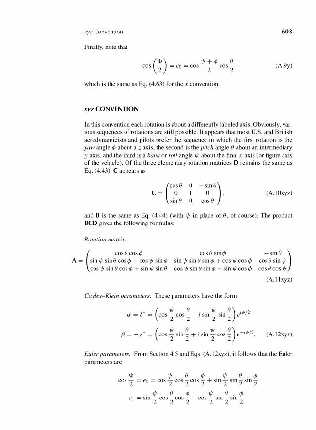
“Z01 Goldstein ISBN AppA” — 2011/2/11 — page 603 — #3
xyz Convention 603
Finally, note that
cos
(�
2
)= e0 = cos
ψ + φ2
cosθ
2(A.9y)
which is the same as Eq. (4.63) for the x convention.
xyz CONVENTION
In this convention each rotation is about a differently labeled axis. Obviously, var-ious sequences of rotations are still possible. It appears that most U.S. and Britishaerodynamicists and pilots prefer the sequence in which the first rotation is theyaw angle φ about a z axis, the second is the pitch angle θ about an intermediaryy axis, and the third is a bank or roll angle ψ about the final x axis (or figure axisof the vehicle). Of the three elementary rotation matrices D remains the same asEq. (4.43), C appears as
C =⎛⎝cos θ 0 − sin θ
0 1 0sin θ 0 cos θ
⎞⎠ , (A.10xyz)
and B is the same as Eq. (4.44) (with ψ in place of θ , of course). The productBCD gives the following formulas:
Rotation matrix.
A =⎛⎝ cos θ cosφ cos θ sinφ − sin θ
sinψ sin θ cosφ − cosψ sinφ sinψ sin θ sinφ + cosψ cosφ cos θ sinψcosψ sin θ cosφ + sinψ sin θ cosψ sin θ sinφ − sinψ cosφ cos θ cosψ
⎞⎠
(A.11xyz)
Cayley–Klein parameters. These parameters have the form
α = δ∗ =(
cosψ
2cos
θ
2− i sin
ψ
2sin
θ
2
)eiφ/2
β = −γ ∗ =(
cosψ
2sin
θ
2+ i sin
ψ
2cos
θ
2
)e−iφ/2. (A.12xyz)
Euler parameters. From Section 4.5 and Eqs. (A.12xyz), it follows that the Eulerparameters are
cos�
2= e0 = cos
ψ
2cos
θ
2cos
φ
2+ sin
ψ
2sin
θ
2sin
φ
2
e1 = sinψ
2cos
θ
2cos
φ
2− cos
ψ
2sin
θ
2sin
φ
2
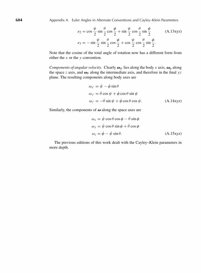
“Z01 Goldstein ISBN AppA” — 2011/2/11 — page 604 — #4
604 Appendix A Euler Angles in Alternate Conventions and Cayley–Klein Parameters
e2 = cosψ
2sin
θ
2cos
φ
2+ sin
ψ
2cos
θ
2sin
φ
2(A.13xyz)
e3 = − sinψ
2sin
θ
2cos
φ
2+ cos
ψ
2cos
θ
2sin
φ
2.
Note that the cosine of the total angle of rotation now has a different form fromeither the x or the y convention.
Components of angular velocity. Clearly vψ lies along the body x axis, vφ alongthe space z axis, and vθ along the intermediate axis, and therefore in the final yzplane. The resulting components along body axes are
ωx ′ = ψ − φ sin θ
ωy′ = θ cosψ + φ cos θ sinψ
ωz′ = −θ sinψ + φ cos θ cosψ. (A.14xyz)
Similarly, the components of v along the space axes are
ωx = ψ cos θ cosφ − θ sinφ
ωy = ψ cos θ sinφ + θ cosφ
ωz = φ − ψ sin θ. (A.15xyz)
The previous editions of this work dealt with the Cayley–Klein parameters inmore depth.
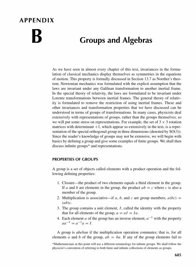
“Z02 Goldstein ISBN AppB” — 2011/2/14 — page 605 — #1
APPENDIX
B Groups and Algebras
As we have seen in almost every chapter of this text, invariances in the formu-lation of classical mechanics display themselves as symmetries in the equationsof motion. This property is formally discussed in Section 13.7 as Noether’s theo-rem. Newtonian mechanics was formulated with the explicit assumption that thelaws are invariant under any Galilean transformation to another inertial frame.In the special theory of relativity, the laws are formulated to be invariant underLorentz transformations between inertial frames. The general theory of relativ-ity is formulated to remove the restriction of using inertial frames. These andother invariances and transformation properties that we have discussed can beunderstood in terms of groups of transformations. In many cases, physicists dealextensively with representations of groups, rather than the groups themselves, sowe will put some stress on representations. For example, the set of 3 × 3 rotationmatrices with determinant +1, which appear so extensively in the text, is a repre-sentation of the special orthogonal group in three dimensions (denoted by SO(3)).Since the reader’s knowledge of groups may not be extensive, we will begin withbasics by defining a group and give some examples of finite groups. We shall thendiscuss infinite groups* and representations.
PROPERTIES OF GROUPS
A group is a set of objects called elements with a product operation and the fol-lowing defining properties:
1. Closure—the product of two elements equals a third element in the group.If a and b are elements in the group, the product ab = c where c is also amember of the group.
2. Multiplication is associative—if a, b, and c are group members, a(bc) =(ab)c.
3. The group contains a unit element, I , called the identity with the propertythat for all elements of the group, a = aI = I a.
4. Each element a of the group has an inverse element, a−1 with the propertyaa−1 = a−1a = I.
A group is abelian if the multiplication operation commutes; that is, for allelements a and b of the group, ab = ba. If any of the group elements fail to
*Mathematicians at this point will use a different terminology for infinite groups. We shall follow thephysicist’s convention of referring to both finite and infinite collections of elements as groups.
605
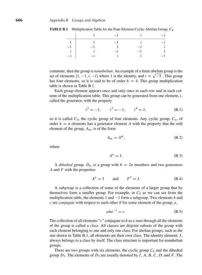
“Z02 Goldstein ISBN AppB” — 2011/2/14 — page 606 — #2
606 Appendix B Groups and Algebras
TABLE B.1 Multiplication Table for the Four-Element Cyclic Abelian Group, C4
1 −1 i −i
1 1 −1 i −i−1 −1 1 −i i
i i −i −1 1−i −i i 1 −1
commute, then the group is nonabelian. An example of a finite abelian group is theset of elements {1,−1, i,−i} where 1 is the identity, and i = √−1 . This grouphas four elements, so it is said to be of order h = 4. This group multiplicationtable is shown in Table B.1.
Each group element appears once and only once in each row and in each col-umn of the multiplication table. This group can be generated from one element, i ,called the generator, with the property
i2 = −1, i3 = −1, i4 = 1, (B.1)
so it is called C4, the cyclic group of four elements. Any cyclic group, Cn , oforder h = n elements has a generator element A with the property that the mthelement of the group, Am , is of the form
Am = Am, (B.2)
where
An = I. (B.3)
A dihedral group, Dn , is a group with h = 2n members and two generatorsA and F with the properties
An = I and F2 = I. (B.4)
A subgroup is a collection of some of the elements of a larger group that bythemselves form a smaller group. For example, in C4 as we can see from themultiplication table, the elements 1 and −1 form a subgroup. Two elements b andc are conjugate with respect to each other if for some element of the group, a,
aba−1 = c. (B.5)
The collection of all elements “c” conjugate to b as a runs through all the elementsof the group is called a class. All classes are disjoint subsets of the group witheach element belonging to one and only one class. For abelian groups, such as theone shown in Table B.1, all elements are their own class. The identity element, I ,always belongs to a class by itself. The class structure is important for nonabeliangroups.
There are two groups with six elements, the cyclic group C6 and the dihedralgroup D3. The elements of D3 are usually denoted by I , A, B, C , D, and F . The
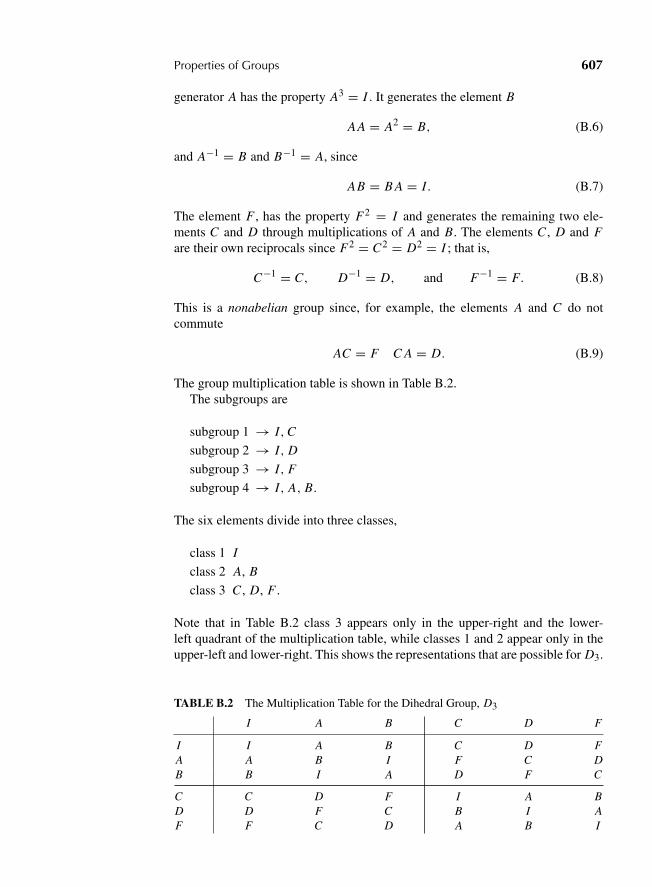
“Z02 Goldstein ISBN AppB” — 2011/2/14 — page 607 — #3
Properties of Groups 607
generator A has the property A3 = I . It generates the element B
AA = A2 = B, (B.6)
and A−1 = B and B−1 = A, since
AB = B A = I. (B.7)
The element F , has the property F2 = I and generates the remaining two ele-ments C and D through multiplications of A and B. The elements C , D and Fare their own reciprocals since F2 = C2 = D2 = I ; that is,
C−1 = C, D−1 = D, and F−1 = F. (B.8)
This is a nonabelian group since, for example, the elements A and C do notcommute
AC = F C A = D. (B.9)
The group multiplication table is shown in Table B.2.The subgroups are
subgroup 1 → I,C
subgroup 2 → I, D
subgroup 3 → I, F
subgroup 4 → I, A, B.
The six elements divide into three classes,
class 1 I
class 2 A, B
class 3 C , D, F .
Note that in Table B.2 class 3 appears only in the upper-right and the lower-left quadrant of the multiplication table, while classes 1 and 2 appear only in theupper-left and lower-right. This shows the representations that are possible for D3.
TABLE B.2 The Multiplication Table for the Dihedral Group, D3
I A B C D F
I I A B C D FA A B I F C DB B I A D F C
C C D F I A BD D F C B I AF F C D A B I
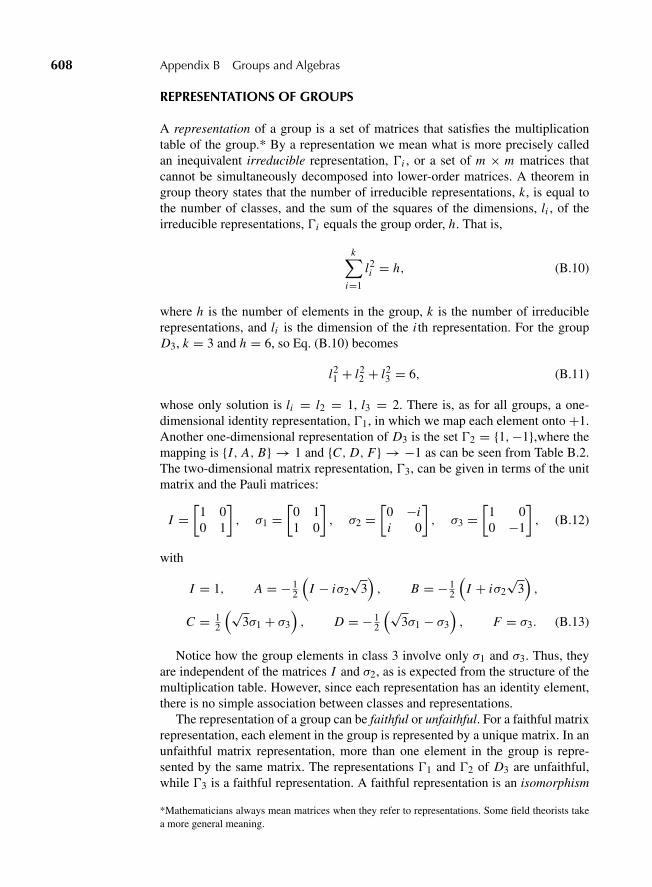
“Z02 Goldstein ISBN AppB” — 2011/2/14 — page 608 — #4
608 Appendix B Groups and Algebras
REPRESENTATIONS OF GROUPS
A representation of a group is a set of matrices that satisfies the multiplicationtable of the group.* By a representation we mean what is more precisely calledan inequivalent irreducible representation, �i , or a set of m × m matrices thatcannot be simultaneously decomposed into lower-order matrices. A theorem ingroup theory states that the number of irreducible representations, k, is equal tothe number of classes, and the sum of the squares of the dimensions, li , of theirreducible representations, �i equals the group order, h. That is,
k∑i=1
l2i = h, (B.10)
where h is the number of elements in the group, k is the number of irreduciblerepresentations, and li is the dimension of the i th representation. For the groupD3, k = 3 and h = 6, so Eq. (B.10) becomes
l21 + l2
2 + l23 = 6, (B.11)
whose only solution is li = l2 = 1, l3 = 2. There is, as for all groups, a one-dimensional identity representation, �1, in which we map each element onto +1.Another one-dimensional representation of D3 is the set �2 = {1,−1},where themapping is {I, A, B} → 1 and {C, D, F} → −1 as can be seen from Table B.2.The two-dimensional matrix representation, �3, can be given in terms of the unitmatrix and the Pauli matrices:
I =[
1 00 1
], σ1 =
[0 11 0
], σ2 =
[0 −ii 0
], σ3 =
[1 00 −1
], (B.12)
with
I = 1, A = − 12
(I − iσ2
√3), B = − 1
2
(I + iσ2
√3),
C = 12
(√3σ1 + σ3
), D = − 1
2
(√3σ1 − σ3
), F = σ3. (B.13)
Notice how the group elements in class 3 involve only σ1 and σ3. Thus, theyare independent of the matrices I and σ2, as is expected from the structure of themultiplication table. However, since each representation has an identity element,there is no simple association between classes and representations.
The representation of a group can be faithful or unfaithful. For a faithful matrixrepresentation, each element in the group is represented by a unique matrix. In anunfaithful matrix representation, more than one element in the group is repre-sented by the same matrix. The representations �1 and �2 of D3 are unfaithful,while �3 is a faithful representation. A faithful representation is an isomorphism
*Mathematicians always mean matrices when they refer to representations. Some field theorists takea more general meaning.
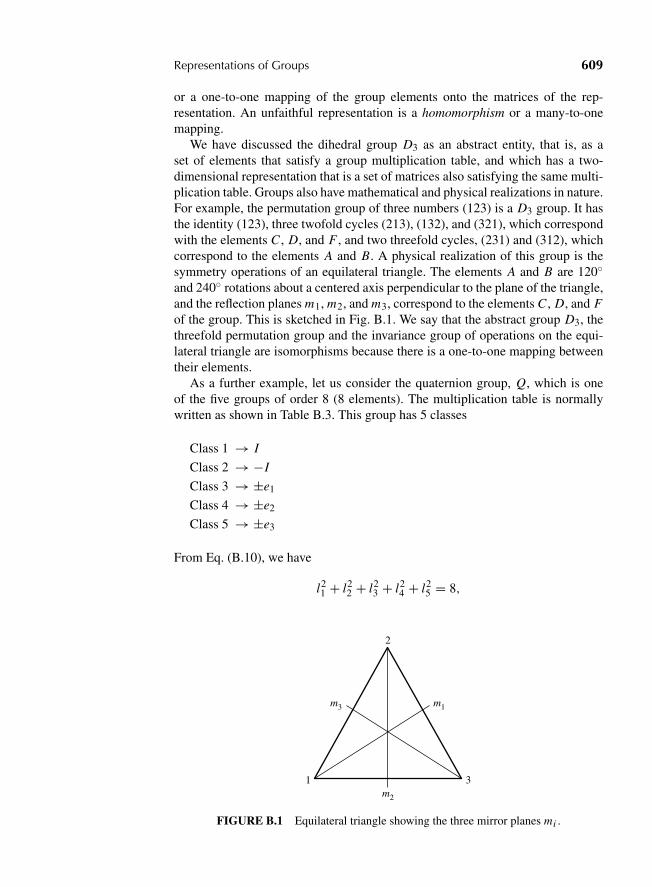
“Z02 Goldstein ISBN AppB” — 2011/2/14 — page 609 — #5
Representations of Groups 609
or a one-to-one mapping of the group elements onto the matrices of the rep-resentation. An unfaithful representation is a homomorphism or a many-to-onemapping.
We have discussed the dihedral group D3 as an abstract entity, that is, as aset of elements that satisfy a group multiplication table, and which has a two-dimensional representation that is a set of matrices also satisfying the same multi-plication table. Groups also have mathematical and physical realizations in nature.For example, the permutation group of three numbers (123) is a D3 group. It hasthe identity (123), three twofold cycles (213), (132), and (321), which correspondwith the elements C , D, and F , and two threefold cycles, (231) and (312), whichcorrespond to the elements A and B. A physical realization of this group is thesymmetry operations of an equilateral triangle. The elements A and B are 120◦and 240◦ rotations about a centered axis perpendicular to the plane of the triangle,and the reflection planes m1, m2, and m3, correspond to the elements C , D, and Fof the group. This is sketched in Fig. B.1. We say that the abstract group D3, thethreefold permutation group and the invariance group of operations on the equi-lateral triangle are isomorphisms because there is a one-to-one mapping betweentheir elements.
As a further example, let us consider the quaternion group, Q, which is oneof the five groups of order 8 (8 elements). The multiplication table is normallywritten as shown in Table B.3. This group has 5 classes
Class 1 → I
Class 2 → −I
Class 3 → ±e1
Class 4 → ±e2
Class 5 → ±e3
From Eq. (B.10), we have
l21 + l2
2 + l23 + l2
4 + l25 = 8,
2
m2
m1m3
1 3
FIGURE B.1 Equilateral triangle showing the three mirror planes mi .
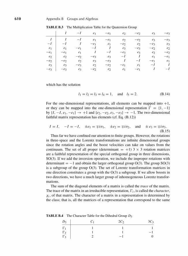
“Z02 Goldstein ISBN AppB” — 2011/2/14 — page 610 — #6
610 Appendix B Groups and Algebras
TABLE B.3 The Multiplication Table for the Quaternion Group
I −I e1 −e1 e2 −e2 e3 −e3
I I −I e1 −e1 e2 −e2 e3 −e3−I −I I −e1 e1 −e2 e2 −e3 e3e1 e1 −e1 −I I e3 −e3 −e2 e2
−e1 −e1 e1 I −I −e3 e3 e2 −e2e2 e2 −e2 −e3 e3 −I I e1 −e1
−e2 −e2 e2 e3 −e3 I −I −e1 e1e3 e3 −e3 e2 −e2 −e1 e1 −I I
−e3 −e3 e3 −e2 e2 e1 −e1 I −I
which has the solution
l1 = l2 = l3 = l4 = 1, and l5 = 2. (B.14)
For the one-dimensional representations, all elements can be mapped into +1,or they can be mapped into the one-dimensional representation � = {1,−1}by {I,−I, e1,−e1} → +1 and {e2,−e2, e3,−e3} → −1. The two-dimensionalfaithful matrix representation has elements (cf. Eq. (B.12))
I = I, −I = −I, ±e1 = ∓iσ1, ±e2 = ∓iσ2, and ± e3 = ∓iσ3.
(B.15)Thus far we have confined our attention to finite groups. However, the rotations
in three-space and the Lorentz transformations are infinite dimensional groupssince the rotation angles and the boost velocities can take on values from thecontinuum. The set of all proper (determinant = +1) 3 × 3 rotation matricesare a faithful representation of the special orthogonal group in three dimensions,SO(3). If we add the inversion operation, we include the improper rotations withdeterminant = −1 and obtain the larger orthogonal group O(3). The group SO(3)is a subgroup of the group O(3). The set of Lorentz transformation matrices inone direction constitutes a group with the O(3) a subgroup. If we allow boosts intwo directions, we have a much larger group of inhomogeneous Lorentz transfor-mations.
The sum of the diagonal elements of a matrix is called the trace of the matrix.The trace of the matrix in an irreducible representation, �i , is called the character,χi , of that matrix. The character of a matrix in a representation is determined bythe class; that is, all the matrices of a representation that correspond to the same
TABLE B.4 The Character Table for the Dihedral Group D3
D3 C1 2C2 3C3
�1 1 1 1�2 1 1 −1�3 2 −1 0
“Z02 Goldstein ISBN AppB” — 2011/2/14 — page 611 — #7
Lie Groups and Algebras 611
class have the same character. For the dihedral group D3, the relation between theclasses Ci of the two-dimensional representation, �3, is given as follows:
TABLE B.5 Characteristics of the Dihedral Group D3
Class Ci Elements Character χi
Class 1 I +2Class 2 A, B −1Class 3 C , D, F 0
For the one-dimensional representations �1 and �2 of D3, the characters are thesame as the one-dimensional matrices. This information can be most convenientlyexpressed in a character table. For D3, this is shown in Table B.4.
In Table B.4, the headings nCm on the columns give the number of elementsn in the class Cm of that row. The characters in the first row for class C1 alsogive the dimensionality of the representation. The rows of the character table areorthogonal to each other, provided we take into account the number of elements ineach column. For example, considering �2 and �3, we have 1×2+2×(1×−1)+3 × (−1 × 0) = 0. In quantum mechanics the �i ’s can represent energy levelssplit from a parent atomic state by an electric field environment of D3 symmetry.
LIE GROUPS AND ALGEBRAS
The terms Lie group and the associated idea of Lie algebra are used in severalchapters. A Lie group is a manifold, which is also a group. A manifold is a contin-uous geometric object; for example, Euclidean space, the spacetime of the specialtheory, and a circle of radius 1 in the complex plane are all manifolds. Most ofthe manifolds considered in physics are continuous manifolds.* For a manifoldto be a Lie group, there must exist a group operation (termed multiplication) forall pairs of points in the manifold, which is consistent with the continuous natureof the manifold. Consider four points in the manifold a, b, c, and d and denotethe group operation of a and c by ac. Consistent means, if a and b are close toeach other and c and d are also close to each other, then ac, ad, bc, and bd areall close to each other. If we restrict our attention to the Lie groups that physicistsare likely to encounter, there are only a few. One set of Lie group elements cor-responds to rotations in odd dimensions, for example, the three-dimensional ro-tation group O(3). A second set is the rotations in even dimensions, for example,the Lorentz group in 4 dimensions. Another set involves the unitary groups, forexample, SU(2), which is the set of 2 × 2 unitary matrices with determinant +1.
*A continuous manifold is a manifold with the concept of nearness. That is, for every point, P , in themanifold, there exist other points in the manifold that are as close to P as desired. As the mathemati-cians would say, for every point, P , in the manifold and given any ε > 0, there exists another point inthe manifold that is closer to P than ε, no matter how small ε.
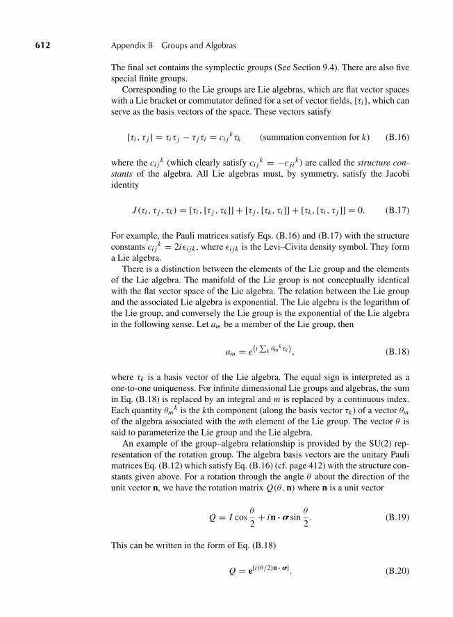
“Z02 Goldstein ISBN AppB” — 2011/2/14 — page 612 — #8
612 Appendix B Groups and Algebras
The final set contains the symplectic groups (See Section 9.4). There are also fivespecial finite groups.
Corresponding to the Lie groups are Lie algebras, which are flat vector spaceswith a Lie bracket or commutator defined for a set of vector fields, {τi }, which canserve as the basis vectors of the space. These vectors satisfy
[τi , τ j ] = τiτ j − τ jτi = ci jkτk (summation convention for k) (B.16)
where the ci jk (which clearly satisfy ci j
k = −c jik) are called the structure con-
stants of the algebra. All Lie algebras must, by symmetry, satisfy the Jacobiidentity
J (τi , τ j , τk) = [τi , [τ j , τk]] + [τ j , [τk, τi ]] + [τk, [τi , τ j ]] = 0. (B.17)
For example, the Pauli matrices satisfy Eqs. (B.16) and (B.17) with the structureconstants ci j
k = 2iεi jk , where εi jk is the Levi–Civita density symbol. They forma Lie algebra.
There is a distinction between the elements of the Lie group and the elementsof the Lie algebra. The manifold of the Lie group is not conceptually identicalwith the flat vector space of the Lie algebra. The relation between the Lie groupand the associated Lie algebra is exponential. The Lie algebra is the logarithm ofthe Lie group, and conversely the Lie group is the exponential of the Lie algebrain the following sense. Let am be a member of the Lie group, then
am = e(i∑
k θmkτk), (B.18)
where τk is a basis vector of the Lie algebra. The equal sign is interpreted as aone-to-one uniqueness. For infinite dimensional Lie groups and algebras, the sumin Eq. (B.18) is replaced by an integral and m is replaced by a continuous index.Each quantity θm
k is the kth component (along the basis vector τk) of a vector θm
of the algebra associated with the mth element of the Lie group. The vector θ issaid to parameterize the Lie group and the Lie algebra.
An example of the group–algebra relationship is provided by the SU(2) rep-resentation of the rotation group. The algebra basis vectors are the unitary Paulimatrices Eq. (B.12) which satisfy Eq. (B.16) (cf. page 412) with the structure con-stants given above. For a rotation through the angle θ about the direction of theunit vector n, we have the rotation matrix Q(θ,n) where n is a unit vector
Q = I cosθ
2+ in ? s sin
θ
2. (B.19)
This can be written in the form of Eq. (B.18)
Q = e[i(θ/2)n ? s]. (B.20)
“Z02 Goldstein ISBN AppB” — 2011/2/14 — page 613 — #9
Clifford Algebras 613
This follows from the expansion of the exponential in a power series. An expan-sion of the scalar product
n ? s = nxσx + nyσy + nzσz (B.21)
enables us to identify 12 nkθ with the parameter θm
k of Eq. (B.18) and to identify τk
as σk . The matrices Q are a faithful representation of SU(2). The use of SU(2) wasintroduced into classical dynamics long before quantum mechanics was devised.It was used because SU(2) notation allows a finite rotation to be described interms of a single angle and a single direction vector (cf. Eq. (B.21)). For a moreextended discussion, see Section 4.5 of the 2nd edition of this text.
Another example of the Lie group–Lie algebra relationship is the Heisenbergalgebra which, in one dimension, has the three elements x , p and I , and the threecommutators
[x, p] = I = ih/2π,
[x, I ] = 0 (B.22)
[p, I ] = 0.
An associated Lie subgroup comprises the infinite set of elements eiαp whichtransform a wavefunction |x > in the quantum-mechanical coordinate represen-tation as follows:
eiαp|x >= |α + x >, (B.23)
where α is a real constant. Another Lie subgroup comprises the eiβx operatorswhich transform a wavefunction |p > in the quantum-mechanical momentumrepresentation in the following manner:
eiβx |p >= |β + p >, (B.24)
where β is real. The overall Heisenberg Lie group is formed by group multiplica-tion of the corresponding subgroup elements eiαp with eiβx .
For most physical theories, there exists an action that remains unchanged invalue for certain continuous chances in the dynamical variables. This is used inChapters 1, 7, 8, 10, and 13 to derive dynamical equations of the Lagrange andHamiltonian approaches. We can now see that the set of transformations of thedynamical variables that leave the action integral unchanged form a representationof the invariance group (often a Lie group) of that physical theory.
CLIFFORD ALGEBRAS
The three Pauli matrices σk , their three counterparts iσk , the 2×2 unit matrix I andthe matrix i I together form another type of algebra called a Clifford algebra. Thelowest order Clifford algebra contains the two elements i and 1. A higher orderClifford algebra is formed from the 4 × 4 Dirac matrices γi and their products.
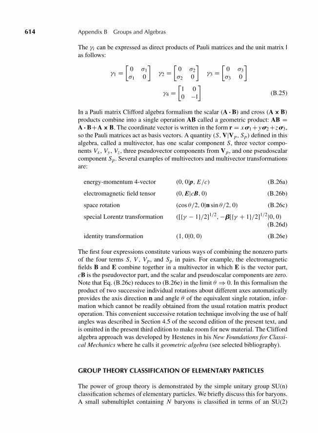
“Z02 Goldstein ISBN AppB” — 2011/2/14 — page 614 — #10
614 Appendix B Groups and Algebras
The γi can be expressed as direct products of Pauli matrices and the unit matrix Ias follows:
γ1 =[
0 σ1σ1 0
]γ2 =
[0 σ2σ2 0
]γ3 =
[0 σ3σ3 0
]
γ4 =[
I 00 −I
](B.25)
In a Pauli matrix Clifford algebra formalism the scalar (A ?B) and cross (A3B)products combine into a single operation AB called a geometric product: AB =A ?B+A3B. The coordinate vector is written in the form r = xs1+ ys2+zs3,so the Pauli matrices act as basis vectors. A quantity (S,V|Vp, Sp) defined in thisalgebra, called a multivector, has one scalar component S, three vector compo-nents Vx , Vy , Vz , three pseudovector components from Vp, and one pseudoscalarcomponent Sp. Several examples of multivectors and multivector transformationsare:
energy-momentum 4-vector (0, 0|p, E/c) (B.26a)
electromagnetic field tensor (0,E|cB, 0) (B.26b)
space rotation (cos θ/2, 0|n sin θ/2, 0) (B.26c)
special Lorentz transformation ([{γ − 1}/2]1/2,−b[{γ + 1}/2]1/2|0, 0)(B.26d)
identity transformation (1, 0|0, 0) (B.26e)
The first four expressions constitute various ways of combining the nonzero partsof the four terms S, V , Vp, and Sp in pairs. For example, the electromagneticfields B and E combine together in a multivector in which E is the vector part,cB is the pseudovector part, and the scalar and pseudoscalar components are zero.Note that Eq. (B.26c) reduces to (B.26e) in the limit θ ⇒ 0. In this formalism theproduct of two successive individual rotations about different axes automaticallyprovides the axis direction n and angle θ of the equivalent single rotation, infor-mation which cannot be readily obtained from the usual rotation matrix productoperation. This convenient successive rotation technique involving the use of halfangles was described in Section 4.5 of the second edition of the present text, andis omitted in the present third edition to make room for new material. The Cliffordalgebra approach was developed by Hestenes in his New Foundations for Classi-cal Mechanics where he calls it geometric algebra (see selected bibliography).
GROUP THEORY CLASSIFICATION OF ELEMENTARY PARTICLES
The power of group theory is demonstrated by the simple unitary group SU(n)classification schemes of elementary particles. We briefly discuss this for baryons.A small submultiplet containing N baryons is classified in terms of an SU(2)
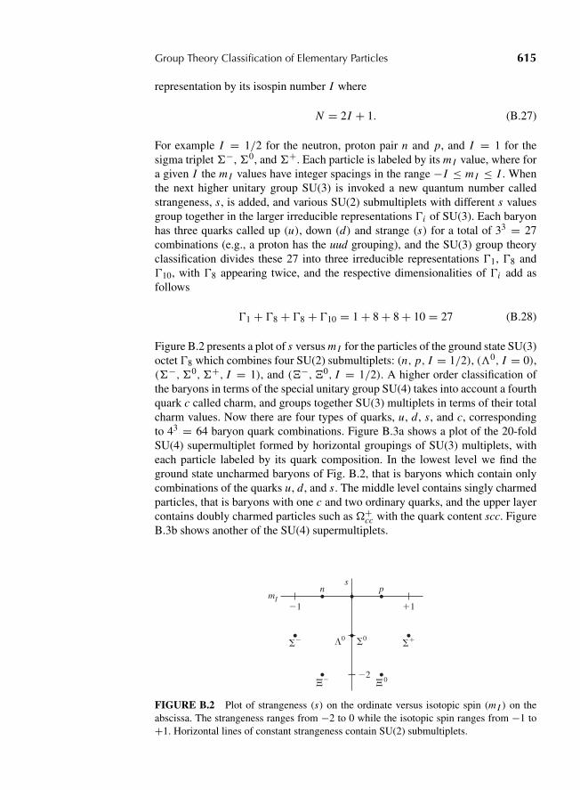
“Z02 Goldstein ISBN AppB” — 2011/2/14 — page 615 — #11
Group Theory Classification of Elementary Particles 615
representation by its isospin number I where
N = 2I + 1. (B.27)
For example I = 1/2 for the neutron, proton pair n and p, and I = 1 for thesigma triplet −, 0, and +. Each particle is labeled by its m I value, where fora given I the m I values have integer spacings in the range −I ≤ m I ≤ I . Whenthe next higher unitary group SU(3) is invoked a new quantum number calledstrangeness, s, is added, and various SU(2) submultiplets with different s valuesgroup together in the larger irreducible representations �i of SU(3). Each baryonhas three quarks called up (u), down (d) and strange (s) for a total of 33 = 27combinations (e.g., a proton has the uud grouping), and the SU(3) group theoryclassification divides these 27 into three irreducible representations �1, �8 and�10, with �8 appearing twice, and the respective dimensionalities of �i add asfollows
�1 + �8 + �8 + �10 = 1 + 8 + 8 + 10 = 27 (B.28)
Figure B.2 presents a plot of s versus m I for the particles of the ground state SU(3)octet �8 which combines four SU(2) submultiplets: (n, p, I = 1/2), (�0, I = 0),( −, 0, +, I = 1), and (�−, �0, I = 1/2). A higher order classification ofthe baryons in terms of the special unitary group SU(4) takes into account a fourthquark c called charm, and groups together SU(3) multiplets in terms of their totalcharm values. Now there are four types of quarks, u, d, s, and c, correspondingto 43 = 64 baryon quark combinations. Figure B.3a shows a plot of the 20-foldSU(4) supermultiplet formed by horizontal groupings of SU(3) multiplets, witheach particle labeled by its quark composition. In the lowest level we find theground state uncharmed baryons of Fig. B.2, that is baryons which contain onlycombinations of the quarks u, d, and s. The middle level contains singly charmedparticles, that is baryons with one c and two ordinary quarks, and the upper layercontains doubly charmed particles such as �+
cc with the quark content scc. FigureB.3b shows another of the SU(4) supermultiplets.
�1�1
�2
s
mI
n p
��
�� �0
�0 �0��
FIGURE B.2 Plot of strangeness (s) on the ordinate versus isotopic spin (m I ) on theabscissa. The strangeness ranges from −2 to 0 while the isotopic spin ranges from −1 to+1. Horizontal lines of constant strangeness contain SU(2) submultiplets.
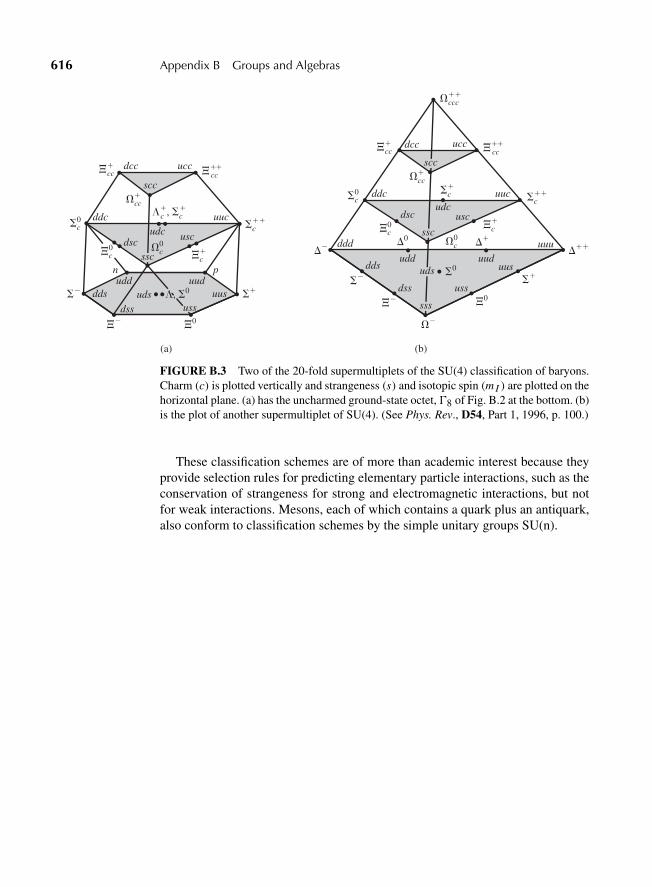
“Z02 Goldstein ISBN AppB” — 2011/2/14 — page 616 — #12
616 Appendix B Groups and Algebras
�� ���0
�� ��
���
��
��
�0
�0
�c���c
�
�c�
��cc
���cc
��cc
�c0
�c0
�c0
ssc
scc
dsc
ddc
dcc
sss
uds
udcuuc
ucc
usc
uududduus
ussdss
dds
ddd uuu
���ccc
(a) (b)
pn
dss
ddsudd uud
uus
uuc
scc
uscdsc
ddc
dcc ucc
udc
uds ����
�� �0
�c��
�c�, �c
���
cc
��cc
���cc
�c�
�c0
�c0
�c0
ssc
�, �0
uss
FIGURE B.3 Two of the 20-fold supermultiplets of the SU(4) classification of baryons.Charm (c) is plotted vertically and strangeness (s) and isotopic spin (m I ) are plotted on thehorizontal plane. (a) has the uncharmed ground-state octet, �8 of Fig. B.2 at the bottom. (b)is the plot of another supermultiplet of SU(4). (See Phys. Rev., D54, Part 1, 1996, p. 100.)
These classification schemes are of more than academic interest because theyprovide selection rules for predicting elementary particle interactions, such as theconservation of strangeness for strong and electromagnetic interactions, but notfor weak interactions. Mesons, each of which contains a quark plus an antiquark,also conform to classification schemes by the simple unitary groups SU(n).
“Z03 Goldstein ISBN AppC” — 2011/2/11 — page 617 — #1
APPENDIX
C Solutions to Select Exercises
CHAPTER 1
Exercise 11
For a conservative force, curl F must be zero. Hence, evaluating curl F
curl F =
∣∣∣∣∣∣∣∣i j k
∂
∂x
∂
∂y
∂
∂zyz zx xy
∣∣∣∣∣∣∣∣= i
[∂
∂y(xy)− ∂
∂z(zx)
]+ j
[∂
∂z(yz)− ∂
∂x(xy)
]
+ k
[∂
∂x(zx)− ∂
∂y(yz)
]= 0.
Since ∑i
[∂
∂y(xy)− ∂
∂z(zx)
]= 0,
the force is conservative.
Exercise 12
Orbital radius for the satellite r = 6720 km
= 6.72 × 10⁶ m.
Orbital period T = 2πr
R
√r
g
= 2 × 3.14 × 6.72 × 106
6000 × 103×√
6.72 × 10⁶
9.83
= 5815 s.
617
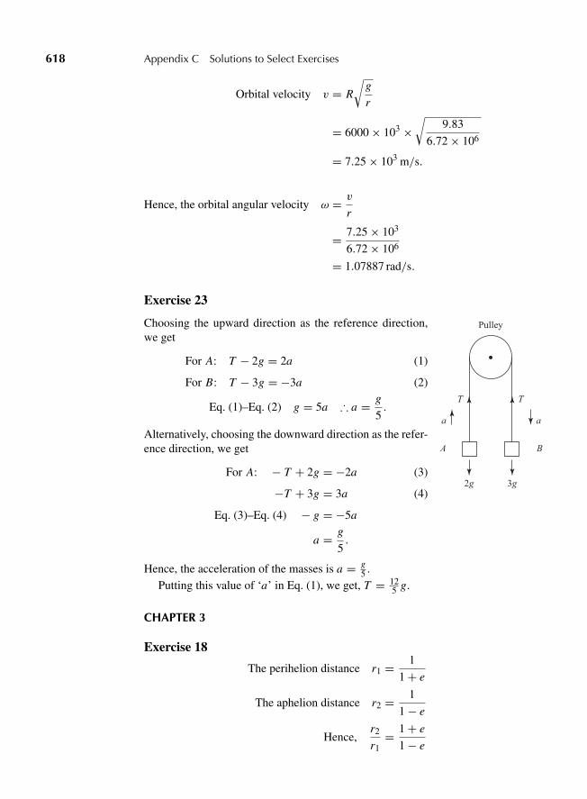
“Z03 Goldstein ISBN AppC” — 2011/2/11 — page 618 — #2
618 Appendix C Solutions to Select Exercises
Orbital velocity v = R
√g
r
= 6000 × 103 ×√
9.83
6.72 × 106
= 7.25 × 10³ m/s.
Hence, the orbital angular velocity ω = v
r
= 7.25 × 10³
6.72 × 106
= 1.07887 rad/s.
Exercise 23
aa
A
TT
B
3g
Pulley
2g
Choosing the upward direction as the reference direction,we get
For A: T − 2g = 2a (1)
For B: T − 3g = −3a (2)
Eq. (1)–Eq. (2) g = 5a ∴ a = g
5.
Alternatively, choosing the downward direction as the refer-ence direction, we get
For A: − T + 2g = −2a (3)
−T + 3g = 3a (4)
Eq. (3)–Eq. (4) − g = −5a
a = g
5.
Hence, the acceleration of the masses is a = g5 .
Putting this value of ‘a’ in Eq. (1), we get, T = 125 g.
CHAPTER 3
Exercise 18
The perihelion distance r1 = 1
1 + e
The aphelion distance r2 = 1
1 − e
Hence,r2
r1= 1 + e
1 − e
“Z03 Goldstein ISBN AppC” — 2011/2/11 — page 619 — #3
Chapter 3 619
The angular momentum of Earth being conserved at all points in its orbit, wehave
mev1r1 = mev2r2,
where me is the mass of Earth and v1 and v2 are the velocities at the perihelionand aphelion, respectively.
∴ v1
v2= r2
r1= 1 + e
1 − e= 1 + 0.023
0 − 0.023= 1.047.
Exercise 27
V = −Gme
R
= −G
R× 4
3πR3ρ, where ρ is the mean density of Earth
= −G · 4
3πR2ρ
= −6.6 × 10−6 × 4
3× 3.14 × (6.1 × 108)2 × 5
= −51.41 × 10¹⁴ erg/gm.
Exercise 30
The number of particles Nφ scattered/s at an angle φ is given by
Nφ α cosec4(φ
2
)
N(6◦)N(4◦)
= cosec4(6◦/2)cosec4(4◦/2)
=(
sin 2◦
sin 3◦
)4
=(
2
3
)4
(for small θ , sin θ → θ ),
∴ N(6◦) = N(4◦) ×(
2
3
)4
= 106 × 16
81
= 0.1975 × 10⁶ particles/s.
CHAPTER 5
Exercise 16
X =∑
mi xi∑mi
i.e. = m1x1 + m2x2 + m3x3
m1 + m2 + m3
“Z03 Goldstein ISBN AppC” — 2011/2/11 — page 620 — #4
620 Appendix C Solutions to Select Exercises
2 = 40x1 + 50x2 + 60x3
40 + 50 + 60
30 = 4x1 + 5x2 + 6x3. (1)
The 70 gm mass is placed at a point (x4, y4, z4) so that the new center of mass ofthe combination is at (0, 0, 0), then
0 = 40x1 + 50x2 + 60x3 + 70x4
40 + 50 + 60 + 70,
4x1 + 5x2 + 6x3 + 7x4 = 0 (2)
Eq. (1)–Eq. (2) 7x4 = −30
x4 = −30/7
Similarly, y4 = z4 = −30/7
Hence, the 70 gm mass must be placed at
(−30
7,−30
7,−30
7
).
CHAPTER 6
Exercise 6
The equation of motion of the other pendulum if one is damped is
md2x
dt2= −kx − mgx
l(for small oscillations)
ord2x
dt2+[
k
m+ g
l
]x = 0,
which represents a simple harmonic motion of period
T = 2π√km + g
l
= 2π√3
0.23 + 108
= 1.24 s.
Exercise 9
Potential energy in the resting position = 8 J
Potential energy at maximum displacement = 13 J
Gain in potential energy = 13 − 8 = 5 J
“Z03 Goldstein ISBN AppC” — 2011/2/11 — page 621 — #5
Chapter 6 621
Hence,1
2K x2 = 5
1
2K (1)2 = 5
∴ K = 10 N/m.
CHAPTER 7
Exercise 14
(a) l = l0
√(1 − v2
c2
)
= 2
√1 −
(.73c
c
)2
= 1.366 m.
(b) l02
= l0
⎛⎝√
1 − v2
c2
⎞⎠
∴ 2
√1 − v2
c2= 1
4
(1 − v2
c2
)= 1
∴ v2
c2= 1 − 1
4
= 3
4
∴ v
c= 0.866
∴ v = 0.866c.
Hence, when the rod travels at 0.886c, its length will be half its rest length.
Exercise 18
(a) m = m0√1 − v2
c2
“Z03 Goldstein ISBN AppC” — 2011/2/11 — page 622 — #6
622 Appendix C Solutions to Select Exercises
= 9.1 × 10⁻³¹√1 −
(0.84c
c
)2
= 16.77 × 10⁻³¹ kg.
(b) when ν → 0, m → ∞ as the denominator → 0
As the mass → ∞, it will be impossible to accelerate an electron to the velocityof light.
Exercise 20
� t = � τ√1 − v2
c2
= 28 × 10−9√1 − (0.8)2
= 46.6 × 10⁻⁹ s
= 46.6 nano second.
Exercise 22
(a) Realtivistic mass m = p
c
= h
λc
= 6.62 × 10⁻³⁴
3 × 108 × 6600 × 10−10
= 3.343 × 10−36 kg.
(b)
m
λ
“Z03 Goldstein ISBN AppC” — 2011/2/11 — page 623 — #7
Chapter 7 623
m = constant
λ
m → ∞ as λ→ 0
m → 0 as m → ∞
Exercise 24
Given l = 12 m
v = 35 km/s = 3.5 × 10⁴ m/s
λ = 5 × 10⁻⁵ cm = 5 × 10⁻⁷ m
Fringe shift �N = 2lv2
c2λ
= 2 × 12 × (3.5 × 104)2
(3 × 108)× 5 × 10−7
= 0.653
Exercise 29
Kinetic energy = (m − m0)c2
= 3 MeV
∴ m = m0 + 3 × 10⁶
c2ev
= 9.1 × 10⁻³¹ + 3 × 106 × 1.6 × 10−19
(3 × 10⁸)2
= 6.243 × 10⁻³⁰ kg.
Since m = m0√1 − v2
c2
,
we have 6.243 × 10−30 = 9.1 × 10⁻³¹√1 − v2
(3×10⁸)2
∴ v = 2.968 × 10⁸ m/s.
Exercise 30
The obseved wavelength λ′ = λ(1 − v
c
)
“Z03 Goldstein ISBN AppC” — 2011/2/11 — page 624 — #8
624 Appendix C Solutions to Select Exercises
= λ[1 − v
c
]−1
= λ
[1 + v
c+ v2
c2· · ·]
(1)
Assuming vc to be � 1, the higher terms can be neglected; hence, Eq. (1) becomes
λ′ = λ[1 + v
c
]
i.e. v = λ′ − λX
· c
= 5435 − 5100
5100× 3 × 108
= 1.9 × 10⁷ m/s
Hence, the star is moving away from us with a speed of 1.9 × 10⁷ m/s.
CHAPTER 9
Exercise 22
{Q, P} = ∂Q
∂q· ∂P
∂p− ∂Q
∂p· ∂P
∂q
∂Q
∂q=
√2 · 1
2· q−1/2 · eα cos p;
∂P
∂p=√
2q · e−α cos p
Hence, {Q, P} = 2 × 1
2× e0 cos2 p + 2 × 1
2× e0 sin2 p
= 1.
Hence, the transformation into (Q, P) basis is canonical.
Exercise 23
p · dq − P · d Q = p · dq −√
2 · log(sin p)[√
2 · q · sec2 p · dp
+√
2 · tan p · dq]
= p · dq − 2q · log(sin p) · sec2 p · dp
− 2 log(sin p) · tan p · dq

“Z03 Goldstein ISBN AppC” — 2011/2/11 — page 625 — #9
Chapter 9 625
= [p − 2 log(sin p) tan p] · dq
− 2q log(sin p) sec2 p · dp
= d[q(p − 2 log(sin p) tan p]
This is an exact differential. Hence, the transformation is canonical.
Exercise 24
In order to show that the given transformation is canonical, the required conditionsare that
[Q, Q] = [P, P] = 0 and [Q, P] = 1
In the given case,
[Q, Q] = ∂Q
∂q· ∂Q
∂p− ∂Q
∂p· ∂Q
∂q= 0
Similary, [P, P] also becomes zero. Evaluating,
[Q, P] = ∂Q
∂q· ∂P
∂p− ∂Q
∂p· ∂P
∂q
= 0 × q · 2p −(− 1
p2× p2
)= +1
∴ [Q, P] = 1.
Therefore, the given transformation is canonical.
“Z04 Goldstein ISBN Bib” — 2011/2/11 — page 626 — #1
Selected Bibliography
TEXTBOOKS ON CLASSICAL MECHANICS
V. I. Arnold, Mathematical Methods of Classical Mechanics, (Berlin: Springer-Verlag, 1989). A very advanced treatment of the subject.
A. Arya, Introduction to Classical Mechanics, (Upper Saddle River, NJ: PrenticeHall, 1998). Undergraduate text.
V. Barger and M. Olsson, Classical Mechanics: A Modern Perspective, (NewYork: McGraw Hill, 1995). Undergraduate text that contains some discussionof chaotic dynamics and a unique section on Newtonian Cosmology.
H. C. Corben and P. Stehle, Classical Mechanics, (New York: Dover, 1994).Reprinted as a classic.
A. L. Fetter and J. D. Walecka, Theoretical Mechanics of Particles and Continua,(New York: McGraw Hill, 1980). Has extensive discussion of continuous sys-tems.
G. Fowles and G. Cassiday, Analytical Dynamics, (Ft. Worth, TX: Saunders,1999). Undergraduate text with many computer problems.
L. Hand and J. Finch, Analytical Mechanics, (Cambridge, England: CambridgeUniversity Press, 1998). Covers standard topics, including Chaos, at a levelsimilar to that of the present text.
D. Hestenes, New Foundations for Classical Mechanics, (Dordrecht, The Nether-lands: Kluwer, 1999). An unconventional approach to classical mechanicswritten in the mathematical language of geometric algebra. It has many keeninsights on the subject.
J. V. Jose and E. J. Saletan, Classical Dynamics, A Contemporary Approach,(Cambridge, England: Cambridge University Press, 1998). A good overall cov-erage of the subject. Much of the theory is expressed in terms of configurationmanifolds and tangent bundles.
L. D. Landau and E. M. Lifshitz, Mechanics, Volume I of Course in TheoreticalPhysics, (Oxford, England: Pergamon, 1976). A very economical and peda-gogic approach to Mechanics. Contains many popular partially worked outexamples.
J. B. Marion and S. T. Thornton, Classical Dynamics of Particles and Systems, (Ft.Worth, TX: Saunders, 1995). A standard undergraduate text recently updatedwith some chaotic dynamics in the context of nonlinear oscillations.
F. Scheck, Mechanics: From Newton’s Laws to Deterministic Chaos, (Berlin:Springer-Verlag, 1990). This recent textbook on classical mechanics includes
626
“Z04 Goldstein ISBN Bib” — 2011/2/11 — page 627 — #2
Selected Bibliography 627
a chapter on the geometric aspects of mechanics which develops the theory inthe language of manifolds. There is also a chapter on chaos.
LAGRANGIAN FORMULATION
Chapters 1 to 3
D. Hestenes, New Foundations for Classical Mechanics, op cit. It has many goodexamples from astronomy. The three-body problem, together with the Eulerand Lagrange solutions, are explained very well.
L. D. Landau and E. M. Lifshitz, Mechanics, Volume I of Course in TheoreticalPhysics, op cit. A very pedagogic approach to mechanics.
K. R. Symon, Mechanics, (Reading, MA: Addison Wesley, 1971). Discusses therestricted three-body problem.
RIGID BODIES
Chapters 4 and 5
T. L. Chow, Classical Mechanics, (New York: Wiley, 1995). Provides an excellenttreatment of the spinning top.
D. Hestenes, New Foundations for Classical Mechanics, op cit. Provides new in-sights into rigid body motion, including the symmetric top.
L. D. Landau and E. M. Lifshitz, Mechanics, op cit. A good, pedagogic discussionof rigid bodies.
SMALL OSCILLATIONS
Chapter 6
L. D. Landau and E. M. Lifshitz, Mechanics, op cit. Treatment includes damped,unharmonic, and nonlinear oscillations.
C. P. Poole, Jr., H. A. Farach and R. J. Creswick, Superconducitivity (Boston,Academic Press, 1995). Chapter 13 discusses Josephson junctions and theirmechanical analogues.
RELATIVITY
Chapter 7
C. W. Misner, K. S. Thorne, and J. A. Wheeler, Gravitation, (San Francisco; Free-man, 1973). A complete introduction to the geometric notation as applied toboth the special theory and the general theory of relativity.

“Z04 Goldstein ISBN Bib” — 2011/2/11 — page 628 — #3
628 Selected Bibliography
B. F. Schutz, A First Course in General Relativity, (Cambridge, England: Cam-bridge University Press, 1985). The first four chapters introduce the reader tothe formalism of the special theory of relativity in a form that can carry overto the general theory.
E. F. Taylor and J. A. Wheeler, Spacetime Physics, (San Francisco: Freeman,1992). An excellent discussion emphasizing the physical thoughts behind andthe physical processes of relativity.
HAMILTONIAN FORMULATION
Chapters 8 to 10
I. Percival and D. Richards, Introduction to Dynamics, (Cambridge, England:Cambridge University Press, NY, 1982). Good treatment of canonical trans-formations, Hamilton–Jacobi equation, and action-angle variables.
CHAOS
Chapter 11
H. Bai-Lin, Chaos, (Singapore: World Scientific, 1984). The first part of the bookconsists of ten good introductory chapters that explain chaos. Chapter 2 de-velops the theory of chaos from Hamilton’s equations and Chapter 3 discussesthe logistic equation. The second and main part of the book is a collection of41 reprinted papers, many of them landmark articles in the development of thesubject.
R. H. Enns and G. McGuire, Nonlinear Physics with Maple for Scientists andEngineers, (Boston: Birkhauser, 2000). A good selection of problems with adisk of Maple programs.
M. Henon, Numerical Exploration of Hamiltonian Systems, Course 2 in ChaoticBehavior of Deterministic Systems, Les Houches Ecole D’Ete de PhysiqueTheoretique, 1981, ed. G. Iooss, R. H. G. Hellerman and R. Stora, (New York:North Holland, 1983). This 114-page lecture is very readable. It provides oneof the best explanations of the Henon–Heiles Hamiltonian, and covers severalother topics included in the present chapter.
E. A. Jackson, Perspectives of Nonlinear Dynamics, (Cambridge, England:Cambridge University Press, 1990). This two-volume set provides a readablepresentation of a variety of complementary approaches to topics in nonlineardynamics. There are useful discussions of several topics covered in this chap-ter such as the Henon–Heiles Hamiltonian, the logistic equation, Liapunovexponents and Poincare maps. An explanation is given of the KAMtheorem.
S. A. Kauffman, The Origins of Order, (New York: Oxford University Press,1993). An introduction to the concepts of complexity.
“Z04 Goldstein ISBN Bib” — 2011/2/11 — page 629 — #4
Selected Bibliography 629
W. Kinzel and G. Reents, Physics by Computer, (New York: Springer,1998). Numerical solutions of linear and nonlinear problems using Mathe-matica and C.
H. O. Peitgen, H. Jurgens and D. Saupe, Chaos and Fractals, New Frontiers ofScience, (Berlin: Springer-Verlag, 1992). This volume constitutes one of thebest available sources for information on fractals, and it does a good job ofexplaining the chaotic behavior of the logistic equation. The text is very longand wordy, but it contains many beautiful figures of fractals and trajectories ofattractors.
L. E. Reichl, The Transition to Chaos, (Berlin: Springer-Verlag, 1992). The the-ory is developed from the viewpoint of classical mechanics, using, for example,action-angle variables. There are good discussions of Poincare sections, Lia-punov exponents, the Henon–Heiles Hamiltonian, and Kolmogorov’s approachfor proving the KAM theorem.
PERTURBATION THEORY
Chapter 12
I. Percival and D. Richards, Introduction to Dynamics, op cit. Good treatment ofperturbation theory.
CONTINUOUS SYSTEMS AND FIELDS
Chapter 13
B. S. Dewitt, Dynamical theory of groups and fields, in B. S. Dewitt and C. Dewitt(eds.) Relativity, Groups and Topology, (New York: Gordon and Breach, 1964).An excellent formalistic approach to the use of groups in modern field theory.
A. L. Fetter and J. D. Walecka, Theoretical Mechanics of Particles and Continua,op cit. Has an extensive discussion of continuous systems.
C. W. Misner, K. S. Thorne, and J. A. Wheeler, Gravitation, op cit. This con-tains an excellent discussion of the concepts of field theory in a Riemannianspacetime. The material is presented in multiple level tracks.
APPENDIX B
H. Goldstein, Classical Mechanics (Reading, MA: Addison Wesley, 1st ed., 1950,2nd Ed., 1980). The first and second editions of the present work have thoroughexplanations of the correspondence between the 2×2 complex unitary matricesof SU(2) and the 3× 3 real orthogonal matrices of O(3), including the Cayley-Klein parameters. These discussions involve applications of Clifford algebrasto classical mechanics.
“Z04 Goldstein ISBN Bib” — 2011/2/11 — page 630 — #5
630 Selected Bibliography
M. Hamermesh, Group Theory, (Reading, MA: Addison Wesley, 1962). A goodcoverage of group theory and its applications to physical problems. Lie groupsand algebras are discussed in Chapter 8.
D. Hestenes, New Foundations for Classical Mechanics, op. cit, A classical me-chanics textbook with extensive sections written in the formalism of Cliffordalgebra, illustrating the insights to be gained by this approach.
C. P. Poole, Jr. and H. A. Farach, Pauli-Dirac Matrix Generators of Clifford Al-gebras, Found. Phys, 12, 719–738 (1982). This article provides background onthe role that Clifford algebras can play in classical mechanics.
M. Tinkham, Group Theory and Quantum Mechanics, (New York, McGraw Hill,1964). A well written introduction to groups. Chapter 5 covers the rotationgroup and angular momentum.

“Z05 Goldstein ISBN AuthorIndex” — 2011/2/11 — page 631 — #1
Author Index
Abel, N. H., 608. See also Abelianin subject index
Arnold, V. I., 484, 487, 489, 626Arya, A., 626Atwood, G., 27, 28
Bai-Lin, H., 489, 628Baker, G. L., 507, 508, 519Barger, V., 626Barone, A., 269Bernoulli, J., 43Bertrand, J., 89Bessel, F. W., 127Binet, A, 203Bohlin, 549Bohr, N. H. D., 95, 466Boltzmann, L. E., 85, 128Boyle, R., 128Bryan, 154
Cambel, A. B., 519Cantor, G. F. L. P., 516, 517,
519, 522Cassiday, G., 626Caratheodory, C., 394Cayley, A., 154, 182, 603, 629Chandler, S. C., 208, 228Chasles, M., 161, 184, 228Chow, T. L., 627Clausius, R. J. E., 84, 128Clifford, W. K., 614, 629Corben, H. C., 626Coriolis, G. G., 174, 326Coulomb, C. A. de, 111Cramer, G., 149, 263Creswick, R. J., 265, 517, 627
D’Alembert, J., 16, 18, 296, 313,
548. See alsoD’Alembertian in subjectindex
Delaunay, C. E., 477Descartes, R., 25. See also
Cartesian in subject indexdeVries, C., 587, 596Dewitt, B. S., 629Dirac, P. A. M., 588, 630Duffing, G., 523, 524
Einstein, A., 139, 276, 326, 327,538
Enns, R. H., 628Euclid, 278, 517. See also
Euclidean in subject indexEuler, L., 45, 122, 150, 155, 165,
196, 197, 200, 209, 234,319, 564, 626
Farach, H. A., 265, 517, 627, 630Faraday, M., 297, 298Feigenbaum, M. J., 506–515Fermat, P. de, 360Fetter, A. L., 626, 629Finch, J., 626Foucault, J. B. L., 179Fourier, Baron J. B. J., 14, 126,
259, 274, 460, 545,551, 575
Fowles, G., 626
Galilei, G., 2. See also Galilean insubject index
Gibbs, J. W., 337Goldschimdt, 65Goldstein, H., 629Gollub, J. P., 507, 508, 519
Gordon, W., 584, 585, 596Gram, 249
Hamermesh, M., 630Hamilton, Sir W. R., 34, 44, 45,
313, 324, 334, 430, 479,488, 562. See alsoHamiltonian in subjectindex
Hand, L., 626Hausdorff, F., 517Helmholtz, H. L. F. von, 337Henon, M., 484, 492, 496, 497,
628, 629Heiles, C., 484, 492, 496, 497,
628, 629Helleman, R. H. G., 497, 628Hertz, H. R., 361Hestenes, D., 121, 626,
627, 630Hooke, R., 52, 91, 316Huygens, C., 132
Iooss, G., 497, 628
Jackson, E. A., 489, 628Jacobi, K. G. J., 61, 334, 338, 361,
390, 398, 426, 430, 479,488, 566, 597
Jose, J. V., 626Josephson, B. D., 265, 271, 627Jurgens, H., 629
Kauffman, S. A., 628Kelvin, Baron W. T., 85, 338Kinzel, I. W., 629Klein, F., 154, 182, 218, 228, 584,
585, 596, 603, 629
631

“Z05 Goldstein ISBN AuthorIndex” — 2011/2/11 — page 632 — #2
632 Author Index
Kepler, J., 73, 92, 101, 347, 370,414, 445, 466, 470, 484,495, 537
Kirchhoff, G. R., 66Kolmogorov, A. N., 484, 487,
489, 629Korteweg, D. J., 587, 596, 600Kronecker, L., 138, 190
Lagrange, J. L., 14, 123, 198, 200,319, 392, 533, 561, 564,627. See also Lagrangian insubject index
Landau, L. D., 627Laplace, P. S., marquis de 102,
264, 413Larmor, Sir J., 231, 318Legendre, A. M., 224,
334, 539Lenz, H. F. E., 102–104, 413Levi-Civita, T., 169, 410Liapunov, M. A., 484, 492, 512,
519, 629Lie, M. S., 171, 385, 392, 411,
613, 630Lifshitz, E. M., 626, 627Liouville, J., 419, 483Lissajous J. A., 83, 258, 439, 358,
462, 464Lorentz, H. A., 22, 131, 280, 319,
328, 415, 580, 611Lorenz, E. N., 523, 576
MacCullagh, 225Mach, E., 324Marion, J. B., 626Maxwell, J. C., 54McGuire, G., 628Minkowski, H., 278, 287, 290, 319,
576, 580, 601
Misner, C. W., 627, 629Moser, J., 484, 487, 489
Napier, J. N., 476Newton, Sir I., 1, 5, 101, 132, 199,
299, 526. See alsoNewtonian in subject index
Nielsen, A. C., 30Noether, A. E, 344, 566, 589, 597
Olsson, M., 626
Paterno, G., 269Pauli, W., 610, 614, 630Peitgen, H. O., 512, 513,
515, 629Percival, I., 628, 629Planck, M. K. E. L., 380Poincare, J. H., 282, 394, 494, 524,
545, 629Poinsot, L., 201, 202, 206, 234Poisson, S. D., 225, 388, 398, 411,
532. See also subject indexPoole, C. P., Jr., 265, 517,
627, 630Ptolemy, C., 129
Raman, Sir C. V., 258Ray, J., 47Rayleigh, Baron R. J. S., 23Reents, G., 629Reichl, L. E., 489, 629Ricci-Curbastro, G, 327Richards, D., 628, 629Riemann, G. F. B., 326, 327,
566, 629Rossler, O. E., 523Routh, E. J., 56, 347Runge, C., 102–104, 413Rutherford, Baron E., 110, 113
Saletan, E. J., 626Sander, L. N., 524Saupe, D., 629Scheck, F., 626Schrodinger, E., 54, 571, 584, 599Schutz, B. F., 628Schmidt, 249Schwarzschild, K., 538Shaw, R., 512Sierpinski, W., 517, 519, 522Sommerfeld, A. J. W., 218, 228Staeckel, 447Stehle, P., 626Stokes, Sir G. G., 20, 24, 52Stora, R., 497Symon, K. R., 627
Tait, P. G., 154Taylor, B., 239Taylor, E. F., 628Thomas, L. H., 282, 330Thomson, Sir W., see Baron (Lord)
KelvinThorne, K. S., 627, 629Thornton, S. T., 626Tinkham, M., 630
van der Pol, B., 490, 491Vinti, J., 463
Walecka, J. D., 626, 629Weber, W. E., 366Wheatstone, Sir C., 66Wheeler, J. A., 324, 619, 627,
628, 629Witten, I. H., 524
Young, T., 559
Zeeman, P, 232
“Z06 Goldstein ISBN SubjectIndex” — 2011/2/11 — page 633 — #1
Subject Index
1-form, 289charge, current, 295covariant vector, 290definition, 290energy, momentum, 295figure, 290table, 290
4-vectorenergy, momentum, 293,
300, 301photon momentum, 304table, 287velocity, 286–288
4-velocity, 286–288
Abbreviated action, 359, 434Abelian group, 605Acceleration, centripetal, 27, 80Acoustics, 54, 235, 238Action, 356
abbreviated, 359, 434and reaction, 7
strong law, 7, 10weak law, 5
at a distance, 324, 583integral, 359, 596variable, 452
integral over orbit, 458Action-angle variable, 430,
452–478, 628celestial mechanics, 456chaos, 485completely separable, 457–466degeneracy, 73, 464, 468harmonic oscillator, 456Kepler problem, 466–478one degree of freedom, 452–457periodic motion, 452perturbation, 541proper variables, 481
Adiabatic invariance, 549–555Algebra, 611
Clifford, 614, 629geometric, 626Heisenberg, 613Lie, 611, 612. See also Lie
algebraAnalogy, structural, 54Analytical mechanics, 1Angle variable, 455
Fourier expansion, 460libration, 460multiply periodic, 460quasi-periodic, 461rotation, 461time dependence, 454, 458, 460
Angular momentum4-vector, 310areal velocity, 73canonical, 405central force problem, 72conservation, 3, 72, 73, 571
total, 7definition, 2density, total, 571eigenvalue, 411electromagnetic, 8ellipsoid, 203mechanical, 8, 405Poisson bracket, 408, 411relativistic, 309rigid body, 188spherical symmetry, 72spin, 11total, 8
Angular velocity in Euler angles,601, 615
Anharmonic oscillator, 545Anomalistic year, 131Anomaly
eccentric, 100mean, 102true, 540
Antiproton, 304Antiquark, 616Aphelion, 484Approximation, semiclassical, 114Apsidal
distance, 78, 95, 96vector, 87
Areal velocity, 73Ascending node, 472Astronomy, medieval, 99Attitude angle, 154Attractor, 489, 516, 629
regular, 493strange, 490, 492, 500strange, Henon-Heiles 500
Atwood’s machine, 27, 28Axis
rigid body, 135screw, 161semimajor, 95, 475semiminor, 101symmetry, 161
Azimuth, 209
Backward glory, 114Bank angle, 154, 603Barrier, centrifugal, 112Baryon, 614, 615, 616Basis vector, 286Bertrand’s theorem, 89, 92Bessel function, 126Biform, 296Bifurcation, 454, 484, 505,
513, 514diagram, 506, 508, 513, 515
Bilinear, 219, 388form, 194
633
“Z06 Goldstein ISBN SubjectIndex” — 2011/2/11 — page 634 — #2
634 Subject Index
Binet ellipsoid, 203, 204Biot-Savart law, 8Bivector, 296Black box, 120Bohr
quantum mechanics, 466theory, 95
Boltzmannconstant, 185factor, 128
Boost, 282. See also Lorentztransformation
Bounded motion, 80, 484Boyle law, 128
and virial, 84Brachistochrone, 42, 63
Calculusoperational, 275of variations, 36, 43
fundamental lemma, 38Canonical, 338
equations of Hamiltonian, 338extended transformation, 371invariant, 388momentum, 55, 314
relativistic, 322, 323perturbation theory, see
Perturbation theoryrestricted transformation, 371variables, 335, 377
Canonical transformation, 348,368–421, 628
active and passive, 400, 405cyclic Hamiltonian, 369, 377,
399, 430, 441degeneracy, 464, 470equations, 368–375examples, 375–377explicit time dependence, 385,
397, 402generated by Hamiltonian, 420generating function, 373group, 387harmonic oscillator, 377–381infinitesimal, 385, 402invariant,
phase space volume, 393,420
Poisson bracket, 389
Jacobi matrix, 382, 394parametric, 385, 405, 408restricted, 371, 381, 382, 387symplectic, 381–388table of, 373
Cantor set, 516, 519, 522Capacitance, 271Caratheodory theorem, 394Carousel, 183Cartesian coordinates, 25, 141Catenary, 41, 42, 64Cayley-Klein parameters, 154, 182,
601, 602Celestial mechanics, 533Center of
energy, 312force, 106gravity, 185mass, 5, 6, 185, 312momentum, 301, 312
system, 301Central force problem, 70–126. See
also Kepler problemCentrifugal
barrier, 112effect, 126
Centripetal acceleration, 27, 176Chain rule, 18Chandler wobble, 208, 228Chaos, 483–522, 626, 628
attractor, 489–491bifurcation, 505–509damped harmonic oscillator,
505–509dimensionality, 616–522fractals, 516–522Henon-Heiles, 496–503, 506Islands, 503–505KAM theorem, 487–489logistic equation, 509–516motion, 491onset, 492, 501, 503parametric
oscillator, 508resonance, 509
perturbation theory, 487–489properties of, 491trajectory, 491, 494,
521, 522Character table, 610
Characteristicequation, 157value, 156
Charge density, 588Charged particle in
electromagnetic field, 23,317, 553
Charm, 615, 616Chasles’ theorem, 161, 184Class of group, 607Classical mechanics, 1–600Clifford algebra, 614, 629Closed orbit, 89, 452Colliding beam, 304Collision
elastic, 118, 120, 306inelastic, 118
C-O-M, center of momentum, 301Commensurability, 463
condition, 464Commensurate, 105, 463
completely, 464condition, 464frequency, 462m-fold, 464
Commutator, 171, 411quantum mechanics, 392, 398relations, 170
Configuration space, 34, 356, 357point transformation, 370variation, 36
Congruence transformation, 245,246, 252
Conic section, 94, 99Conjugate momentum, 55,
335, 351Conservation
differential theorem, 594energy function, 62momentum, 403
Conservation theorems, 7, 55, 72,343, 597
angular momentum, 3, 344total, 7
canonical momentum, 315, 340energy, 4, 11, 345, 450linear momentum, 2, 6, 344
system of particles, 6Noether’s theorem, 589Poisson bracket, 396, 402

“Z06 Goldstein ISBN SubjectIndex” — 2011/2/11 — page 635 — #3
Subject Index 635
relation to symmetry properties,54–59
Conservative system, 4Conserved current, 594, 595Constant of motion, 105, 397, 402,
403, 415algebraic, 418central force, 105Jacobi identity, 397, 411Poisson bracket, 398
Constraint, 12–16, 24differential, 16equation, 15holonomic, 12nonholonomic, 12nonintegral, 16rheonomous, 13rigid body, 12rolling, 182schleronomous, 13, 25semiholonomic, 46, 49virtual work, 16, 17, 48weak, 321
Continuityconditions, 572equation, 595
Continuous system, 265, 558, 568Hamiltonian formulation,
572–577Lagrangian density, 561–566stress energy tensor, 566–572transition from discrete to
continuous, 558–561Contour integration, 469Contraction, 290, 295
of tensor, 191Contravariant, 289Control parameter, 503, 506
logistic equation, 510Coordinate
basis, 286Cartesian, 184contraction, 295cyclic, 55, 343, 369, 445generalized, 13, 19, 239internal, 272mass weighted, 241, 258normal, 251, 257, 259polar, 72pseudo-Cartesian, 294
rotating, 175Coriolis, 174–179
acceleration, 176circulation of fluid
dynamics, 177deflection, 176–178, 182effect, 125, 174–179, 326
on meteorologicalphenomena, 177
force, 175Foucault pendulum, 179hemisphere, 178pressure gradient, 176
Correspondence principle, 325,390, 392, 398
Poisson bracket, 388, 391,392, 398
Cosmological constant, 328Cosmology, 626Coulomb
field, 109, 110law, 274scattering, 110
Coupled electrical circuits, 53Covariant
definition, 277equation, 297Hamiltonian, 349, 352Lagrangian, 318, 321, 322,
350, 351principle, 325relativistic, 577vector, 289
Cramer’s rule, 149, 263Cross section
high energy limit, 127Rutherford, 110total, 110
Crossing the T, 8Current
conserved, 594, 595density, 588
elastic rod, 568field flow, 568, 571, 594flow, RL circuit, 52
Curvature scalar, 327Cyclic
coordinate, 56, 343, 369Kepler problem, 445
group, 606
Cyclotronfrequency, 318, 553resonance, 318
δ-function, 588δ-variation, 38δi j Kronecker delta, 138,
181, 190�-variation, 357–359D’Alembert
characteristic, 548principle, 16–20, 46, 313
D’Alembertian, 296Damping, 519
exponential, 262van der Pol equation, 490
Deflection angle, scattering, 113Degeneracy, 244, 465
conditions, 465exact, 547Kepler problem, 470, 484proper, 547vibrational modes and
frequencies, 257Degrees of freedom, 13, 245, 255,
342, 427, 541, 549, 563Hamiltonian, 342many, 457molecular vibrations, 256n particles, 13oscillator, 264rigid body, 135vibration, 257
Delaunay variables, 477Deltaδ-function, 588δ-variation, 38Kronecker (δi j ), 138, 181, 190
Dense quasi-periodic orbits, 491Derivative, functional, 574Deterministic, 483Differential equation,
inhomogeneous, 259Diffusion, 524Dihedral group, 606, 607Dilation of time, 279Dimension
Cantor set, 516fractal, 516, 517Hausdorff, 517

“Z06 Goldstein ISBN SubjectIndex” — 2011/2/11 — page 636 — #4
636 Subject Index
Dipole momentgravitational, 226magnetic, 185, 230
Dirac δ-function, 588Direction cosines, 136
orthogonality, 138transformation, 139
Dissipationexponential damping, 263forces, 258, 259function, 21–24, 53, 63, 261
Rayleigh, 23Disturbing function, 533Divergence, 295
4-divergence, 296relativistic, 565theorem, four dimensional,
581, 593Divergenceless, 581Doppler effect, 329Drag force, 24, 52Dual space, 292Duffing oscillator, 523
inverted, 524Dumbbell molecule, 347Dynamic steady state, 267
εi jk Levi-Civita density,permutation symbol,169, 410
Earthequatorial bulge, 223figure axis, 226Lagrangian for precession,
227potential, 226, 227precession, 226spinning ring, 228torques, 236
Earth-Moon system, 124Eccentric anomaly, 99Eccentricity, 94, 95, 532
Sun and Moon, 227Ecliptic, 208, 228Eigenvalue, 156–158
angular momentum, 411equation, 157
oscillations, 241Euler’s theorem, 157inertia tensor, 194, 196
linear triatomic molecule, 254problem, 157transformation matrix, 160
Eigenvector, 247indeterminacy, 258inertia tensor, 196linear combination, 248orthonormal, 249oscillations, 244
Eigenwerte (German foreigenvalue), 156
Einsteinfield equations, 327, 538summation convention, 139tensor, 327velocity addition law, 283, 328
Elasticcollision, 118, 120, 306scattering, 120solid, 563wave, 560
Electric circuitequation, 264Lagrangian, 53
Electromagneticfield, 30, 51, 55, 274,
571, 587Lagrangian, 350Lagrangian, covariant, 351
potential, 342radiation, 54theory, 276
Elementary particle, 51, 54,300, 614
Ellipse, 81figure, 96harmonic oscillator, 377orbit equation, 484phase space plot, 97–98properties, 97semimajor axis, 95, 475shape, scale, orientation,
105, 473table, 97
EllipsoidBinet, 203, 204inertia, 196, 201kinetic energy, 204, 258
rigid body, 185–188moment of inertia, 197
Ellipsoidal coordinates forHamilton-Jacobiequation, 479
Ellipticfunction, 89integral, 234region for chaos, 504
Elsewhen, 279Elsewhere, 279Energy
center of, 312conservation, 61
central force, 74, 77free, Gibbs, 337free, Helmholtz, 337function, 61–63, 314
conserved, 61–63hypersurface, 494potential, 4
Ensemble, 419microcanonical, 421
Enthalpy, 336Equant, 129Equation
of motion, 74of state, gas, 85
Equilateral triangle group, 609Equilibrium
generalized forces, 238indifferent, 240neutral, 240stable, 238statistical, 421unstable, 239
Equinox, 539precession, 223–230
Equipotential curvegravitation, 125Henon-Heiles, 498
Equivalence principle,324, 346
Ergotic hypothesis, 418Ether, 566Euclidean
dimension, 518, 519space, 517
Eulerequations, 198, 199, 234
derived from Lagrange’sequations, 200

“Z06 Goldstein ISBN SubjectIndex” — 2011/2/11 — page 637 — #5
Subject Index 637
heavy symmetrical top, 210symmetric body, 205
inhomogeneous function, 86parameters, 155, 182, 602, 603solution of three body problem,
122theorem, 155–161
homogeneous functions, 320Euler angles, 150–154, 196, 601
angular velocity, 602, 615conventions, 154figure, 152infinitesimal, 165left handed, 152SU(2) rotation, 412time changes, 210x-convention, 154, 601xyz-convention, 154, 603y-convention, 154, 601
Euler-Lagrange, 564complex scalar field, 583electromagnetic field, 587equation, 45, 64, 65, 319, 354relativistic equation, 564, 588
Event, 279, 311Extremum
path, 40problem, 39surface area, 40
Faraday tensor, 297, 298Feigenbaum
diagram, logistic equation, 510,513–515
number, 514plot, 506point, 511
Fermat’s principle, 360Field
canonical equations, 574classical theory, 571complex, 596
scalar, 583definition, 566elastic, 51electromagnetic, 30, 51, 55, 274,
571, 587elementary particle, 51equation, Lagrange-Euler, 583gravitational, 176, 185, 210, 274
relativistic, 571scalar 287, 583
meson, 571, 599theory, 558–589
Hamiltonian formulation,571–577
Noether’s theorem, 589–598relativistic, 583–598
Figure axis, 539Fission, 120Fluid
dynamics, 419perfect, 579
Flux density, 107Force
central, 8, 70centrifugal, 175, 176cut off, 111driving, 259effective, 80, 94, 175electromagnetic, 259external, 5generalized, 19, 21, 59, 238gradient of potential, 10gravitational, 93inertial, 5internal, 5, 12inverse square, 77, 92linear restoring, 83long range, 110Lorentz, 22, 131, 237, 317, 350Minkowski, 299, 322relativistic, 297reversed effective, 18, 80strong, 300weak, 300
Foucault pendulum, 179, 183, 184Four-vector, see 4-vectorFour-velocity, see 4-velocityFourier
series, 14, 126, 574convergence, 545multiple, 460
transform, 274Fractal, 516, 629
area, 521dimension, 490
Sierpinski carpet, 519geometry, 491self-similarity, 505, 514
Free energyGibbs, 337Helmholtz, 337
Frequencycharacteristic, 266commensurate, 106critical, 266cyclotron, 318, 553driving, 490imaginary, 244Larmor, 231resonant, 490
Friction, 23atmosphere, 31drag, 24electrical, 52oscillating system, 262rolling, 17
Functional, 287, 293derivative, 574, 575
Future, 279
Galactic center, 496Galaxy model, Henon-Heiles, 496,
497, 516Galilean
system, 2transformation, 276–280
Gas, equation of state, 85Gauge transformation, 595
general, 628General relativity, 324Generalized
force 19, 20, 57, 58mechanics, 65
Generating function, 371, 372canonical transformations, table
of, 373chaos, 488infinitesimal
canonical transformation(I.C.T.), 403
rotation, 404Poisson bracket, 404, 406symplectic, 394table, 373
Geodesic 40, 324–326, 361deviation, 325
Geoid, 176Geostrophic wind, 178

“Z06 Goldstein ISBN SubjectIndex” — 2011/2/11 — page 638 — #6
638 Subject Index
Gibbs free energy, 337Glory scattering, 114Goldschmidt solution, 65Gradient, 295Gram-Schmidt method, 249Gravitational
charge, 226field, 176, 185, 210, 274quadrupole moment, 226
Greek subscript convention, 286Group
abelian, 605canonical transformation,
387class, 607conjugation, 606cyclic, 606definition, 605dihedral, 606, 607generator, 606Lorentz, 282, 610multiplication table, 606properties, 387, 605–611quaternion, 610representation, 608rotation, 171symmetry, 412
for system, 413symplectic, 387, 612theory, 605
Gyration, radius of, 198Gyrocompass, 223Gyromagnetic ratio, 230Gyroscope
inertia, 222torque free mounting, 213
Hamilton’s principle, 34–36,44–50, 313, 324, 354,562, 564
Lagrange’s equations derivation,44, 45
modified, 354, 355, 598nonholonomic systems,
45–50Hamiltonian, 334–353
as total energy, 339covariant, 349, 352degrees of freedom, 342density, 573, 586
formulationcontinuous systems, 572relativistic mechanics, 349
generates canonicaltransformation, 420
generator of system motion, 399Henon-Heiles, 492, 497, 522perturbation, 526quantum mechanics, 613symplectic, 576
Hamiltonian formulation, 334–363advantages, 51–54characteristic function, 434,
440–444comparison of characteristic and
principal functions,442–443
conservation theorems, 347–349cyclic coordinates, 343–349Hamilton equations of motion,
334–363, 368, 397, 402derived from variational
principle, 353least action principle, 356–363
Legendre transformationderivation, 334–342
principal function, 430–434,433, 528
compared with characteristicfunction, 442
relativistic formulation, 349–353Routh procedure, 347–349symplectic approach, 339–343variational principle derivation,
353–356Hamilton-Jacobi theory and
equation, 334, 430–451,488, 528, 549, 628
central force, 448chaos, 485completely separable, 444cyclic coordinates, 445–451ellipsoidal coordinates, 479harmonic oscillator, 434–439method, 434–439new constant coordinates, 432Kepler problem, 445–451
spherical coordinates, 451separation of variables,
444–445
two methods of solution, 442Handedness convention, 169Harmonic oscillator, 434–440,
485action-angle variables, 455,
456, 485adiabatic invariant, 550canonical transformation, 377constants of motion, 417coordinate space plot, 440damped, 269
driven, 505, 507ellipse, 377Feigenbaum plot, 508Hamilton-Jacobi, 434–440isotropic, 82
three dimensional, 274perturbation, 529, 542phase diagram, 380Poisson brackets, 417relativistic, 316two dimensional, 415, 416
anisotropic, 437Heading angle, 154Heisenberg
algebra, 613picture, 408
Helmholtz free energy, 337Henon-Heiles
chaos, 484equipotentials, 498galaxy model, 516Hamilton equations, 497Hamiltonian, 492, 496, 497, 522islands in chaos, 502Poincare map, 499–501potential, 497
Hermitean matrix, 412Herpolhode, 202, 203Hertz principle of least
curvature, 361Hierarchy of islands, 504, 505High energy physics, 300Hodograph, 131Holonomic, 12
constraint, 12system, 199
Homogeneousfunction, 320problem, 320, 359

“Z06 Goldstein ISBN SubjectIndex” — 2011/2/11 — page 639 — #7
Subject Index 639
Homomorphism, 418, 609Hooke’s law, 53, 92, 316, 559Hoop
rolling, 50vertical, 66
Huygens’ waves, 132Hydrodynamic derivative, 419Hyperbola, 81, 316Hyperbolic
motion, 315point, 504region, 504
Hypersurface, 580energy, 494spacelike, 580
Hypocycloid, 64Hysteresis, 270, 271, 523
I.C.T. (infinitesimal canonicaltransformation), 385, 386,402, 403, 408, 410, 413
Identity transformation, 146, 156Ignorable, see cyclicImbedding in chaos, 514–516Impact parameter, 107Inclination, 532Incommensurate, 548
frequency, period, 462, 489, 548oscillator, 521
Inelastic collision, 118Inertia
ellipsoid, 197, 201tensor, 191
components, 195diagonal, 196eigenvalue, 195, 196eigenvector, 196integral, 194principal axes, 196principal moments, 197properties, 195similarity transformation, 196
Inertialframe, 2system, definition, 2
Infinitesimalcanonical transformation, 385,
386, 396, 398, 399, 401rotation, 163, 166
Infrared spectroscopy, 258
Instability, 205Integrability breakdown, 502Integral
invariants of Poincare, 394Jacobi, 62line, 35variation, 44
Integrating factor, 15Invariable plane, 202Invariance
adiabatic, 549condition, 594group, 613logistic equation, 484Lorentz, 302Poisson bracket, 388rotation, 60scale, 591translation, 60
Inversion, 150, 181Islands
in chaos, 502, 503hierarchy, 504, 505various orders, 504
Isomorphism, 608
J -matrix, 342, 382–389, 393Poisson bracket, 388
Jabberwocky, 202Jacobi
determinant, 394form of least action principle,
361identity, 393, 398, 424, 428
integral 62, 566, 597Lagrange brackets, 424Poisson bracket, 390
matrix of canonicaltransformation, 427
Josephson junction, 265,271, 627
KAM (Kolmogorov-Arnold-Moser) theorem, 484,487–492
Kamiltonian, 370Kepler
equation, 102, 126, 131second law, 73third law, 101, 470
Kepler problem, inverse square lawpotential, 70–126, 347, 415
action variables, 471action-angle variables, 466closed orbits, conditions, 89–92cyclic coordinate, 445equations of motion, 72–76equivalent one body problem,
70–71equivalent one dimensional
problem, 76–83inverse square law, 92–98Lie algebra, 414motion in time, 98orbit equation, 86–89, 98–103perturbation, 536Poincare map, 495, 496scattering, 106–121spherical polar coordinates, 467symmetry group, 414virial theorem, 472
Kinematicsrigid body, 134, 184tools, 184
Kinetic energyellipsoid, 203rigid body, 184rotational, 191total, 10
Kinetic theory, 85, 112Kirchhoff junction conditions, 66Klein-Gordon
equation, 585field, 585particle, 596
Kolmogorov-Arnold-Moser(KAM) theorem, 484,487–492
Korteweg-deVries equation,596, 600
Kronecker delta (δi j ), 138,181, 190
Laboratoryframe, 302system, transformation, 306time, 279
Lagrangebracket, 392–394
fundamental, 393
“Z06 Goldstein ISBN SubjectIndex” — 2011/2/11 — page 640 — #8
640 Subject Index
calculus of variations, 36equations, 16, 21–23
derivation from Hamilton’sprinciple, 44, 45
Euler equation derivation, 200Nielsen form, 30perturbation, 533
multipliers, 16, 67point, 124solution of three body
problem, 123undetermined multiplier, 198
Lagrangianapplications, 24–29central force, 71conserved quantities, 566covariant, 318, 321,
322, 352definition, 21density, 564, 567, 583
continuous system, 561–566discrete system, 558–560
electromagnetic field, 350formulation versus
Newtonian, 199from Hamilton’s principle, 44heavy symmetrical top, 208precession of Earth, 227relativistic, 312rigid body, 185, 199separable, 185
Laplace transform, 264Laplace-Runge-Lenz vector,
102–106, 131, 428Larmor
frequency, 231precession, 318theorem, 232
LC circuit, 51Least action principle, 356, 361�-variation, 359Jacobi form, 361restrictions, 358
Legendrepolynomial, 539polynomial generating
function, 224transformation, 334, 335,
375, 549Levi-Civita density, (εi jk ) 169, 410
Liapunov exponent, 491, 519damped pendulum, 519diagram, 520dimension, 521logistic equation, 514, 519negative, 492Sierpinski carpet, 519solar system, 494
Libration, 452, 455, 460Lie
algebra, 171, 412–415, 611–613definition, 412Kepler problem, 414Poisson bracket, 392structure constant, 413, 612
bracket, 171relations, 415
group, 411, 412, 611–613subgroup, 613
Light cone, 279, 280Lightlike, 278, 304Limit cycle, 489
figure, 491van der Pol equation, 491
Line of nodes, 150, 473Linear momentum, 1
particle, 1system of particles, 6total, 6
Liouville theorem, 419–421,428, 483
Lissajous figure, 83, 258, 439,458, 462
noncommensurate, 464sketch, 440, 463
Ljapunov, see LiapunovLogistic equation, 509, 628
control parameter, 510Feigenbaum diagram, 510,
513–515fourfold cycle, 510iterations, 510Liapunov exponent, 512, 514self-similarity, 514twofold cycle, 510
Longitude of ascending node, 474Lorentz, 282
boost, 282force, 22, 131, 237, 350frame, 580
group, 282, 610invariance, 302, 577ten constraints, 282transformation, 280–265
boost, 282equations for ct ′ and r ′, 281general matrix, 281homogeneous, 282inhomogeneous, 282, 610invariance, 302pure, 284scattering, 306
Lorenz condition, 297Lorenz equations, 523Lyapunov, see Liapunov
M-matrix, 382–389, 394MacCullagh formula, 225Mach’s principle, 324Magnetic
fieldcharge particle motion,
22, 317uniform, 409
moment, 230rigidity, 318
Manifold, 576, 611, 627Mapping, 287
quadratic, 503Mass
center of, 312reduced, 71weighted coordinates, 241
Matrixaddition, 145antisymmetric, 148, 165cofactor, 340determinant, 159hermitean, 412infinitesimal element, 164inverse, 147J -, 342, 383–389M-, 382–389, 394multiplication, 144orthogonal, 147reciprocal, 147rectangular, 147skew symmetric, 148transpose, 147unitary, 412

“Z06 Goldstein ISBN SubjectIndex” — 2011/2/11 — page 641 — #9
Subject Index 641
Maxwell’s equations, 54, 276,297, 350
covariant form, 298Mean anomaly, 102Mechanics, see Classical
mechanicsMerry-go-round, 183Meson, 616
scalar, 571, 599Metric
Minkowski space, 287, 580matrix, 287
tensor, 327MeV, definition, 32Microcanonical ensemble, 421Million electron volt,
definition, 32Minimum
gravitational couplingprinciple, 325
surface of revolution, 40Minkowski
coordinate, 288force, 299, 322space, 278, 580
two dimensional, 287Mixing, 516
property of chaos, 491Mode, normal, 252Moderator, 120Molecule
internal coordinates, 272linear triatomic, 272pentatomic, 272polyatomic, 258, 259
rotation and vibration,180
triatomic, 274vibrating, 253, 258
linear polyatomic, 558Moment
of force, definition, 2of inertia, 191
about axis of rotation, 192choice of origin, 193coefficients, 187ellipsoid, 197integral, 194operator, 188parallel axes, 193
Momentumangular, 187, 344canonical, 55, 314center of, 312conjugate, 55, 335, 351conservation, 403density, 569, 573, 579electromagnetic, 55generalized, 55, 56linear, 1, 6, 24, 344representation, 576, 598
Monochromatic light, 259Monogenic, 34Monopole, magnetic, 131, 426Motion
bounded, 80, 484chaotic, 491–493equation, 74hyperbolic, 315periodic, 484
Multiplet, 615Multiply periodic, 458, 461Multivector, 614
Napier’s rules, 476Network, electrical, 264Neutron scattering, 120Newtonian
equations of motion, 199formulation versus
Lagrangian, 199mechanical corpuscles, 132second law, 1, 299third law, 6
Nielsen form of Lagrange’sequations, 30
No-interaction theorem,324, 353
Nodeascending, 472line of, 150, 473
Noether’s theorem, 344, 566,589, 594
conditions, 590conserved current, 594conserved quantities, 418discrete, 596, 597statement of, 594,
595, 597symmetry properties, 598
Non-Euclidean, 278Nonabelian group, 606Noncommensurate, 464Nonholonomic system, 45Noninertial system, 175Normal
behavior in chaos, 515coordinates, 250, 251modes, 252, 256
Number theory theorem, 463Nutation, 215
heavy symmetrical top, 209, 214
O(3) group, 610Oblateness
Earth, 229Moon, 229
Occupation number, 253One dimensional problem,
equivalent, 76One-form, see 1-formOperational calculus, 274Optics
geometric, 112meteorological, 114
Orbitbounded, 80chaotic, 522circular, 80, 81, 94closed, 452
conditions for, 89commensurate, 106degenerate, 106elliptic, 94, 95, 484equation, 99
of state, 86integration, 93
hyperbolic, 94, 110inclination, 474open, 452osculating, 531parabolic, 94phase space, 452quasi-periodic, 490reflection symmetry, 87regular, 522satellite, 229shape, scale, orientation,
105, 473stable, 90

“Z06 Goldstein ISBN SubjectIndex” — 2011/2/11 — page 642 — #10
642 Subject Index
unbounded, 79unstable, 90
Orbiting, 113Orthogonal
matrix, 147transformation, 139
Orthogonality condition, 140Oscillation, 238–265
eigenvalue equation, 241–249forced, 259–265free vibration frequencies,
249–253Josephson junction, 271normal coordinates, 249–253pendulum, damped and driven,
265–271potential expansion, 238–241principal axis transformation,
241–249triatomic molecule, 253–258
Oscillatoranharmonic, 545double, 486parametric, 508
Parabola, 81, 94, 128Parametric resonance, 505, 508,
509Parity, 590Past, 279Pauli matrices, 412, 612, 613Pendulum
damped driven, 265double, 14equation, 267hysteresis, 270periodicity, 453perturbation, 533phase angle, 533plane, 234spherical, 83, 428
Pentatomic molecule, 272Periapsis, 99, 108, 540, 541Periastra, 474Pericynthion, 99Perigee, 474Perihelion, 99, 100, 474,
477, 484Mercury, 332, 538, 539
Period doubling, 516
Periodicfrequency, 455motion, 452, 484
libration, 452rotation, 452
multiply, 458orbits of pendulum, 454quasi, 461
Permutationgroup, 609symbol (εi jk ), 169, 173, 181
Perturbation, 487action-angle variables, 541adiabatic invariance, 549–555degeneracy, 547, 548fast variable, 547first order, 530, 534, 537Hamilton-Jacobi equation, 543Hamiltonian, 526harmonic oscillator, 529Kepler problem, 536n-th order, 530pendulum, 533precession
equinoxes, 539Mercury, 538, 539satellite orbits, 539
second order, 534, 544secular, 532, 535slow variable, 547solar system, 532theory, 229, 338, 483,
526–555quantum, 526time dependent, 526–533
examples, 533–541time independent, 541–549
Phase space, 335, 370, 453, 573ellipse, 97–98harmonic oscillator, 380
damped driven, plot of, 507uncoupled, 486, 487
Kepler problem, 97–98orbits, 454point transformation, 370regular orbits, Henon-Heiles,
502trajectory, 353
Photomeson production, 304Photon, 253
Pitch angle, 154, 603Planck’s constant, 380Poincare
integral invariants, 394map, (or section), 494, 495
Henon-Heiles, 499–501Kepler problem, 495
transformation, 282Poinsot’s construction, 201, 202,
206, 234Point
inflection, 42Lagrange, 124saddle, 124transformation, 30,
370, 422configuration space, 370phase space, 370
turning, 78Poisson
equation, 225theorem, 398
Poisson bracket, 388–411angular momentum, 408–411applications, 396canonically invariant, 390conservation theorem,
402–404correspondence principle,
390, 398double, 390equation of motion,
396–398, 407fundamental, 389, 411generating function, 402–406infinitesimal canonical
transformation (I.C.T.),398–405
integral invariants ofPoincare, 394
invariance, 388Jacobi identity, 390Jacobian determinant, 394Lagrange bracket, 392Lie algebra, 392linear and angular
momentum, 411nested, 408perturbation theory, 532symmetry groups, 411–418

“Z06 Goldstein ISBN SubjectIndex” — 2011/2/11 — page 643 — #11
Subject Index 643
symplectic, 388, 389theorem, 411
Polar coordinate, 72central force Lagrangian, 73plane, 25spherical, 31
Polhode, 202Polyatomic molecule,
258, 259linear, 558rotation and vibration, 180
Potential, 4energy, 4
equilibrium, 239total, 11
equivalent one dimensional,central force, 78
generalized, 21gradient, 10Henon-Heiles, 497, 498hole, 82integrable, 86linear restoring force, 83power law, 86, 87scalar, 20velocity dependent, 21–24
Power series, 43Precession, 206
astronomical, 208, 228average frequency, 217Earth, 207, 226equinoxes, 209, 223–229fast and slow, 219force free motion, 207free body, 205heavy symmetrical top, 209Larmor, 231magnetic field, 230Mercury, 332, 538, 539orbital plane, 540pseudoregular, 218regular, 218satellite, 228system of charges, 230Thomas, 282, 330
Principal axis transformation,241
Proper time, 279, 310, 321Proton-neutron reaction, 304Pseudoscalar, 614
Pseudotensor, 189Pseudovector, 168, 614Ptolemaic system, 129
Q value, 304Quadratic
forms, diagonalization, 252iterator, 509mapping, 503
Quadrature, 75, 76, 211Quadrupole moment
gravitational, 226Sun, 541
Quantization, 54Quantum
commutator, 392corrections, 115electrodynamics, 54field theory, 576Hamiltonian, 613Heisenberg picture, 408mechanics, 111
Bohr, 466perturbation theory, 526scattering, 120theory, 290transition from classical
mechanics, 76Quark, 615Quasi-
periodic, 461, 490static motion, 268
Quaternion group, 609
Radiusgyration, 198vector, 73
Rainbow scattering, 114Raman spectroscopy, 258Randomness, 483Rayleigh’s dissipation function,
23Reactance, 53Regularity, 488
breakdown, 488Relativity, 276–328, 627
4-vector, 287angular momentum,
309–312collisions, 300–309
electromagnetism, 297–300force, 297–300general, 324–328, 538Lagrangian, 312–324metric tensor, 287, 288, 291reduced mass, 71spacetime, 278–280special, 265, 276–324
postulates, 277Representation
faithful, 608, 613group, 608irreducible, 608momentum, 576
Repulsive centrifugal barrier, 78Residue, 469Resonance, 260, 548
deep, 549parametric, 509shallow, 549transients, 260vibrating system, 260
Resonant frequency of lineartriatomic molecule, 255
Reversed effective force, 80Reversible process, 336Rheonomous, 13Ricci tensor, 327Riemann
surface, 469tensor, 326, 327
Rigid body, 12angular momentum, 185–188definition, 134–138degrees of freedom, 134equations of motion, 184,
198–200Euler
equations, 198–200theorem, 155, 156
heavy symmetrical top motion,208–223
kinematics, 134, 184Lagrangian, 199motion, 134, 155–174nutating, 209, 214orientation, 169rotation, 155–174
finite, 161–163infinite, 163–171
“Z06 Goldstein ISBN SubjectIndex” — 2011/2/11 — page 644 — #12
644 Subject Index
solving problems, 198torque free motion, 200–223
Rigidity, 318Roll angle, 154, 603Rolling
constraint, 14disk, 15hoop, 50
Rossler equations, 523Rotation, 141, 452, 455
active sense, 143clockwise, 162counterclockwise, 170finite, 161formula, 162, 170generator, 171group, 171infinitesimal, 162, 163instantaneous axis, 172kinetic energy, 191matrix, 142passive, 169
sense, 143proper, 158trace, 160vector, 59
RouthKepler problem, 348procedure, 57, 347Routhian, 348
Rutherfordcross section, 110
Satelliteartificial, 229close, 229orbiting Earth, 474orbits, 223, 229
Scalar, 189, 293curvature, 327field, 287meson, 571
field, 599potential, 20product, Minkowski space, 288,
290, 291scale invariance, 591transformation, 370
Scattering, 106, 306angle, 112, 308, 309
center of mass, 116cross section 107deflection angle, 114differential cross section,
107, 119elastic, 118, 120, 306glory, 114inelastic, 118laboratory coordinates,
114–120neutron, 120rainbow, 112Rutherford, 111
Schrodingerquantum theory, 576spacetime, 566vector, 286velocity, 588wave function, 571
Schrodinger equation, 54,584, 599
Schwarzschild solution of Einsteinfield equations, 538
Scleronomous, 13, 25Screening, nucleus, 111Screw
motion, 161symmetry axis, 161
Secularchange, 531equation, 157, 244
linear triatomic molecule, 254perturbation, 532, 535
Self-similarity, 505, 514fractal, 516–519logistic equation, 513–515
Semiclassical approximation, 114Semiholonomic, 46, 48, 49Semimajor axis, 95, 475Semiminor axis, 101Sensitivity to initial
conditions, 491Separation constant, 445Siderial
day, 175year, 538
Sierpinskicarpet, 517–519, 522
fractal dimension, 518sponge, 522
Sigma elementary particle, 615Similarity transformation, 149,
158, 189trace, 160
Simultaneity, 580Sine-Gordon
equation, 585field, 585
SO(3) group, 413, 418, 610SO(4) group, 414SO(n) group, 418SOHO, 126Solar day, 175Soliton, 587, 596Sound vibrations in gas, 598Space
configuration, 34, 357dual, 292filling, 521Minkowski, 278, 290
Spacelike, 278, 580Spacetime, 278
interval, 278Special relativity, 276
postulates, 277Spherical triangle, 181, 476Spin angular momentum,
11Spiraling, 113Stability, 205
marginal, 493Staeckel conditions, 446, 447Stationary
path, 37value, 35
Steady state, dynamic, 267Stochastic, 483Stokes’ law, 24, 52Strange attractor, 490,
492, 500dimension, 521fractal dimension, 520Henon-Heiles, 500, 501
Strangeness, 615Stress
energy tensor, 566, 570, 589conservation, 595properties, 578symmetrize, 572, 600
tensor, 570
“Z06 Goldstein ISBN SubjectIndex” — 2011/2/11 — page 645 — #13
Subject Index 645
Stronglaw of action and reaction, 7nuclear force, 300
Structureanalogy, 54constant, 412, 413, 612
SU(2) group, 413, 418, 611, 614,616, 629
SU(3) group, 418, 615SU(4) group, 616SU(n) group, 418, 614, 616Subgroup, 606Submultiplet, 614Summation convention, 138,
169, 186Superconductivity, 627Supermultiplet, 614, 616Susceptance, 53Symmetry
groups, 411–418mechanical systems, 411–418properties, 60spherical, 60, 72
Symplectic, 343, 381approach, 339, 343canonical transformation,
381, 382condition, 384, 387, 422generating function, 394group, 387, 611Hamilton’s equations, 343matrix, 384Poisson bracket, 388, 397
Systemcontinuous, 568discrete, 558vector, 409, 410, 413
Tachyon, 278Tait-Bryan angles, 154Tardyon, 278Taylor series, 239
potential expansion, 482Temperature, definition, 85Tensor, 188–191
alternating, 169Cartesian, 189definition, 293first rank, 189inertia, 191–198
isotropic of rank 3, 169metric, 286moment of inertia, 191–198product, 294properties, 188rank, 293second rank, 188slots, 293unit, 190wedge product, 295zero rank, 189
Thermodynamics, 336Thomas
frequency, 285precession, 282, 330
Three body problem, 121–126, 626Euler solution, 122Lagrange solution, 123restricted, 124, 133
Threshold energy, 302–305Time dilation, 279Timelike, 278Top
Euler equations, 210fast, 215, 221heavy symmetrical, 200,
208, 482with one point fixed, 208motion, 208, 212
sleeping, 221symmetric, 627tippie, 221uniform, 221
Topological dimension, 518Torque, 2
critical, 266damping, 266gravitational, 223pendulum, 266
Torus, 487, 492Tour de force, 407Trace of similarity
transformation, 160Transformation
active sense, 143canonical, 368–421
infinitesimal, 396restricted, 371, 382
congruence, 245,246, 252
equation, 14extended canonical, 371formal properties, 144Galilean, 281gauge, 595generating function, 371identity, 146, 156, 395improper, 151, 168infinitesimal, 165
canonical (I.T.C.), 396Transformation (cont.)
Legendre, 375, 549examples, 375
linear, 187Lorentz, 280matrix, 144
elements, 140operator, 142orthogonal, 139–150, 184passive sense, 143point, 31, 370, 422principal axis, 241proper, 151restricted canonical, 371, 382rigid body rotation, 139–155scale, 370similarity, 149, 158, 180,
189, 244Transient, 260Translational mode, 272Triatomic molecule, 274Triple cross product, 186Turning angles, 213Twin paradox, 285
Ultrarelativistic, 303region, 308
Undetermined multipliers ofLagrange, 46, 362
Unitary matrix, 412Unstable moment of inertia
axis, 205
van der Polequation, 490limit cycle, 491
Variablecanonical, 335fast, 547slow, 547
“Z06 Goldstein ISBN SubjectIndex” — 2011/2/11 — page 646 — #14
646 Subject Index
Variation, 354δ-type, 38, 44�-type, 357, 359integral, 44line integral, 35
VariationalHamiltonian, 353principle, 5, 34–43, 51
Vector4-vector
energy, momentum, 295,300, 301
photon momentum, 304table, 287velocity, 286–288
addition, 163axial, 168conserved, 104covariant, 289field, table, 287first rank tensor, 189flux density, 569Minkowski space, 286polar, 167
radius, 73rate of change, 171–174system, 409, 410, 413tangent, 286, 326
Velocityaddition law, 282angular, 172, 187
critical, 221rigid body, 172
areal, 73critical angular, 221field, 588four-, 286generalized, 25, 319
Vibrationanharmonic, 255forced, 258, 264free, 250, 253
modes, 260linear triatomic molecule, 253longitudinal mode, 257number of normal
modes, 255transverse mode, 257
VirialClausius, 84, 128theorem, 83–86, 94, 472
Virtualdisplacement, 16, 20work principle, 17
Viscosity, 51, 265
Wavefunction, 613Weak nuclear force, 300Weber’s electrodynamics,
366Wedge product, 295, 296Wheatstone bridge, 66Witten and Sander diffusion
model, 524Wobble, Chandler, 208, 228Work, 9
Yaw angle, 154, 603Year, anomalistic, 131Young’s modulus, 559, 560
Zeeman effect, 232