MP350 Classical Mechanics - Maynooth University ...
109
MP350 Classical Mechanics Jon-Ivar Skullerud with modifications by Brian Dolan December 11, 2020
-
Upload
khangminh22 -
Category
Documents
-
view
1 -
download
0
Transcript of MP350 Classical Mechanics - Maynooth University ...

MP350 Classical Mechanics
Jon-Ivar Skullerudwith modifications by
Brian Dolan
December 11, 2020

1

Contents
1 Introduction 5
1.1 Physics is where the action is . . . . . . . . . . . . . . . . . . . . . . . . 5
1.2 Overview . . . . . . . . . . . . . . . . . . . . . . . . . . . . . . . . . . . . 6
2 Lagrangian mechanics 8
2.1 From Newton II to the Lagrangian . . . . . . . . . . . . . . . . . . . . . 8
2.2 The principle of least action . . . . . . . . . . . . . . . . . . . . . . . . . 8
2.2.1 Hamilton’s principle . . . . . . . . . . . . . . . . . . . . . . . . . 11
2.3 The Euler–Lagrange equations . . . . . . . . . . . . . . . . . . . . . . . . 12
2.4 Generalised coordinates . . . . . . . . . . . . . . . . . . . . . . . . . . . . 15
2.4.1 The shortest path between two points (optional) . . . . . . . . . . 20
2.4.2 Polar and spherical coordinates . . . . . . . . . . . . . . . . . . . 21
2.5 Lagrange multipliers [Optional] . . . . . . . . . . . . . . . . . . . . . . . . 24
2.5.1 Constraints . . . . . . . . . . . . . . . . . . . . . . . . . . . . . . 24
2.6 Canonical momenta and conservation laws . . . . . . . . . . . . . . . . . 29
2.6.1 Angular momentum . . . . . . . . . . . . . . . . . . . . . . . . . 30
2.7 Energy conservation: the hamiltonian . . . . . . . . . . . . . . . . . . . . 32
2.7.1 When is H conserved? . . . . . . . . . . . . . . . . . . . . . . . . 33
2.7.2 The Energy and H . . . . . . . . . . . . . . . . . . . . . . . . . . 34
2.8 Lagrangian mechanics — summary sheet . . . . . . . . . . . . . . . . . . 37
3 Hamiltonian dynamics 39
3.1 Hamilton’s equations of motion . . . . . . . . . . . . . . . . . . . . . . . 40
3.2 Cyclic coordinates and effective potential . . . . . . . . . . . . . . . . . . 42
3.3 Hamilton’s equations from a variational principle . . . . . . . . . . . . . 44
3.4 Phase space [Optional] . . . . . . . . . . . . . . . . . . . . . . . . . . . . 45
3.5 Liouville’s theorem [Optional] . . . . . . . . . . . . . . . . . . . . . . . . . 48
2

3.6 Poisson brackets . . . . . . . . . . . . . . . . . . . . . . . . . . . . . . . . 50
3.6.1 Properties of Poisson brackets . . . . . . . . . . . . . . . . . . . . 50
3.6.2 Poisson brackets and conservation laws . . . . . . . . . . . . . . . 52
3.6.3 The Jacobi identity and Poisson’s theorem . . . . . . . . . . . . . 53
3.7 Noethers theorem . . . . . . . . . . . . . . . . . . . . . . . . . . . . . . . 54
3.8 Hamiltonian dynamics — summary sheet . . . . . . . . . . . . . . . . . . 57
4 Central forces 59
4.1 One-body reduction, reduced mass . . . . . . . . . . . . . . . . . . . . . 59
4.2 Angular momentum and Kepler’s second law . . . . . . . . . . . . . . . . 61
4.3 Effective potential and classification of orbits . . . . . . . . . . . . . . . . 64
4.4 Integrating the energy equation . . . . . . . . . . . . . . . . . . . . . . . 64
4.5 The inverse square force, Kepler’s first law . . . . . . . . . . . . . . . . . 66
4.5.1 The shapes of the orbits . . . . . . . . . . . . . . . . . . . . . . . 68
4.6 More on conic sections . . . . . . . . . . . . . . . . . . . . . . . . . . . . 69
4.6.1 Ellipse . . . . . . . . . . . . . . . . . . . . . . . . . . . . . . . . . 70
4.6.2 Parabola . . . . . . . . . . . . . . . . . . . . . . . . . . . . . . . . 72
4.6.3 Hyperbola . . . . . . . . . . . . . . . . . . . . . . . . . . . . . . . 72
4.7 Kepler’s third law . . . . . . . . . . . . . . . . . . . . . . . . . . . . . . . 74
4.8 Kepler’s equations . . . . . . . . . . . . . . . . . . . . . . . . . . . . . . 76
4.9 Runge-Lenz vector . . . . . . . . . . . . . . . . . . . . . . . . . . . . . . 77
4.10 Central forces — summary sheet . . . . . . . . . . . . . . . . . . . . . . . 78
5 Rotational motion 80
5.1 How many degrees of freedom do we have? . . . . . . . . . . . . . . . . . 81
5.1.1 Relative motion as rotation . . . . . . . . . . . . . . . . . . . . . 82
5.2 Rotated coordinate systems and rotation matrices . . . . . . . . . . . . . 82
5.2.1 Active and passive transformations . . . . . . . . . . . . . . . . . 84
5.2.2 Elementary rotation matrices . . . . . . . . . . . . . . . . . . . . 84
5.2.3 General properties of rotation matrices . . . . . . . . . . . . . . . 84
5.2.4 The rotation group [optional] . . . . . . . . . . . . . . . . . . . . . 87
5.3 Euler angles . . . . . . . . . . . . . . . . . . . . . . . . . . . . . . . . . . 88
5.3.1 Rotation matrix for Euler angles . . . . . . . . . . . . . . . . . . 89
5.3.2 Euler angles and angular velocity . . . . . . . . . . . . . . . . . . 90
5.4 The inertia tensor . . . . . . . . . . . . . . . . . . . . . . . . . . . . . . . 91
3

5.4.1 Rotational kinetic energy . . . . . . . . . . . . . . . . . . . . . . . 91
5.4.2 What is a tensor? Scalars, vectors and tensors. . . . . . . . . . . . 96
5.4.3 Angular momentum and the inertia tensor . . . . . . . . . . . . . 98
5.5 Principal axes of inertia . . . . . . . . . . . . . . . . . . . . . . . . . . . 98
5.5.1 Rotations and the inertia tensor . . . . . . . . . . . . . . . . . . . 98
5.5.2 Comments . . . . . . . . . . . . . . . . . . . . . . . . . . . . . . . 101
5.6 Equations of motion . . . . . . . . . . . . . . . . . . . . . . . . . . . . . 102
5.6.1 The symmetric heavy top . . . . . . . . . . . . . . . . . . . . . . 102
5.6.2 Euler’s equations for rigid bodies . . . . . . . . . . . . . . . . . . 104
5.6.3 Stability of rigid-body rotations . . . . . . . . . . . . . . . . . . . 105
4

Chapter 1
Introduction
1.1 Physics is where the action is
In these lectures we shall develop a very powerful (and beautiful) way of formulatingNewtonian mechanics. The basic idea is to derive Newton’s equations from a variationalprinciple, meaning that for a given dynamical system we look for a function of thedynamical variables and velocities such that the time evolution of the system is obtainedby minimising this function. The function is called the action for the system. This givesan extremely concise and elegant way of describing the dynamics: for systems withmany degrees of freedom and/or many particles we do not need to write down a messof complicated coupled differential equations to define the dynamics — we just writedown a single function, the action. In principle we can write all the laws of physics onthe back of a postage stamp.
In order to solve the dynamics though we need to pick it apart, and that requiresderiving dynamical equations from the action and solving them, which can still be quitecomplicated. But the simplicity and elegance of the variational formulation often pointsto a choice of variables that makes the solution easier. Moreover the action principle isthe springboard to new physics. The methods introduced in this course can easily beextended to both special and general relativity and were instrumental in the developmentof quantum mechanics at the beginning of the 20th century. Indeed today the actionis fundamental to our current understanding of the Standard Model of particle physicsand relativistic quantum field theory, it is the principal tool used to study matter at themost fundamental level.
We shall not sail into such exotic waters in this course though, we shall leave that tolater modules. The focus here will remain on Newtonian mechanics, but there is a shiftin emphasis, from Newtonian forces and acceleration to the more general and abstractformulations that were developed in the late 18th and the 19th century, associated withnames like Euler, Lagrange, Hamilton and Jacobi. Therefore, this course is not moreof the stuff you have already studied in modules like MP110, MP112 and MP205, butinstead represents a completely new way of looking at mechanics, and one which formsthe foundation of nearly all modern mathematical physics.
The focus in this course is on methods and formulations rather than on answers ornumbers. In part, this is because the key to solving complicated problems is very often
5

to formulate them properly and to select appropriate methods. However, there are otherreasons for this shift in focus:
• Often, we are not that interested in numerical solutions, but more in the qualitativefeatures of a system, and we can find out a lot about this without doing anynumerical calculations.
• We will see that wildly different physical systems can look identical from a math-ematical point of view, so solving one can immediately give us the solution to theother. Starting with numerical calculations can obscure this.
• Symmetries will play an extremely important role, and we will learn to identifyand exploit symmetries to simplify and understand mechanical systems. Puttingin numbers at the start will often hide the symmetries.
The Lagrange–Hamilton formalism and the symmetry principles which we will becomeacquainted with here, are used all throughout modern physics:
• quantum mechanics;
• statistical mechanics;
• condensed matter theory (quantum statistical mechanics)
• classical field theory (electromagnetism, general relativity)
• particle physics (quantum field theory and symmetry groups)
• chaos theory
• etc
1.2 Overview
The module will cover the following topics:
• The principle of least action (Hamilton’s principle), the lagrangian and the Euler–Lagrange equations.
• Generalised coordinates (how to formulate a mechanical problem in the most sen-sible way given symmetries and constraints).
• Canonical momenta and conservation laws; energy conservation.
• Hamilton’s equations of motion.
• Poisson brackets.
• Central force motion, angular momentum conservation.
• Planetary motion, Kepler’s laws.
6

• Rotations and rotation matrices.
• Inertia tensor, principal axes of inertia.
• Euler’s equations of (rotational) motion.
Learning outcomes
At the end of this course, you should be able to:
• formulate the basic principles of the Lagrange–Hamilton formalism;
• use these principles to derive equations of motion for dynamical systems;
• explain the relation between symmetries and conservation laws;
• apply conservation laws to analyse the motion of dynamical systems; and
• describe the mathematical properties of rotations and systems with rotationalsymmetry.
7
Chapter 2
Lagrangian mechanics
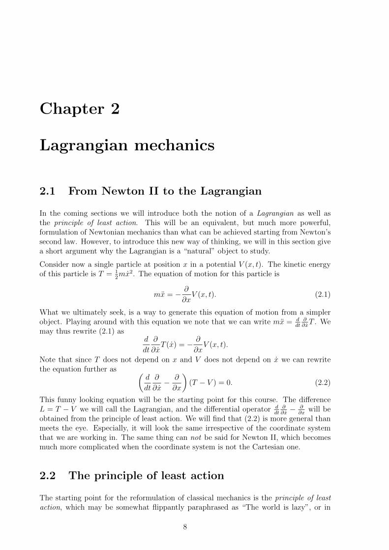
2.1 From Newton II to the Lagrangian
In the coming sections we will introduce both the notion of a Lagrangian as well asthe principle of least action. This will be an equivalent, but much more powerful,formulation of Newtonian mechanics than what can be achieved starting from Newton’ssecond law. However, to introduce this new way of thinking, we will in this section givea short argument why the Lagrangian is a “natural” object to study.
Consider now a single particle at position x in a potential V (x, t). The kinetic energyof this particle is T = 1
2mx2. The equation of motion for this particle is
mx = − ∂
∂xV (x, t). (2.1)
What we ultimately seek, is a way to generate this equation of motion from a simplerobject. Playing around with this equation we note that we can write mx = d
dt∂∂xT . We
may thus rewrite (2.1) asd
dt
∂
∂xT (x) = − ∂
∂xV (x, t).
Note that since T does not depend on x and V does not depend on x we can rewritethe equation further as (
d
dt
∂
∂x− ∂
∂x
)(T − V ) = 0. (2.2)
This funny looking equation will be the starting point for this course. The differenceL = T − V we will call the Lagrangian, and the differential operator d
dt∂∂x− ∂
∂xwill be
obtained from the principle of least action. We will find that (2.2) is more general thanmeets the eye. Especially, it will look the same irrespective of the coordinate systemthat we are working in. The same thing can not be said for Newton II, which becomesmuch more complicated when the coordinate system is not the Cartesian one.
2.2 The principle of least action
The starting point for the reformulation of classical mechanics is the principle of leastaction, which may be somewhat flippantly paraphrased as “The world is lazy”, or in
8

the more flowery words of Pierre Louis Maupertuis (1744), Nature is thrifty in all itsactions :
The laws of movement and of rest deduced from this principle being preciselythe same as those observed in nature, we can admire the application of it toall phenomena. The movement of animals, the vegetative growth of plants. . . are only its consequences; and the spectacle of the universe becomes somuch the grander, so much more beautiful, the worthier of its Author, whenone knows that a small number of laws, most wisely established, suffice forall movements.
This very general formulation does not in itself have any predictive power, but theidea that nature’s “thrift” could be used to derive laws of motion had already beensuccessfully applied in optics for a long time:
Fermat’s principleThe path taken between two points by a ray of light is the path that can be traversedin the least time.
This principle was first formulated by Ibn al-Haytham (aka Alhacen) in his Book ofOptics from 1021, which formed one of the main foundations of geometric optics andthe scientific method in general. He proved that it led to the law of reflection. It wasrestated by Pierre de Fermat in 1662, who also derived Snell’s law of refraction fromthis principle.
Example 2.1 Fermat’s principle of least time
Consider a beam of light traveling across a planar interface from a point A in onemedium (e.g. air) in which the speed of light is v1, to a point B in a different medium(e.g. water) in which the speed of light is v2. What trajectory will minimise thetime taken for the light to travel from A to B? The light will travel in a straightline in medium 1 and a straight line in medium 2, but we can vary the point O totry and minimise the time.
2
θ1
O
x
y
y
1
1
2
v2
v1
A
B2xd
θ
Since A and B are fixed y1 and y2 are fixed and x1 +x2 = d, but we can vary x1 andx2 by moving the point O though only one of them is independent as x2 = d − x1.
9
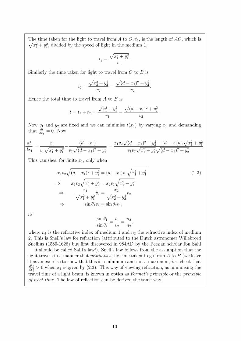
The time taken for the light to travel from A to O, t1, is the length of AO, which is√x2
1 + y21, divided by the speed of light in the medium 1,
t1 =
√x2
1 + y21
v1
.
Similarly the time taken for light to travel from O to B is
t2 =
√x2
2 + y22
v2
=
√(d− x1)2 + y2
2
v2
.
Hence the total time to travel from A to B is
t = t1 + t2 =
√x2
1 + y21
v1
+
√(d− x1)2 + y2
2
v2
.
Now y1 and y2 are fixed and we can minimise t(x1) by varying x1 and demandingthat dt
dx1= 0. Now
dt
dx1
=x1
v1
√x2
1 + y21
− (d− x1)
v2
√(d− x1)2 + y2
2
=x1v2
√(d− x1)2 + y2
2 − (d− x1)v1
√x2
1 + y21
v1v2
√x2
1 + y21
√(d− x1)2 + y2
2
.
This vanishes, for finite x1, only when
x1v2
√(d− x1)2 + y2
2 = (d− x1)v1
√x2
1 + y21 (2.3)
⇒ x1v2
√x2
2 + y22 = x2v1
√x2
1 + y21
⇒ x1√x2
1 + y21
v2 =x2√x2
2 + y22
v2
⇒ sin θ1v2 = sin θ2v1,
orsin θ1
sin θ2
=v1
v2
=n2
n2
,
where n1 is the refractive index of medium 1 and n2 the refractive index of medium2. This is Snell’s law for refraction (attributed to the Dutch astronomer WillebrordSnellius (1580-1626) but first discovered in 984AD by the Persian scholar Ibn Sahl— it should be called Sahl’s law!). Snell’s law follows from the assumption that thelight travels in a manner that minimises the time taken to go from A to B (we leaveit as an exercise to show that this is a minimum and not a maximum, i.e. check thatd2tdx2
1> 0 when x1 is given by (2.3). This way of viewing refraction, as minimising the
travel time of a light beam, is known in optics as Fermat’s principle or the principleof least time. The law of reflection can be derived the same way.
10

2.2.1 Hamilton’s principle
In mechanics the proper mathematical formulation of Maupertuis’ principle is due toWilliam Rowan Hamilton1, building on earlier work by Joseph Louis Lagrange.
We will denote the kinetic and potential energy of a particle, or of a mechanical systemin general, as
T = kinetic energy
V = potential energy
T usually depends on the velocities vi = dxidt≡ xi T = T (xi)
but may also depend on position and explicitly on timet T = T (xi, xi, t)V usually depends on the positions xi V = V (xi)
but may also depend on velocities and explicitly on timet V = V (xi, xi, t)(for example with time-varying external forces).
xi and xi here denote all the coordinates and their time derivatives. So for example wehave
xi → x for a single particle in one dimension
xi → x, y, z for a particle in three dimensions
xi → x1, y1, z1, x2, y2, z2, . . . , xN , yN , zN for N particles in three dimensions
We now define the lagrangian L as the difference between kinetic and potential energy,
L(xi, xi, t) = T − V . (2.4)
Note that L will be a function of the coordinates xi, the velocities xi, and the time t,although in many cases there is no explicit time dependence; ie, if we know the positionsand velocities of all the particles we know the lagrangian.
A particular path is given by specifying the coordinates xi as a function of time, xi =xi(t). (Note that if xi(t) is known, its derivative xi(t) is also known.) For a given path,the action S is defined as
S[x] ≡t2∫t1
L(x(t), x(t), t)dt . (2.5)
We are now in a position to formulate Hamilton’s principle of least action.
1On a General Method in Dynamics, Phil. Trans. Roy. Soc. (1834) 247; (1835) 95.
11

The principle of least action:
The physical path a system will take between two points in a certain time interval isthe one that gives the smallest action S.
Comments:
1. The potential energy V is defined only for conservative forces, so the action as itis written here is defined only for conservative forces. It is possible to generalisethis to certain non-conservative forces and obtain the correct equations of motion(we will see examples of this later). However, all microscopic (fundamental) forcesare conservative.
2. The action S is a “function of a function” since it depends on the function(s) xi(t).We call this a functional, and denote it by putting the function argument in squarebrackets, S = S[x].
2.3 The Euler–Lagrange equations
x1(t
1)
x2(t
2)
x(t)
x’(t)
What does ‘the path that gives the smallest action’ actuallymean, and how can we find it? To work this out, let usconsider a path x(t) and another path x′(t) = x(t)+αh(t),where h(t) is some arbitrary smooth function of t, and αis a parameter that we will vary.
Since we are looking for the path the system will take between two specific points in aspecific time interval, the endpoints of the two paths must be the same. We thereforehave
x(t1) = x′(t1) = x1 ; x(t2) = x′(t2) = x2 ⇐⇒ h(t1) = h(t2) = 0 . (2.6)
We can now write S[x+ αh] = S(α), and treat it as a function of the parameter α. Fora given h(t), the minimum of S will occur when dS
dα= 0.
This allows us to restate the principle of least action:For any smooth hi(t) with hi(t1) = hi(t2) = 0, the physical path xi(t) is such that
d
dαS[x+ αh] =
d
dα
t2∫t1
L(xi + αhi, xi + αhi, t)dt = 0 . (2.7)
We often use the shorthands αh = δx and S[x+ δx]− S[x] = δS = the variation of S,and call δS
δxthe functional derivative of S. The principle of least action is then often
written as
δS = 0 orδS
δx= 0 ⇐⇒ d
dαS[x+ αh] = 0 for any h(t) . (2.8)
12

Let us now calculate the variation δS. For a single particle in one dimension, we have
d
dαS[x+ αh] =
d
dα
∫ t2
t1
L(x+ αh, x+ αh, t)dt (2.9)
=
∫ t2
t1
(∂L
∂xh+
∂L
∂xh
)dt (2.10)
=
∫ t2
t1
∂L
∂xh dt+
[∂L
∂xh
]t=t2t=t1
−∫ t2
t1
(d
dt
∂L
∂x
)h dt (2.11)
=
∫ t2
t1
(∂L
∂x− d
dt
∂L
∂x
)h(t)dt . (2.12)
In the first step we used that L is a function of the three variables x, x, t, but t does notdepend on α. We can then use the chain rule for a function of two variables,
d
dαf(x, y) =
∂f
∂x
dx
dα+∂f
∂y
dy
dα.
In the second step we used integration by parts,∫uvdt = uv −
∫uvdt with u =
∂L
∂x, v = h .
In the final step the boundary term vanishes since h(t1) = h(t2) = 0.
But h(t) is a completely arbitrary smooth function, and we must have δS = 0 for anyh(t). This is only possible if the term within the brackets in (2.12) is 0 for all t, ie
d
dt
∂L
∂x− ∂L
∂x= 0 The Euler–Lagrange equation (2.13)
If we have N coordinates xi, the derivation proceeds following the same steps. Usingthe chain rule for a function of 2N variables, we find
d
dαL(x1 + αh1, x2 + αh2, . . . , xN + αhN , x1 + αh1, x2 + αh2, . . . , xN + αhN)
=∂L
∂x1
h1 +∂L
∂x2
h2 + · · ·+ ∂L
∂xNhN +
∂L
∂x1
h1 +∂L
∂x2
h2 + · · ·+ ∂L
∂xNhN
=N∑i=1
(∂L
∂xihi +
∂L
∂xihi
). (2.14)
Using integration by parts on the second term (for each i) gives us
d
dαS[x+ αh] =
N∑i=1
∫ t2
t1
( ∂L∂xi− d
dt
∂L
∂xi
)hi(t)dt = 0 . (2.15)
Since all the hi are independent, arbitrary functions, the expression within the bracketsmust vanish for each i:
13
d
dt
∂L
∂xi− ∂L
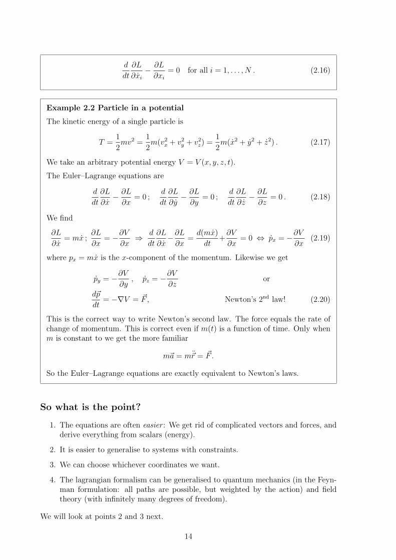
∂xi= 0 for all i = 1, . . . , N . (2.16)
Example 2.2 Particle in a potential
The kinetic energy of a single particle is
T =1
2mv2 =
1
2m(v2
x + v2y + v2
z) =1
2m(x2 + y2 + z2) . (2.17)
We take an arbitrary potential energy V = V (x, y, z, t).
The Euler–Lagrange equations are
d
dt
∂L
∂x− ∂L
∂x= 0 ;
d
dt
∂L
∂y− ∂L
∂y= 0 ;
d
dt
∂L
∂z− ∂L
∂z= 0 . (2.18)
We find
∂L
∂x= mx ;
∂L
∂x= −∂V
∂x⇒ d
dt
∂L
∂x−∂L∂x
=d(mx)
dt+∂V
∂x= 0 ⇔ px = −∂V
∂x(2.19)
where px = mx is the x-component of the momentum. Likewise we get
py = −∂V∂y
, pz = −∂V∂z
or
d~p
dt= −∇V = ~F , Newton’s 2nd law! (2.20)
This is the correct way to write Newton’s second law. The force equals the rate ofchange of momentum. This is correct even if m(t) is a function of time. Only whenm is constant to we get the more familiar
m~a = m~r = ~F .
So the Euler–Lagrange equations are exactly equivalent to Newton’s laws.
So what is the point?
1. The equations are often easier : We get rid of complicated vectors and forces, andderive everything from scalars (energy).
2. It is easier to generalise to systems with constraints.
3. We can choose whichever coordinates we want.
4. The lagrangian formalism can be generalised to quantum mechanics (in the Feyn-man formulation: all paths are possible, but weighted by the action) and fieldtheory (with infinitely many degrees of freedom).
We will look at points 2 and 3 next.
14

2.4 Generalised coordinates
It is often advantageous to change variables from the cartesian coordinates xi, yi, zifor each particle i = 1, . . . , N to some other variables qj, j = 1, . . . , n. These are calledgeneralised coordinates.
Consider for example a system of N particles. We need 3N independent coordinates todescribe the system completely: we say that there are 3N degrees of freedom.
Now, imagine that there is a constraint relating the 3N coordinates, for example:
1. Two particles are tied together with a rod of length l, so that
(x1 − x2)2 + (y1 − y2)2 + (z1 − z2)2 = l2 . (2.21)
2. The N particles are all moving on the surface of a sphere, ie
x2i + y2
i + z2i = R2 ∀i = 1, . . . , N . (2.22)
3. A ball in a squash court, 0 ≤ x ≤ L, 0 ≤ y ≤ L, z ≥ 0.
The first two of these can be described by M equations of the form
fj(~x1, . . . , ~xN , t) = 0 , j = 1, . . . ,M . (2.23)
Such constraints are called holonomic (or integrable) constraints, and we will mostlyfocus on such constraints in the following (though a general procedure for dealing withnon-holonomic constraints is described in §2.5). With such constraint equations, thecoordinates xi, yi, zi are no longer independent. Instead we have
M relations =⇒ n = 3N −M real degrees of freedom.
By choosing n suitable generalised coordinates to describe these degrees of freedom, weachieve two things:
• We eliminate the forces of constraints which are required in the newtonian formu-lation. No net work is done by these forces, so they can safely be eliminated.
• The Euler–Lagrange equations look exactly the same in the new coordinates, sothe problem is no more difficult (and probably easier) than the original one.
In the first example above, the constraint (2.21) reduces the number of degrees of freedomfrom 6 to 5. The 5 coordinates can for example be chosen to be the centre of masscoordinatesX, Y, Z for the two particles, and two angles θ, φ that describe the orientationof the rod.2
In the second example, each particle is described by 2 instead of 3 coordinates. Thesecan be chosen to be the ‘latitude’ θ and ‘longitude’ φ of each particle (corresponding tospherical coordinates, see Sec. 2.4.2).
2In Chapter 5 we will look more at how these angles can be chosen.
15

Example 2.3 Simple pendulum
Consider a simple pendulum with length `, mass m in a constant gravitational fieldg (see Fig. 2.1).
rAAAAAAAAAAA|
`
m
. ................ ................................................
θ
Figure 2.1: A simple pen-dulum
Here it is convenient to choose the angle θ as our coor-dinate. The x (horizontal) and z (vertical) coordinatesand their time derivatives can be written in terms of θas
x = ` sin θ x = `θ cos θ , (2.24)
z = −` cos θ z = `θ sin θ . (2.25)
The kinetic energy is
T =1
2m~v2 =
1
2m(x2 + z2)
=1
2m`2θ2(cos2 θ + sin2 θ) =
1
2m`2θ2 . (2.26)
The potential energy is
V = mgz = −mg` cos θ . (2.27)
The lagrangian therefore becomes
L = T − V =1
2m`2θ2 +mg` cos θ . (2.28)
The Euler–Lagrange equation is
∂L
∂θ=
d
dt
∂L
∂θ=⇒ −mg` sin θ =
d
dt
(m`2θ
)(2.29)
=⇒ θ = −g`
sin θ . (2.30)
This is the equation of motion for the pendulum.
Once we have found the equation of motion for θ, and the solution to this equation, wecan go back and calculate x and z as functions of time. However, in the example of thesimple pendulum, we are not usually interested in this.
We note that the mass m does not appear in the equation of motion. We could haveseen this already by inspecting the lagrangian: the EL equations are unchanged if thelagrangian is multiplied by an overall constant α, L→ αL. In this case, since the massjust enters as an overall factor in the lagrangian, the EL equation will not depend onthe mass.
16

Solutions to the equations of motion?
Now we have found the equation of motion for the simple pendulum, and we may wantto know the solutions to this equation, ie what the actual motion of the pendulum is fordifferent initial conditions. It is actually possible to integrate the equation (2.30) andwrite down a solution, but this involves elliptic integrals and lots of other complicatedmaths, and will not help us to understand the physical system. It will be more useful tofind numerical solutions, and in Computational Physics MP354 we will learn how thiscan be done.
What we can do to understand the system better, is
• look at the general types of solutions we may have. We will do this when wediscuss conservation of energy;
• consider limiting cases such as small oscillations. This is what we will do now.
If θ is small, we may approximate sin θ with the first term in its power expansion (Taylorexpansion),
sin θ = θ − 1
3!θ3 +
1
5!θ5 + · · · ≈ θ . (2.31)
In that case (2.30) simplifies to
θ = −g`θ . (2.32)
We recognise this as the equation for a simple harmonic oscillator, x+ω2x = 0, with x→θ, ω2 → g/`. We therefore see that for small oscillations, the simple pendulum behavesas a simple harmonic oscillator with angular frequency ωs =
√g/`, ie the frequency is
inversely proportional to the square root of the length of the pendulum (and independentof the mass).
17

Example 2.4 Double Atwood machine
m1
x
?
.......................................
..........................
......................................................................................................................................................................... ............. ............. ............. ............. ............. ............. ............. ............. .............
.................................................................
x
`1 − x
? .......................................
..........................
......................................................................................................................................................................... ............. ............. ............. ............. ............. ............. ............. ............. .............
.................................................................
s
?
y
m2
?
`2 − y
m3
Figure 2.2: Double Atwood machine.
Consider the double Atwood machine inFig. 2.2. We assume that:
• the pulleys are light, so we canignore their kinetic energy;
and
• the ropes do not slip (or they slidewithout friction).
Here we have two independent degrees offreedom, which we can choose to be x andy. In terms of these, the positions of thethree blocks are
x1 = −x ,x2 = −(`1 − x+ y) ,
x3 = −(`1 − x+ `2 − y) .
The kinetic and potential energy of thethree blocks are
T1 =1
2m1x
2
T2 =1
2m2
[ ddt
(`1 − x+ y)]2
=1
2m2(y − x)2
T3 =1
2m3(x+ y)2
V1 = −m1gx
V2 = −m2g(`1 − x+ y)
V3 = −m3g(`1 + `2 − x− y).
The lagrangian becomes
L =1
2(m1 +m2 +m3)x2 +
1
2(m2 +m3)y2 + (m3 −m2)xy
+ (m1 −m2 −m3)gx+ (m2 −m3)gy +m2g`1 +m3g(`1 + `2) .
Note that the last two terms are constants which do not play any role in the equationsof motion. We get two equations of motion:
d
dt
∂L
∂x= (m1 +m2 +m3)x+ (m3 −m2)y =
∂L
∂x= (m1 −m2 −m3)g
d
dt
∂L
∂y= (m2 +m3)y + (m3 −m2)x =
∂L
∂y= (m2 −m3)g.
18
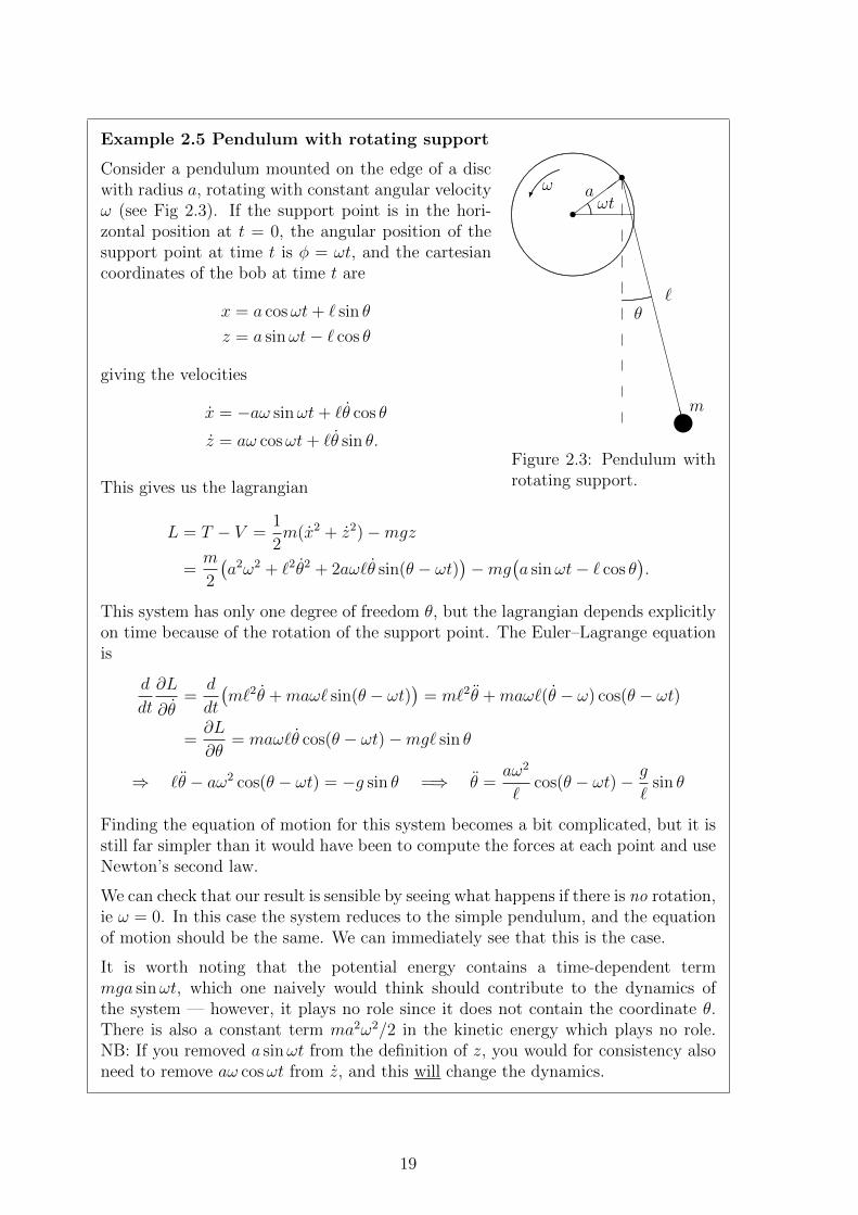
Example 2.5 Pendulum with rotating support
.................
..................
..................
..................
.................
................
................
...................................
............................................................................................................................
.................
................
................
.................
..................
..................
..................
........
........
.
........
........
.
..................
..................
..................
.................
................
................
.................
.................. .................. .................. ................. ................. ....................................
...................................
................
................
.................
..................
..................
..................
.................sa
............................. ωt
................
..............
..........................................................
ω
sCCCCCCCCCCCCCCCCCC
`
|m
. ..................... ...................... ......................
θ
Figure 2.3: Pendulum withrotating support.
Consider a pendulum mounted on the edge of a discwith radius a, rotating with constant angular velocityω (see Fig 2.3). If the support point is in the hori-zontal position at t = 0, the angular position of thesupport point at time t is φ = ωt, and the cartesiancoordinates of the bob at time t are
x = a cosωt+ ` sin θ
z = a sinωt− ` cos θ
giving the velocities
x = −aω sinωt+ `θ cos θ
z = aω cosωt+ `θ sin θ.
This gives us the lagrangian
L = T − V =1
2m(x2 + z2)−mgz
=m
2
(a2ω2 + `2θ2 + 2aω`θ sin(θ − ωt)
)−mg
(a sinωt− ` cos θ
).
This system has only one degree of freedom θ, but the lagrangian depends explicitlyon time because of the rotation of the support point. The Euler–Lagrange equationis
d
dt
∂L
∂θ=
d
dt
(m`2θ +maω` sin(θ − ωt)
)= m`2θ +maω`(θ − ω) cos(θ − ωt)
=∂L
∂θ= maω`θ cos(θ − ωt)−mg` sin θ
⇒ `θ − aω2 cos(θ − ωt) = −g sin θ =⇒ θ =aω2
`cos(θ − ωt)− g
`sin θ
Finding the equation of motion for this system becomes a bit complicated, but it isstill far simpler than it would have been to compute the forces at each point and useNewton’s second law.
We can check that our result is sensible by seeing what happens if there is no rotation,ie ω = 0. In this case the system reduces to the simple pendulum, and the equationof motion should be the same. We can immediately see that this is the case.
It is worth noting that the potential energy contains a time-dependent termmga sinωt, which one naively would think should contribute to the dynamics ofthe system — however, it plays no role since it does not contain the coordinate θ.There is also a constant term ma2ω2/2 in the kinetic energy which plays no role.NB: If you removed a sinωt from the definition of z, you would for consistency alsoneed to remove aω cosωt from z, and this will change the dynamics.
19

2.4.1 The shortest path between two points (optional)
In deriving the Euler-Lagrange equations (2.16) we did not actually make use of thedefinition of L in terms of T and V : we could have used any functional evaluated alongthe path between the two points — for example the length of the path itself!
Example 2.6 The shortest path between two points
Consider a curve y = y(x) between two points (x1, y1) and (x2, y2). The length dsof an infinitesimal segment (dx, dy) of this curve is given by Pythagoras:
ds2 = dx2 + dy2 = dx2 + (y′(x)dx)2 = (1 + y′(x)2)dx2 (2.33)
=⇒ ds =√
1 + y′(x)2dx . (2.34)
If, to make life simpler for ourselves, we assume that x is monotonically increasingalong the curve, we find that the total length of the curve is
S =
∫ x2
x1
√1 + y′(x)2dx =
∫ x2
x1
L(y(x), y′(x), x)dx with L =
√1 + y′2 . (2.35)
This looks like what we had before, but with t→ x;x(t)→ y(x); x(t)→ y′(x).
The Euler–Lagrange equation becomes
d
dx
∂L
∂y′− ∂L
∂y= 0 . (2.36)
We see immediately that ∂L/∂y = 0. To find ∂L/∂y′ we use the chain rule,
∂L
∂y′=dL
du
∂u
∂y′with u = 1 + y′
2; L =
√u
=⇒ ∂L
∂y′=
1
2√
1 + y′2· 2y′ = y′√
1 + y′2.
To find ddx
∂L∂y′
we use the product rule and the chain rule:
∂L
∂y′= vw with v = y′ , w =
1√1 + y′2
= u−1/2 (2.37)
=⇒ d
dx
∂L
∂y′=dv
dxw + v
dw
du
du
dx=dy′
dxw + y′
dw
du
du
dy′dy′
dx
= y′′1√
1 + y′2+ y′ ·
(− 1
2u−3/2
)· 2y′ · y′′
= y′′( 1√
1 + y′2− y′2
(1 + y′2)3/2
)=
y′′√1 + y′2
(1− y′2
1 + y′2
)=
y′′√1 + y′2
1
1 + y′2.
(2.38)
Sod
dx
∂L
∂y′= 0 =⇒ y′′(x) = 0 =⇒ y(x) = Ax+B . (2.39)
This describes a straight line, so we have shown that the shortest path between twopoints is a straight line!
20

2.4.2 Polar and spherical coordinates
When we have rotational motion, or a system with rotational (or spherical) symmetry,it is very often most convenient to use polar coordinates (in 2 dimensions) or sphericalcoordinates (in 3 dimensions). The definition of these coordinates are given in Fig. 2.4.Since we will be using them often, we need to know what the kinetic energy of a particleis in terms of these coordinates.
-
6
*
y
x
rθ
.
.................
..................
..................
..................
-
6
SS
. .............. ............... ............... ...............
.............
................. ............... ............... ............... ............... ...............
...............
θ
φ
r
z
x
y
Figure 2.4: Plane polar coordinates (r, θ) (left) and spherical coordinates (r, θ, φ) (right).
Polar coordinates
The relation between cartesian and polar coordinates is given by
x = r cos θ =⇒ x = r cos θ − rθ sin θ (2.40)
y = r sin θ =⇒ y = r sin θ + rθ cos θ (2.41)
This gives for the kinetic energy,
T =1
2m(x2 + y2)
=m
2(r2 cos2 θ + r2θ2 sin2 θ − 2rrθ cos θ sin θ + r2 sin2 θ + r2θ2 cos2 θ + 2rrθ cos θ sin θ)
=m
2(r2 + r2θ2) . (2.42)
21
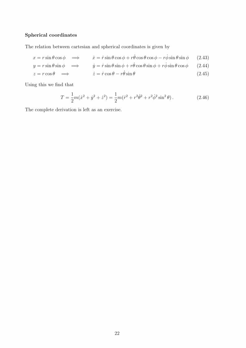
Spherical coordinates
The relation between cartesian and spherical coordinates is given by
x = r sin θ cosφ =⇒ x = r sin θ cosφ+ rθ cos θ cosφ− rφ sin θ sinφ (2.43)
y = r sin θ sinφ =⇒ y = r sin θ sinφ+ rθ cos θ sinφ+ rφ sin θ cosφ (2.44)
z = r cos θ =⇒ z = r cos θ − rθ sin θ (2.45)
Using this we find that
T =1
2m(x2 + y2 + z2) =
1
2m(r2 + r2θ2 + r2φ2 sin2 θ) . (2.46)
The complete derivation is left as an exercise.
22

Example 2.7 Coriolis force
Strange things can happen in a rotating co-ordinate system. Let x and y be Cartesianco-ordinates in 2-dimensions and consider changing to a rotating co-ordinate system
x = x cosωt+ y sinωt, y = −x sinωt+ y cosωt,
where ω is a constant angular frequency. Conversely we can express (x, y) in termsof (x, y),
x = x cosωt− y sinωt, y = x sinωt+ y cosωt, (2.47)
and of coursex2 + y2 = x2 + y2.
From (2.47)
x = (cosωt) ˙x− (sinωt) ˙y − ω(x sinωt+ y cosωt)
y = (sinωt) ˙x+ (cosωt) ˙y + ω(x cosωt− y sinωt)
from which we get
x2 + y2 = ˙x2 + ˙y2 + ω2(x2 + y2) + 2ω(x ˙y − y ˙x).
In the rotating co-ordinate system the Lagrangian for a free particle of mass m is
L =m
2
˙x2 + ˙y2 + ω2(x2 + y2) + 2ω(x ˙y − y ˙x)
.
The x(t) equation of motion follows from
∂L
∂ ˙x= m( ˙x− ωy),
∂L
∂x= m(ω ˙y + ω2x)
from which
d
dt
(∂L
∂ ˙x
)=∂L
∂x
⇒ ¨x = ω2x+ 2ω ˙y. (2.48)
Similarly the y(t) equation of motion is
¨y = ω2y − 2ω ˙x.
Define a vector in the z-direction
ω = ωz,
then we can write the equation of motion in the rotating co-ordinate system as
d2r
dt2= ω2r− 2ω × dr
dt.
The first term is the centrifugal force and the second is known as the Coriolis force.The Coriolis force is responsible for forcing winds moving into the centre of an areaof low pressure to spiral rather than to move in straight radial lines and causes thebeautiful spiral pattern of hurricane clouds.
23

2.5 Lagrange multipliers [Optional]
Using the constraint equations to reduce the number of coordinates is usually the moststraightforward way of handling constraints. But it is not always practical:
• It may not be straightforward to solve the constraint equations.
• The constraint equations may involve velocities.
• The constraint equations may be expressed as differential rather than algebraicequations.
• We may want to know the forces of constraint (for example, to find out when theybecome too large or too small to physically constrain the system).
It is useful to develop a technique for handling such situations.
2.5.1 Constraints
Suppose the generalised co-ordinates are not all independent but are constrained in someway. In particular we suppose that under an infinitesimal variation
N∑i=1
Ai(q, t)δqi +B(q, t)δt = 0 (2.49)
whereAi(q, t) andB(q, t) are given functions and q represents the whole set of generalisedco-ordinates, q1, . . . , qN . This constraint affects the variational approach: when a pathqi(t) is varied by qi(t) → qi(t) + αhi(t), with t fixed, set δt = 0 and δqi(t) = αhi(t) in(2.49) and this enforces a constraint on the variation∑
i
Ai(q, t)hi = 0. (2.50)
The constraint (2.50) can be incorporated into the variational approach by adding somemultiple of it to the variational equations arising from the Lagrangian∑
i
d
dt
(δL
δqi
)hi =
∑i
∂L
∂qihi →
∑i
d
dt
(δL
δqi
)hi =
∑i
∂L
∂qihi + λ(t)
∑i
Ai(q, t)hi
(2.51)and considering the N equations
d
dt
(δL
δqi
)=∂L
∂qi+ λ(t)Ai(q, t). (2.52)
λ can be eliminated by choosing one of the equations, say i = N , and solving for λ,
λ =1
AN
(d
dt
(δL
δqN
)− ∂L
∂qN
). (2.53)
24

An example of the Coriolis force. A hurricane is caused by a smallarea of very low pressure at the centre making very strong winds blowtoward the middle. Since the Earth is rotating there is a componentof angular velocity normal to the plane, ω = ω0 cos θ, where ω0 = 2π
T
with T = 24 hours and θ the co-latitude (i.e. latitude−90). ω pointsupwards in the northern and downwards in the southern hemisphereand the resulting Coriolis force −2ω × ˙r makes the wind bend to theright in the northern hemisphere and to the left in the southern hemi-sphere. Can you work out which hemisphere the above storm is in?Exactly on the equator the Coriolis force would vanish as ω wouldhave no normal component there.
25

This can now be used in the other N − 1 equations in (2.52) to give N − 1 equationsfor the N functions qi(t) and the function λ(t) has been eliminated. One other equationcomes from including (2.49) explicitly in the form
N∑i=1
Ai(q, t)qi +B(q, t) = 0. (2.54)
A complete formulation of the problem is now given by
d
dt
(δL
δqi
)=∂L
∂qi+ λ(t)Ai(q, t), i = 1, . . . , N − 1; (2.55)
N∑i=1
Ai(q, t)qi +B(q, t) = 0, (2.56)
with λ given by (2.53). These are N equation for the N functions qi.
Physically what is happening here is that constraints must be implemented by forces, Fi(large forces so that the internal dynamics of the system can never overcome the force),and (2.52) is just a way of writing
d
dt
(δL
δqi
)=∂L
∂qi+ Fi, i = 1, . . . , N − 1, (2.57)
and the constraining forces being applied externally are Fi = λAi.
There may be more than one constraint, suppose there are M of them (M < N)
N∑i=1
Aai(q, t)δqi +Ba(q, t)δt = 0 (2.58)
with a = 1, . . . ,M . Then path variations are constrained by M equations∑i
Aai(q, t)hi = 0. (2.59)
In that case introduce M functions λa(t) and the above procedure easily generalises.
In principle (2.56) can be solved to eliminate one of the unknown functions qi(t), forgiven Ai and B, leaving N − 1 equations to deal with, but in practice the procedure canbe rather complicated. The situation is much simpler if the constraints are holonomic.For a single constraint (M = 1) there are N + 1 independent functions in (2.49) but, asdescribed in §2.4, the constraint is holonomic if it arises from varying a single function,f(q, t) = C, with C a constant,
δf(q, t) =N∑i=1
∂f
∂qiδqi +
∂f
∂tδt = 0. (2.60)
26

We can incorporate this into the dynamics by introducing a new generalised co-ordinateλ(t) and adding a term to the Lagrangian,
L = T (q, q)− V (q) → Lλ = T (q, q)− V (q) + λ(f(q, t)− C
). (2.61)
Since there is no λ in the Lagrangian Lλ (there is no dynamics associated with λ) itsequation of motion is particularly simple
0 =d
dt
(δLλ
δλ
)=δLλδλ
= f − C. (2.62)
The equation of motion for λ is the constraint. The remaining equations are
d
dt
(δL
δqi
)=δL
δqi+ λ(t)
δf
δqi. (2.63)
The function λ(t) is called a Lagrange multiplier.
With M holonomic constraints,fa(q, t) = Ca (2.64)
with Ca constants, we need M Lagrange multipliers λa(t) and
d
dt
(∂L
∂qi
)=∂L
∂qi+
M∑a=1
∂fa∂qi
λa(t) (2.65)
The Euler–Lagrange equations with Lagrange multipliers
We now have N +M unknown functions qi(t), λa(t), but we also have N +M equations:the N EL equations (2.65) and the M constraint equations (2.64). This will thereforecompletely determine the dynamics of the system once the initial conditions are given.
If we know the Lagrange multipliers, we can find the (generalised) constraint forces Fi.These are given by
Fi =∑a
∂fa∂qi
λa . (2.66)
Example 2.8 A hoop rolling down an inclined plane without slipping
.............
.............
.............
..........................
..............................................................................
..........................
.............
.............
........
.....
........
.....
.............
.............
.............
............. ............. ............. ............. ............. ....................................................
.............
.............
.............HH
HHHHHH
HHHHH
@@
.............
.............
............
........
....
HHHjx
θ
Φ
Figure 2.5: A hoop rollingdown an inclined planewithout slipping.
Consider a hoop of radius R and mass m rollingdown an inclined plane without slipping as shown inFig. 2.5. The condition of no slipping relates x to θ,under an infinitesimal change in x there is a corre-sponding change in θ
δx = Rδθ (2.67)
27

orδx−Rδθ = δ(x−Rθ) = 0,
this is a holonomic constraint. This forces the veloc-ities to satisfy
x = Rθ. (2.68)
The kinetic energy is the sum of the translational and the rotational kinetic energies,
T =1
2mx2 +
1
2mR2θ2. (2.69)
If the plane has length l and is inclined at an angle Φ to the horizontal then thecentre of mass of the hoop is always a distance R cos Φ above the point of contact.The potential energy is mgh where h = R cos Φ + (l − x) sin Φ is the height of thecentre of mass of the hoop above the foot of the plane. The R cos Φ can be ignored,it is just a constant and adding a constant to the potential energy changes nothing.So we take the potential energy to be
V (x) = mg(l − x) sin Φ. (2.70)
Including a Lagrange multiplier for the constraint the Lagrangian is
Lλ =1
2mx2 +
1
2mR2θ2 −mg(l − x) sin Φ + λ(x− rθ) (2.71)
giving the equations of motion
mx = mg sin Φ + λ,
mR2θ = −λR.
From the second equationλ = −mRθ
and this can be used to eliminate λ from the first
x+Rθ = g sin Φ.
Finally (2.68) tells us that x = Rθ and we only need solve simple equation
x =1
2g sin Φ (2.72)
to completely determine the motion. Assuming the hoop is initially at rest andstarts rolling from the top of the plane the solution is
x(t) =1
4(g sin Φ) t2.
The hoop arrives at the bottom of the plane after a time
t = 2
√l
g sin Φ.
28

with velocityv =
√lg sin Φ.
This is actually rather a simple example because the constraint is linear in thegeneralised co-ordinates x and θ. We could just set Rθ = x in the Lagrangian
L =1
2mx2 +
1
2R2θ2 − V (x) = mx2 − V (x)
forget about λ and θ and just use the single co-ordinate x. The dynamics is exactlythe same as for an unconstrained system with one degree of freedom, x, and twicethe mass. For non-linear constraints however Lagrange multipliers are often themost efficient way of solving the problem.
2.6 Canonical momenta and conservation laws
Assume the lagrangian L does not depend explicitly on the coordinate qi. Such coor-dinates are called cyclic. The Euler–Lagrange equations for the cyclic coordinate qibecomes
d
dt
∂L
∂qi=∂L
∂qi= 0 =⇒ ∂L
∂qi≡ pi = constant . (2.73)
We call the qunatity pi the canonical momentum conjugate to (or corresponding to) qi.
Why momentum?
Consider the ‘usual’ case where
1. we use cartesian coordinates qi = xi;
2. there are no constraints; and
3. the potential depends only on the coordinates, V = V (x).
In this case we have
L = T − V =1
2m∑j
x2j − V (x) =⇒ ∂L
∂xi= mxi = pi = ordinary momentum.
So we have found the law of conservation of momentum pi if the potential V does notdepend on the coordinate xi — ie, if the system is translationally invariant in the i-direction. Note that if V does not depend on xi this implies that there are no net forcesin the i-direction.
We may in a similar way demonstrate conservation of total momentum for a system ofn particles if the potential energy does not depend on the centre of mass coordinate.But the concept of canonical momenta is much more general and powerful than this,and can be used to derive a whole host of other conservation laws. One of the mostimportant is angular momentum, which we will look at next.
29

2.6.1 Angular momentum
Consider a one-particle rotationally symmetric 2-dimensional system, and let us usepolar coordinates (r, θ) to describe the parrticle. Rotational symmetry then means thatthe potential energy V (r, θ) = V (r), independent of the angle θ. The lagrangian is then
L = T − V =1
2m(r2 + r2θ2)− V (r) . (2.74)
We see that θ is a cyclic coordinate, and the canonical momentum pθ is therefore con-served. What is this canonical momentum?
We straightforwardly find
pθ =∂L
∂θ=
∂
∂θ
(1
2mr2θ2
)= mr2θ . (2.75)
But θ is the same as the angular velocity ω, and we know that the velocity vθ in theangular direction (perpendicular to the radius r) is vθ = rω = rθ, so pθ = r(mvθ). Butthis is exactly equal to the angular momentum of the particle,
Jz = (~r × ~p)z = mrvθ . (2.76)
So the canonical momentum conjugate to the angle θ is the angular momentum, whichis conserved if the system is rotationally symmetric, ie the lagrangian does not dependon θ.
Angular momentum in spherical coordinates
In section 2.4.2 we found that the kinetic energy in spherical coordinates (see Fig. 2.4 is
T =1
2m(r2 + r2θ2 + r2 sin2 θφ2) . (2.46)
The angle φ corresponds to rotations about the z-axis: if a particle rotates about thez-axis, φ changes while r and θ are unchanged. If the potential energy does not dependon φ, we have rotational symmetry about the z-axis, and the canonical momentum pφis conserved. From (2.46) we find
pφ = mr2 sin2 θφ = r(mr sin θφ)(sin θ) . (2.77)
We now want to show that this is equal to the z-component of the angular momentum,Jz = (~r × ~p)z.
6z
. ............ ............ ............ ............θ
...................... .......... ........... ........... ........... ........... ........... ...........
...............................φ r
@@@Rθ
φ
Figure 2.6: Unit vectors inspherical coordinates.
We can put unit vectors (r, θ, φ) in the direction ofincreasing a coordinates at the point ~r and decomposethe velocity in its (r, θ, φ) components,
~v = vrr + vθθ + vφφ (2.78)
The unit vector r denotes the radial direction, ie thedirection where r changes, while θ, φ are unchanged.Similarly, θ denotes the direction where θ changes
30
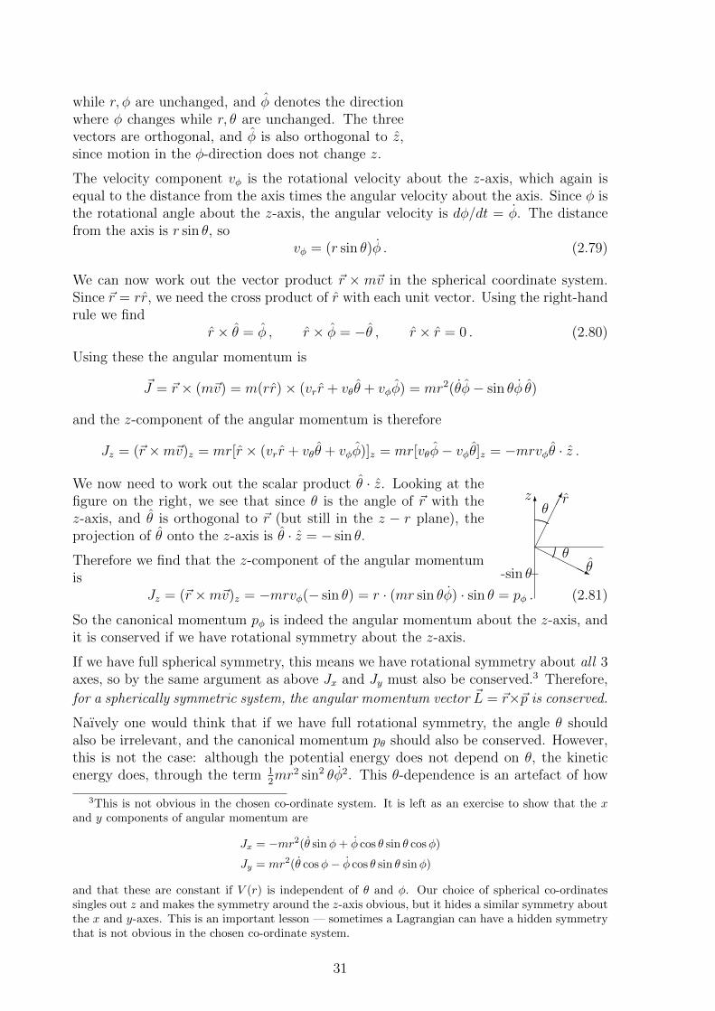
while r, φ are unchanged, and φ denotes the directionwhere φ changes while r, θ are unchanged. The threevectors are orthogonal, and φ is also orthogonal to z,since motion in the φ-direction does not change z.
The velocity component vφ is the rotational velocity about the z-axis, which again isequal to the distance from the axis times the angular velocity about the axis. Since φ isthe rotational angle about the z-axis, the angular velocity is dφ/dt = φ. The distancefrom the axis is r sin θ, so
vφ = (r sin θ)φ . (2.79)
We can now work out the vector product ~r × m~v in the spherical coordinate system.Since ~r = rr, we need the cross product of r with each unit vector. Using the right-handrule we find
r × θ = φ , r × φ = −θ , r × r = 0 . (2.80)
Using these the angular momentum is
~J = ~r × (m~v) = m(rr)× (vrr + vθθ + vφφ) = mr2(θφ− sin θφ θ)
and the z-component of the angular momentum is therefore
Jz = (~r ×m~v)z = mr[r × (vrr + vθθ + vφφ)]z = mr[vθφ− vφθ]z = −mrvφθ · z .
6z
r
HHHHHjθ
. ......... .......... .......... ..........
θ
............................. θ
-sin θ
We now need to work out the scalar product θ · z. Looking at thefigure on the right, we see that since θ is the angle of ~r with thez-axis, and θ is orthogonal to ~r (but still in the z − r plane), theprojection of θ onto the z-axis is θ · z = − sin θ.
Therefore we find that the z-component of the angular momentumis
Jz = (~r ×m~v)z = −mrvφ(− sin θ) = r · (mr sin θφ) · sin θ = pφ . (2.81)
So the canonical momentum pφ is indeed the angular momentum about the z-axis, andit is conserved if we have rotational symmetry about the z-axis.
If we have full spherical symmetry, this means we have rotational symmetry about all 3axes, so by the same argument as above Jx and Jy must also be conserved.3 Therefore,
for a spherically symmetric system, the angular momentum vector ~L = ~r×~p is conserved.
Naıvely one would think that if we have full rotational symmetry, the angle θ shouldalso be irrelevant, and the canonical momentum pθ should also be conserved. However,this is not the case: although the potential energy does not depend on θ, the kineticenergy does, through the term 1
2mr2 sin2 θφ2. This θ-dependence is an artefact of how
3This is not obvious in the chosen co-ordinate system. It is left as an exercise to show that the xand y components of angular momentum are
Jx = −mr2(θ sinφ+ φ cos θ sin θ cosφ)
Jy = mr2(θ cosφ− φ cos θ sin θ sinφ)
and that these are constant if V (r) is independent of θ and φ. Our choice of spherical co-ordinatessingles out z and makes the symmetry around the z-axis obvious, but it hides a similar symmetry aboutthe x and y-axes. This is an important lesson — sometimes a Lagrangian can have a hidden symmetrythat is not obvious in the chosen co-ordinate system.
31

we have chosen the coordinate system, but it is an unavoidable artefact: no matterhow we choose our spherical coordinate angles, these coordinates must break the fullspherical symmetry somehow.
We realise the full symmetry by noting that we could have chosen the coordinatesdifferently, eg we could have chosen θ to be the angle with the x-axis and φ to correspondto rotations about the x-axis — which would have led us to find that Lx is conserved.Similarly, if we choose θ to be the angle with the y-axis we will find that Ly is conserved.
2.7 Energy conservation: the hamiltonian
We know that when we have conservative forces, the potential energy depends onlyon positions, and not on time, and the total energy is conserved. We have derivedconservation of linear and angular momentum in lagrangian mechanics, so we may askourselves if we can also derive energy conservation within the same framework?
The answer to this is that not only can we do this, but the energy conservation theoremwe arrive at is more general than the one we already know!
To see how this works, let us take the (total) time derivative of the lagrangian L =L(qi(t), qi(t), t). Using the chain rule and the Euler–Lagrange equations we get
dL
dt=∑i
∂L
∂qiqi +
∑i
∂L
∂qiqi +
∂L
∂t
=∑i
(d
dt
∂L
∂qi
)qi +
∑i
∂L
∂qi
dqidt
+∂L
∂t
=d
dt
∑i
∂L
∂qiqi +
∂L
∂t
(2.82)
⇐⇒ d
dt
(∑i
∂L
∂qiqi − L
)+∂L
∂t≡ dH
dt+∂L
∂t= 0 , (2.83)
where we have defined
H =∑i
∂L
∂qiqi − L =
∑i
piqi − L = the hamiltonian (2.84)
So we find that if the lagrangian does not depend explicitly on time, then the hamiltonianor energy function H is conserved.
To see how this relates to energy conservation as we know it from before, consider asystem of particles in cartesian coordinates, described by the lagrangian
L = T − V =1
2
∑i
miq2i − V (q) .
32

The hamiltonian for this system is
H =∑i
∂L
∂qiqi − L =
∑i
(miqi)qi −[1
2
∑i
miq2i − V (q)
]=
1
2
∑i
miq2i + V (q) = T + V .
(2.85)
So we find that the hamiltonian is equal to the total energy, so conservation of thehamiltonian is the same as energy conservation in this particular (most common) case.
2.7.1 When is H conserved?
We found that H is conserved if L does not depend explicitly on time, ie L(q, q, t) =L(q, q). We would like to understand in what circumstances an explicit time dependencecould appear in the lagrangian. One possibility would be that the potential energydepends explicitly on time in the first place. But there are also other possibilites. Thekinetic energy, written in terms of the original cartesian (or, for that sake, ordinarypolar or spherical coordinates) does not have any explicit time dependence. But timedependence could still appear in either the kinetic or the potential energy when we writeit in terms of generalised coordinates.
To see how this can happen, let us recall why we introduced generalised coordinates inthe first place:
1. Constraints: There are fewer actual degrees of freedom in the system because ofconstraints. We use generalised coordinates to denote the real (relevant) degreesof freedom. An example of this would be the pendulum, where the original x andz coordinates are reduced to the single coordinate θ.
2. Symmetries: There are symmetries in the system which mean that using non-cartesian coordinates may give a simpler description. An example of this wouldbe using polar coordinates for a system with rotational symmetry.
Explicit time-dependence can appear in both those types of cases, leaving us with threepossibilites for how explicit time-dependence could appear in the lagrangian:
1. The potential energy is explicity time-dependent, V = V (x, t). Physically, thismeans that there are external or non-conservative forces, so the energy of thesystem is not conserved.
2. The constraints are time-dependent. An example of that would be Example 5,the pendulum with rotating support. In such cases, external forces are usuallyrequired to maintain the constraint, so the energy of the system is not conserved.
3. We have chosen to use time-dependent transformations xi = fi(q, t) between theold coordinates x and the new coordinates q because this may simplify the de-scription of the system. In this case, the hamiltonian may not be conserved evenif the total energy is conserved.
33
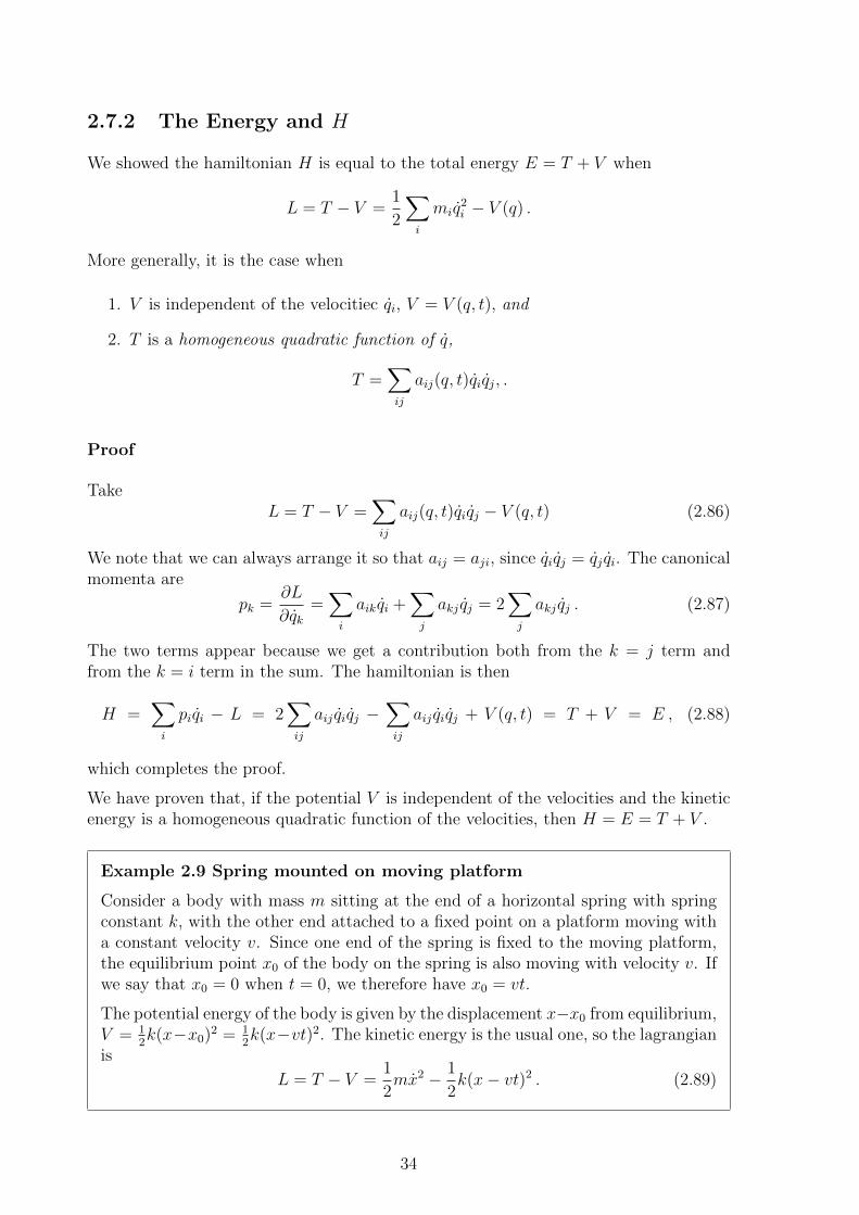
2.7.2 The Energy and H
We showed the hamiltonian H is equal to the total energy E = T + V when
L = T − V =1
2
∑i
miq2i − V (q) .
More generally, it is the case when
1. V is independent of the velocitiec qi, V = V (q, t), and
2. T is a homogeneous quadratic function of q,
T =∑ij
aij(q, t)qiqj, .
Proof
TakeL = T − V =
∑ij
aij(q, t)qiqj − V (q, t) (2.86)
We note that we can always arrange it so that aij = aji, since qiqj = qj qi. The canonicalmomenta are
pk =∂L
∂qk=∑i
aikqi +∑j
akj qj = 2∑j
akj qj . (2.87)
The two terms appear because we get a contribution both from the k = j term andfrom the k = i term in the sum. The hamiltonian is then
H =∑i
piqi − L = 2∑ij
aij qiqj −∑ij
aij qiqj + V (q, t) = T + V = E , (2.88)
which completes the proof.
We have proven that, if the potential V is independent of the velocities and the kineticenergy is a homogeneous quadratic function of the velocities, then H = E = T + V .
Example 2.9 Spring mounted on moving platform
Consider a body with mass m sitting at the end of a horizontal spring with springconstant k, with the other end attached to a fixed point on a platform moving witha constant velocity v. Since one end of the spring is fixed to the moving platform,the equilibrium point x0 of the body on the spring is also moving with velocity v. Ifwe say that x0 = 0 when t = 0, we therefore have x0 = vt.
The potential energy of the body is given by the displacement x−x0 from equilibrium,V = 1
2k(x−x0)2 = 1
2k(x−vt)2. The kinetic energy is the usual one, so the lagrangian
is
L = T − V =1
2mx2 − 1
2k(x− vt)2 . (2.89)
34

The canonical momentum is px = mx, which gives us the hamiltonian
Hx = pxx− L =1
2mx2 +
1
2k(x− vt)2 = T + V = E . (2.90)
Since the lagrangian depends explicitly on time, the hamiltonian (and the totalenergy) is not conserved. We can understand this by noting that the motor drivingthe platform will have to do work to maintain a constant velocity; in the absenceof this the platform will undergo oscillations along with the body attached to thespring.
We can now introduce a new coordinate
q = x− vt =⇒ q = x− v (2.91)
=⇒ L(q, q, t) =1
2m(q + v)2 − 1
2kq2 =
1
2mq2 +mvq − 1
2kq2 +
mv2
2. (2.92)
The canonical momentum is pq = m(q + v), and the hamiltonian is
Hq = pq−L = mq2+mvq−1
2mq2−mvq+1
2kq2−mv
2
2=
1
2mq2+
1
2kq2−mv
2
2. (2.93)
When written in terms of q, the lagrangian does not depend explicitly on time, andtherefore the hamiltonian (2.93) is conserved! However, it is not equal to the totalenergy, rather
Hq = Hx + pq q − pxx = E + px(q − x) = E −mvx.
So, by changing coordinates, we have here traded a non-conserved hamiltonian, fora conserved hamiltonian that is not equal to E.
Example 2.10 Electrodynamics
One case where the distinction between ordinary and canonical momentum is im-portant is electrodynamics. A particle with charge Q moving with velocity ~v in anelectric field ~E and a magnetic field ~B is
~F = Q( ~E + ~v × ~B), (2.94)
which is called the Lorentz force law. Using Maxwell’s laws, we can introduce theelectrostatic and vector (‘magnetic’) potentials φ, ~A:
∇ · ~B = 0 ⇐⇒ ~B = ∇× ~A , (2.95)
∇× ~E = −∂~B
∂t⇐⇒ ~E = −∇φ− ∂ ~A
∂t, (2.96)
where φ is the electric potential, so the potential energy of a charged particle Q isV = Qφ, and Ai(x, t) is called the vector potential for the magnetic field ~B. TheLorentz force law (2.94) can be derived from the Lagrangian
L =1
2m
3∑i=1
x2i −Qφ+Q
3∑i=1
Aixi . (2.97)
35

We have
∂L
∂xi= mxi +QAi ⇒ d
dt
(∂L
∂xi
)= mxi +Q
(∂Ai∂t
+∑j
xj∂Ai∂xj
)∂L
∂xi= −Q ∂φ
∂xi+Q
∑j
xj∂Aj∂xi
giving equations of motion
mxi = −Q ∂φ
∂xi−Q∂Ai
∂t+Q
∑j
xj
(∂Aj∂xi− ∂Ai∂xj
)= Q( ~E + ~v ×B)i ,
which is the Lorentz force law (2.94), since
(~v × ~B)i =(~v × (∇× A)
)i
= ~v.
(∂ ~A
∂xi
)− (~v.∇)Ai =
∑j
xj
(∂Aj∂xi− ∂Ai∂xj
).
The canonical momentum is
pi =∂L
∂xi= mxi +QAi . (2.98)
This is not the ordinary momentum, a distinction which becomes quite importantin quantum mechanics, where it is the canonical momentum that enters into thecommutation relations that are used to quantise the system. Note that in general
mxi +QAi = −Q ∂φ
∂xi+Q
∑j
xj∂Aj∂xi
so momentum is not conserved.
The hamiltonian of the particle is
H =3∑i=1
pixi − L =3∑i=1
(mxi +QAi)xi −1
2m
3∑i=1
x2i +Qφ−Q
3∑i=1
Aixi
=1
2m
3∑i=1
x2i +Qφ .
(2.99)
We see that the vector (magnetic) potential does not contribute to the energy. Phys-ically this is because no net work is done by the magnetic field,
~v. ~F = Q~E.
36

2.8 Lagrangian mechanics — summary sheet
1. Lagrangian L = T − V = kinetic energy − potential energy.L = L(q, q, t) is a function of the coordinates qi, their time derivativesqi and time t.
2. Generalised coordinatesFor a system of N particles, we may instead of cartesian coordinates~ri = (xi, yi, zi), i = 1 . . . N , use any set of coordinates
qj = fj(~r1, . . . , ~rN) , j = 1 . . .M .
M is the number of degrees of freedom of the system. For an uncon-strained system M = 3N , but if there are constraints then M < 3N .
3. Principle of least actionNature “chooses” the path q(t) that minimises the action
S =
∫ t1
t0
L(q(t), q(t), t)dt
with q(t0) = q0, q(t1) = q1 kept fixed, or
δS = limα→0
S[q(t)]− S[q(t) + αh(t)]
α= 0
for arbitrary h(t) with h(t0) = h(t1) = 0. This leads to
4. Euler–Lagrange equations
d
dt
∂L
∂qi− ∂L
∂qi= 0
5. Canonical momentum
pi =∂L
∂qi
(a) Linear momentumIf qi = xi and L = 1
2
∑imix
2i − V (x), then pi = mxi .
(b) Angular momentumIf qi is a rotational angle φ about some axis, then pi is the angularmomentum [~L = ~r × (m~v)] about that axis.
6. Conservation lawsFrom the Euler–Lagrange equations we see that if L does not dependexplicitly on the coordinate qi then
dpidt
= 0 ⇐⇒ pi is conserved.
37

7. HamiltonianH =
∑i
piqi − L
If there are no time-dependent constraints or velocity-dependentforces (or potentials) then H = T + V = total energy.
dH
dt= −∂L
∂t,
so if the lagrangian L does not explicitly depend on time, then thehamiltonian H is conserved.
38

Chapter 3
Hamiltonian dynamics
The main idea in hamiltonian dynamics is that instead of using only the coordinatesqi(t) and their derivatives to describe the system, we think of the coordinates qi and themomenta pi as independent variables.
This may seem like an odd idea, since once we know the coordinates qi(t) as a functionof time, we also know their time derivatives qi(t), and through that the momenta pi(t).So how can q and p be considered independent?
One way of making sense of this is to note that knowing the position of a body at aparticular time does not in itself tell us anything about its velocity (or momentum), orvice-versa. It is only if we know the position at several different times that we will beable to work out its velocity. And the full relation between q(t) and q(t), or betweenq(t) and p(t), can only be known if we know the coordinate q(t) at all times t — butthis amounts to having solved the problem of the motion of the body! So in this sense,q and p (or, indeed, q and q) can be considered independent variables.
Secondly, the relation between coordinates and canonical momenta is not a simple onelike the relation between a coordinate and its derivative, but is related to the dynamics ofthe system as encoded in the lagrangian (or, as we shall see, the hamiltonian). Therefore,it makes sense to consider p as independent of q in a way that q cannot be.
Thirdly, as you will see in quantum mechanics, the two must be treated as independentquantities there. From the quantum mechanical commutation relations between coordi-nates and canonical momenta, [qi, pk] = ihδjk, one can derive Heisenberg’s uncertaintyrelation, ∆qi∆pi ≥ h, which holds for all (q, p) pairs. Therefore, in quantum mechanics,it is impossible to know the coordinate and momentum of a particle at the same time.Also, statistical mechanics, which forms the basis of the modern treatment of thermalphysics, is formulated in the phase space where coordinates and momenta are consideredas independent variables.
So our first step in arriving at the hamiltonian formulation of mechanics will be touse the relation between momenta pi and velocities qi to eliminate q, and write thehamiltonian as a function of coordinates and momenta,
H = H(qi, pi, t) as opposed to L = L(qi, qi, t) . (3.1)
This will be our starting point in this chapter.
39
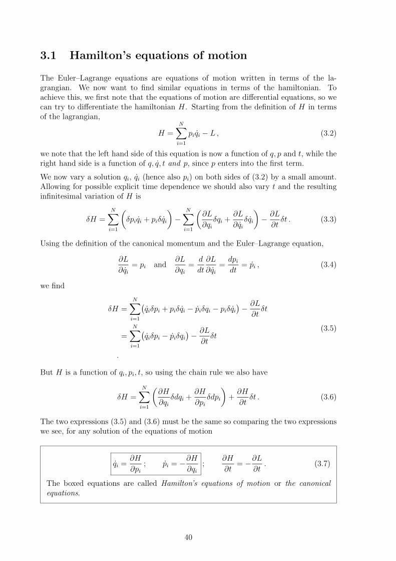
3.1 Hamilton’s equations of motion
The Euler–Lagrange equations are equations of motion written in terms of the la-grangian. We now want to find similar equations in terms of the hamiltonian. Toachieve this, we first note that the equations of motion are differential equations, so wecan try to differentiate the hamiltonian H. Starting from the definition of H in termsof the lagrangian,
H =N∑i=1
piqi − L , (3.2)
we note that the left hand side of this equation is now a function of q, p and t, while theright hand side is a function of q, q, t and p, since p enters into the first term.
We now vary a solution qi, qi (hence also pi) on both sides of (3.2) by a small amount.Allowing for possible explicit time dependence we should also vary t and the resultinginfinitesimal variation of H is
δH =N∑i=1
(δpiqi + piδqi
)−
N∑i=1
(∂L
∂qiδqi +
∂L
∂qiδqi
)− ∂L
∂tδt . (3.3)
Using the definition of the canonical momentum and the Euler–Lagrange equation,
∂L
∂qi= pi and
∂L
∂qi=
d
dt
∂L
∂qi=dpidt
= pi , (3.4)
we find
δH =N∑i=1
(qiδpi + piδqi − piδqi − piδqi
)− ∂L
∂tδt
=N∑i=1
(qiδpi − piδqi
)− ∂L
∂tδt
.
(3.5)
But H is a function of qi, pi, t, so using the chain rule we also have
δH =N∑i=1
(∂H
∂qiδdqi +
∂H
∂piδdpi
)+∂H
∂tδt . (3.6)
The two expressions (3.5) and (3.6) must be the same so comparing the two expressionswe see, for any solution of the equations of motion
qi =∂H
∂pi; pi = −∂H
∂qi;
∂H
∂t= −∂L
∂t. (3.7)
The boxed equations are called Hamilton’s equations of motion or the canonicalequations.
40

Using Hamilton’s equations of motion, it is very straightforward to show that the hamil-tonian is conserved if it does not depend explicitly on time:
dH
dt=
N∑i=1
(∂H∂qi
qi +∂H
∂pipi
)+
∂H
∂t=
N∑i=1
(piqi + qipi
)+
∂H
∂t=
∂H
∂t. (3.8)
Example 3.1
Consider a particle constrained to move on the cylindrical surface x2 + y2 = R2,subject to a central force ~F = −k~r.
Using cylinder coordinates (θ, z) with x = R cos θ, y = R sin θ we find
V =1
2kr2 =
1
2k(R2 + z2) , (3.9)
T =1
2m(x2 + y2 + z2) =
1
2m(R2θ2 + z2) (3.10)
=⇒ L =1
2m(R2θ2 + z2)− 1
2k(R2 + z2) . (3.11)
The canonical momenta are
pθ =∂L
∂θ= mR2θ , pz =
∂L
∂z= mz . (3.12)
We can use this to find θ, z in terms of pθ, pz:
θ =pθmR2
, z =pzm. (3.13)
The hamiltonian is
H = pz z − pθθ − L = pzpzm
+ pθpθmR2
− 1
2m[R2( pθmR2
)2
+(pzm
)2]+
1
2k(R2 + z2)
=p2z
2m+
p2θ
2mR2+
1
2kz2 +
1
2kR2 = H(z, pz, pθ) . (3.14)
It is equal to the total energy since the potential energy does not depend on velocitiesand the kinetic energy has the usual form. It is conserved since there is no explicittime-dependence in L (or H).
Hamilton’s equations of motion for this system are
pθ = −∂H∂θ
= 0 , θ =∂H
∂pθ=
pθmR2
(3.15)
pz = −∂H∂z
= −kz , z =∂H
∂pz=pzm
(3.16)
We can use (3.15), (3.16) to arrive at
pθ = mR2θ = constant, z =pzm
= − kmz . (3.17)
These are the Euler–Lagrange equations for the system, so we have shown thatHamilton’s equations are exactly equivalent to the Euler–Lagrange equations, asthey should be.
41

In the example above we see that θ does not appear in the expression for H: it is acyclic coordinate. This implies that the canonical momentum pθ is conserved, but in thehamiltonian framework it actually simplifies the system even further: in the remainingequations we can simply treat pθ as any other constant, so the whole motion in theθ-coordinate decouples from the remaining equations: instead of 3 variables z, z, θ wenow just have 2: z, z.
This decoupling is a generic feature which can simplify the analysis of the system con-siderably, as we shall see below.
3.2 Cyclic coordinates and effective potential
To see how this works out, let us look at a slightly more complex system, that of thespherical pendulum. This is a pendulum that can swing freely in all directions, not justin a plane. Using spherical coordinates (θ, φ), where θ is the angle with the vertical axis,we find that the lagrangian of this system is
L =1
2m`2(θ2 + φ2 sin2 θ) +mg` cos θ . (3.18)
The canonical momenta are
pθ =∂L
∂θ= m`2θ (3.19)
pφ =∂L
∂φ= m`2 sin2 θφ (3.20)
From (3.19), (3.20) we find
θ =pθm`2
, φ =pφ
m`2 sin2 θ. (3.21)
Since there is nothing funny going on in this system, the hamiltonian is equal to thetotal energy,
H = T + V =p2θ
2m`2+
p2φ
2m`2 sin2 θ−mg` cos θ . (3.22)
Hamilton’s equations of motion are then
θ =∂H
∂pθ=
pθm`2
, pθ = −∂H∂θ
=p2φ cos θ
m`2 sin3 θ−mg` sin θ , (3.23)
φ =∂H
∂pφ=
pφm`2 sin2 θ
, pφ = −∂H∂φ
= 0 . (3.24)
Since pφ is constant, the two last terms in (3.22) depend only on θ. They can be takento define an effective potential,
Veff(θ) =p2φ
2m`2 sin2 θ−mg` cos θ (3.25)
with
pθ = −dVeffdθ
42

(we use an ordinary derivative with respect to θ here, rather than a partial derivative,because it is understood that everything else is constant).
Let us now look at a system with a single degree of freedom θ, with kinetic energyp2θ/(2m`
2) and potential energy Veff(θ). The hamiltonian of this system is exactly thesame as (3.22), and therefore Hamilton’s equations of motion for θ, pθ are exactly thesame as (3.23).
0 0.5 1 1.5 2 2.5 3
θ
-1
0
1
2
3
Veff
/mg
l
k = 0
k = 0.02
k = 0.1
k = 0.5
k = 1.0
k = 1.5
Figure 3.1: The effective potential for the spherical pendulum, for different values ofk = p2
φ/2m2g`3.
We can use the effective potential to find out what types of motion are possible in theθ-direction. Figure 3.1 shows Veff as a function of θ for several values of pφ. We can seethat for all pφ 6= 0 the effective potential goes to infinity at θ = 0 and θ = π. This meansthat only bounded motion exists for pφ 6= 0. The minimum of the potential correspondsto circular motion at a fixed angle θ, given by
mg` sin4 θ =p2φ
m`2cos θ . (3.26)
In contrast, for pφ = 0 (the solid line), both bounded motion (through θ = 0) andunbounded motion are possible, for −mg` < E < mg` and E ≥ mg` respectively. Inthis case, the spherical pendulum reduces to the plane (simple) pendulum.
What we have seen in this example is quite typical of what happens if one or more ofthe coordinates are cyclic. In general, if the hamiltonian can be written as
H(q1, q2, p1, p2) = f(q1)p21 + g(q1)p2
2 + V (q1) , (3.27)
where f and g can be any function of the coordinate q1, then we immediately see thatthe second coordinate q2 is cyclic, and the momentum p2 is therefore conserved, ie it is
43

a constant. We can then define an effective potential
Veff(q1) = g(q1)p22 + V (q1) , (3.28)
and the hamiltonian will be equivalent to that of a 1-dimensional system with kineticenergy T1 given by
T1 = f(q1)p21 =⇒ H(q1, p1) = T1 + Veff(q1) . (3.29)
It is clear that the equations of motion of q1 and p1 we obtain from (3.29) are the sameas what we obtain from (3.27) since the two hamiltonians are exactly the same: all wehave done is group the terms in a different way,
If are only interested in the motion in the q1 coordinate we can stop as soon as we havesolved the equations of motion resulting from (3.29). If we also want to determine q2(t),we use its equation of motion,
q2 =∂H
∂p2
= 2p2g(q1) =⇒ q2(t) = 2p2
∫ t
q2(t0)
g(q1(t′))dt′ . (3.30)
Once we have found q1(t) it is in principle straightforward to perform this integral toobtain q2(t).
3.3 Hamilton’s equations from a variational princi-
ple
We arrived at Hamilton’s equations from the lagrangian and using the Euler–Lagrangeequations, but it is also possible to derive them directly from a variational principle, aswe shall now see. To this end, we can rewrite the action S =
∫Ldt as
S =
∫ (pq −H(q, p, t)
)dt . (3.31)
The equations of motion will now be derived by requiring δS = 0, where now p and q canbe varied independently. We proceed analogously to how we derived the Euler–Lagrangeequations in Section 2.3, using the shorthand δS instead of dS/dα:
δS = δ
∫ (pq −H(q, p, t)
)dt
=
∫ t2
t1
[∑i
(δpiqi + piδqi
)−∑i
(∂H∂pi
δpi +∂H
∂qiδqi
)]dt
=∑i
∫ t2
t1
[qiδpi +
d
dt(piδqi)− piδqi −
∂H
∂piδpi −
∂H
∂qiδqi
]dt
=∑i
(piδqi
)∣∣∣t2t1
+∑i
∫ t2
t1
[(qi −
∂H
∂pi
)δpi −
(pi +
∂H
∂qi
)δqi
]dt = 0 .
(3.32)
The first term on the last line is zero because the endpoints qi(t1), qi(t1) are fixed, soδqi(t1) = δqi(t2) = 0. In the second term, the integral must be zero for any arbitrary
44
variations δpi, δqi, which can both be chosen indenpendently for all degrees of freedomi. The only way this can be the case is if both terms inside the ordinary brackets arezero at all times, and for all i. This gives us
qi =∂H
∂pi, pi = −∂H
∂qi, (3.33)
which is Hamilton’s equations of motion.
3.4 Phase space [Optional]
We can consider the values of p, q = (p1, . . . , pN , q1, . . . , qN) as coordinates of a pointin a 2N -dimensional space. This space is called phase space. The evolution of the systemin time can then be thought of as a trajectory in this space. The state of a system isgiven by its location in phase space, ie by the values of all the generalised coordinatesand momenta — in other words, every point in phase space describes a unique state.There are two important aspects of this:
1. The trajectory of a system in phase space provides a complete description of themotion of the system.
2. The complete trajectory is uniquely determined by the initial coordinatespi(t0), qi(t0). Mathematically, this is because Hamilton’s equations of motionconstitute a set of first order ODEs for the phase space coordinates as a functionof time, and the solution of a first order ODE is uniquely determined by the initialvalues. Physically, it is because the position and momentum together completelydetermine the motion of any particle or system.
An important corrollary of this is that trajectories in phase space never cross. Identicalstates will have identical futures (and identical pasts). The description of a system interms of states in phase space is a cornerstone of statistical mechanics.
It is worth looking at how this changes in quantum mechanics. Here, Heisenberg’s un-certainty relation ∆q∆p ≥ h/2 implies that a system cannot be identified with a uniquepoint in classical phase space. This means that identical states can have different fu-tures. The appropriate description in quantum mechanics is in terms of vectors (points)in a Hilbert space of quantum states rather than in classical phase space, and it is pos-sible to make connections between the two — but this goes way beyond the topic of thismodule.
45

Example 3.2 Particle in constant gravitational field
z
p
Figure 3.2: Phase space trajecto-ries for a particle in a constantgravitational field.
The hamiltonian is here given by
H =p2
2m+mgz . (3.34)
Since H is conserved the trajectories in phasespace are given by those curves in the (p, z)plane where H is constant. We can describethese curves in two (equivalent) ways:
1. In terms of initial coordinates p1, z1:
p2
2m+mgz =
p21
2m+mgz1 (3.35)
⇐⇒ p2 − p21
2m= mg(z1 − z) (3.36)
⇐⇒ z = z1 +1
2m2g(p2
1 − p2) . (3.37)
This describes a parabola. The resulting trajectories are shown in figure 3.2
2. In terms of the total energy E:
p2 +mgz = E =⇒ mgz = E − p2
2m=⇒ z
z0
= 1− p2
p20
(3.38)
with
z0 =E
mg; p0 =
√2mE = m
√2gz0 . (3.39)
46

Example 3.3 Plane pendulum
π θ
pθ
a)b)
c)
Figure 3.3: Phase space trajecto-ries for a plane pendulum. Notethe bifurcation point at pθ =0, θ = π. See text for discussionof the trajectories a), b), c).
The hamiltonian is
H =p2θ
2m`2+mgl(1− cos θ) = E , (3.40)
where we have chosen the potential energy tobe zero at the stable equilibrium point of thependulum. Reorganising this we find
p2θ
2m`2= E −mg`(1− cos θ) (3.41)
=⇒(pθp0
)2
= 1− 1
Qsin2 θ
2, (3.42)
with
p0 = `√
2mE , Q =E
2mg`. (3.43)
Depending on the value of Q, we have three classes of trajectories:
a) 0 < Q < 1. this gives ellipse-like trajectories: if we write q = sin θ2, then (3.42)
can be rewritten as(pθp0
)2
+
(q
q0
)2
= 1 , with q0 =√Q . (3.44)
The motion is bounded in both pθ and θ.
b) Q = 1. Here the trajectories touch at pθ = 0, θ = π — but strictly speakingthey do not actually cross A system moving along the trajectory b) in Fig. 3.3will take an infinite amount of time to reach this point, and a system findingitself at this point will be in an unstable equilibrium. If a system does end upat this point and is subject to a small perturbation, it can continue either downalong the solid line, or up along the dotted line. This is called a bifurcationpoint. Bifurcation points are important in chaos theory.
c) Q > 1. Here the motion is unbounded in θ but bounded in pθ, with
1− 1
Q≤(pθp0
)2
≤ 1 . (3.45)
Example 3.4 Particle on cylinder
Take a particle moving on the surface of a cylinder with radius R, subject to aharmonic force ~F = −k~r. In cylinder coordinates the potential energy is V =
47

12kr2 = 1
2k(z2 +R2) and the hamiltonian is (ignoring the constant zero-point energy)
H =p2θ
2mR2+
p2z
2m+
1
2kz2 . (3.46)
Since θ is cyclic, pθ is constant and we can ignore it. The resulting phase space isthree-dimensional: (pz, z, θ). We have
p2z
2m+
1
2kz2 = const , (3.47)
giving an ellipse in the (pz, z) plane, or a uniform elliptic spiral in (pz, z, θ)-space.
3.5 Liouville’s theorem [Optional]
In statistical mechanics we do not know the detailed (microscopic) state of the system,ie the position and momentum of every single particle (for example, every molecule in agas). Instead, we consider ensembles of possible states, ie collections of states that areconsistent with what we know about the system. Every point in phase space correspondsto a possible state, and each has its own unique trajectory.
We are interested in finding out what happens to nearby trajectoriesas they evolve in time (see figure on the right). At time t1, thesepoints are located in a particular region of phase space. At somelater time t2, where will they be relative to each other, and whatkind of region of phase space will the occupy?
We assume that a region ∆V in phase space contains N (represen-tative) states. We can then define the density of states as
ρ =N
∆Vwith ∆V = ∆p1∆p2 · · ·∆pN∆q1∆q2 · · ·∆qN . (3.48)
(p,q)
dq
dp
Figure 3.4: Flow of phasespace trajectories througha small volume dpdq.
Let us now consider a small volume dpdq and look at theflow of states in and out of this volume. This is illustratedin fig. 3.4. In a small time dt, a point near (p, q) will movea distance pdt to the right, and a distance qdt up.
The inflow dNl across the left boundary and dNb across thebottom boundary are given by
dNl = ρ(p, q)pdqdt , (3.49)
dNb = ρ(p, q)qdpdt . (3.50)
Both ρ, p and q vary with p and q, so the outflow across theright and top boundaries will be slightly different. They are
48

given by
dNr = ρ(p+ dp, q)p(p+ dp, q)dqdt =[ρ(p, q)p+
(∂ρ∂pp+ ρ
∂p
∂p
)dp]dqdt , (3.51)
dNt = ρ(p, q + dq)q(p, q + dq)dqdt =[ρ(p, q)q +
(∂ρ∂qq + ρ
∂q
∂q
)dq]dpdt . (3.52)
The total net inflow is then
dN = dNl + dNb − dNr − dNt = −(∂ρ∂pp+ ρ
∂p
∂p
)dpdqdt−
(∂ρ∂qq + ρ
∂q
∂q
)dqdpdt , (3.53)
and the change in density is
∂ρ
∂t=
dN
dV dt=
dN
dpdqdt= −
(∂ρ
∂pp+ ρ
∂p
∂p+∂ρ
∂qq + ρ
∂q
∂q
). (3.54)
But according to Hamilton’s equations of motion we have
p = −∂H∂q
q =∂H
∂p=⇒ ∂p
∂p+∂q
∂q= − ∂
2H
∂p∂q+∂2H
∂q∂p= 0 , (3.55)
so we end up with
∂ρ
∂t+∂ρ
∂pp+
∂ρ
∂qq ≡ dρ
dt= 0 . (3.56)
If we have N coordinates p1, . . . , pN , q1, . . . , qN , we do the same for each pk, qk. Theleft boundary is now a hyper-surface with area dV/dpk, and similarly for the otherboundaries. Taking the sum over all k, we find
Liouville’s theorem
dρ
dt=∂ρ
∂t+
N∑k=1
(∂ρ
∂pkpk +
∂ρ
∂qkqk
)= 0 (3.57)
Liouville’s theorem can be expressed in words as
As the (representative) states of the system evolve in time, their density in phasespace remains constant.
Another way of expressing it is that the volume in phase space occupied by N trajectoriesremains the same throughout the evolution of the system.
This result is a cornerstone of statistical mechanics, as well as of chaos theory.
49

3.6 Poisson brackets
Consider some function f(q1, . . . qN , p1, . . . , pN , t), ie an arbitrary function of coordi-nates, momenta, and time. Let us now find the total time derivative (ie rate of change)of this function. Using the chain rule we have
df
dt=∂f
∂t+
N∑k=1
(∂f
∂qkqk +
∂f
∂pkpk
)=∂f
∂t+
N∑k=1
(∂f
∂qk
∂H
∂pk− ∂f
∂pk
∂H
∂qk
), (3.58)
where in the last step we have made use of Hamilton’s equations of motion. We canwrite this in shorthand form as
df
dt=∂f
∂t+ f,H . (3.59)
f,H is called the Poisson bracket of H and f .
For two general functions f and g of coordinates and momenta, we define the Poissonbrackets as
f, g ≡∑k
(∂f
∂qk
∂g
∂pk− ∂f
∂pk
∂g
∂qk
)(3.60)
3.6.1 Properties of Poisson brackets
From the definition (3.60) we can immediately see that the Poisson bracket is antisym-metric, f, g = −g, f.
We can also prove the following relations for arbitrary functions f, g, h and constantsa, b, c:
f, f = 0 , (3.61)
f, c = 0 , (3.62)
af + bg, h = af, h+ bg, h (3.63)
fg, h = fg, h+ gf, h (3.64)
f, pk =∂f
∂qk, (3.65)
f, qk = − ∂f∂pk
. (3.66)
For example, the proof of (3.62) is
f, c =∑k
(∂f
∂qk
∂c
∂pk− ∂f
∂pk
∂c
∂qk
)=∑k
(∂f
∂qk· 0− ∂f
∂pk· 0)
= 0 , (3.67)
50

since c is a constant and therefore does not depend on either p or q.
To prove (3.66) we note that all coordinates and momenta are independent variablesand therefore depend only on themselves,
∂pk∂qi
=∂qk∂pi
= 0 ∀i, k ;∂pk∂pk
=∂qk∂qk
= 1 ∀k ;∂pk∂pi
=∂qk∂qi
= 0 if i 6= k. (3.68)
We therefore have
f, pk =∑i
(∂f
∂qi
∂pk∂pi− ∂f
∂pi
∂pk∂qi
)=
∂f
∂qk· 1 =
∂f
∂qk. (3.69)
Proving the other relations will be left as an exercise.
From (3.66), (3.65), we immediately find the fundamental Poisson brackets, which arethe Poisson brackets of coordinates and momenta. They are
qj, qk = pj, pk = 0 ∀j, k (3.70)
qj, pk = δjk =
1 , j = k
0 , j 6= k(3.71)
You may note the similarity between these expressions and the commutation relationsbetween the position and momentum operators in quantum mechanics,
[pi, xj] = −ihδij . (3.72)
This analogy was noted early on, and is often used to formulate the quantum mechanicalversion of a classical mechanics system. In general, one may find the Poisson bracketsof any two quantities f and g, and this will give the commutation relation between thequantum mechanical operators f , g,
f, g −→ − ih
[f , g] . (3.73)
In particular, applying this to (3.59) yields Heisenberg’s equation of motion,
df
dt=i
h[f , H] +
∂f
∂t, (3.74)
which is valid for all quantum mechanical operators.1
1In the Heisenberg picture, where the operators depend on time. This is in contrast to theSchrodinger picture, where the states depend on time and the operators are in general independentof time.
51
3.6.2 Poisson brackets and conservation laws
From (3.59) we can see that if f does not depend explicitly on time, ie f = f(p, q),then df/dt = H, f. Specifically, for any motion integral (conserved quantity which isa function of coordinates and momenta) I, we have
I,H = 0 . (3.75)
We can use this to demonstrate that a quantity is conserved, even if it is not the canonicalmomentum of a cyclic coordinate. The example below will illustrate this.
Example 3.5 Angular momentum
Consider a particle with mass m moving in a central force (spherically symmetric)potential V (r). The hamiltonian for this system is, in spherical coordinates (r, θ, φ),
H = T + V =p2r
2m+
p2θ
2mr2+
p2φ
2mr2 sin2 θ+ V (r) . (3.76)
Since the azimuthal angle φ does not appear in H (ie, it is a cyclic coordinate), wecan immediately see that the canonical momentum pφ is conserved:
pφ = pφ, H = −∂H∂φ
= 0 . (3.77)
In a spherically symmetric system all angles should be irrelevant, so one wouldnaıvely expect that pθ would also be conserved. However, because of the way wesingled out the z-axis when defining our coordinates, θ is not cyclic, and we get
pθ = −∂H∂θ
=p2φ
mr2
cos θ
sin3 θ6= 0 . (3.78)
Let us now consider instead the quantity
J2 ≡ p2θ +
p2φ
sin2 θ. (3.79)
We can use Poisson brackets to find the rate of change of J2:
dJ2
dt= J2, H
=∂J2
∂r
∂H
∂pr− ∂J2
∂pr
∂H
∂r+∂J2
∂θ
∂H
∂pθ− ∂J2
∂pθ
∂H
∂θ+∂J2
∂φ
∂H
∂pφ− ∂J2
∂pφ
∂H
∂φ
= 0− 0 +(−
2p2φ cos θ
sin3 θ
)· pθmr2
− 2pθ ·(−
p2φ cos θ
mr2 sin3 θ
)+ 0− 0
= 0 .
(3.80)
Therefore, J2 is conserved.
52

What is the physical meaning of J2?
We can write the angular momentum ~J in spherical coordinates as
~J = ~r × ~p = m~r × (vrr + vθθ + vφφ) = mrr × (rr + rθθ + r sin θφφ) . (3.81)
The vector products of r with the unit vectors are
r × r = 0 ; r × θ = φ ; r × φ = −θ . (3.82)
Therefore,
~J = mr2θ φ−mr2 sin θφ θ = pθφ−pφ
sin θθ (3.83)
~J2 = p2θ +
( pφsin θ
)2
= J2 , (3.84)
since the two vectors θ, φ are orthogonal. We see that J2 is just the square of thetotal angular momentum, J2 = J2
x + J2y + J2
z = ~J. ~J .
We have already shown (2.81) that pφ = Jz is the z-component of the angularmomentum. It may also be shown, using Poisson brackets, that
Jx = −pθ sinφ− pφ cot θ cosφ (3.85)
is conserved, this is left as an exercise. In fact all four of Jx, Jy, Jz and J2 areconserved, but they are not all independent. Only two of them are independentconserved quantities and it is often convenient to use J2 and Jz. For a rotationallysymmetric system we can always choose the axes so that the conserved vector ~Jpoints in the z-direction and Jx = Jy = 0.
3.6.3 The Jacobi identity and Poisson’s theorem
One important relation that Poisson brackets obey is the Jacobi identity,
f, g, h+ g, h, f+ h, f, g = 0 , (3.86)
for any three arbitrary functions f, g, h. The proof of this is straightforward but ex-tremely tedious, so we will not show it here. We will however note that the same identityholds for other antisymmetric products, including commutators and vector products:
[A, [B,C]] + [B, [C,A]] + [C, [A,B]] = 0 , (3.87)
~A× ( ~B × ~C) + ~B × (~C × ~A) + ~C × ( ~A× ~B) = 0 . (3.88)
The proof for commutators is very straightforward and relatively short:
[A, [B,C]] + [B, [C,A]] + [C, [A,B]]
= [A,BC − CB] + [B,CA− AC] + [C,AB −BA]
= ABC − ACB − (BCA− CBA) +BCA−BAC − (CAB − ACB)
+ CAB − CBA− (ABC −BAC)
= 0 .
(3.89)
53
We can use this identity to prove that the Poisson brackets F,G of two conservedquantities F and G is also conserved:
d
dtF,G =
∂
∂tF,G+ F,G, H =
∂
∂tF,G − H, F,G (3.90)
= ∂F∂t,G+ F, ∂G
∂t+ F, G,H+ G, H,F (3.91)
= ∂F∂t
+ F,H, G+ F, ∂G∂t
+ G,H = 0 . (3.92)
In (3.90) we have used (3.59); in (3.91) we have used the product rule for ∂/∂t and usedthe Jacobi identity to rewrite H, F,G. Finally, in (3.92) we have used the generalproperties of Poisson brackets, f, g = −g, f and f, g + h = f, g+ f, h.
This gives us
Poisson’s theorem:
dF
dt=dG
dt= 0 =⇒ d
dtF,G = 0 . (3.93)
We can use this to construct further conserved quantities from ones we already know,although this is not quite as useful as it may at first seem: in many cases the Poissonbrackets of two conserved quantities will simply vanish.
Example 3.6
Given the hamiltonian (3.76) and Jx defined in (3.85), we can, with a minimum ofcalculation, construct a further conserved quantity Jy. We already know that pφ isconserved, and using the Poisson brackets we have found that Jx is also conserved.Therefore the Poisson brackets of the two,
Jy = pφ, Jx = −∂Jx∂φ
= pθ cosφ− pφ cot θ sinφ , (3.94)
is also conserved.
3.7 Noethers theorem
We have earlier seen that if a variable qi is cyclic then there is a conserved quantitypi = ∂L
∂qirelated to it as
pi =∂L
∂qi= 0.
But it goes deeper than that. As soon as the Lagrangian as a symmetry, then therewill be a conserved quantity related to that quantity. This result is called Noetherstheorem.
54
Assume you can change your variables q → q(α) and q → q(α) by a parameter α andstill keep the Lagrangian invariant
∂
∂αL (qi (α) , qi (α) , t) = 0. (3.95)
This could be simple things like q → q + α or something more complicated, like q1 →q1 cosα− q2 sinα, q2 → q1 sinα+ q2 cosα. Note here that α is independent of time andalso that we do not change the time coordinate — if we do the result bellow will needto be generalized.
We have∂
∂αL (qi (α) , qi (α) , t) =
∑i
(∂L
∂qi
∂qi∂α
+∂L
∂qi
∂qi∂α
).
Assuming that α is independent of time and derivatives with respect to α and t commute,∂qi∂α
= ∂∂t∂qi∂α
this can be written as
∂
∂αL (qi (α) , qi (α) , t) =
∑i
∂L
∂qi
∂qi∂α− d
dt
(∂L
∂qi
)∂qi∂α
+d
dt
(∂L
∂qi
∂qi∂α
)=∑i
∂L
∂qi− d
dt
(∂L
∂qi
)∂qi∂α
+d
dt
∑i
(pi∂qi∂α
)= 0.
This vanishes because we assume that varying α is a symmetry of the Lagrangian (3.95),we have not assumed that qi is a solution of the equations of motion. If qi is a solutionthen we can deduce that
d
dt
(∑i
pi∂qi(α)
∂α
)= 0.
We have shown that
C =∑i
pi∂qi(α)
∂α(3.96)
is a conserved quantity.
From this immediately follows something we already knew: If qi is cyclic then pi isconserved. This follows since if ∂L
∂qi= 0 then the Lagrangian is also invariant under
under qi → qi(α) = qi + α. We therefore have ∂qi(α)∂α
= 1 and so
Ci = pidqi(α)
dα= pi
which shows that pi is conserved when qi is cyclic.
55
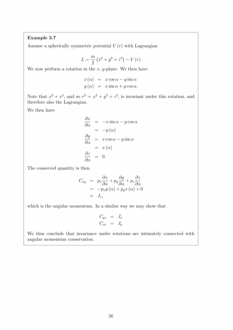
Example 3.7
Assume a spherically symmetric potential V (r) with Lagrangian
L =m
2
(x2 + y2 + z2
)− V (r)
We now perform a rotation in the x, y-plane. We then have
x (α) = x cosα− y sinα
y (α) = x sinα + y cosα.
Note that x2 + x2, and so r2 = x2 + y2 + z2, is invariant under this rotation, andtherefore also the Lagrangian.
We then have
∂x
∂α= −x sinα− y cosα
= −y (α)
∂y
∂α= x cosα− y sinα
= x (α)
∂z
∂α= 0.
The conserved quantity is then
Cxy = px∂x
∂α+ py
∂y
∂α+ pz
∂z
∂α= −pxy (α) + pyx (α) + 0
= Jz,
which is the angular momentum. In a similar way we may show that
Cyz = Jx
Czx = Jy
We thus conclude that invariance under rotations are intimately connected withangular momentum conservation.
56

3.8 Hamiltonian dynamics — summary sheet
1. Hamiltonian formalismWe consider coordinates qi and momenta pi as independent variables,and write the hamiltonian as a function of coordinates and momenta,H(q, p, t).
2. Hamilton’s equations of motion
qi =∂H
∂pi, pi = −∂H
∂qi.
3. Modified principle of least actionHamilton’s equation can be derived from the condition
δ
∫ t2
t1
(∑i
piqi −H(q, p, t)
)dt = 0 ,
where now qi(t) and pi(t) can both be varied independently, but arekept fixed at the endpoints t1, t2.
4. Poisson bracketsFor a system with N degrees of freedom,
f, g ≡N∑i=1
(∂f∂qi
∂g
∂pi− ∂f
∂pi
∂g
∂qi
).
5. Equation of motion for a quantity f(q, p, t)
df
dt= f,H+
∂f
∂t.
6. Integrals of motionFor a motion integral or conserved quantity F , dF/dt = 0, so
F,H+∂F
∂t= 0 .
If F does not depend explicitly on time, this reduces to
F,H = 0 .
7. Jacobi identity
f, g, h+ g, h, f+ h, f, g = 0
for any functions f, g, h of coordinates and momenta.
57

8. Poisson theoremIf F and G are motion integrals, then their Poisson bracket F,Gis also a motion integral:
dF
dt=dG
dt= 0 =⇒ d
dtF,G = 0 .
9. Noethers theoremIf the Lagrangian is invariant under a tranformation qj → qj(α),qj → qj(α), then
C =∑i
pidqidα
is a conserved quantity.
58
Chapter 4
Central forces
If the force between two bodies is directed along the line connecting the (centres of massof) the two bodies, this force is called a central force. Since most of the fundamentalforces we know about, including the gravitational, electrostatic and certain nuclearforces, are of this kind, it is clear that studying central force motion is extremely imortantin physics.
Moreover, the motion of a system consisting of only two bodies interacting via a centralforce is one of the few problems in classical mechanics that can be solved completely(once you add a third body it becomes, in general, unsolveable). Examples of suchsystems are the motion of planets and comets around a star, or satellites around aplanet, or binary stars; and classical scattering of atoms or subatomic particles. Thefull description of atoms and subatomic particles requires quantum mehcanics, but evenhere the classical analysis of central forces can yield a great deal of insight.
In the two-body problem we start with a description in terms of 6 coordinates, namelythe three (cartesian) coordinates of each of the two bodies. We shall see that it is possibleto reduce this to just 2, and for some purposes only 1 effective degree of freedom. Thisreduction will happen in 3 steps:
1. We can treat the relative motion as a 1-body problem.
2. The relative motion is 2-dimensional (planar).
3. We can use angular momentum conservation to treat the radial motion as 1-dimensional motion in an effective potential.
4.1 One-body reduction, reduced mass
We start with a system of two particles, with coordinates ~r1 and ~r2. We need sixcoordinates to describe this system, and this is provided by the three components of~r1 and the three components of ~r2. However, since we know that the potential energyonly depends on the combination r = |~r| = |~r1− ~r2|, we may want to describe it insteadin terms of the three components of the relative coordinate ~r = ~r1 − ~r2 and a second
59

vector, which we can take to be the centre-of-mass vector
~R =m1~r1 +m2~r2
m1 +m2
. (4.1)
First we need to express ~r1 and ~r2 in terms of the new coordinates ~R,~r. We have
~r = ~r1 − ~r2 ⇐⇒ ~r1 = ~r + ~r2 (4.2)
~R =m1~r1 +m2~r2
m1 +m2
=m1(~r + ~r2) +m2~r2
m1 +m2
= ~r2 +m1
m1 +m2
~r , (4.3)
which gives
~r2 = ~R− m1
m1 +m2
~r (4.4)
~r1 = ~r + ~r2 = ~R +m2
m1 +m2
~r (4.5)
We now plug (4.4), (4.5) into the expression for the kinetic energy,
T =1
2m1 ~r
21 +
1
2m2 ~r
22
=1
2m1
(~R +
m2
m1 +m2
~r)2
+1
2m2
(~R− m1
m1 +m2
~r)2
=1
2m1
(~R2 +
2m2
m1 +m2
~R · ~r +m2
2
(m1 +m2)2~r2)
+1
2m2
(~R2 − 2m1
m1 +m2
~R · ~r +m2
1
(m1 +m2)2~r2)
=1
2(m1 +m2) ~R2 +
1
2
(m1m
22
(m1 +m2)2+
m21m2
(m1 +m2)2
)~r2
=1
2M ~R2 +
1
2µ~r2 .
(4.6)
The total lagrangian is therefore
L = T − V =1
2M ~R2 +
1
2µ~r2 − V (r) (4.7)
whereµ =
m1m2
m1 +m2
.
We see that the lagrangian splits into two separate parts: one describing the motion ofthe centre of mass, and one describing the relative motion. We can therefore analyse therelative motion without any reference to the overall motion of the centre of mass. More-over, ~R is cyclic, so its canonical momentum is conserved. The canonical momentumconjugate to ~R is
Pi =∂L
∂Ri
= MRi =⇒ ~P = M ~R . (4.8)
This is just the total momentum of the system:
~P = M ~R = (m1 +m2)m1 ~r1 +m2 ~r2
m1 +m2
= m1 ~r1 +m2 ~r2 . (4.9)
60

Therefore, the absolute motion is merely linear motion with constant total momentum.From now on, we will ignore the absolute motion completely, and focus only on therelative motion — ie, we will drop the first term in (4.7). The lagrangian then becomes
L =1
2µ~r2 − V (r) . (4.10)
This looks exactly like the lagrangian for a single particle with position ~r in a potentialV (r), but with mass
µ =m1m2
m1 +m2
= the reduced mass (4.11)
We have therefore reduced two-body motion to the equivalent motion of a single bodywith mass µ.
It is worthwhile looking more closely at the reduced mass and its relation to the massesm1,m2. We can assume without any loss of generality that m1 ≥ m2 (since we couldjust swap the labels if it were the other way around). Then we have
m1
m1 +m2
≥ 1
2,
m2
m1 +m2
≤ 1
2(4.12)
=⇒ m1
2≥ m1m2
m1 +m2
≥ m2
2. (4.13)
So we see that the reduced mass has a value that lies between half the larger mass andhalf the smaller mass.
Two special cases of particular interest are where the two masses are equal, and whereone mass is much larger than the other. The first includes scattering of identical particles(for example two α-particles) as well as some binary stars. The second includes themotion of a planet or comet around the sun, or satellites around a planet.
In the first case, m1 = m2 = m, we get that the reduced mass is µ = m/2, ie the reducedmass is half the mass of each body.
In the second case, m2 m1, we can rewrite the reduced mass as
µ = m21
1 + m2
m1
= m2
(1− m2
m1
+(m2
m1
)2
+ . . .). (4.14)
If m2 is small enough compared to m1 (for example, for the earth–sun system we haveM⊕/M = 3 · 10−6) we can just set µ = m2, ie the reduced mass equals the smaller ofthe two masses.
4.2 Angular momentum and Kepler’s second law
Our system is now equivalent to a single particle with mass µ moving in a sphericallysymmetric potential V (r). Since we have spherical symmetry, the angular momentum~J = ~r× ~p is conserved, both in magnitude and in direction. We will use this to simplifythe problem further.
We have seen that, when the potential V (r) depends only on r and is independent of theangular variables θ and φ, then the total angular momentum (3.84) and the z-component
61

of angular momentum (2.81) are conserved. We can choose the z-axis of our coordinate
system to be pointing in the direction of ~J , ie ~J = `z, and in this case both ~r and ~pmust be in the xy-plane.
We can get a more physical understanding of this by noting that as long as ~p = m~rremains in the xy-plane, ~r will not move out of this plane, while as long as ~r remainsin that plane there is no force that will move ~p our of the plane, since the central forcealways points towards the centre (or away from it, in the case of a repulsive force), iealong the vector ~r.
We have therefore reduced the motion to planar (2-dimensional) motion, and we canuse polar coordinates (r, θ) to describe this motion (where θ is the angle with somearbitrarily chosen direction in the plane of motion). The lagrangian for the system, inthose coordinates, becomes
L =1
2µr2 +
1
2µr2θ2 − V (r) . (4.15)
Since L does not depend on the angle θ (this is the remaining rotational symmetry), theangular momentum ` = pθ is conserved,
` = µr2θ = constant . (4.16)
This is exactly equivalent to Kepler’s second law for planetary motion, which gives anice geometrical interpretation of angular momentum conservation. Consider the areadA swept out by the radius vector in a small (infinitesimal) time dt. The angle sweptout in that time is dθ = θdt, and the length of the arc swept out is ds = rdθ = rθdt(see fig. 4.1). If dθ is small we can approximate the area by a triangle with length r andheight ds, ie
dA =1
2rds =
1
2r · rθdt ⇐⇒ dA
dt=
1
2r2θ =
`
2µ= constant . (4.17)
r(t)
r(t+dt)
dθ
rdθ
Figure 4.1: The area swept out by a radius vector.
Kepler’s second law reads, in words,
A line joining a planet and the Sun sweeps out equal areas during equalintervals of time.
62

Kepler came to this conclusion through painstaking observation of planetary motions,and the apparatus of newtonian and lagrangian mechanics, which we are using here,was developed long after his time. But from this derivation we can see that this law isvalid not just for planetary motion, but for all central force motion, whatever the forceis, and is equivalent to conservation of angular momentum.
Example 4.1
The planet Mercury orbits the Sun in 87.97 days, in an elliptic orbit with semimajoraxis a = 57.91 · 106km and semiminor axis b = 56.67 · 106km.
1. What is the areal velocity of Mercury?
2. Use the relation between areal velocity and angular momentum to find thespeed of Mercury
(a) at its perihelion (closest to the sun), 46.00 · 106km from the sun;
(b) at its aphelion (furthest from the sun), 69.82 · 106km from the sun.
Answer:
1. Since the areal velocity is constant, it is just equal to
dA
dt=A
T=
πab
87.97d=π · 57.91 · 56.67 · 1012km2
87.97 · 86400s= 1.3565 · 109 km2/s , (4.18)
where we have also used that the area of an ellipse is A = πab.
2. From the relation between areal velocity and angular momentum `, we have
dA
dt=
`
2µ=|~r × µ~v|
2µ=
1
2|~r × ~v| . (4.19)
At perihelion and aphelion, the radial velocity is zero, so ~v is orthogonal tothe radius vector ~r. At these points we therefore have
dA
dt=
1
2rv =⇒ v =
2dA/dt
r. (4.20)
At perihelion:
v =2 · 1.3565 · 109km2/s
46.00 · 106km= 58.98km/s. (4.21)
At aphelion:
v =2 · 1.3565 · 109km2/s
69.82 · 106km= 38.86km/s. (4.22)
63

4.3 Effective potential and classification of orbits
Now that we have shown that angular momentum is conserved, we can use this tosimplify the problem further. We have already seen how a 2-dimensional system canbe treated as one-dimensional motion in an effective potential when one coordinate iscyclic. In our case, we have
pθ = ` = µr2θ ⇐⇒ θ =`
µr2, (4.23)
so we can write the hamiltonian or total energy as
H =p2r
2µ+
p2θ
2µr2+ V (r) , (4.24)
or
E =1
2µr2 +
`2
2µr2+ V (r) =
1
2µr2 + Veff(r) . (4.25)
The term Vc(r) = `2/2µr2 is sometimes called the centrifugal potential, and can bethought of as giving rise to a (fictitious) “centrifugal force” Fc ∝ r−3. By investigatingthe shape of the effective potential Veff we can find out what kinds of motion are possiblein the radial direction. Some examples of effective potentials are shown in figure 4.2.
In general, if ` 6= 0, the centrifugal potential Vc(r)→ +∞ as r → 0, providing a barrieragainst the bodies getting too close. This term will dominate at short distances unlessV (r) is strongly attractive, meaning that V (r)→ −∞ fast enough. “Fast enough” heremeans that
V (r) ∼ − 1
rn, n > 2 , (4.26)
since if n < 2 we will always find that ar−n < br−2 for any a, b if r is small enough.
4.4 Integrating the energy equation
We can also use (4.25) to completely solve the motion in r, by using energy conservationand rewriting it to get
1
2µr2 = E − Veff(r) (4.27)
⇐⇒ r =dr
dt= ±
√2
µ
(E − Veff(r)
)= ±
√2
µ
(E − V (r)− `2
2µr2
)(4.28)
=⇒∫
dr√2µ
(E − Veff(r)
) =
∫dt = t− t0 . (4.29)
Note that this does not tell us anything directly about the shape of the orbit, since forthat we still need to know θ(t), but once we have found r(t) it is straightforward toobtain θ from (4.23). In particular, if the motion is bounded, we can use this to findthe period T of the radial motion, ie the time it takes to complete one full oscillation in
64

V(r)=kr2
V(r) = k/r
V(r) = -k/r
V(r) = -k/r³
Figure 4.2: The effective potential (4.25) for different types of potential V (r). Thedotted red curves denote the centrifugal potential, and the dotted black curves V (r).The thick blue curve is the effective potential Veff(r). Top left: a quadratic (harmonicoscillator) potential. The motion in r is bounded for all values of ` > 0. Top right: arepulsive, inverse-square force law, V (r) = k/r. In this case, only unbounded motion ispossible.Bottom left: an attractive, inverse-square force law. The different solid curvescorrespond to different values of `. Here the motion is always bounded if E < 0, andunbounded if E > 0. Bottom right: an attractive multipole force with V (r) = −k/r3.Here we can have bounded motion through the origin or unbounded motion.
the radial direction, from rmin to rmax and back again. This is given by
T = 2
rmax∫rmin
√µ/2 dr√
E − Veff(r), (4.30)
where the factor 2 accounts for the “return journey” from rmax to rmin.
However, if we want to obtain the shape of the orbit, and are not particularly interestedin the motion in time, we can use a similar trick to obtain r as a function of θ orvice-versa. Using (4.23) and (4.28) together, we can write
dθ
dr=dθ
dt
dt
dr=
`
µr2
±√µ/2√
E − Veff(r)(4.31)
=⇒ `√2µ
∫dr
r2√E − Veff(r)
=
∫dθ = θ − θ0 . (4.32)
This gives us θ(r), which we can then invert to find r(θ), which defines the shape of theorbit.
65

Again, if the orbit is bounded, we can find the angular period ∆θ, which is the angleswept out in the course of one full radial oscillation. It is given by
∆θ =
√2
µ`
rmax∫rmin
dr
r2√E − Veff(r)
. (4.33)
If ∆θ = 2πm/n, where n and m are integers, then the system will return to the sameplace after n radial oscillations, having completed m revolutions of an angle of 2π. Suchan orbit is closed. A remarkable result is that closed (non-circular) orbits are extremelyrare: Bertrand’s theorem (1873) states that the only potentials that give rise to suchorbits are the harmonic oscillator V (r) = kr2 and the inverse-square force V (r) = −k/r(see Goldstein, pp. 89–92 for an explanation).
4.5 The inverse square force, Kepler’s first law
From now on we will concentrate on the attractive inverse-square force law, ie
V (r) = −kr
=⇒ Veff(r) =`2
2µr2− k
r. (4.34)
This describes the gravitational force between two bodies, with k = Gm1m2 (wherem1,m2 are the masses of the two bodies). It could also describe the electrostatic at-traction between two opposite charges Q1,−Q2, in which case we would have k =Q1Q2/4πε0.
Looking at Veff(r), we find that bounded motion is possible if Emin ≤ E < 0, whereEmin is the minimum value of Veff (which we will derive in a moment). For E ≥ 0 theradial motion is unbounded, although for any ` 6= 0 there is a minimum distance rmin.If E = Emin we have a stable circular orbit.
Let us now find the minimum and maximum distances for a particular energy andangular momentum. They are given by
Veff(r) =`2
2µr2− k
r= E (4.35)
⇐⇒ Er2 + kr − `2
2µ= 0 (4.36)
⇐⇒ r = rmin,max =−k ±
√k2 + 2E`2
µ
2E= − k
2E
(1±
√1 +
2E`2
µk2
)= a(1± e) ,
(4.37)
with
a = − k
2E, e =
√1 +
2E`2
µk2. (4.38)
Inspecting (4.37) we see that
66

• If E < Emin = −µk2/2`2, the expression inside the square root becomes negative,and there is therefore no solution.
• If E = Emin the square root (e) is zero, and we have rmin = rmax = a = `2/µk.This corresponds to a stable circular orbit with r = r0 = `2/µk. You can verifythat this also corresponds to the minimum of Veff, where V ′eff(ro) = 0.
• If Emin < E < 0 there are two solutions, rmin = a(1− e), rmax = a(1 + e), and theradial motion is bounded between these two distances.
• If E = 0, a→∞, but (4.35) still has a single solution at r = rmin = `2/2µk. Thereis no maximum value for r, so the motion becomes unbounded.
• If E > 0 we have e > 1 and a < 0. Since the distance r must be positive, onlythe minus sign in (4.37) gives a physically acceptable solution, rmin = a(1− e) =(e−1)k/2E. There is again no maximum value for r, and the motion is unbounded.
Example 4.2
The asteroid Pallas orbits the sun in an orbit with perihelion distance rmin = 3.19 ·1011m and e = 0.231. The speed of Pallas relative to the sun at perihelion isv = 2.26 · 104m/s. Find the aphelion distance rmax of Pallas and its speed at thatpoint.
Answer: From (4.37) we find that the aphelion distance rmax is
rmax =1 + e
1− ermin =
1.231
0.769· 3.19 · 1011m = 5.11 · 1011m . (4.39)
To find the speed at aphelion, we need to use either conservation of angular momen-tum or conservation of energy. Using angular momentum is easier. At perihelionand aphelion we have ~v ⊥ ~r and therefore ` = mvr where m is the mass of theasteroid. The aphelion and perihelion speeds va, vp are therefore related by
` = mvprmin = mvarmax (4.40)
=⇒ va =rmin
rmax
vp =3.19
5.11· 2.26 · 104m/s = 1.41 · 104m/s . (4.41)
We can now use the methods of Section 4.4 to find an equation for the orbit. ForV (r) = −k/r (4.32) becomes
θ(r) = ±∫
`dr
r2
√2µ(E + k
r− `2
2µr2
) = ±∫
dr
r2
√2Eµ`2
+ 2µk`2r− 1
r2
. (4.42)
We now make the substitution
u =1
r=⇒ du = −dr
r2, (4.43)
67

and also introduce the parameter α = `2/µk. This gives us
θ(r) = ±∫
du√2Eµ`2
+ 2uα− u2
= ±∫
dv√e2
α2 − v2
, (4.44)
where in the second step we have made the further substitution v = u − 1/α andintroduced the parameter e from (4.38). We can look up this integral in a table, or solveit using additional clever substitutions. We can introduce the angle φ given by
v =e
αcosφ =⇒ dv = − e
αsinφ dφ ,
√e2
α2− v2 =
e
α
√1− cos2 φ = ± e
αsinφ ,
(4.45)and therefore
θ =
∫dv√e2
α2 − v2
= −∫dφ = −φ , (4.46)
where we have chosen the integration constant to be zero. We can do this because therotational symmetry of the problem means that we can choose θ = 0 to be any directionin the plane. Working our way back, we then find
v =e
αcos θ =
1
r− 1
α⇐⇒ α
r= e cos θ + 1 (4.47)
⇐⇒ r =α
1 + e cos θwith α =
`2
µk, e =
√1 +
2E`2
µk2. (4.48)
This is the equation for a conic section, where e is the eccentricity, and governs theshape of the orbit (while α governs the size).
• If e = 0, r is constant and the orbit is a circle, as can be easily seen from (4.48).
• If 0 < e < 1, the orbit is closed, with 1/(1 + e) ≤ r ≤ 1/(1− e). In this case, theorbit is an ellipse.
• If e = 1, r → ∞ as θ → π, so the orbit is open (just). In this case the orbit is aparabola.
• If e > 1, the orbit is again open (unbounded), but there is a limit to the possibleangles, cos θ < 1/e. In this case the orbit is a hyperbola.
4.5.1 The shapes of the orbits
Starting from equation (4.48) we may now write the shape of the orbit in Cartesiancoordinates. We remember that cos θ = x
rand insert that into (4.48), yielding
r =α
1 + exr
This equation can be rewritten as r = α−ex. By squaring the equation and substitutingr2 = x2 + y2 we get
y2 = α2 − 2αex+ (e2 − 1)x2.
68

This is the equation for a conic section, which has a solutions ellipses, parabolas andhyperbolas. We note that the sign in front of x2 depends on whether e > 1 or e < 1.Completing the square over x then reads
y2 = α2 +(e2 − 1
)(x2 − 2x
αe
e2 − 1
)(4.49)
= α2 +(e2 − 1
)(x2 − 2x
αe
e2 − 1+
α2e2
(e2 − 1)2 −α2e2
(e2 − 1)2
)= α2 − α2e2
e2 − 1+(e2 − 1
)(x− αe
(e2 − 1)
)2
= − α2
e2 − 1+(e2 − 1
)(x− αe
e2 − 1
)2
which can be re-arranged to give
(1− e2)2
α2
(x− αe
e2 − 1
)2
+(1− e2)
α2y2 = 1. (4.50)
Now if we identify a2 = α2
(1−e2)2 and define b2 = α2
|1−e2| we can reformulate this as
(x+ ea)2
a2± y2
b2= 1 with e2 − 1 =
2E`2
µk2(4.51)
where the sign depends on whether e > 1 or e < 1, i.e. on the sign of E, the plus signfor E < 0 and the minus sign for E > 0.
We can now see that when:
• E < 0 ⇒ 1 − e2 > 0. This equation describes an ellipse with semi-major axis aand semi-minor axis b. See Figure 4.3.
• E = 0 ⇒ e = 1. Then it is best to go back to (4.49) from which we see thaty2 = α2 − 2αx, which is a parabolic curve.
• E > 0⇒ e > 1, we use the minus sign in (4.51) and the above equation reads
(x+ ea)2
a2− y2
b2= 1.
This equation describes a hyperbolic curve with the closet passage to the originbeing ea and the asymptotic lines being y = b
ax. See Figure 4.4.
4.6 More on conic sections
Conic sections are all solutions of equations of the type
Ax2 +Bxy + Cy2 +Dx+ Ey + F = 0 .
They are called conic sections because this type of equation appears when you intersecta cone, described by the equation x2 +y2 = kz2, with a plane, described by the equationαx + βy + γz = δ. The type of curve described by these equations depends on theparameters A,B,C:
69

• If B2 − 4AC < 0, we get an ellipse. After a change of variables, this curve can bewritten on the form
x2
a2+y2
b2= 1 . (4.52)
• If B2 − 4AC = 0, we get a parabola. The equation can then be written, after achange of variables, as
y = ax2 . (4.53)
• If B2 − 4AC > 0, we get a hyperbola. We can then make a change of variables towrite the resulting equation as
x2
a2− y2
b2= 1 or xy = a2 . (4.54)
That this definition is equivalent to (4.48) is by no means obvious. In the following wewill look in some more detail at the different definitions of conic sections, and establishthat they are indeed equivalent. In the process, we will also find some important relationsbetween the various parameters of the conic sections, in particular the ellipse.
There is yet another general definition of a conic section, namely the curve defined byr = ep, where p is the distance to a straight line, called the directrix. It is straightforwardto prove the equivalence of this and (4.48). If we place a straight line parallel to they-axis at x = α/e, then the distance p from a point on the curve (4.48) to this line is
p =α
e− x =
α
e− r cos θ =
α
e− α cos θ
1 + e cos θ
=α(1 + e cos θ)− eα cos θ
e(1 + e cos θ)=
α
e(1 + e cos θ)=r
e. (4.55)
4.6.1 Ellipse
An ellipse, pictured in Figure 4.3, can be defined by first identifying two points, calledthe foci (denoted by crosses in Fig. 4.3). If `1 and `2 are the distances of a point fromeach of the two foci, then an ellipse is any set of points where the sum of `1 and `2 isconstant,
`1 + `2 = 2a . (4.56)
This definition has an optical interpretation: if you place a light source at one focus(and a screen between to the two foci), then light that is reflected off any point of theellipse will gather at the second focus — which is indeed why it is called a focus. Thisdefinition can also be used to draw an ellipse, using two pins and a piece of string. Youpin the ends of a string of length 2a at each focus, pull the string tight with the tip ofyour pen, and move the pen around while keeping the string tight. This will trace outan ellipse.
We will now show that (4.56) is equivalent to (4.52), if we take the origin to be at thecentre of the ellipse (so x+ ea→ x in (4.51)). The two foci are then located at (−c, 0)and (c, 0), and the distances `1, `2 from a point (x, y) to each focus are
`21 = (x+ c)2 + y2 , `2
2 = (x− c)2 + y2 . (4.57)
70

x
l1
θ
r
O
b
a
y
l2
c=ea
Figure 4.3: An ellipse with major semiaxis a, minor semiaxis b and foci at a distancec = ea from the centre of the ellipse. The distance l1 + l2 = 2(rmin + c) = 2a is the samefor all points on the ellipse.
The ellipse is given by
`1 + `2 =√
(x+ c)2 + y2 +√
(x− c)2 + y2 = 2a (4.58)
⇐⇒√
(x+ c)2 + y2 = 2a−√
(x− c)2 + y2 (4.59)
⇐⇒ (x+ c)2 + y2 = 4a2 + (x− c)2 + y2 − 4a√
(x− c)2 + y2 (4.60)
⇐⇒ 2cx = 4a2 − 2cx− 4a√
(x− c)2 + y2 (4.61)
⇐⇒√
(x− c)2 + y2 = a− c
ax (4.62)
⇐⇒ x2 − 2cx+ c2 + y2 = a2 − 2cx+c2
a2x2 (4.63)
⇐⇒ y2 +a2 − c2
a2x2 = a2 − c2 (4.64)
⇐⇒ x2
a2+y2
b2= 1 with b2 = a2 − c2 . (4.65)
The two main (“long” and “short”) diameters of the ellipse, with lengths 2a and 2b, arecalled the major axis and the minor axis, respectively. The parameters a and b, beinghalf of the major and minor axes, are called the major semiaxis and minor semiaxis.
To show that this is also equivalent to (4.48), we will have to put the origin at one of
71

the foci. Let us choose the right one to be specific. Instead of (4.52) we now have
(x+ c)2
a2+y2
b2= 1 (4.66)
⇐⇒ a2b2 = b2x2 + 2b2cx+ b2c2 + a2y2
= (b2 − a2)x2 + a2(x2 + y2) + 2b2cx+ b2c2
= −c2x2 + a2r2 + 2b2cx+ b2c2
(4.67)
⇐⇒ a2r2 = b2(a2 − c2)− 2b2cx+ c2x2 = b4 − 2b2cx+ c2x2 = (b2 − cx)2 (4.68)
⇐⇒ r =b2 − cxa
=b2 − cr cos θ
a(4.69)
⇐⇒ r(
1 +c
acos θ
)=b2
a(4.70)
⇐⇒ r =α
1 + e cos θwith e =
c
a, α =
b2
a= a(1− e2) (4.71)
So we see that (4.48) indeed corresponds to an ellipse, with the origin at one of the foci,if e < 1. This corresponds to Kepler’s first law:
The planets move in elliptical orbits, with the sun at one focus.
4.6.2 Parabola
If one of the foci is taken away to infinity, the resulting curve becomes a parabola.The optical interpretation of this is that parallel rays (corresponding to rays coming infrom a source at infinity) are focused in a single point. This property is widely used intelescopes and satellite dishes, which all tend to have a parabolic shape.
It will be left as an exercise to prove that (4.48), with e = 1, is equivalent to the usualy = Ax2.
4.6.3 Hyperbola
If the eccentricity e > 1, the resulting curve is a hyperbola. On inspection of (4.48) youwill see that r → ∞ as θ → ± cos−1(1/e) = ±θmax. The curve will therefore approach,but never touch, the two straight lines defined by θ = ±θmax. One may also constructthe mirror image of this curve,
r =α
1− e cos θ=
α
1 + e cos(π − θ). (4.72)
The two mirror images, called the two branches of the hyperbola, can be shown to beequivalent to the expressions (4.54). In the second case, we see that θmax = π
4or 45.
Example 4.3
A satellite in orbit around the earth has speed v = 7400m/s at its apogee, 630kmabove the surface of the earth. What is its distance from the surface of the earth atperigee, and what is its speed at that point?
72
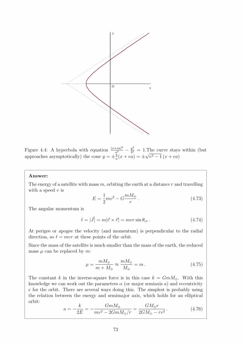
O x
y
Figure 4.4: A hyperbola with equation (x+ea)2
a2 − y2
b2= 1.The curve stays within (but
approaches asymptotically) the cone y = ± ba(x+ ea) = ±
√e2 − 1 (x+ ea)
Answer:
The energy of a satellite with massm, orbiting the earth at a distance r and travellingwith a speed v is
E =1
2mv2 −GmM⊕
r. (4.73)
The angular momentum is
` = | ~J | = m|~v × ~r| = mvr sin θvr . (4.74)
At perigee or apogee the velocity (and momentum) is perpendicular to the radialdirection, so ` = mvr at these points of the orbit.
Since the mass of the satellite is much smaller than the mass of the earth, the reducedmass µ can be replaced by m:
µ =mM⊕m+M⊕
≈ mM⊕M⊕
= m. (4.75)
The constant k in the inverse-square force is in this case k = GmM⊕. With thisknowledge we can work out the parameters α (or major semiaxis a) and eccentricitye for the orbit. There are several ways doing this. The simplest is probably usingthe relation between the energy and semimajor axis, which holds for an ellipticalorbit:
a = − k
2E= − GmM⊕
mv2 − 2GmM⊕/r=
GM⊕r
2GM⊕ − rv2. (4.76)
73

In our problem, the speed of the satellite at apogee is v = 7400m/s. The distancefrom the centre of the earth is r = 630 km + R⊕ = 7.000 · 106 km. This gives
a =6.674 · 10−11m3/kg s2 · 5.9736 · 1024kg · 7.000 · 106m
2 · 6.674 · 10−11m3/kg s2 · 5.9736 · 1024kg − 7.000 · 106m · (7400m/s)2
= 6740km . (4.77)
The sum of the apogee distance r+ and the perigee distance r− is twice the majorsemiaxis,
r+ + r− = 2a ⇐⇒ r− = 2a− r+ = 2 · 6740km− 7000km = 6481km . (4.78)
Therefore, the height of the satellite above earth at perigee is r− −R⊕ =111km.
The speed may be found from the angular momentum,
` = mv+r+ = mv−r− =⇒ v+ =r−r+
v− =7000
64817400m/s = 7994m/s . (4.79)
4.7 Kepler’s third law
Let us look again at the elliptic orbit. We can use the relations we have found above,together with Kepler’s second law, to derive an expression for the period, the tine T ittakes to complete one full orbit. From Kepler’s second law we have
dA
dt=
`
2µ=⇒ A =
∫ T
0
dA
dtdt =
`
2µT . (4.80)
The area of an ellipse is A = πab, so we will need to find a suitable expression for theminor semiaxis b. We know from above that b2 = a2(1 − e2). Using the expression forthe eccentricity e, we get
b = a√
1− e2 = a
√−2E`2
µk2= a
√`2
µka=
`õk
a12 . (4.81)
Putting this together, we have
T =2µ
`A =
2πµ
`ab =
2πµ
`
`√µka3/2 = 2π
õ
ka3/2 , (4.82)
or
T 2 =4π2µ
ka3 . (4.83)
For planets orbiting the sun, the ratio µ/k = 1/G(m+M) ≈ 1/(GM) to a very highapproximation, so the proportionality constant will be the same for all planets! This
74

is Kepler’s third law: The square of the orbital period varies like the cube of the majoraxis.
Example 4.4
A comet is observed travelling at a speed of 64.0 km/s at is closest approach to thesun, 64.5 million km from the sun. Will this comet ever be seen again, and if so,when?
What would the answer be if the closest distance to the sun was 65.0 million km?
Answer: The solution of this problem follows the same lines as that of Example 3,with the mass of the sun, M, replacing the mass of the earth, M⊕. The cometwill be seen again if the orbit is closed, which happens if the total energy E < 0.Alternatively, it is possible to calculate the eccentricity e and determine whethere < 1 (closed orbit) or e > 1 (open orbit).
We may first note that Newton’s constant G and the mass of the sun M alwaysoccur in the combination GM so we may calculate this product once and for all,
GM = 6.674 · 10−11m3/kg s2 · 1.9881 · 1030kg = 1.3275 · 1020m3/s2
= 1.3275 · 1011km3/s2 .(4.84)
If the speed of the comet at perihelion is v = 64.0 km/s and the distance isr = 64.5 · 106 km, we find that
E
m=v2
2− GM
r=
64.02
2km2/s2 − 1.3275 · 1011km3/s2
64.5 · 106km= −10.14km2/s2 . (4.85)
So E < 0 and the orbit is closed (an ellipse). The comet will therefore be seen again.To find out when, we use Kepler’s third law,
T =2π√GM
a3/2 . (4.86)
We must first find the semimajor axis a, which is given by
a = − GM2E/m
=1.3275 · 1011km3/s2
2 · 10.14km2/s2= 6.5152 · 109km . (4.87)
Inserting this into (4.86) gives
T =2π√
1.3275 · 1011km3/s2(6.5152 · 109km)3/2 = 9.069 · 109s = 104963d = 287yr .
(4.88)The comet will be seen again in 287 years.
Making the perihelion distance just a bit larger, 65.0 million km, we find that
E
m=(642
2− 1.3275 · 1011
65 · 106
)km2/s2 = 5.69km2/s2 . (4.89)
This comet now moves in a hyperbolic orbit, and will never be seen again.
75
4.8 Kepler’s equations
It is possible to integrate the angle equation,
dθ
dt=
`
µr2=`(1 + e cos θ)2
µ(`2/µk)2⇐⇒ dθ
(1 + e cos θ)2=µk2
`2dt . (4.90)
However, the integral that we obtain from this is very ugly and must be expressed interms of special functions (elliptic integrals) that cannot be straightforwardly invertedto obtain θ as a function of the time t.
Instead, we can go back to the energy equation, and the integral (4.29) we obtainedfrom this,
t− t0 =
õ
2
r∫rmin
dr√E + k
r− `2
2µr2
=
õ
−2E
r∫rmin
rdr√−r2 − k
Er − k
4E2 + k2
4E2 (1 + 2`2Eµk2 )
=
õ
−2E
r∫rmin
rdr√a2e2 − (r − a)2
.
(4.91)
We can now make the substitution
r − a = −ae cosψ (4.92)
=⇒√a2e2 − (r − a)2 = ae sinψ , (4.93)
rdr = (r − a+ a)dr = (−ae cosψ + a)(ae sinψdψ) (4.94)
Putting this into (4.91) we get
t =
õ
2|E|
∫(−ae cosψ + a)dψ =
õ
k
√k
2|E|a(ψ − e sinψ) + C
=
õ
ka3/2(ψ − e sinψ) + C .
(4.95)
To determine the integration constant C, we take t = 0 at perihelion. At this point wehave
r0 − a = a(1− e)− a = −ae = −ae cosψ0 =⇒ ψ0 = 0 , C = 0 . (4.96)
This gives us
r = a(1− e cosψ)
t =
õ
ka3/2(ψ − e sinψ)
Kepler’s equations (4.97)
The parameter ψ is called the eccentric anomaly. This name dates back to medieval,ptolemean astronomy where all the heavenly bodies were assumed to move in perfectcircles. To rescue this assumption the planets were assumed to sit on circles which
76
were themselves orbiting the earth (or the sun in the Copernicus picture). This epicyclemotion motion was called the ‘anomaly’. The angle θ is called the true anomaly. Wehave already seen that θ = ψ = 0 at the perihelion, and we can also see that θ = ψ = πat aphelion. If e = 0 (circular motion) we have ψ = θ always.
Solving Kepler’s equations is not straightforward. In fact, Kepler himself said:
I am sufficiently satisfied that it cannot be solved a priori, on account of thedifferent nature of the arc and the sine. But if I am mistaken, and any oneshall point out the way to me, he will be in my eyes the great Apollonius.
4.9 Runge-Lenz vector
We have seen that angular momentum is conserved for central forces, f = −f(r)r with
potential V (r) so f(r) = −dV (r)dr
,
dL
dt=
d
dt(r× p) = r× p + r× p =
1
mp× p + r× f = 0.
For the particular case of an inverse square force, with f = − kr3 r, there is another
conserved vector, called the Runge-Lenz vector,
A = (p× L)− kmr.
To see that this is conserved first consider the time derivative of the unit vector r. Sincethe magnitude does not change the derivative can only be a rotation
dr
dt= ω × r =
1
mr3(L× r).
ThusdA
dt= p× L− k
r3(L× r) = − k
r3(r× L)− k
r3(L× r) = 0.
To understand the physical significance of A we calculate its direction and magnitude.Since it is a constant vector we can calculate it at any point in the orbit and, for abound orbit, it is convenient to do this at the point of closest approach: r = r−a(1− e)where l = mr−v and L, p and r are all mutually perpendicular. Then
p× L = m2v2r
so
A =(rm2v2 − km
)r = km
(l2
kmr−− 1
)r = km
(l2
kma(1− e)− 1
)r.
Since a = − k2E
this is
1
kmA =
(−2El2
k2m(1− e)− 1
)r =
(−2El2
mk2 − (1− e))
1− er =
(−e2 + e)
1− er = e r.
We have evaluated this at the point of closest approach, were r is parallel to the majoraxis of the ellipse, but it is a constant hence A is always parallel to the major axis ofthe ellipse and A
kmis the eccentricity e.
Thus the constant vector A reproduces facts that we already knew: the closed orbitshave constant eccentricity e and keep a constant orientation in space.
77

4.10 Central forces — summary sheet
1. Relative motion, reduced massWe can write the kinetic energy of a two-body system as
T =1
2M ~R2 +
1
2µ~r2 , with
~R =m1~r1 +m2~r2
m1 +m2= centre of mass,
~r = ~r1 − ~r2 = relative coordinate,
µ =m1m2
m1 +m2= reduced mass
For an isolated system, V (~r1, ~r2) = V (~r) =⇒ ~P = M ~R =constantand the CM motion is trivial.
2. Planar motionFor V = V (r), all motion is in the plane spanned by ~r and ~p, or-thogonal to the constant angular momentum ~L = ~r × ~p.
3. Angular momentum
L =µ
2(r2 + r2θ2)− V (r)
Since L does not depend on θ,
pθ =∂L
∂θ= µr2θ = constant = `
4. Kepler’s second lawArea swept out in time dt:
dA =1
2r(rdθ) =⇒ dA
dt=
1
2r2dθ
dt=
`
2µ= constant
Bodies in a central force field move with constant areal velocity.
5. Effective potential
θ =`
µr2=⇒ 1
2µr2θ2 =
`2
2µr2
H = E = T + V =1
2µr2 +
`2
2µr2+ V (r) =
1
2µr2 + Veff(r)
78

6. Exploiting energy conservation E = constant
r =
√2
µ
(E − Veff(r)
)=⇒ t(r) =
õ
2
∫ r
r0
dr′√E − Veff(r′)
dr
dt
dθ
dr=dθ
dt=
`
µr2=⇒ dθ
dr=
`
µr2
√µ/2√
E − Veff(r′)
7. Kepler problem: orbit equationIntegrating dθ/dr with V (r) = −k/r gives
r(θ) =α
1 + e cos θ, with α =
`2
µk, e =
√1 +
2E`2
µk2.
This is the equation for a conic section:
e = 0 circle
0 < e < 1 ellipse
e = 1 parabola
e > 1 hyperbola
8. Kepler’s first lawThe planets move in elliptic orbits, with the sun at one focus.
Major semiaxis: a = α(1− e2) =k
−2E=GmM−2E
Minor semiaxis: b = a√
1− e2 = a
√α
a= a1/2 `√
kµ
9. Kepler’s third law
dA
dt=
`
2µ=A
T=πab
T=⇒ T = 2π
õ
ka3/2
For planets, µ/k ≈ 1/(GM) = constant.The square of the orbital period varies like the cube of the major axis.
10. The Laplace–Runge–Lenz vector
~A = ~p× ~L− mk~r
r,
Ax = prpθ sin θ +p2θ cos θ
r−mk cos θ , Ay = pθ, Ax
79

Chapter 5
Rotational motion
A rigid body is defined as a body (or collection of particles) where all mass points stay atthe same relative distances at all times. This can be a continuous body, or a collectionof discrete particles: the same equations of motion hold for both cases. A rigid bodywill move as a single entity, but it can change its orientation, and this motion can behighly nontrivial as we shall see.
The notion of a rigid body is an idealisation, since no real completely rigid bodies exist inthe real world. Firstly, real bodies consist of atoms and molecules which always undergovibrations (and electrons, as quantum particles, are never at rest). These complicationscan be ignored for macroscopic bodies. Secondly, it is always possible to deform anactual body, and this can happen even in the absence of external forces if for examplethe internal forces keeping the constituents apart are not strong enough to balance theattractive forces — or vice-versa!
Still, the idealised description is reasonable for many macroscopic solids, and provide agood description of for example tops, gyroscopes, bicycle wheels, falling sandwiches andtumbling cats.
Learning outcomes
At the end of this section, you should be able to
• identify appropriate degrees of freedom and coordinates for a rigid body;
• describe rotations using rotation matrices, and explain the general properties ofrotation matrices;
• define the inertia tensor and explain the relation between the inertia tensor, rota-tional kinetic energy and angular momentum;
• calculate the inertia tensor for simple objects;
• explain what is meant by principal axes of inertia and how they may be found;
• use the equations of motion for rotating bodies (Euler equations) to analyse themotion of rotating systems.
80

5.1 How many degrees of freedom do we have?
Let us imagine a rigid body consisting of N discrete particles. Altogether this gives us3N coordinates. The requirement that the body is rigid, ie all the internal distancesare fixed, imposes constraints on these coordinates. We denote the distance betweenparticles i and j by rij. We can work out how many constraints and hence degrees offreedom we have:
N = 2 Here we have a single constraint r12 = r, and hence we have a total of 3 · 2− 1 = 5degrees of freedom.
N = 3 We now have 3 internal distances to be fixed: r12, r13 and r23, giving 3 constraintsand 3N − 3 = 6 degrees of freedom.
N = 4 Here there are 6 internal distances to be fixed, so we have 3 · 4− 6 = 6 degrees offreedom. Strictly speaking, there are 2 different configurations which both satisfythese 6 constraints, corresponding to rigid bodies that are mirror images of eachother. This ambiguity does not correspond to any physical degree of freedom,however.
N = 5 Now it appears there would be 10 constraints, corresponding to the 10 pairs ofparticles we have. However, if you construct a 5-particle body from a 4-particleone, you will see that once the fifth particle has been positioned relative to 3 ofthe others, the position relative to the fourth one is also given. (You may try thisfor yourself!) We therefore only have 9 constraints, and 3 · 5 − 9 = 6 degrees offreedom.
N ≥ 6 As was the case for N = 5, we will need to specify 3 relative distances to positionthe 6th particle relative to the other 5, 3 more for the 7th particle, etc. Thiscancels out the 3 coordinates that each new particle comes with, so we end upwith 6 degrees of freedom in every case.
In summary, we find that a rigid body has 6 degrees of freedom, except for N = 2, whichis a special case, and has only 5 degrees of freedom. A more careful analysis will revealthat there are only 5 degrees of freedom whenever the rigid body is 1-dimensional (allthe constituent particles are located on a single line), and 6 otherwise.
Three of these degrees of freedom can be taken to represent the position of the body,and it is natural to use the centre of mass coordinates of the body as corresponding gen-eralised coordinates. The three remaining degrees of freedom represent the orientationof the body, and it is natural to choose three angles as coordinates. We will come backto how these angles may be chosen later on.
Dynamically, the 3+3 degrees of freedom correspond to two different kinds of motion:the linear motion of the centre of mass, and the rotation of the body about its centreof mass. We can now see why there are 3 such degrees of freedom: they correspond torotations (changes in orientation) about 3 axes going through the centre of mass. Inthe case of a 1-dimensional body, there are only 2 rotational degrees of freedom, sincerotation about the line the body is located on does not correspond to any real motion.
81
This discussion can be summarised in Chasles’ theorem, which states
Any motion of a rigid body is the sum of a translation and a rotation.
From now on we will focus on how we can describe and study the rotational motion anddegrees of freedom.
5.1.1 Relative motion as rotation
Suppose a rigid body is rotating about some axis. Choose some particular point inthe body on the axis of rotation — we can choose this point to be the origin of ourcoordinate system. For any other point in the body the position ~r changes if the pointis not on the axis of rotation but the distance r of the point from the origin does notchange, because the body is assumed to be rigid, only the direction from the origin canchange. In a short time the displacement of the point d~r will be at right angles to theposition, d~r ⊥ ~r. This defines an infinitesimal rotation angle dφ about the axis passingthrough the origin. Since all the points in the body remain at a fixed distance relative tothe origin, they all rotate about an axis through the origin, and since the body retainsits shape, they all rotate about the same axis.
This can be summarised in Euler’s theoremx:
Any movement of a rigid body with one point fixed is a rotation about someaxis.
If we say that the vector d~φ points along the axis of rotation, and this vector forms andangle θ with the position vector ~r, we have
|d~r| = |~r| sin θ|d~φ| or d~r = d~φ× ~r . (5.1)
The velocity of the point ~r relative to the origin is then
~v =d~r
dt=d~φ
dt× ~r = ~ω × ~r . (5.2)
If in addition, the whole body moves with some linear velocity ~V , the total velocity ofthe point P is
~v = ~V + ~vrel = ~V + ~ω × ~r (5.3)
You have in the past studied the case where the axis of rotation, ie the direction of ~ω isfixed. But in the general case, ~ω = ~ω(t) can change both magnitude and direction, andwe need to describe this general situation.
5.2 Rotated coordinate systems and rotation matri-
ces
Before we go on to discuss the kinematics and dynamics of rotational motion, let uslook at the coordinates we can use to describe the rigid body. It is clearly convenient to
82

d n
φd
O
drθ
r
dφ= φ
Figure 5.1: A clockwise rotation through an infinitesimal angle dφ about an axis pointingin the direction of a unit vector ~n is represented by a vector ~dφ = dφ~n whose length isdφ and direction is ~n.
describe the shape of the body, or the relative positions of the constituent parts of thebody, using a coordinate system that is sitting in the body and moving with it. It willalso turn out to be convenient to describe the rotational motion of the body in such asystem, since it is natural to describe this as the body rotating about its own axes. Wecall such a coordinate system the body coordinate system.
But to describe the motion of the body in space we need a coordinate system fixed inspace, not moving with the body. We therefore need to know the relation between thebody coordinate system and this fixed coordinate system.
Ignoring any linear displacements, these coordinate systems will be rotated relative toeach other. We therefore need to know how coordinates change when the coordinatesystem is rotated.
Let us call the original coordinates of a point (eg in the fixed coordinate system)~r = (x, y, z) and the coordinates in the rotated (eg the body) coordinate system~r′ = (x′, y′, z′). We call the angles between the axes in the original and the rotatedcoordinate systems θij, i = x, y, z: for example, θxz is the angle between the x′-axis andthe z-axis. We can then write the position vector (or indeed any vector) as
~r = xx+ yy + zz = x′x′ + y′y′ + z′z′ . (5.4)
Since x′, y′, z′ are orthogonal, we can find the rotated coordinate x′ by
x′ = ~r · x′ = xx · x′ + yy · x′ + zz · x′ = x cos θxx + y cos θxy + z cos θxz . (5.5)
Similarly we find
y′ = x cos θyx + y cos θyy + z cos θyz , z′ = x cos θzx + y cos θzy + z cos θzz , (5.6)
This can be written as a matrix equation,x′y′z′
=
cos θxx cos θxy cos θxzcos θyx cos θyy cos θyzcos θzx cos θzy cos θzz
xyz
⇐⇒ ~r′ = R~r (5.7)
The 3× 3 matrix R is called the rotation matrix.
83

5.2.1 Active and passive transformations
There are two equivalent ways of thinking about rotations:
1. You rotate the coordinate system, as described above. This is called a passiverotation, since it is not doing anything to the world, only to the mathematicaldescription of it. The rotation matrix then gives the relation between the old andthe new coordinates.
2. You leave the coordinate system in place, but rotate your points (for example thebody you want to describe) in the opposite direction. This is called an activerotation, since you are now doing something to the world. The rotation matrixthen gives the positions of the body after it has been rotated, given the positionbefore.
The two points of view are mathematically equivalent: the relation between old andnew coordinates are exactly the same.
The two pictures: active and passive, and the equivalence between them, can be extendedto other transformations, such as translations, where it is the same whether you movean object from a position x to a position x + a or you shift the coordinate system by−a.
5.2.2 Elementary rotation matrices
For a rotation about the z-axis, it is clear that the z-coordinates are unchanged. If werotate an angle θ, then we have that θxx = θyy = θ (the angles between the old and newx- and y-axes respectively). The angle θxy between the old y-axis and the new x-axis is90 − θ, while the angle θyx between the old x-axis and the new y-axis is 90 + θ. Therotation matrix is therefore
Rz(θ) =
cos θ cos(90 − θ) 0cos(90 + θ) cos θ 0
0 0 1
=
cos θ sin θ 0− sin θ cos θ 0
0 0 1
(5.8)
Similarly we find for rotations about the x- and y-axes,
Rx(θ) =
1 0 00 cos θ sin θ0 − sin θ cos θ
, Ry(θ) =
cos θ 0 − sin θ0 1 0
sin θ 0 cos θ
. (5.9)
5.2.3 General properties of rotation matrices
1. Any combination of two successive rotations about the same point (albeit aboutdifferent axes through that point) is a rotation about that point.
This is ‘obvious’, since the relative distance of each point from the fixed point(origin) remains unchanged throughout. We can therefore describe the combinedrotation by a rotation matrix which is the product of the two rotation matrices.
84

If we call the coordinates after the first rotation ~r′ and after the second rotation~r′′, and the two rotation matrices R (first rotation) and R′ (second rotation), wehave
~r′′ = R′~r′ = R′(R~r) = (R′R)~r = R′′~r with R′′ = R′R . (5.10)
Note that the first rotation matrix is on the right and the second rotation matrixis on the left.
Example 5.1
Find the rotation matrix corresponding to a 30 rotation about the x-axisfollowed by a 45 rotation about the z-axis.
Solution: A rotation of an angle 30 about the x-axis is, according to (5.9),
Rx(30) =
1 0 00 cos 30 sin 30
0 − sin 30 cos 30
=
1 0 0
0 12
√3 1
2
0 −12
12
√3
. (5.11)
The matrix for a 45 rotation about the z-axis is
Rz(45) =
cos 45 sin 45 0− sin 45 cos 45 0
0 0 1
=
12
√2 1
2
√2 0
−12
√2 1
2
√2 0
0 0 1
. (5.12)
The combined rotation is
R = RzRx =
12
√2 1
2
√2 0
−12
√2 1
2
√2 0
0 0 1
1 0 0
0 12
√3 1
2
0 −12
12
√3
=
12
√2 1
4
√6 1
4
√2
−12
√2 1
4
√6 1
4
√2
0 −12
12
√3
(5.13)
2. Rotations (about different axes) are not commutative: the order in which you dothem matters.
We know that matrix multiplication is not commutative: AB 6= BA if A and Bare matrices. You can also show for yourself that if you for example rotate a book90 about the x-axis followed by 90 about the y-axis, you get something differentfrom doing the two in reverse order.
Example 5.2
The rotation matrix for a 45 rotation about the z-axis followed by a 30
85

rotation about the x-axis is
R′ = RxRz =
1 0 0
0 12
√3 1
2
0 −12
12
√3
12
√2 1
2
√2 0
−12
√2 1
2
√2 0
0 0 1
=
12
√2 1
2
√2 0
−14
√6 1
4
√6 1
214
√2 −1
4
√2 1
2
√3
6= RzRx (5.14)
3. All rotation matrices are orthogonal, RTR = 11.
Proof: We know that the distance of any point from the origin is the same beforeand after the rotation. Therefore we have that
~r′2 =(x′ y′ z′
)x′y′z′
= r′T r′ = (Rr)T (Rr) = rTRTRr = ~r2 = rT r (5.15)
⇐⇒ RTR = 11 . (5.16)
We can check explicitly that all the matrices in the examples above are orthogonal.We can also show that if R and R′ are orthogonal, then their product RR′ is alsoorthogonal:
(RR′)T (RR′) = (R′TRT )(RR′) = R′T (RTR)R′ = R′TR′ = 11 . (5.17)
4. For every rotation R there is an inverse rotation given by RT which brings us backto our starting point.
It is physically obvious that you can always get back to your starting point byreversing all your rotations in reverse order. It follows from point 3. that theinverse rotation matrix is given by RT .
5. (a) Any (proper) rotation can be expressed as a combination of elementary ro-tations about coordinate axes.
(b) No combination of such rotations can produce a reflection ~r → −~r.(c) All proper rotations have detR = 1. Improper rotations (involving an odd
number of reflections) have detR = −1.
The proof of (a) is complicated, but we will use this fact later on when we willdefine coordinates corresponding to the the rotational degrees of freedom.
Statement (c) follows from the properties of determinants. It is straightforwardto show that the elementary rotation matrices all have detR = 1. We also have
det(RR′) = (detR)(detR′) (5.18)
so any combination of elementary rotations must have determinant 1. Moreover,any orthogonal matrix R must have detR = ±1:
det 11 = 1 = det(RTR) = detRT detR = (detR)2 . (5.19)
86

Finally, the reflection matrix, which takes (x, y, z)→ (−x,−y,−z) is
I =
−1 0 00 −1 00 0 −1
, det I = −1 (5.20)
(the notation is meant to convey I for invert in the origin). It is clearly impossibleto construct this from a product of matrices with determinant 1. Physically, thismeans that it is impossible (in 3 dimensions) to rotate a body into its mirrorimage.
5.2.4 The rotation group [optional]
A group is defined as a set of elements, together with a composition (multiplication)operation, with the following properties:
1. There exists an identity element (called 1 or e) which is a member of the group.
2. The combination a · b of two elements a and b is also a member of the group.
3. For every member a of the group there is an inverse a−1 which is also a memberof the group, such that a · a−1 = a−1 · a = 1.
We see that rotations form a group according to this definition: properties 1 and 4 ofSec. 5.2.3 correspond to properties 2 and 3 above. The identiy element is the operationof doing nothing, corresponding to the identity matrix.
We can use the rotation matrices to define this group, and this gives the rotation groupits name: O(3), or “the group of real orthogonal 3×3 matrices. The set of all proper rota-tions also form a (smaller) group, called SO(3), or “the group of all special [determinant1] real orthogonal 3×3 matrices”. However, this is merely a particular representation ofthe general operation that we call rotations. We could equally well represent the groupelements by actual rotations in space, or by 3 angles (with a suitably defined multiplica-tion operation), or in many other ways. All these different representations would sharethe same multiplication table, which is what ultimately defines the group.
This theory of different representations of the same group is mathematically extremelypowerful, and the group-theory properties of rotations are extremely important in mod-ern physics. For example, particles and bodies in general may be classified according tohow they behave when rotated, and this turns out to be a fundamental classification.
It is possible to express any rotation matrix formally as
R = e~L·~T , with T1 =
0 0 00 0 10 −1 0
, T2 =
0 0 −10 0 01 0 0
, T3 =
0 1 0−1 0 00 0 0
.
(5.21)This expression is very useful theoretically, but useless if you want to find an explicitform for R. It does however give a direct connection between rotations and angularmomentum. The T matrices obey the commutation relations
[T1, T2] = −T3 , [T2, T3] = −T1 , [T3, T1] = −T2 . (5.22)
87
These are essentially the commutation relations of the angular momentum operatorsin quantum mechanics, and the vector ~L is proportional to the angular momentumof the particle in question. But it turns out that there is another group with thesame multiplication table, namely the group of 2 × 2 complex unitary matrices withdeterminant 1, called SU(2). The operations of this group actually describe the rotationsof fermions, while bosons such as photons are described by the usual 3 × 3 rotationmatrices. The SU(2) matrices can be written in a similar form to (5.21),
R = ei~S·~σ , (5.23)
where
σ1 =
(0 11 0
), σ2 =
(0 −i−i 0
), σ3 =
(1 00 −1
), (5.24)
are the three Pauli matrices, which obey the same commutation relations as the T -matrices in (5.21) (up to a factor i). The vector ~S is a new form of angular momentumcalled spin, which corresponds to an ‘internal rotation’ degree of freedom. A curiousresult is that we must rotate a fermion by 4π (2 full rotations) to get back to where westarted!
5.3 Euler angles
We now go on to discuss which coordinates we can use to describe the orientation of arigid body, or alternatively, which three parameters can be used to uniquely obtain arotated coordinate system from an original one. There are several possibilities:
• The most natural would be to use rotation angles about the x-, y- and z-axes. Thisleads to the three Tait–Bryan angles, which are widely used for aircraft. However,since rotations do not commute, unless supplemented with a prescription for theorder of the three rotations, these angles are not unique, except for small rotations.
• The next most natural parameter would be to find the axis and angle of rotation,ie the vector ~φ above. This is called the Cayley–Klein or Euler parameters. Theseare mathematically very nice, and can be related to the vector ~L given above, butare not very practical.
• The third, most widely used parametrisation in mechanics is in terms of the threeEuler angles. Here, a general rotation is constructed from 3 successive elementaryrotations:
1. The body is rotated an angle φ ∈ [0, 2π〉 about the z-axis. The x- and y-axesmove to x′ and y′, while the z = z′ axis is unchanged.
2. The body is rotated an angle θ ∈ [0, π] about the new x′-axis. The z′- andy′-axes move to z′′ = z′ and y′′ = y′, but the x′′ = x′ axis is unchanged.
3. The body is rotated an angle ψ ∈ [0, 2π〉 about the new z′′-axis. The x′′ andy′′-axes move to x′′′ and y′′′, while the z′′′ = z′′-axis is unchanged.
Note that there is no rotation about any y-axis here; instead there are two rotationsabout (different) z-axes. These three rotations are summarised in figure 5.2. Itcan be proved that any rotation can be expressed in this way.
88

Figure 5.2: The Euer angles
5.3.1 Rotation matrix for Euler angles
We can now construct the general rotation matrix explitly as a function of the Eulerangles. Calling the vectors in the intermediate coordinate systems ~ρ, ~ρ′ respectively, thefirst rotation gives us ~ρ = Rz(φ)~r. The second rotation gives us ~ρ′ = Rx(θ)~ρ, and thefinal rotation ~r′ = Rz(ψ)~ρ′. Putting all this together, we find
R = Rz(ψ)Rx(θ)Rz(φ)
=
cosψ sinψ 0− sinψ cosψ 0
0 0 1
1 0 00 cos θ sin θ0 − sin θ cos θ
cosφ sinφ 0− sinφ cosφ 0
0 0 1
=
cosψ cosφ− sinψ cos θ sinφ cosψ sinφ+ sinψ cos θ cosφ sinψ sin θ− sinψ cosφ− cosψ cos θ sinφ − sinψ sinφ+ cosψ cos θ cosφ cosψ sin θ
sin θ sinφ − sin θ cosφ cos θ
.
(5.25)
Example 5.3
Find the Euler angles corresponding to a rotation of an angle ϑ about the y-axis.
The rotation matrix is
Ry(ϑ) =
cosϑ 0 − sinϑ0 1 0
sinϑ 0 cosϑ
. (5.26)
Comparing the bottom right (zz) element of the matrices, we immediately see thatϑ = θ. Comparing the bottom left elements we then must have sinφ = 1⇒ φ = π/2.While comparing the top right elements requires sinψ = −1, so ψ = 3π/2. You maythen confirm that all the other elements come out as desired. You may also checkfor yourself that you may indeed achieve a rotation about the y axis by the followingcombination of rotations:
1. rotate it by 90 about the z-axis;
2. rotate it about the x-axis (by your desired angle);
89

3. rotate it back by 90 about the z-axis.
5.3.2 Euler angles and angular velocity
The total angular velocity can be constructed as the sum of angular velocities that resultfrom the changes in each of the three Euler angles. Note that simply adding these threevectors together is ok, since these correspond to infinitesimal changes in orientation,and for such changes the order does not matter.
Rz(δφ) = 1 +
1 δφ 0−δφ 1 0
0 0 1
+O(δφ2)
Rx′(δθ) = 1 +
1 0 00 1 δθ0 −δθ 1
+O(δθ2)
Rz′′(δψ) = 1 +
1 δψ 0−δψ 0 0
0 0 1
+O(δψ2)
Hence
Rz′′(δψ)Rx′(δθ)Rz(δφ) = 1+
1 δφ 0−δφ 1 0
0 0 1
+
1 0 00 1 δθ0 −δθ 1
+
1 δψ 0−δψ 0 0
0 0 1
+· · · .
(5.27)To lowest order it does not matter what order we combine the rotations, and this is allthat matters for derivatives. For angular velocities we can therefore write
~ω = ~φ+ ~θ + ~ψ . (5.28)
The magnitude of each of these three vectors is the respective angular velocity: φ, θ, ψ.But in which directions are they pointing? We will in the end want to express theangular velocity in the body coordinate system, since it will turn out that the equationsof motion are best expressed in these coordinates. This requires performing a furtherfinite rotation through Euler angles (φ, θ, ψ) on the angular velocity ~ω:
~φ This vector points along the original z-axis, which is unchanged by the first ro-tation. The second rotation is about the intermediate x′-axis, and changes thevector (0, 0, φ) → (0, φ sin θ, φ cos θ). After the final rotation of an angle ψ aboutthe final z′′-axis, we get
~φ = (φ sin θ sinψ, φ sin θ cosψ, φ cos θ) . (5.29)
~θ This vector points along the intermediate x′-axis, so after the second rotation we
have ~θ = (θ, 0, 0). After the final rotation about the final z′′-axis it becomes
~θ = (θ cosψ,−θ sinψ, 0) . (5.30)
90
~ψ This vector points along the body’s final z′′-axis, so ~ψ = (0, 0, ψ).
Adding up these, we get
~ω = ~φ+ ~θ + ~ψ =
φ sin θ sinψ + θ cosψ
φ sin θ cosψ − θ sinψ
φ cos θ + ψ
(5.31)
We will use this to derive the equations of motion. But first we need to determine thekinetic energy.
5.4 The inertia tensor
5.4.1 Rotational kinetic energy
Let us now work out the total kinetic energy of a rigid body. From (5.3) we get that
T =1
2
∑α
mα(V + ~ω × rα)2 =1
2
∑α
mα
[V2 + 2V · (~ω × rα) + (~ω × rα)2
]=
1
2MV2 + V · ~ω ×
(∑α
mαrα
)+
1
2
∑α
mα(~ω × rα)2
(5.32)
where M =∑
αmα is the total mass.
If one point P in the body is fixed, ie the motion is pure rotation, then the one canchose the origin of the body coorinate system at P . Then V = 0 so the first two termsvanish, and the third is the rotational energy Trot, where rα is the distance from particlenumber α to the point P .
More generally suppose the body is rotating about an axis and at the same time a pointP on an axis of rotation, but fixed withing the body, is moving with linear velocity ~V .Let R be the position of the centre of mass relative to the point P and rα the positionof a particle α in the body relative to P . Then we write
rα = R + rα (5.33)
where rα is the position of the particle α relative to the centre of mass. The centre ofmass is defined by ∑
α
mαrα = 0. (5.34)
In terms of rα (5.32) can be simplified using (5.34) and written
T =1
2MV2 + V · ~ω ×
(∑α
mα(R + rα)
)+
1
2
∑α
mα
(~ω × (R + rα)
)2
=1
2MV2 +MV · (~ω ×R) +
1
2M(~ω ×R)2 +
1
2
∑α
mα
(~ω × rα)2
=1
2MV2
CM +1
2
∑α
mα
(~ω × rα)2,
(5.35)
91

where VCM = V + (~ω ×R) is the velocity of the centre of mass.
We have derived the simple result that
T = TCM + Trot =1
2MV2
CM +1
2
∑α
mα(~ω × rα)2 , (5.36)
where rα is the distance of particle α in the body from the centre of mass.
We now use that the angular velocity ~ω is the same for the whole body. We furthermoreuse the identity
( ~A× ~B)2 = A2B2 sin2 θAB = A2B2(1− cos2 θAB) = A2B2 − ( ~A · ~B)2 . (5.37)
With this the rotational kinetic energy in (5.36) becomes
Trot =1
2
∑α
mα
[r2αω
2 − (rα · ω)2]
(5.38)
=1
2
∑α
mα
[r2α
∑i
ω2i −
∑ij
(xα,iωi)(xα,jωj)]
(5.39)
=1
2
∑ij
∑α
mα
(∑k
x2α,kδij − xα,ixα,j
)ωiωj (5.40)
=1
2
∑ij
Iijωiωj =1
2~ω · I · ~ω . (5.41)
We end up with
Trot =1
2
∑ij
Iijωiωj , (5.42)
Iij =∑α
mα(r2αδij − xα,ixα,j
)→
∫ρ(x)(x2δij − xixj)d3x (5.43)
The parameters Iij are called the moments of inertia and the 3 × 3 matrix I = Iijis called the moment of inertia tensor or often just the inertia tensor of the body. Itcharacterises the way the body rotates about any particular axis and how it respondsto torques..
We have defined the inertia about the centre of mass (CM). If we had chosen a differentpoint P we would have got a different inertia tensor — it depends on the choice of P(figure 5.3). More generally the inertial tensor is defined as
Iij =∑α
mα(r2αδij − xα,ixα,j
)(5.44)
92

m
ω
r
r
P
~α
α
CM
R
α
Figure 5.3: A rigid body rotating about an axis through point P fixed in the body. Thecentre of mass (CM) is displaced by R from P .
with rα = R + rα. Then
Iij =∑α
mα(r2αδij − rα,irα,j) (5.45)
=∑α
mα
(|R + rα|2δij − (Xi + xα,i)(Xj + xα,j
)=∑α
mα
((R2 + r2
α)δij − (XiXj + xα,ixα,j
)= M(R2δij −XiXj) +
∑α
mα(r2αδij − xα,ixα,j)
⇒ Iij = M(R2δij −XiXj) + Iij. (5.46)
where Xi are the Cartesian co-ordinates of the centre of mass. Iij are the componentsof the inertia tensor about a general point P , relative to which the centre of mass is atR.
With the moment of inertia tensor in hand we can calculate the moment of inertiaassociated with rotation of any axis. Let n = ~ω/ω be a unit vector along the axis ofrotation, then the moment of inertia about n is defined to be
I(n) =3∑
i,j=1
Iijninj (5.47)
and the rotational kinetic energy is
TRot =1
2I(n)ω2. (5.48)
93

n
d
θ
=ω n
P
ω
CM
R
Figure 5.4: Geometry of the Parallel Axes Theorem.
If ~ω is directed purely along one of the coordinate axes, for example ~ω = (0, 0, ω), wesee that Trot reduces to the expression we have encountered before,
Trot =1
2
∑ij
Iijωiωj =1
2Izzω
2 , (5.49)
where Izz is the moment of inertia about the z-axis. But the expression (5.42) is muchmore general, and will hold in any (orthogonal) coordinate system, regardless of whichdirection the rotation vector is pointing.
The inertia tensor Iij depends on the point about which it is calculated but does notdepend on any particular axis. The moment of inertia I(n) depends on the point aboutwhich it is calculated and on a choice of axis. We can see how I(n) depends on thepoint from (5.46). Referring to figure 5.4
I(n) = MR2(1− sin2 θ) + I(n) = Md2 + I(n). (5.50)
This result is known as the Parallel Axes Theorem, the difference between I(n) and I(n)depends only on the distance between the two axes and not on their direction.
We can now calculate the inertia tensor once and for all. Once we know I in one coor-dinate system, we shall see that we can relatively easily find it in any other coordinatesystem.
94

Example 5.4
6
-x
y
. ............ ............ ............ ............θ
x
zm1
r1
m2
r2
Figure 5.5: A dumbbell
Find the inertia tensor of the dumbbell pictured infig. 5.5, and find the kinetic energy if it rotates withangular velocity ω
1. about the y-axis,
2. about the z-axis,
3. about its own axis.
Answer:
Particle 1 is located at ~r1 = (r1 sin θ, r1 cos θ, 0).Particle 2 is located at ~r2 = (−r2 sin θ,−r2 cos θ, 0).
We divide the computation of I as I = Idiag − Iprod where Idiagi,j = δi,j
∑αmαr
2α and
Iprodi,j =
∑αmαxα,ixα,j. The two terms are computed as
Idiag = (m1r21 +m2r
22)1
=
m1r21 +m2r
22 0 0
0 m1r21 +m2r
22 0
0 0 m1r21 +m2r
22
and
Iprod = m1
r21 sin2 θ r2
1 sin θ cos θ 0r2
1 sin θ cos θ r21 cos2 θ 0
0 0 0
+m2
r22 sin2 θ r2
2 sin θ cos θ 0r2
2 sin θ cos θ r22 cos2 θ 0
0 0 0
= (m1r
21 +m2r
22)
sin2 θ sin θ cos θ 0sin θ cos θ cos2 θ 0
0 0 0
Subtracting them we get the full intertial tensor I as
I = (m1r21 +m2r
22)
cos2 θ︷ ︸︸ ︷
1− sin2 θ − sin θ cos θ 0
− sin θ cos θ
sin2 θ︷ ︸︸ ︷1− cos2 θ 0
0 0 1
1. For rotation about the y-axis, ~ω = (0, ω, 0), so
Trot =1
2Iyyω
2 =1
2(m1r
21 +m2r
22)ω2 sin2 θ
2. For rotation about the z-axis, ~ω = (0, 0, ω), so
Trot =1
2Izzω
2 =1
2(m1r
21 +m2r
22)ω2 .
95

3. For rotation about the body axis, ~ω = (ω sin θ, ω cos θ, 0), so
Trot =1
2Ixxω
2x +
1
2Ixyωxωy +
1
2Iyxωyωx +
1
2Iyyω
2y
=1
2(m1r
21 +m2r
22)ω2[cos2 θ sin2 θ − 2(sin θ cos θ)(sin θ cos θ) + sin2 θ cos2 θ]
= 0 .
It should not be a surprise that we get Trot = 0 here, since nothing is actuallymoving in this case!
Example 5.5
Find the inertia tensor for a homogeneous cube with mass M and length L with theorigin at one corner and edges along coordinate axes.
Answer:
The density of the cube is ρ = M/L3. We find
Ixx =
L∫0
L∫0
L∫0
M
L3(y2 + z2)dxdydz =
M
L2
L∫0
L∫0
(y2 + z2)dydz
=M
L2
L∫0
(L3
3+ z2L
)dz =
M
L2
(L4
3+L3
3L)
=2
3ML2 ,
(5.51)
Ixy =
L∫0
L∫0
L∫0
M
L3(−xy)dxdydz
= −ML2
L∫0
1
2L2ydy = −M
2
(1
2L2)
= −1
4ML2 .
(5.52)
Since the x, y and z axes are completely symmetric, it is clear that Ixx = Iyy = Izzand Ixy = Ixz = Iyz, and the inertia tensor is
I =
23ML2 −1
4ML2 −1
4ML2
−14ML2 2
3ML2 −1
4ML2
−14ML2 −1
4ML2 2
3ML2
= ML2
23−1
4−1
4
−14
23−1
4
−14−1
423
. (5.53)
5.4.2 What is a tensor? Scalars, vectors and tensors.
In practice, you can think of a tensor as a kind of matrix, where the rows and columnscorrespond to directions in space. You may then treat the expression for Trot as avector–matrix–vector multiplication.
96
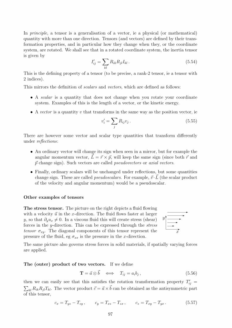
In principle, a tensor is a generalisation of a vector, ie a physical (or mathematical)quantity with more than one direction. Tensors (and vectors) are defined by their trans-formation properties, and in particular how they change when they, or the coordinatesystem, are rotated. We shall see that in a rotated coordinate system, the inertia tensoris given by
I ′ij =∑kl
RikRjlIkl . (5.54)
This is the defining property of a tensor (to be precise, a rank-2 tensor, ie a tensor with2 indices).
This mirrors the definition of scalars and vectors, which are defined as follows:
• A scalar is a quantity that does not change when you rotate your coordinatesystem. Examples of this is the length of a vector, or the kinetic energy.
• A vector is a quantity v that transforms in the same way as the position vector, ie
v′i =∑j
Rijvj . (5.55)
There are however some vector and scalar type quantities that transform differentlyunder reflections :
• An ordinary vector will change its sign when seen in a mirror, but for example theangular momentum vector, ~L = ~r × ~p, will keep the same sign (since both ~r and~p change sign). Such vectors are called pseudovectors or axial vectors.
• Finally, ordinary scalars will be unchanged under reflections, but some quantitieschange sign. These are called pseudoscalars. For example, ~v ·~L (the scalar productof the velocity and angular momentum) would be a pseudoscalar.
Other examples of tensors
6
-
y
x
-----
The stress tensor. The picture on the right depicts a fluid flowingwith a velocity ~u in the x-direction. The fluid flows faster at largery, so that ∂yux 6= 0. In a viscous fluid this will create stress (shear)forces in the y-direction. This can be expressed through the stresstensor σxy. The diagonal components of this tensor represent thepressure of the fluid, eg σxx is the pressure in the x-direction.
The same picture also governs stress forces in solid materials, if spatially varying forcesare applied.
The (outer) product of two vectors. If we define
T = ~a⊗~b ⇐⇒ Tij = aibj , (5.56)
then we can easily see that this satisfies the rotation transformation property T ′ij =∑klRikRjlTkl. The vector product ~c = ~a×~b can be obtained as the antisymmetric part
of this tensor,
cx = Tyz − Tzy , cy = Txz − Tzx , cz = Txy − Tyx . (5.57)
97

The electromagnetic field. In 4-dimensional spacetime, the electric field ~E andmagnetic field ~B form the (antisymmetric) field tensor Fµν = −Fνµ,
Fµν =
0 Ex Ey Ey−Ex 0 Bz −By
−Ex −Bz 0 Bx
−Ez By −Bx 0
. (5.58)
(Note that in 4-dimensional space-time, ‘rotations’ include Lorentz boosts.)
5.4.3 Angular momentum and the inertia tensor
We want to find the angular momentum ~L of a rigid body about some point O. Thispoint can be
• the centre of mass (for a body tumbling freely in space, for example), or
• some point fixed in space (for example a spinning top).
The momentum of some particle α is ~pα = mα~vα = mα~ω×~rα. Using the vector identity
~A× ( ~B × ~A) = A2 ~B − ( ~A · ~B) ~A (5.59)
we can write the total angular momentum as
~L =∑α
~rα × ~pα =∑α
mα
(~rα × (~ω × ~rα)
)=∑α
mα
(r2α~ω − (~rα · ~ω)~rα
)(5.60)
Li =∑α
mα(r2αωi −
∑j
xα,jωjxα,i) =∑α
mα
∑j
(r2αδij − xα,jxα,i)ωj (5.61)
=∑j
[∑α
mα(r2αδij −−xα,jxα,i)
]ωj =
∑j
Iijωj . (5.62)
So we find
Li =∑j
Iijωj or ~L = I · ~ω (5.63)
5.5 Principal axes of inertia
5.5.1 Rotations and the inertia tensor
The rotational kinetic energy depends on the point about which it is calculated and onthe direction of the axis about which the body is rotating, but it should not depend onour choice of x, y and z axis in space. How does the inertia tensor change if we rotate
98
our coordinate system? To answer this question, we can use the fact that the kineticenergy must be the same regardless of how we choose our coordinates (it is a scalar):
Trot =1
2
∑ij
ωiIijωj =1
2
∑ij
ω′iI′ijω′j . (5.64)
But ~ω is a vector, and changes in the same way as the position vector when rotated1,
ω′i =∑k
Rikωk . (5.65)
Substituting this into (5.64), we get
Trot =1
2
∑ij
∑k
RikωkI′ij
∑l
Rjlωl =1
2
∑kl
ωk(∑
ij
RikI′ijRjl
)ωl =
1
2
∑kl
ωkIklωl .
(5.66)So we find that Ikl =
∑ij RikI
′ijRjl or I = RT I′R = R−1I′R.
Life would be a lot simpler if, in some coordinate system, the inertia were diagonal,
I =
I1 0 00 I2 00 0 I3
(Iij = Iiδij) . (5.67)
We would then have
Li = Iiωi ; Trot =1
2
∑i
Iiω2i . (5.68)
In particular, if the body rotates about one of the axes of such a coordinate system, wehave ~L = I~ω, Trot = 1
2Iω2.
The good news is that it is always possible to find such a set of (body) coordinateaxes. These axes are called principal axes of inertia, and the corresponding I1, I2, I3 arethe principal moments of inertia.
The question then is how we find these axes. There are two methods:
• Find a rotation matrix R such at R IRT = I′ is diagonal. The coordinate axes inthe rotated system are then the principal axes.
• Find vectors (directions) ~ω such that ~L = I · ~ω = I~ω. These vectors form theprincipal axes of inertia, and the numbers I are the principal moments.
In fact, both these methods are mathematically identical. Let us first look at method2. If ~ω points along a principal axis of inertia, we have
Li =∑j
Iijωj = Iωi , (5.69)
1Strictly speaking, this is not quite the case: under a reflection, ~r → −~r, but ~ω is unchanged. Wecall a vector which behaves this way a pseudovector or axial-vector. The angular momentum is anotherexample of such a pseudovector.
99

where I is the corresponding moment of inertia, or
L1 = Iω1 = I11ω1 + I12ω2 + I13ω3
L2 = Iω2 = I21ω1 + I22ω2 + I23ω3
L3 = Iω3 = I31ω1 + I32ω2 + I33ω3
(5.70)
This is an eigenvalue problem. The condition for a nontrivial solution is det(I−I11) = 0.This gives us a (third-degree) equation for I, called the characteristic equation. Thesolutions are the principal moments of inertia (or eigenvalues of I). Once we havefound one of the solutions (eigenvalues), we can find the corresponding principal axis
by substituting the values of I into the equation for ~L = I~ω = I · ~ω. This gives us thedirection of ~ω, or equivalently, the ratios ω1 : ω2 : ω3. The vectors ~ω are the eigenvectorsof I.
Example 5.6
Show that the homogeneous cube with the origin at one corner has a principalmoment of inertia I = 1
6ML2, and find the corresponding principal axis of inertia.
Answer:
We found that the inertia tensor was
I = ML2
23−1
4−1
4
−14
23−1
4
−14−1
423
. (5.71)
I is a principal moment of inertia if det(I− I11) = 0. Setting I = 16ML2, we find∣∣∣∣∣∣
23ML2 − I −1
4ML2 −1
4ML2
−14ML2 2
3ML2 − I −1
4ML2
−14ML2 −1
4ML2 2
3ML2 − I
∣∣∣∣∣∣ =
∣∣∣∣∣∣12ML2 −1
4ML2 −1
4ML2
−14ML2 1
2ML2 −1
4ML2
−14ML2 −1
4ML2 1
2ML2
∣∣∣∣∣∣=(1
4ML2
)3
∣∣∣∣∣∣2 −1 −1−1 2 −1−1 −1 2
∣∣∣∣∣∣ =(1
4ML2
)3[2(2 · 2− 1) + 1(−1 · 2− 1)− 1(1− 2 · (−1)
]= 0 . (5.72)
The corresponding axis is given by
Iω1 = I11ω1 + I12ω2 + I13ω3 =⇒ 1
6ω1 =
2
3ω1 −
1
4ω2 −
1
4ω3 (5.73)
Iω2 = I21ω1 + I22ω2 + I23ω3 =⇒ 1
6ω2 = −1
4ω1 +
2
3ω2 −
1
4ω3 (5.74)
Iω3 = I31ω1 + I32ω2 + I33ω3 =⇒ 1
6ω3 = −1
4ω1 −
1
4ω2 +
2
3ω3 (5.75)
Only two of these equations are independent, since (5.75) is equivalent to
100

(5.73)+(5.74). We thus have
1
2ω1 −
1
4ω2 −
1
4ω3 = 0 (5.73)
−1
4ω1 +
1
2ω2 −
1
4ω3 = 0 (5.74)
(5.73)− (5.74) :3
4ω1 −
3
4ω2 = 0 ⇐⇒ ω2 = ω1 (5.76)
(5.73) =⇒ 1
2ω1 −
1
4ω1 −
1
4ω3 =
1
4ω1 −
1
4ω3 = 0 ⇐⇒ ω3 = ω1 (5.77)
We thus have ω1 = ω2 = ω3, or the principal axis is along the diagonal (1,1,1).
We might have guessed this from the symmetry of the cube, and rotated our systemso that the new x-axis is along the diagonal. This can be obtained by a 45 rotationabout the x-axis, followed by a rotation of cos−1
√1/3 about the z′-axis. The matrix
for this rotation is
R =
√
13−√
23
0√23
1√3
0
0 0 1
1 0 0
0 1√2
1√2
0 − 1√2
1√2
=1√6
√2√
2√
2−2 1 1
0 −√
3√
3
. (5.78)
The rotated inertia tensor is
I′ = RIRT =ML2
6
√2√
2√
2−2 1 1
0 −√
3√
3
23−1
4−1
4
−14
23−1
4
−14−1
423
√2 −2 0√2 1 −
√3√
2 1√
3
=ML2
12
2 0 00 11 00 0 11
. (5.79)
This also gives us the other two principal moments of inertia, which we find to beequal.
5.5.2 Comments
1. Finding the principal moments and axes of inertia (diagonalising the inertia tensor)by hand can be a very tedious process. Sometimes it can be simplified by symmetryconsiderations (see below), but in most cases it is better left to computers.
2. For the cube with the origin at one corner, we found that two of the principalmoments of inertia were equal, I2 = I3 = 11
12ML2. This means that the two
corresponding principal axes can be any orthogonal pair of axes perpendicular tothe diagonal — ie, the moment of inertia is the same about any axis orthogonalto the diagonal.
3. For a body where all three principal moments of inertia are equal, all directions oraxes are equivalent. We can see this by noting that in this case the inertia tensor in
101

the coordinate system defined by the principal axes is proportional to the identity(matrix), I = I11, which commutes with all rotation matrices, so I′ = IR11RT = I11for all R ∈ O(3).
4. Any body which is rotationally symmetric about some axis has one principal axisof inertia along that axis. The two other axes can be arbitrarily chosen in theplane perpendicular to the first principal axis, ie I2 = I3.
Definitions
• A body with I1 = I2 = I3 is called a spherical top.
• A body with I1 = I2 6= I3 is called a symmetric top.
• A body where all principal moments are different is called an asymmetric top.
• A body with I1 = 0, I2 = I3 is called a rotor.
For example, the cube with the origin at the centre is a spherical top; the cube with theorigin at one corner is a symmetric top, and the dumbbell (or a diatomic molecule) is arotor.
5.6 Equations of motion
Having found the principal axes of inertia, we can now use them to define the bodycoordinate system. This will greatly simplify the equations of motion. The kineticenergy is given by
T =1
2
∑i
Iiω2i . (5.80)
Using (5.31) we can write this as
T =1
2I1(φ sin θ sinψ+ θ cosψ)2 +
1
2I2(φ sin θ cosψ− θ sinψ)2 +
1
2I3(φ cos θ+ψ)2 . (5.81)
The equations of motion for generic values of the moments of inertia and a genericpotential energy will become very complicated. We will instead focus on two specificcases: a symmetric top (I1 = I2) with one point fixed and under the influence of constantgravity, and force-free motion of an asymmetric top (all I1, I2, I3 are different).
5.6.1 The symmetric heavy top
For a symmetric top, we can take I1 = I2, and (5.81) becomes
T =1
2I1(θ2 + φ2 sin2 θ) +
1
2I3(φ cos θ + ψ)2 . (5.82)
We now take the top to be rotating about a fixed point at the bottom of the symmetryaxis, under the influence of a constant gravitational field g. We take θ to be the angle
102

the symmetry axis forms with the vertical. In that case, the potential energy of the topis V = Mgh cos θ, where M is the mass of the top, and h is the distance from the baseof the top to the centre of mass along the symmetry axis. The lagrangian is therefore
L =1
2I1(θ2 + φ2 sin2 θ) +
1
2I3(φ cos θ + ψ)2 −Mgh cos θ . (5.83)
The meaning of the three Euler angles in this case is:
• θ denotes the angle the axis of the top makes with the vertical.
• φ denotes the orientation of the (tilted) axis relative to the fixed reference coordi-nate system.
• ψ denotes the orientation of the top relative to its own axis.
We will find that in general, θ will oscillate between a minimum and a maximum, whileboth φ and ψ will be monotonically increasing (or decreasing). The motion in ψ reflectsthe top spinning around its own axis. The motion in φ corresponds to the orientationof the axis precessing around the vertical axis. Finally, the motion in θ corresponds toperiodic “wobbles” in the tilt of the top, called nutation.
We may now derive the Euler–Lagrange equations for the top and use them to study thismotion in detail. We will not do this here, but instead perform a qualitative analysis ofthe possible motion. First we determine the canonical momenta,
pφ =∂L
∂φ= I1φ sin2 θ + I3ω3
∂ω3
∂φ= I1φ sin2 θ + I3 cos θ(φ cos θ + ψ) , (5.84)
pθ =∂L
∂θ= I1θ (5.85)
pψ =∂L
∂ψ= I3ω3
∂ω3
∂ψ= I3(φ cos θ + ψ) . (5.86)
Since L does not depend explicitly on either φ or ψ, ∂L/∂φ = ∂L/∂ψ = 0, and we seestraightaway that the canonical momenta pφ, pψ are conserved. In particular, pψ = I3ω3,so the top spins with a constant angular velocity ω3 about its own axis. However, theprecession rate, governed by the constant pφ is more complicated.
We now proceed to derive the hamiltonian of the system. From (5.86) we see thatω3 = φ cos θ + ψ = pψ/I3. We can use this to rewrite (5.84),
pφ = I1φ sin2 θ + I3 cos θω3 = I1φ sin2 θ + pψ cos θ (5.87)
⇐⇒ pφ − pψ cos θ = I1φ sin2 θ ⇐⇒ φ =pφ − pψ cos θ
I1 sin2 θ. (5.88)
Since the kinetic energy is quadratic in the generalised velocities, and the potentialenergy does not depend on velocities, the hamiltonian is equal to the total energy,
H = T + V
=1
2I1
[(pφ − pψ cos θ
I1 sin2 θ
)2
sin2 θ +(pθI1
)2]
+1
2I3
(pψI3
)2
+Mgh cos θ
=p2θ
2I1
+p2ψ
2I3
+(pφ − pψ cos θ)2
2I1 sin2 θ+Mgh cos θ .
(5.89)
103

Since pφ and pψ are both constant, there is effectively only one degree of freedom θ, andthe second and third term in H can be combined with the final term V = Mgh cos θ toform an effective potential Veff(θ). The first term is the usual kinetic energy term.
The first term in Veff is just a constant, so it has no effect on the dynamics of the system,other than increasing the minimum energy. Unless pφ and pψ are both precisely zeroor pφ = ±pψ, the second term is nonzero and diverges to +∞ as θ → 0 and θ → π.2
Therefore, the motion in θ is bounded for all but very special values of pφ, pψ, with θmax
in general being smaller the larger the value of pψ. If θmax < π/2 this ensures the topdoes not fall over.
5.6.2 Euler’s equations for rigid bodies
Consider now force-free motion of a rigid body. In this case, we have3
L = T =∑i
Iiω2i . (5.90)
The Euler–Lagrange equations are given by
d
dt
∂L
∂φ=∂L
∂φ;
d
dt
∂L
∂θ=∂L
∂θ;
d
dt
∂L
∂ψ=∂L
∂ψ. (5.91)
We will however only consider the third of those, and then derive two additional equa-tions of motion from symmetry considerations.
We can write the Euler–Lagrange equation for ψ as
d
dt
∂L
∂ψ=
d
dt
(I3(φ cos θ + ψ)
)=
d
dt(I3ω3) =
∂L
∂ψ=
3∑i=1
Iiωi∂ωi∂ψ
. (5.92)
We first note that
∂ω1
∂ψ= φ sin θ cosψ − θ sinψ = ω2 , (5.93)
∂ω2
∂ψ= −φ sin θ sinψ − θ cosψ = −ω1 . (5.94)
Since ω3 does not depend on ψ the last expression in (5.92) becomes
∂L
∂ψ= I1ω1
∂ω1
∂ψ+ I2ω2
∂ω2
∂ψ= I1ω1ω2 + I3ω2(−ω1) = (I1 − I2)ω1ω2 , (5.95)
so (5.92) becomes
I3dω3
dt= (I1 − I2)ω1ω2 . (5.96)
However, the labels 1, 2 and 3 for the three axes is arbitrary, and we may just aswell rename them, as long as we ensure the coordinate system remains right-handed(corresponding to cyclic permutations. This gives us the three equations
2If pφ = pψ the second term in Veff diverges as θ → π but goes to 0 as θ → 0, and conversely ifpφ = −pψ. This, however, requires finely balanced initial conditions.
3Note that the translational energy can be ignored since ~R is cyclic.
104

I1dω1
dt= (I2 − I3)ω2ω3 , (5.97)
I2dω2
dt= (I3 − I1)ω3ω1 , (5.98)
I3dω3
dt= (I1 − I2)ω1ω2 . (5.99)
These are Euler’s equations for force-free motion.
5.6.3 Stability of rigid-body rotations
Let us now look at what happens when we set a body rotating about one of the threeprincipal axes. For example, if it rotates purely about the first axis, we have ω1 6=0, ω2 = ω3 = 0. In practice, it is not possible to have exactly zero rotation about theother two axes, so what we have is that ω2 and ω3 are both much smaller (in magnitude)than ω1. We now want to find out how ω1, ω2 and ω3 each evolve with time. If ω2 and ω3
remain small and are either damped to zero or fluctuate around zero, the rotation aboutthe first axis is said to be stable. On the other hand, if the magnitude of ω2 and/or ω3
grows with time, they will eventually become as large as ω1 and the body is no longerrotating about its original axis. In that case, the rotation is unstable.
Without any loss of generality, we can take I1 > I2 > I3 since we are allowed to labelour axes as we wish. We then have three different cases to deal with:
1. If ω2 ∼ ω3 ω1 the three equations become
I1dω1
dt= (I2 − I1)ω2ω3 ≈ 0 =⇒ ω1 = constant , (5.100)
I2dω2
dt= (I3 − I1)ω3ω1 =⇒ ω2 =
(I3 − I1
I2
ω1
)ω3 , (5.101)
I3dω3
dt= (I1 − I2)ω1ω2 =⇒ ω3 =
(I1 − I2
I3
ω1
)ω2 , (5.102)
Differentiating (5.101) and using (5.102) we get
ω2 =I3 − I1
I2
ω1ω3 =(I3 − I1)(I1 − I2)
I2I3
ω21ω2 (5.103)
⇐⇒ ω2 + Ω21ω2 = 0 with Ω2
1 =(I3 − I1)(I2 − I1)
I2I3
ω21 > 0 . (5.104)
This has the solution
ω2(t) = A cos Ω1t+B sin Ω1t = C cos(Ω1t+ δ) (5.105)
ω3(t) ∝ ω2(t) = A′ cos Ω1t+B′ sin Ω1t = C ′ cos(Ω1t+ δ′) . (5.106)
ω2 and ω3 oscillate about equilibrium values ω2 = ω3 = 0. The tip of ~ω describes
and ellipse,ω2
2
C2 +ω2
3
C′2 = 1 and the body wobbles about the direction of the principleassociated with the larges moment of inertia I1.
105

2. If ω1 ∼ ω2 ω3, by the same procedure as in the first case, we obtain
ω3 = const , ω1 ∝ ω3 , ω2 + Ω23ω2 = 0 , Ω2
3 =(I3 − I2)(I3 − I1)
I1I2
ω23 > 0 ,
which again has solutions
ω1(t) = A cos(Ω3t+ δ) , ω2(t) = A′ cos(Ω3t+ δ′) . (5.107)
3. If ω1 ∼ ω3 ω2, then, using the same procedure again, we now find the equations
ω2 = constant , (5.108)
ω3 =I1
(I2 − I3)ω2
ω1 , (5.109)
ω1 =(I3 − I2)(I2 − I1)
I1I3
ω22ω1 = Ω2
2ω1 . (5.110)
The general solution to (5.110) is
ω1(t) = AeΩ2t +Be−Ω2t , (5.111)
so ω1 (and ω3) will increase exponentially with time, at least until the approxima-tions ω1 ω2 and ω3 ω2 are no longer valid.
The upshot of this is that rotations about the “long” and “short” axes are stable, whilethose about the intermediate axis are unstable. You can verify this for yourself by tossinga rectangular block (for example a a book held together by an elastic band) up in theair, rotating it about each of its three axes.
If two of the principal moments of inertia are equal, I1 = I2 say, then ω3 is strictlyconstant and
ω1 =I1 − I3
I1
ω2ω3, ω2 =I3 − I1
I21
ω1ω3
⇒ ω1 = −(I1 − I3)2
I1
ω23ω1, ω2 = −(I1 − I3)2
I21
ω23ω2,
so ω1 and ω2 oscillate with the same frequency Ω3 = |I1−I3|I1
ω3 and there is no instability.
106
5.7 Rigid body motion — summary sheet
1. Linear and angular velocityThe total velocity of a particle rotating with angular velocity ~ω abouta point moving with linear velocity ~V is
~v = ~V + ~ω × ~r .
2. Rotation matricesThe relationship between coordinates before and after a rotation isgiven by the rotation matrix A:
~r′ =
x′y′z′
= A~r = A
xyz
Rotation A1 followed by A2 gives the matrix B = A2A1 6= A1A2.All rotations are orthogonal: ATA = 11.Elementary rotations about x-, y- and z-axis:
Ax =
1 0 00 cos θ sin θ0 − sin θ cos θ
Ay =
cos θ 0 − sin θ0 1 0
sin θ 0 cos θ
Az =
cos θ sin θ 0− sin θ cos θ 0
0 0 1
3. Scalars, vectors and tensors
When you rotate a coordinate system,
• a scalar is a quantity that does not change;
• a vector v transforms as v′i =∑
j Aijvj;
• A tensor T transforms as T ′ij =∑
klAikAjlTkl .
4. Euler anglesAll rotations can be represented as a series of 3 rotations:
(a) An angle φ about the (old) z-axis,
(b) An angle θ about the (intermediate) x-axis,
(c) An angle ψ about the (new) z-axis.
5. Inertia tensorThe kinetic energy of a rotating rigid body is
Trot =1
2
∑i,j
Iijωiωj with
Iij =∑α
mα(r2αδij − xαixαj) =inertia tensor
107

In a rotated coordinate system the inertia tensor is
I ′ij =∑kl
AikAjlIkl or I′ = AIAT
6. Angular momentum
Li =∑j
Iijωj
7. Principal axes of inertiaWe can always rotate our coordinate system so that I is diagonal,
I =
I1 0 00 I2 00 0 I3
I1, I2, I3 are the principal moments of inertia. The correspondingcoordinate axes are the principal axes of inertia. These define thenatural body coordinate system.
8. Euler’s equations for a rigid body (force-free motion)
I1ω1 − (I2 − I3)ω2ω3 = 0
I2ω2 − (I3 − I1)ω3ω1 = 0
I3ω3 − (I1 − I2)ω1ω2 = 0
These are given in the body coordinate system defined by the prin-cipal axes of inertia.
108