Mechanics - CiteSeerX
504
Mechanics (draft, 2013) by James Nearing Physics Department University of Miami [email protected] Copyright 2008, James Nearing Permission to copy for individual or classroom use is granted.
-
Upload
khangminh22 -
Category
Documents
-
view
0 -
download
0
Transcript of Mechanics - CiteSeerX

Mechanics(draft, 2013)
by James Nearing
Physics Department
University of Miami
Copyright 2008, James Nearing
Permission to copy for
individual or classroom
use is granted.

Contents
Bibliography iv
0 Mathematical Prependix 1SeriesHyperbolic FunctionsCoordinate SystemsVectorsDifferentiationVelocity, AccelerationComplex AlgebraSeparation of variablesConstant Coefficient ODEsMatricesIterative Solutions
1 Introduction 44Dimensions and UnitsTypes of MassConservation LawsThe ToolsChecking Solutions
2 One Dimensional Motion 68Solving F=ma: F(t)Solving F=ma: F(v)Solving F=ma: F(x)Falling with resistanceEquilibriumConservation of Energy
3 Simple Harmonic Motion 102Simplest CaseComplex ExponentialsDamped OscillatorsOther OscillatorsForced OscillationsHarmonic ForcingStable Motion
Unstable MotionCoupled OscillationsNormal ModesGreen’s FunctionsAnharmonic Example
4 Three Dimensional Motion 158Projectile MotionGeneral ResultsE and B fieldsMagnetic MirrorsApproximate SolutionsPendulum, large angles
5 Non-Inertial Systems 200Galilean TransformationRotating SystemCoriolis ForceCentrifugal ForceShape of the EarthTidesFoucault Pendulum
6 Orbits 241Harmonic OscillatorPlanetary OrbitsKepler ProblemInsolationApproximate SolutionsSpherical PendulumCenter of Mass TransformationExtrasolar PlanetsAnother OrbitHyperbolic OrbitsTime DependencePerihelion of MercuryElliptic Integrals
i

7 Waves 300A StringStatic caseThe Wave EquationEnergy and PowerComplex FormThree Dimensional WavesReflectionsStanding WavesOther WavesOther VelocitiesWaves and TidesAn Algebraic AsidePerturbation TheoryStiffness
8 Rigid Body Motion 345Center of MassAngular MomentumTensor ComponentsPrincipal AxesProperties of EigenvectorsDynamicsPerturbation Theory
9 Special Relativity 389Time Dilation, Length ContractionSpace-Time DiagramsRelative VelocitySpace-Time Intervals
Superluminal SpeedsAccelerationRapidityEnergy and MomentumApplicationsYarkovsky EffectConservation LawsEnergy-Momentum transformationsPoynting-Robertson Effect
10 Coupled Oscillators 442EnergyNormal ModesScalar ProductsInitial ValuesTuned Mass DampersChain of MassesPerturbation Theory
11 Nonlinear Oscillations 473Forced Pendulum, QualitativelyA Method that FailsA KludgeWorkable, but Special MethodGeneral Approach
12 Statics and Bifurcations 481Bifurcations
Index 489
ii

I wrote this text for a one semester course at the sophomore-junior level. There’smore here than you can comfortably cover in that time, and in a two semester course,you will have to add material from other sources, probably Lagrange’s formulation ofmechanics.
Putting mathematics together with Newtonian MechanicsHow do you learn intuition?The exercises that appear at the chapter ends are supposed to be easy, a warmup
before starting the problems. Do them to make sure that you have the basic ideas ofthe chapter in hand.
The pdf file is hyperlinked. This applies both to the equation cross-referencesand to the index. The contents also appear in the bookmark window.
In several chapters, there are some sections that many will want to skip. They aremore mathematical, and especially for a one semester course you can’t do everything.This is my selection to omit.
ch 3: Green and anharmonic
ch 4: pendulum for large angles
ch 5: Foucault
ch 6: time dependence, perihelion of Mercury
ch 7: waves and tides, perturbation theory
ch 8: perturbation theory
ch 9: conservation laws, Poynting-Robertson
ch 10: chain of masses, perturbation theory
iii

Bibliography.
Analytical Mechanics by Grant R. Fowles. Brooks-Cole.
Analytical Mechanics by Fowles and Cassiday. A second author was added. I preferthe original.
Mechanics by Symon. Addison-Wesley The same subject as this text, at about thesame level. It’s been in print for almost 40 years, so it’s got to be pretty good.
Introduction to Classical Mechanics by Arya. Allyn and Bacon I think the recentedition is quite good.
Special Relativity by A.P. French. MIT Press I think this remains the best intro-duction to the subject.
Mathematical Methods for Physics and Engineering by Riley, Hobson, and Bence.Cambridge University Press For the quantity of well-written material here, it is sur-prisingly inexpensive in paperback.
Mathematical Methods in the Physical Sciences by Boas. John Wiley Pub Aboutthe right level and with a very useful selection of topics. If you know everything in here,you’ll find all your upper level courses much easier.
Street-Fighting Mathematics by Mahajan. MIT Press “In problem solving, as instreet fighting, rules are for fools: do whatever works–don’t just stand there!” Aspractical as you can get.
Mathematical Tools for Physics by Nearing. Dover Pub or an online version In myunbiased opinion, it’s pretty good.
Schaum’s Outlines by various. There are many good and inexpensive books inthis series: for example, “Complex Variables”, “Advanced Calculus”, “Bookkeepingand Accounting”, “Advanced Mathematics for Engineers and Scientists”. Amazon listshundreds.
Linear Differential Operators by Lanczos. It exploits the close relationship betweendifferential equations and matrices to gain deep insights. Read the user comments onAmazon.
A Brief on Tensor Analysis by James Simmonds. Springer This is the only text ontensors that I will recommend. To anyone. Under any circumstances.
iv

Linear Algebra Done Right by Axler. Springer Don’t let the title turn you away.It’s pretty good.
Linear Algebra Done Wrong by Treil. an online text as a pdf. Still another view ofthe subject, and maybe even better. (Views differ.)
v

Mathematical Prependix.
This preliminary chapter could as easily be an appendix to the text, but I preferto put it here. It is a collection of topics that you will need at many places later on, butthat you don’t have to study in detail now. In each section I will try to indicate wherethe material is used, and when you get to the chapter where you need it I will indicatethe reference here. You should at least skim this material now, so that you will haveseen where it is. If something catches your eye and you want to study it now, don’t letme stop you.
0.1 Series
This section is used in some form in every chapter in the text.Infinite series is a tool that you see in an introductory calculus course, and you maynot then have realized just how useful it is. Especially power series. There are a fewseries that show up so often that you need to have them instantly available. Binomial,trigonometric, exponential, geometric, occasionally the logarithm.
ex = 1 + x+x2
2!+x3
3!· · · =
∞∑0
xk
k!(a)
sinx = x− x3
3!+x5
5!· · · =
∞∑0
(−1)kx2k+1
(2k + 1)!(b)
cosx = 1− x2
2!+x4
4!· · · =
∞∑0
(−1)kx2k
(2k)!(c)
ln(1 + x) = x− x2
2+x3
3− · · · =
∞∑1
(−1)k+1xk
k(|x| < 1) (0.1)
(1 + x)n = 1 + nx+n(n− 1)x2
2!+ · · · =
∞∑k=0
n(n− 1) · · · (n− k + 1)
k!xk (|x| < 1)
sinhx = x+x3
3!+x5
5!+ · · · =
∞∑0
x2k+1
(2k + 1)!(f)
coshx = 1 +x2
2!+x4
4!+ · · · =
∞∑0
x2k
(2k)!(g)

Mathematical Prependix 2
1
1− x= 1 + x+ x2 + x3 + · · · =
∞∑0
xk (|x| < 1) (h)
The hyperbolic functions, sinh and cosh have power series similar to those forsin and cos except that the signs are all positive (f,g) instead of alternating (b,c).Differentiate the power series for sine and cosine to get the familiar differentiationformulas. Now do the same thing for the hyperbolic sine and cosine. Differentiate theseries for the logarithm (d), and relate it to the last series (h) on the list, called the“geometric series”. This geometric series is a special case of the binomial series forn = −1.
What is√
2? Use the 5th series, the binomial expansion: (1+1)1/2 = 1+ 12 =
1.5. Not bad for two terms, even though it is at the edge of its domain of validity.
What is 1/0.9? Use the last series: 1/(1− 0.1) = 1.1.
What is 0.991/10? Use the binomial series again: (1− 0.01)1/10 = 1− .001 =0.999.
Evaluate this limit. This example pulls together several techniques with series;it is very worth your time to be able to reproduce this example on your own.
limx→0
[1
1−√
1− x− 2
x
](0.2)
Use the binomial expansion a few times. Work first on the complicated fraction:
1
1−√
1− x=
1
1−[1− 1
2x−18x
2 − · · ·] =
112x+ 1
8x2 + · · ·
=1
12x[1 +
(14x+ · · ·
)] =2
x
[1−
(14x+ · · ·
)+( )2 · · · ]
Put this into the original expression[2
x− 1
2− 2
x
]−→ −1
2
Test this limit by a numerical experiment on a calculator. Take x = 0.5, 0.1, 0.01
What is (sin 0.1)/(sinh 0.1)? Use (b), (f), and the geometric (h) series:(0.1− 0.001/6)/(0.1 + 0.001/6) = (1− .01/6)/(1 + .01/6)

Mathematical Prependix 3
= (1− .01/6)(1− .01/6) = (1− .02/6) = 0.996667.A calculator gives 0.99667221535
What is the behavior of the function x(t) =√c2t2 + c4/a2 − c2/a for small
time? Use the binomial expansion, but first you must arrange the square rootas√
1 + small. This simply involves factoring the larger term out of the squareroot.
x(t) =c2
a
√1 +
a2t2
c2− c
2
a≈ c2
a
[1 +
a2t2
2c2
]− c
2
a=
1
2at2 (0.3)
This expression for x(t) is the relativistic expression for motion with constant(proper) acceleration, and at2/2 is the non-relativistic approximation to it. It isderived in section 9.6.
Suddenly apply a force to a mass that is attached to a spring. The result forx is (see Eq. (3.33))
x(t) =F0
k
[1− cosω0t
]where k is the spring constant, and ω0 =
√km
What is the behavior of x for small time? And remember that small is not zero.
x(t) =F0
k
[1− (1− ω0t
2/2 + · · ·)]
=F0
k
[ω2
0t2/2]
=F0
kkmt2
2=F0
mt2
2
and that is at2/2. At the start of the motion the spring hasn’t yet stretched, sothe only force is the one that you apply.
All of these expansions are special cases of the Taylor series.
f(x) = f(x0)+(x−x0)f ′(x0)+1
2(x−x0)2f ′′(x0)+
1
3!(x−x0)3f ′′′(x0)+ · · · (0.4)
Where does this representation come from? If you assume that there is an expansionof the form
f(x) = A+B(x− x0) +C(x− x0)2 +D(x− x0)3 + · · · (0.5)
then evaluate both sides at x = x0 and you immediately have A = f(x0). Nowdifferentiate the hypothesized equation (0.5) for f
f ′(x) = B + 2C(x− x0) + 3D(x− x0)2 + · · ·

Mathematical Prependix 4
and again evaluate it at x = x0. This gives B = f ′(x0). Another derivative and anevaluation and you have 2C = f ′′(x0). And again, and again, . . .
This is where all the coefficients in Eq. (0.4) come from, and every one of theseries in Eq. (0.1) can be derived this way (with x0 = 0 in all cases).
The manipulations in the example of equation (0.3) are typical of the mostcommon way that series are used in this text. When there is a complicated mathematicalresult for the solution to a problem, the most important step is to understand thatresult. Series approximations are a powerful tool to dig simple results out of complexmathematics. There are technical details to learn too, though that is not the point ofthis text: Under what conditions do these series converge? Under what conditions dothey converge to the functions they supposedly represent?
Example What is the power series expansion of the function f(x) = a − bx + cx3 about itminimum, out to second order terms? Take a, b, c > 0.First where is the minimum?
f ′(x) = −b+ 2cx2 = 0 −→ xmin = ±√b/2c
Which if either of these two points is a minimum? For an answer you can either takea second derivative (do so) or you can sketch a graph. Close to the origin the −bxterm in f has it going down toward the right and up toward the left, then the cx3 termeventually becomes very positive on the right and very negative on the left. That meansthe minimum is the one on the right and the one on the left is a maximum. Call it x0.
x0 = +√b/2c, f (x0) = a− b
(b2c
)1/2
+ c
(b2c
)3/2
= a− b3/2
2(2c)1/2
f ′(x0) = 0, f ′′(x0) = 6cx0 = 3√
2bc
f(x) = f(x0) + (x− x0) . 0 + 12f′′(x0)(x− x0)2 + · · ·
= a− b3/2
2(2c)1/2+ 3
2
√2bc(x− x0)2 + · · ·
0.2 Hyperbolic FunctionsThis section appears in chapters 3, 9, and 10.The circular trigonometric functions such as sine and cosine are familiar, but the hy-perbolic trigonometric functions may not be. These functions are defined in terms ofexponentials as
coshx =ex + e−x
2sinhx =
ex − e−x
2tanhx =
sinhxcoshx
(0.6)

Mathematical Prependix 5
Their reciprocals are sech, csch, coth in analogy with the definitions of the correspondingcircular functions.
Why are these hyperbolic? First, why are the others circular? Answer: the sineand cosine satisfy a simple identity that allows them to describe a circle.
If x = cosφ and y = sinφ,
then x2 + y2 = cos2 φ+ sin2 φ = 1
φ
Fig. 0.1
There is a similar identity for hyperbolic functions, and its derivation involves nothingmore than using the definitions.
cosh2 φ− sinh2 φ =
(eφ + e−φ
2
)2
−
(eφ − e−φ
2
)2
=e2φ + 2 + e−2φ − e2φ + 2− e−2φ
4= 1
Divide this equation by cosh2 φ to get 1− tanh2 φ = sech2 φ.
If x = coshφ and y = sinhφ,
then x2 − y2 = cosh2 φ− sinh2 φ = 1(0.7)
The coordinates x and y describe a hyperbola. In the circular case there is a simplegeometric interpretation of φ. In the hyperbolic case there is not. It’s not that thereisn’t an interpretation at all, just that it is not very useful.
What are the derivatives of these functions? Differentiate the equations (0.6) orthe series in (0.1) for cosh and sinh, then the product (or quotient) rule for tanh.
ddx
coshx = sinhxddx
sinhx = coshxddx
tanhx = sech2 x (0.8)
The hyperbolic functions involve exponentials, so it should not be too surprisingthat the inverse hyperbolic functions involve logarithms.
y = sinh−1 x means x = sinh y =1
2
(ey − e−y
)(0.9)

Mathematical Prependix 6
Multiply by 2ey and rearrange. The result is a quadratic equation.
e2y − 2xey − 1 =(ey)2 − 2xey − 1 = 0 which implies ey = x±
√x2 + 1
The exponential ey is positive, so that forces the + sign on the right. Now take thelogarithm.
y = sinh−1 x = ln(x+
√x2 + 1
)similarly, cosh−1 x = ln
(x±
√x2 − 1
)(x ≥ 1)
(0.10)
Common circular trigonometric identities have their parallel here. For example
cosh(x+ y) = coshx cosh y + sinhx sinh y
sinh(x+ y) = sinhx cosh y + coshx sinh y(0.11)
Use the series for the circular and the hyperbolic functions to see the relationsbetween the two sets of functions. For example, what is cos(ix)? Substitute ix intothe third series of Eq. (0.1). Similarly, substitute ix into the series for the sine to seeits relation to the hyperbolic sine.
Fig. 0.2
These are six graphs of the sixhyperbolic functions. It’sup to you to puzzle out whichcurves go with which functions.
To get the inverse functions,invert these graphs in the45 line x = y.
0.3 Coordinate Systems
This section appears in chapters 3, 4, 5, 6, 7, 8 (at least).There are a few common coordinate systems that you will use all the time. In twodimensions there are rectangular and polar. In three dimensions the common ones arerectangular, cylindrical, and spherical. When you need parabolic coordinates or toroidalcoordinates, you can look them up somewhere else, but the five drawn here are the onesyou have to master.

Mathematical Prependix 7
xy
x
y
r φ x
y
rectangular polar
xy
z
r
φ
z r
θ
φx
y
z
x
y
z
x
y
z
rectangular cylindrical spherical Fig. 0.3
All the coordinate lines simply represent the functions that say all the othercoordinates are constant. In the common plane rectangular coordinates the lines parallelto the x-axis are the graphs of the equations y = 1, or y = −10, etc.The equationx = 5 is a line parallel to the y-axis, and the equation for that line is x = 0.
In plane polar coordinates the coordinate lines are r = constant (circles) or φ =constant (rays that start from the origin because r ≥ 0).
The relation between these two coordinate systems is simple. When you describea single point using (x, y) one time and (r, φ) another time, the equations relatingthese pairs are
x
yr φr =
√x2 + y2, φ = tan−1(y/x)
x = r cosφ, y = r sinφ(0.12)
The only place to stumble in this transformation is in computing φ from y and x. Youneed both numbers y and x to specify the quadrant for φ because the inverse tangentis multiple valued. The signs of y and x will however tell you that tan−1(1/1) = π/4and that tan−1(−1/− 1) = 3π/4, thereby removing the ambiguity.
In three dimensions, rectangular coordinates (x, y, z) are much like those in twodimensions, except that an equation such as y = 1 is now a plane perpendicular to they-axis as x and z vary from minus to plus infinity. To get a line requires two equations.

Mathematical Prependix 8
For example the pair x = 5 and z = 6 describes a line parallel to the y-axis andpuncturing the x-z plane at (5, 6). The z-axis itself is described by the two equationsx = 0 and y = 0.
Cylindrical coordinates (r, φ, z) are an extension of two-dimensional polar coor-dinates, simply stretched parallel to the z-axis. The z-coordinate is the same as therectangular z-coordinate, and the (r, φ) are the same as the two dimensional polarcoordinates. The equation z = constant is a plane parallel to the x-y plane as before,and the equation r = constant is now a cylinder centered along the z-axis. The thirdcoordinate φ = constant is a half-plane with one edge along the z-axis (0 < r < ∞and −∞ < z <∞).
Spherical coordinates (r, θ, φ), use r to mean the distance to the origin, incontrast to cylindrical where it means the distance to the z-axis. The two angles aremeasured from the positive z-axis and around the z-axis respectively. The coordinatesurfaces are now r = constant (sphere), θ = constant (a cone with apex at the origin),and φ = constant (a half plane with one edge along the z-axis). In geography, thelatitude and longitude define a point on the surface of the Earth. The latitude is like θexcept that latitude is measured North and South from the equator (zero to 90 each),and θ is measured strictly South from the North Pole. Longitude is measured East andWest from the Greenwich meridian (zero to 180 in each case), and φ is measured inone direction starting from the x-axis (0 ≤ φ ≤ 2π). Just to keep you on your toes,some people prefer to use −π ≤ φ ≤ +π.→ Watch out for varying conventions here. Commonly in math books the role of
θ and φ in spherical coordinates are reversed, but the convention that I’m using is thestandard in physics and engineering. What is not so conventional is that I choose isto make the angle φ the same for polar, cylindrical, and spherical coordinates. It is theangle around the z-axis and in the x-y plane. You do have to watch out for conventionsused elsewhere because you will often find that θ is used for this angle in polar andcylindrical coordinates. I’m trying to be consistent here, using φ for the same angle inall three coordinate systems.
As with rectangular and polar coordinates, you can find the relationships betweeneach pair of these coordinates. For rectangular and cylindrical, it is the same as withrectangular and polar, because z is the same for each. Just use the equations (0.12)again.

Mathematical Prependix 9
For the conversions between rectangular and spherical coordinates,
r =√x2 + y2 + x2, θ = cos−1 z
r, φ = tan−1(y/x)
z =r cos θ, x = r sin θ cosφ, y = r sin θ sinφ ←
(0.13)
The second line of this pair is the set of equations encountered most often.
For the conversions between cylindrical and spherical I’ll leave it as an exercise,
problem 0.17, but you see immediately that there is a problem in notation: what is r?
I’ve used the same notation r in both systems, and that can be confusing. There is no
standard way to do this. Some will do as I have done; others choose the Greek symbol
ρ for the cylindrical radius; some will choose s; some will choose R, and there are
probably other notations. I find that using r for both rarely causes confusion though,
because it is usually clear from context which one is meant. On the rare occasions that
I do need to make the distinction, I commonly use r⊥ to indicate the perpendicular
distance to the axis (the cylindrical r).
x
y
z r
φ
θ
Fig. 0.4
In two dimensions you can draw the coordinate grid as a set
of lines parallel to the x and y axes, and in three dimensions you
would do the same thing, with lines parallel to the three axes. The
only place to do this however is in your mind, because the drawing on
paper will become so cluttered that you can’t see what has happened.
In spherical coordinates the grid is formed of lines and arcs of
circles: Hold the two coordinates θ = constant, φ = constant, and
you have a radial line, the ray starting from the origin. For the next
pair of coordinates, r = constant, φ = constant is the intersection
of a sphere and a half-plane that has one edge along the z-axis. It
defines half of a great circle, and that is the θ coordinate curve. The third pair of
coordinates are r = constant, θ = constant, and they form the intersection of a sphere
and a cone whose axis is along z. This defines the φ coordinate curve as a small circle
parallel to the x-y plane.
This map of the Earth* shows the prime meridian at zero longitude, corresponding
to the zero point for φ. Similarly, the lines of constant latitude show the relation:
latitude = |90 − θ| (N or S).
* www.worldatlas.com

Mathematical Prependix 10
Fig. 0.5
The equations for simple curves can look very different in the various coordinatesystems. In rectangular and in plane polar coordinates the equations for straight linesare respectively
y = mx+ b and r = a sec(θ − θ0) (0.14)
Equations for a circle can come in several forms
x2 + y2 = R2, or r = R, or r = a cosφ,
or r2 = a+ br cos(φ− φ0)(0.15)
An ellipse is
x2
a2+y2
b2= 1, or r =
1
A+B cosφ(B< A), or
x = a cos θy = b sin θ
, or r1+r2 = 2a
(0.16)Some of these are familiar. Probably some are not. The last one is in two-center
bipolar coordinates — not one of your standards.There are many examples of pictures of functions in rectangular and polar coor-
dinates in The Famous Curves Index. In some cases, they have Java versions that allowyou to play with the parameters.www-groups.dcs.st-and.ac.uk/˜history/Curves/Curves.html
Areas and VolumesOne of the traditional uses for integration is to computes areas and volumes. Evenwhen that’s not the aim, you still need to know how to set up such problems. Whenyou compute moments of inertia or a center of mass it is a necessary tool.

Mathematical Prependix 11
For two dimensions the rectangular and polar coordinates are all you need, alongwith the two pictures. ∆x
∆y
∆r
r∆φ
Fig. 0.6
The two shaded regions are rectangles defined respectively by the lines at x, x + ∆x,y, and y + ∆y or between r and r + ∆r, φ, φ + ∆φ. Well, in the polar case onlyapproximately rectangular, but in the limit that the two sides go to zero it’s true. Thearea of a rectangle is the product of its sides, so the area elements are
∆A = ∆x∆y → dA = dxdy and ∆A = ∆r r∆φ → dA = r dr dφ(0.17)
The area of a circle is
∫dA =
∫ R
0r dr
∫ 2π
0dφ = 2π
∫ R
0r dr = πR2
A comment on notation. You may be accustomed to seeing multiple integrals writtendifferently, something like ∫ R
0
∫ 2π
0r dφdr
with the convention that you work from the inside out. There’s nothing wrong with thatnotation, but I find it less confusing if I write the differential next to the integral signand its associated limits. Multiplication is commutative and associative, so r dφdr =dφ r dr = dr r dφ. Then integrate right to left.
In three dimensions, the volume element in rectangular coordinates is just as itis in two dimensions, but with an extra factor of ∆z. In cylindrical coordinates, it isthe same as two-dimensional polar except for the same extra factor for the distance inthe z-direction
dV = dxdy dz dV = r dr dφdz (0.18)
The spherical case requires a little more drawing.

Mathematical Prependix 12
x
y
z
φ
θ
r sin θ
r dθ
r sin θ dφ
Fig. 0.7
Fix r for a moment and the piece of area on the surface of constant r is boundedby (θ, θ + dθ) and (φ, φ + dφ). Again, this forms a rectangle in the same way thatdr and r dφ form a rectangle in plane polar coordinates even though all four sides arereally arcs of circles. The sides are r dθ and r sin θ dφ. In the first case the radius ofthe circle is r, with center at the origin. In the second case the radius is r sin θ withcenter on the z-axis.
dA = r2 sin θ dθ dφ dΩ = sin θ dθ dφ (0.19)
What about the volume? Just multiply this rectangle by dr to get the volume of therectangular box with this area as a base. The combination dΩ shows up so much it hasits own symbol, and Ω is called “solid angle”.
dV = r2 sin θ dr dθ dφ
x
y
z
φ
θ
r sin θ
r dθ
r sin θ dφ
dr
Fig. 0.8
The volume of a sphere is then∫dV =
∫ R
0r2 dr
∫ π
0sin θ dθ
∫ 2π
0dφ
= 2π∫ R
0r2 dr
∫ π
0sin θ dθ = 2π
∫ R
0r2 dr 2 =
4
3πR3
Limits of IntegrationA very common problem when faced with multiple integrals is figuring out the limits

Mathematical Prependix 13
of integration. What happens to those limits when you do the integrals in a differentorder. The key is
draw a picture of the domain of integration
and read the limits from the picture. Even in plane rectangular coordinates you will getfrustrated without a picture to guide you.
The simplest example: what is the area of a right triangle, done as a doubleintegral? Divide the area into little pieces of area, ∆A’s, and add them together, finallytaking a limit as each piece goes to zero. Now decide: in what systematic order are yougoing to add the pieces together? Certainly not randomly.
∆A
∆xi
∆yj
a
by = bx/a
Fig. 0.9
If the typical piece of area is ∆A = ∆xi∆yj then when you do the sum∑i,j ∆xi∆yj you must choose the order of summation. In the first picture the sum is
∆xi∑j
∆yj the y’s go from 0 to bxi/a, so this is ∆xi . bxia
The sum on ∆xi becomes an integral from 0 to a,∫ a
0 dx bx/a. The sum in the otherorder and using the second picture starts with a sum on the ∆xi and you have to readthose limits from the picture, starting at ayj/b and ending at a.
A =
∫ a
0dx∫ bx/a
0dy =
∫ b
0dy∫ a
ay/bdx =
ab2
(0.20)
0.4 VectorsThis section appears in most chapters from four on.Velocity, acceleration, momentum, angular momentum, electric field, magnetic field,gravitational field, force, torque, angular velocity. And these are just vectors that appearin this book.
The general definition of a vector is that it is an element of a vector space, butfor here and now that is more generality than needed. The algebra of vectors in two orthree dimensions starts from the pictures
~A~B
~C~A
~B
~D~C = ~A+ ~B ~D = ~A− ~B

Mathematical Prependix 14
and these pictures apply whether you are talking about gravity or momentum or anyof the other vectors listed above. There is a mathematical theorem guaranteeing this,saying that once you know you are working with three dimensional vectors, then theyare all essentially the same. In mathematical jargon, isomorphic. The same for twodimensions (or seven). This means that you do not have to learn everything differentlyfor different sorts of vectors — they all behave the same way.
Does a velocity vector look like a line with an arrowhead attached? Very fewcars today have arrows sticking out of the front end, designed to skewer pedestrians,*but the import of this statement about vectors is that it doesn’t matter. These picturesmodel velocity or magnetic fields or any other vector and you are guaranteed that theyall give the same results. This is why you study the geometry of vectors as a subject ofits own. There is no need to relearn it when you encounter the next sort of vector.
~A
~B
~A× ~B
θ
∣∣ ~A× ~B∣∣ = AB sin θ
~A . ~B = AB cos θ(0.21)
The vector product (cross product) of two vectors ~A and ~B is another vector perpen-dicular to these two and having magnitude AB sin θ, where θ is the indicated anglebetween them. The scalar product (dot product) is the scalar AB cos θ. Here I am
using the convention that the magnitude of the vector ~A is the letter A. See theproblems 0.24–0.32 for some review and practice.
The vector product as just stated is ambiguous because there are two directionsthat are perpendicular to the two input vectors, and they are in opposite directions.Which one to pick is chosen by convention: the right-hand rule.
Why are these the correct definitions for products of vectors? Why a cosine inone case and a sine in the other? Probably when the subject was being invented theseweren’t the first attempts made in defining products, but these are the ones that havegood properties — especially the distributive law. 5 .(3 + 4) = 5 . 3 + 5 . 4 = 35, and forvectors
~A .( ~B + ~C
)= ~A . ~B + ~A . ~C, ~A×
( ~B + ~C)
= ~A× ~B + ~A× ~C (0.22)
What about the other sorts of multiplication laws: commutative and associative?5 . 4 = 4 . 5 and
~A . ~B = ~B . ~A, but ~A× ~B = − ~B × ~A
* but find a picture of a 1950-era Oldsmobile!

Mathematical Prependix 15
so the commutative rule works for the dot product but not for the cross product. Itanti-commutes instead. For the associative law, 5 .(3 . 4) = (5 . 3) . 4 = 60, but
~A .( ~B . ~C ) doesn’t make any sense. The dot product is between vectors.
For the cross product, ~A× ( ~B× ~C ) makes sense, but it is not associative, and you cansee that easily by writing a simple example.
x× (x× y) = x× z = −y, but (x× x)× y = 0× y = 0
The closest that the cross product comes to associativity is the Jacobi identity,
~A× ( ~B × ~C ) + ~B × (~C × ~A ) + ~C × ( ~A× ~B ) = 0 (0.23)
It doesn’t show up very often in ordinary vector algebra, but it appears near the end ofchapter four.
A useful identity involving this triple cross product is
~A×( ~B × ~C
)= ~B
( ~A . ~C)− ~C
( ~A . ~B)
(0.24)
(Do these last two equations work with the simple example x× (x× y) of a few linesback?)And the triple scalar product obeys the identities
~A .( ~B × ~C
)=( ~A× ~B
). ~C interchange dot and cross
~A .( ~B × ~C
)= ~B .
(~C × ~A)
= ~C .( ~A× ~B
)cyclic permutation of factors
(0.25)
Bases, Unit VectorsThe geometry of vectors can become cumbersome to manipulate, especially when thereare many vectors involved. The technique of components is a way to turn much of thegeometry into algebra and even arithmetic. It is to vectors what analytic geometry isto plane geometry. In rectangular coordinates the system should be familiar. In twodimensions pick two vectors, one parallel to the x-axis and one parallel to the y-axis.Call them x and y, the pair forming a basis, and make them have magnitude one. Notone meter or one second, just one dimensionless.
x
y
xy
xy
~A
Axx
Ayy

Mathematical Prependix 16
You can write any vector in the plane as the sum of two other vectors, one parallel tox and one parallel to y. The former is a multiple of x (positive or negative) and the
latter is a multiple of y. The two components of the vector ~A are the two numbers Axand Ay, with units as appropriate.
The point of writing a single vector in terms of two other vectors (three othersin three dimensions) is to change geometry into algebra and arithmetic. It changes theproblem of differentiating vectors into the more familiar problem of differentiating ordi-nary functions. The basis vectors you will encounter in this book are mostly orthogonaland normalized to one. That is a convenience not a necessity, and in other contextsyou can make other choices to define a basis.
The dot product of two vectors is easy to compute in terms of these basis vectors.
~A . ~B =(Axx+Ayy +Az z
).(Bxx+Byy +Bz z
)=
AxBxx . y +AxByx . y +AxBzx . z +AyBxy . y +AyByy . y
+AyBz y . z +AzBxz . y +AzBy z . y +AzBz z . z
= AxBx +AyBy +AzBz (0.26)
The simplicity appears because the basis vectors are orthonormal. That is, each hasunit magnitude and they are mutually perpendicular.
Does the product rule for derivatives apply to the product of vectors? Yes, andyou can see why by differentiating the component form:
ddt~A . ~B =
dAxdt
Bx +AxdBxdt
+ · · · = d ~Adt
. ~B + ~A . d~Bdt
The same analysis applies to the cross product.
Index NotationA convenient and powerful notation to manipulate the components of vectors: Denotethe basis vectors by a unified notation, ~e1, ~e2, and ~e3 instead of respectively x, y, andz. You then write the vectors as
~A = A1~e1 +A2~e2 +A3~e3 and ~B = B1~e1 +B2~e2 +B3~e3
That these vectors, ~ei, are orthogonal and unit vectors translates to
~e1 .~e2 = 0, ~e3 .~e3 = 1, and all other such combinations
Introduce a standard notation:
δij =
1 if i = j0 if i 6= j
then ~ei .~ej = δij (0.27)

Mathematical Prependix 17
where the indices i and j take on any and all of the values 1, 2, 3. This is called theKronecker delta symbol.
The dot product is exactly the same as in Eq. (0.26), only the final result justhas subscripts 1, 2, 3 instead of x, y, x. It doesn’t seem to be worth all the trouble doesit? It is. First a version of the calculation in this notation.
~A . ~B =∑i
Ai~ei .∑j
Bj~ej =∑i
∑j
AiBj~ei .~ej =∑i
∑j
AiBjδij
Now do the sum on j∑j
Bjδij = Bi Remember: δij = 0 for the two terms where j 6= i
The rest is∑iAiBi, exactly as in Eq. (0.26).
The summation convention was introduced by Einstein when it became clear tohim that in manipulations with this notation for the components, a summation symbol(
e.g.∑i) always appeared whenever an index was repeated in a single term. So why
bother to write it? The convention is that whenever an index is repeated in a single termit is to be summed. The immediately preceding calculation is then shortened to
~A . ~B = Ai~ei .Bj~ej = AiBj ~ei .~ej = AiBj δij = AiBi (0.28)
This convention also means that if you encounter an expression with three identicalindices, such as Ajk = BiCikCji then go back and find your mistake. This can’thappen.
With this convention you have for example, δijvj = vi. (Write it out.)How do you handle cross products in this notation? You need to introduce
another piece of notation.
~ei .~ej × ~ek = eijk the alternating symbol (0.29)
This is ±1 if the indices i, j, k are different from each other, i.e. a permutation of 123.It is +1 for 123 and any cyclic permutation of 123, i.e. 231 and 312. Interchange anytwo (e.g. 132) and you get −1. If any two indices are the same then this is zero. Youcan easily verify that eijk equals 1
2(i− j)(j − k)(k− i), though this identity is more ofa curiosity than anything particularly useful.
~A× ~B = ~ei eijkAjBk, eijkeimn = δjmδkn − δjnδkm (0.30)
These are easy to check. At worst just look at all the possible cases. Elegant derivationscan come later. The second is equivalent to Eq. (0.24).

Mathematical Prependix 18
0.5 DifferentiationThere’s no chapter in this book in which this is not used.So much of this subject depends on knowing what derivatives are and how to manipulatethem that it’s worth spending some space to review the subject (and maybe in theprocess to introduce some ideas you haven’t seen).
The standard definition of the derivative of a function of one variable is
dfdx
(x) = lim∆x→0
f(x+ ∆x)− f(x)
∆x(0.31)
The “prime” notation, f ′(x), for the derivative is useful too, but if that’s the onlynotation you use it can hinder you to the point of incapacity. The Leibnitz notationof Eq. (0.31) lends itself to manipulation while the f ′ does not. For an immediateexample, the most common method used to differentiate anything is the chain rule, andthat is remarkably obscure in one notation while being quite intuitive in the other.
h(x) = f(g(x)
)−→ h′(x) = f ′(g)g′ or
dhdx
=dfdgdgdx
(0.32)
How do you derive this? The definition of the derivative and the Leibnitz form dictatethe manipulations to use. Start from the definition:
h(x+ ∆x)− h(x)
∆x=h(x+ ∆x)− h(x)
g(x+ ∆x)− g(x). g(x+ ∆x)− g(x)
∆x(0.33)
or in a shorter form,∆h∆x
=∆h∆g
. ∆g∆x
As ∆x → 0, the increment in g must approach zero also, as otherwise its derivativewould not exist and the chain rule would not apply.* The second factor in Eq. (0.33)becomes, in the limit that ∆x → 0, the derivative dg/dx. Also, because in the samelimit ∆g = g(x+ ∆x)− g(x)→ 0, the first factor becomes df/dg, and that ends thederivation. A common way to write the composition of functions is to use, instead ofh(x) = f
(g(x)
), the notation h = f g.
A possibly unfamiliar rule occurs when you encounter the derivative of a functionin which the independent variable appears in several unrelated places. For example,
f1(x) = xx, or f2(x) =
∫ x
0t√x− t dt (0.34)
* What is the derivative of the function “h(x) = x” at the point x = 0? One ofcourse. Now let f(x) = 1/x and g(x) = 1/x, then it looks like h = f g, but neitherf ′(0) nor g′(0) exist.

Mathematical Prependix 19
Think of either of these as a function f(x, x), where the first x is one of the two x’sin xx and the second x is the other. Now start from the definition and manipulate,adding and subtracting the same term.
f(x+ ∆x, x+ ∆x)− f(x, x)
∆x=
f(x+ ∆x, x+ ∆x)− f(x, x+ ∆x) + f(x, x+ ∆x)− f(x, x)
∆x
=f(x+ ∆x, x+ ∆x)− f(x, x+ ∆x)
∆x+f(x, x+ ∆x)− f(x, x)
∆x
As ∆x→ 0, the second term becomes the definition of the derivative of f with respectto the second x. In the same limit the first term becomes the derivative with respect tothe first x. (This assumes that all the derivatives are continuous, so that as ∆x → 0the fact that the first differentiation is approached from near x instead of at x will notmatter.)
A notation common in some calculus texts can be useful here.
ddxf(x, x) = D1f(x, x) +D2f(x, x) (0.35)
Here D1 means differentiate with respect to the first argument and D2 with respect tothe second.
This derivation shows that if x shows up in two different places, differentiate withrespect to one of them and then with respect to the next one and add the two results.The familiar product rule is a special case of this.
ddxf(x)g(x) =
dfdxg + f
dgdx
(0.36)
In the less familiar cases, Eq. (0.34),
df1
dx=
ddxxx = xxx−1 + lnxxx = xx(1 + lnx)
anddf2
dx= 0 +
1
2
∫ x
0
t√x− t
dt
Parametrized DifferentiationOnce you see the explanation of this it seems remarkable simple, but if you encounterthe phenomenon in an unfamiliar context you may not think of it.

Mathematical Prependix 20
If u is a function of time and v is a function of time, what is du/dv?
At times t and t+ ∆t ∆u = u(t+ ∆t)− u(t) and ∆v = v(t+ ∆t)− v(t)
then∆u∆v
=∆u/∆t
∆v/∆t
and the limit as ∆t→ 0 isdudv
=du/dt
dv/dtalso =
dt/dv
dt/du(0.37)
Example In polar coordinates, x = r cosφ and y = r sinφ. What is dy/dx as you go arounda circle? Here r is constant, so
dydx
=dy/dφ
dx/dφ=
r cosφ−r sinφ
= − cotφ
It is easy to check this at angles such as φ = 0 or π/4 etc. This technique will showup in a more complicated example in chapter nine, relativity, when computing relativevelocity and acceleration.
0.6 Velocity, AccelerationThis section appears in most chapters from four on.The definitions of velocity and acceleration are
~v =d~rdt
= ~r and ~a =d~vdt
= ~v
This doesn’t depend on your coordinate system, be it rectangular, polar, spherical, oroblate spheroidal. Computing them in different coordinate system can get technicalthough. Fortunately three common cases (rectangular, polar, cylindrical) are easy.Spherical is more involved but still manageable, and the rest are rare enough that youcan learn them when or if you need them. The “dot” notation over the letter is likethe ′ so common in calculus texts, but it has a particular meaning. It always meansdifferentiation with respect to time.
x
yx
y
rφ
r
φ
Fig. 0.10
r =√x2 + y2
tanφ = y/x

Mathematical Prependix 21
Rectangular is familiar
~r = xx+ yy + zz, so ~v = xx+ yy + zz and ~a = xx+ yy + zz
Read the components from these equations. E.g. ax = x = d2x/dt2. For cylindricalcoordinates the appropriate basis vectors conform to this system, with r pointing awayfrom the origin and φ perpendicular to that. ~r = zz+rr, and plane polar simply omitsthe z. Now the unit vectors are functions of position, implying that as a particle movesthese unit vectors will change, and you have to use the product rule to differentiate theterms. z is constant so it causes no trouble.
~v = zz + rr + r ˙r
The one new feature is the third term, and for that you need to notice that r is afunction of the coordinate φ, though not of z or r. To evaluate this derivative, use thechain rule.
drdt
=drdφ
dφdt
The first of these derivatives, dr/dφ, is now a problem in geometry, and there’s aresult about differentiating vectors that have a constant magnitude: the derivative isperpendicular to the original vector. To show this, let ~u be any vector of constantmagnitude. That is, ~u .~u = C. Differentiate this with respect to anything.
ddt~u .~u =
dCdt
= 0 = 2~u . d~udt
(0.38)
That’s all that’s necessary, because it says that the derivative is either zero or is per-pendicular to ~u as claimed.
dr/dφ is perpendicular to r. It is in the φ direction. Now, what is its magnitude?A sketch answers the question. The sketch will also answer the question: “Why is it inthe +φ direction and not along −φ?”
φ r(φ)
r(φ+ ∆φ)
∆r
Fig. 0.11
The three vectors r(φ), r(φ+∆φ), and ∆r form an isosceles triangle. Constructthe bisector of the vertex angle, and you immediately see that the length of ∆r is∣∣∆r∣∣ = 2 . 1 . sin(∆φ/2)

Mathematical Prependix 22
As ∆φ→ 0, the sine behaves as ∆φ/2 itself, so the quotient∣∣∆r∣∣/∆φ→ 1.
drdφ
= φ, and similarlydφdφ
= −r (0.39)
Now back to velocity and acceleration.
~v = d~r/dt = zz + rr + r ˙r = zz + rr + rφφ (0.40)
Another derivative:
~a = d~v/dt = zz + rr + r ˙r + rφφ+ rφφ+ rφ ˙φ
= zz + rr + rdrdφφ+ rφφ+ rφφ+ rφ
dφdφφ
= zz + r(r − rφ2
)+ φ
(rφ+ 2rφ
)(0.41)
Here you need dφ/dφ, another derivative of a unit vector, so it is perpendicular to φ.How big is it? You can do the same sort of geometry as with r, or notice that
r . φ = 0 −→ ddφr . φ = 0 =
drdφ
. φ+ r . dφdφ
= 1 + r . dφdφ
and this establishes the sign and magnitude of dφ/dφ as in Eq. (0.39). Increasing theangle φ a little bit rotates an object a little bit counterclockwise. That rotates r toward
φ. It rotates φ toward −r.That the basis vectors vary with position and are not parallel to each other as you
move around the coordinate system is a familiar idea in another context: geography.Up, ˆSouth, and ˆEast change direction as you move around the Earth, though they alwaysremain orthogonal to each other.
For spherical coordinates the derivations can be done along the same lines as forcylindrical, but with a lot more algebra. It is not worth the trouble to go through it,and you don’t need the results as often. The answer is (remember to distinguish thespherical coordinate r from the cylindrical one — they’re spelled the same).
~r = rr
~v = ~r = rr + rθθ + rφ sin θφ
~a =(r − rφ2 sin2 θ − rθ2
)r +
(rθ + 2rθ − rφ2 sin θ cos θ
)θ
+(rφ sin θ + 2rφ sin θ + 2rθφ cos θ
)φ
(0.42)

Mathematical Prependix 23
In geographical terms,
r ≡ Up θ ≡ South φ ≡ East
Example
Circular motion is a familiar example from introductory courses. If z = 0 and r = aconstant, the equations (0.40) and (0.41) are
~v = rφφ and ~a = −r rφ2 + φ rφ = −r v2
r+ φ
dvdt
(0.43)
The last form comes from using the magnitude of the first of these equations for ~v,that is v = rφ, and it reproduces the familiar inward radial acceleration for circular
motion (rφ2 = v2/r). The tangential component is rφ = d(rφ)/dt = dv/dt. Nowwait a minute! If you believe this manipulation, look again more critically. Is the motioncounterclockwise or clockwise and does it matter? Is φ positive or negative? Is themagnitude of a vector positive? When you express a vector in terms of components,is the coefficient of the unit vector the magnitude of the vector or a component of thevector? Answer: the correct equation is not v = rφ, but vφ = rφ, stating that the
phi-component of the velocity is rφ. Go back and modify these equations appropriately.
Example
x = x0, a constant, y = v0t should have constant velocity and zero acceleration,but that’s not so obvious if you see it in polar coordinates.
r =√x2 + y2 =
√x2
0 + v20t
2 and φ = tan−1(y/x) = tan−1 v0tx0
~v = r r + φ rφ
= rv2
0t√x2
0 + v20t
2+ φ
√x2
0 + v20t
21
1 +(v0t/x0
)2 . v0
x0
= rv2
0t√x2
0 + v20t
2+ φ
v0x0√x2
0 + v20t
2
(0.44)
You can see that this has the correct behavior at t = 0 and as t → ∞. Does it havethe correct magnitude? And what is its derivative?

Mathematical Prependix 24
0.7 Complex Algebra
This section appears in chapters 3, 4, 6, and implicitly many other places.There are some standard manipulations with complex arithmetic that take some practice.Even the basic +, −, ×, and ÷ are not exactly what you learned in third grade, so I’llstart with those. The standard commutative, associative, and distributive laws apply tothe first three, so
(7 + 2i)(6 + 3i) = (6 + 3i)(7 + 2i) = 36 + 33i
(1 + 2i)[(3 + 4i)(5 + 6i)
]=[(1 + 2i)(3 + 4i)
](5 + 6i)
= (1 + 2i)(−9 + 38i) = −85 + 20i
(1 + 2i)[(3 + 4i) + (5 + 6i)
]= (1 + 2i)(3 + 4i) + (1 + 2i)(5 + 6i)
= (1 + 2i)(8 + 10i) = −12 + 26i
As for division, it is no more commutative here than it is for real numbers, buta simple trick allows you to simplify some expressions. The complex conjugate of anumber is the number found by changing the sign of the imaginary part.
z = 5 + 7i −→ z∗ = 5− 7i
The ∗ notation is a common one for this operation, though z is another notation thatmany prefer. What is the product of a number and its complex conjugate?
z = 5 + 7i, z∗ = 5− 7i −→ z∗z = (5− 7i)(5 + 7i) = 25 + 49 + 35i− 35i = 74
z∗z is always real and positive: (a+ib)(a−ib) = a2 +b2 is the square of the magnitudeof the complex number, the square of
√a2 + b2. How do you use this to manipulate
division? Rationalize the denominator of a quotient.
1 + 2i3 + 4i
=(1 + 2i)(3− 4i)(3 + 4i)(3− 4i)
=11 + 2i
25(0.45)
Multiplying a number by its complex conjugate results in a real, so you can multiply thenumerator and denominator of a quotient by the complex conjugate of the denominatorand bring the result into a simpler form. If you ever want to make the numerator realinstead, use the same idea.

Mathematical Prependix 25
Example A few cases of such manipulation, simplifying complex expressions:
3− 4i2− i
=(3− 4i)(2 + i)(2− i)(2 + i)
=10− 5i
5= 2− i.
(3i+ 1)2
[1
2− i+
3i2 + i
]= (−8 + 6i)
[(2 + i) + 3i(2− i)
(2− i)(2 + i)
]= (−8 + 6i)
5 + 7i5
=2− 26i
5.
i3 + i10 + ii2 + i137 + 1
=(−i) + (−1) + i(−1) + (i) + (1)
=−1
i= i.
What is the geometric interpretation of i? It is a factor it rotates by 90.
z = 1 + 3iiz
i2z i3z
iz = i(1 + 3i) = −3 + i
i2z = i(−3 + i) = −1− 3i
i3z = i(−1− 3i) = 3− ii4z = z
What is in? Each multiplication by i rotates by 90 in the complex plane, soi4 = 1, and i217 = i4
. 54+1 = i.Various roots of 1 or of −1 or of i appear commonly, and you need the exponential
representation, Euler’s formula, to find them. This is
x+ iy = r cos θ + ir sin θ = reiθx
y
θ
(0.46)
You can derive this equation from the series (0.1). Put iθ into the series for theexponential and collect the real and imaginary pieces, done in section 3.2. The resultis eiθ = cos θ + i sin θ.
Special cases of this equation say
e2πi = 1, eπi = −1, eiπ/2 = i, e2nπi = 1
There are three cube roots of one, and all that you need to find them is the precedingline.
11/3 =(e2nπi
)1/3

Mathematical Prependix 26
Take n to be a succession of integers
n = 0 −→ 11/3 = 1
n = 1 −→(e2πi
)1/3= e2πi/3 = cos 2π/3 + i sin 2π/3 = (−1 + i
√3)/2
n = 2 −→(e4πi
)1/3= e4πi/3 = cos 4π/3 + i sin 4π/3 = (−1− i
√3)/2
If you keep going to n = 3, 4, etc. or use negative integers, you simply repeat thesethree values. A picture of the roots shows them equally spaced around the unit circle,exactly as dictated by Euler’s equation, and the same sort of picture appears for higherroots too.
e2iπ/3e2iπ/8
e10iπ/8
The polar form of complex numbers uses the exponential representation, and hereare some examples that use this manipulation.
√i =
(eiπ/2
)1/2= eiπ/4 =
1 + i√2.(
1− i1 + i
)3
=
(√2e−iπ/4
√2eiπ/4
)3
=(e−iπ/2
)3= e−3iπ/2 = i.
(2i
1 + i√
3
)25
=
(2eiπ/2
2(
12 + i1
2
√3))25
=
(2eiπ/2
2eiπ/3
)25
=(eiπ/6
)25= eiπ(4+1/2) = i
Another application of Euler’s formula is to ordinary trigonometry. What happenswhen you multiply two complex numbers expressed in polar form?
z1z2 = r1eiθ1r2e
iθ2 = r1r2ei(θ1+θ2) (0.47)
Putting it into words: multiply the magnitudes and add the angles in polar form.From this you can immediately deduce some of the common trigonometric iden-
tities. Use Euler’s formula in the preceding equation and write out the two sides.
r1(cos θ1 + i sin θ1)r2(cos θ2 + i sin θ2) = r1r2
[cos(θ1 + θ2) + i sin(θ1 + θ2)
]

Mathematical Prependix 27
The factors r1 and r2 cancel. Now multiply the two binomials on the left and matchthe real and the imaginary parts to the corresponding terms on the right. The result isthe pair of equations
cos(θ1 + θ2) = cos θ1 cos θ2 − sin θ1 sin θ2
sin(θ1 + θ2) = cos θ1 sin θ2 + sin θ1 cos θ2
(0.48)
and this is a much simpler derivation than usual for these common identities. Youcan do similar manipulations for other trigonometric identities, and in some cases youwill encounter relations for which there’s really no other way to get the result. Thatis why you will find that in physics applications where you might use sines or cosines(oscillations, waves) no one uses anything but complex exponentials. Get used to it.
The important applications of complex numbers in this text appear when youwant to differentiate complex functions, especially the exponential.
ddxeix = i eix =
ddx
(cosx+ i sinx
)= − sinx+ i cosx
and obviously, the second and the fourth forms agree. Do another derivative and youget
d2
dx2eix = i2eix = −eix
so this function eix satisfies the harmonic oscillator equation, the subject of chapterthree.
There are some practice exercises on complex algebra at the end of this chapter,but for more examples see chapter three of Mathematical Tools, mentioned in thebibliography on page iv.
0.8 Separation of variablesThis section appears in chapters 2, 3, 4, and in another version, in chapter 7.The subject of differential equations is large enough to make a profession of it and stillnot exhaust the subject, but in this text, when you solve differential equations, thereare just two methods that show up with any regularity. “Separation of variables” is one.“Linear constant coefficient equations” is the other (next section). After that there area few equations such as Eq. (6.10) that stand on their own, and you can wait until youget there to find out about them.
A differential equation is an equation relating a function and one or more of its
derivatives, and ~F = m~a is this semester’s differential equation. The first tool in yourkit is separation of variables, and it is easiest to understand by starting with an exampleor two. Let c be a constant.
dxdt
= c2 + x2 −→ dxc2 + x2
= dt −→∫
dxc2 + x2
=
∫dt

Mathematical Prependix 28
The first of these is the differential equation to be solved. It is a first order equation,meaning that it is a relation between the function x and only the first derivative dx/dt.There are two variables here, the independent variable t, and the dependent variable x.You cannot simply integrate this with respect to t because the right side is a functionof x, and that is an (unknown) function of the variable t. To separate variables put allthe x’s on one side of the equation and all the t’s on the other. The second equationdoes this. It is now set up for integration.
Now do the integral, a trig substitution works: x = c tan θ.
dx = c sec2 θ dθ −→∫
c sec2 θ dθc2 + c2 tan2 θ
=
∫1
cdθ =
1
cθ =
1
ctan−1 x
c= t+D
and the solution is x(t) = c tan c(t+D). With an initial conditions such as x(0) = x0
it is
x(0) = x0 = c tan(cD) −→ D =1
ctan−1
(x0/c
)−→ x(t) = c tan
(ct+ tan−1(x0/c)
)Check the last expression: x(0) = c tan
(tan−1(x0/c)
)= x0. Never assume that you
haven’t made a mistake. As time increases, x(t) increases, so (c2 + x2) increases, sodx/dt increases, so the slope of the curve x versus t gets bigger and bigger — that’show the tangent of t behaves.
This method looks like such a special one; the combination of factors that allowyou to do this seems so improbable that it can’t work very often. True. But, it happensin enough important special cases that you have to know about it and learn to recognizewhen it can apply.
1 : dN/dt = −λN, 2 :d2xdt2
= −ω2x, 3 : tdxdt
= αx+β, 4 : tdxdt
+αtx = βx
(0.49)Equations 1, 3, and 4 are separable, but not 2, though in chapters 2 and 3 you will seesome manipulations that will dig a separable equation out of even that one.
Wait, couldn’t you manipulate the second of these to be d2xx = −ω2 dt2 and
integrate? No! There’s no such mathematics as this, so don’t try.For other examples of this method, look at Eqs. (2.13), (2.17), (2.23), (3.55).
0.9 Constant Coefficient ODEsThis sort of differential equation shows up often in this course, starting in chapter two,and commonly after that. It looks like
3d2xdt2− 4
dxdt
+ 7x = 0 or γd3xdt3
+ δd2xdt2
+ εdxdt
+ ζx = A cosωt

Mathematical Prependix 29
The dependent variable can have any number of derivatives, but it appears just to thefirst power, no x2 or xdxdt or sin(kx). That makes these equation linear. That thecoefficient of the x’s are constants make these constant coefficient linear equations.That the first one has only terms in x or its derivatives makes it homogeneous and thatthe second one has an extra term with no x at all makes it inhomogeneous. The precisedefinition of homogeneous is that if you multiply the variable x by a constant λ, thenthe whole expression is multiplied by some power of λ, i.e. λn. Here n = 1.
The first case, the linear constant coefficient homogeneous one, has a simplesolution. All you need to notice is that the derivative of an exponential is an exponential,and then try a solution x(t) = Aeαt.
3d2xdt2− 4
dxdt
+ 7x = 0 −→ 3Aα2eαt − 4Aαeαt + 7Aeαt = 0
Aeαt[3α2 − 4α+ 7] = 0
Since neither A nor the exponential are zero, that leaves 3α2−4α+7 = 0, a polynomialequation with two roots, giving two solutions to the equation. Because you are trying toundo two derivatives to get x, you will somehow get two arbitrary constants. The keyproperty of linear homogeneous equations is that the sum of two solutions is a solution,so the full solution to this equation is
A1eα1t +A2e
α2t, where α1, 2 =(2± i
√17)/
3
How do you handle the inhomogeneous case example above? An exponentialwon’t work here. You will not get A cosωt out of it in order to match the right-handside. The sum of two solutions is no longer a solution. But, there is one simplification:If you (temporarily) throw away the inhomogeneous term (A cosωt), you can solve theremaining homogeneous part of the equation with a simple exponential. O.k. you get acubic equation, but it’s only a polynomial equation so there are ways to handle it. Thispartial solution will have three arbitrary constants. Now if somehow you can find anyone solution to the whole equation the trick is to add the two partial solutions.
γd3xhom
dt3+ δ
d2xhom
dt2+ ε
dxhom
dt+ ζxhom = 0, with three arbitrary constants
γd3xinh
dt3+ δ
d2xinh
dt2+ ε
dxinh
dt+ ζxinh = A cosωt, with none
Then x(t) = xinh(t)+xhom(t). How do you verify this? Plug in to the original equationand watch it work.
For the problems encountered in this book, finding the special, inhomogeneoussolution will not be difficult, and later you will see some general methods for findingsuch solutions even when it is difficult.

Mathematical Prependix 30
0.10 MatricesThis section appears in chapters 4, 8, 10.Just as you have components of vectors with respect to a basis you will have componentsof certain types of vector-valued functions. You have (vx, vy, vz) or (vr, vθ, vφ) withthree components for a vector. An important sort of function (a linear, vector-valuedfunction of a vector variable) appears in describing the angular momentum of a rigidbody. It also appears in describing dielectric properties of a crystal. And in describingrotations of vectors. And. . . . Anyway, it too has components (nine this time) and theseform matrices. The development of these ideas, showing the reason for the odd-lookingrules that matrices obey, can wait until they’re needed in section 8.2. For the momentthis will be a summary of some rules, without any discussion of the reasons that theyare the way they are.
For the moment then a matrix is a square array of numbers. They can be rect-angular too, but not here. They can be added, multiplied, divided, even exponentiated.(
a bc d
)+
(e fg h
)=
(a+ e b+ fc+ g d+ h
)(0.50)
and of course subtraction just changes all the + signs to −. What matrix plays the roleof zero so that adding it changes nothing? An array of all zeroes.
I said that there are nine components and these objects have only four. If youknow everything about 2 × 2 arrays, the extension to 3 × 3 is easy. Just as with witheither mechanics or calculus, the step from one dimension to two is the big one. Afterthat the step to three dimensions or even N dimensions is relatively small. Besides, it’seasier to write these and they take only about 8/27 of the arithmetic to manipulate.
Multiplication obeys(a bc d
)(e fg h
)=
(ae+ bg af + bhce+ dg cf + dh
)(0.51)
Run across the rows of the first matrix and down the columns of the second matrix inorder to construct the entries in the product. Just as there is a zero matrix for addition,there is a unit matrix for multiplication. What is it? What entries in the first factor of(0.51) make the product equal the array of e, f, g, h, thereby reproducing the secondfactor? For the top left entry of the product,
ae+ bg = e for all e and for all g =⇒ a = 1, b = 0
This makes the top right entry work too. Similarly for the bottom entries the equationsare c = 0 and d = 1. That makes the identity matrix
( I ) =
(1 00 1
)

Mathematical Prependix 31
The order of multiplication matters, and multiplication is not commutative. You canhowever check the special case showing that this identity matrix functions just as wellas the right hand factor as it does on the left.
The inverse of a matrix is that matrix such that the product with the original isthe identity. Set the right side of Eq. (0.51) to the identity matrix and solve the fourequations in the four unknowns a, b, c, d. I’ll just write the answer, but you shouldcarry out the algebra so that the result is yours and not mine.(
e fg h
)−1
=1
eh− fg
(h −f−g e
)(0.52)
Multiply this by the original matrix and verify that you get the identity. It works ineither order, so check it both ways.
There is no common notation for a matrix as there is for vectors. In the latter caseyou see boldface type or an arrow or sometimes a squiggly underline, but for matricesthere are no standards. Sometimes a boldface sans serif font is chosen for this purpose,and it serves as well as anything else so that’s what I will use here.
A =
(a bc d
), B =
(e fg h
), then AB = C =
(ae+ bg af + bhce+ dg cf + dh
)The inverse matrix as in Eq. (0.52) obeys
BB−1 = B−1B = I
The statement that matrix multiplication is not commutative is AB 6= BA. You do havethe associative law though: A(BC) = (AB)C. Also the distributive law: A(B + C) =AB + AC.
Simultaneous equationsMatrices appear in many interesting and elegant contexts. They also appear in mundanesettings, but these are no less important. How do you solve two linear equations in twounknowns?
ax+ by = p, cx+ dy = q.
multiply the first by d and the second by b, then subtract
dax+ dby = dp, bcx+ bdy = bq −→ dax− bcx = dp− bq −→ x =dp− bqda− bc
multiply the first by c and the second by a, then subtract (0.53)
cax+ cby = cp, acx+ ady = aq −→ cby − ady = cp− aq −→ y =cp− aqbc− ad

Mathematical Prependix 32
This is matrix inversion in disguise.(a bc d
)(xy
)=
(pq
)or Mx = p
Multiply both sides of this matrix equation by the inverse of M from Eq. (0.52).
M−1Mx = x = M−1p =1
ad− bc
(d −b−c a
)(pq
)=
(xy
)This is exactly the same as the preceding explicit solution for x and y. In fact, thatexplicit solution is how the inverse matrix is derived, so this comparison is really circular.
Does this always work? No. You can’t divide by zero, and in Eq. (0.53) I ignoredthat important point.
dax− bcx = dp− bq −→ (da− bc)x = dp− bq also (da− bc)y = aq − cp(0.54)
What if da−bc = 0? then the right sides of the equations must be zero, otherwise thereis no solution. There is a solution if p and q are both zero or if a particular combinationof p, q, and the elements of the matrix conspire to make the right side zero.
ad− bc = determinant of the matrix
The determinant determines the nature of the solutions (deterministically of course).1. If the determinant is non-zero then the solution exists and is unique.2. If the determinant is zero and p or q is non-zero there is no solution
unless special circumstances occur; then there are an infinite numberof solutions.
3. If the determinant is zero and both p and q are zero there are aninfinite number of solutions.
Case #1 is routine. You solve simultaneous equations and you expect to find asolution. The second case is exceptional, and it can be used to determine properties ofthe right-hand side. It will show up in disguise in sections 7.13 and 10.7. The third caseis the most common for the purposes of this book. It means that the two equationsyou are solving are
ax+ by = 0, cx+ dy = 0 but ad− bc = 0 (0.55)
If for example d and b are 6= 0, multiply the first of these by d: dax+ dby = 0. Nowad = bc, so this equation is the same as bcx+ bdy = 0 or cx+ dy = 0. That meansthere is really only one equation for the two unknowns, not two. That in turn means

Mathematical Prependix 33
that there are an infinite number of non-zero solutions x and y for the answer. Onceyou have found one such solution, simply multiply x and y by the same constant andyou have another. You can understand this most simply by a graphical interpretation.
ax+ by = 0 is a straight line through the origin.
and this graph represents an infinite number of possible solutions.And how do you write “boldface sans serif” on paper? Perhaps by using “Black-
board Bold” style: ABCDEFGHIJKLMNOPQRSTUVWXYZ. This is a way to fakeboldface type in writing.
Index NotationAij is the set of elements of the matrix A. The indices i and j run from one to whateverthe size of the matrix is (two in these examples). The first index specifies the row andthe second the column.
Arow, column = Aij ←→ A ←→(A11 A12
A21 A22
)← first row← second row
These are three notations for the same thing because you don’t have to think of thesubscripts i and j as particular values. It is like the common notation for a function,f(x). You are not supposed to think of this as some particular “x” but as a place-holder for any value that argument can take on.* In this notation matrix addition andmultiplication are
A + B = C ←→ Aij +Bij = Cij and AB = C ←→N∑j=1
AijBjk = Cik
A column matrix has a single index
xi ←→ x ←→(x1
x2
)and Ax = y ←→
∑k
Ajkxk = yj ←→(A11 A12
A21 A22
)(x1
x2
)=
(y1
y2
)
* Mathematicians will argue that this is bad notation, and that you should think off at the function and f(x) as the particular value of the function at the point x. Theyhave a point. That is technically the correct thing to do, and making that distinctioncan help keep you out of trouble, but it is cumbersome, and this good advice is oftenignored. There is a case in chapter eight however, where I will raise this issue again,and there I will side with the mathematicians.

Mathematical Prependix 34
This sort of product-and-sum occurs so often that the conventional notation isagain to omit the summation symbol just as in Eq. (0.28). Whenever a product appearswith a repeated index summation is implied. The two sums just above then appear as
AijBjk = Cik and Ajkxk = yj (0.56)
In this kind of manipulation you will find that a repeated index always appears as a pair.If you find a combination such as AijBjkCjn then go back and find your mistake. Itshouldn’t happen.
0.11 Iterative SolutionsThis material is used in chapters 4 and 5.Sometimes a complicated equation is really a simple equation in disguise. You just haveto look at it the right way. Take the quadratic equation
.01x2 − x+ 1 = 0, and solve: x =(1±√
0.96)/.02
but really, this is almost a linear equation: −x + 1 = 0 −→ x = 1, and that’s mucheasier. What if you need more accuracy? Just rearrange the equation to be
x = 1 + .01x2, then an improved solution is x = 1 + .01(1)2 = 1.01
If that’s still not good enough then you can iterate the process until you’re tired of it.
x = 1 + .01(1.01)2 = 1.010201
and again, x = 1 + .01(1.010201)2 = 1.01020506060401
or maybe you want to do it again to get 1.0102051426447 or just 1.0102051, and youmay then decide that 1.01 was probably good enough.
Why do this when you have the quadratic formula? What if the equation is.01x5 − x + 1 = 0? You will have to hunt very hard to find the quintic formula.Iteration however is no harder than it was for the quadratic equation.
x = 1 + .01x5 −→ x = 1.01 −→ x = 1 + .01(1.01)5 = 1.0105101005
−→ x = 1 + .01(1.0105101005)5 = 1.0105367 −→ x = 1.010538
If the equation is not algebraic, maybe you can do the same thing. If you en-counter the equation x+1+.01 sinx = 0 then do a single iteration to get x = −0.9916.But of course all these examples were set up so that you could do such repetitivecalculations easily. That doesn’t always happen, but then nothing always works. That’s

Mathematical Prependix 35
why you need a large tool kit. This method will be used in sections 4.1, 4.5, and 5.3.It will greatly simplify the solution and the interpretation of the results found there.
Though you don’t need it for later applications in this text, you may be wonderingabout the other solution to the quadratic equation .01x2 − x+ 1 = 0. (If you weren’t,why not?) Sketch a graph of this function. It is 1 − x plus a small bit of x2. Thatmeans that it doesn’t come back up to intersect the x-axis until some large value of x.If x is large, what can balance it in this equation? Not 1 certainly. That means it mustbe the .01x2 term that balances it — that is all there is left.
.01x2 − x = 0 −→ .01x− 1 = 0 −→ x = 100
This is the lowest order approximation to the result. How do you improve on it?Rearrange the equation to take advantage of the fact that x is now large: Divide by it.
.01x2−x+1 = 0 −→ .01x−1+1
x= 0 −→ x−100+
100
x= 0 −→ x = 100− 100
x
Now iterate using this.
x = 100− 100
100−→ x = 99 −→ x = 100− 100
99= 98.9898, etc.
Exercises
1 In Eq. (0.1) you have the series for 1/(1 − x). Differentiate it with respect to x.Next use the binomial series for n = −2 and expand 1/(1 − x)2 to see if the resultsmatch.
2 Divide one of the two equations in Eq. (0.11) by the other and manipulate to obtainan identity for tanh(x+ y).
3 Verify the equations (0.11) by multiplying out the expressions on the right side usingthe definitions of the hyperbolic functions.
4 Verify that x2 + y2 + z2 = r2 in the second set of equations (0.13).
5 Either verify Eq. (0.43) or correct it if it’s wrong.
6 Verify that the result in Eq. (0.44) is right. Not that the derivation is right, that theresult is! Also, what is its time-derivative?

Mathematical Prependix 36
7 Use the series in Eq. (0.1) to derive Eq. (0.46).
8 Set the right side of Eq. (0.51) equal to the unit matrix. If you know the numberse, f, g, h, then solve for a, b, c, d. For example, ae + bg = 1 is your first equation.Ans: Eq. (0.52)
9 Take M =(
1 11 1
)and find all the p’s and q’s such that the equations (0.54) do have
a solution. Then how many solutions do they have?
10 Use the procedure starting at Eq. (0.5) to derive the power series for the sine andfor the cosine.
11 Compute the area of the triangle with vertices (0, 0), (a, 0), (a, b). Do it twice asa double integral dxdy, interchanging limits. Now integrate the function x over thesame area both ways and see if you again get the same answer both ways. Since you’vedone both integrals, divide the second result by the first.
12 Verify that the spherical coordinate velocity and acceleration, Eq. (0.42), reduce tothe plane polar coordinate versions in the equatorial plane (θ = 90). Verify the samealong constant longitude (φ = constant).
13 In what states are the most Northern, Southern, Western, and Eastern points in theUnited States? Ans: You’re probably wrong. Look very closely at the map on page 10,or consult a large atlas.
14 Each day the Earth gains about 100 000 tons from space debris (rocks, dust, etc.)About what is the average daily change in the Earth’s radius from this bombardment?Express the result in atomic diameters. If you find yourself involved in a lot of arith-metic, reread Eq. (0.31). Do not become involved with subtracting large, almost-equalnumbers. Let the algebra do the labor for you.

Mathematical Prependix 37
Problems
0.1 Find the next order correction to the series expansion for Eq. (0.3). Check theresult by a numerical comparison of the exact result versus your approximate result fora couple of modest sized values of at/c. Use a = g, but first convert g = 9.81 m/s2 tothe units light-years per year squared.
0.2 Write the power series expansion about t = 0 for 1/(1 + t), then evaluate theintegral
∫ x0 dt/(1 + t) by integrating this series. Ans: See table Eq. (0.1).
0.3 Use series expansions to find the limit as x→ 0 of
1
sin2 x− 1
x2
The series for the sine and the binomial series are what you need. Test your resultexperimentally by putting various values of x into a hand calculator.
0.4 Improve on the preceding calculation and find the behavior of that function for smallx. Find the results in a power series up through terms in x2. Check your approximateresult versus the exact one using a calculator for a couple of small x. Again you will usethe sine series and the binomial expansion, but keep the next order terms. Ans: 1
3 + 115x
2
0.5 The limit taken in Eq. (0.2) was simply the value as x→ 0. Improve it by keepingmore terms and finding the behavior for small x instead of just for zero x. Ans: −1
2−18x
0.6 The relativistic expression for the kinetic energy of a non-zero mass particle is
K = mc2
[1√
1− v2/c2− 1
]
For small speed (v c) expand this to terms in v4 at least.
0.7 The hyperbolic sine is an odd function, sinh(−x) = − sinhx, so the inversehyperbolic sine is odd too. Equation (0.10) doesn’t look odd, but prove that it isanyway.
0.8 Derive the equations (0.8).
0.9 From the definition of sinh, write sinh(2x) then factor the result and derive theidentity sinh(2x) = 2 sinhx coshx. Similarly, find cosh(2x) in terms of hyperbolicfunctions of x.

Mathematical Prependix 38
0.10 Derive the power series expansions of sinhx and coshx about x = 0. Ans: Seetable Eq. (0.1).
0.11 (a) y = sinh−1 x means x = sinh y. Differentiate the latter equation with respectto x, solve the result for dy/dx, use a simple identity to eliminate the cosh, and showthat the derivative of sinh−1 x is 1/
√1 + x2. (b) Repeat this calculation of the
derivative, but starting from Eq. (0.10).
0.12 Just after the equation (0.10) there is a set of graphs of the various hyperbolicfunctions. Sort out which graph is which.
0.13 In Eq. (0.7) you see how the hyperbolic functions produce a hyperbola for a graph.Now change variables (rotate coordinates) to x′ = (x+ y)/
√2, y′ = (x− y)/
√2 and
draw the corresponding graph for this.
0.14 Substitute ix into the power series for cosx to get cos(ix) and show that it iscoshx. Find an analogous relation for sin(ix).
0.15 From the preceding problem to get cos and sin of ix, show how to go from theknown identities for cos(x+ y) and sin(x+ y) to the corresponding ones for cosh andsinh. Ans: cosh(x+ y) = coshx cosh y + sinhx sinh y
0.16 From the equation cos2 x+ sin2 x = 1 you get a useful identity by dividing it bycos2 x. What is the analogous result starting from cosh2 x− sinh2 x = 1?
0.17 Similar to the relations in Eq. (0.13), find the relations between cylindrical andspherical coordinates.
0.18 Compute the area of the triangle in Eq. (0.20) using polar coordinates. The trian-gle has vertices at (0, 0), (a, 0), and (a, b). Carefully consider the order of integration,drawing enough pictures to allow you to make a considered choice.
0.19 Compute the volume of a sphere using (a) spherical coordinates, (b) cylindricalcoordinates.
0.20 Compute the area of a sphere using (a) spherical coordinates, (b) cylindricalcoordinates, (c) rectangular coordinates.
0.21 Compare the areas on the Earth between 10 and 11North latitude to the areabetween 79 and 80. Take the ratio. Can you do this by brute force, using a calculatorthat keeps a zillion digits? Yes, but don’t. Use algebra and some thought instead beforeyou grab the calculator. Ans: tan 10.5 = 0.1653

Mathematical Prependix 39
0.22 A moment of area is∫r2 dA. Use the area of the triangle that led to Eq. (0.20)
with r measured from the origin, and evaluate this moment, doing the integral twice,once in each order shown.
0.23 Express the rectangular components x, y, z of a point in terms of its sphericalcoordinates. Verify x2 + y2 + z2. Ans: e.g. x = r sin θ cosφ
0.24 (a) Compute the dot product of (3x+ 4y) and (4x+ 3y) two ways: once usingcomponents and once using the original definition of the dot product, Eq. (0.21). Equatethe results and deduce the angle between the vectors. (b) Repeat the calculation tofind the angle, but using the cross product instead — once with the definition and oncewith basis vectors and components. What ambiguities appear in these results? Ans: inpart 16.3
0.25 Obtain the law of cosines in trigonometry by interpreting the product( ~A −
~B)
.( ~A− ~B
). Let ~C = ~A− ~B. No components please.
0.26 (a) For a triangle with two sides being ~A and ~B, show that ~A× ~B has magnitude
twice the area of the triangle. (b) Make the third side of the triangle ~C and (having
chosen the directions appropriately) show that ~A× ~B = ~A× ~C. From there derive thelaw of sines. Again, no components please.
0.27 Show by drawing pictures and using the geometric definitions of the products that~A . ~B × ~C is (±) the volume of the parallelepiped spanned by the three vectors. Fromthis picture, show why the first of the identities Eq. (0.25) is true. The second one too.
0.28 Let ~a be a fixed vector. Show that the in the plane, r2−2~a .~r = 0 is the equationof a circle. Interpret this equation to show that the angle inscribed in a semicircle is aright angle.
0.29˙ If ~A . ~B = 0 and ~A is not zero, show that the simultaneous equations ~V × ~A = ~Band ~V .A = p have the solution
~V =( ~A× ~B + p ~A
)/ ~A . ~A
0.30 If u is a unit vector in an arbitrary direction, show that for any vector ~A thisidentity holds. Also, draw a picture to show what this identity looks like.
~A = u( ~A . u
)+ u×
( ~A× u)

Mathematical Prependix 40
0.31 Evaluate (remember the summation convention)
δijδjk, δiiδjj , δijδij , δiiδii, δiiδjk
0.32 (a) Derive the Jacobi identity, Eq. (0.23) from Eq. (0.24). (b) Derive Eq. (0.24)equation from Eq. (0.30). (c) Derive that equation too.
0.33 Carry out the calculations of the derivatives of Eq. (0.34), with answers a fewlines after that. Also compute the derivatives of f3 = df1/dx and of f4(x) =∫ x/2
0 t√x− t dt. In the case of f4, also evaluate the integral and differentiate the
result to see if the two ways to calculate the derivative give the same answer. To dothe integral, notice that the factor t can be written as
(− (x− t) + x
).
0.34 (a) Compute the derivative with respect to t of∫ 2tt dx e−tx
2. (b) Make a change
of integration variables so that the new limits are constants. Now compute the timederivative and compare the two answers.
0.35¨A tricky derivative. Try it the straight-forward way first and demonstrate howit blows up on you. Next do a partial integration to put the integral into a differentform and then do the derivative. f(t) is an unspecified, but differentiable, function oft. Show that the result it
ddx
∫ x
0dt
f(t)√x− t
=1√xf(0) +
∫ x
0dt
f(t)√x− t
Test this on an explicit, non-constant, special f for which you can do the integral; thendo this derivative directly and with the formula that you just derived.
0.36¨The preceding problem can also be done by going back to the ∆-definition ofa derivative and manipulating that. No partial integrations, just the definitions andmaybe a coordinate shift.
0.37 Start from the product rule for differentiation, Eq. (0.36), integrate it and soderive the equation for partial integration,
∫udv = uv −
∫v du.
0.38 A function of x is defined to be∫∞
0 tx−1e−tdt. Call it Γ(x). Change variables inthe integral to t = αu. Differentiate the result with respect to α. Of course, the answerhas to be zero doesn’t it? Now set α = 1 and show that this gives Γ(x+ 1) = xΓ(x).(b) Evaluate Γ(1). Now what are Γ(2), (3), (4), (5)?

Mathematical Prependix 41
0.39 Computeddx
∫ 2x
xdt ext
3,
ddx
∫ x
−xdt ext
3
without doing the integral (you won’t be able to anyway). Check one point of each ofyour results by asking what these derivatives are at x = 0. [For small (not zero) x,what is the integral?] Compare your solutions to this special case. Sketching a graphmay help.
0.40 (a) Take the square of Eq. (0.46) and deduce two common identities concerningtrigonometric functions of double angles. (b) Take the cube of the same equation anddeduce two not-so-common trigonometric identities for triple angles.
0.41 Start from the equation (0.1) for the exponential and substitute x = iθ. Collectthe real and imaginary parts, and use other series from (0.1) to derive Euler’s formulafor eiθ.
0.42 Express in polar form, reiφ
1 + i1− i
,−1 + i
√3
+1 + i√
3, 1 + i, 14− 17i
0.43 Sketch the points in the complex plane: |z| < 1, |z − 2| > 1, z + z∗ = 5,z − z∗ = 5.
0.44 Show that cosx = 12(eix + e−ix) and that sinx = 1
2i(eix − e−ix).
0.45 Assume that the equations of problem 0.44 are valid for complex values of x,and use that to define cos(x + iy) and sin(x + iy). That is, start with cos(x + iy)defined by replacing x → x + iy in problem 0.44, then rearrange the result to showthat (a) sin(x + iy) = sinx cosh y + i cosx sinh y. (b) Find the analogous equationfor cos(x + iy). (c) And what are these when x = 0? (d) What is cos−1 2? What issin−1 2? Ans: in part: 1.570796− i1.316958
0.46 Differentiate eiθ with respect to θ to derive the differentiation formulas for sineand cosine.
0.47 What is cosh(x+ 1
2iπ)?
0.48 Find the area of an ellipse. Doing the integral∫dA =
∫dxdy is easiest in
rectangular coordinates, with the equation Eq. (0.16). Ans: πab

Mathematical Prependix 42
0.49 In Eq. (0.38) there’s the derivative of a dot product. Can you really do this?Write ~v .~v in rectangular components, differentiate it, and reassemble the results toshow that it works.
0.50 In Eq. (0.39) it says “and similarly”, leaving the rest of the derivation to you. Doit.
0.51 Fill in the steps leading to the example result, Eq. (0.44), and verify that theresult is plausible. Then compute its acceleration. Pictures of course. Lots of arrows.
0.52 A car starts from rest and moves along a circular track of radius R. It has constantforward acceleration, so the distance along the track is at2/2. Write its velocity and
acceleration in the r-φ basis and sketch the ~r, ~v, and ~a vectors at different times.
0.53 (a) Compute d~a/dt = d3~r/dt3 in plane polar coordinates. (b) What is this for
circular motion at constant speed? Ans: r(
˙r−3rφ2−3rφφ)+φ(r ˙φ+3rφ+3rφ−rφ3
)0.54 In Eq. (0.45) it shows how to simplify a fraction by rationalizing the denominator.What do you get if you rationalize its numerator instead?
0.55 Use the identities in Eq. (0.48) or another way if you prefer, and derive theoccasionally useful identities
cosx+ cos y = 2 cos
(x+ y
2
)cos
(x− y
2
)cosx− cos y = 2 sin
(x+ y
2
)sin
(y − x
2
)
0.56 Solve by separation of variables dx/dt = a + x with the initial condition thatx(0) = b. Ans: x(t) = (a+ b)et − a
0.57 Solve the 1st, 3rd, and 4th of the equations in Eq. (0.49), finding the generalsolution.
0.58 Find a combination of numbers a, b, c, d, p, q in Eq. (0.54) so that one or both ofp and q are not zero, the determinant is zero, and there is still a non-zero solution forx and y.
0.59 Sometimes a quadratic equation is a linear equation in disguise.(a) Solve the equation 0.001x2−x+2 = 0 by noticing that it is almost linear, so x = 2is almost right. (b) Use iteration. Get the second solution too.

Mathematical Prependix 43
0.60 How do you take the square root of a number by hand? You solve the equationx2 = a by iteration. If x0 is an approximate answer and ε is the error, then
a = (x0 + ε)2 = x20 + 2x0ε+ ε2 ≈ x2
0 + 2x0ε −→ ε ≈ a− x20
2x0
The improved estimate of the root is x1 = x0 + ε. Finish this algebra for the newx = x1 and use it to compute
√2 by repeating this process with improved values at
every step. Start with a stupid initial guess such as x0 = 1 and iterate to see how fastit converges. This is the basis for the internal square root algorithm used inside somecomputers. There however, they will make a more intelligent starting choice. Ans: 1.,1.5, 1.417, 1.414216, 1.4142135623747, . . .

Introduction.
Read sections 0.4 0.5
What are Newton’s laws of motion? For a caricature of them (don’t believe this)you have
1. An object with no external forces on it will either remain at rest orstay moving at constant velocity.
2. ~F = m~a.
3. Action equal reaction.
Start with the last one. What in the world is “action”* let alone “reaction”? Theanswer is that you would never write this law in such a language today. A formulationin contemporary language is
3. If one object exerts a force on a second, then the second will exerta force on the first of the same magnitude but opposite direction. Incolloquial mathematics this is
~Fon 1 by 2 = −~Fon 2 by 1
Not obviously so, but another, better way to state the third law ismomentum is conserved. See problem 4.47 for a puzzle about this.
For the first law, can’t you derive it from the second? Just set the total force onan object to zero, then ~a = 0 and the velocity is constant. Didn’t Newton notice this?
As stated, the first law is obviously false. The sun goes around the Earth daily. Itis moving on a circle and its velocity is certainly changing, but there’s no force causingit to do this. You say that this is because of the Earth’s rotation on its axis? Where, inthe first law as stated above, is this precluded? The last time that I was on a merry-go-round I saw people moving up and down and going in circles around me. They weren’tmoving at constant velocity even though there was no force to push them into this oddmotion. If you think that I’m wrong to say this, that I’m the one who’s moving, thenexplain why I can’t assume that I’m the center of the universe. What if I prefer to thinkthat the world moves around me and that I am forever standing still?
* The Oxford English Dictionary says it is either momentum times time, or kineticenergy times time, or maybe closest to our purposes, “The exertion of force by onebody upon another; influence”. And these don’t exhaust the possibilities.

1—Introduction 45
The answer is that I can do this. It is a question of complexity. Newton’s firstlaw is really a definition: that of an “inertial frame”, and it is only in inertial systemsthat the laws of nature take on an especially simple form. A statement of Newton’s
first law is
1. An inertial observer (or inertial frame or inertial coordinate system)is one for which IF no forces act on an object — there are no discernibleinteractions with any other body — THEN that object will move withconstant velocity. This is the definition of an inertial system.
This doesn’t say that there’s anything wrong with a coordinate system that is notinertial. It simply says what it means to be inertial. The Earth is not an inertial system.The merry-go-round isn’t either. Does that mean there’s anything wrong with settingup a coordinate system centered on either of these? No, it simply means that you can’tuse Newton’s laws in their simplest form. Chapter five is devoted to this question.
For the second law,
2. IF you are in an inertial frame, THEN the acceleration of a point
mass is equal to the total force on it divided by its mass. ~a = ~F/m.
More generally, ~F = d(m~v )/dt if the mass that is in motion happensnot to be constant.
When writing the laws this way you can’t even ask that question about derivingthe first law from the second. You need the definition stated in the first law even tostate the second law. Do these restatements of the laws of mechanics clarify everything?No. There are still some ideas to resolve, some of them hard. What is acceleration?(easy) What is mass? (pretty easy) What is force? (tough)
Which is correct, ~F = m~a or ~F = d(m~v)/dt? That is an experimental question,and when the mass of an object is not constant, the two forms aren’t the same. Thesecond one is right, and that’s the one that is consistent with conservation of momen-tum. Of course the validity of that law is an experimental question too. Example: araindrop is falling and while falling it picks up more water from the surrounding moistair. Example: a rope is coiled on the table. Pick up one end, pulling it straight up atconstant speed; only some of the mass is moving at any time. For most of the materialin this text, the mass will be constant, so you can pull it out of the derivative and usethe simpler form. But,
In a non-inertial system ~F 6= m~a and it 6= d(m~v )
dteither.
What do you do if you really want to work in a non-inertial system? Read chapter five.This statement of Newton’s first law defines an inertial frame, but if you’re not
satisfied, look up plato.stanford.edu/entries/spacetime-iframes/ for a far more detailed

1—Introduction 46
definition. It will tell you more than you want to know about the subject. Despite thissnarky comment, it is very clear and readable. It lays out and discusses some of thesubtleties that I’ve ignored here.
1.1 Dimensions and UnitsAlmost every physical quantity that you encounter will have some sort of dimensionalproperty: mass, length, time, charge, temperature, etc. There is a difference betweendimensions and units, though you can easily ignore this distinction without seriousconsequence. If mass is a dimension, then kilograms, grams, even slugs are units. Forthe dimension length you have units meter, decimeter, light-year, furlong, mile, andmany others.
If an object has a mass of two kilograms that says that the ratio of its mass tothe mass of a certain piece of platinum-iridium alloy kept in a vault near Paris is two toone. When you use a unit of measurement, that’s all you are doing — stating a ratio ofwhat you measure to some conventional standard. If it seems arbitrary that’s becauseit is, but it is exactly what you do any time that you measure something, including yourown weight (unit: pound, stone, grzywna*, or Newton).
When measuring a length, the common unit is the meter, and that is definedin terms of the properties of light in conjunction with a special atomic clock. Onemeter is the distance that light travels in a vacuum in 1/299 792 458 seconds. It isjust as arbitrary as the kilogram, but at least it uses a physical standard that can bereproduced anywhere in the world. You do not have to go to Paris for it, though perhapsthat’s a point against it.
What is mass? Maybe not in any very fundamental way, but what is a definitionthat will let me know what I am measuring? One way is to let two masses interact witheach other, perhaps by putting a very light spring in between them and letting thempush apart. After they have pushed apart, measure their speeds.
m1 m2
~v1 ~v2
Fig. 1.1
Define the ratio of the two masses to be m1/m2 = v2/v1. That way, if m2 is a standardkilogram then you are measuring m1 in kilograms. What about the spring? Well, thisis really some sort of limit as the spring shrinks to nothing.
Is this the only way to define such a mass ratio? No, you could measure accelera-tions and define this using the ratio of the measured accelerations. You can even definethe ratio in another way that may make no immediate sense, but is the right definition
* I did not make this up

1—Introduction 47
when you encounter relativity.
m1
m2=v2
√1− v2
1/c2
v1
√1− v2
2/c2
In this equations c is the speed of light in vacuum, c = 299 792 458 m/s, and forordinary speeds this definition reduces to the first one. For most purposes these precisestatements aren’t necessary, but it is appropriate to understand that they are needed atsome point in order to define the words that we use.
At a fundamental level there are just a few types of forces. They are
1. gravity
2. electromagnetism
3. weak nuclear
4. strong nuclear
electroweak
standard model
?
At one time (before Maxwell in the 1860s) electricity and magnetism were two differentforces, but he found that they were just two different aspects of the same thing. Morerecently the electromagnetic force was united with the weak nuclear force (responsiblefor beta-decay). A little later these were combined with the strong nuclear force (reallythe interaction of quarks). Now we’re stuck.
In classical mechanics there are exactly two types of forces that you encounter:gravity and electromagnetism, and in the latter case the most common manifestation isthe contact force. Two objects touch each other and exert forces on each other. Thoseare in fact molecule to molecule forces and those are electrical. Fortunately you neverhave to examine the problem at this level; simply say that there is a force of contactbetween two objects and then let Newton’s equations figure out how big it is. That itinvolves interacting molecules is someone else’s business.
For this entire book the only forces are 1. gravity, 2. contact, 3. electric or mag-netic fields — mostly numbers one and two. Are there exceptions? You could argue thatthe inertial forces in chapter five are different, but those are the result of a coordinatetransformation. Friction? That is just a contact force, so it is basically electromagnetic,intermolecular forces.
1.2 Types of MassMass is in some sense a resistance to acceleration. Any of the ways to define mass inthe preceding section came from this idea. When two masses push each other apart the
more massive one accelerates less. In the equation ~a = ~F/m, the bigger the mass theless the acceleration, other things being equal.

1—Introduction 48
Mass appears in another basic physical law, gravity. The equation ~Fgrav = m~gsays that a gravitational field ~g pushes on an object in direct proportion to some specialproperty of the object, commonly called mass.
Look at the last two paragraphs. The same word, “mass”, appeared in twodifferent meanings. One involved resistance to acceleration and the other involved the
effect of a gravitational field. If I say that the electric field, ~E, caused a force m~Eon an object, you should object. Why is it that the effect by an electric field behavesso differently from the effect by a gravitational field? There are logically two differenttypes of mass. One is inertial mass, describing the resistance to acceleration; the otheris gravitational mass, describing the coupling to the gravitational field.
~a = ~Ftotal/mi, and ~Fgravitational = mg~g
Who says that these two masses are the same?It is an experimental question. Are they? The question was first asked by Newton,
but the real credit goes to Eotvos. In the late 1800’s and continuing into the first decadeof the 1900’s, he carried out some miraculously precise experiments to measure the ratioof the two masses, mi/mg. Is it the same for all materials? His conclusion was yes, toa precision of about one part in 108. Later experiments by Dicke improved this to onepart in 1011 and more recently Adelberger et al. added another factor of about 100. Atthis point it seems safe to say that the two masses are the same.
1.3 Conservation LawsClassical mechanics is not just about forces and accelerations. Even if the problemsexamined are traditional ones with masses interacting — gravity, friction, magnetism,etc. There are other ways to approach those problems, and the conservation laws are at
least as basic as ~F = m~a. Conservation of energy, of momentum, of angular momentum
can all be derived from that equation, but did you know that you can derive ~F = m~afrom energy? If so, then which of the two is more fundamental?
Work, EnergyIn one dimension with point masses, the work-energy theorem is very simple and is notat all difficult to derive from Newton’s equations. There are a couple of ways to doso, one involves the full power of calculus manipulations and a few lines of algebra; theother is more intuitive, but more tedious.
Start with the first way (and if you haven’t reviewed section 0.5 then go backand do it now).
Fx = max = mdvxdt
= mdvxdx
dxdt
= mvxdvxdx
(1.1)

1—Introduction 49
This used the chain rule for differentiation and then it used the definition of velocity.Now integrate this equation with respect to x between some specified initial and finallimits.
W =
∫ xf
xi
Fx dx =
∫ xf
xi
mvxdvxdx
dx =
∫ x=xf
x=xi
mvx dvx
=m2v2x
∣∣∣∣x=xf
x=xi
=m2v2
f −m2v2
i = ∆K (1.2)
Strip the intervening material from this and it is the work-energy theorem:
W =
∫ xf
xi
Fx dx =m2v2
f −m2v2
i = ∆K (1.3)
This took two (long) lines, but you need to have a complete understanding of the chainrule for differentiation and of the methods to change variables in an integral. Thereare two parts to this derivation: First, knowing how to do the manipulations. Second,understanding what the manipulations mean and why they are valid.
A second way to reach this result is longer but simpler. It doesn’t involve anyspecial calculus tricks, only the definition of an integral. It starts with the special caseof a constant force, then since ax = Fx/m the acceleration is a constant. That’s afamiliar case:
ax = constant −→ vx = axt+C, then x = 12axt
2 +Ct+D
Use the initial conditions that at t = 0 position is x = x0 and velocity is vx = v0.
v0 = ax . 0 +C, x0 = 12ax
. 02 +C . 0 +D
so vx = axt+ v0, and x = 12axt
2 + v0t+ x0
Eliminate the variable t between the last two equations
t =(vx − v0
)/ax, so x = 1
2ax(vx − v0
)2/a2x + v0
(vx − v0
)/ax + x0
Rearrange the last result, simplifying the algebra to get
x = 12
(v2x − v2
0
)/ax + x0 or max(x− x0) = 1
2mv2x − 1
2mv20
All of this rearrangement was just elementary algebra, and the reason for the finalmanipulation, multiplying by m was to get the combination max in the first term.That becomes
Fx . (x− x0) = 12mv
2x − 1
2mv20 (1.4)

1—Introduction 50
Now for the real case. Constant forces are textbook idealizations of the realworld. At best you can approximate some force to be close enough to constant formost purposes. What about the more common case for which the force is not at allconstant? Answer: use successive approximations as in calculus, and then sneak up onthe result. Approximate a position-dependent force as a sequence of steps.
Fx(x) =
F1 (x0 < x < x1)F2 (x1 < x < x2)F3 (x2 < x < x3)F4 (x3 < x < x4). . .FN (xN−1 < x < xN )
x0x1x2 · · ·
Fig. 1.2
In each of these intervals, the equation (1.4) applies. At each point x0, x1,. . . the speedis v0, v1, etc.
F1(x1 − x0) = 12mv
21 − 1
2mv20
F2(x2 − x1) = 12mv
22 − 1
2mv21
F3(x3 − x2) = 12mv
23 − 1
2mv22
F4(x4 − x3) = 12mv
24 − 1
2mv23
F5(x5 − x4) = 12mv
25 − 1
2mv24
· · ·FN (xN − xN−1) = 1
2mv2N −
12mv
2N−1
The sum of all these equations is
F1(x1−x0) +F2(x2−x1) +F3(x3−x2) + · · ·+FN (xN −xN−1) = 12mv
2N −
12mv
20
because the terms on the right telescope: All the terms except the first and the lastcancel in pairs. In conventional notation this is
N∑k=1
Fk∆xk =
N∑k=1
Fx(xk) ∆xk = 12mv
2f − 1
2mv2i where
∆xk = xk − xk−1
xN = xf
x0 = xi
The limit of this equation as ∆xk → 0 is just the definition of the word “integral”, sothis reproduces Eq. (1.3).
These two derivations of the same equation, W = ∆K, look completely different,but they aren’t. Look closely at them and compare them step by step they are muchmore alike than you first think. The second derivation says that the combination of

1—Introduction 51
force times distance is important — especially force times a little bit of distance: Fx dx.Write down this combination and manipulate it.
Fx dx = max dx = mdvxdtdx = m
dvxdtdx = mdvx
dxdt
= mvx dvx
However you do it, this is the work-energy relation stating that the work on a pointmass (
∫Fx dx) equals the change in its kinetic energy.
What happens if this is not a point mass? What if you aren’t operating in onedimension? What if the force is not a function of position alone? All good questionsand all will have to be addressed in chapters 8, 4, and 2 respectively.
Mechanical EnergyFor this same simple case of a point mass in one dimension, and if the force is a functionof position only, you can rearrange the work-energy theorem to get a conservation law.
The work is an integral of Fx(x) dx. When you evaluate integrals, the mostcommon way is to find an anti-derivative and then to evaluate it at the endpoints ofthe integration interval, the fundamental theorem of calculus: If f has an antiderivativeand if f is integrable then the two are related.
If f(x) = dF (x)/dx then
∫ b
af(x) dx = F (b)− F (a) (1.5)
In the present case the function you’re integrating is Fx(x) and I will denote its anti-derivative by −U(x). That is,
Fx(x) = −dU(x)
dx, then
∫ xf
xi
Fx(x) dx = −U(xf) + U(xi) (1.6)
Now apply this to the work-energy theorem, Eq. (1.3).
W = ∆K is
∫ xf
xi
Fx(x) dx = −U(xf) + U(xi) =m2v2
f −m2v2
i
which ism2v2
i + U(xi) =m2v2
f + U(xf) (1.7)
This is the reason for the minus sign in the definition of U in Eq. (1.6). If you don’tput in that minus sign you would not get a plus sign here, in this conservation of energyequation.
U is called the potential energy corresponding to the force Fx(x), and thisequation says that the sum of the kinetic and the potential energies has the samevalues throughout the motion; the sum is conserved.

1—Introduction 52
Can’t you always do this manipulation to get conservation of mechanical energyout of the work-energy theorem? Can’t you always find an anti-derivative (maybe in abig table of integrals)? For example, what about common dry friction? Perhaps youremember an equation such as Ffr = −µkFN. The frictional force as an object slidesover a surface is the coefficient of (kinetic) friction times the normal component of theforce on the surface. It’s just a constant, so you can certainly integrate a constant andget a potential energy U and then get conservation of mechanical energy.
No.In this example of dry friction, the frictional force is velocity dependent even
though it doesn’t look like it — there’s no velocity in the expression −µkFN. True,but that’s because this expression is wrong. The frictional force is velocity dependentbecause it is always opposite the velocity. This commonly used expression for the forceis simply not right. A more correct way to write it is
~Ffr = −µkFN v (1.8)
where v = ~v/v is the unit vector in the direction of the velocity of the sliding mass.If it slides in the reverse direction, the force from friction is reversed and you can havetwo opposite values of the force at the same value of the position. It is not a functionof x alone and no U exists. Why don’t people (including me) write this the correctway? Answer: It’s awkward and I’m lazy.
Notice that I keep using the clumsy phrase “conservation of mechanical energy”instead of “conservation of energy”. Why? That’s tied in to the fact that conservation ofenergy was one of the most difficult laws to sort out. Newton may have written his basicequations in the late 1600s, but conservation of energy did not become an accepted lawof physics until the middle 1800s. These two expressions, kinetic energy and potentialenergy, seem easy to derive now, but historically even these were discovered throughtortuous and tortious routes.* The problem is that energy is not just mechanical energy.
Energy is an abstraction, a bookkeeping device much like money. It is a prescrip-tion saying that certain mathematically described properties of a system are to be addedtogether and if you do it right, you can come back later, redo the sum and you’re goingto get the same answer. The historical confusion arose in trying to figure out whatterms to include in this sum. It was resolved when heat was seen to be another form ofenergy (a term in the sum). Then light, sound, chemical energy, and eventually masswere added to the mix. Energy is not a thing, even though you can get that impressionby reading newspaper articles on the subject.
Did I just say that money is an abstraction? Isn’t it just the bills and coinsthat you carry with you? No. If you buy a car, do you pay for it with hundred dollar
* but not torturous

1—Introduction 53
bills? Most people don’t, and bills and coins are nowhere near conserved. If you includewhat’s in your checking account, that’s not bills and coins stored in a vault. It is a setof bits stored on a computer disk. A savings account is more of the same. Then thereare whatever mysterious manipulations the Federal Reserve Board can implement. Thetotal “money” is a combination of many different things, of which just a tiny amountis in any sense concrete. If you ask five economists to define money you will likely getfive answers (M1, . . . , M5). The difference with the abstraction called energy is thatwe think we know what goes into it. Or do we? Cosmologists were surprised by thediscovery that the expansion of the universe is accelerating, caused by something called“dark energy” for lack of a better name. No one knows what it is.
Derive F = maA few paragraphs back I said that you can derive F = ma from energy. How? Takeconservation of mechanical energy and differentiate it:
“E =1
2mv2
x + U(x) is conserved ” meansdEdt
= 0
ddt
[1
2mv2
x + U(x)
]=
1
2m 2vx
dvxdt
+dUdx
dxdt
= vx
[mdvxdt
+dUdx
]= 0
or, mdvxdt
= −dUdx
and that is Fx = max. This is not just a pretty theorem, it is sometimes a usefulway to derive the equations of motion in specific cases. Often it involves much easiermanipulations to reach the answer, and I’ll regularly use this method later in the text.
MomentumThere are other ways to manipulate Newton’s equation. The first and least interestingway is to start from Newton’s equation for a single point mass and integrate it withrespect to time.
~F = m~a −→∫ t2
t1
~F dt =
∫ t2
t1m~adt = m~v(t2)−m~v(t1)
When there are two or more interacting masses, you get something more useful
~Fon 1 by 2 = m1~a1, ~Fon 2 by 1 = m2~a2 (1.9)
Add these, and the two forces cancel because of Newton’s third law, leaving
0 = m1d~v1
dt+m2
d~v2
dt=ddt
[m1~v1 +m2~v2
](1.10)

1—Introduction 54
This is conservation of momentum. It doesn’t matter how complicated to two forcesare as long as the third law is satisfied.
If you have three or three million particles the result is the same, only the notationchanges. Put indices i and j on the masses instead of simple 1 and 2. The total forceon particle i is the sum of the forces from all the other particles
mi~ai =∑j 6=i
~Fon i by j
Now add this equation over all values of the index i.∑i
mi~ai =∑i
∑j 6=i
~Fon i by j = 0 Write this out for three masses! Really (1.11)
Because acceleration is the time-derivative of velocity, this equation says that
ddt
∑i
mi~vi = 0, or∑i
mi~vi = a constant (1.12)
Can you really go from Eq. (1.9) to (1.10)? What if mass isn’t constant? Then~F 6= m~a anyway and you should have been using ~F = d~p/dt. That also makes thewhole process much more natural. (Go back and do it that way. It’s easy.)
Angular MomentumAnother manipulation of Newton’s equation uses the cross product. Pick an originand let ~r be the coordinate vector of a single point mass from that origin. Notice thedifference here: This result depends on having chosen an origin. It doesn’t matter whichorigin you pick, but you have to pick one.
~r × ~F = ~r × d~pdt
= ~r × d~pdt
+d~rdt× ~p =
ddt
(~r × ~p
)(1.13)
What was the trick that appears after the second equals sign? The term that I addedis zero because it is simply ~v× ~p = ~v×m~v = 0. The final term is the ordinary productrule for derivatives, and the terms in this equation get names, torque and angularmomentum.
~τ =d~Ldt
is torque = time-derivative of angular momentum (1.14)
~L = ~r1 × ~p1 + ~r2 × ~p2 + · · · (1.15)

1—Introduction 55
Again, with many particles, you put indices on the masses and sum over all theparticles, but unlike the case of linear momentum the results are sufficiently complexthat they deserve a complete chapter (eight) to themselves.
In the absence of external forces, you have the conservation law: ~Ltotal =constant. How to derive this? The force on a single particle, the ith one, is
~Fi = Fi, external +∑j 6=i
~Fon i by j
This represents the total force on a single particle as caused by everything else in theuniverse. The index j is for all the other particles in the body. In the present case,there is no external force, and
~τ =∑i
~ri × ~Fi =∑i
~ri ×∑j 6=i
~Fon i by j
Look at one particular pair of terms in this sum, the ones for which i = 1, j = 2 andi = 2, j = 1. Those are
~r1 × ~Fon 1 by 2 + ~r2 × ~Fon 2 by 1
These two forces are opposite, so this is
~r1 × ~Fon 1 by 2 − ~r2 × ~Fon 1 by 2 =(~r1 − ~r2
)× ~Fon 1 by 2
If the forces acting between these masses act along the line between them then thiscross product is zero. The same will apply to all pairs of forces. If the force is notaligned this way, then this sum is not zero, and the expression for angular momentumpresented here is not conserved. See problem 4.47 for an example of this, though theresolution of the problem is left for elsewhere.
MassMass is conserved. If two objects collide and they have masses m1 and m2, then afterthe collision the total mass will be the same.
m1 +m2 = m3 +m4
This doesn’t mean that m3 = m1 and m4 = m2. Mass can be moved from one objectto the other, perhaps by chipping off or because a loose part of one mass becomesattached to the other.

1—Introduction 56
You can see why this is true if you assume that momentum conservation is valid.Measure the velocity of some mass to be ~v and let a friend of yours, moving by atvelocity ~u do the same. Your friend will conclude that the velocity of the mass is ~v−~u.If momentum conservation holds for you then it should hold for your friend. The twoequations are
m1~v1 +m2~v2 = m3~v3 +m4~v4 and
m1(~v1 − ~u) +m2(~v2 − ~u) = m3(~v3 − ~u) +m4(~v4 − ~u)
Subtract these and the result is (for all ~u )
m1~u+m2~u = m3~u+m4~u =⇒ m1 +m2 = m3 +m4 (1.16)
The idea here appears again in much more detail in chapter nine, especially section9.11. There, in the context of special relativity you will see that mass conservation isnot quite right after all.
This derivation showed that, starting from momentum conservation and lookingat it from another point of view, you get a very interesting result. What if kinetic energyis conserved — a completely elastic collision — what does a different point of view sayabout that?
1
2m1v
21 +
1
2m2v
22 =
1
2m3v
23 +
1
2m4v
24
=⇒ 1
2m1(~v1 − ~u)2 +
1
2m2(~v2 − ~u)2 =
1
2m3(~v3 − ~u)2 +
1
2m4(~v4 − ~u)2
If this is true for all values of ~u, then the coefficients of u2 and of ~u itself must agree.These are
m1 +m2 = m3 +m4 and m1~v1 +m2~v2 = m3~v3 +m4~v4
This says that once you’ve assumed a completely elastic collision, you automaticallyget conservation of momentum and of mass. That is “automatically” if you assumethat differently moving observers will all have the same basic equations for mechanics.Galileo went to great pains to argue why that is true. Look on page 389 for a quotefrom his text on the subject.
1.4 The ToolsIs mechanics a collection of tricks to solve variously contrived problems or is it a sys-tematic approach to analyzing complex systems? I think it is the latter, but it oftenappears more like the former in introductory texts. There are a handful of rules that,

1—Introduction 57
systematically followed, will allow you to set up even very complicated problems. Theresulting equations can still be hard to solve, but that’s only because of the mathematics,not because of the physics.
These are mechanical systems that we’re dealing with here, and that limits thesort of things you have to deal with. I will lay out a set of rules and then show byexample just what they mean. The whole point is that every problem is attacked thesame way. You don’t learn one method now and a different method later. You will notbelieve me when I say this, but following these systematic rules will save you a huge
amount of time.
1. Draw a sketch of the physical system. It doesn’t have to be pretty, butit should convey an idea of what is happening.
2. There are typically several masses in each problem, so for each one ofthem list in ordinary language the things that are acting on it. A force isnot a thing; an acceleration is not a thing; even an m~a is not a thing. Atable is a thing; a hand is a thing; a rope is a thing; the Earth is a thing.Remember: Here a thing can act on a mass only by either being in contactwith the mass or by its gravitational pull.
3. For each mass, go down the list of things acting on it and draw thatmass together with the vectors showing the directions of the forces exertedby those things. Also, draw an acceleration vector for each mass. Labeleach mass and each vector. Use symbols that convey some meaning.
4. Pick a basis in terms of which you can write the vectors. Note thatyou are not required to use the same basis as you turn your attention fromone mass to another. You can think of them as separate problems, andthe mathematics will unite them for you. Label your coordinates.
5. For each mass write ~F = m~a in the basis chosen. Or, ~F = d~p/dt ifyou need the more general form.
6. Break the vector equations into equations for their various components,so that you don’t have vectors to carry through the rest of the algebra.
7. Did you need to use Newton’s third law? Is the magnitude of this forceequal to the magnitude of that force?
8. Count the number of equations and the number of unknowns. If theymatch, you (may) have a winner.
9. Solve.
10. Analyze the results.
11. The most popular method to turn an easy problem into a difficult oneis to skip steps.

1—Introduction 58
Example Two masses are in contact and are sitting on a horizontal table. Push the left onetoward the right and find their common acceleration and the forces between them.Assume zero friction.
1. Sketch:
2. Acting on the left mass: 1. you, 2. table 3. Earth (gravity) 4. othermass
Acting on the right mass: 1. table, 2. Earth 3. other massNotice: You are not acting on the right mass.
3.
~Fyou
~Ftabl,1
m1~g−~Fcontact
~Fcontact
~Ftabl,2
m2~g
~a (both)
4.y
x The same basis for both masses
5. ~F1 = Fyoux−m1gy + Ftable,1y − Fcontactx = m1axx~F2 = −m2gy + Ftable,2y + Fcontactx = m2axx
6. Fyou − Fcontact = m1ax Fcontact = m2ax The y-components are oflittle use.
7. Newton’s third law was used in applying ±Fcontact to the two masses.
8. The unknowns are Fcontact and ax, and there are two equations.
9. ax = Fyou/(m1 +m2) and Fcontact = Fyoum2/(m1 +m2)
10. The dimensions are correct, but you do have to look.If m1 m2 then the contact force is approximately Fyou.If m1 m2 then the contact force is much smaller then Fyou.
Fyoum1
m2
Fig. 1.3
Should you believe this? Do the experiment: Use a bookand a pen or a book and a wadded-up piece of paper. Place themin contact on a table and push on one side or the other. How doyou measure the contact force? Put a finger of your other handbetween them. Then reverse your hands and push on the other mass to feel the contactforce again.
Do you have to do this every time that you set up a problem? Yes, until the timecomes that you no longer make mistakes. Then you can start skipping steps. (I’m stillwaiting.) It’s also true that following all these steps is a great time-saver. You don’t

1—Introduction 59
believe this. No one believes it at the beginning.
Example
Atwood’s Machine: This is a classic example of a mechanical system, a device thatappears in every introductory physics book (probably by an act of Congress). You cansee pictures of real versions of this apparatus at this web site of early scientific apparatus:physics.kenyon.edu/EarlyApparatus/Mechanics/Atwoods Machine/Atwoods Machine.html
m1 m2
y
y
m1~g
T1
m2~g
T2
Fig. 1.4
Must you execute this systematic procedure by the numbers? Maybe not. Hereit is a narration, but all the steps are present:Hang two masses on strings and run the string over a fixed pulley. The heavier mass willstart to drop and the lighter one to rise, and the problem is to figure out the accelerationof either. Can I neglect the mass of the pulley? Probably not, but I will do it anywayfor now. Can I neglect the mass of the string? Again, maybe not, but do it anyway thistime. Later, return to the subject when you wish to add more reality to the analysis. Ichose the basis with y up for one mass and with it down for the other. Is this necessary?No, but it’s a convenient option because you can then easily use one coordinate y forboth masses, and as long as the string behaves, ay is the same for both.
The things that act on m1 are gravity and the string. Acting on m2 are againgravity and the string. The single coordinate y applies to the motion of each mass ifyou make the reasonable assumption that the string doesn’t stretch (conservation ofstring). Apply Newton’s law to each mass, treating the two masses as two separateproblems having nothing to do with each other.
~F1 = m1~g + ~T1 = m1~a1, ~F2 = m2~g + ~T2 = m2~a2
(1) F1y = m1g − T1 = m1ay, (2) F2y = −m2g + T2 = m2ay(1.17)
These are two equations in the three unknowns (ay, T1, T2), so you need anotherequation. That is T1 = T2. Why is this so? It comes from a torque equation. Ifthe mass of the pulley is zero, any non-zero torque on it would give it infinite angular

1—Introduction 60
acceleration (Eq. (8.5)), and that can’t happen. With these three equations you cansolve for everything.
ay =m1 −m2
m1 +m2g, T1 = T2 =
2m1m2
m1 +m2g (1.18)
In analyzing this solution there are three cases that push it to its limit: m1 = m2,m1 m2, and m1 m2.
First: m1 = m2 : ay = 0, T =2mmm+m
g = mg
It balances, giving zero acceleration and with just enough tension in the string to makethe total force on each mass zero.
Second: m1 m2 : ay ≈m1
m1g = g, T ≈ 2m1m2
m1g = 2m2g
With m1 dominant, that mass accelerates at +g, causing the other mass to accelerateup at +g. As m2 experiences a downward force from gravity of m2g, this requires thestring to pull up with twice this force, and it does.
Third: m1 m2 : ay ≈ −m2
m2g = −g, T ≈ 2m1m2
m2g = 2m1g
Now m2 accelerates toward −y and pulls m1 up against gravity, requiring a tension of2m1g to do so.
Why did Atwood invent his machine and why is it important enough even to havea name? Perhaps he invented it as a way to harass physics students. Perhaps a betterreason is as a device to verify Newton’s Laws. Also as a device to measure g. In 1780,electronic timers hadn’t yet been invented, and this machine slowed the motion enoughto make measurements of acceleration easier. If you look at the Kenyon historical linkto early scientific apparatus on page 59, you will see that Atwood’s original machinedoes not look like the simple picture here; it has complications designed to reduce theeffects of friction because good, low-friction bearings didn’t exist then.
What does this have to do with energy? In chapter two you will find much moreon the subject of energy, but for now I’ll assume that you have seen something of thesubject before and that the development of mechanical energy in the last section isfamiliar. You remember the gravitational potential energy to be mgh, and if you don’t,then the equation (1.6) tells you that
Fy = −mg = −dUdy, so U(y) = mgy

1—Introduction 61
In the Atwood machine as drawn, I will assume that everything starts at rest when themasses have coordinates y = 0. Take the zero-point of potential energy to be zero atthat point too. Later the masses will have picked up speed and their positions will havechanged. Write down the total mechanical energy.
E =1
2m1v
2y +
1
2m2v
2y +m2gy −m1gy
The two kinetic energies are positive and (for positive y) the m2 gets positive potentialenergy and the potential energy for m1 is negative.
Energy is conserved. That means that the derivative of the total energy withrespect to time is zero.
E =1
2m1v
2y +
1
2m2v
2y +m2gy −m1gy
dEdt
= 0 =ddt
[1
2m1v
2y +
1
2m2v
2y +m2gy −m1gy
]= m1vy
dvydt
+m2vydvydt
+m2gdydt−m1g
dydt
0 = (m1 +m2)dvydt
+ (m2 −m1)g (1.19)
The third line used the chain rule for derivatives to differentiate v2y with respect to t.
The fourth line used the definition of velocity, vy = dy/dt, to cancel some factors.Solve the final equation for the acceleration ay = dvy/dt and you have the resultEq. (1.18). Or at least part of it. Using energy methods is often an easier way to getto the result you want, but it does not always give all the results you want. In thiscase it doesn’t provide an equation for the tension in the string. If you need that, use~F = m~a on one of the two masses and combine it with this result derived from theenergy equation to find the tension.
1.5 Checking SolutionsThis is not a key to all the problems in the book, but it is a key to finding out foryourself if you’ve made mistakes and it is a key to understanding the results that you’vecalculated.
If you have solved for the acceleration of the mass m1 in the Atwood system ofFigure 1.4 and you’ve gotten a result for the acceleration of m1 to be ay = m1g/(m1−m2) how can you tell if it is likely to be right?0. Does it have the correct dimensions? mass . g/mass is an acceleration, so this doeshave the right dimensions.1. If m1 m2 you expect m1 to accelerate down, and that is positive ay. This

1—Introduction 62
expression says that if m1 is large enough ay ≈ m1g/m1 = g, and that is right. Sofar, so good.2. If m2 m1 this expression goes to zero. That doesn’t seem too likely.3. If m1 = m2, this expression has zero in the denominator. It blows up. That is veryunreasonable.It’s wrong, so go back and find the error.
These simple procedures are the primary tools you will use to analyze your results,though other techniques will be built around them. Take another example, one thatyou can solve with a modest effort, but that’s not what I want to do now.
x
~F0
θ
Fig. 1.5
Example
A block of mass m is on a ramp inclined at an angle θ to thehorizontal, and you are pushing it horizontally, trying to keep itfrom sliding. Your applied force has magnitude F0. The box isinitially moving downhill and there is a coefficient of sliding frictionµk between the box and the ramp. What is the acceleration down the ramp?Examine some proposed solutions and determine if any are plausible. I leave the dimen-sion checks to you.
(1) ax = g[sin θ − µk cos θ]− F0
m[sin θ + µk cos θ]
(a) If F0 and µk both equal zero, this is g sin θ. That is a result you’ve seen before.It makes sense, going from 0 to g as θ varies from 0 to π/2, so it passes thistest.
(b) If θ = 0, this is ax = −µkg − F0m µk. If the friction is now zero, µk = 0, this
whole thing vanishes. This is wrong, because the force F0 should be slowing itdown. Draw a picture.
(c) If θ = π/2, this is ax = g − F0/m. The only thing that F0 should be doing isincreasing the normal component of the force on m, and so increasing the effectof friction. This g−F0/m is independent of µk, so that makes no sense. Again,draw a picture.
(2) ax = g[sin θ + µk cos θ] +F0
m[cos θ + µk sin θ]
(a) This is always positive (as long as F0 and θ are positive), but if the friction isbig enough, it should decelerate the mass, making ax negative.
(b) Let the friction coefficient be very large. This expression for ax says that theacceleration gets bigger (and stays positive). Friction should be slowing it down.
(c) The bigger F0 gets, the more positive ax gets. That’s the wrong direction.
(3) ax = g[cos θ − µk sin θ] +F0
m[cos θ − µk sin θ]

1—Introduction 63
(a) The signs in front of the µ’s are negative, tending to make the acceleration morenegative. Good. That’s the way it should be.
(b) If θ = 0 and F0 = 0, this is ax = g, saying that on a level surface with no otherforces, it will accelerate horizontally at a rate g. Not very likely.
(c) If θ = π/2 and if F0 = 0, this should drop with an acceleration g. Instead, thisequation says ax = −µkg, so it is wrong.

1—Introduction 64
Exercises
1 Verify the chain rule with an example constructed so that it has enough structure toshow something, but is simple enough to work with easily.
h(t) = f(g(t)
)then
dhdt
=dfdgdgdt
Take g(t) = At2 and f(x) = Bx3 and evaluate dh/dt two ways. First use the chainrule. Next write h explicitly in terms of t and differentiate that.
2 If your analysis of the Atwood machine had come to the conclusion for Eq. (1.18)that
ay =m1 +m2
m1 −m2g or ay =
m1 −m2
m1 +m2 + 1g
explain why each of these is obviously wrong.

1—Introduction 65
Problems
1.1 Derive Eq. (1.12) again, but starting from ~F = d~p/dt, so mass may or may notbe constant.
1.2 Write out Eq. (1.11) for the case of three masses.
1.3 In the deep oceans, the speed of a wave is expected to be a function of at mostthe gravitational field, g, the density of the water, ρ, and the wavelength of the waves,λ. Assume that the speed is given by an expression v = gaρbλc where a, b, and c areunknown numbers. You know the units of all the items, v, g, ρ, λ in the equation;determine the values of a, b, and c so that the equation is dimensionally consistent.
1.4 The speed of sound in a fluid such as air may depend on the pressure, the densityand the wavelength of the sound, as v = paρbλc where a, b, and c are unknownnumbers. Solve for the values of a, b, and c so that the equation is dimensionallyconsistent. In this case there is another parameter that can enter the equation: γ =cp/cv is the ratio of the specific heats, but it is dimensionless, so there’s no way bylooking at the dimensions to tell if or how it affects the results. In air at low frequenciesit enters as γ1/2, but at very high frequencies (megaHertz) it approaches one.
1.5 Solve for the acceleration for Figure 1.5, then subject your solution to the samesort of analysis shown there.
y
y
M
m1
1.6 A mass m1 hangs from a string that is wrapped around a pulley of massM . As the mass m1 falls with acceleration ay, the pulley rotates. Someoneclaims that the acceleration of m1 is one of the following answers. Examineeach of them to determine whether any are plausible, and remember: that doesnot mean solving the problem and comparing these to your solution. The pointis to explain why a proposed answer is impossible.
(a) ay =(M +m1)g
m1(b) ay =
m1gm1 −M
(c) ay =m1gM + 1
(d) ay =
m1gM
(e) ay =Mg
m1 −M(f) ay =
MgM +m1
(g) ay =Mg
m1 + 1(h) ay =
Mgm1
1.7 A mass moves in a straight line and its velocity satisfies the equation vx = C/xfor some constant C. Find the force acting on this mass as a function of x > 0. Sketcha graph of this force. Ans: ∝ 1/x3

1—Introduction 66
1.8 A mass m2 is at rest. Another mass m1, having velocity v1x collides with it.Assume that all the motion is along a straight line and that both kinetic energy andmomentum are conserved. Find the velocities of m1 and m2 after the collision. Examinespecial cases to see if your result is plausible. Ans: v′2x = 2m1v1x/(m1 +m2)
1.9 Two particles have the same mass m. One has zero velocity and the other hasvelocity ~v0. They collide elastically, so that kinetic energy is conserved, and they moveoff with velocities ~v1 and ~v2, not along a straight line this time. Write down theconservation of kinetic energy and conservation of momentum and show that the finaltwo velocities are perpendicular to each other. No components please.
1.10¨(a) The same as problem 1.8, except that mass is exchanged so that the finalmasses are m3 and m4. Take m1 = m2 = m to save on the algebra. Don’t forget theconservation of mass equation. Test this in detail, looking at the effect when the finalmasses are the same and when they are very different. Also, are the two equations for
v3 and for v4 properly related to each other? Ans: v3 = 12v1
[1±
(m4/m3
)1/2]1.11 If two masses collide and in the process they break into three, must mass still beconserved?
1.12 Two particles have momenta ~p1 and ~p2, with coordinates ~r1 and ~r2 respectively.Write their total angular momentum, and show that if the total linear momentum iszero then the total angular momentum is independent of the origin chosen for the two
~r ’s. Recall the identity: ( ~A+ ~B)× ~C = ~A× ~C + ~B × ~C (and draw pictures).
1.13 Read section 1.4 again. You can sometimes find an amusement park ride calleda Rotor. You walk into a cylindrical room and stand against the vertical wall. Theroom starts to rotate, and after it has come to a sufficient rotation rate, the floordrops by a few feet. If there is enough friction with the wall, you will not slide down.What is the relation between the radius R, ω, and the coefficient of static friction µs
(Ffr < µsFN) so that you stay up? Check the dimensions of your result and see if thisminimum ω behaves in a plausible way as µs is changed. Recall that the magnitude ofthe acceleration of an object moving along a circle at constant speed is v2/r = rω2.Ans: ω2 > g/µsR
1.14 ˙ A variation on a Rotor is a Gravitron. The difference is that the cylindrical wallis not vertical; it tilts out by an angle α (which was zero for the Rotor in the precedingproblem.). What determines whether you will stay against the wall and not slide either

1—Introduction 67
up or down when you can no longer use the floor? ω is the angular speed of theapparatus, R is measured from the axis, and the requirement is claimed to be
~ω αgR
. 1− µs tanαtanα+ µs
< ω2 <gR
. 1 + µs tanαtanα− µs
The second inequality applies only if tanα > µs. If that’s not true then there is noupper limit on ω. Is this plausible? That is: check units; check what happens if µs islarge or small; check what happens if α is increased or decreased; check what happens ifα is negative (they don’t normally do that — probably too many customer complaints);what if R is large or small; you can even vary g. See problem 4.48 for some commentson deriving these results.
1.15 Using the same stated result as in the preceding problem, what happens if youcoat the wall with teflon and wear silk? I.e. make friction very small. How far up thewall will you come to an equilibrium? Let R0 be the radius at the bottom and ` be thedistance up the tilted wall. The typical Gravitron design puts this about halfway up thewall.
m1
m2
m3
1.16 In the complicated-looking pulley system sketched, the masses andmoments of inertia of the pulleys are negligibly small. The axle of the toppulley is attached to wall and everything is released to rotate and fall. Hereare four proposed solutions for the tension in the cord that is attached to themass m1, that is, the magnitude of the force the cord exerts on m1. Examineeach and explain why it could not possibly be correct.
(a) T =m2m3g
m1 +m2 +m3(b) T =
2m1(m2m3 +m3m1)gm1m2 +m2m3 +m3m1
(c) T =8m1m2m3g
m1m2 +m1m3 − 4m2m3(d) T =
m1(2m2 + 2m3 −m1)gm1 +m2 +m3
m1
m2
xθ
1.17 In the system as drawn, there is no friction, and themass of the pulley is negligible. The acceleration of mass m2
is claimed to be one of the following. They can’t all be correct,so show what is wrong with most (or all) of them. That is,analyze all these proposed solutions and determine whetherthey are reasonable.
(a) ax =m2 sin θ −m1
m2 +m1 cos θg (b) ax =
m2 cos θ +m1
m2 sin θ +m1g
(c) ax =m2 sin θ −m1 cos θ
m2 +m1g

One Dimensional Motion.
Read sections 0.1 0.8
The simplest problems seen in a first introduction to mechanics start to becomeharder as soon as you add some reality. Remembering some of the formulas for constantacceleration will get you only so far and then you come up against various forms offriction and against position- or time-dependent forces and life becomes difficult.
Toss an object straight up: The simplest model representing the force acting onit assumes that only gravity acts and that the gravitational force is a constant in time
and space. In this one-dimensional case, ~F = m~a is (y is positive up as usual.)
Fy = −mg = may = md2ydt2
The mass conveniently cancels and then you need to do a couple of integrals.
vy(t) =
∫ay dt = −gt+C, y(t) =
∫vy dt = −1
2gt2 +Ct+D
The two arbitrary constant C and D come from the integration and you need two moreequations to determine them. Boundary conditions are equations such as
y(0) = 0
vy(0) = v0
or
y(0) = 0
y(T ) = 0
or
y(0) = 0
vy(T ) = v1
(2.1)
In the first pair, specify the initial position and velocity. In the second pair, specify theinitial position and the time you want it to return. In the third pair, specify the initialposition and the velocity you desire at a later time. These give the respective resultsvy(t) = v0 − gty(t) = v0t− 1
2gt2
y(t) = −1
2gt(t− T )
vy(t) = −gt+ 12gT
y(t) = −1
2gt2 + (v1 + gT )t
vy(t) = −g(t− T ) + v1
You should check first if these equations are reasonable. Take some cases to see if theydo what they are supposed to do. Do problem 2.1.
What if you now remember that there’s an atmosphere on Earth. What effectwill that have on the motion? Usually lots. If the object is massive enough and movingslowly enough you can get away with ignoring such air resistance, but most of the timeyou can’t. Air resistance is complicated, and you must make some simplifying model

2—One Dimensional Motion 69
to describe it. There are a few commonly used mathematical models for air resistance,with varying simplicity and accuracy. More of the former typically means less of thelatter.
Dry friction is the sort that is typical of an object sliding on a dry surface at alow speed, and a typical equation is something like Ffriction = µkFN. This frictionalforce depends on the velocity, but only through its direction and not its magnitude. Itis not even close as a way to describe air resistance.
Wet friction is a model along the lines Fx = −bvx, so that it is explicitly de-pendent on the velocity, both in magnitude and direction. This sort of behavior ischaracteristic of objects sliding along lubricated surfaces or of objects moving at (very)low speed through air.
A respectable model for air resistance is F = cv2. This applies to a broad rangeof objects as long as the speed isn’t too high.
Then there are the experimentally determined functions that needed for exactwork. Golf is big business, and the flight of golf balls is as well studied as the flight ofany spacecraft has ever been. I would try to refer you to the experimentally determinedair resistance functions for commercial golf balls, but you don’t think that Titleist isgoing to share their data with Callaway do you?
Don’t forget also that the gravitational field of the Earth decreases with altitude.Does that matter? Not for a golf ball, but does it make a difference when you fire aprojectile many kilometers? Yes, and this will show up in problem 4.46.
2.1 Solving F=ma: F(t)Time to get away from the generalities and to start solving some problems. To do that,stay in one dimension for a while so that the basic equation to solve for a single mass is
Fx(t, x, vx) = mdvxdt
= md2xdt2
Whether this is easy, hard, or nightmarish depends on the function Fx. Start with thesimplest case, for which Fx depends on t alone, then simply do a couple of integrals.
Fx(t) = md2xdt2
=⇒ vx(t) =
∫dt
1
mFx(t), =⇒ x(t) =
∫dt∫dt
1
mFx(t) (2.2)
Each integral has a constant of integration that must be determined, so this meansthat you need two more equations in order to find these two constants and to solve theproblem. Commonly these equations will come from specifying an initial position andan initial velocity, though not always, as in the examples of Eqs. (2.1).
Example Take Fx(t) = F0 sinωt (t > 0). Assume that the mass starts from the origin andwas at rest before time zero. Before doing the mathematics, what do you expect the

2—One Dimensional Motion 70
mass to do? You’re applying an oscillating force, as much positive as it is negative,so will m wander around the origin or will it move away? Well, which do you expect?Test your intuition; pre-judge the problem and say what you expect, then analyze theanswer to check your ideas. Was your intuition correct? Of course do not discount thepossibility that your intuition is right and your calculation is wrong. That can happentoo.
vx(t) =1
m
∫dtF0 sinωt = − F0
mωcosωt+C, then
x(t) =
∫dt vx(t) = − F0
mω2sinωt+Ct+D
Apply the initial conditions.
vx(0) = 0 = − F0
mω+C, so C =
F0
mω
x(0) = 0 = − F0
mω2. 0 +C . 0 +D, so D = 0
Put this together and you have
x(t) =F0
mωt− F0
mω2sinωt (2.3)
Does this make sense? First check the dimensions. F0 is (dimensionally) [F0] =ML/T2. This uses the fairly common notation that the square brackets denote “thedimensions of”, and the individual dimensions are
M = mass, L = length, T = time
The parameter ω has to be such that ωt is an angle, so [ω] = 1/T. This meansthat the two terms in Eq. (2.3) have the same dimensions, because dimensionally, t isthe same as 1/ω. Now, are they the correct dimensions?
[F0
/mω2] =
(ML/T2
)/(M/T2
)=(ML/T2
)(T2/M
)= L
and the dimensions pass their test.What is the behavior of the solution for small time? Not zero time! For small
time use the power series expansion of the sine. Remember the equations (0.1), (b) inparticular.
x(t) =F0
mωt− F0
mω2
[ωt− 1
6(ωt)3 + · · ·
]=F0
6mωt3 + · · ·

2—One Dimensional Motion 71
Check the dimensions again. You cannot change any dimensions by making an approx-imation to the result, but you can always make a mistake. This starts off as t3. CanI understand why? For comparison I know that if it started as a0t2/2 then this wouldimply that there was a force ma0. This force function F0 sinωt however starts at zeroforce. That implies that it has to start more slowly than t2, and that’s t3.
x
tFig. 2.1
What is the behavior for large time? The sine term oscillatesand goes nowhere, but the t term means that it has an averagedrift velocity of F0/mω. It moves away gradually. Compare prob-lem 2.3, which replaces the sine with a cosine, and then puzzleout the differences between the two results. This graph showsEq. (2.3); be sure to sketch a graph of the result of problem 2.3. The dashed line isthe linear drift, F0t/mω.
What if the time dependence of the force can’t be written in a single, simpleequation? What if Fx(t) is a sinωt on Monday and a cosωt on Tuesday and an eωt
on Wednesday? Answer: notice that the end of Monday is the beginning of Tuesdayand the end of Tuesday is the beginning of Wednesday. The position and the velocityat the end of one day determine the position and the velocity at the start of the nextday. You break the problem into several pieces. Can this get to be a lot of work? Ofcourse.
Example
Take a concrete example of a constant force for the time from zero to T1 andanother constant from T1 to T2 > T1. Start from rest at the origin. I’ll do this twodifferent ways; the first one is straight-forward, but rather clumsy. The second one usesa technique that seems almost obvious after you’ve done it a few times, but you’re notlikely to invent it. It will save a lot of effort and confusion.
Fx(t) =
F1 (0 < t < T1)F2 (T1 < t < T2)
Fx
x(2.4)
The First Way:In the first interval
ax =dvxdt
=F1
m−→ vx(t) =
F1
mt+C −→ x(t) =
∫vx dt =
F1
2mt2+Ct+D (2.5)
Apply the initial conditions:
vx(0) = 0 = C, x(0) = 0 = D giving vx(t) =F1
mt and x(t) =
F1
2mt2
(2.6)

2—One Dimensional Motion 72
all very familiar, the old 12axt
2 + v0t+ x0.In the second interval
ax =dvxdt
=F2
m−→ vx(t) =
F2
mt+C ′ −→ x(t) =
∫vx dt =
F2
2mt2 +C ′t+D′
(2.7)Now the conditions at the start of this F2 -force are values of x and vx at the end ofthe first force. The new initial conditions are the old terminal conditions.
vx(T1) =F1
mT1 and x(T1) =
F1
2mT 2
1
Apply these equations to determine the values of C ′ and D′.
vx(T1) =F2
mT1 +C ′ =
F1
mT1 −→ C ′ =
F1
mT1 −
F2
mT1
x(T1) =F2
2mT 2
1 +C ′T1 +D′ =F1
2mT 2
1 −→ D′ =F1
2mT 2
1 −F2
2mT 2
1 −C ′T1
D′ =F1
2mT 2
1 −F2
2mT 2
1 −(F1
mT1 −
F2
mT1
)T1 = − F1
2mT 2
1 +F2
2mT 2
1
→ Surely there must be a better method! ←
The Second Way:There is. In Eq. (2.7) you are starting a new part to the problem, but does that meanthat you must keep the same coordinates as in the first part? Of course not. Choicesof coordinates are up to you and in this case the coordinate in question is t. I justautomatically used the same t in the second interval as in the first interval, but insteadyou can start over with a new time measured from T1. Call it t′. Now the equations (2.7)appear the same, but their meaning is different when you apply the terminal conditionsfrom the first interval.
ax =dvxdt′
−→ vx(t′) =F2
mt′ +C ′ and x(t′) =
F2
2mt′2 +C ′t′ +D′ (2.8)
vx(t′ = 0) = vx(t = T1) −→ F2
m. 0 +C ′ =
F1
mT1
x(t′ = 0) = x(t = T1) −→ F2
2m. 02 +C ′ . 0 +D′ =
F1
2mT 2
1
The equations (2.8) now become
vx(t′) =F2
mt′ +
F1
mT1
x(t′) =F2
2mt′2 +
F1
mT1t′ +
F1
2mT 2
1
(2.9)

2—One Dimensional Motion 73
Now combine all of these results into a fairly compact set of equations. The newtime coordinate is just a shifted version of the old: t′ = t − T1. The equations (2.6)and (2.9) become
vx
tT1 T2
vx(t) =1
m
F1t (0 < t < T1)F2(t− T1) + F1T1 (T1 < t < T2)
(2.10)
x(t) =1
m
12F1t2 (0 < t < T1)12F2(t− T1)2 + F1T1(t− T1) + 1
2F1T 21 (T1 < t < T2)
(2.11)
Study this version of the solution carefully. See why it is obvious. Atleast, see why it’s obvious after you’ve studied it closely for a while andcan explain why you should have been able to write it down directly.
When you can explain to someone else why this is evident, then you’re well on your wayto understanding a lot of the basic structure in the solution of complex problems.
2.2 Solving F=ma: F(v)If the force is a function of the velocity alone,
Fx(vx) = mdvxdt
becomes dt = mdvx
Fx(vx)
This separation of variables method described in section 0.8 easily breaks the equationinto two parts,each of which can be integrated.
Slide an object along a tabletop. Give it an initial speed v0 and see how ittravels. What is the frictional force? Maybe it is common dry friction, for whichthe magnitude of the force is approximately independent of the sliding speed. If youlubricate the surface this won’t be a good approximation at all, and something suchas a force of magnitude Ffr = bv is a better approximation, with b a constant. Underother circumstances perhaps bv2 will be a better model. How do the results of theseassumptions vary, starting each case with the same velocity v0 at position x = 0? Thereis a qualitative difference in the behavior of these various solutions, and the only way tounderstand these behaviors is to grasp the result of each solution: handle it; massageit; caress it; feel how it responds. Only then can you begin to appreciate the variedconsequences of your assumptions.

2—One Dimensional Motion 74
Example (a) Constant friction:
md2xdt2
= −Ffr −→ vx(t) = v0 − Ffrt/m, x(t) = v0t− Ffrt2/2m (2.12)
This applies until the mass stops: vx(t) = 0 at timemv0/Ffr and for all times thereafter.
Example (b) Friction proportional to speed:
mdvxdt
= −bvx −→dvxvx
= − bmdt −→
∫dvxvx
= − bm
∫dt −→ ln vx = − b
mt+C
(2.13)This solution used separation of variables as in section 0.8. The initial condition thatvx(0) = v0 determines the constant C = ln v0, and you can combine that logarithmwith the one on the left side of the equation. Next, solve for vx = dx/dt and integrate.
lnvxv0
= − bmt −→ vx = v0e
−bt/m =dxdt
−→ x =
∫dt v0e
−bt/m = −mbv0e−bt/m +D (2.14)
With the same initial position as in the preceding case, x(0) = 0, this determinesD = mv0/b.
OR, you can do the same calculation more efficiently by using definite integralsto apply the initial conditions directly. When the two limits on an integral are equal,so that the integration interval is zero, then the integral is zero. That is such a simpleidea that you may not immediately see what good it is. Repeat the preceding lines asdefinite integrals:
mdvxdt
= −bvx −→∫ vx
v0
dvxvx
= −∫ t
0
bmdt
−→ ln vx − ln v0 = − bmt −→ vx(t) = v0e
−bt/m (2.15)
When t = 0 the dt integral vanishes, and this in turn requires the vx integral to vanish.That happens if the two limits there are equal, and you have then applied the initialconditions, vx(0) = v0. Next,do the integral to get x, applying the limits the sameway:
vx = v0e−bt/m =
dxdt−→
∫ x
0dx =
∫ t
0v0e−bt/mdt
−→ x(t) = −mbv0e−bt/m +
mv0
b(2.16)

2—One Dimensional Motion 75
Example
(c) Friction proportional to speed squared:
mdvxdt
= −bv2x −→
∫ vx
v0
dvxv2x
= −∫ t
0
bmdt −→ − 1
vx+
1
v0= − b
mt (2.17)
Again, separation of variables handled this equation. This b is of course different fromthe one before. It doesn’t even have the same dimensions. Now to get x, solve for vx,then integrate.
vx =dxdt
=v0
1 + bv0m t
−→∫ x
0dx =
∫ t
0
v0
1 + bv0m t
dt
=mb
∫ t
0
bv0/m
1 + bv0m t
dt −→ x(t) =mb
ln
(1 +
bv0
mt
)(2.18)
In all three cases, start the analysis at the start. How do these solutions behave forsmall (not zero) time? In Eq. (2.16) for −bvx it appears that x(t) blows up as b→ 0.Does it? The power series expansion of Eq. (0.1)(a) is what you need for this.
For Fx = −bvx,
ex = 1 + x+ x2/2! + x3/3! + · · · , so Eqs. (2.16) are
vx = v0e−bt/m = v0
[1− bt
m+
1
2
b2t2
m2− · · ·
]and
x(t) = −mbv0e−bt/m +
mv0
b
= −mbv0
[1− bt
m+
1
2
b2t2
m2− · · ·
]+mv0
b= v0t−
bv0
2mt2 + · · ·
The t2 term in this equation for x shows the familiar form axt2/2, so you can imme-diately recognize that the initial acceleration ax = Fx/m = −bv0/m, and that saysthat the initial force is −bv0, exactly as it should be. The apparent difficulty as b→ 0in Eq. (2.16) is now gone. The series expansion not only shows that this singularitydoes not happen, it shows that the small time behavior (through t2) agrees with whatyou would have expected if you had thought about it in advance. (Well, maybe nexttime. . . )

2—One Dimensional Motion 76
Equations (2.18) for the −bv2x case call for two other series from Eqs. (0.1), the
geometric series (h) and the logarithm (d):
1/(1 + x) = 1− x+ x2 − x3 + · · · and ln(1 + x) = x− x2/2 + x3/3 + · · ·
vx =v0
1 + bv0m t
= v0
[1− bv0
mt+
b2v20
m2t2 − · · ·
]x =
mb
ln
(1 +
bv0
mt
)=mb
[bv0
mt− b
2v20
2m2t2 − · · ·
]= v0t−
bv20
2mt2 + · · ·
The x equation shows that the frictional force starts out as −bv20 , so the t2 term shows
the initial acceleration ax = Fx/m, again because it is in the form axt2/2. Also, xreally doesn’t blow up as b→ 0.
x
vx
x
vx
x
vxt(a) (b) (c)
Fig. 2.2
What happens for large time?(a) Equations (2.12) for constant friction show that the velocity reaches zero in
a finite time and the position goes to a finite limit at that time.(b) Equations (2.16) for Fx = −bvx behave differently. The velocity never
reaches zero, but even as time goes to infinity the position approaches a finite value. Itmoves no farther than mv0/b and that is the horizontal asymptote for x in the graph.
(c) Equations (2.18) for −bv2x again have the property that the velocity never
equals zero, but for this case the position function also goes to infinity as time increases.The x-graph keeps going up,though ever more slowly as time approaches infinity.
Why the difference? For (a), as vx → 0 the frictional force does not go to zeroand it maintains its slowing effect all the way to the end. If you brake a car to a stopthis way, you feel an abrupt halt,with a large jerk at the end as the acceleration dropsfrom −Ffr/m to zero in an instant. (Jerk is the time-derivative of acceleration, andthis equation (2.12) would describe an infinite jerk.)
For (b), the friction does go to zero as the mass comes to a halt, and makes thebraking more gentle. The velocity approaches zero fast enough that the integral for xconverges; e−t goes to zero very fast.
For (c), as the velocity drops toward zero the friction drops really fast, and astime goes on it becomes so small that it isn’t even capable of bringing the mass to ahalt in a finite distance. But notice that it takes a long time to get very far. Herethe velocity approaches zero as 1/t, and the corresponding integral for x ∼
∫dt/t is
divergent.

2—One Dimensional Motion 77
Don’t skip this analysis!Why spend all that effort to check and to analyze the solutionto a fairly simple set of problems? These are the tools that youwill use on every problem that you solve in the future. If youever want to publish the results of some of your work, wouldn’tit be nice if they’re correct? Wouldn’t you like to find your ownmistakes before they’re in print? If you decide to become a sur-geon, don’t you want to be sure you’re removing the right leg?
You’re not born with intuition. That is a skill acquired only through long andcareful thought — at least that’s the case with good intuition. Most people’s intuitionabout most things comes from casual and unconsidered experiences. A black cat passesin front of me and I then slip and skin my knee, so black cats are unlucky. I notice thatwhen a book slides across the table it soon comes to a halt, so force is always requiredto sustain motion.
How do you acquire good intuition? Just solving a problem is just the start;analyzing how the result behaves is the next step. The subject of mechanics is aparticularly good one on which to hone these skills because you already have ideasabout how things move. You must tie those ideas to the mathematical descriptionsyou learn here, and then use those ties to get some intuition about the mathematicsdescribing the real world. In the process you will probably find that some of your picturesof reality will change. Your intuition about how things move is unlikely to be 100%accurate.
When you’ve analyzed the results of your calculations often enough you can usethe intuition that your analysis provides to solve problems without solving them! Whatwill happen if the frictional force is
Fx = −F0
(1− e−v/v1
)(2.19)
and the mass m starts with velocity v0 as in the preceding examples? You can solve theproblem using separation of variables, but instead, try to anticipate what the answerwill be even before you carry out the solution.
For large v the braking force approaches the constant F0, so in that domain themotion will look like example (a) above. For small v (what means small?) the behaviorof Fx follows from a series expansion.
for small v
Fx = −F0
(1− [1− v
v1+ · · ·]
)≈ −F0
vv1
Fx
−F0
v1
Fig. 2.3

2—One Dimensional Motion 78
and the first non-vanishing term of this looks like example (b).Put these together and they say that if the initial velocity is well above v1, the
acceleration is constant and the velocity and position look like equations (2.12), withthe velocity dropping linearly. After the velocity has dropped to the neighborhood of v1
or so, the braking is more like the equations (2.16), so that though the velocity neverexactly goes to zero, the total distance travelled will still be finite.
2.3 Solving F=ma: F(x)I’ve looked at the cases for which the force is a function of t alone and of vx alone,now for the case that it is a function of x alone.
Fx(x) = md2xdt2
= mdvxdt
(2.20)
You can’t integrate this with respect to t because x isn’t a constant, making it impossibleto carry out the
∫Fx(x) dt until after you know the solution for x(t). And if you
already know the solution for x, why would you want to integrate it dt anyway? Youcan however integrate the left side of (2.20) with respect to x, and with the properchange of variables you can do the same on the right.∫
Fx(x) dx =
∫mdvxdt
dx =
∫mdvx
dxdt
=
∫mvx dvx =
1
2mv2
x (2.21)
The integral of Fx on the left defines (minus) the potential energy. Why minus? Itmakes later manipulation easier to interpret. Call its constant of integration E, then
Fx = −dUdx, so −U(x)+E =
1
2mv2
x, or1
2mv2
x+U(x) = K+U = E
(2.22)This constant of integration E is the total mechanical energy, kinetic plus potential,and the final equation is arranged so that the integration constant is on the right andeverything else on the left. It is in the form of a conservation law. Something, K +U ,remains constant throughout the motion. This is why there’s a minus sign in definingU ; the total energy is then the sum instead of the difference of two terms. Look backat section 1.3 for a more detailed presentation of this.
This is a conservation law, conservation of mechanical energy, because it saysthat the same mathematical expression evaluated at two different times is guaranteedto give the same value. mv2/2 is the kinetic energy and U is the potential energy.This conservation of energy equation is a relation between position and velocity, andsometimes that’s all you want. If you need to go all the way to the end and to findthe position as a function of time, this equation is separable, as in section 0.8. Solve

2—One Dimensional Motion 79
for vx = dx/dt, then move everything involving x to one side of the equation andeverything involving t to the other.
vx =dxdt
=
√2
m
(E − U(x)
), which rearranges to
dx√2(E − U(x)
)/m
= dt
(2.23)Whether this integral is hard or easy will depend on U . At the very worst it is reducedto something that to integrate numerically, as in the example of section 3.12.
Example The absolute simplest case to start with ought to be a constant force, at least that’swhat you may think. Start with y = 0 at t = 0, and take the common gravitationalforce near the Earth’s surface: Fy = −mg = −dU/dy. This says U(y) = mgy so∫ y
0
dy′√2(E −mgy′)/m
=
∫ t
0dt′ (2.24)
Why did I start sprinkling primes around the y and t variables? Because it is poor formto use the same symbol for two different things in the same equation. y′ is the variableof integration and y is the limit; t′ is the integration variable and the final coordinate isthe time t. If you confuse the (dummy) integration variable with one of the parametersof the problem you can cause yourself confusion and will probably make mistakes thatcan be very hard to find. If you look at previous pages you will find that I sometimesdon’t obey this rule myself even though I know better. Keep it in mind though. Perhapsyou would like to go back to equations (2.15)–(2.18) and correct my notation.
The integral is easy, and if you don’t show any fear, the algebra is too.
−1
g
√2(E −mgy′)
m
∣∣∣∣∣y
0
= −1
g
√2(E −mgy)
m+
1
g
√2Em
= t −→ y = −1
2gt2+
√2Em
t
(2.25)and the last term is v0t. This is clearly the hard way to solve this problem.
Even before doing the integrals there is much more to glean from the conservationequation (2.22). You can get qualitative information even without finding a full solution,and sometimes that’s more important than a detailed analytic result.

2—One Dimensional Motion 80
U
x
E
a
b c d e
f
Fig. 2.4
Take as an example the potential energy U(x) =kx2/2, with the corresponding force −dU/dx = −kx (likea simple spring). The kinetic energy as a function of x isK(x) = E−U(x), and the total energy as a function of xis E = constant. In this graph of U versus x you can alsograph E versus x. This is the horizontal line representingthe constant total energy.
This graph has several vertical lines showing thedifference K = E − U , and they represent the kineticenergies at those values of x. As the mass moves alongthe x-axis its kinetic energy increases as it approaches x = 0, and the kinetic en-ergy decreases after it has passed that point and moves away from the origin. Asx approaches the intersection of the E and U curves, passing through the pointe and headed toward f, the kinetic energy approaches zero. At the point of intersectionf, the mass stops. Even at this stopping point there is still a force on the mass;−dU/dx = −kx pushes it back toward the center and this force continues until themass hits the other stopping point at a. From a it is pushed to the right and repeatsthe cycle. This example is a simple harmonic oscillator, and chapter three is devoted toit.
From the graph Fig 2.4 alone, what can you say about the force function? (Yes,you already know it, but pretend you don’t.) On the right, the slope dU/dx is positive,so Fx = −dU/dx is negative. The same reasoning says that Fx is positive on theleft. At the origin the slope is zero, so Fx is zero there. From looking at this graphof U alone can you tell that the graph of Fx is a straight line? No, just that it passesthrough the origin and gets more negative on the right and more positive on the left.Now remember that Fx = −dU/dx = −kx, so that it really is a straight line passingthrough the origin.
In the preceding example, kx2/2, you can proceed from this qualitative analysisand find a complete solution because you can do the integral in Eq. (2.23) withouttoo much trouble, (problem 2.15). If the force and its corresponding potential energy ismore complicated this may not be practicable, but the graphical analysis is still available.Take the following potential energy (please):
U is some function of x, and however the mass moves, the combination of kineticand potential energies stays constant. That means that just as in the simple specialcase above, the graph of total energy versus position is just a straight horizontal line,and K(x) = E − U(x) is the vertical distance between the line E and the curve Uin the graph. It can never go negative; it can however go to zero. That’s where themass stops. Portions of the E = constant graphs are solid to indicate where the mass

2—One Dimensional Motion 81
is allowed to be (K > 0), and portions are dashed to indicate the forbidden regions(K < 0).
U
xE1
E2
E3
E4
E5
a A
b B
c C d D
f Fg G
Fx
xc
C
d a
A
gG
Fig. 2.5
Fx = −dU/dx tells you the direction of the force by reading the slope of thegraph of U . This Fx-graph shows the force that you find by looking at the potentialenergy graph and estimating not just the sign but the size of the slope. The points atwhich Fx = 0 correspond to the minima and maxima of the potential energy, so thoseare easy to find. Between c and C for example there is a minimum of the potentialenergy; that means that the Fx curve passes through zero between those two points.Similarly, between C and d there is a maximum of U so another zero for Fx. Thestopping points for the energies E1−4 are indicated by dots on the Fx-curve, and a fewof them are labelled. For example, g and G label values of x at which U(x) = E4. Atthat energy the mass can oscillate between these points. (At the same energy it canalso oscillate between points f and F.)
K +U = E shows that you can read the kinetic energy straight from the graphas the difference between the total energy E and the potential energy U , and if I knowthe energy then I can determine where (or whether) the mass will stop. That point iswhere its kinetic energy goes to zero, and there it stops. The slope of U at the samepoint says that it gets pushed back where it came from. For the same potential energyyou can have oscillation between points a and A or between c and C or d and D or fand F or g and G, but apparently not when the energy is too big. Of course there maybe more to the graph and there could be a stopping point way to the right.

2—One Dimensional Motion 82
In the example of E4 between f and F, you can read the kinetic energy from thegraph and tell that after it leaves f it speeds up until it passes the bottom of the curve.It then slows down but doesn’t stop and then it speeds up even more before finallystopping at F. Then it returns. You can find the total period of this oscillation from fto F and back to f by doing the integral Eq. (2.23) from xf to xF and multiplying theresult by two. The
∮represents an integral over the whole cycle.
Period =
∮dt =
∮dx
dx/dt=
∮dxvx
= 2
∫ xF
xf
dxv
= 2
∫ xF
xf
dx√2(E4 − U(x)
)/m
Example For a more interesting example, use gravity. The gravitational field of the Earthdrops off with distance, the details of which are discussed in detail in chapter six. Fornow, say that the radial component of the force on a mass m is Fr = −mg0R2/r2.Here the single coordinate is r, the distance from the center of the Earth, and g0 is thegravitational field at the Earth’s surface (at distance R from the center). If you fire aprojectile straight up, how high will it go (ignoring air resistance)?
This is still a one-dimensional problem with coordinate r (R < r <∞), so it isthe same as the equations (2.20) and (2.22) but changing the name of the variable.
Fr(r) = −mg0R2
r2and Fr = −dU
dr−→ U(r) = −mg0R2
r1
2mv2
r + U(r) = E (2.26)
These equations represent firing something straight up with an initial speed v0. Theyalso pretend that there is no atmosphere to complicate the mathematics and that heEarth isn’t rotating. How high will it go? Where is its stopping point, to use thelanguage of this section?
E =1
2mv2
0 −mg0R2
R(at surface)
= 0− mg0R2
rstop(at stop)
UrR
E
rstop Fig. 2.6
The graph of potential energy behaves as 1/r only above the Earth’s surface. It has adifferent form inside, but you do not need that because you typically don’t fire a rocket

2—One Dimensional Motion 83
from below ground. The equations simply evaluate the energy at two points, at r = Rand at r = rstop.
This conservation of energy equation gives the final height in terms of the initialspeed.
E =1
2mv2
0 −mg0R2
R= −mg0R2
rstop−→ rstop =
R
1− v20/2g0R
(2.27)
If E is large enough the horizontal line for the constant E-graph will never intersectthe potential energy curve, and the projectile will never stop (E > 0). Move the line ofconstant E upwards in this graph and watch the point of intersection with the −1/rgraph move to the right. Stated another way, if v0 is increased enough the denominatorin the solution for rstop will go to zero and the stopping distance goes to infinity. Thatdefines the escape speed from the planet.
STOP! Is this result for rstop plausible? Does it have the correct dimensions?What his it if the initial speed is small? How big must v0 be to escape the Earth?Compute the number, and is that number reasonable? Can you compare it to any othernumber you’ve seen? How does the number compare to the orbital speed of a satellitein near-Earth orbit? [If you don’t know this number, maybe you know about how muchtime it takes an orbiting ship to go around the Earth.]
F(v) againYou can sometimes combine the methods of the preceding two sections by solving theproblems of a velocity-dependent force as a function of x instead of t. The same trickthat you saw in Eq. (2.21) to solve for forces depending on x alone also works for F (v).
Fx(vx) = mdvxdt
= mdvxdx
dxdt
= mvxdvxdx
−→ dx = mvx dvxF (vx)
(2.28)
Integrating this gives a relation between x and vx. Is this more useful than gettingvx(t)? Usually not, but it is another tool in your utility belt, and it’s sometimes justwhat you need. For example see problem 2.53.
2.4 Falling with resistanceA plausible example comes by assuming that air resistance is proportional to velocity.It’s not all that accurate, but it is a fairly simple place to start. A more accurate modelwill assume that air resistance is proportional to v2, but this is easier.
may = mdvydt
= md2ydt2
= −mg − bvy = −mg − bdydt
(2.29)

2—One Dimensional Motion 84
There are several ways to solve this equation. I’ll use separation of variables again,moving all the vy’s to one side of the equation and all the t’s to the other.
mdvydt
= −mg − bvy −→ mdvy
mg + bvy= −dt
This is something that I can integrate. Use the same initial conditions as in the precedingexample, vy(0) = v0, and let u = bv′y
m∫ vy
v0
dv′ymg + bv′y
= −∫ t
0dt =
mb
∫ bvy
bv0
dumg + u
=mb
ln(mg + u)
∣∣∣∣bvybv0
=mb
lnmg + bvymg + bv0
= −t
Solve for the velocity.
mb
lnmg + bvymg + bv0
= −t −→ vy(t) = −mg/b+(v0 +mg/b
)e−bt/m (2.30)
Before proceeding, does this make sense? At time zero you have vy = v0 as required.(Look at both equations in Eq. (2.30) to check.) At large time, vy approaches −mg/b,and from the original differential equation of motion, Eq. (2.29), this make the accel-eration zero. That is the terminal velocity.
Rewrite Eq. (2.30) directly in terms of this terminal speed.
vt =mgb, then vy(t) = −vt + (v0 + vt)e
−gt/vt (2.31)
To find y(t) you have a simple integral with respect to time. Use the boundarycondition that y(0) = 0 and
y(t) =
∫ t
0dt′[−mg/b+
(v0 +mg/b
)e−bt
′/m] = −mgbt′ −
(bv0 +mg
)mb2e−bt
′/m
∣∣∣∣t0
= −mgbt+
(bv0 +mg
)mb2
[1− e−bt/m
]= −vtt+ (v0 + vt)
vt
g
[1− e−gt/vt
](2.32)
Do these make sense? First, check the dimensions! Do not assume that you will nevermake a mistake. Notice that it is easier to check dimensions now that everything isexpressed in terms of vt instead of m, b, and g. Next, see what the behavior of thesolution is in some special cases. Start with the small time behavior (not zero time).

2—One Dimensional Motion 85
The initial velocity of the mass should be vy = v0, and its acceleration should be(−mg − bv0)/m. Why this last expression? Look at the original equation (2.29), andthat tells you the acceleration at all times, in particular the time t = 0. Now use apower series expansion on y(t) to find the small time behavior.
y(t) = −mgbt+ (bv0 +mg)
mb2
[1−
(1− bt
m+
(bt)2
2m2− (bt)3
6m3+ · · ·
)]≈ v0t− (bv0 +mg)
t2
2m+ (bv0 +mg)
b6m2
t3
= v0t−1
2m(mg + bv0)t2 + (bv0 +mg)
bt3
6m2
= v0t− gt2
2− v0
bt2
2m+ g
bt3
6m+ · · · (2.33)
• When I multiplied out the last equation, I was careful to keep terms to a consistentorder in b. That means that when I drop a b2 term in one place I should drop iteverywhere.• Some of the terms canceled: Those that involved 1/b. That’s an important checkon the algebra because if they don’t cancel then everything goes to infinity as the airresistance vanishes.• Some terms become independent of b as the viscosity approaches zero, and thoseare the ones that reproduce what you expect in the much simpler calculation for zeroviscosity.• The correction for small viscosity comes in the terms linear in b. These go beyond theelementary calculation, so look at the initial acceleration. That is in the t2 terms, theordinary at2/2, so you can recognize that the acceleration has the correct initial value,though it was hidden inside a more complicated exponential expression, waiting to bedug out. The initial force is the sum of gravity (down) and the friction (also down),producing initial acceleration ay0 = (−mg − bv0)/m.
The t3 term is starting to get harder to interpret, but the sign is east to under-stand. As the object start to rise, it starts to slow down (−gt). This in turn impliesthat the viscous force is not quite as big as it would have been without gravity, hencethis correction has a positive sign.
You’re not done. What happens in the opposite case, for which the viscosityis very large? Perhaps you’re firing a bullet into a barrel of honey. If b is large theexponential e−bt/m will go to zero very quickly. The viscous force will be much greaterthan the gravitational force: bv0 mg. In this case the solution (2.32) will beapproximately
y(t) ≈ mv0
b− mgt
b(2.34)

2—One Dimensional Motion 86
This means that it very quickly goes up a distance proportional to its initial momentum,stops at a height mv0/b, and then slowly drifts down at its constant terminal speedmg/b. Can I see why any of this is true independent of solving the whole equation?The terminal velocity is easy to see. Just go to the original equation Eq. (2.29) andask for the value of the velocity for which the acceleration is zero.
may = 0 = −mg − bvy −→ vy = −mg/b, the terminal velocity
For large times, the exponential e−bt/m dies out, and you are left with a constantvelocity,
y(t) ≈ −mgbt+
(v0 +mg/b
)mb
= −mgb
[t− m
b
(1 +
bv0
mg
)](2.35)
What can I say about the second term? It is positive, and that’s correct, because theball has to spend some time going up before it starts down and eventually reaches itsterminal speed. The bigger the initial speed, the more time it spends going up. Did ithelp to rearrange the factors in the last expression and to put it in the form of somethinglike (t− t0)? Probably not, but you don’t know until you try.
Still another way to squeeze information out of this result: What if the airresistance is very small? Maybe even zero? One thing that I cannot do is to let b becomesmall in the last equations, because I was very careless in the preceding paragraph whenI said “For large times. . . ” What is large? That is meaningless because time is notdimensionless. Large compared to a femtosecond or large compared to a galactic year?What I should have said is that bt/m 1, making the exponential small compared toone. Go back to the original equation (2.32), and look at that for small b. There I goagain. What is “small b”? This time it is bt/m 1, and I essentially analyzed this casein Eq. (2.33), where I said that t is small. Set b = 0 there, and you get v0t − gt2/2;the correction is linear in the factor b.
Is there more that you can analyze in this simple-looking problem. Yes, seeproblem 2.14.
Example When solving problems, the goal is not an answer. The goal is understanding. Youwill not get this understanding by checking whether your answer agrees with the backof the book or if it agrees with someone else, or if a teacher says it’s right. Does yoursolution make sense?
In section 2.2, what if (2.18) had been different, perhaps saying
vx =v0
1 +( bv0m t)2 ?

2—One Dimensional Motion 87
Would this make sense? It is dimensionally correct; at least it has the same combinationof parameters bv0t/m that appeared in Eq. (2.18), so if it was correct there then it ishere too. As t→∞ this goes to zero faster than the other solution. Is that bad? Notobviously so. Before, the integral of vx dt went to infinity for large time because thevelocity went to zero so slowly. Does that happen here? No, because∫ ∞ dt
1 + t2converges to a finite value
That’s different, but again, not obviously wrong. What about small time?
vx ≈ v0
[1−
( bv0m t)2]
for small t. (the geometric series, Eq. (0.1)(h))
This implies that at time zero, the acceleration = −2b2v30t/m
2 = 0. Even with the airresistance, −mv2, assumed in deriving Eq. (2.17) this says that there is no decelerationat the beginning. That is clearly wrong because v 6= 0 at that time.
Example
If you have a simple mechanical system with a mass hanging on a string thatis wrapped around a pulley, what will the acceleration be? In chapter one theequation (1.19) said
dvydt
=m1 −m2
m1 +m2g
What if it had said
=m1 +m2
m1 −m2g or =
m1
m1 +m2g ?
In the first case, look at the expression for the special case that m1 = m2. Thedenominator vanishes, and that’s almost always a bad thing. In the second case, noticethat this ay is always positive. Even though the direction of ay should reverse ifm2 > m1 changes to m1 > m2. Both of these results for dvy/dt are wrong, and youcan say this whether you know the correct solution or not.
2.5 EquilibriumAt a point of equilibrium, the total force on the mass is zero, and in one dimensionthat’s all you need. Fx = −dU/dx, so a point of U at which the slope vanishes is anequilibrium point. Now, is it stable or unstable? Stable equilibrium means that if themass is disturbed slightly from the critical point, then the force pushes it back toward

2—One Dimensional Motion 88
the equilibrium position. If being a slight distance away from equilibrium causes it tobe pushed even farther away then it is an unstable equilibrium.
U
x (2.36)
The first of these curves has a potential maximum at dU/dx = 0, an unstableequilibrium. To the right of the maximum the force, −dU/dx, is positive — toward theright; to its left it’s to the left.
The second curve has a potential minimum as dU/dx = 0, a stable equilibriumbecause to the left the force is to the right and on the right it is to the left.
The third has a potential minimum even though the derivative isn’t zero there. Infact it doesn’t even exist there. It is a stable point however. Just look at the directionsof the forces on the left and the right.
The fourth graph has a point with zero derivative, but it is not a stable equilibriumwhen you consider motions in both directions. On the left the push is back to the right,but on the right the push is also to the right.
And of course the x-axis itself graphs a potential function that has zero derivativeeverywhere. Neutral equilibrium.
See which of these curves correspond to which regions in the graph on page 80.The graph of U on page 81 shows several equilibria. Between c and C and
between a and A and between g and G there are minimum points of U . Those are stableequilibrium points. Move to the right from any of them and dU/dx becomes positive,making Fx = −dU/dx negative. There are unstable equilibria between C and d andbetween F and g and just to the right of G. If the energy is just above that of a stableequilibrium, the motion near that point will be an oscillation around the equilibrium.The next chapter, on harmonic motion will look at that motion quantitatively.
When two atoms are bound into a diatomic molecule, the potential energyrepresenting the force binding the atoms together is a function of their separationdistance. For the example of the molecule HCl, the chlorine and hydrogen nuclei havean equilibrium separation distance of about 1.3 A (0.13 nm), however there is no simpleexact expression for the potential energy of the molecule as a function of the atomicseparation. There is however a very good approximate function representing this energy;it was developed by Philip Morse. You can see from the graph of this function that whenthe interatomic distance shrinks, the force (−dU/dr) pushing them apart becomes verylarge. When the atoms are farther apart than the equilibrium position they are pulledback together unless they are too far apart and then the attractive force drops to zero

2—One Dimensional Motion 89
as the slope of the graph of U becomes flat. This flattening represents the fact thatthe molecule can break apart if you give it too much energy — dissociation.
U(r) = B[1− e−β(r−r0)
]2 B
r0
Morse Potential
(2.37)
The three parameters B, β, and r0 can be fit to the data for various diatomic molecules.For this example of HCl they are (data from T. Zielinski)
r0 = 0.127 nm, B = 7.39× 10⁻¹⁹ J = 4.61 eV, β = 1.81× 10¹⁰ m−1 = 18.1 nm−1
(2.38)Morse’s function is a clever one for two reasons. First, it fits the energy data quite wellwith only three parameters. Second, when you get into quantum mechanics and studymolecules, this choice of potential energy function leads to an equation that can besolved exactly — not easily, but it is possible.
2.6 Conservation of EnergyWhen energy is conserved it is sometimes easier to start from that conservation law
than it is to start from ~F = m~a. Differentiate Eq. (2.22) with respect to time and usedE/dt = 0 to state that energy is conserved. Use the chain rule a couple of times.
dEdt
=ddt
[1
2mv2
x + U(x)
]=
1
2mdv2x
dvx
dvxdt
+dU(x)
dxdxdt
= mvx ax +dU(x)
dxvx = 0
The vx factors cancel and you have max = −dU/dx = Fx, Newton’s equation ofmotion. When problems start to get complicated, heading straight for the conservationlaws is often the easiest way to get through the difficulties.
Example
As an instance of this consider the Atwood machine, hang two masses over a pulleyand find the acceleration of either mass. This is very easy to set up, and if you lookback to chapter one in Eqs. (1.17) and (1.19), it is already there. But. Remember thatthe rope holding the masses has mass too. Suddenly it becomes hard just to write theequations of motion. The figure on page 59 remains the same, but that’s all.
Ignore the mass of the pulley and ignore friction. The linear mass density of therope is µ (= dm/d`). The length of the rope is L, and y is the coordinate of thetop of each mass, measured up for m2 and down for m1. Take the potential energy tobe measured from y = 0, then the potential energies of m1 and of m2 are easy. For

2—One Dimensional Motion 90
the rope you have to divide it into three pieces. The two vertical segments and thesemicircle over the top.
potential energy of mass m2: m2gy
length of rope above m2 when y = 0: h = (L− πR)/2
midpoint of rope above m2 when y 6= 0: (h+ y)/2
mass of rope above m2 when y 6= 0: µ(h− y)
potential energy rope above m2: µ(h− y) g (h+ y)/2
for m1, just change the signs of y.
y
m2
(h− y)/2
y = h
m1
The total energy is
E =1
2m1v
2y +
1
2m2v
2y +
1
2µLv2
y +m2gy −m1gy
+ µg(h− y)(h+ y)/2 + µg(h+ y)(h− y)/2
The kinetic energy is clear, coming from the two masses and the rope. The potentialenergy for the two masses m1 and m2 are clear. For the rope, the length πR at thetop doesn’t change its position so it doesn’t matter. For the two vertical segments ofrope you have for m1 and m2 respectively
mgycm = µ(h− y) . g .(h+ y)/2 or µ(h+ y) . g .(h− y)/2
If you set µ = 0 and differentiate this with respect to t you get the same resultas Eq. (1.18).
dEdt
= (m1 +m2)vydvydt
+ (m2 −m1)gvy = 0, or ay =m1 −m2
m1 +m2g (2.39)
For the more complex case in which you don’t neglect the mass of the rope, dothe same thing.
dEdt
=(m1 +m2 + µL)vydvydt
+ (m2 −m1)gvy − 2gµyvy = 0
or (m1 +m2 + µL)d2ydt2− 2µgy = (m1 −m2)g (2.40)
I’ll leave the solution of this equation for chapter three, problem 3.72. If you would like
to try setting up this equation starting from ~F = d~p/dt (not ~F = m~a), you’ll see thatit is not so easy to do. Notice that even if m1 = m2 = 0, so that there are no masseshanging on the ends, you still get acceleration. Does this equation put it in the correctdirection at least?

2—One Dimensional Motion 91
Exercises
1 What happen in Eqs. (2.10) and (2.11) if T1 = 0? Is this plausible? What if F2 = 0?
2 Do the dimensions in Eq. (2.14) agree? For both x and vx.
3 Starting at Eq. (2.24) I started to be more careful to distinguish between integrationvariables (dummies) and parameters. What would equations (2.15) through (2.18)become with more care in writing? As it says on page 79, “go back. . . and correct mynotation.”
4 In Eq. (2.3) the solution x(t) started off as t3 for small time. What is the behaviorof x(t) near the point where ωt = 2π and where is this point in the graph Fig. 2.1?
5 Start from the result Eq. (2.31) and analyze the velocity for small friction. That isfor large terminal speed vt. Carry the analysis at least through terms linear in b. Howdoes this analysis differ from analyzing the system for small times instead?
6 In Eq. (2.26) the zero point of potential energy was at infinity; the constant ofintegration in finding U was zero. Instead, now assume that the potential energy iszero at the Earth’s surface, U(R) = 0. Redo the calculation leading to Eq. (2.27) andcompare the answers.
7 A pendulum has a very light, rigid rod instead of a string to hold the mass at itsend. (a) What is the potential energy of the mass as a function of the angle from thevertical? And graph it of course. (b) Use this to describe all the qualitatively differentsorts of motion this mass can have.
8 Sketch a graph of the force function for the Morse potential energy, Eq. (2.37).
9 Write the total energy for a mass falling freely under gravity. Differentiate it withrespect to t.
10 In Eq. (2.40), what is the acceleration for µ = 0? More important: Analyze thisanswer for plausibility.
11 With the parameters stated, does the equation (2.37) really agree with the graphdrawn there? Check some numbers.

2—One Dimensional Motion 92
Problems
2.1 For the three sets of conditions specified in Eq. (2.1), (b) solve for C and D andget the corresponding y and vy, verifying (or not) the results stated in the equationfollowing there. (a) But first, are the results stated there plausible?
2.2˙ The solution for a purely time-dependent force, Eq. (2.2), can be written as a singleintegral.
x(t) = x0 + vx0t+1
m
∫ t
0dt′ (t− t′)Fx(t′)
Differentiate this twice to verify that it works. The general framework and the reasonwhy this is correct can wait until section 3.11 and problem 3.42, though deriving thisparticular result is problem 2.54. Read section 0.5, even if you think that you don’tneed to.
2.3 Repeat the example leading to Eq. (2.3) but using a force proportional to cosineinstead of sine. Especially, repeat the analysis of the solution and compare the resultshere to those with the sine. Explain why there is a difference from the previous result.What is the graph that corresponds to figure 2.1?
2.4 Repeat the example leading to Eq. (2.3) but using a force proportional to sinesquared instead of sine. Can you anticipate what at least some pieces of the solutionshould be even before you do any integrals?
2.5 A force along the x-direction is given to be F0 for the time between zero and T . Itthen drops to zero in a straight line for the time from T to 2T . (a) Write this functionFx using the notation of Eqs. (0.27) and (2.4). Then graph it. (b) A mass m startsat the origin from rest and is subject to this force. The position and velocity equationsare proposed to be
vx(t) =F0
mt
x(t) =F0
2mt2
(0 < t < T )
vx =F0
mT +
F0
mT
[T (t− T )− 1
2(t− T )2]
x =F0
2mT 2 +
F0
mT
[T 2(t− T ) + 1
2T (t− T )2 − 16(t− T )3
](T < t < 2T )
Determine if you should believe these. Try to show that they’re wrong, and if you failthen maybe they’re right. First try sketching what you expect the graph of velocityversus time should be. Then sketch the graph of this equation and compare it to yours.

2—One Dimensional Motion 93
Then examine these to see if they behave properly. (You did check that they have thecorrect units didn’t you.)
2.6˙ Derive the equations in the preceding problem, unless of course you have concludedthat they are wrong. In that case, derive the correct equations. Also, assuming thatthe force is zero after time 2T , what are x(t) and vx(t) then?
2.7 In the example leading to the equations (2.10) and (2.11), assume that for timet > T2 the applied force is zero. Compute the velocity and position for this third caseand finish the graph shown there. Add a third line to each of the two equations.
2.8 For the constant force Fy = −mg, you already have the solution Eq. (2.25), but dothe qualitative and graphical analysis as in the example following it, where U = kx2/2.Do this as if you don’t already know the answer. Use all the tools in that second analysisto verify the plausibility of this solution. Stopping points, force, kinetic energy,. . . Fromthis, find the stopping point under the initial conditions vy(0) = v0.
2.9˙ Instead of the specific functions of velocity as in Eq. (2.12) or (2.14), assume thefriction obeys Fx = −bvαx . Starting from x(0) = 0 and vx(0) = v0, the motion isclaimed to be(let β = 1− α, γ = 2− α)
vx =[vβ0 − βbt/m
]1/βx = (m/bγ)
[vγ0 −
[vβ0 − βbt/m
]γ/β]Analyze this proposed solution to see if it is plausible. Examine dimensions, small time,large time, various ranges of α’s. To analyze the special case α = 1, recall the basiclimit for the exponential function: limn→∞(1 + x/n)n = ex.
2.10¨Derive the result claimed in the preceding problem. (Assume α 6= 1, 2 for reasonsthat should become clear in the middle of the calculation.)
2.11 A mass is initially moving at a velocity vx(0) = v0 > 0, starting from the origin.The frictional force is −F0ekv (v > 0). The position is claimed to be
x = v0t−[(1 + γt) ln(1 + γt)− γt
]/kγ
where γ = ekv0kF0/m. Analyze the results (dimensions, small time, large time, smalland large k) to see if the claim is plausible.
2.12˙ Derive the result claimed in the preceding problem.
2.13 Start from the form of Eq. (2.26) and solve for dt. Set up the integral to find therelation between r and t, then carry out the integral in the special case that E = 0.The integrals aren’t so bad in this case and you can spend your time analyzing theresult.

2—One Dimensional Motion 94
2.14 You thought I spent enough time on analyzing the results of Eq. (2.30) and (2.32)but no. (a) Find the maximum height to which the projectile rises. (b) For small airresistance your result looks like it is going to infinity. Find its behavior for small b andsee if it is plausible. (c) Approximately what is this result for large air resistance? Thatis, what terms dominate?
Ans: ymax = −v2tg ln
(1 + v0
vt
)+ vtv0
g ≈ (v20/2g)− (bv3
0/3mg2) + · · ·
2.15 After Eq. (2.23) there is a qualitative analysis of the potential energy U(x) =kx2/2. Now do the integral in Eq. (2.23) to get t in terms of x (a trig substitution)and then solve for x(t). Compare your solution to the qualitative description in thetext.
2.16 (a) Analyze the preceding quadratic potential energy qualitatively as in the text,but turn it upside down first. Now U(x) = −kx2/2. (b) For the example in the text,I did not consider the cases for which E < 0. Why not? What about doing so for thisnew potential? For the quantitative analysis of this problem, see problem 2.56.
2.17 Answer all the questions presented immediately after Eq. (2.27).
2.18 A particle of mass m moves along the x-axis. Its potential energy is given byU(x) = ax3 − bx, where a > 0 and b > 0. (a) What is the force Fx on this particle?(b) Draw U . (c) Find all equilibria and say if they are stable or unstable (and of course,why). (d) If the mass is at the minimum of potential energy, what kinetic energy mustit have to become unbound?
2.19˙ A particle of mass m is subject to the force as specified by the potential energyU(x) = U0|x|/a where a is a (constant) length and U0 is a positive constant havingthe dimensions of energy. The mass has a total energy E. What is the period ofoscillation? The amplitude? How does this period vary with the amplitude of theoscillation? Sketch a graph of T versus E. Suggestion: Write |x| as two cases: x > 0
and x < 0. Ans: T = 8(a/U0)√mE/2
2.20 ˙ When you brake an automobile to a halt, none of the velocity-dependent formsof friction in section 2.2 apply. The frictional force between the brake pads and thebrake disk may be dry friction as in Eq. (2.12), but you vary the force with your foot.A smooth stop requires no big jerk at the end — that’s jx = dax/dt. You are goingfrom v0 to a stop in a distance L. Devise a force function, Fx(t) = max that doesthis with no big jerk at the end. Also no big jerk in the middle. (It’s “big” if you tryto differentiate a step function.) Suggestion: Graphs, lots of graphs. Figure out whatsort of graph would accomplish this and then construct a function that matches it.

2—One Dimensional Motion 95
2.21 A particle with mass m is subjected to a force Fx(x) = −F0x3/a3. At timet = 0 the particle is at rest at position x0 (a) Find vx(x), draw the potential energygraph in the process. (b) Set up the integral that you would have to do to go fromthe result in (a) to get the relation between x and t. If you find that you can do theintegral easily, go back and find your mistake, starting with the units of course.
2.22 When a mass m is oscillating within a potential energy function kx2/2, as on page80, you can try assuming the simplest functional form for the motion, x(t) = A cosωt.Do not assume that you have any knowledge of A or ω. Compute the total mechanicalenergy mv2/2 + kx2/2 for this assumed x. This E(t) will be a function of time, butit is not supposed to be. Find the value of ω so that E is independent of t. This iseasier than solving a differential equation.
2.23 If an elastic ball is bouncing on the floor, the potential energy curve is like thethird one at Eq. (2.36). A straight line mgy for y > 0 and jumping almost straight upat y = 0. Assume the ball’s total energy is E and use the methods of section 2.3 tofind the total time between bounces. Ans: (1/g)
√2E/m
2.24 Find x(t) if Fx = F0ect, given x(0) = 0 and vx(0) = 0. (Is it necessary to say
that you should analyze the result?) Ans: F0mc
[1c
(ect − 1
)− t]
2.25 Derive the equation (2.11) using the result of problem 2.2.
2.26 In the problem leading to Eq. (2.11), the force F2 is turned off after time T2.What are vx and x for all times after that?
2.27˙ For the force in Eq. (2.19), with initial velocity v0, find the velocity and positionas a function of time. Analyze the results and compare this analysis to that done in theparagraphs just after that equation.
2.28 During a bungee jump, what is the maximum force that you will feel? You willhave to make (and explain) some plausible assumptions that you must make about thebungee cord. It is quite elastic, with a force when stretched that is proportional to thestretch. Is the cord tied so that it exerts a force on you from the moment you start todrop? Is it tied so that you have a distance of free fall before the cord is straightenedout? Check out Wikipedia for information on bungee jumping.
2.29 ˙ The assumption about air resistance made in Eq. (2.29) isn’t very good, as thedependence on velocity is more nearly quadratic than linear. Take the same initialconditions as there but assume the air resistance is −bv2
y on the way up, so may =
−mg − bv2y. A result claimed to be true for the velocity during the upward journey is

2—One Dimensional Motion 96
vy(t) = vtv0 − vt tan(gt/vt)
vt + v0 tan(gt/vt)
where vt is the terminal speed, mg = bv2t . (a) Analyze this claimed result to determine
its plausibility: small time, large time, dimensions, graphs, etc. (b) Show that if vt =100 m/s (typical for a 30 caliber bullet) then no matter how big the initial speed isthe mass will stop in less than about 16 seconds. Does the same statement apply toEq. (2.30)?
2.30˙ Derive the result claimed in the preceding problem.
2.31˙ In problem 2.29, if the mass is moving down then the air resistance is Fy = +bv2y,
not minus. You have to handle this case separately because the form of the equationis different, and there’s not a neat analytical way do both cases at once. Solve for thevelocity if the mass starts from rest and drops.
2.32 A boat is slowed by a frictional force Fx(v). Its speed decreases according to theequation v(t) = c2(t− t1)2 where c is a constant and t1 is the time at which it stops.
Find the force Fx(v) as a function of v. (t < t1 of course.) Ans: −2mcv1/2
2.33˙ If a mass is bouncing up and down elastically on a rigid floor, the probabilityof seeing the mass within the interval y to y+∆y is proportional to the amount oftime it spends in that interval. (If you look at it only occasionally, the probability ofseeing it somewhere is proportional to the time it spends where you look.) Statedmathematically, the probability dP to see it in the interval dy is C dt, where dtis the time spent there and C is some constant. The probability density is definedas dP/dy, so this is C dt/dy = C/v up to ymax. (a) Compute this as a functionof y for a bouncing ball that has total energy E = mgymax, and the floor is aty = 0. The total probability must be one:
∫dP = 1. This lets you evaluate C
and then graph dP/dy versus y. Why does the graph have the shape that it does,and does it make any sense? Do the dimensions of dP/dy make sense? Examinethe simulation on the right and compare it to your result. And when in doubt,remember that physics is an experimental science so you may want to try bouncinga tennis ball yourself. (b) Just as the total probability is one
(∫dP = 1
)the
mean (or average) value of the height is∫y dP =
∫ ymax
0 y(dP/dy) dy. Evaluate
this. (c) Also, what is the mean value of 1? Ans: (b) 23ymax Cf. the video at
leaderboard.com/glossary_liquidmetal
2.34 ˙ In the preceding problem, you have 100 balls all bouncing up and downrandomly (but all with the same energy). (a) At any one time, if you take aphotograph of all of them at once, approximately how many of the balls would

2—One Dimensional Motion 97
be at a height from the ground up to one-half the maximum height? (b) The medianheight is that height so that one-half the balls are below it and one-half are above. Whatis that median for these bouncing balls and how does it compare to the mean valuefound in the preceding problem? There are 100 dots in the simulation on the right, soyou may want to check your answers against that. Ans: (a) 29%, (b) ymed = 3
4ymax
2.35 A force acts on m, with Fx = Av2/x. Find x(t) if x(0) = x0 > 0 and vx(0) =v0 > 0.
2.36 A particle of mass m is initially at rest at a coordinate x = x0. It is repelled fromthe origin by a force Fx = A/x3. Solve for x(t) and vx(t).
Ans: x =[x2
0 +At2/mx20
]1/2
2.37 A mass m moves in one dimension and subject to a variety of forces and initialconditions. In each case, does the mass stop in a finite time or distance as the casemay be?[a] Fx = −α/t for t > 0. At time t = t0, the velocity is vx = v0 > 0; find vx(t).[b] Fx = −α/vx for vx > 0. At time t = t0, the velocity is vx = v0 > 0; find vx(t).[c] Fx = −α/x for x > 0. At position x = x0, the velocity is vx = v0 > 0; find vx(x).
2.38 The force on a mass m is Fx = kvxx where k is a positive constant. At timet = 0 the mass has x(0) = 0 and vx(0) = v0. Find x(t).
2.39 The coefficient of friction between a mass m and the horizontal table on whichit rests is µk. The air also provides a frictional force proportional to velocity. The massis given an initial velocity v0. Find vx(t). Find x(t).
2.40˙ Air resistance depends on the density of the air, and there is less at greater altitude.Assume that air resistance is governed by Eq. (2.29), bv2, and that b is proportional
to air density. A reasonable model for air density is ρ(y) = ρ0e−y/h, where ρ0 is thedensity at sea level and h is about 8 km. When you jump from a plane in free fallyou reach terminal speed fairly fast (mg = bv2
t ). (a) What is the terminal speed as afunction of y, expressed in terms of the terminal speed at sea level, v0? (b) Assumethat you are falling at this varying terminal speed all the way down, then what is thetime to reach sea level given that you start at height H? (c) Someone jumps from36 km up and doesn’t open a parachute until almost at the surface, how much timedoes it take? Terminal speed at low altitude is about 200 km/hr if you are falling prone.(d) How much time would it have taken if you used the sea-level terminal speed forthe entire drop? (e) Explain why the approximations here are unreasonable all the wayto the top for this 36 km fall. (f) What time do you get for a 10 km fall? Ans: (a)
v0ey/2h, (c) (2h/v0)(1− e−H/2h
)

2—One Dimensional Motion 98
2.41 A potential energy us given by U(x) = (a/x2) − (b/x), where a, b, and x arepositive. Analyze the possible motions qualitatively. For what range of energy is themotion periodic? For what range is it not?
2.42˙ For the potential energy of the Earth, as described in Eqs. (2.26)-(2.27), howmuch time does it take to go from the surface, r = R, to the stopping point. As usual,what is this result in limiting cases: escape or small (not zero) v0.
2.43 A wheel of radius R is rotating about a horizontal axis. The angle through whichit has rotated is φ(t) = At3 where A is a constant and φ is measured in radians fromthe bottom. When the point that was at the bottom at time t = 0 has gone around Ntimes and then comes up to the position directly to the right of the axis, a small pieceof the wheel at that point breaks off and flies straight up. Use the axis of the wheel asthe origin and find the displacement vector from the origin to the position of this pieceat the time it reaches its maximum height.
2.44 The more general form of Newton’s equation of motion is Fx = d(mvx)/dt, not= max. An open railroad car of mass M is traveling in a straight line, starting withan initial velocity v0. It rains straight down, causing water to fill the car at a ratedm/dt = β. Find the car’s velocity and the position as a function of time. Assumeno friction. When you analyze the solution, one question to ask is: Why is the initialacceleration proportional to −M? Ans: x = (Mv0/β) ln
(1 + βt/M
)2.45¨A uniform chain is hung vertically with its bottom point just touching a table.Release the chain, letting it drop onto the table. Compute the force the chain exertson the table as this happens. Show that as the chain drops, this force is three timesthe weight of the chain that has already come to rest on the table. There are exactlytwo things acting on the chain: gravity and the table. One approach is to figure outwhat the motion will be and then take the time derivative of the chain’s momentum.Another approach is to draw careful pictures at the times t and t+ ∆t and to see what
has happened between the two times. Remember: ~F 6= m~a; it = d~p/dt.]
2.46 In chapter nine you will find an analysis of a relativistic effect that causes dustparticles orbiting the Sun to lose energy and to spiral gradually inward, eventuallyeither evaporating or hitting the Sun. The equation describing the orbital radius isr(t) =
√r2
0 − 2αt where α is a parameter whose value, expressed in AstronomicalUnits (AU) and years is numerically 1/2800. r0 is the initial orbital radius. (This is fora 1µm radius particle.) An Astronomical Unit is very close to the distance from Sun toEarth (1 AU = 150 × 109 km). (a) What are the units of α? (b) What is the inwardcomponent of velocity as a function of t? of r? (c) Starting from an orbital distanceof 1 AU, how much time will it take to hit the sun?

2—One Dimensional Motion 99
2.47 A mass m is dropped with initial velocity zero, and the forces on m are fromgravity and some form of air resistance. Measure the coordinate y positive downwardfrom the starting position. Someone got the result
y(t) =v2
t
gln
[sinh
(gtvt
)](a) What is this position function for large time? Is the behavior correct? (b) Whatis this function for small time, keeping enough terms that you may be able to surmisewhat the assumed form for the air resistance force is? Are these results plausible?
2.48 Someone else got a different answer for the preceding problem:
y(t) =v2
t
gln
[cosh
(gtvt
)]In the same way, also analyze this solution for large and for small times, and try todetermine what the air resistance force is. Determine if this solution is more or lessplausible than the other solution.
2.49 For the potential energy function U(x) = U0
(x2/a2 − α cos(x/a)
), analyze the
possible motions. (U0 > 0.) For example, if α is small (≈ 0.1) what motion can occur?Or if it’s big (≈ 10)? Without lots of graph sketching, this is hopeless. With carefulsketching, it’s easy.
2.50 A molecule more complicated than HCl has a potential energy function morecomplicated than the Morse potential of Eq. (2.37). It is
U(r) = B[1− e−β(r−r0)
]2 − εBe−2β2(r−r1)2
where ε = 0.05 and r1 = 3r0. Describe the behavior and possible equilibria of thismolecule. For these equilibria, and using the numbers in Eq. (2.38), how much energywould it take to kick the molecule out of one equilibrium state and into the other? Howmuch to kick it back? Look up the term “metastable”. If you find this problem hard,that means that you didn’t sketch a careful graph.
2.51 A simple pendulum is a point mass m on the end of a string of length `. Thepotential energy of the mass is mgh measured from whatever height you choose. Writethe total mechanical energy and compute dE/dt, setting it equal to zero to derive thedifferential equation of motion. Express everything in terms of the angular coordinate.And how does your result change if you change the origin from which you measureheight?

2—One Dimensional Motion 100
2.52˙ Use the same frictional force as in problem 2.12, but now the mass starts fromrest and drops because of gravity. Assume F0 < mg.
2.53 Fire an object straight up at initial speed v0, and assume that the air resistance isproportional to the square of the speed. Use the method of Eq. (2.28) to find (a) howhigh the object will go and (b) its speed when it returns to the original height. Expressthe results using vt, the terminal speed, instead of the other parameters.2.54˙ (a) Take the triangle in the x-y plane to the right of x = 0, belowy = a, and left of x = y. Compute its area by a double integral dxdy.Then interchange the order of integration and compute the area againas another double integral. If you do this without thought and withoutcarefully drawing a picture of the sums you are taking, you may by mistakeget the right answer but you will be unable to do the next part of theproblem.(b) If you think you did part (a) correctly then the corresponding problemfor the area bounded by y = x2 (0 < x < a) should be easy. If not, thenyou probably didn’t do part (a) correctly and you’d better do it again.(c) Take the equation (2.2) for x(t) and rewrite it as a definite integralin the spirit of Eqs. (2.15) and (2.16). (Start over from Fx = mdvx/dtto do this.) Interchange the order of integration in the double integral to derive theresult of problem 2.2. Reread the comment after Eq. (2.24) concerning using the samesymbol for two different things in the same equation. If you attempt to interchangethe order of integration without drawing a picture of the domain of integration you willmost likely not succeed.
2.55 A pencil, 20 cm long, is stood on its point, or almost so. (a) If it starts withzero velocity at the small angle θ0 from the vertical, write the total energy as at fallsover. Then separate variables to get a well-defined definite integral to determine howmuch time it will take to fall to the horizontal surface. (b) This is a hard integral, soto estimate it, assume that the angle θ as measured from the vertical is small all theway up to π/2, so that sin θ ≈ θ and cos θ ≈ 1 − θ2/2; evaluate the time to fall andevaluate it numerically for initial angles of 1, 10−3, and 10−6. Even though thisapproximation looks crude, it gives pretty good results. That’s because for most of theduration of the fall (i.e. when it’s just starting out), the angle is small.
2.56 The equation (2.23) lets you get time as a function of how far you’ve gone.(a) Apply this to the potential energy U(x) = −kx2/2, starting at x = x0 > 0 withvelocity zero to get t(x). (b) As x −→ ∞, is this finite? That is, does the integralfor the time versus the distance converge? (c) What is the behavior of t versus x (orbetter: x versus t) for small time, and is it right? (d) More generally, for what values

2—One Dimensional Motion 101
of the exponent in U(x) = −kxa/2 (a > 0) will that time to reach infinity be finite
and for which is it infinite? Ans: (a) t = 1ω cosh−1(x/x0), ω =
√k/m
2.57 For small speeds, constant acceleration from rest gives x = at2/2. Include rela-
tivity and the result has the form x = A+ (c2t2 +B)1/2, where c is the speed of light.(a) Find the values of A and B so that this agrees with x = at2/2 for small time.(b) Graph both x’s versus t. Ans: see Eq. (9.26).

Simple Harmonic Motion.
Read sections 0.2 0.7 0.9
Why have a whole chapter devoted to the simple harmonic oscillator? Justbecause it is easy maybe? No, in fact some of the developments in this one subjectwill take some hard thought to understand. The reason for the emphasis on this oneproblem is that it is ubiquitous. Every time that you look at a new problem there’sprobably a harmonic oscillator hidden somewhere in it. Certainly any question aboutequilibrium will reveal an oscillator lurking in the background.
The second reason is of course: because it is simple. It doesn’t have all thecomplexities that occur in other problems, but it does require using many of the toolsthat these other, more complex problems entail.
x Fig. 3.1
3.1 Simplest CaseThe first instance of an oscillator is a mass attached to the end of a spring. Assumethat the mass is sliding on a horizontal table and that there’s no friction. The forcethat a spring applies is, to a good approximation and for small distances, Fx = −kx,where the coordinate x is measured from the point of equilibrium.
Fx = −kx = max = md2xdt2
(3.1)
This is a simple differential equation for x(t) and there are several ways to solve it.The first and easiest is to guess the solution. You can’t do this very often, so takeadvantage of it when you can. What functions do you know whose second derivativeis proportional to themselves? A moment’s thought and you can easily come up withsines, cosines, exponentials, and that’s about it.
The way to find out if a guess is right is to try it. Does it satisfy the equation?cos t doesn’t work. sin t doesn’t work. et doesn’t work. Try the cosine.
−k cos t ?=md2 cos tdt2
= −m cos t No.
It has the right form of function. It has the right sign. It doesn’t have the rightconstants. You can see even before plugging it into the differential equation that it’s

3—Simple Harmonic Motion 103
wrong; it doesn’t even have the right dimensions. What is the cosine of a day? Also,the output of the cosine is dimensionless, but this x(t) isn’t. You need to sprinkle someconstants around to take care of the units if nothing else.
Try x(t) = A cosω0t instead.
−kA cosω0t ?=md2A cosω0t
dt2= −mAω2
0 cosω0t
The cosines match. The signs match. All that’s left are the constants, and A betternot be zero or it’s a trivial solution, where nothing is happening.
kA = mAω20 implies ω2
0 = k/m or ω0 =√k/m
For this value of the constant ω0 you have a solution. It says nothing about A. Willx(t) = A sinω0t work too? Yes, just try it. How about x(t) = Aeαt? Try this andyou have
−kAeαt ?=md2Aeαt
dt2= mAα2eαt, which implies
α2 = −k/m or α = ±√−k/m = ±i
√k/m = ±i ω0
(3.2)
All of these are correct, and there’s more about the last one in a few pages.For a second order differential equation there are two arbitrary constants in the
complete solution. You are undoing two derivatives, and each gives a constant ofintegration. Also, you need two constants in order to be able to specify an initialposition and an initial velocity. The solutions can come in several different forms,noting specifically that for this equation the sum of two solutions is a solution.
−k(x1(t) + x2(t)
)= m
d2(x1 + x2)
dt2
If x1 and x2 satisfy this equation separately then their sum does.
x(t) = A cosω0t+B sinω0t = Ceiω0t +De−iω0t (3.3)
Other equivalent forms are
x(t) = F cos(ω0t+ δ1) = G sin(ω0t+ δ2) (3.4)
These are all different forms of the solution and they all equal each other if the coef-ficients are arranged appropriately. This means that you can use whichever of these is

3—Simple Harmonic Motion 104
the most useful for a particular problem: most often, one or the other of Eq. (3.3). Forexample, to see if the first and the fourth of these agree,
A cosω0t+B sinω0t = G sin(ω0t+ δ) = G(
sinω0t cos δ + cosω0t sin δ)(3.5)
which requires A = G sin δ, B = G cos δ
That last step is simply the observation that Eq. (3.5) has to be correct for all valuesof t. That’s really an infinite number of equations, so the respective coefficients ofcosω0t and of sinω0t must match. Now you have two equations for the two unknownsG and δ, and to solve them, take the square root of the sum of the squares of the twoequations and also take the quotient of the equations.
G =√A2 +B2 and tan δ = A/B (3.6)
The relations between the other forms of solution in (3.3) and (3.4) also follow with alittle algebra, problem 3.1.
Is guessing the solution somehow unsatisfactory? Maybe there’s another way toget the answer, one that’s more difficult and that will make you feel that you’ve doneenough real work that to be comfortable using the result. Yes, start from the definingequation and integrate it with respect to x, getting the energy integral as in sections1.3 and 2.3. An abbreviated form of those sections is
mdvxdt
= −kx =⇒ m∫dx
dvxdt
= m∫vx dvx =
∫−kxdx
=⇒ 1
2mv2
x = −1
2kx2 +E
where E is an arbitrary constant of integration. This equation, which is Eq. (2.22), canbe rearranged in order to apply the method of separation of variables as in section 0.8.Solve for vx
vx =dxdt
=
√2Em− kmx2
This equation separates; move all the x’s to one side and all the t’s to the other.
dx√2Em −
kmx
2= dt
and this is a standard integral, easily done by a trigonometric substitution: x = A sinφthen dx = A cosφdφ ∫
A cosφdφ√2Em −
kmA
2 sin2 φ= t− t0

3—Simple Harmonic Motion 105
Now choose A so that the denominator simplifies. Make the factors in the two termsmatch: A2 = 2E/k, and the integral is now√
2E/k√2E/m
∫cosφdφ√1− sin2 φ
= t− t0 −→ φ =
√km
(t− t0)
t0 is another integration constant, and when you put φ back into the equation x =A cosφ you have
x(t) = A sinφ =
√2Ek
sinω0(t− t0), where E and t0 are arbitrary constants
(3.7)This matches the fourth of the four forms in Eqs. (3.3) and (3.4).
Example
A mass moves along the x-axis in a potential energy function
U(x) =−U0a2
a2 + x2(3.8)
What are the equations of motion and their solution? At least in the approximation thatthe motion is small enough to be harmonic.
A couple of ways to do this: First compute the force directly from the energyfunction.
Fx = −dUdx
= − ddx−U0a2
a2 + x2=−U0a22x(a2 + x2)2
This force is zero at x = 0 as you can also see from the graph of U , which has zeroslope there. Near to this point the denominator is mostly (a2)2 = a4 because x is
small. In this approximation ~F = m~a is
Fx =−2U0xa2
= md2xdt2
and this is a harmonic oscillator as in Eq. (3.1), and whose oscillation frequency is
ω0 =√
2U0/ma2.Is this the “frequency” or is this the “angular frequency”? That’s a choice of units.
Do you measure an angle in degrees, radians, or cycles? They’re all correct, and it is amatter of convenience which you choose. 2π radians = 1 cycle, so 2π radians/second =1 cycle/second = 1 Hertz. For reasons of both history and convenience it is ω if it is in

3—Simple Harmonic Motion 106
radians per second and f or ν in Hertz. The important point to note however is thatthese manipulations with derivatives are valid only in radians.
You can do this calculation another way with a geometric series as in Eq. (0.1)(h).Equivalently, use the binomial series (0.1)(e) with n = −1.
U(x) =−U0a2
a2(1 + x2/a2)= −U0
(1− x
2
a2+ · · ·
)−→ −dU
dx= −U02x
a2+ · · ·
and this again gives the harmonic oscillator differential equation mx = −U02x/a2. Thisseries manipulation is a very common technique. Get used to it. Remember when usingthe binomial expansion that you need to put it in the form (1 + something small)n.
Whichever way you do this, you neglect a higher order term in an infinite series.This applies to both methods, except that it is explicit in the second one, so you can usethat series to estimate either how good the approximation is or the range over which itmakes sense. In the geometric series the next term appears as (1−x2/a2+x4/a4−· · ·),so you need x4/a4 x2/a2, or |x| a. And where in the graph at Eq. (3.8) are thepoints |x| = a?
Example In the first figure in this chapter, suppose now that a bullet is fired from the right,hitting m and becoming embedded in it. The bullet has mass m0 and speed v0. Whatis the motion of the mass afterwards? Use conservation of momentum to find the initialvelocity of the combined mass:
(m+m0)v1 = −m0v0
Now v1 is the initial velocity of the combined mass, and this mass starts from theequilibrium position x = 0. The most convenient form for the solution is sines andcosines as in Eq. (3.3).
x(t) = A cosω0t+B sinω0t, then x(0) = 0 = A, and x(0) = ω0B = v1
The solution is thenx(t) = − m0v0
(m+m0)ω0sinω0t
First, the dimensions are right, because these are lengths. For small time, the powerseries expansion of the sine is sinω0t = ω0t − 1
6ω30t
3 + · · ·, so this starts as x(t) ≈−m0v0t/(m+m0). If m0 m (a big bullet), this is close to −v0t. Both of thesematch the expected behavior of the solution.
Example And here is where you need to know everything in section 0.1.What happens in a potential energy such as the one on page 81? Between points a and

3—Simple Harmonic Motion 107
A or between points c and C or g and G you have oscillations. Is the motion simpleharmonic? No, but as in the example Eq. (3.8) it is approximately simple harmonic forsmall oscillations about the equilibrium. I have no equation available to describe thesegraphs because they were just drawn at random, so computing with them is difficult.Instead, make a new function to illustrate the ideas.
U(x) =α2
x− β2
x− x1(x1 > 0) (3.9)
First you must sketch this function, and I mean you. Now! The procedure to do thissketch is:
1. Sketch U for x close to x = 0.2. Sketch U for x close to x = x1.3. Sketch U for x large and positive (but not infinite). [Arbitrarily pick
α > β.]4. Sketch U for x large and negative (but not infinite).5. Now fill in the gaps.
The next step: where is the minimum energy?
dUdx
= −α2
x2+
β2
(x− x1)2= 0
This is a quadratic equation in x, so it’s not hard to find the roots. From the sketchthat you just drew, you can easily see that one of the roots corresponds to a minimumof U , and with somewhat more effort you will be able to verify that the other root isat a maximum.
α2(x− x1)2 = β2x2 −→ α(x− x1) = ±βx −→ (α∓ β)x = αx1
The root x0 = αx1/(α+ β) lies between 0 and x1 and is the stable equilibrium point,as you see from the graph of U that you just sketched.
There are (at least) four ways to proceed from here:1. Expand the potential energy about x0 using the general Taylor expansion Eq. (0.4).2. Expand the potential energy about x0 using the binomial (or other standard) seriesexpansion in Eq. (0.1).3. Expand the force about x0 using the general Taylor expansion.4. Expand the force about x0 using the binomial (or other) expansion.
When applicable, three and four are usually the easier methods. Start withnumber three:
The Taylor series is Fx(x) = Fx(x0) + F ′x(x0)(x− x0) + · · ·

3—Simple Harmonic Motion 108
so compute F ′x(x0)
Fx = −dUdx
= +α2
x2− β2
(x− x1)2
dFxdx
= −2α2
x3+ 2
β2
(x− x1)3
at x0 this = −2α2
x30
+ 2β2
(x0 − x1)3
= −2α2(
αx1/(α+ β))3 + 2
β2(αx1/(α+ β)− x1
)3=
2
x31
[−α
2(α+ β)3
α3+β2(α+ β)3
(−β)3
]= − 2
x31
(α+ β)3
[1
α+
1
β
]= − 2
x31
(α+ β)4
αβ(3.10)
The force near the equilibrium point is now a Taylor series. See also problem 3.29.
Fx(x) = Fx(x0) + F ′x(x0)(x− x0) + · · · = 0− 2
x31
(α+ β)4
αβz = m
d2zdt2
where z = x − x0, and of course d2z/dt2 = d2x/dt2. This is a simple harmonicoscillator equation with solution
z(t) = A cos(ω0t+ δ) and ω20 =
2
x31
(α+ β)4
mαβ
x(t) = x0 +A cos(ω0t+ δ)
(3.11)
What is the behavior of this solution? The first point to notice is that as x1 → 0,this frequency → ∞. Why? The potential energy is singular at the origin, and whenx1 becomes smaller the point of minimum potential is squeezed between 0 and x1.The potential energy curve that you sketched right after Eq. (3.9) then rises ever moresteeply and as a result the frequency of oscillation becomes larger, exactly as Eq. (3.11)says. What happens if α or β moves toward zero?
In this example, method three is easier than four, but that’s not always so. Youneed to know all these ways to handle problems.

3—Simple Harmonic Motion 109
3.2 Complex ExponentialsThe complex exponential that appears as one of the forms of these solutions in Eq. (3.3)isn’t essential for anything up to this point, but for the next steps you can’t really dowithout it. It is time to stop and go over that bit of mathematics to be sure that youcan manipulate it. First, go back and read section 0.7. That is a review of the basicarithmetic of complex numbers, and it is essential for what follows. Do all the problems0.42 through 0.47.
For a complex number z = x+ iy, what is ez = ex+iy? The first step is to usethe property of exponentials that this is the same as exeiy. You already know what thefirst factor ex is. What then is eiy? The answer was stated in Eq. (0.46), and one wayto derive it is to use the infinite series expansion of the exponential.
eiy = 1 + iy +1
2(iy)2 +
1
3!(iy)3 +
1
4!(iy)4 + · · · =
=
[1− 1
2!y2 +
1
4!y4 − 1
6!y6 + · · ·
]+ i
[y − 1
3!y3 +
1
5!y5 − · · ·
]= cos y + i sin y
The last line comes from recognizing the known series expansions of the sine and cosine,Eq. (0.1). This formula, Euler’s, is the single most useful equation involving complexnumbers. You will see it everywhere. Complex numbers can be represented graphicallyas points in the x-y plane — rectangular coordinates. The polar coordinates, r and φ,in the same plane represent the complex exponential.
x+ iy = r cosφ+ ir sinφ = r eiφ
y
x
rφ
r cosφ
r sinφr eiφ = x+ iy
eiφ
1
φ
Fig. 3.2
How does a graph of eiφ = cosφ + i sinφ appear in the complex plane? It’s acircle. The radius of the circle is one and the angle φ is the angle between the radialline and the +x-axis. The magnitude of a complex number is defined in terms of thePythagorean Theorem as the length of this radial line, so this is
∣∣eiφ∣∣ =
√cos2 φ+ sin2 φ = 1

3—Simple Harmonic Motion 110
The exponential is periodic,
ei(φ+2π) = eiφe2iπ = eiφ(cos 2π + i sin 2π) = eiφ
and this is clear in the picture because as phi increases, the point representing thecomplex number keeps wrapping around the circle counterclockwise. The special caseφ = π is notable: eiπ = −1.
Example What is the square of eiφ?(eiφ)2
= e2iφ = cos 2φ+ i sin 2φ = (cosφ+ i sinφ)2 = cos2 φ− sin2 φ+2i cosφ sinφ
(3.12)Compare the third and fifth expressions and to get an instant derivation of the doubleangle formulas of trigonometry, because the respective real and imaginary parts heremust match. If you want the triple angle formulas (not so well known), cube theexponential, problem 3.3.
When you add and subtract complex numbers, it is usually more convenient touse the rectangular form, as x + iy. When you multiply them the polar form hasadvantages, because
r1eiφ1 r2e
iφ2 = r1r2 ei(φ1+φ2) (3.13)
The radii multiply as ordinary positive numbers, and the angles add. What happens ifyou use Euler’s formula on the left side of this equation?
r1(cosφ1 + i sinφ1) r2(cosφ2 + i sinφ2) = r1r2 ei(φ1+φ2)
The factors r1r2 cancel, and you can multiply the remaining binomials. Also use Euler’sformula on the right side.
(cosφ1 cosφ2 − sinφ1 sinφ2) + i(cosφ1 sinφ2 + sinφ1 cosφ2)
= cos(φ1 + φ2) + i sin(φ1 + φ2)
The real and imaginary parts must match, so this provides an immediate derivation ofthe sine and cosine of the sum of two angles.
When differentiating complex exponentials such as eiω0t, the manipulations areexactly the same as with real exponentials.
ddteiω0t = iω0e
iω0t
That the derivative results in a multiple of the original function is what makes complexexponentials so easy to use when you’re trying to describe oscillations. Take anotherderivative of eiω0t to get −ω2
0eiω0t, showing again that this exponential satisfies the
harmonic oscillator differential equation.

3—Simple Harmonic Motion 111
3.3 Damped Oscillators
When friction is present in a system, you still don’t know what the force is. Friction iscomplicated and you have to make some simplifying assumptions about it in order tomake any headway in solving the resulting mathematics. The sort of friction seen inintroductory texts is dry friction, using an equation for the magnitude of the force thatlooks like F = µkFN, where µk is the coefficient of friction, FN is the component of theforce perpendicular to the sliding surfaces, and the resulting force is then independentof the magnitude of the velocity, depending only on its direction. This is a decentapproximation for dry surfaces over a range of speeds and normal forces, but it isn’texact.
When the surfaces are lubricated (wet friction) the frictional force is dependentnot only on the direction of the relative velocity of the surfaces, but on its magnitude.When a golf ball is flying the air resistance depends in a complicated way on its velocity,though a decent first approximation assumes that the resistance is proportional to thesquare of the speed.
All this leads to the fact that I have to make some assumptions, and as muchas anything I’ll make the assumptions for convenience, not for the best possible repre-sentation of physical reality. Having said that, I’ll start by picking the frictional forceto be linear in the velocity. I do this not because it is the best approximation, butbecause it’s mathematically the simplest. In some applications, such as in electricalcircuits, this approximation can be a very good one. It enters as the resistance in thecircuit. I’ll spend a little time on one of the other models, but any serious treatmentof it will require some of the tools that won’t appear until another chapter, thoughthis linear approximation is actually a pretty good representation for an object movingslowly through a fluid.
With this viscous damping the equation (3.1) become
Fx = −kx− bvx = −kx− bdxdt
= max = md2xdt2
(3.14)
Sines and cosines are not enough here, because the first derivative changes one into theother. This differential equation falls into a class of equations that appear repeatedly.They are
linear, homogeneous, constant coefficient
differential equations of the sort described in section 0.9. That is, The dependentvariable, x, or its derivatives appear just to the first power, and the coefficients areall constants. Such equations are easy to solve because of the special property ofexponentials. The derivative of an exponential is itself. That doesn’t mean that et is

3—Simple Harmonic Motion 112
a solution (much less ex). It doesn’t even have the right dimensions. (For the linear,inhomogeneous case, see section 3.5.)
Use x(t) = Aeαt, then md2xdt2
+ bdxdt
+ kx = 0 is
mα2Aeαt + bαAeαt + kAeαt = 0 = Aeαt[mα2 + bα+ k
]The exponential is not zero, and A 6= 0, so you’re left with a quadratic equation for α.
α =−b±
√b2 − 4km
2m= − b
2m±√
b2
4m2− km
(3.15)
The general solution to Fx = max is the sum,
x(t) = A1eα1t +A2e
α2t (3.16)
where A1 and A2 are arbitrary constants and the two α’s are the ones that I just found.In the common case that the damping is not too large (the underdamped case),
the argument of the square root is negative, so Eq. (3.15) becomes (introducing theparameters γ and ω′ in the process)
α = − b2m± i√km− b2
4m2= −γ ± iω′, ω′ =
√ω2
0 − γ2 (3.17)
and this i is where the oscillations come from. Try initial conditions specifying that attime t = 0 the position is x = 0 and the velocity is vx = v0. The general solution inEq. (3.16) produces
x(0) = A1 +A2 = 0, and x(0) = α1A1 + α2A2 = v0
Solve these for the coefficients and put them into the equation for x(t).
x(t) =v0
α1 − α2
[eα1t − eα2t
](3.18)
In the underdamped case it is easier to interpret by switching to the explicitly complexform, in which α1,2 = −γ ± iω′.
x(t) =v0
−γ + iω′ − (−γ − iω′)e−γt
[eiω
′t − e−iω′t]
=v0
2iω′e−γt
[cosω′t+ i sinω′t− cosω′t+ i sinω′t
]=v0
ω′e−γt sinω′t (3.19)

3—Simple Harmonic Motion 113
In the end this is real, and it has to be because everything in the differential equationis real and the initial conditions are real, so if this hadn’t come out real I would thenhave to go back and find my mistake. The oscillation frequency ω′ =
√ω2
0 − γ2 is less
than the undamped frequency ω0 =√k/m. The damping slows the oscillations.
Does it make sense? First check the dimensions. [Do so.] What is the behavior forsmall time? The power series expansion for the exponential starts off as ex = 1+x+ · · ·and for the sine as sinx = x− x3/6 + · · ·. The first terms are then
x(t) =v0
ω′[1− γt+ · · ·][ω′t− ω′3t3/6 + · · ·] = v0t− bv0
t2
2m+ · · ·
and this is easy to interpret. The first term, v0t, says that the mass starts with velocityv0 as specified. The second terms is in the form at2/2, and shows the initial accelerationto be−bv0/m, which in turn says that the initial force is−bv0. That is the initial viscousforce because the spring hasn’t yet started to act (x = 0). At the other extreme, forlarge times the motion dies out exponentially as the damping removes the energy. SeeFigure 3.3 for some graphs.
Overdamped OscillationsIf the damping is large, so that b2/4m2 > k/m (or γ > ω0), then the α’s are real andnegative (the overdamped case), and equation (3.18) is all that’s needed. What signdo these α’s have?
α1,2 = − b2m±√
b2
4m2− km
andb2
4m2− km<
b2
4m2
which makes the square root smaller in magnitude than the −b/2m term. This impliesthat both α’s are negative, and that both terms in the solution are decaying exponentials.If you put a mass on the end of a spring and then immerse everything in a vat of honeyyou don’t get any oscillations, and in time the mass will approach x = 0.
If you now start a mass at t = 0 at the origin with velocity vx = v0, you getprecisely Eq. (3.18) for the answer. You don’t have to do it again. All that changesis that both α’s are now real. Take α1 as the α with the plus sign, then letting
η =√
b24m2 − k
m
x(t) =v0
2√
b24m2 − k
m
e−bt/2m [eηt − e−ηt] =v0
ηe−bt/2m sinh ηt (3.20)
and since η < b/2m the decaying exponential wins over the growing hyperbolic sineand the coordinate approaches zero for large time.

3—Simple Harmonic Motion 114
Critical DampingThere is one further case, though it is sort of a special instance of either of the first two.What if the discriminant of the quadratic equation inside the square root in Eq. (3.15),is zero? The two α’s are then the same and you have only one solution to the differentialequation. When you want to specify the two initial conditions, position and velocity,there are not enough arbitrary constants to go around and you cannot get a solution.The answer is that you already have the solution Eq. (3.18) in front of you for the casethat the damping does not have this special value. If the two α’s are almost, but notquite the same, maybe differing by 10−20 or so, then does it matter? The solutioncan’t change much if α changes by a tiny amount. Put in mathematical language, startwith the solution for the under- or overdamped case and take the limit of Eq. (3.18) asα1 → α2.
x(t) = limα1→α2
v0
α1 − α2
[eα1t − eα2t
]= v0
ddαeαt = v0 te
αt = v0 te−bt/2m (3.21)
This limit is nothing more than the definition of the derivative* with respect to α. Onepoint that’s easy to miss is that in evaluating this special limiting case you must applythe initial conditions first and only after that can you take the limit. Just try it in theother order and you will see that nothing works. Is the small t behavior of Eq. (3.21)correct?
γ = 0
γ = 0.1ω0
γ = 0.25ω0 →critical, γ = ω0 →
x
t
Fig. 3.3
These four graphs show the motion for values of the damping from zero through criticaldamping, all with the same initial velocity: Eqs. (3.19) and (3.21).
The shock absorbers in an automobile are strongly damped because you do notwant the car to keep oscillating up and down after you go over a bump. (If that happens,then it is time to replace them.) If the damping is too large however, the ride becomesuncomfortably stiff, so the standard choice it to make the damping parameter very closeto critical.
EnergyHow does the energy behave in a damped oscillator? The power by the frictional force,
* These sort of limits are not always just a derivative. Usually you have to apply alittle effort, as in problem 3.12

3—Simple Harmonic Motion 115
the time derivative of total energy, is dE/dt = Fx,frictvx = −bv2x. That is
dEdt
=ddt
(12mv
2x + 1
2kx2)
= mvxax + kxvx = (max + kx)vx = −bv2x
= −2mγv2x = −2mγ2 v
20
ω′2e−2γt [− sinω′t+ cosω′t
]2(3.22)
= −2mγ2 v20
ω′2e−2γt [1− sin 2ω′t]
Caution: Do not use complex exponentials in computing energy. You must firstconvert everything into the real (cosine, sine) form. The square of eiωt has cross terms
that do not belong. The real part of[eiωt
]2is cos 2ωt and that is nothing like cos2 ωt.
3.4 Other OscillatorsAny stable equilibrium will provide a harmonic oscillator for small motions. Well, almostany; see section 3.12 for one that doesn’t.
φm
z rφ
Fig. 3.4
PendulumThe pendulum is one of the easiest oscillators to study and for this reasonit was probably the first (Galileo). The ideal model of a pendulum has apoint mass on the end of a light and inelastic string. To find its equationof motion, use plane polar coordinates with the angle φ measured fromthe vertical.pendulum
d2φdt2
= −g`
sinφ (3.23)
Derive this either by using the torque equation, ~τ = I~α, or byusing the equations (0.41) describing acceleration in polar coordinates,or by using energy conservation, dE/dt = 0. Take the second choicefirst, so look back at section 0.6. Here the radius r is a constant, `, so its derivativesare zero and the acceleration is
~a = r(r − rφ2
)+ φ
(rφ+ 2rφ
)= r(− `φ2
)+ φ
(`φ)
Eq. (0.41)
The force on m comes from gravity and the string, taking z positive downward.
~F = −rFstring +mgz = −rFstring + rmg cosφ− φmg sinφ
Combine these to get
−rFstring + rmg cosφ− φmg sinφ = m(r(− `φ2
)+ φ
(`φ))

3—Simple Harmonic Motion 116
−→ − Fstring +mg cosφ = −m`φ2 and −mg sinφ = m`φ (3.24)
The last equation is the one of interest here, as it is the differential equation for φversus t. The problem is that it’s not a simple harmonic oscillator, so what’s it doingin this chapter? It says that the second derivative of φ with respect to t is a sine of φ,not φ itself. The simple forms of solution such as cosωt or eαt are not right. Try itand see. It is certainly not a linear, constant coefficient differential equation.
There is however an approximation that works surprisingly well. If the angle ofoscillation is small then you can use the series expansion of the sine to get
d2φdt2
= −g`
sinφ = −g`
[φ− 1
6φ3 +
1
120φ5 − · · ·
]≈ −g
`φ
How good is this approximation? The term omitted should be a lot less than what I’mkeeping.
1
6φ3 φ so if the ratio is 1% then φ3 < .06φ, or φ <
√.06 = .24 = 14
A more detailed calculation, section 4.6, shows that the error in calculating the frequencyis about 0.4% when φ swings back and forth ±14. This is smaller than 1% becausethe error in estimating the sine reaches its worst value only at the ends of the swing.For most of the pendulum’s motion, the error is smaller than its maximum value.
With this small angle approximation, the equation of motion is that of a simpleharmonic oscillator
d2φdt2
= −g`φ =⇒ φ(t) = A sin(ω0t+ δ), where ω0 =
√g`
(3.25)
That the frequency of oscillation is (nearly) independent of the amplitude (A) of theoscillation was a surprise to Galileo and others of his time (ca. 1600). A consequence ofthis observation was the development of the pendulum clock. In the next approximation,keeping the φ3 term, the frequency is approximately
ω0 ≈√g`
[1− 1
16φ2max
](3.26)
See section 4.6 and problem 4.44 for the details of this.
Energy MethodAnother method to derive the differential equation of motion uses conservation ofenergy, and this way doesn’t require knowing the equation (0.41) for acceleration in

3—Simple Harmonic Motion 117
polar coordinates. Write the total energy. The kinetic energy is mv2/2 = m`2φ2/2,and the potential energy is the gravitational mgh = mg`(1− cosφ). Here I took thezero of potential at the bottom of the swing. Energy is conserved, so its time-derivativeis zero.
`φ
h
E =1
2m`2φ2 +mg`(1− cosφ),
thendEdt
=1
2m`2dφ
2
dφ
dφdt−mg`d cosφ
dφdφdt
= m`2φd2φdt2
+mg` sinφdφdt
= 0
(3.27)
The chain rule is the only mathematical tool needed to do these manipulations. Thefactor of φ cancels, and the result is Eq. (3.23) again, but with less effort. Do you loseanything by using this simpler approach? Yes, but just the part of Eq. (3.24) for thetension in the string.
Electric CircuitsThe simplest electric circuits will exhibit oscillations. All that you need is an inductorand a capacitor.
I
L
q C
R
LdIdt
+qC
= 0, and I =dqdt
=⇒ Ld2qdt2
+qC
= 0
Put in a resistor and you have
Ld2qdt2
+Rdqdt
+qC
= 0
Add an oscillating voltage source; replace the zero on the right side by V0 cosωt.There is nothing new in these equations; they’re the same equations as in the
last several pages except that the symbols have changed. In describing mechanicalfriction I made a point about the sort of modelling needed to describe it, and the samequestion arises here. Can you really say that the electrical resistance is IR with aconstant R? Sometimes and in some approximation you can, but not always. For anordinary incandescent light bulb you probably expect this to be valid, but it too is justan approximation. The resistance in the tungsten filament depends on its temperature,

3—Simple Harmonic Motion 118
and that in turn depends on the size of the current going through it. That replaces thepotential difference IR with a slightly nonlinear function of I . With a fluorescent bulb,the situation is not even close to linear, and the relation between current and voltagein that case is not even single-valued. It is not a function, and the voltage-currentrelation even has a negative slope (dI/dV < 0) in some regions. That’s the reasonthat fluorescent fixtures use a ballast to keep the system stable. That ballast could bejust another resistor, but in practice that would waste too much energy so other devicesare used instead.
3.5 Forced OscillationsWith any sort of harmonic oscillator you can also have other forces besides the springand the damping (or the capacitance and the resistance). If the oscillator is a child ona swing (a pendulum) you may be pushing periodically. If it’s a mass on a spring youmay be pulling on the end of the spring, varying the force on the mass by changing thelength of the spring. In any case, the differential equation will be something like
md2xdt2
= −bdxdt− kx+ Fexternal(t) (3.28)
This is not a linear, homogeneous, constant coefficient differential equation, and thesum of two of its solutions is not a solution, but it comes pretty close.
Terminology: “Homogeneous” means that if you multiply the dependent variablex by a constant then every term in the equation is multiplied by that constant.* Equa-tion (3.14) satisfies this, but (3.28) doesn’t. It is an inhomogeneous equation.“Linear” means that the dependent variable and its derivatives appear only to the firstor zeroth power. Both of these equations satisfy this.
There is a plan of attack for handling inhomogeneous problems such as these.1. Toss out the inhomogeneous term and find the general solution of this homogeneouspart, complete with all the arbitrary constants.2. Find any one solution to the full, inhomogeneous equation, and it doesn’t need tohave any arbitrary constants.3. Add the results of steps 1 and 2.This will provide a solution to the full equation complete with the arbitrary constantsneeded to fit the initial conditions. To show that this is true, simply plug the result intothe original equation.
Example
x
Put a mass on the end of a spring and hang the spring vertically. The equationof motion is
md2xdt2
= Fx = −kx+mg (3.29)
* or a power of that constant

3—Simple Harmonic Motion 119
Step one: Toss out the mg term and you already know the solution to bexhom(t) = A sinω0t+B cosω0t.Step two: The most efficient way to find a solution to an equation is guesswork. Whatfunction does it take so that a combination of the function and its second derivativegives a constant? A constant of course. There are more systematic ways that I’ll getto in section 3.11, but this will do for the simple cases. xinh = C = mg/kStep three:
x = xhom + xinh = Aeiω0t +Be−iω0t +mg/k (3.30)
If the initial conditions are that I release the mass from rest at the origin,
x(0) = 0 = A+B +mgk
x(0) = 0 = Aiω0 −Biω0
givingA = B = −mg
2k
x(t) =mgk
[1− cosω0t](3.31)
As usual, what does this say? The dimensions check easily. Also, it’s real. During thederivation of the answer, all the equations were complex, so that it comes out real saysthat I haven’t made too many mistakes. Now, what does it look like for small time?Use the series for a cosine.
small t =⇒ x ≈ mgk
[1−
(1− 1
2ω20t
2 + · · ·)]
=1
2
mgkω2
0t2 =
1
2gt2
The first thing it does is drop. Of course.After that it oscillates between x = 0 (when cosω0t = 1) and the bottom pointx = 2mg/k (when cosω0t = −1). The equilibrium point, where the total force is zero,is halfway between these two.
tx
Example
Apply a constant force to an oscillator, but for a finite time. Then shut it off. Assumethe mass starts at the origin at rest, mx = −kx+ F (t)
F (t) =
F0 (0 < t < T )0 (otherwise) 0 T
F0
(3.32)
For the interval 0 < t < T the differential equation is mx+kx = F0, and the solutionto this is
x(t) = A cosω0t+B sinω0t+ F0/k

3—Simple Harmonic Motion 120
Use the initial conditions.
x(0) = 0 = A+ F0/k, x(0) = 0 = B
which imply x(t) =F0
k[1− cosω0t] (t < T ) (3.33)
At the end of the T -interval, start again with the final conditions at the end of 0 < t < Tas the initial conditions for T < t <∞. (I will set this up the hard way first, then showan easier way.) The differential equation no longer has the F0 term, so the solution is
for t > T, x(t) = C cosω0t+D sinω0t,
from (3.33): x(T ) =F0
k[1− cosω0T ], x(T ) =
F0
kω0 sinω0T
match x and x: x(T ) = C cosω0T +D sinω0T =F0
k[1− cosω0T ]
x(T ) = −Cω0 sinω0T +Dω0 cosω0T =F0
kω0 sinω0T
The last two lines are two equations for the two unknowns C and D. Straight-forwardto solve, but this is not the easy way to do the problem. This is the same sort ofdifficulty that occurred in the example at Eq. (2.4), and you simplify the algebra in thesame way. Look back to that equation and see what occurred there.
Instead of grinding through this algebra, jump to the easier method. . .Plan ahead and choose your coordinates carefully. This includes where the clock
starts. The natural origin for the second half of the problem is T , not zero. Thatsuggests writing the solution as
x(t) = C cosω0(t− T ) +D sinω0(t− T ) (t > T )
then C = x(T ) =F0
k[1− cosω0T ] and D = x(T )/ω0 =
F0
ksinω0T (3.34)
Any time that you find yourself with an algebraic mess, look to see if you could haveset it up more skillfully. If not, then show no fear and plunge ahead, but here you seewhat a little insight will do. Put this all together and
x(t) =
0 (t < 0)F0
k [1− cosω0t] (0 < t < T )F0
k
[(1− cosω0T ) cosω0(t− T ) + (sinω0T ) sinω0(t− T )
](T < t)
(3.35)Examine the results.(a) If ω0T = 2π all motion stops after t = T . That happens because at the time just

3—Simple Harmonic Motion 121
before T the mass comes in to a gentle stop at the origin. If you turn off the force atthat instant then it stays stopped.(b) If the force lasts just a short time (short compared to what? ω0T 1), then themotion is approximately
x(t) ≈ F0
k
[12(ω0T )2 cosω0t+ ω0T sinω0t
]The second (sine) term is the dominant one now,
F0
kω0T sinω0t =
F0Tm
. mkω0 sinω0t =
F0Tm
ω0
ω20
sinω0t =vinitial
ω0sinω0t
and vinitial = F0T/m is the velocity just after the impulse.(c) You can find a trigonometric identity to simplify the appearance of Eq. (3.35). Doesit help?
Are there still easier and more systematic ways? Yes; go to section 3.11 to see.
3.6 Harmonic ForcingAnother time-dependent force, one that appears very often and in many contexts. If Ihold a spring by one end with the mass hanging from the other and I then move myhand up and down, that will provide an oscillating force on m. If a child is on a swingand I push periodically, that’s a time dependent force. The simplest mathematical formfor such a push is a cosine or sine. The generalization to a more complicated periodicforce can wait. Call the frequency of this force Ω (capital ω), then
md2xdt2
= −kx− bdxdt
+ Fexternal(t) where Fexternal(t) = F0 cos Ωt (3.36)
If the damping term is absent, it is easy to guess a solution to this. You want a functionsuch that the second derivative plus the function itself result in a cosine of Ωt. Acosine itself will do that. You have to adjust the coefficient, but that’s not hard. Seeproblem 3.14. The damping term makes inspired guessing more difficult to do becausethe first derivative changes a cosine into a sine.
Here is where the complex exponential form comes into its own. Up to nowthere’s little I’ve done that I couldn’t do just with simple sines and cosines, but thedamping term makes those much harder to deal with. The right technique is to saythat the cosine is the real part of the complex exponential. Solve everything with theexponential form and then take the real part of the result.
md2xdt2
+ bdxdt
+ kx = F0eiΩt (real part understood) (3.37)

3—Simple Harmonic Motion 122
A more explicit way to say this is that instead of solving one equation, solve two. Twodifferent forcing functions (cosine and sine) give two different x’s (xr and xi) thatsatisfy two different differential equations.
md2xrdt2
+ bdxrdt
+ kxr = F0 cos Ωt and md2xidt2
+ bdxidt
+ kxi = F0 sin Ωt
Now take the first of these equations and add it to i times the second.
md2(xr + ixi)
dt2+ b
d(xr + ixi)dt
+ k(xr + ixi) = F0(cos Ωt+ i sin Ωt)
If I let x = xr + ixi, this is Eq. (3.37).Now, to get an exponential output on the right hand side, put an exponential in.
Use a solution that’s a constant times eiΩt and you have a solution.
xinh(t) = CeiΩt −→ −mCΩ2eiΩt + ibCΩeiΩt + kCeiΩt = F0eiΩt
The exponential cancels and you have the equation for C.
C =F0
−mΩ2 + ibΩ + k, and xinh(t) =
F0eiΩt
−mΩ2 + ibΩ + k(3.38)
Before worrying about adding the solution to the homogeneous part of the equation, I’lllook more closely at this inhomogeneous solution. It takes a bit of manipulation to putthis into a simple and useful form, and the key is to remember that while addition andsubtraction of complex numbers is more easily done in terms of rectangular components,multiplication and division work more easily in polar form.
A
Bδ
√A2 +B2The denominator is
−mΩ2+ibΩ+k = A+iB =√A2 +B2
A+ iB√A2 +B2
(3.39)
The reason for this multiplication and division by the samefactor is that it makes the final fraction have magnitude one.That allows me to write it as an exponential, eiδ. From the picture, the cosine and thesine of the angle δ are the two terms in the fraction.
A+ iB =√A2 +B2(cos δ + i sin δ) =
√A2 +B2 eiδ and tan δ =
sin δcos δ
=BA
(3.40)

3—Simple Harmonic Motion 123
There’s a slightly tricky point about this. If δ = tan−1(B/A) then what happens whenA is zero? Or if it changes sign? Do you get π/2 or −π/2? What is tan−1(−1)?The real way to do this is to look back at the rectangular form, A + iB. Knowingthe quadrants that A and B are in will specify which angle you are dealing with.The arctangent is multiple valued, and by specifying both rectangular components youremove the ambiguity.* The best way remains: look at the picture. Where are Aand B in the complex plane? That answers the question. This way tan−1(y/x) →tan−1(1/− 1) = 3π/4 and tan−1(−1/1) = −π/4 or +7π/4.
The denominator in Eq. (3.38) is now
√(−mΩ2 + k)2 + b2Ω2 eiδ, where tan δ =
sin δcos δ
=bΩ
k −mΩ2(3.41)
This inhomogeneous solution is then
xinh(t) =F0eiΩt√
(−mΩ2 + k)2 + b2Ω2 eiδ=
F0ei(Ωt−δ)√(−mΩ2 + k)2 + b2Ω2
(3.42)
For the real part of this, change ei(Ωt−δ) → cos(Ωt − δ). It is also easier to interpretthe result if you divide numerator and denominator by m and write ω2
0 instead of k/m.The angle δ is called the phase lag, appearing as it does in (Ωt− δ).
xinh(t) =(F0/m)ei(Ωt−δ)√(
− Ω2 + ω20
)2+ b2Ω2/m2
(3.43)
For the real part, the numerator of xr(t) becomes (F0/m) cos(Ωt − δ). Thisis worth more study all by itself before combining it with the homogeneous solution.Suppose that the damping coefficient b is small, and examine the denominator of thelast equation. The square root factor is a function of the applied frequency Ω, and asΩ varies from zero to infinity the first term, (ω2
0 −Ω2)2, varies from ω40 to infinity, but
notice: it vanishes in between. When Ω2 = ω20 = k/m this parenthesis is zero and
all that’s left in the denominator of (3.43) is the damping factor bΩ/m and I said I’massuming that b is small. When this denominator is small the inhomogeneous solutionis large. This is the phenomenon of resonance.
In the same analysis, when the forcing frequency varies, then what happens tothe angle δ in Eq. (3.41)? As Ω → 0, the angle goes to zero. As Ω increases the
* If you write a computer program that calls on the inverse tangent function, lookfor a library version that takes two arguments (A and B) and not just one.

3—Simple Harmonic Motion 124
denominator goes to zero so tan δ goes to infinity. Now what? The answer is reallymuch easier to find by looking at the original complex form, Eq. (3.39).
−mΩ2 + ibΩ + k ∝ eiδ
In this rectangular form, small Ω makes this positive real and then δ → 0 as stated. AsΩ increases you pick up a positive imaginary part, carrying δ up to π/2 when mΩ2 = k.Finally, for very large Ω this is mostly negative real (−Ω2) plus a comparatively smallamount of positive imaginary (iΩ), so δ → π.
The next three graphs show the amplitude and the phase δ as a function of thedriving frequency Ω. There are six plots in each case, for various values of b/mω0 from0.5 to 0.02. The first is the amplitude (the 1/
√factor in Eq. (3.42)). The second
plots the phase for the same parameters. The third plots the complex number that isthe whole coefficient of F0eiΩt in the same equation. It is worth seeing how variousparts of the third graph correlate with the first two graphs.
ω0
Ω
.5→.4→.3→.2→
b/mω0 = .1→↑ 0.02
Fig. 3.5 (a)
Ωω0
δ
0
π
.5→ ← .02
Fig. 3.5 (b)
In the second graph you can see the phase δ as it starts from zero, meaningthat when you push with a slow oscillation the mass will follow your push. If howeverthe forcing frequency Ω is high, then δ → π and the response approaches 180 outof phase from the applied force. These phase differences have a major effect on thestructure of ocean tides, discussed in chapter five on page 224. The graph showing howthe phase approaches π when the forcing frequency is well above the natural frequencyhelps explain why the highest high tides can occur near the time that the Moon is eitherrising or setting, not when it is overhead. (Did you know that?)
.5
.1
.02
Fig. 3.5 (c)
←− 1
−mΩ2 + ibΩ + k

3—Simple Harmonic Motion 125
The next logical step would be to add the full solution of the homogeneousequation and to apply initial conditions. I won’t. It is not very instructive and it ismoderately complicated. I’ll expect you to do it for the undamped case, problem 3.14,because in that special case there is enough payoff for the relatively modest effortinvolved.
Terminology: The inhomogeneous term that I just derived is called the steady-state term, and the homogeneous term computed in section 3.3 is the transient. Thatis simply because the homogeneous solution has a negative exponential in it and iteventually dies out. The steady-state term keeps going.
Is the value Ω2 = k/m = ω20 the position of the peak in the first of these graphs?
That’s the one that shows the amplitude of the response to the force. No it is not. Thepeak occurs when the denominator in Eq. (3.43) is a minimum, and to find that youhave to differentiate with respect to Ω. Better yet, differentiate with respect to Ω2.
ddΩ2
((− Ω2 + ω2
0
)2+ b2Ω2/m2
)= 2(Ω2 − ω2
0
)+ b2/m2 = 0
then Ω2 = ω20 − b2/2m2
You see from this that the resonance peak really occurs slightly below the natural fre-quency. For the most common interesting cases the damping is small and this distinctionis not large, but it is there and you can see it in the amplitude graph, Figure 3.5 (a).
Mechanical Resonance ExampleAttach a mass to the end of a spring and let it hang down from your hand. Now moveyour hand up and down in a low frequency oscillation. The mass will follow your handin essentially the same motion. Gradually increase the frequency of your hand’s motionand the amplitude of the mass’s motion will rise, eventually becoming large enough thatthe mass may fly off the end of the spring. This follows the left side of figures Fig. 3.5 (a)and Fig. 3.5 (b). The amplitude of m’s motion increases, while it more-or-less stays inphase with the motion of your hand: 0 < δ < π/2.
Now repeat the experiment but start with a high frequency oscillation of yourhand. Then gradually lower the frequency and watch the mass. Now you are followingthe same two figures, but coming in from the right. Again, the response of the masswill increase dramatically, but its direction of motion will be opposite to that of yourhand, corresponding to the mathematical statement π/2 < δ < π.
Optical Resonance ExampleLight hits an atom, and as a consequence it applies an oscillating force to the atom.If the frequency of the light matches one of the natural transition frequencies in theatom, there is a large response, and the light is either strongly absorbed or stronglyscattered. In the sun this phenomenon causes the Fraunhofer lines. The light from

3—Simple Harmonic Motion 126
the hot sun passes through the (relatively) cooler solar atmosphere where un-ionizedatoms can exist, and the specific colors of light whose frequencies match the resonantfrequencies of some of the atoms is absorbed or scattered, leaving a dark line in thespectrum.
400 450 500 550 600 650 700 750
wavelength in nm
656.2 656.4 656.6 656.8 657.0 657.2 657.4 657.6 657.8
Fig. 3.6
The line labeled “C” in the first picture is the Hα line due to the presence ofexcited hydrogen atoms. The second picture is a greatly magnified version in which thisline appears as the large blob at a wavelength just below 656.3 nm. The large width ofthis line is partly caused by the natural width of the resonance as in the graph on thepreceding page, but the atom also suffers many collisions with its neighbors, and thisaccounts for most of the spreading in this case.
Detailed understanding of this phenomenon requires quantum mechanics, but itis surprising just how far the intuition that you get from the classical harmonic oscillatorextends to the quantum treatment.
Example A few lines back I said that I didn’t want to add the full homogeneous solution to theproblem. I will make an exception here. In the undamped case, what does the solutionlook like with an oscillating external force?
Fx = −kx+ F0 sin Ωt = mx −→ xhom = A cosω0t+B sinω0t (3.44)
For the inhomogeneous part, you want a combination of x and x to produce a sin Ωt.That’s easy: a sin Ωt does the job.
xinh(t) = C sin Ωt −→ mxinh − kxinh = C[−mΩ2 + k
]sin Ωt = F0 sin Ωt
That determines the constant C and the whole solution is now
x(t) = A cosω0t+B sinω0t+F0
−mΩ2 + ksin Ωt

3—Simple Harmonic Motion 127
Use the initial condition that the mass starts at the origin with zero velocity.
x(0) = 0 = A, x(0) = 0 = Bω0 +F0Ω
−mΩ2 + k
Put these together and use ω20 = k/m to get
x(t) =F0/m
ω20 − Ω2
[sin Ωt− Ω
ω0sinω0t
](3.45)
First, in order to see if this makes sense, what must it look like for small time? Thespring starts with no force and the added force starts at zero, so it must start with zeroacceleration. Expand it:
x(t) =F0/m
ω20 − Ω2
[Ωt− 1
6Ω3t3 + · · · − Ω
ω0
(ω0t− 1
6ω30t
3 + · · ·)]
=1
6
F0
mΩt3 + · · ·
Is this acceleration right? Two derivatives give x = (F0/m)Ωt+ · · ·, and that is exactlywhat the starting equation (3.44) says. It is, isn’t it?
What does this solution look like at later times? The equation (3.45) has twooscillations of two different frequencies. Sometimes they add; sometimes they subtract.A graph will help.
Fig. 3.7
This graph uses two fairly random frequencies (Ω = 7.97 and ω0 = 11.3 in some equallyarbitrary units). The individual frequencies are already hard to discern in this graph.
There is an interesting example of what happens to these resonances in a circum-stance only slightly more complicated than these: a forced pendulum is almost a forcedsimple harmonic oscillator, but not quite. This leads to some very surprising results,and there is a qualitative description of the phenomenon in section 11.1. It’s somethingthat you’re not used to in this book — pages without any equations.
3.7 Stable MotionWhen do you encounter harmonic oscillators? Not just in springs and pendulums oreven electric circuits. If you have a system in equilibrium and you disturb it a little,what happens? If it’s a stable equilibrium then it is pushed back toward its originalconfiguration. If it’s unstable then it is pushed farther away. If you’re skateboarding ina valley or on top of a hill you have different concerns. If an atom is in a molecule and

3—Simple Harmonic Motion 128
it gets bumped to the side then the other atoms in the molecule will push it back intoplace.
Every one of these examples leads to a harmonic oscillator, and you can see whyby looking at the potential energy, E = mv2/2 +U(x). The condition for equilibriumis that Fx = −dU/dx = 0, and whether this is stable or not depends on whether thepotential energy function curves up or down.
U ∝ x2
x
U ∝ −x2
x
U ∝ x3
x
Fig. 3.8
The first graph leads to stable oscillations and the second graph provides a forcethat pushes the mass away from equilibrium. Fx = −dU/dx, so a positive slope forU implies a negative Fx and vice versa. In the first graph that force is toward theorigin and in the second graph that is away from it. The third graph (U = Ax3)is neither, but it never happens in practice* because even the slightest change in thesystem changes the graph into something quite different. If you add ±10−20x to thisU then its behavior changes. See problem 3.19.
You can get the equation of motion directly from energy conservation by sayingthat dE/dt = 0.
ddt
[1
2mv2 + U(x)
]= 0 = mv
dvdt
+dUdx
dxdt
= v
[mdvdt
+dUdx
](3.46)
Cancel the v and you see that using energy methods is often a faster way to theequations of motion. What if there’s friction? See problem 3.22.
The power series expansion of U allows for a quantitative analysis of the motion
U(x) = U(x0) + (x− x0)U ′(x0) +1
2(x− x0)2U ′′(x0) +
1
3!(x− x0)3U ′′′(x0) + · · ·
If x0 is an equilibrium point of the potential energy U ′(x0) = 0, then the dominantterm after that is the quadratic, U ′′(x0)(x − x0)2/2. If U ′′(x0) > 0 then this lookslike the first picture above and you have stable equilibrium
mx = Fx = −dU/dx = −U ′′(x0)(x− x0)
* This shape is called generically unstable. A little change make a qualitative dif-ference, not simply quantitative.

3—Simple Harmonic Motion 129
This is a standard harmonic oscillator with center at x0. Take a specific example anddo it several different ways.
U(x) = −A sech(αx) = − Acoshαx Fig. 3.9
The first method (and usually the hardest) is to plug in to the Taylor series formula toget the series representation for U out to the quadratic term. U(0) = −A, and
U ′(x) = αA sechαx tanhαx −→ U ′(0) = 0
U ′′(x) = α2A(− sech2 αx tanh2 αx+ sech3 αx
)−→ U ′′(0) = α2A
U(x) = −A+ 12α
2Ax2 + · · ·
The equation of motion is
mx = Fx = −dU/dx = −α2Ax (3.47)
and this is the simple harmonic oscillator with frequency ω0 = α√A/m. If α is small,
the potential well is wide and has a weak restoring force; the corresponding frequencyis small.
The second method to obtain the approximate equation of motion from thepotential is to stop after doing the first derivative.
mx = Fx = −dUdx
= −αA sechαx tanhαx (3.48)
For small x, the sech is essentially 1, and tanhαx ≈ αx so this equation reproducedEq. (3.47) for small oscillations.
The third method is to use series expansions on the potential energy and todifferentiate that. Eq. (0.1) includes the cosh and the binomial expansions.
U(x) = − Acoshαx
= − A
1 + 12α
2x2 + · · ·= −A
[1− 1
2α2x2 + · · ·
]and the force comes from the derivative of the second term, giving the same equationas before. Once you have more practice with series, this is commonly the easiest choice.
Whichever way you arrive at it (only occasionally the first method), the equationto solve is Eq. (3.47), and that solution is the standard x(t) = C cos(ω0t + δ) withω2
0 = α2A/m. Is this an exact solution for Eq. (3.48)?. No, but just because theapproximation that α|x| 1 is required. This is however exactly the same difficulty

3—Simple Harmonic Motion 130
that occurred in Eq. (3.1) for a mass attached to a spring. I said that the force by thespring is represented by Fx = −kx, but that’s an approximation too. It is valid only if|x| is small enough in some unspecified way. The difference in the present example isthat I can specify just what I mean by “small enough”, and for the spring I couldn’t.
This sort of expansion is typical of why the harmonic oscillator appears so often,even in contexts for which you don’t expect it. It will even show up in the study ofplanetary orbits, section 6.5.
Example What is the behavior of a piece of wood floating in the water? If you leave it alone,
nothing. If you disturb it then it will oscillate up and down according to ~F = m~a. Makeit a rectangular block, so the geometry is easy, and let y be the distance the bottom isbelow the surface (dashed line) of the water. The forces on it come from gravity andthe surrounding water, and the latter is computed easily by the rule that Archimedesfound for buoyant forces.
Fy = +mg − ρwgAy = myh
A
y
Fig. 3.10
The mass density of water is ρw, and m is the mass of the box. A is the area of the top.This is an inhomogeneous, linear, constant coefficient differential equation. A solutionfor the inhomogeneous part is a constant, yinh = m/ρwA, the equilibrium position.After that you have a harmonic oscillator with solution yhom(t) = C cos(ω0t + δ) andω2
0 = ρwgA/m.In this example the differential equation is exactly a harmonic oscillator, with no
approximations needed. Or is it? Water has to flow around the box as the box moves,and fluid flow is notoriously complicated to figure out. There will at the least be fluidfriction (viscosity), and probably much more. But that is another book.
If the box is not rectangular the procedure is the same, but the volume submergedwill not be as simple to calculate as Ay, and the resulting differential equation willusually have to be expanded in a power series about the equilibrium point.
3.8 Unstable MotionBalance a pencil on its point. It is easy to write the equations for its motion; just writethe total energy.
E =1
2Iω2 +Mg` cos θ (3.49)
I is the moment of inertia about the tip and ` is the distance from the tip to the centerof mass. The angle θ is measured from the top. Simpler conceptually, but completely

3—Simple Harmonic Motion 131
equivalent mathematically: Put a point mass M on the top of a massless rod of length` and balance the rod on the other end. Then
E = 12Mv2 +Mgh = 1
2M`2θ2 +Mg` cos θ (3.50)
For the equation of motion, simply differentiate this with respect totime.
dEdt
= 0 = M`2θθ −Mg` sin θ θ
Cancel the θ factor and the result is
`θ − g sin θ = 0
Just as with the standard pendulum, this inverted pendulum simplifies enormously witha small angle approximation. Then
`θ − gθ = 0 (3.51)
and this linear equation is handled the same way as all the other linear equations in thischapter. Assume an exponential.
θ = Aeαt −→ `θ−gθ = `Aα2eαt−gAeαt = 0 −→ `α2−g = 0 −→ α = ±√g/`
(3.52)The general solution to the differential equation is now
θ(t) = Aeωt +Be−ωt, with ω =√g/`
This is like using the complex exponential solutions for the simple harmonicoscillator. It is often more convenient to use sines and cosines directly in that case, andhere it is often more convenient to use hyperbolic sines and cosines as in section 0.2.
θ(t) = Aeωt +Be−ωt = C coshωt+D sinhωt (3.53)
A typical initial condition is to start at rest with initial angle from the vertical θ0, then
θ(0) = C = θ0 and θ(0) = ωD = 0
θ(t) = θ0 coshωt, and if ` = 20 cm = 0.2 m then ω =√
10/0.2 = 7.07 s−1
(3.54)

3—Simple Harmonic Motion 132
How much time would this take to hit the table starting with an initial angle of onedegree?
1 coshωt = 90 −→ t = ω−1 cosh−1 90 = 5.193/√
50 = 0.73 seconds
How much more time would it take to fall this far if the initial angle is smaller? Perhapsstarting at 0.1 or 0.01? Plug them in and find out just how little difference thischange makes: respectively 1.09 and 1.39 seconds.
Maybe the linear approximation made in Eq. (3.51) is not good enough. Howmuch difference would there be in the time it takes to hit the table? You have to goback to Eq. (3.50) and separate variables.
E = 12M`2θ2 +Mg` cos θ −→ dt =
dθ√2(E −Mg` cos θ)/M`2
(3.55)
Integrate this from θ0 to π/2 to get the time to fall. What is E? Assuming thateverything starts from rest that is E = Mg` cos θ0, making this∫
dt =
∫ π/2
θ0
dθ
ω√
2(cos θ0 − cos θ)(3.56)
This is not an integral that you’re likely to have seen before, and you cannot do it interms of the familiar functions (polynomials, roots, trig, exponentials). It is an ellipticintegral, and there will be a brief introduction to the subject in section 4.6. For thethree angles used one paragraph back, the results using this integral are respectively0.742 s, 1.069 s, 1.379 s. See problem 3.70.
They are remarkable close to the numbers you get by using the linear approxi-mation in the second paragraph back, so that invites the question: Why? The linearapproximation to the sine function is good even at 30, but at 90, it is terrible. Thetimes predicted for the fall have no right to be as good as they are. Or do they? Theexplanation of why Eq. (3.54) gives such good results is that as the mass falls it spendsmost of its time moving slowly, when it is near the top. Most of its time is spent wherethe small angle approximation is good, and then is zips through the last part of its fall.
3.9 Coupled OscillationsOscillators don’t always come singly. You get a single oscillator when you have a stableequilibrium and examine small oscillations about that equilibrium point. A moleculeconsists of several atoms, and each is in some sort of equilibrium. If they are disturbedin any way they will oscillate about that point, but now each oscillator can affect allthe other oscillators. That’s the subject now.

3—Simple Harmonic Motion 133
As a prototype for all oscillators, I’ll use a mass on a spring again. Rather, twomasses on three springs. When you understand this example you can graduate to thevibrational properties of water and then to those of hemoglobin.
x1 x2
k1m1 k2
m2 k3
Fig. 3.11
The two coordinates, x1 and x2 are measured from the equilibrium position ofthe respective masses, so the total forces are zero at x1 = 0 and x2 = 0. After that,when the coordinates change then the additional forces that arise will appear becauseof the change in length of the attached springs. For the first mass, the force from theleft spring is −k1x1. That’s easy. The force from the middle spring is proportional tothe compression of that spring, that is to (x1 − x2). Nail x2 down and let x1 alonevary, then it is easier to see that the force this spring applies is −k2(x1 − x2).
m1d2x1
dt2= −k1x1−k2(x1−x2) and m2
d2x2
dt2= −k3x2−k2(x2−x1) (3.57)
The reasoning for the second mass repeats that for the first. Notice that the two forcesfrom the middle spring obey Newton’s third law, and that the force on the middle springis zero. That’s required because of the approximation that the springs have zero mass.(Or did I forget to say that? See problem 3.44 for something about this.)
These equations are not as formidable as they may appear, because the are thefamiliar linear, homogeneous, constant coefficient differential equations that this wholechapter is devoted to. It’s just that they are simultaneous differential equations, so youhave to learn a couple of new techniques. One of the key properties of these equations,one that I’ve already used several times is that the sum of two solutions is a solution.That means that if the pair of functions x1A(t) and x2A(t) are a solution and if x1B(t)and x2B(t) are, then so is their sum.
m1d2(x1A + x1B)
dt2= −k1(x1A + x1B)− k2
((x1A + x1B)− (x2A + x2B)
)and m1
d2(x2A + x2B)
dt2= −k3(x2A + x2B)− k2
((x2A + x2B)− (x1A + x1B)
)Just look at the terms with subscript A and they already agree. The same with theB-terms. This is like saying that if cosω0t and sinω0t satisfy Eq. (3.1) then so doescosω0t+ sinω0t.
A DigressionThere is a little bit of elementary algebra that you probably already know,

3—Simple Harmonic Motion 134
but I’m going to do it again anyway. It’s important.
Solveax+ by = 0cx+ dy = 0
for x and y. (3.58)
To solve for x, multiply the first equation by d and the second by b, thensubtract. Now start over and eliminate x by multiplying respectively by cand a and subtracting.
dax+ dby = 0bcx+ bdy = 0
=⇒ adx− bcx = 0
cax+ cby = 0acx+ ady = 0
=⇒ bcy − ady = 0
(3.59)
These are both in the form (ad− bc)× (x or y) = 0. If the product of twonumbers is zero then one or both of the numbers is zero, and this impliesthat if ad − bc 6= 0 then both x and y are zero. The only way to have anon-zero solution for x or y is to have ad− bc = 0. The quantity ad− bcis the determinant of these simultaneous equations.
A further point: If ad = bc then the two equations (3.58) are the sameequation. At least one of the numbers a and b is non-zero. (Otherwisewhy bother?) Say a 6= 0, then multiply the second of the pair of equationsby a to get acx + ady = 0 = acx + bcy = c(ax + by). The secondequation is a multiple of the first. (If c = 0, look at that case for yourselfand show that the result still holds.)
Now return to Eqs. (3.57) and solve them. These equations are linear, homoge-neous, constant coefficient equations, and an exponential solution works here just as itdid in the previous cases. Now however there are two functions, with two coefficients.
x1(t) = Aeαt, x2(t) = Beαt (3.60)
Plug in.
m1α2Aeαt = −k1Ae
αt − k2(Aeαt −Beαt)m2α
2Beαt = −k3Beαt − k2(Beαt −Aeαt) (3.61)
eαt is a common factor; that’s why this method works. Cancel it and rearrange.(m1α
2 + k1 + k2
)A− k2B = 0
−k2A+(m2α
2 + k3 + k2
)B = 0 (3.62)

3—Simple Harmonic Motion 135
These equations are in precisely the form of Eq. (3.58). If there is to be a non-zerosolution for A and B then the determinant of the coefficients must vanish. Thatdetermines α.
Instead of grinding through the rather messy algebra of this general problem,take a special and more symmetric case. Let the two masses be equal and let the twosprings on the ends be equal.
m1 = m2 = m and k1 = k3 = k =⇒(mα2 + k + k2
)A− k2B = 0
−k2A+(mα2 + k + k2
)B = 0
(3.63)The determinant of these equations must be zero.(
mα2 + k + k2
)2 − k22 = 0
This is the difference of squares, so it factors.(mα2 + k + k2 + k2
)(mα2 + k + k2 − k2
)= 0 =
(mα2 + k + 2k2
)(mα2 + k
)and the four roots for α are now
±i√km
= ±iω and ± i√k + 2k2
m= ±iω′ (3.64)
You’re not done. This tells only the frequencies of oscillation, now what are A andB— needed to get the functions x1 and x2.
In the equations (3.58), once you know that the determinant is zero, there isreally just one equation, as each is a multiple of the other. Pick one, whichever is moreconvenient, and solve for the ratio of x to y. Geometrically that determines a straightline through the origin in the x-y plane.
For the present application, pick one of the alphas, say α2 = −k/m and substi-tute it into the first of Eqs. (3.63).[
m
(− km
)+ k + k2
]A− k2B = 0, or A = B
The other choice for alpha with the same equation gives[m
(−k + 2k2
m
)+ k + k2
]A− k2B = 0 or A = −B

3—Simple Harmonic Motion 136
You now have four solutions to the original equations, and the general solution is alinear combination of all of them.
ω =√k/m, then x1(t) = A1e
iωt +A2e−iωt, with x2(t) = x1(t)
ω′ =√k + 2k2/m, then x1(t) = A3e
iω′t +A4e−iω′t, with x2(t) = −x1(t)
The total, general solution is now the sum of these.
x1(t) = A1eiωt +A2e
−iωt +A3eiω′t +A4e
−iω′t
x2(t) = A1eiωt +A2e
−iωt −A3eiω′t −A4e
−iω′t
OR, often easier to deal with,
x1(t) = C1 cosωt+C2 sinωt+C3 cosω′t+C4 sinω′t
x2(t) = C1 cosωt+C2 sinωt−C3 cosω′t−C4 sinω′t(3.65)
What do these solutions look like? Pick one: C1 6= 0, C2,3,4 = 0.
x1(t) = C1 cosωt, x2(t) = C1 cosωt (3.66)
The two masses are moving together, so as one moves to the right so does the other.The length of the middle spring does not change, and the (x1−x2) terms in Eq. (3.57)are identically zero. The solution behaves as if the middle spring is not there (leftpicture).
ω ω′Fig. 3.12
For the other form of solution, C3 6= 0, C1,2,4 = 0.
x1(t) = C3 cosω′t, x2(t) = −C3 cosω′t (3.67)
Here the two masses are oscillating in opposite directions, and the middle spring issqueezed from both sides. That’s why the frequency ω′ involves the combination k+2k3
(right picture). As the left mass moves by x1 to the right, the k3 spring is squeezed byx1−x2 = 2x1. This frequency is higher then the first one because there’s now a largerrestoring force applied to each mass. These solutions are the two modes of oscillationof the system.*
* If you want to see this normal mode problem fully worked out without makingassumptions of symmetry, so that k1 6= k3 and m1 6= m2, look up chapter four of thetext Mechanics by Keith Symon. It is no different conceptually but it involves muchmore algebra.

3—Simple Harmonic Motion 137
Example Take as initial conditions that you push the coordinate x1 to the value x0 whileholding x2 in place at zero. Then release everything from rest.
x1(0) = x0 = C1 +C3, x2(0) = 0 = C1 −C3
x1(0) = 0 = ωC2 + ω′C4, x2(0) = 0 = ωC2 − ω′C4
The solutions are C2 = C4 = 0 and C1 = C3 = x0/2.
x1(t) =x0
2
[cosωt+ cosω′t
]x2(t) =
x0
2
[cosωt− cosω′t
]You will have seen equations like these before if you’ve studied the subject of beats insound. These become much easier to interpret if you rewrite them using two not-so-well-known trigonometric identities for the sum and difference of two cosines. Recallproblem 0.55.
x1(t) = x0 cos
(ω + ω′
2t
)cos
(ω − ω′
2t
)x2(t) = x0 sin
(ω + ω′
2t
)sin
(ω′ − ω
2t
) (3.68)
ω′ is larger than ω because of its extra 2k2, representing the extra force from the middlespring pushing the masses apart. Draw graphs of the motion for the case that k2 is notvery big, making ω′ only a little larger than ω. That makes the terms involving ω′ −ωin Eq. (3.68) oscillate much more slowly than the others. A graph of x2(t) and the twofactors that compose it is
x2
Fig. 3.13
This graph shows the functions from the second of the equations (3.68). Thetwo sine factors that multiply to form x2 are drawn lightly, and the product is drawnas the heavy graph. When you draw the same sort of graph for x1 you will see thatthe energy that was given to mass #1 gradually shifts over to #2 and then back againto #1. This is the same sort of phenomenon you hear when you listen to two musicalnotes that have slightly different frequencies and that are played together. The periodicpulsations in intensity are called beats in that context, and the mathematics describingthem is the same as here, with the amplitude of oscillation of mass #1 slowly goingfrom zero to maximum and back again.

3—Simple Harmonic Motion 138
To find a life-saving application of coupled oscillators, go to section 10.5. Thereyou can see how a tuned mass damper, which is a special kind of coupled oscillator,can be used to make tall buildings more resistant to damage from earthquakes. Youmay choose to skip the details there, but if nothing else, look at the interpretationaccompanying Figure 10.6.
3.10 Normal ModesThe two modes of oscillation represented by the equations (3.66) and (3.67) are callednormal modes of oscillation. The reason for this is not that the word normal means“typical” or anything like that. It is used in the sense of “perpendicular” as when twolines intersect at right angles.
You can think of the components of a mode of oscillation as the coefficients inthe equation (3.66), so that the first (ω) mode is represented by the column matrix
P =
(C1
C1
)Similarly Eq. (3.67) states the components for the second (ω′) mode as
Q =
(C3
−C3
)These are orthogonal to each other in the sense of the scalar product
P
(m1 00 m2
)Q = (C1 C1 )
(m1 00 m2
)(C3
−C3
)= m1C1C3 −m2C1C3 = 0
(3.69)because m1 = m2, and where the tilde over the P means transpose. This is like thescalar product
~A . ~B = AB cos θ =(Axx+Ayy
).(Bxx+Byy
)= AxBx +AyBy
and the vectors ~A and ~B are perpendicular if ~A . ~B = 0. This example could bemisleading because the equal masses here make the example so special, and you maythink that you could simply omit the mass matrix in the middle of Eq. (3.69). Startingwith Eq. (3.63) the masses m1 and m2 were set equal, and if you go back to theequation preceding it (3.62), carrying out all the calculations, you would find that theproduct in Eq. (3.69) would still be zero provided that you have the two masses m1 andm2 in the product. The modes themselves will be more complicated, but the product
(C∗1 C ′∗1 )
(m1 00 m2
)(C3
C ′3
)will still be zero. (3.70)

3—Simple Harmonic Motion 139
This redefinition of the scalar product may be unfamiliar, but it is part of a larger picturethat is explored in chapter ten, and it is a special case of Eq. (10.22). It can wait untilthen. The complex conjugates weren’t needed for the preceding examples, but whenyou write the solutions in terms of e±iωt instead of sines and cosines they becomenecessary. The coefficients will be complex too in that case. Refer to the solution inSymon’s text, mentioned in the footnote on page 136 to see that more general solution,and then you can find how the masses enter into the orthogonality.
You can use this orthogonality relation as a guide to determine the shape of themodes in more complex cases. See for example problem 3.80.
3.11 Green’s FunctionsIs inspired guesswork the only way to solve for the inhomogeneous solution to (3.28)?No. There is a systematic method developed by Green, a method that turns out to beof astoundingly great utility. It is central in the subject of scattering theory in quantummechanics and quantum field theory.*
Take the specific problem of the undamped harmonic oscillator with a forcingfunction.
md2xdt2
+ kx = Fext(t) (3.71)
The idea behind this method is to treat the added force as a sum of impulses, andbecause of the atomic nature of matter, this is not so far from the truth anyway. If themass is at rest and you kick it, you give it an initial velocity and after that it obeys thehomogeneous equation mx+ kx = 0. An initial velocity of v0 at time t = 0 producesx(t) = (v0/ω0) sinω0t for t > 0. If you administer the kick at time t′ instead of zero,that simply shifts the origin, so
x(t) =v0
ω0sinω0(t− t′) (t > t′) (3.72)
I specify explicitly that the solution = 0 for t < t′. This says that it’s the external forcethat is causing the motion, not some distant initial conditions.
How is this v0 related to the applied force? A force F1 applied for a (short) timeinterval ∆t1 changes the momentum by∫
dp =
∫F dt −→ F1∆t1 = mv1
* George Green’s life as a scientist is the stuff of fiction. He started life in the familybusiness, as a miller, and was largely self-taught in mathematics when he published hismost famous works.

3—Simple Harmonic Motion 140
and this v1 is the v0 of the preceding equation. If you later give a second kick F2∆t2you don’t have to know the result of the first kick to find the result of the second kick.The key fact about the equation that you’re trying to solve is that it is linear.
md2x1
dt2+ kx1 = F1(t) and m
d2x2
dt2+ kx2 = F2(t)
then md2(x1 + x2)
dt2+ k(x1 + x2) = F1(t) + F2(t)
x1
x2
x1 + x2
+ =
Fig. 3.14
In these graphs you apply an impulse at one time (t1) to get the first graph. Separatelyapply an impulse at a later time (t2) to get the second graph. The third graph is thesum of the first two, and it is the solution to the original differential equation whenboth impulses are applied.
In the example that started from Eq. (3.32), the process required solving theproblem completely up to the second time (T in that case) and then using the terminalconditions before T as the initial conditions after T , leading to the solution (3.35). Inthe current problem, with two kicks, a similar solution would use the terminal conditionsjust before the second kick as the initial conditions at the second kick. Green’s insightwas that the linearity of this differential equation allows you to avoid that complexityand to handle the two impulses independently.
But what about another sort of forcing function, one that is not just the sumof a couple of impulses? Another insight: every function is a sum of impulses, or atleast it is a limit of such a sum. Just as when you define an integral, you divide theindependent variable into small pieces and approximate the function by a sequence ofsteps.
k = 0k = 1
k = 2
= + + + +
Fig. 3.15

3—Simple Harmonic Motion 141
The kth interval has width ∆tk = tk − tk−1, and the force there has heightF (tk). One such box is an impulse, or at least it will be when eventually ∆tk → 0.Take a typical one of these boxes and compute its effect on the harmonic oscillator,assuming that ∆tk is small. The equation (3.72) becomes
F (tk)∆tk = mvinit so xk(t) =F (tk)∆tkmω0
sinω0(t− tk), (t > tk)
As when there were just two impulses, add the results of all these impulses to get the(approximate) result for the motion of m.
x(t) ≈N∑k=1
F (tk)∆tkmω0
sinω0(t− tk) (t > tk)0 (t < tk)
As with any other integral, improve the approximation by taking smaller time intervals,and finally make it exact in the limit. That the response to the impulse is zero until theimpulse happens dictates the limits of integration.
x(t) = lim∆tk→0
∑k
(tk<t)
1
mω0F (tk) ∆tk sinω0(t−tk) =
1
mω0
∫ t
−∞dt′ F (t′) sinω0(t−t′)
Note that you have to be careful to use different notations for the various time variables,especially to distinguish the integration variable t′ from the independent variable t.
G(t− t′) =1
mω0
sinω0(t− t′) (t > t′)0 (t < t′)
so that x(t) =
∫ t
−∞dt′G(t− t′)F (t′)
(3.73)
and this function is called Green’s function for this differential equation. Because thisGreen’s function is defined to be zero for negative arguments t < t′, you could writethe limits on this integral as ±∞ without changing anything. I prefer the redundantform, using an explicit limit.
Does it Work?Apply this to the example Eq. (3.32). The solution is now a plug-in:
x(t) =
∫ t
−∞dt′G(t− t′)F (t′) =
1
mω0
∫ t
−∞dt′ sinω0(t− t′) .
F0 (0 < t′ < T )0 (otherwise)

3—Simple Harmonic Motion 142
This integral is ∫ t
−∞=
∫ 0
−∞+
∫ t
0
The first integral is zero, and the next has two cases: t < T and t > T .∫ t
0dt′ F (t′) sinω0(t− t′) =
∫ t0 dt
′ F0 sinω0(t− t′) (0 < t < T )∫ T0 dt′ F0 sinω0(t− t′) (T < t)
then x(t) =F0
mω20
1− cosω0t (0 < t < T )cosω0(t− T )− cosω0t (T < t)
This is identical to the solution Eq. (3.35), though you will have to do a small amountof algebra to verify that fact. Notice that this solution is continuous at t = T and it hasa continuous derivative there too. This is so despite the fact that the Green’s functionhas a discontinuity in its derivative and the force function is discontinuous at 0 and T .You are integrating over these points, and that smooths the result.
Other Green’s FunctionsYou have seen Green’s functions before, though perhaps not under that name. Whatis the electrostatic potential produced by a point charge? That’s a Green’s function.The total potential produced by a lot of charges is the sum (integral?) over the poten-tials produced by the individual charges. Instead of an impulse in time to produce anoscillation, this is an analogous potential function of position produced from a point inspace.
The potential from a single point charge at the origin is φ(r) = q/4πε0r, andthe potential from several point charges is the sum over such contributions. For twocharges the potential is
q1
4πε0|~r − ~r1|+
q2
4πε0|~r − ~r2|For many charges, including a continuous distribution of them you have
G(~r − ~r ′) =1
4πε0|~r − ~r ′|−→ φ(~r ) =
∫dq′G(~r − ~r ′) =
∫d3r′ρ(~r ′)G(~r − ~r ′)
ρ is the volume charge density, and the Green’s function in this case is conventionallydefined without the q.
The analog of Eq. (3.73) for the damped harmonic oscillator is
G(t− t′) =1
mω′
e−γ(t−t′) sinω′(t− t′) (t > t′)0 (t < t′)
(3.74)
You can easily derive this yourself, problem 3.66.

3—Simple Harmonic Motion 143
3.12 Anharmonic Example˙What happens if the approximation of a linear harmonic oscillator isn’t even close tobeing right? There are examples in problems 2.19 and 3.32, but the latter one is sort ofextreme. The first really different potential energy after x2 that still gives oscillationsis x4. To solve that problem, write the energy equation directly and separate variables.
E =1
2mx2 + αx4 −→ x2 =
2Em− 2αmx4∫
dx√1− αx4/E
=
∫ √2E/mdt
U = αx4
E (3.75)
If you know about elliptic integrals and elliptic functions you can solve this for x(t)in terms of known functions. If you don’t know about them then they are unknownfunctions, but now they are known unknown functions and not unknown unknownfunctions.
In any case, it is sometimes easier to solve such problems numerically, and sincethere are some technical points about this example, I will proceed along this route fora while. The first thing to do is to change variables to get rid of a lot of parameters.Make all the E’s, m’s, and 2’s disappear.
LetαEx4 = y4 and
(αE
)1/4√
2E/m t = u then
∫ y
0
dy√1− y4
= u
(3.76)Here I chose the initial condition that x(0) = 0, so y = 0 when u = 0. It also sets thederivative dy/du = 1 at u = 0. This integral expresses time as a function of positioninstead of the reverse, but you take what you can get.
If you try a brute-force numerical integration of this equation (or let a computerdo the dirty work), you will run into trouble when you get near y = 1. That is a turningpoint (the arrows in the drawing), and the integrand blows up there. The integral isstill finite, because the function you’re integrating goes to infinity only as one over asquare root, and that’s integrable, but it can still give a computer hiccups.
The trick to get around this annoyance is to make a change of variables. Factorout the bad behavior near y = 1.
1− y4 = (1− y)(1 + y+ y2 + y3), so letdy√1− y
= dz −→ z= 2− 2√
1− y
with y = 0←→ z = 0 and y = 1←→ z = 2. You now have the integrals
u =
∫ z
0
dz√1 + y + y2 + y3
where y = z − z2/4 (0 < z < 2) (3.77)

3—Simple Harmonic Motion 144
The point z = 2 corresponds to the y = 1 turning point of the oscillator. It comes toa stop there and reverses direction. The original integral in terms of y worked only upto that turning point, where it hit a singularity. This form in terms of z applies all theway back to when the mass returns to the origin. That is, 0 < z < 4, though becauseof the periodicity it is only necessary to compute it up to z = 2.
The procedure to compute this is
0. Pick an integer N ≥ 1.1. Divide the interval 0 ≤ z ≤ 2 into N pieces, ∆z = 2/N .2. Choose your favorite integration method (midpoint, trapezoid, Simpson, . . . ).3. Set k = 1 and z0 = 0 and z1 = ∆z and u0 = 0.4. Integrate from zk−1 to zk = zk−1 + ∆z.5. uk = uk−1+ this integral.6. Compute yk from zk.7. Unless you’re done (k = N), increment k by 1 and go back to step 4.
This provides two arrays: the uk (time) and the yk (position). Plot one versusthe other and then remember that the function is periodic so you can use the sameresults to plot the rest of the graph.
u
y
z = 2|
z = 4|
Fig. 3.16
The solid line is this quartic oscillator, and the dashed line is a pure harmonicoscillator having the same period and amplitude. They aren’t as different from eachother as you might have expected. The value of u when y = 1 (and z = 2) isu = 1.311029, and that corresponds to a quarter of a period.
Exercises
1 What is the power series expansion of secx about x = 0 out to terms in x2? If youdon’t remember the derivative of a secant, just recall that secx = 1/ cosx. OR, justuse secx = 1/ cosx and cosx = 1 −
(12x
2 − 124x
4 + · · ·), then apply the geometric
series Eq. (0.1)(h).
2 What is the power series expansion of 1/(a2 +(x−b)2
)about x = b out to quadratic
terms What is its similar expansion about x = 0?
3 Where are the equilibrium points for the potential energy U(x) = A cos kx forA > 0.Which are stable and which are unstable?

3—Simple Harmonic Motion 145
4 Do the dimensions of Eq. (3.19) come out correctly?
5 Perhaps you’re more familiar with l’Hospital’s rule for evaluating certain types oflimits; apply it to Eq. (3.21) to see if you get the same answer as there.
6 For the equation Eq. (3.24), it says in that text that the solution φ(t) = A cosωtwon’t work. Try it and see.
7 Write in the form reiθ: (a) 1− i, (b) (1 + i)3, (c) 1/(−1− i). Pictures!
8 Write in rectangular form: (a) 5e−iπ/2, (b) e−1eiπ, (c) e137iπ/4.
9 In Eq. (3.53), what are C and D in terms of A and B?
10 Let α be an arbitrary complex number, α = γ + iδ, then ddte
αt = αeαt. Write thisout using Euler’s formula and verify that the differentiation works as promised.
11 Let α be an arbitrary complex number, then ddte
iαt = iαeiαt. Write this out usingEuler’s formula and verify that the differentiation works as promised.
12 Graph the exact (not approximate) solution in Eq. (3.20). Take b/2m = 1 andη = .5 (in some units).
13 Solve the problem Eq. (3.29) with x(0) = 0 = x(0). This time, use Green’s functionmethods.
14 What is the general solution for md2x/dt2 − kx = 0? And sketch some of them.
15 A potential energy is given to be (in one dimension) U(x) = αx2 + βx4, whereα > 0 and β > 0, and a mass m moves in this potential.(a) Show graphically why there are oscillations.(b) For small motions about equilibrium, find the motion, x(t).
16 Two masses m1 and m2 are connected by a spring and there is no damping. Whenm1 is held fixed, m2 oscillates with a frequency ω0. Find the frequency of oscillationswhen m2 is held fixed instead.
17 Sketch the potential energy U(x) = U0a2 cos(αx)/(a2 +x2) and describe the sortof motions that occur. If there are oscillations, how do they behave?
18 What solutions do appear for mx+ bx− kx = 0 and for mx− bx+ kx = 0?
19 Just after Eq. (3.76) it states that dy/du = 1 at u = 0. Show why.
20 Use Eq. (3.73) to solve the problems presented in Eq. (3.29) with the initial conditionthat it is dropped from rest.
21 In going from Eq. (3.29) to Eq. (3.31), once you have the homogeneous solutionin step 1, change the order, applying the initial conditions first and then adding theinhomogeneous term. What happens?

3—Simple Harmonic Motion 146
Problems
3.1 Find the relations between the other forms of the solutions given in Eq. (3.5)
3.2 Find the general solution to
d2Λ
dℵ2= −ΞΛ, (Ξ > 0)
3.3 From the cube of eiφ, derive expressions for the sine and cosine of triple angles interms of single angles.
3.4 A particle of mass m is subject to a force computed from the potential energy:U(x) = −U0e−αx
2. Set up Fx = max for this mass and in the approximation that it
moves only a small distance from the origin find the general solution for the motion,x(t). At time t = 0 it is at the origin and you give it an initial velocity vx(0) = v0. Findthe later motion. How big can the “small distance” be? That is, for the approximatesolution to the equation to be good, how small must the oscillations be — and checkthe dimensions of your answer. Which of the methods on page 107 will you choose?
3.5 Express − cosωt− sinωt as D sin(ωt+ δ), finding D and δ. When you’re done,take some special cases for t (or ωt) and check that your result matches what youstarted with.
3.6 Derive the formulas for the sine and cosine of sums of angles. The derivation shouldoccupy not much more space than does Eq. (3.12).
3.7 Use Euler’s formula to evaluate√i, both of them, with a sketch in the complex
plane. Since you already have i expressed as a complex exponential, what is ii?
3.8 From eiφ you also have e−iφ = cosφ− i sinφ. Add and subtract these to expresscosφ and sinφ in terms of complex exponentials. From these, what are cos(iφ) andsin(iφ)? Use the standard equation for functions of sums of angles (from problem 3.6)to evaluate cos(x+iy) and sin(x+iy). Check your result numerically by trying cos(1+i)in Google. Similarly, check the results of problem 3.7.
3.9 A mass m is subject to a frictional force Fx = −bvx, and x(0) = 0 with zerovelocity. Starting at time t = 0 there is an additional force Fx = ct, where c is aconstant. The motion is claimed to be
x =(mc/b2
)[− m
b
(e−bt/m − 1
)− t]
+ c2bt
2

3—Simple Harmonic Motion 147
Analyze this thoroughly to see if it is plausible.
3.10 Derive the result claimed in the preceding problem. Ans: See the precedingproblem.
3.11 Derive the critically damped solution for the harmonic oscillator starting from theunderdamped (oscillating) solution, Eq. (3.19).
3.12 In the damped harmonic oscillator specify the initial conditions that x(0) = x0
and vx(0) = 0. (a) Evaluate the solution in the general case and finally (b) take a limitto get the critically damped solution. Ans: (b) x0
(e−αt + αte−αt
), α = b/m
3.13 If there is no damping in the harmonic oscillator and there is a forcing termF0 cos Ωt, you can easily guess a solution for the inhomogeneous equation. For fixedω0, plot the amplitude of this inhomogeneous solution versus Ω. Compare the result tothe graphs on page 124.
3.14 ˙ If the damping term is missing in Eq. (3.36) you easily guessed a solution forthe inhomogeneous equation in the preceding problem. Add the solution of the homo-geneous equation and then apply the initial conditions that x(0) = 0 and x(0) = 0.Analyze the resulting solution in detail, small t, large t, Ω ω0, Ω ω0.
3.15 ˙ In the preceding problem what happens to your solution if Ω = ω0? Take thelimit Ω → ω0 of your solution there, and then analyze the result. Graphs of course!Ans: x =
(F0/2mω0
)t sinω0t
3.16 In the paragraph following Eq. (3.43), it says “I’m assuming that b is small.”This really makes no sense, because b is not dimensionless. It has to be compared tosomething. What?
3.17 You can solve Eq. (3.36) without resorting to complex exponentials. You simplyassume a solution of the form x(t) = A cos(Ωt − δ) and plug it in to the differentialequation. On the left you get a combination of sines and cosines of (Ωt−δ) and on theright you have a cos Ωt. You can expand the left side using trigonometric identities andthen making the two sides match. It’s a lot of algebra. OR, you can write the right-handside as F0 cos
((Ωt − δ) + δ
)and expand that. It saves a lot of effort. Compare the
result to the solution in the text. Ans: The real part of Eq. (3.43)
3.18 (a) Write the potential energy for a simple pendulum as mgh and express it interms of the angle with respect to the vertical. Expand this for small angles about theequilibrium point at the bottom to show the shape of the energy function there. Do itagain for the equilibrium point at the top.(b) Express the kinetic energy in term of θ and compute dE/dt just as in Eq. (3.46)

3—Simple Harmonic Motion 148
to get the equations of motion.(c) Assume that the position is near the top, and get the differential equation for smalldeviations from the vertical there. What is the solution to this equation for small anglesfrom the vertical, assuming initial conditions θ(0) = 0 and θ(0) = θ0.
3.19 The potential energy function U(x) = Ax3 has Fx = 0 at x = 0, but it doesn’tlook like either of the two parabolic potentials that I analyzed for stability or instability.What happens to the conditions for equilibrium (stable, unstable) if I add εx to thepotential energy, where ε is as small as I like, positive or negative. Describe the possiblemotions in all cases and if there is an equilibrium, find where it is and determine itsstability.
3.20 What is the behavior of the damped harmonic oscillator if it starts at x = x0 andvx = 0 and is just slightly overdamped?
3.21 Using the equations (3.24), find the tension in the pendulum’s cord as a function
of time. Use φ = A sinω0t as the small angle solution to the second (φ) equation andkeep terms to a consistent order in the amplitude A. Examine various special cases ofyour result. Ans: mg
[1 + 1
4φ2max(1 + 3 cos 2ω0t)
]3.22 Derive the equation of motion for a simple harmonic oscillator directly from energyconsiderations as in Eq. (3.46), but now include friction. The time derivative of the totalmechanical energy is the power from other forces, and that is Fxx in one dimension.Here the Fx is specifically the frictional force. In the model used in Eq. (3.14) that is−bx.
3.23 The standard conservation equation for the simple harmonic oscillator is E =12mv
2 + 12kx
2. Consider instead the combination 12ma
2 + 12kv
2. Is this dimensionallyconsistent? Show that it is conserved too. Will something like this happen with anypotential energy other than that of a simple harmonic oscillator?
3.24 What is the behavior of the solution Eq. (3.31) near the bottom of the oscillation.I.e. , do a series expansion about that point, near the time π/ω0. Can you anticipatethe answer before doing the expansion to derive it?
3.25˙ A mass m moves in one dimension in the potential energy U(x) = ax3− bx+ c,where a, b and c are positive constants. Find where the mass is in stable equilibriumand find the frequency of small oscillations about there. Ans: ω0 =
√2/m (3ab)1/4
3.26¨An undamped harmonic oscillator is subjected to a force Fx = α + βt2 startingwith the initial conditions x(0) = 0 and vx(0) = 0. Find the subsequent motion.

3—Simple Harmonic Motion 149
3.27 A particle of mass m moves in one dimension with an applied force Fx =−F0 sinhαx, where F0 and α are positive constants. (a) Find the frequency of smalloscillations about the equilibrium position.(b) Next, find the potential energy function and sketch it. Ans: ω2
0 = F0α/m
3.28˙ Another model for damping is one for which the damping force is proportional tothe amplitude (not velocity) but is 90 out of phase with it. You can model this asmx+hix+kx = 0, where i is the usual imaginary unit and h is a damping parameter.It would be wrong, but you can do it. Solve this equation with the usual exponentialsolutions and show why it doesn’t make much sense. [I did not make this up.]
3.29˙ In the calculations leading to the equations (3.11) I made some algebraic mistakse,resulting first in the expression (a) and later in expression (b) for the coefficient ofz = x− x0.
(a) − 2(α+ β)4
βx31
, (b) − 2(α+ β)4
α2x31
I quickly realized that (a) was wrong and backtracked to find the source of the error.Why is (a) clearly wrong?After making another error to get (b) I realized that it too must be wrong. Why is (b)not possible as a solution? For this one, look at the behavior of U(x) as the parametersα and β vary. Draw graphs!
3.30 An undamped harmonic oscillator has mass m and spring constant k. It is subjectto an additional force = ct for time t > 0, and it starts from the origin with zerovelocity. (a) Find its position as a function of time. (b) What happens when k → 0?Ans: x(t) = (c/ω0k)
(ω0t− sinω0t
)3.31˙ Do the problem that started at Eq. (3.9), but use either method one or twoinstead.
3.32 A mass m is moving under the force from a potential energy that is given by
U(x) = U0
(xa
)1000000
Carefully sketch U and analyze the motion qualitatively first! Find the period of oscilla-tion for m if it has a total energy E. How does this period depend on E, and compareit the corresponding dependence in the case of a simple harmonic oscillator.
3.33 A critically damped simple harmonic oscillator starts at the origin at rest, and issubject to an additional force Fext = F0t/t0. Find the subsequent motion.

3—Simple Harmonic Motion 150
3.34 A mass m is moving in one dimension, and the potential energy associated withthe force on it is
U(x) = ax+bx, (a > 0 b > 0)
Sketch this and find the frequency for small oscillations about the equilibrium point.Ans: ω2
0 = (2/m)(a3/b)1/2
3.35¨A piece of wood is floating in the water. Unlike the example of section3.7 however its shape is not rectangular. It is conical. The base of the coneis a circle of radius R and the height of the cone is h. Set it to float with thebase down and determine the frequency for small vertical oscillations of thispiece of wood. A more difficult problem is to determine the circumstances (R, h) so that
it will not tip over. I’m not asking that however. Ans: ω20 = (3gρw/ρh)[(ρw−ρ)/ρw]2/3,
where ρw is the density of water and ρ that of wood. What happened to R?
3.36˙ Two point masses M are fixed on the x-axis at the coordinates x = ±a andy = 0. A third mass m is placed on the y-axis. Find the gravitational force exerted onm by the other two masses in terms of G and the given quantities. If |y| a, find
the differential equation from ~F = m~a and then the general solution y(t). If m startsfrom rest at y = y0 a, what is the future motion?
3.37 Same as the preceding problem except that the mass m is placed on the x-axisat |x| a. Find the solution of the equations of motion after it is released from restat position x0 (small x).
3.38 The equation (3.68) has two equations. The graph of the second one appears inthe text. Graph the first one and compare to two graphs to see how the energy movesfrom one mass to the other and back.
3.39 In (3.57), replace the spring in the middle with a viscous damper, so that theforce it applies is not ±k2(x1 − x2), but is proportional to the relative velocities of themasses, ±b(vx1−vx2). (a) Set up the general differential equations and then solve thespecial symmetric case as in the text. (b) Without actually solving the more generalcase, explain why the system with this special symmetry will qualitatively behave verydifferently from the more general case.
3.40 The three springs for the system described by the equations (3.57) are replace byviscous dampers. Each damper produces a force proportional the relative velocity ofits two ends, for example −b2(vx1 − vx2), or −b1vx1. Find the general motion of sucha system. Set up the equations assuming that the masses are different and the threedampers are different. To solve it, make it symmetric so that the masses are equal andthe two outside dampers are equal.

3—Simple Harmonic Motion 151
3.41 What is the solution to the equation mx + kx = F0 sinω0t? Assume that theforce starts as t = 0 and that the mass was not moving before then. Do this usingGreen’s function methods. ω0 =
√k/m. Ans:
(F0/2mω2
0
)[sinω0t− ω0t cosω0t
]3.42 Mimic the derivation starting with Eqs. (3.71) and (3.72) and culminating in(3.73), applying it to the equation md2x/dt2 = Fx(t). This will result in a singleintegral that undoes two derivatives. Verify by two differentiations that your answerproduces the correct result. Ans: problem 2.2.
3.43 For the potential energy of the problem 3.4, assume now that U0 < 0. Start theparticle at the origin with the same small initial velocity and find (approximately) thefuture motion. For about what time interval will this solution be good?
3.44¨A mass M is on the end of a spring having spring constant k and with the springfixed at the other end. Take the fixed end as the origin, x = 0. The spring itself hasmass m. Assume that M is oscillating as x = L + A cos(ωt), but don’t assume youknow what ω is. L is the unstretched (equilibrium) length of the spring. (It shouldcancel from the final result.) Each little piece of the spring will be moving at a speedproportional to the distance from the fixed end, and getting to its maximum value at theend where M is attached. At time t, what is the kinetic energy of each dm of the spring,and what then is the total kinetic energy in the spring? Use the usual k(x−L)2/2 forthe potential energy, and add this to the kinetic energy of the spring and of the massM . What must the value of the frequency ω be so that this is conserved? (That is,
independent of time.) Ans: ω =[k/(M + 1
3m)]1/2
3.45 A mass m is moving in one dimension, and the potential energy associated withthe force on it is, for x > 0,
U(x) = ax2 + b/x2 (a > 0, b > 0)
Sketch this function, and find the frequency and period for small oscillations aboutthe position of equilibrium. The period of oscillation turns out to be independent ofthe energy, so your approximate result is in fact, exact. (Cf. problems 3.67 and 6.50.)
Ans:√
8a/m
3.46 The velocity of a particle varies with position as vx = C/x for x > 0. Find theforce acting on the particle as a function of x, i.e. Fx(x).
3.47 A particle of mass m moves in one dimension with a potential energy
U(x) = −A cos kx (A > 0)

3—Simple Harmonic Motion 152
Sketch the potential energy and the corresponding force.Write the differential equation of motion.The particle starts at rest at the origin and, beginning at t = 0 is subjected to anadditional force F0. Assuming this force to be sufficiently small that the particle doesnot move far from equilibrium, find the approximate solution for x(t).
x1 x2
k m k m3.48 Find the normal modes of oscillation for the systemdrawn here. Write the general solutions for x1(t) andx2(t). If the system was at rest for t < 0 and you givemass m2 a kick to start its velocity as v0, find the futurex1(t) and x2(t).
3.49˙ A particle of mass m moves in one dimension in a potential energy
U(x) = − Aa2 + (x− b)2
(A > 0)
(a) Sketch U . (b) Write the differential equation of motion, and for the case thatthe particle does not move far from the position of equilibrium, find the approximatesolution to the equation of motion: x(t). Ans: ω2
0 = 2A/ma4
3.50 A spring is attached at one end to a wall and at the other end to a mass m. Thecoordinate for m is x. Neglect the mass of the spring. Everything starts at rest andat time t = 0 you start to apply a force Fx = αeβt. (a) Find x(t). Of course, youwill ask how your solution behaves for small β. (b) Also, for a real spring that starts aslength L, about how much time will it take before this question and answer will makeno sense? Take k = 1 N/m, m = 1 kg, α = 1 N, β = 1 s, L = 1 m or L = 100 m.(Compare the latter two.)
3.51 When a mass oscillates as x(t) = A sinω0t the velocity is dx/dt = Aω0 cosω0t.If you look at the mass at random times you will find it somewhere between ±A, whatis the probability that you will find it near different places between those limits? Ina little interval between x and x + dx the probability of seeing it is proportional tothe amount of time dt that it is in that interval. The probability per interval is thenproportional to dt/dx. Evaluate this probability density as a function of x and graphit. Is such behavior plausible? The total probability of being found somewhere is one,so the integral of this function with respect to x must be one. Use that to evaluate theproportionality constant and then graph the function. Cf. the plot immediately belowand see problem 2.33. Ans: 1/π
√A2 − x2

3—Simple Harmonic Motion 153
3.52 As in the preceding problem, what is the probability density for the motion inproblem 3.32?
3.53 Take the preceding problem, 3.52, and add a term αx to the potential energy.Now what is the probability density? Assume that α is in some sense small. How bigcan it be before you have to reconsider your answer?
3.54 A simple pendulum has a spring attached to the (stiff) rod holding themass. The other end of the spring is attached to a wall. Find the frequencyof oscillation of the mass. The spring is unstretched when the pendulum isvertical.
3.55˙ Two springs having spring constants k1 and k2 are attached end-to-end(in series). Derive the effective spring constant of the whole combined spring. (Whatis the force on the point of attachment?) Ans: 1
ktot= 1
k1+ 1
k2
3.56 A one dimensional potential energy is U(x) = −U0xae−x/a. Sketch it. What is
the position of equilibrium? What is the frequency of small oscillation about equilibrium?Ans: ω2
0 = U0e−1/ma2 (and where is your graph?)
3.57 A particle of mass m moves in a straight line with a potential energy given byU(x) = αx2−βx4, where α and β are positive constants. (a) Determine the range ofenergies for periodic motion. (b) What is the period of small oscillations?
3.58 The Morse potential, Eq. (2.37), has a stable equilibrium at r = r0. For smalloscillations about that point, find the frequency of oscillation of a mass m. Apply thisto the HCl molecule where m is the mass of the H-atom, assuming Cl is big enoughthat it doesn’t move much. Use the parameters stated there to compute the numericalvalue of this frequency. Assume that the molecule emits radiation at that frequency,what is its wavelength and where is it in the electromagnetic spectrum? See section6.7 or problem 3.61 to see that the motion of the Cl atom modifies the answer only bychanging the mass m to the “reduced mass”, mHmCl/(mH +mCl). This is a changeof slightly less than 3%.
3.59 Electric circuits involving inductors and capacitors will have currents that canundergo harmonic oscillations, and two such circuits can form coupled oscillators. Thecircuit drawn has two currents, one for each part of the circuit. The capacitances are C,

3—Simple Harmonic Motion 154
the self-inductances are L, and the mutual inductance is M . The resulting equationsfor the two parts of the circuit are
I1 I2Ld2I1
dt2+
1
CI1 +M
d2I2
dt2= 0
Ld2I2
dt2+
1
CI2 +M
d2I1
dt2= 0
Find the modes of oscillation of the currents I1 and I2 so that you can write thegeneral form of I1(t) and I2(t). (L > |M |) and why must this inequality be true?Draw pictures of how the currents move in each mode.
3.60 A circuit involving inductors and capacitors will have currents that can undergoharmonic oscillations and even coupled oscillations. The circuit drawn has two currents,one for each part of the circuit. The two capacitors are the same, C, and the twoinductances on the ends are L. The one in the middle is L′. The resulting equationsfor the two parts of the circuit are
L L′ L
I1 I2 1
CI1 + L
d2I1
dt2+ L′
d2
dt2(I1 + I2
)= 0
1
CI2 + L
d2I2
dt2+ L′
d2
dt2(I1 + I2
)= 0
Find the modes of oscillation of the currents I1 and I2, then write the general form ofI1(t) and I2(t). Draw pictures of how the currents move in each mode.
3.61 The carbon monoxide molecule, CO, can be modeled as two masses on the endsof a spring. Solve for the oscillations of this molecule, assuming that the motion isalong the single long axis between the atoms. Compare your result to what appears insection 6.7, especially Eq. (6.47), derived by different methods.
3.62 Two masses, m and m, are sitting on a table with no frictionand initially at rest. They are connected by a spring. At time t = 0,start to apply a constant force F0 to one of the masses, along theline connecting the masses. The motions of the two masses are (maybe)
x1,2(t) = F0 t2/4m± (F0/4k)
[1− cosω0t
](ω2
0 = 2k/m)
Analyze these equations to determine if they are plausible.
3.63˙ Derive the motion, x1(t) and x2(t), in the preceding problem.

3—Simple Harmonic Motion 155
3.64˙ From the result of the preceding problem, (a) compute the work done by the forceup to time t. (b) Compute the total mechanical energy in the system at that time andcompare the two results.
3.65˙ Two equal masses m are attached to three springs as shown on page 132. Thespring constants on the ends are k and the one in the middle is k′. A constant horizontalforce F0 is now applied to the mass on the left.(a) Write all the differential equations of motion for the coordinates x1 and x2.(b) Find an inhomogeneous solution to the equations.(c) Find the general solutions for the homogeneous part of the equations.(d) Write the total solution.(e) At time t = 0 both masses are at their equilibrium position with zero velocity. Findtheir future positions.
3.66 For the case that the harmonic oscillator is damped (underdamped), find Green’sfunction for the solution, deriving Eq. (3.74).
3.67 ¨The motion in the potential energy function of problem 3.45 can be solved,resulting in an anharmonic oscillator. The solution is x(t) = (α cos2 γt+ β sin2 γt)1/2
for appropriate values of the constants. Verify that this is so by substituting it into theconservation of energy equation K + U = E and showing that for appropriate α, β,and γ it is correct. You can solve for these in terms of E, a, and b, but it is simpler ifyou work backwards and let a, b, and α be the controlling parameters, expressing E,γ and β in terms of them. And of course analyze the results. Is the frequency correct?And draw graphs. What does the graph of x(t) look like for small energy and for largeenergy? And can you anticipate what the graph should look like even before trying touse the equation to sketch it? The reason this problem can be solved will be clear afterdoing problem 6.50.Ans: γ =
√2a/m, E = aα+ b/α, β = (b/aα), xmin =
√α, xmax =
√β.
3.68 A potential energy is specified to be (α > 0)
U(x) =
0 (x ≤ 0)αx2 (x > 0)
A mass m starts at a point x = −d with a speed v0 to the right. How much time doesit take to return to its initial point? Also, sketch a graph of the force function thatcomes from this potential.
3.69 In Eq. (3.56) there is a special case that you can do approximately in order tocheck the analysis. Assume that θ0 = π
2 −α0 and that α0 is small. Expand the cosinesnear π/2 and do the resulting (now pretty easy) integral. This is a result that you can

3—Simple Harmonic Motion 156
compare to a simple at2/2 type of calculation, where you just let the mass at the endof the pendulum drop a short distance.
3.70 For those who want to try a numerical integral, look at the comparison of the exactintegral and the linear approximation in Eqs. (3.54) and (3.56) to check the numericalresults stated there. To do this integral numerically, first recognize that the integrandis singular at θ = θ0. If you make the substitution θ − θ0 = x2, then the integrand inthe x variable is no longer singular, but you must evaluate it as x→ 0 in order to findits value at zero. Then integrate dx from x = 0 to where θ = π/2.
3.71 ˙ The Atwood’s machine described in section 1.4 has the masses m1 and m2 asindicated, but now the cord has a constant linear mass density µ. Neglect the massof the pulley. The system starts at time zero with velocity equals zero and the initialcoordinate is y(0) = y0. The position y of mass m1 is claimed to be one or anotherof these results. Check the dimensions of the proposed answers, then consider variousspecial values of the parameters m1, m2, µ, y0 and demonstrate that all of theseproposed answers are impossible. Do not solve the problem and try to compare theanswer to these proposed. (That comes next.)
y(t) = y0 coshωt with ω2 =m1 −m2
m1 +m2 + µL
y(t) = y0 coshωt+m1 −m2
2µ
(1− coshωt
)with ω2 =
2µgm1 +m2 + µL
3.72 Solve the equation (2.40) for the motion of Atwood’s machine. Assume It startsfrom rest at initial y = y0. Many cases to analyze here: (a) µ = 0, (b) m1 = m2 = 0,(c) there’s an exponential in this solution. Can the acceleration ever be larger than g?The special case (b) will suffice for this one.
3.73 (a) Write the equation for conservation of energy for the potential functionU(x) = −kx2/2, and sketch the graph of U .(b)Separate variables to get dt and write the integral that will allow you to find t interms of x. (c) Evaluate the integral for the special case that E = 0 and apply theinitial condition that x(0) = x0 to solve for x(t).
3.74˙ Two masses, m1 and m2, are sitting on a table with no friction. They areconnected by a spring, and a force F0 cosωt is applied to m1 along the line connectingthe masses. (a) Find the steady-state solution (the inhomogeneous solution) for themotion. (b) Graph the amplitude for the motion of each mass as a function of theapplied ω.
3.75 For the simple harmonic oscillator, the period is independent of the energy. Forthe quartic potential, U ∝ x4, how does the period depend on the energy? Alsocompare these to the solutions of problems 2.19 and 3.32. Is there a pattern?

3—Simple Harmonic Motion 157
3.76 Two pendulums are coupled with a light spring. The two lengthsof the pendulums are the same, but the masses are different. The springis attached at a common distance ` from the support and the lengths ofthe pendulums are L. The masses are m1 and m2. When the masses arehanging vertically the spring is unstretched. Set up the equations of motionand find the frequencies and modes of oscillation. If you think that you’regetting involved in solving a quartic equation, look more closely; it’s not that hard.Verify that these solutions are orthogonal in the sense of Eq. (3.69). [This is an easydemonstration to set up and to see that the mass matrix is important in making thesemodes orthogonal.]
3.77 The manipulations that led from Eq. (3.75) to Eq. (3.77): do the same for thesimple harmonic oscillator.
3.78 Do the numerical integral, Eq. (3.77) from 0 to 2. Use the midpoint rule withN = 1 and with N = 2 (or Simpson — look it up). The more accurate answer for thisu when z = 2 is 1.311029.
3.79 In the same way that you plot position versus time in figure 3.16, plot the motionfor problem 3.32.
3.80 In Eq. (3.70) you see the orthogonality relation for normal modes. Consider thesame two-mass, three-spring example used in section 3.9, but take all the springs tobe equal and take one mass to be much larger than the other, say m2 = 100m1 orso. You can go through the whole solution of a quadratic equation, the determinant ofEq. (3.62), but without the symmetry. But don’t. Instead, draw pictures of what youexpect the modes ought to look like and then apply the orthogonality relation. Yourfirst guess may not be right, but use the fact that they have to be orthogonal to adjustthe factors. What then are the two frequencies, at least approximately? Justify yourreasoning for the shape of the modes. In other words, solve this problem approximatelywithout solving the equations.
3.81 (a) Show that in Eqs. (3.75) and (3.76) the relation between the dimensionless
velocity and v is dx/dt = (dy/du)√
2E/m. (b) Show that even if the energy is raisedso that the amplitude of the oscillation is greater, then the shape of the curve for xversus t remains unchanged, being the same as in Figure 3.16.

Three Dimensional Motion.
Read sections 0.3 0.4 0.6 0.11
The world isn’t one dimensional. The added complexities that come when youleave the straight line lead to some pretty results, some surprising results, some per-plexing results, and some just plain hard results.
Stay with the case of constant mass for now, so that ~F = m~a for a single particle.Start with the same sort of special cases as have in one dimension, for which the forceis a function of time or velocity or position, and then put them together.
When ~F is a function of time alone, there’s seems to be not much difference fromthe one-dimensional case except to turn everything into vectors: d2~r/dt2 = ~F (t)/m.Can that be all there is to this case? Pretty nearly so. You have three times as muchcalculation to do, and the pictures of the results will be harder to draw, but there’sno new concept here — at least in rectangular coordinates! In polar coordinates, thedifferential equation for r will involve the angle φ(t) and the equation for φ will involver. Not necessarily simple.
4.1 Projectile Motion
A standard problem that every introductory physics text handles is that of figuring out
motion in a uniform gravitational field, ~F = m~g. There are a couple of easy integralsand the rest is interpreting the algebra. Of course you neglect air resistance in orderto start with the easiest problems first. What if you don’t neglect it? How do youdescribe air resistance mathematically? To do so fully is quite difficult and complicated,because it depends on many factors. Why does a golf ball have dimples? Because ifyou use a smooth ball you can’t hit it nearly as far. The reasons for this are complex,involving the change in air resistance when turbulence is induced and the lift causedby the interaction of the ball’s spin with the air — the Magnus force that appears inEq. (4.51).
Air resistance with any object is strongly dependent on velocity. At low enoughspeeds it is typically a linear function of v, then at somewhat higher speeds it is morenearly quadratic. At still higher speeds it can even decrease with increasing speed forsome ranges of v.
Assume that the resistance is linear in v, not because it is a good approximationfor ordinary speeds, but because it is the only assumption allowing you to use straight-forward mathematics. Every other model is more difficult to handle. Qualitativelythough, it’s still pretty good.

4—Three Dimensional Motion 159
Example In this model the equation to examine is
~F = m~g − b~v = m~a, or −mgy − b~v = md2~rdt2
(4.1)
where I pick the y-axis to be up. Take the initial conditions to be
~r(0) = 0, and ~v(0) = vx0 x+ vy0 y = v0 cos θ x+ v0 sin θ y
With these conditions the z-coordinate stays at zero.
md2xdt2
+ bdxdt
= 0, md2ydt2
+ bdydt
= −mg (4.2)
These are linear constant coefficient differential equations, one inhomogeneous. Youcan solve them in several different ways, and I choose to use the method of section 0.9.
Both of Eqs. (4.2) have the same homogeneous part, so do that first. Assumean exponential.
x = Aeαt =⇒ mAα2eαt + bAαeαt = 0, so α = 0 or α = −b/m
The homogeneous solution is then x(t) = A+Be−bt/m. The same for y, though withdifferent constants.
The inhomogeneous part of the differential equation is a constant, so try a con-stant times time for a solution:
y = Ct =⇒ m . 0 + bC = −mg, or C = −mg/b
Put these together and the total solution is
x(t) = A+Be−bt/m, y(t) = A′ +B′e−bt/m −mgt/b
Apply the initial conditions to evaluate the constants.
x(0) = 0 = A+B, y(0) = 0 = A′ +B′,
and vx(0) = v0 cos θ = − bmB, vy(0) = v0 sin θ = − b
mB′ − mg
b
−→x(t) =
mbv0 cos θ
[1− e−bt/m
]y(t) =
mb
[v0 sin θ +
mgb
] [1− e−bt/m
]− mgt
b
(4.3)

4—Three Dimensional Motion 160
First check that the dimensions are correct. This has to be a reflex, so I’ll leave it toyou. [Quickly: Look at the exponent in e−bt/m and determine the units for m/b. Thenlook at all the other places that m/b appears.] Of course you should also go back tothe very first equation where b shows up and check that the units for m/b match there.
Back in chapter 2 you looked at what linear viscosity did to the motion of aparticle, but that was without gravity, and the solution appears in the equations (2.13)through (2.16) in section 2.2(b). The results here, Eqs. (4.3), should agree with thoseprevious equations simply by turning gravity off. Check it out.
The next step is to check that these new results are plausible. If there is no airresistance after all, then you know the answer is a simple 1
2gt2 sort of result. Does this
give the right answer if b → 0? For x(t) you get 00 . For y(t) you get 1
0. 1
0. 0 − 1
0 , so
this requires power series expansions. Start with the e−bt/m term; the exponential is,from Eq. (0.1)
e−bt/m = 1− btm
+b2t2
2m2− b3t3
6m3+ · · ·
Substitute into x(t) and it is
x(t) =mbv0 cos θ
[1−
(1− bt
m+b2t2
2m2− b3t3
6m3+ · · ·
)]=mbv0 cos θ
[btm− · · ·
]= v0 cos θ t+ · · ·
(4.4)
All the rest of the terms go to zero as b → 0, and this is the correct result for zeroresistance.
Next examine y:
y(t) =mb
[v0 sin θ +
mgb
] [1−
(1− bt
m+b2t2
2m2− b3t3
6m3+ · · ·
)]− mgt
b
=mb
[v0 sin θ +
mgb
] [ btm− b2t2
2m2+b3t3
6m3+ · · ·
]− mgt
b
= v0 sin θ t− 1
2gt2 + · · ·
(4.5)
Again, the rest of the terms vanish as b → 0. These two limiting equations for x andy are what you must find or you have to go back and discover your mistake.
Go to the opposite extreme now. What happens to this trajectory after a longtime? This is pretty simple: In the equations (4.3), the exponential factor e−bt/m will

4—Three Dimensional Motion 161
go to zero after a long enough time, and all that is left after that is
x(t) ≈ mbv0 cos θ and y(t) ≈ m
b
[v0 sin θ +
mgb
]− mgt
b(4.6)
It has gone some distance horizontally and is then dropping vertically at constant ve-locity. The terminal speed is mg/b. It may of course hit the ground before this “longenough” time has been reached. You can get into this terminal speed zone by firingsomething from the edge of a cliff, allowing enough time then before hitting the ground.You can also get into this domain if you fire the projectile into a large barrel of honey,increasing b sufficiently.
We’re not done yet. Just as with the zero viscosity case you can eliminate tbetween the equations (4.3) for x and y to get a non-parametric equation for thetrajectory.
y = x
[tan θ +
mgbv0 cos θ
]+m2gb2
ln
[1− bx
mv0 cos θ
](4.7)
That helps a lot, doesn’t it?
x
y Fig. 4.1There really are some things that to dig out of this equation:As x starts at zero, this is zero. When x increases, the argument ofthe logarithm drops from one to zero. The log goes to −∞ there,and that point is x = mv0 cos θ/b, the same value as computedfrom Eq. (4.6). What is the behavior for small x? Is it whatyou expect? Do a power series expansion again, remembering theseries for a logarithm, ln(1+x) = x+ · · ·. Then the terms in 1/ cos θ cancel each otherand you are left with y = x tan θ, precisely as needed.
The vertical dashed line in the figure shows a vertical asymptote x = mv0 cos θ/b,and the trajectory approaches that vertical motion as time goes to infinity (or until ithits the ground). The curved dashed line is the trajectory the of the same mass withthe same initial conditions but without friction. The shape of the motion with frictionis no longer the symmetric parabola that you’ve seen so often in elementary work, andyou cannot make some of the simplifying assumptions that you may then have takenfor granted. Does it take the same time to come down as to go up? No. Is the peakof the curve halfway between the left and right intercepts with the x-axis? No.
Example
To get a qualitative feel for how equations such as Eq. (4.7) behave, examine it forsmall not zero values of the air resistance. Use a series expansion to see the effect ofthe air. The first b is in the denominator, so it looks like the right side is approachinginfinity as b approaches zero, but carry on. The series for the logarithm from page 1 isall that’s needed.

4—Three Dimensional Motion 162
y = x
[tan θ +
mgbv0 cos θ
]+m2gb2
ln
[1− bx
mv0 cos θ
]= x
[tan θ +
mgbv0 cos θ
]+m2gb2
[− bxmv0 cos θ
− 1
2
(bx
mv0 cos θ
)2
− 1
3
(bx
mv0 cos θ
)3
− · · ·
]
= x tan θ − gx2
2v20 cos2 θ
− gbx3
3mv30 cos3 θ
− gb2x4
4m2v40 cos4 θ
− · · · (4.8)
and the 1/b terms have disappeared. Where does it land? Assume the simplest case,that it is fired on a level surface so that the equation for the ground is y = 0. You solvethat as a simultaneous equation with (4.8). One root factors instantly, x = 0, and therest is
tan θ − gx
2v20 cos2 θ
− gbx2
3mv30 cos3 θ
− gb2x3
4m2v40 cos4 θ
− · · · = 0 (4.9)
You could look up the cubic formula and find the solution, but let’s not. You couldtry examining the effect of the first new term, the one in bx2, using the more familiarquadratic formula for that. But no, there’s a better way. If the air resistance is small,then this equation is almost linear, consisting of the first two terms. This calls for theiterative methods described in section 0.11. If you’ve skipped it, then read it now. Youwill see it again several times.
Apply the iteration method to Eq. (4.9) to see the effect of the frictional factorb.
tan θ − gx
2v20 cos2 θ
− gbx2
3mv30 cos3 θ
= 0 −→ x =2v2
0
gcos2 θ tan θ − 2b
3mv0 cos θx2
(4.10)In the lowest order approximation neglect the final term, proportional to b. This givesthe zeroth order approximation
x0 =2v2
0
gcos θ sin θ =
v20
gsin 2θ
showing the range in a vacuum. This is the case in which the maximum range occursfor a firing angle of 45, where sin 2θ = 1. The correction to this as caused by airresistance is what comes next. Iterate the quadratic equation to get an improved root,x1, by putting x0 into the right hand side of Eq. (4.10).
x1 =2v2
0
gcos θ sin θ − 2b
3mv0 cos θ
[2v2
0
gcos θ sin θ
]2

4—Three Dimensional Motion 163
=v2
0
gsin 2θ − 8bv3
0
3mg2cos θ sin2 θ
=v2
0
gsin 2θ − 4bv3
0
3mg2sin 2θ sin θ (4.11)
You see that the range has decreased from the simple vacuum result. (Surprise!) Lookat the coefficient of the second term. It is bv0/mg times the first term (times 4
3 sin θ).This is just the ratio of the force by the air to the force by gravity, and that is just whatyou expect. Or is it? Did you anticipate that it would come out this way? Maybe nexttime. Does the maximum range still occur for a firing angle of 45? No.
Why does the added factor in the second term have a sin θ in it? Is it plausible?You see that when θ is very small, this correction is very small and when θ is up near90 the correction is bigger. That makes sense because at small angles, it is not inthe air for a long time; it stays in the air far longer when fired at larger angles. Thecorrection should then be bigger for larger θ than for smaller, and it is. Compare thesize of the correction for θ = 1 and θ = 89.
Can you get a still better result by repeating this iteration, getting x2 by puttingx1 into the right hand side of Eq. (4.10)? No! That would be wrong. Can you figureout why? And what would you have to do to find the higher order correction correctly?Don’t worry; we won’t.
Without deriving the result, I will state that the maximum range, found by settingdx1/dθ = 0 from Eq. (4.11), occurs for an angle slightly less than 45:
θmax range ≈π4− 2bv0
mg√
2
So this is what you get into when you start to add the slightest bit of reality to thesepreviously elementary problems.
4.2 General ResultsIf you read Newton’s Principia you will not find the equation ~F = m~a. You will not
even find the equation ~F = d~p/dt. His presentation of physics was nothing like themodern way to develop the subject, and it is close to unreadable today.* The treatmentwe are accustomed to was mostly developed by Leonard Euler, and if you look up Euler’scollected works you will find the language and the notation remarkable modern. Thatis because we mostly use Euler’s notation.
* though there is an amazing book by S. Chandrasekhar that attempts to make itaccessible: “Newton’s Principia for the common reader”.

4—Three Dimensional Motion 164
Starting from the basic equation describing the motion of a particle, there aresome general results to derive. Start with one dimension.
Fx = mdvxdt−→ Fxvx = mvx
dvxdt−→ Fxvx =
m2
dv2x
dt
Reading from right to left, this says that the power, the rate of change of energy is
dWdt
=ddt
1
2mv2
x = Fxvx
Still another way to manipulate it is to integrate with respect to t.∫ tf
ti
Fxvx dt =
∫ tf
ti
m2
dv2x
dtdt =
∫ t=tf
t=ti
m2d(v2
x) =1
2mv2
f −1
2mv2
i (4.12)
This is the simplest form of the work-energy theorem,
Wtotal =
∫ tf
ti
Fxvx dt =
∫ xf
xi
Fx dx = ∆K = Kf −Ki (4.13)
Does this look familiar? If so, that may be because you’ve studied sections 1.3 and 2.3,but I thought it worth repeating.
In one dimension, Fxvx dt = Fx dx, and if the force Fx is a function of thecoordinate x alone, then the integral depends on the initial and final values of x andnot on how fast or how slowly the mass went from the start to the finish. Fx(x) hasan anti-derivative, and the fundamental theorem of calculus says that you evaluate thisanti-derivative at the endpoints and subtract. Call this anti-derivative −U .
Fx(x) = −dUdx, then
∫ xf
xi
Fx(x) dx = −U(x)
∣∣∣∣xf
xi
= −U(xf) + U(xi) (4.14)
Put this into the preceding equation and rearrange it.
−U(xf) + U(xi) =1
2mv2
f −1
2mv2
i −→ 1
2mv2
i + U(xi) =1
2mv2
f + U(xf) (4.15)
This is in the form of a conservation law. Something evaluated at one time equals thesame thing evaluated at a later time: Conservation of mechanical energy. This is thereason for choosing the minus sign on U . It produces a nicer result.
Staying with one dimension for a moment, what can go wrong? A simple formof force that you’ve seen in an introductory course is friction. Common dry friction is

4—Three Dimensional Motion 165
velocity dependent, violating the assumptions leading to this conservation law. Whenan object slides along a surface, dry friction is represented by Ffr = µkFN, where FN
is the perpendicular (normal) component of the object’s force on the surface and µk isthe coefficient of kinetic (sliding) friction. Assuming that this coefficient is independentof the speed of sliding, the component of force, Fx, depends on the direction of themotion. It may not depend on the magnitude of the velocity, but it depends on v. Atone value of x, if the object slides to the right then the force is to the left; if it slidesleft, the force is to the right. There is no Fx(x) and so no U(x). A more completeform for the equation of dry friction appears in Eq. (1.8).
Example
x
θ Fig. 4.2
For a simple example of this, look at a mass sliding upand back down a slope. It starts uphill with speed v0. Howfast is it moving when it comes back to its starting position(assuming that it does)? For this example there are two cases,corresponding to the direction of motion and correspondingly to the direction of friction.
(up) Fx = −mg sin θ − µkmg cos θ, then
W =
∫ xtop
0dxFx =
(−mg sin θ − µkmg cos θ
)xtop = ∆K = 0− 1
2mv2
0
That was on the way up. Coming down it is
(down) Fx = −mg sin θ + µkmg cos θ, and
W =
∫ 0
xtop
dxFx = −(−mg sin θ + µkmg cos θ
)xtop = ∆K =
1
2mv2
f − 0
Divide these equations to eliminate xtop, leaving a relation between vf and v0. Thensimplify the result.
v2f = v2
0
sin θ − µk cos θsin θ + µk cos θ
(4.16)
If the friction is too large or the angle too small, of course it doesn’t return. Then toothere is the pesky fact that static friction is not the same as kinetic. This will affectwhether it sticks at the top or not. In any case, there is no conservation of mechanicalenergy. There is no U .
Even in this example with friction there is a part of the force (gravity) for whichpotential energy exists. In the work-energy theorem it is useful to divide the force intotwo types: Conservative (there is a potential energy) and Nonconservative (there isn’t).
Fx = Fx, cons + Fx, other, then Fx, cons(x) = −dUdx
and Wtotal =
∫ xf
xi
Fx dx = −U(x)
∣∣∣∣xf
xi
+
∫ xf
xi
Fx, other dx

4—Three Dimensional Motion 166
Put this into (4.12) and rearrange.∫ xf
xi
Fx, other(x) dx =(
12mv
2f + U(xf)
)−(
12mv
2i + U(xi)
)Wother = ∆E
(4.17)
and this E is the total mechanical energy, K + U . This form of the work-energytheorem is equivalent to the others, but it includes the other forms as special cases. Ifthere is no “other” force then this is conservation of mechanical energy. If you decidenot to use the potential energy then you simply make “other” the whole thing.
Potential Energy, 3-dEqs. (4.12) and (4.17) applies to one dimension, and in two or three dimensions thereare more complexities. Even if the force is a function of position alone, the resultingwork integral may not be a function of position alone (i.e. not a function of its endpointsalone). Eq. (4.12) relates the change in kinetic energy to an integral of the force, andthat integral will usually depend on the path that that goes from the initial position tothe final position. It is a function, not of the endpoints of the path, but of the wholepath. Is the path a straight line? Is it an arc of a circle? In Eq. (4.14), if there is apotential energy function of position the initial value of the energy has some determinedvalue, so the final value does too. The work integral cannot then depend on the way youwent from the initial to the final position and in three dimensions the same conditionmust hold.
There are conditions on the force needed in order that the potential energy exist.
When the force is a function of the rectangular coordinates, ~F (x, y, z), the necessaryconditions are
∂Fx∂y−∂Fy∂x
= 0 (4.18)
You also need the same equations, but with (y, z) and with (z, x) instead of (x, y),giving then a total of three equations. The partial derivative notation (∂ instead of d)means that the other two coordinates are treated as constants during the differentiation.To see why this equation is needed, look at the case where the potential energy integralgoes around a loop, so that the final point is the same as the initial point. See problem4.30 for a quick derivation.
In three dimensions the differential relation between force and energy simplyextends that of Eq. (4.14) to more components.
Fx(x, y, z) = −∂U∂x
, Fy(x, y, z) = −∂U∂y
, Fz(x, y, z) = −∂U∂z
(4.19)

4—Three Dimensional Motion 167
And you see from these that Eq. (4.18) is the statement that you can do partial deriva-tives in either order:
∂2U∂x∂y
=∂2U∂y∂x
All these say is that a particular component of the force is (minus) the derivative of thepotential energy with respect to the distance in that direction. It is just as true of r:
Fr = −∂U∂r
whether spherical or cylindrical. The gravitational force by the Earth on a mass m isradial and is a function of the single coordinate r (at least to a good approximation).In this approximations it has the potential energy:
Fr = −GMmr2
= −dUdr
−→ U(r) = −GMmr
(4.20)
Example Two dimensions are enough to see what’s happening here. Take
U(x, y) = 12k(x2 + y2), then Fx = −∂U
∂x= −kx and Fy = −∂U
∂y= −ky
Assemble the force vector from these components and
~F (x, y) = −kx x− ky y = −k~r
Fig. 4.3
The force is directed radially toward the origin, pointing from higher toward lowerpotential energies, and the force’s magnitude is proportional to the distance to the
origin: F = k(x2 + y2
)1/2. This is just a spring force. The drawing shows a set of
equipotentials — curves with U = a constant — for equal increments in the value of U .The arrows represent the force vectors at various starting points, with their magnitudesproportional to the distance to the origin.
Are these equations as easy to derive in three dimensions as in one? If you’refamiliar enough with vector manipulations they are.
~F = m~a −→ ~F .~v = md~vdt
.~v =d(mv2/2
)dt
−→∫ tf
ti
~F .~v dt =
∫ tf
ti
d(mv2/2
)dt
dt = 12mv
2f − 1
2mv2i (4.21)

4—Three Dimensional Motion 168
Are these manipulations legal? Yes, but until you are comfortable with them you shouldwrite them out in x-y-z components to see what’s happening, especially the m~a .~vequation.
ddt
(v2x + v2
y + v2z) = 2vx
dvxdt
+ 2vydvydt
+ 2vzdvzdt
= 2~v .~a
and you see that the manipulations were valid.The first of the integrals in Eq. (4.21) is not necessarily well-defined without
more effort.∫ tfti~F .~v dt will almost always depend on the path from the beginning to
the end. Simply giving the limits ti and tf is not enough. In three dimensions there aremany ways to get from one point to another; in one dimension, there are not so many,but even there you can look back at the analysis at figure 4.2 and leading to Eq. (4.16)to see that the work integral from zero to zero depends on the path.
W =
∫ 0
0Fxdx = 0 if the mass doesn’t move at all
W =
∫ xtop
0Fxdx+
∫ 0
xtop
Fxdx
=(−mg sin θ − µkmg cos θ
)xtop −
(−mg sin θ + µkmg cos θ
)xtop
= −2µkmg cos θ xtop 6= 0 if it goes up and back
In section 2.3 a graph of potential energy U(x) became a useful tool to gaina qualitative (and quantitative) understanding of the motion of a mass. Even whenyou can’t solve the equations explicitly you can see how the mass behaves, bouncingbetween stopping points. The same sort of pictures help in three dimensions too.
Just as the equation (4.13) shows that power in one dimension is dW/dt = Fxvx,the equation for work in three dimensions gives
W =
∫~F . d~=
∫~F .~v dt −→ dW
dt= ~F .~v (4.22)
This is true whether the integral depends on the path or not because power is a derivativeand you need to go only the short distance ∆~r = ~v∆t to evaluate it.
∆W =
∫ ~r+∆~r
~r
~F . d~= ~F (~r ) . ∆~r −→ dWdt
= ~F . d~rdt
= ~F .~v
If the work integral,∫ ~F .~v dt =
∫ ~F . d~, does in fact depend on only the startingand ending points, and not on how you go from one to the other, then potential energy

4—Three Dimensional Motion 169
exists, otherwise it does not. The equation (4.14) defines U as a function of the upperlimit, xf ; what happens to the integral as the upper limit is changed? Rewrite thatequation, taking the zero of the potential to be at x0.
U(x) = −∫ x
x0Fx(x′) dx′ then U(x+ ∆x) = −
∫ x+∆x
x0Fx(x′) dx′
Subtract these, and the parts of the integrals from x0 to x cancel.
U(x+ ∆x)− U(x) = −∫ x+∆x
xFx(x′) dx′
For small enough ∆x the integral is just Fx(x)∆x, so you can write this as a differential
dU = −Fx(x) dx
What happens in three dimensions? Much the same thing. If the integral does dependon only the endpoints and not on the path from one to the other,
U(~r ) = −∫ ~r
~r0
~F (~r ′) . d~ ′
Here, d~ is the little bit of path along which you are integrating. Make a little changein the endpoint and
U(~r + ∆~r )− U(~r ) = −∫ ~r+∆~r
~r0
~F (~r ′) . d~ ′ +∫ ~r
~r0
~F (~r ′) . d~ ′ = −∫ ~r+∆~r
~r
~F (~r ′) . d~ ′
and just as in one dimension, when the increment ∆~r is small enough the integral isjust a product, and this is
dU = −~F . d~r (4.23)
How to picture this? As you move around, the potential energy will change. If
you move in a direction perpendicular to the force, the dot product ~F . d~r is zero and the
potential energy does not change in that direction. Move in the direction of ~F and Udecreases. Move in against ~F and the potential energy increases. For the gravitationalfield of the Earth, the force is close to radial (in the pretty good approximation thatthe Earth is spherical). That implies that the surfaces of constant U are spheres. Theequation for U is Eq. (4.20), U = −GMm/r, and if this is a constant then r isconstant. The equipotentials are spheres.

4—Three Dimensional Motion 170
Fig. 4.4
This is a map of the Earth’s gravitational potential energy mgh over the surfaceof the Earth in a mountainous region. The factor mg is omitted from the contours, sothat they represent the height above mean sea level as you wander over the ground. Thecomponent of force you must contend with on your hike is downhill, and Eq. (4.23) says
that if you move (d~) perpendicular to the downhill direction then U doesn’t change.You are walking along a contour. Compare the simpler set of contours in the figure 4.3.
Example If in two dimensions U = αy − βx2 where α and β are positive constants, theequipotentials are
αy − βx2 = C (4.24)
and Each C defines a different parabola as an equipotential. The force correspondingto this potential is everywhere perpendicular to these parabolas. What is the force?Equation (4.23) determines the answer. If d~r is in the direction such that y is aconstant, then
d~= xdx, so dU = −~F . d~= −~F . xdx = −Fx dx
That just gives the first of the equations (4.19), Fx = −∂U/∂x = 2βx. For the othercomponent, just move in the y-direction to get Fy = −α. Draw some equipotentialsand draw some force vectors.
4.3 E and B fieldsHow does a charge behave in an electromagnetic field? The force law is
~F = q( ~E + ~v × ~B ) = m
d2~rdt2
(4.25)
The values of the electric and magnetic fields have to be computed somewhere else, be-cause that’s another subject. Suppose that someone else derives them or measures them,the problem now is to determine their effect on charges. If it sounds straight-forward,that’s probably because you’ve looked at the cases of uniform fields in a beginningcourse on the subject. Even there, you probably saw only the two fields separately. Put

4—Three Dimensional Motion 171
them together and you already get some interesting and surprising results. When thefields are functions of position the mathematics escalates dramatically, but there’s oneimportant simplification that applies to all magnetic fields, uniform or not: a magnetic
field does no work. Recall the expression (4.22) for power: ~F .~v. If the force is magneticthen
power = ~F .~v = q~v × ~B .~v = 0 (4.26)
It’s the electric field alone that does work.*Start with the case of uniform fields ~E = 0 and ~B = B0z. You’ve seen the
result. The charge will go in a circle. Well no, a helix is more likely. The equation(4.26) says that the kinetic energy and hence the speed of the charge will be constant.Recall from a previous course that the expression for the radial acceleration of a massmoving in a circle is v2/r, so use that here. The magnetic force is toward the centerof the circle, so
F = qvB0 = mv2/r −→ v/r = qB0/m = ω
The period of the circular orbit is the circumference over the speed: 2πr/v =2π/ω, and this ω is the (constant) angular frequency of the orbit, (ra-dians/second). Where does a helix enter? Don’t forget that there is noforce along the z-axis, so the component of velocity in that direction is aconstant. Combine that with the circular motion around the z-axis and youhave a helix.
Here I will get the same result using methods that are not so elementary, butthat allow for later generalization.
md2~rdt2
= md~vdt
= q~v ×B0z = q[xx+ yy + zz
]×B0z = qB0
[yx− xy
](4.27)
Let qB0/m = ω, then this breaks into components
dxdt
= ωy,dydt
= −ωx, dzdt
= 0 (4.28)
The third of these equations stands by itself and says that the z-component of velocityis a constant. As for the other two, they are simultaneous equations for x and y. Howdo you solve them? Several ways. (1) Just as with algebraic equations: eliminate one
* Then how does it appear that in an electric motor the magnetic field is pushingon the currents and doing work? This is a subtle problem involving the Hall effect, andI won’t try to resolve it here.

4—Three Dimensional Motion 172
of the variables between them and get a single equation in one dependent variable.(2) Follow the methods of section 3.9 and assume an exponential solution. (3) Usematrix methods. (4) Use operator methods. (5) Use complex algebra.
The first method is not the most general, but it is a perfectly good way to getto the solution. More powerful methods are not needed, so they can wait for a pageor two. To eliminate one of the coordinates between the equations (4.28), take y fromthe first equation and substitute it into the second equation.
y =1
ωdxdt−→ dy
dt=
1
ωd2xdt2
= −ωx −→ d2xdt2
= −ω2x
This is a simple harmonic oscillator equation for x, so the solution is
x = A cos(ωt+ δ), then the first equation of (4.28) says
dxdt
= −Aω sin(ωt+ δ) = ωy(4.29)
These are the solutions for x and for y. One integral each and you have the functionsx(t) and y(t) themselves (plus z).
x(t) =1
ωA sin(ωt+ δ) +C, y(t) =
1
ωA cos(ωt+ δ) +D, z(t) = z0 + vzt
(4.30)The constant A is arbitrary, so A/ω is too. Call the combination another arbitraryconstant, and I will pick the letter R.
x(t) = R sin(ωt+ δ) +C, y(t) = R cos(ωt+ δ) +D (4.31)
Verify that these really do satisfy the equations (4.28). They describe a circle of radiusR and with a center at the x-y coordinates C and D.
(x−C)2 + (y −D)2 = R2
~v
Is it going in the correct direction? Set δ = 0, C = 0, D = 0, and take q > 0 to check.
x(t) = R sin(ωt), y(t) = R cos(ωt) (4.32)
Equation (4.32) starts at (x, y) = (0, R), and a little time later the x-coordinate is a
little bit positive. This says ~v ∝ x, with ~B ∝ z. The acceleration is along ~v × ~B, and

4—Three Dimensional Motion 173
this is proportional to x×z = −y. This is exactly what the picture shows — accelerationtoward the center of the circle. (Where did I use assumption that q > 0? And what ifit isn’t?)
With vz < 0 in the picture, you haveFig. 4.5
The quantity ω = qB/m is called the cyclotron frequency. The name refers to itsapplication in the first particle accelerator to achieve high energy at low voltages. It wasinvented in 1932, and despite its antiquity, this accelerator still has some applications,mostly in medicine.
Operator SolutionThis is an excuse to show a totally different way to attack problems. It will look likenothing you’ve seen before and you may well ask if it is legitimate. It is. The equationof motion for a charge in a magnetic field is
md~vdt
= q~v × ~B, ord~vdt
= − qm~B × ~v
This has the same form as the simple equation dx/dt = αx, and the solution to thatis an exponential. Starting from the initial position x0 the result is
dxdt
= αx −→ x = eαtx0
Then why can’t I solve the previous line as
d~vdt
= − qm~B × ~v −→ ~v = e−
qtm~B×~v0 (4.33)
Now if I can just figure out what the exponential of “ ~B×” is.I can define it by its power series representation. To keep the algebraic factors
from accumulating, let ~ω = −q ~B/m, then
ex = 1 + x+x2
2!+x3
3!+ · · · with x = t ~ω× gives
~v(t) = et ~ω× ~v0
= ~v0 + t ~ω × ~v0 +t2
2!~ω × (~ω × ~v0) +
t3
3!~ω × (~ω × (~ω × ~v0)) + · · · (4.34)

4—Three Dimensional Motion 174
There is still some manipulation to put this series into a manageable form (less thanyou may think though). Each term in the series is a well-defined product of vectors,so I can at least ask if it satisfies the differential equation. You do that the usual way:plug in. Differentiate the series (4.34) term by term.
ddt~v(t) = ~ω × ~v0 +
2t2!~ω × (~ω × ~v0) +
3t2
3!~ω × (~ω × (~ω × ~v0)) + · · ·
and this is ~ω×(4.34) itself. It works!Now for some vector manipulation. The initial vector ~v0 can be in any direction,
but in the series for ~v all the terms after the first are perpendicular to the direction of ~ω(or ~B). Call ~B the z-direction, then vz stays constant and only the other componentschange. Just set vz = 0 for now, and add it back later.
~ω × ~v0 rotates ~v0 by 90 about ~ω
and each successive factor of ~ω× effects a rotation by another 90 about the +~ωdirection. Looking down along the z-axis
( ~B (out) and ~ω = −q ~B/m (in)), the first
few are (and yes, the directions are right; look again)
~v0 ~ω × ~v0
(~ω×)2~v0
(~ω×)3~v0
(~ω×)4~v0Fig. 4.6
Now the series of terms in Eq. (4.34) are easy to sum. The 1st, 3rd, 5th, etc. arein (±) one direction and the 2nd, 4th, etc. are in (±) the perpendicular direction. Indrawing the picture the lengths of the vectors change because of the factor ω. If youdraw the picture using the unit vector ω× as the factor, then all the lengths would bethe same. The cross product by a unit vector z applied to the x-y plane is purely a 90
rotation about the z-axis.Write the initial velocity as two terms. One along the z-axis and the other
perpendicular to it: ~v0 = zv0z + ~v1, and only the ~v1 is rotated. Equation (4.34) is
~v(t) = zv0z + ~v1 + ωtω × ~v1 +ω2t2
2!
(− ~v1
)+ω3t3
3!
(− ω × ~v1
)+ω4t4
4!
(~v1
)+ . . .
= zv0z + ~v1
[1− ω
2t2
2!+ω4t4
4!− · · ·
]+ ω × ~v1
[ωt− ω
3t3
3!+ω5t5
5!− · · ·
]= zv0z + ~v1 cosωt+ ω × ~v1 sinωt (4.35)

4—Three Dimensional Motion 175
The position as a function of time is now
~r0 +
∫ t
0dt′ ~v(t′) = ~r0 + zv0zt+
1
ωω × ~v1 +
1
ω
(~v1 sinωt− ω × ~v1 cosωt
)(4.36)
Does this agree with Eq. (4.31)? It represents motion along a helix: a constant velocityin one direction and uniform circular motion about that direction as an axis. Seeproblem 4.20.
Both E and BWith both fields present (but still uniform) the equations are
~F = q( ~E + ~v × ~B ) = m
d~vdt
(4.37)
This is a linear, inhomogeneous differential equation for ~v. As such you can divide theproblem in two, finding the general solution to the homogeneous part and finding anyone solution to the inhomogeneous part. The homogeneous part is Eq. (4.31), so that’s
done. For a solution to the inhomogeneous part, notice that ~E and ~B are constants,
so a constant ~v is a plausible guess. It isn’t right because ~v× ~B is perpendicular to ~B,
and that is not necessarily in the direction of ~E. A function that is linear in t works.
x
y ~E
~B out
Instead of pursuing a general solution to these equations, take a specialcase and solve it by the simplest possible methods. After that go for the
generalities. Take ~B along the z-direction and ~E along the y-direction, bothuniform. (q > 0.) Start the charge at the origin with zero velocity. The firstthing to happen is that the charge accelerates along y because of the electricfield, and the magnetic field does nothing (initially) because the velocity iszero. In a little time the velocity has a y-component and now the magnetic field will
act. The magnetic force q~v × ~B is in the y × z = x-direction, so it pushes the charge
along the x-axis, perpendicular to both ~E and ~B.
md~vdt
= q(Ey + ~v ×Bz
)−→
mvx = qBvymvy = qE − qBvxmvz = 0
(4.38)
The third equation says that vz started at zero and so it stays at zero. Let ω = qB/m,then without the E-term these are the equations (4.28) with solutions vx(t) and vy(t)in (4.29), so you know the solutions to the homogeneous part of these equations. Nowtry guessing a particular solution for the inhomogeneous part, and start with the simplestguesses. Try a constant, and if that doesn’t work, add a term proportional to t. If vy is

4—Three Dimensional Motion 176
a constant, the first implies that vx ∝ t, then the second equation can’t be right. If vxis a constant, the first implies that vy is zero, and the second does work for the rightvalue of the constant vx.
vx, inh =EB, vy, inh = 0, vx, hom = A cos(ωt+ δ), vy, hom = −A sin(ωt+ δ)
The general solution is the sum of these.
vx(t) =EB
+A cos(ωt+ δ), vy(t) = −A sin(ωt+ δ) (4.39)
The velocity at time zero is zero, so this determines δ = 0 and A = −E/B. Nowintegrate these, starting at the origin, x(0) = 0 = y(0), and getting
x(t) =EBt− E
Bωsin(ωt), y(t) =
EBω
[1− cos(ωt)
](4.40)
x
y
2πE/Bω
~Ex
~B⊙
Fig. 4.7
This curve is called a cycloid.* If a pebble is caught in the tread of a car’s tire then asit drives down the road, the pebble will trace this cycloidal curve.
What is the initial behavior of this motion? Expand the solution for small time.
x(t) ≈ EBt− E
Bω
[ωt− ω3t3/6
]=Eω2
6Bt3
and y(t) ≈ EBω
[1− 1 + ω2t2/2
]=Eω2B
t2 =qE2m
t2
For these small times, the t2 term is much bigger than t3, so the motion starts along they-direction as expected. The shape of the curve near the origin behaves as y ∝ x2/3,consistent with the graph just before Eq. (4.38).
The average velocity comes from Eq. (4.40) and is xE/B, perpendicular to both
fields, and you can write it as the product ~E× ~B/B2. Is it possible for this result to bebigger than the speed of light? Of course, just make the magnetic field small enough,but then you must use the relativistic version of these equations. The result when withthese more complicated equations and small enough B is that there is no oscillation,
* see the Famous Curves Index mentioned at the end of section 0.3.

4—Three Dimensional Motion 177
and the mass will continue to accelerate, approaching the speed of light as time goeson. No more cycloid. The condition for oscillatory motion is simply E < cB, thoughwell below this point the equations will no longer be exactly those of a cycloid.
In solving the equations for crossed electric and magnetic fields, all the equationsused components. I didn’t try to show manipulations using the whole vector formalism
with ~E’s and ~B’s. Can you do it that way? Yes, but it is a lot of effort without enoughbenefit.
Other Initial ConditionsThe equations (4.40) assume that the charge started from rest. A more general initialcondition is easy enough to implement simply by integrating the equations (4.39).
x(t) = α+EBt+ β sin(ωt+ δ), y(t) = γ − β cos(ωt+ δ) (4.41)
Depending on the initial conditions or equivalently, on your choices of the four arbitraryconstants in these equations, you will get other shapes for the curves. They look like
yx
yx Fig. 4.8
The curves are called trochoids instead of cycloids, and these two examples simplyhave respectively positive and negative initial components of velocity in the x-direction.
Non-uniform B-fieldsYou may think that a non-uniform magnetic field will be a little more difficult than a
uniform one. You would be wrong; even without ~E in the mix it’s a lot more difficult.The simplest such B-field has space dependence linear in x, y, and z, and it is somethinglike
~B = B0z + α[zz − 1
2xx−12yy
]The factors are necessary in order to satisfy Maxwell’s equations. The analog of theequations (4.27) and (4.28) involve products of functions, such as xy and yz. Thismakes the differential equations non-linear and far more difficult to solve. In fact theycan’t be solved exactly in terms of standard functions. They require either finding purelynumerical solutions or using far more sophisticated approximation methods.
4.4 Magnetic MirrorsThere is one case however on which I want to spend some time. That’s not because it isany easier, but because the result is both interesting and important, so that it is worththe time to look at it. The Earth’s magnetic field is not uniform, being larger near themagnetic poles and weaker in between. The solar wind consists of charged particles,

4—Three Dimensional Motion 178
electrons and ions, sent at high speed from the sun, and in the absence of the Earth’smagnetic field its abrasive effect would gradually strip the Earth of its atmosphere. Thismay be what has happened on Mars because that planet’s magnetic field is far too weakto deflect these particles.
When charges reach the Earth, many are deflected, but some are trapped in theEarth’s field and form belts of charged particles that bounce around in magnetic mirrors.These are the Van Allen belts. In a uniform magnetic field, a charge moves accordingto Eq. (4.30) — a helix. The Earth’s field is not uniform, but to a good approximationan electron will spiral around a B-field line, with the axis of the helix bending around tofollow the field. Furthermore, as the field gets stronger the radius of the electron’s orbitwill get smaller and its motion along the field line will slow. Eventually the electron’sorbit will stop and reverse, sending it back toward the other magnetic pole. The mirroreffect is what traps the charges in the Van Allen belts.
The equations describing the Earth’s magnetic field are sufficiently complicatedthat you don’t want to start with them. Instead, take a simplified model of the fieldthat requires less geometry but that still captures the essence of the problem.
+z
B-field linesz = 0
~B = B0z +B0
[z2z − z(xx+ yy)
]/`2
(4.42)
The z-axis is left and right, and the x-axis is up. Look at how the ~B-field varies along
the z-axis. When x = y = 0 it is ~B = B0
(1 + z2/`2
)z, so that the field gets stronger
near the two ends. Also, as in moving toward ±z you pick up a component of ~B thatpoints toward the z-axis. This is like the Earth’s field, which is largest near the Northand South magnetic poles, though it differs in that it doesn’t have to curve aroundthe Earth. This mathematical model simply straightens out the field lines while stillmaintaining the essential structure of the field. The parameter ` is the scale over whichthe field changes a lot. On the axis, going from z = 0 to z = ±` the field strengthdoubles and the field lines come closer to each other. Without deriving it I will simplystate that the equation for the magnetic field lines is r⊥ =
√x2 + y2 = α/
√`2 + z2,
where α is a parameter that specifies which field line you are referring to, and theline lies in a plane with the z-axis, which is left-to-right. (See problem 4.36 for thederivation. Knowing the right trick and it’s really easy.) The picture shows many fieldlines, with the magnetic field strength largest on the left and right.

4—Three Dimensional Motion 179
The equations describing the motion of an electron in a magnetic field are
d~rdt
= ~v,d~vdt
=qm~v × ~B
With initial data ~r(0) = ~r0 and ~v(0) = ~v0 you can, using a lot of arithmetic, marchthe electron a little bit at a time through its motion. Call the little bit of time by thetraditional name: ∆t. The step from time zero is approximated by
~v(∆t) = ~v(0) + (q/m)~v(0)× ~B(~r(0)
)∆t, ~r(∆t) = ~r(0) + ~v(∆t)∆t (4.43)
After the first step comes the second step, from ∆t to 2∆t. It’s the same as the firststep except that the initial conditions are now the values of ~r(∆t) and ~v(∆t) that youjust computed. And keep doing this one ∆t at a time. (Computers are good at blindlyrepetitive arithmetic.)* Repeat this for n = 0 on up to n = the end of your patience,
~v((n+ 1)∆t
)= ~v(n∆t) + (q/m)~v(n∆t)× ~B
(~r(n∆t)
)∆t
~r((n+ 1)∆t
)= ~r(n∆t) + ~v
((n+ 1)∆t
)∆t
Is this result accurate enough? If not, use a smaller ∆t. If still not, then you can learnone of the more sophisticated methods to do this sort of computation. Runge-Kutta orRunge-Kutta-Fehlberg are popular techniques. Look up chapter 11 of “MathematicalTools for Physics” for an introduction to the subject. The primitive form that I wroteabove is rarely used in practice because it is not very accurate, and the better methodsare not much harder to implement.
In making this plot, I used a fourth-order Runge-Kutta method to step throughthe motion of the charge as it traverses the field.
Fig. 4.9
This picture shows two of the magnetic field lines as in the preceding drawing, oneof them along the axis. For both field lines the charge starts on the left side with
* Why isn’t the last term in Eq. (4.43) ~v(0)∆t? Both forms are correct, but theone I gave is slightly more stable.

4—Three Dimensional Motion 180
initial velocity at some angle to the field, and it spirals around the direction of ~B asrepresented by the field line. As the field becomes weaker toward the midpoint theorbital radius increases, the transverse component of the velocity decreases, and thelongitudinal component of velocity increases. Toward the right side, the longitudinalcomponent of velocity decreases to zero and the charge is reflected back along its path.The center of the orbit follows the field line to good accuracy.
How is it possible to understand this motion without recourse to all this numericalcomputation? There are two key facts that provide insight, allowing you to understandmost of these results without detailed calculations. Deriving them gets into the subjectof adiabatic invariants, which is well beyond anything in this book, but I will simplystate the results and use them: As the charge moves through the field it circles arounda field line, and the center of the circle follows that field line. Also, the product ofthe local magnetic field and the area of the circular orbit stays constant (the adiabaticinvariant). Both of these statements are approximate but useful. If you accept them,they explain the results of the preceding paragraph. One assumption needed to makethis valid is that the movement along the field is slow compared to the rotation aroundit. v‖ v⊥. The second assumption is that the field does not change much over thediameter of the circle.
~v‖
~v⊥
~B
r
Fig. 4.10
For a little circle around the field line, take B as the value at the center of thecircle. The charge has speed v with components parallel to the axis and perpendicularto the axis: call them v‖ and v⊥. The speed is constant v2 = v2
‖+v2⊥. Why constant?
Magnetic forces do no work, Eq. (4.26), so mv2/2 doesn’t change. For this circle, the
radial component of ~F = m~a is
mv2⊥r
= qv⊥B −→ v⊥r
= ω =qBm
I claimed that πr2B is an adiabatic invariant, which means that it’s nearly constant.Combine that equation with this equation for ω.
πr2B = Φ andv2⊥r2
=q2B2
m2imply
v2⊥
Φ/πB=q2B2
m2
Rearrange this to get
v2⊥ =
q2Φ
πm2B (4.44)

4—Three Dimensional Motion 181
The factors are less important than the relation between v⊥ and B. It says that asthe magnetic field gets stronger, the component v⊥ gets bigger. But, the speed staysconstant, so that says that the other component, v‖, must get smaller. When B getsbig enough, that parallel component goes to zero and the motion along the field linestops. That’s the magnetic mirror.
You can get a surprising result out of this by writing the equation for the kineticenergy of the charge. (A constant, remember.)
K =1
2mv2 =
1
2m(v2‖ + v2
⊥)
=1
2m
(v2‖ +
q2Φ
πm2B
)(4.45)
Look at the motion along the axis, where the field has only the z-component. FromEq. (4.42),
B = B0 +B0z2/`2 −→ K =
1
2m
(v2‖ +
q2Φ
πm2
(B0 +B0z
2/`2))
Compare this to the energy equation for a simple oscillator, E = mv2/2 + kx2/2.
1
2mv2‖ +
1
2
q2Φ
πmB0z2
`2= a constant (4.46)
That is a harmonic oscillator. This result means that not only does the motion alongthe field line stop, it reverses and keeps bouncing back and forth in simple harmonicmotion until it hits something.
The Earth’s magnetic field is, to a decent approximation, that of a magneticdipole. Do the same energy analysis that led to Eq. (4.46), and you will find that themotion of the electron matches that of a pendulum, the subject of sections 3.4 and 4.6.
To get an idea of the frequency of oscillation of these electrons in the Van AllenBelt,
ω20 =
km
=1
m. q
2ΦB0
πm`2
The factor Φ = πr2B = πr20B0, where r0 is radius of the electron’s circular motion at
the middle of the oscillation; B = B0 there. The electron charge is q = −e.
ω20 =
e2r20B
20
m2`2=
(eB0
mr0
`
)2
The quantities e and m are known. B0 for Earth is about 1/2 Gauss. ` is some plausiblepart of the Earth’s radius, perhaps 4000 km. Finally, r0 is the least well-known, and will

4—Three Dimensional Motion 182
vary greatly from one electron to the next. Make a guess of one millimeter and you atleast have a place to start:
ω0 =eB0
mr0
`=
1.6× 10⁻¹⁹ . 0.5× 10⁻⁴
9.1× 10⁻³¹. 1.0× 10⁻³
4× 106= 0.002 s−1
so this period, 2π/ω0, is about an hour. If you now change r0 from 1 mm to 1 m, thisperiod changes from about an hour to about 3 seconds.
4.5 Approximate SolutionsSometimes “. . . a sleazy approximation that provides good physical insight into what’sgoing on in some system is far more useful than an unintelligible exact result.” Here Ipresent a particular method by showing some examples.
If you haven’t read section 0.11 and solved prob-lem 0.59(a), then now is a good time for it. Therest of this section will make much more senseafter that. Eq. (4.11) also used this method.
Example To illustrate a particular method, iteration, look again at Eqs. (4.1) and (4.2), butthis time see what happens if by assuming from the beginning that the air resistance issmall, or equivalently that the mass is large. To a first approximation then, Eq. (4.1) is
m~g = −mgy = md2~r0
dt2
denoting the approximate solution by the subscript zero. With the same initial conditions
as before (~r(0) = 0 and ~r(0) = ~v0), this is
d2~r0
dt2= ~g −→ ~r0 = ~A+ ~Bt+ 1
2~gt2 −→ ~r0(t) = ~v0t+ 1
2~gt2 (4.47)
So far this is all old material. Now use this approximate result to construct an improvedresult. If the b~v term is small compared to the other terms in the equation for ~r, thenwrite
d2~rdt2− ~g = − b
md~rdt−→ d2~r1
dt2− ~g = − b
md~r0
dt= − b
m(~v0 + ~gt) (4.48)
This uses the approximate solution ~r0 in the small term −b~v/m, and because thisterm is small anyway, using a slightly wrong value for ~r(t) will introduce only a small

4—Three Dimensional Motion 183
error. The function ~r1(t) is the improved approximation for the solution. This can beintegrated just as easily as the original equation that didn’t include air resistance:
~r1 = ~A+ ~Bt+ 12~gt
2 − bm
(12~v0t
2 + 16~gt
3)
(4.49)
Again, use the initial conditions ~r1(0) = ~v0 and ~r1(0) = 0, to get
~r1(t) = ~v0t+ 12~gt
2 − bm
(12~v0t
2 + 16~gt
3)
(4.50)
Just how good is this approximation, and does it really give information aboutthe exact result? There’s no doubt that it’s simpler, but is simpler good enough?Fortunately, in this case you have an exact solution, so this example is a laboratory inwhich to test the validity of the iterative solution. Go back to the equations (4.3) – (4.5).Those equations include the exact solution and then they expand it in a series, keepingonly the lowest order term — the equivalent of ~r0(t) in the language of this section. Allthat you need to do is to keep the next order terms in those equations, one more powerof b
m , and you will see that they match Eq. (4.50) perfectly. Notice also that derivingEq. (4.50) is far quicker and simpler than all the labor in section 4.1. If you know thatyou are aiming for an approximate solution to a problem, you are generally better offmaking the approximations at the beginning, not at the end of the calculation.
In the last equation, how do the two new terms compare? Factor out 12t from
each and you have bmt2
(~v0t+ 1
3~gt2). The first term in the parentheses is the distance
the object would have gone in time t and the second term is 23 the distance it would
have dropped. If you’re dealing with an object that is moving rather fast, then thesecond term can be much smaller than the first and the expression for ~r1(t) would stillbe nearly a parabola. But notice: the tip of this parabola is not at the top. The parabolais tilted, as if there is an effective gravitational field given by ~g ′ = ~g − b
m~v0. Comparethis to the drawing in Figure 4.1.
Example What about a problem that can’t be solved exactly? (That is, almost all otherproblems.) Air resistance is more accurately described as quadratic in v, and in chaptertwo, where the motion was along a straight line, calculating this was left to a coupleof homework problems: 2.29 – 2.31. The results there are complicated but manageable.If you try to do the same thing in three dimensions, you get an equation that can’t besolved at all without resorting either to numerical methods or as here, to an iterativetechnique.
The differential equation for the motion in this case, written as vectors, is
md2~rdt2
= m~g − bv2v = m~g − bv~v

4—Three Dimensional Motion 184
This “b” is of course different from the previous one, and the beginning of the problemis the same:
d2~r0
dt2= m~g −→ ~r0 = ~A+ ~Bt+ 1
2~gt2 −→ ~r0(t) = ~v0t+ 1
2~gt2
The next step is the same too, at least in principle.
d2~r1
dt2− ~g = − b
m|~r0|~r0
where ~r0 = ~v0 + ~gt and |~r0| =[v2
0 + 2~v0 .~gt+ g2t2]1/2
Can you integrate this? Yes, although you probably don’t want to. The result isa complicated combination of algebraic and inverse hyperbolic functions. It is notenlightening, and spending time here to carry out the algebra just isn’t worth it. Ihave included this example only to show that this iterative method can be used even incomplicated cases, and if you really need the results, you can get them.
Curve BallsA more interesting example: Why does a curve ball curve? In baseball the pitcherstands 60 ft (18.3 m) from the batter and throws the ball at a speed that would violatetraffic laws anywhere but on the Autobahn. A skilled pitcher can throw the ball so thatit curves in various directions by a scarily large amount (scarily if you’re the batter). Ifyou’re more familiar with soccer, or international football (the spherical kind) then youknow that a properly kicked ball can move on a surprisingly bent path. This is the samephenomenon as the curved baseball path, so I’ll describe everything in one language:baseball.
The spinning ball is moving through the air, and because the air has some viscositysome of the air just next to the surface of the ball is dragged along with that surface.The details are complicated, but when the dust settles the additional force due to theinteraction of the ball’s spin with the air can be reasonable well described by a simpleexpression called the Magnus force.
~FM = C~ω × ~v (4.51)
What is C? Wind tunnel tests verify that this force is proportional to ωv, so C can’tinvolve either of those factors. Dimensional analysis can provide a lot of information.What can C possibly depend on?
ρ, the density of air, dimensions M/L3
η, the viscosity of air, dimensions M/LT
R, the radius of the ball, dimensions L

4—Three Dimensional Motion 185
C itself must have dimensions force over acceleration = M. What combination offactors can produce the correct dimensions for C?
[C] = M = [ρ]a [η]b [R]c =
(M
L3
)a( M
LT
)b(L)c
−→ a+ b = 1, −3a− b+ c = 0, −b = 0
−→ a = 1, b = 0, c = 3
The expression for C is then some dimensionless factor times ρR3. A value of 12ρR
3 isa good place to start for this factor, but it’s never quite that simple.
On a baseball the size of this force is small compared to gravity, so this iterativemethod should work well here. Follow the pattern of the example Eqs. (4.47).– (4.49).
md2~rdt2
= m~g + ~Fair resistance +C~ω × ~v (4.52)
The air resistance can be either the simple linear one, or quadratic, or something worse,but for the present purposes it doesn’t matter. The iterative method allows you to solvethat part separately from the Magnus force and then, for this first order iteration, toadd the two results.
Do the Magnus force alone then.
md2~rdt2
= m~g −→ ~r0(t) = ~v0t+ 12~gt
2
md2~r1
dt2= m~g +C~ω × ~r0(t) = C~ω ×
(~v0 + ~gt
)~r1(t) = ~A+ ~Bt+ 1
2~gt2 + (C/m)~ω ×
(12~v0t
2 + 16~gt
3)
= ~v0t+ 12~gt
2 + (C/m) ~ω ×(
12~v0t
2 + 16~gt
3)
(4.53)
Now for the fun part: Where is the curve ball in this equation? Start by looking at therelative sizes of the last two terms. Factor a 1
2t from (12v0t2 + 1
6gt3) to get two terms,
v0t and 13gt
2. When the ball reaches the plate, the first of these is just the distance v0tfrom the pitcher to the batter. The second is 2
3. 1
2gt2, and that is 2
3 the amount thatthe ball will naturally drop by the time it reaches the plate. In this case, the secondterm is really going to be much less than the first. Concentrate then on
~v0t+ 12t
2[~g + (C/m)~ω × ~v0
](4.54)
and picture it as the batter will see it. The ball is coming at high speed almost straightat you. At least you hope that it is “almost”. Assume that the ball is thrown horizontally,simply because that makes it easier to picture what will happen.
~v0 is horizontal. ~g is down. ~ω × ~v0 is perpendicular to ~v0

4—Three Dimensional Motion 186
This means that the ball’s acceleration is not necessarily down. It can be in any directionthat is perpendicular to the ball’s initial velocity. If the Magnus term is large enough,it could in principal be up, though probably no human pitcher can do this.
What is the ratio of the second term in the brackets of Eq. (4.54) to the first?Take C = 1
2ρR3, then the ratio is
ρR3ωv0
2mg=
(1.27 kg/m3) .(3.7 cm)3
2 . 145 gm . 9.8 m/s2ωv0 = 2.3× 10⁻⁵ s2
mωv0
If v0 is 85 mph, or 38 m/s, and ω is 20 rev/s, or 126 rad/s, then this ratio is about 0.1,and that’s a big effect. It is especially big when you remember that the batter has onlya time d/v0 = 18 m
/(38 m/s) = 0.5 s from when the pitcher throws the ball to when
the batter is expected to hit it.Take left and right from the pitcher’s vantage to describe this.
If ~ω × ~v0 is down (~ω left) then the added force is down; the ball sinks faster than~g alone would cause.
If ~ω × ~v0 is up (~ω right) then it will sink less than expected.
If ~ω × ~v0 is left (~ω up) then it is a left curving ball. And of course ~ω down impliesa right curve.
What is the shape of this curve in the last two cases? That’s easy. It just lookslike the usual parabolic trajectory of a ball moving in a gravitational field, but that fieldisn’t pointing exactly down; it has a component either left or right. Instead of ~g, youhave ~g ′. Equation (4.54) is
~r(t) = ~v0t+ 12~g′t2 with ~g ′ = ~g + (C/m)~ω × ~v0 (4.55)
Will this be a tilted parabola as in Figure 4.1 or Eq. (4.50)? No, because ~ω × ~v0 isalways perpendicular to ~v0. Instead, this parabola is rotated around the ~v0 direction asan axis.
Why do batters think that the ball “breaks”? Why should it appear that the ballis coming pretty nearly straight at you for a while and then it takes a sudden detour?The pitcher will throw the ball nearly horizontally, maybe a little up. During the firsthalf of the ball’s trip to the plate it will drop at most one-fourth of its total drop, andless than that if it starts out with a slight upward component of velocity. On averagethe distance from the batter to the ball is three times as large during the first half of theball’s trip as in the second half, so the batter sees it move sideways through an anglethat is about 3× 3 = 9 times greater during the last half of the trip as during the firsthalf. Hence the illusion of a breaking ball.

4—Three Dimensional Motion 187
Compare the effects for a baseball with mass 145 gm, radius 3.7 cm and theAssociation football (soccer ball) with mass 425 gm, radius 11 cm. The coefficientC/m in the latter case is larger by a factor (11/3.7)3
/(425/145) = 9. Of course you
still have to get a large enough ω. That’s the art and why Beckham earned the bigbucks.
4.6 Pendulum, large angles˙The pendulum was an example of a simple harmonic oscillator in the last chapter, butit wasn’t exactly harmonic, any more than any other oscillation about an equilibriumwill be. In Eq. (3.23) you had something that was not a simple harmonic oscillator, andit became simple only in the small angle approximation. What if the angle isn’t small?
Solving for the position as a function of time is difficult, but if all you want isthe period of oscillation then that’s not so hard — all that is involved is doing a difficultintegral. In the equation (3.27) the energy is
φ
U
E E =1
2m`2φ2 +mg`(1− cosφ) (4.56)
In that chapter, I differentiated the energy, dE/dt = 0 and got the differential equationsof motion. Instead, solve this energy equation for dt directly.
2
m`2
[E −mg`(1− cosφ)
]=
(dφdt
)2
−→ dt =dφ√
(2E/m`2)− (2g/`)(1− cosφ)
This separates the equation, and all you have to do now is to integrate. It is a toughintegral but not impossible, and it helps to do a little manipulation first. Rememberthe trigonometric identity for half-angles?
sin2 φ2
=1
2(1− cosφ)
dt =dφ√
(2E/m`2)− (4g/`) sin2(φ/2)=
√`
4gdφ√
(E/2mg`)− sin2(φ/2)(4.57)
Why manipulate the expression in this way? It is not obvious, and I’m sure that thefirst person to solve this problem did not find the right path through the maze the firsttime.

4—Three Dimensional Motion 188
The motion of the pendulum is back and forth between the stopping points as insection 2.3. The stopping points occur when the kinetic energy drops to zero — whenthe line of constant E in the graph, Eq. (4.56), crosses the curve U(φ). That is when
φ = 0,
φ = 0 =⇒ E = mg`(1− cosφ) = 2mg` sin2(φ/2), φ = φmax
and that is the point where the denominator under dφ vanishes in Eq. (4.57).Now try to do the integral of dt to get the period of the pendulum, and up to
this point all the manipulations have been the same kind that you see in a “techniquesof integration” chapter in your introductory calculus text. But now comes a clever trick.Again, it is nothing beyond what is done in beginning calculus (a change of variables),but it is not an obvious change. The period of the pendulum is four times the time ittakes to go from the center to the stopping point
T = 4
∫dt = 4
∫ φmax
0
√`
4gdφ√
(E/2mg`)− sin2(φ/2)
where φmax = 2 sin−1
√E
2mg`
The integral goes from zero to a limit that depends on the energy. It would be mucheasier to handle if the limit is fixed. The trick: let√
E2mg`
sin θ = sinφ2
(4.58)
This is designed so that as θ goes from zero to π/2, the angle φ goes from zero toφmax. Why should this help? If it did not I wouldn’t be spending time on it. Executethe change of variables. √
E2mg`
cos θ dθ =1
2cos
φ2dφ
dφ√(E/2mg`)− sin2(φ/2)
=
√E
2mg`cos θ dθ
12 cos φ2
√(E/2mg`)− sin2(φ/2)
= 2cos θ dθ√
1− sin2(φ/2)√
1− sin2 θ
= 2dθ√
1− k2 sin2 θwhere k2 =
E2mg`
= sin2 φmax
2
(4.59)

4—Three Dimensional Motion 189
Assemble everything to get the period of oscillation
T = 4
∫dt = 4
√`
4g
∫ π/2
0dθ
2√1− k2 sin2 θ
= 4
√`g
∫ π/2
0dθ
1√1− k2 sin2 θ
(4.60)There are a lot of missing steps in this derivation, but not big ones, and you should carryout these details for yourself. Why k2? That’s simply the most common convention inthe treatment of these Elliptic Integrals though not the only one. In Abramowitz andStegun they use the letter m instead of k2. The standard notation for this “ellipticintegral of the first kind” is
K =
∫ π/2
0dθ
1√1− k2 sin2 θ
, so T = 4K
√`g
(4.61)
In section 6.13 you will find a brief introduction to these functions and some of theirproperties.
Should I believe the answer? If the oscillations are small enough this must reduceto the solution for T with oscillations having small enough energy to allow small angleapproximations. Small enough energy means that the parameter k2 =
√E/mg` 1.
Start by making it zero.
T = 4
√`g
∫ π/2
0dθ
1
1= 4
√`gπ2
= 2π
√`g
and that is 2π/ω0 from Eq. (3.25), so it works.Now what if the energy is not so small? k2 can still be small but not negligible.
Do a power series expansion using the binomial series of Eq. (0.1).
(1 + x)n =1 + nx+n(n− 1)x2
2!+ · · · and for n = −1/2 this is
1− 1
2x+
1 . 3
22 . 2!x2 − 1 . 3 . 5
23 . 3!x3 + · · ·
T = 4
√`g
∫ π/2
0dθ
[1 +
1
2k2 sin2 θ +
1 . 3
22 . 2!k4 sin4 θ + · · ·
](4.62)
= 2π
√`g
[1 +
(1
2
)2
sin2 φmax
2+
(1 . 3
2 . 4
)2
sin4 φmax
2+
(1 . 3 . 5
2 . 4 . 6
)2
sin6 φmax
2+ · · ·
](4.63)

4—Three Dimensional Motion 190
You can easily do the second term, the one in sin2 θ, yourself, but the rest of themrequire another integral, that of sin2n θ dθ, and you can either learn how to do it(probably with complex variables) or have a big enough table of integrals such as thatby Gradshteyn and Ryzhik. The integral here is equation number 3.621.3 in their book:∫ π/2
0dθ sin2n θ =
(2n− 1)!!
(2n)!!
π2
The double factorial notation means the product of every other integer up to the givenone. For example 5!! = 15 and 6!! = 48.
For an angle of φmax = 30 this series is
2π
√`g
[1 + 0.01674 + 0.000005 + · · ·
],
[ ]= 1.017 (4.64)
For 90 it is
2π
√`g
[1 + 0.1250 + 0.0352 + 0.0122 + 0.0003 + · · ·
],
[ ]= 1.173
Even at 90 this series converges rapidly and changes the small angle result by about17%. If you want to try 179 you will quickly conclude that there’s got to be a betterway, because this time the sine of φmax/2 is close to one and the series converges veryslowly. At this point, look up a reference on elliptic integrals to find that the quantityin brackets is approximately 3.90, evaluated using Eq. (4.65) in the next paragraph.
k2 = sin2(179/2) = 0.9999238 −→ K ≈ 6.128 −→[ ]
= 2πK = 3.90
The defining equation for this elliptic integral can be evaluated by the series shownfor not too big values of k, and the equation following is an approximate expression thatis useful for larger k (near one). It is from Abramowitz and Stegun, equation (17.3.26).
K=
∫ π/2
0dθ
1√1− k2 sin2 θ
=π2
[1 +
(1
2
)2
k2 +
(1 . 3
2 . 4
)2
k4 +
(1 . 3 . 5
2 . 4 . 6
)2
k6 + · · ·
]
∼ 1
2ln
(16
1− k2
)as k → 1 (4.65)
Though this function approaches infinity as k → 1, it does so slowly. The logarithmhas a very mild sort of infinity.

4—Three Dimensional Motion 191
Exercises
1 Do problem 0.59.
2 On page 163 it says that “getting x2 by putting x1 into Eq. (4.10)” would be wrong.Why?
3 Using Eq. (4.11), compare the size of the correction term for θ = 1 and for θ = 89.
4 Apply Eq. (4.18) to Eq. (4.19).
5 What happens to the equation (4.1) if there is a wind, ~vw? This wind can be in anydirection.
6 Draw several equipotentials for the potential energy in Eq. (4.24). Draw some forcevectors in the same picture.
7 Check the radial force function ~F (x, y) = (k/r2)r = (k/r3)~r against Eq. (4.18).
8 Using only the elementary methods (before you ever heard of a differential equation),Find the relations between speed, radius, angular frequency, and magnetic field strengthfor a charged particle moving in a uniform magnetic field.
9 Rearrange Eq. (4.46) in terms of the cyclotron frequency at z = 0, qB0/m, and theradius of the orbit at z = 0, r0.
10 Can you use the same method as in Eq. (4.34) to define e~B .
?
11 In the paragraph after Eq. (4.55), it says “an angle that is about 3 × 3 = 9 timesgreater”. Where do the two factors of three come from?
12 If a pendulum clock had an error equivalent to the correction in Eq. (4.64), howmuch would it gain or lose in one day (and which)? And is the number in this equationcorrect?

4—Three Dimensional Motion 192
Problems
4.1 Fill in the missing steps in taking the limits, Eqs. (4.4) and (4.5). Also, find thenext order terms in b for these equations — the first non-vanishing correction.
4.2 Derive Eq. (4.7).
4.3 What is the maximum height as found from either Eq. (4.3) or (4.7).
4.4 In the equations (4.3), if you turn off gravity the results should reduce to those ofEq. (2.16). Do they?
4.5 Expand Eq. (4.7) for small b, keeping terms up to those linear in b. What is therange of the projectile, assuming a level surface, and getting your answer correct toterms linear in b. Is your answer plausible?
4.6 A mass drops from rest without air resistance, starting from coordinates x = x0,y = y0, z = 0. Compute its angular momentum (Eq. (1.13)) about the origin at time t;compare it to the torque on the mass. Repeat this, but pick your origin for the angularmomentum and torque about the point (x, y, z) = (2x0, 0, 0).
4.7 The equation (4.7) will tell you where the projectile hits the ground: the range.The equation for the ground is y = 0 if you assume that the ground is level. First takethe case b = 0 and solve for the range; for that you have the simple equations (4.4)and (4.5). For small air resistance (small b) the range is claimed to be approximately(2v2
0/g)[ sin θ cos θ− 43(bv0/mg) sin2 θ cos θ]. Analyze this claim for plausibility or lack
thereof.
4.8¨Derive the expression in the preceding problem. Expand Eq. (4.7) to the first orderin b and find the first order correction to the range. If you haven’t done problem 0.59,now would be a good time; the quadratic equation that you get here is best solved byiteration. If you find something not quite right about the answer stated in the precedingproblem, find a better answer and then check it for plausibility.
4.9˙ If you fire a projectile up a hill and want to find its range, the equation for theground is no longer y = 0. Assume that the hill is represented by a straight line atan angle α from the horizontal and write its equation. Find the range of a projectilefired up such a hill. For this problem, assume zero air resistance. Do you measure theposition where it hits horizontally or along the hill? Your choice. At what angle do youfire it to get the maximum range? (And is this angle measured from the horizontal orfrom the hill itself? Again, your choice.) Do you choose your coordinate system x-y ashorizontal and vertical or do you choose it parallel and perpendicular to the hill? Again,

4—Three Dimensional Motion 193
your choice, but I recommend the latter. Does your answer reduce to the correct valuesin all the special cases for which you can find the answer easily? E.g. special values ofα or of the firing direction.
4.10 The projectile analyzed in section 4.1 now has a headwind; the air has a horizontalvelocity −vairx. Solve for the trajectory now and analyze the result. What wind will ittake to bring the mass back to its starting point?
4.11 Following the methods of section 3.11, find the Green’s function solution for
equations of the form Eq. (4.2), but for an arbitrary force on the right: md2ydt2 + bdydt =
F (t).
4.12˙ (a) Now use the formula from the preceding problem and apply it to Eq. (4.2).(b) The result doesn’t agree with the y part of Eq. (4.3) because the initial conditionvy(0) = v0 sin θ is not included. You can handle that if you remember that −mg isnot the only force that acts on the projectile. You had to apply a force to give it theinitial velocity; that is an impulse, a large force acting for a very short time, and it isFy(0) dt = mv0 sin θ. If you include this in the integral, so that the very first timeinterval contributes a large chunk to the whole integral, you add this to the result frompart (a) to get the full solution for y(t) in agreement with Eq. (4.3).
4.13˙ Start from ~r(t) = x r(t) cos(φ(t)
)+y r(t) sin
(φ(t)
)and differentiate it once and
twice. Rearrange the components and group the terms in order to derive the expressionfor acceleration found in Eq. (0.41), expressed in polar coordinates. Here you are gettingthe same result by a different method, and you will need this result a lot in chapter six.
4.14 Draw pictures of the equipotentials and of ~F for the example in Eq. (4.24).
4.15 A mass m is attached to a very light string, and the other end of the string isattached to the ceiling. Set the mass moving so that it goes in a circle parallel to thefloor, a conical pendulum. Find the relations among the length ` of the string, theangle α that the string makes with the vertical, the radius of the circle, the speed ofthe mass, and any other parameters that may enter the problem. How does the speedvary with the angle from the vertical? Same for the rotational frequency. In the end,express your answer in terms of constants and the angle α. And of course your answermakes sense doesn’t it?
4.16˙ In the preceding problem of a conical pendulum, add some reality to it by assumingnow that there is a small air resistance affecting the motion of the mass. Take this force

4—Three Dimensional Motion 194
to be −b~v. As energy it lost, the angle α will gradually drop, and it is claimed that therate at which this angle changes is
dαdt
= −2bm
sinα cosα1 + 3 cos2 α
Is this plausible?
4.17¨Derive the result claimed in the preceding problem. What is the kinetic energyand the potential energy of the mass? Express the total mechanical energy in termof the angle α the string makes with the vertical, eliminating any other parametersthat depend on time. Assume that the air resistance is −b~v, and determine the rateof loss of energy due to this resistance, dE/dt. (a) What then is dα/dt? Recall:dα/dt = (dE/dt)
/(dE/dα). Ans: see the preceding problem. (b) Since you’ve
done all this work, what is the result if the air resistance is −bv2, which is a morerealistic value anyway. You need not do any more than about two additional linesof algebra because you have already done the hard part. There are some significantdifferences in the way these two solutions behave. What are they? Ans: (b) dα/dt =
−[2b`1/2g1/2/m
][sin2 α cos1/2 α/
(1 + 3 cos2 α
)]4.18 Eq. (4.28) can be solved several different ways, as mentioned in the paragraphright after it. Do it using method (2), assuming a solution x = A1eαt and y = A2eαt
just as in Eq. (3.60). Follow that method through to get a non-zero solution for A1
and A2 and then on to the complete solution.
4.19 As stated in the second paragraph of section 4.3, you can solve for the motionof a charge in a uniform magnetic field by elementary means, using such equations asa = v2/r. Do so. Is the result compatible with the expression ω = qB0/m as foundin the text?
4.20 Show that the solutions in Eqs. (4.36) and (4.31) agree.
4.21 For motion in uniform electric and magnetic fields, start a charge at the origin
with zero velocity and take ~E = E0x, with ~B = B0x. Find the motion of the charge.
4.22 There is a lot of algebra between equations (4.56) and (4.63). (a) Fill in themissing steps. (b) Then evaluate the integrals for the first two terms in the seriesEqs. (4.62) and (4.63), through sin2.
4.23˙ There is one case for which the integral in Eq. (4.57) is possible in terms ofelementary functions: E = 2mg`. Start the pendulum at the bottom with exactly this

4—Three Dimensional Motion 195
kinetic energy and you want the angle as a function of time. The answer is proposedto be
φ(t) = 2 tan−1 sinhωt where ω =√g/`
(a) First show that this is the same as
2 cos−1 sechωt and 2 sin−1 tanhωt
You never know which form of the result will be easier to interpret. (b) Also showthat this result is, for large values of time, approximately φ ≈ π − 4e−ωt. If you can’tfind the trigonometric identities to tell you this, then at least check it numerically fora couple of values of ωt. (c) Are these equations for φ plausible? Is the energy evencorrect? Include a graph of φ(t).
4.24¨Derive the result claimed in the preceding problem. This is a tough integral, soinstead of beating your head against it (or looking up the subject of Gudermannians),verify that this function as written in any one of these three forms, satisfies the conser-vation of energy equation (4.56).
4.25 A particle of mass m can slide freely along a wire. The wire is straight andhorizontal, and is made to rotate in a horizontal plane about an axis perpendicular toone end at a fixed angular speed ω0. At time t = 0 the mass is at radius r0 and haszero radial velocity. Find the future motion of m. Assume zero friction. What is theforce that the wire exerts on m? Have you done problem 4.13 yet? Sketch the motion.Ans: r = r0 coshω0t, Fφ = 2mω2
0r0 sinhω0t
4.26 A particle of mass m is displaced slightly from its equilibrium position at the topof a smooth fixed sphere of radius R, and it slides because of gravity. Through whatangle does the particle move before it leaves the sphere?
4.27 In Eq. (2.27) you determine the escape speed from the Earth. That assumed thatthe planet is not rotating. At the equator you have the speed of the ground added tothe total velocity vector. Take that into account and determine the minimum speedthat you have to give the rocket relative to the ground so that it escapes. Put in thenumbers and compare the two speeds.
4.28 A gravitational force is ~F = −GMmr/r2. Show that Fx = −GMmx/r3 andthat this force satisfies Eq. (4.18).
4.29 In Eq. (4.59) and those preceding it, what happens if E > 2mg`? And drawsome graphs.

4—Three Dimensional Motion 196
4.30 If the work integral in three dimensions is independent of path, then inparticular, the work going around a closed loop is zero. (One possible pathfrom a point to itself just sits still, going nowhere.) Apply this to a very tinyrectangular loop in the x-y plane, from y to y + ∆y and from x to x+ ∆x.Since this rectangle is so small, you can approximate the value of the integral along
each side by assuming that ~F has the constant value it attains at the midpoint of each
side. For example, on the right-hand side ~F = ~F (x + ∆x, y + 12∆y). For that side,
d~ → y∆y. The integral in this approximation is just the sum of four dot products.Divide by the area of the rectangle and take the limit as ∆x and ∆y → 0. Show thatthe result is Eq. (4.18).
4.31 Using crossed electric and magnetic fields as in Eq. (4.38), find the initial con-ditions on the velocity so that the charge is unaccelerated, and determine if theseconditions are possible.
4.32 To obtain Eq. (4.40) the charge started at rest. What is the shape of the path ofthe charge if the initial velocity is in the −x direction? In the +x direction?
4.33 ˙ A charged particle has an initial velocity perpendicular to a uniform magnetic
field (no ~E ). Now there is friction with the air, assumed to be a force −b~v. Find(and of course sketch) the charge’s subsequent motion. Note: This assumption −b~vis not a good one for this process. A constant magnitude force (like dry friction) isbetter, but the mathematics is much harder in that case. Suggestion: You’ve seenin chapter three what a damped oscillator looks like. This is more of the same, so asubstitution ~v(t) = ~v1(t)eαt will help. You will have to choose α. Using the complex
combination z = x + iy is useful too.. Ans: x(t) = R cos(ωt + φ)e−bt/m, y(t) =
−R sin(ωt+ φ)e−bt/m (depending on choice of origin)
4.34 In the magnetic mirror of section 4.4, and for motion along the central axis,where is the stopping point? Did you do the exercise #8 to express this in terms of thecyclotron frequency?
4.35 For the same magnetic mirror, what is the frequency of oscillation determined byEq. (4.46)? Also get the numerical value for an electron in a field the size of Earth’s:0.5 Gauss = 0.5 × 10⁻⁴ T, with ` half the Earth’s radius. Pick radii for the electron’scircular motion of 1 mm and 1 m. Look up the data for the Sun and for Jupiter to dothe similar computations.

4—Three Dimensional Motion 197
4.36 On page 178 you find the equation to describe all the magnetic field linesfor the mirror stated to be
√x2 + y2 = r⊥ = α/
√`2 + z2. To derive this, use
Gauss’s law for magnetism,∮ ~B . d ~A = 0, applying it to the closed surface that
consists of two disks, centered on the z-axis and parallel to the x-y plane at z = z1
and z = z2. The rest of the closed surface follows the ~B-field lines to connect theedges of the two disks. (That means that given z1 and z2, the radius of one diskdetermines the radius of the other, and no flux escapes the side.)
4.37 In the same spirit as the operator solution in section 4.3, starting at Eq. (4.33),interpret the following operator acting on functions of the real variable x.
ehddxf(x) (h is a constant)
4.38˙ Going back to section 4.1 again, there is an equation, (4.11), that gives anapproximate result for the firing range with air resistance. At what angle is the rangemaximum? It is no longer 45. Differentiate with respect to θ and remember that thesecond term is small and also that cos 2θ is small near the root. This will let you use aniterative method again to get a simple solution. θ = π
4 + δ. Ans: δ = bv0/(3mg√
2)
4.39 An Atwood machine has two masses hung over a pulley, and idealized versionsuse massless strings and pulleys. In this otherwise ideal Atwood machine, submerge oneof the masses in water so that it feels a force −b~v. Now solve for the motion assumingthat the system starts from rest. Neglect buoyancy effects.
4.40˙ There’s more to say about the coupled oscillators of section 3.9. Apply an oscil-lating force to one of the masses: F0 cos Ωt. Write the equations of motion as donethere, and now examine the inhomogeneous (steady-state) solution to the equations.Do it in the symmetric case m1 = m2 and k1 = k3. It is just like the forced simpleharmonic oscillator except that the two functions x1(t) and x2(t) will have differentamplitudes. Compare it to problem 3.13. The proposed solution is
x1(t) =F0
m
12(ω2
1 + ω22)− Ω2
(ω21 − Ω2)(ω2
2 − Ω2)cos Ωt x2(t) =
F0
m
12(ω2
1 − ω22)
(ω21 − Ω2)(ω2
2 − Ω2)cos Ωt
ω21 =
k + 2k2
mω2
2 =km
Examine this to see if it is plausible. Most important: draw graphs of the amplitudesof each mass’s oscillation. One graph for each mass, showing the amplitude of its

4—Three Dimensional Motion 198
oscillation versus the applied frequency Ω (or versus Ω2 will be easier). I suggest youstart by examining the neighborhood of the singularities. Why do the graphs behavethis way?
4.41˙ Solve the differential equations of motion that you wrote in the preceding problem.Follow the same procedure as in problem 3.13, except that you have simultaneousequations now, and derive the solution stated in the preceding problem.
4.42˙ What if air resistance is modeled the same way as common dry friction? That is~Fair resistance = −bv = −b~v/v. Use the iteration method of section 4.5 with the sameinitial conditions used in the first example there. That is, look at the trajectory thatstarts with Eq. (4.47) and use this form of friction to find the velocity as a function oftime.
4.43¨Problem 4.33 has a charged particle moving in a magnetic field, but with airresistance. Do this again, but use the model for friction as in the preceding problem,~Fair resistance = −bv = −b~v/v. This is a much more realistic model for the behavior ofions in a medium than is problem 4.33. Here, the energy loss per distance travelled inconstant. Again, an iterative solution is appropriate.
4.44 In chapter three, Eq. (3.26), there is an approximate expression for the frequencyof a pendulum. Derive it from Eq. (4.63).
4.45 In problem 3.39 one spring was replaced by a damper. What if all three springsare replaced by dampers? Again, make the problem symmetric so that the two on theend are the same.
4.46 ˙ The Earth’s gravity drops off with height. g(y) = −g0R2/r2 where R is theEarth’s radius; r = R+ y is the distance from its center; g0 is the gravitational field atthe surface. Expand this to the first order in y, getting the variation of g with altitudenear the surface. Fire a projectile from the surface at initial speed v0 and angle from
the horizontal θ. Set up and solve ~F = m~a for this case, neglecting air resistance thistime. Still assuming a flat Earth, find where it hits the ground and then the differencebetween this answer and the traditional one that assumes g has the constant value ithad at the surface. How large is this change if θ = 45 and v0 is large enough to getan uncorrected distance of 30 km? How does the answer scale with the uncorrecteddistance so that without further effort you can answer the same question changing 30to 3 or to 60. Depending on how you solved this problem you may need to do a seriesexpansion to get a simple result. Ans: about 100 m.

4—Three Dimensional Motion 199
4.47˙ The electromagnetic force that one charged particle exerts on another starts withthe Coulomb law. The next approximation is that a moving charge creates a magneticfield that will affect the other charge if it too is moving. The total of these is
~Fon 2 by 1 =q1q2
4πε0r2
[r + 1
c2~v2 ×(~v1 × r
)]where r is the unit vector pointing from charge q1 toward charge q2. What is the total
force on the two interacting particles, ~Fon 1 by 2 + ~Fon 2 by 1? To simplify the result youwill have to hunt up the Jacobi Identity involving cross products. Be sure to checksome special cases to verify your result. What happened to Newton’s third law? And ifyou can’t answer this last question then ask someone about the momentum carried byradiation. Ans:
(q1q2/4πε0c2r2
)r ×
(~v1 × ~v2
)4.48˙ Derive the result stated in the Gravitron problem 1.14. Recall that the frictionalcomponent of the force is related to the normal component by −µsFN < Ffr < +µsFN
If you follow the rules stated in section 1.4, not skipping any steps, then this is astraight-forward problem. The only twist is that because of the nature of dry frictionyou have to write down two inequalities instead of one equation. Pick your basis withsome thought to it. Don’t forget that when you multiply or divide an inequality bya negative number you have to reverse the direction of the inequality, so you have towatch for various cases.
4.49 In the discussion after the approximate solution found in Eq. (4.50), it says thatif the projectile is moving rather fast, the solution still looks like a parabola, but a tiltedone. Analyze this statement to see of it makes sense. Draw enough pictures to explainwhat is happening.
4.50¨This is in the spirit of problem 2.33. Place a gun at the origin and fire a bulletwith speed v0 at an angle θ with respect to the horizontal ground. Where does it land?(Ignore air resistance.) give that distance the coordinate x as measured from the origin.Now fire many bullets at random angles uniformly spread from 0 to π/2, all with thesame speed and all in the same plane. (a) What is the probability density for a bullet’slanding near the point x. Stated another way, the fraction of the bullets that are firedbetween angles θ and θ+ ∆θ is ∆θ/(π/2). These land between x and x+ ∆x. Whatis the fraction per ∆x? In the limit as ∆x → 0 this gives dP/dx as the probabilitydensity for the bullets to land. Graph dP/dx versus x. The integral
∫dP should be
one. Is it? Cautions: A particular value of x can come from two different θ’s. Youmust add these fractions. Also: Sometimes a positive dθ corresponds to a positive dx;sometimes not. (b) The mean value of x is 〈x〉 =
∫xdP . What is it? Also show its
position on your graph of dP/dx. (c) Where is the median x— half above, half below.
Ans: 2/(π√x2
max − x2)
(0 < x < xmax), 〈x〉 = 0.637xmax, xmed = 0.707xmax

Non-Inertial Systems.
Read sections 0.1 0.4 0.11
The first of Newton’s laws, chapter one, is the definition of an inertial system.
The second law says that if you’re in an inertial system then ~F = m~a (or d~p/dt).The Earth is not an inertial system; it is rotating. That means that you can’t use thisequation on the Earth. Well no, not really. The Earth isn’t rotating all that fast, soit’s probably o.k. to ignore the error. Is it? How big is the error and are there anycircumstances where it matters? Look at page 45 again.
For something small, the size of a house or a bathtub or even a golf course, theeffect of the Earth’s rotation is not large enough to detect without delicate instrumentsand careful controls. If you want to understand the Gulf Stream or weather systems orhow to fire long-range artillery, then the effect is very important.
To use the basic equation, Newton’s second law, requires being in an inertialsystem. That means that to describe something on the Earth you should use a sun-centered coordinate system. Trying to understand the weather is complicated enoughwithout adding that sort of obstacle, so the better way to do it is to work out the
mathematics of finding what changes to make in ~F = m~a in order to apply it to anon-inertial system.
5.1 Galilean TransformationBefore jumping to the rotating case, work out the simpler example of transforming toa coordinate system that is accelerating in a straight line, a car perhaps. And beforethat I’ll look at the transformation to a coordinate system moving at constant velocity,the Galilean transformation. My coordinate system is (x, y, z, t) and your (moving)coordinate system is (x′, y′, z′, t′). You are in motion along the my x-axis at a velocityv0, so the change of coordinates is
x′ = x− v0t, y′ = y, z′ = z, t′ = t (5.1)
y y′
O O′x x′
x′ = x− v0tFig. 5.1
To check that the signs are right, your moving coordinate’sorigin is at x′ = 0 and that’s x − v0t = 0. This is exactly whatit’s supposed to be because it is what I will write down in mycoordinate system for your position. Now what are the velocityand acceleration in your system?
dx′
dt′=d(x− v0t)
dt=dxdt− v0

5—Non-Inertial Systems 201
d2x′
dt2=ddt
(dxdt− v0
)=d2xdt2
(5.2)
Time is the same for each system, so it doesn’t matter whether you use t or t′. (Thatwill change when in special relativity, section 9.6.) Here the acceleration is the same
for both, so ~F = m~a is the same for both. Or is it? Suppose that the force is velocitydependent; frictional forces commonly depend on velocity. Does that mean that theforce will be different in the two systems? No. All frictional forces depend on therelative velocity of two things. A book sliding on a table, an airplane going through theair, a swimmer in water. When you transform the velocity of one object you have to doit for all, and that means that the difference of two velocities will not change and thatthe forces remain unaffected.
Accelerated SystemNow suppose that your moving coordinate system is accelerated at a constant rate.
x′ = x− v0t−1
2a0t
2, y′ = y, z′ = z, t′ = t (5.3)
The position x′ = 0 again defines the position of the moving observer. Repeat theprevious calculation:
dx′
dt′=d(x− v0t− a0t2/2)
dt=dxdt− v0 − a0t
d2x′
dt2=ddt
(dxdt− v0 − a0t
)=d2xdt2− a0 (5.4)
In the primed coordinate system Newton’s second law now becomes
Fx = md2xdt2
= m
(d2x′
dt2+ a0
)Rearrange this and make is look like the old F = ma.
Fx −ma0 = md2x′
dt2The y and z part are unchanged (5.5)
If you are in the accelerated system this looks like the normal ~F = m~a, but with anextra term that looks and behaves just like an extra force. It is not one of the basicforces of nature (gravity, electromagnetism, etc.) but mathematically you can handle itas if it is. It is variously called an “inertial force” or a “fictitious force” and it appearssimply because of the transformation to a non-inertial system of coordinates.

5—Non-Inertial Systems 202
Could you do something even more complicated than constant acceleration?Sure. Let the position of the moving observer be f(t) where f is anything you want.Mimic the derivation that starts with Eq. (5.3) and everything works.
x′ = x−f(t) −→ dx′
dt=dxdt−f(t) −→ d2x′
dt2=d2xdt2−f(t) −→ Fx−mf = m
d2x′
dt2
Example
y
y′
Fig. 5.2
If you are in an elevator that is accelerating upward, take the y-axisup and let the y′ coordinate be fixed inside the elevator. In the eleva-tor’s coordinate system the forces on you are (1) gravity, (2) floor, and(3) inertial force. Here you are analyzing the motion in your own (self-centered) coordinate system, so you must include the extra inertial force.Your coordinate y′ is constant, d2y′/dt2 = 0, and the equation of motion(5.5) in this system is
md2y′
dt2= 0 = Ffloor −mg −ma0, implying Ffloor = m(g + a0)
The first two terms, from the floor and from gravity, are the two “real” forces, but thenon-inertial system adds the extra term. The force that you feel from the floor makesit feel that your weight has increased, because from your perspective you are standingstill and not accelerating.
What would this system look like from the inertial frame? The final answer mustbe the same, but now there are just the two real forces.
md2ydt2
= ma0 = Ffloor −mg, implying Ffloor = m(g + a0)
You never feel a gravitational force! You don’t feel your weight because everyatom in your body is pulled in the same way. What you perceive as weight is the force bythe floor on your feet, and that’s really molecule-to-molecule contact — electromagneticforces in disguise. If you jump off a diving board, that force from the floor is removedand you temporarily feel weightless. That doesn’t mean that gravity has stopped, justthat the force that you are able to feel (the contact force) has stopped. If you don’tbelieve this, the next time you jump off a high-diving board carry a bathroom scale andweigh yourself on the way down. For an example to (sort of) contradict this claim, seeExercise 7 on page 232.
Example When you are a passenger in a car that is turning the corner to the left, acceleratingleft, you are sitting still (with respect to yourself). It’s the rest of the universe that

5—Non-Inertial Systems 203
is accelerating. From your self-centered viewpoint your acceleration is zero and thereare two horizontal forces on you: the seat is pushing you left and some other forceis pushing you right. That’s −ma0. The force from the seat and the inertial forcecombined to keep you in equilibrium. From the vantage of an inertial pedestrian there’sonly one horizontal force pushing on you and that’s the seat pushing left. You respondto that push by accelerating left — moving the ma0 term from one side of the equationto the other.
This idea of an accelerated coordinate system will be essential in understanding thedaily tides in the ocean. See section 5.6.
5.2 Rotating SystemTo work out the transformation to a rotating system, it’s the same idea as in thepreceding work, but with vectors. The key calculation is pretty much the same as forstraight-line motion: what is the time derivative of a vector that is itself expressed inthe transformed system? The result has two terms, one from the change of the vectorwithin the transformed system and the other from the change of the transformed system
itself. Sort of like Eq. (0.35). For an arbitrary time-dependent vector ~Q, the result willbe
d~Qdt
=d~Qdt
∣∣∣∣∣′
+ ~ω × ~Q (5.6)
To derive this, look at it in terms of components and it is nothing more than the product
rule. The vector ~Q is the vector ~Q in either coordinate system.
~Q = Qxx+Qyy +Qz z = Q′xx′ +Q′yy
′ +Q′z z′
The first set of components, Qx, Qy, Qz, is expressed with respect to a stationary set
of basis vectors, so to differentiate ~Q all that’s needed is to differentiate its components.The second (primed) set is in terms of the rotating basis vectors. For the time-derivative
of ~Q in this basis, use the product rule for differentiation.
d~Qdt
=dQ′xdt
x′ +Q′xdx′
dt+ · · · (5.7)
The first term, such as (dQ′x/dt)x′, of each pair is nothing more than the time deriva-
tive that the rotating observer sees. That person says that x′ is fixed, but that thecomponent Q′x may be changing. To complete the equation, all that’s left is to do thederivatives of the rotating unit vectors with respect to the fixed (inertial) system. Thatis, to compute dx′/dt. The first observation to make about such a derivative is that

5—Non-Inertial Systems 204
rotations leave magnitudes unchanged. For any vector, unit vector or not, if the timederivative of u2 is zero, then
u θ
u sin θ ~ωdφ = ω dt
Fig. 5.3
ddt
(~u .~u
)= 0 = 2~u . d~u
dtThat means that if the vector ~u has constant length thenthe time derivative of ~u is perpendicular to ~u itself. Toget the details of this derivative, draw a picture of a vectorrotating about an axis with angular speed ω.
In time dt the tip of the vector ~u rotates by an angledφ = ωdt about the ~ω-axis, and along a circle of radiusu sin θ. The length of the arc along this circle is then rdφ =u sin θ ω dt, and the length of the derivative is
|d~u|dt
=u sin θ ωdt
dt= u sin θ ω
The direction of d~u/dt is perpendicular to ~u and from the picture it is also perpendicularto the vector ~ω. Put those two facts together with this magnitude, uω sin θ, and thatis the definition of the cross product, where ~ω is the angular velocity vector.
d~udt
= ~ω × ~u (5.8)
Now go back to Eq. (5.7) and apply this result to the derivatives of the rotatingunit vectors.
d~Qdt
=dQ′xdt
x′ +Q′xdx′
dt+ · · ·
=dQ′xdt
x′ +Q′x~ω × x′ +dQ′ydt
y′ +Q′y ~ω × y′ +dQ′zdt
z′ +Q′z~ω × z′
=dQ′xdt
x′ +dQ′ydt
y′ +dQ′zdt
z′ + ~ω × ~Q (5.9)
The first three terms form the time-derivative of ~Q as seen in the rotating system.That’s the meaning of the first term in Eq. (5.6).
Now back to the question of transforming ~F = m~a into a rotating coordinate
system. In the preceding equation ~Q can be anything. I’ll first compute it for the vector~r and then for the velocity vector.
~v =d~rdt
=d~rdt
∣∣∣∣′ + ~ω × ~r

5—Non-Inertial Systems 205
In order not to get too bogged down in notation, call the first term on the right ~r, andestablish, for this chapter* only, the convention that d/dt means the time derivativein the inertial system and the dot means the time derivative in the rotating system.
~v =d~rdt
= ~r + ~ω × ~r (5.10)
If ω = 0 this equation says that there’s no difference between the inertial system and
the non-rotating system. Duh. If ~r = 0 then an object’s velocity comes solely from thefact that it is held fixed in the rotating system. E.g. dx′/dt = ~ω × x′.
Now repeat the process with ~Q = ~v and compute the acceleration
~a =d~vdt
=ddt
[~r + ~ω × ~r
]=[~r + ~ω × ~r
].+ ~ω ×
[~r + ~ω × ~r
]= ~r + ~ω × ~r + ~ω × ~r + ~ω ×
[~r + ~ω × ~r
]= ~r + ~ω × ~r + 2~ω × ~r + ~ω × (~ω × ~r ) (5.11)
Put this into ~F = m~a and move everything but the ~r term to the other side.
~F −m~ω × ~r − 2m~ω × ~r −m~ω × (~ω × ~r ) = m~r (5.12)
This is the modified form of Newton’s second law needed in a rotating coordinatesystem. Everything in this equation is now expressed in the rotating system, so all that
you need to have given is ~ω and ~ω. That last vector, ~ω, has a simplification that you
can easily overlook. Apply the same equation (5.9) to the vector ~ω itself. How does ~ωcompare to d~ω/dt?
d~ωdt
= ~ω + ~ω × ~ω = ~ω (5.13)
This time derivative of ~ω is the same in both systems. This means for example that ifthe rotation axis is fixed in the stationary system, then ~ω is fixed in the rotating system.
Look at the figure on page 372 for a not-so-obvious example of this. In fact the ~ω termin Eq. (5.12) seldom comes up; it’s the other two terms that are important. They’reimportant enough to have names:
−2m~ω × ~r “Coriolis force” −m~ω × (~ω × ~r ) “Centrifugal Force”
* and section 8.6

5—Non-Inertial Systems 206
Example
You are rotating at constant angular velocity and according to you a mass is standingstill at a distance r away. What does this equation say? You say that the mass is not
moving, so your coordinates have ~r and ~r both zero. Also ~ω = 0. Take your angularvelocity to be z′ ω, and put the mass along the x′-axis, at x′ r. Plug in to Eq. (5.12).
x
y x′y′
inertial rotating
~F − 0− 0−mz′ ω × (z′ ω × ~r) = 0
~F −mz′ ω × y′ ωr = ~F +mx′ rω2 = 0
(5.14)
This says that there must be some force ~F pulling the mass toward you and holdingit in place. Perhaps it is gravity, perhaps it is your hand, but it is some real force onm, and the equation dictates just what value that force must have. For the moment Iam preserving the notation that x′ is the coordinate in the rotating frame. (Of coursez′ = z.)
Example
What does this equation say about a mass that is just sitting at rest in empty space,but where you are still rotating at constant ~ω = ωz and looking at it move aroundyou. Make it a distant star, and you are on the rotating Earth. Just to keep thepicture simple, examine the specific time that the mass crosses your x′-axis. That wayaccording to you the star’s velocity will by in the −y′ direction and its acceleration will(according to you) be the usual v2/r = rω2 toward the center of the circle. Use thesame equation (5.12) as before, then
~F = 0, ~ω = 0, ~r = −y′ rω, ~r = −x′ rω2
xy x′y′
inertial rotating
0− 0− 2m(ωz′)× (−y′ rω)
−mωz′ × (ωz′ × x′ r) = m(−x′ rω2)
−2mx′ rω2 +mx′ rω2 = −mx′rω2
(5.15)
This equation says that it is a combination of the Coriolis force and the centrifugalforce that keeps the star rotating about you (according to you) The first of this pair ofexamples, Eq. (5.14), should look very familiar. This second one, Eq. (5.15), is differentfrom what you are used to, and it will take some time to get a feeling for the Coriolisforce.

5—Non-Inertial Systems 207
5.3 Coriolis ForcePicturing the effects of this term (−2m~ω × ~r ) takes some effort because it doesn’tbehave the way that you’re accustomed to, and it takes practice with a variety ofexamples to become used to it. The most interesting applications occur when you tryto figure out what effects the Earth’s rotation has on the motion of the atmosphere andthe oceans, but that can wait.
~ω
Fig. 5.4Example
When you want to throw a ball to someone else, you expect to throw it in thedirection toward the person trying to catch it. What if however, the two of you arein a playground, standing on opposite sides of a spinning platform? If you throw itstraight at your friend on the other side of the turntable, what direction will it go?What path will it take? The answer will depend very much on who’s watching the ball,and someone standing on the ground will give a description very different from yours.If you are in the Rotor of problem 1.13 or in a rotating space station, you can ask thesame question.
you~vtotal ~ω out
inertial system
top views
~ω out~v0
~ω × ~v0
you
rotating system
Fig. 5.5
The left picture is a top view as seen by someone standing still and watchingthe platform rotate — the inertial system. (Forget about gravity for this example; itjust causes the ball to drop.) You throw the ball straight toward your friend, but abystander will say that you are moving and that you gave the ball an initial sidewayscomponent of velocity Rω. In that inertial system as pictured on the left, the equationsto describe the motion are simple: the ball moves in a straight line. This is true evenif you choose not to throw the ball directly across, but instead give it your own extrasideways component v1. The solution is trivial:
x = −R+ v0t y = (v1 −Rω)t (5.16)
If v1 = 0, the ball starts with a negative y-component of velocity because of theturntable’s rotation. If v1 = Rω, the ball will (in this inertial system) go straight acrossthe turntable, passing through its center. Does that mean that the ball will hit your

5—Non-Inertial Systems 208
friend? No. Remember that in this system that person is moving too, rotating aroundby an angle ωt in the time t = 2R/v0. Draw the picture.
The right hand picture is a top view in the rotating system, so that the platformappears stationary as the world turns around you. The initial Coriolis force is −2m timesthe vector ~ω×~v0 drawn in the second figure, and that pushes the ball to the thrower’sright. It gives a trajectory something like the one drawn. This is a circumstance forwhich the equations just aren’t enough to let you easily visualize what happens in thisrotating system. Fortunately, there are videos readily available demonstrating exactlywhat happens. Here is a good example on YouTube, and a search for the word Coriolison that site will provide others.
www.youtube.com/watch?v=LAX3ALdienQ
How to compute the details of this trajectory? There are two ways. You can
write ~F = m~a in the rotating system, using Eq. (5.12) and solving it. Or, you cansolve it in the non-rotating coordinate system for which all those extra inertial forcesare absent. Then do a coordinate transformation at the end to get the equations inthe rotating system. The first way involves more algebra, but it does not involve anymath different from what you’ve done in previous chapters. It is however, tedious. Thesecond way is easier, but it involves methods that are less familiar. I choose the latter.
The equations that relate the coordinates of an object as seen in two coordinatesystems, rotated by the angle θ with respect to each other are
xR = xI cos θ + yI sin θ
yR = −xI sin θ + yI cos θ θ
xI
yI
xRyR Fig. 5.6
(Check the special cases: θ = 0 and θ = 90. At least.) The derivation of theseequations is at Eq. (9.4), but you can probably do it yourself by drawing one line: theradial line from the origin to the dot. Designate φ as the angle it makes with the xI
axis. Then you need a couple of common trig identities, the sine and cosine of thedifference of angles.
The equations for the motion in the inertial system are already here, in Eq. (5.16):(xI and yI). The rotating system makes an angle θ = ωt with respect to the inertialsystem, so the coordinates in that system are
xR = (−R+ v0t) cosωt+ (v1 −Rω)t sinωt
yR = −(−R+ v0t) sinωt + (v1 −Rω)t cosωt(5.17)
This starts the ball moving at the left edge of the disk with initial velocity in therotating system v0x + v1y. The picture on the right in Figure 5.5 has v1 = 0, so the

5—Non-Inertial Systems 209
thrower there was aiming directly across. Near t = 0, do a series expansion, keepingonly a couple of terms and assuming that the thrower aims straight across the turntable:v1 = 0.
x = −R(1− 1
2ω2t2)
+ v0t(1− 1
2ω2t2)−Rωt
(ωt− 1
6ω3t3)
y = R(ωt− 1
6ω3t3)− v0t
(ωt− 1
6ω3t3)−Rωt
(1− 1
2ω2t2)
The constant terms: x = −R, y = 0. Yes, it starts at the left edge.
The “t” terms: x = −R+ v0t, y = 0. No initial motion along y, but just a couple ofparagraphs back didn’t I say that it should have a sideways component of magnitudeωR? What’s wrong? Go back and read that paragraph again.
The “t2” terms: x = −R + v0t − 12Rω
2t2, y = −v0ωt2. It has an acceleration leftand down in this picture. I can interpret the Rω2 term as coming from the centrifugalforce; it is outward and has the right magnitude. The v0ω term is from the Coriolisforce; it is sideways (the cross product) and the size of this acceleration is 2v0ω.
Here are two pictures of the equations Eq. (5.17). In the first picture, the lowesttrajectory has v1 = 0 so that it is thrown straight across (in the rotating frame). Eachsuccessive path has larger v1 so that the ball is thrown laterally harder and harder. The4th one comes close enough to the catcher that he should easily be able to field it.
In the second picture both v0 and v1 are varied, decreasing v0 and increasing v1
so that successive curves represent throws that come closer to being a loop. For the lastthrow the ball returns very near to the person who threw it, and without a boomerang.
Fig. 5.7
rotating system inertial system
~ω ~ωN N
Fig. 5.8
Coriolis Force on EarthOn the Earth, ~ω is pointing out of the NorthPole. (The sun rises in the East.) If you arestanding at the North Pole the vector ~r fromthe Earth’s center to you is parallel to ~ω, andthe term representing the centrifugal force onyou has a factor (~ω × ~r), so it is zero. If younow throw a rock horizontally, what does the
Coriolis term do? ~ω is up and ~r is horizontal in front of you.
−2m~ω × ~r is to your right.

5—Non-Inertial Systems 210
The rock that you threw will (in this rotating system) experience a Coriolis force to theright and that is the direction its trajectory will curve, as in the first picture. This iseasy to understand if you just step off the Earth for a moment. No more Coriolis force,but the Earth is rotating counterclockwise under you. The rock will go straight, butthe Earth turns left underneath it as in the second picture. It’s the same thing.
This Coriolis force resembles the magnetic force on a moving charge, q~v × ~B.You shouldn’t then be surprised when it twists motion around at right angles just asthe magnetic field does for the motion of a charge.
From the previous paragraph you may get the impression that the Coriolis forceis easy to understand intuitively. To reassure you that it is not, consider the case thatyou are standing on the equator and that you throw the same rock straight up. Now
see what −2m~ω × ~r becomes.
N
UP
W
~ω−2m~ω × ~r ∝ − ˆnorth× up = + ˆwest
and the rock will experience a Coriolis force that pushes it a lit-tle west of where you threw it. This is not so obvious, even ifyou stand off the Earth to look at it. It then gets even morecomplicated because when the rock comes back down, its velocityis reversed — coming down instead of up. The Coriolis force is reversed as it drops,pushing it east. Which one wins? Wait until Eqs. (5.22) and (5.26) to see.
If you play golf must you consider the Coriolis force? What if you’re handling alarge gun on a battleship, aiming at something five or ten kilometers away? For bothof these cases ignore the curvature of the Earth; that isn’t important in the first caseand approximating the Earth as flat doesn’t even have a huge effect in the second case.Does it make sense to have a rotating, flat Earth? Yes. All it means is that you’re stilldealing with distances that don’t take you over the horizon. For now I will ignore thecentrifugal force term and air resistance, what’s left is
m~r = m~g − 2m~ω × ~r (5.18)
To see how big this new term is, plug in some numbers. Fire a rifle bullet at 300 m/sand compare the Coriolis term to the gravitational term.
2mωvmg
=2 .(2π/day) .(300 m/s)
10 m/s2. 1 day
86 400 s=
4π . 300
864 000≈ 4× 10⁻³
This correction is small even at this speed, and at low speeds such as walking, or at thespeed of water draining from a sink, it is more like 10−5 so the Coriolis effect at thesesmall speeds is imperceptible, despite all contrary urban legends and stage magic.

5—Non-Inertial Systems 211
Equation (5.18) is a linear, inhomogeneous, constant coefficient differential equa-tion for ~r, and as such you can solve the homogeneous part using an exponential solution,just as in section 3.9. In components this would look like
x = Aeαt, y = Beαt, z = Ceαt or more simply, ~r = ~r0eαt
I’m not going to do it this way. It is not that it’s wrong. It is rather that it is complicatedand hard to interpret the results. I can take advantage of the fact that the Earth isrotating slowly, so the corrections due to the ω terms are small. That suggests aniterative attack, for which I ignore the Coriolis term at first and then go back and treatit as a correction. This is the method described in section 0.11 and used both at theend of section 4.1 and in section 4.5.
In the equation (5.18), the lowest order approximation to the equation is
~r = ~g − 2~ω × ~r −→ ~r0 = ~g (5.19)
This is pretty easy. Take initial conditions to start from the origin with velocity ~v0, then
~r0 = ~gt+ ~C = ~gt+ ~v0,
and ~r0 = 12~gt
2 + ~Ct+ ~D = 12~gt
2 + ~v0t (5.20)
The subscript zero on r indicates that this is the lowest order approximation to the finalanswer, ignoring Coriolis effects. Use these equations as input to the right-hand side ofEq. (5.18), canceling the m’s. The improved approximation is ~r1, which now satisfies
~r1 = ~g − 2~ω × ~r0 = ~g − 2~ω ×(~gt+ ~v0
)(5.21)
Integrate this equation to get ~r1, including a couple of arbitrary constants, then reapply
the initial conditions to evaluate these constants. ~r1(0) = 0 and ~r1(0) = ~v0.
~r1 = 12~gt
2−2~ω×(
16~gt
3 + 12~v0t
2)+ ~Et+ ~F = ~v0t+ 1
2~gt2−2~ω×
(16~gt
3 + 12~v0t
2)
(5.22)
If you need still higher order accuracy, put this into the right side of Eq. (5.18) and
repeat the process to get a still better result: ~r2 = ~g − 2~ω × ~r1. If this looks familiarthen you’ve probably studied section 4.5 about curve balls. If not, then you may wantto look back at it.
To understand this result, try lots of special cases:
1. At the North Pole and firing directly up, the ~g and ~v0 terms in Eq. (5.22) are alongthe vector ~ω, so the cross products vanish and the Coriolis force contributes nothing.

5—Non-Inertial Systems 212
What goes straight up comes straight down.
2. At the equator aiming due North the ~ω × ~v0 term is zero, but the term in −~ω × ~gpoints East.
~r1 = ~v0t+ 12~gt
2 − 13~ω × ~gt
3
These three terms are respectively North, Down, and East. Why East? Step off theEarth for a moment and watch what happens. The projectile moves North and startsto drop. As it drops, it is moving closer to the axis of rotation, but it keeps the largerEastern component of velocity that it had when it started at the larger distance fromthe axis. That means that it is getting ahead of its surroundings and that means thatit drifts East.
3. At the equator aiming due East the −~ω × ~v0 term is Up and the −~ω × ~g term stillpoints East.
Eq. (5.22) is ~r1 = ~v0t+ 12~gt
2 − 13~ω × ~gt
3 − ~ω × ~v0t2
These terms are respectively East, Down, East, and Up. The fourth one is new, and it isnot easy to track down a simple interpretation for it. It does come out of the equationsthough.
4. With the same equation but at the equator firing straight up ~ω × ~g is West, and~ω × ~v0 is East. To find where the projectile hits the ground, note that neither of thesetwo terms affect the amount of time that the projectile stays in the air, because Eastand West are not up and down. The time aloft is governed solely by the old terms in~r1(t): 1
2~gt2 + ~v0t = 0. At the value of t that this determines, compute the position of
the projectile, ~r1, from Eq. (5.22).
−1
2gt2 + v0t = 0 ⇒ tf =
2v0
gthen the corrected term ~r1 back at ground level is
~r1(tf) = −2~ω ×(
16~g
2v0
g+ 1
2~v0
)(2v0
g
)2
= −2(− 1
3 + 12
)~ω × ~v0
(2v0
g
)2
=4ωv3
0
3g2West (5.23)
For a speed of 300 m/s this is
4 .(2π/day) .(300 m/s)3
3 .(10 m/s2
)2 . 1 day
86 400 s= 26 m (5.24)
At least this answers the question raised a few paragraphs back: Which part of theCoriolis force wins? The one while the rock is going up or the one when it’s goingdown? Well, which is it?

5—Non-Inertial Systems 213
Does this result of 26 m seem to be much larger than you would expect? To seehow reasonable this is, ask how much time the bullet is it in the air and how high doesit go? Answer:
tf =2 . v0
g=
2 . 300
10= 60 seconds, max height =
v20
2g=
2 . 3002
2 . 10= 4.5 km
(5.25)Will a bullet go that high? No, not even close. Air resistance is very important here,and it cuts these results by a big factor. Still, the Coriolis effect is significant.
To see how much air resistance can affect these results, go back to problem 2.30.For a 30 caliber bullet (not tumbling) the terminal speed is about 100 m/s, and if itis fired up at 300 or 400 m/s it comes to the maximum height in under 15 seconds.You can make a very crude estimate of the Coriolis effect in this case by assuming theextreme case that it reaches terminal speed very fast. Then replace the 300 m/s inEq. (5.24) by 100 m/s, changing the result from 26 m to 1 m. Reality is closer to thelatter number than the former, but working out the details requires a little effort. Asimpler version of this calculation appears in problem 5.13.
x
zWhat is the trajectory of the bullet you just fired? It is no longer astraight line up and down, but something described by Eq. (5.22). For this, usea coordinate system with x East, y North, and z Up — like the coordinate systemsketched below, but on the equator. The motion described by this equation isthen all in the x-z plane.
~ω = ωy, ~g = −gz, ~v0 = v0z
~r1 = x1x+ z1z = −12gzt
2 − 2ωy ×(− 1
6gzt3 + 1
2v0zt2)
+ v0zt
x1 = 13ωgt
3 − ωv0t2, z1 = −1
2gt2 + v0t (5.26)
These equations, x1(t) and z1(t) describe the x-z coordinates in terms of thetime parameter, and this graph shows the path of the bullet. The horizontal scale onthis graph is greatly exaggerated so that you can see the effect.
5. For another example, fire a projectile and see where it lands, but this time start froman arbitrary latitude. Again use coordinates x-East, y-North, z = x× y. The latitudeis λ, so
~ω
λ
xy
~ω = ω(y cosλ+ z sinλ) (5.27)

5—Non-Inertial Systems 214
The initial conditions are x0 = 0 and the other initial velocity components non-zero.Eq. (5.22) is
~r1 = 12~gt
2 + ~v0t− 2ω(y cosλ+ z sinλ)×(
16~gt
3 + 12~v0t
2)
(5.28)
~g = −gz, and ~v0 = y0y + z0z, so this is
~r1 = 12~gt
2 + ~v0t+ 13ωgt
3x cosλ+ ωt2x(y0 sinλ− z0 cosλ)
which says that the y and z-coordinates are not affected by ω (to this approximation),only x is. Where will it land? That is determined by z.
z1(t) = z0(t) = 0 = z0t− gt2/2 =⇒ tf = 2z0/g
then y1 = y0tf = 2z0y0/g (5.29)
and x1 =1
3gω cosλ (2z0/g)3 + ω
(y0 sinλ− z0 cosλ
)(2z0/g)2
Simplify this. Group terms and express the initial velocity in terms of speed v0
and the angle α above the horizontal.
x1 = −4
3ωz3
0
g2cosλ+ 4ω sinλ
y0z20
g2
= ωv3
0
g2
[−4
3sin3 α cosλ+ 4 sin2 α cosα sinλ
] (5.30)
How big is this for a golf ball? Choose the latitude of Scotland, λ = 55, with sphericalcoordinate θ = 90−λ, and hit the golf ball α = 45 above the horizontal. The averageworld champion golfer can hit the ball about 300 meters, so from Eq. (5.29)
y1 =2z0y0
g=
2v20 cosα sinα
g=v2
0 sin 2αg
= 300 m =⇒ v0 =√
3000 = 55 m/s
Then the deflection is
x1 =2πday
(55 m/s)3
(10 m/s2)2
[− 4
3. 1
23/2. 0.57 + 4 . 1
23/2. 0.82
](1 day
86 400 s
)= 0.11 m = 11 cm
Compared to all the other variables, especially wind, this is not much, and I supposethat an expert golfer will have even this effect trained into the muscles. What happenswhen the tournament is in Southern Australia?

5—Non-Inertial Systems 215
Take the same equations and fire a large artillery shell in the same way, but fastenough to go 30 km instead of 300 m. Everything else is the same, so all I have todo is see how the result scales with the range. The distance is 100 times greater, soEq. (5.29) for y1 says the speed is larger by 1001/2. Then Eq. (5.30) says that the
deviation, the value of x, varies as speed cubed, so 1003/2 = 1000 and the deviation is110 meters, which is not so small any more.
The result for x1 is positive, meaning that the deflection is toward the East.Stand off the Earth a moment and try to visualize the motion in an inertial coordinatesystem. Is that the direction it should move?
Example
For us, the most important application of the Coriolis force is to weather, and a large
part about understanding weather comes not from ~F = m~a, but from ~F = 0. Theaccelerations are commonly very small, and the forces within the atmosphere almostcancel out. Are there exceptions? Yes! Start with tornadoes and work down. Still, thisis a place to start.
N
H
HL
L
Fig. 5.9
(~ω )If there is a low pressure region somewhere, and there alwaysis, why does it rotate and why does it rotate in the direction that itdoes? Look at the forces involved. A higher pressure region will exerta larger force on the adjacent air than does a low pressure region — nosurprise there. You would expect then that air would be pushed bya surrounding high pressure inward toward a region of lower pressureand that everything would quickly reach an equilibrium.
But then there’s the Coriolis force, −2m~ω×~v. In the Northernhemisphere, the vertical component of ~ω is up. If the surrounding air pressure acceleratessome air in toward the center of the low pressure region, then −~ω×~v is in the direction−up × in, and that is to the right. The air will start to circulate counter-clockwisearound the center of the low pressure region. Now there is a Coriolis force from thevelocity of this counter-clockwise circulation. The −~ω × ~v term from this is in thedirection −up × right, and that is outward, away from the center of the low pressureregion. When the circulation is big enough then the force from the pressure gradientand the Coriolis force from the wind around the center will tend to cancel, leaving asteady counter-clockwise circulation around the low, called “cyclonic” flow. With ahigh pressure region, the circulation reverses, and the result is “anti-cyclonic” flow —clockwise in the North.
The preceding paragraph is a bare sketch of the very difficult reality. The at-mosphere is not in equilibrium. There’s friction. Everything depends on altitude. Andprobably a dozen other complications. It’s a full profession to sort it all out.

5—Non-Inertial Systems 216
A Useful AnalogyThere is a familiar analog to the Coriolis Force: Magnetism.
Coriolis force: − 2m~ω × ~v, Magnetic force: q~v × ~B
Except for an exchange of symbols between ~B and ~ω and an extra factor of q/2m,they are the same. This means that whatever intuition that you have about the motionof charges in a magnetic field can now be carried over directly to intuition about the
motion of of masses in a rotating system, with ~ω replacing ~B. Go back to the severalexamples in this section and translate them into this language. Does it help? Only youcan answer that.
5.4 Centrifugal ForceThis is easier to visualize than the Coriolis force; It behaves more like things you’reaccustomed to. Return to the general equation (5.12) and look closely at the other
inertial force term, −m~ω×(~ω×~r ), and now ignore the Coriolis term. Use ~A×( ~B× ~C ) =~B( ~A . ~C )− ~C( ~A . ~B )
−m~ω × (~ω × ~r ) = −m~ω(ω .~r ) +m~rω2
Choose the coordinate system so that z is along ~ω, and this is
−zmω(ωz) +m(xx+ yy + zz)ω2 = mω2(xx+ yy)
It points away from the axis of rotation. In this rotating system an extra force thenappears, pushing away from the axis.
There is a problem in notation here. The symbol ~r is overused. It is the vectorfrom the origin in spherical coordinates. It is the vector from the axis in cylindricalcoordinates. This doesn’t usually cause confusion, but here I need both in the samediscussion. I’ll resolve the dispute by using a special notation for the vector perpendicularto the axis as in cylindrical coordinates:
~r⊥ = xx+ yy then ~r = zz + ~r⊥ (5.31)
~r⊥ is perpendicular to the z-axis, letting ~r remain as the vector from the origin. Thecentrifugal force term is then mω2~r⊥.
When in a car turning a corner you can take the perfectly defensible point of viewthat you are the center of the universe and that you are not moving. This is certainlynot an inertial system, so you must include the centrifugal force term to make sense of
the world. ~r = 0, so
~F −m~ω × (~ω × ~r ) = m~r = 0, or ~F +mω2~r⊥ = 0

5—Non-Inertial Systems 217
The seat cushion friction pushes you in toward the center of rotation and the centrifugalforce pushes you out, giving a total force of zero. You then have zero acceleration withrespect to yourself.
When standing still on the surface of the Earth, what effect does the centrifugalforce have? At the North and South Poles nothing, because ~r⊥ = 0 there. At the equa-tor, ω2~r⊥ is away from the Earth and of magnitude ω2R = (2π/1 day)2(6400 km) =0.034 m/s2. This gives you an apparent decrease in weight of about 0.3%.
It is not quite as simple as the preceding paragraph implies, because the Earthisn’t exactly spherical. It has an equatorial bulge with about 41 km greater diameter atthe equator than through the poles. This changes the gravitational field of the Earthfrom the simple 1/r2 of a spherical Earth to a more complicated form, and that factprovides a significant change. You haven’t computed your apparent weight withoutincluding both effects.
Example Put water into a bucket, suspend it from a rope, and spin the rope about its verticalaxis so that the bucket spins in the same way. The surface of the water will come toan equilibrium in a concave shape; what is that shape?
~ωz
r
mgmrω2
θFp
θ
In the rotating coordinate system, the forces on a molecule at the surface are
1. centrifugal, 2. gravity, and 3. the surrounding molecules,
and their sum is zero. These forces have respective magnitudes mg, mrω2, and an
unknown Fp. All that you know about ~Fp is that its direction is perpendicular to thesurface, but that is enough. Temporarily and to save clutter, this r is the cylindricalcoordinate. The z-coordinate of the surface is a function of this radial coordinate r,and its slope is
tan θ =dzdr
with tan θ =mrω2
mg
Combine these to getdzdr
=rω2
g−→ z =
r2ω2
2g+C (5.32)
This is a paraboloid. The bigger the spin rate, the steeper the surface is. This resultis the foundation of spin casting, a method for constructing very large mirrors forastronomical telescopes (among other things).

5—Non-Inertial Systems 218
5.5 Shape of the EarthIn an Earth-centered coordinate system the effective force is the gravitational force plusthe centrifugal force. What does this do to the shape of the Earth? Think of the oceansfirst, because it is easier to see that the ocean surface should be an equipotential. Ifit isn’t then the higher parts would slide over to the lower parts at a lower potentialenergy and bring the surface back to an equipotential. What about the tides? Thatbrings in the Moon, and one thing at a time if you don’t mind.
What is the potential energy of a mass m in this system? The force on a massm at the distance r from the center of a spherical Earth is
~F = Frr where Fr(r) = −GMm/r2
M is the mass of the Earth. The equation (2.22) relates force to the potential energy;this is
Fr = −dU/dr which implies U(r) = −GMm/r
The potential energy associated with the centrifugal force follows from the samedefining equation, but here the only component is the cylindrical radius r⊥, not thespherical r.
~F = +mω2~r⊥, or Fr⊥ = +mω2r⊥ = − ddr⊥
U(r⊥) −→ U = −mω2r2⊥/2
The total potential energy for a mass m near the Earth’s surface is the sum of thesetwo:
U = −GMmr
− 1
2mω2r2
⊥ (5.33)
But wait, the whole point of this section is the shape of the Earth, so how can I assumethat the Earth is spherical in getting that first term? You can’t really, but as a firstapproximation to figuring it out I’ll try the simplifying assumption that it is almostspherical and then return to see if that is good enough. (It is pretty good first try, butnot good enough; the result will be off by a factor of about two.)
The centrifugal potential energy is like a harmonic oscillator energy turned upsidedown, and this centrifugal term is much smaller than the gravitational energy, so theEarth is nearly spherical. Its shape is r = R + ε, where R is some average radius thatcan be specified later. Using spherical coordinates, as in Figure 0.3, ε is a function of theangle θ alone, measured from the North Pole. The distance to the axis is r⊥ = r sin θ.
U = −GMmR+ ε
− 1
2mω2(R+ ε)2 sin2 θ
= −GMmR
(1− ε
R
)− 1
2mω2
(R2 + 2Rε
)sin2 θ
R
ε
N
SFig. 5.10

5—Non-Inertial Systems 219
This is a binomial expansion on each term, keeping only the first order in ε. For anequipotential, set this to a constant.
U0 = −GMmR
− 1
2mω2R2 sin2 θ +
GMmR
εR−mω2Rε sin2 θ (5.34)
The fourth term is much less than the third term. To see this, simply interpret themeaning of the two coefficients of ε:
GMmR2
is the gravitational force on m, and mRω2 is the centrifugal force.
The latter is much less than the former (≈ 0.3%), so I can neglect the mω2Rε sin2 θterm in Eq. (5.34). This leaves
U0 = −GMmR
− 1
2mω2R2 sin2 θ +
GMmR
εR
or ε =R2
GMm
[U0 +
GMmR
+1
2mω2R2 sin2 θ
]The last term is the only θ-dependent part of ε, so pull it out for examination.
ε = · · ·+ R2
GMm1
2mω2R2 sin2 θ = · · ·+ 1
2
mω2R2
GMm/R2sin2 θ
Pull out a factor of R from the top in order to make the final quotient dimensionless.Also cancel the m’s:
ε = · · ·+ R2
ω2R
GM/R2sin2 θ (5.35)
The coefficient of sin2 θ is R/2 times the ratio of the centrifugal acceleration at theequator to g.
Compute the difference of the equatorial and polar diameters (2ε). It is
R2ω2
g=
(6400 km)2(2π/day)2
10 m/s2.(
1 day
86 400s
)2
.(
1000 m
1 km
)= 22 km
How accurate it this 22 km result? Not very, as the measured value of the differencein the diameters is closer to twice this. The major error in this calculation is in theassumption that the gravitational field is spherically symmetric. It is a plausible as-sumption, but it turns out to introduce an error that is about as big as the effect you’re

5—Non-Inertial Systems 220
calculating, so it is not good enough. Working out the more correct version would taketoo much time and effort for this single result, so I’ll leave it to other sources.
Is it necessary to evaluate the constant C? No. There is however one ma-nipulation that relates this expression to something that you will encounter often inelectromagnetism and even elsewhere in this chapter. It’s simply a different way towrite ε, and though not really needed here, I’ll describe it anyway. The equatorial bulgeis ε(θ) ∝ sin2 θ. This measures the deviation from a sphere by taking it to be zero atthe poles. That’s arbitrary, but convenient. Another way to set the zero point is tomake the average value over the surface of the Earth zero. That will make the redefinedε negative at the two poles and positive at the equator. The result is
ε′(θ) = −R3
ω2R
GM/R2
(32 cos2 θ − 1
2
)(5.36)
The last expression that appears in parentheses is a combination that you will soon cometo know and love (or not). It is a Legendre polynomial, and these sort of polynomialsappear often whenever you are looking at any problems involving potentials. And lots ofother places too. You can at least see that because cos2 θ = 1− sin2 θ, this expressiongives the same coefficient as in Eq. (5.35). Use spherical coordinates as in Figure 0.7,and integrate this over the whole Earth and the result is zero.
5.6 TidesWhy are there tides? The Moon’s pull on the side of the Earth nearer the Moon isstronger than its pull on the farther side of Earth. Now, why are there two tides? Air ismuch easier to push around than water, so are there air tides? (Yes.) Are there Earthtides? (Also yes, but smaller.) For now, look at the ocean.
There are several steps in understanding this. The first is to ask what determinesthe shape of the ocean’s surface. That is the same question that I asked when deter-mining the shape of the rotating Earth. The surface of the ocean is an equipotential.This time however the combining forces are not gravity and centrifugal forces, but thegravity of the Earth and of the Moon and the inertial force from the acceleration ofthe Earth. Take into account the presence of the Moon but ignore the distortion of theEarth caused by the Earth’s rotation. The potential energies from the Earth and fromthe Moon are the first term in Eq. (5.33).
−GMmr
and − GM′m
r′ Earth Moon
r r′
M M ′Fig. 5.11
Why am I carrying along the factor m for the mass of a drop of ocean water? No goodreason. The gravitational potential, as distinct from the gravitational potential energyis the potential energy per mass. It’s easier to deal with V = −GM/r and −GM ′/r′.

5—Non-Inertial Systems 221
Near the Earth’s surface, where you can use U = mgh, the gravitational potential isV = gh. And why is all of this in a chapter on non-inertial systems? That will be thefinal step, yet to come. Remember that the Moon pulls on the Earth, accelerating it.What will that do?
Find the total gravitational potential near the Earth’s surface by adding thepotentials from both Earth and Moon. Use R for the distance between the centers ofthe two bodies.
V = −GMr− GM
′
r′
= −GMr− GM ′√r2 +R2 − 2rR cos θ
Earthr r′
MoonR
θ
Fig. 5.12
The last line used the law of cosines (problem 0.25) in order to express all the informationin terms of coordinates centered on the Earth.
Now recall the geometry of the system. r = 6400 km and R = 380 000 km. Thissuggests a series expansion because r R.
V = −GMr− GM ′
R√
1 + (r2/R2)− 2(r/R) cos θ
Use the binomial expansion with n = −1/2 (and you will need terms out to x2).
(1 + x)n = 1 + nx+n(n− 1)
2x2 + · · · = 1− 1
2x+
3
8x2 + · · ·
V = −GMr− GM
′
R
[1− 1
2
(r2
R2− 2
rR
cos θ
)+
3
8
(r2
R2− 2
rR
cos θ
)2
+ · · ·
]
= −GMr− GM
′
R
[1 +
rR
cos θ +r2
R2
(3
2cos2 θ − 1
2
)+ · · ·
](5.37)
In the last step I collected all the terms out to the order r2/R2, dropping the higherpowers of r/R. Again, Legendre polynomials show up.
If you drop all the terms in r/R because it is small, the equipotential is
V = −GMr− GM
′
R= a constant
and that says that r is constant, a sphere, and to the lowest order that is correct. Callit RE. The ocean surface is only approximately a sphere, so try including the next term.
−GMr− GM
′
R
[1 +
rR
cos θ]
= a constant (5.38)

5—Non-Inertial Systems 222
The radius r is approximately RE, but it’s the correction that is important here. Let δbe the tide’s height above (or below) mean sea level, then r = RE + δ and
(a) − GMRE + δ
− GM′
R
[1 +
RE + δR
cos θ
]= C
(b) − GMRE
[1− δ
RE
]− GM
′
R
[1 +
RE + δR
cos θ
]= C
(c)GM
R2E
δ = C +GMRE
+GM ′
R+GM ′RE
R2cos θ
(d) δ =R2
E
GM. GM
′RE
R2cos θ =
M ′
M
R3E
R2cos θ (5.39)
δ =7.35× 10²² kg
5.98× 1024 kg.
(6.37× 10⁶ m
)3(3.84× 10⁸ m
)2 cos θ = 21.5 m cos θ
(a) is Eq. (5.38) written in terms of δ.(b) used the binomial expansion on the first term.(c) solved for δ while dropping δ/R2 δ/R2
E.(d) that the mean sea level is at δ = 0 determines C.*
Nδ
θ Moon
Fig. 5.13
The equation (5.39) is most positive at θ = 0 andmost negative at θ = π. That is one (very large) high tideunderneath the Moon and one very low tide on the oppositeside of the Earth. The range from low tide to high tide is2 × 21.5 = 43 m. There are two difficulties with this approx-imation. First it has only one high tide per day, and secondthe height of that tide is about 22 meters, making life alongthe ocean coasts very wet. About 3/4 of Florida would be underwater at high tide, aswould the entirety of some nations.
What is missing? It is the fact that the Earth is accelerating toward the Moon,and is not an inertial system (even ignoring its daily rotation). This figure looks downfrom above the North Pole and the Moon is on the right.
What is the Earth’s acceleration as caused by the Moon?
a = F/M = GMM ′/MR2 = GM ′/R2 ≈ 3× 10⁻⁵ m/s2
It doesn’t sound like much, but it is enough to change everything. Call this accelerationa0 and apply Eq. (5.5), to transform to the accelerated (Earth) coordinate system.
Fx −ma0 = md2x′
dt2
* How so? What is the average value of cos θ over the whole sphere? UseEq. (0.18).

5—Non-Inertial Systems 223
This says that a mass m sitting on the Earth or in its oceans feels an inertial force ma0
down, and here “down” means away from the Moon. In this system a0 behaves like anextra, uniform gravitational field. What is the potential energy for that? mgh, or inthis case ma0h. The “height” h is the distance toward the Moon from your origin, thecenter of the Earth. The “inertial energy” is then
Uinertial = ma0h = ma0r cos θ = mGM ′
R2r cos θ, so Vinertial =
Um
=GM ′
R2r cos θ
Add this to Eq. (5.37) and that troublesome cos θ term precisely cancels, leaving
Vtotal = −GMr− GM
′
R
[1 +
r2
R2
(3
2cos2 θ − 1
2
)+ · · ·
]Already you can see that the problem of the single high tide is gone, because wherebefore there was a cos θ there is now a cos2 θ and that is positive on both sides of theEarth. Now solve the size of the tides in exactly the same way as led to Eq. (5.39).(That’s up to you to do.)
Nδ
θMoon δ =
M ′
M
R4E
R3
(3
2cos2 θ − 1
2
)(5.40)
This is positive at θ = 0 and θ = π— toward and away from the Moon. It is negativehalfway between, the low tides. How big is it? As compared to the previous result,Eq. (5.39), it is smaller by a factor RE/R = 6400/380000 = 0.017, bringing it downto a size comparable to what you see at the shore, though at 21.5× 0.017 = 0.36 m itseems a bit too small. (But keep going. There’s a lot more to come.) The tidal range(low to high tide) is 3
2 × 0.36 = 0.54 m. Why 32? Evaluate the quantity in parentheses
in Eq. (5.40) at θ = 0 and at θ = π/2. The difference is 1− (−12) = 3
2 .
Notice that the tidal effect varies as the inverse cube of the distance to the Moon(∝ 1/R3). That’s because the gravitational force from the Moon varies as 1/r2, so thechange in the force over the diameter of the Earth varies as the derivative of this withrespect to distance; hence 1/r3.
A simple point: The Moon goes around the Earth in a month. Why are theredaily tides? The Earth rotates, and if the bulge stays aligned with the Moon, the Earth’ssurface rotates underneath the bulge to give the two daily tides.

5—Non-Inertial Systems 224
Does the sun have an effect? It is much farther away, but it is also much moremassive. Let M be the sun’s mass and R the Earth-sun distance, then the ratio ofthe tidal effects is, from Eq. (5.40)
solar tide
lunar tide=
(M/M)(R4E/R
3)
(M ′/M)(R4E/R
3)=MM ′
R3
R3
=2.0× 1030 kg
7.4× 10²² kg
(380 000 km
1.5× 10⁸ km
)3
= 0.44
The solar tide is almost half as large as the lunar tide. This means that when the Sunand Moon are roughly lined up near new Moon and full Moon the effects add, and whenthey are at right angles as seen from Earth, they try to cancel. The trigonometric factorin Eq. (5.40) is +1 at θ = 0 and −1/2 at θ = 90. The high tide when they are addingis then 1.44 times the Moon’s effect alone. The high tide when the are subtracting isa factor of 1−0.22=0.78. The ratio of the highest high tide to lowest high tide is thenabout 1.44/0.78 = 1.85.
Is this the whole story of tides? Far from it. There’s the Earth’s rotation. Thenthe Moon’s orbit is not above the equator nor is its orbital distance constant. Nor is theEarth’s orbital distance from the Sun constant and the Earth’s rotational axis is tiltedwith respect to the plane of its orbit. Then friction. And don’t forget continents. Andmaybe resonant interactions with natural ocean sloshing (e.g. The Bay of Fundy, whichhas a tidal range of 15 to 20 meters). We have barely started.
Fig. 5.14
The most important of these is the fact that the oceans arenot in static equilibrium. It is a dynamical system in which theperiodic tidal force from the Moon (and Sun) are acting on a systemthat is already a sort of harmonic oscillator. To see why, ignore thecontinents for a start and think of a wave moving West across theocean. Why West? We’re in an Earth-centered system, in which theMoon rises in the East, so if it starts a wave moving in the ocean,that’s the direction it will start it moving. This wave would try to goaround the Earth with its own natural period, and depending on latitude, the naturalperiod of such a long wave trying to go around the Earth can be more or less than aday. How does the natural period of this circumpolar wave vary with latitude? Simple:the distance around is ` = 2πR sin θ = 2π cosλ, where θ is the usual polar coordinateand λ is the latitude. The natural period of the wave around the Earth is this distanceover its speed, `/v.
The Moon’s apparent daily motion around the Earth (still viewed in our system)applies a force to this wave. How does the frequency of this force compare to thenatural frequency with which ocean waves will naturally move around the Earth?
Look back at the material on forced harmonic oscillators in chapter three, andthe graphs, Figure 3.5. Notice especially the graph of δ, showing the phase differencebetween the forcing function and the response function. When the forcing function

5—Non-Inertial Systems 225
has a frequency higher than the natural frequency of the oscillator, the response of theoscillator is between 90 and 180 out of phase with the force. That’s what happenswith the tides. The period of the Moon’s tidal force is just over 12 hours (two per dayremember), but the natural period for the tidal sloshing is substantially longer. Thisforced oscillator (the ocean) will have a steady-state response that follows the frequencyof the Moon’s tidal force, and the phase difference between force and response putsthem as much as 180 out of phase. This implies that the high tides will not occurwhen the Moon is overhead (or even on the opposite side of the Earth). At the extremecase, for which there is a 180 phase shift, high tide would occur when the Moon is onthe horizon. That is a six hour difference.* In the more realistic cases, the tidal bulgeis ahead the point under the Moon’s position, but by less than 90 of longitude. Watchout for a point of confusion here, as degrees of longitude and degrees of phase shiftdiffer from each other by a factor of about two because there are almost two high tidesper day. See section 7.11 for a more quantitative analysis of this subject.
Sample Tide Table† for the Eastern Atlantic (St. Augustine, FL) June 1, 2011(New Moon)
high tide height sunrise moonrise/low time feet sunset moonset
Low 3:03 AM 0.5High 8:52 AM 4.3 6:25 AM 6:03 AMLow 2:57 PM 0.3
High 9:14 PM 5.4 8:21 PM 8:26 PM
In this sample from a large tide table, notice that the high tides are not exactly atmoon- or sunrise, but they can be close. In the morning they’re about midway betweenhigh and low tides, while in the evening the moon/sun-rise is only an hour away fromthe time of high tides.
The Moon does not orbit above the equator, so one lunar tidal bulge can be northof the equator and one south of it. As your point on the Earth moves around, you maymove through the middle of a bulge at one time and then about 12 hours later movethrough the edge of the bulge. You experience a higher high tide and then a lower hightide. They aren’t the same, and if you are far enough north you may experience onlyone high tide in a day.
Qualitatively, what does friction do to the water? A simplistic model would saythat the Earth is rotating underneath the tidal bulge, so it pushes the water ahead.This means that as the Moon orbits the Earth, the Earth’s rotation pushes the bulge
* Recall: 180 phase difference is about 90 of longitude.† www.saltwatertides.com

5—Non-Inertial Systems 226
a few degrees ahead of the Moon’s position. As you are carried around by the Earth’ssurface, you will pass under the Moon’s position and a little later you will pass throughthe center of the tidal bulge. This too simple model is overwhelmed by the dynamicprocesses described in the last few paragraphs, but one aspect of it does apply: Thetidal friction affects the Earth. It acts as a brake, gradually increasing the length of aday. The tidal bulge also applies a torque to the Moon: The leading bulge applies acomponent of force forward, parallel to the Moon’s velocity vector, and the trailing bulgeapplies a smaller component backwards — the trailing bulge is farther away. The actualcomputation of this effect can’t be done separately from the resonance phenomenondiscussed two paragraphs back.
~v
Fig. 5.15
This torque on the Moon tries to accelerate the Moon, and that puts it into ahigher orbit. The tides on the Earth cause the Moon to recede gradually from the Earth.You can see this another way: The tidal friction slows the Earth’s rotation, causing itto lose some of its rotational kinetic energy (Iω2/2). Where does that energy go? Partof it goes into heating, the way friction usually does, but a significant part of it putsthe Moon into a gradually higher energy orbit (farther away). This recession rate is afew centimeters per year. Notice that this forward force on the Moon causes the Moonto slow down.
There is more discussion of the tides in section 7.11, part of chapter seven onwaves. There you will find a more detailed analysis about the relationship between theposition of the Moon and the position of high tide. In particular, how can low tidehappen when the Moon is more-or-less overhead?
5.7 Foucault Pendulum˙
A classic experiment to give a decisive answer to the question: Does the Earth ro-tate? After all, just because such authorities as Galileo and Newton said it does, isthat enough? As late as the middle 1800’s this was an important question becausepeople wanted to have some simple, easy-to-see evidence of the rotation, evidence notdepending on the motion of the stars. If a pendulum is set up at the South* Pole, whatwill the Earth’s rotation do to it? Stand off the Earth again and the pendulum will beswinging back and forth in a plane while the Earth rotates underneath it. To someonestanding on the surface it will appear that the plane of the pendulum’s swing will rotate
* Why not the North Pole? There’s an ocean there.

5—Non-Inertial Systems 227
counterclockwise once every 23 hours and 56 minutes, the time it takes the Earth to
rotate once on its axis.
www.phys.unsw.edu.au/PHYSICS_!/FOUCAULT_PENDULUM/foucault_pendulum

5—Non-Inertial Systems 228
xy
z
θ
`
m
Fig. 5.16
To figure out what happens at any point on the Earth other thanthe poles takes some effort and the apparatus of rotating coordinate sys-tems developed in this chapter. To describe the mechanics, use the samecoordinate system as in Eq. (5.27), except that now there’s another forceon the mass, that of the cord that suspends the mass from the ceiling.These equations become
m~r = −mgz − Fcordr − 2m~ω × ~rm~r = −mgz + Fcord(z cos θ − x sin θ cosφ− y sin θ sinφ)− 2m~ω × ~r
(5.41)θ and φ are the spherical coordinates from the point of suspension on theceiling as in section 0.3, except that contrary to tradition the angle θ is measured fromthe −z axis. The pendulum becomes a simple problem only in the approximation thatit is oscillating through a small angle. That means that the cord is almost vertical. θis small and the z-component of acceleration is small, so the z-component of the forceis small too.
cos θ ≈ 1 and Fcord ≈mg (5.42)
The x and y-coordinates are related as in Eq. (0.13) to the spherical coordinates:
x = ` sin θ cosφ, and y = ` sin θ sinφ
Put these into the equation of motion and approximately
m~r =mg`
(−xx−yy)−2m~ω×~r =mg`
(−xx−yy)−2mω(y cosλ+z sinλ
)×~r (5.43)
Look at the components in the x-y plane, the plane parallel to the Earth’s surface.
x = −g`x+ 2ω sinλ y y = −g
`y − 2ω sinλ x (5.44)
To solve these, note that these are simultaneous, linear, constant coefficient equationsand perhaps use an exponential solution. This is a perfectly correct method and itworks, but I’ll show two other methods to solve these equations more easily.
The use of complex algebra leads to much simpler equations. Take the first ofthe equations (5.44) and add i times the second equation.
x+ iy = −g`
(x+ iy) + 2ω sinλ(y − ix) = −g`
(x+ iy)− 2iω sinλ(x+ iy) (5.45)

5—Non-Inertial Systems 229
Let q = x+ iy and this is
q = −g`q − 2iω sinλq
This is an ordinary constant coefficient equation with a solution
q(t) = Aeαt with α2 + 2iω sinλα+g`
= 0
α = −iω sinλ±√−ω2 sin2 λ− g/` = i
[− ω sinλ±
√ω2 sin2 λ+ g/`
]To interpret this, recall that the Earth is rotating slowly so that ω2 g/`. Use thisobservation to get a simpler approximate value of α by a series expansion. Let ω2
0 = g/`,then ω2/ω2
0 1.
α = i[− ω sinλ± ω0
√1 + ω2 sin2 λ/ω2
0
]= i[− ω sinλ± ω0
(1 + ω2 sin2 λ/2ω2
0
)]= ±iω0 − iω sinλ
More directly, note that you are going to keep just the lowest order terms in ω, droppingω2. This means that you can drop it while it is still inside the square root, getting theanswer more quickly.
Start the pendulum by pulling it to one side and releasing it gently.
x(0) = R, x(0) = 0, y(0) = 0, y(0) = 0 −→ q(0) = R, q(0) = 0
q(t) = Aei(ω0−ω sinλ)t +Bei(−ω0−ω sinλ)t
q(0) = A+B = R, q(0) = Ai(ω0 − ω sinλ) +Bi(−ω0 − ω sinλ) = 0
In these equations for the coefficientsA andB, do I need to include the terms in ω sinλ?No. All the action occurs in the exponents controlling the phase of the exponentials.
A = B = R/2, q(t) =R2
[ei(ω0−ω sinλ)t + ei(−ω0−ω sinλ)t
]= R cosω0t e
−iω sinλ t
The real and imaginary parts of this are
λ > 0
x(t) = R cosω0t cos(ω sinλ t)
y(t) = −R cosω0t sin(ω sinλ t)(5.46)

5—Non-Inertial Systems 230
and this is an oscillation in the x-y plane with frequency ω0, but the plane of theoscillation is rotating with the slow rotation rate ω sinλ. In this picture the rotationof this plane is greatly exaggerated, and during one swing the pendulum appears toexecute a figure eight. If the oscillation period of this pendulum is two seconds, theperiod of rotation of the Earth would have to be less than one minute for this picture.For the real case the figure-eight motion will squeeze into something so close to a lineyou can’t tell the difference, and the pendulum will appear to move back and forth ina plane that rotates once per day if you’re at the Earth’s pole or once every two daysat latitude 30.
Sometimes you will see an explanation of the Foucault pendulum claiming thatthe plane of the pendulum’s oscillation stays fixed with respect to the stars. That’s trueif you are at the North or South Pole, but nowhere else. The equator is an extremecase that clearly shows the error of this statement. Simply start the pendulum movingin a north-south plane and it stays there, having no rotation with respect to the Earth,but rotating once per day with respect to the stars.
The Slick WayAnd then there’s another, more clever way to solve this. Go back to the equations(5.44). Forget about the fact that these refer to a rotating coordinate system andpretend that someone handed them to you in an inertial system. These are now (except
for m’s) ~F = m~a in a (pretend) inertial system. Transform these x-y coordinates intoa new rotating system. If I do it right I can cancel the ω terms.
The new rotating system will have (unknown) angular velocity about the z-axis,~ω ′ = zω′. Equation (5.12) tells you how to modify the equations of motion by addingthe inertial forces. As before, don’t bother with the centrifugal force term and simply
add the Coriolis term to the forces, −2~ω ′ × ~r.
x = −g`x+ 2ω sinλ y
y = −g`y − 2ω sinλ x
−→x = −g
`x+ 2ω sinλ y + 2ω′y
y = −g`y − 2ω sinλ x− 2ω′x
If I choose ω′ = −ω sinλ the equations become two separate harmonic oscillators andin that system the pendulum does not rotate. Go back to the system fixed in the Earthand it says that the plane of oscillation of the pendulum will rotate at this rate ω′
and it even gets the direction right. If you’re at the North Pole it gives ω′ = −ω, or~ω ′ = −zω so that it is rotating clockwise. Again step off the Earth for a moment toverify that this is correct. (I had to use dots for time derivatives in both systems. Whatelse can I do?)
In the next chapter, in section 6.6 you will see an analysis of the precession ofa pendulum even without a rotating Earth. The case examined there is quite a long

5—Non-Inertial Systems 231
way from the one here because it concerns a pendulum going around almost in a circle,but the basic ideas will still apply. If the pendulum is swinging back and forth butstarted with even a tiny amount of angular momentum about the vertical axis, so thatthe original motion is not a straight line but a very narrow ellipse, then there is aprecession that can easily be much larger than that caused by the Earth’s rotation. Itwill completely mask the Foucault effect. This is one reason it was so difficult to builda pendulum to measure the Earth’s rotation. Foucault’s achievement was not trivial!*
The Really Slick WayGo back to Eq. (5.41) and leave everything in vector form. After all isn’t the use ofvectors supposed to simplify the mathematics? Take the cross product of each side with~r.
m~r = −mgz − Fcordr − 2m~ω × ~r Eq. (5.41)
m~r × ~r = −mg~r × z − ~r × Fcordr − 2m~r ×(~ω × ~r
)(5.47)
m(~r × ~r
).= −mg~r × z − 0− 2m
[~ω(~r . ~r )− ~r (~ω .~r )
]~L = −mg~r × z + 2m~r (~ω .~r )
= −mg~r × z − 2m~r ω` sinλ (5.48)
This is how you derive the angular momentum equation from ~F = m~a, as in section1.3. The right side is the torque: The first term is the vector version of mg` sin θ, andthe last term is the one that causes all the interesting problems.
As was done a couple of paragraphs back, pretend this is a stationary system andgo to a new system rotating with respect to it.
d~Ldt
= −mg~r × z − 2m~r ω` sinλ = ~L+ ~ω ′ × ~L (5.49)
where this new unknown ~ω ′ is the rotation with respect to the old coordinate system.
~L+ ~ω ′ × ~L = ~L+m~ω ′ ×(~r × ~r
)= ~L+m
[~r (~ω ′ . ~r )− ~r (~ω ′ .~r )
](5.50)
If the rotation of this system is about the vertical axis, the vector ~ω ′ is perpendicular
to the velocity vector ~r. (Remember: small angle approximations here.) The equationis now
~L−m~r (~ω ′ .~r ) = −mg~r × z − 2m~r ω` sinλ (5.51)
* The book ”Pendulum: Leon Foucault and the Triumph of Science” by Aczel is agood history of the subject.

5—Non-Inertial Systems 232
Now let ~ω ′ = −2ω sinλz and the second terms on the two sides then cancel, leavingonly the mg` sin θ term that causes the pendulum to swing back and forth. There’sno rotation left, so this defines the coordinate system in which the pendulum does notprecess. Notice: slicker does not mean easier.
Exercises
1 When a car turns a corner with a radial acceleration of magnitude no more than g,how fast can it be moving to go from the right lane into the right lane if the lanes are12 feet wide?
2 A mass is at rest in a coordinate system that is also at rest. Now the mass remains atrest with respect to this coordinate system, but the system starts to rotate at constantangular acceleration, so ω = αt. Just as the rotation starts, what does Eq. (5.11) sayabout the mass, and what force does it take to hold it at rest in this system?
3 If a vector is stationary in an inertial system, what is its time derivative in a rotatingsystem?
4 Find a root of 0.001x3 + x+ 1 = 0 to at least four significant figures.
5 Find a root of x− 2 + .01 sinx = 0 to five or more significant figures.
6 In Figure 5.4, if the person throwing the ball throws it directly to his right, whatdirection will the Coriolis force on it be? And if he throws it to his left?
7 The same as the immediately preceding exercise, only now describe what an aerialview by a stationary observer will be.
8 Fill in the algebra to get Eq. (5.40).
9 If the Sun is compressed to a point, a black hole, and you are falling into it feet first,how far from the origin would you have to be so that the gravitational field on yourhead and on your feet differ by 10 m/s2 (the onset of spaghettification)? This is justan extreme version of a tide. [Ans: about 3700 km] See also problem 6.14 for anotheraspect of this question. You can do this the hard way or you can compute dg/dr.
10 In the preceding exercise on spaghettification, at what speed would you be movingif you are falling in from very far away?
11 On page 226 it says that the Moon is receding from the Earth at a few centimetersper year. How far away would this say that it will be in one billion years? Why is thisestimate a great exaggeration?

5—Non-Inertial Systems 233
Problems
5.1 Generalize the equations (5.3) to arbitrary straight-line motion: x′ = x − f(t)where f is any function. How are velocity and acceleration transformed?
5.2 If you are in a car that’s accelerating at a0, use Eqs. (5.5) to describe the totalforces that you perceive, assuming that you use the accelerated coordinate system inwhich you are at rest.A cord is hanging down from the roof inside the car. What angle does it make with thevertical in this case? Ans: tan−1(a0/g)
5.3 As in the preceding problem the cord is hanging down from the roof inside the car,but this time you are standing by the side of the road in an inertial coordinate system.Now figure out all the forces and deduce what angle the cord makes with the vertical.Ans: Still tan−1(a0/g)
5.4 A mass is hanging at the end of a one-meter length of light string, and it issuspended from the roof of the elevator that you are taking. You notice that the periodof the pendulum is 3 seconds. Are you in trouble? If so, how much?
5.5 Derive Eqs. (5.17) from Eqs. (5.16) using Eqs. (9.5) on page 398. Here, the angleα = ωt.
5.6¨Derive the equations (5.17) by solving the equations (5.12) directly. Pick ~ω = ωz,and there’s a trick that will save you a lot of work: Instead of the basis x and y, use(x+ iy) and (x− iy).
5.7 Fill in the missing steps in Eqs. (5.18)–(5.30).
xy
x′y′
φ
5.8˙ In two dimensions, you have basis vectors x and y. Now take twoother unit vectors that are rotating so that φ = ωt. Write x′ and y′
in terms of x and y. A vector ~r is expressed in the rotating systemas x′(t)x′ + y′(t)y′. Express the rotating unit vectors in terms of thestationary x and y and from this compute d~r/dt. Compare this to thegeneral result in the text. Apply this to the particular example for whichx′(t) = x0 and y′(t) = v0t, drawing enough pictures to be sure that you understandwhat is happening.
5.9 For the golf ball and the artillery shell from Eq. (5.30) what result do you get if youaim south instead of north? What happens in the southern hemisphere at 55 Southlatitude?

5—Non-Inertial Systems 234
5.10 ˙ Stand in the center of a rotating platform and fire a bullet horizontally. Turnoff gravity for a moment to make this a two-dimensional problem. (a) What is thetrajectory of the bullet in your coordinate system? That is, what are r(t) and φ(t) asseen by you. For this problem, you see that it is much easier to ask someone who is inan inertial system to solve it, then translate what this means into your r(t) and yourφ(t). (b) Having done this, determine if your results satisfy the equations of motion inyour rotating system, i.e. Eq. (5.12). Also, draw pictures of what the trajectory lookslike to you and what it looks like to your inertial friend. You will also need Eqs. (0.40)and (0.41). (c) Also express your results in polar coordinates as an equation for r interms of φ so you can more easily see how the shape of the trajectory will appear toyou. Ans: (c) r = − v
ωφ
5.11 Analyze Eq. (5.30) for various special cases, e.g. equator, North or South pole,fired vertically, fired almost horizontally — all combinations. When is it zero?
5.12¨There is a force in the x-y plane ~F0 = k~r⊥ = k(xx + yy) where k > 0. Amass m under this force will move rapidly away from the neighborhood of the origin.
(Show this.) The magnetic force on a charged particle is ~F1 = q~v × ~B. If ~B is alongthe z-axis, show that a sufficiently strong magnetic field will stabilize the motion ofthe (charged) mass, and that the motion of this mass will then be confined to someregion around the origin. For this problem you’re better off in rectangular coordinates.The Coriolis force has the same structure as this magnetic force, and in analyzing themotion of the Trojan asteroids the problem is quite similar to this one (but with a lotmore algebra). To see that analogous problem of the Trojan asteroids worked out, lookup chapter 7 of the mechanics text by Symon, mentioned in the bibliography, page iv.Ans: Stable if qB/m > 2k/m
5.13¨You can include air resistance in the calculations that started at Eq. (5.19): adda term −b~v. The solution for ~r0 is already done starting at Eq. (2.29), and you can usethat result here in order to improve the calculation leading to Eqs. (5.23) and (5.24).Assume that the projectile is fired straight up with the same initial speed 300 m/s andthat the terminal speed is 100 m/s. Now where will it land? A still better calculationwould be to use the added force ∝ v2 as in problem 2.30, but that would be cruel.
a0
m1
m2
5.14 The masses shown are connected by a string of negligible mass over apulley, also of negligible mass. The pulley accelerates up at a0 because ofan external force. Find the accelerations of the two masses in the inertialsystem. Take m1 ≥m2. If a0 = 0 or if g = 0, what results do you get?
5.15 In the example starting at Eq. (5.27), derive algebraically how the sizeof the deflection depends on the initial speed of the golf ball. That is, howdoes the deflection scale as you multiply the speed by some factor?

5—Non-Inertial Systems 235
5.16˙ Assume that Coriolis is the only force present. No gravity, no centrifugal,with ~ω straight up and a flat Earth. Fire a rifle horizontally and get the trajectory. Userectangular coordinates to solve this problem, and don’t throw away any roots justbecause you expect them to be unimportant. Describe the shape of the trajectory.Ans: ~r = 1
2ω~v0 sin 2ωt+ 12ω ω × ~v0
(cos 2ωt− 1
)5.17˙ Add centrifugal force to the preceding problem and now find the trajectory.
5.18 (a) In the analysis of the trajectory of an object thrown straight up from theequator, leading to Eq. (5.26), what is the horizontal velocity of the projectile when itreturns to the ground? (b) In trying to understand why the effect of the up and downmotion gives a net result to the West of the starting point, how does the answer to part(a) help?
5.19 If you didn’t do problem 5.7, then at least fill in the steps leading to Eq. (5.22).Then continue the process to find the next iteration.
5.20 Drop a mass from a height h, initially at rest. Where does it land? You are atlatitude λ. Neglect air resistance, just the opposite of the next problem.
5.21 Jump from a great height and you quickly reach terminal speed because of airresistance. Assume that you Jump from height h and quickly reach terminal velocityvt straight down (and there’s no wind), where do you land? Also assume that theterminal speed is a constant, even though it really depends on the air density, whichvaries with height. You are at latitude λ. Take terminal speed to be 60 m/s, λ = 30,and h = 2 km. Reaching terminal speed quickly — take it to mean that all the forcesexcept Coriolis balance. For air resistance, use the simplest form, −b~v and evaluate thenumbers on the equator. Ans: about 11
2 m East, a negligible effect.
5.22 An insect is trying to walk on a rotating turntable, and with respect to theturntable its motion is a constant speed v0 directly away from the center. (a) Findthe force (magnitude and direction) that the turntable must exert on the insect. Thecoefficient of static friction is µs. (b) At what point will it start to slip? (c) Under
what conditions will it always slip? Ans: (a) ~F = φ 2mωvt− r mω2vt, (b) Slip when
ωv[4 + ω2t2
]1/2> µsg
5.23 Under what circumstances will the deviation of a golf ball as found in Eq. (5.30)be zero? For a reasonable choice of α, where is this?
5.24 If a bird is flying in level flight at speed v and desires to fly in a straight linedespite a horizontal component of Coriolis force, how much force must the bird exert

5—Non-Inertial Systems 236
to do so? Do this for a flight north and for flight west. Pick your favorite bird andlatitude and evaluate the size of this force.
5.25 Repeat problem 4.25 using the methods of this chapter.
5.26 The differential equation for a charged particle in a magnetic field and an electricfield is
md2~rdt2
= q[~E +
d~rdt× ~B
]as in section 4.3. Write this equation in a coordinate system rotating with constant
angular velocity ~ω. Show that if ~B is a constant you can pick ~ω so as to eliminate ~B ifyou neglect terms proportional to B2. What is the differential equation to solve now?You may use components to solve this problem only if you want to do a lot of extraalgebra and then get results that are difficult to interpret. (Larmor’s Theorem)
5.27 ˙ Find the differential equation of motion for a pendulum in a coordinate systemwhere the pendulum is stationary. Note that you will need all the terms in Eq. (5.12),including the one that hasn’t been used in this chapter at all. You don’t have to includethe Earth’s rotation for this one. Ans: Eq. (3.23).
5.28˙ Fill in the missing steps (and explain the steps that are there) for Eqs. (5.47)through (5.51). Also draw some vectors to explain the signs.
5.29 For the problem 4.25, a mass on a wire, assume now that there is dry friction,Ffr = µkFN.
5.30 Tie a mass to the end of a string and whirl it around your head in a circle.(a) Ignore gravity and find the relation between the radius of the circle, the speed ofthe mass and the tension in the string, the magnitude of the force that it applies. Doesit matter if the motion is clockwise or counterclockwise?(b) Now you are standing at the center of a platform rotating with angular speed ω.Repeat the problem of part (a). Solve this in the rotating system, but verify that itagrees with what you would expect in the stationary system.
5.31 ˙ An insect is trying to walk on a rotating turntable, and with respect to theturntable its motion is a constant speed v0 around a circle of radius R and centeredat the origin. (a) Find the force (magnitude and direction) that the turntable exertson the insect. The coefficient of static friction is µs. (b) For what speed v0 will itslip? Assume that the insect is moving around the circle in the same direction thatthe turntable is rotating. Be sure to simplify the result before you start to interpret it.Ans: (b) v0 = µs
√gR−Rω

5—Non-Inertial Systems 237
g
ω
θ
5.32 ˙ A mass m is free to slide on a circular wire of radius R. The wireis rotating about a vertical axis with fixed angular velocity ω. Find theequation of motion for m then find all points of equilibrium for M anddetermine their stability for various ω. Ans: φ = 0, ± cos−1(g/Rω2).
5.33˙ For the stable equilibria in the preceding problem, find the frequencyof oscillation. Ans:
√g/R− ω2 and ω
√1− (g/Rω2)2.
5.34 A particle with no forces on it will move in a straight line at constant velocity — inan inertial coordinate system. Now analyze this problem in a coordinate system that isnot only rotating, but is doing so with non-constant ω. Let ω = αt about the z-axisso that the angular acceleration is constant, and start with the rotated coordinatescoinciding with the stationary ones at t = 0. Now the modified F = ma has all theextra terms in it including the ω term that we don’t normally need. It does not havethe “real” force term. Don’t try to solve the equations (or if you succeed, tell me how).Instead write the known solution in the inertial frame, x = x0, y = v0t, and transformit to the rotating system. Then show that this satisfies the equations. It will be asufficient amount of algebra to verify one of the two components.
5.35 In a carnival ride you go inside a cylindrical room and stand against the wall. Theroom spins up and then the floor drops out from under you while you remain againstthe vertical wall. Find the relation between your coefficient of friction with the wall andthe rotation rate and anything else you need in order that you stay pinned against thewall and off the floor. Ans: ω2 > g/rµs
5.36 Estimate the equatorial bulge that the planet Jupiter should have. Ans: NASAfact sheet: nssdc.gsfc.nasa.gov/planetary/factsheet/jupiterfact.html
5.37 With the result of Eq. (5.40), is the mean sea level really at δ = 0? What is the av-
erage of this equation over the surface of the Earth?∮δ dA = R2
E
∫ π0 sin θ dθ
∫ 2π0 dφ δ
5.38 (a) Considering just the lunar tides, what is the numerical value the equation(5.40) predicts for the daily range from high tide to low tide? (b) Now add the solartide and get the range from highest high tide to lowest low tide.
5.39 Use the data from the tide table on page 225 to sketch the positions of the Earthand Moon and the shape of the ocean surface at moonrise and at moonset. Of courseextrapolation from one point to the whole ocean is dicey, but do what you can.
5.40 At the start of section 5.7 it says that a rotation of the Earth occurs every 23 hours,56 minutes (and 4.1 seconds). Why not 24 hours? And are these numbers close toright?

5—Non-Inertial Systems 238
5.41 (a) Derive the result for a spinning bucket containing water as in Eq. (5.32), butusing the inertial system — no centrifugal or Coriolis force. (b) Also derive the sameresult using the concept of centrifugal potential energy as in section 5.5.
5.42 In the equation (5.43) there is a z-component in the last term and it was veryconveniently ignored. What effect does it have?
5.43 Leave the results for the Foucault pendulum, Eqs. (5.46), in terms of q = x+ iyas in the equation preceding it. What is the phase of q and what does that have to dowith interpreting the results?
5.44 In some oversimplified explanations of the Foucault pendulum you will read thestatement that with respect to the inertial system the plane in which the pendulumoscillates does not rotate. Show why this is false (with two exceptions). With respectto the inertial frame, what is the rotation rate of the plane of oscillation?
5.45 In section 4.3 you saw the solution of the equations (4.28) by a couple of methods,but not by using complex algebra as in Eq. (5.45). Return to the magnetic field problemand solve it using complex algebra this time.
5.46 You are to design a space station in the form of a cylinder that spins along its axisto provide an artificial gravity for people standing on the inside surface. The centrifugalforce there is to be mg and the maximum Coriolis force is to be less than 0.05mg forsomeone moving at one meter per second in any direction. What radius and angularspeed must the cylinder have (inequalities)? And would you like to be a juggler on sucha space station?
5.47 The torque on the Earth shown in Figure 5.15 causes the Moon to increase itsdistance from the Earth. Apply conservation of angular momentum to find the changein the Moon’s orbital distance from Earth as caused by an increase in our day by onesecond.
5.48 You are in a space ship accelerating at g so that it feels like home. A light beamenters horizontally through a window on one side of the ship and hits the far wall. Inthe inertial system it travels in a straight line, but in your system it doesn’t. (a) Whatcurve does it follow according to you? (b) At what angle will it be aimed by the timeit hits the wall? The width of the ship is L. Ans: ∆α = gL/c2
5.49˙ Same as the preceding problem, only now the light doesn’t enter horizontally, butat some angle to the horizontal. Now compute the deflection of the angle when it hitsthe far wall, showing the answer is the same as for the case that it entered horizontally.

5—Non-Inertial Systems 239
5.50¨Assume that light will behave the same way in a gravitationalfield that it does in an accelerated system, then you can deduce theangle by which light is deflected as it passes by the sun. To a firstapproximation light travels on a straight line. At each point it is ina gravitational field GM/r2, so as it moves a distance ∆x you canthink of it as passing through a little space ship that is accelerating at GM/r2 in aradial direction. Then figure out the width of the ship in terms of the ∆x and the angleit enters the ship. Then find the corresponding deflection angle. Then get an integralto find the total deflection angle of light passing the sun. Note: the real answer istwice as big as this one because the correct calculation uses general relativity theory.Ans: 2GM/c2R ≈ 0.87′′
5.51 In problem 5.50, get an approximate value for the result by assuming that theSun’s gravitational field is constant and equal to its value at the surface. Then picturethe ship as one large box of width 2R. What is the deflection of light in this crudeapproximation? Ans: Same as the exact answer to problem 5.50. You get lucky.
5.52¨Hang a very long cable straight down from a point in a high orbit so that thecable’s bottom end touches the surface of the Earth and so that its far end is a distanceL straight up. If L is long enough, the whole system will orbit in equilibrium withthe cable remaining straight and with zero tension at both the top and bottom ends.This must of course be done at the equator. This skyhook has been proposed as aneconomical way to get cargo into space. Really. The Earth’s radius is R, its angularspeed is ω, and g0 is the gravitational field strength at its surface (g = g0R2/r2). Howlong must L be so that this cable will stay up? Assume that its linear mass density isconstant. As a check on your algebra, if L→ 0, what must ω do? To solve the (cubic)equation approximately, assume that L R. Ans: L ≈ 150 000 km, but an iterationon the equation will make it closer to 130 000 km.
5.53¨In the preceding problem concerning the skyhook, consider the total force on themass between r and r + ∆r, and find the tension in the cable as a function of height.Where is it maximum? And how large is that maximum for a cable of linear mass densityλ? Look up the breaking stress [tension over cross-sectional area] for some standardcable and see if the cable will snap or not, first expressing the maximum stress youjust calculated in terms of volume mass density ρ. Now look up the breaking stress forcarbon fiber. Ans: 20 000 km. Tmax/area = stress = ρg0R
[− 3R
2r + 1 + 12Rω
2/g0
]≈
ρg0R(1− 3
2. 6400/20000) = 0.52ρg0R
5.54 The next time that you get on a merry-go-round, you may decide to take along abucket that is half-full of water. Put it on down on the platform and see what it does

5—Non-Inertial Systems 240
after you’ve come up to speed. What angle does the surface of the water make withthe ground?

Orbits.
Read section 0.6
When two objects are orbiting each other, for example two stars in a binarysystem, or the Earth and Moon, or even the Earth and the Sun, you have to take intoaccount that fact that each is pulled by the other and that both are accelerating. I’mgoing to pretend that’s not happening for the moment. For the Earth going around theSun, this is a very good approximation, and you can comfortably assume that only theEarth is moving and that the Sun is fixed. Section 6.7 shows a fairly easy way to correctthis simplification, finding along the way that there are cases where the correction reallyis important.
6.1 Harmonic OscillatorMost of the problems involving orbits will involve stars and planets or sometimes collidingnuclei, but there’s one example that doesn’t, and it is unusual in the way you solve it.Most of these problems are best attacked in spherical or cylindrical coordinates, but thethree-dimensional harmonic oscillator is better done in a rectangular system.
~F = −k~r, or with less symmetry
~F = −k1xx− k2yy − k3zzFig. 6.1
In the second form the constants can be different in three different direction, and inthe first form everything is symmetric about the origin. Picture this as a mass held inplace by a set of springs, or as an atom sitting in a crystal lattice and held in place byneighboring atoms. Both represent oscillations about a stable equilibrium so both are,in the small motion approximation, harmonic oscillators.
Simply apply ~F = m~a to get
d2xdt2
= −k1
mx,
d2ydt2
= −k2
my,
d2zdt2
= −k3
mz (6.1)
and you know the solutions to these.
x(t) = A1 cos(ω1t+ δ1
), y(t) = A2 cos
(ω2t+ δ2
), z(t) = A3 cos
(ω3t+ δ3
)(6.2)

6—Orbits 242
or any of the other convenient forms, such as complex exponentials. If this is thesymmetric case, then the frequencies are all the same.
It is easier to draw pictures in two dimensions, so stay with that case for now,setting z = 0. Also, start with the symmetric case so there is only one k. I can pickthe starting time so that δ1 = 0, and that changes nothing. Now the equations are
x(t) = A1 cos(ωt), y(t) = A2 cos
(ωt+ δ
)(6.3)
A couple of special cases first. Take δ = 0, then y is a constant times x, so this is astraight line, but just over the values specified by the cosine. It is a line segment withslope y/x = A2/A1 and length 2
√A2
1 +A22.
If δ = π/2 the equation for y is a (negative) sine.
x(t) = A1 cos(ωt), y(t) = −A2 sin
(ωt)
(6.4)
Eliminate the time parameter with the identity cos2 ωt+ sin2 ωt = 1.
x2
A21
+y2
A22
= 1
and this is the equation for an ellipse.
δ = 0 δ = 90 δ = 60
A1
A2
Fig. 6.2
Any other value of δ will produce an ellipse oriented at some angle to the axes, as in thethird figure. If δ < 0 the direction of the orbit reverses. See problem 6.3 for the details.Even the third, tilted, picture above is an ellipse, so that means that by using the rightcoordinate system, an x′-y′ set that is itself tilted, you can put the general form ofEq. (6.3) into the simpler looking form of Eq. (6.4). Proving this and constructing thealgebra is not all that easy and not very interesting.
Lissajous FiguresWhat if the k’s aren’t equal? Eq. (6.2) will then have ω1 6= ω2. With this simple-lookingchange, the orbits get complicated. Take ω2 = 2ω1 as an example.
x(t) = A1 cosω1t, y(t) = A2 cos(2ω1t+ δ)

6—Orbits 243
If δ = 0 this is
x = A1 cosωt, y = A2(2 cos2 ωt− 1),
y = A2(2x2/A21 − 1)
It is an arc of a parabola, but only in the finite domain −A1 ≤ x ≤ A1.If δ = π/2 the picture is
x = A1 cosωt, y = A2 sin 2ωt (6.5)
It is a figure eight, being a type of curve called a lemniscate. A change to δ = π/4results in a curve halfway between these two, and you will have to spend a little time tofigure out what that means. Very quickly you find that a computer graphics programis a useful adjunct to your tool kit.
Fig. 6.3
These general curves are Lissajous figures, and they get compli-cated rapidly. Just let ω2 = ω1
√2 for the example in figure 6.3, and
for more details, including a Java Applet, see Wikipedia andwww-groups.dcs.st-and.ac.uk/˜history/Curves/Curves.html
Do such complicated curves show up in real situations? Yes.A variation on these equations appears in the full three-dimensionalform much like Eq. (6.2) when you examine one aspect of the gravitational three bodyproblem. The Trojan asteroids are in the orbit of Jupiter but both leading and trailingthe planet by 60. They move according to equations much like these.
For a more mundane example, there is a device called a “sand pendulum”. Thesupport of the pendulum lets it swing in two perpendicular directions and with twodifferent frequencies. The bottom end of the pendulum executes a Lissajous figure andin the process the tip of the pendulum draws that figure in sand. Look for images ofthese on YouTube.
6.2 Planetary OrbitsIn the early 1600’s Kepler wrote a series of books on the structure of the solar system.Most of his ideas are forgotten by all but specialists in the history of science. There

6—Orbits 244
are three exceptions, now simply called Kepler’s laws. They were right and they wereimportant.
1. Planets move along orbits that are ellipses, and the Sun is at one focus of theellipse.
2. The line from the Sun to a planet sweeps out equal areas in equal times.3. The periods of the planets are related as T = ka3/2, where T is the period, a is
then the semi-major axis of the ellipse, and k is an empirical constant.For the next major step, can you deduce all of Kepler’s empirical laws from one
basic idea? If you’re Newton, yes. He published his results in 1687, in the processinventing what we now call mathematical physics.
Newton’s problem is one mass m in motion near a center of force such that~F = f(r)r. For Newton’s theory of gravity that is f(r) = −GMm/r2, but until Ineed to I will simply leave this as f(r), and the setup will then apply to any centralforce.
z
r
φ
Starting from ~F = f(r)r = m~a, you can show thatthe trajectory of the planet lies in a single plane. There area couple of ways to see this, and the simplest is to think ofthe problem in rectangular coordinates. Start the planet attime zero in the x-y plane with a velocity that is also in thatplane. d~v = ~a dt has no z-component, so in each incrementof time the new velocity vector will remain with no z-component. That’s all it meansto say that the motion remains in the x-y plane.
Is there a more elegant way to show this? Always. The angular momentum obeys
equation (1.14), ~τ = ~r × ~F = d~L/dt. The torque is ~r × f(r)r = 0, so the angular
momentum ~L = ~r×~p = ~r×m~v remains constant. This says that the velocity is alwaysperpendicular to the constant angular momentum vector, and that defines the plane in
which the planet moves. ~L = Lz z in the coordinate system of the preceding paragraph.Use cylindrical coordinates to describe the motion, as in section 0.6, with the
z-axis perpendicular to the plane of the orbit. What is this angular momentum in polarcoordinates? Eq. (0.40) implies
~L = ~r ×m~v = m~r ×(r r + rφ φ
)= mrr × φ rφ = mr2φ z (6.6)
The ~r× r term in the torque is zero, so this calculation implies that r2φ is a constant.In this system the equation of motion is, using the acceleration from Eq. (0.41)
f(r)r = m~r = m[r(r − rφ2) + φ(rφ+ 2rφ)
](6.7)
The components provide two differential equations, one of which does not even dependon the nature of the force, except for that fact that it is purely radial.
m(r − rφ2) = f(r) and rφ+ 2rφ = 0 (6.8)

6—Orbits 245
You can solve the second of these independently of the first, and there are a couple ofways to do so. If you’re up on your differential equations you can find an integratingfactor. That’s something to multiply the equation by so that the result is a derivativeof something else — then integrate it.OR, look back at the preceding paragraph on angular momentum. To say that somethingstays constant is to say that its time-derivative is zero. That is,
d~Ldt
= 0 =ddtmr2φ z
Since m and z are constant, this is
ddtr2φ = r2φ+ 2rrφ = 0
Divide this equation by r, and suddenly the second of the equations (6.8) is solved. Itis
r2φ = a constant. Call it ` (6.9)
This ` = r2φ is the angular momentum per mass, as in Eq. (6.6).
Now use the expression φ = `/r2 from Eq. (6.9) in the first of the differentialequations (6.8).
r − r(`r2
)2
=1
mf or r =
1
mf(r) +
`2
r3(6.10)
This looks like (and is) a one-dimensional problem with a force that is a combination
of the real force f and something extra that came from the rφ2 term in the originalequations. This combination is referred to as an effective force. That it is one dimen-sional doesn’t necessarily make it easy. For example if the force f is zero, you knowthat the motion will be a straight line, but it’s hard to see a straight line coming out ofEq. (6.10).
Example What does this orbital equation say about simple circular orbits?
Here, r =1
mf(r) +
`2
r3= 0, so f(r) = −m`
2
r3= −
m(r2φ)2
r3= −mrφ2
This is the familiar elementary result that you get using a = rω2 = v2/r, because ω is
φ.

6—Orbits 246
Example Halley’s Comet has a period of 75.32 years. It goes a long way out and then falls inin a narrow orbit toward the Sun, making a tight swing around it. From this informationalone, and using Kepler’s 3rd law, estimate the maximum distance from the Sun thatthis comet reaches.
Kepler’s law is T = ka3/2; apply it both to the Earth and to this comet.
TE = ka3/2E , and TH = ka
3/2H
Divide these.TH
TE=
(aH
aE
)3/2
−→ aH
aE=
(TH
TE
)2/3
The longest distance the comet could go occurs if its elliptical orbit is a straight line —an extreme case. That would make the maximum distance from the sun twice itssemi-major axis.
2aH = 2aE
(TH
TE
)2/3
= 2aE. 75.322/3 = 35.67aE (6.11)
The true distance will be a little less than this, and is measured to be 35.1 AU, whereone astronomical unit (AU) equals 150 × 109 m = 150 Gm, which is almost exactlythe semi-major axis of Earth’s orbit. This puts the greatest radial distance of Halley’scomet out beyond Neptune’s orbit.
6.3 Kepler ProblemNow pick a specific f that varies as 1/r2. A straightforward attack on equation (6.10)is difficult, but there’s a clue leading to a method that does work. Kepler’s analysis ofthe orbits of planets shows that there are some simple-looking results, one of which isthat the orbits are shaped as ellipses. Knowing the shape of the orbit doesn’t tell youanything about how the planet moves as a function of time. It provides no clue aboutsolving (6.10) directly. The clue is the simple result found if you eliminate the timevariable in favor of something else. This works, and the other independent variable touse is φ. If I can solve for the function r(φ) perhaps I’ll recognize it as the equation foran ellipse. Now how many people know enough analytic geometry to write the polarequation for an ellipse? Rectangular coordinates maybe, but probably not polar.
The equation in question is
r(φ) =A
B +C cosφ
(|C| < |B|
)(6.12)

6—Orbits 247
A more familiar rectangular equation for an ellipse is
x2
a2+y2
b2= 1 centered at the origin, or more generally,
(x− x0)2
a2+
(y − y0)2
b2= 1
(6.13)Write Eq. (6.12) as Br +Cr cosφ = A; write r and r cosφ in terms of x and y, andyou can finish it easily in problem 6.4, showing that the polar form and the rectangularform describe the same curve. Another way to define an ellipse parallels the definition ofa circle. A circle is the set of points all at a constant distance from one fixed point. Anellipse take two points and looks for the set of points so that the sum of the distancesto the two points is a constant, as in the picture at Eq. (6.17).* The two points arethe foci of the ellipse.
This polar equation for an ellipse doesn’t have any obvious properties that Imight recognize in a differential equation, but what about 1/r? That’s proportionalto B + C cosφ and we spent a whole chapter on functions such as that — harmonicoscillators. Working backwards from the experimental results then suggests two changesof variables, both the independent and the dependent ones.
t→ φ and r → u = 1/r
Now it’s a lot of application of the chain rule. You can do the changes one at a timein either order, but once you’ve done this you will ask if there’s an easier way. Thereis: Do both at once.
Recall: ` = r2φ, so `u2 = φ
drdt
=drdu
dudφ
dφdt
= − 1
u2
dudφ`u2 = −`du
dφ
d2rdt2
= −`d2udφ2
dφdt
= −`2u2 d2udφ2
Put this change into Eq. (6.10) to get
−`2u2 d2udφ2
=1
mf( 1
u
)+ `2u3, or
d2udφ2
+ u = − 1
m`2u2f( 1
u
)(6.14)
This is starting to look like a harmonic oscillator. Can you solve it? That dependson f , and for which functions f is it easy? If the right side is a constant or if it is
* What about difference, product, or quotient of distances? Also the sum or dif-ference of squares of distances? They’re fun too.

6—Orbits 248
proportional to u, then you can do it without difficulty, otherwise it’s hard. Whathappens with the Kepler problem?
f(r) = −GMmr2
=⇒ d2udφ2
+ u = − 1
m`2u2
[−GMmu2
]= +
GM`2
(6.15)
Leave the other easy case for later, section 6.9, because though those results areamusing, they’re not very important. (What f would that be?) Most of the restof this chapter will concern the exact solutions to the Kepler problem and approximatesolutions to all the others.
Equation (6.15) is easy.
u =GM`2
+C cos(φ− φ0), or1
u= r =
`2/GM1 + ε cos(φ− φ0)
(6.16)
C was an arbitrary constant so ε = C`2/GM is too, and it’s dimensionless. This isthe ellipse as stated in Kepler’s laws as long as the parameter ε has magnitude less thanone. (More on that later, section 6.10.) The numerator of (6.16) is a length, and φ0
is an angle. I may as well assume that ε ≥ 0 because if not, then I can redefine theparameter φ0 by adding π to it. That changes the sign in front of the cosine back topositive again. With this convention on ε, the angle φ0 is the direction in which thedenominator is largest. It points toward the smallest r in the orbit.
When talking about planets going around the Sun, the orbital point nearest theSun is the perihelion, and the one farthest away is the aphelion. For objects orbitingthe Earth, the corresponding names are perigee and apogee, and the generic terms areperiapsis and apoapsis.
ε = 0.66 a
b
f
r
cφ
r′foci
r =a(1− ε2)
1 + ε cosφ
f = aε
b = a√
1− ε2
a2 − b2 = f 2
r + r′ = 2a
A = πab
c = a− f = a(1− ε)
(6.17)
This figure summarizes many properties of the ellipse. The two governing parametersare a, the semi-major axis, and ε, the eccentricity. Other values that can be derived in

6—Orbits 249
terms of these start with the semi-minor axis b, the distance from the center to a focusf , and the perihelion distance c. The origin of the polar coordinate system is at theright hand focus. That’s where the Sun is. The other focus is symmetrically placed onthe other side of the ellipse, and the sum of the distances from the two foci (r + r′) isa constant. The ellipse in the drawing has a fairly large eccentricity, ε = 0.66, whichis far larger than the eccentricity of any planet. Earth’s is 0.017, and even Mercuryhas an eccentricity of only 0.21, the largest of all the planets.* On the scale of thisdrawing, Earth’s orbit is so non-eccentric that the Sun’s position would be almost in thecenter of the ellipse — just on the edge of the darkened part of the vertical axis in thepicture. Only Venus has a lower eccentricity than Earth’s: 0.0068. The error in drawingEarth’s orbit as a perfect circle is about the thickness of the line representing the orbit.Despite this, Tycho’s observational data, taken before 1600 and before the invention ofthe telescope, were so accurate that Kepler was able to use them to discover his laws.For the derivations of these properties of the ellipse, see the exercises on page 288
Example
What happens to this ellipse if it is stretched out to infinity along the major axis?That depends on how it’s done, because you could stretch it while keeping b constant.That will result in two lines parallel to the horizontal axis and a distance 2b apart. Amore interesting limit appears if you let a → ∞ while keeping c constant. c is thedistance of closest approach on the right end.
c = a(1− ε), so this requires ε→ 1 as a→∞
Go to the first equation in Eq. (6.17), the one for r.
r =a(1− ε2)
1 + ε cosφ=
c(1 + ε)1 + ε cosφ
−→ r =2c
1 + cosφas ε→ 1
To see what this represents, put it in rectangular coordinates, with the origin at thefocus.
r + r cosφ = 2c −→√x2 + y2 + x = 2c
−→√x2 + y2 = 2c− x −→ x2 + y2 = 4c2 − 4cx+ x2
−→ y2 = 4c2 − 4cx
(6.18)
This is a parabola opening to the left (x ∝ −y2). It has its vertex at y = 0, x = c.
* Now that Pluto (0.25) has been dethroned.

6—Orbits 250
How much time does it take a planet to orbit the Sun? There are enough relationshere to figure that out. Start with ` = r2φ. Solve it for
dt =1
`r2 dφ r
r dφ
At this point you can substitute Eq. (6.16) and if you know something about complexvariables and contour integration you can do the integral fairly easily. (If you don’t youshould learn, but that’s another story.) There’s an easier trick here anyway. The factorr2dφ is an area. It is twice the area of a triangle with vertex at the origin.
dA =1
2r . r dφ so dt =
2
`dA (6.19)
Notice that this equation is Kepler’s second law as in section 6.2! The area swept outis proportional to the time elapsed. Integrate dt over the whole ellipse, 0 < φ < 2π,and you have the period T = 2A/`. Combine this with the known area of an ellipse,πab, Eq. (6.16), and the other properties in Eq. (6.17).
T =2πab`
=2πa2
√1− ε2`
Now use`2
GM= a(1− ε2) from Eqs. (6.16) and (6.17)
Solve the last expression for√
1− ε2 to get
√1− ε2 =
`√GMa
then T =2πa2
`. `√
GMa=
2π√GM
a3/2 (6.20)
and this is the third of Kepler’s laws. When the eccentricity is zero the semi-major axisis the radius of the circle, T ∝ r3/2, and you can derive that special case by elementarymethods.
EnergyAngular momentum conservation has played an important role in this analysis; countthe number of times that ` = r2φ has been used so far. What about energy? Thatshould have some significance too.
E =1
2mv2 + U(r), where − dU
dr= f(r)

6—Orbits 251
In the same cylindrical coordinates, this is
E =1
2m[rr + rφφ
]2+ U =
1
2m[r2 + r2φ2
]+ U (6.21)
Combine this equation with angular momentum, ` = r2φ, to eliminate the φ variable.
E =1
2m
[r2 +
`2
r2
]+ U =
1
2mr2 +
[m`2
2r2+ U(r)
](6.22)
This looks like a one-dimensional problem again, with the x-coordinate replaced by r.The role of potential energy is played by the final combination in the last equation,not U alone, but combined with another term called the “centrifugal potential” energy.The combination is called the “effective potential energy”.
Ueff = U(r) +m`2
2r2(6.23)
For the Kepler problem Eq. (6.23) is
Ueff(r) = −GMmr
+m`2
2r2
Ueff
r
E1
E2
E3
∝ 1/r2
∝ −1/r(6.24)
The same sort of analysis done in section 2.3 applies here too. In this effectivelyone-dimensional problem the total energy determines the qualitative behavior of thesolution. If E = E2, the allowed motion is back and forth between the two stoppingpoints where the line E2 intersects the effective potential energy curve. This is justthe elliptical orbit described in the preceding section, and the stopping points are theperihelion and aphelion. You cannot however tell from just this simple energy analysisthat the orbit is an ellipse. The value of the energy in this case is
ε = 0, 0.33, 0.66, 0.99
focus
E2 = − m`2
2a2(1− ε2)= −GMm
2a(6.25)
You can derive this by finding the stopping point for E2 and then expressing it in termsof the minimum (or maximum) value of r from Eq. (6.17). See problem 6.32. The

6—Orbits 252
energy depends solely on the semi-major axis of the ellipse, a. The set of ellipses drawnhere all have the same energy and a common focus. That focus is at the center of theleftmost ellipse (the circle) and that dot is less than the line thickness from the leftmostpoint in the narrowest ellipse. It’s hard to see.
If E = E1, the single allowed energy lies at the bottom of the curve and thatsays that r is a constant in time — a circle. If E = E3 the motion is unbounded. Themass comes in from far away, stops at the intersection of E3 with Ueff and returns toinfinity. That is orbit is a hyperbola, discussed in section 6.10.
The boundary between the elliptic and the hyperbolic cases is the line E = 0.This orbit is unbounded, like the hyperbola, but its shape is a parabola instead, as inEq. (6.18)
There are more relationships among these parameters, and some of them are evenuseful. They are all easy to derive from the other equations in the last couple of pages,and in section 6.11 there is a lot of manipulation that will require several of them. Letc denote the orbital distance at perihelion, then with ε < 1
c = a− f = a(1− ε)
E = −m`2
2c2
1− ε1 + ε
f =c ε
1− ε`2 = GMc(1 + ε)
b = c
√1 + ε1− ε
r =c(1 + ε)
1 + ε cosφ
(6.26)
6.4 InsolationNotice the spelling; this refers to the power received from the Sun, not what you putin your attic. The power radiated by the Sun is P = 2 × 1030 Watts. It spreads outradially and at a distance r is spread over a sphere of area 4πr2. The irradiance*, powerper area, at that distance is P/4πr2. How does the power hitting the Earth vary withthe season? From the first of Eqs. (6.17),
πR2 . P4πr2
=PR2
4
(1 + ε cosφ)2
a2(1− ε2)2
where R is the Earth’s radius. The ratio at perihelion (φ = 0) to that at aphelion is,with ε = 0.017,
(1 + ε)2
(1− ε)2= 1.07
The perihelion is in January and the aphelion is in July. “” is a commonly used symbolfor the Sun.
* The term intensity is sometimes used here, but that word is also used for powerper area per solid angle. (That’s radiance.) It’s better to use the technical term andavoid confusion.

6—Orbits 253
The annual energy received from the Sun is the integral
PπR2
∫dt
1
4πr2= PπR
2
∮dφ
dtdφ
1
4πr2
= PπR2
∮dφr2
`1
4πr2= PπR
2 2π`4π
= PπR2
2`
(6.27)
and in this equation the eccentricity cancels, leaving only the dependence on angularmomentum. As a check, what should this be for a circular orbit, where ` = vr, anddoes it agree with this result?
It is worth looking at the result expressed in terms of other variables. Combinepieces of Eqs. (6.26) to get
` =√GMa(1− ε2), so P
πR2
2`= P
πR2
2√GMa(1− ε2)
(6.28)
Without further information about the parameters, it is not clear that thereare any implications to be drawn from these equations. A detailed analysis of theinteractions of the planets does lead to important consequences however. The solarsystem consists of the Sun and Jupiter plus detritus. Maybe you can include Saturntoo, but that’s about it. The question is: what is the effect of Jupiter on Earth’s orbit.That is far beyond this text, but I can quote some results.
The shape of Earth’s orbit changes over time so that the eccentricity will varyslightly, as will the direction of the perihelion with respect to the distant stars, andthe time scale for these changes is the order of 100 000 years. One thing that does notchange on this time scale is a, the semi-major axis. The immediate consequence of thisis that the annual energy reaching the Earth will vary over time as ε varies. This isapparent in the last form in Eq. (6.28). This is a sufficiently complicated problem thatit is still not fully understood, and you can search for information relating to it underthe heading of “Milankovitch cycles”. There you will see that I’ve barely started on thesubject.
What is the quantitative implication of the preceding paragraph? That dependson how much ε varies. If it varies from 0.01 to 0.06 (not out of line with expected
values), the ratio of the mean insolations will be [(1 − .012)/(1 − .062)]1/2 = 1.0018.A naıve calculation would imply that this will provide a temperature change of about0.13 C. Life is never that simple of course. There are probably interactions with theprecession of the Earth itself, and it may matter whether perihelion occurs during theNorthern winter as it does now, or during the Northern summer as it will in about adozen millenia.

6—Orbits 254
6.5 Approximate SolutionsThere are few orbit problems that can be solved exactly in terms of familiar functions.And if there are others that can be solved in terms of unfamiliar functions, then whichgives more insight, an exact complicated solution or an approximate simple solution?Usually the latter.
Some examples of force laws that can really happen:(1) Is our sun exactly spherical? If it is slightly oblate the way that the Earth is, thenits gravitational field isn’t exactly the same as a point mass at its center. It will have asmall part that drops off as 1/r4 added to the usual 1/r2 force.(2) If the solar system is embedded in a background of a uniformly dense material (darkmatter? dust?) how does that affect orbits?(3) There are relativistic corrections to the equations, and they will affect the orbit.(4) The gravitational pull by the other planets, especially Jupiter, contribute. This is byfar the largest of all these effects, but deriving it can wait until the end of the chapter,section 6.12, as it is somewhat involved.
There are two sorts of questions I want to examine about orbits: What is theirshape? What is the time dependence of the object in orbit? There are two startingpoints for this analysis, Eqs. (6.10) and (6.14). The second is concerned with only theshape of the orbit and the first can do either, but not as easily.
Example
A reminder of the methods: If you apply F = ma to the case Fx(x) = mx,what happens at or near a point of equilibrium? Use series expansions. For example,Fx(x) = αx− βx3 and equilibrium occurs when this is zero.
Fx(x0) = 0 −→
Fx(x) = Fx(x0) + (x− x0)F ′x(x0) + · · ·
mx = F ′(x0)(x− x0)
Let z = x− x0
mz − F ′(x0) z = 0
αx0 − βx30 = 0
x0 = (α/β)1/2
F ′x = α− 3βx2
F ′x(x0) = −2α
Fx(x) = 0 +−2α(x− x0)
mx = −2α(x− x0)
mz + 2αz = 0
And the last equation is a harmonic oscillator, assuming that α is positive of course.
First MethodStart with Eq. (6.10). First write the equation defining a circular orbit, r = r0. This is

6—Orbits 255
for an arbitrary radial force at this point.
r =1
mf(r) +
`2
r3, then 0 =
1
mf(r0) +
`2
r30
(6.29)
For a nearly circular orbit, r will be nearly r0. That means that I can write r = r0 + xand assume that x is small compared to r0. Next do a series expansion to determinethe properties of x. As with the sort of expansions so familiar from chapter three, thiswill be a harmonic oscillator.
r = x =1
mf(r0 + x) +
`2
(r0 + x)3=
1
m
[f(r0) + xf ′(r0) + · · ·
]+
`2
r30(1 + x/r0)3
=1
m
[f(r0) + xf ′(r0) + · · ·
]+`2
r30
(1− 3
xr0
)x =
[1
mf ′(r0)− 3
`2
r40
]x =
1
m
[f ′(r0) +
3
r0f(r0)
]x (6.30)
The leading terms, the ones without the x, add to zero. I used Eq. (6.29) twice in thelast line, first to eliminate the constant term, then to rearrange the coefficient of x. Isthis a harmonic oscillator? That depends on the sign of the last factor: Is it negative?Try the Kepler case; you already know the exact answer there, so it’s a good laboratory.A graph of the effective radial force versus r:
f(r) = −GMmr2
,
f ′(r0) +3
r0f(r0) = 2
GMm
r30
− 3
r0
GMm
r20
= −GMm
r30
r0
feff(r) = −GMmr2 + `2
r3
r
The differential equation (6.30) for x is then a harmonic oscillator equation.
x = −GMr3
0
x =⇒ r(t) = r0 + x = r0 + x0 cos(ω0t+ δ), where ω20 =
GM
r30
=`2
r40
Where did that last equation for ω20 come from? That is Eq. (6.29) for the case that
f(r) = −GMm/r2. This equation tells only the way that r oscillates. It doesn’t byitself describe the orbit because you need to know the angular variable φ(t) for that.This angular coordinate will come from Eq. (6.9) for angular momentum per mass.
φ =`r2
=`
(r0 + x)2−→ `
r20
(1− 2x
r0
)= ω0
(1− 2x
r0
)

6—Orbits 256
If x = x0 cosω0t, then φ(t) = ω0t−2x0
r0sinω0t (6.31)
If all you want is the shape of the orbit, the second (small) term in φ(t) isn’timportant, so I will start by ignoring it. At the end, come back and see what it does.
φ(t) = ω0t, r(t) = r0 + x0 cosω0t (6.32)
As t increases from 0 to 2π/ω0, the angle φ goes from zero to 2π. The planet orbitsonce. In that same period, r starts at r0 + x0, decreases to r0 − x0, and then returnsto its starting point. It is a closed orbit.
r0
r0 − x0r0 + x0
φ
Fig. 6.4
Compare this to the exact result from Eq. (6.16), and then look at the first term in itsseries expansion.
r =`2/GM
1 + ε cos(φ− φ0)≈ r0
(1− ε cos(φ− φ0)
)Is `2/GM equal to r0? Yes, go back and check it out. How about the sign? Takeφ0 = π and it’s the same. x0 = εr0.
The shape of the approximate orbit matches the shape of the exact orbit. Now,what about that extra term in Eq. (6.31)? φ = ω0t− (2x0/r0) sinω0t. At time zero,
the positions match, but φ is a little smaller than the ω0 that it had without this extraterm. Farther away from the sun, the angular speed is less, and that is nothing morethan conservation of angular momentum, mr2φ. Now what about the linear speed?
v = (r0 + x0)φ = (r0 + x0)ω0(1− 2x0/r0) = r0ω0(1− x0/r0)
It is a little less than the speed r0ω0 for the original circular orbit. That makes sense;the planet is farther away, so its kinetic energy is a little less. It has climbed up thepotential well. On the other side of the orbit the speed is correspondingly larger thanrω0 so it catches up.

6—Orbits 257
To see an example of what another shape of orbit could be, suppose that therate of radial oscillation is exactly five times the revolution rate.
φ = ω0t, r = r0 + ε cos(5ω0t)
Second MethodStart with Eq. (6.14) to examine the orbit alone, without following the time dependence.The aim again will be to examine some almost circular orbits. With u = 1/r,
d2udφ2
+ u = − 1
m`2u2f( 1
u
)Eq. (6.14)(6.33)
A circular orbit is r(φ) = r0 = constant. For this case the term d2u/dφ2 is zero, sou0 = 1/r0 satisfies
u0 = − 1
m`2u20
f( 1
u0
)(6.34)
This may be a hard equation to solve or it may be easy, but leave it alone for nowbecause it isn’t yet clear just how much of the equation needs to be solved. If andwhen I have to come back and solve it I will. To determine the shape of an orbit thatis almost circular, assume that u is almost constant, so look for a solution in the form
u(φ) = u0 + x(φ), so thatd2xdφ2
+ u0 + x = − 1
m`2(u0 + x)2f( 1
u0 + x
)When x ≡ 0 this of course satisfies the immediately preceding equation for the circle.If x is small ( u0) do a series expansion on everything
d2xdφ2
+ u0 + x = −[
1
m`2u20(1 + x/u0)2
]f( 1
u0(1 + x/u0)
)= − 1
m`2u20
(1− 2x/u0)f( 1
u0(1− x/u0)
)= − 1
m`2u20
(1− 2x/u0)
[f( 1
u0
)− f ′
( 1
u0
) xu2
0
]= − 1
m`2u20
f( 1
u0
)+
1
m`2u20
[f( 1
u0
)2xu0
+x
u20
f ′( 1
u0
)]d2xdφ2
+ x = +1
m`2u20
[f( 1
u0
) 2
u0+
1
u20
f ′( 1
u0
)]x (6.35)

6—Orbits 258
The last simplification used the equation for a circular orbit, (6.34). This is now asimple equation for x(φ), because all the coefficients are constants. Does this providea solution for r(φ)? Just one more step.
r =1
u=
1
r0 + x=
1
u0
(1− x
u0
)= r0 − r2
0x (6.36)
You already know the exact solution for the Kepler problem, where the forcevaries as 1/r2, so the first question to ask should be whether this approximate equationpredicts correct results when you know the answer. I’ll leave this to the problem (6.11),but with the caution that it has a minor pitfall near the start of the problem, so if youget a result that fails to agree with the exact one, go way back.
Example
Suppose the radial force is constant, f = −f0. The equation (6.35) is then
d2xdφ2
+ x =1
m`2u20
f2
u0x then
d2xdφ2
+ x[1 + 2f0/m`
2u30
]= 0
I still need the equation for r0.
u0 = +1
m`2u20
f0, or u30 = f0/m`
2
The equation for the perturbation x is now
d2xdφ2
+ x[1 + 2
]= 0, x(φ) = A cos(
√3φ+ δ)
The orbit is r(φ) = r0 + r1 cos(√
3φ + δ), where r1 = −Ar20 is another form for the
arbitrary constant representing the small deviation from a circular orbit.
Fig. 6.5
When φ increases by 2π, the oscillation in radius will have gonethrough a phase of 2π
√3, a little less that 13/4 cycles. In the Kepler
problem, when the planet has gone around once, φ = 2π, the planet isback where it started and with the same velocity. The orbit is closed. Incontrast, here no no matter how many times the mass orbits, it nevercomes back to exactly the same position and velocity.
√3 is not a
rational number; it can’t be expressed as the quotient of two integers,so no integer multiple of it will be an integer. Can this happen in the real world?

6—Orbits 259
Yes, remember that calculations for the Kepler problem assumed that the singlething affecting the motions of a planet is the sun. What about the pull by the otherplanets? When you take them into account the problem is of course far more difficult,but one consequence is that the elliptical orbits are only a (very good) first approximationand the orbits don’t quite close. The perihelion of Mercury precesses around the Sunat the rate of about 575 seconds of arc per Earth century. That is 0.16 per century.It doesn’t sound like much, but it was measured by about 1800 and (most but not allof) the explanation was worked out as due to the pulls by the other planets.
Example If the solar system is filed with a uniform dust cloud of density ρ, it will provide anadded force on the planets: Fr(r) = −Gmρr/3. Evaluate the effect on the planet’sorbit caused by this dust. It will be enough to find the orbit without finding the timedependence.
The total force on the planet is −GMm/r2 − Gmρr/3, and using the samechange of variables as in Eq. (6.14), u = 1/r, the equation for the shape of the orbit is
d2udφ2
+ u = − 1
m`2u2f( 1
u
)= − 1
m`2u2
[−GMmu2 −Gmρ/3u
]=GM`2
+Gρ
3`2u3
For small oscillations about the constant radius, u = u0 + x, and this becomes
d2xdφ2
+ u0 + x =GM`2
+Gρ
3`2(u0 + x)3≈ GM
`2+
Gρ
3`2u30
(1− 3x/u0
)The equation for the circular orbit is just x ≡ 0, which determines u0. The equationfor x itself is then
d2xdφ2
+ x = − Gρ
3`2u30
3xu0
This is familiar: x(φ) = x0 cos(ωφ)
where
ω =(1 +Gρ/`2u4
0
)1/2 ≈ (1 +Gρ/2`2u40
)≈(1 +Gr4
0ρ/2`2)
(Check the units.) This is a little larger than one, so when φ goes around by 2π, theproduct ωφ is slightly large than 2π. This means that the perihelion will have beenreached slightly before the full revolution about the sun. The planet precesses backwards(retrograde). By how much? Just set ωφ = 2π to get φ = 2π/ω. This in turn gives
2πω− 2π = 2π
(1
ω− 1
)= 2π
(1
1 +Gr40ρ/2`2
− 1
)= −πGr
40ρ
`2= ∆φ

6—Orbits 260
How does this vary? The first thing to ask then is what is `? Look back and findthat `2 = GMa for a circular orbit (with no perturbation). That implies that this∆φ ≈ −πa3ρ/M . That’s 3
4 the ratio of the mass of dust in the orbital sphere to thesolar mass, a very plausible result.
Does friction ever play a role in the motion of objects going around the Sun?Surprisingly, yes. There is an effect discussed in section 9.13 that is unimportant fordescribing the motion of planets, but is very important for the orbital motion of dust inthe solar system. There is no dust you say? Actually there is some, but not much, andthe reason there’s not much is a relativistic effect described in that section, showinghow sunlight exerts a drag on the dust.
For a major application of these methods see sections 6.12 and 6.13. Theydescribe a calculation of the precession of the orbit of Mercury, and this was the basisof an important test of Einstein’s theory of gravity (General Relativity).
6.6 Spherical Pendulum
This is an example of a problem that involves all the apparatus of perturbed orbits, butthat doesn’t require you to leave Earth to check its validity. Hang a heavy mass fromthe ceiling and start it moving around a circle parallel to the floor. Finding the periodof this motion is an elementary exercise, giving T = 2π
√L cos θ/g, where L is the
length of the cord.
That is a conical pendulum, but what if the orbit of the pendulum is not exactlycircular? The coordinate system to describe this is of course spherical. You can use~F = m~a directly, using the result stated in Eq. (0.42), and this is a perfectly workablemethod. This problem is still sufficiently simple however, that you can use conservationlaws to find the equations of motion. The velocity in spherical coordinates is easy:
x
y
z
rθ
φ
dr r dθ
r sin θ dφ
θ
φ
z
mFig. 6.6
Change the r-coordinate by dr and that is the displacement in the r-direction.Change the θ-coordinate by dθ and the displacement in the θ-direction is r dθ. Changethe φ-coordinate by dφ and the displacement in the φ-direction is r sin θ dθ— notethat as φ changes the point moves around a small circle of radius r sin θ. Put these

6—Orbits 261
together, divide by dt, and
~v =d~rdt
= r r + rθ θ + r sin θ φ φ
Set the z-coordinate to be positive downward and the energy is
E =1
2mv2 + U =
m2
[r2 + r2θ2 + r2 sin2 θ φ2
]−mgr cos θ (6.37)
The z-component of angular momentum is also conserved because there is no torqueabout that axis. Compute it
~r ×m~v = mrr ×[r r + rθ θ + r sin θφ φ
]= mrr ×
[rθ θ + r sin θφ φ
]The product r × θ is in the φ-direction, and that is perpendicular to the z-axis so it
doesn’t contribute. The other term has r × φ = −θ, which does have a z-component.
(Remember the definitions of the unit vectors: r is in the direction of increasing r; φis in the direction of increasing φ; θ is in the direction of increasing θ.)
z . ~L = z .mrr × r sin θ φ φ = z .mrr sin θ φ (−θ) = mr2 sin2 θ φ (6.38)
That is Lz = mr2 sin2 θφ. Simplify the expression for the energy by eliminating
φ from E.
E =m2
[r2 + r2θ2 + r2 sin2 θ
L2z
m2r4 sin4 θ
]−mgr cos θ
For the spherical pendulum the length of the cord is constant so r = 0 and the equationfor conservation of energy is dE/dt = 0
dEdt
=ddt
[m2
[r2θ2 +
L2z
m2r2 sin2 θ
]−mgr cos θ
]= 0
= mr2θθ +L2z
mr2
− cos θ
sin3 θθ +mgr sin θ θ
Cancel the common factor θ and rearrange the terms to get
θ +gr
sin θ − L2z
m2r4
cos θ
sin3 θ= 0 with φ =
Lzmr2 sin2 θ
(6.39)

6—Orbits 262
These have the same structure as the equations (6.9) and (6.10), which were analyzedstarting in Eq. (6.29).
But first, there’s a simple special case to check. What if the angular momentumis zero? That is, the pendulum is going back and forth in a single plane. The equationis then
θ +gr
sin θ = 0
and this is Eq. (3.23), precisely as required.If the pendulum is swinging in an almost circular orbit that is almost parallel to
the floor, use a series expansion about this orbit. Start with the exact, simple solution,θ a constant, so that the orbit is a circle,
gr
sin θ0 −L2z
m2r4
cos θ0
sin3 θ0= 0 then sin4 θ0 =
rgL2z
m2r4cos θ0 (6.40)
Eliminate Lz in favor of φ0, combining (6.40) with the second of the equations (6.39).
φ0 is the angular speed for the circular orbit. It yields
φ0 =√g/r cos θ0 (6.41)
This special case of a conical pendulum gives an equation that you can also (and should)derive by elementary methods, problem 4.15.
Now expand the differential equation (6.39) about θ0. Let θ = θ0 + δ, then
δ +gr
sin(θ0 + δ
)− L2
z
m2r4
cos(θ0 + δ
)sin3
(θ + δ
) = 0
Expand in powers of δ up to the first.
δ +gr
[sin θ0 + δ cos θ0
]− L2
z
m2r4
cos θ0 − δ sin θ0
sin3 θ0 + 3δ sin2 θ0 cos θ0= 0
δ +gr
[sin θ0 + δ cos θ0
]− gr
sin4 θ0
cos θ0
[cos θ0
sin3 θ0− sin θ0
sin3 θ0δ − cos θ0
sin3 θ03
cos θ0
sin θ0δ
]= 0
δ + δgr
[cos θ0 +
sin2 θ0
cos θ0+ 3 cos θ0
]= 0
δ +gr
1 + 3 cos2 θ0
cos θ0δ = 0
This manipulation used the general form of Taylor’s series, Eq. (0.4). Then the relationfor Lz in Eq. (6.40). Then the binomial expansion. Then some routine manipulation.

6—Orbits 263
Now everything is set up to solve and analyze.
δ +gr
1 + 3 cos2 θ0
cos θ0δ = 0 and φ0 =
√g
r cos θ0(6.42)
The simplest case first, always. Suppose that the angle θ0 is small, so that the pendulumis hanging almost vertically, then
δ +4grδ = 0 and φ0 =
√gr
The rate of oscillation about the circular orbit is governed by δ:
θ = θ0 − δ0
θ = θ0 + δ0
θ(t)θ(t) = θ0 + δ(t) = θ0 + δ0 cosωt
φ(t) = φ0t with ω = 2φ0
(6.43)
This is a closed orbit, and is approximately an ellipse. When the angle φ goes from 0 toπ, the argument of the cosine goes from 0 to π and all the way to 2π, giving two pointsof maximum excursion. Does it go clockwise or counterclockwise? That depends onhow it starts out.
Is there an easy way to see that this is the form the solution must take? Yes,solve it in rectangular coordinates and go back to the middle of section 6.1, Figure 6.2.
What if the mean angle θ0 is small but not negligible? The key parameter thatdetermines the result is the ratio of the two angular frequencies in Eq. (6.42).
ω2
φ20
=
(1 + 3 cos2 θ0
)/ cos θ0
1/ cos θ0= 1 + 3 cos2 θ0 = 1 + 3
(1− θ2
0/2 + · · ·)2
= 4− 3θ20
The ratio of the frequencies is ω/φ0 = 2√
1− 3θ20/4 = 2
(1 − 3θ2
0/8). This is not a
simple ratio of integers, so the orbit doesn’t close — it precesses. What happens to theposition of the farthest point on the orbit as m goes around once and returns to thefarthest point? The radial oscillation is governed by ωt, and when that has oscillatedtwice what had φ done?
When ωt = 4π, then angle φ changes by
φ0t =φ0
ωωt =
1
2(1− 3θ2
0/8) . 4π = 2π
(1 + 3θ2
0/8)

6—Orbits 264
The apex of the ellipse has precessed forward by an angle 3πθ20/4 in one orbit, and
this is something that you can check experimentally by hanging a cord from the ceiling.Attach a mass to it and set it going in an almost circular path. You can put paperon the floor to mark the changing apex and see how far it goes in ten revolutions orso. Because of friction, the angle θ0 will decrease slightly during the experiment. Itwill be a reasonable approximation to use the average of its initial and final values ofθ0 in computing 3θ2
0/8. This forward precession is called “prograde”. The opposite is“retrograde”.
6.7 Center of Mass TransformationWhen there are two bodies interacting, such as the Sun and Jupiter or Earth and theMoon, there are six coordinates to contend with. This can quickly become unman-ageable, so it’s fortunate that there’s a way to transform these six coordinates to twosimpler and independent sets of three each. Assume that you have two masses that acton each other; also allow for some external forces.
~Fon 1 = ~Fon 1 by 2 + ~Fon 1, external = m1d2~r1/dt
2
~Fon 2 = ~Fon 2 by 1 + ~Fon 2, external = m2d2~r2/dt
2(6.44)
Add these equations and use the property that the two mutual forces add to zero by
Newton’s third law: ~Fon 1 by 2 = −~Fon 2 by 1. This gives
~Fon 1, ext + ~Fon 2, ext = m1d2~r1
dt2+m2
d2~r2
dt2= (m1 +m2)
d2
dt2
(m1~r1 +m2~r2
m1 +m2
)~Ftotal = mtotal
d2~rcm
dt2(6.45)
The last parenthesis presents the definition of the center of mass of two objects — ofN objects by extending the sums in the numerator and the denominator.
~rcm represents three of the six new coordinates. For the other three, that willdepend on the nature of the external forces. To make things clearer, start by assuming
no external forces, ~Fon 1,2 ext = 0. Now in the equations (6.44) divide by m1 and m2
respectively, then subtract 1 from 2 and use Newton’s third law again.
1
m2
~Fon 2 by 1 −1
m1
~Fon 1 by 2 = d2~r2/dt2 − d2~r1/dt
2(1
m2+
1
m1
)~Fon 2 by 1 =
d2
dt2(~r2 − ~r1
) (6.46)
Rearrange the last equation: multiply by m1m2; divide by (m1 +m2).
~Fon 2 by 1 =m1m2
m1 +m2
d2~rdt2
where ~r = ~r2 − ~r1 (6.47)

6—Orbits 265
This is an equation for the other three new coordinates, ~r, the relative coordinates.That this switch from
(~r1, ~r2
)to(~rcm, ~r
)is just a change of coordinates, and
can be reversed if needed, is easy to see with a little algebra; just solve the first line toget the second
~rcm =m1~r1 +m2~r2
m1 +m2
~r2 = ~rcm +m1
m1 +m2~r
~r = ~r2 − ~r1
~r1 = ~rcm −m2
m1 +m2~r
(6.48)
~r1
~r2~rcm
~rm1
m2
What happens to these equations when m1 m2? when m2 m1?How often do you encounter cases in which the external forces are zero (or at
least negligible)? Atoms or molecules in a gas will feel only small average forces fromtheir neighbors, so this change of coordinates will work in analyzing a diatomic moleculeor a hydrogen atom. Even when there are external forces, you can sometimes use thistransformation anyway. For the case of gravity, the forces are proportional to the massesof the object being affected, and if the external gravitational field is fairly uniform, then
~Fon 1, ext = m1~gext, ~Fon 2, ext = m2~gext (6.49)
with nearly the same external ~g for both. The Sun acts on the Earth and the Moon,and at this distance the Sun’s gravitational field at the Earth’s position is nearly thesame as that at the Moon’s position.
Use Eq. (6.49) in Eqs. (6.44), and divide the equations bym1 andm2 respectively.Now subtract, and the external force terms will cancel.
1
m2
~Fon 2 by 1 +1
m2m2~gext −
1
m1
~Fon 1 by 2 −1
m1m1~gext = d2~r2/dt
2 − d2~r1/dt2
The external forces are gone, and the internal forces are related because of Newton’sthird law just as in Eqs. (6.46) and (6.47).
~Fon 2 by 1 =m1m2
m1 +m2
d2~rdt2
where ~r = ~r2 − ~r1 (6.50)

6—Orbits 266
This process took the six coordinates and separated them into three plus three. Thecenter of mass ~rcm obeys equation (6.45) involving the total external force. The relativecoordinate ~r obeys the equation (6.50), and it is affected by the internal force alone.Each of these has the appearance of a single mass under a single force, though themasses in the two cases are neither m1 nor m2, but
mtotal = m1 +m2 and mreduced = µ =m1m2
m1 +m2(6.51)
The reduced mass is the combination that takes the place of the ordinary mass in thetransformed equation. These two equations are
~Ftot,ext = Mtotd2~rcm
dt2and ~Fon 2 by 1 = µ
d2~rdt2
(6.52)
where µ is a common notation for the reduced mass, though some prefer to use mr.If the mass m1 is much larger than m2, this reduced mass is close to m2 and
the correction from treating m1 as fixed is small — the Sun (m1) and Earth (m2)for example, or even the Sun and Jupiter. All the mathematics done in solving thegravitational orbit problem is now the same except for a change in one symbol: the min “~F = m~a ” becomes µ, but watch out, because the m in GMm/r2 remains m.Eq. (6.20) for the orbital period becomes (check it out). Look back at section 1.2 andfigure out which types of mass apply to these two m’s.
T =2π√
G(M +m)a3/2 (6.53)
The equation for the acceleration of the center of mass is independent of anythingelse, and the interesting action is in the other, the relative coordinate. When you studysome quantum theory, enough to be able to compute the structure of the hydrogenatom, the reduced mass of the nucleus and the electron is what appears in the energycalculations. It is a small correction because the proton’s mass is 1836 times that ofthe electron. Replace the proton by a deuteron (twice the mass), and the energies willchange only slightly, though still enough to be detected.
For the Earth-Moon system, mEarth = 81mMoon, so the reduced mass µ =(81/82)mMoon. The distance of the center of mass from the origin is |~rcm − ~r1| =m2r/(m1 + m2), and this is about 4700 km, placing it a little more than 1000 kmbelow the Earth’s surface. In a binary star system, two stars orbit each other. If theirmasses are the same, then the reduced mass is µ = m2/2m = m/2.
This center of mass change of variables is of great general utility. It appears in thestudy of atomic and molecular structure. It greatly simplifies calculations in scattering

6—Orbits 267
theory. It is necessary in doing orbital calculations of binary stars. The next sectionuses it in trying to understand how other planetary systems were first discovered.
Is it really correct to apply this transformation to the Earth-Moon system, andto ignore the fact that the Sun’s gravitational field is not really uniform? To a goodapproximation yes, but not for precise results. For those it is impossible to ignore thevariation in the Sun’s gravity with distance, and the problem is far more involved. Itcan’t fully be reduced to something elementary by a simple transformation such as thisone, and you have to go much farther into advanced mechanics to calculate the detailsof the Moon’s orbit. Newton himself made great progress in analyzing the problem, butthe whole theory took a couple more centuries to figure out. The name Delaunay is notso well known, but in the middle 1800’s his pioneering work established the foundationsfor modern developments in the subject.
Example
Two separate masses have a combined mass M . They are released at zero velocityand attract each other, finally colliding. For what ratio of the masses will the time untilcollision be the shortest?
The relative distance, r obeys the equation (6.50) or equivalently, (6.52), sostarting from rest and then moving along a straight line, the equation becomes
µd2rdt2
= −Gm1m2
r2−→ d2r
dt2= −G(m1 +m2)
r2= −GM
r2
This acceleration depends on the sum of the masses only, not their separate values. Itdoesn’t make any difference what the mass ratio is; the time is the same.
6.8 Extrasolar PlanetsFor centuries, since the realization that Earth is a planet, people have speculated aboutthe existence of planets around other stars. Now there is in orbit a telescope with theprimary function of scanning for planets around other stars. It has found so many it’shard to keep up.
TransitsTo see a planet of another star directly requires luck, and the year 2008 was the firsttime that someone observed a planet* passing in front of its star, causing the star’slight to be dimmed. It is a tiny effect, but now it is being used even by (some verygood) amateur astronomers to find new planets. Of course for this to be possible, theplane of the planet’s orbit has to allow the planet to pass directly between us and thestar, and that is a rare occurrence. Or is it?
* other than Mercury or Venus

6—Orbits 268
If a star has radius Rst and a planet of radius rpl is orbiting the star at a distanceRorbit, what is the probability that the planet will pass in front of the star? To bespecific, ask for the likelihood that the center of the planet passes in front of the star.
1
2
3
4
1
23
4
Rstar
Rorbit
planet
USδ
orbit normal direction3
In the left sketch, it shows the star with several possible (circular) planetaryorbits. They are all the same distance from the star, but they don’t all pass in frontof it; only the number 3 and 4 do, with 1 just grazing the edge. The vectors aroundthe outside represent directions normal to the respectively numbered orbital planes, andthose are the precisely the vectors that will determine just how likely we are to see atransit. From the center of the star, all directions are equally likely, so you expect thatthese normal directions are randomly and uniformly distributed around the sphere. Ifsuch a normal points directly at us, that means that the planetary orbit lies in the planeperpendicular to our line of sight and will appear as a circle, definitely not giving atransit. Only those normals that lie close enough to the plane perpendicular to our lineof sight will produce transits.
The right hand sketch places us now as observers on the far right side, andonly orbits whose normals are within an angle δ, with sin δ = Rstar/Rorbit, of theperpendicular plane will have their center pass in front of the star. The orbit sketchedhas its orbital plane seen edge on, so that its normal points toward the upper left andso that the center of the planet just grazes the edge of the star as seen by US. On asphere, what is the area within an angle δ of the equator as compared to the area ofthe whole sphere?∫
r2dΩ =
∫ 2π
0dφ∫ +δ+π/2
−δ+π/2dθ sin θr2 = 2πr2
[− cos θ
]+δ+π/2
−δ+π/2= 2πr2 . 2 sin δ
The whole area is 4πr2, so the ratio of these two numbers is the probability of a transit,and that is simply sin δ = Rstar/Rorbit. This is the case in which you ask about thecenter of the planet passing in front of the star. If you ask about any part of the starpassing in front, the probability becomes slightly larger.

6—Orbits 269
How big is this number for the Earth? About 700 000 km/150 000 000 km =0.0047, which means that if we use this method and find one planet in an Earth-sizedorbit around a Sun-sized star, the probability is that there are more than 1/0.0047 ≈ 200other such planets that we can’t detect this way. The surprise has been just how manyplanets have been found at all by this method. The easiest planet to observe would beone in a small orbit, so that the probability of its passing in front of the star is muchlarger. Also, if it does pass in front of the star it will do it frequently — the orbitalperiod is small. The next thing to make it easy to see is if it is a large planet, more likeJupiter than like Earth. Then the drop in the light from the star will be much more,being proportional to the planet’s area. The Kepler satellite, now in orbit but out ofcommission, was specially designed to search for such planets, and it has been a roaringsuccess. Many such planets have now been found, far more than previous theories ofplanetary formation had predicted. Back to the drawing boards. . .
The detailed measurement of these transits gives still more information about theorbits, and you cannot assume that they are circles as I have done in this introduction.If there are variations in the times of the transits, it even provides a sensitive methodto detect the presence of other planets that do not pass in front of the star, but whosegravitational pull affects the ones that you do detect. (“Transit Timing Variation”)
WobblingThe first time that a planet was found around another star was 1995, and it involved amethod that has the center of mass transformation at its core. It did not involve thestellar dimming caused by a planet passing in front of the star. That transit methodcame later, and each has its uses.
From Eqs. (6.52), if there is no net external force, then the center of mass willmove with constant velocity, and using Eqs. (6.48) you see that the star (~r1) will wobblebecause of the pull of the planet. As the relative coordinate ~r represents the planet’sorbital motion, the star’s motion will wobble by the amount −m2~r/(m1+m2). Becausethe planet’s mass m2 will be a lot less than the star’s, m1, the star’s motion will besmall, but it can be detected.
Solve for ~rst and ~rpl.
~rcm =mst~rst +mpl~rpl
mst +mpland ~r = ~rpl − ~rst
=⇒ ~rst = ~rcm −mpl
mst +mpl~r and ~rpl = ~rcm +
mst
mst +mpl~r
When mst mpl, the small mass mpl moves on a big ellipse. The star in turn moveson an orbit scaled down by a factor mpl/mst from the planet’s orbit, and even for aplanet as large as Jupiter this is 1/1050.

6—Orbits 270
mst
mpl
How do you detect the motion of the star? The Doppler effect. As the planet
orbits its star, the star’s velocity is ~rst = −~rmpl/(mst +mpl). As a first attack on theproblem, start with the simplifying assumption that the orbit is circular. The equationfor the motion is then
Gmstmpl/r2 = µrω2 −→ G(mst +mpl) = r3ω2 (6.54)
The speed of the star in its own circular orbit is then
vst = |~rst| =mpl
mst +mplrω =
mpl
mst +mpl
√G(mst +mpl)
r= mpl
√G
r(mst +mpl)
(6.55)The component of the star’s velocity in the direction of the Earth is vst cosωt sinα,where α is the angle the normal to the orbit makes with the direction to Earth. TheDoppler equation then says that the wavelength of the light received is related to thatemitted as
∆λλ
=vst
ccosωt sinα (6.56)
If you can measure this shift over time, what information can you dig out of it?The orbital frequency ω of course and the product vst sinα. Next, when examininga particular star you already know its spectral classification and so you have a decentestimate of its mass mst, at least to within 5−10%. This mass is much larger thana planetary mass, Eq. (6.54) provides the distance r between the star and the planet.Equation (6.55) isn’t enough to determine the mass mpl of the planet, because you knowonly vst sinα, not vst. Multiply this equation by sinα you can determine mpl sinα,which determines a lower bound on the planetary mass.
What can go wrong? ∆λ/λ is the tough part. It is small and difficult to measure,and the techniques to measure it were developed in the 1980’s, but not with enoughprecision to believe the results. Only as recently as 1995 did anyone develop sufficientlyreliable techniques to produce measurements that are widely believed. How big is v/c?
6—Orbits 271
Calculate it first for our sun and Jupiter:
mst = 1.99× 1030 kg, mpl = 1.9× 1027 kg, r = 7.78× 10⁸ km
−→ vst
c=
1.9× 1027
3× 10⁸
√6.67× 10⁻¹¹
7.78× 10⁸ . 2.0× 1030= 1.3× 10⁻⁶
∆λ/λ is still smaller by a factor sinα, so this is an impressively difficult quantity to
measure, and it is not surprising that the first planets found were larger than Jupiter.
Their masses were several times more and their orbital radius was much less than that
of Jupiter, a combination that very much surprised astronomers.
What if the orbit isn’t circular? It’s an ellipse, the planet has varying speed so that
the Doppler shift is not simply a cosine as in Eq. (6.56). There is enough information
in this time dependence to determine the eccentricity of the orbit, but I will leave that
to other references.
6.9 Another Orbit
In section 6.3, Eq. (6.14) you find the equation for the shape of an orbit in a general
central force. The Kepler problem has the force f(r) = −GMm/r2, leading to an
easily solved equation. There’s another case for which the orbital equation is just
as easy, though it’s more of a curiosity than anything else. The inverse cube force
make this differential equation simple, though interpreting the solutions is more effort.
Equation (6.14) is
u =1
r, ` = r2φ,
d2udφ2
+ u = − 1
m`2u2f( 1
u
)
Take the attractive force f(r) = −mα/r3. This is not a physically relevant example,
but the solution is interesting anyway.
d2udφ2
+ u = +1
m`2u2αmu3 =
α`2u −→ d2u
dφ2+(
1− α`2
)u = 0 (6.57)

6—Orbits 272
This is sometimes another harmonic oscillator, but with various forms of solution, de-pending on the parameters.
α`2< 1
1
u= r(φ) =
r0
cos(β(φ− φ0)
) β =√
1− α/`2
α`2
= 11
u= r(φ) =
r0
φ− φ0
α`2> 1
1
u= r(φ) =
r0
cosh(γ(φ− φ0)
) γ =√−1 + α/`2
r(φ) =r0
sinh(γ(φ− φ0)
)r(φ) = r0e
±γ(φ−φ0)
The arbitrary constants can be written in several ways, but these forms make thesolutions easier to interpret.
Why no 1/sine? That’s the same as 1/cosine with a different phase angle φ0.There’s no similar (real) transformation for the hyperbolic functions, but see prob-lem 0.47. Here are a set of plots of these orbits. Sometimes the value of one of theparameters β or γ makes a significant change in the shape, so there are more plots thanthere are separate functions. It is up to you to figure out which plot goes with whichfunction and very roughly what parameter values are involved. The parameter φ0 = 0in all cases, and the scales are not necessarily the same from one sketch to the next, soyou can say nothing about r0.
1. 2. 3.
4. 5. 6.

6—Orbits 273
7. 8. Fig. 6.7
You can see from these pictures that there is no stable orbit. A circular orbit is
just zero distance away from an orbit that either crashes into the center or flies away.
The inverse cube orbit is what to expect in a universe with four dimensions of space.
For a contrast, look at the effective potential energy graph for F ∝ −1/r and you
will see that nothing can escape anything else and all stars would coalesce. This is
the potential you get in two dimensions, so three is the magic number. We got lucky.
Graph Ueffective for the inverse cube force. That will explain a lot.
6.10 Hyperbolic Orbits
In the analysis of the Kepler orbits, equations (6.15) and (6.16), the eccentricity ε was
less than one. What if it isn’t? The polar equation for the ellipse from Eq. (6.17)
becomes the equation for a hyperbola, though it needs a sign change when ε > 1.
r =a(ε2 − 1)
1 + ε cosφ
Now when ε > 1 the denominator can vanish. That is for φ = cos−1(−1/ε), ±. These
angles have φ > π/2 and φ < −π/2 at the symmetric positions. To verify that this is
a hyperbola, put it in the more familiar rectangular form.
r + εr cosφ = a(ε2 − 1) −→√x2 + y2 + εx = a(ε2 − 1)
x2 + y2 =[a(ε2 − 1)− εx
]2= a2(ε2 − 1)2 − 2aε(ε2 − 1)x+ ε2x2
x2(1− ε2)− 2aε(1− ε2)x+ (1− ε2)a2ε2 − (1− ε2)a2ε2 + y2 = a2(ε2 − 1)2
(1− ε2)(x− aε)2 + y2 = a2(ε2 − 1)2 + a2(1− ε2)ε2 = −a2(ε2 − 1)
(x− εa)2
a2− y2
a2(ε2 − 1)= 1

6—Orbits 274
Fig. 6.8
The hyperbola has two branches, but only one applies to the orbit. The otherbranch is the dashed curve, and it will not be needed until problem 6.55. In order todraw the solid curves easily, parametrize them by
x = εa− a coshα, y = a√ε2 − 1 sinhα (6.58)
For the other (dashed) branch, change the sign in front of the coshα in this expressionfor x. The orbits drawn here have eccentricities 1.15, 1.3, 1.7 — which is which? Theorbits of comets can be ellipses with very large eccentricity, so that they will returnevery 76 or 10000 years as the case may be. Cometary orbits can also be hyperbolassuch as these, and such a comet will then appear only once, then leave forever. Thesehyperbolic orbits correspond to the energy E3 at Eq. (6.24).
6.11 Time Dependence˙All the calculations concerning the Kepler problem resulted in the shape of the orbit,but they didn’t give the position as a function of time. The reason I’ve put that questionoff is that there is no neat, explicit solution to the equations in terms of time. There ishowever a solution, just not an explicit one. The calculation is a little intricate, but nosingle step is too bad.
This procedure will not produce equations for r and φ as functions of t. Insteadyou will get three equations that give you r, φ, and t as functions of a fourth parameter.
The typical way to solve for r(t) from Eq. (6.10) is to get the energy integraland then to use separation of variables. The procedure here is close to that, but with atwist. The energy integral is Eq. (6.22), and after solving for r it is separable, just asin Eq. (2.23). Proceed along this route, and the integral to do for t(r) would be
E =1
2mr2 +
m`2
2r2− GMm
r−→ dt =
√m2dr
/√E − m`
2
2r2+GMmr
(6.59)
To do the integral, multiply the numerator and denominator of the dr integral byr, making the big square root a quadratic polynomial. Now complete the square on

6—Orbits 275
that polynomial and integrate. That will yield t(r), not r(t), and you can’t invertthe resulting expression to get r explicitly. The clever thing to do is to redefine theindependent variable t. I find the simplest way to present it follows Sundman* andchanges variables in the energy equation.
Doing this, it is easier to work with the energy equation from the first half ofEq. (6.59) and not the manipulated and separated form that is the second half. Changevariables from t to s, where
dsdt
=γr
thendrdt
=drdsdsdt
=γrdrds. Let r′ =
drds
E =m2
γ2
r2
(r′)2−GMm
r+m`2
2r2−→ 1
2m(r′)2−GMm
γ2r+
m`2
2γ2=Eγ2r2 (6.60)
This is a harmonic oscillator if E < 0. The parameter γ is still arbitrary and I canchoose it for convenience. Two plausible choices are γ = 1 and γ =
√GM , but I will
let the choice hang for now because it is just as easy to carry the γ along until youare forced to decide. Is this really a harmonic oscillator? Yes, just complete the square(remember, E < 0).
1
2m(r′)2 − E
γ2
(r +
GMm2E
)2
= −m`2
2γ2− G
2M2m2
4Eγ2(6.61)
This is in the same form as the energy conservation equation that for a mass ona spring:
12mv
2 + 12k(x− x0)2 = E0 =⇒ x(t) = x0 +A cos(ωt+ φ),
ω2 = k/m, kA2/2 = E0
With this you can read the frequency (√k/m), the center (x0) and the amplitude of
oscillation (A =√
2E0/k). The translation table for the present case is then
x(t)→ r(s), m→m, k → −2E/γ2,
x0 → −GMm/2E, E0 → −m`2
2γ2− G
2M2m2
4Eγ2
* It is sometimes said that the general solution for the time dependence of threemutually orbiting masses is impossible — the three body problem. Poincare did provethat it is impossible using the particular methods that he applied, but Sundman showedthat there are other ways, demonstrating how to find a series solution in powers of t1/3,albeit a very slowly converging one. The n-body solution wasn’t found until the 1990’s.

6—Orbits 276
Look back again at the picture of an ellipse at Eq. (6.17). The value of r varies from amaximum of a + f down to a minimum of a − f . Translate this into the language ofa harmonic oscillator and that says x0 → a and A→ f . The equation for r(s) is then
• r r(s) = a−f cosω(s−s0) (6.62)
Translate further:
ω2 =km→ − 2E
mγ2, x0 → a = −GMm
2E,
A2 =2E0
k→ f 2 =
[− 2
m`2
2γ2− 2
G2M2m2
4Eγ2
]/(− 2E/γ2
)=m`2
2E+
(GMm)2
4E2(6.63)
What about t? Take s = 0 when t = 0, and for convenience choose s0 = 0.
• t dsdt
=γr−→ γdt = r ds = (a−f cosωs) ds −→ t(s) =
1
γ
[as− f
ωsinωs
](6.64)
r2φ = `, sodφdt
=dφdsdsdt
=dφdsγr
=`r2−→ φ′ =
`γr
•φ φ(s) =`γ
∫ s
0ds
1
a− f cosωs=
2`γωb
tan−1
(b
a(1− ε)tan(ωs/2)
)(6.65)
=2`γωb
tan−1
(√1 + ε1− ε
tan(ωs/2)
)=
2`γωb
tan−1(cot(α) tan(ωs/2)
)=
2`γωb
sin−1
cos(α) sin(ωs/2)√sin2(α) cos2(ωs/2) + cos2(α) sin2(ωs/2)
Here b is the usual semi-minor axis of the ellipse, b2 = a2 − f 2 and f = aε andcos 2α = ε. (Gradshteyn and Ryzhik 2.553.3)
r
t
φ
s→
r = a+ f
r = a− f = c
φ = 0 φ = 2π,t = 0, t = 1 yr
Fig. 6.9

6—Orbits 277
These three graphs show r, φ, and t as functions of s for an orbit with eccentricity0.66 as in the picture at Eq. (6.17). To read and interpret these graphs, take as anexample a specific part of the orbit: the perihelion. For minimum r = a − f , s iszero — the left end of the graph. What is dφ/dt at that point?
dφdt
=dφdsdsdt
=dφds
/dtds
At the left (or right) ends of the graph the slope of the t-curve is at its smallest
and the slope of the φ-curve is at its largest. This gives φ its largest value there, atperihelion, just as Kepler’s law says. The planet doesn’t spend much time near theperihelion. At the other extreme, the aphelion in the middle, look at the slopes andverify that φ is smallest there.
Why are there so many different versions of the result for φ(s) in Eq. (6.65)?The answer is that when solving a complicated problem you don’t immediately knowwhich form of the result will be the most useful. It is prudent to write it in severaldifferent ways until you get a better idea of the route to take. For example, there’s aminor technical difficulty when plotting the graph of φ if you use the first form. Thearctangent is multiple valued, so you have to use some care in evaluating it. If you useany of the first three versions you may need to write the tangent as (sine over cosine)and then to treat the arctangent as a function of two variables. That will let you keeptrack of which quadrant you are in. The fourth version doesn’t have this difficulty.The third version however will have advantages when you are start to look at unbound(E > 0) orbits.
Does this complicated looking set of equations reduce to the correct results whenthe orbit is a circle? ε = 0, b = a, f = 0, so
r(s) = −GMm2E
= a, t(s) =1
γas, φ(s) =
`γ
2
ωatan−1 tan(ωs/2) =
`γas
The statement that A = 0 (no variation in r) determines `.
A2 =m`2
2E+
(GMm)2
4E2= 0 −→ `2 = −G
2M2m2E
−→ ` =GM√−2E/m
dφdt
=(`/γa)ds
(a/γ)ds=
`a2
and that is (r2φ/r2) as it should be.

6—Orbits 278
6.12 Perihelion of Mercury˙This section is more demanding than most of this text, but it shows the power ofthe tools that you’ve studied. The solar system is a whole lot more complicated thananything done here so far, and this section develops one aspect of this complexity.1. The gravitational forces are not just from the sun.2. The planets move only approximately in closed orbits along ellipses.3. It is possible to figure out the effects that the planets have on each other, at leastto a very good approximation. (We can’t do everything here.)
The development of perturbed orbits a few sections backhas an important application that at first may seem impossible todo: Precession of the perihelion of Mercury. Each planet is pulledby the sun, but it is also pulled by all the other planets, and thatwill affect the shapes of their orbits. Mercury’s orbit in particularwas found to have measurable deviations from a simple ellipse. Itsorbit precessed by an amount that was large enough to be observedas far back as 1800, and this measurement is associated with asignificant milestone in the history of physics because the calculations of the precessionand the measurements of the precession did not agree.* Accurate measurements ofthe perihelion’s motion were made in the 1850’s, and precise methods to calculatethe predicted motions had been developed by then. For more than half a century thedisagreement remained a vexing problem. Only when Einstein published his theory ofgravity (general relativity) in 1916 was the problem resolved. The drawing is greatlyexaggerated, both in the eccentricity of Mercury’s orbit and in its rate of precession.The dots are near where the perihelion is on these orbits. The angle of precession inone Earth century is
532′′(Newtonian) + 43′′(general relativity) = 575′′(measured)
How did they compute this precession? That’s what I want to do here — at leastin part. The person who found the discrepancy between theory and observation wasUrbain Le Verrier, and you can read something about him in Wikipedia. (He also wasone of the two people who independently predicted not only the existence, but theposition of Neptune.)
The perturbation methods described so far in this chapter involved making smallchanges in the potential energy and in the corresponding radial force, Fr = −dU(r)/dr.In all cases the small change involved adding something that was spherically symmetric.All the changes to U(r) added another small term U1(r), and whether it was a cloudof dust in the solar system or a bulge at the Sun’s equator it was symmetric. The pull
* Close, but no cigar.

6—Orbits 279
on Mercury by the planets Venus or Jupiter is not at all symmetric; their attractionsare not toward the Sun and they are very much time-dependent. So now what?
There is a clever trick due to Gauss. He noted that planets orbit the Sun in periodsthat are measured in years — 1/4 year in the case of Mercury, 165 years for Neptune. Themeasured precession rate of Mercury is only about 0.16 in one Earth century, and thisis an extremely slow motion compared to that of any planet, so why not smear outand average the positions of the planets? They’re whizzing around so (comparatively)fast that their detailed position as a function of time shouldn’t matter, only their orbit.The average in this case means that you replace the orbit of a given planet by a ring ofuniform linear mass density, then the effect of such a ring on the motion of Mercury willbe symmetric. Here I will make the pretty good simplifying approximation that all theplanetary orbits (except Mercury) are circles and all of them orbit in exactly the sameplane as Mercury. Refinements beyond this are more difficult and I’ll save mention ofthem until the end. It is quite amazing however just how close this simplified modelcomes (about 4%).
This is now, at least in principle, the same sort of perturbation problem developedearlier in this chapter. The only initial difficulty is in figuring out the field of a ring ofmass. The answer for the potential energy is
U1(r) = −GMm2π
∫ 2π
0dφ
1√R2 + r2 − 2Rr cosφ
, V1 =U1
m(6.66)
M is the mass of the outer planet; R is its orbital radius; m is Mercury’s mass, U isthe potential energy, and V is the gravitational potential. This r is in the plane of thering, and the denominator in the integral comes from using the law of cosines. Don’tbe intimidated. This sort of calculation becomes fairly routine once you’ve taken oneE&M course beyond the first. (dM = M dφ/2π)
As a check on this expression for the potential, what is it at r = 0?*
V1(0) = −GM2π
∫ 2π
0dφ
1√R2
= −GM2π
2πR
= −GMR
and since the entire mass M is at the constant distance R, this is correct. Ratherthan spending time discussing how to evaluate this integral, I will state the result forits lowest order power series representation. At the end of this section there is a morecomplete result. Out to terms in r2 this potential is (see problem 6.71 for how to dothis.)
V1(r) ≈ −GMR
(1 +
r2
4R2
), U1(r) = mV1(r), (6.67)
* and what is it for r R?

6—Orbits 280
The next pictures shows a view from above the plane of the planet’s orbit on the rightand a side view of the orbit on the left. It also shows a graph of V (r), and you can seeboth its curved (r2) shape near r = 0 and its behavior near r = R. I chose to label itas the orbit of Venus, but it could as easily be any of the other planets farther out.
Fig. 6.10
Top ViewSide View
V (r) R
Orbit of Venus
The radius of Mercury’s orbit is about one-half of Venus’s, so you can see roughlywhere in this graph to put Mercury. It also means that the behavior of V near r = Rwill not be relevant to the problem.
Now for the effect of this extra force on the planet Mercury, and this takes usback to section 6.5. The core equation is Eq. (6.14), where u = 1/r and M is thesolar mass. Also, f = −dU/dr and leads to Eq. (6.35).
f(r) = −GMmr2
+GMm
2R3r = −GMmu2 +
GMm2R3u
d2udφ2
+ u = − 1
m`2u2f( 1
u
)=GM`2
− GM2`2R3u3
Follow the same procedure as there, looking for oscillations about a circular orbit:u(φ) = u0 + x(φ), with x u0 = 1/r0, and keeping terms only to first order in x.
d2(u0 + x)
dφ2+ u0 + x =
GM`2
− GM2R3(u0 + x)3
d2xdφ2
+ u0 + x =GM`2
− GM
2`2R3u30
(1− 3
xu0
)−→ u0 =
GM`2
− GM
2`2R3u30
andd2xdφ2
+ x = +GM
2`2R3u30
3xu0
The solution for x is then
x(φ) = x0 cosωφ, where ω2 = 1− 3GM
2`2R3u40
Remember that this is a first order expansion, so in putting u0 into this ω to evaluateit, keep terms to a consistent order. The equation for u0 has the GM term as a small

6—Orbits 281
correction to the first term, so when you use this to evaluate ω, it would be inconsistentto keep it. Use `2 = GMr0 to simplify the equations.
1
r0= u0 ≈
GM`2
−→ ω2 = 1− 3
2
GMu0
1
`2R3u30
≈ 1− 3
2
MM
r30
R3
r =1
u=
1
u0 + x=
1
u0(1− x
u0) = r0 − r2
0x = r0 − r20x0 cosωφ (6.68)
with ω = 1− 3
4
MM
r30
R3(6.69)
This is what we now have to analyze, putting in the numbers and seeing what it predicts.
First: ω < 1, so in order that ωφ = 2π, the angle φ must be greater than 2π. Mercurydoesn’t get back to the perihelion until it has gone slightly more than once around theSun. This is called prograde precession, the opposite of retrograde.Second: How much more than once around? ω .(2π + δ) = 2π, or to this order
(1− 3
4
MM
r30
R3
)(2π + δ) = 2π −→ δ = +
3
4
MM
r30
R3. 2π (6.70)
Third: What is r0? Mercury’s path is really an ellipse, recall. From Eq. (6.68) itsperihelion is at a radius r0 − r2
0x0 and its aphelion (at φ = π) is at r0 + r20x0. That
means that 2r0 is the whole major axis and that r0 is then the semi-major axis, a.Each of the outer planets will contribute to the yearly advance of the perihelion
of Mercury an amount given by Eq. (6.70).
δtotal =
k=Neptune∑k=Venus
3
4
Mk
M
a3
R3k
. 2π (6.71)
R/RE M/ME
Mercury 0.38710 0.05527Venus 0.72334 0.8150 1.767× 10⁻⁶
Earth 1.0 1.0 = 5.9736× 1024kg 8.3095× 10⁻⁷
Moon 0.0123Mars 1.52371 0.10745 2.4933× 10⁻⁸
Jupiter 5.2029 317.83 1.85246× 10⁻⁶
Saturn 9.537 95.159 9.005× 10⁻⁸
Uranus 19.189 14.500 1.685× 10⁻⁹

6—Orbits 282
Neptune 30.061 17.204 5.204× 10⁻¹⁰
Pluto 39.482 0.0022Sun 333 000. = 1.989× 1030kg = M
Should some of the larger moons be included? Ganymede, a moon of Jupiter, is0.025 the mass of Earth, but our own moon is half the mass of Ganymede and it’s fivetimes closer to the Sun, so it will count for much more, and it is still a small correction.
This table is expressed as ratios to the orbital distance and the mass of Earth,and because Eq. (6.71) involves only ratios, that is all that’s needed.
3π2
a3
M
k=Neptune∑k=Venus
Mk
R3k
=3π2
0.38713
333000
[0.815
0.723343+
1.0123
13
+0.1074
1.52373+
317.83
5.20293+ · · ·
]= 4.5686× 10⁻⁶ radians per orbit of Mercury
= 0.9423′′ per orbit× 365.24× 100/87.97
= 391′′ per Earth century = 0.11 per Earth century
The right hand column in the table above is made up of the successive terms in thisseries. You can see that the order of influence is Jupiter, Venus, Earth, with the otherplanets well behind. Go to higher orders in the calculation of U1(r), keeping terms inr4/R4, and Venus will take and keep the lead. This estimate is not a bad start, but0.11 as compared to 0.16 is not yet good enough.
It is possible to calculate this precession without making the approximation inEq. (6.67), that the potential is proportional to
(1 + r2/4R2
). The methods described
in the next section allow manipulation of the potential in Eq. (6.66) exactly, or if youprefer, there is a more familiar type of method available: Use a series representationfrom Eqs. (6.73) and (6.74). That is
V1(r) = −GMR
[1 +
(1
2
)2 ( rR
)2+
(1 . 3
2 . 4
)2 ( rR
)4+
(1 . 3 . 5
2 . 4 . 6
)2 ( rR
)6+ · · ·
]
Use each successive term in this series to compute its effect on Mercury, followingexactly the same procedure as for the r2 term. You will need a lot of terms to geta really good result, which is why, in the next section, I want to show a less familiarmethod that avoids this series.

6—Orbits 283
6.13 Elliptic Integrals˙I’m including this section hoping to persuade you that if you encounter an integral or afunction that you’ve never heard of before, you shouldn’t be intimidated. If you see a“sine integral” when studying optics then you should be ready to look up what it is. Ifyou study electromagnetism or any of dozens of other topics then don’t be surprised byBessel functions, there are books, tables, and computer programs to deal with them.Gamma functions too are ubiquitous, and they are easy. Legendre polynomials are easytoo, and you’ve already run into them here in Eq. (5.36). Legendre functions can be anuisance, but there are tools readily available to handle them. If however you shouldface a Mathieu function in a dark alley, you will have my sympathy.
Here are two commonly used functions, K and E: the “complete elliptic integralsof the first and second kinds”. Along with their definitions, here are some useful formulasstraight out of standard references.
K(k) =
∫ π/2
0dθ
1√1− k2 sin2 θ
=
∫ 1
0dx
1√(1− x2)(1− k2x2)
= 12
∫ π
0dφ
1√1 + k2 − 2k cosφ
E(k) =
∫ π/2
0dθ√
1− k2 sin2 θ =
∫ 1
0dx
√1− k2x2
1− x2(6.72)
π/2
1
k0 1
K
E
dKdk
=E(k)
k(1− k2)− K(k)
kdEdk
=1
k
(E(k)−K(k)
)
K(k) =π2
[1 +
(1
2
)2
k2 +
(1 . 3
2 . 4
)2
k4 +
(1 . 3 . 5
2 . 4 . 6
)2
k6 + · · ·
]
E(k) =π2
[1−
(1
2
)2
k2 −(
1 . 3
2 . 4
)2k4
3−(
1 . 3 . 5
2 . 4 . 6
)2k6
5− · · ·
](6.73)
From the two equations for dK/dk and dE/dk you see that higher derivatives of Kand E can also be expressed in terms of the original K and E functions simply bydifferentiating these derivatives repeatedly — sort of like the sine and cosine. Equation(6.66) calls for the first of these functions K, but the perturbation equations that followit will require the first and second derivatives of K.
U1(r) = −GMm2π
∫ 2π
0dφ
1√R2 + r2 − 2Rr cosφ

6—Orbits 284
= −GMm2πR
∫ 2π
0dφ
1√1 + (r2/R2)− 2(r/R) cosφ
= −2GMmπR
K(r/R
)(6.74)
A reason not to shy from using these integrals is that there are some very fast andefficient ways to evaluate them, and those methods are much faster then a straightnumerical integration or a series expansion would be. Also, what we need now is touse Eq. (6.14), which requires knowing only f and f ′, and those come from dU/drand d2U/dr2, and those in turn require evaluating K and E only at a/Rk for severalplanets. This is really not too much effort for a very important result. And why arethese functions called “elliptic”? See problem 6.72 to find out.
The graph above shows the behavior of K and E in the domain 0 ≤ k < 1and they are obviously even functions. The left end of the graph at k = 0 is easy toevaluate from the equations (6.72) using the dθ integrals. At the other end, at k = 1,the dx form make the calculation of E easy, but if you look for K at the same pointyou will see that the integral diverges. It’s a mild divergence, being only logarithmic,and the behavior of K near k = 1 is K(k) ∼ 1
2 ln(8/(1− k)
). The second derivatives
of K and E come by differentiating the expressions at Eq. (6.73) that give their firstderivatives. It is tedious but straight forward, and the results are
d2Edk2
=−E + (1− k2)K
k2(1− k2),
d2Kdk2
=(−1 + 3k2)E + (1− 2k2)(1− k2)K
k2(1− k2)2
Now return to the perturbed orbital equations. u = 1/r, and M and R are theother planet’s mass and orbital radius. Use the method that starts with Eq. (6.33):
d2udφ2
+ u = − 1
m`2u2f( 1
u
)with f(r) = − d
drU(r) = − d
dr
[−GMm
r− 2GMm
πRK(r/R
)]=−GMm
r2+
2GMmπR2
K ′(r/R
)Using the same u = u0 + x with x(φ) being the perturbation from a circular orbit,
d2udφ2
+ u =GM`2
− 2GMπR2`2u2
K ′(1/Ru
)d2(u0 + x)
dφ2+ u0 + x =
GM`2
− 2GMπR2`2(u0 + x)2
K ′(
1
R(u0 + x)
)

6—Orbits 285
d2xdφ2
+ x = −u0 +GM`2
− 2GM
πR2`2u20
(1− 2x
u0
)K ′(
1
Ru0
(1− x
u0
))= −u0 +
GM`2
− 2GM
πR2`2u20
(1− 2x
u0
) [K ′(
1
Ru0
)−K ′′
(1
Ru0
)x
Ru20
]The terms without “x” on the right of the final equation define the circular orbit u0.The terms with an x are the ones that contribute to the precession.
d2xdφ2
+ x
[1− 2GM
πR2`2u20
[K ′(
1
Ru0
)2
u0+K ′′
(1
Ru0
)1
Ru20
]]= 0
ω2 = 1− 2GMr20
πR2`2
[2r0K
′(r0
R
)+r2
0
RK ′′
(r0
R
)]Simplify this using r0 = a and `2 = GMa to this order, then
ω = 1− Ma2
πMR2
[2K ′
( aR
)+aRK ′′
( aR
)]The first check: Does this agree with the first order calculation of Eq. (6.69)?
I think that it does, but you’d better look, using the power series for K. As in theprevious, lowest order calculation the precession comes from ω .(2π + δ) = 2π. Then
δ = +2Ma2
MR2
[2K ′
( aR
)+aRK ′′
( aR
)](6.75)
To check the sign, look at the graph of K on the preceding page. What are the signsof K ′ and of K ′′, and does that match the sign for δ in Eq. (6.70)? To include theeffects from several planets, use the same notation as in Eq. (6.71):
δ =
k=Neptune∑k=Venus
2Mka2
MR2k
[2K ′
(aRk
)+
aRk
K ′′(aRk
)]= 553.4′′ per Earth century
(6.76)
This is about 4% larger than the result usually quoted for this effect (531.6′′). Oneerror in the present approximation is that the plane of Mercury’s orbit is 7 off fromthe plane of most other planets. Another is that its orbit is more eccentric than theother planets, ε = 0.21, so that assuming a small deviation from a circle may not begood enough. Also, the orbits of the other planets are not circles, and the limitationsof replacing the moving planet by a uniform ring of mass must be reexamined because

6—Orbits 286
planetary speeds vary over an orbit, making the effective mass density bigger where itmoves more slowly. All of these contribute to the effect and account for the changefrom 553 to 531 seconds. You will have to find those calculations elsewhere, as they gowell beyond what you see here.
Computing elliptic integralsThis uses the “arithmetic-geometric mean” method, and if you think that it’s notobvious why it works, you’re right. It involves making some incredibly clever changesof variable in the original integrals.*
n= 0
0. a0 = 1 b0 =(1− k2
)1/2c0 =k d= c2
0
1. an+1 = 12(an + bn) bn+1 =
(an bn
)1/2cn+1 = 1
2(an − bn) d= d+ c2n+1
. 2n+1
2. if cn+1 is small enough then stop, else increment n and repeat step #1
K(k) = π/(2an+1), E(k) = K(k) .(1− d/2)
This process converges very fast. For example, if k = 1/2, b0 =√
3/4 and
0. a0 = 1 b0 = 0.86602540 c0 = 0.5 d= 0.251. a1 = 0.933012702 b1 = 0.930604859 c1 = 0.066987298 d= 0.2589746002. a2 = 0.931808780 b2 = 0.931808003 c2 = 0.001203921 d= 0.2589803943. a3 = 0.931808392 b3 = 0.931808392 c3 = 0.00000039 d= 0.25898039
K(0.5) =π
2a3= 1.685750354812596 E(0.5) = 1.467462209339427
These numbers were really computed with almost twice the number of digitsshown, and it took no more steps. If all that you want is K, then you don’t need eithercn or d. Here, however, computing K ′ and K ′′ involves E, so you need both.
Exercises
1 Sketch a Lissajous figure for the case ω2 = 10ω1.
2 For the two-dimensional harmonic oscillator of Eqs. (6.1) – (6.3), what is the angularmomentum? Is it constant? I.e. take z = 0 here.
* See the Wikipedia entry for arithmetic-geometric mean.

6—Orbits 287
3 From the information given at and just after Eq. (6.17), what is the ratio of thesemi-minor axis to the semi-major axis for Earth and for Mercury? What is the ratio ofthe perihelion distance to the aphelion distance in the same two cases?
4 What figure results if the sum of the squares of the distances from two points addto a constant?
5 For the thinnest ellipse at Eq. (6.25), what are b and c?
6 Communications satellites are placed in orbits above the Earth’s equator so thatrelative to the Earth, they stay in a fixed position. How far are they from the Earth’scenter and from the Earth’s surface?
7 A mass is in orbit about a fixed center, and the attractive force law is such that it canorbit in a circle at radius r0 from that center. The angular speed is φ0 = ω0. The orbitis slightly perturbed, so that the mass orbits in a nearly circular orbit and the radiusoscillates about the circle with frequency 3ω0/2. Draw the resulting orbit and explainthe reasons that your drawing appears as it does.
8 What is the ratio of the solar power reaching Earth at its perihelion (January) to thatat its aphelion (July)? Now what about Mercury and Mars?
9 Check the dimensions of the equations (6.27) and (6.28).
10 In the set of ellipses at Eq. (6.25), if the circle represents Earth’s orbit, radius150 × 106 km, what is the perihelion distance for the most eccentric of these orbits?And what is its semi-minor axis? In the same picture, where is the orbit of Mars?
11 In looking for planetary transits of another star as on page 268, what do the pictureslook like in the extreme cases that sin δ 1 and the case that sin δ is almost equal toone.
12 The expression Lz = mr2 sin2 θφ follows Eq. (6.38). Show how to derive it in oneor two lines.
13 Jupiter’s orbital period is about 12 years. Orbiting at the same distance, what wouldJupiter’s period be if the Jupiter had the same mass as the Sun? Or if the Sun had thesame mass as Jupiter?
14 Graph Ueffective(r) for forces proportional to −1/r, −1/r2, and −1/r3.
15 User the first terms of the series expansion for K to check that Eq. (6.76) producesEq. (6.71).

6—Orbits 288
not All About Ellipses
16 If you remember that the polar equation for an ellipse is something like r = K/(1+ε cosφ), but you don’t remember what K is, evaluate this expression at the two endsof the major axis, at φ = 0, π, and add the results to solve for K. For the answer, seethe first equation in Eq. (6.17).
17 Where does the second of the equations in Eq. (6.17) come from? Imagine twoequal point masses at the two ends of the major axis, and compute their center of mass,measured from the origin. Use the equation from the immediately preceding exercise.
18 The third equation in Eq. (6.17) tells you b. How so? The length of the semi-minoraxis is the maximum y-coordinate on the ellipse, so maximize y = r sinφ by takingdy/dφ = 0.
19 The fourth equation in Eq. (6.17) follows from the two preceding exercises.
~r~r ′
~F
20 The fifth equation in Eq. (6.17) is just a little more involved.Use the same figure as with the four preceding exercises, but
now express everything in terms of vectors. ~r ′ = ~r + ~F , and~F = 2~f . To relate the lengths, use ~r ′ .~r ′ = (~F − ~r ) .(~F − ~r )and eliminate r cosφ by using the preceding exercises.
21 The sixth equation is problem 0.48. If you haven’t done it, now would be a goodtime.

6—Orbits 289
Problems
6.1 In Eq. (6.10), if the force f is zero, the motion should somehow represent a straightline. Take the case as represented in rectangular coordinates by x = x0 and y = v0t;translate it into an expression for r(t), and show that it works.
6.2 The Lissajous curve in Eq. (6.5) can be expressed as a polynomial equation in xand y. Do so.
6.3˙ Referring to the equations (6.3) and to the picture, Figure 6.2, show that the angleby which the third ellipse is rotated is φ, where tan 2φ = A2
2 sin 2δ/(A2
1 −A22 cos 2δ
).
If your answer comes out in a different form, then check a few numerical values of theparameters to see if the two expressions agree.
6.4 Transform Eq. (6.12) into the form Eq. (6.13) to show that this is the polar form ofan ellipse. Not really. Find the conditions on A, B, and C so that it is an ellipse. Whatshapes do you get if these conditions are violated? Catalog and sketch the possibilities,including B = C.
6.5 (a) For a planet in circular orbit around the sun, what is the planet’s speed as afunction of distance from the sun? (b) A year on Mars is very close to two Earth years.One astronomical unit is (very close to) Earth’s mean distance from the sun; How manyAU is Mars from the sun?
6.6 In Eq. (6.14), let the force be zero. Solve, and show what the shape of the orbitis.
6.7 If r1 and r2 are the distances of perihelion and aphelion for a planet, what are theirarithmetic and their geometric means? Ans: a and b
If you didn’t do problems 4.15 and 4.16, now would be a good time. Also problem4.13.
6.8 The Earth-Sun distance is 150 Gm. Start from elementary principles, commonlyknown data, and the value of G to deduce the mass of the Sun.
6.9 A particle in a central force moves in a spiral orbit given by r = aφ. Find the forceand find the time dependence of φ, i.e. , φ(t).
6.10 Improve on the result calculated in Eq. (6.11) by using the fact that the orbit ofHalley’s comet has eccentricity ε = 0.96714.

6—Orbits 290
6.11 Start from Eq. (6.35) and examine the case of the Kepler problem. Plot the polarcoordinate orbit r(φ) and compare the result to the exact solution.
6.12 The force on an orbiting planet of mass m is given as the sum of two terms: Oneis a central force; the other is a velocity dependent friction term.
~F1 = −F0 sech3(αr)K3(βr)r, ~F2 = −γ~v
where sech is the hyperbolic secant and K3 is the Bessel function of the third kind withimaginary argument. The angular momentum about the origin is given at time t = 0
to be ~L0. Find the angular momentum at later times.
6.13 The force on a mass m is given to be ~F = kr/r3. The mass is given an initialspeed v0 and is aimed so that in the absence of forces, it will miss the center of therepulsive force by a distance b (the impact parameter). Find the distance of closestapproach to the origin and what is its speed when it reaches that point? (Don’t solve
for the orbit unless you need the extra work.) Ans:√b2 + k/mv2
0
6.14 An object starts at a negligibly small speed from a long distance away from thesun, falling straight into the sun. (a) As it passes distance to the sun equal to theradius of the Earth’s orbit, how much time does it have before it hits the sun? Expressthe answer as a ratio to the period of Earth’s orbit, and then express it in weeks ordays. (b) And since you’ve done the labor already, go back to the exercise #4 on page232 to find how much time it would take from the onset of spaghettification to hit thecenter of attraction in that case, and with the same assumption of falling from a greatdistance. Ans: (a) almost a month and (b) about 0.3 second.
6.15 ˙ If the Earth stopped still with respect to the sun, how much time would it taketo fall into the sun? Set up the equation of motion for straight line radial motion, getthe conservation of energy equation and rearrange to get dt in terms of dr. Set up awell-defined definite integral for the final answer, then evaluate it. This is an integralyou may have to look up. Express the answer as a multiple of the orbital period ofthe planet. How many weeks or days is that for the Earth? Ans: 1/4
√2 years — about
2 months
6.16˙ A central attractive force is given by the equation ~F = −αrβ r. Here α > 0,but β can have either sign. (a) Assume that the orbit is almost circular and find thevalues of β for which the orbit is stable. (b) Find the values of β for which the orbitis closed — at least in the perturbation approximation used in this chapter. Ans: a:β > −3

6—Orbits 291
6.17 A particle in a central force moves in a spiral orbit given by r = a/φ. Find theforce that does this. And sketch this orbit.
6.18 Derive Eq. (6.53).
6.19 A mass m is moving in the central force ~F = −k~r. For a circular orbit, what isthe frequency (or period) of the orbit as a function of the orbit’s radius?
6.20 For the same force as the preceding problem, find the shape of an almost circularorbit and explain why it comes out as it does.
6.21˙ Two massesm1 andm2 are attracted to each other by a force directly proportionalto their distance apart. Transform to the center of mass coordinate system and solvethe problem of their motion as a function of time.
6.22¨For the same force as in problems 6.19 and 6.20, transform to a system rotatingwith the frequency that you found in the first of these problems. One solution is ofcourse that the mass is at rest at its initial radius and angle, say r = r0 and φ = 0.Expand the equations about this to first order and get linear differential equations inr − r0 = δ and in φ. For small δ and φ plot the orbit. Do you believe it?
6.23˙ Assume for the moment that the Earth and Moon are held stationary. A smallmass is placed at a point between the Earth and Moon where the total gravitationalforce on it is zero. Find this point and then (a) The mass is displaced a small amountalong the line joining the Earth and Moon and released from rest. Find the force onit for small distances from that equilibrium position and then solve the equations ofmotion for its position. (b) Like (a) but it is displaced along a line perpendicular to theline joining the Earth and Moon.
6.24 In the figure at Eq. (6.17), if the orbit represents an asteroid that comes in justclose enough to the sun to graze Earth’s orbit, to 1 AU, then how far out will it go?What planet has an orbit of about that radius? Ans: 4.88 AU
6.25 Two particles of mass m1 and m2 are repelled from each other by a force ofmagnitude k/r2. They start at rest; find the speed of each as a function of the distancetravelled.
6.26˙ Imagine a spherical, non-rotating planet of mass M and radius R. A satelliteis sent up from the surface of the planet with a speed v0 at angle 30 from the localvertical. In its subsequent path it reaches a maximum distance 5R/2 from the centerof the planet. (a) Find v0. Ignore the atmosphere. (b) Now assume that the planetis rotating with angular speed ω and the satellite is fired from the equator. What isv0 now? Two cases: fired east, fired west. What is this effect for the Earth, and

6—Orbits 292
in particular what is the ratio of the energies required to launch the satellite? Alsocompare the smaller of these to the energy required to launch from the North Pole.
Ans: a:√
65gR/ cos 30
6.27 An asteroid is headed in the general direction of Earth, and its speed when faraway is v0 relative to the Earth. It is aimed so that in the absence of gravity it wouldpass the Earth at a distance b from Earth’s center. (a) In the presence of gravity howfar from the center will it pass? You can do this simply using conservation laws, or thehard way using all the apparatus of this chapter. (b) If it just barely scrapes the planet,what would b have to be? Express this last result in terms of v0 and the escape speed
from the planet. Ans: (b) b > r[1+v2
esc/v20
]1/2and of course, is this answer plausible?
6.28˙ For the spherical pendulum with an almost circular orbit, what is the shape of theorbit if you have set it moving so fast that the cord holding the mass is almost, but notquite, horizontal?
6.29˙ In a noted experiment by Dicke, he concluded that the sun is not exactly sphericalbut has a slight bulge toward the equator. This would cause an alteration in thegravitational potential energy to
U(r) = −GMmr
− ηGMmR2
r3
where η 1. (This form for the correction applies only for the case that the planet isin the plane of the sun’s equator.) For a planet in an almost circular orbit, this addedterm will cause a small precession of the planet’s orbit. Find this precession by doing aperturbation analysis about a circular orbit.
6.30˙ If the gravitational field has a small inverse cube part in addition to the usual one,you can solve for the orbit without approximation.
Fr(r) = −GMmr2
− δGMmRr3
Go back to the orbital differential equation for a general force and apply it to this. Justget the relation for r(φ) instead of the coordinates as functions of time. Plot the orbitfor both positive and negative small δ.
6.31 “As the Earth and Moon move around the Sun together, the Moon’s orbit isalways concave toward the Sun.” Is this true? If so, does it mean that the Moon isorbiting the Sun and not the Earth?
6—Orbits 293
6.32 Derive Eq. (6.25). Also, what is the radius for the orbit with energy E1 in thesame picture?
6.33 What is the minimum energy E1 from Eq. (6.24) and interpret this result in termsof Eq. (6.25).
6.34 Find the force law for a central force that allows a mass to move in a spiral orbitr = kφ2 where k is a constant.
6.35 Toss an object straight up at the surface of the Earth, and you usually assumethat g is constant. Of course, it isn’t. For a coordinate y measured from the Earth’ssurface,
g =GMr2
=GM
(R+ y)2=
GM
R2(1 + y/R)2
Expand this to first order in y/R and use the resulting force to find the motion of amass thrown straight up at initial speed v0, neglecting air resistance and the rotationof the Earth. What is the maximum height in this case? Compare the result to thesimple case that assumes g remains at the same value it had at the surface. How bigis the effect if the simpler version gave a result of 10 km? 100 km?
r2
r1
6.36˙ Space debris is a problem in near-Earth orbit. If you are in a shipin such an orbit, the fact that you’re moving at several kilometers persecond is not the problem, because most debris will be moving at aboutthe same speed in about the same direction. The key word is “about”.Assume that your orbit is circular with radius r1 and that someone oncelost a ball-peen hammer that wound up in a orbit with perigee r1 andapogee r2 = r1 + δ. If it hits your ship, how fast will it be movingrelative to you? Do this for small δ, and express the result in terms of r1, g, and δ.Here g is the Earth’s gravitational field at this height. For low orbit, if δ = 100 km,what is this speed? This speed corresponds to a fall from what height at the Earth’ssurface? Ans: δ
√g/r1 /4, almost 50 meters
6.37 A mass m is orbiting in a field with a central force Fr = −Ar4. It has angularmomentum L. A > 0, L > 0. (a) What is the potential energy for this force? Take itto be zero at r = 0. (b) Find the energy for which this orbit will be circular, and what
is its radius? Ans: (b) r =(L2/mA
)1/7
6.38˙ A mass is moving in a central potential in a circular orbit. This circular orbit passesthrough the center of the force. That is, the center of the field is on the circumferenceof the circle. This type of motion is possible for exactly one form of central force. Find

6—Orbits 294
that form. (It is something like r−n for some n.) First show that the orbit can bedescribed by the equation r = Rmax cosφ
6.39 The Hohmann transfer orbit between planets (assume circular planetary orbits)puts the spacecraft in an elliptical orbit that is tangent to the orbit of the startingplanet and tangent to the orbit of the destination planet. How much time would thisorbit take getting from Earth to Mars? This neglects the acceleration time at the startand the acceleration time at the end. What directions are these two accelerations?Ans: 8.5 months
6.40¨A small moon of mass m and radius a orbits a planet of mass M while keepingthe same face toward the planet. Show that if this moon is too close to the planet, thenloose rocks lying on the surface of the moon will be lifted off. What is this distance,and what is it for the Earth-moon system? The moon’s mass is 1/81 of the Earth’s; itsradius is 1740 km. Ans: r (center-to-center) ≈ 11 000 km
6.41 ˙ A planet is orbiting a star, but all that you know about the force of attractionis that its potential energy is U(r) and that the planet does have an orbit. Whatis the angle through which the planet will orbit as it goes from minimum r to max-imum r? The result will be an integral in which U(r) appears. Test your resultfor the special case that U(r) = −GMm/r to see if it gives the correct answerthere. Use conservation of energy and angular momentum. Eliminate dt between
them. Ans:∫ r2r1
(`/r2
)dr/√
2(E − U(r)−m`2/2r2
)/m
6.42 In section 6.9 there are plots of many orbits. Figure out which ones go withwhich equations. There is one pair that is too close to call, but in that case you canstill determine which pair of equations are the candidates. The parameters β and γcan make a big change in the shapes, and in turn the angular momentum per mass, `,controls these — how?
6.43 ˙ Now take the physical system of the preceding problem and find the shape ofthe orbit, assuming that it is only almost horizontal. Use cylindrical coordinates, r-φ-z, and write down the total energy of the mass. Write the z-component of angularmomentum, which is conserved. Because r and z are not independent variables inthis situation, eliminate z. Eliminate φ and solve for the almost circular radial motion
as a function of time. Combine this with φ to determine the shape of the orbit.
Ans: ωradial/φ0 =√
3 sinα

6—Orbits 295
6.44 Return to the analysis of section 6.9, but now make the force repulsive instead ofattractive and analyze the solutions. These orbits are not nearly as wild.
6.45 A mass is sliding around the inside of a cone that has vertex angle2α. Assume no friction and that the mass is sliding in a horizontal circle.Find the relation between its angular speed and the height of the circleabove the vertex of the cone. Ans: φ0 =
√g/z0 cotα
6.46¨For the elliptical orbits of Eq. (6.3), what is the semi-major axis forarbitrary δ?
6.47 A planet is orbiting a star in an almost circular orbit of mean radiusr0. If there is, in addition to the usual GMm/r2 gravitational force, a
small harmonic oscillator force ~F1 = −k~r, find the effect on the orbit inthe approximation that the orbit differs little from a circle.
6.48 The problem 6.15 can be done with no integration, using three or four lines ofalgebra and Kepler’s laws. Do so.
6.49 (a) For two masses m1 and m2, what is the total momentum in terms of coordi-nates ~r and ~rcm (and their derivatives) as in Eq. (6.48).(b) What is their total kinetic energy in terms of CM variables.(c) What is their total angular momentum in terms of CM variables.In all three cases you should have no cross terms between the relative and the CMcoordinates. Do the answers depend on which one is mass #1 and which is #2?Ans: mtot~vcm, 1
2mtotv2cm + 1
2µv2rel, mtot~rcm × ~vcm + µ~rrel × ~vrel
6.50 ˙ Set up the two-dimensional isotropic harmonic oscillator in polar coordinates asin sections 6.2 and 6.3. (a) Write the differential equation for r(t). (b) What is theeffective potential energy for this system? (c) You have the solution to this problemin rectangular coordinates from section 6.1, so from that you can construct the polarsolution for r(t). (d) Why is the solution expressed in problem 3.67 correct and do theresults there agree with what you get from the calculation here?
6.51¨Two masses are tied to the two ends of a light string, andone of them is suspended through a hole in a table. Assume thatthere is no friction anywhere and that the mass m1 is moving ona circle, held at a constant radius by the tension in the string.(a) Find v, r, ω for this motion. (b) For the general case inwhich m1 has arbitrary motion in r and φ, write the total energy and the angularmomentum and use them to find the orbit of m1 if it is almost circular.Ans: φ2
0/ω20 = (m1 +m2)/3m1.

6—Orbits 296
6.52˙ A satellite is in a circular orbit of radius r0 above the Earth. (a) What is its total(kinetic plus potential) energy? If the orbit is low enough (say 200-300 km or so) therewill be some very small friction with the atmosphere, applying force of magnitude Ffr
to the satellite. (b) In one orbit, what is the change in energy of the satellite? (c) Inthat orbit, what will be the change in r? What then is the change in r per time forthe satellite, dr/dt, the decay rate? (d) Make the implausible assumption that thefrictional force is a constant all the way down to the Earth’s surface, how much timewill it be before the satellite hits the ground? (e) How does the speed of the satellitevary over time because of this frictional force?
6.53 Show that you can quickly and easily go from the beginning of section 6.6 all theway to the results implied by Eq. (6.43) if you start with small angles, use rectangularcoordinates, and follow the methods of section 6.1.
6.54 In section 6.8 the equation sin δ = Rstar/Rorbit appears. Fill in the missing stepsin its derivation.
6.55 The hyperbolic orbits in section 6.10 led to a picture in which only one half thehyperbola was the orbit. The other half (the dashed lines) didn’t seem to correspond toanything. Show that they represent the solution if the inverse square force is repulsiveinstead of attractive. For an example of this, consider two positively charged particles,e.g. a proton and an atomic nucleus.
6.56¨For those who know the mathematical technique, start from dt = r2 dφ/` and(6.16), using contour integration to derive Kepler’s law Eq. (6.20).
6.57˙ For the orbital equation (6.14), what is the equation if the force has two terms,the usual Newtonian gravity plus a 1/r4 term.
f(r) = −GMmr2
− 3GMm`2
c2r4
Here, c is the speed of light. Does this even have correct dimensions? This is the orbitalequation derived from Einstein’s theory of gravity, the General Theory of relativity. Usethe methods starting with equation (6.34) to find the angle by which the ellipticalorbit described by the first term alone will precess in each orbit. Look up the orbitalparameters for the planet Mercury to get the numerical value for this result and thenconvert it into the conventionally reported value of the precession per Earth century (43′′
per century). Cf. section 6.12, which addresses the (larger) effect of the gravitationalpull by the other planets.
6.58¨Add a uniform magnetic field to the spring force of Eq. (6.1), assuming that allthe spring constants are equal, and that the mass has a charge q. Choose the z-axis

6—Orbits 297
along the direction of the magnetic field. Solve for the motion of the mass and sketchsome solutions, especially for weak B-fields.
6.59 The carbon monoxide molecule, CO, can be modeled as two masses on the endsof a spring having unstretched length `. Solve for the oscillations of this molecule,the normal modes, assuming that the motion is along the single long axis between theatoms. Compare your result to what appears in section 6.7, especially Eq. (6.47).
6.60 Estimate the period for the close orbit of a pebble arounda rock. More than one asteroid has been observed with such asatellite. Assume the density of the rock is comparable to theaverage density of Earth. Look up Ida and Dactyl, pictured on theright.
6.61 In section 6.9 you see a variety of complicated orbits. Now examine the case thatthe inverse cube force is repulsive, and solve for those orbits in this case.
6.62 Verify that the equations (6.58) describe the hyperbola as stated there.
6.63 Take all the complicated results in section 6.11 and apply them to the case of acircular orbit to see if they give the correct results. (This is how I found some missingfactors.)
6.64˙ For the special case that an asteroid starts from an initial distance R from thesun at zero velocity, what do the equations for r(s), t(s), φ(s) in section 6.11 become?And analyze the results. Check out the various versions of Eq. (6.65) to compare theirutility. How much time does it take to hit the sun?
6.65˙ For the Kepler orbit, use the equation for r in terms of φ, the first of Eqs. (6.17)
and compute the velocity of the planet, ~v = rr + rφφ. Use ` to express this interms of φ alone. Show that the vector coefficient of ε is the constant unit vector
y = r sinφ + φ cosφ. Finally use this to show that the graph of ~v(t) is a circlecentered at `εy/a(1− ε2). This is called a hodograph.
6.66 Easier than the preceding problem for the Kepler orbit, what is the locus of ~v(t)for the anisotropic two-dimensional harmonic oscillator?
6.67 In section 6.3 you saw the change of variables from r(t) and φ(t) to u = 1/r withthe independent variable φ. Try another approach: Again use φ as the independentvariable, but use vφ, the angular component of the velocity as the dependent variable.What differential equation do you get for this? Solve it. If you can’t, then go back andfind your mistake.

6—Orbits 298
6.68 Show that the ratio of the solar tidal effect at perihelion is (1 + 6ε) ≈ 1.1 timesthe solar tide at aphelion.
6.69¨A variation on the problem 6.41 is actually useful. Again for an arbitrary U(r),an object starts from very far away and is headed toward the general direction of thecenter of the force, though aimed so as to miss. Far away it has a speed v0 and its lineof motion is aimed to pass at a distance b from the origin, the impact parameter. Followthe procedure described in problem 6.41 to eliminate dt between the two conservationlaws, and find the angle (the “scattering angle”) at which it will leave the system afterhaving come to its distance of closest approach. Since the first half of the orbit is amirror image of the second half, find the direction change between the distance of closestapproach and when it’s infinitely far away. Then double the result. The equation for rmin
comes from conservation of energy and of angular momentum. Check: what if U ≡ 0?What if v0 → ∞? In this check, you may need the equation
∫∞0 dθ sech θ = π/2,
depending on what change of variables you make for the integral.
Ans: −π + 2∫∞rmin
(`/r2
)dr/√
2(E − U(r)−m`2/2r2
)/m, where ` = v0b
6.70¨Use the result of the preceding problem to find the scattering angle for an α-particle aimed at a gold nucleus. Ignore the motion of the nucleus, as it is quitemassive. This result is important in understanding Rutherford’s experimental discoveryof the existence of the nucleus. Here the potential energy is kq1q2/r, where q1 = 2e,q2 = Ze, and Z = 79 for gold.
6.71 Derive V1(r) in Eq. (6.67) from Eq. (6.66). Factor R from the denominator and
use the binomial expansion for (1 + x)−1/2 out to second order in x.
φ6.72 An ellipse can be written as two parametric equations:
x(φ) = a cosφ and y(φ) = b sinφ
Use these to find the circumference of an ellipse: ds =√dx2 + dy2.
Express the result in terms of an elliptic integral as in Eq. (6.72). Is theresult correct in the two cases for which you can write down the answer easily? If youstudy more orbit theory you will encounter the term “eccentric anomaly”. That’s whatthis φ is.

6—Orbits 299
6.73 (Irrelevant to this material, but fun) An ellipse is a conic section. Thatmeans that the intersection of a plane and a cone is an ellipse (or a hyperbolaor a parabola if the angles are different). You can inscribe two spheres insidethe cone and tangent to the intersecting plane at two points. What are thesetwo points? (What else could they be? )
6.74 Show that E(ik) =√
1 + k2E(k/√
1 + k2)
.
Also, K(ik) = 1√1+k2
K(k/√
1 + k2)
.
This needs only the simplest trigonometric identities.
r
R6.75 Derive Eq. (6.66). dM = M dφ/2π.
6.76¨The expression for potential energy of a ring, Eq. (6.66), is exactlythe same if r > R, and you can express it in terms of an elliptic integral byfactoring the larger radius r out of the denominator instead ofR. (a) Showthat you get U1(r) = −(2GMm/πr)K(R/r) this time. Also, check thatit behaves properly for large r and for r near to R. (b) The largest perturbation on theorbit of Saturn comes from Jupiter; just look at the numbers following Eq. (6.71) tosee why. Compute the precession of the perihelion of Saturn because of the presenceof Jupiter. (c) Add the effects from Uranus and Neptune, as they use the same formsof the equations that appear in the text, applying to Mercury (r < R).

Waves.
The general subject of waves is so large that it would take several books justto get some idea of the extent of the subject. I won’t do that. Instead, this chaptercontains a few of the ideas and some of the simplest applications, chosen because theyappear in so many contexts.
7.1 A String
The prototype wave is a wave on a string. It can be a guitar string or a bullwhip, but
the basic analysis is the same and it starts from ~F = m~a.
Assume that the string is stretched straight along the x-axis, and I’ll assume thatits oscillations occur in a single plane so that the y-coordinate says how far the string isfrom this equilibrium position. The shape of the string is then defined by the equationy = f(x, t), representing the displacement of the string from the axis at point x andtime t.
The key trick in setting up the equations of motion is to imagine slicing the stringapart and examining the segment between x and x+ ∆x. This segment will then haveforces acting on it caused by the part of the string (< x) pulling in one direction andpart of the string (> x + ∆x) pulling in another. There will also be the forces bygravity and by the surrounding air. If this sort of division, using an imaginary cut in thestring, looks fairly plausible and maybe even commonplace, it wasn’t when the subjectwas invented. That you can imagine slicing the string (without really doing it) was thesubject of great debate and worry by those who did it the first time.
y
x x+ ∆x
As with most other problems involving oscillations, this becomes simple onlywhen the displacements are small. Without that assumption the resulting differentialequations will be extraordinarily difficult. If you’ve ever looked at a guitar or any otherstringed instrument being played, you know that the motion of the string is very tinyand so this small motion approximation will be a very good one.
The linear mass density is µ = dm/dx and the tension in the string is T (x).This tension, the force that one part of the string exerts on the part it is connected to,need not be a constant, and the same is true of the mass density. The interval ∆x issmall (eventually → 0), so the mass in the interval is ∆m = µ(x)∆x.

7—Waves 301
x x+ ∆x
θ(x)
θ(x+ ∆x)
Fig. 7.1
The forces on this ∆m come from the two adjacent parts of the string, fromgravity, and from the surrounding air.
Fy = −T (x) sin θ(x) + T (x+ ∆x) sin(θ(x+ ∆x)
)−∆mg − b∆xvy (7.1)
Here I’m taking the simplest model for the air resistance, linear viscosity, with a pro-portionality factor b. This string is horizontal, so that determines the gravitationalterm. The angle that the string makes with the x-axis depends on x, so to get they-component of the force I needed to indicate that explicitly.
Up to here the presentation is straight-forward, I’ve just been very careful inexpressing the forces. Now for a trick. The displacement of the string is small and theangle that it makes with the axis is small. That means that I can use a small angleapproximation for the sine. Not the usual one though.
small angle =⇒ sin θ ≈ θ ≈ tan θ
Instead of approximating the sine by theta, approximate it by the tangent of theta.The reason for wanting to do this is that the tangent is simply the derivative of y withrespect to x. Equation (7.1) now becomes
Fy = −T (x)∂f∂x
(x, t)+T (x+∆x)∂f∂x
(x+∆x, t)−µ(x)∆xg−b∆x∂f∂t
(x+∆x/2, t)
(7.2)I took the last term at the center point of the interval, but it won’t matter in the end.I switched to partial derivative notation because there are two independent variables,and for the x-derivative time is fixed. For the t-derivative, position is fixed. For thema side of the equation,
Fy = ∆may = µ(x)∆x∂2f∂t2
(x, t)
If you think that this ought to be evaluated at x + ∆x/2 instead, try it, and verifythat it won’t matter. If I now take the limit as ∆x→ 0, I get the most uninformativeequation, 0 = 0. Not very helpful. Instead, first divide by ∆x and then take the limit.
1
∆x
[−T (x)
∂f∂x
(x, t) + T (x+ ∆x)∂f∂x
(x+ ∆x, t)
]−µ(x)g − b∂f
∂t(x+ ∆x/2, t)
= µ(x)∂2f∂t2
(x, t)

7—Waves 302
Now as ∆x→ 0, most of the terms the equation simply become the function at x. Thefirst term is different however, and it goes to 0/0. It is nothing more than the definitionof a derivative. [something(x+ ∆x) − something(x) all divided by ∆x] The limit is
∂∂x
(T∂f∂x
)− µg − b∂f
∂t= µ
∂2f∂t2
(7.3)
Have I left out any physics? Yes. A thin string is easy to bend, but a thicker oneresists deformation. It is stiff and I’ve ignored this property. Is that important? It isif you are a professional piano tuner and have a demanding client. One aspect of thisproblem will appear in section 7.14. For now, think of this as a thin chain for which ittakes no effort to rotate one link with respect to the next one.
What about Fx on the mass ∆m? Go back to the equation (7.1) and the picturethat accompanies it.
Fx = −T (x) cos θ(x) + T (x+ ∆x) cos(θ(x+ ∆x)
)(7.4)
In this example, because the string is horizontal there is no x-component from gravity.This implies that when the string is horizontal, then for small angles and for motion inthe y-direction, Fx = ∆max is zero and the tension is constant. I will leave the Tfactor as is anyway, allowing that it may vary with x, not because it’s needed for thisproblem with the string but because it’s harmless, not causing any extra work. Alsothere are plenty of wave problems where something analogous to this factor will showup and you may as well get used to it here. In most cases here it will be constant.Of course if the string is vertical instead of horizontal there is a term in ∆mg in thisequation but not in the Fy equation. In that case, put the extra term (±)∆mg intoEq. (7.4) and it will determine how the tension varies with x.
7.2 Static caseStart with the simplest circumstance. Nothing is moving. A string is stretched tautbetween two posts and it sags. Let the tension and the mass density be constant here.
The equation (7.1) for the shape of the string is now
T∂2f∂x2
− µg = 0 (7.5)
This is easy to integrate. (Drop the t from f(x, t).)
f(x) = µgx2/2T +Ax+B
Apply the boundary conditions that the string is tied at the two ends
f(0) = f(L) = 0 =⇒ B = 0 and µgL2/2T +AL = 0

7—Waves 303
The curve is then
f(x) = −µg2Tx(L− x) (7.6)
The shape of the wires hung between telephone poles in this small angle approximation*is a parabola. The bigger the tension, the less it sags. The heavier it is, the more itsags. Also look at problem 7.33 for a different way to look at this question.
7.3 The Wave EquationIn Eq. (7.3), the simplest case that exhibits waves comes by assuming that the massdensity and the tension are constant and that gravity and air resistance are negligible.
T∂f∂x2
= µ∂2f∂t2
or∂2f∂x2
− 1
v2
∂2f∂t2
= 0 where v2 =Tµ
(7.7)
This is called “the” wave equation, as if there were no others. It is the most importantwave equation, and it fully deserves the definite article. The parameter v has dimensionsof speed, and that’s easy to see because f is the same in the numerator in both termsof the equation, so the denominators, x2 and v2t2 must have the same dimensions. vis the propagation speed of the wave.
How do you solve the wave equation? There are many ways, starting with inspiredguesswork and carrying on through separation of variables and on into the world ofcharacteristics. I’ll mostly stay with the first method, though one direct approach tothe solution appears in problem 7.21. For now, try a cosine, f(x, t) = A cos(kx−ωt+δ)and see what happens.
∂2f∂x2
− 1
v2
∂2f∂t2
= −Ak2 cos(kx− ωt+ δ) +Aω2 1
v2cos(kx− ωt+ δ)
= −A cos(kx− ωt+ δ)[k2 − ω2/v2
]= 0
(7.8)
The cosine isn’t identically zero and A better not be or there’s nothing there. What’sleft determines the relation between k and ω.
k2 − ω2/v2 = 0, or v2 =ω2
k2=Tµ
(7.9)
This is already an infinite number of independent solutions because I can make ωanything that I want, and as long as k has the corresponding value ±ω/v this works.
* The static problem can be solved without the small angle approximation, and theresult is a catenary — a hyperbolic cosine

7—Waves 304
Compare the harmonic oscillator, where there are exactly two independent solutions andone frequency for the system, not an infinite number. This richness of solutions here istypical of partial differential equations such as (7.7).
vt kx− ωt+ δ = 0
Fig. 7.2
Is v really a speed? Draw a picture of the function y versus x, and where doyou find its peak? A peak will occur wherever the argument of the cosine is zero or amultiple of 2π. That define the equation for the position of a peak. Pick one:
kx− ωt+ δ = 0 implies x =ωkt+
δk
= ±vt+ a constant (7.10)
The position of the maximum moves at precisely the value of v, either to the right orleft depending on the sign of ω/k.* Most commonly the frequency, omega, is takenas positive and k can have either sign, thereby determining the direction of the wave’stravel as right or left as k is positive or negative. k is called the wave number, and hasdimensions of angle per distance, just as ω is angle per time. The distance in whichthe wave repeats is the wavelength, λ. This implies that |k|λ = 2π.
The equation (7.7) is linear. That means that the sum of two solutions is asolution, which implies that you can create arbitrarily complicated waves by addingwaves of different frequencies. All that’s needed is that ω2
1/k21 = ω2
2/k22 = . . . = v2.
A1 cos(k1x− ω1t+ δ1) +A2 cos(k2x− ω2t+ δ1) +A3 cos(k3x− ω3t+ δ3) + · · ·
This is a picture of such a combination formed by picking a set of random valuesof the A’s, k’s, and δ’s (at t = 0). Sound obeys the same wave equation as Eq. (7.7),and you know that sound waves can carry enormously complex information, whether inmusic or in words.
Are there any other solutions besides the cosines (or sines for that matter)? Yes,just as the ordinary differential equation md2x/dt2 = −kx has two arbitrary constants
* This is called the phase velocity to distinguish it from other definitions of velocitythat will show up later, in section 7.10. The name comes from the fact that you arefollowing a point of constant phase, the argument of the cosine: (kx− ωt+ δ) in thewave.

7—Waves 305
in its solution, A cosωt+B sinωt, the wave equation has two arbitrary functions!
y = f(x, t) = f1(x− vt) + f2(x+ vt) (7.11)
The demonstration of this fact is no more than plugging in to the equation and usingthe chain rule.
∂f1
∂x= f ′1(x− vt), ∂2f1
∂x2= f ′′1 (x− vt),
∂f1
∂t= −vf ′1(x− vt), ∂2f1
∂t2= (−v)2f ′′1 (x− vt)
Substitute these into Eq. (7.7) and it works. Note: the “prime” notation is the derivativeof f with respect to its argument, not the derivative with respect to x, so that sin′ = cos.The same calculation works for f2(x+ vt). This means that any wave form will movealong the string. All that you need do is to get it started. The cosine solution thatI started with is simply a special case of this general solution. And yes, Eq. (7.11) isthe most general solution for the wave equation. The proof is tedious but not difficult,involving only a change of variables. See problem 7.21.
Any function (well, any function with two derivatives) will provide a solution,and that is why waves can carry so much information. To find the behavior of a singlemass, you need to specify its initial position and velocity, and essentially the same thinghappens here. Specify the initial position and initial velocity at each point on the string.Assume
f(x, 0) = F (x),∂f∂t
(x, 0) = G(x) (7.12)
Apply Eq. (7.11) for the general solution, then these become
f1(x) + f2(x) = F (x) and − vf ′1(x) + vf ′2(x) = G(x)
Differentiate the first of these to get f ′1(x) + f ′2(x) = F ′(x) and you now have twoalgebraic equations for the two unknowns f ′1 and f ′2. Solve:
f ′1(x) = 12F′(x)− 1
2vG(x), f ′2(x) = 12F′(x) + 1
2vG(x)
And now do two integrals. These are all functions of a single variable, so nothingunusual happens. You have constants of integration, but they’re easy to handle.
f1(x) =1
2F (x)− 1
2v
∫ x
0G(x′) dx′ f2(x) =
1
2F (x)+
1
2v
∫ x
0G(x′) dx′ (7.13)

7—Waves 306
y = f(x, t) =1
2F (x− vt)− 1
2v
∫ x−vt
0G(x′) dx′ +
1
2F (x+ vt) +
1
2v
∫ x+vt
0G(x′) dx′
=1
2
[F (x− vt) + F (x+ vt)
]+
1
2v
∫ x+vt
x−vtG(x′) dx′ (7.14)
You should of course directly verify that this expression satisfies the initial conditions.See problem 7.8. And is there anything special about taking the limits in Eq. (7.13) aszero? (No.)
Example
Take F (x) = A(L2 − x2) for −L < x < +L and zero elsewhere. Take the initialvelocity to be zero: G ≡ 0, then
f(x, t) =1
2
[F (x− vt) + F (x+ vt)
](7.15)
This is a plucked string, and the disturbance goes equally in both directions. For astruck string, see problem 7.10.
7.4 Energy and PowerWaves can transport energy. Certainly ocean waves do, and sound waves that areloud enough can carry enough energy to damage your ears. On a string, the analysisis pretty straight-forward, leading to the ideas of kinetic energy density and potentialenergy density.
Start with the kinetic energy; it’s easier. Do the same thing that I did to get thewave equation in the first place: look at a small piece of the string in the interval fromx to x + ∆x. It has a mass ∆m ≈ µ(x)∆x. Its kinetic energy is then given by theusual mv2/2 formula.
Watch out! v is not v.
The v that shows up in the wave equation is the speed with which the disturbancemoves along the string,
√T/µ. The v that appears in the expression for kinetic energy
is the speed of the mass m. They are not at all the same thing. The former is thespeed with which a shape moves, not the speed with which a mass moves. That latterone occurs at a fixed value of x so it is a partial derivative, ∂f/∂t.
∆K ≈ 1
2µ∆x
(∂f∂t
)2
so∆K∆x
→ dKdx
=1
2µ
(∂f∂t
)2
(7.16)
This is the kinetic energy density (Joules per meter). There’s nothing in this derivationthat requires µ to be a constant. It applies just as well to the general equation, Eq. (7.3).

7—Waves 307
For the first solution, the cosine, what is this? f(x, t) = A cos(kx− ωt), so
dKdx
=1
2µ(−Aω sin(kx− ωt)
)2=
1
2µA2 sin2(kx− ωt)
f dK/dx
Fig. 7.3
This shows the two functions f and dK/dx on the same graph, and you can see thatthe kinetic energy density is zero when the magnitude of the wave is at its maximumand vice versa. When the string is at its peak, the molecules at that peak have stoppedand have not yet turned around — that’s zero speed.
The potential energy is a little trickier. When you use the equation ∆m = µ∆x,the mass is what occurred along the axis in the interval ∆x. The length of the stringwhen it is deformed can’t stay exactly the same though, because the y-coordinates atits ends aren’t the same as when it was at rest. Its length is
∆` =√
(∆x)2 + (∆y)2 ∆x∆y
It takes some work to stretch this string. All that I have to do is to compute this workand that will give me the potential energy in this piece of stretched string. The tensionin the string is T , or T (x), and the work that I do in changing the length of this stringsegment is this force times the stretch.
∆W ≈ T[∆`−∆x
]To evaluate this, use the binomial series.
∆` = ∆x
√1 +
(∆y)2
(∆x)2= ∆x
[1 +
1
2
(∆y)2
(∆x)2+ · · ·
](The slope is small.) Subtract the original length ∆x and
∆W ≈ T∆x1
2
(∆y)2
(∆x)2so
∆W∆x
→ dWdx
=1
2T
(∂y∂x
)2
(7.17)
This is the potential energy density. As before, this derivation applies to the generalequation, for which T can be a function of position. The total energy density is thesum of these.
dEdx
=1
2µ
(∂f∂t
)2
+1
2T
(∂f∂x
)2
(7.18)

7—Waves 308
How does energy flow down the string? One part of the string pulls on itsneighbor and does work on it. What is the power transmitted? There are a couple ofways to do this and I’ll do one here, leaving the other (much easier) method to you inproblem 7.2.* The total energy within the interval a < x < b is the integral over theenergy density.
E(t) =
∫ b
adx
dEdx
=
∫ b
adx
[1
2µ
(∂f∂t
)2
+1
2T
(∂f∂x
)2]
(7.19)
Note that this is a function of time as the wave moves past. The time variable doesnot appear in the limits of the integral; they’re fixed. It remains in the wave functionf itself, because it is just the x-variable that you are integrating. The t-variable is justsitting inside the integral waiting to be differentiated. (Look ahead to Eq. (7.25) to seea concrete example of this.) From conservation of energy, the total power flowing intothis region is the time-derivative of E.
dEdt
=ddt
∫ b
adx
dEdx
The limits a and b are not functions of time, so I can simply move the derivative underthe integral, make it partial, and do the differentiation on the two terms.
dEdt
=
∫ b
adx
[µ∂f∂t∂2f∂t2
+ T∂f∂x
∂2f∂x∂t
](7.20)
Now what? I haven’t used that fact that y = f(x, t) satisfies the wave equation, andI’ll have to do that or I can’t get anywhere. The only obvious place that I can applythe equation is on the first term. It becomes∫ b
adx
[µ∂f∂tv2∂
2f∂x2
+ T∂f∂x
∂2f∂x∂t
](7.21)
Now integrate by parts. You can do it on either term; I’ll pick the first. I’m assumingthat T is independent of x, though the more general case is no different: problem 7.15∫ b
adxµ
∂f∂tv2∂
2f∂x2
= µ∂f∂tv2∂f∂x
∣∣∣∣ba−∫ b
adxµ
∂2f∂t∂x
v2∂f∂x
(7.22)
* Maybe you will want to start with that problem and then come back here.

7—Waves 309
Put this back into the equation (7.21) and the two integral terms cancel. Do they?You’d better check. All that’s left is
dEdt
= µ∂f∂tv2∂f∂x
∣∣∣∣ba
= T∂f∂t∂f∂x
∣∣∣∣ba
= T (b)∂f∂t
(b, t)∂f∂x
(b, t)− T (a)∂f∂t
(a, t)∂f∂x
(a, t)
(7.23)This says that the rate of change of the total energy in this interval comes from
two terms: one at the right end and one at the left end. This is what I ought to haveexpected. The energy within this interval can come only from something happening atthe ends; it can’t jump over and appear at some distant point. I can then interpret theexpression
P = −T ∂f∂t∂f∂x
(7.24)
as the power moving (to the right) past the point x. Why the minus sign? Look atthe term in Eq. (7.23) at the point a. If that term (with its minus sign) is positive,it represents energy coming into the interval from the left. Having gone through this,you can better appreciate the simplicity of the alternate derivation in problem 7.2.Then why did I bother with this more complicated approach? The methods, such asdifferentiating the integral, are important and common and you have likely not seenthem applied before.
Example Take the cosine wave solution from Eq. (7.8), setting δ = 0 for convenience (f =A cos(kx− ωt)), and see what the total energy in an interval is.
dEdx
=1
2µ
(∂f∂t
)2
+1
2T
(∂f∂x
)2
, and f(x, t) = A cos(kx− ωt)
E =
∫ b
adx
1
2A2[µω2 sin2() + Tk2 sin2()
]= A2Tk2
∫ b
adx sin2(kx− ωt)
= A2Tk2
∫ b
adx[1− cos
(2(kx− ωt)
)]= A2Tk2
[(b− a)− 1
2k
(sin(2(kb− ωt))− sin(2(ka− ωt))
)](7.25)
(Remember Eq. (7.9).) The first term in the result represents the average energy inthe interval, and the other terms represent the fluctuations in total energy as the waveenters at a and leaves at b.
The power itself in this example is
P = −T ∂f∂t∂f∂x
= −T(
+Aω sin(kx− ωt))(−Ak sin(kx− ωt)
)= +A2Tkω sin2(kx− ωt) = A2µω2v sin2(kx− ωt) (7.26)

7—Waves 310
Notice that the power is zero where the wave is a maximum and vice versa. Or is it?And what is the time derivative of the energy computed in Eq. (7.25) and do you believeit?
7.5 Complex FormThe equation (7.11) showed f(x ± vt) as the most general solutions of the waveequation. Nothing restricts f to being real, and using complex notation provides agreat simplification in many calculations about waves. This is the same idea as in usingeiωt instead of cosines and sines for the simple harmonic oscillator. In the easy problemsit doesn’t matter, but when the going gets tough. . . .
Instead of cos(kx− ωt), use eikx−iωt (real part understood)
It will take some practice to get used to using this complex form, but eventually you willwonder why someone would do anything else. If you doubt this, try solving problems7.45 or 7.46 using sines and cosines, then solve them with complex exponentials. Thelength of one method is measured in pages; the other way is measured in lines. It isup to you to decide which you prefer. Note: When you compute energy or power youcannot use complex amplitudes. It involves squares of the amplitude, and the real partof (eix)2 is not the same as (cosx)2
7.6 Three Dimensional WavesWaves on a string are deceptively simple because they can move only in a single di-mension. Sound waves, light waves, and seismic waves are examples of more complexwaves that are not confined to a line. Sound in air is the first step in adding thiscomplexity because the dependent variable is the scalar pressure variation from themean air pressure, and it satisfies the same equation as a wave on a string but withmore variables.
∂2f∂x2
− µT∂2f∂t2
= 0 becomes∂2p∂x2
+∂2p∂y2
+∂2p∂z2− 1
v2
∂2p∂t2
= 0 (7.27)
Here v2 = γp0/ρ0 for ordinary frequencies. p0 and ρ0 are the average background airpressure and density, while p(x, y, z, t) is the deviation from this background. The factorγ is the ratio of specific heats that appears so often in the subject of thermodynamics.For frequencies of about 108 Hz and more, the factor deviates from γ to something thateventually approaches one as ω increases.
Without going into the derivation of this equation, what do its solutions looklike? The answer is not much different from the wave on a string, only with morepossibilities. A trigonometric function or a complex exponential will still represent awave of a particular frequency. You can write
p = A cos(kxx+ kyy + kzz − ωt
)= A cos
(~k .~r − ωt)
or Aei(~k .~r−ωt) (7.28)

7—Waves 311
Put this into the equation to see if it works.
∂2p∂x2
= −k2xA cos
(kxx+ kyy + kzz − ωt
)with similar results for the derivatives with respect to y and to z. Assemble these toget
−A(k2x+k2
y+k2z
)cos(kxx+kyy+kzz−ωt
)− 1
v2
(−Aω2
)cos(kxx+kyy+kzz−ωt
)?= 0
The requirement for this to work is that the coefficient of the cosine be zero.
−(k2x + k2
y + k2z
)+ω2
v2= 0 −→ ω2
k2= v2, where k2 = k2
x + k2y + k2
z
It doesn’t matter if you use a cosine or a sine or a complex exponential: ei(~k .~r−ωt) is
just as much a solution as a cosine. ~k is the wave number vector, with units of radiansper meter. It is the spacial analog of frequency. Do this calculation yourself for thecomplex exponential.
One aspect of this is actually easier if you use the three dimensional vectornotation: Which direction is the wave moving? In one dimension, if the wave is movingright you had cos(kx−ωt) or sin(kx−ωt) or ei(kx−ωt). If the wave is moving left youcan change the sign in front of the ω or you can change the sign in front of the k. Forthe cosine it doesn’t matter, but for the sine it does, turning the function upside down.In three dimensions, when you change directions there’s really one thing you can do.
Change the direction of the vector ~k. There is then no ambiguity in how to proceed.
7.7 ReflectionsWaves often meet barriers. Light waves hit glass. Ocean waves hit a reef. Soundwaves hit a wall. The analysis of all these is similar, so spending some time looking atreflections on a string will not be wasted.
Construct an example that typifies the process by tying two strings together, onethicker and heavier than the other. Light is partially reflected when it hits glass (justlook in a window), so it is not surprising when the same thing happens here. Let themass density be µ1 to the left of the origin and µ2 to the right. A wave comes in fromthe left and some of it gets through the boundary, but not all. Some is reflected. Whatequation do you have to solve? The same equation that started this chapter, Eq. (7.3).After dropping the µg term, I assumed that T and µ were constant in order to produce“the” wave equation. Now µ isn’t constant, but T will be for the first example.
T∂2f∂x2
= µ(x)∂2f∂t2
−→ ∂2f∂x2
=1
v2(x)
∂2f∂t2
(7.29)

7—Waves 312
The mass density is constant in two domains, µ = µ1 for x < 0 and µ2 for x > 0. Ineach region there are the corresponding (constant) wave speeds.
v(x) = v1 =√T/µ1, (x < 0) and = v2 =
√T/µ2, (x > 0)
This equation is exactly the same equation as when light (coming along the normal)hits a sheet of glass. The speed ω/k of the light wave in air decreases in glass by afactor of n, the index of refraction. The function f is an electric field instead of thelateral displacement of a string. The mathematics is the same.
If you look only at the left part of the string or only at the right part, you alreadyknow the solutions. They are waves such as A cos(kx− ωt) or B cos(−kx− ωt), andall you need is that the functions satisfy the wave equation, which means ω/k = v1 or= v2 in the two halves. If they have the same frequency then*
k1 = ω/v1
k2 = ω/v2
f(x, t) =
A cos(k1x− ωt) +B cos(−k1x− ωt) (x < 0)C cos(k2x− ωt) +D cos(−k2x− ωt) (x > 0)
or it =
Aei(k1x−ωt) +Bei(−k1x−ωt) (x < 0)Cei(k2x−ωt) +Dei(−k2x−ωt) (x > 0)
(7.30)There’s something missing. This works for x < 0 and for x > 0, but what aboutx = 0? It does not work there, at least not automatically, and this leads to the subjectof boundary conditions. You do not have a solution to the differential equation if youdon’t have it everywhere. If it misses one point, then it’s not a solution.
Boundary ConditionsFor the particular problem of a string with two mass densities, the boundary conditionsare
f is continuous, ∂f/∂x is continuous (7.31)
and where do these come from? I will show two different ways to get the answer. Oneby physical reasoning, the other mathematical. Fortunately they give the same answer.
The string hasn’t broken. That is the first condition, the continuity of f .Next, look at the point of attachment; did you tie a knot to attach the strings
together? If so that knot has a mass and you must apply ~F = m~a to it. In specifyingthe mass density µ(x) I tacitly assumed that there is no knot at x = 0, just somesort of massless attachment. The force Fy on that zero-mass connection must be zero:ay = Fy/m = Fy/0. Let the point −ε be a little left of zero and +ε a little to the
* Do they have the same frequency? This is addressed at the end of this section.

7—Waves 313
right of zero. The equation (7.2) then says
Fy(at zero) =− T (−ε)∂f∂x
(−ε, t) + T (+ε)∂f∂x
(+ε, t) (in the limit)
−→− T ∂f∂x
(0−, t) + T∂f∂x
(0+, t) = 0
(7.32)
This says that the derivative is continuous. The slope just to the right of the origin
is the same as the slope just to the left. What if the knot tying the two parts of
the string together isn’t massless? Then there is a different condition on the slope,
a constraint on the discontinuity itself because the right side of equation (7.32) isn’t
zero in those circumstances. See problem 7.45. What about Fx? If the knot tying the
strings together is massless, this better be zero; that’s why T is continuous.
For a straight mathematical treatment of the boundary conditions, remember
that you are trying to solve the differential equation (7.29) everywhere, not just to the
left and to the right of the origin, but also at the origin. The method to find the
boundary conditions is a typical math trick: assume the opposite and show that you get
a contradiction. Assume that f does have a discontinuity at x = 0. Then differentiate
it with respect to x in order to plug it into the differential equation. You can’t easily
differentiate a discontinuous function, so draw a graph assuming that it rises in a very
short interval. Draw graphs of f , ∂f/∂x, and ∂2f/∂x2. The first graph has a step
(almost), so the second has a spike. The third (f ′′) has a positive then a negative spike.
The density µ(x) has a step too (almost).
x x x
f f ′ f ′′
If then and
xµ
In Eq. (7.29) the time derivatives do not change the shape of the curve; only the
x-derivatives and the factor µ(x) can do that. What is the graph of the terms in the

7—Waves 314
differential equation?
T∂2f∂x2
?=µ(x)∂2f∂t2
is graphicallyf ′′
?=µ
×f
There is no way that the product of two steps can equal the double spike on the left ofthe equation. This is a contradiction, so f must be continuous.
Can it have a discontinuous derivative? No, and the reasoning is the same.Assume the slope of f changes abruptly at x = 0, and the graphs of the derivatives off are
x x x
f f ′ f ′′
If then and
Again, try to insert these functions into the differential equation to see if it works.
T∂2f∂x2
?=µ(x)∂2f∂t2
has the graph
f ′′ µ f?= ×
As before, this does not match. The right side has a step, but no spike. Thisassumed discontinuous slope doesn’t work, so the slope must be continuous.
Why go through all this extra manipulation when the physical derivation wasso simple and clear? The reason is that this sort of analysis appears in many otherplaces where the physical intuition is not clear. For example, it lets you find theboundary conditions that occur when you solve Maxwell’s equations. I’ve even usedit in the somewhat esoteric subject of singular Sturm-Liouville equations, and I don’tknow anyone who can do that intuitively.
Back to the ProblemThis started with a wave coming along a cord on which there is a discontinuous massdensity. Now the boundary conditions are well-settled, it is time to attack the originalproblem. When a wave comes in from the left and hits the discontinuity, some part of

7—Waves 315
the wave will continue forward and some part will be reflected. If the incoming wavehas a frequency ω then the transmitted and the reflected waves will have that frequencytoo.
f(x, t) =
A cos(kx− ωt) +B cos(kx+ ωt) (x < 0)C cos(k′x− ωt) (x > 0)
(7.33)
The boundary conditions are
f(0−, t) = f(0+, t) =⇒ A cos(−ωt) +B cos(ωt) = C cos(−ωt)=⇒ A+B = C
f ′(0−, t) = f ′(0+, t) =⇒ −kA sin(−ωt)− kB sinωt = −k′C sin(−ωt)=⇒ kA− kB = k′C
µ1 µ2
λ1 λ2Fig. 7.4
Solve the equations for B and C in terms of A because you can control theincoming wave amplitude (A) and you want to know where the wave goes.
A+B = C, kA− kB = k′C −→ B =k − k′
k + k′A and C =
2kk + k′
A
(7.34)What happens to the energy in the wave? The incoming wave (A) carries energy andthe two outgoing waves (B and C) carry energy. You may then expect conservation ofenergy to say that A = B +C, or maybe A2 = B2 +C2. Neither is correct; computethem and find out. Why not? Simply that these coefficients don’t represent the power.To get that you must use Eq. (7.24) applied to the wave Eq. (7.33). On the left, x < 0this is
P = −T ∂f∂t∂f∂x
= −T[Aω sin(kx− ωt)−Bω sin(kx+ ωt)
].[−Ak sin(kx− ωt)−Bk sin(kx+ ωt)
]= TωkA2
[sin2(kx− ωt)− B
2
A2sin2(kx+ ωt)
](x < 0)
Notice how nicely this exhibits two terms that you can easily interpret as flow rightminus flow left. Next, on the right the power flow is
P = −T[Cω sin(k′x− ωt)
][−Ck′ sin(k′x− ωt)
]= TC2ωk′ sin2(k′x− ωt)
= TωkA2 k′
kC2
A2sin2(k′x− ωt) (x > 0)

7—Waves 316
The last manipulation makes it easier to compare the various expressions. Now all ofthem have the factor TωkA2. Except for this factor and the sin2 factors, the powerflow is
1 (incoming from the left),B2
A2=
(k − k′
k + k′
)2
(outgoing to the left),
k′
kC2
A2=k′
k
(2k
k + k′
)2
(outgoing to the right)
(7.35)The two outgoing power factors add to(
k − k′
k + k′
)2
+k′
k
(2k
k + k′
)2
=k2 − 2kk′ + k′2 + 4kk′
(k + k′)2= 1
and energy is conserved.In trying to understand why light is reflected at a window, you are solving
Maxwell’s equations involving electric and magnetic fields. The details of the solu-tion are different, but for the case that the light is coming in perpendicular to thesurface, the resulting equations (7.35) are identical. If light hits the glass at an angleother than along the normal, then the equations are more complicated and depend onthe polarization of the light. (Look up the Fresnel equations.) For light you usuallysee the equations (7.35) expressed in terms of the index of refraction, so that thereflected and transmitted intensities for light going from vacuum or air to glass withindex n = c/v = (ω/k)
/(ω/k′) = k′/k are
1 (incoming to the surface),B2
A2=
(1− n1 + n
)2
(reflected from the glass),
k′
kC2
A2= n
(2
1 + n
)2
(transmitted into the glass)
(7.36)
Example Do this calculation using complex exponentials instead. The setup is already therein the Eqs. (7.30). For the same wave entering from the left you again have D = 0, so
f(x, t) =
Aei(kx−ωt) +Bei(−kx−ωt) (x < 0)Cei(k
′x−ωt) (x > 0)
The e−iωt is a common factor, so when you apply the continuity conditions, it willcancel. At x = 0 then
f(0−, t) = f(0+, t) −→ A+B = C and
∂f∂x
(0−, t) =∂f∂x
(0+, t) −→ ikA− ikB = ik′C

7—Waves 317
Multiply the first of these by ik and add to get C. Multiply the first by ik′ and subtractto get B. The results are the same as before.
Conservation of FrequencyIn the equations (7.30) I assumed that the frequency is the same on both sides of theboundary. It’s easy to believe, but shouldn’t it be possible to prove it? Assume thatthey are not the same and discover the consequences:
k1 = ω1/v1
k2 = ω2/v2
f(x, t) =
A cos(k1x− ω1t) +B cos(−k1x− ω1t) (x < 0)C cos(k2x− ω2t) +D cos(−k2x− ω2t) (x > 0)
What happens at the boundary? The wave is supposed to be continuous, so this is
f(0−, t) = f(0+, t)
A cos(−ω1t) +B cos(−ω1t) = C cos(−ω2t) +D cos(−ω2t)
(A+B) cos(ω1t) = (C +D) cos(ω2t)
If either one of (A+B) or (C+D) is non-zero, this is a contradiction. The two cosinesare linearly independent. Specifically, take the case t = 0 then take t = π/(2ω2) forwhich the right side is zero but not the left. What else is needed? Don’t forget thatthe slope is continuous too. That gives still another equation involving k1(A−B) andk2(C −D). They have to vanish also and that makes the whole solution identicallyzero. This nails down the intuitively plausible statement that the transmitted frequencyis the same as for incoming frequency. If the power company is supposed to deliveryelectricity at 60 Hz and you discover that it is only 59.9 Hz, would you believe them ifthey ascribe it to frequency loss in the lines?
7.8 Standing WavesA guitar string doesn’t have a wave moving toward plus or minus infinity. The wavestops at the end of the string, so I need different kinds of solutions for this circumstance.I will consider the case for which T and µ are constants, Eq. (7.7), but I’ll use a methodfor solving it that is common in these contexts: separation of variables. I could simplyguess the solution, as I did in Eq. (7.8), but this method is almost as easy and it is ofgreat general utility. It is in an extension of the ideas in section 0.8 about the separationof ordinary differential equations.
Assume a solution in the form of a product of functions, one of x and one of t.
f(x, t) = F (x)G(t)
Not all solutions will be like this, but the important result is that all solutions are sumsof solutions like this. That means that if I can find all the solutions that are products

7—Waves 318
then I can add them and get all the other solutions that aren’t.* To see if it works,plug in.
∂2f∂x2
− 1
v2
∂2f∂t2
= 0 =d2F (x)
dx2G(t)− 1
v2F (x)
d2G(t)dt2
Now move one term to the other side of the equation and divide by the product FG.
1
F (x)
d2F (x)
dx2=
1
v2G(t)d2G(t)dt2
The left side depends solely on the independent variable x. The right side depends solelyon the independent variable t. I can change x any way that I want without changingt, and in doing so the right side stays constant. That means that the left side mustbe constant. A similar argument holds for the right side, allowing t to vary. And theconstants have to be the same.*
1
F (x)
d2F (x)
dx2= C,
1
G(t)d2G(t)dt2
= Cv2 (7.37)
These are ordinary differential equations, and they’re the same equation that I spent awhole chapter on: the harmonic oscillator. Or are they? Harmonic motion requires thatC is negative and how do I know that? At this point I don’t. C can be anything, evencomplex, and it provides a valid solution to the wave equation. The equation doesn’tknow that the string is tied down at its ends — that fact produces a set of boundaryconditions that will determine the details of the solution, including the nature of C.
In order to represent a system that’s tied at the two ends I have to specify thefunction at those points. Pick the coordinate x to be zero at the left and L at theright. The y-value is zero where the string is at rest.
y = f(0, t) = 0 and y = f(L, t) = 0
Apply this to the separated solution F (x)G(t) and it implies F (0) = 0 and F (L) = 0.The equation that F satisfies is F ′′ = CF , and if C is a positive number its solutionsare real exponentials. A hyperbolic sine vanishes at one point, but only at one point,so you can’t make it match these boundary conditions at both ends. If C is negativeyou have sinusoidal solutions, and these vanish at many places, allowing the possibilityof matching the boundary conditions at both places. (What if C = 0?)
* Proving this is hard work. I won’t.* If T or µ are functions of x then v is too, and you’d better move the v2 to the
left side to make this work. But then you may have to go back to the form where T isinside the derivative on the left anyway.

7—Waves 319
If C is negative, denote it by C = −k2, then
d2F (x)
dx2= −k2F =⇒ F (x) = A sin(kx+ δ)
You must use the same constant for the G equation,
G = Cv2G = −k2v2G =⇒ G(t) = B sin(ωt+ δ′) where ω2 = k2v2 (7.38)
Now apply the boundary conditions.
f(0, t) = F (0)G(t) = 0, so F (0) = A sin δ = 0 and δ = 0
You can pick another δ, such as π or −9π, but that just changes everything by anoverall minus sign and just redefines A.
Next the other end of the string:
f(L, t) = F (L)G(t) = 0 =⇒ F (L) = A sinkL = 0 so kL = nπ
for integer n. Now put them together. ω = kv, so
f(x, t) = A sin(nπxL
)sin(ωnt+ δn) where ωn =
nπvL
, n = 1, 2, 3, . . .
(7.39)Negative n are unnecessary here because they would just reproduce the same functionsas do the positive n. The δn’s are arbitrary.
Some pictures of these waves at maximum displacement, i.e. when sin(ωnt +δn) = 1:
n = 4n = 1 n = 2 n = 3
Stroboscopic pictures of the motionFig. 7.5
The first set of graphs show the waves at one instant, the peak displacement for eachmode. The second set shows the waves at eleven instants, equally spaced in time frompeak positive to peak negative amplitude, i.e. over half a period of oscillation.
The respective frequencies for various n are ω1 = πv/L, ω2 = 2πv/L, etc., andthey are the sequence of harmonics that heard when you pluck the string on a musicalinstrument.
The lowest frequency, the fundamental, is ω1 = π√T/µ
/L. It says that the
greater the tension in the string, the higher the frequency. The same happens if the

7—Waves 320
mass density of the string is less. Tuning such a musical instrument means adjustingthe tension. Could you change the mass density instead? Actually yes. Look at thestrings of a guitar or a piano and compare the strings for low frequencies and those forhigh frequencies. The former have higher linear mass density.
You can hear the separate harmonics from a guitar string if you pluck it properly.Touch the tip of your finger to the midpoint of the string and pluck the string withyour thumb, immediately releasing contact from your finger. You will hear the upperharmonic (n = 2) because your finger damped out the n = 1 motion without affectingthe n = 2 component. Similarly place your finger at the 1/3 or 1/4 point to hear stillhigher harmonics. An expert musician can use this technique to good effect.
OrthogonalityThese standing wave solutions have a special property that won’t appear particularlyimportant now, but it will later. The idea of orthogonal vectors is one that you’re
familiar with: ~A . ~B = 0. There is a similar concept for waves. For each positiveinteger n, the equation (7.39) provides a mode of oscillation shaped as
un(x) = sin(nπx/L), n = 1, 2, 3, . . .
Take two different such modes and evaluate the integral
I =
∫ L
0dx sin
(nπxL
)sin(mπx
L
)for n 6= m (7.40)
This simply requires the right trigonometric identity, and that is
sinx sin y = 12
[cos(x+ y)− cos(x− y)
]I =
∫ L
0dx
1
2
[cos
((n+m)πx
L
)− cos
((n−m)πx
L
)]=
1
2
[L
(n+m)πsin
((n+m)πx
L
)− L
(n−m)πsin
((n−m)πx
L
)]L0
= 0
These functions un and um are said to be orthogonal to each other because of thisintegration. For an analogy, you can compute the common three-dimensional scalarproduct as AxBx +AyBy +AzBz, a sum over three indices running over x, y, and z.The integral Eq. (7.40) is analogous to a sum over a continuous index that runs fromzero to L.
In what will probably seem like very different sorts of problems, essentially thesame idea will appear in the equations (8.42) and (10.21).

7—Waves 321
7.9 Other Waves
The structure of waves on a string with constant tension and constant mass densityis so simple that is is misleading. Studying this is like studying electromagnetic wavesin a vacuum. They are important, but as soon as you encounter matter they becomecomplicated. The speed of light is a function of the wavelength (rainbows); the speedof light depends on the polarization of the wave (birefringence, optical activity); thespeed of light by the definition of speed that you’ve seen in this chapter so far can begreater than c, its speed in vacuum. In other words it is a lot more complicated thanyou may think.
What about the most commonly observed wave in nature, surface waves on theocean. People saw these long before anyone knew that sound is a wave, much lessthat light is. Oddly enough, these ocean waves are some of the more complicated sortsof waves to analyze mathematically. For example, the wave speed is v =
√gλ/2π
for deep water. This means that long wavelength waves travel much faster than shortwavelength waves. A little ripple in a pond can travel at walking speed or less. Atsunami can travel at hundreds of kilometers per hour. The equations that these wavesobey is not the wave equation of Eq. (7.7), the one that this chapter is devoted to. Itis very different, and its wave solutions appear because of some very special boundaryconditions at the ocean surface.
That you can listen to music at all without its sounding garbled tells you that forsound in air and within the range of human hearing the dependence of the sound speedon wavelength must be very slight. The speed does change at ultrasonic frequenciesbecause at those very short wavelengths heat can flow quickly from a compression regionto a rarefaction region and make the process nearly isothermal. At low frequencies andlong wavelengths the distance is too great for this heat transfer to occur in the shorttime between wave crests, and in the low frequency domain that we are accustomed tohearing, the compression is adiabatic. That makes it harder to compress the air thanit is in the isothermal case, and the speed for very high frequencies decreases by thefactor
√γ = 7/5 ≈ 1.18. γ is the ratio of specific heats discussed so extensively in
thermodynamics, and the transition between the two speeds occurs in the neighborhoodof 100 MHz for air.
Earthquake waves have speeds that depend on whether they are longitudinallyor transversely polarized. And then there are torsional waves in which the rocks aretwisted instead of being pushed forward and backward or side to side. This differencein the speed of different types of earthquake waves allows geologists to get informationabout what is under the ground. It also allows them to determine the distance to anearthquake that occurs a thousand kilometers away — without receiving a phone callfrom someone in the middle of the quake itself.

7—Waves 322
7.10 Other VelocitiesI have alluded to that fact that the definition of the velocity of a wave is more compli-cated than what is in Eq. (7.10), v = ω/k. That expression is called the phase velocitybecause it describes the motion of a point having constant phase, kx−ωt = constant,but it is not the whole story. There are four different definitions for the velocity of awave:
phase velocity, group velocity, information (or signal) velocity, energy velocity
The first two are all that I will describe here, as the other two get very technical veryfast. They were described by Sommerfeld and Brillouin.*
If a wave has the property that its phase velocity ω/k is itself independentof frequency, that’s all there is. It’s the end of the subject because all these foursorts of wave velocity are then identical. A light wave in a vacuum is like this. Themore interesting problem is the one for which the phase velocity is not independentof frequency. The most visible example is that of light when it is passing through amedium such as water or glass or even air, because in those cases the index of refraction,n = c/vphase, depends on the frequency of the light, and that is the reason there arerainbows. This is dispersion.
Any real wave has a beginning and an end, and contains a mixture of frequencies.If these frequencies travel at different speeds, the wave cannot maintain the exact sameshape that it did at the beginning. It will deform, typically spreading its width. It canin some circumstances have truly odd behavior.
Analyzing this in detail takes Fourier analysis, but I will take an easier route andexamine the simplest possible case to show how the concept of group velocity arises.Any real wave is a mixture of many frequencies, and the simplest circumstance to dealwith is two frequencies. What happens when there are two waves moving in the samedirection, and one has a frequency slightly different from the other? Assume that theyhave the same amplitude and have frequencies ω and ω′. The two waves will thenhave (phase) velocities v = ω/k and v′ = ω′/k′, but you cannot simply say that“the velocity” of the wave is the average of these two numbers. Notice that the wavenumbers k and k′ aren’t the same either.
The total wave is
f(x, t) = A cos(kx− ωt) +A cos(k′x− ω′t) (7.41)
You need a trig identity here, problem 0.55, in order to add these two cosines.
cosx+ cos y = 2 cos(x+ y
2
)cos(x− y
2
)* Leon Brillouin: Wave Propagation and Group Velocity, Academic Press 1960,
still a standard reference.

7—Waves 323
f(x, t) = 2A cos(k + k′
2x− ω + ω′
2t)
cos(k − k′
2x− ω − ω
′
2t)
(7.42)
Picture this wave at time zero, and assume that the frequencies are close, so thewave numbers k and k′ are close also. That means that the (k − k′) in the secondfactor is much smaller than the (k + k′) in the first, so the first cosine factor oscillatesin space much more rapidly than the second. The whole function at this instant is theproduct of two spatial oscillations: one with a short wavelength and one with a longwavelength: f(x, 0) = 2A cos
((k + k′)x/2
)cos((k − k′)x/2
).
cos kx
cos k′x
cos kx+ cos k′x
Fig. 7.6envelope
The outline of the sum, the envelope, follows the ± cos((k − k′)x/2
)factor, and that
is shown with the slowly-varying curves. When this envelope drops to zero, you can seethat the two component waves in the upper two graphs are 180 out of phase. Followthe vertical dotted line.
The velocity of one of these waves alone is ω/k = vk, and that of the otherwave is ω′/k′ = vk′ . The combined wave does not have a single velocity, so examinethe two factors in Eq. (7.42). Each factor has its own phase velocity.
cos(k + k′
2x− ω + ω′
2t)
has phase velocityω + ω′
k + k′
cos(k − k′
2x− ω − ω
′
2t)
has phase velocityω − ω′
k − k′
(7.43)
Unless the ratios ω/k and ω′/k′ are the same, these two velocities can be quite differenteven if the two frequencies are very close! If the two frequencies are close, the first ofthese velocities, (ω + ω′)/(k + k′), is close to the average of vk and vk′ ; all threeare about the same, the phase velocity. The second equation however has a velocity∆ω/∆k that is almost a derivative and there’s no reason to expect this to be closeto any of the other velocities. That would be like saying that the slope of a function,f ′(x), is the same as f(x)/x.
ω − ω′
k − k′−→ dω
dk= vgroup (7.44)

7—Waves 324
This is called the group velocity. The shorter wavelength waves within the envelopemove at the phase velocity, while the envelope of the wave moves at the group velocity.The still image on the previous page is animated at the linkwww.physics.miami.edu/nearing/mathmethods/groupvelocity.html and in more detailatwww.falstad.com/dispersion/groupneg.html
How different can these velocities be? In quantum mechanics you will see arelation between ω and k that follows ω = hk2/2m, so
vphase =ωk
=hk2m
, while vgroup =dωdk
=hkm
This group velocity is twice the phase velocity. For ocean waves, see problem 7.27. Foran example in which the group velocity can even be in the opposite direction from thephase velocity, see Eq. (10.42) with the graph, Figure 10.12. For light travelling in amedium, both the phase and group velocities can, under some circumstances, exceed c,but the signal and energy velocities (the ones that I’m not doing here) will always staybelow c.
7.11 Waves and TidesNear the end of chapter five, at page 224, there was a discussion of ocean tides andsome of the probably confusing and certainly counter-intuitive aspects of the subject.In particular, how is it that a high tide can occur when the Moon is near the horizon?Shouldn’t the high tide be more-or-less underneath the Moon (or at the antipode)as in the picture at Eq. (5.40)? In describing the phenomena involved I did a lot ofhand-waving and made many qualitative statements. Here I propose to present somequantitative analysis to back up the previous work.
A simplified model that shows the phenomena uses a wave on a string. This timehowever, wrap the string around in a circle and set it spinning the way some people canspin a lasso. The rope forms a circle and is rotating about the central axis perpendicularto the plane of the circle. To simplify the problem, let it be rotating in empty space,and the only tension in the rope is there because it is spinning. The rope is still a rope,
so the basic equation is ~F = m~a, and that in turn implies the wave equation Eq. (7.3)but without the µg or b ∂f/∂t terms.
v0
∆φ
The linear mass density is no different from before, but what isthe tension? Look at the arc of the rope having length R∆φ. At thetwo ends the rest of the rope pull on it with the tension T , and theonly component of that force that survives is the one pointing towardthe center of the circle. The vector tangent to the circle rotates by±∆φ/2 as it goes from the midpoint of the arc to one or the other of

7—Waves 325
its ends, so its component toward the center is T sin(∆φ/2) ≈ 12T∆φ
and the total force is on the arc is 2T sin(∆φ/2) ≈ T∆φ.
The mass of this segment is µR∆φ and its acceleration is toward the center with
magnitude v20/R = Rω2
0 . Here v0 is the speed at which the rope is moving around.
Combine these:
T∆φ = µR∆φ . v20/R −→ T
µ= v2
0
From Eq. (7.7), this is the familiar relation for the speed at which a wave will
move along the string. It says that the wave speed is the same as the speed at which
the rope itself is moving: v0. The wave equation will then govern the motion of waves
around the loop in either direction.
Not so fast. In which coordinate system is the speed of the wave√T/µ? Not
the one where you are standing on the side watching the rope spinning around. The
coordinate system in which the wave equation first appeared, back in section 7.1, was
the one in which you were standing next to the rope and the rope wasn’t going anywhere.
Here, that is the system rotating with angular speed ω0 = v0/R. In that system the
waves will move clockwise and counterclockwise with speed v0. What do these waves
look like to the stationary bystander? In one direction the wave will move at speed 2v0
and in the other direction it is a standing wave. To see in more persuasive detail what
happens when you try to run after a wave, do problem 7.34, or at least study the answer
stated there.
Now to get back to tides: The ocean tides on Earth will correspond to the waves
moving around this circular string. To make the parallel more realistic, look at the
rope in the rotating system, so that the waves will go in either direction at speed v0.
Now what will correspond to the tidal force from the Moon? That force, because of
the Earth’s acceleration toward the Moon, behaves as if there are two pulls that tug
on opposite sides of the Earth and its oceans, as in section 5.6. In that system, the
average total force (vector) over the whole surface is zero as in problem 5.37. In this
simplified model with a rope, the function that does this is an added radial force that
varies as cos 2φ, or because the Moon is orbiting the Earth, as cos(2(φ − Ωt)
). For
the Earth-Moon system Ω is a little less than 2π/day. Remember: We are now in
the Earth-centered system, in which the Moon takes slightly more than one day to go
around us because the Moon’s orbit is in the same direction as the Earth’s rotation on
its axis, though about 28 times slower.

7—Waves 326
Translate the wave equation (7.3) into angular variables and add the externaltidal force. x→ Rφ
∂∂x
(T∂f∂x
)− µg − b∂f
∂t= µ
∂2f∂t2
−→ T∂2f∂x2
= µ∂2f∂t2
−→ TR2
∂2f∂φ2
+ F cos(2(φ− Ωt)
)= µ
∂2f∂t2
Here, F is the peak force density (force per length) of the mock tidal force. Thisis an inhomogeneous partial differential equation, solved the same way that you solveinhomogeneous ordinary differential equations. First, find some one solution to theinhomogeneous part, then find the general solution to the homogeneous part, then addthem.
Two derivatives of a cosine come back to a cosine, so try that for the inhomo-geneous term.
f ?=A cos(2(φ− Ωt)
)−→ T
R2(−4A) cos
(2(φ− Ωt)
)+ F cos
(2(φ− Ωt)
)?=µ(− 4AΩ2
)cos(2(φ− Ωt)
)F = µ
(− 4AΩ2
)− TR2
(−4A)
−→ A =F/µ
4((T/µR2)− Ω2
) =F/µ
4(ω2
0 − Ω2) T
µR2=v2
0
R2= ω2
0 (7.45)
Ω < ω0 Ω > ω0
Fig. 7.7F F
F F
The dashed circles represents the mean sea level, a constant height. Or, it representsthe constant circle that the rope maintains when it is in equilibrium. The solid linesrepresent the tides going around the Earth daily. Or, they represent the disturbance inthe rope as F moves around. The natural frequency of the wave around the rope isω0 = v0/R, and when the forcing frequency Ω is less than this, the factor in Eq. (7.45)is positive. When it is greater, the factor is negative. This is just like the results inEq. (3.43) only without the complication of friction. Of course if Ω = ω0 this solutiondoesn’t work, but that is familiar from the previous study of resonance in chapter three.You need the damping effects to make it finite. That adds reality and complexity to

7—Waves 327
the problem. In the case of the Earth-Moon system, there is friction and there arecontinents and there are enough other interesting features to make a profession of thesubject.
For the Earth-Moon system, just how do ω0 and Ω compare? As noted above,Ω is just a little less than 2π/day. For ω0 you need some information about the speedof very long wavelength ocean waves. This will depend strongly on ocean depth, buta number such as 200 m/s is a plausible place to start. That corresponds to an oceandepth of 4 km. For ω0, divide this speed by the radius, but what radius? Not necessarilythe Earth’s. For simplicity, assume that the Moon orbits above the equator. For awave going around the Earth at the equator, ω0 = (200 m/s)/R is right, but at otherlatitudes the radius of the circle around the Earth is R sin θ, and that is the relevantradius here.
At the equator
ω0 =200 m/s
6400 km= 4.33× 10⁻⁵/s = 2.7/day < 2π/day ≈ Ω
In the Antarctic Ocean, θ ≈ 30, so ω0 ≈ 2.7/ sin 30 = 5.4/day. That is much closerto the forcing frequency Ω, so you expect (and get) larger tides.
7.12 An Algebraic AsideHow do you solve a cubic equation? (And what does this have to do with waves?Patience.) That depends on the cubic. Try to solve
x− 1− 0.01x3 = 0
If you have read section 0.11 or solved problem 0.59 or worked through Eqs. (4.9)-(4.11),you may think that you have done this before and you have, but not this way. Whatfollows is a different approach to the same sort of problem, one that closely parallelswhat I will do for the wave equation. Just notice that 0.01 1. There is a solution tothe equation near x = 1, and I can use the equation itself to find a series representationfor this root. The coefficient “0.01” is the expansion parameter. The idea is to assumethe form of the series even though you do not know any of its coefficients. Then use theequation you’re solving to determine those coefficients. Let ε = 0.01 be the parameter.
x− 1− εx3 = 0, and x = x0 + εx1 + ε2x2 + ε3x3 + · · · (7.46)
You do not know any of the coefficients xk, but plug the assumed solution into theequation anyway. In cubing the series, treat x0 as one term and everything else as a

7—Waves 328
second term; that way you are cubing a binomial.
x0 + εx1 + ε2x2 + · · · − 1− ε(x0 + εx1 + ε2x2 + · · ·
)3= 0
x0 + εx1 + ε2x2 + · · · − 1
−ε(x3
0 + 3x20
(εx1 + ε2x2 + · · ·
)+ 3x0
(εx1 + · · ·
)2+(εx1 + · · ·
)3)= 0
Expand everything and collect terms in powers of ε, multiplying out the square and cubeof the parenthesized expressions and carefully getting all the terms with like powers ofε. This can get tedious, but carry on. This is very different from the iteration methodsused earlier.
x0 + εx1 + ε2x2 + · · · − 1− ε(x3
0 + 3εx20x1 + 3ε2x2
0x2 + 3ε2x0x21 + · · ·
)= 0
For this to be a valid series expansion in ε, all the like coefficients of powers of ε mustmatch.
ε0 : x0 − 1 = 0
ε1 : x1 − x30 = 0
ε2 : x2 − 3x20x1 = 0 (7.47)
ε3 : x3 − 3x20x2 − 3x0x
21 = 0
Solve these equations in sequence to get
x0 = 1, x1 = 1, x2 = 3, x3 = 12, · · ·
The value of the root is x = 1 + .01 + .012 . 3 + .013 . 12 + · · · = 1.010312 Putthis into the original cubic and the value is x − 1 − .01x3 = −5.61 × 10⁻⁷. Forcomparison, put x = 1 into the equation and the error is 10−2. The next term in theseries for x is ε4x4 = 10−8x4. This example shows the essential idea of perturbationtheory. Continuing this to higher orders in ε produces 1.01031257881011 as a betterapproximation to the exact solution.
The spirit of this approximation is that you start with an easy solution to asimplified form of the problem and then improve the solution by using the complicatedpart to generate the correction. Are there ways other then series expansions to do this?Yes, the subject of numerical analysis and of perturbation theory is well-developed andthere are many variations on this theme, which brings me to the reason for this diversion.

7—Waves 329
7.13 Perturbation Theory˙If the mass density of the string isn’t constant, Eq. (7.3) is more complicated than thesimple wave equation. The same is true if the tension isn’t constant throughout. Canthis happen? Yes, easily. For a non-uniform density place a wad of chewing gum on thestring. Or maybe use a bullwhip for the string. To get non-constant tension, simplyhold the string vertically. The part of the string at the top has to support everythingbelow, so the tension at the top will be greater than that at the bottom. Will this be abig effect in a musical instrument? No. The tension in that case is always far greaterthan the weight of the string, so this effect is not important, but if the string is notunder great tension then this will alter the harmonic structure substantially. There areother examples of physical systems where the same equation appears and for which theeffects of variable T (or its analog) are important.
There are a few special problems for which you can solve the equations exactlywhen T or µ are not constant, but instead of spending time on those I’ll show a generalprocedure that’s valid for any T or µ as long as they are almost constant.
The technique, perturbation theory, parallels the series solution for the cubicequation in the preceding section, and it starts from what you already know, the solutionfor the uniform string. Here the solution for the non-uniform case should be very closeto the known, simple solution.
Take T to be constant and µ to be almost constant.
µ(x) = µ0 + µ1(x), |µ1| µ0
If µ1 is absent, I know how to solve the problem for which the string is tied down at twoends; that’s section 7.8 and Eq. (7.39). I said that the idea is to expand everything inpower series, but what is the variable to use? I’ll make one up. Change the precedingequation to
µ(x) = µ0 + εµ1(x)
and use ε as a dimensionless parameter for the series. This allows me to keep track ofthe terms easily.
To be certain that I’m not missing anything, I will return to the original waveequation (7.3), but with T = a constant and no gravity and no friction.
T∂2f∂x2
= µ(x)∂2f∂t2
The technique of separation of variables still works, even when µ (or even T ) dependson x.
f(x, t) = F (x)G(t), then Td2F (x)
dx2G(t) = µ(x)F (x)
d2G(t)dt2

7—Waves 330
To separate variables this time, divide by FGµ.
TµF
d2Fdx2
=1
Gd2G(t)dt2
and again the equation is separated, with all the x’s on one side and all the t’s on theother. They must therefore be (the same) constant. Back in Eq. (7.37) I called it C,but in the end it turned out to be proportional to ω2, so I’ll use that notation from theoutset.
1
Gd2G(t)dt2
= −ω2,TµF
d2Fdx2
= −ω2 (7.48)
The time equation is unchanged, so the solution is the familiar sine, cosine, orexponential: eiωt or sin(ωt+δ). The difference is in the equation for F , and that’s wherethe action occurs. I take the same boundary conditions as before, F (0) = F (L) = 0,so that the string is tied down.
Td2Fdx2
= −µω2F (7.49)
Now however µ, F , and ω2 are different, though they should be close to the unperturbedcase. Write all of them in terms of a power series in ε, just as in Eq. (7.46). The densityµ of course has only two terms, so it hardly warrants the name power series.
µ = µ0 + εµ1
F = F0 + εF1 + ε2F2 + ε3F3 + · · · (7.50)
ω2 = ω20 + εω2
1 + ε2ω22 + · · ·
The coefficients F0, F1, ω22 , etc. are unknowns to be determined. The expansion for ω
may look a little odd, but it is ω2 that shows up as the natural parameter, not ω itself,so this is the way to write it. It would probably be more consistent notation to call thecoefficients (ω2)0, (ω2)1, . . . , but that is being unnecessarily fussy and it is too clumsy,so I won’t. Now plug in.
T[F ′′0 +εF ′′1 +ε2F ′′2 +· · ·
]= −
[µ0+εµ1
][ω2
0 +εω21 +ε2ω2
2 +· · ·][F0+εF1+ε2F2+· · ·
]This looks like I’m taking a difficult problem and turning it into an impossible one. NowI have an infinite number of unknowns. But,
The left side is a power series in ε. The right side is a power series in ε. They’resupposed to agree no matter what ε is. For that to happen all the coefficients of likepowers have to match. The coefficient of ε0, the coefficient of ε1, etc.
TF ′′0 = −µ0ω20F0
TF ′′1 = −µ0ω20F1 − µ1ω
20F0 − µ0ω
21F0
TF ′′2 = −µ0ω20F2 − µ2ω
20F0 − µ0ω
22F0 − µ1ω
21F0 − µ1ω
20F1 − µ0ω
21F1
(7.51)

7—Waves 331
This is now an infinite number of equations for an infinite number of unknowns. Itdoesn’t look promising. First, some reassurance: I’m going to go just as far as the firsttwo of these equations. F2 will have to find itself.
Rearrange them.
TF ′′0 + µ0ω20F0 = 0 (a)
TF ′′1 + µ0ω20F1 = −µ1ω
20F0 − µ0ω
21F0 (b)
TF ′′2 + µ0ω20F2 = −µ2ω
20F0 − µ0ω
22F0 − µ1ω
21F0 − µ1ω
20F1 − µ0ω
21F1 (c)
(7.52)The systematic procedure to solve these:
1. Solve the 1st, easy equation.2. Use the F0 from step one to find the frequency correction ω2
1 from the 2nd
equation.3. Solve the 2nd equation for F1.4. Use the F1 from step two to find the frequency correction ω2
2 from the 3nd
equation.5. Solve for F2 etc.(I’m not going past step three anyway.)
I haven’t yet chosen a particular problem that I want to solve, trying to leave thesetup general. Now to be specific, I have to set down the boundary conditions, and theones I choose are the same ones that I used before. Tie the string down at two ends.This says that f(0, t) = f(L, t) = 0 as before. Eq. (7.52)(a) is the same as Eq. (7.38),so it has the same solution, Eq. (7.39).
TF ′′0 + µ0ω20F0 = 0 −→ F0(x) = A sin
(nπxL
), with T
n2π2
L2= µ0ω
20
Now comes the key observation that breaks open this complicated looking set ofequations.
Take the unperturbed solution, F0(x), multiply the left-hand side of the equation(7.52)(b) by F0, and integrate from 0 to L with respect to x, you get zero. Stated inthe language of vectors,
F0 is orthogonal to TF ′′1 + µ0ω20F1 (7.53)
whatever F1 is (as long as it satisfies the same boundary conditions and vanishes at 0and L).
The proof of this involves nothing more than a couple of partial integrations. Ihave to compute the following integral, showing that it is zero.∫ L
0dxF0(x)
[TF ′′1 + µ0ω
20F1
]?= 0 (7.54)

7—Waves 332
Work on the first term by itself, recalling that T and µ0 are constants.∫ L
0dxF0(x)TF ′′1 = TF0(x)F ′1(x)
∣∣∣L0− T
∫ L
0dxF ′0(x)F ′1(x)
= TF0(x)F ′1(x)∣∣∣L0− TF ′0(x)F1(x)
∣∣∣L0
+ T∫ L
0dxF ′′0 (x)F1(x)
Put this into the integral (7.54).
TF0(x)F1(x)∣∣∣L0−TF ′0(x)F1(x)
∣∣∣L0
+
∫ L
0dx[TF ′′0 (x)+F0(x)µ0ω
20
]F1(x) = 0 (7.55)
This last integral is zero because by assumption F0 satisfies the original, unperturbedequation (7.52)(a), and that is precisely what appears in brackets as the coefficient ofF1 inside the integral. The other terms are evaluated at the boundaries, 0 and L, andthe boundary conditions that I placed on the problem, that F (0) = 0 = F (L), makethis zero because F0 and F1 will vanish at these points. This result parallels those youwill see in seemingly very different contexts in Eqs. (8.40) and (10.19).
Now multiply Eq. (7.52)(b) by F0 and integrate the whole equation from 0 toL. The left side is now zero.∫ L
0dxF0(x)
[TF ′′1 + µ0ω
20F1
]= 0 =
∫ L
0dx[− µ1ω
20F
20 − µ0ω
21F
20
](7.56)
The single unknown here is ω21 , the first correction for the frequency-squared. Solve for
it.
ω21 = − ω2
0
∫ L
0dxµ1(x)F0(x)2
/µ0
∫ L
0dxF0(x)2 (7.57)
The denominator is easy, and the numerator’s complexity depends on µ1. I didn’t haveto solve any complicated differential equations to get this result, I have only to do twointegrals.
Example What if the string is tapered slightly, so that the mass density varies linearly from oneend to the other? Take µ1(x) = αx, making the string slightly thicker toward x = L.
F0(x) = sin(nπx/L), and ω20 = n2π2T/µ0L
2
The integrals are∫ L
0dx sin2(nπx/L) = L/2, and∫ L
0dxx sin2(nπx/L) =
∫ L
0dx[(x− L/2) + L/2
]sin2(nπx/L) = L2/4 (7.58)

7—Waves 333
The correction to the frequency is then to this order
ω21 = −ω
20αL
2/4
µ0L/2= −ω2
0
αL2µ0
so that ω2 = ω20
[1− αL
2µ0
](7.59)
Is this plausible? If α is positive this is a decrease in the frequency, and that’s just whatyou should expect because it represents an increase in the linear mass density over theµ0 that I started with, and the density appears in the denominator of
√T/µ. And what
about the frequency itself, not just the squared frequency? See problem 7.16. Are thedimensions of (7.59) right?
Example
How is the frequency altered if a small mass is added at one point along the string?Perhaps a tenacious fly lands on it. In this case the perturbing mass density µ1 is zeroevery place except very near the one point. Specifically a small mass m is added atthe point x = d. In the numerator of Eq. (7.57) the integrand is then zero everywhereexcept very close to the point d.
∫ L
0dxµ1(x)F0(x)2 =
∫ d+ε
d−εdxµ1(x)F 2
0 (x)
where 2ε is the tiny width of the mass. As F0 is a smooth function it won’t changesignificantly over this small range of x and I can approximate the integral by evaluatingF0 at x = d.
≈∫ d+ε
d−εdxµ1(x)F 2
0 (d) = mF 20 (d) = m sin2(nπd/L)
The denominator in the frequency correction is µ0L/2, so the whole correction is
ω21 = −ω2
0
m sin2(nπd/L)
µ0L/2
Notice how this varies with d. Take n = 2 for example. There are two humps (±)with a node at the center, L/2. If the mass is placed exactly at the node, thensin2(2πL/2L) = 0 and there is no shift in the frequency. This makes sense becausethe center point on the string isn’t moving anyway, so it doesn’t matter if there is aextra mass there or not. In the same n = 2 mode, if you put the extra mass at L/4 or3L/4 then the effect is maximum. It is negative; it has the correct dimensions.

7—Waves 334
Finding F1
All the preceding calculation did was to get the lowest order correction for the frequency,and that’s often all that you want. But what about the wave itself? Sometimes youneed more than the frequency. That’s Eq. (7.52)(b).
TF ′′1 + µ0ω20F1 = −µ1ω
20F0 − µ0ω
21F0
Now you know the right side of the equation because you’ve found ω21 and you already
knew ω20 and F0. This is an inhomogeneous linear differential equation for F1, and you
have seen examples of exactly this equation in chapter three. The sections 3.5 and 3.11were devoted to it. The independent variable was t instead of x, and the dependentvariable was x instead of F1, but that makes no difference because the equations arethe same. The only difference between this calculation and those is the extra use ofboundary conditions.
Why would you need F1? One reason is that the equation for the second ordercorrection to ω2 uses it. That is in the third of the equations (7.52), and you need F1 todetermine the right side of that equation. Do the same thing as in equations (7.52)(b)and (7.56) and suddenly you have ω2
2 . For here and now, it is not worth pursuing thismatter, but precisely this sort of calculation appears in quantum mechanics and thehigher order corrections can be important in that context.
7.14 StiffnessIn the first section of this chapter I mentioned that I had left out some physics, thestiffness of the string. If you look at a guitar or inside a piano you will see that thelow pitched notes have heavy, strings and they are stiff and harder to bend. How doesthis affect the frequencies you hear when the instrument is played? The tools in thepreceding section on perturbation theory apply here too.
The first question: how to describe stiffness mathematically? For a wire ofcircular cross section the extra force comes from a combination of Young’s modulus(Y ), the cross-sectional area (S), and a dimensionless factor (α = 1/4π).
µ∂2f∂t2
= T∂2f∂x2
− αY S2∂4f∂x4
(7.60)
I won’t attempt to derive this here, I will simply use it. Does it at least have the correctdimensions?
What does this do to the frequency of standing waves? You can solve thisparticular problem exactly, but treating the added term as a perturbation is enoughfor many circumstances. Start from the same solution as Eq. (7.39) and introduce adimensionless expansion parameter in front of the new term: ε. Use the same sort ofexpansion as in Eq. (7.50) though now there is no change in the mass density, no µ1.

7—Waves 335
There is no change in the tension either, so that doesn’t need an expansion of its own.The x and t variables separate just as in Eq. (7.48), so that the equation (7.49) is
Td2Fdx2
− εαY S2d4Fdx4
= −µω2F (7.61)
Use Eqs. (7.50) for F and ω2, and collect the terms in ε0 and ε1. I won’t go beyondthis.
Td2F0
dx2= −µω2
0F0
Td2F1
dx2− αY S2d
4F0
dx4= −µω2
0F1 − µω21F0
Rearrange this to put it in the form of Eqs. (7.51).
Td2F0
dx2+ µω2
0F0 = 0
Td2F1
dx2+ µω2
0F1 = αY S2d4F0
dx4− µω2
1F0 (7.62)
The first of these gives the same standing wave as before,
F0(x) = A sin(nπxL
), with T
n2π2
L2= µω2
0
Now use the same equation (7.54) as before. Multiply the second of these equations(7.62) by F0 and integrate from 0 to L.∫ L
0dxF0(x)
[Td2F1
dx2+ µω2
0F1
]= 0 =
∫ L
0dxF0(x)
[αY S2d
4F0
dx4− µω2
1F0
]This determines the correction ω2
1 for the frequency.
ω21 =
αY S2
µ
∫ L0 dxF0(x)F ′′′′0 (x)∫ L
0 dxF0(x)2=αY S2
µn4π4
L4
The total frequency squared to this order is then
ω2 =Tµn2π2
L2+αY S2
µn4π4
L4(7.63)
This says that the overtones of the string are not quite in a simple harmonic sequence,ω is approximately proportional to n, but the overtones are stretched to slightly highervalues. Can you hear this? I can’t, but a good piano tuner can.

7—Waves 336
Exercises
1 Do the algebra to get the equations Eq. (7.34).
2 Solve x− 1 + .01x4 = 0 to ±10−4.
3 Apply the equations for reflection (7.36) and determine the fraction of the light powerreflected from ordinary window glass. While you’re at it, what is the sum of the twoexpressions there?
4 What is the time derivative of the energy computed in Eq. (7.25) and do you believeit?
5 Is there any circumstance for which the energy calculated in Eq. (7.26) is a constant?
6 You are supposed to get electric power from the local utility as an alternating voltageat 60 cycles per second. You discover that it is coming in at only 59 cycles per second.The power company’s response to your complaint is that this is due to frequency lossin the lines. Your response?
7 In the development of section 7.7, at the discontinuity the frequency ω stayed thesame, but the wave number k changed. Why can’t it be the reverse, with ω changingand k staying the same?
8 In the equation (7.29) does the original derivation of the wave equation in section7.1 have to be modified? Perhaps adding a term in dµ(x)/dx?
9 For light travelling through a dilute gas such as air, and in the visible part of thespectrum, the relation between ω and k is, to a good approximation ω = αk + βk2.Here the constant α is close to c and the other term is small over the visible range.The index of refraction for blue light is larger than that for red light. Is β positive ornegative?
10 For what index of refraction is the transmitted and the reflected power the same?
11 In Eq. (7.58) I used the manipulation x =[(x−L/2) +L/2
]. Why does this help
you to do the problem in your head? Sketch some graphs.
12 What is f if f ′(x) = f(x)/x? And what does this have to do with group velocity?
13 In deriving Eq. (7.31) by physical reasoning, I tacitly assumed that the tension, T ,is continuous. Why is that correct?

7—Waves 337
Problems
7.1 For the wave on a uniform string, A cos(kx−ωt), compute the kinetic and potentialenergy densities and show that they are the same. Does this work for the more generalfunction f(x− vt)?
7.2 You can derive Eq. (7.24) directly from the expression ~F .~v for power in a simple
mechanical system. Do so. Just write the vectors ~F and ~v. (Recall: ~F on what bywhat?)
7.3 A string can be tapered, as with a bullwhip. Stretch it between two posts anddetermine how much it sags, assuming the static case. What is the shape of the stringnow? Assume that the linear mass density is µ(x) = A + Bx for 0 < x < L. Doesit matter if A = 0? And does your result reduce to the original result for which thedensity is constant? Where is the lowest point and where is the center of mass of thestring? For computing the center of mass, assume that the string is almost straight.Ans: If A = 0, the minimum is at L/
√3, < xcm.
7.4 Start from Eq. (7.21) again and do the partial integration on the second terminstead, showing that you get the same result Eq. (7.24) this way too.
7.5 Show that the two equations (7.16) and (7.17) remain valid even if T and µ arefunctions of x. Then show that the equations for power, (7.23) and (7.24) are alsovalid here.
7.6 The wave speed for water waves in very deep water depends at most on the density,ρ, the wavelength, λ, and g. (a) Use dimensional analysis to determine the only possibleform for the wave speed in terms of these. (b) For shallow water or long wavelengththe speed depends on ρ, g, and the depth d. What is the form for the speed now?
(c) A general expression for wave speed is v =[(gλ/2π) tanh(2πd/λ)
]1/2. Show that
this reproduces the first two results.
7.7 A cord is hanging vertically. (a) Find the tension in the cord as a function of thedistance from the bottom. (b) What is the speed of a wave as a function of position onthe cord? (c) Compute the acceleration, dv/dt, of a wave pulse moving up the cord.Ans: g/2
7.8 (a) Verify that the solution presented in Eq. (7.14) does satisfy both of the initialconditions on f as given by Eq. (7.12). (b) What happens if the two limits of integrationwere not taken to be 0 and 0, but two other numbers: either the same as each otheror different?

7—Waves 338
7.9 What initial conditions on the wave function will guarantee that the wave is movingto the right only. I suggest that you don’t start with the final formula to answer this.For the simple initial pulse in the example of Eq. (7.15), sketch and interpret the F andG that do this.
7.10˙ What would the resulting wave be if in the example at Eq. (7.15) you have F ≡ 0and G(x) = a2v0/(a2 + x2) This means that you struck the string instead of pluckingit. Sketches please. This function is chosen so that it should make the integrals easyand the graph sketching and interpretation not too bad. Also, sketch the shape of theinitial velocity curve for small and large values of a.As t→∞, you should find that y(0, t)→ πav0/v.
7.11 (a) For the plucked string at Eq. (7.15), what is the total energy before the stringis released? (b) Compute its total energy after it has been released and the two pulseshave separated?
7.12 For the wave f = A cos(kx−ωt), explicitly evaluate the integral Eq. (7.19) andthen differentiate the result with respect to time, interpreting the result.
7.13 (a) Find the kinetic energy density and the potential energy density in a standingwave between two fixed points. (b) What is the total kinetic and total potential energyand is the sum constant? Does it have to be?
7.14 Find the ε4 term for the solution of the cubic equation (7.46). Put the resultingnumber into the original equation and examine the accuracy of the total.
7.15 In Eq. (7.22) the factor v2 was treated as a constant, as if T and µ are independentof x. Go back to the calculation and repeat it, but allowing T and µ to depend on x.You should get the same answer.
7.16 In the perturbation calculation for standing waves, it was not the frequency thatwas easy to calculate but the square of the frequency. Show that to first order in ε, thecorrection to the frequency produces
ω =√ω2
0
[1 +
ε2
ω21
ω20
+ · · ·]
7.17 (a) Follow the procedure to go from (7.30) to Eq. (7.34), but use a sine insteadof a cosine. Compare the results. (b) Perhaps you remember from an introduction tooptics and the discussion there of the 180 phase change on reflection at a surface.Show that using a sine instead of a cosine gives the opposite answer for whether thereis a phase change going from low index to high or high to low.

7—Waves 339
7.18 Starting from the solution to the wave equation, Eq. (7.14), what relation is therebetween F and G so that the result is a wave moving only to the right?
7.19 Following the development of section 7.7, show what happens to the reflectedand to the transmitted waves if µ2 µ1. Same question if µ2 µ1.
7.20 Starting from the modes of oscillation of a string of uniform tension and massdensity held at points x = 0 and x = L, change the mass density by the small amountµ1(x) = µA sin(Nπx/L), whereN is a given integer. Find the effect on the frequenciesof the oscillation modes of the string assuming that µA µ0. How does the effect ofthis perturbation depend on which mode of oscillation you are dealing with? Sketch aplot of the size of the correction versus n, the mode number.
7.21¨In the wave equation (7.7) you can solve for the most general solution directlyby making the right change of variables. Let z = x − vt and w = x + vt. Use themultivariable chain rule four times to evaluate the derivatives ∂2f/∂x2 and ∂2f/∂t2
in terms of derivatives with respect to z and w. For example,
∂f∂x
∣∣∣∣t
=∂f∂z
∣∣∣∣w
∂z∂x
∣∣∣∣t
+∂f∂w
∣∣∣∣z
∂w∂x
∣∣∣∣t
where the sub-w or -t etc. indicate which variable is held constant. Show that the waveequation in the variables z-w is
4∂2f∂z∂w
= 0 or with more explicit notation, 4∂∂z
∣∣∣∣w
∂∂w
∣∣∣∣zf = 0
Now do two integrals to get the answer for f in terms of z and w. When you integratea partial derivative, note that you don’t get an arbitrary constant, but an arbitraryfunction of the other variable. When you are done, replace z and w by their valuesin terms of x and t, and you will have actually solved the wave equation by straightintegration instead of just guessing the answer.
7.22 In the calculation leading up to Eq. (7.59), in which the string is slightly byµ1 = αx, there is another way to arrange the calculation. Let the original µ0 bereplaced by µ0 + αL/2 with µ1 = α(x − L/2). Recompute ω2
0 and ω21 using these
definitions. Show that the final answer agrees with the old one, at least to first orderin α. That is, you may have to do a power series expansion to see if they agree.
7.23 Sketch the wave Eq. (7.15) when the two parts have moved only partway fromeach other. vt = L/4 perhaps.

7—Waves 340
7.24˙ A uniform string is stretched between two walls and allowed to oscillate. Nowattach a set of small, evenly spaced masses to the string and to lowest order, find theeffect on the frequency of oscillation. The string has length L. The N − 1 masses mare placed a distance a apart so that Na = L. Under which circumstances is the effectbiggest and when is it smallest?7.25 Three strings are attached to walls as shown and they vibrate onlyperpendicular to the plane of equilibrium (in and out in the drawing). Findthe lowest frequency normal mode. The strings are initially horizontal andare tied at the middle with a massless knot. They are at 120 from eachother. Ans: ω = πv/2L
7.26 In the equations (7.41) and (7.42), suppose that they describe sound within thefrequency range of human hearing. In this problem the two velocities ω/k and ω′/k′
are the same. In this simpler case, determine what these equations and the followinggraphs say about what you will hear.
7.27 The phase velocity of deep water ocean waves is vphase =√gλ/2π. Express this
as a relation between ω and k, then compute the group velocity and compare it tothe phase velocity. How large is this phase velocity for wavelengths of 1 cm and 1 km?Same for the group velocities.
7.28 A string is tied down at one end, and the other end is attachedto a very light ring that is free to move without friction on a rod. Takethe mass of the ring to be zero and find the boundary conditions thatmust be satisfied at the two ends of the string. Find the modes andfrequencies of oscillation of the string. Ans: ωn = (2n+ 1)πv/L, with v = (T/µ)1/2
as usual. n = 0, 1, . . .
7.29 In Eq. (7.32) I tacitly assumed that the tension T itself is continuous. Prove thatit is. (Look at Fx.)
7.30˙ Take the system defined in problem 7.28, but instead of letting the ring slide upand down freely, grab hold of it and force it to move as y = A cosωt. After the stringhas settled into its steady-state motion so that it too is oscillating with a frequency ω,what is the motion of the string? Explain the singularities you (should) find.
7.31¨Return to problem 7.25 and find the next lowest frequency mode of oscillation.Again, look at vibrations perpendicular to the plane of equilibrium.

7—Waves 341
7.32¨A string of length L is made of two parts: mass density µ1 for 0 < x < L/2 anddensity µ2 for L/2 < x < L. The string is fixed at x = 0 and at x = L. Show that amode of oscillation, y = f(x, t) = F (x)G(t), will have the form
F (x) = A sin k1x (0 < x < L/2), F (x) = B sink2(x− L) (L/2 < x < L)
where k1 and k2 can, when needed, be expressed in terms of the tension, the frequency,and the respective mass densities. (a) Use the fact that F and dF/dx are continuousto get equations determining the mode, and find the condition for a non-trivial solutionto exist (a mode of oscillation). Don’t try to solve the equation explicitly, but checkit by showing that it gives the right result when the two mass densities happen to beequal. (b) Also, what happens to the modes if the mass density µ2 → ∞? (c) Ifµ2 → 0 be extra careful in your analysis. Make it small, not zero in order to see whathappens. Your sketches should properly describe what is happening.Show that one of your limiting cases looks like
7.33 Return to the problem of the static, sagging string as in section 7.2. Assume asa guess that the shape of the sagging string is approximately a quadratic function of x.This quadratic satisfies the boundary conditions f(0) = f(L) = 0, but don’t assumethat it satisfies the wave equation. That leaves one free parameter in the function.Instead, compute its energy. This will be the sum of two terms, gravitational potentialenergy and the stretching of the string as see in Eq. (7.17) for the elastic potentialenergy. Use this quadratic to compute the total potential energy,
∫dmgy for gravity
and∫dx (dW/dx) for the elastic energy. Minimize this total energy as a function
of the remaining free parameter in your f(x). How does the shape at this minimumenergy solution compare to the solution in Eq. (7.6)? This method is useful in findingapproximate solutions to complicated problems, though you’re rarely as lucky as in thisexample.
7.34¨(a) For those who want to demonstrate their mastery of the multivariable chainrule, what is the wave equation as seen by someone who is moving parallel to the x-axiswith velocity u? That is, show that the change from variables (x, t) to variables (x′, t′)where x′ = x− ut and t′ = t changes the wave equation from
∂2f∂x2
− 1
v2
∂2f∂t2
= 0 to∂2f∂x′2
− 1
v2
[∂2f∂t′2
− 2u∂2f∂x′∂t′
+ u2 ∂2f
∂x′2
]= 0
(b) Show that the general solution to the original equation, Eq. (7.11), is now the sumof the two terms
y(x′, t′) = f(x′ − ct′) where c = −u± v

7—Waves 342
There is an application of this is section 7.11.
7.35 (b′) Someone else got a different answer for the preceding equation, getting thefinal solution to be
y(x′, t′) = f(x′ − ct′) where c = u± v
Analyze the proposed solutions to explain what they look like to the moving observerand decide which, if either, may be right. (c′) Describe the two proposed solutions inthe special case that u = v.
7.36 Using the solution to problem 7.34, see what happens if the person chasing thewave is moving at the same speed as the wave. (a) Show that there is a static solutionnow, and find what form it can take. (b) Show that the other, non-static, solutionsatisfies a first order partial differential equation.
7.37˙ Solve for the modes of a string governed by Eq. (7.61) and fixed at the ends,but now do it exactly. Expand your answer for small corrections and compare it to theapproximate result in the text.
7.38 In the first of the equations (7.43), the velocity is almost the same as either wavealone. Show that the arithmetic mean of the two separate velocities differs from theoriginal by terms of second order. I.e.
ω + ω′
k + k′=
1
2
(ωk
+ω′
k′
)+ terms of order (∆ω)2 and (∆k)2
7.39 In chapter ten, Eq. (10.41), you find the relation ω = 2√T/µa2 sin(ka/2).
Compute the phase and group velocities in this case. Graph and compare them.
7.40 The equation (7.60), which includes the stiffness of the string, has wave solutions:ei(kx−ωt). Put this into the equation and find the relation between ω and k. What arethe group and phase velocities? Sketch graphs of both as a function of either ω or k(your choice). As a start, assume that the stiffness is small, but then ask if there areranges of frequency for which this added term has a noticable effect on the speeds evenif it is small.
7.41¨Use the same picture as in problem 7.28. Now however the ring at the right endhas a mass M , though it is still free to slide up and down without friction. (a) Showthat the boundary condition at the right end is
−T ∂f∂x
(L, t) = M∂2f∂t2
(L, t)

7—Waves 343
and find the modes of oscillation. You will not get explicit algebraic solutions for thevalues of k or ω, but draw graphs of the equation that has to be solved for k and indicatethere what the solutions will be. (b) What does the graphical solution approach in thelimit that M → 0? (c) What does it approach in the limit that M → ∞? In thissecond case, show that there is a solution that is not the same as when the string istied down at the end, and interpret it.
7.42 Find an approximate solution to problem 7.32, assuming that the mass densityof the string is µ1 everywhere and that you add a small perturbing mass density δµ =µ2−µ1 µ1 to the right half. Use perturbation theory to find the approximate changein the frequency(squared) for all the modes of oscillation.
7.43 Do the preceding problem 7.42 another way: Change the original, unperturbedmass density to the constant value (µ1 + µ2)/2. (a) Then use as a perturbing massdensity the function
δµ(x) =
−(µ2 − µ1)/2 (0 < x < L/2)+(µ2 − µ1)/2 (L/2 < x < L)
and use perturbation theory to find the correction to the normal mode values of ω2.(b) Show that to lowest order in (µ2 − µ1) the results of the two ways to solve thisproblem agree. Also note that one method is easier.
7.44 For the example of a stiff string, Eq. (7.60), the first order correction to the fre-quency (squared) appears in Eq. (7.63). Now go back to the equation for the correctionto the wave function itself and solve that, Eq. (7.62), for F1. (Surprise? ) Perhaps youwould like to explain what happened.
7.45˙ Take a uniform string and attach a point mass to it. Stretch the string out withtension T and send a wave toward this mass, coming from the left side. What arethe amplitudes of the transmitted and the reflected waves? The boundary condition atthe mass (x = 0) is like that of problem 7.41 except that the force comes from both
sides so there are two terms on the left (from ∂f∂x (0−) and ∂f
∂x (0+). Naturally you willexamine how the results depend on M and on any of the parameters for the incomingwave. Is energy conserved? Are the phases of the reflected and transmitted waves fixedor do they depend on any aspects of the incoming wave? This is a problem in whichyou really do want to use the complex forms for the waves as in section 7.5. Ans: Letγ = Mk/2µ = Mπ/λµ. Reflection amplitude = iγ/(1− iγ). Transmission amplitude= 1/(1− iγ). Fraction of power reflected = γ2/(1 + γ2).
7.46˙ Use the string plus mass system of the preceding problem, but rotate everythingso that the string is vertical. Notice that the tension in the string is not the same on the

7—Waves 344
two sides of the central mass. Now compute the reflection and transmission amplitudeswhen a wave comes in from one or the other end of the string. Also check conservationof energy. Assume that the string is light enough that the tension within each side ofthe string is constant.

Rigid Body Motion.
Read section 0.10
There’s no such thing as a rigid body of course, because everything is at leastslightly flexible. No matter. To a good approximation a lot of objects are reasonablyrigid, meaning that in the course of their motions the distances between all the pointsin the body are nearly constant. d|~ri − ~rj |/dt = 0, where the ~r ’s are coordinates ofdifferent atoms.
Unless you live on the Pacific Rim, it is a useful approximation to say that theEarth is rigid. The tire of a car flexes under the car’s weight, but you can still treatit as rigid for many purposes. A satellite in orbit around the Earth and having onlyelectronic components is a rigid body — or is it? One early Earth-orbital satellite waslost by making this approximation; it wasn’t quite rigid enough. See the end of section
8.6, Figure 8.13.
When describing rotations, there are a couple of ideas that may seem fairlyintuitive, but I want to state them explicitly.1. Any motion (except pure translation) of a rigid body is a pure rotation about some
axis.2. Any motion of a rigid body is a translation of the center of mass plus rotation aboutthe center of mass.These are basically geometric theorems and their proofs aren’t very enlightening, so Iwon’t go through them.
8.1 Center of MassNewton’s equation ~F = m~a applies to a point mass. Except maybe for an electron,there are no point masses, so how can you get away with treating things as if they are?Is the Earth a point mass? It is if the subject is stellar astronomy; it isn’t if you’re ameteorologist.
Any real object is made of many others — atoms at least, and the total force onit is the sum of all the forces on the individual pieces. In this calculation, I will assumethat each mass remains constant, so I can move masses inside and outside of derivativesat will. The idea of the center of mass came up in section 6.7, but in that context I
was trying to introduce a change of variables to simplify an orbit problem. The purposenow is different, so I’ll repeat the calculation in a form that is more useful here.

8—Rigid Body Motion 346
The point masses are mk, k = 1, 2, . . ., and the force on one such mass is~Fk.
~Fk = mkd~vkdt
=⇒∑k
~Fk =∑k
mkd~vkdt
Each ~Fk has two parts, one from interactions with the other parts of the body and onefrom outside. Handle these separately
~Fk = ~Fk, external +∑k′ 6=k
~Fk by k′ (8.1)
If the Earth the Moon are a system of two particles, the force on the Moon is the sum ofthe forces from Earth and the Sun. Similarly on the Earth from the Moon and the Sun,treating the Sun as an external force on the Earth-Moon system. Add all the forces inEq. (8.1). ∑
k
~Fk =∑k
~Fk, external +∑k
∑k′ 6=k
~Fk by k′
If these are the Earth and the Moon, with the Sun providing an external force, this is
~Fon E + ~Fon M = ~Fon E by S + ~Fon M by S + ~Fon E by M + ~Fon M by E︸ ︷︷ ︸= ~Fon E by S + ~Fon M by S
= 0
Newton’s third law says that the force on k by k′ is minus the force on k′ by k, soin this sum over all the possible pairs of masses k and k′, every term is canceled by
another. ~Fk by k′ = −~Fk′ by k This implies
∑k
~Fk =∑k
~Fk, external =∑k
mkd~vkdt
=∑k
mkd2~rkdt2
=d2
dt2∑k
mk~rk
Now manipulate the last equation. Multiply and divide by the same factor, the totalmass.
Mtotal =∑k
mk, thend2
dt2∑k
mk~rk = Mtotald2
dt2
(∑kmk~rkMtotal
)(8.2)
The final parenthesized expression defines the center of mass, and I’ll switch to theintegral notation for the sum as it is more convenient to manipulate.
~rcm =1
Mtot
∫dm~r and ~Ftot, ext = Mtot
d2~rcm
dt2(8.3)
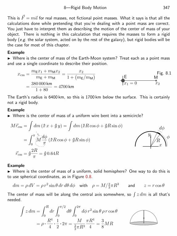
8—Rigid Body Motion 347
This is ~F = m~a for real masses, not fictional point masses. What it says is that all thecalculations done while pretending that you’re dealing with a point mass are correct.You just have to interpret them as describing the motion of the center of mass of yourobject. There is nothing in this calculation that requires the masses to form a rigidbody (e.g. the solar system, acted on by the rest of the galaxy), but rigid bodies will bethe case for most of this chapter.
Example Where is the center of mass of the Earth-Moon system? Treat each as a point massand use a single coordinate to describe their position.
xcm =mEx1 +mMx2
mE +mM=
x2
1 +(mE/mM
)=
380 000 km
1 + 80= 4700 km
x1 = 0 x2
E MFig. 8.1
The Earth’s radius is 6400 km, so this is 1700 km below the surface. This is certainlynot a rigid body.
Example Where is the center of mass of a uniform wire bent into a semicircle?
M~rcm =
∫dm (x x+ y y) =
∫dm (xR cosφ+ yR sinφ)
=
∫ π
0Mdφπ
(xR cosφ+ yR sinφ)
~rcm = y2Rπ
= y 0.64R
φ
dφ
Rx
y
Example Where is the center of mass of a uniform, solid hemisphere? One way to do this isto use spherical coordinates, as in Figure 0.8.
dm = ρ dV = ρ r2 sin θ dr dθ dφ with ρ = M/23πR
3 and z = r cos θ
The center of mass will be along the central axis somewhere, so∫z dm is all that’s
needed.∫z dm =
∫ R
0dr∫ π/2
0dθ∫ 2π
0dφ r2 sin θ ρ r cos θ
= ρ . R4
4. 1
2. 2π =
M23πR
3
πR4
4=
3
8MR

8—Rigid Body Motion 348
so zcm = 38R. This is less than halfway from the center to the top, and that is plausible,
in that there is more mass toward the bottom.In the first of these examples, I treated the Earth and Moon as point masses.
The last I saw, they aren’t. Is it correct to do this? Can you compute the center ofmass of an object by treating portions of it as if they are themselves point masses? Yes,but it requires a little proof.
Mtot~rcm =
∫dm~r =
∫first mass
dm~r +
∫second mass
dm~r = m1~rcm 1 +m2~rcm 2 (8.4)
Now divide by the total mass and that’s all there is to it.
What does that mean?In Eq. (8.3) you see the notation
∫~r dm. How do you integrate position with respect to
mass? The answer involves looking back to where that expression came from and thencombining that with the concept of an integral. Eq. (8.2) doesn’t involve an integralbut a sum,
∑kmk~rk. The concept of an integral is that you divide a complicated
thing into pieces in order to get an approximate result for a sum, then improve theapproximation by refining the divisions.
Here you can divide the region into small volumes and find how much mass is ineach volume. Call the volumes ∆V` and the masses ∆M`. The coordinate vector tothe center of each volume is ~r`, so an approximate value for the sum is
∑`
~r`∆M`
That doesn’t look any different from the original sum but it is different, because eachof these smaller number of terms represents a group of point masses. The idea of anintegral is that you improve the approximation by taking smaller volumes and in theideal case take a limit.
Who says that a particular mass ∆M6 will go to zero? It may not. For theregions where the limit ∆M`/∆V` approaches a limit, call it the mass density ρ and letdM = ρdV . If it doesn’t approach a limit because there is a big point mass there, youare simply left with a discrete, separate term in the sum, M~r. The final limit is thenan ordinary volume integral plus some separate terms that come from point masses.This notation,
∫~r dm, is simply a shorthand for what you would probably do anyway
if you’re confronted with a mixture of continuous and discrete distributions of mass.*
* For a full-blown mathematical treatment of this way to look at an integral, lookup Riemann-Stieltjes integrals. It’s a useful concept.

8—Rigid Body Motion 349
8.2 Angular MomentumThe first step in describing the dynamics of a rigid body is to start with a point massand apply a force to it.
~F = d~p/dt
Pick an origin and take the cross product of this equation with ~r, the coordinate vectorfor the point mass.
~r × ~F = ~r × d~pdt
= ~r × d~pdt
+d~rdt× ~p
=ddt
(~r × ~p
)The second line adds zero because ~v ×m~v = 0. The next step is the product rule forderivatives, combining the terms. This is
~τ = ~r × ~F =ddt
(~r × ~p
)=d~Ldt
(8.5)
Torque is the time derivative of angular momentum (for a point mass).For a rigid body, the only change in Eq. (8.5) is to add an index to the factors.
The index says that now there are many masses and you simply sum over those massesto get the total torque and total angular momentum.
~τ =∑k
~rk × ~Fk =ddt
(∑k
~rk × ~pk
)=d~Ldt
(8.6)
The next, and most important, step is to organize the bookkeeping for this sum de-scribing the angular momentum.
~L =∑k
~rk × ~pk
To describe rotation about an axis, use the equation (5.8), ~v = ~ω × ~r, giving
~L =∑k
~rk ×mk~vk =∑k
~rk ×mk(~ω × ~rk)
This shows how the angular momentum depends on the angular velocity and it is thedefining equation for the function called the tensor of inertia. What’s a “tensor”? Waita few pages for a full explanation.
~L = I(~ω ) =∑k
~rk ×mk(~ω × ~rk)

8—Rigid Body Motion 350
The function I is a vector-valued function of a vector variable, and that is the centraldefining property to keep your eye on. This is where you start to learn about tensors,and it is at the core of the rest of this chapter.
When you deal with a rigid body, most often it is a continuous distribution ofmass and not some discrete masses. A more appropriate notation for both cases is then
~ω
dm
~r
Fig. 8.2
~L = I(~ω ) =
∫dm~r × (~ω × ~r )
=
∫dm
[r2~ω − ~r(~ω .~r )
][ ~A× ( ~B × ~C
)= ~B
( ~A . ~C)− ~C
( ~A . ~B)]
(0.24)
(8.7)
Either way that you write it, you are computing the properties of the rigid body withrespect to a point, the origin — not an axis as you may have been expecting. Thismanipulation used the vector identity (0.24) for the triple cross product,
Example A straight, uniform rigid rod rotating about an axis through one end. Mass M ,length a. Place it along the x-axis with one end at the origin, and make the axis ofrotation the z-axis. The element of mass is dm = M dx/a between x and x + dx,then
~ω × ~r = ωz × x x = ωx y
~r × (this) = x x× ωx y = ωx2z∫dm (that) =
∫ a
0dx
Maωx2z =
Maωzx3
3
∣∣∣∣a0
=1
3Ma2 ωz
xz~ω
x
dm
(y in)Fig. 8.3
In this example the angular momentum is parallel to the angular velocity, and the
proportionality factor is called the moment of inertia: ~L = I0~ω, and I0 = Ma2/3 isthe moment of inertia of the rod about this axis through its end. As you will quicklyfind, life is not always so simple. Here I0 is a number multiplying ~ω. On the preceding
page and in most of this chapter, I is a function relating ~ω and ~L. You will see wherethey fit together shortly.
Example A dumbbell is spinning about an axis as shown. Treat the two masses as points and
compute the sum for ~L.
~r1 ~r2
m1 m2
~ω
~v1 out~v2 in ~r1 ~r2
m1
m2~ωα
~v1 out
~v2 in~L
Fig. 8.4

8—Rigid Body Motion 351
In the first picture, ~r1 × ~v1 is up along the same direction as ~ω. The same is true for
the second mass, and you can write ~L as a constant times ~ω. In the second picturehowever, ~r1×~v1 points to the upper left, perpendicular to the line between the masses.The same for ~r2×~v2. Neither is parallel to ~ω, so in this second simple-looking example
a relation such as ~L = I0~ω is just can’t be true. It’s still easy to figure out ~L though.The angle between ~ω and ~r1 is 90 + α, and between ~ω and ~v2 it is 90 − α.
~v1 = ω × ~r1 → v1 = ωr1 cosα then ~r1 × ~v1 = ω r21 cosα to the upper left
Similarly |~r2×~v2| = ω r22 cosα in the same direction, and the total angular momentum
is the sum of two terms,
~L =(m1r
21 +m2r
22
)ω cosα to the upper left [check α = 0 and α = 90]
Example A square plate is rotating about an axis that is at an angle α from the axis ofsymmetry of the plate (the z-axis). In the coordinate system drawn, ~ω is in the y-zplane, and the plate (in the z = 0 plane) has x and y coordinates that go from −a/2to +a/2. Use the area mass density, σ = m/a2. In the equation (8.7),
~L =
∫dm
[r2~ω − ~r(~ω .~r )
]~r = xx+ yy
~ω = z ω cosα+ y ω sinα
dm = σ dxdy, where σ = m/a2x
y
z α ~ω
dm = σ dxdy
Fig. 8.5
~L =
∫ a/2
−a/2dx∫ a/2
−a/2dy σ
[(x2 + y2)
(zω cosα+ yω sinα
)− (xx+ yy)ω y sinα
]There’s a little simplification before plunging ahead: the y2ω sinα terms cancel; theterm with an xy factor integrates to zero because the limits on x (or y) go from −a/2to +a/2. What is left is
~L = σ∫ a/2
−a/2dx∫ a/2
−a/2dy[(x2 + y2)zω cosα+ x2yω sinα
]= σ
∫ a/2
−a/2dx[(x2a+ 1
12a3)zω cosα+ x2ayω sinα
]= σ
[( 1
12a4 + 1
12a4)zω cosα+ 1
12a4yω sinα
]= 1
12ma2[2z cosα+ y sinα
]ω (8.8)

8—Rigid Body Motion 352
Compare this to the direction of ~ω = z ω cosα + y ω sinα and you see that ~L and ~ωdon’t align. The angular momentum points closer to the z-axis than does ~ω. Draw ~L.What happens if α equals 0 or 90?
DefinitionThe key defining property of a tensor:
A linear, vector-valued function of a vector variable is a tensor.
That a function f is linear means
f(~v1 + ~v2) = f(~v1) + f(~v2) and f(c~v ) = c f(~v )
or in a single line: f(a~v1 + b~v2) = a f(~v1) + b f(~v2)(8.9)
and a, b, c are scalars. Another name for this type of function is “linear transformation”or “linear operator”. This doesn’t completely define the subject of tensors, but it coversthe case at hand. For a general definition to cover the other cases, see chapter 12 ofMathematical Tools.
~A~B
~C
30A common example of a tensor is a rotation. Rotate all vectors
by 30 about the z-axis, and this defines a function. You have a vectorin and a vector out. If you add two vectors and rotate the result orif you rotate the two vectors and then add them, you get the same
answer. ~A+ ~B = ~C both before and after rotation. If you double thelength of a vector before or after rotating it, the answer is the same.Rotation defines a linear function.†
The function I in the equation ~L = I(~ω ) satisfies the definition (8.9). It has avector input and a vector output. The cross product and the integral in Eq. (8.7) arelinear, so the combination is linear too.
I(~ω1 + ~ω2) =
∫dm~r ×
((~ω1 + ~ω2)× ~r
)=
∫dm~r ×
(~ω1 × ~r + ~ω2 × ~r
)=
∫dm~r × (~ω1 × ~r ) +
∫dm~r × (~ω2 × ~r )
= I(~ω1) + I(~ω2) (8.10)
And I(c~ω ) = c I(~ω ) even more easily.
† This is a more restrictive definition of “linear” than used withdifferential equations. It would be “linear, homogeneous” in that con-text, but here that’s all there is.

8—Rigid Body Motion 353
f(x)f
f
x
Notice: I did not refer to “the function I(~ω )”. This object,
I(~ω ) = ~L, is not a function but a vector. It is the output of the
function I when you feed the vector ~ω to it, and that output is ~L, theangular momentum vector. This distinction between a function and thevalue of the function for some particular argument sounds trivial andpedantic, and don’t you commonly refer to f(x) as a function? It is really not; it is thevalue of the function at the point x. Does this matter? When you’re talking about thefunction f and the number f(x) for common real-valued functions of real variables, itprobably makes no difference and it seldom causes confusion. Here however if you don’tpay attention to this distinction here, it will cause needless difficulties, so watch the useof language in this chapter. At the end of section 0.10 I briefly raised this issue in afootnote but it was not important then. In the picture just above, “f ” is the wholegraph and “f(x)” is the value of f at the point x.
Example
~F
~d
Fig. 8.6
Suspend a mass with springs and let it come to equilibrium. Now applya small force to the mass and look at its displacement. The displacementis a function of the applied force, and it is a linear function of that applied
force. This defines a tensor f , where ~d = f(~F ). If the springs are all
the same, then ~d will be in the same direction as ~F and it is as simple
as ~d = ~F/k, but if the springs on the left and right are weaker than the
others then this displacement won’t even be in the same direction as ~F . Push in adirection between the springs and the displacement will be more toward the weakersprings then the stronger.
Parallel Axis TheoremThere are a couple of useful relations for computing these functions, the parallel axistheorem and the perpendicular axis theorem. Calling them “theorems” is stretchingthe word a bit, but they are useful. The first relates a tensor for a body to its tensorwhen the center of mass is the origin. It says that the tensor of inertia about a pointP equals the tensor of inertia about the center of mass plus another term that is thetensor of inertia of a point mass place at the center of mass and using the original Pas the origin. The proof is easy: add and subtract a term, ~rcm.∫
dm~r × (~ω × ~r ) =
∫dm
((~r − ~rcm) + ~rcm
)×(~ω ×
((~r − ~rcm) + ~rcm
))=
∫dm
(~r − ~rcm
)×(~ω ×
(~r − ~rcm
))+
∫dm~rcm ×
(~ω × ~rcm
)(8.11)

8—Rigid Body Motion 354
dmcm
~r
~rcm
Fig. 8.7
What happened to the cross terms? They’re zero.∫dm
(~r−~rcm
)×(~ω×~rcm
)=
[∫dm
(~r − ~rcm
)]×(~ω×~rcm
)The last parentheses formed a single constant inside the inte-gral, so you can pull it outside the integration (on the right).The definition of the center of mass is
~rcm =1
Mtotal
∫~r dm (8.12)
so that makes the integral in the cross term vanish. The two terms in Eq. (8.11) arenow precisely the statement of the parallel axis theorem because in the first integral,(~r − ~rcm
)is the coordinate of the mass dm with respect to the center of mass, and in
the second integral the entire integrand is a constant.
I(~ω ) = Icm(~ω ) +Mtotal~rcm ×(~ω × ~rcm
)(8.13)
The perpendicular axis theorem is even easier, but it refers to the components ofthe tensor, not to the tensor itself. It can wait until Eq. (8.30).
Example
What is the angular momentum of a Hula Hoop when you are spinningit about your waist? The hoop is a circle, but it is not spinning it aboutits center but about its edge. If you are working really hard at it, then toa good approximation a point on the edge is nearly standing still. Whatis the hoop’s angular momentum? Use the parallel axis theorem and startby finding the angular momentum assuming that the hoop is spinning about an axisthrough the center of the circle. ~ω is along this axis.
~ω × ~r
In the integral about the center (in the second picture), ~L =∫dm~r×(
~ω×~r), and all the radii have the same magnitude; all the ~ω×~r are tangent
to the circle with magnitude ωr. In turn, ~r× this vector is along the axis
with magnitude ωr2. That makes ~L = Mr2~ω along the axis (out of thepage and parallel to the angular velocity).
Now add the second term of Eq. (8.13), where ~rcm points from the right edge to thecenter of the circle. Do the two cross products and this term adds an equal amount
Mr2~ω to the total. ~L = 2Mr2~ω.

8—Rigid Body Motion 355
8.3 Tensor ComponentsComputing with tensors is like computing with vectors — the geometry gets out of handquickly. For vectors you can use the tool of components to do calculations, and thesame thing is true here. Tensors have components, but instead of the usual threecomponents for vectors, there are nine* for tensors.
Go directly for the components of the inertia tensor. Other tensors are conceptu-
ally no different. Start with the vectors ~ω and ~L. These have components with respectto whatever basis you’ve chosen:
~ω = ωxx+ ωyy + ωz z and ~L = Lxx+ Lyy + Lz z
Now relate these vectors with the function I .
~L = I(~ω ) is Lxx+ Lyy + Lz z = I(ωxx+ ωyy + ωz z) (8.14)
Use the linearity property of Eq. (8.9), which is the defining property of a tensor.
I(ωxx+ ωyy + ωz z ) = ωxI(x) + ωyI(y) + ωzI(z) (8.15)
The expression I(x) is a vector. As such it has three components. Denote these as
I(x) = Ixxx+ Iyxy + Izxz (8.16)
In the same way, express the other terms in components:
I(y) = Ixyx+ Iyyy + Izy z and I(z) = Ixzx+ Iyz y + Izz z (8.17)
The indices denote which output basis vector and which input basis vector arereferred to, and the order of the indices is carefully chosen for later convenience. Forexample, Ixy is the x-component of the vector I(y). Insert equations (8.15), (8.16),and (8.17) into equation (8.14) to get
Lxx+ Lyy + Lz z = ωx[Ixxx+ Iyxy + Izxz
]+ωy
[Ixyx+ Iyyy + Izy z
]+ωz
[Ixzx+ Iyz y + Izz z
]* There are generalizations of this statement for other kinds of tensors, but for
today this is good enough.

8—Rigid Body Motion 356
For these vectors to be equal, their respective components must match. Equate thecoefficient of x on the left to the coefficient of x on the right. Now repeat the process
for y and z. This expresses the components of ~L in terms of the components of ~ω.
Lx = Ixxωx + Ixyωy + IxzωzLy = Iyxωx + Iyyωy + Iyzωz (8.18)
Lz = Izxωx + Izyωy + Izzωz
In matrix notation this isLxLyLz
=
Ixx Ixy IxzIyx Iyy IyzIzx Izy Izz
ωxωyωz
(8.19)
and this is the reason for the peculiar-looking way that you are told to multiply matrices,across the row of the first factor and down the columns of the second. It all comesfrom the equations (8.14)-(8.17), defining the components of a tensor. The meaningof the expression (8.19) is the set of equations (8.18). The matrix indices are arrangedas I(which row), (which column). Compare the placement of the indices in Eq. (8.18) and inEq. (8.17). The notation is designed to come out in the way conventionally used withmatrices.
An abbreviated form for these equations is easier to write by using a unifiednotation for the basis vectors. ~ei, with the index i running over the set x, y, z (ormore often 1, 2, 3). ~ei replaces the three vectors x, y, z, and the equations (8.16) and(8.17) become one equation.
I(~ei) =∑j
Iji~ej (8.20)
Recall the discussion at Eq. (0.27).The manipulations that take you from equation (8.14) through (8.19) become
far more compact using the notation of Eq. (8.20).
~L =∑i
Li~ei = I(~ω) = I(∑
j
ωj~ej)
=∑j
ωjI(~ej) =∑j
ωj∑i
Iij~ei (8.21)
The basis vectors ~ei are independent, so the coefficients of ~ei must agree on the twosides of the equation. That is,
Li =∑j
Iijωj (8.22)

8—Rigid Body Motion 357
These two lines are so much more compact that you should compare their contentline-by-line with the preceding equations to verify that they are what they claim to be.
To compute these components, go back to the definition of the inertia tensor,Eq. (8.7). You need a vector identity for the triple cross product to manipulate this,Eq. (0.24).
~A× ( ~B × ~C ) = ~B( ~A . ~C )− ~C( ~A . ~B ) =⇒
I(~ω ) =
∫dm~r × (~ω × ~r ) =
∫dm
[r2~ω − ~r (~ω .~r )
](8.23)
Now compute I(x).
I(x) =
∫dm
[r2x− ~r (x .~r )
]=
∫dm
[(x2 + y2 + z2)x− (xx+ yy + zz)x
]=
∫dm
[(y2 + z2)x− yxy − zxz
]= Ixxx+ Iyxy + Izxz
The last line is the defining equation (8.16). Now all that you need do is to read offthe coefficients of x, y, and z, getting the first column of the matrix of components,and the calculations for the other six components are identical, giving the second andthird columns of the matrix.
Ixx =
∫dm (y2 + z2) Ixy = −
∫dmxy Ixz = −
∫dmxz
Iyx = −∫dmyx Iyy =
∫dm (x2 + z2) Iyz = −
∫dmyz
Izx = −∫dmzx Izy = −
∫dmzy Izz =
∫dm (x2 + y2)
The three diagonal components, Ixx, Iyy, and Izz, are the moments of inertiaabout the three axes, and the other components are called the products of inertia.There’s some symmetry among the nine components, as Ixy = Iyx etc, making thematrix in Eq. (8.19) symmetric. This is a special property of the inertia tensor, and itis not true for all tensors. You can write this matrix as
(I) =
∫dm
y2 + z2 −xy −xz−xy x2 + z2 −yz−xz −yz x2 + y2
(8.24)

8—Rigid Body Motion 358
In the spirit of Eq. (8.21) can these calculations of the components of the inertiatensor be more compact? Yes. Use x1, x2, and x3 for the coordinates instead of x, y,and z, then apply the summation convention as in Eq. (0.28), then Eq. (8.23) becomes
Li~ei = I(~ω) =
∫dm[xjxjωi~ei − xi~eiωjxj
]Li =
∫dm[xjxjωi − xiωjxj
]=
∫dm[xjxjδik − xixk
]ωk
Iik =
∫dm[xjxjδik − xixk
]Li = Iikωk (8.25)
Recall that now a repeated index within a single term is automatically summed. Also,such a summed index is necessarily a dummy variable, so that you can change its nameat will, a fact that was used to advantage in the second line of this little calculation (lookfor it). This same summation convention also simplifies the appearance of Eq. (8.21)by removing all the explicit summation symbols. They are unnecessary now.
Example A thin uniform rectangular plate is placed with one corner at the origin and with thesides along the x and y axes: (0 < x < a), (0 < y < b). What are the components ofthe tensor of inertia?
Look at Eq. (8.24): A lot of terms are zero — everywhere there’s a z. This meansthat the only integrals to do are∫
dm of x2, y2, xy
The area mass density is σ = m/ab, and∫ a
0dx∫ b
0dy x2 =
ba3
3,
∫ a
0dx∫ b
0dy y2 =
ab3
3,
∫ a
0dx∫ b
0dy xy =
a2b2
4
Multiply each of the these expressions by the area mass density and put them into theirappropriate slots in the matrix for the tensor components.
(I) =mab
13ab
3 −14a
2b2 0
−14a
2b2 13ba
3 0
0 0 13(ab3 + ba3)
= m
13b
2 −14ab 0
−14ab
13a
2 0
0 0 13(a2 + b2)
(8.26)
What happens to this result if a or b equals zero? Does that result make sense? Perhapsrelate it to some equation appearing earlier in this chapter.

8—Rigid Body Motion 359
In a previous study of rotations, you probably encountered the moment of inertia
as a subject in its own right, leading to the equation ~L = I~ω. You can now see that thiswas only a first approximation to the subject. But then what is that old I as expressedin the new language? The answer is∫
r2⊥ dm or ~ω . I(~ω )/ω2 (8.27)
where r⊥ is the perpendicular distance to your axis. The first expression is what appearsin an introductory text, though perhaps not in this notation. If you use a coordinatesystem where this axis is the z-axis, then r⊥ =
√x2 + y2 and this is Izz, the bottom
right element of the above matrix. The other diagonal elements of the matrix are thenthe moments of inertia about the x- and y-axes. The second, more complicated lookingexpression in Eq. (8.27) is a more general way to relate the tensor to the moment. Youcan derive it in problem 8.11. Notice how easy it is to abuse the notation, using I forthe moment of inertia and I for the tensor of inertia. Stay alert.
Example ~L
~ωα
yz
x out
1
2
Fig. 8.8
Repeat a previous example, Figure 8.4, only now express it in anew language. Two point masses are at the ends of a light rod lyingin the y-z plane as shown on the right. The integral is just a sumover two terms this time. For both masses the value of x is zero,and when you evaluate this sum, the y2 + z2 factor is just r2
1 or r22
depending on which mass you’re dealing with.
Ixx = m1r21 +m2r
22
Iyy = (m1r21 +m2r
22) sin2 α, Izz = (m1r
21 +m2r
22) cos2 α
Ixy = Ixz = 0, Iyz = −(m1r21 +m2r
22) sinα cosα
As a matrix this is
(m1r21 +m2r
22)
1 0 00 sin2 α − cosα sinα0 − cosα sinα cos2 α
(8.28)
If the angular velocity is along the z-axis, the angular momentum components areLxLyLz
= (m1r21 +m2r
22)
1 0 00 sin2 α − cosα sinα0 − cosα sinα cos2 α
00ω
= (m1r
21 +m2r
22)ω
0− cosα sinα
cos2 α
=⇒ ~L = (m1r
21 +m2r
22)ω cosα(−y sinα+ z cosα) (8.29)

8—Rigid Body Motion 360
The angular momentum is pointing toward the upper left, perpendicular to the axisbetween the masses, and not in the direction of ~ω. This behavior is typical, becauseit is only in the case of a symmetrical rotating body or in cases of a special ~ω thatthese two vectors will line up. The impression that you may have gotten in your firstintroduction to this subject was no doubt restricted to such select examples.
If the angular velocity is along the axis of the rod, ~ω = y sinα + z cosα, then
compute ~L as
(m1r21 +m2r
22)
1 0 00 sin2 α − cosα sinα0 − cosα sinα cos2 α
0ω cosαω sinα
=
000
~ωzy
Around this line of rotation, all the mass is on the axis, so there’s no angular momentumin this approximation that these are point masses.
If the axis of rotation is in the direction (−y sinα+ z cosα), the direction of theresult in Eq. (8.29), and the direction perpendicular to the axis between the masses,compute the angular momentum:
(m1r21 +m2r
22)
1 0 00 sin2 α − cosα sinα0 − cosα sinα cos2 α
0−ω sinαω cosα
=(m1r
21 +m2r
22)
0−ω sinαω cosα
This ~L is in the same direction as ~ω, and if you start with ~ω = ωx (out of the page),you get a similar result, with the same proportionality factor, (m1r2
1 + m2r22). Along
these directions the vectors ~ω and ~L are aligned.
Perpendicular Axis TheoremThis is a special result about the components of the inertia tensor, and it is occasionallyuseful.
It applies when a mass is distributed in a plane, so that it is essentially two-dimensional. Make that the x-y plane, then Izz = Ixx + Iyy. The proof involvesnothing more than writing the values of the components from Eq. (8.24):
Izz =
∫dm (x2 + y2),
but Ixx =
∫dm (y2 + z2) =
∫dmy2
and Iyy =
∫dm (x2 + z2) =
∫dmx2
(8.30)

8—Rigid Body Motion 361
because z = 0 for all dm, and that’s all there is to it.
Example
x
y
z
RFig. 8.9
A thin disk of mass M and radius R has its center at the originand has z = 0. Compute the inertia components:
Izz =
∫dm (x2 + y2) =
∫ R
02πr dr
MπR2
r2 =MR2
2
Use the perpendicular axis theorem, and because the symmetry ofthe disk implies that Ixx = Iyy = Izz/2, you see that both of theseare MR2/4. The products of inertia are all zero because they all involve integratingan odd function over a symmetric domain:
∫ a−a xdx = 0.
(I) =MR2
4
1 0 00 1 00 0 2
(8.31)
Suppose that at some instant the angular velocity is between the z and y direc-
tions: ~ω = ω(z cosα+ y sinα). Then ~L = MR2ω(2z cosα+ y sinα)/4. It points ina direction closer to z than does ~ω. If I keep turning the disk about this ~ω direction, theangular momentum will rotate around it. All the components of the inertia tensor arenow time dependent, but don’t worry about it because I’ve already found the relation
between ~L and ~ω, and that’s all I need. ~L will trace out a cone around ~ω, and thatmeans that there must be a time-varying torque to make this happen: ~τ = d~L/dt.
The angle between the two vectors is (problem 8.26).
sinβ = cosα sinα/√
3 cos2 α+ 1 (8.32)
α
β
~L~ω
z
y
x
~L~ω
Fig. 8.10
How much torque does it take to keep this disk rotating about the line ~ω ? Forget
the coordinate system; that will just get in the way now. The vector ~L is spinning

8—Rigid Body Motion 362
about a fixed line defined by ~ω. The length of ~L is constant, so its time derivative isperpendicular to itself. It is also perpendicular to ~ω, and its value is then
d~L/dt = ~ω × ~L = ~τ
The magnitude of this torque is ωL sinβ, and you can get the magnitude L from the
vector ~L in the preceding paragraph.
ωL sinβ = 14ωMR2ω
(4 cos2 α+ sin2 α
)1/2cosα sinα
/√3 cos2 α+ 1
=1
4M2ω2 cosα sinα
There was so much cancellation of the complicated factors in this calculation that youshould suspect that there’s an easier way. There is. The magnitudes and angles areconstant, so why not evaluate the magnitude of the product at the initial time?
~ω× ~L = ω(z cosα+ y sinα)×MR2ω(2z cosα+ y sinα)/4 =1
4MR2ω2x cosα sinα
Can you do this calculation of the torque without referring to a specific coordinatesystem, just manipulating the original form for I(~ω)? Yes, but it’s not much help:
~ω × ~L = ~ω × I(~ω) = ~ω ×∫dm~r × (~ω × ~r )
= ~ω ×∫dm
[r2~ω − ~r (~ω .~r )
]= −
∫dm (~ω × ~r ) (~ω .~r )
If you can find a use for this equation, you’re welcome to it.
This calculation has a very practical application. When you have driven your carfor a long time it may need adjustment. If you hit a curb with the wheel of your caryou can knock the wheel out of alignment, and it will certainly need adjustment whenyou then feel strong vibrations in the car’s steering wheel as you drive it. You then takethe car in to the shop and ask a mechanic to adjust the wheels so that their angularvelocity and angular momentum vectors are parallel, hoping thereby to eliminate thetorque ~ω×~L. Perhaps not. You may get better results if you ask for a wheel alignment.
A related problem will occur if the axis of rotation does not pass through thecenter of mass of the wheel. It is then out of balance and will also cause vibrations,calling for a wheel balancing.

8—Rigid Body Motion 363
Example
What is the tensor of inertia of a ball about a point on its surface? Inthe problem 8.20 you will compute the moment of inertia of a uniformball about an axis through its center. The result is 2MR2/5. Once youknow this, you immediately know all the components of its inertia tensorbecause of the ball’s symmetry: this same moment of inertia appears allalong the matrix diagonal and all the off-diagonal elements are zero. It isa multiple of the unit matrix. What are the components when the origin is a point onthe surface of the ball? Choose the coordinate system so that the z-axis passes throughthe center and use the parallel axis theorem.
I(~ω) = Icm(~ω ) +M~rcm ×(~ω × ~rcm
)−→ (I) =
2MR2
5
1 0 00 1 00 0 1
+M
y2 + z2 −xy −xz−xy x2 + z2 −yz−xz −yz x2 + y2
at center
=2MR2
5
1 0 00 1 00 0 1
+M
R2 0 00 R2 00 0 0
=MR2
5
7 0 00 7 00 0 2
Kinetic EnergyWhen a rigid body is rotating about a fixed axis, what is its kinetic energy? It is astraight-forward calculation.
K =1
2
∫v2 dm =
1
2
∫dm (~ω × ~r )2 =
1
2
∫dm (~ω × ~r ) .(~ω × ~r )
=1
2
∫dm~ω .
[~r × (~ω × ~r )
]=
1
2~ω . I(~ω) (8.33)
The sole vector identity that you need for this is that you can interchange the dot and
the cross product in the triple scalar product: ~A . ~B× ~C = ~A× ~B . ~C, where ~C = ~ω×~r.
If ~L and ~ω are aligned, so that ~L = I~ω, then this kinetic energy is 12Iω
2.
What if a body is both rotating and moving? For example rolling motion. Thecalculation is similar, again adding all the pieces of kinetic energy in the body. Let ~ωbe the rotation rate about the moving origin, and let ~v0 be the velocity of this originwith respect to you. The velocity of a mass dm is then ~v0 +ω×~r, where this ~r is from

8—Rigid Body Motion 364
the moving origin to dm.
~v0 ~ω
dm
K =1
2
∫dmv2 =
1
2
∫dm
[~v0 + ω × ~r
]2=
1
2
∫dmv2
0 +1
2
∫dm
(ω × ~r
)2+ ~v0 . ~ω ×
∫dm~r
=1
2mv2
0 +1
2~ω . I
(~ω)
+m~v0 . ~ω × ~rcm
(8.34)
If the origin for computing the inertia tensor is the center of mass, then the final termis zero, and the total kinetic energy is in that case the sum of the rotational energyabout the center of mass and the kinetic energy of a point mass at the center of mass.
In the same spirit, what is the angular momentum for an object that is bothmoving and rotating?
~L =
∫dm~r × ~v =
∫dm~r ×
(~v0 + ω × ~r
)=
(∫dm~r
)× ~v0 +
∫dm~r ×
(ω × ~r
)= ~rcm ×m~v0 + I
(~ω)
(8.35)
This is the sum of the angular momentum of a point mass at the center of mass plusthe rotational angular momentum about the center of mass.
Having looked at kinetic energy and angular momentum from different origins,
what about torque? The torque on a piece of mass dm is ~r × d~F . If you choose a
different origin, so that the position of the old origin is ~R with respect to the new origin,then the coordinate of dm is
~rnew = ~r + ~R so ~τnew =
∫~rnew × d~F =
∫ (~r + ~R
)× d~F = ~τold + ~R×
∫d~F
If the total force is zero, the torque is independent of the origin.
8.4 Principal AxesAside from spinning with zero torque, there are other reasons to be interested in liningup the angular velocity and the angular momentum; it makes calculations easier. Whencalculating the components of the inertia tensor for the example of two point masses,Eq. (8.28), the matrix would have been diagonal if you had chosen the coordinate systemdifferently. If y is along the line connecting the masses then ~ω would have had twonon-zero components, but the matrix of inertia components would have been diagonal.

8—Rigid Body Motion 365
~L~ω
α
yz
The integral for the inertia components is the same as be-fore, being a sum of two terms, but this time the sum is easier.
Ixx = m1r21 +m2r
22, Izz = (m1r
21 +m2r
22)
All other components zero
The equation ~L = I(~ω ) translates into components asLxLyLz
= (m1r21 +m2r
22)
1 0 00 0 00 0 1
0ω sinαω cosα
=⇒ ~L = (m1r
21 +m2r
22)z ω cosα
This agrees exactly with Eq. (8.29). Look and see.When you compute the components of I , the definition is I(~ei) = Iji~ej (recall
the implied sum). If there is a direction such that ~ω and ~L are parallel, choose ~e1
along that direction. Then ~L = I(~ω) and I(~e1) = (a multiple of)~e1 = I11~e1. The firstcolumn of the matrix has exactly one non-zero entry in the upper left corner of thematrix. The matrix is symmetric, so the upper row has only a single entry as well.
If you can find other directions along which ~ω is parallel to ~L, you can use thosedirections for basis vectors too. If there are three such directions, then you have acomplete basis and the matrix is diagonal. Can you do this? Yes. In the case of theinertia tensor it’s guaranteed.
Eigenvectors and Eigenvalues
The statement that ~ω is parallel to ~L means that one vector is a multiple of the other:~L = λ~ω. This is the equation
I(~ω) = λ~ω (8.36)
If this is satisfied, then ~ω is an “eigenvector” of I , and λ is an “eigenvalue”. Severalquestions arise.
inertia tensor all tensors1. Do these eigenvectors always exist? yes yes2. Can you always make a basis out of them? yes no3. If you can make a basis, is it orthogonal? yes no4. How do you find them? Therein lies a tale.
Translate the problem into components. In the notation of Eq. (8.19) the lastequation (8.36) becomes Ixx Ixy Ixz
Iyx Iyy IyzIzx Izy Izz
ωxωyωz
= λ
ωxωyωz

8—Rigid Body Motion 366
Assuming that you’ve already done the integrals to know the components of I , there arefour unknowns in these three equations: λ and the three components of ~ω. It doesn’tsound promising. There is always one solution, ~ω = 0, so all three components of thisvector are zero and λ is arbitrary. That is not a very interesting solution though, andyou can’t start to construct a basis out of it. Are there any non-zero solutions? No, atleast not for arbitrary λ. But, there are always certain values of λ for which there is anon-zero solution for ~ω.
Now would be a good idea to review section 0.10, especially the material onsimultaneous equations. Also reread the material leading to equation (3.59).
Rewrite this set of equations by moving everything to one side. Ixx Ixy IxzIyx Iyy IyzIzx Izy Izz
− λ 1 0 0
0 1 00 0 1
ωxωyωz
=
000
Further rewrite it as Ixx − λ Ixy Ixz
Iyx Iyy − λ IyzIzx Izy Izz − λ
ωxωyωz
=
000
(8.37)
This matrix acting on the components of ~ω gives the zero vector. Under almost allcircumstances that requires ~ω to be zero, but there can be an exception. That is thatthe matrix be singular — its determinant is zero. If you want a non-zero solution (andyou do), then the determinant of the coefficients of the three linear equations mustbe zero*. That is an algebraic equation for λ, a cubic equation, and it will alwayshave a solution. In the case at hand, the tensor of inertia, it will always have threereal solutions. For each solution λ (an eigenvalue), there is a corresponding ~ω (aneigenvector).
There are a few general results to prove about this process, but first I’ll carrythrough the solution in a special case, one that doesn’t entail as much algebra as thegeneral case, and the cubic equation will be easy to solve. The mass is confined to aplane, and that will define the x-y coordinates.
* Go through this statement for a 1× 1 matrix with a one element column matrix.What does it translate to?

8—Rigid Body Motion 367
Example
x
y
a
a
z out
Four masses, all the same, are at the four corners of a square: (0, 0),(0, a), (a, a), (a, 0), all at z = 0. Now to compute the nine componentsof the inertia tensor, there are really just three integrals,∫dmx2 = 2ma2,
∫dmy2 = 2ma2, and −
∫dmxy = −ma2
Any term involving z gives zero, so the defining equation (8.24) produces the compo-nents
(I) =
2ma2 −ma2 0−ma2 2ma2 0
0 0 4ma2
The eigenvector equation I(~ω)− λ~ω = 0, expressed in components as (8.37) is 2ma2 − λ −ma2 0
−ma2 2ma2 − λ 00 0 4ma2 − λ
ωxωyωz
=
000
Before setting the determinant of this matrix to zero, make a change of variables:λ = ma2λ′. This saves a lot of writing.
detma2
2− λ′ −1 0−1 2− λ′ 00 0 4− λ′
= 0 = (ma2)3(4− λ′)[(2− λ′)2 − 1
]with roots λ′ = 4, 3, 1.
For each of these eigenvalues, compute the eigenvector.
λ′ = 4 −→
−2 −1 0−1 −2 00 0 0
ωxωyωz
=
000
−→−2ωx − ωy = 0
−ωx − 2ωy = 0
0 = 0
The first pair have the unique solution ωx = ωy = 0, the last equation offers noconstraint, so ωz is arbitrary and the eigenvector is ωz z. That is, any multiple of z.
λ′ = 3 −→
−1 −1 0−1 −1 00 0 1
ωxωyωz
=
000
−→−ωx − ωy = 0
−ωx − ωy = 0
ωz = 0

8—Rigid Body Motion 368
This has zero z-component for ~ω, and ωx = −ωy. The eigenvector is then ~ω = x− yor any multiple of it.
λ′ = 1 −→
1 −1 0−1 1 00 0 3
ωxωyωz
=
000
−→ωx − ωy = 0
−ωx + ωy = 0
3ωz = 0
This time the eigenvector is any multiple of x+ y.Picture these motions. For the λ′ = 1 case, the rotation is about the line from
the origin to the far corner of the square. Only two masses are moving and they aresymmetrically placed with respect to the rotation axis at a distance r⊥ = a/
√2. The
angular momentum is obviously in the same direction, and the moment of inertia about
this axis is 2m(a/√
2)2
= ma2. That’s precisely the eigenvalue λ for this case.
x
y
x
y
x
y
~ω~ω
~ω outλ′ = 1 λ′ = 3 λ′ = 4
Fig. 8.11
For the λ′ = 3 case, the rotation axis is still in the x-y plane, but along y − x,perpendicular to the preceding one. Now three masses are moving, and the rotational
inertia about this axis is 2m(a/√
2)2
+m(a√
2)2
= 3ma2 as promised. This direction
still has enough symmetry that it is easy to believe that ~L is in the same direction as~ω.
For λ′ = 4, the eigenvector is along z, and again three masses are in motion,
with moment 2ma2 + m(a√
2)2
= 4ma2. This is a sufficiently non-symmetric casethat it is not immediately obvious that the angular momentum is in the same directionas ~ω, but do a couple of cross products and you can easily persuade yourself that it’strue. Again, the eigenvalue λ = 4ma2 is this moment of inertia about the z-axis.
The basis x, y, z, in which I computed the components of I in this example werearbitrary. I picked them for their obvious convenience in computing the answer. Whatif I pick another basis, one consisting of the three orthogonal eigenvectors that I justfound? I’ll call them ~e1, ~e2, and ~e3 as a common notation used for basis vectors.
~e1 =(x+ y
)/√
2, ~e2 =(y − x
)/√
2, ~e3 = z (8.38)
Does it matter that these are unit vectors? No, as long as they are independent thatis good enough. You could drop the
√2 and compute the matrix for I , but for other

8—Rigid Body Motion 369
manipulations you should be consistent. In keeping with the change I will use subscripts1, 2, 3 instead of x, y, z on the components
I(~e1) =∑j
Ij1~ej = I11~e1 + I21~e2 + I31~e3 = λ1~e1
This determines the first column of the matrix for I in this basis. The other columnsare found the same way.
I(~e2) =∑j
Ij2~ej = I12~e1 + I22~e2 + I32~e3 = λ2~e2
I(~e3) =∑j
Ij3~ej = I13~e1 + I23~e2 + I33~e3 = λ3~e3
The matrix for I is now
(I) =
λ1 0 00 λ2 00 0 λ3
=
ma2 0 00 3ma2 00 0 4ma2
and in this basis the matrix is diagonal. That can provide significant advantages inmanipulation for further calculations. Notice that you would get the same matrix evenif you do not put in the
√2 factors in Eq. (8.38).
Is it always easy to find the eigenvectors? No, this example is very easy and youdidn’t really have to confront a cubic equation to solve for the eigenvalues. Alas, it isnot typical.
8.5 Properties of EigenvectorsThere are some general results to be proved about these eigenvectors and eigenvalues,and the methods of proof used here will show up in several other important contexts,so they are worth learning. First an identity about the inertia tensor.
I(~ω ) =
∫dm~r × (~ω × ~r ) =
∫dm
[r2~ω − ~r (~ω .~r )
]~ω*
1. I(~ω2) = ~ω*
1.∫dm
[r2~ω2 − ~r (~ω2 .~r )
]=
∫dm
[r2~ω*
1. ~ω2 − ~ω*
1.~r (~ω2 .~r )
]= I(~ω*
1) . ~ω2 (8.39)
What is a complex conjugation doing here when all these vectors are supposed to bereal? And what does it mean anyway? Here I am allowing for the possibility that these

8—Rigid Body Motion 370
may be complex in order to prove that they aren’t. How can a vector be complex? In theusual basis, just allow the components to be complex numbers. You won’t represent itby a single arrow any more (you could use two), but you won’t need to do that anyway.
This symmetry property of the inertia tensor,
~ω*1
. I(~ω2) = I(~ω*1) . ~ω2 (8.40)
plays a key role in much of this analysis. Very similar identities appear in very different-looking contexts such as differential equations, and there they will lead to results muchlike the ones here. A tensor satisfying this equation is called “Hermitian” or “symmetric”depending on whether a physicist or a mathematician respectively is talking. It parallelsthe results in the equations (7.53) to (7.55).
In the calculation of eigenvalues and eigenvectors in the example of the precedingsection, the eigenvalues (roots of a cubic) were real and the eigenvectors are orthogonal.Is that a general property? For tensors that satisfy the identity derived in Eq. (8.40) itis. To prove this the manipulations are simple but not obvious. Assume that there aretwo eigenvectors:
I(~ω1) = λ1 ~ω1 and I(~ω2) = λ2 ~ω2
Take the scalar product of the first with ~ω*2 and the second with ~ω*
1.
~ω*2
. I(~ω1) = λ1 ~ω*2
. ~ω1 and ~ω*1
. I(~ω2) = λ2 ~ω*1
. ~ω2
Take the complex conjugate of the second equation:
~ω1 . I(~ω*2) = λ*
2 ~ω1 . ~ω*2
Subtract this from the first of the preceding equations.
~ω*2
. I(~ω1)− ~ω1 . I(~ω*2) = (λ1 − λ*
2)~ω1 . ~ω*2
The identity Eq. (8.40) says that the left side of this equation is zero, and the right sideis
0 =(λ1 − λ*
2
)~ω*
2. ~ω1 (8.41)
Now take the special case that ~ω1 = ~ω2. These two vectors are the same vector, sonecessarily the two eigenvalues are the same also
0 =(λ1 − λ*
1
)~ω*
1. ~ω1
The second factor is not zero, and this implies that the first factor must be. That inturn says that λ is real. With real λ and real components of the inertia tensor, all thecomponents of ~ω are real too.

8—Rigid Body Motion 371
Now Eq. (8.41) is0 =
(λ1 − λ2
)~ω2 . ~ω1 (8.42)
and this implies that for two different eigenvalues, i.e. λ1 6= λ2, the correspondingeigenvectors are orthogonal, as exemplified in the example of Figure 8.11: (z)⊥ (y −x)⊥ (x+ y).
These eigenvalues are the moments of inertia about the axis defined by theeigenvector, and they are of course non-negative. Of course? Yes, for an eigenvector,
λω2 = ~ω . I(~ω ) =
∫dm
[r2ω2 − (~r . ~ω )2
]= ω2
∫dmr2
⊥
where r⊥ is the perpendicular distance from dm to the axis defined by ~ω. This integralwill be zero only in the special case that all the mass is on the axis — when the body isa line. In all other cases it is positive. This final integral is the moment of inertia aboutthe ~ω direction.
8.6 DynamicsThe basic equation for rotating objects is ~τ = d~L/dt, Eq. (8.6). Now ~L is nothingmore than a tensor expression involving ~ω.
~τ =ddtI(~ω) = I
(d~ωdt
)+dIdt
(~ω)
Written this way all the components of the inertia tensor are time-dependent, and that’snot a fruitful approach. The trick is to transform to the rotating coordinate system inwhich the body is at rest. Then the the tensor I is constant. From the equation (5.6),
~τ =d~Ldt
= ~L+ ~ω × ~L = I(~ω)
+ ~ω × I(~ω)
and this again uses the chapter five convention that the dot now refers to the timederivative in the rotating system. In this rotating system, you can pick the coordinatesso that the components of I are a diagonal matrix — the basis using eigenvectors of I .
~τ = I(~ω)
+(xωx+yωy + zωz
)×(Ixxxωx + Iyyyωy + Izz zωz
)τx = Ixxωx + ωyωz(Izz − Iyy)
τy = Iyyωy + ωzωx(Ixx − Izz) (8.43)
τz = Izzωz + ωxωy(Iyy − Ixx)

8—Rigid Body Motion 372
These are the Euler equations. (As if he didn’t have enough things named for him. Heeven used to be on the Swiss ten franc note.)
Example If your automobile tire is misaligned, its axis of rotation doesn’t line up with its axisof symmetry. Call the z-axis the symmetry axis of the tire, then Ixx = Iyy. As youdrive at constant velocity what torque does this cause on your tire? In the inertialsystem ~ω is a constant because it is defined by the axle of the car. What happens to ~ωin the rotating system? Again, Eqs. (5.6) and (5.13):
~ωα
z-axisx-axis
~τFig. 8.12
d~ωdt
= ~ω + ~ω × ~ω = ~ω = 0 (8.44)
and this means that it is constant in the rotating system too. The equations (8.43) arenow
τx = ωyωz(Izz − Iyy), τy = ωzωx(Ixx − Izz), τz = 0
If the misalignment between ~ω and the axis of the tire is the angle α then pick the x-ycoordinates (rotating) so that ~ω = ωz cosα− ωx sinα.
τx = 0, τy = ω2 cosα sinα(Izz − Ixx), τz = 0
This is a constant torque about the y-axis, so why does it cause the wheel to shake?This is the rotating system remember. In the inertial system (the driver) this torquevector, τyy, is spinning about the axle at a rate ω, and the size of this torque varies asthe square of ω.
How can you picture this? Imagine yourself standing on this disk(tire?) and hanging on to the z-axis as hard as you can. Your feet arestraddling the x-axis, which is stationary between your legs. If you lookstraight ahead you see the angular velocity vector standing still in front
of you (~ω = 0). But if you look in the distance you may get dizzy fromwatching the world spinning around. If you look down and to your right youwill see the torque vector at your feet, pointing along the y-axis. (Notice
that Izz > Ixx.) And where is ~L?
~L = I(~ω) = I(ωz cosα− ωx sinα) = ω(Izz z cosα− Ixxx sinα
)

8—Rigid Body Motion 373
This points in a direction closer to the z-axis than the ~ω vector does. Asyou look straight ahead you can see it fixed in front of you on the near side
of ~ω. Remember, ~L = 0. I didn’t draw this vector because the picture iscluttered enough already.
Free RotationWhat if there is no torque, and the object is free to rotate in space like a frisbee or aplanet. The equations (8.43) (with ~τ = 0) are differential equations for ~ω. They canbe solved, but except for the case of a symmetric rigid body the solution is non-linearand tough. For that reason pick Ixx = Iyy.
0 = Ixxωx + ωyωz(Izz − Ixx)
0 = Ixxωy + ωzωx(Ixx − Izz) (8.45)
0 = Izzωz + 0
The last line says that ωz is a constant. That in turn makes the first two equationslinear equations for ωx and ωy. You know how to solve those: eαt.
ωx(t) = Aeαt, ωy(t) = Beαt
0 = IxxαA+ ωz(Izz − Ixx)B
0 = IxxαB − ωz(Izz − Ixx)A
A non-zero solution for A and B requires that the determinant vanish.
I2xxα
2 + ω2z(Izz − Ixx)2 = 0 −→ α = ±i ωz
Izz − IxxIxx
= ±i ω′ (8.46)
Put these back into one of the equations for A and B to get
0 = IxxA
(±i ωz
Izz − IxxIxx
)+ ωz(Izz − Ixx)B −→ ±iA+B = 0
A solution is now
ωx = Aeiω′t +A′e−iω
′t, ωy = −iAeiω′t + iA′e−iω′t
Chose some initial conditions:
ωx(0) = ω0, ωy(0) = 0 then ωx(t) = ω0 cosω′t, ωy(t) = ω0 sinω′t(8.47)

8—Rigid Body Motion 374
The rotation axis precesses about the z-axis at an angular velocity ω′.
Example
Earth. It is freely spinning in space and it is slightly ellipsoidal so that the momentsof inertia aren’t the same about all axes. The equatorial bulge makes Izz > Ixx = Iyy.If the angular velocity of the planet exactly lined up with its axis of symmetry, theconstant ω0 in Eq. (8.47) would be zero. It would be too much of a coincidence forthe alignment to be perfect and it isn’t. It misses by an amount such that if you go tothe North pole and look for the angular velocity vector you will find it several metersaway. Then it wanders around the pole at a rate ω′ ≈ 2π/400 days. Its motion isnot as regular as this rigid body analysis would lead you to believe, but the Earth isn’tperfectly rigid either.
That the Earth isn’t rigid should lead to damping of this oscillation within yearsor centuries, but it’s still here. It has been a puzzle what keeps this Chandler wobblegoing, but recent analysis points to fluctuating pressure on the bottom of the ocean asa likely source of the excitation.
This precession can give geologists information about the interior of the planet.Equation (8.46) tells you about Izz − Ixx and that gives some constraints on thedistribution of mass within the Earth. And not just Earth; Mars too. One of themeasuring devices sent to Mars looked at that planet’s wobble, and that says somethingabout the interior structure of Mars. Why hasn’t the wobble been completely dampedin the case of Mars? After all, it has no oceans to excite the oscillation. Unknown.Maybe the idea that the oceans cause it on Earth is wrong. You will have to do asearch of the current literature on the subject to get some ideas of the complexity ofthe problem.
Stability of RotationsWhat happens when you toss a hammer or a tennis racket up and set it spinning? Theanswer depends very much on how you do it, and the motion can be very smooth orvery wild. If you don’t have either a hammer or a racket handy, perhaps you have aheavy rubber band. Then you can wrap it around a book so that the pages don’t openup when you toss it up and spinning. Depending on the axis about which it is spinningyou will get very different results.
To analyze this, start again from Euler’s equations (8.43). This time assume thatthe three moments of inertia are different from each other, but assume that the angularvelocity vector is almost along one of the principle axes. This calculation will involvea series expansion and a linearization. Assume that the rotation is almost along thez-axis. The torque is zero because you have tossed the object up and it is then free torotate as it will.
~ω(t) = ω0z +~ε (t), with ε ω0

8—Rigid Body Motion 375
Start from the equations (8.43) with ~τ = 0, and as usual with these expansions, keeponly the first order terms in ε.
0 = Ixxεx + εyω0(Izz − Iyy)
0 = Iyy εy + εxω0(Ixx − Izz)0 = Izz εz
Every place that an ε2 appeared I dropped it, and the resulting equations are linear. Inthe third equation, both ωx and ωy are first order in ε so that killed its final term.
The third equation says that εz is a constant, and I may as well take it to bezero because a non-zero value would just be a redefinition of the original rotation rateω0 about the z-axis. The other two equations are linear differential equations for εxand εy. You know how to handle those: an exponential.
εx = Aeαt, εy = Beαt
then
(00
)=
(Ixxα ω0(Izz − Iyy)
ω0(Ixx − Izz) Iyyα
)(AB
)To get a non-zero solution the determinant must vanish.
IxxIyyα2 − ω2
0(Ixx − Izz)(Izz − Iyy) = 0 (8.48)
The nature of these solutions depends on the sign of α2. If it is negative then α isimaginary and there are oscillations about the z direction; if α2 is positive then α isreal and there is exponential movement away from there the z-axis: that rotation isunstable.
α2 ∝ (Ixx − Izz)(Izz − Iyy)
If z has the largest moment, Izz > Ixx and Izz > Iyy, then α2 < 0
and this says that α is imaginary and that the motion is stable. If Izz is the smallest ofthe three moments you have the same result: α is imaginary and the motion is stable.It is only in the third case, when Izz is intermediate between the other two moments ofinertia, that α2 is positive and α comes out to be real. That motion is unstable. Takea book and wrap a heavy rubber band about it. Now toss it in the air, spinning aboutone of the three axes of symmetry. Do it for each axis, and the difference in the resultswill be very obvious. See for example the YouTube video Solid Body Rotation, done inorbit.
There is more to learn about the stability of these rotations. What is the kinetic
energy of rotation about each axis? Use Eq. (8.33) about each axis: K = 12~ω
. ~L.
~ω = ω0x −→ K =1
2Ixxω
20, ω0y −→
1
2Iyyω
20, ω0z −→
1
2Izzω
20

8—Rigid Body Motion 376
The angular momentum in each case is easy because these are eigenvectors of the inertiatensor and are respectively
Lx = Ixxω0, Ly = Iyyω0, Lz = Izzω0
Write the energy in terms of these angular momenta.
~ω = ω0x −→ K =L2
2Ixx, ω0y −→
L2
2Iyy, ω0z −→
L2
2Izz
This assumes the same magnitude for the angular momentum in every case, and theseequations say that for a given angular momentum the rotation about the axis with thelargest moment of inertia has the smallest kinetic energy.
Whether this object is a rigid body or not, if there are no torques on it theangular momentum is conserved. For a truly rigid body, both angular momentum andmechanical energy are conserved, but completely rigid bodies are a mathematical fiction,and any real object will flex slightly. This has an important consequence: If a satellite isset to rotating about one of its principle axes and if that is one of the two stable axes,then you might expect the rotation to remain about that axis forever. But. . . A tinyflexibility will cause a tiny friction — a way to dissipate energy. The only truly stablerotation in this case will be about the axis with the largest moment of inertia, the onethat has the smallest kinetic energy for the given angular momentum.
~ω
Fig. 8.13
Early in the space program the satellite Explorer-1 was placed in orbit around Earthand set spinning about its long axis, the one with the smallest moment, and one theythought would provide a stable rotation. The satellite however, had whip antennas withmore than enough flexibility to destabilize this rotation and to set it tumbling about itsreally stable axis — end over end — much to the embarrassment of the engineers andphysicists involved.
If you have seen the motion pictures 2001 and its sequel 2010, a space shipwas left in orbit around Jupiter’s moon Io at the end of the first picture, and whenthey returned in the sequel it was tumbling end-over-end. They made no commentin the movie, but they got the physics right. The same applies to the more recentmovie, “Gravity”. When Sandra Bullock was first cut loose from the spacecraft, shewas tumbling wildly. After a brief time she was rotating smoothly head over feet. Wasthat really about the axis with the largest moment of inertia? Should it be sideways

8—Rigid Body Motion 377
or as shown, front to back? That does depend on the mass of her backpack, and itappears that they did it correctly in the movie.
8.7 Perturbation Theory˙If the equation for the eigenvalues of an inertia tensor is easy to solve then you’re lucky.What if it isn’t? At worst you may have to resort to solving it numerically, but thereis an intermediate situation that comes up surprisingly often and that falls betweenthese extremes. If the problem is close to one that is easily solved, then the method ofperturbations is available. This involves a series expansion that can be very useful inboth the quantitative and qualitative analysis of these problems.
For example, for a mass of uniform density and in the shape of a rectangular box,it is easy to find the eigenvectors and eigenvalues of the inertia tensor using the centerof the box as the origin. The principle axes are parallel to the edges of the box, andthe eigenvalues are easily computed. What if you now add a small mass to the cornerof the box? Suddenly the symmetry is lost and you don’t have any intuitive feeling forthe directions of the eigenvectors, but in some sense the eigenvectors ought to be closeto the original ones that were parallel to the edges.
Example
Compute the components of the inertia tensor in the example just mentioned. Thenwhat are the eigenvectors and eigenvalues of the tensor? Call the sides of the box a, b,c. First compute
∫dmx2. After that it’s all downhill. For dm use a slice of the whole
mass:
dm =Mabc
bc dx −→∫dmx2 =
∫ a/2
−a/2
Mabc
bc dxx2 =Max3
3
∣∣∣∣a/2
−a/2
=Ma2
12
The integrals of y2 dm and z2 dm just change a to b to c, and the off-diagonal elementsare zero. This produces (I0). For little m, it is just a point mass, so Eq. (8.24) producesthe result without any integration. This is (I1).
(I0) =M12
b2 + c2 0 00 a2 + c2 00 0 a2 + b2
(I1) =m4
b2 + c2 −ab −ac−ab a2 + c2 −bc−ac −bc b2 + c2
Fig. 8.14
The total tensor comes from both of the masses and the componentsare the sum of these two matrices. Suddenly, finding the eigenvectors andeigenvalues is hard. If you want a general answer for this case, look up theformula for the solution of a general cubic equation. You will then see whyI’m not going to use it.

8—Rigid Body Motion 378
If m M , the eigenvectors and eigenvalues will be close to thoseof I0, and because that matrix is diagonal, you already know what these approximatevalues are. The next problem is to find the corrections to them.
The idea is to assume that there is a power series expansion for these results andthen to compute the terms of that expansion one at a time. This is
I = I0 + εI1 and I(~ω ) = λ~ω, with
~ω = ~ω0 + ε~ω1 + ε2~ω2 + · · · and λ = λ0 + ελ1 + ε2λ2 + · · ·(8.49)
This introduction of “ε” is a convenient way to keep track of the many terms. Noneof these ~ω0, 1, 2, . . . or the similarly subscripted λ’s are known. That doesn’t matterbecause you will let the equations tell you what they are. Plug in:(
I0 + εI1
)(~ω0 + ε~ω1 + · · ·
)=(λ0 + ελ1 + · · ·
)(~ω0 + ε~ω1 + · · ·
)Multiply everything and look for the various coefficients of powers of ε.
ε0 : I0(~ω0) = λ0~ω0
ε1 : I0(~ω1) + I1(~ω0) = λ0~ω1 + λ1~ω0
ε2 : I0(~ω2) + I1(~ω1) = λ0~ω2 + λ1~ω1 + λ2~ω0
· · ·
When you have two power series that equal each other, this requires that the individualterms must match too, and that is all that I did to extract the separate equations.
Now rearrange these equations to put them into a standard form.
I0(~ω0)− λ0~ω0 = 0 (0)
I0(~ω1)− λ0~ω1 = λ1~ω0 − I1(~ω0) (1)
I0(~ω2)− λ0~ω2 = λ1~ω1 + λ2~ω0 − I1(~ω1) (2)
· · · (8.50)
The most important property that these equations possess that that under almost allcircumstances they cannot be solved. They have no solutions. If you plunge ahead andtry to solve them anyway then at some point you will find yourself dividing by zero.This doesn’t mean that the problem is hopeless, it just means that you have to find thevery special cases in which they can be solved. There are two ways to do this, bruteforce or cleverness. Both are instructive, but the second one is what you should masterbecause it is a technique that you will see many more times. You may have seen italready if you have worked through the sections 7.12 and 7.13. Work problem 8.52 forthe brute force method. It’s not hard in this case.

8—Rigid Body Motion 379
The 0th equation above is the one that you supposedly know how to solve. It’sthe one without the extra complicating term coming from the point mass on the corner.For the rest. . .
The clever method is to use Eq. (8.40), but now all the numbers are real:[~ω1 . I(~ω2) = I(~ω1) . ~ω2
]. Apply it to these perturbation equations. Take the scalar
product of Eq. (8.50)(1) with ~ω0.
~ω0 .[I0(~ω1)− λ0~ω1
]= ~ω0 .
[λ1~ω0 − I1(~ω0)
](8.51)
Apply the symmetry property of the inertia tensor to change the left side of this to
I0(~ω0 ) . ~ω1 − λ0~ω0 . ~ω1 =[I0(~ω0 )− λ0~ω0
]. ~ω1 = 0
This implies that the scalar product on the right side of Eq. (8.51) must be zero also.That is
~ω0 .λ1~ω0 − ~ω0 . I1(~ω0) = 0 −→ λ1 =ω0 . I1(~ω0)
~ω0 . ~ω0
and you have found the correction to the original eigenvalue without doing any additionalmatrix manipulation — only taking a scalar product. The magnitude of ~ω0 cancels fromthis equation, so you can make its size anything you want. Translate this into thenotation of matrices and you have
~ω0 =
ω0
00
−→ λ1 = ( 1 0 0 )m4
b2 + c2 −ab −ac−ab a2 + c2 −bc−ac −bc b2 + c2
100
=m4
(b2 + c2) (8.52)
as the first order correction to the first eigenvalue. You will easily see that the firstorder corrections to the other eigenvalues are the other diagonal elements of (I1).
What is the first order correction to the eigenvector? ~ω1? That requires solvingEq. (8.50)(1). Write it out in all its gory detail, and the the equations that you haveto solve are surprisingly simple.
I0(~ω1)− λ0~ω1 = λ1~ω0 − I1(~ω0)
M12
b2 + c2 0 00 a2 + c2 00 0 a2 + b2
ω1x
ω1y
ω1z
− M12
(b2 + c2)
ω1x
ω1y
ω1z
=m4
(b2 + c2)
ω0
00
− m4
b2 + c2 −ab −ac−ab a2 + c2 −bc−ac −bc b2 + c2
ω0
00
(8.53)

8—Rigid Body Motion 380
−→ M12
0(a2 − b2)ω1y
(a2 − c2)ω1z
=m4
0−ab−ac
ω0 (8.54)
And here you have the equations for ω1y and ω1z. Their sizes are proportional to m/M ,as befits their being small corrections.
Are you done here? I may be but you aren’t. What does this result look like? Ifa, b, and c are something like 1, 2, 3 in some units, then how does the direction of theeigenvector change when this correction is added? Is it toward or away from m? Andif the sides are instead 2, 3, 1, then does your answer to this change? Play around withspecial cases.
What about ω1x, the other component of the correction. Take that to be zero,because including it would just redefine the original ω0. (And there’s a technical reason,because if you go into the higher order corrections it will really mess things up if youdon’t do this.)
Exercises
1 Three equal point masses m are at the corners of the right triangle (x, y) = (0, 0),(a, 0), (0, b). Where is the center of mass?
2 Remove the masses from the preceding triangle and replace the sides with thin rodsof constant linear mass density λ. Where is the center of mass?
3 Remove the rods from the preceding triangle and replace the area with a uniformsheet of constant area mass density σ. Where is the center of mass?
4 Write out the equations (8.4) explicitly for 2 + 2 = 4 point masses and verify that itdoes what it says.
5 A tensor f is defined by the equation f(~v ) = ~v for all ~v. Compute the componentsof f .
6 A vector-valued function F acts on vectors in the plane, reversing the direction ofeach. Compute the components of this function, a 2× 2 matrix.
7 With respect to the origin, what are the components of the tensor of inertia for apoint mass m at the point (x, y, z) = (a, 0, 0)?

8—Rigid Body Motion 381
8 With respect to the origin, what are the components of the tensor of inertia fora point mass m at the point (x, y, z) = (a, a, 0)? and what if its coordinates are(a, a, a)?
9 Use the summation convention and notation of Eq. (0.56) to write the equations(8.17), (8.21), (8.22).
10 For the springs that appear in figure 8.6, call them k1 left and right and k2 top and
bottom. What are the components of the f in ~d = f(~F )?
11 What are the dimensions of I(x)?
12 Starting at Eq. (8.38), drop the denominators√
2 from the basis vectors, so that~e1 = x+ y etc. Now compute the components of the same inertia tensor as done there.
13 Four point masses m are at the four corners of a square in the z = 0 plane andwith (x, y) = (a, a), (a,−a), (−a,−a), (−a, a). Compute the components of thetensor of inertia with the basis x, y, z.
14 For the same four masses as in the preceding exercise, compute all the componentsusing the rotated basis x′ = (x+ y)/
√2 and y′ = (−x+ y)/
√2. z′ = z.
15 In the preceding two exercises, you compared results in two bases, one of which isrotated 45 with respect to the other. What would the answer be if the basis is rotatedby the angle 20.14 instead?
16 If a rigid body is both spinning and moving with no external forces, you expect itskinetic energy to stay constant. In Eq. (8.34) however the first two terms are constant,but the center of mass is moving, so the last term is always changing. What’s wrong?
17 In the analysis of free rotation leading to Eq. (8.47), what happens if there is zerorotation about the z-axis?
18 A point mass m is at coordinates specified by the vector ~r and it is rotating aboutthe axis ~ω. What is its velocity ~v ? What then is its angular momentum ~r×m~v ? This
is ~L = I(~ω ), so what are the components of I? That is, compute I(x), etc.

8—Rigid Body Motion 382
Problems
8.1 Explicitly write out the derivation leading to Eqs. (8.2) and (8.3) for the case oftwo masses.
8.2 Compute the volume of a solid hemisphere of radius R. (a) cylindrical coordinates.(b) spherical coordinates. (c) Find the center of mass of a solid hemisphere with uniformmass density.
8.3 Write out the proof in Eq. (8.4) for the special case of 4 = 2 + 2 masses to verifythe calculation.
8.4 Find the center of mass of the parabolic-shaped plane object in problem 2.54(b).
8.5 Suppose the rod in Figure 8.3 is not along the x-axis, but is at an angle α aboveit, still starting from the origin. Now calculate the angular momentum for the same ~ω.
8.6 Does f(~v ) = ~v + ~c define a tensor f , where ~c is a constant vector?What about f(~v ) = ~c .~v ?What about f(~v ) = z × ~v ?What about f(~v ) = c~v ?What about f(~v ) = x x .~v ?What about f(~v ) = y x .~v ?What about f(~v ) = v2~v ?What about f(~v ) = v ?In each case, draw pictures that explain what the function does.
8.7 The force on a charge moving in a magnetic field depends on its velocity as ~F =
q ~v× ~B. Show that this function of velocity, f(~v ) = ~v× ~B, defines a tensor and compute
its components in terms of the components of ~B. Write the result as a matrix. Pick a
simple, special ~v and ~B, to verify that your result works.
8.8 In two dimensions rotating vectors by a fixed angle α defines a tensor. Use theusual x-y basis to compute the components of this tensor: ~u = f(~v ). Ans: in part,f21 = + sinα.
8.9 If an object is pivoted about some point and the only other forces on it are from auniform gravitational field, show that the torque about the pivot is the same as if all themass were concentrated at the center of mass. If the gravitational field is not uniform,show by a counterexample that this is false.

8—Rigid Body Motion 383
8.10 A meter stick is hanging, pivoted about its end, and you start to accelerate thesupport (the pivot) horizontally at a0. Find the initial angular acceleration of the stickand find the initial linear acceleration of the other end of the stick. Ans: α = 3a0/2`
8.11 Show that the moment of inertia about any axis is ~ω . I(~ω )/ω2 =∫r2⊥dm,
where the origin for the tensor of inertia is on the axis and ~ω is in the direction alongthe axis. No components. Just use vector manipulation and the definition Eq. (8.7).And you will need a vector identity for the triple cross product.
8.12 Take the example in Figure 8.5 and repeat it in the language of tensor componentsin order to be certain that the results are the same.
8.13 Derive all the components in the equation (8.28).
8.14 For a uniform rigid rod rotating about an axis perpendicular to the rod, but passingthrough a point on the line with the rod, compute the rotational kinetic energy. Therotation axis can intersect the line of the rod anywhere. For fixed ω, find the positionof the axis for which this kinetic energy is a minimum.
8.15 Derive the component Ixx =∫dmy2 in Eq. (8.31) by direct integration.
8.16 For the functions in problem 8.6 that do define tensors, which ones are symmetricas defined in Eq. (8.39)? I.e. ~v∗1 . f(~v2) =
(f(~v1)
)∗ .~v2.
8.17 For the functions in problem 8.6 that do define tensors, find their components
with respect to some (clearly stated) basis of your choice. Ans: e.g.(
010
000
000
)8.18 Start with the rectangular plate whose components were computed in Eq. (8.26).Move the plate up a distance c so that its corner is at the coordinates (0, 0, c), thoughstill parallel to the x-y plane. Now what are the components of its tensor of inertia?
8.19 Compute the components of the tensor of inertia of a thin, uniform spherical shell,mass m and radius R, about an axis through its center. Note: you must do this in yourhead! No complicated integrals allowed.
8.20 Compute the moment of inertia of a ball of uniform volume mass density aboutan axis through its center. Mass = M and radius = R. Do this two ways.(a) Straight-forward integration of
∫dmr2
⊥ =∫dm (x2 + y2) in your choice of coor-
dinates, probably cylindrical but maybe spherical or (least likely) rectangular.(b) Compute
∫dmr2, where this r is the spherical coordinate. Then use this result to
get the moment of inertia of part (a). Ans: 25MR2.

8—Rigid Body Motion 384
8.21˙ A uniform ball is rolling downhill without slipping and starting from rest. (a) Com-pute its kinetic energy as a function of the distance travelled by using the result ofEq. (8.34) with the origin at the center of the ball. (b) Compute its kinetic energyby noting that the point of contact is not moving, so that it is at any instant movingwith pure rotation about that point. Find the moment of inertia about this new axis ofrotation in order to get the kinetic energy with this origin. It will be nice if the answersagree.
8.22 In the example leading to Eq. (8.8), what torque is needed to maintain the angularvelocity a constant? Ans: ~τ = 1
24ma2ωx sin 2α
8.23 At what point in the development from Eq. (8.14) to (8.19) did I use the factthat x, y, etc. are orthonormal?
8.24 There is nothing in this chapter that required you to multiply two matrices, thoughI hope you’ve seen the method before. Where did that rule for multiplication comefrom? It follows from the definition of components as summarized in Eq. (8.20). Letf and g be tensors so that their components are defined as f(~ei) =
∑j fji~ej and
g(~ei) =∑j gji~ej . The composition of two functions is defined: h = f g means
h(~v ) = f(g(~v )
). (This is just like Eq. (0.32), though here you’re not doing calculus.)
(a) Show that h is linear, satisfying Eqs. (8.9). (b) Compute h(~ei) using the equations(8.20) and (8.9) to express hmn in terms of the components of f and of g. Ans: hmn =∑k fmkgkn
8.25 Two equal masses are placed at coordinates (a, 0, a) and (0, a, a). Find thecomponents of the tensor of inertia about the origin in terms of the basis x, y, z in thiscoordinate system.
8.26 Derive the angle between ~L and ~ω for the spinning disk, Eq. (8.32). The picture
there implies that ~L is closer to the z-axis than ~ω. Show that this equation agrees withthat statement.
x
y
z a
a8.27 (a) Find the components of the inertia tensor for a triangular plateas shown in the sketch. The plate is in the x-y plane. (b) Find theeigenvectors and eigenvalues of the tensor. Ans: (a) Izz = 4
12Ma2
8.28 ˙ (a) Evaluate the components of the tensor of inertia of a uniform
cube of mass m and side `. The origin is at one corner. (b) What is ~Lif ~ω is through the origin and along the main diagonal of the cube? (c) What is themoment of inertia of the cube about the main diagonal? Ans: (c) ma2/6
8.29 Find the components of the inertia tensor for a thin rod of mass m and length `.One end is at the origin and the other is at the point (`, θ, φ) of the spherical coordinatesystem. Ans: Ixx = 1
3m`2(sin2 θ sin2 φ+ cos2 θ)

8—Rigid Body Motion 385
8.30 A solid, uniform, rectangular block of mass m has sides a, b, c. Themoment of inertia about the long axis from one corner to its opposite is(perhaps)(m/6)
(a2b2 + b2c2 + c2a2
)/(a2 + b2 + c2
). Analyze this proposed answer,
trying to show that it is wrong. If you fail, then maybe it’s right.
8.31˙ Derive the expression stated in the preceding problem.
8.32 Generalize the parallel axis theorem to find a relationship between two inertiatensors, neither of which is about the center of mass. This theorem is not so useful.
8.33 Apply the equation (8.40) to all the combinations of basis vectors x, y, and z todetermine what it says about the components of the inertia tensor in this basis. Do thiswithout using the computed form of the tensor in terms of m’s and ~r ’s. Just Eq. (8.40)itself.
8.34 In previous chapters you have sometimes started with energy insteadof force equations, knowing that you can differentiate the former to get thelatter. There is an easy, elementary derivation of τ = Iα in the same spirit.You know that K = 1
2Iω2 for rotation in the special case of a symmetric body spinning
about a fixed axis. Attach it to an axle through its center and wrap a string aroundit. Now pull with constant force F for a distance x, and as a function of this distancepulled, get the work done. This work is the rotational kinetic energy: differentiate thisequation with respect to time. Ans: τ = Iα
8.35 Parallel to the result in Eq. (8.40), take the tensor f , where f(~v ) = ~v × ~B for
fixed ~B, only there are no integrals this time. What is the relation between ~v ∗1 . f(~v2 )and f(~v ∗1 ) .~v2? Repeat problem 8.33 for this case to determine what it says about thecomponents of this tensor.
a
a
b
b
8.36˙ This figure is a plane sheet of metal of mass M and di-mensions as shown. A coordinate system is set up in the lowerleft corner. (a) Compute the components of the tensor of inertiain this coordinate system. Find the eigenvectors of this tensor.(b) By how much would the coordinate system as given have tobe rotated in order that the matrix of components be in diagonalform? You will of course check your result in all the special cases.Ans: Izz = 2
3M[b3 + ba2 − a3
]/(2b− a)
8.37¨Toss a disk into the air, so that it is horizontal and spinning it about its axis as itflies. Not exactly on axis though because unless you toss it perfectly you will see thatit wobbles. Find the rate of wobbling and compare it to the rate of rotation of the disk

8—Rigid Body Motion 386
itself. First, what is the relationship between ωz and ω′? Which rotates faster, theplate or the wobble? That is, interpret the equations and describe exactly what you willsee when you watch such a thin plate tossed into the air and wobbling about its axis.Try it; make sure that there is some sort of pattern imprinted on the disk so that youcan see its rotation.
8.38 A thin, uniform rectangular plate has mass m, sides 2a and 2b. Take the originat the center of the plate.(a) Find the components of the inertia tensor of the plate.(b) If the rectangular plate is rotating about a diagonal with an angular speed ω findthe angular momentum and the kinetic energy of the system.
8.39˙ Three equal masses m are placed at coordinates (0, a, a), (a, 0, a), and (a, a, 0).(a) Find the components of the tensor of inertia about the origin in terms of the basisx, y, z in this coordinate system.(b) If the system is rotating as a rigid body about the z-axis through the origin, what is
the angular momentum? Draw a picture of the vectors ~ω and ~L in this system. If it’shard to do the drawing, then add some words to say what the directions are. In fact,put some words in anyway.(c) Find any one eigenvector of I , and its corresponding eigenvalue. You may eitherderive it by computing it or you may guess an answer and demonstrate that it is correct.(c) Having found one eigenvector and eigenvalue, find the other two. At worst, youhave started with a cubic equation and know one root. Now factor it and then get theothers. Or, you can try to find a more clever way.
2
1
~ω8.40 ˙ A solid cylinder has mass m, radius R, and moment of inertia I .It is set spinning clockwise about its axis with an angular speed ω0 andplaced on the floor next to a wall as shown. The coefficient of kineticfriction between the floor and the cylinder is µ1 and between the walland the cylinder it is µ2. The angular deceleration of the cylinder is claimed to beα = mgRµ1(1 + µ2)
/((1 + µ1µ2)I
)= 2µ1g(1 + µ2)
/((1 + µ1µ2)R
).
Is this plausible?
8.41˙ Derive the angular deceleration as stated in the preceding problem. Perhaps rereadsection 1.4 ?
8.42¨A plane homogeneous plate of surface mass density σ is bounded by the logarith-mic spiral r = keαφ and the radii φ = 0 and φ = π. (a) Find the components of theinertia tensor about the origin. The plate is in the x-y plane. (b) Find the eigenvaluesand eigenvectors of this tensor. Any special cases to check the validity of your solution?

8—Rigid Body Motion 387
8.43 Eight point masses m are placed at the eight corners of a cube of side a. Theorigin is at one corner of the cube and the x, y, and z axes run along edges of thecube. (a) Compute the components of the tensor of inertia in this coordinate system.(b) What is the moment of inertia about the long diagonal of the cube?
8.44 Find all eigenvectors and eigenvalues of a tensor with components(
0−10
100
000
). Apply
this result to the result of problem 8.7. Ans: x± iy, z
8.45 ˙ Generalize problem 8.14 to an arbitrary body rotating about an arbitrary axis.Among the set of all axes parallel to some given one, derive the axis that presents thesmallest kinetic energy for a fixed ~ω. Use the parallel axis theorem and Eq. (8.33).When you want to simplify this, draw pictures.
8.46 In Fig. 8.12 and assuming that the disk is thin, picture yourself as the personholding on to the z-axis. Where will you have to look to see the angular momentum
vector? With respect to you, what is the motion of ~ω and of ~L? What are thesemotions with respect to a pedestrian?
8.47 The ice in Antarctica is up to a few kilometers thick in spots, averaging about1.6 km. If it melts and spreads out over the surface of the Earth, estimate its effect onthe number of seconds in a day and the cumulative effect for a year. Also, what wouldit do to sea level? Don’t plug in any numbers until you’ve simplified all the algebra andso that you aren’t subtracting two large numbers to get a small number.Ans: 5
3T m/M ≈ .5 s or so per day. This answer assumes the Earth is a uniform ball.It isn’t, so in which direction does that fact change the answer? Bigger or smaller?
8.48 The Sun rotates once in a little less that one Earth month. If the Sun collapses toa radius of 10 km while conserving angular momentum, what would its rotation periodbe? This is about the size of a neutron star, the remnant of an explosive stellar collapse.What would the speed of a point on its equator be? What would the collapsed star’sdensity be? And of course not just a number. Find something to compare it to.
8.49 ˙ Compute the components of the inertia tensor for a solid cone of uniform massdensity. The origin is the vertex. Mass: M , height: h, radius of base, R. What is itskinetic energy if it is rotating about its axis of symmetry with angular speed ω?Ans: Diagonal: Izz = 3
10MR2, Ixx = Iyy = 35Mh2 + 3
20MR2, K = 320MR2ω2
8.50 ˙ The cone in the preceding problem is lying on a table and free to roll withoutslipping. Its vertex stays fixed, and the line of contact with the table is instantaneouslyat rest, so that defines the axis of rotation. What is its kinetic energy, expressed interms of the given information and ω?Ans: 1
2Mω2[
310R
2 +(
35h
2 + 320R
2)R/h
]/(1 +R2/h2)

8—Rigid Body Motion 388
8.51 Use Eq. (8.34) to find the total kinetic energy of a solid cylinder rolling downhillwithout slipping. (a) Do this using an origin at the center of the cylinder. (b) Do thisusing an origin at the (moving) point of contact of the cylinder with the surface.
8.52 The equation (8.50)(1) usually has no solution. Pick one of the eigenvectors of
I0 and its corresponding eigenvalue, perhaps ω0
(100
), or another. Plug this ~ω0 into the
right side of (8.50)(1) and see what happens when you try to solve for ~ω1.
8.53˙ (a) Repeat the calculations of Eqs. (8.52)-(8.54) for one of the other two eigen-vectors, getting both the correction to the eigenvalue and for the eigenvector. (b) Takethe scalar product of the ~ω0 + ~ω1 that you find with the ~ω0 + ~ω1 of the example, theone that started with ω0x. This dot product should be zero, at least to the order thatyou’ve calculated the vectors. That is, the product should be zero out to order m/M ,but don’t expect it to be any better than that unless you decide to compute the secondorder corrections and to include them.
8.54 The Earth has a bulge at the equator so that its diameter is about 41 km largerthan it is from pole to pole. Model the Earth’s tensor of inertia by estimating this as afat cylinder of thickness 20.5 km and height perhaps 1/3 of Earth’s diameter. Add thisto the rest of the Earth, assumed to be a sphere, to get the total tensor of inertia. TheEarth’s rotational axis does not align perfectly with the polar axis, so this will causea wobble. Compute it, and see how this simple model compares to the experimentalvalue of about a 400 day period. The results will of course depend on your choice ofdensity for this bulge.
8.55 Use the box example of Figure 8.14 (but without the extra mass) and force it tospin with angular speed ω about its long axis. What torque does it take to do this?
8.56 A right triangle has sides a, b, and c, and it has a uniform area mass density.What is the moment of inertia about an axis perpendicular to the plane and throughits center of mass. I suggest that you start by computing its moment about an axisthrough a corner first. Ans: 1
36m(a2 + b2 + c2
)

Special Relativity.
Read sections 0.2 0.5
The history of special relativity is fascinating: filled with partial answers, cleverideas, false starts, intellectual barriers, and some smart people who, given enough ad-ditional time, would have figured it all out. Einstein got there first. He cut throughthe complexities that had slowed or stalled other work and he found the underlyingsimplicity. That is where I will start.
Galileo was really the first to articulate one of the foundational concepts, and hedid it three and a half centuries before Einstein was born. In his Dialog on the TwoChief World Systems he made the idea concrete by describing what you would see if youare in the main cabin below decks on some large ship, first when it is standing still, andthen when you
...have the ship proceed with any speed you like, so long as the motionis uniform and not fluctuating this way and that. You will discovernot the least change in all the effects named, nor could you tell fromany of them whether the ship was moving or standing still.*
Put in modern terms,
1. Without looking outside the room, you can’t tell how fast you’re mov-ing.
or 2. Only relative velocities are measurable, not absolute velocities.or 3. The Results of Measurement depend only upon the relative velocity
of observer and observed and not upon their absolute velocities.(And the third one is also Galileo’s phrasing — surprisingly modern.)
Chapter five started with the Galilean transformation, which is the mathematicalcodification of the change to a moving coordinate system.
x′ = x− v0t, y′ = y, z′ = z, t′ = t Eq. (5.1)
As you saw there, as long as forces depend on at most the relative velocity of interactingobjects, Newton’s equations remain the same when switching to a moving observer.~F = d~p/dt no matter how fast you move. The problem is that Newtonian Mechanics isnot all. Maxwell found a set of equations that describe electromagnetism extraordinarily
* Translation: Stillman Drake

9—Special Relativity 390
well, and they do not transform properly under the Galilean transformation. That meansthat something has to give: Newton, Galileo, or Maxwell.
When these difficulties arose in the late 1800’s the natural response was to gowith the familiar, keeping Newton and Galileo, but modifying Maxwell. The mostfamous approach was to say that Maxwell’s electromagnetic equations are valid in onlyone coordinate system and no other: the “ether” theory.
That didn’t work, and Einstein’s approach kept Galileo and Maxwell, while forcingNewton to change. It all sounds so simple doesn’t it? When one choice doesn’t work,try another. This caricature of the history as I’ve sketched it in these few paragraphshas filled, and will further fill, whole books putting flesh on the details.
What is it about Maxwell’s theory that caused a problem? The simple and mostprofound fact is that it produces a unique value for the speed of light in a vacuum. Notspeed relative to something, just speed. The simplicity of the theory of special relativityis that you start from two assumptions:
1. Only relative velocities are measurable2. The speed of light in a vacuum is the same for everyone.
This assumes that Maxwell is right and that Galileo’s verbal statement of theprinciple of relativity is right, but not the transformation equations written above. Inparticular the fourth one, t′ = t, will be sacrificed, and that is the most startling andperplexing aspect of this theory. The concepts “simultaneity”, or “at the same time”,or “now” will become puzzles to be sorted out. In Galileo’s day, or Maxwell’s, and allthe way up to Einstein’s, this equation stating that time is the same for everyone wasso obvious that it wasn’t even stated. It was just wrong.
What will replace the Galilean transformation of Eq. (5.1)? The answer is
x′ =x− v0t√1− v2
0/c2, y′ = y, z′ = z, t′ =
t− v0x/c2√1− v2
0/c2
where c is the speed of light in a vacuum. These are called the Lorentz transformation,but developing them will take some effort, concluding at Eq. (9.10). Notice that ifc→∞, these reduce to the Galilean transformation.
A matter of typography: Most of the time I have tried to be careful about howI write the mathematics, sometimes probably to the point of being annoying. In thischapter there are so many velocities that I won’t bother with the distinctions such asthose between v (speed) and vx (velocity). I will leave it to you to figure out which iswhich from context, otherwise there would be too many sub-x’s filling the pages, andby now you should be able to handle such an abuse of notation.

9—Special Relativity 391
9.1 Time Dilation, Length ContractionThe first step is to show that an immediate implication of the assumptions of specialrelativity is that moving clocks run slow, which means that measurements of time mustbe handled very carefully. There is a simple way to demonstrate this, one that is fairlystandard in texts on relativity. It involves using a special kind of clock to analyze theeffects of velocity. Because light in a vacuum is at the center of one of the assumptionsof the theory, this clock is built precisely from light in a vacuum. Build an evacuatedbox with mirrors at the top and bottom and a source of light inside.
L0 = cT0
your viewvT
cT
your friend’s viewFig. 9.1
In the sketch on the left, the light source starts a pulse of light moving straightup the tube until it hits the (perfect) mirror at the top. It bounces (straight) back downand hits the bottom (also perfect). The light keeps bouncing up and down, and thatbouncing is the ticking of the clock. Any real clock will have imperfections of course,but the analysis of this idealized version is where to start. What is the time betweenticks? The length is L0 and the speed of light is c = 299792458 m/s, so T0 = L0/c isthe time for the light to go bottom to top or back.
As you observe the light pulse repeatedly hit the bottom and the top mirrors,a friend of yours is driving toward the left at (very) high speed v. He has no doubtthat the light is hitting the mirrors, but says that the clock is moving right at highspeed, so that during the time that the light pulse went from the bottom to the top,the clock itself has travelled some distance. If you say that he is moving left then hewill say that the clock is moving right. That in turn implies that the light pulse will,according to your friend, be travelling along a diagonal path up and another diagonalpath down. The second drawing shows three images of the clock as it moves right.When the light left the bottom mirror, when it hit the top one, and finally when itreturns to the bottom.
If this were a discussion of Newtonian mechanics, and Maxwell hadn’t been bornyet, this would be easy to analyze. In the first picture the light pulse is moving at speed

9—Special Relativity 392
c. In the second picture, the clock and the light are moving right with a horizontalcomponent of velocity v. The light has a vertical component of velocity c, so the totalspeed of the light according to your friend is
√c2 + v2. All very simple, but that’s not
the way the universe is built. Instead, the speed of light is the same for everyone, andthat is taken to be one of the fundamental assumptions of special relativity: c, not√c2 + v2.
What changes is the time measurements themselves. The previous paragraphtacitly assumed that both people measured velocities by the same methods and thatthe clocks each used to measure the time-of-flight of the light behaved the same way.That assumption has to go. In the original calculation of the ticking of the clock,T0 = L0/c. For the other person looking at the clock you cannot assume that the timeto tick is the same; call it T instead (to be determined).
cT
vT
L0
In the time of one tick, the clock moves a distance vT horizontally,and the light moves a distance cT along the diagonal. Remember the secondassumption of the theory: light moves at the speed of light. There’s a righttriangle in this picture, and you can apply the Pythagorean Theorem to solvefor T .
(vT )2 + L20 = (cT )2 −→ (vT )2 + (cT0)2 = (cT )2 −→
c2T 20 = (c2 − v2)T 2 −→ T 2 =
c2T 20
c2 − v2−→
T =T0√
1− v2/c2= γT0 (9.1)
and γ is a standard abbreviation for 1/√
1− v2/c2.This is time dilation. The moving clock takes longer to tick. The moving clock
runs slow. Wait a minute. Isn’t it your friend who’s moving? Not the clock? Remem-ber the first assumption of the theory: Galileo’s idea that only relative velocities aremeasurable. That means that everyone is entitled to claim “I am standing still.” “I amnot moving; it is the rest of the universe that is moving.” Everyone is right, includingyour friend, who says that the clock is moving right at speed v.
This is the first indication that these two innocuous-sounding assumptions canlead to surprising and puzzling consequences. When time has become slippery can spacebe far behind?
Point of ConfusionIf your friend’s clock is running slow by a factor 2, you see that it takes a longer-than-expected time between his ticks. If you see two events that occur 10 seconds apart,does he say that they occurred 5 s apart or 20 s? If these are the only two choices, thenthe answer is either, depending on where the two events took place. See problem 9.9.

9—Special Relativity 393
After the whole Lorentz Transformation is available in a few more pages, then I hopethis question and its semi-mysterious answer will be clearer.
LengthsIf clocks run slow, making time measurements complicated, then what about lengths?If you have stopped at a train crossing and a long train passes in front of you, is thelength of the train according to you the same as the length of the train according toa passenger on the train? No. To measure the length of the train, measure the timeit takes to move past and multiply it by the speed: L = vT0. (T0 is the time thatyou read on your clock.) The question is now to find the length as measured by apassenger. Call the length and the time that the passenger measures L0 and T insteadof L and T . (L0 is the length the passenger observes for the [to him, stationary] train.)The passenger doesn’t need another clock to measure T , all that’s needed is to beable to read your clock. If yours recorded T0, and according to the passenger you aremoving at speed v, then (again according to the passenger) your clock is running slow.The passenger then says that the time T for you to have moved from one end of thetrain to the other is greater than your measured T0. The calibration factor between theclocks is
√1− v2/c2, so the passenger says that the time in which you go from one
end of the train to the other is longer than the T0 that you read on your slow clock.It is T0/
√1− v2/c2. This is the passenger’s T and the length as measured by the
passenger is L0 = vT . (Reread the above Point of Confusion.)
your view
v
T0 passenger’s view
v
T0
Fig. 9.2
you: L = vT0
passenger: L0 = vT = vT0
/√1− v2/c2 = L
/√1− v2/c2
length change: L = L0
√1− v2/c2 = L0/γ (9.2)
You see the train as shorter than the passenger does. This length contraction is asecond peculiar feature of special relativity.
This derivation of length contraction (also called the Lorentz contraction) involvesonly the simplest algebra, but it requires careful attention to the details of who’s lookingat what and when. There is another way to get to this result, one that reverses thesetwo difficulties. There the concepts are easy, but the algebra is more involved. The idea

9—Special Relativity 394
is simply to take the light clock of the previous two pages and turn it on its side, sothat the light is going left-to-right and right-to-left as the clock moves right. It shouldread the same time as it did when it was upright, and that will let you figure out whatits length is. See problem 9.6 for some suggestions about how to do this calculation (orbetter, you can try it on your own first and find the stumbling blocks yourself).
It is easy to mix up the applications of these dilation and contraction equations,so before applying either of Eqs. (9.1) or (9.2) you should think about the qualitativebehavior of the time and distance measurements. If a clock takes two seconds to markoff a second, its owner will think that someone just did the 100 meter dash in fiveseconds. This means that you can’t simply plug into formulas. The qualitative analysisshould come first.
A moving clock runs slow.The calibration factor between clocks is γ = 1/
√1− v2/c2.
That factor is greater than one.So, does the factor go in the numerator or in the denominator?
Terminology: Proper length is the length of an object as measured by someonewho says it is not moving. Proper time is the time interval between two events asmeasured by someone who says the occurred at the same place* — the clock is standingstill. For the train example, L0 is the proper length of the train, and T0 is the propertime on my clock. There is no universal convention about how you place subscriptshere, so don’t assume that a sub-0 will always be proper. For proper acceleration seeequation (9.22). [What would “proper velocity” be?]
If length contracts, shouldn’t the L0 in the original clock, Figure 9.1, contract?Should the L0 in Eq. (9.1) be a variable too? No, but it is not only a legitimatequestion, it’s an important one. In that derivation I assumed that both you and yourfriend used the same value for that number, the length perpendicular to the motion. Isthat valid? The answer is yes, but now you have to test it to be certain.
The proof is by contradiction. Assume the statement is false and show thatit doesn’t work. Take the light clock, supposedly length L0. Your friend wants tomeasure it to see if it remains L0 even when it moves past, so he uses a ruler of lengthL0 and holds it up so the ruler and the clock just miss each other. To be certain ofhis measurement he attaches a pair of paint brushes to the two tips of the ruler, set sothat they will mark the ends of the clock as it passes. If the clock shrinks because ofits motion then the paint brush on one end of the ruler will mark the clock while theother end misses. The trouble is that paint leaves a permanent mark on the clock. Youand your friend can get together over a beer after the experiment in order to comparedata. If your clock has only one paint mark, then there is a lateral length contraction
* There is an obscure word for this: collocal is the spatial analog of simultaneous.

9—Special Relativity 395
and you were moving. If it has two paint marks that are not at the ends, then he wasmoving. Either way you have violated the first axiom of the theory, that only relativevelocities can be measured. What if lateral lengths expanded instead of contracting?You get into exactly the same contradiction, but interchanging who is moving.
Another way to picture this: If a railroad train is entering a tunnel through amountain, and if the tunnel is just barely large enough to accommodate the width ofthe train when the train is moving slowly, what will happen when the train is movingrapidly? If there is either a lateral contraction or expansion because of the speed thensomeone, either the train engineer or the person who built the tunnel, will think thatthe train will still fit while the other will expect a crash. That is a qualitative difference,so they can’t both be right.
ParadoxesUnder normal circumstances, i.e. before you started to study relativity, you may havean occasion to think that your watch keeps good time and that your friend’s is runningslow. Your friend, who thinks just as highly of his timepiece, would think that yourwatch is running fast. The calculation of time dilation leading to Eq. (9.1) says thatyour friend’s clock runs slow because it’s moving. If the first assumption of relativity iscorrect, that it’s impossible to tell which of you is moving, then both of you will believethat the other’s clock is running slow — and both be right. How can that happen?
The same paradox applies to lengths. If the moving train contracts, a passengeron that train can look out and say that another train you think to be standing still hasshrunk. How can both be true? Resolving both of these problems will have to wait afew pages until the Lorentz transformation appears.
If you drive a long car and have a short garage, can you fit your car within thegarage by driving extra fast? Someone standing outside and watching you try to dothis would say yes; your car has shrunk, so it now fits inside. You, as the driver, see thegarage approaching, only it is now even shorter than it was before. You’re never goingto fit inside now. Who’s right?
If two people are approaching each other, one at 34c from the left and the other
at 34c from the right, and you ask one of them how fast the other is moving, the answer
will not be 32c, but 24
25c. A derivation of this will appear in Eq. (9.13).
Example
Before going into some more analytical problems with relativity, a few elementaryexamples are useful. Cosmic rays are (mostly) very high energy protons that come fromouter space and hit the Earth’s atmosphere. When such an energetic proton collideswith an oxygen or nitrogen nucleus it simply blasts the nucleus apart and in the processcreates many thousands or millions of other new particles. A major component of theresulting debris is the muon. These are particles that are basically massive, but unstable,

9—Special Relativity 396
electrons; mµ = 207me, and the mean lifetime of these particles is 2.2 microseconds.In this short time, even moving at nearly the speed of light, the mean distance such aparticle goes before decaying is about
cτ = (3× 10⁸ m/s)(2.2µs) = (300 m/µs)(2.2µs) = 660 m = 0.66 km
What does “mean life” mean? Radioactive decay follows statistical laws, andstarting with a population of particles at time zero, the fraction of them left at time tis e−t/τ , or expressed in terms of the total population, N(t) = N0e−t/τ . To find theaverage value of the decay time, let dN be the change in this number in time dt, sothat −dN is the number that decayed between time t and t + dt. The mean time todecay is then a sum over all these times divided by the total number of particles:
1
N0
∫t (−dN) =
1
N0
∫ ∞0−tdN
dtdt =
∫ ∞0
1
τte−t/τdt = τ
Starting from an altitude of 20 km and moving straight down, the fraction ofthese particles that would reach the Earth’s surface is e−20/0.66 ≈ 10−13. Despite this,so many reach the surface that you will have a thousand or more of them passingthrough you each minute. This is not because there are so many cosmic rays that hitthe Earth, but because of time dilation. The muons are moving so fast that the timedilation effect is large, and their lifetime is far longer than the two microseconds thatthey have when at rest. A factor of 1/
√1− v2/c2 = 10 is typical, and you might guess
that such a factor would lead to a change in the number reaching the surface by abouta factor of 10. Not so. This exponential changes the fraction hitting the surface from
e−ct/cτ = e−20km/0.66km = 7× 10⁻¹⁴ to e−20/6.6 = 0.05 (9.3)
That is a factor of about 1012, and this is a major part of the background radiationthat you live with all your life.
I used the “mean lifetime” to describe this and you may be more familiar with the“half-life”. They are proportional. See problem 9.3 to understand the relation betweenthese two ideas: t1/2 = 0.693 τ . Also, not all muons will have the same speed, so theywon’t all have the same time dilation factor. How do you handle that? See problem 9.8.
Example
The Global Positioning System is so commonly used that it is standard equipment insome cars, and is available for personal use almost everywhere. It depends on preciselymeasuring the signals from several satellites in orbit at a radius of 26600 km (measured

9—Special Relativity 397
from the Earth’s center). The orbital period is about half a day; its orbital speed isabout 3.8 km/s. At this speed the time dilation effect is
γ =1√
1− v2/c2≈ 1 +
v2
2c2, with
v2
2c2=
1
2
(3.8
300 000
)2
= 8× 10⁻¹¹
In one day = 86 400 s, the clock error would be 86 400 s×8×10−11 = 7µs. At the speedof light, the distance error from this is then 7µs . 300 000 km/s = 2 km. If no correctionhad been made for this effect the GPS would have been worthless. The effects fromgeneral relativity have the opposite sign but are even larger, giving a combined driftthat, if uncorrected for these relativistic effects, would be about 10 km/day.
9.2 Space-Time DiagramsAs with almost everything else in physics, the ability to draw a sketch of your problemis invaluable. Sometimes it’s a drawing and sometimes it’s a graph. Here, the goal isto turn conceptually difficult questions about measurements with clocks and rulers intoconceptually simpler problems in analytic geometry. When describing the motion of aparticle, you can give its position as a function of time and graph that. For now, onedimension of space (x) will be enough. The y and z coordinates will come along later.
Dealing with objects that move near or at the speed of light makes it necessaryto choose convenient units. The speed of light is 3× 10⁸ m/s = 300 m/µs = 1 ft/ns.The trick to make this easy is to measure time in microseconds and measure space inunits of 300 meters. In other words,pick the units so that c has the numerical value one.If you prefer light-years and years or feet and nanoseconds, that’s o.k. too. Choose thetime axis up* and the x-axis left and right and the pictures will look like these:
t
x
t
x
t
x
t
x
stationary
x = x0
simultaneous
t = t0
x = ct x = vt, v < c
Fig. 9.3
The second one represents a set of events that occur at the same time, the equation ist = t0.
* Why is time up and space left and right? For the same reason that peoplein the U.S. drive on the right and those in the U.K. drive on the left. That’s thecustom. Besides, if the coordinates are x, y, and t, then laying out the x-y planesort-of horizontally seems better.

9—Special Relativity 398
The first and fourth graphs present constant velocity motion of a particle, one of themwith v = 0 and the other with v = 300 m/4µs = c/4.
The third is a graph of the motion of a photon, v = c.The t and x coordinate axes have equations that are respectively x = 0 and t = 0.The two points in the third graph represent events at (x, t) = (2.5, 0.5) and (1.5, 2.5)
in the units of 300 m, 1µs.But First:When dealing with ordinary two-dimensional rectangular coordinate x and y,
sometimes you need to switch to a rotated coordinate system. If you’re doing an ele-mentary mechanics problem and ~g is down, you may choose x horizontal and y vertical,or you may not. Perhaps some other aspect of the problem, maybe a hill, suggests adifferent coordinate system with x′ along the incline of the hill and y′ perpendicularto it. What it the relationship between these coordinates? Just express each pair ofcoordinates in terms of r and the angles. The angle the hill makes with the horizontalis α, and the single point P has coordinates
x
x′
y
y′rφ
α
φ− αP
Fig. 9.4
x = r cosφ
y = r sinφ
x′ = r cos(φ− α)
y′ = r sin(φ− α)
(9.4)
=⇒x′ = r cosφ cosα+ r sinφ sinα = x cosα+ y sinα
y′ = r sinφ cosα− r cosφ sinα = −x sinα+ y cosα(9.5)
These equations show how to relate the coordinates that two different people use todescribe the same point, and all that was needed was a couple of standard trig identities.[Look at the exercises at the end of this chapter, page 431.]
A trivial-sounding question: What are the equations for the various axes? Asimple answer: the x-axis equation is y = 0 and the y-axis equation is x = 0. Similarly,the x′- and y′-axes have equations y′ = 0 and x′ = 0. If this seems trivial, just waituntil Figure 9.7.
The reason for looking at these rotated coordinate systems is that something verymuch like this can be done with space-time coordinate systems. The transformationswill not be rotations, but they will have many properties analogous to them. For spaceand time, the key step is to realize that you have to provide a precise statement of whatthese coordinates mean. You’ve already seen that times and lengths are no longer suchsimple concepts, so the coordinates that build on them have to be defined with care.

9—Special Relativity 399
One method to define these coordinates uses tools that are conceptually verysimple: a clock and a radar set. The radar set sends out electromagnetic pulses thatcan bounce from a distance object and a clock times the reflected signal, telling howfar away the object is.
Let t1 be the time the radar pulse is sent and t2 the time it returns. The totaltravel time of the pulse is t2− t1, half in each direction, so the time at which the pulsehits the object is
t1 +1
2(t2 − t1) = 1
2(t1 + t2), and the distance to it isc2
(t2 − t1)
Translate this into the analytic geometry of space-time diagrams. The light travels atconstant speed, so that going out its graph is a straight line in the picture. Returning,it’s another straight line.
x = −c(t− t2)
x = c(t− t1)
t
xt1
t2
E
Fig. 9.5
xE = c2(t2 − t1)
tE = 12(t2 + t1)
(9.6)
The event at which the radar pulse hits the object is labeled E. Perhaps it is a policeradar hitting a speeding car. In any case, the space-time coordinates of the event aredefined by the two measurements of time back at the radar set.
Now comes the interesting part: Bring your friend back into the picture, movingat velocity v. Using the same definitions to do the computation, what coordinatesdoes your friend find for this same event? For now, make the velocity v a constantbecause it makes the mathematics far easier, and the motion is a straight line in thepicture, x = vt. Instead of having a separate radar and clock, which would have to becalibrated, simply use the same set for both. Then it is a question of computing whatmeasurements the moving observer will get.
The outgoing and the returning radar pulses pass your friend at two points labeleda and b. The times at which they pass are ta and tb. Computing each of those times isnow finding the intersection of two lines, solving the two pairs of simultaneous equations

9—Special Relativity 400
on the left.
b: x = −c(t− t2)
x = vt
a: x = c(t− t1)
x = vt
t
xa
b
ta
tb
x = vt
E
Fig. 9.6
tb = ct2/(c+ v) = t2/(1 + v/c)
ta = ct1/(c− v) = t1/(1− v/c)
(9.7)
These times are when you think the radar pulse passed the moving observer when it
goes out and returns. They are not the times the moving clock will read. That clock is
running slow, remember, by a factor√
1− v2/c2, so the actual times that he sees the
radar pulse pass by are the smaller times t′1 and t′2:
t′1 = ta
√1− v2/c2 =
t1(1− v/c)
√1− v2/c2
t′2 = tb
√1− v2/c2 =
t2(1 + v/c)
√1− v2/c2
(9.8)
Now all that’s left is algebra, eliminating all the unwanted variables, (t1, t2, ta,
tb, t′1, t′2). The new coordinates of the event are
x′E = c2(t′2 − t′1)
t′E = 12(t′2 + t′1)
and solving Eqs. (9.6) for t1 and t2 −→t1 = tE − xE/c
t2 = tE + xE/c(9.9)
x′E =c2
[t2
(1 + v/c)− t1
(1− v/c)
]√1− v2/c2
=c2
[tE + xE/c
1 + v/c− tE − xE/c
1− v/c
]√
=1
2
[(ctE + xE)(1− v/c)
1− v2/c2− (ctE − xE)(1 + v/c)
1− v2/c2
]√
=xE − vtE√1− v2/c2

9—Special Relativity 401
t′E =1
2
[t2
(1 + v/c)+
t1(1− v/c)
]√1− v2/c2
=1
2
[tE + xE/c
1 + v/c+tE − xE/c
1− v/c
]√
=1
2
[(tE + xE/c)(1− v/c)
1− v2/c2− (tE − xE/c)(1 + v/c)
1− v2/c2
]√
=tE − vxE/c2√
1− v2/c2
Just as Eq. (9.5) referred to the point P without writing the letter, these look neater as
x′ =x− vt√1− v2/c2
= γ(x− vt) t′ =t− vx/c2√1− v2/c2
= γ(t− vx/c2)
y′ = y z′ = z(9.10)
These Lorentz transformation equations are an algebraic codification of the two axiomswritten on the first page of this chapter. γ = 1/
√1− v2/c2 as before, and β = v/c
is often used too.
What about the other coordinates, y and z? They don’t change, and the reasonis nothing but the argument on page 394, showing that there is no contraction in thelateral direction.
This was a fair amount of algebra to arrive at these rather simple-looking equa-tions, and if you look at other introductory texts on relativity you will find other, farless complicated derivations of the same two equations. Why then did I choose such aninvolved way to get to a result that another author may choose to do in a few lines?The first reason is that this method may be algebraically more complex, but it uses onlythe simple concept of determining how you measure x and t. A second reason is thatthis method is not restricted to motion at constant velocity; after all, if an observercan’t make measurements while undergoing an acceleration even as small as g, thenit’s an awfully limited theory. There’s no conceptual change in having an acceleratedreference frame, just a big change in the quantity of mathematics.* See problems 9.44and 9.45.
As with the coordinate change Eq. (9.5) and the accompanying diagram, thepicture of this transformation is important. As you can easily see, it is not a rotation,
* and despite what you may see in some books, this has nothing to do with generalrelativity.

9—Special Relativity 402
and the new axes don’t look like those on page 398.
x-axis: t = 0
t-axis: x = 0
x′-axis: t′ = γ(t− vx/c2) = 0
t′-axis: x′ = γ(x− vt) = 0 x
t
x′
t′simultaneous′
simultaneousFig. 9.7
The dashed lines fill in the coordinates as defined by the equations x′ = constant andt′ = constant. The picture has v = c/2.
SimultaneityThe phrase “at the same time” refers to events that occurred at the same value of t.The moving observer however uses different coordinates, so “at the same time” refers tothe same values of t′, the dashed lines parallel to the x′-axis in the above drawing. Thatsimultaneity depends on the motion of the observer is the central radical departure inspecial relativity. It is this departure from common intuition that allows the paradoxesin the theory to be resolved.
How big is the effect? For an astronomical example, the Earth orbits the sun ata speed of about 30 km/s. This is 10−4c. At the distance of the star nearest the sun,about four light-years, how big a discrepancy does this make?
t′ = 0 = t− vx/c2, −→ t = vx/c2 = 10−4c . 4 lt-yr/c2
= 4 . 10−4 yr . π × 107 s
1 yr= 12000 s ≈ 3.5 hr
This appears insignificant, but under some circumstances a much smaller speedcan produce a very large effect. The current in an ordinary electric wire consists ofelectrons in motion. The average drift velocity of those electrons is surprisingly small,and in home wiring its magnitude is commonly less than 0.1 millimeters per second.How can such a small speed account for a large electric current? There are a lot ofelectrons.
Come back to the question of current in a moment. First, look further at si-multaneity and use the Lorentz transformation to rederive length contraction. It’s aconsistency check, and it better give the same answer as before. Someone is movingpast at a speed v and he claims to have an object of length L0. Notice: He says thatit isn’t moving, so he gets to say that its proper length is L0. What are the algebraicequations describing the front and back end of this object?
x′ = 0, x′ = L0 for all t′— what could be simpler? (9.11)

9—Special Relativity 403
I took the left end at zero to save algebra. The two lines of constant x′ producetwo parallel lines in the x-t coordinate system. Simply combine the Lorentz equations,Eq. (9.10) with the equation x′ = L0 and find the intersection of that line with the linet = 0. That is the dot in the figure.
x′ = L0
t = 0
x′ = γ(x− vt)
−→L0 = γx
x = L0
√1− v2/c2 x
t t′
x′x′ = L0
The direct application of the transformation equations then reproduces the length con-traction equation correctly. Can you do the same sort of analysis for time instead oflength? Yes, you can, see problem 9.5.
If you happen to have a ruler (stationary according to you) that is exactly this
length L = L0
√1− v2/c2 then what does your moving friend see? (You would call
this L a proper length, but the symbol L0 is already taken.) The equation for theright-hand end of your ruler is x = L, the dashed line in the next picture. What is thevalue of x′ at the time t′ = 0? What do you expect it to be? That is the dot in thispicture. Again, the Lorentz transformation appears.
x
t t′
x′x′ = L0
x = L
t′ = 0
x = Land
t′ = γ(t− vx/c2)
x′ = γ(x− vt)
Eliminate x and t to get
x′ = γ(L− v . vL/c2) = L√
1− v2/c2
and the Lorentz contraction appears again! Each person says that the other’s rulershave shrunk.
CurrentAn ordinary copper wire carrying a current I has two parts: the stationary positivecharges and the moving negative ones. There are cases such as fluorescent lightswhere both types of charge move, but that’s an unneeded complication. In fact itdoesn’t matter whether the positive charges are moving right or the negative chargesare moving left. Both represent a current to the right.* If it’s convenient to simplify the
* It wasn’t until 1879, when Edwin Hall discovered the Hall effect, that it waspossible to tell the difference, and the electron itself wasn’t discovered until the late1890s.

9—Special Relativity 404
explanations by assuming that the positive charges are moving right and the negativecharges are stationary, that’s o.k. It matters not which. The wire has no net charge,so the distance between the positive charges is on average the same as the distancebetween the negative ones. At t = 0, the x-axis, for every positive charge there is anegative one. In this picture the positive charges are moving right (x = const. + vt)and the negative ones are stationary (x =const.)
x
t
x′
t′
– + – +
Fig. 9.8
Positive and negative charges in a wire
Dashed lines are the charges.
Without solving a single equation, you can look at this picture and see that themoving observer, who says that the x′-axis is represents simultaneous points,concludes that the positive charges are farther apart than the negative ones. Thatimplies that the moving observer sees a net negative charge density on the wire.
If the “moving observer” is a charge, it will feel a force because of the net chargeon the wire. If that moving charge moves faster it will see more charge on the wire andwill feel a larger force. You will notice that this force is perpendicular to the velocityvector. This velocity dependent force is there even though you, as a stationary observer,say that there is nothing to push the charge; the wire is neutral. Instead you call theeffect a “magnetic field”, and conclude that its effect is proportional to velocity. Thisis how you derive magnetism from the combination of electric fields and relativity.
There are a few details to fill in to get the familiar “q~v× ~B” expression, but theessential ideas are already here. The consequence of the analysis is that just as spaceand time become intertwined in relativity, so do electric and magnetic fields. What is
an ~E to me will be a combination of ~E and ~B to you. Similarly, my ~B will be your
mixture of ~B and ~E. The relevant equations are not the Lorentz transformation thistime. They’re quite different.
Future and PastIf simultaneity has become malleable, what happens to the meaning of the words futureand past? Are they affected? Yes. According to a stationary observer, us, the futureis defined by the inequality t > 0. The past is t < 0. Someone in motion uses thesame concept, but it becomes t′ > 0 and t′ < 0 instead, and these are indicated by thevarious shaded regions in the drawings.

9—Special Relativity 405
t < 0
t > 0
t′ < 0
t′ > 0
x
t
x′
v > 0 Fig. 9.9
The familiar part is defined by the horizontal line, the x-axis that separates ourpast from our future. The unfamiliar part is the past and future for the moving observer.t′ > 0 is tilted because t′ = γ(t−xv/c2), so the demarcation between past and future isthe line t = vx/c2. Remember the units I’m using to draw the pictures: c = 300 m/µs,the line x = ct is at 45. c = 1 in units of 300 m and 1µs, so the boundary betweenpast and future will not get any steeper than ±45. If the motion is in the oppositedirection, v < 0, the tilt is reversed and goes from upper left to lower right.
This picture implies that what is in the future for me may be in the past for youand vice versa. The two dots in the preceding Figure 9.9 represent events doing that.Notice that the dot on the left is an event that occurred before the one on the rightaccording to us, but it occurs after the one on the right for the moving observer. Theirtime-order is reversed. Does this mean that cause and effect can be reversed? No,because signals can’t travel faster than light, and that implies that these two dots arefar enough apart that light can’t get from one to the other in the time between them.
There are two types of future and two types of past: relative and absolute.Absolute future is something that everybody agrees on. Relative future will meandifferent things to different people, depending on their relative velocities. The two dotsabove represent a case where future and past are relative to the observer, but rememberthat the x′-axis can tilt only up to ±45 and no farther. There is a limit on just howfar the relative future and past can be pushed.
absolute past
absolute future
relative past
relative future
t
xx
y
t
Fig. 9.10
The events in the absolute future are in the future according to everyone, andthey are also events that can be reached by a signal that starts at the origin. Such a

9—Special Relativity 406
signal has the equation x = vt with |v| ≤ c, and it can pass through any point withinthe absolute future. In the next picture, jumping up a dimension so that there are twospacial coordinates x and y to go along with t, the absolute future is within the upperpart of the cone. This cone is the “light cone”, r =
√x2 + y2 = c|t|.
The concepts of cause and effect involve the order of time. A cause precedesan effect. If the past and the future can become muddled because of relativity, thenit puts some constraints on the way that things can interact. Something can cause aneffect only if the effect is in the future of the cause according to everyone. This meansthat something that happens at the origin (x = 0, t = 0) can only cause somethingon or within the future light cone, at a distance r ≤ ct. Outside that cone, the pastand future become relative concepts, and the relative past and future there are perhapsbest called “elsewhere”.
9.3 Relative VelocityYou are at rest (according to you). There are two objects, a moving observer withvelocity v and some other object with velocity u. What is their relative velocity?This question will have different answers depending on just how you define the phrase“relative velocity”. For one possible definition you can ask how you would measure theirdistance apart and how fast that distance is changing. In your time interval ∆t themoving observer goes a distance v∆t. The object goes a distance u∆t. The distancebetween those two has changed by the amount u∆t − v∆t. You then say that therelative velocity is
u∆t− v∆t∆t
= u− v
What could be simpler? This is exactly what you get if you know nothing aboutrelativity, and it is not wrong. It is just not the definition of relative velocity neededhere; there is a subtle difference in how it is stated.
The other way to define the relative velocity: Ask the moving observer whatvelocity the other object has. That will give a different answer, not the one in thepreceding equation. A slick and easy way to derive the equation for relative velocitystarts from the basic definition of velocity as a derivative and then uses a commondifferentiation trick to manipulate it.
x′ and t′ are functions of x and t (the Lorentz transformation).x is a function of t (x = ut).So, x′ and t′ are functions of t.Compute dx′/dt′ using t as a parameter, as in Eq. (0.37).

9—Special Relativity 407
dx′
dt′=dx′/dt
dt′/dt, then
x′ = γ(x− vt)t′ = γ(t− vx/c2)
=⇒dx′/dt = γ
(dx/dt− v
)dt′/dt = γ
(1− v(dx/dt)
/c2)
(9.12)
divide: u′ = u′x =dx′
dt′=
γ(dx/dt− v)
γ(1− v(dx/dt)/c2) =
u− v1− vu
c2(9.13)
Pay attention to this derivation. It carries through with little change in more complicatedcases, such as in computing acceleration, Eq. (9.21) or superluminal speeds, Eq. (9.20).A probable point of confusion here: v is a number, not a function of time. Whatdepends on t are x, x′, t′, and of course t itself.
If the object is a photon then u = c, and
c− v1− vc/c2
=c− vc− v
c = c (9.14)
Everyone agrees about the vacuum speed of light. If instead, the observer and objectare moving toward each other, say u positive and v negative, at 3
4c, then the speed ofone according to the other is
u′ =34c+ 3
4c
1 + (34c)
2/c2=
32c
1 + 916
=24
25c
and this is not the 32c expected from a non-relativistic of velocity additon.
What about the other components of velocity? Recall that the Lorentz transfor-mation for these other coordinates says that y and z don’t change. Does that implythat uy is the same for both? No, because t is different. Do the same calculation for y′
as for x′, using the same equations as in Eq. (9.12), but including y′ = y. Notice thatin the work of the last few lines, the symbol “u” is really “ux”. It’s just that most ofthe development has been in one dimension of space, so it hasn’t mattered. Sometimeshowever, you have to be a little more careful.
dy′
dt′=dy′/dt
dt′/dt, and
dy′/dt = dy/dt
dt′/dt = γ(1− v(dx/dt)
/c2)
divide: u′y =dy′
dt′=
dy/dt
γ(1− v(dx/dt)/c2) =
uyγ(1− v(dx/dt)/c2
) =uy
γ(1− vux
c2)
(9.15)Even if ux = 0, the y-component of velocity will change, decreasing by a factor of γ.

9—Special Relativity 408
Example
What if the original ux and uy represent the motion of a photon? What does themoving observer find for the speed of the photon? This is just a bunch of algebra,but it is worth checking. Maybe you can find a slicker way to avoid the followingmanipulations.
u′x =ux − v1− vux
c2, u′y =
uyγ(1− vux
c2)
u′2x + u′2y =(ux − v)2γ2 + u2
y
γ2(1− vux
c2)2 =
(ux − v)2 + u2y(1− v2/c2)(
1− vuxc2)2
=(ux − v)2 + (c2 − u2
x)(1− v2/c2)(1− vux
c2)2 [original speed = c]
=u2x − u2
x + v2 − v2 − 2vux + c2 + u2xv
2/c2(1− vux
c2)2 = c2
9.4 Space-Time IntervalsIn the Euclidean geometry expressed in the picture and equations (9.4), there is aninvariant of the transformation: the distance to the origin, OP. It is the square root ofx2 + y2 or of x′2 + y′2, whichever coordinate system you choose. You can verify thisalgebraically by using the equations (9.5) directly.
x′2 + y′2 = (x cosα+ y sinα)2 + (−x sinα+ y cosα)2 = x2 + y2
Multiply all the factors and collect the terms.There is a similar relation for the geometry described by the Lorentz transfor-
mation, but it is not a geometry that Euclid would have recognized. Instead of thesum of squares, you use the difference of squares to compute the invariant. You alsoneed factors of c in order to keep the dimensions straight, so the expression to examineis not x2 + y2, but x2 − c2t2. Instead of rotational transformations, use the Lorentztransformation Eq. (9.10).
x′2 − c2t′2 =(γ(x− vt)
)2 − c2(γ(t− vx/c2)
)2= x2 − c2t2 (9.16)
Again, just multiply all the factors and collect terms.In order to interpret what this means, it is better to interchange the terms and
to look at t2 − x2/c2. Even better, use the interval between two events instead of thedistance to the origin. Take the events to have coordinates (xa, ta) and (xb, tb), with

9—Special Relativity 409
the intervals
t
x
(xa, ta)
(xb, tb)
∆τ ∆t = tb − ta∆x = xb − xa
−→(∆t)2 − (∆x)2/c2 = ∆τ 2 (9.17)
Let this line segment represent your friend’s motion, so that he was at coordinatexa at time ta and in the time interval ∆t = tb − ta he moved to the point xb. Youcan look at this and say that the time interval is ∆t, but how much time has elapsedon your friend’s clock, remembering that it is running slow according to you. You knowthe calibration factor, and all that you need to know is his speed. That’s easy; it isv = ∆x/∆t. His own clock then reads an interval (the proper time interval) that issmaller than ∆t by the standard calibration factor.
∆t
√1− v
2
c2= ∆t
√1− (∆x/∆t)2
c2=√
(∆t)2 − (∆x)2/c2 = ∆τ (9.18)
This invariant space-time interval that appeared in Eqs. (9.16) and (9.17) now has asimple interpretation: It is the proper time interval between two events, so of course it’sthe same for everyone — an invariant.
When you look at it from a reversed perspective, this proper time interval mustbe an invariant and must have the same value according to all observers. If you ask yourfriend what the time interval was between these two events, he gives you an answer. Ifsomeone else, moving three times as fast and in the other direction, asks him the samequestion he will give the same answer. This proper time interval has the same value foreveryone, and everyone can compute its value by the same algorithm that you used inEqs. (9.17) and (9.18).
Non-constant VelocityThe proper time interval between two events is ∆τ . The preceding calculation assumeshowever that your friend who went from (xa, ta) to (xb, tb) moved at constant velocity.What if that’s not the case? You do the same thing that you do whenever you havea complicated problem: break it into little pieces and do successive approximations. Inother words, use calculus.
x
t
tat1t2
tbtN−1
Fig. 9.11
Let the starting time for the curve be ta and the ending timetb as before. Pick N − 1 points along the curved path shown,dividing the curve into N parts: ta = t0 < t1 < . . . < tN−1 <tN = tb. The straight line approximation to the curve in the timeinterval tk < t < tk+1 has a proper time
∆τk =√
(∆tk)2 − (∆xk)2/c2

9—Special Relativity 410
The total proper time from the start of the path to its end is thelimit of the sum
lim∆tk→0
N−1∑0
∆τk =
∫ b
adτ =
∫ tb
ta
√(dt)2 − (dx)2/c2 =
∫ tb
tadt√
1− v2/c2
with v = dx/dt.
The Twin EffectThe simplest example applying this integral uses paths that are straight line segments.You stay home at x = 0 and your friend leaves at high speed v. At some time he turnsaround and returns at the same speed. How do your ages compare? That is, compareyour elapsed proper time to his elapsed proper time.
You:
∫dτ =
∫ T
0dt = T
Him:
∫dτ =
∫ T/2
0dt√
1− v2/c2 +
∫ T
T/2dt√
1− v2/c2
= T√
1− v2/c2
Tx = −v(t− T )
x = vt
(Hardly worthy of calculus.) If v = 0.99c and T = 50 yr your friend returns having aged50√
1− .992 = 7 years. This effect seems to upset many people — “That can’t be.” or“There must be some mistake.” No, that’s the way the universe is built. Twins willnot be the same age, and one travelling identical twin can be 43 years younger than theother who stayed behind.
If the space-time path is not straight, but curved, the calculation is the same.Take a path with constant acceleration, d2x/dt2 = −g.* That path is a parabola,x = A + Bt − gt2/2. Adjust the parameters so that this starts from the origin andreturns at time T , then this is x = gt(T − t)/2. Now the proper time on the journey is
τtotal =
∫dτ =
∫ T
0dt√
1− g2(T − 2t)2/4c2 =
∫ t=T
t=0
cgdu√
1− u2
* Watch out for a distinction here: this is not proper acceleration. That will appearin section 9.6.

9—Special Relativity 411
where u = (2t− T )g/2c. Now let u = sin θ, then
τtotal =cg
∫cos2 θ dθ =
cg
∫1
2
[1 + cos 2θ
]=
c2g
[θ + 1
2 sin 2θ]
=c
2g
[θ + sin θ cos θ
]∣∣∣∣t=Tt=0
=cg
sin−1 gT2c
+gT2c
√1−
(gT2c
)2
T
x
t
(9.19)
Naturally, the final step is to analyze this carefully. In particular, what can go wrongwith this answer? Did you notice that this path is along the ±x-direction only, so itsmotion is along a straight line. Yet it’s called a “curved path” because the picture isin space-time and not in space alone. The geometry has taken a step up. See problem9.15.
In Euclidean geometry you are accustomed to the fact that the shortest distancebetween two points lies along a straight line, but in this (pseudo-Euclidean) space-timegeometry the straight line produces the longest space-time interval between two events.That’s easy to see because this integral,
∫dτ , is the same for all observers, and for the
observer (your friend again) who says that the positions at ta and at tb are the same,the answer is tb − ta.∫
dτ =
∫ tb
tadt = tb − ta but any other path has
∫dτ =
∫ tb
tadt
√1− v
2
c2
and that final square root is always less than or equal to one. In the correspondingEuclidean calculation of the distance between two points you can choose your x-ycoordinates so that both ends of the path have the same x-coordinate. Then thestraight line path has length∫
d` =
∫ yb
ya
dy = yb − ya but another path has
∫d` =
∫ yb
ya
√(dx)2 + (dy)2 =
∫ yb
ya
dy
√1 +
(dxdy
)2
x
y
and this square root is always greater than or equal to one, implying that the straightline has the shortest length.
Your car’s odometer will tell you how far your car has travelled over the courseof all its journeys. If you drive your car from Toronto to Miami while a friend does

9—Special Relativity 412
the same but uses a different route, you will not be at all surprised to find that theodometers on the two cars will register different distances for the trips. Why then is itso baffling that a clock (which is an odometer for time) will register different durationsfor such a trip? And someone who stays home will register both different distances anddifferent times. The bafflement lies not in the physics but in the psychology. You’renot used to it.
9.5 Superluminal SpeedsJets of high energy gas can be emitted from distant quasars or from violent objects inour own galaxy. Under the right circumstances the jet can appear to be moving at aspeed greater than light. It is an illusion, but the analysis is interesting.
x
y~r =~v t
USLθ
A ball of intensely hot gas is ejected at an angle θ to our line of sight, and it ismoving at some speed v radially away from the source. Take t = 0 as the time it wasejected, then the x and y-coordinates of the ball as a function of time are
x = vt cos θ, y = vt sin θ
The center of the system is at a distance L away from us, and the light emitted attime t will have less distance to travel than did the light that was emitted at the start(t = 0). The source is trying to catch up to the light, and the light emitted at time twill reach us at time
tarrival = t+ (L− vt cos θ)/c, coming from the y-coordinate y = vt sin θ
The derivative of the y-coordinate with respect to the arrival time is its apparent lateralvelocity,
dydtarrival
= vapparent =dy/dt
dtarrival/dt=
d(vt sin θ
)/dt
d(t+ (L− vt cos θ)/c
)/dt
=v sin θ
1− vc cos θ
(9.20)
If v is close to c and the angle is small, this can be larger than c. For example, ifv = 0.95c and θ = 0.1 radian = 6 then this apparent speed is 1.73 c. You can easilyverify that the maximum (over all theta) apparent speed is vγ and that this is greaterthan c if β = v/c > 1/
√2. Notice that the only aspect of relativity that shows up in
this calculation is the statement that we all agree on the same speed for light and thatits speed is independent of the motion of the source of the light.
Other examples of this sort of analysis appear in problems 9.18 and 9.19.
9—Special Relativity 413
9.6 AccelerationYou did read section 0.2 didn’t you? You also did problems 0.7 – 0.16.How does acceleration behave when you switch to a moving observer? In chapter fiveit was simple. In Eq. (5.2) everyone agreed on the value of the acceleration. There,d2x′/dt′2 = d2x/dt2, but that no longer holds because the equation relating times forthe two observers is no longer t′ = t.
When an object has an acceleration that is d2x/dt2 = du/dt according to you,what is it according to someone moving at velocity v? Look back carefully at thederivation of relative velocity in Eq. (9.12). Understand it there and the following willbe just some more algebra, but without any new conceptual complications. As in thatprevious derivation, v is a constant. Here u = du/dt:
du′
dt′=du′/dt
dt′/dt
du′
dt=ddt
u− v1− uv/c2
=u
1− uv/c2− u− v
(1− uv/c2)2.(−vuc2
)= u
1− v2/c2
(1− uv/c2)2
dt′
dt=ddtγ(t− vx/c2) = γ(1− vu/c2)
du′
dt′=u(1− v2/c2)
/(1− uv/c2
)2γ(1− uv/c2
) =u(1− v2/c2)3/2(1− uv/c2
)3 (9.21)
If v = 0 then this reduces to u, as it must. Also look at what happens as v becomesclose to +c. In that case, unless u is also close to +c, the moving observer says thatthe object is already moving at very close to the speed of light, so it can’t speed upmuch. Its acceleration must be small and that is exactly what this equation says. Thenumerator is (1− v2/c2)3/2.
For an important special case of this equation, take v = u. That means that thenew acceleration, du′/dt′, is being computed by the person who says that the object is(momentarily) at rest. That is the definition of proper acceleration.
aproper =u(1− u2/c2)3/2(1− uu/c2
)3 =u(
1− u2/c2)3/2
= γ3u (9.22)
If you are taking an interstellar journey in a ship accelerating at what you perceive tobe a constant a, then what does someone remaining behind on Earth say about yourmotion? In other words, what is the equation to describe constant proper acceleration;what replaces at2/2? For a more realistic example, the acceleration of a charged particlein a uniform electric field will be described by constant proper acceleration. If you thinkthat’s not obvious, you’re right.

9—Special Relativity 414
This is a differential equation, and for a constant proper a, and recalling section0.2 and problem 0.16
a =u(
1− u2/c2)3/2
−→ adt =du(
1− u2/c2)3/2
−→ at =
∫ u
0
du(1− u2/c2
)3/2
Let u = c tanhω then (with ω = 0 being t = 0)
at =
∫c sech2 ω dω(
1− tanh2 ω)3/2
= c∫
coshω dω = c sinhω (9.23)
What is x now (starting at x = x0)?
x− x0 =
∫ t
0udt =
∫c tanhω dt = c
∫tanhω
ca
coshω dω =c2
a
∫sinhω dω
=c2
acoshω
∣∣∣∣t=tt=0
=c2
a(coshω − 1) (9.24)
This is a particularly nice expression if you choose the initial value of x to be x0 = c2/a.Then
x
tx =
c2
acoshω and t =
ca
sinhω
x2 − c2t2 =c4
a2
[cosh2 ω − sinh2 ω
]=c4
a2
(9.25)
This is an equation for a hyperbola, replacing the non-relativistic parabola. Anotherway to say this is
x = x0 +at2
2becomes x =
√c4
a2+ c2t2 + x0 −
c2
a(9.26)
If you’re skeptical, do a series expansion about t = 0 to check it.
9.7 RapidityThe parameter ω that showed up as a change of variables in Eq. (9.23), appearingsimply as a way to do an integral, is really much more than that. Go back to theLorentz transformation itself, Eq. (9.10), and make the same change of variable fromv to ω.
v/c = tanhω,√
1− v2/c2 =√
1− tanh2 ω = sech ω, γ = 1/ sechω = coshω
(9.27)

9—Special Relativity 415
x′ = γ(x− vt) = coshω (x− ct tanhω)
t′ = γ(t− vx/c2) = coshω (t− (x/c) tanhω)
= x coshω − ct sinhω
= t coshω − (x/c) sinhω(9.28)
This variable is called the rapidity.
What does velocity addition look like in terms of this variable?
tanh
v1 + v2
1 + v1v2/c2= c
tanhω1 + tanhω2
1 + tanhω1 tanhω2= c tanh(ω1 + ω2)
−→ ωtotal = ω1 + ω2
(9.29)If you’re not sure about this identity for the hyperbolic tangent of a sum, multiply nu-merator and denominator by coshω1 coshω2 and refer to section 0.2 and problem 0.15.These equations (9.28) look much more like the equations for rotations, Eq. (9.5), thandoes the other way of writing the Lorentz transformation, using v. The rapidity variablebehaves the same way that the angle variable does in rotations, and it is a parameterthat is far more convenient and natural than v in most applications. You expect thesum of two angles to be the total angle, but v doesn’t do that. Rapidity however does.Cf. problem 9.10.
9.8 Energy and MomentumIt should be no surprise that energy and momentum do not behave the same way thatas in Newtonian mechanics. First the results, and leave the derivation until section9.11, after you’ve used them for a while. For the moment, no potential energy.
E2 = p2c2 +m2c4, ~p =Ec2~v (9.30)
These are the exact, no approximation, cover-all-cases equations relating energy, mo-mentum, velocity, and mass. Anything else is either a special case or an approximation.This energy E is not the kinetic energy, but it now includes mass as another form ofenergy. To see this, look at what happens for zero velocity.
~v = 0 −→ ~p = 0 −→ E2 = 02c2 +m2c4 −→ E0 = mc2
Here E0 is a common notation for the value of the energy when the velocity is zero — therest energy.
Instead, what if the speed is small? In this case E is still close to the rest value,mc2, so the momentum is
~p ≈ mc2
c2~v = m~v
and this reduces to the ordinary classical result. Now what about the kinetic energy?That’s the difference between the energy E and the rest energy E0 = mc2. For small

9—Special Relativity 416
speeds, the momentum is small, so this allows a series expansion. Rearrange the termsinto the form (1 + small)n.
K = E −E0 =√p2c2 +m2c4 −mc2 = mc2
(1 + p2/m2c2
)1/2 −mc2
= mc2
(1 +
1
2
p2
m2c2+ · · ·
)−mc2 =
p2
2m+ · · · (9.31)
In this small speed approximation, ~p = m~v, then p2/2m = (mv)2/2m = mv2/2 and itrecovers the familiar, non-relativistic result. You also see what the word “small” meansin order to allow this approximation: pmc, and that in turn is equivalent to v c.
These manipulations assumed that the mass is non-zero. What happens if m =0? The first of the equations (9.30) is then
E2 = p2c2 + 0 −→ E = cp (9.32)
That in turn makes the second of those equations
~p =Ec2~v =
cpc2~v = p
~vc
The magnitude of this equation is |~p | = p = pv/c, and that implies v = c. A masszero particle must move at the speed of light. (For example, light.) That the massof a particle is zero does not imply that its energy or momentum is zero. That’sa misconception carried over from Newtonian mechanics, and it does not apply here.That light, a particle of zero mass, carries energy is clear enough — just step outside andinto the sunshine. That it carries momentum is not so obvious because from Eq. (9.32)the momentum is p = E/c, and on a human scale that’s not much. For an electronhowever it can be a lot, and the force light exerts on that scale can be significant. Thispressure from sunlight can have a noticeable effect on small objects such as dust particlesand asteroids. The force on an asteroid occurs because the sunlight hits one side ofthe asteroid while the other is in shade. It can even measurably affect the motion ofasteroids though a surprising mechanism called the Yarkovsky effect, discussed in section9.10. At high intensity the force exerted by light can be used to compress matter byhuge factors, firing 192 high intensity lasers from different directions, aimed at a smallsample. This has been used in the hope that it can lead to controlled nuclear fusion,with release of enough energy to create a commercially feasible source of power. (Well,maybe someday.)
You’ve usually seen kinetic energy and momentum expressed in terms of velocity,and you can do that here simply by algebraic manipulation of the equations (9.30).Eliminate p between the two equations and for m 6= 0 the result is
E =mc2√
1− v2/c2= mc2γ, then ~p =
m~v√1− v2/c2
= m~vγ (9.33)

9—Special Relativity 417
As in Eq. (9.31) you can expand this energy expression to get
E = mc2γ = mc2 +1
2mv2 + · · ·
What are energy and momentum expressed in terms of rapidity? As with theLorentz transformation and the velocity addition formula, the energy and momentumbecome especially simple in terms of ω. From Eq. (9.27)
E = mc2γ = mc2 coshω, p = mcvcγ = mc tanhω coshω = mc sinhω (9.34)
The first energy-momentum equation of (9.30) is now a trigonometric identity.
E2 − p2c2 = (mc2)2 cosh2 ω − (mc2)2 sinh2 ω = m2c4
What identity is the second energy-momentum equation?And where does potential energy fit into this?
Etotal = Ekinetic +Emass +Epotential = E +Epotential
This means that when you add this complication, the mass-energy equation is(Etotal −Epotential
)2 − p2c2 = m2c4
We won’t be using this, but if someday you need to understand the fine structure ofthe hydrogen atom, come back here. It is the total energy that’s conserved.
9.9 ApplicationsAt the atomic level particles are not conserved. Protons, electrons, and of coursephotons can be created where there were none before. Such processes still must obeyother conservation laws: energy, momentum, angular momentum, and a few others,but mass is not one of the conserved quantities. The most obvious example of this isradiation. An atom in an excited state in a vacuum with no other atoms around canemit a photon. That’s a particle that didn’t exist before the radiative process occurred.The photon carries energy and momentum (E = pc), so the atom will have lowerenergy than it did before, and it will recoil by carrying momentum opposite in directionto the emitted photon. The atom’s mass is less than before it emitted the photon.
An electron can collide with another electron, and the two electrons then go offin different directions. If the collision occurs at high enough energy the result can be thecreation of other particles. Start with two electrons, and after the collision you can havethree electrons and a positron (an anti-electron with the same mass as the electron but

9—Special Relativity 418
opposite charge). This pair creation process can happen only if the incoming electronhas high enough energy. Simply look at the mass-energy before and after the creationprocess: You have 2mc2 before the collision and 4mc2 after the collision. You mightthink that the incoming electron would then need 2mc2 worth of kinetic energy in orderfor there to be enough total energy to create two new particles having rest energy mc2
each. Not that simple. When you add conservation of momentum to the mix, theequations become a little more involved and you will in the end, need 6mc2 of kineticenergy to create an electron-positron pair, problem 9.34.
When a positron comes near to an electron they attract each other and will oftenform a sort of atom, called positronium. It’s like a hydrogen atom but replacing theproton by a positron. In a short time, about 10−10 s, the particles can annihilate eachother and emit two* photons. What energy do these have? If the positronium formed atrest then conservation of momentum implies that the two photons must have oppositemomenta, ~p1 = −~p2. Their energies are then the same and must each be one halfthe original energy: 2mc2/2 = mc2. For the electron, mc2 = 511 000 eV, or about0.5 MeV. For comparison the photons in a medical X-ray are about 50 000 eV and invisible light the photon energy is about 2 eV.
How much energy does it take to create a positron-electron pair when a highenergy photon collides with an electron? Before the collision the photon has momentumof magnitude p and energy E = pc. The electron has zero momentum and energy mc2.After the collision there are to be two electrons and one positron moving off in variousdirections and carrying various amounts of energy. To find the minimum energy possible,the three particles should be moving very slowly with respect to each other — in fact youdon’t want them moving away from each other at all. The minimum final state is threeparticles all having the same momentum and moving together. Call the momentum ofeach ~p ′ with energy E ′.
~p
before
~p ′~p ′~p ′after
E = pc (Eq. (9.32))
E +mc2 = 3E ′ (cons. energy)
~p = 3~p ′ (cons. momentum)
E ′2 = p′2c2 +m2c4 (Eq. (9.30))(9.35)
These are four equations in four unknowns; solve for the initial energy, E.
E = 3p′c −→ 3p′c+mc2 = 3E ′
−→ (3p′c+mc2)2 = (3E ′)2 = 9E ′2 = 9p′2c2 + 9m2c4
* Other, modes are possible too, with three and more rarely, more photons.

9—Special Relativity 419
−→ 6p′mc3 +m2c4 = 9m2c4
−→ p′ = 43mc −→ E = 3 . 4
3mc2 = 4mc2 ≈ 2 MeV (9.36)
This is far more than the 2mc2 needed simply to account for the created mass-energyof the new positron and electron because much (half) the original kinetic energy of thephoton goes into the kinetic energy of the final particles and not just into their masses.
The calculation doesn’t change on switching from electrons and positrons toprotons and anti-protons. The same concepts apply, where the anti-proton is a nega-tively charged version of a proton. A photon can hit a proton and create a p-p pair.The minimum energy that the photon must have is again 4mc2, but this time it isthe proton’s mass, almost 2000 times that of the electron. The standard equations torepresent these two reactions are
γ + e− → e− + e− + e+ and γ + p→ p + p + p (9.37)
p-p collisionsA proton moving at high speed can collide with another proton and create more particles.Cosmic rays are the high energy protons described briefly on page 395, and their collisionswith atmospheric nuclei produce showers of new particles. Look at the simplest case,where two new particles are created: p + p→ p + p + p + p. How much energy does ittake to allow this? The same ideas of energy and momentum conservation apply heretoo.
The picture of this process, again at the minimum possible energy is like theone in the preceding two paragraphs, except for the addition of one more particle ofmomentum ~p ′ on the right and the fact that the photon on the left is now proton ofmomentum ~p. What changes in the equations (9.35)?1. The first equation, E = pc, is replaced by Eq. (9.30).2. In the second and third equations “3” becomes “4”.When you solve the equations, following the same procedure, the result is E = 7mc2,so the required initial kinetic energy is 6mc2. I leave the algebra to you, problem 9.34.
photon emissionWhen an atom emits a photon, both energy and momentum are conserved. When anucleus emits a photon, the same applies. The difference is that in the first case it’scalled light and in the second case a gamma-ray. The initial state is an object of massm and it emits a photon resulting in an object of smaller mass m1. Is the photon’senergy given by this mass difference times c2? No, except sometimes pretty nearly yes.
Write out the details assuming that the initial system is at rest. Use f for thefinal state of the atom and γ for the photon
initial state: E = mc2, p = 0 final state: E = Ef +Eγ , p = −pf + pγ

9—Special Relativity 420
Write the conservation equations together with the general energy-momentum relationsin the first column. The manipulations of these four equations form the second column.
mc2 = Ef +Eγ0 = −pf + pγ
E2f − c2p2
f = m21c
4
Eγ = cpγ
−→
E2f −
(cpγ)2
= m21c
4
E2f −E2
γ = m21c
4(mc2 −Eγ
)2 −E2γ = m2
1c4
m2c4 − 2mc2Eγ = m21c
4
−→ Eγ =(m2 −m2
1)c2
2m
If the mass change is very small, m−m1 m, then
Eγ =(m+m1)(m−m1)c2
2m≈ (2m)(∆m)c2
2m= ∆mc2
This case is typical of the emission of light from an atom. The emitted photon has theenergy determined solely by the mass difference between the initial and the final state,and the recoil energy of the atom is usually negligible. In the case of photon emissionfrom nuclei — gamma rays — the same approximation is usually still good, though indelicate measurements it can be quite significant. The energy of gamma rays can be amillion times the typical light radiation from atoms, but it is still small compared to themc2 of the nucleus. At the opposite extreme, starting with positronium and end withtwo photons, m1 = 0 and
Eγ =m2c2
2m=
1
2mc2
In this case there is no final atom, only another photon, so the recoil carries half theenergy.
CollidersIn the collision calculations presented here, there is a massive inefficiency at high en-ergies. E.g. in p-p collisions you need 6mc2 of kinetic energy just to create two newparticles of total mass-energy 2mc2. That happens because the process has to conservemomentum, and that takes up a lot of the available energy. At still higher energies withstill more complicated processes it only gets worse. The largest particle acceleratorsin the world (LHC in Geneva, Tevatron near Chicago) circumvented this problem byturning the laboratory into a “zero-momentum frame”. Fire two protons at each otherwith the same speed but opposite direction, and the reaction p + p → p + p + p + prequires only 2mc2 of kinetic energy to create the two new particles, not 6. The totalmomentum here is zero, so it involves no kinetic energy.
Having particles moving at nearly the speed of light, being aimed at each otherand expecting a collision, is a problem. Much easier would be to have two baseballpitchers throwing fast balls toward each other and wanting the balls to collide in midair.Still, it is done (with protons anyway).

9—Special Relativity 421
9.10 Yarkovsky Effect
The concept of this phenomenon is simple, but it took a clever civil engineer, workingin his spare time, to think of it. Light can affect the motion of small asteroids. Sunlightcarries momentum, so it will apply a force directly on any object in its path. Once youknow that mass zero particles (photons) carry momentum, you pretty much expect it,but this effect is a different and more surprising one. As an asteroid orbits the sun androtates on its axis, it will be heated during its day and cooled during its night.
hot
cool
sun
All objects radiate, and a hotter object radiates more. Radiation carries momentum(p = E/c), so the hot part of an asteroid will be emitting more momentum than theother parts of its surface. Conservation of momentum implies that this provides a netforce on the asteroid in the direction away from the hot part of the surface. Surely thatis negligibly small! No. It has been measured for some asteroids, and the importantpoint is that even though it is small, it is unceasing. Over millenia, or even decades forsmaller asteroids, it becomes a significant effect. For still another surprising effect inthe same spirit as this, see section 9.13.
With have a hot surface, how much momentum is emitted from it? The powerper area of the radiation emitted from a hot surface is
dPdA
=dEdt dA
= εσT 4
Here, σ is the Stefan-Boltzmann constant and ε is the emissivity of the surface. Foran ideal black-body surface, ε = 1, but most surfaces fall short of that. σ = 5.67 ×10⁻⁸ Wm−2K−4.
This power is radiated in all directions above the surface, but in any given di-rection the amount received by a detector will vary with the angle at which it sees theemitting area. If you look at a piece of white paper straight on and then hold it atan angle so that it is almost edge on, the amount of light that enters you eye fromthe paper will be very different. It is proportional to the solid angle* that the papersubtends at your eye. That in turn is proportional to the cosine of the angle from the
* See Mathematical Tools, section 8.13

9—Special Relativity 422
normal to the surface.
dP =1
πεσT 4 . dAsource cos θ . dΩ
dΩ =dAdetector
r2= sin θ dθ dφ
dAsource
dAdetector
rθ
n
How much momentum does this element of area (dAsource) emit? For each chunkof energy dE that it emits, there is a momentum of magnitude dp = dE/c. The vectorsum of all the d~p is along the normal to the area, so
dFn = n . d~pdt
=
∫1
cdP cos θ
=
∫ θ=π/2
θ=0
1
πcεσT 4 cos2 θ sin θ dθ dφdAsource =
2
3cεσT 4dAsource
The part of the asteroid facing the sun gets hot. That hot region then rotatesso that the side at right angles to the sun is still hot, and it radiates and cools. Itkeeps cooling until it gets all the way around to face the sun again. That cooler sideradiates much less (∝ T 4 recall), so the radiation on the hotter side wins the battle andpushes the asteroid sideways in its orbit. This is one of the many effects that makesthe tracking of near-Earth asteroids far more complicated than a naıve analysis wouldimply.
Pioneer AnomalyA variation on this effect is the most likely explanation for a long-standing puzzle inspace flight. In 1972 and 1973 the Pioneer spacecraft were sent on long voyages tosurvey the outer planets, which they did extraordinarily well. They are now headedout of the Solar System, and are far beyond Pluto. The orbits have been carefullytracked, and they show the odd behavior that, even after taking account of all theknown forces, the ships have an additional accelerations of almost 9× 10⁻¹⁰ m/s2. Itdoesn’t sound like much, but it is well beyond the plausible errors from known causes.A recent (publ: PRL July 2012) explanation that fits this data quite well is that it is aneffect like Yarkovsky’s: heat radiation with resulting recoil from the emitted photons.The heat in this case comes from plutonium-238 that is present as a power source forthe craft, and detailed calculations imply that the exterior heating is not uniform overthe surface of the craft. There is enough asymmetry to account nicely for the observedanomalous acceleration, resolving this decades-old question.∗
∗ A general interest book on this anomaly and why it was considered important is“The Pioneer Detectives” by Konstantin Kakaes. And there’s also Wikipedia.

9—Special Relativity 423
9.11 Conservation LawsHow to derive the equations for energy and momentum? There is a famous paper byEugene Wigner (more often cited than read) that provides the most complete, rigorous,and thorough analysis of this question and of many closely related questions. It is alsoway beyond anything I’m prepared to do here.
Instead of trying to demonstrate a general solution to the question, I will stayin one dimension and try to address the question of what sort of conservation laws areeven possible. What constraints does relativity place on them. To do this, the wholetransformation apparatus won’t be needed, only the velocity addition law.
v − u(1− vu/c2)
= v′ ←→ ωv − ωu = ω′ Eqs. (9.13), (9.29)
Look back at the derivation leading to Eq. (1.16) for the idea behind this analysis.The basic question will be: What sort of conservation equation will work for both astationary and a moving observer? Examine the collision of two masses m1 and m2 withvelocities v1 and v2. After the collision they have masses m3 and m4 and velocitiesv3 and v4. Can masses change? Of course. In a hard impact a piece of m1 can chipoff and get stuck to the other mass, and in the collisions of elementary particles, newparticles can be created.
m1,~v1 m2,~v2 m3,~v3 m4,~v4
In the left picture two particles are about to collide, and the right picture is after thecollision.
Non-relativistic ConservationBefore attacking the relativistic problem, go back to classical Newtonian mechanics andsee what happens there. Instead of the Lorentz transformation it will be the Galileantransformation, the first equation in this chapter and the first equation in chapter five.If someone is moving at velocity u with respect to you, those coordinates are
x′ = x− ut −→ dx′
dt=dxdt− u −→ v′ = v − u
This is the ordinary equation for relative velocity that you are most familiar with. Aconservation law for this collision will be of the form
m1f(v1) +m2f(v2) = m3f(v3) +m4f(v4) (9.38)
where f is some function yet to be determined. You expect it to describe energy ormomentum, but don’t assume that.

9—Special Relativity 424
When someone is trying to catch up with the motion, chasing with velocity uafter the particles, this will be
m1f(v1 − u) +m2f(v2 − u) = m3f(v3 − u) +m4f(v4 − u) (9.39)
Now differentiate with respect to u and then set u = 0.
−m1f′(v1)−m2f
′(v2) = −m3f′(v3)−m4f
′(v4)
This immediately says that if mf(v) is conserved, then so is mf ′(v). That in turnimplies that mf ′′(v) is conserved. . . . Does this mean that there are an infinite numberof conservation laws? If this happens then you’re in trouble because the sole solution tothis system of many equations in four unknowns (m3, m4, v3, v4) is that no collisioncan occur, and the right side of Eq. (9.38) must identically match the left side. Nothingcan happen.
If you have four unknowns (or fewer) on the right, you can have only four orfewer independent equations for them. That means that this method of generating newconservation laws by differentiation must come to a stop. There are various ways thatcan happen. Either1. the sequence terminates in a constant so that the next step gives zero, or2. the sequence repeats.3. the masses are zero, making Eq. (9.39) trivial.
Case 1: The last “f ” in the sequence is a constant. Make it f ≡ 1. The f justbefore that is v and the one before that is v2. (Look familiar?) Could there be a v3 orv4?
f = 1 −→ m1 +m2 = m3 +m4
f = v −→ m1v1 +m2v2 = m3v3 +m4v4
f = v2 −→ m1v21 +m2v
22 = m3v
23 +m4v
24
f = v3 −→ m1v31 +m2v
32 = m3v
33 +m4v
34
The first is conservation of mass though it does not require that m3 = m1 orm3 = m2. The second and third are the familiar conservation of momentum andkinetic energy. The fourth is an impossibility. If all four of these held, you would havefour equations for four unknowns, and all of the factors in the final state would bedetermined a priori. The obvious solution is all there is — nothing happens and all theinitial masses and velocities come out unchanged. Of course in a particular instance notall of these laws may hold. You can have an inelastic collision for which kinetic energy isnot conserved, then only the two conservation laws, p and m, remain. The relativisticversion of this is even more tightly constrained.

9—Special Relativity 425
Case 2. You have an equation such as f ′ = αf or f ′′ = αf or f ′′′ = αf ormaybe even f ′′′ = α1f ′′ + α2f . These have familiar exponential solutions such as ev
or the like. But wait! The expression ev makes no sense dimensionally. What is theexponential of 5 m/s? To make this work you would need an additional constant to
handle the units, something such as ev/v0 . Classical Newtonian mechanics has no suchbuilt-in speed parameter, so you can’t have such a conservation law, which brings us to
Relativistic Conservation,which does. The procedure for the relativistic case is the same, but you may get involvedwith a lot more algebra if you don’t plan ahead. If you use the variables v1, v2, etc.,you will fill the page(s) with algebra. Use rapidity instead, and remember the equation(9.29), ωtotal = ω1 + ω2, that describes velocity addition (or in this case subtraction).
The proposed conservation law is in the form
m1f(ω1) +m2f(ω2) = m3f(ω3) +m4f(ω4)
If someone chases after these particles with a rapidity ω (no subscript), this becomes
m1f(ω1 − ω) +m2f(ω2 − ω) = m3f(ω3 − ω) +m4f(ω4 − ω) (9.40)
This looks exactly like Eq. (9.39) except for changing the symbols. That implies thatall the mathematics that follows is the same too. There are then three possible typesof conservation laws with possible forms for f being either ω2, ω, 1, or the sort ofexponentials that result from solving equations such as f ′′ = f , or zero mass.
This time the first case is not possible because we know that mass is not con-served. There are high energy reactions such as
e− + e+ −→ p+ p
in which a positron hits an electron and converts to a proton and an anti-proton. Iff ≡ 1 is disallowed, then its precursors ω and ω2 can’t be valid either. The secondcase is now possible however, because there is a built-in speed parameter — c.
In the same way that there can be no more than three conservation laws in thenon-relativistic case, there can be no more than two here. From conservation laws aloneyou can’t determine anything about the final masses, because experimentally you canhave anything from a totally elastic collision to something such as the e−e+ → ppreaction above to its reverse, pp→ e−e+. This means that f ′′ is not independent of fand f ′.
Could you have a differential equation such as f ′′ = f + f ′? No. If conservationlaws hold, then they should hold just as well if you reversed the coordinate system,changing every ω to −ω. This differential equation doesn’t satisfy that criterion. The

9—Special Relativity 426
f ′ term behaves oppositely from the other two. The only linear, constant coefficient,second order differential equation that works is f ′′ = ±α2f for some α. The solutionsare then respectively even and odd. Why not first order? You expect two conservationlaws not one, because in the non-relativistic limit that is what you have.
f ′′ = ±α2f −→(+) f(ω) = coshαω, f ′(ω) = α sinhαω
(−) f(ω) = cosαω, f ′(ω) = α sinαω
The circular functions are unexpected; are they possible? They would have the featurethat as one increases the other decreases, and in the non-relativistic limit nothing likethat occurs. On that basis alone, look at the other equations.
Are there any restrictions on α? No, it’s completely arbitrary and I can makeit anything that I want. Back when the rapidity ω appeared in the equations (9.24)and (9.27) it could just as easily have been v/c = tanh 2ω and nothing would havechanged. In the former instance ω was a change of variable in an integral, and theresult of an integration can’t depend on your choice of how to do it. In the secondinstance a change of ω to αω would just be carried through the next few equationsintact, accomplishing nothing. So, just make it α = 1 and be done with it. This is likechoosing to work in radians when you use circular functions. You could work in degrees,but why carry along the extra factor of π/180?
One constraint is the non-relativistic limit. If p = A sinhω and E = B coshω,then for small ω ≈ v/c,
p ≈ Aω ≈ Av/c and E ≈ B[1 + ω2/2
]≈ B
[1 + v2/2c2
]This p should match mv and the non-constant part of E should match mv2/2, so
A/c = m and m = B/c2 −→ p = mc sinhω, E = mc2 coshω
These are precisely the equations (9.34).The quotient of these equations relates E to p without m:
pE
=mc sinhωmc2 coshω
=1
ctanhω
For a photon, moving at the speed of light (ω →∞), this says that E = cp, and thatis just that third allowed way to have a consistent conservation law. There is no massin the equation. Of course, it is an experimental question whether the photon has zeromass or not. The experimental upper limit on its mass is something like 10−20 electronmasses, and some claim even tighter bounds.

9—Special Relativity 427
Does this analysis show that anything is conserved? No. It does show that youdon’t have very much choice in the form of conservation laws if they do exist. Thereare other ways to obtain these results, but the real one, the derivation that nails it downso it is inescapable, is the 1939 paper by Wigner. (Good luck!)
In the non-relativistic case, you could have conservation of momentum in aninelastic collision, for which kinetic energy is not conserved. Here, because f ′′ = f ,you can go in either direction, getting conservation of energy out of conservation ofmomentum. d
dω coshω = sinhω, but ddω sinhω = coshω too, so you can’t have one
without the other.
9.12 Energy-Momentum transformationsWhat happens to energy and momentum when switching to a moving observer? Answer:They transform using the Lorentz transformation, just as t and x do. You can showthis using the same method as in Eq. (9.40), changing the rapidity and using thetrigonometric identities in Eq. (0.11).
A mass m has rapidity ω1, so its energy and momentum are
E = mc2 coshω1, p = mc sinhω1
Someone is chasing it with rapidity ω, so that person will see that the mass has rapidityω1 − ω and that the energy is (problem 0.15)
E ′ = mc2 cosh(ω1 − ω) = mc2[
coshω1 coshω − sinhω1 sinhω]
= E coshω − pc sinhω
Similarly he sees that its momentum is
p′ = mc sinh(ω1 − ω) = mc[
sinhω1 coshω − coshω1 sinhω]
= p coshω − 1cE sinhω
These are identical to the Lorentz transformation equations (9.28), and you shouldcompare this derivation to the derivation of coordinate rotations in Eq. (9.4). To allowfor more general expressions, put in all the x, y, and z coordinates, though take thetransformation velocity along x as usual.
ct′ = ct coshω − x sinhω
x′ = x coshω − ct sinhω
y′ = y
z′ = z
x←→ cpxct←→ E
E ′ = E coshω − cpx sinhω
cp′x = cpx coshω −E sinhω
cp′y = cpy
cp′z = cpz(9.41)

9—Special Relativity 428
The invariant space-time interval t2 − x2/c2 from Eqs. (9.16) and (9.17) isprecisely reflected in the equation E2 − p2c2 = m2c4 from Eq. (9.30). With morecoordinates, y and z behave just as py and pz do, being unchanged by a Lorentztransformation along x, and E2 − c2~p 2 is still invariant. With all these c’s floatingaround, you can see why people who do this sort of thing for a living commonly pickthe units so that c is one.
Example Light is aimed in the +y-direction and you are moving in the +x-direction. Accordingto you, what direction is the light coming from? (If you are in a moving car and seesomeone throw a rock straight across the road, what direction does it appear to moveaccording to you?)
(1) (2)
v+x
+yθ
Fig. 9.12
A stationary observer (1) says that you have velocity v along+x and the photon has energy E and momentum py = +E/c, withpx = pz = 0. Now to determine what you (2) should expect to see.First of course, you see that you are at rest (with respect to yourself).For the photon, apply the Lorentz transformation equations, Eq. (9.41).Here I have to be careful about the notation, because this is not justone dimension. For the photon, the components of momentum in the two systems are
(1) stationary observer: px = 0, cpy = +E
(2) according to you: E ′ = E coshω − cpx sinhω = E coshω
cp′x = cpx coshω −E sinhω = −E sinhω
cp′y = cpy = E
(9.42)
Check: is the energy momentum relation still correct?
E ′2 − c2p′2x − c2p′2y = (E coshω)2 − (E sinhω)2 −E2 = 0 (9.43)
This is just what it is supposed to be for a massless particle. From what direction isthe photon coming according to you?
−p′xp′y
= tan θ =E sinhω
E= sinhω
It is coming from an angle such that it appears to be from a direction slightly in frontof you. For small speeds, sinhω ≈ tanhω = v/c, and for the case of the Earth’sorbital speed around the sun this is v/c = 30/300000 = 10−4. Convert this fromradians to degrees to get 0.0057 = 21 seconds of angle, and stars will appear to shift

9—Special Relativity 429
their position back and forth by as much as this amount every six months, thoughless for stars whose position is not lined up at right angles to the Earth’s motion. Forprecise astronomical work, this is huge. It is called stellar aberration of light, and itis large enough that it was observed as far back as the late 1600s. That was in thetime that the parallax of stars had not yet been measured, and attempts to make thosemeasurements were enormously confused by the existence of this effect. You can seewhy because the parallax of even the nearest star to our Sun is less than one secondof angle. This stellar aberration however did provide a way to estimate the speed oflight to respectable accuracy. At the other extreme, at very high speeds, ω 1 andθ → π/2; the light will then appear to you to be coming from almost straight ahead.See problem 9.42.
9.13 Poynting-Robertson EffectWhen light is emitted from the Sun, it is moving radially outward. Well, almost radial,because the Sun is not a point, and when you’re close to it there is a spread of anglesproportional to the Sun’s diameter. The effect I want to describe here shows that evenif you neglect this small spread of angles and assume that the light is moving purelyradially, then a dust particle orbiting the Sun will experience a tangential force fromthe light. This will slow the dust and cause it to fall inward. This effect sounds asif it is trivial and negligible, but it is important in understanding a major observationabout our Solar System: Except for planets, comets, and asteroids, it is mostly empty.There’s little dust. Why?
In Eq. (9.42) you have an equation stating the x-component of the momentum ofa photon as seen by a moving observer: p′x = −(E/c) sinhω. Now the moving observeris a speck of dust orbiting the Sun, and in the frame of the dust — that’s frame (2) in thesketch — the outward moving photon will appear to have this component of momentumagainst the direction of the orbital motion. That provides a force slowing the orbitingdust particle.
For each photon of energy E that hits the particle, Eq. (9.42) says that thex-component of its momentum will have magnitude (E/c) sinhω, and this ≈ Ev/c2
for the orbital speeds that we are dealing with. Let P be the total power radiated bythe Sun. The distance to the sun is r and the radius of the particle is R. In time ∆tan energy ∆E hits the particle, and that is
∆E = P∆t . πR2
4πr2−→ momentum transfered = ∆px = ∆E . v
c2
The momentum per time that is transferred to slow the dust is then the retarding force:
∆px∆t
= FPR = P . πR2
4πr2
vc2
(9.44)

9—Special Relativity 430
How does this compare to the gravitational force from the Sun, GMm/r2? How doesit compare to the outward force by the light, (P/4πr2)πR2/c? Do either of thesetwo questions matter? To answer the last question first, no. Both are radial forces anddon’t change the (mean) speed of the orbiting particle. This new force opposite ~v hasexactly the same form as a viscous drag, tending to cause the dust to lose energy andto spiral inward.
Stay with circular orbits because it makes the computations easier. The basicequations in that case are
Fgrav =GMmr2
= mv2
rand E =
1
2mv2 − GMm
r= −GMm
2r
A tangential force such as Eq. (9.44) gives a power ~F .~v = −Fv, so
dEdt
= −FPR v −→ddt
(−GMm
2r
)= − P
4πr2πR2v
2
c2
−→ +GMm
2r2
drdt
= − P4πr2
πR2v2
c2= −PR
2
4r2c2. GMr
rearrange −→ drdt
= − PR2
2mc2r= −α
r−→ r(t) =
√r2
0 − 2αt (9.45)
The last step was just separation of variables to solve the differential equation for r(t),with r0 being the distance from the Sun at time zero. The units check. The mass ofthe particle varies as the cube of its radius R, so the factor α is proportional to one overthe radius of the particle, which implies that larger particles are affected less. Good.I believe that. Put in some numbers, using the Earth’s orbital distance as a startingpoint, and choose a plausible density and size.
P = 3.8× 1026 Watt, ρ = 2000 kg/m3, R = 10−6 m, r0 ≈ 1 AU = 150 Gm,
m = 43πR
3ρ −→ α =P
83πRρc
2=
3.8× 1026
83π
. 10−6 . 2000 . 9× 1016= 2.5× 10¹¹ m2/s
The time to drop into the Sun is r20/2α = 5× 10¹⁰ s ≈ 1400 year. You see in this last
equation that the time, r20/2α, is proportional to R, so if you change the particle radius
from one micrometer to one millimeter the time to reach the center becomes more than106 years, which is still small compared to the age of the Solar System.
The early solar system is believed to have condensed from a cloud of gas and dust,so the question was: why is there so little dust now? This calculation is the beginningof understanding the solution, but there’s a lot more to it. In the early stages, the

9—Special Relativity 431
dust was probably thick enough to be mostly opaque. That means that this Poynting-Robertson effect would have been suppressed except very near to the sun. Today, wesee comets that leave dust behind in their orbits, and asteroids collide with each other,replenishing the dust supply. Then too, the radiation pressure from the Sun will applya force that depends on the area of the particle, so watch out for that. You see that itis now becoming a more involved problem to analyze how much dust there should be,but this seemingly tiny relativistic effect remains central to understanding this majorfeature of the solar system.
Exercises
1 Check special cases of Eqs. (9.5) to verify they they work: 0, ±π/4, ±π/2, π.Various points.
2 In Eqs. (9.5), solve for x and y.
3 Using the picture above Eqs. (9.5) and taking α = 45, graph the curve x′y′ = 1.Then express the equation in terms of x and y.
4 The Earth’s gravitational field is g. Express it in the units light-years/year2.
5 Two events occur at the space-time coordinates
x1 = 0, t1 = 0 and x2 = 2400 m, t2 = 5µs
Use the Lorentz transformation to determine a speed v such that either (a) the twoevents are simultaneous or (b) the two events occurred at the same position. Solve forv in each case and show that one solution is possible and the other is not. Recall: thespeed of light is c = 300 m/µs.
6 You have two masses of one kg each, and one of them is here in your hand while theother is one light-year away. The center of mass is then one half light-year away. Nowquickly move the one in your hand by one meter toward the other mass and the centerof mass instantly moves by one half meter. Doesn’t this contradict the idea that thingscan’t move faster than light?
7 Can positronium decay by emitting a single photon? e− + e+ → γ. Write theequations for conservation of energy and of momentum and verify that this is impossible,showing that they have no solution.

9—Special Relativity 432
8 The π+ meson, an unstable particle, lives on the average, about 2.6× 10⁻⁸ s (mea-sured in its own frame of reference) before decaying.(a) If such a particle is moving with respect to the laboratory with a speed of 0.8c,what lifetime is measured in the laboratory?(b) What average distance, measured in the laboratory, does the particle move beforedecaying?
9 A photon of energy E is emitted by an atom of mass m, which recoils in the oppositedirection. Assuming the atom can be treated nonrelativistically, compute the recoilvelocity of the atom. Hence, show that the recoil speed is much smaller than c wheneverE is much smaller than the rest energy mc2 of the atom.
10 A space ship if moving past you left to right. It has two clocks at the front andback, synchronized according to the ship’s captain. As it moves past you, which clockhas the earlier and which the later time according to you?
11 At what speed is the momentum of a particle twice as great as the result obtainedfrom the nonrelativistic expression mv?
12 A particle is observed to go (on average) 6,000 meters in 100µs before decaying.If its mean life at rest is 80 milliseconds, what was v/c? (assume no acceleration).
13 At what speed is the rest energy of a particle equal to its kinetic energy?
14 Two objects are moving toward you at speed v. One coming from your left and theother from your right. According to you what is their relative speed, and what is themaximum value that it can have?
15 In Eq. (9.21), look more closely at the case for which the moving observer “v” hasvelocity very close to +c and then again when it is close to −c. For both of these, whatdoes the equation say if u is close to +c and to −c? (Four cases)
16 Expand Eqs. (9.23) and (9.24) to get t and x for small times. Eliminate ω betweenthem to get x(t) for small times.
17 Derive Eqs. (9.33) from Eqs. (9.30).
18 The non-relativistic analysis starting from Eq. (9.38) led to conservation of energyand momentum. You can have an inelastic collision with conservation of momentumbut not kinetic energy, but can you have a collision with conservation of kinetic energybut not of momentum?
19 Equation (9.43) verifies one of the two energy-momentum relationships Eq. (9.30).What about the other one?

9—Special Relativity 433
20 Draw the pictures in Figure 9.9, but now use the primed coordinate system for both.
21 Derive Eq. (9.16) using rapidity, Eq. (9.28).

9—Special Relativity 434
Problems
9.1 In the picture of the Lorentz transformation, and in the units for which c = 1, showthat the angle between the x and x′ axes is tan−1 v. The same for the angle betweenthe t and t′ axes.
9.2 Solve the Lorentz transformation equations as expressed in Eq. (9.28), for x and t.
9.3 On page 395 the mean lifetime of a muon was stated to be τ = 2.2µs. Thatmeans that starting with N0 muons, the number of muons as a function of time isN(t) = N0e−t/τ . Perhaps you are more familiar with the half-life, the time in which
one-half of the muons decay, so that N(t) = N02−t/t1/2 . What is the relation betweenthe mean life, τ , and the half-life, t1/2, and what is the muon’s (proper) half-life?Ans: 1.5µs
9.4 A light source at x = 0 is emitting light to the right at frequency f = 1/Twhere T is the period of the wave. Draw a space-time diagram displaying thex-t plots for several wave crests. For convenience, assume that one of thecrests has coordinate x = 0 at time t = 0. You are moving to the rightwith velocity v, so draw the picture of your motion in the same diagram.Find the time interval according to you at which two successive wave crestmove past you. You will have to find some intersections of lines and apply the Lorentztransformation. What frequency do you receive? If v c, then approximately what isyour result? Compare it to the Doppler shift equations you’ve seen before for sound.Power series expansions will be appropriate. Ans: f ′ = f
√(1− v/c)/(1 + v/c)
9.5 ˙ Starting at Eq. (9.11) you see how two people can each observe that the other’srulers have shrunk. Now follow the same technique and show how each can observethat the other’s clock runs slow. The action this time will be along the t and t′ axesinstead of x and x′.
9.6 ˙ Another way to derive the length contraction factor ofEq. (9.2): just turn the light clock on its side. It will keepthe same time, and that fact will determine its length. Thepicture shows the clock at times t = 0, t = t1, and t = t2.(Notice that it takes the light less time to return than to go;the ticks are asymmetric.) The dashed line is the coordinatex = 0, and the unknown length of the clock is L. You knowthat the time for the light to return, t2, is 2T0/
√1− v2/c2 = 2(L0/c)/
√1− v2/c2.
What is the x-coordinate of the light at t1 (computed two ways)? The same question

9—Special Relativity 435
when it returns. Now eliminate t1 and solve for L. And how does t1 compare to t2 andis that plausible?
9.7˙ When an object of proper length L moves toward you, its length as measured byyou will be only L′ = L
√1− v2/c2. But, when you look at it your eye registers the
light that hits your eye at one instant. Think of a rod aimed (almost) at your head. Toreach your eye at a single specified time (maybe t = 0 or some other T0) the light fromthe far end of the object must have left earlier than the light from the near end, andat that earlier time it was farther away. This introduces an apparent stretching of thelength. How long does the object appear to be to your eye? Use a space-time diagramto assist in doing this, drawing all the paths involved, of both the front and back endsof the object and the light (think of the photons) from both. Remember that when youdraw the front end of the object, that is a line in the space-time graph. The back endof the object is another line parallel to the first. Ans: L
√(1 + v/c)/(1− v/c)
9.8˙ The muons that come from high energy cosmic ray collisions with the upper atmo-sphere do not all have the same energy. Let f(γ) = dN/dγ describe this spread as afunction of γ, (1 < γ <∞ and E = γmc2). Make the same assumption as in the text,that they all hit the atmosphere at the same height (h = 20 km), move straight down,and have the mean life at rest so that cτ = h0 = 0.66 km. What fraction of the incidentparticles reach the ground? Now to evaluate the integral, assume that f(γ) = A/γ2
where A is a constant. First, what is A for a total of N0 muons? What is the result iff is proportional to 1/γ3 instead? Ans: γ−3 =⇒ 2
a2[1− e−a(1 + a)
]= 0.002
9.9 You see two events that occur at times t1 and t2, time interval ∆t = t2 − t1.They are at positions x1 and x2 and ∆x = x2 − x1. (a) If your friend is moving by atvelocity v, What time interval will he measure for the two events? (b) If ∆x = 0 andyou measure the time interval as 10 s and his γ = 2, what time interval does your friendmeasure? (c) If ∆x/c∆t = w < 1, how fast must your friend be moving in order thathe gets the same value of ∆t that you do? Ans: v/c = 2w/(1 +w2)
α s
1
9.10 The expressions Eq. (9.28) look much neater than the originalLorentz equations. For an analogy in the opposite direction, expressthe rotation equations (9.5) in terms of the variable s instead of α:tanα = s
9.11 Draw the space-time figure on page 404 as seen by your friend, who of coursesays that you are the one moving to the left. What does your friend conclude aboutthe total charge density that you see?
9.12 Analyze the problem leading to Eq. (9.3) from the viewpoint of someone ridingalong with the muon instead of someone standing the the Earth’s surface.

9—Special Relativity 436
9.13˙ Your friend’s automobile is too long to fit inside a garage, so you suggest that hedrive it very fast so that it shrinks and then it will fit within the length of the garage.He does this, but later complains that you were wrong — the garage shrank and sincehe didn’t fit in before, then he certainly didn’t fit while the garage was shorter. Instead,he had major repair bills. (a) Who was right? Draw careful space-time diagrams ofeverything. To be specific when crafting your picture, say that the proper length of thecar is 5 meters; the proper length of the garage is 41
2 meters; you recommend that hedrive at v = 0.6c. (b) At the time (according to your friend) at which the front ofthe car is hitting the back of the garage, where is the door to the garage (according tohim)? (c) Same questions, but now according to you.
9.14 An unstable star is surrounded by a spherical shell ofdust at a large distance R from the center of the star. Thestar explodes. After a time R/c the light reaches the shellof dust and illuminates it, with the light scattering in all di-rections. We view this from a large distance, so what will wesee? Which light do we see first? In terms of ∆t, the timeafter the first light seen, what is the picture?
Ans: Ring or disk, radius[2cR∆t− (c∆t)2
]1/2
9.15 Analyze the results in Eq. (9.19) thoroughly. There are many things to explore,and you have done the preliminary exercise 4 haven’t you? Is τtotal really less than T ?And when does the whole calculation go wrong? And if g is the gravitational field atthe Earth’s surface, what are the largest values that T and τ can have? What is thesmallest possible ratio of τ/T over all possible accelerations and times? Is the expansionfor small T useful, keeping terms out to the first correction?
9.16 (a) Verify that the maximum apparent speed (over all theta) in Eq. (9.20) is vγ.Also that this maximum is greater than c if v > c/
√2. (b) For what angle does this
maximum occur if β is close to one? Ans: θ ≈√
2(1− β)
9.17 A star is a distance L = 4 lt-yrs away from Earth. A ship travels at an unknownspeed v from here to there, and the pilot ages a time T = 3 yrs in the process. Whatis v? Does your algebraic result make sense if T is very large or if T is very small?Ans: v = 0.8c for the numerical value.
9.18˙ If a star is orbiting a black hole so that the star’s speed is a substantial fractionof the speed of light, what does the star’s orbit look like to us? Assume that the orbitis a circle and that we view it edge on. (a) First, take the case for which the star’sspeed is v c and plot y versus tarrival where the coordinates are as in section 9.5.(b) Now what does the plot look like if the star’s speed is much larger, say v = 0.5c

9—Special Relativity 437
or 0.9c? Suggestion: As in section 9.5, get y(t) and get tarrival(t). (Perhaps better:y(ωt), where θ = ωt and v/c = ωR/c.) Now plot both y and ωtarrival versus ωt.Then you’re ready to do the plot you want.
9.19¨If the speed of light depended on the motion of its source the way the velocity ofa ball thrown from a moving car depends on the velocity of the car, what would a binarystar system look like? Look at the same case as in the preceding problem where a staris in a circular orbit around another star (taken to be fixed) and we see its orbit on edge.You don’t have to assume that the star’s speed is such a large fraction of c in order todiscover something interesting, only that you are viewing it from astronomical distances(which of course, you are). Remember that when you want to solve an equation, agraph can help.
v∆t
θ
you
9.20 A generalization of problem 9.4 does not assume that the source ismoving directly toward or away from you. Instead, the source of the lightis moving by, and the angle in the drawing indicates the direction you haveto look to see the light coming toward you. f is the source’s frequencywhen at rest. v∆t it the distance the source moves in (your) ∆t. Checkthe results at θ = 0,±π/2. Ans: f ′ = f/
(γ(1− v
c sin θ))
9.21 A very high energy photon can create many more than one positron-electron pair during a collision. Suppose that Eq. (9.37) is γ+e− → e−+Ne−+Ne+,so that N pairs are created. What minimum kinetic energy must the incoming photonhave? Show that for large enough energy the number of pairs that can be created variesapproximately as the square root of the photon energy. And did you verify that yourresult is ok for N = 1? Ans: E = 2N(N + 1)mc2
9.22 Derive Eqs. (9.33).
9.23 Use a series expansion to show the relation between the two expressions for x(t)in Eq. (9.26).
9.24 In the graph at Eq. (9.25) what is the distance (a time really) between thehyperbola and the “x = ct” line, measured vertically for large time?
9.25 Take the result of problem 9.4 and express its answer in terms of the rapidityvariable ω. Don’t stop with the first expression that you get. You must simplify it, andif the result isn’t really simple, work harder.
9.26 Let dτ be the proper time interval as in Eq. (9.18), then (a) what are dt/dτand dx/dτ? (b) Call them u0 and u1 respectively and compute the difference of theirsquares, putting in appropriate factors of c in order to make the units come out right.(c) Now what are mdt/dτ and mdx/dτ?

9—Special Relativity 438
9.27˙ What is the composition of two Lorentz transformations? That is, Eq. (9.10)gives (x′, t′) in terms of (x, t). The same equations will then provide (t′′, x′′) in termsof (x′, t′), though with a possibly different velocity u. What then are (x′′, t′′) in termsof (x, t)? Ans: Eq. (9.13) (up to signs)
9.28 Do the preceding problem, but now using the form of the Lorentz transformationstated in Eq. (9.28). Ans: Eq. (9.29).
9.29 Use the results of the problem 9.26 to show directly why energy and momentumobey the same Lorentz transformation laws as time and position, Eqs. (9.10) and (9.41).
9.30 From Eq. (9.25) you can compute dx/dt = (dx/dω)/
(dt/dω). Show that thisis v = c tanhω.
9.31 Express the answer to part (c) of problem 9.9 in terms of rapidity and then explainwhy the result should be obvious. You may have to look up a hyperbolic identity.
9.32 ˙ (a) What is the proper time as integrated along the path of constant properacceleration in Eq. (9.25)? The ω variable makes the integration easier. (b) For anacceleration of a = 1 light-year/year2 ≈ g, what is the distance travelled in a propertime of 1 year? 5 years? 24 years?Ans: τ = cω/a, x = (c2/a)(coshω−1) −→ x = (c2/a)(cosh(aτ/c)−1). 5 yr→ 73 lt-yr.
9.33 For constant proper acceleration starting from rest, what is the velocity as afunction of time? Do it two ways: dx/dt = (dx/dω)
/(dt/dω) and directly from
Eq. (9.26).
9.34˙ Complete the setup and do the algebra to find the minimum kinetic energy requiredfor the pair production reaction p+ p→ p+ p+ p+ p as in the discussion immediatelyafter Eq. (9.37). What is the in terms of electron-Volts? Ans: Kmin = 6mc2 ≈ 6 GeV
9.35 Two particles, each of mass m are headed straight toward each other at the samespeed v = c tanhω. In terms of ω, how fast is one moving with respect to the other?What is the energy of one as viewed from the other? What should the answer be in thenon-relativistic case, and does your result agree for v c (ω 1)?
9.36˙ (a) The equation (9.19) represents constant acceleration d2x/dt2, but what accel-eration will the person taking this journey feel? That is, what is the proper accelerationfor this motion? (b) For the case of constant proper acceleration as in Eq. (9.25), whatis the acceleration d2x/dt2? In both cases, how does the answer behave when you pushtoward small or large speed?

9—Special Relativity 439
9.37 Plot the two graphs in Eq. (9.26) on the same graph and to the same scale. Takex0 = c2/a. At what point on your graph does the non-relativistic expression exceedthe speed of light?
9.38 (a) What happens when you try to catch up to a photon? Part of the answer isEq. (9.14), but what happens to the energy and to the momentum of a photon whenyou chase it? Or when it chases you? (See Eq. (9.41) for a start.) If you work this outin terms of ω, translate the result to v and vice versa. (b) In quantum mechanics youfind that the energy of a photon is proportional to the frequency of the correspondingwave. What then is the relation between the two frequencies? This is another derivationof the Doppler effect. See problems 9.4 and 9.25.
9.39 Use the energy and momentum transformation equations to express the quantityE ′2 − p′2c2 in terms of E and p. Since you know the value of this for p = 0, you nowhave it for all p and E.
9.40¨In chapter seven, problem 7.34, the question was to find the effect on the waveequation of changing to a moving coordinate system. The result is stated there, and itmesses up the equation. Now ask if there is another transformation, not the Galileanone, that will leave the wave equation alone. That is, try a change of variables
x′ = αx+ βt, t′ = γx+ δt
(a) And demand that the transformed equation look exactly the same as the originalbut in the variables x′ and t′ and with the same wave speed as before. (b) What ifthe transformed equation has the same form as the original, but the wave speed can bedifferent?
9.41 An atomic nucleus with mass m emits a photon that you measure to have energyEγ , and the nucleus recoils as a result. Start from the exact conservation of energyand momentum relations to find the mass of the recoiling nucleus. From the resultingequation, what is the largest value that Eγ can be? What does the result give whenthe photon energy is small (but not zero)?Ans: m′2 = m2 − 2mEγ/c2
9.42˙ Someone moving to the right with velocity v emits a photon at an angle θ withrespect to the forward direction. That is, θ according to him. (a) What is the angle thatyou will observe? One approach is to use the transformation equations (9.41), togetherwith the relations for py and pz stated there. (b) If photons are emitted with equalprobability in all directions according to the moving emitter, then within what angle fromthe front will you detect half the photons? (c) If v is very close to c, approximatelywhat is this angle? And what is it for v/c = 0.99? I.e. Hint: If cos−1(1−x) = y, solve

9—Special Relativity 440
this for the case of small y.Ans: (a) cos θyou =
(cos θ + v
c
)/(1 + v
c cos θ), (b) θ1/2 = cos−1(v/c), (c) θ1/2 ≈√
2(1− v/c), 8.
9.43 For a particle moving very close to the speed of light and having a total energyE, (a) show that the difference between its speed and that of a mass zero particle is
very nearly c − v = c2
(mc2/E
)2. (b) If a photon does not in fact have zero mass,
but is about 10−20 electron masses, then in a race that started shortly after the bigbang, (about 13.8 billion years ago), by how much distance will an X-ray photon beata photon of visible light? Take the energies to be 50 000 eV and 2 eV. (c) In the samerace, what wavelength photon would arrive one second behind either of these?Ans: (b) About 1
2 cm (c) λ about 1.2 light-years9.44˙ The Lorentz transformation was derived assuming that the moving ob-server has constant velocity. If instead, the moving observer is accelerating,you can still use a clock-radar definition of his coordinates in the same wayas in Eq. (9.7). There is no change in the concepts, only a (big) changein the amount of algebra. An equation for constant proper accelerationis Eq. (9.25), and the corresponding equation showing proper time for theaccelerated observer is problem 9.32. If you use the construction for a coordinate systemfollowing the same clock-radar procedure as for the standard Lorentz transformation,Eqs. (9.6)-(9.10), you get
x = kex′/k cosh(ct′/k) ct = ke−x
′/k sinh(ct′/k), k = c2/a
a is the constant proper acceleration. Here x′ and t′ are the coordinates assigned toan event by the accelerated observer, and (x, t) are the coordinates according to theone who stayed behind. E.g. x′ = 0 is the hyperbola that represents the acceleratedobserver. Notice that when t′ = 0 and x′ = 0 you have x = k and t = 0. That meansthat the two observers don’t have the same origin.(a) Show that the path of this accelerated person is the same as in Eq. (9.25).(b) Near the apex of the hyperbola (x′ near k and t′ small) what are x and t?(c) What do these transformation equations become when the acceleration a→ 0?(c’) Now how do you modify the equations so that this has a more useful limit? (Changethe origin.)(d) Solve these equations for x′ and t′. (multiply them and take the difference ofsquares).(e) If the accelerated observer look back to see what’s behind, what does he see? Thereare a lot of stars out there; draw the space-time paths of the stars and of the photonsthat leave them and reach him. In particular, if a = g and if at time t = 0 a star at a

9—Special Relativity 441
distance 4 light-years back (at x = −3 light-years) blows up, what does this acceleratedobserver see?
9.45¨Derive the equations in the preceding problem.
9.46 Use the equations of problem 9.44, and determine how far a traveller would go atconstant acceleration g in (the traveller’s) time 1 year, 10 years, 20 years, 30 years. Usethe units of light-years for distance and years for time. The first question: What is x′
for the traveller?

Coupled Oscillators.
Read section 0.10 again
In section 3.9 you saw what happened when two harmonic oscillators are coupledto each other. The result was that two different frequencies appeared in the same systemalong with two correspondingly different modes of oscillation. With three masses in aline there are three frequencies. If you have 1023 atoms bound together in a crystaland oscillating together in three dimensions, will there be correspondingly many modesof oscillation? (Yes, 3 × 10²³.) This last example is important in understanding thequantum theory of the specific heat of solids. If you skipped that part of chapter three,then it will be prudent to go back there first because it forms a gentler introduction tounderstanding modes of oscillation.
The first example above led to equations (3.57).
Fig. 10.1
m1x1 = −k1x1 − k2(x1 − x2)
m2x2 = −k3x2 − k2(x2 − x1)(10.1)
Another example has three masses that are allowed to move in the plane. Takethe coordinates to be measured from their points of equilibrium. That is, place thesemasses on a table at rest then you measure ~r1, ~r2, and ~r3 from these initial positions
m1~r1 = −k12
(~r1 − ~r2
)− k13
(~r1 − ~r3
)m2~r2 = −k12
(~r2 − ~r1
)− k23
(~r2 − ~r3
)m3~r3 = −k13
(~r3 − ~r1
)− k23
(~r3 − ~r2
)Fig. 10.2
When these are moved from their equilibrium positions and released, the motions willhave various frequencies of vibration about their original position. There have six com-ponents altogether, so you could have up to six frequencies. There will actually befewer in this case, but in this circumstance some of them are the same. Change thisto three dimensions, letting the system move freely in space and you have the sameequations with nine coordinates: a water molecule is an example of such a system. Theforces between the atoms don’t come from springs, but the basic picture and much ofthe mathematics is the same as in the real, quantum mechanical description.
Electric circuits provide even more complex possibilities. Self-inductance playsa role like mass. Self- and mutual-capacitances play the role of (reciprocal) spring

10—Coupled Oscillators 443
constants. Mutual inductance has no analog in mass; it would be something like a termwhere the acceleration of one mass directly affects the acceleration of another withoutsprings or capacitors in between. The currents in various parts of the circuits are thecoordinates, the analogs of the x’s.
Fig. 10.3
L11d2I1
dt2+I1
C1+ L12
d2I2
dt2= 0
L22d2I2
dt2+I2
C2+ L21
d2I1
dt2= 0
(10.2)
L11 is the self inductance of coil one. L12 = L21 is the mutual inductance of the twocoils, and the capacitances are C1 and C2. Mutual capacitance will add an I2 term tothe first equation and an I1 term to the second. This (L) matrix is probably not theway you’ve seen inductance stated before, but it is the more systematic way to writethe equations. Compare problem 3.59 for the other notation.
What all of these have in common is a linear combination of the coordinates andof their derivatives adding to zero. The use of matrices provides a compact and powerfulnotation to do all of these problems at once. Use x1, x2, etc. for the coordinates andwrite these as a column matrix with N elements.
Mx = −Kx, for N = 2,
(M11 M12
M21 M22
)(x1
x2
)= −
(K11 K12
K21 K22
)(x1
x2
)(10.3)
For Eq. (10.1) these are
M =
(m1 00 m2
), K =
(k1 + k2 −k2
−k2 k2 + k3
)x =
(x1
x2
)(10.4)
and for Eq. (10.2) they are
M =
(L11 L12
L21 L22
), K =
(1/C1 0
0 1/C2
)x =
(I1
I2
)The equation (10.3) compactly represents a set of linear constant coefficient differentialequations, and the way to solve them is the same as if there were no matrices involved:use an exponential solution. This works because differentiating an exponential leavesit alone and it then cancels from the equations. Use eαt or eiωt as you prefer becauseyou expect this to oscillate. If α comes out to be real or ω turns out imaginary, eitheryou’ve made a mistake or you have a surprise and the system is unstable.

10—Coupled Oscillators 444
The solutions of the general case or of such a specific case as Eq. (10.1) followthe same pattern.
x = x0eαt, then Mx = −Kx is Mx0α
2 = −Kx0 =⇒(α2M + K
)x0 = 0
Here, x0 is a constant column matrix, and the final one of these equations says thatthe matrix α2M + K on a non-zero vector gives zero. That implies that this matrix issingular; its determinant is zero, as in Eq. (3.59) or (0.55) or for that matter Eq. (3.1).That provides the algebraic equation with which to determine the α’s. The exampleshere use 2 × 2 matrices, but for an example using 1 × 1 matrices look at Eq. (3.2),where in that case x0 is A.
The particular example (10.1) is, in this notation[α2
(m1 00 m2
)+
(k1 + k2 −k2
−k2 k2 + k3
)](x10
x20
)=
(00
)(10.5)
This is the same as the equations (3.62), and the statement that the determinant iszero is
det(α2M + K
)=(α2m1 + k1 + k2
)(α2m2 + k2 + k3
)− k2
2 = 0 (10.6)
This is a quadratic equation in α2, but it’s messy. If there are three masses instead oftwo, even if they’re oscillating along a straight line as these are, you will get a cubicequation instead of a quadratic. Unless there’s some special symmetry that allows asimplification, these problems rapidly becomes intractable. Fortunately, there often aresuch symmetries.
For the circuit in Eq. (10.2) the corresponding equations are[α2
(L11 L12
L21 L22
)+
(1/C1 0
0 1/C2
)](I10
I20
)=
(00
)(10.7)
and (α2L11 + 1/C1
)(α2L22 + 1/C2
)− α4L2
12 = 0
There are some general theorems about these equations that will apply to anysuch system, and they provide a guide to looking for a solution. First though I’ll requirethat the matrices M and K satisfy certain properties:
M and K are real and symmetric, Mij = Mji, Kij = Kji
M and K are positive definite: x∗Mx > 0 and x∗Kx > 0 for all non-zero x(10.8)

10—Coupled Oscillators 445
You can check, in the special case coming from Eq. (10.1), that the symmetry propertiesare satisfied. The positive definite requirement is needed to be sure that both the kineticenergy and the potential energy are positive. If this doesn’t hold, then the oscillator isunstable. Of course if you’re trying to stand a pencil on its tip, that instability is exactlywhat you expect and it isn’t wrong. Just don’t expect to use the results of this chapterwithout modification.
First a quick review of the notation and of the pertinent parts of the subject ofmatrices. Look back at section 0.10 for a running start.*
M is the transpose of M. (M)ij = Mji M =
(a bc d
)=⇒ M =
(a cb d
)(10.9)
M∗ complex conjugates each element, and M∗
= M† is the adjoint
MN = NM and (MN)† = N†M†
To prove the first of these equations just write out the meaning of each side.
→ Remember the summation convention! (page 17) ←(MN
)ij = MikNkj and the transpose of this interchanges i and j, so(
MN)ij = MjkNki = NkiMjk =
(N)ik
(M)kj =
(NM
)ij (10.10)
The corresponding equation for the adjoint adds some complex conjugations among theEqs. (10.10).
If x =
(x1
x2
), then x† = (x∗1 x∗2 )
(Mx)†
= x†M†(10.11)
and x†My is a number whose complex conjugate is y†M†x(10.12)
If x = y, this says (x†Mx)∗ = x†M†x (10.13)
How do you derive these equations? The same way as in Eq. (10.10).
Before you proceed, you should explicitly write out thedetails of the last half dozen lines for the 2 × 2 casein order to see exactly what is happening. That is, do
problems 10.1 and 10.2 for M =(a bc d
)and N =
(e fg h
).
* Use M for the whole matrix; use Mij or (M)ij for the single number sitting in
the i-j position: M(which row), (which column).

10—Coupled Oscillators 446
10.1 EnergyWhat is the energy for these equations? If you are dealing with the example ofEqs. (10.1) or (10.2) you already know the kinetic and potential energies (at leastfor (10.1)), though your memory of the energies in the circuit may be hazy. What arethe corresponding answers for Eq. (10.3)? That presents a different sort of problembecause the M’s and K’s could be almost anything.
To answer this, go back to how energy appeared in the first place. It started
with a differential equation (~F = m~a ). Then came integration with either a dx or .d~ror whatever the coordinates were. In the present, more general case, the coordinatesform the column matrix x. Look back to sections 1.3, 2.3, and 4.2. In the third one inparticular, the power was ~F .~v in Eq. (4.21).
~F = m~a −→ ~F .~v = md~vdt
.~v =d(mv2/2
)dt
Eq. (4.21)
OR, writing the one-dimensional case and working backwards,
E =1
2mv2
x + U(x) −→ dEdt
=m2
ddtv2x +
dU(x)
dt
=m2
dv2x
dvx
dvxdt
+dUdx
dxdt
= mvxax +dUdxvx = 0
The last expression is just (max − Fx)vx = 0.In the present context ~v is replaced by x and the dot product with ~v is multipli-
cation by the row matrix ˙xWhat can replace mv2/2 for a system of masses obeying Mx = −Kx? The mass
is now a matrix and the velocity vx or ~v becomes x, a column matrix. You still wantkinetic energy to be a scalar. There aren’t very many options to construct a scalar froma column matrix and a square matrix.
˙xMx, x†Mx are about it.
You need a column matrix on the right and a row matrix on the left. That means thatthere is either a tilde or a dagger there. The only difference between these two formsis a complex conjugation in the second instance. Remember however, that the use ofcomplex exponentials for simple harmonic motion is a trick that works only because thedifferential equations involved are linear ones. An x2 or x3 in the equation and wouldprevent using complex exponentials because of the cross terms. Energy is not a linearfunction of the coordinates. It involves squares and that means that you must use thereal form of the solution in these calculations. That in turn means that the transpose

10—Coupled Oscillators 447
and the dagger become identical. It is better in this case to stay with the real notationand avoid the temptation to use complex numbers. In the one dimensional oscillator,with a solution x = Aeiω0t, then is 1
2mx∗x = 1
2mω20A
2 the kinetic energy? (No, incase there is any doubt.)
Try E = 12
˙xMx + 12 xKx and compute
dEdt
(10.14)
to see what happens. Would it be more satisfying to start from the equations of motionand derive energy directly from them? Probably, but this is easier.
Do the derivatives.
ddt
[12
˙xMx + 12 xKx
]= 1
2¨xMx + 1
2˙xMx + 1
2˙xKx + 1
2 xKx
Already the middle two terms cancel because they have the common factor ˙x on theleft of Mx + Kx = 0. The first and last terms require only a little manipulation. Theidentity in Eq. (10.11) is
(Mx)
= xM, and by assumption, M = M and K = K. Therest of this equation then becomes
ddt
[12
˙xMx + 12 xKx
]= 1
2¨xMx + 1
2 xKx = 12
(Mx)
x + 12
(Kx)
x = 12
[Mx + Kx
]x = 0
Of course, when you reduce this to a single mass it is the usual 12mv
2 + 12kx
2.What is this energy for the mass-spring system in Eq. (10.1)?
M =
(m1 00 m2
), K =
(k1 + k2 −k2
−k2 k2 + k3
)
E = 12 ( x1 x2 )
(m1 00 m2
)(x1
x2
)+ 1
2 (x1 x2 )
(k1 + k2 −k2
−k2 k2 + k3
)(x1
x2
)= 1
2
(m1x
21 +m2x
22
)+ 1
2
((k1 + k2)x2
1 + (k2 + k3)x22 − 2k2x1x2
)= 1
2
(m1x
21 +m2x
22
)+ 1
2
(k1x
21 + k3x
22 + k2(x1 − x2)2
)(10.15)
and this is just what you would write down by looking at the physical system directly —three springs compressing, two masses moving, and an energy in a pear tree.
The kinetic energy and the potential energy for a spring are both supposed tobe positive numbers. That is the reason for the positive definiteness assumptions inEq. (10.8).

10—Coupled Oscillators 448
10.2 Normal ModesThe various frequencies of oscillation correspond to different shapes for the way thatthe masses move. These are called normal modes. What’s normal about them andare other oscillations abnormal? Here, normal means perpendicular. The differentoscillations are normal to each other, and normal means that the scalar product of onemode with another mode will be zero. Which scalar product? Probably not the oneyou are thinking of.
NotationThere will be a lot of subscripts here, and some of them will refer to different vectorswhile others will refer to different components of vectors. It is easy to get them confused.There’s no accepted standard way to handle this, so I’ll make up my own.
Subscripts a, b, c, or the like will represent different vectors, andthe subscripts i, j, k, etc. will represent components of a particularvector.
Basic TheoremThis important result comes without solving a single differential or algebraic equation.It involves only some matrix manipulation to derive the necessary result about normalmodes. For the equation
(α2M + K
)x = 0, let xa and xb be two non-zero solutions
for two values of α found by setting the determinant to zero. For now I don’t needthe values of the roots α, just that they exist. Because these are linear differentialequations, complex notation is allowed.(
α2aM + K
)xa = 0
(α2
bM + K)xb = 0
Multiply the first of these by x†b and the second by x†a.
x†b(α2
aM + K)xa = 0 x†a
(α2
bM + K)xb = 0 (10.16)
Both of these are numbers. Take the complex conjugate of the second one and useEq. (10.12).[
x†a(α2
bM + K)xb
]∗= 0 −→ x†b
(α∗2b M† + K†
)xa = 0 (10.17)
Recall the assumption that both M and K are real and symmetric, so M† = M andK† = K. That means that I can combine the equations (10.16) and (10.17) as
x†b(α2
aM + K)xa = 0 and x†b
(α∗2b M + K
)xa = 0 (10.18)

10—Coupled Oscillators 449
Now subtract these equations and the K terms cancel.
(α2
a − α∗2b
)x†bMxa = 0 (10.19)
This is the result I was aiming for. From this equation I can deduce two usefulconsequences, all without solving any equations.
For the first result take the special case in which the two solutions are the samesolution. xa = xb and αa = αb. (
α2a − α∗2a
)x†aMxa = 0
One of my assumptions (and here’s why) was that the product x†aMxa > 0. M ispositive definite. This number can’t vanish unless the x itself is zero. The only waythat the product of two numbers can be zero is if one of the two numbers is itself zero,so this implies that the other factor(
α2a − α∗2a
)= 0
That is, α2 is real. It doesn’t say if it’s positive or negative, but at least it’s not complex.In fact it will be negative for these equations, and that is easy to show by one furthersimple manipulation. Start from the same equation and this time take the product withxa itself:(α2
aM + K)xa = 0 −→ x†a
(α2
aM + K)xa = 0 −→ α2
a = −(x†aKxa
/x†aMxa
)(10.20)
Both the numerator and the denominator are positive, and that’s all it takes to makethis negative. You can now write it as α2
a = −ω2a .
Now go back to the general case(α2
a − α2b
)x†bMxa = 0 (10.21)
The α2’s are real now so I can drop a complex conjugation. If the two α2’s are differentthen this time the first factor cannot be zero and that means that the second factormust be zero.
If α2a 6= α2
b, then x†bMxa = 0 (10.22)
This is a scalar product. This is the sense in which the modes are “normal”. Their scalarproduct vanishes. The mass matrix defines a way to multiply the two vectors, xa and xb,and it is by using this particular definition of scalar product that you get the nice theorem.Go back to the material on waves and look closely at the equations (7.53)–(7.55). In aseemingly distant context you are doing essentially the same manipulations as here. In

10—Coupled Oscillators 450
those equations you used partial integration. Here you used matrix transposition, butthere are close parallels.* Also look back to section 8.5 where you saw the orthogonalityof the eigenvectors of the tensor of inertia. The proof there is essentially the same asfor normal modes here, just with different notation.
What happens if α2a = α2
b? Can that ever happen? In one-dimensional problemsof the sort you encounter here, it’s not common, but in realistic three-dimensionalproblems it is unavoidable. Fortunately there’s a cure. You can always choose linearcombinations of these (“degenerate”) vectors so that they are orthogonal, then theorthogonality property will hold for all your eigenvectors. See for example problem 10.40.
The particular values of the parameters α2 that come from equations such asEq. (10.6) are called “characteristic values” or “eigenvalues”† of the system. Thecorresponding solutions for x are then called characteristic vectors or or more com-monly, eigenvectors. In this language, the equation (10.21) states that eigenvectorscorresponding to distinct eigenvalues are orthogonal.
10.3 Scalar ProductsWhat makes this a scalar product? Is it legitimate to call x†2Mx1 a scalar product? Yes.To see why, it is necessary to understand what a scalar product is.
The fundamental definition of a scalar product is that it is a scalar-valued functionof two vector variables and that it must satisfy a certain set of requirements. Call thefunction f for now, so that f(~v1,~v2) is a scalar and f has these four properties:
1. f(~v1,~v2 + ~v3) = f(~v1,~v2) + f(~v1,~v3)
2. f(~v1, α~v2) = αf (~v1,~v2)
3. f(~v1,~v2) = f(~v2,~v1)∗
4. f(~v,~v ) ≥ 0, and f(~v,~v ) = 0 if and only if the vector ~v is itself the zero vector.(10.23)
1, 2 : ↔ “linear in 2nd arg” 3 : ↔ “conjugate symmetric” 4 : ↔ “pos-itive definite”
Any function that satisfies these requirements is called a scalar product. If thescalars are all real then the complex conjugation in the third requirement is unnecessary.
* This parallel is much closer than you may think. The book Linear DifferentialOperators by Lanczos, mentioned in the bibliography page iv, explains and exploits thislink.
† This is an odd, sesquitranslated word. It started life in English as characteristicvalue, then it was translated into German as Eigenwerte, then half-translated back aseigenvalue. There it stuck.

10—Coupled Oscillators 451
Does the familiar dot product satisfy them?
f( ~A, ~B ) = ~A . ~B = AB cos θ is certainly a scalar.
4. ~A . ~A ≥ 0 and it is never zero except when ~A is itself zero.
3. ~A . ~B = ~B . ~A2. ~A .(α~B ) = α( ~A . ~B ) If α < 0 remember that cos(θ + π) = − cos θ.
1. This is the only part that takes any effort. Draw the picture of ~A .( ~B+ ~C ) assumingthat everything is in a single plane. That one is not so hard to prove — simply writeout the meaning of each term. With a little more thought the same picture works forthe three dimensional case too.
~B
~C
~AB cos θ1 C cos θ2 Fig. 10.4
~A .( ~B + ~C
)?= ~A .B + ~A . ~C∣∣ ~B + ~C
∣∣ cos θ3 = B cos θ1 +C cos θ2
The projections of ~B and of ~C on ~A sum to the projection of ~B + ~C on ~A. I didn’tdraw the angles explicitly because it would make the sketch too cluttered; you can easilyfigure out which angle is which.
Express displacement vectors in the plane in terms of rectangular coordinates,so that ~r1 = x1x + y1y and similarly for ~r2, the standard scalar product is ~r1 .~r2 =x1x2 + y1y2. Suppose however that x is measured in meters and y in centimeters.This product would have to be modified to account for this, looking something like~r1 .~r2 = x1x2 + ky1y2, where k = 10−4 m2/cm2. Go back to section 3.10 and nowyou can easily understand what it was about. Also, look at chapter six of MathematicalTools for Physics for much more on the subject, with many more examples.
The example Eq. (10.22) is like this, although the mass matrix came naturallyout of the computation instead of being an artifice of changing units. That (10.22)satisfies the requirements to be a scalar product (Eq. (10.23)) is easy to check, and isessentially a translation of the assumptions that I made about M in Eq. (10.8):
“real, symmetric” (10.8) −→ property 3 (10.23)“positive definite” (10.8) −→ property 4 (10.23)
10.4 Initial ValuesJust as in section 3.9, Eq. (3.68), you can apply initial conditions to these results,resulting in sometimes unexpected results. The matrix methods used here will organizethe calculations so that they become simple to set up. (Though I make no promise thatthey will never be tedious.) The initial values here are conditions on x and x.

10—Coupled Oscillators 452
These differential equations are linear and homogeneous, meaning that the sumof solutions is a solution and a constant times a solution is one too. The key resultabout these special forms of matrices M and K, the ones satisfying the requirements inEq. (10.8), is that such eigenvectors “span the space”. Every vector can be written asthe sum of these eigenvectors. The proof that this is true given the stated propertiesof M and K is something that I will leave to appropriate math books.
Let xa (a = 1, 2, . . .N) be eigenvectors, so that −ω2aMxa+Kxa = 0. This second
order differential equation will require two initial conditions, position and velocity. Callthem xinitial and xinitial. The general solution is a linear combination of all the xa, andthis is
x(t) =
N∑a=1
βaxa cosωat+
N∑a=1
γaxa sinωat (10.24)
where α2a = −ω2
a . At time t = 0 the initial position and initial velocities are
N∑a=1
βaxa = xinitial andN∑
a=1
γaωaxa = xinitial
These are 2N equations in 2N unknowns. Instead of brute force to solve them, simplyuse the orthogonality of the eigenvectors. Take the scalar product of both sides of thefirst of these equations with xb. Remember, the scalar product you need is the one thatmakes the vectors orthogonal, Eq. (10.22). Also, remember the notation: xb is the bth
eigenvector, but (x)i or xi or (xa)i is the ith component of a single vector x or xa.
x†bMN∑
a=1
βaxa =
N∑a=1
βax†bMxa = βbx†bMxb = x†bMxinitial
βb =x†bMxinitial
x†bMxb
(10.25)
All but one term in that sum on a from one to N is zero. That one term is a = b.For the initial velocity, repeat this for the second of the initial value equations.
N∑a=1
γaωaxi = xinitial −→ γb =x†bMxinitial
ωbx†bMxb
(10.26)
Now you have all the factors, βa and γa in the equation (10.24).Go back to the problem in section 3.9 and repeat that calculation using this
formalism, going all the way through to Eq. (3.68), but in the process figuring out whatM, K, and all the orthogonality properties are for this 2× 2 case.

10—Coupled Oscillators 453
Other standard methods of solving differential equations apply here too, includingthe method of Green’s functions as in section 3.11. This lets you add a forcing functionand then easily solve for the results. Or, if not easily then at least it reduces the problemto evaluating an integral. See problems 10.22 – 10.24 and 10.34 – 10.36.
10.5 Tuned Mass DampersThis is a very practical application of normal modes used for providing protection againstearthquakes, for minimizing oscillations in the crankshaft of an automobile engine, forstabilizing tall smokestacks against buffeting caused by vortex shedding of the wind,. . .more.
A very tall building will respond to an earthquake by oscillating, as every buildingis necessarily elastic to some extent. They are, after all, made of ordinary matter, andeverything has some elasticity. A tall building can sway a disconcertingly large distancewhen an earthquake hits, and it becomes a very large oscillator. If any part of theearthquake’s vibration is near to the natural frequency of such an oscillation there canbe a resonant effect large enough to destroy the entire structure.
How do you protect against this? The simplest answer of course is not to buildtall buildings. Another answer is to make them so rigid and so strong that no plausibleearthquake can cause severe damage. This first is wasteful of land, and the second iswasteful of money. Then too there’s always one more, still larger quake yet to come.
Is there a better way? Some clever engineers came up with the idea of placinga large mass at the top of the building and configuring it so that it can oscillatehorizontally. If the building starts to sway, then this mass can be constructed so thatit will move to minimize the building’s motion. The details will involve some carefulcalculations to optimize the effect, but that’s what mechanical engineers are paid todo.
To see the idea of what happens, take a simpler model, one that you now havesome experience with: two masses coupled by springs. Apply an oscillating force, theearthquake, to m1, which represents the building. The tuned mass damper is m2, andit is attached only to m1, so that it is not in contact with the applied force from theground. Both masses have damping given by the terms in x.
F0eiΩt
k1 k2m1 m2
Fig. 10.5
m1x1 = −k1x1 − k2(x1 − x2)− b1x1 + F0eiΩt
m2x2 = − k2(x2 − x1)− b2x2
Translate this into matrix notation.
Mx + Bx + Kx = f (10.27)

10—Coupled Oscillators 454
M =
(m1 00 m2
), K =
(k1 + k2 −k2
−k2 k2
), B =
(b1 00 b2
)The inhomogeneous solution has x1 ∝ eiΩt and x2 ∝ eiΩt. Then this equation, (10.27),becomes
(−m1Ω2 + k1 + k2 + b1iΩ −k2
−k2 −m2Ω2 + k2 + b2iΩ
)(x1
x2
)=
(F0
0
)eiΩt
The solution involves nothing more than inverting a 2× 2 matrix:(a bc d
)(xy
)=
(ef
)−→
(xy
)=
1
det
(d −b−c a
)(ef
), det = ad− bc
(10.28)
x1(t) =F0
det
(−m2Ω2 + k2 + b2iΩ
)eiΩt, x2(t) =
F0
detk2e
iΩt
det =(−m1Ω2 + k1 + k2 + b1iΩ
)(−m2Ω2 + k2 + b2iΩ
)− k2
2
(10.29)
The amplitudes of these oscillations are simply the magnitudes of the coefficientsof eiΩt in each x(t). Choose the parameters so that the motion of m1 is greatlyreduced, and graph the magnitude of its motion, |x1|, versus Ω. The k2 = 0 graph,with x2(t) ≡ 0, is equivalent to having no second mass present, and the k2 = 0.1 graphshows how effectively this much smaller tuned mass reduces the motion of m1.
k2 = 0
k2 = 0.1
Ω
|x1|
Fig. 10.6
m1 = 1
k1 = 1
b1 = 0.04
m2 = 0.1
k2 = 0.1
b2 = 0.032
The parameters for the graph are picked simply to illustrate the effect, and ina real situation you will have to choose them much more carefully in order to achieveyour goal. Then too, what is that dotted graph in the picture? It is the magnitude ofthe motion for the second mass, |x2|, plotted to the same scale, and this graph impliesthat though I may have minimized the motion of the building itself, the cost is to havethe mass damper swing back and forth by almost as much as the building would haveswayed anyway. Maybe this is acceptable, but clearly this design requires some moreanalysis.

10—Coupled Oscillators 455
10.6 Chain of Masses˙A string is made of molecules. Many molecules. How can you model the motion ofa string in terms of the motion of these constituents? Picture a line of masses mconnected by very light cords. The cords are elastic and hold the masses in line, butthe masses can move up and down by a small amount. Ignore gravity.
equilibrium
yn
`
Fig. 10.7
Let the equilibrium distance between the masses be `, so that the x-coordinateof the nth mass is xn = n`. The vertical coordinate of the nth mass is yn, and as usualthe departure from equilibrium is assumed to be small, with |yn − yn−1| `. Let thetension in the connecting cords be T, then the y-component of force on the nth mass is
Fy,n = −T (yn − yn−1)/`− T (yn − yn+1)/`
This is just like the force calculation on a continuous string, as done in section 7.1.T is the magnitude of the force the cord exerts, and the factor multiplying it is thetrigonometric sin θ ≈ tan θ factor giving the vertical component of the force.
This gives the differential equations
md2yndt2
+T`
(− yn−1 + 2yn − yn+1
)= 0 (10.30)
Translate this into the matrix notation, M and K.
M = m
. . .
1 0 0 00 1 0 00 0 1 00 0 0 1
. . .
K =
T`
. . .
2 −1 0 0−1 2 −1 0
0 −1 2 −10 0 −1 2
. . .
(10.31)
How big are these matrices? As big as the chain. There’s another, equally importantquestion: What happens at the ends of the chain? How is the chain tied off? Thereare several possible ways to do it. The first and seemingly the simplest is to tie theends down so that they don’t move. A second is to tie the ends to massless rings, asin problem 7.28. There is still a third way, and that is to wrap the chain around in a

10—Coupled Oscillators 456
circle and attach the leftmost mass to the rightmost mass as if it’s just another mass.You have a choice among these boundary conditions.
Fig. 10.8
Think of this third way as wrapping the cord around a smooth cylinder so thatit is pulled taut and the masses are free to move up and down along the surface of thecylinder. If this third way looks peculiar and perhaps artificial, maybe it is, but it is alsothe simplest mathematically, and in real problems involving crystal structure, it’s themethod that is by far the most commonly used. In the study of solid state physics it isthe only choice you will ever see. Of course in that case, the wrapping around is donein all three dimensions, so it’s a little harder to picture, though the mathematics is nodifferent.
There is another question that I skipped over in setting up the matrices (10.31).What happens in the corners of the matrices where there are the diagonal dots? How dothe matrices end? This question and the choices of physical boundary conditions arereally the same question in different guises.
Case 1: There are N masses with index n = 1, . . . ,N and the y-coordinates y0
and yN+1 are tied down to zero.
→ Explicitly write out all three equations (10.30) for the case N = 3.←
You see, because you just wrote out the case N = 3 explicitly, that the K matrixis
K =T`
2 −1−1 2 −1 zeros
−1 2 −1
−1. . .
zeros 2 −1−1 2
(10.32)
The second case is just as easy if you write out the N = 3 differential equationsagain. Remember now that the rings on the end, y0 and yN+1 have zero mass, so theycannot have any vertical component of force. Think of these as extra coordinates 0 and

10—Coupled Oscillators 457
4 that obey different equations: y0 = y1 and y4 = y3
K =T`
1 −1−1 2 −1
−1 2 −1
−1. . .
2 −1−1 1
(10.33)
To figure out the third case, you should write out the differential equations forN = 4. Now, with the cord going around in a circle, the N th (4th) mass is directlyattached to the 1st mass. Again, that’s like having extra coordinates 0 and 5 withy5 ≡ y1 and y0 ≡ y4.
K =T`
2 −1 −1−1 2 −1
−1 2 −1
−1. . .
2 −1−1 −1 2
(10.34)
All three of these K matrices satisfy the requirements of Eq. (10.8), though proving thepositive definite requirement, x†Kx > 0, takes some slightly more serious knowledge oflinear algebra.
Now to find the solutions to the equations of motion, and to get the normalmodes: With x proportional to e−iωt, the algebraic equations to solve are (−ω2M +K)x = 0. (Why minus iωt? This sign is arbitrary, but its convenience will be clearwithin a few pages.) Trying to set the determinant of this N ×N matrix to zero andsolving an N th-degree equation is more-or-less hopeless, but there’s an easier way.
The easiest of the three possibilities that I’ve written is the third one. This uses“periodic boundary conditions”, and it is simpler because in this case it is easy to usecomplex exponentials in the calculations, while in the other cases you will need to usetrigonometric functions. This form of boundary condition may be less familiar now, butits use is so common that you should get used to it. The way to solve this system is touse a method very much like the one used to solve homogeneous, constant-coefficientdifferential equations — assume an exponential form. Here however the independentvariable is not position or time (x or t), but the index n, and instead of using an ex youuse something more like en. Look at the nth line in the equation (−ω2M + K)x = 0.
yn(t) = qne−iωt −→ −mω2qn + (T/`)
(− qn−1 + 2qn − qn+1
)= 0 (10.35)

10—Coupled Oscillators 458
This is of course nothing more that Eq. (10.30) for a solution proportional to e−iωt.What makes the periodic boundary conditions easier to use than the others is that thisequation applies to all the masses. There is no need for exceptions at the ends. Whatyou do have is that the (N + 1)th mass and the 1st mass are the same mass. (Or 0th
and N th — the same thing and usually easier to use.)This is a linear, constant-coefficient difference equation, and you solve it using
the methods so familiar with linear, constant-coefficient, differential equations, onlyhere the independent variable is n instead of t. Assume an exponential solution. Isthe exponential in the form pn or eiβn? Both work, and if p = eiβ they are the sameanyway. Anticipating that there may be waves here, I’ll choose the second notation:qn = eiβn
−mω2eiβn + (T/`)(− eiβ(n−1) + 2eiβn − eiβ(n+1)
)= 0
−mω2 + (T/`)(− e−iβ + 2− eiβ
)= −mω2 + (2T/`)
(1− cosβ
)= 0(10.36)
With a simple trigonometric identity, the last of these equations is
ω2 =4Tm`
sin2(β/2) −→ ω = ±2
√Tm`
sin(β/2) (10.37)
Take ω to be positive always, allowing β to be positive or negative. This is a choice,but it is convenient.
How do you handle the condition that q0 and qN describe the same mass? It isvery straight-forward, and it determines the allowed values for β.
qN = q0 −→ eiβN = eiβ0 = 1 −→ βN = a multiple of 2π
−→ β = 0, ±2πN, ±2 . 2π
N, ±3 . 2π
N, · · · (but see Eq. (10.39))
(10.38)
How far does this set of numbers go? It has to be finite because there are only a finitenumber of modes. Explore a special case first, and look at the shape that the functionqn takes. It is
qn = eiβn =
1, eiβ, e2iβ, e3iβ, . . .
The β = 0 case is trivial — nothing moves, as Eq. (10.37) says that ω = 0 in this case.*Now comes the first non-trivial case, where β = 1 . 2π/N , and here I take the real partto interpret it.
yn(t) = qne−iω1t = ei(2πn/N)−iω1t −→ cos
((2πn/N)− ω1t
)* Not really. Look back to Eq. (10.30) and see what happens if all the yn have
the same value.

10—Coupled Oscillators 459
At t = 0, as n goes from zero to N − 1 and then to N (which is the same as zero),this cosine goes through one full cycle. At later times this cosine will move, and thepeak will be defined by the point
((2πn/N)−ω1t
)= 0. This is a wave, and it has the
maximum wavelength possible along the loop. In this picture, N = 10 and t = 0.
n = 0 n = 10←→ n = 0
5 β = 1 . 2π/10, t = 0
Fig. 10.9
Draw a picture at a short time later, and the cosine will have moved to the rightand around the loop. Take the time ω1t = 2π/5 as an example
n = 0 n = 10←→ n = 0
5 β = 1 . 2π/10, ω1t = 2π/5
Fig. 10.10
What if you choose the negative sign for β? Simple: The wave is moving in the oppositedirection.
In Eq. (10.38) how large can β be? So far you’ve looked at only β = 0, ±2π/N .An easy case to test is β = N . 2π/N = 2π. This is again trivial, just as β = 0 was,
because eiβn = ei2πn ≡ 1. Eq. (10.37) tells you that ω = 0 here too. Nothing moves.What if β comes from an index one less than N? β = (N − 1)2π/N =
2π− 2π/N . Then eiβn = ei(2π−2π/N)n = e−2πin/N . This is identical to the case thatβ = −2π/N , and this wave is moving left, having the same wavelength as in thesepictures, except for the direction of motion. It’s not a new wave, only the same shapemoving in the opposite direction. You can see from this reasoning that going downfrom zero or down from N gives the same set of solutions, and that means that thenumber of different solutions can be taken from the set (0, 1, 2, . . . ,N −1) or from theset (0,±1,±2, . . . ,±N/2) as you choose. Not quite. Does it matter if N is even orodd? You should try the cases N = 3 and N = 4, and see. You should in fact writeout all the solutions for all the modes for N = 2, 3, and 4 in order to get a feeling forwhat they do.
Cutting through all the verbiage,
0 ≤β < 2π in steps of 2π/N (See the graph, Figure 10.12.)
i.e. β = 2πs/N, s = 0, 1, 2 . . . , (N − 1)(10.39)
How short can the wavelength be? That is when β is at the halfway point: N/2for N even or (N ± 1)/2 for N odd. For the pictures here, with N = 10, that will beβ = 5 . 2π/10 = π.
qn = eiπn −→ yn(t) = eiπn−iω5t −→ cos(πn− ω5t) (10.40)

10—Coupled Oscillators 460
0 10←→ 0
5β = 5 . 2π/10 = π, t = 0
Fig. 10.11
You can get an idea in this picture why this represents the shortest wavelengthavailable in this system. I kept the vertical scale the same in all three drawings, eventhough it makes it appear very exaggerated in the third one. Which direction is itmoving, left or right? Remember that small positive β gave motion to the right. If βis just less than N it moved left. This one is in the center, so what does it do? [Whatis the cosine of the difference of two angles in Eq. (10.40)?]
Look at the case in which there are many masses. This model can approximatea continuous string, but it will demonstrate some phenomena that don’t appear in thesimpler models of chapter seven. For example, in the equation (10.37), ω ∝ sin(β/2)implies that there is a maximum frequency that a wave can have. That doesn’t happenwith light or sound. Or does it? With sound, what if the frequency is so high thatthe corresponding wavelength is comparable to the distance between molecules? Sounddoesn’t make much sense any more, so there really is an upper limit for sound too.
• The letter “`” is the distance between the masses, so m/` = µ is the average linearmass density.
• The wavelength of a wave is the distance between adjacent crests, so in the presentcontext that is going from n = 0 to the value of n such that βn = 2π. The distancecorresponding to this n is n`. Eliminate n and this says λ = n` = 2π`/β, which inturn means that the wave number is k = 2π/λ = β/`.
• In terms of the variables ω and k, the equation (10.37) is then
ω2 =4Tm`
sin2(β/2) =4Tµ`2
sin2(
12k`)
(10.41)
The phase velocity of the wave satisfies
v2 =ω2
k2=
4Tµ`2
sin2(
12k`)
k2
For small values of k`/2, less than 1/2 or so, the sine function is nearly linear, and thisspeed then agrees with v2 = T/µ as in the case of a continuous string, Eq. (7.7). Putthis in terms of the wavelength and it is k` = 2π`/λ<∼ 1, or λ>∼ 2π`. One wavelengthspans many masses so that the system starts to look like a continuous string.
Put the wave itself into the notation appropriate for waves.
yn = ei(2πn/N)−iω1t = ei(βn−ωt) = ei(k`n−ωt) = ei(kx−ωt)

10—Coupled Oscillators 461
This is exactly the standard form used in chapter seven. k is positive or negativedepending on the direction of motion. This is also why I chose the oscillation to beproportional to e−iωt instead of +i.
Look back at the discussion about the several different definitions of wave velocity,section 7.10, Eq. (7.44). Recall the differences between two of the possible definitionsof wave velocity: phase velocity and group velocity. Here they are
vphase =ωk
=
√Tµ
sin 12k`
12k`
, and vgroup =dωdk
=
√Tµ
cos 12k` (10.42)
When the wavelength is long enough (k` 1), both of these velocities become√T/µ.
At much higher frequencies, for which the wavelength gets down near the spacing `,these become
2πk` = β
vgroup
vphase
√T/µ
Fig. 10.12
What is β when λ = `? Notice that the group velocity can be in the opposite directionfrom the phase velocity. See www.falstad.com/dispersion/groupneg.html for animatedimages of this.
There are some curious puzzles about this system. Look again at the exampleused on the last few pages, N = 10, so that β = 2πs/10 for 0 ≤ s < N with san integer. For s = 5 this is β = π, and yn = cos(πn − ωt) = cos(πn) cos(ωt).The picture is Figure 10.11, and from Eq. (10.41) you can see that this is the highestfrequency of all the modes of oscillation. But, this wave is not going anywhere; it isstanding still. This is so despite the fact that the phase velocity is not zero. That’s odd,but notice that the group velocity is zero at that point. This is another indication thatthe phase velocity is not as useful a concept as you may have been led to believe, eventhough it was probably the only wave velocity that in your first introduction to waves.The group velocity is negative for values of β above the middle, and this correspondsto the fact described a couple of paragraphs after Figure 10.10: When moving downfrom the maximum β, you get a left-moving wave.
10.7 Perturbation Theory˙The special cases for which the matrices are simple and the problem is readily solvableare precisely that — special. What about the other cases for which a direct attack willlead to a morass of messy mathematics?

10—Coupled Oscillators 462
There is one set of circumstances for which there is hope. That occurs when thesystem is almost easy. That is, if the matrices are very close to ones for which there isan easy solution. (Or at least a known solution.)
The idea of perturbation theory is to write M and K each as the sum of twoterms: one simple, one small. Then write x and ω2 as a sum of terms, an infiniteseries typically, for which I can compute the first few terms. This can provide a goodapproximate solution to the full problem.
For an example of this, take the prototype problem, Eq. (10.1). If
m1 = 1.01, m2 = 0.98 (kg), k1 = 10.0, k3 = 10.2, k2 = 5.0 (N/m)
then the system is almost symmetric and its solution is close to that of the simple,symmetric system. But how close?
Use an expansion parameter ε as a convenient way to keep track of the powersin an expansion, and assume a series expansion for the unknowns x and ω2.
M = M0 + εM1
K = K0 + εK1
x = x0 + εx1 + ε2x2 + · · ·ω2 = (ω2)0 + ε(ω2)1 + ε2(ω2)2 + · · ·
(10.43)
Substitute these into the equations that I want to solve.
−ω2Mx + Kx = 0
−[(ω2)0 + ε(ω2)1 + ε2(ω2)2 + · · ·
][M0 + εM1
][x0 + εx1 + ε2x2 + · · ·
]+[K0 + εK1
][x0 + εx1 + ε2x2 + · · ·
]= 0
The only way that this can be valid for arbitrary ε is for the respective coefficients ofthe powers of ε to agree.
(ε0)
(ε1)
(ε2)
−(ω2)0M0x0 + K0x0 = 0
−(ω2)0M0x1 − (ω2)0M1x0 − (ω2)1M0x0 + K0x1 + K1x0 = 0
−(ω2)0M0x2 − (ω2)0M1x1 − (ω2)1M0x1−(ω2)1M1x0 − (ω2)2M0x0 + K0x2 + K1x1 = 0
(10.44)
It appears that I’ve made the problem worse, not better. I’ve replaced one difficultequation by an infinite number of difficult equations. But no. In what looks to be ahopeless tangle, there’s some simplicity hidden. Besides, I’m never going to get aroundto using the third of these equations, only the first two. And why the frequency squaredinstead of the frequency? That’s just the way it works, but see problem 7.16. Writingthe frequency this way is unnecessarily cumbersome, so I will stop doing it. Instead of(ω2)1 I will write ω2
1.

10—Coupled Oscillators 463
Equation (ε0) is the equation that I’ve already solved. It’s the one that is sup-posedly simple. The first new equation that I have to examine is (ε1).
−ω20M0x1 + K0x1 =
(− ω2
0M0 + K0
)x1 = +ω2
0M1x0 + ω21M0x0 −K1x0 (10.45)
Look at the way that I rearranged this equation and notice that on the right-hand sidethe only thing that is unknown is ω2
1, the term that gives the first order correction to thefrequency. On the left side there is something that looks like the simple, unperturbedequation. At this point I have to stop and present a theorem. It is such an easy theoremthat you may wonder why I’d bother calling it such, but it is the key to solving all theseequations. It breaks open the entire structure and makes it manageable.
Theorem: If (1) H is a matrix that satisfies H† = H∗
= H,(Hermitian)and (2) H has a null eigenvector — there is an x such that Hx = 0then for any column matrix y,
x†Hy = 0 (10.46)
That is, if x is an eigenvector with zero eigenvalue then x is orthogonal to theoutput of H for any input.
The proof involves writing it out.
x†Hy =(Hx)†
y = 0 (10.47)
It’s as simple as that. To see it written in terms of components it is:
x†Hy =∑i,j
x∗iHijyj =∑i,j
(H∗ijxi
)∗yj =
∑i,j
(H∗jixi
)∗yj
=∑i,j
(Hjixi
)∗yj =
(Hx)†
y (10.48)
The matrix on the left side of Eq. (10.45) and that acts on x1 is precisely sucha matrix. The (ε0) equation says that x0 is a null eigenvector. That means that if I
multiply the equation (ε1) by x†0 then I must get zero.
x†0(− ω2
0M0x1 + K0x1
)= 0 = x†0
[ω2
0M1x0 + ω21M0x0 −K1x0
]

10—Coupled Oscillators 464
There’s no matrix inversion to do here, just a scalar product, and the result is that itdetermines the first order correction to the frequency, ω2
1.
0 = ω21x†0M0x0 + x†0
(ω2
0M1x0 −K1x0
)so
ω21 = x†0
(− ω2
0M1x0 + K1x0
)/x†0M0x0 (10.49)
Computing the lowest order correction to the frequency (squared) is now just somematrix multiplication. Notice that what shows up in the denominator is the same scalarproduct as in Eq. (10.22).
Does all of this material seem familiar, something you’ve studied before? Returnto section 7.13 and the development of perturbation theory for standing waves. Therethe mathematics were differential equations and here they are matrices, but the under-lying structure of the calculations are the same. Here are some key equations from bothcalculations so that you can compare them.
Eq. (7.50)
µ = µ0 + εµ1
F = F0 + εF1 + ε2F2 + ε3F3 + · · ·ω2 = ω2
0 + εω21 + ε2ω2
2 + · · ·
Eq. (10.43)
M = M0 + εM1, K = K0 + εK1
x = x0 + εx1 + ε2x2 + · · ·ω2 = ω2
0 + εω21 + ε2ω2
2 + · · ·
If you’ve studied perturbation theory for the inertia tensor in section 8.7 then again, youare repeating the same basic ideas. The equations (8.49) look very much like (10.43).This material is sufficiently important that it is worth doing three times. Maybe more.
Eq. (7.52)(b)
TF ′′1 + µ0ω20F1 =
−µ1ω20F0 − µ0ω
21F0
Eq. (10.45)(− ω2
0M0 + K0
)x1 =
+ ω20M1x0 + ω2
1M0x0 −K1x0
Eq. (7.54)∫ L
0dxF0(x)
[TF ′′1 + µ0ω
20F1
]= 0
Eq. (10.46)
x†Hy = 0
Eq. (7.57)
ω21 = −ω2
0
∫ L
0dxµ1(x)F0(x)2
/µ0
∫ L
0dxF0(x)2
Eq. (10.49)
ω21 = x†0
(− ω2
0M1x0 + K1x0
)/x†0M0x0

10—Coupled Oscillators 465
Example Take the case of two masses and three springs, Eq. (10.1). If this is the specialsymmetric case for which k1 = k3 and m1 = m2 then the modes and the frequenciesare simple.
ω20 =
k1
m, x0 =
(11
)and ω2
0 =k1 + 2k2
m, x0 =
(1−1
)(10.50)
What happens if I stick a small wad of chewing gum on one of the masses? Now it’snow not such a symmetric system and the result is more complicated. In this case youcan actually solved for the frequencies, so that you can test this perturbation method onsomething that you can do explicitly. Let m2 = m1 = m be changed to m2 = m+mg.What does the perturbation method say about the modified frequency?
M0 =
(m 00 m
), M1 =
(0 00 mg
), K1 =
(0 00 0
)(10.51)
The equation (10.49) now gives the correction to the frequency for each mode ofoscillation.
x0 =
(11
)−→ ω2
1 =
( 1 1 )
[−k1
m
(0 00 mg
)(11
)]/( 1 1 )
(m 00 m
)(11
)= −k1
m
mg
2m(10.52)
x0 =
(1−1
)−→ ω2
1 =
( 1 −1 )
[−k1 + 2k2
m
(0 00 mg
)(1−1
)]/2m = −k1 + 2k2
m
mg
2m(10.53)
Both frequencies are lowered, which is what you expect in adding some mass to thesystem.
The exact solution is stated in problem 10.25, allowing a check on these results.
Exercises
1 In the example at Eq. (10.1), take the case in which k1 = k3 = 0 and add the twoequations. What does this result mean?

10—Coupled Oscillators 466
2 What happens if you add the three equations at Figure 10.2?
3 Just before Eq. (10.5) there is a reference to Eq. (3.1). How does this new materialapply to that equation? Where’s the matrix?
4 Verify the result of Eq. (10.10) for the 2 × 2 case, with M =(a bc d
)and N having
components e, f, g, h.
5 Paralleling the calculation in Eq. (10.15), find the energy for the circuit of Eq. (10.2)
6 Answer the question in the paragraph immediately after Eq. (10.40).
7 What happens to the result in Eq. (10.24) if all the normal mode solutions (the xa)are multiplied by two?
8 Explicitly verify Eq. (10.47) for the 2 × 2 case. That is, take the matrix H =( a bb∗ c
)with null eigenvector x =
(ef
)and show that x†Hy is zero no matter what y is. Note:
you do not have to solve the eigenvalue equation; just use it.
9 Translate the equations (10.24) through (10.26) into the 1 × 1 case. That is, whatare these equations for the simple harmonic oscillator of chapter three?
10 In the equation (10.28), look at the whole expression in front of the second(ef
).
What is its determinant?
11 There are two vectors with components (1, 1, 1), (0, 1, −1), and a third isorthogonal to the first two. Find it.

10—Coupled Oscillators 467
Problems
10.1 Explicitly write out the steps of the derivation presented in Eq. (10.10) for the2× 2 case, with M and N being arbitrary. etc.
10.2 Derive the equations (10.11) and (10.12). Also, explicitly write out each of themterm-by-term for the 2×2 matrix case.
10.3 For the special case Eq. (10.4), explicitly write out the equations (10.16), (10.17),(10.18), and (10.19)
10.4 If the mass matrix is proportional to(
1 23 4
), and the scalar product of two column
matrices is defined as in Eq. (10.22), which of the four requirements for a scalar productare violated? Which of the properties of Eq. (10.8) are violated?
10.5 Do the manipulations starting at Eq. (10.14) explicitly for the 2×2 case, verifyingthe results by longhand.
10.6 Set up the equations for the frequencies of oscillation of the coupled circuits,Eq. (10.2), and(a) find the frequencies of oscillation.(b) In the special case that the mutual inductance is zero, do your results reduce to thecorrect values?(c) If the two capacitances have the equal values and the self-inductances do too, findthe frequencies and modes of oscillation.
10.7 Write out the manipulations of Eq. (10.48) explicitly for the two by two case,
with H =(a bc d
).
10.8 If you didn’t do problem 7.16, now is a good time.
10.9 Verify that Eq. (10.22) satisfies the requirements for a scalar product.
10.10 Two pendulums have the same length and the same mass at theirends. They are attached to each other by a very light spring as in thedrawing, and the spring is relaxed when both masses are hanging vertically.Set up the equations of motion and solve for the normal modes of oscillationand their frequencies.
10.11 Use the general expression, Eq. (10.14), for energy in a coupled har-monic system, compute the energy for the coupled circuit in Eq. (10.2). This is not theenergy that normally associated with capacitors and inductors as described in any book

10—Coupled Oscillators 468
on electromagnetism. There you will see only q’s and I ’s, with no dI/dt. Is somethingwrong? Go back and do problem 3.23 to answer this.
10.12 Solve for the vibrational modes of oscillation of a carbon dioxide molecule. CO2
is linear, making the math a bit easier than for a water molecule. For this problem,assume that motion is confined to one dimension. Ans: One mode has frequencyω2 = k
(2mo +mc
)/(momc)
10.13˙ Repeat the preceding problem for the CO2 molecule, but this time the moleculeis rotating about an axis through the C-atom and perpendicular to the axis of themolecule. Assume that the angular velocity is fixed in space with magnitude Ω.
10.14¨Repeat the preceding problem for the CO2 molecule, with the molecule rotatingabout an axis through the C-atom and perpendicular to the axis of the molecule. Nowadd a touch of realism by noting that angular momentum is conserved: Lz = 2mr2ωz,so that the angular velocity is not constant.
10.15 Use the methods of section 10.4 to solve the problem in section 3.9 leading toEq. (3.68).
10.16 You can do the example in equations (10.50) and (10.51) another way. Rewritethe matrices in a more symmetric form before doing the perturbation calculation.
M0 =
(m+ 1
2mg 0
0 m+ 12mg
), M1 =
1
2
(−mg 0
0 mg
), K1 =
(0 00 0
)The says that the perturbation involves subtracting some mass from one and adding itto the other. Now repeat the perturbation analysis. Show that to first order in mg thetwo results agree. This way is easier.
10.17 In the example shown in Figure 10.2, assume that the masses are all the same,as are the springs. Without solving any equations, draw pictures that will describe themodes of oscillation. This is in the plane, two dimensions, so there are six coordinatesand so six modes. In three of the cases you should be able to write the frequencycorresponding to the mode exactly. In the other three cases you would have to do somealgebra to find the result, but you need not. If you find seven possible solutions, youshould be able to show that one is a linear combination of two others.
10.18 Two pendulums are coupled with a light spring. The two lengthsof the pendulums are the same, but the masses are different. The springis attached at a common distance ` from the support and the lengths ofthe pendulums are L. The masses are m1 and m2, and when the masses

10—Coupled Oscillators 469
are hanging vertically the spring is unstretched. The solutions for the twooscillation frequencies are ω2 = g/L and ω2 = (g/L)+(k`2/L2µ) where µis the reduced mass. The respective amplitudes of motion for the two modes are ( 1 1 )and ( 1 −m1/m2 ). Analyze these proposed solutions to see if they are plausible. Arethe modes orthogonal? [This is an easy demonstration to set up and to see that themass matrix is important in making these modes orthogonal.]
10.19 ˙ Derive the solution for the preceding problem. Set up the equations of motionand find the frequencies and modes of oscillation. If you think that you’re gettinginvolved in solving a complicated quartic equation, look more closely.
10.20 Three masses, all equal to each other, are connected in a straight linebetween fixed walls as in the drawing Figure 10.1. All four springs are identicaltoo. Without solving the equations, draw sketches showing what the normalmodes will be. As a guide, remember the orthogonality relation, Eq. (10.22).It will help you in getting the shapes of the modes. One of the modes should bevery easy to figure out exactly. Another one should be easy to do at least approximately.For the third, remember the orthogonality.
10.21 A string of N equal masses, m, are connected along a straight line by equalsprings, k. The last springs on each end are attached to walls. (a) Write down the Mand K matrices for this system. (b) If instead of being attached to walls, the systemis pulled around into a large circle so that the masses are free to move only along thefixed circumference of the circle. The last spring is then attached to the first mass,making a system with circular symmetry. Write M and K now. (c) In both cases, dothese matrices satisfy the real-symmetric requirements of Eq. (10.8)?
10.22 ˙ In section 3.11 you find the Green’s function for a simple harmonic oscillator.There is a similar result for coupled harmonic oscillators, only now the function will bea matrix of functions. Take the simplest special case of two equal masses and threesprings (symmetric) and kick the first one of the masses, as in Eq. (3.72). Find theresponse of the two masses to this kick and then follow the pattern of the calculationleading to Eq. (3.73) to get the result for an arbitrary force applied to the first mass.You will get integrals giving you x1(t) and x2(t). Repeat this for a force on the secondmass and finally write the whole result in matrices
x(t) =
∫ t
−∞dt′G(t− t′)f(t′)
where G is a 2×2 matrix and f is a two element column matrix representing the forces.Does your answer make sense if the middle spring becomes either very weak or very

10—Coupled Oscillators 470
strong?Ans: G11 = 1
2m
[1ω sinωt+ 1
ω′ sinω′t]
10.23 ˙ In the preceding problem you used the basis(
10
)and
(01
). What if you switch
to the basis(
11
)and
(1−1
)? I.e. , make the first kick equal on both masses (→,→).
Make the second kick opposite on the two masses (→,←). Now what is the matrix G?Again, does your answer make sense if the middle spring becomes either very weak orvery strong?
10.24 (a) Use the result of problem 10.22 to to describe what happens if you applythe force F0 sinωt to the first mass. (b) What is the result if the force is F0 sinω′t?Here ω and ω′ are the two natural frequencies for the system.
10.25˙ The exact solution for the frequencies found in the equations (10.52) and (10.53)are
ω2 =[(2m+mg)(k1 + k2)±
√m2
g(k1 + k2)2 + 4m(m+mg)k22
] /2m(m+mg)
Verify that a series expansion of the exact solution reproduces the two approximatesolutions.
10.26 What will replace Eq. (10.24) if you use e±iωt instead of cosωt and sinωt?
10.27˙ Like problem 10.10, but with three pendulums in a row. Set up the generalequations and the algebraic equation for the frequencies. It is a cubic equation forω2, but you should be able to see one solution instantly. Factor that root out of theequation. Now you can see the shape of another mode easily and then compute itsfrequency. Factor that root out of the equation and you have a linear equation for thefinal ω2. What is the shape of that mode, and are the three modes orthogonal?
10.28 In problem 10.19 you may have solved the problem exactly, but even if you didn’t,and if the masses are not very different, use perturbation theory to find the oscillationfrequencies approximately.
10.29˙ Use the methods of section 10.4 to solve problem 10.22.
10.30 Draw pictures like those in the figures 10.9–10.11 for the cases of two and ofthree masses: N = 2, 3.
10.31 What is the time dependence in Figure 10.11? I.e. draw the picture at latertimes.

10—Coupled Oscillators 471
10.32 Solve problem 3.59. Are the modes orthogonal? Is the scalar product positivedefinite? Don’t just assume that it is; check it. If you don’t know any fancy theoremsto do this, then perhaps you can compute the eigenvectors and eigenvalues of M, thendeduce the result from there.
10.33˙ To differentiate a function numerically, using only the data at discrete, equallyspaced points, the simplest method estimates the result by the “midpoint rule”: f ′(x+12h) ≈
[f(x + h) − f(x)
]/h. You can estimate the second derivative by first using
this method to get f ′(x − h/2) and f ′(x + h/2). Then get the second derivative atx by applying the same midpoint rule and using these two results. Now go back toEq. (10.30), divide it by `, and see what it (approximately) is. You can even take thelimit as `→ 0, and compare this result to the wave equation of chapter seven.
10.34 ˙ Generalize problem 10.22 to solve an arbitrary coupled oscillating system withan applied force: Mx + Kx = f(t). Use the notation of section 10.4, and the answer isclaimed to be
x(t) =
∫ t
−∞dt′G(t− t′)f(t′), with G(t) =
∑b
sinωbt
ωbx†bMxb
xbx†b
Check whether this is plausible. If you’re not sure what xbx†b means (and why shouldyou be?), just put it in front of the f(t′) and see what it looks like then.
10.35¨Derive the result for the preceding problem. Sorting out the notation is probablythe hardest part. Note: Do not assume that the matrix M is diagonal. This impliesthat if you start from rest and give an impulse to the first mass, then perhaps all themasses will immediately start moving. E.g. Eqs. (10.2). Play with the 2 × 2 case firstto see what is going on, writing out all the M11, M12, . . . explicitly. Go back to thederivation starting with Eq. (3.71), only now m is the matrix M and 1/m is the matrixM−1.
10.36 Use the result of problems 10.34 and 10.35 to derive the result for problem 10.22.
10.37 (a) If you haven’t solved problem 3.80, do it now. Even if you have, look at itagain and see how much easier it seems. I hope. (b) Compare your approximate answerto the exact answer stated in problem 10.25.
10.38 Examine the result stated in Eq. (10.29) and determine if it is plausible.
10.39 How do the phases of the motions of the two masses in Eq. (10.29) compare?The quotient x1(t)/x2(t) cancels both the time dependence and the det’s. Plot thisrelative phase versus Ω.

10—Coupled Oscillators 472
10.40 Three masses, all = m, are spaced equally around a wire and areable to slide along the wire. Springs connect the masses, all the same,and the masses can oscillate. Find the normal modes of this system. Didyou do all of the preliminary exercises at the end of this chapter?
10.41 Return to problem 3.60 and analyze it using the tools of this chap-ter. What is the orthogonality relationship between the normal modes,and what do they look like?
10.42 In section 10.6 the boundary conditions on the masses required that there are afinite number of them, and the endpoints were connected in some way. Now assumethat the chain is like the infinitely long string used at the beginning of chapter 7. It neverstops. This means that you can more easily represent the solutions as running wavessuch as eikx−ωt. (a) What is the relation between ω and k for this case? (b) Graphthe phase and group velocities as in Figure 10.12. (c) What constraints are there nowon the possible values of ω and k?

Nonlinear Oscillations.
The simple harmonic oscillator provides an excellent model for oscillations aboutequilibrium. A mass on a spring, a pendulum, a planet in an almost circular orbit, anatom vibrating in a crystal. . . . Even with the pendulum however, it is apparent thatwe are omitting something. In that case more than any of the others I was explicit inapproximating the sine by its argument. In the series expansion sin θ = θ − θ3/6 + · · ·I dropped everything but the first term and looked back only once, in section 4.6. Isthis approximation good? How good? In such an approximation are there qualitativelydifferent phenomena that I am ignoring or are the errors only those of the next decimalplace?
Regarding the last question, there are some of each. For the pendulum, as longas the oscillations don’t take it near the top, there are only quantitative differences.Apply an oscillating force to it however, and there are other, radically different, thingsthat can happen, starting with hysteresis and on up to chaos.
11.1 Forced Pendulum, Qualitatively
Before attacking this material, go back to section 3.6 on theforced harmonic oscillator, and read it again. Especially, un-derstand the graph Figure 3.5 (a) and the material that leadsup to it. What follows will then make a whole lot more sense.
Recall the phenomenon of resonance from chapter three, section 3.6. Apply anoscillating force to a simple, undamped harmonic oscillator, and if the forcing frequencyΩ is close to the oscillator’s natural frequency, there is a large response. If the forcingfrequency is at the natural frequency you get a response that runs away and growswithout limit. Include some friction, and it tames the result so that it stays finite, as inthis graph and the graph from Figure 3.5(a). Here, b/mω0 = 0.1
ω0Ω
Fig. 11.1
If this oscillator is a pendulum, then this analysis is good only to the extent thatthe small angle approximation is good, allowing the pendulum to be approximated by asimple harmonic oscillator. If this graph represents the maximum angle of oscillation for

11—Nonlinear Oscillations 474
the pendulum and if the vertical scale makes the peak of the graph 30 then this holdsno surprises because 30 = π/6 = 0.5236, and that is still very close to sin 30 = 0.5.What if there is less damping, so that the peak of this resonance curve would take thependulum to 90 or 150? Then this small angle approximation breaks down. Moreimportantly, it breaks down not only quantitatively, but qualitatively. New phenomenaappear, ones that don’t show up in the small angle approximation.
The natural period of a pendulum changes as the maximum angle increases.When the maximum angle gets up to 179.9, it stops and waits while it considerswhether to return or to go over the top. The period is then much longer at this largeangle of oscillation, and it is fully solved in Eq. (4.63).
Start this analysis by pushing the pendulum at a frequency well above the naturalfrequency, so that you’re to the right of the peak in the curve of Figure 11.1 The responseis then proportionate, following the right side of a graph just like the one above. Next,gradually decrease the forcing frequency. The response gets bigger. Do it again, it’sstill bigger.
Fig. 11.2 Fig. 11.3
Now comes the twist: As the amplitude of the pendulum gets bigger, its naturaloscillation period gets bigger, so the natural frequency gets smaller, moving to theleft of the original ω0: ω = 2π/T . This means that as you move to the left in thisgraph, Figure 11.2, you are not as close to the resonance peak as you expected, andthe response is not quite as large as the linear theory (and the original graph) wouldhave said. The response follows the other, the heavier curve in that figure.
Keep going. Decrease the driving frequency Ω some more, and the amplitudegets bigger and the natural frequency again decreases and the response is still smallerthan the simple previous graph above would say. As you climb the right-hand side ofthe same graph, it responds by leaning away toward the left. If you keep moving to theleft, you can get to a frequency below the original ω0 itself and the curve will still keepclimbing and leaning left.
Now start over, and approach resonance from the other side. Start with a lowfrequency force and gradually increase the frequency, approaching ω0 from the left. Aswith the analysis of the right-hand side, the response will grow as you move the forcingfrequency toward the resonance, but as the amplitude of the oscillation increases, thenatural frequency again decreases (that part is the same), but this time it means thatthe response to the oscillating force is larger than you would expect from the linear

11—Nonlinear Oscillations 475
theory: Figure 11.3.
Continue to the right, and the response grows enough that it decreases the
resonant frequency enough that the system runs away! The curve disappears from
underneath you. Does it run all the way away to infinity? No. It is not that bad. What
the oscillation will do is to flip over and meet the left leaning resonance curve that you
found on the way down from high frequencies — jumping to a point on the other curve.
Fig. 11.4 Fig. 11.5
This picture 11.4 puts it together. The resonance curve is still continuous, and
it maintains the qualitative shape that it had before. It is however no longer a function.
It is not single valued. One value of the driving frequency can have two (or even three)
possible values for the amplitude of the response. The next picture, 11.5, includes the
dashed line to show what happens as you move from low frequency forcing on up toward
the resonance; The response jumps to the upper curve. Similarly, if you move down
from high frequencies you will reach a point at which the resonance curve disappears
from beneath you and the system then jumps down to the lower amplitude motion. You
can go counterclockwise around this loop as much as you want, but you will never find
yourself on that middle portion of the curve in between the dashed lines. That part
represents unstable motion. This multi-valued phenomenon, going around a loop, is
called hysteresis.
What is the difference between these two solutions that can appear at the same
forcing frequency? One will be on the lower branch and one on the upper with a larger
amplitude, but how else do they differ? The answer lies in looking at the other curve
that you need to describe the simple linear resonance, Figure 3.5(b). That shows the
phase of the response. At frequencies below ω0 the mass oscillates more-or-less in phase
with the applied force. For frequencies higher than ω0 they tend to be out of phase —
approaching 180 at high enough frequency. When the nonlinear oscillator makes a
jump from the lower branch to the upper, as in Figure 11.5, the motion will change in
two ways: The size of the oscillation will be bigger, but also it will switch from being
pretty much in phase with the forcing function to being closer to 180 out of phase
with it.

11—Nonlinear Oscillations 476
Fig. 11.6 Fig. 11.7
In Figure 11.6 you have one of the curves representing the phase lag in thesimple harmonic oscillator response. It goes from 0 to π, and is one of the curvesin Figure 3.5 (b), the one with b/mω0 = 0.1 as were the curves on the precedingtwo pages. Figure 11.7 is approximately what the corresponding curve looks like for apendulum, and the dashed line is the phase jump, paralleling the amplitude jump ofFigure 11.5.
ComplicationsSo far, this description resembles the simple analysis that you saw in the forced harmonicoscillator. It has some unexpected features, but nothing too bad. If only.
Continue this analysis and you will find a result that is easy to see coming: If theinitial conditions provide enough energy the pendulum can go over the top. Then youwill not have oscillations at all but circular motion instead. That’s easy to predict — justput way more energy than 2mg` into the system and it is unavoidable. Now what elsecan happen? There is an intermediate state that occurs when the initial conditionsprovide an energy close to the amount needed just to carry it over the top (close to2mg`). In this circumstance the slightest change in an initial position or velocity willchange the motion dramatically. It is incredibly sensitive to initial conditions.
11.2 A Method that FailsStart with the example of the pendulum without any forcing. The techniques to solveit more completely are illustrative of the more general methods.
d2θdt2
= −g`
sin θ ≈ −ω20
[θ − 1
6θ3 + · · ·
](11.1)
If I drop the θ3 and higher terms, this is a simple harmonic oscillator and the solutionis θ0 sinω0t. I’ll first show you what does not work. If the maximum angle θ0 is small,then the exact solution ought to be close to the first one that I wrote. I’ll treat it as acorrection and try to solve for it.
θ(t) = θ0 sinω0t+ u(t) (11.2)
This function u ought to be small, so I will try to get an approximate equation for it.Substitute into Eq. (11.1), and keep terms up to θ3.
d2θdt2
= −ω20θ0 sinω0t+
d2udt2
= −ω20
[θ0 sinω0t+ u(t)− 1
6
[θ0 sinω0t+ u(t)
]3]

11—Nonlinear Oscillations 477
Cancel what I can and get
d2udt2
= −ω20u+
1
6ω2
0θ30 sin3 ω0t+
1
2ω2
0θ20 sin2 ω0t u+ · · ·
Here I’m trying to assume that u is small enough that I can (at least for the firstcorrection) neglect u2 and higher terms. Use some trigonometric identities on this.
d2udt2
+ ω20u =
1
6ω2
0θ30
[3
4sinω0t−
1
4sin 3ω0t
]+
1
4ω2
0θ20
[1− cos 2ω0t
]u (11.3)
Recall that θ0 is small and u is supposed to be a small correction to this. On theright-hand side then the terms in θ2
0u will be a lot smaller than the terms in θ30. Again,
because this is to be the first correction, I neglect them and now I’m down to an easyequation.
d2udt2
+ ω20u =
1
6ω2
0θ30
[3
4sinω0t−
1
4sin 3ω0t
](11.4)
There are two terms on the right. The sin 3ω0t causes no problem. Assume a solutionB sin 3ω0t and for the right value of B you get what you want, B = +θ3
0/192. Theother term in sinω0t is a problem because it has a resonance. You can’t use a sinω0t or acosω0t because they make the left side zero. You need Ct cosω0t, where C = ω0θ3
0/16.
θ(t) = θ0 sinω0t+1
192θ3
0 sin 3ω0t+1
16θ3
0ω0t cosω0t (11.5)
This doesn’t work. Just wait a while and the second correction term will grow withoutlimit and in no sense will it be small. This supposedly small correction isn’t.
What went wrong? The problem is that the exact frequency is not the same asthe frequency ω0 for the small angle solution. This implies that the difference betweenthe exact and the approximate solutions must eventually become large. The difference[
cos t − cos(1.01t)]
will, after the time 100π, be equal to 2 and that is not small. Akey to untangling the problem is to note that the culprit that prevents the perturbationexpansion from working is the sinω0t term in the equation for u. It behaves as aresonance force and you know that such terms cause the solution to grow. Somehowyou must find a way to eliminate these terms.
There are a variety of ad hoc methods to conquer this problem, starting witha simple adjustment of the frequency of the solution, making these growing termsdisappear by hand. That works in the sense that it gets the correct answer to thisparticular question. It fails in that it doesn’t provide a systematic way to solve anythingelse. I’ll do it for this non-linear oscillation not because it is the best way to attack thegeneral problem, but because it shows the spirit of the technique in this special case. It

11—Nonlinear Oscillations 478
will let you can see more easily what is happening, and I will shortly present a methodthat is more general and not that much more difficult than this special case, though itsessential idea is the same: systematically get rid of those growing terms.
11.3 A KludgeStart with the solution Eq. (11.5) and assume that you can patch it up by simply andarbitrarily changing the frequency in the answer. (Don’t look back to see if it stillsatisfies the desired equation. It won’t.) Just change ω0 to ω = ω0 + ε, where ε issmall, and plug this into the (bad) approximate solution.
θ(t) = θ0 sin(ω0 + ε)t+1
192θ3
0 sin 3(ω0 + ε)t+1
16θ3
0ω0t cos(ω0 + ε)t
What value of ε will kill the undesirable linear growth term when I do a series expansion?
θ(t) = θ0
[sin(ω0t) + cos(ω0t)εt
]− 1
192θ3
0 sin 3(ω0 + ε)t+1
16θ3
0ω0t cos(ω0t)
I left the 3(ω0 +ε) term alone because its behavior isn’t even close to the others. To getthe desired result, killing the growing term in t cosω0t, force the coefficient of t cosω0tto be zero.
coefficient = θ0ε+1
16ω0θ
30 = 0 −→ ε = − 1
16ω0θ
20 (11.6)
This is a slight decrease in the frequency of oscillation. Is that reasonable? To see thatit is, imagine making the amplitude of the pendulum much larger, even to the pointthat it almost goes over the top. In that extreme case the pendulum can almost balancebefore falling back, so that the time to oscillate will be much larger than the period forsmall oscillations, and the frequency correspondingly smaller. This is a recapitulationof some of the commentary in the first section of this chapter.
The equation for the period of a pendulum was found near the end of chapterfour, Eq. (4.63). It is
T = 2π
√`g
[1 +
(1
2
)2
sin2 φmax
2+ . . .
]
and from that period you see that the frequency = 2π/T agrees with this result to theorder θ2
0. The φmax there being the θ0 here.
T = 2π
√`g
[1 +
(1
2
)2(φmax
2
)2
+ . . .
]=
2πω0
(1+ 1
16φ2max
)−→ 2π
T= ω0
(1− 1
16φ2max
)

11—Nonlinear Oscillations 479
This agrees with Eq. (11.6), so the kludge worked.
11.4 Workable, but Special MethodThe idea of writing the solution as a sinusoidal oscillation plus a correction is essentiallyright. Just modify it a bit. Change one letter in Eq. (11.2) and it is
θ(t) = θ0 sinωt+ u(t) (11.7)
The next equation is then
d2θdt2
= −ω2θ0 sinωt+d2udt2
= −ω20
[θ0 sinωt+ u(t)− 1
6
[θ0 sinωt+ u(t)
]3]Rearrange it to get a differential equation for u and you have the new version ofEq. (11.3),
d2udt2
+ω20u =
[ω2−ω2
0
]θ0 sinωt+
1
6ω2
0θ30
[3
4sinωt− 1
4sin 3ωt
]+
1
4ω2
0θ20
[1−cos 2ωt
]u
Or,
d2udt2
+ω20
[1− θ
20
4
]u =
[ω2−ω2
0 +1
8ω2
0θ20
]θ0 sinωt− 1
24ω2
0θ30 sin 3ωt− 1
4ω2
0θ20 cos 2ωtu
As before, I neglect the smallest terms, the ones in θ20u.
d2udt2
+ ω20u =
[ω2 − ω2
0
]θ0 sinωt+
1
6ω2
0θ30
[3
4sinωt− 1
4sin 3ωt
]It was the sin
11.5 General ApproachAn equation close to the harmonic oscillator, but a small added term that can be almostanything is
x+ ω2x = εf(τ, x, x), where τ = εt
This is approximately a harmonic oscillator, but the term on the right can be anyfunction of x, x, and it can even be a slowly varying function of time.*
* This treatment is based on the work by Bogoliubov and Mitropolsky: “AsymptoticMethods in the Theory of Nonlinear Oscillations”.

11—Nonlinear Oscillations 480
Problems
11.1 Fill in the details in solving Eq. (11.4).

Statics and Bifurcations.
In a first introduction to statics, the whole subject appears as a special case of~F = m~a in which ~F = 0. Next you require that, in addition to all the forces vanishing,all torques are zero too. These are sufficient to determine all the forces and torquesin the entire system — at least it is sufficient in the carefully selected special cases forwhich it is sufficient.
m1 m2
M
F0 F1 F2
Fig. 12.1
In the first picture a board is placed centrally on a pivot and two people sit on theboard a different distances from the center. In order that the system be in equilibriumthe total force and the total torque on the board must be zero.
Fy = −Mg −m1g −m2g + Fpivot = 0, τ = `1m1g − `2m2g = 0
These determine the force by the pivot and the relative positions of the people.
In the second picture the same board of length L is pivoted without friction atone end, and it is supported at the middle and the other end by two posts.
Fy = −Mg + F0 + F1 + F2 = 0, τ = 0−MgL/2 + F1L/2 + F2L = 0
The three unknowns, F0, 1, 2 can’t be determined by these two equations, and there’sa simple reason why not. Suppose that the left post is made of a soft rubber and theright post is made of steel. You know that the one on the right will then bear most ofthe weight. Reverse the posts and you reverse the statement.
In the second example, replace the two posts by two very stiff springs, with springconstants k1 and k2. The board will push each down by some (small) distance, δx1
and δx2. If you assume that the board remains straight, and that it drops by only asmall angle, the above two equations still hold, and now you have
δx1 δx2
F1 = k1δx1, F2 = k2δx2, δθ =δx1
L/2=δx2
L

12—Statics and Bifurcations 482
Four more equations but only three more unknowns (and you can ignore δθ). They areeasy to solve:
F0 =2Mgk2
k1 + 4k2, F1 =
Mgk1
k1 + 4k2, F2 =
2Mgk2
k1 + 4k2, δx1 =
Mgk1 + 4k2
= 12δx2
(12.1)You can easily see what happens if k1 k2 or if k2 k1 or if k1 = k2. That isexactly the same as if you replace the posts by rubber and steel, or by steel and rubber,or by steel and steel, because any real material will compress slightly when you squeezeit — even steel. Put the steel at the end and the resulting displacement is only 1/4 ofwhat it would be if you put the steel in the middle.
You can look at this same problem another way: minimize the energy. Forequilibrium you don’t have to worry about kinetic energy, just potential. Here you havegravitational and spring potential energies, so the total is
E = −Mgδx1 + 12k1δx
21 + 1
2k2δx22 (12.2)
This problem has two variables subject to the geometric equation δx2 = 2δx1. Here itis simple to eliminate one of the variables and then to minimize the result. With morevariables it will be useful to introduce Lagrange multipliers to handle the manipulations,but not for this.
E = −Mgδx1 + 12k1δx
21 + 2k2δx
21
To get the minimum energy,
dEd δx1
= −Mg + k1δx1 + 4k2δx1 = 0 −→ δx1 =Mg
k1 + 4k2
agreeing with the results in Eq. (12.1).This is typical of problems about static equilibrium. You can’t determine the
results until you take into account the elastic properties of the constituents. Only inthe very simplest cases can you avoid this analysis. Building a bridge is not as easy asit looks.
Even in this first, simple-looking problem, this analysis is not enough. Does theboard bend? If k1 k2 you expect the board to sag in the middle. If the board istoo flexible it will completely change the preceding results. Use a piece of uncookedspaghetti versus a piece of cooked spaghetti for the board. The differences are thenobvious.
**************************

12—Statics and Bifurcations 483
12.1 BifurcationsPick up a meter stick and squeeze it — not in the middle though; push straight in atthe ends as if you’re trying to make it shorter. At first nothing happens, but if you pushhard enough (and the meter stick is made of wood and not thick steel), it will suddenlybend.
The first of these is an ordinary equilibrium. The total force is zero and there areno torques. The same statement applies to the second picture, so what has changed?The answer is that just being in “equilibrium” is not enough. Is the equilibrium stable oris it unstable? In the first image the straight line is stable, but in the second image thatstraight line has somehow changed from being stable to being unstable, and anotherconfiguration has become the stable one.
To analyze this phenomenon, make a simple model that captures its essencewithout having its complexities. Instead of a continuous stick that can bend anywhere,connect two perfectly stiff sticks by a torsion spring.
θτ = −κθE = 1
2κθ2 (12.3)
This spiral spring acts to keep the two rods aligned by applying a torque proportional tothe angle of bend in either direction. The energy stored in the spring is then
∫κθ dθ =
κθ2/2, which is of course a minimum at θ = 0. Now push straight in on the two endsof these sticks.
Push one end with a constant force F0 and see what the energy of the system isas a function of how far it has moved from a straight line. If your hand moves a distanceδx, you do work F0δx, and the system does the opposite work on you: −F0δx. Thatmeans that this contribution to the potential energy of the system is −F0δx. Just tokeep the setup simple, attach the other end to the wall so it doesn’t move; it can onlyrotate.
δx
θφ δx = 2L
(1− cosφ
)You can use the angle φ as a single coordinate for the system and then describe theenergy using it alone. (θ = 2φ.) One term is the potential energy in the spring,κθ2/2 = 2κφ2. The other term is −F0δx. Do not assume that everything is inequilibrium. You can’t analyze the stability if you do that. Just let φ be arbitrary, with

12—Statics and Bifurcations 484
δx following along as a non-independent variable. Taking F0 to be a constant force,and the total potential energy is
U = −F0δx+ 12κθ
2 = −2F0L(1− cosφ
)+ 2κφ2 (12.4)
With this potential energy, the −F0δx term drives the system toward positive δx andthe +2κφ2 drives it toward smaller φ:
− dd δx
(− F0δx
)= +F0, and − d
dφ2κφ2 = −4κφ
What is U for small φ?
U = −2F0L[1−
(1− 1
2φ2 + 1
24φ4 − · · ·
)]+ 2κφ2
=[2κ− F0L
]φ2 + 1
12F0Lφ4 + · · · (12.5)
Notice that the angle φ can be only as large as π/2, after which your push on the leftend hits the wall at the right end. You can see from the first term in this expansionthat if F0 small enough (< 2κ/L) then the coefficient of φ2 is positive and φ = 0 is apoint of minimum energy. The straight line configuration is stable. If you push harderthan 2κ/L, the zero angle solution is still an equilibrium because dU/dφ = 0 there,but it is an unstable equilibrium because the coefficient of φ2 is now negative. U thenhas a maximum at φ = 0 and the system buckles. To understand the stability, look atthe energy function itself and draw some graphs.
φ
U
F0 = 0 F0 = 2κ/L F0 = 2.4κ/L Fig. 12.2
Equation (12.4) shows U as a function of φ, and these three plots of U displaythree qualitatively different behaviors.1. The first has has a zero or small applied force F0 and it has a single minimum energyat φ = 0. Near that point U ∝ φ2, and this leads to the familiar simple harmonicmotion that was the subject of the whole of chapter three.2. The second graph is at the critical point between stability and instability. The graphlooks sort of the same as the first but with the big difference that the behavior near theorigin is ∝ φ4, so the bottom of the curve is flatter than you see in a simple harmonicoscillator. This will still exhibit stable oscillations, but not simple harmonic. Theoscillations about the origin in this case will not behave like the simple sine and cosine

12—Statics and Bifurcations 485
oscillations that you’re accustomed to. They are more like the anharmonic oscillationsof section 3.12.3. The last graph has U ∝ −φ2 at the origin and it shows the instability at φ = 0, asin section 3.8. It also has two minimum potential points representing two new stableconfigurations. These are the angles to which the rods buckle when you apply too muchforce. This transition is referred to as an exchange of stability.. The horizontal scale in each graph is −π/2 < φ < +π/2.. The vertical scale is −0.5κ < U < +1.0κ. The minima in the third graph are at φ = ±1 radian.
What about using the approximate potential energy in Eq. (12.5)? In the threegraphs drawn, you couldn’t tell the difference. There’s a little change at the very endsof the third graph, but that’s all, so it’s not enough to matter — at least up to thevalues of F0 used here. If you push the system hard enough that your hand meets thewall then you will easily be able to see the difference, but all the interesting phenomenawill have long since passed by.
Now where are these new, bifurcated equilibria? From the graphs you can seethat there are two, and you set the derivative of U to zero in order to find them. Keeponly the terms through φ4 in the expansion for U , Eq. (12.5).
dUdφ
= 2[2κ− F0L
]φ+ 1
3F0Lφ3 = 0 −→ φ = 0 or φ = ±
(6(F0L− 2κ)
F0L
)1/2
(12.6)
F0
φeqF0 = 2κ/L
F0=0(12.7)
This graph of φeq versus F0 shows the equilibrium angle plotted as a function ofthe applied force. Below a critical force there is only one equilibrium angle, but thenthe function splits (“bifurcates”) into three equilibria. The stable solutions are shownwith a solid line and the unstable one is dashed. How good is the approximation ofcosφ by just three terms in its power series expansion? Good enough that even if theequilibrium solution is φ = π/4, with the rods forming a right angle, the error wouldchange this graph by less than the thickness of the heavy line drawn.
As you push the end, F0 changes from zero at the left end of the graph and itincreases toward the vertex at κ/2L. As it passes the bifurcation point the straight-linesolution becomes unstable and the system will quickly flip over to one of the two newstable equilibria. Which way it goes can be determined by a random gust of air or anunsteady hand pushing the rod or any other random fluctuation. If you release the force

12—Statics and Bifurcations 486
it will return to the straight line. Notice that the curve representing the new, stablesolution has an infinite derivative at the bifurcation point, so the transition to the newsolution is quite abrupt, though it is at least continuous. There are many cases for whicheven that property does not hold, and you see the analysis that starts at Eq. (12.8) foran example of this.
OscillationWhat happens just before the bifurcation point? You are pushing on the left end ofthese sticks and something different is about to happen, but does the system feel anydifferent because of this? Yes, there are precursors, and by looking at the dynamicsjust before and at the bifurcation point you can tell that this is not just another simpleharmonic oscillator.
First look at the potential energy in Eq. (12.5) more closely. For small oscillationsit is still a harmonic oscillator, but what is happening to the frequency of the oscillation?The harmonic term in the potential is
U = [2κ− F0L]φ2, −→ −dUdφ
= −2[2κ− F0L]φ
This implies that the frequency of oscillation is going to zero as F0 increases towardthe critical point. The period of oscillations then goes to infinity, and it take longer andlonger to return to the equilibrium point after a disturbance. Eventually, this harmonicapproximation is no good and you need the next (φ4) term in U .
Just at the bifurcation point the potential energy is, to lowest order, U =F0Lφ4/12 = κφ4/6, with oscillations of the form you saw in section 3.12.
Imperfect AttachmentWhat happens if you don’t make the apparatus perfectly? Did you align the rods andspring so that the original equilibrium point is exactly 0.00000000? Probably not. Nowwhat are the equations to describe the system, and does such a minor deviation fromthe ideal really matter? Yes, more than you would probably expect. The original energyin Eq. (12.4) simply becomes
U = −F0δx+ 12κ(θ − θ0)2 = −2F0L
(1− cosφ
)+ 2κ(φ− φ0)2 (12.8)
The parameter θ0 = 2φ0 is the misalignment, and I will assume that it is small. Howdoes this change the three graphs of potential energy (figure 12.2)? For the first andthird, not much at all. The middle one, just at the bifurcation, is subtly different. Theflattened bottom now has a slight tilt down to the right (assuming φ0 > 0). Thismeans that as the force F0 is increased to the point of bifurcation, the system willbe predisposed to flip into the state with positive φ. Do the derivative to see that

12—Statics and Bifurcations 487
dU/dφ(0) = −4κφ0. These are the same potential functions as a couple of pagesback, but with this bias added.
The next step in the calculation is just as before: solve for the equilibria.
U = −2F0L[1−
(1− 1
2φ2 + 1
24φ4 − · · ·
)]+ 2κ(φ− φ0)2
=[2κ− F0L
]φ2 + 1
12F0Lφ4 + · · · − 4κφ0φ
Do you need the term in φ20? No, not because it is small but because it is a constant.
That means it cannot contribute to the forces and it just redefines the zero point ofenergy.
Where is the equilibrium now? Again, differentiate.
dUdφ
= 2[2κ− F0L
]φ+ 1
3F0Lφ3 − 4κφ0 = 0
Can you solve this? Of course, just use the cubic formula. No, not very helpful.Remember that φ0 is small, so the only occasion in which this extra term is significantis when the other terms are either small or when they almost cancel. That means thatthis extra term is significant only near to the original solutions, Eq. (12.6). The firstcase is the simplest, where the original solution was φ = 0.
2[2κ− F0L
]φ+ 1
3F0Lφ3 − 4κφ0 = 0 −→ φ =
2κ2κ− F0L
φ0
For small enough F0, this is φ0, but as the applied force increases so does the bend.The interesting point is near the bifurcation, where of course this simple equation nolonger applies and the cubic term becomes important.
Look at the problem graphically. Rearrange this equation so it becomes easyto graph, and in order to make it look simpler, change variables. Let x = αφ with*
α =√
16F0L
−εx+ x3 − η = 0, where ε = F0L− 2κ, x = αφ, η = 2ακφ0
* Why this value for α? Just plug in an arbitrary x = αφ and see which choicemake the greatest simplification.

12—Statics and Bifurcations 488
Now instead of trying to plot x versus ε, plot ε versus x, then turn the graph on itsside and flip it over. That way you orient the graph the same way as the graph (12.7):F0 left to right and φeq positive up and negative down.
ε =x3 − ηx
εx
(12.9)
For large positive or negative x, ε varies as x2 and for very small x it looks like −η/x.In the graph of φ versus F0 on the previous page, ε is zero at the bifurcation point andit goes from negative values on the left to positive on the right.
Now if you gradually change the force F0 this graph implies that the system willalways follow the one curve leading to the side θ0 where it was originally bent. Ofcourse if you advance F0 to the immediate neighborhood of the bifurcation, then asmall breeze or an unsteady hand could shift the equilibrium to the other side if theoffset angle φ0 (or η) is small enough.
What happens if you’re already on the lower branch of the graph, so that thestick is bent downward, and you gradually decrease the push that holds it bent? Onthe graph you are moving right to left on the lowest part, getting closer and closer tothe tip of the curve. At that point, if you decrease ε further (you decrease F0 further),the curve disappears from under you. The only equilibrium is over on the other branchof the graph and the equilibrium jumps discontinuously from bent down to bent up.
Different ControlsIf you try to set up a physical system and really do the experiment described in the lastfew paragraphs, something should feel wrong.
Exercises
1 In the equations (12.8) and following, what is the position of the angle for minimumU when the applied force is exactly at 2κ/L? What is this if φ0 = 0.01 radians = 0.6?Ans: 22

Index.
2001, 376•aberration, 429Abramowitz and Stegun, 189absolute future, past, 405abuse of notation, 390accelerated coordinate system, 201, 222,
440accelerated reference frame, 401acceleration, 20, 42, 45, 413
polar coordinates 22proper 3, 413transformation 413
action, 44Adelbereger, Eric, 48adiabatic, 321adiabatic invariant, 180adjoint, 445air resistance, 68, 83, 94, 97, 158, 183,
213, 234, 301amplitude, 116, 124, 197, 315, 322analyzing results, 76, 86, 147, 192, 234,
411angular momentum, 54, 192, 231, 251,
261, 262, 290, 295, 349–364,377
angular velocity, 204, 206, 230, 236,349, 361, 372
anharmonic, 485anharmonic oscillator, 143, 155Antarctica, 387anti-cyclonic, 215anti-proton, 419, 425aphelion, 248, 252, 277, 287, 289, 298apparent speed, 436
apparent weight, 217approximate orbits, 254arbitrary function, 305, 339Archimedes, 130arithmetic-geometric mean, 286artillery, 215associative, 14, 24, 31asteroid, 234, 292, 297, 416, 421astronomical unit, 98, 246, 289atmosphere, 68, 178, 215, 296, 395, 435Atwood, 197Atwood machine, 59, 89, 156AU, 98, 246, 289•ballast, 118baseball, 184, 420basis, 15, 16, 21, 30, 57, 203, 233, 355,
365, 369Bay of Fundy, 224beats, 137Beckham, David, 187bend, 302β, 401bifurcate, 485binary star, 266, 437binomial series, 2, 35, 37, 189, 307birefringence, 321black hole, 232, 436blackboard bold, 33boomerang, 209boundary condition, 68, 84, 302,
312–320, 331, 334, 340periodic 456, 457
brake, 76, 94, 226

12—Index 490
breaking ball, 186
Brillouin, Leon, 322
bucket, 217, 238
buckle, 484
Bullock, Sandra, 376
bullwhip, 300, 329, 337
bungee jump, 95•c is one, 428
Callaway, 69
capacitance, 117, 153, 442, 467
carbon monoxide, 154, 297
caress, 73
caricature, 390
center of mass, 264, 345, 353, 431
centrifugal:force, 205, 216–220, 235, 238potential 218, 251
chain, 455
chain rule, 18, 49, 61, 117, 305, 339
Chandler wobble, 374
characteristic value, 450
charge, 142, 170, 173, 178, 234, 382,403–406
charge density, 142
circuit, 111, 117, 153, 442, 467
clock, 116, 391–403
CO2, 468
collider, 420
comet, 246, 274
commutative, 14, 24, 31
complex:algebra, 24–27, 228, 238conjugate 24, 370, 445exponential 25, 109, 115, 121, 139,
146, 446magnitude 24, 109plane 25, 41, 109, 123
component:gradient, 167index notation 16inertia 361–371matrix 30tangential 23tensor 355–369vector 15, 30
composition, 18, 384, 438conic section, 299conical pendulum, 193, 262conservation:
angular momentum, 55, 244–256energy 51, 78, 89, 115, 128, 155,
250, 261, 275, 290, 308, 315frequency 317laws 48, 164, 417, 423–427mass 56, 424momentum 45, 54, 56, 106, 418relativistic 426string 59
conservative, 165constant coefficient, 29, 111, 133constant of integration, 103contact force, 47, 58contour integration, 296contour map, 170converge, 4, 76, 190coordinate, 38, 398
accelerated 201, 222center of mass 264, 266cylindrical 6, 8inertial 45, 215moving 401polar 6, 7, 246relative 266rotated 398rotating 205, 230, 371space-time 399spherical 6, 8, 228, 260transformation 207, 233, 398
Coriolis force, 207–232cosmic ray, 395, 419, 435

12—Index 491
coupled circuit, 467coupled oscillators, 132, 153, 197critical damping, 114cross product, 14, 54, 174, 204, 349,
363crystal, 241cubic equation, 327, 338, 366current, 118, 403–406
oscillations 154curve ball, 184curved path, 411cycloid, 176cyclonic, 215cyclotron frequency, 173, 191•Dactyl, 297damped oscillator, 111–115, 196dE/dt = 0, 115, 128definite integral, 74, 100degenerate, 450Delaunay, Charles, 267density:
charge, 142kinetic energy 306, 338mass 89, 130, 239, 300, 320, 332potential energy 307probability 96, 152, 199
derivative, 18of f(x, x) 19parametrized 19, 406, 412
determinant, 32, 134, 366, 373, 444,457
deuteron, 266diagonal, 363, 384diagonal components, 357, 364diagonal matrix, 365, 369, 371Dialog, 389diatomic molecule, 88, 265Dicke, Robert, 48, 292difference equation, 458
differential equation, 27, 103constant coefficient 28, 211, 443,
458Green 139–142linear 446nonlinear 116separation 27simultaneous 133, 443types 111
differentiation, 18–20dimensional analysis, 184dimensions, 46, 70, 84, 103discriminant, 114dispersion, 322dissociation, 89distributive, 14, 24dω/dk, 324, 461Doppler effect, 270, 434, 437, 439dot convention, 205, 371dot product, 14, 451double angle formula, 41, 110double factorial, 190Drake, Stillman, 389dry friction, 52, 111, 164dumbbell, 350dust, 98, 429•E&M, 279~ei, 16, 356, 358, 384Earth, 9, 22, 45
acceleration 222eccentricity 249magnetic field 177, 181orbit 248, 253potential 167rotation 209–220shape 218, 374
earthquake, 453earthquake waves, 321eccentric anomaly, 298eccentricity, 249

12—Index 492
effective force, 245effective potential, 251eigenvalue, 365, 369, 450, 463eigenvector, 365, 369, 452, 463
orthogonal 370Einstein, Albert, 278, 389electric circuit, 117, 443electric force, 47electromagnetic field, 170electron, 178, 417electrostatic potential, 142elevator, 202ellipse, 10, 41, 246, 248, 288ellipsoid, 374elliptic integral, 132, 189, 283
computing 286embarrassment, 376energy, 116, 306, 315, 415, 427, 446
and rapidity 417conservation 424flow 308integral 78, 104, 274mechanical 51, 52, 78potential 78, 83qualitative 79relativistic 415velocity 322
Eotvos, Lorand, 48equatorial bulge, 217, 374equilibrium, 88, 127, 133equipotential, 170, 218, 220escape speed, 83, 195, 292ether, 390Euclidean geometry, 408, 411Euler, Leonard, 163
equations 372, 374formula 25, 26, 41, 109, 145
eV, 418event, 399exchange of stability, 485
experiment, 264Explorer-1, 376exponential of a vector, 173extrasolar, 267, 269•factorial, 190falling, 83, 232Famous Curves, 10femtosecond, 86fictitious force, 201field line, 178, 197flexibility, 376fluorescent, 118focus, 249football, 184forcing frequency, 123, 124, 224Foucault pendulum, 227Fourier analysis, 322Fraunhofer lines, 125free rotation, 373frequency, 105, 116, 317, 322frequency loss, 317Fresnel equations, 316friction, 52, 69, 74, 85, 111, 117, 165function, 350, 353fundamental theorem of calculus, 51,
164future, 404•Galilean transformation, 200, 389, 423Galileo, 115, 226, 389, 390γ, 112, 310, 392Gauss’s law, 197general relativity, 239, 278, 397, 401generically unstable, 128geography, 23geometric series, 2, 76, 106geometry, 408, 411Get used to it., 27, 106, 457Global Positioning System, 396

12—Index 493
golf, 69, 158, 210, 214Gradshteyn and Ryzhik, 190, 276gravitational:
deflection, 239field 48, 82, 217, 232, 254mass 48potential 170, 220
Gravitron, 66gravity, 47, 376Green’s function, 139–142, 151, 155,
193, 469, 471Green, George, 139Greenwich, 8group velocity, 322, 324, 461, 472grzywna, 46Gudermannian, 195Gulf Stream, 200•half-life, 396, 434Hall effect, 171, 403Halley’s Comet, 246, 289harmonic oscillator, 27, 102–142, 172,
181, 224, 247, 255, 275, 295,304, 318, 442
damped 111–115forced 118–127, 147, 197, 224, 334non-simple 116three-dimensional 241
HCl, 88, 153helix, 171, 175, 178Hermitian, 370, 463hiccups, 143history, 278hodograph, 297homogeneous, 29, 111honey, 85hopeless, 457Hula Hoop, 354hydrogen, 88, 126, 266, 418
hyperbola, 5, 38, 252, 273, 296, 414,437, 440
hyperbolic function, 2, 4, 414hysteresis, 475•Ida, 297impact parameter, 290, 298impulse, 139, 142index notation, 16, 33index of refraction, 312, 316, 322indices, 17, 33, 355inductance, 154, 442inductor, 117, 153inertia tensor, 350–380
components 357principal axes 364
inertial:force, 201, 216, 220mass 48system 45, 200
information velocity, 322inhomogeneous, 29, 118, 126, 159, 175,
334inhomogeneous solution, 139initial conditions, 114insolation, 252integral, 50, 348integrating factor, 245intensity, 252interval:
space-time, 408, 409, 428intuition, 77inverse cube force, 271Io, 376irradiance, 252isomorphic, 14isothermal, 321iteration, 34, 43, 162, 182, 211•Jacobi identity, 15, 40, 199jerk, 76, 94

12—Index 494
Jupiter, 237, 253, 254, 271, 376•~k, 310Kenyon College, 59Kepler, 243, 246, 255, 273, 290kick, 139kinetic energy, 51, 66, 78, 90, 117, 151,
166, 181, 445density 306photon 419, 437relativistic 416rotational 363, 375, 383
Kronecker delta, 17•Larmor’s Theorem, 236lasso, 324latitude, 8, 213, 224, 327Le Verrier, Urban, 278Legendre polynomial, 220, 221, 283lemniscate, 243length contraction, 393, 403, 434LHC, 420life-saving, 138light, 321, 322light bulb, 117light clock, 391, 434light cone, 406light deflection, 238light-year, 37linear, 29, 111, 304, 352
homogeneous 29, 133inhomogeneous 118, 334
liquid metal, 96Lissajous figures, 243longitude, 8, 225Lorentz contraction, 393Lorentz transformation, 390, 401, 408,
414, 427low pressure, 215
lunar tides, 223•magnetic field, 170, 176, 199, 236, 296,
382, 404Earth’s 178, 181lines 178, 197
magnetic force, 47, 175, 210, 216, 234magnetic mirror, 178, 181, 196Magnus force, 184Mars, 178, 289, 294, 374mass, 46, 415, 417
change 420conservation 56, 66, 424density 300, 311, 320, 332gravitational 48inertial 48matrix 138, 157, 449, 469nonconservation 425zero 416, 421, 440
massage, 73matrix, 30–34, 138, 356, 443, 469
adjoint 445column 444diagonal 369diagonalize 365index notation 33inertia 357inversion 32mass 138, 157, 469multiplication 384positive definite 445singular 366, 444symmetric 445transpose 445
Maxwell’s equations, 177Maxwell, James Clerk, 47, 389mean lifetime, 396, 434mechanical energy, 52, 78, 166median, 97Mercury, 259, 278, 296merry-go-round, 44, 239metastable, 99

12—Index 495
meter, 46MeV, 418Milankovitch cycles, 253misaligned, 372mode, 136, 320, 442
normal 138, 448molecule, 460moment of inertia, 130, 350, 357, 359,
363, 368, 371, 383momentum, 44, 54, 56, 98, 415, 427
and rapidity 417conservation 424light 416relativistic 415
money, 52Moon, 220, 224, 264, 324, 346, 347morass, 461Morse potential, 89, 99, 153muddle, 406muon, 395, 434, 435•Neptune, 246, 278neutron star, 387Newton, 52, 226, 244, 267, 390
first law 45laws 44second law 89, 200, 201, 205third law 53, 57, 199, 264, 265, 346
non-inertial system, 45, 200, 201–232nonconservative, 165normal mode, 138, 297, 448, 457North Pole, 8, 209, 211“now”, 390numerical integration, 143•ocean wave, 65, 321, 327, 340odometer, 411Oldsmobile, 14~ω, 203, 349, 350Ω, 12, 268, 422
ω/k, 304, 322, 461ω (rapidity), 414operator, 173, 197, 352optical activity, 321orbit, 178orbits, 241, 327orthogonal, 16, 138, 320, 331, 365, 371,
450, 463, 469orthonormal, 16, 384oscillator, 105
nonlinear 475overdamped oscillation, 113•pair creation, 418, 419parabola, 186, 249, 252, 414paraboloid, 217paradox, 395, 402parallax, 429parallel axis theorem, 354, 387Paris, 46partial differential equation, 304, 326,
342partial integration, 331, 450past, 404pear tree, 447pendulum, 99, 115, 473
conical 193, 260, 262coupled 157, 469forced 473Foucault 227–232inverted 131large angles 187–190, 474period 188sand 243spherical 260
perihelion, 248, 252, 278periodic boundary conditions, 457perpendicular, 448perpendicular axis theorem, 360perturbation theory, 327–335, 377–380,
461–465

12—Index 496
perturbed orbit, 255phase, 124, 224, 304phase lag, 123phase velocity, 304, 322, 460, 461, 472photon, 417, 419, 429, 439
mass 426, 440piano, 320piano tuner, 302Pioneer Anomaly, 422plausible, 62, 65Poincare, Henri, 275point mass, 348polar coordinates, 7, 10, 109, 115, 117,
193poor form, 79positive definite, 445, 447, 449, 457positron, 417, 425positron-electron pair, 418, 437positronium, 418, 431potential, 279potential energy, 78, 80, 98, 128,
165–170, 218, 279centrifugal 218, 251
power, 164, 252, 309, 315, 421power series, 1, 75, 106, 128, 160Poynting-Robertson effect, 429precession, 263, 278, 292, 374pressure gradient, 215pretend inertial, 230principal axis, 364probability, 96, 152, 199, 268product of inertia, 357product rule, 19prograde, 264proper time, 409proper:
acceleration, 3, 410, 413, 438, 440length 394, 436time 394, 409, 410, 438velocity 394
proton, 417, 419, 425, 438
pseudo-Euclidean, 411
psychology, 412
Pythagorean Theorem, 109, 392•quantum mechanics, 89, 324, 439
quartic oscillator, 144
quasar, 412•r⊥, 9, 216, 359
radar, 399
radial acceleration, 23, 232
radian, 105, 426
radiance, 252
radiation, 199, 417, 421
radical departure, 402
rainbow, 321
random wave, 304
range, 162
rapidity, 415, 425, 426
reduced mass, 153, 266, 469
reflection, 311, 316
relative coordinates, 265
relative future, past, 405
relative velocity, 201, 390, 406
relativistic, 176, 397
resistor, 117
resonance, 123–126, 147, 326, 453, 473,477
resonance peak, 125
rest energy, 415
retrograde, 259, 264
Riemann-Stieltjes integral, 348
rigid body, 345
roots of one, 25
rotated coordinate, 237, 398
rotating system, 203–232, 325, 371

12—Index 497
rotation, 174, 226, 349, 352, 372, 373,387
not 402stability 374
rotational dynamics, 371Rotor, 66Runge-Kutta, 179•sand pendulum, 243satellite, 291, 296, 376scalar product, 14, 139, 448, 449, 450,
464, 467scattering angle, 298Scotland, 214separation of variables, 27, 73, 79, 104,
274, 303, 317, 329series, 1, 75, 106, 174, 221, 327
geometric 2perturbation 329, 462
shock absorber, 114simultaneity, 390, 402simultaneous equations, 31skyhook, 239sloshing, 224, 225small oscillations, 105, 129snarky, 46solar tides, 224solar wind, 177solid angle, 12, 252, 421Sommerfeld, Arnold, 322sound, 310, 460space-time, 410space-time diagram, 397spaghettification, 232, 290span, 452special relativity, 389speed of light, 176, 321, 390spherical coordinates, 8, 22, 228spike, 313spinning, 207
spring, 80, 102, 353, 481stability, 148, 237, 374, 484stable, 87, 115, 127, 234, 375standing waves, 317steady-state, 125, 225Stefan-Boltzmann, 421stiffness, 334, 342, 343stopping point, 80–83, 188, 251stress, 239string, 300, 455stroboscopic, 319Sturm-Liouville, 314summation convention, 17, 34, 358, 445Sun, 224, 246, 267, 429
symbol 252Sundman, Karl, 275superluminal, 412surface wave, 321symmetric, 357, 365, 370syncopated clock, 435•Taylor series, 3, 262tennis ball, 96tension, 236, 300tensor, 352–377
components 355of inertia 349, 353symmetry 370
terminal speed, 84, 86, 96, 97Tevatron, 420thermodynamics, 321thin string, 302three body problem, 243, 275tidal friction, 226tide table, 225tides, 124, 220–226, 324–327time dilation, 391, 392, 396Titleist, 69torque, 54, 226, 244, 349, 362, 364,
372, 481

12—Index 498
torsional waves, 321trajectory, 161transformation, 352
coordinate 207, 233, 398energy-momentum 427Galilean 200, 389, 423Lorentz 390, 401, 408
transient, 125transit, 268transit timing, 269trigonometric identities, 26, 27triple angle formula, 110triple cross product, 15, 199, 216, 350,
357, 383triple scalar product, 15, 363trochoid, 177Trojan asteroids, 234, 243tsunami, 321tuned mass damper, 138, 453turntable, 207twin effect, 410–412Tycho, 249•underdamped, 112, 155uninformative, 301unit matrix, 30, 363unit vector, 16, 21, 203units, 46unstable, 87, 127, 375, 485urban legend, 210•Van Allen belts, 178vector, 13vector product, 14velocities, 322velocity, 20, 406velocity addition, 415, 423, 425velocity additon, 407viscosity, 85, 130viscous damping, 111
volume element, 11, 347•wave equation, 303, 308, 341, 439wave number, 304, 311, 322, 460wavelength, 304, 321, 327, 459waves, 300weather, 215weight, 202, 217welcome, 362wet friction, 69, 111wheel alignment, 362Wigner, Eugene, 423wobble, 269, 374, 386, 388wood floating, 130work, 168
magnetic field 171work-energy theorem, 48, 49, 164, 166worldatlas.com, 9•Yarkovsky effect, 416, 421Young’s modulus, 334YouTube, 208, 243, 375•zero-momentum frame, 420Zielinski, T., 89