Advanced Unsaturated Soil Mechanics and Engineering Charles & Bruce
Upload
khangminh22Category
view
0download
0
Engineering Mechanics Statics and Dynamics
Irving H. Shames Professor Dept. of Civil, Mechanical and Eirvirorrmenrul En,qirierring The George Washington Uiiiver.yiQ
Prentice Hall, Upper Saddle River, New Jersey 07458

Acqui\ii ionr Editor: William Stenquiit Editor in Chic1 Marcia Hoiton I’mduclion Editor: Ro\e Krrnao Text I l e s p c r : Christme Wull Covcr Dc\igsei: Amy Roam Editorial Ashiavant: Meg Wci.1 Manufacturing Buyer: Lhnna Sullivan
0 1907. 19811. 1Yhh. 1959. 10% hy Prsnlice~Hall, Inc Simon & SchusterlA Viacom Company Upprr Saddle River. Ncw Jcrsey (17458
K&jJ The author and puhlisher ol Ihis hook have u ~ r i l ihcir k s t eflurl\ in preparing this hook. These cfforti include Ihe development, rcsearch, anti crrling ofthe theurieq and progrilms 10 deteiminc their sffeclirenen. ‘The mthur arid puhlirher shall not he liable m any cveiit for incidcniel o r cunrequeiitial d;mngrs wilh. or arising w l OS, lhc furnishing. pcrformiincc. or usc of their p n i p m s .
All rights lsscrvcd. N o pact ofrhis h w k may be repruduscd o r rrmsmillcd in m y form or hy m y mrilns. without written peimi\sion in writing from Ihc puhliahei.
Printetl in the Unilml States of America
I I J 0 8 7 6 5 4 3 2 I
I S B N 0-L3-35b924-l
Prcnlice-Hall lntcriiilli~niil (UKI Limited. Lundon Prcnlicc-Hall of Australia Ply Limmd. SyJocy Prriilice~Hnll Can.tda Inc.. Toconlu Prcnlicc~Hall Hispanuamcricima, S.A. . Mexico Prcnlicc-Hall of India Privillc I.imiled. New Dc lh i Prentics~Hilll 01 Japan. Inc.. Tokyo Simon & Schuhlcr Ask& PIC. Lld., S i n p p o r r Edilorn Prenlice Hall do Rmsil, I.tda., Rio d,: J;meilo
Contents
Preface ix
1 Fundamentals of Mechanics Review I 3
tl.1 t1.2
71.3 71.4 71.5
1.6 1.7
11.8 1.9
Introduction 3 Basic Dimensions and Units of Mechanics, 4 Secondary Dimensional Quantities 7 Law of Dimensional Homogeneity 8 Dimensional Relation between Force and Mass 9 Units of Mass 10 Idealizations of Mechanics 12 Vector and Scalar Quantities 14 Equality and Equivalence of Vectors 17
t1.10 Laws of Mechanics 19 1.11 Closure 22
2 Elements of vector Algebra Review II 23
t2.1 Introduction 23 72.2 Magnitude and Multiplication
of a Vector by a Scalar 23
$2.3 Addition and Subtraction of Vectors 24
Components 30 t2.5 Unit Vectors 33
2.4 Resolution of Vectors; Scalar
2.6 Useful Ways of Representing Vectors 35
2.7 Scalar or Dot Product of Two Vectors 41
2.8 Cross Product of Two Vectors 47
2.9 Scalar Triple Product 5 1
2.10 A Note on Vector Notation 54 2.11 Closure 56
3 Important vector Quantities 61 3.1 Position Vector 61 3.2 Moment of a Force about a Point 62 3.3 Moment of a Force about an Axis 69 3.4 The Couple and Couple Moment 77 3.5
3.6 Addition and Subtraction of
The Couple Moment as a Free Vector 79
Couples 80

IV CONTENTS
3.7 Moment of a Couple About a Line 82 3.8 Closure 89
4 Equivalent Force systems 93 4.1 Introduction 93 4.2 Translation of a Force to
a Parallel Position 94 4.3 Resultant of a Force System 102 4.4 Simplest Resultants of Special
4.5 Distributed Force Systems 107 4.6 Closure 143
Force Systems 106
5 Equations of Equilibrium 151 5.1 lntroduction 15 I 5.2 The Free-body Diagram 152 5.3 Free Bodies Involving
Interior Sections 154 5.4 Looking Ahead-Control
Volumes 158 5.5 General Equations of Equilibrium 162 5.6 Problems of Equilibrium I 164 5.7 Problems of Equilibrium 11 183 5.8 Two Point Equivalent Loading 199 5.9 Problems Arising from Structures 200 5.10 Static Indeterminacy 204 5.11 Closure 210
*
6 introduction to structural Mechanics 221
Part A: Trusses 221
6.1 The Structural Model 221 6.2 The Simple Truss 224 6.3 Solution of Simple Trusses 225 6.4 Method of Joints 225 6.5 Method of Sections 238
6.6 Looking Ahead-Deflection of a Simple, Linearly Elastic Truss 242
Part B: Section Forces in Beams 247
6.7 Introduction 247 6.8 Shear Force, Axial Force,
and Bending Moment 247 6.9 Differential Relations
for Equilibrium 25Y
Part C: Chains and Cables 266
6.10 Introduction 266 6.11 Coplanar Cables; Loading is a Function
ofx 266 6.12 Coplanar Cables: Loading is the Weight
of the Cable Itself 270 6.13 Closure 277
7 Friction FOrCeS 281 7.1 Introduction 281 7.2 Laws of Coulomb Friction 282 7.3 A Comment Concerning the
7.4 Simple Contact Friction Problems 284 7.5 Complex Surface Contact Friction
7.6 Belt Friction 301 7.7 The Square Screw Thread 3 17
7.9 Closure 323
* Use of Coulomb’.: Law 284
Problems 299
*7.8 Rolling Resistance 319
8 Properties of surfaces 331 8.1 Introduction 331 8.2 First Moment of an Area and
the Centroid 331 8.3 Other Centers 342 8.4 Theorems of Pappus-Guldinus 347

CONTENTS V
8.5 Second Moments and the Product of Area of a Plane Area
8.6 Tranfer Theorems 356 8.7 Computations Involving Second Moments
and Products of Area 357 8.8 Relation Between Second Moments and
Products of Area 366 8.9 Polar Moment of Area 369 8.10 Principal Axes 370 8.11 Closure 375
355
9 Moments and Products oflnertia 379 9.1 9.2
9.3
9.4 “9.5
*9.6 *9.7
9.8
Introduction 379 Formal Definition of Inertia Quantities 379 Relation Between Mass-Inertia Terms and Area-Inertia Terms 386 Translation of Coordinate Axes 392 Transformation Properties of the Inertia Terms 395 Looking Ahead-Tensors 400 The Inertia Ellipsoid and Principal Moments of Inertia 407 Closure 410
10 *Methods of virtual work and stationary Potential Energy 413
10.1 Introduction 413
Part A: Method of Virtual Work
10.2 Principle of Virtual Work for a Particle 414
10.3 Principle of Virtual Work for Rigid Bodies 415
10.4 Degrees of Freedom and the Solution of Problems 418
414
10.5 Looking Ahead-Deformable Solids 424
Part B: Method of Total Potential Energy 432
10.6 Conservative Systems 432 10.7 Condition of Equilibrium
for a Conservative System 434 10.8 Stability 441 10.9 Looking Ahead-More on Total
10.10 Closure 446 Potential Energy 443
11 Kinematics of a Particle-simple Relative Motion 451
11.1 Introduction 45 1
Part A: General Notions 452
11.2 Differentiation of a Vector with Respect toTime 452
Part B: Velocity and Acceleration Calculations 454
11.3 Introductory Remark 454 11.4 Rectangular Components 455 11.5 Velocity and Acceleration in
Terms of Path Variables 465 11.6 Cylindrical Coordinates 480
Part C: Simple Kinematical Relations and Applications 492
11.7 Simple Relative Motion 492 11.8 Motion of a Particle Relative to a Pair of
Translating Axes 494 11.9 Closure 504

V i CONTENTS
12 Particle Dynamics 511 12.1 Introduction 5 1 I
Part A: Rectangular Coordinates; Rectilinear Translation 512
12.2 Newton's Law for Rectangular Coordinates 5 12
12.3 Rectilinear Translation 5 12 12.4 A Comment 528
Part B: Cylindrical Coordinates; Central Force Motion 536
12.5 Newton's Law for Cylindrical Coordinates 536
12.6 Central Force Motion- An Introduction 538
*12.7 Gravitational Central Force Motion 539
"12.8 Applications to Space Mechanics 544
Part C: Path Variables 561
12.9 Newton's Law for Path Variables 561
Part D: A System of Particles 564
12.10 The General Motion of a System of Particles 564
12.11 Closure 571
13 Energy Methods for Particles
Part A: Analysis for a Single Particle 579
13.1 Introduction 579 13.2 Power Considerations 585
13.3 Conservative Force Field 594 13.4 Conservation of Mechanical
13.5 Alternative Form of Work-Energy Energy 598
Equation 603
Part B: Systems of Particles
13.6 Work-Energy Equations 609 13.7
13.8 Work-Kinetic Energy Expressions Based
13.9 Closure 631
609
Kinetic Energy Expression Based on Center of Mass 614
on Center of Mass 619
14 Methods of Momentum for Particles 637
Part A: Linear Momentum 637
14.1 Impulse and Momentum Relations for a Particle 637
14.2 Linear-Momentum Considerations for a System of Particles 643
14.3 Impulsive Forces 648 14.4 Impact 659
"14.5 Collision of a Particle with a Massive Rigid Body 665
Part B: Moment of Momentum
14.6 Moment-of-Momentum Equation for a Single Particle 675
14.7 More on Space Mechanics 678 14.8 Moment-of-Momentum Equation
for a System of Particles
of Continua 694
675
579
686 *14.9 Looking Ahead-Basic Laws
14.10 Closure 700

CONTENTS vii
15 Kinematics of Rigid Bodies: Relative Motion 707 15.1 Introduction 707 15.2 Translation and Rotation of
Rigid Bodies 707 15.3 Chasles’ Theorem 709 15.4 Derivative of a Vector Fixed
in a Moving Reference 71 1 15.5 Applications of the Fixed-Vector
Concept 723 15.6 General Relationship Between
Time Derivatives of a Vector for Different References 743
15.7 The Relationship Between Velocities of a Particle for Different References 744
15.8 Acceleration of a Particle for Different References 755
15.9 A New Look at Newton’s Law 773 15.10 The Coriolis Force 776 15.11 Closure 781
16 Kinetics of Plane Motion of Rigid Bodies 787 16.1 Introduction 787 16.2 Moment-of-Momentum
Equations 788 16.3 Pure Rotation of a Body of Revolution
About its Axis of Revolution 791 16.4 Pure Rotation of a Body with Two
Orthogonal Planes of Symmetry 797 16.5 Pure Rotation of Slablike Bodies 800 16.6 Rolling Slablike Bodies 810 16.7
16.8
General Plane Motion of a Slablike Body 816 Pure Rotation of an Arbitrary Rigid Body 834
*16.9 Balancing 838 16.10 Closure 846
17 Energy and Impulse-Momentum Methods for Rigid Bodies 853 17.1 Introduction 853
Part A: Energy Methods 853
17.2 Kinetic Energy of a Rigid Body 853 17.3 Work-Energy Relations 860
Part B: Impulse-Momentum Methods 878
17.4 Angular Momentum of a Rigid Body About Any Point in the Body 878
17.5 Impulse-Momentum Equations 882 17.6 Impulsive Forces and Torques: Eccentric
Impact 895 17.7 Closure 907
18 *Dynamics of General Rigid-Body Motion 911
18.1 18.2 18.3 18.4
18.5
18.6
18.7 18.8
Introduction 91 1 Euler’s Equations of Motion 914 Application of Euler’s Equations 916 Necessary and Sufficient Conditions for Equilibrium of a Rigid Body 930 Three-Dimensional Motion About a Fixed Point; Euler Angles 930 Equations of Motion Using Euler Angles 934 Torque-Free Motion 945 Closure 958

... VI11 CON'lt.NlS
I9 Vibrations 961 19.1 Introduction 961 19.2 Frce Vihratioii 961 19.3 Torsional Vibration 973
*19.4 Examples of Other Free-Oscillating Motions 9x2
*IY.S Energy Methods 984 19.6 Linear Restoring Force and a Force
Varying Sinusoidally with Time 900 19.7 Linear Restoring Force with Viscous
Damping 999 19.8 I.inelrr Rehtoring Force, Viscous
Damping, and a Harmonic Disturhance IO07
of Freedom I O I4 19.9 Oscillatory Systems with Multi-Degrees
19.10 Closurc 1022
*
APPENDIX I Integration Formulas xvii
APPENDIX II Computation of Principal Moments of Inertia xix
APPENDIX 111 Additional Data For the Ellipse xxi
APPENDIX IV Proof that Infinitesimal Rotations Are Vectors xxiii
Projects xxv
Index Ixxvii

Preface
With the publication of the fourth edition, this text moves into the fourth decade of its existence. In the spirit of the times, the first edition introduced a number of “firsts” in an introductory engineering mechanics textbook. These “firsts” included
a) the first treatment of space mechanics b) the first use of the control volume for linear momentum consid-
c ) the first introduction to the concept of the tensor
Users of the earlier editions will be glad to know that the 4th edi- tion continues with the same approach to engineering mechanics. The goal has always been to aim toward working problems as soon as pos- sible from first principles. Thus, examples are carefully chosen during the development of a series of related areas to instill continuity in the evolving theory and then, after these areas have been carefully dis- cussed with rigor, come the problems. Furthermore at the ends of each chapter, there are many problems that have not been arranged by text section. The instructor is encouraged as soon as hekhe is well along in the chapter to use these problems. The instructors manual will indicate the nature of each of these problems as well as the degree of difficulty. The text is not chopped up into many methodologies each with an abbreviated discussion followed by many examples for using the spe- cific methodology and finally a set of problems carefully tailored for the methodology. The nature of the format in this and preceding edi- tions is more than ever first to discourage excessive mapping of home- work problems from the examples. And second, it is to lessen the memorization of specific, specialized methodologies in lieu of absorb- ing basic principles.
erations of fluids
ix

X PREFACE
A new feature in the fourth edition is a series of starred sections called “Looking Ahead . . . .” These are simplified discussions of top- ics that appear in later engineering courses and tie in directly or indi- rectly to the topic under study. For instance, after discussing free body diagrams, there is a short “Looking Ahead” section in which the concept and use of the control volume is presented as well as the sys- tem concepts that appear in tluid mechanics and thermodynamics. In the chapter on virtual work for particles and rigid bodies, there is a simplified discussion of the displacement methods and force methods for deformable bodies that will show up later in solids courses. After finding the forces for simple trusses, there is a “Looking Ahead” sec- tion discussing brietly what has to be done to get displacements. There are quite a few others in the text. I t has been found that many students find these interesting and later when they come across these topics in other courses or work, they report that the connections so formed coming out of their sophomore mechanics courses have been most valuable.
Over 400 new problems have been added to the fourth edition equally divided between the statics and dynamics books. A complete word-processed solutions manual accompanies the text. The illustra- tions needed for problem statement and solution are taken as enlarge- ments from the text. Generally, each problem is on a separate page. The instructor will be able conveniently to select problems in order to post solutions or to form transparencies as desired. Also, there are 30 computer projects in which, for a number of cases, the student pre- pares hidher own software or engages in design. As an added bonus, the student will be able to maintain hidher proficiency in program- ming. Carefully prepared computer programs as well as computer out- puts will be included in the manual. I normally assign one or two such projects during a semester over and above the usual course material. Also included in the manual is a disk that has the aforementioned pro- grams for each of the computer projects. The computer programs for these projects generally run about 30 lines of FORTRAN and run on a personal computer. The programming required involves skills devel- oped in the freshman course on FORTRAN.
Another important new feature of the fourth edition is an organi- zation that allows one to go directly to the three dimensional chapter on dynamics of rigid bodies (Chapter 18) and then to easily return to plane motion (Chapter 16). Or one can go the opposite way. Footnotes indicate how this can be done, and complimentary problems are noted in the Solutions Manual.

PREFACE X I
Another change is Chapter 16 on plane motion. It has been reworked with the aim of attaining greater rigor and clarity particu- larly in the solving of problems.
There has also been an increase in the coverage and problems for hydrostatics as well as examples and problems that will preview prob- lems coming in the solids course that utilize principles from statics.
It should also be noted that the notation used has been chosen to correspond to that which will be used in more advanced courses in order to improve continuity with upper division courses. Thus, for mo- ments and products of inertia I use I,, I,, lxz etc. rather than ly l,, P, etc. The same notation is used for second moments and products of area to emphasize the direct relation between these and the preceding quantities. Experience indicates that there need be. no difficulty on the student’s part in distinguishing between these quantities; the context of the discussion suffices for this purpose. The concept of the tensor is presented in a way that for years we have found to be readily under- stood by sophomores even when presented in large classes. This saves time and makes for continuity in all mechanics courses, particularly in the solid mechanics course. For bending moment, shear force, and stress use is made of a common convention for the sign-namely the convention involving the normal to the area element and the direction of the quantity involved be it bending moment, shear force or stress component. All this and indeed other steps taken in the book will make for smooth transition to upper division course work.
In overall summary, two main goals have been pursued in this edition. They are
1. To encourage working problems from first principles and thus to minimize excessive mapping from examples and to discourage rote learning of specific methodologies for solving various and sundry kinds of specific problems.
2. To “open-end” the material to later course work in other engineer- ing sciences with the view toward making smoother transitions and to provide for greater continuity. Also, the purpose is to engage the interest and curiosity of students for further study of mechanics.
During the 13 years after the third edition, I have been teaching sophomore mechanics to very large classes at SUNY, Buffalo, and, after that, to regular sections of students at The George Washington University, the latter involving an international student body with very diverse backgrounds. During this time, I have been working on improv- ing the clarity and strength of this book under classroom conditions

xii PREFACE
giving it the most severe test as a text. I believe the fourth edition as a result will be a distinct improvement over the previous editions and will offer a real choice for schools desiring a more mature treatment of engineering mechanics.
I believe sophomore mechanics is probably the most important course taken by engineers in that much of the later curriculum depends heavily on this course. And for all engineering programs, this is usu- ally the first real engineering course where students can and must be creative and inventive in solving problems. Their old habits of map- ping and rote learning of specific problem methodologies will not suf- fice and they must learn to see mechanics as an integral science. The student must “bite the bullet” and work in the way he/she will have to work later in the curriculum and even later when getting out of school altogether. No other subject so richly involves mathematics, physics, computers, and down to earth common sense simultaneously in such an interesting and challenging way. We should take maximum advan- tage of the students exposure to this beautiful subject to get h i d h e r on the right track now so as to be ready for upper division work.
At this stage of my career, I will risk impropriety by presenting now an extended section of acknowledgments. I want to give thanks to SUNY at Buffalo where I spent 31 happy years and where I wrote many of my hooks. And I want to salute the thousands (about 5000) of fine students who took my courses during this long stretch. I wish to thank my eminent friend and colleague Professor Shahid Ahmad who among other things taught the sophomore mechanics sequence with me and who continues to teach it. He gave me a very thorough review of the fourth edition with many valuable suggestions. I thank him pro- fusely. I want particularly to thank Professor Michael Symans, from Washington State University, Pullman for his superb contributions to the entire manuscript. I came to The George Washington University at the invitation of my longtime friend and former Buffalo colleague Dean Gideon Frieder and the faculty in the Civil, Mechanical and Environmental Engineering Department. Here, I came back into con- tact with two well-known scholars that I knew from the early days of my career, namely Professor Hal Liebowitz (president-elect of the National Academy of Engineering) and Professor Ali Cambel (author of recent well-received book on chaos). 1 must give profound thanks to the chairman of my new department at G.W., Professor Sharam Sarkani. He has allowed me to play a vital role in the academic pro- gram of the department. I will be able to continue my writing at full speed as a result. 1 shall always be grateful to him. Let me not forget

... PREFACE XI11
the two dear ladies in the front office of the department. Mrs. Zephra Coles in her decisive efficient way took care of all my needs even before I was aware of them. And Ms. Joyce Jeffress was no less help- ful and always had a humorous comment to make.
I was extremely fortunate in having the following professors as reviewers.
Professor Shahid Ahmad, SUNY at Buffalo Professor Ravinder Chona, Texas A&M University Professor Bruce H. Kamopp. University of Michigan Professor Richard E Keltie, North Carolina State University Professor Stephen Malkin, University of Massachusetts Professor Sudhakar Nair, Illinois Institute of Technology Professor Jonathan Wickert, Camegie Mellon University
I wish to thank these gentlemen for their valuable assistance and encouragement.
I have two people left. One is my good friend Professor Bob Jones from V.P.I. who assisted me in the third edition with several hundred excellent statics problems and who went over the entire man- uscript with me with able assistance and advice. I continue to benefit in the new edition from his input of the third edition. And now, finally, the most important person of all, my dear wife Sheila. She has put up all these years with the author of this book, an absent-minded, hope- less workaholic. Whatever I have accomplished of any value in a long and ongoing career, I owe to her.
To my Dear, Wondeijiil Wife Sheila

About the Author
Irving Shames presently serves as a Professor in the Department of Civil, Mechanical, and Environmental Engineering at The George Washington University. Prior to this appointment Professor Shames was a Distinguished Teaching Professor and Faculty Professor at The State University of New York-Buffalo, where he spent 31 years.
Professor Shames has written up to this point in time 10 text- books. His first book Engineering Mechanics, Statics and Dynamics was originally published in 1958, and it is going into its fourth edition in 1996. All of the books written by Professor Shames have been char- acterized by innovations that have become mainstays of how engineer- ing principles are taught to students. Engineering Mechanics, Statics and Dynamics was the first widely used Mechanics book based on vector principles. It ushered in the almost universal use of vector prin- ciples in teaching engineering mechanics courses today.
Other textbooks written by Professor Shames include:
Mechanics of Deformable Solids, Prentice-Hall, Inc. Mechanics of Fluids, McGraw-Hill
* Introduction to Solid Mechanics, Prentice-Hall, Inc. * Introduction to Statics, Rentice-Hall, Inc. * Solid Mechanics-A Variational Approach (with C.L. Dym),
Energy and Finite Element Methods in Structural Mechanics, (with
- Elastic and Inelastic Stress Analysis (with F. Cozzarelli), Prentice-
McCraw-Hill
C.L. Dym), Hemisphere Corp., of Taylor and Francis
Hall, Inc.

X V I ABOIJTTHF AI'THOK
In recent ycars, I'rofesor Shalne\ has expanded his teaching xtivitics and t i a h held two suiiiiner fiicully workshops in mechanics \ponsored by the State (if Ncw York, and one national workshop spon- sorcd by the National Science Foundation. The programs involved the iiitegr:ition both conceptually and pedagogically 0 1 mechanics from the sophomore year on through gt-aduate school.

Statics

REVIEW I*
Fundamentals of Mechanics +l.l Introduction Mechanics is the physical science concerned with the dynamical behavior (as opposed to chemical and thermal behavior) of bodies that are acted on by mechanical disturbances. Since such behavior is involved in virtually all the situations that confront an engineer, mechanics lies at the core of much engi- neering analysis. In fact, no physical science plays a greater role in engineer- ing than does mechanics, and it is the oldest of all the physical sciences. The writings of Archimedes covering buoyancy and the lever were recorded before 200 B.C. Our modem knowledge of gravity and motion was established by Isaac Newton (1642-1727), whose laws founded Newtonian mechanics, the subject matter of this text.
In 1905, Einstein placed limitations on Newton's formulations with his theory of relativity and thus set the stage for the development of relativistic mechanics. The newer theories, however, give results that depart from those of Newton's formulations only when the speed of a body approaches the speed of light ( I 86,000 mileslsec). These speeds are encountered in the large- scale phenomena of dynamical astronomy. Furthermore for small-scale phenomena involving subatomic particles, quantum mechanics must be used rather than Newtonian mechanics. Despite these limitations, it remains never- theless true that, in the great bulk of engineering problems, Newtonian mechanics still applies.
*The reader is urged 10 be sure that Section 1.9 is thoroughly understood since this Section is vital for a goad understanding of statics in panicular and mechanics in general.
Also, the nutation t before the titles of certain sections indicates thal specific queslions concerning the contents of these sections requiring verbal answers are presented at the end of the chapler. The instructor may wish to assign these sections as a reading asignment along with the requirement to answer the aforestated asssiated questions as the author routinely daes himself.
3

4 CHAPTER I FUNDAMENTALS OFMECHANICS
t1.2 Basic Dimensions and Units of Mechanics
To study mechanics, we must establish abstractions to describe those charac- teristics of a body that interest us. These abstractions are called dimensions. The dimensions that we pick, which are independent of all other dimensions, are termed primary or basic dimensions, and the ones that are then developed in terms of the basic dimensions we call secondary dimensions. Of the many possible sets of basic dimensions that we could use, we will confine ourselves at present to the set that includes the dimensions of length, time, and mass. Another convenient set will he examined later.
Length-A Concept for Describing Size Quantitatively. In order to deter- mine the size of an object, we must place a second object of known size next to it. Thus, in pictures of machinery, a man often appears standing disinter- estedly beside the apparatus. Without him, it would be difficult to gage the size of the unfamiliar machine. Although the man has served as some sort of standard measure, we can, of course, only get an approximate idea of the machine's size. Men's heights vary, and, what is even worse, the shape of a man is too complicated to be of much help in acquiring a precise measure- ment of the machine's size. What we need, obviously, is an object that is constant in shape and, moreover, simple in concept. Thus, instead of a three- dimensional object, we choose a one-dimensional object.' Then, we can use the known mathematical concepts of geometry to extend the measure of size in one dimension to the three dimensions necessary to characterize a general body. A straight line scratched on a metal bar that is kept at uniform thermal and physical conditions (as, e.g., the meter bar kept at Skvres, France) serves as this simple invariant standard in one dimension. We can now readily cal- culate and communicate the distance along a cettain direction of an object by counting the number of standards and fractions thereof that can be marked off along this direction. We commonly refer to this distance as length, although the term "length could also apply to the more general concept of size. Other aspects of size, such as volume and area, can then be formulated in terms of the standard by the methods of plane, spherical, and solid geometry.
A unit is the name we give an accepted measure of a dimension. Many systems of units are actually employed around the world, but we shall only use the two major systems, the American system and the SI system. The basic unit of length in the American system is the foot, whereas the basic unit of length in the SI system is the meter.
Time-A Concept for Ordering the Flow of Events. In observing the pic- ture of the machine with the man standing close by, we can sometimes tell approximately when the picture was taken by the style of clothes the man is
'We are using the word "dimensional" here in its everyday sense and not as defined above.

SECTION 1.2 BASIC DIM!3”SIONS AND UNITS OF MECHANICS 5
wearing. But how do we determine this? We may say to ourselves: “During the thirties, people wore the type of straw hat that the fellow in the picture is wearing.” In other words, the “when” is tied to certain events that are experi- enced by, or otherwise known to, the observer. For a more accurate descrip- tion of “when,” we must find an action that appears to he completely repeatable. Then, we can order the events under study by counting the num- her of these repeatable actions and fractions thereof that occur while the events transpire. The rotation of the earth gives rise to an event that serves as a good measure of time-the day. But we need smaller units in most of our work in engineering, and thus, generally, we tie events to the second, which is an interval repeatable 86,400 times a day.
Mass-A Property of Matter. The student ordinarily has no trouble under- standing the concepts of length and time because helshe is constantly aware of the size of things through hisher senses of sight and touch, and is always conscious of time by observing the flow of events in hisher daily life. The concept of mass, however, is not as easily grasped since it does not impinge as directly on our daily experience.
Mass is a property of matter that can be determined from two different actions on bodies. To study the first action, suppose that we consider two hard bodies of entirely different composition, size, shape, color, and so on. If we attach the bodies to identical springs, as shown in Fig. 1.1, each spring will extend some distance as a result of the attraction of gravity for the hod- ies. By grinding off some of the material on the body that causes the greater extension, we can make the deflections that are induced on both springs equal. Even if we raise the springs to a new height above the earth’s surface, thus lessening the deformation of the springs, the extensions induced by the pull of gravity will he the same for both bodies. And since they are, we can conclude that the bodies have an equivalent innate property. This property of each body that manifests itself in the amount of gravitational attraction we call man.
The equivalence of these bodies, after the aforementioned grinding oper- ation, can be indicated in yet a second action. If we move both bodies an equal distance downward, by stretching each spring, and then release them at the same time, they will begin to move in an identical manner (except for small variations due to differences in wind friction and local deformations of the bodies). We have imposed, in effect, the same mechanical disturbance on each body and we have elicited the same dynamical response. Hence, despite many obvious differences, the two bodies again show an equivalence.
The pcoperry of mpcs, thn, Chomcrcrke8 a body both in the action of na1 a n r a c k and in tlu response IO a mekhnnicd
To communicate this property quantitatively, we may choose some convenient body and compare other bodies to it in either of the two above-
Body A Body B
Figure 1.1. Bodies restrained by identical springs.

6 CHAPTER I FUNDAMENTALS OF MECHANICS
mentioned actions. The two basic units commonly used in much American engineering practice to measure mass are the pound mass, which is defined in terms of the attraction of gravity for a standard body at a standard location, and the slug, which is defined in terms of the dynamical response of a stan- dard body to a standard mechanical disturbance. A similar duality of mass units does not exist in the SI system. There only the kilugmm is used as the basic measure of mass. The kilogram is measured in terms of response of a body to a mechanical disturbance. Both systems of units will he discussed further in a subsequent section.
We have now established three basic independent dimensions to describe certain physical phenomena. It is convenient to identify these dimen- sions in the following manner:
length [ L ]
time [tl mass [MI
These formal expressions of identification for basic dimensions and the more complicated groupings to he presented in Section 1.3 for secondary dimen- sions are called “dimensional representations.”
Often, there are occasions when we want to change units during com- putations. For instance, we may wish to change feet into inches or millime- ters. In such a case, we must replace the unit in question by a physically equivalent number of new units. Thus, a foot is replaced by 12 inches or 30.5 millimeters. A listing of common systems of units is given in Table 1.1, and a table of equivalences hetween these and other units is given on the inside covers. Such relations between units will he expressed in this way:
1 ft 12 in. = 305 mm
The three horizontal bars are not used to denote algebraic equivalence; instead, they are used to indicate physical equivalence. Here is another way of expressing the relations above:
Table 1.1 common systems of units
c!P
Mass Gram Length Centimeter Time Second F O K C Dyne
English
Mass Pound mass Length Foot Time Second Force Poundal
SI
Mass Kilogram Length Meter Time Second Force Newton
American Practice
Mass Slug or pound mass Length Foot Time Second Force Puund force

SECTION 1.3 SECONDARY DIMENSIONAL QUANTITIES 7
The unity on the right side of these relations indicates that the numerator and denominator on the left side are physically equivalent, and thus have a 1:l relation. This notation will prove convenient when we consider the change of units for secondary dimensions in the next section.
t1.3 Secondary Dimensional Quantities When physical characteristics are described in terms of basic dimensions by the use of suitable definitions (e.g., velocity is defined2 as a distance divided by a time interval), such quantities are called secondary dimensional quanti- ties. In Section 1.4, we will see that these quantities may also be established as a consequence of natural laws. The dimensional representation of secondary quantities is given in terms of the basic dimensions that enter into the formula- tion of the concept. For example, the dimensional representation of velocity is
[velocity] = - [Ll [/I
That is, the dimensional representation of velocity is the dimension length divided by the dimension time. The units for a secondary quantity are then given in terms of the units of the constituent basic dimensions. Thus,
[velocity units] = - [ftl [secl
A chunge of units from one system into another usually involves a change in the scale of measure of the secondary quantities involved in the problem. Thus, one scale unit of velocity in the American system is 1 foot per second, while in the SI system it is I meter per second. How may these scale units he correctly related for complicated secondary quantities? That is, for our simple case, how many meters per second are equivalent to 1 foot per second? The formal expressions of dimensional representation may he put to good use for such an evaluation. The procedure is as follows. Express the dependent quantity dimensionally; substitute existing units for the basic dimensions; and finally, change these units to the equivalent numbers of units in the new system. The result gives the number of scale units of the quantity in the new system of units that is equivalent to 1 scale unit of the quantity in the old system. Performing these operations for velocity, we would thus have
l(&) I(*) = . 3 0 5 ( 2 )
>A more precise definilion will be given in the chapters on dynamics.

8 CHAPTER I FUNDAMENTALS OF MECHANICS
which means that ,305 scale unit of velocity in the SI system is equivalent to I scale unit in the American system.
Another way of changing units when secondary dimensions are present is to make use of the formalism illustrated in relations 1.1. To change a unit in an expression, multiply this unit by a ratio physically equivalent to unity, as we discussed earlier, so that the old unit is canceled out, leaving the desired unit with the proper numerical coefficient. In the example of velocity used above, we may replace ft/sec by mlsec in the following manner:
It should he clear that, when we multiply by such ratios to accomplish a change of units as shown above, we do not alter the magnitude of the actual physical quantity represented by the expression. Students are strongly urged to employ the above technique in their work, for the use of less formal meth- ods is generally an invitation to error.
t1.4 law of Dimensional Homogeneity Now that we can describe certain aspects of nature in a quantitative manner through basic and secondary dimensions, we can by careful observation and experimentation leam to relate certain of the quantities in the form of equa- tions. In this regard, there is an important law, the law of dimen.siona1 homo- geneity, which imposes a restriction on the formulation of such equations. This law states that. because natural phenomena proceed with no regard for man- made units, basic equations representing physical phenomena must be valid f o r all systems of units. Thus, the equation for the period of a pendulum,
t = 2 x , / ~ / g , must be valid for all systems of units, and is accordingly said to be dimensionally homogeneous. It then follows that the fundamental equations of physics are dimensionally homogeneous; and all equations derived analyti- cally from these fundamental laws must also be dimensionally homogeneous.
What restriction does this condition place on an equation? To answer this, let us examine the following arbitrary equation:
7
x = y g d + k
For this equation to be dimensionally homogeneous, the numerical equality between both sides of the equation must he maintained for all systems of units. To accomplish this, the change in the scale of measure of each group of terms must be the same when there is a change of units. That is, if the numer- ical measure of one group such as ygd is doubled for a new system 0 1 units, so must that of the quantities x and k . For 1hi.r to occur under all systems of units, it is necessary that everj grouping in the eyuution have the .same dimensirmal representation.
In this regard, consider the dimensional representation of the above equation expressed in the following manner:

SECTION 1.5 DIMENSIONAL. RELATION BETWEEN FORCE AND MASS 9
[XI = bg4 + [kl
[XI = [yg4 = [kl
From the previous conclusion for dimensional homogeneity, we require that
As a further illustration, consider the dimensional representation of an equation that is not dimensionally homogeneous:
[LI = [fl’ + [rl When we change units from the American to the SI system, the units of feet give way to units of meters, but there is no change in the unit of time, and it becomes clear that the numerical value of the left side of the equation changes while that of the right side does not. The equation, then, becomes invalid in the new system of units and hence is not derived from the basic laws of physics. Throughout this book, we shall invariably be concerned with dimensionally homogeneous equations. Therefore, we should dimensionally analyze our equations to help spot errors.
t1.5 Dimensional Relation Between Force and Mass
We shall now employ the law of dimensional homogeneity to establish a new secondary dimension-namely force. A superficial use of Newton’s law will be employed for this purpose. In a later section, this law will be presented in greater detail, but it will suffice at this time to state that the acceleration of a particle3 is inversely proportional to its mass for a given disturbance. Mathe- matically, this becomes
(1.2) 1 a = - m where - is the proportionality symbol. Inserting the constant of proportional- ity, F, we have, on rearranging the equation,
F = m a (1.3) The mechanical disturbance, represented by F and calledforce, must have the following dimensional representation, according to the law of dimensional homogeneity:
[ F ] = [ M I - [Ll [ f IZ (1.4)
The type of disturbance for which relation 1.2 is valid is usually the action of one body on another by direct contact. However, other actions, such as mag- netic, electrostatic, and gravitational actions of one body on another involving no contact, also create mechanical effects that are valid in Newton’s equation.
‘We shall define panicles in Section 1.7.

10 CHAPTER I FLNDAMENTALS OF MECHANICS
We could have initiated the study of mechanics by consideringfiirce as a basic dimension, the manifestation of which can he measured by the elon- gation of a standard spring at a prescribed temperature. Experiment would then indicate that for a given body the acceleration is directly proportional to the applied force. Mathematically,
F m a; therefore, F = mu
from which we see that the proportionality constant now represents the prop- erty of mass. Here, mass is now a secondary quantity whose dimensional rep- resentation is determined from Newton's law:
As was mentioned earlier, we now have a choice between two systems of basic dimensions-the MLt or the FLr system of basic dimensions. Physi- cists prefer the former, whereas engineers usually prefer the latter.
1.6 Units of Mass
As we have already seen, the concept of mass arose from two types of actions -those of motion and gravitational attraction. In American engineering prac- tice, units of mass are based on hoth actions, and this sometimes leads to con- fusion. Let us consider the FLt system of basic dimensions tor the following discussion. The unit of force may he taken to be the pound-force (Ihf), which is defined as a force that extends a standard spring a certain distance at a given temperature. Using Newton's law, we then define the slug as the amount of mass that a I-pound force will cause to accelerate at the rate of I foot per second per second.
On the other hand, another unit of mass can he stipulated if we use the gravitational effect as a criterion. Herc. the pound muxs (Ihm) is defined as the amount of matter that is drawn by gravity toward the earth by a force of I pound-force (Ihf) at a specified position on the earth's surface.
We have formulated two units of mass by two different actions, and to relate these units we must subject them to the sumt. action. Thus, we can take 1 pound mass and see what fraction or multiplc of it will be accelerated 1 ft/sec2 under the action of I pound afforce. This fraction or multiple will then represent the number of units of pound mass that are equivalent to I slug. It turns out that this coefficient is go, where g, has the value corresponding to the acceleration of gravity at a position on the earth's surface where the pound mass was standardized. To three significant figures, the value of R~ is 32.2. We may then make the statement of equivalence that
I slug = 32.2 pounds mass

SECTION 1.6 UNITS OF MASS 11
To use the pound-mass unit in Newton’s law, it is necessary to divide by go to form units of mass, that have been derived from Newton’s law. Thus,
where m has the units of pound mass and &go has units of slugs. Having properly introduced into Newton’s law the pound-mass unit from the view- point of physical equivalence, let us now consider the dimensional homo- geneity of the resulting equation. The right side of &. 1.6 must have the dimensional representation of F and, since the unit here for F is the pound force, the right side must then have this unit. Examination of the units on the right side of the equation then indicates that the units of go must be
(1.7)
How does weight tit into this picture? Weight is defined as the force of gravity on a body. Its value will depend on the position of the body relative to the earth‘s surface. At a location on the earth’s surface where the pound mass is standardized, a mass of 1 pound (Ibm) has the weight of 1 pound (Ibf), but with increasing altitude the weight will become smaller than 1 pound (Ibf). The mass, however, remains at all times a I-pound mass (Ibm). If the altitude is not exceedingly large, the measure of weight, in Ibf, will practically equal the mea- sure of mass, in Ibm. Therefore, it is unfortunately the practice in engineering to think erroneously of weight at positions other than on the earth‘s surface as the measure of mass, and consequently to use the symbol W to represent either Ibm or Ibf. In this age of rockets and missiles, it behooves us to be careful about the proper usage of units of mass and weight throughout the entire text.
If we know the weight of a body at some point, we can determine its mass in slugs very easily, provided that we know the acceleration of gravity, g, at that point. Thus, according to Newton’s law,
W(lbf) = m(s1ugs) x g(ft/sec*)
Therefore,
(1 3)
Up to this point, we have only considered the American system of units. In the SI system of units, a kilogram is the amount of mass that will accelerate 1 m/sec2 under the action of a force of 1 newton. Here we do not have the problem of 2 units of mass; the kilogram is the basic unit of mass. However, we do have another kind of problem-that the kilogram is unfortu- nately also used as a measure of force, as is the newton. One kilogram of force is the weight of 1 kilogram of mass at the earth‘s surface, where the acceleration of gravity (Le., the acceleration due to the force of gravity) is

12 CHAPTER I FUNDAMENTALS OF MECHANICS
9.81 m/sec2. A newton, on the other hand, is the force that causes I kilogram of mass to have an acceleration of 1 m/sec2. Hence, Y.8 1 newtons are equiva- lent to I kilogram of force. That is,
9.81 newtons 1 kilogram(force) = 2.205 Ibf
Note from the above that the newton is a comparatively small force, equaling approximately one-fifth of a pound. A kilonewton (1000 newtons), which will be used often, is about 200 Ib. In this text, we shall nor use the kilogram as a unit of force. However, you should he aware that many people do."
Note that at the earth's surface the weight W o1a mass M is:
W(newtons) = [M(kilograms)](Y.81)(m/s2) (1.9)
Hence:
W(newtons) M(kilograms) = _ _ _ _ ~ ~ ~ ~ 9.81 (rnls')
(1.10)
Away from the earth's surfxe, use the acceleration of gravity x rather than 9.81 in the above equations.
1.7 Idealizations of Mechanics As we have pointed out, basic and secondary dimensions may sometimes be related in equations to represent a physical action that we are interested in. We want to represent an action using the known laws of physics, and also to be able to form equations simple enough to he susceptible to mathematical computational techniques. Invariably in our deliberations, we must replace the actual physical action and the participating bodies with hypothetical, highly simplified substitutes. We must he sure, of course, that the results of our substitutions have some reasonable correlation with reality. All analytical physical sciences must resort to this technique, and. consequently, their coni- putations are not cut-and-dried but involve a considerable amount of imagi- nation, ingenuity, and insight into physical behavior. We shall, at this time, set forth the most fundamental idealizations of mechanics and a hit of the phi- losophy involved in scientific analysis.
Continuum. Even the simpliI"ica1ion of matter in to molecules, atoms, elec- trons, and so on, is too complex a picture for many problems of engineering mechanics. In most problems, we are interested only in the average measur- able manifestations of these elementary bodies. Pressure, density, and tem- perature are actually the gross effects of the actions of the many molecules and atoms, and they can be conveniently assumed to arise from a hypotheti- cally continuous distribution of matter, which we shall call the continuum, instead of from a conglomeration of discrete, tiny hodies. Without such an
'This is particularly true in the marketplace where the word "kilos" is often heard

SECTION 1.7 IDEALIZATIONS OF MECHANICS 13
artifice, we would have to consider the action of each of these elementary bodies-a virtual impossibility for most problems.
Rigid Body. In many cases involving the action on a body by a force, we simplify the continuum concept even further. The most elemental case is that of a rigid body, which is a continuum that undergoes theoretically no defor- mation whatever. Actually, every body must deform to a certain degree under the actions of forces, hut in many cases the deformation is ton small to affect the desired analysis. It is then preferable to consider the body as rigid, and proceed with simplified computations. For example, assume that we are to determine the forces transmitted by a beam to the earth as the result of a load P (Fig. 1.2). If P is small enough, the beam will undergo little deflection, and we can carry out a straightforward simple analysis using the undefomed geometry as if the body were indeed rigid. If we were to attempt a more accu- rate analysis-even though a slight increase in accuracy is not required-we would then need to know the exact position that the load assumes relative to the beam afrer the beam has ceased to deform, as shown in an exaggerated manner in Fig. 1.3. To do this accurately is a hopelessly difficult task, espe- cially when we consider that the support must also “give” in a certain way. Although the alternative to a rigid-body analysis here leads us to a virtually impossible calculation, situations do arise in which more realistic models must be employed to yield the required accuracy. For example, when deter- mining the internal force distribution in a body, we must often take the defor- mation into account, however small it might be. Other cases will be presented later. The guiding principle is to make such simplifications as are consistent with the required accuracy ojthe results.
Point Force. A finite force exerted on one body by another must cause a finite amount of local deformation, and always creates a finite area of contact between the bodies through which the force is transmitted. However, since we have formulated the concept of the figid body, we should also be able to imagine a finite force to be transmitted through an infinitesimal area or point. This simplification of a force distribution is called a point force. In many cases where the actual area of contact io a problem is very small but is not known exactly, the use of the concept of the point force results in little sacri- fice in accuracy. In Figs. 1.2 and 1.3, we actually employed the graphical rep- resentation of the point force.
Particle. The particle is defined as an object that has no size but that has a mass. Perhaps this does not sound like a very helpful definition for engineers to employ, but it is actually one of the most useful in mechanics. For the tra- jectory of a planet, for example, it is the mass of the planet and not its size that is significant. Hence, we can consider planets as particles for such com- putations. On the other hand, take a figure skater spinning on the ice. Her rev- olutions are controlled beautifully by the orientation of the body. In this motion, the size and distribution of the body are significant, and since a
Figure 1.2. Rigid-body assumption-use original geometry.
Figure 1.3. Deformable body.

14 CHAPTER 1 FUNDAMENTALS OF MECHANICS
particle, by definition. can have no distribution. i t i s patently clear that a par- ticle cannot represent the skater in this case. If; however, the skater should he hilled as the “human cannonball on skates” and he shot out of a large air gun. i t would be possible to consider her as a single particle i n ascertaining her Lra- jectory, since arm and leg movements that werc significant while she was spinning on the ice would have l i t t le effect on the arc traversed by the main portion of her body.
You wi l l learn later that the wiitri- ofnirrss 01- muss w i i f r r i s a hypii- thelical point at which one can concentrate thc mass ot the body for ccrliiin dynamics calculations. Actually i n the previous cxamplcs of thc planet and the “human cannonball on skates,” the particle wc reler to i s actually the mass center whose motion i s sufficient for the desired infiirmation. Thus, when the motion of the mass center o f a body suffices for thc information desired, we can replace the body by a particle. n m e l y the mass center.
Many other simplifications pervade mechanics. The perfectly elastic body, the frictionless fluid, and so on. wi l l become familiar as you study var- ious phases nf mechanics.
11.8 Vector and Scalar Quantities We have now proposed sets of basic dimensions and secondary dimensions to describe certain aspects uf nature. However. more than just the dimensional identification and the number (if units arc often necdcd to convey adequately the desired information. For instance, to specify fully the motion o f a car, which we may represent as ii particle at this tiine. we must answer the lollow- ing questions:
1. How fast? 2. Which way?
The concept o f velocity entails the information desired in questions I and 2. The first question, “How fast?”, i s answered hy the speednmeter reading, which gives the value o f the velncity in miles per hour or kilometers per hour. The second question, “Which way~y , i s more complicated. hecause two sepa- rete factors arc involved. First, we must specify the angular orientation of the velocity relative to a reference Srame. Second, we [nust speciSy the sense (if the velocity, which tells us whether we are moving rowird or uw’ay.from ii
given point. The concepts o f angular orientation of the velocity and sense o f the velocity are often collectively denoted as the dire&irr of the velocity. Graphically, we may use a directed linr, .rrgmr’nt (an arrow) to describe the velocity of the car. The length o f the directed line segment gives information as to “how fast” and i s the magnitude of the velocity. The angular orientation of the directed line segment and the position of’the arrowhead give inturma- tion as to “which way”-that is, as tii the direction of the velocity. The

SECTION 1.8 VECTOR AND SCALAR QUANTlTlES 15
directed line segment itself is called the velocity, whereas the length of the directed line segment-that is, the magnitude-is called the speed.
There are many physical quantities that are represented by a directed line segment and thus are describable by specifying a magnitude and a direc- tion. The most common example is force, where the magnitude is a measure of the intensity of the force and the direction is evident from how the force is applied. Another example is the displacement vecior between two points on the path of a particle. The magnitude of the displacement vector corresponds to the distance moved along a straighr line between two points, and the direc- tion is defined by the orientation of this line relative to a reference, with the sense corresponding to which point is being approached. Thus, pae (see Fig. 1.4) is the displacement vector from A to B (while p,, goes from B to A).
7
Path of *-- a particle
-\.(
1.4 \ I
Figure 1.4. Displacement vector pAB.
Certain quantities having magnitude and direction combine their effects in a special way. Thus, the combined effect of two forces acting on a particle, as shown in Fig. 1.5, corresponds to a single force that may be shown by experiment to be equal to the diagonal of a parallelogram formed by the graphical representation of the forces. That is, the quantities add according to the parallelogram law. All quantities that have magnitude and direction and that add according to the parallelogram law are called vector quaniities. Other quantities that have only magnitude, such as temperature and work, are called scalar quantities. A vector quantity will be denoted with a boldface italic let- ter, which in the case of force becomes F.5
The reader may ask Don’t all quantities having magnitude and direc- tion combine according to the parallelogram law and, therefore, become
F, + F2 e Figure 1.5. Parallelogram law.
.iYour inslmclm on the blackboard and you in your homework will not be able lo use bld; face notation lor vcctors. Accordingly, you may choose IO use a superscript arrow or bar, e.&. F or F (E or E are other possibilities).

16 CHAPTER I FUNDAMENTALS OF MECHANICS
vector quantities? No, not all of them do. One very important example will he pointed out after we reconsider Fig. 1.5. In the construction of the parallelo- gram it matters not which force is laid out first. In other words, “F, combined with F,” gives the same result as “F, combined with F,.” In short, the com- bination is commutative. If a combination is not commutative, i t cannot in general he represented by a parallelogram operation and is thus not a vector. With this in mind, consider the finite angle of rotation of a body about an axis. We can associate a magnitude (degrees or radians) and a direction (the axis and a stipulation of clockwise or counterclockwise) with this quantity. However, the finite angle of rotation cannot he considered a vector because in general two finite rotations about different axes cannot he replaced by a single
~
I 90”
Figure 1.6. Successive rotations are not commutative.

SECTION I .Y EQUALITY AND EQUIVALENCE OF VECTORS 17
finite rotation consistent with the parallelogram law. The easiest way to show this is to demonstrate that the combination of such rotations is not commuta- tive. In Fig. I .6(a) a book is to he given two rotations-a 90" counterclock- wise rotation about the x axis and a 90" clockwise rotation about the i axis, both looking in toward the origin. This is carried out in Figs. 1.6(b) and (c). In Fig. 1.6(c), the sequence of combination is reversed from that in Fig. 1.6(b), and you can see how it alters the final orientation of the hook. Finite angular rotation, therefore, is not a vector quantity, since the parallelogram law is not valid for such a ~ombina t ion .~
You may now wonder why we tacked on the parallelogram law for the definition o f a vector and thereby excluded finite rotations from this category. The answer to this query is as follows. In the next chapter, we will present cemin sets of very useful operations termed wctur algebra. These operations are valid in general only if the parallelogram law is satisfied as you will see when we get to Chapter 2. Therefore, we had to restrict the definition of a vector in order to he able to use this kind of algebra for these quantities. Also, i t is to he pointed out that later in the text we will present yet a third defini- tion consistent with our latest definition. This next definition will have certain advantages as we will see later.
Before closing the section, we will set forth one more definition. The /ine (,faction of a vector is a hypothetical infinite straight line collinear with the vector (see Fig. 1.7). Thus, the velocities of two cars moving on different lanes of a straight highway have different lines of action. Keep in mind that the line of action involves no connotation as to sense. Thus, a vector V' cnllinear with V in Fig. 1.7 and with opposite sense would nevertheless have the same line of action.
1.9 Equality and Equivalence of Vectors We shall avoid many pitfalls in the study of mechanics if we clearly make a distinction between the equality and the equivalence of vectors.
Twjo L'ecfors are equal if they have the .same dimcmsions, rnugnirudc,, and direction. In Fig. 1.8, the velocity vectors of three particles have equal length, are identically inclined toward the reference xyr, and havc the samc sense. Although they have different lines of actinn, they are nevertheless equal according to the definition.
Two vectorr are equivalent in a certain capac iy if each prodnces the vev ,same ef tk t in this capacity. If the criterion in Fig. I .8 is change of ele- vation of the particles or total distance traveled by the particles, all three vectors give the same result. They are, in addition to being equal, alsu
"However. wriishingly rniull rotations can be considered a i YCE~UIS since thc commutative law applies for the combiniltiun of such rotations. A proof of this assertion is presenlcd in Appcn- din IV. The tbct that infinitesimal rotations are vectors in accordance with our definition wi l l be an irnpoltant consideration when we discuss angular velocity in Chapter 15.
+== /
-m
Figure 1.7. Line of action of B vector.
Figure 1.8. Equal-velocity vectors.

18 CHAPTER I ~UNUAMLNTALS or MECHANICS
equivalent fur thcsc capacities. I f the absolute height u l the parlicles above the .cy plane i s the quesliiin in piiint, these vectors wi l l no1 he equivalenl despite their equality. Thus, i t must be cinphasizcd that cquol 1wtor.s need t i u f uIwri?,s bP ryuivulent: i f deprid.s cririrelv oii / h e situuriori ut hund. Fur- thermore, vectors that itre n o t equal may s t i l l hc cquivalcnt in soine capac- ity. l'hus, in the beam i n Fig. 1.9, forces F , and C; are unequal, since their magnitudes are IO Ih and 20 Ih, respectively. However, it i s clear from ele- mentary physics cliat their mnments ahiiul the hase 01 the heani are equal, and su the forces liave the same "turning" action at the fixed end of the heain. I n that capacity. the forces are equivalenl. If. however, we are inter- ested in the dellcction of the free end of the heam resulting from each force, there i s no longer ;in equivalcncc hclwcen thc force.;, since each wi l l give a different dcllcctiun.
, ,]' ~~~~~
I_ Figure 1.9. F , and I.? equivalent Tor iiioriient ahw1 A.
To sum up. the ryrcnli~y nf two vecturs i s determined by the vectors themselves. and thc equivuleurp hctwecn two vccturs i s dctcrniined hy the task involving the vectors.
In probleins o f mech;mics. we can prufitehly delineate three classes of situatiuns cunccrning equivalence of veckirs:
1. 5'irirution.s it[ M h i d ~ vw/o,- .v miry he p . s i r i o w d unywherr in .spuce wirlwur 1o.u or (.huuKr r,/meuriinp providrd thuc mu,ynilurlr und dir(,<.tim u w k e p intu(.t. Under such circ~iinstaiices the vectors are c:nlled free ve('tor.r. For example. the velocity v c c t i m in Fig. I .X are lrce vectors a s far as total dis- Lance traveled i h concerned.
2. .Si/iiution.~ in w/iir./~ Lvt'lor.v mriy 1)r mmw/ u l o q /li<,ir 1iur.s o f w t i m wirli- on/ c'hungr o/ ,nrui,iin,y. Under such circunislainces the vectors are called truri.smi.s.sible vi't 'tutx For cxample. in towing the object in Fig. I. IO, we may apply the lorce anywhere alung t l i t rupc AH or inay piish at point C. The resulting motion i s lhe same in all cases. s i i lhe Snrce i s a transinissihle vector for this purpose.
3. Situurions in w/i ir .h fhP I ' ~ ~ ' I o ~ s i n u t br rippli~4 NI r1c:finite I1oinl.s. The point may he represented as the tail or head of the arrow iii thc graphical representation. For this case. n o other positioii of application leads tu

SECTION 1.10 LAWS OFMECHANICS 19
equivalence. Under such circumstances. the vector is called a bound vec- tor. For example, if we are interested in the deformation induced by forces in the body in Fig. 1.10, we must be more selective in our actions than we were when all we wanted to know was the motion of the body. Clearly, force F will cause a different deformation when applied at point C than it will when applied at point A . The force is thus a bound vector for this problem.
Figure 1.10. F i s transmissible for towing.
We shall be concerned throughout this text with considerations of equivalence.
tl.10 laws of Mechanics The enure structure of mechanics rests on relatively few basic laws. Never- theless, for the student to comprehend these laws sufticiently to undertake novel and varied problems, much study will be required.
We shall now discuss briefly the following laws, which are considered to be the foundation of mechanics:
1. Newton’s first and second laws of motion. 2. Newton’s third law. 3. The gravitational law of attraction. 4. The parallelogram law.
Newton’s First and Second Laws of Motion. These laws were first stated by Newton as
Every particle continues in a state of rest or uniform motion in a straight line upless it is compelled to change that state by forces imposed on it.
The c b g c of motion is proportional to the naturn1;ferCe impressed and is made in a direction of the straight line in which the force is impressed.
Notice that the words “rest,” “uniform motion,” and “change of motion’’ appear in the statements above. For such information to he meaningful, we must have some frame of reference relative to which these states of motion can be described. We may then ask: relative to what reference in space does every particle remain at “rest” or “move uniformly along a straight line’’ in the absence of any forces? Or, in the case of a force acting on the particle, relative to what reference in space is the “change in motion proportional to the force”? Experiment indicates that the “fixed stars act as a reference for which the first and second laws of Newton are highly accurate. Later, we will see that any other system that moves uniformly and without rotation relative to the fixed stars may be used as a reference with equal accuracy. All such references are called inertial references. The earth’s surface is usually employed as a refer- ence in engineering work. Because of the rotation of the earth and the varia-

20 CHAPIEK 1 FUNl1AMENTAI.S OF MECHANICS
ticins in its miition around the sun, i t i s iiot, strictly speaking. iui inertial rcScr- ence. However, the departure i s xi small Sor m o s t situiitiiins (cxccptions arc the motion iif guided missile!, and spacccralt) that the trior incurred i s very slight. We shall, therefore, usually consider the earth's sur lxc as an inertial reference, but wi l l keep in mind the somewhat appr(iximatc iiaturu of this stcp.
As a result n t the preceding discus~ion. we may define equilihriuni as thuc .slate ($'I hoc/y in which ull its c~instiru~vrt purtid<,s u m ut r('.st or n i o h g irn~/?wmly ulon(: u straighl line w l u t i v e to 11ii i i i e ~ ~ i i i l r&wiiw. The coiivcrse nf Newton's first law, then, stipulates Ibr the equilibrium stale that there [must be nu force (os equivalent action of no force) acting on the body. Many situii- rions f a l l into this category. The study of bodies in equilibrium i s called S I U I -
i c s . and i t wi l l be an important consideration in this text. In addition tn the reference limitations explained above. ii serious limitti-
tion was brought to light at tlic turn ill this century. As pointed out carlicr. the piiineering work 11f Einstein revealed that the laws 01 Newtun become increas- ingly more approximate a!, the spccd ul' a body incrcii. Ncar the spccd of light, they are untenable. hi the vast majority of ciigincc ciimpututions. the speed iif a body i s so small compared to the speed light that these departures from Newtonian mechanics. called r<dutivi.stic. e[ 1.5, may be entirely disrc- farded with little sacrifice in accuracy. In ciinhidci-ing the motion of high- energy elementary particles occurring in nuclear phenomena, however, we cannot ignore relativistic effects. Finally, when we get down to very small dis- tances. such as those between the protons and neutrons in the iiucleus o f iui
atom. we find that Newtonian mechanics cannot explain many observed phe- rionieiia. In this case, we must rexiit to quantum mechanics. arid then New- t u n ' s laws give way to the Schrddingcr e i p l i i i n a s the key equation.
Newton's Third Law. Newton stated in his third law:
To every action rhere is always opposed an equul rcucrion, or the mutual actiuns of mu bodies upon euch other are ulwuys equal arid directed to contrary points.
This i s illustrated graphically in Fig. I. I I , where the action and reaction between two bodies arise Srom direct contact. Other imporrant actions in which Newton's third law holds arc gravitationdl attractions (to be discussed next) and electrostatic forces between charged pat-ticks. I t should he pointed out that there are actiiiiis that dii nut fii l low this law. nutably the electrinnag- netic fiirces between charged moving bodies.'
Law of Gravitational Attraction. I t has alrcady been piiintcd out that these i s an attraction between the earth and the bodies at its surface, such as A and B
'Llectmmagnclic fi,rcrs b ~ t w r ~ n chrgcd mwing ~ ~ I I I C I C I iiir cqu'ti and ,q'pubiiu hui i i iu
iiut wllincilr and ~ C I I C L . arc ~IDI "dircclcd LO contray poiair."

SECTION 1.10 LAWS OF MECHANICS 21
in Fig. 1.1 I . This attraction is mutual and Newton’s third law applies. There is also an attraction between the two bodies A and B themselves, but this force because of the small size of both bodies is extremely weak. However, the mechanism for the mutual attraction between the earth and each body is the same as that for the mutual attraction between the bodies. These forces of attraction may be given by the law of gravitational attractiun:
Figure 1.11. Newton’s third law
Two anicles will be attracted toward each other along their connecting line ith a force whose magnitude is directly proponional to the product of the masses and inversely proportional to the distMce squared between the pqnicles. ~
!
Avoiding vector notation for now, we may thus say that
F = G - m1mz ( 1 . 1 I ) I 2
where G is called the universal gravitational constant. In the actions involv- ing the earth and the bodies discussed above, we may consider each body as a particle, with its entire mass concentrated at its center of gravity.* Hence, if we know the various constants in formula I , I 1, we can compute the weight of a given mass at different altitudes above the earth.
Parallelogram Law. Stevinius (1 548-1 620) was the first to demonstrate that forces could be combined by representing them by arrows to some suitable scale, and then forming a parallelogram in which the diagonal repre- sents the sum of the two forces. As we pointed out, all vectors must combine in this manner.
*To be studied in detail in Chapter 4.

22 CHAPTER I FIINDAMENTA1.S OF MECHANICS
1.11 Closure In this chapter, we havc introduccd the basic dimensions by which we can describc in a quanlikttivc manner certain aspccw 01 nalurc. These hasic, and from them secondary, dimensions may be related by dimensionally homoge- ncous equations which, with suitable idcalirations, can represent certain actions i n nature. The baric laws of mechanics were thus introduccd. Since the equations of these laws relate vector quantities, we shall introduce a use- ful and highly dercriplive set of vector operations in Chapter 2 in order to learn to handle these laws effectively and to gain more insight into mechanics in general. These operations are generally c:illcd
Check-Out for Sections with 'i
1.1. What are two kinds of limitations on Newtonian mechanics'? 1.2. What are the two phenomena wherein mass plays a key role? 1.3. If a pound force is defined by the extension of a standard spring,
define the pound mass and the slug. 1.4. Express mass density dimensionally. How many scale units of
mass density (mass per unit volume) in the SI units are equivalent to I scale unit in the American system using (a) slugs, ft, sec and (b) Ibm, ft, sec?
1.5. (a) What is a necessary condition for dimensionul lumogeneily in an equation'?
(b) In the Newtonian viscosity law, the frictional resistance T (force per unit area) in a fluid is proportional to the distance rate of change of velocity dV/dy. The proportionality constant pis called the coefficient of viscosity. What is its dimensional representation?
1.6. Define a vector and a scalar. 1.7. What is meant by line of action o f a vector? 1.8. What is a di.splucement vector? 1.9. What is an inertial reference?

REVIEW I1 *
Vector Algebra 72.1 Introduction In Chapter I , we saw that a scalar quantity is adequately given by a magnitude, while a vector quantity requires the additional specification of a direction. The basic algebraic operations for the handling of scalar quantities are those famil- iar ones studied in grade school, so familiar that you now wonder even that you had to be “introduced” to them. For vector quantities, these methods may be cumbersome since the directional aspects must be taken into account. Therefore, an algebra has evolved that clearly and concisely allows for certain vely useful manipulations of vectors. It is not merely for elegance or sophisti- cation that we employ vector algebra. Indeed, we can achieve greater insight into the subject matter-particularly into dynamics-by employing the more powerful and descriptive methods introduced in this chapter.
t2.2 Magnitude and Multiplication of a Vector by a Scalar
The magnitude of a quantity, in strict mathematical parlance, is always apos- ifive number of units whose value corresponds to the numerical measure of the quantity. Thus, the magnitude of a quantity of measure -50 units is +50 units. Note that the magnitude of a quantity is its absolute value. The mathe- matical symbol for indicating the magnitude of a quantity is a set of vertical lines enclosing the quantity. That is,
1-50 units1 = absolute value (-50 units) = +50 units
*The reader is urged to pay particular attention to Section 2.4 on Resolution of Vectors and Section 2.6 on Useful Ways of Representing Vectors.
-tAgain, as in Chapter I, we have used the symbol t for cenain section headings to indicate that at the end of the chapter there are questions to be answered in writing pertaining to these sec- tions. The instmcter may wish tu assign the reading of these seclians along with the aforemen- tioned questions.
23

24 CHAlTEK 2 t L L M t N I ' S 01: VC("I0R ALGCRRA
Similarly. the miignitude of a vector quantity i s a positive riumhcr 01 unit5 corresponding to the length of the vector in those units. Using our vector symh~ils. we ciin say that
magnitude u i wctor A = A 1 A
Thus, A i s ii positivc sciiliir qu;inlity. We m;iy iiow di\ciiis the iiiiil1iplic;ition oi. 'I b ~ t 0 1 _. . by ii scii l i i i~.
The definitinn (71 the product o i vectoi A h y wiliir iii, written simply iis m A , i s given in the following IiiiinncI:
Thc vector -A iiiay he ciiii\idcred a\ 1he p~i ic luct o i thc sciiliir - I ;ind the vector A . 'lhu\. ironi the 5lateiiicnt ahove u e see that -A d i i f w lrom A in that i t has an opposite w i s e . I'urtlierniore. [hac npcriitims havc nothing to do with the line ofactinii < > f a bector. .;oA and -A may 1 h : i ~ dilfcrcnt lines 01'
x t i o n . This wi l l he lhc ciise n1 tlic couple lo he \tudied in Ch;ipter 3.
.:2.3 Addition and Subtraction C i n of Vectors
(ill
In ;idding a number 01 wcto~- \ . \re miiy rcpeiitcdly cmpluy Ihc parallclogram con- \t~-uction. Wc ciiii dci this graphically hy sciiliiig the Icngllis d t h c iirrou's accord- ing to the niiigiiiludc~ n l the \'ccti)r q i i~ i i i t i l ie~ they rcprcvnt. The magnitude (it. lhc final iirrou' ciiii then he iiiterpretcd in teiniir o i i t s length by cinployinf tlic chosen scale f k t o r . A.; xi ea:iinple, ciinsider thi' coplaniir' \cctors A. R. and C shown in Fig. 2. I(a). .I'he addition of the \cctors A . H. and C h a hccn iicconi- plishcd in two ways. 111 t ig . 2.11hl we lirst add 11 and C and thcn iidd the rcsult- ing vector (showii cla\lied) lo A . This cnmhin;iti(in ciin he represented hy the i iot i i t i~n A + IH + CI. 111 Fig. 2. l lc). \\ idd A iind B. and then add the result- iiig vectoi- (shoum (Iadied) to C. The reprc\eiilatioii 01 this combination is givcii iis IA + R ) + C'. Nolc that thc f i n a ~ectoi- is identical fiIr hotli procedures. Thus.
A t I n-ci
, 4 - C - & ~~~~~~~
f h l H
-. .~ C' *&<
A + ( R + CI = ( A + R l t C (2.1) [A -111 -< ' --.- Whcii the quiiiititics i t ivol\cd iii xi algchraic opcriition ciin hc froupcd witli-
out rcstriclinii. ilic ~ i ~ ~ c ~ r i i l i o i i i s s;ii i l to hc n r s i r i o t i i ~ e . Thus. the ;idditinn o i
'To determine ii siin~iiiatii i i i (11. Ict u s h a y . two vectors uritliout recoursc to graphics. we need nnly inlakc ii siinplc \ketch o S the vectors approximatcly IO sciilc. By tising hi i i i i l iw trigonnineti-ic relation\. we can get a dircct cvii lu- ation o i thc result. This i s illiistratcd iii the f i ~ l l ~ i w i n g ca;iinples.
_,'
~.
,.* /--;, -11 C t o rs i s hnth coninii~tiitivc. iis caplained enrliei-, uid a\sociati\'c,
I C 1
Figure 2.1. Addition hy pmillclograiii iau.
l('q>law. imcmio: " w n c plm." t \ ,t i i ~ b i i l

SECTION 2.3 ADDITION AND SUBTRACTION OF VECTORS 25
Example 2.1
Add the forces acting on a particle situated at the origin of a two-dimen- sional reference frame (Fig. 2 .2 ) . Onc force has a magnitude of 10 Ib act- ing in the positive x direction, whereas the other has a magnitude of 5 Ib acting at an angle of 135" with a sense directed away from the origin.
y I
I R
A - li 0 IOlb
Figure 2.2. Find F and a using trigonometry
To get the sum (shown as F) , we may use the law of cosines' for one of the triangular poriions of the sketched paiallelogr~m. Thus, using triangle OBA,
IF1 = [ I 0 2 + 5 2 - (2)(10)(5)cos45"]1~2
= (100 + 25 - 70.7)"2 = \'54.3 = 7.37 Ib
The direction of the vector may he described by giving the angle and the sense. The angle is determined by employing the law of sines for triangle OBA.?
(5)(0.707) sin a = = 0.480 7.37
Therefore.
F = 7.31 Ih a = 28.6"
The sense is shown using the directed line segment

26 ('HAPTFR 2 EIXMENTS 01' Vk.CI'OK AlMitHKA
Example 2.2
A simple slingshot (hec Fig. 2.3) i s about to be "fired." I f the entire rubber band requires 3 Ib per inch of elongation, what force does the hand exert on the hand'! Thc total unstretched length of the rubber band i s 5 in.
The top view 01 the slingshot i s shown in Fig. 2.4. The change in overall length of the ruhher hand A L from i t s unstretchcd length i s
AL = 2(1.5' + ~ 2 ) " ~ - 5 = I 1.28 in.
The teiisiiin i n the entire extended rubber hand i s then (I I .28)(3) Ib. Con- sequently, the fiircc F transmitted by rorh / c y of the slingshot i s
Figure 2.3. Simplc dingshut.
F = ( I I .2X)(1) = 33.84 lb
1.y-
and the value of H I .5 0 = tan-' ~ = 10.62° 8 -. .
1 3 " I n Fig. 2.5, we show a paralleliigram involving the Ibrccs Farid their suni R where R i s the force that the hand exerts on the hand. We ciin use the law of cosines on either of the triangles to get K . Thus Figure 2.4. Top \ i e u 01 the slingchor.
842 + 33.84' - (2)(33.84)(33.84)cos cx Noting that cy = 180" - (?)(10.62") = 158.8" we have
F = 13.X4 Ih K = [(2)(33.84)'(1 - c o ~ 1 5 X . X ' ) ] ~ ~ ~ = 66.52
A more direct calculation can be used by considering two right triangles within the chosen triangle. Then using elementary trigon<iinctry we have
R = (2K33.84) COS (10.62)" = 66.52 Ib Figure 2.5. Parsllclogram 01 1orcrs
It must be emphatically pointed out that thc additiim (if vectorsA and R only involves the vectors themselves and iiot thcir lines of actions or thcir posi- tions along their respective lincs 0faction. That is. we can change their lines 01 action and miive them along their rchpcctive lines of action 50 a s to form two sides 01 a parallelogram. For thc additional vector algebra that we wi l l devclop in this chapter, we can tnkc siiniliir liheilics with the ~ e c ~ o r s involved.
We inay also add the vectors by moving them successively to parallel positions so that the head of one v c c t ~ r connects to the lail of the i iext vector, and s o (111. The sum of the \'cctors wil l then he ii vcctor w l i ~ s e tail connects to the tnil 01 the first vector and whose head connects to the head of the last vec- tor. This last step wi l l lorin a polygon from the vec t~ rs . and wc say that the vector sum then "closcs the polygon." Thus. adding thc IO-lh vector to the

SECTION 2.3 ADDITION AND SUBTRACTION OF VECTORS 27
5-lb vector in Fig. 2.2, we would form the sides OA and AB of a triangle. The sum F then closes the triangle and is OB. Also, in Fig. 2.6(a), we have shown three coplanar vectors F,, F2, and Fi. The vectors are connected in Fig. 2.6(h) as described. The sum of the vectors then is the dashed vector that closes the polygon. In Fig. 2.6(c), we have laid off the vectors F,, F2. and Fi in a differ- ent sequence. Nevertheless, it is seen that the sum is the same vector as in Fig. 2.6(b). Clearly, the order of laying off the vectors is not significant.
Figure 2.6. Addition by “closing the polygon.”
A simple physical interpretation of the above vector sum can he formed for vectors each of which represents a movement of a certain distance and
, direction (i.e,, a displacement vector). Then, traveling along the system of given vectors you start from one point (the tail of the first vector) and end at another point (the head of the last vector). The vector sum that closes the polygon is equivalent to the system of given vectors, in that it takes you from the same initial to the same final point.
The polygon summation process, like the parallelogram of addition, can be used as a graphical process, or, still better, can be used to generate analyti- cal computations with the aid of trigonometry. The extension of this proce- dure to any number of vectors is obvious.
The process of subtraction of vectors is defined in the following man- ner: to subtract vector B from vector A , we reverse the direction of B (i.e., multiply by - 1) and then add this new vector toA (Fig. 2.7).
This process may also be used in the polygon construction. Thus, consider coplanar vectors A , B, C, and D in Fig. 2.8(a). To form A + B - C - D , we proceed as shown in Fig. 2.8(b). Again, the order of the process is not sig- nificant, as can be seen in Fig. 2.8(c).
Figure 2.7. Subtraction of vectors.
(h)
B+A-D-C
k c\P -D ” x D
-c (c)
Figure 2.8. Addition and subtraction using polygon construction.

2.1. Add ii 20-N force pointing in the positive r direction to a 50-N forcc at an nnple 45" to the .r axis in the f i rst quadrant and dirccted away from the origin.
2.2.
2.3. using the force polygon. and then do i t aialytically.
magnitude of force 8 and the direction of forcc C? (For the Eim-
plcst rcsulti, usc the force polygon, which for this caw i s ;I right triangle. and pcrform analytical computations. 1
Subtract the 20-N force in Prohlem 2.1 from the SO-N force.
Add thc \,ectors in the .x? plane. Do this f i rst graphically.
A w
(7. S j 20 Ih c-)
10 N
Fieure P.2.h
2.7. A light cahlc from a Jccp i\ tied to the peak of an A-fi-amr m d c x c m it lorcc of450 N along thc cahlc. A I,OOO-kg log i s su\- pcnded from a .;ecimd cahlc, which i s fastened to the peak. Whal
Figure P.2.3
2.4. A lightweight homemade plane i s bcinf ohserved LIS i t flies i, the t ~ , l a l fri,,n c.,hle\ ,," rhr A-fr;i,,,c'! at constant altitude hut in a wries of scparatc comtant directions. At the outset, i t goes rluc east for 5 km, then due north for 7 kin. thcn southcast fur 4 km. and finally, southwmt for R km. (iraphi- cally determine the shortest dislancc from thc starting poinl to the end point of the previous ohscrvationi. See Fig. P.2.4.
Figure P.2.7
2.8. Find thr toLal force and i t \ direction from the cahlr acting on each of the three pulleys. each of which i s free tu turn. The IOO-N weigh1 i\ stationary.
A
Figure P.2.4
2.5. A homing pigcon i s released at point A and is observed. I t flier I O krn due south, then gocs duc east for IS km. Next i t goes southcast for I O k m and finally gocs due south 5 km to reach i t s
destination H. Graphically drtrmminc thc \hwtcst distance betweeii A and B. Ncglcct the earth'\ cuwature.
add up to a forcc C that has n magnitude of 20 N. What is the Figure P.2.8

2.9. If the difference between forces B and A in Fig. P.2.6 is a force D having a magnitude of 25 N, what i s the magnitude of B and the direction o f D ?
2.10. rods to the pin at A?
What is the sum of the forces transmitted by the structural
f 4 0 0 N
Figure P.2.10
2.11. Suppose in Problem 2.10 we require that the total force transmitted by the members to pin A be inclined 12" to the hori- zontal. If we do not change the force transmitted by the horizontal member, what must be the new force for the other member whose direction remains at 40"? What is the total force?
2.12. Using the parallelogram law, find the tensile force in cable AC, T,,., and the angle a. (We will do this problem differ- ently in Example S.4.)
n = so* W = 1,000 N
T ~ w = h O f l N
Figure P.2.12
2.13. In the preceding problem, what should the angle 6 be so that the sum of the forces from cable DE and cable EA is colinear with the boom CE? Verify that S = 55".
2.14. Three forces act on the block. The 500-N and the 600-N forms act, respectively, on the upper and lower faces of the block, while the 1,000-N force acts along the edge. Give the magnitude of the sum nf these forces using the parallelogram law twice.
/ 30"
Figure P.2.14
2.15. A man pulls with force Won a rope through a simple fric- tionless pulley to raise a weight W. What total force is exerted on the pulley?
, .. I
Figure P.2.15
2.16. Add the three vectors using the parallelogram law twice. The 100-N force is in the xz plane, while the other two forces are parallel to the yz plane and do not intersect. Give the magnitude of the sum and the angle if forms with f h e x axis.
x Figure P.2.16
2.17. A mass M is supported by cables (I) and (2). The tension in cable ( I ) is 200 N, whereas the tension in ( 2 ) is such as to main- tain the configuration shown. what is the mass of M in kilograms? (You will leam very shortly that the weight of M must be equal and opposite to the vector sum of the supporting forces for equilibrium.)
0
Figure P.2.17 I
29

2.18. Two foothall player, are pushing a hlocking dummy. Playcr A pushcs with Ill(l-lh forcc whilc player R pushes with ISO-lh force toward how C of thc dummy. What i s the total furce cxertcd on the dummy hy the players'!
a
Figure F.2.19
*2.20. Dn prohlcin 2.19 tind then lorm an intciactivc computer prnpram \o that l l i e wer at ii prumpl i s askcd 10 insert an anglc n in radian.: fbr which the program wi l l deliver the onricct values of F;, F,. :Ind /7
H
2.21. Twu soccer player5 approach a stntir,nary hall I O ft away t r im the gnal. Simitltaner~udy. a player on triini 0 inffensc) kicks rhc hall with frrcc 100 Ih Snr a split sccnnd while a player on team rl (defense) kick.: with force 70 Ih durinp the samc timc intcrval. Does the offense score (asuming lhiit the g d i c i s asleep)'!
Figure P.2.18
2.19. What ire the fo~mxs and F; and the angle !3fw any given mglr a to relieve the force of gravity W from the horiiomal \up- part of the hlock at A'! Thc rollers on thc side u l the hlock tlo not crmtrihute to thc vertical support nf the hlock. The wire5 cnnnect til the gcrrmerric center of the hlock C. The weight W i s 5 0 0 N . Form three independent equations for any given a involving the unknowns f ; . f:, and b.
70 Ih - l[l'-/ Figure P.2.21
Stipulated directions
Figure 2.9. Two-dimensional rewlution of vcctor C.
Figure 2.10. Vector C i s replaced hy i t \ components and is m) longer opcrativc.
2.4 Resolution of Vectors; Scalar Components
The opposite action (11 addition nf vectors i s c;illed rc~.solrrriori. Thus, liir a given vector C , we may find 8 pair nf vectors in any two stipulated directions coplanar with C such that thc twn \'cctnrs. callcd ~'onii~onrnt.s, sum ti) the original vector. This i s a tn.o~ifin~i~n.vionir1 resolution invnlving two compo- nent vectors i,oplwzor with the original vector. We shall discuss three- dimensional resolution involving three noncoplanar component vectors later in the section. The two-dimensional resolution citn he accomplished by graphical construction 0 1 the parallelogram. or by using simple helpful sketches and then emplnying trigonometric relations. An example nf ~ W O - dimensional rcsiilution is shown in Fig. 2.9. Thc two vectors C , and C , formed in this way are the compomnt vectors. Wc olten replace a vector by its components siticc the cnniponents are alway:, cquivalcnt i n rigid-body nicchanics to the original vector. When this i s done. i t i s ofteii helplul to indi- cate that the original vcctor i s no longer operative by drawing it wavy line through the original veclor as shown in Fig. 2.10.

SECTION 2.4 RESOLUTION OF VECTORS: SCALAR COMPONENTS 3 1
Example 2.3
A sailboat cannot go directly into the wind, but must tack from side to side as shown in Fig. 2. I I wherein a sailboat is going from marker A to marker I3 5,000 meters apart. What is the additional distance AL beyond 5,OOO m that the sailboat must travel to get from A to B?
Clearly the displacement vectofl pAR is equivalent to the vector sum of displacement vectors pAc plus pcR in that the same starting points A , and the same destination points B, are involved in each case. Thus, vectors pAc and pcR are two-dimensional components of vector pas Accordingly, we can show a parallelogram for those vectors for which triangle ABC forms half of the parallelogram (see Fig. 2.12). We leave it for you to jus- tify the various angles indicated in the diagram. Now we first use the law (if sines.
A C 5,000 s i n p s i n n
~~ ~
And
BC - s,oon sin y s i n n
Hence the increase in distance AL is
AL = (2,418.4 + 2,988.4) - 5,000 = 406.8 m
Marker A
Figure 2.11. Sailboat tacking.
L I-ZO.
'A di.splac?menf vector. we remind you, connects two points A and B in spacc and i s often denoted as p,, The order of the subacnpts gives the sense of the vector-here going from A to 8.
Figure 2.12. Enlarged parallelogram.
It is also readily possible to find three components not in the .same plane as C that add up to C. This is the aforementioned three-dimensional resolution. Consider the specification of three orthopnal directions' for the resolution of C positioned in the first quadrant, as is shown in Fig. 2.13. The resolution may be accomplished in two steps. Resolve C along the z direction, and along the
c4 /
sAlthough the vector can be resolved along three .skew directions (hence nononhogonal), Figure 2.13. Orthogonal or rectangular components. the orthogonal directions are used most often in engineering practice.

32 CHAPTER 2 ELEMENK OF V E r I O K Al.(iEHRA
intersection o f Ihc x? planc and the planc formed by C and the : axis. This is ii
twii-ilimcnsi~inal recolulioii with tlie par;illelogr;im hccmiing a rectangle because o l the niwinalcy of the : axis to IIic .x? plane. This gives nrthogonal \'cctoi-s C , and C, t l i i i~ replace original toi- C. Next take vector C,, and r c s o h e it along axes . x ~ and ? hy ii hecond t u~o~d in i cn i~ ina l res(iluti~in involving a 1-ectangle oncc iigain thus forming 1 ogoiial vectors C , and C , tliat may replace veckir C,. Clearly (irthogonal 01s C , , C , , illid c, add up 10 C and accordingly can replace C undr~- any and all circuni ces. Hence C , . C2. and C , w e called orf l i i ip,wi l or ~ ~ ~ ~ ( i ~ i ~ i i k i r uwii/iiJiwii/
The direction of a rector C re lat ive ttr iiii or~li~iyon;il rcference i s given by the cosines 01 the angles fol-med by the \ecror arid tlic rcspcclive c(iordi- nille axes. These are called dir~wlioii ~r)sine.s and arc dcnoted as
cos ( C . .1) = cos n z i cos (C , ?) = cos p F Ill
cos ( C . :) = 1'11s y = ,I
(2 .2)
uhcrc (x , p. and yare associ:ited with tl ie .c. ?. and : iixcs. rcspectively. Now le1 us consider the right triangle. whose sides iire C and the comlxmi'iil vector. C , . \howti sliiided in Fig. 2. 13. I t t l ici i l ~ c c o ~ i i e ~ clciir. froiii tr ig~ii i~i i i ietr ic coii- sidcriilioiis rif the right triangle. thal lor thc fir71 qiiadrant
( 2 . 3 ) ,C,I = iC1 co\ y = Cl I1
If wc h:id decided 10 resolve C first in the direction instcad of the : direc- tion. we would havc pl-duccd ii gc(iiiictry froni which we could ciincludc that lC,l = ~C~I I I . Siniilwly. u'c cii i i say tliiit lC,l x ~Cli. Wc ciin thcn exprey\ IC in terms 01' i t \ orthogon;il components i n the fi,llowing iminner. using the Pythagorean theorem."
IC1 = [( CIIf + (lCin)2 + (~C!l l)~] l (2 .4 )
From this equation we cim dchnc tl ie IJ~-I / IO~O~IO/ or rwlm~iiliir su i lu r m n i ~
pm7~ ' i i t . ~ of thc vcctor C having w i ? orientatinn a s
= (C(1. C, = (C(nr. C': = ( C , N (2.51
Note tlial (;. (;, and (.:~ may hc ncgative. depending on Lhc sign of the dii-ec- fioii cosincs. l-'in:illy. i t i i i i i s t he poinled out tliiil ~ i l l l i o i ~ , y l ~ C;. C;. mil C~ (ire cmo<.io/ed wi ih wr-lui,i ii,rc,v liiid l r e i r w wr/<,i,z i I iw<~t imv, tly? i t o i . r hec,i
Iiqml .si,tiliir.s (irrd i i i i i . s r he 11iimIl~~d ( i s .sm/iir,s. l'lius. an cquatiori such as IOV = cos a i s 1101 correct. bcciiusc (l ie lest side i s ii veclor and the right side i s a scalar. This sh(iuld spui- you lo obscrvc care in your notation
Sotnctimcs only o w of the sciiliir iirthiigiiiiiil coniporients o f a ngular sciilar coniponciit) i h desired. Then. .just one direc-
tion i s prescribed. as shown in Fig. 2.14. Thus. h e scalar rectangular coin- ponent C', i s C8 cos6. Note u e have shii\vn a pair of other recliingular
1, /
Figure 2.14. Rcctaogular component OF C.

SECTION 2.5 UNIT VECTORS 33
components as dashed vectors in Fig. 2.14. However, it is only the single component C, that we often use, disregarding other rectangular components. It is always the case that the triangle formed by the vector and its scalar rec- tangular component is a right triangle. In establishing C, we therefore speak of “dropping a perpendicular from C to s ” or of “projecting along s.”
The scalar rectangular component Cy could also be the result of a fwo- dimensionul orthogonal resolution wherein the other component is in the plane of C and Cy and is normal to C,. It is important to remember, however, that a component of a nonorthogonal two-dimensional resolution is nof a rec- tangular component.
As a final consideration, let us examine vectors A and B , which, along with directions, form a plane as is shown in Fig. 2.15. The sum of the vectors A and B is found by the parallelogram law to be C. We shall now show that the projection of‘ C along s is the same as the sum of the projections of the two-dimensional components of A and B , taken along s . That is,
Cy = Ay + E,
ac = ad + ub
q On the diagram, then, the following relation must be verified:
c s ( a )
(b)
Figure 2.15. C, = A, + B,. But
uc = ab + bc
Also, it is clear that
ad = bc (C)
By substituting from Eqs. (b) and (c) into Eq. (a), we reduce Eq. (a) to an identity which shows that the projection of the sum of two vectors is the same as the sum of the projections of the two vectors.
2.5 Unit Vectors It is sometimes convenient to express a vector C as the product of its magni- tude and a vector a of unit magnitude and having direction corresponding to the vector C. The vector a is called a unit vector. The unit vector is also at times denoted ash. (You will write it as 6.) It has no dimensions. We formu- late this vector as follows:
(2.6) C a(unit vector in direction C) = ~
Clearly, this development fulfills the requirements that have been set forth for this vector. We can then express thc vcctor C in the form
IC1
C = lCla (2.7)
The unit vector, once established, does not have, per se, an inherent line of action. This will be determined entirely by its use. In the preceding equation,

34 CHAPTER 2 ELEMENTS OF VECTOR ALGEBRA
Figure 2.16. Unit vector a.
Figure 2.17. Unil vec~ors lor .r?i axcs
the unit vector a might be considered collinear with the vector C. However, we can represent the vector D , shown in Fig. 2.16 parallel to C, hy using the unit vector a a s follows:
I ) = lD!a (2.7a)
It thus acts as a free vector. Occasionally. it is useful to lahel a unit vector meant to have the line of action of a certain vector with the lowercase letter of the capital letter associated with that vector. Thus. i n Eqs. 2.7 and 2.7(a) for this purpose we might have employed in the place ofa the letters c and d ( in your case i. and &, respectively. Next, if a given vector is represented using a lowercase letter, such as the vector r , then we oflen make use of the circuni- flex mark to indicate the .ociated uni t vector. Thus,
r = lrli (2.7h)
Unit vectors that are of particular use are those dircctcd along the direc- tions of coordinate axes of a rectangular reference, where i, j . and k (your instructor will prohahly use the notation ?,,r, and &) comespond to the x. y. and i directions, as shown in Fig. 2.17.'
Since the sum of a set of concurrent vectors is equivalent in all situa- tions to the original vector, wc can always replace the vector C by its rcctun- gular scalar components in the following manncr:
C = C:i + C,/ + C.k (2.8)
In Chapter I , we saw that vectors lhal are q u a l havc the same m a p - lude and direction. Hence, if A = B , we can say that
A , i + A , j + A;k = 0.i + B , j + Brk (2.9)
Then, since the unit vectors have mutually different dircctions. we conclude €rom ahove that
A , i = R,i
A , j = B,j
A,k = B:k
It then follows that
A , = R,
A, = B,.
A; = B:
'Curvilinear caardinalc rystems iiilvc associated sei* (11 u r ~ l YCCLOIE just 8s do the rectan- gular coordinatc ayslcrns. As will be seen Iaitcr. however. culain or Ihew unit vectors do not a11 have tined directions in space for a given rclcrcncc as tlu rhc vectois i . j . arid k .

SECTION 2.6 USEFUL WAYS OF REPRESENTING VECTORS 35
Hence, the vector equation, A = B, has resulted in three scalar equations that in totality are equivalent in every way to the vector statement of equality. Thus, in Newton's law we would have
F = m (2.1021)
as the vector equation, and F, = ma,, F, = ma,, F, = maI (2. IOb)
as the corresponding scalar equations.
2.6 Useful Ways of Representing Vectors Quite often, we show a rectangular parallelepiped with sides oriented parallel to the coordinate axes and positioned somewhere along the line of action of a vector (see Fig. 2.18) such that this line of action coincides with an inside diagonal of the rectangular parallelepiped. The purpose of this rectangular parallelepiped and diagonal is to allow for the easy determination of the ori- entation of the line of action and hence the orientation of a vector. AB in the diagram is such a diagonal used for the determination of the line of action of vector F . Numbers for this purpose are shown along the sides of the rectan- gular parallelepiped without units. Any set of numbers can be used as long as the ratios of these numbers remain the ones required for the proper determi- nation of the orientation of the vector. That determination proceeds by first replacing the displacement vector p,,, from comer A to comer B by a set of three vector displacements going from A to B along the sides of the rectangu- lar parallelepiped. We thereby can replace the vector p,, by the sum of its rectangular components. Thus, for the case shown in Fig. 2.18 we can say8
= l O j - 4i + 6k = 4i + l O j + 6k PA,
B
6
z
I A I O
X / Figure 2.18. Rectangular parallelepiped used for specifying the direction of a vector.
XImagine you are "walking" from A to B hut restricting your movements to he along the coordinate directions. This movement i s equivalent to going directly from A to B in that the Same endmints result.

36 CHAPTER 2 ELEMENTS OF VECTOR AI.OE~RA
,
h
Figure 2.19. Other ways to use the reclangular parallelepiped.
Now using the Pythagorean theorem, divide pAn by i t s magnitude, namely:
, 4 2 + + 6', We thus form the unit vectorbA8. That is.
= -.3244i + .81 I lj + .4867k P A # - -4; + I O j + 6k - -
b A t { - 7 lP,,Hl \42 + IO' + 6'
As a final step we can give vector F as fMows:
F = F(-.3?44i + .81 I1.j + .4867k)
I f F = 100 N we then can say:
F = -32.441' + 81.1 1.j + 48.67k N
Note that the rectangular parallelepiped can he anywhere along the line of action of F including cases where F i s not inside of the parallelepiped or extends heyond the parallelepiped (see Fig, 2.19). In the two-dimensional case. a right triangle serves the same purpose as the rectangular paral- lelepiped i n three dimensions. This i s shown i n Fig. 2.20 where vector V i s in the x? plane. Here we can say.
= V(.9762i + .2169j) v = v 9 i + , I \.2' + 9 2 .;2? + 97
L- -~
Figure 2.20. Right triangle used fur sppecifying the direction ot it vector m two dirnensionq.
There are times when the rectangular parallelpiped i s not shown explic- itly. However. thc Icngth o f the sides of one having the proper diagonal may hc availahle so that the replacement of the diagonal displacement vector into rectangular components can he readily achieved. The simplest procedure i s IO mcntally move from the beginning point o f the diagonal to the final point always moving along coordinatc directions, or, in other words, always mov- ing along the sides 0 1 the hypothetical rectangular parallelepiped. Thus. i n Fig. 2.21, for the v e c t ~ r F, we can consider A B to he the diagonal and in p i n g from A to B we could first move i n the minus x direction by an amount -1 . then move in the plus ?' direction by the amounl 1.5, and finally in the I dircclion hy an amount 3 . This would take us from initial point A to final point IT. The corresponding displacement veclor would then he
p,, = -1; + I.Sj + 3 j
The following example wi l l illustrate the use of orthogonal resolution as well a s the use of rectangular components of vect~rs.

SECTION 2.6 USEFUL WAYS OF REPRESENTING VECTORS 37
Example 2.4
A crane (not shown) is supporting a 2,000-N crate (see Fig. 2.21) through three cables: AB, CB, and DB. Note that D is at the center of the outer edge of the crate; C is 1.6 m from the comer of this edge; and B is directly above the center of the crate. What are the forces Fl, F2, and Fi transmitted by the cables?
We will soon l ean formally what our common sense tells us, namely that the vector sum of force F,, force 5. and force Fi must equal 2,OWk N. We first express these three forces in terms of rectangular components. Thus,
1 -li + 1.5j + 3k
= .;(-.2857i + ,42861 + .8571k) N
= F,(-.1761i - ,44021 + .8805k) N
We now sum the three forces to equal 2,OOOk N.
F,(-.2857i + .4286j + .8571k) + F2(.3162i + .9487k) + F3(-.I761i - .4402j + .8805k) = 2,OOOk
We have three scalar equations from the previous equation.
Solving
-2857 Fl + ,3162 F2 - ,1761 F3 = 0 ,4286 Fl + 0 - ,4402 F3 = 0
,8571 Fl + ,9487 F2 + ,8805 F7 = 2,000
simultaneously, we get the following results:
3 m
Figure 2.21. A crate is supported by three forces.

2.22. the slot shown and in the vertical direction.
Resolve thc 100-1h force into a set of components along
F ig i re P.2.2.5
2.26. Two tughants are maneuvering an w e a n liiw The desired iota1 inrcc i s 3,000 Ih at an angle r r f I S " a h cliown i n the diagram. If thc tughaat frrrces have dircctim\ a s shown, what inwt the forces I.', and F- he''
Figure P.2.22
2.23. A lamer needc to build a fence from the corner of his ham to the corner of hic chicken house 10 m away in the NE dircction. However, he wants to enclose ils much of the harnyard as possi- hie. Thus, he nins thc fcncc cmt, from thc corner of his ham to thc prnpeny line and then NNE to thc corncr of his chickcn housc. How long i s the fencc?
2.24. and a component parallel to NC.
Resolve the force F into a component perpendicular to AR
Figure P.2.24
2.25. A simple truss (to be studied later in detail) supports two forces. If the forces in the members are colinear with the mem- hcrs, what arc the forces in thc mcmbcrs? Him; The lorccs in thc mcmherq must have a vector w m q u a l and opposite to the vcctoi sum of E; and F,. The entire Eystem i s coplanar.
* /
Figure P.2.26
2.27. = 40", what should I.; and n he so that F, + F? yiclds the indicated
I n the previous pruhlem, if F2 = I.000 Ih and
vmn-ih ~CKCC'!
2.28. A I.000-N force is resolvcd into component.; along AH and Ac. If the component along AH i s 700 N. determine the angle n and the value of the component along AC.
Figure P.2.28

2.29. Two men are trying to pull a crate which will not move until a 150-lb total force is applied in any one direction. Man A can pull only at 45' to the desired direction of crate motion, whereas man B can pull only at 60" to the desired motion. What force must each man exert to start the box moving as shown?
Desired motion +
y
C' 1 5001b
A Figure P.2.31
2.32. The orthogonal components of a force are: x comvonent 10 Ib in oositive x direction y component 20 Ib in positive y direction z component 30 Ib in negative z direction (a) What is the magnitude of the force itself? (b) What are the direction cosines of the force?
2.33. What are the rectangular components of the 100-lb force? Figure P.2.29 What are the direction cosines for this force?
z
2.30. What IS the sum of the three forces? The 2,000-N force IS
in the y z plane.
I A4 I
Y
x
Figure P.2.30
2.31. The 500-N force is to be resolved into components along the AC and AB directions in the xy plane measured by the angles a and p. If the component along AC is to be 1,000 N and the com- ponent along AB is to be 800 N, compute a and p.
\ , , \
/ '45" '\\ I I
Figure P.2.33
2.34. The 1,000-N force is parallel to the displacement vector <A while the 2,000-N force is parallel to the displacement vector CB. What is the vector sum of these forces?
x
Figure P.2.34
39

2.35. A S(l-m-long diagrinal inemher Ot i n ii space iiallir I\
inclined a1 a = 70" and 7: 30" t o the I and Y BXCS. respecl ix ly. What is y? How long mist rncmhel-c OA. A ( ' . ON. HC, and ( 'E hi. to suppafi b: <)i 01;'
I t:
Figure P.2.35
2.36. What is thc orthogonal total f h x cwnponcnt in tlic .I
direction 01 the ioice t iansmittcd to pin A of a roo1 t n h i h i tl ic four rncrnher,'! What is the total cirmpi,nent in the ? dbrcction"
Cahlcc :KC i n
, 1
Figure P.2.37
40
/'
Figure P.2.43

2.44. Express the 100-N force in terms of the unit vectors i, j , and k . What is the unit vector in the direction of the 100-N force'! The force lies along diagonal AB.
2.45. Express the unit vectors i, j , and k in terms of unit vectors e;. eo, and e7. (These are unit vectors for cvlindricul coordinates.) Express the 1,000-lb force going through the origin and through point (2, 4, 4) in terms of thc unit vectors i, j , k and E?, eti, eZ with 0 = 60". (See the footnote on p. 34.)
Figure P.2.44 Figure P.2.45
2.7 Scalar or Dot Product of m o Vectors
In elementary physics, work was defined as the product of the force compo- nent, in the direction of a displacement, times the displacement. In effect, two vectors, force and displacement, are employed to give a scalar, work. In other physical problems, vectors are associated in this same manner so as to result in a scalar quantity. A vector operation that represents such operations con- cisely is the scalar product (or dot product), which, for the vectorA and B in Fig. 2.22, is defined as'
< Figure 2.22. a is smallest angle between A and B .
A . B = IAI IBl cos a (2. I 1 )
where a is the smaller angle between the two vectors. Note that the dot prod- uct may involve vectors of different dimensional representation, and may be positive or negative, depending on whether the smaller included angle a is less than or greater than 90". Note also that A * B is equivalent to first pro- jecting vector A onto the line of action of vector B (this gives us IAI cos a), and then multiplying by the magnitude of vector B (or vice versa). The appro- priate sign must, of course, be assigned positive if the projected component of vector A and vector B point in the same direction; negative, if nol.
The work concept for a force F acting on a particle moving along a path described by s can now be given as
W = J F . d s
where ds is a displacement on the path along which the particle is moved
''TO ensure that there is 11" c u n l u h n between the dot product of two vectors and the ordi- R = C as "A nary product or two scalars that you have used up to now, we urge you to read A
dotted intoR l i e l ds C."

42 CHAPTER 2 ELEMENTS OF VECTOR ALGEBRA
As with addition and subtraction of vectors, the dot product operation involves only the vectors themselves and not their rcspective lines of action. Accordingly, for a dot product of two vectors. we can move the vectors so a s Lo intersect at their tails as in Fig. 2.22. Remember in so doing we must not alter the magnitudcs and directions of the vectors.
Let us next consider the scalar product of mA and nu. If we carry i t out according to our definitions:
( n A ) * (nB) = Id/ jrrR1 cos (d. nBJ (2.131 = (inn) IAI IRI cos (A. R ) = (mnJ (A B )
Hence, the scalar coefficients in the dot product of two vectors multiply in the ordinary way, while only the vectors themselves undergo the vectorial opera- tion as we have defined it.
From the definition, clearly thc dot product is commutnrivr. since the numher /AI lB1 cos (A , BJ is independent of the order of multiplication of its terms. Thus,
A - R = R - A (2.14)
Let us now consider A * ( B + C). By definition, we may project the vector ( B + C ) onto the line of action of A and then, assigning the appropri- ate sign, multiply the magnitude of A times the projection of B + C. How- ever, in Section 2.4 we showed that the projection of the sum of two vectors is the same as the sun1 of thc prtijections of the vectors, which means that
A . ( R + C ) = A * B + A . C (2.15)
An operation on a sum of quantities that is the same as the sum of the opera- tions on the quantities is called a di.rtrihurive nprnr ion. Thus, the dot product is distributive.
The scalar product between unit vectors will now be carried out. The product i * j is 0, since the angle a in Eq. 2. I I is 90". which makes cos a = 0. On the other hand. i * i = I . We can thus conclude that the dot product of equal orthogonal unit vectors for a given reference is unity and that of un- equal orthogonal unit vectors is zero.
If we express the vectors A and B in Cartesian components whcn taking the dot product, we get
(2.16) A * B = ( A , i t A , j + A r k ) * ( B , i + H , j + B:k)
= A t B z t A y B y t A.B. . . Thus, wc see that B scalar producl of two vectors is the sum of the ordinary products of the respective components."'
"'Thus the ordinary griide school producr of two numhers, i.e. (o)(h), is n special C ~ S C 0 1 the dot product n * b where the the vectors have thc w n c direcl im Thus
<ti hi = (ii)(h)

SECTION 2.1 SCALAR OK DOT PRODUCT OF TWO VECTORS 43
Similarly, the following useful relations are valid:
C , = C * i , C , = C . j , C . = C . k
Finally, express the unit vector i directed out from the origin (see Fig.
If a vector is multiplied by itself as a dot product, the result is the square of the magnitude of the vector. That is,
k
A A = /AI IAl = A’ (2.17)
Conversely. the square of a number may be considered to be the dot product of two equal vectors having a magnitude equal to the number. Note also that
A A = A: + A;. + A: = A’ (2.18)
We can conclude from Eq. 2.18 that ~~~
A = ./A: + A: + A:
which checks with the Pythagorean theorem. The dot product may be of immediate use in expressing the scalar rec-
tangular component of a vector along a given direction as discussed in Sec- tion 2.4. If you refer back to Fig. 2.14, you will recall that the component of C along the direction s is given as
c, = IC/ cos 6 Now let us consider a unit vector s along the direction of the line s. If we carry out the dot product of C and s according to our fundamental definition, the result is
c s = IC1 Is1 cos 6
2.23) in terms of the orthogonal scalar components:
3 = (i - i ) i + (3 - j ) j + (i * k)k /L, 0
1- But Figure 2.23. Unit vector i directed from 0. i * i = 131 lil cos (3, n) = /
Similarly, 3 - j = m and 3 k = n. Hence, we can say that
3 = li + mj + nk (2.19)
Thus, the orthogunal scalar components of a unit vectur are the direction cosines of the direction uf the unit vector. Now, computing the square of the magnitude of i , we have
li12 = 1 = / 2 + mz + nz (2.20)
We thus arrive at the familiar geometrical relation that the sum of the squares of the direction cosines of a vector is unity.

Example 2.5
Cables GA and GB (see Fig. 2.24) are par1 (11 it guy-wire system support- ing two radio transmission towers. What are the length:, of GA and GLI and
We may directly set up thc vectorsGA and GB hy inspecting the dia- gmni. l h u s on moving along the coordinate directions, i t is easy to scc that
ZA = 3Wlj - 400i + 5OOk rn Gii = 3Oi j + 100i + S O O ~ m
Using the Pythagorean theorcm, we can ray Sur the length:, ofGA and& :
<;A = (300’ + 400L + 5002)1/L = 707 in
the angle a hetween them? - -
-
G H = (300’ + 100’ + 5 0 0 2 ) ” 2 = 592 111
Now we usc the dot product definition to find thc angle. - ( ;A * 63 = (GA)iGLI) cos (Y
Thcrclbrz.
Hence,
a = 44.18” A
Figure 2.24. Kvdio transmission tiiwers.

2.46. Given the vectors
A = 10i + 20j + 3k B = -l0j + 1%
what is A * B ? What is cos (A, E)? What is the projection of A along E ?
2.47. Given the vectors
A = 16i + 3j.
compute
(a) C(A * C) + B (b) -C + [ E - (-A)IC
E = 10k - 6i, C = 4j
2.48. Given the vectors
A = 6 i + 3 j + 1 0 k B = Z - S j + S k C = 5i - 2j + l k
what vector D gives the following results'?
D - A = 2 0 D . B = 5 D . i = I O
2.49. A sailboat is tacking into a 20-knot wind. The boat has a velocity component along its axis of 6 kn but because of side slip and water currents, it has a speed a speed of .2 kn at right angles to its axis. What are the x and y components of the wind velocity and the boat velocity? What is the angle between the wind d o c - ity and the sailboat velocity'?
Figure P.2.49
2.50. Show that
cos (A, E ) = 11' + mm' + nn'
where I , m, n and 1', m', n' are direction cosines of A and E , respectively, with respect to the given xyz reference.
2.51. Explain why the following operations are meaningless:
(a) (A * E ) - C (b) (A E ) + C
2.52. the yz plane. How far does the block have to move if the force F is to do I O ft-lb of work?
A block A is constrained to move along a 20' incline in
z
1 F = 10i + 20i + 15k Ib
Y
X
Figure P.2.52
2.53. An electrostatic field E exerts a force on a charged pani- cle of qE, where q is the charge of the particle. If we have for E :
E = 6i + 3j + 2k dyneslcoulomb
what work is done by the field on a panicle with a unit charge moving along B straight line from the origin to position x = 20 mm, y = 40 mm, z = -40 mm?
2.54. with direction cosines 1 = .7, m = .2, n = .59 relative to a ref- erence xyz. The vector points away from the origin. What is the component of the force vector along a direction a having direc- tion cosines 1 = -.3, m = . I , and n = 9 5 for the xyz reference'? (Hint: Whenever simply a component is asked for, it is virtually always the rvctrrngulrrr component that is desired.)
A force vector of magnitude 100 N has a line of action
4:

2.55. AB! The force is i n thc diagonal plane GCDE.
What is the anglc bctwccn the I ,0011-N force and the axis 2.60. alirrig the diagonal Iron, R to A'!
What is the rectangular component UC the 500-N forcc
I
Fieure P.2.60 ~
/I I\,l,lllllli.
2.61. A radio ti iwci is held by guy wires. It AH were t<> he moved to inleriect CII whilc rcmaining pardkl ID i t s original position, what is the angle brtwccn AH and UT!
Figure P.2.55
2.56, have a rectangular component of X N along a line having a unit vectur i = .hi + .Xk, what shuuld A hc'! What is the angle hetween F arid i?
2.57. give a rectaiigular ctimpr~nent 01 Ill N iii the direction
(iiven a force F = I oi + sj + Ak N. If this force is
Given a twce Ai + Bj + 2llk N, what must A and H he to
i , = .?i + .6j + .742k
as wcll as il cornpuncot of 18 N i n the dircctiun
i, = .4i + .Yj + .1732k!
2.58. Find the dot prtiduct ul the vectors represented hy thz diagonal5 from A to I" arid trmn 1) to G. Whal is thc angle hetween them?
I Figure P.2.61
2.62. tion vector r'!
What is the angle bctweeii the 1.000-N force and the posi- c (? , , ------ *--_ Y
, l(1' ,' I
XI' 1)
Figure P.2.58
2.59. A force F is givcn as
F = 8OOi + hOOj - I ,000k N x '
What is the recfrmyulur cornporrenr along an axis A ~ A equally inclincd tu thc positive x, s, and : axes?
46
Figure P.2.62

SECTION 2.8 CROSS PRODUCT OF TWO VECTORS 47
2.8 Cross Product of N o Vectors There are interactions between vector quantities that result in vector quanti- ties. One such interaction is the moment of a force, which involves a special product of the force and a position vector (to he studied in Chapter 3). To set up a convenient operation for these situations, the vecfor cross product has been established. For the two vectors (having possibly different dimensions) shown in Fig. 2.25 as A and B , the operation" is defined as
A X B = C (2.21)
where C has a magnitude that is given as
IC1 = IAI lB1 sin a (2.22)
Figure 2.25. A x B = C.
The angle a is the smaller of the two angles between the vectors, thus making sin a always positive. The vector C has an orientation normal to the plane of the vectors A and B. The sense, furthermore, corresponds to the advance of a right-hand screw rotated about C as an axis while turning from A to B through a-that is, from the first stated vector to the second stated vector through the smaller angle between them. In Fig. 2.25, the screw would advance upward in rotating from A to B, whether the procedure is viewed from above or below the plane formed by A and B. The reader can easily ver- ify this. The description of vector C is now complete, since the magnitude and direction are fully established. The line of action of C is not determined by the cross product; it depends on the use of the vector C.
Again we remind you that the cross product, like the other vector alge- braic operations, does not involve lines of action, so in taking a cross product we can move the vectors so as to come together at their tails as in Fig. 2.25.
As in the previous case, the coefficients of the vectors will multiply as ordinary scalars. This may he deduced from the nature of the definition. However, the commutative law breaks down for this product. We can verify, by carefully considering the definition of the cross product, that
(A X B ) = -(B X A) (2.23)
"Again, we urge you to read A X B = Cas "A crossed into B yields C.'

48 CHAPTER 2 EI.EMENTS OF VECTOR AI.GERRA
We can readily show that the cross product, like the dot product. is a distributive operation. To do this, consider i n Fig. 2.26 il prism mniipqr with edges coinciding with the vectors A , H , C, and (A + B ) . We can represent the area of each face of the prism as a vector whose inngnitude equals the area o l the face and whose direction is norm;~l to the face with a sense point- ing out (by convention) from thc body. I t will be left to the student to justil'y the given formulation for each of the vectors in Fig. 2.27. Since the prism is a closed surface, the net projected area in any direclion must be zero, and this. in turn, means that the total arm \sector must he zero. We then gct
P
,
i t (A + B ) X C + $ A X B + 4 B X A + C X A + C X H = 0 Figure 2.26. Prim using A , B, and C.
Figure 2.27. Area vzctorc tor prism f icm
Noting that the second and third expressions cancel each olher. we get. 011
rearranging the terms.
C X ( A + B ) = C X A + C X B (2.24)
We have thus demonstrated the di,stributiw property of the cross product. Next. consider the cross product of rccliinpular uni t vectors. Here, the
product of equal vector5 is zero hecause a and. consequently. sin CY are iero. The product i X j is unity i n magnitude. and hccnusc (if h e right-hand-screw rule must he parallel 111 the :axis. If the : a x i s has been erected in a seiise con-
Istt-hand triad
i x j = - k
/ Ki@t~hand triad
(ill (hi Figure 2.28. Diffcrent kinds of rcfcrcnccs.

AA Av A:
B.\ By 4 i j k
(2.27)
(2.26)
For the products along the dashed diagonals, we must remember in this method tu multiply by -I. We then add all six products as follows:
A , B > k + H,A,j + A,B:i - A ; B , i - B,A,j - A,B,k
= ( A , B - A$, ) i + (A,B, - A,B;)j + (A,B, - A,B,)k Clearly, this is the same result as in Eq. 2.25. I t must be cautioned that this method of evaluating a determinant is correct only for 3 x 3 determinants. If the cross product of two vectors involves less than six nonzero components, such as in the cross product
(6 i + lOj) X ( 5 j - 3 k ) then it is advisable to multiply the components directly and collect terms, as in Eq. 2.25.

Example 2.6
A pyramid i s shown in Fig. 2.30. If the height of the pyramid i s 300 I t . find the angle brtweeii the outward n(irnia1s ti1 planes A D B and HIlC."
We sliall first find the unit normals to the aforesteted planes. Then. using lhc dot product between these normals. we can easily find the desircd angle.
To get thc unit normal n I lo plane ABD, we Sirst coinpulc the area vectorA , for this plane. Thus. from simple trigiinomelry and the delinition o f the cross priiduct.
A , = ; A % x A %
"G = l00j f t
N11k next that
- Furthcrmiire. we cai cxprcss AD in rcctangular components by moving lrom A t i i I) along coordiiiatc directions as f~ i l l i iws:
A% = S O j - 5Oi + 300k f t
Hcnce.
A, = i (I 00 j ) x (-5Oi + soj + 3nok ) = 15,oooi + 2.S00k ft?
Accordingly
(a ) A 1~,000i + 2,sook ~~~ I - - ~~
IA, 1 = .c)X64i t . lh44k
"I = , 15,0002 + 2.5002
A h for unit n(iriiiiil ti2 corresponding Lo plane UIlC, whohe arm vectiir we denote as A ,. we havc
A, = ~ 7 . x n7, . .
Niitc chat
2 = -I OOi I t - And once again. moving along coordinate directions. we have for B D
871 = -SOj -- S O i + 300k ft
/ A 100' H
Figure 2.30. Pyramid.

SECTION 2.9 SCALAR TRIPLE PRODUCT 5 1
Example 2.6 (Continued)
Hence,
A, = &(-1OOi) x (-50; - 5 0 j + 300k)
= I5,OOOj + 2,500k ft2
Accordingly,
n ----- 4 - I5,000j+2,500k lA21 115,0002 + 2,5W2 2 -
= .9864j + .1644k
Now, we use the dot product of n, and n2. Thus,
n , n2 = cos /3 (C)
where p is the angle between the normals to the planes. Substituting from Eqs. (a) and (b) into (c), we get
cos p = ,0270
Therefore,
We see from this example that a plane surface can be represented as a vector, and if that plane surface i s part of a closed surface, by convention the area vector is in the direction of the outward normal.
2.9 Scalar miple Product A very useful quantity is the scalar triple product, which for a set of vectors A , B , and C is defined as
(A x B ) * C (2.28)
This clearly is a scalar quantity. A simple geometric meaning can be associated with this operation. In
Fig. 2.3 I , we have shown A. E , and C as an arbitrary set of concurrent vec- tors. We have set up an xyz reference such that the A and B vectors are in the xy plime. Further, a parallelogram abcd in the xy pkne is shown in the dia- gram. We can say that
IA X Bl = IAI lB1 sin a = area of ahcd

, /' _;11111-1 Figure 2.31. A and R in p planc.
Using thi.; gemictrical iiitzrpretati(in (if the \ca lx triplc pr(iduct. the reader can e x i l y conclude that
( A x R ) * C = ~ ( A X C) B = ~ (C X B ) * A (2.29)
Thc computation 01 ihe scalar lriple pmduct i s a very sm i~h th rw i~ rd pi-ocess. I t wil l he left iis an cxercise (Prohleni 2.72) for you to demonstrate that
I , A , A s A~
( A X H ) - C = 13~ 19> n~ ( 2 . 3 0 ) C.) C> C<
In liiler chapters. we shall einploy the svalar triple product. although wc chall not alwayh want 10 associate ihc preceding gcomclric inteq~reltation of this prodticl.
defined Ihr vectors A . B. and C a s A x (B x C). Thc vector triple product i s a vector quantity and wi l l appear quitc o l tcn i n sttidier oidynamics. It wil l be lef t h r you lo demonstrate that
A X (B X C ) = R ( A * C ) - C(A * B ) (2.11)
Another opcration involvinz thrcc vectors i s ~ l l c I
Notice here that the vector triple product can he carried oi11 by uhing only dot products.
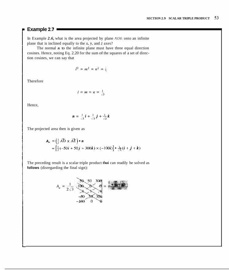
SECTION 2.9 SCALAR TRIPLE PRODUCT 53
Example 2.7
In Example 2.6, what is the area projected by plane ADE onto an infinite plane that is inclined equally to the x, y , and z axes?
The normal n to the infinite plane must have three equal direction cosines. Hence, noting Eq. 2.20 for the sum of the squares of a set of direc- tion cosines, we can say that
Therefore
Hence,
The projected area then is given as
A,, = (; A ~ I x AZ) - n = [ $ ( - 5 O i + 5 0 j + 3 0 0 k ) x ( - I O O i ) ] * - L ( i + . 3 j + k )
The preceding result is a scalar triple product that can readily be solved as follows (disregarding the final sign):

2.10 A Note on Vector Notation When expressing ryirations. we must at all times clearly denote sciilar and vectoi- qiiaiititics ;ind hmdlc them ;iccordingIy. When ire simply identify- ing quantities in il di.scu.s.sioii or in a rliugi-(irrm. however, instead of using the vector reprcscntation. I;. we can .just LISZ I.. On the other hand. / ~ ' w i l l be undcrstiiiid to rcprcscnt i n ;in equatioii the magnitude ol the vector F . Thu, using f i n thc itnit \'cctor in the direcIion of I>. w e can then say:
F = /'f
= b'lcos (I;. r)i + cos tF. ! ) j + co\ (F , : ) k ]
A \ another exaniplc. wc might wiiiit to employ the lorcc F, which i s shown in the coplanar diagr;im o f Fig. 2.32ia) al a kn~ iw i i i i i c l ina l i~n and acting a1 a point (1. A correct representation ol this Ii irce in a vector equation would he I.(-cos ai + sin aj).
As for \ c a lx components 01 any vecfor 1:. we shall adopt the following understanding. The I iot i l t im t';, h i , or t'; labeling some vector component i n a r/iu,y,-rinr wi l l hc undcrsloiid to rcprcscnt the niu,yi~ii~ide of that particular con- ponent. Thus, in Fig. 2.32(b) the two ctimponcnLs shown arc cqual in magni- tude hut opposite in sense. Ncvcrtheless. thcy xrc both Iahclcd F,. H11wever. in an cquetion inviilving these quantities. thc scnsc must propcrly he accounted for by the appropriatc usc o f signs.

2.63. If A = I O i + hj - 3k and B = 6i, find A x B and B x A . What is the magnitude of the resulting vector'! What are its direction cosines relative to the xyz reference in which A and B are expressed?
2.69. If the coordinates of vertex E of the inclined pyramid are ( 5 , SO, 80) m, what is the angle between Outward normals to faces A L E and BCE!
2.64. What are the cross and dot products for the vectors A and B given as: E
A = 6 i + 3 j + 4k B = Ri ~ 3j + 2k?
2.65. If vectors A and B in the xy plane have a dot product of SO units, and if the magnitudes of these vectors are I O units and R units, respectively. what is A x B ! 2.66. (a) If A * B = A - B'. does B necessarily equal E'?
Explain.
Explain. (b) If A X B = A X E, does B necessarily equal B"! Y
2.67. A to B times the displacement vector from C to D'!
What is the cross product of the displacement vector from
X
I Figure P.2.69
2.70. In Prvblem 2.69, what is the area of face ADE of the p y m mid? What is the projection of the area of face ADE onto a p l a ~ whose normal is along the direction 6 where:
C
X ' ~ = O . h i - 0.Rj
2.71. (a) Compute the product
/ ( A X B ) - C
Figure P.2.67 in terms of onhogonal components.
part (a). (b) Compute (C X A ) B and compare with the result i n 2.68.
normal to thc inclined surface ABC. Making use of the cross product, give the unit vector n
I 2.72. Compute the determinant
A r Ay A: B, gv B: c1 cy c:
where each row represents, respectively, the scalar components of A , B , and C. Compare the result with the computation of (A x B )
C by using the dot-product and crowproduct operations.
2.73. In Example 2.5, what is the area vector for GAB assuming a straight line connects points A and E ! Give the results in kilo- /
Figure P.2.68 meters squared.

Fixure P.2.71
2.11 Closure
Check-Oulfor Sections with t 2.1 What i s meant by thc n i u p i t ~ ~ k o fa vector? What sign iiwst i t hauc'? 2.2 Can you multiply a vector C by ii sciilar s ? If so, dcscribc the rcsull. 2.3 What are the Im, o f u m i w s and the law qfsiiirs'? 2.4 What i s nicaiil by the <rs.w(.iariw law of addition'? 2.5 Describe two ways to add ;my three vectors graphically. 2.6 How do you subtract vector D Srom vector F'? 2.7 Given a vector D , how would you forni a m i t vector collinear with D'! 2.8 What are the cciiliir equations 01 thc following vector equation'?
Di + E,j - Ihk = 20i + i I S + G)k

2.78. Flight 304 from Dallas is tlying NE to Chicago XJU miles away. To avoid a niilssive storm Srvnt, the pilot decides instead to Ily due north to Topcka, Kansas, and then ENE (see Fig. P.2.4 f ix compass settings) to Chicago. What are the distances that he must travel from Dallas to Topeka and from Topeka ti) Chicago'!
N
Chicago
Figure P.2.80
2.81. Cuntractori encountered an irnpasiahle swnmp while build- inp a road from town T to city C SO kin SE. To avoid the swamp, they built the road SSW from T and thcrr ENE to C. How long is the road? ( H i m : See the compass-settings diagram, Fig. P.2.4.)
45" E
Dallas Figure P.2.78
2.82. Sum all forces acting on the block. Plane A is parallel to the .r.v plane. We will later m d y the special properties of two par- allel forces (called a coupk) that are opposile in direction atid
2.79. the diiplaccrnent vector p,,,"'?
What is thc cross product between the 1,000-N force and in magnitude'
. I,11011 N / / " (3.4, - 2 ) -y
Figure P.2.79
Figure P.2.82
2.80. Four member, of a space frame are loaded as shown. What are the orthogunill scalar components of the forces on the ball joint at O? l h e 1,000-N force goes thmugh points D and E of the rectangular p;irallelepiped. its direction cosincc"
2.83. The r and I compunsnti of the force F arc known tu be 100 Ih and -311 Ib, respectively. What i q thc f k c F and what are
SI

,

500 Ib with a speed of 100 d s e c . What are the force components on the electron'? The charge of the electron is l.hOlX x coulombs.
400 Ib
s n
Figure P.2.92
Figure P.2.89 L. 2.90. heirht i of point A'?
A skeet shooter is aiming his gun at point A . What is the
7 A(2,15,z)m 2.93. For the line segment A X , determine zx and direction . cosines m and n.
Figure P.2.90 /--?
2.91. F, and F,
If F, and the 5 W N force sum vectorially to FT, determine / Figure P.2.93
2.94. Using the scalar triple product, find the area projected onto the dane N from the surface ABC. Plane N is infinite and is nor- mal to the vector
r = 50i + 40j + 30k ft
500 N
Figure P.2.91
2.92. is given as
The force on a charge moving through a magnetic field B
F = ~ V X B A Y
where q = inagnitude of the charge, coulombs F = force on the hody, newtons
x
Figure P.2.94 V = velocity vector of the pafiicle. meters per second B = magnetic flux density. webers per meter2 2.95. A 500-lh crate is held up by three forces. Clearly the three
forces should add up to a force of 500 Ib going upward. What Suppose that an electron moves through a uniform magnetic field of IO" Wh/mz in a direction inclined 30' to the field, as shown,
should forces F , and F, he for this condition'? All forces are coplanar (in the same plane).
59 I

2.100. What i s thc anglr S hclwccn r and the displaccmcnt !hl Il a hze-bee gun i s to sliont down thc ballowi, assun- ing i t is morncnlarily slali<mary ill C. what arc thc direction corinrs ol the prupcr lint. r i f sight?
" C C t O l p,,,,.!
Figure P.2.96 Figire P.2.100
60

Important Vector Quantities
z
3.1 Position Vector In this chapter, we shall discuss a number of useful vector quantities. Con- sider first the path of motion of a particle shown dashed in Fig. 3.1. As indi- cated i n Chapter I, the di,splacemenr vecfor p is a directed line segment connecting any two points on the path of motion, such as points I and 2 in Fig. 3.1. The displacement vector thus represents the shortest movement of the panicle to get from one position on the path of motion to another. The purpose of the rectangular parallelepiped shown in the diagram is to convey the magnitude and direction of p as explained earlier. We can readily express p between points I and 2 in terms of rectangular components by noting the distance in the coordinate directions needed to go from I to 2. Thus, in Fig. 3.1, p l r = -2i + 6 j + 3k m.
The directed line segment r from the origin of a coordinate system to a point P in space (Fig. 3.2) is called the position vector. The notations R and p
magnitude of the position vector is the distance between lhe origin 0 and point P. The scalar components of a position vector are simply the coordi- nates of the point P. To express r in Cartesian components, we then have
Figure 3.1. Displacement vector p hetween points 1 and 2.
are also used for position vectors. You can conclude from Chapter 2 that the )/; . o j Y x
x
Figure 3.2. Position vector.
r = x i + y j + zk (3.1) y"\! __---
We can obviously express a displacement vector p between points 1 and 2 (see Fig. 3.3) in terms of position vectors for points 1 and 2 (Le., r , and r2) as follows:
__ p = r? - r , = (x2 ~ x , ) i + cy2 ~ y , ) j + ( z , - z , jk ( 3 . 2 )
Figure 3.3. Relation hetween a displacement vector and position Yectors.
61

62 ("AFTER 3 IMI'ORTANT VECTOR QUANTITIES
Example 3.1
Two bets ul' refercnces. .YK and XYZ. arc shown in Fig. 3.4. The position vector ol the origin 0 o l r y : rclative to XYZ is given as
R = IOi + 6j + Sk m (a)
r' = 3i + 2.1 - hk m (h) What is the position vector r of point f' relative ti1 .v?i? What arc the coor- dinates .I, y. and i of I"?
The position vector. r'. i f a point P relative t i l XY7 is
From Fig. 3.4. i l is clear that
r ' = K + r I C 1
Therefore.
r = r' -- R = (3i + Z j - 6 k ) - ( I O i + hJ + Sk)
r =-7 iL4 j - I l k m I4
X' We can then conclude that
x = -7m y = -4m z = -11 m
Figure 3.4. Refercnccs .q; and X ) % scpamtcd hy position vector it. (c)
t" 3.2 Moment of a Force About a Point Case A. For Simple Cases. The moment of a force about a point 0 (see Fig. 3.5). you will recall from physics, is a vector M whose magnitude equals the product of the force magnitude times the perpendicular distance d from 0 to the line of action of the force. And the direction of this vector is perpendicular to the plane of the point and the force, with a sense determined from the familiar right-hand-screw rule.' The line of action of M is determined by the prohlem at hand. In Fig. 3.5, the line of action of M i s taken for simplicity through point 0.
Case B. For Complex Cases. Another apprwach is to employ a position vcctcir r from point 0 to nnypoinf P along the line ol'action of force F as shown in Fig. 3.6. The nioment M of F about point 0 will he shown to he given as1
M = r x F ( 3 . 3 )
Figure 3.5 Moment 0 1 force F nhoul 0 is F d

SECTION 3.2 MOMENT OF A FORCE ABOUT A POINT 63
For the purpose of forming the cross product, the vectors in Fig. 3.6 can he moved to the configuration shown in Fig. 3.7. Then the cross product between r and F obviously has the magnitude
lr X FI = /rl IF\ sin a = IF1 lrl sin p = IF1 r sin f i = Fd where r sin f i = d, the perpendicular distance from 0 to the line of action of F , as can readily he seen in Fig. 3.7. Thus, we get the same magnitude of M as with the elementary definition. Also, note that the direction of M here is identical to that of the elementary definition. Thus we have the same result as for the elementary definition in all pertinent respects. We shall use either of these formulations depending on the situation at hand.
The first of these formulations will he used generally for cases where the force and point are in a convenient plane, and where the perpendicular distance between the point and the line of action of the force is easily mea- sured. As an example, we have shown in Fig. 3.8 a system of coplanar forces acting on a beam. The moment of the forces about point A is thenZ
MA = -(5)(1,000).4 - (4)(600)k + (11)R,k ft-lb = ( I IR, - 7,400)k ft-lb
x
Figure 3.6. Put r from 0 to any point along the line of action of F .
Figure 3.7. Move vector r end F
Figure 3.8. Coplanar forces on a beam
For a coplanar force system such as this, we may simply give the scalar form of the equation above, as follows:
MA = IIR, - 7,400ft-lh The second formulation of the moment ahout a point, namely r X F ,
is used for complicated coplanar cases and for three-dimensional cases. We shall illustrate such a case in Example 3.2 after we discuss the rectangular components of M.
Consider next a system of n concurrent forces in Fig. 3.9 whose total moment ahout point 0 (where we have established reference xyz) is desired. We can say that
M = M , + M , + M , + . . . + M n
= r x F , + r x F , + r X F , (3.5) + . . . + r x F,
‘Please nole that we still use lhe right-hand-screw rule in determining Ihe signs of the respective moment% Figure 3.9. Concurrent forces

Now. hecause (if the distrihutive pixipei-ty of the c r w s product. Eq. 3.5 can he bvrittcn
M = r X (6 + F, + F3 + . . . + I;,,) (3.61
Wc ciin conclude iriii i i the preceding eqiiatioiis that thc s u m of the minimits ahout it point of a system of concurrent fixcss i s the same iis ihc ~iionicnt ahout tlic point of the \un i 01 rhc force^. l h i r i-esul~ i s kiiinvn iis \'uri,qmm'v I/i('ofwi~. which y>u may UCII reciill Srofii physics.
Ax ii hpccial ca\c of Varigniin's thcorcni, we inay find i t convenient io deconipose a iorcc F inti1 i h rcclangular ciimpiincnts (Vi;. 1. IO). and tticn to i ise these coniponents ior taking iiioiiieiits ahwt ;I point. Wc cim Ihrn s;ly that
( 3 . 7 ) M = r x F = r x (P; i + /I./ + F k )

SECTION 3.2 MOMENTS OF FORCE ABOUT A POINT 65
Example 3.2
Determine the moment of the 100-lb force F , shown in Fig. 3.11, about points A and E , respectively.
As a first step, let us express force F vectorially. Note that the force is collinear with the vector pljE from D,, to E, where
pllK = X i + 4j - 4k To get a unit vectorp in the direction of P , , ~ . we proceed as follows:
Figure 3.11. Find moments at A and 8. (b) P,], Xi + 4 j - 4k - = ~
lPDE/ is2 + 4 2 + 42 = .X16i + .408j - .408k
We can then express the force F in the following manner:
F=I.'pf,,=(100)(.816i+.408j-.40Xk)
=81.6;+40.Xj-40.8k (c)
To get the moment MA about point A, we choose a position vector from point A to point D which is on the line of action of force F. Thus, we have, for cn,
and for MA, we than get G~~ = IOi + 4j - Xk ft (d)
MA = r A , , X F = ( 1 0 i + 4 j - 8 k ) X (81 .6 i t40 .8j -40 .8k) =I% ,
- m, W.6 40.8 - .
= (10)(40.8)k + (Xl.6)(-8)j + (4)(-40.8)i -(-8)(40.8)i - (40 .8) (10) j - (4)(81.6)k
Therefore. MA = 163.21 - 245j + X1.6k ft-lh (e)
As tor the moment about reference point E , we employ the position vector rBI, from B to position D, again on the line of action of force F. Thus, we have
rHfj = 4j - Xk ft Accordingly,
M , = rHIl x F = (4j - Xk) x (81.6i + 40.Xj - 40.8k) = (4)(81.6)(-k) + (4)(-40.8)(i) + (-X)(XI,6)(j) + (-X)(40.8)(-;) (t)
MB = 163.23 - 653j - 326k fklb

3.1. What is thc position v e c t ~ r r from the origin (0, 0, 01 to the poinl (3, 4, 5 ) ft'! What are its magnitude and direction cosines?
3.2. to position ( I O , --3, 4) ft'?
3.3. A surveyor determines that the top 0 1 a radir, transmission tower is at position r, = (1,OOOi + I,OOOj + 1,000k) m relillivc :(I her position. Similarly. the top of a sccond tower is locatcd hy 5 = (2,000i + 500j + 700k) m. What is the distance hetwcen .he two tower tops?
3.4. Reference XJZ is rotated 30" counterclockwise about its ~i
rxis to form reference XYZ. What is the position vector r for refer- :nce xyz of a point having a position V C C ~ O I r' h r rcfcrencc X Y 7 :iven as
What is the displacement vector from position 16. 13, 71 f t
r' = hi' + 107 + 3k' m ?
3sc i , j , and k (no primes) lor unit vectorb auaciatcd with refer- :nce 1y7.
1.5. ind ahwl support A of the simply supported hzam.
Find the momcnt of thc SO-lb forcc ahout the support at A
- 61)'- )--- 100'----t
Fieure P.3.S.
1.6. hen ahout point R.
Find the moment of the two lorces first ahout point A and
(a) Do not use r X F fbrmat-only scalar prodncts. (h) lJsc vector approach.
I,OOO N
x
-2m---,
Figure P.3.h.
3.7. A particle mmes along ii circular path in the xy plane. What is the position vector r of this p;irticle as ii function of the wordi. nxte r"
I I
Figure P.3.7.
3.8. A particle moves along a paraholic path i n thc i; plane. If the particle has a1 ow point n pmition vrctii i r = 4 j + Zk, give the piisition ~ c c t o i ~ a1 any point on Ihe path i i i ii fimotion of Ihr : c o w din;ilc.
v
Figure P.3.8.
3.9. An nnillery spotter on Hill 350 (350 rn high) eqimiltes the posirioii o i an cncmy tnnk as 3.000 m NE of him at a n CIcvat im
200 m helow hi? position. A 105-nim howmer unil with n range of I1.(100 m i s 10,1100 m doc south oltht . spotter. and il 155-mm howitm unit with a rangu of 1.000 m is 11,001) m SSE o l t h r spottcr (rce Fig. P.2.41. Both gun units are located at an elevation OS 150 111. Can eil l irr o r hoth gun uni t , hit thc tank, o r r m w t an air mike be callcd in?

3.10. Find the moment of the forces about points A and B . (a) Use scalar approach. (b) Use vector approach.
Figure P.3.10.
3.11. The crew of a submarine patrol plane, with three-dimen- sional radar, sights a surfaced submarine 10,000 yards north and 5,000 yards east while flying at an elevation of 3,000 ft above sea level. Where should the pilot insmct a second patrol plane flying at an elevation of 4.000 ft at a position 40,000 yards east of the first plane to look for confirmation of the sighting?
3.12. A power company lineman can comfortably trim branches I m from his waist at an angle of 45” above the horizontal. His waist coincides with the pivot of the work capsule. How high a branch can he trim if the maximum elevation angle of the arm is 75“ and the maximum extended length is 12 m?
1.5 m Figure P.3.12.
3.13. The total equivalent forces from water and gravity are shown on the dam. (We will soon be able to compute such equiv- alents.) Compute the mnment of these forces about the toe of the dam in the right-hand comer.
(Asrume a11 forces
8’ k + L - I ‘Toe
Figure P.3.13.
3.14. In an underwater “village” for research. an American flag is in place as shown. It is of plastic material and can rotate so as to be oriented parallel to the flow of water. A uniform friction force distribution from the flow is present on both faces of the flag hav- ing the value of 10 N per square meter. Also the flagpole has a uniform force from the flow of 20 N per meter of length of the flagpole. Finally there is an upward buoyant force on the flag of 30 N and on the flagpole of 8 N. What is the moment vector of these forces at the base of the flagpole?
Figure P.3.14.
3.15. Three transmission lines are placed unsymmetrically on a power-line pole. For each pole, the weight of a single line when cov- ered with ice is 2,ooO N. What is the moment at the base of a pole?
Figure P.3.15.
67

3.22. What i \ the moment of a IO-lh I w c e F directed ;ilonf lhe di:igmaI of a cuhr ahout thc c ~ m c n of the cuhc'! 'The sidc 01 thc w h c i s (i I t .
3.17. A truck-mounted crane has a 20-m hrxnn inclincd a1 60" to the horizontal. What i \ the moment ahout the honm pi\ot due to a liftcd wcight of 30 k N ? Do hy vector and hy scilliii~ methodi.
Figure P.3.22. 3.23. Three guy wi res are used in the suppon syslem lor a trle- \ i s i o n transmicrion towcr that i \ h0O m tal l . Wircb A and R arc tiphtcnrd to a tzmion o f hO LN. whereit\ w,irc C has i inly 30 kN 01
Figure P.3.17. tcmion What i s thr nomrnt 01 h e wire I w c v a h w l the hax 0 o f lhe tower'i Thc y :,xi\ i': ciillincar with AO.
3.18. A small hlirnp i s lempr,l-arily mrxrred as shown in the d i i i -
gram wherein / I C and the centerline of AH arc coplanar. A force F from wind, weight. and buoyancy i s shown ;sling ill Ihc centerline of the hlirnp. I t
I F = 5i + l l j + IXk kN
what are the moment w c t m from F ahwt A. N. and c?
I hi1 111
Figure P.3.18.
68
Fipre P.3.23.

3.24. Cables CD and AB help support member ED and the I ,000-lb load at D. At E there is a ball-and-socket joint which also supports the member. Denoting the forces from the cables as Fer, and FAB. respectively, compute moments of the three forces about point E. Plane EGD is perpendicular to the wall. Get results in terms of Fro and T,r
Figure P.3.24.
3.3 Moment of a Force About an Axis Case A. For Simple Cases. By means of a simple situation, we shall set forth a definition of the moment of a force about an axis. Suppose that a disc I s mounted on a shaft that is free to rotate in a set of bearings, as shown in Fig. 1.12. A force F, inclined to the plane A of the disc, acts on the disc. We decompose the force into two coplanar rectangular components, one normal to plane A of the disc and one tangent to plane A of the disc, that is, into forces FB and 5, respectively, so as to form a plane shown tinted, normal to plane A.
We low
Figure 3.12. 5 turns disc
)m experience that Fs does not cause : disc rota1 know from physics and intuition that the rotational motion of the disc is
69

70 CHAPTER 3 IMPORTANT VEC'TOR Ol~\Wl'l'llliS
delermincd by the product (if F;1 and the perpendicular distance d Imm the centerline (if the shaft to the line of action of F4. You wi l l remember from physics, this product i s nothing more than t l ie mmncnt 01. force F ahout the axis (if the shaft. We sliall next generalire from this simple case tn the general case o f taking Ihc moment d'un\. force F ahout ow? axis.
To compute the moment (or tnrque) of a force F i n a planc perpendicular to plane A ahout an axis B-B (Fig. 3.13). we pass any plane A perpendicular to the axis. This plane cuts i3-R a1 (I and thc line of action of forcc Fat some poini P. 'The fnrce F i s then pro.jectcd to fomi a reclmgular component r;, along ii
line at P normal 10 plane A and t l i i is parallel tu R-B. a s shown in the diagram. 'The intersection of plane A with lhe plane of Snrceh F,$ and F (the latter plane ih
shown shaded and i h a plane throush F and pcrpeiidicular to plane A ) sives ;I direction C-C along which the other rcclangular component of I.: denoted :is ti. can he projected." The moment of F about the line 8 - ~ B i s then defined as the scalar reprcsentation of the mnment of lj ahout point ( I with a inagnitude equal to <</--a prcihlcni discussed a1 the heginning OS the previous section (Case A). Thus in accordance wilh the definition, the component kjr which i s parallel to the axis 11-8. contributes 110 moment about the i ixis, and wc may say:
H '
Figure 3.13. F(1rmula% the mOll1ellt ahout an axis R -8.
Mnment ahout ax i s B-H = l<)ldl = (cos a) (d)
with nn appropriate sign. The moment about an ax is clrarly i s a scalar. evcn though this niomcnt i s associated with a particulx axis that has ii distinct direction. 'The situation i s the same as it i s with the scalar components V,, V,. v, etc.. which arc associated with certain directinns but which are scalar\. The reader wi l l he quick to noLe that Fig. 3.13 reprchents ii generalization (it Fig. 3.12 having an axis H-B. a plane A normal to this axis and fillally an arhitrary force E To explain further. we have redrawn Fig. 3.13 Isec Fig. 3.14Ia)l showing only plane A , axes R-R and C-C, and the force I;. In Fig. 3.14(h), we have also included the moment vector M . This latter diagram then takes us back Lo Fig. 3.5 where wc first defined the moment vector o f . 'I 1. nrce ahout a point in a most simple manner. Accordingly, we note, nn the cine hand. for the moment ahout point (I [scc Fig. 3.14(b)], we can get the vector M , whereas 011 the other hand i n Fig. 3.I4la) we can get the scalar iiiomciit M ahout an axis B-8 at point n and perpendicular to planc A . Thus, by taking the scalar value ofM in Fig. 3.14(b), wc get the moment about the ax is at puint ( I
normal to plane A as formulated in the development of Fig. 3. 13.
Figure 3.14. Comparison of Figs. 3.13 and 3.5.

SECTION 3.3 MOMENT OF A FORCE ABOLIT AN AXIS 7 1
We can thus conclude, on considering Fig. 3.15. that the moment of F about point C can be considered in two ways as follows:
Figure 3.15. Consideration of the moment of F about point A .
Before continuing, we wish to point out that 4 in Fig. 3.13 can be decomposed into pairs of components in plane A. From Varignon's theorem we can employ these components instead of 6 in computing the moment about the B--B axis. For each force component, we multiply the force times the perpendicular distance from a to the line of action of the force component using the right-hand-screw rule to determine the sense and thus the sign.
Case B. For Complex Cases. When we discussed the moment of a force about apoint, we presented a formulation useful for simple cases (i.e., a vector of magnitude Fd) as well as a more powerful formulation that would be needed fix more complex situations (Le., r x F ) . Thus far, for moments about an axis, we have presented a formulation Fd that is useful for simple cases? and now we shall present a formulation that is needed for more com- plex cases. For this purpose, we have redrawn Fig. 13.13 as Fig. 13.16(d). In Fig. 13.16(b), we have shown axis B-B of Fig. 13.16(a) as a n n axis and have set up coordinate axes y and z at any point 0 anywhere on axis B-B. The coordinate distances x, y . and z for the point P are shown for this reference. The position vector r to P is also shown. The force component FH of Fig. 3.16(a) now becomes force component F,. And, instead of using FA, we shall decompose it into components <. and 4 in plane A as shown in Fig. 3.16(b). We now compute the moment about the x axis for force F using this new arrangement which does not require F to be in a plane perpendicular to plane A . Clearly, F, contributes no moment, as before. The force components <. and 5 are in plane A that is perpendicular to the axis of interest and so, as before in the case of 5, we multiply each of these forces by the perpendicu- lar distance of point a to the respective lines of action of these forces.
'That is. for cases where the force and point in question are in a plane easily seen to he nor^
mal to the ru-is in question. thus allowing for an easy determination of the perpendicular distance between the point and the line of action of the force.

72 CHAPTER 3 IMPORTANT VECTOR amNri-r iEs
, "
For Sorce t;.. this pcrpcndicular distance i s clc;irly x. a h can rcadily be the diagmni, and, lor force E ; , this perpendiculx distance i s :. Using the right- hand-scrcw rule fiir :isccrt;iining ll ic sense oleach o i the momenls. wc: can say:
~ii~iiieiit ahout~raxis = IxF - :.f< j (3.10)
Were we to hikc moments OFF ahout the origio 0, wc \vould get (scc Eq. 1.8)
M = M , i + M , j + M : k = r x F
= IyF - : F : ) i + iC1.i - x F ; ) , j + (.r/,; - yF\;,)h (3.1 I )
Comparing Eqs. 3.10 arid 3.1 I. wc ciin conclude that tlie i i io i i ie i i l about the .I
axis i s simply M , . 1he.v coiiilionent o l M about 0. We ciin thus concludi: that the moment about the .v axis 01 the Iilrce F is ihc component in the .\ direction of the moment 0 1 F about a point 0 positioned m~wlwrc , along the I axis, T ~ I is.
moment ;ihout 1 ax is 7 M, = M,, - i = ( r X F ) * i (1.12)
We may generali/e tlie preceding discussion iis Iollows. Consider iiii arbitral-y axis i i-i i to which we have ;is\igned a unit vector 11 (Fig. 3.17). An uhitrary force I; i\ a l m shown. 'lo gut the iiioiiicnl M,, of I'orcc F ahout axis 11-PI. \\e clioosc any point 0 along 11-11. Then draw ii pos i th i vector r Iron1 point 0 to
any point dong Ihc line 01 ; d u n of F. Thih h a been shown i n [he diagraiii. We can then hay. fironi our prcvious discussion.
+~/ Figure 3.17. M,, = ir X F) * 12.
/'
M,, = (r X I;) - n (3.13)

SECTION 3.3 MOMENT OF A FORCE ABOUT AN AXIS 13
(Notice from Eqs. 3.12 and 3.13 that the moment of a force about an axis involves a scalar triple product.) Equation 3.13 stipulates in words that:
The moment of a force about an axis equak the scalar component in the direction qf the axis of the m m e n f vector taken about any point along the axis.
This is lhe more powerful formulation that can he used for complex cases.
Note that the unit vector n cdn have two opposite senses along the axis n, in contrast to the usual unit vectors i, j, and k associated with the coordinate axes. A moment M,, about the n axis determined from M * n has a sense con- sistent with the sense chosen for n. Thdt is, a positive moment M,, has a sense corresponding to that of n, and a negative moment M,, has a sense opposite to that o fn . If the opposite sense had been chosen for n, the sign of M n would be opposite to that found in the first case. However, the same physical moment is obtained i n both cases.
If we specify the moments of a force about three orthogonal concurrent axes, we then single out one possible point in space for 0 along the axes. Point 0, of course. is the origin of the axes. These three moments about orthogonal axes then become the orthogonal scalar components of the moment of I; about point 0, and we can say:
M = (moment about the x axis)i + (moment about they axislj + (3.14) (moment about the z axis)k = M,i + MJ + M:k
From this relation, we can conclude that:
The three orthogonal components ojthe moment of a force about a point
the point as an origin. are the muments of this force about the three o e
You may now ask what the physical differences are in applications of monients about an axis and moments about a point. The simplest example is in the dynamics of rigid bodies. If a body is constrained so it can only spin about its axis, as in Fig. 3.12, the rotary motion will depend on the moment of the lorces about the axis of rotation. as related by a scalar equation. The less familiar concept of moment about a point is illustrated in the motion of bod- ies that have n o constrhints, such as missiles and rockets. In these cases, the rotationiil motion of the body is related by a vector equation to the moment of forces acting on the body about a point called the center ofmass. (The center of mass will he defined completely later.)

14 CHAPTER 3 IMPORTANT VECTOR QUANTITI~S
Example 3.3
Coinpiitc the moment of a force F = 1Oi + hj N. which gocs through po5ition cz = 2 i + 6.j in (see Fig. 3.181, about a line going through points I and 2 having the respective position vectors i
! I
rl = hi + I O j - i k in r, = -3i - 12j + 6k in
T u compute this moment. we can take the moment o f F about either
direction of the displacement vector hetween I and 2 or between 2 and I. Mathematically, wc have, using a displacement vector from point I tu point u. namely (c, - r , ) .
.. point I or point 2, and then rind the component or this vector along the /' -. r,'
Figure 3.1X. Find momenl d F ahout line.
M = Iir,, - r , ) x FI * fi ( 3 ) I'
where i j i s the unit vector along thc line chosen to have a sense going from point 2 to point I. The formulation ahove i s the scda r triple product exani- incd in Chapter 2 and we can usc the determinant approach for the calcu- lation m c e the components 01 the vectors (r,, - rl). F , and i j have been determined. Thus. we have
i r(! - rI = ( 2 i + 6 j ) - (h i + lO j - i k ) I
= -4i - 4.j + 3k m
F = IOi + 6 j N
= .354i + X66 j - .354k
We then have, for M,,:
3~ ! -4 -4
10 h 01 = 13.94 N-m ib) i
i i :
i !
Mp = I 354 ,866 - . 1 d #
Because M,, i s pobilive. wc have a clockwisc inoiiieiil about thc line as we look from point 2 to point I . I 1 we had chosen p lo have an opposite sense, then M,, would have been computed a s -13.94 N-in. Then. we would con- cludc that MI, i s a coiintcrclockwix rniimcnt about the line a s one looks from point I to point 2. Note that the same physical inoinent i s determined in both cases.

SECTION 3.3 MOMENT OF FORCE ABOUT AN AXIS 75
M , =
Example 3.4
A deep submergence vessel is connected to its mother ship by a cable (Fig. 3.19). The vessel becomes snagged on some rocks and the mother ship steams ahead in a forward direction in an attempt to free the sub- merged vessel. The connecting cable is suspended from a crane directed up over the wdter 20 m above the center of mass of the mother ship and 15 m out from the longitudinal axis of the mother shim The cable transmits a
0 -15 20
1 0 0 -144 -52.4 -128.6 kN-m
I
force of 200 kN. I t is inclined 50" from the vertical in a vertical plane which. in turn, is oriented 20" from the longitudinal axis of the ship. What is the moment tending to cause the mother ship to roll about its longitudi- nal axis (].e., the x-axis)?
The position vector from the center of mass C to point A is
r = -1Sj + 2 0 k m

3.25. Disc A has a radius of 600 mm. What i s the moment of the %rces ahout the center of thc disc? What i s the torque of thew brces ahout the axis of the shaft'!
3.29. blimp i s
A blimp i\ moored to a tmvcr at A. A forcc on A Irmr th ib
F = Si + 3 j + I.Xk kN
I What i s the moment ahaut tixis C ' c m the gmund'! Knowledge 01 this m o m c ~ ~ t and othcr ni~nirnt\ at the bas t is nreded to pnqxrly dchign the fciundation of the tower.
I I\N
Figure P.3.25. /2 k N
L2h. A fmce F acts at position (3 , 2, 0) f t . It I S in thc ,Q planc md is inclined at 30" from the I axis with a s c n x directed away rom the origin. What is the momcnt of this force ahout an axis ping through thc paints (6, 2. 5 ) ft and (0, -2. -3) f t ?
1.27. A force F = IOi + C r j N goes through the origin of the .uordinate system. What is the nioment 01 this fircr F about an !xis going through points I ;md 2 with position vcctors?
A /
c, Figure P.3.29.
r , = 6i + 3k m r2 = 16j - 4 k m
1.28. Given a forcc F = IOi + 3j N acting at posirion = S j + I0k ni, what i s the turquc ahout the diagonal showti iii
3.30. Compute thc thrurt 01 the applicd tnrcci shown aluog the axis nf the rhair and the torque of the firrcr? about the a x ~ s of the shaft.
100 Ih . . . .. he diagram? What i? the t n ~ m e n t about point E!
L)
3 m
,...t...-;h,--i Figure P.3.30.
2 m
Figure P.3.28.
3.31. What i s the milximuni load W that the craiic c u i lift witli- out tipping about A'! Hirrr: when tipping is irnpcnding, what i s Lhc suppoiring force tit thc wheel at IT!
'6

3.34. The base of a Sire truck extension ladder is rotated 75” counter-clockwise. The 25-m ladder j s elevated 60‘ from the hor- izontal. The ladder weight is 20 kN and is regarded as concen- trated at a point I O m up from the base (the lower part of the ladder weighs much more than the upper part). A 9 0 - N fireman and the 500-N young lady he is rescuing are at the top of the lad- der. (a) What is the mument at the hase of the ladder tending to tip over the fire truck’! (b) What is the moment about the horizontal axis having unit vector 6 shown in the diagram?
L .x
Figure P.3.31.
3.32. hetween points D and C.
Find the moment of the I ,000-lh force about an axis going
Figure P.3.32.
3.33. forces about axis CD?
In Problem 3.24, what is the mumenr of the three indicated
View A-A Figure P.3.34.
3.4 The Couple and Couple Moment I A\,-F y
A special arrangement of forces that is of great importance is the cuuple. The cuuple is formed by any two equal parallel forces that have opposite senses (Fig. 3.20). On a rigid body, a couple has only one effect, a “turning” action. Individual forces or combinations of forces that do not constitute couples may “push” o r “pull” as well as “turn” a body. The turning action is given quantitatively by the moment of forces about a point or an axis. We shall, accordingly, be most concerned with the moment of a couple, or what we shall call the couple moment.
1
Figure 3.20. A couple.
I1

78 CHAI'PdK 3 IMI'OKrANT VECTOR QUANTITIES
Let us now evaluate the moment of the couple about thc vrigin. Posi- tion vectors have heen drawn in Fig. 3.21 to points I and 2 anywhere along the respective line OS action of each force. Adding the monient of each force about 0, we have f i r the couple moment M
e = 1rl-r:)
-F
M = rl x F + rL x ( -F) (3.15)
= (rl - r.) x F
We can see that (rl - r , ) i s a displacement vector between points 2 and I, and if we call this vector-e, the formulation above hecomes
Figure 3.21. Cornpule ~ i i i m c n ~ of couplc M = e X F 13.16) abuut 0.
Since e i s i n thc planc o f the couple. i t i h clear froin thc dcfinition of a cross product that M i h in an i r i en ta t i~n norinal to the plane o S the couple. The sense in this case may he seen in Fig. 3.22 to he directed downward. in accor- dance with the right-hand-screw rule. Notc thc use of the double arrow to rep- resent the ciiuple miiment. Note also that the riitatiiin of e to F , a s stipulated in the cross-product lormulation, i s i n the siiiiie direction as the "turning" action u t the two force vectors, and from now vn wc shall use the latter crite- rim for determining the sense of r~ ta t i on to he used with the right-hand- screw rule.
M Figure 3.22. I he cuuplc moment M
Now that the direction of couplc ~nornent M has hem established for the couple, wc need only compute the niagnitude for a complete description. Points I and 2 may be chosen anywhere along the lines of action of the forces without changing the resulting moment. since the forces arc transmissible for taking moments. Therefore, to compute Ihc magnitude 01 the ciiuple moment vector i t wi l l be simplest to choose positions I and 2 s o that e i s prpendiru- lar to the lines of action of the forces (e i s then dcnvted as eL). From the def- inition of thc cross product, we can then say:
(3.17)
where the more familiar notation. (1. has been used in place v1 lell as the per- pendicular distance hetween the lines of action 01 the forces.
IMI = lell IF! sin '10" = led = IFId

SECTION 3.5 THE COUPLE MOMENT AS A FREE VECTOR 19
Note that in the computation of the moment of the couple about origin 0, the final result in no way involved the position of point 0. Thus, we can assume immediately that the couple has the .same moment about every point in space. More about this in the next section.
3.5 The Couple Moment as a Free Vector Had we chosen any other position in space as the origin, and had we com- puted the moment of the couple about it, we would have formed the same moment vector. To understand this, note that although the position vectors to points 1 and 2 will change for a new origin O‘, the difference between these vectors (which has been termed e ) does not change, as can readily be observed in Fig. 3.23. Since M = e X F, we can conclude that the couple hus the sume momenr about every point in space. The particular line of action of the vector representation of the couple moment that is illustrated in Fig. 3.24 is then of little significance and can be moved anywhere. In short, the couple moment is n free vecror. That is, we may move this vector anywhere in space without changing its meaning, provided that we keep the direction and magnitude intact. Consequently, for the purpose of taking moments, we may move the couple itself anywhere in its own or a parallel plane, provided that the direction of turning is not altered-i.e., we cannot “flip” the couple over. In any of these possible planes, we can also change the magnitude of the forces of the couple to other equal values, provided that the distance d is simultane- ously changed so that the product IFld remains the same. Since none of these steps changes the direction or magnitude of the couple moment, all of them are permissible.
Figure 3.23. Vector e is the same for both references.

80 CHAPILR 1 IMI'OKTANT VFCTOR OI'ANTITIFS
As we pointcd out ciirlicr. the only effect of a couple on ii rigid hody i s
i t s turning action. which i s represented quantitatively by lhc miimcnt of the couple-i.c., thc ciiuplc iniimcni. Since this i s its sole effect. it i s only naturiil to represent the couple hy specifications of i t s moment; i ts magnitude. then. becomes IFId and its direction that of i t s monient. Thi\ i h tlic siliiic a s identi- lying a person by Iicrlhih joh (i.e., its :I teacher. plumber, etc.). Thus, in Fig. 1.24. the cmiple niiiment C inay he used to seprcmit the indicated couplc.
3.6 Addition and Subtraction of Couples loo lh-ft
Since couples thcinscl\,cs liavc x r o iiet lorccs. addition per se of coiiplcs alw;iys yields 7ei-c lorcc. Fur this rciis1111. the ;iddition and suhtsactioii of ciiuples i s interpreted to i i ieai i ;idditiiin and subtsaction 01 the t?zotnwii.s of thc couples. Since ciiuple nioniciits arc lrec vector\. we ciiii tilways arrange to have a concurrent system 01 vector\. We r h l l iiow tahe the iipportuiiity ki
illustrate inany 01 the ciirlies remarks about couples by adding the two couples \tiown on the face 111 the cuhe iii I"g. 3.25. Noticc that the couple miiment vectors 01 thc couples have heeii drawn. Sincc lliese vectors arc frcc. lhey may be moved ttr ii convenient position and then added. The total couplc inoiiienl llirii hcciimcs 103.2 lh-ft i i t an anglc 111 16- with the Iiorimiitill. as shown in Fig. 3.26. The couple that crcatcs [hi\ lusning action i s in ;I plane at right ;inglcs ti) thih oriciitation with ii cli>chwise senw iis (ihscrvcd froin below.
25 Ib-I1
100 lh-It 4 103.? lh-li Figure 3.25. Add cr~ ip les .
25 Ih-ft

SECTION 3.6 ADDITION AND SUBTRACTION OF COUPLES 8 1
This addition may be shown to he valid by the following more elemen- tary procedure. The couples of the cube are moved in their respective planes to the positions shown in Fig. 3.27, which does not alter the moment of the couples, as pointed out in Section 3.5. If the couple on plane B is adjusted to have a force magnitude of 20 Ib and if the separating distance is decreased to 514 ft, the couple moment is not changed (Fig. 3.28). We thus form a system of forces in which two of the forces are equal, opposite, and collinear and, since these two forces together cannot contribute moment. they may he deleted. leaving a single couple on a plane inclined to the original planes (Fig. 3.29). The distance between the remaining forces is
425 + ft = 5.16ft
and so the magnitude of the couple moment may then be computed to be 103.2 Ib-ft. The orientation of the normal to the plane of the couple is readily evaluated as 16" with the horizontal, making the tntal couple moment identi- cal to our preceding result.
Figure 3.27. Movc couplcs.
Figure 3.28. Change values ol two furcea.
Figure 3.29. Eliminate collincnr 20-lb f0VXS.
A common notation for couples in a plane is shown in Fig. 3.30. The values given will be that of the couple moments.
Figure 3.30. Repressentiltiun of couple moments in a plene.

82 C H A P T ~ K i IMPORTANT VECTOR Q U A N T I T I ~ S
Example 3.5
Replace the system of forces and couple shown in Fig. 1.31 by ii single couple moment. Note that the 1.000-N-in couple m ~ m c i i t i s in thc diago- nal plane ABCD. As a first step in the prohlem. identify ii second couple moment i n addition to the couple moment i n the diagonal plane.
Examine the vertical forces. There i s an upward sun) of 1.700 N clearly not colinear with the downward 1,700-N force. These forces form the second couple. To gel the couple moment for these forces. we take m~imcnts ol these forces about the origin as follows:
C , = 3k x 80Oj + ( 3k + 2;) x (700 - 17O(l)j + 2; x 200j = 600; - 1.600k N-m
As for the I ,000-N-ni couple moment. wc look in it direction along lhe .\ axis toward the origin as shown in Fig. 1.32.
The angle a in Fig. 3.32 i s given as follows:
tan a = 314 :_ a = 36.87''
Hence we have fix the second couplc moment C,.
C , = -1,000 cos 36.87"k + I.000 sin 16.87'j = -800k + 6OOj N-m
Now we can add the two couple moments to get C,,,,,.
C , , , , = C , + C2 = (600; - 1,600k) + (-800k + 600j)
CmAL = 6001 - 2,400k N-m Figure 3.32. View along the .I a i \ .
Figure 3.33. To tind moment of F ahout A-A.
Figure 3.34. 10 find moment of couple about A-A.
3.7 Moment of a Couple About a line In section 3.3. we pointed out that the moment of a force I: about a line A-A (see Fig. 3.33) i s fiiund by first taking the moment of F about or!? point P on A - A arid then dotting this ifector into a. the unit bector along the l i i ~ Thai is,
M,,,, = ( r X F ) * a (3. lX)
Consider now the moment i i f a couple about a liiic. For this purpose, we show a couple niomeiit C and line A-A in Fig. 3.13. As belirrc, wc Irrst want the nioineiit of the couple about any point P along &,l. Hut the inomcnt of C ahout ever? point in space i s simply C itself. Therelore, tu gel the moment aboul thc line &A all we nccd to do i s dot C into a . Tho\,
h ~ , ~ , , = C - a (3.10)
Since C i s a free vector, the moments o lC about all lines parallel to A-A m u s t have the same value.

SECTION 3.1 MOMENT OF A COUPLE ABOUT A LINE 83
Example 3.6
Consider the steering mechanism for a go-cart in Fig. 3.35. The linkages are all in a plane oriented at 45" to the horizontal. This plane is perpendic- ular to the steering column. In a hard turn, the driver exerts oppositely directed forces of 30 Ib with each hand in order to turn the 12-in. diameter steering wheel clockwise as the driver looks at the steering wheel. What is the moment applied to each wheel about an axis normal to the ground? Assume half the transmitted torque goes to each wheel
Steerine X
I- + View looking down
steering column Figure 3.35. Steering mechanism of a go-cart.
The couple moment applied to the steering wheel is readily determined as
C = (30)(12)(.7071' - .707j) = 254.51 ~ 254.5jin-lb
The torque about the vertical axis for each wheel is now easily evaluated. Thus
, . I 2 Torque = ~ (254.5 - 254.53) - j = -127.3 in-lb

84 ('HAPIER 3 IMPORTANT VECTOR QUANTITIES
Example 3.7
I n Pis. 3.36, find
(a) the sum 01 the lbrces (b) the sun1 of thc couplcs (c) the torquc of the entire system about axis C-C having direction
cosines I = .46 and rn = .61 mil going through point A .
Figure 3.36. Force system in spisr.
= 700i + 267.3; + 534.5j + 8OI.Xk
X F = 967.3i + 534.5j + 801.8kN
S i - 8 / ' + 7 k ,5' + 82 + 72
W I T 1
(h) c C = 400k + 5 0 0
4 j - 21 + I k 4' + 2' + I'
+ 800

SECTION 3.1 MOMENT OF A COUPLE ABOUT A LINE 85
Example 3.7 (Continued)
ZC = 400k + 212.8i - 340.53 + 297.9k + 594.2j - 297.1i + 445.7k
z i + 253.1j t 1 , I W
(c) To find M,, we proceed by first finding the unit vector along C-C, which we denote as P . Thus from geometry
/* + m2 + n2 = I :_ .462 + .63* + n2 = I
n = ,6257
Hence,
c? = .46i + .63j + .6257k
We now get M<.(..
M,, = {(6i - 3i - S j - 16k) x (700i) + (-3i - S j - 16k) x (267.3 + 534.51 + 801.8k) + (212.81' - 140.5j + 297.9k)
+ (594.2j - 297.11' + 445.7k) + 400k) (.46i + 63 j + .6257k)
Carrying out calculations in the large bracket, we get:
M,, = {(5,60Ok - II,20Oj)+(2,138i-l ,872j +534.9k)
+ (212.8i - 340.5j + 297.9k) + (594.2j - 297.1i + 445.7k)
+ 400k) (.46i + .63j + .6257k)
Mc.c = 944 7 - 8,075 + 4,554 = -2,516 +-

i i
Figure P.3.37. Vigilre l'..UIl

3.41. A couple is shown in the yz plane. What is the moment of this couple about the origin'! About point (6, 3, 4) m'! What is the moment of the couple about a line through the origin with direc- tion cosines I = 0. rn = .8, n = -.6? If this line is shifted to a parallel position so that it goes through point (6, 3, 4) m, what is the moment of the couple about this line'?
3.44. What is the moment of the forces shown about point A and about a point P having ii position vector
r,, = IOi + 7 j + ISkm'!
I E I 10N
.v+y Figure P.3.41.
3 m
200 N
x
Figure P.3.44.
- 3.42. Given the indicated forces, what is the moment of these 3.45. Find the torque about axis A-A developed by the 100-lb force and the 3,000-ft-lb couple moment. The position vector r, is:
r , = l O i + 8 j + 12kft
forces about points A and E?
Figure P.3.42.
3.43. pumping water stops turning because a bearing on the blade shaft has "frozen up." However, the wind still blows, so each blade is subjected to a 25-lb force perpendicular to the (flat) blade surface. The force effectively acts at 2 ft from the centerline of the shaft to which the blades are attached. The blades are inclined at 60" to the axis of rotation. What is the total thrust of all the blade forces on the windmill shaft'? What is the moment on the stalled shaft?
An eight-bladed windmill used for power generation and / Figure P.3.45.
3.46. the diagonal from point A
~i,,d M~~ N~~~ that the 400.ft.]b couple is along point 8,
I
of blade u Figure P.3.43. Figure P.3.46.
87

Figure P.3.49. Figure P.3.53.

3.54. An oil-field pump has two valves, one on top and one on the side, that must be closed simultaneously. The valve wheels are each 21 in. in diameter and are turned with both hands by workers who can exen hetween 50 Ib and 125 Ib with each hand. I f a weak worker tums the side wheel and a strong worker turns the tap wheel, whet ic the total twisting moment (couple mument) on the pump'? S m 3.55. tem shown'! S N
3.56. sides of the rectangular parallelepiped.
Add the couples whose forces act along diagonals of the
, , What is the mal moment about the origin of the force sys- ,
10 m Figure P.3.56.
Y
/
Figure P.3.55.
3.8 closure In this chapter, we have considered several important vector quantities and their properties. In particular, for rigid bodies we found we could take certain liberties with a couple without invalidating the results.
Note in particular that in the chapter on vector algebra, the line of action was of no significance. However, i t should now be abundantly clear that in taking moments we cannot change the line of action of the force. On/? the line of action of a couple momerrf can be changed to any parallel position for rigid bodies. Moreover, i t is important to remember that we can always move a force along its line of action any time we are computing moments.
We are now ready to pursue in greater detail the impottant subject of equivalence of force systems for rigid body considerations. We will see that in equivalence considerations of rigid bodies, we again must he careful about what to do with lines of action. They will play a vital role in our deliberations.
89

3.57. An A-framc fbr hoiyting and dragging equipment i? hcld in the position shown by a cahle C. To determine thc cahlc force. the mnment of the applicd force about axib 8-8 must bc known. What is that momcnt whcn n 1,000-N lbrcr is applied a i shown'!
t I .nno I\: Figure P.3.57.
3.58. A plumber places his hands I8 in. apart on a pipe threader md can push (and pull) with 80 Ih of force. What couple moment joes he exert'.' How much could he exert i f he moved his hand5 tu he ends so that his hands are 24 in. apart'! Whet force musi hc ipply at the ends to achieve the came couple nwnxnt :IF when he ield his hands 18 in. apart?
0 I- I X"+
Figure P.3.58.
1.59. Find the torque ahnut e l inr gving fi-im point I to point 2.
/ P = 1.OOOi t 6OOjN
Figure P.3.59.
3.60. 3.110(1-N-m c i~up lc ncting 011 the cantilcvcr hr:rm?
What i s thc moment ahout A of thc 500-N force and the
000 N-ni
Figure P.3.60.
3.61. A furcr F = Ih i + l O j - 3k Ih goes through point i t
havinz ii position wut i i i r,, = Ih i - j + 12k ft. What is the innnienl ahout an :,xis p i n g Ihl-oush prrintc I arid 2 having rcspcc- t i w pixitm, vectors given :s\
r , = hi + 3 j - 2h fi r~ = 3; - 4.j + IZk li'!
3.63. What i i the tulal c w p l c imoment of thc three couples shown? What IS the i n ~ ~ n e n t ~f thir force systcm ahout point (3. 4. 1) It'! What i s Ihc rnomcnt nf this f k c system nhout the pwition vector r = 3; + 4 j + 2k fl takcn ab an axis'! What i s
thr total fkroc of thi, \\,stun'!

I
300 3.?il Ih
Figure P.3.63.
3.64. Find the torque about axis AB.
I / Figure P.3.64.
3.65. A force is developed by a liquid nn a pipe any time the pipe changes the direction or the speed of flow as a result of an elbow or a nozzle. Such fbrces can he of considerable magnitude and must be taken into account in building design. We h a w shown three such forces. What moment stemming from thece forces must be counteracted by the support at O?
I I.',
3.66. Compute the moment of the XX)-lb force about points P, and
p,.
/ XI0 Ib
Figure P.3.66.
3.67. A tow tNck is inclined at 45" to the edge A-A of a ravine with sides sloping at 45" to the vertical. The operator attaches a cable to a wrecked car in the ravine and starts the winch. The cable is oriented normal to A-A and develops a force of IS kN. What are the moments tending to tip over the tow truck about the led1
wheels (rocking backward). (Hint; Use the position vector from C to B in Fig. P.3.67(c).) Notc that view 0-0 is n m n d l to A-A and parallel to the incline.
./ Figure P.3.67.
Figure P.3.65. I

3.68. A surveyor on a IIlO-m-high hill dctcrrnines that Ihr cnrnrl~ of a huilding at thc hair of the hi l l is 600 m east :ind 1.500 m north of her pmition. What is tho posilian of the huildiog comri relati\-e to another surveyor on top of a 5,~100-m-high mountain that is 10,000 m wcst and 3,000 ni south of the hill'? What i\ ihc distance from thc second \ u i n r y w to the huilding c m ~ r ' !
3.69.
3.71. Find the t m p e of lhr fwcc sy.;tcm ahout i ixi5,4-/<.
ComQUIr the rnomcnt of the 1.00ll-lh furcr :ih<,ut support^ I N ing points A and H . . .. ~
1 I ,000 ih
Figure P.3.69.
3.70. diagonal A-n?
What is the turning action OS the forcsc shown about the
, ~i
Figure P.3.71.
Figure P.3.72
Figure P.3.70.
92

Equivalent Force Systems 4.1 Introduction In Chapter I , we defined equivalent vectors as those that have the same capacity in some given situation. We shall now investigate an important class of situations, namely those in which a rigid-body model can be employed. Specifically, we will he concerned with equivalence requirements for force systems acting on a rigid body. Parenthetically, we will begin to see that the line of action plays a vital role in the mechanics of rigid bodies.
The effect that forces have on a rigid body is only manifested in the motion (or lack of motion) of the body induced by the forces. Two force sys- tems, then, are equivalent if they are capable of initiating the same motion of the rigid body. The conditions required to give two force systems this equal capacity are:
1. Each force system must exert an equal “ p u s h or “pull” on the body in any direction. For two systems, this requirement is satisfied if the addition of the forces in each system results in equal force vectors.
2. Each force system must exert an equal “turning” action about any point in space. This means that the moment vectors of the force systems for any chosen point must be equal.
Although these conditions will most likely be intuitively acceptable to the reader, we shall later prove them to be necessary and, for certain situations, sufficient fbr equivalence when we study dynamics.
As a beginning here, we shall reiterate several hasic force equivalences for rigid bodies that will serve as a foundation for more complex cases. You should subject them to the tests listed above.

1. The sun1 o l a set of concurrent lorces i s a singlc liirce that i s equivalent to the original system. Convei-sely, a single f171ce i s equivalent to any coin- plctc set of i t s cc~niponcnts.
2. A Sorce may he moved along its linc oiaction (i.c., forces are transmissi- hlc vectors).
3. The only elSect tliat ii couplc develops on ii rigid hody i s cmhodied in the couplc momen[. Since the ciiople monicni i s a l w a y it lree vector. for our purposcs at present the couplc may he altcl-cd in m y way as long as thc c1)uplc i i iomei i l i\ tnot changcd.
Note for ( I ) and (2 ) ;ihiive. we ciiiinot change thc linc OS action alone while maintaining equivalence.
In succccding sectioiis. k e shall present other equivalence relatioils for rigid bodies and then examine peifectly general h r c e \yslcnis with a view to rcplacing Lhcm with iiiiii-e convcnicnt and simplcr cquivaleiit force systems. Thcsc simple i-epl;tccnicnts air oftcn called nmilruiir.r iif the more general YYStems.
4.2 Translation of a Force to a Parallel Position
In Pig. 4.1. let us c o n d c r [he pos<ihility of miiving ii force F (solid arrow) acting [in a rigid hody to a parallel position at point (I wliilc maint;iining rigid- hody equivalence. I f at posilioii (I we apply equal and iipposite forces, one of which i s F and the othcr -F, ii syctcm of thiee I irces i s fortricd that i s clearly equivalent 111 the original single forcc F. Note tliiit Ihc original liircc F and thc new Sorcc i n the oppositc sense form a couple (thc pair i s identified hy a wavy connecting line). As usual. we represent the couple hy its moment C. as shown in Fig. 4.2. iiorniiil to the plane A of point a and llic original h c c F . Thc magnitude of thc couple imonic~it C i s 1I;d. where d i s (he perpendicular distance hetween point (I and (he original line iii action o f the fol-cc. The cou- plc imonient may hc moved 10 any palallel liositioii. i nc lud in~ the orib' Tin. as indicated in Fig. 4.2.

SECTION 4.2 TRANSLATION OF A FORCE TO A PARALLEL POSITION 95
Thus, we see that a force may be moved tu any parallel position, pro- vided rhat a couple moment of rhe mrrecf orientation and magnitude is .simnltaneously provided. There are, then, an infinite number of arrangements possible to get the equivalent effects of a single force on a rigid body.'
We now present a simple method for computing the couple moment developed on moving a force to a parallel position. Return to Fig. 4. I and compute the moment M of the original force F about point a. We can express this as [see Fig. 4.3 (a)]
,
x 1
(a) (b)
Figure 4.3. Couple moment on moving F is p x F .
M = p X F (4.1)
where p is a position vector from a to any point along the line of action of F . Now the equivalent force system, shown in Fig. 4.3 (h), must have the same moment, M, about point a as the original system. Clearly, the moment about point a in Fig 4.3 (b) is due only to the couple moment C. That is,
M = C (4.2)
Accordingly, we conclude, on comparing the previous two equations, that
C = p X F
Thus, in shifting a force to pass through some new point, we introduce a couple whose couple moment equals the moment of the force about this new point.
We illustrate this in the following examples.
' A moment of thought will give credence to the ahove procedure of maintaining rigid hody equivalence while moving B force to a different line of action. By moving F IO go rhruugh point a, you are eliminating the moment ahout a that existed before the move. The couple moment inserted at 1ht: time of the move realores this lost moment.

'Thcrclore.
C = -12k - 12j - 54; -t (ii + 24; + 51k
C = -4Xi + 1 2 j + 42k ft-lb I

SECTION 4.2 TRANSLATION OF A FORCE TO A PARALLEL POSITION 91
Example 4.2
What is the equivalent force system at position A for the 100-N force shown in Fig. 4.5?
Figure 4.5. Find equivalent force system at A.
The 100-N force can he expressed vectorially as follows:
F = -48.Oi - 68.55' + 54.8k'N
We then have the force given above at A. In addition, we have a c ~ u p l e moment, C, found using a position vector, r , from A to any point along the line of action of the 100-N force. Thus, choosing point B for r, we have
C = (I0i - S j + 8 k ) x ( - 4 8 . 0 i - 68.5j + 54.8k)
= (10)(-68 5 )k + (-48)(8)j + (-8)(54 8 ) i
- (8)(-68.5)i - (54.8)(10)j - (-E)(-48 O)k
Therefole,
C = 109.6i - 9321 - 1,069191-m (h)
- _-I

98 CHAPTER 4 EQUIVALENT FORCE SYSTEMS
The reverse of the proccdurc just presented may be instituted in reduc- ing a force and a c(iuplc in rhe S N ~ P p lme to a .sitigle cquivalcnt force. This is illustrated in Fig. 4.6 (a) where ii couple composed 01 lorces R and -8 a distance d , apart and :I force A are shown i n planc N . The moment repreuen- tation of thc couple is shown with force A i n Fig. 4.6 (h ) .
(1,) Fulrs A and couple moment
Figure 4.6. A coplanar frircr and couple.
Equal and opposite forces A and -A may i i r x t he added ti) the systcm at a specific position e (see Fig. 4.7). The purpose olthis step is to form another couple moment with a magnitude lAld2 equal to IHId, and with a directon of turning opposite to the original couple moment (see Fig. 4.8) and this dictates the position of P. The couple ninrnents then cancel each other out and we are left with only a single force A going through point r . Therelbre. we can alwdys reduce a rwcc and a couple in the s3me plane to a single force which clearly must have a .spwjfk line ,!f nction f i x the case at hand.
Figure 4.7. Equal and opposite ~orccs placed at e
I _/” ‘
Figure 4.8. Adjiisr d2 so that couple moments cancel.
We now exemplify the ahovc procedure in the following example

SECTION 4.2 TRANSLATlON OF A FORCE TO A PARALLEL POSITION 99
Example 4.3
In Fig. 4.9(a), we have shown a cantilever beam supporting a single force and a couple in the xy plane. We wish to reduce this system to a single force equivalent to the given system for purposes of rigid-body mechanics.
In Fig. 4.9(b), we have shown the couple moment and a point P to which we shall shift the I ,000-N force. It should be clear on inspection that the couple moment accompanying this shift will have a sign opposite to the original couple moment. Our task now is to get the correct distance d so as to effect a cancellation of the couple moments. Thus we require that
di x (1,000) (.707i ~ ,707j) + SSOk = 0
:. -(707d)k + 550k = 0 tf s J78m
Note we could have reached the above result more simply if we had resolved the force into rectangular components first. Only the vertical component has nonzero moment about e and so dispensing with vectors, we can directly say
-707d + 550 = 0 d = ,778 m
I I , (a) Coplanar loading (h) Move force to point e
x
i
(c ) Single force at e
Figure 4.9. Reduction of a coplanar force and couple to a single force with a specific line of action.

4.1. Replace the 100-lb force hy an equivalent \ystcm, fmm n rigid-body point of view, at A . Do the same lor point H . Do thk problem by the technique 01 adding equal and opposite collinear forces and also by using (he cross prriduct.
r 100 Ih
+-- 3(l,+
Figure P.4.1.
4.2. Tri hack an airplane away from the boarding gate. it tractor pushes with a force of 15 kN on [he nose wheels. What i s rh? equivalent farce system on the landing-gear pivot point. which i s 2 m above the point where the tractor pushes?
~~~~~~
/
' PivotPoint / A 3
* - 3 111 ~-
Figure P.4.4.
5. A plumber cxcns a vertical 60-lh fol-cc on il pipe wren< 1
inclined at 10" to thc hnrimnlal. What f w c r and couple nomcnt on thr pipe are equivalent tn thc plumber'& action?
Figure P.4.5. Figure P.4.2.
1.3. Replace the 1,000-1b force by equivalent systcms at pointr 4 and 6. Do so by using the addition of cqud and opposite iollinear force components and hy using the c r o s ~ product.
4.6. A tractor pera at or i s attzmpting to l i ft a IO-kN bouldcr. What arc thc cquiialent lwuc systims :it A a n d at H l r m thr hnuldcr'!
Figure P.4.3.
+- n cy,
Figure P.4.6.

4.7. A small hoist has a lifting capacity of 20 kN. What are the largest and smallest equivalent force systems at A for the rated maximum capacity?
r I
x
Figure P.4.7.
4.8. Replace the forces by a \ingle equivalent force
1001b 1200lb
20' +20, +20
Figure P.4.8.
4.9. Replace the forces and torques shown acting on the appara- tus by a single force. Carefully give the line of action of this force.
4.10. A carpenter presses down on a brace-and-bit with a 150-N force while turning the brace with a 200-N force oriented for maximum twist. What is the equivalent force system on the end of the bit at A?
Figure P.4.10.
4.11. A force F = 3 i - 6 j + 4k lb goes through point (6, 3, 2) ft. Replace this force by an equivalent system where the force goes through point (2, -5, IO) ft.
412. A force F = 20i - 60j + 30k N goes through a point (10, - 5, 4) m. What is the equivalent system at point A having position vector rA = 20i + 3j - 15k m?
4.13. cantilever pipe system stemming from force F = 1,000 Ib.
Find the equivalent force system at the base of the
Figure P.4.13. Figure P.4.9.
101

4.14. Replace the h.000-N force and the I0,OOtI-N-m ciiupli moment hy ii single Iorcu. Whcrc docs this force cross tht x axis'!
6,000 N Figure P.4.14.
4.15. In Prohlrrn 4.13. the pipe weighs 20 Ih/ft. What i\ thc rquivalcnt force system at A froin the weight of thc pipc'! [Hirir: Concentrate the weight, of the pipe sections at thc rwpective c c w ters of grsvity (gcomstric centcis i n thi, ca\c).I
4.16. 'The operator o i a sinall hoam-type crane i s rrying tu drag a chunk of cnncrete. The hoorn i s I O " ahove the hwimntal and rotated 30" clackwisc as seen l r o r ahovr. Thc cahlc i s directed as shown in thc diagmn arid has 60 kN of tension. What is thc cquiv- nlent force systcm at thc hoom pivot point!
4.17. A wpplementary mppoiling guy-wirc systcm for a 00-rn~ Ld1 tower IS lightened. The cables ;ire fiistcncd to thc gmond at [101t11\ 120" apart mtl 100 m irom thc towu hasc. Whnt i\ the cquivalent i ~ c e hyslent acting on thc tower hasc whcrt the tensioii i s SO kN in cahlc AT, 75 kN i n 81: a n d 25 kN in ('7'1
7
Figure P.4.17
4.3 Resultant of a Force System As defined at the beginning of the chapter. :I resultrint o f r r . f i ~ r ~ .s?srrm i s n simpler equivalent [ w e systcm. I n many compulatims i t i s desirable first to establish a resultant before cntcring into other comptrtations.
For a general arrangcmcnt of forces, no niattcr how complex. we can always move a11 forces and couplc imimcnts. the latter including hoth those given and those lorined from the movement 01 fwces. to proceed through any single point. The result i s then a systcm (if concurrenl forccs at the point and a system (if concurrent couple moments. These systems may then he coin-
I 02

SECTTON 4.3 RESULTANT OF A FORCE SYSTEM 103
bined into a single force and a single couple moment. Thus, in Fig. 4.10 we have shown some arbitrary system of forces and couples using full lines. The resultant force and couple moment combination at the origin of a rectangular reference is shown as dashed lines.
z
Figure 4.10. Resultant of general force system
Thus, any force system can be replaced at any point by equivalents no more complex than a single force and a single couple moment. In special cases, which we shall examine shortly, we may have simpler equivalents such as a single force or a single couple moment. Finally, for equilibrium of a body, it is necessary that at any chosen point the simplest resultant system of force and couple moment acting on the body he zero vectors-a fact that will he discussed in dynamics2
The methods of finding a resultant of forces involve nothing new. In mov- ing to any new point, you will recall, there is no change in the force itself other than a shift of line of action; thus, any component of the resultant force, such as the x component, can simply be taken as the sum of the respective x components of all the forces in the system. We may then say tor the resultant force
(4.3)
The couple moment accompanying FR for a chosen point a may then be given as
C, = [r l X Fl + r2 X F2 + . . . I + [C, +C,+. . . I (4.4) where the first bracketed quantities result from moving the noncouple forces to a, and the second are simply the sum of the given couple moments. The vectors r are from a to arbitrary points along the lines of action of the forces. In more compact form, the equation above becomes
The following example is an illustration of the procedure
‘When we refer hereafter to a resultant, we yhall mean the simplest resultant
(4.5)

104 CIIAPTER 1 CQUIVALCNI' I:ORCI< SYSTEMS
r Example 4.4
T w o forces and a couplc arc shown in Fig. 1. I I, the couplc hciiig pmiiioncd in the I? plnne. We shall find thc resultant (if the teiir at thc w-igin 0.
Figure 4.11. Find i rcwlt i im at 0
At 0 we will have ii set of two concurrcnt fcirce5. which nlay hc added to give 1,;:
= (10 + hi; + ( 3 + 3 ) j + ( 6 - 2 ) k
4 = 16; + 6j + 4 k N
The resultant couple niornent ill piiint 0 i s the vector ~ U I I I or ihc ciiuplc- mnmetit vector? devclopcd by mii\'ing the two forces. plu\ Ihc couple rnornent of the couplc i n thc :! plane. Thus,
C, = r l X PI + r , x P, - 30; N-in
N O W
r l x Fl = (10; + S j + 3 k ) X 1 IOi + 3.j + hkl = 2 I i - 3Oj - 20k N-111
rr X F, = (10; + 3 j i X ( h i + 3.j - ? k )
= -6; + 2O.j + IZk N-til
Hence,
C, = - 1 5 - l O j - SkN-m
The rehultanl i h shown in Fir_. 3.12. I

SECTION 4.3 RESULTANT OF A FORCE SYSTEM 105
* Example 4.5
What i s the resultant at A of the applied loads acting in Fig. 4.13’! The forces are directed to intersect the centerline of the shaft along which we
Figure 4.13. Find resultant at A ; F , and F , are concurrent.
have placed the z axis. We first express the loads vectorially. Thus,
= -40.2i + 53.7j - 134.lk Ib
= 94.8i - 176k Ib F3 = -100jlb
C = -50k ft-lb
We can now readily find the resultant force system at A. Thus,?
F, = (-40.2 + 94.8)i + (53.7 - l0O)j + (-134.1 - 176.0)k
FR = 54.62 - 46.31’ - 3IOklb
C, = (-Ilk) X F; + (-8k) X (Fz + FJ + (-50k)
= - I lk X (-40.2i + 53.7j - 134.lkJ + (-8k) X (94% - 17h.Ok - IOOj ) - 50k
CR = -u)9i - 316j - 50k ft-lb
‘Remember that for C rcauliing lrvin il muvement of a force, the posirion vector gora from the point (in this CBSC point A) to the line of action of the force.

106 CHAPTER 4 EQLIJVALENT PVKCE SYSTEMS
4.4 Simplest Resultants of Special Force Systems
We shall now consider special but important force systems and will establish the sirnplrst resultants possible for each case. Examples will serve to illustrate the method of procedure.
Case A. Coplanar Force Systems. In Fig. 4.14, a system of forces and couples is shown in plane A. By moving the forces to a common point a in plane A, we will form additional couples in the plane. The force portion of the equivalent system at such a point will he given as
x FK = [ T ( < , ) t ] i + [ T ( < , ) v ] j (4.6) Figure 4.14. Coplanar force system.
The couple moment portion of the equivalent system can be given as (using the right hand rule h r proper signs):
c, = ( F d , + F*d2 + . . .)k + (C, + C, + . . . ) k (4.7)
where d,, d,, etc., are perpendicular distances from point a to the lines of action of the noncouple forces, and C,, C,, etc.. are the values of the given couple moments. The resultant at o is shown in Fig. 4.15.
b; f 0) we can move the force
from a to yet a new parallel position so as to introduce a second couple moment to cancel C, nf Fig. 4.15 i n the manner described earlier in Section 4.2. Since the x and y directions used are arhitrary, except for the condition that they be in thc plane of the forces, we can make the following conclusion. ~ t h e . f i i r c ( ~ cornpnents in any direction in rht. plane add to uther rhun zero, we may replace the entire coplunar .system by ( I singlr,forcr x'ifh a specific
F, = O ? Without a force at point
a, we can no longer eliminate a couple in plane A . Thus, our second conclu- sion is that if 7, are v r o , the resiiltont m u f he u couple
mament ur be z r o . In thc coplanar case, therefore, the simplest equivalent force system
must be a single force along i) specific line of action, a single couple moment, or a null vector. The following example is used to illustrate the method of determining such a resultant directly without the intermediate steps followed in this discussion.
If FR # 0, (i.e.. if Fr t 0 andor P I'
x
Figure 4.15. Resultant at point u. line (?r flcti,lrl. What happens if c F, = 0 and
P P
Ft arid P I'

SECTION 4.4 SIMPLEST RESULTANTS OF SPECIAL FORCE SYSTEMS 107
Example 4.6
Consider a coplanar force system shown in Fig. 4.16. The simplest resul-
tant is to be fnund. Since F~ are not zero, we know that we
can replace the system by a single force, which is
F c and I' P
We now need to find the line of action in the plane that will make this sin- gle force equivalent to the given system. To be equivalent for rigid-body mechanics, this force without a couple moment must have the same tum- ing actinn about any point or axis in space as that of the given system. Now the simplest resultant force must intercept the x axis at some point X4 We can determine X by equating the moment of the resultant force without a couple moment about the origin with that of the original system of forces and couples. Using the vector Ti as a position vector from the origin to the line of action of FR (see Fig. 4.17), we accordingly have
xi X (6i + 13j) = (Si + 2 j )
x (6i + 3 j ) + (Si + 3j ) x (IOj) - 30k fb)
Carrying out the cross products,
24k ~ 12k + S0k - 30k = I 3 2 (C)
Hence.
By specifying the x intercept, X, we fully determine the line of action of the simplest resultant force. We could have also used the intercept with they axis, y, for this purpose. In that case, the position vector from the origin out to the line of action is yj , and we have, on equating moments about 0 of the resultant without a couple moment with that of the original system:
j$ X (6i + 13j) = (Si + 2j) X (6i + 3j ) + (Si + 3j) X (IOj) - 30k
Y =
Figure 4.16. Find simplest resultant
L
Figure 4.17. Simplest resultant.
'If the resultant force is parallel to the x axis, the intercept will be at infinity.

108 CHAPTER 4 EQUIVALENT FORCE SYSTEMS
Example 4.7
Compute the .simplest resultant for the loads shown acting on the heam in Fig. 4. I X(a). Givc thc intercept with the x axis.
.. . /+ifJ- 75 N IL )
Figure 4.18. Find siinplcst resultant.
I t i s immediately apparent on inspection of the diagram that
F , = loOi - 75j N (a)
Let x he the intercept with the x axis of the line o f action of I$ when this line o f action corresponds to zero couple moment C, [see Fig. 4. IS(b)l. I n Fig. 4.18(c). we have decomposed F, along this line of action into rcctati- gular components so as to permit simple calculations of moments about the origin 0 (here we mean moments about the z axis). Accordingly, equating moments about the z axis of F, without a couple moment, with that 0 1 the original system o f loads, we get,
-(75)(i;) = 50 - (2.5)(75) - (.4)(100)
X = 2.37 m I Thus, the simplest resultant i s a force lOOi - 75j N intercepting the bearrl axis at a position I = 2.37 ni.
As pointed out earlier, in the instance wherein F, = 0. we then possi- hly have as the simplest resultant a couple moment normal to the plane o f the coplanar force system. There i s also the possibility that there i s zero couple moment, in which cahe the lorces o l the coplanar force system i~ornplulr ly cancel each other’s effects on a rigid body. To find the couple moment for the case where FK = 0, we simply take inutnents o f the coplanar force system ahout m y p i n t i n space. This moment, if i t i s not equal to zero, i s clearly the couple-moment vector sought.

SECTION 4.4 SIMPLEST RESULTANTS OF SPECIAL FORCE SYSTEMS 109
Example 4.8
What is the simplest resultant for the forces shown acting on beam AB in Fig. 4 .19 '
L
J t . 6 m 6 1.2 "1 - Figure 4.19. Cuplanar loading un a simply aupported beam
Our first step will he to compute the resultant force by adding up the force vectors. Thus
F, = 1,500j - 666.2 - (I,SXS.X)(.S)j + (1,585.8)(.866)i - 707. l i ~ 707. l j
Collecting terms, we have F, = (-666.2 + 1,373.3 - 707.l) i + (IS00 - 792.9 - 701.1)j = 0
The simplest resultant clearly must he either a couple moment or be a null vector. For this information, we shall take moments about point A.
C, = ( [ . 3 - (.2)(.707)]i - (.2)(.707)jJ x (-666.2)
+ (.3)(1,5OO)k - (.6)(1,SX5.8)(.5)k
+ ( l i + .2j) x (-707.li - 707. l j )
C, = -94.20k + 4SQk - 47S.7k
- 707.lk + 141.4k = '-685.6ki-J-m
We have a couple moment in the minus z direction having any arbitrary line of action as the simplest resultant.
It is important thet the nature of the equivalence just instituted be clearly understood. Thus, for finding the supporting force system, we can use the undeformed geometry and hence the single force replacement. However, for finding the deflection of the heam, it should be obvious that the replace- ment is invalid. Note, finally, that there is only one point on the beam that will allow for a single force to he equivalent to the original system for pur- poses of rigid-body considerations.

110 CHAPTt3 4 EQUIVALENI FOK('E SYSTEMS
Figure 4.20. Parallel system rrf force\.
Figure 4.21. Simplcst rcsultnnt f o r parallel furce system.
Case B. Parallel Force Systems in Space. Nuw. consider the sys- tem 01 I I pa~ t l l e l forces i n Fig. 4.20. wherc the : direction has been selected parallel to the forces. We also include m couples whose planes are parallel to the : dircction bec;ruse such couples can be considered to he composed of equal and opposite forces parallel to the : direction. We can i n o x the forces s o that they all pass through the origin uf the .q: axes; the force portion of the equivalent hysteni i s then
F,? = E'<,) k (4.8) 1 l h c couple inomenl ponion of the equivalent system i s found by applying Eq. 4.5 to this case:
wlicrc F represents tlic noncouple Ibrces. Cairyiiig out the crocs product, we get
Froin this. we sec that the couple mi)nicnt must always be parallel tu the .I?
plane (i.e., perpendicular to the directioii of the forces). We then have at the origin il single force and a single couple moment at right angles to each uther [see Fig. 4.2I'a)l. llFM # 0, wc can move Ft again to anothcr line of action in a plane A perpendicular to C# / see Fig. 4.21(h)J and. choosing the proper value of d , ensure that /$I = lC,l with ii sense opposite to CMS such that we eliminate the couple ~noinent. We thuh eiitl up wirh a single force having a particular line 01 action specified hy the intercept T,? of the line of action of the f'urcc with the .ky planc. I f the suninration of forces should happen tu he Lero. the equivalent system tnust thzn he a couple moment or a inull vector.
Thus, ltw sirnplrst rrrulrunl syrfewi o ( o parrillt.1 fiJWC sy,sfvrri i.5 either u , f . r ~ wifh ( I .sp(witic line ofwt ion, u .siiiRle wupl<, niommt, or (1 nul l i'ri'tor. The following cxample wi l l illustrate how we can directly dctcrmine lhe s in- plest resulrant.

SECTION 4.4 SIMPLEST RESULTANTS OF SPECIAL FORCE SYSTEMS 11 1
Example 4.9
Find the simplest resultant of the parallel force system in Fig. 4.22(a)
i
I’
(b) X’
Figure 4.22. Find simplest resultant.
The sum of the forces is 30 Ib in the negative z direction. Hence, a position can he found in which a single force is equivalent to the original system. Assume that this resultant force without a couple moment pro- ceeds through the point X, 7 [Fig. 4.22(b)]. We can equate the moment of this resultant force about the x and y axes with the corresponding moments of the original system and thus form the scalar equations that yield the proper value of Y and 7. Equating moments about the x axis, we get
(30)(2) - (20)(2) - (4O)(lO) = -3Oj;
Therefore,
7 = 12.7
Equating moments about they axis, we have
-(30)(2) + (20)(4) + (40)(4) = 30T
Therefore.
You can also show, as an exercise, that the same result can he reached for x, j by equating moments of the resultant force without a couple moment about the origin with that of the original system about the origin.
~

i 12 CHAPTER 1 FQIIIVA1,CNl I,OR('I-: SYSTEMS
Example 4.10
Consider the parallel Iorcc system in f:ig. 4.23(a). What i s tlic 4inplcxt resultant?
FR = 0. Therefore, 1hc simplest resultant inusl be a couple inon icn~ or he a null vector. To gel Lhih ciiuplc iiiiinienf, Cr we c m lake inioiiieti1s 0 1 the fkrces about rmy poi111 in space. Thi i tnonient bectiir then c q i d s tlic desircd couplc niwneiit C,?. One proccdurc i s ti) use l l ic origin nl'thc refer- rncc as the point ahout whicli 10 lakc iniiiiients. Then we ciin \ay (ha1 C = (4i + 2 j ) x (-.iOk) + (3; + 2.1') X (4llk) + C?i + 4.1') X (-1Ok)
Here we have a c:ise whcrc Ihc sum (if the forces is x i - c mil \(I 411 N
(3.2)m ( 2 . 4 J m , /' ( 4 . 2 ) m
, i l l
K
= -2Oi + 20j N-iii (a! The rectangular conipincnls (if C, along the .v and y i ixes are the iniiimcnl~ of the brcc system ahout these axes. Thus.
(C,), = -20 N-iri (C,), = ?ON-Ill (h!
and thus generate [he ciimpoiieiits or [ l ie dcsircd ciiuple ii ioii ienl <it. We can get the riiciments ofthe foi-ce\ about [lie x aiid y axe\ directly I " C,<= Xl i 4 2Ilj \ ~ w
117,
Accordingly, using rhc clt'meiitary definilion 01 l l ie i i ioi i ic i i l 01 :I force about a line as presented earlier. we have
(e,)\ = -(10)(4j + (40K2) - (30!(2) = -20 N-ni (C,)? = (10)(2) - (40)(1) + (10)(4) = 20 N-iri
Thus, the moment of lhe force syslcin abmit the origin, ; ~ n d hcncc ahout any point. i s 1lien [he desired couple nii i~ncnt (Fig. 4.23Ih))
I;igure 4,23, P;,I-allcl f,lrce sr,tr,ll,
C, = -2Qi + 20jN-m . . .. . . , ., ,., .. . . .
N(iw rhal v e l i i i \~c ciriisidered the coiiccpl (if the siinplcsl rcsultant for coplanaI and parallel hi-ce systems. wc wish to pi1 hach to tlic ,qewrdf;ww sys- tems for a irioiiieiil. We Iciirned eai-lier l t ia l ~ ' c caii nlw;iys replace such ii systenr iii r ig id-hdy inechanich hy a single fhrcc F< and a single couple moinent C, iil any chosen point. I C this ;ilw;iys t l ie very simplest systeiii 1o1- rigid-body iiiech;rii- ics? No. i t i s iiiit. '1.0 \how this. deciini~nisc tlie couple iniinicnt C,, iiito t w o rec- tangular c(iiiipoiicn1s (; arid peq~cndicular to the forcc and collinear with [he liirce. respectively. We ciiii iiow concciu;ibly 1111)ve the force 10 ii specilic p a i d kl piisiti(iii iuid ciin cliiiiiniile C,. thc c~i~i iponcnl i i lc i iuple iiioiiiciil iioriiial 10 the force. Hiiwever. there i s i i d i i n g that u'e can d(1 ahout thc C;, conipiinent of cou- ple inoiiient collincx (or parallrl) to the force. The rc;ixin Ibr this i s that any inovei i ie i i l OS thc forcc 10 a pafiillcl 1nisitioii i,/wiys introduces a couplc i i ioi i ienl /~',rp~~it[l;(,i ,fli~r to thc liirce. Thus the ciinipiineiit canniil he affected. By eli i i i i- rialing C, we end up with the force c3 ;iid C, collinear with F,. This systcni i s tlii' siniplcst iii tlie ge i i c r i case aiid il i\ c;illcd a wr~md7 iscc Fig. 4.24). H(iwcver. %'e shall nlit generally use the \~ renc t i coiicept in this text and will work instead with ll ic rcsultiint hrcc F,< ;uid tlie couplc ini imeiit C, iil m y chosen point.
'% Figure 4.24. Enamplci of thc v-ca l lcd wrench. This is ,he \ jmplcs t leprearnt;ltj~, l l
,cy1* 01 a general force \ystern.

500 Ih
i j
Figure P.4.18.
4.19. Compute the iesultnnt force bystem at A stemming from the indicnted 50-lb force. What is the twist developed about the axis of the shaft at A'! The 50-lh force is normal to the wrench.
Ac- / I
k l X +
Figure P.4.19.
4.20. Find the resultant of thc fvrce systcm at point A. The 100- N. 200-N, and 900-N Iruds are at the centers r i f the pipe sections.
?' I
YO0 N c-d
400 N
s in N Figure P.4.20.
4.21. A 20-kN car and an XO-kN truck are stoppcd (in a bridge. What is the resultant force system of these vehicles at the cenler of the bridge'? At the center of the left end of the bridge? The dis- tanceq given to truck and car are to respective centers of gravity where we can concentrate the weights.
Figure P.4.21.

4.22. Two heavy machinery criltes (A weighs 20 kN and B weighs 3 1 kN) are placed on a truck. Whilt is the resultant force syblem at Ihc center of the rear axle'! The ~entcrs of gravity 01 the crates. where we can conccntriite the weights, are at the geometric centers.
Figure P.4.22.
4.23. Replace the system of forces hy a iesultilnt at A
Figure P.4.23.
4.24. Evaluate Farces F ; . F2, and F;, so that thr resultant of the forces and torque acting on the plate is /ern in both force and cou- ple moment. (Hint; If the resultant is zero for one point. w i l l it not be zero for any point? Explain why.)
I S O Ih Figure P.4.24.
4.25. the beam. Give thc intel-ccpt with the axis of the beam.
Find thr simplcw resuliilnt of the lul-ces shown acting o n
I.5I)O It,
500 Ib
Figure P.4.25.
4.26. the pulley. Givr the intwcrpt with thc .t axib.
Find the . s i m p l ~ w redfarit of thc forces \hewn acting on
Figure P.4.26.
4.27. A inail raises a 50-lb bucket of water to the top of a brick- layer's scaffold. Also. a Jeep winch i s used 10 m i x a 2In-lh load of bricks. What i c the ,sinrple.sr resultant fi~rcc iyrtem on the scaf- fold'? Givr the i intercept. Consider the pulleys to bc frictionless so that the 50-1b force and the 200-lb force are trtinimitted respec- tivcly to the man and tu the Jeep.
Figure P.4.27.
4.2% Find the resullanl x1A.
I .ooo s Figure P.4.28.
I14

4.29. beam. Give the intercept with the axis of the beam.
Compute the simplest resultant for the loads acting o n the
v
25'* S ' 2 0 ' 4
Figure P.4.29.
4.30. of this resultant clearly.
Find the .simpIm resultant for the fiirces. Give the location
4.32. A parallel system of forces is such that: a 20-N force acts at position x = 10 m, y = 3 m: a 30-N force acts at position x = 5 m, y = -3m; a SO-N force acts at position x = -2 m, y = 5 m.
If all forces point in the negative z direction, give the simplest resultant force and its line of action. If the 50-N force points in the plus i direction and the others in the negative i direction. what is the simplest resultant?
(a)
(b)
4.33. What is the .simplrst resultant of the three forces and couple shown acting on the shaft and disc'! The disc radius is 5 ft.
/ SO0 Ib It
Figure P.4.33.
Figure P.4.30.
4.31. ~~~l~~~ the system of forces acting on the rivets of the plate by the simplest resultant. Give the intercept of this resultant with the x axis.
y
4.34. What is the simplest resultant for the system of forces? Each square is 10 mm o n edge.
I
I l + .---.-I-- I I
I t
U Figure P.4.31. Figure P.4.34.

1.35. icriori crash lhc .t ani\'!
What i s the simplc>t rculvant? Where docs i t s line 11f
Figure P.4.35,
1.36. rure 1c, give its line dau t i on .
What i s thc simplest r e d t a n t 01 the loadings shown? Be
Figure P.4.36.
1.37. T w o hoists arc operaled UII the w n c ovcrhzad track. Hoist 4 has a 1.000bkN I<iilil. arid hoisl N has a 4,000-kN load. Whal is ihe r e d m l Cwcr syslcm at the left cnd 0 of the track'! Where due\ the ,simpip.rr reiiiltiint f w c e act'.'
Figure P.4.37.
4.38. A I<,-hoy trailer weighs l h .000 Ih atid i\ Ihded with :I
I5.000-1h hulldozcr A arid il I2.0011-1b front-rnd l o ~ d e r M. What is the siinplcst rcsultanl 1orce and where does i t act'! The weiphts ot the michincs and trililer act at lhcir rchpeilivc centcis of gve\ity (C.G.I.
1+-22'-I
Figure P.4.3X.
1110 N uesullilllt
/
Figure P . 4 3
20 k N Figure P.4.40
I I 6

SECTION 4.5 DISTRIBUTED FORCE SYSTEMS I 17
4.5 Distributed Force Systems Our discussions up to now have been restricted to discrete vectors-in partic- ular, to point forces. Vectors as well as scalars, may also be continuously dis- tributed throughout a finite volume. Such distributions are called vecror and ,sr.ulur,field,s, respectively. A simple example of a scalar field is the tempera- ture distribution, expressed as T(x, y , I, I), where the variable t indicates that the field may be changing with time. Thus, if a position x,,, yo. zl) and a time fl) are specified, we can determine the temperature at this position and time provided that we know the temperature distribution function (i.e., how T depends on the independent variables x, y , z, and t). A vector field is some- times expressed in the form F(x, y. z, t). A common example of a vector field is the gravitational force field of the earth-a field that i s known to vary with elevation above sea level, among other factors. Note, however, that the grav- itational field is virtually constant with time.
In place of the vector field, it is more convenient at times to employ three scalar fields that represent the orthogonal scalar components of a vector field at all points. Thus, for a force field we can say:
fcxce component in .r direction = g(x, J’, i, I ) force component in y direction = h(x, y, z, t) force component in z direction = /(x. .y. i, f)
where g, h. and 1 represent functions of the coordinates and time. If we sub- stitute coordinates of a special position and the time into these functions, we get the force components F,. <., and F for that position and time. The force field and its component scalar fields are then related in this way:
F(x, y . i, f) = n(x. y, I, t)i + h(x, y. z , t)j + l(x, y. i, t)k
More often, the notation for the equation above is written
F(x. y. z, t ) = FJx. Y , z, i)i + F,.(x. y, z, t)j + F(x, y, z, t)k (4.1 1 )
Vector fields are not restricted to forces but include other quantities such as velocity fields and heat-flow fields.
Force distributions, such as gravitational force, that exert influence directly on the elements of mass distributed throughout the body are termed body fiirce distributions and are usually given per unit of mass that they directly influence. Thus, if B(r , y, z, t) is such a body force distribution, the force on an element dm would be B(x. y . 7, t)dm.
Force distributions over a surface are called surfhceforce distributionsh T(x. y , z, t) and are given per unit area of the surface directly influenced. A simple example is the force distribution on the surface of a body submerged in a fluid. In the case of a static fluid or of a frictionless fluid, the force from the fluid on an area element is always normal to the area element and directed
“Surface forces are often called suriuce rrucrions in solid mechanica.

1 18 CHAPTER 4 EQIIIVALtNl FOR(
Figure 4.25. Area vector
Figure 4.27. Grwity hody force distrihution.
.'I! SYSTEMS
i n toward thc hiidy. The force per unit area stemming Sriim such fluid action i s ca l l edp r~ssu r r and i s denoted a s p Pressure i s a scalar quantity. The direc- tion of thc force resulting lroni a pressure on a surface is given by the uricn- tat imi of the surfiicc. [You wi l l recall f r m Chapter 2 that an arm clement can be considered as a vector which i s normal to thc arc3 clement and directed outward from the enclosed body (Fig. 4.25).1 The infinitesimal force on the area clement i s then h' ' Ivell 21s
df = -1' &
A more specialiml. but nevertheleqs common, force distribution i s that of a continuous load on a beam. This i s oftcn a parallel loading distribution that i s synimctrical about the center planc .x?. of a beam, as illustrated i n Fig. 4.26. Various heights of hricks stacked on ii beam would he an example of this kind of Iwading. We can replace such a I i~ading hy an equivalent coplanar distributioii that acts a l the cciilcr plane. The loading i s given per unit length and i s denoted as M', the i i irei isif?. 01 loiidblg. Thc lorce on an element dx of the heam, then. i s IV dr .
We have thus presenlcd force systeriis distributed throughout volumes (biidy lorcesj, over surfaces (surlace forces or trxtionsj. and over lines. The conclusions about resultants that were reached carlicr for general. parallcl, and coplanar point force systems are also valid for these distrihuted force sys- tenis. These concIusii~iis are true hecause each distributed force system can he considered as an infinite nurnher US infinitesimal point lurces of the type used heretofore. We shall illustrate the handling of force distributions in the fol- lowing cxmiples.
Case A. Parallel Body Force System-Center of Gravity. Consider a rigid body (Fig. 4.27) whose density (masslunit volume) i s given as p(x, y, zj . I t i s acted 011 by gravity, which. for a small body, may be con- sidered to result i n a distributcd parallel lorce field.
Since we have here ii parallel system O S lorces in space with the same sense. we know that a single lorcc without a couple moment along a certain line of action wi l l he equivalent to thc distribution. Thc gravity body furce

SECTION 4.5 DISTRIBUTED FORCE SYSTEMS 119
B(x, v , 2 ) given per unit mass is -gk. The infinitesimal force on a differential mass element dm, then, is -g(p dv)k, where dvis the volume of the element? We find the resultant force on the system by replacing the summation in Eq. 4.8 with an integration, Thus,
FR = -J,g(pdv)k = -gk[ V pdv = -gMk
where, with g as a constant, the second integral becomes simply the entire mass of the body M.
Next, we must find the line of action of this single equivalent force without a couple moment. Let us denote the intercept of this line of action with the xy plane as X, j ; (see Fig. 4.27). The resultant at this position must have the same moments as the distribution about the x and y axes:
- F - - - RY - g J" YPdl I FRx = -gJV xp dc',
Hence, we have
xp dv yp dt. ~ y = -
Thus, we have fully established the simplest resultant. Now, the body is reori- ented in space, keeping with it the line of action of the resultant as shown in Fig. 4.28. A new computation of the line of action of the simplest resultant for the second orientation yields a line that intersects the original line at a point C. It can be shown that lines of action for simplest resultants for all other orientations of the body must intersect at the same point C . We call this point the center ( fgruv i ty . Effectively, we can say for rigid-body considera- tions that all the weight of the body can be assumed to be concentrated at the center of gravity.
M x = - M
I Line of action om firpt onentation
Y
X Line of action from second orientation
Figure 4.28. Location of center of gravity
'Note that gp is the weight per unit volume. which is often given as y. the so-called specific weight.

Find Ihc cciitcr 01 gravity of the tii;ingiilar block having a uniloriii dcnxily p shown in Fig. 4.20.
The toti i l weight ~ S l t i c hody i s easily cv i i l i~ i i tcd iis
= : ' p (d ,< . '2 ) ( 2 1 )
To find 7. we wi l l equiitc the in11111c1iI o i I,;? ahoui the .I i i h is with ihiit of the weight distrihution O S Ihc hlock. '1'11 kicilit:~ic lhc lalter. we shall choo\c within the hlock h!/iuilc.~brrol elements whosc weights are ciisily coinputed. A h Ihc inoriiciit 01 the weight o S ciicli c lci i icnl ahout the I axis i s 111 he likewise easily coniptiteil. Inlinilcsimal slices < i t thickncss (I? paiallcl to the .r; plant! lu l f i l l (1111 requi ic l i ic i i ls nicely. The weight 0 1 w c h a slice i \ simply !:h cly),i,y. whci~c: i s Ihc height 01tl ie \lice (scc Fig. 4.2'1). because all points (11 tht slice i i i c iit t l ie si i i i ic criiirdin;itc disliiiicc v irom the .r axis. clc;irly the ~ i i i m c i i t of t l ie weight 01 the \lice i s easily coiiiputed a s -?(:/J i1yjp.q. By letting i' 11111 Sroiii l l 10 ( I during iiii i i i t c g ~ i t i ~ i . w c ciiii ~ i c c o u ~ i t lor iill the \ l ice\ iii the hody. T l i i i s . \vc have
I
-,I: I<. = / i : ! ( : / J </l'Jp,V ! I1 1
The tcrni : ciin he cxpl-essed with the ;11d 171 similar lr imglrs in Ici-iii\ ol lhc inlcgralion v;il-iahli. J
.- 1' ~~
< ' (i
: = ( ; ; J We then have for tk. lh!. on rcp lx i i ig I.,,, using F:q. (a) .
( C J

SECTION 1.5 DISTRIBUTED FORCE SYSTEMS 121
Example 4.12
Find the center of gravity for the body of revolution shown in Fig. 4.31. The radial distance of the surface from they axis is given as
r = & y 2 ft (a:
The k ~ d y has constant density p , is IO f t long, and has a cylindrical hole at the right end of length 2 f t and diameter I ft.
‘/? I- 7 ’ 4
IO’ -I Figure 4.31. Body of revolution. Find center ofgravity.
We need only compute 7, since i t is clear that 2 = X = 0, owing to symmetry. We first compute the weight of the body. Using slices of thick- ness dy, as shown in the diagram, we sum the weight of all slices i n the body assuming it is whole by letting y run from 0 to I O in an integration. We then subtract the weight of a 2-ft cylindcr of diameter I f t to take into account the cylindrical cavity inside the body. Thus, we have, noting that the area of a circle is nrz or nD2/4
Using Eq. (a) to replace 12 in terms of y , we get

122 C H A R K R 4 EQlIIVALk~NT FORCE SYSTEMS
Example 4.12 (Continued)
To get y , we equate the moment of W about the x axis with that of the weight distribution. For the latter, wc sum the momcnts ahout thc .v axis of the weight of a11 slices, assuming first n c inside cavity. Then. we subtract fm111 this the moment about the .r axis of the weight of il cylinder corresponding to the cavity in the body. Because p is constant, the center of gravity of this lat- ter cylinder is at its geometric center s o that the monient arni froin thc ~Y axis for the weight of the cylinder is clearly 9 ft. Thus. we have
Suppose as will be the case in Pmblern 4.43 that y (= pg), which is the .specific fi,eiRht (weight per unit volume). varies with y. That is, y = y (y ) . Then for this problem, note that
also
Note here we cannot take the short cuts used in the original problem wherc y was a constant,

SECTION 4.5 DISTRIBUTED FORCE SYSTEMS 123
Example 4.13
A plate is shown in Fig. 4.32 lying flat on the ground. The plate is 60 mm thick and has a uniform density. The curved edge is that of a parabola with zero slope at the origin. Find the coordinates of the center of gravity.
The equation of a parabola oriented like that of the curved edge of the plate is
We can determine C by noting that y = 2 m when x = 3 m. Hence, y = CX* (a)
2 = C * 9 (b) Therefore,
c = 2 9
The desired curve then is 2 y = ~ $
‘ 9 - Therefore,
= -1- y”2 (C) 42 We shall consider horizontal strips of the plate of width d y
which is weight per volume (see Fig. 4.33). Using the specific weight, and is equal to pg. we have for the total weight W of the plate:
where f is the thickness. We replace x using Eq. (c) to get
Integrating, we get 2
(d) W = r y+ (y3 / * ) (z ) ( 1 = ry&(2)3” = 4ry N L’ 2 3 1 1
We next take moments about the x axis in order to get 7. Thus,
I
Figure 4.32. Find center nf gravity of plate.
Figure 4.33. Use of horizontal strips.
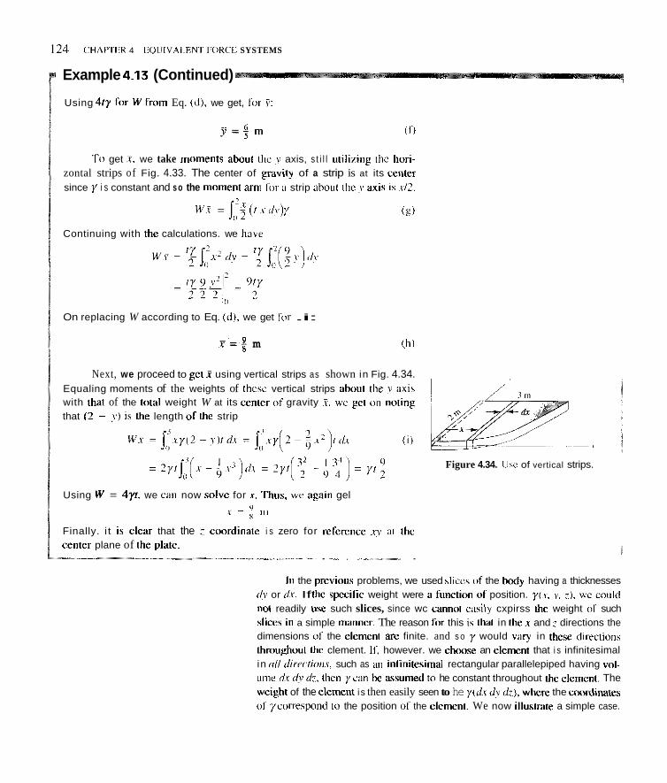
124 C'HAPTER 4 COLIIVAI.ENT FOKCL SYSTEMS
Example 4.13 (Continued)
Using 4ry ior W from Eq. (d). we get, for v: . y = $ m I fl
Tii get i. we take miiments ahout the ! axis, s t i l l utili7iiig the hori- zontal strips of Fig. 4.33. The center of gravity of a strip is at its center since y i s constant and s o the miiinent aim 1111- ii strip ahout tlic y ax is i c .xi?.
(F) W.? = 1;; ( r .r (l!)?,
Continuing with the calculations. we l iavc
On replacing W according to Eq. Id), we get fir .i:
.r=# m (,hl
Next, we proceed to get .X using vertical strips as shown in Fig. 4.34. Equaling moments of the weights of lhcsc vertical strips ahiiut the y axih with that of the tntal weight W at its ccnlcr of gravity .I. wc gel oil rioting that ( 2 - J) i s the length 0 1 Ihe strip
Using W = 4y1, we can now solvc for .r. l h u s , we again gel 7 = <I ni
Finally. i t i h clear that the ? ciiordinate i s zero for rehence .I;Y ill thc centcr plane of the plate.
~ _- . -" ,, ..I~___._ .
Figure 4.34. Use of vertical strips.
111 the prcviiios problems, we used sliccs of the body having a thicknesses rl? or d z . If the spccilic weight were ii fiinction of position. y(. i . no1 readily uhe such slices, since wc cannot ziisily cxpirss the weight 01' such i l iccs iii a simple iniiniicr. The reason fix this i\ that in the .r and r directions the dimensions 01 the elemen1 are finite. and s o y would vary in thcse din-ections thimughout thc clement. If, however. we chime an elenicnt that i s infinitesimal in r i l l r l I r~ i~ l i i ~ t t . s , such as an inrinitesimal rectangular parallelepiped having vi11- unie dx cl! 11:. then y ciin he aswmed to he constant throughout the clcincnt. The wcight of the elcmcnt i s then easily seen to he y(d.r d? d:.), whcre the coordinates of ycorrespond Lo the position o i the elenienl. We now illuslriite a simple case.

SECTION 4.5 DISTRIBUTED FORCE SYSTEMS 125
Example 4.14
Consider a block (see Fig. 4.35) wherein the specific weight y at comer A is 200 Ihf/ft’. The specific weight in the block does not change in the x direction. However, i t decreases linearly by 50 IhWft’ in 10 ft in the y direction, and increases linearly by 50 Ihf/ft’ in 8 ft in the z direction, as has been shown in the diagram. What are the coordinates 2, g of the center of gravity for this block’?
X
Figure 4.35. Block with varying y
We must first express y at any position P(x, y , z ) . Using simple pro- portions, we can say
(a) v y = 2 0 0 - ~ ( 5 0 ) + q S O ) 8 ‘ I O
= 200 - 5 y + 6.252 Ibf/ft’
We shall first compute the weight of the block (Le., the resultant force of gravity), We do not use an infinitesimal slice or rectangular rod of the block, as we have done heretofore. With the specific weight varying with both y and z , it would not he an easy matter to compute the weight and moment of a slice or a rod. Instead, we shall use an infinitesimal rec- tangular parallelepiped having volume dx dy dz, located at a position hav- ing coordinates x, y , and z as has been shown in Fig, 4.36(a). Because of the yanishingly small size of this element, the specific weight y can he considered constant inside the element, and so the weight dW of the ele- ment can he given asx
dW = y(dx dy dz) = (200 - 5y + 6.252) dr dy dz
“We are dcleting higher order quantities.

126 CIIAPTER 4 ~ I J I J I V A L E N I FORCE SYSTEMS
Example 4.14 (Continued)
T u include thc weight o l u l l such elenicnls in the block. we first let .v “run” from 0 lo 4 ft while holding J and z fixed. Thr rectangular parallclcpiped OS Fig. 4.3hla) then heconics a rectangular rod ac shown in Fig. 4.36(hl. Having ruii its course. x i s no longer a variable i n this summation priicess. Next. let y ”run” from 0 to IO while holding I constant. The rectangular rod of Fig. 4.36(h) then bcciinies an infinitesimal slice. a s shown i n Fig. 4.361~). The variable y has thus run its course and ir. no longer a variablc. This lcaves only the variable ;, and now we let r “run” froni 0 to X. Clcady, we cover the entire hkick hy this process.
We can do this inathcmatically by a process called in id~iple inrrfim- tion. We pcrt~irm three iiitcgrations, paralleling tlic thrcc steps oullined in the previous paragraph. Thus. we can lormulate W a s ffoll~iws:
We first consider integr;ition with reqpecl ti1 x holding ? and I constant. That i c
J(:(200 - SJ + 6.25;)dr
As iii the firsl step set lorth in the previous paragraph, to go from a rectan- gular pnrallelepiped to a rectangular rod, wc integrate with respect (o .i from ,x = 0 tu .t. = 4 n,hile holding? and : constant. ‘Thus,
I j ( , (200 - 5y + 6 .25: )rh = (2l~ l Ix - S?X + 6.25:.*)1;
= xoo - 20y + 25;
With .v no longer a variable (since i t has run its course), the equation for W becomes
Now, we hold 3 constant and integrate with respect toy from 0 to IO. (This takes us from a rectangular rod to ii slice.) Thuh,
N o w ? has I-UII i t s cw~rse. and wc have
X
11 w = J (7,000 + 250:) if:
(C)
Figure 4.36. (a) Infinitesimal element at P(.y y, :); lb ) I runs from 0 IO 4. while i and v are fixed, to form rcctangular rod: ( c ) ? runs from 0 to I O , while holding: fixed. 11, frrrm slice.

SECTION 4.5 DISTRIBUTED FORCE SYSTEMS 127
Example 4.14 (Continued)
By integrating with respect to z . we sum up all the slices, and we have cov- ered the entire block. Thus,
To get j , we equate the moment ahout the x axis of the resultant force without a couple moment with the moment of the distribution. Thus, using multiple integration as described above:
R 10 4 -(64,0OO)p = -I I / v(200 - 5y + 6.252) dx dy dz
n n n ' Therefore, integrating with respect to x, then y. and then z as before, we have
64,OOO.v = lRji"(200yx - Sy'x + 6.25yzx)/,, 4 dydz n o
= /,"I:" (800y - 20)'' + 25.~2) dy dz
= ~ox(40,000 - 6,667 + 1,250z)dz
= [ 3 3 , 3 3 3 ~ + 1250 5 = 307,000 * I and
y = 4.79 a
Because y dots not depend on x, we can directly conclude by mpection that X = 2 ft.
Next, in the case of a body made up of simple shapes (subbodies) such as cones, spheres. cylinders, and cubes, we can find the center of gravity of the body by using the centers of gravity of the known subbody shapes. Thus, we can say on taking moments about they axis that
y",a[(z) = X.w;(3' (4.12)
where W is the weight of the ith subbody and where [z), is the x coordinate to the center of gravity of the ith subbody. Bodies made up of simple subbodies are called composite bodies.

<- L2is

SECTION 4.5 DISTRIBUTED FORCE SYSTEMS I29
Case B. Parallel Force Distribution over a Plane Surface- Center of Pressure. Let us now consider a normal pressure distribution over a {dune surface A in the ,ty plane in Fig. 4.38. The vertical ordinate is taken as a pressure ordinate, s o that over the area A we have a pressure distri- bution p(x, y ) represented by the pressure surface. Since in this case lhere is a parallel force system with one sense of direction, we know that the simplest resultant is ii single force, which is given as
Figure 4.38. Prcsure distribution
The position x , y can hc computed by equating the moments about they and x axes of the resultant force without a couple moment with the corresponding momcnts of thc distribution. Solving f<)r Z and 7,
I p r [/A x = ~~ ~~ J / I d.4
iv dA ,: = 11 </A
Since wc know that 11 is a function of .r and y over the surface, we can carry out the preceding integrations either analytically or numerically. The point thus determined is called the center ofpressure.
(In later chapters. we shall consider distributed frictional forces over plane and curved surfaces. In these cases, the simplest rcsultant i s not neccs- sarily a single forcc as it was in the special case above.)

130 CHAPTkR 4 EQUIVALENT FORCE SYSTEMS
A plate ABCD on which both distributed and point force systems act is shown i n Fig. 4.39. The pressure distribution is given as
(21)
Find the simplest resultant lor the system. To get the resultant for-ce, we consider a strip dy along the plate as shown
in Fig. 4.39. The reason fix using buch a strip is that the prcssure 17 is uniform along this stnp, as ciln he seen lroni the diagram. Hence, the force from the pressure on the strip is simply / I dA = p[dy)lS). Thus. we can ~ i l y that
/ I = -4? + 100 psf
f i f l = - jSp(s , (m. , 11 - son
Example 4.16
FK = (20” - 500y)’ - 500 = -2,167 lb 3 ~ r l
To get the position ~F, J of the resultant force FK without a couple moment. wc cquate moments of FK about the I and y axes with that of the original system. Thus. starting with the x axis, we have using strip d? as before:
-2,1677 = - j i ) ’p (sdy) - (500)(2)
= -j$-4U.’ + 100)dU. - 1.000
- i.ooo = -4.125
Therefore, 7 = 1.904 ft
Now, considering they axis, we still use the strips dv because / I is uniform along such strips. Howcvcr. the force <If= 11 dA = p(S)[<fy) may he conyid- ered acting at the center of the strip, and accordingly has a moment arm about the ? axis equal to SI2 for each slrip. Hence, we can say that
5 0 0 2.167.r = I’ 2 pis(/y) + (sno)12) - :--- I 1 - 12
2 - - q - 4 , ’ + IOO)dJ+ 1.000-41.7 = 5.125
;t- -*! Figure 4.39. Find simplest m u l l a n t .
- ~___._....I_... ~ --_ll-...--.......l.- ~
In a statlonay liquid. the pressure at the surface of the liquid is transmitted uniformly Ihmughout the liquid. In addition, there is superposed a lineal-ly increas- ing pressure with depth resulting from gravity acting on thc liquid. Thus. i l we havc [ I , , , ,~ , at the surface (often called the free surface). the prewtre in the liquid is
P = P,,,z,, + P where y i s the specific weight of thc liquid and I’ is the depth helow the sur- hcc . Thus, for a given liquid the presburc is unilorm at any constant distance below the frcc surface. With this in mind. examine the following example.

SECTION 4.5 DISTRIBUTED FORCE SYSTEMS 13 1
Example 4.17
In Fig. 4.40 find the force on the door AB from water whose specific weight is 9,806 N/mZ and on whose free surface there is atmospheric pres- sure equal to 101,325 Nlmz (= 101,325 Pa).q Also find the center of pres- sure.
The pressure on the door AB is then
11 = P ~ ~ , ~ + (y)(r) = P , , , ~ + (y)(.s)(sin 45")
where s is the distance from 0 along the inclined wall OR. The resultant force is then
= 1sy[101,325 + (9,806)(.707)~](2)ds
101,325s + (9,806)(.707)%
To get the center of pressure equate moments about 0 with that of the resultant. Thus using the notation S to locate the center of pressure we have
9
5 1.199 x 10hs = 5 s [ ~ = , ~ + (y)(s)(sin45")](2) ds
= [lO,,32S$ + (9,806)(.707)% (2) I: :. 3 P 7.061 m
Clearly the total force on the door from inside and outside would include the contribution of the atmospheric pressure on the outside. We can e a d y determine this force by deleting p<,<,,, in the preceding calculations.'U
'The unit of pressure in the SI system is the pascal, where I pascal = 1 Pa = I Nlm'. "We have touched here on the subject of hydrostnrics. For a treatment of this suhjcct
that may he similar to what you will study in your upcoming course in fluid mechanics, see Shames, I.H.. Mechunics off nu id.^, 3rd Edition, 1992. McCraw-Hill, Inc., Chapter 3
, Door AB
Figure 4.40. Door AB is exposed on one side to water and on the other side t o air.
We finish this series of examples with a multiple integration problem.

*Example 4.18
I' What i s thc simplest rehulkint and the ccnier iif pressure l11r the prccsurc distribution shown in Fig. 4.41'?
Notice that thc pressure varics linearly in the x and y directions. Thc pressure at any poinl x, y in the distrihution can he givcn :I\ follows with the aid of similar triangles:
, ! 211 N i m ~
/ = 2: + 6.1 Pa
1,'igurc 4.41. N i r n u n i l u r m I~ICSSLIIC
d i w i h i i t i o i i . We cannot employ a convenient strip here along which the pressure i s u n - form, an in Example 4.16. For this reasnn we consider rectangular :ire3 elc- ment d-r h. tn work with (scc Fig. 4.41). For such i1 s i i i i i l l area. w ciiii
assume the pressure a s constant s o that p d x i/y i\ Ihc lirrce 1111 lhc cIcnicn1. To find the resultant lnrce, we mint inlcgnlte over thc IO x 5 re~t i lng le. This integration involvcs twn vnri;ihle\ and i s again ii case o l m ~ , t t i p / ~ ~ itif<,- Rmtion. Thus, we can say that
wherein we first integrate with respect lo .x while holding v constant and then inlcgrate with respcct t o s ( i n this way we cover the cntil-e 10 x 5 I-cc- tangular arca). Thus. we have
I l l = - j,, (I I)\. + 7 5 ) (/y
FR = - 1,250 N
To find ~V for FH without il couple mon1cnt. we equate moments 01 F;? about the x axis with that of the distrihittioti. Thus.
. ". . ... .. ~~ ~ . . .. ., ,. " , , ~I .,^.___. . __" ",

SECTION 4.5 DISTRIBUTED FORCE SYSTEMS 133
Example 4.18 (Continued)
Therefore, 1 i n 5
1,250 n n - v = - I I ( 2 ~ + 6 x ) ~ d x d y
5 - ~ - J I '0 ( 2 v 2 r + ~ ~ ) l 6 x 2 dy
0 1,250 o
1,250 = -In 1 10 (1oy2 + 7 5 y ) d y 10
0
p = 5.67 m
A5 for 3, we proceed a3 follow9 i n 5
X(1,250) = 5, I, px dx dy
I=- ' SIn J5(2y + 6 x ) x dx dy
Therefore, ~
1,250 o o 5
- _ - l,&oJ:0(2~$ +y)l 0
= ---I I ' 0 (25y + 250)dy 1,250 n
x = , 3 The center of pressure is thus at (3.00, 5.67) m.
Case C. Coplanar Parallel Force Distribution. As we pointed out earlier, this type of loading may be considered for beams loaded symmet- rically over the longitudinal midplane of the beam. The loading is represented by an intensity function w(x) as shown in Fig. 4.26. This coplanar parallel force distribution can he replaced by a single force given as
FR = -J w ( x ) d x j
We find the position of FR without a couple moment by equating moments of FR and the distribution w about a convenient point of the beam, usually one of the ends. Solving for .F, we get

134 CHAPTER 4 EQUIVALI:NT I'ORCE SYSTEMS
Example 4.19
A simply supported heam i s shown in Fig. 4.42 supporting a 1,000-lh point h r ce , a S O 0 Ib-ft couple. and a coplanar. parabolic. distrihutcd load w Ih/St. Find thc simplest i-esulliint of this force systcm.
To exprcss the intensity of loading lor the coordinate system shown in the diagram. we hegin with thc gcneral iormulation
Lt,? = a t + h
Note from the diagram that when A = 25 we have w = 0, and when x = 6s. wc h w c IV = 50. Suh.jccting Eq. ( a ) to these conditions, wc can determine fi and ti. Thus.
0 = 4251 + i, ih)
( e )
Fig''re 4.42. Find qimQlest reSU'tan'.
2.500 = i i l6S) + h
Subtracting. we can gel ( i as follows:
-2.500 = -4Iki
Therefore,
( i = 62.5
From Eq. (h). we gcl
h = -(25)(62.i) = -1,562.5
Thus, wc have
I+ = h2.5.1 - 1,562.5 (d)
Summing forces. wc get i c r b;.
h i
25 F+( = -1,000 - J .,'62.5~t - 1,502.5 N I X (el
To integratc this. we may change rari;ihlcs as follows:
11 = 62.S.t - 1.562.5 i 0 Thercfim.
N;LI = h 2 . i d t ~
Substituting into the intcgral i n Eq. ( e ) , wc have"

SECTION 4 5 DISTRIBUTED FORCE SYSTEMS 135
ExamPle 4.19 (Continued)
We now computer for the resultant without a couple as follows: 65 -~ 25
-2,3337 = -(10)(1,000) - 1 x>/62.5x - 1,562.5 dx - 500 (g)
We can evaluate the integral most readily by consulting the mathematical formulas in Appendix 1. We find the following formula (No 6):
In our case b = 62.5 and a = -1,562.5, so the indefinite integral for our case is
Putting in limits, we have
.. = 65,333 - 0 = 65.333
Going back to Eq. (g), we can now solve easily for X, Thus, ~ 1 x = -__ 2,330 [-(10)(1.000) - 65,300 - 5001
Z = 32.5 ft
Before closing, it will he pointed out that, for a loading function w(x). the resultant [,'w dx, equals the area under the loading cuwe. This fact is particularly useful for the case of a triangular loading function such as is shown in Fig. 4.43. Hence, we can say on inspection that the resultant force
Fn = ~(5)(1,000) = 2,500 N
Furthermore, you can readily show that the simplest resultant has a line of action that is (2/3) x (length of loading) from the toe of the loading.'' Thus, 4 without a couple moment is at a position (2/3)(5) to the right of a (see Fig. 4.43). You are urged to use this information when needed.
has the value 5 I FR = (;i(5i(1.000)
Figure 4.43. Triangular loading resultant.
"In Chapter 8, you will learn that the simplest resultant force for a distribution w(x) goes through the cvnrrnld of the area under w(x). The centroid will be carefully defined at that lime.

Figure P.4.15.
Figure P.J.4.3. Figure P.4.46.

4.47. frustum are, respectively.
Show that thc volume and center 01 gravity of the conical
r; + qr2 + r i )
and
crowyection I - h l Figure P.4.47.
4.48. straight line and a parahola.
Find the center of gravity of the piate bounded hy a
Figure P.4.48.
4.49. A massive radio-wave antenna for detcction of signals from outer space is a body of revdutinn with a parabolic face (see the diagram). These antennas may be carved from rock in a valley
4.50. center of gravity if the total weight is 2.37 x I O x kN.
*4.51. A plate of thickness 30 mm has a specific weight ythat varies lincarly in the x direction from 26 k N / d at A to 36 kN/m3 at R, and varies in they direction a i the square 01) from 26 kN/m’ at A to 40 kN/m‘ at C. Where is the cenler of gravity of the plate?
In Problem 4.49 find the distance from the ground to the
s
A sm n Figure P.4.51.
4.52. You are looking down on n plate with a hole in it as shown. Thc thickness has a constant value equal to t and the specific weight y is constant. Find the coordinates F, 7 o1Ihe e w e r qf ,vuviq.
A Figure P.4.52.
4.53. Find the center of gravity of the plate having uniform thickness and uniform specific weight. You are looking down onto the top of thc plate.
I ?’ away from other disturbing signals. What would the antenna weigh if invde Srom concrete (23.6 kN/m’) for locatiun in a remrxe desert area’!
-
Figure P.4.49. Figure P.4.53.
137

4.54. cnordinatcs r, v .
Thc tup view of a platc i s shown. Find center 01 grevit!
Y i s conslant and thickness I
?
.2 m -1- .I rnd i s constant
.2 "I Figure P.4.54.
4.55. The thin circular rod has a weight of MI N/m. What i s the > coodinarc of i t s C C ~ ~ C I of gravity? The rud fumis me-half of a circle
Y
Figure P.4.55.
4.56. a hole in i t .
Find J for the uentcr of gravity of the horizontal plate with
Y
I m
5 m
I
V.57. Suppose in Pmhlem 4.12 that
.f = ( . O I ~ k + 2 1 + . k ) k ot./lhni
Find Ihe .sinrplr.sr resultant for p = 450 Ihmlfl'. Find the plopel- line of action.
4.58. After il fast stop and swerve 10 Ihc left. the load of sand (specific wcight = I S kNhn') in a dump truck i s i n the positirm shown. What i s thc simplest resultan1 force on thc truck ti-om thc sand and where does i t act'! If the truck was full (wi th a I c v d tup) hcforc thc stop, how inuch sand spillcd'.' U w the results of Problem 4.46.
Figure P.4.58.
In Problems 4.5Y rhmufiir 4.62 U.IP rhc k n o w , posiliom o/ <cnfe~.s
of ,q'at,iry of ,simple .) hiipc,.s.
4.59. An I-heain cantilwered out from a wall weighs 30 Ihlft and support\ a 300-1h hoist. Steel (4x7 Ihift') cover plates I i n thick are welded on thc hcam near the wall to increme the carry- ing capacity o f the heam. What i s the moment at the wall duc to
the weight ofthe reinforced b c m and the hoisted load of4.000 Ih at thz outermost position of the hoist? Whilt is thc .sinzplv.st resul- tant force and its location'?
Figure P.4.56. Figure P.4.59.
138

4.60. The bulk materials trailer weighs 10,ooO Ib and is filled with cement ( y = 94 Ib/ft’) in the front compartment (sections 1 and Z), and half-filled with water ( y = 62.5 Ib/ft3) in the rear compartment (sections 3 and 4). What is the simplest resultant force, and where does it act? What is the resultant when the water is drained? Use the center of gravity and volume results from Problem 4.47 (conical frustum).
1’ 2 Trai1erC.G. 3 4
Figure P.4.60.
4.61. Find the coordinates (x, y), vf the center of gravity of the loaded conveyor system. The centers of gravity of the crates C and D are at their geometric centers. WE is the weight of the frame whose C.G. is at its geometric center.
Y
We= 1001b W c = 8 0 l b WD = 300 Ib WE= 1,000lb
2 WBELT = 5 Ib/ft Figure P.4.61.
4.62. Find the center of gravity of the body shown. It has a con- stant specific weight throughout. Cone and cylinder are on block surfaces.
C i m e h = . I l m
Figure P.4.62. 4.63. Find the .simplest resultant of a normal pressure distri- bution over the rectangular area with aides a and b. Give the coor- dinates of the center of pressure.
P
Figure P.4.63.
4.64. Find the simplest resultant acting on the vertical wall ABCD. Give the coordinates of the center of pressure. The pres- sure varies such that p = E/Cv + I ) + F psi, withy in feet, from IO psi to 50 psi, as indicated in the diagram. E and F are constants.
-I Figure P.4.64.
139

4.65. One lloor of a warehouse i s divided into lour area?. Area I i s s tack4 high with TV scts such that thc distrihutcd load i s p = 120 Ihlft2. Arm 2 has refrigerators with 11 = 65 Ibift'. Area 3 has stcreos stacked s o that 11 = XO Ih/ft2. Area 4 has wa.;hing machines with 11 = SO Ihlft'. What i q thc simplest resultant force and where does i t act'!
1 - 100' t
Figure P.4.65.
4.66. Consider a prcssurc distrihution 1, fbrminp a hemispherical surpace over a domain 01 radius 5 in. IS the inaximuni pressure i s 5 Pa, what i s the s i m p k s l resultant from this prcs\urc distrihution'!
I'
s ( m ) Figure P.4.66.
4.67. A reclangular lank contains watcr. If the tank i s rotated clockwise IO" ahout an axis normal to the page. what toque i s required to maintain the configuration? Width o f tank i s I 11.
1- t x i t
___ - 2,-1+- 2,-1
Figure P.4.67.
4.68. (a) Find the torque about axis i\H from thc wrcocl~. (h) Find the torque ahout axih An lroni lhc distrihutcd
loads. ( H i m ; I.ooh dowm lirwn a h w e to hclp vicw prohlcm.)
Il l m
Figure P.4.68.
4.69. For the system 01 lorccs shown. determine the turquc ahout the ax is going trorn A to B. Noir : 'The 100-N force and thc triangular load distribution are i n the y: planc and the 100-N-m couple i s mi the tup facc d thc rcuiimpular hux.
v
Figure Y.4.6Y.

4.70. A manornerrr is a simple pressure measuring device. One such manometer called B U rube is shown in the diagram. The tank contains water including the tube to level M where mercury i s pre- sent. M and N are at the same Icvel. What is the gage pressure (ie., the pressure abwz atmosphere) at point LI in the tank for the following data:
d , = .2 111 d, = .6m yH:o = 9,806 N/m3
y,,, = (13.7)(yHP) Nim'
[ H i n t : M and N are at the same level and are joined by the same fluid, namely mercury. Hence, the pressures there are equal.]
4.12. (a) Calculate the force on the door from all fluids inside and outside. The specific gravity of the oil is 0.8. This means that the oil has a specific weight y which is 0.8 times lhat of water (y,,,,, = 62.4 Ihlft'). Note that a uniform pressure on the surface of a liquid extends undiminished throughout the depth of the liquid.
(b) Determine the distance from the surface of the oil to the .rimpIrst rrsultant force on the door from al l fluids.
t, ft
qS ft
10 i t 2 Figure P.4.72.
Mercury
Figure P.4.70.
4.71. Imagine a liquid which when stationary stratifies in such a 4,73, Ar what height way that the specific weight is proportional to the square root of The door is the pressure. At the free surface, the specific weight is known and has the value & What is the pressure as a function of depth frvm the free surface? What is the resultant force un one face AH of a rectangular plate submerged in the liquid! The width of the plate is b.
will the water the door to wide, Neglect friction and the weight
of the door.
piitm
X 36 kN
L
Figure P.4.71. Figure P.4.73.
141

4.74. Find the krcc on the door front the inside and uulsiile prebsureh. Give the poritiuri of the re%dlml lurce ahvvc the base of the door. The specific grevity .S of the oil i s 0.7, i.c.,
x>,, = K.7)Yk, 0.
4.77. A hlock I ft thick i h suhniergcd i n water. Computr thr siinplest resultant force and the center of prehsure uti [he huttom .;urt~icc. Take y = 62.4 Ih/tt'.
/p\ ,,Top i \ ripen
Figure P.4.74.
4.75. Find the total f k x o n door Ail fri,m fluid\. The spccific gravity S o l a fluid i h y; .,", J x , ~~. Take$>,, = 1l.h. Find the pinition of this force from thc hottuirlof the dour.
Figure P.4.75
4
I ? t l
H J it
Figure P.4.77.
*4.78. Wha1 i s thc r ~ s ~ l t m l force from wiler and where does i l
act on thc 40-m-high circular concrctc d a m hetwero two wall, of a rocky gorge? (Water wcishs Y.XO6 Nlm' . )
40 111 t- Tup "icw
Figure P.4.78.
4.79. The weight of the wire AHC'L) per unit length. w, incrcascs linearly lr<m 4 orlft at ,t ti) 2 0 o,lft nl 11. Where is thc center 01 gravity <,1 thc wire?
4.76. What i \ the simplest r5sd13111 flircc t r i m the water and where due\ i t acl un the h O - m - h ~ ~ h X00-m-laog rtraight canhiill dam'! (Water weigh, O . X O 6 N/m'.1
Figure P.4.76. Figure I'.4.79

4.80. Find the center of gravity of the wire. The weight per unit length increases as the square of the length of wire from a value of 3 ozlft ai A until it reaches the value of 8 ozlft at C. It then decreaaes I orJft for every 10 ft of length.
4.82. At what distance i from point A can the system of thin rods be suspended so that it will just balance? Use the formula developed in the previous problem for the radial distance to the
center of gravity of a thin circular rod, namely - 3 6 0 r . 9 E9 s'n-i
Y
,, = . I R m I W . = 500 Nim
Figure P.4.80.
4.81. What is the center of gravity coordinate y, for a thin circu- lar rod shown in the diagram? It has a weight of w Nlm. The rod is placed symmetrically about they axis. The angle Q is in degrees.
Y
Figure P.4.81.
1 4; = 70'
Figure P.4.82.
4.6 Closure We now have the tools that enable us to replace, for purposes of rigid body mechanics, any system of forces by a resultant consisting of a force and a couple moment. These tools will prove very .helpful in our computations. More important at this time, however, is the fact that in considering condi- tions of equilibrium for rigid bodies we need only concern ourselves with this resultant to reach conclusions valid for any force system, no matter bow com- plex. From this viewpoint, we shall develop the fundamental equations of std- tics in Chapter 5 and then employ them to solve a large variety of problems.
143

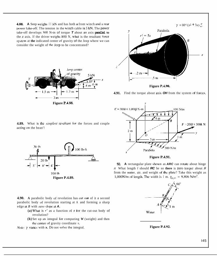
4.88 A Seep weigh5 I I kN and has hoth a front winch and a r e a powcr takeoff. The tension in the winch cable is 5 kN. The puwer take-off develops 300 N-tn of torque T ahout an axis parallel to the x axis. If the driver wcighs XU0 N, wh;it is the resultant force sy\tem at the indicated center of gravity of the Jeep where we can consider the weight of thc Jcep to he concentrated?
c1 1 Scencenter
x
-1 .Sm- + 1 . 2 m - 3 m i i 1
Figure P.4.XX.
4.89. actin3 011 the bean'!
What is thc .simpk~t r e d t a n t for the forces and couple
311 Ih 4
100 Ih Figure P.4.89.
4.90. A parabolic body of revolution has cut out of it a second parabolic body uf revolution starting at A and forming a sharp edge at H with x r o dopz at A.
(a) What is I' as a function ol .r for the cut-out body of
(h) Set up an integral for computing W (weight) and then revolution?
thc center of gravity coordinate i. Notr; y vxic:; with x. Do not solvc the integral.
y = Ill* (x' + 3x) ;: Parabola
I- Figure P.4.')0.
4.91. Find the torque about axis OH from the system of forces.
7
F =200i+300kN
Figure P.4.91.
92. A rectangular plate chown as ARC can rotate about hinge E . What length 1 should RC be so there is zero tarquc about H from the water, air. and weight o l thc platc'! Take this weight as 1,000 Nlm o l Icngth. Thc width i ? I m. x , , ~ = 9,806 Nlm'.
Figure P.4.92.
I45

4.93. water. The dimensions iirc \hewn.
An open rectangular bank u t water 15 partially f i l led wi th
t i l ) rk te rn t ine thc hrcc on ihc h m w n 01 thc t a d l r o n ~ the water.
(hl Detemmine the force on the donr <hmvn at thc Cidc 01 the tank. Indicate the pwition of this firrcc 1r<m l l i c bottom of the tank.
Note that the atmospheric pressure develops equal and opposite forces on both sides of the door and hence yizlds n o inut f<,rcc.
,
Figure P.4.93.
4.94. Sandhags are piled on a bean. Each hag ih I 11 witlc and weighs 100 Ih. What i s the simplcst resultant force imd where doe& i t act’? What linear mathematical function ofthe di\crihuted Ioiiil ciin he used to represent the sandhap <rvec the left 1 ft 01 the tieiii i i ’ l
i
Figure P.4.94.
4.95. A cantilcvcr b u m i s subjected to a linearly w q i n p I h d over pdn 01 i t s length. What i s the .sit!rpl<ml rcwlt:int f~rrce. and where does it act’! What i c the moment :It thc suppomd cnd?
146
,i

4.98. Find the resultant force system at A for the forces on the 4.100. The L-shaped concrete past supports an elevated railroad. bent cantilever beam. BC is parallel to z axis
V
Figure P.4.98.
4.99. (a) Find equations describing both parabolas.
~~
The concrete weighs 150 Ib/ft3. What is the simplest resultant Force from the weight and the load and where does it act? Load acts at center of top surface.
40,000 Ib
15'
1 Figure P.4.100.
4.101. Explain why the system shown can he considered a sys- tem of parallel forces. Find the simplesr resultant for this system.
(h) Using rjerfical strips (and a composite body approach), The grid is of squares, find weight of plate in terms of yt.
(c) Using vaticill strips, find X of C.G.
X
( IO , -3) ft
Figure P.4.99. X
Figure P.4.101.
I47

l.102. A plate 01 thickness f has as the uppcr edge a parabolic :uwc with infinite slope at the origin. Find the x, y coordinates 01 hc criitei ut gravity fnr this plate.
2' Figure P.4.102.
1.103. A rectangular tank conmitih a liquid. At the tup UI the iquid there i s a pressure ol ,1380 Nlmm' absolute. What i s the .iinplesl resultatit lbicr in the inside surface of the dour AH! Nhwe is thc ceiitcr ot pressuse relative to the bottom of the door'! rake y = 8,190 Nlm' for the liquid.
Air
f 5 m
Liquid
bigure P.4.103.
l.104. The sprcilic weight ot thr material i n a right circular me varies directly :IS the s q u a r ~ Crt the distance? from the hase. f 1;, = S O Ih/ft3 i s the cpecific weight at the base. and i f y' = 70 hlft ' is the specific wcight at the tip, when, i \ the center u lgrav- ly ,!I the cone'! (Szz hint in Pmhlrm 4.45.)
Figure P.4.1U4.
*4.105. region). If ths spccific weight is given a h
A block has 8 rectangular portion removed (darkened
tind x for the CCIIISI of gravity
/
/7 I? m A- y
I2 n,
Figure P.4.105.
4.106. irig un the simply supported beam. t i i v r the line of action
Compute the sirnl,ics1 resultant fix the loads shown act^
48

4.107. Fmd the center ot gravity ot the plate. *4.109. The pressure pO at the corner 0 of the plate is SO Pa and increases linearly in they direction by 5 Pdm. In the x direction, it increases parabolically starting with zero slope s o that in 20 m the pressure has gone from S O Pa to 500 Pa. What is the simplest resultant for this distribution'! Give the coordinates of the center of pressure.
x
Figure P.4.107. ~ / c - ' " m +
Figure P.4.109.
- - v
4.110. A sluice-gate door in a dam is 3 m wide and 3 m high. The water level i n the dam is 4 m above the top of the door. The gate is opened resultant force on the closed door at hoth water levcls? Where du the forces act (i.e., where i s the "center of pressure" i n each case)? Water weighs 4,806 Nlm'.
4.108. Find the center of gravity of the W s s . All members have the same weight per unit length.
the level f a l l s 4 ,,,. What is the
v
Figure P.4.108. Figure P.4.110.
149
~- ~ ~ ~~ __

4.111. A cylindrical tank of watcr is rotated at cmbtilnt angular speed Wuntil the water ceases to chmgc shapc. The result is a Srw surface which, from lluid inrchaiiicr cansidcrations, is that of a paraboluid. If the prcswl-e varics direclly as the depth hclow Ihc I r e sutfke. wha t i \ the w s d ~ m t force on a qu:idmnt ~ r f the hasr 01 the cylirrder? Take y = 62.4 Ihlft'. [H im: Use circular strip in quadrant having area l l 4 ~ 2 n - d r ) . ~
4.112. the hodich \hewn. Thehe ci ins iq of:
Firid lhc 'i arid Y coordinates UT the center of gravity 0 1
( a ) A plate AH('whose thicknsss I = SO niin. (hj A rod I> 01 d ~ i m z t e r .? m :md leneth 3 m. (i.) A hlock F whocc thickness (not \huwn) is 3 in.
'Ihc density of thc three bodich i \ the SJIIIC.
Figure P.4.111. Figure P.4.112.
I S O

Equations of Equi I i br ium 5.1 Introduction You will recall from Section 1.10 that apurficle in equilibrium is one that is stationary or that moves uniformly relative to an inertial reference. A body is in equilibrium if all the particles that may be considered to comprise the body are in equilibiium. It follows, then, that a rigid body in equilibrium cannot be rotating relative to an inertial reference. In this chapter, we shall consider bodies in equilibrium for which the rigid-body model is valid. For these bod- ies, there are certain simple equations that relate all the surface and body forces, or their equivalents, that act on the body. With these equations, we can sometimes ascertain the value of a certain number of unknown forces. For
the weight W of the beam, and we want to determine the forces transmitted to the earth so that we can design a foundation to support the structure properly. Knowing that the beam is in equilibrium and that the small deflection of the beam will not appreciably affect the forces transmitted to the earth, we can write rigid-body equations of equilibrium involving the unknown and known forces acting on the beam and thus arrive at the desired information.
Note in the beam problem above that a number of steps are implied. First, there is the singling out of the beam itself for discussion. Then, we express certain equations of equilibrium for the beam, which we take as a rigid body. Finally, there is the evaluation of the unknowns and interpretation of the results. In this chapter, we will carefully examine each of these steps.
Of critical importance is the need to be able to isolate a body or part of a body for analysis. Such a body is called afree body. We will first carefully investigate the development of free-body diagrams. We urge you to pay special heed to this topic, since if is the must important step in the solving of mechunics problems. An incorrect free-body diagram means that all ensuing
instance, in the beam shown in Fig. 5.1, we know the loads F; and 5 and also W
Figure 5.1. Loaded beam.
151

+ w I 5.2 The Free-Body Diagram
I<
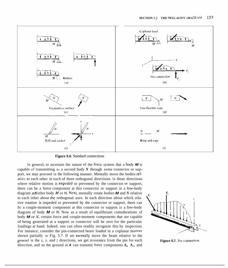
SECTION 5.2 THE FRELBODY DIAC;KAM 153
M Rollcra I
(ill
( C I
Figure 5.6. Standard connections
In general, to ascertain the nature (11 the fnrcc system that a body M is capable of transmitting to a second body N through some connector or sup- port, we may proceed in the following manner. Mentally move the bodies rel- ativc to each other in each of three orthogonal directions. In those directions where relative motion is impedcd or prevented by the connector or support, there can be a Sorce component at this connector or support in a free-body diagram of either body M or N. Next, mentally rotate bodies M and N relative to each other about thc orthogonal axes. In each direction about which rela- tive rotation is impeded or prevented by the connector or support, there can bc a couple-moment component at this connector or suppon in a free-body diagram of body M or N. Now as a result of equilibrium considerations of body M or A', certain force and couple-moment components that are capable of being generated at a support or connector will he zero for the particular loadings at hand. Indeed. one can often readily recognize this by inspection. For instance, consider the pin-connected beam loaded in a coplanar manner shown partially in Fig. 5.7. I f we mentally move the beam relative to the gnmnd in the I, y. and 7 directions, we get resistmce from the pin for each direction, and so the ground at A can transmit force components A,, A,, and
Figure 5.7. Pin connectim

154 CHAPTER 5 IiQlJATIONS OF EQLIILIRRIIJM
B \
Figure 5.8. Rigid hod) i n cquilihrium
Figure 5.10. Canti lc\w beam.
IV
Figure 5.1 1. Free-hdy diogr;im 01 cmtilever heam.
A ~ . Howe\~cr. hecause the loading is coplanar iii the .i\' plane, the force coni- poncnr A _ niuit bc Lero and can he deleted. Next. inlentally rotale the be;m rclati\'c to the ground at A about the three orthogonal axes. Because of the smooth pin conlicetion. thcrc i s t i i ) resistance ahout the : axis and MI
M; = 0. But there i s resistancc ahout thc~r and? axcs. Howevcr, the coplanar loading iii the .r?. plane cannot ext i t iiiorncnts ahout the ~r arid s axes. and s o the couple inioiiients M , and M, arc 721-0. All told. then. we jus1 have Icirce cc)mp~~nenls A , and A , a1 the pin connection, a\ hiis heeri shown earlicr in Fig. S.h(bJ. whcrciii w e rclicd on physical reasoning for this result.
5.3 Free Bodies Involving Interior Sections
l,tt us consider;^ rigid body in equilihriuiii as shown in Fig. 5.8. Clearly, every portinti ( i t t h i s hocly inul iilso he in equilihriuin. If we consider the hody as two pirts A and 8. we can present cithei- part in a lice-body diagram. To do this, we niust includc 011 the poition chosen to he the free hody the Ibrces f i m t
flip ot / i ( , t - /~urt that x isc at the coniinon section (Fig. 5.Y). The suilacc between both seetioils may he any curved or plane surface, and ovcr i t there wil l hz a c ~ n t i n u o u ~ force dislrihution. I n the general c a e . wc know that such ;I distrih- utioii can he replaced by a single force and ii single couple nioinent (at any chosen point) and this has been done in the tiec-hody diagram or parts A aiid B in Fig. 5.4. Nolice that Newton's third law has heen ohserved.
Figure 5.9. krcc hodics ot parts .1 and H
As a special case. consider a beam with one end cmbeddcd in a iiiassivc wall (canlilcver beam) aiid loaded within the .x:v plane (Fig. 5. IO). A free hndy 01 the port im (if Ihc heam cxteiiding from Ihe wa l l i s shown in Fig. 5. I I Recause 01 the geometi-ic symmetry OS the hcam ahout the .(I plane and the Iact that thc loads arc in this pliine. thc cxposcd forces in the cut section can he considered coplanar. Hence, these exposed I i rceq ciin he replaced by a single lorce and ii single couplc inonienl in the centcr plane. and il is the usuiil practice to dccomposc the I'orcc into components F, and PI. Allhough a line 111
actiori for the liirce can hc found that would enahlc us to climinate the couple ninlnent. i t i s dcsirahle in slructural problems to work with an equivalent i ys - tcni that has the lorcc p i n g through the center 01 the heam cross section. arid thus to liave a couple moment. 111 the i icxt section. we wil l see how F a n d C. can he ;iscertiiincd.

SECTION 5.3 FREE BODIES INVOLVING INTERIOR SECTIONS 155
Example 5.1
As a further illustration of a free-body diagram, we shall now consider the frameZ shown in Fig. 5.12, which consists of members connected by fric- tionless pins. The force systems acting on the assembly and its parts will he taken as coplanar. We shall now sketch free-body diagrams of the assembly and its parts.
Free-body diagmm of the entire assembly. The magnitude and direction of the force at A from the wall onto the assembly is not known. However, we know that this force is in the plane of the system. Therefore, two components are shown at this point (Fig. 5.13). Since the direction of the force C i s known, there are then three unknown scalar quantities, A,, A,, and C, for the free body.
Free-body diagram of the component parts. When two members are pinned together, such as members DE and AB or DE and BC, we usually consider the pin to be part of one of the bodies. However, when more than two members are connected at a pin, such as members AB, BC, and BF at B, we often isolate the pin and consider that all members act on the pin rather than directly on each other, as illustrated in Fig. 5.14. Notice four sets of forces that form pairs of reactions have been enclosed with dashed lines. The fifth set is the 1,000-lb force on the pin and on the member BE
Figure 5.12. A frame.
A
1,OOU Ih
Figure 5.13. Free-body diagram of frame.
I
Figure 5.14. Free-body diagrams of parts.
frame i s it system of connected straight or benr, long. slender members where some of the connecting pins are not at the ends of the members as is the case for structures that we will study kter called I T U I S ~ S .

Example 5.1 (Continued)
Do niil he cwncerned about the pi-nper ,SPII,SP [if an unknown force ciimlmient that yrw draw 1111 the free-body diagram, for you m a y choose cithei- a pnsiti\'e or n c g a t i x scnse for tlicsc components. When the \piilues 01 these qi~antities :ire ascertained by methods iil stiltics, the proper sense (breach coinponcot can then he estahlishcd: hut. liavins chosen a seiisc for a mniponcnt, you must he sure that the rrw(.tion to this ciimponent has the oppasir<, s e i i s c ~ ~ ~ - e l s e yiru aril1 \ irilate Newtiin's third law.
Free-body d i q r n m ofportion of the assemhly to the right o fM-M. I n making a free body 01 the portion to the right [if section M-M (see Fig. 5 . I Sa). we must rememhcr to piit i n the weight of the portions n l the inernhers remaining &v the cut liiis hccn made. At the two cut5 made hy h--M we must replacc coplanar fiirce distrihutions hy resulkints. as i n the case nf the previously coiisidercd cnntilcvcr heaiii. This is accomplished by inserting two hrcc co~i ipi incnls nsu;illy normal and tangential to the cross section and a couple mnnient a h \vas done for the cantilever bcam. Note i n Pig. 5 . I X b ) tliat there arc w v c n unhnown scalar quantities lor this free-body diagram. They iirc C',, CL. t;. F,. t;?. and Fd. Apparently. the numher 01 unknowns varieq widely lor the various free bodies that may he drawn O r thc system. For this reawn. you nitist choose the free-body diagram that is suitahle 101- your ncedr wilh snmz discretion in ordcr ti) eflectively solvc l i r the desii-ed unknowiis.

SECTION 5.3 FREE BODIES INVOLVING INTERIOR SECTIONS 157
Example 5.2
Draw a free-body diagram of the beam AB and the frictionless pulley in Fig. 5.16 (a). The weight of the pulley is W,, and the weight of the beam is K8.
Figure 5.16. (a) Beam AB: (b) Free-body diagram of AB; (c) Free-body diagram of Pulley D
The free-body diagram of beam AB is shown in Fig. 5.16(b). The weight of the beam has been shown at its center of gravity. Components U, and U,, are forces from the pulley D acting on the beam through the pin at B. The free-body diagram of the pulley is shown in Fig. 5.16(c).
Some students may he tempted to put the weight of the pulley at U in the free-body diagram of beam AB. The argument given is that this weight “goes through B.” To put the pulley weight at U on free body AB is strictly speaking an error! The fact is that the weight of the pulley is a body force acting throughout the pulley and does not act on the beam UD. It so hap- pens that the simplest resultant of this body force distribution on D goes through a position corresponding to pin B. This does not alter the fact that this weight acts on the pulley and nor on the beam. The beam can only feel forces U, and U, transmitted from the pulley to the beam through pin U . These forces are related to the pulley weight as well as the tension in the cord around the pulley through equations of equilibrium for the free body

Example 5.3
We finish this series of free-hody diagrams with a three~diineiisional case. In Fig. 5.17(a) we sl iou' a structure having h;ill-joint connections at A and n, a fixed-end support at U and. finally. at i" the column R resting directly on the foundation. Draw the frcc-body diagratn fcir the slruclure.
We show the frcc hody diagr;nn Or this case i n Fig. S.I7(h).
"5.4 looking Ahead-Control Volumes I n rigid-body irw<./iuiri(,s wc use Ihc free hody whcrein wc isolate a hody or a portion ( f a hody and wc identify all the external f ime7 acting on the body so that we can employ Newti in 's lab .
I n ./7uid mw/wiiii.s. we may either make :I free body of some chosen chunk ot lluid (here i t i s called a system). but more likely i t wi l l be more prot- itable to identify some volume i n space involving fluid flow through the vol- unic. Such a v(iIu~iic i s celled ii ( * i t i f r .d inlinfne. Here, as in the case of a free body, wc must specify crll the cxrrrnol fi)rms such as triictions on the hound- ing suifaccs of the conrrol v ~ l u m e and. i n addition, hody forces on the mater- ial inside the con t r~ l voluiiic. Thih identification and force specification i s needcd to ensure, in appropriate equations, that Newton's law and other laws i ire satisfied for the fluid and other bodies inside the control voluiiic at any Lime f.
Thos. you must dcveliip sensitivity at this early stage o f your studies in depicting cxternal fotres fiir a frcc hody. The ~ a m e carc wi l l he needed in your upcoming courses i n l luid nicchanics.

5.1. lifted at the handle to a 45" open position.
Draw the free-body diagram of the gas-grill lid when it is 5.3. Draw a free-body diagram of the A-frame
Figure P.5.1.
5.2. A large antenna is supported by three guy wires and rests on B large spherical ball joint. Draw the free-body diagram ofthe antenna.
Figure P.5.2.
Figure P.5.3.
5.4. Draw complete free-body diagrams for the member AB and for cylinder D. Neglect friction at the contact surfaces of the cylinder. The weights of the cylinder and the member are denoted as y , and W,,, respectively.
Figure P.5.4.


5.11. trimmer.
Draw lire-body diagrams of each pan of the me-branch
Branch 2 3 Figure P.5.11.
Figure P.5.14. 5.12. Draw free-body diagrams for the two booms and the body E of the power shovel. Consider the wcight of each part to act at a central location. (Regard the .;havcl and payload as concentrated forces, W, and W,,., respectively.)
5,15, Draw a free-body diagra,n of members CG, AG, and the disc B. Include as the only weight that of disc B . Label all forces. (Hitit: Consider the pin at G as a scparate free body.)
P Figure P.5.12.
Figure P.5.15.
5.13. Draw the free-body diagram for the hulldozer, B, hydraulic ram, R, and tractor, T. Cunsidcr the weight of cach part, R, X, and T.
5.16. tilevered beam. Use only XI: components of a11 vectors drawn.
Draw the free-body diagram of the horizontally bent can
. .
Figure P.5.13.
5.14. Draw a free-body diagram of the whule apparatus and of each of its parts: AB. AC, BC, and I). Include thc weights of all bodies. Label forces. Figure P.5.16.
16

5.5 General Equations of Equilibrium For every free-hody diagram. we can replace the system of forces and couples acting on the hody by a single lorce and ii single couple moment at a point ( 1 .
The forcc will have the same magnitude and direction, n o matter where point a is chohen 10 n i o ~ e the entire system by methods discussed earlier. However. the couple-moment vector will depend on the point chosen. We will pmve in dynamics that:
The necessary cimditiuns,fnr a rigid body IO be in equilibrium are rhat the resultant force F, and the resultant couple moment C, .for any point a be 7ero vectors.
That is,
FR = 0 c, = 0
We shall prove i n dynamics, furthermore, that the conditions above are .s@ c.iriit tn maintain an inifiully .rfationury body in a state nfequilibriutn. These arc the fundamental equations of statics. You will rememher from Section 4.3 rhat the resultant FR is the sum nf the forces moved to the cotnmon point, and that the couple moment C, is equal 10 the sum of the moments of all the orig- inal forces and couples taken about this point. Hence, the cquations ahove can hc written
(5.221)
(S.2h)
where Ihe p,'s are displacement vectors from the conirniin point (1 to any p i n 1 on the lines of action of the respective forces. Frnm this form of the equations oS statics. we can conclude that for equilibrium tn exist, the wmr .rum of tlw ~;Jw..s m u s I be zero and the moinewt of rhr .y>'.s/rrn ,!f,fi)rw.s mnd miiiplm about miy point in .ypace musf be zero.
Now that we have summed forces and have taken moments ahout a point ti. we will demonstrate that we cannot find another independent equa- tion hy taking moments ahout a diffrrent point ti. For the hody in Fig. 5.18. wc have initially the fdlowing equations of equilibrium using point (I:
x F~ + p, x F, + 11, x F, + pd x F~ = n (5.41

SECTION 5.5 GENERAL EQUATIONS OF EQUILIBRIUM 163
Figure 5.18. Consider moments about point h
The new point h is separated from a by the position vector d. The position vector (shown dashed) from h to the line of action of the force F, can be given in terms of d and the displacement vector p, as follows. Similarly for (pJh, which is not shown, and others.
( P , ) ~ = (d + P,)
(p2Ih = (d + P& etc.
The moment equation for point b can then he given as
(P , + dl x 4 + (P, + 4 X F2 + (P, + 4 X F3 + (p4 + 4 X F4 = 0
Using the distributive rule for cross products, we can restate this equation as
(5.5)
Since the expression in the second set of parentheses is zero, in accor- dance with Eq. 5.3, the remaining portion degenerates to Eq. 5.4, and thus we have not introduced a new equation. Therefore, there are only two indepen- dent vector equations of equilibrium for any single free body.
We shall now show that instead of using Eqs. 5.3 and 5.4 as the equa- tions of equilibrium, we can instead use Eqs. 5.4 and 5.5. That is, instead of summing forces and then taking moments ahout a point for equilibrium, we can instead take moments about rwo points. Thus, if Eq. 5.4 is satisfied for point a, then for point b we end up in Eq. 5.5 with
d X ( F , + F , + F , + F , ) = O (5.6) If point b can be any point in space making d arbitrary, then the above equa- tion indicates that the vector sum of forces is zero. If a point b happens to be chosen making Eq. (5.6) identically 0 = 0. (and hence useless), choose another point b. We then have equilibrium since F, = 0 and C, = 0.
Using the vector Eqs. 5.2, we can now express the scalar equations of equilibrium. Since, as you will recall, the rectangular components of the moment of a force about a point are the moments of the force about the onhog- onal axes at the point, we may state these equations in the following manner:
(P, X F, + X F2 + P, X F3 + p4 X F4)
+ d X (F, + F2 + F? + F4) = 0

164 CHAPTER 5 EQUATIONS OF t?QUIL.IRRIlJM
From this set o f equations, i t i s clear that !io more than si.^ unknown scular- qiiun1ifir.s i l l / /!e ,qmrru/ m s c ~ r n he s o l d hy lnellior/.s of .stuli~~s,fi~i' u .sin,s/e
We can easily express on? nrrrnhu oT scalar equations of equilibrium for a free hody by selecting references that have different axis directions, along which we can sum forces and ahout which we can take moments. How- ever, in choosing s i x indepewlmr equations, we wi l l find that the remaining equations wi l l he dependcnt (111 these s ix. Thac is, these equations wi l l he sums, differences, ctc., of the independent set and so wi l l he o f no use in solv- ing lor desircd unknowns othet- than for purposcs (it' checking calculations.
. fWC h<J</Y.'
5.6 Problems of Equilibrium I We shall now examine prohlems of equilihrium in which the rigid-body assumption i s valid. 'lo solve such prohlems, wc musl find the value o f cer- lain unknown fhrces and couple niomcnts. We first draw a rree-body diagram of the entire system or portions thcreof to clearly rxpose pertinent unknowns for analysis. We then write the equilibrium equations in terms of the unknowns along with Lhe known forces and geometry. As we have seen. for any free hody there i s a limited number of independent scalar equations of equilibrium. Thus. at times we must employ several free-body diagrams for portions of the system to produce cnough independem equaiinns to solve all the unknowns.
For any lrcc hody, wc may proceed hy expressing two hasic vector equations of statics. After carrying out such vector operations as cross prod- ucts and additions in Ihe equations, we form scalar equations. These scalar equations are then solvcd simultaneously (logcther with scalar equations from other free-body diagrams that may hc needed) to find the unknown forces and

SECTION 5.6 PROBLEMS OF EQUILIBRIUM I 165
couple moments. We can also express the scalar equations immediately by using the alternative scalar equilibrium relations that we formulated in previ- ous sections. In the first case, we start with more compact vector equations and amve a1 the expanded scalar equations by the formal procedures of vec- tor algebra. In the latter case, we evaluate the expanded scalar equations by carrying out arithmetic operations on the free-body diagram as we write the equations. Which procedure is more desirable? It all depends on the problem and the investigator’s skill in vector manipulation. It is true that many statics problems submit easily to a direct scalar approach, hut the more challenging problems of statics and dynamics definitely favor an initial vector approach. In this text, we shall employ the particular procedure that the occasion warrants.
In statics problems, we must assign a sense to each component of an unknown force or couple moment in order to write the equations. If, on solv- ing the equations. we obtain a negative sign .for a component, then we have guessed the wrong .sen.sefor that componenr. Nothing need he redone should this occur. Continue with the remainder of the problem, retaining the minus sign (or signs). At the end of the problem, report the correct sense of your force components and couple-moment components.
We shall now solve and discuss a number of problems of equilibrium, These problems are divided into four classes of force systems:
1. Concurrent. 2. Coplanar. 3. Parallel. 4. General.
The type of simplest resultant for each special system of forces is most useful in determining the number of scalar equations available in a given problem. The procedure is to classify the force system, note what simplest resultant force system is associated with the classification. and then consider the number of scalar equations necessary and sufficient to guarantee this resultant to he zero. The following cases exemplify this procedure.
[Case A. Concurrent System of Forces. I In this case, since the simplest resultant is a single force at the point of concurrency, the only requirement for equilibrium is that this force he zero. We can ensure this con- dition if the orthogonal components of this force are separately equal to zero. Thus, we have three equations of equilibrium of the form
As was pointed out in the general vector discussion, there are other ways of ensuring a zero resultant. Suppose that the moments of the concur- rent force system are zero about three nonparallel axes: a, b, and y. That is,
C(M,) ! = 0, c c M p ) i = 0, c ( M y ) i = 0 (5.9) i

166 CHAFTER s ~QIIATIONS OF EQIJILIBRIUM
Any m e of the follnwing three conditions must then hc true:
1. The rcsultant forcc F; i s ~ c r o . 2. F; cuts all three axcs (see, Fig. 5.19). 3. FA cuts two axes and i s parallel 10 the third (see Fig. 5.201
Figure 5.19. F , cuts t h m axes.
Figure 5.20. F,< cuts t w axes and i s parallel 10 third.
We can guarantee condition I and thus equilibrium i f we select axes a, 0, and y so that no straight line can intersect a l l three axes or can cut two axes and he parallel to the third. Then wc can use Fqs. 5 9 as the equations o f equilih- rium under the aforcstdted conditions rather than using Eqs. 5.8. What hap- pens i f an axis used violates these conditions? The resulting equation wil l either he an identily 0 = 0 or wil l be dependent on a previous independent equation of equilibrium for onc of the axcs. No harm i s done. Onc should usc nther axes until three independent cquationq are found.
Similarly, m e can sum forcer in one direction and take moments ahoul two axes. Setting these equal lo zero can yicld three independent equations nf equilibrium. If not. use other axes.
The essential conclusion 10 he drawn i s that there nrc three independent srnlnr f,quntions of equilibrium / i w a coiicizrrmt ,fi,n.c .system. For such systems i t i s most likely that you wil l always wn i forces rather than take moments. However. for olher fnrce systems that we shall undertake, there wi l l be ample opportunity to profitably cmploy alternate fnrms o f equations other than those that we shall at first prescribe. The imporvdnt thing to remember i s that, just as in (he concurrent force systems, only a definite num- ber of equations for a given free hody wil l he independent. Simply writing more equations beyond this number wi l l only lead to identities and equations that wi l l he of no use for wlving for Ihe desired unknowns.

SECTION 5.6 PROBLEMS OF EQUILIBRIUM I 167
Example 5.4
What are the tensions in cables AC and AB in Fig. 5.21? The system is in equilibrium. The following data apply:
W = 1,000 N j3 = 50" a = 37"
Figure 5.21. Derrick holding a beam.
Immediately i t should be clear from observation of the diagram that
TAD = 1,000 N (tension)
A suitable free body that exposes the desired unknowns is the ring A, which may be considered as a panicle for this computation because of its comparatively small size (Fig. 5.22). Physical intuition indicates that the cables are in tension and hence pulling away from A as we have indicated in the diagram although, as mentioned previously, i t is nor necessary to recognize at the outset the correct sense of an unknown force. The force system acting on the particle must be a concurrent system. Here it is also coplanar as well, and therefore we may solve for only two unknowns. Hence, we can proceed to the scalar equations of equilibrium. Thus,
C F v = O 1,000 ~ TAc cos 37" - TAR cos 50' = 0
:. .7986TA, + .6428TA, = 1,000 (a)
Solving for c, and c, from Eqs. (a) and (h), we get
9" 4
l& = 602.6N l& = 767.1 N
Since the signs for TAc and ce are positive, we have chosen the correct senses f ix the forces in the free-body diagram.
T,,= 1,000N i
Figure 5.22. Free-body diagram of pin A .

168 CHAPTER S EQUAIIONS OF F<OUII.IIJKIIIM
p Example 5.4 (Continued)
Anotlicr way (if ai-riving at the ~ ~ ~ u t i o t l , i s to collsider tile,fivce /J,J/y- gon that wils discussed in Section 2.3. Bccause the forces arc in equilihrium. the polygon niiisl close; that is. lhc haid of the final lorcc niiist coincide with thc tail of the inilial Force. In this cast. we have il triillifde. ils ~how' I1 ill I.ONI N I Fig. 5.23 ;ipproximately 10 scale. We can nnw use the l i iw 6f sines
T,,, = 602.6 N
The force polygon m:iy lhu.; be used lo good ad\wita$c whcn threc concurrcnt coplanar forces arc in cquilihrium.
As a final allernative. I C I 11s now initiate thc ci)rnputation lor the unknown tensions from the hasic i 'C('fOl' equ;ltionc (11' Stiltics. pirxt. U c must expresh all forccs in \'ectur notation.
?<. = TI, (-sin 1 7 ' i - c o h 17" j j
C,, = T,,+ (\ in SO" i - cos So" . j )
We get the lollowing equation when the \'eclor s u m of the lorccs i s sct equal lo zero:
%(. (-.6OlXi - .7YXbj) + r;, (.766Oi - ,612X.j) + I ,OOOj = 0
Choosing point A. t l ie point OF concun-ency, we clearly scc thiit the \uni of moments 01 thc fiirces about this point i s zero. s o the \econd hasic equa- tion of equilibrium i s intrinsically satisfied. Wc now regroup tlic terms o i the preceding cquiition in tlie following niiinncr:
(-.601X?;,. + .76hO3,,)i + (-.7'>863, - .h4?X7;,j + l.OO0j.j = 0
To satisfy this equation. each of tlie quantities in parentheses must he wr(i. This gives the ccalar equations t i i ) and (h) sl i i lc t l e:irliei-. fi.oiii which the scalar quantities ! ; , j iintl Cc. cim he sol\cd.
Thc three dtcrniitive inelhods of solutivn iue apparently 01 equal uyc- lulness in this simple pri)hlcin. Howcvcl-. the lcircc p~i lygon ih only (if practi- cal use for tlirce c01icur1~111 c~ipl~uiar forces, where thc trigi)nomctric properties 01 ;I triangle can he directly uscd. The olhcr method\ can be readily cxtended to inure complex concurreiit pi~ohlcms.
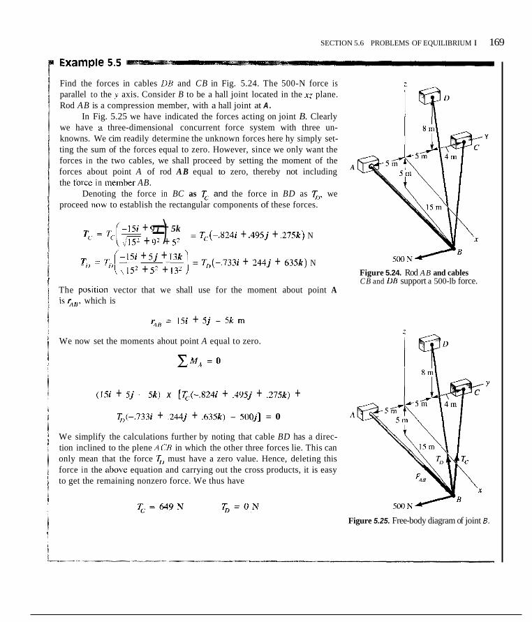
SECTION 5.6 PROBLEMS OF EQUILIBRIUM I 169
Find the forces in cables DB and CB in Fig. 5.24. The 500-N force is parallel to the y axis. Consider B to be a hall joint located in the xz plane. Rod AB is a compression member, with a hall joint at A .
In Fig. 5.25 we have indicated the forces acting on joint B. Clearly we have a three-dimensional concurrent force system with three un- knowns. We cim readily determine the unknown forces here hy simply set- ting the sum of the forces equal to zero. However, since we only want the forces in the two cables, we shall proceed by setting the moment of the forces about point A of rod A B equal to zero, thereby not including the forcc in member AB.
Denoting the force in BC as c. and the force in BD as G, we proceed inow to establish the rectangular components of these forces.
A
-1% + 9 j + 5k ,- ==) = Tc(-.824i + .495j + ,275.k) N
1 1 5 2 + 92 + S’ - 1 5 + S j + 13k
= T,(-733i + 2 4 4 j + 63%) N \ 152 + 5’ + I?’
The poyition vector that we shall use for the moment about point A ib % H . which is
‘aH = 1Si + 5 j - 5k rn
We now set the moments ahout point A equal to zero.
E M A = O
( 1 % + S j - Sk) X [T,.(-.624i + ,495j + ,275k) + 7;,(-.733i + 2 4 4 j + .63Sk) - SOOJ] = 0
We simplify the calculations further by noting that cable BD has a direc- tion inclined to the plene ACB in which the other three forces lie. This can only mean that the force 7, must have a zero value. Hence, deleting this force in the above equation and carrying out the cross products, it is easy to get the remaining nonzero force. We thus have
q = 6 4 9 N & = O N
Y
Figure 5.24. Rod A B and cables CB and LIB support a 500-lb force.
Figure 5.25. Free-body diagram of joint E .

170 CHAPTEK 5 F,QLIAlIONS OF EQUILlt(KII!M
Example 5.5 (Continued)
Finally. as indicated at the outset. we could proceed hy summing Sorces in the coordinate directions. The resulting scalar equations for al l three unknown forces are
-0.8247; - 0.7337;, + 0.90ST4 = 0
0.495T. + 0.2447;, + 0.302~; = 500
(3.2757;. + 0.6157;, - 0.3027; = 0
We may now solve the sitnultaneuus equations using C'rrinwr'r d r . Thus we calculate first the determinant of the coelficicnts of the unknown\. Thus
0.495 0.244 0.302 = 0.272 -0.824 -0.733 0.905
0.275 0.635 -0.302 I 0 -0.733 O.YO5
1500 0.244 0.302
I To calculate T . we pruceed as follows:
Note that the first column of the deterniinant consists of thc right side terms of the set of simultaneous equations i n placc 01 the coellicients of the desired unknown. We can solve for the other unknowns similarly. We then would have the comprcssive h r c e in member AB which i b 541 N.
I Case B. Coplanar Forces System. 1 we h;lve shown that the sini- pleg resultant for a coplanar force system (see Fig 4.14) is a single force or a single couple monicnt nomial to the plane. Thus. to ensure that the resultant furcc is 7.ero. we require lor a coplanar system in which all forces are in the ~ v x plane: c (b-< J , = 0 . ( F ; J , = 0 (5.10)
To ensure that the resultant couplc moment is zero. we require for mninenls abuut any axis parallel to the z axis:
We conclude that there are three scalar equations olequilibriuni for a copla- nar lurce system. Other combinations, such as two moment equations for twu axes parallel to the :. axiz and a single force summation. i l properly chosen, may bc employed to give the three independent scalar equations of equilih- rium, as was discussed in case A.

SECTION 5.6 PROBLEMS OF EQUILIBRIUM I 17 1
Example 5.6
Figure 5.26. A car i s being towed up an incline at a constant speed.
A car shown in Fig. 5.26 is being towed at a steady speed up an incline having an angle of 159 The car weighs 3,600 Ib. The center of gravity is located as is shown in the diagram. Calculate the supporting force on each wheel and force 7:
Y
\ 3,6W Ib
N, Figure 5.27. Free-body diagram of the car
A free-body diagram of the car is shown in Fig. 5.27. The forces N, and Nz are the total forces, respectively, for the rear wheels and the front wheels. Note, because the wheels are rotating at cnnstant speed, there are no friction forces present. We have thus formed on this free body a coplanar force system involving three unknowns and hence the unknowns are solvable by rigid-body statics. Using axes tangent and normal to the incline we have

172 CHAPTER 5 EQUATIONS OF liQll l l . lRRIUM
Example 5.6 (Continued)
C F , = o T - WsinO = o :. T = i3,hOO)(siii 15") = 931.7 Ih
i T = 931.7 1h 1
+io11 7)(1 5 ) l = 1.785 Ih
From Eq.( I ) . we can now per N,. Thu,
N, = 3,477 - N2 = 3.477 - 1,785 = 1,692 Ib
Clcarly each rear whccl has acting on it 21 normal fbrcr OF N,l2 = 846. I Ib and each front wheel has ii normal force olN, l2 = XY2.5 Ih.
Rear wheel support force = 846.1 Ib Front wheel support force = 892.5 lb
..
We may now check this soIuliu~i by using a rcdundant equation uf equilibrium. Thus
We have here il roundoff error, which wc can scccpt fix thz accuracy ol the calculations Laken in this pnrblcm.

SECTION 5.6 PROBLEMS OF EQUILIBRIUM I 113
Example 5.7
A frame is shown in Fig. 5.28 in which the frictionless pulley at D has a mass of 200 kg. Neglecting the weights of the bars, find the force trans- mitted from one bar to the other at joint C.
D
Figure 5.28. Loaded frame
To expose force components C, and Cy, we form the free body of bar BD. This is shown as F.B.D. I in Fig. 5.29. It is clear that for this free body we have six unknowns and only three independent equations of equilib- r i ~ m . ~ The free-body diagram of the bent b a AC is then drawn (F.B.D. I1 in Fig. 5.29). Here, we have three more equations hut we bring in three
F B D 1 F B D I1 Y
- 1.962 N
5.000 N F.B.D. 111
Figure 5.29. Free-body diagrams of frame parts
41t should be noted that it is possible to have situations wherein there we more uriknowns than independent equations of equilibrium for a givm free body, but wherein some of the unknowns--perhaps the dcsircd onea--can be still determined by the equations available. However, not all the unknowns “ I the free body can be solved. Accordingly, be alert for such situations, so as to ,minimize the work involved. In this case. we must consider other free-body diagrams.

I14 ("AFTER 5 FQLIATIONS OF FQIIII.IHKIUM
Example 5.7 (Continued)
more unknowns. Finally, the tree-body diagram 0 1 the pulley (F.B.D. 111 in Fig. 5.29) gives threc more equations with no additional unknowns. We now have nine equalions available and nine unknowns and can proceed with confidence. Since only two ot. the unknowns are desired, we shall take select scalar equations from each of the free-hody diagrams to arrive at the components C, and <.! most quickly
From F.H.D. 111:
Therefore.
Therefore.
Therefore.
From F.B.D. I:
Therefore,
Fmnz F.B.D. 11:
-I ,962 - s.000 + 0, = 0
11, = 6.962 N
-(1.3)(14) - (7')(3. l) - C,(4) + C s ( 2 . S ) = 0
Thereiore,
C, = 24.300 N
We can give the Sorce at C (transmittcd from bar AC lo bar BD) as
C = 2 4 , W + 11.313jN

5.17. In a tug of war, when team B pulls with a 400-lb force, huw much force must team C exert for a draw? With what force does team A pull'?
A
Ropes tied to a ring
B - C
Figure P.5.17.
5.18. cables ride over frictionless pulleys E and F.
Find the tensile force in cables AB and CB. The remaining
1- Figure P.5.18.
5.19. assumed to be frictionless in this problem.
Find the force transmitted by wire BC. The pulley E can be
5.20. Find the tensions in the three cables connected to B. The entire system of cables is coplanar. The roller at E is free to turn without resistance.
Y B
Figure P.5.20.
5.21. A 700-N circus performer causes a .15-m sag in the middle of a 12-m tightrope with a 5,000-N initial tension. What additional tension is induced in the cable? What is the cable ten- sion when the performer is 1 m from the end and the sag is .I2 m?
Figure P.5.21.
5.22. A 27-lb mirror is held up by a wire fastened to two hooks on the mirror frame. (a) What is the force on the wall hook and the tension in the wire? (b) If the wire will break at a tension of 32 Ib, must the wall hook be moved (i.e., the wire lengthened or sholt- ened and the 4-in. rise distance changed)? If so, to what point?
Wall hook
Figure P.5.19. Figure P.5.22.
17.

/ ' c ( M , ) , = 0. Axe\ d and e arc in,>[ ~ ~ i l i t i l l c l to the A; plane.
Moreover, the axe, are oricntcd so that the linc 01 action 0 1 the re\ultanl force cannot inter\rct hoth axcs.
5.24. weighs 1,000 N. C m ~ ~ p ~ i l e all contact force&.
Cylinders A and H weigh 500 N ciich mil c)l lndc~. ( ' ' %
/i
Figure P.5.25. Figure P.J.2X.

5.29. Find the supporting force systems far the beams shown. Note that there is a pin connection at C. Neglect the weights of the beams.
v 1.000 N
I00 N/m
n--I
klTlTL 8 m Figure P.5.29.
5.30. of C R is 8 m.
Find the supporting force systems at A and B. The length
A
Figure P.5.30.
5.31. shown? What are the forces in members AB, BE. and BC?
What are the supporting forces at A and D fbr the frame
. . .. . . . . .
Figure P.5.31.
5.32. wights except the IO-kN weight. Disregard friction.
What are thc supporting forces for the frame'! Neglect all
R
Figure P.5.32.
5.33. offer n o rotational resistance from friction at the beerings.
Find the supporting forces at E and K Pulleys A and B
Figure P.5.33.
177

Figure P.5.34.
35. An e l a l i c cord AH i \ .just tau1 beliore 1,000 force i \ iplied. I f il takes 5.0 N/mm of elongalion of the card, what is the r l i i i ) i i 7 ' in the curd after the I ,000-N force i s applied'! Set up the Iuation for 7'hut do ~101 solve.
Figure P.S.35.
36. A thin hoop o1 radius I 1x1 and weight 500 N rests on an :line. What friction force/ at A i s needed for this configun~atiun'? hat i s the tension iii wire CB?
Kigure P.5.36. k ipure P.5.39.
8

5.40. beam? Neglect the weight of the beam.
What is the supporting force system at A for the cantilever 5.43. Find the supporting force aystem at A
D
I-' -kid Figure P.S.40.
A Figure P.S.43.
5.41. the crms section at B.
In Problem 5.40, find the force system transmitted through 5.44. A light bent rod AD is pinned to a straight light rod CB at C. The bent rad supports a uniform load. A spring is stretched to connect the two rods. The spring has a spring constant of IO4 N/m, and its unstretched length is .8 m. Find the supporting forces at A and B. The force in the spring is I O 4 times the elongation in meters.
5,42. A to a simply suppone,j beam RC. For the luads given, find the supporting force systcm at A. Determine force components that are normal and tangential to the cross-section of beam AB. Neglect the weights of the beams.
beam AB is pinned at
Y
- 2 m
Figure P.S.42. Figure P.S.44.
175

5.45. Light rods A I ) and HC are pinncd together at C and sup- wi t a ?OWN and a IOO-N Indd. What arc the supporting forces a1 I and H?
5.47. Ih, and RC weighs 150 Ih.
Sulve fbr the supponing f r ~ e s at A and (T. AB weighs 100
300 N
Figure P.5.45.
Figure P.5.47.
i.46. A light rod CI) is held in a horiiontal position hy a strung ,lastic hand AH (shock cord), which acts like a spring in that it akrs IO3 N per meter felong gat ion vfthe band. The upper part of he band i s connected to a small wheel free to roll on a horizontal llrfdce. What is the angle a needed tu suppoit a 200-N l w d .s shown?
5.48. What torque 7 i s ncsded to maintain the configura- tion shown for the cumprcssor if p , = 5 psig'! The system lies horizontally.
Figure P.5.46. Figure P.5.48.
80

5.49. BC weighing 3 Ib and CD weighing 5 Ib.
Wurk Problem 5.48 for the system oriented vertically with 5.52. Find the supporting forces at A and G. The weight of W is 500 N and the weight of C is 200 N. Neglect d l other weights. The cord connecting C and D is vertical.
5.50. rium in t enns of ai, a, W,, and W,.
Neglecting friction, find the angle p of line AB for equilib-
Figure P.5.50.
5.51. If the rod CD weighs 20 Ib, what torque T i s needed to maintain equilibrium? The system is in a vertical plane. Cylinder A weighs 10 Ib and cylinder B weighs 5 Ib. Disregard friction. At D there is a slot.
Figure P.5.51.
Figure P.5.52.
5.53. weighs 500 N and CD weighs 30U N?
What torque T is needed for equilibrium if cylinder R
30"
Figure P.5.53.

5.54. jiameler 311 in. Gear 1: is pinned t n har AI3 and meshes with the wo planctary pears. which in turn mesh with statimary gear I). II 1 tirrquc 7 ' 0 1 100 N ~ m i s applicd 10 bar AH, ~ 1 ~ 1 c' t~cmi l l torquc s ncedcd to he applied t u thc upper planctary g c x 10 iniiintain
A har A l l i s pinned tn twn identical planewy g a r s ellch of A
Figure P.5.54.
I . I I .5 111
i.56. A Bucyrus+Eris tianhi1 crilnr i s holding il chimnc) having I weight 01 20 kN. The chirnnq is held by il cahle that gw\ w e r L pulley at A, thcn gee. i w c i a cccntid pullry at I) . and thcn to a uinch ill K . The position of baom AI! (on to,,) i s inaintaincil hy WII heparate cahles, one from A to /I. and the other from R to p~kI- ey C. Find the tensions in cohle5 AH and RC. Nuts that HC is oii-
veight of the load and neglect fr ictim. ,ntcd 30" from [he vertical f o r the setup show!. Consider only ttir /
Figure P.5.57.
3.121 m
82

SECTION 5.7 PROBLEMS OF EQUILIBRIUM 11 183
System
5.7 Problems of Equilibrium II
Number oJ Equations Simplest Resultant for Equilibrium
lease c. Parallel Forces in Space. I In the case of parallel forces in space (see Fig. 4.20), we already h o w that the simplest resultant can be either a single force or a couple moment. If the forces are in the z direction, then
Concurrent
Coplanar
Parallel
(three-dimensional)
single couple moment
(three-dimensional)
= 0 (5.12)
Single force 3
Single fkce or
Single force or
3
single couple moment 3
ensures that the resultant force is zero. Also,
guarantees that the resultant couple moment is zero, where the .r and v axes may be chosen in any plane perpendicular to the direction of the Thus, three independent scalar equations are available fur equilibrium of par- allel forces in space.
A summary of the special cases discussed thus far is given below. For even simpler systems such as the concurrent-coplanar and the parallel- coplanar systems, clearly, there is one less equation of equilibrium.
'For parallel forces in the I direction, a simplest resultant consisring ot a couple moment only murl have this couple moment parallel to the xy plane (see diagram). Recall from Chapter 3 that the orthogonal q z components of C, equals the torque of the system about these axes. Hence. by setting x ( M r ) , = C ( M v ) , = ( I , weareensuring thatC, = 0.

184 CHAPTER 5 I~QUATIONS < ) F F.QlllLlUKlllM
Example 5.8
Dcteriniiie ttic ~ W C C S required to suppoi-t (hi ' unifi)rm heirin in Fig. 5.30 showii Iwded with ii couple. a point force. iiiid ii downw;ird par;ihi)lic ( l is- trihutim of lo:ld hnring 7er-0 slope :it the origin. Thc weiftit o1 thr, hzam i s I O 0 I b.
20' ~ -- &~ ~~~
lO(1 Ihiul.1
Figure 5.30. Find \upp<r l ing force\
Since ii couple ciin hn rotated w i l l iw t afleclins Ihc cquilihriurli of the hody. we ciiii orieiil lhc couple s o llliil the lorccs arc vertic:il. AccoId- ingly. wc have here ii hcam loaded hy ii system 01 parallel coplanar loads. Clearly. Ihc siippoi-lin$ forces imusi hc wrtical, i ih shown ill F:ig. 5.31. wlicre %'e havc ii frcc-hirdy di;igl-aiii of ttic hciuii. Siiicc tlicrc ;ire imly IH(I unknown quantities. UT ciin handle the prohlcm hy \Liiticid considcralion 01 this free body.
K I H, Figure 5.31. f+cc,-hodj di:igr:wi
The cquatinn Ibr thc loading curve must he I V = m' + h. whcrc o and I, are ttr IR dctcriniiicd l i r ~ n i the Ir,;iding ilat,~ and tlic c h k c i i l rr ferei lce. With an .q rcfcreiicc ;it thc lelt end. tis shown, M'U then havc the conditions:
1. Whcnx = (1. bt' = 0.
2. When v = 20, 11' = 400.
To satisfy these cmiditimih, h niust he /ern ;ind (I niusl hc uiiity: the Itxiding liinctiim i\ lhus given a\
II' = ~ x ' lhifi

SECTION 5.1 PROBLEMS OF EQUILIBRIUM I1 185
Example 5.8 (Continued)
In this problem, we shall agein work directly with the scalar equti- tions. By summing moments about the left and right ends of the beam, we can then solve for the unknowns directly:
2u -500 - (10)(100) - (15)(500) - I, xy dx + 20R2 = 0
Replacing y by xz, then integrating and canceling terms, we get
-9,000 - + 20R, = 0 4' !:'I By inserting limits and solving, we get one of the unknowns:
R, = 2,450lb
Next,
-20Ri - 500 + (10)(100) + (5 ) (500) + 1,:(20 - x)ydx = 0
Replacing y by x2, integrating and then solving for R , , we have
R , = 817lb
As a check on these computations, we can sum forces in the vertical direction. The result must he zero (or as close to zero as the accuracy of our calculations permits):
20 R, + K2 - 100 - 500 ~ I x 2 d,x = 0
U
Therefore,
2,667 - 2,661 = 0
Always take the opportunity to check a solution in this manner (i.e., by using a redundant equilibrium equation). In later problems, we shall rely heavily on calculated reactions (supporting forces); thus, we must make sure they are correct.

186 CHAPTER 5 EQUATIONS OF FQIIII.IBRIIIM
Example 5.9
I n Fig, 5.32. find the suppnrting I i r c e s at A. D. and I ) . Note thc pin ~(111-
ncction at C. Also inole that at I< we haw n weldcd connection
Y
Figure 5.32. h lcmhcn . A ( ' and ( ' I ) arc pinncd 31 ('.
The free-hody diagram for thc entire system is shown i n Fig. 5.33. We have a coplanai s y s k m (if forces fkr this free body and s o we hmc only three independent equations of equilibrium. Howcvcr we have I ie i~r four unknowns. One of the unknowns, namcly A , , can he ser i i hy it i-
spection to he /,cro lea\'ing now a coplanar parallel system with three unknowns but with on ly two equations ofeqiiilihriuin.
\ '
I
Figure 5.33. Rcc-hudy d i a g a n i I. (F.R.I). I)
We shell next consider the frcc hody 01 mernhcr [ I ) . This is shown in Fig. 5.34 where we have simplified the distributed loading i n order to better facilitate the ensuing computakiiins. Clearly. for F.B.D. I I in Fig. 5.34. we will then haue only two unknmwis lor which we havc two equations of equilibrium. By raking moments ahout point C' in Fig. 5.34, we can directly dererniine [Ir.
i i i t i s t he x ro . Thus . 7' <',
Figure 5,34, R-ec-hody diagl~am (F.H.D. 11)

SECTION 5.7 PROBLEMS OF EQUILIBRIUM II 187
Example 5.9 (Continued)
C M c = 0 : ~ ~~~
(D,)(IS) - (2cu)( l s ) (y) - (:)(1s)(300)[(~)(15)] = 0
We may now go hack to Fig. 5.33 to solve for the remaining two unknowns. Thus, simplifying the loading between C and D as we have done i n Fig. 5.34. we have
I A> + E ) + 3,000 - (200)(34) - 1(300)(1S) = 0 c M, = 0: ~-
-A,(13) + (3,000)(21) ~ (200)(34)(2; - 13)
-~ (300) (15 ) [h+(~ ) ( IS ) ] 2 = 0
From Eq. (h), we get
And from Eq. (a), we have ,*
4.- 6,069N
Note that A, was negative indicating that we had inserted the wrong sense for this force in F.B.D. 1. We did not make any changes in the ensu- ing calculations while going to Eq. (a) (valid for F.B.D. 1) to calculate B, (i,e., we used the result from Eq. (c) with the negative sign of A, intact).
Also, if you were tempted in F.B.D. 1 to include the force C, at pin C in this diagram you were flirting with the prime error in the statics of rigid bodies-namely, including a force which is infernal to the particular free body drawn.
general case is a force and a couple moment. Six equations of equilibrium can be given for each free-body diagram. We now examine two examples for this case.

Example 5.10
A derrick i s shown in Fig. 5.35 supporting a 1,000-1b load. The verticil1 heam has a ball-and-socket coniiection inti, the ground at r l and i s held hy guy wircs ( IC' and t ic Neglect the weight of the mcinhers and guy wires. and find the tensiirns in the guy wires u r ' , hr. and ('e.
Figure 5.35. Loaded rlrrriok.
If we select as ti free hody both membcrs and the interconnecting guy wire w, we shall cxpose two of the desired unknowns (Fig. 5.36). Note that this i s a general three-dimensional hrce system with i inly five unknowns." Allhough all these unknowns can be solved by statical consid- erations of this free hody, you wi l l notice that, if we take monicnts ahout point d , we wi l l involve in a vector equation only thc desired unknowns Th,. and T,, . Accordingly. all unknown for-ces need riot he computed kir this free-body di;ipr;im. You should always look for such short cuts in sit- uations such as this.
To determine the unknown tension ?;.<,, we musl employ another free-body diagram. Either the vertical cor horimntal member wil l expose this unknown i n it manner susecptihle ti) solulion. The latter has been selected and i s shown in Fig. 5.37. Note that we have here a coplanar force system with ttircc unknowns. Again. you ciln Fee that, by taking moments about p in t , / . wc wi l l involve only the desired unknown.
Figure 5.3h. F'er-budY diagram I.
4 P
6; I,OOO Ih '% \ h i ~ o l d hc clciii on 8sipection ,,I big. 5.35 Ihiit. duc 11) symnclry. forma in the ~ W O
supp<,niog ~ i i h l ~ b nwst he eqii i l l . Usmg i l i i s intoimiitmr1 i\ l i in t i i rn~~in l to using cine of thc cquiitiow d c q o i l i h r i i ~ i n . Hiwcrcr. ror praclice we w i l l not uhc this inforination and we w i l l bu l \c lor h o l h 0 1 ihcxl cnhlcs and d e m ~ ~ n w a t c lhcir cqu"liiy. Also, iiutc that there i s it sixth cquiiliori dcqui l ihr i i i r t i llijll i, iklcniicnlly \ulialicd. To hcc this. look a1 rnooients of the forcer about a x ~ q mi in E g . 5.36 Why i s Ihc l ~ t i t l i i ioii iciit dcnt icidly quill i m zero ahuut this axi,, lhuc denyiiip \ I \ im qu i l t i on io hclp ~ I V C for unLnrwns'! I \ the derrick complcicly coii- ctraiocd" F.xplisin
Figure 5.31. Free-body diagram 2.

SECTION 5.7 PROBLEMS OF EQUILIBRIUM II 189
Example 5.10 (Continued)
The vector T,, may then be given as
Similarly, we have for Tbc ,
Using the free-body diagram in Fig. 5.36, we now set the sum of moments about point d equal to zero. Thus, employing the relations above, we get
13k x __ '' ( S i - l O j - 13k) + 13k x - ( - S i Tbc - l O j - 13k) m x'333 + l O j x (-1,000k) = 0 (c)
When we make the substitution of variable tl = and f2 = Tb< /m3, the preceding equation becomes
[130(tl t t2) - lO,OOO]i t [104(tl - t 2 ] j = 0 (d)
The scalar equations,
130(tl + fz) - 10,000 = 0 104(tl - t2) = 0
can now be readily solved to give f l = f2 = 38.5. Hence, we get cc = 38.5 ~ 6 % = 702 Ib and qc = 38.5 (333 = 702 lb.'
Turning finally to free-body diagram 2 in Fig. 5.37, we see that, in summing moments about f, the horizontal component of the tension q, has a zero-moment arm. Thus,
(10)(0.707)T,, ~ (IO)(l,OOO) = 0
Hence,
'By taking moments in Fig. 5.36 about the line connecting points a and d (see Fig. 5.35). we could get Tbc directly using the scalar triple product. We suggest that you try this.

190 CH.\PIt% 5 EQlli\llONS OF CQLIII.IHKIIIM
Example 5.11
A blimp i s \ h o w in Fig. 5.38 fixed at Ihc mooring lower n by a ball-ioint coiiiieclion. and held by ciihles A B and A<'. The lhlimp has a ma!.\ of l,SOO hg. Thc s imp lcb l resultirnt forcc P from air prcssure (includ- ing the effect\ 01 wind) is
F = I7.500i + I .OOOlj + I ,500k N
at ii position hhown in the diagram. Compute the tensior in the cables a s well as the I0rcc tran\initled L o the ball ,j(iint at the top 111 the towx i i t D. Also, what Sorce syslcni is transinittcd to the ground at G through the mooring tower? l h e towcr weighs 5.000 N.
Figure 5.38. Telhrl-cd hliiiip. We shall f irst consider ;I frec-body diagram of the hlinrp. as shown
i n Fig. 5.34. We have five unknown 1orcez hcrc. and we can d v e a l l 01
tlieiii by using equation!. ~Sequi l ihr iu ln for this free As it Sirst step, we express the cahlc tensions vectorially. That is.
We now gii hack to the basic vector cquation ~Iequ i l ih r iun i . 'l'hur Figure 5.39. Fize-body diagram OF hlimp.

SECTION 5.7 PROBLEMS OF EQUILIBRIUM I1 191
I I Example 5.11 (Continued) The scalar equations are
DL + 2,785 - .933%,. - .894T,, = 0 Dy + 1,000 + .447%, = 0 D. + 1.500 - .359%, = 0
(a) (b) (C)
Next take moments about point D
1 3 j x (9.81j(I,SOO)(-i)+ I h j x (17,500i + I,OOOj + 1,500k) + 2 9 j x TA,(-.933i - .359k) + 291 x TA,(-.894i + ,4471) = 0
Carrying out the various cross products, we end up nnly with k and i com- ponents, thus generating two scalar equations.' They are
-10.41T,,. + 24,000 = 0
25.9%, + 27.I%,. - 88,700 = 0
(d)
(e)
We now have five independent equations for five unknowns. We can thus solve these equations simultaneously. From Eq.(d), we have
T,, = 2,305 N
From Eq. (e), we have
TAB = 1,012
From Eq. (cj, we have
Dz = -673 N
From Eq. (b), we have
D, = -1,452 N
T h e lhird equation is 0 = 0. That is, there are no moments ahout they axis. because all forces pass through the Y axis.

Hcncc.
Frim t l i i h . we gcl
M b = 0 M , = 17.470 N-III M = -37,xoo N-Ill
We ciiii conclude t l i i i t . iil the ceiiler ol thc h i l h c . the Siircc systcm from t he ground is !
I' = 5.2701' ~
C = 17.47Uj - 37.XOOk N-iii
Thc Ibrcc system acting on the gr<~und iit the ccntcr 0 1 tlic hasc i\ tlrc re- action to Llie sy\ te~i i ahiibc. Thus.
l,4S2j - h72k N
i
i 6
<,,> ,,,, = -.5,27Oi + 1.452j + 612kN
C,cc,t,,, = -17,470j + 37,800k N-m

5.58. The triplc pulley sheave and the double pulley sheave weigh I S Ib and 10 Ih, respeclively. What rope fbrce is necehsary to l if t a 350-1b engine'! What is the force on the ceiling hook!
Figure P.5.58.
5.59. A multipurpose pry bar can be used tn pull nails in the three positions. If a fbrce of 400 Ib is required to remove a nail and a carpenter can exen SO Ib, which position(s) must he use'?
~ I .25"
c Figure P.5.59.
5.60. At what position must the operator of the cuunterwcight crane locate the SO-kN counterweight whcn he lifts a IO-kN h a d of steel?
I
Counter welght I
Figure P.5.60.
5.61. A Jcep winch is used to raise itself by a force of 2 kN. What are the reactions at thz Jeep tires with and without the winch load'? The drivcr weighs 800 N. and the Jeep weighs I I kN. The cenler of gravity of the Jeep is shown.
t ~ . ~ m + ) I- 1 . 3 m 3.1 m-
Figure P.5.61.
5.62. r, . and rz.
A diflerrnriul p d l q is shown. Compute F in terms of W,
F
Figure P.5.62. 19

5.63. What is the longest portion of pipe weighing 400 Ib/ft that can he lifted without tipping the 12,000-lh tractor'! Take the center
of rravity of the tractor at the L'eonietiic centcr.
5.66. An 1-hcam canrilevcred out Srom a ud l wcighs 30 lhift and supprim a 700-lh hoist. Steel (4x7 Ihilt'l TIIVCI plates I iii. thick arc uvlded on thc heam iirx the wiill lo incieiice the mmient- - . Carl-yinp capacity of the heam. What arc the reiictioiis at the u.all when a 400I-lh In;id is hoisted at thc out~rmost pmition of the hoist'.'
I,>,\, >P>p
I
<y- ~
9 Y/ I t - 8'-+
+ -5'-l
Figure P.S.63. Figure 1'5.66.
5.64. The L-shilped concrete post supports an clevated railroad. 5,67, the fc,rcc fill- ci iltlvcI. he; ,,,, The concrete weighs 1501 Ih /W What are the reactions at thr hese of the post'!
shr,wn (.,
r i
40.000 Ih
-8 Figure P.5.64.
5.68. cmncctcd to har A H hy pins.
Find the \upporting force sysrcm lor ttir cmtilewr heams
5.65. Two hoists arc operated on the same overhead track. Hoist A has a 3,000-lh load, and hoist R has ii 4.000-lh load. What are
rc.cti~,ns the ends c,c Lhr trach when the hoi,ts arc i n [he position shown?
Figure P.S.6X.
5.69. The tciilcr weighs SO kN and is loadcd w i t h crate\ wigti- i n s ' )O kN and 4 1 k N . What iiic thc rriictions at thr ,car wheel ;ind rm the tractor at ,I..'
Figure P.5.65. I'igure P.S.69. I 194

5.70. What load W will a pull P of IO0 Ib lift in the pulley sys- tem? Sheaves A, H, and C weigh 20 Ih, 15 Ih, and 30 Ib, respec- tively. Assume first that the three sheaves are frictionless and find W, Then, calculate W that can he raised at constdnt speed for the case where the resisting torque in each of sheaves A and H is .01 times the total force at the bearing of each of sheaves A and H .
Figure P.5.70.
5.71. A piece of pop art is being developed. The weight of the body enclosed by the full lines is 2 k N . What is the smallest dis- tance d that the artist can use for cutting a .5-m-diameter hnle and still avoid tipping'? The body is uniform in thickness.
I 4 m *-2 m-1 I
t=- i m
I=' Figure P.5.71.
5.72. What is the largest weight W that the crane cdn lift without tipping? What are the supporting forces when the crane lifts this load? What is the force and couple-moment system transmitted through section C of the beam? Compute the force and couple- moment system transmitted through section D. The crane weighs 1 0 tons, having a center of gravity as shown in the diagram.
50' ~
I 'c 20
Figure P.5.72.
5.73. A 20-kN block is being raised at constant speed. If there is no friction in the three pulleys, what are forces F,, 4, and F7 needed for the job! The block i s not rotating in any way. The line of action of the weight vector passes through point C as shown.
Figure P.5.73.
5.74. A 10-ton sounding rocket (used for exploring outer space) has a center of gravity shown as C.G.,. It is mounted on a launcher whose weight is S O tons with a center of gravity at C.G.,. The launcher has three identical legs separated 120" from each other. Leg At4 is in the same plane as the rocket and suppolting arms CDE. What are the supporting forces from the ground? What torque is transmitted from the horizontal arm CD to the ramp ED by the rack and pinion at hinge D to counteract the weight of the rocket'?
e Figure P.5.74.
195

5.75. A door i s hinged at A and N and contains watcr whosc spe- cific weight y is 62.5 Ihift'. A firrce 1.' nornral to the dnor keeps the door closed. What are the forccs on the hinges A and II and thr force F to ctrunteract the water? As noted in Chapter 4, thc prei- sure in thc water above atmosphere i s givcn as yd. where rl i s the pcrpendicular distance from the k e surface of the wjatcr.
Figure P.S.75.
5.76. A row of hooks of length 750 niin and weighing 200 N si ts .m a three-legged tahle as shown. 'The legs are equidistant from :ach other with one leg N coinciding with the y axis. l 'he crthcr :wo legs lie along a line parallel to the ,t axis. If thc tahle weighs 100 N, wil l i t tip'! If not, what hie the fhrces on the legs'?
Figure P.S.76.
i.77. A small helicopter i s in a hovering mancuvc~~. The lhcli- opter rntor hladcs givc a lifting force I ; hut therc result\ from the ir forces on the hlades B lorquc c', . The rex rotor prevents thc ielicupter from rotating ahout the i axis hut drvclaps n torquc C , . :ompute the force F; and couple C, i n terns of the weight @ iow arc F, and (I, related'!
96
A
1 7 111
t '
Figure P.5.77.
5.78. Find the supporting force and couple-moment system for the cnntile\icr hcam. What i s the force and couple-moment system Irammitted through a cross section of the heam at R'!
I
500 Ih Figure P.S.78.
5.79. A structure i s supported hy a ball-and-socket joint at A , a pin connection at N offering no resistance in the direction AB, and a himplr roller support at C. What are the supporting forces fcrr the lnads shown'!
+ 2(H) kN
Figure P.5.79.

5.80. Compute the value of F to maintain the 200-lb weight shown. Assume that the bearings are frictionless, and determine the forces from the bearings on the shaft at A and B.
5.83. Determine the vertical force F that must be applied to the windlass to maintain the 100-lb weight. Also, determine the sup- porting forces from the bearings onto the shaft. The handle DE on which the force is applied is in the indicated XI plane.
F
Figure P.5.80.
5.81. A bar with two right-angle bends supports a force F given as
F = 10i + 3j + IOOkN
If the bar has a weight of I O N/m, what is the supporting force system at A'?
Figure P.5.81.
5.82. the section at A? The couple is parallel to plane M.
What is the resultant of the force system transmitted across
V
i
1- I . z m +
Figure P.5.82.
Figure P.5.83.
5.84. A transport plane has a gross weight of 70.000 Ib with a center of gravity as shown. Wheels A and B are locked by the braking system while an engine is being tested under load prior to take off. A thrust T of 3,000 Ib is developed by this engine. What are the supporting forces?
Figure P.5.84.

5.85. Two cahles GH and K N support a rod A R which connCCtC to a ball-and-socket joint wpporl at A and q q m r l s ii 500-kg hady C at R. Whal are the tensioni in the cahle and the supporting forces at A’!
Figure P.5.85.
5.86. What changc in elentirm fkr thc 100-lh weight wil l a coii- ple of 300 Ih-ft support if wc neglect li.ictian in the hearings :it A and R? Alw, determine the suppolling fbrce cwnponcnts at the I bearings for this crrnfiguration.
Figure P.S.87.
5.88. What force P i s needed tu huld thr door i n a hwimntal pohilion? ‘lhc door weighs SO Ih. Dcterminc the SuppOl-li~lf l o ~ w c \ :it A and 8. At A there i s a pin and at / I therc i\ il hall-and- mckrt ,joint.
Figure P.S.88.
*S.RY. A onilbnn has of length /and weight 1V i s connecled to the ground hy a ball-and-wckct iomt, and r a t s on a wnicylindcr i ron which i t 15 not allowed to slip down hy n wall at U. If we crinsidcr the wall and cylindcr 10 he frictiotilcah. dctcmiine the supporting I r c z c at A for the follou,ing data:
I = I m < = 30 111
,’ _I .?O 111
h = ..101n W = 1 0 0 N
I Figure P.5.86.
5.87. Dctcrmine thc frircc P requircd to ep the 150-N or of an airplane open SO” while in Ilight. Thc Sorce P IS excrfed ill il
dircctinn normal to the fiiselagc. There is a i i ~ t prersure increase o n thc ootcide surfxx of .02 N/,nmz. Alw. determine the support- ing forces at thc hinge&. Consider thal the top hinge supports any vertical force on the door. Figure P.5.89.
198

SECTION 5.8 TWO POINT EQUIVALENT LOADINGS 199
5.8 Two Point Equivalent Loadings We shall now consider a simple case of equilibrium that occurs often and from which simple useful conclusions may readily be drawn.
Consider a rigid body on which the equivalent systems of two separate forces are respectively applied at two points a and b as shown in Fig. 5.41. If the body is in equilibrium, the first basic equation of statics, 5.l(a), stipulates that F, = -F2; that is, the forces must be equal and opposite. The second fun- damental equation of statics, 5.l(b), requires that C = 0, indicating that the forces be collinear so as not to form a nonzero couple. With points a and b given as points of application for the two forces in Fig. 5.41, clearly the com- mon line of action for the forces must coincide with the line segment ab. Such bodies, where there are only two points of loading, are sometimes called “two-force” members. Such members occur often in structural mechanics problems. Furthermore, there is considerable saving of time and labor if the student recognizes them at the outset of any problem.
Figure 5.41. Two-force member.
We often have to deal with pin-connected structural members with loads applied at the pins. If we neglect friction at the pins and also the weight of the members, we can conclude that the equivalent of only two forces act on each member. These forces, then, must be equal and opposite and must have lines of action that are collinear, with the line joining the points of application of the forces. If the member is straight (see Fig. 5.42). the common line of action of the two forces coincides with the centerline of the member. The top member in Fig. 5.42 is a compression member, the one below a tensile mem- ber. Note that the bent member in Fig. 5.43, if weightless, is also a two point loaded member. The line of action of the forces must coincide with the line ab connecting the two points of loading. However, the beam in Fig. 5.44 is not a two point loaded member since at the left end there will be a couple moment, And, clearly, such a loading must entail two points of loading to accommodate the two equal and opposite forces comprising the couple. There are then in effect three points of loading for this member. Accordingly, use caution here when dealing with a cantilever beam.
Before considering an example, it should be emphasized that the forces 4 and 5 in Fig. 5.41 may be the resultants of systems of concurrent forces at a and b, respectively. Since concurrent forces are always equivalent to their resultant at the point of concurrency, the member in Fig. 5.41 is still a two- force member with the resulting restrictions on the resultants & and F2.
4 + Figure 5.42. Compression and tension members
a b )
Figure 5.43. Line of action of F collinear with ab.
Figure 5.44. Cantilever beam is not an example of a two point loaded member.

A device lor crushing rock\ ic chown i n Fig. 5.45. A pistiin I ) having iiii %in. diameter is aclivated hy il pressure 11 of 5 0 p i g (~~i iundh per sql ia le inch above that or the atmosphere). Rod?, A B , 11C'. ;1nd I l l) can he consid- ered wcightlcss for this prohlcni. What is the horimnkil force tranhrnitled at A tn the trapped rock shown i n the diagram'?
We have he]-e thrcc two-force menibcrh coining kigethci- iit 11. Accordingly. if we i d a t e pin I1 a s a rrec body. we will h;ir.c Ilircc forces acting o n thc pin. These forces must he collinciir with the cenlerliiieh 01 the respectivc mcnihers. a s explained earlier (Fig. 5.42).
Thc force I.;> is easily computed by considcring the iictioii 1 i i Ihc piston. Thus. we get
Figure 5.45. Rock crusher.
/;] = 150)nx' = 2,51(1 Ih 4
The lorcc transmitted to the rock i n the horimiitiil dircction ic f l ie i i 4.850 1 cos I S " = 4.690 Ih. I;,
Figure 5.36. trce-hmly dia;rarn o i pin H. i :. Horizontal force transiniltcd to thc rock = 4,690 Ib
5.9 Problems Arising From Structures

SECTION 5.9 PROBLEMS ARISING FROM STRUCTURES 201
Example 5.13
Rod C shown in Fig. 5.47 is welded to a rigid drum A, which is rotating about its axis at a steady angular speed wof 500 RPM. This rod has a mass per unit length w, which varies linearly from the base to the tip starting with the value of 20 kg/m at the base to 28 kglm at the tip. If normal .strexs is defined as the normal force at a section divided by the area of the sec- tion (similar to pressure except that the force can be pulling away from the section rather than always pushing against the section), what is the normal stress at any cross section of the cylinder at a distance r from the centerline B-B of the drum due only to the motion?
,Rod C
Figure 5.47. Rods attached tu il rotating rigid drum
First we expose a section of the rod at a distance r from B-B in a ,frre-bod? diagram as shown in Fig. 5.48 in which we denote the normal stress acting on this section as rrr. The force from this section must restrain the centrifugal force stemming from the angular motion of the portion of the rod beyond position r . For this purpose, we consider an infinitesimal slice of the rod (see Fig. 5.48). We shall use the variable q to denote the distance to the slice from the centerline B-B. Furthermore, the thickness of the slice shall he dq. We shall use rl to position slices bctween end posi- tion r of the free-body diagram and the tip of the rod. We are using this approech for bookkeeping purposes. Now you will recall from freshman physics that the centrifugal force on this slice is given by

202 CHAPTEK 5 EQUATIONS OF EQlJlLIBRlUM
Example 5.13 (Continued)
F.B.D , XCentritugal turcr
B R
Figure 5.48. Free hody exposes T,, at section r. Note that q is a dummy wriahle.
Consequently, the total centrifugal force for the material beyond position r in the free body of Fig. 5.48 will he found by integration to be
7 f,,,, = WJJ dq 0' (b)
Next, note that the term w varies linearly with JJ as follows:
w = 20 + ' 1.2 8 kg/m
Clearly from this equation we see that when q = .2, we get a' = 20 kglm and when JJ = .7, we get M' = 28 kg/m. Also, the variation is linear. Now, going back to Eq. (b), we have
f,,,,, = 2.742 x IO' Integrating
= 2.742 x 10'[4.116 + 1.829 - 8.40r2 ~ 5 . 3 3 3 ~ ~ 1
We can give the desired stress T , ~ by dividing by the cross-sectional area nD2/4 = 7.854 x 10-'mZ. We thus have the desired normal stress distri- bution for sections of the rod as follows:

SECTION 5.9 PROBLEMS ARISING FROM STRUCTURES 203
Example 5.14
Consider a thin-walled tank containing air at a pressure of 100 psi above that of the atmosphere [see Fig. 5.49(a)]. The outside diameter D of the tank is 2 ft and the wall thickness t is 114 in. We consider as a free body from the tank wall a vanishingly small element such as ABCE in the dia- gram having the shape of a rectangular parallelepiped. What are the stresses on the cut surfaces of the element? Neglect the weight of the cylinder.
(4 (b) (C)
Figure 5.49. Thin-walled tank with inside gauge pressure p .
We can examine face BC by considering a free body of part of the tank, as shown in Fig. 5.49(h) exposing BC. (Note that we have not included the pressure on the inside wall). Because there is a net force from the air pressure only in the aria1 direction of the cylinder, we can expect normal stress r,, (like pressure except that it is tensile rather than com- pressive) over the cut section of the cylinder, as has heen indicated in the diagram. Furthermore, because the wall of the tank is thin compared to the diameter, we can assume that the stress r,,, is uniform across the thickness. Finally, for reasons of uxiul symmet? of geometry and loading, we can expect this stress to he uniform around the entire cross section. Now we may sily from considerations of equilibrium in the axial direction that
L J
= 2.325 psi p ( D - 2 t )2 (IOO)(24 - $1' :. 7 = -- (a) nl D2 - ( D - 2 t )2 = -24* - 23.52
Hence, on face BC we have a uniform stress of 2,325 psi. Clearly, this must also be true for face AE. This is called an uxiul stress.
To expose face EC next, we consider a half-cylinder of unit length such as is shown in Fig. 5.49(c). Because it is j a r from the ends and because the wall is thin, we can assume as an approximation that the stress rn2 shown is uniform over the cut section." A pressure p is shown acting
"Nenr the ends of the tank lhe stress distribution varies in value because of 1he pror- imily ofthe comp/icoredyrornrrry atid the contributions toward equilibrium afthe end plates.

204 ('HAPTEII s EQUATIONS or EQUILIBKIIJM
Example 5.14 (Continued)
: normal to the insidc wall surface. (The stress r,,, computed earlier i s licit ; shown, to avoid cluttering the diagram.) Now we consider an end view of ! this body i n Fig. 5.50 lor cquilihriuin in the vertical directiiin. Wc havc
4
2[(r,,? ) ( / ) ( I ) ] -- lrp(; - / )c /Q( l ) s i nQ = o (b)
:. r,,2 = I [,,( '2' -- I ) ] ( - cos Q)~n I1
21 3 t
y
Figure 5.50. I k r bridy of pari of cylinder. r,,2 = ,J( 2 - 1 ) = 4,700 psi
I I ! i We puinl out now that the force in a piirlicular direclion friini a uni- : lorm Dressitre on a curved surfice equals lhc Drcssurc times the uroiected
5 , , r . . area of this surface i n the directkin ( i f thc dcsircd force. (You wil l leiiri i this in your studies (if hydrostatics.) Thus for the case at hand tlie projected area i s that of a rectangle I x (11 - 21). s o that the second expresion of
sanie result as ahovc.
,sfre.s,s r,, . Wc show element A M % with the stresscs present in Fig. 5.51
r " \ Eq. (h) becomes p ( D - 2). You inay rcadily verify that this give\ thc
TI, The stress r,,, i s called the hoop .srrc.ss; i t i s about twice the u~rirrl
Figure 5.51. Free body u l ~ n clcrncnt of the cylinder.
. ," ,__x_I . . . ,. ~ .... , ;_______.. . , . ... .. . ., _"l_l_.. ,
5.10 Static indeterminacy Examine the simple beam i n Fig. 5.52, with known external loads and weight. I S thc defiirniation of the heam i s small, and the final positions o f the external loads alter deformation differ only slighlly Srom their initial positions, we can
unic the bcem to be rigid and. using the wideformed gcomctry, we can solve the \upporting forces A, I<<, and B,. This is piissihle since we have three equationa (if equilibrium available. Suppose, now, that an additional support i s made availahle to the beam, as indicated in Fig. 5.53. Thc beam can still be coiisidered a rigid body, since the applicd Imd wi l l shift even less hecause 0 1 de1orm;ition. Thcrclore, the resultant force coming from the ground to coun- tciilct the applied loads and wcight of the beam niust he the sume as before. In ti le first case, in which two supports wei-e given, howcvcr, a unique set 01 val- ues for the Siirces A. Bl , and By gsve us the required rcsullant. In other words, we wcrc able to solve for these liirccs hy stdtics alone, without further cun-
I{,
Figure 5.52. Skitically drtel-minatc problem

SECTION 5.10 STATIC INDETERMINACY 205
siderations. In the second case, rigid-body statics will give the required same resultant supporting force system, but now there are an infinite number of possible combinations of values of the supporting forces that will give us the resultant system demanded by equilibrium of rigid bodies. To decide on the proper combination of supporting forces requires additional computation. Although the deformation properties of the beam were unimportant up to this point, they now become the all-important criterion in apportioning the sup- porting forces. These problems are termed statically indeterminute, in con- trast to h e statically determinate type, in which statics and the rigid-body assumption suffice. For a given system of loads and masses, two models-the rigid-body model and models taught in other courses involving elastic behav- ior-are accordingly both employed to achieve a desired end. In summary:
indeterminate problem, we must satisfy both the equaiions of fur rigid bodies and the equations that stemfrum deformation
tions. In statically determinare problems, we need only satisfy ons of equilibrium.
In the discussion thus far, we used a beam as the rigid body and dis- cussed the statical determinacy of the supporting system. Clearly, the same conclusions apply to any structure that, without the aid of the external con- straints, can be taken as a rigid body. If, for such a structure as a free body, there are as many unknown supporting force and couple-moment components as there are equations of equilibrium, and if these equations can be solved for these unknowns, we say that the structure is externally statically determinate.
On the other hand, should we desire to know the forces transmitted between internal members of this kind of structure (i.e., one that does not depend on the external constraints for rigidity), we then examine free bodies of these members. When all the unknown force and couple-moment compo- nents can be found by the equations of equilibrium for these free bodies, we then say that the structure is internally statically determinute.
There aTe structures that depend on the external constraints for rigidity (see the mucture shown in Fig. 5.54). Mathematically speaking, we can say for such structures that the supporting force system always depends on both the internal forces and the external loads. (This is in contrast to the previous case, where the supporting forces could, for the externally statically determi- nate case, be related directly with the external loads without consideration of the internal forces.) In this case, we do not distinguish between internal and external statical determinacy, since the evaluation of supporting forces will involve free bodies of some or all of the internal members of the structure; hence, some or all of the internal forces and moments will be involved. For such cases, we simply state that the structure is statically determinate if, for all the unknown force and couple-moment components, we have enough equations of equilibrium that can be solved for these unknowns.
Figure 5.53. Statically indeterminate problem.
Figure 5.54. Nonrigid structure

5.90. Draw tree-hudy diagram\ liir the hoe. aims, and tractor 01 the bdckhuc. Conhidcr thr weight of cach part to act at a central location. Thc backhoe IS inot digging at thc insmil shown. Neglect the weights of the hydraulic systcms CE, AH, and Fli ,
Figure P.5.90.
5.Yl . A parking-lot gate ami weighs 150 N. Becauw 01 thc .itper, thc weight can he regarded a\ conccntl-a~cd at a puint I .?5 11 from the pivot point. What iorce must he exrrtcd hy the sole- loid to l i l t the galc? What mlcnoitl force i\ necehsary it a 300-N :r,unlerwcight i s plised .25 111 to the left o l t h e pivot point?
i.92. Find thz force dclivcrcd ill c' i n a lhiiiimnval direction v crush the rock. Presrurc p = 100 p i g arid p , = hO psig pressures nieebured a h w r atmmpheric prehwrci. The diameter\ )I the pistons are h iii. each. Nrglcot thc wciplit d thr rock Figure P.5.94

5.95. Find the values of F and C so that members AB and CD fail simultaneously. The maximum load for AB is 15 kN and for CII is 22 kN. Neglect the weight of the members.
5.98. (a) Find the supporting forces at B. Neglect the weights of
(b) What is the force in the member CB? the members.
1 1 100 mm
Figure P.5.95.
5.96. The landing carriage uf a transport plane supports a sta- tionary total vertical load of 200 k N There are two wheels on each side of shock strut AB. Find the force in member EC, and the forces transmitted to the fuselage at A, if the brakes are locked and the engines are tested resulting in a thrust of 5 kN, 40% of which is resisted by this landing gear.
Figure P.5.98.
5.99. Find the suppotting forces at B and C. Disc A weighs 200 N. Neglect the weights of the members as well as friction.
5.97. Find the magnitudcs (if the supporting forces fur the frame show You may only use fuv free-body diagrams for this prob- lem. k t forth a complete system of equations for solving the desired unknowns hut do not carry out the algebra for actually solving these equations for the desired unknowns.
Figure P.5.99.
5.100. Find the supporting force system at C. Neglect friction.
Figure P.5.97. Figure P.5.100.
207

c
U Figure P.5.102 Figure I'.5.I04.

5.105. A trdp door i s kept open hy a rod CD, whose weight we shall neglect. The door has hinges a1 A and R and has B weight OS 200 Ib. A wind hlowing against the outside surface of the door creates a prersure increase o f 2 Iblft'. Find the force in the rod, assuming that i t cannot slip from the position shown. Also deter- mine the forces transmitted to the hinges. Only hinge B can resist motion along direction AR.
Figure P.5.105.
5.106. Find the Ibrce BO. Al l conncctims are ball-and-socket ,ioints. Neglect the wcights of a l l the members. Member AB has two XI' bends. Member RI) i s in the yz. plane.
Figure P.S.106.
5.107. Find the supporting forces at A and C. You must show and use only m e free-body diagram.
2 m k+
Figure P.5.107.
5.108. A coupling between two shafts transmits an axid load ot 5,000 N. Four bolts ha\ing a diameter each of 13 mm, cmnects the two units. Befbrc loading of the shafts, thesc bolts have anly negligible tensile forces. Assuming that each bolt carries the same Inad, what i s the average normal stress in each bolt stemming from the 5.(100 N lotid?
5 0 N m C F " Figure P.5.108.
5.109. A circular shaft i s suspended from above. The specific weight OS the shaft material i s 1.22 x I O * Nlm'. What i s the ten- sile stress r.. o n cross sections of the shaft a i a function of r?
Figure P.5.109.
5.110. Do the previous pmblrm k r the czce whex the specific weight y varies with the syuure of z starting with the value of 6.50 x IO" Nlm' at the top and reaching a value of 7.50 x I O 4 Nlm' at the bottom.
209

Figure 1'.5.1 11.
5.11 Closure

5.113. mass of 600 kg. Note that GH is in the yz plane.
Determine the tensions in 811 the cables. Block A has a
Figure P.5.113.
5.114. Determine the force components at G. E weighs 300 Ih.
Figure P.5.114.
5.115. A scenic excursion train with cog wheels for steep inclines weighs 30 tons when fully loaded. If the cog wheels have a mean radius to the contact points of the teeth of 2 ft, what torque must he applied to the driver wheels A if wheels B run free? What force do wheels B lransmit to the ground?
I I /-
5.116. A and F.
Find the forces on the block of ice from the hook.; at
A + I 5' *I
Figure P.5.116.
5.117. Members AB and BC weighing, respectively, 50 N and 200 N are connected to each other by a pin. BC cunnecls to a disc K on which a turque T, = 200 N-m is applied. What turque T is needed on A B tu keep the system in equilibrium at the configura- tion shown'?
Figure P.5.115. Figure P.5.117.
21

5.1 I X . A transport j e t planr has ii weight without frirl uf220 kN. I f om wing i s I<,aded with S O k N r i f f k l , what are the force? in eich 01 the three landing gear?
H--' 4 111 4 111
Figure P.5.118.
5.119. A rod AB i s connected by a hall-and-wcket joiiit to a frictionlesc sleeve at A , arid by a ball-and-sochet .joint to ii fixcd position at 8. What are the supporting fbrccs at B and at A i l we ncglect the weight of AB? The 100LIh load i\ connected 10 the C C I I ~ C I 0 1 A l l .
i
8'
212
Figure P.5.119. Figure P.5.122.

5.123. Light rods RC and AC are pinned together at C and sup- port a BOO-N load and a 500-N-m couple moment. What arc the supporting forces at A and B ?
5.125. A bent rod AUCB supports two weights-one at the cen- ter of AU and one at the centcr of UC. There are ball-and-socket joint supports at A and R . With one scalar equation using the triple scalar product, determine the tension in cable Uc'.
2 m
10,
I Figure P.5.123.
5.124. A rod AB is held by a hall-and-socket joint at A and sup- ports a 100-kg mass C at 8. This rod is in the z? plane and is inclined to the? axis by an angle of 159 The rod is 16 m long and F is at its midpoint. Find the forces in cables DF and ER. Crosa- hatching indicates part of the V E plane.
x
Figure P.5.124.
x
Figure P.5.125.
5.126. Use only one free body.
Find the tension in cable FH. The disc C weighs 500 Ih.
H
Figure P.5.126.
213

Figure I'S.131

5.132. wires. What are the tensions in these wires?
A uniform block weighing 500 Ih is constrained by three
A n
Figure P.5.132.
5.133. Find the suppvrting forces for thz frame shown
,,- ~ k 2,000 Nini
2-
Figure P.5.133.
5.134. Four cables supporl a black of weight 5,000 N. The edges of the block are parallel to the coordinate axes. Point B i s at (7, 7, -15). What are the forces in the cables and the direction cosines for cable CI)?
Figure P.5.134.
5.135. A mechanism consists OS two weights W each OS weight 50 N, tour light linkagi: rods each of length (i equal 10 200 mm, and a spring K whose spring constant i s X Nlmm. The spring i c unextended when H = 450 I f held vertically, what is the angle B fix equilihrium'! Neglect friction. The force from the spring equals K times the compression of the sprins.
Figure P.S.135.
5.136. tant supporting force system at E!
Find the compressive force in pawl AB. What is the resul-
, ~, ,, .,:__ fi:
Figure P.5.136.
5.137. A IO-kN load is lifted in the front loader bucket. Whal are the furces at the connections tu the bucket and to ann AEI Hydraulic ram DF i s prrpcndicular to arm AE, and AC is hor imn~ tal. Points A and I. ;ire iit the same height above the friiund.
I S ' " ,
Figure P.5.137.

n
L-1
Figure P.5.142.

5.144. Ncglect friction.
What force F do the pliers develop on the pipe section Ll?
10 mm
'13ON
Figure P.5.144.
5.145. weights except the IO-kN weight.
What are the supporting forces for the frame'? Neglrct a11
n Figure P.5.145.
5.146. lor O < B < 7 ~ 1 2 as
A 20-m circular arch must withstand a wind load given
f = 5,000( I - n) e Nlm
where B is measured in radians. Note that for 8 > 7~12, there i? n o loading. What are the supporting forces? (Hint: What is the point lor which taking moments is simplest'!)
Wind load normal to arc
A ti Figure P.5.146.
5.147. An arch is formed by uniform plates A and R. Plate A weighs 5 kN and plate R weighs 2 kN. What are the supporting forces at C, 1). and E'!
20 kN I
Figure P.5.147.
5.148. Find the iupponing forces at the ball-and-socket connec- tions A , 0, and C. Mcmbers A 8 and DB are pinned together through member EC at R.
I.000 Ib Parallel
x Figure P.5.148.
217


5153. A bar can rotate parallel to plane A about an axis of rota- tion normal to the plane at 0. A weight W is held by a cord that is attached to the bar over a small pulley that can rotate freely as the bar rotiltes. Find the value of C for equilibrium if h = 300 mm, W = 30 N, @ = 3(Y, I = 700 mm, and d = 500 mm.
x x
Figure P.5.153,
5.154. Neglect weights of member?.
Find the supporting forces at A and B in the frame.
I I O Ih/ft
F
40'
Figure P.5.154.
5.155. What is the force on the bolt from the cutter edge?
A holt cutter has a force of 130 N applied at each handle.
,Bolt
130 N
Figure P.5.155.
5.156. A steam locomotive is developing a pressure of .20 Nlmm' gage. If the train is stationary, what is the total traction force from the two wheels shown? Neglect the weight of the various connect- ing rods. Neglect friction in piston system and connecting rod pins.
30 m ... .4? m
5.157. weight ofthe rod. Use only one free-body diagram.
Find the supporting forces at A , A, and C. Neglect the
IW Ib
c 30" Figure P.5.157.
5.158. The 5,000 Ib viin A of an airline food catering truck rises straight up until its floor is level with the airplane tloor. A hydraulic ram pulls on the right bottom support of the lift mechanism at which we have rollers to prevent friction. The two members of the lift mechanism are pinned at their center. The center of gravity of the van is its geometric center. What is the ram force for this position?
I- 1 2 ' 4 No friction
Figure P.5.158.
219
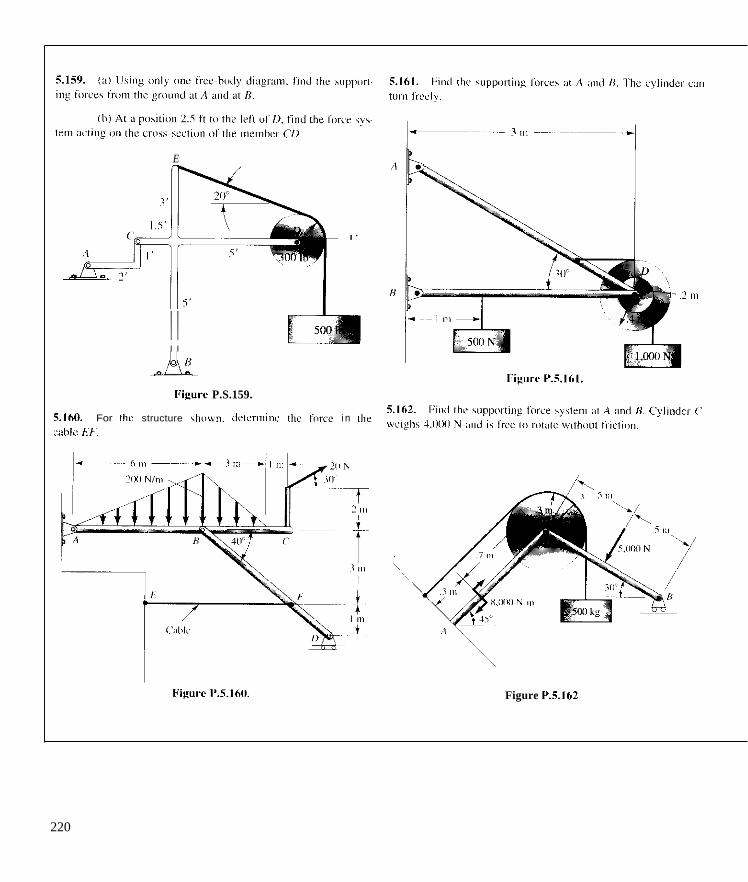
E
! !
I '
Figure P.S.159.
S.IU1. For lhc structure \houii. dc lemi ine i hc i m c e i n the ;:ihlc Et' .
Figurc P.S.lh0. Figure P.S.162
220

Introduction to Structural Mechanics Part A Trusses
6.1 The Structural Model A trus,? is a system of members that are fastened together at their ends to sup- port stationary and moving loads.' Everyday examples of trusses are shown in Figs. 6. I and 6.2. Each member of a truss is usually of uniform cross-section along its length; however. the various members typically have different cross- sectional areas because they must transmit different forces. Our purpose in Part A of this chapter is to set forth methods for determining forces in members of an elementary class of trusses.
As a first step, we shall divide trusses into two main categories accord- ing to geometry. A truss consisting of a coplanar system of members is called a plane Irus.7. Examples of plane trusses are the sides of a bridge (see Fig. 6.1) and a roof truss (see Fig. 6.2). A three-dimensional system of members, on the other hand, is called a p a c e truss. A common example of a space truss is the tower from an electric power transmission system (see Fig. 6.3). Both plane trusses and space trusses consist of members having cross-sections resembling the letters H, I, and L. Such members are commonly used in many structural applications. These members are fastened together to form a truss by being welded, riveted, or bolted to intermediate structural elements called Russet plates such as has been shown in Fig. 6.4(a) for the case of a plane truss. The analysis of forces and moments in such connections is clearly quite complicated. Fortunately, there is a way of simplifying these connections
' A i i u s , ~ is different than a,frame (see the footnote on p. 157) in that the members of a truss are always connected together at the ends of the members. as will soon become evident, whereas a frame has some rnemhers with connections not at the ends of the member.
22 I

222 CHAPTER 6 INI 'ROI~IICTION TO STRUCTURAL MECHANICS
Figure 6.1. Foot hridgc near author's former home. Sidcs oi sirucfurc are plane irusscs
Figure 6.2. Roof trusses that are plane trusses

SECTION 6.1 THE STRUCTURAL MODE 223
Figure 6.3. Space tmsscs supporting transmission lines sending power into the northeast grid of the United States.
such as to incur very little loss in accuracy in determining forces in the mem- hers. Specifically, if the centerlines of the members are (nncurrenf at the connections, such as is shown in Fig. 6.4(a) for the coplanar case, then we can replace the complex connection at the points of concurrency by a simple pin connection in the coplanar truss and a simple ball-and-socket connection for the space truss. Such a replacement is called an iderzliiution of the system. This is illustrated for a plane truss in Fig. 6.4, where the actual connector or joint is shown in (a) and the idealization as a pinned joint is shown in (b).
In order to maximize the load-carrying capacity of a truss, the external loads must he applied at the joints. The prime reason for this rule is the fact that the members of a truss are long and slender, thus rendering compression members less able to c a y loads transverse to their centerlines away from the ends? If the weights of the members are neglected, as is sometimes the case, it should be apparent that each member is a t ~ ' ~ ~ f i ) r c e member, and accord- ingly is either a tensile member or a cornpression member. If the weight is not negligible, the common practice as an approximation is to apply half the weight of a member to each of its two joints. Thus, the idealization of a mem- ber as a two-force member is still valid.
'You will understand these limitations innre clearly when you study huckling in your strength 0 1 materials course.

rr i i iovi i l 01 ;my of i t s menrherc dcst ioyc i t s rigidity. Ii rcmo\:ing :I mrniher does not dcstioy rigidity, the \ti-ucture I \ said IO be ( iv?r~ri ,qid. Wc shiill he

SIXTION 6.4 METHOD OF JOINTS 225
forces acting on it from the members can always he found. (One such joint is the last joint formed.) Each unknown force from a member onto this joint must Iiavc a direction collinear with that member, and hence has a known direction. There are, then, only three unknown scalars, and since we have a concurrent forcc system they can he determined by statics alone. We then find another joint with only three unknowns and so carry on the computations unti l the forces in the entire structure have been evaluated. For the simple plane truss, it similitr procedure can be followed. The free body of at least one joint has only two unknown forces. We have a concurrent, coplanar force sys- tem, and we accordingly can solve the corresponding two equilibrium equa- tions in two unknowns at that joint. Wc then proceed to the other joints, thereby evaluating all member forces by the use of statics alone.
6.3 Solution of Simple Trusses Generally, the first step in a truss analysis is to compute the supporting forces in the ovurall truss. This calculation of the external forces or reactions that must exist to keep the truss in equilibrium is independent of whether the truss, internally, is statically detcrminate or statically indeterminate. Simply regard the truss as a rigid body to which forces are applied, some known (given applied forces) and some unknown (rcactions),' and solve for the reactions as we did in Chapter 5. We have shown a simple plane truss in Fig. 6.7(a) and have shown the features of the truss in Fig. 6.7(b) thal are essential for the cal- culations of the reactions. Note that members such as CA, DB, and DE need not he shown in the free body since they provide irirmnirrl forces for the body.
Once the free-body diagram has heen carefully drawn, use three equa- tions of equilibrium to determine the reactions of a plane tmss (six equations for a space truss). It is highly advisable to then check your results by using another (dependent) equation of equilibrium. You will be using the computed reactions for many subsequent calculations involving forces in internal mem- hers. Accordingly, with much work at stake. it is important to start off with a correct set of reactions.
We shall present two methods for determining the forces in the mem- hers of the truss. One is called the rnezhod oj'joinrs and the other is called the merhod of serliorrs. As will be seen in the following sections, the prime dii- ference between these method:, lies in the choice of the free bodies to he used.
6.4 Method of Joints In the method of joints, the free-body diagrams to he used. once the reactions are determined, are the pins or hall joints and the forces applied to them hy the attached members and external loads. Note that we havc already alluded
'Suppming Ibrrch are o r h c j l l cd rwcliom i n S I ~ U F I U T . ~ ~ mcchanics
c I)
10 m
R , t *, Z.(xx) N
(b)
Figure 6.7. Free-hody analysis of truss.

226 CHAPTER 6 INTRODUCTION TO STRUCrtJKAI. M[.C'HANICS
577 N
500 N
(b)
Figure 6.9. Procedure for method of joints (a) Notation for mcmhers AB and CH: (b) free-body diagram of A.
to this method in Section 6.2. Consider first Ihc trian$ular plane truss shown i n Fig. h.X(a). Niitice we havc already determined the I'L ' i lctions. ' '
1.000 N I .lIOO N
51111 N ilil N 5110 N ( B l l h l IC1
Figure 6.8. Mcthod ol.juint\ joint B.
Next, consider the free hody of pin B [Fig. h.X(b)l. The unknown forces from the members arc shown cnlliiiear with the centerlines o f Ihese member5 since they are two-liirce nienihers. We can so lve fiir these foi-ccs by setting the sum of forces equal to zern in the hnrizont;il and vertical directinns. to g c ~
Because both forces arc p m h i r q against pin B. the corresponding members arc compressive rathcr than tension rnenihers. We can mnst readily see this fact hy considering Fig. 6.X(c), where members AH and C" have been cut ;it vwinus places. Notice that AH i s also pushing againsl pin A as dncs ('8 against pin <'. Thus, nnce having decided that the incmhers arc. compressive meinhers 21s ii result of considerations itf a pin at one end o f the member. we can conclude that the member i s pushing with equal force against the pin at the other end. To make for specd and accuracy in we go Svi i i i i nnr .joint to ;mother. wc rec- ornmend that, once the nature of the Inading in a mcmher has heen established hy considerations at a pin. we mark down this viilue using a T for tensi~n or ii
C for compression after i t on the trusb diagram. as shown in Fig. h.Y(a). Note also that apprnpriate arrows arc drawn in the memhcrs. Thcsc imows rcprescnr forces developcd by the tnrmher,~ ,,n die phia. Hence. for minprevsior! the arrnws point lowcirri the pins, ;uid for r c v s i o r i they point c i w < y lrom the pins. Acciirdingly. if we now comidcr the Iree hody of pin A a s shiiwii in Fig. h.S)(h). we know the direction and valuc nf the Ihrcc 011 A lrnm nicmher AB.
If a negative valuc i s found fiir a I i r c e at ii pin. the seiise CIS the force has heen taken incorrectly iit the outset. With thi\ i n mind. wc deciclc whether the memher ~issociated with Ihc fnrce is a teii\ion or comprehsiiin inemher and we label the mcrnher accordingly, a b shwm in Fig. h.Y(a) for use later in examining the pin at the other end 01 the incinher as a ltee hody.
We now consider the solutiiin nf ii plane ti-ucs prnhlem hy the method ofjnints i n prcater detail.

SFCTION 6.4 METHOD OF JOINTS 227
Example 6.1
A simple plane truss is shown in Fig. 6. IO. Two I ,000-lh loads are shown D
acting on pins C and E. We are to determine the force transmitted by each member. Neglect the weight of the members.
In this simple loading, we see by inspection that there are 1,000-lb vertical forces at each support. We shall begin, then, hy studying pin A , for which there are only two unknowns.
Pin A. The forces on pin A are the known 1,000-lb supporting force and two unknown forces from the members AB and AC. The orientation of these forces is known from the geometry of the truss, but the magnitude and sense must be determined. To help in interpreting the results, put the forces in the same position as the corresponding members in the truss dia- gram as is shown in Fig. 6.1 l . That is, avoid the force diagram in Fig. 6.12, which is equivalent to the one in Fig. 6.11 but which may lead to errors in interpretation. There are two unknowns for the concurrent coplanar force system in Fig. 6.1 I and thus, if we use the scalar equations of equi- librium, we may evaluate sR and FAc:
1.000lh 1,000Ih
Figure 6.10. Plane truss
F A ( . A
= 0 ~
F~~ - n 707~,, = 0
-0 7 0 7 ~ ~ ~ + 1,000 = n F, = 0
~- ~~
Therefore,
FAB = 1,414B , FAc 0 1 , m m
I 1,000 Ih
Figure 6.11. Pin
1,000 Ib Since both results are positive, we have chosen the proper senses for the forces. We can then conclude on examining Fig. 6.1 I that AB is a com- pression member, whereas AC is a tension member:? In Fig. 6.13, we have labeled the members accordingly.
If we next examine pin C , clearly since there are three unknowns involved for this pin, we cannot solve for the forces by equilibrium equa-
F A X
Figure 6.12. Pin A--avoid this diagram.
tions at this time. However, pin B can be handled, and once Gc is known, the forces on pin C can be determined.
Pin E. Since AB is a compression member (see Fig. 6.13) we know that it exerts a Sorce of 1,414 Ib directed against pin B as has been shown in Fig. 6.14. As for members BC and ED, we assign senses as shown.
F A 1,000 Ih T
I I,(XX)lh 1,000lh 1.000lh I.OMlIh
Figure 6.13. Notation for members A 8 and AC.
sHad we used Fig. 6.12 as a lree hody. the State of loading in the memkrs (i.e.. tension or compression) would not he clear.. Therefore. we strongly rccommend putting forces reprc~ senting memkrs in positions coinciding with the members.

228 CHAPTER 6 INTRODIICTION TO S I K t ~ ( ' T 1 I R A I . MM'HANII 'S
Example 6.1 (Continued)
Figure 6.14. Pin l i ,
Summing forces on pin A (Fig. 6.14). wc get
(1.414)(0.707) + Fk( = 0
FBc = -1,000 Ib
Hcrc we have ohtained Lwo negativc qumtitic\. indicating t l i i i t wc have made incorrect clioiceb 0 1 sense. Kccping t h i h in mind, we can con- clude that memhes R D i s a compression membcr, when-ens mcnihcr IK' i\ a tension mcmher. Noticc that wc havc shown thebe li irccs propci-1) iii Fig. 6. I S .
We can proceed in this nianner i rom .joint to ,joint. AI thc last .joint a11 the forces wi l l havc hecn computed without using il iis ii frcc hody. Thus, i t i s available to he used iis ii check on the solution. 'lhnt is. thc win of the known forces for thc last joint in the i and directions should hc zero or closc to zero, dcpcnding (in the accuracy of yiiur ciilciilation\. We urge you to take advantage of this check. The final wluti im ih ~ I i o ~ n In Fig. 6.15. Notice that membcr CI) has zero load. This docs not i n e m that we can get r id of this nieniher. Othes luxlings expccted for thc t r i i s y hill result in nonzero forcc lor C.'D. Furtherninre. without CI) thc t russ wi l l not he rigid.
i !
I Figure 6.15. Solution lor tius?.

SECTION 6.4 METHOD OF JOINTS 229
Example 6.2
A bridge truss is shown in Fig. 6.16 supporting at its pins half of a roadbed weighing 1,000 Ib per foot. A truck is shown on the bridge having esti- mated loads on pins E, G, and I of the truss equaling, respectively, 1 ton, 1.5 tons, and 2.5 tons. The members weigh 45 Ib/ft. Include the weight of the members by putting half the weight of a member at each of its two sup- porting pins. Find the supporting forces.
A F H J
L. Figure 6.16. A bridge truss supporting a roadbed and a truck
We first determine the forces on the pins from the weight of the members denoting them as (W,)j . Thus we have
I ~ a d s 1: Weights of members
(W,)* = (W,), = 2[?(20)(45)] I
(W,),. = (W,), = (W,)(; = 3[;(20)(45)]+ 2[1(m)(45)] I 20
= 900 Ih
I 20 ( y ) R = (T), = 2[;(20)(45)] + - 2(.707) ~ (45) = 1,536.5 Ib
= 2,623 Ib
(W,)” = (W,))H = (W,)E = 3[;(20)(45)] = 1,350 Ib
Next we get to the roadbed
Loads 2: Weights from the roadbed
1 (Wz),, = (W2) , = 2(500)(20) = 5,000 Ib (W2)<: = ( W 2 ) E = (Wz)G = (500)(20) = 10,000 Ib
Finally, we list the loads from the truck.
Loads 3: Weights from the truck
(W?), = 2,000 Ih (W,),; = 3,000 Ib (WJ, = 5,000 Ib
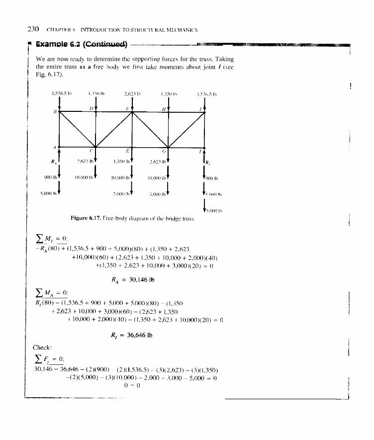
230 CHAPTliR 6 INTROL~lJ( 'Tl0N TO S'IKII('TC'RAL MIX'IIANICS
ExamtAe 6.2 (Continued) I We are now rcady to determine [he supporling fiwcec for the ti-ins. Taking
the entire truss a s a frce hody we firs1 take niulncnts ahout joint I ( w e Fig. 6.17).
!
1 S.lUl0 Ih

SECTION 6.4 METHOD OF JOINTS 231
Example 6.3
Ascertain the forces transmitted by each member of the three-dimensional truss [Fig. 6.18(a)].
We can rcddily find the supporting forces for this simple structure by considering the whole structure as a free body and by making use of the symmetry of the loading and geometry. The results are shown in Fig. 6.18(b).
Figure 6.18. (a) Space tmss and (b) free-body diagram
Joint F. It is clear, on an inspection of the forces in the x direction acting
on joint F, that :FpE = 0 , since all other forces are in a plane at right
angles to it. These other forces are shown in Fig. 6.19. Summing forces in
they and z directions, we get F
I,&JOlb
Figure 6.19. Free-body diagram of joint F.
Therefore,
I FBD = 2,240 lb compression
cz F = 0 :
10 4500
-FAF + 1,000 - 2,240- = 0
Therefore, CF = I.000 - 1,000 = 0

232 CHAPTER h INTRODUCTION TO STRUCTURAL. MI~CIIANK'S
Example 6.3 (Continued)
Joint B. Going to .join1 B, we see ]Fig. 6.1X(h)l that FnR = 0 and
, Since thcre are 110 olhcr li irce components on pin B i n the tiE = 0
directions of these members. Finally.
Joint A . Let u h ncxt consider,joini A (Fig. (i.20). Wc cim express I11l-c~ ct(. and 5,: vectorially. Thuc.
FBc = 2.000 Ih tension
Joint I). expressed 21s lollows:
We now consider.ioint D (Fig. 6.21). Forces 4.,) and F:,, i ~ r e Figure 6.21. I'rec-hmly diasmrii of jainl IJ.
"I__- . ..,. .. . ~ .

SECTION 6.4 METHOD OF JOINTS 233
I Example 6.3 (Continued)
I
Hence, summing forces, we get
-2,000j - 1,000k - F,,,i + 2,240(.894j + .447k)
+ F,,(-.40Xi - .816j - .408k) = 0
-2,000 + 2.000 - .81bF,, = 0
(d)
Thus,
(e)
(0 (8)
l& + .408F,, = 0
-1,000 + 1,000 - ,4085, = 0
We see here that FED = 0 and F,, = 0 ,
Joint E. The only nonzerc) forces on joint E are the supporting forces and
F;.&, as shown in Fig. 6.22(a). We solve I& = Z&Wlbcompression .
Joint C. As a check on our problem, we can examine joint C. The only nonzero forces are shown on the joint [Fig. 6.22(b)]. The reader may read- ily verify that the solution checks.
E X
1,000 Ib
1,000 Ib (a) (b)
Figure 6.22. (a) Free-body diagram ofjoint E and (b) joint C.

234 ('HAPTER 6 INTKOIXJ(:TION TO STKIICIIIRAI. MECHANICS
Belore proceeding with the problems. i t will he well to comment on the loading 01 plane roo1 trusscs. IJsually there will be a series of \cp;ir;itetl parallel t t uhzeh supporting the loading from the r o d such as i h S ~ O W I I i n Fig. 6.23, wlicre a wind pressurc is shown on a roof as 11. Niiw the Oisiilr t ru\h can he considered to support the loading over a region extending h;lllway tc each neighboring trus? (shown as dis tanced) . Furthermore. pins A and B sup- pori thc force exerted on area I l m k while pins B and C suppol-t the forces excrtcd on area /IT/,. When dcaling with the entire inside truss a s a free hody, you can use thc resultant force from pressure ovcr krwn. Howcvcr. when dcaling with thc pins as ii free hody you must use the forces coming on tu each pin as described ahove and no1 the totnl resultanl, which was iiscd tor lhc free hody of the entire internal truss. Clearly. thc outhide trusses support halt the Iimds descrihed ahove.
Figure 6.23. R o d trussc? supporting 21 wind load
Finally, we wish Lo remind you that a curved meinhcr i n a truss. such as appears in Prohleins 6.5 and 6.8. is a two-forcc incinher with forces coming only lrom the pinz. Rccdll that. for such nienihrrz, the force transmitted to the pins niiist he collinear with the line connecting the pins. such as is shown i n Fig. 6.14.

6.1. which are not.
Slate which of the trusses shown are simple trusses and
23
(a) Pratt INSS
I
(b) Fink ~ N S S
(c) Special-purpose t r u s ~ Figure P.6.1
6.2. Find the forces transmitted by each member of the truss
5,000 Ib Figure P.6.2.
6.3. The simple country-road bridge has floor beams to carry vehicle loads tn the tmss joints. Find the forces in all members for a truck-loaded weight of 160 kN. Floor beams I are supported by pins A and B, while floor beams 2 are supported by pins B and C.
+ 4 m + ~-
Figure P.6.3.
6.4. A rooftop pond is filled with cooling water from an air con- ditioner and is supported by a series of parallel plane trusses. What are the forces in each member of an inside truss'! The roof trusses are spaced a1 10 ft apart Water weights 62.4 IMA.',
i: f i 10'
Figure P.6.4.
6.5. truss. DC is circular
Find the forces transmitted by the straight members of the
B * Figure P.6.5.

6.6. Roof tiusscs such 215 the o n r shown arc spaced 6 rn apart in il long, ncctangular huilding. During thc wintcr. MIOW loads of LIP
to I kN/rn2 (or I kPa) ac~uniulate on the central portion o l the nnrf. Find the force in each memher for il t r u \ no1 at the cnda of the huilding.
6.9. Find the lol-crs in thc mcmhrrs of the truss.
I,OOO N
8 IO", ( ' 1 0 m F p IO 111
45" Figure P.h.h.
A .
Figure P.6.Y.
6.7. 'Ihc bridge supportr a rtradway Imd of I.000 Ihilt lor each 0 1 the twu trusses. Each mcinhcr weighs 30 Ihilt. Crmpute the fiirces i n the rnernhers, accounting approxim;itcly for the weight [if the rnrrnhcrs.
6.10. ;tppruxim:itcly. The mmmhrrs each weigh 100 Ih/ft.
In Example 6.1. incluilc the weights ut the memhcrs
I' H
6.11. Dctcriiiiiic the lorurs in thc mrmhel-s. T h r pulley5 ill c'and I'cach weigh 300 N. Ncplecl all iithct vicighth. Bc surc yuu have il check OII your iiiluIiuii.
Figure P.6.7. 1.000 N
6.8. Find the force, i n the straight incmhcrs u l Ihc tiuhh
/I 1 0 , 1) a IO' IO'
500 Ih 500 Ih Figure P.h.8
+ T
Figure P.h.11

6.12 Roadway and vehicle loads are transmitted to the highway bridge ~ N S S as the idealized forces shown. Each load is 100 kN. What are the forces in the members?
D
1- 6 panela at 6 m 2 Figure P.6.12.
6.13. A hoist weighing 5 kN lifts railroad cars for truck repair. The hoist has a 150-kN capacity and hangs from a truss with an L- shaped member to clear boxcars. What are the forces in the straight members for full capacity of the hoist’?
Figure P.6.13.
6.14. A 5-kN traveling hoist has a 50-kN capacity and is s u s ~ pended from a beam weighing I kN/m, which, in turn, is fastened to the roof truss at I and G as shown. In addition, wind pressures of up to 2 kN/m2 (or 2 kPA) act on the side of the roof. The result- ing force is transmitted to pins A and J . If the trusses are spaced S m apart, what are the forces in each member of the truss when the hoist is io the middle of the Span?
Figure P.6.14.
6.15. Find the forces i n the members of the truss. The 1.000-lb Force is parallel to they axis, and the 500-lb force is parallel to the :axis.
Figure P.6.15.
6.16. for the space truss ABCD. Note that BDC is in the XI plane.
Find the forces in the members and the supporting forces
Figure P.6.16.
231

n
rJ-
6.5 Method of Sections
23R

SECTION 6.5 METHOD OF SECTIONS 239
well inside a truss and avoid the laborious process of proceeding joint by joint until reaching a joint on which the desired unknown force acts.
Generally a free body is created by passing a section (or cut) through the truss such as section A-A or section B-B in Fig 6.25(a). Note that the sec- tion can he straight or curved. The corresponding right hand free-body dia- grams [see Fig. 6.25(b) for cut A-A and Fig. 6.25(c) for cut B-B] involve
B A
(c)
Figure 6.25. Section cuts.
coplanar force systems. We have, accordingly, three equations of equilih- rium available for each free body. One can also choose to use left-hand free- body diagrams for these cuts. Note that in contrast to the method of joints, one or more equilibrium equations can most profitably he moment equations. The choice of the section (or sections) to find the desired unknowns inside a truss involves ingenuity on the part of the engineer. Helshe will want the fewest and simplest sections to find desired forces for one or more members inside the truss. The method of sections is used for efficiently finding limited information. The method of joints for such problems is by contrast one of "brute force."
We now illustrate the method of sections in the following examples.


Exa
A pla is des the di
5w ( diagr; equat
takin; infori C H . i
(Note butio
~~~
SECTION 6.5 METHOD OF SECTIONS 241
iple 6.5
tru% is shown in Fig. 6.21 for which only the force in member AB rd. The supporting forces have been determined and are shown in :ram.
1,000 N
I 7x9 N 1.077 N
Figure 6.21. Plane truss.
I Fig. 6.28(a) we have shown a cut J-J of the truss exposing force lis is the same force diagram as that which results from the free-body I of pin A,) We have here three unknown forces for which only two ns of equilibrium are available. We must use an additional free body. hus, in Fig. 6.28(b) we have shown a second cut K-K. Note that by moments about joint B, we can solve for <,c directly. With this ition we can then return to the first cut to get the desired unknown cordingly, we have, for free body 11:
C M B = 0 :
-(10)(500) + (30)(789) - (FAc)(sin 30")(30) = 0
ve have transmitted FAc to joint H in evaluating its moment contr- ) Solving for FAc we get
FAc = 1,245 N
.. a) Free body I from cut J-J
Figure 6.28. Free bodies needed for the computation of fiirce FAD. (a) Free body I1 lrom C u t K-K

242 ('HAPTLIK 6 INTKOIIIICTION 7'0 STKllCTliKAL. ME('IIANI('S
Example 6.5 (Continued)
Summing forces for free body 1. we have"
F,,,,cos 30" ~ FA<. cos 30" ~ 1.000 sin 30" = 0
Thcrcfbre, Pi,,, = I .X22N
Therefore.
FAB = -66IN
We see that member A B i s a Leiision nieinber rathcr than ii compressim member a i wiis our initial guess in drawing thc free-hody diagrams.
I n retrospect. you wi l l note that. in the method of joints, errurs made early wi l l (if neccssity propagate through the calculations. There is , on the other hand, much less likelihood of this occurring in the method of. sections. However. for simple trusses with many members, we may profitahly use the method of joints in conjunction with a computer for which the brute-force approach of the method o f joints i s ideally suited. I1 i s to be pointed out that there i s computer soltw;rre availahle which makes this kind of computation routine and quick.
*6.6 Looking Ahead-Deflection of a Simple, Linearly Elastic Truss
In the solids or structures courses you wi l l soon hc laking. you wi l l he given inhtruction for dctcnnining the nioxnient o f the pins of a linearly elastic, s in- ple truss steiriniing from the cxtcrnal loads. It i s true that you can now deter- mine the forces in il simple truss and from this you can determine the change in length of each memher. However, using t h i s data as well a s the accompany- ing changes o f orienllition (if the meinhen, you wi l l find i t next to impossible to get the movements o f the pins for all hut the most tr iv ial trusses.

! SECTION 6.6 LOOKING AHEAD-DERECTION OF A SIMPLE, LINEARLY ELASTIC TRUSS 243
You movable movemeit’ while no are held changes thetical < computei. addition the worb the forcqs procedure able pin?. plying tke the x a n i monly form n s
~
will learn later of a neat method of doing this. In this method, each (unconstrained) pin is imagined to be given first a hypothetical
6, in one of two orthogonal directions, say the x direction here, movement is allowed for that pin in the y direction. All other pins fixed for the preceding action. We now evaluate via geometry the in length stemming from 6, of all members affected by this hypo- isplacement. Also, the energy of deformation8 for these members is
The aforementioned displacement is shown in Fig. 6.29 for 6,. In to the energy of deformation nf the affected members, we compute done by external forces that undergo movement from 6,, keeping constant during this movement. Here the work is F(cos a)6,. This is canied out for each such x and y displacement for all of the mov- We then add up all the energy terms and all the work terms, multi- latter by - I . We then have a function of all of the n 6’s comprising y components of all movable pins. This function, which is com-
dmoted as n, is then extremized with respect to the n 6’s. We then multaneous equations from
i = l ,2, ... n (%)i = O
truss, th- energy
’This discuss the:
xYoi structures is the
members were deformable and we mentioned that we needed the c f deformation for the use of the total potential energy principle.
is called a virruol displucemenl and will be discussed further in Chapter 10 when we method of virtual work. will learn to calculate the energy of deformation in your solid mechanics or your
where S is the axial change in length of the member, A EOUTSB. The formula is 2 L
cross-sectional area. E is the modulus of elasticity. and L is the length of the member.
Figure 6.29. A simple truss has its free pin H given a hypothetical dnplacement 6, while keeping all other displacement components fixed. Note that only members CH, EH, and H E are involved. Work done is F(cos a)&,.

6.25. 11U\\.
Find the Iorucs in members C'D. DG, and llC i n the plane
I .oi)o ih
Figure P.6.22.
Figure P.6.23.
'44
6.27. 'The roof is subjected t o :I wind hading of 20 Iblft'. Find the 1orurs iii rncinhers LK and K.101 an interior tius5 if thc irusse\ arc spaccd 10 11 apdl~l.

m M
IIj0-k; Guideway 1 “5-kN hoist
Figure P.6.28.
t 45-kN lOdd
supported at J and G only
6.29. CE.
In Example 6.2, determine the forces in members FG and
I
6.30. (a Find the forces in members DG and DF by the method of .secrio 2. Stare whether the members are tension or compression members I
members AC, AB, CB, and CD by the diagram in an appropriate manner and
are in tension or compression.
I 80 kN I SOkN I SO kN
, I Figure P.6.30.
6.31. A pair of trusses supports a roadway weighing 500 Ib/ft. By method of sections, find the forces in DF and DE. The road- way is supported at pins A , D, F, and H on the two trusses.
15’ I ” F 1 5 ’
Figure P.6.31.
6.32. truss.
Find the force in members H E , FH, FE, and E‘C of the
S K
Figure P.6.32.
245

6.33. Find the force in member JF in the truss.
+ Ion1 +
I Figure P.6.33
?,500 N
2,500 N
2,500 N
2.500 N
6.35. A railmad engine i \ stairing to cros\ the deck-type truh, hridge chawn. If ths wcighc of the engine i s idealiied by Ihr hul- SO-kip loads," find che l i ~ e \ in mrmbcrs AH. HL. Cti. CL, /.ti. /)ti. K.I. and I N
S O K X I K X!K 5 0 K
''A kip ib a kilopound, 01 1.000 Ib.
246

I SECTION 6.8 SHEAR FORCE, AXIAL FORCE, AND BENDING MOMENT 241
6.8
Part IB: Section Forces in Beams'"
Shear Force, Axial Force, and Bending Moment
6.7 /Introduction

I., .I
M ' fl
1UJ
Figure 6.30. Kesoltant ;it ii scctiii i i
additional slicilr c impimcnt V~ !ree Fig. 6.3 I). oi ie additional hending- momeiit cnmponenl M > , and ii couple inomcnl along the axis of tlic beam M\. which we shall call the twt.\f;ti,q tnom(w.
Notice in Fig. 6.3!)(c) that a sectind ll-cc-hody diagram h a s hcen drawn which exposcs [lie "othei- side" o f thc cross-section at position x. The shear Force. axial fwcc . and bending momrnl Cor [his section h w e heen prinicd in ilic d i a p n i . We know f r o m Ncwtiin's third law that they should he equal and opposite 10 the ciirresponding unprimcd qunnlities i n part ( b ) of the diag'ani. We can thus choose for our conipuralions cither ii left-liand or n right-hand free-body diagram. But this poses somewhat of ii prohlem for 11s whcn u e m m c ki reporting the s i g i \ o f Ihe transmitted forccs and couple morncnts :I( ii
section. We catin01 use the direction of a lorcc or couple inotnenl a1 thc scc- Lion Clearly. this would hc inadcquiite since the s e n x ol Ihc force or couplc t i i ~ m e n t iit :I wctioii would depend on whether a left-hand or a right-hand lrce-body diagram wiis used. 'Tu associate an unambiguous sign lor shcar lorcc, axial force. and bending tmoriicnt i i t a secfion. we ;tdiipt the following invention:

1 SECTION 6.8 SHEAR FORCE, AXIAL FORCE. AND BENDING MOMENT 249
A forc componenf for a section is positive sectio and the force component both in the egative dbct ions of any orie i
The sam is true for the bending moment. T s, consider Fig. 6.30. For the left-hand free-body diagram, the area
vector f r section x points in the positive x direction. Note also that H, y,, and the vect 'a1 representation of M2 also point in positive directions of the xyz axes. Hence, a cording to our convention we have drawn a positive shear force, a pos- itive axi I force, and a positive bending moment at the section at x. For the right- hand fre ~ -body diagram, the cross-sectional area vector points in the negative x direction And, since H', V!', and Mlpoint in negative directions of the x, y , and z axes, th 'e components are again positive for the section at x according to our conventi m. Clearly, by employing this convention, we can easily and effectively specify e force system at a section without the danger of ambiguity. i i P
1 Figure 6.31. Section resultant for three-dimensional loading
A pointed out earlier, we can solve for Vy, H, and Mz at section x using rigid-bo y mechanics for either a left-hand or a right-hand free-body diagram provide that we know a11 the external forces. The quantities y , , H , and M2 will dep nd on x, and for this reason, it is the practice to sketch shear-force and bending moment diagrams to convey this information for the entire heam. i e now illustrate the computation of V and M.
"S me authors employ the reverse convention for shear force from the one that we have proposed. O u r convention is consistent with the usual convention used in the theory of elarticity f k thc si n of stress at a point. and it is fnr this rcilson that we have employed this mnvznlian rather tha I the other one.

250 CHAPTER 6 INTRODUCTION TO STRIICTIIRAI. MECHANIC’S
Example 6.6
We shall express the shear-fiirce and hending-m(irnent equations fnr thc simply supported heam shown in Fig. h.RZ(a). whose weight we shall neglect. The support forces ohtained frcini equilihrium are S O 0 N each.
To get the shear force at a section x, we isnlate either thc left or ]right side of the beam at x and employ the equations of. equilibrium 011 thc resulting free hody. If .r l i es between A and C [if the heam. the only noniii- ternal force present for a left-hand free hody i s the left supporting fwcc [see Fig. 6.32(h)l. Notice that we have used directions for Vand M (rherc i s no need for suhscripts in the simple pniblem) correspiinding to the po.s- i t iw states frrirn the point o f view [if our convention. Clearly, the (i/,qehroi(. sign we get for these quantities from equilihrium calculations wi l l then correspond to the umvmrion sign. If li i s between C and H for such a free body. two external forces appear lsee Fig. h.32(cJl. Therefore. i l thc shcar force i s to be cnprcssed as a function of .r. clearly separate equation5 COY-
ering the two ranges. 0 < .r < 112 and 112 < x < /, are necessary. Summing forces we then get
o<li__< 112: 500 + V = 0: therefore. V = ~ ~ 5 0 0 N
112 < x < I : ~~~~ ~
S O 0 - 1.000 + V = 0; therefore. V = 5Oll N (h)
Notice from the above results that therc i s a sudden chaiigc of the shear force from -S(X) N to +XK) N as we pas? the position of the concentrated I ,000-N load. Clearly then, the value l i t shear niiist perforce he in~lr/r,rni- nrrtr at the position of this concentrated load. I t i s f(ir this very reason that. in the ranges o l applicability of Eqs. (a) and (hl. we have excluded the positions o f the three concentrated loads ol the problem. Note further that il there wcrc only a diatrihuted load starting at point C. therc would not he discontinuity in shear and so we would not have to delete the position of point C i n the rangc applicahility of the shear equatinns.
Now let us turn ti1 the bending-moment equ;lti~ins. Again, UK inust consider two discrete regions. Taking moments ahout position 1. we gct
s
-S00x + M = 0; therefore, M = 5011s N-in I C 1
1 t
/ /2<r 5 i : ~
-soox + i .n00(~ - $1 + M = (I:
therefore. M = S O O ( / - x) N-in (11)
, ._--I_ . . .. . .. . , . _”__ ..
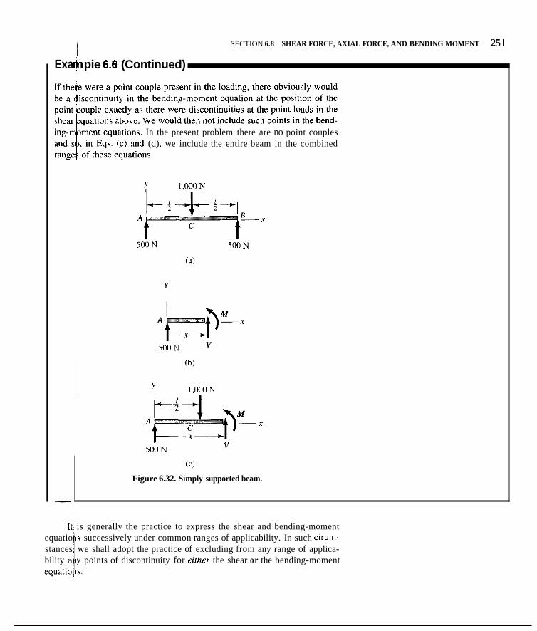
i SECTION 6.8 SHEAR FORCE, AXIAL FORCE, AND BENDING MOMENT 25 1
Exa pie 6.6 (Continued) 4 In the present problem there are no point couples (d), we include the entire beam in the combined
Y
A
V 500 N
1.000N y
V 500 N
(c )
Figure 6.32. Simply supported beam.
It/ is generally the practice to express the shear and bending-moment equatio s successively under common ranges of applicability. In such cimm- stances we shall adopt the practice of excluding from any range of applica- bility a y points of discontinuity for eirher the shear or the bending-moment equatiobs.
I

252 CIIAI"I1IK h lNTR0I)L'ClION TO STRUCTURAL MK'HANICS
r Example 6.7 r
j Dctei-mine llic hhcar-force and hending-moment equations for the simply !
W e inus1 first find [he supporting Iorccs for the hcani. Hence. we :
supported bean shown in Fig. 6.33. Neglect the weight of tlie hcam.
liave tising the right-hand irulc
K,(2?) - soo - (50)(X)(X) - (I.ooo)(x, = 0
a Ttrcreliirc. i R, = 532 Ih ;
In Fig. 6.34(a) we have shown a l ra-body diagram exposing sec- tions between the left suppnrt and the uniform Inad. Summing forces and taking moments ahout a point in the seclinn. where we have drawn V aid M a s positive according IO o u r wiivcntioii. we gct
i i
i (l<r~<_ 4:
868 + V = 0: thcreliire, V = -868 Ih -86Xi + M = 0: therefore. M = X68.x f t - lh
The i icxt i i i te i -v i ih hctweeii ttir heginning ol Ihc uniform lond and the poinl fiirce. 'Thus, ohwrving I'ig. h.?4(h):
I 8
4~ 5 . l . ~ < &
l i i r V, 808 - 5O(x - 4 ) + V = 0
:. V = 50.x - 1.068 Ih
and fix M
:. M = -25r' + I.llh8.~ - 400 fl-lh
We now ciinsider the interval hctwccn the poinl force and the end trf the utiilorin lox i Thus. ohserving Fig. 6.34(c):
I
?-Ll - -S 12: lor v. I
868 - so(^, - 4) - m o + v = o :. 1' = S t r ~. 68 Ih
Figure 6.34. Free-hody diagrams irir various r a n p a
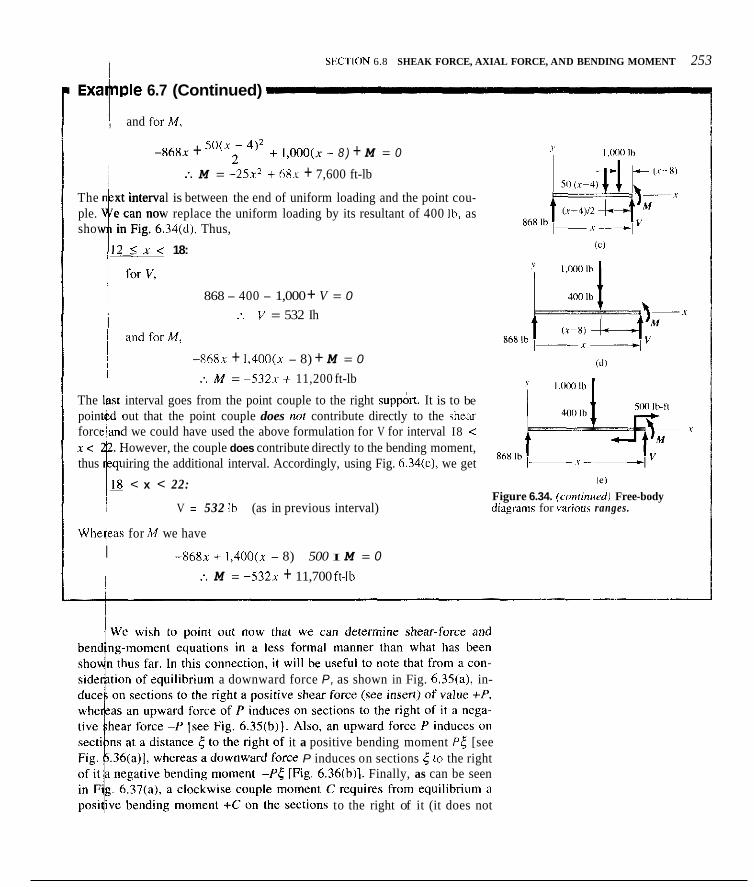
SECTION 6.8 SHEAK FORCE, AXIAL FORCE, AND BENDING MOMENT 253
ple 6.7 (Continued)
, and forM, I ~
5 0 ( x - 4)2 -868x + ~~ * + I,WO(x - 8 ) + M = 0
:. M = -25x2 1 6 8 1 + 7,600 ft-lb
The ple. show in Fig. 6.34(d). Thus,
xt interval is between the end of uniform loading and the point cou- e can now replace the uniform loading by its resultant of 400 Ib, as i,.. 18:
868 - 400 - 1,000 + V = 0 :. 1' = 532 Ih I
i ~ andforM,
-868x + 1,4OO(x - 8) + M = 0
:. M = -5321 1 11,200 ft-lb
The I st interval goes from the point couple to the right supp&rt. It is to be point d out that the point couple does mi contribute directly to the shear force and we could have used the above formulation for V for interval I8 < x < . However, the couple does contribute directly to the bending moment, thus uiring the additional interval. Accordingly, using Fig. 6.34(e), we get
~
~
I ~
i8 < x < 22:
i V = 532 Ih (as in previous interval) ~
Whepas for M we have I ~
-868x + 1,4OO(x - 8) - 500 I M = 0 :. M = -532x + 11,700 ft-lh j
(el
Figure 6.34. (conrinurdJ Free-body diagrams for various ranges.
a downward force P, as shown in Fig. 6.35(a), in-
it a positive bending moment P t [see P induces on sections 5 to the right
6.36(b)]. Finally, as can be seen
to the right of it (it does not

254 CHAPTER h INTRODUCTION 1'0 STRUCTURAL MECHANICS
require from equilibrium a shear force), whereas a counterclockwise couple moment C [Fig. 6.37(h)l requires ;I negalive bending moment 4' on sec- tions to the right of i t . 111 the following example. we shall show how by this reasoning we may more directly formulate the shear-force and hending- moment equations.
I I
Figure 6.36. Rending mornen1 mduced h) P
Figure 6.37. Bending moinent induced hy C.

Exi
Eva shoy
med the I
The
The
We vie\
We ing-
-
SECTION h.8 SHEAR FORCE, AXIAL FORCE, AND BENDING MOMENT 255
lDle 6.8
te the shear-force and bending-moment equations for the beam in Fig. 6.38. 4 free-body diagram of the beam is shown in Fig. 6.39. We can im- ely compute the supporting forces as follows, remembering to use ht-hand rule.
CLL M - 0 .
-R,(26) + (500)(21) - 800 + (500)(5) = 0
ore, R, = 4691b
E M , = 0:
Q(26) - (500)(21) - 800 - (500)(5) = 0
ore, R, = 531 Ib
111 now directly give the shear force Vand bending moment M while g Fig. 6.39. Thus,
n < x < 5 : V = -469 Ib
M = 469xft-lb 5 < x < 13:
V = -469 + 500 = 31 Ib
M = 469s - 500(s - 5 ) = -31x + 2,500 ft-lb
13 < x 5 16: __ ~~
V = 31 Ib (same as previous interval)
M = 469x - 500(x - 5 ) + 800 = -31x + 3,300 ft-lb
16 5 x < 26:
V = -469 + 500 + 50(x - 16) = -769 + 50x Ib
50(.x - 16)? 2 M = 469s - 500(x -- 5 ) + 800 - -
= - 2 5 ~ ’ + 769x - 3,100 ft-lb
all present effective methods of sketching the shear-force and bend- m e n t diagrams in Section 6.9.
i
x
” J?L Figure 6.38. Simply supported beam.
9- i-
f ,
Figure 6.39. Free-body diagram of beam

256 CHAPTEK 6 INTKiXW(710N TO SIRLICTUKAI. R.IECHj\KICS
Bcliire we proceed further. i f must he carefully pointed uut that the replacement (if a distributcd load by il single rcsultiiiit lorcc is iinly mcaniiigful fix the pili-ticular lrec hody on which the i i r c e distrihurion acts. Thus, to coni- pute the rcacticiiis Sur the entire heaiii taken as n tree hody (Fig. 6.40). we can
replace the wcight di\tribution ivO hy the torill weight at position 1.12 (Fig. 6.41). FoI l l ic hendiiig iiioiiieiit iit ~ x , the restillant of the loading lur thc Sree
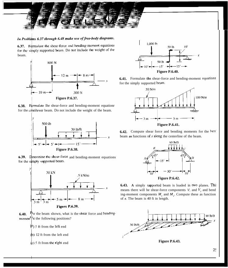
beam. ~
1
300 N
! Figure P.6.37.
6.38. for the c' ntilever beam. Do not include the weight of the beam.
F rmulatz Ihe shear-force and bending-moment equationr
J
:: - X
Figure P.6.38.
and bending-moment equations
I
6.40. moment at the following positions?
or the beam shown, what is the shear force and bending~ I ( ) 5 ft from the left end (1) I2 ft from the left end
&) 5 ft from Ihc right end
x
Figure P.6.40.
6.41. for the simply supported beam.
Formulate ths shear-force and bending-moment equalions
Figure P.6.41.
6.42. beam as functions o f s along the centerline of the beam.
Compute shear force and bending moments for the bent
IO lhlfl
Figure P.6.42.
6.43. A simply suppmted beam is loaded in two planes. Thi: means there will be shear-force components V, and Vz and bend ing-moment components M: and My. Compute these as function of x . The beam is 40 ft in length.
I
Figure P.6.43.
2:

6.44. What are tlic shear force, hcnding moment. and axial force for tlic three-dimensional cantilever hram! Give your results sep- arately for the three porlians AH, H C . and Cl). Neglrct the weight of thc memhcr. Usc ,s as the dictairce along the ccnterline from I ) .
6.47. A hoist can move along a bcnm whilc supporting a l0,OOIl- Ih l o x . It the hoist st:~rts 31 lhe left and moves liom 4 = 3 to I = I?. dctcl-mine Ihe shear f k e and hmding momcnt at A in terms 01 i. At what priiition i do we get thc ineninurn shear fbrcc ill A and thc mnxiiniiin hending mornenl a1 ,I,! What i l ls their v;ilues'!
I ,noo N
Y ' " , x
Figurc P.6.44 10.000 Ih
Fipre P.6.47.
6.48. A pipe weighs I O lhift and has an imide diameter of 2 i n If il i s full of wiitcr and the p r e w r c irf the water i y that r i f the atmrnphei~c iit the ciitratlct. A. coniporc thc \hear force, i ix i i i l force. ant1 hending mimien1 01 the pipe from A to 11. l l se coordinate i mcaured fmm A olonp the centcrline 01 the pipe.
6.45. Oil flow\ from a tank through il pipc AB. Thc oil weighs 40 Ibift' and. in flowing, dzvelops a drag on the pipe r r f I Ihift. The pipe has an inside diainctci 013 in. and a length of211 ft. f k w condition?, arc assumed ID he the same along the entire length of the pipe. What arc the shear force, bending nrmmt, :md axial force along the pipe? The pipe weighs IO lhirl. I
. i
~1 ,'
Figure P.h.45.
6.46. force a s lunctions u i H for thc circular heam.
Determine the shear iixcc, bending moment, and zix i i i l Figure P.6.48.
6.49. After finding the supporting iorces, detzrmine fur Pnrhli-m 6.37 the \hsar-l<rcc and hending-moment equations without thc fiirthei iiid of free-hwiy diagrams.
6.50. t r r i Frohlcm 6.7U without the ;lid of frcc~hody di. ',Pl<U"\. .'
6.51. I n Priihlrin 6..39. alter delermlning the supporting forces. tletcimine thr shcar-fbrce and hending-motncnt equation? without
Deterrninc the <hcac-torcr and hendingmoment equittiona ll&
A 1 4 5 " ~
Figure P.h.46. thr aid of li-er-hody di,: 'Ail : l",b.
258

6.52. In Problem 6.40, after finding the supporting forces, write the shear force and bending moment as a function of x for the beam wit out the aid of free-body diagrams.
6.53. Gi e the shear-force and bending-moment equations for the cantil ver beam. Except for determining the supporting forces, do not us free-body diagrams.
i
1,000 N
i i
I
~
I Figure P.6.53.
6.54. Formulate the shear-force and bending-moment equations for the simply supported beam. [Suggestion: For the domain 5 < x < IS, it i s simplest to replace the indicated downward triangu- lar load, going from 400 Nlm to zero, by a uniform 4Ml-NIm uni- form downward load from x = 5 to x = IS plus a triangular upward load going from zero to 400 Nlrn in the interval.]
4Ml Nlrn
x
-l5m------t - 20m Figure P.6.54.
6.9 1 Differential Relations 1 for Equilibrium
In Secti n 6.8, we considered free bodies of finite size comprising variable portion of a beam in order to ascertain the resultant force system at sections along t beam. We shall now proceed in a different manner by examining an infinite 'mal slice of the beam. Equations of equilibrium for this slice will then yi Id diferenrial equations rather than algebraic equations for the vari- ables V ndM.
C nsider a slice AX of the beam shown in Fig. 6.43. We adopt the con- ventionl that intensity of loading w in the positive coordinate direction is
of the beam has been included
diagram of the element in Fig. 6.44. Note we have and bending-moment convention as presented
Figure 6.43. Element Ax of beam.
' ' V+AV
Figure 6.44. Free-body diagrdm of element.
1 z
forces:
F, = 0: L , -V + ( V + A V ) + WAX = 0 i Taking moments about corner a of the element, we get i L M, = 0:

260 CHAPTER 0 INTRODUCTION TO S T R U C T I K A I , MECIIANICS
where p i s some lraction which. when multiplied hy Ax, gives the proper moment arm OS the force I$’ Ax ahout corner (1. Thcsc equations can he written i n the following niaiinei- after we cancel tcrins and divide through hy Ar:
i\v - - Ax -I”
AM = -I/ + ivPAi A I
In the liniit a s hr i (1. we get the following differential equations:
dV - dx = -w (6.321)
We may next integrate Eqs. 6.3(a) and 6.3(b) from position I along the beam to position 2. Thus, UT ha\c
and (6 .4)
(M)? -(M), = - p h
( M ) , = ( M ) , - JIVdx
I
Thercforc,
(6.5)
Equation (6.41 incans that the ctmige in the shear lorce hetwccn two points on a hcam ecluiils m i n u (l ie area under the loading curve hetwccn these pointq provided that there i s no point force present i n thc interval.? Note that. if w ( . x ) i s positive in an inlei-val. the area under this curve i b positive in this interval: i lw ( l i i is nepative in a n interval. Ihc iirea under this curve i s negative in this interval. Siinilarly, FA]. 6.5 indicates that thc change in hending moment hctweeri Iwo points on a beam equals minus the area (if the shear- force diagram hetwccn these points pro\’ided that there arc n o point couplc moments applied in the inter\al. If Vi.r) i s positivc in an interval. [hc area undcr this curvc i s positive in tliib interval: i l V ( x ) i s negative in an interval, the area under thc curve i s ncpativc lor this intcrval. In cketching the diagram. we shall make use oSEq. 6.4 and 6.5 a s well as thc diffei-entii equations 6.3.
“lbu dilirrenfial cq i i~ l io i i b.~i,:i) I C o ~ l y meenmgful with i t conimuous Ionding p r e m ~ i . while t$ h Xhj i \ w>ly \ h I iri the Aihirnce 01 p o i n t ‘m~tplc riiorncnt\.

SECTION 6.9 DIFFERENTIAI. RELATIONS FOR EQUILIBRIUM 261 j
I Exa pie 6.9 i. and bending-moment distributions for the simply in Fig. 6.45 and label the key points.
x
Figure 6.45. Simply supported beam. ~
IThe supporting forces R, and R, are found by rules of statics. Thus,
(-R,(20) + (500)(14) + (50)(10)(10/2) - 100 = 0 I
R, = 470 Ib
= 0:
R2(20) - (500)(6) - (50)(10)(15) - 100 = 0
R, = 530lb
~
Therd fore. 530 Ih
sketching the diagrams, we shall employ Eqs. 6.3, 6.4, and 6.5-
of the shear-force and bending-moment equations, evaluating
on the shear diagram that the 470-lb supporting force
ia)
x
-470 (b)
2.820 2.025
2,7u(1 M- 1.925
A r 11 I B
V, and we have a 30-Ib shear force at point D. Again, since w = 0 in i C )

262 rttAPTCR 6 INTRODUCTION TO STRIJCTUKAL blFCIIANICS
Example 6.9 (Continued) load at D, there i s ino sudden change iii shear as we crash this point. Ncnt. the change in shear hetween 1) and I1 i s i i i i i i i i s the area (11 the loading curvef4 in this interval in ;scordance with Eq. 6.4. But this ;rea i s (-SO)( IO) = -500. Hcnce, from Eq. 6.4 the value (IS vj (.iu\t Io (he left lit. the support) i s yj - (-500) = 530 Ih. Also, since N i s incpti stant hetween I1 and B. the slope of the shear curve should he positive and constant, in accorkincc with Eq. h.Xa1. Hence. we can draw it straight line between V,, = 30 Ih and V, = 530 Ih. As we now cross the ]right support force. we see that it induces a negative h e a r <if 530 Ih on scclioiis 10 thc right of thc support, and s o at I3 the shear curw conics hack t i l zero.
We now proceed with the bending-moment curve. With iio point coil- ple moment presenr at A. the value o f M,* must he zcrii. The changc in moment between A and C i s then minus the area underneath the shear curve in this interval. We can then say from Eq. 6.5 that M,. = M , - (-470)i6) = 0 + 2,820 = 2,820 It-lh, and we denote this in the nioineiil diagram. Fur- thermore the value of V i s a negative constiin1 in the interval and. accord- ingly [see P:q. 6.3(h)J, the slope (if thc moment curvc i s positive and constant. We can then draw a straight line hctweeri MA and M,.. Hetwecn C and 11 the area for the shear diagram i s 120 Ih-St, and s o we can say thal M,, = M,. - (120) = 2.820 - 120 = 2,700 St-lh. Again. with Vconslant and positive in the iiitcrvd, the slope of the moment curve must he negativc and constant in the i n t e r d and has heen so drawn. Hetweeii I ) ant i F the iirea under the shear curve i s readily sccn to he ( 3 0 ) ( 5 ) + + ( 5 ) ( 2 5 0 ) = 775 ll-lh. Hence, the bending moment goes from 2,700 St-lb at 11 to 1,925 St-lh at F. Now the shear cuwe i s positive and irrrrv,.sing in value ;IF we go from D to F. This means that the slope of the bending-moment curve i s ncgatike atid hecoming steeper a s we go from D to I:. As wc go by F wc eiicounter l l lc 100-ft-lh point couple moment and we can say that this point couple moment induces a positive 100-St-lh mnmcnt on sections to the right (if point F. Accordingly, there is a sudden increase in bending ni(iment o l 100 It-lh at F, as has heen shown i n the diagram. The area ofthe shear diagram hetwcen F and L( is readily seen from Fig. 6.46(h) to he (2XO)(S) + ;(5)(2SO) = 2,025 ft-lh. We see thcn that the bending miiment gocs to zero ill H. Since the shear Iorce i s positive and inr.reu.sing hetween F and H. wc conclude that the slope o f the hcnding-inomcnt curve i s negativc and hecoining ,stef’pcr as we approach R. We have thus drawn the shcar-force and bend- ing-moment diagram and have labeled a l l key points.
Note that to he correct, both the shear-force and hending-nioment curves must go to zero at the end of the beam to the right iif the right sop- port. This serves a s a check o n the correctnes iir the calculations.
laNotc tlmt the pnim couplr mnment l las a r.cru nrf frorce and b n nerd no1 he ill concern in the inlcrvill from D lo Bas far as shear i s conccrned. Howcwr. i f will hc ii p m i l ulicic auddrn chengr occurs in the hending-momcnr diagram
- . ~ . - .

I SECTION 6.9 DIFFERENTIAL RELATIONS FOR EQUILIBRILM 263
In xample 6.9, we can get equations and diagrams of shear force and bending moment independently of each other. With simple loadings such as point fo ces, point couples, and uniform distributions, this can readily be done. In eed, this covers many problems that occur in practice. Usually, all that is n eded are the labeled diagrams of the kind that we set forth in the pre- vious pr I blem. In problems with more complex loadings, we usually set forth the equ ions in the customary manner and then sketch the curves using the equatio s to give key values of V and M (the areas for the various curves are no long r the simple familiar ones, thus precluding advantageous use of Eqs. 6.4 and 3; the key points are then connected by curves sketched by making use o f t e slope relations as in Example 6.9.
It ill be helpful to remember that if a curve has inareusing magnitude (absolut 1 value), the subsequent curve must have a steepening slope over the
hand, if a curve has decreasing magnitude curve must have aflatrening slope over the
n
Figure 6.48. At V = 0, possible maximum for M.
and bending-moment curves where there is zero value of be possible maximum values of shear force and bending

IO K
n ++I++
Figure P.6.55.
c + I + + + Si10 N-111 Xi1 Nlm
-+
10 I hlit
I ,lli)i~ Ih
Figure P.6.58.
Figure P.h.57. Figure P.6.60
!64

6.61. ! the sin mamen
6.62. for the
6.63. througt at right
lrilrl af
to least
tch the shear-force and bending-moment diagrams for ,idally loaded beam. What is the maximum bending
w = sin i i x / L Ib/ft /
Figure P.6.61.
6.64. A cantilever beam supports a parabolic and a triangular load. What are the shear-force and bending-moment equations'! Sketch the shear-force and bending-moment diagrams. See the suggestion in Problem 6.54 regarding the triangular load.
- X
Figure P.6.64.
imulate the shear-frxce and bending-moment equations tm. Sketch the shear and moment diagrams.
'imply supported I-beam is shown. A hole must be cut e web to allow passage of a pipe that mns horizontally gles to the heam.
Where, within the marked 24-ft section, would the hole t the moment-carrying capacity of the beam?
In the same marked section, where should the hole go ec t the shear-carrying capacity of the beam'?
2'1- 24'-4 4,000 Ih 8,000 Ih 5.000 Ib
4' r l7'-p5'1 3' \
111 1 1 1 1 Ul 11 1 80 Ib/fl
6.65. Determine the shear-force and bending-moment equations for the beam. Then sketch the diagrams using the aforementioned equations if necessary to ascertain key points in the diagrams, such as the position between the supports where V = 0. What is the bending moment there?
1,000 Ih 60,000 Ib-ft
I 00 I b/ft
Figure P.6.65.
t Figure P.6.63.
265

266 CHAI'TCK 6 INTRODIICTION TO SI'KIJ('TIJRA1. MFCllANlCS
Part C: Chains and Cables
6.10 Introduction
We often cncountcr I-elatively llzxihlc cables or chains that are used to s u p port Iuads. I n suspension hridgcs, lur cxample, we h i d a coplanar arrange- ment i n which a cable wpports a large load. The weight of ttic cable itself in mch cascs may oliun be considcrcd negligible. 111 traiisniissiixi lincs, oil ttrc ollicr hand, the principal Iircc i s the weight o l the cahle itscI1. In Part C. wc shall c\'iiluate the sh;ipc 01 and the tension in the cahles f o r both these cascs.
Tu Ihcilitalc computations. thc model OS Llic structural system wil l he assunicd 1 0 bc perfectly flexible and inextensihlc. The llexihility assumption ineiins that at the center of any cross section 01 the cahle only a tensile force i s lransmittcd and there can hc no bending municnt there. The Surcc transmit- lcd Iliriiugh tlie cablc inusl. under these conditiiins. he tangent to the cable at all posilions along thc cahle. The inextcnsibility assumption means that the length of thc cable ih consveiit.
6.11 Coplanar Cables: Loading is a Function of x
r-~ / ~_r/ We shel l i i i iw consider lhc case of a cahle suspended helwecn two irigid S U ~ -
porls A and 1) under thc action o f a loading function W(I) given per unit length a s measured in the hnri:ontnl direction. This Ii,ading wi l l bc consid- crcd to he copliinar with the cahle and directed vertically. as shown in Fig. 6.49. Consider an clcnient of the cahlc of length A.7 a s a (tee hody (Fig. 6.50). ;I/-\ ~- ~~
I ,
~~~~ ~ Y ~~~~ ~ ~~
Figure 6.49. Copl;inar cahlr; i v = I* ' ( , )
Summing liirces in the .r and directions, respectivcly. we get
- 7 . ~ 1 s 6' + ('I' + A T ) cor($ + A@ = 0 (6.6a) -Tsin H + ( T + A/ ' ) sin (6' + AH) - w , ~ A.l; = 0 (h.6b)
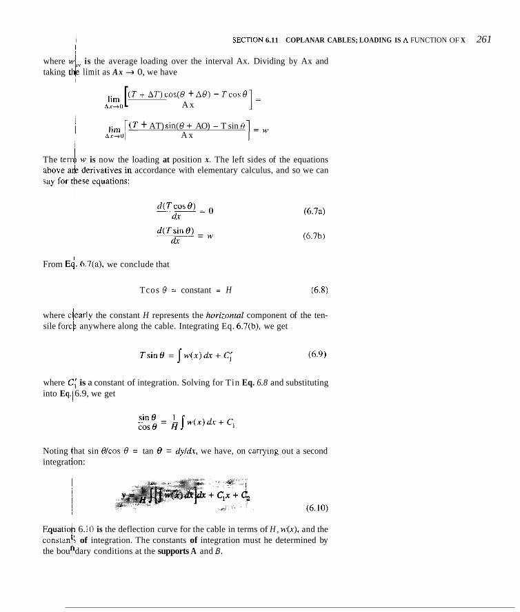
i SECllON 6.11 COPLANAR CABLES; LOADING IS A FUNCTION OF X 261 I
where $ is the average loading over the interval Ax. Dividing by Ax and taking t limit as Ax + 0, we have
i
( T + AT)cos(B + AO) - TcosO ~~
A x lim [ ~
~
Ax-0
i
i
lim [ ( T + AT) sin(O + AO) - T sin B 41-0 A x i
I
The terd w is now the loading at position x . The left sides of the equations accordance with elementary calculus, and so we can
(6.7a)
(6.7b)
From Ed. 6.7(a), we conclude that
Tcos O = constant = H (6 .8)
where c/early the constant H represents the horizontal component of the ten- sile forcb anywhere along the cable. Integrating Eq. 6.7(b), we get
i TsinO = / w ( x ) d x + ~ ; (6.9)
is a constant of integration. Solving for Tin Eq. 6.8 and substituting
~
where into Eq. 6.9, we get d ~
Noting hat sin Olcos O = tan 8 = dyldx, we have, on canying out a second integrat on: t
Equatioh 6. 10 is the deflection curve for the cable in terms of H , w(x). and the constan s of integration. The constants of integration must he determined by the bou t dary conditions at the supports A and B .


i SECTION 6.1 I COPLANAR CABLES; LOADING IS A FUNCTION OF X 269
Exa ple 6.10 (Continued) + the largest 0 occurs at x = 112 (i.e., at the supports). we have, for
Cons+pently, we get for T,,,:
H cos[ tan-I ( ~ 1 1 2 H ) ]
T,,, = --
Fromltrigonometric consideration of the denominator, I
Substituting for H using Eq. (c), we then get, on rearranging the terms,
I ]Finally, to determine the lrngth ofrhe cuble for the given conditions, we m st perform the following integration: P
Now he slope, dy/& equals wxlH [see Eq. (01, which on substituting for H Lse Eq. (c)] becomes 8hxll.z Therefore, F This ay be integrated using a formula to be found in Appendix I to give in
Subs ituting limits, we have I r
Rea anging so that the result is given as a function of the sag ratio hll and the s an 1, we get finally 1 !


, SECTION 6.12 COPLANAR CABLES: LOADING IS THE WEIGHT OF THE CABLE ITSELF 271 i I
Dividinglthrough by As and taking the limit as As + zero, we get equations analogo+ to Eqs. 6.7.
Integratilg, we have I TcosO = H i ~ T s i n e = J ’ w ( s ) d s + ~ ;
(6. I I a) (6.1 1 b)
Eliminating Tfrom Eqs. 6.1 I , we get, as in the previous development:
9 = w(s)d.s + C, dx
equation is a function of s. Thus, we cannot directly inte- Accordingly, note that
~ dy = (d.? - dx2)1’2
Hence, flom this equation,
Substituting for dyldx in Eq. 6.12 using the preceding result, we get
Solving lor &/&, we have
(6.13)
Separatihg variables and integrating, we get I
~
i I ~ (6.14)
i ~
t step, if possible determine the constant C , by applying a slope- in Eq. 6.14, solve for s as a func-

272 CHAFTER 6 INTRODUCTION IO STRUCTURAL M1:CHANICS
Example 6.11
Consider a uniform cablc having a span / ;uid ii sag /I a\ s h i n \ n i n Fig. 6.52. The weight per u i i i l length I I ' ~ the cahle is a constant. Ikteriiiiiic ihc shape of the cahle when i t i ( loaded only by its own weight.
For simplicity. we have placed a relerencc at the ccntcr of the span where the slope or (he ciiblc i h Lei-o. Acciirdingly. considw Eq. 6. I2 for rhia case:
When s = 0 we I-equirc Ihal &Idr = 0. whcrcupiin sider Eq. 6.14:
i s /.cro. NOM- c o w
Integrating the right side 01 the equation using integralion forniul;i IO lrom Appendix 1, wc gct

SECTION 6.12 COPLANAR CABLES; LOADING IS THE WEIGHT OF THE CABLE lTSELF 213
Example 6.11 (Continued)
The constant C, must also he zero, since x = 0 at s = 0. Solving for s from Eq. (cj, we get
H . xw s = - sinh - w H
Substituting for s in Eq. (a) using the preceding result, we have
dv . w rr;r = sinh - x H
Integrating, we get
Since y = 0 at x = 0, the constant C, becomes -Hlw. We then have the deflection curve:
This curve is called a catenmy curve.'' To determine H , we set y = h when x = 112. Thus,
This equation can be solved by trial and error by the student or by a com- puter. We may then proceed to determine the maximum force in the cable as well as the length of the cable in the manner followed in Example 6. 10.
'"rhe Latin for chain i s curenu

Example 6.12
A watcr ckicr i s shown in Fig. 6.53 dmpling Iron1 a kite that is towed hy a powerhoal at a speed i r I 30 inph. 'The hoat devzlops a thi-ust (11 200 Ih. Thz drag on the hoar from the water i s estiinated a s 100 l t i . At Ihc sopport A. the ropc has a tangent ol 30". I1 the man weighs I50 Ib. find the height and the l i f t of thc kite as well as the maximum tension in the rope. The kite
- weighs 25 Ih. Thc u i i i l i rn i rupc i!. SO I t long ; ~ ~ i d weighs 3 Ih/It. Neglect aerodynamic eflccts on the rope.
We stail with Eu. 6.12. which heciimcs f i r this ca.e:
lJsing a reference at A as shown in the diagram, we know that dy1d.t = tal l 30- = 377 when i = 0. Thus, we get for C , .
= 577
Equation 6.14 i b condered next. We have
Integrating by making a change in variable to replacc [(w/H).s + ,5771 and using the inlegration f(irmula 10 in Appendix I. we get
Solving kir s, we have
Substituting Sor s in Eq. (a) using Erl. (2). we get
lnlegraling again, we have
We must now zvaluatc thc unknown constants C,, <'~+. and H using thc boundary conditions and data of thc priihlem. First.iince H is the hor- izontal comp~inent of fbrce transmittcd hy the rope. we k n o w that H i s the thrust of Lhe hoat minus the drag of Ihe watcr. 'Thus.
H = 100lh
Also, x = 0 when s = 0 . s o that from Eq. (,e). we get C2 a s iollows:
5 100 sinh(- A (' ) = ,577

SECTION 6.12 COPLANAR CABLES, LOADING IS THE WEIGHT OF THE CABLE ITSELF 275
Example 6.12 (Continued)
Therefore.
-_ " C = sinh-' ,577 = ,549 loo 2
Hence,
C, = -109.8
Finally, note that x = 0 when y = 0. From Eq. (e), we can then get con- stant C, in the following manner:
C, = -Tcosh[s(-109.8)] 100 100
= -200 cosh ,548 = -23 1
We may now evaluate the position x', y' of point B of the kite. To get x', we insert for s in Eq. (b) the value of S O ft. Thus,
Now from Eq. (e) we can get y' and consequently the desired height.
y' = Kcosh[(40.9 + 109.8)-]- 5 231 .s 100
(0 ,,. .. -X' = 28.6 fc
The maximum tension in the rope occurs at point B, where 0 is greatest. To get Omdx, we go back to Eq. (a). Thus,
Therefore,
= 39.6"
Hence, from Eq. 6.1 I(a) we have for I",,,:
To get the lifting force of the kite, we draw a free-body diagram of point B of the kite as shown in Fig. 6.54. Note that F, and F,c are, respec- tively, the aerodynamic lift and drag forces on the kite. The lift force F y of the kite then becomes
F, = 175 + Tmax sin 39.6" = ' (i)
Figure 6.54. Free-hody diagram of kite support.

6.66. Find the length of a cahlc wctched hetween twu suppolts at thr sainc elevat ion with \pen / = 200 f t and s q I t = 50 fi, if it i s huh.jccted to a vertical h a d u t 4 lblft uniformly dist~ibuted in thc h o r i i ~ n t ~ l direction. (Assume that the weight of the cable is cithcr nrgligihle o r includcd in the 4~lhIft distrihutiwi.) Find the maxi- m u m tcnsioii.
6.67. A cahlc xqports an X000-kg uniform har. What is the equa- t ion d w r i h i n g the shape of the cahle and what is the inaxiinurn tension i n the c;ihle'l
i - ?K tn ---+I 1
Figure P.6.67.
6.6X. A cable supports a uniform londing UI 100 Iblft. If the low- est point of the cablc occur& 20 ft S rm? point A as shown, what is thc ni i ih i in~ in te i ih i im i n the cahle and its length? Usc A as the ori- gin of rrtcrrncc.
-L R X(] ' .__~ .
6.70. The lefl side of a cahle i s mourned at an elcvatim 7 111
hclow the right side. The \ag. msaiorcd from the left iuppon, i s 7 m. Find the niaximum tension if the cahlr has il un(fiwn2 loading i n the vertical direction of 1500 Nlm. [ B c , y f i c v f i o , z ; Place rcfcrence at position of zero slope and dctcrmiiie the location 01 this point fram the houndary conditions.]
Figure P.6.70.
6.71. A blimp is dragging a chain of leiiglh 400 f t and weight 10 IMft. A thrust of 300 Ib is developed hy the hlimp a b i t moves against an air resistniicc of 2~10 Ih. HOW much chair, i\ 011 the ground and how high i ? the hlimp? l h e vertical l ift of !tie blimp on the cable is takzn as 1,000 Ib.
i
Firurr P.6.71. Figure P.6.68.
6.69. A unif ixm cahlc ih \ h o w whose weight we shall ncglrct. If a hading givcn ac 5r Nlm i s imposed wi thc cahle, what i s the dctlcctim curve of the cable i t thew i s a zero slope of thc curve at point A'! What is the maximum tunsian?
6.72. A Iargc halloon has a hrioymt fixci. of 100 Ib. 11 i s held hy a l50-ft cahle whose weight i s .5 Ih/ft. What i \ !he hcight /z of the balloan above the ground w h m a steady wind cuuscs i t 111 assun~s thc position shuw,n? What i s the maximum tension i n thc cahlc'l v
Figure P.6.69. Figure P.6.72.

6.13. What is the detlection curve for the uniform cable shown weighing 30 N/m? Find the maximum tension. Compute the height h of the support B .
Figure P.6.73.
6.14. A search boat is dragging the lake floor for stolen mer- chandise using a 100-m chain weighing 100 N/m. The tension of the chain at support point B is 5,000 N and the chain makes an angle of SV there. What is the height of point B above the lake bed'? Also, what length of chain is dragging along on the bottom'! Do not consider buoyant effects.
- Figure P.6.14.
6.15. A cable weighing 3 Ib/ft is stretched between two points on the same level. If the length of the cable is 450 ft and the ten- sion at the points of support is 1,500 Ib, find the sag and the dis- tance between the points of support. Put reference at left support.
6.16. A flexible, inextensible cable is haded by concentrated forces. If we neglect the weight of the cable, what are the support- ing forces at A and B? What are the tensions in the chord AC and the angle d! [Hint: Proceed by using finite free bodies and work- ing from first principles.]
Figure P.6.76.
6.11. A system of two inextensible, flexible cables is shown supporting a 2,000-lb platform in a horimntal position. What are the inclinations of the cable segments AB, BC, and DE to accom- plish this and what lengths should they be'! Neglect the weight of the segments and note the hint in Problzm 6.76.
Figure P.6.71.
6.13 closure Essentially what w e have done in this chapter is to apply previously devel- oped material t o situations of singular importance in engineering. Further information (in structures can be found in hooks on strength of materials and structural mechanics. We turn again to new material in Chapter I , where w e will discuss the Coulomb laws of friction.

8LZ I
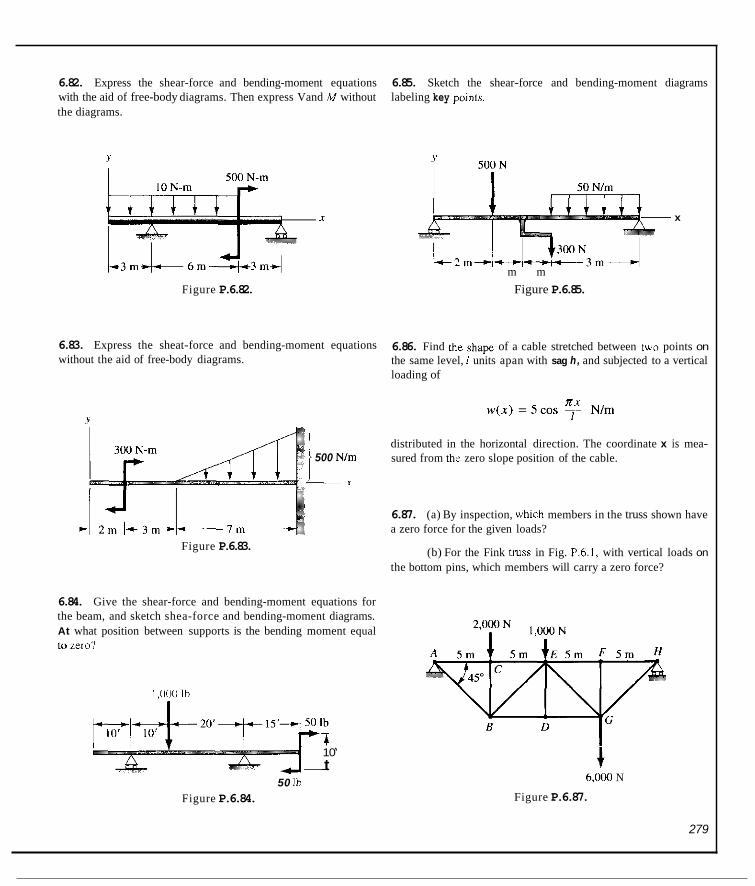
6.82. Express the shear-force and bending-moment equations 6.85. Sketch the shear-force and bending-moment diagrams with the aid of free-body diagrams. Then express Vand M without the diagrams.
labeling key point.5.
Y Y
x x
m m Figure P.6.82. Figure P.6.85.
6.83. without the aid of free-body diagrams.
Express the sheat-force and bending-moment equations 6.86. Find the shape of a cable stretched between two points on the same level, I units apan with sag h, and subjected to a vertical loading of
n.x w ( x ) = 5cos r- N/m
distributed in the horizontal direction. The coordinate x is mea- sured from the zero slope position of the cable.
l
500 N/m
6.87. a zero force for the given loads?
(a) By inspection, which members in the truss shown have
(b) For the Fink ~ N S S in Fig. P.6.I. with vertical loads on Figure P.6.83.
the bottom pins, which members will carry a zero force?
6.84. Give the shear-force and bending-moment equations for the beam, and sketch shea-force and bending-moment diagrams. At what position between supports is the bending moment equal ti) Lero?
I .ooo Ib
10' - t
50 Ib Figure P.6.84.
+ 6,000 N
Figure P.6.87.
279

30'
4,000 N A
Figure P.h.88.
Figure P.6.91.

Friction Forces 7.1 Introduction Friction is the force distribution at the surface of contact between two bodies that prevents or impedes sliding motion of one body relative to the other. This force distribution is tangent to the contact surface and has, for the body under consideration, a direction at every point in the contact surface that is in oppo- sition to the possible or existing slipping motion of the body at that point.
Frictional effects are associated with energy dissipation and are there- fore sometimes considered undesirable. At other times, however, this means of changing mechanical energy to heat is a beneficial one, as for example in brakes, where the kinetic energy of a vehicle is dissipated into heat. In statics applications, frictional forces are often necessary to maintain equilibrium.
Coulomb .friction is that friction which occurs between bodies having dry contact surfaces, and is not to he confused with the action of one body on another separated by a film of fluid such as oil. These latter problems are termed lubrication proh1em.s and are studied in the tluid mechanics courses. Coulomb, or dry, friction is a complicated phenomenon, and actually not much is known about its true nature.’ The major cause of dry friction is believed to be the microscopic roughness of the surfaces of contact. Inter- locking microscopic protuberances oppose the relative motion between the surfaces. When sliding is present between the surfaces, some of these protu- berances either are sheared off or are melted by high local temperatures. This is the reason for the high rate of “wear” for dry-body contact and indicates why it is desirable to separate the surfaces by a film of fluid.
‘Fur a imme complcle discussion ol friction. rce F. P. Bowdm and D. Tabor, The Friction und Luhrkution oj‘Solk/.~. Oxfwd Unircraiiy Press, New York. 1950.
28 I

We have previously employed the ternis “smooth’ and “rough” sur- faces of contact. A “smooth” surface can only suppnlt a normal force. On the other hand. ii “rough” surface in addition can support a force tangent to the contact suiface (i,e,, a frictiiin iorcc). In this chapter. we shall consider certain situatinns wherehy the friction Snrce can be direclly related to the normal force at a surface of contact. Olhcr than including this incw relationship, we use only thc usual static equilibrium equatiwis.
7.2 Laws of Coulomb Friction (‘omlition of imprndine Everybody has gnne thniugh the experience nf sliding lurniture along a floor.
We exert a continuously increasing force which i s ciiinpletely resisted hy fric- tion until the nhject heginc to nii)ve-usuall) with ii lurch. .The lurch occurs hecausc once the oh.ject hegins to move. there i s ii decrease in firictional force from the maximum force attained under static condili(ins. An idealized plot nf thi? force as a function of tiinc i s shown in Fig. 7. I where the force P applied to the furniture, idealizcd as ii hloch in Fig. 1.2. i s shown 10 drnp from the highcst or l imiting valiie 10 a Iowcr value which i s constiint with lime. This latter constant value i s independent iif the velocity o f the nhject. The condi- tion corresponding to the maximum value i s termed thc conditiiin nf irnpfvid- irrg rnori i i i i or itnpmdinI: slippqqe.
By carrying out experiments on hlocks tending to i n w e without rota- tion or actually moving without ~ri~tatioii on flat surfaces, Couliimh in 1781 presented certain concIusions which ;ire applicable at the c(inditiini of impmding .slippafie os once clippuge I i a . ~ hegirn. These h a w since hecomc known as Coulomh’s laws of fr ict ion For hliick psnhleinr. hc reported that:
1. The total fnrce nf f r ic l im that can he develiiped i s independent of the magnitude (if the area nf c~ntact .
2. For low relative velocities between sliding objects. the lrictional force i s practically independent n i veliicily. However. the sliding lrictiiinal force i s
lcss than the frictional fnrce corres~oiiding t n inipending slippage. 3. The lotal frictional force that can he developed i s prnportional to the tior-
inal force transmitled iicrnss the surfice of cnnlacl.
Figure 7.1. Idealized plot of applied forcc P.
Fig,ure 7,2,
Conclusions I and 2 iiiay cnime as a surprise IO inost of you and be coii- lrary to your “iiitiiition.” Nebel-theless. they arc iiccuraft’ enough statements for many engineering applicalions. More precise studies 01 friction, as wds
pointed out earlicr, are complicated and involved. We can rxprcss conclusion 3 mathematically a h :
L.r 1 - N
Therefore.
f = }‘A’ (7. I )
where ji i s called the ( .mf/i , . irni q:fi-icriori.

SECTION 1.2 LAWS OF COULOMB FRICTION 283
Equation 7.1 is valid only a t conditions uf impending slippage or while the body is slipping. Since the limiting static friction force exceeds the dynamic friction force, we differentiate between coefficients of friction for those conditions. Thus, we have coefficients of static friction and coefficients of dynamic friction, pT and p,,, respectively. The accompanying table is a small list of static coefficients that are commonly used. The corresponding coefficients of friction for dynamic conditions are about 25% less.
Static Coefficients of FrlctionZ
Steel on cast iron Coppe,.r on steel Hard steel on hard steel Mild steel on mild steel Rope on wood Wood on wood
.40 3 6 .42 .57 .70 .20-.75
Let us consider carefully the simple block problem used to develop the laws 0 1 Coulomb. Note that we have:
1. A plane surface of contact. 2. An impending or actual motion which is in the same direction for all area
elements of the contact surface. Thus, there is no impending or actual rota- tion between the bodies in contact.
3. The further implication that the properties of the respective bodies are uni- form at the contact surface. Thus, the coefficient of friction p is constant for all area elements of the contact surface.
What do we do if any of these conditions is violated? We can always choose an infinitesimal part of the area of contact between the bodies. Such an infin- itesimal area can he considered plane even though the general surface of con- tact of which it is an infinitesimal part i s not. Furthermore, the relative motion at this infinitesimal contact surface may he considered as along a straight line even though the finite surface of which it is a part may not have such a sim- ple straight motion. Finally, for the infinitesimal area of contact, we may con- sider the materials to he uniform even though the properties of the material vary over the finite area of contact. In short, when conditions 1 through 3 do not prevail, we can still use Coulomb’s law in the small (i.e., at infinitesimal contact areas) and then integrate the results. We shall call such problems complrx surface contact problems and we shall examine a series of such problems in Section 1.4.
ZF. P. Bowden and D. Tabor. The Friction and Lubrication ojSolidr, Oxford University Press. New York, 1950.

"7.3 A Comment Concerning the use of Coulomb's Law
Ac a simple illu\lralion <if why curvature (11 the surtacc of contilcl is sccond order and hence negligihlc. consider yourself at a location on the earth where i t i s perfectly round as ii planet. As you look around you over a small area compared to ii significant portion o f thc earth':, surSacc. there i s no evidence to your ohservatiini ur in what yiio normally do that indicares the presence of cur- vature of the earlh. In Lhc same way, an infinitesimal arca ciin he considered Slat cvc~ i i f i h part OS II finite curved :,urhcc when considering Couloinh's law.
Furthcrinore. a s~ntion;iry. iiiinrolatinp ohserver in inertial space look- ing at ii similar sniiill iirzii on the earth's surfice a1 Ihc equator sccs the ~ e l o c - ity of the area essentially as given by R o where R i s thc radius o f the Earth ;ind w i:, its angular velocity. All parts o f this small arca wi l l have this same velocity up ti) only sccond-der varialio~i as seen hy this observcr. And, so friim this viewpoint. all points within the area are esscntially translating with the af~,rcmentioned speed. 'lo explain lurther. we wi l l now say that lhis small area has a maximum dimension given by thc Icngth r. The rolutioilul specd of ;my point seen by an inertial and herice inonriitating observer at the area and tran4atinp witli the area must he no greater than v u . Clearly then, this rota- tional spccd i s iie,qli~yih/y smoll when compared with Rw. Hence, an infinites- imal arca at a finite dislancc from the ax is (iI~r(it~tio11 01 ii rotating surface can he considcrcd as having primarily a translational velocity and so permits the use of Ciiulnmh's law ''in the small."
7.4 Simple Contact Friction Problems We i iow examine simple ciintacl problems where Ciiuliimh's laws apply to the coiitiict surtice ci.s CL ~ ; h o l r without requiring integration pri~cedures. We shall thus consider uniforni blocklike hodics akin to those used by Coulomb. Also. we shall considcr hodies which however complex havc very smrrll coli-
L ' . &t surf'accs. . then he coiisidcred an inlinitesinial plane area and for rzasons set forth ear- lier, we shall directly use Coulomh's laws whcn approprialc as has been rhown in Fig. 7.3(h).
Beiorc proceeding to the examples. we have one additional point to make. For ii l'inite simplc surface of contact. such as the block shown in Fig. 7 . 2 . we iiiust note that wc do nut generally know the line [if action fur the simplest rehultant supporting force N, since wc do not generally know the iiorniiil force dislrihution hetween the two hodics. Hencc, we cannot take moments for such free-body diagrams without intriiducing additional unknown distanccs in the equatiiili. Conccquently. for such prohlems we l iniit ourselves to suiiirniiig iorces only. This ih tior true. however, when we havc a poiiu
such a:, i n Fig. 7.3(al . Clearly. the whole c~ntaet surface can

SECTION 1.4 SIMPLE CONTACT FRICTION PROBLEMS 285
contact such as in Fig. 7.3(a). The line of action of the supporting force must be at the point of contact, and we can thus take moments without introducing additional unknown distances.
Figure 7.3. (a) Small contact surface; (b) Coulomb's laws applied.
Two common classes of statics problems involve dry friction. In one class, we know that motion is impending, or has been established and is uni- form, and we desire information about certain forces that are present. We can then express friction forces at surfaces of contact where there is impending or actual slippage as pN according to Coulomb's law and, using L. for other friction forces, proceed by methods of statics. However, the proper direction must be given to all friction forces. That is, they must oppose possible, impmding, or actual relative motion ut the contact surfaces. In the second class of problems. external loads on a body are given, and we desire to deter- mine whether the friction forces present are sufficient to maintain equi- librium. One way to attack this latter type of problem is to assume that impending motion exists in the various possible directions, and to solve for the external forces required for such conditions. By comparing the actual external forces present with those required for the various impending motions, we can then deduce whether the body can he restrained by frictional forces from sliding.
The following examples are used to illustrate the two classes of problems.

286 CII,APTCR 7 ~RICTION FORCLS
Example 7.1
An automnhile i s shown in Fig. 7.4(;1) o n ii roadway inclined at an anplc H wilh thc hprizontal. I1 the coefficients of. static and dynamic friction between the (ires and the road are taken RS (1.6 and 0 . 5 . rcspectibely. what i s the ni;lxinnum inclination H,><;,% that the car can climb at uiiiS<)rm speed'! I t has rear-wheel drive and has a total Iuadcd weight 01 3.600 Ih. The cell- tcr (11 gravity ior this loaded conditinn ha\ been shown in thc diagram
~ '
; !
I.ct us assume that the drive wheels do not "spin"; thit 1 rclative vc l i i~ i ty hetween the tire sui-fke and the niad sur1.a : c1111t~1ct. Thai, clearly, the maximum friction li irce pixsihlc i s times the
inorinill forcc at lhis contact surldcc, iis ha\ hccn indicated in Fig. 7.4(hj.' We cain considcr this to be a u ~ p / ( i n ( i i - problem with thrcc unknnwns.
1 N, . N2. and Hc,l,th. A c c d i n g l y . sincc the fricticin force i s reslricted to a point. three equation\ [if equilihriutn arc avnilablc. IJsing l l ie rcicrcnce .rv shown in the diagi-an. we have:
F; = 0: ~~ ~ ~
.6N, - 3,600 sin B,,,,, = 0 ( a )
( h i
CF; = f) :
C M : , 0 :
N , + N, ~ 3.600 cos H,,,,,, = 0
ION, ~ (3,h(10cosH,,, , ,)(~) + (3.600sinH,,,;,,)(I) = 0 ( C i
'l'n solve Sor H,,,:,,. wc eliminate N , Srnm Eqs. (a) and (bl, gctting a s B rcsult the equatiiin
(d ) N, = 3.600 cos e ,,,,, ~ 0,000 sin
Now. elimin;iting N, froin Eq. ( c j using Eq. (dl, wc get
I X . 0 0 0 cos B ,,,,, ~ - 56.400 sin 0 ,,,:, = 0
'There f ire,
tan Hrl,2,x = ,320 (C)
B,,,, = 17.1" ( 1 )
Hence. !
! i
i -
If the drive wheel5 wcre caused to spin. we would have to use p,, in place 0 f p 5 for this pnihlein. We would then arr ive iit ii smaller H,,,,,,. which S i x this problem would bc 14.7".
'You wil l nolicc lllnl lhcrc I \ IIO iriclicin Imcc o n th? Iront wheel\. 'This IS SI) hecauw ihc i r I \ IIW m q u c ciirrririg iron1 rhr autorrwh~ie's IMmmission onlcl lhrse uhcei,. whilc it1 the siiiiic liinc llic whceh .IK 1oiii1~ng ill co i ih t i in i speeil. Note we are ncplroing "nilling" ve\is. ~iincc ilsmriiiig lmni the i l c l o ~ ~ ~ m i o n 0 1 ihc ro.d \urTacc and lhc mc. i j s~iiiill Iorcc 10 he c o w iidered an Sciiion 1.8. a \i;wved hcciion
i

SECTION 7.4 SIMP1.E CONTACT FRICTION PROBLEMS 287
Example 7.2
Using the data of Example 7. I , compute the torque needed by the drive wheels to move the car at a uniform speed up an incline where f3 = 15". Also, assume that the brakes have " locked while the car is in a parked position on the incline. What force is then needed to tow the car either up the incline or down the incline with the brakes in this condition? The diameter of the tire is 25 in.
A free-body diagram for the first part of the problem is shown in Fig. 7.5(a). Note that the friction f0rce.f will now he determined by Newton's law and not by Coulomb's law, since we do not have impending slippage between the wheel and the road for this case. Accordingly, we have, f0r.f:
F = n : .f - 3,600 sin 15' = 0
______ c 1 Therefore,
,f= 932 Ib
The torque needed is then computed using the rear wheels as a free body [see Fig. 7.5(a)]. Taking moments about A, we have
torque = ( f ) ( r ) = (932)(*$) = 971 ft-DJ
For the second part of the problem, we have shown the required free body in Fig. 7.5(b). Note that we have used Coulomb's law for the friction forces with the dynamic friction coefficient p,, on all wheels. We now write the equations of equilibrium for this free body.
TuD - S(N, + N z ) - 3,600sin 15' = 0 (a)
(N, + N 2 ) - 3.6Oocos 15" = 0 (b)
Solving for N, + N2 from Eq. (b), and substituting into Eq. (a), we can now solve for Tup. Hence,
Ttzp = (.5)(3,600)( 966) + 932 = (c)

' ,-
I,,,,.,

SECTION 7.4 SIMPLE CONTACT FRICTION PROBLEMS 289
Example 7.3
In Fig. 7.6 a strongbox of mass 75 kg rests on a floor. The static coeffi- cient of friction for the contact surface is 20. What is the largest force P and what is the highest position h for applying this force that will not allow the strongbox to eithcr slip on thc floor or to tip ?
The free-body diagram for the strongbox is shown in Fig. 7.7. The condition of impending motion has been recognized by the use of Coulomb’s law. Furthermore, by concentrating the supporting and friction forces at the left corner, we are stipulating impending tipping for the proh- lem. Thesc two impendin& conditions impose the largest possible values of P and h that we are seekine.
1- .h m 4 Figure 7.6. Strongbox being pushed.
The pertinent the midplane of the equilibrium:
- forces constitute a coplanar system of forces strongbox. We procecd with the scalar equations
at of
I
N = 75g = 7 3 6 N
P = .2N = 147.1.5N
~(75g) ( .3 )+ (147.1S)h = 0
Therefore, we get for the largest P and the largest h the following results:
P,,,sx = 147.15 N h,,, = 1.50 m
i
Thus, the height of the applied load must he less than or equal to I .SO m in order to avoid tipping.
Figure 7.7. Impending tipping and dlpplng
The three examples presented illustrated the,first type of friction proh- lem wherein we know the nature of the motion or impending motion present in the system and we determine certilin roorces or positions of certain forces. In the last example of this series, we illustrate the .second type of friction problem set forth carlier-namely the problem of deciding whether bodies will move or not move under prcscrihed external forces.

290 CHA1"Ik;K 1 FRICTlClN bOK('ES
Example 7.4
1 Thc ciicfficienl of static friclicin kir all contiic1 surfaces in Fig. 7.X i s .2. Does thc 50-lb force move the block A iip. hold i t in equilihrium. or i s i l too small to prcvmt A from coming down and H fr(nn moving w t ' ! The 1 50-lb fiircc i s exerted at the niidpl;inc iif the hlircks s o llial we cain consider this ii coplanar pmblcm.
I
4
.i
I 200 Ib
We ciin cmipute ii l i irce P in placc 111. the 50-lh fhrcc I(I cause i n - pending mot i i i~ i 01 block H to the left, and ii forcc P fb1- impcnding mi l ion of hlock R to the right. I n th is way, we can judge hy comp;irism the action that tht: SO-Ih tiirce wil l C:IUSZ.
The f ro -body &igrains for impending nr(ilion olhlock H to the le f t have hccn shown in Fig. 7.9, which conlains the unknown fwcc I' iiieii- tioned abiivc. We necd not be ciincerned ahoul the correct Iocatioii (11 the centers of gfii\'ity n1 thr hloch\, since wc shall only add forces in the analysis. (Wc do not know the line of action o f thc inorniiil l i i rccs iit
lhc cwitact surlxec and thcrefore in not takr moments.) Summing forces on block A . wc gel
iV2cos IS" j -N,sin I S ' ' i - ~ . 2 N , j - X ( ) j
+ N,i - .2NZ co\ 15"i '. .2N, sin IS':j = 0
The scalar cqi i i i t i i i i i~ arc:
N , - .?59N, - .1932N, = 0 .OhhN, - .?N, - 200 - .051XN, = 0
Solving cimultiineously. wc get
N, = 243 Ih. N, = 1OY.R Ih

SECTION 7.4 SIMPLE CONTACT FRICTION PROBLEMS 291
Example 7.4 (Continued) For the fre.e-body diagram of B. we have, on summing forces,
-N2 cos 157 + Nz sin 15"i - Pi + .2N3i + N , j - 1 0 0 j + . 2 N 2 c o s 1S"i+.2N2sin ISy=O
This yields the following scalar equations:
-P + 62 .9 + .2N3 + 46.9 = 0 -235 + N , - 100 + 12.6 = 0
Solving simultaneously, we have
P = 174 Ib
Clearly, the stipulated force of 50 Ih is insufficient to induce a motion of block B to the left, so further computation is necessary.
Next, we reverse the direction of force P and compute what its value must be to move the block B to the right. The frictional forces in Fig. 7 .9 are all reversed, and the vector equation of equilibrium for block A becomes
N2 cos 15y - Nz sin 1S"i + . 2N, j - 2OOj + N,i + .2N2 cos 1% + .2N2 sin l5y = 0
The scalar equations are:
N , - .259N2 + .1932N2 = 0 .966N2 + .2N, - 200 + .0518N2 = 0
Solving simultaneously, we get
N2 = 194.1 Ib, N , = 12.80 Ib
For free body B we have, on summing forces,
-N2 cos l 5 . j + N2 sin 15Oi + Pi - .2N3i + N 3 j - lOOj - .2Nz cos 157 - .2N2 sin 157 = 0
The following are the scalar equations:
P - .2N3 + 50.3 - 37.5 = 0 -100 + N3 - 187.5 - 10.05 = 0
Solving, we get P = 46.7 Ib. Thus, we would have to pull to the right to get block B to move in this direction. We can now conclude from this study that the blocks are in equilibrium.

7.1. A hlock has a force F applied to it. If this force has a timc variatioii as shown in the diagram, draw a simple sketch showing the friction force variation with time. Take p3 = .1 and p,, = .2 for the problem.
I
Figure P.7.1.
7.2. Show hy increasing the inclination @ o n an inclined surface unlil there is impending slippage of supported hodics. we rrach the anfile ofrepose 9, so that tan $$ = p>
1.3. Tu what minimum angle must the drivcr elevate thc dump bed of the truck to cause the wooden cratc of weight W to slide out? For wood on steel, p, = .6 and p,, = .4.
Figure P.7.3.
7.4. A platform is suspendcd by two ropes which are attached 1~
docks lhat can slide horizontally. At what value of W does the hitform begin to descend'? Will W stan tipping'?
!92
Figure P.7.4.
7 .5 Explain how a violin how. when drawn oyer a string, main- tains the vibration oi the string. Put thi.: in leimi 0 1 friction forccs and the difference i n static and dynamic cocfficients of frictirin.
7.6. Whit is thc valuz of thc force F. inclined at 30" to thc hnri- ~oi i ta l , nccded to get thc hlock juct ctartetl up the incline? What is the forcc F needed tu keep it .just moving up at s constant speed'! The coefficients of ctntic and dynamic friction arc .3 ;md .?lF, respectively.
W = 100 Ih
Figure P.7.6.
7.7. Bodies A and L( weigh 500 N and 300 N, respeclivcly. The plalfol-m nn which they are placed is raised from thc horizontnl poaition to an anplc H. What i ' i the ~, iu in i ron anplc that can he reached before the bodies slip down the incline'? Takc p> for body N and the plane as .2 and f l? for hod! A and the plane as .i.
Figure P.7.7.

7.8. What is the minimum value of p,v that will allow the rod AB to remain in place? The rod has a length of 3.3 m and it has a weight of 200 N.
Data W = 2 0 0 N L = 3.3 m
A
Figure P.7.8.
7.9. Find the minimum force P to get block A moving
Dofa W, = 200 Ih W, = 90 Ih F ' = 3
Figure P.7.9.
7.10. What minimum force F is needed to staR body A moving to the right if px = .2S for all surfaces? The following weights are given:
W, = S O N W, = 125 N W,, = 100 N
The length oSAB is 2.5 m.
Figure P.7.10.
7.11. A 30-ton tank is moving up a 30" incline. If ps = .6 for the contact surface between tread and ground, what muximum torque can be developed at the rear drive sprocket with no slipping? What maximum towing force F can the tank develop? Take the mean diameter of the rear sprocket as 2 ft.
Figure P.7.11.
7.12. A SCi-lb crate A rests on a I,OM)-lb crate B. The centers of gravity of the crates are at the geometric centers. The coefficients of static friction between contact sufaces are shown in the diagram. The force Tis increased from zero. What is the fin1 action to occur?
Figure P.7.12.
7.13. the right? The coefficient of static friction for all surfaces is .3.
What force F is needed to get the 300-kg block moving to
p, = .3
Figure P.7.13.
29:

Y
Figure P.7.19.

7.20. The cylinder shown weighs 200 N and is at rest. What is the friction force at A ? If there is impending slippage, what is the static coefficient of friction? The supporting plane is inclined at 60" to the horizontal.
Figure P.7.22.
Figure P.7.20.
1.23. An insect nies to climb out of a hemispherical bowl of radius 600 mm. If the coefficient of static friction between insect and bowl is .4, how high up does the insect go? If the bowl is spun ahout a vertical axis, the bug gets pushed out in a radial direction by the force m m 2 , as you learned in physics. At what speed o will the bug just be able to get out of the bowl?
7.21. Armature B is stationary while rotorA rotates with angular speed 0. In armature B there is a braking system. If M~ = .4, what is the braking torque on A for a force F of 300 N? Note that the rod on which F 1s applied is pinned at C to the armature B Neglect friction between B and the brake pads C and H.
Figure P.7.21.
Figure P.7.23.
1.24. A block A of mass 500 kg rests on a stationary support B where the static coefficient of friction ps = .4. On the right side, support C i s on rollers. The dynamic coefficient of friction .ud of the support C with body A is .2. If C is moved at constant speed to the left, how far does it move before body A begins to move?
7.22. A 200-lb load is placed on the luggage rack of the 4,500-lh station wagon. Will the station wagon climb the hill more easily or with greater difficulty with the luggage than without'? Explain. The static coefficient of friction is .55. Figure P.7.24.
295

Figure V.7.27. Figure P.7.32.
296

7.33. The block of weight W is tu he moved up an inclined plane. A rod of length c with negligible weight is attached to the block and the force F is applied to the tup of this rod. If the coef- ficient of static friction is determine in terms o fu , d, and p,r the mnximum length c for which the block will begin to slide rather than tip. tal arms.
7.36. What is the minimum static coefficient of friction required to maintain the bracket and its 500-lh load in a SVdtic position? (Assume point contacts at the horizontal centerlines of the arms.) The center of gravity is I in. from the shaft centerline. Hint: Note that there is clearance between the veitical shaft and the horizon-
Figure P.7.33.
7.34. Determine the range of values of W, for which the block will either slide up the plane or slide down the plane. At what value of W, is the friction force zero? W2 = 100 Ih.
W- = 100 Ih
Figure P.7.34.
7.35. A 200-kN tractor is to push a 60-kN cuncrete beam up a 15' incline at a construction site. If pc, = .5 between beam and din and if pr is .6 between tractor tread and din, can the tractor do the job? If so, what torque must be developed on the tractor drive sprocket which is .8 m in diameter'? What force P is then devel- oped to push the beam'?
Figure P.7.36.
7.31. If the static coefficient of friction in Problem 7.36 is .2, at what minimum distance from the centerline of the vertical shaft can we support the 500-lh load without slipping?
7.38. A rod is held hy a cord at one end. If the force F = 200 N, and if the rod weighs 450 N, what is the mruimum angle a that the rod can he placed for !J,$ between the rod and the floor equal to .4? The rod is I m in length.
Figure P.7.3S. Figure P.7.38.
297

7.39, Suppose tliat a i l ice liftcr IS uscd to support a hard block nf matcrial hy friction only. What i s the ,ni,iimunr coefficient of static friction, u,, to accomplish this for any weigh1 Wand frri the g e m - etry shown i n the di;ig!ram'!
7.41. A hcam supports loud C' wcighiiip 500 N. At suppoflh .4 and H. the static coefficient of frictioil i\ .2. At thc Contact surlac~! helween load C and the bcam. the dynamic coefficient 0 1 friction i s . l S . It force I : move> C'steadily tu rhc Icit. how far doe\ it IIIII\IC
b e f k thc bcam hegins tu move'! The beam w e i g h 200 N. Neglect tlic hcighi i ol the hriuii in p u r ciilculiltioiii.
10" ,~
A i
t
~ 111
Figure P.7.41.
7.42. imv account. 'lakc I = 120 in in
DO Problsni 7.41 fur thc cilx whcrc [lie height 1 i, takcn
7.43. A roil is supported h i IWO u,hrrls spinning in oppoiitc directions. If the wheels were horirmtal, the rod wimld he placed centrally over thc wheel, for equilihriuni. However, the wheels have an inclination ol20" a s shown, and lhr rnd m u h t he placed at LI pusition off center for equilibrium. If thc cocflicienl of fricliuii i s L I , , = .8, how many lcct oll w i t c r iiiuhi the rud he placed?
Figure P.7.39.
7.40. A rectangular case is loaded with uniform vertical thin rods such that when i t i s full, as shown in (a), the case has a total weight of 1,000 Ih. The case weighr 100 Ib whcn ciripty and hits a cocfficient of static friction of .3 with tlic tlwx as shown in thc diagram. A forcc 7'of 200 Ih i s nnintained un the ci\se. It the r d s are unloaded a\ shown in (h) , what i s thc limiting value o f x for equilibrium to he inaintiiined'! I
I O 0 Ih
Figure P.7.43
P.7.44. How much forcc /: !nust hc applied ti) the wedge I n hepin to iilisc the cratc? Neglcct changes in gcrmetry. What force must the hiopprr hlock provide to prevent the crate frnm inwing to
the Icft'! The slatic coefficient oi friction hetwccn a l l wtiaccs i s 3
c-..- (,'d (a) (h)
Figure P.7.40. Figure P.7.44.

7.45. What is the ninrimum height x of a step bo that the force P will roll the 50-lb cylinder over the step with no slipping at a? Take p,, = 3.
1.41. If we neglect friction at rhc mllen, and the coefficient of static friction is .2 for all surfaces, ascendin whether the 5.000-lb weight will go up, go down, or stay stationary.
Figure P.7.45.
7.46. The rod AI1 ic pulled at A and i t moves to the left. If the coefficient of dynamic friction for the rod ar A and B is .4, what must the minimum value of W, be to prevent the block from tipping when a = ZO"? With this value of W,, determine the minimum coefficient of static friction between the block and the supporting plane needed to just prevent the block from sliding. W , is 100 N.
0 nim
A 6 0 m m -1 1- Figure P.1.46.
4,000 Ib - Figure P.7.47.
7.5 Complex Surface Contact Friction Problems
In the examples undertaken heretofore, the nature of the relative impending or actual motion between the plane surfaces of contact was quite simple-that of motion without rotation. We shall now examine more general types of con- tacts between bodies. In Example 7.5. we have a plane contact surface hut with varying direction of impending or slipping motion for the area elements as a result of rotation. In such problems we shall have to apply Coulomb's laws locally to infinitesimal areas of contact and to integrate the results, for reasons explained in Section 7.2. To do this, we must ascertain the distribu- tion of the tiormal force at the contact surfdce, an undertaking that is usually difficult and well beyond the cdpahilities of rigid-body statics, as explained in Chapter 5. However, we can at times approximately compute frictional effects by ertimating the manner of distribution of the normal force at the sur- face of contact. We now illustrate this.

300 CHAPTFK 7 FKlCrlON FOKC'FS
Example 7.5
Compute the frictional resistancc to rotation of a rotating solid cylinder with an attached pad A pressing against a flat dry surface with a h r c e P (see Fig. 7.10). The pad A and the stationary tlnt dry surface constitute a dry rlirust hrurinR.
The direction of the frictional forces distributed over the contact sur- face is no longer simple. We therefore takc an infinitesimal area for exan- illation. This area is shown i n Fig. 7.10, where the clement has been formed from polar-coordinate differentials so as lo he related simply to the boundaries. The arca CIA is equal to r d0 dr. We shall ussuirw that the nor- mal force P is uniformly distributed over the entire area of contact. The normal force on the area element is then
The friction force associated with this lcirce during moliori is
The direction oE df must opposc the relative motion between the surfaces. The relative ni(iti~in is rotation 01 concentric circles ahout the ccnterline, so the direction of a force dfl (Fig. 7. I I) must lie tangent to a circle of radius r. At 180" from thc position of thc area element for df;, we may carry out a similar calculation fhr ii force (If , , which for the same rmust be equal and opposite to df;, thua forming a couple. Since thc cntire area may he decomposed in this way, wc can conclude that there are only couples in the plane of contact. If we take moments of all infinitesimal forces ahout the center, we get the magnitude of the total frictional couple moment. The direction of the couple moment is along the shaft axis. First, consider area elements on the ring (if radius r:
\ A P
Figure 7.10. Dry thrust bearing.
Figure 7.11. Friction forces f< rm couplcs.

SECTION^.^ BELTFRICTION 301
Example 7.5 (Continued)
Taking pd as constant and holding r constant, we have on integration with respect to 8: i
dM = p d - 2m2dr nDZ/4
We thus account for all area elements on the ring of radius r. To account for all the rings of the contact surface, we next integrate with respect to r from zero to 012. Clearly, this gives us the total resisting torque M. Thus,
What we have performed in the last three steps is multiple integration, which we introduced in Chapter 4 when dealing with rectangular coordinates.
7.6 Belt Friction A flexible belt is shown in Fig. 7.12 wrapped around a portion of a drum, with the amount of wrap indicated by angle p. The angle p i s called the angle of wrap. Assume that the drum is stationary and tensions T , and T, are such that motion is impending between the belt and the drum. We shall take the impending motion of the belt to be clockwise relative to the drum, and there- fore the tension T , exceeds tension T2.
ds
I Figure 7.12. Belt wrapped around drum.

302 CHAFTER 7 FRICTION bowi~s
Consider an infinitesimal segment 01' the bell as a lrce hody. This seg- ment subtends an angle d 8 a1 thc drum cenier as shown in Fig. 7.13. Sum- ming force components in the radial and transverse directions and equating them to zcrn as per ryrrilihriurn, we get the following x a l w equations:
Figure 7.13. he -hody diagram of regiirnr (if helt; impending blippage.
Therefore, dN dT cos 7 = fll ON -
Therefore. dt) rl t) -2T sin -~ - dT sin -$ f dN = 0 2 -
The sine of a very small angle approximately equals thc angle ilself i n radi- ans. Furthermore, to the same degree of accuracy, the cosine of a sinal1 angle apprwches unity. (That these relations are true inay bc seen by cxpanding the sine and cosine in a powcr series and then retaining only the firs1 tcrms.) Thc preceding equilibrium equations then become
dT = 0% (IN (7.2a)
(7.2b) d8 2 -7a8 - dT + dN = 0

SECTION 7.6 BELT FRICTION 303
In the last equation, we have an expression involving the product of two infinitesimals. This quantity may he considered negligible compared to the other terms of the equation involving only one differential. Thus, we have for this equation:
T d 0 = d N (7.3)
From Eqs. 1.2a and 7.3, we may form an equation involving T and 0. Thus, by eliminating dN from the equations, we have
dT = &T d 0 Hence,
Integrating both sides around the portion of the belt in contact with the drum,
we get
01
We therefore have established a relation between the tensions on each part of the belt at a condition of impending motion between the belt and the drum. The same relation can he reached for a rotating drum with impending slippage between the belt and the drum i fwe neglect centrifugal eflects on the belt. Furthennore, by using the dynamic coefficient of friction in the formula above, we have the case of the belt slipping at constant speed over either a rotating or stationary drum (again neglecting centrifugal effects on the belt). Thus, for all such cases, we have
(7.5)
where the proper coefficient of friction must he used to suit the problem, and the angle ,8 must he expressed in radians. Note that the ratio of tensions depends only on the angle of wrap 0 and the coefficient of friction p. Thus, if the drum A is forced to the right, as shown in Fig. 7.14, the tensions will increase, hut if ,8 is not affected by the action, the ratio of T,IT, for impending or actual constant speed slippage is not affected by this action. However, the torque developed by the belt on the drum as a result of friction is affected by the force F. The torque is easily determined by using the drum and the portion of the belt in contact with the drum as a free body, as is shown in Fig. 7.14.
T j w
-c ’2
l?igure 7.14. F Q ~ C ~ F affects T , and T~ but not T,IT,.

304 CHAPTER 7 wt(-rro[V FORCES
Thus.

SECTION 7.6 BELT FRICTION 305
Example 7.6
A drum (see Fig. 7.15) requires a torque of 200 N-m to get it to start rotat- ing. If the static coefficient of friction us between the belt and the drum is .35, what is the minimum axial force F on the drum required to create enough tension in the belt to start the rotation of the drum?
Torque required = 200 N-m Radius = 250 mm
72 Figure 7.15. Drum is driven by a belt.
The angle of wrap /3 clearly is n radians. To get the minimum force F, we use the condition of impending slippage between belt and drum so that we can say
(a) L ~ - $5, = 3 00 T2
T
For the condition of starting rotation we have
Mu = torque required = 200 N-m ~~
:. (T, - T2)(.25) = 200 (b)
It is now a simple matter to solve the previous two equations simultane- ously to get
T , = 1,200 N T2 = 400 N
Finally we can determine the minimum value of F for this problem by summing forces in the x direction as follows:
Fnli,l = 1,200 + 400 = 1,600 N
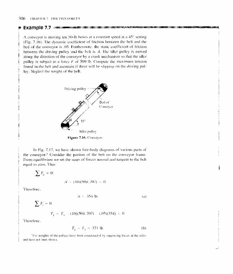
i
J

SECTlON 7.6 BELT FRICTION 307
Example 7.7 (Continued)
For the idler pulley (no resisting or applied torques), we have
T3 = T2 (C)
From Eqs. (c) and (d), we conclude that
T2 = T3 = 250 Ib (e)
From Eq. (b) we now get for the maximum tension T,:
TI = T,+37I = (f)
We must next check the driving pulley to ensure that there is no slip- page occumng. For the condition of impending slippage, we have, using as T2 the value of 250 Ib and solving for T ,
T I - T - *e 4 X = (250)(3.51) = 878 Ib
Clearly, since the T , needed is only 621 Ib (see Eq.(f)), we do not have slip- page at the dnving pulley, and we conclude that the maximum tension is indeed 621 Ib.
Belt on conveyor frame
SO0 Ib
j = .OS N
Driving pulley
I /
Torque
Idler pulley
Figure 7.17. Various free-body diagrams of parts of conveyor.

308 ( ' I I A P I I I K 1 I~KI (TION l:OU('l?i
'3 Example 7.8
An electi-ic motor (not \hewn) i n Fig. 7.18 drives at constant speed the pulley B. which c~innecl\ to pulley A by ii belt. Pulley 4 is ui t~ncctcd to il
compressor (not shown! which rcquircs 700 N-m torque 10 drive i t ill ~1111-
stai i t speed 01,~. I f ,u, Ibr the belt and either piillcy is .A, what nnininium value o f t h e indicated force F is required to have ino dipping anywhcrc?
1
1 I
I if^-_^-_____ , ,,, Figure 7.18. Del i -dr iver comprrssuu'.
As ii f'ir\t stcp. we determine the m g l e s of wrap p for the respeclive pulleys. For thi, pui-p(ix, wc first compute a (Fig. 7.19). Note that thc radii 0 , l l and OljE. k i n g perpendicular 10 lhc same line DE.. iire thei-cforc pariillel to each r1ther. Drawing E<'par;lllel to 0,Ow we t l i m forin ix i n the shaded triiinglc. Hence. wc can say:
,
Fi'iQure 7.19. Find an$lcs of wrap $
1 Note i n Fig. 7.1') Ihiil is pcrpendicular to <:E and [hat ( I . , ( ; is perpen- 1 dicular 10 I l l ; , Thcrclore. the included angle between OA6' aiid O~,G most
cqual the included angle hctwccn C1:' and Ill.'. Thih an&!le i s n. Clearly. the ;mgk hctwccn O,j.l ;ind O,,ti is also this angle ix. We cim inow express t h r angles (if w r q fur holh pulleys a s follows:
i
p , = 1x0" + 2(5.74) = 191.5' 31.74) = 168.5" p, = 180"
. . ., . ,l_" .. . "". , , . .. . .. . . . .

SECTION 7.6 BELT FRICTION 309
Example 7.8 (Continued)
Now consider pulley A as a free body in Fig. 7.20. Note that the minimum force F corresponds to the condition of impending slippage. Accordingly, for this condition at A, we have
Figure 7.20. Free-body diagram of A.
Also, summing moments about the center of the pulley, we have
[(TI), - (T2),I(.50) - 700 = 0
Solving Eqs. (a) and (b) simultaneously, we get
= 1,898 N; ( T J A = 498 N
From equilibrium, we can compute force FA as follows:
(1,898 + 498) cos 5.74" ~ FA = 0
Now go to pulley B to see what minimum force FR is needed so that the belt does not slip on it during operations. Consider in Fig. 7.21 the free- body diagram of pulley E. For impending slipping on pulley E , we have
Figure 7.21. Free-body diagram of B

3 1 0 CHAlTEK 7 FRIrTION FOKCES
Example 7.8 (continued)
The torque for pulley B needed I o dcvelop 700 N-m on pulley A is next computed. Thus,"
Therefore, M, = 320 N-in
Summing moments in Fig. 7.21 ahout the ccnler of. B. we then have on using the above resull
- [(TI),, . - lT2),](.30) + 420 = 0
Therefore,
(TI),$ ~ Cr,), = 1,400 (e)
Solving Eqs. (d) and (c) simultaneously, we gct
(TI),, = 2,112.5 N: (T2),j = 625 N
Hence, the minimum F,, needed for pulley B is
r;, = (2.025 + 625) cos 5.74" =
Notc that the ratios til' the tcnsions for irnpendiny .sli/qiiiKe f o r the two cylinders art'
T
T
1)riven cylindcr.4 ti^ = 3.81 FA = 2,384 N
Driving cylinder B & = 1.24 fi; = 2,637 N 5
If we use impending slippage for driven cylinder A , we will have slipping for driving cylinder B, which we cannot tolerate. Thub, if we use the larger force of 2,617 N. we will hc well under the impending slippage condition of the driven cylinder A. Clearly. the optimum result to uvoid slip[i~ge and to minimize the belt tension ior greater life of the belt is to have a force somewhere above 2.617 N . Here is a place for good engineering judgement and experience.
"Note [hill the ratio oi tranimitlcd torques MJM, between directly connected pulleys and gears wil l cquiil r J r , or l)Jll , 01 the pullcyr o r gear*. Can you vcriiy lhis yourself'

7.48. dry thrwt bearing. The coefficient of friction is taken aspc
Compute the frictional resisting torque for the concentric 7.51. Compute the frictional torque needed to rotate the trun- cated cone relative to the fixed member. The cone has a 20-mm- diameter base and a 60" cone angle and is cut off 3 mm from the cone tip. The dynamic coefficient of friction is .2.
7.49. The support end of a dry thrust bearing is shown. Four pads form the contact surface. If a shaft creates a 100-N thrust uniformly distributed over the pads, what is the resisting torque for a dynamic coefficient of friction of , 1 '?
7.52. A 1,000-N block is being lowered down an inclined sur- face. The block is pinned to the incline al C, and at E a cord is played out so as to cause the body to rotate at uniform speed about C. Taking pd to be .3 and assuming the contact pressure is uni- form along the base of the block, compute T for the configuration shown in the diagram.
7.50. In Example 7.5, the normal force distribution at the con- tact surface is not uniform but, as a result of wear, is inversely proportiunal to the radius r. What, then, is the resisting torque M?


7.57. The seaman pulls with 100-N force and wants to stop the motorboat from moving away from the dock under power. How few wraps n OS the rope must he make around the post if the motorboat develops 3,500 N of thrust and the static coefficient of friction between the rope and thc post is .2?
Figure P.7.57.
7.58. A length of belt rests on a flat surfact and runs over a quarter of the drum. A load Wrests on the horizontal portion of the belt, which in turn is supported by a table. If the static coeffi- cient of friction for all surfaces is 3, compute the maximum wcight W that can be moved by rotating the drum.
Figure P.7.58.
7.59. The rope holding the 50-lb weight E passes over the drum and i s attached ~t A. The weight of C is 60 Ib. What is the mini^ mum static coefficient of friction between the rope and the dNm to maintain equilibrium of the drum'?
I I
Figure P.7.59.
7.60. What is the maximum weight that can be supported by the system in the position shown? Pulley B connor turn. Bar AC is fined to cylindcr A, which weighs 500 N. The coefficient of static friction for all contact surfaces is 3.
Figure P.7.60.
7.61. A mountain climber of weight W h a y s freely suspended by one rope that is fatened at one end to his waist, wrapped one- half turn about a rock with I(, = .2, and held at the othcr end in his hand. What minimum force in terms of W must he pull with to maintain his position'! What minimum force must he pull the rope into himself with to gain altitude?
Figure P.7.61.
7.62. Pulley B is turned by a diesel engine and drives pulley A connected to a generator. If the torque that A must transmit to the generator is 500 N-m, what is the minimum static coefficient of friction between the belt and pulleys for thz case where the force F is 2,(100 N ?
l-2m-l
Figure P.7.62.
313

7.63. A hand hrake ik \ h o w Ii p<, = .4, what i s the rcristing li~l-i]oe when thc rhait is rotating'! What are the supporting fbrce.; mi the rod AB.
Figure P.7.63.
7.64. A conyeyor i s shown with two driving pulleys A and B . Drivel- 4 has no angle o f Wdp of 330". wherca5 B has a wrap of 1x0". If the dynamic cuefficient nf fr ict ion between the hell and the hed o l the wn\,ryr,l- is .I. atid the m a l weight to he Iran\- ported is 1(1,000 N. what is the .s,nnlirrf sfatic coefficient of fric- t ion between the belt and the driving pulleys'! One-fifth of the Iuad can he assumed to he hetween thc twn pulleys at dl times. and the tension in the slack side (underneath) i s 2,000 N. Therc i s a free-wheelin$ pulley at the left end uf the conveyor. You wil l have to SOIYC an cquation hy (r ial and ciror.
Figure P.7.64.
7.65. A freely turning idlcr pulley i s used 10 increase the angle of wrap for the pullcys shown. If the tension in the slack side a h w e is 200 Ih, find the nrmi~num torque that a n be transmitted hy the pulleys for a static coefficient uf friction of .3
Idler pulley
Figure P.7.65.
314
1.66. (a ) What force P i s necded to drvelop a resisting torque 01 hS N-m on the rrrtating drum'! 'The dynamic coellicient of friction / I < , i s 0.4.
(h) With thc same force P from part (a), %,hat must the value o f p,, he in wdcr 11, increilw the resisting t i rqur hy IO N-m'.'
Figure P.7.66.
1.67. What is the maximum value r f a x i a l l o a d P 10 maintain a rritational speed 0 = 5 r;id/s of the dry thrust hearing'! The sum of the hell forces is 200 N . The cwifact surtaor helween the hclt and drum and hetween the dry thrust hcaring and base havc the mmc H , and p,, of .4 ;and 3. rcyvx t ivc ly .

7.68. Rod AR weighing 200 N is supported by a cable wrapped around a semicylinder having a coefficient of friction pT equal to .2. A weight C having a mass of IO kg can slide on rod AB. What is the maximum range x from the centerline that the center of C can be placed without causing slippage?
250 mm
/ 1.2m
7.71. length, w, acting on a drum from a belt is given as
From first principles, show that the normal force per unit A B
w, = 2 r
Use the indicated diagram as an aid. [ H i n o Start with Eq. 7.2(a) and use Eq. 7.4 for any point a.]
" 7.69. The cable mechanism shown is similar to that used to move the station indicator on a radio. If the indicator jams, what force is developed at the indicator base to free the jam when the required torque applied to the turning nob is IO b i n ? Also. what are the J forces in the various regions of the cable? The static coefficient of T2
--," I P friction is .IS.
I T,
Figure P.7.71. Idler Pulley 7.72. what minimum force F is needed so that dmm A can transmit
a clockwise torque of 500 N-m without slipping? The coefficient of friction, pa, between A and the belt is .4. What minimwn caefftcient of static friction is needed between drum R and belt for no slipping?
Figure P.7.69. ~
F 7.70. What are the minimum possible supporting force c o m p - nene needed for pulley B as a result of the action of the belt? The static coefficient of friction between the belt and pulley B is .3 and between the belt and pulley A is .4. The torque that the belt delivers to A is 200 N-m.
+lm+ Figure P.7.72.
315

induced hy hod) (. weighing S O 0 N? The weight (11 A i \ 100 N . The m t i c c w l l i c ! r n t ,if friction hetween the hclth arid A i s .J. and between A iuid the w;i l l i i s . I. Neglect li-ictiun at pulley (;.
IO0 1111
Figure P.7.1
7.14. A V-hell i \ \huwn. ShnN that
Figure P.7.74.
Figure P.7.16.
7.77. .A pullcy A i\ dri\cn hy an outadc ;ipenl at a spccd w o i 100 I-pm. A bclt weighing 30 Nlm i s driven hy thc pulley. Il T2 = 21x1 N. what i s the , ,ro.rirmm pmhihle tciisiiin 7, computed without con- sidering ccntrilirp;il r f f e a c ? Cornputt: T, accounting lin- ccntrifugal ellcuts, and g i w the perccntqc cmor incurred hy tnot including CCII-
trilupal cffccts. 'The \tittic cncfficient ot triution hetween tho helt iind thc pullq i\ 3. Suc Prohlerri 7.76 hcfirre doing this pmhlem.
Figure P.7.17.

SECTION 7.7 THE SQUARE SCREW THREAD 3 11
7.7 The Square Screw Thread We shall now consider the action of a nut on a screw that has square threads (Fig. 7.22). Let us take r as the mean radius from the centerline of the screw to the thread. The pitch, p. is the distance along the screw between adjacent threads, and the lead, L, i s the distance that a nut will advance in the direction of the axis of the screw in one revolution. For screw threads that are single- threaded, L equals p . For an n-threaded screw, the lead L is np.
Forces are transmitted from screw to nut over several revolutions of thread, and hence we have a distribution of normal and friction forces. How- ever, because of the narrow width of the thread, we may consider the distrib- ution to be confined at a distance r from the centerline, thus forming a “loading” strip winding around the centerline of the screw. Figure 7.22 illus- trates infinitesimal normal and frictional forces on an infinitesimal pan of the strip. The local slope tan a as one looks in radially is determined by consid- ering the definition of L, the lead. Thus,
L np slope = t a n a = - = - 2 n r 2 n r
All elements of the proposed distribution have the same inclination (direction cosine) relative to the z direction. In the summation of forces in this direction, therefore, we can consider the distribution to be replaced by a single normal force Nand a single friction force f at the inclinations shown in Fig. 7.23 at a position anywhere along the thread. And, since the elements of the distribution have the same moment ann about the centerline in addition to the common inclination, we may use the concentrated forces mentioned above in taking moments about the centerline. There is thus a “limited equivalence” between N and f and the force distribution from the nut onto the screw. The other forces on the screw will be considered as an axial load P and a torque M7 collinear with P (Fig. 7.23) . For equilibrium at a condition of impending morion to raise the screw, we then have the following scalar equations:’
-P + Ncos a - ptNsin a = 0
+,,N cos a r - N sin a r + M, = 0
Figure 7.22. Square screw thread
Figure 1.23. Free-body diagram.
’The equalions also apply to .steady rotation of the n u t on the scccw, in which case one uses the dynamic coefficient of friction fld in the equations.
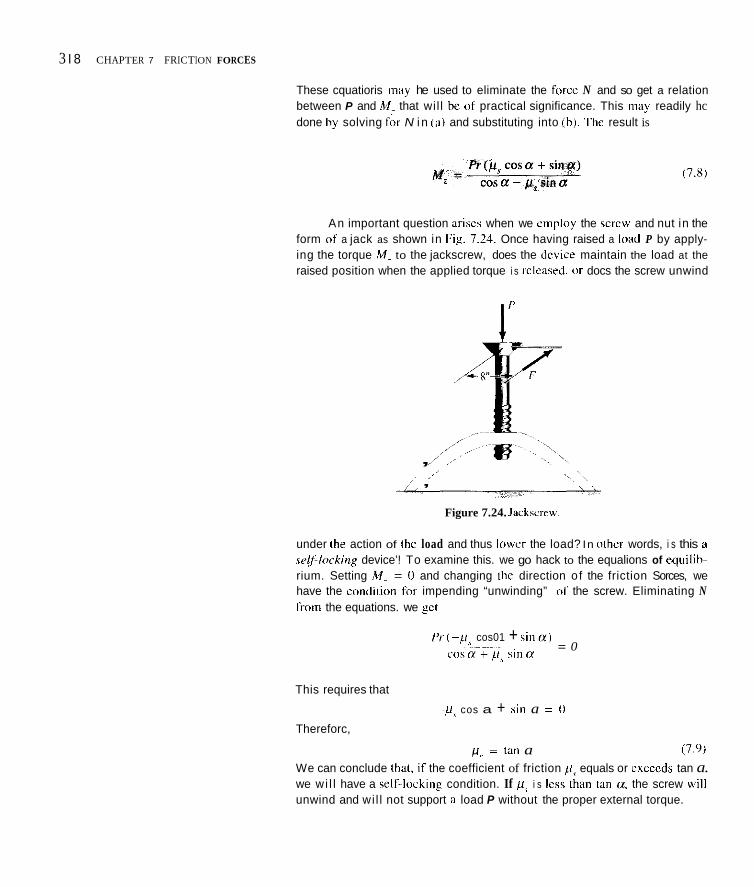
3 I 8 CHAPTER 7 FRICTION FORCES
These cquatioris ]nay he used to eliminate the Scirce N and so get a relation between P and M. that wil l hc o S practical significance. This may readily hc done by solving S& N i n ( a ) and substituting into ih). Thc result is
An important question arises when we employ the scrcw and nut in the form of a jack as shown in Fig. 7.24. Once having raised a Imad P by apply- ing the torque M. to the jackscrew, does the dcvice maintain the load at the raised position when the applied torque i s rcleased. (11 docs the screw unwind
_,,, \, ’ ,’ , , ,/ ,
Figure 7.24. Jackscl-rw.
under the action of the load and thus lower the load? In other words, i s this a selflorking device’! To examine this. we go hack to the equalions of equilih- rium. Setting hf. = 0 and changing thc direction o f the friction Sorces, we have the condilion for impending “unwinding” 01 the screw. Eliminating N l‘rom the equations. we get
/‘!-(-/I< cos01 + s ina) c11sa-+rS s i n a = 0
This requires that
-pr cos a + \in a = 0 Thereforc,
p . = tan a (7.9) We can conclude thal. if the coefficient of friction pr equals or excccds tan a. we wi l l have a self.-locking condition. If M, i s less than tan 01, the screw %,ill unwind and wi l l not support ii load P without the proper external torque.

SECTION 7.8 ROI. I . INC; RESISTANCE 319
Example 7.9
A jackscrew with a double thread of mean diameter 2 in. is shown in Fig. 7.24. The pitch is .2 in. If a force F of 40 Ibis applied to the device, what load W can be raised'? With this load on the device, what will happen if the applied force F is released! Take / I , = .3 for the surfaces of contact.
The applied torque M, is clearly:
M. .. = 12 (40) = 26.7 Ib-ft (4
The angle a for this screw is given as
Therefore,
a = 3.64'
Using Eq. 7.8 we can solve lor P . Thus,
M. (cos a - @,$ sin a ) r ( p , cosa + sin a )
p =
(26.7)[.998 ~ (.3)(.0635 ,&[(.3)(.998) + ,06351
~ _ _ _ _ -~ - -
The load W is 864 Ih. The device is self-locking since @,s exceeds tan a = ,0636.
p, > tan (r ,,:. 8e ng,
To lower the load requires a reverse torque. We may readily com- pute this torque by using Eq. 7.8 with the friction forces reversed. Thus,
864(&)[-(.3)(.998) + ,06351 ( MZ )down = ~- - 16.71 Ih-tt (d) ,998 + (.3)(.0635)
"7.8 Rolling Resistance Let us now consider the situation where a hard roller moYes without slipping along a horizontal surface while supporting a load W at the center. Since we know from experience that a horizontal force P is required to maintain uni- form motion, some sort of resistance must he present. We can understand this resistance if we examine the deformation shown in an exaggerated manner in

Fig. 7.75. If foi-cc P i s ahng the cciiterline a h shown, Ihc cquivalenl l i irce sys- tein cwi i ing 01110 tl ie roller from the regioti o f cnntiicI niiist he ihat O S a force N whosc line O S i iclion i i l so gocc through t h ~ center OS the rnller since, you wi l l recall S i r i n i Chapter 5. three notipal-allel forces niiist he c o n ~ i ~ r r c ~ i t for equilibrium, 111 ordcr to develop ii r cs i~ tu i ce 10 ~ i i ~ t i o n . clearly N i i i u s i he ori- ented iit iin anglc 4 with the vertical direction. i i s i s shown in Fig. 7.25. The sciiliir equ;iti,iiis O S qu i l i l i i . i u i i t hccome
vi ~ lo;rd />,I U t l C C i
I' ~ l w c c wquiwtl tor c,~nit,,,ll >pccct
W = N cos 6 : P = A' cin 4
Therefore. Figure 7.25. Rolling ie*i\liincc modcl. ; = lil t1 @ (7.10,
Since i l ic iireii 01coti1iic1 i s sni:ill, we ticite t l i i i t q5 i s ii smal l angle and that tali @ = \in $. The h i l i @ i\ sccn to he u i i ~ Srnni I:ip. 7.25. Thcrcriirc, we inay sa) Illill
Solving fort', we gel
( 7 . I I h) , - w < r I -
The dist;incc ( I i n tliex cqu;itirins ih ciillcd the c , w / f ; ( . i ~ ~ oj ' tdIi i8,y rrsisru,i(.e. Couloinh suggesled that l i i r wiriorhle Ioadc 1V. the ri it in PIW is cons tm i
for given m;ikrials and ii gibe11 geometry ( r = cm\tant). Liioking at Eq. 7. I la , we scc t l i i i t (I must then he ii c~nc t i i i i t lcii~ given geomc~ry iind inateri- iilc. Ciiuloinh added that, Sor given materials and iwrinhic I-adius, the riitin PIU'varics in\'ei-sely iis r ; that is , a s the radiuh O S the cyliridcr i s increased. the reci~tancc lo uniform ir iutioii lor ii given load W decre;ises. Thus. considering Ik l . 7. I l a iigain. we may cnnclude that. for given nialcriiils, (I i s a l so c ~ n ~ t m t for iill s i x s oi rollers atid loads. I lowevcr. other invcsligiitors have contested huth ~tate~i icnts, 1xirticul;irly the laltei- one. ;ind ihcrc i s :I nccd for further invcstig;ition i n l l i i s iireii. I.aching hetter datii. we prcwnt the fol lowing list of rolling ~ ~ c l l i c i c i i t ~ Stir your iise. hot we tiiust ciiution th;il you ehould iint expect great ;iccur;icq froiii t h i s general procediir:~.
Coefficients of Rolling Resistance ~.. ~ ~. .. .. .. ~ ~
-. ~ ~ ~ . . ~ . ~~ ~. ~~~~ ~
t i (in.)
.Oh ~ .IO ~!I? - SI1 .!I4 - .Oh
S t c d on hieel ,007 .!I I 5 Sicel ,111 wood Pwum;itic tires , , I / viiuiith raid Pncuni;ilic liw 011 mod ro:td H;iidrnrd \tee1 on h:il-deneJ \ t c d .0!,02 .0005

SECTION 7.8 ROLLING RESISTANCE 321
Example 7.10
What is the rolling resistance of a railroad freight car weighing 100 tons? The wheels have a diameter of 30 in. The coefficient of rolling resistance between wheel and track is ,001 in. Compare the resistance to that of a truck and trailer having the same total weight and with tires having a diameter of 4 ft. The coefficient of rolling resistance a between the truck tires and road is ,025 in.
We can use Eq. 7. I 1 b directly for the desired results. Thus. for the railroad freight car, we haveK
For the truck, we get
We see a decided differences between the two vehicles, with clear advan- tage toward the railroad freight car.
T h e number of wheels n plays no role here since we divide the load by n to get the load per wheel and then niultiply hy n to get Lhc m a l resirtanfe.

7.78. A simple C-clamp i s used to hold two pieces of metal together. The clamp has a single square thread with a pitch 01 12 in. and a mean diameter of .75 in. The static coefficient of fric- tion i s 30. Find the torque required i f a 1,000-lh compressive had i s required on the blocks. If the thread I S a double thread. what i s
the required torquc?
Figure P.7.78.
1.79. The mast of n railhoat i s held hy wires called shroud,, iis
rhown in the diagram. Racing sailors are carelul to get the pmpcr ension in the shrouds hy adjusting the lurnhucklc at the hattom or :he shrouds. When wc do this we say wc are .'tuning" thc hoat. II i tension of I S 0 N exists in the chroud. what torque I S needed l o itart tightening further by turning the tumhuckle? 'lhc pitch of the ;ingle threaded screw i s 1.5 mni and the mean diameler i s X . 0 mni. The static coefficient of friction i s .2.
Figure P.7.79.
1.80. Forccs F of SO Ih are applied to the jackscrew shown. The hread diametcr is 2 in. and the pitch i\ 4 in. The %,tic coefficimt if friction Tor the thread IS .OS. The wripht I?J and colliir arc nm ierniitted to rotate and so the collar must rotatc on the shaft o1 the crew. If the static cocfficient of friction hctween the colliir and haft is .I. determine the wcight W that can he liftcd hy this system.
c
Figure P.7.82. 122

7.83. Consider a single-threaded screw where the pitchp = 4.5 mm and the mean radius is 20 mm. For a coefficient of friction p,\ = .3, what torque is needed on the nut for it to turn under a load of 1 .(XI0 N ? Compute this for a square thread and then do it for a tri- angular thread where the angle p is 30". See Problem 7.82 before doing this problem.
7.84. If the coefficient of rolling resistance of a cylinder on a flat surface is .05 in., at what inclination of the surface will the cylin- der of radius r = I ft roll with uniform velocity?
7.85. A 65-kN vehicle designed for polar expeditions is on a very slippery ice surface fur which the static coefficient of friction between tires and ice is ,005. Also, the coefficient of rolling resis- tance is known to be .8 mm. Will the vehicle be able to move? The vehicle has four-wheel drive.
~ 1 . 2 m 4 - 1.3 m-.,
Figure P.7.85.
7.86. In Problem 735, suppose there is only rear-wheel drive available. What is the minimum static coefficient of friction needed between tires and ground for the vehicle to move?
7.87. A roller thrust bearing is shown supporting a force P of 2.5 kN. What torque Tis need to turn the shaft A at constant speed if the only resistance is that from the hall hearings? The coefficient of rolling resistance for the balls and the bearing surfaces is ,01270 mm. The mean radius from the centerline of the shaft to the balls is 30 mm.
Figure P.7.87.
7.9 Closure In this chapter, we have examined the results of two independent experi- ments: that of impending or actual sliding of one body over another and that of a cylinder or sphere rolling at constant speed over a flat surface. Without any theoretical basis, the results of such experiments must be used in situa- tions that closely parallel the experiments themselves.
In the case of a rolling cylinder, both rolling resistance and sliding resistance are present. However. for a cylinder accelerating with any appre- ciable magnitude, only sliding friction need be accounted for. With no accel- eration on a horizontal surface, only rolling resistance need be considered. Most situations fall into these categories. For very small accelerations, both effects are present and must be taken into account. We can then expect only a crude result for such computations.
Before going further. we must carefully define certain properties of plane surfaces in order to facilitate later computations in mechanics where such properties are most useful. These plane surface properties and other related topics will be studied in Chapter 8.
323

7.88. the force F needed to start the 2 0 - N weight moving to the right.
If thc static coefficient of friction for all surV~ces is 3 5 , find 7.91. A lriction drive is shown with A the drivcr dicc and R the dri\eti disc. If fiwce F pressing R onto A is I S 0 N. what i ? the ninrimu~rr torque M , that can he developed'? For this torque. whal is the lurquc M , needed for thc drive disc A ? The static coefficient of friction bctwccn A and H is .7. What mitical force must COLI G wilhsrand fo r thc action dcscrihed ahrivr! i, 30"
Figure P.7.XX.
7.89. A loaded crate is shown. Thc crate weighs 500 Ih wilh il
ccnier of gravity at its geometric center. Thc contact w h c z between crate and floor has a static coefficient of friction of .2. II H = 90", show that the crate will slide hefore m c can increasc I enough f c w tipping to occur. If a stop is to bc inserted in rhc floor at A to prevent slipping so that the cmte could he tipped. whal minimum horizontal force will he exerted on thc stop?
Figure P.7.91.
7.92. Detmninc thc weight of hlock A for impending motion to the right. Thc static coefficient of friction hctwern the vahle and thc wrlaccs which it conlacts is 0.2. Thc m l i c crrcfficienl 0 1 fric- tion helwrrn hkrch A a i d the burface upon which i t rei15 is (1.4. Tht. two prist\ are circular with ii diameter of0.25 in.
A Figure P.7.89.
Figure P.7.92.
7.90. In Problem 7.K9, compute a value of H and I whzre dip- ping and tipping will occur siinultancously. If the actual angle H i \ smaller than this value of 8, is there any further nerd of the slop at 7.93.
the kil. lh Pnrhlem 7.92 till- impending slippage of hody A to
4 to prevent slipping'?
324

7.94. A tug is pushing a barge into a berth. After the barge turns clockwise and touches the sides of the pilings, what thrust must the tug develop to move it at uniform speed of 2 knots fanher into the berth? The dynamic Coefficient of friction between the barge and the sides of the berth is .4. The drag from the water is 3,000 N along the centerline of the barge.
7.96. The drum is driven by a motor with a maximum torque capability of 500 Ib-ft. The static coefficient of friction between the drum and the braking strap (belt) is .4. How much force P must an operator exert to stop the drum if it rotates ( I ) clockwise and (2) counterclockwise? What are the belt forces in each case'?
Side P
Figure P.7.96.
Figure P.7.94.
7.97. The four drive pulleys shown are used to transmit a torque from pulley A to pulley D on an electric typewriter. If the static coefficient of friction between the belts and the pulleys is .3, what is the torque available at pulley D i f 10 b i n . of torque is input to the shaft of pulley A? What are the belt forces?
7.95. The static and dynamic coefficients of friction for the upper surface of are ps = .4, pd = .3, and for the lower surface of contact B are p,, = . I and pd = .OS. What is the minimum force P needed to just get the cylinder moving'!
A of the
R - Figure P.7.93. Figure P.7.97.
325

7.98. A scissors jack i s shown lifting the cnd of a car s o that K = 6.67 kN. What torque T i s needed krr thic operation? Notc that A i s merely a bearing and at B we linvc a nut. 'I'he \crcu is sin& threaded with a pitch of 3 mm and a mean diamcter o f 20 mnl. The static coefficient of frictinn hetween the screw and nut at 13 is .3. Neglect the weight ofthe members and evaluiltc Tfor B = 45" and for 0 = 60".
7.100. A hot rcctanpolar mctal i n g u IS to he flatlcncd hy passing through cylindrical roller\. I I tl ic ingm i \ 10 he drawn into the r d e n hy friction once il toiiches the ~DIICIS, what i\ the minhrrum thickness I ofthe ingnl that can he auhiwed hy thi5 pmccss on one
p i s 9 'I'hc static cocfficicnl of friction for tlic contact between inpwt and cylindcr i ' l .3. The cylindel~, rotate a i showu with ang'u- lal- rpced w.
1"
Pigwe P.7.100,
Figure P.7.98.
1.99. A hlack C weighing 1 0 k N i q being moved on rollerr A ind B each weighing I kN. What force P i s nceded to m;iintain steady motion? Take the coefficient of rolling rcsiitancr hetween .he mllers and the ground to he .h mm and hetween hlock L' ;MI hc rollers to be .4 mm.
C
Figure P.7.99.
7.101. A ccmc clutch i~ bhown. Assuming that uniform pressure\
exist hetwcen thc wri tact surlacei, compute thc m ~ x i , m m torque that can hc tran\mittcd. Thc \tiitiu c d f i c i e n t of I i~ ict iun i s .30 and the activating force F i c 100 Ih. IMim Acsurne that the niming cone transmits i l h 100-1h ax ia l fwcc trr the statinmry c m e hy pres- sure primarily. That i\ . wc wil l neglect the friction-torcr compo^
nent un thr cone wriace normal ti, thc lrmsverse direction.l
t "I
+- l[y- F ~~ 100 Ih t
Figure P.7.101.
126
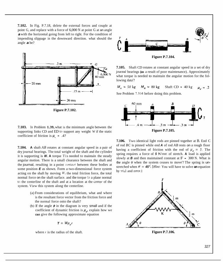
7.102. In Fig. P.7.18, delete the external forces and couple at point G, and replace with a force of 6,000 N at point G at an angle a with the horizontal going from left to right. For the condition of impending slippage in the downward direction. what should the angle a be?
Figure P.7.102.
7.103. In Problem 1.39, what is the minimum angle between the supporting links CD and ED to support any weight W if the static coefficient of friction is p~ = .4?
7.104. A shaft AB rotates at constant angular speed in a pair of dry journal bearings. The total weight of the shaft and the cylinder it is supporting is W. A torque T i s needed to maintain the steady angular motion. There is a small clearance between the shaft and the journal, resulting in a point confacf between these bodies at some position E as shown. Form a two-dimensional force system acting on the shaft by moving W, the total friction force, the total normal force on the shaft surface. and the torque to a plane normal to the centerline of the shaft and at a location at the centei of the system. View this system along the centerline.
(a) From considerations of equilibrium, what and where is the resultant force vector from the friction force and the normal force onto the shaft?
(b) If the angle @ in the diagram is very small and if the coefficient of dynamic friction is p<!, explain how we can give the following approximate equation
T = Wp<,r
where I is the radius of the shaft.
Figure P.7.104.
7.105. Shaft CD rotates at constant angular speed in a set of dry jouinal bearings (as a result of poor maintenance). Approximately what torque is needed to maintain the angular motion for the fol- lowing data'?
MA = 50 kg MB = 80 kg
See Problem 1.104 before doing this problem.
Shaft CD = 40 kg ud = .2
60 mm A R
Figure P.7.105.
7.106. Two identical light rods are pinned together at B. End C of rod BC is pinned while end A of rod AB rests on a rough floor having a coefficient of friction with the rod of pd = .5. The spring requires a force of 5 Nlmm of stretch. A load is applied slowly at B and then maintained constant at F = 300 N. What is the angle 0 when the system ceases to move'? The spring is un- stretched when 0 = 45". (Hinc You will have to solve an equation by trial and error.]
F
Figure P.7.106.
327

I70 i i im
Figure P.7.107.
I A I
L . . . l Figare 1'.7.109.

I
7.112. In Prohlem 7.27, what maximum value should W, be ir order to S tan moving the system to the left? All other data art unchanged.
Figure P.7.110.
7.111. A triangular pile of width I ft is being driven into the ground slowly by a force P of 50,000 Ib. There is pressure an the lateral surfaces of the pile. This pressure varies linearly from 0 ai A to /io at B, as has been shown in the diagram. If the coefficient of dynamic friction between the pile and the soil is 0.6, what is the ma.ximum prcssure ,I(,'!
Figure P.7.111.
7.113. A block rests on a surface for which there is a coefticienl of friction p, = .2. Over what range of angle p will there be nc movement of the block for the 150-N force? (You will have to solve an equation by trial and error.)
F L , = 2 Figure P.7.113.
7.114. What is the largest load that can be suspended without moving blocks A and E'? The static coefficient of friction for all plane surfaces of cuntact is 3. Block A weighs 500 N and block B weighs 700 N. Neglect friction in the pulley system.
Width pile =
of I ft
Figure P.7.114.
329

7.115. weighing 100 Ih'! Takc IC, = .2 liir all surf.ict.s of contac~.
What is the minimum force F to hold the cylinders. each
Figure P.7.115.
1.116. A compressor is shown. If the prcsaurc in the cylinder is 1.40 N1mm2 above atmosphere (gage), what mininzum torque 7 i h
iccdcd to initiate mution in rhc systcm? Neglect the weight of thc :rank and connecting rod as far as thcir ctintrihution triward imov- ng the system. Consider fi-ictioii only hetwecn thc piston and :ylinder walls where the coefficient 01 Irictiun = . I S .
= I 10 Nlmm'
Figure P.7.116.
7.117. Find the cord tension ifhlock I attains mnximuni friction
L.-l Figure P.7.117
330

Properties of Surfaces 8.1 Introduction If we are buying a tract of land, we certainly want to consider the size and, with equal interest, the shape and orientation of the earth’s surface, and possibly its agricultural, geological, or aesthetic potentials. The size of a surface (Le., the area) is a familiar concept and has been used in the previous section. Certain aspects of the shape and orientation of a surface will he examined in this chap ter. There are a number of formulations that convey meaning about the shape and disposition of a surface relative to some reference. To he sure, these for- mulations are not used by real estate people, hut in engineering work, where a variety of quantitative descriptions are necessary, these formulations will prove most useful. In general, we shall restrict our attention to coplanar surfaces.
8.2 First Moment of an Area and the Centroid
A coplanar surface of area A and a reference xy in the plane of the surface are shown in Fig. 8.1. We define thefirst moment of area A about the x axis as
M x = j A Y & (8.1)
and the first moment about the v axis as
These two quantities convey a certain knowledge of the shape, size, and orientation of the area, which we can use in many analyses of mechanics.
331

332 CHAPTHK 8 PKOPEKTII<S OF SIJKPACES
\
:-I
Figure 8.1. Plane area.
You will no doubt notice the similarity of the preceding integrals 10 those which would occur f(ir computing moments about the x and? axes from a parallel force distribution oriented normal to the area A in Fig. 8.1. The moment of such a force distribution has been shown for the purposes of rigid- hody calculations to be equivalent to that of a single resultant force located at a particular point 1. 7 . Similarly. we can concentrate lhe entire area A at a posilion x , , y,, called the wi i / i -o id ' where, for computations of lint moments. this new amngement is equi\dent In the original distribution (Fig. 8.2). The coordinatcs x . and are usually called the wntruidul ~nordiririrr.~. To coni- pute these coordinatcs. we simply eqiiatc miimenls 111 the distributed arcii with that of thc conccntratcd area ahout both axes:
,
Figure 8.2. Centmdal 'oord!n.iie\
'The location of the centriiid of an area can readily bc shown to be indeppn- &iit ( i t the r&wiiw U X ~ S employed. That is. the centroid is a proprro, only of the owii ilsclS. We have wked the render to prove this in Problem 8.1
If the axe5 ,ry havc their origin at the centroid, thcn thcsc axes are called nd clearly the first nioineiits about (hcsc axes must be zero.
Finally. we point out that all axes going through the centroid of an arc3 arc called renrroiilirl ii.ies for that area. Clearly. the .fir.v n i o i ~ i ~ n t s o / r m ureu uhoiit nti.y < ! / i / . v wntroidul i i . ir .s iniisf hr :era. This inust he true since the per- pendicular dislmce frnm the cenlroid lo the centroidal axis must he zero.

SECTION 8.2 FIRST MOMENT OF AN AREA AND THE CENTROID 333
Example 8.1
A plane surface is shown in Fig. 8.3 hounded by the x axis, the curve y’ = 25x, and a line parallel to they axis. What are the first moments of the area about the x and y axes and what are the centroidal coordinates?
We shall first compute M, and My for this area. Using vertical infini- tesimal area elements of width dx and height y . we have noting that y = 5,’x
To compute M , we use horizontal area elements of width dy and length (IO-x) as shown in the diagram. Thus
v could alsc we used vertical strips for computing M, as follows u: centroids of the vertical strips:
R
M, = I lo - ( y d x ) = I Y 7 d . x 25x 0 2 0
10
= (l’2.5)($)~ = 625 ft3 n
To compute the position of the centroid (x,., y,), we will need the area A of the surface. Thus, using vertical strips:
t ”’ 250’
pdL 10’
Figure 8.3. Find centroid,
= 105.4 ft2

334 CHAPTER 8 PROPERTIES OF SURFACES
f Example 8.1 (Continued)
The centroidal coordinates are, accordingly,
To get the moment of the area about an axis y’. which is 15 It Io thc lelt of t h e y axis. simply proceed as follows:
i = 105.4 6.00 + 15 = 2.213 ft’ .~. ..
Consider now a planc arca with an arI.\ ,!/.sytritiicJrry such a s is \howl1 ill Fig. X.4, where the J axis is collinear with the axis 01 symmetry. I n coinput- ing x,. for this area. we havc
5ymmctry
Figure 8.4. Arca with one axis of symmelry
I n evaluating the inkgrid ahove. we i i i n considcr iircii element\ in syn~metric pairs such as shown in Fig. 8.4. where we have hhown ii pair of area elcnicnls which are iiiii-ror images O S cach other ahout the axis 0 1 iymmetry. Clearly, the first moment of such a pair about the axis of symmetry is ~ e r o . And. since the entire area can he considered as composed of such pairs. we can conclude that ,r? = 0. Thus, the cenlriiid of a11 area with onc axis of symmetry must therefore lie somewhcrc along thih axis of cyminetry. The axis of symmetry then is a centroidal axis. which is another indication that the first ninmcnl of area must he 7.ero about such an axis. With two orthogonal axcs of syn~met~-y , the centroid inust lie at the inlersccti(in O S these axes. T h w . lor such areas 21s circles and rectangles. the centroid is easily determined by inspcction.
In many problem>, the arca (11 interest ciin he imcidered formed hy [he addition o r subtracti(in iif ciinple familiar arciis whiihe centroids arc known by inspection as well as by otlier firmiliar areas. cuch iis triangles and sectors of circles whosc centroids and areas are givcn i n handhoohh. Wc call areas rnade up of such simple areas u i r n / m ~ I / e arcas. ( A listing of familiar areas is given fiir your convcnicncc on the inside bach covcr of this text.) For such p r i b Icms. we can say that
where .< and \;, (with proper signs) are the cenlroickil co(irdinatcs to simple area Ai, and where A is the totid area.

SECTION 8.2 FIRST MOMENT OF AN AREA AND THE CENTROID 335
Example 8.2
Find the centroid of the shaded section shown in Fig. 8.5
t 60 rnm
X 1- 200 mm -d Figure 8.5. Composite area.
We may consider four separate areas. These are the triangle ( l ) , the circle (2) and the rectangle (3) all cut from an original rectangular 200 x 140 mm2 area which we denote as area (4). In composite-area problems, we urge you to set up a format of the kind we shall now illustrate. Using the positions of the centroid of a right triangle as given in the inside covers of this text, we have:
~~~ ~
A , = -f(30)(80) = -1,200 10 -12,000 113.3 -136,000 A , = - 7 ~ 5 0 ~ = -7,850 100 -785,000 70 -549,780 A, = -(40)(60) = -2,400 180 -432,000 110 -264,000 A, = (20Ol(140) = 28,ooo 100 2,800,000 70 1,960,000
A = 16,550 mm2 c AjXj = E A j Y , =
1.571 x 106mm3 1.011 x 106mm3 -
Therefore.

336 CHAPTER K PKOFERTIFS OF SUKI'ACES
We now illustrate ho\+ wc can use the composilc-;i~-c:a approach lor finding the ceiitniid ol iin m i l c(imp~iscd <if fmi l ia r parts iis just described.
In clo.;ing. wc would likc to piiint out that the centroid ciincept can he of use in finding Llic simples1 resultant ol a dislrihulcd loading. Thus. con- sider thc di\ti-ihuted kiiiding ii.f.rI shmvn in Fig. X.6. The rcsultant fi irce <, 01' t t i i i loading. also shown i n the diagi-ani. i\ given iis

8.1. Show that the centroid of area A is the same point for axes XJ and x'y'. Thus, thc pasition of rhc ccntroid of an area is a pmp- crty only of the area.
v'
-1,-
I ~
t
Figure P.8.1.
8.2. \ = M D .
Show that thc centroid of the right triangle is x, = 2a/3.
v
Figure P.8.2.
8.3. is the first moment of this area about axis A 4 1
Find t h r ccntroid of thc area under the half-sine wave. Whal
?
Y = sin .r 7 L, ki. A
Figure P.8.3.
8.4. What are the first moments of the area about the x and y ares? The curved houndary is that of a parabola. [Him: The gen- eral equation for parabolas of the shape shown is y2 = ai + h.1
Figure P.8.4.
8.5. What are the centroidal cormiinates for the shadzd arza? The curved boundary is that of a parabola. [Hint: 'The general equation for parabola? of the shape shown is J = cr.r2 + b.1
v
Parabola J T 20 ni
I.. l 5 m -__(
Figure P.8.5.
8.6. shown in the diagram.
Show that the centroid of the area under a semicircle is ab
n
Figure P.8.6.
33:

I*-- / -+I Figure P.8.7.
Figure P.8.10.
4'
I t- 1
~~ ~~ I
20' Figure ILX.8.
ti
I- 4 Figure P.X.V.
8.11. Show that thc ccntrrrid of thc trianglc is at x, = ( o + b]/3. v, = hl?. [Hint: B i n ~ ~ h thc triaoglc inlo two right trianglcr i w which the uetitmids arc known fioiri Problcni 8.2.1
t 1- "
h
I-- li -~ +I Figure P.8.11.
8.12. The outer hoondziry is that ,if it circle having ii radius of I 111.
What are the cetitroidal cnordinates for the shaded area'?
kigure P.8.12.
338

8.13. What are the coordinates of the centroid of the shaded area? The parabola is given as y2 = 2x withy and x in millimeters.
Y
y = 7 m m
x = 10 mm Figure P.8.13.
8.14. Find the centroid of the shaded area. The equation of the curve is y = 5xz with x and y in millimeters. What is the first moment of the area about line AB?
y
I I I
80 mm c + 1 m m m +
Figure P.8.14.
8.15. Find the centroid of the shaded area. What is the first moment of this area about line A-A. The upper boundary is a parabola y2 = 501 with x and y in millimeters.
x
Figure P.8.15.
In rhr remaining problems of this secrion, UJY cenmidal
Find the centroid of the end shield of a bulldozer blade.
p0SirilJn.C of'rimple ur?u.s us jilund in rhe inside co~erx.
8.16.
1 - 4 4
Figure P.8.16. 8.17. In Example 2.6, determine ic for the centroid of the ui- angular faces of the pyramid plus the base area ABCE. The height of the pyramid is 300 ft.
8.18. A parallelogram and an ellipse have been cut from a rec- tangular plate, What are the centroidal coordinates of what is left of the plate? What i h M,, for this area? Use formulas given on the inside ofthe hack covers.
Y' \
AIY, 7)
c
Figure P.8.18.
339

8.19. A mrdiu,i axis has the mnic aira o n one side of the axis as it does on the other side. Find the distance hetween the horizontal (median l ine and a parallel centmidal axis. t
1, f 50 mm
I+- 5' ..*I I: 60'
Figure P.X.22. I---. 100 irim *I -
Figure P.8.19.
8.23. end lvilder.
Find thc centroid of the end of rhc buckct of B sinall frrrnt
/(----A X.20. Find thc ccntroid of the truss gnwt.1 platc.
Find the centroid of thc indicatcd area.
v I
4 l.20'-(
Figure P.X.21.
r
8.22. ti iw rhc results in meters. [Hinr: Sec Fig. P.8.f.l
Find the crntruidal cuordin;acs ftrr the shaded area shown
Figure P.8.23.
8.24. (whole area)'!
Whew is the czntroid of the airplane's vertical stabilizer
1- J 111 -1 It I 111
Vigure P.8.24.
I 340

8.25. onal A-A? [Hinr: Consider symmetry.]
What is the first moment of the shaded area about the diag- 8.27. A wide-flange I beam (identified as 14WF202 I beam) is shown with two reinforcing plates on top. At what height above the bottom i s the centroid of the beam located'?
Figure P.8.25.
.r
1 Figure P.8.27.
8.26. A built-up beam is shown with four 120-mm by 120-mm by 20-mm angles. Find the vertical distance above the base for the centroid of the cross-section.
8.28. [ H i m See Fig. P.8.6.1
Compute the position of the centroid of the shaded u t a .
0 In,"
5
f 4T
1-35 mm+ 21 mm -1
13 mm
- 41 mm A+- 35 mm
Figure P.8.28.
34 I

Figure P.8.30.
I C L , - - r l
Figure P.8.2Y.
8.3 Other Centers We employ the concepts of ni~incnts and ccntroids in mechanics for three- dimensional bodies as wcll as for plaiie areas. Thus, we intriiduce now the first tnoment 01 a volunie. V. 01 a hiidy (see Fig. X.X) ahout a point 0 where I
(8.6)
Figure 8.8. Center of voIume. C.V.. of a hody.
v?. = j j j r d r . i
Thcrrlore.
r ' = v ! Jjjr i / r ' (8.7)
We see that the center of volume is the poinl wherc we could hypothetically concentrate thc entire volu~ne of il body for purposcs of computing the firhi moment of the volume lit. the hody about some point 0. The components of Eq. 8.7 pibe the ( ~ ~ ~ ~ ~ , , i d d i ~ i ~ i i i ( . ( , . ~ of volttine .x, , );, and z c . Thus, we have
1
342

SECTION 8.3 OTHER CENTERS 343
The integral about the yz plane, etc.
we get thefirst moment o f m a n about 0. That is,
x do. it should be noted, gives the first moment of volume
If we replace dv by dm = p du in Eq. 8.6, where p is the mass densiv,
moment vector of mass = 111 r p dz: (8.9) V
The cenfer of mass rc is then given as
(8.10)
where M is the total mass of the body. The center of mass is the point in space where hypothetically we could concentrate the entire mass for purposes of computing the first moment of mass about a point 0. Using the components of Eq. 8.10, we can say that
ISf =p dv
IIJ p dv , 2, =
YP dL'
' yc = J j J p d v lls X P dv
" = I l j p d Z J
In our work in dynamics, we shall consider the center of mass of a system of n particles (see Fig. 8.9). We will then say:
Therefore,
mi';
M - i=l (8.1 I)
$/.Me V
x e m , where M is the total mass of the system. Clearly, if the particles are of infini- tesimal mass and constitute a continuous body, we get hack Eq. 8.10.
Finally, if we replace dv by ydu, where y(= pg) is the specific weight, we arrive at the concept of center of gravity discussed in Chapter 4. We have used the center of gravity of a body in many calculations thus far as a point to concentrate the entire weight of a body.
You should have no trouble in concluding from Eq. 8.10 that if p is constant throughout a body, the center of mass coincides with the center of volume. Furthermore, if y(= pg) is constant throughout a body, the center of gravity of the body corresponds to the center of volume of the body. If, finally, p and g are each constant for a body, all three points coincide for the body.
We now illustrate the computation of the center of volume. Computa- tion for the center of mass follows similar lines, and we have already com- puted centers of gravity in Chapter 4.
Figure 8,9. System of panic,es showing center of mass, C.M.

c

SECTION 8.3 OTHER CENTERS 345
Example 8.4
What is the coordinate s? for the center of volume of the body of revolu- tion shown in Fig. 8.1 I'! Note that a cone has been cut away from the left end whilc. at the right end, we have a hemispherical region. 8
!
1- 4 mm-11 mm
Figure 8.11. Compovte valume
We have a composite body consisting of three simple domains-a cone (body I ) , a cylinder (body 21, and a hemisphere (body 3). Using furinulas from the inside covers, we have:
Tliereforc,
We have presented 8 number of three-dimensional problems for detcr- mining the center of volume, ccnter of mass, and the center of gravity of com- posite bodies. We will leave i t to the student to work hidher way through these problems, working from first principles, without the need of examples. However, we ask that you follow the following format, which clearly is an extension 01' what we havc been doing up to this point.

346 CHAPlEK X PROP1IRTIES I F SURFACES
. ..
.
( p ; I ,
In closing. wc wish to point o u t further that curved surfaces and lines have centroids. Since we shall have occasion in the next section to consider the ccntrnid of a line, wc simply point nut inow (see Fig. 8.12) that
Figure 8.12. Czntniid frir c i i rwd line.
(8.12a)
(X.12hi
Figure 8.13. Ccntroid for coinporite line.
wlicre 1. i s the length nf the line. Note that the centroid C wil l not gcnerally lie along the line.
Consider next a curve tnadc u p nf simple curves each of whose cem troids i s known. Such i s the case shnwn in Fig. 8.13. inade up nf straight lines. .The linc segment I.,. has for instance centroid C, with coordinates il, 7,. i i s has heen shown in the diagram. We can then suy for the enlire curve that
(8.13)

SECTION 8.4 THEOREMS OF PAPPUS-GULDINUS 341
"8.4 Theorems of Pappus-Guldinus The theorems of Pappus-Guldinus were first set forth by Pappus about 300 A.D. and then restated by the Swiss mathematician Paul Guldinus about 1640. These theorems are concerned with the relation of a surface of revolution to its generating curve, and the relation of a volume of revolution 10 its general- ing area.
The first of the theorems may be stated as follows:
Y Generating curve
Figure 8.14. Coplanar generating curve.
To prove this theorem, consider first an element d/ of the generating curve shown in Fig. 8.14. For a single revolution of the generating curve about the x axis, the line segment d/ traces an area
dA = 2Ry dl
For the entire curve this area becomes the surface of revolution given as
A = 2 n I y d l = 2 n y , L (8.14)
where L is the length of the curve and y, is the centroidal coordinate of the curve. But 2 % ~ ~ is the circumferential length of the circle formed by having the centroid of the curve rotate about the .r axis. The first theorem is thus proved.

348 CHAPTEI< K PROPERTIES OF St!KFA(TS
An(ithcr way 01 intcrpreting Eq. X.14 i h to note that the area ofthe hody <)I revolution i s e q u l to 211 times thc .fii:st monwir 0 1 the generating curve about the axis of rc\'oIulioii. If the genernting c u I \ ~ c i h coinposcd of himplc curves. I-,. whose ccntroidh iirc known. such a s the cncc shiiwn i n Fig. 8.13. thcn we can exprcs, A iic l i i l l ows :
whcl-c 7, i s the centniidsl c~iordinate to the ith line segment L,. Thc second theoreni may he stated a s liillciws:
Consider a plane su$ace and an axis of revolution coplonar with the sur- ,face bat oriented such that the axis cui1 intersect the surface only as u tan- gent at the boundary or havv no intersection ai all. The volume of the body ufrevolution developed by rotating the plane surface about the axis uf revolution equals the product O f the area of the suface times tbe cir- cumference of the circle fiirmed by the centroid qf the suface in the process of generating the body uf revolution.

SECTlON 8.4 THEOREMS OF PAPPUS-GULDINUS 349
Thus, the volume V equals the area of the generating surface A times the cir- cumferential length of the circle of radius yc. The second theorem is thus also proved.2
Another way to interpret Eq. 8.16 is to note that Vequals 2a times the first moment of the generating area A about the axis of revolution. If this area A is made up of simple areas At, we can say that
(8.17)
where y,, IS the centroidal coordinate to the ith area A , . We now illustrate the use of the theorems of Pappus and Guldinus. As
we proceed, it will be helpful to remember the theorems by noting that you multiply a length (or area) of the generator by the distance moved by the cen- troid of the generator.
'11 is ta be pointed out that the cenVoid of a volume of revolution will not be coincident with the centroid of a longitudinal cross-section taken along the axis of the volume. Example: a cone and its triimgular. longitudinal cross-section.
Example 8.5
Determine the surface area and volume of the bulk materials trailer shown in Fig. 8.16.
Figure 8.16. Bulk materials trailer.
We shall first determine the surface area by considering the first moment about the centerline A-A (see Fig. 8.17) of the generating curve of
lte"'7- e 20'-
A A
Figure 8.17. Generating curve for surface of revolution

350 CHAPTEK 8 I'KOPFRTIES 0 1 ' SIJKI:A('FS
Example 8.5 (Continued)
the surface of rwiilutimi. This curvc is a h c t (11' 5 straight l ine5 e d i of whose centroids is misily known by inspection. Accordingly we niay use Eq. 8.15. For clarity, we use a column forinat for the data as follows:
L, (f l) v, ( f l ) L, T, I f13
I. 1 I .s 4.5 2. \,,X' + I 2 = I(.Oh 3.S 28.21 3. 20 i 80 3. 8.06 3.5 X 2 l 5 . 3 1.5 1.5
L , V , = 115.43
Thcrcfore. A = (2rO(135.33) = 914ft'
To get the voliinic. we next show i n Fig. 8. I X the generating arcii lor Ihe hody of rcvolutioii. Notice il has been dcconiposed into simple com- positc areas. We shall ciiiploy Eq, 8.17 arid hencc wc sha l l iieed the Sirst nionient ofarca iibiiut the iixis A-A of the composite arcas. Again. we shall employ a columii formal for the data.
A ,A
I. 24 I .s 16
3. 80 2 I60 4. 1 1.137 13.33 5. 24 I .S 16
2. $(8)(1) = 3 3 + ; = 3.33 13.73
1 A,T, = 2513.7
Therefore.
V = 2 i i x A , T , = ( 2 1 ~ ) ( 2 5 8 . 7 ) = 1,625ft3
The theorems or Pappus and Guldinus h a w enahled us to computc the sur- face area and the volume of the bulk inaterials trailer quickly and easily.

8.31. centroidal distance x, of the body.
If r2 = ax in the body af revolution shown. compute the
I
Figure P.8.31.
8.32. Using venical elements of volume as shown, compute the centroidal coordinates x, , yC of the body. Then, using horizontal elements, compute ?<.
i
1
Figure P.8.32.
8.33. of height h and radius at the base r.
Compute the center of volume of a right circular cylinder
Figure P.8.33.
8.34. Determine the position of the center of mass of the solid hemisphere having a uniform mass density p and with a radius a.
Figure P.8.34.
8.35. having a uniform density p.
Find the center of mass for the paraboloid of revolution
i
Figure P.8.35. 8.36. A small bomb has exploded at position 0. Four pieces of the bomb move off at high speed. At f = 3 EZC, the following data apply:
m (kgi r (m) Zi + 3j + 4k I. .2 4i + 4j ~ 6k 2. . I
3. . I S -.li + 2j - 3k 4 ?? 2 - 3i + 2k
Whdt is the position of the center of mass?
Figure P.8.36. 75

4

8.43. Find the center of gravity of the bent plate. The rectangular cutout occurs at thc geometric center of the surface in the-ic plane.
I
8.46. Two thin plates are welded tugether. One has a circle of radius 2llO mm cut out ns shown. If each plate weighs 450 Nlm', what is the position 01 thc center of mass?
.3 m IJ
Figure Y.8.43.
8.44. A hen1 aluminum rod weighing 30 N l m is fitted intu a plastic cylindrr weighing 200 N, as shown. What are the centers of volumc, mass. and gravity?
Figure P.8.44.
8.45. An illuniinum cylinder fi t5 snugly into a brass block. The brass weighs 43.2 kN1nv' and the illuniiiium wzighh XI kN1m'. Find the center af volume, the center of mass, and the center of gravity.
T l? 6OU mm
""/I- 500 mm -AJ Figure P.8.45.
Figure P.8.46.
8.47. Ill Nlm'!
Where is the center of mass of the bcnt wire if it weighs
i
I
Figure P.8.47.
8.48. plane. The wirc weighs IS Nlm.
Find the centci of mass of the bent wire shown in the z?
400 mm y
900 mm \ Figure P.8.48.
8.49. In Prohlcm 8.41, involving a wooden cone-cylinder with i cylindrical hole, find the center of mass for the case where tht cylinder has a density of4h.C Ibmlft' and the cone has a density oi 30.0 Ibmlft'.
35:

8.50. The volume uf an ellipsoidal body ofrevolution is known from calculus to be inab2. If the area of an ellipse is linbI4, find the centroid of the itred for a semiellipse.
Figure P.8.50.
1.51. ising the theorems of Pappus and Guldinus.
Find the centroidal coordinate y , of the shaded area shown,
Y
Figure P.8.51.
1.52. The cutting tool of a lathe is programmed to cut along the lashed line as shown. What are the volume and the area of the rody of revolution fnrmed on the lathe'?
b f ? L 20" 4 3 'J+8"4 Figure P.8.52.
l-~ ~u in m m I 2 0 mrn 2nn mm
Figure P.8.54. 8.55. used Sor lunar cxploralion.
Find the volumc and ru f ixc nrca n1 the Apollo rpaceship
Figure P.8.55.
8.56. Find the cenler of volume 5 for thc machine elerncnt shown.
i.53. Find the surSace area and volume of the right conical
r
I IO
I 1. Figure P.8.53.
54. Find the surface area and volume of the Earth entry cap- ile for an unmanned Mars sampling mission. Approximate the xmded nose with a pvinted nosc as shown with the dashed lines.
54
- - 1 1 ) - j y
Figure P.8.56.

SECTION 8.5 SECOND MOMENTS AND THE PRODUCT OF AREA OF A PLANE AREA 355
8.5 Second Moments and the Product of Area3 of a Plane Area
We shall now consider other properties of a plane area relative to a given ref- erence. The second mnrnenfs of the area A about the x and y axes (Fig. 8.19), denoted as I,, and lyv, respectively, are defined as
I,, = j y? dA
Ivy = j,, x z dA
(8.18~1)
(8.18b) A
I I y- Figure 8.19. Plane surface
The second moment of area cannot be negative, in contrast to the first moment. Furthermore, because the square of the distance from the axis is used, elements of area that are farthest from the axis contribute most to the second moment of area.
In an analogy to the centroid, the entire area may be concentrated at a single point (kx, kJ to give the same second moment of area for a given refer- ence. Thus,
The distances k,, and k v are called the radii ofgyration. This point will have a position ihui depend.y nui only on the shape (fl the area but also on the posi- tion of the reference. This situation is unlike the centroid, whose location is independent of the reference position.
The product .f area relates an area directly to a set of axes and is defined as
I,, = 1, xydA (8.20)
‘We often usc the expressions moment and product of inenin for second moment and prod- uct of area. respectively. However. we shall also use the former expressions in Chapter 9 in con- necticin with mass distributions.

356 CHAPTER x PROPERTIES OF S~JRFACES
? This quantity may hc negative. I I the area under consideration has an axis of symmetry, the product of
area for this axis and any axis orthogonal to this axis must he zero. You can readily reach this conclusion hy considering the area in Fig. 8.20, which is symmetrical ahout the axis A-A. Notice that the centroid is somewhere along this axis. (Why ?) The axis of symmetry has hccn indicated as the y axis. and an arbitrary x axis coplanar with thc area has hecn shown. Also indicated arc two elemental areas that are positioned as mirror images ahout the J axis. The contnhution to the product of area of each elcmciit is .KJ CIA. hut with opposite signs, and so the net i-esull i h x r o . Since the ciitire iireii can he considered to he composed OS such pairs;. it hecomes evident that the product of area for such cases is zero. This should no/ he taken to nican that a nonsymmetric area cannot have a zero product of area ahout a set of axes. We \hall discuss this
dA
T Area synlnlrlric axis, last condition in more deud later.
8.6 Transfer Theorems We shall now set foith a theiircm that will he 01gre;u use in computing scc- ond moments and products of are8 for areas that can he decomposed into sim- ple parts (composite areas). With this theorem, wc can find second moments or products of area ahout any axih in terms of second moments or products of area ahout a pnmllel set of axes going through the cmtroid of the area in question.
An .r axis is shown in Fig. 8.21 pal-allel to and at B distance d from an axis x’ going through the centroid of the area. The latter axis you will recall is a centi-ooidal axis. Thc second momcnt of area about rlic I axis is
where the distance y has been replaced hy (J’ + d) . Carrying out the squaring operation and integrating, le;ids to the rcsiilt
= y” </A + 2dj , , y’dA + Ad’ :I
The first term on the right-hand side is by definition I r , < , . The second term involves the first moment of area ahout the .I’ axis. But the .x’ axis here is a centroidal axis, and so the second term is zero. We can inow slate the transfcr thcorem (frequcntly called the parallel-axis theorem):
,cl
+ Ad2 (8.21) u y axis - ‘about a par die^ a i s at eenmoid
Figure 8.21. x and x’ are parallzl axes. -
where d is the perpendicular distancc hctween Ihc axis for which I is being ciimputed and the parallel ccntroidal axis.

SECTION 8.7 COMPUTATION INVOLVING SECOND MOMENTS AND PRODUCTS OF AREA 351
In strength of materials, a course generally following statics, second moments of area about noncentroidal axes are commonly used. The areas involved are complicated and not subject to simple integration. Accordingly, in structural handbooks, the areas and second moments about various cen- troidal axes are listed for many of the practical configurations with the under- standing that designers will use the parallel-axis theorem for axes not at the centroid.
Let us now examine the oroduct of area in order to establish a Darallel- Y Y’
axis theorem for this quantity. Accordingly, two references are shown in Fig. 8.22, one (x’, y’) at the centroid and the other (x, y ) positioned arbitrarily but parallel relative to x’y’. Note that c and d are the x and y courdinates, respec- tively, of the centroid of A as measured from reference xy. These coordinates accordingly must have the proper signs, dependent on what quadrant the cen- troid ofA is in relative toxy. The product of area about the noncentmidal axes xy can then be given as
Figure 8.22. c and d measured from xy.
In = I, xy dA = 5, (x ’ + c)(y’ + d ) dA
Carrying out the multiplication, we get
Clearly, the first term on the right side by definition is Ix.,.. whereas the next two terms are zero since x’ and y ’ are centroidal axes. Thus, we arrive at a parallel-axis theorem for products of area of the form:
It is important to remember that D and d a r e measured from the xy axes to the centroid and must have the appropriate sign. This will be carefully pointed out again in the examples of Section 8.7.
8.7 Computations Involving Second Moments and Products of Area
We shall examine examples for the computation of second moments and products of an area.
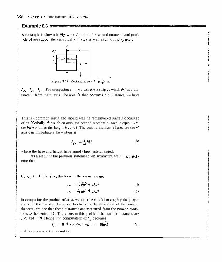
3.58 (‘HAPTER X PROPERTIES Ob S I J K b N ‘ t S
Example 8.6
A rectangle is shown i n Fig. 8.23. Compute the second moments and prod. ucts o l area about the centroidal x’y’axci iis well as ahout thc .q axcs.
iii
i~. x L
Figure 8.23. Rectangle: hasc h. height h.
ly,v,, I r ,s,. For computing It ,,,, we can use a strip of width d?‘ at a dis- tance s ’ from the x’ axis. The area r l A then hecomes h &‘. Hence, we have
This is a common result and should well he remembered since it occurs so often. Verhally. fnr such an axis, the second moment 01 area is equal tn %. the hase h times the height h cubed. The second moment of area for the J’’
axis can immediately he written as
(h)
where the hase and height have simply heen interchanged.
note that As a result of the previous statement? on symmctry. we iinmediatcly
6. I> \ , I , , Emplnylng the tran\ler thcoreni\, we get
I LI = hbh’ +bhe2
I VY = &hb3 + bM2
In computing the product of area. we must he careful to cmploy the proper signs for the transfer distances. In checking the derivation of the transfer theorem, we see that these distances are measured from the noncentroidal axes to the centroid C. Therefore, in this prohlem the transfer distances are (+e) and (H). Hence, thc computation of I t , becomes
(0 :”.,>
I+ = 0 + (hh)(+r)(-d) =
and is thus a negative quantity.

SECTION 8.7 COMPUTATTON INVOLVING SECOND MOMENTS AND PRODUCT OF AREA 359
Example 8.7
What are 6, I,. and IX, for the area under the parabolic curve shown in Fig. 8.24?
To find I,, we may use horizontal strips of width dy as shown in Fig. 8.25. We can then say for IXx:
10 I , = y2[dy(10 - XI]
x = q m i y 2 But
Therefore, 10 I, = yz(IO - &6y1'2)dy
0
As for I",. we use vertical infinitesimal strips as shown in Fig. 8.26. We can, accordingly, say:
Finally, for LY we use an infinitesimal area element dn dy shown in Fig. 8.27. We must now perform multiple integration4 Thus, we have
I0 v=r1/10 s =I0 jVX0 * y d y h
Notice by holding x constant and letting y first run from y = 0 to the curve y = 3/10 we cover the vertical strip of thickness dn at position x such as is shown in Fig. 8.26. Then by letting x run from zero to IO, we cover the entire area. Accordingly, we first integrate with respect toy holding x constant. Thus,
Next, integrating with respect to x, we have
"This multiple integration involves boundaries requiring some variable limits, in con- trast to previous multiple integrations.
Y
Figure 8.24. Plane area.
Figure 8.25. Horizontal strip.
k - 1 0 m m 4 Figure 8.26. Vertical strip.
Y
y=M, /A+ b l O m m 4 x
Figure 8.27. Element for multiple integration

360 CHAPTER 8 PKOPERTIES OF SURFACES
> . . "..". ..-.,. Example 8.8 :'-
Compute the second niomcnt (if arcil (if a circiiliii- iireii ah(ii11 ii di;iiiictcr (Fig. 8.28).
i
Figure 8.28. Circular area with p d a r ciiwdinarc.;.
Using polar coordinates, we hiivc' lor i l l;
Completing the integration. uc h a w
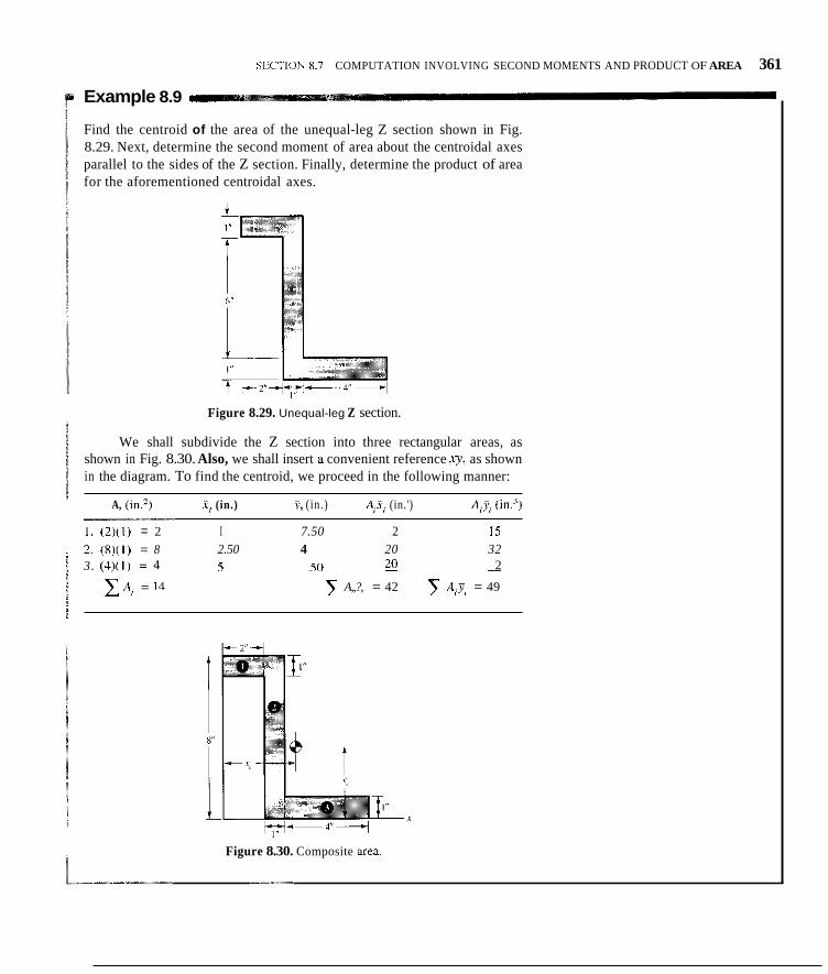
SECTION 8.7 COMPUTATION INVOLVING SECOND MOMENTS AND PRODUCT OF AREA 361
Example 8.9
Find the centroid of the area of the unequal-leg Z section shown in Fig. 8.29. Next, determine the second moment of area about the centroidal axes parallel to the sides of the Z section. Finally, determine the product of area for the aforementioned centroidal axes.
Figure 8.29. Unequal-leg Z section.
We shall subdivide the Z section into three rectangular areas, as shown in Fig. 8.30. Also, we shall insert a convenient reference xy, as shown in the diagram. To find the centroid, we proceed in the following manner:
A, (in.?) ?, (in.) V . , (in.) A,rj (in.') A;?; (in.')
1. (2)(1) = 2 I 7.50 2 15
2
EA, = I4 A,,?, = 42 A,Y, = 49
2. (8)(1) = 8 2.50 4 20 32 3. (4)(1) =A S .so 20 -
Figure 8.30. Composite area.

362 CHAPTER x PROPERTIES OF SURFACES
Example 8.9 (Continued)
Therefore,
We h w e shown the centroidal axes .xc);. in Fig. 8.31. We now find lxcxc and ly,vt, using the parallel-axis theorem and the lormulas &hh’ and &hb3 for the second moments of area about centroidal axes of symmetry of a rectangle.
+[(&1(4)(13) + (4)(3*)] = 4
0
I ?<>? . = [(&)(1)(23 + ( 2 ) ( 2 2 ) ] + [(/2)(8)(13) + (8)(fP]
0 0
+[(&)(I)(49 + (4)(22)] = 32. i < a
Finally, we consider the product of area Cc?<,. Here we must be cau- tious in using the parallel-axis theorem. Remember that xcy, are centroidal axes for the entire ales of the Z section. In using the parallel-axis theorem for a subarea, we must note that x<y< are not centroidal axes for the sub- area. The centroidal axes to he used in this problem for subareas are the axes of symmetry of each subarea. In short, x,V, are simply axes ahout which we are computing the product of area of each subarea. Therefore, in the parallel-axis theorem, the transfer distances c and d are measured.from the x,y, uxer to the rentroid in each subarea, as noted in the development of the parallel-axis theorem. The proper sign must be assigned each time to the transfer distances with this in mind. We have for lrcJt:
Figure 8.31. Centroidal axe, XJ

8.57. results in feet. constant c.
Find lxx, /vY. and I=\, for the triangle shown. Give the 8.61. Find I,\ for the shaded area. You must first determine the
Y Y I
Figure P.8.57.
8.58. What are the second moments and products of area of the ellipse for reference xy'? [Hint: Can you work with one quadrant and then multiply by 4 for the second moments?]
Y
Figure P.8.58.
Find I,, and I,, for tbe quarter circle of radius 5 m 8.59.
Y
x 5 m
Figure P.8.59.
8.60. Find lix, I">, and I., for the shaded area.
Y
Figure P.8.61,
8.62. Find I v y for the area between the curves
y = 2 sin x ft y = sin 2x ft
fromx = Otox = nft .
8.63. and y = sin x and the lines x = 0 and x = nI2.
Find I", for the areas enclosed between curves y = cos x
8.64. for the right triangle.
Show that I_ = bh3/12, 5, = b3k/12, and I,, = b2h2/24
Y
I
X
:i\ I+-+- 1
Figure P.8.60. Figure P.8.64.
363


8.74. In Problem 8.73, show that I,,,, = bh3t36, Iv+ = (bhI36Kb2 - ab + a'). and lxcjc = (h2bI72)(2a - b ) for the tri- anele. IHint: Use the results of Problems 8.1 I and 8.73 and the
8.77. Disregard all rounded edges.
Find In, !,. lxsc, and I, for the stmctural "hat" section C~ c
~. parallel-axis theorem.]
8.75. Find I-. Ivy . and I,, of the extruded section. Disregard all rounded edges. Do this problem using 4 areas. Check using 2 areas.
Y
I Figure P.8.77.
8.78. Find In. Ivy. and <," of the hexagon.
x
X
Figure P.8.75. k R d / Figure P.8.78.
8.79. A beam cross-section is made up of an I-shaped section with an additional thick plate welded on. Find the second
'CY,. Of the cross- section. What is
8,76, Find the second moment of area of the rectangle (with a hole) about the base of the rectangle. Also, determine the product of area about the base and left side.
Of area for the Give the results in millimeters.
+ 9" i
i_2:l(t:i Figure P.S.76.
? b 6" - t i Figure P.8.79.
365
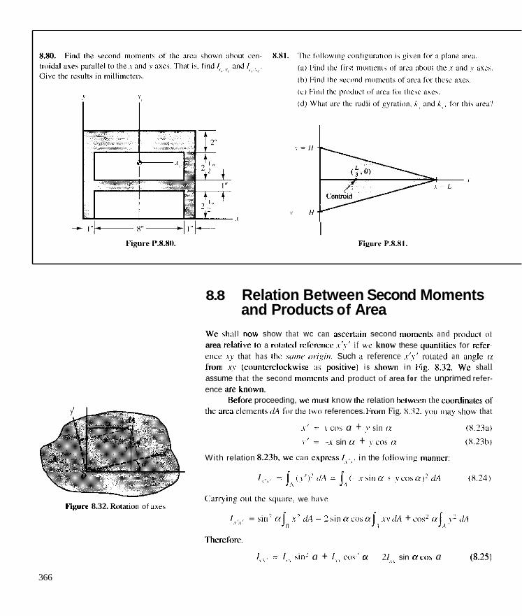
I I
Figure P.X.XI. I
Figure 8.32. Rimlion of axe\
8.8 Relation Between Second Moments and Products of Area
We sh:ill i iow show that wc can iisccrliiin second miiments and producl 0 1 area re lat iw to a rolalcd rclcrcncc .A'!' i f we know these quilnlities for refer- encc ry that has tlic .surne o r i ~ i ~ i . Such ii reference x'y' tmated an anglc a froni x? (countcrclockwise :is positive) i s shown in Fig. X.32. Wc shall assume that the second miimcnts wid product of area f o r the unprimed refer- ence are kiiowii.
Hefiire proceeding, wc mu\t know Lhr relation hetween the coordinalcs o1 thc area clcmcnts (/A 101- the Iwo references. Froiii Fig. X.32. yi)u inlay show that
~ i ' = i cos a + y sin n IX.23a)
s' = -i sin a + ? c o s n lX.23h)
With relation 8.23h. wc can cxprcss I t ,$, in the follo\ving manncr:
= j , , , t y ' ~ c / ~ = j , ~ t - . ~ s i n a + y c ~ ~ s ~ ~ i ~ [ / ~ (X.24)
('arrying ouI thc scj~iiire. we h a b e
/s , t , = sin? c x j ~ t ? <!A ~ ?hili n c o s a j . x v < / ~ + c o s i a j y?'/il n 1 A
Thrrefiire.
I>,>, = sin' a + cos2 n ~ 21$) sin cxcos a (8.25)
366

SECTION 8.8 RELATION BETWEEN SECOND MOMENTS AND PRODUCTS OF AREA 367
A more common form of the desired relation can he formed by using the fol- lowing trigonometric identities:
cos2 a = $(I + cos 2a) sin2 a = $ ( I - cos2a)
(a) (b) (C) 2 sin a cos a = sin 2a
We then have6
To determine I;,., we need only replace the a in the preceding result by (a + ED). Thus,
Note that cos (2a + z) = -cos 2a and sin (2a + n) = -sin 2a. Hence, the equation above becomes
€ - I - am 2a + 1, (8.27~
Next, the product of area /+.can be computed in a similar manner:
/xc. = j , x ’y (d~ = I A ( x c o s a + y s i n a ) ( - x s i n a + y c o s a ) ~
This becomes
1 I I = sin a cos a (5, - /J + (cos’ a - sinZ a)/xY X Y
Utilizing the previously defined trigonometric identities, we get
(8 28) i = + I,coSzq
Thus, we see that, if we know the quantities 1,. I,, and I,, for some reference xy at point 0, the second moments and products of area for every set of axes at point 0 can be computed. And if, in addition, we employ the transfer theo- rems, we can compute second moments and products of area for any refer- ence in the plane of the area.
“!3quations 8.26. 8.27, and 8.28 are called rrnnsfomarion equations. They will appear in the next chapter and in your upcoming solid mechanics course for variables other than second moments and products of area. In the remaining portions of this chapter, you will see that a num- ber of imponant properties of second moments and products of area are deducible direcrly from these transformation equations. This primarily accounts for the importance of the transformation equations. Chapter 9 will give you additional insight into this topic.


SECTION 8.9 POLAR MOMENT OF AREA 369
8.9 Polar Moment of Area In the previous section, we saw that the second moments and product of area Sor an orthogonal reference determined all such quantities for any orthogonal reference having the same origin. We shall now show that the sum of the pairs of second moments of area is a constant for all such references at a point. Thus, in Fig. 8.35 we have a reference xy associated with point a. Summing I,, and Ivy we have
Figure 8.35. J = I,, + I . > .
Since r2 is independent of the orientation of the coordinate system, the sum IA, + I _ is independent of the orientation of the reference. Therefore, the sum of second moments of area ahout orthogonal axes is a function only of the position of the origin u for the axes. This sum is termed the polur moment of area, J .x We can lhen consider J to be a scalar field. Mathematically, this statement is expressed as
J = J(x: y ' ) (8.29)
where x' and y ' are the coordinates as measured from some convcnicnt reference x'y'for the point of interest.
That the quantity ( I r r + IJ does not change on rotation of axes can also be deduced by summing transformation equations 8.26 and 8.27 as we suggest you do. This group of terms is accordingly termed an invuriunt. Par- enthetically, we can similarly show that (/&v - I;,) is also invariant under a rotation of axes.
XQuite oftcn I,, i s used for the polar moment of are&.

370 CHA1”I‘ER X PROPERTIES OF SURFACES
Figure 8.36. Principal axes
8.10 Principal Axes Still othcr conclusions may he drawn about second iiiotiients and products of arm associated with ii point in an area. In Fig. 8.36 ail area i s showti with a reference xy having its urigin at point o. We shall assume that I , .< . I $ , , and I, , are known for this reference. and shall ask at what angle CY we shall find an axis having the inuirnuni second mu~iient of :ireti. Since the sum of thc sec- ond moments of area i s constant Iur any reference with origin at (1. the nrirti- rnurn second niniiicnt of area must then correspond 10 iui iixis at rifihf anglcs to the axis having the maximimi second tiinmetit. Sincc second nimnen~s of area have heen expressed i n Kqs. 8.26 and 8.21 a s lunctiotis 0 1 lhc variable a at a point. these extremcs may readily he determined by setting the partial derivative nf I \ , & , with rcspcct to uequ;il to (erii. Thus.
II we denote the value nf a that satisfies the equation above iis iU, we haw
Hence,
This formulation gives us the angle ri. which corresponds tO an extreme value of I > , , , (i.e.. ti) a maximum or minimum valuc). Actually, there are two possi- ble valucs u f 2 N which are nradians apart that wil l satisfy the equation above. Thus,
o r
2 i x = p +i[ This means that we have two values o f ri, given a s
Thus. there are two axes orthogonal to each other having extreme values for the second monienl of area at (1. On tie of thehe axes i s the n iax i i n~m second moment of area and. a s pointed out carlicr. thc minimum second moment nf area must appear on the other axis. These axes are called the p r i i i ~ ~ i p l L L I P S .

SECTION 8.1o PRINCIPAL AXES 31 1
Let us now substitute the angle ti into Eq. 8.28 for Q,,:
(8.31) ~ I,'v I . .= - '~ sin 2 8 + /_, cos 2 8 x i . 2
If we now form a right triangle with legs 2'- and (Ivy - 6) and angle 22 such that Eq. (8.30) is satisfied we can readily express the sine and cosine expressions needed in the preceding equation. Thus
By substituting these results into Eq. 8.31, we get
Hence,
(,y, = 0 Thus, we see that the product of urea corresponding to the principul
u e s is zero. If we set I,.,. equal to zero in Eq. 8.28, you can demonstrate the converse of the preceding statement by solving for a and comparing the result with Eq. 8.30. That is, if the product of area is zero for a set of axes at a point, these axes must be the principal axes at that point. Consequently, if one axis of a set of axes at a point is symmetrical for the area, the axes are principal axes at that point.
The concept of principal axes will appear again in the following chap- ter in connection with the inertia tensor. Thus, the concept is not an isolated occurrence hut is characteristic of a whole family of quantities. We shall, then, have further occasion to examine some of the topics introduced in this chapter from a more general viewpoint.

372 VHAPTER x PKOPEKTIES 01. SURFACES
Example 8.11
Find the principal second moments of area at the centroid of the Z section of Example X.9.
We have from this example the following results that will be of use LO Ub:
/ccrc = 113.2
I = 32.67 in.4
I = -42.0 in.4 Y( V(
/'?<
Hence, we have
2h = 46.21 O, 226.2" For2ir = 46.21":
113.2+32.67 + 1 1 3 . 2 - 3 2 . 6 7 c o s ~ 4 6 , 2 1 ~ ~ - ~ - 4 2 ~ ~ , n 4 6 , 2 1 ~ 2 2 I , =
= 72.9 + 27.9 + 30.3 = 131.1 in.4
For 2 0 = 226.2": ~~,..',~.. .
l2 = 72.9 - 27.9 - 30.3 = &.&%%$
As a check on our work, we note that the sum of the second moments of area are invariant at a point for a rotation of axes. This means that
I r , I( + IVt V / = 1, + '2
113.2+32.7= 131.1+14.75
Therefore,
145.9 = 145.9
We thus have a check on our work.
Before closing, we wish to point out that there is a graphical construction called Mohr's circle relating second moments and products of area for all possible axes at a point. However, in this text we shall use the analytical rela- tions thus far presented rather than Mohr's circle. You will see Mohr circle construction in your strength of materials course where its use in cnnjunction with the important topics of plane stress and plane strain is very h e l p f ~ l . ~
"See I . H . Shames, Iniroducnon 10 Solid Mechontr..>. Second Edition. Prmrice-Hall. loc.. Englrwuod Clills. N.J.. 1989.

8.82. moments and products of area for the centroidal axes shown:
It is known that area A is IO ft2 and has the following
I= = 40 ft4, I , = 20 ft‘,
Find the moments and products of area for the x’y’ reference at point a.
5, = 4 ft4
v ’ X’
Figure P.8.82.
8.83. The cross-section of a beam is shown. Compute I,;.. ly.,., and c,,, in the simplest way without using formulas for second moments and products of area for a triangle.
Y’
Figure P.8.83.
8.84. polar moment of area at points a and b.
Find I,=, I,\, and I,, for the rectangle. Also, compute the
I
Figure P.8.84.
8.85. Express the polar moment of area of the square as a func- tion of x , y, the coordinates of points about which the pola moment is taken.
Y
Lx Figure P.8.85.
8.86. Use the calculus to show that the polar moment of area of a circular area of radius I is nr41? at the center.
Y
6 - x
Figure P.8.86.
8.87. tion at point A.
Find the direction of the principal axes for the angle sec-
Y
. ,
Figure P.8.87.
8.88. gin for the area of Example 8.7?
8.89. for the area shown.
What are the principal second moments of area at the ori-
Find the principal second moments of area at the centroid
4 2 ” k
1- IT^ t Figure P.8.89.

7 L
4 1,1111
I
t L,
"I- r- Figure P.8.91.
8.YZ. imuiii are rotated from n by an angle a so that
Show that thc axe5 for which the product of area i s il ~ i i i i x -
Figure P.8.92.
8.93. What is thc value of the mgle 01 lor thc principal axss at A.
I ' I '
" -2.-
kigure P.8.93
3' I

SECTION 8.1 I CLOSURE 375
8.11 closure
In this chapter, we discussed primarily the first and second moments of plane areas as well as the product of plane areas. These formulations give certain kinds of evaluations of the distribution of area relative to a plane reference xy. You will most certainly make much use of these quantities in your later courses in strength of materials.
In this chapter, we have touched on subject matter that you will en- counter in the next chapter and also, most assuredly, in later courses. Specifi- cally, in Chapter 9 you will he introduced to the so-called second-order inertia tensor having nine terms which change (or transform) in a certain par- ticular way when we rotate coordinate axes at a point. These particular trans- formation equations define the inertia tensor. Any other set of nine symmetric terms that transform via the same form of equations, are symmetric second- order tensors. You will also learn that the second moments and products of area form a two-dimensional simplification of the inertia tensor. The trans- formation equations 8.26 through 8.28 are thus special cases of the three- dimensional defining equations of the inertia tensor. Take note that certain vital results emerged from these simplified two-dimensional transformation equations. They included
1. Invariant property at a point for the sum (In + ZJ on rotation of axes. 2. Principal axes and principal moments of area at a point. 3. A graphical construction called Mohr’s circle that depicts the transforma-
tion equations. This topic has been omitted in this chapter hut will be described in your solids course where yon will study the two-dimensional simplifications of the stress and strain tensors. At that time one can make much use of the Mohr’s circle construction and it is a simple matter then to describe Mohr’s circle for second moments and products of area.
We will emphasize in the next chapter that there are many symmetric sets of nine terms that transform exactly like the terms of the inertia tensor and we classify all of them as second-order tensors. Identifying these sets as second-order tensors immediately yields vital properties common to all of them such as those presented above for the two-dimensional moments and products of area.
There will be more to be said on tensors in a “looking ahead” section of the next chapter which we invite you to examine.

r - I

8.102. A half body of revnlution is shown with the x: plane as a plane of symmetry. Determine the centroidal coordinates. The radius at any section x varies as the square ofx.
8.105. troid of the area of a qualter-circle.
Using the theorems of Pappus and Guldinus, find the cen-
J
Figure P.8.11)5. Figure P.8.102.
8.103. (a) Find Irk, I,,. and 18> fur the .r? axes at position A . 8.106. A tank has a semisphericdl dome at the left end. Using the theorems af Pappus and Guldinus, compute the surface and volume of the tank. Give the results i n meters. (b) Find the principal recond moment5 of area at point A.
Figure P.B.106.
8.107. Find I and I , , , , for the set of axes at point A fur the
v'
Figure P.8.103. VX' 8 m
t X.104. Whet are the directions of the principal axes at point A'?
12m
~i; 10m-!-ll (11
Figure P.8.1117.
A
S '
Figure P.8.104,
8.108. Find the centroid of the aren, and then find the second moments of thc area about centroidal axes parallel to the sidcs of the area.
311

Figure IL8.108.
1.109. where I&> = 321 in?.
Find the principal semiid moments of area at a point = I I X . 4 in?, and 1 , ) = 1.028 i d .
I, + 2 0 I,, ~~
+
Figure P.X.110.
1.111. ( a ) What are the centmidal coordmatrs o f the shaded area'!
(b) What ai(: M&,, and M , , for axes x'v' at A'? 1Il;nr: Ucr ormulas fur the sector o f a circle given on the imide hack cover.I
8.112. A wide-flanged I heam i\ s h ~ ~ w d " Far the upper flangr. what i \ the first imonienl 0 1 t h ~ \haded area as a function o h meii- \tired froiii .v = 0 at the right rrid t o where s apprrlaches the weh'! Next pet hl, fur the entirc a m i ahove the position shown a\ i n t h r wch. Let Y go from (.in the lop of thc wch.
l c - - 1 7 1 5 -
Figure P.8.112.
, - 8 , "
Figure P.8.113.
Figure P.8.111.
78

and Products of Inertia' 9.1 Introduction In this chapter, we shall consider certain measures of mass distribution rela- tive to a reference. These quantities are vital for the study of the dynamics of rigid bodies. Because these quantities are so closely related to second moments and products of area, we shall consider them at this early stage rather than wait for dynamics. We shall also discuss the fact that these mea- sures of mass distribution-the second moments of inertia of mass and the products of inertia of mass-are components of what we call a second-order tensor. Recognizing this fact early will make more simple and understandable your future studies of stress and strain, since these quantities also happen to be components of second-order tensors.
9.2 Formal Definition of Inertia Quantities
We shall now formally define a set of quantities that give information about the distribution 0 1 mass of a body relative to a Cartesian reference. For this purpose, a body of mass M and a reference xyz are presented in Fig. 9.1. This reference and the body may have any motion whatever relative to each other. The ensuing discussion then holds for the instantaneous orientation shown at time t . We shall consider that the body is composed of a continuum of par- ticles, each of which has a mass given by p do. We now present the following definitions:
Figure 9.1. Body and reference at time f.
#This chilpter may he covered at a later stage when studying dynamics. In that case, it should be covered directly after Chapter 15.
379

380 CHAPTER 9 MOMENTS AND PRODUCTS OF INERTIA
(9.1~1)
(9. I b)
(9.1C)
The terms lxr, I+ and in the set above are called the muss momerifs ujiner- tiu of the hody'ahout the x,y. and 7. axes. respectively.' Note that in e x h such case we are integrating the mass elements p d7: times the peipmdicular dis- tance squared from the mass elements tn the coordinate axis about which we are computing the moment of inertia. Thus, if we look along thex axis toward the origin in Fig. 9.1, we would have the Yiew shown in Fig. 9.2. The quan- tity y* + z 2 used in Eq. 9. la for /,ct is clearly d i the perpendicular distance squared from dti to the x axis (now seen as a dot). Each of the terms with mixed indices is called the mass product of inertio ahout the pair of axes given by the indices. Clearly. from the definition of the product of inertia, we could reverse indices and thcrehy form three additional products of inertia fir
a reference. The additional three quantities formed in this way. however, are equal to the corrcsponding quantities of the original set. That is,
Figure 9.2. View of hody along x axis.
We now have nine inertia terms at a point for a given reference at this point. Thc values of the set of six independent quantities will, for a given body.
"Nc use the same clntilticm as wa? used for second inoinents and product\ 01 a n n , which arc dsu suinetinies called inornents and pruducts of inertia. 778s i i standard practice in mechanics. Thm nccd he no cunfusion i n using thew qaaniitic\ i f we keep the cmlext ofdiscucsinnh clearly in mind.

SECTION 9.2 FORMAL DEFINITION OF INERTIA QUANTITIES 38 1
depend on the posifion and inclination of the reference relative to the body. You should also understand that the reference may be established anywhere in space and need nor be situated in the rigid body of interest. Thus there will be nine inertia terms for reference xyz at point 0 outside the body (Fig. 9.3) computed using Eqs. 9.1, where the domain of integration is the volume V of the body. As will be explained later, the nine moments and products of iner- tia are components of the inertia tensor.
z
Figure 9.3. Origin of xyz outside body.
It will he convenient, when referring to the nine moments and products of inertia for reference xyz at a point, to list them in a matrix array, as follows:
Notice that the first subscript gives the row and the second subscript gives the column in the array. Furthermore, the left-to-right downward diagonal in the array is composed of mass moment of inertia terms while the products of inertia, oriented at mirror-image positions about this diagonal, are equal. For this reason we say that the array is symmetric.
We shall now show that the sum of the mass moments of inertia for a set of orthogonal axes is independent of the orientation of the axes and depends only on the position of the origin. Examine the sum of such a set of terms:
Combining the integrals and rearranging, we get
I _ + I v y + Iz , = IJ/2(x2 + y * + zZ)pdu = IS/2lr(’pdu (9.2)
But the magnitude of the position vector from the origin to a particle is inde- pendent of the inclination of the reference at the origin. Thus, the sum of the moments of inertia at a point in space for a given body clearly is an invariant with respect to rotation of axes.
V V

382 C"A1"I'b:K V MOMliNTS ANI) PRODLICTS OF INKRTI.4
Clcal-ly. 011 inspecli(in nf thc equations 0. I. i t i s clear that the iiioniciits (11 inertia must always be positive, while the products o f inertia may he posi- tiYe or negativc. 01 intercst i s the case where one 01 the coordinate planes i s ii plww nf.s\mmrrr\ h r the miss distrihution of the body. Such a plene i s thc I\ plane shown i n Fig. 9.4 cutting a hody into two parts, which. by definition of symmctry. are niirror iniagcs o f each other. For the computation of I > : , each half wi l l give ii crintrihuti(in ofthe same magnitude hut ol'oppositc sign. We can most readily hcc that this i s so by loohing along the y axis tiiwai-d thr origin. The plane of symmetry then appears as a line coinciding with thc z i i x i c (ECC Fig. 9.5). We can cnnsidcr the body to he composed of pairs of inass
and shape ahout the planc of symmetry. The product (if inertia Sor such ii
pair i s then
,! "
1 %
, elements diii which are mirror imagcs of each other with respect to pnsition
Figure 9.4. :? i\ plane 0 1 cymmrlry.
I: dm ~ Y: dwt = 0
Thus. we can cnncludc that
I < . = J .x; ({in - 1: (1111 = 0
lkh
I - -- i---i "FbI
<I,/ 111.1 I,, tl<li,,li,,
This c(inclusion i s a lso (rue for I \ $ . We can say that I\>, = 1,: = 0. But on consulting Fig. Y.4. you shmild be ahle to readily decide that the terni I.\ wil l haw a positivc value. Note that those products of inertia having .r as ;in index are /era and tlial the .v coordinate axis is normal to the plane of symmctry. Thus, we can conclude that if iw, ~ ~ ~ ~ . s . f i i r ~ n N p l u w of,swnmc,rry f i i r ihr ~no.s.s di,strihu~ion ofu l x d y , tlte p,-o'dum oriner l ia hoi'ing (1,s r m index the cooro'i- note thar i,s normal to the plaw o/ .swmel r ! . w,ill he ZPIO.
Considcr next it body ofri~r.olutio~~. Take the z axis to coincide with the axis of symmetry. I t i s easy Io conclude for the origin 0 of xy? anywhere iil(ing the ax is of symmetry that
Figure 9.5. Vir% along v ax ic .
I = I = I > > = 0 I x 5 = I \ , = co11stallt
I: ,:
for all possihlc .xy axes iormed hy rotating ahout the z axis at 0. Can you jus- tify these conclusions?
Finally. we define mdi i of,syui ion in a manner analognus to that used for second moments of iircii in Chaptei- 8 . Thus:
where k 5 , k v . arid k . i r e lhe radii (11 gyration and M i s thc total I i iass .

SECTION 9.2 FORMAL DEFINITION OF INERTIA QUANTITIES 383
Example 9.1
i Find the nine components of the inertia tensor of a rectangular body of uniform density p about point 0 for a reference xyz coincident with the edges of the block as shown in Fig. 9.6.
We first compute I,. Using volume elements dii = dx dy dz, we get on using simple multiple integration:
= ( a 9 + a'bc - ) p = PV ( b 2 + a * ) Figure 9.6. Find /,! at 0 3
where V i s the volume of the body. Note that thex axi5 about which we are computing the moment of inertia I,x IS normal to the plane having sides of length a and h, Le., along the z and y axes. Similarly:
I_ = - - ( c2 PV + a 2 )
I.,, = --(b PV
.. 3
.~ 3 2 + e 2 )
We next compute lxv
Note for f x v , we use the lengths of the sides along the x and y axes
We accordingly have, for the inertia tensor:

384 C",\PTIR U M O M E N I S AND I'R0r)UCI'S OF INtRTlh
8 Example 9.2 I
Computc the components of thc inerlia icnsor iit the ccnicr or il s111id sphere 0 1 uniform dcnsity p iis shown in Fig. 9.7.

SECTION 9.2 FORMAL. DEFINITION OF INERTIA QUANnTIES 385
Example 9.2 (Continued)
With the aid of integrdtion formulas from Appendix I, we have
n 2n Iv,, = PI, I,, r* cos? $[- 4 cos @(sin2 e + 2)]/: dqdr
Integrating next with respect to 4, we get
Finally, we get
R' 4 R' 4 5 3 5 3 I,, = p - - r r + p - - n
8 x ' 15 : . I = -prrR'
But
M = p'nR3 3
Hence,
I_ = $ MR2
Because of the point symmetry about point 0, we can also say that
I _ = liZI = $MR2
Because the coordinate planes are all planes of symmetry for the mass dis- tribution, the products of inertia are zero. Thus, the inertia tensor can be given as

386 CHAPTER Y MOMENTS AND PRODIJCTS OF INERTIA
9.3 Relation Between Mass-Inertia Terms and Area-Inertia Terms
We now relate the second inomrnt and product of area studied in Chapter 8 with the inertia tensor. To do this, consider a plate of constant thickncss I and uniform density p (Fig. 9.9) A rcferencc is selected so that the ~x? plane is in the midplane of this plate. The components of the inertia tensor are rewritten for convenience as
Figure 9.9. Platc <f thickness I
Now consider that the thickncss I is sninll comparcd to the lateral dimension\ of the plate. This means that I is restricted to ii range of values having a small magnitude. As a resull, we can make two simplifications i n the equations above. First. we shall set i equal to zero whenever it appears on the right side of the equations abuve. Second. we shall express d i ’ a s
r /z , = I dA

SECTION 9.3 RELATION BETWEEN MASINERTIA TERMS AND AREA-INERTIA TERMS 387
where dA is an area element on the surface of the plate, as shown in Fig. 9.10 Equations 9.3 then become
A
X
Figure 9.10. Use volume elements r dA
Notice, now, that the integrals on the right sides of the equations above are moments and products of area as presented in Chapter 8. Denoting mass-moment and product of inertia terms with a subscript M and second moment and product of area terms with a subscript A, we can then say for the nonzem expressions:
Thus, r a ct pt throughout, we can compute the inertia tensor components for reference xvz (see Fig. 9.9) by using the second moments and product of area of the surface of the plate rel- ative to axes xy.
I t is important to point out that pr is the mass per unit area of the plate. Imagine next that f goes to zero and simultaneously p goes to infinity at fates such that the product pt becomes unity in the limit. One might think of the resulting body to be a plane area. By this approach, we have thus formed a plane area from a plate and in this way we can think of a plane area as a spe- cial mass. This explains why we use the same notation for mass moments and products of inertia as we use for second moments and products of area. How- ever the units clearly will be different.We now examine a plate problem.

388 CHAPTER 9 MOMENTS AND PRODUCTS OF INERTIA
Example 9.3
Determine the ine tive to the indicated axes xyz. The weight of the plate is ,002 N/mm.I For the top edge, y = 2 ~ ' x with x and y in millimeters.
It is clear that for pt we have, remembering that this product repre- sents mass per unit area:
-
002 9.81 - ' pt = - - 000204 kglmm'
We now examine the second moments and product of area for the surface of the plate about axes xy. Thus?
.~ 1ilil y=z\* Figure 9.11. Plate of thickness I. =I, v=" v 2 d y d x
1"" yi IO0 * 2 . -*
= I, dx = 7x3'zdx u . 0
= 1.067 x IO' mm4
IW -~ I no = I,, x 2 y l ~ ' ~ ' dx = x2(2\x)dx
n
i I
!
= 5.71 x IO6 mm4 ?
xy d y dx
= = 6.67 x los mm4
'Note we have multiple integration wherc one of [he boundaries is variable. The proce dure to follow should he evident from the cxample.

SECTION 9.3 RELATION BETWEEN MASS-INERTIA TERMS AND AREA-INERTIA TERMS 389
Example 9.3 (Continued) i Using Eq. (a), we can then say for the nonzero inertia tensor components:
Y = (.000204)(1.067 X IO') = 21. .71 x 106) = I16 .67 x 10')
= (. (I& = (.
Note that the nonzero inertia tensor components for a reference xyz on a plate (see Fig. 9.9) are proportional through pt to the corresponding area- inertia terms for the plate surface. This means that all the formulations of Chapter 8 apply to the aforementioned nonzero inertia tensor components. Thus, on rotating the axes about the z axis we may u s e the transformation equations of Chapter 8. Consequently, the concept of principal axes in the midplane of the plate at a point applies. For such axes, the product of inertia is zero. One such axis then gives the maximum moment of inertia for all axes in the midplane at the point, the other the minimum moment of inertia. We have presented such problems at the end of this section.
What about principal axes for the inertia tensor at a point in a general three-dimensional body? Those students who have time to study Section 9.7 will leam that there are three principalaxes at a point in the general case. These axes are mutually orthogonal and the products of inertia are all zero for such a set of axes at a point? Furthermore, one of the axes will have a maximum moment of inertia, another axis will have a minimum moment of inertia, while the third axis will have an intermediate value. The sum of these three inertia terms must have a value that is common for all sets of axes at the point.
If, perchance, a set of axes xyz at a point is such that xy and xz form two planes of symmefv for the mass distribution of the body, then, as we learned earlier, since the z axis and they axis are normal to the planes of symmetry, Ix," = I,, = I,, = 0. Thus, all products of inertia are zero. This would also be true for any two sets of axes of xyz forming two planes of symmetry. Clearly, axes forming two planes of symmetry must be principal axes. This informa- tion will suffice in most instances when we have to identify principal axes. On the other hand, consider the case where there is only one plane of symme- try for the mass distribution of a body at some point A. Let the xy plane at A form this plane of symmetry. Then, clearly, the products of inertia between the z axis that is normal to the plane of symmetry xy and any axis in the xy plane at A must be zero, as pointed out earlier. Obviously, the z axis must be a principal axis. The other two principal axes must be in the plane of symme- try, but generally cannot be located by inspection.
5The third principal axis for a plate at a point in the midplane is the z axis normal to the plate. Note that (/zz)M must always equal + (IJW Why?

9.1. Compute I , > and
A uniform hum<igcneous 4cnder rod r i f mass M is shown
Figure P.9.1.
9.2. Find I _ and I , , for the thin rod of Prohleni Y. I for the case wherc the mass per unit length at the left end is 5 Ihm/ft and increases linearly so that at the right cnd i t is 8 Ihmirt. Thc rod i s 20 f t in length.
Figure P.9.5.
9.6. 5hown. The hody is homogeneous and has a mass hi.
Compute the moment of inertia, I,,, for the half-cylinder
9.3. Compute I,> for h e thin homogcneous hrxrp of mass M.
B Figure P.9.6.
Figure P.9.0.
9.4. lar parallelepiped. of maw M.
compute I r < , I . , , I:?, and I , , for the ~lomoyrneous 9.7. Find 1 . ~ and l l v lor the homueencous right circular cylinder
r
i
Figure P.Y.7.
Figure P.9.4. 9.8. For the cylindzr in Prohlem Y.7, the density increases lin- carly in the 2 direction from a value o f . 100 gramsimm' at the left end to a value of ,180 pramsimm' at the right end. Take I = 30 mm and I = IS0 mm. Find
3 . 5 A wire having the shape of a parabola is shown. The curve s in the yz plane. If the mass of the wire is .3 N/m,~what are I , , , ind lrz'? [Hinr: Replace dr along ihe wire by l ( d y 1 &)2 + I dz. 1 and I.. .

9.9. Show that I, for the homogeneous right circular cone is + M R ~ .
Figure P.9.9.
9.10. In Problem 9.9, the density increases as the square of z in the z direction from a value of ,200 gramslmm’ at the left end to a value of ,400 grams/mm3 at the right end. If r = 20 mm and the cone is 100 mm in length, find lz,.
9.11. A body of revolution is shown. The radial distance r of the boundary from the x axis is given as r = .Z.? m. What is I, for a uniform density of 1,600 kg/m3?
y I
x
Figure P.9.11.
9.12. A thick hemispherical shell is shown with an inside radius of 40 mm and an outside radius of 60 mm. If the density p i s 7,000 kglm,’ what is
Figure P.9.12.
9.13. Find the mass moment of inertia I , for a very thin plate forming a quarter-sector of a circle. The plate weighs .4 N. What is the second moment of area about the x axis? What is the prod- uct of inertia? Axes are in the midplane of the plate.
Y I
Figure P.9.13.
9.14. Find the second moment of area about the x axis for the front surface of a very thin plate. If the weight of the plate is .02 N/mm2, find the mass moments of inertia about the x and y axes. What is the mass product of inertia I=??
x
Figure P.9.14.
*9.15. A uniform tetrahedron is shown having sides of length a, b, and c, respectively, and a mass M. Show that lyz = &Mac. (Suggestion: Let z mn from zero to surface ABC. Let x run from zero to line AB. Finally, Let y run from zero to B. Note that the equation of a plane surface is z = a* + py + 1: where a, p, and y are constants. The mass of the tetrahedron is pabc16. It will he simplest in expanding ( I - xlb - y/c12 to proceed in the form [(I - ylc) - (x /b) I2, keeping (1 - ylc) intact. In the last integration replace y by [ - c(1 ~ ylc) + cl, etc.)
Figure P.9.15.
391

9.18. Can you identify hy inspection any o i ihr principii1 iixe\ 01 inertia iit A'! At R' Explain The dcnsitj oithu matcriiil i\ onii<>l-ni. Figure P.9.19.
392

SECTION 9.4 TRANSLATION OF COORDINATE AXES 393
Note that the quantities bearing the subscript c are constant for the integration and can be extracted from under the integral sign. Thus,
JIS p where p dz: has been replaced in some terms by dm, and the integration
i n the first integral has been evaluated as M, the total mass of the body. The origin of the primed reference being at the center of mass requires of the first moments of mass that I j j x ’ d m = I I J y ’ d m = / / j z ’ d m = 0. The middle two terms accordingly drop out of the expression above, and we rec- ognize the last expression to be Jz,;,. Thus, the desired relation i s
V
I.. ‘. = I ,. .,., + M(x: + y:) (9.7)
By observing the body in Fig. 9.12 along the z and z’ axes (Le., from directly above), we get a view as is shown in Fig 9.13. From this diagram, we can see that y: + x,Z = d.’ where d is the perpendicular distance between the z‘ axis
of inertia. We may then give the result above as through the center of mass and the z axis about which we are taking moments Y’
Izz = i Md2
Figure 9.13. View along L direction (from above). Let us generalize from the previous statement.
The momea of inenia of a body any ais the inenia of the body about a parallel a i s that goes tkough the center of mass, plus the total mass times the perpendicular db a e s squared.
We leave it to you to show that for products o f inertia a similar relation can he reached. For I t+ for example, we have
Here, we must take care to put in the proper signs of xc and y, as measured .from the xyz reference. Equations 9.8 and 9.9 comprise the well-known par- allel-uxir lhc~orems analogous to those formed in Chapter 8 for areas. You can use them lo advantage for bodies composed of simple familiar shapes, as we now illustrate.

394 CHAPTER 0 MOMENTS AND PROOLJCTS OF INERTIA
Example 9.4
Find I,, and I,, for the body shown in Fig. 9.14. Take pas constant for the body. Use the formulations for moments and products of inertia at the cen- ter of mass as given on the inside front cover page.
We shall consider first a solid rectangular prism having the outer
of the cylinder and the rectangular block that have been cut away. Thus, we have, for the ovcriill rectangular block which we consider as body I,
dinlensions given in Fig. 9.14, and we shall then subtract the contribution I S ’
Figure 9.14. Find lu and ilv. From this, we shall take away the contribution of the cylinder, which we denote as body 2. Using the formulas from the inside front cover page,
( I x r ) 2 = M(3rZ + h z ) + Md’
= &[pn(1)2(1S)][3(l’) + IS2] + [ p ~ ( l ) ~ ( l S j ] [ 6 ’ + 7.5’1 = 5 , 2 4 3 ~
(b)
Also, we shall take away the contribution of the rectangular cutout (bod) 3):
( lxx)3 = &M(u2 + h 2 ) + Md2
= &[P(8)(6)(4)](4* + 6 2 ) + [P(8)(6)(4)](2’ + 3’) ( c ) = 3 , 3 2 8 ~
The quantity lrA for the body with the rectangular and cylindrical cavities is then
lax = (231,200 - 5,243 ~ 3 , 3 2 8 ) ~
I,, = 2 (d)
We follow the same procedure to obtain lxy. Thus, for the block as a whole, we have
(IkV), = (I,,,, + Mx,yc
At the center of mass of the block, both the (x’), and ( y ’ ) ] axes are normal to planes (if symmetry. Accordingly. (I,,),. = 0. Hence,
C~,,), = 0 + [P(20)(8)(1S)1(-4~(-IO) = 96,nnop (e)
For the cylinder, we note that both the ( x ‘ ) ~ and (.y’), axes at the center of mass are normal to planes of symmetry. Hence, we can say that
-
(I,>), = 0 + 1p(~)(I2)(15)1(-8)(~6) = 2 , 2 6 2 ~ ( f )

SECTION 9.5 TRANSFORMATION PROPERTIES OF THE INERTIA TERMS 395
Example 9.4 (Continued)
Finally, for the small cutout rectangular parallelepiped, we note that the (x ' )~ and cy'), axes at the center of mass are perpendicular to planes of symmetry Hence, we have
(I& = 0 + [~(8)(6)(4)1(-2)(-16)
The quantity /Iy for the body with the rectangular and cylindrical cavities is then
= 6,144~ (g)
If p is given in units of lbdft ,) the inertia terms have units of Ibm-ft.z I "9.5 Transformation Properties of the
Inertia Terms Let us assume that the six independent inertia terms are known at the origin of a given reference. What is the mass moment of inertia for an axis going through the origin of the reference and having the direction cosines 1, m, and n relative to the axes of this reference? The axis about which we are interested in obtaining the mass moment of inertia is designated as kk in Fig. 9.15.
Y
x
Figure 9.15. Find lhh
From previous conclusions, we can say that
(9.10)

396 CHAPTER 9 MOMENTS AND PRODUCTS OF INERTIA
where @ is the angle between kk and r . We shall now put sin2 @into a more uscful form by considering the right triangle Sormed by the position vector r and the axis kk. This triangle is shown enlarged in Fig. 9.16. The side a of the triangle has a magnitude that can be given hy the dol pniduct of r and the unit vector E, along kk. Thus.
0 = r - E k = (.xi + ~f + zkj (/i + mj + nk) (9. I 1)
Figure 9.16. Right triangle Sormcd by rand k k
Hence
11 = /.r + niy + IIZ
Using the Pythagorean theorem, we can now givc side b as
h? = lr12 - 0 2 = (.r2 + y2 + .. ? 1 - (/Y + m2j2 + ii2? + ? h r y + 2lrzxz + 2mnyz)
Thc lerm sin2 $may next be givcn iis
Substituting hack into Eq. 9.10. wc get, on canceling kernis.
- (Pr’ + m’j’ +iiZ;’ + 2 /n~r? + 2/nrz + ~ m n y z j l p d i ,
Since I’ + in2 + ti2 = I , we can multiply the tirst bracketed exprcssion in thc integral by this sum:

SECTION 9.5 TRANSFORMATION PROPERTIES OF THE INERTIA TERMS 397
Carrying out the multiplication and collecting terms, we get the relation
Refemng back to the definitions presented by Eqs. 9.1, we reach the desired transformation equation:
We next put this in a more useful form of the kind you will see in later courses in mechanics. Note first that 1 is the direction cosine between the k axis and the x axis. It is common practice to identify this cosine as ab instead of 1. Note that the subscripts identify the axes involved. Similarly, m = u and n = akz. We can now express Eq. 9.13 in a form similar to a matrix array as follows on noting that Izy = 6, etc.
b
This format is easily written by first writing the matrix m a y of I‘s on the right side and then inserting the a’s remembering to insert minus signs for off-diagonal terms.
Let us next compute the product of inertia for a pair of mutually per- pendicular axes, Ok and Oq, as shown in Fig. 9.17. The direction cosines of Ok we shall take as I , m, and n, whereas the direction cosines of Oq we shall take as l‘, m’, and n’. Since the axes are at right angles to each other, we know that
Ek.€ = o Y
Therefore,
II’ + mm’ + nn’ = 0 (9.15)
Noting that the coordinates of the mass element p dv along the axes Ok and Oq are r * ek and r * eq, respectively, we have, for Ikq:
k
Y
x
4
Using xyz components of r and the unit vectors, we have
= jjj[(i + yj + ~ k ) * (1i + n ~ ‘ + A)] V

398 CHAPTER 9 MOMENTS .\iW PKODIK'TS OF I N L K I I A
Hcnce.
+xdin' t .x:lii' + y n l ' + yrmn' + wi/' + -\.nni')p (11'
Collecting k i l n s and bringiiig ~ I i c iiirrctii)n cosines outside the inlegratiolis. wc gel
Noting lhc definitions i n Eil. 9 I . we ciiii statc Ihc desired Lransforinalion:
li,, = ~ i i i t l i r / ~ r ~ ,illr/ ~ + (/n1' + I n / ' ) / , ,
+ ( Id + d ! I , ~ + (111li' + Ii?d!/), (9.19)
We can now rewrilc the p r e \ i w s cquarion in ii more u\cIuI mil simple torin using U ' Y iis direction cosine\. Thus. noting !hat I' = (I,,). ctc.. we proceed as in Eq. [ I . 14 to uhtain

SECTION 9.5 TRANSFORMATION PROPER'IlES OF THE INERTIA TERMS 399
EXaI'rIple 9.5
Find Iz,7, and I,,,, for the solid cylinder shown in Fig. 9.18. The reference x'y'z' is found by rotating ahout they axis an amount 30", as shown in the
It is simplest to first get the inertia tensor components for reference diagram. The mass of the cylinder is 100 kg. z
xyz. Thus, using formulas from the inside front cover page we have 2
Ja = - M r 2 I = L(lOO)(!$) = 21.13 kg-mz 2 2
= 85.56 kg-m2
Noting that the xyz coordinate planes are planes of symmetry, we can con- clude that
l x z = I = I = o Y l YZ
-Ew 30"
x' b l . 3 m ~ +
Figure 9.18. Find lz.,, and ldz, Next, evaluate the direction cosines of the z' and the x' axes relative
For z' axis: to nyz. Thus,
a:,= = COS 60" = ,500 a = cos 90" = 0 ai.? = cos 30" = ,866
Z'Y
For .c' axis:
aXlr = COS 30" = ,866 a*Y = cos90° = 0 a~c,z = cos 120" = -SO0
First, we employ Eq. 9.14 to get J,,,,.
= (85.56)(.500)z + (21.13)(.866)'
= '37.h
Finally, we employ Eq. 9.20 to get I,;,.
-Ix,,, = (85.56)(.500)(.866) + (21.13)(.866)(-,500)
Therefore,

400 CHAPTER 9 MOMWTS AND PROIlI!('TS OF INEXI'IA

SECTION 9.6 LOOKING AHEAD: TENSORS 401
You will leam that because of the common transformation law identifying certain quantities as tensors, there will be extremely important common chardc- teristics for these quantities which set them apat from other quantities. Thus, in order to leam these common characteristics in an efficient way and to understand them better, we become involved with tensors as an entity in the engineering sci- ences, physics. and applied mathematics. You will soon he confronted with the stress and strain tensors in your courses in strength of materials.
To explore this point further, we have shown an infinitesimal rectangu- lar parallelepiped extracted from a solid under load. On three orthogonal faces we have shown nine force intensities (Le., forces per unit area). Those with repeated indices are called normal stwsses while those with different pairs of indices are called shear stresses. You will leam, that knowing nine such stresses, you can readily find three stresses, one normal and two onhog- onal shear stresses, on any interface at any orientation inside the rectangular parallelepiped. To find such stresses on an interface knowing the stresses shown in Fig. 9.19, we have the .same fran.~jbnnation eyuutions given by Eqs. 9.21 and 9.22. Thus stress is a second-ordijr tensor.
- .x r1.r
/ / Figure 9.19. Nine stresses o n three orthogonal interfxes at a point.
A two-ilimensional simplification of r!, involving the quantities T ~ ~ , T,,., and T~~ (= T,J as the only nonzero stresses is called plune .stress. This occurs in a thin plate loaded in the plane of symmetry as shown in Fig. 9.20. Plane stress is the direct analog of second moments and products ofurea, which is a two-dimensional simplification of the inertia tensor. Clearly, plane stress and second inoments and products of area have the same transformation equations, which arc Eqs. 8.26 through 8.28 with 5,. ~~ 5,. T~;. replacing I<,, I+ -IrY, - - Ir , , respectively.
In solid mechanics, you will also learn that there are nine terms sjj that describe deformation at a point. Thus consider the undeformed an infinitesimal
Figure 9.20. The case of plane stress.

402 CHAPTER Y MOMENTS AND PRODUC'IS OF INERTIA
di.
Figure Y.21. An iniinilesimal rectangular parnllclrpiped with three cdgrh highlighted
rectangular parellelepipcd iii Fig. %2l. Whcn there is it dcforniation there are namml .struiri.s q,, t~. along thr direction 01 the darkened edges which give the change7 of length per unit original length o i these edpcs. Furthennore, when
t:, that give the ch;inge i n angle i n radialis i r m that of the right angles 1)f the three darkened edges. Knowing these quantities. we can find any othcr strains in thc rectangular parallelepiped. Thesc other strains ciin be found by using trans- li)rmation Eqs. 9.2 I atid 9.22 arid so v tn i i r i is illso a .sec~~rzd-orrkr teiisor.
The two-diniensional simplification 0 1 t involving thc quantities, e l , , (= e \ , ) a s the only iii)iizero strains is cal ledplai ie slrrriir and rcp-
resents the strains i n a prismatic body constraincd at the ends with loading noriixil to the ccntcrhne in which the lodding docs not vary with : (see Fig. 4.22). Also, thc prismatic body must not be suhjcct ti) bending. Plane strain is an analogous mathematically to plane stress and sccond moments and prod- ucts of area. 411 three are two-dimensional simplifications of second-ordcr sylrlnielric tcnsors and have the .\(1111? t r ~ ~ ~ i . ~ : ~ ~ r ~ ~ r r a ~ i ~ : r ~ r y u r i t i ~ ~ n . ~ 21s well as other matheniatical properties. Finally. in elcctroniagnetic theory and nuclear physics. you will be inti-oduced t i ) the quadruple tensor.'
there is a dcfi~rmation. therc arc six slwrrr . s ~ , r r b r , s e t$ = E , , , E , : = e, I . tyz - ~
arid

In thr ,fi,llowing prohlenis. use rhe lbrmulus ,fin’ momen1.s unci produluctr of inertia ut rhr mo.s,s cenler 10 be ,found in the inside front cover pugr.
9.20. and x’y’i’ axes for the cylinder?
What are the moments and products of inertia for the XJZ
x Figure P.9.22.
Figure P.Y.20.
9.23. moments of inertia at mass center 0:
I,, = I5 kg-m2 I\? = 13 kg-m* I,,, = -10 kg-m2
A thin plate weighing 100 N has the following mass 9.21. For the uniform block, compute the inertia tensor at the center of mass, at point u, and at point h far axes parallel to the x y i reference. Take the mass of the body as M kg.
i
What are the moments of inertia lx,r,, I v ,?,, and I,,i, at point P having the position vector:
r = .5i + .2j + .hk m
Also determine I,,:, at P.
Y’
? I 1 X
Figure P.9.21.
9.22. Determine l t r + lv, + 1:: a i a function of x, y, and 7 for all Doints in mace far the uniform rectangular parallelepiped. Note that I?: has its origin at the center of mass and is parallel to the sides. Figure P.Y.23.
40

9.24. of ,,\a'.i Ilt
A crate with its contents weighs 20 kN and has its center 9.26. A block having a uniform den i iy of 5 frmlsicm' ha\ a hole of diamctcr 41) ntm cut out . Whilt arc the principal m c m e ~ ~ t s US iiicitia a1 p<lint A ill the ccntroid of thr right lace of the block? r, = 1 . 3 + ?j + .Xk in
/ J 11, 8
Kigure P.Y.24.
9.25 ter V I IIUS i s at
A cylindrical crate and its cmtents wzigh 500 N. 'The cell-
rc = .hi + .7j + 2k m
I t i \ kiiown that at A
( I , , ) , , = X S hg-ni' ( I , ,),,, = -22 kg-m'
Find I s , and I , \ 211 I<.
Figure P.9.25.
40 m -e+--
100 ,"", --t Figure P.Y.26.
9.27. A. The hlnck wrighc 20 N and thc ccmr weighs 14 N.
Find niilxiiiiuni and minimum miiniciits 01 inertia at point
15
I
Figure P.Y.27.
9.28. Solid sphcl-cs C arid I ) each weighing 25 N and having radius 01 S O inm are attilched to a thin solid rod wcighing X1 N. Also. solid sphcrcs E and G each weighing 20 N and having radii of 30 rmn are attached to a thin rod weighing 20 N. The rods iiic
attachctl to he unhugunal to each other. What air thc principal nwmeiits of inertia at point A ?
Figure P.Y.28.

9.29. A cylinder is shown having a conical cavity oriented along the axis A-A and a cylindrical cavity onented normal to A-A. If the density of the material is 7,200 kg/m3, what is lap?
A - - A
Figure P.9.29.
9.30. A flywheel is made of steel having a specific weight of 490 Ih/ft.3 What is the moment of inertia about its geometric axis? What is the radius of gyration?
Figure P.9.30.
9.31. Compute I v y and for the right i ular cylinder, I has a mass of 50 kg. and the square rod, which has a mass kg, when the two are joined together so that the rod is radial I
cylinder. The x axis lies along the bottom of the square rod.
mss-9ection 5 mm X 25mm
t X
I Figure P.9.31.
9.32. axes. The specific weight is 490 Ib/ft' throughout.
Compute the moments and products of inertia for the *y
Figure P.9.32.
9.33. A disc A is mounted on a shaft such that its normal is ori- ented IO' from the centerline of the shaft. The disc has a diameter of 2 ft, is 1 in. in thickness, and weighs 100 Ib. Compute the moment of inertia of the disc about the centerline of the Shaft.
Figure P.9.33.
9.34. A gear B having a mass of 25 kg rotates abuut axis C-C. If the rod A has a mass distribution of 7.5 kgim, cumpute the moment of inertia ofA and B about the axis C-C.
C
C Figure P.9.34.
405

Y.35. , A inertia ahoiit thc diagimiil 11-I).
A hlock wcighing 100 N ih h w r i . Cimipolt. the tmimieiit 9.38. A bent rod weighs . I Nlmm. What i s I,,,, lor
c,, = .iOi + .4Sj + .X4lk?
Figure P.9.35.
Figure P.9.38. 1.36. A solid qphere A of diameter I f t and weight 1110 Ih i i C O ~ I -
iccted to the shaft B-B hy a \ d i d rod weighing 2 Ihllt and having I i l iamclei~ 0 1 I in. Computc I . . . . for the rod and hall. 9.39.
axcs rclativc to the unprimcd axrs Evaluate the nut r ix of direction cmine?, for the primcd
A - v 20" .L?' B
/
l.37. In Prohlem 9 13. Figure wc found P.9.36. the fdlowiny r r w l t s lor Ihr $4YY . ~~
' i in platc:
I , l = I , , = . IOl ' )grams-m~ I' j (P
.1 I , , = ,1164') gram<-rn'
Figure P.Y.39. 'ind a11 cmponcnts lor Ihr incrtia tensor for relerence x'J':'. LXCS ~s'y' l i e in Ihr midplane ot the plate. 9.40. The hlock i s uniform 111 density and weighs ION. Find I,,:,
.- 4 Figure P.9.37. Figure P.Y.40.

*9.41. relative 10 x'v'z' such that
A thin rod of length 300 mm and weight 12 N is oriented V.42. Show that the transformation equation for the inertia ten- SOT components at a point when there is a rotatiun of axes &e., Eqs. 9.14 and 9.20) can be given as follows:
c,! = .4i' + .3j' + .X66k'
where k can be x', y', or z' and y can be x'. y', or 7'. and where i and j go from .r to y to z . The equation above is a compact defini- tion of s~nnd-order t m m r s . Remember that in the inertia tensor you must have a minus sign in front of each product of inertia term (i.e., - I r v , -Iv2, etc.). [Hint: Let i = 5; then sum overj; then let i = y and sum again o w j ; etc.]
/ 1 x'
Figure P.Y.41.
*9.43. In Problem 9.42, express the transformation equation to get I+:, in terms of the inertia tensor components for reference xyz having the same origin as x's'z'.
k
"9.7 The Inertia Ellipsoid and Principal Moments of Inertia
Equation 9.14 gives the moment of inertia of a body about an axis k in terms
with an origin 0 on the axis, and in terms of six independent inertia quantities for this reference. We wish to explore the nature of the variation of Ikk at a point 0 in space as the direction of k is changed. (The k axis and the body are shown in Fig. 9.23, which we shall call the physical diagram.) To do this, we will employ a geometric representation of moment of inertia at a point that is developed in the following manner. Along the axis k , we lay off as a distance the quantity OA given by the relation
of the direction cosines of that axis measured from an orthogonal reference Y
Figure 9.23. Physical diagram.
where d is an abitraly constant that has a dimension of length that will render OA dimensionless, as the reader can verify. The term d<ilM is the radius of gyration and was presented earlier. To avoid confusion, this operation is shown in another diagram, called the inertia diagram (Fig. 9.24), where the new 5, rl. and <axes are parallel to the x, y , and z axes of the physical dia- gram. Considering all possible directions of k, we observe that some surface will be formed about the point O', and this surface is related to the shape of the body through Eq. 9.14. We can express the equation of this surfdce quite
6'
f
Figure 9.24. Inertia diagram.
407

N o w replace tt ic d i rcc l io i i cosine\ i n 141. 9.13. using the relations above:

SECTION ‘3.7 THE INERTIA ELLIPSOID AND PRINCIPAL MOMENTS OF INERTIA 409
therefore imagine that the XK reference (and hence the {qcreference) can be chosen tu have directions that coincide with the aforementioned symmetric axes, 0‘1, 0’2, and 0’3. If we call such references x’y’z’ and t’q’c, respec- tively, we know from analytic geometry that Eq. 9.27 becomes
where <’,q’, and c are coordinates of thc ellipsoidal wrtace relative to the new reference, and fx, ,z . , I,.,,, and IZ.?, are mass moments of inertia of the body about the new axes. We can now draw several important conclusions from this geometrical construction and the accompanying equations. One of the symmetrical axes of the ellipsoid above is the longest distance from the origin to the surface of the ellipsoid, and another axis is the smallest distance from the origin to the ellipsoidal surface. Examining the definition in Eq. 9.24, we must conclude that the minimum moment of inertia for the point 0 must cor- respond to the axis having the maximum length, and the maximum moment of inertia must correspond to the axis having the minimum length. The third axis has an intermediate value that makes the sum of the moment of inertia terms equal to the sum of the moment of inertia terms for all orthogonal axes at point 0, in accordance with Eq. 9.2. In addition, Eq. 9.28 leads us to con- clude that Ix,?, = fV,:, = /,.,, = 0. That is, the products of inertia of the mass about these axes must be zero. Clearly, these axes are the principal uxrs of inertia at the point 0.
Sincc the preceding operations could be carried ou t at any point in spdce for the body, we cm conclude that:
AI each point there is a set of principal axes having the extreme values of moments of inertia for that point and having zero products of inertia.’ The orientation of these axes will vary continuously j%m point to poinr throughout space for the given body.
All symmetric second-order tensor quantities have the properties dis- cussed above for the inertia tensor. By transforming from the original refer- cnce to the principal reference, we change the inertia tensor representation from
In mathemalical parlance, we have “diagonalized” the tensor by the preced- ing operations.
“A gcncriil prucedure fur coinpuling principal ~~loments of inertia is set forth in Appendix !I.

dl 0 CHAPTER 9 MOMENTS ANLJ PKODtICTS OF INFRTIA
9.8 closure In this chapter. we first introduccd the ninc cnnipiincnts comprising the incr- l ia tensnr. Ncxt. we ciiniidered thc ciise of l l ic very thin flat plale in which l l ie .q axes form the 1nidp1;iiie of the plale. We Ioond that the m a s s n im ien ts and prodocts of inertia terms ( I , ) , , , Ibi- t l ie plate are pmpnr- tional, rcspcctively. to ( I , < ) , . ( I > , I,.,. and (/,,I,, . tlie iecond nioinents and prod- uct [if area 111 the plate surface. As a result. we could set forth the concept of principal axes for the incrtiii tensor a s an extcnsion of thc work in Chapter X. Thus, wc pointed nut that for thesc axes tlic prnducts o f inertia wi l l he zerii. Furtherinnre. one principal a s k corresponds lo the iiiaximuni moment 01 inertia at the point while another of the pi-incipal axes corrcspoiids to the inin- imum moment of incrtia at the point. We pointed out that for hodies with two nrthogm;il planes of symmetry. l l ie principal axes al any point on the line (if intcrsectioii of the planes of symmetry inust hc alnng this line nf inter~ectiii i i and nnrinal lo this liiic in the p1;ines of symmetry.
Those readers who studied the starred sections from Section 9.5 onward wil l have Ioond proofs 111 the extensinns set lorth earlier ahiiut principal axes frnm Chaptcr 8. Ewn niore imporlant i s the disclnsure that the incrtia tensor components change their \'slues when the axes are rotated at a point in exactly the same way a s inany cithcr physical qiiaiititirs having ninc cornpo- nents. Such quantities ;ire called second-order teninrs. Because OS the c ~ r - ninn transformation equation for such quantities, thcy h;we many imporlant identical properties. such a s principal axcs. In your cnurse i n strength O S inalerials you shnold learn that stress and strain arc second-order tensors iind hence h a w principal axes.'" Additionally. y < u wi l l find that a two-dimen- s in i ia l stress distributim called I h n e sIres.s i s da t ed to the stress tensor csactly a s thc moments and products iif area are related to the incilia tensnr. The sanie situation exists with strain. Consequcntly. there are similar innthe- inaticiil formulatiiins for plane stress and the corrcsponding (plane itrain). Thus. hy tahing the extra time to coiisider llie mathcniatical considerations n l Sections 03 thi-ough 9.7. yciu wi l l find unity hetween Chnp- ler 9 and some vcry important aspects of strength 01. materials to he studied later in your program.
I n Chapter I O , we shall introducr another apprnxh tn studying eqiiilih- rii ini heyoiid what we l iavc used thus far. This ;ipprn;ich i s valuahlc lor cer- tain importanl classes 01 sltdtics priihlenir and ;it the same time fni-ins the grnundworh for ii nuinher of advanced lechnique? that many students wil l study later i n theii- programs.
and

9.44. Find for the body of revolution having uniform density of .2 kg/mm?. The radial distance Out from the I axis to the sur- face is given as
9.47. cipal moments of inertia for the inertia tensor at O!
In Problem 9.46, what are the principal axes and the prin-
where z is in millimeters. [Hint: Make use of the formula for the moment of inertia about the axis of a disc,
9.48. What are the principal mass moments of inertia at point O? Block A weighs 15 N. Rod B weighs 6 N and solid sphere C weighs I O N. The density in each body is uniform. The diameter of the sphere is 50 mm.
M?.]
7
5
x
Figure P.9.48. Figure P.9.44.
9.45. mula but using multiple integration instead.
In Problem 9.44, determine 1,: without using the disc for- 9.49. inertia about anis AB.
The block has a density of 15 k&.? Find the moment 01
9.46. about axes xyz? The plate weighs 2 N.
What are the inertia tensor components for the thin plate
100 mm 50 mm
- X
/O /
I
Figure P.9.46.
E E 5
Figure P.9.49.
41

9.50. 0 1 thc crate and its contents is at
A crate and its contents weigh.: IO kN. The center of mass
r, = .40i + .3Oj + .6Ok m
If at A we knuw that
lv,, = 800 kg-m’ 1,. = 500 kg-m?
find /?, and 1,: at 8.
4
x Figure Y.9.50.
1.51. A semicylinder weighs S O N. What are the principal noments of inertia at o? What is the prnduct of inertia I,,,::? What onclusirm can you draw about the direction of principal axes at O?
- ’ I
206 m;n ,/ x’ /+300mm -I.-
Figure P.9.51.
12
9.52. of the right Cam of the block. Take p = p,, kglm.’
Find ivr and ivr. The diameler of A is 0.3 m. R is thc centel
Figure P.9.52.
9.53. have a uniform mass density p equal tn I O kg/m.’
A body is composed of two adjoining hlocks. Both blocks
la) Find the mass moments of inertia, I < % and lzz (b) Find the product of inertia iL3. IC) Is thc product of inertia 1,: = 0 (yes or no)’? Why’!
f Figure P.9.53.

"Methods of Virtual Work and Stationary Potential Energy 10.1 Introduction In the study of statics thus far, we have followed the procedure of isolating a body to expose certain unknown forces and then formulating either scalar or vector equations of equilibrium that include all the forces acting on the body. At this time, alternative methods of expressing conditions of equilibrium, called the method of virtual work and, derived from it, the method of sfation- ary pofential energy, will be presented. These methods will yield equilibrium equations equivalent to those of preceding sections. Furthermore, these new equations include only certain forces on a body, and accordingly in some problems will provide a more simple means of solving for desired unknowns.
Actually, we are making a very modest beginning into a vast field of endeavor called variational mechanics or energy methods with important applications to both rigid-body and deformable-body solid mechanics. Indeed, more advanced studies in these fields will surely center around these methods. I
A central concept for energy methods is the work of a force. A differ-
/ ?
entia1 amount of work d d k due to a force F acting on a particle equals the component of this force in the direction of movement of the particle times the differential displacement of the particle:
dWk = F - d r (10.1)
And the work Wi on a panicle by force F when the particle moves along some path (see Fig. 10.1) from point 1 to point 2 is then
Figure 10.1. Path of particle on which F does work.
'i"lIk = 1,; F * dr ( I 0.2)
'For a treatment of energy methods for deformable solids. see 1. H. Shames and C. Dym. Energy and Finite E l m e m Method? in Structural Mechanim Taylor and Francis Publishers. 1955.
4

, 1’
Figure 10.2. Paltick (VI ii hictionles\ surface
Note that the value and direction o f F can vary along tlie path. This fact iiiusl he taken into account during the intcgratiiin. We shall have inure to say ahoul the concept of work in liitcr sections.’
Part A: Method of Virtual Work
10.2 Principle of Virtual Work for a Particle
For our intrixluction to the principle of virtual work, we will first consider a par- ticle actcd on hy cxternal loads K,. K, ,..., K,,, whose rcsiiltant f i x e pushcs the particlc ;igainsi ii rigid constraining surface S in space (Fig. ((1.2). This sur(ace S is assuincd Iu he frictionless and wil l thus exert a constraining forceNon the par- Lick which i s iioriniil to .F. The forccs K, arc called r,ctiwfi,n~e5 in cciniicctioii with the method 01‘ virtual wnrk. while N retiiiiih l l ie identilication 01 a rnnvrruin- i r r f i .fiirw a\ iised prcviiiusly. Employing the resultiint actiw forcc K,. we ciin give the neceswy and sufticicnt’ conditions lor cquilihriuin ioi- tlie particle :is
(10.3)
We sha l l i i i iw prove that we caii expre\\ [he iiccescary and sufficient ciinditions 01 equilibrium in yet another way. Let us iiniiginc that we givc the particle an infinilesimiil tiypothctical arhitrary displaceincnt that i s consistent n i t h the coiihtraints (i.c., along the surlace). while keeping the forces K, and “Vonstant. Such a displacement i s termed ii i.irtunl ‘i;,~,,l‘,~,~,n,~,,~t, and wi l l he denoted by &, in conlmst to a rciil infiniicsiinal displaceincnt. dr, which might i ictudly iiccur during a lime intcrviil ilr. We can Illen take the dot priid- uct oi the vector Sr with the Ibrce wxtors in thc equation above:
K, + A’ = 0
K, * Sr + N * Sr = 0 (10.4)
Sincc N is normal 10 thc surface and Sr is tangential to the surface. the corie- spunding scalar product must he 7.ero. leaving
(I 0.5)
The uxpres\ion K,<.Sr i s called (tic virniol i n d 01 the \y\tcrn (if tbrces and i s denoted as 8Tt’v,,~,. Thu\. thc \:iriuiil wnrk by the active forces oil a plirticlc
K, * Sr = 0

SECTION 10.3 PRINCIPLE OF VIRTUAL WORK FOR RIGID BODIES 415
with frictionless constraints is necessarily zero for a particle in equilibrium for any virtual displacement consistent with the frictionless constraints.
We shall now show that this statement is also sufficient to ensure equi- librium for the case of a particle initially at rest (relative to an inertial refer- ence) at the time of application of the active loads. To demonstrate this, assume that Eq. 10.5 holds but that the particle is nor in equilibrium, If the particle is not in equilibrium, i t must move in a direction that corresponds to the direction of the resultant of all forces acting on the particle. Consider that dr represents the initial displacement during the time interval dt. The work done by the forces must exceed zero for this movement. Since the normal force N cannot do work for this displacement,
K , . d r > O (10.6)
However, we can choose a virtual displacement 6r to be used in Eq. 10.5 that i s exactly equal to the proposed dr stated above, and so we see that, by admit- ting nonequilibrium, we amve at a result (10.6) that is in contradiction to the starting known condition (Eq. 10.5). We can then conclude that the conjec- ture that the particle is not in equilibrium is false. Thus, Eq. 10.3 is not only a necessary condition of equilibrium, but, for an initially stationary particle, is in itself sufficient for equilibrium. Thus, Eq. 10.5 is completely equivalent to the equation of equilibrium, 10.3.
We can now state the principle of virtual work for a panicle.
The case of a particle that is not constrained is a special case of the situation discussed above. Here N = 0, so that Eq. 10.5 is applicable for all infinitesi- mal displacements as a criterion for equilibrium.
10.3 Principle of Virtual Work for Rigid Bodies
We now examine a rigid body in equilibrium acted on by active forces K , and constrained without the aid of friction (Fig. 10.3). The constraining forces Ni arise from direct contact with other immovable bodies (in which case the con-
4This test breaks down for il panirk thar is moving. Consider a panicle constrained 10
move in a circular path in a horirontal plane, as shown in the diagram. The particle is moving with constant speed. '%her no active furces. and we consider the constraints as frictionless. The work for a virtual dis rnent cumistent with the constraints at any time I gives us a m o result. Nevenheless, the p i s not tn equilibrium, since clearly there is at time I an accelera~ tion toward the center of curvature. Thus. we had to restrict the sufficiency condition lo panicles that are initially stationilry.
~i~~~ 10.3, ~ i ~ , d body and ideal constraining forces.
forces

straining forces iirr oricnted inormil to Ihc cont~ ic l sur1iucl 01- irom conkict wilh iniinovahlc bodies thniugh pin and ball-joint ciinnections. We shall considel- the body to he made up of elementar) particles for the purposes o i discusion
Now consider ii particle of inass m,. Actibc loads. cxterniil coiislraining iorccs. ;ind forces iron1 other piiiticlcs i i u y possibly he acling on the pal-t ick The forces from uther particles :ire internal forces S, which maintain h c rigid- ity ofthc body. Using tlic rcsultiinls ot'lhcsc !<ari(ius forces on thc particle. wc miy slate iron1 Nen'tiin's liiw that ttic neceswy arid sufficient5 condition 1111-
equilihi-ium of the ith parriclc i s
I K , ) , 4. I N , ) , + ( S i < ) , = 0 (lO.7)
Nov.,. u'e give the pal-tick ii virtual displ;iccnient fir, that i s consistent with the exlcrior coiislrii itit~ and with (he condition that thc body i s rigid. Taking lie dot priiiluct 01 the vectors in the cquatiiin ahovc wilh 6ri. we gcl
1 I O . X l
Cleai-ly, (IV,), * 6r, tiiust he zero. lheciiiise Sr, i s normal ior N j ior constraint stemming from direct contact with itnniovahlc bodies or hecausc Sr, = 0 for conslraint stcmniing from pin and Ixill-j~iiiit coiiiieciioiis with irnmovirtilc bodies. l.et us then sun1 the resulting cquarions of rhc iol-m 10.8 for all tlic particles that are considel-cd to mahc up the body. Wc Ixive. for 8 1 panicla.
(K, ) ;Sr , t (N,);Sr; + ( S I , ) , - 6 r , = I )
1x1 us now consider in niorr detail the internal forces in order to sho\v that the second qunnlity on the left-h;ind side of the eqoalioli aho\e i s LCIO.
The force on m, from pxticle iii, wil l be equal ;ind iippositc IO ~ h c force (in liarticle i i i from parliclc iii,. according to Ncwton's third liiw. The interniil iorces on Lhesc particles :Ire s l i i ium as S and S,, in Fig. 111.4. The first s u b script identifies the particle on which ii force acts. while the second subscript idcntifies the particle exerting this fiircr. Wc ciiii tlirii say that
I
s = -s ( I O . IO)
Any virtual motion wc give tu :my pair of particles mus t niiiiiitnin a colistiuit dihliince between the particle\. Thih req i i i ~~n icn l sitetiis ironi Ihc rigid-hody condition and wil l he truc if:
I . Both parliclcc are given the si i i i ie di\placcment SH. 2. The particles ill-e rulatcd 6@ relative to eiicli other.''
We liow consider the general ciise where both motions Lire prcscnt: that i\. hoth I N , untl IW, arc given ii \irli ial displaceincnt SH, and lurthel-nirirc, HI, i s
' 7 h c d l i c i e n q I~C~IIICIIICIII iagiiiii ; ~ t > p l ~ \ i o an irr~i~atty hla~ionary p~ritclc. "Thc viirlual ~ t i ~ ~ d ~ ~ c c ~ n c ~ ~ ~ ~ (Sr, ,)I e;wh 01 ill? iwt) P:IIIICIC\ r m i ~ Ihcn hu Ihc I C I U I L ,,i 11,c
<ulxrpwi i ,m 01 6R iimt bo?.

SECTION 10.3 PRINCIPLE OF VIRTUAL WORK FOR RIGID BODIES 417
rotated through some angle 64 about inj (Fig. 10.4). The work done during SI, = -s,, ; ,ndmj the rotation must he zero, since Sj, is at right angles to the motion of the mass m.. Also, the work done on each particle during the equal displacement of both masses must he equal in value and opposite in sign since the forces move through equal displacements and are themselves equal and opposite. The mutual effect of all particles of the body is of the type described. Thus, we can conclude that the internal work done for a rigid body during a virtual displacement is zero. Hence, a nrcessais condition for- equilibrium is
I
-Y $8
Figure 10.4. Two panicles of a body undergoing displacement 8R and rotation S+. 2 (K,), * 6r, = 6~,~;, , = o (10.11)
Thus, the virtuol w r k done by nctiveforcrs on a rigii body having friction- less constraints daring virtual iii.spluccments consistent with rhr consfrainfs is zero if the body is in equilibrium.
We can readily prove that Eq. 10. I I is a silfficienr condition for equi- librium of an initially stationary body by reasoning i n the same manner that we did in the case of the single particle. We shall state,first that E4. 10.11 is validfor a body. If the body is not in equilibrium, it must begin to move. Let us say that each particle ini moves a distance dr, consistent with the con- straints under the action of the forces. The work done on particle mi is
,=I
(K,II - dr, + i N J j * rfri + (S,); - drj z 0 (10.12)
But (A',), * drj is necessarily zero because of the nature of the constraints. When we sum the terms in the equation above for all particles, c(SH)j - dr,
must also be zero because of the condition of rigidity of the body as previ- ously explained. Theresore, we may state that the supposition of no cquilib- rium leads to the following inequality:
i ( K , ) ; ' d r , > 0 (10.13)
But we can conceive a virtual displacement 6r, equal to dr, for each particle to he used in E q . IO . I I , thus bringing us to a contradiction between this equation and Eq. 10.13. Since we have taken Eq. 10.1 1 to apply, we conclude that the supposition of nonequilihrium which led to Eq. 10.13 must be invalid, and so the body must he in equilibrium. This logic proves the sufficiency condition for the principle ol virtual work in the case of a rigid body with ideal con- straints that is initially stationary at the time of application of the active forces.
Consider now severiil movable rigid hodies that are interconnected by smooth pins and hall joints or that are in direct frictionless contact with each other (Fig. 10.5). Some of these bodies are also ideally constrained by irnmow able rigid bodies in the manner described above. Again, we may examine the system of particles mi making up the various rigid bodies. The only new kind of force to he considered is a force at the connecting point between bodies. The force on one such particle on body A will he equal and opposite to the force on the corresponding particle in body B at the contact point; and so on. Since such
,=I

418 CHAPTER 10 METHOIIS OF VIRTUAL WOKK AND STATIONARY POI'ENTIAI. ENERG\
Figure 10.5. System 0 1 ideally co~islrilinetl rigid hodie\ acted on hy forces K ,
pairs ut' contiguous particles have the same virtual displacement, clearly the vir- tual work al all connecting points hetween hodies i s zero for any virtual dis- placement [if the system cnnsisteiit with the cwistrainls. Hence, using thc same rmsoning ils heforc. we can xiy,(hr- (1 !em o / iniliall? s m r i o n r i n : rigid bodies. the n r ~ ~ r . s s r i ~ (2nd .rriffi&nf i.onrliriorr offtquilihiiuin is thor the virtrrul work o/ tlw uctivr f i i rws be :era f iw t i l l po,vsihle i , i r tud displuwmntrs (.onsi.slrirr M , i r h r l i r con.s!ri~int,s. We may then use the fiillowirig equation instead [if equilihriuin:
(I I). 14)
where ( K N ) ; arc the iicti\,c forces [in the system of rigid bodies and Sr, are the movements of the point of application n1 these forces during a virtual dis- placement of the system consistent with the constraints.
(K, ), . Sr, = 6'71 '\,T, = 1)
10.4 Degrees of Freedom and the Solution of Problems
We have developed equations sufficient lor equilihriuni 01 initially stationary systems i i l hiidies by using the concept of \'irtual work for \'irtual displace- ments consistent with the constraints. These equations do lint involve rclac- tions or connecting hrces. arid when these forces are lint of interest, the method i s quite useful. Thus, we may snlve for as inany unknown a<.tiw forces as there arc indqwmkwr cquations stemming from \,irtuaI displace- nients. Thcn our prime interest i s to know hnw many independent equations can he written lor a system stemming from virtual displacements.
For this purpose. we definc iIw ruitiihcr ofilq,ur.s ,!/rrr(4,,in o / o tein l i s tlw itumh(~r o/ g~~nenrli:rd co~~rdit t i ir~~.~' n k i d ! i.s required 10 full! .sprcIfi rhr, wnfijiurotion r$tlre .sy.rtmt. Thus. tni- the pcnduluin in Fig. 10.6. which i s restricted to i n w e in ii plane. one iriilqienrlenr cnrirdinatc 0 locates the pendulum. Hence, this system has hut w e degree of lreedom. We m a y ask: Can't we specify i and y nfthe hob. and thus aren't there two degrces or
'Gmcml r i~d coonlirratrm are a y \et of indqi"mi<,rii v r i r i d h ~ ihal can i u l y q izc i iy the coniigsralicr " fa aysiein. Gcnrrnlizcd cmrdioatc* cm iriclutk a n y 01 lhc usual coordinux such :is C a r l w i x C O i ) l t l i n ~ t e b or cylindricvl coordin;~le~. huI iiecd no^. We shall only cunuder lhow CIISEL wlierc lhc iiiiiiil coi,rdmalec SZPC its ~hr ~ e n c i m i r s d coor~l i~i i i ics.
I
Figure 10.6. Plene pciiduluin.

SECTION 104 DECR!z.ES OF FREEDOM AND THE SOLUTION 01. PROBLEMS 419
freedom? The answer is no, because when we specify x or y, the other coor- dinate is determined since the pendulum support, being inextensihle, must sweep out a known circle as shown in the diagram. In Fig. 10.7, the piston and crank arrangement, the four-bar linkage,8 and the balance require only one coordinate and thus have hut one degree of freedom. On the other hand, the double pendulum has two degrees of freedom and a particle in space has three degrees of freedom. The number of degrees of freedom may usually be readily determined by inspection.
Since each degree of freedom represents an independent coordinate. we can, for an n-degree-of-freedom system, institute n unique virtual displace- ments by varying each coordinate separately. This procedure will then given independent equations of equilibrium from which n unknowns related to the active forces can he determined. We shall examine several prohlcms to illus- trate the method of virtual work and its advantages.
Before considering the examples, we wish to point out that a torque M undergoing a virtual displacement 6@ in radians does an amount of virtual work 6wk equal to
6<M/, = M - 64 (10.15)
The proof of this is asked for in Problem 10.30
Pislun and Four-har Balance crank linkage L arrangement
MULTI DECREE-OF-FREEDOM SYSTEMS
Figure 10.7. Various systems illustrating degrees of freedom.
*The fourth har ih the hare.

420 CHAPTER 10 METHODS OF VIRTUAL WORK AND STATIONARY POTENTIAL FNEKGY
Example 10.1
A device for compressing metal scrap (a compaclor) is shown in Fig. 10.8. A horizontal force P is exerted on joint R. The piston at C then comprcsses the scrap material. For a given force P and a given angle 8, what is the hrce F developed on the scrap by the piston C? Neglect the friction hetween the piston and the cylinder wall, and consider the pin joints to he ideal.
We see by inspection that one coordinate 8 describes the configura- tion of the system. The device therefore has one degree of freedom. We shall neglect the weight of the members, and so only two active forces are present, P and F. By assuming a virtual displaccment 60, we will involve in the principle of virtual work only those quantities that arc of interest to us, P. F, and 8.' Let us then compute the virtual work of the activc forces.
Force P. The virtual displacement 68 is such that force P has a motion in the horizontal direction of ( 1 68 cos 8) as can readily he deduced from Fig. 10.9 by elementary trigonometric considerations. There is yct another way of deducing this horizontal motion, which, sometimes, is more desirable. Using an x)i coordinate system at A as shown in Figs. 10.8 and 10.9, wc can say Cor the position of joint B:
)in = 1sin0 (a)
I ,!
Figure 10.8. Cantpilcting devicc. "It we had used a free~hody approach. wc would h a w had to bring in force component\
at A and at C, and we would have had lo dirmemher thc iysten,. To appreciate the mclhod nf v i m a l work even for this simple prohlcm. we urge you to nt least set up the prohlcm hy the use ot free-body diagrams.
Figure 10.Y. Virtual m(ivement ni leg AB.

SECTION 111.4 DEGREE OF FREEDOM AND THE SOLUTION OF PROBLEMS 42 1
Example 10.1 (Continued)
Now take the differential of both sides of the equation to get dya = 1 cos 0 d8 (b)
A differential of a quantity A, namely dA, is very similar to a variation of the quantity, 6A. The former might actually take place in a process; the lat- ter takes place in the mind of the engineer. Nevertheless, the relation between differential quantities should be the same as the relation between varied quantities. Accordingly, from Eq. (b), we can say:
Sy, = 1 cos 8 68 (C)
Note that the same horizontal movement of B for Seis thus computed as at the outset using trigonometry.
For the variation GOchosen, the force P acts in the opposite direction of Sy,, and so the virtual work done by force P i s negative. Thus, we have
G( '7dvin)p = -PI COS 8 60 (d)
Force F. We can use the differential approach to get the virtual displace. ment of piston C. That is,
xc = 1 cos8 + i c o s e = 2 1 ~ 0 s ~ dx, = -21 sin 0 d0
Therefore,
SX, = -21 sin 8 60 (e)
Since the force F is in the same direction as SX,, we should have a positive result for the work done by force F. Accordingly, we have
(f)
We may now employ the principle of virtual work, which is sufficient here for ensuring equilibrium. Thus, we can say that
6(wvif i )F = F(21 sin 0) 68
-PI cos 0 60 + F(21 sin 8 ) 60 = 0 (g)
Canceling 1 60 and solving for F, we get
For any given values of P and 8, we now know the amount of compressive force that the compactor can develop.

422 CMhPTER I l l MLIIHODS OF VIRTUAL W O R K ANI) STATIONARY POTENTIAL ENERGY
r Example 10.2 I
A hydraulic-lift plallurin for loading trucks is shown i n Fig. 10. IO(n). Only one side ofthc system is shown: Ihc other side is identical. If thc diameter of the piston in the hydraulic rani is 3 in., what pressurcp is nceded to support ii load W O S S.000 Ib when 8 = 60"? The lollowing additional data apply:
I = 24 in. (1 = 60 in. <' = 10 in.
Pin A is at Lhc center O S the rod. Wc have hcre n system with om d e p e of fi-redum characterized hy
the angle 8. The iictive forces that do work during a virtual displacement 60 are the weight W a n d thc l ime from the hydraulic rani. Accordingly. the virtual rnovenicnts of both the platform E and ,joint A of the hydraulic ram mu?t he found. Using referencr ~x,:
xp, = ?I sin 8
Therefore.
a?,: = 2 l c o s 0 SB (ill
For thc ram forcc, we want tlic nioverncnt of pin A i n the direction ofthe axis 01 the pump. namely SI] where is shown i n Fig. I O . IO(a). Ohserving Fig. 10. IO(h) we cm say Sor r):
~ A("+ C H ? = ( I sin 8 - PI' + ((1 - I c o u 8 1 ~ !h)
Hence. we ha\e
2 q 67 = 2iIsin 8 - eI(lcos6')SO + 2id - /cos@)(/sin 0 )S8 ( c )
Solving for 6q. we get
67 = I(/ sin 8 - c ) cos 8 + ( d - I coc 0) sin 81 68 ' I I r) I 17
(d) = - ( Is inHcosB.- t . c t ) s B + d s i n B - I s i n B c o s 8 ) S 0
= - ( d s i n 8 - e c o s 8 ) 6 8
The principle CIS virtual woi-k is now applied to ensure equilihriurn. Thus, considering one side of the system and using half the Inad, we have

SECTION 10.4 DEGREES OF FREEDOM AND THE SOLUTION OF PROBLEMS 423
Example 10.2 (Continued)
Hence,
- ( 2 , 5 0 0 ) ( 2 1 ~ 0 ~ ~ 6 O ) + p ( 4 1 r ) 6 0 = 0 (e) i 1
Figure 10.10, Pneumatic loading platform
The value of q at the configuration of interest may be determined from Eq. (b). Thus,
qZ = [(24)(.866) - 1012 + [60 - (24)(.5)]*
Therefore, q = 49.2 in.
Now canceling 60 and substituting known data into Eq. (e), we may then determine p for equilibrium:
-(2,500)(2)(24)(.5) + p(4~){$[(60)(.866) - (lO)(.S)]} = 0
Therefore.

/ Figure 10.12. Virtual displacemcnt WCIOIK
In a few of the homework prohlcnih. yon I i i i w t(i i iw siniplc kinein:rrics ( 1 i a cylinder rnlling without slipping (see Fig. 10. I I j . Y o u wil l r c c d li~liii
physics thai ihc cylinder i s iiciually rntitliiig ahout i l ic piiiti l o1 c ~ i i t i i c r -I. I i Ihc cylinder rotate\ an angle SH then N' = -,' 68. We sli:ill con>idcr h i m - niatics of rigid hoclics in detail li11cr in IIK ICXI.

SECTION 10.s LOOKING AHEAD: DEFORMABLE SOLIDS 425
We may also introduce the concept of the varied,function such that given a function G(.x, y. 7) we may form
G = G(x + & y + 6, z + 6 i , ) ( IO. 17)
where SX, s\, and 6z are components of Sr"'. We now define the variation of G, denoted as SG, as
6 G = G - G ( IO . 18)
In a deformable body we can give the movement of each point in the body when deformation occurs by using the displacement ,field u(x, y, z ) . Specifically, when coordinates of a specific point in the underformed geome- try are suhstitutcd into the particular vector function u(x, y. 7) depicting a spe- cific deformation, we get the displacement of that point resulting from this deformation.
We now extend the concept of a virtual displacement of a point to that of a virtual displacement f ie ld , which is a single-valued, continuous vector field representing a h.!qxitherirml dpfimmble body movement consistent n,ith the constraints pre.wnt. We shall restrict ourselves here to virtual displace- ment fields, which result only in infinitesimal deformation." We have shown the gross exaggeration of a virtual displacement field in Fig. 10.13. wherein you will notice that tlie constraints have not been u,iolated. I t should now be clear that we: can conveniently set fonh a virtual displacement field by employing the so-called variational operator 6. Thus Su may be considered as a virtual displacement field from a given configuration to a vaned configura- tion; the constrainls present being taken into account by imposing proper con- ditions on the variation.
The virtual work concept can now he extended to the case of a deformable body. We compute the work of the external forces during a vir- tual displacement of the body with the proviso that these external forces he maintained constant. With a total body force distribution B(x,y, z ) and a total traction force distribution T(x,?, z), we can then give the virtual work, denoted as 6M1,,,, as follows:
S Wv,r, = 111 B * 6u d~ + # T 6u dA V c
(10.19) Figure 10.13. Virtudl displacement field cotisistent with constraints.
For rigid bodies, the virtual ~ ' o r k had to he zero for equilibrium. For d&irmuhlr bodies tliis is no longer lrue. Instead, for equilibrium the external virtual work SW,,, given above must he equal to infernal virtual work, which
"The changes in thc coordinates x, y, and: are nut linked tu lime through thr basic laws of physics a$ would be the case i f we wcrc considering G 10 represent some physical quantity in
1 8 0 n e nerd not s o rrslrict onehell. That is. we ~ i l n work wiih virtwd displacement fields for /inire deformation and fonnulatc a principle ofv i i lua l work. Thia would lilkc us beyond the scopc oithis hook. however.
*omc real proccss.

426 CHAPTER IO METHODS OF VIRTUAI. WORK AND STATIONARY POTENTIAL. ENERGY
must he zero for rigid bodies but which is nut necessrily zero for deformable solids. In your solid mechanics course you will learn that the internal work for
a deformable body is given by T,,)d€,, d i : wherc the indices i and.j
range over 1, y, and i forming terms i n the integrand such as rtL6ttt, rAV6t,%. etc., (nine expressions). The satisfaction of the resulting formulation is a ncc- essary and sufficient condition for equilibrium and can he used in place of the familiar equations of equilibrium." Why would one want to do this'! Actu- ally, as we pointed in the Looking Ahead section in the chapter on structural mechanics, we can readily solvc certain types of problems using virtual work. and the theorems derived from virtual work, whereas the approach for these problems using the equilibrium equations i s extremely cumbersome. One important case is the solution of indeterminate truss problems. You will come to these problems later in your studies of structures and in your studies ol machine design.
Virtual work and two other theorems derivable from it are ciilled enerEy di,vp/acemenf merhod.? because of the use of the virtual displace- ment." There is an equally useful set of three formulations analogous to the three energy displacement methods and they are called rrwrgvforcv methods. wherein we hypothetically vary the forces instead of hypothetically varying the deformation.
Before moving [in, the author would like to share a philosiiphical thought with you. In science we often physically disturb cettain surroundings in the lab- oratory and carefully observe resulting behavior to learn to understand natural phenomena. We perhaps unwittingly mimic this approach here in the study of mechanics. That is. we have instituted mathematical "disturbances" and eval- uated the results in order to Understand certain vital analytically userul conse- quences. Thus, we instituted the mathematical "disturbance" of the virtual displacement field to amve at extremely useful conclusions which form thc basis of a considerable amount of structural mechanics. Also, we pointed out that we can institute varied force fields as our mathematicdl disturhanccs. Again, vital and useful conclusions follow.
I .I
"The second energy displacemcm method i s called the rncrhod of iorulporrniial cnryqy. It wab this principal that was prcsenlcd in the "Looking Ahead Section 6.2 fur determining the pin deflections uf simple t ~ u s c s . The \pccial ca<e 01 this principle lur co11sc~v~11~c iorcc f ields i ict~ ing on pwiicle.s and rifiiil hodics IS divrlopcd in Pan R o l this chapter. 'The third energy dis placement mclhotl deiivahle lrum the secontl i s the h n i Cbsngbono I%eorrm.
For a Ihoruugh dewlopinen1 0 1 rhesc six principles with many applications and which i s withh reach of atudrnts who have ahsorhcd thc key C O I ~ I C ~ ~ of the stdies portion u l this lex<. see Shames, I.H., Inrmducrion V J Soiid Mechanic.>. seconded., Prentice-Hall. Inc.. Cnglrwootl Clitti. N.J., Chapters 1 X and 19. A good grasp of ibex six principles is vital l i i iiiuic advanced work in solid and structuiill mcchimics. not 111 speak of machine design.

10.1, possess'! What coordinates can be used to locate the system?
How many degrees of freedom do the following systems
(a) A rigid body not constrained in space. (b) A rigid body constrained to move along a plane sutiace. (c) The board AB in the diagram (a). (d) The spherical bodies shown in diagram (b) may slide
along shaft C-C, which in turn rotates about axis E-E. Shaft C-C may also slide along E-E. The spindle E-E is on a rotating plat- form. Give the number of degrees of freedom and coordinates for a sphere, shaft C-C, and spindle E-E.
10.3. can be lifted without tipping the 12,000-lb tractor?
What is the longest portion of pipe weighing 4M) Ib/ft that
T i-
A B
Figure P.10.3.
10.4. equilibrium.
If W, = 100 N and W, = 150 N, find the angle 0 for
E * I I +
C
B
(b) Figure P.10.1.
10.2. A parking-lot gate arm weighs 150 N. Because of the taper, the weight can be regarded as concentrated at a point 1.25 m from the pivot point. What is the solenoid force to lift the gate? What is the solenoid force if a 300-N counterweight is placed .25 m to left of the pivot point?
I . I 5 m' r__- -
Figure P.10.2.
Figure P.10.4.
10.5. The triple pulley sheave and the double pulley sheave weigh 150 N and 100 N, respectively. What rope force is neces- sary to lift a 3,500-N engine'?
Figure P.10.5.
42;

10.6. position shiiwn i f thc cable tension is 7''
What weight W call hc lifted with Ihc A-frame hoist in the 10.9. Whal is the tencion in the cahles ofa IO-ft-wide 12-ft-l<mg h000-1h drawhridge whrn the hndge is first raised? When thc hridge is at 35"''
3 m -,
Figure P.I0.6.
Figure P.10.9. 10.7. innximuin possihle cahlc tension load'!
A small hoist has a lifting capacity of 20 kN. What is thc
10.10. if P lor cquilihrium.
Assuming frictionless cmtacts, determine the magnitude
.h 111
Figure P.10.7. Figure P.I0.10.
10.11. A ruck cruhher i'. \how" i n aclivn. If,>, = 50 psiig and p, = 100 psig. what is the forcr on the rock at the configuraiion \hewn! Thc dinmeter uf the pihlons is 4 in.
10.8. equilibrium.
I f W = 1.000 N and P = 300 N, find the anglc H For
W Figure P.10.8. Figure P.lO.ll.

10.12. A 20-lb-ft torque is applied to a scissor jack. If friction is disregarded throughout, what weight can be maintained in equilib- rium? Take the pitch of the screw threads to be .3 in. in opposite senses. All links are of equal length, I ft.
Figure P.10.12.
10.13. The 5,000-lb van of an airline food catering truck rises straight up until its floor is level with the airplane floor. What is the ram force in that position'?
Figure P.10.13.
10.14. What are the cable tensions when the arms of the power shovel are in the position shown? Arm AC weighs I3 kN, arm DF weights 11 kN, and the shovel plus the payload weigh 9 kN.
A
,/ I ' ' H C.G. 2 .12m
Figure P.10.14.
10.15. A hydraulically actuated gate in a 2-m-square water-car- rying tunnel under a dam is held in place with a vertical beam AC. What is the force in the hydraulic ram if the specific weight of water is 9818 N/m3?
Figure P.10.15.
10.16. Find the angle p for equilibrium in terms of the parameters given in the diagram. Neglect friction and the weight of the beam.
Figure P.10.16.
10.17. Do Problem 5.54 by the method of virtual work
Do Problem 5.55 by the method of virtual work.
What is the relation among P, Q, and 0 for equilibrium'?
10.18.
10.19.
1p
Figure P.10.19.
425

.
Figure P.IO.ZI.
--+-
k i c k hcrc
Figure P.lO.23
Fizure P.10.25

10.26. weight of C for equilibrium.
If A weighs SO0 N, and if B weighs 100 N, determine the
10.29. Rod ABC is connected through a pin and slot to a sleeve which slides on a vertical rod. Before the weight W of 100 N is applied at C, the rod is inclined at an angle of 4 5 ~ . If K of the spring i s 8,000 N/m, what is the angle 0 for equilibrium? The length of AB is 300 mm and the length of BC is 200 mm when 0 = 45'. Neglect friction and all weights other than W. (Note: The force from the spring is K times its contraction.)
Figure P.10.26.
10.27. An embossing device imprint,s an image at D on metal stock. If a force F of 200 N is exerted by the operator, what is the force at D on the stuck? The lengths of AB and BC are each 150 mm.
10.30. rotation &$ is given as
Show that the virtual work of a couple moment M for a
sw = M . 6 6
[Hint DeL-umpoSK M into components normal to and collinear with &$.I Figure P.10.27.
Sd, M
10.28. A support system holds a 500-N load. Without the load, 0 = 45* and the spring is not compressed. If K for the spring is 10,000 N/m, how far down d will the 500-N load depress the upper platform if the load is applied slowly and carefully'? Neglect all other weights. DB = BE = AB : CB = 400 mm. (Note; The force from the spring is K times its contraction.) Figure P.10.30.
43 1

432 CHAPTER IO METHODS OF VIRTUAL WORK AND SThTIONAIIY P0TI:NIIAI. ENI tK iY
Part B: Method of Total Potential Energy
W
Y , -
10.6 Conservative Systems We shall restrict oiirscI\~cs in this vct ion to cL'rtiiin types ol active tirrces. Thih restriction will pcrmit LIS to arrivi: at some additional very uscful relations.
Conzider first i i hody x t c d on only hy gswity lorce W a s an active Ibrcc iiiid moving iiloiig a fi-icrionlcss p i th lrom position I to posilioii 2. iih
shown in Fig. 10.14. The work ~ l o n c hy grabity. '71.', ~, i s then
$ F . i l r = o (10.23i
How i s the piilcnlial enel-g) l'uiiction V rclnted to F? '10 i imwci- this query. consider tl iat iui w h i t r q iiiljnittlsinial path segment rlr tliirts from point I . We can then f i v e Eg. 10.12 iis
(10.?41 1.' * ilr = -(I\)

av I &
F =- -
! Or, in other words,
= - [ j ; i + z ~ + z k a . a . a
SECTION 10.6 CONSERVATIVE SYSTEMS 433
(10.26)
(10.27)
= -grad V = -VV The operator we have introduced is called the gradient operator and is given as follows for rectangular coordinates:
(10.28) grad =V=-t + ~ J + - k
We can now say, as an alternative definition, that a conservative force field must be ( I function of position and expressible as the gradient of a scalar ,field function. The inverse to this statement is also valid. That is, ifa force ,field is a function of position and the gradient of a scalarfield, it must then be a ~f~il,rservatiw~lrcrfield. Such are the following two force fields.
Constant Force Field. If the force field is constant at all positions, it can always he expressed as the gradient of a scalar function of the form V = -(M + by + C Z ) . where a, b, and c are constants. The constant force field, then, is F = ai + bj + ck.
In limited changes of position near the Earth's surface (a common situation), we can consider the gravitational force on a particle of mass, m, as a constant force field given by .-mgk. Thus, the cunstants for the general force field given above are a = b = 0 and c = -mg. Clearly, V s P.E. = mgz for this case.
Force Proportional to Linear Displacements. Consider a body limited by constraints to move along a straight line. Along this line a force is developed directly proportional to the displacement of the body from some point on the line. If this line is the x axis, we give this force as
F = -Kxi (10.29) where x is the displacement from the point. The constant K is a positive num- ber, so that, with the minus sign in this equation, a positive displacement x from the origin means that the force is negative and is then directed hack to the origin. A displacement in the negative direction from the origin (negative x) means that the force is positive and is directed again toward the origin. Thus, the force given above is a restoring force about the origin. An example of this force is that sesulting from the extension of a linear spring (Fig. 10.15). The force that the spring exerts will be directly proportional to the amount of elon- gation or compression in the x direction beyond the unextended configuration. This movement is measured from the origin of the x axis. The constant K i n this situation is called the spring constant. The change in potential energy due to the displacements from the origin to some position x, therefore, is
a . a . a A & &

434 CHAPTER IO METHOIX 01: VIRTUAL WORK AND STATIONARY POTENTIAL ENERGY
( K ; 2 ) since -V ~ = -K.ri
Thc chungr in potential energy has been defined as the nr,yufive of (he wurk done by a conservative force as we go from one position to another. Clearly, the potential energy change i s then directly eyuul to the work done by the t-~actiorr IO the conservalive force during this displaccment. In thr case of the spring, the reaction force would he the furce,fr(im the surroundings acting on thc spring at point A (Fig. 10.15). During extension or compression o f the spring from the undefotmed position, this force (from the surroundings) clearly inus1 do a positive amuunt o f work. This work must, as noted above, equal the potential energy change. We now note that we ciin consider t h i s work (or in other words the change in potential energy) to be a rneasurc of the energy srored in the spring. That is, when allowed to return to its original position, [he spring wi l l do t h i s aniuunt o f positive work on the surruundings at A , provided that the relum motiun i s slow enough tu prevent oscillations, etc.
, H
~ / ~ / ~ / ~ / ~ / ~ / ~ / ~ / ~ / ~ / ~ / ~ / ~ / ~ / ~ / ~ / ~ K 1 ~~~~
Figure 10.15. Linear spring
10.7 Condition of Equilibrium for a Conservative System
L e t 11s now consider a system of rigid bodies that i s ideally constrained and acted on by conservative active f ixes. For a virtual displacement from a configuration of equilibrium, the virtual work done by the active forces, which are maintained constant during the virtual displacement, must bc zero. We shall now show thac the condition of equilibrium can be stated in ye1 another way for this system.
Specifically, suppose that we have 11 conservative lbrces acting on the system of bodies. The incremenl of work for a real infinitesimal movement of the system can be given iis follows:
where V without subscripts refers to tofu1 potential energy. By treating 6r l ikc dr,, in the equations abovc, we can express the virtual work 8711vrr, as
I'

SECT10N 10.7 CONDITION OF EQLLIBRRIM FOR A CONSERVATIVE SYSTEM 435
But we know that for equilibrium for equilibrium:
= 0, and so we can similarly say
a i a"= 0 (10.31)
, ,
Mathematically, this means that the potential energy has a stationary or an extremum value at a configuration of equilibrium, or, putting it another way, the variation (f V is zero at a configuration of equilibrium.15 Thus, we have another criterion which we may use to solve problems of equilibrium for con- servative force systems with ideal constraints.
For solving problems, determine the potential energy using a set of inde- pendent coordinates. Then, take the variation, 6, of the potential energy. For example, suppose that V is a function of independent variables 4,. q2'..., q,, thereby having n degrees of freedom. The variation of Vthen becomes
(10.32) av av av 6 V = -&q, + -6q, + ... + -6q, aY1 ay, ay,
For equilibrium, we set this variation equal to zero according to Eq. 10.31. For the right side of the equation above to be zero, the coefficient of each 6qc must be zero, since the &. are independent of each other. Thus,
We now have n independent equations, which we can now solve for n unknowns. This method of approach is illustrated in the following examples.
1 IPJ (bJ (CJ
Figure 10.16. Stationary or extremum points' 15To funher understand this, consider Vas a iuncrion of only one variable, x. A s r a f i ~ w ~ y
value (or, as we may say, an extremum) might be B local minimum (a in Fig. 10.16). a local ma - imum (b in the figure), or an inflection point (c in the figure). Note far these points that for a dii- ferential movement. hr. there is zero first-order change in V ( i .L 6v = 0).

436 CHAPTER I O METHODS OF VIRTUAL WORK AND STATIONARY POTENTIAL ENERGY
Example 10.3
A block weighing W Ib is placed slowly on a spring having a spring con- stant of K IMft (see Fig. 10.17). Calculate how much the spring is com- pressed at the equilibrium configuration.
Figure 10.17. M a w placed on B
linear spring.
This is a simple problem and could be solved by using the definition of the spring constant, but we shall take advantage of the simplicity to illustrate the preceding comments. Note that only conservative forces act on the block, namely the weight and the spring force. Using the unextended top position of the spring as the datum for gravitational potential energy and measuring x from this position we have, tor the potential energy uf the system:
V = -Wx + ; K x 2
Consequently, for equilibrium, we have since there is only one degree of freedom
LV = - w + Kx = 0 dx
Solving for x, we have

SECTION 10.7 CONDITION OF EQUILIBRIUM FOR A CONSERVATIVE SYSTEM 431
Example 10.4
A mechanism shown in Fig. 10.18 consists of two weights W, four pinned linkage rods of length a, and a spring K connecting the linkage rods and which rides along a stationary vertical rod. The spring is unextended when 0 = 45". If friction and the weights of the linkage rods are negligible, what are the equilibrium configurations for the system of linkage rods and weights?
Only conservative forces can perform work on the system, and so we may use the stationary potential-energy criterion for equilibrium. We shall compute the potential energy as a function of 0 (clearly, there is but one degree of freedom) using the configuration 8 = 45' as the source of datum levels for the various energies. Observing Fig. 10.19, we can say that
V = -2Wd + f K(2d)' (4
d = a ~ o s 4 5 ~ - a c o s 0 (b) As for the distance d, we can say (see Fig. 10.19)
Hence, we have, for Eq. (a), V = -2Wa(cos45" - cos0) + f K4a2(cos45" - c 0 s 0 ) ~
For equilibrium, we require that
(C) __ dV 0 = -2Wasin0 + 4KaZ(cos4So- cosO)(sin0) d 0 We can then say
sin0 -W-2Ka cos0-- = O [ ( Ail We have here two possibilities for satisfying the equation. First, sin 0 = 0 is a solution. so we may say that 0 - 0 (this may not be mechanically pos- sible) is a configuration of equdlbnum. Clearly, another solution can be reached by setting the bracketed lerms equal to zero:
. .' T
-W - 2Ka cos0 - - = 0 ( h1 Therefore,
The solutions for 0 then are
We have here two possible equilibrium configurations.
Figure 10.18. A mechanism.
i - t
Figure 10.19. Movement of mechanism as determined by 0.
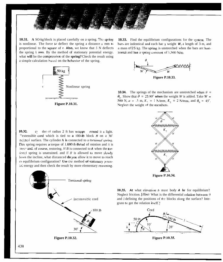
10.31. A SO-kg block is placed carefully on a spring. Thc spfing is nonlinear. The force ta deflect the spring a distance 2 rnm is proportional to the squarz of x. Also, we know that 5 N deflects the spring I mm. By the method of stationary potential energy. what will he the comprcssion of the spring? Check the result using a simple calculation hased on the hehavior of the spring.
10.33. Find the equilibrium configurations for the syslern. The bars are indentical and each hac n weight W , a length of 3 m, and a mass of25 kg. The Fpring is unstrerched when the bars arc hori- mntal and has a Tpnng const:mt of 1.500 Nlm.
Figure P.10.33.
10.32.
< < 1 < Nonlinear spring
10.34. The springs of the mechanism are unstretched when 6 = e,,. Show that 0 = 1 S . Y W when the weight W is added. Take W = S O 0 N, o = .3 m, K , = I Nlmm. K2 = 2 Nlmrn, and e,, = 45~. Ncglect the weight of the memherc.
4 7 c
Figure P.10.31.
der of radius 2 ft has wrappr iround it il light. "extensible cord which is tied to a iocj-ib block n on a 70' nclined surface. The cylinder A is connected to a ror.cionrrl rpring. rhis spring requires a torque of IS100 ft-lblrad of rntntion and i t is inear and, of c o m e , restoring. If B is connected to A when the tor- ;ional spring is unatrained. and if R is allowed to move h w l y h w n the incline, what distanced do you allow il to move to reach m equilibrium configuration? Use the method of stationan. noten-
I , . ial energy and then check the result by more elementary reasmine.
Inextensible cord
Figure P.10.34.
10.35. At what elevatiim h must body A he for equilibrium'! Neglect friction. [ H i n t What is the differential relation hetwren 6 and 1 defining the positions VI thc blocks alrrng the surface? Inte- grate to get the relation ihelf.1
\ ,100 Ih
Figure P.10.32. Figure P.10.35.

10.36. the 20-kg rod AB. Neglect friction.
Show that the position of equilibrium is 8 = 77.3- for 10.39. energy.
Work Problem 10.28 using the method of total potential
10.40. energy.
Work Problem 10.29 using the method of total potential
Figure P.10.36.
10.41. Do Problem 10.25 by the method of total potential energy. [Hint: Consider a length of cord on a circular surface. Use the top p m of the surface as a datum.]
10.37. A beam BC of length 15 ft and weight 500 Ib is placed against a spring (which has a spring constant of 10 Ihlin.) and smooth walls and allowed to come to rest. If the end of the spring is 5 ft away from the vertical wall when it is not compressed, show by energy methods that the amount that the spring will be compressed is ,889 ft.
I S ' K=10 Iblinch
Figure P.10.37.
10.38. Light rods AB and BC support a 500-N load. End A of rod AB is pinned, whereas end C is on a roller. A spring having a spring constant of 1,000 Nlm is connected to A and C . The spring is unstretched when R = 45~ . Show that the force in the spring is 1,066 N when the 500-N load is being supported.
R
Figure P.10.38.
10.42. If member AB is 10 ft long and member BC is 13 ft long, show that the angle R corresponding to equilibrium is 3 4 . 5 ~ if the spring constant K is 10 Iblin. Neglect the weight of the members and friction everywhere. Take R = 3 0 ~ for the configuration where the spring is unstretched.
Figure P.10.42.
10.43. A combination of spring and torsion-bar suspension is shown. The spring has a spring constant of 150 Nlmm. The tor- sion bar is shown on end at A and has a torsional resistance to rotation of rod AB of 5,000 N-d iad . If the vertical load is zero, the vertical spring is of length 450 mm. and rod AB is horizontal. What is the angle a when the suspension supports a weight of 5 kN? Rod AB is 400 mm in length.
End view of torsion bar
Figure P.10.43.
439

10.44. Light rods AB and CB are pinned together at B and pasr through frictionless hearings IJ and E. These bearings arc con- nected to the ground by ball-and-socket connections and are free to rotate about these joints. Sprinzs, each having a s p k f constant K = 800 N/m, restrain the rods as shown. The springs are unstretched when 8 = 4 5 ~ . Show that the deflection of B i s 440 m when a 500-N load i s attached slowly to pin 8. The rod.. are each I m in length. and each unstretched spring i s ,250 m in length. Neglect the weight of the rods. Rods are weldcd to small plates at A and C
Figure P.10.44.
10.45. Do Problem 10.2h by the method of tntal potential mergy. [Hint; Use E as a datum and get lengths EJ. K P , and PN in terms of length H E , including unknown constants.]
10.46. An elastic band is originally 1 m long. Applying a ten- sion force of 30 N, the hand wil l stretch .8 ni in length. What jeflection a does a 10-N load induce on the band when the load i s %pplied slowly at the center of the baud? Consider the l o r e vs. dongation of the band to be linear like a spring. [Hint: If you con- sider half of the band, you double the "spring constant."l
1-1 m - i
10.47. In Problcm 111.46. the hand i\ l i n t strctched and then tied while strstched lu supports A and H w that there i s an initial tell- sion in the hand 0 1 I N. What i': then the deflection (, caused hy the Ill-N load'?
10.48. A ruhher hand of length .7 m i i stretched to connect to
points A and 13. A tcnsim force , > I 30 N i s thereby de~~elopeil i n the hand. A 211-N \r,eight i s then attached to the hand at C. Find thc distance (I that point C iiioves downward if the 20-N weight i\ cnnstraincd to move vertically downward along a frictionless rod. [Hbir: I i you considcr pan rfthc hand, the "cprinp conwnt" for i t wil l he greater than that nf the whole hmd.]
Figure P.10.48.
10.49. 'The spring connecling hodies A and H has a spring cnn- t m t K oi. 3 Nlmm. The unstrctched length o f the spring i\ 450 mm. II hody A weighs 60 N and hody B weighs 90 N, what is the metched length of the spring for cquilihrium'! [Hinr: I/ wi l l hc il
Fhction of two varinhles.1
Figure P.10.46. Figure P.10.4Y

SECTION 10.8 STABILITY 441
10.8 Stability Consider a cylinder resting on various surfaces (Fig. 10.20). If we neglect friction, the only active force is that of gravity. Thus, we have here conserva- tive systems for which Eq. 10.31 is valid. The only virtual displacement for which contact with the surfaces is maintained is along the path. In each case, dyidx is zero. Thus, for an infinitesimal virtual displacement, the first-order change in elevation is zero. Hence, the change in potential energy is zero for the first-order considerations. The bodies, therefore, are in equilibrium, according to the previous section. However, distinct physical differences exist between the states of equilibrium of the four cases.
Case A. The equilibrium here is said to he stable in that an actual displace- ment from this configuration is such that the forces tend to return the body to its equilibrium configuration. Notice that the potential energy is at a minimum for this condition.
Case B. The equilibrium here is said to he unstable in that an actual dis- placement from the configuration is such that the forces aid in increasing the departure from the equilibrium configuration. The potential energy is at a maximum for this condition.
Case C. The equilibrium here is said to be neutral. Any displacement means that another equilibrium configuration is established. The potential energy is B constant for all possible positions of the body.
Case D. This equilibrium state is considered unstable since any displace- ment to the left of the equilibrium configuration will result in an increasing departure from this position.
How can we tell whether a system is stable or unstable at its equilibrium configuration other than by physical inspection, as was done above? Consider again a simple situation where the potential energy is a function of only one space coordinatex. That is, V = Vix). We can expand the potential energy in the form of a Maclaurin series about the position of equilibrium." Thus,
( I 0.34)
x x
Figure 10.20. Different equilibrium configurations.
IhNote that in a Maclaurin series the coefficients of the independent variable x a ~ e evalualed at x = 0, which for us is the equilibrium position. We denote this position with the subscript eq.

442 CHAPTER I O METHODS OF VIRTUAL WORK AND STATIONARY POTENTIAL ENERGY
We know from Eq. 10.33 applied to one variable that at the equilibrium con- figuration ( d V / d ~ ) ~ = 0. Hence, we can restate the equation above:
For small enough x. say xo. the sign of AV will be determined by the sign of the first term in the series, ( l /2!)(d2V/dr2Je4 x2," For this reason this term is called the dominant term in the series. Hence, the sign of (d2V/dxZ)eq is vital in determining the sign of AV for small enough x. If (d2V/dx2),q IS positive, then AV is positive for any value of x smaller than .q,. This means that Vis a local minimum at the equilibrium configuration as can be deduced from Fig. 10.2021, and we have stable equilibrium.'8 If (d2V/dx2)eq is nega- tive, then V is a local maximum at the equilibrium configuration and from Fig. 10.20 we have tinsfable equilibrium. Finally, if (d2V/dx2)eq is zero, we must investigate the next higher-order derivative in the expansion, and s o
For cases where the potential energy is known in terms of several vari- ables, the determination of the kind of equilibrium for the system is corre- spondingly more complex. For example, if the function V is known in terms of x and v. we have from the calculus of several variables the following.
forth.
For minimum potential energy and therefore for stability:
av dv
For maximum potential energy and therefore for instahility:
(10.36a)
(lO.36b)
(10.36~)
(10.37a)
The criteria become increasingly more complex for three or more indepen- dent variables.
"As x gets smaller than unity, xz will become increasingly larger than 2' and powcrs of I
higher than 3. Hence. depending on the values uf derivatires of Vat equilibrium, them will h e a value of *--say x,,-For which the first tern in the series will he larger than the sum of a l l <,lhci
"That is. if the body is displaced a distance x < x,? the hody will return to equilibrium on terms for ValUeE of r < I,,.
TdCVSC.

SECTION 10.9 LOOKING AHEAD: MORE ON TOTAL POTENTIAL ENERGY 443
Example 10.5
A thick plate whose bottom edge is that of a circular arc of radius R is shown in Fig. 10.21. The center of gravity of the plate is a distance h above the ground when the plate is in the vertical position as shown in the dia- gram. What relation must be satisfied by h and R for stable equilibrium?
The plate has one degree of freedom under the action of gravity and we can use the angle O(Fig. 10.22) as the independent coordinate. We can express the potential energy V of the system relative to the ground as a function of 8 in the following manner (see Fig. 10.23):
where W is the weight of the plate. Clearly, 8 = 0 is a position of equilib- rium since
V = W[R - ( R - h) COS s] (a)
Now consider d2Vld8’ at = 0. We have
($$) = W ( R - h ) e o
Clearly, when R > h, (dZVld8Z), =
requirement for stable equilibrium. Thus for stable equilibrium, R > h. is positive, and so this is the desired
R-(R-h) COS 0 Figure 10.21. Plate with circular bottom edge. freedom.
Figure 10.22. One degree of Figure 10.23. Position of C.G,
10.9 Looking Ahead: More on Total Potential Energy
When we have conservative forces acting on pruticles and rigid bodies, we found earlier that for establishing necessary and sufficient conditions of equi- librium we could extremize the potential energy Vassociated with the forces. That is, we could set
6 V = 0 to satisfy equilibrium. Recall that this result was derived from the method of virtual work. We have a similar formulation for the case of an elastic (not neces- sarily linearly elastic) body wbeEby we can guarantee equilibrium. This more-

444 CHAPTER I O METHODS OF VIRTUAL WORK AND STATIONARY POTEiYTI,\L liNFR(;Y
general principle is derivable from the more-gencral virtual work principle mentioned earlier i n section lO.5. Hcre. we 11iu\t extrenii7.e an exprcssinn inore complicated (as you might expect) than V. This expi-ession is denotcd as nwith no relation to the number 3.1416.. . . The expression n is what we CJII a . f i m . - t iond, whercin for the substitution of each functim such as v(~r) , into the func- tional a nunihcr is established. A simple example of ii functional I is as follows:
where F is a function o f r (the so-called independent \iiriahIe), y, and clyldr. Subtilutinn of. a function y(.C into F fiillnwed hy iiii integration hetween the fixed limils. yields for this funclion y(.i) :I number h r 1. Fonctionals per\,adr the field of mechanicc and most other analytic Ciclds o l knowledge. A vital step is to find the function ~ ( n ) that wil l cxtremix I . This function then becomes knnwn aq the urrrrriral/un,.fion. 'The ciiIcuIus Ir,r doing this is called the w l d u s 0 1 variat ions. Thc particular functional for the method of tntill potential cncrgy is h' riven as
n = -111 B * u 0'1. - 8 7 u d.4 + L'
The function to he adjusted to cxtremize ii is u(.x, J, z) taking the placc of ~ ( ~ 1 )
in the preceding functional. and iinw the independcnt \,;iriablcs are .x. y. and 2
i n place of just .r in thc preceding functional. The expression 11 is the energy of defnrmation that you will study l a t a in your solids ciii~rse and presented cai-lier in Section 10.5 a- 111 Ti,&,, </I, . The principle of total potential
energy for the case of elastic hodies is written i n the following deceivingly simple looking lormulation:
6n = 0 What is most intriguing about this imoccnt looking equation is that it is oftcn considercd to he thc most powerful equation in solid mechanics!
We have touched on a h r i d area of sludy. namely vari;itinnal methods. park of which you will encounter in many o f y 0 u r htudies. For cxamplc. j u t the method (it' total potential energy has thc following ma,jnr uses:
1. It plays an important role i n opfiinixiti,Jii iIimii:i,. 2. I t can he used profitably to dcrive the p r q w r q u a t i o m and thc houndor?
cnnditiuiis for many areas of vital importance such a h plate theory, elastic stability theory, dynamics of plates and beams. torsion theory, etc,
3. From it we can develop a numher of vital approximation methods. The most prominent of these methods is the methiid of.finirr drmmts.
Ii .\
1' t I
Clearly this i y an impressive
'vYou can aiudy 111 wme drlail rhr conte i i l i 01 rhc lwi I.imking Ahead scc~ions of lh i \ chaps, i n I . R . Shamea. lnlrwluclio,~ 10 .Solid M<dwnU.r. 2nd ed.. 1%9. Prcnlice~Hnll. Inc.. Englewood Cliffs. N.J. Thih i i i a t~ r i i i l ihoukl he wiihi i i thc wach of hrig,hi *ccimd-semester sopho~ imorcs and cerlninly of juniors. Thc author ha\ raught (hi\ maiciiiil hi iriany year, 1 0 seconil- sentester sophomores OUI of the aiwemesrioned hook. See Chiqxcia 18 i ind 1'1.

10.50, A rod AB is connected to the ground by a frictionless ball-and-sockrt connection at A. The rod is free to rest on the inside edge of a horizontal plate as shown in the diagram. The square abcd has its center directly over A. The curve eJg is a semi- circle. Without resorting to mathematical calculations, identify positions on this inside edge where equilibrium is possible fur the rod AB. Describe the nature of the equilibrium and supply sup- porting arguments. Assume the edge of plate is frictionless.
Figure P.10.50.
10.51. a position of unstable equilibrium for the rod.
10.52. Rod AB is supported hy a frictionless ball-and-socket joint at A and leans against the inside edge of a horizontal plate. What is the nature of the equilibrium position a for the rod? Assume that the edge of the plate is frictionless.
In Problem 10.50, show mathematically that position h is
i
Figure P.10.52.
10.53. Consider that the potential energy of a system is given by the formulation: V = 8x3 + 6x2 - 7x. What are the equilibrium positions? Indicate whether these positions are stable or not.
10.54. A section of a cylinder is free to roll on a horizontal sur- face. If yof the triangular portion of the cylinder is 180 Ib/ft3 and that of the semicircular portion of the cylinder is 100 IMft', is the configuration shown in the diagram in stable equilibrium?
Y
I
Figure P.10.54.
10.55. A system of springs and rigid bodies AB and BC is acted on by a weight W through a pin connection at A. If K is 50 N/mm, what is the range of the value of W so that the system has an unstable equilibrium configuration when the rods AB and BC are collinear'? Neglect the weight of the rods.
P," connecuon
Figure P.10.55.
10.56. A weight W is welded to a light rod AB. At B there is a torsional spring for which it takes 500 ft-lh to rotate 1 rad. The torsional spring is linear and restoring and is, for rotation, the ana- log of the ordinary linear spring for extension or coneaction. If the torsional spring is unstrained when the rod is vertical, what is the largest value of W for which we have stable equilibrium in the vertical direction?
Figure P.10.56.
44

I 10.57. A light rod A B is pinned to a hlock of weight W at A. Also at A are two identical springs K. Show that, for W less than 2K1, we have stable equilibrium in the vertical position and, for W > 2K1, we have unstable equilibrium. The value W = 2KI is Called il cririrul load for reasons that are explained i n Problem 10.5X.
10.58. I n Problem 10.57, apply a small transverse force F to body A as shown. Compute the horizontal deflection 6of paint A for a position of equilibrium by using ordinary statics as developed i n earlier chapters. Now show that when W = 2K1 @e., the critical weight), the deflection 6mathemdtically blows up to infinity. This shows that, even if W < 2KI and we have stable equilibrium with I.’ = 0, we get increasingly very large dcflections as the weight W approaches its critical value and a side load F, however small, is introduced. The study of stability of equilibrium configuration therefore is an important area of study in mechanics. Most of you will encounter this topic in your strength of materials course.
Figure P.10.58. 10.59. Cylinders A and B have semicircular cross-sections. Cylinder A supports a rectangular solid shown as C. If p, = 1,600 kg/mz and p< = 800 kg/m’, ascertain whether the arrange- ment shown is in stable equilibrium. [ H i m Make use of point 0 in computing V.1
I t
6 m -
10.10 Closure In this chapter, wc have taken an approach that differs radically from the approach used earlier in the text. In earlier chapters, we isolated a hody for the purpose of writing equilibrium equations using all the forces acting on the body. This is the approach we often call vectorial mechanics. In this chapter, we have mathematically compared the equilibrium configuration with admis- sible neighboring configurations. We concluded that the equilibrium configu- ration was one from which there is zero virtual work under a virtual displacement. Or, equivalently for conservative active forces, the equilibrium configuration was the configuration having stationary (actually minimum) potential energy when compared to admissible configurations in the neigh- borhood. We call such an approach variational mechanics. The variational mechanics point of view is no doubt strange to you at this stage of study and far more subtle and mathematical than the vectorial mechanics approach.
Shifts like the one from the more physically acceptahle vectoriul mechanics to the more abstract variational mechanics take place in other engineering sciences. Variational methods and techniques are used in the study of plates and shells, elasticity, quantum mechanics, orbital mechanics, statistical thermodynamics, and electromagnetic theory. The variational methods and viewpoints thus are important and evcn v i t d in more advanced studies in thc engineering sciences, physics, and applied mathematics.
446

10.60. At what position must the operator of the counterweight crane locate the 50-kN counterweight when he lifts the IO-kN load of steel?
20 m
Figure P.10.60.
10.61. What is the relation between P and Q for equilibrium?
Figure P.10.61.
10.62. A 50 Ih-ft torque is applied to a press. The pitch of the screw is .5 in. If there is no friction on the screw, and if the base of the screw can rotate frictionlessly in a base plate A, what is the force P imposed by the base plate on body B?
-ft
Figure P.10.62.
10.63. The spring is unstretched when 0 = 3LT. At any position of the pendulum, the spring remains horizontal. If the spring con- stant is 50 Iblin., at what position will the system be in equilibrium?
Figure P.10.63.
10.64. If the springs are unstretched when 0 = 0,. find the angle 0 when the weight W is placed on the system. Use the method of stationary potential energy.
Figure P.10.64.
10.65. A mass M of 20 kg slides with no friction along a vertica rod. Two internal springs K, of spring constant 2 Nlmm and ai external spring K2 of spring constant 3 Nlmm restrain the weigh W. If all springs are unstrained at 6' = 3LT, show that the equilib rium configuration corresponds to 0 = 27.8'.
Figure P.10.65.

10.66. When rod AH i h in thc vaticill position, the spring attached to the wheel by a flexible cord is unstretched. Determinc all the possible angles L? for equilibrium. Show which are stable and which are not stable. The spring has a spring constant 01 8 Ib/in.
Figure P.10.66.
10.67. Two identical rods are pinned together :it H and arc pinned at A and C. At H there i s a torsinnal spring requiring SO0 N-mlrad of rotation. What is the maximuin weight W thal ciich Ii,d can have for a c11w uf stable equilibrium when thc ~riids arc collinear?
Figure P.10.67.
IO.6X. A rectangular xdid body ( 1 1 height h rests on ii cylinder with a semicircular scctiun Set u p criteria for \lahlc and unstable riluilihrium iii trrnis ni ii and X 1 1 ~ 1hc pasilion shoun
Figure P.10.68.
448

Dynamics

Kinematics of a Particle- Simple Relative Motion 11.1 Introduction Kinemutics is that phase of mechanics concerned with the study of the motion of particles and rigid bodies without consideration of what has caused the motion. We can consider kinematics as the geometry of motion. Once kine- matics is mastered, we can smoothly proceed to the relations between the factors causing the motion and the motion itself. The latter area of study is called dynamics. Dynamics can be conveniently separated into the following divisions, mnst of which we shall study in this text:
1. Dynamics of a single particle. (You will remember from our chapters on statics that a particle is an idealization having no volume but having mass.)
2. Dynamics of a system of particles. This follows division 1 logically and forms the hasis for the motion of continuous media such as fluid flow and rigid-body motion.
3. Dynamics of a rigid body. A large portion of this text is concerned with this important part of mechanics.
4. Dynamics of a system of rigid bodies. 5. Dynamics of a continuous deformable medium.
Clearly, from our opening statements, the particle plays a vital role in the study of dynamics. What is the connection between the particle, which is a completely hypothetical concept, and the finite bodies encountered in physical problems? Briefly the relation is this: In many problems, the size and shape of a body are not relevant in the discussion of certain aspects of its motion; only the mass of the object is significant for such computations. For example, in towing a truck up a hill, as shown in Fig. 11.1, we would only be concerned
45 I
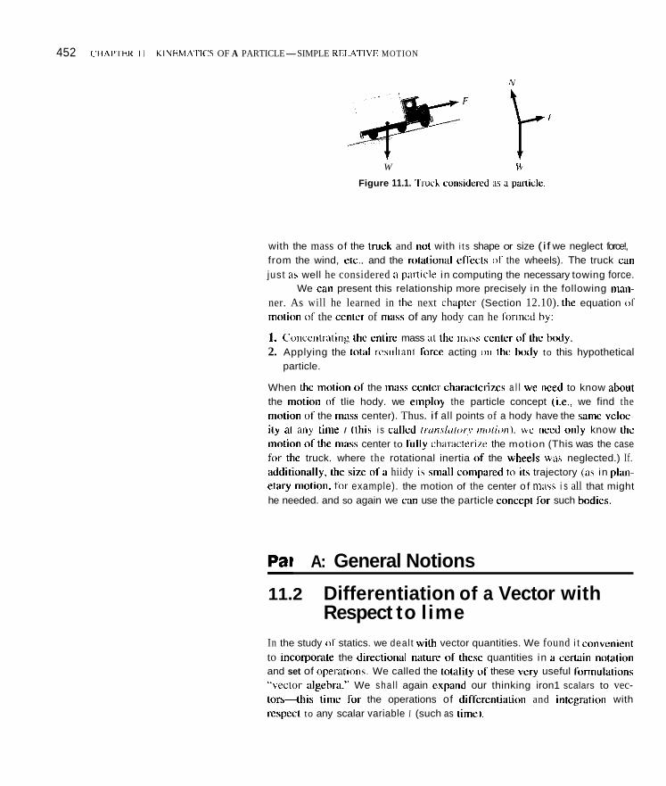
452 ( 'HAPTRK I I K1NEM:YI'ICS OF A PARTICLE-SIMPLE REl.AT1VE MOTION
W i+
Figure 11.1. 'liwck uimsidcrrd :is u pxiiclc.
with the mass of the truck and 1101 with i t s shape or size (if we neglect force!, from the wind, etc.. and the riitatiiinal cffects (if the wheels). The truck can just a, well he considered i i p;uticle in computing the necessary towing force.
We car present this relationship more precisely in the following ntaii- ner. As will he learned in tlie next chapter (Section 12.10). the equation iii inotioii o f the center of nias\ of any hody can he foriiied by:
1. C(mccntriiting thc cntirc mass ill thc miss cciitcr of thc h d y . 2. Applying the total rc\LiIIant lorce acting [in thc hiidy to this hypothetical
particle.
When the iniition of the mass ccntcr charactcrizcs a l l we nced to know ahout the motiiin (if tlie hody. we employ the particle concept (i.e,, we find the motion of the miss center). Thus. if all points of a hody have the same vcluc- ily at airy tinie I ([hi\ i s callcd rrun.rl~iror~ inolioi i) . we necd i inly know the miition o i t l ie mass center to liilly ch;ir;~cterize the motion (This was the case fix thc truck. where the rotational inertia of the wheels was neglected.) If. additiiinally, the sizc i i f a hiidy i \ \mall compared to itr trajectory (as in plari- e l x y niiitiiin. for example). the motion of the center o f n i x \ i s all that might he needed. and so again we can use the particle conccpt ior such hodics.
Part A: General Notions
11.2 Differentiation of a Vector with Respect to lime
In the study of statics. we dealt with vector quantities. We found i t con\cnient to incorporale the directional naturc of thcsc quantities in ii certain n~itatiiin and set of opevatiiiii\. We called the tolalily iii these \ery useful foi-intilalions "\ector algehra." We sha l l again enparid our thinking iron1 scalars to vec- tors-hi\ tinic for the operations of differenti;ition and intcgration with rcspcct to any scalar variable I (such as timr).

SECTION I I .2 DIFFERENrIATION OF A VECTOR WITH RESPECT TO TIME 453
For scalars, we are concerned only with the variation in magnitude of some quantity that is changing with time. The scalar definition of the time derivative, then, is given as
(11.1)
This operation leads to another function of time, which can once more be dif- ferentiated in this manner. The process can he repeated again and again, for suitable functions, to give higher derivatives.
In the case of a vector, the variation in time may he a change in magni- tude, a change in direction, or both. The formal definition of the derivative of a vector F with respect to time has the same form as Eq. I I . I :
(11.2)
If F has no change in direction during the time interval, this operation differs little from the scalar case. However, when F changes in direction, we find for the derivative of F a new vector, having a magnitude as well as a direction, that is different from F itself. This directional consideration can be somewhat troublesome.
Let us consider the rate of change of the position vector for a reference xyz of a particle with respect to time; this rate is defined as the vrlucily vector, V , of the particle relative to q z . Following the definition given by Eq. 11.2, we have
The position vectors given in brackets are shown in Fig. 11.2. The subtrxtion
I .. Path of
Figure 11.2. Particle at times f and f + Al
between the two vectors gives rise to the displacement vector Ar, which is shown as a chord connecting two points As apart along the trajectory of the particle. Hence, we can say (using the chain rule) that

wherc M'C have multiplied and di\'idrd hy As i n thc l i i s t cxpression As A/ goes to Lerci. the direction ol Ar approaches tangency to the trajectory at posi- tion r ( / ) and apprixiches A,\ i n magnitude. Consequently. i n the limit. ArlAs hecoines a unit w c t w e,. tangent to the traieclor>. Tliat i \
We c i ~ i then s i i ~
( I 1.3)
Therefore. drlih leads to a vector having n magnitudc equal to the speed 01 the pailicle and a dii-ection ~aiigent to the trajectory. Kccp i i i mind that there can he any ansle hetueen the p(isition Vector and the velocity vector. Stu- dents seem to \'ant to limit this anglc to 90c', which actually restricts you to ii
cit-culiir pa th The acceleration ~ e c t o r (il a Ixirtick ciin then be given as
The dillcrcntiation and integration of vector( r , V . and a will concern LI'I
thniuphout tlic text.
Part 6: Velocity and Acceleration Calculations
11.3 Introductory Remark As you know lroni statics. wc ciin expres? ii vector i n many ways. For ill- stance, we can use rectangular compiinents. or. as we udl hhortly explain, we can use cylindrical components. I n evaluating dcriviitivcs of vectors with respect 10 time. we mu51 pi-oceed i n accordance with the nianner in which the vector has heen expre\rcd. I n Part B of this chapter. wc will therefore exai i i - ine certain diffcrcntiation processes tliiit iirc used extensively i n mcchanics. Other diftkrenti;ition proccsses will he exaniined l a t ~ r at appropriate tiiiies.
We have already carried out a derivative operation in Section 11.2 directly on the vector r . You will scc in Section 11.5 that llic approach u x d gives tlic dcrivative ii i terms 01' potti vorilrblr~c. This approach will he one o S several that we shall i iow examine with some care.
SECTION 11.4 RECTANGULAR COMPONENTS 455
11.4 Rectangular Components Consider first the case where the position vector r of a moving particle is expressed for a given reference in terms of rectangular components in the fol- lowing manner:
r ( t ) = x ( r ) i + y ( r ) j + z( t )k ( I 1.6)
where x ( f ) , y ( t ) , and z(t) are scalar functions of time. The unit vectors i, j , and k are fixed in magnitude and direction at all times, and so we can obtain drldt in the following straightforward manner:
dr dx(t) ' dy( t ) j + w k = i ( t ) i + y ( t ) j + i ( r ) k ( I 1.7) dt = V ( t ) = - t + - dt dt
A second differentiation with respect to time leads to the acceleration vector:
= a = i ( t ) i + j i ( t ) j + Z(t)k (11.8) df2
By such a procedure, we have formulated velocity and acceleration vectors in terms of components parallel to the coordinate axes.
Up to this point, we have formulated the rectangular velocity compo- nents and the rectangular acceleration components, respectively, by differen- tiating the position vector once and twice with respect to time. Quite often, we know the acceleration vector of a particle as a function of time in the form
a(t) = X ( t ) i + s ( t ) j + Z(r)k ( I 1.9)
and wish to have tor this particle the velocity vector or the position vector or any of their components at any time. We then integrate the time functionx(t), y(t ) , and i ( r ) , remembering to include a constant of integration for each inte- gration. For example, considerx(t). Integrating once, we obtain the velocity component V , ( r ) as follows:
Vx(t) = 1 f ( t ) dr + C, (11.10)
where C, is the constant of integration. Knowing \ at some time to, we can determine C, by substituting to and (V,),, into the equation above and deter- mining C , . Similarly, for x( r ) we obtain from the above:
x ( t ) = j [ j f ( r ) d t ] d t + C , t + C ? (11.11)
where C, is the second constant of integration. Knowing x at some time f , we can determine C , from Eq. 1 1.1 I . The same procedure involving additional constants applies-to the other acceleration components.
We now illustrate the procedures described above in the following series of examples.

456 ( ' t IA1Tl:tt I I K
Example 11.1
Pins A and H must aluayh remain in the vrrtical sIo1 01 yrAc C'. which tno\'e\ ttr tlic right at a c~ t i s t i i n t spccd o f 6 I t l sec in Fig. I I ..?. titrthcrmorc. the pins cannot leave the elliptic s lot . (a) What is the speed at which the pins apprmach each whet- wlieti the yoke s lo t is at ~r = 5 ft? ( h ) What i s the rate olch;nrge of \peed k i w m l ciicli nlhcr when the yoke \lot i\ at .i~ = 5 ft'!
Thc cqu:ltioti of Ihc clliptic path iii which the pins in i i i c t ii~ovc i \ seen by inspection to he
.\z r- ~~~~ + > - _ I IO' 6' (:I) Figure 11.3. Pin \ l i d o in \IDI ; ~ n d )rihc.
j t ! t
clciirly. iIcoordinates (.1. y) are to represent tlic cii(irdinatcs of pin R. tiicy m u ~ t he time functions i i ich Ih:it for any tinie i llie v;iliies .r!i) and ?( I ) sill- isfy Eq. (a). Also..i(/) andy(i) t i iust hc such that piti II t i i m e s at all times in the elliptic path. We cati s i t i d y thesc rcquircnictits hy f i rs t dilrcrcnlial- iiif Eq. (a) with respect to t i i i ic. Cancelins (lie factor 2. we ohtain
Now ~ ~ ( 0 . Y(II..~(I), andy(i) ~ i i i i s ~ sati\fy Ikl . ( h ) fur i i l l vii lucs o f i 1 0 cnsurc that H rciniiiiis iii the elliptic path
We can now proceed to calve par1 (a ) of this pi-ohleln. We !wow that pili H must have a velocity .i = h fllscc hcciiiisc (II tlic yokc. Furthcrniiirc. when ~c = 5 I t . we know from E[]. (a) that
i j
:. v = 5.20 ft
N o w going tu Eq. (b). we can solve fo r i at the i i i \ t i i i i l 01 intcrcit.
!
; Thus. pin H tiioves downward with ii spccd of ?.OX ft lccc. Clcarly. pili A n i u s t move upwird with the s m i c speed nf 2.08 f t l x c . Thc pins apprmacli each olhcr at the itistatit o f intcrcsl at ii speed 014.10 I'tlscc.

SECTION 11.4 RECTANGULAR COMPONENTS 457
Example 11.1 (Continued)
To get the acceleration? of pin H, we first differentiate Eq. (b) with respect to time.
The accelerations.? and? must satisfy the equation above. Since the yoke moves at constant speed, we can say immediately that x = 0. And using for x, y , k, and j known quantities for the configuration of interest, we can solvc for? from Eq. (d). Thus,
= 0 o+ 65 + ~~ 5 . 2 0 ~ + 2.0X2
102 62
Therefore
j i = -3.32 ft/sec*
Pin B must be accelerating downward at a rate of3.32 ft/sec2 while pin A accelerates upward at the same rate. The pins accelerate toward each other, then, at a rate of 6.64 ftt/secz at the configuration of interest.
In the motion of particles near the earth’s surface, such as the motion of shells or ballistic missiles, we can often simplify the problem by neglecting air resistance and taking the accelcration of gravity g as constant (32.2 ftlsec? or 9.XI mlsec’). For such a case (see Fig. I1.4), we know immediately that y(r) = -g andi(r) = i ( t ) = 0. On integrating these accelerations, we can often determine for the particle useful information as to velocities or positions at certain times of interest in the pmhlem. We illustrate this procedure in the following examples.
L X
Figure 11.4. Simple ballistic motion of a shell
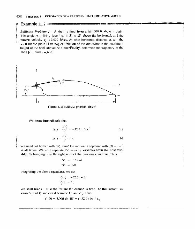
458 ('IIAPTER I I K I N I M A l I C S OF A PARTICLE- Slh.1I't.ti KEIATIVI'. !KITION
Example 11.2
Ballistics Problem 1. A shcll i s fired from a hill 500 I t ahove n plain. Ttic angle (1 of firing (see Fig. I I . S I i s 15' ahovc thc horimntal. and the muizle velocity v) i s 3.000 ftisec. At what horizontal distance. d, wil l lhc shcll hit the plain if wc ncglcct frictioti of the air'? What i s the nhaximun~ hcighl of the shell ahovc LIE plain? l:iti;illy, determine the trajectory of thc shell 1i.e.. find v =.f(.xll.
We know imnicdiately tt iat
We need not hothcr with ?(f). since the motion i s coplanar with i(11 = : = 0 at all times. We iicxt separate the velocity variahles froni the timc viiri- ahles hy bringing rlf to Ihe right sidc.: 0 1 the previous cqoations. Thus
dVv = -32.2dr "V, = Odt
Inlegrating the ahove equations. we get
V > [ J ) = -32.21 + V ) ( I ) = <.,
We shall lake f = 0 211 the i i is ta i i t the camion is fired. At this instant. WL'
k n o w L; and V, ;rnd can dctcrmine C , atid C,. Thus.
V$Ol = 3,000sin 15" = ( -32 .?) (0) + C',

SECTION 11.4 RECTANGULAR COMPONENTS 459
Example 11.2 (Continued)
Therefore,
C, = Vv(0) = 776ft/sec
Also
V\(0) = 3,000cos1S" = C,
Therefore,
C2 = b'a(Oj = 2,900 ft/sec
We can give the velocity components of the shell now as follows:
dv d t dx dt
V,(t) =
V,(rj = ~ = 2,900 ft/sec
= -32.2r + 776 ft/sec
Thus, the horizontal velocity is constant. Separating the position and time variables and then integrating, we get the J and y coordinates of the shell.
(e)
(f)
t 2 y ( t ) = -32.2 ~ + 776t + C, 2 *(I) = 2,900t + C,
When f = 0, y = x = 0. Thus, from Eqs. (e) and ( f ) , we clearly see that C, =
C, = 0. The coordinates of the shell are then
y ( f ) = -16.1t2 + 776f x ( f ) = 2,900t
To determine di.stancp d, first find the time f for the impact of the shell on the plain. That is, set y = -500 in Eq. (g) and solve for the time t. Thus,
-500 = - lh . l t2 + 776f

460 CHAPTER I I KINEMATICS OF A ['AKrlC'l E C I h I I ' I E K t l U I V F hlOTlON
Example 11.2 (Continued)
Therefore,
Using the quadratic forintila, we get for I :
f = 48.8 vi.
Substituting this value of I i n l c Fq. lhl . we gc'l
d = (2,9OO)t48 8 ) ~ 141,500 ft
To get the moximirm hpiRhz x,,,,,,. firs1 iind Itre tirile I ;\.hi.ii \; = 0. Thus from Eq. (c) we get
1) - 12 2: I 776 Therefore,
I = 24.1 St'C
Now suhstirute t .: 21.1 sei' i i i lo F.q. ( € 1 . ' i h i h gt t :<, I , \ ! , , ,.
:. y- = 9,350 ft
'Thercfnre.
y = -1.917 X 10"x2 + , 2 6 8 ~
Clearly, the tra.jectoi-y is that of a puwholn.

SECTION 11.4 RECTANGULAR COMPONENTS 461
Example 11.3
Ballistics Problem 2. A gun emplacement is shown on a cliff in Fig. 11.6. The muzzle velocity of the gun i s 1,000 d s e c . At what angle a must the gun point in order to hit target A shown in the diagram'? Neglect friction.
y
Figure 11.6. Find a to hit A.
Newton's law for the shell is given as follows for a reference n)' having its origin at the gun.
j f t ) = -9.81 i ( t ) = 0
Integrating, we get
s(/) = Vv(t l = -9.81r + C,
X ( t ) = V\(t) = C, (a) (bl
When f = 0, we have j = 1,000 sin a and j; = 1,000 cos a. Applying these conditions to Eqs. (a) and (b), we solve for C, and C,. Thus,
1,000 sin a = 0 + C,
C , = 1,000 sin a Therefore,
Also,
Therefore. 1,000 cos a = c2
c, = 1,000 cos a Hence, we have
$ ( t ) = -9.81t + 1,000sina i ( t ) = 1,000cosa
Integrating again, we get
~(f)=-9.811+1.000sinaf+C, f 2
x ( t ) = 1,ooocosa/+C,

Using the quadratic lormula. wc linii the l i i l lowing anglcs:
ccI = 8.17" "2 = 81.44"
Therc tire thus two possible firing angles thal wil l pennil the rtiell 10
hit the target, as shown i n Fig. I I .7.
Example 11.3 (Continued)
I

SECTION 11.4 RECTANGULAR COMPONENTS 463
Example 11.4
The engine room of a freighter is on fire. A fire-fighting tughoat has drawn alongside and is directing a stream of water to enter the stack of the freighter as shown in Fig. I I .8. If the initial speed of the jet of water is 70 ft/sec, is there a value of a of the issuing jet of water that will do the job? If so, what should a be'?
Figure 11.8. Fire-fighting tughuat directing a jet of water into the stack of a freighter.
Consider a particle within the stream of water. Neglecting friction. Newton's law for the particle is given as follows:
y = -32.2 ftlsec' Y = 0 ft/sec?
Integrating twice, and using initial conditions at A, we get
$ = -32.2f + 70 sin a ft/sec (a) i = 70 cosa ft/sec (c)
y = -16.1t2 + 7 0 s i n a t ft (h) I = 7 0 c o s a t ft (d)
Solve for f from Eq. (d) and substitute into Eq. (b) to get y = -16.1[-L] 2 + 7 0 ~ i n a [ - ~ ]
70 cos a 70 cos a
Replace cos2 a by I / ( I + tan? a) and (sin a/cos a) by tan a in the previous equation and then substitute the coordinates of point B at the stack where the water is supposed to reach. That is, set x = 40 ft and y = 30 ft. We then get
30 = -(3.29 x 10-')(402)(1 + tan2 cy) + 40 t a n a :_ tan2 a - 7.61 t a n a + 6.71 = 0
Using the quadratic formula we get

464 C'HAPTRII I I KIK\FMA'I'I('S OF A l ' ~ ~ l ~ ~ l l ~ l , ~ - ~ S l ~ l l ~ l . l ~ . KI11.:\lIVE V l l I l O N
Example 11.4 (Continued)
We thus havc IMW aiiglcs h r a, ciicli i i l w t i i c t i wil l the,rl-clically ciiusc the streiilii 10 go ttr piiiiit I1 o i the .;tack. Thew iingles :ire
(1, = 4?.?0' a, = x 1.37" Docs 1 1 1 ~ . 11011c. or hott i angles ;ihovc yield i i s~rc i i i i i i)t wiiter that wi l l
c(ii1ie down iil R YO iis t o enter the stxk'! We i'iiii detzriiiinc th i s hy liiiding thc ii i i ixii i iuiii viilue oI J aiid locating [tie p(isilioii t Iiir chi, i i i i ix ir i iu i i i valuc. To do this, we bel? = 0 and x i l ve for f using each IY. ' I l i i i s u'c have
i
' :
i I . ? ? I 2.14') :. I = { ) scc
i A Acwh (11 the two possihlc Ird.jectories i\ shown i n 1:ig. I LO. ClcarIy the shallow trajcclory will hi? the side of t l ie slack nnd i s uiiacceplahlr. while 1 ?hc high trajcct(iry wil l deposit water iiisidc the stack and i s thus tlic
1 desired ti-ajcckiry. Thus.
i
a = 81 37"

SECTION 11.5 VELOCITY AND ACCELERATION IN TERMS OF PATH VARIABLES 465
We do not always know the variation of the position vector with time in the form of Ey. I I .6. Furthermore, it may he that the components of velocity and acceleration that we desire are not those parallel to a fixed Cartesian ref- erence. The evaluation of Vanda for certain other circumstances will be con- sidered in the following sections.
11.5 Velocity and Acceleration in Terms of Path Variables
We have formulated velocity and acceleration for the case where the rectangu- lar coordinates of a panicle are known as functions of time. We now explore another approach in which the formulations are carried out in terms of the path variables of the particle, that is, in terms of geometrical parameters of the path and the speed and the rate of change of speed of the particle along the path. These results are particularly useful when a particle moves along a path that we know apriori (such as the case of a roller coaster).
As a matter of fact, in Section 1 1.2 (F4. I I .4) we expressed the veloc- ity vector in terms of path variables in the following form:
(11.12) ds dt V = - E
where drldt represen& the speed along the path and E, = dr1d.s (see Eq. 11.3) is the uni t vector tangent to the path (and hence collinear with the velocity vector). The acceleration becomes
(11.13)
Replace dq/dr in this expression by (dc,lds)(drldt), the validity of which is assured by the chain rule of differentiation We then have
(11.14)
Before proceeding further, let us consider the unit vector E, at two posi- tions that are A,s apart along the path of the particle as shown in Fig. 11.10. If. A.7 is small enough. the unit i:ector$ e,(.s) and +[.s + A.s) can be considered to intersect and thus to form a plane. If As + 0, these unit vectors then form a limitirrg plane. which we shall call the osculating plune.' The plane will have an orientation that depends on the position s on the path of the particle. The osculating planc at r( t) is illustrated in Fig. 11.10. Having defined the oscu- kiting plane, let us confinur discusxion of Eq. 11.14.
& m ,*E,(\)
s r ( f + Ai) €,(S + A,7)
Figure 11.10. Osculaling plane arr(f).
IFrum Ihe definition. it should be apparent that the usculating plane at position .Y along a C U W ~ is act~ill ly iorixe,il Lo Lhc curve at posirion J. Since usculalc means lo kiss. the plane "kisac.," thc curie. its it were. at .$.

Since we haw not fiirniiilly carried out thc differentiation or a \'cctor with respect 10 a spatial coiirdinatc. we shall carry out the derivative dc,lil.v riecdcd i n Eq. 11.14 from thc basic definition. Thus.
l h e vccmrs ~ p ) and E,(S + A.vj are shown in Fig. I I. I I(3) along the path and arc d s i i shown (cnliirgcd) with AE, as a \cctor triangle in Fig. 1 1 . 1 I(h). Ac piiintcd out earlier, lirr small enough A.s the lincs OS action of thc unit vector5 eJ.sj and E,(.$ + As) wil l intersect tn form a plane as shown in Fig. 1 1 . 1 I(a1. Now in this plane. draw nonilill line:, to thc aSiircmentioned vcctnrs at the respcctiivc positions s and ,s + A.s. These lines will intcrscct at some point 0. a s shriwn in the diagram. Next. concidcr what happens to the plane and to point 0 as A s --f 0. Clearly. the limiting planc is our osculating plane at .s [see Fig. I I , I I IC)]. Furthermore. the limiting position airived at for point 0 is f i r tlrr o.sdati i ig plonc and i s callcd the c'en/er o { m , ~ ~ i t i r ~ ~ for the path at s . The dis- taiicc hctwccn 0 and .s i\ denotcd iis R and i s called Ihc riu1iu.s o i ' i ' ~wwt im. Finaly, the vector Ac, (see Fig. I I. I I ih)). in the limit a s As + 0, ends up in the osculating plane norind to the path at c and directed toward thc center of cu-- viiturc. 'The unit vect~rciil l incar ujitli the linritirlg vcctor for AE, i\ dcniitcd as e,, and i s called the p r i i i c i p ~ t l norniul w i ' i o r .
A
/ C /
Figure 11.1 I . Devcli~pment ill the osculating plane and the center of cunalurc.
With the limilitig diwctioii o f Ae? cstablihed. we next evaluate the imi,ytz;fudo of AE, iis an approximate value that hecomes corrcct as Av --f 11. Ohserving the vector triangle in Fig. I I .I I(h). we can uxiirdingly say:
jAe,I = IE,~AO A* t I l . l h )

SECTION I 1.5 VEI.OCITY AND ACCELERATION I N TERMS OF PATH VARIABLES 461
Next, we note in Fig. 1 I. I I (a) that the lines from point 0 to the points s and s + A,T along the trajectory form the same angle A@ as is between the vectors E,(s) and E,(S + A,?) in the vector triangle, and so we can say:
A+ = ~ A.s = A'! Os R (11.17)
Hence, we have for Eq. I I . 16:
(11.18) As IAEI =
We thus have the magnitude of AE, established in an approximate man- ner. Using E,,, the principal normal at 5 , to approximate the direction of AE, we can write
AE, = ~ en
If we use this result in the limiting process of Eq. 1 I . 15 (where i t becomes exact), the evaluation of dr,ld.s becomes
A.7 R
When we substitute Eq. I 1 . I9 into Eq. I I . 14, the acceleration vector becomes
d2s (ds/dt)* dt2 R 'fl
a =- e +- (I I .20)
We thus have two components of acceleration: une cwmimnenr in u dirrctimrr tangent to the path und one component in the osculating plane uf right anglc,s to the puth und poinfinji toward the center ifcun,uture. These components are of great importance in certain problems.
For the special case of a plane curve, we learned in analytic geometry that the radius of curvalurt. R is given by the relation
Furthermore, in the case of a plane curve, the osculating plane at every point clearly must correspond to the plane of the curve, and the computation of unit vectors E,, and
How do we get the principal normal vector en, the radius of curvature R, and the direction of the osculating plane for a three-dimensional curve'? One procedure is to evaluate E, as a function of s and then differentiate this vector with respect to s . Accordingly, from Eq. 1 I . 19 we can then determine E, as well as R. We establish the direction of the osculating plane by taking the cross product E, x E,, tn get a unit vector normal to the osculating plane. This vector is called the binormul vector. This is illustrated in starred problem I 1.7.
is quite simple, as will be illustrated in Example 11.5.

Example 11.6 ..
A particle i s tnovirig iii ilic ~ A Y pl;ine almg ii parabolic path giveii a.; Y = 1.22: .I (see Fig. I1 .13J wi th~r i i i ic l? in inclcrs. AI position A . the par-
t ic le ha\ a spccd ( 1 1 3 misec d h a \ ii rate 01 change of speed n l 3 miscc' iiloiig ilic path What i s Ihc ii ior o f llic p r l i d c i i ~ thih position'?

SECTION 11.5 VELOCITY AND ACCELERATION IN TERMS OP PATH VARIABLES 469
Example 11.6 (Continued)
where
At the position of interest (x = I .5 m) we have
Therefore, u = 26.5"
Hence,
.st = .X95 + ,4461 (C)
As for e,,, we see from the diagram that
en = S i n a i - c o s a j
Therefore,
en = ,4461' - ,895 j (d)
Next, employing Eq. I 1.21, we can find R. We shall need the following results for this step:
(e)
( f )
dY = . 6 1 0 ~ - ' / ~
C ~ * Y .~ - -,305x-i/2 dr? -
Substituting Eqs. (e) and (f) into Eq. 11.21, we have for R:
[i + (.6inx- l /2)zr R = 305*-1/2 (SI
At the position of interest, x = 1.5, we get
R = 8.40 m (h)
We can now give the desired acceleration vector. Thus, from Eq. I 1.20, we have
0) 9 a = 3(.895i + ,446j) + ,,(.4461' - ,895.j)
:. a = 3.16i + ,3791

470 CHAPTER I I KINEMATICS OF A I'ARTICl.r.-SIMPI I:. RFl./\TlVE hlOTIOK
*Example 11.7
A particle i s made t o m o w ; h n g a spirzil palh, iis i s shown in Fig. I I . 13.
I
Figure 11.14. Thc equations rcprcscnting thc p ~ h arc given parametricall? iii terins o i Ihe uriahle r iii thc Solliiwing iiiannc.l-:
%
/ j .xi, = A 'in r l r
- = c T ',, y,, = A U I \ qr ( A . q. <' arc hni~ \vn cwistant,) i i l l 1
where the cuhcci-ipt 11 is t i 1 rcniind the rcader that these reliifioti'r rcfcr t o ii
f ixed path. When thc par l ick i s iit the .rp pliiiie (7 = I)). i l ha\ ii spccd c ) l V,, I'tJhec and ii riitc: ol'changc o i \peed of N fticec.'. What i s the ~ I C C C I C R I - tioii of the partick iii this position?
To answer this. \be must asccrtiiiii E, . E,,. and K . To pct E, M'C w r i ~ c :
'
1
I
Solving lor t hc ilillcrcntials dr . (lp , ;itid (/: I rwn Eq. (a ) and iuhstiluting into Eq. (d) . wc gct:
,' I'
i

SECTION 11.5 VELOCITY AND ACCELERATION IN TERMS OF PATH VARIABLES 41 I
Example 11.7 (Continued)
in which we replaced (cosz q7+ sin2 qzJ by unity. Returning to Eq. (cJ. wc can thus say:
[Aq(cosqzi - Sinqz j J + Ck] (gJ I
( A 2 q 2 + C2 Jll2 E =
To get E" and R we employ Eq. I 1.19, but in the following manner:
in which we have replaced dsldz using Eq. ( f ) . We can now employ Eq. (g) to find de,/dz:
When we substitute this relation for dq ldz in Eq. (h), the principal normal vector becomes:
If we take the magnitude of each side, we can solve for R:
We now have e, and E, at any point of the curve in terms of the parameter z. As the particle goes through the *y plane, this means that the z coordinate of the position of the particle is zero and zp of the path corre- sponding to the position of the particle is zero. When we note the last of Eqs. (a), it is clear, that zmust be zero for this position. Thus en and E, for the point of interest are:
( A q i + CkJ I (A2q2 + C2)'/*
E , =
where we have used Eq. (k) to replace R in Eq. (m). We can now express the acceleration vector using Eq. 11.20. Thus:
The direction of the osculating plane can be found by taking the cross product of E , and E,,.

Figure P.lI.2.
472

What is the acceleration of the particle at f = 3 sec? What distance has been traveled by the particle during this time? [Hint: Let dr = <d.r2 + d?' + d:' and divide and multiply by dr in second
Figure P.11.K.
half of problem. Look up integratiun f h n pendix I.]
vn' + f'df in Ap- 11.9. The face of a cathode ray tube is shown. An electron is made to move in the horizontal (x) direction due to electric fields in the cathode tube with the following motion:
I !~ ~ ~~
x = A sin Of mm 11.7. In Example I I . I , what is the acceleration vector for pin B if the yoke C is accelerating at the rate of I O ft/sec2 at the instant of. inlerest? Also, the electron is made to move in the vertical direction with
the following motion:
y = Asin (cot + a ) m m ?
Show that for a= 1112, the trajectory on the scrcen is that of a cir- cle of radius A mm. If a = 11, show that the trajectory is that of a straight line inclined at -45" to the xy axes. Finally, give the for- mulations for the directions of velocity and acceleration of the electron in the .xy plane.
I O ftlsec' X
6 fUsec
Figure P.11.7.
11.8. Particles A and B are confined to always be in a cir- c u l a r groove of radius 5 ft. At the Fame time, these parti- cles mus t also be in a slot that has the shape of a parabola. The slot is shown dashed at time I = 0 . If the slot moves to the right at a constant speed of 1 ftlsec, what are the speed and rate of change of speed of particles toward each other at f = I sec?
x
Figure P.11.9.
413

Figure P.II.10.
I -I .-- I
Figure P.11.IZ.
-. ,
Figure P.11.13.
11.14. A churgcd panicle i \ \hot a1 tirric f = 0 at an angle of45" w i t h ii q ~ " e d 10 ftlsec. It an r l rc l i i c i ir ld i s such L l i i l t [lie body har an ~~ccu l c l i i t i i i r - X W j f~ Iwc ' , what i \ the cquation for the trajec- tory'! What IS thi. value <> id f w impact'.'
Figure P.ll.11.
ti
I'igure P.11.14.
474

11.15. A projectile is fired at a speed of 1,000 mlsec at an angle E of 40" measured from an inclined surface, which is at an angle $ of 20" from the horizontal. If we neglect friction, at what distance along the incline does the projectile hit the incline?
Figure P.11.15.
11.16. Grain is being hlown into an open train container at a speed !I,) of 20 fthec. What should the minimum and maximum elevations d be to ensure that a11 the grain gets into the train? Neglect friction and winds.
\ ..: .. .. .:.
.., .i
6- IS'
(b) Figure P.11.17.
11.18. relative to the ground reference X Y as
In the previous problem, the vane has a velocity given
V = -St' + 27.8 mls
What is the distance 6 between the vane and the position of impact of the water that left the vane at time I = 0. Use the trajec- tory of the preceding problem, which relates x and s for a refer- cnce xy attached to the vane and moving to the left at I = (1 at a speed of 100 kmlhr = 27.X mls. The trajectory of the water after leaving the vane at I = 0 is
y = -.00721x2 + , 3 6 4 ~ m
with x in meters.
i 11.19. mi* when it fires its cannon at a target at 8. The cannon hila a m u d e velocity of 1,000 mls (relative to the gun barel).
A fighter-bomber is moving at a constant speed of 500 l ( 1 ' 4
Figure P.11.16. (a) Determine the distanced. Use reference shown.
11.17. A racket-powered test sled slides over rails. This test sled is used for experimentation on the ability of man to undergo large persistent accelerations. To brake the sled from high speeds, small scoops are lowered to deflect water from a stationary tank of watec placed near the end of the run. If the sled is moving at a speed of 100 kmlhr at the instant of interest, compute h and d of the detlected stream of water as seen from the sled. Assume no loss in speed of the water relative to the scoop. Consider the sled as an iner- tial reference at the instant of interest and attach xy reference to the sled.
(b) What is the horizontal distance hetween the plane and position B at the time of impact'!
Muzzle velocity = 1.000mls Plane velocity = S O 0 mls . , , .. ,
Figure P.11.19.
475

.* , . . . . ..
Figure 1'.11.20.

y 11.28. In the preceding prohlem, a second smaller destroyer is firing at the target as shown in the diagram. The data of the pre- ceding problem applies with the following additional data. Due to strong wind and current, the destroyer has a drift velocity of 6 km/hr in a northeast dircctiun in addition to its full speed o l 75 kmihr. Form two simultaneous transcendcntal equations for a and p and verify that a = 2 1.39" and that p = 10.727".
N I 1 )
Figure P.11.26.
11.27. A destroyer is making B run at full speed of 75 kndhr. When abreast of a missile site target, it fires two shells. The target is 12,000 m fioin the destroyer. If the muzzle velocity is 400 misec. what is the angle of firing a with the horizontal that the computer must set the guns? Also, what anglc pmust the turret be rotated relative to the line of sight at the instant of firing? [H im To hit target, what must V, of the shell be? Result: a = 23.7" and p = 3.260.1
y
S
12,000 111 .
(in Same horizontal plane as
Figure P.11.28.
*11.29. A Jeep with an archer is moving at a speed of 30 mi/hr. At 100-yd distance and moving at right angles to the Jeep is a deer running at a speed of 15 mihr. If the initial speed of the arrow shot hv the archer to bae the deer is 200 ftisec. what inclinatiiin a must - the shot have with the horizontal and what angle p must thc vertical projection of the shot ontn the ground have relative to the line A n ?
I
A I
nonzontai piane as guns ) I I
@ r l S milhi
Figure P.11.27. Figure P.11.29. n
477

, ,
I I !
Cockpit
Figure P.11.34.
I'ipurc P.11.36.

X
1 '\\,, J ,,(' .. .' A
Figure P.11.40.
11.43. A passenger plane is moving at a constant speed of 200 kmihr in a holding pattern at a conslant elevation. At the instant of interest, the angle p between the velocity vector and the x axis is 30". The vector is known through o n - b o d gyroscopic instrumentation to be changing at the rate p of -5"Isec. What is the radius of cur-
vature of the path at this instant?
?'
11.41. A panicle moves with a constant speed of 3 mlsec along the path. What is the acceleration a at position x = I .5 m'? Give the rectangular components of a.
x
y Figure P.11.43.
Y = 3x2 11.44. At what position along the ellipse shown does the normal vector have a set of direction cosines (.707, .707, OY! Recall that the equation for an ellipse in the position shown is *2iu2 + v2/h2 = 1.
Figure P.11.41.
h = 5 '
kx at 11.42. has A , a what speed A i s particlc of the 10 magnitude ft/sec moves and along of a rate the a acceleration'? of sinusoidal change of path. speed What If the is of the 5 particle ft/sec2 mag- ex a = IO '
nitude and direction of the acceleration of the particle at E, if it has a speed of 20 ft/sec and a rate of change of speed of 3 ftlsec' at this paint?
Figure P.11.44.
y
11.45. A panicle moves along a path given as I I 1 5' i~~
I I The projection of the particle along the x axis varies as d.2t2 ft (where t is in seconds) starting at the origin at t = 0. What are the
sec? What is the radius of curvature at this point?
x x = 5 x - I O
4 acceleration components normal and tangential to the path at f = 2 2 0 ' 4 Figure P.11.42.
479

4x0

SECTION 1 I .6 CYLINDRICAL COORDINATES 48 1
Figure 11.15. Cylindrical coordinates.
Unit vectors are associated with these coordinates and are given as:
e7, which is parallel to the i axis and, for practical purposes, i s the same as k . This is considered to be the aria1 direction.
e?, which i s normal to the z axis, pointing out from the axis, and is identified as the radial direction from z .
eP which is normal to the plane formed by e? and eiand has a sense in accor- dance with the right-hand-screw rule for the permutation z , 7, 8. We call this the transver.se direction.
Nutc thut ei rind eo will change direction as the particle mows relntive to the xyz reference. Thus, these unit vectors are generally Junctions of lime, whereas e7 is a constant vector.
Using previously developed concepts, we can express the velocity and acceleration of the particle relative to the xyz reference in t e r m uf cunrpo- nentr ulwuys in the transverse, radial, and axial directions und can use cylin- drical coordinates exclusively in the process. This information is most useful, for instance, in turbomachine studies (i.e., for centrifugal pumps, compres- sors, jet engines, etc.), where, if we take the z axis as the axis of rotation, the axial components of fluid acceleration are used for thrust computation while the transverse components are important for torque considerations. It is these components that are meaningful for such computations and not components parallel to some x y z reference.
The position vector r of the particle determines the direction of the unit vectors ei and ee at any time f and can be expressed as
( I 1.23) r = ?ei + ze .
To get the desired velocity, we differentiate r with respect to time:

4x2 I ' I i A l ' I t X I I KINI(MATICS OF h I~ \KI I ( 'L t ;~SIM~l . I I KELATIVE M O I I O N
Our t a h k here i s to evaluate ET On consulting Fig. 11.16. we see clearly that changes iii direction 01 e, occiir only wtieii the ctrordinatc (if thc particlc changcs. Hence. rememhering ltial the m:ignirude of e, i s aluays c~inskinl, n e hiivc Ibr E7 using the chain rule:
der <kr [It) dc, 6 ' - ~ = e ( I 1.24)
8 ill '10 (If i l H
c,(H i~ AH)
I i
Tu cvaluatc [ I t r IdH. we have shown in Fig. I l.l6(a) the ve:ctor e7 for a g i w n ?and :.:it position\ correspoiiding to H nnd ( O + AOL In Fig. I l . l6(h), iurther- more. we have loriiied an enlarged vector triangle from these vectors md. in this way. we have shown the tor Ac, (i.c.. Ihc change in E , durinf a chanfc in the coordinate 8). From the vector triangle. we see thal
!A€, = le, ~ A e = A 0
Ae, = IAe, 'e,# = A 0 e,,
( 1 1.25)
Furthcrinorc. as A 0 ~i 0 wc see. on consulting Fig. I I. 16. that tlic dircwlion ill Ae, appn,achc\ Ih:it 01 the unit veclor and \o wc can approximate Ac, as
( I I .xi
where we habe uwd tiq. I I .25 in the last step. Going hack ti) liq I 1.24. we titilix the preceding result to write

SECTION 1I.h CYLINDRICAL COORDINATES 483
In the limit, as A 8 + 0, all the previously made approximations become exact statements and we accordingly have
ds . dr 2 = BE, (11.28)
The velocity of particle P is, then,
(11 29)
To get the acceleration relative to q z in terms of cylindrical coordinates and radial, transverse, and axial components, we simply take the time deriva- tive of the velocity vector above:
dV dr a = ~ = ?ei + ?67 + + roes + r f j ~ , + ?si ( I 1.30)
Like si, the vector E, can vary only when a change in the coordinate 0 causes a change in direction of this vector, as has been shown in Fig. I l.l7(a). The vectors E&@) and ~ ~ ( 0 + A@ have been shown in an enlarged vector triangle in Fig. I 1.17(b) and here we have shown A€@ the change of the vector E, as a result of the change in coordinate 8. We can then say, using the chain rule,
We must next evaluate
(11.31)
(a) (b)
Figure 11.17. Change of unit vector

484 CHAPTER I I KINEMATICS OF 4 PARTICLE- SIMPLE KELAIIVE h t ( ~ i ' i m
As A 0 + 0, the dirrctii in of A E ~ hecomes that of -ti and the nugnitude of A E ~ on consulting tlie vectoi- triangle, clearly approacheh 1 t 8 , / A 0 = A 0 Thus, the vector At , become\ appriiximalely -A0 E ~ . I n the limit, wc' then get fiir Eq. 11.31:
= -&, (11.321
l ising b:qs. I I .2X ;ind I I .32. we find thal Eq. I I .30 now hecmnes
u = ?E, + i&, + i.&, + r&" - r@'Er + :E
Collecting coinponciits. wc write
a = ( i -rg")et + (TO + 2PB)c, + re, (11.33)
Thus;. we have accompli.;hed the desired tahh. A similar procedure can he followed to reach corresponding forinulaliiins kir spherical coordinates. By now you should hc nhlc to produce the preceding equations readily from the foregoing habit principle\.
I:or mntion in R c.i,v.lr in the .r? plane. notc 1ha1 ? = : = 0, and 7 = r. We yet the folloning simplifications:
Furthermore. the unit vector E~ is rangent 10 l l ic palh. and t l i e unit vector E , i\ normal ti1 the path and points away from thc ccnler. Thcrcforc. when we c ~ r r i - pare Eq. I I .34h with tliiise cteiiiiriing lr(riri considerations irf path variable, (Section 11,s). c l e x l y for c i rcu lx motioii in the .xy coordinate plane iif u right-hand triad:
E , ~ - E, (for counterclockwise motion
E ~ , = -E. (for clochu,i\e miticin ( I 1.351 ii\ sccii from + :)'
Thus. Eqh. I1.34h and I I . X I are equally risclul for quickly expressing the acceleration 0 1 ii particle moving in a circular path. YIIU prohahly remember these formulas from carlicr physics courses and may umii 1 0 use them in t l ~ c rnsuing work iif thir chapter.

SECTION 11.6 CYLINDRICAL COORDINATES 485
Example 11.8
A towing tank is a device used for evaluating the drag and stability of ship hulls. Scaled models are moved by a rig along the water at carefully controlled speeds and attitudes while measurements are being made. Usually, the water is contained in a long narrow tank with the rig moving overhead along the length of the tank. However, another useful setup consists of a rotating radial a m (see Fig. I I . IS), which gives the model a transverse motion. A radial motion along the arm is mother degree of freedom possible for the model in this system.
Figure 11.18. Circular towing tank
Consider the case where a model is being moved out radially so that in one revolution of the main beam it has gone, at constant speed relative to the main beam, from position ?= 3.3 m to i= 4 m. The angular speed of the beam is 3 rpm. What is the acceleration of the hull model relative to the water when i = 4 m?
In order to find the radial speed of the model, note that one revolu- tion of the arm corresponds to a time tevaluated as:
1 r = = 20 sec ~
60
Hence, we can say for P: ~ 4 - 3.3 - r = -~ - ,035 d s e c
T
We can now readily describe the motion of the system at the instant of interest with cylindrical coordinates as follows:
r = 4 m ,
i; = ,035 d s e c , i = 0, L = O
0 = 3(2”) 60 = ,314 rad/sec
Using Eq. 11.33, we may now evaluate the acceleration vector,
a := [0 ~ ( 4 ) ( . 3 1 4 ) 2 ] ~ ~ + [0 + ( ~ ) ( . 0 3 5 ) ( . 3 1 4 ) ] ~ ~ + [0]5 = -.394e, + , 0 2 2 ~ ~ m/sec2
Finally, 101 = ,395 mlsecz
Note that we could have used notation r instead of i here. (Why?)

Example 11.9 ~-c*
A firetruck hac ii lclcsc<iping hiwin holding a firefi$itcr :is shown in Fi?. 1 1 . 19. At l inic I. lhc boom i s cutciiding at the ratc 01 0 niis ;~nd incrcnsing i t s riitl: 01 cxLcnsioii at .3 ni/s2. i\ls<i at time I . I = 10 n i and [j = 30' . II ii velocity component o f the firefighter in the vertical d i r c c i i m i s 1 0 he 3.3 mlscc at this instant . what \hould/j h c ? Also. if iit this instant the wr- tical ~~cccIc~..~tion 01 i l ic firelighter i s to he I .7 Inis?. wliiii hhould f l he'! N o t thal thc nioi i i i i i of thc firefighter i s that u1,joint A .
:
i
We f irst inwrt skilionwy rcScrence.~y: at the h a w ( i l t l i c hiuim u i ih tlic hoom in thc ~y plane iis shown in Fig. I1.20. C'lcarly. tlic hoiini i s rotating
!

SECTION 1 I .6 CYLINDRICAL COORDINATES 487
Example 11.9 (Continued)
about the I axis and so this axis is the axial direction for the system. Further- more, the bourn being normal to the z axis must then be in the radial direc- tion. It should be obvious that there is no motion of the firefighter in the axial direction. We now give the velocity vector as follows, noting that 0= p here.
v = ?e, + FOE. + Z E ;
= (.6)e, + ( l O ) ( b ) ~ , + O E ~ m/s
We require that V - j = 3.3 d s . We thus have for this purpose
3 . 3 = ( . 6 ) ( ~ ; j ) + ( I O ) ( B ) ( E B . j ) = . 6 s i n P + I O b c o s p
where we have used the fact that the dot product between two unit vectors is simply the cosine of the angle between the unit vectors. Noting that at the instant of interest p= 30". we can readily solve forb. We get
Now we write the equation for the acceleration.
a = (P - r @ 2 ) E r + ( r e + 2rLB)e, + OE*
= (.3 - (lO)(.346)*)er + (lop + (2)(.6)(.346))ee
= -.900er + ( l o p + , 4 1 6 ) ~ ~ m/s2
We require that a j = I .I d s z . Hence
1.7 = -.900(~, j ) + (lop + .416)(c0 * j )
= -.900sin30"+(IO~+.416)cos30"
We then have the following desired information:
Again, as in the preceding example, we could have used r instead of i.

Figure P.11.51.
Vigore P.Il.52.
I p = 1.3- I ( ) I X I

N v
x
1 1
4 C 40mm = radius
I N
Fizure P.11.54.
11.55. A paiticle moves with a constant speed of 5 ft/sec along a straiphl line having direction cosines I = .5, rn = .3. What are the cylindrical coordinates when lrl = 20 ft? What are the axial and transverse velocities of the panicle at this position'!
Figure P.11.55.
Figure P.11.56.
11.57. A plane is shown in a dive-homhing mission. It has at the instant of interest a speed of 4x5 km/hr and is increasing its speed downward at a rate of 81 kmhrlsec. The propeller is rotating at 150 rpm and has a diameter of4 m. What is the velocity of the tip of the propeller shown at A and its acceleration at the instant of interest? Use cylindrical velocity components.
A Z
X
Figure P.11.57.
11.58. given as follows:
The motinn of a panicle relative to a reference xyz is
i = .2 sinh f m 13 = .5 sin lif rad z = 6tZ m with f in seconds. What are the magnitudes of the velocity and
and cash = 3,7622,
11.59. Given the following cylindrical coordinates for the motion of a panicle:
0 = 2nr rad with f in seconds. Sketch the path. What is (his curve? Determine the velocity and acceleration vectors.
11.56. A wheel i s rotating at time f with an angular speed o o f 5 acceleration vectoT6 at time = set. Note that = 3.h269 radlsec. At this instant, the wheel also has a rate uf change of angular speed of 2 radlsec'. A body H is moving along a spoke at this instant with a speed of 3 mlsec relative to the spoke and is increasing in its speed at the rate of 1.6 dsec' . These data me given when the spoke, on which B is moving, is vertical and when H is .h m from the ccnter of the wheel, as shown in the diagram. What ;we the velocity and acceleration of B at this instant relative to the fixed reference XK?
i = 20 m z = 51 m
489


Figure P.11.65.
11.66. A simple garden sprinkler is shown. Water enters at the base and leaves at the end at a speed of 3 mlsec as seen from the rotor of the sprinkler. Furthermore, it leilves upward relative to the rotor at an angle of 60" as shown in the diagram. The rotor has an angular speed w of 2 radlsec. As seen from the ground. what are the axial, transverse. and radial velocity and acceleration compo- nents of the water just as it leaves the rotor?
Figure P.11.66.
11.67. The acceleration of gravity on the surface of Mars is ,385 times the acceleration of giaviry on earth. The radius R of Mars is ahout ,532 times that ofthe earth. What is the time of flight of one cycle for a satellite in a circular parking orbit 803 miles from the surface of Mar?'? [Nore: GM = sK2.1
11.68. A threaded rod rotates with angular position I3 = ,3151' rad. On the rod is a nut which rotates relative to the rod at the rate w = .4f radisec. When I = 0, the nut is at a distance 2 ft from A. What is the velocity and acceleration of the nut at I = 10 sec'! The thread has a pitch of .2 in (see foatnole 4). Give results in radial and transverse directiuns.
Figure P.11.68.
11.69. Undcrwater cable is being laid from an ocean-going ship. The cable is unwound from a large spool A at the rear o l the ship. The cable must be laid so that is no1 drugged {in the ocean bottom If the ship is moving at a speed of 3 knots, what is thc necessary angu- lar speed wof the spool A when the cable is coming off at a radius of 3.2 m? What is the average rate of change of w for the spool required for proper operation? The cable has a diameter of I S 0 mol.
Figure P.ll.69.
11.70. A variable diameter drum is rotated by a motor at a con- stant speed w of I O 'pm. A rupe of diarnzter d of .5 in. wraps around this drum and pulls up a weight W. It is desired that the velocity ofthe weight's upvard movement he given as
12 x = . 4 + - 8,000 ftisec
where for r = 0 the rope is just about to start wrapping around the drum at Z = 0. What should the radius i of the drum he as a func- tion o f Z to accomplish this'! What are the velocity components Y and i of the weight W when f = I O 0 sec?
X
Z
Figure P.11.70.
49 1

492 CHAPTER I I KINFMATI('S ( I P A P.4RlICI I S l h l P I t: REI Al ' lVt ! hI(1TIOK
Part C: Simple Kinematical Relations and Applications
11.7 Simple Relative Motion Up to ~ncnv, u c h a w comidercd only a hiiiplc rclerence ill our kinemalical coli- sideralioiis. Thcrc ai-c rime.; when IUO or morc references may he protitahiy einploycd in describing ll ic inmior of a particle. Wc shall considcr in (hi\ scc- tion a ver)' siinple case lliiil wi l l fulfil l our needs iii tlic early portiiin of the l ex f .
As a first step consider twn rcierence, . r ~ m d XYZ (Fig. I I .2 I) moving in such a way l h a i Ihc direction OS the a x e OS ty: d w a y s rctain the same orientation relat ive IO XYZ such iis has heen suggeslrd hq the dashed refer- ences giving Eiicccssive posilion\ d v v : . Such ii Iiiotioii o l . r y relative io XYZ i s called rmndnrio, i .
Y
Figure 11.21. Axcc ~ i y r are translating rel;iti\c io XY/.
Suppow iiow l l i i l t we have ii vccliir Al t j wliicli varies with time. Now i n ihe gciirral case. the time wriatioii o S A wil l depcnd mi from which rcScrcnce we iire observing the time nriatini i . Fur this reason. UT otten include \uhscripr\ 10 identify Ihc refcrence re la l iv r 10 which (he time viiriiilioii i\ Liken. l l u s , we have (dAldl ) ,~z and ldA/i/f)xy, iis time derivatives o f R iis seen lroni the .SK and XYZ axes. respectively. Hou' iire these dcrivatiws related for axes ~rv: and XYZ that are lranslating rclativc to eiicli ollicr'! For this purpose. consider (dA/dljx,L We wil l decompose A into components parallel to the . x y axes and s o us h a c
whei-e A , , . 4 , , and /I. arc thc scalar mmponcnts of A almg the .ry; axes. Because x?:. trandatcs rclative to XYZ ( w e Fig. I I .?I I , the unit vectors ol. i -r .

SECTION 11.7 SIMPLE RELATIVE MOTION 493
which we have denoted as i , j , and k, are constant vectors as seen from XYZ. That is, whereas these vectors may change their lines of action, they do nor change magnitude and direction as seen from XYZ and are thus constant vec- tors as seen from XYZ. We then have, for the equation above:
But A,. A,y, and A. are scalurs and a time derivative of a scalar, as you may remember from the calculus, is not dependent on a reference of observation.5 We could readily replace (dALdt),, by (dA;dt)xyz, etc., with no change in meaning--or we could leave off the subscripts entirely for these terms. Thus, we can say now:
Now consider (dAldt)xsz. Again, decomposing A into components along the q z axes and noting that i , j , and k are constant vectors as seen from xyz, we can conclude that
( I 1.39)
where as discussed earlier we have dropped the xyz subscripts. Observing Eqs. 11.38 and 11.39, we conclude that
( I I .40)
That is, the rime derivative o f a vector is the same fo r all reference axes that are rransluting relative to each uther.
Note in the discussion that the fact that the unit vectors of q z were con- stunt relative to XYZ resulted in the simple relation 11.41. If xyz were rotuting relative to XYZ, the unit vectors of xyz would not be constant as seen from X Y Z and a more complex relationship would exist between (dAldt),, and (ddldr)~~,,z. We shall develop this relationship later in the text.
‘Clearly. the time variation of the temperalure T(x,y,z), a scalar, at any position in the class^ room does not depend on the motion of an observer in the classroom who might he interested in the temperature at B particular position at a particular time.

11.8 Motion of a Particle Relative to a Pair of Translating Axes
A pair of references .LK and XY7. are shown now i n Fig. 11.22 moving in translation rclati\z t o eiicli tither. The wlo<.ii? i ' w i o I 01' any particle P depends 011 thc referencc fr,irii wliicli the ~ntrliiiin ic ohserved. More precisely, wc say that the velocity ol' particle l'relativc 10 refcrcnce X U is the time rate oichange OS the piisition veclor r Siir this rcfxeiicc. where this rate of change i\ Yiewed froti? the XYZ refercncc. Thih can h e slated mithematically as
Similarly. ior ~l i c \:elocity ofpurliclc Pa' x c n froni rclcrcnce xy. we have
wherc u'e iiow iise pmitiim wctnr p firr refcrence .ryz and view the change from the .rxz. rclcrence (scc Fig. I I .22). Ry thc same tohcn. (dRidr),, i s the velocity of h e iirigiii O i tlic .n.; rekrcnce as scen froni XYZ. Since a l l points of rhc .y; refcrcnce h a w the same velocity rcliirive 10 X Y Z at any time I for this c i i ie (translation of .XK], u'e can say that (dRldr),y,, is the velociry or ref-
Y
Figure 11.22. Axe.. . \K we transl:ning rclat i i r 11) XY'Z
From Fig. I 1.22 we can relate position vectors p and r hy thc equation r = K + p (11.44)
N o w tahc the lime rille 11Sclimgc 01 thew Yeclor\ :I\ iccn from XYZ. We get
The tcrin on the Ich side of this equiition is VxyL, iis indicated earlier, and we sha l l use rlie IIoLiitiiiiiR Sor (dRldt),lr We ciiii replace the last tern by the

SECTION 11.8 MOTION OF A PARTICLE RELATIVE TO A PAIR OF TRANSLATING AXES 495
derivative (dp/di)xyc in accordance with Eq. I I .41 since the axes are in trans- lation relative to each other. But (dpldt),,? is simply yvz, the velocity of P rel- ative IO .xyz. Thus, we have
v,, En V,‘ ( I 1.46)
By the same reasoning, we can show that the acceleration of particle P is related to references XYZ and xv? as followsh:
( I I .47)
Equations I I .46 and 11.47 convey the physically simple picture that the motion of a particle relative to XYZ is the sum of the motion of the particle relative to xyz plus the motion of g z relative to XYZ.
It must be kept clearly in mind that the equations which we have developed apply only to references which have a translatory motion relative to each other. In Chapter 15 we shall consider references which have arbitrary motion relative to each other. (Since a reference is a rigid system, we shall need to examine at that time the kinematics of rigid bodies in order to develop these general considera- tions of relative motion.) The equations presented here will then be special cases.
How can we make use of multiple references’? In many problems the motion of a particle is known relative to a given rigid body, and the motion of this body is known relative to the ground or other convenient reference. We can fix a reference n)’z to the body, and if the body is in translation relative to the ground, we can then employ the given relations presented in this section to express the motion of the particle relative to the ground.
If, in ensuing chapters, we talk about the “motion of particles relative to a point,” such as, for example, the center of mass of the system, then it will be understood that this motion is relative to a hypothetical rqfrrence moving with the center of mass in a translatory manner or, in other words, relative to a nonrotating observer moving with the center of mass.’
We illustrate these remarks in the following examples.
“s you 110 douht will anticipate. the acceleration of a panicle as seen from reference XLZ i s
Similarly. we hivc fororl,;.
’Using a p i n t to convey information ahout relative motion ora panicle only allows you to convcy information as to how far or how near the panicle is Io the paint and also as to the rpccd and rate of change of speed of the panicle toward or away from the point. The imponant infor- mation regarding direction i s entirely left out, requiring a reference frame in order to give this kind of information.

.I___ ... . . ..___ ... , . - . . ., , . . - .I . ~ . .

SECTION I 1.8 MOTION OF A PARTICLE RELATIVE TO A PAIR OF TRANSLATING AXES 491
Example 11.10 (Continued)
1 Thus, denoting the total force from the airplane as FpIanc. and remembering that the gate valve weighs 4 Ib, we have
I
I k = (e) I (- 44j ~ 89.5k3 F*l',"e ~ z wherc - i k is the fbrce of gravity. Solving for Fpl:~~,c we get
FDlanc = -.684j - .890k Ib ( f )
Example 11.11
The freighter in Fig. 11.24 is moving at a steady speed V, of 15 k d h r rel- ative to the water. The freighter is 200 m long at the waterline with point A at midship. A stalking submerged submarine fires a torpedo when the submarine and freighter are at the positions shown in the diagram. The tor- pedo maintains a steady speed V, of 40 kmlhr relative to the water. Will the torpedo hit thc freighter?
V, = 15 km/hr V2 = 40 km/hr Freighter length = 200 m
Figure 11.24. A torpedo is fircd toward n freighter. Does it hit or miss'!
A key feature in solving this problem (and othcrs like it) is that we can readily tell whether there is a hit or a miss and, if there is il hit. exactly where this takes place. This is done by simply observing the torpedo from a vantage point of the freighter. The torpedo vclocity relutivr I O the.freighter (Le., !.he motion seen by an on-board observer) will point directly to the position of potential contact with the freighter or will indicate a miss.

398 CllAPTER I I K I N l i M A ~ I K ' S OF A PARTICLE-SIM1'I.I KI:I.ATIVE MOTION
Example 11.11 (Continued)
We accordingly make thc following referencc l incs:
Fix xyz to the freighter Fix XYZ to the water
This is shown i n Fig. I 1.25. The velocity o f - ~ y . and. hence the freighter, relative to XYZ(i.c.,H) is (-15 cos 3O'i + I? sin XYj) hmlhr. 'The vclocity of the torpedo relative tu XYZ is 40j kmlhr. We can t l u s;ly
v,,, = v,, + R
Figure 11.25. Veliicity vcctrm arid relerencc? lor the cnpgcrncnt
Hence. 3Oj = Vt~yy - - I S coc 30"; + I S sin 3O" j
:. V , ! : = IL.YY; + 12.Sj kmlhi- (a )
To just miss the freightcr, thc vclocity veclor of thc torpedo relative to the freighter, Vlyz, must havc ii coursc such that this vcctoI forms an angle o(, with the horizontal axis given a\ (see Fig. 11.261
( h )
Now go hack to Eq. ( a ) to ohtain thc actual angle. p,,,., (sce Fig. I I .25). fo r the actual relative velocity wctor VI:.
I 100~~ + 6(," = h(J.')5" pa = n + 60" = tall 6,000
Thus we may all relax: the torpedo.just niisses the freightcr m c e p,.,,~.., > o,,, Figure 11.26. Relative vclocily wxtw V , . fm.juri I n k + the frcightcl-.

11.71. Two wheels rotate about s ta t ionq axes each at the same angular velocity, 8= 5 mdJsec. A particle A moves along the spoke of the larger wheel at the speed V, of 5 fdsec relative to the spoke and at the instant shown is decelerating at the rate of 3 fdse? relative to the spoke. What are the velncity and acceleration of particle A as seen by an observer on the hub of the smaller wheel? What are the velocity and acceleration of paticle A as seen hy an observer on the huh of the smaller wheel if the axis of the larger wheel moves at the instant of interest to the left with a speed of 10 ftJsec while decelerating at the rate of 2 ftJsecz'? Both wheels maintain equal angular speeds.
Figure P.11.71.
11.72. Four particles of equal mass undergo coplanar motion in the ,xy plane with the following velocities:
v, = 2 d s e c v, = 3 d s e c V, = 2 d s e c V, = 5 d s e c
We showed in Section 8.3 that the velocity af the center of mass can be found as follows:
where ities of the particles relative to the center of mass?
is the velocity of the center of mass. What are the veloc-
11.73. A sled. used by researchers ti1 test man's ahility to per- form during large accelerations over extended periods of time, is powered by a small rocket engine in the rear and slides on lubn- cated tracks. If the sled is accelerating at 68, what force does the man need to exert on a 3-ounce body to give it an acceleration rel- ative to the sled of
30i + 2Oj ft/secZ
Figure P.11.73.
11.74. On the sled of Problem I I .73 is a device (see the diagram) on which mass M rotates about a horiLontal axis at an angular speed w of5.000 rpm. If the inclination Oof the arm BM is maintained at 30" with the vertical plane C-C, what is the total force on the mass Mat the instant it i s in its uppermost position? The sled is undergo- ing an acceleration of 58. Take M as having a mass of .I5 kg.
A
c Figure P.11.74.
11.75. A vehicle, wherein a mass M of I Ihm rotates with an angular speed w equal to 5 radlsec, moves with a speed V given as V = 5 sin CLI ftlsec relative to the ground with f i n seconds. When f = I sec, the rod AM is in the position shown. At this instant, what is the dynamic force exerted by the mass M along the axis of rod AM if R = 3 radlsec?
Figure P.11.75.
499

11.79. A rackr l ninve? at a ?peed of 700 mlsec and accalciatus at :i rate of 5~ re lat iw to the g w n d refercncc XYZ. The products of combustion at A leave thc sockct at B spccd of 1.700 mlsec rel- iiti\,c t o thc rocket and are acczlcrating at the ratc of30 rnlscc' re+ ativc 10 thc rricket. What arc' thc spccd and acceleration of an cleincnt o f thc c ~ m b u ~ t i n n pruducri, a i heen from the ground? Thc iriichel mow, along ii straight-line path w,hosc dircctirin cosines fcir thc XYZ reference iirr I = .h and ,n = .6.
L
.i .I
x Figure P.11.79.
X------
Figure P.1 I.80. Figure P.Il.78.

11.81. A train is moving at a speed of 10 km/hr. What speed should car A have to just barely miss the front of the train? How long does it take to reach this position? Use a multireference approach only.
Figure P.11.81.
11.82. A Tomahawk missile is being tested for its effect on a naval vessel. A destroyer is towing an old expendable naval frigate at a speed of 15 knots. The missile is shown at time f mov- ing along a straight line at a constant speed of 500 miihr, the guid- ance system having been shut off to avoid an accident involving the towing destroyer. Does the missile hit the target and if so where does the impact occur? The missile moves at a constant ele- Yation of I O ft above the surface ofthe water.
15 hots
I * W l f
5W mi/hr
!lA z
Figure P.ll.82.
11.83. On a windy day. a hot air balloon is moving in a transla- tory manner relative to the ground with the following acceleration:
a = 2i - 5 j + 3k m/s2
Simultaneously. a man in the balloon basket is swinging a small device frw measuring the dew point. The device of mass 5 kg is
connected to a massless rod. At the instant shown, o = 2 radlsec and 0 = 3 radIsec> both relative to the balloon. What force does the rod exert on the device at this instant? Give the result in vector and scalar form. The rod is in a horizontal position (see elevation view) at the instant shown and has a length of .5 m.
Plan view
Elevation view
Figure P.11.83,
11.84. A submarine is moving at a constant horizontal speed of I5 knots below the surface of the ocean. At the same time, the sub is descending downward by discharging air with an acceleration of ,023g.s while remaining horizontal. In the submarine, a flyball governor operates with weights having a mass of 500 g each. The governor is rotating with speed w of 5 radlsec. If at time f, 0 = 30", 8 = .2 radlsec, and d = I rad/sec2, what is the force developed on the support of the governor system as a result solely of the motion of the weights at this instant'! [Hint: What is the acceleration of the center of r n a ~ . ~ of the spheres relative to inertial space'?]
Figure P.11.84.
501

~ Y

11.90. Mass M of 3 kg rotates about point 0 in an accelerating rocket in the xy plane. At the instant shown, what i s the force from the rod onto the mass? Include the effects of gravity if fi = 7.00 mls' at the elevation of the rocket.
The helicopter blade i s rotating relative to the helicopter in the fol- lowing manner at the instant of interest:
o, = 1OOrpm 0, = 10.3 rpmlsec
t m1s2 n
The blade i s I O m long. What i s the velocity and the acceleration nf the tip B relative to the ground reference X T L ? Give your results in meters and seconds. The blade i s Darallel to the X axis at the instant of interest.
V
R O m 45" - x X
o = 5 rad/s2 V a - + L, = 2 radlsz
z Figure P.1 1.92.
Z 11.93. A destroyer in rough seas has thc following translational acceleration as s e w froin inertial relerencc X Y Z when it is firing its main battery in the Y Z plane:
Figure P.11.90. a = S j + 2k mls'
What must m, and OJ, of the gun harrcl he relative to the ship at this instant S I , that tip A of the barrel has zero acceleration relative to XYZ?
11.91. A light plane i s approaching a runway in a crnss-wind. This cross-wind has a uniform <peed y, of 33 milhr. The plane has a velocity component V, parallel to the ground of 70 milhr relative to the wind at an angle p of 30'. The rate of descent i s such that the plane wil l touch down somewhere along A-A. Will this touchdown occur on the runway or off the runway for thc data given'?
- A - - - - - - - Figure P.11.93.
Figure P.11.91. 11.94. lowing mntion relative tn the ship:
A small clewtor E i n an nccan-going vessel has thc fol-
11.92. the following motion:
A helicopter i s shown moving relative to the ground with a ,.,,,, = .2gR m/s2
'The ship has thc following motion relative to nearby land: V = 13Oi + 70j + 20k kmlhr a = I O i + 16j + 7k kmlhrls a, ,,,,, = .2i + 3j + .6k mls'
503


11.96. A particlc at position (3 , 4, 6) ft at time I(, = 1 sec i s given a constant acceleration having the value 6i + 3j ftisec'. If the velocity at the time I,) i s I6i + 20j + 5k ftlsec, what i s the velocity of the panicle 2.0 sec later'! Alsti give the position of the panicle.
11.97. A pin i s confined to slide in a circular slot uf radius 6 m. The pin must also slide in a straight slot that moves to the right at B cmstant speed, V, of 3 mlsec while maintaining a constant angle of 30' with the horizontal. What are the velocity and acceleration of the pin A at the instant shown?
y
I
Figure P.11.97.
11.98. A freighter i s inwing in a river at a speed of 5 knots rela- tive to the water. A small boat A i s moving relative to the water at a speed of 1 knots in a direction as shown in the diagram. The river i s moving at a unifbrm sped of .h knots relative ti) the ground. Wil l the hoat hit the freighter and, i f so, where will the impact occur?
- - + + - - 4 - +
5 h o t s
3.ooo'
.6 knots
~ , " ,: , ,..? Figure P.11.98.
11.99. A light linc attachcd to a streamlined weight A i s "shut" by a line rifle from a small boat C to a large boat D in heavy seas. The weight must travel a distance of 20 yd horizontally and reach the larger boat's deck, which i s 20 ft higher than the deck of hoat C. I f the angle a of firing i s 40", what minimum velocity V,, i s needed! At the instant of tiring, buat C i s dipping down into the waler at a speed of 5 ftlsec. Assume that the larger boat remains essentially fined at constant level.
&---'--I 2 0 yd
Figure P.11.99.
I1.1W. A projectile is fired at an angle of 60" as shown. At what elemtion ? does i t strike the hi l l whose equation has been estimated as y = IO-'.$ m ? Neglect air friction and take the muz- le velocity as 1,llOO mlscc.
I.
Figure P.11.100.
11.101. A proposed space laboratory, in order to simulate gravity, iotiltes rclative to an inertial reference XTL at a rate wI. For occu- pant A in the living quarters ti) be comfortable. what should the approximate value of w , be'! Clearly, at the center, there i s close to ,em gravity for zero-g experiments. A conveyor connects the living quarters with thc zero-g laboratory. At the instiant of interest, a package D hei a ?peed of 5 m l s and a iilte of change of speed of 3 m/s2 rchtivc to the Space station, both toward the laboratory. What arc the axial. transverse, and rddial velocity and acceleration com- ponents at the instant of interest relative to the inertial reference? What are the rectangular cumponents of the acceleration vector?
505

/-------i------. i>i,ii Id k
I t l
Figure P. I 1.104.
Figure P.II.IUh.

l l . lU7. Pilots of tighter planes war special suits designed til prevent blackouts during a severe maneuver. These suits tend to keep the blood from draining out of the head when the head i s accelerated in a dil-ectiuo from shoulders to head. With this suit, B
flier can take 5~'s of acceleration in the aforementioned direction. If a tlicr is diving at a speed of 1,001) kmlhr, what i s the minimum radius of curvature that he can manage at pullout without suffcr- i l lg had physiological effects'?
11.108. A particle mwes with constant speed uf 1.5 mlyec along a path given as x = j2 ~ In y m. Give the acceleration vector of the particle in terms of rectangular components when the partick i s at position y = 3 m. Do the problem by using path coordinate tech- niques and then by Cartesian-component techniques. How many x ' s of acceleration i s the particle subject to'!
ll.109. A submarine i s moving in a translatory manner with the following velocity and acceleration relative to an inertial refer- cnce:
V = hi + 7.5j + 2k knots a = .2i ~ .24j + .X?k knotils
A device inside the submarine consists of an arm and a mdSb at die end of the arm, At the instant of interest, the arm i s rotating in a vertical plane with the following angular speed and angular accel- eration:
w = It) r a d s dJ = 3 rad/s*
The ann i s vertical at this instant. Thc mass at the end of the md may he ctrnsidered to he a particle having a mass of 5 kg. What are the velocity and acceleration vectors for the motion of the par- t icle at this instant relative to the inertial reference? Use units of meters and seconds. What must he the force vector from the arm onto the particle at this instant?
11.110. A mechanical ''aim" for handling radioactive matcriiils i s shown. The distance Fcan he varied by telescoping action of the arm. The ann can he rotated about the vertical axis A-A. Finally, the arm can he raised or lowered by a worm gear drive (not shown). What i s the velocity and acceleration of the object C if the end of the arm mvves U U ~ radially at a rate of 1 ftJsec while the arm turns at a speed w of 2 radsec? Finally, the arm is raised at a rate of 2 ftJsec. The distance T at the instant of interest i s 5 ft. What i s the acceleration in the direction E = .Xi + ff!
L
I A
/ " x
Figure P.ll.llO.
11.111. A top-section view of a water sprinkler i s yhown. Water cnteis at thc center Srom helaw and then goes thrvugh four pas- ~agewayi in an impeller. The impeller is rotating at constant speed w of 8 rpm. As xzii from the impeller. the water ICBVCS at a speed of I O ft/sec at an angle uf 3U" relative to r. What is the velucity and acceleration as seen from the ground of the water as i t leaves the impeller and becomes free of the impeller? Give results in the radial, axial, and transverse directions. Use one reference only.
Y I
Figure P.11.109. Figure P . l l . l l l .
507

11.112. A luggdgc dispcnscr at ;m aiiyort rcxmblch a pyramid with iix flat scgrncnts as sidcs as \liowri in the diagram The S Y ~ ~ ~ I T I IOLLLI~S
with ail angular spced w u l 2 rpm. Luggagc is dropped from above ind slidzb duwii lhc lilccs tu bz pickcd up by Iwc Ie r s at the ~ J W
A piecc (if luggage IS shmw on a fx r . It ha\ j u c t heeri Jropped at the position indicaled. If has at thir instant ieru vcloc- ity as \een from the rotating face but has at this instmt and there- iftci an acceleration crf .2g along the f i c c . What i s the tovill iccrlcriltiun, as seen from the ground, of the l u ~ ~ n e t . a> i t rcac l i c~ he hasr ill H'I Use one reference only.
Figure P.11.113.
11.1 14. A jet uf wiltet Ihiu 3 sped ai the nou le of 20 mi\. At what pos i t ion dues i t lhit thc parabolic hill? What i s i t & speed at l l i i l t puiril'! Dc IIOI include I l i c t iw i .
Sidc view
Figure P.11.112.
11.11 A landing craft i s in the pn,ce\r 01 landing o n M: i.herr the accclcratmn of gravity i s . 3 X S times that 01 the c a I'he craft has thc followmg :iccelerntiiin relative 10 the landing iur fkx at the instant 01 interest:
a = .2gi i .4gj ~ 2xk rni\cc'
where fi 1s the :icceleretirm 01 gravity o n thc with. At this ~iisliliit.
XI astnrnaut is raising a harid c imcw weighing 3 N on the earth. I1 he i \ giving the ciliiirril an upward :I Icrution 0 1 3 mdscc' rela- l ive tu the landinp craft, whiit forcc i i i u~ t the igtimnilut cxcrt (in [he :aniera at the instant of intercct'.'
iO8

Figure P.11.116.
*11.117. A particle has a variable velocity V(t) along a helix wrapped around a cylinder of radius e. The helix makes a constant angle a with plane A perpendicular to the z axis. Express the acceleration a of the particle using cylindrical coordinates. Next, express 6, using cylindrical unit vectors and note that the sum of the transverse and axial components of a (lust computed) can be given simply as VE,. Next, express the acceleration of the particle using path coordinates. Finally, noting that E , , = --E-, show that
the radius of curvature is given as R = ?-- cos2 a
Figure P.11.117.
11.118. An eagle is diving at a constant $peed of 40 ftlsec to catch a IO-ft snake that is moving at a constant speed of 15 fl/sec. What should ff be so that the eagle hits the small head of the snake‘? The eagle and the snake are moving in a vertical plane.
Figure P.ll.118.
11.119. given as
A tube, must of whose centerline is that of an ellipse
?I ? 2 -+- - I 1.8’ .122
has a cross-sectional diameter D = 100 mm. The tube has the fol- lowing rotational motion at the instant of interest:
w = . I 5 radis W = ,036 radls’
Water is flowing through thc tube at the following rate at the instant of interest:
Q = . I 8 Lis Q = ,025 L/s’
The tube is in the vertical plane at the instant of interest. What is the acceleriltion of the water particles at the centerline of the tube at point C using cylindrical coordinates and cylindrical compo- nents’! Assume over the cross-section of the tube that the water d o c i t y and acceleration are uniform.
’ I ’
Figure P.11.119.
11.120. a speed of60 k d h r . At time lo it has an acceleration given as:
A World War I fighter plane is in level tlight moving at
a = .2gi ~ 3 g j + 2 k m/s2
Also at this time, the co-pilot is raising a camera upward with an acceleration of 0. IR relative to the plane. If the camera has il m a s of .01 kg, what forcc must thc co-piloi exert on the camera to give it the desired motion at time t,,? Note that the plane never rotates during this action. Take g = Y.81 d s ’ .
X’ Figure P.II.120.
509


Particle Dynamics
12.1 Introduction In Chapter 1 I , we examined the geometry of motion-the kinematics of motion. In particular, we considered various kinds of coordinate systems: rec- tangular coordinates, cylindrical coordinates, and path coordinates. In this chapter, we shall consider Newton’s law for the three coordinate systems mentioned above, as applied to the motion of a particle.
Before embarking on this study, we shall review notions concerning units of mass presented earlier in Chapter 1. Recall that a pound mass (Ibm) is the amount of matter attracted by gravity at a specified location on the earth’s surface by a force of I pound (Ibf). A slug, on the other hand, is the amount of matter that will accelerate relative to an inertial reference at the rate of I ft/secz when acted on by a force of 1 Ibf. Note that the slug is defined via Newton’s law, and therefore the slug is the proper unit to be used in Newton’s law. The relation between the pound mass (Ibm) and the slug is
(12.1)
Note also that the weight of a body in pounds force near the earth’s surface will numerically equal the mass of the body in pounds mass. It is vital in using Newton’s law that the mass of the body in pounds mass be properly converted into slugs via Eq. 12. I
In SI units, recall that a kilogram is the mass that accelerates relative to an inertial reference at the rate of I meter/sec2 when acted on by a force of I newton (which is about one-fifth of a pound). If the weight W of a body is given in terms of newtons, we must divide by 9.81 to get the mass in kilo- grams needed for Newton’s law. That is ,
M (Ibm) 32.2 M (slugs) =
W (N) 9.81 M(kg) = ~
(12.2)
We are now ready to consider Newton’s law in rectangular coordinates. 511

Part A: Rectangular Coordinates:
12.2 Newton's law for Rectangular
Rectilinear Translation
Coordinates In iect,ingul,ii c i i~ i i c I i n~ i l c \ wc ciin expic\\ Ncuton \ I,\\\ d\ tollow\
If the notion i s hnown rclalivc IC) mi incrtiill rclercncc. we can easily ~ I v c for the rcckingulai- ciiiiiprincnts oc ( l ie rcst t l~ i in~ force on the palticlc. The eqoatii)ns IO he so lved arc j u s 1 algebraic cqiiations. The iiii.er.re o f this problem. wherein the forces iirc known ovcr ii l ime inlcrviil and thc motion i s desired during this i i i tcr\~~iI, i s no1 s o himplc. For the in\,crsc case. wc tnu\t get inwilved generally with intcgrxtiiin procedures.
In the next section. we s l i i i l l considcr siiuatioiis in which the resultiiiit lorce on a piisiiclc hiis thc \amc dirccliiin and line 0 1 d o n tit al l t imes. Thc resulting niotiiiii i s then confined to ii sll-ai:hc line and i s usually called r w l i ~ llmYrr fr',~l.~l~~fio~~.
12.3 Rectilinear Translation For reclilinciir tran&lalion. wc ma) considcr l l ic line of action 01 the tnotion to be collinew with one axis 01 a rectilinear coordiiiale \yhlein. Newton'\ law i \ then one of the cquatiiins (11 the set 12.3. Wc shall use the .r axi.; to coincide with the line 01 iiclion (11 the nici1ioii. The reculinnt lorce I- (we shall not bother with the .t siihxript hcrc) can hc a conslaiit. a functioii of time, ii func- tion 01 speed, ii luticlion o f piisitioii. or any comhinalion of these. At thic time, u'c shall enamine some 0 1 these caes . leiiving others to Chapter 19. where. with the aid of the \tudcnts' knowlcdgc (if differential equations,' wc s h a l l he iniorc prcparcd l o crinsidcr Ihcni.
Case 1. Force Is a I'unction ofl'imc or a Constant. A piirticlc of mass t,z acted oii by ii l imc-\arying force F(r) i s shown in Fig. 12.1. The plane on which the hod? iiio\cc\ i \ lrictiiinlcss. Tlic Ihrcc 01 gravity i s equal and opposite

SECTION 12.1 RECTILINEAR TRANSLATION 5 13
Figure 12.1. Rectilinear translation.
to the normal force from the plane so that F(t) is the resultant force acting on the mass. Newton’s law can then be given as follows:
Therefore, (12.4) d2.x F( t ) - ~~
dr2 m
Knowing the acceleration in the x direction, we can readily solve for F(f). The inverse problem, where we know F(t) and wish to determine the
motion, requires integration. For this operation, the function F(t ) must be piecewise continuous? To integrate, we rewrite Eq. 12.4 as follows:
Now integrating both sides we get
where C, is a constant of integration. Integrating once again after bringing dt from the left side of the equation to the right side, we get
(12.6)
We have thus found the velocity of the particle and its position as func- tions of time to within two arbitrary constants. These constants can be readily determined by having the solutions yield a certain velocity and position at given times. Usually, these conditions are specified at time t = 0 and are then termed initial conditions. That is, when t = 0,
V = V, and .x = xo (12.7)
These equations can be satisfied by substituting the initial conditions into Eqs. 12.5 and 12.6 and solving for the constants C, and C,.
Although the preceding discussion centered about a force that is a func- tion of time, the procedures apply directly to a force that i s a constant. The following examples illustrate the procedures set forth.
>That is, the function haa only a finite number d finice discontinuities.

5 14 CHAPTER 12 PARTICLE DYNAMICS
Example 12.1
A 100-lb body is initially stationary on a 45" incline as shown in Fig. 12.2(a). The coefficient of dynamic friction pd between the block and incline is .5. What distance along the incline must the weight slide before it reaches a speed of 40 fthec?
A free-body diagram is shown in Fig. 12.2(b). Since the acceleration is zero in the direction normal to the incline, we have from equilibrium that
1 0 0 ~ 0 ~ 4 5 ~ = N = 70.7 Ib (a)
Now applying Newton's law in a direction along the incline, we have
Therefore,
2 = 11.38
Rewriting Eq. (b) we have
d ( 2 ) = I1.38dt
Integrating, we get
(C)
(4
- 2 = I1.38f + C,
t 2 s = 11.38- + C,t + C, 2
When f = 0, s = dddt = 0, and thus C, = C, = 0. When dddi = 40 ft/sec, we have for t from Eq. (c) the result
40 = I1.38t
Therefore,
f = 3.51 sec
Substituting this value off in Eq. (d), we can get the distance traveled to reach the speed of 40 ftlsec as follows:
Figure 12.2. Body slides on an incline.

SECTION 12.3 RECTILINEAR TRANSLATION 5 15
rn Example 12.2
A charged particle is shown in Fig. 12.3 at time f = 0 between large par- allel condenser plates separated by a distance d in a vacuum. A time-vary- ing voltage V (notation not to he confused with velocity) given as
"
V = 6 sin ut (a)
is applied to the plates. What is the motion of the particle if it has a charge q coulombs and if we do not consider gravity'?
As we learned in physics, the electric field E becomes for this case
The force on the particle is qE and the resulting motion is that of rectilin- ear translation. Using Newton's law we accordingly have
y -
Figure 12.3. Charged particle dZx 6 s i n o t between condenser plates. z = q m d (C)
Rewriting Eq. (c). we have
df d( x) = 4 7- dx 6 sin wt
Integrating, we get
- dx - -- 6q c o s w t + c , dt wmd
Applying the initial conditions x = b and dx/dt = 0 when f = 0, we see that C, = hq/mwd and C, = b. Thus, we get
The motion of the charged particle will he that of sinusoidal oscillation in which the center of the oscillation drifts from left to right.
Case 2. Force Is a Function of Speed. We next consider the case where the resultant force on the particle depends only on the value of the speed of the particle. An example of such a force is the aerodynamic drag force on an airplane or missile.
We can express Newton's law in the following form:
~- dV ~ F(V) dr m
(12.8)

516 CHAPTEK I? PAKTICLL DYNAMICS
where F(V) is a piecewise continuous function reprcsenting the force in the positive x direction. If we rearrange the equation in the following manner (this is called separnrion of vuriuhlrs):
we can integrate to obtain
(12.9)
The result will give I as a function of V. However, we will generally prefer to solve for V in terms off . The result will then have the form
v = H ( t , c, )
where H is a function of t and the constant of integration C,. A second inte- gration may now he performed by first replacing V by dxldt and bringing dt over to the right side of the equation. We then get on integration
x = j H ( r , C, rir + c2 ( 12. I O )
The constants of integration are determined from the initial conditions of the problcm.
1 rn Example 12.3
A high-speed land racer (Fig. 12.4) is moving at a speed of 100 mlsec. The resistance to motion of the vehicle is primarily due to aerodynamic drag. which for this specd can he approximated as .2V2 N with V in mlsec. If the vehicle has a mass of 4,000 kg, what distance will i t coast before its speed is reduced to 70 mlsec?
We have. using Newton's law for this case.

SECTION 12.3 RECTILINEAR TRANSLATION 5 17
Example 12.3 (Continued) Integrating, we have
(c) - _ - - I - 5 x lo-% + c, V
Taking f = 0 when V = 100, we get C, = -1/100. Replacing Vby dx/dt, we have next
(4 I df 5 x IO-% + - V - & = 100
dt - - dx
Separating variables once again, we get
5 x 10⁻⁵t + (1/100)
To integrate, we perform a change of variable. Thus
lJ = 5 x IO-% + (1/100)
:. dlJ = 5 x Io-sdf
We then have as a replacement for our equation
3 = 5 x 10⁻³ dx II
Now integrating and replacing lJ, we get
In ( 5 x 1 0 -5 f + l m ') = 5 x lo-%+ c,
When t = 0, we take x = 0 and so C, = In (l/lOO), We then have on combining the logarithmic terms:
ln(5 x + I ) = 5 x 10-5.r (e)
Substitute V = 70 in Eq. (d); solve for f. We get t = 85.7 sec. Finally, find x for this time from Eq. (e). Thus,
In[(5 x 10⁻³)(85.7) + I ] = 5 x l0-h
Therefore,
The distance traveled is then 7.13 km.

518 CHAPTER I 2 I'AKI'ICLb; IUYNAMICS
Example 12.4
A conveyor i s inclined 20" from the horizontal ah shown in Fig. 12.5. As a i-esult o l spillagr ciluil (in l l iz belt. Ihcrc i s a viscous friction Scirce hctwzen body 11 and the helt. This foi-ce equals I). I Ihf per unit relative velocity between body L, and thc hell. Thc helt moves at il conhtant speed VN up the conveyor while inilially hrdy I ) hac a speed (V,,),, = 2 Il/scc relative 10 the ground i n :I direction doum the conveyor. What \peed V;, should the belt have in order for hody 1) l o be ahlc to cvciitually approach a Lero velocity rclatiw to tlic ground? For hell speed VI,. and Sor the giuen initial speed o l body 0, namely IV,,),, = Z ftlsec, detcmiinc the time when body 1) attains a !,peed of I ftlsec relative to the ground. l h c mass of ll i s 5 Ibm
I.'iFure 12.5. A I h d y \lides i lvwn a convcyoi~ hell WCI
with oil.
We hegin hy assigning axes for the prohlem a s I i l l i i u , s (see Fig. 12.6):
Y
Figure 12.6. Friction force f 15 0.1 l imes the relati\c vclority hrtwzcn hody D and the hrlr.
From kinematics we can say

SECTION 12.3 RECTILINEAR TRANSLATION 5 19
Example 12.4 (Continued)
For the friction forcefwe have
f = -( .MVD)qz = -(.lW, + VB)xni
We may now use Newton's law for body D in the x direction. Since all velocities from here on will be relative to the ground, we can dispense with the reference subscripts. Thus
When body D attains a theoretical permanent zero velocity relative to the ground, V, and dV, are equal to zero. This gives us (noting that V, now becomes V i ) dr
Now determine the time for body D to attain a velocity of 1 ft/sec relative to the ground for a belt speed of 17.10 ft/sec. For this we go back to Eq. (a).
dVD - (-.l)(V, + 17.10) + 5sin20' = -.lVD dt
3.22 5 :. In V, = - -r + C,
When
f = 0, V, = 2 ftlsec, :. Ct = l n 2
Hence, on combining log terms3
In [ $1 = -.644r
Set V, = 1 ftlsec. Solve for f .
f = --] ' n(S00) = ,644
'Note from this equation that V, = 2e4.M4' and that VD = -1.288e4.w' and so we see that as t approaches infinity both of these quantities approach zero. Thus, theoretically body D could appmach a permanent zero velacity relative to the gmnnd.

Case 3. Force Is a Function of Position. As the final case of this series. we now consider the rectilinear motion of a body under the action of a force that i s exprcssihlc cis ii function of pocilion. Pcrhaps the simplest example of such a case i s Ihc frictionless miss-spi-ing system shown in Fig. 12.7. The body i s shown at a position where the spring i s unstrained. The horizontal force froni the spring at d l positions of the body clcarly w i l l be a function of position .c,
Figure 12.7. Mn\s-spring systcm.
Nrwfi,,! ',T In),. for position-dependent forces can hc giber] as
We caiiiiol scpur;ilc the variables for this form ol thc cquiltion as in previous c:iscs since there are three variables (V. f. and.r). However, by using the chain rulc of differentiation. we can change thc left side of the equation 10 a inore desirable tnrrn in the Ibllowinp manncr:
We ciin now scparate the variable? in Eq. 12.1 I as follows:
r17VdV = F ( s ) r l . r
Intcgrating. we pet
(12. I?)
Solving 1,r Vand using rl.rldt i n i t s pliicc, we get

SECTION 12.3 RECTILINEAK TRANSLATION 521
Separating variables and integrating again, we get
For a given F(x) , V and x can accordingly be evaluated as functions of time from Eqs. 12.12 and 12.13. The constants of integration C, and C, are deter- mined from the initial conditions.
A very common force that occurs in many problems is the lineur re- storing,forct!. Such a force occurs when a body W is constrained by a lin- ear spring (see Fig. 12.7). The force from such a spring will be proportional to x measured from a position of W corresponding to the undefiirmed configuration of the system. Consequently, the force will have a magnitude of IKxI, where K, called the .spring consfunf, is the force needed on the spring per unit elongation or compression of the spring. Fur- thermore, when x bas a positive value, the spring force points in the nega- tive direction, and when x is negative, the spring force points in the positive direction. That is, it always points toward the position x = 0 for which the spring is undeformed. The spring force is for this reason called a restoring force and must be expressed as -Kx to give the proper direction for all values of x .
For a nonlinear spring, K will not be constant but will be a function of the elongation or shortening of the spring. The spring force is then given as
SpmE (12.14)
In the following example and in the homework problems, we examine certain limited aspects of spring-mass systems to illustrate the formulations of case 3 and to familiarize us with springs in dynamic systems. A more complete study of spring-mass systems will be made in Chapter 19. The motion of such systems, we shall later learn, centers about some stationary point. That is, the motion is vibratury in nature. We shall study vibrations in Chapter 19, wherein time-dependent and velocity-dependent forces are pre- sent simultaneously with the linear restoring force. We are deferring this topic so as to make maximal use of your course in differential equations that you are most likely studying concurrently with dynamics. It i s important to understand, however, that even though we defer vibration studies until later, such studies are not something apart from the general particle dynamics undertaken in this chapter.

522 CHAPTER 1 2 PARTICLE DYNAMICS
Example 12.5
A cart A (see Fig. 12.8) having a mass of 200 kg is held on an incline so as to just touch an undeformed spring whose spring constant K is SO N/mm. If body A is released very slowly, what distance down the incline must A move to reach an equilibrium configuration'? If body A is released sud- denly, what is its speed when it reaches the aforementioned equilibrium configuration for a slow release'!
1 u - 1
Figure 12.8. Cart-\pring \y\tem
As a first step, we have shown a free body of the vehicle in Fig. 12.9. To do the first part of the problem, all we need do is utilize the
(200 )'(Y x I
Figure 12.9. Free-hody diagram of cart
definition of the spring constant. Thus, if. 6represents the compression of the spring, we can say:

SECTlON 12.3 RECnLlNEAK TRANSLATION 523
Example 12.5 (Continued)
Therefore,
Thus, the spring will be compressed ,01962 m by the cart if it is allowed to move down the incline very slowly.
For the case of the quick release, we use Newton’s law. Thus, using x in meters so that K is (SO)( 1,000) N/m:
200x = (200)(9.81)sin 30” - (5O)(l,OOOJ(x)
Therefore,
f = 4.905 - 250x
Rewritingi, we have
dV V ;i; = 4.905 - 250x
Separating variables and integrating,
- _ v2 - 4.9051 ~ 1 2 5 ~ ’ + C, 2
To determine the constant of integration C, , we set x = 0 when V = 0. Clearly, C; = 0. As a final step, we set x = ,01962 m and solve for V.
V = { 2[(4.905)( ,01962) - (125)( .01962)’]\” ’
The following example illustrates an interesting device used by the U S . Navy to test small devices for high, prolonged acceleration. Hopefully, the length of the problem will not intimidate you. Use is made of the gas laws presented in your elementary chemistry courses.

524 CHAPTER 1 2 PARTICLE DYNAMICS
Example 12.6
An air gun is used to test the ability of small devices to withstand high prrr longed accelerations. A “floating piston” A (Fig. 12.10). on which the device to he tested is mounted, is held at position C while region I> is tilled with highly compressed air. Region E is initially at atmospheric pressure hut is entirely sealed from the outside. When “fired,” a quick-release mechanism releases the piston and it accelerates rapidly toward the other end of the gun, where the trapped air in E “cushions” the motion so that the piston will begin eventually to return. However, as it starts back. the high pressure developed in E is released through valve F and the piston only returns a short distance.
Suppose that the piston and its test specimen have a combined mass of 2 Ihm and the pressure initially in the chamber D is 1,000 psig (above atmosphere). Compute the speed of the piston at the halfway point of the air gun if we make the simple assumption that the air in D expands accord- ing t o p = constant and the air in E is compressed also according to pt> = ~ o n s t a n t . ~ Note that I ’ is the specific volume (Le., the volume per unit mass). Take / ‘of this fluid at D to he initially ,207 ftg/lbm and oin E to he initially 13.10 ft’llbm. Neglect the inertia of the air.
The force on the piston results from the pressures on each face, and we can show that this force is a function ofx (see Fig. 12.10 for refercnce axes). Thus, examining the pressure plj first for region D, we have, from initial conditions,
( a )
Furrherrnore, the mass of air D given as MI, is determined from initial data as
Val
Figure 12.10. Air gun.
( p f , ~ ’ f j ) c , = [ci,cno + 14.7)(144)](.~07) = m o o
where (V,,), is the volume of the air in D initially. Noting that p7) = const. and then using the right side of Eq. (a) for pf,tiL, as well as the first part of Eq. (h) for cD, we can determine pf, al any position x of the piston:
‘YOU should r ~ d l liom your earlier work 10 physics and chemistry thilr “U we using 11em the isothermal form of the quilt ion of state for a perfect gas. Two factors of caution should be pointed out ~ ~ I a t i v e to the use of chis expression. First. at the high pressures involved in p‘uf ofthe expansion, the pedcct gas modi is only an approximation for the gas. and so the yuar ion ol state
of a perfect gas that gives uspri = Consrant is only apprurimale. Fnnhemorr. the assumption 01 isotherm4 expansion gives only an approximatim of the actual process. Perhaps il better approx- imation is to ilssumr an adiaharic expansion (i.e. no heat wmler). This is dune in Prohlem 12.130,

SECTION 12.3 RECTILINEAR TRANSLATTON 525
Example 12.6 (Continued)
We can similarly get p, as a function of x for region E . Thus,
(pEuE)o = (14.7)(144)(13.10) = 27,700
and
Hence, at position x of the piston
27,700 27,700 - 27,700 - - P E = - - - v E VE/M, (rr/4)(Iz)(50 - x)/2.88
Therefore, 101,600
P E = 5O-x
Now we can write Newton’s law for this case. Noting that V without subscripts is velocity and not volume,
(4 dV zl2 M V - - - 50 - x
where M is the mass of piston and load. Separating variables and integrat- ing, we get
- M V Z = $[293,00OInx+ 101,6001n(50-x)]+C, ( e ) 2
To get the constant C,, set V = 0 when x = 2 ft. Hence,
C, = - $ (293,000 In 2 + 101,600 In 48)
Therefore, C, = 468,000
Substituting C, in Eq. (e), we get I n
V = (6) {~[293 ,000lnx+101,600ln(50~x) ] -468 ,000
We may rewrite this as follows noting that M = 2 Ibdg:
V = 566[23 In x + 7.98 ln(50 - x) - 46.81”’
At x = 25 ft, we then have for V the desired result:
V = 566(231n 25 + 7.98 In 25 - 46.8)”’

526 CHAPTER I? PARTICLE DYNAMICS
*Example 12.7
A light stiff riid i s pinned at it and i s constrailled by two linear springs. K, = 1.000 Nitn and K? - = 1.2(X) Nim. The spring are urirtretched when the rod i s horimntal. At the right end of the rod. ii mass M = 5 kg i s attached. If Ihc rod i s rotated 12" doc.kwi.sc front a horizontal ciintiguration and thcn released, what i s the spccd of the mass when the rod returns to a position cor- responding to the .s/& ~~q~r i l ihr i i rn~ posilion with miss M attached'!
Fieure weightless
A free-hody diagram 01 the systcin for pi.s i / iw H i s shown in Fig. 12.12(;1) end a free-hody diagram of the pailicle M i s shown in
F . m I F.B.U. I I (a, (hl
Figure 12.12. Frcc-body iliagrams of thc system and the pnniclr il,r positive c)
Fig. I2.12(b). The spring forces F; ai id F, 011 tlic rod arc givrn as follows for small positive ro1iitions H :
4 = ( . 3 ) ( H ) ( K , l = 3000N
F2 = - ( . I ) ( B ) ( K ? ) = - 1 2 0 O N ( a i
where 8 is in radians. In the first free hody. we wi l l think 01 the rod as a illassless perfectly irigid Icvcr iih sludied in high school or perhaps even

SECTION 12.3 RECTILINEAR TRANSLATION 521
Example 12.7 (Continued)
earlier. Then we can say for the forces on the secund of our free bodies stemming from the springs5
F; F;
(fromF;) = -4 = -300ON 1 (fromFz) = ? ( F , ) = 4 O N
We can now give Newton's Law for M as follows using y for the vertical coordinate of the particle:
5 y = - 5g -300e -40e
.. . j i = -g-340 5 e (b)
Next, from kinematics, we can say for small rotation
Now going back to Eq.(b) we replace y by
in order to be able to separate variables. Also replace O by yl.3. We then may say
ydy=(-227y-g)dy
Integrating
2
When O = - 12" = -(&)(2n) rad = - ,2094 rad,8 = y = 0. We can
then solve for the constant of integration using y = .3 8. 360
L J
Hence,
SNote that a positive B gives negative values for F; and F; on M and vice versa. It is for this reason that we require the minus signs.

528 CHAPTER 1 2 PAKTICL~. U Y N A M I ~ S
Example 12.7 (Continued)
For the stiitic equilihrium configuratior of the rod. we require firoin Fig. 12.12(al
Suhstituting values ir im Eqs. (a) and noting that we are only using the magnitudes of the forces ahiive ii)r the required ncSativc ino~iici i ts wc get
-(SI(9,Xl)(.3) - (300B,/ j(.3) - ~120B,~ , l l ~ . l l = 0
BE</ = -. 1-1-13 rad
y ,,,, = (.3)(-. 1443) = -.0432x 111
Solving for (I,,(,
Hcncc
Now gii to Eq. ( d j and suhstitutc :,:,/. Wc get
112 y,2<# = , r[(-l13.5)(-.0432X)' - ('~.X1~(-.04328) - ,16831
The desired result i s then
YE. = 0.968 m / s
12.4 A Comment
._ .. .. .
111 Part A. we haw considcrcd only rccl i l i i iwr inotiiins iif particles. Actu;rlly in Chapter I I, we coiisidercd the coplanar tiiotiiiii of particle having a ciin- stili11 acceleriition ( 1 1 grabity in tlic minus : dircctiiin nnd x r o ;rcceleration iii the .I direction. These were the hulli.sfic. prohlcms. We treated them earlicr i n Chapter I I because rhc considcl-;itioiis were priniarily kinematic in iiature. In [lie p rex i i t chaplcr. thcy ciirrcspond to the coplanar niotiiiti 0 1 a particle hav- ing ii constilnl iorce in the ininus : direction ;rlong with an initial velocity coniponent iii this direction, plus a zero tioire i n thc .I dircctiiin, with a possi- ble initial veliicity compiinent in (his dircctioii. Therelure. in Ihc cimtcxt ( i t Chapter 12 we would hn\c intcgratcd two scalar equations of Newton's law in rectangular ciimpiinents (Hq\, 12.3) lor ii single particlc. The resulling inw tion i s soinctiiiics called <.urvilim,,ir traiislation.

12.1. field given as
The particle starts from rest at position (3 , 5 , -4). What is the pasitian and velocity of the particle at time I = 8 sec? What is the position when the particle is moving at a speed of 20 ftlsec?
12.2. given as
A particle of mass 1 slug is moving in a constant Sorce
F = 3i+ l 0 j ~ Sklb
A particle of mass m is moving i n a constant force field
F = 2mi ~ I2mjN
Give the vector equation for r(r) of the panicle if, at time r = 0, it has a vzlocity y ) given as
y , = hi + I 2 j + 3k misec
Also, at time I = 0. it has a position given as
ri, = 3i + 2 j + 4k m
What are coordinates of the body at the instant that the body reaches its maximum height, yn,,,'!
12.3. A block is permitted to slide down an inclined surface. The coefficient of friction is .05. If the velocity of the block is 30 ftJsec on reaching the bottom of the incline, how far up was i t released and how many seconds has i t traveled?
Figure P.12.3.
12.4. An arrow is shot upward with an initial speed of 80 ftisec. How high UP does i t go and how long does it take to reach the maximum elevation if we neglect friction'?
12.5. A mass D at I = 0 is moving to the left at a speed of .6 mlsec relative to the ground on a belt that is moving at constant speed to the right at 1.6 misec. If there is coulombic friction p~ sent with N,, = 3, how long does i t take before the speed of D rel- ative In the belt is .3 mlsec to the left?
A B
12.6. the horizontal so that end B is above end A.
Do Problem 12.5 with the belt system inclined 15" with
12.7. A drag racer can develop a tuque of 200 Ft-lb on each of the rear wheels. If we assume that this maximum torque is main- tained and that there is no wind friction, what is the time to travel a quarter mile from a standing start'? What is the speed of the vehi- cle at the quarter-mile mark? The weight of the racer and the driver combined is 1,600 Ih. For simplicity, neglect the rotational effects of the wheels.
Figure P.12.7.
12.8. A truck is moving down a 10" incline. The driver strongly applies his brakes to avoid a collision and the truck decelerates at the steady rate of I d s e c 2 . If the static coefficient of friction p, between the load Wand the truck trailer is .3, will the load slide or remain stationary relative to the truck trailer? The weight of W is 4,500 N and it is not held to the truck by cables.
n
Figure P.12.8.
12.9. A simple device for measuring reasonably uniform accel- erations is the pendulum. Calibrate Oof the pendulum for vehicle accelerations of 5 St/sec2, 10 ftlsec2, and 20 f!Jsec2. The bob weighs I Ih. The bob is connected to a post with a flexible string.
Figure P.12.5. Figure P.12.9.
529
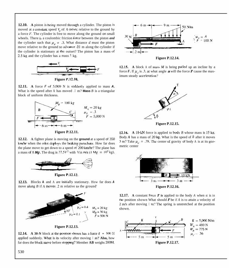
12.10. A piston is bcing moved through a cylinder. The piston is moved at a canstant speed y, ol .6 mlsec relative to the ground hy a force F, The cylinder is free to move along the ground on small
the cylinder such that p,j = .3. What distance d must the piston move relative to the ground to advancc .01 m along the cylinder if the cylinder is stationary at thc outset? The piston has a mass of 2.5 kg and the cylinder has a mass 5 kg.
wheels. There is a coulombic friction fbrce between the piston and 30 i ILd = .4 ', F - IOON
Figure P.12.14.
12.15 A block A of niass M is heing pullcd up an incline by a force F. If p,j is 3, at what angle a will the force F cause the max- imum steady accrlrrafirm'?
Figure P.12.10.
12.11. A force F of 5,000 N is suddcnly applied to mass A. What is the speed after A has moved . I m? Mass B is a triangular block of uniform thickness.
&f4 = 20 kg +d = .3 F = 5,000 N
Figure P.12.15.
Figure P.12.11. 12.16. A IO-kN force is applied to hody B whose mass is 15 kg. .. Body A has a mass of 20 kg. What is the speed of B after it moves 3 m? Take p(, = .2X. The center uf gravity of body A is at its geo-
12.12. A fighter plane is moving on the ground at a speed of 350 k d h r when the oilot deolovs the brakine oarachutc. How far does
metric center L I - I
the plane move to get down to a speed of 200 km/hr'! The plane has a mass of 8 Mg. The drag is 27.SV2 with Vin m/s ( 1 A4g = IO'kg).
12.13. move dung B if A moves .2 m relative 10 the ground'
Blocks A and A are initially stationary. How far does A Figure P.12.16.
12.17. A constant fnrcc F is applied to the hody A when 11 is in thc position shown What should F be if A is to attain a velocity of 2 mli after moving I m'! The spring is unstretched at the position shown.
v ,A K = 5,000 Nlm I , .' K
W, = 480 N Figure P.12.13. x IiL = 775 N
12.14. A 30-N block at lhe vmition \how" ha* a furce t = Io0 N u , = 36 applied suddenly. what is i t q velocity after moving I m? Also, how far does the block move before st~pplllg? Member AB weighs 200M.
530
Figure P.12.17.

12.18. Two slow moving steam roller vehicles are moving in opposite directions on a straight path. They start at A and B at the time f = ,O. How far from point A do they pass each other? What are their speeds when this happens? [Hint: Show that the time for this is 1.5 hours.] Note f is in hours.
Force
L 22,695 km ~
r - A ' A VB 8
Time 5 sec 10sec Figure P.12.21.
12.22. A body of mass I kg is acted on by a force as shown in the diagram. If the velocity of the body is zero at r = 0, what is V, = 6f i. q'?; + 3 kmlhr V, = 5 + t2" + 0.Sr"' kmihr
Figure P.12.18. the velbcity and distance traversed when r = 1 min? The force acts lor only 45 sec.
12.19. As you learned in chemistry, the cueficirnt ofviscosity g is a measure, roughly speaking, of the "stickiness" of a fluid. To measure this property for a highly viscous liquid-like oil, we let a small sphere of metal of radius R descend in a container of the liq- uid. From fluid mechanics, we know that a drag force will be developed from the oil given by the formula
Force
Time 10 sec 30sec 45 sec F = hnpVR
This relation is called Stoke's luw. The other forces acting on the sphere are its weight (take the density of the sphere as psp,,,j and the buoyant force, which is the weight of the oil displaced (take the density of the oil as poJ. The sphere will reach a constant velocity called the tenninul velocity denoted as VTerm,. Show that
Figure P.12.22.
12.23. Three coupled streetcars are moving down an incline at a speed of 20 k d h r when the brakes are applied for a panic stop. All the wheels lock except for car B, where due to a malfunction all the brakes on the front end of the car do not operate. How far does the system move and what are the forces in the couplings between the cars? Each streetcar weighs 220 kN and the coeffi- cient of dynamic friction gd between wheel and rail is 30. Weight is equally distributed on the wheels.
p = -- 9 "k" g R Z (Pspherc -Poi,)
12.20. A force F is applied to a system of light pulleys to pull body A. If F is 10 kN and A has a mass of 5,000 kg, what is the speed of A after 1 sec starting from rest'?
Figure P.12.23.
12.24. given by
A body having a mass of 30 Ibm is acted on by a force
F = 30tz + e-' Ib
If the velocity is 10 IVsec at r = 0, what is the body's velocity and the distance traveled when r = 2 sec?
12.25. A body of mass 10 kg is acted on by a force in the x direction, given by the relation F = 10 sin 61 N. If the body has a velocity of 3 d s e c when f = 0 and is at position x = 0 at that instant, what is the position reached by the body from the origin at f = 4 sec? Sketch the displacement-versus-time curve.
Figure P.12.20.
12.21. A force represented as shown acts on a body having a mass of I slug. What is the position and velocity at f = 30 sec if the body starts from rest at f = O?
531

12.26. A water skier is shown d a n g l i q from a kite that is towed via a light nylon cord by a powerboat at a constdnt speed of 30 mph. The powerhoat with passenger weighs 700 Ih and the man and kite together weigh 270 Ih. If we neglect the mass of the cable, we can take it as a straight line as shown in thc diaeram. The horizontal drag from the air on the kite plus man is estimatcd from fluid mechanics to he 80 Ih. What is the tension in the cahle'? If the cable suddenly snaps, what is the instantznerus hurimntal relative acceleration hetween the kite system and the powerhoar?
Figure P.12.26.
12.27. A mdSs M is held hy stiff light telescoping rods that can elongate or shorten Sreely hut cannot hcnd. Each rod is pin con- nected at the ends A , R . C. and 11. The system is o n a horimntal. frictionless surface. Two linear springs having spring constants K , = 880 N/m and K2 = 1,400 N/m are connected to the rods as shown in the diagram. If mass M = 3 kg is moved ,003 m to thr right and i s released from rest, what is the equation for the vcloc- ity in the x direction as a function of*'? What is the speed of the mass when it returns to the vertical position of the rods?
y
12.29. A hlock A of mdSS 500 kg is pulled by a force of 10,000 N as shown. A second block R of mass 200 kg rests on small fric- tionless rollers on top of block A. A wall prevents block B from moving 10 the left. What is the speed of hlock A after I sec start- ing from a stationary position? The coefficient of friction pd is .4 hetween A and the horizontal surface.
Figure P.12.29,
12.30. Block B weighing SOII N rests on block A, which weighs 300 N. The dynamic coefficient of friction hetween contact sur- faces i s .4. At wall C there are rollers whose friction we can neglect. What is the acceleration of body A when a force F of 5,000 N is applied?
K , = 880 Niin Kz = 1,400 Nlm M = l k g
Figure P.12.30.
12.31. A hndy A of mass I Ibm is forced to move by the device shown. What total force is exerted on the body at time f = 6 sec? What is the maximum total force on the body, and when is the first timc this force is developed aftzrr = O?
cos 2t ft/sec 1
Figure P.12.27,
12.28. A force given as 5 sin 3f Ib acts on a mas!, 01 I slug. What is the position of the mass at f = 10 sec'? Determine the total dis- tance traveled. Assume the motion started from rest.
532
21 ' fU%C
Figure P.12.31.

12.32. Do Problem 12.10 for the case where there is viscous friction between piston and cylinder given as 150 NImJsec of rela- tive speed. Also, what is the maximum distance 1 the piston can advance relative to the cylinder?
12.33. The high-speed aerodynamic drag on a car is .02V2 Ib with V in ftlsec. If the initial speed is 100 mihr, how far will the car move before its speed is reduced to 60 miihr? The mass of the car is 2.000 Ibm.
12.34. A block slides on a film of oil. The resistance to motion of the block is proportional to the speed of the block relative to the incline at the rate of 7.5 N/m/sec. If the block is released from rest, what is the rerminul sneed? What is the distance moved after I O sec?
1
0"
Figure P.12.34.
35. When you study fluid mechanics, you w the drag Don a hody when moving through a fluid with mass density p i s given as ?C#Vz A where Vis the velocity of the body rela- tive to the fluid A is the frontal area of the object: and C,, is the so-called coeficienr of drag usually determined by experiment.
A racing plane on landing is moving at a speed of 350 k d h r when a braking parachute is deployed. This parachute has a frontal area of 70 mz and a C, = I .2. The plane has a frontal area of 20 m2 and a C,, = 0.4. If the plane and parachute have a com- bined mass of 8 Mg, how long does it take to go from 350 kmhr to 200 kmhr by just coasting? Take p = 1.2475 kglm' and neglect rolling resistance from the tires. There is no wind.
I
12.37. Mass R is on small rollers and moves down the incline. It is connected to a linear spring, which at the position shown is stretched from its undeformed length of 2 m to a length of 5 m. What is the speed of R after it moves 1 m? Use Newton's law as well as the x coordinate shown in the diagram.
MA = 40 kg M B = 20 kg pd= .2 lo = 2 m (""stretched length of spcing) K = 20 N/m
Figure P.12.37.
am th 12.38. A wedge of wood having a specific gravity of 0.6 i s forced into the water by a 150-lb force. The wedge is 2 ft in width.
(a) What is the depth d? (h) What is the speed of the wedge when it has moved
upward 0.48 ft after releasing the 150-lb force assuming the wedge does not turn as it rises? Recall, a buoyant force equals the weight of the volume displaced (Archimedes).
Figure P.12.35.
12.36. In the previous problem, what is the largest frontal area of the braking parachute if the maximum deceleration of the plane is to be 58's when at a speed of 350 k d s the parachute is first deployed?
X
wI
w - Y
Figure P.12.38.
533
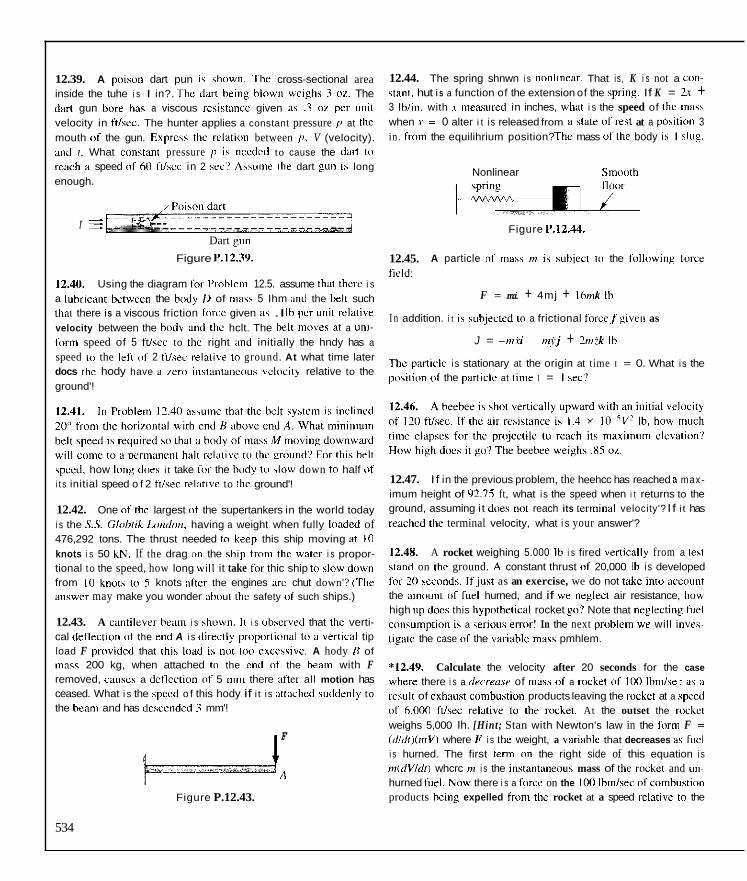
12.39. A poistm dart pun i c chrwn. The cross-sectional area inside the tuhe i s I in?. Thc dart heing hlown wcighs 3 IM The dart gun how haq a viscous icsistilnce given LIE .1 WL pcr (init velocity in ftlszc. The hunter applies a constant pressure p at the mouth if the gun. Exprc\q the d a t i o n between p, V (velocity). ;md f. What cirnstmt pressure p i\ nccdcd to cause the dart tu rcach a speed of hO ftlscc in 2 xc ' ! Aswine Ihe dart pun i\ long enough.
- I' Dart gun
12.44. The spring shnwn i s nrmlmcar. That is , K i s not a COII-
stant. hut i s a function of the extension of the qpring. If K = 2r + 3 Ihlin. with ~I ineastired in inches, wh;e i s the speed of the m a ~ s when x = 0 alter i t i s released from B state of rest at a poaition 3 in. firom the equilihrium position? Thc mass olthe body i h I slug.
Nonlinear Smooth
Figure F.12.44.
Figure P.12.3Y. 12.45. f irld:
A particle nf mass m i c suhiect tu the following furce
12.40. Using the diagram for Pnrhlem 12.5. assume that there i s a luhricant hctwcen the body I ) of maw 5 Ihm and the hclt such F = mi + 4mj + lhmk Ih
I n addition. i t i s suhlectcd to a frictional frxcc f givcn as thnl there is a viscous friction Iurce given a~ .I Ih pcr unit izlativr velocity between the hodv and the hclt. The helt moves at a uni- form speed of 5 ftlscc to thc right m d initially the hndy has a J = -mi i - myj + 2 r n 3 Ih speed to the lcft of 2 il/ec relatiw to ground. At what time later docs thc hody have a iero in\lanlaneous vclrrcity relative to the ground'!
Thc particle i s stationary at the origin at time I = 0. What i s the podion of the particlc at time I = I SCC?
cpeed. how long docs i t take lor the hody to \low down to half of i t s initial speed o f 2 ftlsec r e l a t i w to the ground'!
12.42. One of thc largest (rt the supertankers in the world today i s the S.S. Clohfik Londo,r. having a weight when fully laaded of 476,292 tons. The thrust needed to keep this ship moving iit I O knots i s 50 kN. If the drag on the ?hip from thc watcr i s propor- tional to the speed, how long w'i l l it take for thic ship to slow down from I O knots IO 5 knots :~ller the engines arc chut down'? (Thr ans~e r may make you wonder nhmt thc safety of such ships.)
12.43. A cantilwcr heam i s shrwn. I t i s ohmved that thc verti- cal detlection of the rnd A i s dircctly pnprt ioni t l 10 I I vertical tip load F provided that thih load i s no1 too exce\\ive. A hody H of inass 200 kg, when attached t i l the end of the heam with F removed, C ~ U S C S a dcilcction of 5 inni there after all motion has ceased. What i s the spccd o f this hody if i t i s attachcd suddcnly to the heam and has dcsccnded 3 mm'!
F
A
Figure P.12.43.
534
12.47. I f in the previous problem, the heehcc has reached a max- imum height of 92.75 ft, what i s the speed when i t returns to the ground, assuming i t docs !not reach its teimiiial velocity'? I f i t has ieachcd thc terminal velocity, what i s your answer'?
12.48. A rocket weighing 5.000 Ih i s fired venically from a te\t Eland on thc ground. A constant thrust of 20,000 Ib i s developed for 20 scconds. l f j us t as an exercise, we do not tdke intu account the amount of fucl hurned, and if wc ncglect air resistance, h i w high up does this hypothctical rocket g a ? Note that neglecting luel conrumption i \ a ceiious error! In the next prohlem WE will inves- tigaie the case of the variahle mas? pmhlem.
*12.49. Calculate the velocity after 20 seconds for the case whcrc there i s a rlrrrm.sr of mass of a rocket of 100 Ihmlsc result of cxhaust combustion products leaving the rocket at a spzed of 6,IH)O ft/sec iclativr t i l thr rockzt. At the outset the mckct weighs 5,000 Ih. [Hint; Stan with Newton's law in the form F = (d1dI)fmV) where F i s the weight, a vziriahla that decreases as fiiel i s hurned. The first term o n the right side of this equation i s m(dV1dl) whcrc m i s the instantaneous mass of thc rockct and u n ~ hurned fuel. Now there i s a fmcc on the IO(1 Ihmlsec ofcomhustion products heing expelled from the rocket at a speed relativc to the

rocket of 6,000 ft/sec. The rate of change of linear momentum associated with this force clearly must be- (dm/dt)(6,M)o). The reaction to this force for this momenNm change is on the rocket in the direccion of flight of the rocket and must he added to m(dV/dt). The force exerted by the exhaust gases on the rocket is a propul- sive force and is called the thrust of the rocket. Again, neglect drag of the atmosphere since it will be small at the outset because of low velocity and small later because of the thinness of the atmosphere,]
12.50. We start with a cylindrical tank with diameter 50 ft con- taining water up to a depth of 10 ft. Initially the solid movable cylindrical piston A having a diameter of 20 ft and a centerline colinear with the centerline of the tank is positioned so that its top is flush with the bottom of the tank. Now the cylinder is moved upward so that the following data apply at the instant of interest assuming the free surface of the water remains flat:
4 = 2 f t & = 5 ft/sec i;z = 3 ft/sec2
What is the external force from the ground support on the water needed for this condition not including the force required to sup- port the dead weight of the water?
Figure P.12.50.
12.51. A sleeve slides downward along a pipe on which there is dry friction with pd = .35. A wire having a constant tension of 80 N is attached to the sleeve and moves with it always retaining the same angle a with the horizontal. If the sleeve weighs 60 N, what should a be for the sleeve to move for I O seconds before stopping after starting downward with an initial speed of 5 d s ?
12.52. An electron having a charge of -e coulombs is moving between two parallel plates in a vacuum with an impressed voltage E. If at t = 0, the electron has a velocity V, at an angle a. with the horizontal in the q plane, what will be the trajectory equation tak- ing the initial conditions to be at the origin ofxy? Show that
+ x t a n a o y = - + eE x2 2m (vo c o ~ a , ) ~
where m is the mass of the electron. Note we have neglected grav- ity here since it is very small compared with the electrostatic force.
Y
_r - acuum - -
Figure P.12.52.
12.53. A system of light pulleys and inextensible wire connects bodies A, B, and C a s shown. If the coefficient of friction between C and the support is .4, what is the acceleration of each body? Take 4 as 100 kg, MB as 300 kg, and h& as 80 kg.
Figure P.12.51.
I Y
Figure P.12.53.
535

536 CIIAPTER 12 PARTICI.K IIYNAMICS
Part B: Cylindrical Coordinates: Central Force Motion
12.5 Newton's Law for Cylindrical Coordinates
In cylindrical coordinates we caii cxpress Newton's law as follows:
I;_ = ,n(l+ ~ 7 0 2 )
F" = m(T4 ~ 2 i 6 ~ I: =
If the motion is known. i t is a simple iniitter lo ascertain tlic lorce coni- ponents using Eqs. 12.15. Thc inverse prohlcni of determining the inotion given the forces is particulai-ly difficult i n this casc. The reason lor this diffi- culty, a s you may havc alrcady learned in your differential equations course. is that Eqs. 12.15a and 12.15b iirc I I , I I I / ~ I W O ~ " fcir all lorce fnnctions. For this reason, we cannot present integration proccdures as in Part A of this chapter. The following example will sene t o illustrate the kind of prihlem we are able to solve with the methods thus far presented in t h i h chapter.
Example 12.8
A platform shown in Fig. 12.13 has a constant angular velocity coequal to
5 radlsec. A mass L( of 2 kg slides in a frictionless chute attached to the plaU'orm. .The mass is connected via a light inextensible cahle to a linear spring having a spring constant K of 20 Nlm. A swivel connector at A allows the cable to turn freely relative to the spring. The spring is un- stretched when the mass B is at the center ('of the plalltirm. If the mass B is releascd at I = 200 m m from il stationary position relative to the pia- form, what i s its speed relative to the platform when it has movcd Lo posi- tion r = 400 min'? What is the transverse force on the hody B at this position'!
We have hcrc a coplanar motion for which cylindrical coordinates iirc iniist useful. Because the motion is coplanar. we can use r instead of T with no ambiguity. Applying Eq. 12.151 first, we have
-20r = 2 ( r - 2 5 r ) Figure 12.13. Slider on mvaiing platform. j

SECTION 12 5 NEWTON'S LAW FOR CYLINDRICAL COORDINATES 531
I Example 12.8 (continued)
Therefore,
r = 15r (a)
As in Example 12.5, we can replace i. so as to allow for a separation of variables.
Therefore,
Vr dV, = 15rdr
Integrating, we get
+ c, I - - 15r2 2 2
To determine C,. note that, when r = .20m, = 0. Hence,
600 cl =-2
Equation (b) then becomes
V j = 15rZ ~ ,600 ( C )
When r = .40 m, we get for VF from Eq. (c):
v, = 1.
This is the desired velocity relative to the platform.
known data into the equation, we have To get the transverse force G, go to Eq. 12.15b. Substituting the
Fs = 2[(.40)(0) + (2)(1.342)(5)]
F, = 26.W.N'
This is the transverse force on the mass B.
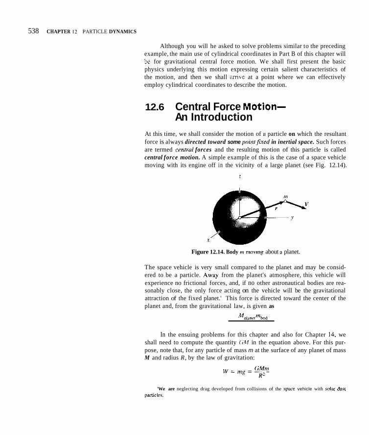
538 CHAPTER 12 PARTICLE DYNAMICS
Although you will he asked to solve problems similar to the preceding example, the main use of cylindrical coordinates in Part B of this chapter will be for gravitational central force motion. We shall first present the basic physics underlying this motion expressing certain salient characteristics of the motion, and then we shall amve at a point where we can effectively employ cylindrical coordinates to describe the motion.
12.6 Central Force Motion- An Introduction
At this time, we shall consider the motion of a particle on which the resultant force is always directed toward some point.fired in inertial space. Such forces are termed centrul forces and the resulting motion of this particle is called central force motion. A simple example of this is the case of a space vehicle moving with its engine off in the vicinity of a large planet (see Fig. 12.14).
i
Figure 12.14. Body m rnovins about B planet.
The space vehicle is very small compared to the planet and may be consid- ered to be a particle. Away from the planet's atmosphere, this vehicle will experience no frictional forces, and, if no other astronautical bodies are rea- sonably close, the only force acting on the vehicle will be the gravitational attraction of the fixed planet.' This force is directed toward the center of the planet and, from the gravitational law, is given as
In the ensuing problems for this chapter and also for Chapter 14, we shall need to compute the quantity GM in the equation above. For this pur- pose, note that, for any particle of mass m at the surface of any planet of mass M and radius R, by the law of gravitation:
'We are neglecting drag developed from collisions of the space vehicle with solar dwt partid.%.

SECTION 12.7 GRAVITATIONAL CENTRAL FORCE MOTION 539
where g is the acceleration of gravity at the surface of the planet. Solving for GM, we get
GM = gR2 (12.17)
Thus, knowing g and R for a planet, it is a simple matter tu find GM needed for orbit 'calculations around this planet.
As pointed out earlier, the motion of a space vehicle with power off is an important example of a central force motion-more precisely a gravitu- tionul cehtral force motion. The vehicle is usually launched from a planet and accelereFd to a high speed outside the planet's atmosphere by multistage rockets (8ee Fig. 12.15). The velocity at the final instant of powered flight is called the burnout velocity. After burnout, the vehicle undergoes gravitational central force motion. Depending on the position and velocity at burnout, the vehicle can go into an orbit around the earth (elliptic and circular orbits are possible), or i t can depart from the earth's influence on a parabolic or a hyperbolic trajectory In all cases, the motion must be coplanar.
J Space vehicle
Figure 12.15. Launching a space vehicle
In the following sections, we shall make a careful detailed study of gravitational central force trajectories. Those who do not have the time for such a detailed study of the trajectories can still make many useful and inter- esting calculations in Chapter 14 using energy and momentum methods that we shall soon undertake.
"12.7 Gravitational Central Force Motion d---
For gravitational central force motion, we shall employ an inertial reference q in the plane of the trajectory with the origin of the reference taken at the point P toward which the central force is directed (see Fig. 12.16). We shall use cylindrical coordinates r a n d 9for describing the motion. Because z = 0 at all times, these coordinates are also called polar coordinates. Since the mo- tion is coplanar in plane xy, we can delete the overbar used previously for r with no danger of ambiguity.
Figure 12.16. xy is ineltial reference in plane of the trajectory.

540 ('HAPIER 12 I'AKTICI F DYNAMICS
Imt us consider Nrwron's Iuw for ii body of m i s s in, which i s moving near a star OS m a s s M:
(12.18) dV - -(; ~~~~~ Min dl r 2
Canceling m and using cylindrical coordinates and componenls, we can ex- press the cquatiuti above in the following manner:
in -
( 12. I9 1
Since tr and i arc identical vecturs, the scalar equations o f the preceding cqua- tion become
GM r 2
(i' - r d 2 ) E , + i r 8 + 2r8)t , = -
r &2 = -GMIr? (12.20a)
,-B + 2i-8 = 0 (12.20hi
Equation 12.20b can he expressed in the lumi
1 ( r 2 8 ) = 0 (I 2.2 I ) Y dl
a h you can readily verify. We ciin conclude from Ey. 12.21 that . .
r 2 0 = constant = C (12.22)
Equation 12.22 leads to an iniportant conclusion. To estahlish this, coli- sider the arca swept nut by r during a time dr, which in Fig. 12.17 i s the shaded
I &--- \
Figurc 12.17. Purriclc r w r r p UUI awn
area. By cnnsidcring Ihis area to hc tliiit OS a triaiigle, we can cxprcss i t as
Dividiiig through hy dr. we have
Now dAId1 i s the rate iit which area i s heing swept nut by r : i t i s called uiwril i .?lwit?. And, sincc $8 i s a cniistiint Sur each gravitational central force rnolion (see tk . 12.22). wc can conclude that the areal velocity i s a coi lmi i t
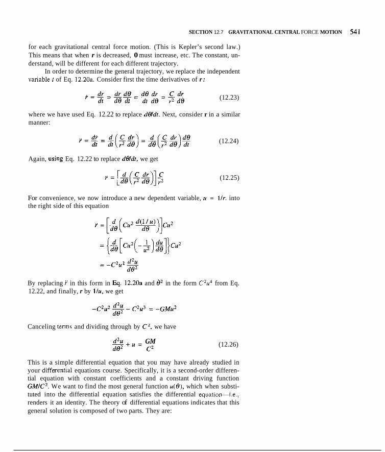
SECTION 12.7 GRAVITATIONAL CENTRAL FORCE MOTION 541
for each gravitational central force motion. (This is Kepler’s second law.) This means that when r is decreased, 0 must increase, etc. The constant, un- derstand, will be different for each different trajectory.
In order to determine the general trajectory, we replace the independent variable f of Eq. 12.20a. Consider first the time derivatives of r :
(12.23)
where we have used Eq. 12.22 to replace d0ldt. Next, consider r in a similar manner:
(12.24)
Again, wing Eq. 12.22 to replace dO/dt, we get
(12.25)
For convenience, we now introduce a new dependent variable, u = l / r , into the right side of this equation
By replacing i: in this form in Eq. 12.20a and e2 in the form C2u4 from Eq. 12.22, and finally, r by l/u, we get
Canceling terms and dividing through by C 2 , we have
GM C2
(12.26)
This is a simple differential equation that you may have already studied in your diffqrential equations course. Specifically, it is a second-order differen- tial equation with constant coefficients and a constant driving function GMIC2. We want to find the most general function .(e), which when substi- tuted into the differential equation satisfies the differential equation-i.e., renders it an identity. The theory of differential equations indicates that this general solution is composed of two parts. They are:

542 CHAPTER 12 PARrlCLE DYNAMICS
I . The general solution of the diffcrrntial equation with the right side of the differcntial equation set equal tu 7e1-(I and hence given a s
This solution is called thc ~ n i n ~ i l e i n ~ ~ r i l u t ~ ~ (or l i o ~ r r ~ i , g ~ ~ r r o u s ) solution, u,
2. An? solution u,, that satisfies the fiill differential cquation. This part is called
The desired general solution is then the sum of thc cornplcmentary and par- ticular solutions. I t is a simple matter to show by substitution that the functiun A sin e wtisfies Eq. 12.27 for any value of A . This is similarly truc for H cos 0 fcir any value of 8. 'The theory 01 differential equations tells u s that therc arc two independcnt functions lor thc solutiun ul' Eq. 12.27. The general comple- mentary solution is then
thc purtir.alur .solutio~i.
1 1 , = A sin e + Hcos e (12.28)
where A and B arc arbitrary constants (I!' integration. Considering the full differential equation (Eq. 12.26). we sec by inspection that a particular solution is
The general solutinn to the differential equation (Eq. 12.26) is then
By simple trigonoinetiic considerations. we can put the complementary solution in the equivalent form, D cos ( 0 ~ f i ) . where I1 and /3 are then the constilnts of integralion.' Wc then have as an alternative fiir~nulation fo ru (= 1/19:
You may possibly recognize this equation as the general conic equutiun i n polar coordinates with the focus at Ihe origin. In your iinalytic geo-

SECTION 12.7 GRAVITATIONAL CENTRAL FORCE MOTION 543
J x 2 +).z S P P p + ? 2
Dtb Simple algebraic manipulation permits us to put the preceding equation into the following form:
(I - . ')x2 + yz + 2pr 'x - czp2 = 0 (12.36)
If c > I , the coefficients of xz and y2 are different in sign and unequal in value. The equa-
If c = I , only one of the squared terms remains and we have aparnhola. If c < I, the coefficients of the squared terms are unequal but have the same sign. The
C . x
tion then represents a hyperbola
curve is that of an ellipse
metry class, you probably saw the following form for the general conic e q ~ a t i o n . ~
1 1 1 ' q P - = - + -cos(@ - p, (12.37)
where E is the eccentricity, p is the distance from the focus to the directrix, and pis the angle between the x axis and the axis of symmetry of the conic section.
I Comparing Eqs. 12.31 and 12.37, we see that
(1238a) P=o
DC2 E = - GM (1 2.3%)
'A conic section is the locus of all points whose distance from a f i edpo in l has a consmnl rnlio to the distance from a fued line. The fixed point is called the/ocus (or focal point) and the line is termed the direcfrir. In Fig. 12.18 we have shown paint P, a directrix DD, and a focus 0. For a conic Section to be traced by P, it must move in a manner that keeps the ratio rim, called the rccenfricify, a fixed number. Clearly, for every acceptable position P, there will be a mirror image position P (see the diagram) about a line normal to the directrix and going through the focal point 0. Thus, the conic section will be symmetrical about axis OC.
r \ P
Focus \ \ \ \
r \ \ D Pp ------------------&p' X
D
C Using the letter c to represent the eccentricity, we can say: (12.32)
where p is the distance from the focus to the directrix. Replacing cos q by --cos (e - p), where 0 (see Fig. 12.18) is the angle between the x axis and the axis of symmetry, we then get
= c (12.33)
Now. rearrangins the terms in the eauation. we anive at a standard formulation far conic sections:
I - _ - m - € = p + ,cos
- rcas(e - p ) Directrix
Figure 12.18. rlw = E E constant for conic (12.34) section.

544 WAPTliK 12 P,\KTICI.I DYNAMIC'S
From our knowledge if conic sections. we can then iay that i f
x
\ . '.. Figui :e 12.20. Launching at axis of symmetry.
1": > 1. the trajectiiry i h ii hypcrhola (12.3%) GM
~~ 'Ic' = I, the trajectory i s a piirahiilii GM
~~ I"' ~ < I. the trajectiiry ih an ellip\e GM
(l2.39h)
( I 2 . 3 9 ~ )
Fb = 0. the trajectory i s a circle (12.3YlI)
Clearly, L)CWM, ~ I i c ecccnwicitj. i\ :in exlrcniely iinportant quanlity. Wc shall next look into the practical applications of the preceding fcrieral theory to prohlems in space niechii i i ics.
"12.8 Applications to Space Mechanics We sliull i iow employ the theory scl rorth in the previous section to study Ihe motion o f space vchicles--a prohlciii of great present-day interest. We shall assume that at the end of powcred flight the puhition r,) ;mil velocity I;; of the vehicle are known from rocket calculaliotis. The reference cmploycd wi l l he an inertial relcrence at the ceiitcr of the planet and s o the reference wi l l Irans- late with the planet relative tu the "fixed stars." Accordingly. the earth hill rotate one cycle per day for such a reference. We know that the trajectory of the hody wi l l l h i ii plme fixed in iriertiitl space and so, forci~nreniencc. we take the .r? plane of lhc relerence to he the plane of thc trajectory. I t i s the usual practice to chixist. the .x axis to hc the axis of cymmctry for the tra,jec- tory. If there i s a zt'ro rodid vrlociry component at "hurnout," then the launching clearly occurs at a position along the ax is of symmetry o f the tra- jectory (i.e., along the .r axis). This ciise l ias hcen shown in Fig. 11.20. wherein the suhscript 0 denotes launch d;ita. If. on thc other hand, a ]radial component (v),, i s present at hurnouc. then the launch condition occurs ill
somc piisition O,, from the .x axis. as shown i n Fig. 12.21. We generally do not know e,, a priori, since its value depends un the cqu;itioii of thc trajectory. Finally, the angle n s h o k n in the diagram wi l l he called the l i i i r n d ~ i n j i L i i i , y I e in the ensuing discussion.
Since the .r axis has heen chosen to he the ax is of symmetry. the q u a - t ion of motion of the vehicle aflcr powercd Ilight i s given in lcrnis of x h i - Irary conslants C and D hy Eq. 12.31 with the anglc set equal to zero.
\ Thus. we have \ . '\
1 = + Dco,H (12.401 '. Figure 12.21. Burnout with radial velocity r (-2
present.

StCTION I2 8 AI’PLICATIONS TO SPACE MECHANIC.\ 545
The problem is to find the constants C and D from launching data. We shall illustrate this step in the examples following this section. Note that when these constants are evaluated, the value of the eccentricity E = DC2/CM is then available so that we can state immediately the general characteristics of the trajectory.
Furthermore, if the vehicle goes into orbit, we can readily compute the orbital time z for one cycle around a planet. We know from the theory that the aerial velocity is constant and given as
But r%equals the constant C in accordance with Eq. 12.22. Hence,
(1 2.42) c dA = - dt 2
The area swept out for one cycle is the area of an ellipse given as nub, where u and b are the semimajor and semiminor diameters of the ellipse, respec- tively. Hence, we have on integrating Eq. 12.42:
Therefore,
2nab C
z = -~
We have shown in Appendix I11 thar
a =- EP I - $
b = u(l - € * ) ‘ I 2
Replacing p by 1/11 in accordance with Eq. 12.38a, we then get
(12.43)
(12.44~1)
(12.44h)
(12.45a)
( I 2.45b)
Thus, we can get the orbital time T quite easily once the constants of the trajectory, D and C, are evaluated.

54h C'HAP'JER 12 PAKrlCI,F. UYNAMICS
To illustrate many of the previous general remarks in a most simple manner, we now examine the special case where, a s shown in Fig 12.22, var- ious launching.; ii.c., burnout conditions) are made from a given point a such that the launching angle a = 0. Clearly ( V ) , , = 0 f(ir these cases and the launching axis corresponds to the axis of symmetry (if the various trajectories. Only v, will be varied in this discussioii.
.x 3 \
I I
Figure 12.22. Various laurrchinys liom the earth or some other planer.
The c~~is ta i i t s C and U arc readily available for thesc trajectories. Thus. we have from Eq. 12.22:
C = r ? @ = r V H - - r 11 v n (12.46)
And Sroni ELI. 12.40. setting r = q) when I3 = e,, = 0. we gct, on solving for 0:
(I 2.47)
Since C and I1 ahove, for a given ro. depend only on V,,, we conclude that the eccentricity here is dependent only on C;, lor a given ro.
If V,, is so large that DCZ/GM exceeds unity, the vehicle will have the trajcctory 111 a hyperbola (curve I ) and will eventually leavc the intluence of the earth. If V,, is decreased to a valuc such that the eccentricity is unity. the trajcctory becorncs a parabola (curve 2 ) . Sincc a further decrease in the value of yl will cause the vehicle tu orbit. curve 2 is the limiting trajectory with our launching conditions for outer-space night. The launching velocity for this case is accordingly called the rscapr ~elocir\ and is denoted as We can

SECTION 12.8 APPLICATIONS 1'0 SPACE MECHANICS 547
solve for ( y J E for this launching by substituting for C and D from Eqs. 12.46 and 12.47 into the equation DC21GM = I . We get
(12.48)
a result that is correct for more general launching conditions (i,e., for cases where launching angle a # 0). Thus, launching a vehicle with a speed equal- ing or exceeding the value above for a given r,, will cause the vehicle to leave the earth unti l such time as the vehicle is influenced by other astronomical bodies or by its own propulsion system. If V, is less than the escape velocity, the vehicle will move in the trajectory of an ellipse (curve 3). The closest point to the earth is called perigee; the farthest point is called apogee. Clearly, these points lie along the axis of symmetry. Such an orbiting vehicle is often called a space satellite. (Kepler, in his famous first law of planetary motion, explained the motion of planets about the sun in this same manner.) One focus for the aforementioned conic curves is at the center of the planet. Another f o c u s , r now moves in from infinity for the satellite trajectories. As the launching speed is decreased,f' moves towardj When the foci coincide, the trajectory is clearly a circle and, as pointed out earlier (see Eq. 12.39d). the eccentricity E is zero. Accordingly, the constant D must be zero (the con- stant C clearly will not be zero) and, from 9. 12.47, the speed for a circular orbit (l(JC is
For launching velocities less than the preceding value for a given ro, the eccentricity becomes negative and the focus f' moves to the left of the earth's center. Again, the trajectory is that of an ellipse (curve 5). However, the satel- lite will now come closer to the earth at position b, which now becomes the perigee, than at the launching position, which up to now had been the mini- mum distance from the earth." If friction is encountered, the satellite will slow up, spiral in toward the atmosphere, and either burn up or crash. If Vu is small enough, the satellite will not go into even a temporary orbit but will plummet to the earth (curve 6). However, for a reasonably accurate descrip- tion of this trajectory, we must consider friction from the earth's atmosphere. Since this type of force is a function of the velocity of the satellite and is not a central force, we cannot use the results here in such situations for other than approximate calculations.
"'Note that with Ihr positive I axis going through perigee, I i s minimum when 0 = 0. From Eq. 12.40. we can conclude for this case (0 is measured here from perigee) thil, to m i 6 miLe r. the conatam D mUSl be posilive. me eccentricity must then he positive for 0 measured from perigee. If the positive x axis goes through apogee, then r is marimurn when 0 = 0. From Eq. 12.40 we can conclude that D must be negative for this case (0 is here measured from apogee). Thus, the eccentricity is negative fof 0 measured from apogee. This is clearly the case for curve 5.

Example 12.9
The first American satcllile. the V a n p a r d . win launched at ii velocity 01
18.000 milhr at an altitude 01 400 mi (see Fig. 12.23). I I the "humout" velocity of the last stage is parallel to the earth's \iirface. compute t l ic inaximum iiltitudc from the a i - t h ' s surface that the Vanguard iatcllite will reach. Consider the earth to hc perfectly spherical with a radius O S 3.960 mi (ti) is therefore 4.360 mi).
Figure 12.23. 1.aunching 01 ilie V : i n p a r ~ l siitrllit~.
We muh t now compute thc quantitich GM, C. and D lrom thc initial data and other known data. To detcrmint. GM. we employ Eq. 12. I 7 and i n terms units of iiiilcs and hours wc get
= 1 .1 .3L j x [ ( I " inii/hr'
The ccinstmt C i \ readily dctcriiiincd directly froin initial data a:,
<' = q,y, = (4.3h0)~18.001))
= 7.85 x 10 'mi2/hr
Finally. the cimstaiit I1 i:, available Srom Eq. 12.47:
= .ZX~ x ((1 n i i ~ I
The eccentricity 1)C'IGM can nriu he computed iis
The Vanguard will thus definitely riot e x a p e in to outel- s p x z The tra,jectory 01. this n i v l j ~ u i is fiirnied from tk. 12.41:
__..x__I_ ..",, ..... -, . . .... . . . "___ .

SECTION 12.8 APPLICATIONS TO SPACE MECHANICS 549
I Example 12.9 (Continued)
Therefore,
( e ) I r ~ = 2.01 x i o 4 + ,283 x i o 4 case
We can compute the maximum distance from the eaith’s surface by setting 0 = Kin the equation above:
-~ I - (2.01 - ,283) X IO-‘ = 1.727 x 10” mi-’ rn,,
Therefore,
r- = 5,790 mi
By subtracting 3,960 mi from this result, we find that the highest point in the trajectory is 1,830 mi from the earth’s surface.
I Example 12.10
In Example 12.9, first compute the escape velocity and then the velocity for a dircular orbit at burnout.
Using Eq. 12.48, we have for the escape velocity:
2(1 239 X IO”)]”’ \ ‘il 4,360
(V& = 23,840 mi/hr
For a circular orbit, we have from Eq. 12.49:
(V& = E = 1 milhr
Thus, the Vanguard is almost in a circular orbit.

550 CllhPTER I ? PAKTICL.1: IDYNAMICS
Example 12.11
Determine the orhital time in Examplc 12.1) Sor the Viinguard siitellitc. Wc employ Eys. 12.44 for the semimajor and semiminor axe\ OS the
i elliptic orbit. Thus, recallinp t h a t l ~ = lill we have I
x 5,080 ini
/ I = dl - e l ) ’ / ? = 5,080(1 -,1408?)”’
Theretiire, from E q 12.43 wc have f o r the oi-hitiil time:
z = 2.05 hr = 122.7 min
Example 12.12
A space vehicle i \ in ii circular “parking” orhit around the pliinet Vcnus. 320 km ahovc the surtace o f thiq planet. The radius o f Venus i a 6.160 kin, and the escape velocity at the surticc i s 1.026 x IOi mlsec. A retro-rockct i s fired to a l i w the vehicle \n that i t w i l l cnine within 12 kin of the planet. If we consider that the rocket changes the speed d t h e vehicle w e r a com- paratively short distance ot its tmvcl, what i s this change of apeed? What i s the speed ofthe vehicle at i t s closest position tu the su r fxc of Venua’!
We show the vehicle in a circular parking nrhit i n Fig. 12.24. We shall considcr that the rctro-rocketa are fircd at position A SO as Lo estahlibh a new elliptic orhit with apogee at A and perigee at l j .
As e first step, we shell compute GM using the escape-velocity equa- tion 12.48. Thus, we havc
Thereforc,
,
Figure 12.24. Ch,ingc “1 orbit
= 4.20 x IO’? krn’ihr’

SECTION 12.8 APPLICATIONS TO SPACE MECHANICS 55 1
Example 12.12 (Continued)
The equation for the new elliptic orbit is given as
(a) - - ~ I - GM + Dcose r cZ
Note that when
e = 0, r = r,, = 6,480 km (h)
e = f f , r = r,,, = 6,192 km (C)
To determine the constant C, we subject Eq. (a) to the conditions (b) and (c). Thus,
1 4.20 x IO1* +
6,480 = c* 1 4.20 x IO'* - 6,192 = c2
Adding these equations, we eliminate D and can solve for C. Thus;
8.40 x loLz - ~ I 1 C* - 6,480'6,192
Therefore, C = 1.631 x 10⁸kmz/h~
Accordingly, for the new orbit,
r,V, = 1.631 x lo8
Therefore, V, = 25,168 km/hr
For the circular parking orbit the velocity y. is ~~~ #EM 14.20 x loLz vc= I - = j r, 1 6,480
= 25,458 km/h~
The change in velocity that the retro-rocket must induce is then
AV = 25,168 - 25,458 =
The velocity at the perigee at B is easily computed since
rBVB = C = 1.631 x IO8
Therefore, V, = (1 631 X 108)/6,192 =

Now le t us consider more general launching conditions where the launching angle a i \ not 7,ero (see Fig. 12.25. The canslant C is still eahily cvaluated (sce Eq. (12.46)) in tcnns of launching data as ro(K,)l,. To get D. we write Eq. 12.40 lor lauiichinf condition\. Tliur.
1
Figure 12.25. I.aunch witti d i a l \elr ici fy.
The value of 4, i\ not yet known. Thus. we have two unknown quantities in this equation, namcly I1 and qr Differentiating Eq. 12.40 with respect to time and siilving for r, we get
i = W 8 s i n H = DCsinH (12.51)
Noting Lhatk i s equal to ", and submitting the preceding equation to launching conditions. we then form a accond equation for the e\'aluation n l the unknown coiistiint\ D and 4,. Thus.
( y = DCsiii B,, ( I 2.52 1
Rearranging Eq. 12.50. we havc
I ~ w = ,g c<,\ e,, (12.51)
Divide both sides 01 Eq. 12.52 by C. Now. squaring Eqs. 12.52 and 12.53, adding terms, and using the lact tliat sin2 e,, + cos' Olj = I. we get for the constant Ll the result : I '
5) C?

SECTION 12.8 APPLICATIONS TO SPACE MECHANICS 553
Having taken the positive root for D, we note (see footnote #IO on page 545) that 0 is to be medwred from perigee. The eccentricity is
First, bringing C’ into the bracket and then replacing C by r0(V,), in the entire equation, we get the eccentricity conveniently in terms of launching data:
One can show, using the preceding formulations, that the equation for the escape velocity developed earlier, namely
is valid for any launching angle a. Remember that % in this equation is mea- sured from a reference xyz at the center of the planet translating in inertial space. The velocity attainable by a rocket system relative to the planet’s sur- face does not depend on the position of firing on the earth. but depends pri- marily on the rocket system and trajectory of flight. However, the velocity attainable by a rocket system relative to the aforementioned reference xyz di~es depend on the position of firing on the planet’s surface. This position, accordingly, is important in determining whether an escape velocity can be reached. The extreme situations of a launching at the equator and at the North Pole are shown in Fig. 12.26 and should clarify this point. Note that the motion of the planet’s surface adds to the final vehicle velocity at the equator. but that no such gain is achieved at the North Pole.
Figure 12.26. Launching at equator and North Pole.

554 CHAFTER 12 PARTICLE DYNAMICS
Example 12.13 Suppose that the Vanguard satellite in Example 12.9 is off course hy an angle a = 5" at the time of launching but otherwise has the same initial data. Determine whether the satellite giies into orbit. If so, determine the maximum and minimum distances from the earth's surface.
The initial data for thc launching are
7, = 4,360 mi, y, = 18,000 miihr
Hence,
(V,),, = (18.000)sinrx = (1X,OOO~(O.O872j
= 1.569 mi/hr
[V,j,, = ( lX.I l00)cosa = (IX,OOO)(O.Y96i
= 17,930 milhr
To determine whether we have an orbit, we would have to show first that the eccentricity E is less than unity. This condition would preclude the possibility of an escape from the earth. Furthermore. we must he sure that the perigee of the orbit is far enough from the carth's surface to ensure a reasonahly permanent orbit. Actually, for both questions we need only cdl- culate r for B = 0 and e = ?I. An infinite value of one of the r 's will mean that we have an escape condition, and a value not sufficiently large will mean il crash or a decaying orbit due to atmospheric friction.
Using the value of GM as 1.239 x 10" mi3/hrz from Example 12.9 and using Eq. 12.54 for the constant D, we can express the trajectory of the satellite (Eq. 12.40) as

SECTION 12.8 APPLICATIONS TO SPACE MECHANICS 555
Example 12.13 (Continued)
Therefore,
Set 0 = 0:
Hence,
I ~ = 2.03 x I O F 4 + 3.33 x IO-' cosomi-l (a)
= 20.3 x IO-' + 3.33 x lO-'mi-' 4)
r', , = 4 ni
Thus, after being launched at a position 400 mi above the earth's sur- face, the satellite comes within 270 & of the earth as a result of a 5" change in the launching angle. This satellite, therefore, must he launched almost parallel to the earth if it is to attain a reasonably per- manent orbit.
Now, setting 0 = n, we get
Hence,
'ma, = 5,893 mi
Obviously, the maximum dntance from the earth's burface is

54. A d w i c e uscd at amucemcnt parks cnnsists of a circular m that i s made to r e ~ o l v e ahout its :,xi\ 01 \ymmctry. People ~d up against the wall, as shown i n the diagram. Altcr rhc whole m has been hmught up to spccd, thc flooi~ i\ lowcrcd. What timum angular s p e d i s required to c n s ~ i i e that a p c ~ n n w ~ l l not
, dciwn the wal l when the tloor i s Iuwrred? ' lake pb = .3 .
Figure P.12.54
55. A t lywhccl is rotating at a s p e d 111 0, = IO radlceu and at this instant a rate n l changu o l spceil 0 of 5 rsdlsec'. A
m o i d at thi5 instnnt m w c s a valve toward the centerline i f t h c ,wheel at a speed 0 1 I .S imlrcc and i s decelerating at rhc rate 01 nlsec'. The \-alve haa il mils\ O S I kg and i c .3 t m f r o m the axis rotatian at the timc of interest. What i\ the total forur on thc ve'!
56.
I
Figure P.12.55.
:mica1 pendulum of Icngth 1 i s > w n The nadc tn rotate ill a constant angular spccd of wahoo axis. Compute the tension in the cord if thc pcndulum huh ha!
5
ueight W. What i s the distancc of thr plane otthc tra.jectrry of the hoh lrnrn thc support at o?
, ' I I
, , -. - _- Figure P.12.56.
12.57. A \haft AH mt:itcs 11 an angular velocity nf 100 rpm. A hody E of m a s IO kg can move without friction along rod CI) l ixcd to AI(. I l t h c hody E i\ to remain mtionary d a t i v e 10 ('1) at any position along CD. how mi is1 the spring cnnstant K vary'? The tlistancc 5, frum the a x i i i\ thc onstl-ctchcd length n f t h c spring.
- A
c
C
A -
> lO(1 rpm
__ Figure P.12.57.
12.58. A drvicc u m \ i s t \ 01 three m a l l miisics. thrzc wrightle\r mk. and ii linrilr y i n p with K = 200 N l m The system i s rot at^
trig in thc g v r n fixed configuration at :i conctant rpecd w = 10 rad/\ i n a lhorimntiil plme. 'The li>llowing data apply:
M, = 2 kg M,j = 3 kg
If thr spi~inp i\ \trctchcd h) an a m r u n t .(I25 m. dcterminc the total lurce components :sting o n thc miisr at ('and the tenqile force in mcmher /),4 [ I l i n i ('onwicr a single panicle. then a \y\tem 0 1 pmticIc\; I;\ and OH arc pin connec1ed.l
M,. = 2 kg

x-
, .' Figure P.12.58.
_--
12.59. In the preceding problem consider that member DA is welded to the sphere at A . Now, at the instant of interest, there is also an angular acceleration of the system having the value of .28 rad/sec* counterclockwise. What are the force components acting on panicle C. and what are the force components from rod AD acting on panicle A'? See hint given in the preceding problem.
12.60. A device called a flyhall governor is used to regulate the speed of such devices as steam engines and turbines. As the gov- ernor is made to rotate through a system of gears by the device to he controlled, the halls will attain a configuration given by the angle 6'. which is dependent on both the angular speed w of the governor and the force P acting on the collar hearing at A. The up- and-down mntion ofthe bearing at A in response to a change in w is then used to open or close a valve to regulate the speed of the device. Find the angular velocity required to maintain the config- uration of the flyhall governor for 8 = 30". Neglect friction.
Figure P.12.60.
12.61. A platform rotates at 2 radhec. A body C weighing 450 N rests on the platform and is connected by a flexible weightless cord In a mass weighing 225 N, which is prevented from swinging out by pan of the platform. For what range of values o fx will bod- ies C and B remain stationary relative to the platform? The static coefficient of friction fix a11 surfaces is .4.
wL,= .4 for 811 surfac
Figure P.12.61.
12.62. A particle moves under gravitational influence about a body M, the center of which can he taken as the origin of an iner- tial reference. The mass of the particle is 50 slugs. At time t, the particle is at il position 4,500 mi from the center of M with direc- tion cosines I = .5 , m = -3. n = ,707. The panicle is moving at a speed of 17,000 milhr along the direction E, = .Xi + .2j + .Shhk. What is the direction of the normal to the plane of the trajectory?
Figure P.12.62.
12.63. If the position of the particle in Problem 12.62 were to reach a distance of 4,300 mi from the center of hody M, what would the transverse velocity V, of the particle be?
551

12.64. is x r u , the trujectoq nmsl he that of a circle.
12.65. A satellite ha\ at m c t ime during its flight around thc caith a radial crrmpment 01 velocity 3.200 krnlhl- and a tlans\.cr\e cm~poneril 0 1 2h.XIO km/hr. I1 the s;ilrllitc i \ at a distanvc 01 7.040 krn frtmm tlic cciitzr 01 the eimrth. u'hal is i l \ arral velocity'!
12.66. Compute the c s u p e velocit) ;it :I pnsition X.000 In, f i r m the center of the sarlh. What q x c d i s needcd to inninlain il circw tar orhit at that di.;tance from the earth's center? Derive Ihc cqua~ tiaii for the speed riccdcd fur il circular orhit direclly from Neuston's law without ucing infill-malioo iibrrut ecccnlricilieh. ctc.
Use Eqs. 12.38h and 12.40 to show' that i f t h c eccentricity
z
I sonnection
Figure P.12.67.
i5X
Figure P.12.69.

12.72. Consider a satellite of mass m in a circular orbit around the earth at a radius R, from the center of the earth. Using the universal law of gravitation (Eq. 1.1 I ) with M as the mass of the eanh and using Newron's law in a direction normal to the path, show that
12.78. The satellite Hyperion about the planet Saturn has a motion with an eccentricity known to he ,1043. At its closest dis- tance from Saturn, Hyperion is 1.485 x IO6 km away (measured from center to center). What is the period of Hyperion about Sat- urn? The acceleration of zravitv of Saturn is 13.93 m/recz at its
" I - surface. The radius of Saturn is 57,600 km IGM "ctrc. = '- 4 Ro
12.79. Two satellite stations, each in a circular orbit around the earth, are shown. A small vehicle is shot out of the station at A tangential to the trajectory in order to "hit" station B when it is at a position E 120" from the x axis as shown in the diagram. What is the velocity of the vehicle relative to station A when it leaves? The circular orbits are 200 miles and 400 miles, respectively, from the earth's
for a circular orbit. Now at the earth's surface use the gravitational law again and the weight ,,f the body, to show that CM = gRE.ar,,, where y is the acceleration of gravity.
12.73. The acceleration of gravity on the planet Mars is about ,385 times the acceleration of gravity on earth, and the radius of Mars is about ,532 times that of the earth. What is the escape veloc- ity from Mars at a position 100 mi from the surface of the planet?
12.74. In 1971 Mariner 9 was placed in orbit around Mars with an eccentricity of .5. At the lowest point in the orbit. Mariner 9 is 320 km from the surface of Mars.
(a) Compute the maximum velocity of the space vehicle
(b) Compute the time of one cycle.
relative to the center of Mars.
Use the data in Problem 12.73 for Mars.
12.75. A man is in orbit around the earth in a space-shuttle vehi- cle. At his lowest possible position, he is moving with a speed of 18,500 mihr at an altitude of 200 mi. When he wants to come back to earth, he fires a retro-rocket straight ahead when he is at the aforementioned lowest position and slows himself down. If he wishes subsequently to get within SO mi from the earth's surface during the first cycle after firing his retro-rocket, what must his decrease in velocity be? (Neglect air resistance.)
12.76. The Pioneer 10 space vehicle approaches the planet Jupiter with a trajectory having an eccentricity of 3. The vehicle comes to within 1,000 mi of the surface of Jupiter. What is the speed of the vehicle at this instant? The acceleration of gravity of Jupiter is 90.79 ftlsec' at the surface and the radius is 43,400 mi.
12.77. If the moon has a motion about the earth that has an eccentricity of ,0549 and a period of 27.3 days, what is the closest distance of the moon to the earth in its trajectory?
x
Figure P.12.79.
12.80. In Problem 12.79, determine the total velocity of the vehicle as it arrives at E as seen by an observer in the satellite B. The values of C and D for the vehicle from Problem 12.79 are 7.292 x IO' m i 2 h and 7.373 x mi-', respectively.
12.81. The Viking I space probe is approaching Mars. When it is 80,650 km from the center of Mars, it has a speed of 16,130 kmihr with a component (V,) toward the center of Mars of 15,800 kmJhr. Does Viking I crash into Mars, go into orbit, or have one pass in the vicinity of Mars? If there is no crash, how close to Mars does it come? The acceleration of gravity on the surface of Mars is 4.13 m/sec2, and its radius is 3,400 km. Do not use formula for D as given by Eq. 12.54, but work from the trajectory equations.
559

12.83. 110 I'mhlcm 12.U2 u'i lh the i l i t l of Eq. 12.14.
12.85. Do Prohleni 12.84 wi th the aid of Eq. 12.54.
Figure l'.l2.87.
Figure P.12.88.

SECTION 12.9 NEWTON’S LAW FOR PATH VARIABLES 561
Part C: Path Variables
12.9 Newton’s Law for Path Variables We cm express Newton’s law lor path variables as follows:
<=m, d 2 s dt
(12.57a)
Notice that the second of these equations is always nonlinear, as discussed in Section 12.5.’’ This condition results from both the squared term and the radius of curvature R. It is therefore difficult to integrate this differential equa- tion. Accordingly, we shall be restricted to reasonably simple cases. We now illustrate the use of the preceding equations.
‘%quation 12.57a could also he nonlinear, depending on Lhe nillure of the function $.
Example 12.14
A portion of a roller coaster that one finds in an amusement park is shown in Fig. 12.27(a). The portion of the track shown is coplanar. The curve from A to the right on which the vehicle moves is that of a parabola, given as
( y - loop = loox (a)
v ,’ , , , , , , I / / I ’
1: n
x
n
P,
(a) (b) Figure 12.27. Roller coaster trajectory.

562 CHAPTER 12 PARTI(’1.E DYNAMICS
Example 12.14 (Continued)
with x and y in feet. If the train of cars is moving at a speed of 40 ft/sec when thc front car is 60 fl above the ground, what is the total normal force exerted hy a 200-1h occupant nf thc front car on the seat and floor of lhe car’!
Since we requirc only the force F normal to the path, we need only he concerned with u,~. Thus, we have
Wc can compute R from analytic geometry as follows:
wherein from Eq. (a) we have
d\ SO &=m
Substituting into Eq. ( c ) , we have
AI the p o w o n of intere\t. we get

SECTION 12.9 NEWTONS LAW FOR PATH VARlABLES 563
Example 12.14 (Continued)
Accordingly, we now have for y,, as required by Newton's law:
Nnte that I;; is the total force component normal to the trajectory needed on the occupant for maintaining his motion on the given trajectory. This force component comes from the action of gravity and the forces from the seat arid floor of the car. These forces have been shown in Fig. 12.27(h), where P, and pa re the normal and tangential force components from the car acting on the occupant. The resultant of this force system must, accord- ingly, have a component along n equal to 94.6 Ib. Thus,
-200 cos + P, = 94.6 (h)
To get p, nnle with the help of Eq. (d) that
Therefore.
/3 = 51.3"
Suhstituting into Eq. (h) and solving for P,. we get
9, = 200 COS SI .30 + 94.6
This is the force component from the vehicle onto the passenger. Tne reac- tion to this force is the force component from the passenger onto the vehicle.

564 CHAPTER I ? PARTICLE DYNAMICS
Part D: A System of Particles
12.10 The General Motion of a System of Particles
I.et us examine a system of n particles (Fig. 12.28) that has inlcractions between thc particles fiir which Newton '.s thit-d lobe of motion (action equals
Figure 12.28. Force\ on ith pairiclr of the system
reaction) applies. Newror~'.s srt.ond /ai?. for any particle (lcl us say thc ith par- ticle) is then
(12.58)
, * I
wherc4.;. is the force on particle i from particle j and is thus considered an internal force for the system of particles. Clearly. the,, = i term of thc suni- mation musf be deleted since tlic ith particle cilnnoi exert force iin itself. The force F, reprcscnts the resultant force on the ilh particle from the forccs < w c , i - nrrl to thc syslem of paniclcs.
If thehe equations are added for all n particlcs, we have
(12.59)
Carrying out the double summation and excluding terms with rcpeakd indexes, such as&,,&,. etc., we find that lor each term with any one set o f indexes there will he a term with Ihe reverse of thcse indexes present. For example. lor the force.(,, it lorcef2, will ex is^. Considering the ineming iifthe indexes. we see thatf.. andJ, represent action and reaction lorccs between a pair of particles. Thus, as a result of N e w o n ' s third I r r w . thc double summation i n Eq. 12.59 should add LIP t u zero. N<wtrn i '~ .srmrtd law lor a system iif paiticlcs then becomes:
,.I
I 2.60 1
where F now rcprehenls the vector sum of all the r,rtr,ruol forccs acting on all the panicles of the system.

SECTION 12. io THE GENERAL MOTION OF A SYSTEM OF PARTICLES 565
To make further useful simplifications, we use the first moment of mass of a system of n particles about a fixed point A in inertial space given as
first moment vector = C miri i=l
where 7 represents the position vector from the point A to the ith particle (Fig. 12.29). As explained in Chapter 8, we can find a position, called the
Figure 12.29. Center of mass of system
center of mass of the system, with position vector r,, where the entire mass of the system of particles can be concentrated to give the correct first moment. Thus,
Therefore,
(1 2.61)
Let us reconsider Newton's law using the center-of-mass concept. To do this, replace m,r( by Mr, in Eq. 12.60. Thus,
(12.62)
We see that the center ofmass of any aggregate ofparticles has a motion that can he computed by methodr already ser,forth, since fhis i.7 a problem involv- ing a single hypothetical particle of mass M . You will recall that we have alluded to this important relationship several times earlier to justify the use of the particle concept in the analysis of many dynamics problems. We must realize for such an undertaking that F is the total external force acting on all the particles.

566 CHAPTER 12 PARTlCLt DYNAMICS
Example 12.15
Three charged particles in a vacuum are shiiwn in Fig. 12.30. Particle I has a mass of 1W5 kg and a charge o f 4 x IO-' C (coulomhs) and i s at the origin at the instanl (if interest. Particlcs 2 and 3 each have a mass of 2 x 1 0 kg and a charge o f 5 x 10 C and are located. respectively, at the
rP? Figure 12.30. Char& particles in field E .
inslant of interest I ni d img they axis and 3 m along the : axis. An elec- tric field E given a s
E = 2.ti + 3 r j + 3(r + .?)k NIC ( a )
i s imposed from thc nutsidc. Compute: (a) the position [if the center 01 mass for the system. (h) the acceleration o f the center o f mass, and (c) the acceleratinn o f particle I
To get the position [if the ccnter of mass, we merely equate moments of the masses ahnut the origin with that of R particle having a mass equal to the sum o f masses of the system. Thus.
( I + 2 + 2 ) x IO ' r , = ( 2 x 10 i )j + ( 2 x 1Wi)3k
Therefore, rc = .4j + 1.2km (h)
To get the acceleration of the mass center. we must f ind the sum of the extrmal forccs acting on thc particles. Two cxternal forccs act on each particle: the force o f gravity and the electrostatic force from the external field. Recall from physics the1 this electrostatic force i s given as 4E, where 4 i s the charge on the particle. Hcnce, the total exlemal force for each par- ticle i s given a s Sollows:
Fl = -(9.X1)(11i~7)k + 0 N (C)
Fz =-(9,Xlj(2x 1 0 ~ ~ j k + ( 5 ~ 1 0 ~ ~ j ( 3 k ) N (d) F3 = -(9.81)(2 x ( e ) jk + (5 x I O s ) ( 9 j + 27k) N

SECTION 12.10 THE GENERAL MOTION OF A SYSTEM OF PARTICLES 561
Example 12.15 (Continued)
The sum of these forces FT is
F~ = 45 x i o - 5 j + 100.9 x 10⁻⁵k N (f)
Accordingly, we have for<:
.. rc = 45 x 10-5j + 100.9 x 10"k
s x 10-5
Finally, to get the acceleration of particle I , we must include the coulombic forces from particles 2 and 3. As you leamed in physics, this force is given between two particles a and b with charges q, and qb as fol- lows:
where P is the unit vector between the particles, and eo is the dielectric constant equal to 8.854 x lO~'* F/m (farads per meter) for a vacuum. Note that the coulombic force is repulsive between like charges. The total cou- lombic force 4 from particles 2 and 3 is
= - I S j - 2kN
The total force acting on particle 1 is then
( F ) - -(9.81)(10-5)k + 0 + (-18j - 2k) N (i) I T - , . , -- from from from
weight external l"f0rnal field field
Clearly, the internal field dominates here. Newton's law then gives us
-18j - 2k fl
10-5
We see here from Eqs. (g) and (j) that although the particles tend to "scramble" away from each other due to very strong internal coulombic forces, the center of mass accelerates slowly by comparison.

568 CHAPICK I 2 PAKllCLE DYNAMICS
Example 12.16
A young man i s standing in a canoe awaiting a young lady (Fig. 12.3 I) . The !man weigh:, 150 Ih. and, a s shown. i s positioncd ticiir the end of the canoe, which weighs 200 Ih. When the ynung lady appear:,, he quickly scramble:, forward to greet her, hut when hc has moved 20 fl 10 the f i r - ward end nf thc canoe. l ic finds (nnt having htudied mcclianich) that he cannot reach her. How far i s the tip of the ciinoc from the dock after our hem has made the 20-ft dash? The ciinoc is i n tin way ticd to the dock and there are no water currents. Neglect friction frnm (l ie water on the canoe.
Figure 12.31. Man in i.anor awaits hi, date.
The center o l i i ias' i ofthc inan plus the canoe cannot change posilioii during this action sincc there i s 110 iict external lorcc acting nn (hi:, hystem during this action. Hencc thc firht mnincnt of mass about a n y fixed posi- tion r n u b t rcmain constant during this action. I n Fig. 12.32 we have shnwn the man in the forward position and we choose the position at the tip of the dock to equate ~ i ~ o ~ i i c t i t of tilass iil the beginning <if the action and ,iu\t when the inan has moved the 20 fc. We then can say, noting that we arc denoting the unspecified distance hetween the tip of the canoc and the for- ward position o1'Lhe iiiaii as d as shown in Figs. 12.31 and 12.32.
Conccling terms where possible we then liiive
7511, = 7 0 0 0 . I R571 ft , . ._ ., . . . . ,. - .- , . . ..

12.90. A wamor of old is turning a sling in a vertical plane. A rock of mass ..3 kg is held ill the sling prior to releasing it against an enemy. What is the minimum speed u t o hold the rock in the sling?
with x and y in feet. A small one-passenger vehicle is designed to move along the catenary to facilitate repair and painting of the bridge. Consider that the vehicle moves at uniform speed of 10 ft/sec along the curve. If the vehicle and passenger have a com- bined mass of 250 Ibm, what is the force normal to the curve as a function of position x ?
F _
Figure P.12.90.
12.91. A car is traveling at a speed of 55 mi/hr along a banked highway having a radius of curvature of 500 ft. At what angle should the road he bdnked in order that a zero friction force is
Figure P.12.94.
needed for the car to go around this curve? 12.95. A rod CD rotates with shaft G-G at an angular speed u of 300 rpm. A sleeve A of mass 500 g slides on CD. If no friction is present between A and CI), what is the distances for no relative motion between A and CD?
12.92. A car weighing 20 kN is moving at a speed Vvf 60 k d r on a road having a vertical radius vf curvature of 200 m as shown. At the instant shown, what is the maximum deceleration possible from the brakes along the road for the vehicle if the coefficient of dynamic friction between tires and the road is .55?
200 ni
Figure P.12.92.
12.93. plane sinusoidal path given as
A particle moves at uniform speed of 1 d s e c along a
y = 5 sin l ix m G Figure P.12.95.
What is the pusition between x = 0 and x = 1 m for the maxi- mum fbrce normal to the curve? What is this force if the mass of the particle is I kg?
12.94. A catenary curve is formed by the cable of a suspension bridge. The equation of this curve relative to the axes shown can
12.96. In Problem 12.95. what is the range of values for S for which A will remain stationary relative to CD if there is coulom- hic friction hetween A and CD such that p,5 = .4?
12.97. A circular rod EB rotates at constant angular speed u of he given it\
y = 5 (e" + e-") = a cosh M
50 rpm. A Fleeve A of mass 2 Ibm slides on the circular rod. At what position B will sleeve A remain stationary relative to the rod ELI if there is no friction?
569

C Figure P.12.97.
12.98. In Problem 12.91 assume that thcre is coulombic friction between A and EB with p,$ = .3. Show that the minimum value of Ofor which the sleeve will remain stationary relative to the rod is 75.45".
12.99. time t = 0
The fbllowing data for a system of particles are given a1
M, = SO kg at position ( I , 1.3, -3) m
M2 = 25 kg at position (-.6, 1.3, -2.6) m
M3 = 5 kg at position (-2.6, 5.3, 1 ) m
The particles are acted an by the following respective external forces:
6 = 5Oj + l0rk N (particle 1 )
F2 = 50kN (particle 2)
F, = 5t2i N (particlc 3)
What is the velocity of M , relative to the mass center after 5 sec, assuming that at f = 0. thc particles are at rest?
*12.100. Given the following force field:
F = -2xi + 3j - zk lbislug
what is the force on any particle in the field per unit mass of the particle. If we havc two particles initially stationary in the field with position vcctors
r , = 3i + 2j ft
r2 = 4i - 2j + 4k ft
570
what is the velocity of each particle relative to the center of mass nf the system after 2 sec have elapsed'! Each particle has a weight of . I O L .
12.101, that maintain constant magnitude and direction at all times. If
A stationary uniform block of ice is acted on by forces
F; = (25,y)N
5 = (log) N
F? = (15g) N
what is the velocity ofthe center of mass ofthe block after 10 sec'! Neglect friction. The density OS ice is 56 Ihm/fti.
Figure P.12.101.
12.102, A space vehicle decelerates downward ( Z direction) at 1 ,h I3 kmlhrisec while moving in a translalory manner relative to inertial space. Inside the vehicle is a rod BC rotating in the plane of the paper at a rate of S O radisec relative to the vehicle. Two masses wtate at the rille of 20 radisec around BC on rod EF. The masses are cach 300 mm from C. Determine the force transmitted at C hetween BC and EF if the mass of each of the rotating bodies is 5 kg and the mass of rod EF is I kg. BC is in the vertical posi- tion at the time of interest. Neglect gravity.
Py I
X Figure P.12.102.

12.103. Two men climb aboard a barge at A to shift a load with the aid of a fork lift. The barge has a mass of 20,000 kg and is 10 m long. The load consists of four containers each with a mass of 1,300 kg and each having a length of 1 m. The men shift the con- tainers tv the opposite end of the barge, put the fork lift where they found it, and prepare to step off the barge at A , where they came on. If the barge has not been constrained and if we neglect water friction, currents, wind, and so on, how far has the barge shifted its position? The fork lift has a mass of 1,000 kg.
Figure P.12.103.
12.104. An astronaut on a space walk pulls a mass A of 100 kg toward him and shonens the distance d by 5 m. If the astronaut weighs 660 N on earth, how far does the mass A move from its original position? Neglect the mass of the cord.
Figure P.IZ.104.
12.105. Two identical adjacent tanks are each 10 ft long, 5 ft high, and 5 ft wide. Originally, the left tank is completely full of water while the right tank is empty. Water is pumped by an inter- nal pump from the left tank to the right tank. At the instant of interest, the rate of flow Q is 20 ft3/sec, whileQ is 5 ft3/sec2. What horizontal force on the tanks is needed at this instant from the foundation? Assume that the water surface in the tanks remains horizontal. The specific weight of water is 62.4 Iblft’.
I-- IO’ -1- 1 0 ’ 4
Figure P.12.105.
12.11 Closure In this chapter, we integrated Newton’s law for various coordinate systems. Also, with the aid of the mass center concept, we formulated Newton’s law for any aggregate of panicles. In the next two chapters, we shall present alter- native procedures for more efficient treatment of certain classes of dynamics problems for particles. You will note that, since the new concepts are all derived from Newton’s law, whatever problems can be solved by these new methods could also be solved by the methods we have already presented. A separate and thorough study of these topics is warranted by the gain in insight into dynamics and the greater facility in solving problems that can be achieved by examining these alternative methods and their accompanying concepts. As in this chapter, we will make certain generalizations applicable to any aggre- gate of particles.
57 1
-

12.106. mass 8 kg. A force F equal to 100 N pulls block A . The coefficient
A hlock A of mass 10 kg rests on a second block R of -"
of friction between A and A i s .S; between B and the ground. . I What is the speed of block A relative to block B in 0.1 sec if the system starts from rest?
Figure P.12.108.
12.109. A ipring requires a fiircr x2 N for a deilection UIX ~mm, where 1 is the deflection of the spring from the undeiurmcd georri- et?. Because the deflection i'i n a l propottimiil to .li to t h r Iirsi power, the spring is Cdkd a rLo,ilitieor spring. If a I(lO-kg hlock is suddenlv released on the undetnrmrd sormg. what i s the meed of ~~~~ ~ -. ~~ ~ , ~~
~~
Figure P.12.106. the block after il has descended I O mn'!
*12.107. A block B slides from A to F along a rectangular chute where there is coulombic friction on the faces of the chute. The coefficient of dynamic friction is .4. The bottom face of the chute is parallel to face EACF (a plane surface) and the other two faces are perpendicular to EACF. The body weighs 5 Ib. How long does it take R to go from A to F starting from rest'?
/'Z Figure P.12.107.
12.108. A tugboat is pushing a barge at a steady speed of X knots. The thrust from the tugboat needed for this motion is 800 Ih. The barge with load weighs I00 tons. If the wilier resisrancr 10
the barge is proportional to the speed of the barge. how l w p will it take the barge to slow to 5 knots after the tugboat ceascs to push? (Note: 1 knot equals 1.152 milhr.)
Figure P.12.109.
1Z.IJU. A horifontal platform is rotating at il coilstant angular speed 0 ot 5 radls. Fixed to the platiorni is a triclionlcw chute i n which two identical masses each of 2 kg are constrained hy a pair 01 lincar spring, cach 01 q x i n p conitant K = 250 Nlm. If the unstrctched length lo of rach o i thc qxings i b . I K m, \how that at ?teddy stiltc the anglc 0 must hilvc the value 36x7". Springs are fixed to the platform at A.
K = 250 Nlm
Figure P.12.110.
572

12.111. What is the velocity and altitude of a communications satellite that remains in the same position above the equator rela- tive to the earth's surface? I = ,215 m
D = 5 0 m m 12.112. A satellite is launched and attains a velocity of 19,000 o = 300rpm mihr relative to the center of the earth at a distance of 240 mi e = 45" from the earth's surface. The satellite has been guided into a path that is parallel to the earth's surface at burnout.
12.116. (read Problem 12.60 for details on how the governor works):
The following data are giveii for the flyhall governor
(a) What kind of trajectory will it have'? (h ) What is its farthest position from the earth's surface? (c) 11it is in orhit, compute the time it takes to go from the minimum point (perigee) to the maximum point (apo- gee) from the earth's sutiace. (d) What is the minimum escape velocity for this posi- tion of launching?
12.113. A rocket system is capable of giving a satellite a veloc- ity of 35,200 km/hr relative to the earth's surface at an elevation of 320 km above the earth's surface. What would be its maximum distance h from the surface of the earth if it were launched ( I ) from the North Pole region or (2) from the equator, utilizing the spin of the earth as an aid?
12.114. A space vehicle is to change frnm a circular parlang orbit 320 km above the surface of Venus to one that is 1,620 h above this surface. This motion will be accomplished by two fK-
P Figure P.12.116.
~
ings of the rocket system of the vehicle. The first firing causes the vehicle km above the surface of
achieve the desired circular orbit. What is the change in swed
attain an apogee that is What is the force P acting on frictionless collar A if each ball has a mass of I kg and we neglect the weight of all other moving members Of the system?
At this apogee, a second firing is accomplished so as -
demanded for each firing if the thmst is maintained in each instance over a small portion of the trajectory of the vehicle?
velocity at the surface is 1.026 x I O 4 mlsec2.
~2.117. A spy to observe the united states is put into a circular orbit about the North and South Poles. The satellite is to
surface of the earth for this satellite? Neglect friction. The radius Of Venus IS 6,160 km, and the escape make 10 (24 hr), What must he the distance from the
12.115. Weights A and B are held by light pulleys. If released from rest, what is the speed of each weight after 1 sec? Weight A is 10 Ib and weight B is 40 Ih.
N
S Figure P.12.115. Figure P.12.117.
513

12.118. A skylah i s in a circular w h i t ahout the earth at a dir- ance of 500 km a h w e the earth's surface. A space shuttle has .endezvoused with the skylab and now, wishing tu dcpart, dcoou- ,les and fires i ts rockets to move more slowly than thc skylah. I f he rockets are fircd vver il shon time interval, what should the .elalive speed between thc spdcc shuttle and skylah he at thc end ~f rocket fire if the space shuttle ir tu come as cluse as IO0 k m tu he earth's surface in auhxqurnt ballistic (rocket motoii off1 light'!
12.119. A space vehiclc is launched at a speed of 19,001) milhi dat ive to the earth's center at a position 250 mi ahwe the earth'\ iutiace. If the vehicle has a radial velocity component of 3 ,000 nilhr toward the earth's center, what is the eccentricity o i the t r a ~ ectory'! What i s the maximum elevation ahwe the earth's aurfcc a c h e d by the vehicle'? Do not usc Eq. 12.54.
12.120. A skier is moving down a hill at a speed of 30 milhr when he is at the position shown. I i the skicr weighs I X O Ih, what uta1 force do his skis exert 011 thc muw surikcr? Assumc that thc :oefficient of friction is . I . The hill Can hc taken a h a paldhdiu surface.
50' ___/ Figure P.12.120.
12.121. A submarine is moving at cunstant speed of 15 knuli ielow the surface of the ocean. The sub i s at the same time de- ,tending downward while remaining horimntal wnh an accelera- ion of , 0 2 3 ~ . In the submarine a tlyball gvvernor opcrates with weights having a mass each of 500g. Thc governor i s rotating with ipeed w of 5 r d s e c . If at time I. 0 = 30", 0 = .2 radlaec, and 0 = I rad/sec2, what i s the fwce developed on the upport of guver- lor system as a result solely of the mution iif the wcights at thia nstant?
i74
(h)
Figure 1'. 12.12 1
Figure 1'. 12.122.

12.123. at timet:
Three bodies have the following weights and positions 12.125. A small body M of mass 1 kg slides along a wire from A to B. There is coulombic friction between the mass M and the wire. The dynamic coefficient of friction is .4. How long does it take to go from A to B? W, = IOlb, x, = 6ft,
y , = 10 ft, ZI = 10 ft
W, = 5 Ib, x2 = 5 ft, y1 = 6 ft, z2 = 0
y., = -4 ft, zj = 0
W, = 8 Ib, x3 = 0,
Determine the position vector of the center of mass at time t . Determine the velwity of the center of mass if the bodies have the following velocities:
V, = 6i + 3jfUsec
V, = 1Oi - 3kftisec
V, = 6k ft/sec
Figure P.12.125.
z 12.126. ForM = I slug and K = 10 Ibhn., what is the speed at x = 1 in. if a force ot 5 Ib in the x direction is applied suddenly to the massspring system and then maintained constant? Neglect the mass of the spring and friction.
Y e
X w2
Figure P.12.123. X
Figure P.12.126.
12.127. A rod B of mass 500 kg rests on a block A of mass 50 kg. A force F of 10,ooO N is applied suddenly to block A at the position shown. If the coefficient of friction pd is .4 for all contact sutiaces, what is the speed ofA when it has moved 3 m to the end of the rod?
w3 /L;;. 12.124. the respective particles:
In Problem 12,123, the following external forces act on
6 = 6fi + 3 j - 1Ok Ih (particle 1)
F2 = l5i - 3 j l b (particle 2)
F,, = OIb (particle 3)
What is the acceleration of the center of mass, and what is its posi- tion after I O sec from that given initially? From Problem 12.123 at t = o
rc = 3.1% + 4.26j + 4.35k ft
V, = 4.7% + 1.304j + 1.435k ft/sec Figure P.12.127. I

12.128. A simply supported beam is shown You will learn in your course on strength of materials that a vertical furcc I applicd at the center cause.: a dellection 6at the center giveii a\
If a mdSS of 200 Ihm, fd\tened to the hsam at i t s midpoint. is sud- denly relcased. what will its speed hc when the dellrction i\ in.'! Neglect the mass of the heam. The lcngth of the ham, L. i s 20 i t . Young's modulus E is 30 x IO" psi. and the moment of incrtia 0 1 thc cross bection I i\ 20 in?.
W ( j Figure P. 12.13 I .
L
Figure P.12.128. MA = 101!kg M,# = KOks M , = 5Ohg
12.129. A piston is shown mainlaining air ill a pressure of X psi ahore thal of the almo.sphrre. I I the piston is all~iwrd 1,) ~ccslerale to the left, Whdl i s the speed of the piston a h it I ~ O Y C S 3 in.? Thc pis- ton assembly has a mass 01 3 lhin. Assume that the air rxpends ndi~ ahuticdly (i.e.. with no heat transfer). This meenh that :it al l times (,Vi = constant, where V i ? thc volume of the gas and k ib a coil- - stant which fa r air cquals I .4. Neglect the incrtiill elfects of the air I '
I Figure P.lZ.I.32.
f
Figure P.12.129.
.I., 100 kg M,, .~ 60 kg
t i . . I ~ f , 30' L.x
*12.130. In Example 12.6 assume that there are adiabatic expan- s i o n s and compressions of the gave, (i .c. . that = constant with k = 1.4). Compare thc 1esu1ts for thc speed of the piston. Explain why yuur result should bc higher or lmvw than h r the isothermal case.
12.131. Body A and hvdy B are connected hy an incxtenrihle curd as shown. If hoth bodies are released cimultanetiu\ly. what dislance do they move in i e c ? Take MA = 25 kg and Ma = 35 kg. The coefficient of friction p,, is .3.
f ~ 3.000 N
Figure P.12.133.

12.134. The system shown is released from rest. What distance does the body C drop in 2 sec? The cable is inextensible. The co- efficient of dynamic friction pd is .4 for contact surfaces of bodies A and A.
Figure P.12.134.
12.135. Do Problem 12.134 for the case where there ic viscou\ damping for the cmtact surfaces of bodies A and B given as .5V Ih, with V i n ftlsec.
12.136. Two biidies A and A are shown having masses of 40 kg and 30 kg, respectively. The cables are inextensible. Neglecting the inertia of the cable and pulleys at C and D, what is the speed of the block A I sec after the system has been released from rest'?
Figure P.12.137.
12.138. A car is moving at a constant speed of 65 kmlhr on i
road pan of which (A-R) is paraholic and part (if which (C-D is circular with a radius vf 3 kin. If the car has an anti-lock brak~ ing system and the static coefficient of friction LI, between the road and the tires is 0.6, what is the maximum deceleration posi- ble at the x = 2 km position and at the .x = I O km position'? The total vehicle weight is 12,000 N.
The dynamic coefficient of friction p,, for the contact surface of body A is 3. [Hint: From your earlier work in physics, recall that
I
I O km ,
pulley I ) is instantaneously rotating about point ( I and hence point c lnnves at a speed that is twice that of point h.]
2 k m Figure P.12.138.
12.139. A mass rrf 3 kg is moving along a vertically oriented parabolic rod whose equalion is? = 3.4~' . A linear spring with K = 550 Nim connects to the mass and is unstretched when the mass is at the bottom of the rod having an unstretched length & = I m. When the spring ccnterline is 30" from the vertical, a< shown i n the diagram, the mass is moving at 2.8 mls. At thih instant, what is the force component on the rnd directed normal tn the rod'!
I L 2 4r' .. ~
M - 3 k g K = sso N/,,, Figure P.12.136.
150 Ib, respectively. If released from rest, what are the respective 12.137.
speeds of the bodies after I sec? Neglect the weight of pulleys.
Bodies A , A, and C have weights, of 100 Ib, 200 Ih, and - -x
Figure P.12.139.
577

12.140. A heated cathode gives off electnins which are attracted to thc pusitivc anode. Some go through a s m d 1 hole and enter the parallel plales at an anglc with the hori/ontal o f a,, = 0 and a velcrcily of vr Dctrrrninc the horizontal and ve!iical motiorls of the declron inside the plates as a function of time. Letting r = /. find thc time that the clectron i s in the parallel plalc rcgion and then "blain thc exit vertical velucily. Assuming straight-line motion until the electrm~ hits thc screen. show that the vcnicill position of impact, assuming thc screen i s flat. i s
*12.141. A weightless cord supports two identical milh\es cauh o l weight W. The cord i s heing pulled at a constdnt speed y, by a force I.'. Formulate im equation for F ill terms of l{j, L, i. W, and h. Detmmine t for the filllowing condition\:
\{, = 2.2 nil\ W = $0 N
L = 3.3 111 I , = . I6 m
/ = .2h 111
Location of sinall hole
Figure P.12.140. Figure P.12.141.

Energy Methods for Particles
Part A Analysis for a Single Particle
13.1 Introduction In Chapter 12, we integrated the differential equation derived from Newton's law to yield velocity and position as functions of time. At this time, we shall present an alternative procedure, that of the method of energy, and we shall see that certain classes of problems can be more easily handled by this method in that we shall not need to integrate a differential equation.
To set forth the basic equation underlying this approach, we start with Newton's law for a particle moving relative to an inertial reference, as shown in Fig. 13.1. Thus,
d z r dt? dt
F = m - - mdV (13.1)
z
1
X
Multiply each side of this equation by dr as a dot product and integrate from r, to rr along the path of motion:
In the last integral, we multiplied and divided by dt, thus changing the var- able of integration to t . Since drldt = V. we then have
Figure 13.1. Particle moving relative to an inertial reference.
519

580 CHAPTER I3 ENERGY METHODS FOR PART1CLb.S
On carrying out the integration, we arrive at the familiar equation
(I 3.2)
where the left side i s the well-known expression for work (to be denoted :it times as ?li-2)l and the right side i s clearly the change in kinetic. enrr,q? as the mass moves from position rI to position r2.
We shall see in Section 13.7 that for any system ofparticles, including. of course, rigid bodies. we get a work-energy equation o f the form 13.2, where the velocity i s that of the mass center, the force i s the resultant external force on the system, and the path of intcgration i s that of the mass center. Clearly, then. we can use a single particle model (and consequently Eq. 13.2) for:
I. A rigid hody movirig without nmtion. Such a motion was discussed in Chapter I I and i s called traiislatioii. Note that line:, in a translating body remain parallel lo their original directions, and points i n the body move over a path which has identically the same form for all points. This condi- tion i s illustrated in Fig. 13.2 for two points A and B. Furthermore, each point in the body has at any ins1:int oft i inc I the same vel(ici1y as any other point. Clearly the motion o f the center o f mass fully characterizes the motion o f the body and Eq. 13.2 wi l l hc used often for this hituation.
2. Sometimes for a bod)> whose s i i e is sniull c.o,izporrd to i t s t r (~ j r l rct i~r~. Here the paths of points in the body d i l t r very little from that of the mass cen- ter and knowing where the center o i i n a s s i s tells us with sufficient accu- racy all we need tu know about the position o f the body. However, keep in mind that the v e k ~ i t y and ucwl6'mliivJ 1-el;itive to the center of mass of a pan of the body may be Very large. irrespective o f how small the body may be when compared to the trajectory OS i t b center of mass. Then, infor- mation about the velocity and acccleration of this part o f the body relative to the center of mass would require a more detailed consideration beyond a simple one-particle model centered around the ccnter o f mass.
1
Figure 13.2. lranslating hody.
Thus, as i n our considcrations or Newton':, law in Chapter 12. when the motion of the in as^ center characterizes with sufficient accuracy what we want to know about thc motion of a body. we USE a particle at the mass cen- ter for energy considerations.
Next, suppose that we have a component OS Newton's law in one direc- tion. say the x direction:

SECTION 13.1 INTRODUCTION 581
Taking the dot product of each side of this equation with hi + dyj + dzk (= dr), we get, after integrating in the manner set forth at the outset:
Similarly,
(13.3b)
Thus, the foregoing equations demonstrate that the work done on a particle in any direction equals the change in kinetic energy associated with the compo- nent of velocity in that direction.
Instead of employing Newton’s law, we can now use the energy equa- tions developed in this section for solving certain classes of problems. This energy approach is particularly handy when velocities are desired and forces are functions of position. However, please understand that any problem solv- able with the energy equation can he solved from Newton’s law; the choice between the two is mainly a question of convenience and the manner in which the information is given.
ExamDle 13.1
An automobile is moving at 60 mihr (see Fig. 13.3) when the driver jams on his brakes and goes into a skid in the direction of motion. The car weighs 4,000 lb, and the dynamic coefficient of friction between the rubber tires and the concrete road is .60. How far, 1, will the car move before stopping?
A constant friction force acts, which from Coulombs law is pdN = (.60)(4,000) = 2,400 Ih. This force is the only force performing work, and c l e d y it is changing the kinetic energy of the vehicle from that corre- sponding to the speed of 60 mihr (or 88 ft/sec) to zero. (You will learn in thermodynamics that this work facilitates a transfer of kinetic energy of the vehicle to an increase of internal energy of the vehicle, the road, and the air, as well as the wear of brake parts) From the work-energy equa- tion 13.2, we get2
Hence,
1 4,000 -2,4001 = - -- (0 - 88*) 2 g
I =
(Perhaps every driver should solve this problem periodically.)
‘Note that the sign of the work done is negative since the friction force is opposite in s m s e to the motion.
4.oM) Ib
Figure 13.3. Car moving with brakes locked.

582 CHAPTER I 3 ENERGY METHODS FOR PARTK'LES
Example 13.2
Shown in Fig. 11.4 i s a light platSorm R guided hy vertical rods, Thc plat- form i s positioned so that the spring has been compressed 1 0 mm. In thir configuration a body A weighing 100 N i s placed on the platiorm and re- leased suddenly. If the guide rods give a total ciinstant resistance forccf to downward movement CIS the platform 1ir 5 N, what i r the largest distancc that the wcight f i l l s ' ? The spring used here i s il rionliricor spring requiring .Sx2 N of f ixx for il deflection of x mm.
We take as the position OS interest for thc body the location 6 helo\u the initial configuration at which Iiication thc body A reaches x r o velocity for the f i r s t l ime alter having been released. The change i n kinctic encrgy ovci- the interval i s accordingly zerii. Thus, zero net work IY d i m hy the fiirces acting on the body A during diydacemcnl 6. Thcse forces comprihc the force ofgravity. the friction force Sroin the guides. and finally the force from the spring. Using as thc origin for our tne:tsuretnenls the r indrf iwmi4 top end position 01 the spring,' we can say:
6'+ 306' - 2706 = 0 (L ) Therefiirc,
One solution to Eq. (c) i s 6 = 0. Clearly, no work i s done if there i s no detlection. But this solution has no meaning Tor this problem since the force in the spring i s only .5x2 = .5(10)2 = SO N, when the weight of 100 N i s released. Therefore, there must be a non7,erii positive valuc of 6that satislics the equation and has physical meaning. Factoring out onc 6 from the equa- tion, we then set the resulting quadratic expression equal 10 7.erci. Two roots result and the positive root 6 = 7.25 mm i s the one with physical meaning.
6 = 7.25 mm
'Since the force in the apring i \ il lunction 01 lhc rlongalion ut the ipi i i ig from i t \ i,n,k,~ formed gmnetry. we must pul Ihe origin ot mu referenre at a pas i l i im c ~ r m p m ~ l i n p 10 i l ic undelormcd geometry. At this position. both I and the bpriog h l ~ c arc KIC ~~,,,~,l,~,,,~,,~,~l~
In the f~ i l lowing example we deal with two bodies which can he cii i i- sidrred as pnrticles, lathcr than with one body as lids been the case in the pre- vious examples. We shall deal with these biidies separately in t h i s example. Later i n the chapter. we shall consider s?.srenn of particles, and in that con- text we wi l l he ahlc t i i consider this problem a\ a system of particles with less work needed ti1 reach a siilutiiin.

SECTION 13.1 INTRODUCTION 583
Example 13.3
In Fig. 13.5, we have shown bodies A and B interconnected through a block and pulley system. Body B has a mass of 100 kg, whereas body A has a mass of 900 kg. Initially the system is stationary with B held at rest. What speed will B have when it reaches the ground at a distance h = 3 m below after being released? What will he the corresponding speed of A? Neglect the masses of the pulleys and the rope. Consider the rope to he inextensihle.
'r I I r c ' X B h
Figure 13.5. System of blocks and pulleys.
You will note from Fig. 13.5 that, as the bodies move, only the distances l, and lA change; the other distances involving the ropes do not change. And because the rope is taken as inextensible, we conclude that at all times
l , + 41A = constant (a) Differentiating with respect to time, we can find that
l , + 41, = 0
Therefore,
in = -4i, (b)
On inspecting Fig. 13.5, you should have no trouble in concluding that = -V, and that in = V,. Hence, from Eq. (h), we can conclude that
v, = 4 5 (C)
Next take the differential of Eq. (a):
dl, + 4dlA = 0
Therefore,
dlB = -4dl, (d)

584 CHAPIBR I3 ENEKGY MtTI lODS I'OK PARTICLES
Example 13.3 (Continued) ?
Nok that d ~ , ~ = ( / IH and lhat 'It,, = -dl,l. Hencc we szc Irom Eq. (dl that :I niovcnicnt magnitudc A, 0 1 hody A rcsults in a no\clnent ningnilude. i
8 4A,. of hwly H : I A,j = 4A,, I C )
: With these kinemaLic;ll conclusions as a hackground. we arc now rcady to
pnicced with llie workbenergy considerations. For lhis purpose, wc liave shown a lrcc-hody diagram of body /I
in Fig. 13.6. Thc work-energy equation for hody /I can then he givcn 21s I~l l l~>w5:
r 4
' 3
Therefore.
(981 ~- T)i3) = IOOV; if)
Now consider thc Iree-body diagram of hody A in Fig. work-energy equation for hotly A i s then
13.7. The p
( 4 7 ) i A , , ) = i9ilOV: cg)
I And according to Eq. IC).
? \/ L \/ (i) .I ~I R
Suhslituting thc results Ironr Eqs. ( h ) and (i) into (gl. MC gel !

SECTION 13.2 POWER CONSIDERATIONS 58s
i Example 13.3 (Continued)
Adding Eqs.(f) and (j), we can eliminate T to form the following equation with V, as the only unknown:
(981)(3) = f ( V i ) ( l O O + F) Therefore,
V,, = 6.14 d s e c downward
Hence,
V, = 1.534 d s e c to the left
13.2 Power Considerations The rate at which work is performed is calledpowrr and is a vely useful concept for engineering purposes. Employing the notation <wk to represent work, we have
Since dwk for any given force F. is <. - 4., we can say that the power being developed by a system o f n forces at time f is, for a reference xyz,
(13.5)
where is the velocity of the point of application of the ith force at time I as seen from reference . ~ y z . ~
In the following example we shall illustrate the use of the power con- ccpt. Note, however, that we shall find use of Newton’s law advantageous in certain phases of the computation,
“We could haw defined work %i in terms of power as follows:
When the force acts on a particular particle. the result ahove hecomcs the familiar 5,: F * dr.
where I is the pohition vestor uf the panicle since V dr = dr. Thcrc are times when the force acls on ionrinuourly <hanging particles as time pasaer (see Section 13.8). The more general fur mu la^ l ion above can then be used effectively.

586 CHAPTER 13 ENERGY METHODS FOR PARTICLES
Example 13.4
In hilly terrain, motors of an electric train are sometimes advantageously employed as hrakes, particularly on downhill runs. This is accomplished hy switching devices that change the electrical connections of the motors so as 10 comespond to connections for generators. This allow? power developed during hraking to he returned to the power source. In this way, we save much of the energy 1051 when employing conventional hrakcs-a considerable saving in every round trip. Such a train consisting of B single car is shown in Fig. 13.8 moving down a 15" incline at an initial speed of 3 mlsec. This car has a mass of 20,000 kg and has a cogwheel drive. If the conductor maintains an adjustment of the fields in his generators s o as to develop a constant powcr O M ~ ~ U I of 50 kW, how long does it take before the car moves at the rate of S nilsec'? Neglect the wind resistance and rota- tional effects of the wheels. The efficiency of the generators is 90%
Figure 133. Train moving downhill with generators acting as brakes
We have shown all the forces acting on the car in the diagram. Newton's law along the direction of the incline can he given as
( a )
where ,f is the traction force from the rails developed by the generator action. Multiplying hy V to gel power, we get
dV dt
W s i n l Y - / = M
( h )
If the efficiency of the generators (i.e., the power output divided by the power input) is .YO. we can computc.fV. which is the power input to the generators from the wheels. in the following manner:
d V dt
Wsin15°V-, fV = M V ~
generator output .90
~
- . f V (c) ~~~~~

SECTION 13.2 POWER CONSIDERATIONS 587
Example 13.4 (Continued)
Hence
Equation Ibj can now be given as5
(2O,OoO)(Y.81)(.25Y)V - 55,560 = 20,000 V$
Therefore.
(e) dV 2.54V - 2.78 = V- dt
We can separate the variable5 as follows:
V dV 2.5411 - 2.78 dt =
Integrating, using formula I in Appendix I, we get
1 2.54= f = -[2.541/ - 2.78 + 2.78ln (2.54V - 2.78)] + C (g)
To get the constant of integration C, note that when t = 0, V = 3 d s e c . Hence,
1 2.54=
0 = -{(2.54)(3) - 2.78 + 2.78 In [(2.54)(3) - 2.78]} + C
Therefore.
C = -1.430
We thus have for Eq. (g):
f = - [2.54V - 2.78 + 2.78 In(2.54V - 2.78)] - 1.430 2.54=
When V = 5 mlsec, we get for the desired value off:
f=-- I {( 2 .54)(5) - 2.78 + 2.78In[(2.54)(5) - 2.78]} - 1.430 2.542
t = l
watt (W) is I Jlsec, where J =joule, which in turn i s I N-m.

13.1. What value of constant force P is required to bring the 100-lb body, which starts fmm rest, to a velocity of 30 ft/sec in 20 f t? Neglect friction.
Figure P.13.1.
13.2. A light cable passes over a frictionless pulley. Determinz the velocity of the 100-lh block after it has moved 30 ft from rest. Neglect the inertia of the pulley. The dynamic cocfficienl of fric- tion between block and incline i s 0.2
F,, = 2 Figure P.13.2.
13.3. In Problem 13.2, the pulley has a radius of I ft and has a resisting torque at the bearing af I O Ib-ft. Neglect the inertia of the pulley and the mass of the cable. Compute the kinetic energy of the 100-lb block after i t has moved 30 ft frvm rest.
13.4. A light cahle is wrapped around two dmms fixed between a pair of blocks. The system has a mass of 50 kg. If a 250-N ten- sion is exerted on the free end of the cable, what is the velocity change of the system after 3 m of travel down the incline? The body starts from rest. Take u~, for all surfaces as .OS.
588
Figure P.13.4.
13.5. A 50-kg mas5 on a spring is maved so that it extends the spring 50 mm frnm its unextended position. If the dynamic cveffi- cient of friction hetwecn thc mass and the supporting surface is 3.
(a) What is the velocity of the mass as it returns to the undeformed configuration of the spring? (b) How far will the spring be campressed when the mass stops inskmtaneously beforc starting to the left'?
F,, = .3
Higure P.13.5.
13.6. A truck-trailer is shwm carrying three crushed junk auto- mobile cubes each weighing 2,500 Ih. An electromagnet i s used to pick up the cubes as the truck moves by. Suppose the truck starts at pasition I by applying a constant 600 in.-lb total torque on the drive wheels. The magnet picks up only one cuhe C during the process. What will the velocity of the truck he when it has maved a total of 100 It? l h e truck unloaded weighs 5,0130 Ib and has a tire diameter of I 8 in. Neglect the rotational effects of the tires and wind friction.
A -I Position I 25' ' l " ~ l 0 '
Figure P.13.6.

13.7. removed as they go by the magnet.
13.8. A passenger ferry is shown moving into its dock to unload passengers. As it approaches the dock, it has a speed of 3 knots (1 knot = ,563 d s e c ) . If the pilot reverses his engines just as the front of the ferry comes abreast of the first pilings at A, what con- stant reverse thrust will stop the feny just as it reaches the ramp B? The ferry weighs 4,450 kN. Assume that the ferry does not hit the aide pilings and undergoes no resistance from them. Neglect the drag of the water.
Do Problem 13.6 if the first cube B and the last cube D are
Figure P.13.8.
13.9. Do Problem 13.8 assuming that the ferry rubs against the pilings as a result of' a poor entrance and undergoes a resistance against its forward motion given as
f = 9(x + 50) N
where I is measured in meters from the first pilings at A to the front of the ferry.
13.10. A freight cdr weighing 90 kN is rolling at a speed of 1.7 d s e c toward a spring-stop system. If the spring is nonlinear such that it develops a .0450x2-kN force for a deflection of x mm, what is the maximum deceleration that the car A undergoes?
Figure P.13.10.
13.11. A 1,000 N force is applied to a 3,000-N block at the posi- tion shown. What is the speed of the block after it moves 2 m? There is Coulomb friction present. Assume at all times that the pressure at the bottom of the block is uniform. Neglect the height of the block in your calculations. Roller at right end moves with the block.
pn= .2
Figure P.13.11.
13.12. Two blocks A and B are connected by an inextensible chord running over a frictionless and massless pulley at E. The system starts from rest. What is the velocity of the system after it has moved 3 ft? The coefficient of dynamic friction fid equals .22 for bodies A and U.
W, = 50lb
Figure P.13.12.
13.13. What are the velocities of blocks A and B when, after stalting from rest, block U moves a distance of .3 ft? The dynamic coefficient of friction is .2 at all sudaces.
Y
X
Figure P.13.13.
589

13.14. Forcc field:
A particle of mass 10 Ihm is acted on hy the following
F = 5x i + ( I h + 2 y ) j + 2Ok Ih
When it is at the origin. the particle has a vclricity y , given iis
v, = Si + l 0 j + Xkftisrc
What is ils kinetic energy when it reaches positiun (20. 5. I O ) while moving along a frictionless path'! Does the shape of llie path xtween the origin and (20, 5, I O ) affect the resull'?
13.15. A plate AA is held down by screws C and 11 xi that a 'nrce of 245 N is developed in cach spring. Mass M of 100 kg is ilaced on plate AA and released suddenly. What is the inaxiiniim iistance that plate AA descends if the plate can slide freely down :he vertical guide rods'! Take K = 3,600 Nlm.
A A
Figure P.13.15.
13.16. A 200-1h block is dropped o n the system of springs. I f Y, = 600 Iblft and K2 = 200 Iblft, what is the niaxinium force leveloped (in the body'!
5' I
Figure P.13.16.
13.17. A block weighing S O Ih i ' i shown on an inclined surfacz. The block is released at the position shown at a rest condition. Nhat is the maximum compression of the spring'? The spring har I spring constant K of 10 Iblin., and the dynamic coefficient 0 1 riction between the hlock and the incline is .3.
i90
, .
Figure P.13.17.
13.1% A classroom demonstration unit is used i o illustrate vihration': and interactions of bodies. Body A has a mass 01.5 kg and is moving to the left at a s p e d of 1.6 i i i lsec at the position indicated. 'The body rides o n il cushion of air supplied from thc t u k H through \mall openings in the tube. If there is a ~ ~ n s i a n i frictioii force of . I N, what speed will A have when it returns ID thc position shown in the diagram'! Thcrc are two spring? at (',
each having a ~pnt ip constant nf 15 Nlm.
Figure P.13.18.
13.19. An clcctmn mwes i n a circulx orbit in a plane at right anglcs to Ihe direction of a uniform magnetic field N . I S the strength of I3 is slowly changed si) that thc radius of the orbit is halved, what is the I d h OS the final to the initial angular speed of the electron'! Explain the steps you take. The force F on a chu-ged particle is yV x H , where q is the chargc and Vis the veloclty d the p;sticle.
H X X X x x X
Magnaio J Field
x X
X X x x
x x x x x x
Figure P.13.19.

13.20. A light rod CD rotates about pin C under the action of constant torque T of 1.000 N-m. Body A having a mass of 100 kg slides an the lhorizontal surface for which the dynamic coefficient of friction is .4. If rod CD starts from rest. what angular speed is attained in one complete revolution? The entire weight of A is borne by the horizontal surface.
Figure P.13.22.
\ 13.23. A conveyor has drum D driven by a torque of 50 ft-lb. Bodies A and B on the conveyor each weigh 30 Ib. The dynamic coefficient of friction between the conveyor belt and the conveyor bed is .2. If the conveyor starts from rest, how fast along the con- vevor do A and B move after traveline 2 ft? Drum C rotates freely,
'1
~
and the tension in the belt on the underside of the conveyor is 20 Ib. The diameter of both drums IS 1 ft. Neglect the mass of
1 Top view drums and belt. A and B do not slip on belt. Figure P.13.20.
13.21. An astronaut is attached to his orbiting space laboratory by a light wire. The astronaut is propelled by a small attached compressed air device. The propulsive force is in the direction of the man's height from foot to head. When the wire is extended its full length of 20 ft, the propulsion system is started, giving the astronaut a steady push of 5 Ib. If this push is at right angles to the wire at all times, what speed will the astronaut have in one revolu- tion about A ? The weight on earth of the astronaut plus equipment is 250 Ib. The mass of the laboratory is large compared to that of the man and his equipment.
Figure P.13.21.
13.22. Body A, having a mass of 100 kg, is connected to body B by an inextensible light cable. Body B has a mass of 80 kg and is on small whcels. The dynamic coefficient of friction between A and the horizontal surface is .2. If the system is released from rest, how far d must B move along the incline before reaching a speed of 2 d s e c ?
Figure P.13.23.
13.24. Bodies A and B are connected to each other through two light pulleys. Body A has a mass of 500 kg, whereas body B has a mass of 200 kg. A constant force F of value 10,000 N is applied to body A whose surface of contact has a dynamic coefficient of friction equal to .4. If the system starts from rest, what distanced does B ascend before it has a speed of 2 mlsec'! [Hinr: Consider- ing pulley E, we have instantaneous rotation about point e. Hence, v, = fy.1
e F
Figure P.13.24.
591

Figure P.1.3.27.
Vigure P.13.28.
Figure P.13.29.

the path. The spring is unstretched when P is released. Neglect friction and find how far P drops. Take 7 = 7~12, A = C = 1
Figure P.13.30.
13.31. A body A of mash 1 Ibm is moving at time f = 0 with a speed V gf I ft/sec on a smooth cylinder as shown. What is the speed of (he body when it arrives at E! Take I = 2 ft.
Figure P.13.31.
13.32. 4 n automobile engine under test is rotating at 4,400 rpm and develops a torque of 40 N-m. What is the horsepower devel- oped by *e engine'? If the system has a mechanical efficiency of .90, wha( is the kilowatt output of the generator'? [Hinr: The work of 4 torque equals the torque times the angle of rotation in radianq.1
13.34. A 15-ton streetcar accelerates from rest at a constant rate a,, until i t reaches a speed V , , at which time there is zero accelera- tion. The wind resistance is given as KV2. Formulate expressions for power developed for the stated ranges of operation.
..
Figure P.13.34.
13.35. What is the maximum horsepower that can be developed on a streetcar weighing 133.5 kN? The car has a coefficient of sta- tic friction of .20 between wheels and rail and a drag given as 32V2 N, where Vis in d s e c . All wheels are drive wheels.
13.36. A 7,500-kg streetcar starts from rest when the conductor draws 5 kW of power from the line. If this input is maintained constant and if the mechanical efficiency of the motors is 90% how long does the streetcar take to reach a speed of 10 k d h r ? Neglect wind resistance. ( I kW = 1.341 hp.)
13.37. A children's boat ride can be found in many amusement parks. Small boats each weighing 100 Ib areTotated in a tank of water. If the system is rotating with a speed 0 of 10 rpm, what is the kinetic energy of the system? Assume that each boat has two 60-lb children on board and that the kinetic energy of the support- ing structure can be accounted for by "lumping" an additional 30 Ibm into each boat. II a wattmeter indicates that 4 kW of power is being absorbed by the motor turning the system, what is the drag for each boat? Take the mechanical efficiency of the motor to be 80% ( 1 kW = 1.341 hp.)
~~ ~~
Figure P.13.32.
13.33. A rocket is undergoing static thrust tests in a test stand. A thrust of h ( H ) , 0 0 0 Ib is developed while 300 gal of fuel (specific gravity 2) is burned per second. The exhaust products of combus- tion ha"$ a speed of 5,000 Wsec relative to the rocket. What power is emg developed on the rocket'! What is the power d e w - oped on t , b e exhaust gases'! ( I gal = ,1337 ft'.) Figure P.13.37.
593

594 CHAPTER I? t:NER(iY METHOIS FOR PARTICLES
,' W 13.3 Conservative Force Fields i', In Section 10.6 we discussed an important class [if fnrccs called conservatiw
fiirces. For convenience. wc shall now repeat this discussion. Consider first a hody acted on only by gravity W a s an active force (i.c.. ii
fiirce that citn do wnrk) and moving along a frictionless path from position I to position 2, as shown in Fig. 13.9. The vmrk done by gravity Tt: i s tllcn
2 '2 0 x i * ~ ) ~ = f l Z ~ . ( ~ r = ~ 1 2 ( - ~ ) . ( ~ r ~ = ~ ~ l ( ~ s
(13.6)
Note that the work done dops iiof d(,pmil on the path, but depends only oil the positions of the end points of the path. f:orw.fieldy ~ ~ O S P work like ,y~ -~ ib , i f? i.\ iridependmr of fhf, pa fh are c.a/led wnscrvative ,/orce firld,s. In general. we can say f o r conservative force field F(n. y, :) that, along any path hetween positions I and 2, the work i s
Figure 13.9. Panicle moving along = =W(y, - V I ) = W(., = ,.?I frictimless path.
(13.7)
where \?is a function [if position of the end points and i s called the poferifiol
~ ~ ~ 1 ~ 2 =1 ~ ~ . i l r = = , ~ ( . r I . . .~) - \?(x ,y , ; ) 1
-Jl'F.dr=\-:(n, (13.R)
f~mction." We may rewrite Eq. 13.7 as follows:
Note that the potential energy, X'(.x, y, z ) , depends on the reference .q used or. a s we shall often say. the dmum used. However, the <.hunge in potential cncrgy, AX), i s in&pmdmr of the datum used? Since we shall hc using the change in potential energy. the datum i s arbitrary and i s chosen f(ir convenience. From Eq. I3.X, we can say that the chongP in potenrial energy, A I ' ( = I.! - of it
conservative force field is rlir nrgutive of r l i ~ work (lone hv this coir.wn'arii,e lorwf ield on i i purfide in p i n g from pmifiim I fo po.yitio,, 2 nlon,? any patli. For any do.sed path. clearly the work done hy a cnnservative lbrce field F i s then
$ ~ . d r = O ( I 3.9)
Hence. this i s a second way to define a conservative force field. How i s the potential energy function %)related to F ? To answer this query, consider that an infinitesimal path dr st i i f ls from point I . We can then give Eq. 13.8 a s
(13.10) F - dr = -dl i

SECTION 13.3 CONSERVATTVE FORCE FIELD 595
E x p r e s s ~ g the dot product on the left side in terms of components, and expressing d v a s a total differential, we get
, F A & + F y d v + F d 7 = - (13.11)
We can tonclude from this equation that
In other Lords.
- r + - - ~ + - k J V . av. av ax ay az
(13.12)
( I 3.13)
The opetator grad or V that we have introduced 13 Cdlled the gradient opera- tor8 and IS given as follows for rectangular coordinates:
( I 3.14)
We can now say as a third definition that a conservarive forcejield must be a fun+tiun of position and expressible as the gradient of a scalarfunction. The invebse to this statement is also valid. That is, $a forcefield is a function of positi n and the gradient of a scalarfield, it must then be a conservative
T d o examples of conservative force fields will now be presented and ,force&
4 discusse#.
Cnns ta j t Force Field. If the force field is constant at all positions, it can alw ys be expressed as the gradient of a scalar function of the form 7 / = -( + by + cz), where a, b, and c are constants. The constant force field, then, is F = ai + bj + ck.
In limited changes of position ne% the earth’s surface (a common situ- ation), d e can consider the gravitational force on a panicle of mass, m, as a
The~gradient operator comes up in many situations in engineering and physics. In short. the gradie t repre\enta a driving action. Thus. in the present case. the gradient is a driving action to cause A s s to k v e . And, the gradient of temperature causes heat to tlow. Finally, the gradi- ent ofelec(ric potential causes electric charge to tlow.

596 CHAPTER I 7 ENRROY METHODS FOR PARTICLES
constant force field given by -ingk (or -Wk). Thus, the constants for the general force field given abovc are u = h = 0 and c = -mg. Clearly. PE = m g for this case.
Force Proportional to Linear Displacements. Consider a hody limited by constraints to move along a straight line. Along this line is developed a force dircctly proportional tu the displacemcnt of the body from some position 0 at x = 0 along the line. Furthermore, this force is always directed toward point 0; it is then termed a wstoriiig force. We can give this force as
F = -Kxi (13. IS)
where .x is the displacement from point 0. An example of this force is that of the linear spring (Fig. 13. I O ) discussed in Section 12.3. The potential energy of this force field is given as follows wherein x is measured from the unde- formed geometry (don't forget this important factor) of the spring:
configuration
Figure 13.10. Linear spring.
What is the physical meaning of the term PE'? Note that the change in potential energy has been defined (>re Eq. 13.81 as the negative of the work done by a conservative furce as the particle on which it acts goes from one position to another. Clearly, the change in the potential energy is then direct/! equal 10 the work donc by the rmction to thc conscrvative furce during this diqplacenient. In the case of the .spring. the rcaction force would be the furce ,fron7 the surroundings acting 0 1 7 the spring at point B (Fig. 13.10). During extension or ciimprcssion of the spring from thc undeformed position, this force (from the surroundings) does a positive amount of work. This work can bc considered as a nieasure uf the energy storm1 in the spring. Why'! Because when allowed to return to its original position, the spring will do this amwnt 01 positive work on the surroundings at B , provided that the return motion is slow enough to prevent oscillations; and so on. Clearly then. since PE equals work of the surroundings on the spring, then PE is in effect thc stored energy in the spring. In a general case, PE is the energy stored in the force field as mcasurcd from a given datum.

SECTION 13.3 CONSERVATIVE FORCE RELD 597
In' previous chapters, several additional force fields were introduced the gra$tational central force field, the electrostatic field, and the magnetic field. Let us see which we can add to our list of conservative force fields.
Cinsider first the central gravitational force field where particle m, shown ib Fig. 13.11, experiences a force given by the equation
Mm r2 F = 4 - f (13.1 7)
Figure 13.11. Central force on m.
Clearly, this force field is a function of spatial coordinates and can easily be expressed as the gradient of a scalar function in the following manner:
F = -grad (- F) (13.1 8)
Hence, this is a conservative force field. The potential energy is then
(13.19)
Next, the force on a particle of unit positive charge from a particle of
GMm r
PE = -~
charge q, is given by Coulomb's law as
(13.20)
Since this equation has the same form as Eq. 13.17 (Le., is also a function of l/r2), we see immediately that the force field from q , is conservative. The potential energy per unit charge is then
(13.21)
The remaining field introduced was the magnetic field where F = qV x B. For this field, the force on a charged particle depends on the velocity of the particle. The condition that the force be a function of position is not satisfied, therefore, and the magnetic field does not form a conservative force field.

598 CllhPTEK 13 ENERGY METHODS FOK PARTICLES
13.4 Conservation of Mechanical Energy 1x1 tis i iow consider the niotion of a particle upon which only a co~iscr~~ittivc fiirce field does work. We btart with Eq. 11.2:
F. dr = InjV? ~ tn lV’ I (13.221
Using the definitiiin of potential energy, we replace the left side of the equa- tioii in the following manner:
(11.231
2 2 -
(PE) , ~ (PE), = !,mVt ~~ i m V ; - . .
Rearranging terms. wc rcach the fdlowing tr~cltrI rehti(1n:
-$nq = (PE), + $rnq ( 13.24)
Since positions I and 2 are arhitrdry, obviously rlrr .sitni ~ f r l w I imi i t i r i l enrr,y?. und the kinetic. ow’rgy,fi,r a purricle rmrnim < oiisfaiit ut r i l l rimes d u r i q the morion of I h P p r r i d e Thir statement is sometimes called the Iukc o / ( ’ o r i . s ~ r ~ varion of nz~hu, i i cu l mergy, f i i r ~nn.s(,ri,Nrivt, ,swe,n.s. The usefulness 01 this relation cii i i he denionstrated by the lollowing examples.
Example 13.5
A particle is dropped with Levo initial rclocity down a frictionless chute (Fig. 13.12). What is the magnitude of its velocity if the vertical drop dur- ing the niotion is h ft’?
For small trajectorics. we cat1 assume a unifiirm force field -m.yi. Sincc this is the only force that can pertomi work on the particle (the nor- mal force lrom the chutc docs 110 work). we can employ the conservation- of-mechanical-energy equation. I f we take positii~n 2 as a datum. wc then havc from Eq. 13.24:
I r)atum -0 Figure 13.12. Paiticlc on irictionlrrs chute
I mg/i + 0 = 0 + inVi - Solving for V’, we get
v, = SZaR The advantages of the energy approach fiir conservative ficlds
become appai-ent li-om this prohleni. That is. not all thc lirrccc need he considered in computing velocities, and the path, howevcr complicated. is of n o conccrn If friction were present. a n ~ n c ~ n ~ e r v i i t i v c fwce would per- form work, and we would have ti1 g11 back t~ the pencral relation given hy Eq. 11.2 for thc analysis.

SECTION 13.4 CONSERVATTON OF MECHANICAL ENERGY 599
I EXafnple 13.6
A mass is dropped onto a spring that has a spring constant K and a negligible mass (see Fig. 13.13). What is the maximum deflection S? Neglect the effects of permanent deformation of the mass and any vibration that may occur.
In this problem, only conservative forces act on the body as it falls. Using the lowest position of the body as a datum, we see that the body falls a distance h + 8. We shall equate the mechanical energies at the uppermost and lowest positions of the body. Thus,
m g ( h + S ) + 0 + 0 = 0 + f K S z + 0 (a) Figure 13.13. Mass dropped on spring - - +- - - - - PE gravity PE spfinng KF. PEgravify PE spnDg KE
Rearranging the terms,
We may solve for a physically meaningful Sfrom this equation by using the quadratic formula.
EXafnple 13.7
A ski jumper moves down the ramp aided only by gravity (Fig. 13.14). If the skier moves 33 m in the horizontal direction and is to land very smoothly at B, what must be the angle 0 for the landing incline? Neglect friction. Also determine h.
Y
Figure 13.14. A ski jump with a landing ramp at an angle 0 to be determined.
We first use conservation of mechanical energy along the ramp. Thus
( m g ) ( 1 7 ) = i m V 2
:. V = 4(2g)(17) = 18.26 d s _-

600 C'HAPI'EK I3 ENFR(;Y MKIHOOS TOR PARTI('I.FX
Example 13.7 (Continued)
Using a reference t A a s hhown in Fig. 13.14 and nieasuring time fnin1 the instant thal thc nkiei- is at the origin. we tiow use Newton's law for the frcc flight. Thus
i; = -9.Xl i = -9.x I1 + c,
I 2 1' = -<).XI ~ + ( ' ] I + <; 2
When I = 0. \. = 0. and we take 1' = 0. Hcncc.
<, = (,., = 0 I
Also. j; = 0
= c ~X = C,l + C,+
:_ C3 = 18.26 r, = o Whcn f = 0, .i = 18.26, ;ind .Y = 0,
Thus wc have
i. = - 0 . X l l (21) i = IX.26 (C)
1' = -9.81 - (b) x = IX.26t (d) 12
To get 11, h e t .X = 33 iii Eq. (d) and solve Ihr lhc h i e t.
:. 33 = IX.?6/ 1 = 1.807 scc
Hence, going t o Eq. (h) we get
/ I = -9 81(' 'r2)~ = i6.01 m
Now gct $ at landing. Using Eq. (a) we havc
i = -(9,Xl)(I,Xl~7) = -17.73 rn ls
Also, we have at all tiinch i = 18.26 1111s
Fur best landing, Vis parallel to incliiic
t3 = 44.15"

SECTION 13.4 CONSERVATION OF MECHANICAL ENERGY 601
Example 13.8
A block A of mass 200 kg slides on a frictionless surface as shown in Fig. 13. IS. The spring constant Kl is 25 Nlm and initially, at the position shown, it is stretched .40 m. An elastic cord connects the top support to point C on A. It has a spring constant K2 of 10.26 Nlm. Furthermore, the cord discon- nects from C a t the instant that C reaches point G at the end of the straight portion of the incline. If A is released from rest at the indicated position, what value of 0 corresponds to the end position B where A just loses con- tact with the surface? The elastic cord (at the top) is initially unstretched.
,~,~-~ I (.Y2)(707) mrn
- Datum
Figure 13.15. Mass A slides along frictionless surface.
We have conservative forces performing work on A so we have conservation of mechanical energy. Using the datum at 6 and using 1, as the unstretched length of the spring with 6 as the elongation of the spring, we then say that
where the last term is the energy in the elastic cord when it disconnects at G . Therefore, noting that = .94 m and that OB = .92 m, we have on ohyerving vertical distances in Fig. 13.15:
(.200)(9.SIJ[(.Y2)(.707) + (.92)(.707) + (.92Jsin@] + 0 + $(25)(.40)Z = 0 + 1(.20)V: + &(25)(.92 - /o)2 + 4(10.26)(.94)2 (a)

602 CHAPTER 13 ENERGY METHODS FOR PARTICLES
Example 13.8 (Continued)
To get I , , examine the initial configuration of the system. With an initial stretch of .40 m for the spring, we can say observing again vertical dis- tances in Fig. 13.15:
1, = [(.92)(.707) + (.92)(.707)] - .40 = ,901 m
Equation (a) can then he written as
V: = .I490 + 18.05sin0 (b)
We now use Newton’s law at the point of interest B where A just loses contact. This condition is shown in detail in Fig. 13.16. where you will notice that the contact force N has been taken as zeru and thus deleted from the free-body diagram. In the radial direction. we have
Figure 13.16. Contdcl I \ fir71 lost at 0
Therefore,
This equation can be written as
V: = 2.20 ~ 9.03 sin 8
Solving Eqs. (b) and (c) simultaneously for 0, we get
e = 4.349

SECTION 13.5 ALTERNATIVE FORM OF WORK-ENERGY EQUATION 603
13.5 Alternative Form of Work-Energy Equation
With the aid of the material in Section 13.4, we shall now set forth an alter- native energy equation which has much physical appeal and which resembles thefirst law of thermodynamics as used in other courses. Let us take the case where certain of the forces acting on a particle are conservative while others are not. Remember that for conservative forces the negative of the change in potential energy between positions 1 and 2 equals the work done by these forces as the particle goes from position 1 to position 2 along any path. Thus, we can restate Eq. 13.2 in the following way:
f F dr ~ AW‘E)l,2 = A ( W l , 2 (13.25)
where the integral represents the work of nunconservative forces and the A represents the final state minus the initial state. Calling the integral 5%-2, we than have, on rearranging the equation:
(13.26)
In this form, we say that the work of nunconservative forces goes into chang- ing the kinetic energy plus the potential energy for the particle. Since potential energies of such common forces as linear restoring forces, coulombic forces, and gravitational forces are so well known, the formulation above is useful in solving problems if it is understood thoroughly and applied properly.’
YEquatim 13.26. you may notice. is actually a form of the first law of thermodynamics for the case of no heat transfer.
Example 13.9 I Three coupled streetcars (Fig. 13.17) are moving at a speed of 32 km/hr down a 7” incline. Each car has a weight of 198 kN. Specifications from
Figure 13.17 Coupled streetcars.

604 CHAPTER 13 ENERGY METHODS FOR PARTICLES
Example 13.9 (Continued)
the buyer requires that the cars must stop within SO m beyond the position where the brakes are fully applied so as to cause the wheels to lock. What is the maximum number of brake failures that can he tolerated and still satisfy this specification? We will assume for simplicity that the weight is loaded equally among all the wheels of the system. There are 24 brake systems, one for each wheel. Take p,, = .45.
The friction force f on any one wheel where the brake has operated is ascertained from Coulomb’s law as
We now consider the work-energy relation 13.26 for the case where a minimum number of good brakes, n, just causes the trains to stop in SO m. We shall neglect the kinetic energy due to rotation of the rather small wheels. This assumption permits us to use a single particle to represent Lhe three cars, wherein this particle moves a distance of 50 m. Using the end configuration of the train as the datum for potential energy of gravity, we have for Eq. 13.26:
AKE + APE = wl-2
= -(w)(l 1,050)(50)
> I = 10.89
The number of brake failures that cdn accordingly be tolerated is 24 - I I = 13.
N e fa 13
Another example of conservation of mechanical energy will he in the next section (Example 13.1 I ) for the case of a system of particles.

13.38. A railroad car traveling 5 kmmr runs into a stop at a rai- road terminal. A vehicle having a mass of 1,800 kg is held by a linear restoring force system that has an equivalent spring con- stant of 20.000 Nlm. If the railroad car is assumed to stop sud- denly and if the wheels in the vehicle are free to turn, what is the maximum force developed by the spring system'? Neglect rotd- tional inertia of the wheels of the vehicle.
5 km/hr
Figure P.13.38. 13.39. A mass of one slug is moving at a speed of 50 ft/sec along a horizontal frictionless surface, which later inclines upward at an angle 45". A spring of constant K = 5 Iblin. is present along the incline. How high does the mass move,?
Figure P.13.39. 13.40. A block weighing 10 Ib is released from rest where the springs acting on the body are horizontal and have a tension of 10 Ib each. What is the velocity of the block after it has descended 4 in. if each spring bas a spring constant K = 5 Iblin.?
l t l ( Y ' + l o +
A B
Figure P.13.40. 13.41. A nonlinear spring develops a force given as ,063 N, where x is the amount of compression of the spring in millimeters. Does such a spring develop a conservative force? If so, what is the potential energy stored in the spring for a deflection of 60 mm?
Figure P.13.41.
13.42. In Problem 13.41, a weight W of 225 N is released sud- denly from rest on the nonlinear spring. What is the maximum deflection of the spring?
13.43. A vector operator that you will learn more about in fluid mechanics and electromagnetic theory is the curl vector operator. This operator is defined for rectangular coordinates in terms of its action on Vas follows:
curl V(x, y. z ) = - - - I (2 2).
(When the curl is applied to a fluid velocity field Vas above, the resulting vector field is twice the angular velocity field of infini- tesimal elements in the flow.) Show that if F is expressible as V 4 ( x , y , z ) , then it must follow that curl F = 0. The converse is also true, namely that ifcurl F = 0, then F = V$ (x , y. z ) and is thus a conservative force field.
13.44. vative or not.
(a) F = (1Oz + y j i + (15yz + x ) j + lox + ~ k
(b) F = ( z sin x + y ) i + ( 4 y z + x ) j + ( 2 y 2 - 5 cos x ) k
See Problem 13.43 before doing this problem.
13.45.
Determine whether the following force fields are conser-
[ I:")
Given the following conservative force field:
F = (102 + y ) i + (15yz + x ) j + l o x + 9 k N 2 1
find the force potential to within an arbitrary constant. What work is done by the force field on a particle going from r, = 1Oi + 2j + 3k m to r2 = -2 + 4 j - 3k m? [Hint: Note that if w d x equals some function (xy2 + I), then we can say on integrating that
X ? j J 4 = 2 + ui + P(Y, 2 )
where ~ ( y , z ) is an arbitrary function of y and z . Note we have held y and z constant during the integration.]
13.46. If the following force field is conservative,
F = (52 sin x + y ) i + (4yz + x ) j + (2y2 - 5 cos x)k Ib
605

(where x. y . and I arc i n ft), find the lorce potential up to an arhi- trary ciinstanl. What i s thc wtirh doric on B partick \tarring at the origin and moving in a circular path of radius 2 ft tu 1mn a sem- circle alung the positive x axis'! (See the hint in Problem 13.15.)
13.47. A body A can slide i n a frictionlesi manner along it s t i l t rod CD. At the position shown, the Ypring along CD has been compressed 6 in. and A i s at ii d imnce o f 4 ft from 11. 'The spring connecting A to E has been elongated I in. What is the spccd 01 A after it moves I ft? .The Fpring cmstanla are K , = 1.0 lhiin. and K , = .5 Iblin. The mass oSA is 30 Ibm
Figure P.13.47.
13.48. A collar A uf i n a h s 10 Ihm slides un il frictionless tubs. The collar is cimnectetl to a IiiiCar spring whose spring cnnstant K is 5.0 Ihiin. If the c(illiir i s released frum rest at the position shown, what i? i t s speed when the \ p i n g is at c l w i i l i m h Y ? The spring is stretched 3 in. at thc init ial posilinn of the collar.
Figure P.13.48.
13.49. A mass M of20 kg slides with no friction along a vertical rod. Two springs each of spring constant K , = 2 Nimm and a third spring having a spring constant K , = 1 Nlmm are attached to the mass M. At the starting position when 6 = 30". the springs are unstretched. What is thc velocity of M after it descends a dis- tance d of ,112 in?
606
tiigiire P.13.50
13.51. A slotled rod A i \ ~ m w ~ i i g IO lhe lclt iit :L 5pccd 01 2 i n k c . Pins arc moved 10 the left by this rud. 'I h e w pin\ must slidr in a slnt under the cod as shown i n the diagram. The pins are coil-
nccted hy a spring having ii spring constant K 01 1.500 Nim. Thc spring is uiihtrctched in thr conliguration shown What distance d dc the pills rcach heflirt. \lnppinp iiistantanci,usly'? 'Ibe niaw of the slutted rod i\ IO kg. 'The spring is held in thc .;lotled rod XI a inot to buckle outw:ird. Neglect the mass 01 lhc pin\.
Fipure P.13.51.

13.52. The top view of a slotted bar of mass 30 Ibm is shown. Two pins guided by the slotted bar ride in slots which have the equation of a hyperbola xy = 5, where x and y are in feet. The pins are connected by a linear spring having a spring constant K of 5 Iblin. When the pins are 2 ft from the y axis, the spring is stretched 8 in. and. the slotted bar is moving to the right at a speed of 2 ftlsec. What is V ofthe bar? [Him: Differentiate energy equation.]
13.55. A meteor has a speed of 56,000 k d h r when it is 320,000 km from the center of the earth. What will be its speed when it is 160 km from the earth's surface?
13.56 form of the first law of thermodynamics.
13.57. form of the first law of thermodynamics.
13.58.
Do Problem 13.2 using the energy equation in the usual
Do Problem 13.5 using the energy equation in the usual
Do Problem 13.17 usine the enerev eauation in the usual v
x
I I, 1
form of the tirat law of thermodynamics.
13.59. form of the first law of thermodynamics.
13.60. A constant-torque electric motor A is hoisting a weight W of 30 Ib. An inextensible cable connects the weight W to the motm over a stationary drum of diameter D = 1 ft The diameter d of the motor drive is 6 in., and the delivered torque is I50 Ib-ft. The dynamic coef- ficient of friction between the drum and cable is .2. If the system is started from rest, what is the speed of the weight W after it has been
Do Problem 13.18 using the energy equation in the usual
I r a i d 5 ft? Figure P.13.52.
13.53. when x = 2.25 ft?
13.54. Perhaps many of you as children constructed toy guns from half a clothespin, B wooden block, and bands of rubber cut from the inner tube of an automobile tire [see diagram (a)]. Rub- ber band A holds the half-clothespin to the wooden "gun stock." The "ammunition" is a rubber band B held by the clothespin at C by friction and suetched to go around the block at the other end. The rubber band B when laid flat as in (b) has a length of 7 in. To "load the ammunition'' takes a force of 20 Ib at C. If the gun is
In Problem 13.52, what is the speed of the slatted bar
pointed upward, estimate how high the fired rubber band will go when " t i red if it weighs 4 oz. To "fire" the gun you push lowest part of clothespin toward the nail (see diagram) to release at C.
I
7 1 Nail
14"
Half (a) clothespin
(b)
Figure P.13.60.
13.61. A weighing 10 Ib, can slide i ig a fixed rod B-B. A spring is connected between fixed point C and the mass. AC is 2 ft in length when the spring is unextended. If the body is released from rest at the configuration shown. what is its speed when it reaches the y axis? Assume that a constant friction force of 6 OL acts on the body A. The spring constant K is 1 Ih/in.
x B C
Figure P.13.54. Figure P.13.61.
607

13.62. as shown. II a constant resisrance force 01 I N acts along thr path. what i c the speed of the hndy when i t reaches li? The rnasr of thr bod!' is .S kg and the radiw r ofthc path i s I .h In.
A hody A is releascd from rcst on il vci t ica l circular path E (,ioule)
A
Figure P.13.62.
13.63. A cylinder slides down a rod. What is the distance fithat the qpring is deflected at the instant that the disk stops inFtnnta- newsly'? T a k r p,, = .i.
W ~ 5 0 0 N
8 ' K = IO.II(X1 N l
Figure P.13.63.
13.64. In ordnancc work a very v i k d tebt for equipmcnl i s the attack teit, in which a piccc of equipment i i whjectcd to a certain l e v d of accrleiiltiun of shoii duration. A comrnor technique for thi? test is Ihe drop fmf. The specimen is mounled o n a ripid car- riage, which upon release is dropprd along guide rods onto il XI of lead pads resting irn a heairy rigid anvil. 'The pads dchrrn and ahiorh the energy 01 the carriage and specimen. We estiniatc through other tests that the energy F ahsorhed hy a pad \ersii% compression distvncc S is given as shown, where the curve can bc takcn as a pwabala. For four such pads, each placed dircclly on the anvil, and a height h of 3 111. what is the compressinn 01 the pads'! The carriage mil cpecimen together wrigh SO,? N. Ncglrct the friction of thc guides. (NoIP: I I = I N-m.)
608
Figure P.13.65.
13.66. Suppose in Example l j 4 thal wI! tlic hr&?s t i t i train 11 opcratc and lock. What 1s thc distance il helore stopping? A l w . dctermine the lorcc in each coupling o i the system.
Figure P.13.67.

SECTION 13.6 WORK~ENERGY EQCJATIONS 609
Part 6: Svstems of Particles
13.6 Work-Energy Equations
We shall now examine a system of particles from an energy viewpoint. A general aggregate of n particles is shown in Fig. 1.3. I X. Considering the ith
Z e
particle, we can say, by employing Eq. 13.2:
where, as in Chapter 12, Aj is the force from the j t h particle onto the ith part- x / cle, as illustrated in the diagram, and is thus an internal force. In contrast, F represents the total external force on the ith particle. In words, Eq. 13.27 says that for a displacement between r1 and rz along some path, the energy rela- tions for the ith particle are:
external work + internal work
Inertial reference
Figure 13,18. System of
= (change in kinetic energy relative to X Y Z ) ( I 3.28)
Furthermore, we can adopt the point of view set forth in Section 13.5 and identify conservative forces, both external and internal, so 3s to utilize potential energies for these lorces in the energy equation. To qualify force, an internal force would have to be a function of only the spatial configu- ration of the system and expressible as the gradient of a scalar function. Clearly, forces arising from the gravitational attraction between the particles, electrosta- tic forces from electric charges on the panicles, and forces from elastic connec- tors between the particles (such as springs) are all conservative internal forces.
We now sum Eqs. 13.27 for all the particles in the system to get the energy equation for a .v.vvstem ofparricles. We do nor necessarily get a cancel- lation of contributions of the internal forces as we did for Newton’s law in Chapter 12 because we are now adding the work done by each internal force on each particle. And even though we have pairs of internal forces that are equal and opposite, the movemem of the corresponding particles in general are nut equal. The result is that the work done by a pair of equal and opposite internal forces is not always zero. However, in the case of a rigid body, the contact forces between pairs of particles making up the body have the same motion, and so in this case the internal work is zero from such~forces.1° Also, if there is a system of rigid bodies interconnected by p iny6a l l joint connections, and if there is no friction at these movable connecf’ons, then again there will be no internal work. (Why?) We can then say for the system of particles that
i 13.29) A(KE + PE) = ‘M.j-,
“’We shall show this more directly in Chapter 17.

6 I O CHAITEK I 3 ~ Z N E K G Y ivtimtoiis FOK PARTICLES
I.
Figure 13.19. Pil-ticlei abow refcnencr planc.
where 'kL:~ represents the net work done by internul und exremu/ nonconser- valive forces. and PE represents the total potcntial energy of the conscrvative inlrrnul u r d exlrmol forces. Clearly. i f thzre are no nonconselvative forces present then Eq. ( 13.291 degenerates to the conservation-of-mechanic;~l-eiiergy principle. As pointed out earlier. since wc are employing the i~kange in poten- tiiil energy. the dalums choscn for measuring PE are of littlc significance herc." For instance. any convenient datum for meahusing the potential energy due to gravity of the carth yields the same rcsult for thc term APE.
Looking hack on Eq. ( 13.27). which o n buiiitnatiun over a11 thc particles pave rise to Eq. ( 13.291, namely the equation 10 he used fora system O S parti- cles, we wish to make the following point. I t is the fact that the work contri- bution of each force Stems from the mnwineirr of rudi f i ) rcr wilh ill .spcif ic puiri~ o/uppliwlioii. This should he clear from the 11% oSdr,. with i identily- ing tach particlc. This will be an important considcration later.
Let us now consider the action of gravity on a system of particles. The potcntial energy relative to a datum pI"ne, q, for such a system (see Fig. 13.19) is simply
PE = C n l , ~ ; ,
Notc that the right side of this equation represents the first moment of the weight of the system ahoul the .rj plane. This quantity can he given i n teriiis of the center of gravity and the entire weight of Was follows:
PE = Wr,
where :, is the vertical distance from thc datum plane to the center of gravity. Note that if g is comtant, the center of gravity corresponds to lhe center of mass. And so for any Yystem of particles. the change in potential energy i \ readily found hy concentrating the entire weight at the center of gravity or. as is almost always the case, at the center OS mass.
Before proceeding with the problems we wish to emphasize certain salient features governing the workmergy principle for a system of particles.
5 the mass center.

SECTION 13.6 WORK-kNEKGY EQIJATIONS 61 I
Example 13.10
In Fig. 13.20, two blocks have weights W, and W,. respectively. They are connected by a flexible, elasrii. cahle of negligible mass which has an equivalent spring constant of Kl. Body I is connected to the wall by a spring having a spring constant K2 and slides along a horizontal surfxe for which the dynamic coefficient of friction with the body is p8 Body 2 is supported initially by some external agent so that, at the outset of the problem, the spring and cable are unstretched. What is the total kinetic energy of the system when, after release, body 2 has moved a distance d2 and body 1 has moved a smaller distanced,?
Use Eq. 13.29. Only one nonconservative force exists in the system. the external friction force on body I . Therefore, the work term of the equa- tion becomes
w2 = -W,P<,dl (a)
Three conservative forces are present; the spring force and the gravita- tional force are extrrnal and the force from the elastic cable is inrrrnul. (We neglect mutual gravitational forces between the bodies.) Using the initial position of W, as the datum for gravitational potential energy, we have, for the total change in potential energy:
APE = [$K,d: - 01 + [ iK , (d , ~ d , ) 2 ~ 01 + [0 - W,d,]
We can compute the desired change in kinetic energy from Eq. 13.29 as
As an additional exercise, you should arrive at this result by using the basic Eq. 13.28, where you cannot rely on familiar formulas for polen- tial energies.
'I Figure 13.20. Elastically connected badizs.
In the following example, we will see how using a system of particles approach can make for great simplification in a problem over the procedure of dealing with particles individually. Also we will have a case where there i n no nonconservative work, which then results in a conservation of mechanical energy.

Example 13.11
Masses A and H. each having a mass of 75 kg, are constrained Lo move i n frictionless slots (see Fig. 13.21). They are connected hy ii light rod of length I = 300 mm. Mass B is connected LO two niassless linear springs, each having a spring conslant K = 900 Nlm. The springs are unstretched when the connecting rod LO massesA m d l j i \ vertical. What are thc velocities of H and A when A descends 3 distance of 75 mni? There Is no friction in the end connections of thc rod."
Figure 13.21. 'IV," intrrconrirctrd IIIBSSCS cwnlrained hy Iinciir \pring\.
We shal l use a system of particles approach f o r this case. This will eliniinatc the need to calculate thc work of the rod on cach ma\\ that WL'
would need had we elected tu dcal with cach mass separately. For a syhtrm of particles approach, this work is inlemal hetveen rigid hodies, tiwing 7ero value as a r e d ( of Newton's third law and having ideal pin-conoccted ,joints.
Wc nex t note that only coiisciwa~ive forces arc prcsenl (giravilalional force and spring forces;) s o the first law form of our energy equation de- generates to conhervation of mcchanicid energy. I n Fig. 13.22. we show
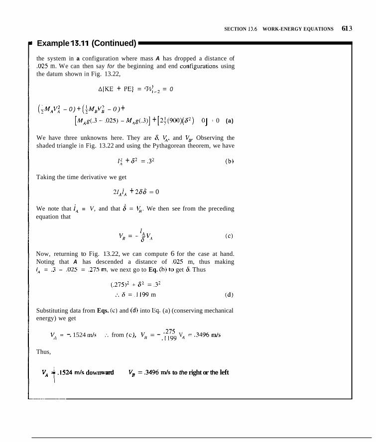
SECTION 13.6 WORK-ENERGY EQUATIONS 61 3
Example 13.11 (Continued)
the system in a configuration where mass A has dropped a distance of ,025 m. We can then say for the beginning and end configurations using the datum shown in Fig. 13.22,
A[KE + PEI = w_2 = 0
($MAV2 - 0 ) + (;M,V; - 0 ) + [Mag(.3 - ,025) - M,g(.3)] + [2f(900)(SZ) ~ 0, : 0 (a)
We have three unknowns here. They are 6, V,, and V,. Observing the shaded triangle in Fig. 13.22 and using the Pythagorean theorem, we have
l; + 62 = .32 (h)
Taking the time derivative we get
ziAi, + 268 = o
We note that i, = V, and that S = 4. We then see from the preceding equation that
Now, returning to Fig. 13.22, we can compute 6 for the case at hand. Noting that A has descended a distance of ,025 m, thus making 1, = .3 ~ ,025 = ,275 m, we next go to Eq. (h) tu get 6. Thus
(.275)' + S2 = .3' :. S = . I I99 m
Substituting data from Eqs. (c) and (d) into Eq. (a) (conserving mechanical energy) we get
V, = -. 1524 m l s :_ from (c), V, = - V = ,3496 m l s .I199 A
Thus,
V, f ,1524 m l s down V, = ,3496 m l s to the right or the left


SECTION 13.7 KINETIC ENERGY EXPRESSION BASED ON CENTER OF MASS 615
the relation above into the expression for kinetic energy, Eq. 13.30, we get
K E = $ ~ ~ , ( v ~ +P, , )* = ~ ~ r n ~ ( V ~ + P ~ ~ ) . ( v ~ + P ~ ~ ) , = I , = I
Carrying out the dot product, we have
Since y. is common for all values of the summation index, we can extract it from the summation operation, and this leaves
Perform the following replacements:
We then have
n (13.34) K E = $MV: + V; d n c m,pci + f C mip2i
, = I i = l
But the expression
represents the first moment of mass of the system about the center of mass for the system. Clearly by definition, this quantity must always be zero. The expression for kinetic energy becomes
(13.35)
Thus, we see that the kinetic energy for some reference can be considered to be composed of two parts: ( I ) rhe kinetic energy of the total mass moving rel- ative to that reference with the velocity of the mass center, plus (2 ) the kinetic energy of the morion of the particles relative io the mass center.

6 16 ('HAI'I'CR 13 1:NliKGY M1:'IHODS FOK I'ARTICl.tS
p Example 13.12 I
j : i i
A hyprithctical vchiclc i s niiiving at specd ",,in Fig. 13.24. (111 this \chicle are lwo hodics ciich of i i i ass 111 diding :dong a liorizonlal rod at a speed 1 '
relative to the rod. This rod i s rotating at an angular specd w l a d k c rela- tivc to the vehicle. What i s the kinetic cnergy of the two hodies relative 1 0
the g r w n d (XYZ) when they arc iit II clistancc I- f ro in point A? Clearly. the cciitcr 01 niass c(irresponds to point A and i s thus miwing
at a spccd V, relatiYc to tlie ground. Hence. we l i i ivc tis part of thc kinetic I cnergy the tei-m
2 , !MV' 7 ,nVi (:I)
The velocity o f cach hill rcliitive to thc center of iiiass i s e x i l y f1,rmcd using cylindrical components. Thus. imagining a reference .x?: at A translating with thc vehicle relat ive to XYZ. we h a w lor the vclocity of each hall rcl;ilive to s ; r
( o r ) ' = 1.2 + (OJI . )? (hJ P' = p2 +
The t01iiJ kinetic cncrg!, of thc ~M:O ni;isse> r c l a l i x Lo tlic griw~id i s thcn
KE = rnVi + rnlt;' + (Wr) ' ] ( e )
I
111 k;xiiniple 13.12, wc co~rsidcrcd ii casc where thc hodics involved constituted a finitc number of diwrc , l~ , particle\. In the nexl cxamplc. we coil- sidcr ii case wliei-e w c h a w a m,zlitzuuni o l particles forming ii rigid hody. The formulatiiin given by Eq. 13.35 can still he uscd hut iiow. iiistcad of sum- ming 1ir a finite nuinher 01 discrete particles. we imust integratc to accuunt f o r the infinite numher of infinitesimal particles comprising thc syslem. We arc thus tiiking a glimpse. 101- simple ciises, 11l' rigid-hody dynamick 10 be sludicd latei- in the tcxt. Those that iki nut have time fiir studying such energy prohlenx in detail wi l l hc able to solvc simple hut useful rigid-body dynam- ics prohlcins on the hiisis of thcsc examples as ucll as liitet- exaiiiples in this chapter.

SECTION 13.7 KINETIC ENERGY EXPRESSION BASED ON CBNTEK OF MASS 617
Example 13.13
A thin uniform hoop of radius R is rolling without slipping such that 0, the mass center, moves at a speed V (Fig. 13.25). If the hoop weighs W Ib, what is the kinetic energy of the hoop relative to the ground?
Clearly, the hoop cannot be considered as a finite number of discrete finite particles as in the previous example, and so we must consider an infinity of infinitesimal contiguous particles. It is simplest to employ here the center-of-mass approach. The main problem then is to find the kinetic energy of the hoop relative to the mass Center 0, that is, relative to a refer- ence q translating with the mass center as seen from the ground reference X Y (see Fig. 13.26). The motion relative to xy is clearly simple rotation; accordingly, we must find the angular velocity of the hoop for this refer- ence. The no slipping condition means that the point of contact of the hoop with the ground has instantaneously a zero velocity. Observe the motion from a stationary reference X Y . As you may have learned in physics, and as will later he shown (Chapter 15), the body has a pure instantaneous rututioizal motion about the point of contact. The angular vclocity w for this motion is then easily evaluated by considering point 0 rotating about the instantaneous center of rotation A. Thus.
A
Figure 13.25. Rolling hoop
Since reference .ry translures relative to reference XU, an observer on xy sees the ,same angular velocify w for the hoop as the observer on X Y . Accordingly, we can now readily evaluate the second term on the right side of Eq. 13.35. As particles, use elements of the hoop which are R d0 in length, as shown in Fig. 13.26, and which have a mass per unit length of Wl(27rh'g). We then have, on replacing summation by integration, the result
The kinetic energy of the hoop is then in accordance with Eq. 13.35:
X A
Figure 13.26. . ~ y Lranblaleb with 0 relative to X Y .

6 18 CHAPTER I3 ENERGY METHODS FOR PARTICLES
Example 13.13 (Continued)
Suppose that the body were a generalized cylinder of mass M (see Fig. 13.27) such as a tire of radius R having 0 as the center of mass with iixisymmetrical distribution of mass ahout the axis at 0. Then, we wnuld I express Eq. (h) 21s follows:
$ T m , P ? , = +JJ&m,iroP id)
You will recall from Chapter 9 that
JJI, IZ dm
is the sccond mornrnl of inrrtiu of the body taken ahout the I axis at 0. That i s .
Thus, we have lor the kinetic energy of such a body:
( e ) K E = - M V 2 + ~ 1 ; z o 2 I 1 2
You may also recall from Chapter 9 that we could employ the mdius /$ ,~vrufion k to express IC; as follows:
i-. = k2M cn Hence, Eq. ( e ) can he given as
Figure 13.27. Rolling generalized cylinder of mass M.
We shall examine the kinetic energy formulations of rigid hodies care- fully in Chapter 17. Here, we have used certain familiar results Srom physics pertaining to kinematics of plane motion of B nonslipping rolling rigid body. For a more general undertaking. we shall have to carefully consider more general aspects of kinematics of rigid-body motion. Thk will be done in Chapter I S . Also, in the last example we see one term of the inertia tensor I,, showing up. The vital role of the inertia tensor i n the dynamics ol rigid hod- ies will soon be seen.

SIXTION 13.8 WORK~KINETIC ENERGY EXPRESSIONS BASED ON CE<NTER OF MASS 61 9
13.8 Work-Kinetic Energy Expressions Based on Center of Mass
The work-kinetic energy expressions of Section 13.6 were developed for a system of piitticles without regard to the mass center. We shall now introduce this point inio the work-kinetic energy formulations. You will recall from Chapter 12 that N ~ W I O I Z ' . ~ law for the mass center of an) system of particles is
F = Mi, (13.36)
where F is the total external forcc on the system of particlcs. By the same development as presented in Section 13. I , we can readily amive at the follow- ing equation:
p dr, = (&%!fv?)2 - ( :MVZ)I (13.37)
It is vital to understand from the left side of Eq. 13.37. where we note the term dr , that the e.rternal.fiirces mmr ail movr with the center uJnioss for the computation of the proper work term in this equation.'d We wish next to point out that the single particle model represents a special case of the use of Eq. 13.37. Specifically. the single particle model represents the case where the motion of the center of mass of a body sufficiently describes the motion of the body and where the external forces on the body essentially mnve with the center of mass of the body. Such cases were set forth in Section 13.1.
Before proceeding to the examples, let us consider for a moment the case of the cylinder rolling without slipping down an incline (see Fig. 13.28). We shall consider the cylinder as an ufifirefiatr ofparticles which form a rigid hody-namely a cylinder. When using such an appruiach, we require that ull thej%rce.r horh extrrnal and intenial inlist ~ O V P with their reipective points of applkurion. Let us then consider the external work done on the particles mak- ing up the cylinder other than the work done by gravity. Clearly, only particles on the r im of the cylinder are acted on by external forces other than gravity. Consider one such particle during one rotation of the cylinder. This pasticle will have acting on it a friction Corce.fand a normal force N at the insrant when the particle is in contacr with the inclined surface. The particle will have zero exter- nal force (except for gravity) at a11 other positions during the cycle. Now, at the instdnt of this contact, the normal force N has zero velricity in its direction because of the rigidity of the bodies. Therefore, N transmits no power and does no work on the particle during the cycle under consideration. Also, the friction
Figure 13.28. Cylinder on incline

620 CHAPTER 13 ENERGY MIiTIIODS FOR PAKTlCl.liS
1orcc.f acts on a particle having zero velocity at the instant of contact because of the no .slipping rondition. Accordingly.,IIransniii\ no power and does 110 wnrk on the panicle during thi? cycle." This result must he true for each and evcry pai'icle on the rim of the cylinder. Thus, clcarly,,f and N do no work when the cylinder rolls down the incline. Also. because (if the rigidity of the body the internal forces do no wo pointed out carlisr. Thus. only gravity docs work.
Howevcr. in consi ng the motion of the w i r e r o fn i~ iss C of the cyl- inder in Fig. I3.2X. wc noie that forcc fnow mow^ with C and hence do^ work.
At the risk of heing repetitive, wc now summarize the key lealures 1 1 r properly using the center-or-mass approtach.
I . Only external forces are involved. 2. 8 all move with the r of m&ps when computing work (see
ic energy of the center of maas is used.
Example 13.14
A cylinder with a mass o f 25 kg is released frorn rest on an incline, a h
shown in Fig. 13.29. The diameter of the cylinder is .hO m. If the cylinder rolls without slipping, compute the speed of thc centerline C after i t has moved 1.6 m along the incline . Also. ascertain the friction force acting 011 the cylinder. Use the result from Problem 13.76 that the kinetic energy of a cylinder rotating aboul its own stationary axis is a M R 2 ~ ' , where rn i E the angular speed in radisec.
In Fig. 13.29 we have shown the free budy of the cylinder. We pro- ceed to use thc work-energy equation for a system of particles. Recall that w e can concentrate the weigh1 at the center of gravity (Scctiiin 13.6). Accordingly, using the luwest position as a datum and noting from our earlier discussion that the friction forcc,/diies no work \tc have
A i P E + KE) = '71: ~

SECTION 13.x WORK-KINETIC ENERGY EXPRESSIONS BASED ON CENTER OF MASS 621
Example 13.14 (Continued)
where the kinetic energy of the cylinder is given as the kinetic energy of the mass taken at the mass center (straight line motion of C ) plus kinetic energy of the cylinder relative to the center of mass (pure rotation about C ) . Noting from Example 13.13 that
o=-=li V R .30
we substitute into Eq. (a) and solve for y.. We get
Now to findf, we consider the motion of the mass center of the cylin- der. This means that we use Eq. 13.37 for the center of mass. Now all ex- ternal.forces maSt move with the center of mass; thus, .f does work. Since the center of mass moves along a path always at right angles to N , this force still does no work. Accordingly, we can say:
-.f(l.6) + W(1.6sin30") = fMVZ
-f'(I.6) + (25)(9.81)(1.6)sin3Oo = $(25)(3.23*)
f a
Before going further, let us consider the two cylinders and the block in Fig. 13.30 as simply a system of particles. If there is no slipping between the block and the cylinders, the velocities of the particles on the block and the cylinders at the points of contact between these bodies have the same velocity at any time t. Furthermore, the friction force on the cylinder from the block is equal and opposite to the friction force on the block from the cylinder at the point of contact. We can then conclude that there is zero net work done by the friction forces between block and cylinders when considering them as an aggregate of particles.
Also, in the next problem, we will consider as a system of particles, rigid bodies which are joined by rigid connectors with frictionless inter- connections.
Figure 13.30. Three rigid bodies moving without slipping at any of the contact points.

622 C'HAITLK I 1 I:WR(;Y MHTHOI)S to^ I'AKI'IC'I.I:S
Example 13.15
An extcriiiil lorquc 7 <,I 50 N-in i s applied to ii solid cylindcr I1 ( x c Fig. 13.31). which I i i ~ h i~ tii its$ of 30 hg iiiid ii radius o i .2 111. Thc cylinder roll' willioiit dippiiig. Block A, hitving i i iiiii% o I 20 kg, i s dr;iggcd LIiJ the 15 incline. Thc dynamic cdf i c i cn t o f iriction ki,, between hloch A and thc incline i \ .25. The coiiiiectioii\ iit (' iiiid I ) iirr Iricl ionlehs.
( a ) What i\ the \cIocity of the \ystcm :iller miiving ii d i i t i i i i w il
(I)) Whal i s tlic lrictiirii llricc on the cyliiider? ()i 2 I ~ ~ ?
Neglect thc ! n i i h h o i thc coniiccting rod
Wc show ii Srcc-hody diagrairi o i l l i e !,ywiii in Pig. 13.32. Wc hrgin by employing ii syslem of particles point o i vicu. Note tlierc :m pair\ o S intcrnal forccs prcscnt hclwccn the r(id ('11 i i i id hody 4 i l l (tie c o i i t x t point

SECTION 13.x WORK-KINETIC ENERGY EXPRESSIONS BASED ON CENTER OF MASS 623
Example 13.15 (Continued)
and similarly between CD and cylinder B. These force pairs are equal and opposite because of Newton's third law. And because the forces in each pair move exactly the same distance at the respective points of contact, there will be zero internal work from these force pairs. Hence, using the uppermost configuration as the datum,
%:+: = APE + AKE
TO - (pdNA)(d) = [(WA + W,)(d)(sin 15") - 0]
Note that as the cylinder moves without slipping a distance d along the incline, the circumference of the cylinder must come into contact with the incline along the very same distance d. Hence, by dividing d by the radius r, we get the rotation of the cylinder in radians associated with the move- ment of its center.
d 0 = -- r
We then get for Eq. (a), on substituting data for the problem
( S O ) [ - (.25)[(2Og)(cos 150)](2) = [(5Og)(2)(.2588)]
+ (50)1 + z(30)(.22)- c v2 (.2Y "' 1
Next, use the center-of-mass approach. We have on noting that a couple which is translating does no work. (Why?)
f F * drc = +MTo,a,(V; ~ V:)
- ( .25) (NA)(d) -(W, + W,)(sinIS")(d) + fd = f(50)(2.158')
-(.25)[(2Og)(cos 1So)](2) ~ (SOg)(.2588)(2) + ,f(2) = 116.4
f = 232.5

624 C I I A P T I R I3 E U H t ( ; Y \IETHOlYi FOR l ' A 1 ~ ~ l ~ ' L E S
Example 13.16
111 Example 13.15. suppcxe that cylinder II i s .slippitig. What i s Ihc dyn;iinic ciicSSicierit or Sriclioii ( p,,In hetween the cylinder wid the iii- cline cn tliiit the system reaches a speed i if I .5 mlc after miiving il distaiicc d = 2 111 starting from rest? :
Usiiig ~ h c ccnter-of-mass apprmrch. wc thaw
(pd)H = ,7122
111 the next example. we shall coiisider a case where i , , / ~ , , ~ , , ' i i , ~ , ~ ~ , ~ , ~ do work.
Example 13.17
A die.;el-powered electric triiiii movex up ii 7'' grirde in Fig. 13.31. If ii
torque of 750 N-m i s developed i i t eiicli of i t s s ix pair, of drive u'heels. what i s the iricrcasc of spccd of thc tiniii aftcr il ~i iovc\ 100 iii'? l i i i t i i i l l y . thc lriiin ha\ a spccd 01 16 knilhr. The lrain weighs 00 kN. 'I'hc drive whccls h a w a diameter of hilO min. Neglect tlie rotational energy of the drivc whccls.
Figure 1.4.33. I l ic\clLcIccIric Iraiii.
! Wc shall consider thc train as ii tern of particles including thc h pairs of whccls arid the body. We have shown tlic I n i n iii Fig. 13.34 \\i lh tlic cxtcriiiil 1orces. W. N. and/: In addition. %'e ha\c shiiwii cc~rli i i i i iiilcriial
13,34, L:xlcln;,l i,,rL.r,,~,l fc,rccs :mi r ~ r q u c ~ .

SECTION 13.8 WORK-KINETIC ENERGY EXPRESSIONS BASED ON CENTER OF MASS 625
Example 13.17 (Continued)
torques 7:lh The torques shown act on the rutor,y of the motors, and, as the train moves, these torques rotate and accordingly do work. The reucfiuns to these torques are equal and opposite to T according to Newton's third law and act on the sfuturs of the motors (Le.. the field coils). The stators are sta- tionaly, and so the reactions to T do nu work as the train moves. Thus we have an example wherein, using a system of particles approach, internal forces pelform a nonzero amount of work. We now employ Eq. 13.29. Thus
APE + KE = w,,,, (a)
For the rolling without slipping condition, the friction forces f do no work. We then have
I 90,000 (16)(1,000) 2 s [- 3,600 ]?) [(90,000J(100sin7" - O)] +
= (6)(750)(8) (b)
where 0 is the clockwise rotation of the rotor in radians. Assuming direct drive from rotor to wheel, we can compute Bas follows for the 100-m dis- tance d over which the train moves:
(C) d 100 r .3
B = - = ~~~ = 333.3 rad
Substituting into Eq. (b) and solving for V, we get
V = 10.38 m/sec
Hence, the increase of speed of the train is
To determine the friction fo rces j we now adopt a center-of-mass approach. Thus all forces now move with the center of mass. And they must be e.rtemul,fi,rces. Accordingly we have
[6f - (90,000)(sin 7")](1OOJ I 90 000 (16)(1,000) ( 3,600
I 90,ow 2 9.81 2 9.81 (10.38), --A -~ - -
'"Figure I? 34 accordingly. 19 not a free-body dngram

13.68. A chain of total length L is relcased from res1 on a smooth support as shown. Delerminr the veliicily of tlic chain when the last link m w e s off the horizonVal wrtacr. In this prohlem, neglect the friction. Also, d o no t attempt to accnunt for centrirugal cffecth ctemining f r < m the chain links rounding the corner.
Figure P.13.68.
13.69. A chain is SO ft long and wcighs IN) Ih. A force PUT 80 Ih has been applied at the configuratian shown. What is the s p d of the chain after force P has moved IO fl! 'The dynamic coefticiznl of friction hetween the chain and the cupporting surface i q .3. Utilize an apprvximatc snlilysis.
Figure P.13.69.
13.70. A hullet of weight ing W, Ih. The bullet lodges in the wood, and both hodies then move to the dashed Dosition indicated in the diamam before
is fired into a hlock of wood weigh
Figure P.13.71)
13.71. A device is mountcd mi 3 plntfnrm that I S rotating with an anguliir s p d 01 10 nldlarc. The devicc consists of t w i masse\ (each i \ ,I 'lug) rotating on a spindle with an angular specd of 5 rad-crc relativr to the platfbmi. The m a w s arc iiwving radially outward with a ?peed of I O ftlsrc, and the cntire platf<>lm is being raised at a speed rrf S fllsec. Compule thc kinetic encrgy n1 the system of two particles when they are I ft from the qpindlc.
+,IC radlsec ~ A S radlsec
Each m a u ~~ 0. I d u g
Figure P.13.71.
13.72. A hoop. with four spoke&. rolls without slipping such that Ihc ccntcr C moves at a bpced V of I .7 mlsec. The diameter of the hixrp ih 3.3 m and Ihe weight pcr unit length o l t h e rim is 14 Nlni. The y o k c 5 arc uniform rods also having a wright p ~ l - unit length of 14 Nlm. A w m c that rini and spokes arc th in What is the kinetic energy ot thu body'!
falling back. Compute the amount 01 internal work done during the action. Discuss the effects of this work. .The hullet has il apecd V,, hefore hitting the black. Neglect the mass of the supporting rrid and friction at A .
626
Figure P.13.72.

13.73. Three weights A, L1, and C slide frictionlessly along the system of connected rods. The bodies are connected by a light, llexihlc, inextensible wire that is directed by frictionless small pulleys at E and F . If the system is released from rest, what is its speed after it has moved 300 mm? Employ the following data firr the body mas5e.s:
Body A: 5 kg
Body H : 4 kg
Body C 7.5 kg
Figure P.13.73.
13.74. B d i c s E and F slide in frictionless grooves. They are interconnected by a light, flexible, inextensible cable (not shown). What i s the speed of the system after it has moved 2 ft? The weights of bodies E and F a r e 10 Ih and 20 Ih, respectively. A is equidistant from A and C. E remains in top groove.
x
Figure P.13.74.
13.75. A tank is moving at the speed Vof 16 k d h r . What is the kinetic energy of each of the treads for this tank if they each have a mass per unit length of 300 kgim'?
l- Figure P.13.75.
13.76. A cylinder of radius R rotates about its own axis with an angular speed of w. If the total mass is M, show that the kinetic energy is i MRW.
13.77. Cylinders A and C each weigh 100 Ih and have a diame- ter of 2 ft. Body A, weighing 300 Ih, rides on these cylinders. If there is nu slipping anywhere, what is the kinetic energy of the system when the body A is moving at a speed Vof 10 fvsec'? Use result of Problem 13.76.
Figure P.13.77.
13.78. A pendulum has a hob with a comparatively large uni- form disc of diameter 2 ft and mass M of 3 Ibm. At the instant shown, the system has an angular speed e of .3 radlsec. If we neglect the mass of the rod, what is the kinetic energy of the pen- dulum at this instant? What error is incurred if one considers the hob lo be a particle as we have done earlier for smaller hobs'? Use the result of Problem 13.76.
Figure P.13.78.
627

13.79. pendulum rises.
13.80. Do Example 13.3 hy treating as an aggregate ofpitrliclc\.
13.81. Do Problem 13.27 hy treatmg iis an aggregate ofpwt ic les.
13.R2. Do Prohlem 13.22 hy treating a c a n agprrgatc of paniclrc.
13.83. Do Problcm 13.24 hy treating a\ an aggrcptc of p a l t i c k \ .
13.84. A constant force P' is applicd t o the nxic of a cylinder, as shown, causing thc axis to increasc its speed from I ftisec trr 3 Slliec in 10 ft without slipping. What i s the friction force acting on the cylinder'? The cylinder weighs 100 Ih.
In Problem 13.7X compute the maximum angle that the
Figure P.13.84.
13.85. A cylinder with a maw nf 25 kg i \ releaced from rest m :in incline, a i shown. 'The inner diameter 11 01 the cylindcr i s 30(1 mm. If the cylinder rolls without 'lipping, compute the peed nf the cen- terline 0 after the cylinder has muwd I .h m almg the incline. Ascertain the friction Ibrce acting on the cylinder. The radius 01 gyration h at 0 i s .30/\'2 in
Figure P.13.86.
13.87. Cylindcrs A and B w u h havc a mass <if 25 kg and a d i m - eter of 100 mm. Block C, riding on A and H. has a mass of 100 kg. I f the ~ y c t e m is released fmni rc\t at thc configuratinn chown. what i s the speed of 1.attcr the cylindera h w c made hall a revdii- Lion'! Use thc r ew l t 01 Pmhlrm I3.70.
Figure P.13.X7.
13.88. Shown arc two iilsnliual hlocks A and H , a c h weighing SO Ih. A force /.'of 100 Ih i s applied Lo thc lower hlrick, causing i t i n n u x 10 the right. Blrrck A . Ihowever. is rcitrained hy thc wall ('. I f hlock H rcaches a speed of I O ttlscc 1n 2 11 starling from rcit at thc pri\ition shown in thc diagram. \*hat i~ thc I-cctraining lorce from thc mall'! The dynamic coefficient 01 friction hctwecn H and the grciund w1.111cc i \ .3. L>o this p h l e n , firs1 by using Eq. 1 3 . X Then check thc r c w l t h) using scparatc lrce-hody diagrams. and 511 o n
Figure P.13.85.
13.86. A uniform cylinder having a diameter o f2 ft and a wright of 100 Ih TOIIS down a 30" incline without slipping. as shown. What is the speed o f t h e center after i t has mrwcd 20 ft'! Compare this result with that fnr the case whcn thcre i\ no friction present. [Hint: Use the result of Problem 13.76.1 Figure P.13.XX.
I 628

13.89. What is the tension T to accelerate the end of the cable downward at the rate of 1.5 mlsec'? From body C, weighing 508 N, is lowered a body D weighing 1 2 . 5 ~ N at the rate of 1.5 m/sec2 relative to body C. Neglect the inertia of pulleys A and R and the cable. [Hint; From e i l i e r courses in physics, recall that pulley B i s rotating instantaneously ahout p i n t e, and hence point b has an acceleration half that of pointf. We will consider such relations carefully at a later time.]
T
f" e
Figure P.13.89.
13.90. Cylinder C is connected by a light rod AR and can roll without slipping along the stationary cylinder D. Cylinder C weighs 10 N. A constant torque T = 20 N-m is applied to AB when it is vertical and stationary. What is the angular speed of AB when it has rotated YI)"? The system of bodies is in the vertical plane. Recall from physics that a body which is rolling without slipping has instantaneous rotation about the point of contact.
Figure P.13.90.
13.91. An 800-N force F is pulling the vehicle. The cylinders A and Reach weigh I,OoO N and roll without slipping. The indicated spring has a spring constant K equal to 50.0 Nlmm and is com- pressed a distance S of 20.0 mm. The pad slides on the upper guide with a dynamic coefficient of friction p,, equal to 3. Neglect all musses except the cylindcrs, whose diameter D is .2 m.
, Pad w, = w, = i nwr
K = m n Nimm
6 = 20 0 mrn
Figure P.13.91.
(a) What is the velocity of the vehicle after it moves a distance of I .7 m staning from rest?
(b) What is the total friction f0rce.f on the cylinders from the ground?
13.92. a horizontal surface and then along a 30" incline.
(a) How far up the incline does it move?
(b) What are the friction forces on the cylinder along the
A cylinder weighing 500 N rolls without slipping, first on
horizontal surface and along the incline'?
Figure P.13.92.
13.93. tical position.
A hoop with four spokes is released from rest from a ver-
(a) What is the velocity of point C after it moves 1.3 m?
(h) What is the tension in the wire?
The rim and the spokes each have a weight per unit length of 15 Nlm and are to be considered as thin. The wire is wrapped around the hoop and is the sole support
t 5 m
Figure P.13.93.
629

I Figure P.13.W. l4pure l'.l.3.Y4.
(hi W1i;it arc lhe ir icrion ii~l-ccs 1cmr11 tlir grliiiiiitl O I I each cylinder A'!
M,, = 2(10 hp 2 M,, = SO kg
M , = 30 kg
Figure P.13.95.
I= 500 N
13.96. A cylinder i s i l h 0 ~ 1 t u roll down an incline without slip^

SECTION 13.9 CLOSURE 631
13.9 Closure In this chapter, we presented the energy method as applied to particles. In Part A, we presented three forms of the energy equation applied to a single particle. The basic equation was
J12F.dr=' * ( M V Z ) , - f ( M V 2 ) , (13.38)
For the case of only conservative forces acting, we presented the equation for the consemuion of mechanical energy:
(PE), + WE), = (PE), + (KE), (13.39)
Finally, for both conservative and nonconservative forces, we presented an equation resembling thefirst law of thermodynamics as it is usually employed:
A(PE + KE) = 'Wy.',, (13.40)
In Pan 8 , we considered a system of particles and presented the above equation again, but this time the work and potential-energy terms are from both internal and external force systems.'? Furthermore, all work and poten- tial-energy terms are evaluated by using the actual movement of the points of application of internal and external forces.
Next, we presented the work-energy equation for the center of mass of any system of particles:
j l zF-dr , : = $ ( M V Z ) , - ~ ( I W V : ) ~ (13.41)
where F , the resultant external force, moves with the center of mass in the computation of the work expression. We pointed out that the single particle model is a special case of the use of Eq. 13.41 applicable when the motion of the center of mass of a body sufficiently describes the motion of a body and where the external forces on the body move with the center of mass of the body.
To illustrate the use of the work+nergy equation for a system of parti- cles, we considered various elementary plane motions of simple rigid bodies. A more extensive treatment of the energy method applied to rigid bodies is found in Chapter 17.
We now turn to yet another useful set of relations derived from Newton's law, namely the methods of linear impulse-momentum and angular impulse- momentum for a particle and systems of panicles.

Figurr P.13.98.
,I
532
..-
Figure P.13.101.
Figure P.13.102.
Figure 1'.13.103.

13.104. A self-propelled vehicle A ha? a weight of & ton. A gaso- line engine develops toque on the drive wheels to help muveA up the incline. A countenveight B of 300 Ib is also shown in the diagram. What horsepower is needed when A is moving UP at a speed of 2 ftlsec and has an acceleration of 3 ftlsec2? Neglect the weight of the pulley. [Hint: The pulley rolls along cod dg without slipping. It therefore has an instantaneous center of rotation at d. What does this mean about the relative value of velwity of point h on the pulley and p i n t a?]
Figure P.13.104.
*13.105. Set up an integro-differential equation (involving deriv- atives and integrals) for B i n Problem 13.31 if there is Coulombic friction with pz, = .2.
13.106. circular surface'?
*13.107. be expressed in the following way:
At what angle Qdoes bodyA of Problem 13.31 leave the
Show that the workxnergy equation for a particle can
Integrating the right side by parts," and using relativistic mass m,l<l ~ V z / c ' , where m,, is the rest mms and c is the speed of
light, show that a relativistic form of this equation can be given as
so that the rdntivistic kinetic energy i s
KE = nx2 ~ m,c2
*13.108. By combining the kinetic energy as given in Problem 13.107 and m,,? to form E, the total energy, we get the famous furmula of Einstein:
E = mc2
in which energy is equetrd with mass. How much energy is eqUiVd- lent to 6 x Ihm of matter'? How high could a weight of 100 Ib be lifted with such energy?
13.109. A 100-lh boy climbs up a rope i n gym in I O sec and slides down in 4 sec after he reaches uniform speed downward. What is the horsepower developed by the boy going up'! What is the average horsepower dissipated on the rope by the boy going down after reaching uniform speed'? The diqtance moved before reaching uniform speed downward is 2 ft.
Figure P.13.109.
13.110. An aircraft carrier is shown in the process of launching an airplane via a catapult mechanism. Before leaving the catapult, the plane has a speed of 192 k d h r relative to the ship. If the plane is accelerating at the rate of Ig and if it has a mass of IR,000 kg, what horsepower is bring developed hy the catapult system at the end of launch on the plane if we neglect drag? The thrust from the jet engines of the plane is 100,000 N.
Figure P.13.110.
Therefore
The l a i t formulation i? called integration by parls.
633

13.111. Vehiclz B, weighing 25 kN, is to go down a 30" incline. The "chicle is connecled to hody A through light pulleys and il
capstan. Whilt should body A weigh if starting from rest it restricts hody B 111 a speed of 5 mlsec when R mowc 3 in? There are two wraps of rope around the capstan.
13.115. Cylinders A and B havc mtas\c~ of 50 kg cach. Cylindcr A can ouly roLil1.e about a stalionary axis while cylinder B rolls without slipping. Block C has a mass of 100 kg. Slarting from rest, what is the speed of C after nioviiig . I it? Force P is 500 N and the diainetcr of the cylinders is .2 n,.
F igure P.13.111.
13.112. A jet pussenger phne is moving along the runway for a takeoff. If cach of ils four engine\ is developing 44.5 kN olthrust. what is the horsrpowcr dcvcloprd w h m the plimr is moving a1 a speed of 240 kmlhr?
13.113. Block R, with a n a s i of 200 kg. i s being pulled up an inclinc. A inotor C' pulls on one cable, developing 3 hp. 'The other cable is connected to a counterweight A having a inass of 150 kg. If B is moving at li s p e d of 2 mlscc, what is its acceleration? [Hinr: Stalt with Newton's law lor A and B . ]
Figure P.13.113.
13.114. A block G slidcs along a frictionlcss path as shown. What is the minimum initial speed that G should have along the path if it is to izniain in contact when it gcts ton, the uppermost positirrn ofthe path? 'The block weigh\ 9 N. Whilt i s the nulmal Surcr ou the path when forthe condition descrihed the hlock is at position H?
Figure P.13.Il4. h34
Figure P.13.115
13.116. A ryslrm o f 4 d i d cylinder\ and a heavy hluck move vcrtically downward aidcd by a 1,00(1-N forcr F. What is the angular ?peed of the whecli after thc systcin descends .5 m after mrting fnrm rest'! What is thc friction friicc Irum Itit. walls on each wheel'! The wheels rol l without slipping.
I Figure P.13.116.
13.117. A wllilr H having a inass uf IO0 g moves along a frktion- less curved rod in a vertical plane. A light rubbri~ band cunnccts B to a lixed p i n t A . Thr rubber band is 230 intn in length when unmetched. A force of 30 N is required io exlend Ihe band 50 mm. It thc collar is released from rest. what distance muht d he so that the downward nrrrinal h r c c on the rod at C is 20 N?
I-'!+-! Figure P.13.117.

13.118. When your author was B graduate student he built a sys- tem for examining the effects of high-speed moving loads over elastically supported beams (see the diagram). A "vehicle" slides along a slightly lubricated square tube guide. At the base of the vehicle is a spring-loaded light wheel which will run over the beam (no1 shown). The vehicle is catapulted to a high speed by a strelched elastic cord (shock cord) which i s pulled back from position A-A to the position B shown prior to "firing." At A-A thr shock cord is elongated 10 in., while at the firing position it is elongated 30 in. A fbrce of I O Ib is required for each inch ofelon- Eation of the cord. If the cord weighs a total of 1.5 Ib and the vehi~ cle weighs 10 OL, what is the speed of the vehicle when the cord reaches A-A after firing? Take into account in some reasonable way the kinetic energy of the cord, but neglecl friction.
S
Side view (a)
from rest from a position where the elastic cord is unstretchcd, what is body B's speed after it tnoves 3 m?
/ H
Figure P.13.119.
13.120. A collar slides o n a frictianless tube as shown. The spring is unstretched when i n thr hurimntal position and has a spring constant of I .O Iblin. What is the minimum weight u f A to just reach A' when released from rest from the pusitiun shown in the diagram? What is the force o n the tube when A has traveled half the distance to A'?
Figure P.13.120.
13.121. A 15-kg vehicle has t w ~ bodies (each with mass I kgj mounted on it, and there bodies nitate at an angular speed of 50 radsec relative to the vehicle. If a 500-N force acts on the vehicle for a distance of 17 m, what is the kinetic energy of the system, assuming that the vehicle starts from rest and the bodies in the vehicle have constant rotational speed? Neglect frictivn and the inertia of the wheels.
100 mm 3oll mm 1-64
Figure P.13.118.
13.119. A body B of mass 60 kg slides in a frictionless slot on an inclined surface as shown. An elastic cord connects B to A. The cord has a "spring constant" of 360 N/m. If the body B is released Figure P.13.121.
635

13.122. Two identical solid cylindcrs each weiehing 100 N &up- port a load A wcighing SO N. If ii force F nf 300 N acts as shown. what i q the speed 01 the vehicle after rmwing S m? Alsu. what i s the total friction iorce on each wheel'! Nrglect the inass nl the wpporting system connecting the cylindesr. Note that thc kinetic ene rg uf the angular m r t i o n of a cylinder about i t \ own axis i h
i M K L u ' . l h e sy\tcrn stiirts from st.
13.125. Two discs move ou il horimntnl Srictiunlcss aurface h ~ w n luokiiig down from ahuvc. Each djsc wighs 20 N . A rec- tangular rncmber B weighing SO N i'i pullrd hy i~ fiwcr F having ii viiliie ut 2I)O N. If there is no slipping anywhcre cxccpt , in thc horimatal \upport surfacc, what 15 thc speed of B aftrr it 1110va
I 8 cm? Determine the i r i c i i w lol-ce\ t r i m the wall\ onto the cylinders.
Figure P.13.123
13.124. 'l'hrcc block, arc conncctcd hy an Inextensible t lexihlr cahle. The hlocki arc rcleaied from :L rmt configuration with thc cable taut. I t A can only fall a disrance h equal 10 2 11, what IS the velocity of bodics c' and B after each har moved a distance u t 3 ft? Each hody beighs 100 Ih. The cozSfiuent of dynamic fric- tion fur body C i s .3 and lor body B i s .2.
Figure P.13.125.
Figure P.13.124. Figure P.13.126.

Methods of Momentum for Particles Part A: Linear Momentum
14.1 Impulse and Momentum Relations for a Particle
In Section 12.3, we integrated differential equations of motion for particles that are acted upon by forces that are functions of time. In this chapter, we shall again consider such problems and shall present alternative formulations,
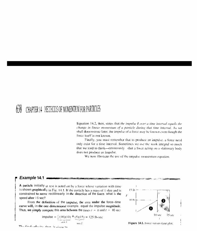
638 CHAPTER 18 METHODS OF MOMENTll i FOR PARTICLES
Example 14.1
A particlc initially i s shown graphicall constrained tv n iwc rectilinearly in the dii-ectinn 01' the l i m e . what i\ the speed after I S sec?
From the definiliiin of the irnpuhc. the area under the force-time curve will, i n the one-dirncnhional example. equal the impulse magnitudc. Thus, we ?imply compulc this area hclween the times I = 0 and I = I C sec:
,L
I J
I O \ C C 15 \ec :
I . / ,<a 2 Figere 14.1. l , ~ , ~ ~ ~ ~ ~ ~ , , , , ~ ~ t , , , ~ ~ plot. j
impulse = 4 (10)(10) + (5)(15) = 125 Ih-sec I -- iri
, l lCil I
T L . ~ t:-..l .,-l,~,.;+>, th ,~ , - ic , / c

SECTION 14.1 IMPULSE AND MOMENTUM RELATIONS FOR A PARTICLE 639
Example 141 - I I rZ prticle A with a mass of I ke has an initiai velocitv I! : 1Oi + - , " 6j d s e c . After particle A strikes particle B , the velocity becomes V = 16i - 3j + 4k d s e c . If the time of encounter is IO msec, what average force was exerted on the particle A ? What is the change of linear momen- tum of particle B?
The impulse I acting on A is immediately determined by computing the change in linear momentum during the encounter:
ZA = (1)(16i - 3j + 4k) - ( I ) ( l O i + 6j) = 6i - 9j + 4k N-sec
Since
/,: FA dt = IA At
the average force (Fa& becomes
(<JA(O.OIO] = 6i - 9j + 4k
Therefore,

Example 14.3
Two bodies, I and 2. are connected hy an inextensihle and weightless cord (Fig. 14.2). Initially, the bodies are at rest. If the dynamic cocnicient of fric- tion is pd for body I on the surface inclined at angle a, compute the velocity of the bodies at any time f before body 1 has reached the end of the incline.
Figure 14.2. Two bodics corinectsd hy il cord.
Since only constilnt forces exist and since a time interviil has hcen
free-body diagrams of bodies I and 2 are shown i n Fig. 14.3. Equilihrium considerations lead to the conclusion that Nl = W, cos a, s o the frictiiin forcef; is
specified, we can use momentum considerations advantageously. The ~~~ {, W; \ in (I
,fi = p d N , = pdWi cos a )*P W. Fnr hndv I take the cnmuonent of the linear impulse-momentum equii- N,

SECTION 14.1 IMPULSE 4 N D MOMENTUM RELATIONS FOR A PARTICLE 641
By adding Eqs. (a) and (h), we can el;m;nate T and solve for the desired unknown V. Thus,
V g
( - ~ c , W , c o s a + W , s i n n + W , ) r = ~ ( W , + W 2 )
Therefore.
Note that we have used considerations of linear momentum for a sin- gle particle each time in solving this problem.
Example 14.4
A conveyor belt is moving from left to right at a constant speed V of 1 ftlsec in Fig. 14.4. Two hoppers drop objects onto the belt at the total rate II of 4 per second. The objects each have a weight W of 2 Ib and fall a height h of I ft before landing on the conveyor belt. Farther along the belt (not shown) the objects are removed by personnel so that, for steady-state operation, the number N of objects on the belt at any time is IO. If the dynamic coefficient of friction between belt and conveyor bed is .2 , esti- mate the average difference in tension T2 - T , of the belt to maintain this operation. The weight of the belt on the conveyor bed is I O Ib.

642 CHAP'rER I4 METHODS Or MOMENTUM FOR PARTICLES
Example 14.4 (Continued)
We shall superimpose the fdlowing effects to get the dcsired result.
1. A friction force from the bed onto the belt results from the static weight of the ten ohjccts riding on the belt and the weight of the portion of belt (in the hed.
2. A friction I i rce froin the bed ontu t l ic hclt results from the force in tlie directinn needed tu change the r r r l icul linear tmnmentuni of the fillling ohjccls from a value corresp<inding to the free-fall velocity just before impact ( , 2 ~ : / c ) to a value nf z c r ~ after impact.
3. Finally, the he l l must supply a foi-ce in thc .i direction to change the lm,-i:o,ild liiiear iiinmcmum of the lhlling objects from it value of zero to it value cwre~pondinp LO tlie speed of the helt.
Thus. wc have for the first contriholicin. which we dunale as A T . the fol- lowing result:
AT, = (NW + lO)p<( = 1(10)(2) + 10](.2) = 6 Ih (a1 As for the Yecond con~ributii~ri. we can only compute an average value
hy iiiiting that each impacting oh.ject i s given a vertical change in litiear iiioiiientum equal to
W ,~~
fi
fi
vertical change i n l inear rnoiiientiini per object = ~ (,,28/1)
7 = 7 , (2g)(I)
= ,498 Ib-sec
where we have assumed a free kill sparling with zero velocity at the hop- per. For fi iur in ipx th per second. we have as lhe total vertical change in h iea r i i io~iicntuin per second Lhc v ~ l u e (4)(.498) = 1.994 Ih-scc. The average vertical forcc during thc I-scc interval tu give the impulse needed for this change i i i linear m~iinenturn is clearly 1.994 Ib. Sincc this result is enrrect f o r rvzry \econd, I .994 Ih is tlic avcrage normal force that the bed of the conveyor must Lransmit to I t for arresting the vertical motion
.. ., , ,. . . F ~ c . ~ . ~ ~
.. . ,. . . . , . -. I .

SECTION 14.2 LINEAR-MOMENTUM CONSIDERATIONS FOR A SYSTEM OF PARTICLES 643
Example 14.4 (Continued) For four impacts per second we have as the total horizontal change in lin- ear momentum developed by the belt during 1 sec the value (4)(.0621) = ,248 Ib-sec. The average horizontal force during I sec needed for this change in linear momentum is clearly ,248 Ib. Thus, we have
[(AT),lav = ,248 Ib (C)
The total average difference in tension is then
(AT)=" = 6 + 399 + 248 = lb
14.2 LineaFMomentum Considerations for a System of Particles
In Section 14. I , we considered impulse-momentum relations for a single particle. Although Examples 14.3 and 14.4 involved more than one particle, nevertheless the impulse-momentum considerations were made on one particle at a time. We now wish to set forth impulse-momentum relations for a system of particles.
Let us accordingly consider a system of n particles. We may start with Newton's law as developed previously for a system of particles:
n dV. ~ = z m . - I dt
j = l
(14.3)
Since we know that the internal forces cancel, F must be the total external force on the system of n particles. Multiplying by dt, as before, and integrat- ing between ti and 5, we write:
Thus, we see that the impulse of the total external force on the system of particles during a time interval equals the sum of the changes of the linear- momentum vecturs of the particles during the time interval.
We now consider an example.

644 CHAPTER 1.1 METHODS OF MOMENTUM FOR PARTICI.FS
Example 14.5
A 3-ton truck is moving at a speed 01 60 inilhr. [See Fig. 14.S(a).l The driver suddenly applies his hrakes at time f = 0 so as to lock his wheels in a panic stop. Load A weighing I ton breaks loose from its ropes and at time f = 4 sec is sliding rrlufivi, 10 rhr rrirck at a speed of 3 ftlsec. What is the speed of the truck at that time? Tdke ,u,/ between thc lires and pave- ment to hc .4.
Since we do tzot kriow the nature of the forces hctween thc truck and IiiadA whilc the latter is breaking loose, it is easiest to consider the 01 two particles comprising the truck and the load simultaneously whereby the af<)rementiorred forccs become i i i terr~d and arc imf considered. Accord- ingly. we have shown the system with all the external loads i n Fig. 14.Xh). Clearly. N = (4)(2,000) = 8,000 Ih and tlic friction force is (.4)(8.0001 = 3,200 Ih. We now employ Eq. 14.4 in the ~I direction as follows:
~-
(b)
Figure 14.5. l i u c h undcrp ing panic 1% d =[?..;.’ - [ Z n ! v J ] \10p.
2 1 I i (21) (3)i 2,000 I (I )(?.ilOO)
(V. + 31 ~~~ ~~~~
~~~ v, + ,s
Note that the first quantity inside the first brackets on the right side 01 Eq. (a) is the inomenturn of h e truck at f = 4 sec. and the second quantity inside Ihe same hrackels is the miiineiituin of thc Imid a1 this instant. We may readily solve f o r V,:
V, = 35.7 ftlsec
Introducing ni(i.s.s-wtirt’r quantities inti, Eq. 14.4 is easy and sometimes ad\,antageous. You u’ill reinemher that:
Mr, = Crn,r , (14.5) i=l
Diffcrcnliating with respect lo lime. we get
M V = - p l , V ) (14.6) !-I
Thus, we see from this cqualion that rlir rorul lirrrar nio~nrrir~trn of0 vysrem of /xirlic/e.s c,yriol.s fhr lirieor I ? I U I I I P ? I ~ I ~ of n partidc, ihur has rhr fotul muss 01

SECTION 14.2 LINEAR-MOMENTUM CONSIDERATIONS FOR A SYSrEM OF PARTICLES 645
the system and that moves with the velocily of the mass center. Using Eq. 14.6 to replace the right side of Eq. 14.4, we can say:
Thus, the total external impuke on a s.ystem ofparticles equa1.T the change in linear momentum af a hypothetical particle having the mass oj the entire aggregate and moving with [he mass center.
When the separate motions of the individual particles are reasonably simple, as a result of constraints, and the motion of the mass center is not eas- ily available, then Eq. 14.4 can he employed for linear-momentum considera- tions as was the case for Example 14.5. On the other hand, when the motions of the particles individually are very complex and the motion of the mass cen- ter of the system is reasonably simple, then clearly Eq. 14.7 can he of great value for linear-momentum considerations. Also, as in the case of energy considerations, we note that the single-particle model is really a special cast of the center-of-mass formulation above, wherein the motion of the center of mass of a body describes sufficiently the motion of the body in question.
I Example 14.6
A truck in Fig. 14.6 has two rectangular compartments of identical size for the purpose of transporting water. Each compartment has the dimensions 20 ft x 10 ft x 8 ft. Initially, tank A is full and tank B is empty. A pump in tank A begins to pump water from A to B at the rate Q , of I O cfs (cubic feet per second) and IO sec later is delivering water at the rate Q2 of 30 cfs. If the level of the water in the tanks remains horizontal, what is the average horizontal force needed to restrain the truck from moving during this interval?
Figure 14.6. Truck with tank compartments.

646 CHAPTER I ? METHODS OF MOMFNTIJM FOR PAUTICLES
Example 14.6 (Continued)
In this setup, the mess center 11f the water in the tanks is moving from left tn right and niiiving noniin(f0rrnly during the time interval 0 1 interest. We show thc water in Fig. 14.7 at home tiinc f where the level i n
v Water surface area = 20’ x 8’ t
tank A has dropped an amnunt ’1 while, hy conservalion of niass, the levcl in tank B has risen exactly the same amount q. The position x, of the cell- ter of mass at [his instant can he readily calculated in terms of 7. Thus. using the basic dcfinition of the center of mass, we can say:
M.t-, = iM,,)(.r,,) + W&,J
1(20)(x)(in)i(pj(~~) = ~ i z o ) ( x ~ i i o - rl)i(p)(io) + 1120i(8)(rl~l(P)(~Oi (>I)
Since we are interested in the time n~tc of change of I< so that wc cat1 profitably employ Eq. 14.7, we next diflerentiate wilh respect t u lime as follows:
[(20)(8)( IO)](pj(i.) = -[(2O)(Xj h] (p ) ( IO) + [(ZOjCX)(i~~l(p)(30) (h)
But (ZOj(8)O is the volume of flow2 from tank A tc> tank B at t ime 1. Using Q lo represent lhis volume flow, we get for the equation above:
~(20)(8)( lol I(~”r< = -(P)ilO)Q + (p)i3o)Q = (2o)(pic)
i = ~ Q I
Solving foric,we have
(C) .‘ XI )
‘Remember r h a ~ 20 fl x X fl 1s the irra of the lop water surf8tcc in each tank. a\ r h u w n in Fig. 14.7.

SECTION 14.2 LINEAR-MOMENTUM CONSIDE RATIONS FOR A’SYSTEM OF PARTICLES 647
Example 14.6 (Continued)
Now consider the momentum equation in the x direction for the water using the center of mass. We can say from Eq. 14.7:
where we have used Eq. (c) in the last step. Putting in Q, = 30 cfs and Q , = I O cfs, we then get for the average force during the IO-sec interval of interest on using p = 62.4/g slugdft’:
(e)
This is the average horizontal force that the truck exerts on the water. Clearly, this force is also what the ground must exert on the truck in the horizontal direction to prevent motion of the truck during the water transfer operation.
From another viewpoint, this system is not unlike a propulsion system like a jet engine to be studied with the aid of a control volume (see Section 5.4) in your fluids course.
If the total external force on a system of panicles is zero, it is clear from the previous discussion that there can he no change in the linear momentum of the system. This is the principle of conservation of linear momentum, which means, furthermore, that with a zero total impulse on an aggregate of particles, there can be no change in the velocity of the mass center. If at some time to the velocity of the mass center of such a system of particles is zero, then this velocity must remain zero if the impulse on the system of particles is zero. That is, no matter what movements and gyrations the elements of the system may have, they must he such that the center of mass must remain stationary. We reached the same conclusion in Chapter 12, where we found from Newton’s law that if the total external force on a system of particles is zero. then the acceleration of the center of mass is zero.’
’Problems 12.103 and 12.104 are examples of this condition.

14.3 Impulsive Forces 1x1 its i iow cxaininc the action involved i n the explosiiin o f a h i m h that is i n - tially snspmdcil fi-nin a wire. a s shown i n Fig. 14.8. Firht, consider thc hitua- tion directly i4fie.r tlic explosion has been set off. Since very large forces are present from expanding gases. a / r r r p n r f t f of tlic honih receivcs ;in xpprecia- hlc impul\e during this short time irileiwal. A l w . directly alter the explosion. the gravitatiiinal forccs itre no longer countcractcd hy the sitppiirting wire. s o
thcrc is an additional impulse acting on the fragmcnt. But sincc the gravit;i- tional force i h snia11 coniparcd to fcirces from the esplobion. the gravilalional impul\e on ii friignrent can he considcrcd negligibly small for the short period of time under discuhsion coniparcd to that [ i f the expanding gases acting (in the lragiiient. A plot of thc impulsiuc force (fmni the explosiiin) arid the fwcc o f gravity on a fragmcnt i \ shown i n Fig. 14.1). I t is clear from this diagram

SECTION 14.3 IMPULSIVE FORCES 649
that the impulse from the explosion lasts for a very short time At and can he significant, whereas the impulse from gravity during the same short time is by comparison negligible. Forces that act Over a very short time hut have never- theless appreciable impulse are called impulsiwforces. In actions involving very small time intervals, we need only consider impulsive forces. Further- more, during a very short time At an impulsive force acting on a particle can change the velocity of the particle i n accordance with the impulse-momentum equation an appreciable amount while the particle undergoes very little change in position during the time At.'' It is simplest in many cases to con- sider the change in velocity of a purticle from an impulsive .force to occur over zero distunce.
Up to now, we have only considered a fragment of the bomb. Now let us consider a11 the fragments nf the bomb taken as a system of particles. Since the explosive action is inferno1 to the bomb, the action causes impulses that for any direction have equal and opposite counterparts, and thus the total impulse on the bomb due tu the explosion is zero. We can thus conclude that directly ufter the explosion the center of mass of the bomb ha,y not moved uppreciubly despite the high velocity of the fragments in all directions, as illustrated in Fig. 14.8. As time progresses beyond the short time interval described above, the gravitational impulse increases and has significant effect. If there were no friction, the center of mass would descend from the position of support as a freely falling particle under this action of gravity.
The following problems will illustrate these ideas.
iThis idealization can he explained more preciacly ab fullows. For an impulsive force F acting on a hody of milss M. we ciln say from the linear momentum equation
The tnvrimuiu iiiovement of the hody M during this time interval according LO Ncwan ' s law on using the above result for Vi s then
Nulc that V,,,,," ih proportimill 10 At while x is proponional to (AI)>, Clearly for a v e q inwli inter^ "ill Ar the value of the movement x of the mass M can he considered ~ecvnd order cumpared tu the value of the velocity V. For simpliciry. with minimal error, we can say that the mash M d w s ;
',,. mi move while underpin8 ' 8 dzun8r qfveiuciiy in rrrponse to on impuisivr force.

650 CHAPTER 14 METHODS OF MOME,WTUM OR P A R T I C ~ S
Example 14.7
Some top-flight tennis players hit the ball on a service at the instant that the hall is at thc top of its trajectory after being released by the free hand. The ball i s often given a speed V o f 120 milhr by the racquet directly after the impact i s complete. I f the time 01 duration of the impact process is .On5 scc, what is thc magnitude of the average force from thc racquet on the hall during this time interval'? Take the weight of the ball as 1.5 OL.
Figure 14.10. Impact of a rciinis hall at service.
We have here acting on the ball during a very small time interval an impulsive force and [he force of gravity. We will ignore the gravity force during the timc of impact and wc will consider that the ba l l achieves a post impact velocity while not moving. as explained earlier in the model for impulsive force behavior. As shown in Fig. 14.10, the impulse I generated on the hall by the racquet accordingly is
= ..5124[.99hi ~ .0872j ) Ib-sec
Next. we go to the impulse momentum equation. Thus
(F,\)(.nns) = .5124(.996i ~ .0872j)
The magnitude of the average furce is l"inally given as follows:
Aster the impact, the hall will havc a trajectory determined hy gravity. wind furces. and the initial post-impact conditions.

SECTION 14.3 IMPULSIVE FORCES 65 1
Example 14.8
A 9,000-N idealized cannon with a recoil spring (K = 4,000 Nlm) fires a 45-N projectile with a muzzle velocity of 625 mlsec at an angle of SV (Fig. 14.1 I ) . Determine the maximum compression of the spring.
I
Figure 14.11. Idealized cannon..
The firing of the cannon takes place in a very short time interval. The force on the projectile and the force on the cannon from the explosion are impulsive forces. As a result, the cannon can be considered to achieve a recoil velocity instantaneously without having moved appreciably. Like the exploding bomb, the impulse on the cannon plus projectile is zero, as a result of the tiring process. Since the linear momentum of the cannon plus projectile is zero just before firing, this linear momentum must be zero directly after firing. Thus, just after firing, we can say for the x direction:
(MY)<a""o" + (MV.)proje& = " (a)
Using y. for the cannon velocity along the x axis and 7 = y. + 625 cos S O for the projectile velocity along the x axis we get
%?!? y. + 9 [(625)(cos 50') + y , ] = 0 R 8
Solving for y., we get = -2.00 mlsec (b)
After this initial impulsive action, which results in an instantaneous velocity being imparted to the cannon, the motion of the cannon is then impeded by the spring. We may now use conservation of mechanical energy for a particle in this phase of motion of the cannon. Denoting 6 as the maximum deflection of the spring, we can say:
-~ ' 9~000(2.00') = i(4,000)(Sz) 2 R
Therefore.

652 CHAPTER IJ METHODS OF MOMENTUM FOR PARTICI.ES
Example 14.9
For target practice, a 0-N rock i s thrown inti, the air and fired im by a pis- tol. The pistiit bullet, of m a s s 57 g and moving with a speed of 312 mlsec, strikes the rock as i t i s descending vcrrically at a specd of 6.25 nilsec. [See Fig. 14.12(a).] Bolh the velocity of the hullet and the rock are parallcl to the ~ry plane. Directly after (he hullet hits the rock, the lack hreakh up inti) two pieces, A weighing 5.78 N and R weighing 3.22 N. Whal i s the veloc- ity of R after collision for the given coplanar postcollision wliicitics of the hullet and the piece A shown i n Fig. 14.12(h)'? Thc bodies, thr clarity, are shown separated in the diagram. Keep i n mind, nevertheless, that they are very close ti1 cach other at post-impact. I n our model of the impact process. they would not even have moved relative to each other during lhis process. The indicated 219-mlsec and 25-mlsec vclocities are in the x? plane. If we neglect wind resistance, how high up doe? the ccnter of mass o f the rock and hullet system rise after collision'!
irll
21') rni,rc
A
Figure 14.12. Bullet striking ii rock.
Linear momentum is conserved during the collision, 50 we can equate linear momenta directly belore and directly after collision. Thus,
(.057)(312)(.51' + ,866;) + ~ ( -6 .25 j i 9 .s
5.78 = (.057)(219)(-sin2O"i + c r i c 2 0 " J i
+ - ~~~~ 25(.8(i(ii + .5 j ) + 3.22 [(I/,, i + ( v ~ ) , , j ] R fi

SECTION 14.3 IMPULSIVE FORCES 653
We may solve for the desired quantities (V,), and (V’)y to get
We now compute the velocity of the center of mass just before colli- sion. Thus,
9 M y . = -~ + .OS7 y . = -(-6.2S)j + (.057)(312)(.5i + .866j) t 1 Therefore,
V . = 9.12% + 9.92 j d s e c
Hence, for the center of mass there is an initial velocity upward of 9.92 d s e c just before collision. Directly after collision, since there has been no appreciable external impulse on the system during collision, the center of mass srill has this upward speed. But now considering larger time inter- vals, we must take into account the action of gravity, which gives the cen- ter of mass a downward acceleration of 9.81 d s e c . 2 Thus,
jic = -9.81 yc = -9.81t + C,
f 2 y, = -9.81 - + C,t + C, 2
When I = 0, yc = 9.92 and we take y‘ = 0 for convenience. Hence we have
- < v , = -9.81t + 9.92 (a)
(b) t , v , = -9.81- + 9.92t
. < 2
Set 4;, in (a) equal to zero and solve for 1. We get
I = 1.011 sec
Substitute this value of t in Eq. (b) and solve for v(., which now gives the desired maximum elevation of the center of mass after collision. Thus,
(C)

14.1. A body wcighing 100 Ib reachcy an incline o f 3 0 ~ while i t IS moving at SO ft/iec. I f the dynamic coefficient of friction is 3, how long before [he hody stops'!
Figure P.14.1.
14.2. A particle of mass I kg is initially stationary at thc origin of a reference. A force having a known variation with time acls on the panicle. That is,
F(r) = ?i + (hi + l0)j + I.hi'k N
where r is in seconds. After 10 sec, what is the whci ty of thz body?
14.3. A unidirectional force acting on B particle of mass I6 kg is plotted. What is the velocity of the particle at 40 sec'! Initially, the particle is at rest.
10 20 30 Time (sec)
Figure P.14.3.
14.4. A 100-lb block is acted 011 by a force P. which varies with time as shown. What i s the sped of the block atter X O hec'! Assume that the block stan\ from rest and neglect friction. The time axis gives timc intervals.
~ 100 Ib y
14.5. It the coefficient of static friction is .S iii Plohlem 14.4 and ihe coefficient of dynamic friction i c .i. what is the speed of thc hlock after 2X scc?
14.6. A hody is dropped lrom reil. (a) Dctermine the liillr
rcquired for i t IO acquire a vclocity of I h mi\ec. (h ) Determinc thr t imc nerdcd tu increace its velocity from I6 misec 10 23 m l w
14.7. ing forcc:
A hody having a mass u l 5 lhirr i ? actcd mi by thc fkllow
F = 8ri + ( 6 + 3 ; l ) j + (16 + 3r')k Ih
where r is in seconds. What is the velocity 01 the hody aftei 5 ccc i f the init ial velocity i ?
V , = hi + ij ~ Illk ftlsec'!
14.8. A body with ii masr of If, kg is rl-quirrd to change its velocity from V , = 2i + 4 j -. IOk mlsec to a velocity V , = I O i - S j + 20k mlsec in I O sec. What average force F,, over this lime intervill will dc the jrib'!
14.9. In Prohlem 14.X. determine the forcr as ii fiincliun ollitiir tor the case where f i ~ c e vnrics lincarly with lime slarting with ii
ZCIO valuc.
14.10. A hockey puck miivcb ai 30 fllwc troin left In right. The puck is intercepted by a player who whisks i t at 80 I l lsec toward god A. a\ shoun. The puck i s also risks lrom the ice ill a rille of I O ftlsec. What is thc impolrc 011 Ihe puck. uhrrhe weight is 5 ox ' !
30 ftlsec
1.1
Figure P.14.4.
654
Figure P.14.10.

14.11. Gravel is released from a hopper at the rate of I kglsec. At the exit of the hopper it bas a speed of . I 5 m i s . The belt is moving at a constant speed of 3 mis. If there is 20 kg of gravel on the conveyor helt at all times and if the belt on the conveyor bed has a weight of 50 N, what is the difference in tension T, - T , for the belt to maintain operation? The dynamic coefficient of friction between bed and belt is 0.4. Assume that the gravel drops 0.2 m from the hopper outlet.
Figure P.14.11.
Y
- X
Figure P.l
14.16. Two boxes per second each weighing 100 Ih land on a circular conveyor at a speed of 5 ftlsec in the direction of the chute. If there are 6 boxes on the circular belt at any one time, determine the average torque needed to rotate the helt at an angular speed of .2 radlsec. The dynamic coefficient of fric- tion between the belt and the conveyer bed is .3. What horse- power is needed for operating this belt? Neglect the rotational effect on the boxes themselves as they drop from the chute onto the conveyor. Also, does the radial change in velocity of the boxes affect the torque needed by the conveyor? Neglect any radial slipping of the boxes as they land.
14.12. Do Problem 12.5 by methods of momenhm
v-. Belt rides on a bed: u=.3 14.13. Do Problem 12.6 by methods of momentum
14.14. A commuter train made up of two cars is moving at a speed of 80 k h r . The first car has a mass of 20,000 kg and the second 15,000 kg.
(a) If the brakes are applied simultaneously to both cars, determine the minimum time the cars travel before stopping. The coefficient of static friction between the wheels and rail is 3.
If the brakes on the first car only are applied, deter- mine the time the cars travel before stopping and the force F transmitted between the cars.
(b)
14.15. Compute the velocity of the bodies after 10 sec if they start from rest. The cable is inextensihle, and the pulleys are fric- tionless. For the contact surfaces, pd = .2.
2 bores per sec. 6 boxes on belt
Chute w = 2 m d l w
Figure P.14.16.
655

Figure P.14.M
556

14.21. surface. A moves 4 ft in 1 sec and WB = 20 Ih.
In Problem 14.20, compute the impulse on the horimntal 14.25. Two vehicles connected with an inextensible cable are rolling along a road. Vehicle A, using a winch, draws A toward it so that the relative speed is 5 ftfsec at f = 0 and I O ft/sec at 1 = 20 sec. Vehicle A weighs 2,000 Ih and vehicle A weighs 3,000 Ib. Each vehicle has a rolling resistance that is .01 times the vehicle's weight. What is the speed of A relative tn the ground at 1 = 20 sec if A is initially moving tu the right at a speed of 30 f thc ' !
14.22. An antitank airplane fires two 90-N projectiles at a tank at the same time. The mum12 velocity af the guns is 1,000 d s e c relative to the plane. If the plane before firing weighs 65 kN and is moving with a velocity of 320 k d h r , compute the change in its speed when i t fires the two projectiles.
14.23. A toboggan has just entered the horizontal pan of its run. It carries three people weighing 120 Ib, 180 Ih. and 150 Ib, respec- tively. Suddenly, a pedestrian weighing 200 Ib strays ontn the course and is turned end for end by the toboggan, landing safely amvnr! thz riders. Since the tohorean Dath is icv. we can nedect Figure P.14.25. - I- . ,,
friction with the toboggan path for all actions descrihed here. If the toboggan 1s traveling at a speed of 35 mph just before collision occurs, what is the speed after the collision when the pedestrian has become a rider'? The tobuggan weighs 30 Ih. 14.26. Treat Example 14.3 as a two-particle system in the
impulse-momentum considerations. Verify the results of Example 14.3 for V. (Be sure to include all external forces far the system.)
14.27. Determine the velocity of body A and body A after 3 sec if the system is released from rest. Neglect friction and the inertia Figure P.14.23. of the pulleys.
14.24. An 890-N rowboat containing a hhX-N man is pushed off the dock by an 800-N man. The speed that is imparted to the boat is .30 mlsec by this push. The man then leaps into the boat from the dock with a speed of .60 mlsec relative to the dock in the direction of motion of the boat. When the two men have settled down i i i the boat and before rowing crimmences, what is the speed of the boat'! Keglect water resistance.
Figure P.14.27.
Figure P.14.24. A and E . )
657

14.29. A 40-kN (ruck i s cnoving at the speed of 40 km/hr carry- ing a 15-kN load A. ‘The load is restrained only by friction with the floor of the truck whcie there i i a dynamic coefficient of friction of .2 and thc static cuelficicnt of friction is 3. The driver suddenly jams his hrahes on si) as to loch all wheels for I .5 sec. At the cnd ofthis interval, the hraker arc rslcased. What is the final speed Vuf the truck neglecting wind reristance and rotational inertia of the wheels after load A stops slipping’! The dynamic ctrefficient of fric- tion hetwcen the tire? and the road is .4.
Figure P.14.32
Figure P.14.29. 14.33. A device to be detonated i s shown i n (a) suspended above the ground. Ten seconds after detonation, there are four fragments having the following masses and position vectors relative to refer- ence X Y Z :
14.30. A I ,300-kg Jeep i s carrying thrcc 100-kg passengers. The Jeep is in Sour-wheel drive and i s under test to see what maximum speed i s posrihlc in 5 sec from a start on an icy mad surface for which !.I$ = .I. Compute ,,,, at I = 5 sec. m , = 5 kg
Figure P.14.30.
14.31. Two ad.jacrnt tanks A and B are qhown. Both tanks are rectangular with a width of 4 ni. Cawline from tank A is heing pumped into tank B . When the level of lank A i s .7 m frum the top, the rate of flow Q frum A to R is 1 O i l livrslsec, and 10 sec Iatcr i t i s 500 literslsec. What is the average horizontal force from the fluids onto the tank during this IO-sec timc interval? The density of thc gasoline i s . R x IO’ hg/m’. Tank A is originally full and tank H is originally empty.
r ; = l,(A%Ji + X o O j + 90M m
tn, = 3 kg ri = 80Oi + l , X i K l j + 2,500k m
ini = 4 h g rl = 400i + I ,000j + 2,OOiJk m
m, = 6 kg r, = X4i + Y,j + Z4k
Find the position ri if thc center of mass of the device is initially at position r(,, where
T,, = 600i + 12iJij + 2,300k m
Neglect wind reqistance.
4
Figure P.14.31.
14.32. Two tanks A and H are shown. Tank A is originally full of water (p = 62.4 Ibmlft’), while tank B ic empty. Water is pumped from A to R. If initinlly 100 cfs of water is heing pumped and if this flow incrcasu at the rate of 10 cfslsec’ For 30 sec thereafter. what
this timc period, itside from thc static dead weight of thc water! Figure P.14.33.
i is the average verticil1 force onto the tiinks from the watcr during X

SECTION 14.4 IMPACT 659
14.4 Impact In Section 14.3, we discussed impulsive forces. We shall in this section discuss in detail an action in which impulsive forces are present. This situation occurs when two bodies collide but do not break. The time interval during collision is vely small, and comparatively large forces are developed on the bodies during the small time interval. This action is called impact. For such actions with such short time intervals, the force of gravity generally causes a negligible impulse. The impact forces on the colliding bodies are always equal and opposite to each other, so the net impulse on the pair of bodies during collision is zero. This means that the total linear momentum directly after impact (postimpact) equals the total linear momentum directly before impact (preimpact).
We shall consider at this time two types of impact for which certain definitions are needed. We shall call the normal to the plane of contact during the collision of two bodies the line cfimpuct. If the centers of mass of the two colliding bodies lie along the line of impact, the action is called central impact and is shown for the case of two spheres in Fig. 14.13.5 If, in addi- tion, the velocity vectors of the mass centers approaching the collision are collinear with the line of impact, the action is called direct central impact. This action is illustrated by V, and V, in Fig 14.13. Should one (or both) of the velocities have a line of action not collinear with the line impact-for example, VI and/or V'-the action is termed ublique central impact.
In either case, linear momentum is conserved during the short time interval from directly before the collision (indicated with the subscript i ) to directly after the collision (indicated with suhscriptf). That is,
(mIVl); + (m,VJ, = ( m l y ) , + (m,V,), (14.8) In the direct-.central-impact case for .smooth bodies (i.e., bodies with no fric- tion), this equation becomes a single scalar equation since (V,)fand (V,),are collinear with the line of impact. Usually, the initial velocities are known and the final values are desired, which means that we have for this case one scalar equation involving two unknowns. Clearly, we must know more about the manner of interaction of the bodies, since Eq. 14.8 as it stands is valid for materials of any deformahility (e& putty or hardened steel) and takes no account of such important considerations. Thus, we cannot consider the bod- ies undergoing impact only as particles as has been the case thus far, hut must, in addition, consider them as deformable bodies of finite size in order to generate enough information to solve the problem at hand.
For the oblique-impact case, we can write components of the linear- momentum equation along the line of impact and for smooth (frictionless) bod- ies, along two other directions at right angles to the line of impact. If we know the initial velocities, then we have six unknown final velocity components and only three equations. Thus, we need even more information to establish fully the final velocities after this more general type of impact. We now consider each of these cases in more detail in order to establish these additional relations.
Plane of Line of
y ' O O
Figure 14.13. Central impact of two 'pheres.
Central impact
'Noncentral or ecwnfrk impact i s examined in Chapter 17 for the case of plane motion.

660 CHAPTER 14 MbTHODS 01. MOMENTUM FOR PARTICLES
Case 1. Direct Central Impact. Let us first examine the direct-central- impact casc. We shall consider the period of collision to be made up of two subintervals of timc. The period (?f deformation refers to the duration of the collision. starting from initial contact of the bodies and ending at the instant of maximum deformation. During this period, we shall consider that impulse ID df acts oppositely on each of the bodies. The second period, covering the time from the maximum deformation condition to the instant at which the bodies just separate? we shall term the period ofrestitution. The impulse act- ing oppositely on each body during lhis period we shall indicate as I R dt. If the bodies are perfec.t/y elastic, they will reestablish their initial shapes during the period of restitution (if we neglect the internal vibrations of the bodies), as shown in Fig. 14.14(a). When the bodies do not reestablish their initial shapes [Fig. 14.14(b)], we say that plastic deformation has taken place.
1 deformation ' restitution ' Pcrfrctly elastic collisinn
( a i
, f Penodof Periodof-4
deformation restitution Inelastic collision
( h )
Figure 14.14. Collision process
Thc ratio of the impulse during the rcstitution period R dt to the impulse during the deformation period I D dt is a number E, which depends mainly on the physical properties of the bodies in collision. We call this num- ber thc coeficirnr 4 rmtitntion. Thus,
j Rdr impulw dunng deformation ] "; (14 9) impulse during restitution - e =- ~~
We must strongly point out that the coefficient of restitution depends also on the size, shape, and approach velocities of the bodies before impact. These dependencies result from the fact that plastic deformation is related to the magnitude and nature of thc force distributions in the bodies and also to the rate of loading. However, values of E have been established for different materials and can he used for approximate results in the kind of computations
VI( thcy don'l separate. the end of the second pcriod occun \,hen the hodiet cease to deform. Wc cal l such B process B plaStir impact.

SECnON 14.4 IMPACT 661
to follow, We shall now formulate the relation between the coefficient of restitution and the initial and final velocities of the bodies undergoing impact.
Let us consider one of the bodies during the two phases of the collision. If we call the velocity at the maximum deformation condition (VID, we can say for mass I :
Ddr = [(m,V,), -(m,V,),] = -ml[(Vl)i -(VI),] (14.10)
During the period of restitution, we find that
Dividing Eq. 14. I1 by Eq. 14. IO, canceling out m,, and noting the definition in Eq. 14.9, we can say:
(14.12)
A similar analysis for the other mass (2) gives
In this last expression, we have changed the sign of numerator and denomina- tor. At the intermediate position at the end of deformation and the beginning of restitution the masses have essentially the same velocity. Thus, (VI), = (VJD. Since the quotients in Eqs. 14.12 and 14.13 are equal to each other, we can add numerators and denominators to form another equal quotient, as you can demonstrate yourself. Noting the abovementioned equality of the yj terms, we have the desired result:
This equation involves the coefficient E , which is presumably known or esti- mated, and the initial and final velocities of the bodies undergoing impact. Thus, with this equation we can solve for the final velocities of the bodies after collision when we use the linear-momentum equation 14.8 for the case of direct central impact.
During a perfectly elasric collision, the impulse for the period of resti- tution equals the impulse for the period of deformation? so the Coefficient of restitution is unit?, for this case. For inelastic collisions, the coefficient of restitution is less than unity since the impulse is diminished on restitution as a
’The impulses are equal kcause during the period of restitution the body can k consid- ered to undergo identically the reverse of the process corresponding to the deformation period. Thus. from a thermodynamics poinl of view, wc are considering the elastic impact to k a rcvcrsiblr process.

662 CHAPTER 14 METHODS OF MOMENTUM FOR PARTICLES
result of the failure of the bodies to resume their original geometries. For a i ) ~ , ~ ~ ~ r l y / ) l o s t i i . impact, e = 0 1i.e.. (V2) , = (V , ) , ] and the bodies remain in contact. Thus t ranges from 0 tu I
Case 2. Oblique Central Impact. Lct us now consider the case of oblique central impact. The velocity components along the line of impact can be related by the scalar component of [he linear-momentum equation 14.8 in this direction and also by Eq. 14.14, where velocity componcnls along the line of impact are used and where the coefficient of reslilution may he considered (for smooth bodies) lo be thc same as for the direct-central-impact case. If we know lhe initial conditions, we can accordingly solve for those velocity com- ponents after impact in the direction of the line of impact. As for the other rectangular components of velocity, we can say that for smooth bodies, these velocity components are unaffected by the collision. since no impulses act in these directions on either hody. That is, the velocity components normal to the line of impact for cacli hody are the samc immediately after impact as hefore. Thus, the final velocity components of both hiidies can be established, and the motions of thc hodies can he determined within the liniils of the discussion. The following examples are used to illustrate the use of thc pre- ceding fiirmulations.
Note that the mass and iiiaterials of the colliding bodies for both direct or ohlique central impact can he different from each other.
Example 14.10
Two hilliard hall? (of the same sizc and mass) collide with the velocities of approach shown in Fig. 14.15. For a coefficient of restilutioii of .90. what are the final velocities of the halls directly after they part? What is the loss in kinetic energy?
i
5 t
--x
7,,,7 I ftisec \ I O Rlscc
Figure 14.15. Ohlique CZIIII~I impact.
A reference is established si1 that the .x axis is iilong line (if impact and they axis is in the plane of contact such that the reference plane IS par-

SECTION 14.4 IMPACT 663
Example 14.10 (Continued)
allel to the billiard table. The approach velocities have been decomposed into components along these axes. The velocity components Cy), and (V,),, are unchanged during the action. Along the line of impact, linear-momen- turn considerations lead to
5m - 7.07~1 = mt(V,)J, + m~W2)J, (a)
Using the coefficient-of-restitution relation (Eq. 14.14). we have
We thus have two equations, (a) and (b), for the unknown components in then direction. Simplifying these equations, we have
[(v1)~i, + ~(VJJ, = -2.07 (C)
(d) I(V,)J, + [(VJJ, = -10.86 Adding, we get
[(V,)J, = - 6.47 ft/sec
Solving for [(V,)J, in Eq. (c), we write
[(VJJ- 6.47 = -2.07
Therefore,
[(V,)J, = 4.40 ft/sec
The final velocities after collision are then
The loss in kinetic energy is given as
(KE), - (KE) f= ($52 + 4m1O2) - [im6.472 + 1m(7.072 + 4.402)]
AKE=$m[25 + 100 - (41.9 + 50.0 + 19.33)]
Please note that mechanical energy is conserved only if E is unity (i.e., a perfectly elastic impact). For all other cases, there is always dissipation of mechanical energy into heat and permanent deformation. However, all impacts involve conservation of linear momentum for the system.

664 CHAPTER 14 Mtl'HODS O F MOMENIUM FOR PAKTICI.ES
Example 14.11
A pile driver is used to forcc a pile A into the ground (Fig. 14.16) as part of a program to properly prepare the foundation for a Lall building. The device consists of a piston C on which a pressurc p is developed from steam or air.
The piston i s connected t n a I ,000-lh hanrriier R. The assembly is suddcnly released and accelerates downward a distance h n l 2 f t 10
impact on pile A weighing 400 Ih. If the earth develops a constant resisting forcc to inoverncnt of 25,000 Ih, what distance d will the pile niovc Cor a drop involving 110 contribution Crmr 11 (which is then 0 psig). Take thc impact as plnstic.. The weight of the piston and the connecting rod is 100 Ib.
We begin hy using conservation of mechanical energy lor the freely falling system to a position just before impact (preinipact). Using the initial configuration as the datum we have
0 + (1.000 + 100)i2) = 7 I ('J,o"!vz + 0 I
:, v = ,'2R/L = , ' (2)[32.2)(2) = 11.35 ftisec
Now we get to the impact process. We have conservation of linear momentum while the bodies remain hypnthc1ic;llly a1 the p~~silion at which contact is first made. Thus, for plastic impact we can say Figure 14.16. S~enn-d l - i vm pilc driver.
Finally. we come to the post-impact process where we shall use thc work energy equation for the pile driver and the pilc.
where the terin nn the left side must he negative hecause the ~nct force on the system (23,500 Ih) is in the nppositc direction to the rno~ion (see Eq. 13.2). Solving f o r d wc get
d = ,0686 ft = 3'2.3 in

SECTION 14.5 COLLISION OF A PARTKLE WITH A MASSIVE RIGID BODY 665
"14.5 Collision of a Particle with a Massive Rigid Body
In Section 14.4, we employed conservation-of-momentum considerations and the concept of the coefficient of restitution to examine the impact of two smooth bodies of comparable size. Now we shall extend this approach to include the impact of a spherical body with a much larger and more massive rigid body, as shown in Fig. 14.17.
\
Figure 14.17. Small body collides with large body
The procedure we shall follow is to consider the massive body to be a spherical body of i&ite mass with a radius equal to the local radius of cur- vature of the surface of the massive body at the point of contact A . This con- dition is shown in Fig. 14.18, The line of impact then becomes identical with the normal n to the surface of the massive body at the point of impact. Note that the case we show in the diagram corresponds to oblique central impact. With no friction, clearly only the components along the line of impact n can change as a result of impact. But in this case, the velocity of the sphere repre- senting the massive body must undergo no change in value after impact because of its infinite m a w R We cannot make good use here of the conserva- tion of the linear-momentum equation in the n direction because the infinite mass of the hypothetical body (2) will render the equation indeterminate. However, we can use Eq. 14.14, assuming we have a coefficient of restitution E for the action. Noting that the velocity of the massive body does not change, we accordingly get
(14.15)
Thus, knowing the velocities of the bodies before impact, as well as the quan- tity E, we are able to compute the velocity of the particle after impact. If the
"Otherwise. there would he an infinite change in momentum for chis bphere,

666 CHAPTER 14 METHODS 01- MOMENTUM m u PARTICLES
collision is perfectly elastic. E = I, and we see from Eq. 14. IS that for a sta- tionary massive body
I
I I I
I
I I I
\ I \ ,
\ , , I , , , , . ,
Figure 14.18. Anglc of i m j d m c e and angle of retlection.
This means that the angle of incidence 0 equals the angle of reflection p. For E c I (i.e., for an inelastic collision), the angle of reflection p will clearly exceed 0 as shown in Fig. 14.18.
We now illustrate the use of these formulations
Example 14.12
A ball is dropped unto a concrete floor from height h (Fig. 14.19). If the coefficient of restitution is .90 for the action, to what height h' will the ball rise on the rebound:)
Here the massive body has an infinite radius at the surface. Further- more, we have a direct central impacl. Accordingly. from Eq. 14.15 we have
h
1 ~~~ ~ (v) - 0 ,/2gh' ( V I , - t i $3 Figure 14.19. Ball dropped on concrete
<=---l = _ ~
floor. Solving for h', we get
3h = 81h

SECTION 14.5 COLLISION OF A PARTICLE WITH A MASSIVE RIGID BODY 661
In the following interesting example as well as in some homework prob- lems, we will have to determine, for a given uniform distribution of stationary particles in space, how many of these particles collide per unit time with a rigid body translating through this cloud of particles at constant speed V,. To illus- trate how this may be accomplished easily, we have shown a cone-cylinder moving through such a cloud of particles at constant speed y , in Fig. 14.20.
Figure 14.20. A conexylinder moving through a cloud of particles
During a time interval Ai, the cone A moves a distance V, At, colliding with all the particles in the volume swept out by the conical surface during this time interval as shown in Fig. 14.21, where this region is outlined with dashed lines. This volume can easily be calculated. It is that of a right circu- lar cylinder shown in Fig. 14.22 having a cross section corresponding to the projected area of the cone taken along the axis parallel to the direction of motion of the moving body. Clearly, by adding the volume of cone A to the right circular cylinder along its axis at the forward end and then deleting the same volume at the rear end, we reproduce the dashed volume in Fig 14.21 during the time interval Ai. In general, the volume swept out by a body during a time interval can readily he found by using the projected area of the body in the direction of motion. We then use this area to sweep out a volume during this time interval. This negates having to deal with the actual more compli- cated three-dimensional end surface itself. We shall make use of this proce- dure in the following example.
f- _fi
Figure 14.21. Dashed region is volume swept oUt by the coneA during At,
I- VOAt -I Figure 14.22. Volume swept by cone A

668 CHAPTER 14 METHODS OF MOMENKJM FOR PARTICLES
Example 14.13
A satellite in the fnrm of a sphere with radius K [Fig. 14.23(a)l is n~iving above the earth’s surface i n a region of highly rarefied atmosphere. We wish to estimate the drag on the satellite. Neglect the cmtribution from the antennas.
ihl i C )
Figure 14.23. Satellite imoving at high spccd i n space.
In this highly rarefied atmosphere, we shall assume that the average spacing of the molecules is large enough relative to the satellite that ue cannot use the continuum approach of fluid dynamics, wherein mntter is assumed to be continuously distributed. Instead, we must consider colli- sions of the individual molecules with the satellite, which is a n ~ n c o i i - tinuum approach, 21s discussed in Section I .7. The mass per molecule is in slugs and the number density of the molecules is uniformly 11 moleculesift.’ Since the siltellite is moving with a speed much gra ter than the speed of the molecules (the inolecules move at about the speed of sound), we can assume that the molecules are staiionary relative to inertial space reference XYZ and that only the satcllite is moving. Furthcrmore, we assume that when the satellite hits a inolecule there is an elastic. Irictionlcss collision
To study this prohlem, we have shown ;I section of the wtrllite in Fig. 14.23(b). A referencexx is fixed tu the satellite at its center. We shall consider this refercnce a l s o to be an inertial relcrence--a step that for small drag will introduce littlc error for the ensuing calculations. Kelalive ti) this refcrmce. the molecules approach the satellite with :I horizontal velocity v , as shown lor one molecule. ‘They then collidc with the surlice

SECTION 14.5 COLLISION OF A PARTICLE WITH A MASSIVE RIGID BODY 669
with an angle of incidence measured by the polar coordinate 8. Finally, they deflect with an equal angle of reflection of 8. The component of the impulse given to the molecule in the x direction (I,,,), is
(Im0JA = ( m y cos 28) - ( - m y ) = ( m y ( I + cos 28) (a)
This is the impulse component that would he given to any molecule hitting a strip that is R d8 in width and which is revolved around the x axis as shown in Fig. 14.23(c). The number of such collisions per second for this strip can readily be calculated as follow^:^
collisions for strip per second projected area distance the number of
= of the strip strip moves molecules per
= [(R d8 cos B)(2nRsin B ) ] [ y ] [ n ] = 2nR2nV7 sin 8 cos B d8
[in x direction ][in 1 sec I[ unit volume ] (b)
The impulse component dl, provided by the stnp in 1 sec is the product of the right sides of Eqs. (a) and (b). Thus,
(c) dIx = 2nmnR2V3 (sin @cos 8)(1 + cos 28) d8
Noting that 2 sin OcosB = sin 20, we have d', = nmnRZV?(s in20+ sin2Bcos28)dB
2
Integrating from 8 = 0 to 8 = n/2,1° we get the total impulse for 1 sec by the where:
The average force needed to give this impulse by the satellite is clearly nmnRZV:, and so the reaction to this force is the desired drag.
YAs is shown here the volume swept out by the strip in one second will be a right circular tube of length V, Ac = (<)(I) and thickneas R d 8 cos 8 and having a radius equal to
Example 14.13 (Continued)
~
R sin 8. # W e integrate only up to 7112 because collisions take place only on thefront part of the
sphere. (Note also, we are already rotating for any 8 completely around the axis of the sphere.) This is so since. in our model, the molecules are moving only trom left to right toward !he sphere with no collisions possible beyond 8 = n12.
RdO cos H


14.43. Cylinder A, weighing 20 Ib, is moving at a speed of 20 ftlsec when it is at a distance 10 ft from cylinder B, which is stationary. Cylinder B weighs 15 Ih and has a dynamic coefficient of friction with the rod on which it rides of .3. Cylinder A has a dynamic coefficient of friction of .I with the rod. What is the coefficient of restitution if cylinder B comes to rest after collision at a distance 12 ft to the right of the initial position?
k I O ' 4 Figure P.14.43.
14.44. A load is being lowered at a speed of 2 d s e c into a barge. The barge weighs 1,000 kN, and the load weighs 100 ldu. If the load hits the barge at 2 d s e c and the collision is plastic, what is the maximum depth that the barge is lowered into the water, assuming that the position of loading is such as to maintain the barge in a horizontal position? The width of the barge is 10 m. What are the weaknesses (if any) of your analysis? The density of water is 1,000 kglm.' [Hint: Recall the Archimedes Principle]
Chains
ej I-- 3 0 m +
Figure P.14.44.
14.45. A tractor-trailer weighing 50 kN without a load canies a LO-kN load A as shown. The driver jams on his brakes until they lock for a panic stop. The load A breaks loose from its ropes. When the truck has stopped the load is 3 m from the left end of the trailer wall (see diagram) and is moving at a speed of 4 d s e c rel- ative to the buck. The coefficient of dynamic friction between the load A and the trailer is .2 and between the tires and road is .5. If there is a plastic impact between A and the trailer and the driver keeps his brakes locked, how far d does the truck then move?
Figure P.14.45.
14.46. Two identical cylinders, each of mass 5 kg, slide on a fric- tionless rod. Each is fastened to a linear spring ( K = 5,000 N/m) whose unstretched length is .65 m. The spring mass is negligible. If the cylinders are released from rest by raising the restraints,
What is their speed just after colliding with a coeffi- cient of restitution of .6? How close do they come to the walls'?
(a)
(b)
Restraints Q&&@ M = 5 k g e = 6
Figure P.14.46.
14.47. A light ann, connected to a mass A, is released from re51 at a horizontal orientation. Determine the maximum deflection of the linear spring ( K = 3,000 N/m) after A impacts with body B with a coefficient of restitution equal to .8. If body B does not reach the spring, indicate this fact. Note that there is Coulomb friction between the body B and the floor with pd = .6. Consider bodies A and B to be small.
B I .02 m f T
1 .3 m
MA= l0kg M B = 7 k g
c = .8 K = 3,000 N/m
Figure P.14.47.
14.48. Mass M,,, slides down the frictionless rod and hits mass M,, which rests on a linear spring. The coefficient of restitution e for the impact is .8. What is the total maximum deflection 6 of the spring?
67 I

Figure 1'.14.54.

*14.55. A neutrvn N is moving toward a stationary helium nucleus He (atomic number 2) with kinetic energy I O MeV. If the collision is inelastic, causing a loss of 20% of the kinetic energy, what is the angle 0 after collision? See the first paragraph (only) of Prohlem 14.54. [Hinr: There is no need (if one is clever) to have to convert the atomic number to kilograms.]
14.57. Masses A and LI slide on a rod which is frictionless. The spring is initially compressed from .8 m to the position shown. The system is released from rest. A and LI undergo a plastic impact. The spring is mdSskss.
What is the speed of the masses after B moves .2 m'! What is the loss in mechanical energy for the system?
(a) (h)
Hefrm collision After collision Figure P.14.55.
14.56. Cylinders A and 6: are free to slide without friction along a rod. Cylinder A is released from rest with spring K , to which it is connected initially unstretched. The impact with cylinder B has a coef'ficient of restitution E equal tu .X. Cylinder B is at rest hefore the impact supported in the position shown by spring K2. Assume springs are massless.
How much is the lower spring cornpressed initially? How much does cylinder B descend after impact before reaching its lowest position?
(a) (h)
I n
M x = 1 kg i t 4 M . I m K = 1,000 N/m
Figure P.14.57.
14.58. A ball is thrown against a floor at an angle of 6 0 ~ with a speed at impact of 16 m/sec. What is the angle of rebound a if t = .7? Neglect friction.
Figure P.14.58.
14.59. A ball strikes the xy plane of a handhall court at r = 3i + l j ft. The ball has initially a velocity V, = - IOi - l O j - 15k fricec. The ctiefficient of restitution is .8. Determine the final velocity V, after i t hounces off the xy, yz, and xz planes once. Neglect gravity and friction.
K , = I.000 Nlm K z = 11.000Nlm t = .x
x Figure P.14.56. Figure P.14.59.
673

14.60. A cpace vehiclc i n the shape of a cone ~cy l indr r i s lilov- ing at B \peed V mlcec, many times the spccd of sound thrvugh highly rarefied atmosphere. I f rach molecule of the pas has a mass m kg and if therc are. on thc average, n moleculcs per cubic meter. unmputz thc drag i m the cone-cylinder. Thc cone half-angle i b
3V. Take the collision to he perrcctly ~ l i i i t ic .
Figure P.14.60.
14.61. 110 Problem 14.00 lor a cake wheic the cnllisiiins arc assumed tu be inelastic. Assumr the cocfficieiii of restitution 10 be .E.
14.62. A double-wedge ikiifoil rection for a space g k h i s shown If the glidcr riiove~ in highly rarcfield atmosphere at il
speed V many t i m s grrater than the hpccd d r o u n d . what is thr drag per unit length of th is airfoil? Asiunie thc ciillision to he pcr- l c t l y elastic. There are ,I niolecuIes pcr It'. each having II n ~ a ' i h ti,
in slugs.
t i
4- 2 V
14.63. C u n d c r a parallel heam of light having a n cnergy flux of S wilt ti in^^. shining nornial to a Oat surface that c o n - plctely ahsorhr the cnergy. You leiirned in physics that an impulre dl is devclopcd on the suidacc during titne dl given hy the formula
where < IS the rpacd of light in V ~ C U O i n mdsec. If the surfacc retlecti the light, then we have an impulse ill developed on the ~ r f i u t . given as
Compute the fcirce uteinming tiom the rellection of light \hinine n ~ r r n a l 10 il perfectly retlecting mirror having an area of I tm2 , The light has an cnergy flux S 01 20 W i d Take the apeed (' = 3 x IOx mlsec. Whet is the iililiation prrsbnre ,,,ad on the mirror'!
*14.64. Thc Echo satellite when put inlo orhit i s inllated trr a 4S-iii-diamctcr hphcre having a skiti nude up of a Imindte u l aluiniiium ovcr mylar ovci alutnioum. .This \kin is highly reflec- taiit of light. Bccause of the m a l l mass 111 this satellite. i t may he nt~lectcd hy sma l l forces such as that vternming firm tht: rellec- lion of light. If a parallel h a i n of light having an energy drnrity S of .SO Wlmm' impinges on the Echo satdlite. what total firer i \ dcvclq,cd on the hatrllite from this soul-CC? Fmm physics (hcc Pnrhlcm 14.63). thc radiation pressure, /,r,,cr on a reflecting rurtice frolr a hcain ollight inrlincd hy 8' from the iwrnial to the s u r l x e i \
Figure P.14.62.
614

SECTION 14.6 MOMENT~OF-MOMENTUM EQUATION FOR A SINGLE PARTICLE 615
Path of particle z 3
Inertial reference X
Figure 14.24. Point a fixed in inertial space
If this point ti is positioned at a fixed location in XYZ, we can simplify the right side of Eq. 14.16. Accordingly, examine the expression (d/dt)(p= X P):
%p, x P ) = p" x P + & ' x P (14.17) dr
But the expression p, x P can he written as p , x m i . The vectors p,, and I are measured in the same reference from a fixed point a to the panicle and

676 CHAPTER 14 METHODS OF M O M I N I U M FOR PARTICLFS
lrom the origin to the particle. respectively (sce Fig. 14.25). They are thus different at all t inies to the extent o f a constilnt vector&. Note that
r = GI + p,,
Figure 14.25. Pocitim vector5 111 ni and ii
'Therefore.
r = b,, Accordingly. the expression fi', X m i is zcro. Thus. Ey. 14.11 becomes
and Eq. 14.16 cii i i he Nritteii in the form
Therelcxc
where M. is the torque 01 the total external fiirce about the z axis ;ind H: is the moment of the rnoiiieiitiiin (or ;rngular moincntuni) ahout the :. axis.

SECTION 14 6 MOMENT-OF~MOMENTUM EQUATION FOR A S1NC;I.E PARTICLE 677
Example 14.14 A boat containing a man is moving near a dock (see Fig. 14.26). He throws out a light line and lassos a piling on the dock at A. He starts drawing in on the line so that when he is in the position shown in the diagram, the line is taut and has a length of 25 ft. His speed V, is 5 ft/sec in a direction normal to the line. If the net horizontal force F on the boat from tension in the line and from water resistance is maintained at 50 Ib essentially in the direction of the line, what is the component of his velocity toward piling A (i.e., 4) after the man has pulled in 3 ft of line? The boat and the man have a combined weight of 350 Ih.
We may consider the boat and man as a particle for which we can apply the moment of momentum equation. Thus,
MA = H;, (a)
Clearly, here MA = 0 since F goes through A at all times. Thus. HA is a constant-that is, the angular monientum about A must be constant. Observing Fig. 14.27, we can say accordingly
r , X mV, = r2 X mV2
Since rl is perpendicular to V, and r2 is perpendicular to (V,),, we get a simple scalar product from above. Thus
(25l(m)(5) = (22l(ml(V,),
Therefore,
(V,), = 5.68 ft/sec (bl
We need more information to get the desired result V, toward the piling. We have not yet used the fact that F = 50 Ib. Accordingly, we now employ the work-kinetic energy equation from Chapter 13. Thus,
j: F * dr = ( ; M y 2 ) ’ - (k M V 2 ) I
1350 I350 (50 ) (3 ) = - - ( V , ) ’ ---(25) 2 8 2 8
Therefore,
V, = 7.25 Wsec (cl
Now V, is the total velocity of the boat at position 2. To get the desired component % toward the piling, we can say, using Eqs. (b) and (c):
v: = ( V J ? + v; (7.25)’ = (5.68)’ + V i
Therefore,
Figure 14.26. Man pulls toward piling
y
Figure 14.27. Boa1 a l po\itions I and 2.

678 CHAPTER I 4 MCTHOlX OF LIOMENTIIM I'OR PhKIICl.ES
14.7 More on Space Mechanics Many problems o i cpacc mechanics can be ~(rlved by using energy and angii- Iar-momentuni method\ of thi5 and thc preceding chapter without considering the detailed trajectory equations ol' Chapter 12. I.et Lis thereliire set forth some d i e n t Factors concerning the motion of a space vehicle moving in the vicinity o i ii pl;inet or star with the cngine shu t ~ i l i a n d with negligible I"-iction from the outside."
After the .;pace veliicle hiis heen propelled ;it great spced by i t s r o c k t engines ti1 a positiiiii oi i tside the planel's atmiiqiherc ( the final piiwered vclocity i\ called the tmmoiif vcliicity), thc vehiclc then imdergiies plane. gravitational. wi i t ru l : / i ) rw motioii (Section 12.6). If i t continue5 to go around the planet. the vehicle i s said to go in10 orhi! and the trajcctiiry i s that of a cir- cle or that of iiii ellipse. IF. on the other hand. the vehicle scapes frmn the influence of thc plaiiet. then the tra,jectol-y wi l l either bc :I parabola or a hyper- bola. In the case 0 1 xi elliptic orhit. the pmil ion closest 111 the curl icr ol the planet i s called I w r i p c (see Fig. 14.2X) and the position Fartheqt friini the cur- I c e of tl ic plaiict i s called u/xi,qf'f'. Notice that iit apogcu and perigcc the vclocity vectors V, and y , r i l thc veliicle are parallel to the surface oi the planet and s o at the% points (and m l y at thcsc points)
v 1 L' H , ", = 0
I n thc case OF ii <,ircuIor orbit OF radius ,- and relocity V.. we ciin use New- tm' s law and the grwit;itional law to state
where M i c the mass of t l ie planet and io i c the angular speed of the radius vector ti1 the vehiclc. Kep lac iq the acceleration lcrin NO' by V'irand solving for y , we get
l r vc = (14.20)
Knowing GM and r. we can readily ciimpute the spced L: for a particular circular orhit. In Section 12.6 we showed that GM can he ea5ily computed iisiiip (he re l i i t im
CM = gR2 ( 14.21 1

SECTION 14.7 MORE ON SPACE MECHANICS 619
where g is the acceleration of gravity at the surface of the planet and R is the radius of the planet.
In gravitational central-force motion, only the conservative force of gravity is involved, and so we must have conservation of mechanical energy. Furthermore, since this force is directed to 0, the center of the planet, at all times (see Fig. 14.28), then the moment about 0 of the gravitational force must he zero. As a consequence, we must have conservation of angular momentum about 0."
Y
ee x
Figure 14.28. Elliptic orbit with perigee and apogee
We shall illustrate in the next example the dual use of the conserva- tion-of-angular-momentum principle and the conservation-of-mechanical- energy principle for space mechanics problems. In the homework problems you will he asked to solve again some of the space problems of Chapter 12 using the principles above without getting involved with the trajectory equations. Such problems, you will then realize, are sometimes more easily solved by using the two principles discussed above rather than by using the trajectory equations.
"Those who have studied the Vajeclory equations of Chapter 12 mighl realize that
c = rva = CDnStant
is actually a statement of the conservation of angular momentum since mrV, is the moment ahout 0 of the linear momentum relative lo 0.

680 ('HAPTER 1-1 METIIOIX ni: MOM+.KTLIM rot? P.%KTI('I.I~S
Example 14.15
A space-shutlle vehicle 011 a iresciic ~iiissiiiii (hcc Fig, 14.29) i \ sell1 into a circular orhil ;it ii distiincc of 1.200 kin above the earth'\ surface. Thih orbit is inserted so as 10 be in the same plane as that of a spii rocket engines will not start, thus preventing it from initiating a priicedure f(1r returning to earth. Thc goal of thc shuttle is to enter a ti-ajcctory that will permit docking with the disahled spacecraft and then to rescue the iiccupant\. The timing of insertion of the circtilar orhit of the space shuttle h;is ho been chosen thal Ihc space shuttle by firing i l h rockets at rhe piisi- tion shown can. by thc proper change ot. speed. rcacli apiigec at the siiinl:
time and sanie location a\ docs thc cripplcd \pace vehicle. At thih lime. docking proccdures caii he carried O U I . Considcring tlliit the rocket engines o l the spau-\hut t le vchicle iiperalc during ii w i : v shorl < l i s r m ~ ~ , of travclli to achieve the proper velocity V,, fiir the mission. determinc the change in speed that thc \pace chuttle intist achieve. The radiuh of the earth
i T
j I
!
i j i \ 6,373 kni.
i

SECTION 14.7 MORE ON SPACE MECHANICS 68 I
Example 14.15 (Continued)
We shall first compute GM. Thus, working with kilometers and hours,
(6,373)2 = 5.16 x km’/hr2
The velocity for the circular orbit for the space shuttle is (hen
From conservation of angular momentum for the space-shuttle rescue orbit we can say
mr,,c;, = m(rV).pop..
(7.573)(c;$ = (Io’ooo)(v)ap”gc~
Therefore,
c;, = 1.320v>p<>gee (b)
where V, is the speed of the space shuttle just afer firing rockets. Next, we use the principle of conservation of mechanical energy for the rescue orbit. Thus,
Substitute for yp,>gce using Eq. (b) and solve for V,. We get
V,, = 27,861 k m h r
Hence, using Eq. (a), we can say:
AV = 27,861 - 26,105 = 1,756km/hr

14.65. A particle mfates at 30 radlscc along a frictionlcss sui- 'ace at a distance 2 ft from the center. A tlcxihlc card restrains the iarticlc. If this cord is pulled so that the particle moves inward at I velocity of 5 ftlsec, what i s the magnitudt: of the total vzlncity when the panicle is I ft from the center'!
14.69. A hody A weighing I O Ib is moving initially at a speed of V , n f 2 0 ftisec on ii frictionless surface. An elastic cordA0, which ha\ a length / nf 20 ft. hccnmes taut hut not stretched at the posi- tion shown in the diagram. What is the radial speed toward 0 of the hody whcn the c rml is strctched 2 ft? The cord has an cqui\,a- lei i t spring convtant of 3 Ihlin
14.66.
t s ftiscc Figure P.14.65.
satellite has an apogee of 7.12X k m I t i ? mov
0
;peed iatellite of when 36,4X(1 I = kmlhr. 6,970 km'? What is the transverse velocity of at the a "3, _ _ - _ _ _ _ _ _ _ .~
14.67. IJ ,if 2 rad/sec. A inass A of 1.5 kg is held against II spring such hat the spring is cmnpressed 100 mm. If thc devicc <i holding the nass in position is suddenly rrmirved. determine how far taward he vertical axis of the system the mass will move. 'The spring :onstant K is ,531 Nlmm. Neglect all friction and inertia of the u r . The spring is not connected to the m a s .
A system is shown rotating l ieely with an angular speed "I
Figure P.14.6Y.
14,70, A h a l l Ih is n,tating a YertiCal at a speed (u, nf The ball is hearings
shaf, by light inextensible strings a length ,o f ft.
' lhc mglc 8, is 30'. Wh:a is the angular speed o, of the hall if hearing A is moved up 6 in:!
.. . so "In?
Figure Y.14.67.
14.68. Do Pmhlem 14.67 fix the case where therr is Coulombic riction hctwcen the mass A and the horimnral rod with a constant I , , cqual to .4.
. . Figure P.14.70.
i82

14.71. A mass m uf I kg is swinging freely about the I axis at a speed w, of IO radlsec. The length I , of the string is 250 mm. If the tube A through which the connecting string passcs is moved down a distance rl of 90 mm, what is w2 of the mass'? You should get a fourth-order equation for w2 which has as the desired root w2 = 21.05 radlsec.
14.73. A space vehicle is moving at a speed of 37,000 km/hr at position A, which is perigee at a distance of 250 km from the earth's surface. What are the radial and transverse velocity com- ponents as well as the distance from the eerth's surface at R? The trajectory is in the xy plane.
~V
Perigee
Figure P.14.73.
14.74. A space vehicle is in orbit A around the eanh. At position ( I ) it is 5,000 miles from the center of the earth and has a velocity of20,000 milhr. The transvene velocity at ( I ) is 15,000 milhr. At apogee, it is desired to continue in the circular arbit shown dashed. What change in speed is needed to change orbits when firing at apogee?
i
Figure P.14.71.
14.72. A small 2-lb ball B is rotating at angular speed w, of 10 radlsec about a horimntal shaft. The ball is connected 10 the bearings with light elastic cords which when unstretched are each 12 in. in length. A force of 15 Ih is required to stretch the cord I in . The distance d , between the bearings is originally 20 in. I f bearing A is moved to shorten d by 6 in., what is the angular velocity w2 of the ball? Neglect the effects of gravity and the mass of the elastic <:or& [Hint; You should arrive at a transcendental equation for t17 whose solution is 54.49~.]
/ \ I \
I
x
+ 4 + Figure P.14.72. Figure P.14.74.
683

14.75. momentum and con\eiwiltim of mcchanical cnerpy.
Dc Prohlem 12.75 using the principles ofconserwtion of R = 6,373 km < I ~ I,200 km L;. 1 5,000 kmlhr
14.76. 111 Prrrhlcm 12.Xh iind thc radial velocity hy using the method of wnservatim of angol;il- nimnenlum and mechanical energy.
Figure F.14.82.
14.77. Do Prohlem 12.82 hy the method 01 conrervatiiin id angular mnmentuni and mechanical energy.
14.83. A space vzhiclr i s in a circular parking orhit 300 mile\ ahovc thc wrtacr ,if the earth II the vehicle i c tu reach an aniierr . L
at locatinti 2 uhich i q 500 nilc.; a h w r the earth's suriace. what increaw in velocity mu\1 the vehicle attain hy firing Its rockets f ix ii \hart timc at Incation I'! The radiw n l the earth i s 3.'9hO miles.
14.78. surfnce of the hy the c,f cilnscrvati,m momentum and mechanical energy.
In Prohlrm 12.87, find the height of the hulk1 above the
0 14.79. In Problem 12.1 19, find thc maximum e l w a t i m ahove the canh's surface hy the methods n l cunscwation rrf angular mmnentuin and mcchanical rncrgy.
3 1 0 miles 14.80. 110 Prohlem 12.1 14 hy methds ( 1 1 unnserwlinii of an- p l a r mnrnentuin a n d mechanical energy. [Hint: The ercape
= ,?_(:MI, = ,, 2 1: .I
I 14.81. of angular inmientuni and mechanical encrgy.
Do Prohlrm 12.1 13 using the principles of conservation
14.82. A \pace vchiclc i c i n a circular orhit 1.200 km a h w e the suifacc 0 1 rhr earth. A prnjcctiic is \hot liar thi'i space vch- cle at a specd relative to the vchiclc of 5.000 kmlhr i n 21 radial direction a \ secn from the vehicle. What are the q q q nd the
distances from the cenier or the earth lnr the trajector? of rhc prnjectilc'? the pn>,jcctilc'!
14.84. A cp;ioc stiltion i c i n it circular parking mhit i iruund the earth ;at a tli'itancc 0 1 5.000 mi from thc crntri. A pl-nicctilr ih fired ahead in t i dircctiim taugunrial to the tra,jactnry of thc upace tii it inti with ii \peed of 5.000 milhr relative tn the space statioii. W h a t i \ the miixiniuin distance frnm earth reached hy
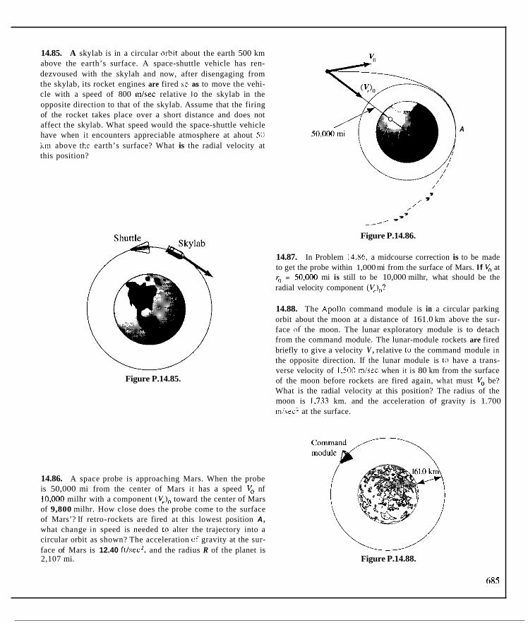
14.85. A skylab is in a circular orhit about the earth 500 km above the earth’s surface. A space-shuttle vehicle has ren- dezvoused with the skylah and now, after disengaging from the skylab, its rocket engines are fired so as to move the vehi- cle with a speed of 800 mlsec relative lo the skylab in the opposite direction to that of the skylab. Assume that the firing of the rocket takes place over a short distance and does not affect the skylab. What speed would the space-shuttle vehicle have when i t encounters appreciable atmosphere at ahout 5 0 km above the earth’s surface? What is the radial velocity at this position?
A
Figure P.14.85.
, , I
/ / , , ,
-_/’
Figure P.14.86.
14.87. In Problem 14.86, a midcourse correction is to be made to get the probe within 1,000 mi from the surface of Mars. I f V, at ro = 50,Wll mi is still to be 10,000 milhr, what should be the radial velocity component (v);! 14.88. The Apollo command module is in a circular parking orbit about the moon at a distance of 161.0 km above the sur- face of the moon. The lunar exploratory module is to detach from the command module. The lunar-module rockets are fired briefly to give a velocity V , relative to the command module in the opposite direction. If the lunar module is lo have a trans- verse velocity of 1,500 miiec when i t is 80 km from the surface of the moon before rockets are fired again, what must V, be? What is the radial velocity at this position? The radius of the moon is 1,733 km. and the acceleration of gravity is 1.700 misec’ at the surface.
14.86. A space probe is approaching Mars. When the probe is 50,000 mi from the center of Mars it has a speed V, nf 10,000 milhr with a component (V,), toward the center of Mars of 9,800 milhr. How close does the probe come to the surface of Mars’? If retro-rockets are fired at this lowest position A, what change in speed is needed to alter the trajectory into a circular orbit as shown? The acceleration of gravity at the sur- face of Mars is 12.40 ft/sec2, and the radius R of the planet is 2,107 mi. Figure P.14.88.
685

685 < IIAf’I tR I 4 MTTHODS Or MO”VlrNT11M I O K P A R I I C Lt 5
14.8 MOment-Of-MOmentUm Equations for a System of Particles
I m
X
0
0
~
0
We shall now develop the n i i ~ ~ i i c n t ~ ~ i l ~ t n ~ i ~ i i c n l i ~ ~ n cquetion\ for an aggrcgatc (if particlcs. The rcwlt i i ig cquatiiins w i l l hc of vi tal imporkincc when we apply then1 to rigid hodies in later chapters. We shall consider ii number of cases.
Case 1. Fixed Reference Point in Inertial Space. An aggregate of n par- t icles a n d an incrtiiil rclercnce are shown in Fig. 14.30. The moiiictit ol tnonicnluni cquetiiin for the ith particle i\ now written about the origin of thih rcfcrcncc:
’
Figure 14.30. Systcrn of ii particles. i 1
i where. a\ uwal.J, i s the internal force froni ttic.jth particle on the ith particle. We now sum (hi\ equation for all n particles:
/ I ,, + cc(r, X .f;!I = $ [ g ( r , X I ‘ , ) ] = k,,,k,l (14.23)
,=I ,=I
Y where the suninlation operation hxs heen put after the dillcrcntiation on the right side (perniishible because of the distrihutive property of difreren- tiation with respect to addition). For any pair of particles. the intcrn;tl forces wi l l hc equal and oppiisitc mil collinear (see Fig. 14.31). Hence, the forces wi l l have a ~ c r o iiioincnt ahiiut the origin. (This result i s most easily understood by reinemhering tha t , for purposes of taking moments ahout a point. forces w e tmn\mi\\ iblc.) W e can Ihcn conclude that the expi-ession
X
Figure 14.31. Inlernal equal and nppmitc forces.
in Ci is equation i s x I o . Rcaliritif l l i i i t c r , x I ; i s the tiital tiiorneiil of the
exlemal forces ahout the origin, we have iis ii 1-esult fiir Eq. 14.23:
Ma = H a (14.24)

SECTION 14.8 MOMENT-OF-MOMENTUM EQUATIONS FOR A SYSTEM OF PARTICLES 687
where this moment is taken about the aforementioned point a.I4
point can he given as the angular momentum of the center of
ri = rc + pcj (14.25)
X 0 Figure 14.32. c is center of mass of aggregate
The ar
Carry
4 1 =
But si]
Id
XYZ. Hm with res
ir momentum for the aggregate of particles about 0 is then
.he cross product and extract r‘ from the summations:
I is the center of mass, it follows that
u could also be moving with a constant velocity y , relative to inertial reference er, a would then be fined in another inertial reference X’Y’Z’, which is translating to XYZ at a speed Yr

Going hack to Eq. 14.27, we righr %ide are t~ he delered and we get then the desired result lor H,) :
that the second and third expressions on the
H,, = r, x ~ r ; +El?, x I I I , ~ , = r, x M?, + H ,
where H i\ the inomeiit ;ihour the center of in i i cs n i the linear tnoineiituni as seen from the center iif ]miss for the aggregate." ' l 'h is n a y he rewritten and cxprccced for (itty lixcd point (i whcrc, u\ing (,, a\ tlic positiiin vectni from f i xed point (1 to the center of tiiiiss c ' , we have
(14.2)
Thus, in ii rniiiiiier analogcius to thc c a w 01 kinetic enerfy (see Section 13.7). the rnoinciit i i f riioiiiciiluin ahiiut point ti is l l ic \uin (if the imiii iciit (if iiionieii- tuin rcliiti\'c to the cciitcr ol r i i i i s i plus ihc iiioniciit o i inoiiicntum o i the cc11- ter of inash ahiiut point ( I . Note tha1 i s the \'elocity (if (' reli i t ive rn fixed point <I and i s thus c q u i to the d o c i V o i the n m s center ~-eliiti\'c ti1 XYZ. Thus. we ciin express k l l . (14.2Xl a s
I I , , = I I , + ',,, x Mi, , ,
Furthermore. we have fiir lt ,:
H,, = H, + r,< x MI;:
whcre wc hiivc u\cd thc tact that r,,( = V to delete one expression Note in efiect wc h a c put d w ovci-H,, H , and V in Eq ( 14.3) to reach to iihove equa- tiim. We may now reet:ite E q 14.24 fni- ( i . f i . i dp ,~ i t i r ~i i l s iulliiws on replacing
I f , uhiiig the iihove equation. Then. uhing a, lir V wc have the desired rcsult:
M, = Hc + <,c X Ma, ( 14.30)
Case 2. Reference Point at the Center of Mass. We ciin use Eq. 14.30 for thih purpose. I'int. we wi l l replace M,, usins the left side of Eq. 14.23. BUI i n s o doing. we wil l rephce 5 iii the f i i -st expression hy (< + tic,). Note next th i i t Eq. 14.30 cal ls fix stationary point (1. Wc wi l l want to he the origin 0 o i XYZ ar id si) {,, hecoiiici 'itiiply 5 . l:iiiiilly. \+e replace a, hy i;' in liq. 14.30 ;ind w e have altcr thc\c steps
The internal force\ f . f iw LCIO contrihutiiin in this cqiiatiiin a s explained earlier and we Ihii\,c on i-c;irranging the remaining ternis in thc cqu;itim
' ' I

~ SECTION 14.8 MOMENT-OF-MOMENTUM EQUATIONS FOR A SYSTEM OF PARTICLES 689
wton's law for the center of mass, we know that F, = Mi, and so on the left and right sides of the equation above cancel. The
on the left side of the equation is the moment about the external forces. We then get
M, = Hc (14.31)
the same formulation for the center of mass as for a fixed point Please note that H,. is the moment about the center of mass
of niass but that the time
Toward or Away from the Mass Center. There to he considered and that is a point a acceler-
mass center of the aggregate (Fig. 14.33).
0 0
Figure 14.33. Point ii accelerates toward or away from c
For such a point, we can again give the same simple equation presented for cases I a d 2. Thus,
Ma = H" (14.32)
where is taken relative to point u (i.e., relative to axes xyz translating with poi t u ) . Wc have asked for the derivation of this equation in Prob- lem 14.9
Th component of the equation M,, = Hu for any one of the three cases in say th x direction,
i 1 I hf, = H c
ry useful. Here, M,, is the torque about the x axis, and Hr is the f momentum (angular momenturn) about the x axis. We now exam- problem in the following example.

690 CHAF'TEK 14 METHODS OF MOMENTIJM FOR PARlICLES
Example 14.16
A heavy chain of length 20 ft lies on a light plate A which is freely rotating at ;in angular specd of I r a d k c (see Fig. 14.34). A channel C acts as a guide lor the chain on the plate, and a stationary pipc acts as a guide for thc chain helow the plate. What is the speed of the chain after it moves 5 fr .stan- ing froin rest relative to the platform'? Neglect friction. thc angular mornen- tum of the platc, and the angular momentum of the vertical section of the chain ahout its own axis. The chain weight per unit length, n', is I O IhMi.
We \hall first apply the moment-of-momentum equation about paint 11 f(ir the chain and plate. Taking the component of this equation a lmg the I axis. we can say:
M; =
Clearly M: = 0. and so we havc conservation of angular momentum. That is,
(h) Fieure 14.34. Sliding chain
whcre I and 2 refer to the initial condition and the condition after the chain moves 5 ft. We can then say:
Therefore, wr = 8 radsec (cl
To find the speed iir iiiovemerit of the chain, we musr next gii 10
energy considcrations. Because only conservative forces are acting here, we may employ the conservation-of-mechanical-energy principle. I n so doing. we shall use as a datum the end of the chain R at the initial condi- tion (see Fig. 14.34). We can then say:
(PE), = ( IO)(W,)( IOJ + (in)(w)(s) = i.snnSt-lh
Observing Fig. 14.35. wc can say for condition 2: (PE), = (S)(M.)(IO) + (IO)(w,)(5) ~ (S)(w)(2.5)
= 875 ft-lb
As for kinetic energy. we have

SECTION 14.8 MOMENT-OF-MOMENTUM EQUATIONS FOR A SYSTEM OF PARTICLES 691
Exa ple 14.16 (Continued)
wher the first two expressions on the right side give the kinetic energy from the motion relative to the channel and pipe, respectively. The lasl expr ssion is the kinetic energy due to rotation of that part of the chain that is i n he channel. Clearly, V&rl = V . = 0 initially, and so we have I w e
I (KE), = +(lJ2[Y) j i " r Z d r = 51.Xft-lb
Furthbrmore, at condition 2, we have (see Fig. 14.35)
Notelhat (yhannr,)2 = ( V . ) Simply calling this quantity V2, we have P W 2'
= 3 . 1 1 V : + 4 1 4 i 1 : We c n now state
WE), + WE), = (PW, + WE), 1,500 + 51.8 = 875 + (3.11 V; + 4 1 4 )
Ther fore, i v* i: 9.19
a speed of 9.19 ft/sec along that the plate A is rotating al
Datum
I i Figure 14.35. Chain after motion of 5 ft.
M ch time will he spent later in the text in applying Ma = fie to a rigid body. T ere, the rigid body is considered to he made up of an infinite number of conti uous elements. Summations then give way to integration, and so on. The fin equations of this section accordingly are among the most important in mech nics.
In the homework assignments, we have included, as in Chapter 13, several ery simple rigid-body problems to illustrate the use of the equation M , = and to give an early introduction to rigid-body mechanics.'h We now illu i trate such a problem.
instructor may wish not to get into rigid-body dynamics at this time. T h i s approach

692 CHAPTER 14 METHODS OT'MOMENTI'M FOR PARTICLES
Example 14.17
A uniform cylinder of radius 400 mm and mass 100 kg is acted on a1 its center by a force of SO0 N (hee Fig. 14.36). What is the (tiction force.f? Takefi> = .2.
/ z
Figure 14.36. Rolling cylinder.
We have shown a free-hody diagram of the cylinder in Fig. 14.37. A reference xy: with origin al C translates with the center 0 1 mass. We first apply Newton's law relative to iiiertial reference XYZ.17 Thus. for the X direction we have for the center of mass C:
N
Figure 14.37. Free hody
Next, we write the moment-of-momentum cquation about the : axis, which goes through the wnrr,,- of mass. Thus, noting that we have simple circular motion relative to the ? ax i \ for a11 narticles of thc cvlinder and

I SECTION 14.8 MOMENT-OF-MOMENTUM EQUATIONS FOR A SYSTEM OF PARTICLES 693
ple 14.17 (Continued)
the cylinder and I is the thickness of the and differentiating with respect to time as
.40.f = - ( p l ) ( 2 z ) ( h ) [ q ]
f = -.I 005(p/)d
M = 100 = ( p I ) [ ~ ( . 4 0 ) ~ ] pl = 198.9kg/m2 (C)
(.40)0 = -x Ther fore,
(.40)W = - X
1 I Subs ituting for pI and r3 in Eq. (b) using Eqs. (c) and (d), we get
,f = (-.1005)(198.9) -~ [ . f O )
Now solve for X from Eq. (a) and substitute into Eq. (e):
f = ( . 1 0 0 5 ) ( 1 9 8 . 9 ) ( 7 ) 5 - . O l f '
Solvi g for j, we get
f = 166.6N I 6 We must now check to see whether our no-slipping assumption i s
valid The maximum possible friction force clearly is
fmax = (100)(9.81)(.2) = 196.2 N
whic is greater than the actual friction force, so that the no-slip assump- tion i consistent with our results.

694 CHAPTER 14 METHODS 0 1 ' MOMENTUM FOR PAKTICLES
"14.9 looking Ahead- Basic Laws of Continua
In the preceding tlircc chapters, we have presented three alternate ;Ipplo;lches. They were. broadly speaking:
1. 2. Energy mcth(ids. 3.
Thesc all conic from a c o n m o i l source (i.e.. Newton'\ law) iind si1 we can u\e any one for particle imtl rigid-body pnihlcms.
Later, when you study more cmiiplcx cunlinua such a s a tl(iwing iluid wilh heat transfer and compression you wi l l have Lo salisfy four hasic laws. Thcsc hasic laws are:
Direct applic;ition of Newl~in 's law.
I.inear-momcntuin methods and moiiient~of-miiiiicntum imettiod~
1. Coiiservati(in 111 mass. 2.
3. First law of Lhermodyiiamics. 4. Second law of thermodynamics.
For more general ciintinua. the above nientimicd fmir hasic laws" ire itid?- p n i l r . , ~ of each other (i.e., they must he separ;itely catisfied) whereas in par- t i ck and rigid-body mechanics that wc have bccn studying. 2 and 3 directly ahove. are cquivalenr to each other; I i s satisfied by simply keeping the ma\\ M constant: and 4 i s satisfied by making sure that friction impede\ the rela- tive motion hctwccn two bodies in contact.
Funhermore, we applied the approaches of the preceding thrcc chapters to free bodies, For more general continuuni studies. such iis lluid Ilou'. we can apply thc I.riur hasic law\ to systems (i.c., frcc bodies) and also to so- called coiitrol volumes (fixed voIumes i n space) as discussed in the I.ooking Ahead Section 5.4.
Thus. in this b~ iok , we are conqidering a very simplc phzisc [if coi i- t inuuni mechanics whcrehy. in effect. we need only consider explicitly one of the basic laws. Your view wi l l hriiaden a s you move thriiogh thc curr iculum
In some mechanics hooks there i s presented a n elementary preseimtion lor determining the force develiiped by ii stream of wiitcr or orher fluid on a
Linear momcntum and moment 01 momentum (Ihese are now Newton's law).

SECTION 14.9 LOOKING AHEAD BASIC LAWS OF CONTINUA 695
ng a similar approach, the other basic laws are developed in the
r the conservation of mass, we equate the net efflux rate of mass
author believes these laws in the above form should be taken up
f the basic laws needed in fluid mechanicsl9 and
IYSek I.H. Shames. Mechanics ofF/uid.r, McGraw-Hill. 3rd ed., 1992, Chapters 5 and 6.

4.89. #lane. Thc following datir apply:
m , = I Lg. m2 = 0.7 Lg. ,>I, = 2 kg. rnd = I .S hg.
A system u r particles i \ shown at t ime t moving in thc ,r!
V, = Si + Sj mlscc V , = -4i + 3,j mlscc V, = - 4 j mlscc V, = 3i ~ 4 j mlsec
(a) (h) (c)
What i \ thc total linear momentum of the \ystem'! What i s Ihc linear momentum ofthe ccntcr OS m a s s ? What i s the total inirrnent of mmlentum of the svstem about the origin i ind ahout point ( 2 , 6)'!
x f t k c
VIq (- 2 . 2
\ "4
Figure P.14.89.
14.90. .ies and masse\:
A \ystem of particles at time f has the following veloci-
V, = 20 fVsec, V, = I X ftlsrc. V, = I S ftlscc. v, = 5 ftlsec.
m , = I lhm mz = 3 Ihm m, = 2 Ihm
= I Ihm
Determine (a) the total linear momentum of the bystctn, (hJ the mgular mtrmentum rr f the systcnl ahout the wigin, and IC) the angu- lar momcntum nf the systrm ahout point (1.
s90
I n,
Figure P.14.90.
14.91. A system 01 particles :it t ime f , ha'i ~masscs V I , = 2 Ihm. I I Z ~ = I Ihm. in, = 3 lhm and location< and vdoci t ic \ a\ shown i n ( a ) . The cnmc system of musscs 15 \houri i n (h) a1 lime I,. What i q the total linear impulse o n the sysrcm durinp thib time intenal'! What is the total angular impulse 1 M di during thih t imc i n t r na l ahwl thc origin'?

45". -1
14.92. I .5 "11.
mass (I
AB whs that ins
(b) Time f2
Figure P.14.91-b.
m.
YO masses slide alvng bar AB at a constant speed 01 Bar AB rotates freely about axis CD. Consider only the : sliding bodies to determine the angular acceleriltion 01 l e hodies are 1.5 m from CU if the angular velocity 81
is I O radliec.
C
D Figure P.14.92.
14.93. A mechanical system is composed of three identical bod ies A , B, and C each of mass 3 Ibm moving along frictionless rod 120~ apart on a wheel. Each of these bodies is connected with ai inextensihle cord ti) the freely hanging weight D. The connectioi of the cords to L) is such that no torque can be transmitted to D Initially, the three masses A, B, and Care held at a distance of 2 f from the centerline while the wheel rotates at 3 radlsec. What ii the angular speed of the wheel and the velocity of descent of I if, after release of the radial bodies, body D moves I ft? Assumi that body D is initially stationary &e., is not rotating). Body L weighs 100 Ib.
I n
Figure P.14.93.
14.94. Two sets of particles a, b, and L', d (each particle of mass m) are moving along two shafts AB and CD, which are, in turn rigidly attached to a crossbar EF. All particles are moving at a constant speed V, away from EF, and their positions at the moment of interest are as shown. The system is rotating about G, and a constant torque of magnitude Tis acting in the plane of the system. Assume that all masses other than the concentrated masses are negligible and that the angular velocity of the system at the instant of discussion is w. Determine the instantaneous angular acceleration in terms of m, T, w, 9,. and s2.
w Figure P.14.94.
697

14.95. A uniform rod with a makc of 7 kglm lies flat on a fiic- tionless surface. A fhrce of 250 N act? on the rod as shown in the diagram. What i s the angiilar accclcralion o f the rod'! What i s thc acceleration of thc m
14.97. A unifbrm cylinder of cadius I 111 r d l s without dipping down a 30" incline. What i s tllc angular acccleriltion of thc cylin- der i f i t has ii ~nlilss 01 S O kp''
Figure P.14.97.
A cylinder of lungth i m a i d r n 14.98. 5 kg i q acted o n by a torque T = ( I 1.251 + ? I t ' ) N - m iwhcre I i s in seconds) about its gcomrtric %xi\ . What i s the anpular speed aftcr 10 SCC? The cylin- der i \ ill irc\t uhcn the torqur ih ;appllcd.
Figure P.14.95 7 7~ ~~~~~~~~ ~ , ~
A _ X ~ ~~ ~
*14.96. Consider an aggregate of particles with C i l k thc mass ,- mm centcr and m i n t A iiccelcratinz toward o r :LW:IY f n m C' . Starl wlth - the expression for H ahout 0 given :IS I*--- 3 111
Figure P.14.98. X P = xp , , , ) x * l '
14.99. 4 conmiit torque 7 of 800 N-m is :ipplied tu il uniform cyliiidcr 01 mdiur 400 cmn and mass 50 kp. A 1.500-kN weight is iiitached 10 thc cylindcr with ii liglil cable. What is the accclcration UI W !
Formulate Mi, in term, of I; arid use Newton's law to rlirninatr terms. Next show from the vxi l t inp equation that
I I M,, = € I ,
Figure P.14.96. I x'
14.101. A u m t i i n t t m p e Tu1 500 i w l h i \ applied t i l a uniform cylinder of r;itliii\ I it. A light inrxtcnsihlr cable i \ urapped part])

connected to a block W of W if the cable doe.s not the hlock. For the cylin-
14.102 a widtt assume section center1
What i water i axes)?
i i (
14.103 frictior the an$ the ma;
Figure P.14.103.
14.104. Do Problem 14.103 for the case where a force given as: & = .1
F = S0i + 7SjN Figure P.14.101.
is applied at point u instead of the 500-N force.
14.105. A cylinder weighing 50 Ib lies on a frictionless surface. " and a depth Of ". The Of water is Two forces are applied simultaneously as shown in the diagram.
What is the angular acceleration of the cylinder'? What is the
canal with a rectangular cross section is shown having
be zero at the banks and 10 V Z Y Parabolically over the iown in the diagram. If 6 i s the radial distance from the f the channel, the transverse velocity Vs is given as
of the center?
V, = $225 ~ a*) ft/sec
angular momentum Ha about 0 at any time f of the circular portion of the canal (Le., between the x and y
radial component v i s zero.
Y
Figure P.14.102.
hoop with mass per unit length 6.5 kg/m lies flat on a surface. A 500-N force is suddenly applied. What is acceleration of the hoop? What is the acceleration of nter?
Figure P.14.105.
14.106. A thin uniform hoop rolls without slipping down a 3V incline. The hoop material weighs 5 Ib/ft and has a radius R of 4 ft. What is the angular acceleration of the hoop?
Figure P.14.106.
699

700 CHAPTtK I 4 MFTHODS Ob MOMtNTUM FOR PAKTICLtb
14.10 Closure One o l the topics studied in this chapler i s the impact of bodies under certiaiia restricted conditions. For such problems, we can consider the bodies as parti- cles before and after impact, but during impact tlic bodies act as deformahlc media for which a particlc model i s n o t meaningful or sufficient. By making an clcmcntnry piclure of the action. we introduce the coefficient of restitutiun to yield additional infiirmation we need t i i determine velocities after impact. This i s an empirical approach. s o our analyses are limited to simple prohlems. Tu handle more complex prohlems or to do the siinplc ones more precisely. we would have ti1 makc a more rational invcstigation o f the deformatioii actions taking place during impst- that is. i a continuum approach (11 part 111
thc problem would he rcquircd. However, we cannut makc a careful rtudy 01 the deformation aspects in this text since the suhject 111 h ighpeed defornaa- tion of solids i s ii difficult one that i s s t i l l under careful study by engineers and physicists.
Note in the last two chapterr we started with Newton‘s law F = Mu and pcrformed the fiillowing operations:
1. ‘Took tlic dot pruduct of hotti sides using piisilion vcclur r . 2. Multiplied both sides by ilr and integr:iicd. 3. Took thc cross product of both sidcs using position Yector r .
These steps permitted a surprisingly large number of very useful t?irmulaliiins and concepts that have occupied us for some considerable time. These wcrc thc energy methods. the lincar-momentum methods. and the moment-of- niomentuiii methods. I t should now be clear that Newton’s law requires coti- siderable study tu fully explore i t s use.
In our study o f moment of tiiwneiiturn fur a system of particles. we set foith one o f the kcy equations nf inechanics, M,, = HA. and we inlroduced in the examples several considerations whose mure cai-eful and complete study wi l l occupy a good purtiim o f the remainder of the tcxt. Thus, in Example 14.17 we have “in miniature.” as i t were. the major cleinents involved in the rludy of much of rigid-body dynamics. Recall khat “c employed Newton’i law for the mass center and thc n i~ in i en t~o f~ i r~o ine r~ tu~ i~ equation about the mass center to reach the desired rcsults. In 50 doing. however. we had to make use of certain elementary kinematical idcas from our carlicr work in physics. Accordingly. ti1 prepare ourselvcs fur rigid-body dynamics in Chap ters I 6 and 17. we shall dcvote ourselves in Chapter I S to a rather ciareful examination o f the general kinematics of a rigid body.
Although we shall he much conccrned in Chapter 15 with the kinemat- ics of rigid budies. we shall nut cczse to consider particles. You will see that an understanding of rigid-body kinematics wi l l pcrmit us 10 formulate very powerful rclatiuiis for the gcncral relative motions of ;I particle involving references that niuve in any arbitrary manner with respect to each other.

Figure P.14.107. 1 = (100 + 5 0 ~ ' ) Ib
"; = 30 Ib, W, = 60 Ib, and W, = 50 Ib, what is the force'? The dynamic
P
Figure P.14.108.
200 km'!
x
,
Figure P.14.109.
14.110. A space ship is in a circular parking orbit around the earth at 200 miles above the earth's surface. At space headquar- ters, they wish to get the vehicle to a position 10,ooO miles from the center of the earth with a velucity at this position of 25,000 miihr. The command is given to fire rockets directly to the rear for a specified shon time interval. What is the change in speed needed for this maneuver? What are the radial and tangential velocity components of the 25,000 mi/hr velocity vector?
, . , , ,
I i
f I I \ \ \
, - _ _ / . Figure P.14.110.
70 1

14.111. A small clastic ball is dropped from a height of5 m onto a rigid cylindrical body having a radius of 1.5 111. At what position on thex axis does the hall land after the cullision with thc cylinder?
strikes 1.5 rn above the .r axib and i f the c o l l i i i m is pe~ltclly ela\- tic, what i \ the maximum height rcached hy the bullet as It iico- chets'! Nrglcct air rmihtanoc and rake thc belocity 01 the hullct on impact as 700 m/scc with a dircctiw thdt I S p~ra l le l to the I axis.
1.
v
I 5 m
I Figure P.14.115
14.116. I n Plohleni 14.1 15. ilsbunic an inela'tic impact with t = .h. A t what position along ,x does the bullet strike the p a r a h h after the irnpxr'?
14.117. aruund the earth 200 k m above the earth's hurfacr. I t i \ lo lransfrr tu another circular orbit (2) 500 km ahow the earth's surface. The transfer to the second orhit i s dune in two stage,.
A >pace \rehick is in a circular "parking" orhit ( I
x
Figure P.14.111.
I 14.112. Do Problem 14.1 I I for an inelastic impact with t = .h. 1. Fire rucheth so the vehicle has an upoper cquill tu the r d i u 0 1 the sccond circular urhit. Whal uhangc of speed i \ required l o i ~ this 14.113. A small elastic sphere i s dropped fiom pusitiun (2, 3,
30) f t onto a hard soherical body havine a radiub of 5 ft positiuned - so that the I axis of the reference shown is along a diameter. Far a perfectly elastic collision, give the speed of the s m d 1 sphere directly after impact.
2. At u~ iopw rockets are (ired again t i l get into the second circu- lar orhit. Whal i s thi\ srcund change of hpced?
~- 500 k m , , ~~ . \,' ,_---.- .. - \ .~., \
0 I 1 I I I I I I
, - ~~ ~ ~~
2 00km- ~. , Figure P.14.117.
*14.118. A tugbwdt weighing 100 tuns is moving toward a statiuii- ay buge weighing 200 tom and cuy i ng a load C wcighing 50 ton&. The tug ib moving at 5 knots and its propellers arc devcloping a thrust of 5,000 Ib when it cwlacts the huge. Ai a result of thc soft padding at the nose of the tug. consider that there i s plastic impact. If the load C IS not tied in any way to the huge and has B dynamic coefticient of friction o f . I with the slippery deck of the harge, what i\ the sped V of the barge 2 sec after the tug first contacts the barge'! 'The load C slips during a I-see internal starting at the beginning of the contact.
/
Figure P.14.113.
14.114, D~ problem 14,113 for an inelastic impact with = ,6,
14.115. A bullet hits a smooth, hard, massive two-dimensional body whose boundary has been shown as a parabola. If ihe bullet

x i I Figure P.14.118.
Figure P.14.119.
14.120. A body A weighing 2 tons is allowed to slide down an incline o a barge as shown. Body A moves a distance of 25 ft along the incline before it is stopped at E . If we neglect water resistanc I how far does the baree shift in the horizontal direction?
1 \/ 25’ -4
. ..... . ..- -. _ _ _ _ _ ~ Figure P.14.120.
14.121. A water droplet of diameter 2 mm is falling in the atmos- phere at t e rate of 2 d s e c . As a result of an updraft, a second water droplet o diameter 1 mm impinges on the aforementioned droplet. The vel ity of the second droplet just prior to impingement is i
3i + 1 j mlsec. After impingement three droplets are formed mov- ing parallel to the ry plane. We have the following information:
D , = .6 mm,
D, = 1.2 mm,
V, = 2 d s e c ,
V, = I mlsec,
8, = 45’
0, = 3W Find D,, V,, and 8,.
3 mlsec 7 1 m/sec
(a) (b) Figure P.14.121.
14.122. If the coefficient of restitution is .8 for the two spheres, what are the maximum angles from the vertical that the spheres will reach after the first impact? Neglect the mass of the cables.
2.5 kg Figure P.14.122.
:tior 123. Thin discs A and B slide along a s surface. Each disc has a radius of 25 mm. Disc ~A has a mass of 85 g, whereas disc B has a mass of 227 g. What are the speeds of the discs after collision for c = .7? Assume that the discs slide on a frictionless surface.
I . , . ,
;_I Figure P.14.123.
703

14.124. A BB i \ shot at the hard, rigid surface. The speed o l l l i c pellet is 3110 fisec a\ i t strikrs the suriace. If the directimi of the velocity for the prllel i s @\en hy thc i d low ing unit vector:
14.127. Cmipnle thc angular cmonicntiim uhout 0 01 a uniform Irrd, of Icngth L = 3 r i i iind n i t w pcr unit Icnglh nr (11 7.5 hs/rn. ill l l i e ina i i i f Nhcn i t i i \ert ici t l iind h a \ an a n g ~ i l a ~ ~ speed (0 (6
t = -.6i - .Xk 3 i-adlscc. what is thc f inal velocity \'ectoi of thc pcllet lor ii col l is ion havinz E = .7? 0
I 7-
k
,/ \
A 5 '
Figure P. 14.124.
A chain 0 1 wrriught i1on, with length o f 7 111 and il n i a v
of 100 kg, is held so thal i t jus1 touches the \upport AB. I l t l i e ~ h i i i r i i s rclcased, determine the total impulse driririg 2 sec in thc wrtic:il directinn cxpcrienced by thc support if the impiicl i\ plastic (i.u., the chain does not bounce up) arid i f we m w t : thz support \(I that thc links land UII the platfimn and 1not 011 each othcr'! IHirit: Notc that any chain wrsrin*. on AH dclivcrc a vcrtiCal impulsc. Also check 10 see if thc entire chaiii lands 0 1 , AH hcfiire 2 sec.]
!5.
Figure P.14.125.
14.126. Two trucks x e shown moving up ii I O incliiir. Tmck ,A weighs 26.7 kN and i s developing il 13.30-kN driving lorce on thc road. Truck R wzighs 17.8 hN and i \ curinccled with an incxtensihle cable to truck A. By operating a winch h, truck B approaches truck A with a conmnt acceleratim oi 3 m/xc.'llill lime f = 0 both r l u c k ~ have a speed of 10 mlsrc. what arc their ipeeil\ a1 timer = 15 scc?
Figure P.14.126.
w
Figure P.14.127.
Fieurc P.14.12X.
704

14.130. closed container is full of water. By rotating the container or some time and then suddenly holding the container stationary we develop a rotational motion of the water, which, you will I am in fluid mechanics, resembles a vunex. If the veloc- ity of the uid elements is zero in the radial direction and is given as 101r f sec in the transverse direction, what is the angular momentu i of the water?
14.131. rod that i' the masse; mtates at from this which have for the CO
relative tu 1 0 Ibm. Show that
1 Ill'
Figure P.14.130.
dentical thin masses A and B slide on a light horimntal attached to a freely turning light vertical shaft. When are in the position shown in the diagram, the system
;I speed wof 5 radlsec. The masses are released suddenly position and move out toward the identical springs.
a spring constant K = 800 Iblin. Set up the equation npression 6 of the spring once all motions of the bodie?
the rod have damped out. The mass of each body ii Neglect the mass of the rods and coulombic friction
S = .OX361 in. satisfies your equation.
I Figure P.14.131. I
14.132. A spacecraft has a burnout velocity Vo of 8,300 mlsec at an elevation of 80 km above the earth's sulface. The launch angle a is 1 5 ~ . What is the maximum elevation h from the earth's surface for the spacecraft?
Figure P.14.132,
14.133. A set of particles, each having a mass of 112 slug, rotates about axis A--A. The masses are moving out radially at a constant speed of 5 ft/sec at the same time that they are rotat- ing about the A-A, axis. When they are I ft from A-A, the angular velocity is 5 radlsec and at that instant a torque is applied i n the direction of motion which varies with time f in seconds as
torque = ( 6 1 ~ + l o t ) lb-ft
What is the angular velocity when the masses have moved out radially at constant speed to 2 f t?
Torque
Figure P.14.133.
14.134. A torpedo hoat weighing 100,000 Ib moves at 40 knots ( I knot = 6,080 ftlhr) away from an engagement. To gv even faster, all four 50-caliber machine guns are ordered to fire simul- taneously toward thc rear. Each weapon fires at a muzzle veloc- ity of 3,000 ftlsec and fires 500 rounds per minute. Each slug weighs 2 0%. How much is the average force o n the boat increased by this action'? Neglect the rate of change of the total mass of boat.
705

14.135 A devicc to be detunatcd with a small charge ir suspended in space [ser (a)] . Dircctly after detonation. lour frag- ments are formed moving away from the paint of suspension. The following information is known ahout thcse fragments:
m , = I Ihm
m, = 2 lhm
v, = 200; ~ l0O.j f l k c
= 1 2 3 + I X O j ~ 100k Wsec
m, = 1.6 lhm V , = ~ 200; + l S O j + 1X0k fUsec
= 3.2 Ibm
What is the vclacity <'!
to the war of 10 Wsec relative tu the initial spccd uf thc octopus. What horicpowcr is hcing dcvckrped hy the octopus in thc ahme action i T it occurs in I rec'!
*14.138. I n the ,fission procebs i n a iiuclziir reactor, a r isU nucleus first ahsorhs (11 captures a neutron lsee (a)]. A short tinic later. the "'U nucleu5 hreakr up into lission products plus ncu- troiis, which may suhsequently he captured by ulher 23'U nuclei and inaintain a <.kiiiw r rw l i on . Energy is rcleased in each fiwion. 111 (h) we have shown the results of a possible fission. The fnllnw- ing information is known fnr this fission:
Kinetic Maw Energy No. (MeV) Direction of V
Figure P.14.135.
14.136. A hawk is a predatory h i d which olten auacks snvallei birds in flight. A hawk having a inass of 1.3 kg is swooping down nn a sparrow having a mass of I S 0 g. Just hcfore se i~ing the rpar- row with its claws. the hawk is moving downward with a speed VH of 20 kmlhr. l h r spnrrow i s moving horizontally at a speed C; of I S kmlhr. Directly after cei7.ure. what is the speed of the hawk and its prey'! What i c the loss in kinetic energy in J~xdes ' !
14.137. The principal mode of propulsion of an ~ctopua i s tu take in water through the mouth and then after closing the inlet to cject the water to the rear. If a 5-lh octopus after taking in I Ih of water is moving at a spccd of 3 ftlscc, what is i ts \peed directly after ejecting the water'? The water is ejcctcd at an average \peed
Prr,duct A I3X E E,, = .3i - .2j + .YXk
Neutron I I IO E , = .hi + .8j Neutron 2 I IO E , = .4i - .hj - .hWk
Prclduct n 96 90 eH = l,i + m8j + n,$
What i s the energy E of product A in MeV and what is the V C C ~ O ~
E" for the velocity of product B? Assume that before fissiun the nuclcus of 235U plus captured neutrons is stationary: [Hinr: You do not h u e to aclually ciinvert MeV to j d c s or atomic number to kilogram5 to cilrry out the pnihlem.]
f Y4
l b ) X
Figure Y.14.138.
706

Kinematics of /Rigid Bodies: Relative Motion
Introduction
ble to analyze complicated motions in a more simple systematic several references. Second, the motion of a particle is often
set the stage for our main effort in the remaining ponion
15.2 Translation and Rotation of Rigid Bodies
For pu ses of dynamics, a rigid body is considered to be composed of a continuo s distribution of particles having fixed distances between each I I 707

708 CHAPTER 15 KlNEMAllCS OF RIGID BODIES: RELAI'IVC MOTION
,dl
Figure 15.1. TrJnrlation of il hod?
Rotation. I1 ii ripid hmly IIIOK\ s o that alonx wmc \tlaight line all [he px- ticks of thc body. ( I I ~ II 1hypothctic;il r x i e m i o ~ ~ o f t l i c hod). have veloc- ity relative io wnie refcrcnce. lhe hody 15 said to he ill roiolron rclatiw to
this relrrencu. 'l'he l ine o l atation:uy p x l i c l e i i i called thc irris qt m r ~ r r i o , ~ .
We shall now conhider how wc nleahure the rotation of a body. A s i l l - gle revoIution i h defined as the iiiilount of rotiitiun in either a clockwise or a counterclockwisc direction ahout the n i s of rotation that hrings the hody back ti1 its original position. Partial revolution\ ciin ciinveniently he rneasurcd hy obserbing riny line segmenl cuch :IS ,113 in thc hody (Fig. 15.2) from a vicwpoint M-M directed along the asis 0 1 rcrlation. In Fig. 15.3, we have hhown this vizw of AB at thc bcgititiiiig of the partial rotation as seen along Ihz axis of rotation. as well iis the \,ien' A'H' iit 1hc end of the paitial rotation. TIE angle f l that these line\ f<rrni wil l he the same lirr the initial and final
J \\\ ,\ M
\ \ -
,\ f
0 /'
Firure 15.2. Ilotatim u t a hody.
Figure 15.3. Mrnsurc of a part ial wlatiun.

SECTION 15.3 CHASLES' THEOREM 709
e angle so formed
, so that infinitesimal rotations dp are vector quantities. There- magnitude dpldt with
15.3 Chasles' Theorem
e displacement vector for this translation is shown at
ngle A$ about an axis of rotation which is normal to the plane and ses through point E'.
1 Figure 15.4. Translation and rotation of a rigid body.

710 CHAPTER 15 KINEMATICS OF RIGID BODIES RELATIVC MOTlOh
What changes would occur had we chosen some lither point C for such a procedure? Consider Fig. 15.5, where we have included an alternative procedure by translating the body so that point C reaches the correct final position C'. Next. we must rotate the hody an amount A@ ahout an axis of rotation which is normal to the plane and which passes through C' in order k1
get to the final orientation of the body. Thus, we have indicated twu routes. We conclude from the diagram that ihc displacement ARC differs from AR,. hut there is no difference in the amount of rotation A@, Thus, in general. AR arid rhe axis of rototion will drpend on rlir poiiit ,,ho.rrn. uliilr rhr r i i n ~ i i i i f 01 rotation A@ 4 1 he the .same.for r i l l such pobit.r.
!
A R,
Figure 15.5. Tmnslatim and rotiition of a rigid body u\inp point\ N ; ~ n d C'.
Consider now the ratios ARlAr and A@IAt. Thcsc quantities can he regarded as an average translational velociiy and an average rotational speed, respectively, of the body, which WE could soperpme to get from the initial position to the final posilion in the timc AI. Thus, ARIA/ and A@lAl rcprescnt an average measure o f the miitiiin during the time interval At. Ifwe go io rhr limit by letring A I + 0, use have in.rruntunrous tran.slutional and angular velocities which, when superposed, give the iristantrineuus motion qfrhr body. The displacement vector of the chosen point B in the previous discussion rep- resents the translation of the body during the time A/. Furthermore. the chosen point B undergoes no other n~otion during At oiher than that occurring during translation. Thus, we can conclude that, in the limit, the trun.rlntionu1 velor.i/y used for the hody corresponds to the acrual insrurrrurleous velocity of the cho- sen point B at time t. The angular velocily w t o be used i n the movement US the body, as described ahove. is the ~ a m e vector for d l puints B chosen Accord- ingly, w is the instantaneous ungular velocity of the body.
We have thus far considered the movenient of the body along a plane surface. The same cunclusioiis can he reached for the general motion of an arbitrary rigid body in space. We can then make the following statements for the description of the general motion of a rigid body relative to some refer- ence at time t These statements comprise Chasles' theorem.
1. Select any poinl B in the body. Assume that all particles of the hody havc
2. Superpose a pure rotational velocity w about an axis of rotation going at the time r a velocity equal to V,, the aciual velocity of the poini B.
through point B.

SECTION 15.4 DERIVATIVX OF A VECTOR FIXED IN A MOVING REFERENCE 71 1
V , and w, the actual instantaneous motion of the body is deter- w will be the same for all points B which might be chosen. Thus,
velocity and the axis of rotation change when different
15.4 Derivative of a Vector Fixed in a Moving Reference
arbitrarily relative to each other in Fig.
equal to the velocity of 0, onto a rota- axis of rotation through 0.
Howeve), be zero. followin 1. Consider
tion A cannot
2. We with
'The action doe, O f equality
Figure 15.6. Vector A fixed in xyz moving relative to XYZ.
suppose that we have a vector A of fixed length and of fixed on- reference xyz. We say that such a vector is "fixed" in
Clearly, the time rate of change of A as seen from reference can express this statement mathematically as
as seen from XYZ, the time rate of change A will not necessarily To evaluate (dAldt),, we make use of Chasles' theorem in the ; manner:
the translational motion k. This motion does not alter the direc- o'A as seen from X Y Z . Also, the magnitude of A is fixed; thus, vector
change as a result of this motion.' nt:xt consider solely a pure rotation about a stationary axis collinear (1) and passing through point 0.
line of action of A, however. will change as seen from X Y Z . But a change of line of not signify a change in the vector, as pointed out in Chapter I on the discussion
of "Cctors.

To best observe this rotation, we shall employ at 0 a srationury refer- cncc X’Y’Z’ po\it imed sci lhar %’ coincides with the axis of rotation. This ref- erence i s shown in Fig. 15.7. Now thc vcctorA i s rotaling ill this instant abiiul
X /’ I4gwe 15.7. (~‘ylindrica comlxmcnts f i r i \cccor A
h e Z‘ axis. We have \tiown cylindrical coordinates to the end o f A (Le.. iit point ( 1 ) ; :mil hiivc shown cylindrical components Ai. A,,. and A,. In Fif. 15.8. we h a w sh(iun point i i with unil vcctors E?. ea. and e7,, for cylindrical coiirdinatcs a1 thih point. Wc can accordingly cxpress A as
A = A,€, + AH€# + AL.e7
Y’
X Figure 15.8. Unit vectors fbr cylindriual coordinate
Clcarly, 3s A rotales ah(iu1 z‘. the values of the cylindrical scalar componcncs o l A for X’Y’Z’. namely Ai, A,. and A,,. do not change. Hence. as seen from

~ SECTION 15.4 DERIVATIVE OF A VECTOR FIXED IN A MOVING REFERENCE 7 13 I
X'Y'Z, 4 = A, = A, = 0. Also, noting that iZ, = 0, we can say that
Thc: reference we see lines of in q z i s
1. The
2. The itself
position.
We
We have already evaluated the time derivatives of the unit vectors for cylin- drical c rdinates. Hence, using Eqs. I 1 2 8 and 11.32 and noting that 6' correspo ds to 0, we have 1.
foregoing result gives the time rate of change of a vectorA fixed in x.yz moving arbitrarily relative to reference XYZ. From this result,
that (dAldi),, depends only on the vectors w and A and not on their action. Thus, we can conclude that the time rate of change of A fixed lot altered when:
vx to r A is fixed at some other location in xyz provided the vector
a:tual axis of rotation of the xyz system is shifted to a new parallel s not changed.
can differentiate the terms in Eq. 15.1 a second time. We thus get
side is simply the cross product of w andA as you can see cross product with cylindrical components. Thus,
We conc ude that ! relative to XYZ, we would observe the same time reference as from the former reference. That is,
and we can conclude that
(15.1)

714 CHAPTER is KINEMATICS OF RIGID BODIES: RELATIVE MOTION
Using Eq. 15.1 to replace (dAldrJ,, and using & to replace (dwldt),,, since the reference being used for this derivative is clear,2 we get
You can compute higher-order derivatives by continuing the process. We suggest that only Eq. 15.1 be remembered and that all subsequent higher- order derivatives he evaluated when needed.
In this discussion thus far, we have considered a vectorA fixed in a ref- erence hyz. But a reference xyz is a rigid system and can he considered a rigid body. Thus, the words ‘!fixed in a rsferencr xyz” in the previous discussion can he replaced by the words ‘ : fwd in a rigid body.” The angular velocity w used in Eq. 15.1 is then the angular velocity of the rigid body in which A is fixed. We shall illustrate this condition in the following examples, which you are urged to study very carefully. An understanding of these examples is vital for attaining a good working grasp of rigid-body kinematics.
As an aid in carrying out computations involving the triple cross prod- uct, we wish to point out that the product
o , k x (@,k x cj) = -0;c j
That is, the product is minus the product of the scalars and has a direction corresponding to the last unit vectnr, j . Remembering this will greatly facili- tate our computations.3
Additionally, consider a situation where the angular velocity of body A relative to body B is given as wI, while the angular velocity of body B rela- tive to the ground is w2. What is the total angular velocity w7 of body A rel- ative to the ground? In such a case, we must rememher that the angular velocity wI of body A relative to body B is actually the difference between the total angular velocity w,of hody A as seen from the ground and the angu- lar velocity w2 of body B as seen from the ground. Thus.
w1 = W T - w 2
Solving for wy we get
w7 = w 1 + W2
We see from above that to get the total angular velocity wT, we simply add the various relative angular velocities just as we would with any pair of vectors.
‘When it is clear from the discussion what reference is involved fur a time derivative. we
’Of course, i f the j vector weie a k vector, then clearly we would amiw at a iiull value for shall use the dot to indicate a time derivativc.
the triple vector product.

Exal
A dis with whicl const paral' veloc (d2w
ily gi
At th
To g alwa: dot ti
Cons to he c h r may since
SECTION I 5.4 DERIVATIVE OF A VECTOR FIXED IN A MOVING REFERENCE 115
pie 15.1
7 is mounted on a shaft AB in Fig. 15.9. The shaft and disc rotate onstant angular speed wz of 10 radlsec relative to the platform to earings A and B are attached. Meanwhile, the platform rotates at a angular speed wI of 5 radlsec relative to the ground in a direction to the Z axis of the ground reference XYZ. What is the angular vectorw for the disc C relative to XYZ? What are (dwldt)xrz and
ie total angular velocity w of the disc relative to the ground is eas-
2 )xyz?
1 at all times as follows:
w = w, + w2 radlsec
istant of interest as depicted by Fig. 15.9, we have for w:
Disk C &wJf
I Platforin I Ground Reference Figure 15.9. Rotating disc on rotating platform.
the first time derivative of w, we go back to Eq. (a), which is valid and hence can be differentiated with respect to time. Using a :present the time derivative as seen from XYZ, we have
ri, = ri,, +&J2 (b)
'r now the vector w2. Note that this vector is constrained in direction ways collinear with the axis AB of the bearings of the shaft. This is a physical requirement. Also, since q is of constant value, we nk of the vector w2 as $red to the platform along AB. Therefore, 2 platform has an angular velocity of wI relative to XUZ, we can say:
(C) G2 = w , x w2

7 16 C H A P T ~ K I S KINEMATK'S or' RIC;II) Bouifs KEI.ATIVI: MOTION
Example 15.1 (Continued)
As Cor W,, namely the other vector in Eq. (b). wc iiotc Lhal iis s e m f rnm XYZ, w , i s a cnnslant veclur and si) at all times r U , = 0. Hcncc Eq. (h) can be written 21s Si)llows:
& = w l x u , ((1)
This equatinn i s valid at all times and s o can he differentiated again. AI the instant of intercut as depicted by Fig. 15.9. wc l iavc for W:
To get &, we ~ i o w differentiate (d) with respect to time. W c llavc
ij = W l x w2 + w, x &> = 0 + wI x lw, x W, i ( 1 )
where we have wed the Sac1 that h, = 0 at a l l times a s well a s ti. ( c ) I i r W,. At the instant nf interest, we have
ij = Sk x ( 5 k x lO. j i = -2Mjradsec3
Example 15.2
In Example 15.1, consider a position vector p hctween two points nn the rotating disc (see Fig. 1 5 . 1 0 ) . The length o f p i s 100 rnm and. at the instanl of interest, i s in the vertical direction. What are the l in t and hecond time derivatives ofp at this instan( as seen from the ground referencc'?
It should he ohvious that the vector p i s fixed ti) the disc which has at all times an angular velocity relatiw ti) X Y Z equal to w , + w,. Hencc. at al l times we can say:
p = tw, t w ? ) X p i a ) Figure 15.10. Displaccrnrnl V ~ C I O ~ p in disc. A t the instant o f interest. we have noting that p = IOOk
ii = ( S k + lOji x IO(lk = 1,000imdsec
p = (&, + & > I x p + ( w , + W 2 ) x p
( h i
To get the secnnd derivalivc n t ~ ) . go back (11 Eq. (a) and diSkreiitiate:

SECTlON 15.4 DERIVATIVE OF A VECTOR FEED IN A MOVING REFERENCES 7 17
I Exa ple 15.2 (Continued)
Notin that cbl = 0 at all times and, as discussed in Example 15.1, that w2 is ixed in the platform, we can sdy:
p = (0 + W I x w 2 ) x p + (wl +w:) x p (C)
p = (Sk x l O j ) X lOOk + (5k + I O j ) x 1,000imm/sec2
I At th instant of interest we have, on noting Eq. (b): 1
AI hough we shall later formally examine the case of the time deriva- tive of v ctorA as seen from XYZ when A is notfixed in a body or a reference xy:, we an handle such cases less formally with what we already know. We illustrate ! this in the following example.
I Exa pie 15.3
For t e disc in Fig. 15.9, oz = 6 radlsec and d2 = 2 rad/sec2, both rela- tive the platform at the instant of interest. At this instant, wI = 2 radls c and hl = -3 rad/sec2 for the platform relative to the ground. Find the a gular acceleration vector dJ for the disc relative to the ground at the insta t of interest.
The angular velocity of the disc relative to the ground at all times is
For 4 , we can then say
It is pparent on inspecting Fig. 15.1 I that at all times w I is vertical, and so w i , can say:
w = 0 1 + w 2 (a)
dJ = cbl + c b 2 (b)
''

71 8 CHAPTER I S KINEMATK‘S 0 1 : RIGID BODIES: Rlil.ATIVE MUIION
Example 15.3 (Continued)
However, w2 is changing direction and, mnst imporlantly. is changing magnitude. Because of the latter, w2 cannot he considercd lixcd i n ii refer- ence or a rigid body Sor pui-poses of computing b2. To get around this diS- ficulty, we fix a unit vector j ’ 011f0 tlw plu!fi,rm to he colliiiciir with the centerline of the shaft A B as shown in Fig. 15.1 I. Wc know the ;In_pular velocity of this unit vector; it is w , at all Limes. We can then express o2 i n the following manner, which is valid at all time\:
w2 = w2j ’ ( d )
X relerenie Figure 15.11. Unit veclorj’ fixed Lo platform.
We can differentiate the above wilh respect to time as fol low\:
b2 = [b7 j ’ + w2 J’
Butj’ is fixed to the platlorin which ha\ angular vclocily w , relalive 10
XYZ at all times. Hence. we have for thc above.
( e ) G2 = (b2j ‘ + 02(wI x j ’ )
Thus, Eq. (b) then can be L’ w e n ns
b = w , k + o i 2 j ’ + m 2 ( w , X j ’ )
This expression is valid at all Limcs and could he differentiated agnio. At the instant of interest, we can say. noting thatj’ = j ifit this instant,
b = -3k + 2 j + b ( 2 k x j )
2 j - Y r d s

15.1. Is the motion of the cabin of a ferris wheel rotational or translational if the wheel moves at uniform speed and the occu- pants cause no disturbances? Why?
15.2. A cylinder rolls without slipping down an inclined surface. What is the actual axis of rotation at any instant? Why? How is this axis moving?
15.3. time t a velocity relative to reference XYZ given as
A reference xyz is moving such that the origin 0 has at
V, = 6 i + 12j + 13kftlsec
The xyz reference has an angular velocity w relative to X Y Z at time t given as
o = 1Oi + 12j + 2kradIsec
What is the time rate of change relative to XYZ of a directed line segment p going from position (3,2,-5) to (-2.4.6) in xyz? What is the time rate of change relative to XYZ of position vectors i’ and k’?
z
/ X’
Figure P.15.3.
15.4. of the origin given at time I as
A reference xyz is moving relative to X Y Z with a velocity
V , = 6 i + 4 j + 6 k d s e c
The angular velocity of reference xyz relative to XYZ is
w = 3i + 14j + 2kradlsec
What is the time rare of changc as SCCCT from XYZ of a directed line segment P , , ~ in xyz going from position 1 to position 2 where the position vectors in ry z for these points are, respectively,
p , = 2 i ’ + 3 j ‘ m p7 = 3 i ‘ - 4 j ’ + Z k ’ m
Z
x
i I Z
x
X / Figure P.15.4.
15.5. Find the second derivatives as seen from XYZ of the vector p and the unit vector i’ specified in Problem 15.3. The angular acceleration of qi relative to XYZ at the instant of interest is
& = 5 i + 2 j + 3 k r a d / s e c 2
15.6. Find the second derivative as seen from X Y Z of the vector P , , ~ specified in Problem 15.4. Take the angular acceleration of xyz relative to X Y Z at the instant of interest as
& = 1% - 2k rad/secz
15.7. A platform is rotating with a constant speed 0, of IO radlsec relative to the ground. A shaft is mounted on the platform and rotates relative to the platform at a speed o2 of 5 radlsec. What is the angular velocity of the shaft relative to the ground? What are the first and second time derivatives of the angular velocity of the shaft relative to the ground!
C;-
X Py Figure P.15.7.
7 1‘

15.8. In I'rohlem 11.7, what are the f i n 1 mil second t i m e derivati\!ec of il dircctcd line segment p i n the disc at thc instant [hill the \ystem has thc gewncir) \Iiown? 'The x c t o r p i \ 01 length I O inin
Figure P.15.Y.
Figure 1'.15.11.
X ry Figure P.15.12.

Figure P.lS.15.
Figure P.15.13.
15.14. An electric motor M is mounted on a plate A which is welded to a shaft D. The motor has a constant angular speed w2 relative to plate A of 1,750 rpm. Plate A at the instant of interest is in a vertical position as shown and i s rotating with an angular speed w , equal to 100 rpm and a rate of change of angular speed b, equal to 30 rpmlsec-all relative to the ground. The normal projection of the centerline of the motor shaft onto the plate A is at an angle of 45" wilh the edge of the plate FE. Compute the first and second lime derivatives of w, the angular velocity of the motor, as seen from thc ground.
Z
Figure P.15.14.
15.15. A racing car is moving at a constant speed of 200 milhr when the driver turns his front wheels at an increasing rate, W , , of .02 radlsec2. If w , = ,0168 radscc at the instant of interest, what are w and cb of the front wheels at this instant? The diameter of the tires is 11:l in.
Y
15.16. A cone is rolling without slipping such that its centerline rotates at the rate w , of 5 revolutions per second about the Z axis. What is the angular velocity w of the body relative to the ground? What is the angular acceleration vector for the body?
X Figure P.15.16.
15.17. A small cone A is rolling without slipping inside a large conical cavity B. What is the angular velocity w of cone A relative to the large cone cavity B if the centerline of A undergoes an angular speed w , of 5 rotations per sccund about the Z axis?
Z
I \ 0 1
C
/ x i . Figure P.15.17.
12 1

15.18. An amusement park ride comisis of a staiionary verlical tower with arms that can swing outward from the Lower and a1 the same time can rotate about thc tower. At the ends of the arms, cockpits containing passenger5 can rotate relatiw to ihe arms. Consider the case where cockpit A rotales at angular speed wz rel- ative to arm BC, which rotates at angular speed m1 relative lo the tower. If % i s fixed at YO", what are the total angular velocity and the angular acceleration of the cockpit relative til the ground? Use o, = .2 radisec and w? = .h rad/sec.
~ I 1,
l
Figure P.15.20.
15.21. whcrc 0, = .2 rad/secz and i-l, = .3 rad/iei2.
In PI-rrhlem 15.18, find & of the cockpit A for the case
15.22. ground it a1 the instant shown the fbllowing data apply:
In Prohlem 15.13, find & o l bcem AB relative to the
Y wl = .3 radlsec
X <u2 = .6 rad/sec W, = .2 radkec '
W? = - . I rad/sec2 Figure P.15.18.
15.19. In Prohlem 15.18. find i, of the cockpit for the case where 0 = m, = .8 radlsec at the instant that 0 = Yo".
In Pr~,hlem find the angular acceleration for the gun harrel, if, for the instant shown in the diagram. the fnl- lowing data apply:
15.20. and Dare moving as shown.
(a) What is the velocity vector of m a s A?
(b) If cylinder G is free to rotate and there is no slipping, what is its angular velocity'?
l'he following data apply:
Mass A is connected 10 an inextensihle wire. Supports C I$ = 3 0 radlsec. 4 = .26 rad/sec2,
B = 20" q$ = 30"
6 = . I7 radlsec
8 = -.34 radlsec'
15.24. I n Problem 15.1 1. find V if at the instani shown in the diagram:
h = 2 m ( V . 1, = .24 Lm/F , . L = 3 m ( V , , ) , = 2 1 rn/\ 1 = 2 m R - l m
a = 45' ( V $ ) , = .5 t d s
CV, j , = .6 m/s
l'he last four problems of this SPI w e d w i p d /Or those .stu
dents who huvr studied Example 15.1.
wI = 5 rad/sec
W. = IO rad/sec2 W, = 2 radlsec
W, = 3 radlsec' V = IO mlsec
0 = s m/sec2

SECTION 15.5 APPLICATIONS OF THE FIXED-VECTOR CONCEPT 123
15.5 Applications of the Fixed-Vector Concept
In Section 15.4, we considered the time derivative, as seen from a reference XYZ, o f a vector A fixed in a rigid body or fixed in reference xyz. The result was a simple formula: ’
A = w X A
where w is the angular velocity relative to XYZ of the body or the reference in whichA is fined. In this section, we shall use the preceding formula for a vec- tor connecting mu points a and b in a rigid body (see Fig. 15.12). This vector, which we denote as pclh, clearly is fixed in the rigid body. The body in accor- dance with Chasles’ theorem has a velocityR relative to XYZ corresponding to some point 0 in the body plus an angular velocity w relative to XYZ with the axis of rotation going through 0. We can then say on observing from X Y Z :
f o b = f o b (15.4)
Now consider position vectors at a and b as shown in Fig. 15.13. We can say:
x
Figure 15.12. pab fixed in rigid body.
‘0 + Pnb = ‘h
Taking the time derivative as seen from XYZ, we have
($1 +(+) =[%) X Y Z
X I Z X Y Z
This equation can be written as
(“I;;“) = V , - V a (15 5 ) X X Y Z
Since (dpa,ldt),, is the difference between the velocity of point b and that at point a as noted above, we can say that (dpabldt),, is the velocity of point h relative to point Next, using Eq. 15.4 to replace (dpab/dt)xyz, we have, on rearranging terms, a very useful equation:
Figure
(15.6)
In using the foregoing equation. we must he sure that we get the sequence of subscripts correct on p since a change in ordering brings about a change in sign (i,e., pab = -p,,J. This equation is a statement of the physically obvious result that the velocity of particle b o f a rigid body as seen from XYZ equals the velocity of any other particle a of this body as seen from XYZ plus the velocity ojpurticle b relative to particle a.
‘That is, (dpaJdt)xn i s the velocity of h as seen by an ohserver translating relative to XYZ with point a. i.e , as seen hy a nonrotating observer moving with a.

124 CHAPTER I? KINEMA.IICS 01: KICIIl HODIFS REI.ATIVB MOTION
Figure 15.14. Cylinder rnlling w i t h w t slipping on il flat sut ixc .
Differentiating Eq. 15.6 again. we can get a relation involving the acceleration vectors nf two points on a rigid body:
Hence, we have on using Eq. 15.4 in the last cxprcssion
ah = a, + &L”paa + w YI. (157)
We have thus formulated relations between rhr morioris of two poinrs of a rigid body as s e m f r o m a .single referenm. Such relations can he very useful i n the study nf machine elements.
Before going lo the examples, let us now consider the case of a circular cylinder rolling wifhoul slipping (see Fig. 15.14). The point of contact A of the cylinder with the ground has instantaneously zero velocity and hence we have pure instantaneous rotalion at any time f ahout an instantaneous axis of rotation at the line of contact. Thc velocity of any point B of the cylinder can then easily he found by using Eq. 15.6 for points R and A . Thus:
v, = v, + w x P*rr
v, = 0 + w x p,,n = w x pa,{
Thcrcforc.
From the ahnvc cquatinn it is clear that fnr ciimputing the velocity of any point on the cylinder we can think nf the cylinder as hinged at the point of contact. In particular tor point 0. the center of the cylinder. we get from ahove:
V, = --w Ri
If the velocity is known. clearly the angular velocity has a magnitude of K I R . Another way nf relating V and w is to realize that the distance s that 0
moves must equal the length lit. circumference coming into contact with the ground. That is, measuring 0 from the X axis to the Y axis:
,Y = - RO
Differentiating we get:
V - - R B = - R o I1 ~
thus reprnducing the previous result. Differentiating again, we get ..
(i 0 = - R B = - R a (15.8)
relating now the acceleration of 0 and the angular acceleration a. Clearly, the accclcration vector fnr 0 must he parallel to the ground. Again, for comput- ing a,,, we have a simple situation.

SECTION I 5.5 APPLICATIONS OF THE FIXED-VECTOR CONCEPT 725
Next, let us determine the acceleration vector for the point of contacf A of the cylinder. Thus, we can say for points A and 0
a, = aA + & x pAo + w x (w x pAo)
Therefore, -Re i = aA + ek x Rj + 6k x (ok x R j ) (15.9)
Carrying out the products: - R e i = aA - Rei - RO2j
Therefore, cancelling terms, we get
aA = R e 2 j (IS. IO)
We see thatpoinf A is accelerafing upward toward the center of the cylinder.' This information will be valuable for us in Chapter 16 when we study rigid- body dynamics.
T h i s conclusion must apply also to a sphere rolling without slipping on a flat surface. As lor acceleration of other points of the cylinder, we do not have a simple formula but
must insen data Ibr these points into the accderiltim formula valid for two points of a rigid body.
Example 15.4
Wheel D rotates at an angular speed wI of 2 radsec counterclockwise in Fig. 15.15. Find the angular speed oE of gear E relative to the ground at the instant shown in the diagram.
I- 3.5' 4
Figure 15.15. Two-dimensional device
We have information about two points of one of the rigid bodies, namely AB, of the device. At B, the velocity must be downward u*ith the

726 ('HAI'TER 15 KINEMATICS OF RI(;lLI BODIES: KELATIVE MJT10N
Example 15.4 (Continued)
value of (m,)(r1, ) = 4 ftlscc as shown i n Fig. 15.16. Furthermore, since point A must t ravel a circular path of radius GA we know that A has ~ e l o c - i ty V, with a direction at right angles Lo GA. Acctirdingly. since the anglc hetween GA and the vertical is ('IO" - 45" ~ a ) = (45" - n) as can readily he seen on inspecting Fig. 15.16. thcn the angle bctween V, and the horizontal must a l s o he (45" ~ a) because of the muruol per~'nni~.rriorii? of the sidcs of these angles. If wc can determinc vclocity V,, we can get the desired angiilar qpeed 01 gear A imrncdiately.
1- 3.5' - 1
Figure 15.lh. V c l i ~ i l y Y C C ~ O ~ S lor IWO point? r i f o rigid hod? s h ~ w n .
Before cxamining rigid body AB. we have some geomctrical steps to take. Considcring triangle GAR in Fig. 15.16, we can first sol^ fiir n using the law olhines iis hollows:
Therefore, since &Gli4 = 45'
Solving for a. we get a = 15.37" (h )
The angle 0 is then casily evaluated considering tiic angles i n the triangle GBA. Thus,
p = 180" ~ a ~ &GRA = 180" - 15.37" ~ 45" = 119.6" ( e )
-- .. _XI__

SECTION 15.5 APPLICATIONS OF THE FIXED-VECTOR CONCEPT 727
Example 15.4 (Continued)
Finally, we can determine AB of the hiangle, again using the law of sines. Thus,
GA - AB s inp sin4Y
AB -~ 4 sin 119.6" - .707
Solving for AB, we get AB = 4.92 ft (d)
We now can consider bar AB as our rigid body. For the points A and B on this body, we can say:
'A = 'E + wAB PEA
Noting that the motion is coplanar and that was must then be normal to the plane of motion, we have6
VA[cos(45" - a)i - sin(45" - a ) j ] = - 4 j + wABk X 4.92.- cos 4 5 3 - sin 4 Y j )
Inserting the value w = 15.37", we then get the following vector equation:
VA(.869)i - VA(.4Y4)j = - 4 j - 3.48wA,j + 3.48wA,i (e)
The scalar equations are .86YV, = 3 . 4 8 ~ ~ ~
-.494vA = -4 - 3.480,, (f)
( 9 )
Solving, we get' V, = -10.66 ftlsec
wAB = -2.66 rad/sec
Thus, point A moves in a direction opposite to that shown in Fig. 15.16. We now can readily evaluate w,, which clearly must have a value of
in the counterclockwise direction.
*Our practice will be to consider unknown angular velocities as positive. The sign for the unknown angular velocity coming out of the computations will then correspond to the actual cowention sign for the angular velocity.
'By having assumed mAB as positive and thus counterclockwise for the reference xy employed, we conclude from the presence of the minus sign that the assumption is wrong and that mAB must be clockwise for the reference used. It is significant to note that as a result of the initial positive assumption, the result mAB = -2.66 rad/sec gives at the same time the cor- recf conwntion sign for the actual angular velocity for the reference used.

72X CHAPTER 15 KINHMATICS OF RIGID RODIES: KEI.AlIVE MOTION
Example 15.5
In the device in Fig. I S . 17, find the angular velocities and angular acceler- ations OS both hars.
-I I .3 11, ~
Figure 15.17. Two-dimensional dcvice
W e shall consider points A and 6: 01 bar AB. Note first that at the instant shown:
V,, = - ( .300) (u l i~ . ) j ni/sec V" = (21(.30O)i
= .6OOi m/sec
Noting that wIIj m u h t he oriented in the Z direction hccaust: we have plane motion in the X Y plane, we have for Eq. 15.6:
VI, = "A + WAR x P,IH -.3OOo,,.,j = .6OOi + (w, ,k) x ( i + .?OOjl (C)
-.300wl,,.j = .hOOi + w,,,j - .3OOo,,i
Note we have assumed wHc. and wAx as positive and thus counterclockwise. The scalar equations are:
600 = 3000", - 300Wl,, = W A R
W e then get = 2 radlsec
@lx = -6.67 radlsec
Thcrcftirc. wnR i h counterclockwise while oxr. must be clockwise.
hars. We consider separately now points A and B CIS bar AB. Thus, I,et us now turn tu the angular acceleratim considerations Iiir the
a?, = ( r o ? ) , j = ( . 3 0 0 ) ( 2 2 ) , j = 1.200jni/scc2
a], = ~ , p $ ~ i + p l i ( ~ ~ l i c ! - . i ) = (.300)(-6.67* )i - .300hli,.j = 13.33i - .300hl,c.j

SECTION 15.5 APPLICATIONS OF THE FIXED~VECTOR CONCEFT 729
Example 15.5 (Continued)
Again, we have assumed W H c positive and thus counterclockwise. Cunsid- ering bar AB, we can say fur Eq. 15.7:
an = aA + bAB x pAR + wAB x (oAB x pas) ( f )
Noting that hAH must be in the Z direction, we have for the foregoing equation:
13.33i - .300hR,j = 1.2OOj + hA8k X (i + . 3 0 0 j ) + ( 2 k ) X [ 2 k X ( i + .3OOj)] (g)
The scalar equations are
17.33 = - .300hA, - . 3 0 0 b B , = hAB
We get
Clearly, for the reference used, hAH must be clockwise and hHC must be counterclockwise.
I Example 15.6
(a) In Example 15.5, find the instantaneous axis ($rotation for the rod AB.
The intersection of the instantaneous axis of rotation with the xy plane will be a point E in a hypothetical rigid-body extension of bar AB having zero velocity at the instant of interest. We can accordingly say:
v, = VA + W A H x PAE
0 = .60i + ( 2 k ) x (hi + Ayj)
Therefore,
(a)
where point A to the center of rotation E. The scalar equations are:
and Ay are the components of the directed line segment from
0 = .60 - 2Ay 0 = 2hx
Clearly, A? = .3 and Ax = 0. Thus, the center of rotation is point 0.

730 CHAPTER I S KINEMATICS OF RIGID BODIES: RELATIVE MOTION
Example 15.6 (Continued)
We could have casily deduced this result by inspection in this case. The velocity ofcach point of bar AH must be at right angles to a line from the center of rotation to the point. The velocity of point A is in the hori- zontal direction and the velocity of point LI is in the vertical direction. Clearly, as seen from Fig. 15.18, point 0 is the only point from which lines to points A and H are normal to the velocities at these points.
v, B
v, B
I Y LilllOL = 7 { ...a = 73.3" L,
Figure 15.18. Instantaneous axis of rotation of AH.
(b) Now using the instantaneouh axis of rotation, find the magiii- tudes of the velocity and acceleration of point D (Fig. 15.IX) using data from the previous example.
In Fig. 15.19, we show the velocity vector normal to line OD. Uhing the law of cosines for triangle AOD, we can find OD which is a key distance for this example. Thus noting from Fig. I S . 18 that a = 73.3". we have
= [.7' + 3' - (2)(.7)(.3)(cns73.3")]"* = ,6777 in
..
Figure 15.19. Velocity vector tor point 11.
We then say from rotational motion ahout the instantaneous center of rota- tion 0.
v,, = ( .6777)(~, ,) = (.6777)(2) =~i:52hnh

SECTION 15.5 APPLICATTONS OF THE FIXED~VECTOR CONCEPT 73 I
Example 15.6 (Continued)
For the acceleration, we have (see Fig. 15.20) 112
a , = [(a,,): +(a,):]
where (uEJC and (uD),, respectively, are the centripetal and tangential com- ponents of acceleration at point D. Noting that r for point D is ,6777 m, we get for the above
= {[N)' + [(.6777)(57.8)]' = 39.26 idsz (h) r We now get the vectors V, and a,. For this purpose we determine the angle p of the tinted triangle in Fig. 15.20 by first using the law of sines for triangle AOD
,6777 ~~ - ~ - .7 sin(90O - p) sin 73.3"
:. /3 = 8.373'
Y
90' - y ) = 8.373" = 0 Figure 15.20. Acceleration components of point D.
Hence, looking at the tinted triangle it is clear that y = 90" - 8.373" = 8 1.639 We can now give ";, (see Fig. 15.19).
V, = V,(cosyi + s i n y j ) = 1.355(cos81.63i + sin81.63j)

732 CHAPTEK I S KINEMATICS OF RIGID BOUIES: RELATIVE MOTION
Example 15.6 (Continued)
For thc acceleration vector, wc rcfer back to Eq. (b) til- components ofa,, Noting Fig. 15.20, we havc
V' a,, = 1 . ( ( ; ) ~ ~ ) [ c o s ~ i + s i n y j 1 + ~ ' [ ~ c i ) s P i + \ i n 1 3 j ) I
= (.6777)(-57.8)lc~is X I ,633 + sin 81.63" i I
A disk b: i s rotating ahout a fixed axih HG at a coiistilnt angular spccd o, 015 radlsec i n Fig. 15.21. A har CD is held by the wheel at D by a hall-joint connection and is guided along il rod AB cantilevered at A and I3 by a collar at C having a second hall-joint connection with CD. as shown i n thc diagram. Compute the velocity of C.
1.7 m -
Figure 15.21. 'l'hree-dioiensioiial dcvicc.
We shall need the vector p,,<. Thus,
*Example 15.7
._"I..

SECTION 15.5 APPLICATIONS OF THE FIXED~VECTOR CONCEPT 133
Example 15.7 (Continued)
Now employ Eq. 15.6 for rod CD. Thus,
vc = v, + W C D x PDC
Therefore, assuming C i s going from B to A Vc(cos 3O"i - sin 30"k)
= (5)(.30)k + ( f o r i + w,j + w-k) X (-.1590i - 1.7j + ,265k)
V,.(.866i - .500k) = 1.50k - 1.70rk - .265wxj + ,1590wvk
+.265w,,i - .IS90oi j + I .7w$
The scalar equations are:
.866Vc = , 2 6 5 ~ ~ + 1 .7wZ (a) (b) ( c )
From these equations, we cannot solve for w,. w,, and w, because the spin of CD about its own axis (allowed by the ball joints) can have any value without affecting the velocity of slider C. However, we can determine V,, as we shall now demonstrate.
0 = -.265wx - , 1 5 9 0 ~ ~ -.500Vc = 1.50 - 1.70, + .1590wv
In Eq. (b), solve for w, in terms of w,.
6.1, = -.600wZ (d)
In Eq. (a), solve for my in terms of wz:
my = 3.27Vc - 6 . 4 1 5 ~ ~ (e)
Substitute for w, and w, in Eq. (c) using the foregoing results:
-.500Vc = 1.50 - (1.7)(-.600w7) + (.1590)(3.27Vc - 6 . 4 1 5 ~ ~ )
Therefore,
-1.020vc = 1.5 + 1.020wz - 1.020wz V, = -1.471 mlsec
Hence,
Vc = -1.471(cos 30"i - sin30"k)
Clearly, contrary to our assumption C is going from A to B

134 CHAPTER IS KINEMATICS OF R I C ~ I D ROUICS: RELATIVE MOTION
Before going on ti) thc next section, we wish lo point out a simple relation that will he of usc i n thc remainder of thc chapler. Suppose that you have a moving particle whose piisition vector r hiis a magnitude that is constant (see Fig. 15.22). 'This position vector. however. has an angular velocity w rclativc to .I?:, We w i y h 10 know the velocity of thc particle /' relative to ";.
We could iinaginu for this purposc that particlc P is part of a rigid body attached to .xSz 211 0 and rotating with angular velocity w. This situation is shown in Fig. 15.23. ([sing Eq. 15.6, we can then say:
v,, = v,, + w x Pi,,>
Figure 15.23. P iiuw conbidered a\ a point i n il rigid body attached at 0 and having angular vclouty w.
But VI = 0 and pop is simply r . Hcnce, we have
V , = w X r
We thus have a simple formula for the vclocity of a particle moving at a fixed distance from the origin of .rvz. This velocity is simply the cross product of the angular velocity w of the position vector ahiiut xyz and the position vector r.

15.25. A body is spinning about an axis having direction cosines I = .5, m = .5, and n = ,707. The angular speed is 50 radlsec. What is the velocity of a point in the body having a position vector r = 6i + 4 j ft?
Figure P.15.25.
15.26. In Problem 15.25, what is the relative velocity between a point in the body at position x = I O m, y = 6 m, z = 3 m and a point in the body at position x = 2 m, y = -3 m, z = 0 m?
15.27. If the body in Problem 15.25 is given an additivnal angular velocity w2 = 6j + 1Ok radlsec, what is the direction of the axis of rotation? Compute the velocity at r = l0j + 3k ft if the actual axis of rotation goes through the origin.
15.28. A wheel is rolling along at 17 mlsec without slipping. What is the angular speed? What is the velocity of point B on the rim of the wheel at the instant shown?
Figure P.15.28.
15.29. A flexible cord is wrapped around a spool and is pulled at a velocity of 10 ftlsec relative to the ground. If there is no slipping at C, what is the velocity of points 0 and D at the instant shown?
z I
Figure P.15.29.
15.30. A piston P is shown moving downward at the constant speed of 1 ftlsec. What is the speed of slider A at the instant of interest'?
Figure P.15.30.
15.31. A rod AB is I m in length. If the end A slides down the surface at a speed V, of 3 mlsec, what is the angular speed of AB at the instant shown?
Y
Figure P.15.31.

corner I)?
Figure P.15.32.
I Figure P.15.33.
II
cc
I- ~
bigwe P.15.37.

15.38. A wheel rotates with an angular speed of 20 radlsec. A connecting rod connects points A on the wheel with a slider at B. Compute the angular velocity of the connecting rod and the veloc- ity of the slider when the apparatus is in the position shown in the diagram.
15.41. Member A B is rotating at a constant speed of 4 radlsec in a counterclockwise direction. What is the angular velocity of bar RC for the position shown in the diagram? What is the velocity of point 1) at the center of bar BC? Bar BC is 3 ft in length.
Z
Figure P.15.38. Z
Figure P.15.41. 15.39. In Pioblem 15.38, if V , = 14.30 d s e c and was = -Y.33 radlsec, where is the instanfdneous axis of rotation of con- necting rod AB'?
15.40. A piston, connecting rod, and crankshaft of an engine are represented schematically. The engine is rotating at 3,000 rpm. At the position shown. what is the velocity of pin A relative to the engine block and what is the angular velocity of the connecting rod AR?
15.42. instantaneous axis of rotation for bar BC.
In Problem 15.41, determine in the simplest manner the
15.43. Suppose that bilr A B of Problem 15.41 has an angular velocity of 3 radlsec counterclockwise and a counterclockwise angular acceleration of 5 radlsec'. What is the angular accelera- tion of bar BC, which is 3 It in length?
15.44. A rod is moving on a horizontal surface and is shown at time f. What is Vv of end A and w of the rod at the instant shown'? [Hinr: Use the fact that the rod is inextensible.]
A x
V, =-2i + V, j d s e c C
Figure P.15.40. Figure P.15.44.
131

15.45. :omen A and H have the fnllowinp velocities:
A plate AfK'I I inovcs un a horirontal surface. At time I 15.48. A mcchanism with two sliders is shown. Slider A at the instiltit of interest has a speed of 3 inisec and is accelerating at the rate of I .7 nrlsec2. If mcmher AB is 2.5 m in length. what lire the angular velocity and :iogular acceleratinn for this member'!
V, = 3i + 2 j mlszc V,, = CV,)-i + Sj mlscc
Find the IuCation of the instiintiinews u i \ 01 rotation
i il'\ n B
2 "7
A
Figure P.15.45.
15.46. t i nd the velocity and accclcliitiiin relative to the ground .,f pin H un the wheel. 'The u'heel ro l ls without slipping. Also, find .he angular velocity 01 thc i lottcd bar in which the pin H of the whcel sl ides when Ho f thc hac i \ 30".
Figure P.15.48.
15.49. of bar Al l i f V, is 2.7 mlsec.
In Pmhlcm 15.4X find the instantaneous center of rutation
15.50. timc I :
The velocity nf co rna A of the black is known to he at Figure P.15.46.
15.47. 11~0, = S r:idlwc and&, = 3 radlsec' h r h w C1). compute :he angular velocity iwd angular accclcration of thc g c a 11 relative to :he ground. Salvc the problem wing Eq\. 15.6 and 15.7, and then
V, = I O i + 4 j - 3 k mlsec
:heck thc result by considering simple cilcular motion Of point [). 'fhe angular speed about edge ATj i s 2 rad/sec, and the ang~~lar speeds abaut the diagonals and arc known tu he 3 radlsec and 6 md/\ec. rrspectibely. What i \ thc vclocity of corner B at this instant'!
Y I
I
J I
Figure P.15.47,
71x
Figure P.15.SO.

15.51. points A and B on the surface have the values at time f:
A rigid sphere is moving in space. The velocities for two 15.53. A conveyor element nioves down an incline at a speed of 15 mlsec. A plate hangs down from the conveyor element and, at the instant of interest shown in the diagram, is spinning about AB at the rate of 5 radlsec. Also, the axis AB swings in the YZ plane at the rate w , of I O radlsec and 6, = .i radlaec’ at the instant of interest. DB is parallel to the X axis at this instant. Find the veloc- ity and acceleration of point D at the instant shown.
V,, = 6i + 3j + 2k ftlsec V , = ( V J j + 6 j ~ 4k ftlsec
The position vectors for points A and LI are at time f:
r, = I O i + I S j + 1 2 k f t r, = 7i + 20j + 18k ft
What is the angular velocity of the sphere? At the instant of inter- Z est the sphere has zero spin about axis z, I , = I O radlsec in YZ plane
X PY Figure P.15.51.
&. w2 = 5 radlsec ahout AB axis
X 3 m
Figure P.15.53.
15.54. A cylinder rolls without slipping. It has an angular veloc- 15.52. A conveyor element moves down the incline at a speed of ity w = .3 radlsec and an angular acceleration b = ,014 rad/sec2. 5 ftlsec. A shaft and platform move with the conveyor element What are the angular velocity and angular acceleration of hut have a spin of .5 radlsec about the centerline AB. Also, the member AB’? shaft swings in the YZ plane at a speed w, of I radlsec. What is the velocity and acceleration of point D on the platform at the instant it is in the YZ plane, as shown in the diagram’? Note that at the instant of interest AB is vertical.
Z
X
I 1 Figure P.15.52 Figure P.15.54.
139

15.55. Slider A moves in a parabolic slot with speed i = 3 mis and S = I mls' at the instant shown in the diagram. Cylinder E is connected to A by rod AB.
(a) Find the angular velocity of cylinder E at the time of interest.
(h) Also, find the angular acceleration of cylinder E and rod AB a1 this instant
r
,
\ \
Figure P.15.56.
15.57. Find the velocity and acceleration 01 the center o f A
= 2.5 111 /.: Y = Jx2
Figure P.15.57.
15.58. What is the angular velocity of rud Am! What is the mag- nitude of the velocity 01 point (' of rod AD'! Rod RC is vertical at thr instant of iiiterest.
v = .6 rndr
Figure P.15.55.
- /
15.56. Find mA and i,,, a1 the instant shown. The following data apply:
K, = .3 m K, = .2 m
Disc A rolls without slipping.
740
<'/I = C m V, = .2 mis
Figure P.15.58.
v

15.59. What are the angular velocities of the two rods? Slider A has a speed of .4 d s e c , whereas slider C has a speed of 1.2 d s e c .
A
1.2 m/s
Figure P.15.59.
15.60. In Problem 15.33, find the instantaneous center 0 of rotation for rod CB in the simplest possible manner. What is the speed of the midpoint of CB found using O? From Problem 15.33, osc = 2.89 raUsec.
15.61. Find o& and 4 at the instant shown.
Figure P.15.61.
15.62. A bent rod is pinned to a slider at A and a cylinder at B. Find the velocity and acceleration of the slider at the instant depicted in the diagram.
tj = 2 raddisec 8 = 3 radlsec'
t .2 m
I
Figure P.15.62.
15.63. A cylinder rolls without slipping. Develop a formula for ag in terms of V,, v,), and R. Then get a formula fora, in terms of V,, Po, R, and d.
Figure P.15.63.
15.64. Two stationary half-cylinders I-- and I are shown, on which roll cylinders G and H. If the motion is such that line BA hdS an angular speed of 2 radlsec clockwise, what is the angular speed and the angular acceleration of cylinder H relative to the ground? The cylinders roll without slipping.
I
-8.75' -4 Figure P.15.64.
74 I

15.65. In Problem 15.64, : i s sum that cylinder G is rotating a1 a speed of5 I-adiscc clockwise as seen from the ground. What i s the rpccd and intc 01 change 01 speed uf point C rclativc 10 thc ground'? Assume that (no slipping OCCLIIS.
15.66. A wheel I1 01 radius K , = 6 in. rnti?les ill il sprcd [u, = 5 radlsec as shown A sccond wheel Cis connectcd ti) wheel I1 by COO- necting rod AH. What is thc angular speed of whccl Cat the instant ihmvn? TIC radius K. = 12 in 'The wheel5 ire scparalrd hy a dis- tancc d = 2 ft. At A and at H there are hall-and-socket cnnnectms.
Y . X
Figure P.15.66.
/ y
Figure P.15.67.
'42
15.68. Mcmher AH connect\ twu sliders I{ and H . If y8 = 5 mi\ and V,, = 3 mi+. what are [u,4x and hA,, at the confiyuration shown'!
I "1
Figure P.15.68.
15.69. Find u,~" and a).,,(. Cylinder 11 rol ls without slipping with
Figure P.15.69.

SECTION 15.6 GENERAL RELATIONSHIP BETWEEN TIME DERIVATIVES OF A VECTOR FOR DIFFERENT REFERENCES 143
15.6 General Relationship Between Time Derivatives of a vector for Different References
In Section 15.4, we considered the time derivatives of a vectorA “fixed” in a reference xyz moving arbitrarily relative to XYZ. Our conclusions were:
We now wish to extend these considerations to include time derivatives of a vec- tor A which is not necessarily fixed in reference xyz. Primarily, our intention in this section is to relate time derivatives of such vectors A as seen both from refer- ence xyz and from XYZ, two references moving arbitrarily relative to each other.
For this purpose, consider Fig. 15.24, where we show a moving particle P with a position vector p in reference xyz. ReferenFe xyz moves arbitrarily relative to reference XYZ with translational velocity R and angular velocity w in accordance with Chasles’ theorem. We shall now form a relation between (dpldt), and (dpldr),, We shall then extend this result so as to relate the time denvative of any vector A as seen from any two references.
Figure 15.24. xyz moves relative to XYZ
To reach the desired results effectively, we shall express the vector p in
p = xi + y j + zk (15.11)
where i, j , and k are unit vectors for reference xyz. Differentiating this equa- tion with respect tn time for the xyz reference, we have!
terms of components parallel to the q z reference:
(1 5.12)
sNote that i, j , and 2 are time derivatives of scalars and accordingly there is no identifica tion with any reference as far as the time derivative operation is concerned.

If we next take the derivative o l p with respect to l ime lo r the XYZ re l - erc~ice. we niust remember that i, j, and k of Eq. 15.1 I gcncrdly w i l l ciich hc a function of time. since these tors wi l l generally have soinc rotational motion relative f o the XYZ reterence. Thus, i t diits arc used lor the time derivatives:
(<e) = ( . i i + i j + ~ k ) + ( , , i + ? - J + ; k j 115.13) (If Y Y /
Thc unit \cctor i i s a bector, f i .w/ i n reference .!~K. and :iccordingly squills w X i. The siiiiie conclusions apply to j and k . .The l a s t expression in paren-
can thcn I lC staled a s
lri + \-J + : k ) = x(w x i j + y(w x j ) + :iw x k )
= w X ( x i ) + w X ( j j l + w X ( ; k ) = w x i.ri + v , j + : k l = w x 1)
(15.14)
In Eq. 15.11 we can Ieplace (.ii + :j + t k ) by (dpldtl,v:, in accordance with Eq. 15.12. wid ( r i + y j + : k ) by w X p. in accimlance with t<q. 15.14. Hence.
We c x i generalize the preceding rcsull fix any vector A :
(15.16)
15.7 Relationship Between Velocities of a Particle for Different References
We shall now define the velocity of a particle again i n the presence ol several references:
The velocity of a particle relative to a reference is the derivative as seen from this reje,rcnce ufthe position vector of the

SECTION 15.1 RELATIONSHIP BETWEEN VELOCITIES OF A PARTICLE FOR DIFFERENT REFERENCES 745
In Fig. 15.24, the velocities of the particle P relative to the XYZ and the xyz references are, respectively,Y
Since a vector can always be decomposed into any set of orthogonal compo- nents, V,, can be expressed in components parallel to the x w reference at any time t while y>z may be expressed in components parallel to the XYZ ref- erence at any time t.
Now, we shall relate these velocities by first noting that
r = R i p (15.18)
Differentiating with respect to time for the XYZ reference, we have
The tcrm (dRldt),, is clearly the velocity of the origin of the xyz reference relative to the XYZ reference, according to our definitions, and we denote this velocity as R . The term (dpldt),, can be replaced, by use of Eq. 15.15, in which (dpldt)tvz is the velocity of the particle relative to the xyz reference. Denoting (dpldf)~rvi simply as yYz, we find that the foregoing equation then becomes the desired relation:
(15.20)
We reiterate the understanding that w without subscripts represents the angular velocity of xyz relative to XYZ. This w always goes into the last expression of Eq. 15.20.
Note that in Sections 15.4 and 15.5 we considered the motion of two particles in a rigid body as seen from a .single reference. Now we are consid- ering the motion of a single particle as seen from two references.
The multireference approach can be very useful. For instance, we could know the motion of a particle relative to some device, such as a rocket, to which we attach a reference qz. Furthermore. from telemetering devices, we know the translational and rotational motion (Chasles' theorem) of the rocket (and hence x.yz) relative to an inertial reference X Z . It is often imponant to know the motion of the aforementioned particle relative directly to the inertial reference. The multireference approach clearly is invaluable for such problems.
We now illustrate the use of Eq. 15.20. We shall proceed in a particular methodical way which we encourage you to follow in your homework prob- lems. In these problems, we remind you the dot over a vector generally repre- sents a time derviative as seen from XYZ.
"Generally, we have employed I as a position vector and p as a displacernenr vector. With two references, we shall often use p to denote a position vector lor one of the references.
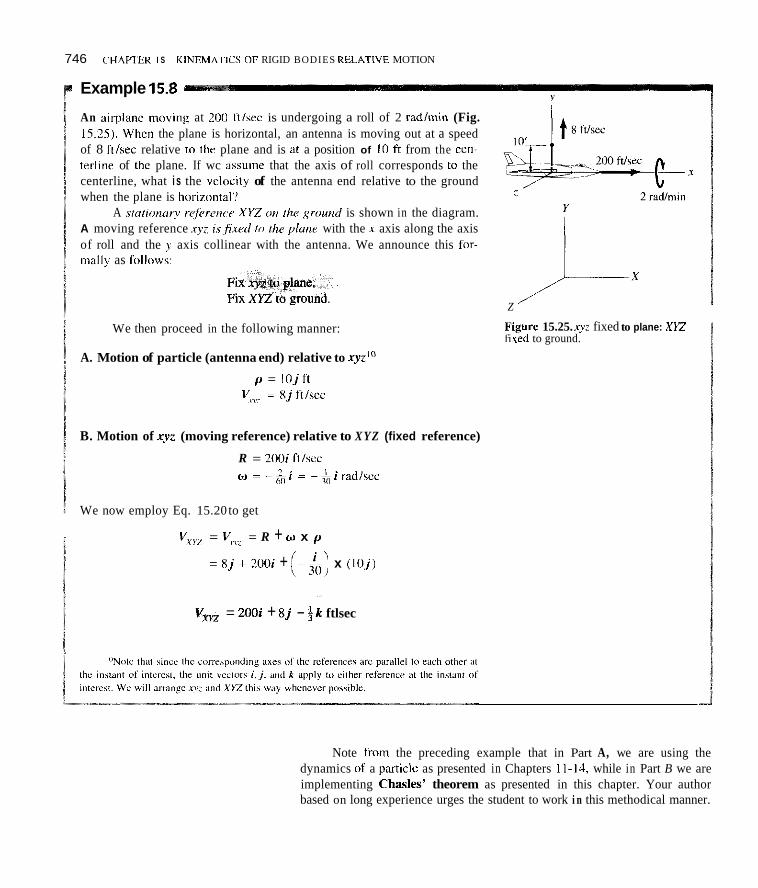
746 CHAPI'EK I S KINEMAIMX OF RIGID BODIES RELATIVF. MOTION
An aii-plane moving at 200 Itlsec is undergoing a roll of 2 radlmin (Fig. 15.25). Whcn the plane is horizontal, an antenna is moving out at a speed of 8 filsec relative to thc plane and is at a position of 10 ft from the cen- terline of thc plane. If wc assume that the axis of roll corresponds to the centerline, what i s the vclocity of the antenna end relative to the ground when the plane is horiz~intal'?
A srarionon rq'erencr XYZ on (he ground is shown in the diagram. A moving reference xyz i,s@d 10 h e plunr with the x axis along the axis of roll and the y axis collinear with the antenna. We announce this h r - mally as fo l l~~ws :
Fi Fi
Y Example 15.8
I
We then proceed in the following manner:
A. Motion of particle (antenna end) relative to xyz'"
p = I O j f t V?vy L 8 j ft/sec
B. Motion of xyz (moving reference) relative to XYZ (fixed reference)
R = 200i mScc w = - 2 i = - L i rad/scc
hn ill
We now employ Eq. 15.20 to get
v,, = vn; = R + w x p
= 8 j + 200i + (-&) x ( I 0 . j )
..
V, = 2OOi + 8 j - ik ftlsec
/ Z
Figure 15.25. xyz fixed to plane: XYZ fixed to ground.
Note lrom the preceding example that in Part A, we are using the dynamics ut' a pluticle as presented in Chapters 11-14, while in Part B we are implementing Chasles' theorem as presented in this chapter. Your author based on long experience urges the student to work i n this methodical manner.

SECTION 15.7 RELATIONSHIP BETWEEN VELOCITIES OF A PARTICLE FOR DIFFERENT REFERENCES 141
Example 15.9
A tank is moving up an incline with a speed of 10 k m h r in Fig. 15.26. The turret is rotating at a speed w, of 2 radlsec relative to the tank, and the gun barrel is being lowered (rotating) at a speed o2 of .3 rad/sec relative to the turret. What is the velocity of point A of the gun barrel relative to the tank and relative to the ground? The gun barrel is 3 m in length. We proceed as follows (see Fig. 15.27).
A A. Motion of particle relative to xyz
p = COS 307 + sin 30"k) = 2.60j + 1.50k m
Since p is fixed in the gun barrel, which has an angular velocity w2 rela- tive to xyz, we have
V ";z = ($1 = w2 x p = (- 3i) x (2 .60j + 1.5k) xy7
= -.780k + .45j mlsec
B. Motion of xyz relative to XYZ
R = .65j
Figure 15.26. Tank with turret and gun barrel in motion.
Since R is fixed in the turret, which is rotating with angular speed w I rel- ative to XYZ, we have
R = w I X R = 2k X .65j = -1 .3idsec w = w , = 2k radlsec A
We can now substitute into the basic equation relating y~vr to VxYz That is,
v,, = VI?? + R + w x p = (-,780k + . 45 j ) - 1.3i + ( 2 k ) X (2 .60j + 1.50k)
This result is the desired velocity ofA relative to the tank. Since the tank is moving with a speed of (10)(1,0OO)l(3,600) = 2.78 d s e c relative to the ground, we can say that A has a velocity relative to the ground given as X
Figure 15.27. xyz fixed to turret; XYZ fixed to tank. V,,,,,, = V,, + 2.781

748 CHAPTEK 15 KINEMATICS 01’ Rlt i lD BOIIIES: RELATIVE MOrlON
Example 15.10
A gunboat in heavy seas is firing its main battery (sec Fig. 15.28). The gun barrel has an angular velocity w, relative to the tumet, while the turret has an angular velocity w2 relative to the ship. If we wish to h a w the velocity components of the emerging shell to bc zero in the slationary X and Z directions at a certain specific Lime I. what should w, and u2 he at this instant? At this instant, the ship has a translational vclocity given as
VSJr,,, = .02i + ,016kmIs
Take the inclination ol the harrel to he 0 = 30”. Determine also the vcloc- ity of the gun barrel tip A .
Figure 15.28. A gunboat i n heavy sea\ firing its main battery
We proceed to solve this problem by the following positioning of axes shown on Fig. 15.28.
We can now procced with the detailed nnalysis of the prohlem
A. Mution of A relative to xyz
p = -(4)(.X66)j + (4)(.5)k = -3.464j + 2k m V,,: = w, X p = w,i X (-3.4645’ + 2 k ) = -3.464w,k - 2 u , j i d s

SECllON 15.7 RELATIONSHIP BETWEEN VELOCITIES OF A PARTICLE FOR DIFFERENT REFERENCES 149
B. Motion of xyz relative to XYZ R = - 3 j m l? = w,k x (-3j) + (.02i + ,016k) = (30 , + .02)i + .016k mls w = o ,k rad/s
We can now proceed with the calculations.
v,, = V,,? + + w x P
= (-3.4640,k - 20,j) + (30 , + ,023 + .016k + (w ,k ) x (-3.4641 + 2
= -3.4640,k - 20,i + 3 0 4 + .02i + .Olbk + 3.4640,i :. V,, = (3w, + 3.4640, + ,023 + ( -20, ) j + (-3.4640, + .016)k m/s
Let (V,,), = 0
:. 6.4640, = -.02
:. -3.464w, = -.016
In some of the homework problem diagrams, in the remainder of the chapter, a set of axes *yz has been shown as a suggestion for use by the stu- dent. This has been done to help clarify the geometry of the diagram. Also, if the student chooses to use these axes helshe will be able to compare more easily hisher solution with that of the author as presented in the instructor’s manual. However, (and note this carefully) the student must decide indepen- dently as to how to fa this reference and to state clearly as we have done in the examples how this reference has beenfixed.
Also, we strongly urge the student to make careful clear diagrams and to follow the orderly progression of steps (A. Motion of particle etc., etc. followed by B. Motion of xyz etc., etc.).
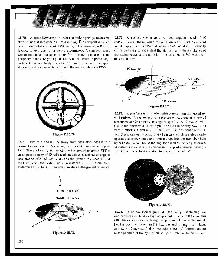
15.70. A space lahimtory. in order lo \imultite gravity, rotata rcl- ative 10 inerlial reference X y 7 at a rate 0,. For occupant A to ieel comfonahle, what should W , he? Clearly, at the center room R, thcre i s closc to ~ e r o gravity for rcro-i: enpcriments. A conveyor along One of the spokes transpart\ items from thr l iving quaiters at the periphery to the erwgravi ty Inbormrry at thc center. In pimicular, a particlc D has a velocity toward R of 5 mlsec relalive to the space
15.72. A panic lc rotiitcs at a con\lJnt angular spced 01 I O ladlsec o n II platfwm. while thc pli l t f imn roti~les with a u m t i l i i t
imguliir \peed of SO radlsec 'thwt ax i s &A. What i s thc velocity of thr particle P ai rhc instant thc plal lwm i c in the X Y plan? and the radius veclor t u the particle forms an ;ingle of 30" with the Y iixis as chow'. '
s t a t im What is irs velocity rclative to Ihe inertial rcference XYZ?
1
Figure P.15.70
15.71. Birdies ~i and h slide away from each other each with a :onstmt velocity OS 5 fllsec along thc axis C-C mountcd on a plat- lorn. The platfbrm rotatcs relativc to the ground rcfercnce X Y Z at
m angular velocity of 1 0 radlscc ahout axis & E and ha?, ail angular icceleration of S radisec' relarive 10 the ground relercnce XYZ at !he time whcn the hodirs arc a t a distance r = 3 ft from E-E. Determine thc vclocity if panicle h relative to the ground reference.
i I L
5 radl\ec' k . I IO radlsci
Figure P.15.71.
150
A
, X '
Figure P.15.72.
15.73. A p la t f o r r A IS mtiit ing with wnstmt ;ingular \pecil (0) 01 I radlcec. A sccond platform H ride, on A. m n t i i i r i i a row ol test tubes, and hac a con\tanr angular speed W , 01.2 I-adiw lr la- t i v r to the platform A. A third platfkmm Cis in no way cunncctcd with platfimns A and R. E <in platfwm C ii positioned above A and tl and carries di\penszrs 01 chcmicalb which are electrically operated at pi~opel- times to dispensc drops into the test tuhes held hy R belrrw What shuuld the angular speed 0 , hc fnr platform E at instant qhown if i t i \ to dispense :I drop nf chemical having ti
zero 1;ingenlial vclocity r c l a t i w to the test tuhe helow?
Figure P.15.73.
15.74. I n an amiiscmerit park ride, the cixkpil containing iwo occupants can mrarc at an angular spced rclativtl to the inain ann OB. The illin can lnriite with angular spced W , rclativz t o the prr,und. For the p s i t i o n shown in the diagrern and fbr W , = 2 radlccc and W2 = .2 rurlisei.. i ind thc velocity o fpr i i i i t A (corresponding to the position (if thc eyrs of an occupant) relalive to the groun~l.

15.76. A tank is moving over rough terrain while firing its main gun at a fixed target. The barrel and turret of the gun partly com- pensate for the motion of the tank proper by giving the barrel an angular velocity w , relative to the turret and, simultaneously, by giving the turret an angular velocity w2 relative to the tank proper such that any instant the velocity of end A of the barrel has zero
I
velocity in the X and Z directions relative to the ground reference. What should these angular velocities be for the following transla- tional motion of the tank:
V,,,, = IOi + 4k mis
z XYZstationary
-1 b . 6 5 r n Figure P.15.74.
15.75. A water sprinkler has .4 cfs (cubic ftlsec) of water fed into the base. The sprinkler turns at the rate 0, of I radlsec. What is the speed of the jet of water relative to the ground at the exits? The outlet area of the nozzle cmss section is .75 in2. [ H i m The volume of flow through a cross section is VA, where V is the velocity and A is the area of the cross section.]
Figure P.15.76.
15.77. We can show that Eq. 15.6 is actudlly a special case of Eq. 15.20. For this purpose, consider a rigid body moving relative to X Y Z . Choose two points a and h in the body. The body has a translational velocity corresponding to the velocity of point a and a rotational velocity w as shown in the diagram. Now embed a reference xyz into the body with origin at point a. Next, use this diagram and consider point h to show that Eq. 15.20 can be refor- mulated to be identical to &. 15.6.
Top view Figure P.15.75. Figure P.15.77.
75 1

752

H I m Figure P.15.82.
15.83. A cone is rolling without slipping about the Z axis such that its centerline rotates at the rate w, of 5 radlsec. Use a mul- tireference approach to determine the total angular velocity of the body relative to the ground.
X 4' + Figure P.15.83.
15.84. Find the velocity of gear tooth A relative to the ground reference XYZ. Note that W , and W2 are both relative to the ground. Bevel gear A is free to rotate in the collar at C. Take W , = 2 radlsec and w2 = 4 radlsec.
2
w2 = 4 rad/sec
Figure P.15.84.
15.85. In a merry-go-round, the main platform rotates at the rate w, of 10 revolutions per minute. A set of 45" bevel gears causes U to rotate at an angular speed 0 relative to the platform. The horse is mvunted on AR, which slides in a slot at C and is moved at A by shaft B, as indicated in the diagram, where part of the merry-go-round is shown. If AB = 1 ft and AC = 15 ft, compute the velocity of point C relative to the platform. Then, compute the velocity of point C relative to the ground. Take 0 = 45" at the instant of interest. What is the angular velocity of the horse relative to the platform and relative to the ground at the instant of interest?
Ai I "
(b) Figure P.15.85.
753

15.86. Rod H O in ta les at a cntislant angular sped 0 oi 5 radlsec clockwise. A collar A on thc rod i s pinned tn a sl idcr C, which moves in the groiwc shown i n the diagram. Whcn B = 60". corn- pule the spced of the co l l i i i~ A rclntivc io thz ground. What is (hi. speed n ico l l a rA rcliiti\c t n thc mil!
I- 1.6 111 -I Figure P.IS.XX.
15.89. In Problmi I5.XX. a s u n l e , i n addition in the rotatimi ot bar AD, that pin A i s moving at ii spced of 1.6 mlrec up the gromrd incline.
I* I I)' Figure P.IS.86. 15.YO. Rnd AC' i s cmnectud to il gear I ) and is guided by a
hearing R . Bcaring H can rntdte only i n the planc 01 the p a r \ . I i the mgular speed of AC ih 5 radlscc cluckwisc. whvt is the angw
I1 is 2 ft. 1. '11 . bpced . of gear I1 relative to the gl-nund'! The diarneler of gcer
15.87. Wurk Prohlem 1S.Xh assuming thiit pin 0 is mi I.IIIICIS moving to thc right at ii speed of 3 f t lscc ireliltive to the gnrund. I n addition, O R rotates at a cunstimt anpuliii~ spced H oi 5 radlscc clockwix all a1 the i i istanl of in tcr \ t .
1S.XX. R o d A D rotale\ at :I conslilnt speed 4 o f 2 mdlscc. Col- lar C. on the rod DA i h constrained to m o w in the circular grno\'e shnun i n Ihe diagram. Whcn the rod is a1 thc porition shown, compotc the \peed of coll i ir C' rclative to the gnmnd. What i s the \peed of co l la r C reliitivc tn the rod AI).! Frlint /I i \

SECTION 15.8 ACCELERATION OF A PARTICLE FOR DIFFZRENT REFERENCES 755
15.8 Acceleration of a Particle for Different References
The accrleration of a particle relative to a coordinate system is simply the time derivative, as s r m f r o m the coordinate .system, of the velocity relative to the coordinarr system. Thus, observing Fig. 15.29, we can say:
(15.21)
~~
Figure 15.29. xyz moves arbitrarily relative to XYZ.
"his notation may at first seem cumbersome to you, but it will soon he sim- plified.
Let us now relate the acceleration vectors of a particle for two refer- ences moving arbitrarily relative to each other. We do this by differentiating with respect to time the terms in Eq. 15.20 for the XYZ reference. Thus,
Now cany out the derivative of the cross product using the product rule.

756 CHAPTER 15 KINEMAIICX O F RIGID BODIES: RELATIVE MOTION
To introduce more phyyically mcaningful terms, we can replace
using Eq. 15.16 in the following way:
Substituting into Eq. 15.23, wc get
+ w x (w x p ) + (%IXYL p
You will notc that (dVJdt i tJ2 is aY>:; that (dp/dtjryc is Vrvz; and that (dw/dtj,yvz is 6. Hence, rcarranging terms, we have
where w and 6 are the angular velocity and acceleration, respectively. of the xvz reference relalive lo the XYZ reference. The vector 2(w x Vxvz) is called the Cnrin1i.s nccdei-ntion \'error; we shall examine its interesting effects in Section 15.10.
Although Eq. 15.24 may seem somewhat terrifying at first, you will find that, by using it, prohlems that would otherwise he tremendously diffi- cult can readily he carried ouI in a systematic manner. You should keep in mind when solving problems thnt nny ($the methods developed in Chapter I 1 ('nn be i is~d.f i i r determining the motirin ofthe particle relntiue to the xyz rpferencr or.for determining the motion nf the origin of xy i relative to the XYZ re/krmce. We shall now examine several problems, in which we shall use the notation, w,. wL, etc.. to denote the various angular velocities involved. The notalion, w (i.e., without subscripts), however, will we repeat hc reserved to represent the angular velocity of the .I?: reference relative to the XYZ reference.

SECTION 15.8 ACCELERATION OF A PARTICLE FOR DIFFERENT REFERENCES 151
Example 15.11
A stationary huck is canying a cockpit for a worker who repairs overhead fix- tures. At the instant shown in Fig. 15.30, the base D is rotating at angular speed o+ of . I radsec with 4 = .2 rad/secZ relative to the truck. Ann AB is rotating at angular speed o1 of .2 rad/sec with hl = .8 rad/sec2 relative to DA. Cockpit C is rotating relative to AB so as to always keep the man upright. What are the velocity and acceleration vectors of the man relative to the ground if a = 45' and p = 30" at the instant of interest? Take DA = 13 m.
(4 6.
Figure 15.30. Truck with moving cockpit.
Because of the rotation of the cockpit C relative to arm AB to keep the man vertical, clearly, each particle in that body including the man has the same motion as point B of arm AB. Therefore, we shall concentrate our attention on this point.
This situation is shown in Fig. 15.31.
A:! 1" x
Figure 15.31. xyz fixed to DA; X Y Z fixed to tmck
A. Motion of B relative to xyz
p = 3(cospi - s i n p j ) = 2.60i ~ 1 .5 jm

758 CHAPTER 15 KINEMATICS OF K l G l l I HOIIIES: KFI.ATIVF MOT10N
Example 15.11 (Continued)
Since Ii i s fixed in Af j . which ha? a ~ i g ~ ~ l ~ vclocity w , reliitive t o x ~ , we have
V b r ~ = w , X ti = (.ZkJ X (2.6Oi - I . S j )
= ,520 i + 3; d s e c
As seen froin .r??, only thc valuc 111 w , and not i t s direction i s changing. Also note that (flpIdfJ~~: = yvT. Hence.
= ( . 8 k ) x (2.hOi ~ L S j ) + ( . 2 k ) X (.52OJ + 3) = 1 . O Y i + 2.14j misec?
B. Motion of x y relative to XYZ R = 13(.707i + ,707.j) = 9.1Yi + 9.19j in
Since R i s fixed in DA. and since DA rotates with angular velocity w, re1 ative to X Y Z we havc
R = wz x R = (.l,j) X (9 . IY i + Y . l 9 j )
R = 61- x R + w, x R = -.9 19k in lhec
= ( . 2 j ) X ( 9 . 1 9 i + Y . I S , j J + ( . I j ~ X (-.‘119k) = -1.83Xk ~ .O91Yim1sec2
w = w2 = . I j rad lsec
& = = .2jrad/sec2
Hence,
v,, = Vav: + R + w x p
= 3 2 0 j + .3i ~ .919k + (. l j) x (2.hOi ~ l3 jJ
V,, = .3i + 320j - 1.179k mlsec
.. a, , = a ,v7 + R + 2w X V,y: + & x p + w X ( w X pJ
= 1.O9i + 2.14j - 1.818k ~ .0919i + 2 ( . l , j ) x ( . 5 2 O j + . 3 i 1 + ( . 2 j ) X ( 2 . 6 0 i - I . S j ) +( . l j ) x l ( . l j ) X (2.60i - I . S j ) l
axlz = ,9781 + 2.14j - 2.42k mlsec?
Notice that thc cssenlial aspects of thc analysis come in thc consideration of parts A and R of the problem, whilc thc remaining portion involves dircct suhstitution and vector algehraic operations.

SECTION 15.8 ACCELERATION OF A PARTICLE FOR DIFFERENT REFERENCES 159
Example 15.12
A wheel rotates with an angular speed w2 of 5 radlsec on a platform which rotates with a speed wI of 10 rad/sec relative to the ground as shown in Fig. 15.32. A valve gate A moves down the spoke of the wheel, and when the spoke is vertical the valve gate has a speed of 20 ft/sec, an acceleration of 10 ft/sec2 along the spoke, and is 1 ft from the shaft cen- krline of the wheel. Compute the velocity and acceleration of the valve gate relative to the ground at this instant.
Z ?
to the platform.
Figure 15.32. qi fixed to wheel; XYZ fixed to ground.
A. Motion of particle relative to xyz
p = k f t Vqz = -20k ft /sec
= -10k ft/sec2 axYz
B. Motion of xyz relative to XYZ
R = 5 j f t
Since R is fixed to the platform: = wI x R = (-10k) x ( 5 j ) = 50ift /sec
= 0 + (-IOk) X (50 i ) = -500jft/sec2 = cb, X R + w , X k
w = w2 + wI = 5 i - 10k radlsec cb = h2 +dl
Note that w2 is of constant magnitude hut, because of the hearings of the wheel, w2 must rotate with the platform. In short, we can say that w2 is fixed to the platform and so h2 = w, x w2. Hence,
h = w1 x w2 + o = (-10k) x ( 5 i ) = -50jrad/sec2
We then have
v,, = vqz + k + w x p
= -20k + 50i + ( 5 i - 10k) x k
v, = - si -

760 CIlAPTIiR I S K1Nk:MA'IICS 01 K K i l l l HOIIIES: RFI.ATIVF MOT10ii
Example 15.12 (Continued)
Also,
f l X Y L = a"; + R + 2w x Vr1: + 6l x p + w x (W x p )
= -IOk - 5OOj + 2 ( 5 i - Ink) x ( - 2 0 k ) + ( - S 0 . j ) x k + ( 5 i - I O k ~ X ~ ( 5 i - 1 O k l X k ]
ax. = -1oOi - 300j - 35k ft/sec2
i I I ._____._I" ...... .. , , . ,... . . . . ~ I .... ,, _ _ _ _ ~ .... . .. , ~ .__._
Example 15.13
In Example 15.12. thc wheel accelerates at thc instant under discushion with f& = 5 radlscc'. arid the platlorn1 xccleri l tes with Ui, = 10 firdlscc' (see Fig. 15.32). Find the velocity and acceleration of the wl\,e gate A .
If wc rc\'icw the contents of parts A and B of Example 15.12. i t wi l l he clcar that only R and 6l are affcctcd hy the fact that Ui, = I O radlsec' and ih2 = 5 radlsec'. 111 this regard, consider w2. It i s 110 longer oi con- stant value and cannot he considered as.fi.wd in the platform. However we can express w, a s w j ' (11 ull tinim. wherein i' is,fi.wd in the platform a s shown in Fig. 15.32. Thus, we cim say for w:
w = w,i' + w I 1 Therelore.
I 6l = oj2i' + w,i' + 611
= S i ' + S(w, X i ' ) - IOk = S i ' + S ( - l O k ~ x i ' - l O k
!
A t the instant o i interest, i' = i . Hcncc.
6 = 51 - 5Oj - IOkrad/sec2
Hence. we usc the ahove 6l in part H of Exmaplc IS. I 2 to compute V,y,, and ax)./. Thc computation ofR is straightforward and so we can compute oxy, accordingly, We lrave the details to the rcadcr.
,
~ i

SECTION 15.8 ACCELERATION OF A PARTICLE FOR DIFFERENT REFERENCES 761
An understanding of Examples 15.11, 15.12, and 15.13, involving two angular velocities of component parts is sufficient for most of the homework problems of this section covering a wide range of applications. In the next example, we have three angular velocities to deal with. We urge you to exam- ine it carefully if time allows. It is an interesting problem, and comprehension of the three different analyses given will ensure a strong grasp of multirefer- ence kinematics.
Example 15.14"
To simulate the flight conditions of a space vehicle, engineers have devcl- oped the cenfi-ijzrge, shown diagrammatically in Fig. 15.33. A main arm, 40 ft long, rotates about the A-A axis. The pilot sits in a cockpit, which can rotate about axis C-C. The sear for the pilot can rotate inside the cockpit about an axis shown as R-R. These rotations are controlled by a computer that is set to simulate certain maneuvers corresponding to the entsy and exit from the earth's atmosphere, malfunctions of the control system, and so on. When a pilot sits in the cockpit, hislher head has a position which is 3 ft from the seat as shown in Fig. 15.33. At the instant of interest the main arm is rotating at 10 rpm and accelerating at 5 q m 2 . The cockpit is rotating at a constant speed about C-Crelative to the main arm at 10 rpm. Finally, the seat is rotating at a constant speed of 5 rpm relative to the cockpit about axis B-B. How many g's of acceleration relative to the ground is the pilot's head subject to?I2 Note that the three axes, A-A, C-C, and B-B, are orthogonal to each other at time 1.
A
A
Figure 15.33. Centrifuge for simulating flight conditions
"Example 15.14 was given as two homework problems in both the first and second editions of this LCXI. They were so instructive thvt for aubsequent editions the author decided ID move the problems into the main lext.
"A g 01 acceleration is an amount of acceleration equal to that of gravity (32 .2 ftlsec' or 9.81 misec'). Thus. a 4g ilcceleration is equivalent to an acceleration of 128.8 fUsec'.

162 CHAPTER 15 KINEMATICS OF RIGID BODIES: REL.ATIVC MOTION
Example 15.14 (Continued) In Fig. 15.14 the arm O S the ccntriluge rolales relalive 10 the ground
at an angular vclocity i)C 0,. The cockpit meanwhile rotates relative to the arm with angular s p e d wz. Finally, thc seat rotates rclativc to the cockpit at an angular speed w,. For constant wz. we see that, bccause of bearings i n the arm, thc vcctor w2 is "fixed" i n the ann. Also. Cor constant a?. because of hearings in the cockpit. the vector o1 i h '%sed" i n the cockpit. Before we examine the acceleration of the pilot's head. note that at the instilnt of interest:
4 I Z
C Y
A Figure 15.34. Ccnvilhge listing w's.
wI = w2 = 10 rpin = 1.048 rad/scc &, = 5 rpm2 w,, = 5 rpin
= .00873 rad/sec' = 524 radiscc
We shall do this problem using three different kinds of moving referenccs qz.
ANAI.YSIS 1
Fix nyz to ann. Fix X Y Z to ground
Nolc in Fig. 15.35 that ~q? and the arm to which i t is fixed arc shown dark. Notc also that the axes XY: and XYZ are parallcl to cach othcr at the instant of interest.

SECTION 15.8 ACCELERATION OF A PARTICLE FOR DIFFERENT REFERENCES 163
Example 15.14 (Continued) A
Y
A
Figure 15.35. Centrifuge with xy; fixed to arm.
A. Motion of particle relative to xyz
p = 3kft Note that p is “fixed” to the seat and that the seat has an angular velocity of (w, + w,) relative to the arm and thus to xyz. Hence, - Vxv: = (w* + 0,) x P
= ( l .048j + ,5241) X 3k = 3.141 - 1.572jftlsec
Clearly, relative to the ann, and thus toxyz, w2 is constant. And w, is fixed in the cockpit that has an angular velocity of w2 relative to xyz. Thus, we have
= (0 + w* x w,) x P + (w* + w,) x vmz = (1.048j x ,5241) x 3k + (1.048j + ,5241) X (3.141 - 1.5721) = -4.12k ft/sec2
B. Motion of xyz relative to XYZ R = -4Ojft
Note that R is fixed in the arm, which has an angular velocity wI relative to XYZ. Hence,
k = wl X R = 1.048k X (- 40j) = 41.9iftlsec k = wI X k + & , X R
= 1.048k X 41.9i + .00873k X (-4Oj) = 43.95’ + 3 4 % ft/sec2
w = o, = 1.048k radlsec & = &, = .00873k rad/sec2

764 CHAPTER 15 KINEMATICS OF Kl( i l l1 ROnlES: RELATIVE MOTION
Example 15.14 (Continued) We can now substilute into the following equation:
axyz = arvc + R + 2w x Vav: + Cb x p + w x (w x p )
Thcrcfore. ax,,/ = 3.64; + S0.Sj - 4.12k ft isec?
ANALYSIS I1
@x xyz to cockpit XPIZ to ground.
This silualioii is shown i n Fig. 15.36
, 4 ... , Cockpit
Figure 15.36. Ccntrifuge with .XJ: lined t i l cockpit
A. Motion uf particle relative to xyz
p = 3k I t
Note that p i s llxed to the seat, which has an angular velociiy of wi rela tive to thc cockpi l and thus relativc LO xyz. Hence,
V>yr = wi X p = 324; X 3k = -1.572jftisec
But w3 i h ~ ~ r i ~ l i l i i t as sccn from [he cockpit and thus from xy;. Hence,
acv7 = n x p + wi x v<\: = ,524; x (-1.572;)
= -.824k Stisec’
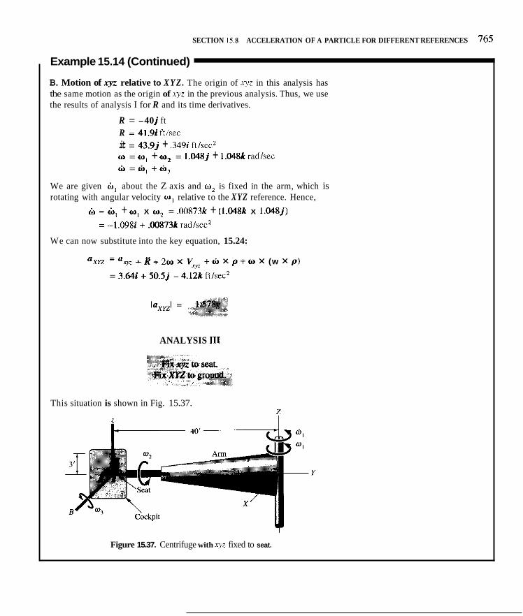
SECTION 15.8 ACCELERATION OF A PARTICLE FOR DIFFERENT REFERENCES 165
Example 15.14 (Continued)
B. Motion of xyz relative to XYZ. The origin of xyz in this analysis has the same motion as the origin of xyz in the previous analysis. Thus, we use the results of analysis I for R and its time derivatives.
R = -40 j ft R = 41.9i ft/sec it = 43.9j + ,3491' ft/sec2 w = wI + w2 = 1.048j + 1.04% rad/sec Ch = Ch, +Ch7
We are given &, about the Z axis and wz is fixed in the arm, which is rotating with angular velocity wI relative to the XYZ reference. Hence,
6 = + w, X w2 = .00873k + (1.048k X 1.048j) = -1.098i + .00873k rad/secZ
We can now substitute into the key equation, 15.24:
axYZ = % y z + R + 2 w x Vqz + C h x p + w x (w x p)
= 3.64i + 50.5j - 4.12k ftlsec'
ANALYSIS 111
This situation is shown in Fig. 15.37. z
Figure 15.37. Centrifuge with xyz fixed to seat.

166 CHAPTER I S KINEMATICS OF RIGID BODIES: KE1.ATIVE MOTION
Example 15.14 (Continued)
A. Motion of particle relative to xyz
p = 3k I t
Since the patticlc is fixcd to thc seat and is thuh fixed i n .XK. we can h a y :
vltc = n a>, : = 0
R. Motion ofxyz relative to X Y Z . Again. the origin olxy; has idenlically the same motion as in thc prcviouc analyses. Thus. we have the samc results as hefclre lor R and its derivatives.
R = -4Oj ft R = 41.y; Itisec i2 = 43.yj + .MY; It/sec' w = w , + w, + col = 1.04Xk + 1.04Xj + ,524; lh = cb1 + lh2 + h a
Note that h, is given. Also, w2 i h fixed i n the arm. which rolakcs with angular speed w 1 rclalive to XYZ. Finally, wj is fixed iii the cockpit. which has an angular vclucity w2 + wI relative to XYZ. Thus,
h = h 2 + w 1 x w , + ( w I + w 2 ) x w i = .00X73k + (1.048k x 1.048j) + (1.048k + 1.04X.j) x 1.524;) = - I . O Y X i + 54Y j ~ ,540.k
Wc now go to the basic equation, IS 24
Substituting, we gel
axy7 = 3.64; + S O S j - 4.12k ltlsecz
In the final example ol this series, we have a case where it is advanta- geous to use cylindrical coordinates in parts or thc problem arid lhcn latcr IO
convert to rectangular coordinate\.

SECTION 15.8 ACCELERATION OF A PARTICLE FOR DIFFERENT REFERENCES 161
Example 15.15
A submersible (see Fig. 15.38) is moving relative to the ground reference XYZ so as to have the following motion at the instant of interest for point A fixed to shaft which in turn is fixed to the submersible:
V = 3i + .6 j mls a = 2i + 3 j - .5k mls2
Figure 15.38. Rotating device inside a moving submersible. E is fixed to the submersible.
At the instant of interest, the vessel has an angular speed of rotation ff = .3 radls about the centerline of as seen from the ground reference. A horizontal rod m has the following angular motion about m:
6 = .3 rad/s 8 = .4 rad/s2
Two spheres, each of mass 1 kg, are mounted on a rod turning about m with the following angular motion
fi = .2 radls fl = .5 radls2
Also, the rod and the attached spherical masses advance toward following rate:
at the
i. = -3 mls i' = -2 mlsZ
at a time when r = .25 m. Finally, at the instant of interest, the horizontal rod with a speed of .5 mls and a fate of change of speed of .2 m/sZ. What force must rod exert at point G at this instant due only to the motion of the two spheres?
moves up along vertical rod

768 CHAPTFK I S KINEMATICS 01: RIGID BODIES: I<ELATIVC MOTIOK
Example 15.15 (Continued)
We will first consider thc motion of the 1.ntter i f i i i ~ . s ~ of the rotat- in& spheres which cle;irly must hc G. We now proceed to ?el the accelel-a- tion of G relative to X Y Z (see Fig. 15.3Y).
Fix xyz to the vessel at A. Fix XYZ to the ground.
A. Motion of C relative to xyz (using cylindrical coordinates). Use Figs. 15.38 and 15.39.
p = ,256, = .25 j in
Vn; = Pr, + rdr, + I 6 = - 3 E r + (.2S1L3Jre + .?E = - 3j - ,075 + .Sk = -.I175 - 3 j + .Sk m/s
= ( y - ~ B ' I E ~ + (r i i + 2 f B ) t , + = [-2 -- ( .2?)( .3) ' ]€ , + [(.251(.4) + (2)(-3I(.3l]rfl + . 2 t ~
= -2.0236, - 1.7~" + . 2 t ~ = I.7i - 2.023j + .2k mis?
B. Motion ofxyz relative to X Y Z
R = 3i + .hj m/s R = 2i + 3 j - .Sk mis? w = .3k rndis &I = n radis'
We may now express axy, lor point G. Thus
axyz = u t > : + R + 2w x v,,: + 6 x p + w x (w x pl
= (1.7i - 2.023j + . 2 k ) t (2i + ? j - . 5 k ) + 2 ( . i k )
X (-.075i - i j + . S k ) + 0 x 11 + (.RkJ x ( . 3k x .25j )
= 5.5 + .909?j - .3k m/s2
Now we apply Newton's law to the inass ccntcr G at the imtmt of inter- csl. Denoting the force fr0m the rod AD onto <; a s F,,,,,,. WL' get
F,,(,,) - 2mgk = 5 . 5 + .YrOOSj - .3k :. = ( 2 l i l ) ( Y . 8 l l k + 5 . 5 + .YOY5j - .3k
FROD = 5 . 5 + ,90953 + 19.32kN
This is our desired result

15.91. A truck has ii speed V of 20 milhr ;md an acceleration $ of 3 milhrlsec at time I. A cylinder of radius equal tu 2 St is rolling without slipping at time f such that relative to the truck it has an angular speed LO, and angular acceleration (6, of 2 radlsec and I radlsec’, respectively. Determine the velocity and acceleration of thz center of the cylinder relative to the ground.
15.95. to the ground.
In Problem 15.74, find the accelcration of pointA relative
15.96. In Prohlem 15.79. find the acceleration of the tip of the propeller relative to the ground reference. Take the yaw rotation to be zero and the loop rotation radius r tu he 500 m.
Figure P.15.91.
15.92. A wheel rotates with an angular speed o2 of 5 radlsec relative lo a platform, which rotates with a speed wI of 10 raUsec relative to the ground as shown. A collar moves down the spoke of the wheel, ;md, when the spoke is vertical, the collar has a speed of 20 ftliec, an acceleration of 10 Stlsec2 along the spoke. and is positioned I ft from the shaft centerline of the wheel. Cam- pute the velocity and acceleration of the collar relative to the ground at this instant. Fix xyz to platform and use cylindrical coor- dinates.
Figure P.15.92.
15.93. cle at the instant uf interest.
In Problem 15.71, determine the acceleration of the part-
15.97. to the ground.
In Problem 15.80, find the acceleration of point R relative
15.98. In Problem 15.80, find the ilccelcriltiun of paint LI relative t u the ground for the fdlowing data at the instant of interest sliowri i n the diapmt.
CO, = .2 radlsec
w2 = .4 radlsec o j = -.I radkec’
[;2 = .3 radlsec?
15.99. tip of the gun relativc to the ground.
In Prohlem 15.82, determine the acceleration of the top
15.100. In Problem 15.74, find the acceleration of point A rela- tive tu the ground for the contiguration shown. Take w , = 2 radlsec ~, = 7 radlsec’. wi = . I radlsec, and h2 = 2 radlsec’. How inany g’s of acceleration is this puinl subject to?
15.101. the ground. IHbrr; Use two pvsitivii vectors to get p.1
I n Prohlem 15.81, find the acceleration o S 0 relative to
15.102. ground in Problem 15.84.
Find the accelcration of gear tooth A relative to the
15.103. In Problem 15.92, the wheel accelerateq at the instant under discussion with 5 radlsec2 relative to the platform, and the nlatform increases itb aneular meed at 10 radlsec’ relative to the
15.94. relative to the ground reference.
In Problem 15.72, find the acceleration of the particle P ground. Find the velocity and acceleration of the collar relative to the ground.
169

15.104. As uilli llie vrlucily e q u a l ~ ~ r 15.20. we can easily show that Eq. 15.1. relating i i c ~ e l e r ~ t i ~ n s hctuccn two points 011 il rigid body, is actuiilly a \pccial case u l Eq. 15.24. Thus, conridcr Ihc diagiim showing it rigid body moving arhitiarily re la t iw tu XYZ. Choox t w > p o i n t h c r arid h i n the body and cnihed a refrrrncc r?; in the body wi lh thc origjji at ( i . Nom cxpresb the acceleratirm of p i n t h as x e n from the two relerences. Shmu horn, this equalion can bc rcfwmulutcd a\ I?+ 15.7.
X liigure P.15.104.
15.I05. Solve Pniblcm I . X I lor the fn l lowing data
IO, = .3 r;rdi\ec
61, = .1l1radlsr.c' w; = . I S radlsec cb2 = .2 I -adkc'
&J, = .z lrad/sec' iiJ- = .JOr;ld/XC
15.106. 111 Problem IS.X2. find the i.rrmpnnent 01 acceleriitioti of the prrijectilc d a t i v e to the grouiiil which I S normal to the gun hamel at the i t ist i int that the pr,,jeclili. ju.1 Isilvcs the bnrrel. IJse thc lollowing dillii:
iu , = .3 r ~ < l l \ c c
(0, = -.h I-adiscc ih, = -.4 rad/sx '
i J , = .2 rad/scc'
15.107, In Pmhlcm 15.XX. find Ihe magnitude of the tion of co l l iu <' w l a t i w to the ground Cor thc fr>llowing data at the instant ~ W I I :
H = 2 radlscc ii = 5 r;!d/scc'
15.108. A truck is mwing at ii constant specd V = 1.7 mlscc at
t ime I . 'Ihr truck Ionding comparlnimt has at thic instant a constaiit ;mgular speed H 01 . I radlicc at an anglc H = 45". A cylinder of radius 100 nim rolls ielal ivu 10 the compartment at a speed w , oi I I-adkc. accelerating at a rate ih, of .5 ladlsec' at time r. What are the velocity and accclerilti~iii of the ccnter 01 Ihr cylinder rela- t ive t i l the ground at t ime I? The distaicc d ut tiinc i i s 5 (11.
Figure P.15.108.
*15.109. I n Exilmplt' 15.14. \uppose at thz ilistiult of illtcrest that lherr i \ an angular acceleration ih, = 3 radlsec2 of the cockpit d a t i v e t i l thc a m and that tlirre i s an ;in&!uI:u ncceleratioii ih8 = .2 vadliec' 01 the seat iclntive to the cockpit. Find the number ofp 's ti) which the pilot's head i s subjected. Follow analysis 1 in the exaniple. [Hinr: The angular vclncily w , can idways bc c x p l - ~ h ~ d a\ w,f, where E is a unit vector fixed io rhc cockpir having a direc~ tioii along the ~r ax(\ iit the in&timl nl interest.1
15.110. A fin-is wheel is out 01contn)l. At the i i i i t i lnt shuwn, i t has an angular speed u1 equal ti1 .Z radlsec and a rillr of change of angular speed G, of SI4 redlsec' i r~ la l i ve ti1 the ground. At this in~iant a "chair" hhuwn i n the diagram has 311 angular %peed u, relative to the terris wheel equal to 2 5 radlsec nnd a rate chanfe ofspccd 6,. again relative to the fenii wheel. equal to .(I1 radlsrc'. 111 thc figure, wc have hhown details of the parmiyel~ at th is instant. Note that the hingc of the seat i s at A. How many ,q'\ of acceleriltiun i s the passenger's head subject Id
Y
1 I11
x
Figure P.15.110.
15.111. A shalt IK' mtates ielatiLe t i l platform A iit a spccd = 3 4 radlsec. A rod is wclded 10 HC'and i s vertical iu the instanl
of interest. A tube i s fixed to the vertical rod in which a smal l pis- ton head is moving rclative to the tube at a speed V uf 3 inlicc wilh a rate uf change of speed V o l .J mlscc'. Thc platfirm A has an angular velocity relative to the ground givw as w, = .X radlstc
770

with a rate o f change of speed of .5 radlsec2. Find the acceleration vector of the piston head relative to the ground.
Z
V = 3 m/sec REL TO V = .4 rnlsec' 1 TUBE
w , = .34 radlsec 1 REL TO A o2 = .8 radlsec REL TO 'u,= .5 rildlszc' 1 GND.
15.113. A particle moves in a slot of a gear with speed V = 2 mls and a rate of change of speed = 1.2 mls2 both relative to the gear. Find the acceleration vector for the particle at the coniig- "ration shown relative to the ground reference X Y Z
X'J x '
Figure P.15.111.
15.112. relative to an inertial reference XYZ.
w , = 3i + 4j + 10kradIs
A communications satellite haa the following motion
d, = 2i + 3kradls: y ) = a() = 0
A wheel at A i s rotating relative to the satellite at a constant sped w2 = 5 radls. What i s the acceleration of p i n t 0 on the wheel relative to XYZ at the inatant shown'? The following additional data apply:
UA = I rn A D = .2 m
Z
Figure P.15.112.
V = 2 m i s relative to gear V = 1.2 m/s2 relative to gear w , = ,118 radls W , = ,112 radls' r = . 1 5 m
Figure P.15.113.
15.114. A submarine i s undergoing an evasive maneuver. At the instant of interest, i t hds a speed = 10 m l i and an acceleration u,, = I S mls' at i t s center of mass. I t alsti has an angular velocity about its center of mass C of o, = .5 radls and an angular accel- eration 6, = .02 radls'. Inside is a part of an inertial guidance system that consists of a wheel spinning with speed w2 = 20 radls about a vertical axis of the ship. Along a spoke shown at the instant of interest, a particle i s moving toward the center with r, i- and ?as given in the diagram. What i s the acceleration of the par- ticle relative to inertial reference XYZ? Just write out the formula- tions for nXYZ but do not carry out the cross products.
- Y
the time I
Figure P.15.114.
I 1 1

15.115. Find V a n d a 01 H ielillivr 111 XYZ. The single blade p w lion AB i s rutating as shown relative tu the helicoprer with \peed U J ~
about an axis parallel to theXaxi\ at the iiistnnt 01intercst while the cntire blade sysiem i s rotating about the veit ical axis with spccd 0,
,i, U),
x ,L Cmund relerence
Figure P.15.115.
15.116. An F-lh fightcr plane i\ moving at a c o i i i t m ~ s p e d o i S O 0 kinlhr while undergoing a loop a\ \hrrwn in !lie diagram. At the instant of interehl, i t has an angular roll vclociry w-. 01 5 radlmin relativr 10 thc ground. A solenoid i s aclivaled :it this iiislilnt and miwcs the m n i n g portion o f a pate v a l ~ c d~wnw:ird at .I speed ot 3 mi\ with iiii a ~ ~ e l e r ~ t i i i n of 5 m / s L all rcI:itive 1n thc ~lilnr. What i h the tolal external force on the moving piwtinn nf :he gale valve if i t i s 1 n, abuvr the axis of roll ill the instant 01 interest? 'She moving portiun nf the Y$\C har il wcight r r f IO N .
\
Figure P.15.1 I 6
15.1 17. A robot innves a body held by its ",jaws" G a s shown i n he diagram. WhaL i s the velocity and acceleration of point A at he instant shown re la t i~e 10 the glound? Ami EH i\ welded to the ierl ici l l shaft MN. Arm H K G i s i w e rigid mcmher which rotate5 ibout EH. How do you want to fir .tr..-'l
772
Figure P.15.118.

SECTION 15.9 A NEW LOOK AT NEWTON'S LAW 113
"15.9 A New look at Newton's law The proper form of Newton's law has been presented 2s
F = ma X Y Z (15.25)
where the acceleration is measured relative to an inertial reference. There are times when the motion of a particle is known and makes sense only relative to a noninertial reference. Such a case would arise, for example, in an airplane or rocket, where machine elements rnust move in a certain way relative to the vehicle in order to function properly. Therefore. the motion of the machine element relative to the vehicle is known. If, however, the vehicle is undergo- ing a severe maneuver relative to inertial space, we cannot use Eq. 15.25 with the acceleration of the machine element measured relative to the vehicle. This is so since the vehicle is not at that instant an inertial reference, and to disre- gard this fact will lead to erroneous results. In such problems, the motion of the vehicle may he known relative to inertial space, and we can employ to good advantage the multirefeience analysis of the previous section. Attaching the reference xyz to the vehicle and X Y Z to inertial space, we can then use Newton's law in the following way:
F = in[anL + k + 2w X Vry,: + ri, X p + w X (w X p)] (15.26)
Clearly, the bracketed expression is the required quantity aXYZ needed for Newton's law. It is the usual practice to write Eq. 15.26 i n the following form:
F - m[R + 2w X V, +it X p + o
This equation may now be considered as Newton'a law written for a norriner- rial reference xyz. 'The terms -rrr -m(2w x VXyJ and so on, are then con- sidered as forces and are termed inertial fiirces. Thus, we can take the viewpoint that for a nonineitial reference, xyz, we can still say force F equals mass times acceleration, a_z, provided that we include with the applied force F . all the inertial forces. Indeed, we shall adopt this viewpoint in this text. The inertial force --2mw X yvz is the very interesting Coriolis furce, which we shall later discuss in some detail.
'The inertial forces result in haftling actions that are sometimes contrary to our intuition. Most of us during our lives have been involved in actions where the reference used (knowingly or not ) has heen with sufficient accu- racy an inertial reference, usually the earth's surface. We have, accordingly, become conditioned to associating an acceleration proportional to, and in the same direction as, the applied force. Occasions do arise when we find our- selves relating our motions to a reference that is highly noninertial. For exam- ple, fighter pilots and stunt pilots carry out actions in a cockpit of a plane

while the plane i s undergoing severe tnnneuucrs. Llnexpected i e w l t s l i e - queiitly occur for flyers il thcy use thc cockpit interior as a reference I i r their iictioiis. Thus. to nime their hatids from m e posiliiin to ;iniilhcr relative to t i i t circkpit siimctinics rcquires :in exertion that i k iiot thc (me anticipated. caiisitif concidcrahlc conlusioii. The next cxaniple wil l illustrate thi\. and the scctiwis that follow w i l l cxplorc further some of these interesting efI'ccts.l3
Example 15.16
The plan view of a routing platfiirni i s shown in Fig. 15.40. A tiiiiii i s seated at the Iposition Iiihclcd A and i s facing point 0 or the platform. He i\ carrying ti nia% of j\, sliig at (lie late of 10 I l l i c c in ii dircctiiin strxight ahead of liiiii (i.c.. Iiiward the center of. the plallorm). If this platform has an angular spccd of 10 radlsec and an angulx acceleration of 5 r;idisz$ rcliilivc to ~ h c ground at thi, instiitit, what Ixce F niiist he exert to cause thc mass t i i accelerate 5 tilsecz toward tlic center?
Y. !
Figure 1540. Rutating plnrfonn
For purposts of deteitnining iiicrtiiil force\, wtl pnicced a s fiillcw\:
Fix q z to platform. Fix XYZ to ground.

SECTION 15.9 A NEW LOOK A T NEWTON’S LAW 115
Example 15.16 (Continued)
A. Motion of mass relative to xyz reference
p = 10i ft, V,, = -1Oi ftlsec, a = - 5i ft/sec2 wz
B. Motion of xyz relative to XYZ
k = 0, k = 0, w = -10k radlsec, ch = -5k rad lsec2
Hence,
aXYZ= -Si + 2 ( - l O k ) x ( - l O i ) + ( - S k ) x 1Oi +(-lOk)x(-lOkXIOi)
Therefore,
a,, = -Si + (200j - 5Oj - 1,OoOi)
Employing Newton’s law (Eq. 15.27) for the mass, we get
F - h ( 2 0 0 j - 5Oj - 1,OOOi) = $(-5i)
Solving for F, we get
F = 3j -20. l i Ib
This force F is the total external force on the mass. Since the man must exert this lorce and also withstand the pull of gravity (the weight) in the -k direction, the force exerted by the man on the mass is
If the platform were not rotating at all, it could serve as an inertial reference. Then, we would have for the total external force F’:
F’ L(-5 i ) = -‘iIb so I O
The force exerted by the man, FLan, is then
This force is considerably different from that given in Eq. (a). As a matter of interest, we note that aviators of World War I were
required to carry out such maneuvers on a rapidly rotating and accelerating platform so as to introduce them safely to these “peculiar” effects.

HOI)II:S K l i l ATIVR M O I I O N
*15.10 The Coriolis Force
/ I
0 1 ' gre;it inicrc\t i\ tl ie Coriolis liircc. dclined i n Scctiiin l5.cl. particularly as i t relates IO cei&iin terrestrial actiwis. For i i ia i iy of our Iiroblenis. thc cilrth's curf:lce serves with wfficielit iiccuriicy :IS 311 inertial I-efcrcnce. Howcccr. where Lhe tiiiie i n t e n d of interest i s largc (such as in the l l ight of rockcth. or the l l ow 111 rivers. o i the ino\cincnt of winds and ocrii i i currents). we inuct consider such :I relcrcn 15 iionimr1i:iI i n cei-tiiiii iiislanccs ;ind accordingly. when using Newton's law. we inus1 include \<)me or iill of the inertial forces given in Et]. 15.27. For \uch prohlenis ( t i \ you wi l l recall Iron1 Chiiptcr I I. n e o l tc i i iise iui incrti i i l rclerencc that lias i in origin ill the center o l t h e earih ( x c Fig. 15.41) with tl ie L i i x i s c~i l l inc i i r with ttic K S axi\ of the cartli u id 1110~-
ing cuch that the cartli r<itate\ m e rcvoluli i i i i Ipcr 24 hr rekitive to the refer- ence. Thus. tlic relkrence appr(i;iches :I tran\liiliiry niotimi iilxiut the sun. TII ii high ilcprrr of accuracy. il i s iui inertiiil rclcrcnce.
We start hy considering particles t l i i i t i i ic sti i t ioi i i iry rcli it ive to thc c x t h We cliomc ii relerence .xy: l'ixed to the earth ill the cquntor a s shown i n Fig. 11.12. The aiiguliir \c loc i ty i i l ' ~ ~ ~ f ixed ;uiy\vlici-e on the cilrth". curlacc cim rc;idily he c\,iiluiitcd ;is follmv~:
iVwro i i '.s ~ u w , in tlie lbriri ol Eq. IS.27. loi ii "stationary" particle positiiined ill tlie origin o f ~ r : ~ : \iniplilicc to
F - mn = 0 ( I S . ? X )
\itice 11. V , , , , and a, , : :ire zcro ceclors:. I,cl 11' next cv:iIuatc the inertial force. -mR. lor the particle. usins R = 3.960 ]mi:
- t i i n = ~.,ii l-JR'(uL,j) = iri(i.')h0)(5.2801(1.27 x ll)F5)',j = ,U.I l(l51.j I17
C lex l y . [hi \ ii ii "centriiugiil Iirce." iis we learned in physics. Note i n Fig. 15.13 that l l ic direction of t h i s fiirce i s collineai- L c i h thc gr:ivitiitiiinal forcc on ii particle. hut with opposite sense. Note lurthel- thiit tlic centriiugxl force Iiiis ii magnitude that is (.I 1115 ml32.2 nij x 101i = 31% of the grabitational
i t the ii i i l icalcd location. Thus. clearly. i n the u u a l engineering [itoh- Iciiis. such cftcctr iiic iicglcctcd.
A\sumc that the p;~rlicle i s restriiined lriim rcctinf (111 the s u ~ f i ~ c e of thc cii ith by a tlexihlc col-d. 111 iiccordance with E q 15.28. the exieriial fol-ce I' (which include\ gra! itatioiial i it lri iclioii aid the fiircc lIwn Ihe cord) and thc centrilufal lwce - r r i R add up l o L ~ W , and licnce these Ibrces are in elp i l ib- riiini. They arc shuwn in Fig. 15.13 i n which T reprcscnts the contribution 01

SECTION 1.5.10 THE CORIOLIS FORCE 777
the cord. Clearly, a force T radially out from the center of the earth will restrain the particle, and so the direction of the flexible cord will point toward the center of the earth. On the other hand, at a nonequatorial location this will not be true. The gravity force points toward the center of the earth (see Fig. 15.44), but the centrifugal force-now having the value m[R(sin @)02]-
points radially out from the Z axis, and thus T. the restraining force, must be inclined somewhat from a direction toward the center of the earth. Therefore, except at the equator or at the poles (where the centrifugal force is zero), a plumh hoh does not paint directly toward the center of the earth. This devia- tion is very sinall and is negligible for most but not a11 engineering work.
S Figure 15.44. Plumb bob doe\ not point to center of Cdlth
Consider now a body that is held above the earth’s surface so as to always be above the same point on the earth’s surface. (The body thus moves with the earth with the same angular motion.) If the body is released we have what is called a.frer,fall. The body will attain initially a downward velocity Vtvz relative to the earth’s surface (see Fig. 15.45). Now in addition to a cen- trifugal force described earlier, we have a Corioh,forcr given as
In Fig. 15.46 we have shown the w and vectors. The Coriolis force milst point to the right as you should verify (do not forget the minus sign). If we dropped a mass from a position in q z above a target, therefore, the mass as a result of the Coriolis force would curve slightly away from the target (see Fig. 15.47) even if there were no friction, wind, etc., to complicate matters. Furthermore, the induced motion in the x direction itself induces Coriolis- force components of a smaller order in they direction, and so forth. You will surely begin to appreciate how difficult a “free fall” can really become when great precision is attempted.
Finally, consider a current of air or a current of water moving in the Northern Hemisphere, In the absence of a Coriolis force, the iluid would
Figure 15.45. Free fnll at the equdtor.
Figure 15.46. Direction uf Coriolis forcc.
Figure 15.47. Primary Coriolis effect on frrec fall.

778 CHAPTER I S KINEMATICS OF KKilD BODIES: KFl.ATIVf MOTION
move in the direction ol the pressurc drop. In Fig. 15.48 the pressure drop has been shnwn for simplicity along a meridian line pointing toward the equator. For fluid motion in thi? direction. a Coriolis force wil l he present in the nega- tivc J direction and so the tluid wi l l follow the dashed-line path RA. The prinie induced motion i a to tlie right ot tlie direction of tlow developed by the pressure alone. By similar argument. you can demonstrate that, in the South- ern Hcmisphere. thc Coriolis force induces a motion to the left of the flow lhat would he present under the actinn of the pressure drop alone. Such effects are of significance in meteorology and oceanography."
S Figure 15.48. C'ilridis c f f rc l on wind.
The concli~sin~is i n Ihc preceding paragraph explain why cyclones and whirlpools rotate in ii counterclockwise dircction in thc Northern Hemisphere and ii clockwise direction in thc Southern Hemisphere. In nrder to start, ii
whirlpool in cyclone needs a low-pressure region with pressure increasing radially oulward. The pressure drops are shown ah full line\ in Fig. 15.49. For such a prcssure distrihulion. the air wi l l begin to niovc radially inward. As thih happen?. the Coriolis force causes the I luid in the Northern Hetnispherc to swerve to the right of i t s motion. as indicated by the dashed lines. This irewll i s the heginning o l a counterclockwisc motion. You can readily demon- strate (hiit in the Southern Hemisphere a clockwisc rotation wi l l be induced.
44L yy\ ~rcssurr drop
+7
Figure 15.49. Heginning of q!hirlpuol.

15.119. A reference xyz is attached to a space prohe, which has thc fallowing motion relative to an inertial reference X Y Z at a time I when the corresponding axes of the references arc parallel:
R = 100jm/sec2 w = 101' radsec 6 = -8k rad/sec2
If a force F given as
F = 500i + 200j -3OOk N
o2 = 15 radsec
t> uj = 5 radlsec'
e w , = IOradIsec
Figure P.15.121. acts on a particle of mass I kg at position
15.122. on the cylinder for the CdSe when
In Problem 15.91, what is the total external force acting p = .Si + Ij m
what is the ac~eleration vector relative to the probe'? The panicle has a velocity V relative to xyz of v = 5 ftlsec
V = -2 ft/sec2 w, = 2 radlsec h, = 1 rad/sec2'?
V = IOi + 20j d s e c
The mass of the cylinder is 100 Ibm
15.120. In the space prohe of Prohlem 15.1 19, what must the 15.123. A truck is at speed v of 1 0 ,,,i1hr. A velocity vector Vr,,: of the particle be to have the acceleration crane AB is at time t at 0 = 45" with 0 = I radlsec and e = .2
rad/sec2. Also at time f, the base of AB rotates with speed 0, = I radlsec relative to the truck. If AB is 30 ft in length, what is the axial force along AB as a result of mass M of 100 Ihm at B?
a,&\: = 495.21' + lO0j dsec'
if all other conditions are the same? Is there a component of yvz that can have any value for this problem?
15.121. A mash A weighing 4 oz is made to rotate at a constant angular speed of wz = 15 radkec relative to a platform. This motion is in the plane of the platform, which, at the instant of interest, is rotating at an angular speed 0, = I O radlsec and decelerating iit a rate of 5 radisec2 relative to the ground. If we ncglect the mass of the rod supporting the mass A, what are the axial force and shear force at the base of the rod (i.e., at O)? The rad at the instant of interest is shown in the diagram. The shear force is the total force acting on a cross-section of the member in a direction trtngent io the section.
- Figure P.15.123.
715

".,,-".I .. . ......___̂ __I.
15.124. An cxplaratory pmhc shot from the earth ii rettoning 10
the earth. On cntzring the earth'\ atmnrpherr, i t ha* a conqtanl angw lar velocity coniponent (ti, of IO radlscc ahorit an axis nonnnl In thr page and a conslatit comprment n i , of SO radlscc ahout the Lertical axis. The velocity of the pinbe at thc timc of interest i s I.300 mlsec vertically downward with a decclcration of I60 mlsec'. A wm11 sphcre i s rotating ill w, = 5 radlsec inside the pnrhc, as s h o w n At the time of intcrect, the prnhe i s orientrd sn that the trajectory [if the sphere in the probe is in the plane of the page and the arm is \icrticaI. What are the ax ia l force 111 the arni and the hending mirinenr nl i t \
haw (neglect the mass of the arm) at thi\ instant of time, if the sphel-c has a mass of 300 p'! (The hending moment i s the cniiple rniinicnt acting on the c m s ~ section of the hear".)
Figure P.15.124. 15.125. A river flows at 2 ftlsec avei~age v r l x i t y i n Ihe Norlhi.iii Hemisphere at a latitude 0140" in the north -roulh direction. What i s the Coriolis acceleration of the walrr relative to the ccntcr of the earth'? What i s the Coriolir: force on I lhin 01 watcr?
t ~ ~ ~ ~ m ~ ~ ~ c r ~ ~ l rzmh = 7,'JLO ,111
Figure 1'.15.125.
15.126. A clutch aswmhly i s shown. R o d < A H are pinned Iu a disc at H, which Tolate\ at an a n p l n r speed w, = I radlsrc and i i , = 2 radlsec' at time I . .These rods extend lhnwgh a roil EF, which rotates with the rods and at the same time is moving to the left with a speed 1'01 I mlsec. At the instant ?hewn. corresprmrl~ ing to time f, what i s the axial Iurce on the niemher AH a c a result of the motion of particle A having a niass of .h kg'?
7x0
I

SECTION 15.11 CLOSURE 781
15.11 closure In this chapter, we first presented Chasles' theorem for describing the motion of a rigid body. Making use of Chasles' theorem for describing the motion of a reference xyz moving relative to a second reference XYZ, we presented next a simple but much used differentiation formula for vectors A .fixed in the ref- erence xyz or a rigid body. Thus,
(--) dA = w X A XYZ
where w is the angular velocity of xyz or the rigid body relative to XYZ. We next considered two points,fi.red in a rigid hody in the presence of
a single reference. We can relate velocities and accelerations of the points relative to the aforementioned reference as follows:
' 1 , yz + PCih a,, = a<z + b X + 0 X (w x pnh)
where w is the angular velocity of the body relative to the single reference. These relations can he valuable in studies of kinematics of machine elements.
We then considered one particle in the presence <$two refereniz~ v z and XYZ. We expressed the velocity and acceleration as seen from the two references as follows:
v,, = VXFZ + + w x P
aXYZ = alii + ii + 2w x vxYz + b x p + w x (w x p)
In computing y~sc, R, and R, we use the various techniques pre- sented in Chapter I I for computing the velocity and acceleration of a particle relative to a given reference. Thus, use can be made of Cartesian components, path components. and cylindrical components as presented in that chapter. We then explored some interesting and often unexpected effects that occur when we use a noninertial reference.
You will have occasion to use these twn important formulations in your basic studies of solid and fluid mechanics as well as in your courses in kine- matics of machines and machine design.
Now that we can express the motion of a rigid body in terms of a veloc- ity vector R and an angular velocity vector w, our next job will he to relate these quantities with the forces acting nn the body. You may recall from your physics course and from the end of Chapter 14 that for a body rotating about a fixed axis in an inertial reference, we could relate the torque T and the angu- lar acceleration a as
T = Icr
where I is the mass moment of inertia of the body about the axis of rotation. In Chapter 16, we shall see that this motion is a special case of plane motion, which itself is a special case of general motion.

/ I
Figure P.15.129.
I.'
Figure 1'. 15. I32

15.133. A wheel is rotating with a constant angular speed w , of I O radlsec relative to a platform, which in turn is rotating with a constant angular speed m2 of 5 radlsec relative to the ground. Find the velocity and acceleration relative to the ground at a point h on the wheel at the instant when it is directly vertically above point a.
*15.136. relative to the ground iffor the configuration shown:
In Problem 15.86. find the acceleration of the collar C
0 = 5 radlsec 0 = X radisec'
15.137. In Example 15 .11 , find axial force for the beam AB at A resulting from cockpit C. which weighs (with occupant) 136y N. The following data apply:
p = 200 a = 60" w , = .2rad/sec w2 = .I radlsec
Figure P.15.133.
*15.134. Solve Problem 15.133 for the case where 0, is increas- ing in value at the rate of 5 rad/sec2 and where w2 is increasing in value at the rate of 10 rad/sec2.
*15.135. A barge is shown with a derrick arrangement. The main beam AB is 40 ft in length. The whole system at the instant of interest is rotating with a speed 0, of 1 radlsec and an acceleriition ht of 2 rad/sec2 relative to the barge. Also, at this instant 0 = 45", 6 = 2 radlsec, and 4 = I rad/secz. What are the velocity and accel- eration of point B relative to the barge?
15.138. Fin and 3 rad/s2 counterclockwise.
OB and hB if ma and hA are, respectiv
, ̂ ", Figure P.15.138.
783

'84
Figure 1'. 15.I41.
Figure 1'. IS. I .MI Figure P.15.142.

15.143. A vehicle on a monorail has a speed S = I O m / s and an acceleration S = 4 m/sZ relative to the ground reference XYZ when if reaches point A. Inside the vehicle, a 3 kg mass slider along a rod which at the time of interest is parallel to the X axis. This rod rotates about a vertical axis with o = I radls and 6 = 2 rad/s2 relative to the vehicle at the time of interest. Also at this time, the radial distance rl af the mass is .2 m and its radial v e l w ity i: = .4 mls inward. What is the dynamic force on the mass at this instant'?
7
Y
s . . . . . . .
., ' Vehicle at A
I v = . 4 m / s I d = . 2 m
S=lOm/s s=4m/s2
Relative to groundXYZ
15.144. Cylinder A rolls without slipping. What are wxc, h8,.. and hCD At the instant shown, V' = 5 mls and V' = 3 m/s2. Use an intuitive approach only as a check over a formal approach.
Figure P.15.144.
15.145. the instant shown in the diagram?
What is the magnitude of the velocity of the slider C a t
L\
Figure P.15.145. Figure P.15.143.
785

15.146. Rod AH i c mounted un a vertical rod A K fixed to a hori- Lonlnl platform I1 which rotates with anp la r sped w, reldtive to thz ground rererencc XYZ. The shaft AH meanwhile rotates relative to thr platfrmn with \peed w2. Diqc (7 mtatcs ielativc to nrd AH with iprrd wx whohe valuc can hc drtermined hy II n o slipping condition for the &\c and platform contact sutiace. Find the velocity and acceleration vectors for point E on the disc G relative to XYZ. ISug- Srstion: Fix a \econd refcrencc t i l the shaft A H 2,s \hown.l
Y
15.147. A conveyor system i s shown. Rod AB i s welded to plate D. End A i s connected to a vehicle which moves with velocity V, alang a rail. System AH and connected plate D hare angular velocities w, and w2 relative 10 the vehicle A aE shown in !he dia- gram. On plate I), a particle (i has motion given as V, and V, along spoke RE which a1 Ihe instant of interest i s parallel to the X axis ot the stationary reference XYZ. Determine the acceleration of parti- d e (7 at the time of interest. Use as a second reference .r~vz fixed In the plate with the origin at 8 .
,Vehicle
X
w, = 3 rad/s w? = 2 rad/s V, = 3.5 m/s
I V , = I . X m/s’ 5 m
/-/ Z . X m
Figure P.15.147.
786

Kinetics of Plane Motion of Rigid Bodies 16.1 Introduction In kinematics we learned that the motion of a rigid body at any time f can be considered to be a superposition of a translational motion and a rotational motion. The translational motion may have the actual instantaneous velocity of any point of the body, and the angular velocity of the rotation, w, then has its axis of rotation through the chosen point. A convenient point is, of course, the center of mass of the rigid body. The translatory motion can then he found from particle dynamics. You will recall that the motion of the center of mass of any aggregate of particles (this includes a rigid body) is related to the total external force by the equation
F = Me. (16.1) where M is the total mass of the aggregate. Integrating this equation, we get the motion of the center of mass. To ascertain fully the motion of the body, we must next find w. As we saw in Chapter 14,
for any system of particles where the point A about which moments of force and linear momentum are to be taken can be ( I ) the mass center, (2) a point fixed in an inertial reference, or (3) a point accelerating toward or away from the mass center. For these points, we shall later show that the angular velocity vector o is involved in the equation above when it is applied to rigid bodies. Also, the inertia tensor will he involved. After we find the motion of the mass center from Eq. 16.1 and the angular velocity w from Eq. 16.2, we get the instantaneous motion by letting the entire body have the velocity y, plus the angular velocity w, with the axis of rotation going through the center of mass!
'Those readers imdlor inslructors who wish to go to the three-dimensional approach first so P I
to have plane motion merge ah a special case, should now go to Chapter 18. After the general devel- opment and after loking at the solution of three-dimensional problems, m e may wish to come back to Chapter 16 tu study plane motion dynamics in detail. This approach is entirely optional.
MA =PA (16.2)
787

16.2 Moment-of-Momentum Equations Consider now a rigid hody wherein each particle o f the body nioves parallel to a planc. Such a hndy i s said to he in plaiie i n o l h i reliilivc Lo this plane. We \hall consider that axes X Y are in the aforcmcntinncd plane in the ensuing dis- cussion. The Z axis i s then normal to !he velocity vcctor of each point in the body. Furthermore. we considcr only the hiluatinn whcrc X Y Z is an inertial , c / t , r o i w A hody undcrguing plane motion relat ive to XYZ as desei-ihed ahovc i s shown in Fif. 1h.l
Figure 16.1. Body nndrr?oin:i pl ;m m x i m p x d l e l 11, X Y plane. <q{~rans la~c ' will) A.
Chiime \ome point A which is part 0 1 this hody or a hypothetical mass- less rigid body cxtcnsinn o i this body. An elenicnt (hi of the hody is shown at ii positinn p from 4 . The velocity V' of dnr rclative tu A is simply the velocity nf hi relative I ( I an? refeience E I T ~ . wliicli t r t i i ~ s l ~ i f c , s with A relative tn X Y Z . Similarly, the l inear iiinmentuni of ihn relati\'e to A (i.e.. V ' d m ) i s the lineal- inoinerituni of i lm relatiw to ;qc ti-anslating with A . We can now give the miimcnt 01 this Inicimcntum (i.c.. the angul;ir niomcntum) dH, iihiiut A a s
H u l hince A i i lixed in die hody (or in a hypolhetic;il niasslesh exlension of thc body) iuid dm i \ ii par1 O S thc h d y having m a s s . Ihc Ycctnr p must be fixed i n the hody mil. accordingly.
where w i \ the angular \elocity (11 thc h(riiy rcliitivc 10 <q<. However. since <!1< tr~uhsl~ites rel i i t iw to X Y L w i s the angular \elocity of the body relative 1 0 X Y Z a s McII. Hcncc. we ciin \ay:
(16.3) (lf l . , = p X ( w X pidm

SECTION 16.2 MOMENT-OF-MOMENTUM EQUATIONS 789
Note that the angular velocity w for the plane motion relative to the XY plane must have a direction normal to the X Y plane.
Having helped us reach Eq. (16.3), we no longer need reference 5 ~ 5 and so we now dispense with it. Instead w e f i reference q z to the body at point A such that the z axis is normal to the plane of motion while the other two axes have arbitrary orientations normal to z (see Fig. 16.2).
Figure 16.2. Reference q z fixed to body at A; reference XYZ is inertial
Note that the z axis will remain normal to XY as the body moves because of the plane motion restriction. Next, we evaluate Eq. 16.3 in terms of components relative to x w as follows:
(&).ti + W",J + (df&)zk
= (xi + yj + z k ) X [ ( w k ) X (xi + y j + zkjldrn
The scalar equations resulting from the foregoing vector equations are
(dHA)I = -wxzdm
( ~ I Y ' ) ~ = -ww dm
(dH, j? = o ( x 2 + y 2 j dm
Integrating over the entire body, we get'
'Note that the massless extension of the rigid hady has zero density and hence does not contribute to the integration.


SECTION 16.3 PURE ROTATION OF A BODY OF REVOLUTION ABOUT ITS AXIS OF REVOUJTION 791
It is important to note emphatically that the angular velocity as given by w (and later bye ) is always taken relative to the inertial reference XYZ, whereas the moments of forces (as given by (MA)r, (MA)), and (MJZ as well as the inertia tensor components are always taken about the axes xyz faed to the body at A (Eqs. (16.6). Eqs. (16.6) are the general angular momentum equations for plane morion. The last equation is probably familiar to you from your work in physics. There you expressed it as
T = la (1 6.7) or as T = I@ (16.8)
We shall now consider special cases of plane motion, starting with the most simple case and going toward the most general case. However, please remember that for all plane motions relative to an inertial reference, the moment of the forces about the z axis at A always equals lZz& The other two equations of 16.6 may get simplified for various special plane motions.
Also, to use Eqs. 16.6, we must remember that point A is part of the body (because we took p to be fixed in the body so we could use dpldt = w x p ) and is also one of the three acceptable points presented in Chapter 14. Further- more, the xyz axes are fued to the body to render the inertia tensor compo- nents constant.
Finally, we note from the derivation that w, e, and their derivatives are measured from the inertial reference XYZ.
16.3 Pure Rotation of a Body of Revolution About I ts Axis of Revolution
A uniform body of revolution is shown in Fig. 16.3. If the body undergoe? pure rotation about the axis of revolution fixed in inertial space reference XYZ, we then have plane motion parallel to any plane for which the axis of revolution is a normal. A reference xyz is fixed to the body such that the 7
axis is collinear with the axis of revolution. Since all points along the axis of revolution are fixed in inertial space XYZ, we can choose for the origin of reference xyz any point A along this axis. The x and y axes forming a right handed triad then have arbitrary orientation. For simplicity, we choose xyz collinear with axes X Y Z at time t. Clearly, the plane zy is a plane of symmetry for this body, and the x axis is normal to this plane of symmetry. From OUT work in Chapter 9, recall5 that, as a consequence, I,? = I,, = 0.
Figure 16.3. Rigid uniform body of revolution at time f .
sWe pointed out in Chapter 9 that if an axis, such as the x anis, is normal 10 a plane of s y m ~ metry, then the products of inertia with x as a subscript must be zero. This is similarly true for other axes n o m d to a plane of symmetry.

792 CHAPTER l(i KINETIC'S O b PI.ANh MOTION OF Rl(;lD HOIIII-S
Similarly. with ? iiorinal to ii plane of symmetry. x;, we conclude that I)\ = <: = 11. Hcncc, ~ry: iire principal axes. Returning 111 Eq. 16.6. we find that only onc equation ot. the set has n(inzeri) miilnciil. and t t ia l IS
the familiar cquatiirn
M =L.cb. (16.9) . . .
Thc olhcr pair of cquatirms froln 16.6 yicld
N o h wc tiirii to Niwin,r'a I < i i ~ . . For this wc niiiht uie the inci-ti:il ref- crciicc XYZ. Note that at the instant I shown in Fig. 16.3. axe\ ,ry; and axch XYZ have heen taken iis ciillincar. This inem\ tha t iit thi\ instant the forcer on the body needed in Newtiin's law such i ih Fx can he denoted a s I.; since (he direction5 o f X and I arc thc sanic t h i s inStan1 and i t i% only Llie direction that i s significant hcrc. Since Ihc centcr of 111
staliwxiry at all l i n i n ( i t i s on the as i i i i f riitation). \\IC ciin accordingly h a y
from N<>wtoi i ' s l a i i . :
E l ; = ( I
I.; = 0 ( I h . l I I
=(I
Thus. Ihc applied f w c m at any t ime 1. the supporting forces. and thc wcight 01 thc body of rcvoIution satisfy <ill the equation\ of cquilihrium c.u'('pt for motion ahml the i i x i i of re\olution u'lieirt l i q If>.<) applies.
Notice thal Lhe key equation (16.9) has the .w,ne/i,rnz a s Newton's linv for t -uri l i i icwr frirti,si~iriiiii of a panicle along iiii axis. h a y thc .K u i s . We writc hoth equations together as f i ) l lows:
iI6.12a)
(16.12h)
111 ('hnpter 12 we integrated Eq. Ih. l?h i i i r viir ious kinds 01 l w r c func- lions: tinic functionc, velocity functions. and position functions. The same Icchniques used then 10 inlegrille Eq. 16.12h can n o w he u\ed 10 intcgratc Cq. 16. I2a. where [t ie t i ion ie i i t functioii\ cai i a l s o hc lii i ic iuiictiirn\. iingii-
lar velocity functions. and angular position functions. We illustrate these possibilities in the following exaniples. The first
I kirquc wliicli iii part i s :I function 01 angular piisition 0.

SECTION 16.3 PURE ROTATION OF A BODY OF REVOLUTION ABOUT ITS AXIS OF REVOLUTION 193
Example 16.1
A stepped cylinder having a radius of gyration k = .40 m and a mass of 200 kg is shown in Fig. 16.4. The cylinder supports a weight W of mass 100 kg with an inextensible cord and is restrained by a linear spring whose constant K is 2 Nlmm. What is the angular acceleration of the stepped cylinder when it has rotated 10" after i t is released from a state of rest? The spring is initially unstretched. What are the supporting forces at this time'?
We have shown free-body diagrams of the stepped cylinder and the weight Win Fig. 16.5. A tension T from the cord is shown acting both on the weight Wand the stepped cylinder. We have here for the stepped cylin- der a body of revolution rotating about its axis of symmetry along which we have chosen point A . Axes x y i are fixed to the body at A with i along the axis of rotation. Furthermore we have shown inertial axes XYZ at A cnllinear with xyz at the time f.
W = 1 OOg N
Figure 16.4. Stepped cylinder
Figure 16.5. Free-body diagrams of components at time f.
We can accordingly apply the moment-of-momentum equation about the centerline of the cylinder:
TR, - KR:0 = I 0 = ( M k 2 ) 0
T ( . 3 0 ) - [(2)(1,000)](.60)2r9 = (200)(.40)20 (a)
where as indicated earlier 0 is the angular velocity of the body relative to stationary axes XYZ and where 0 is the rotation of the cylinder in radians from a position corresponding to the unstretched condition of the spring.

794 CHAPTER I6 KINETICS OF PLANE MOTION OF RIGID RODIES
Now considering the weight W. which is in a translatory molion, we can say, from Newton's law using inertial rclcrencc XYZ as required by Newton's law
T - W = M L '
Therefore,
T - ( i n o ) ( w i ) = rooY (h )
Froin kinematics we note that ..
K,@ - y
'Therefore.
Substituting for Tin Eq. (a) using Eq. (h) and for Y using Eq. (c), we then have
When @ = (1O0)(21r/36O"i = ,1735 rad, we get for 6 iron1 Eq. (d) the desired result:
0 = 4.11 rad/
From Eqs. (h) and (c), we (hen have for T:
T = 981 - 123.3 = 858N
We next use Newton's law for lhc center of mass A of the Ftepped cylindcr. Thus. considering Fig. 16.5. realizing that lhe center of mass is in equilibrium and assuming collinear orientation of the two sets of axes at time t, we can say A, 3 A x and A, A,, at time t since only direction is involved here. Thus summing hrccs.
AY = 2,820N
-Ar + ((2)(1,000)](.60)(.1745) = 0
A, = 2U9N
Example 16.1 (Continued)

SECTION 16.3 PURE ROTATION OF A BODY OF REVOLUTION ABOUT ITS AXIS OF REVOLUTION 795
It should he clear on examining Fig. 16.4 that the motion of the cylinder, after W is released from rest, will he rotational oscillation. This motion ensues because the spring develops a restoring torque much as the spring in the classic
,, K \/\I\/\/\
spring-mass system (Fig. 16.6) supplies a restoring Iorce. We shall study tor- sional oscillation or vibration in Chapter 19 when we consider vibrations. The key concepts and mathematical techniques for both motions you will find to he identical.
Figure 16,6, Classic spring-mass system,
The torque in the next example is, in part, a function of time.
I Example 16.2
A cylinder A is rotating at a speed w of 1,750 rpm (see Fig. 16.7) when the light handbrake system is applied using force F = (10f + 300) N with f
in seconds. If the cylinder has a radius of gyration of 200 mm and a mass of 500 kg, how long a time does it take to halve the speed of the cylinder? The dynamic coefficient of friction between the belt and the cylinder is .3.
We start by showing the free body of the cylinder and of the brake lever in Fig. 16.8. From the belt formula of Chapter I , we can say for the belt tensions on the cylinder
(31 ($ ) (2X) = 4.1 I
7 L = = p
T2
Figure 16.7. Cylinder and handbrake system.
:. = 4.11T2
F
F B D I1
I Figure 16.8. Free-hody diagrams of cylinder and handbrake lever.

7% CHAPTER 16 KINETIrS OI'Pl.ANI? MOTION OF KIGIU H0L)IES
.' Example 16.2 (Continued)
Now going to the handbrake lever in F.H.1). I1 and taking iiiotiients ahool point B. we gct from equilibrium L
-P - ( .sOo) + T(.200) t 7;(.200) = 0 1 I Inscrting F = IOr + 100 N. we get for (7; + 7;j
q + T, = 2.S( IOr + 300) lh) j t ! Substitute for using Eq. (a).
i 4.1 IT2 + T2 = 2.5(10r + 300)
:. T2 = .489(10t + 300) I C )
j A I ~ O from (a)
7; = (4.1 1)(.489)i10r + 301)) = 2.01(10r + 300) ( d )
Now going lo F.B.1). 1 i n Fig. 16.8 and using axes ,tyr fined to the !
; cylinder at 0, we i iex t write the moment-of-momentum eqoation.
- q i . 3oo j + T2 ( .3~ l l l j = (500)(.200)~ (e)
1.489 - 2.01)(111t + 300)(.300) = (500)(.200)'ti
e = -.02283(lO/ + 300)
Using Eqs. IC) and (d) we then have
I ' Hcncc
Inkgrating
4 = -.I12283 l o r 2 + 3 m ) + (', ( 2
e = (1,75O)(g) = 183.3 lad/\
c When t = 0.
;. c', = 183.3
Thus ! I e = -.02283(51' + 300t) + 183.3
Sei
e = ($)( 183.3) = 9 I .h3 l d / S and solve for r
l e )

SECTION 16.4 PURE ROTATION OF A BODY WITH TWO ORTHOGONAL PLANES OF SYMMETRY 191 . Example 16.2 (Continued) Rearranging, we get
I’ + 60t - 803 = 0 Using the quadratic formula, we have
~~
-60 f 460’ + (4)(803) 2 I =
t = 11.27 s e c
16.4 Pure Rotation of a Body with Two Orthogonal Planes of Symmetry
Consider next a uniform body having two orthogonal planes of symmetry. Such a body is shown in Fig. 16.9, where in (a) we have shown the aforementioned planes of symmetry and in (b) we have shown a view along the intersection of the planes of symmetry. We shall consider pure rotation of such a body about a stationaly axis collinear with the intersection of the planes of symmetry, which we Ydke as the z axis. The origin A can be taken anywhere along the axis of rotation, and the x and y axes are fixed in the planes of symmetry, as shown in the diagram. XYZ is taken collinear with xyz at time f. We leave it to the redder to show that the identical equations apply to this case as to the pre- vious case of a body of revolution.
I x. x (a) (b)
Figure 16.Y. Body with two orthogonal planes of syrnmctry at time t
The torque in the next example is a function of angular speed.b
“Fmm now on it wi l l be understud that in the diagrams xy; will be lixrd tu the body and that XYL will be fixed to the ground and hence to be an inertial reference. This will avoid clut- tering the diagrams unnecessarily.

798 CHAPTER I h KINEIICS OF PLANC MOTIOL OF RIGID B0DlF.S
Example 16.3
A thin-walled shaft is shown in Fig. Ih.10. On i t are welded identical plates A and E . each having a miss of 10 kg. Also wcldcd onto thc \haft at right angles to A and B are two identical plates C and D. cach having il
mass of 6 kg. The thin-walled shaft is of diameter 1(K1 mni and has a miiss of 15 kg. The wind resistance to rotation of this systcni is given fni- siiiiill angular velocities as . 26 N-in. with 6 in rad/sec. Starting from rest, what is the time required for thc syhtem tu reach 100 rpm i f a torque T of 5 N-m is applied'! What are the forces 011 the hearings G and E when this speed is reached?
We have here a body with twii vrthogonal planes of symmetry. The body is rotating about the axis nt' synimetry which we rake as the: axis for axes xyz fixed to the body at 1;. As usual we position ~y: at time I to bc collinear with inertial relerence XYZ.
The mument-of-momentum equati(in about the : ahis is given 8s
follows using moment of inertia formulas t'vr plates (see inhide covers) along with the parallel-axis formula and noting h r the thin-walled \haft that we use 1:; = MrL where, as an approximativn. we take thc outsidc radius for r .
i - .26 = {(15)(.05)2 + 2 [ i ~ ( ~ o ~ ( . m ~ + .oI?) + IOI .~O) ' ]
+ 2[& l 6 ) l . l 0 L + , 0 1 2 ) + (6)(.10)']}8 ( a :
This becomes
We can separate the variables as follows:
Now make the following substitution:
5 - . 2e = 17
Therefore, taking the differential
x. I Figure 16.10. Dwicc with rolationd rSii\filllce.
Hence, we have for Eq. (h):

SECTION 16.4 PURE ROTATION OF A BODY WITH TWO ORTHOGONAL PLANES OF SYMMETRY 799
Example 16.3 (Continued)
Integrate to get
-5.59 In q = t + C,
Hence, replacing q
-5.59ln(5 - .28) = f + C, (C)
When f = 0 . 6 = 0, and we have for C , :
-5.59ln(S) = C,
Therefore,
Hence, Eq. (c) becomes
C , = -8.99
Let b = (100/60)(2z) = 10.47 radsec in the above equation. The desired time t for this speed to be reached then is
We now consider the supporting forces for the system. For reasons set forth in Section 16.3 we know that
M, = 0
M" = 0
for the other moment of momentum equations. Also from Newton's law, while noting that xyz and XYZ are collinear at time f.
for the center of mass. Clearly, the dead weights of bodies (in the z direction) give rise to a constant supporting force of [2( I O + 6) + 1S]g = 461 N at hearing E. All other forces are zero.

800 CHAPTEK I6 KINKIK'S O b PI.ANC MO'I'ION OF KlGIU BODIES
16.5 Pure Rotation of Slablike Bodies We now consider hodics tha t ha\e ii .si i i ,q/e plii i ic (ii \yi i imctry, wch ;is i \ shown i n Fig, 16. I I, Such bodicr w c shall ci111 . , /uh / ikr hodics. Wc hn\'c oriented the body i n Fig. 16.8 s o t h a t thi, plane (11 symiiietry i s parallel to the X Y plane. We shall now consider [tic pure iot i i t ion o i h u c h ii hodq about ii f i xcd axis iiormiil to ll ic XY planc and goins throuph ii point A iii thc planc of \ymmctry o f the hody. We f i k ii icfciei ice .sy: to the body 21
point A with ~y in lhc plme of syinmctry and : iilong [hc i i x is 01' roti l l ion
The angular velocity w i s t l ieii alons t l ie : axis. Siiici. : i i mrnial lo the planc of sy i i imc~ry. i t i s clciir imiiicdiiitcly that I , , = I , = 0. Arid s o the , n o r n ~ ~ v / m o m i + i ~ ~ i n , equations become for thi\ c a w :
If the center of inah5 i s nul at a posilion along the axis of rotation. theii we 110 longer have equilihriuin ciinditions for tl ie center of niah\. I t \ b i l l hc utidergw ing circular motion. However. thniugh NPWIOII '.i / U M wc can rcI:itc the c x k r iiiil ioi~ccs on 1lic body to thc i icuAcratioii of t l ie n i a s cziitei. Wc may then have to use the kinrwulics of rigid-body iriotiwi lo yield cnuuph equations to
solve the problem. Wc now il lustrate this c a e .

SECTION 16.5 PURE ROTATION OF SLARLUKE BODIES 801
Example 16.4
A uniform rod of weight Wand length L supported by a pin connection at A and a wire at B is shown in Fig. 16.12. What is the force on pin A at the instant that the wire is released? What is the force at A when the rod has rotated 45"7
Part A. A free-body diagram of the rod is shown in Fig. 16.13 at the instant that the wire is rcleased at B. We fix x)'z to the body at A. XYZ is stationary. The moment-of-momentum equation about the axis of mta- lion at A. on using the formula for I of a rod about a transverse axis at the cnd, yields
Therefore,
(a) " 3 g e = - - a t t i m e f = O 2 L
Using simple kinematics of plane circular motion, we can determine the acceleration of the mass center at f = 0. Thus, using the inertial reference
where we have used Eq. (a) in the last step. Next express Newton's law for the mass center using A ) = A,, A r = A,:'
Accordingly, at time f = 0 we have, on noting Eqs. (b):
Thus, we see that at the instant of releasing the wire there is an upward force of 4 W o n the left support. I
'Note that wc can replace A, by A > , etc.. becausc of the common direction d X and? as well as the other comsponding axes at timc I. However, we cannot replacc 2 by ,?and Y by r. re reason for thi.9 i* [hot while the orientations of the rtspeclive axes B E the same at time I. the 1act rcrnains that hecnuse 01 the rotational motion 01 xyz re la t iw 10 XYZ. the velwilies and i~cccIcriltions of il particle relstivc to "'r and X Y Z wil l he different requiring us to use only the XYZ axes when deilling with deriviitives uf the panicle coordinates in newton'^ law.
-T R
Figure 16.12. R i d \uppoiled hy wire
\ . Y
Figure 16.13. Wire suddenly cut.

802 ( 'HAPIEK I 6 KINETICS OF PLANE MOTION OF KI(;II> BOUIES
P Example 16.4 (Continued)
! Part B. We next express the momenl-of-momentum equation Cor the rod at ;iny arhitrary position 0. Observing Fig. 16.14, we gel
= --,Lo 1 w 7 . -
2 3 s i Therefore.
(i l l ih) j 1 1 '
lcigure 16.14. (a) Rod a1 pmition H: (h) rod a1 0 - 35".
Consequently. at H = 45" we have
= ( I .5)(.707l ' = I .O6O f ( e l L
Wc shall also nced d, and accordingly we now rewrite Eq. (d) as : follows:
i Separating variables, we get
3 s . dde = ~ -LoSHd8 f i 2 1'
! wlilch we integrate to get
:
! L ' i :
When 8 = 0, 8 = 0 ; accordingly. C = 0. We then liave
i 0' = 3Kcin8 (g)
At the instant of interest. H = 45" and we get for6':
( h ) 8 L = 3 " ( 707) = 2.12
i I . For H = 45", wc can now givc the acceleriltion component u I of the
ccnlcr (if mass directed ~iormal 10 the rod and coiriponent [I? directed i~long

SECTION 16.5 PURE ROTATION OF SLABLIKE tlOD1E.S 803
Example 16.4 (Continued)
the rod [see Fig. 16.14(b)]. From kinematics we can say. using Eqs. (e) and (h):
a, = 7 0 = 7 1.0601' = , 5 3 0 , ~ L " L (
Now, employing Newton's law for the mass center, we have on noting that xy is no longer collinear with X Y .
A - (-a, sin 45" - a, cos 45') x - g
Therefore, using Eqs. (i)
A, = -1.124W
Also, from Newton's law
W g
-A , + W = ~ (-a2 sin 45" + a, cos 45")
Therefore, again using Eq. (i)
A,. = 1.375W (j)
Consider next the case of a body undergoing pure rotation about an axis which, for some point A in the body (or massless hypothetical extension of the body), is a principal axis (see Fig. 16.15). For a reference xyz fixed at A with z collinear with the axis of rotation, i t is clear that = I?, = 0, and hence the moment of momentum equations simplify to the exact same forms as presented here for the rotation of slablike bodies.
p,,-Pfincipd axis
r,,, Cross section
X Figure 16.15. Axis z is a principal axis for point A.

Figure P.16.3.
h
I'ieure F.lh.5.

w Figure P.16.7.
Figure P.16.9.
16.10. Two cylinders and a rod are oriented in the vertical plane. The rod is guided by hearings (not shown) to move vertically. The following arc the weighls of the three bodies:
W, = 1,000 N W, = 300 N W, = 200 N
What is the acceleration if the rod? There is rolling without slipping.
16.8. A pulley A and its rofating accessories have a mass of 1,000 kg and a radius of gyration of .25 m. A simple hand brake is applied a$ shown using a force P. If the dynamic coefficient of friction between belt and pulley is .2, what must force P he to change w from 1,750 rpm to 300 rpm in 60 sec?
P
1
Figure P.16.10.
16.11. A har A weighing 80 Ih is supported at one end by rollers that move with the bar and a stationary cylinder B weighing 68 Ib that rotates freely. A 100 Ib force is applied to the end of the bar. What i s the friction force between the bar and the cylinder as a function of x'? Indicate the ranges for nrm-slipping and slipping conditions. Take p < = . S and ut, = .3.
" 1
l a 0 0 mm ~3 Figure P.16.8.
16.9. A tlywheel is shown. There is a viscoub damping torque due to wind and bearing friction which is known to he -.04w N-m, where w is in radisec. If a torque T = 100 N-m is applied, what i s the speed in 5 min after starting from rest'' The mass of the wheel is 500 kg, and the radius of gyration is . S O m. Figure P.16.11.
805

I
Figure P.lh.16.

16.17. interest wD = 2 rad/sec counterclockwise.
16.111. A torque 7 of 50 N-m is applied to the device shown. The bent rods are of mass per unit length 5 kg/m. Neglecting the iner- tia of the shaft, how many rotations does the system make in I O sec? Are there forces coming onto the bearings other than from the dead weights of the system?
Do Problem 16.16 for the case where at the instant of
/-6OO mm
Figure P.16.18.
16.19. An idealized torque-versus-angular-speed curve for a shunt, direct-current motor is shown as cuwe A. The motor drives a pump which has a resisting torque-versus-speed curve shvwn in the diagram as curve H. Find the angular speed of the system as a function of time, after starting, over the range of speeds given in the diagram. Take the moment of inertia of motor. connectine shaft, and pump to be I .
Torque
0 Angular speed 8
Figure P.16.19.
16.20. Rods of length L have been welded onto a rigid drum A. The system is rotating at a speed w of 5,000 rpm. By this lime, you may have studied stress in a rod in your strength of materials class. In any case, the stress is the normal force per unit area of cross section of the rod. If the cross-sectional area of the rod is 2 in? and the mass per unit length is 5 Ibm/ft, what is the normal stress f, on a section at any position r'? The length L of the rods is 2 ft. What is 5, at I = 1 . 5 ft? Consider the upper rud when it is vertical.
Figure P.16.20.
*16.21. In Problem 16.20, consider that the mass per unit length varies linearly from 5 Ibm/ft at I = 1 ft (at the bottom of the rod) to 6 Ibm/ft at I = 3 ft (at the top of the rod). Find T,, at any poii- tion r and then compute I,, for I = 1.5 ft.
16.22. A plate weighing 3 Ib/ft* is supported at A and H. What are the force components at H at the instant support A is removed'?
ie
Figure P.16.22.
16.23. When the uniform ngid bar is horizontal, the spring at C is compressed 3 in. If the bar weighs 50 Ib, what is the force at B when support A is removed suddenly'? The spring constant is 50 Ib/in.
A
>
A C
f- Figure P.16.23.
807

Figure P.Ih.27

16.28. A hollow cylinder A of mass 100 kg can rotate over a sed- tionary solid cylinder B having a mass of 70 kg. The surface of cmtilct is lubricated s? that there is,a resisting torque between the bodies given as 0.28,4 N-m with 0, in radians per second. The outer cylinder is connected to a device at C which supplies a force equal to -SO?N. Starting from a counter-clockwise angular speed of I radlsec, what is the angular speed of cylinder A after the force at C starts to move downward and moves 0.7 m'!
Y
\
Wire
-50 Y I Figure P.16.28.
16.29. A hox C weighing 150 Ib rests on a conveyor belt. The driving drum H has a mass of 100 Ibm and a radius of gyration of 4 in. The driven drum A has a mass of 70 Ibm and a radius of gyration of 3 in. The helt weighs 3 Ib/ft. Supporting the belt on the top side is a set of 20 rollers each with a mass of 3 Ihm, a diame- ter of2 in., and a radius of gyration of .8 in. If a torque T of SO ft-lb is developed on the driving drum, what distance does C travel in I sec starting from rest? Assume that no slipping occurs.
I- 20'
Figure P.16.29.
16.30. A uniform slender member is supported by a hinge at A. A force P is suddenly applied at an angle awi th the horizontal. What value should t' have and at what distance d should it be applied to result in zero reactive forces at A at the configuration shown if
a = 45"? The weight of the member A B is W. What is the angular acceleration of the bar for these conditions at the instant of interest'?
Figure P.16.30.
*16.31. A rod AB is welded t o a rod CD, which i n turn is welded to a shaft as shown. The shaft has the following angular motion ill
time I :
w = 10 radlsec h = 40 rad/sec:!
What are the shear force, axial force, and bending moment along CD at time f as a function of r'! The rods have a mas? per uni t length of S kgim. Neglect gravity.
Figure P.16.31.
16.32. A four-bar linkage is shown (the ground is the Courth linkage). Each memher is 300 mm long and has a mass per unit length of I O kglm. A torque T o f 5 N-m is applied to ililch of bars AB and DC. What is the angular acceleration of hm AH and Cl)?
R
Figure P.lh.32
809

16.6 Rolling Slablike Bodies We now consider the rolling witlinul slipping i i S slahlike hodies such as cylin- ders. spheres, nr plane gears. As wc have indicated in Chapter 15, the point OS contact of the hody has insrantaneiiusly 3uro vrlociry, and we havc pure i i i -
. S I N I I I ~ I ~ P O I ~ S rol(rriort nhoirr th is uinfrrcr point. We pointed out that Sor getling velocities of points on such a rolling body, we could imagine that there i s ii h i r r p at the piiinl 111 contacI. Also, the iiccclciatioti i i l the center (if a riil l ing withiiut slipping sphere or cylinder can he computed using the simple for- mula-KB. Finally. yini can rcadily show that if the angular speed i s zerii, wc cu i coinpiire the ;icceler;itinn CIS any pnint in the cylinder o r sphere hy again imagining a h i n p at the point (IS cnntiict. Fix other cases. we must use more dctailcd kinematics, as discussed in Chapter I S .
A vcry important cnncIu~ion we reached in Chapter 15 Sor cylinders and spheres was (hat for rolling without slipping the acceleration of the coli- tact point o n the cylinder o r Yphere i s /(iwwrd thu ~rom~, . f i - i i . criitri- ($ the i:diti(li,r 0 ) ,sph(,ri,. If the centel- of mas.; OS the hody lies anywhere along the linc A 0 froin the contact point A to the geometric center 0. then clearly we can usc Eq. 16.6 h r the point A . 'This action i h justified since point A i s thcn iiti example 01 case 1 in Section 16.2 (A accelerates toward the mass center and i s part of the cylinder). Thus, for the body in Fig. 16.16 t'nr n o slipping wc can use T = In iihiiot the point (if contact A nf the cylinder at the instant shown. However. in Fig. 16.17 we c;inniit do this hecause the point of contact A of the cylinder i s not accelerating toward the center ol.niass as in the prcvi- tius case. We can use T = la about the i'eiili'r nf'nz(i.s.s in the latter casc.
Figure 16.16. Point A ~ ~ C C C I C ~ C C toward center of rnasc.
We shall now examinc a problem involving rolling without slipping. The equations of motim, you can readily dcducc. arc ths same as in the pre- vious cection.
Figure 16.17. F'oinl A doer n o t a ~ ~ ~ l c r i i t i . towmrd center of miass

SECTION 16.6 ROLLING SLABLIKE BODIES 81 1
Example 16.5
A steam roller is shown going up a 5' incline in Fig. 16.18. Wheels A have a radius of gyration of 1.5 ft and a weight each of 500 Ih, whereas roller B has a radius of gyration of I f t and a weight of 5,000 Ib. The vehicle, minus the wheels and roller but including the operator, has a weight of 7,000 Ib with a center of mass positioned as shown in the diagram. The steam roller is to accelerate at the rate of I ftlsec'. In part A of the problem, we are to determine the torque T,, from the engine onto the drive wheels.
Figure 16.18. Steam roller moving up incline.
Part A. In Fig, 16.19, we have shown free-body diagrams of the drive wheels and the roller. Note we have combined the two drive wheels into a single 1.000-lb wheel. In each case, the point of contact on the wheel accelerates toward the mass center of the wheel and we can put to good
Figure 16.19. Free-body diagrams of driving wheels and roller.
use thc moment-of-momentum equation (16.9) for the points of contact on the cylinders. Accordingly, we fix xyz to cylinder A and we fix another
___

8 12 CH.\PTEI< 16 K I N I T K ' S OF PI.ANF: hlO'IlON 0 1 ' RIGID RODIES
Example 16.5 (Continued)
reference~iy: to cylinder N :it their respective points of contiict a s has heen shown." Hence. liir cylindcr A wc have
< A t + 1.OOllsinS"l(2) - T& = ~ . 0 0 0 ( 1 . 5 ' ,~ > 2 ) f j i ( a i
where wc havc employed the parallel-axis theorcin in computing the rnoiiient of iiiertiii ;ihi)iit the line 01 cmtitct at <'. Similarly, foi- the roller. u'e have
( h) (5,1)00sin~" - R > ) ( I . s ~ = . ' ~ --(I ' + I . + ~ G , #
W e havc hcrc two equations and no fcwei- than five unknown?. By ciinsid- cring the free hody of the vehicle minus wheels shoun diagrammatically in Fig. 16.20, we can say friini Newton's law noting once again that A, A , , etc., hecausc of the parallel orientation of axes XYZ with axes .ry: of Fig. I f i l Y ( a ) and Fig. I6.lY(h) at titile i
f i
T 000 R
7,000 s A ! - E x - 7,011(lsin 5" = ( 1 ) ( e )
1- ~ - 1 , I '
Figure 16.20. Free-hdy diagram o i vehicle without w~heels and mllcr.
Finally. from kinematics wc can say:
- ' = -.s riidlulc' x = .1 - F,, 2
x = -~ = .. I I1 r,# 1.5
( d ) = -.hh7 r a d k c '
where ,y = I ftlsec' i s the acceleration o f the vchicle up the incline. W e can now readily mIve thc eqoalirrnc. Wc get l3\ directly from Eq. (h) on

SECTION I h.6 ROLLING SLAFLIKE BODIES 8 13
Example 16.5 (continued)
replacing 8, by -.667. Next, we get AA from Eq. (c). Finally, going back to Eq. (a), we can solve for <,,g. The results are:
Cng = 3,250ft-lb Ax = 1,4871b BX = 660 lb
Part B. Determine ne) roller, respectively.
the normal forces N, and Nz at the wheels arid
We can express Newton's law for the wheels and roller in the direction normal to the incline by using the free-body diagrams of Fig. 16.19. Thus,
N, - Av - 1,000 cos 5' = 0 (e )
N , - B y - 5,000 cos 5" = 0 (o Next, we consider the free body of the vehicle without the wheels and roller (Fig. 16.20). Newton's law in they direction for the center of mass then becomes
Av + B, - 7,000 cos 5" = 0 (9)
The moment-of-momentum equation about the center of mass of the vehicle without wheels and roller is
A r ( 2 ) - R~r(2 .5) + A y ( I ) + Br(l I) + Te,,e = 0 (h)
We have four equations in four unknowns. Solve for Av in Eq. (g), and substitute into Eq. (h). Insertin& known values forAr, B,>. and Trig, we have
(1,487)(2) - (660)(2.5) + 7 , 0 0 0 c o ~ 5 ~ - Ex, + Bv(l I) + 3,250 = 0
Therefore,
Now from Eq. (g) we get A?:
E, = 1.155 Ib
Av = 7,000cos.5" + 1,155 = 8,12X Ib
Finally, from Eqs. (e) and (0 we get N, and N2
N, = 8,128 + 1,000cos5" = 9,1201b
N2 = - I , I55 + 5,000 COS 5" = 3,830 Ib
Hence, on each wheel wc have a normal force of 4,560 Ib, and for the roller we have a normal force of 3.830 Ib.

8 14 CHAPTI;K 16 KINI:I'IC5 01; PLANK MiYIION 01: Rl(;lD r30011:.<
'4 *Example 16.6
A gear A weighing 100 N i s connected to a stcpped cylinder H (scc Fig. 16.21) hy a light rod / IC. Thc stepped cylinder weighs 1 hN and has a radius of gyration or 250 iiiin aliing i t s centerline. Tile g e ~ A hiis a radius of gyration of 120 niin ;ilong l i s ccnterlinr. A fol-ce F = 1,500 N i s applied t o the gear ill I ) . What i s thc coniprcc\ive force i n mcmhcr D c i l , at the i i i s fa i i t that F i s applicd, Ihc system i s cr;ition;iry?
I
i ! l lrcc
Noting that I ) ( ' is ;I two-Sorce compressiw mcmhcr. we drau the -body diagrams for the gear and the stepped cylindcr i l l Fip. 16.22.
- x Figure 16.22. R c e - h d y d i q x m o f f ca r and cylinder.
The moment-of-momentum equations about tlie c o i i t x r points Sor both hodie\ (points ( I and h. respectively) iire
' : :
~- . - . ~ . . , ...._I_^x_" .... .... ... . . . -.

SECTION 16.6 ROLLING SLABLIKE BODIES 8 15
Example 16.6 (Continued)
-(IO0 + I,SOO)(.lS) + DC(sin20")(.15) = ( g ) [ ( . 1 2 ) 2 + (.15)2]8A (DCsin20" + I,000)(sin30")(.10) - (DCcos20°)(.30 + .10cos30°)
These equations simplify to the following pair:
,0513DC - 240 = ,3768,
-.3462DC + SO = 1.398,
(a)
(b)
Clearly, we need an equation from kinematics at this time. Considering rod DC, we can say:9
ac = a, + h j n c x PDC + wIlc x (wDc x P i x )
e,k x [(.3O + .1Ocos3O")j - (.lOsin30")i]
= FDj + &,,k X (cos 20"i - sin 20"j) + 0
The scalar equations are -38668, = .342hDc (C)
-.058, = y, + .940h,, (d)
Also, from kinematics we can say. considering gear A : .. Y ~ , = .neA (e)
Multiply Eq. (c) by .940/.342 and rewrite Eq. (d) below it with %replaced by using 1%. (e):
- I ,0638, = .940hlJ,
-.OSOB - . 15eA = .940d1,~:
Subtracting, we get -1.0138, + = 0
Therefore, = 6.1Se, (fl
Solving Eq. (a), (b), and (0 simultaneously gives us for DC the result
Also, note that Y cnmes out negative indicating that D accelerates downward.
Wote that because cylinder B has zero angular velocity. we can imagine i t to be hinged at b for computing a? Also, we do not know the sign of FD and so we leave i t as positive and thus let the mechanics yield the correct sign at the end of the CdCUlationS.

x /

SECTION 16.7 GENERAL PLANE MOTION OF A SLABLIKE BODY 8 17
Example 16.7
Find the acceleration of block B shown in Fig. 16.24. The system is in a vertical plane and is released from rest. The cylinders roll without slipping along the vertical walls and along body B. Neglect friction along the guide rod. The I 50 N-m torque MA is applied to cylinder A.
We first draw free-body diagrams of the three bodies comprising the system as shown in Fig. 16.25 where it will he noticed that we have deleted the horizontal forces since they play no role in this problem. As usual, X Y Z is our inertial reference. Points a, b, d, and e in F.B.D. I and F.B.D. 111, respectively, are contact points in the respective bodies where, we repeat, there is rolling without slipping. Furthermore, i t should be clear that points u and b are accelerating toward respective mass centers. Accordingly we fix xyz to the cylinders at these points.
F.U.D. I P.R.D. I1 F.B.D. 111
Figure 16.25. Free-body diagrams rrf the system elements with horizontal forces deleted.
We may immediately write the moment-of-momentum equations for the two cylinders about their respective points of contact a and h. Thus
F.B.D. I
.. :. -31; - 165 = ,3448, (a)
F.B.D. 111
50 (f2)(.2)+(50)(.1) = +--(.l)2pc R
I Guide 0 rod
Data W, = 100 N W , = 300 N W,.=S0N MA = IS0 N-m
Figure 16.24. A block and two c: in a vertical plane.

81 8 CHAPTER I6 KINETICS OF PLANE MOTION OF 131G11) RODlES
Example 16.7 (Continued)
Next going to F.R.D. I1 we employ Newton's law since we have simplc translation. Refelmirig now Io tlic incrt id reference XYZ we have
F.H.D. I1
Since the three bodies are interconnected hy nonslip rolling conditions we must next consider the kinematics of the system. Thus
.. .. 38, = Y, .2 ti,. = - Y;,
Using the ahove rcwlts to replace G,, and gc. in Eqs. (a) and (b) wc get
Now solve for.( and/z in thc above equations and suhstitutc into Eq. ( c ) We get
:. = -24.10m/sz
Now from Eqs. (d) and (c) we can determinef, and f,.
,f, = -457.9 N ,f, = 21.07 N
Thus. cylinder A fcirccs hiirly H downward whilc cylinder C resists this motion.
Notice, unless we want tu determine the friction fiirces at the walls therc i s no need to use Newton's law for the cylinders. Also note that we could not use the moment-of-momentum equations for points (' and d of the cylinders even lhough there i s rolling without slipping there. The reason for thiq. :is you must know. i s that these points d o not rrccckmte towurd or uwmfrom t h mn,m cenrer,~ of thc r$iriden.
. .,.. _ _ , .. .., . . . , .. .... . .. .

SECTION I 6.7 GENERAL PLANE MOTION OF A SLABLIKE BODY 8 19
Example 16.8
A stepped cylinder having a weight of 450 N and a radius of gyration k of 300 mm is shown in Fig. 16.26(a). The radii R , and R, are, respectively, 300 mm and 600 mm. A total pull Tequal to 180 N is exerted on the ropes attached to the inncr cylinder. What is the ensuing motion'? The coeffi- cients of static and dynamic friction hetween the cylinder and the ground are, respectively, .I and .OX.
Y, Y R . = 300 rnrn I
Figure 16.26. (a) Stepped cylinder; (b) free-body diagram of cylinder. XYis stationary.
A free-body diagram of the cylinder is shown in Fig. 16.26(h). Let us assume first that there is no slipping at the contact surface. Of course, we will have to later check this supposition. We have then pure instantaneous rotation ahout contact point A . Fix xyz to the body at A. X Y Z as usual is stationary. We can then say for the moment-of-momentum equation ahout the axis of contact:
T ( / $ - R,) = (" k 2 +;.:)e s
wherein we have used the parallel-axis theorem for moment of inertia. Inserting numerical values. we can solve directly for 0 at the instant that the force T i s applied. Thus,
Therefore,
0 = 2.62 radlsec' (b)

1x0 + / 7 w x I C 1 s
j i ‘ 10 Coulomb’s law.
Thus. Sor no \lipping. we n i t t \ t he ;ihlc t n (kwlop ;I friction Iorcc of 1117.9 N. Thc miixiiniini lriclion Irircz lh;it u’e can have. however. is. according
le!
Accordingly, u’c niii\r cnncliidc: that the cylindrr h m slip. and UK nimt re- examine the prohlem ;IS :I , q m 6 , u d ~ ~ i ( ~ i ~ ~ ~ - i i i ~ ~ i ; ~ ~ i ~ prohlem.
= Wjl , ~ (450)(.11 = 45 N
[
! Using AI,, = .OX. wc now takc. j to hc 36 N and employ the moment- of-momentum eqtl;ition for t h r rentrr of mas4 with w: iinw fixed a r the center of mass. We thcn h a w IF]?. l6.26(h)i
.. X = -3.14 rnlsec* 11)

SECTTON 16.7 GENERAL PLANE MOTION OF A SLABLIKE BODY 821
Example 16.9
A 4.905-kN flywheel rotating at a speed o of 200 rpm (see Fig. 16.27) breaks away from the steam engine that drives it and falls on the floor. If the coefficient of dynamic friction between the floor and the flywheel sur- face i s .4, at what speed will the flywheel axis move after 2 sec? At what speed will it hit the wall A? The radius of gyration of the flywheel is 1 m and its diameter is 2.30 m. Do not consider effects of bouncing in your analysis. Neglect rolling resistance (Section 7.7) and wind friction losses.
A
Figure 16.27. Runaway flywheel at initial position
We assume slipping occurs when the flywheel first touches the floor (see Fig. 16.28). Newton’s law for the center of mass of the flywheel is
(.4)N = (4;’ki:5j -- x ”
Therefore,
X = 3.92 mlsec,
Integrate twice: X = 3.921 + C, (a) X = 1.962t2 + C,t + C, (b)
At r = 0, .i‘ = 0 and X = 0. Hence, C, = 0 and C, = 0. The moment-of- momentum equation for axes fixed to the body at the center of mass is next given.
Therefore,
8 = 4.51 rad/sec2
Integrate twice:
e = 4.51t + c, (C)
(dl 0 = 2.261’ + C,t + C,
I N = 500g
Figure 16.28. xv fixed at initial position.

822 ('HAPTER I6 KIVI:'I'ICS OF PL.hNk. blUrlON OF RI(;III tl0l)lF.S
Example 16.9 (Continued) I-.*-
When I = 0. 6 = 0. ; ind 6 = -(200)(2n/f/hO) = -2O.W r;idlsec. llcncc. C., = -20.94 and C,; = 0.
We now ask when does the slipping stop? Clearly, i t stops whcn thcrc i s :PTO w l w i l ~ 01 the point of contiicI 01' the c)linder."' Friinn kinematics we havc for this condilirm:
y + (2$!)8 = ( e l
Substituting from Eq. (:I) and ( c j 111- k and d, respectively. w~ have 111- Eq. (e):
3.92/ + (2.$)(4.5 I, -- 20.041 : 0 - Thrrclore.
I = 2.64 scc
Since we get a Lime tiers greater than Lcro. we ciin be iissurcd that (tic iiii- tial slipping aswmption i s valid. Thc position X, ill ltic lime o i i i i i t i i i l no-slipping i s deduced fhn i Eq. (h). Thus.
i I X, s, = ( I .Oh2ji2.64)' = 13.67 111 9
Accordingly, thc flywheel hits the wall ( ( f icr i t stiirts rolling withoof dip- ping. At f = 2 sec, thcrc i s s l i l l slipping. and U c cii i i L I ~ C Eq. ( ; I ) t o find X at this instant. Thus.
(a,,,,, = (3.92)(2) = 7.85 mlsec
The spred. once ihcre i s no further slipping. i s cwulaiit, ;ind 5 0 the s p n d a t the wall i s f o u n d hy using i = 2.64 scc in k1. ( i l l . Thus,
(&, = (3.92)(2.64) = 10.35 mlsec

16.33. A stepped cylinder is released from a rest configuration where the spring is stretched 200 mm. A constant force F of 360 N acts on the cylinder, as shown. The cylinder has a mass of 146 kg and has a radius of gyration of I m. What is the fric- tion force at the instant the stepped cylinder is released? Take p> = .3 for the coefficient of friction. The spring constant K is 270 N/m.
Figure P.16.33.
16.34. A stepped cylinder is held on an incline with an inexten- sible cord wrapped around the inner cylinder and an outside agent (not shown). If the tension T o n the cord at the instant that the cylinder is released hy the outside agent from the position shown is 100 Ib, what is the initial angular acceleration'? What is the acceleration rd'the mass center? Use the following data:
W = 300lb k = 3 f t
R , = 2 f t R, = 4 f t p = .I
45"
Figure P.16.34.
16.35. The cylinder shown is acted on by a 100-lb force. At the contact point A, there is viscous friction such that the friction force is given as
f = .0sv,
where % is the velocity of the cylinder at the contact point in ft/sec. The weight of the cylinder is 30 Ih, and the radius of gyra- tion k is l ft. Set up a third-order differential equation for finding the position of 0 as a function of time.
Figure P.16.35.
16.36. The cylinder shown weighs 445 N and has a radius of gyration of .27 m. What is the minimum coefficient of friction at A that will prevent the body from moving'? Using half of this coef- ficient of friction, how far d does Doint 0 move in 1.2 sec if the cylinder is released from rest?
x
Figure P.16.36.
82:

16.37. Thc >cIocitic\ B, are
~ W O point\ 0 1 a cylindcr, namcly A and 16.39. A light rod AH connect\ a platc C with il cylinder 0 which may roll without slipping. A torque 7 of \ d u e XI ft-I17 i s
applied to plate C'. What i s the angular accclcratiiin of cylinder I I when the torque i s applied'! The plate ueiphs 100 Ih arid the cyliii- dcr weighs 200 Ih.
Vi = 6 111 /\ y j = 2 111 I\
What i s the veloci ty 01 pninl /I? Ii tlre cylinder hila il mass vi 4.2 kc, what i \ tlir ancolar iiccelcriition for il dynamic cucfficient I '
Figure P.16.37.
X
I '
Figure P.lh.39.
16.40. A semicircular cylinder A i s shou'tr. 'ihe iliiiniclcr ut A I C
I fl. ;and the wright is 100 Ih. What i s thc mgukir :iccelcmtim of A at the QC,\ili<nl \howl if at this instant l l icrc i b no slipping and the semicylinder is stationary'!
16.38. A thin ring liaving a m a s 01 0.4 kg i i released from rest and rol ls without slipping undcr tlir action r r f a IO-N force. Two identical tirctal scctors caclr o t mass 0.83 kg arc attached to the ring, Wh;,t i , thr ;infu];Lr ilCCCIClilti,ln rlfthe Each scctclr has 1 radius of gyra t im :it it, ocntroid cqual to h = 0.1 8 m.
Figure P.16.40.
16.41. A 20 kg ha, Ab' cilnncct'i two gcav G and ti. These gears each have a mass of 5 kg and a diamctci of 300 mm. A torque 7oi 5 N-m i s applied t r i gear H . What i s the angular \peed of / I a f t c i~ 211 sec if thr Yyytem starts Rom rest'! The b n t e i i i i s i n a troriionrill plane. Bar AH i c 2 m long.
X
Figure P.lh.3X. Figure P.lh.41.
324

16.42. A bar C weighing 445 N rolls on cylinders A and B, each weighing 223 N. What i s the acceleration of bar C when the 90-N force is applied as shown'! There is no slipping.
16.47. A pulley system is shown. Sheave A has a mass of 25 kg and has a radius of gyration of 250 mm. Sheave 8 has a mass of 15 kg and has a radius of gyration of 150 mm. If released from rest, what is the acceleration of the 50-kg block'? There is no slipping.
f 3 . 2 m--3 2 m -3 2 m 1 .' ' 9 0 N
Figure P.16.42.
16.43. In Problem 16.42, at what position of the bar relative to the wheels does slipping first occur after the force is applied? Take p,$ = .2 for the bottom contact surface and p,$ = . I for the contact surface between bar and cylinders. From Problem 16.42, i. = 1.442 m/sec2.
16.44. A platform 8, of weight 30 Ih and carrying block A of weight 100 Ib, rides on gears D and E as shown. If each gear weighs 30 Ib, what distance wi l l platform 8 move in . I sec after the application of a 100-lb force as shown?
Figure P.16.44.
16.45. A crude cart is shown. A horizontal force P of LOO Ih is applied to the cart. The coefficient of static friction between wheels and ground i s .6. If D = 3 ft, what is the acceleration of the cart to the right'! The wheels weigh 50 Ib each. Neglect friction in the axle bearings. The total weight of cart with load is 322 Ih. Treat the whecls as simple snlid cylinders.
Figure P.16.45.
16.46. What minimum force component P is required to cause the cart in Problem 16.45 to move so that the wheels slip rather than roll without slipping?
Figure P.16.47.
16.48. A steam locomotive drive system is shown. Each drive wheel weighs 5 kN and has a radius of gyration of 400 mm. At the instant shown, a pressure p = .50 N/mm2 above atmospheric acts on the piston to drive the train backward. Ifthe train is moving at 1 d s e c backward at the instant shown, what is its acceleration'! Members AB and RC are to he considered stiff but light in com- parison to other parts of the engine. Also, the piston assembly can be considered light. Only the driving car is in action in this prob- lem. It has one driving system, on each side ofthe locomotive as shown below. It has two additional wheels of the size and mass described above on each side of the locomotive plus additional small wheels whose rotational inertia we shall neglect. The drive train minus its eight large wheels has a weight of 150 kN. Assume no slipping, and neglect friction in the piston assembly.
400 m
Figure P.16.48.
825

16.49. A system of intcrconnected gears is shown. Gear B rotates about a fixed axis, and gear I ) is stationary. If a torque T r,t 2.5 N-ni is applied ti) gear B at the configuratian shown, what is the angular acceleration of gear A'! Gcar A has ii mass of 1.36 kg while gear R has a mass of 4.55 kg. The system is in a vertical ori- entation relative to the ground. What vcrtical force i \ transrriitted to stationary gear W?
Figurc P.16.49.
16.50. A solid semicircular cylinder of weight Wand radius H is released from rest liom the porition shown. What is the friction Force at that instant'?
Figure P.lh.50.
16.51. A cylinder is shown made up of two semicylinders A and Y weighing 15 Ih and 10 Ib, respeclively. If the cylinder ha\ a liamerer of 3 in, what is the angular acceleration when ii is .eleased friim it stationary configuration at the position shown? kssume n u slipping.
326
Figure ILlh.51
16.52. A thin-walled cylinder is shown held in pnsitian by a cord AB. The cylinder has ii mash of I O kg and has an outside diameter of 600 mm. What tire the nuiiilal and frictiirn firrccs at ihe conliict p i n t C a t the instalit that cord AH i \ cut'! Asmmc ihal no slipping occurs.
Figurc P.16.52.
16.53. A bent rod CBL'I. is wrldcd 1,) a chaft. At thc end5 C and F arc idenlical g e m G and H . each of r m a ~ s 3 kg and radius <>f gyration 70 inin. The g e m mmli with rl large stational-y pearl) . A lorqnr T uf 50 N ~ m is applied t i l the shalt. What is the angular *peed of the >haft after I O 5ec i f the \y\trni i \ initially at rest'! The bent rnd has a milss pcr unit lcnplh of 5 hplm. Will there hc forces :an the hcil-ings 0 1 the shali other than tliuw from gravity'? Why?

1 - - 1 IhOmm
Figure P.16.53.
16.54. A tractor and driver has a mass of 1,350 kg. I fa total torque T of 300 N-m i s developed on the two drive wheels by the motor, what is the acceleration of the tractor"? The large drive wheels each have a mass of YO kg. a diameter of I m, and a radius of gyrativn of 400 nim. The small wheels each have a mass 20 kg and have a diam- eter of 300 mm with a radius of gyration of 100 mm.
16.56. A cable is wrapped around two pulleys A and U . A force T i s applied tu the end of the cables at G. Each pulley weighs 5 Ib and has a radius of gyration of 4 in. The diameter of the pulleys is 12 in. A body C weighing 100 Ib i s supported by pulley B. Sus- pended from body Cis il body /I weighing 25 Ib. Body 1) i s Iow- ered from body C s o as tu accelerate at the rate of 5 ftlsec' relative to body C. What force T i s then needed to pull the cable downward at C at the increasing rdte of 5 ftlsec'?
A Figure
16.57. A cylinder A is acted on by a torque T of 1,000 N-m. The cylinder has a mass of 75 kg and a radius of gyration of 400 mm. A light rod CD connects cylinder A with a second cylinder tJ hav- ins a mass of 50 kz and a radius of ZWdtlOn of 200 mm. What is Figure P.16.54.
c I,
the force in member CD when torque T i \ applied'! The system is
of cylinder along the illcline.
16.55. A hlock weighing 100 Ih rides [in two identical cylin- stationari at the d e n C and D weighing 50 Ib each as shown. On top of block U is a block A weighing 100 Ib. Block A is prevented from moving to the left by a wall. If we neglect friction between A and U and between A and the wall and we consider no slipping at the contact surfaces of the cylinders, what is the angular sptcd ufthe cylinders after 2 sec for P = X0 Ib'!
the torque is Assume no slipping
Figure P36.57. Figure P.16.55.

A
400 N Figuru P.lh.58. Figure P.lh.61.
500 N
450 A
I m Figure P.16.59.
A
S Bigure l'.lh.62.
828

16.67. In the preceding problem the disc is in the vertical plane and is held up by a horimrital surface where the coefficients ot frictian are ps = .005 and p,, = ,003. What are the initial linear acceleration of the center of niav and the initial angular accelera- tion of the disc? Start by assuming 110 slipping.
16.68. A cylinder A slide5 off the flatbed of a truck (Fig. P. 16.68.) onto the r o d with zero angular velocity. The niasi of the cylinder is 100 kg; its redius is I m; and its radius ofgyretion about the axis through the center of mass is 0.75 m. The coefficient of friction 1,) betwccn the cylinder and the pavement is 0.6. If marks on the pavemetit from the cylinder while it is sliding extend over a distance along the road of 3 rn. and if the axis of the cylinder re- mains perpendicular to the sides of the road during the action, what was the approximate s p e d of the truck when the cylinder slid off. Ncglcct the apeed of the cylinder relative to the truck whcn it slides off. [Hinr; What do thc pavcmcnt marks signify'?]
Figure P.16.64.
Neglect the mass of the slider at C, hut do not consider it to he frictionless. A strain gauge informs us that there is a torque of 20 ft-lb actine on rod AB at A .
Figure P.16.68.
Y
16.6Y. Three forces act on a plate resting on a frictionless sur- face, They are F, = )()() Ib, p2 = 200 Ih, and a fr,rce T~ = 35" (h ,,,hose direction @ i s t,> be determined so that the ,,late has a cOun~
16.66. A circular disc is shown with a circuhr hole. It rests on a frictionless surface and the view shown is from above. A force F = .M Ib acts on the disc. The thickness of the disc is 2 in and the specific weight is 350 Ih/ft3. What is the initial linear acceleration of the center of mass and the angular acceleration of the disc'!
terclockwice angular acceleration of ,204 red/st.ct. ~~~~~~~i~~ aiso the aCcelerillion for the centel of mBbS of the ,,late, The mass of the ,,late is 178 Ihnl.
t = 2 i n Y
I Y = 350 Iblfl'
6' t I 4 = 2W Ib
Figure P.16.69.
16.70. In Pruhleni 16.63, what force P is needed to uniformly accelerate the cart so that the cylinder A tmoves 1 m i n 2 sec rcla- tive to the cart. Cart R has a mass of 10 kg. Neglecl the inertia of the small rollers wppolling the a r t , and assume there is nn
Figure P.16.66. slipping.
829

16.71. A wcdgc H i s shown udh ii cylinder A of ~ri i i i s 20 kg and diameter SO0 mm o n the incliLw The wedge i s givcn a cimsLm1 acceleration of 20 mlsrc2 to the right. How far d doe\ lhc cylini lci muve in scc relative tu Ihc incline i t there i\ 110 lipp pin^'! 'TI,? systcin starts froin rest.
Figure P.16.71.
16.72. A block weighing 100 N i s hcld h> I h i ~ e r incxlemihli. guy wires. What arc the toroes i n wires ,AC and H I ) at lhc i i i s l m l 1 1 ~ 1
wire EC i s cut?
1' Figure P.16.72.
16.73. A buwlrr relzilscs his bal l at il speed nf 3 mlccc. If thc ball has a diameter ot 250 mn, what spin (I) h > u l d he ~ U I on ihc bull 50 there is 110 blipping? It he puts un unly half of this spin w. keeping the same speed of 3 mlscc, whtl i\ thc final (teinminitl) speed of the ball? What i s thc speed after 3 x c ' ? .lhe ball hiis a "lass of 1.8 kg and a dynamic coefficient of triclioii with thr 1 1 , ~ ~ of .I. Neglect wind resistance :ind rolling resi\tance (a\ d i s c w \ e d in Section 7.7).
Figure P.16.73. Figure P.16.76.

16.77. The great English liner, the Queen Elizabeth (QE 11). is the last transatlantic luxury ship left. All the others have been either scrapped or made into pleasure excursion ships. The QE I1 is 700 ft long and weighs 60,000 tons.
16.79. A cylinder of mass 20 kg can rotate inside a block B whose mass is 35 kg. There is a constant resisting torque for this rotation given as 200 N-m. A horizontal 1,000-N force is applied to a cable firmly wrapped around the cylinder. What is the velocity of the block after moving 0.5 m'? What is the angular velocity of the cylin- der when the block reaches this The coefficient ofdyn&c friction between block B and the flour is 0.3. The system is shown in a vertical orientation.
(a) At a top speed of 4o knots, with the engines produc- ing I 103000 what is the thrust coming from the propellers?
(b) In a harbor, two tugboats are turning an initially sta- tionary QE I1 as shown in the diagram. Determine an approximate value for the angular acceleration of the ship. Consider the ship to be a long uniform rod. Include an additional one fourth of the mass of the ship to account for the water which must be moved to accommodate the movement of the ship. Each tug develops a force of 5,000 Ib.
(c) If the tugs remain perpendicular to the QE 11, and if we assume constant angular acceleration, how many minutes are required to turn the ship IO degrees?
Y
Lx Figure P.16.79.
16.80. A rod AB of length 3 m and weight 445 N is shown immediately after it has been released from rest. Compute the ten- sion in wires EA and DB at this instant.
16.78. A cable supports cylinder A of mass 40 kg and then wraps around a light cylinder B and finally supports cylinder C of mass 20 kg. If the system is released from rest, what are the accel- erations of the centers of A and C? There is no slipping.
Figure P.16.80.
16.81. Rod AB is released from the configuration shown. What are the supporting forces at this instant if we neglect friction'! The rod weighs 200 Ib and is 20 ft in length. Y
Lx Figure P.16.78. Figure P.16.81.
83 I

Figure P.lh.Xh.
832

Figure P.16.88. Figure P.16.90.
16.91. from kinematics:
In Prohlcm 15.48, wjc determined the following results
wAx = -509 rads
hA,, = 14.71 radlszc' !& = -31.28 d s 2
The mass rif rod AB is 1 0 kg. If we neflect the muses of the slid- ers, what are the forces coming onto the end pins of the rod'! The horizontal slot in which slider A is moving is frictionless.
V, = 4.3X mis 16.89. We are looking down from above at a baseball player swinging his bat in a horizontal plane in the process of hitting a baseball at point B. The player is holding the bat such that the resultant of the force from his hands is at point A. At what dis- tance d should the ball hit the bat to render as zero the normal force component from the batter's hands onto the centerline of the bat'? This point B is called the retrfrr of percussion. Because this kind of hit feels effortless to the batter it is often called the "sweet cpot" by athletes in both baseball and tennis. The radius of gyra- tion ahout the center of mass is k..
x
Figure P.16.89.
16.90. A torque 7 = 10 N-m is applied to body C. If there is no slipping, how many rotations does cylinder B make in I sec if the system starts from rest'? A is stationary at all times. The system starts from rest. We are observing the system from above. The fol- lowing data apply.
Mc = 50 kg k , = . 2 m
MB = 30 kg k,* = . I m
A
Y
Figure P.16.91.
16.92. In the preceding problem. the ilider at A no longer moves in the slot without friction and we do not know the friction f k c e there. However, we have a strain gage mounted nn rod AB giving data indicating a 200 N compressive axial force at A . Using the data of the previous problem, compute the force components at the ends of the rod.
x33

16.8 Pure Rotation of an Arbitrary Rigid Body
We now consider ii body having an arhitriiry d ihhu t ion of mass rotating a b ~ u t an axis of rotation fixed in inertial space. We consider th is axis to he the : axis fixed i n the body a\ well a h being an incrtial ciiordiiiate axis %. We can take the origin ofr:~; anywhere along the :axis since all such points are fixed in inc l t id space. The , I IOn?P,11-0f l f lOInr l l f l (n l equations tu be used wi l l now hc the general equations 16.6 hilice I , ~ nnd I ~ > wil l generally 1101 equal zerti. I f the center of inass i s along the : axis. then i t oh\,iously has no acceleration. and 50 we can then apply tlic rulcs 01 statics to the ccntcr of mass. For othei- cases we shall often need t u use N(WIOII'S I r i w iur tlic cciiter of niass. In this !regard i t wi l l he helpful to nole lroni the definition 01 the centcr of mass that ibr a \ysteiii of rigid bodies such ii\ i\ ihown in Fig. 16.29
where ,)I, i s the mass iif the ith rigid body, r, i s the positioii vectnr to the cen- ter of mass of the ith ]rigid hndy, M i s the tnlal mass, and < i \ the position vec- tnr LO Ihe ~ei i le r of n i a h h of the system. We can then say on differrentiatiiig:
111 Ncw~on'., Iuw fiir the mass czntrr (if ii bystcni of r igid hodics. wc coiicludc that we can use the centers nf inass 01 the component parts of the system as given on h e right side of Eq. 16.18 rather than the ccntcr nl inash of the Iutiil Inas\.

SECTION 16.8 PURE ROTATION OF AN ARBITRARY RlGlD BODY 835
Example 16.10
A shaft has protruding arms each of which weighs 40 Nlm (see Fig. 16.30). A torque T gives the shaft an angular acceleration h of 2 rad/sec2. At the instant shown i n the diagram, o is 5 radlsec. If the shaft without
x. x
Figure 16.30. Rotating shaft with arms
arms weighs 180 N, compute the vertical and horizontal forces at bearings A and 5 (see Fig. 16.31 j . Note that we have numbered the various arms for convenient identification.
x, x I
Figure 16.31. Supporting forces
We first fix a reference xyz to the shaft at A. Also at A we fix an iner- tial reference XYZ to the ground. We can directly use Eqs. 16.6a and 16.6b about poitit A . For this reason, we shall compute the required products of inertla of the shaft system for reference xyz. Accordingly, using the parallel- axis theorem, we have:
( / x z = 0 + 0(.3[( .6)( .3)] = .440 kg-m2 8
Hence, for the system, I,, = ,440 kg-m2. We next consider I.,. Accordingly, we have

836 CHAVIEK 1 6 KINETICS OF PLANE MOTION OF R I G I D HOI)I~.S
Example 16.10 (Continued)
KJ,,,~,, = n + o = o
Hence, for the system, 5,. = 4.62 kg-in'. We can now cmploy the moment of momentum equations (Eqr.
16.6) to get the required moment:, M, and M,, about point A needed fol- the motion we are considering. Thus, we have
MA = -(2)(.440) + (S'J(4.62) = 114.7 N-m ( a )
( h i
axis
M, = -(21(4.62) - (5')(.4401 = -20.2 N-III
Summing moments of all the forces acting on the system ;ihout the at A , we can say (see Fig. 16.3 I!:
M3 = -20.2 = -~40)(.60J(.601 - (40)(.60)(1.9)
-(40)(.60)(2.7) - (180)(1.6) + ( B , l(3.2)
Therefore, we require
Summing moments about the s axis at A. we can say
M r = 114.7 = -B>(1.?)
Therefore, we require
Wc next usc Newton's law considering the three arms to be three particles at their mass centers a s ha\ heen shown in Fig. 16.32. In the ~i
i

SECTION 16.8 PURE ROTATION OF AN ARBIlRARY RIGID BODY 837
Example 16.10 (Continued)
Figure 16.32. Arms replaced by mass centers.
direction at time f we have, using Eq. 16.18 and noting that each of the aforementioned particles has circular motion:
118.9 + Ax - 180 - (3)[(40)(.60)] = - (40)(.60) (,30)(02) 8
Setting w = 5 radsec and Ci, = 2 radsec*, we get
In they direction, we can say similarly at time f
Av - 35.8 =
0 " 0 ) ( . 3 0 ) ( h ) - --(.30)(w2) (40K.60) - (40)(.60) (,60)(02 R R R
Therefore,
The forces acting on the shaft are shown in Fig. 16.33. The reactions to these forces are then the desired forces on the bearings. In the z direction it should be clear that there is no force on the bearings.
l l O N 118.9 N
17.78 N 35.8 N
A B Figure 16.33. Forces on shaft.

Ii. in the last cxamplc. wc had ignored the constant lorcch o i p i v i l y . wc would lriivc dclcrmincd lorcc\ at hearings A and /I that are due entirely 1 0
the nitrlion 01 the hody. Forces c~~nipiited in thi< \\':I)' ai-c ciillcd h.iwnri~.,fiin.~,.\. It tlrc hody acre rotating with constant speed w. lhcse lorce\ would clearly h i i ~ constililt viilucs in the .c and y directions. Since the i~ axes are riitaling with the hody rclativc to the ground 1-efercncc XYZ. such dynamic forces inust d s o rotate relative to the ground ahout the a x i s 01 rotation with the spccd (oot thc hody. This i i ieans that. in any l i r r i l direcfioii iroriiiiil 10 the h i l i ill ii hcar- iiig, llicre wi l l be a . ~ ; I I ~ . ~ ~ ~ ; ~ / ~ ~ ~ , / ~ J ~ ~ ~ ~ ~ i w r i < i i i ~ ~ ~ ~ with a frequency correaponding to the angular rotiitioii 0 1 the shaft . Such force\ can induce vibrations 11i Iwge ;iiiiplitudc in lhc s~rucxiirc or support i l ii natural irequency or multiplc 01 a natural frequency i s reached in these hodie?.' I Wlrcn a shall creates rotating iorces on the hcxings hy virtue 01' i t s own rotation, the shah i s m id 111 he uiibalanced. We shall set up critcriii lor halancing ii rotating hody in Ihe next scclion
"16.9 Balancing We shall iiow \el iorth lhc critcriii ior the condilion of dynamic bal;incc in ii I-otaling body. ' l ' l ic~i. w e h l l XI iorth llic rcq~iirc~iicnts needed to achie\c halance in a rotating body. Consider thcn ~ m i c arhitl-ary rigid body rotating with angular speed (0 and ii iriitc of change 0 1 angular speed ahout axis AH (Pig. 16.34). We sha l l set up general cqualioiis lor dctcnnining the supporling iot-ces at the hearings. Considci- point ( i on l l ic i i x i s of rotation at the hc;iring A :urd establish a \et ol iixcs .I!: l i x rd 10 the rotating hody wilh the : iixis cor- responding ttr !he u i h o l rotation Thc .( nnd ! axes are chosen lor convc- nience. Axes XYZ are, iis usi1~1. inertial iixcs. Ilsing the i i i ( , l l i n , i ~ (1 - i~ i , i I 1P l i f i i l ) i
equations ( a ) and (h) in Eq. 16.6 and including only (Iyiiarriic lorces. we get ior p i n t 1,:
/?>I = -I$ + /$ ( I 6. I %I I
H / rz -1 (i, .~. I (01 (Ih.lc)b) v: I;

SECTION 16.9 BALANCING 839
If the axis of rotation is a principal M ~ S at hearing A, then {,z = 5, = 0 in accordance with the results of Chapter 9. The dynamic forces at hearing B are then zero.
Next, we shall show that if in addition the center of mass lies alonx the axis of rotation, this axis is a principal axis for all points on it. In Fig. 16.35 a set of axes x’y’r’ fixed to the body and parallel to the xyz axes has been set up at an arbitrary point E along the axis of rotation. We can see from the arrangement of the axes that for any element of the body dm:
y‘ = y. x’ = x, z ‘ = D + z (16.20)
Figure 16.35. Reference x’v’z’ fixed at E.
Also, we know for the xyz reference that
xzdm = 0, lvz = I M y z d m = 0 (16.21)
And if the center of mass is along the centerline, we can say:
I M y d m = I,y’dm = My, = 0
I,xdm = I,x’dm = Mxc = 0
We shall now show that all products of inertia involving the z’axis at E are zero under these conditions and, consequently, that the z’axis is a principal axis at E . Substituting from Eqs. 16.20 into 16.21, we get
(16.22)
I , x ‘ ( z ’ - D j d m = 0 (a)
j M y , ( z ’ - D j d m = 0 (b)
If we cany out the multiplication in the integrand of the above Eqs. (a) and (b), we get
1, x’z’ dm ~ DIM x’ dm = 0 (C)
(d) y’z’dm - DJ y’dm = 0 M
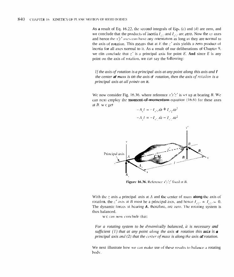
As a result of Eq. 16.22. thc sccond integrals of Eqs. (c) and (d) are zero, and we conclude that the product5 of inertia I1..and I> , , . , arc Lero. Now tlie.ty axes and hence the ~ n i ' i ixcs can have irny orientiition as long a s they are norinal to the axis of rotiitim. This means that at I< the ;' axis yields ii zer11 psiiduct 01 incrtia for all axes nornid to it. As a result of our deliberations of Chaptcr 9. we ciin concludc lhat ;' is :I principal axis for point t . And since E is any point on the axis of rolntion. we can say the follii\ving:
I f the axis uf rotation is a principal axis at any point along this axis and if the center af ma&s is on the axis of rotation, then the axis i j f rutation is a principal axis at ullpointr on it.
Wc now consider Fig. 16.36. where reference ~X~Y'Z' is set up at bcaring / I . Wr ciin ncxl cniploy the moment-of-rnomentuni cquation ( 16.6) f o r these axes i l l I(. w c get
- ~ A 3 1 = -I$,:,h + 18,;,co' -,$,I = - / s , / b - /).;.o?
With lhc : axis ii principal axis at .'i and thc ccntcs of inass along the axis 0 1 rotalion. the 7' iixi5 at B n i i i s t he a pi-incipal a A , and licnce Ir,:, = I > , , . = 0. The dynamic Icirces iit bcaring A. thcrcforc. arc zcro. Thc solatins system is t h i i b balanced.
w c can llOM conclll~lc that:
For a rotating system to be &namically balanced, ir is necessary and sufficient ( I ) that at any point along the axis of rotation this axis is principal axis and (2) that the renter ofmass is along the axis of rotation.
We next illustrate how we can inake use 01 lheie r c d i s tu balancc a rotating bodv.

SECTION 1b.Y BALANCING 841
r Example 16.11
A rotating member carries two particles having weights W, = 5 Ib and A Balancing n ,/ planes
y'wi W, - = 8 Ih at radial distances r l = 1 ft and r2 = I 'h ft, respectively. The weights and a reference xyz fixed to the shaft are shown in Fig. 16.37. They are to be balanced by two other particles having weights W, and W,
,-
(shown dashed) which are to be placed in the balancing Ganes A and ~ ' I > resoectivelv. If the weights are olaced in these olanes at a distance of I ft I ... I L 1- r;, _ / . +w4
> ~~ , from the axis of rotation, determine the value of these weights and their
We have two unknown weights and two unknown angles, that is, four unknowns [see Fig. 16.37(b)], to evaluate in this problem. The condition that the mass center he on the centerline yields the following relations:"
2' position relative to the q z reference. 3' -
(a)
(h) When the numerical values of r,, r2, etc., are inserted, these equations become
Figure 16.37. Rotating system tu w,coso, + W , ~ O S ~ , = 13.18 (a) he balanced.
W, sin 6, - W, sin 6, = -6.77 (b)
Now we require that the products of inertia ivz and lxz be zero for the xyz refere,nce positioned so that xy is in the balancing plane B.
I _ = 0 : W W
R K R !! (h) ( -r , sin 20") + -2 (2) (rz sin 450) + 3 (9)(r3 s ine3) = o (c)
ly7 = 0 :
1 - ( 6 ) ( r , W cos20")+--?(2)(rzcos45")+-(Y)(-r,cos8,) W w1 = 0 (d) K R 6
Equations (c) and (d) can be put in the form
9r% sine, = -6.71
9w1 COS^, = 45.2
'>We are considering the weights to he pilnicles in this dircursion. In solile homework problems you will he asked to halance rotating systems fhc which the partick model will not he proper. You will then have to carry out integrations andlor employ thc formulas and trani~ fer theorems for first moments of m a s and products of inrrlia.

842 CHAPTER 16 K1NI:TICS OF PI.ANF. MOTION 01: Kl(il l1 ROD1F.S
Example 16.11 (Continued)
Dividing Eq. (fl into Eq. (e). wc gct
Ian H3 = -. 1486
e, = 171.~0 or 351.6"
a n d so. from Eq. i t ) .
In order to have I positive weight W,. we chose 0, to he 35 I .6" rather than 171.5". Now we return 10 Eqs. (a) and (h). We can then say. on suh\tituling known values of W, and 8,:
W ~ C ~ , S C ) , = 13.18-5.01 - 8 . 1 6 i p l
W, sin = 6.77 - .75 = 6.02 i hJ
Dividing Eq. (g) into Eq. (hJ. we get
tan 0, = ,738
e, = 36.4" or 216.4"
Hence. from bq (g), we have
where we iise b', = 36.4" rather than 216.4" to prevcnt a negative W,. Thc linal orientation of the halanced system is shown in Fig. l6.3X.
Figure 16.38. Balanced sysit.m.

16.93. A shaft shown supported by bearings A and B i s rotating at a speed w of 3 radisec. Identical blocks C and D weighing 30 Ih each are attached to the shaft by light structural members. What are the hearing reactions in the x and y directions if we neglect the weight of the shaft'?
X 2'
F 3 ' 4 / 12,, Figure P.16.93.
16.94. Shaft A B is rotating at a constant speed w of 20 radlsec. Two rods having a weight of I O N each are welded to the shaft and suppolr a disc D weighing 30 N. What w e the suppolting forces at the instant shuwn'!
I
I
4
2
Figure P.16.94.
16.95. Do Problem 16.94 for the case i n which w = 20 rad/sec and h = 38 rad/icc2 at the iiiitant of interest as shown.
16.96. A uniform wooden panel is shown supported by hearings 4 and 8. A 100-1h weight i s connected with an inextensihle cable to the panel at point G over a light pulley I). If the system is re- leased from rest at the configuration shown, what is the angular acceleration of the panel, and what are the forces at the bearings? The panel weiFhs 60 Ib.
x
100 Ih Figure P.16.96.
16.97. Do Problem 16.96 when there is a frictional torque at the hearings of 10 ft-lh and the pulley has a radius of I ft and a moment of inertia of IOm-fl'.
16.98. A thin rectangular plate weighing SO N is rotating about its diameter at il speed w of 25 radlsec. What are the supporting forces in the .r and s directions at the instant shown when the plate is parallel to t h e y plane?
.r I
300 mm YO0 mm
y
Figure P.16.98.
84:

16.99. A shaft is shown rotating at a speed of 20 radlsec. What are the supporting forces at the bearings? The rods welded to the shaft weight 40 Nim. The shaft weighs XO N.
16.101. ity piven iis
A bent shaft has applied to i t a torque 7 including grav~
7 = IO + 5 r N-m
where 1 is i n scconds. What are thc supporting forces at the bear- ings i n the r and? directions when i = 3 S C C ? The shaft is made from a rod 20 inin in diamctcr and weighing 70 Nlm. At i = 3 sec. the pnsilion of the .;haft i h a b shown.
i
Fipure P.16.99. Figure P.16.101.
16.100. A cylinder is shown mounted at an angle 01 30" to a shaft. The cylinder weighs 400 N. If a torque T of 20 N-m is A ?halt has an angolar velocity o of 10 rad/scc and an applied, what is the angular acceleration of the system? What arc accclcratlOn 0 "1 5 rad/scc: at the instant <jf i,,,e,est, what the supporting forces in the x and j directions at the configuration thz bending this inslant about .I ilxeS just shown wherein the system is stationary! Neglect the mass of the shaft. The centerline of the cylinder is in the x7 plane at the instant rr,ds have yhown.
*l6.102.
[he right thz bearing at A'? ~ l ~ ~ , what arc ,nr,mcnt a,,d shear r,,rces it diameter 01 20 nim and a weight per unit lrnpih of50 N / m
~h~ \haft and
Figure P.16.100. Pigure P.16.102.

16.103. from centerline. Use two weights.
Balance the system in planes A and R at a distance 1 ft
Figure P.16.103.
16.104. Balance the system in Problem 16.103 by using a weight in plane A of I 'h Ih and a weight in plane B of I Ib. You may choose suitable radii in these planes.
16.105. Balance the shaft of Problem 16.94 using rods weighing 50 N/m and welded to the shaft normal to the centerline just next to bearings A and E . Determine the lengths of these rods and their orientations relative to the xv axes.
16.106. A disc and a cylinder are mounted on a shaft. The disc has been mounted eccentrically so that the center of mass is '12 in from the centerline of the shaft. Balance the shaft using balancing planes 5 ft in from hearing A and 3 ft in from hearing B, respec- tively. The balancing masses each weigh 3 Ih and can be regarded as particles. Give the proper position of the balancing masses in these planes.
F i tu re P.16.106.
16.107. Balance the shaft described in Problem 16.106 by removing a small chunk of metal from each of the end faces of the 100-lb cylinder at a position I O in from the shaft cen- terline. What are the weights of these chunks and what are their orientations?
16.108. Balance the shaft in Problem 16.99 using balancing planes just next to hearings A and B. At hearing B use a small bal- ancing sphere of weight 30 N and at heanng A use a rod having a weight per unit length of 35 N/m.
16.109. A disc is shown mounted off-center at B on a shaft CD that rotates with angular speed 0. The diameter of the shaft is 2 in. The disc weighs 50 Ib and has a diameter of 6 ft. Balance the sys- tem using two rods, each weighing 10 Ih/ft and having a diameter of 2 in. The rods are to be attached normal to the shaft at position 1 ft in from bearing C and 2 ft. in from hearing D. Determine the lengths of these rods and their inclination.
C
X
Figure P.16.109.
16.110. Balance the shaft shown for Problem 16.101. Use a hal- ancing plane just next to bearing A and one just next to hearing B. Attach a circular plate normal to the shaft at each bearing, and cut a hole with diameter 60 mm at the proper position in the plate to balance the system. The plates are 30 mm thick and have a spe- cific weight of 8 x IO-' N/mm'.
845

16.10 Closure In this chapter, we Iuve dcvcloped the moment~oE~moiiiciitum equations fnr plane motion of i i rigid body. We applied this cqiiation to viirioiis case? of plane inotioii starting fi-om the simple,l case iind going ti) the i i i ns t difficult case. Many pi-nhlcins I)( engineering interest can he taken i i s pl;inr-motiiin priiblemc: thr results of this chapter are hence quite iniportant. The use 01 MA = H, applied ti) ttiree-diineiision;il miltion of a rigid body is considered i n Chapter I X (starred chapter). Students wli i i cover that chapter will find the devclop- ment of the key cquntion\ (the Euler equation\) \cry similar to the dcvcliip- inent of Eqs. 16.6. !he kcy cquationc for plane inotion.
Ketal next that in Chapter I3 u:e considcred the work-energy equa- tion\ f n r the p lmc 111i)tiiin of siniplc bodics in the process of riilling without slipping. Wc did this to help illutriite the use nf tl ie work+iicrpy cqualioii\ Ifor an aggregate of piirticlcs. Alsii. th is iindcrtaking served ti) inolivalc ii ininre detailed study of kinemei ics of irigid bodies and tn set forth i n iiiiniaturc the more general pioccdurcs t u come liitei. We arc therefore 110w ready l o exiiiii- ine energy inethods i i s applied to rigid bodies in a ininre gcticral way. 'I'hi, will bc done i n Part A of Chapter 17. We shall d lop the work-energy cquatiiins for three-di~irrnsi~i~ial ~ n i i i t i n i i ;ind apply tlicni to all kind\ 01 iiintions, including plane iniifiniis. The student should not lime difficulty i n going dircclly to t l ie g e n e r i c a x : indccd. ii better undcrstandinf of the suh- icct should result.
I n Part H of Chapter 17. we \hall consider the impulse-momeiitu~ii equations lor rigid hiidies. This will he an extension of the uscful i inpulx- nini i ie i i t i in i methods discussed i n Ch;iptcr I4 for particle\ ;ind ;iggregates 01 particles. Again, w e \hall h e able to go to thc general case and lhcn apply the results tci thee- and Iwi)~diiiiciirioti;il i i i i i t i o i i s (plane motions).

16.111. A circular plate A is used in electric meters to damp out rotations of a shaft by rotating in a bath of nil. The plate and its shaft have a mass of 300 g and a radius of gyration of 100 mm. If the shaft and plate very thin down from 30 rpm to 20 rpm in 5 sec, what angular acceleration can be developed by a ,005 N-m torque when o o f the shaft is 10 rpm? Assume that the damping torque is proportional to the angular speed.
Figure P.16.111.
16.112. The dynamic coefficient of friction for contact surfaces E and G is .2 and for A is .3. If a force P of 250 Ib is applied, what will he the tension in the cord HB? Start hy assuming no slipping at A. Check your asaumption at the end of the calculation.
Figure P.16.112.
16.113. A torque T of 15 N-m is applied to a rod A B as shown. At B there is a pin which slides in a frictionless slot in a disc E whose mass i s 10 kg and a'hore radius o f gyration is 100 mm. If the system is at rest at the instant shown, what i s the angular acceleratinn of the rod and the disc? The rod has a mass of 18 kg.
Figure P.16.113.
16.114. A platform A has B torque T applied about its axis of rotation. The platform has a mass of 1,000 kg and a radius of gyration of 2 m. A block B rests on the platform hut i s prevented from sliding off by very thin stops C and D. The block has a mass of I kg and has dimensions 200 mm x 200 mm x 200 mm. The center of mass of the block is at ita geometric center. If a torque T = 20t2 + 501 N-m is applied with f i n seconds, when and how does the block first tip? (Because of the small size and mass of R, consider the system to he a slablike body.)
Figure P.16.114.
847

Figure 1'.16.115,
c
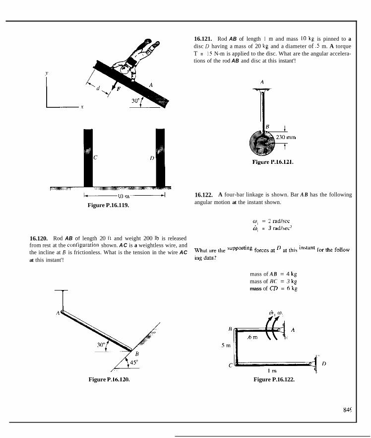
16.121. Rod AB of length I m and mass 10 kg is pinned to a disc 11 having a mass of 20 kg and a diameter of .5 m. A torque T = 15 N-m is applied to the disc. What are the angular accelera- tions of the rod AB and disc at this instant'!
16.122. A four-bar linkage is shown. Bar A B has the following . ., ... angular motion at the instant shown. Figure P.16.119.
W , = 2 rddlsec Oi, = 3 rad/iec2
16.120. Rod AB of length 20 ft and weight 200 Ib is released from rest at the cvnliguration shown. AC is a weightless wire, and the incline at B is frictionless. What is the tension in the wire AC at this instant'!
What are the ing data?
forces at at this for the follow^
1 mass of AB = 4 kg mass of BC = 3 kg mass of CD = 6 kg
Figure P.lh.120. Figure P.16.122.

16.123. when the 10,000 N forcr i\ applied. Plncced as follows:
Starting from T w t , find the acceleration of device A
la) Draw and label lour free-body diapams. (h) Wrire a sys1t.m of eqoationc \n.hmc n u m h r r equals
(c) Do not solve the equ;itions hut do put in any numeri- the numhcl- of unknriwni.
C i d daca.
/)<,la:
M, ( for 2 w'heels) = 50 hg M,, (for 2 wheels) = 100 kg
v,, = 220 kg M,. = 40 kg
ME (lor 2 whecls) = 100 kg k, = .ox "I kp, = 0. I2 "I
I),, = 0.3 m L), = 0.2 ni
IO.000 N - Loose pin
X
N o slipping t i
Figure 1'. 16. I23
.6.124. A cylinder A can rotale ireely ahout i ts fixed cerilerline. ywo sinal ler idcntical cylinders H have axcs of latation nn cyltn- ler A and initially wi l l s t a l l to roll wilhout slipping along the i nd - ,ated walls. What IS the initial angular acceleration of cylinder A tnrting from rest under the action of a torque 7 = 5 N - m ? The ystrm i s in B vertical plane. The following dau apply:
Figure P.16.124.
16.125. I n E x m p l c 15.5 decerminr thc forcc components at plns A and R. The iniaqs (if rod A 8 I S X hg and the rmns o l RC i s S kg. Ilse the kinematic results of the exuinplr.
16.126. A IO-m I-hcnm having a inass ul400 kx i s heing pullcil hy an ilstrmiiiit with his space propulsion rip as shoun. The lwce is 40 N i i ~ l is alwayc i n thc siliiir drcct iwt. Initially, the hzar i s stationary relati\'e 10 the aslmnaut. and the connecting cord i s at right angles to the heam. Consider the heam to hu ii long slender rod. What IS the anpular acceleration whcn thc hcarn ha\ rotated IS"'! What I\ tlic pmit im o l tlir centci of mar\ alter 10 scu? (Can y n u integmle the dilicrentia cqoatiori lor H t o pct t im i l i a r f u i c - t iom? l i x p l o i n . )
Figure P.lh.126.

16.127. A rectangular box having a mass of 20 kg is being trans- ported on a conveyor belt. The center of gravity of the box is 150 mm above the conveyor belt, as shown. What is the maximum stalt- ing torque 7 for which the box will nor tip? The belt has a mass per unit length of 2 kglm, and the driving and driven drums have a mass of 5 kg each and a radius of gyration of 130 mm. The dynamic coefficient of friction between the belt and conveyor bed is .2.
300 m - I r l
I. 5m- < Figure P.16.127.
16.128. A ring is shown supported by wire AB and a smooth sur- fdcc. The ring has a mass of 10 kg and a mean radius of 2 m. A body D having a mass of 3 kg is fixed to the ring a6 shown. If the wire is severed, what is the acceleration of body n?
B\
Figure P.16.128.
16.129. If the md shown is released from rest at the configurd- tion shown, what are the supporting forces at A and B at that instant? The rod weighs 100 Ib and is 10 ft long. The static coeffi- cient of friction is .2 for dl surface cuntacts.
Figure P.16.129.
16.130. Do Problem 16.129 for the case where end A is moving downward at a speed of I O ftlsec at the instant shown and where fl,, = .2.
16.131. In Problem 16.129, find by inspection the instantaneous axis of rotation for the rod. What are the magnitude and direction of the acceleration vector for the axis of rotation at the instant the rod is released? We know from Problem 16.129 that b = 3.107 radlsec' and a? = 7.1% ~ 13.43 fVsec2 for the center of mass.
16.132. Identical bars AB and BC are pinned as shown with fric- tionless pins. Each bar is 2.3 m in length and has a mass of 9 kg. A force of 450 N is exerted at C when the bars are inclined at 60". What is the angular acceleration of the bars?
Figure P.16.132.
16.133. A compressor is shown. Member AB is rotating at a con- stant speed w, of 100 rpm. Member BC has a mass of 2 kg and piston C has a mass of I kg. The pressure p on the piston is 10,ooO Pa. At the instant shown, what are the forces transmitted by pins B and C?
n
m
I50 mm Figure P.16.133.
85 I

*16.134. A thin vcnicill shalt i~ t iues with angular cpecd 1u of 5 r d s e c in heuings A and n ac chmm i n the diagnm. A uniform platc H urighing 50 Ih i s atrachcd to the \halt us i \ ii disc C u'eighing 30 Ih. What ire the hearine reactions at thc confi!!oration shown?
16.137. A X l h cylindcl- which i s spinning a1 a rate w0 of 500 rpm i s nlacrd o n an 8 deerce inclinc. Thc coefficicnts of frictioil are
I
The shaft weighs 20 Ih and the Ihicinrw ofili\c and platc is 2 111.
p, = .4 and p,, = .3. HOM. far does the cyliiidsr mo\'e before therr i s rolling without slipping.'! How much rime elapses hefore the cylinder stops moving instantanwusly?
I
.i h" t
t ,,
3' I
ow I t
I)
,,
.i h" t
3' I
Figure P.lh.134.
*16.135. Do Prohlcm I h. 100 for the car ~ h c i t : w = 5 ir;d/sei ill lhe imtimt of intcrcst.
Y I
8' Figure P.16.137.
16.138. 111 Example 15.1 I . takc wi and h2 hoth equal tu zrlu hut kccp all other data. Detemme the lorce system at A knowing that the Idlowing data apply:
*lh.136. In Example 16.lO. halance the rotating systcin hy Y H = 800 N &,,,~,,,ck ,,,, = 135 kg pmpcrly placing 3h-N spherical rnilbscs in halmcing plane, 300 m n insidc f rom the hearings A and Lj. Asaume thai the halancilig inasses are particlcc
Note that the inan and cockpit are translating and can hc consid- crcd a\ II partick of mass 135 kp.

Energy and Impulse-Momentum Methods for Rigid Bodies 17.1 Introduction
Let us pause to reflect on where we have been thus far in dynamics and where we are about to go. In Chapter 12, you will recall, we worked directly with Newton's law and integrated it several times to consider the motion of a par- ticle. Then, in Chapter 13 and 14, we formulated certain useful integrated forms from Newton's law and thereby presented the energy methods and the linear impulse-momentum methods also for aparticle. At the end of Chapter 14, we derived the important angular momentum equation, MA = HA. In Chapter 16, we returned to Newton's law and along with the angular momentum equation, MA =HA, carried out integrations to solve plane motion problems of rigid bodies. In the present chapter, we shall come back to energy methods and linear impulse-momentum methods-this time for the general motion of rigid bodies. In addition, we shall use a certain integrated form of the angular momentum equation MA =HA, namely the angular impulse-momentum equa- tion. These equations at times will be applied to a single rigid body. At other times, we shall apply them to several interconnected rigid bodies considered as a whole. When we do the latter, we say we are dealing with a system of rigid bodies. We shall consider energy methods first.
Part A: Energy Methods
17.2 Kinetic Energy of a Rigid Body
First, we shall derive a convenient expression for the kinetic energy of a rigid body. We have already found (Section 13.7) that the kinetic energy of an
853

854 (‘HAPTER 17 ENEKGY ANI1 IMI’UI .S~~MOMFNTI!M METHODS FOK KIGII) nOr I l l3
aggregate of particles relative lo any referencc is thc suin of two parts, which we list again a s :
1. The kinetic cncrgy 01 a hypothetical particle that has a mass cqual to thc total mass of the systcm and a inoti(iii corresponding to that of the mas\ center of the system. plus
2. The kinctic cncrgy 01 the particles relativc to thc mia ass ccntcr.
Mathematically
/ I
whcre Let us now consider the foregoing equation tis applicd to ia rigid body
which is a special “aggregate of particles” (Fig. 17. I i. 111 such a case. the velocity of any particlc relatiw to lhc mass center becomes
is thc position vector Sroni the mass center tn the ith particle.
f i = W X 11, (17.21
h’iaii = >M
X F i p r e 17.1. Rigid h d y .
where w is the angular velocity of the hody relative to reference XYZ in which we are computing the kinetic energy. For the rigid body. the discrete particles of mass m, hccomc a continuum of infinitesimal particles each of mass (h. and the sumination in Eq. 17. I then hecomes an integration Thus, we can say for the rigid body. replacing li i 2 hy V:.
where p represents the pocition vectoi- f’rom the center of mass to any element of mass dm. Let us iiow choose a set of orthogonal directions ,rj: at the cen- ter of mass. s o wc can carry o u t the preceding intcffiation in tcrnis 01. thc scalar components o f w and p. This step is illustratcd in Fig. 17.2. We first express the intcgral in Eq. 17.3 i n the fiillowinf nimncr:

SECTION 17.2 KINETIC ENERGY OF A RIGID BODY 85s
z
Figure 17.2. Fix xyz at center of mass.
Inserting the scalar components, we get:
* [ (mxi + wyj + m z k ) x ( M + yj + & ) ] } d m
Carrying out first the cross products and then the dot product in the integrand and collecting terms, we form the following relation on extracting the w’s from the integrals.
You will recognize that the integrals are the moments and products of inertia for the xyz reference. Thus,’
2 111 lox p( dm = I,@: - 1,mp, - Ixzm,mz M -I”xm,m, + 1,m: - Iy$oymz
- l $ p x - 1,ozm, + lam;
#Note that we have deliberately used a matrixlike array for ease in remembering the formulation.

We can now give the kinetic energy of a rigid hody in Ihc following lorni:
1,uxu, - Ixpxuz
+ I YY 62 Y - IVZU,WZ . - I,U~,U, + 1,p;t
(17.5)
Note that the f i rs t expression on the right side of the preceding equation i s the kinetic energy of translation of the rigid body using the center of mass, while the second expression i s thc kinetic energy o f rotation ol the rigid hody about its center of mass. IS principal axe? are chosen, Eq. 17.5 hecomes
K E = MV' +t( l , ,u: + I \ > U .. . (17.61
Note that lor chis condition the kinetic ene1.g.y ternis for rotation have the same form as the kinetic energy term that i s due to translation. with the moment o f inertia coi-responding to i i iass and angular vclocicy corrcsponding tn linear velocity.
As a special case. we shall consider the calculation of kinetic energy n l any rigid hody undergoing prw nmtion relative lo X U with angular \'cIoc- i ty w about an actual axis of rowtion' going through part o f the body or through a rigid hypothetical n iass lew extension of the body. We have shown this situation in Fig. 17.3. where the Z axis i s chosen tn bc collinear with thc w vector and the axis of rotaticin The reference .LE ;it thc cciitcr of mass i s chosen parallel to X Y Z . Clearly. ut = UJ? = (1 and O I ~ = 01 s o t<q. 17.5 hecome,
KE = i M V 2 + ~ i ILoJ? ..

SECTlON 17.2 KINETIC ENERGY OF A RIGID BODY 857
where IZz is about an axis which goes through the mass center parallel to 2. Note that y. = wd, where d i s the distance between the axis of rotation Z and the z axis at the center of mass. We then have
KE = f(MdZ)w2 +flrzo2 = 4 (Izz + M d 2 ) w 2
But the bracketed expression i s the moment of inertia of the body about the axis of rotation Z. Denoting this moment of inertia simply as I , we get for the kinetic energy:
KE = + f a 2 (17.7)
This simple expression for pure rotation is completely analogous to the kinetic energy of a body in pure translation.
Figure 17.4. Plane motion relative to the X Y plane.
For a body undergoing general plane motion (see Fig. 17.4) parallel to the X Y plane, where xyz are taken at the center of mass and oriented parallel to X Y Z . we get from Eq. 17.5:
(17.8)
We now illustrate the calculation of the kinetic energy in the following example

8.58 CHAPTEK 17 ENRK(;Y AND IMPULSE-MOMENTUM MKIHOL)S FOR R K l U BODIES
Example 17.1
Compute the kinetic energy of the crank sysleni i n tlic configuration shown in Fig. 17.5. Piston A weighs 2 Ib. rod AH is 2 f t long and weigh:, 5 Ib, and flywheel D weighs 100 Ib with a radius of gyration of 1.2 ft. The radius r is 1 ft. At the instant of interest. piston A is moving to the right at a speed V of I O itlsec.
~
~
Figure 17.5. Crmk \y\tem
We have here a translalory motiori (piston A). a plane motion (rod AB). and a pure rotation (tlywhecl D). Thus. for piston A we have f o r the kinetic energy:
(a) I ( K E ) , = ? M V 2 - = 2(m)( '
IO') = 3.1 I ft-lh
For the rod AB. we must first consider kinemurid aspects of the motion. For this purpose we have :,hown rod AH again in Fig. 17.6, where V, is the known velocity of poinlA and V, is the velocity vector fkr point B oriented at an angle a such that l$ i!, perpendicular to OB. We can readily find v for the configuration 01 inkrest by trigonometric considerations of triangle AHO. To do this, we use the law of sines to Sirst compute the angle p:
Figure 17.6. Kincmaticr 01 rod A H .
2 - I sin 0 \in 27)" -~
Therelore, /J = 41 2"
. .. ., ~ ...... " .., "._x"_."_^~. .. .., .. ..,..I I_x__.."

SECTION 17.2 KINETIC ENERGY OF A RIGID BODY 859
Example 17.1 (Continued)
Because V, is at right angles to OB, we have for the angle a:
a = 90" ~ p = 46.8" ( c )
From kinematics of a rigid body we can now say:
V, = V, + (w , ,k )x pAH
Hence, V , ( c o s a i + s i n a j j = IOi+w,,kx(2cos20"i+2sin20"jj
:_ V,(.64Xi + .729j j = I O i + 1.X790A,j - .684w,,i ( d j
From this we solve for on, and V,. Thus,
";I = 10.53 ftlsec a,, = 4.09 radlsec
To get the velocity of the mass center C of A B , we proceed as follows:
V,. = V, + (wA,k)xpA, . = I Oi + 4.09k x (.940i + ,342 j j (0 = I O i + 3.843' ~ 1.399i = 8.60i + 3.84jftlsec
We can now calculate (KE),,, the kinetic energy of the rod:
I I (KE),, = 2 MA,V: + 2 171Wi,
(8.602 + 3.84* j + 1 (A & 2')(4.09'j (g j
= 7.32 ft-lh
Finally, we consider the flywheel D. The angular speed m, can easily be computed using V, of Eq. (e). Thus,
' - ' O f 3 = 10.53 radsec (hj % = r- - ~~
Accordingly, we get for (KE),:
(KE), = [ ~ ( ~ ) ( 1 . 2 2 ) ] ( 1 0 . 5 3 2 ) = 248 ft-lh (i)
The total kinetic energy of the system can now be given as
KE = (KE), + (KE),, + (KW,
= 3.1 I + 7.32 + 248 = 298 ft-Ib ( j j

860 CHAPTER 17 ENERGY AND IMPULSE-MOMENTUM METHODS FOR RIGID BODIES
17.3 Work-Energy Relations We presented in Cliaptcr 13 thc wiirkkcncrgy rc l i i t i~n fix a .sin,yle panicle mi ill
a system o l n panicles (see Fig. 17.7) to rcach the f(~l lowing equalion:
Sdr, + [ l ’ tS i ‘dr , = l(m,V,’j? ~ J(m,y’ j , = (AKE), (17.9) , = I I # ,
where f is the f k e from particle j iinto particle i and i s an internal force. (Note that since a particle caiiiiiit exert ii force on itself,J, = 0.) Now consider that the particle ni, i s part of a rigid body. as shown in Fig. 17.8. From New- ton’s third law we can say that
.f,, = Yf,, ( 17. IO)
Y
X / .. Figure 17.7. Splznr 01 particle\.
I t might he intuitively iihviiius to the reader that for any miition o f a rigid body the totality of internal forcesx, can do no work. If not. read the follow ing proof tn verify this c la im
Suppose the rigid hody moves xi infinitesimal amount. We employ Chasles’ theorem, whcrchy we give the entire hody a displaccmcnt dr corre- hponding Lo the actual displacement of particle WI, (sec Fig. 17.8). The total work done hy f ; , and f,, i\ clearly L X I for this displacement a s a result of
/ X Figure 17% Particles of a rigid hody.

SECTION 17.3 WORK-ENERGY RELATIONS 861
Eq. 17.10. In addition, we will have a rotation dq5 about an axis of rotation going through mi. We can decompose dq5 into orthogonal components, such that one component d@, is along the line between mi and mi (and thus collinear withJ,) and two components are at right angles to this line (see Fig. 17.9). Clearly, the work done by the forcesfq andfi, for d+, is zero. Also, the movement of mj for the other components of dq5 is at right angles tofi,, and again there is no work done. Consequently, the work done by f, andfi; is zero during the total infinitesimal movement. And since a finite movement is a sum of such infinitesimal movements, the work done for a finite movement of mi and mj is zero. But a rigid body consists of pairs of interacting particles such as mi and m,. Hence, on summing Eq. 17.9 for all particles of a rigid body, we can conclude that the work done by.furces internal to a rigid budy for any rigid-body movement is always zeru.
Figure 17.9. Rectangular components of d+.
We must clearly point out here that although the internal forces in a rigid body can do no work, forces between rigid bodies of a system of rigid bodies can do a net amount of work even though Newton's third law applies and even though these forces are internal to the system. We shall say more ahout this later when we discuss systems of rigid bodies.
We accordingly compute the work done on a rigid body in moving from configuration I to configuration II by summing the work terms for all the external forces. Thus, for the body shown in Fig. 11.10, we can express the work between I and II in the following manner:
(work),,,, = 4 * ds, + j:' F, * ds, +


SECTION 17.3 WORK-ENERGY RELATIONS 863
In this case the torque T and angular speed 6 are about the same axis. The generalization of Eq. 17.12 for any moment M and any angular velocity w (see Fig. 17.12) then is -
wK = y M * w d t (17.13)
We thus have formulations for finding the work done by external forces and couples on a rigid body. For the conservative forces, we know from Chapter 13 that we can use for work a quantitv that is minus the change in
11
I
potential energy from I to 11 without having to specify the path taken.
rigid body:
Figure 17.12. dwK = M * w df Using this information for computing work, we can then say for any
b I t o I I = A K E (17.14)
where W?? is the work by external forces.
for the rigid body: If there are only conservative external forces present, we can also say
If both conservative and nonconservative external forces are present, we can say:
no (17 16)
These three equations parallel the three we developed for a particle in Chap- ter 13.
The foregoing equations are expressed for a single rigid body. For a system of inferconnecred rigid bodies, we distinguish between two types of forces internal to the system. They are
1. Forces internal to any rigid body of the system 2. Forces befween rigid bodies of the system.
Fur a system of bodies, as in the case of a single rigid body, forces of category I can do no work. However, if the forces between two bodies of 2 system do not move the same distance over the same path, then there may be a net amount of work done on the system by these internal forces. We must include such work contributions when employing Eqs. 17.14-17.16 for a system of inferconnecred rigid bodes.’ Example 17.4 is an example of this situation.
‘Recall from Chapter 13, lhilt Eq. 17.16 and hence Eqr. 17.14 and 17.15 are valid for any aggregate of panicles provided we include lhe work of internal forcra both conservative and nun- conservative.

864 CHAPI'ER 17 ENk.KGY AND IMI ' I I I .ST~MOMENII~M METHOIIS TOR RIGII) HODIES
ExamDle 17.2 i
Neglect the weight ol the cable i n Fig. 17.13. aild find tlic speed of thc 450-N block A alter it has miivcd 1.7 111 along Lhc incline lrom 21 position of rest. The static coefficient (if lriction along the incline is 3 2 . and the dynamic coefficient of friction i \ 30. Consider the pulley B t o be :I Lini-
f k m cylinder
We musl lirst decide which way the hlock nioves along the incline. To overcomc friction and move down the incline, the block m u s l create a force in the downward direction of the cable exceeding 90/2 = 45 N. Con- sidering the block A alone (see Fig. 17.14). we can readily decide t lxlt the maximum fcirce 7., to allow A Lo start sliding downward is
(T , ) , , !~ ,~ = -(.12) N + 4 ~ 0 s i n 3 0 ~
= -(.32)(450) cos 30" + 450 sin 30" = 100.3 h
Clearly, the block goes down the iiiclinc. X We now use the work-kinetic energy equation separately t o r each
hody. Thus. f01- Lhe block wc have. using now thc dynamic coefficient (if lriction
Figure 17.14. Ficu body 01 hlock
I 450 - s (450sin30")(1.7) - (45~~)1ci )s~0"11.30)(1.7) - Ti1.7) = 7-Vf
Therefore.
7; = I0X. I - I3.491/,' ( i l l

SECTION 17.3 WORK-ENERGY RELATIONS 865
Example 17.2 (Continued)
We now consider the cylinder for which the free-body diagram is displayed in Fig. 17.15. Note that the cylinder i s in effect rolling without slipping along the light supporting cable. Hence, Tz does no work as explained in Chapter 13.4 Thus, the work-kinetic energy equation is as follows using the formula $ Mr2 for I of the cylinder:
Therefore,
= 45 + 2.70V; + , 12140~
From kinematics we can conclude on inspection that
(b)
Subtracting Eq. (b) from Eq. (a) to eliminate T,, and then substituting from Eq. (c) and Eq. (dj for V, and w, we then get for 4:
v,=2 (e)
This problem can readily be solved as a system, i.e, without discon- necting the bodies. You are asked to do this in Problem 17.25.
4Recull that the point of contact of the cylinder has zero velocity. and hence the friction force (in [hi, cue, T J transmits no power to the cylinder.
Y i 7 ~ .tt
YON
Figure 17.15. Free body of cylinder
In the previous example, we considered the problem to be composed of two discrete bodies. We proceeded by expressing equations for each body sep- arately. In the following example, we will consider a .system of bodies expressing equations for the whole system directly. In this problem, the forces between any two bodies of the system have the .surne velocity: consequently, from Newton's third law, we can conclude that these forces contribute zero net work. We shall illustrate a case where this condition is not so i n Example 17.5.

866 CHAPTIX 17 tNRRCY A N U IMPLLSF. MOMENTIIM Mk:lHOI)S ['OK KI(;II) H0L)IIIS
Example 17.3
i
' 4
1 :
A conveyor i s rnovinp a weigh1 WoI64.4 Ih in Fig. 17.16. CylindcrsA ;ind H have ii diameter of I ft and weigh 32.2 Ih each. A h , they each have :I
radius of gyration of .4 1.1. Rullers C', I ) , I:. F, and G cach hii\e a diamclcr o f 3 in.. weigh 10 Ih each, iind have a riidius ulgyratioii of I i n Whal cuii- stant torque wi l l increase the spccd 01 W from I ftisec of 3 fl/\ec i n 5 ft o l travel? Thcrc i s no slipping at any of the rollers anit driiiiir. The helt
We shall use the work-kinetic energy reliitiun \pcciiicil in Eq. 11.14 fur this prohlcm. Only cnlernal forces and turqucs do work foi- the systcm: the interactivc lorccs hetweeii hodies do work in a i i i u i i t i t s th:it clearly c x - ccI each other hecause ul' the conditioii of n o slipping. Ilcncc.
i i l )
whcrc T i s the applied torque. Thc general expression for thc hitictic cncrzy
1 !
TH- M/(5)(sin30"j = (KEI, - i K E j ,
'
j i s
1 From kinematics we cii i i say:

SECTION 17.3 WORK-ENERGY RELATIONS 867
Example 17.3 (Continued)
Using these results, we can give the kinetic energy at the end and at the beginning of the interval of interest as
Substituting these results into Eq. (a), we get
TO - (64.4)(S)(sin 30”) = 21.4 ~ 2.37 (c)
From kinematics again we can say for 0, on considering the rotation of a cylinder and the distance traveled by the belt:
(rcyl)(0) = 5
Therefore,
S O = ~ = I O rad
Substituting back into Eq. (c), we can then solve for the desired torque T:
T = &[21.4 - 2.37 + (64.4)(S)(sin 30”)]
I 2
~
T = 18.00 ft-fb
In the next example, we have a case of internal forces between bodies that satisfy Newton’s third law but do not have identical velocities

868 W A V l t K 17 ENERGY ANI1 I L I I ' I I I S I I ~ M O M ~ U ' I I I M MCTtKIIX I-OK IKKilf) HOlllES
Example 17.&
A diesel-powered electric train ~ i ~ n v e s u p ii 7' grade in Fig. 11.11. I f a Iorque of750 N-in i s developed ;it each of its six pairs uldrive wheels. u l i a l i \ thc incrcdsc O S speed of thc twin after i t Iiinves 100 ni? Initially. the train has a speed of. 16 kniihr. The train wcighs YO kN. The drive wheels t ime :I dianic- ter US h(K) mni. Neglect lhc rutatinnal energy US Ihc drive wheel\.
We shall cunsider the t u i n as ii .\WCIII of ri,qirl I,,i~lic~.s iiicluding the 6 pairs of whccl.: m d the hody. Wc have sliuw~i the liiiiii iii Fig, 17. I X with the externid kir , W. N. ;ind f : 111 addition, wc have shown ceniiin internal torques M." The tiiIque\ \tiown act on thc r o i ~ r : ~ of thc motors. and. a s the triiiii move\. these torques rotate :rnd accordingly do work. The , r ( ~ t i o r i s to thcsc torques are equal and uppohite to M according tu Newton's third law and act on {tie i i ~ i i o ~ or illc motor\
(;.e.. the field coil\). The statim are \t;itionary. and 'io the re' .lL110115 10
M do no work iis the train iiiuve'i. Thus. we have :in example o f cqual and oppositc incernal forces hetueen hodics US i i system perlorniing ii
nonzcru net amount of work. Wc now ernploy k:q. 17.16. Thus.
.
APE + AKE = ( i l )
Ilhing the i i i i l ial configurdliun iis the datuiii. UF I1:1vc7

SECTION 17.3 WORK-ENERGY RELATIONS 869
Example 17.4 (Continued)
where 0 is the clockwise rotation of the rotor in radians. Assuming direct drive from rotor to wheel, we can compute 0 as follows for the 100-m dis- tance over which the train moves:
ad (c) I O 0 0 = (2n) = -r .30 -ii
re" radire"
Substituting into Eq. (b) and solving for V , we get
Hence, V = 10.38 m/sec
(10.38)(3,600) IO00 16 ~ 21,4 km,hr AV =
In Chapter 13, we also developed a work-energy equation involving the mass center of any system of pasticles. You will recall that
(1 7.l7a)
where F is the toto1 externalforce [only!) which hypothetically moves with the cenfer oj' mass. This equation applies to a rigid body. Note that an external torque makes no work contribution here since equal and opposite forces each having identical motion (that of the mass center) can do no net amount of work. For a system of interconnected rigid bodies, we can say:
The force F includes only externalforces (internal forces between interconnect- ing bodies are equal and opposite and must move with the mass center of the system; hence they contribute no work to the left side of the foregoing equa- tion). On the other hand, external friction forces on wheels rolling without slip- ping must move with the mass center of the system in this formulation and thus can do work, in contrast to the previous approach, in which the mass center is not used. On the right side, we have summed the kinetic energies of each of the mass centers of the constituent bodies of the system8 We now illustrate the use of Eq. 17.1711.
XWr dixusaed this topic in Section 16.8.

870 CHAPl'EK 17 ENCR(;Y ANI1 IMI'l:I.St:~~MOMr.NT~!M hlliT1101lS I'OK IRlGll) II0T)lF.S
Example 17.5
has four-wheel drive ;and wciglis 22.5 k N . Each wlieel weighs 2 k N ha\ ii
diameter ol 2.5 in and has ii rndius i l l gyration ol I X O mni. It ex11 whccl gel\ a torque of 100 N-m. what i s the ?peed after 20 in of tra\cI \tartin: from res('! A lw . deterniinc the friction force T i -o i i i t l ie groiind on eiich whecl. The weight i i l the vehiclc includch that of pxsseiigers and haggage. Neglect rolling resi\tance since the vchiclc i n this problem is inwing (in i~
Ihrd surlace. Consider r i i l l iny witlioiit slipping.
Figure 17.19. I\ \cIticIc u x d in swilmpliinil.
We l iave shown the free-hod) diagrmi ol'thc sy?tem i i i Fig. 17.20. We %ill first use the system of particles approach. 'This includes internal lorques from tlie vchiclc lriinic tmto lhc wheels iiiid the reiiction lorquc\ from the wheel\ onlo l l ic fr;unc. .The former wi l l dc internal w ) r k because Lhcx torques rotate wit11 thc wheels. Thc reaction torque\ on thc 1 r m e &I
no( rot;ite and obviously do iio worh. Also. because 1 1 1 t h ~ 1111 slippine coil- dilion, the friction hrces from the ground o n m lhc lircs do no work CIS has been explained al length i n Chapter 13. Hcncc, we can say
(4l(T)(H) = IKEI, ~ (KEJ,
Recalling thal H = dislancclriidios. w e gcl
22 5 kN
:. V = 2.354 nils
To get the ir icl i i in liirces,/(u'liy are they the same lor tach whccl'l l wc use the center 11f mass approach. Thus
W, = (AKEJ,.,,,
:. j= 79.4 N

In rhe follow in^ prohlenrs. neglect frictiori unless orhewise 17.3. A thin disc weighing 450 N is suspended from an over- inrrructed. head conveyor moving at a speed of 10 misec. If the disc rotates at
a speed o f 5 radisec in the plane of the page (i.e.. ZY plane), com- pute the kinetic energy of the disc relative to the ground.
17.1. A unifbrm solid cylinder of radius 2 ft and weight 200 Ib rolls without slipping down a 45" incline and drags the 100-lb block 8 with it. What is the kinetic energy of the system if block R is moving at a speed of I O ftlsec? Neglect the mass of connect- ing agents between the bodies.
Figure P.17.1
300 mm X
Figure P.17.3.
17.4. Two slender rods CD and EA ilte pinned together at B. Rod EA is rotating at a speed w equal to 2 radlsec. Rod CD rides in a ver- tical slot at D. For the configuration shown in the diagram, compute the kinetic energy of the rods. Rod CII wcipha 50 N and rod EA weighs 80 N.
I' k
n
17.2. A steam roller with driver weighs 5 tons. Wheel A weighs
total mass of 1.000 Ib and a radius of gyration of 1.6 ft. If the steam roller i s coasting at a speed af 5 ftlsec with motor discon- nected, what is the total kinetic energy of the system?
I ton and has a radius of gyration of .8 ft. Drive wheels B have a E
D
Figure P.17.4. Figure P.17.2.
87

17.5. ing 2 Ih. and compote i ts kinetic energy for the d a h given.
Consider thc connecting rod AH io he a slender rod weigh-
H
M
Figure P.17.8
172
17.9. A cone H weighing 20 Ih rol ls without slipping inside a conical cavil) C. The coni' hiis a Icngh rrf IO ft. The centerline 01 lhi. COIIC rol:itc\ u i th ;in ;in@ol;il- speed (u, o f S r d l s c c h m l the Y i i x i c . Compute the kinctic cncrgy o1 thc cone.
X
Figure 1'.17.11.
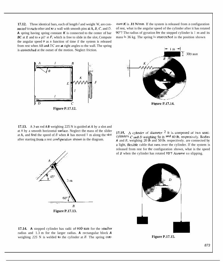
17.12. Three identical bars, each of length 1 and weight W, are con- nected to rach other and to a wall with smooth pins at A, h, C, and D. A spring having spring constant K is connected to the center of bar BC at E and to a pi? iit F, which is free to slide in the slot, Compute the angular speed 8 as B function of time if the system is released from rest when AB and DC are at right angles to the wall. The spring is unslrctched at the outset of the motion. Neglect friction.
itant K is , I 8 Nlmm. If the system is released from a configuration of rest, what is the angular speed of the cylinder after it has rotated 90°? The radius of gyration for the stepped cylinder is I m and its mass is 36 kg. The spring ih unstretched in the position shown
l + l m +
Figure P.17.12.
17.13. A 3-ni rod A B weighing 225 N is guided atA by a slot and at B by a smooth horizontal surfdce. Neglect the mass of the slider at A , and find the speed of B when A has moved 1 m along the sh t after starting from a rest configuration shown in the diagram.
17.15. A cylinder of dialmeter ft is composed of ,wo Semi. 80 ~ b , respectively, ~ ~ d i ~ ~
A and h, weighing 20 Ib and 50 Ib, respectively. are connected by a light, flrxible cable that I’UIIS over the cylinder. If the system is released from rest for the configuration shown, what is the speed of B when the cylinder has rotated YO’? Assume n o slipping.
c and D weighing 50 ~b
//
h Figure P.17.13.
17.14. A stepped cylinder has radii of 600 mm for the smaller radius and 1.3 m for the larger radius. A rectangular block A weighing 225 N is welded to the cylinder at B . The spring con- Figure P.17.15.
873

c'
liigure P.17.16
I Figure 1'.17.18.
30 Ih
Figure P.17.17.
873
W = 200 lh
Figure P.17.20.
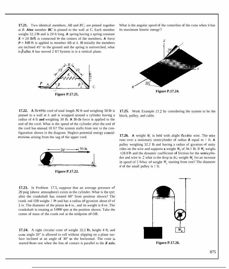
17.21. Two identical members, AB and BC, are pinned together at 6. Also member BC is pinned to the wall at C. Each member weighs 32.2 Ib and is 20 ft long. A spring having a spring constant K = 20 Iblft is connected to the centers of the members. A force P = 100 Ib is applied to member AB at A . IS initially the members are inclined 45" to the ground and the spring is unitretched, what i s p afterA has moved 2 ft'? System is in a vertical plane.
What is the angular speed of the centerline of the cone when it has its maximum kinetic energy'?
z
C X Figure P.17.24. , , ,.
Figure P.17.21.
17.22. A tlexihle cord of total length 50 ft and weighing 50 Ib is pinned to a wall at A and is wrapped around a cylinder having a radius of 4 ft and weighing 30 Ib. A 50-lb force is applied to the end of the cord. What is the speed of the cylinder after the end of the cord has moved 10 ft? The system stalls from rest in the con-
17.25. block, pulley, and cable.
Work Example 17.2 by considering the system to he the
figuration shown in the diagram. Neglect potential energy consid- erations arising from the sag of the upper cord. 17.26. A weight W, is held with alight flexihle wire. The wire
runs over a stationary semicylinder of radius R equal to I ft. A pulley weighing 32.2 Ib and having a radius of gyration of unity rides on the wire and supports a weight W, of 16. I Ib. If W, weighs 128.8 Ib and the dynamic coefficient nf friction for the semicylin- der and wire is .2 what is the drop i n the weight I+; for an increase in speed of 5 ftlsec of weight starting from rest? The diameter d of the small pulley is I ft.
Figure P.17.22.
17.23. In Problem 17.5, suppose that an average pressure of 20 psig (above atmosphere) exists in the cylinder. What is the rpm after the crankshaft has rotated 60" from position shown? The crank rod OB weighs I Ib and has a radius of gyration about 0 of 2 in. The diameter of the piston is 4 in., and its weight is 8 oz. The crankshaft is rotating at 3,000 rpm at the position shown. Take the center of mass of the crank rod at the midpoint of OB.
17.24. A right circular cone of weight 32.2 Ib, height 4 ft, and cone angle 20" is allowed to roll without slipping on a plane sur- face inclined at an angle of 30" to the horizontal. The cone is started from rest when the line of contact is parallel to the X axis. Figure P.17.26.
875
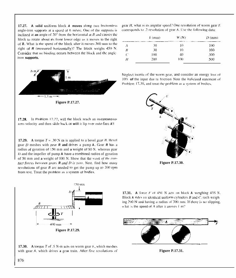
17.27. A solid unifrmm hlock A moves along two fnctl~mlrss angle-iron \upports at a speed of 6 miicc. Onc nf the wppml\ is inclincd at an angle if 20" lioin the horimnta at 8 :ind C:ILISCS thc hlock to rotate ahout it, front IOU,CI rdgc a? it ~moveh to the right of R . What is thc sped of the block aster i t moves 300 mm to thc right of R (meawred horimntally)? The block weighs 4511 N. Consider that no hinding occurs hctu'ccn the hlnck and thc anglc- iron supports.
Figure P.17.27.
17.28. i e ~ n velocity and then slid? hack o r will i t lip n x r onlo face A'!
In Prohlern 11.21, u'ill the block rcach an inrtantaneiw
17.29. A torque l = ,311 N-m is applied tn a bevel f w r R. Bcvcl gear /I meshes with g c x R and dr iws a pump A . <;car R ha\ a radius of gyration of I SO m m and a uxight of SO N. whereas gear I1 and the impeller of pump A have a comhined radios of gyration o f50 mm and a weight of IO0 N. Show that the work qf the c o i i ~ mcf fbn.r.v hrtwrm griin R nnd I) i.r zt'ro. Next. find how nnny revolutions of gear H arc necdcd ti) get the pump up I O 200 irpin from I C C ~ . Treat the prohlem as it cystem of hodies.
Neglcct inertia of the worm g c x , and consider an energy Iosc of Ill<% of the input due t u f r ict ion Note the italicixd mtcment 01 Plohlem 17.30. and treat thc pl-ohlem 11s ii \ystrm of hodie,.
Figure P.17.30.
17.31. A fwce F of AS11 N X'IF ~ r n hlock A wel&!hing 435 N . Block A ride\ o n identtoal unifcrnm cylindcrs H and C. rach weigh- ing 290 N ;and having a radius u t 300 cmn,. I i thew i s (no slipping, u hat i \ the speed oi'A alter i t ~nwves I m?
Figure P.17.29.
17.30. A t o r q ~ x 7'nf .5 N-m acts on worm gear E, which m e s h e with gear ,A, which drives a geai- train. Aftcr f ive rewlut icm of Figure P.17.31.

17.32. Work Example 17.5 using the center-of-mass approach for the whole system. What are the friction furces on the wheels from the ground?
of gyration of300 mm screws onto the shaft. A torque Tof 45 N-m is applied to A as shown. What is the angular speed ofA after three revolutions starting from a rest configuration'! Neglect friction.
17.33. An electric train (one car) uses its motors as electric gen- erators for braking action. Suppose that this train is moving down a 15" incline at a speed initially of 10 m/sec and, during the next 100 m. the generators develop 1.5 kW-hr of energy. What is the speed of the train at the end of this interval'? The train with pas- sengers weighs 200 kN. Each of the eight wheels weighs 900 N and has a radius of gyration of ?SO mm and a diameter of 600 mm. Neglect wind resistance, and consider that there is no slipping. The efficiency of the generators fur developing power is 90%. [Hint: One watt is I N-mlsec.] Do not use center of mass approach. Figure P.17.36.
17.37. A uniform block A weighing 64.4 Ih is pulled by a force P of50 Ib as shown. The block moves along the rails on small, light wheels. One rail descends at an angle nf IS" at point B. If the force P always remains horizontal, what is the speed of the block after it has moved S ft in the horizontal direction'? The hlock is stationary at the position shown. Assume that the block does not tilt forward.
17,34, Work the whole Onto the
17,33 using the center ofmass approach for Also, find the average friction force from the rail Consider that each wheel is attached to a
17.35. A windlass has a mating part which weighs 75 Ih and hai a radius of gyratinn of I ft. When the suspended weight of 20 Ib is dropping at a speed of 20 ftisec, a 100-1h force is applied to the lever at A. This action applies the brake shoe at B, where there is a coefficient of friction of .5. How far will the 20-lh weight drop before stopping'?
1-1'4 Figure P.17.37.
17.38. A solid uniform rod AB connects two light slider hearings A and B. which move in a frictionless manner along the indicated guide rods. The rod AB has a mdss of 150 lhm and a diameter of 2 in. Smooth hall-joint connections exist between the rod and the hearings. If the rod is released from rest at the configuration shown, what is the speed of the hearing A when it has dropped 2 ft?
Figure P.17.35.
17.36. A square-threaded screw has a diameter of S O mm and is inclined 45" to the horizontal, The pitch of the thread is 5 mm, and it is single-threaded. A body A weighing 290 N and having a radius Figure P.17.38.
877

Impulse-Momentum Methods
17.4 Angular Momentum of a Rigid Body About Any Point in the Body
AI we g11 to thrcc dimeiirioiis. we wil l need lormulati~~iis Sor linciir inionion- tuin and angular ini~mentutn of rigid hodich. The li i ieiir ini~nientum i s simply
V din = M V . We shall now fi~rmulate iui cxprcssion for Lhc more coin- plicakd angular momentum H of a rigid body about a point. For this purpose. we choose ii point A in ii rigid body 111 hypiithrtical massless cxtcnsion ofthe rigid body tis shiiwii iii Fig. 17.21. An eleinciil of mass dm at ii position p from A i s shown. Thc velocity V' (if drn reliitive lo A i h simply the velocity of dm relative to reference j t ] < which I ~ W ~ . S / U I ~ S with A relative 10 XYZ. Sinii larly, the linear moincntuiii of dni rclativc to A i s the linciir iiionicntuni of hi
i-elativc to a reierciicc 505 lranslating with A . We caii niiw givc the angular inornenuim dH,, for elemen1 hi ahout ,I a s
115
But since A i s l ixcd in the body (or in thc liypothctical inahslcss extcnsioii 01 thc hody). thc vector p must he f i x e d i n the body. Accordingly. ( i lp ld i )~ , ,~ = w X p. where w i h the angular velocity of the body rclative l o < r ] [ . H o w cvcr. since {I]< translates with rcspcct ttr XYZ, w i s u/.sc t /w irnjiulur iv/oc.i/> o//lw hody w/otii,e I o XYZ LIS w,//. Hence. we can say:
</Hi = p x (W x $11 <OlI (17.IXh)
Wc shall find i t coiivcnient to exprew Eq. 17.18 in terms o f orthogonal ciiniponcnts. For this pu tpow. imagine an arbitrary rclirciice hiidy or rigid-hody exlcnsion of the hody iavi i ig the origin iit /I and any arhitrary

SECTION 17.4 ANGULAR MOMENTUM OF A RIGID BOUY ABOUT ANY POJNT IN THE BOUY 879
' Hypothctical inassless X extension of rigid hudy
Figure 17.22. Reference xyr at A.
orientation relative to X U ? as shown in Fig. 17.22. We next decompose each of the vectors in Eq. 17.18b into rectangular components in the i , j , and k directions associated with the x, y. and z axes, respectively. Thus,
dU, = ( d H , ) ~ i + ( d H , ) ~ j + ( d H , ) : k (17.19a)
(17.19b) ( 1 7 . 1 9 ~ )
p = xi + yj + zk w = oxi + o,j + o , k
We then have for Eq. 17.18b:
(dHA),ri + (dHAIvj + (dH')?k = ( x i i yj + zk) x [(a) + o,j i wzk) X (xi + j j + &)]dm (17.20)
Carrying out the cross products and collecting terms, we have
(dH,), = ~ , ~ ( y * i i 2 ) d m - q x y d m - ozxzdm (17.21a)
(dH,), = -o ,yxdm+w,(x ' + z 2 ) d m - o , y : d m (17.21h)
( dH, ) ; = - w , p d m - o p d m + o.(x' + ?.')dm (1 7.2 IC)
If we integrate these relations for all the mass elements dm of the rigid body, we see that the components of the inertia tensor for point A appear:
(I 7.22a) ( 17.22h) (17 .22~)
We thus have components of the angular momentum vector HA for a rigid body about point A in terms of an arbitrary set of directions x, y. and z at point A.
We now illustrate the calculation of HA in the following example.
yAl this time we can forget about the axes 5. 7, and c. They only become necessilry when we ask the question: Whill i s the velocity or linear momentum "fa particle rclative to point A. To repeal. the velocity or linear momentum of a panicle relative to point A is the velocity or inomcn~ tum relative to a reference < q [ translating with point A as seen from XYZ or, in other words. rel- ative to a nonrotating observer moving with A .

880 ( W A I ~ I I ~ K 1 7 INI.IU;Y ANI) iRiriii.siI~~Ri(~I\.ii~Nt tlni MI'I HOIX FOR i i ~ i i t ) uot)ir<s
Example 17.6
A disc H has a i n a h \ M and i s riitaling ariiund centerliiie /:-E i n Fig. 17.21 iil a speed iuI relati\e to E--E. Ccnterline 1-1. meanwhile, h a s an a~igul;~l- speed (02 about the \crticill axis. Compute the angular momentum of the disc about poinl A as seen f r m i ground refel-encc XYZ.
! The ;ingular veliicity lit. the disc i-cliitivc IO the ground i\
w = coli + w , j ( a )
Y
Figure 17.23. Rolating d i x
Consider ii ccI of axe\ .cy7 with Ihc iirigiri at A arid lixcd Io [lie h d y ha^- in2 cylinder B. At the in\tiinl of interest. thc .q:. axes iirc parallel to the iiicrtiiil Ictcrcnce XYZ and we can say (see Fig. 17.24):
10% = wl . = CO?. (0. = 0 i b )
i 1
!
I . ', ---+ Ttic incl-tia teiiror for the disc taken at A i s next prcsented. I
I t $ = +MK' I $> = o I & : = 0
lVI = (1 I s , = { M K ? + Mrl' I , , = 0 i c )
I.< = 0 1.) = 0 / . = ji MRJ + Md'
Note that the priidoct~ofiricrti~i terms arc 7cro because the .xy and the .x: planes are planes [if symmetry. Clearly, inumcnls of inertia for the .xy; &xes arc priricipal m~irncnts of i i ier l i i~ . K i iw going to Eg. 17.22, we lia\'e I

SECTION 17.4 ANGULAR MOMENTVM OF A RIGID BODY ABOUT ANY POINT IN THE BODY 881
An seen in Example 17.5, when xyz are principul axes, HA simplifies to
(17.23) HA = cawt i + lvpJ + l.p$
which is analogous to the linear momentum vector P. That is,
P = M V L i + My, j + MVk
Note that mass plays the same role as does I , and V plays the same role as does w.
In Chapter 16, we considered with some care the plane motion of a slablike body, the motion being parallel to the plane of symmetry of the body. We have shown such a case in Fig. 17.25. A reference xyz is shown fixed to the body at A with xy at the midplane of the body and with the z axis oriented normal to the plane of motion. Recall now that for a slahlike body the plane x y must be a plane of symmetry or he a principal plane, and consequently that I:,? = I:? = I ) . Also, the only nonzero component of w is w:. Going back to Eq. 17.22, we see that only (HAjr is nonzero, with the result
Because of the importance of plane motion of slablike bodies, we shall often use the foregoing simple formula.
i
I
,
X / Figure 17.25. Slablike body in plane motion
We leave it for you to show that the Eq. 17.24 also applies to a body of revolution rotating about its axis of symmetry in inertial space, where z is taken along this axis. Also, Eq. 17.24 is valid for a body having two orthogo- nal planes of symmetry rotating about an axis corresponding to the intersec- tion of these planes of symmetry in inertial space, where z is taken along this axis. We are now ready to relate linear and angular momenta with force sys- tem causing the motion.

882 CHAI'TT'R 17 FNERCiY A N D IMPUI SF-MOMENTUM METHODS FOK KlGll) BOIIIES
17.5 Impulse-Momentum Equations You wi l l rcciill that Newrton's law for thc cenler or i ~ i a s s of any hiidy i s
where I,bn i s the lirrrirr ir?ipul.sc,. For a system of n rigid hiidies w e have, lor the foregoing equation:
where F is the totiil errrr-nrrl force on the systcm. M, i s the mahs 0 1 the ill] hody, and ( v ~ ) , i \ Ihc velocity of the center 01 mass ol the ith body. We are justified in forming the preceding equation :is a result [if Eq. 16.17.
For the mxiflur in~~iir/.sr~rnornrnluni ~ q u o ~ i o n , we ciinsidcr poiills A which are par1 01 the rigid hody or m less extension of the ]rigid hody and which. in addilion. are either:
1. The center of mass. 2. A point fixed or iiioving a1 c i i nsmt V i n inertial space. 3. A point accelerating towird or away from the center nf mass
I n such cases we can say:
Ml = H , ,
where Hpl i s given by Eq. 17.22. Intcgrating with respect t i i time. u e then get the desired urr,qulur i ~ ~ ~ ~ i i c l s r - r ~ i o n r ~ ~ i ~ t r r r r ~ ryuuri,i i i :

SECTION 17.5 IMPIJLSE-MOMENTUM EQUATIONS 883
Example 17.7
A thin bent rod is sliding along a smooth surface (Fig. 17.26). The center of mass has the velocity
V,. = I 0 i + 15j m/sec and the angular speed o is 5 rad/sec counterclockwise. At the configura- tion shown. the rod is given two simultaneous impacts as a result of a COIL lision. These impacts have the following impulse values:
5,: Fz dt = 3 Nsec
What is the angular speed of the rod and the linear velocity of the iiiass center, directly after the impact? The rod weighs 35 N/m.
The velocity of the mass center after the impact can easily be determined using the linear impulse-momentum equation (Eq. 17.25). Thus, we have
700 I
S i + 3sin60"j - 3cos60°i = (.7 + .7 + .6) ~~ (V2 - 1Oi ~ ISj) Figure 17.26. Bent rod slides on smooth hrwirontdl surface.
CI Solving for V,:
V, = 10.49i + 1136jmlsec; (a )
For the angular velocity, we use the angular impulse momentum equation (Eq. 17.27) simplified for the case of plane motion of a slablike body. Again using the center of mass at which wc fix xyz, we have for Eq. (17.27):
Putting in numerical data and canceling k , we get -(5)(.7O) + (3)(sin60°)(.30) - (3)(coc60°)(.70) = 1.;(w2 .. ~ 5 ) ( c )
We next compute at C:
(.70)(.30' + . 3 5 2 )
= 1.330 kg-mz
Going bark to Eq. (c). we can now give 02'
e2 = 2.16 radlsec

8x4 CHAPTER 17 ENER(;Y 4ii11 I M P I I t . S ~ , ~ M O M ~ N I I I M MkTHOIIS FOR RIGID BOUIES
s- Example 17.8 :
A solid hlock weighing 300 N i s suspcndcd l r i ini a wire (see Fig.
17.27) and is staliiinary when ii hi~rimiital iinpiilsc I F d f cqiial 10 100 N-sec i s applied to the hody a c a restilt of an impact. What is the velocity ofcor- ner A of the hlock,just after impact: Docs thc wire remain taut’?
1
i
I- ~~
Figurr 17.27. Stationary hlock undcr impact.
For the linear momentum equation we can say for the center of niacs (ccc Fig. 17.2X) i n lhc i. .I. and ?‘ directions:
- 1 0 0 \ i n 3 0 ” - ’ ~ ~ j i ~ ) ~ 300 -01 i:
I , ... ,
7 I--.

SECTION 17.5 IMPULSE-MOMENTUM EQUATIONS 885
Example 17.8 (Continued)
From these equations, we get
v. = -2.R3i - 1.63Sk m/sec (b)
For the angular momentum equation about C, we can say, on not. ing that xyr are principal axes:
-(100)(sin 30")(.2S) = /,w, - 0
(C) (100)(sin3O0)(.S) - 100(cos30")(f) 3 = /p, - 0
(100)(cos30")(.25) = /?;cu. - 0
Note that
We then get for w as seen from XYZ from Eq. (c) :
w = -14.43i + 4.321 + 6.79k radlsec
Hence, for the velocity of point A, we have
y = y . + w x pc. = -2.831 - 1.63Sk + (-14.43i + 4 .32 j + 6.79k)
x (-.Si + .2Sj + .15k)
=;-3.881 - 1.2301 - 3
Finally, to decide if wire remains taut, find the velocity of point D after impact.
y1 = v, + w x pCn = -2.8% - 1.635k + (-14.431 + 4.32 j + 6.79k) X ( .25 j ) = - 4 3 3 - 5.24k mlsec
Since there is zero velocity component in the y direction stemming from the given impulse, we can conclude that the wire remains tdut.
In the following example we consider a problem involving a system of interconnected hodie?.

8x6 (~'HAPTFR 17 +.NtK( iY ANI) Ih lP I~I .S l~ .~MOhlFNTlJh l "r1ilHOL)S I ~ O K R I G I D BODIES
Example 17.9
A tractor wcighs 2.000 Ib. including the drircr (Fig. 17.29). The large dri- ver wheels each weigh 200 Ib with ii riidius of 2 f t and a radius of gyi-iition of 1.8 i t . The m a l l wheels wcigh -10 Ib cach, with il radiw of I I1 and a radiuh of gyration of 10 i n Tlic tractor i i pulling ii hale of cotton wciFhing 300 Ih. The coefficient 01 i r icl imi hetween the hale iind the ground is .?. What torque i s needed on the drivc whcclh iroi i i the inotor for the tliicior to go i rom 5 i t l s x 10 I O i t k c in 25 see'.) Assumc Ihal thc t irci do iiot \l ip.
:
Fignre 17.29. Tractw pulling hdc of colloi i
We have shown ii irec-body diag'arn o f the system in Fig. 17.30. Noting (in inspection [hat N, = 300 cos 5". we cui give l l ic linear mo- mentum equation ior Ihc Yyitein in the X direction in
2000 Ih
Therefore.
,f2 ~ f , = 275 ( i l l

SECTION 17.5 IMPULSE-MOMENTUM EQUATIONS 887
Example 17.9 (Continued) We next consider free-body diagrams of the wheels in Fig. 17.31.
The impulse-angular momentum equation for the drive wheels then can be given about the center of mass as
Noting from kinematics that on = -V/2, we have
-T + 2,fz = -4.025 (b)
The impulse-angular momentum equation about the center of mass for the front wheels is then
Noting from kinematics again that or = -V/l, we get from the equation above:
,f, = ,345 Ib (C)
From Eq. (a) we may now solve for.f2. Thus,
,f, = ,345 + 275 = 275.3 Ib
Finally, from Eq. (b) we get the desired torque T:
T = 4.025 + (2)(275.3)
-1b
x x
Figure 17.31. Free-body diagrams of wheels. xy axes are fixed tn wheels.
In Example 17.X, there was no obvious convenient stationary point or sta- tionary axis which could he considered as part of a rigid-body extension of all the bodies at any time. Therefore, in order to use the formulas for H given by Eq. 17.22, we considered rigid bodies separately. In the following example, we have a case where there is a stationary axis present which can he considered as part of (or a hypothetical rigid-body extension of) all bodies in the system at the instants of interest. And for this reason, we shall consider the angular momen- tum equation for the entire system using this stationary axis. Also, if the torque about such a common axis for a system of bodies is zero, then the angular momentum of the system about the aforestated axis must he conserved. In the example to follow, we shall also illustrate conservation of angular momentum about an axis for such a case.

888 CIIAPTER 17 ENERGY ANU IMPULSE-MOMENI'UM METHOIX POI< RIGID RODIIS
Example 17.10
A llyhall-governor apparatus (Fig. 17.32) consists of lour idcntical arms (solid rods) cach 0 1 wcight IO N and two spheres of wcight 18 N and radius o f gyration 30 min about a diamcler. A t the hasc and rot;iting with the system i s ii cylinder B o f weight 20 N and radius o f gyration along its axis o f SO n i m Initially, thc system i s rotating at a spccd wI of SO0 rpm fur 0 = 45". A lorce F a t the hasc B maintains the configuration shown. I f the force i s changed so as to decrease H from 45" to Xi", what i s the angul;o- velocily of thc systcni?
Clearly, there i\ zeini torquc Srom external forces about the stationary axis FD which we take :IS :I Z ~ r x i s at all times. Henrc. w e have coiiservii- Lion of angular momentum about this ax is at all times. And, since the axis i s an axis of rotation lor all hodiec of the systeni,"' we can usc Eq. 17.22 for coinpuling H about FD for iill bodies in the system. As a first stcp we
Consider first member FG. which i s shown in Fig. 17.33. The axes arc principal axes 0 1 incrtia for the rod at F. The rj axis i s collinear
with the Y axis, aiid thew arc normal lo the page. The axes X Y I iirc reached hy <q< by rotating @7< ahout ~ l i c IJ a x i s an anglc R Using the transformation cquationh lor I, (scc Eq. Y. 13). we can say:
shall need /Lzfor thc incinhzrr of the system. z Figure 17.32. I'lyhnii p<,vcrnol- apparatus: Y u i \ i \ l l ~ l r l n d 1'' IVW
z iI,)c>l = OS)? (c) Figure 17.33. til{ arc principal arc\ ,if 'Gat '-.
S
Conservation of angular momentum ahinit the Z tixis then pi-escrihcs thc following:

SECTION 17.5 IMPULSE-MOMENTUM EQUATIONS 889
Example 17.10 (Continued)
Substituting from Eqs. (a), (b), and (c), we have
I10
1 = (4[ff(.30)2(.5)2 + ---(.007S)2(.866)2 I IO 2 g
Therefore,
92.4 Fadl
Before closing the section, we note that we have worked with fixed points or axes in inertial space and with the mass center. What about a poinl acceleratinx toward the mass center? A common example of such a point is the point of contact A of a cylinder rolling without slipping on a circular arc with the center of mass of the cylinder coinciding with the geometric center of the cylinder. We can then say:
M A = H A
The question then arises: Can we form the familiar angular momentum equa- tion from above about point A? In other words, is the following equation valid for plane motion'?
The reason we might hesitate to do this is that the point of contact continually changes during a time interval when the cylinder is rolling. However, we have asked you to prove in Problem 17.60 that for rolling without slipping along a circular or straight path, the equation above is still valid." At times it can he very useful.
"The statement is actually valid for point A when there is rolling of the cylinder without slipping on a ~unrru l path.

17.39. A uniform cylinder C of radius of 1 f t and thicknrh 3 i n wlls without slipping at i ts cenler plane on flic st;ition;ily platform K such lhdl the centerline of CD makes 2 re\,dutions per ~ecorid d a t i v e to the platform. What i s the ungulal- momentum v c c t o ~ ~ lw .he cylinder ahout thc ccntcr of milss c11 the cylinder? The cylinder wcighs 64.4 Ib.
A
&
A Figure P . 1 7 3
17.40. thout the slationdry puirir 0 alorig the veiticnl xxis A 4 .
17.41. A platfixin wtiltes ill ail angular speed 01 10,. whilc a :ylinder or radius I and Icngth a mounted o n the platlorm r o ~ c \ -clativc ti) thc plvtlvrm at an angular speed of (u,. When the axis >f thc cylindcr i s callincur wilh the mtionary Y u i h , what is that mgular momentum wdor UT the cylindcr ahout the ccntrr ,if mais )I the cylinder'! The III:LSF uf thc cylindcr is M .
In Pmblcin 17.39, find thc angular momenturn ot thr disc
z
,
i
Figure P.17.47.

17.48. Work Problem 11.41 for the case where the upward force from the ground on the plane during the first second after touch- down is
N = 8,000r2 N
where r is in seconds after touchdown
17.4Y. A circular conveyor carries cylinders a from position A through a heat treatment furnace. The cylinders are dropped onto the conveyor at A from a stationary position above and picked up at B. The conveyor is to turn at an average speed w of 2 rpm. The cylinders are dropped onto the conveyor at the rate of 9 per minute. If the resisting torque due to friction is 1 N-m, what aver- agc torque Tis needed to maintain the prcscrihed angular motion? Each cylinder weighs 300 N and has a radius of gyration of IS0 mm about its axis.
A
Figure P.17.49.
17.50. A circular rowing tank has a main arm A which has a mass of 1,000 kg and a radius of gyration of I m. On the arm rides the model support B, having a mass of 200 kg and having a radius of gyration about the YCl t iCd l axis at Its mass center of 600 mm. If a torque T of SO N-m is developed on A when B is at position I = I .8 m, what will be the angular speed 5 sec later if B moves out at a constant radial speed of .Im/sec. The initial angular speed of the arm A is 2 'pm. Neglect the drag of the model.
Figure P.17.50.
17.51. A steam roller with driver weighs 5 tons. Wheel A weighs 2 tons and has a radius of gyration of .8 ft. Drive wheels B have a total weight of 1 ton and a radius of gyration of I .5 ft. If a total torque of 400 ft-lb is developed by the engine on the drive wheels, what is the speed of the steam roller after I O sec starting from rest? There is no slipping.
n
Figure P.17.51.
17.52. An electric motor D drives gears C, B, and device A. The diameters of gears C and B arc 6 in. and I6 in., respectively. The mass of A is 200 Ibm. Thc cnmbined mass of the motor armature and gear C is 50 Ibm, while the radius of gyration of this combi- nation is 8 in. Also, the mass of B is 20 Ibm. If a constant counter- clockwise torque of 60 Ib-ft is developed on the armature of the motor, what is the speed of A in 2 sec after starting from rest? Neglect the inertia of the small wheels under A.
Figure P.17.52.
89 I


17.57. A turbine is rotating freely with a speed wof 6,000 rpm. A blade breaks off at its base at the position shown. What is the veloc- ity of the center of mass of the hlade just after the fracture? Does the blade have an angular velocity just after fracture assuming that no impulsive torques or forces occur at the fracture? Explain.
Turbine blade
X
Figure P.17.59. - _ _ - -
Figure P.17.57.
17.58. Two rods are welded to a dmm which has an angular velocity of exactly 2,000 rpm. The rod A breaks at the base at the position shown. If we neglect wind friction, how high up does the center of mass of the rod go? What is the angular orientation of the rod at the instant that the center of mass reaches its apex'! Assume that there are no impulsive torques or forces at fracture. The Y axis is vertical. Neglect friction. Use exact value of 2.000 rpm throughout.
Y
. X
Figure P.17.58.
17.60. Prove that you can apply the angular momentum equa- tion about the contact point A on a cylinder rolling without dip- ping on a circular (and hence including B straight) path. A force P always normal to OA acts on the cylinder as do a couple moment T and weight W. Specifically, prove that
J,: ( 2 ~ r + W s i n o r + ~ ) d t = M(P + r2)(co2 ~ 0,) (a
where o is the total angular speed of the cylinder. [Hint: Express the unplur momentum equation about C and then, from Newton's law using the cylindrical component in the transverse direction, show on integrating that
I,: ( f + P + Wsin8)d t = -M(K- r)(ti, - 4 , )
where f is the friction force at the point of cnntact. Now let .rj rotate with line OC. From kinemutics first show that H B = -3, where $ i s the rotatian af the cylinder relative to xy. Then, show that w = - [ (R - r ) / r ]@ From these three considerations, you should readily be able to derive Eq. (a).]
17.59. A stepped cylinder i s released on a 45" incline where the dynamic coefficient of friction at the contact is .2 and the static coefficicnt of friction is .22. What is the angular speed of the stepped cylinder after 4 sec? The stepped cylinder has a weight of 5 0 0 N and a radius of gyration about its axis of 250 mm. Be Sure to check to see if the cylinder moves at all!
w '. Figure P.17.60.
893

I 8y4

SECTION 17.6 IMPULSIVE FORCES AND TORQUES: ECCENTRIC IMPACT 895
17.6 Impulsive Forces and Torques: Eccentric Impact
In Chapter 14, we introduced the concept of an impulsivefurce. Recall that an impulsive force Fac t s over a very short time interval At but has a very high
value during this interval such that the impulse 1 F d t is significant. The
impulse of other ordinary forces (not having very high peaks during At) is usually neglected for the short interval At. The same concept applies to torques, so that we have impulsive torques. The impulsive force and impulsive torque concepts are most valuable for the consideration of impact of bodies. Here, the collision forces and torques are impulsive while the other forces, such as gravity forces, have negligible impulse during collision.
In Chapter 14, we considered the case of central impact between bodies. Recall that for such problems the mass centers of the colliding bodies lie along the line of impact.’? At this time, we shall consider the eccentric impact of slab- like bodies undergoing plane motion such as shown in Fig. 17.34. For eccentric impact, at least one ofthe mas.7 center.7 dues nut lie along line of impact. The bodies in Fig. 17.32 have just begun contact whereby point A of one body has just touched point B of the other body. The velocity of point A just before con- tact (preimpact) is given as (V,),, while the velocity just before contact for point B is ( VB)? (The i stands for “initial,” as in earlier work.) We shall consider only smooth bodies, so that the impulsive forces acting on the body at the point of contact are collinear with the line of impact. As a result of the impulsive forces, there is aperiod ofdeformation, as in our earlier studies, and aperiod ofrestitu- tion. In the period of deformation, the bodies are deforming, while in the period of restitution there is a complete or partial recovery of the original geometries. At the end of the period of deformation, the points A and B have the same veloc- ity and we denote this velocity a? y7 Directly after impact (post impact), the velocities of points A and B are denoted as (%),and c)p respectively, where the subscript f is used to connote the final velocity resulting solely from the impact process. We shall be able to use the linear impuke-momentum equation and the angular impulse-momentum equation to relate the velocities, both linear and angular, for preimpact and postimpact states. These equations do not take into account the nature of the material of the colliding bodies, and so additional in- formation is needed for solving these problems.
For this reason, we use the ratio between the impulse on each body
during the period of restitution,l R dt, and the impulse on each body during
the period of deformation, D dt. As in central impact, the ratio is a number E , called the cueficient of restitution, which depends primarily on the materi- als of the bodies in collision. Thus,
I R d t
1 D d t
At
n
E = (17.29)
”The line of impact is normal to the plane of contact between the hodies
Figure 17.34. Eccentric impact between two bodies.

Wc shall now show that the components along the line of impact ii-rz of V , and V,. taken iit prc- and po\liriiptict, are related t o t h y the \'cry same relation that we lhad for ceiilri i l imp;icl. Th;it is.
(17.30)
Recall that the nunici-ator rcprcscnl\ thc relative velocity of. separation along I I of ihc pciinth of. contact. uhcrc:is l l ic dcnoiniiiat(ir t-cpresents the relative velocity of approach alon$ II of these points.
We h ~ l l f i rs t considcr hi‘ c a x where the hodies are in 110 wuy ('oil- . s i ~ -~n i i i r i l in their plmc o1 iiiotioii: we can then neglect all inipulscs cxccpt lhiil coming irom the iinptict. We t imv con\ider the hody hiiving cont;ict point A
the component o f tlic 1 ; t iw i - i i i o i iw i i l i i i i i qii(i~im along line 01 impact 11-11. uc can say for t l ie ccnler o i m i s s :
I n Fiz. 17.35 wc h a w shown (hi\ hody with iiiipulse j D dl ai l t i i f . . ' , L v n f I , '
Figure 17.35. Impulw acliiig tin otic of thc horlies.
whcrc (v.!, rcl'crs 10 tl ie preimpact velocity of the ccii lcr (11' mass ;ind whcrc ( y. ) l i i s the vclocily 0 1 the center of m a s s at the end o f the deformatioii period. Sinii lxly. l'br thc pcriud or restitution, we have
J K ' l f = M [ ( V , . ! , ] , , - q ! v i . ! l > ] , , (17.12)
For angu1;ir nioiiietiluiii. we CUI say 1.111- the dcl(irmalion period using I- a s the distancc Iron? the center of m a s s to PI-11:
ri = i(d)lj - i (O, (17.13)
Similarly. for the period ( 1 1 resli l t i t ion:
Ij K i l t =: I (O , - /(o,j (17.34)
Now, suhstitutc thc rifht \ides of Eqs. 17.3 I and 17.32 into Eq. 17.29. We gel (in cimcclliitioii 0 1 M:
Next. suhslitiite lor lhc inipulscs i l l Eq. 17.29 iihing Eqh. 17.33 iind 17.34. We c cet 011 canceling oiily I :
(17.36)

SECTION 17.6 IMPULSIVE FORCES AND TORQUES: ECCENTRIC IMPACT 897
Adding the numerators and denominators of Eqs. 17.35 and 17.36, we can then say on rcaranging the terms:
We pause now to consider the kinematics of the motion. We can relate
(17.38)
Note that the magnitude of pcA is R as shown in the diagram. Since w is nor- mal to the plane of symmetry of the body and thus to pCa , the value of the last term in Eq. 17.38 is Rw with a direction normal to R as has been shown in Fig. 17.36. The components of the vectors in Eq. 17.38 in direction n can then he given as follows:
(17.39)
the velocities of points A and C o n the body (see Fig. 17.36) as follows:
VA = v,. + w x pcA
(v,),, = (y.)n + o R c o s 0
Since R cos e= r (see Fig. 17.36), we conclude that
(V,),, = (V,), + rw (17.40)
With the preceding result applied to the initial condition ( i ) , the final condition 0, and the intermediate condition (D) , we can now go hack to Eq. 17.37 and replace the expressions inside the braces (( )) by the left side of Eq. 17.40 as Follows:
( I 7.41)
A similar procers for the body having contact point B will yield the preceding equation with subscript B replacing subscript A:
Now add the numerators and denominators of the right side of Eq. 17.41 and the extreme right side of Eq. 17.42. Noting that
we get Eq. 17.30, thus demonstrating the validity of that equation. Let us next consider the case where one or both bodies undergoing
impact is constrained to mrate about a ,fued axis. We have shown such a body in Fig. 17.37 where 0 is the axis of rotation and point A is the contact point. If an impulse is developed at the point of contact A (we have shown the impulse during the period of deformation), then clearly there will be an
Figure 17.36. Slab with lpcAl as R.

898 CHAPTER 17 ENERGY AND IMPULSE-MOMENTUM METHODS FOR RIGID BOL>II?S
Figure 17.31. impact for a body under constraint at 0.
Figure 17.38. Velocity of point A is R w
impulsive force at 0, as shown in the diagram. We shall employ the uiigulor inipulsr~momriirum equation ahout the fixed point 0. Thus. we have for the period of delormatioir and the period of restitution:
r j D ~ I = /,,wf, - /p,
r j K d f = /,,of - I,,o,,
Now solve for the impulses in the equation ahove, and substitute into Eq. 17.29. Canceling I(,, the moment of inertia about the axis of rotation at 0, we get
In Fig. 17.38 we see that
V,, = Rw
Thcrcfore.
(V,, I,, = Rw cos 0 = IUO
Using thc above result in Eq. 17.44, we get
But this expression is identical to Eq. 17.41. And by considering the second hody. which is either frce or constrained to rotate, we get an equation corre- sponding to Eq. 17.42. We can then conclude that Eq. 17.30 is valid for impact where one or both bodies are constrained to rotate about ii fixcd axis.
In a typical impact problem, the motion of the bodies preimpact is given and the motion of the bodies postimpact is desired. Thus, thcrc could bc four unknowns-two velocities nf the mass centers of the bodies plus t w o angular velocities. The required equations for solving the problem are formed from linear and angular momcntum considerations of the bodies taken sepa- rately or taken its a system. Only impulsive forces are taken into considefii- tioii during the time interval spanning the impact. I S the bodics are considered separately, we simply use the formulations of Section 17.5, rcmenibering to observe Newtiin’s third law at the point of impact between the two bodies. Furthermore, we must use the coefficient of restitution equation 17.30. Gen- erally. kinematic considerations are also needed to solvc the problcm. Whcn there are n o other impulsive forces other than those occurring at the point of impact, i t might he profitable to consider the hodies as one system. Then. clearly, as a result of Newton’s third law, we must have cons~rvufion of l i f t - eur momenrum relative to an inertial reference, and also we must have cuii- servafion of angular mumrnfum about any one axis fixed in incrtial space.
We now illustrate these rcmarks in thc following scries of examples.

SECTION 17.6 IMPULSIVE FORCES AND TORQUES: ECCENTRIC IMPACT 899
Example 17.11
A rectangular plate A weighing 20 N has two identical rods weighing I0 N each attached to i t (see Fig. 17.39). The plate moves on a plane smooth surface at a speed of 5 mlsec. Moving oppositely at 10 mlsec is disc B, weighing 10 N. A perfectly elastic collision (E = I ) takes place at G. What is the speed of the center of mass of the plate just after collision (postim- pact):’ Solve the problem two ways: consider the bodies separately and consider the bodies as a system
tiun
5 d s e c
Figure 17.39. Colliding bodies.
We can consider the disc to be a particle ce this only translate. Let point G be the point of contact on the rod. U have, for Eq. 17.30:
Therefore, (VGIi - ( V B ) , = 15
will then
(a)
Now, consider linear and angular momentum for each of the bodies. For this purpose we have shown the bodies in Fig. 17.40 with only impulsive forces acting. We might call such a diagram an “impulsive freebody diagram.” We then see that C, must move in the plus or minus y direction after impact. We can then say for body A, using linear impulse-momentum and angular impulse-momentum equations (the latter about the center of mass):

Y
I For body /I we Iiii\,c Sur the linear impulse-momentum equation.
We have i i inv ii coiiiplcte set of equations which wc can solvc. We get:
iv,. j = ~- .305 l l l / sCc 1 1
t d i
Solution 2. Equation ( a ) ahovc S t o i i i the coellicieiit of rcstit i i l ioii and Eq. ( e ) ahove Srmi kirieinaticc a l s o apply to solutioii 2. Suhctitiitiiig 111- ! Q, i i i
Eq. (a) of scilutiun I using Eq. (e) of soliiticvi I . M.C get lor snlutioii 2:
iv, ) # + .130Jl -(L')#), = 1s ! a i ,I
Conservation US linear niornentuin for the system leads to thc I-equire- ~iient iii t i ley dircction that
Wiercforc.
-uL ; . l , i , i i L , # I , - ~111 ( h l
Alsu angular momentum is conserved about any fixcd 2. axis. We choose the axis at the positioii corresponding lo (1, at LIic lime (if itlipact. Noting that I for the plate and i i i m h i s . ( M Y 6 kg-311~ f'ioin so lu t ion I (sec liq. ( e ) ) and noting that R caii he considcicd a s a paiticle. we have

SECTION 17.6 IMPULSIVE FORCES AND TORQUES: ECCENTRIC IMPACT 901
Example 17.11 (Continued)
~ ( I O ) ( . l 3 ) = (.0496)0, + - (Vfl j , ( .13j 10 R R _ c _ -
""gUIU mgular
prrirnpacr p"stimpacr mumenium mOmenfYm
Therefore.
wA = -2.67(Vfl), + 26.7
Solving Eqs. (a), (b), and (c) simultaneously we get:
We leave it to you to demonstrate there has been ronservutiun .f mechanicd er ierp during this perfectly elastic impact. We could have used this iact in place of Eq. (a) in solution I .
Note that there was some saving of time and labor in using the system approach throughout for the preceding problem wherein a rigid body, namely the plate and its arms, collided with a body, the disc, which could he consid- ered as a particle. In problems involving two colliding rigid bodies neither of which can be considered a particle, we must consider the bodies separately since the system approach does not yield a sufficient number of independent equations as you can yourself demonstrate,
In the preceding example, the bodies were not constrained except to move in a plane. If one or both colliding bodies is pinned, the procedure for solving the problem may be a little different than what was shown in Exam- ple 17.1 1 . Note that there will he unknown supporting impulsive forces at the pin of any pinned body. If we are not interested in the supposting impulsive force for a pinned body, we only consider angular mowirrilurn about the pin for that pinned body; in this way the undesired unknown supporting irnpul- sive forces at the pin do not enter the calculations. Other than this one factor, the calculations are the same as in the previous example.
You will recall from momentum considerations of particles that we considered the collision of a comparatively small body with a very massive one. We could not use the conservation of momentum equation for the colli- sion between such bodies since the velocity change of the massive body went to zero as the mass (mathematically speaking) went tu infinity, thus produc- ing an indeterminacy in our idealized formulations. We shall next illustrate the procedure for the collision of a very massive body with a much smaller one. You will note that we cannot consider a system approach for linear or angular momentum conservation for the same reasons set foi th in Cliaptcr 14.

In cithcr casc, lhc vclocity 0 1 cnd B preimp;ut is
Vlj = ,\?,y/I = ,, ( 2 ) ( 3 2 . 2 ) ( 2 ) = 11.35 ft/scc t Ii i I j we now consider each cake sepal-;rrcly.
I Case A. Equation 17.30 can be uscd here. ' I hu \ .
: Thcrcforc.
[ (v ,~ ) , ] = I 1.3s it/\ti. i il I
Ncxl, considering rod AB i n Fig. 17.42 we 1 1 3 ~ ~ . l1)r linear impulse- ;Ind I i I
angular impulse-momentum considerations (the latter ahiiut an axi \ at
the center of mass). L pi/, = '' I!,.)( (-I 1.3511 ( h ) 10i h' -
- (2)(cos30")Jmr = i 2 I ( 20 )(qu, Fieure 17.12. In lpuis ivr lirce-hud) ?
From kinematics. we have" diagrmi
lVl$J, = (V(.Il + w , x I)(.)+
[ ( V , , i ~ ] l i + 1 1 . 3 S j = i V , j , j + m f k x (ZJ(-.X66i-.5j)
[ 1 V ) ] i + I I 3 S . j = ( V,, I j - I ,732~0 , j + (u , i H I /
i t

SECTION 17.6 IMPULSIVE FORCES AND TORQUES: ECCENTRIC IMPACT 903
Example 17.12 (Continued)
We now have a complete set of equations considering F dt as an unknown. Solving, we have for the desired unknowns:
wI = -9.07 radlsec
[ ( V B ) x ] l = -9.07 ftlsec
You can demonstrate that energy has been conserved in this action. We could have used this fact in lieu of Eq. (a) for this problem.
Case B. Here we have no slipping on the rough surface and zero vertical movement of point E . Accordingly, we have shown rod EA with vertical and horizontal impulses in Fig. 17.43. The linear momentum equations for the center of mass then are
The angular impulse-momentum equation about the center of mass is
-2(cos30°)j F, dt + 2(sin30°)1 F2 dt =
From kinematics, noting that at postimpact there is pure rotation about point E , we have
[(VC)J,= C COS ~O")(W,) = 1 . 7 3 2 ~ ~ 0) (i) [(V,),], = -2(sin 30")(0,) = -a,
Substitute for F, dr and 1 F2 dr from Eqs. (0 and (8) into Eq. (h). We get
on then employing Eqs. (i) and (i):
(1.732~, + 11.35) + (2)(.5)(?)(-0,) =
Therefore,
A
S
Figure 17.43. Impulsive free-body diagram.

0
1- 600 mm 4 H I)
G
Y I
I x & Figure P.17.71).

17.72. A stiff bent rod is dropped so that end A strikes a heavy table 11. If the impact is plastic and there is no sliding at A, what is the postimpact speed of end R'? The rod weighs per unit length
mass of the drumstick is 200 g. Idealize the drumstick as a uniform slender rod.
I 300 mm
I
'I ~
Figure P.17.72.
M
(h) 70 mm
Figure P.17.74.
17.73. Solve Problem 17.72 for an elastic impact at A. Take the surface of contact to be smooth. Demonstrate that energy has been conscrved.
17.75. A hlock of ice I It x I ft x $ ft slides along a surface at a speed of I O ftlsec. The hlock strikes slop D in a plastic impact. Does the block turn over after the impact? What is the highest angular speed reached? Take y = 62.4 Ib/ft2.
17.74. A drumstick and a wooden learner's drum are shown i n (a) of the diagram. At the beginning of a drum roll, the drumstick is horizontal. The action of the drummer's hand is simulated by form components I;; and F,. which make A a sta- tionary axis of rotation. Also, there is a constant couple M of .5 N-m. If the action starts from a stationary position shown,
lision hetween the drumstick and the learner's drum? The
I'
what i \ the frequency of the drum roll far perfectly elastic col- r) Figure P.17.75.
905

17.76. A hnrimntal rigid rod i s dropped from a height IO fi above a hcavy tahle. The end of the rod collides with the tahle. II the coefficient nf impact t hetwcen the end <>1 the rod and the cor ncr of the tahle i s .h, what i s the postimpact angular velocity of the rod? Also. what i i the velocity n1 the center n l mass postimpact The rod i s I It in length and weighs 1.5 Ih.
I- 1,-1
Figure P.17.76.
17.77. A rod A 1s dnrpped from a height of 120 mm ahove H. II an elastic cnllisinn takes place at 8, at what timc Ai kiter doe\ a second cnllision with support 11 take placc'! Thc rod weighs 40 N .
l---400 mm -I I . A ?n mm
~
I20 mm
Figure P.17.77.
17.78. A packing crate fall, on the side of a hill at a place where there i s smooth rock. If 6 = .X. determine the speed of the center of the crate just after impact. The clate weigh.; 400 N and has a radius of gyration ahout ai axis through thc center and nnimal t n thc face in the diagram uf $ 2 m.
Figure P.17.78
17.79. An annw mwing esientially horirmtally a1 a speed ot 20 mAec impinges on ii statinnary w<ii)den hlnck which can rotate frccly ahout light rods D E and GH. The arnrwhend weighs 1.5 N, ; ~ n d the shaft, which i s 250 mm long. weighs .7 N . If thc hloch wciph? Ill N. uhat i s the angular velocity ol thc block just after thc armwhrild hrcrmes stuck in thc wood'? The arrowhead sinks into the w m d at point A such that the shalt sticks out 250 mm t n m thc surface ofthe wood.
1) I 1
E
A 400 mm
H H Fizure P.17.79.

SECTION 17.7 CLOSURE 907
17.7 Closure Let us now pause for an overview of the text up to this point. Recall the fol- lowing:
(a) In Chapter 13, we studied energy methods for single particles and sys- tems of particles with a short introduction to coplanar rigid body motions. (b) Then in Chapter 14, we presented linear and angular momentum pnnci- ples for a single particle and systems of particles with again a short introduc- tion to plane motion of rigid bodies.
These methods are derived from Newton's law. In short, they are integrated forms of Newton's law which bring in useful concepts and greater ease in solving many problems. Next, after studying Chasles' theorem and kinemat- ics of rigid bodies in Chapter 15, we went to Chapter 16.
(c) In Chapter 16, we studied the dynamics of plane motion for rigid bodies using Newton's law and the equation MA = HA directly rather than integrated of forms of these equations, namely the energy and momentum equations.
Now in Chapter 17, we went through a partial recycle of the above steps. That is, we went back to Chapters 13 and 14 this time for three-dimen- sional formulations and focused on rigid bodies and systems of rigid bodies. Naturally, there is an overlap with those earlier chapters plus an expansion of viewpoints to include a general formulation and use of H and a look at eccen- tric coplanar impact of more complex bodies. Again, with the aforementioned integrated forms of N e w o n ' s law, we were able to solve some interesting problems.
We are now at a stage comparable to what we were in just preceding Chapter 16. [n Chapter 18, we go back again to Newton's law and MA = fiA, this time for the dynamics of general three-dimensional motion of rigid bod- ies. This is considered the province of a second course in Dynamics and accordingly is a starred chapter. Interested students who go ahead will unlock the mysteries of gyroscopic motion and the performance of gyros among other interesting applications and concepts. In the process, those students will meet the famous Euler equations of motion whose simplified, special form we have been using up to this point.

lelepiped re la t iw IO the ground'?
Figure P.17.81
17.82. A rod .4B is held ill a nositiiin H = 1 5 ' :~nd I L I
after i t rotale\ 9Il"'! Acsumc that the cylinder ~ I I E uithoril slipping.
l e 4, --I

17.84. A tractor with driver weighs 3,000 Ib. If a torque of 200 ft-lb is developed an each of the drive wheels by the motor, what is the speed of the tractor after it moves 10 ft? The large drive wheels each weigh 200 Ih and have a diameter of 3 ft and a radius of gyration of I ft. The small wheels each weigh 40 Ib and have a diameter of I ft with a radius of gyration of .4 ft. Do not use the center-of-mass approach for the whole system.
Figure P.17.84.
Work Problem 17.84 using the center of mass of the 17.85. whole system. Find the friction forces on each wheel.
17.86. What is the angular momentum vector about the center of mass of a homogeneous rectangular parallelepiped rotating with an angular velocity uf 10 rad/sec about a main diagonal? The sides of the rectangular parallelepiped are I ft, 2 ft, and 4 ft, as shown, and the weight is 4,000 Ib.
" 10 rad/sec
Figure P.17.86.
17.87. A force P of 200 N is applied to a cart The cart minus the four wheels weighs 150 N. Each wheel has a weight of 50 N, a diameter of 400 Rim. and a radius of gyration of 150 mm. The load A weighs 500 N. If the cart starts from rest, what is its speed in 20 sec? The wheels roll without slipping.
*17.88. A rod weighing 90 N is guided by two slider bearings A and B. Smooth ball joints connect the I-od to the bearings. A force F of 45 N acts on hearing A . What is the speed of A after it has moved 200 mm? The system is stationary for the configuration shown. Neglect friction.
Y
Figure P.17.88.
e17.89. A device with thin walls ciinlains water. The device is supported on a platform on which a torque 1 of .5 N-m is applied for 2 sec and is zero thereafier. What is the angular velocity wof the system at the end of 2 sec assuming that, as a result of low viscos- ity, the water has no rotation relative to the ground in the vertical tubes. The system of tubes and platform have a weight of SON and a radius of gyration of 200 mm. [Hint: The pressure in the liquid is equal at all times to the specific weight ytimes the distance d below the free surface of the liquid.] Note that for water y = 9,810 Nlm?. Note: water heights in the tuhes change with angular speed.
-~~ 20 mm
Figure P.17.87. Figure P.17.89.
909

30 mm
j F dr
Figure P.17.92. Figure 1'.17.95.

Dynamics of General Rigid-Body Motion
18.1 Introduction’ Consider a rigid body moving arbitrarily relative to an inertial reference X Y Z as shown inFig. 18.1.
/ 5’ X’ Figure 18.1. A rigid body undergoin arbitrary motion relative to inertial reference XYZ. Reference &translates with A.
Choose some point A in this body or in a hypothetical massless extension of this body. An element dm of the body is shown at a position p from A. The velocity V’ of dm relative to A is simply the velocity of dm relative to a refer- ence ET)^ which translates with A relative to XYZ. Similarly, the linear mnmen- tum of dm relative to A (Le., V’ dm) is the linear momentum of dm relative to
lUntil Eq 18.1, we will be repeating the development of the formulations of the compo^
nents of HA first done in Section 16.2. This will eliminate the inconvenience of having 10 turn hack at various times as we move along in Chapter 18.
91 1

tqctranslatinp with A . We can now give the moment ofthis momentum (i.e.. the angular momentum) dH, about A a s
but since A is l'ixed in the body lor i n a hypothctical m a d e % extenbioii of thc hody) the vector iiiusl hc l ihcd i n the h d ) ;ind. acc<irdingly.

SECTION I x. I INTRODUCTION 91 3
We next integrate the above equations over the domain of the rigid body delet- ing of course the massless hypothetical extension. We see on noting the defin- itions of the mass moments and products of inertia that we get the components of HA along a n arbitrary set of axes xyz at A. We thus have at any time f
whcrc we repeat w is the angular velocity of the body relative to XYZ at time f. Now the axes xyz served only to give a set of directions for HA at time I. Thc reference syz remember could have any angular velocity relative to XYZ.
Note that the angular velocity 0 did not enter the formulations for HA at time f . The reason for this result is that the values of the components of HA along xy7 at time f do not in any way depend on angular velocity a-they depend only on the instanlaneous orientation of xyz at time 1. To illustrate this point, suppose that we have two sets of axes x y z and x>’z’ at point A in Fig. 18.3. At time I they coincide as has been shown in the diagram, but xyz has zero angular velocity relative to XYZ, whereas x>’z’ has an angular veloc- ity 0 relative to XYZ. Clearly, one can say at time t:
However, the rime drrivutives of the corresponding components will not be equal 10 each other at time I. Accordingly, in the next section, whereHA is treated, we must properly account for f L
/ X Figure 18.3. .r?z and x’y’z’ coincide at time 1.

914 CHAPTER 18 OYNAMICS O r GENTRAI RIGID BODY MOTlOh
18.2 Euler's Equations of Motion We shall now restrict point A of Section 18. I further, as we did i n Chapter 17. by ciinsidcring only Ihohe points for which thc equation M, = If, i s valid:
1. .The inass center. 2. Points fixed or miiving with constant V at time I in inertial space (i.e.,
points having zero acceleration at time f relative to inertial reference X Y a . 3. A point accelerating toward or away Sroni thc mas$ centel-.
We learned in Chapter 15 that derivatives of a vector as seen from dif- ferent references could he related as follows:
where w i h the angular velocity 0 f . x ~ : rcliitivc 10 X Y Z . We shall employ this equation in the hasic mi,munf-ifl~n,,niPnliim uq11urion to shili the obscrvalion reference fnim X Y Z to .x?: in the following way where now R represents thc mgular vclocity o f .ryz. Thus
The idea tiow i s to choiisc the angular velocity R of reference .zS: at A in such a way that (dH,,/dr),, i s most easily evaluated. With this accomplished. the next qtep is to attempt the integration of the resulting differential equation.
With regard t~ attempts at integration, we point out at this early stage that Eq. 18.3 i s valid only a s king as point A i s one of the three qualified points just discussed. Clearly. if A i s the mass ccntcr, then Eq. 18.3 i s valid at all times and can he integrated with respect l o time provided that the mathematics are not too difticult. However. if for es (2) and ( 3 ) point A qualifies only at time f. then Eq. 18.3 i s valid only at tinic 1 and accordingly c ~ n ~ i o t he integratcd. If. on the lither hand. liir case (2). there i s an axih o f rotation fixed i n inertial space. then Eq. 18.3 i s valid at a11 times for any point A along the axis ofriita- tioii and accordingly can hc intrgrated. We have already done this in Chapter 16. If, furthermore. the axis of r~ ta t i on always p e s thriiugh the fixed point A hut does not have a fixed orientation i n inertial space (see Fig. 18.4). we can again use Eq. 18.3 at al l times and attcmpt to integrate it with respect to time. The carrying out 01 huch inlegrations may he quite dill icult, however.'
Returning to Eq. 18.3, we can work directly with this equation selecting a rcfcrcncc xyz for each problcm tu yield thc siinplcst working equation. On the other hand, we can develop Eq. 18.3 further for certain classes o f refkrences xy;. For example, we could have .vy: translate relative to X Y Z . This would
W
Figure 18.4. Axis of rotation goes throueh fixed point A .
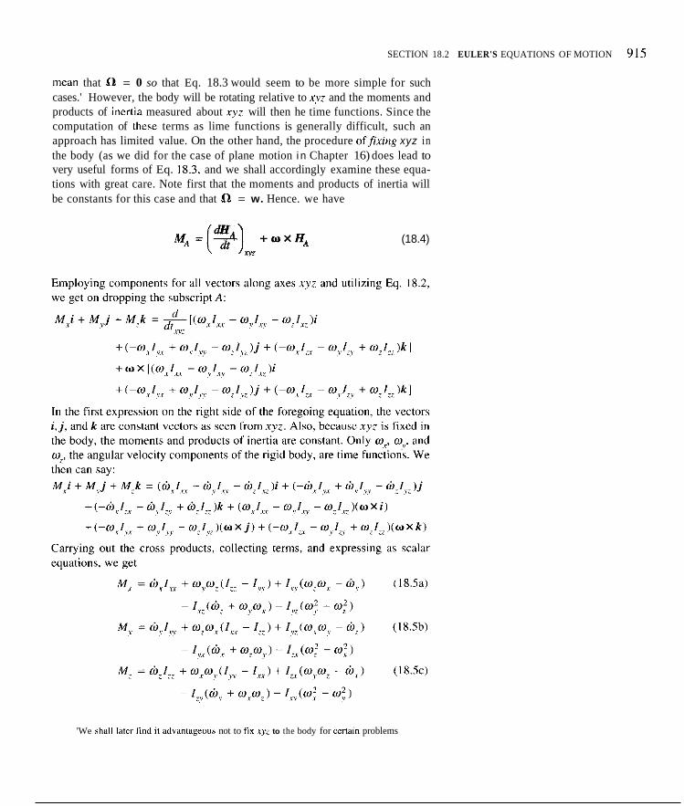
SECTION 18.2 EULER'S EQUATIONS OF MOTION 915
mean that = 0 so that Eq. 18.3 would seem to be more simple for such cases.' However, the body will be rotating relative to x y and the moments and products of inertia measured about xyz will then he time functions. Since the computation of these terms as lime functions is generally difficult, such an approach has limited value. On the other hand, the procedure offixing xyz in the body (as we did for the case of plane motion i n Chapter 16) does lead to very useful forms of Eq. lX.3, and we shall accordingly examine these equa- tions with great care. Note first that the moments and products of inertia will be constants for this case and that 0 = w. Hence. we have
MA=(%) + O X H A M
(18.4)
'We shall liilcr find il advanPagcous not to fin xyc to the body for ccrlilin problems

Thi, i\ iiideed a frirmidable set [if equations. For the impiirtant special case of pliinr nioliori the : axis i h always i imnal to the X Y planc which is the plane o l niotioti. Hence w inusi he iiormal to plane XY and thus collinear with the r i ixic. Thus replacing < by (0 and setting the other components equal lo zero. we get the w m w i f ofmiiii i i ~ t i ~ i i q i d o i u for jioimii pliriir iii~i~im. Thus we haye
(MA).T = -I,$ + I&
(MA J y = -lYza - I,:W2
(MAJy = I$
The reader nay no\+ or iil any tinie li i ter go h;ick to Chapter 16 ior a raiher c~irefuI \tiid), 01 tlic use < I ( !lie ahovc plane motion w m e , i I a / nioimvifuiii
equations. Wc now continue n'ith !lie I1iree~diiiirnsi~)naI approach. Note ncw that if we choose reierence S:K 111 he pr;iic;pol axes of the hody
iit point 11. ltieri i t i s clear thei the products of inertia iirc all zero in the system 01' cqu;itions 18.5. and this iw enables u s 111 siinpliiy the equations consider- ably. The rcsultinF equations given helou' are the fiinious Eider- quo t iom of tilotion. Niitc tliiit these equatiiins relate the 1iigul;ir velocity and thc angular wceleraiion l o lhc !nomen1 01 ihc cxtcrml fiirces ;ahout the point A .
M R = ',,", + m p r ( f z : - I > ? ) M,, = I>$,, + a p , ( I U -
118.h;~)
( I 8.6h)
(18.hc)
111 hoth set\ d Eq\. 18.5 iiiid 18.h. we l i i i~c three siniultaiieous tint-order dif- krenti;il equiiiicms. It the inorion ( i t Ihe hody ahout point A i s known. we can easily compute the required tiioiiien1s ahoul point A . On the other hand. if the iiioineiils are knowii function.; 01 iinic and the angular velocity i s desired, we have the difficult prohleiii of siilvinf siiiiultancous lioiilincar differential equation\ for the uiiknowni (05. coy. and (or. However. in practical problem?. we oitcii kiiow soiiic of Ihc angular velocity and accclcratioii componcnh ircm constrilitits or Fiveti data. so. with the restrictions mentioned earlier. we ciin s<rmetitiies intcsratc tlic cquatioiis readily as we did i n Chapter I 6 for [il;ine iixiti<in. At othcr limes LIZ use them to sii lvc for ccrtain desired i i t , s ru i i -
t i i rvnu.c w l u ' s of the unknown\.
. . M: = lzpjz + m p s ( l v x , - I x x J
We \hall inow discuss the use of Euler', equations.
18.3 Application of Ewler's Equations In this scclion, we shall apply the Euler equations I o a numhcr oiproblems. Rciore laking up these prohlems. let u c l i n t c;ircfully considcr how to chprccs thc conipot icn ts~~, ,~~, , ~iiiil~i~ for iise in Ruler's equations. First note that ha. ir),. and io^ arc time dcrivaiivcs iih sccn Iron1 X Y 7 o f the components ot'w along

SECTION 18.3 APPLICATION OF EULER'S EQUATIONS 9 17
reference xyx. A possible procedure then is to express mA, q, and w, first in a way that ensures that these quantities are correctly stated over a time interval rather than at some instantaneous configuration. Once this is done, we can simply differentiate these scalar quantities with respect to time in this interval to get hx,hy, and&?.
To illustrate this procedure, consider in Fig. 18.5 the case of a block E rotating about rod AB, which in turn rotates about vertical axis CD. A refer- ence xvz is fixed to the block at the center of mass so as to coincide with the principal axes of the block at the center of mass. When the block is vertical as shown, the angular speed and rate of change of angular speed relative to rod AB have the known values (w2)" and (h2),. respectively. At that instant, AB has an angular speed and rate of change of angular speed ahout axis CD of known values ( w , ) ~ and (hI)", respectively. We can immediately give the angular velocity components at the instant shown as follows:
ox = 0 mv = (w*)i] w z = (a,)"
But to get the quantities (hx)o, (h&, and (h7)o for the instant of interest4 we must first express w,, w,, and cu. as genera1,funcfion.y of time in order to per- mit differentiation with respect io time.
Z
D Figure 18.5. Block at time to
To do this differentiating, we have shown the system at some arbitrary time in Fig. 18.6. Note that the x axis is at some angle p from the horizontal. When p become9 zero. we arrive back at the configuration of intereyt, and a,,
D
Figure 18.6. Block at time f
'You may he tempted IO say (ha),, = 0. (hJ, = (hJW and (h7)(, = (h,),) by just inspect- ing the diagram. You will now learn that this will not be correct.

9 18 (‘tIAPTEK I X DYNAMICS (IF GENF.R/\L KlGlD-BODY MOTI(1iX
& I , , o,, and (i2 heclime known valucs to,)(,. tively: The angnl;rr velocity coniponents Tor this arlitimry s i l~~a t ion are:
((02io. and (h21il. respec-
m , = 01, s i i i 0. a), = (0~. to. = mi COS 0 ! 18.7)
Since thcse relatims iire valid over the tiiiic inlcrval oi interest. wc can dir- ferentiate them with respect to time and get
(ht = ci), sin /j + (ill cos /?j hs =<;I, (18.X)
(b. = (il c o s 0 - (O \ in [J/j
It should be clear upon inspectin@ the diaflam that p = -(u,. and so the preccding tcrms hecoiric
c i ~ ~ = (b, s i n 0 - q ( 0 2 c m / ?
h~ = ci), c o i /? .t q o , siii p h, ~= cb, ( 1 X . W
I f wc now k t /I become ze ra u.e reach the ~ ‘ i ~ n f i ~ u r a t i ~ i i ~ id iiilercsl ;md uc get from Eqs. 18.7 ;ind 18.8 thc proper viilucs of the mgular d o c i t y compo- nents and their time dcriv;iti\es at t h i s configuratioii:
(0, = o , OI, = (to2Ili . 01. 7 (al l ),,.
h, = -io1 ),i((l)2)(l
hs := ( ( i )> ! , ,
(2. = !f2, i , ,
Actually. MK &I not have to employ such ii procedurc 111- the e\aluation of these quantitiec. There is :I simple direct ;ipproach that can he uscd. hut wc must prelacc thc discussion of this method by mnie gcncral remiirks ahout the time derivative, as wen ironi thr XYZ;ixcs. o i i i vector A . I h i ? vcctorA i s expressed in terms oicompiincnti ;ilways parallel I U the ~ 1 ~ : rcferenrr. which ~iioves rclaliw to XYZ (Fig. 18.7). Wc can then say. considcrinf i. j . and k :I’
unit veclors for reference .rx::
_j ywkl R X
Figure 18.7. Crrmpmrnt.; r f A along ~ry;.
= / i , i . t A , / + ; \ ; k + A ~ i w X i ! + A , i w x . j ! + A ( w X k ) ( I X . I O l
I i we decompose the vector (dA/dflXyz inlo ciimponcnts parallcl I V the ~t?:
axes at r ime I and carry in i t the cross productr o n the right side i n terms of.i,; components. then we get. ;iller collecting term\ and cxpressing the re\ults as scular equations:

SECTION 18.3 APPLICATION OF EIJLER'S EQUATIONS 919
We can learn an important lesson from these equations. If you take the time derivative of a vector A with respect to a reference XYZ and express the com- ponent! of this vector parallel to the axes of a reference x y z rotating relative to XYZ (these are the terms on the left side of the above equations), then the results are in general not the .same asfir.!t taking the components of the vec- tor A along the directions x y z and then taking time derivatives of these scalars. Thus,
How does this result relate to our problem where we are considering h,, by, and hr? Clearly, these expressions are time derivatives of the compo- nents of the vector w along the moving x y z axes, and so in this respect they correspond to the terms on the right side of inequality 18.12. Let us then con- sider vector A to be w and examine Eq. 18.1 1 :
(1 8.13)
We see that the last two terms on the right side in each equation cancel for this case, leaving us
(18.14)
We see that for the vector o (i,e., the angular velocity of the xyz reference relative to the XYZ reference), we have an exception to the rule stated earlier (Eq. 18.12). Here is the one case where the derivative of a vector as seen from one set of axes XYZ has components along the directions of another set of axes x y z rotating relative to XYZ, wherein these components are respectively equal to the simple time derivatives of the scalar components of the vector along the xyz directions. In other words, you can take the derivative of w first from the XYZ axes and then take scalar components along xyz, or you can take scalar components along xyz first and then take simple time derivatives of the scalar components, and the results are the same.
I f we.ful/y understand the exceptional nature of Eq. 18.14, we can cum- pute h? 0, and hz in a straightforward manner b y simplyfirst determining


SECTION 18.1 APPLICATION OF EILER‘S EQUATIONS 92 I
Example 18.1
In Fig. 18.8 a thin disc of radius R = 4 ft and weight 322 Ib rotates at an angular spced w2 of 100 radlsec relativc to a platform. The platform rotates with an angular speed w, of 20 radlsec relative to the ground. Compute the bearing reactions at A and B. Neglect the mass of the shaft and assume that bearing A restrains the system in the radial direction.
Clearly, we shall need t u use Euler’s equations as part of the soh- tion to this problem, and so we f ix a reference xyz to the center of mass of thc disc as shown in Fig. 18.8. XYZ isfixed t~ the ground. In using Euler’s equations, the key slep is to get the angular velocity components and their time derivatives for the body as seen from XYZ. Accordingly, we have
Figure 18.8. Rotating disc on platfbrm. w = w, + wz = -20k + IOOjradlsec
Hence, we have for the xyz components:
(Or = 0 my = 100 radlsec (0. = -20 radlsec
Next, we have
Ch = Ch, +h2 = 0 + wlx w2
= (-20k) X (100j) = 2.000i radlsec?
We thus havc for the nyz components:
h,\ = 2,000 rad/sec2 il, = 0 6. = 0
Before going to the Euler’s equations, we shall need the principal moments of inertia of the disc. Using formulas from the front inside covers, we get
I ’? = I W R 2 2 g = $(10)(16) = 8 0 slug-ft’
I W I,,,, = I.. = - - R’ = 40 slUg-it* ‘. 4 f i
We can now substitute into the Euler’s equations.
M r = (40)(2,000) + (100)(-20)(40 - 8 0 ) = 160,000ft-lb Mv = (80)(0) + (0)(-20)(40 - 40) = 0 M’: = (40)(0) + (0)(100)(80 - 40) = 0

922 CHAI'TER IH r1YNAMICS OF GIINEHAI. KLCIr)-HOUY MO'IION
Now the monicnt components ahoue i re generated by the hearing-force component:, (sec Fig. 1X.Y). Hencc, we ciiii bay:
We have effectively iwo equutions (or four unknowns We next use Newton's law fur the inash centcl:
The first two cquations are cquilihriuin equation:,. The third cquation relata the radial f i ircc Ay, from the barring A. and the radial i icc~le la t i~n 0 l l h e center of mash of the disc which you will iiotice is iii bimplc circular motion about the Z axis. We now have enough equations for all the tin- knuwns. It is then a simple milter to evaluate the f ixces from the hearing:,. They are:
Ax = B, = 0 Av = 32,0001b B, = 20,161 Ib A7 = -19.839 Ib
The rrai./iii,w.s to thesc forces arc the desired forces mito thc hearing:,
z
Figure 18.9. Bearing f o r m a
Example 18.1 (Continued)
~
In Example I X. I . you may have heen surpriccd at the large value of the hearing furccs in the i direction. Actually. i f we did not include the weight of Ihc disc. then A~ uid B. would have funned a sizable couple. This couple stcins from the fact that a hudy having a high angular momentum about one axis i h madc Lo move such that the aforementioned axis rotates about yet a becond axis. Such ia couple i s called a ,yymscopIi: couplr. It occurs in no small mcasurr for thc lront whccls of ii car that i h steered while moving ai high spceds. I t occurs in thc jet engine of 21 plenc that is changing its direction of flight. You will h;i\,e opportunity tu investigatc these effect5 in the homework problems.

SECTION 18.3 APPLICATION OF EIJLERS EQUATIONS 923
Example 18.2
A cylinder AB is rotating in bearings mounted on a platform (Fig. 18.10). The cylinder has an angular speed w2 and a rate of change of speed W2, both quantities being relative to the platform. The platform rotates with an angular speed wI and has a rate of change of speed W,, both quantities being relative to the ground. Compute the moment of the supporting forces of the cylinder A B about the center of mass of the cylinder in terms of the aforementioned quantities and the moments of inertia of the cylinder.
We shall do this problem by two methods, one using axes fixed to the body and using Euler’s equations, and the other using axes fixed to the platfni-rn and using Eq. 18.2.
Method I: Reference fixed to cylinder. In Fig. 18.10 we have fixed axes xyz to the cylinder at the mass center. To get components ofhfpardlel to the inertial relerence, WE consider the problem when the xyz reference is pard- le1 to the X Y Z reference. The angular velocity vector w for the body is then
w = w I + w , = w , k + o , j
Hcnce,
COr = 0 radlsec
w. = wI radlsec mv = o2 radlsec (a)
Also, we can say noting that j is fixed to the centerline of the cylinder
h = hi + h2 = h i k + ($)rrz(N)2j)
= h ,k + h2j + w,(w, x j ) = h , k + h 2 j + w,(w,k x j ) = h,k + h2 j - w p , i
Accordingly, we have at the instant of interest
hx = -w,w2 radlsec, hv = h, radlsec, hz = W, radlsec2
Figure 18.10. Rotating cylinder on platform
Since I z , = I, we see that I,(-o,w2)) cancels w,w21z, in Eq. (c), and we then have (he desired result:

924 C H A F E R I 8 DYNAMICS 01' GENERAL RI(;IU~BODY MI~ITION
Example 18.2 (Continued)
M = -I,,yw,w,i + I y y w 2 j + Iadlk ( 1)
I t
1
j '
Method 11: Reference fixed to platform. We shall now di1 this problem by having . c ~ i at the mass center C of the cylinder again, hut now fixed to the platlorin. In other words, the cylinder rotates relative L o the ~ r y r reference with angular speed w2. Keeping this in mind, we can still refer to Fig. I X. IO .
Obviously. we cannot uhe Euler's equations here and must retui-n to
i Ecl. 18.2.
' Hcc;iuse the cylinder i s a body of revolution about the s axis. the products of inertia ltv. I\:, and are always zero. and l,~<. I,,.. and 1.. arc u m s f m r s at a11 times. Were these conditions riot present. this method ( 1 1 approach wiiuld bc very difficult, hilice we would have Io ascertilirl the l ime dcriva~ tives of these inertia ternis. Thus. using Eq. 18.2, rrrnembcring that w. thc a n p l a r velocity of thc body, goes into H , . while (1 i s the angular \'clocity
,
1 I o t ~ r y z . we bee that
j ;
Note that i, j . and k arc conslants as scen froin ,ryr. Only wl and w2 are tinic lunctions and undergo simple time diflerentiatior 0 1 scalars. Thlls.
i
1 Noting further that $1 = w , k . we have 011 rubsliluting Eq. ( c ) into Eq. (a) :
M L Iv,d,j + I . ~ c , k + o , k X ( H , i + f l J + H k )
= I ~ ~ r ~ , j + i . . r ~ l k + w , k x ( O i + I , ~ ~ u , j + I L u i , k ) ( d i
M = -Iyyw,w2i + Iyyhj + Iyyw,k I i j I i This equation is identical to the one obtained using method I

18.1. The moving pans of a jet engine consist of a compressor and a turbine connected to a common shaft. Suppose that this sys- tem is rotating at a speed w , of 10,000 rpm and the plane it is in moves at a speed of 600 milhr in a circular loop of radius 2 mi. What is the direction and magnitude of the gyroscopic torque transmitted to the plane from the engine through hearings A and B ? The engine has a weight of 200 Ih and a radius of gyration about its axis of rotation of I ft. The radius of gyration at the cen- ter of mass for an axis normal to the centerline is 1.5 ft. What advantage is achieved by using two oppositely turning jet engines instead of one large one?
Compressor Turbine SwgE
,' R = 2 m i
/'
Figure P.18.1.
18.2. A space capsule (unmanned) is tumbling in apace due to malfunctioning of its control system such that at time t, w , = 3 radlsec, w2 = 5 radlsec, and mi = 4 radlsec. At this instant, small jets are creating a torque T of 30 N-m. What are the angular acceleration components at this instant? The vehicle is a body of revolution with k~ = I m, k> = k, = I .h m, and has a mass of 1.000 kg.
L
I
Figure P.18.2.
18.3. The left front tire of a car moving at 55 niilhr along an unbanked road along a circular path having a mean radius of 150 yd. The tire i s 26 in. in diameter. The rim plus tire weighs 10 Ib and has a combined radius of gyration of 9 in. about its axis. Normal to the axis, the radius of gyration i s 7.5 in. What is thz gyrtiscopic torque on the hearings of this front wheel coming solely from the motion of the front wheel'?
18.4. In Problem 18.3, suppose that the driver is turning the front wheel at a rale m3 <if .2 I-adlsec at the instant where the radius of curvature of the path is 150 yd. What is then the torque needed o n the wheel solely from the motion of the wheel'?
*
150yd \ 0 1
Figure P.18.4.
18.5. A student is holding a rapidly rotating wheel in front of him. He is standing on a platform that can turn freely. If the stu- dent exerts a torque M, as shown, what begins to happen initially'? What happens a little later'!
c M,
Figure P.18.S.
925

x
T
A - 21lO rmn
. .
X /'
Figurc P.IX.7
Figure P.lX.11.

18.12. Explain how the roll of a ship can be stabilized by the action of a heavy rapidly spinning disc (gyroscope) rotating in a set of bearings in the ship as shown.
Figure P.18.12.
18.13. A IO-kg disc rotates with speed w , = 10 radlsec relative to rod AB. Rod AB rotates with speed O2 = 4 radlsec relative ti) the vertical shaft, which rotates with specd w? = 2 radlsec relative to the ground. What is the torque coming unto the beaings atB due to the motion at a time when 8 = 60"? Take u, = G2 = Ui, = 0.
*18.16. Work Problem 18.15 for the following data:
~, = 3 radlsec' h2 = -2 rad/sec2 fb, = 4 radlsec'
The other data are the hame
18.17. A thin disc has its axis inclined to the vertical by an angle 8 and rolls without slipping with an angular speed w , about the supporting rod held at B with a ball-and-socket joint. I f 1 = 10 ft, r = 2 ft, e = 45", and 0, = IO rddlsec, compute the anguldr velocity of the rod BC about axis 0.0. If the disc weighs 40 Ib, what is the total moment about point B from a11 forces acting on the system? Neglect the mass of the rod UC. [Hint: Use a reference xyz at B when two of the axes are in the plane of 0-0 and OC.]
Y 0 ,
Figure P.18.13. Figure P.18.17.
18.14. h2 = 3 radlsec', and ch3 = 4 rad/sec2 in the directions shown.
18.15. A man is seated i n a centrifuge of the type described in Example 15.14. If w, = 2 radlsec, w2 = 3 radlsec, and w3 = 4 radlsec, what torque must the seat develop about the center of mass of the man as a result of the motion? The man weighs 700 N and has the following radii of gyration as determined by expen- ment while sitting in the seat:
Solve Problem 18.13 forthecase where b, = 2 radlsec2, 18.18. A gage indicator CD in an instrument is 20 mm long and is rotating relative to platform A at the rate a, = .3 radlsec. The platform A Is fixed to a space vehicle which is rotating at speed w2 = I radlsec about vertical axis LM. At the instant shown, what are the moment components from the bearings E and G about the center of mass of CD needed for the motion of CD and EG? The indicator weighs .25 N, and the shaft EG weighs .30 N, has a diameter of I mm, and a length of 10 mm.
Figure P.18.15. Figure P.18.18.
921

18.19. An eight-bladed fan i s used i n a wind tunncl to drive thc iir. The angular velocity w, ofthe fan i s 120 p n . A t the inrtanl (11 ntercst, each hladc is rotating about its own axis : (in order to
:hange the ang led attack of thr blade) such that w1 = I r n d l x c m d Ui, i s .5 rddisec2. Each blade weighs 200 N and has the Sol - awing radii of gyration at the miss center (C.M.):
k 5 = (NU) mm
k 5 = 5XOmm
k = 100 tnm
:<insider only the dynamics of the system (and not the :wo- jynarnics) to find the torque required about the i anis of the hl:idc. [ fa couple intrment of 4 N-m is develuped i n thc ,r direction a1 the 3ase of the blade, what force component< i ? nredcd at thc hasc of :he blade for the mution rlescrihcd?
Figure P.18.19
18.20. A swing-wing fighter planc i s imwing with a specd ol Mach 1.3. (Note that Milch I cormpands trr a speed ol iih(iu1 1,200 km/hr.) The pilot iit the instant shown i s Fwinpinp his wings back at the rate ml of .3 raillsec. At the s a n e time he is rillling at
il rate w, of .6 radlsec and is performing a loop :IS shown T h e wing weighs 6.S kN and haa lhc fblluwing radii of gyration at the enter of mass:
k k = .X in
k ) = 4 m k~ = h m
Yhat i s the moment that the lllselage must develap about the CLIW
cr of miss of the wing to accomplish the dynamics of Ihe lescribed molions'! Do not consider arrdynamich.
I28
11\11,
Figure P.lX.20.

18.22. You will learn in fluid mechanics that when air moves across a rotating cylinder a force is developed normal to the axis of the cylinder (the Mupnus rffecf). In 1Y2h Flettner used this principlc to "sail" a vessel across the Atlantic. Two cylinders were kcpt at a cunrtant rotational speed by B motor of w, = 200 rpm relative to the ship. Suppose that in rough seas the ship is rolling about the axis of the ship with a speed 0, of .E radlsec. What con- ple moment components must the ship transmit to the base of the cylinder as a result only of the motion of the ship? Each cylinder weighs 700 Ib and has a radius of gyration along the axis of 2 ft and normal to the axis at the center of mass of I O ft.
Flettneis ship Figure P.18.22.
*18.23. Part of a clutch system consists of idenlical rods AB and AC rotating relative to a shaft at the speed w2 = 3 radlsec while the shaft rotates relative to the ground at a speed w, = 40 radlsec. As a result of the motion what are the bending moment com- ponents at the base of each rod if each rod weighs 10 N?
Y
Figure P.18.23.
*18.24. and h2 = 6 rad/sec2 at the instant of interest.
18.25. A rod D weighing 2 N and having a length 0 1 200 mm and a diameter of 10 mm rotates relative to platform Kat a speed w, of 120 radlsec. The platform is in a space vehicle and turns at a speed wi of 50 radlsec relative to the vehicle. The vehicle rotates at a speed w, of 30 radlsec relative to iiiertial space about the axis shown. What are the bearing forcer at A and B normal to the axis AR resulting from the motion of rod u'! What torque I is needed about AB to maintain a constant value of w, at the inmnt of interest'?
z
Solve Problem 18.23 for the case when h, = 2 radlsec'
I00 mm X #?
Figure P.18.25.
18.26. mass of the armature hut not fixed to the annature.
18.27. In Problem 18.10, find the miiment about the C.M. of the disc using a reference x y i fixed to the rod A B and not to the disc. Take I%, = 10 radlsecl and h2 = 30 radliec2.
18.28. Work Problem 18.11 using refercnce .ryi tixed to the *hip with the origin at the center of mass nf the turbine. Do not use Euler's equations.
18.29. of mass of the disc hut fixed to arm AB.
18.30. Work Problem 18.11 by using a reference xyz fixed to the arm at the center of mass of the disc for the case where h, = 2 radlsec2, h2 = 3 rad/secz, and 6, = 4 rad/sec2 in direc- tions shown.
Solve Problem 18.6 using a reference at the center of
Solve Problem 18.13 using il set of axes xyr at the center
929

18.4 Necessary and Sufficient Conditions for Equilibrium of a Rigid Body
I n this chapter. we ha\,c emplvyed Newton's law :it the mass center as well i is the equation M, = H,.+ and Sroin i t we dcrived Euler's equations for rigid bodies. We can now go hack to our worh in Chapter 5 and put on firm ground the lnct that M = 0 and 1: = 0 are necessary conditions for cquilihriuiri 111 a rigid hody. (You wil l recall we accepted ll iese equations for statics ar tliiil timc hy intuitioii, pending a prvof to cvtne 1:ttcr.j
A particle is in cquilihrium. you wi l l reciill. i l i t i s stationary or moviiig with constant speed along a straight line in inertial spiicc. To he in a state of cquilihrium. cvcry point i n ii rigid body must acciirdingly he stationary o r he moving at uniform speed along straight lines in iiiertial space. The rigidity requirement thus limits a rigid hody in equilibrium to trilnsliitional motion along a stmight line at constant speed i n inertial space. Ih ih ineans that C; = 0 and w = 0 for equilihrium and so, from New/oi~'s lmn and Eirler's cqi iut io i i \ .
we see that b' = bf, = 0 are w c ' For il .sufficicwq proof. we go the other way. For a hody initially in
equilihriuni. the condition I: = M,A = Os ensures that equilihrium asill hc maintained. More specifically. we shall stail %ith a hody in equilibrium at tiinc t and apply ii forcc system ratisfying the preceding cvnditiiins. Wc address ourselves to the qucstion: Does the body stay in a stilte o f equilih- riuin? According tv Newton's luw there wi l l he no change in lhe vclocity i i S
the m a s s center since F = 0. And. with w = 0 at timc t. /+h, - ' ,s ~ q i i ~ f i o m lead 10 the result for M,. = 0, thnl h, = h, = io. = 0. Thus, the angular velocity must remitin zeni. With the vclocity V I the ccnter of niass constiltit. and with & = 0 in incrtial space wc know that the hody remains in equilih- riuin. 'Thus, i f a hody i' iiiirially in ~ ~ y u i l i h r i u m . the condition F = 0 and M,, = 0 i s .si!#ic.imt for maintaining equilihrium.
(7ry conditions for equilihrium. X' Figure 18.1 I . Body with il f ixed point.
18.5 Three-Dimensional Motion About a Fixed Point Euler Angles
We slxi l l 1i11w exaii i ir ie the motion o f sclected rigid hodie, constrained tv havc a p in1 fixed in :in inertial reference ( Iz ie . I X . I I). This tvpic wi l l Iciid to study (11 an important dcvice-the gyroscopc.
We invw chow that angles VI' i-otation Qt, 6>, and H ~ , along iirlliogonal axes 1. y. and : are nor highly suitable for measuring the o;ientation of a hiidy with a fixed point. Thus. ill Fig. IX.IZ(a)consider it cvniciil surIace:tnd ohserre straight line OA which i s on this surface and in tllz .tz planc. Kotatc thc c m c
'Wc linw shown 111 svillics t l h i f i t F = U and M , = 0 ;ahout \ i m c point A (11 inr i i ia space. i l ic i i .M = 0 ahnui an) point ii, i i icrti i i l ~ ~ p c e .

SICTION 18.5 THREE-DIMENSIONAL MOTION ABOUT A FIXED POINT; EULER ANGLES 93 1
an angle (A@., thus causing OA to move to OA' shown as dashed. In Fig. I8.12(b), view line OA along a line of sight corresponding to the x axis. As a result of the rotation iA6')7 about the I axis. there will clearly he a rotation
are mutually dependent and thus not suitable for our use. This result stems from the fact that we are using directions that have a fixed mutual relative orientation. We now introduce a set of rotations that are independent. And, not unexpectedly, the axes for these rotations will not have a fixed relative orientation.
i z
of this line ahout the x axis. Thus, we see that and
Figure 18.13. Rigid body
Accordingly, consider the rigid body shown in Fig. 18.13. We shall specify a sequence iif three independent rotations in the following manner:
I . Keep a reference xyr fixed in the body, and rotate the body about the Z axis through an angle yrshown in Fig. 18.14.
r Z
I vv
Figure 18.14. First rotation is about Z.
2. Now rotate the body about the x axis through an angle B to reach the con- figuration in Fig. 18.15. Note that the i , Z , and y axes form a plane 1 nor- mal to the X Y plane and normal also to the x axis. The axis of rotation for this rotation (x axis) is called the line <$nudes.


SECTION 18.5 THREE-DIMENSIONAL MOTION ABOUT A FIXED POINT EULER ANGLES 933
We call these angles the Eider an,+, and we assign the following names. w = angle of precession 0 = angle of nutation q3 = angle of spin
Furthermore. the z axis is usually called the body axis, and the Z axis is often called the axis of precession. The line of nodes then is normal to the body axis and the precession axis.
Figure 18.17. Axes x y i are fixed to body.
We have shown that the position of a body moving with one point fixed can be established by three independent rotntions given in a certain sequence. For an infinitesimal change in position, this situation would be a rotation d y about the Z axis, dB about the line of nodes, and d@ about the body axis z . Because these rotations are infinitesimal, they can be construed as vectors, and the order mentioned above is no longer required. The limiting ratios of these changes in angles with respect to time give rise to three angular veloc- ity vectors (Fig. 18.1 8). which we express in the following manner:
Z
\ I
Line 0 1 nodes X
Figure 18.18. Precession. nutation, and w i n velocity vectors

934 ('HAl'I'kK I X 1iYNAMIC.S 0 1 . GFNLRAI. KIG1l)~tlOlIY M 0 1 1 0 h
z teJ ;ilong the Z :mi\
dirccled along the line of nodcs dirccted aliing the : htdy i i x i i
(Fixed) 6. 4.
Note that tlie i iutatioii vclocit) vcctor H i s al\vays inorinill to planc I. and consequenlly the nutatioii velocity \ector is alw;iys normal 111 the spin veloc- ity ycctor 6 and the preccssion \,eliicily vector 4. H o w v c r , the spill v e l ~ ~ c i l q vector 4 wi l l generally ti01 be ill right mglcs with the precession velocity 4. and s o this sy \ tem of iinguI;ir vclocity \'ectors generally i\ i i ~ f ilii orttrogoiial systcm.
Finally. i t should lx clciir that l l ic I-efcrcncc ~ 1 ~ : Iiio\ci( with the body during precession iuid niitatiim inotion 0 1 the hody. hut \ re can choorc that i l
L.inc ~~I i io t l e s
would have, for (he iilorchtatcd condition. iiii anguliir velocity. denoted iix 0. etluiil IO 4 + 8. The vclocity of the disc rclative IO .ix is. ;rccordingly, 9 k .
Considcr a hody u i lh IWO orthogorial planes of syiiimctry forming :in
axis in the hody. 'The body is moving ahout ii lixed point A 1111 the body ;mi\ (Fig. 18.19~. Hiiw. d c r u c decide wh;it ~ X C S to usc t o describe the riiiition i n tesiiis OS spin. precession, iind nut;itioii? Fisst. w e take the axis of lhe hody to he the : axis: thc angulx speed ahwt this iixis i s then the spin 4. This \tcp i\ straightliorwnnl for the hiidies that ut! shall consider-. Thc next step is iiol. 131 inspection f ind ii Z ax is in alirrvl diw,.fioti xi i ~ s to form with the aforeinen- tioried hody m i s : :I planc I whose :ingiil;ir speed ahout the Z axi\ i\ cither known o r i s sought. Such ;in axis Z i s t l lci i the /inw.~s;oii iixis ;ihout uh ich we have for thc hody axis : i i precession speed li. 'The i i w r ; / i i o i l ~ . s i s then (l ie axis which at all limes rciiiiiiiis iiiirmil to planc I conl;lining the hody iixi, : and the precescim ax i \ Z. 'Ihc iiulatiwi speed 0 f i r i d l y ic rhc ;ingttlar speed ciirnponent of Ihe body axis : ;iboul the line of nodes.
18.6 Equations of Motion Using Euler Angles
Consider next ii hody ha\iiig ii shapc such that. a1 an) point along thr body i i x k :. thc iiioiiicnl\ o f inertiii l i ir a11 axex n(irniiil to the hody i i x i s at this puiirt have tl ie suiic value 1'. Such would. ol~coursc.. he triic for thc special ca ie 01 a hody of revolution having lhe :.axis as thc axi\ of hyintiictry." We shall cow sider the iiiolioii 01 wch ii body ;ihout :I fixed point 0. which i s smiewhcre iilong the ax is : (see Fig. 18.20). Axes .ry: :ire principal axes. This set i i f a x c s has the sii i i ie nutation ;and prcccssiiin inotioii a b t l ie hody hut uill he chosen

SECTION 18.6 EQUATIONS OF MOTION USING EULER ANGLES 935
such that the body rotates with angular speed 6 relative to it. Since the refer- ence is not fixed to the body, we cannot use Euler’s equations hut must go hack to the equation Mu = Ho, which when carried out in terms of compo- nents parallel to the xyz reference becomes
Mu = (3) + 11 x ( H j + H,j + H z k ) (18.21) x,i
Figure 15.20. Body moving about fined point 0.
Since the xvz axes remain at all times principal axes, we have
H , = T u z , H, = I‘my, H, = loz (18.22)
where I is the moment of inertia about the axis of symmetry and I’ is the moment of inertia about an axis normal to the z axis at 0. Considering Fig. 18.20, we can see by inspection that the angular velocity of the body relative to XYZ is at all times given by components parallel to xyz as follows:
mr = e (1 8.23a) o , = *sin0 ( I 8.23h)
o, = Q + * c o s 0 (1 8 . 2 3 ~ )
Hence, the components of the angular momentum at all times are:
(H I ) = 1’8 ( H v ) = I‘*sinO
(Y) = I ( 4 + I)cosO)
We then have for Ho:
I f o = I ’ ~ i + I ’ ~ s i n O j + I ( B ) + ~ c o s 0 ) k
(18.24)
Remembering that i, j and k are constants as seen from xyz, we can say:

= 1'8; + 1'1v cin H + Wi/eciisO).j + /!$ + v cos0 -
As for the angular velocity (~Freferencc ~r?z. wt! liilve (in considering Eq. 18.24 with 4 deleted becauw ~ry; i! lint tined to the body ;I\ far as \pin i s concerricd:
(IX.26)
s i n O ) h
12 = Hi + y s i n e j + y?crisHk
Consequently. we h u e
$1 x i = -@ sin Ok + @cos O j fL x j = d k - @ c c o s H i (IX.27)
x k = -6.j + @ sin Hi
Substituting the results from Eqs. 18.25, 18.24, and IX.27 into Eq. 18.21. we get
M)i + My j + M.k = I'8i + I ' ($ is i r iO + $v6c( i \H) j
+ I ( $ + cos - I@ (in Hjk + 1 ' 8 ( - @ s i i i B k + v ic ( is#Hj ) ( I X.2X) + I' 1#7 \in H(6k - vi eo\ Hi) + + @ c o s ~ ) ( - H . j + @sin 6';)
The corresponding scalai- equations we:
Mx = 1'8 + ( I - l')(p2 sinBcos8) + 1&sin0 (18.2i)a)
M v I ' Q S ~ S I S + 21'& COS@ - I (4 + COS 6)d ( 18.2Yh)
M, = I ( ~ + $ i c o s 0 - 1 @ s i n @ ) (18.291.)
Thc loregoing equalions arc valid at :ill liriies for llir iiiotion (11 ii homopc- iicous body having I \ ! = lv> = I' moving about a fixed point oil the ax is OF the body. Clzarly. thew equations are also applicable for inotioii about tlic center (if niass for such bodies. Note lhat the cquatioiis iiie iiiinlinear and. cxcept f o i ~ certain \pecial CLISCS. are vcry difficult to integrate. They are. 01 course. vcry uselul as thcy mnd when c(irnputcr methods are to be cinploycd.
As a special C B ~ C , we shall now consider ii motion involving a constiiiit iiuLalion angle H. a constant spin spccd 4, and a consvant preccsion spccd @. Such a motion i s tcrined . s r c w l ? prrw,ssioi i . To detcrniine thc torque M lor a given steady precession. we set 4. 6, ;i ;mi v e i l u ; ~ ~ lo ~ r ( i iii E ~ S . I ~ . X . Accordingly. we gel the f(illowing rcsiilt:
M, = (18.30a) M, = 1) ! I8.3llh) M. = 0 ( I8.30c)
+ @cos 8 ) - ~ ' ( i , c o . ; 81 sin #

SECTION 18.6 EQUATIONS OF MOTION USING EULER ANGLES 937
We see that for such a motion, we require a constant torque about the line uf node.s as given by Eq. 18.30a. Noting that 4 + @cos 0 = w, from Eq. 18.23c, this torque may also be given as
(18.31)
Examining Fig. 18.20, we can conclude that for the body to maintain a con- stant spin speed $ about its body axis (Le., relative to xyz) while the body axis (and also x y i ) is rotating at constant speed $about the Z axis at a fixed angle 0, we require a constant torque ML having a value dependent on the motion of the body as well as the values of the moments of inertia of the body, and hav- ing a direction alwuys nurmul tu the body andprecession axe,s (i.e., normal to plane I). Intuitively you may feel that such a torque should cause a rotation about its own axis (the torque axis) and should thereby change 0. Instead, the torque causes a rotation @of the body axis about an axis normal to the torque axis. As an example, consider the special case where 0 has been chosen as 90" for motion of a disc about its center of mass (see Fig. 18.21). In accordance with Eq. 18.3 I , we have as a required torque for a steady precession the result
M.r = Iwl@ = (18.32)
Here for a given spin, the proper torque M, about the line of nodes maintains a steady rotation @of the spin axis z about an axis (the Z axis), which is at right angles both to the torque and the spin axes and given by Eq. 18.32. Because of this unexpected phenomenon, toy manufacturers have developed various gyroscopic devices to surprise and delight children (as well as their parents). Here is yet another case where relying solely on intuition may lead to highly erroneous conclusions.
M x = (Io. ~ I'@cosB)(i,sinO
Z
Figure 18.21. Steady precession: E = 90"
We should strongly point out that steady precessions are not easily ini- tiated. We must have, at the start, simultaneously the proper precession and spin speeds as well as the proper 0 for the given applied torque. If these con- ditions are not properly met initially, a complicated motion ensues.

938 CHAPTEK I X DYNAMICS O F GENERAL RIGID-ROLIY MOTION
Example 18.3
A .sbiRlr-~~,r.Rrr[,.-n/~/r~,[,d[ji~ ,yyro i s shown in Fig. 18.22. l h r spin ax is 111
dihc E i s held by a gimbal A which can rotate about hcaringc C' and D. Thcse hearings are supported hy the gyro case, which in turn i s gcncrnlly clamped ti1 the vehicle Lo he guided. If the gyro case riitalcb ahout a verti- cal axis (i.e.. i i~r inal Lo its hasc) while the rotor i s spinning, the gimbal A wi l l tend to rotate ah(iuc CII in an attempt to align with the vertical. When gimhal A i s resisted Irom rotation ahout CD by a set ol torsional springs S with a combincd torsional spring constilnt given as K,. the gyro i s called ii mi? g y r o If the rotation of the gyro casc is consrant (at speed OJJ. the gimhal A assumes a f ixcd orientation relative 10 the vertical a s il result of the restraining springs and a damper (not sh(iwn). Ahout [he hody axis : there i? a constant angular rotation (11 the r ~ t ~ r 01 cuI rad/sec maintained by ti miit01 (not shown). This angular rotation i s clearly i$ the spin speed 4. Nexl . note in Fig. 18.23 tha the : axis and lhe fixcd vertical ax is I ronn a plane (plane I ) which has ii known angular .;peed 0, about this lixcd verti- cal axis. Clearly, this fixcd vertical axis wi l l he our precession axis, and the precession speed (irequals (0,. The line of nodes has also hcrn shown; it must at al l times be normal to plane I and is thus collinear with axis C-/l of gimbal A . With 8 fixed, wc have a case 01 steady prcccssiiin.
Fired i.eilicaI axib
Figure 18.22. S i n ~ r l e ~ d c t . r t . 2 - o i f ~ ~ ~ , ~ , n gyro.
Givcn the following data:
/ = 3 x 10 4 slug-ft2 I' = 1.5 x 10 " slug-ft' 0 = 20.000 rad/hec
K, = 4.95 ft-lh/rad 1'/ = I rad/sec
what i s B for lhe condition 01 slcady precesslon'! The torsinnal springs are unstretched when 8 = YO".
Wc have for Eq. 18.30;i:
I_ ---____-XI_-- . . ~~ ... . .
~~ " .. ." ~

SECTION 18.6 EQUATIONS OF MOTION USING EULER ANGLES 939
Example 18.3 (Continued)
iwt = ~ , ( ~ - ~ ) = [ ~ ( d , + l i r c o s ~ ) - ~ . l i r c o s ~ ~ l i . s i n ~ (a)
Line of nodes
Figure 18.23. Gyro showing line of nodes and precession axis.
Putting in numerical values, we have
= [ 3 x I O " ( ~ X I O ' + ( I ) C O S O ) - ( I . S X 1 0 - 4 ) ( 1 ) c o s ~ ] s i n ~
Therefore,
4 . 9 5 x 1 0 4 ( ~ - Q ) = ( 6 x 1 0 4 +l .ScosQ)s inQ
We can neglect the term (1.5 cos Q ) , and so we have
4 . 9 5 ( $ - @ ) = 6 s i n Q
Therefore,
(b) /7
~ - Q = 1.212sinQ 2
Solving by trial and error or by computer, we get
6 = 43" (c)
The way the rate gyro is used in practice is to maintain Q close to 90" by a small motor. The torque M I developed to maintain this angle is mea- sured, and from Eq. 18.30a we have available the proper @, which tells us of the rate of rotation of the gyro case and hence the rate of rotation of the vehi- cle about an axis normal to the gyro case. Now @need not he constant as was the case i n this problem. If it does not change very rapidly, the results from Eq. 18.3Oa can be taken as instantaneously valid even though the equation, strictly speaking, stems from steady precession where @ should be constant.
___

Figure 1X.24. Two dcgrcc +freed,w g y r o
A f ~ ~ ~ f , ~ ~ / ~ ~ ~ ~ ~ ~ - i ! ~ ~ ~ ~ ~ , ~ ~ ~ / f , , ~ i , 4 V , ? l S u J / W i s dwwn i n Fig. 18.24. Thc rotor I- rotates in gimbal A. which in turn rotates i n giinhal ('. Note that the :ixes h-h of the rotor and (PI, of thc gi tnhd C a r e always at right angles to cach other. Ginihal C is held hy hcarings c siipliortcd hy (he fry" cast. Axes c ~ i ' arid u u m u s t ~i lways he al right ~ingles to eiicli nther. 21.: ciin easily he seen from the diagram This hind of suspension 01 the rotor is called a Crinluri .srr.rppn.sion. If the hearings at 11, h. and ( ' are frictionless, a torque cannot he transmitted troni the gyro case thc rnlol-7 The rotor i s said t o
he rnryirr:fiw S i x this case. I F the rotor is given ii rapid spin \.elucily i n a g i w i directim in i ne l -
tial space (such as toward the North Star). then ini- t l ie ide;il casc 0 1 fric- tionless hearings the rotor will maintain this dircction e w r i though the gyro case i s given rapid a n d complicated motions in inertiiil ~pacc . Thi\ constancy (if direction results since 110 tnrque cat1 he transmitted to the rotor fo alter the direction of its angular moiiicntitm. Thus. the two-dimen- sinnal gyrc gives a fixed direction i n ineniiil spicc f o r piirpo.;ec nt giiid- nnce of a vehiclc mch as a niissile. I n we. the gyri' i'asc i ripdly S i x 4 to the framc of the tnissile, and iiieasurernents n i the orientation of tlic mis- sile are accomplished by having pickoffs mounted hetween the gyro case and the outer gimbal and hetween the niitcr and inner gimhals.
Thc presence of soii ic friction i n t l ie gyro bcnriiigs is. id cniirsc. iii- evitahlc. The corinteractinn 0 1 this friction when possible and, when not. the accounting for its action is ni much concern to the gyro engineer. Sup- pme that the gyro has hcen given a inotinii such that t l ~ e spin axis h-h (see Fig, 18.25) has an angular speed (o i i h ~ i i t iixis (-c nf . 1 revlsec while Inlaill- taining a fixed orientation o f X 5 ' with axis < ' ~ ('. Thc gym case is ?t;itionnry.
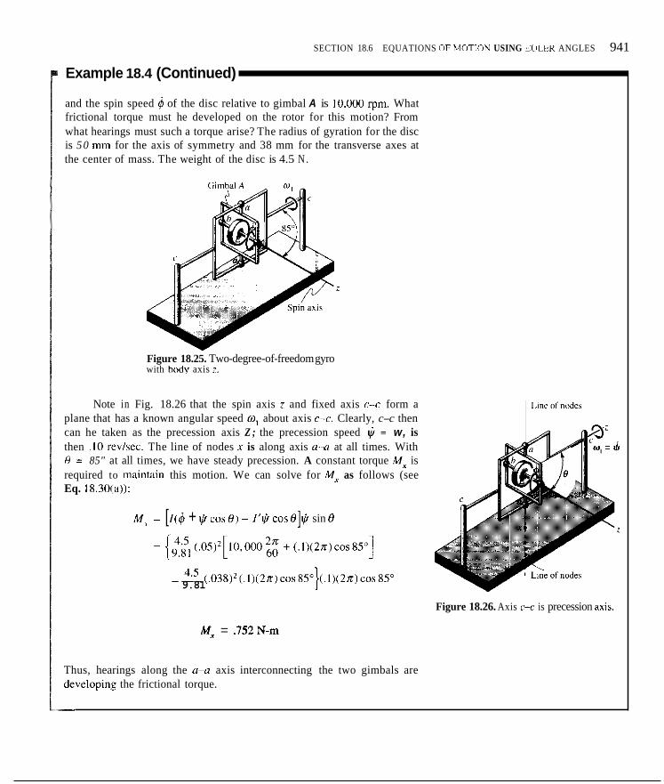
SECTION 18.6 EQUATIONS OFMOTION USING EULER ANGLES 941
Example 18.4 (Continued)
and the spin speed 4 of the disc relative to gimbal A is 10.000 rpm. What frictional torque must he developed on the rotor for this motion? From what hearings must such a torque arise? The radius of gyration for the disc is 50 mm for the axis of symmetry and 38 mm for the transverse axes at the center of mass. The weight of the disc is 4.5 N .
Figure 18.25. Two-degree-of-freedom gyro with body axis i .
Note in Fig. 18.26 that the spin axis z and fixed axis c-c form a plane that has a known angular speed w, about axis c-c. Clearly, c-c then can he taken as the precession axis Z ; the precession speed @ = w, is then . I O rev/sec. The line of nodes x is along axis u-a at all times. With # = 85" at all times, we have steady precession. A constant torque Mx is required to maintain this motion. We can solve for M~, as follows (see Eq. 18.30(a)):
M~ = [ 1(4 + p cos e ) - cos o]p sin 0
_ _ _ 4.5 (.038)2(.1)(2rr)cos85" 9.81
Figure 18.26. Axis c-c is precession axiy.
M, = .752N-m
Thus, hearings along the ri-u axis interconnecting the two gimbals are developins the frictional torque.

Y
/ / , X'
Figure P.18.32.
Figure P.18.34.
x / Iciguw P.IX.36

18.37. t h e centerline of the rod rotates uniformly in a horizontal plane with a constant torque of 2.29 N-m applied about 0. Each cylinder beighs 225 N and has a radius of 300 mm. The discs rotate on a bar AB with a speed w , of 5,000 rpm. Bar AB is held at 0 by a b$l-joint connection. The applied torque is always perpen- dicular t r j AB and can only rotate about the vertical axis. What is the precession speed of the system'?
, - ik77.5mm kII,~4
Figure P.18.37.
18.38. @) In Problem 18.37, consider the disc at B to have an angular speed of 5,000 rpm and the disc at A to have a speed of 2,500 bm. What is the precession speed for the condition of steady prbcession?
/b) If the disc at A and the disc at B have angular speeds of 5,000 Ppm in opposite directions, what is the initial motion of the systeph when a torque perpendicular to B is suddenly applied'?
18.39. Two discs A and E roll without slipping at their mid- planes. Ihght shafts cd and ef connect the discs to a centerpost which rojates at an angular speed a, of rad/sec. ' If each disc weighs 2(, Ib, what total force downward is developed by the discs on the gr/,und support?
I '
I Figure P.18.39.
18.40. A disc is spinning about its centerline with speed 4 while the ccnterline is precessing uniformly at fixed angle B about the vertical axis. The mass of the disc is M. Consider the evaluation of @, and show that such a state of regular precession is possible i f
Also shqw that there are, for every 0, two possible precession speeds. d~ particular, show that as 01: gets very large, the follow- ing precdssional speeds are possible:
[Hint: Cpnsider Eq. 18.3 I for first part of proof. Then use a power expansidn of the root when evaluating @.I
Figure P.18.40.
18.41. A uniform prism has a square cross section. Prove that I,,, for any angle B equals Lx = 1) ) . Thus, in order to use I' = lxx = lv%, a? was dune in the development in Section 18.6, the body need not he a body of revolution. Show in general that if lrr = I v y , and if XJZ are principal axes, then I,,,, = t , = lv3,.
Figure p.18.41.
18.42. A block weighing SON and having a square cross section is spinning about its body axis at a rate 0, of I(X1 rdlsec. For an angle a = 30". what is the precession speed @ of the axis of the block? Neglect the weight of rod AB. See Problem 18.41 before prmeeding.
Ball
Figure P.18.42.
943

Figlire P.18.44.
Vigore P.18.46
1 . h h H/

SECTION 18.7 TORQUWREE MOTION 945
18.7 ~ Torque-Free Motion We shalu now consider possible torqur:free motion for a body having lxt = I v y = I’ for axes normal to the body axis. An example of a device that can approach such motion is the two-degree-of-freedom gyroscope described in example^ 18.4.
Let us now examine the equations of torque-free motion. First, consider the genetal relation
M , = H , (18.33)
H, = H,, ( I 8.34)
Since M., is zero, H, must he constant. Thus. ~
where H,i is the initial angular momentum about the mass center. We shall first assume +d later justify in this section that a11 torque-free motions will be steady p+cessions about an axis going through the center of mass and directed parallel 40 the vector Hll. Accordingly, we choose Z to pass through the center of mass 4nd to have a direction corresponding to that of H,,. as shown in Fig. 18.27. The axis x‘ normal to axes I and Z forming plane I is then the line of nodes anB y’ is in plane 1. The reference xyz is fixed to the body and hence spins abdut the z axis. Axes xy then rotate in the xi.’ plane as shown in the dia- gram. Uding Fig. 18.27, we can then express Hu in terms of its x, y , and z com- ponents Yaving unit vectors i, j , and k in the following way at all times:
Hi, = HI, sin 0 sin $i + HI, sin Q cos # j + till cos Bk ( I 8.35)
7
Figure 18.27. Two~de~ree~af-freedom gyrvscope illustrating torque-free motion. Outer gimbal support is not shown.

946 CHAPTER I X LIYNAMK'S OF G E N I K A I . RI ( ; I I>~HOl)Y MOTION
Since ,YK are principal axes. we can a lso stale:
II , , = I'iqi + I ' q i t l o k (IX.3hl
Comparing Eqs. IK.35 and 18.36. we tlicn ha^
From Eq. IX.3Xc. i t is then clear that
Thus. since H<) end I are constant. we can ciinclude from this equation that rlrr ,~uiaiiori ur ig lc , is a fixed anglc Now consider Eq. IX.3Xh. using the fict that H = Canceling H,, and c;irrying oul tlic differcntiation. we gel
I' ~ H ~ ) sin e,, cos H,, sin @ = o -(sin #,, )(sin @)(d) + 1'1
Therefiirc.
6 = ",;~! HI, cos H,, (IX.40)
Thus. the , s l i i i i , s p t d , 9. is coiisLiiiII. To get the precchsion \peed Vf, note from Fig. 18.27 that
w = lj t $i coc H,,
NOW equatc thc right s i& o t this equation with Ihc risht side 01 Kq. 18.37~:

SECTION 18.7 TORQUE-FREE MOTION 941
Suhwtuting for 4 from Eq 18 40 and zolvlng for I+?, we get
Collectidg terms, we have
H I ~ (I X.42)
The resdlts of the discussion for torque-free motion of the body of revolution can then!be given as
0 = 60 (18.43a) ..
(18.43b) Figure 18.28. Body of revolution is also symmetric about C.M. where it is supported
q = - Ho
~ = ~ H 0 c 0 s 6 0 (18.43c)
I'
SiOce 6, 8, v3 and $are all zero, Eqs. 1X.43 depict a case of steady pre- cession, land so the assumption made earlier to this effect is completely con- sistent 4 t h the results emerging from Euler's equation. Thus, we can consider the assuqption and the ensuing conclusions as correct.
Hdnce, if a body of revolution is torque-free-as, for example, in the case illugtrated in Fig. 18.28, where the center of mass is fixed and where the body hab initially any angular momentum vector Hu, then at all times the angular momentum H is constant and equals Hw Furthermore, the body will have a rigular precession that consists of a constant angular velocity @of the centerlinje ahout a Z axis collinear with Ho at a fixed inclination e,, from Z. Finally, there is a constant spin speed 4 about the centerline. Thus, two angu- lar velodity vectors 4 and 6, are present, and the hiful angular velocity w is at an inblination of E from the Z axis (see Fig. 18.29) and precesses with angular 'peed @about the Z axis. This must he true, since the direction of one compo? .I nt of w, namely 6, precesses in this manner while the other compo- nent, JI,iis fixed in the Z direction. The vector w then can be considered to continuqkly sweep out a cone, as illustrated in Fig. 18.29.
7
I.
Figure 18.29. Vector o sweeps out a conical surface.
We now~illustrate the use of the basic formulations for torque-free motion

Figure 18.30. Space capsule.
i

SECTION 18.7 TORQUE-FREE MOTION 949
Exa+ple 18.5 (Continued)
Therefore,
< = 6.44k + ,3381 ft (a)
To get Hr. we next set up a second reference x’y’z‘ at the center of mass as shown in Fig. 18.31. In accordance with Eq. 18.2, we have for&, on noiing that the only nonzero component of w is in the z’ direction:
H , = - l x , p i - lt+oj + I Z p k (b)
To compute /:,:, we proceed as follows, using the decomposed capsule parts of Fig. 18.32 and employing transfer theorems for moments of inertia:
2 (I?,?, 1 - - - 2.5’ + - 338) = 272 slug-ft2 I - i (‘::”)(
(17.f)2 = ~ ( p ) ( 2 5 ~ ) + - ( I IS0 I so 338)2 = 7.81 6
(2 5)’ - Is’[( 424)(2 5)12} R
+-[338+(424)(25)]’ I 50 = 1843 R
= 104.0
( / < f ) 5 = - - ( 2 S ) 900 2 +-(338)’=1779 900 R 6
(/. ’ ) - - I - 300 (2.5) 2 + -(.338) 300 2 = 30.2 .‘z’ 6 - 2[ g 1 R
Accordingly, we have for I.,..: L.
6
/.,., ‘ _ = c(Ir.)r = 610 slug-ft2 (C) ,=I
We proceed in a similar manner to compute I , , . . We will illustrate this cdmputation for portion I of the system and then give the total result. Thus, employing the parallel axis theorem, we have
= 0 + - -6.44 - ~~ - - ,338 = -383 slug-ft2 (4:)( x7; ) It is important to remember that the transfer distances (with proper signs) used @r computing (I7>,), using the parallel-axis theorem are measured from ,$’yt’, about which you are making the calculution, to the center of mass &f body I . For the entire system we have, by similar calculations:
/z,z, = -329 slug-ft2

i

SECTION 18.7 TORQUII~FRREF. MOTION 95 1
Let us now examine Eqs. 18.43 for the special case where I = 1'. Here leaving only one angular motion, 4, the pre- about the Z axis so the direction of angular
velocity of the body corresponds to Ho. Since this could he a body of revo- lution, tde moment-of-inertia condition for this case ( I = 1') means that the moment4 of inenia for principal axes x, y , and z are mutually equal, and we can veri$ from Eq. 9. I3 that all axes inclined to the q z reference have the same mdment of inertia I (and all therefore are principal axes at the point). Thus, thd body, if homogeneous, could be a sphere, a cube, any regular poly- hedron, qr any body that possesses point symmetry N o matter how we launch this hodj, the angular momentum H will be equal to Iw and will thus al>uays coincide lwith the direction of angular velocity w. This situation cm also be shown adalytically as follows:
!
H = Hxi + H J + Hzk (18.44)
For prindipal axes, we have
H = wxlni + wvl,,,j + wzlzzk ( I 8.45)
If lxx = kv,, = = I , we have for the foregoing
H = I(wxi + w v j + w7k) = Iw (18.46)
indicatink that H and w must be collinear. The situation just described repre- sents theicase of a thrown baseball or basketball.
Th&re are two situations for the case I,,, = ly~y, in which H and w are col1inear.i Examining Eq. 18.43, we thus see that if 8, IS 90", then 4 = 0 = 0, leaving oplly precession @along the Z axis (see Fig. 18.27). The Z axis for the analysis {orresponds to the direction of H. We thus see that since w = 4 then w i$ collinear with H . This case corresponds to a proper "drop kick" or "place kick" of a football [Fig. 18.34(a)1 wherein the body axis i is at right angles to~the Z axis.
Th& other case consists of 8, = 0. This means that 4 and 4 have the same direction-that is, along the Z direction (see Fig. 18.27) which then means thjt w and H again are collinear. This case corresponds to a good foot- ball pass /[Fig. l8.34(b)]. For all other motions of bodies where l _ = I v y , the angular +docity vector w will nor have the direction of ungular momentum Ho
UpQn further consideration, we can make a simple model of torque- free motibn. Stan with the fixed cone described earlier (see Fig. 18.29) about the Zaxia, where the cone surface is that swept out by the total angular veloc- ity vecto{ w of the torque-free body. Now consider a second cone about the spin axis~z of the torque-free body (see Fig. 18.35) in direct contact with the initial stakionary cone. Rotate the second cone about its axis with a speed and sense co&esponding to d, of the torque-free body and impose a no-slipping

conditioii hclwcen the COIIC\. ('learly. l l ic sccond c(mc wil l precess ahout the Z i i x ih at soi i ie spccd $if. Also. the kital angulai- d o c i t y w' OS the inovinf cone will lic along the l ine of coiitact hctwecii coiies and i s tliiis coll i i ieiir with w. Wc s h a l l iiow s h u tliiit t l ic spccil 4' of tlic coiie model equ;ils 4 of the kirilue-frec hody ai id . as a coiiscqiieiice. that w' lor the iiioving cone equals w 01 thc lorque-liec hody. Wr knou iiow that:
1. d, i s the m i i e for hoth l l ie i l e i i c c ;ind tlic physical ciisc. 2. The direction of rcsiilliiiit ;ingular vcliicicy i', the sanic for hoth caws. 3. Thc direction OS Ihc precession velocity m i l s t hc the same for hoth case\
'This situation i i ihown i n Fig. 18.36. Note that 4 i s ltie siiiiie iii hoth (he physicill case and l l ic nicclianiciil modcl and that the dircctions of w and w'iib
well as 4 and &' i i i ~ rcspcctivcly. the sil i i ic for hoth diagrams. Accordinsly, whcn we coiisidcr the coiistructioii 01. the pcirallclofr;im o f \cctors. u e see
tors w and w' iis WCII iis 4 and Ib' must necessarily bc cqiiaI for hiith the physical c i i x iiiid !he iiiodcl. rerpecti\ely.
(i.e.. thc Zdircctioii).
R<)I l ing-cmr ~niodcl.

SECTION 18.7 TORQUE-FREE MOTION 953
Physical case Mechanical rnodd
Figure 18.36. Angular vector diagram\.
Wd shall now investigate more carefully the relation between the sense of rotatiQn for corresponding angular velocities between the model and thc physical base for certain classes of geometries of the physical body.
1. I' > b. From Eq. I X.43c, we see that when e,, is less than rr12 rad, 4 is pos- itive #or this case."' Thus, the spin must be counterclockwise as we look alongithe z axis toward the origin. From Eq. 18.43b. we see that *is pos- itive kind thus counterclockwise as we look toward the origin along Z . Clear!y, from these stipulations, the rolling-cone model shown in Fig. 18.35:has the proper motion for this case. The motion is lermed r e p l a r prece)sion.
2. I' < 1. Here, the spin 4 will be negative for a nutation angle less than 90" as stidulated by Eq. 18.43~. However, the precession *must still be posi- tive i accordance with Eq. 18.43b. The rolling-cone model thus far pre- sente clearly cannot give these proper senses, but if the moving cone is inside( the stationary cone (Fig. 18.37), we have motion that is consistent
1 e relations in Eq. 18.43. Such motion is called retroxrude precession.
Figure 18.37. Retrograde precession.
"'Rekall from Eq. 18.35 that H,, i s just a magnitude. Also. nut? thilt th ih CBSC corrc\pond\ to what hilJ hccn shuwn in Fig. I8.29-ramcly. the cilae we have jmt dihcusscd.

' lhc space capsule of Ex;implc 18.5 i s \howti agaiii in Fig. 18.18 rotating about i t s axis 01 symmeti-y I in i n c r t i i space with an ;ingular hpced u. of 2 rad/,ec. As a rcsult of an impact with a meteorite. the capsule i s given an impulse Io120 Ih-sec at po\ilion A 11s shown in Ihc diafraiii. Ascertain the postimpact motion.
The impact wi l l gibe the cylinder- a n angular impulsc:
= (20 )17 . i ) j = l io j slug-ft'isec
= If, ~ Ha
(a)
From Ihc angular impulse-momentum cquation we c:in say for the impact:
Therelore,
I S O j = H, '- I L w k . . . ,
Thc postimpact angular rrionieiituiii i s Ihcn
H, = I S O j + I (0 k
= I S O j + RISk clug-lt?/sec
Since the ensuing motiw i s forqur:frt,r, we laave thus established the direction 01 the precession axis (n. This axis has hccri shown in Fig. 18.39 coinciding with H 2 in Ihe yr plane. Furtherinure. we can give H , podn i - pact as follows renienibcring that ,YJ: arc principal axes:?
(C) H, = lS0.j + XISk = W ~ I , ~ ~ + ~ ~ l , ~ j + w~lLk . ..
Hence. from Ey. ( c ) wc have at postimpnct:
where f(ir I % % we u\ed the value [if 1,; 21s cciinputed in Eq. ( c ) 01 Example 18 .5 Hence,
~~
w = ,0652.1' + 2krad/sec (dl
Figure 18.38. S p x c cupsulc with l l l l p l l lSZ .
Figure 18.3Y. Conc m d e l : Z i s i n \: plar1c.

! SECTION 18.7 TORQUE-FREE MOTION 955
Exa+ple 18.6 (Continued)
'we can now make good use of the cone model representing the motiop. Accordingly, in Fig. 18.39 corresponding to postimpact we have showd two cones, one about the body axis z (this is the moving cone) and one about the Z axis (this is the stationary cone). The line of contact be- tweed the cones coincides with the total angular velocity vector w. The capsu/e must subsequently have the same motion as the moving cone as i t rolls ith an angular speed I$ = 2 rad/sec about its own axis without slip- ping q n the stationary cone having Z as an axis. We can easily compute the angle$ 0 and E using Eqs. (b) and (d). Thus:
+'
Therefore,
0 = 1043"
Therefore, E = 8.56"
in Fig. 18.40 we have shown w, I$, and 9 in the y7 plane correspond- ing tolpostimpact. Knowing 4, w, E, and 0, we can easily compute @. Thus, usingithe law of sines, we get
P = w sin(0 ~ E ) sin(n - 0)
X
Figure 18.40. Angular-velocity diagram Therqfore,
'Thus, we can say that the body continues to spin at 2 radlsec about its axis, but now the axis precesses about the indicated Z direction at the rate of ,360 radlsec.

18.48. A dynamical nwdrl 01 il device iii orhit cottsi\ts 01 2,0110-1bm cylindrical shell A o t u n i f i ~ m ~ thickness and ii d iw H rolat- ing relative tu the shell at a speed w, ut 5,000 radlmin. 'The disc H i h
I 11 in diamctcr and has a mas 01 1111) Ihni. Thc shcll i'i rotating at a spccd w , US IO radlrnin about axis 11-1) in inriiiill space. Iflhe ahali FF about which H ruttiltc~ is made to line up with 1) 4) by m in(cmill inechanism, what i h the liriill aiigular in(irnziiturr1 vector fcir thc sys- lein'! Neglect the mais if all hudics except the dire H arid the dicll.
I S '
,'
Vigur-e P.lX.50.
Figure P.18.51.

18.53. 4 rocket casing is in orbit. The casing has a spin of 5 radlsec ?bout its axis of symmetry. The axis of symmetry is ori- ented 30" from the precession axis as shown in the diagram. What is the predession speed and the angular monientum of the casing? The casinb has a mass of 909 kg, a radius of gyration <if .hO m ahout the pxis of symmetry, and a radius of gyration about trans- verse axes at its center of mass of I m.
18.56. A space vehicle has zero rotation relative lo inertial space. A jct at A is turned on to give a thrust of 50N fur .8 scc. Identify the hody axis and the subsequent line of nodes. Then. give the nulation angle, thc spin speed 6, and the precession spccd @. The vehicle weighs 10 kN and has a rediiir of gyration k . = I m and, tiansverse t n the i axis at the centcr of mass, k' = .8 111. Con- sider the thrust 10 he imwlsivc.
Figure P.18.53.
18.54. 14 Problem 18.53 assume that an impulse i n the vertical direction Bs developed at point A as a result of an impacl with a meteorite.lIf the imvulse from the imvact is 133 N-sec. what are the new plecession'axis and the rate bf precession after impact'! Ho from Problem 18.53 is 2,952 kg-mz/sec.
18.55. 4" object representing dynamically ii space device is made of three hdmogeneuus blacks A , B, and C each of specific weight on earth df 6,075 Nlm'. Blocks A and C are identical and arc hinged al+g aa and hh. At the configuration shown, the system ir in orbit a+ is made to rntate instantaneously about an axis paral- lel to RR alt a speed w , of 3 radlsec. The block Cis then closed by an internal mechanism. What are the subsequent precession axis and rate of precession?
x I
i
R
3 4 m Figure P.18.55.
Figure P.18.56.
18.57. An intcrmcdiatc-stage rocket engine i ? separated from the first stage hy activating exploding bolts. 'Thc angular velocity of the spcnt enpinc is givcn as
w = ?i + 3 j + .2k radlscc
What is, the spin speed 4. the precession speed @. and thc nutation speed 8? Give dircction ofZaxi5. Identify the line ofnudcs. Notz that 1:: = 1.500 kp-n? and = I , , = 2,000 kg-m2.
Figure P.18.57.
957

18.8 closure 'This c1i;rptcr hrings to a close our study of thc motion of rigid bodies. In the final chaplev of this LexI we sli;i11. 111- the i i iosi part. gii hack 10 particlc mechanics 10 consides ll ic dynamics (11 particles conitrained to move ahwl ii fixed point in a m i a l l domain. This i s thc study t i l sriiall vibration (alluded to in Chapter 12) which we ha\c held i n ;ihey;incc s o iis to take l u l l advant;ige 01 your course work in differenlial equations.
958

18.60. plane just after takeoff i q flying at a speed 1.' of 200 k d h ? and is in the process of retracting its wheels. The hack wheels (udder wings) are being rotated at a speed w, of 3 radlsec and at the~instant of interest have rotated 30" as shown in the dia- gram. l 'ha plane is rising by followillg a circular trajectory of radius I,O(lO m. If at the instant shown, is SO kmlhrlsec, what is the Iota moment coming onto the bearings of the wheel from the motiol of the wheel'! The diameter of the wheel is 600 mm and its weight is 900 N . The radius of gyration along its axis is 250 mm &d transverse to its axis is 180 mm. Neglect wind and hearing frlction.
Figure P.18.60
the disc A on platform G? Bearing K alone supports disc A in the axial direction (i.e, i t acts as a thrust hearing in addition to being a regular bearing).
200mm 200mm L ! L t - L
Z
Figure P.18.61.
18.62. Discs A and B are rolling without slipping at their center- lines against an upper surface 0. Each disc weighs 40 Ib, and each spins about a shaft which connects to a centerpost E rotating at an angular speed w,. If a total of 20 Ib is developed upward on D, what is w,'?
L
18.61. Adisc A weighing I O N and of diameter 100 mm rotates with constant meed w. = 15 radlsec relative tu G. (A motor on G, not /hown, ensuris this constant speed.) The shaft of motor 8" B on C rofates with constant speed w2 = 8 radlsec relative to C
C rotates !with angular speed w, = 3 radlsec relative to the ground. wha t are the supporting forces on bearings H and K of
B , , , " > - . .
and cause4 platform C to rotate relative to C. Finally, platform A
Figure P.18.62.
955

liigurr P.IX.63.
i h ) Figure P.IX.64.

Viblrations
19.1 Introduction
You will!recall that in Chapter 12 we said we would dcfer a more general examination of particle motion about a fixed point until the very end of the text. We bo this to take full advantage of any course in differential equations that you bight be taking simultaneously with this course. Accordingly, we shall noN continue the work begun in Chapter 12.
19.2 ~ Free Vibration
Let us b k i n by reiterating what we have done carlier leading to the study of vibration$. Recall that we examined the case of a particle in rectilinear trans- lation acFd on either by a constilnt force, a force given as a function of time, a force t w t is a function of speed, or, finally. a force that is a function of posi- tion. In ehch case we could separate the variables and effect a quadrature to arrive at ?he desired algebraic equations, including constants of integration. In particulat we considered, as a special case of a force given as a function of position, !the linear restoring force resulting from the action (or equivalent action) 01 a linear spring. Thus, for thc spring-mass system shown in Fig. 19.1. the idifferential equation of motion was shown to he
(19.1)
1
\Frictionless surface Figure 19.1. Spring-mass system.
where K 1s the spring constant and where .x is measured lrum the static equi- librium &sition of the mass. You will now recognize this equation from your studies id mathematics as a second-order, linear differential equation with constant coefficients.
961

962 CHAPILK I Y VIBRATIONS
Instead of rearranging the equation IO el.lect a quadrature. as we did in the previous C ~ S C , ~ wc shall take a more general viewpoint toward thc sol\inp O S differential equations.
'To solve a differential equation, we must find a function of time. r l i ) . which when substituted into the equation satisfics thc cquation (Le.. reduces i t IO an identity 0 = 0) . We can eithcr gucss at ~ x ( / ) o r use a fiirinal procedure. You have learned in your differential equations course that the most general solution o i the ahovc cquetion wi l l consist 01 a lineai- combination of two iunctiuns that c~niior he written ;IS niultiplcs 0 1 cach ollicr (i.c. the functions are linearly independent). There wi l l d s o he two arbitrary constants o f inte- gratioii. Thus, C, cos ~. Kim 1 and C, sin _j K l m f wil l satisfy the equation. as we can rzadily deniiinstrale hy suhsii;ution. m d are independent in the manner descrihed. We can therelorc sa)
where and C, are the aforemenlioned conslanth of integration to he deter- mined froin the-initial conditions.
We can conveniently represcnl each o f the above functions by cmpliiy- ing rotating ~ e c t i i r s of magnitudes that correspond to the coefficients of the functions. This rcpreseiitalion i s shown in Fig. IW. where, if the vector <?, rutatch counterclockwise with an angular velocity of , Kl in radians per unil time and if C, lies along the x axis at time 1 = 0, then the projection of this vector along the .I axis represents m e ofthe functions of Eq. 19.2. namely C'l cos _ _ Klnr f. Vcct(irs uscd in this iilanner ilre called phusor.s.
c', cos d! I
Figure 19.2. Philror rcprrsentation
Consider now the functioii C2 sin , ' K h 1. which we can replace hy C, cos
1 ,'Klwtr ~ ~ 1 2 ) . iis we leariied in elementary trigonometiy. The plrasor rep- resentation for this function. lhcrc1orc. would he a vector o f magnitude C , that rutates with angular velocity ,, Kim and that i s out o f phase by E12 with

SECTION 19.2 FREE VIBRATION 963
the phasof C , (Fig. 19.3). Thus, the projection of C2 on the x axis is the other function bf Eq. 19.2. Clearly, because vectors C, and C, rotate at the same angular speed, we can represent the combined contribution by simply sum- ming the +tors and considering the projection of the resulting single vector
Figure 19.3. Phasors d 2 out of phase.
along theln axis. This summation i s shown in Fig. 19.4 where vector C, re- places thd vectors C, and C,. Now we can say:
Figure 19.4. Vector \urn of phaaors
Because ; C , and C , are arbitrary constants, C, and p are also arbitrary constants; Consequently, we can replace the solution given by Eq. 19.2 by another ebuivalent form:
(19.4)

964 CHAPTER I V VIBRATIONS
From this fiirin, you prohahly reci igni~e that the ~i io l ion 01 the body i\ hurinonic motion. In studying this type of motion. we shall use thc following dcrinitioni:
(.:wlr. The cycle i\ that pol-lion o i :I tiiotioii (or scrics oi event.; in the inme general osagc) which. when rcpcatcd. imms the not ic in On the phasor diagrams. ii cycle wiiuld he the niorion ess(ici;ited with onc rcv(iIuti(in oi the rorating vector.
b ' r c ~ , u ~ ~ t ~ ; ~ . The Iiumhcr 11f cycles per unit timc i s the irequency. The frequency is equal to , Kl i r i l l i r I r l - the ahovc ~i i i i t ion. hecause , K/ i i t ha\
u t i i t s ( 1 1 radians per unit tinic. O l l e t ~ , Kliii i\ tcrmcd the i i u t u r ~ f l . / i - ~ y u ~ ~ i ~ : ~ of the system i n radians per unit t i t l ie or. when di \ idcd hy 211. i n cycle, per unit t imc. The iturrrrul I reqirr i icy i s deiiotcd gcncwlly i n the fo l low- 1ng ways:
fu,, = , K/m I-adl.
/ = ~~~ I , K / ,ti cqc les ls l~c J ) 2 1 1 ,
Prrkid The period. T. i \ l l ic t i i i ie o lone cycle. wid is Ihereliire the re- ciprocal of frequency. Th:it is.
Atnp/irud~~. The Iargcsl displaceiiient attained hy the hody during a cycle i s the amplitude. I n this case. the ;impliludc corrcsp~iidr to the coeffi- cient c,.
Pliuse ut!glc,, Tlie phase anglc is the :ingle hetweeii rhc phiisor and the ~r ax i \ whcn f = 0 ii.e., the m f l c p ) .
A plot (if the niotiuti its a function 01 l ime i s presented in Fig. l1J.S.
where certain (if tlicsc viiriow quantities arc sIim\'n graphically.
Figure 19.5. Plot 01 liariiiii i i ic miition
I t i s u s u d l y eahier t o use the ciirlier limn iii xilution. Eq. 19.2. rather lhan Eq. 19.4 in sati.;iying initial condition\. Acc(irdingly, the position arid velocity can be &. 'iven a s

SECTION 19.2 FREE VIBRATION 965
The initi4l conditions to he applied to these equations are:
when t = 0 x = co, V = V,
Substituting, we get
Theretorg, the motion IF given as ~~~
(l9.6a) “ K v,, : K x = I cos :-I + ==sin <%I \m ,;K/,,,
- (19.6b) ‘ K : K
“ V m \ m \ m v = -.r IK sin 1-1 + V , cos :-t
Wa can generalize from these results by noting that any agent sup- plying a~ l inea r restoring force for all rectilinear motions of a mass can take thep lace of the spring in the preceding computations. We must remember, however, that to behave this way the agent must have negligi- ble m a d Thus, we can associate with such agents an equivalent spring c o n s m d K e , which we can ascertain if we know the static deflection 6 permitted by the agent on application of some known force F. We can then say:#
On4e we determine the equivalent spring constant, we immediately know t h 4 the natural frequency of the system is (112~) 1KJm cycles per unit time! This natural frequency is the number of cycles the system will repeat i n ! a unit time if some initial disturbance is imposed on the mass. Note thad this natural frequency depends only on the “stiffness” of the sys- tem and dn the mass of the system and is not dependent on the amplitude of the motiqn.2
We; shall now consider several problems in which we can apply what we have just learned about harmonic motion.
’ActuUlly. when the amplitude gets coinpararively large, the spring ceases to be linear. and the inocion @ea depend un the amplitude. Our results do not apply for such a condition.

966 ctihi'i'm i q VIIIYATIOUS
Example 19.1
; A miss b,eighing 45 N i s placed on the spring chown in Fig. IY.6 and i \ released x~rry slowly. cxtcnding the spring ii tlistancc (11' SO mm. What i s the natural frcqucncy 111 the \ystcnr'! If the n i x s i s givcn a velocity i i is la i l - tanciiusly of 1.60 ml\cc down from the equilibrium position, what i s thc equation for displacement a s a function of time'?
!
1
T- . . r-
i Figure 19.6. .i mc2iwrcd firom \vatic drilection Ipositioii. I
The spring cimst;inl i s immcdiately available hy the equation I
Tlic equation 01' motion for the mass can he written for a reference whiisc origin i s at the ctatic equilihriunr position shown in the diagram.
1 'Thus,
where 6 i s the distance from tlie unextendcd position (if the spring to the origiri ofthe reference. However. I).orii our initial equatiiin, S = F/K = W / K . Therrforc, wc havc
, I and (he equation hecome, identical to Eq. 19. I:
Thus, the motion wi l l be an iiscillation ahout the position 0 1 static equilih- riuni, which i s an cxtended position of the spring. Measurirlg .r from the srutic equilibrium posit ion and considrring the spring fcirce a i -K~x. we can thus disregard the weight on the body in writing Ncwton's law li,r the body Lo reach Eq. (a) most directly.

SECTION 19.2 FREE VIBRATION 961
EXalfnple 19.1 (Continued) r ,Accordingly, we can use the results stemming from our main dis-
cussion. Employing the notation w, as the natural frequency in units of radiads per unit time, we have
The motion is now given by the equations
x = C, sin 14.01t + C, cos 14.01f x = 14.01C, cos 14.01t ~ 14.01C2 sin 14.01t
From'the specified initial conditions, we know that when f = 0, x = 0, I andx ~= 1.6 mlsec. Therefore, the constants of integration are
I 1 60 c, = 0, C, = = 1142
I The desired equation, then, is
I on the end of a slender considering the motion of
Figure 19.7. Slender cantilever beam with weight at end.
,If we know the geometry and the composition of the cantilever beami and if the deflection involved is small, we can compute from
beam that results from ortional to the load. In
I

968 CHAPTI:.K I'J VIBRATIOUS
Example 19.2 (Continued)
j
1 this case. suppme that we hiiuc computcd ii deflection 01 12.1 111111 lor ii
lorcc o f 4 N (see Fig. 19.8). What wiiuld he thc ~iiitiiI,il frequency (11' tlic body weighing 22 N liir mia l l oscillations i n thc verlical direction;'
I
Figwe 19.X. Bcam :ICIS ;is linear \priiig
Because t l ic motion is restricled to siniill :iniplitudzs. \bc cii i i cciii- sidcr the mass to he i n rcctilinciir iiiotiiin i n the veitical direction iii the same nianner a s the i i i ass on tlic spring i n thc pirvious ciisc. Thc heairi now supplies the linear restoring lorcc. The formu1:uions 111 thi\ we t ion are orice again applicahle. The cquivalcnl spring constillit i i found to he
1 : ;
!
! The natiirill f.requcncy liir vibration 01 tlic 12-N wcight at l l ie end 0 1 tlic ; emtilever is then
Also, uc \vi+ to puint mit that. for s i i i i i l l \'iiluci of H. we can approni- inate sin H hy Hand cos H hy unily. To.jusliiy this. cxpiind sin Hand cos H a c DOWCI series and rctaiii fir\[ tcriiis.

19.1. ISp 5-kg mass causes an elangation of 50 mm when sus- pended frhm the end of a spring, determine thc iiilturill frequency of the spring-inass system.
19.2. of the spring is halved.
(ai Show that the spring constant is douhled if the length
(hi Show that two springs having spring conctants K , and KZ have a~combined spring constant of K , + K2 when connected in parelk(, and have a combined spring constant whose reciprocal is I I K , + i I / K , when combined in series.
Figure P.19.2.
kg rides on a vertical frictionlew guide rod. K , , the natural frequcncy of the system is
2 r d d k c . ; IS we want to increase the natural frequency threelold, what musl the spring constant K, of a second spring he!
Figure P.19.3.
19.4. A mass M Of 100 g rides on a frictionless guide rod. If the natural frequency with spring K , attached is 5 radlsec, what must K, be to increase the nilturd frequency to 8 radiiec?
Figure P.19.4.
19.5. For small oscillations, what is the nilturd frequency of the system in terms of LL h. K , and W? (Neglect the mass of the rod.)
Figure P.19.5.
19.6. A rod is supported on two rotating grooved wheels. The contact surfaces have a coefficient of friction of p,? Explain how the rod will oscillafe in the horizontal direction if it is disturbed in that direction. Compute the natural frequency of the system.
\ Mass = ,,I
1.
Figure P.19.6.
969

19.7. A mass i s held s o it,iust makes contact with a spring. If the mass i s releascd suddenly from this position. give the amplitude. frequency, and the center positiw u i the motian. Firs1 usc thc u n r k f i m w d positiorr 10 meawre x. Then, do the prohlem using r' irom thc static equilibrium position.
K = I 7 Nlmm
Figure P.19.7.
19.8. A hwlrornuter i s a device to measurc thc .spr~(fic , x rm i t~ of liquids. The hydrometer weighs 3 6 N, and the diameter of the cylindrical portion ahovc the hase i s 6 mm. If the hydromztrl~ i s di\turhed in the vertical direction. what i s the frequency of vibration in cycleslsec as i t hob\ up and down'! Recall frnm Airhimrdr..s'prinri/7lu that the buoyant force equals the weigh1 of the water displaced. Water has a density 01 1,000 kglm'.
n H I
l-----l Figure P.19.8.
*19.9. The hydrometer of Problem 1 4 8 i\ used to test the spccific gravity of hattery acid in a car battery. What I S
the period of mcrllation in this casc? [Hin t : Note if hydrome- t u purr down. the hattery acid surfdce wi l l have t o r i se a ccr- tain amount simultaneourly. The hattcry acid has a density of 1,100 kg1m3.l
Figure P.1Y.Y.
19.10. A X-ke block i s suspended using t ~ o light wires. What i s the frequcncy in cycleslsec at which the hloch will swing hack and iorth in the Y direclion ii i t i s slightly iliWrhed in this direc~ tion'! [Hint - For snitdl H. sin 8 = 8 and COT H = I .I
.m I IN1 I","
Figure P.lY.10.
19.11. In Prohlrm l~l.lO, what i c thepcrirrdofsmall oscillations inr n \mall disturbance that causcs thc block to inwe in the : dirrction?
19.12. What i s the natura frcqucnc). r i f motion ior block A for \mall oscillation? Consider I K 10 have ncplipihlc mass and hod) A t i l he a p;u'licle. When hody A I s attachcd to the rod, the static detlection i s ?S mm. The qpring cnmtant K , I S 1.75 Nlmm. Body A weighs I ION. What i s K,'!

19.13. I t bar ABC is of negligible mass. what is the natural fre- quency c# free oscillation of the block for small amplitude of motion? t h e springs are identical, each having a spring constant K of 25 I b h . The weight of the block is 10 Ib. The springs are unstretchdd when A B i s oriented vertically as shown in the diagram.
Figure P.19.13.
19.14. Work Problem 19.13 fix the case where the springs are both stretbhed 1 in. when AH is vertical.
19.15. *hat are the differential equation of motion about the configuration and the natural frequency of
for small motion of BC? Neglect inertial effects
K , = 15 Ib/in.
from BC.:The folluwing data apply:
K , = 20 Ihlin. K3 = 30 Ibiin. WA = 30 Ib
c , . , , h K , + \
5 8,
I Figure P.19.15.
19.16. A horizontal platform is rotating with a uniform angular speed of w radisec. On the platform is a rod CD on which slides a cylinder A having weight W. The cylinder is connected to C through a linear spring having a spring wnstint K . What is the equation of motion for A relative to the platform after it has been disturbed! What is the natural frequency of oscillation? Take ro as the unstretched length of spring.
Figure P.19.16.
19.17. A rigid body A rests on a spring with stiffness K equal to 8.80 Nimm. A lead pad B falls Onto the block A with a speed on impact of 7 misec. If the impact is perfectly plastic, what are the frequency and amplitude of the motion of the system, provided that lhc lcnd pad sticks 10 A at all times'? Takc W, = 134 N and W, = 22 N. What is the distance moved by A in .02 sec'! (Cuurion: Be careful about the initial conditions.)
B
D 0
Figure P.19.17.
97 I

19.18. A small sphere of ureight 5 Ih is held hy taut elastic cordq on africtionless plane. IS50 I ho f force i s needed tn cause an elon- gation of I ill. for rach cord. w'hat is the natural frequency of small oscillation of the weight in B transverse direction'! Also. determine the natural frequency of the weight in a direutiun d u n g the cord for small oscillatinns. Neglect thc mass of the cord. Thr tension in the cord in the configuration vhown i\ 100 Ih.
19.21. A spherical hody A n l mass 2 kg i s attachcd hy a light rad t n a shaft HC' which i\ inclined hy an angle nf 30". For \mull, rotational wcillations ahoiit IK, what i\ the natural fru- quency nfthc cystcm'! [Hint: Recall that the nmrncnt ahout an axis n i s (r X Fl * *.I
Figure P.19.18. Figure P.lY.21.
19.19. Body A weighs 445 N and IS connected to a spring ha\,- ing a spring constant K , of 3.50 N/mm. At the right of A is a second spring having a spring constant K? of 8.80 N h m . Body A is moved 150 mm to the left from the configuration of static equilibrium shown in the diagram, and i t is released horn rest. What i 5 the period of mci l la t ion fix the hody'? Itlinr: Work with half a cycle.1
"19.22. hpec~fic gravity ill I. IO and Is attachitc~ to il c,,nr ha\.,ng a specific gravity ,,f ,8, what i, the equation for up-and-drr,\n ,,,OtiO,, (,f !hc ,,,ass and huo)ant fc,rcc fc,r rilcj c,Lj, F ~ ~ , \.el-y c, , ,a l l ,~s,.~~~~~t,~~,,5,
what i s the ;ippmximatc natural frequency'!
A cube A , .25 171 II,~ a ,ide, has
~~~l~~~
Figure P.19.19,
19.20. Body A. weighing 5 0 Ih, has r? speed of 20 ftiscc to the left. If there i s no friction, what i s the period of oscillatinn nf the hody for the following data:
K , = 20lh/in. K2 = IO Ihhn.
Figure P.19.20.
972

SECTION 19.3 TORSIONAL VIBRATION 913
19.3 ~ Torsional Vibration We sho$ed in Section 16.2 that, for a body constrained to rotate about an axis fixM in inertial space, the angular momentum equation about the fixed axis is
l..h7 .. . = l,.O .. = M: (19.9)
Numerobs homework problems involved the determination of 8 and 0 fbr applied torques which either were constant, varied with time, varied with speed 0,i or, finally varied with position 8. The analyses paralleled very closely the corresponding cases for rectilinear translation of Chapter 12. Pri- marily, the approach was that of separation of variables and then that of car- rying out one or more quadratures.
Patalleling the case of the linear restoring torce in rectilinear translation is the important case where M. is a linear restoring torque. For example, con- sider a c/rcular disc attached Io the end of a light shaft as shown in Fig. 19.9.
A
A
Figure 19.9. Shaft-disc analog of spring-mass systein.
Note thit the upper end of the shaft is fixed. If the disc is twisted by an exter- nal age* about the centerline A 4 of the shaft, then the disc will rotate essen- tially asi a rigid body, whereas the shaft, since it is so much thinner and longer, +ill twist and supply a restoring torque on the disc that tries to bring the disc!back to its initial position. In considering the possible motions of such a skstem disturbed in the aforementioned manner, we idealize the prob- lem by fkmping all elastic action into the shaft and all inertial effects into the

914 C'HAPTIK I'J VIBKAllOUS
disc. We know from sti-ength (if inateriiils that for a circular shalt o l constant cross scction thc i i i i i ~u i i t o f twi\t H induced by torque M~ is, in the elastic rmgc of deforniatii~n.
wliere G is the shcnr modulus iif thc shaft miterial, J ih the polar niiimcnt of area of the shaft cross sectiiin, and L is the length OS thc shal t . Wc can \et forth the concept of a torsionill spring constant K, &' vven as
For (he case at hand. we h w e
'Thus, the thin shalt has thc siinic roll' iii [hi\ discussiiin ii\ thc light linear spring 11f Section 19.2. Employing Eq. 1Y.1 I lor M, and using the proper sign to cnsurc that wc l i a ~ c ii rcstoring action. wc cii i i cxprcss Eq. 19.9 iis
l l ~ l l ~ l ~ ~ s :
Notice that this equatiiin i s identical in form to Eq. 19.1. Accordingly. all thc conclusions developed i n tliiit discu\sion apply with the appIopriate changes i n notation. Thus. the disc. once disturbed hy heing given an angular motion. wil l have a for.sionu/ iiaturiil oscillation frequency of io,,) = > ' K , / / . . rad/scc. The eqiiatioii of motion lor the disc i s
wliere C , and C, are constaiits (if integration to he determined from initial conditions. Thuslfcir H = H,, and 6 = 6, at f = 0 we have
In the cxample j u s t presented, the linear restoring torque stemmed l r i im ~i long thin shaft. There could he other agents that can dcvclop il linear restor- ing torque on a systcm cithcrwisc frcc to rotate about an iixis l i x rd in inertial *pace. We then talk ahoiit an rqui ivr lmf t i i r~ io i i i i l spring constant. We shall illustrate such case? in the following examples.

SECTION 19.3 TORSIONAL VIBRATION 915
Example 19.3
What are the equation of motion and the natural frequency of oscillation for smdl amplitude of a simple plane pendulum shown in Fig. 19.10? The pendulum rod may be considered massless.
Because the pendulum bob is small compared to the radius of curva- ture of its possible trajectory of motion, we may consider it as a panicle. The pendulum has one degree of freedom, and we can use 8 as the inde- pendent coordinate.' Notice from the diagram that there is a restoring torque about point A developed by gravity given as
Mx = ~ WL sin 8 (a)
where W i s the weight of the bob. If the amplitude of the motion 8 is very small, we can replace sin 8 by 8 and so for this case we have a linear restoring torque given as
M~ = -wLe (b)
K, = WL ( C )
We then have an equivalent torsional spring constant for the system
The equation of possible small-amplitude motions for the pendulum is given as
-WLO = ( ~ ~ 2 1 8 (d)
where we have used the moment-of-momentum equation about the fixed point A. Rearranging terms, we get
Noting that W = Mg. we have
8 + 1 8 = 0 1. ( f )
on = $ rad/sec (8)
Accordingly, the natural frequency of oscillation is ,~
L L The equation of motion for this system is
where C, and C, are computed from known conditions at some time to
'One degree of freedom means that one independent coordinate locales the system
A
.. .
Figure 19.10. Pendulum.

1 A stepped disc i s sliown in Fig. 19.1 I soppiirting ii weight bVI wliilc hcing coiiutrained by ii linciir spring having ii spring coi ih t i in l K. 'I'hc m i s s of [he stepped disc i s M and thc radius 01 gyration about i t s gciinictric iixih i s k . What i s the equation 01 motion for the system if the disc i s rotated a s l i i i l l l anglc 8, counterclockwise from i t s static~equilihrium conligura(iiin and thcn huddenly released Sroni rcsl? As \u i i i e the ~ ~ r d Iholdi i i~ 1'11 i s ncight- less arid perfectly Ilcxiblc.
I1 we ineasurc 8 from the static~cquilihriuni Iiositioii ii\ \t io\vii in Fig. 19,I2(aj thc spring i s s l r e l c l ~ rd iiii i i i ~ ~ ~ i i i i t K , ( H + Ooj v,licrciii 8,, i'i the am(iunt 01 rotation induced by the weigh1 U', to ieiicli the slatic- cquilihriuiii configuration. Conhcqucntly. applying thc angular nionien- turn equation IO Ihc stepped disc ahout l l ic axis 01 r ~ t i i l i i ~ ~ i . wc gcl
;
~
R,T ~ KlitC8 t O , , ) = Mk' t j (?I)
Next consider t l ie suspended weight L I T , . Clearly we hii\c m l y triiii\-
lation for this body. ior which Newton's law gives us
I
I
where we haw made the assunipti(in tliiit [lie cord i\ ;ilw;iys tiluf :ind i h
incntcnsible and have considercd thc kinematics 01 the motion. W e may replace T i n Eq. (a) uring ELI. ( h ) a s i i i l l i i ~ ' s :
Rearranging tcriiis. hi: get
Conhidering tlie static-equilihriurn configuration ( ~ f tlic \y\tcm. wc SIT o n suiilming nioiiients ;rhout tlic axis 01 r(itatioii tliiil tlic riglit hide 01 the eqoatiiin ahiivc i s %CI-O. Accordingly. wc Iiinc ior k. (11):
_ _ . .. . . . .. , .. . . ,. . . .. . ..

SECTION 19.3 TORSIONAL VIBRATION 911
Example 19.4 (Continued)
The equation of motion is then
Submitting Eq. (g) to the initial conditions to determine C, and C,, we get
I t is important to note that we could have reached Eq. (e) more directly by using 8 measured from the equilibrium configuration. That is, use the fact that the moment from the weight W, is counteracted by the sta- tic moment from the stretch R,Bu of the spring. Accordingly, only the moment Srom the force-R2K8 from further stretch of the spring as well as the moment from the inertial force-(W,lg)R,8of the hanging weight from Eq. (b) need be considered in the angular-momentum equation (a). Thus, we have from this viewpoini:
- -~ ? Rye ~ KR,?e = Mk2e ( i ) g
Rearranging, we have
KR; @+- 8 = 0 Mk2 + (W,/g)Ry
Accordingly, we arrive at very same differential equation (e) in a more direct manner. We can again conclude as in Example 19. I that when the coordinate i s measured from an equilibrium configuration we can .forget about conrributions of torqurs that are present f o r the equilibrium config- uration and indude only new torques developed when there is a departure .from the equilibrium configuration.
Before you start on the problems, we wish to point out that shafts directly connected L o each other (see the shafts on the right side of the disc in Fig. P. 19.23) are analogous to springs in series as far as the equivalent torsional spring constant is concerned. On the other hand, shafts on opposite sides of the disc are analogous to springs in parallel as far as the equivalent torsional spring constant is concerned. You should have no trouble justifying these observations.

19.23. ;haft <rn thc disc.
Compulc the equivalent tonioiial \pr!tis coilstant of the ~
1 1.20 m
i Figure P.lY.27. Figure P.19.23.
19.24. What is thc equivalent t i n i < spring constant on thc l i x ilron> the shaft? 'The modnlu\ of t icity (i lor the shaft\ i q
10 x 10"' Nlni'. Wh;it i s the natural uency 0 1 the ryqern? If he disc i s twisted I O and then released. what will i t s angular msirion he m I scc? Neglect thc m of rhe <hafts. The disc weighs 1.13 N .
19.28. A \Icndcr rod wcighing 140 N i\ held hy ii frictionless pin at A and hy il \pring having a spring constant of 8.80 Nlmm :it H
(a) What is thc natural frequency of mcil lar im for s ina l l vihrations?
ih) If point ti of the rod i c deprccsed 2S mm iit i = I1 from the <latic-eqnilihriom position. what w i l l i t s position he w h m t = .(I? sec'?
7 H
1.? m -.-.___ - I 111 -1 Figure P.lV.24.
8.80 Nlmm ,5, >
19.25. A small pendulum i s rnountrd in il I-ockrt that i c accclt.~~-
.xitation of thu pendulum i i t h c hoh has :I mass o1 iO,y? Nrf lect thc might 01 the rod. C o n d e r mal l mcilIati,m\.
ttinp upward at thr rm of 3,q. What i\ the natural frcquuncy of , i
Figure P.19.28. 3 .:"'
19.29. What IS the natural fi-eq~iency 01 the pendulum shown for small oicillauon.;? Take into ilccount Ihe incrtiii of the rod whosc mass i \ ,?I Also, considcl- the hob to hc a sphcrc <fd iametr r 1 ) ;mil ma\\ M, ralhci than a pxticle. Thc length 01 the rod i \ I .
t 1iK1 niin
i
Figure P.19.29.
Figure /IA P.19.25.
19.26. Work Prohlrm 10.25 l o i ~ the case wherc thc rockrt IS
lecelerating at .hi: i n the YerticaI dil-cctim.
19.27. :ompound pcndulum supported at A'!
)78
What i y the natural lrequency h r cmiill occillatmns of the

19.30. A cylinder of mass M and radius R is connected to identi- cal springs and rotates without friction about 0. For Small vscilla- Lions, what is the natural frequency? The cord supporting W, is wrapped around the cylinder.
Figure P.19.30.
. L-- I Figure P.19.32.
19.33. In Problem 19.12, do not consider body A to he a particle, and compute the natural frequency of the system for small vibra- tions. Take the dimension of A to be that of a 150-mm cube. If w,, for the particle approach is 19.81 radlsec, what percentage error is incurred using the particle approach?
19.34. Gears A and ti weighing 5 0 Ib and 80 Ih, respectively, are fixed ti) supports C and 11 as shown. If the shear modulus G far the shafts is 15 x 10' psi, what is the natural frequency of oscillation for the system?
19.31. The authur'a 22.f~ Columbia sailboat is suspended by from a crane. The boa[ i s made to swing freely about sup.
pon A in the ru. plane (the plane of the page). What is the radius uf gyration about the i axis at the center of gravity if the period of oscillation is 5 sec'? The him has a mass of 1,000 kg. Neglect the weight of supporting wires and belts.
C
Figure P.19.34.
19.35. A four-bar linkage, ABCD, is disturbed slightly so as to oscillate in the x? plane. What is the frequency of oscillation if
f each bar has a mass of 5.0 g h m ?
Figure P.19.31.
Y
,513 m Figure P.19.35.
19.32. A uniform bar of length Land weight W is suspended hy strings. What is the differential equatiun of motion fur small tor- sional oscillatiun about a vertical axis at the center of mass at C! What is the natural frequency'?
979

Figure P.lY.37
.xo 111
. . . ~...~ ._ A
Figure P.19.39,

19.40. What is the natural frequency of torsional vibration for the stepped cylinder? The mass of the cylinder is 45 kg, and the radius of gyration is .4h m. The following data also apply:
D, = 3 0 m
19.42. A disc B is suspended by a flexible wire. The tension in the top wire is 4,450 N. If the disc is observed to have a period of lateral oscillation of .2 iec for very small amplitude and a period of torsional oscillation of 5 sec. what is the radius of gyration of the disc about its geometric axis? The torsional spring constant for
D, = . 60m K , = .X75Nlmm K2 = 1.8Nimm
WA = 17RN
T
Figure P.19.40.
each of the wires is 1,470 N-mmlrad.
Figure P.19.42.
19.43. 80 discs are forced together such that, at point of contact, a normal force of SO Ibis transmitted from one disc to the other. Disc A weighs 200 Ib and has a radius of gyration of I .4 ft about C. whereas disc B weiehs SO Ib and has a radius of evration
I I,
about D of I ft. What is the natural frequency of oscillation for the system, if disc A is rotated IO" counterclockwise and then released? The center of gravity of B coincides with the geometric center.
19.41. A disc A weighs 445 N and has a radius of gyration of .45 m about its axis of symmetry. Note that the center of gravity does not coincide with the emmetric center. What are the amDlitude of
~
oscillation and frequency of mcillation i f , at the instant that the center of gravity is directly below B, the disc is rotating at a speed of .O I rad/sec counterclockwise'?
19.44. friction
In fot
u
Figure P.19.43.
Problem 1Y.43, find the minimum coefficient of - no slipping between the discs. From Problem 19.43. .. .
Figure P.19.41. w, = 3.68 rad/sec.
98 I

"19.4 Examples of Other Free-Oscillating Motions
In Ihc prcvious sectioiis. we examined the rectiliiiciir translation of a rigid b ~ l y undcr the iictioii o f i i linear restoring fiirce a c \ \e l l ii\ the [pure riitatiiiii 01 a rigid body under the actinii of ii linear restoi-ing Inrque. In this sectinn. we shall first e~iiniiiie a body with one dcgrcc 0 1 frccdom undergoing pkiw ,notio,i governed hy i i diflerential cquiition o f iniolioii oi thc liirm g i \ m i i i thc previous section. The dependent variablc for such ii case u r i c ' s lhnrnionically w i t h time. a i i d ue liii~e ii i ~ i h r u ~ o i : v pli i iw iiio/ioii. Cmsidcr tlic fiilliiwing cxiirnplc.
Example 19.5
Shown in Fig. l !L l3(a i (in an inclined pliinc is ii iiniforni cylindei- i i ia i i i - tnined in n position o f cquilihriuni by a linear spring having a spring constant K. I 1 the cylindcr rolls without slipping. what i s the equ;ition o f inotinn when i t i s distiirhed from its equilihriuni pmilinn?
We have here a case o f plene motinn ahout ii configuration oi cqu- lihriuin. l lsing ~ r ? . ~ as ii .rrori~inurv rclcrencc. wc' shall iiicasiir~' the displace- ment .< o f the center of mass from the equilibrium pnsition iiiitl xctrrdingly shall need to consider nnly thnse fiirces and tnrqucs dcvcl(ipcd iis lhc cylin- der departs from this position. Accordingly. we have for Newton's law lor the mass center [ w e Fig. 19.13(b)l:
( ; I ) - 1 - K.i = M.i
\

SECTION 19.4 EXAMPLES OF OTHER FREE-OSCILLATING MOTIONS 983
Example 19.5 (Continued)
Now employ the angular-momentum equation about the geometric axis of the cylinder at 0. Using 0 to measure the rotation of the cylinder about this axis from the equilibrium configuration, we get
.. - f R = i MR28 (b)
Noting from kinematics that Y = -R0as a result of the no-slipping con. dition, we have for Eq. (b):
.fR = M R 2 ( $ )
Therefore.
Substituting forfin Eq. (a) using this result, we have
My = - 1 M " x - K x
Therefore,
2 K 3 M
y + ---* = 0
We could also have arrived at the differential equation above by noting that we have instantaneous pure rotation about the line of contact A as a result of the no-slipping condition. Thus. the angnlar-mnmen- tum equation can be used as follows about the point of contact on the cylinder:
( iMRZ + MRz)8 = KxR (e)
Noting as before that e = - ?/R, we get
Therefore., as before

984 CHAPTI(K I O VIRRATIONS
Example 19.5 (Continued)
We may solve the differential equation to give us
(f)
whcrc .xII and i,, are tlie initial position and specd of thc ccntcr of ma\r. respectively. Sirice Q = -.dR (we have here only m e degree of freedim' a': B result of the no-slipping condition), we have for Qfroni Kq. (g):
"19.5 Energy Methods Up tu iiuw, the procedure has heen primarily to work with N<wro,c'.$ lob,. or the ~ i ~ i ~ u l u r ~ m o m r ~ r / ~ ~ n ~ (,qiw/i(iii ill reaching the dillel-entia1 equiitiiin i i l inter- est. There i s an alternative approach to tlie handling of frec \,ihratiiiii proh- Icms lhat may he very useful in dealing with simple systems and iii setting u p approxiinate calculiitionh for more complex syh tcmh. Suppose we kno iv Ihi ii iine~degree~of-fi-eedom ':ystcni that 0111) liiicar rchtoring liirces mil tiirques d o work during pos':ihle motiirns 01 Ihc systcm. Then. thc agents developing such Sorces arc c omcrwii lp fcircc agents aiid nray he ciinsidcrcd to stoic potential cncrgy. Y<iu will recall froni Section 13.3 that thc rorol ,m,~.Iumi,~ul
'tcnis is ~ . o n . ~ r r w d . Thus, wc habe
PE + KE = constant ( I 9 I (>)

SECTION 19.5 ENERGY METHODS 985
Also, we know from our present study that the system must oscillate harmon- ically when disturhed and then allowed to move freely with only the linear restoring agents doing work. Thus, if K is the independent coordinate mea- sured from the static-equilibrium configuration, we have
K = Asin(m,,t + b) (19.17)
Hence,
K = Am,, cos (mnf + p ) (19.18)
Now at the instant when K = 0. we are at the static-equilibrium position and the potential energy of the system is a minimum. Since the total mechanical energy must he conserved at all times once such a motion is under way, it is also clear that the kinetic energy must be at a maximum at that instant. If we take the lowest potential energy as zero, then we have for the total mechani- cal energy simply the maximum kinetic energy. Also, when the body is undergoing a change in direction of its motion at the outer extreme position, the kinetic energy is zero instantaneously, and accordingly the potentidl energy must he a maximum and equal to the total mechanical energy of the system. Thus, we can equate the maximum potential energy with the maxi- mum kinetic energy.
(KE)max = (PE),ax (19.19)
In computing the (KE)n,ax, we will involve ( k)mdx and hence Am,, whereas for the (PE),,,z,x we will involve (K)max and hence A. In this way we can set up quickly an equation for m,,, the natural frequency of the system. For example, if we have the simple linear spring-mass system of Fig. 19.1, we can say:
(PE) = $ Kx2
Therefore,
where we have made use of our knowledge that x = A sin (m,! + p ) . And, noting that ,? = Am,, cos (mat + ,@, we have
(KEImiIx = f M(imnr l2 = 4 MiAmn )*
Now, equating these expressions, we get
+KA2 = $ M ( A U , , ) ~
Therefore,
which is the expected result. We next illustrate this approach in a more com- plex problem.
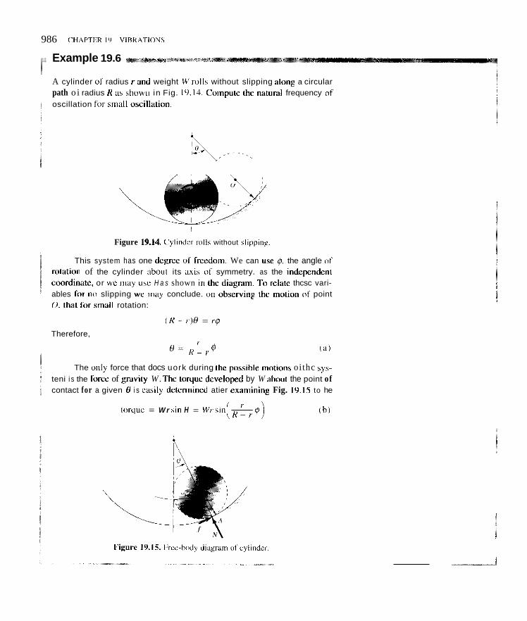
986 CHAPTliK I'J VIKKATIONS
Example 19.6 ,:*m,ive4-"*
A cylinder u i radius r a n d weight W 1ro11s without slipping dung a circular path oi radius K iis shown in Fig. l(I.l4. Compuic ~ h c niitural frequency of oscillation foi- smiill oscillatimi.
Figure lY.14. Vylindcr roi ls without slippiny.
This system has one degree 0 1 lrccdoni. We can u\e @, the angle oi rot;ition of the cylinder ahout its iixis oi symmetry. as the independent coordinatc, or we may use H a s shown i n the diagraln. 1 0 rcliitc thcsc vari- ables ror no slipping we iiiay conclude. on ohservin~ thc mulion of point 0. thal lor sinall rotation:
( K - ,-)e = ,-0
H = r 0 ( a )
Therefore,
R ~ I
The only force that docs uork during [he possihle motions oithc sys- teni i s the lorce of gravily W. Thc torque dcveloped by W ahoul the point of contact for a given H i s casily delerinined atier exariiining Fig. 10.15 to he
torque = W r sin H = Wrsin ( h )

SECTION 19.5 ENERGY METHODS 987
Example 19.6 (Continued)
This is a restoring torque, and because we limit ourselves to small nsrillu- tions it becomes W[rZ@/(R-r)]. which is clearly a linear restoring torque. Because the force doing work on the cylinder is conservative. and because it results in a linear restoring torque, we can employ the energy formula- tion of this section.
The motion may be considered to be given as follows:
or, using t3q. (a).
Expressing the maximum potential and kinetic energies and using C for O,mLx and the lowest position of 0 as the datum, we have:
We have used Eq. (d) in the last expression of Eq. (0. Expanding cos C in a power series and retaining the first two terms (1-Cz/2), we then get, on equating the right sides of the above equations:
Therefore.,
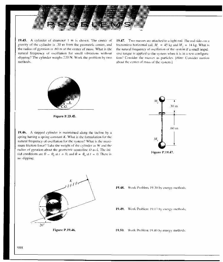
Figure P.19.45.

19.51. A munometer used for measuring pressures is shown. If the mercury has a length L in the tube, what is the formulation for the natural frequency of movement of the mercury?
Inside diameter I O mm
Inside diametei 50 mm
5 1r
I I Figure P.19.53.
Figure P.19.51.
19.54. A stepped cylinder rides o n a circular path. Far sinal l oscillations, what is thc natural frequency'! Take the radius of gyration about the geometric axis 0 as k and the weight 01 the cylinder as w.
19.52. pressure measurements. If the mercury in the tube has a length L, what i s the natural frequency of oscillation of the mercury in the tube?
inclined mOnumefel is often used for more
Figure P.19.52.
19.53. A differential manometer is used for measuring high pres- sures. What is the natural frequency of oscillation of the mercury'? Figure P.19.54.
989

990 CHAPTf K I'J V I B K A T I O V
19.6 Linear Restoring Force and a Force Varying Sinusoidally with Time
Wc sha l l 110\1 coiisidcr tlic ca\c 01 :I ~ i n u x i i d i ~ l i,,!-cc ;icting oil ii :,pring-mass systc~n (Fig. IC). 16) h i \ w i with \t;itionai-y rcicreiice .KJ. Thc sinusoidal iorcc has a frequency ( 1 1 w (not t i l hc coiliuvxl w i t h "I , , . thi. iialuriil frequency) and ;in ;implitudc 0 1 6,. At time i = 0. the i n i i i \ wil l he assunicd lo have some known veli icity and po\ilioii. i i i id n e \hall investigate tllc eii:,iiing iiiotion.
Meiisuring the p~s i t i i in .I lroin [tie unextended position olthe spring. we h a w lor Ncwtoii '.v h i w
J J ? = -K.\ + /;) 'iin ui (IC).XJI
Reiiimiizing the cquiitioii :,(I that thc dcpcndcnt variable and i t s deribativcs arc on the left-hand side iiiitl dividing through hy tit. wc gel the standard limn:
< / I ?
To get a pai~liciil;il- vj lul ioi i .I , . u c can scc by inspcctioii that a lunctioii oftht! Ihr in .I = ('* sin wi w i l l give il s,dutiim if the cimstant (-, i s choscn properly. Suhstiluling t h i s lunctii in inti, Eq. 19.21. wc thus h i i \c

SECTION 19.6 LINEAR RESTORING FORCE AND A FORCE VARYING SINUSOIDALLY WITH TIME 991
Clearly, the value of C, must be
(19.23)
We can now express the general solution of the differential equation at hand:
IK F,lm sin wf (19.24) : K x = C, sin /--I + C2 cos 1-1 +
l m 1 m Klm - w2
Note that there are two arbitrary constants which are determined from the initial conditions of the problem. Do not use the results of Eq. 19.6 for these constants, because we n u t now include the panicular solution in ascertaining the constants. When f = 0, x = xo and x = xo. We apply these conditions to Fq. 19.24
x, = C,
(19.25)
Solving for the constants, we get
c, = 1,)
Returning to Eq. 19.24, notice that we have the superposition of two harmonic motions-ne with a frequency equal to ,/Kim, the natural fre- quency w,, of the system, and the other with a frequency w of the “driving function” (i.e., the nonhomogeneous part of the equation). The frequen- cies w and w, are not the same in the general case. The phasor representa- tion then leads us to the fact that since the rotating vectors have different angular speeds, the resulting motion cannot he represented by a single phasor, and hence the motion is not harmonic. The two parts of the motion are termed the trunsient part, corresponding to the complementary solution, and the sfeudy-sfure part, corresponding to the particular solu- t ion , having frequencies w, and w, respectively. With the introduction of friction (next section), we shall see that the transient part of the motion dies out while the steady state persists as long as there is a disturbance present.
Let us now consider the steady-state part of the motion in Eq. 19.24. Dividing numerator and denominator by Klm, we have for this motion, which we denote as x,,:
, ~~~
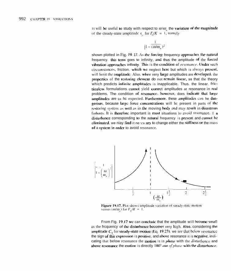
992 CHAPTER I Y VIBK~VI'IONS
I t will bc useful to study with respect to w/W, the var-istion ofthe inagnitudc 01 the cteady-state amplitodc r,. for C/K = I, ~namcly
shown plotted in Fig. 19. 17. A s thc fnrcinp frequency apprimchcs Ihr tiiituriil
frequency. this tertii goes to infinity, ;ind thus the amplitude 01 the fwccd vibration ;ipprmaches inf ini ly. This i s the ciindition 01 rcwtwii('('. Under such
friction. which uc neglect here but which i s alw:~ys pi-esent. inplitudc. Also. when very l x g c amplitudes are de\cloped. the
propcrties of the resloring elenietit do not rernain liiicilr, s o that the theory which predicts infini lc ainpliludcs i s inapplicable. Thus. the linear. fric- tiunless formulations cmi io t yield correct amplitudes at resonance in rcal problems. The condition 01 rcsmancc. howevcr. does indicate that larpc ainplitudcs are t i l hc expected. Furthertnoir. these ;iniplitudcs can he clan- gernuc. because larfe force umcentiiltions wil l hc present in parts 111 the
leni :is well 21s in the moving body and may resii l t in Oisilstrous thei-eforc important in innst situations to aboid resimince. I f a
dicturharice corresponding IO the iiatuiml frequency i s prcscnt and cannut hc eliminated. we niay find i t ne ;rry to change either the qtiffness or the ~ i i i i s \ of a system in ordcr to avoid resonance.
.
From Fig. 19.11 we can conclude that the amplitude wi l l hccorrie st i ia l l :is the frcquency of the disturhancc heconies very h i$ Also. considering the iimplitude C , for steady-statc moliiin (Cq. 19.23). we see that hclow IC~OIIBIICC
the sign o l t l i i s expression i s positive, and above resonance it i s negative. indi- cating that below rcsonance the molion i s in phuse with the di.sturbuwr and ahove resmaticc the i i iotim i s directly 180" oi i f (!fplmw with the disferbanw

SECTION I Y . 6 LINEAR RESTORING FORCE A N D A FORCE VARYING SINUS0II)AI.I.Y WITH TIME 993
Example 19.7
A motor mounted o n springs is constrained by the rollers to move only in the vertical direction (Fig. 19.18). The assembly weighs 2.6 kN and when placed carefully on the springs causes a deflection of 2.5 mm. Because of an unbalance i n the rotor, a disturbance results that is approximately sinu- soidal in the vertical dircction with a frequency equal to the angular speed of the r ~ t o r . The amplitude of this disturbance is 130 N when the motor is rotating at 1,720 rpm. What is the steady-state motion of this system under these circumstances if we neglect the mass of the springs, the friction, and the inertia of the rollers?
The spring constant for the system is
and the natural frequency becomes
,' 1 040 x 106 m n = $ ~~ 2,60019.81
= 62.6 radlsec = 9.97 cycleslsec
The steady-statc motion is
= - 1 . 7 2 0 ~ 10-ssin180.1tm
xp = -.01720 sin 180.lr
Note that the driving frequency is above the natural frequency. In starting up motors and turbines, we must sometimes go through a natural frequency of the system, and it is wise to get through this zone as quickly as possible to prevent largc amplitudes from building up.
. Figure 19.18. Motor with unhalanced rotor

994 ('HAPTtR IU VIHKA7IONC
Example 19.8
A niass on a spring is shown in f'if. 19.19. The support of tlic spring ill .r' is made ti l niove with harnmonic inotiori i n thc vertical direction hy sonie extcriial agent. This mution i s expressed as u \in o f . If ill f = 0 the mas5 is displaced in a downward position a distance of I i n I'rom the static equi- librium position and i f it has ill this instant a \peed downward of 3 in./\ec. what is the position of the mass ill f = 5 sec? T&e (2 = 5 in.. w = IO r;idisrc. K = SO0 Ihill. and rn = I \lug.
\r ,> t i = i in >. 10 = I O radlsec ., . I l l = I 5lup
K = SO0 lhill . 1
Le1 us express Newton's law Ibr the miibs. Notr th;il the e x ~ e i i ~ i o n ol the spring is .r-.x'. Hence,
Replacing x ' by the known function of time. we gcl. upon rearranging the terinx
This is [he sanic form as Eq. 19.21 for lhe casc where the disturhance is exerted on the niash directly. The solution, thcn, is
Putting in the numerical \ d u e s (if ~ Kin ! . etc.. we have
.K = C, sin 22.41 + S> cos27.4f + 6.24sin lot in

SECTION 19.6 LINEAR RESTORING FORCE AND A FORCE VARYING SINUSOIDALLY WITH TIME 995
Example 19.8 (Continued)
Now impose the initial conditions to get
I = c, 3 = 22.4C, + (6.24)(10)
Therefore,
C , = -2.65
The motion, then, is given as
x = -2.65 sin 22.41 + cos 22.41 + 6.24 sin 101 in.
When I = 5 sec, the position of the mass relative to the lower datum is given as
( x ) , = -2.65 sin(22.4)(5) + cos(22.4)(5) + 6.24sin 50 = 1.177 in.
You may approximate the setup of this problem profitably with an elastic band supporting a small body as shown in Fig. 19.20. By oscillating the free end of the hand with varying frequency from law frequency to high fre- quency, you can demonstrate the rapid change of phase between the distur- bance and the excited motion as you pass through resonance. Thus, at low frequencies both motions will he in phase and at frequencies well above reso- nance the motion will he close to being 180" out of phase. Without friction this change, according to the mathematics, is discontinuous, hut with the presence of friction (i.e., in a real case) there is actually a smooth, although sometimes rapid, transition between both extremes.
t Elastic GI/ hand
Figure 19.20. Simple resonance and change of phase demonstration

Miichinc
Figure P.lY.60.

.
19.61. A vibrograph is attached rigidly to a diesel engine for which we want to know the vibration amplitude. If the seismic spring-mass system has a natural frequency of I O cycles/sec, and if the seismic mass vibrates relative to the vibrograph with an amplitude of I .27 mm when the diesel is turning over at I,OoO 'pm, what is the amplitude of vibration of the diesel in the direction of the vihrograph'? The seismic mass weighs 4.5 N. See Problem 19.K before doing this problem.
19.62. Explain how you could devise an instrument to measure torsi(ina1 vihrations of a shaft in a manner analogous to the way the vihrograph measures linear vibrations of a machine. Such instruments are in wide use and are called torsioyrcrphs. What would he the relation of the amplitude uf oscillations as picked up by your apparatus to that of the shaft being measured'? See Proh lem 19.60 before doing this prublem.
19.63. A trailer of weight W moves over a washboard road at a constant speed V to the right. The road is approximated by a sinu- soid of amplitude A and wavelength 1.. If the wheel B is small, the center of the wheel will have a motion x closely resembling the aforementioned sinusoid. If the trailer is connected to the wheel through a lineill. spring of stiffness K , fornulate the steady-state equation of motion x' for the trailer. List all assumptions. What speed causes resonance'?
I'
A X
k-l,+ Figure P.19.63.
19.64. the trailer for the following data:
In Problem 19.63, compute the amplitude of motion of
W = 5.34 kN
V = I6 kmihr
K = 43.8 N/mm
1. = IOm
A = 100mm
What is tlie resonance speed yc\ for this case'? From Probleni 19.63, we have
. 2nvt sin ~
A I' = 11 ~ (2?cV/L)2(W/yK)I L
19.65. A cantilever beam of length L has an electric motor A weighing 100 N fastened to the end. The tip of the cantilever beam descends 12 nim when the motor is attached. If the center of muss of the armature of the niotor is a distance 2 mm from the axis of rotation of the motor, what is tlie amplitude of vibration of the niotor when it is rotating a1 1,750 rpm'! The arinalwe weighs 40 N. Neglect the mass ofthe beam.
A
L
Figure P.19.65. I
19.66. Suppose that a 2-N block is glued to the top of the motor in Problem 19.65, where the maximum strength of the bond is 'h N. At what minimuin angular speed w of the motor will the block f ly off'!
19.67. An important reason for mounting rotating atid recipro- cating machinery on springs is to decrease the transmission of vibration to the foundatiun supporting the machine. Show that the amplitude of force Iranmitted to the gtound, E,w for such cases is
where 4, is the disturbing force from lie machine. 'The factor 11/11 - ( fu /WJ2] l is called the relutive tr~msmi.sxion jircror. Show that, unless the springs are soft, (0 < ~ 0 / 4 2 ) , the use of springs actually increases the transmission of vibratory lorces to the foundation.
19.68. In Example 19.7, what is the amplitude of the force tiatis- mitted to the foundation'? What must k of the spring system be to decrease the amplitude by one-half? See Problem 19.67.
19.69. A machine weighing W N COlltdinS a reciprocating mass of weight w N having a vertical motion relative to the machine given approximately as I' = A sin f u f . l h e machine is mounted on springs having a total spring constant K . This machine is guided so thut it can move only in the vertical direction. What is
997

Figure P.19.72.
1Y.73. wo cphcreh each of mass M = 2 kg arc wcldsd I,> ii light rod that i s p inned at 8. A s e c m d light rod AC i s wcldrd 10 the h t rod. At A we apply a disturbance <, sin 01. At the other end c'.
998
1.
I<
Figure P.lY.75.

SECTION 19.1 LINEAR RESTORING FORCE WITH VISCOUS DAMPING 999
19.7 Linear Restoring Force with Viscous Damping
We shall now consider the case in which a special type of friction is present. In the chapters on statics, you will recall, we considered coulombic or dry friction for the cases of sliding and impending motion. This force was pro- portional to the normal force at the interface of contact and dependent on the material of the bodies. At this time. we shall consider the case of bodies sep- arated from each other by a thin film of fluid. The frictional force (called a dumping force) is independent of the material of the bodies but depends on the nature of the fluid and is proportional for a given fluid to the relative velocity of the two bodies separated by the film. Thus,
where c is called the coefficient of dumping. The minus sign indicates that the frictional force opposes the motion (i.e, the friction force must always have a sign opposite to that of the relative velocity).
In Fig. 19.21 is shown the spring-mass model with damping present. We shall investigate possible motions consistent with a set of given initial conditions. The differential equation of motion is
y
Figure 19.21. Spring-mass system with damping
In standard form, we get
(19.29)
This is a homogeneous, second-order, differential equation with constant coefficients. We shall expect two independent functions with two arbitrary constants to form the general solution to this equation. Because of the pres- ence of the first derivative in the equation, we cannot use sines or cosines for trial solutions, since the first derivative changes their form and prevents a cancellation o f the time function. Instead, we use ept wherep is determined so as to satisfy the equation. Thus, let
x = C!eP'

I1 uill he i c l p i u l IO consider lhrce ciises here.
Case A
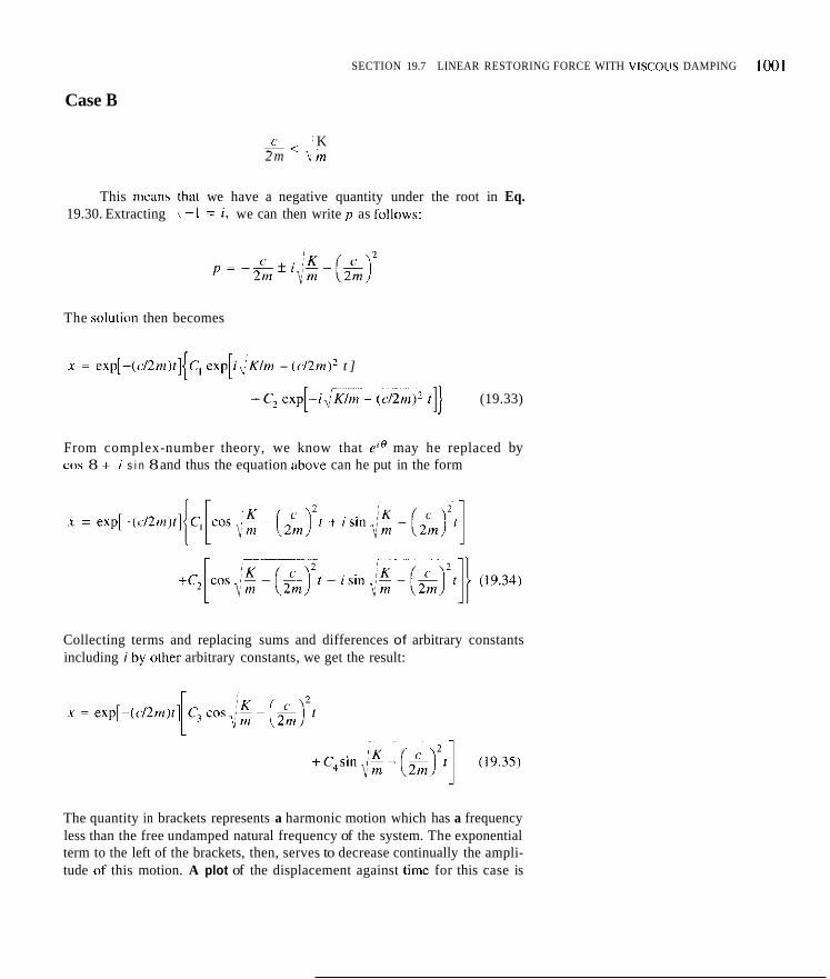
SECTION 19.7 LINEAR RESTORING FORCE WITH VlSCOllS DAMPING 1001
Case B
,,' K 2 m I m - < - c
This means that we have a negative quantity under the root in Eq. 19.30. Extracting I -I = i , we can then write p as Ibllows:
The solutiun then becomes
x = exp[-(c/Zm)t]{C, exp[iiK/m - (d2m)' t ]
- ( ~ / 2 r n ) ~ t]} (19.33)
From complex-number theory, we know that e'' may he replaced by cos 8 + i s i n 8 and thus the equation above can he put in the form
Collecting terms and replacing sums and differences of arbitrary constants including i by olher arbitrary constants, we get the result:
The quantity in brackets represents a harmonic motion which has a frequency less than the free undamped natural frequency of the system. The exponential term to the left of the brackets, then, serves to decrease continually the ampli- tude of this motion. A plot of the displacement against timc for this case is

illustrated i n Fig. 19.23, where the upper dashed envclope corresponds in lorn1 to the exponential function c , - ' ' ~ ~ ~ ' ' ' ~ . We cidl this motinn ~ ~ m l e ~ l i m ~ p e i l motinn.
Figure 19.23. Undurdainped motiiiti.
Case C
Since this i s tlic dividing line hctwcen the overdamped case and one in which oscillation i s possihlc. thc innlion i s tcrmcd a <.rifii.ull\. rluinpcd motion. We have here idmriml roots fnr 13 given a s
imd accordingly lor such a case thc gcncral solurinn to Eq. 19.29 according to the theory of differential equation is then
(19.37)
First we see from this cquation that wc do t iof have an oscill:itory motion. Also. you wi l l recall Srnni the calciiluc that iis f goes to infinity an exponential o f the form r *'. with A a positi\'c constant. goes to Lero faster than Ci goes to infinity. Accordingly, Fig. 19.22 ciln bc used to pictui-e the plot 0 f . x versus I
lor this case. The damping constant for this case i s called the ,,,?ticul damping con-
slant arid i s denntcd a s (;.,~. 'The mluc nt'c;., clearly is
c',., = 2 , Krn (19.38)
I t should he clear that. for a damping constant less than ccr, we wi l l have undcrdainped motion whilc lor il damping cnnstant greater than c ; . ~ we wi l l have overdamped motion.
In all the preceding cases for damped lrcc vibration. the remaining step for il cnniplcte evaluation of the snlution i s to compute the arbitrary constants from the initial condition? nf the particular prnhlem. Note that in discussing damped motinn we shall consider the "natural frequency" of the system to he that OS the corresponding undm~pcd case arid shall refer to the iiclual fre- quency OS the molinn as the frequency (11 Irec. damped inntion.

SECTION 19.7 LINEAR RESTORING FORCE WITH VISCOUS DAMPING 1003
Example 19.9
Springs and dashpots are used in packaging delicate equipment in crating so that during transit the equipment will be protected from shocks. In Fig. 1'1.24, we have shown a piece of equipment whose weight W is 500 N. It is SuppOrted in il crate by one spring and two dashpots (or shock absorbers). The value of K for the spring is 30 N/mm and the coefficient of dunping, c, is I Nlmmlsec for each dashpot. The crate is held above a rigid floor at a height h of 150 mm. It is then released and allowed to hit the floor in a plastic impact. What is the maximum deflection of W relative to the crate?
1" .', _n .,".,iLU1-*~Ln . .
Figure 19.24. Packaging to reduce breakage.
As a first step, we compute the criticul dumping to find what regime we are in.
. ~~~
ccr = 24Km = 2,(30)(1,000)(500)/~ (8)
= 2,473 N/m/sec
The total damping coefficient for our case is
ells, = (2)(1)(1,000) = 2,000 N/m/sec
We are therefore underdamprd. The motion is then given as follows:
Note that

I..I I-____

SECTION 14 1 LINEAR RESTORING FORCE WITH VISCOUS DAMPING 1005
A block W of 200 N (see Fig. 19.25) moves on a film of oil which is 1 m m in thickness under the block. The area of the boltom surface of
the block is 2 x 10" mm2. The spring constant K is 2 N/m. If the weight is pulled in the .K direction and released, what is the nature of the motion'?
.I mm Figure 19.25. S p k - m a s s on film of oil.
You may have learned in physics that friction force per unit area @e., shear stress) on the block W from the oil is given by Newton's viscosity law as:
where t i s the shear stress (force per unit area), p is the coefficient u f v i s - cnsify (not to be confused with the coefficient of friction), and &lay is the slope of the velocity profile at the block surface (see Fig. 19.26). Now the oil wi l l stick to the surfaces of the block Wand the ground surface. And so
Figure 19.26. Slopc of velocity profile at bottom of W

1006 CHAI'TCK I'J VIBRATIONS
Example 19.10 (Continued)
j : '
we ciin ;ipproximatc the \elocity ~profilc as shown in Fig. 10.27. whcrc wc h i i ~ uscd ii straight-linc profile coniiwciiig zerv velocity iit thc hottom and vclocicy .i of the hlock Wil t the top. Such ii i".ocedure fives p o d resrilt\ when lhc film of oi l i s ihin as in the Iprcsciil cat. Thc desircd slope ( a V I ~ y J , , , ~ c , i s then approxinialed iis
1 j
The coefficieni of viscosity ciiii he I'oiind ill h;rndhooks. For our ciisc. ICI us say that p = . ~ l O X O N-seclin'.
Thus. the friction f i~rce i s I t i s i iow an easy iiialter to coinpuie ~ l i c cocf(icicnL ol damping
x 10'/10") = -I.6OO.i N ( c )
Thiis. (' = 1.600. The critical damping for the prohleiii i s
o = ,311 rad/sec = ,0495 cycleshec
!

SECTION 19.8 LINEAR RESTORING FORCE, VISCOUS DAMPLING, AND A HARMONIC DISTURBANCE 1007
“19.8 linear Restoring Force, Viscous Damping, and a Harmonic Disturbance
In the spring-.mass problem shown in Fig. 19.28 we include driving function F(, cos wt along with viscous damping. The differential equation in the stan- dard form then becomes
(19.39)
F, cos mf L Figure 19.28. Spring-mass system with damping.
Equation 19.39 is a nonhomogeneous equation. The general solutinn will he the homogeneous solution worked out in Section 19.7, plus any particular solution of Eq. 19.39.
Beceuse there is a first derivative on the left side of the equation, we cannot expect a particular solution of the form D cos wi to satisfy the differ- ential equation. Instead, from the method of undetermined cneficirnts we shall try the following:
x = D s i n w t + Ecoswt ( I 9.40)
The constants D and E are tn be adjusted to facilitate a solution. Substituting into the differential equation, we write
- D w 2 s i n w t - Ew2coswf + - o D c o s w t - - w E s i n o f
I’
C C
m m K K F + ~ Dsin wt + ~~ Ecoswt = coswt m m m
Collecting the terms, we have
We set each coefficient of the time functions equal to zero and thus get two simultaneous equations in the unknowns E and D:

Rearranging and replacing Khn hy a),,'. we get
I ) ( O l ~ ~ (4 ) + 1: (;;') = 0

SFCTION 19 X LINEAR RESTORING FORCE, VISCOUS DAMPLING. AND A HARMONIC DISTURBANCE 1009
v
(w' -a:)' + (wclm)'
Figure 19.29. Phamr diagram.
where the ainplitudc A i s given as
and v :re a, the phase angle, is given as
(19.45) w(' - - tan-l
K - mw?
We may express the amplitude A in yet another form by dividing numerator and denominator i n Eq. 19.44 by K and by recalling from Eq. 19.38 that thc ratio 2\iKm/ccr is unity. Thus, we get
F,/K A =

where b;,/K = a%,, i s the static deflection. The term
i s called the I~~I,~II;~,,~~I~;,IJI ,fii<.~,,r which i s a dimensionless facloI giving the amplitude of steady-state tnntioii per i t t i i t static deflection. Acciirdinply. this fdctor fhr a given system i s useful for examining thc cffccts of fiequcncy change\ or damping changes on the steady-state vihration mplitude. A plot of the magnilicatioti factor versus wlw,, for various wlues of c./ccr i s slinwii in Fig. 19.30. We scc Irom this plcit that smal l vibrations result when co i s kept far from w,,. Additiiinally. note that niaxi i i i i i i i i amplitude does iiot occur at
resonancc hut actually ill Irequencics somewhat hclow resonance. Only wlieli t l ie damping goeh t(i z.ero docs the mixitnuin ;implitudc occur at resoiiaiicc. However, for light damping we can usually consider that whcn wlw,, = I. wc lliivr an amplitude very close to the milxiinuni amplitudc possible for t l ie system.
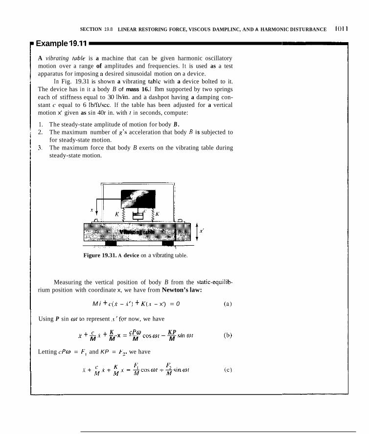
SECTION 19.8 LINEAR RESTORING FORCE, VISCOUS DAMPLINC, AND A HARMONIC DISTURBANCE 101 1
Example 19.11
A vibrating ruble is a machine that can be given harmonic oscillatory motion over a range of amplitudes and frequencies. I t is used as a test apparatus for imposing a desired sinusoidal motion on a device.
In Fig. 19.31 is shown a vibrating tablr with a device bolted to it. The device has in i t a body B of mass 16. I Ibm supported by two springs each of stiffness equal to 30 Ibiin. and a dashpot having a damping con- stant c equal to 6 Iblftkec. If the table has been adjusted for a vertical motion x’ given as sin 40r in. with f in seconds, compute:
1. The steady-state amplitude of motion for body B . 2. The maximum number of R ’ S acceleration that body B i s subjected to
for steady-state motion. 3. The maximum force that body B exerts on the vibrating table during
steady-state motion.
Figure 19.31. A device on a vibrating table.
Measuring the vertical position of body B from the static-equilih- rium position with coordinate x, we have from Newton’s law:
M i + c ( i - i’) + K ( x - x’) = 0 (a i
Using P sin W I to represent .r’for now, we have
(bi K CPO K P . Y + -i + ---x = - - c o s ~ r +--sin Of M M M M
Letting CPW = F , and KP = b-2. we have

i

SECTION 19.8 IJNEAR RESTORING FORCE, VISCOUS DAMPLING, AND A HARMONIC DISTURBANCE 1013
Example 19.11 (Continued)
in = -Am2 cos(mt -a)
= (1,600)(.25) = 400 ft/secz (E)
The maximum force transmitted to the body by the springs and dash- pot during steady-state motion is established clearly when the body B has its greatest acceleration in the upward direction. We have for the maxi- mum force F,, on noting that xp = 0 whenxp is maximum:
= 16.1 .t ($)(400) = 216 Ib ( h )
If there were no spring-dashpot system between B and the vibratory table, the maximum force transmitted to B would be
= 16.1 + ($)[(&)(40jz] = 82.8 Ib (1)
We see from Eq. (f) that the amplitude of the induced motion on B is three times what it would be if there were no spring-damping system present to separate B from the table. And from Eqs. (h) and (i) we see that the presence of the spring-damping system has resulted in a considerable increase in force acting on body B. Now the use of springs and dashpots for suspending or packaging equipment is generally for the purpose of reducing--not increasing-the amplitude of forces acting on the sus- pended body. The reason for the increase in these quantities for the dis- turbing frequency of 40 radlsec is the fact that the natural frequency of the system is 37.8 radlsec, thus putting us just above resonance. To protect the body B for disturbances of 40 radlsec, we must use considerably softer springs.
As an exercise at the end of the section you will be asked in Problem 19.90 to compute K for permitting only a maximum of i in. amplitude of vibration for this problem.

1014 ('HAPTRK 1'4 V I R K A I I O U S
"19.9 Oscillatory Systems with Multi- Degrees of Freedom
Wc shall coiiccrii oitrscl!cs l iere with ii very simple \ystcm lhal l h a h t u o degree\ o i ircedom. iind we sliall he ahlc to getiefiili/c in im th is hilnple ciisc. In the syhtem o i inashes shown iii Fig. 1W2. the niiisscs arc qua l . a s are rl ie .:pring c o i ~ s t i t i ~ ~ s 01 (he outcr hpririgs. Wc nc:.lecl f r i chn . iuiiidagc. ctc. H o u c:ui we dcscrihe tlic iiiolion 1 i i t l ie i i i a s w whwqurt i l IO an) imposed sct 0 1 i i i i t i i i l coiiditions'?
I t ywj imagine that tlic miisscs i re at ;my (ither n(iiilrivia1 piisition, you wi l l s r i l l arrive at ttic ahwc quiit ions.
Because h d i dependent \';iriahles appear i t1 hiith differential equations. lhcy tire termed ,siijti,l/~i,t~,~,,,,~ dil'lerentiiil equations. Wc rearrange the cquil- Lion5 to the Id lowing stand;ird lorm:
Finding a solution i s equivalent to iinding two functions o i time .v , ( l ) and .x,(/), which when siib\titutcd inlo I I L ~ 1').4X ( a ) and ih) reduce eacli equation IO iui identity. Only \ccimd ilei-ibativcs and /.erotti dcrivativr:, appeiu in t l i cx equations, and wc wuolr l thu.: cxpccl that sine or ciicine funcl i~ i~is ot rime would yield a poshihle sdutioii. And since hoth .\,and ~ t l appcar in tlic same

SECTION 19.9 OSCILLATORY SYSTEMS WITH MULTI-DEGREES OF FREEDOM 101 5
equation, these time functions must he of the same form in order to allow a cancellation of the time function. A trial solution, therefore, might be:
x, = C, sin(pt + a) (19.49aj x , = C, sin(pt +a) (19.49b)
where C , , C,,, a, and p are as yet undetermined. Substituting into Eq. 19.48 and canceling out the time function, we get:
(I 9.50aj
(19.50b)
K K - C , p * + - c , + ~ ' ( C , - c , ) = o m m
- c 2 p ~ + - c 2 - - ( c I - C 2 ) = o K K2 m m
Rearranging the above equations, we write:
( I 9.5 la)
One way of ensuring the satisfaction of this equation is to have C, = 0 and C2 = 0. This means, from Eqs. 19.49 (a) and (h), that x, and x2 are always zero, which corresponds to the static equilibrium position. While this is a valid solution, since this static equilibrium is a possible motion, the result is trivial. We now ask: Is there a means of satisfying these equations without setting C , and C, equal to zero'!
To answer this, solve for C,and C, in terms of the coefficients, as i f they were unknowns in the above equations. Using Cramer's rule, we then have:
10 -K,/m 10 - p 2 + Klrn + K,/m __
= -p2 + Klrn + K,/m -K,lm -p2 + Kim + K,/m
O!
-K,/m
l -p2 + Kim + K,lm
- p 2 + Klm + K&
Notice that the determinant in the numeratnr is in each case zero. If the denom- inator is other than zero, we must have the trivial solution C, = C, = 0, the significance of which we have just discussed. A necessmy condition for a nom trivial solution is that the denominator also he zero, for then we gel the indeter- minate form 010 for C, and C,. Clearly, C , and C, can then have possible values other than zero, and so the required condition for a nontrivial solution is:
i-p2 + Klrn + K,lm l-K,lm
-K,/m -p2 + Kim + K,/m
(19.53)

(19.541
Carrying out this determinant multiplication. we gct:
-,>2 + K + " 2 ) - ~ [t; 1- i lii I l l
Takiiig the roots 01 both sides. wc have:
, K K , K, -,r + + ,,; = i ( I'l.55)
111
' r u ~ ~ l values irlpL wtisly the necessary condition wc trnvc inipiised. If u'c usc the positive ronts. the \'illties ci lp are:
, K 1'1 = ',* ,,) ,'. = ,, ~ + ~-~ (10.56)
, K 2 K , - ; 1 1 i I l l
u here and 11. :II-C found l o r tlic pluc and i l i i i r i i s cascs. re\pecti\cly. of the right side 01 Eq. 19.55.
Let u h i iou return to liqs. 19.5 I ( a ) and (h) t o awe!-tain what furthcr restrictions we may have to inipohe to cnsure a x i l u t i o l r , hecause t h e w q u a - tions form the critcrion t o r acceptancc of il set of functions ;IS solutions. Employing ,K i in I'ijri, i n Eq. I%SI (a). we hii\c:
From this equation u c sce that when we iisc th i i \ ~ I u c o i p i t i s iiccesvary that C , = C. to satisly the cquation. The w n c conclusions c:in hc reached h) einploying Eq. l~),?l(h). We can now skrtc il perniissihlc xlutii ,n to the dif- ferential equation. U s i n s A as the anipliludc i n placc 0 1 Cl = C,. we have:
If w c cxamine the sccond \ d u e o l 11. we find th;it t.or [hi. viiluc i t is :is l l ic arbitrary requircd Illat c', = -C,. '['huh il we use B lor C , and iise
\ d u e in the sinc lunction, ;inother possible solulio1i i i :
Let LIS consider each oJ Ilicsr ioliitioiis. I n the lirrr case. thc ino l io i i \ 01 hoth masse\ arc in phare u'ith ciicli other. haw the same aniplitude. and thus movc togethcr with simple h;innnnic inotio1i u d i ii tiilltirill lrequcncy , K/,u hi- this moIio1i. the ccntcr spi.ing is i i i>t eulendcd or comprcsscd. and. ?itice

SECTION 19.9 OSCILLATORY SYSTEMS WITH MULTI-DECREES OF FREEDOM 101 7
the mass of the spring has been neglected, it has no effect on this motion. This explains why the natural frequency has such a simple formulation.
The second possihle independent solution is one in which the ampli- tudes are equal for both masses but the masses are 180" out of phase. Each mass oscillates harmonically with a natural frequency greater than the pre- ceding motion. Since the masses move in opposite directions in the manner described, the center of the middle spring must be stationaly for this motion. I t is a s if each mass were vibrating under the action of a spring of constant K and the action of half the length of a spring with a spring constant K2 (Fig. 19.33), which explains why the natural frequency for this motion is < ( K + 2 K , ) / m . (It will be left for you to demonstrate in an exercise that
halving the length of the spring doubles the spring constant,)
Figure 1Y.33. Bodieh IXO" nut of phase
Each of these motions as given by Eqs. 19.58 and 19.59 is called a natural mode. The first mode refers to the motion of lower natural frequency. and the second mode identifies the one with the higher natural frequency. I t is known from differential equations that the general solution is the sum of the two solutions presented:
Four constants are yet to be determined: A. B, a, and p. These are the con- stants of integration and are determined by the initial conditions of the motion-that is, the velocity and position of each mass at time r = 0.
From this discussion we can make the following conclusions. The gen- eral motion nf the system undcr study is the superposition of two modes of motion of harmonic nature that have distinct natural frequencies with ampli- tudes and phase angles that are evaluated to fit the initial conditions. Thus the basic modes are the "building blocks" of the general free motion.
If the masses, as well as the springs, were unequal, the analysis would still produce two natural frequencies and mode shapes, but these would neither be as simple as the special Case we have worked out nor, perhaps, as intuitively obvious.
As we discussed in the first paragraph of this section, two natural frequen- cies correspond to the two degrees of freedom. In the general case of n degrees of freedom, tlierc will be n natural frequencies, and the general free vibrations will be the superposition of n modes of motion that have proper amplitudes and are phased together in such a way that they satisfy 2n initial conditions.

-- : K , . , \
Figure P.lY.76.
9.77 In Pruhlem 19.76. !tie follawing datd apply:
W = 44s N K , = 8.8 Nlirlin K , = IJ.0 Nlmnl ,' = 825 N l m k c
6 the system underdamped. werdalnpcd. o i ~ cri l ial ly damped'! If he weight W is released 150 nun above i l s static-eiluilibriutll C o n -
'iguratiun. what are the spccd and position 0 1 thc hlock after I scc'! What force is trammitted to the fbundalion at that instant'!
19.78. The damping ~ ~ n s t i l n l c ' f r r r the body is ! IhlIUvx I f . at t i equilibrium positim. the hody is suddenly p v c n a velocity o1 I O ftlscc lo the right. what will the Ircquency of i t \ inlolion he? What ih Ihc positiun 01 the mass a1 r = 5 x c ?
K = 2 Ihlin M = I SI"&!
l Y . X l . ,\ rod 01 length 2; 111 and wcight ?OO N is shown in the \tatic-cquilihriuni position suppol-tcd hy a spring of stiffness K = 14 Nlmm. 'Shc wd is crmnccted til a dashpot having a damping i m r (. 01 64 Nlml\eo. II an Itnpul.;ivr torque givzs the rod an : ~ n p l a r spwd clockwise ,)I 4 radlsec at the position shuwn. what IS the pmition 01 point .1 at I = .2 scc'.'
r
Figure P.lY.78. Figure P.1Y.XI.
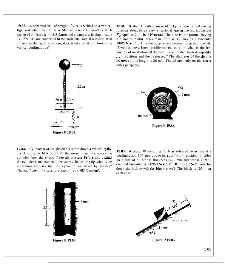
19.82. A spherical ball of weight 134 N is welded to a vertical light rod which in turn is welded at B 10 a horizontal rod. A spring of stiffness K = 8.8 N/mm and a damper c having a value 179 Nlnilsec are cnnnected to the horizontal rod. If A is displaced 75 mm to thr right, how long docs i t take for i t to return to its vertical configuration?
1.6 m
1
19.84. A disc A with a mass of 5 kg is constrained during rotation about its axis hy a torsional Spring having a constant K , equal to 2 x IO-' N-mlrdd. The disc i h in a journal having a diameter 2 tnm larger than the disc. Oil having a viscosity .0085 N-sec/mL fills the outer space between disc and journal. If we assume a linear profile tor the oil film, what is the fre- quency of oscillation of the disc if it is rotated from its equilih- iium position and then released'? The diameter of the dirc is 40 mm and its length is 30 mm. The oil acts only on the disc's outer periphery.
Figure P.19.X4.
Figure P.19.82.
19.83. Cylinder A nf weight 200 N slides down a vertical cylin- drical chute. .4 film of oil of thickness . I mm separates the cylinder from the chute. If the air pressure before and behind the cylinder is maintained at the same value of 15 p i g , what is the maximum velocity that the cylinder can attain hy gravity? The coefficicnl of viscosity of the oil is ,00800 N-sec/m2.
19.85. A block W weighing 60 N is released from rest at a configuration 100 mm above its equilihrium position. It rides on a film of oil whose thickness is .1 mm and whose coeffi- cient of viscosity is ,00950 N-sec/m'. If K is 50 N/m, how far down the incline will the block move'! The block is .20 m on each edge.
Figure P.19.83. Figure P.19.85.
1019

19.86. In Pruhlcm 19.XS. qct up two s i r i i ~ l t a n e ~ ~ s cquntioni to
letemiinc the spring cullstant K su that. alter W is rrleascd. W mnrs hack to its equilibrium position with no mcillatiun. AI a hmt proicct, s d v c tor K using a crmputcr.
4
I---- IO0 imni ...-I Figure P.19.87.
19.89. A furcc F = 15 sin 21 N act': on a b lwk having :t weight 01 ?US N . A \pring having stillness K of 550 N l m and a da5hpot having a dumping factor < ' u l hX N-scclm a i r conncctcd to l l lc
IO20
Figure P.19.89.
Figure P.lY.91

19.92. A platform weighing 222 N deflects the spring 50 mm when placed carefully on the spring. A motor weighing 22 N is then clamped 011 top of the platform and rotdtes an eccentric mass rn which weighs I N. The mass rn is displaced 150 mm from the axis of rotatiim and rotates at an a n g u l i speed of 28 radlsec. The viscous damping present causes a resistance to the motion of the platform of 275 N-mlsec. What is the steddy-state amplitude of thc motion of the platform? See Problem 19.91 before doing this Droblem.
$19.94. In Problem 19.15, i f we include the inertial effects ot rod BC, hiiw many degrees of freedom are there? If rod HC weighs 5 Ib, set up the differential equations of motion for the system.
*19.95 Two bodies of equal inass, M = I slug, are attached i o w d k by springs having equal spring constants K , = 5 Iblin. and are connected t u each other by a spring having a spring constant Kz = I Ib/in. If the mass on the left is relcased from a position (x,)" = 3 in. at f = 0 with zero velocity and the mass at the right is stationary at = 0 at this instant, what is the position of each mass at the time t = 5 sec? The coordinates .li, and x2 are mea- sured from the static-equilibrium positions ofthe body.
Figure P.19.92.
I 19.93. A body weighing 143 N is connected by a light rod to a spring of stiffness K equal to 2.6 Nlmm and to a dashpot having a damping factor (1. Point B has a given motion x' of 30.5 sin t mm with I in seconds. If the center of A is to have an amplitude of steady-state motion of 20 mm, what muyt c be'!
I Figure P.19.95.
1- .4 m-4 *19.96. Let Kz i n Fig. P.lY.95 be very small compared tn K , 1 Assume one mass has been released 81 f = 0 from a position dis-
placed from equilibrium with zero velocity, while the other mass is released lrom thc initial sfationary ]pusition at that instant with
I zero velocity. Show that one inass will have a maximum velocity while the other will have a minimum velocity and that there will be a mntinwal transfer of kinetic energy from one mass to the other at a frequency equal to the heat frequency of the natural fre- quencics of the system.
" K
\I\/\/\ K .I Figure P.19.93. Hinr: Study the phasors A cos <+I and A cos
1021

1022 CHAPTFK l Y VIBRATIONS
19.10 Closure This inlroduclory study ofvihralion hrings ((1 i i c l o x [l ie prcscnt study d ' [ ~ a - - t i ck and rigid-hody mcchaiiics. AI you progress to the study of def(irtn;ihle inedia i n your courscs i n solid and fluid mechanics y o u wil l find that particle inechanics imd, to :i l e s w exLc111 rigid-hody mechanics. bill forin c(irncr- \lories fiir t h e x disciplines. And iii your studies invdr,inf the design of m:ichine\ and the pcriorm;incr oi vcliicle\ you wil l firid rigid-hody rncchanics indispensahlc.
er. th;ii we have by 110 incan\ said thc kist word oii particle mil rigid-hody iiieclimics. MOIK advanced srudics ill cmphasiie 1hc variiitioiiill approach introduced in statics. With the use i i i the ciilculus oi variation .uch topics as Haniiltoii's principle, Lagrangc's equii- tion," and Hamiltori~lac(ihi theory w i l l he prc\enird and y i i u wil l then \ee a ginxtcr unity hctwecii mdi;inics and other areas of physics such a s electro- magnetic themy atid u'iivc mechanic\. Alw thc special thciiry of rclali\ i l ) will niost surely hc considcrcd.
Finally. in yuuI studies of niodcrn physics you wi l l coi i ie t i l more full) understand the lii i i it i i~ioiis 0 1 cliisiiciil mecli i inics when you iirc inlroduccd to quantum niechiiiiics.
I t should he rcdiLed. hii

19.97. free vibration uf .2 sec'? The mass M is 3 kg.
If K , = 2K2 = I .8K3, what should Ks be for a period of
Figure P.19.97.
19.98. In Prohlem 19.55, determine the natural frequency of the system. If the mass is deflected 2 in. and then reledhcd, determine the displacement from equilibrium after 3 sec. Finally, determine the total distance traveled during this time.
Figure P.19.98.
19.99. Find the natural frequency of motion of body A for small rotation of rod BD when we neglect the inertial effects of rod BD. The spring constant K2 is .9 N/mm and the spring constant K , is 1.8 N/mm. The weight of block A is 178 N. Neglect friction everywhere. Kod BD weighs 44 N.
Figure P.19.99.
19.100. What is the equivalent spring constant for small oscilla- tions about the shaft AB? Neglect all mass except the block at B, which weighs 100 Ib. The shear modulus of elasticity G for the shaft is 15 x IOh psi. What is the natural frequency of the system for torsional oscillation of small amplitude'?
A B
K = 50 lbhn
Figure P.19.100.
19.101. What is the radius of gyration of the speedboat about a vertical axis going through the center of gravity, if it is noted that the boat will swing ahout this verticiil axis one time per second? The mass of the boat is 500 kg.
Figure P.19.101.
19.102. A rod of length L and mas M is suspended from a fric- tionless roller. If a small impulsive torque is applied to the rod when it is in a state of rest, what is the natural frequency of oscil- lation about this state of rest?
A
i Figure P.IY.102.
102:

c . K \ .
\
ti. \ .
I023

Integration Formulas
xvii

22. j sin 1'8 cos m0 d0 = - ' ~~ cos 2 m H I m
24. G sin 0 dH = sin 0 - H cos 0
25. j 0 c m H d O = c ( i s H + H s i n H

Computation of Principal Moments of Inertia
We now turn to the problem of computing the principal moments of inertia and the directions of the principal axes for the case where we do not have planes of symmetry. It is unfortunate that a careful study of this impor- tant calculation is beyond the level of this text. However, we shall present enough material to permit the computation of the principal moments of iner- tia and the directions of their respective axes.
The procedure that we shall outline is that of extremizing the mass moment of inertia at a point where the inertia-tensor components are known for a reference xvz. This will be done by varying the direction cosines I , m, and n of an axis k so as to extremize Ikk as given by Eq. 9.13. We accordingly set the differential of I,, equal to zero as follows:
dl,, = 211_ dl + 2m1, dm + 2nlu dn -211, dm - 2 m l _ dl - 21lXz dn ( 1 1 . 1 ) -2nlc dl - 2mI,, dn - 2nlyz dm = O
Collecting terms and canceling the factor 2, we get
( I I _ - mI,yy - nlxz)dl + ( - l I x ~ + m l _ - nIy,)dm + (-11, - mIvz + nl,,)dn = 0 (11.2)
If the differentials dl, dm, and dn were independent we could set their respec- tive coefficients equal to zero to satisfy the equation. However, they are not independent because the equation
/ 2 + m 2 + n2 = I (11.3)
must at all times be satisfied. Accordingly, the differentials of the direction cosines must be related as follows':
Id1 + m d m + ndn = 0 (11.4) 'We are thw cxuemizing I,, in the presence of a constraining equation
xix

XX APPENDIX I1 COMPUTATION OF PRINW'AL MOMENTS OF INERIW,
We can of course consider any two dillerentials a s independent. The third i s then established in accordance with the equation above.
We shall tiow introduce thc Lrigrrmgr ~ n u l ~ i p l i ~ ~ r A to facilitate the extremizing process. This constant i s an arbitrary constant at this stage of the calculation Multiplying Eq. 11.4 by ;L and suhtracting Eil. 11.4 from Eq. 11.2 we get whcn collecting tertiih:
[fit( - AJI - - it,,, ,ii + i l>i + - i ; ) /17 - i l p dni I [- 1 + [ - I ~ , / - / , : w r + i f . ~ - ~ ) n ] < / n = (I (11.51
Let us next consider that in and I I are independent uariablcs arid consider the value of A s o chosen that the coefficient o f d l i s zero. l h a t is.
( I s , - A)/ - I tVm - f s , i r = 0 (11.6)
With the f i rs t tern1 Eq. 11.5 dispiihed of in ttiir way. we arc left with diffcren- tiirls din nnd (hi, which :ire indrpendenl. Accordingly. we cii i i \et thcir respec- Live coefficients equal to zen i i n ordcr to satisfy the equation. Hence. we have in addition to Ey. 11.6 the following equations:
- I t t / + -1,:) - + ( 1 . ~ - A I I I = o (11.7)
- A)lIl -~ /,:I1 = 0
A necessary condition for the solution ill a set oi direction cosines I , m. ;uid 11.
Srom Eqs. 11.6 and 11.7. which does not violate Eq. 11.3' i s that the detcrmi- nant of the coefficients of these variables he zero. Thus:
-.A! - l a , - a ) 1::; 1 = i) (11.81
-It: - 1 , . (/::-a) This results in a cubic equntion for which wc can show there are three real roots for A. Substituting these roots into a n y two if Eqs. 11.6 and 11.7 plus Eq. 11.3. we can delerminc three direction cosines for e;ich root. Thcce are thc direction cosines S i x the principal axes measured rclative to .q:. We could gel the principal moments of inertia next hy substituting a set ill these direction cosines into Eq. 9.13 and solving for lAA. However. that i s not necessary. sii icc i t can be shown l l ia t the thrcc I.;ipranpe inultiplicrs (ii-c the principal nioinciith of inertia.

Additional Data for the Ellipse
If we restrict our attention to the case of an ellipse, as shown in Fig. IV.l, we can compute the length of the major diameter (usually called the major axis) by solving for r from Eq. 12.34 with p set equal to zero, separately for 0 = 0 and for 0 = z, and then adding the results.
Y
Figure IV.1. Ellipse.
Thus,
Therefore,
rI + r2 = 2a = ~p ('-+-) 1 I + € 1- E
Solving for a, we get
a =- EP 1- €
(IV.2)
xxi

xxii APPENDIX 1 1 1 ADDITIONAL DATA FOR THE ELLIPSE
The term a is the semimajor diameter. Tu determine the semiminor diameter, b, we consider point C on the trajectory in Fig. IV.1. Distance rc is indicated a s f in the diagram, and the distance from the focus.f, to the center at M is 3. Using the basic definition of a conic, we can say:
Noting the shaded right triangle in the diagram. we can write
f = \ ' 3 2 + g' (1V.4)
By substituting Eq. IV.4 into equation IV3, squaring hotti sides, and rearrang- ing, we get
h 2 + 8 7 = €?(/I + 3)Z (1V.S)
Observing Fig. IV. I and noting Eq. IV. I , we can express the distance 8 as follows:
Substituting Eq. IV.6 into Eq. IV.5. we get
From Eq. IV.2 we see (hat
I IV 8) CI €
p = -(I - € ? )
Substituting Eq. IV.8 into Eq. IV.7. we have
Canceling terms wherever possible, we get the desired result on noting Eq. 1V.X:
I~ ~
b = a l l - (1V.9)
Finally, we can show hy straightforward integration that the area of the ellipse is given as
A = nab (IV.10)

Proof that Infinitesimal Rotations Are Vectors
You will recall that finite rotations did not qualify as vectors, even though they had magnitude and direction, because they did not combine according to the parallelogram law. Specifically the fact that the combination of finite rotations was not commutative disqualified them as vectors. We shall here show that, in the limit, as rotations become vanishingly small they do combine in a commu- tative manner and accordingly can then be considered as vectors.
Accordingly, consider Fig. V.1 showing a rigid body with point P at position r measured from stationary reference XYZ. If the body undergoes a small but finite rotation A@ about axis A-A, point P goes to P’, as has been in the diagram. We can express the magnitude of Ar between P and P’as follows:
(v. 1) IArI = lr/ sin @A@
Z
Figure V.1. Rigid body undergoes rotation A@.
xxiii

xxiv APPENDIX IV PROOF THAT INFINITESIMAL ROTATIONS ARE VECTORS
If we assume, for the monient. that A+ i b a vector having a direction along the axis of rotation consistent with the right-hand rule. we may express the equation:
Ar = A + X r (V 2)
In the limit as A+ --f 0 the relation above hecomes exact. Now consider two arbitrary, small, but finite rotations represented by
proposed vectors A@,and A& For the first roldtion wc pct a displacement f i x point P given as
Ar, = Ad,l X r (V.3)
And for a second buccessive rotation we get for point P:
Ar, = Aq5, x ( r + Ar l ) iv 4) = Aq5,X(r + A @ , X r )
The total displaccinent for point P is then
Ar, + Ar2 = A+, X r + A+q X ( r + A+l X r ) (V.5) = A @ , X r + A + ~ x r + A + ~ X X A @ , X r )
As the rotations hcciiine vanishingly small, we can replace the npproximetc equality sign by an exact equality sign and we can drop the litst exprebsion in the equation ahovc 11s second order. Wc then havc on collecting terms:
drl + dr, = (dd,l + ~ 1 4 ~ ) X r
We see from the above equation that the total displacement of any point P for successive infinitesimal rotations is inde/vndriit of the order OS these rota- tions. Thus. superposition of vanishingly small rotations i s commutative and we can now fu l ly accept d d , as a vector.
(V6)

Computer Projects: Statics & Dynamics
Preface In this appendix you will find 12 statics projects and 17 dynamics projects specially designed for use on the computer. I have been careful to limit the programming needs for the problems not to go beyond the usual freshman course in Fortran programming. The programs conform completely to the ANSI standard for Fortran 77 and will run on any machine having an ANSI
At SUNY Buffalo and at G.W. we assign one or two projects per semester on ~ o p of our regular program. No regular class time is used to teach programming or to go over solutions. We give our students literature for log- ging in, editing, filing, etc. peculiar to the machine we will work on, and the students are supposed to learn to use the machine with the help of our Com- puting Center “consultants.”
1 would like to thank my graduate students, Dr. Sun Lei Chang and Dr. Anoop Dhingra, as well as Dr. John Hu; they did the original programming under my direction. Ms. Chashia Tracy Chan also deserves thanks for her help in rewriting the programs to make them totally standard conforming.
Standard compiler.

xxvi APPENDIX v COMPUTER PROJECTS: STATICS AND DYNAMICS
Contents Problem File Name
Statics projects 1-12 I . Moment Prohlem 2. Torque Pmblem 3. Equivalent Problem 4. Friction Prohlem 5. Cenrroidal Coordinates of Block 6. Centroidal Coordinates of Plate 7. Beam an Nonlinear Springs 8. Principal Axis Problem 9. Area Second Moments and Products of Area
IO. Maximum Second Moment of Area I I . Moments and Products of Inertia 12. Area Moments and Products of Arcd for Complex Area
Dynamics projects 13-29 13. Projectile Problem With Friction 14. Spring Impact Problem 15. Impdcl Problem (Stationary Panicles) 16. Impact Problem (Moving Particles) 17. Torpedo Impact (Constant Speed) 18. Torpedo Impact (Accelerating Freighter) 19. Conservation of Energy Problem 20. Conveyor Problem 21. Piston Device Problem (Constant Speed of Piston) 22. Piston Device Problem (Accelerating Piston) 23. Light Repair Prnblem
*24. Four-Bar Linkage Problem
$25. Four-Bar Linkage Prohlem
*26. Four-Bar Linkage Problem
*27. Four-Bar Linkage Prohlem
28. Astro-Centrifuge Problem
With Constant Disc Speed. Find ws(.
With Constant Disc Speed. Find O,,
With Accelerating Disc. Find wH(.
With Accelerating Disc. Find ‘uuc.
*29. Constant g Astro-centrifuge Problem
MECHl.FOR MECH2.FOR MECH3.FOR MECH4.FOR PROB5.FOR CENTER.FOR BEAM.FOR PRINCIPL.FOR CEN.FOR P883.FOR BLOCK.FOR TWOF.FOR
MECHS.FOR CLOSE.FOR MOM1.FOR MOM.FOR TORPEDO.FOR TORP.FOR HARM.FOR EX144.FOR PISTON.FOR PISV.FOR COPIT.FOR
FBARS.FOR
FBAR.FOR
FBARVS.FOR
FBARV.FOR CENT.FOR PLOT.FOR
‘Note lhat the Newlon Raphson method can he proiitahly employed in Projects 24. 25, 26, 21, and 29. In each of the programs of these pwjecls. will be round B suhroutine for this well- known method. More detail is readily available in m m milthematics lexthook%.

For all possible following sets of values of A, B, and C:
A ( I . , 2.. 3.) B ( I . , 2 . , 3 . ) C ( I . , 2.5, 4.)
find M,, M,, and M, at D.
(There are 21 different settings for the direction of force F = 1,000 N.)
Print out results as shown.
* Project 1 * Force = 1,000.0 N
A B C Mx MY Mz I .o 1 .o 1 .O 0.2309E + 04 -0.6928E + 04 -0.4619E + 04
etc.
xxvii

Kxviii
i
x
ma,,
a = angle of vertical plane {D = angle of cable from vertical axis
Find the moment tending to tip the boat about its I a i r from the cable shown, for the following conditions:
P = 100 N, 200 N, 300 N, 400 N for each a (O", IO", 20", 30". 40". 50") and for each (O", IO", 20", 30". 40". 50". 60", 70", SO", 90")
Print out data as shown.
Load = 100.0
10 20 30 40 so 0 1.150E+04 .150E+04 .1S0E+W .ISOE+04 .150E+04 .150E+04
etc

50 Ib
... Y
For setting of 8, going from zero to 330" in steps of 30", compute mmponents of equivalent .force .system at "A" for the 50-lb force for two distances of L being 0 in and 10 in.
Print out data as shown
Note: I + t , J + i , K + k
00
30"
60"
330" -
0 in 10 in
F = 0.001 + 0.00J + -50.00K F = 0.001 + 0.001 + -50.00K C = -75.001 +-1OO.OOJ + O.OOK C = -1 16.671+-1oO.OOJ + O.OOK F = F = C = C =
etc
xxix

I Dry Thrust Bearing
F = 100,200,300 N
Pressure= P = K[Iog(2+ \ ' r ) ] ( cos2 r r r )Pu
(K is a constant you must determine)
p varies with r
for r = 0.005 m r=0.015 m r = 0.025 m r = 0.035 in r = 0.045 m r = 0.055 rn r = 0.065 m r = 0.075 m r = 0.085 m r = 0.095 m
p = 0.40
p = 0 . 1 5 p=i ) i n p = 0.07 p = 0.05
p = 0.25
p = 0.04 p = 0.03 p = 0.02 p = 0.0 I
Find Resisting Torque due to Coulomb friction

5 in
- . I .2 .3 .2 .I .2 .I .3 . I .2 .3 .4 .S .4 .3 .4 .s .4 .s .4
.
.s .3 .I .3 .5 -
5 in
in.
Find Centroidal Coordinates. There are 25 equally spaced holes in the block each with its own diameter and lengfh that will be asked for inter- actively during the problem. Please echo the data you use.
D ( I , J) Diameter of each hole
L(1, J) Length of each hole
D ( I , J ) + D ( I + I , J ) > ~ " ~ ~ D ( I , J ) + D ( I , J + I ) > { ' '
D(I , J) + D(I + 1, J) 2 $ " D( I , J) + D ( I , J + 1) 2 5"
Indicate cases where
D ( I , J ) =
. . .I .2 .3 .2 . I .2 . I .3 .I .2 .3 .4 .5 .4 .3 in. L(1, J) = .4 .5 .4 .s .4 .5 .3 .I .3 .s . .
xxxi

Prink out data iis shown:
xxxii

PW
P L
- x
There are un to 100 circular holes randomlv distributed in a rectaneu- - lar plate, each with its own radius and x , y coordinates that will be asked for interactively during the program. The program will check if uverlaps occur between holes or hole and boundary. If overlaps occur then the program will print a message indicating kind of overlap. Otherwise, calculate the centroidal coordinares of the plate. The plate has length PL and width PW that will be asked for interactively.
Procedure
a) Input data; Echo h) Check overlap with boundary (Print out which holes have overlap with
boundaries.) XU) + RU) > Xn,ax Y(I) + RU) > Y,rdx
other.) D(1,J) < K(I) + R(J)
X(1) ~ R(1) < 0 Y(1) - R(1) < 0
c) Check overluy between circles. (Print out which holes overlap with each
d) Calculate area and first moments about X and Y axes. e ) Calculate the centroidal coordinates. f) Print out in the following format:
xxxiii

Length = Width =
Hole XCOOR YCOOR RADIUS
Area of plate i s
The centroidal coordin;ites arc
XCOOR =
YCOOR =
Use your program for the following cases:
Case 1 PL = 50.000
PW = 30.000
I .3.0lJ 45.llll 3x.00
S.OI1 25.00
2 I .Oil 24.00 25.00 23.00 2.IlO
Case 2 PL = 28.00
PW = 14.00
X(I1 Y(1) RII) .- -
5.0 I x.5 25.0 I6.C 22.0 18.0
12.0 2.0
13.0 IO.Il 12.0 3.0
3.0 I .SI 0.5 2.0 3.0 2.0
xxxiv

A nonuniform force distribution acts on a rigid beam AB supported by two different nonlinear springs. Compute the slope of beam AB for the fol- lowing conditions.
Force: -[10sin(Zn~)+15Iog,,(:+I)]e-~ 2 N Spring I: K, = 1 ~ 1 ” ’ x 5 x 10⁴
Spring 2 : K? = 1 ~ 1 ~ ’ ~ x 10 4 N
The length of the beam L will be inputted interactively
Work out for L = 2.0 m and L = 2.5 m
In your output give:
Length of beam Y, and Y , in mm Slope of AB in radians and in degrees.
xxxv

I'M/
For an! set of \palues given inkr;ulivcly.
I.ength: PI. Width: PW
Position: A(X.Y) Angle: n
Find at A and lor llie lollowing data
&,x,, l,y.y.: Sccond inomelits ofarea (cross itched).
1;. 1; : Principal second moinenls of area.
Nute: Point A can hc insidr iiieii.
Work out for the /idlowiii,q d o f o
/'L = 18.00 111111 PLY= 12.00 riiin
a = 22.5,' (X.Y),, = 15.00 mm. 4 . 0 0 inn)
xxxvi

YMAX
PW
i
Hole I
Hole J
PL =MAX
x
There are up to 100 circular holes randomly distributed in a rectangular plate. Each hose has its own radius and x, y coordinates that will be asked for interactively during the program. The program will check if overlaps occur between holes or hole and boundary. If overlaps occur then the program will print a message. Otherwise, the program calculates &, Iw, lxy for area of the plate surface.
Procedure
a) Input. Specify PL, PW, XU), Y(I), R(I), and N (the number of holes) b) Check overlap with boundary
For1 < I < N
X(1) + R(I) > PL X(1) - R(1) < 0
Y(1) ~ R(1) < 0 Y(1) + R(1) > PW
Then print out: “Circle I has overlap with boundary.”
xxxvii

S = ( l
5 in
E
.\ 8 i n \
At what point S along CD do you get the niaxirnuni \econd rn(iment ~~
of area for area CEDF having 2 holes. What is its value'? (Even if you know intuitively where this point i?, show this via thc cornputcr.)
xxxviii

I Y
I
C
z / A
User selects dimensions A , B, C for a block with a random system of holes having
Check for overlap of holes with boundary. If so print out which holes overlap with boundary. Check for overlap of holes with each other. If so print out which holes overlap with each other. Compute lXx. I,. and Ly for unit density of block. Run program for the following cases.
xxxix

I 12.00 18.00 2Y.00 5.50 2 27.00 32.00 3.00 5.10 3 35.00 41 .00 41.00 I .70 4 20.00 20.00 23.00 0.10
Case 2 A = 20 B = 30 c = 40
Hole XU) Y(I) L(I1 r(11
4.00 4.00 4.00 15.00
14.00 3.00 13.00 19.00 19.00 25.00 19.00 26.00 1o.00 15.00 2.00 15.00
13.00 2.00 23.00 2.50 24.00 I .20 I .oo 1.10
28.00 3.00 I .00 0.10
30.00 0.30 I .OO 0.10

c X
I L
Write a program for computing the second moments and products of area
The functions describing the curves are: I,, lxv for the cross-hatched area. User inputs L.
F,(X) = X ( v ) ( s i n h $ ) e - x / L
F2 (X) = X ( 9) cosh( T ) L - x
Run problem for L = 1, L = 50.
xli

X
Projectile with Friction
Newton's L a w , for projectile motion (a spherical body) is given as:
where
Let
C,,= drag coeffiecient for air p = densily of air D = diameter of sphere
= coefficient of viscosity
PI v,> 11) = Re Reynolds number (Dimensionless) ~~~~
Ir

The Scalar Equations are:
OS 0.4
0.3
0.2
Problem:
JJ
GolfBall Weight = 1.5 02.
D = 1.75 in fi = 0.375 x 10⁻⁶ k2 V, = I20 ft/sec p = 0.002378 slugslft'
ft2
a) Find trajectory at discreie points. b) Find time ufflight.
CD I C, = 0.4
Data for C,
3= O'l 0. I I J
9 x 10⁴ Re

Algorithm-Method of Central Diffrrences:
C,, Ke u ( t ) + u(r - At) .(I) = u ( t - At) - 24f-[- 2
,'(I) = \ ( I - A t ) - AI - gAr 24 7
A/
At
* ( I ) = i ( f - AI) + l [ i t ( ~ - - A I ) + / ( ( I ) \
r(f) = ' ( I - A t ) + - [ v ( t 2 - At) + I , ( f ) ]
use At = .04 s e ~ .
Program sh i~ i l d end with J 5 0 (when hall hits ground)
Print out result:
I (set) x ( I t ) ?' (f t) 0.04 4.149 2.17
and thereafter cvcry 0.2 seconds
Hints: ( I ) Solve for ~ ( 1 ) and v ( t ) from Eqs. I before writing program
(2) 1x1 U , = ( ( ( 1 - At) VI = v ( / - AI) u, = u(1) v, = v( t )
Starting with initial data for U, and V, solve for U, and V,. Thcn inc.rc,mrvit by lctting V, = V2 and 0, = U?. This is done with a DO loop nccded to determine C,, and to print out.
.
(3) Use the c(incIition
II((I/S)"S .Eq. I) Print . . .
LO pi-int nut cvcl-y S t h terrii
xliv

Six Linear Springs
Develop a program to find how close bottom of W comes to the base (ground) for the data:
W (weight) (N) D (m) d,. d,. d3 (m) k , , k,, k , (N/m)
that the user will supply interactively. Print out data used and desired distance. Run program for the following data:
W = IOOON D = l . 00m d, = 0.20 m d, = 0.25 m d, = 0.30 m
k , = 15,000N/m k, = 16,000N/m k, = 18,000 N/m
xlv

A Circular Plate of M and Radius H
A circular plate moving initially at spccd V,, to lelt liits a I-andom distribution of palticles which ai-e initially \tationary and u hich haye the following dala:
M ( I I Illass € ( I ) coefficient ol restitution X(/). Y ( / ) , Z ( I ) position
Check that the Y ( / ) c(i(irdirrateh a~-e in asccndins crrder. To avoid thc possibility 01 particle collisions make sure that for thc particles, X ( I ) # X ( J ) and Z ( I ) # Z ( J ) for any I # J . Write a pi-opram lw Ihc s p e d of the disc after it movcs a dis tmce 11. II p lak slops or revcrxs direction helore reach- ing D. have statcineiit pi-inted that plate does not reach position Y = 11. User supplics d l ahove data intcractively. Use SI units. Consider that the data is such that the particles d o i ~ o t c d l i d e with cach other al'tcr inrpacting with the plate.
Run program for following data (SI units). Echo this data i n your output.
The mass of the platc is 100.00 kg Radius is 2.00 in The initial spccd t i l the plate is 60.00 m i s The distance D is 55 111
d v i

No. Mass Restitution X Coordinate Y Coordinate (kgj Coefficient (m) (m)
I 2.500 0.230 1.2(x) 1.200 2 5.500 0.450 0.890 2.300 3 3.300 0.890 3.200 5.800 4 7.500 0.440 4.200 7.600 5 2.200 0.230 0.440 11.100 6 5.500 0.210 0.360 13.500 7 3.100 0.670 0.720 16.600 8 3.100 0.190 0.540 18.300 9 2.200 0.450 0.540 21.700
I O 1.700 0.100 0.210 28.600 I I 0.760 0.880 0.760 31.900 12 0.650 0.560 0.230 36.380 I3 5.800 0.100 0.100 40.100 14 5.100 0.670 1.400 42.100 15 3.200 0.230 1.780 48.400 16 2.100 0.540 5.300 49. 100 17 0.200 0.220 2.300 51.500 18 0.560 0.550 3.200 54.600 19 0.320 0.230 1.100 56.400 20 1.650 0.230 1.430 61.800
Z Coordinate (m)
0.400 0.980 0.440 0.890 6.400 0.870 0.010 9.800
32.700 7.600 0.890 0.650 0.430 1.650 4.200 2.700 1.400 1,000 0.430 3.200
xlvii

In project 16 each particle i s to have its own cnn~tiult velocity component V, before impact.
I . Assume particles are very small compared tn thc plate. 2. Insure that X(/) I X(J 1 and Z( / 1 # Z(./) for I I .I.
User wil l specify the vclocity cnmponent = V = 0.
Procedure: Choosc small distances o f plate innvcnient equal to 0.01 m. At the beginning of the nrh interval you wil l have thc position of the entire systcin and the vclocities of all the particles a s well as the plate velocity (V,,),,. With
Now the these velocities compute ncw pnsilions after the time intcrval Tb$,ln
plate wi l l have moved frnm CY,,),,, to (Y,,),,,,,. a distance equ:d to 0.01 m.
If
M o r e impact keeping
0.01
a ) A particle i has 3 change of piisition u:hich causes i t to cross position (Y,,),,,, during this tiinc interval.
b) Then let impact occur giving the plate a new velocity. As an approx- iination consider this new velocity to occur at the beginning of the ( t i+ 1 ) time step.
c) If the velocity of the plate should hecome 7.eni or negative belore reaching position D. print nul the fict that the plate does not rcach position D.
The Y coordinates can he in any order of scqucnce
Run program fnr the siinil' following &ita
The mass of thc plate i s 100.00 kg. Radius i s 2.00 in. D = 55 111. The initial sped of the plate i s 60.00 ( i d s )
rlviii

Determine if the torpedo hits the freighter and if so how far D from the how of the freighter. The freighter is 20 meters long. Do this for all the following sets of values of V,, V,, a:
a = (15, 20, 25, 30, 35, 40.45)" V, = (15, 20, 25, 30, 35.40) m/s V, = (20, 25, 30, 35, 40, 45) m/s
where
V, = velocity of the freighter V, = velocity of the torpedo a = degree as shown
3,000 rn
Hint: Use law of sines for triangle ABC
xlix

Do projecl 17 where the velocity of the light freighter at the configuration shown is 10 kmihr and which we take at thc lime f = 0. 'Thc velocity viirics i n the following manner.
VI :- I O ~ b 1.8\re-""kmihr
where I is in seconds
Procedure: Choiisc mia l l Lime intervals of 0.01 ,econds. ('onipute velocil) of the torpedo relative to the Sreigliler at each time i i i lcrval. A I k I each timc interval find how much the torpedo has moved along a line n,wniul Lo the freighter atid along a direction p ~ ~ r u l / ~ ~ l to the li-eighler. Whcn the 110t-mi11 dis- tance equals or exceeds ,(3.ooo)' + (5 . I Y O ) ' Inahe your conclusion\. User entcrs V , kmlhr and a" interactively.
Run program for:
V , = 45 kmlhr V, = 35 kmihr V i = 20 kmihr CI = 30"

A mass Mcan slide in a frictionless manner along rod EF. At position shown, spring K , is compressed D , inches and M is at distance D, feet from F. Spring K, is elongated D, inches. The spring constants are K , lhlin and K2 Iblin. The mass is M Ihm. Find the velocity of the mass as a function of the distance it moves, and find the amplitude of the vibration. User specifies M lbm, K , Ihlin, K, Ihlin, D , in, D, ft, D, in. Run the program for the following data:
M = 30lbm K , = I.Olh/in K, = 0.5 lblin D , = 6 in
D, = 1 in D, = 4 fl
E
8 ft
Y -
/ 5 ft F
li

Find (T , ~ 7,) a s ii function of Lime as thc helt accelcralcs uniformly from VI ftisec to V , ftisec in T sec. N(rj bodies at any lime 1. each d mass M Ihm. hit the belt from the hoppers after filling a distance H. The weight of the helt rebling on the bed is W Ib and the coeiricient of dynamic friction between belt and hed of the conveyor is U . The number of impact5 pcr second, N(1). is 2 0 ~ ' ' I' lsin rl. Also at r ( 0 ) there are 2 particles on the hell. Work the prohlcni out in 100 time inlervals.
Kun problem for the id lowing dala:
W = 20 Ib VI = 1.5 ft/sec V2 = 7.5 It/sec 7 = 10 sec M = 0.5 lhni H = 2 f t I / = 0.23
Take time interwls of 0.001 sec and print out thc result at every tenth d il second ;IS rwows:
~ h m e ( 5 % ) Forcc (Ib) 0.00 5.71 0.10 5.36
I I
10.00 25.63


Do project 21 with the velocity of the piston varying with posi/inii s o a s 10
increase as the squiirr iif its vcrticiil distance p i n g froin I ftiscc to 3 W s e c as a giieh from (x = 45" to n = 20'.
Procedure: Devclop equations as instructed in project 21. Wiite a subroutine giving fix any value 1. which will he 8 dummy variable going from 45 t i i 20 iii steps i i S I, t i e Yiilues of a. @, and Y. Now get tlic velocily of the piston to vary a s asked for above. Usc lhe subroutine to iacilitate this. Next a I giic, Srom 45 tu 20. gel a, @, 6. 8. 9. and finally ? in ii DO loop calling i n thc suh- routine lix each 1. Now get X,, and X,. Print ou t results.
i v

Find the magnitude of the velocity and the magnitude of the acceleration of the man in the cockpit as arm DA rotates 90" in 20 equal increments. Get 20 readings during this part of the motion. Consider 20 successive stationary axes XYZ at D with XY axes in the plane of DAB for each setting. Take angu- lar accelerations as constant and the w's given as initial values,
Procedure: Compute V,, and (I,, with p and )unspecified. In a DO loop for each rotation of 4.5" of DA starting from O", determine w2 after each interval. Find the time for that interval. Then get p, wl, w2 at the end of the interval. Now get lVxyzl, laXYZl at the end of the interval and print out results for each interval, O", 4.5". 9", etc.
Take a = 45" and constant DA = 13 ni
lv

..-c-.
Procedure:
ti ) For each a. find /3 and y h) Consider rini A / ( . Gcl ( o ~ , , ~ and \/,r Also gzt /3. Thcn sct c) For each a. print 11111 ({I,,, and (;I,,,
h,,,..
L ” d
Ivi

Compute the angular velocity and angular acceleration of the four bar linkage in FBARS.FOR. Print the angular acceleration of BC and a in 20 steps.
lvii

Do project 24 for variable angular speed of disc given as:
qrlsc = 2 + 1.1 kxlY2 radlsec
where a is in radians.
lviii

Compute the angular velocity and angular acceleration in FBAR.FOR. For this case the angular speed of the disk is variable and is given as:
w = 2 + 1.32.1/2radlsec
Print the angular acceleration of BC and a in 20 steps.
lix

In Example 15. 14. M'C want to chart the pzrfixinancc characterislics of thc cenliiiiigc lo r tlic cirnfigul-ation shown 10 givc thc number of ,q 's accelrralion of thc astronauts hc:id for the following conditions:
(oI 2 i 20 rpni in 10 stcps w, 2 i 12 rpm iii 6 cteps o , = 5 rpm. 10 rpni. and IS rpni (GI = s rpm'. 8 rpm'. and 10 rpm'
I \ WI Cockpit
w
w
~ Y
Given the rcsults in the following iornmat:
For 0, = 5 rpin. 6, = 5 rpm'
2 3 h
For ui = IO rpm. (3, = S rpm2 t t c
Ix

In the centrifuge of example 15.14, find the values of w, and w2 to maintain the same magnitude of acceleration, assuming the other data is fixed. Get results for accelerations of 0.5 g, 1.0 g and 1.5 g.
Use the Newton-Raphson method to determine the minimum value of w, for any value of wz which ranges from 0 'pm to 20 'pm.
Print out wI in the following format:
0.5 g I . 0 g 1.5g a:
0.00 0.50
C
A
An'
Ixi

2.2. 2.4. 2.6. 2.8.
2.10. 2.12. 2.14. 2.16. 2.18. 2.22. 2.24. 2.26.
2.30. 2.32. 2.34. 2.36.
2.42. 2.44.
2.46. 2.48. 2.52 2.54. 2.56.
2.60. 2.62. 2.64. 2.68.
2.74. 2.76.
2.28.
2.40.
2.58.
2.70.
2.78.
2.80.
2.84. 2.86.
2.82.
2.88. 2.90. 2.92. 2.94.
lxii
F = 3X.5 N @> 66.h from r axis. 1. = 2.75 km.
5 = 100 N @ -120' with horimntal. 6, = 76.53 N @ -67.5~ with horiruntal. Fc = 76.53 N @ -22.5" with hol-imntal. F = 846 N CC 17.6X' with horimntal . T,, = 767.2 N a = 36.8" F = 1,206N. F = 137.5 N @ 43.34' from x direction. F = 242 Ih @ 3.07~ from -i direction. t,,,, = 36.4 Ibl: FBc = A30F 2,690 Ih XO3.X Ib. b;,c = 707 N F = 215.9i + 196Xj + 3151kN. F = 07.4 Ih I = ,267 m = ,535 n = -.XO2 6 + 6 = YIX.hi - I5Xl . j - X35.8kN. 7 = 400 N < = -1007 N. F = 25.71' + 24.3 + 16k Ih. A = + 5 i 2 i T 5\.2k. f = ,463 + 3 I 4 j + ,349k. F = 463; + 81.4j + 34.Yk N . -164 -.4h5 -10.5. D = 10i - 769j -3.77k. .4 I 8 It. 17.05 N. A = 2.5 N a = 45.7- -75 ft? 95.94~. -28.R3 N. 47.5 I I. (18; + 20j - 42k) ,804; + ,465j + , 3 7 2 640 m2.
-29.6. (a) -43; + 4Yj + 2k. (b) -136. ( c ) -136. L,,, = 373 miles 162 miles longer.
F; = 57.1 N F = 231.3 N.
n = 17.32 N I* = 60'
= 81.5 Ihf. II,,,, = .590F.
I* = 911~.
47.
I.,,. = 6x9 mile,
FT. = 342.8 N = 971.4 N.
32.4 ft-lh. I l2.C -190.72 Ih 35.7kN. 19.87m. F = -80.1 x I O "k N. 251 ft2.
2.V6.
2.100 2 . ~ 8 .
3.2. 3.4. 3.6. 3.8. 3.10. 3.12. 3.14. 3.16. 3. I 8.
3.20. 3.22.
3.24.
3.26. 3.28. 3.30.
3.38.
3.32. 3.34.
3.40. 3.42. 3.44. 3.46. 3.48. 3.50. 3.52
3.54. 3.56. 3.5x.
3.62. 3.64. 3.66. 3.68
3.70. 3.72.
3.60.
18.21n1 I / . 111. I l l = (.SI.li. .6X611, .5145l.
4 - l 6 j - 3k It. hi + 1.1hj t 7.59Rk m. -1Oh7.4 Pi-,,, l W l . 3 N-nl .
i? '. 2/ . j + :k. --iR.OZh N-in -6.S24.8 N-in. 13.x 111
-251.5k Pi-ni. X413 fl-lh 4412 ft-lh 11 ft-lh. I X O i ~ 50k kN-m. 30; t 7Sj ~~ S(1k kN-in. - I . S S l . X i + 7 j + 3S4.4k kN-tn. -84; + 9Jj - 46k N ~ m . M, = q o k - &ojlh-lt. M,, = 0 lh-It. M, = - "joi + " ' o j Ih-St elc.
(7.277f;,,, + S. i lSF ; , , - 111.000)~ + (? .<)I I/;,,< S.l45fi;.,Jj + (-2,41153,! + s . l 4 s ~ , , l k ti-lb. I .32'1hF It-lh. 22,245 N-m
5,764 Ih-ft. - ~ 1 135 hN-m 71111 I b f t (100 Ih-It 1.200 Ih-li. 175 N. -7,271lk Ih-St lll.405k Ih-fl. MA = M,, = -261; - ZhI j N-m. 4211 It-lh. C = 1 O l l i + S l j - 224k lh-ft. -1.x57 N-In. ,W,, = 4Xi - 3hj - 225.6k N ~ m . M, = 446.9N- tn M = 3,h35 Ih-in (a' hK.2- 10 hwimnla l . C = 35.35; + 22.3(7j + X0.07k N-in. 120 lh-ft 1611 lh-ft 60 Ih. 1.750 N-m. 408.4 N-in. 1.174 f t - lh -4S2k lh-ft -I.202k lh-ft. IO,h00i + 4.SOOj - ?.000k m. 1 2 . 5 4 111.
-27.7 N-m. 217.6 N-m.
,,
M,, = -3Oi + l(ll1j - 3hk N-m llh.2 Ih 77.011 lh-Ut.
- I 17.5 kN-"1.

4.2. 4.4. 4.6.
4.8. 4.10.
4.12.
4.14. 4.16.
4.18.
4.20.
4.22. 4.24. 4.26. 4.28.
4.30.
4.32.
4.34. 4.36. 4.38. 4.42. 4.44. 4.48. 4.50. 4.52. 4.54. 4.56. 4.58.
4.60.
4.62.
4.64. 4.66. 4.68. 4.70. 4.72. 4.74.
F = 15 kN C = 30 kN-m C.C.W. F = 150N C = 187.5 N-m. MA = 8kkN-m M, = 22.7% kN-m. Move 200 Ib force 5 ft to left. FA = -2OOj - 150kN. C, = 34.0i + 26.Ok N-In. F = 20i - 60j + 30k N. C, = 900; + 680j + 760k N-m. 12.375 m froni origin. F = -44.567i - 33.425j - 22.283k N. C :: -31.007i - 160.465’ + 302.71k kN-m. FR = -204i + 604j + 408k Ih. C, = 8,lhOi + 2.032j + 3,264kft-lb. C, = 2,032j - 816k ft-lb. FR = 400i - 1,YOOj + 6OOk N. c, = 24.2130i + 2,OIX)j - 3.30llk N-m.
FA = FH = -IOfkN.
F, = -50k kN 6 = 2h.Y Ib F = 2,100; - SoOj Ib FR = 400i - 1 60Oj N C, = -1,800i - 2 , 4 0 j - 12,600k N-m. FR = 39.441 + 74.71”. X = 6 6 9 m. FH = -10llk N X = 2.5 m Fx = 0 C, = 2XOi + 450jN-m. FR = 0 C, = 860i + 900jN-cm. FR = 353.3 - 653.53 N FR = 43,000 Ib F = 3,164k Ib. X = 10.37 in. = 7. = (I. E = .289 10.84 m. X = 1.292 ft 7 = 7.63 ft. X = ,210 ft = ,0756 ft. 7 = 3.808 m. F 2 -37.5k k N X = ,844 m 7 = 1.067 m (origin at front left lower corner of the load). original weight 90 kN. lost weight = 52.5 kN. F, = -I 11,780k Ib (in from oftrailer C.G.). F, = -86,386k Ib W = .Sl273Yy L . = -.lY68m. FK = 2.315x 10”lb X = 20ft 7 = 12.44ft. FK = 262 N. 4,025 N-m 596.3 N-m.
:c 7.8644 x IO* Pa. F =: 61,740 Ih 10.386ft. F =: 8761 Ih 2.615 ft.
C, = 7 . 3 + 5Oj kN-m.
X = -.OS ft. 5 = 17.6 Ib 6 = 35.5 Ib.
V = 2.2 m.
X = 9.2739 m. .7 = 23.209 ft.
u = .400.
X = -3.78 ft
X = -7.329 ft. x, = ,2042 m y‘ = .I m
4.76.
4.78.
4.80. 4.82. 4.84.
4.86. 4.88.
4.90. 4.92. 4.94. 4.96. 4.98.
4.100. 4.102. 4.104. 4.106. 4.108. 4.110.
4.112.
5.18. 5.20. 5.22. 5.24. 5.26. 5.28.
5.30.
5.32.
5.34. 5.36. 5.38. 5.40. 5.42. 5.44.
5.46. 5.48.
5.50.
F = 1.697 x 10“’N
F = 666 x 108N. @ i m from base. ,? = 21.2 ft x? = ,07441 m. F = 4 o O j kN
1,415 kN 1.915 mfromfrontofload. FR = 4.6981’ - l0.09jkN. MR = -3i + 3.2316kkN-m. I’ = 1 7 . 5 7 ~ ~ - 7 . 0 2 7 ~ + ,7026. I = 3.51 m. F = 2,200 Ib -217.2 N-m. FH = 5OOi - 1.220j N C, = 240i - 2,190k N-m. FR = 58,900 Ib
7 = 1.299 ft. -1,550 Ib j: = 10.94 ft 7 = 12.67 ft. 485.397 kN @ 1.636 m below top of gate. 132.38 I kN @ 1 m below top of gate. X = 4.98 m
24.04 m from base along in- clined surface.
40
7 = 4.67 ft.
MoulSidclanc = 9ook kN-m Mrnh,dc = -3OOk kN-m.
X = 4.136 ft
X = 3.919 from bottom left corner. f x = 1.20ft 7 = 1.125ft i = Tft.
X = 20.04 ft.
= 2.65 m.
Txc = 26.79 Ib
27 Ih 36.35 Ih 4.653 in. 671 N, 447N. 1 ,NON. 409.8 N-m. Ax = 4,233N, AY = 3,140N. R, = 4.233N. Rv = -1,840 N. A~r = 2,OM N, A y = 6,970 N, B = 530.4N. A* = 8.00 kN A\, = -12.50 kN Ex, = 22.5 kN. GD = 462 lh FBc = 215 Ib 4B 375 Ib. T, = 125.0 N
Ax = 433N. A s = 790N MA = 1,167N-m. A r = 200N. Av = 3,464N MA = 1,192N-m. Ar = 9,736 N Av = -2,670 N B, = -9,736 N B>, = 6,670N. a = 17.46‘.
TBA = 37.9 Ib. = 111.81b T8” = 109.Ylb Tsc = 63.71b.
MA = 62,360 N-m
Rx = -8.00 kN
f’ = 125 N. T = 117.4N a = 79 .g
ixiii

5.52.
5.54. 5.56. 5.58. 5.60. 5.62.
5.64. 5.66. 5.68.
5.70. 5.72.
5.74. 5.76. 5.78.
5.80.
5.82.
5.84. 5.86. 5.88. 5.92. 5.94. 5.96. 5.98. 5.100. 5.102. 5.104.
5.106. 5.108. 5.110. 5.112. 5.114. 5.116. 5.118.
5.122. 5.124. 5.126.
5.120.
5.128.
lxiv
A r = 408 N A s = -2SXN G, = -749.5 N Gv = 583 N. 7 = 20 N-m. T,, = 40.5 kN 72 Ih 447 Ih. 4 m.
q,,. = 39.3 kN.
R 5 = I1 = 58,900 Ih M,* = 142,500 f t~ lh . Rr = 0, R , = 4,953 Ib R , = 1,006 Ib M,. = I0.IOX ft-lh. R, , = 294 Ib Mi> = 2.770 it-lh. 270 Ih 253 Ih. ym2,x = 2.5 ton
hl = bl.OX2.5 l i l h .
U> = I 0 . X tun ,lt = 1.7 ton c, = 1.7 ton y = 34 f t - tan /I, = I .7 ton
M,, = 85 it-ton. 17.55 tun (2 supports) 24.Y t i in M = 7 0 ton-ft. F, = 293 N F2 = 52.37 N A = -5Ollj + I .500k Ib MA = 26,260i - 9,100k h-lh B = -5Olj Ih Mx = -9,100k ii-lh. F = 57.14 Ib B> = 93.0 Ih At = 0 A , = SON A~ = lIl(1 N Mt = -200 N-m. M y = -220 N-m 8% = 3.f100 Ih E . =' 26,500 Ih 3 ft A? = 50 N E . = SON. P = 33.7 Ih 11,394 Ib. 65,100 Ih. F,;c = 4.36 kN
Ca x 576 Ih T , = 209 N A = 10,640 Ih C = 6,520 Ih I ) = 6.52(1 Ih G = H = 7,.5lK) Ih F = IO,640 Ih. 1154N 9.418 x 10'' Pn. ? = (6.833 - 6.50: - i x I l l ' Po. 7.. = 281.7 psi Gi. = 750 Ih F, = Az = 806 Ih R , = 41 kN e.,, = 1,694 Ib Ax = 13.15 Ib 1, = 1,688 N T = 30.67 Ih. Ct = -322.3 Ih Ur = -322.7 Ih
F, = 254.3 N.
A, = l60.1 Ih E. = 22.6 Ib A. = I8.W Ih.
M. = I IO N-m. ( ' ~ = 17.11(10 Ih.
A. = 25 Ih A, = -7.50 Ih.
A , = .XOO kN A , = 190.7 hN.
M< = Xll l iY.6 N-In. B~ = 1 6 5 . 9 ~ B , = 2 1 1 6 . 3 ~ /;.,( = m s . n ~ .
C y = 1,326 Ih 7. = 202 N F = 2X6 N.
.,
C! = 650 Ih.
R2 = 88 kN = A , = 500 Ih.
K , = 141 kN. FFF = 4.<J3I Ih.
A, = 142.6 Ib. 1;) = 2,XJ(1 N.
C, = -161.3 Ih D. = -3Y8.9 Ih.
( ' ~ = -5Xi.h Ih
5 . l30
5.132. 5.131.
5.1.36.
5.13x.
5.140, 5.142. 5.144. 5.146. 5.148.
5.150. 5.152.
5.154.
5.156. 5.158.
5.l60. 5.lh2.
6.2.
6.4.
6.6.
6.8.
6.10.
6.12.
' I ' = 2.121 Ih H = 3.000 Ih 1'' = 3.00l1 Ih ' I = 1.1181h H = 2.121 Ih 1,' = 5.121 Ih. I;,,, = 353 Ih 'I:,, = 2x9 Ih 7,,, = 3Y4 Ih. lid = I . E X N I; , = 7WJ N 'Ti = 2.124 N 'I;, = I . I)IZN I = . l lX?X t u = ,728 n = .6 lX I , , , = X.11011 111 I:, = 5.000 Ih &I, = 6.42X lh
11, = 4.XOli N. )lt = EN 1, = 150 N. 63.75 kN-in. & = 4967 N. , t , = 11, = IX.17ON ,4, = 63.hhON. ( 'n = hIi(1 Ih C ' 3 = I1 ( ' = -320 lh P i , = 1.033 Ih I., = 312.5 Ih. p = 2118 p\i p a y . A = 43% - S33j - 19.liOk I h E = 240 Ih. / I = -413; + 13?j - SZOk Ih A x = -28.13 Ih H , = 7011,
,I = 15.08 kN. A = 0 A , = I.L138 Ih ('$ = H 8 = 3.1162 Ih I ) , = 1.')38 Ih. Ram I O I C C = '1.74X Ih. T, , = 1.174N. A = l.39Y x 1Il4N M , = 1.355 x IO' N-m
K = 0. t l , = -W lh
B, = 11.
A , = 5.54') x 10 'N. H = 2.887 N.
E t = 2.01iO Ih 1' ,AI, = J .X l IX Ih T I K = 2.670 Ih. C' etc. IM.' = I X.720 Ih C I I H = X.X25 T
A I 1 = / ) E = 26.8 kN C GC = CF = 3.39 kN C A(; = 11; = I'J hN 1 H ( ' = ( I ) = 20 k N C. IK; = I ) / , ' = ~ 1 . 1 1 k N 'I ' (;I.' = 2 I l h k N ('. ,AH = 7117 Ih C A ( . = ( 'E = XI0 lh 'I E/{ = I1 NO = 500 Ih C' 111 = 707 Ih C:. A N = h.'JSIi Ih V ) A ( ' = 4.414 Ih ' I ' I<(' = 3.207 Ih . I (7) = 11. . A / ? = 353.5 kN c' A/. = 250 hN T /,A' = 250 kN '1 LII = 100 hN 'I IK' = 31h.2 kN I' HK = 70,s kN 'I.
HC; = 18.720 I[, 'r ctc.

6.14.
6.16.
6.18.
6.211.
6.22. 6.24. 6.26. 6.28.
6.311.
6.32. 6.34. 6.36.
6.38.
6.411.
6.42.
6.44.
6.46.
JI = 25 kN T BH = 8 .64kNC AJ = 31.25 kN C BC = S O kN C IH = 56.25 kN T CD = SO kN C BJ = 6.25 kN T HC = 0 etc. C/) = 583 Ih C
H I ) = 1,158 IbT others are xro. AC = 14 .14kNT CO = I4 k N T DE = 2 k N C A / ) = 24.5 k N C others are zero. s,, = 24.246 Ih C, Fnc = 32,709.5 Ib T F,,, = 1,350 Ib C, F,,, = 22,709.5 Ih C. DC = 1,202 Ib T DE = 0. GF = 21.3 kNT. HF = 0 AH = 258 kN T. HC = 115.5 kN T HK = 57.7 kN C DE = 77.0 kN T /I/ = 38.50 kN T EF = 38.50 k N T. DG = YO k N C / I F = 56.6 kN C AR = 127.3 k N 1’ AC = YO kN C CH = S O k N C Cf) = YO kN C. F H = H E = 4 , 7 2 K T F I 7 = 2 , 5 K C F C = O K F I : = . S S X K C E F = . S K C D H = I . l l 8 K T . bLc = 41 .63KC FHc = 83.3X K T M = -5001 + 2.500 ft-lb M = -15.r’ - 2001 + 1,000 ft-lh. V = -737.5 Ih M = 3,6W ft-lb V = 262.5 Ih M = 6,850 ft-lb V = 262.5 Ib M = 1.312.5 Ft-lh.
AC = nc = A / ) = o
F,,. = l62 .SKT <,(; = SO.03 K C.
14.14 < 3 < 29.14 V = -52.5 Ih H = 0 M :: 52.5s - 217 ft-lb. etc. O < . r < I O H = O v = O V,=-2Os M,, = 0 M. = 0 Mx = -IOs2 -~ I O < ,s < 20’ H = 0 y = 200N V = 0 M, = 1.000N-m M) = 0 20 < s < 30 V, = I ) Mb = 0 M! = -1,000s + 21.000N-m M. = 2,OI)O N-m. -~ 0 ’< B <
M: = 2OO(s - IO) H = 200 N V = -1,000 N
V = -70.7 sin B N H = -70.7 cos 0 N M = 424 - 424 cos 0 N-m V = 29.3 ’iin ON
M = 176 cos B N-m.
.c 0 < $ H = 29.3 COS e~
6.48.
6.50.
6.52.
6.54.
6.56. 6.58. 6.60. 6.62.
Section AB H = 0
V = 11.36s - 262lb M, = 410 ft-lb M, = - 5 . 6 8 ~ ~ + 262s - 2,194ft-lh Section BC V = 130.02 + 5.64s Ib H = 227.54 - 9.87s Ib M; = (axial tvrque) = -70.47 ft-lb M; = (bending torque) = -123.33 ft-lb Section CD V = -262 + 11.36s Ib My (axial torque) = -.477 ft-lb Mr = -3,021 + 262s - 5 . 5 8 ~ ~ ft-lb. O < x < 1 5 V = M = O S < x < I O V = 500 Ib M = -5(K)(x - S ) ft-lh I O < x < 25
y = o
M, = 0
M = -5OO(x - S ) - 3O(x -10)2/2. o < x < I O V = -737.5 Ib M = 7 3 7 . 5 ~ ft-lh I O < x < 25 V = 262.5 Ib M = 7 3 7 . 5 ~ - I,CQO(x - IO) 2 5 < X < l O V = 262.5 Ib M = -262.5~ + 10,500 ft-lh. o < . r s s V = -1.333 N M = 1.333xN-m 5 < x < 15 V = -209 + 600x - 3,833 N M = 1,333~ - 2W(x -SI2 + q ( x - 9)’ N-m 1 5 s x < 2 5 V = 667N M = 667x c 16,660 N-m. -500 N-m. Mmdx = -5,334 N-m. M,,vdx = -6,500 ft-lh. O < n < 3 V = -60 + 5x2 N M = 60x - +x3N-m 3 < x < 6 V = -60 + 5.x’ N
6 < x < I I V = -1.000N M = 1,000~ - 16,000 N-ni Mmdx = 5,000 N-m.
M = ~ I I X - ?x3 - s , m n N - m
Ixv

6.64.
6.66. 6.68. 6.70. 6.72. 6.74.
6.76.
6.78.
6.80.
6.82.
6.84.
6.86.
lxvi
0 < x < 5 V = ,596.~~” kN M = -.238xi” kN-in 5 < x < I O V = 6.66 - 3(r - 5 ) + i , l r - 5)’kN
M = -6.66~ + lY.99 + ?(x - 5)’ - j\,(.r - 5)‘ M,,,2sx = -22.6 kN-m length = 230 fl T,,ll,x = 17,OXX Ib 7;,,,, = 35,2llll N. TmdX = 109 Ib elevation (3 H = 17.84 in 61.68 m dragging. A r = 675 N B ) = 5 0 0 N T,, = 937.1 N RC = 45.3 kN C DC = 3 2 k N C DE = 3 2 k N C HA = 45.1 kN T
AE = 1,250lhT AI1 = 1,250 Ih 7 ED = I,lMl Ih C C E = 1,060 Ib C CA = 1 ,O6O Ib C CD = 1,500 Ib T. O < X < 3 V = I I1.x N
101’ 2
7; ,,,,. = 565.8 Ih. L = XI.5 R.
h = I18.1 rl.
R r = 675 N A > = 650 N
a = 43.92”.
un = nE = AE = 11.
M = N.m
3 < . r < Y V = Il lx - lY.44 N
I ? M = -IO- + 19.44(r - 3 ) N-m 2 Y < . X < 12 V = 70.6 N
0 < x < I O V = M = O I O < ,Y < 20 V = -650 Ib M = 65(1(.~ - Ill)fl-lh 20 < x < 40 V = 350 Ib M = 650(.\ - IO) - l.llOll(.r - 20) ft-lh 40 < x < 65 V = O M = -500 ft-lh.
y = h ( l - cos-).
M = -YO(* - 4.5) + 1 ~ . 4 4 ( . ~ - 3 ) + sno ~ - m .
R I /
6.88.
6.90.
7.4. 7.6. 7.8. 7.10. 7.14. 7.16.
7.18. 7.20.
7.24. 7.26. 7 . 2 ~ .
7.30. 7.34.
7.36. 7 3 . 7.40. 7.40. 7.44. 7.46.
7.4x.
7.50.
7.52. 7.54. 7.56. 7.58.
7.62. 7.64, 7.6h.
7.60.
7 = 1233 it-lh. 710 N Iclnckwisel
SO N lui,untercl~,ckwi\e). 1,. = 190.7 N. 3 2 . M Ih < M; < 67.32 Ib.
U; = 5 0 Ih ( n r r friction) P , ~ ,,,, = m s . 01 ,,,,,, = XI)’. d.76 fl. l . f W m. 251.5 Ih. U’, = 7.241 N p ,,,,,, = 0.0270.
7 = 320 N. 7 = 18X.6 N-m. X32 N. 267 Ih. I3h.U N . p\ = O.?hO. p, = 0.OJX. I’ T 202 N p3 = 0.556

7.68. 7.70. 7.72. 7.78. 7.80. 7.84. 7.86. 7.88. 7.90. 7.92. 7.94. 7.96. 7.98. 7.100. 7.102. 7.106. 7.108. 7.110. 7.112. 7.114. 7.116.
x = 277 mm. F, = 256N F,,,, = 2,210 N 133.6 in.-lh 155.6 in.-lb. W = 6,100 Ih. 0.2387~. pT = .00308. F = 128.2N. 0 = 30.9C 7.1 I N . 3,333 N. P = 13.22 1bC.W. P = 163.2lbC.C.W. 40.7 N-m. 94.7 mm. 35.5Y above horizontal. 0 = 41.Y. 256 N. 1.002 x IO4 N. W, = 429.18 N. Wc = 810N. T =: 877 N-m.
F;, = 150.4N. p, = 0.4.
T = 292lb.
8.4. 8.8. 8.12. 8.14. 8.16. 8.18. 8.20. 8.22. 8.24. 8.26. 8.28. 8.30. 8.32. 8.34. 8.36. 8.38. 8.40. 8.42. 8.44.
8.46. 8.48. 8.50. 8.52. 8.54.
M, = I25 ft' X = 14.30 ft = 5.74 ft. xc = 0.1691 m xc = 2.02 mm xc = 0.1217 m xc = 7.23 in. xc = y, = 242.22 mm. X~ = 1.7172m x, = 2.889 m x. = 315.7 mm. x, = 40.1 mm X = 12.92 ft. x = Y y = + b z = 4 c c I '
- 3 z = xu. <. = 1.17Yi + .955j + ,284,4111. .rc = 2.571 m. X = 8.22m = T = 0. X~ = yt, = 0 center of volume X = -9.75 mm 7 = 122.55mm i = 0 center of mass and gravity X = -32.76 mm X = 41.95 mm rc = ,7423 - .1720km.
A = 1,751 in? A = ,8624 m2 V = ,35329 m'.
M v = 200 ftJ.
y , = 0.363 m. y , = 83.6 mm. y, = 0.4478 m.
y, = 2.55 in. M; = 226.1 in.)
y , = 0.1722m. y , = 2.667 m.
y< = 19.51 mm.
c 2 c
z , = 9.78 in.
y = 447 mm Z = 0. 7 = 493 mm t = 608 mm.
2 6 Y< = i (4
V = 5,242in?
8.56.
8.58.
8.60.
8.62. 8.66.
8.68. 8.70.
8.76.
8.78. 8.80.
8.82. 8.84.
8.88. 8.90. 8.94. 8.96.
8.98. 8.100.
8.102. 8.104. 8.106. 8.108.
8.110. 8.112.
9.2.
9.4.
9.6. 9.8.
9.10. 9.12.
rc = 3.39i + 3.44j - 3k in. ab'rr
1, = 1.113units4 lxy = .750 units".
1- = 666.7 W
I= = - 4 ' IYy = .535units4.
IYY = 111 5 2 - 8 ft".
iXy = 791.7 n4.
1- = 4,540 ft4 lyy = 11,250 ft?
ly.v = 1,257 ft4.
I, = 6.646 ft4 5, = 9.52 ft". 1- = 1.512 ft"
Iy, = 15.39 ft".
I=, = 559 W. 3 4 3
1- = 7 R 4 I?, = -,6fP(&)
/,,*"< = 1.8869 x 108 mm". 5;;. = 140.6 ft4 1- = 91.92 ft" J, = 1,547 ft4. 109.2 mm4 2.367 mm". 1,299 mm4 79. I mm4. I, = ,003781 m4 X = 3.16 mm I, = 2.1 I x 10" mm' yc = 1.671 m. 1- = 3.29 x 107mm4 ly,v = 2.89 x lo6 mm' 5, = 6.90 x 106 mm" x = d h y = & o ,
6.75' 96.75". A = 151.24m' V = 113.0mJ. x, = 1.500 in.
IZy = 0. = 8.463 x 107mm4 I=&
IY.,. = 439 ft4 IYy = 1,455 ft4
la,?, = 213 ft'. 5, = -96.52 ft4.
I2 = .0002557m4. y = 1.323 mm.
I2 = 8.0675 x IO3 mm".
= 9.85 x 106mm"
= 1.457~ x IO6 mm". IycYc = 1.607 x IO6 mm"
c 6 E 21n 2, = 0.
I,.. = 83.250 in4.
M. = 10.616s inJ M: = 185.7 - 0.4659 M, = (.1886)[316.8 + (4 + 311)-
4,333 Ibm-ft2 15,333 Ibm-ft2
I "Y = + bz) 1- = &M(b2 + 12) In = + P) . ;MI% 2.67 x 10⁷grams-mm2 3.95 x 1O8grams-mm2. 1.723 x I06 grams-mm2. 3,959 kg-mm2.
lxvii

9.14.
9.16. 9.20.
9.22.
9.24.
9.26.
9.2X. 9.30. 9.32.
9.34. 9.36. 9.38. 9.40. 9.44. 9.46.
9.48. 9.50. 9.52.
10.2.
10.6. 10.4.
10.8. 10.10. 10.12. 10.14.
10.16. 10.18.
10.22. 10.24. 10.26.
10.20.
10.28.
lxviii
= 1 .llil4 x I IF mm'. I , , = 1.875 mm' I , , = 1.172 x 1114mmm' ( / r z ) M = 205 kg-mm' (I , , ,) , = 3.X? k p - n i d
= 23.Y kg-mm'.
37.0 kp-mm' 166.8 kg-mm' 203.X kg-mm'. I$\,, = 6.21 4ug-ft' I .__ = I . . I , = 29.l~slug-ti ' ir, = I 19.1 h g . i t 2 I.. = IO6.6 slup-ft?. I + I + 1~ = E(,,? t h ' + c . 3 + 2M(.xl + i.2 + 3
. . I , , , = 1x.63 S I U F - ~ I ~
* a ,,' .. 6
I,..v.. = 4,615 kp-m'. 1.258 x Ill kp-m' 1.239 x 111~2kg-~n2 3.Yl x 10 I kg-m'. I.650 kg-In2 1.438 kg-m' .5 I3 kp-in'. 1. = 2.54 II lL~r = 8,(193 Ihm-in? l v , = l.601 Ihm-in? I ,% = 1.282 Ihn-in.' I,< = 17.K kg-m'. 3,026 Ihm-ft'. ,574 kg-m'.
362 kg-mm'. ( I>,) , = 534 kg-mm' (I,,,), = 16.59 x Iil'kg-mm' ( l . ~ ) M = 21.9 x 1O'kg-mm'
= 5.68 x IO' kp-nim'
I = 2X,400 Ihm-11'.
-.nnwh k p - d
il,J*, = VJ, = 0. .Sl4Y3 kg-m' .SI01 X7 k p - d .SI503 !if-111'.
1,075 k g - d 92.35 kg-m'. I , ,) = 7.58p,, k p m ' I \: = -I.7XOp,, kg-m'.
S = I.250 N S = 750N. e = 14.4X'. W = ,351 7 e = 8.53'. P = I WI2) Cot H. 2,s I3 Ih. T.& = 7.42 kN TX: = 28.8 kN. tan
T' = 40 N-m. P = ,0545 N . W = 270 Ih. W = 2,770 N. C' = IOX.6 N. d = 72.0 mm.
= 5iIo - 3h)IOi + dl.
10.32. 10.34. 10.36. I0.3X. 10.40. 10.42. 10.44. 10.46. 10.48. 10.52.
10.56.
10.61. 10.62. 10.63.
10.64.
IO.66.
111.67.
10.60.
d = .? f t . 25.9". 77.3~. I .Oh6 N. H = 1'1.?2^. 33.5 ' . 440 m.
a = ,358 111.
id = .I I26 m. Whcn d > 2, slable equilihrium. When il < 2, unstahle equilihriuin. LY,,;,> = 250 Ih. I = I1n1.
P = 7.540 Ih. 0 = 27.7~.
L, = 3)'.
\y,,,,% = I .OOO N. R > l h l l l for ctahlc euuilibriuni.
11.14. 11.16. I I . I X . I I .20. 11.22. 11.24. 1 1.26.
11.2x.
11.30.
11.32. 11.34.

11.36. 11.38. 11.40. 11.42. 11.44. 11.46. 11.48. 11.50.
11.52. 11.54.
11.56.
11.58.
11.60.
11.62.
11.64. 11.66.
11.68.
11.70.
11.72.
11.74. 11.76. 11.78.
11.80. 11.82. 11.84. 11.86. 11.88. 11.90. 11.92.
11.94. 11.96.
11.98. 11.100. 11.102.
11.104.
E,, = .995i - ,09953 lal = 10.616 ft/sec2. V = 891.4 kmhr. 7.68 fVsec2 49.4 fr/sec2. x = -8.94 f t y = -2.24 ft. a = .O~E, + .01504~,~ &see2. a = SE, + 65, m/sec3.
0 = ,275 radlsec2. R = 53.3 radlsec V = 2 1 . 5 5 + 3 5 8 ~ ~ m d s e c a = - 5 1 7 ~ ~ + 127.4 ~~rnmmlsec~. V = - 3 ~ ~ + 3 e g d s e c a = -l6.60c, - 28.8r,m/sec2. V(2) = ,75246, + 1 . 1 3 9 ~ ~ + 2 4 4 d s e c 4 2 ) = - 1 . 0 6 4 ~ ~ + 2.3646, + 12;- d s e c 2 . r = 11.66g + (t' + 1 O ) ~ ~ f t V = 1 1 . 6 6 ~ ~ + 3 9 5 fthec a = 6 r5 ft/sec2. V = l.061EF + , 0 4 2 4 2 ~ ~ + 1.061~.dsec a = - 5 . 2 6 8 ~ ~ + .4329r, + 5 . 3 4 5 ~ ~ d s e c . a = - 4 5 + 3e0 + .019896: fuseez. V = 1 . 5 0 0 ~ ~ + , 6 0 0 ~ ~ + 2 . 6 0 ~ ~ d s e c a = - 1 . 2 0 0 ~ ~ + 6e, - 9.81+dsec2. V = -.01062+ + 12.27~~f t l sec a = -77.285 + 1.093~,ft/sec~. i = ,382 + 2.48 zz f t 2 = ,00694 fusee $' = ,0239 ftlsec. Particle 1 2.3971' - ,397j d s e c Particle 2 3971 + 2.603j d s e c , etc. F := -10,680i + 7.36jN. 0 = 27.4 radlsec Vxvz = - l O j - 12k ftlsec arYi = Sj - 34.2k fusee2. Hit at 3.946 m to right of center. Hit at 77 ft from bow. F = -.0652k N. a = 18.55". 6.76 see p = 80.53". F = -5.731' + 46 . l jN . Vxvz = 36.li + 19.44j - 99.2k d s e c a _ = -1094i + 4.441' - 8.85k m/sec.2 F := l63.li + 244.6j + 1.009 x 10⁴kN. V = 136i + 8Oj + 5kfVsec r = 1.5231 + 1,004j + Io6kft. Hit at midpoint of freighter. y = 34.19 km. V := 1.742i + .8360jdsec a = 6.33% + 10.322jm/sec. 128.5 fr/sec.
R = 101.5m.
e = 1.063
h = 72 radIsec2.
R = 553 radlsec.
11.106. A = 635.8 m2. 11.108. ,00255 g's. 11.110. v = + lor, + 2r,filsec
a = -205 + 4c0 fr/sec2 a * E = -15.2 ft/sec2. 11.112. u = 7.21 ft/secz. 11.114. i = 17.49 m
i' = 15.29 m i = I O d s e c j . = ,1623 d s e c .
11.116. d = 982.2 m S = ,463 m. 11.118. a = 27.62'. 11.120. F,,, = ,019621 - ,029433 + .304k N 11.122. V = 149i + 200j + 60k d s e c .
Tensile force on rod is 45 N. 11.124. E" = ,29311 + .1466j + ,5863k.
12.2. 12.4. 12.6. 12.10. 12.12. 12.14. 12.16. 12.18. 12.20. 12.22. 12.24. 12.26. 12.28. 12.30. 12.32. 12.34. 12.36. 12.38. 12.40. 12.42. 12.44. 12.46. 12.48. 12.50. 12.54. 12.56. 12.58. 12.60. 12.62. 12.66. 12.68. 12.70. 12.74. 12.76. 12.78.
r = IOi + X j + 7km. 99.4 ft 2.485 see. 6.26 see. d = .01021 m. 162.8 m. 10.37 m. 62.90 d s e c . V, = 14.12 kmhr 4 d s e c . 435 d s e c 16,490 m. 96.8 fVsec 64.1 ft. 82.82 Ib 13.22 fVsec2. 17.22 ft distance = 17.22 ft. 77.53 d s e c 2 . d = 13.86mm I = 20mm. 22.4dsec d = 108.1 m. A = 48.83 m2. d = 2.4754 ft r = S22sec. t = 8.58 hours. V = 1.9365 ftlsec. t = 2.10 sec h = 77,280 ft. F = 2411 Ib. d, = 31.29rpm. d = g/02. 350 N. w = 9.64 radfsrc. E, = -.594i + .396j + ,701k. %. = 35,921 kmhour 0 = 1.131 radlsec2 T = ,1978N. Ar = 2.07 hours. V,,, = 15,094 kmihour V = 194,500 mph. r = 548 hours.
% = 6.833 kmihr.
V = -2.72 fVsec.
h = 92.7 ft.
!$ = 25,397 kmhour.
T = 5.36 hours.
lxix

'921"iI 'PZI'EI 'ZZI'El 'UZI'EI 'RII'EI '9 I I 'El .PII 'EI .Z I I 'E l '01 1x1 'Y01'EI 'POI'EI 'ZUI'EI
'Xh'EI %.El 'P6EI
'on I 'E I
' O 6 E I 'RUE1 'VUE1 'PUEI 'ZX'EI 'UUEI 'RL'EI 'PL'EI ZL'EI
'OL'EI
' V Y E I 'PYEI 'ZYEI 'OYEI 'RS'EI '9S'EI WXI 'ZS'EI W . E I 'RP'EI 'YP'EI 'ZP'EI 'OVEI 'XE'EI 'VCEI
'PC'EI 'ZE'EI

14.2. 14.4. 14.6. 14.8. 14.10. 14.12. 14.14. 14.16. 14.18. 14.20. 14.22. 14.24. 14.28. 14.30. 14.32. 1434. 14.36. 14.38. 14.42. 14.44. 14.46. 14.48. 14.50. 14.52.
14.56. 14.58. 14.40. 14.62.
14.64.
14.66. 14.68. 14.70. 14.72. 14.74. 14.76. 14.78. 14.80.
14.82. 14.84. 14.86. 14.88.
14.90.
14.92.
14.94.
V = 333i + 4 O O j + 4,000k d s e c . V = 177.1 ft/sec to left. f = 1.631 sec Ai = .7136 sec. FAY = 12.8i - 14.40j + 48.Ok N. I = -.964i - ,3881' + .97k Ib-sec. f = ,646sec. f = 1.55 sec f = 13.21 sec F = 25,233 N. 1.961 HP. T, = 21.70lb.
= 76.7 Ib-sec. AV = 10.00 kmlhour. V = ,402 d s e c . V, = 5.183 d s e c 4.905 d s e c . F, = 965 Ib. (V,), = 4 . 1 0 d s e c (%), = -1.130mlsec. S = 5.610 in. e = I1.8I". 6 = ,750111. 4.648 d s 6 = ,7990 m. 14.86 ft/sec. (%), = -1.88i + 14. l4j (V& = 8.Olj . A = ,05142 m 50.5". Drag = 3.53 mnV'. Drag = ,468 mnVz.
4 zsR2 F = -- 3.53N. 3 c
37,306 kndhour. d = ,205 m. w, = 8.292 radsec. o2 = 5.107 radsec. 4071 mihour. 6210 kwhour. h = I83 km. (AV), = I135 kmlhour (Av), = 1085 kmlhour. 6354 km 9373 km.
V, = 10.37 d s e c .
AKE = 18.15 N-m.
6 = .36 m.
6 = ,059 m.
rmax = 32,534 miles. r . = 8900 miles AV = 7285 mDh. n
Vo = 741 kdhour = 826 kndhour.
P = 2 .02 - .0435j + ,5966 slug-ft/sec Ifo = 1.9751 - 1.326j - 25.8k slug-ft2/sec H, = -5.61i - 16.761' - 1.21% slug-ft2/sec. I, = -20.0 rad/sec2. . T - 852Vmo w =
4m(s,2 + s22)
14.98. 14.100. 21.0 d s e c 2 . 14.102. 14.104. 0 = ,0375 radsec2 14.106. 0 = 2.01 radsec,. 14.108. V = 21.1 ftlsec. 14.110. (V,), = 12,975 mihour
(51, = 21,370mihour AV = 31,190 - 17,260 = 13,930mihour.
w = 593 cycleslsec = 3725 radsec.
H = 34.4 x IO6 slug-ft'lsec. ec = .1749i + ,2623 dsec ' .
14.112. x = 4.464 m. 14.114. = 34.35 Wsec. 14.116. x = -20,566 m. 14.118. V = 2.778 ftlsec = 1.645 knots. 14.120. S = 2.238 ft V, = ,1791 ftlsec. 14.122. 6, = 5.47" 6, = 29.9". 14.124. 14.126. (%), = 26 .6dsec . [V,), = 31.1 mlsec. 14.128. Ho = 1.51 slug-ft'lsec Po = 0. 14.130. H,, = 5480 slug-ft'laec. 14.132. h = 3000 km rmar = 9371 km. 14.134. F = 2329 Ib. 14.136. V = 18 k d h o u r AKE = 3.24 joules. 14.138. E = 58.96Mev 1, = -325 mR = ,18746
V, = 161i + 17O.Xj - 26.lk ft/sec.
nB = -.97417.
15.4. 15.6. 15.8.
15.10.
15.12.
15.14.
15.16.
15.18.
15.20.
15.22. 15.24. 15.26. 15.28. 15.30. 15.32. 15.34. 15.36.
-10.66i + 7.31j - 35.18k d s . -521i + 108.7j + 65.2k m l s . p = IOi + Sjmmlsec p = -1250k mm/sec2. w = .94Oi + .342j + 1.8kradsec. I, = -.616i + 1.692jrad/sec2. w = -.4i + 170.8j - 170.8kradsec. I, = -.2i - 68.32j - 68.31-k radlsec2. I, = 3.14i + 1356j radsec2 ij = 407j + 14,200k radsec'. w = -121.hjradsec. I, = 3823i rad/sec2. I, = . I2 j rad/sec2 ij = -.024i radhec'. V, = .Si + . 1 2 1 2 j d s 0 = .4788 radsec. e = .lXi - . l j + .2krad/sec2. V = - 2 0 5 - 2.14j + 17.1Ok d s e c 2 . V = -243i + 207j + 2Sk ndsec. w = 56.7 radsec V, = -2 fdsec. w = 4 radsec wc = -10 radlsec. V, = -.548i - ,373jmlsec a, = -43.41' - 63.7j mlsec'.
V, = 29j - 12.03k mlsec.
V, = -fii - 19j mlsec.
lxxi

15.38. w.. = -9.33 radlsec y, = -12,381’ - 7.149k d s e c . 15.118. ax,,/ = -15.SOi + ,405j - 7.XOk mlarc’ (aA)xvL = -I.O5i + ,665j - 2.2k mlhec’,
15.122. F = 12.42; Ib. 15.124. Axial forcr = 30.7 N compression
Bending rnornznt = 21 N-in.
15.40. 15.44. 15.46.
15.48.
15.52.
15.54.
15.56.
15.5X. 15.60. 15.62. 15.64. 15.66. 15.68.
15.72. 15.74. 15.76. 15.78. 15.80. 15.82. 15.84. 15.86.
15.50.
15.70.
15.88. 15.90. 15.92.
15.94. 15.96. 15.Y8. I5.lW.
~ , , q,* = -54.7 radlsec y, = 79.8 ftJaec.
= 14.66 m/SCC OJ = -5 I-adISCC.
v, = I I .95i - 4.949j mlscc
aH = -57.771 - 57.77j mlscc’
9 = 2.625 radlscc. (u ,,,, = -.h09 radlscc v9 = 5.03i + 2 j - i k mlsec. v, = -.Si - 14.7j - 2.710k ftlsrc a,) = -1.2S.j + IOkftlsec’. wax = -0.0176k radlsec i, = -4.34 x I W k radlcec?. m, = 3.643 radlscc hA = -6.45 r u d l d w = 1.273 radlsec v = 1.156 mlsec. ( = 5.478 miscc wH = 7.93 r a d k c
(UA,, = -5 radlscc
iiA,, = 14.7 I radlsec’.
v. = 2. I63 mlsec.
(z,, = -929.6 mlsec’. h,, = 20.7 radlscc’.
e,, = -36O.8 I-ildl\ec?. = 5.00 radlscc.
V,, = X.Xhi + S j mlscc. V’, = -17.32 - l O j - 5Ok fllsec. V,, = 1.3Oi + I . X j + .130knilsec. (0, = 15.40 rndlscc w, = I . Y X 5 radlsec. V,, = -2.05i + 4.02j - 2.66k inlsec.
V,,, = 4.0Oi mlsec. v,,, = 37.9 ftlsec rcl. to ground
V5v: = 3.756 mliec w,> = Y.028 radlsec. V,, = 5Oi - 5 j - 20kfdsec. aXYZ = -1OOi - 3OOj - 35k ft/sec2. aXYL = 2hOOi - l73 .2 j - 1712k fdscc’. axyL = - lh I .Yk mlsec’. axiz = -5.OXi + 2.3 14j + 2.7llk mlsec’. 0”- = 1.9COi - I8.69j - 1.207k mlsec’.
o, = -31.37 radlqec.
, = -.9ORi - .5?53j - .6k mlscc.
vL\: = 9.813 ftlsec rel. to rod. V,, = 7.165 mlsec.
1axy71 = 1.914 g’s. a ,,.,, = -25.6; - 57.6k rnlsec’ 15.102,
A I,.
15.106. a l E ,,,,, = -.403i - .23 i j - l.647k. 15.108. Vxy7 = - 1 . I13i + . I 202 j mlsrc
aXYz = .IJYhYi - . I859j mlsec’. 15.110. axi7 = -1.204i - 2.570jftIsec’.
Iaxy71 = ,08814 g‘s. 15.112. axy7 = -73.22i - 112.63 + 67.3k mlsec’. 15.114. ayyL = -.4j + I - lS j l + 2(5i + 2Ok) X ( . 2 j )
+ (.02i -- I O j , X C-.Oljl + (.Si + 20k) x [(.Si + 2Oj) x (-.olj)l miaec‘.
15.116.
lxxii
F = -.SI; + .I359j - ,07176k N.
15.126. 15.128. 15.130. 15.132. 15.134. 15.136. 15.138.
15.140.
15.142. 15.144. 15.146.
16.2. 16.4. 16.6. 16.8. 16.10. 16.12. 16.14. 16.16. 16.18.
16.22. 16.24. 16.26. 16.28.
16.30.
16.32. 16.34. 16.36. 16.38. 16.40. 16.42. 16.44. 16.46. 16.48.
16.52. 16.54. 16.56. 16.58.
16.20.
16.50.
Yx,>,, = 1.791 N. -125.7i ftlsecl ,732 Ih in DIUS .# direction i, = -4i + 2 j + 30k radlsec’. q = 2.07 radlwc aXYL = -3OOi + I 5 j - 300k ftlsec’. 162.2 ftlsec’. ‘on = -.SI177 radlsec
V, , = 2Oi - 3 l j ftlscc a X m = 2Oi + S j - 5O(lk ftlscc’. V, = I .5oOJi - I.5OO.j mlscc.
V,, = 2 j mlsec axyz = -13.33k mlrrc’.
cbc = -1.7YY radlsec’.
hn = -I.lIl 15 radlsec’.
v, = IO mlsec W<.,> = 20 rad/\rc q,<. = I1
2.12 N - m l6.70 m down. I- = A72 Ih. I’ = 678 N . u,, = -3.27 inkc’. r = ,285 scc. ii, = - . ~ 6 5 7 radisec’. F4H = 163.4 N . 552 Rev. r,, = 71,833 p\i. < = 87.7 Ih B y = C, = 2244 N A, = fl, = 3200 Ih. O,, = -.9583 radlsec.
fi; = 169.7 Ih. 8. = C, = 5.27 N .
O = -49.97 radlscc’. ai, = -12.13 ftiaec’ -2.08 111.
e = -14.96 radlscc’. 28.5 radlsec’. I . U 2 mlsec’.
P = 1437 Ih. 3.43 misec’.
f = 24.53 N .4O5 m/sec2. 7 = 68.53 Ih. a = 0.
8 = -1.035 radlieo’.
.ins6 ft.
f = 283%’ N = 85.0 N .

16.60. 16.64. 13.08 mlsec 0 = 10.90 radiaec. 16.66. i = ,1361 Wsec' i: = 0 k; = ,6932radlsec' 16.68. V, = 7.732 m/cec. 16.70. P = 8.75 N. 16.72. BLI = 49.5 N AC = 37.0 N.
a = -2.512i + 6.26j mlsec2.
16.74. i = -3.343 m/$ec
16.76. e = 19.32 radsec' i: = -16.100 m/sec*. 16.78, i;, = -2.18 misec2 pc = 2.18 mlsec2. 16.80, T, = 246 N T, = ,201 N. 16.82, e = 7.40 radsec2 X =.;7.40 ft/sec2. 16.84. OB,: = -6.43 rad/sec2 e,, = 4.29 radlsec'. 16.86. gAn = 6.54 rad/sec*. 16.88. uA = I.1308i + .6529j &see*
h = ,17125 rad/sec2 uH = ,52549 + ,047523 mlsec2.
= -3.2Y4 misec.
16.90, ,222 Rev. 16.92. A . = -32 N
Av = -212.4N = -176.6 N
B\, = -26.40 N. 16.94. B y = 0 A > = 0
B t = -215 N A>, = -254 N A; = SON.
16.96. ri, = -6.26 rad/sec2 B, = 6.90 Ib Bv = 0 Av = 0.
16.98. B, = 25N = 60.2 N Av = -60.2 N
16.100. B, = 200 N B! = -21.93 N At = -21.93 N.
16.102. M r = -9.171 N-m V, = -48.9N
Ax = 28.9 Ib
A> = 25 N
A - = 2(H) N
My = 20.9 N-m Vy = 8.66 N M; = -3415 N-m.
16.104. r3 = 1.260 ft 0, = 249.5"
16.106. yo = -.667 in. 7 , = 0 zc = 0.
16.108. e, = 270° LA = ,318 m. 16.110. 6, = 223.1" rB = 1.727 m
r4 = 2.21 m. 16.112. T = 169.6lb. 16.114. f = 9.174 see. 16.116. 16.90 mlsecZ. 16.118. -4 I radsec2. 16.120. 60.4 Ih. 16.122. Dv = 6.Y6 N D, = 31.23 N. 16.124. ii, = -3.26 radisec'. 16.126. k; = .0580rad/sec2
r4 = 1.098 ft e, = 192.2".
yc = 5.67 in.
8, = 254.3"
X : = 5 m Y = 5 m .
16.128. u, = 4.06i - 7.20j mJsec2. 16.130. NA = 17.13 Ib NB = 38.9 Ih
4 = 3.43 Ib FR = 7.78 Ih. 16.132. k; = -18.34 radsec'. 16.134. AI = 0 A v = -21.83 Ih
Az = 100lb. 16.136. e, = 226.2" rc = ,256 m
rD = ,416 m. 0,, = 266.8"
MA = 5647.5 N-m. 16.138. A,v = -192.7 N A, = 2500 N
17.2. 4627 ft-lb. 17.4. 24.5 N-m. 17.6. 45.8 N-m 4.954 N-m 17.8. KE = 18.95 ft-lb.
8@P8 17.10. = 1 3 w . 9 [email protected] r -u i ' 17.12. V, = 4 7 5 mlsec. 17.14. w = 2.79 radlsec. 17.18. V, = 5.40 d s e c . 17.20. w. = 20 radsec w. = 10.0 rad/sec 17.22. 17.24. 17.26. 17.30. 17.32. 17.34. 17.36. 17.38. 17.40.
17.42.
17.44. 17.46. 17.48. 17.50. 17.52. 17.54. 11.56. 17.58. 17.62. 17.64.
V, = 11.93 fusee. w, = 2.79 rad/sec. A = ,985 ft. bH = 35.30 radsec. V = 2.354 m/s V = 4.60 misec 25.3 rad/sec. V, = 13.61 ft/sec. ( H J s = 0
( H J Z = 74n ~. (HJZ = 1.941 kg-m2/sec (HJz = 0. h = 1.016m. T , = I130 N L = 8.47 m. w = 2.732RPM. V, = -27.3 fusee. w = 9.09 radsec. f = ,0467 sec. y , = 1431 m I I6. I " . mA = -108.7 radlsec. o = 9.90 radlsec.
f = 79.4 N. f = 7480 N.
2 (Ha)" = 12n slug-ft
see slug-ft2
see ( H J * =
P = 678. I N.
rndl
3 kg-m2/sec
17.66. 17.68. (q), = -165.2 radlsec (w,), = 24.22 radisec. 17.70. w, = 7.64 radlsec. 17.72. V, = 1.542i - I ,028j m/sec. 17.74. f = 15.05 per see.
V, = -1 1.04 mlsec.
lxxii

17.76. 17.7%
17.m. 17.82. 17.84.
17.86.
17.~8. 17.90. 17.92. 17.94.
18.2.
18.4. 18.6. 18.8. 18.10.
18.14. 18.16. 18.18.
1n.20.
18.24. 18.22.
18.26. 18.28.
18.32. 1 x . m
18.34. in.36. 1x38.
lxxiv
-15.24 ftisec [(!I,.),], = -12.39 misec.
15.52 ft-lh. d = . I246 m. V = 7.29 ftlscc.
o, = 60.9 radlscc
= 12.85 mlsec.
Ihm-ft2 (H(.)! = -14,550 ~~~~~
5CC
I hm - Si ( H , ) = -14,530
SCC
2.32 mlsec. o = 4.1 I radlsec. V,: = -.31 17i - .434j m k c w = 14.78 rddlsec.
bx = 12.1') rad/sec2 b, = 7.31 r adkc ' & = .(I10 radlscu'. -.X0Xj ft-lh. 14Y.X; N-m. a = -122.6i - 5 j + 22.Yk mlsec'. Shear Corce = 12.2 Ih Tensile fkrce = 25,0(10 Ih Moment = -2178 ft-lh. M = X . 1 5 - SX6j + 3.5Yk N-m. M = -14X.Xi + 300j - IOX.6k N-in. Moment ahout the center of mass of CD duc to motion d'CL?Mc,, = -3. lX x I O ~ " N - m Moment ahout the center of mass EG due to motion o f f i : i c : M , , = -1.147 x l0"N-In. M = -2462; - IlOhj - 2212kN-m. M = 14741'. T , = 3.12 N-m .I, = -.I10524 N-m 7- = -20.Y5 N-in. M = 1444i N-m. M = -2390 sin .419ti + 4.2Y x I O 4 cos ,419tj N-m. M = X.35; - .S%j + 3.59k N - m @ = 2 radlsec % = o (8 = -13.33 radlsec.
= .no283 radiiec
1744 radlsec. T, = -24.9 SI-lh.
Result is an angular acceleration in the direction of the torque equal to a4xx radlsec~.
18.42.
18.44. 18.46.
18.48. 18.50.
18.52.
1n.54. in.56.
18.58.
18.60.
18.62. 18.63.
18.61.
18.64. 18.65.
18.66.
18.67.
18.68.
@ = -5.43 radsec: 5.82 mdlsec. 1.663 ft-lhlrad. .SO4 N-m from the posts in a direction normal to the plate.
H = 32.4; + 93.2k ___ Ihm - ft2 see
wz = If? + $2 + 24ljrcoso . I _ - 1;: .
@ =- iycoso I:.
$/ = I .3 I4 radlsec 4 = 2 radlsec I3 = 12.9". @ = 3.26 radlsec. e = 13.98" 4 = -.0442 radlsec. @ = ,1264 radlsec. o = 128.3" (8 = -1.194radlsec. M = -29.5i + 318hj + ,409kN-m K = -.1262i + .1433j + Y.17kN H = -.7OOi + ,14331'. 15.54 radsec. 23 I 0 radlsec or ,0654 radlsec. R = 62.7 m.
(8 = -.12X3 radlsec !p = .525 radsec. m\ = . 3 radsec ot = .IX95 radlsec u. L ,423 radlsec. 6 = .2064 radsec Z in direction of z axis. 4 = I .YOS rad/sec e = 7 1.87".
e = 47.30
19.4. K2 = 3.90 N-m.
1Y.6. = 12B radlsec
19.8. ,438 cyclesisec.
19.12. 19.81 radlsec: X.34 Nlmm 19.14. 28.6 radsec.
\ ; L
19.10. ,557 cyciesisec.

w,, = V M - w 2 I K
19.18. 16.05 r d s c c ; 87.9 radlsec. 19.20. 1.420 sec. 19.22.
19.24. ( K ) = 2.43 x IO5 N-mlrad
Y + , 3 2 6 ~ + .01230x2 + .0001S50x' = 0 o = ,0909 cycleslsec.
w, = 3Wrad/sec 8 = -7.42".
19.26. w, = I cyclelsec. 19.28. 7.88 cycleslsec
I -4
0 = -.342".
1Y.34. 235 radlsec. 19.36. 1.377'. 19.38. 19.40. 2.32 rad/sec. 19.42. k = ,518 m. 19.44. p = 0.809.
P = 1(2KL - WlZ)]
19.50. 2.32 radlsec.
19.52. w,~ = v - - r . /(3 + sinalg
B ~ i R - r l ) [ l + ( k z l / r , 2 ) ] '
19.54. w,, =
19.56. x = ,004185 ft. 19.58. ,00992 m.
19.64. 19.66.
19.70. 19.72. 19.74. 19.76.
19.68.
19.78. 19.82. 19.84.
19.86.
19.90. 19.92. 19.94.
19.97.
19.99. 19.100. 19.101.
19.98.
110.7m V = 51.Jkm/hr. w = 15.95 radlsec. 17.89 N K = 553 x IO2 Nim 9.805 N. 1.808 radlsec. -I 1.28". m i + 2ct + ( K , + K , ) x = 0
, ~~ ~~~~~~
IW c<, = iX(KI + 6 )
x(5) = - 2 1 I in. f = ,321 sec. w = ,0225 cyclelsec.
f z 6.92 rad/sec.
(111) +( -.05 + - ) ea7 ] 0155 = 0 a
8.73 Ibhn. .000705 m. 2 degrees of lreedum Y + 45 Ix - 7738 = 0 8 - 3861 + 81208 = 0. K3 = 799Nlm. 1.972 in.; 80.03 in. 2.35 radlsec. 48.2 radlsec. k = ,748111.
_- (68 19.102. w n t T
19.103. w = 19.80 rad/sec. 19.104. W = 64.6 N. 19.105. 8, = ,0608 rad. 19.106. .003014 rad. 19.107. ,221 sec. 19.108. A = .M)1454m
19.109. 21.6 rad/sec = 337 N.
.O1115m c = 192.0 N-sec/m.
lxxv

Index
Acceleration: far different referenccs, 7 4 3 4 4 from translating axes, 492-93 path variables, 4 6 5 4 9 rectangular components, 455-64
Acceleration vector, 454 for cylindrical coordinates, 482-83
Accelerometer. 472 Active forces, 414 Addition of vectors, 24-27 Adiabatic expansion. of a perfect gas. 524 Air gun, 524 Amplitude, 964 Angle of repose, 292 Angle of wrap, 304 Angular imp&, 882 Angular momentum equations, with Euler
Aneular momentum. 677 angles. 93+36
Angular imp&, 882 Angular momentum equations, with Euler
aneles. 93+36 Aneular momentum. 677
f i r plane motion, 788-89
A h h d e s , 3 Areal velocity, 540 Assackatlive law, 24 Axial direction, 481 Axial force. 237
sign convention, 248,249 Anis of precession, 9.33 Axis of rotation. instantaneous, 729
Balancing. 8 3 8 4 2 Ballislics, 458-62 Beam:
definition of. 247 differential equations of equilibrium,
259-60 Sf
Belt friction, Centrifueal
BendinL definition of, 247 diagrams. 2 6 1 4 3
sign conventions, 249 Binormill vector, 567 Body axis. 933 Body forces, 117 Bound vccto~s, IX-19 Bowden, F.P.. 281 Broyt X-20 digger, 206 Bucyrus-Erie Dynahoe digger, 218 Burnout velocity, 539
Catenary c k . 27
moment of momentum, 688 Newton's law, 564 work energy equation, 869
Central force motion, 538-39 gravitational, 5 3 9 4 7
Center of pressure, 129-30 Center of volume, 342 Centroid
coordinates. 332 for volumes. 3 4 2 4 3 of planc area. 332
Chains, 266 Chasles' theorem, 709-1 I Chopper, 808 Circular motion. 474
Coefficient of restitution. 660,895 Coefficient of rolling resistance, 320
ldblr of vducs, 320 Coefficient of viscosity, 22, 1005 Commutative law, 16
for dot product, 42 Compass settings, 28
Complementary solution. 542, 990 Composite areas. 334
area, 360-52 for second moments and products of
Composite material, 848 Composite volumes. 127, 344 Cone clutch, 326 Conic pendulum. 544 Conic section. 543. IY . .
circle, 563 directrix of. 543 cccentricity of, 543 cllipie, 543 foocus "f, 543 hyperhola, 543 parabola. 543
Conservation of angular momentum for satellite, 679
Conservation of lincar momentum, 647 Conservation of mass. 694.695 Conservation of mechanical energy. 598 Conservative force fields, 433, 597 Constrainine force. 414 Cuntinuum,-l2 Control volumc. 158 Coriolis force, 113,116-778 Coulomb friction:
definition of, 281 IilWS "f, 282-81
Couples. 77-79 addition of, 80M2 inoment ahout G line, 82 moment of. 77-79
Cramer's rule. 1015 Critical damping, 1002 Cross product. 4 7 4 9 Curl operator. 605 Curvilinear translation, 528 Cycle, Y64 Cyclone. 778 Cylindrical coordinates, 480

lxxviii INDEX
Datum. change of, 594 Deformable solids:
displacement field, 425 virtual work, 425
Degrees of freedom, 418-19 Derivative of vector. as seen from translating
axes. 493 Derivative:
for di Dielectr
com&ncniarv solution, 542
Dit&sional hbmogeeneitv.' 8-9 Dimensions:
basic, 6 5 force, 9 law of dimensional homogeneity. 8-9 length. 4 primary. 4 secondary, 4.7 time, 4-5
Direct central impact. 659 Directed line segment, 14 Direction cosines, 32 Directrix, 543 Displacement field, 425 Displacement vector, 15 Distributed force systems, 117-18 Distributive law:
for CTOSS product. 474x for dot product. 42
Dot product, 41-43 Drop test, 608 Dym, C.L., 413, 1022 Dynamic coefficient of friction. 282-83 Dynamic forces, 838 Dynamics, definition of, 451
Eccentric impact, 659
Echo satellite. 674 Einstein, Albert, 3 Ellipse, properties of, Iv-lvi Ellipsoid of inenia, 407-9 Energy methods, 413,426 Energy methods:
for a single panicle, 580 for rigid bodies, 853-57 for vibrations. 984-85
Energy. potential, 594 Equality of vectors, 17, 18 Equation of state. for P perfect gas,
Equations of equilibrium: concurrent forces, 16546 coplanar forces. 170 general case, 187
summary of special cases. 183
of slablike bodies, 895
524
parallel forces. 183
Equations of motion. using Euler angles
&uilibyi"m: 934-36
conditrans for, 930 for concurrent forces. 16546 for conservative forces, 432-33 for coplanar forces. 170 for parallel forces. I83
general equations. 1 6 2 4 method of total potential energy, 43 necessary and sufficient conditions, neutral. 441 stable, 441 unstable, 441
torsional, 914 Equivalent spring constant. 965
applicaiion\ of,' 9 I 6 2 4 Extremum points, 435
Farad. 567 Finite elements, 444 Fink truss, 235 First law of thermodynamics, 694-95 First moment of area. 33 1-32 First moment of mars, 343 First moment of volume, 34243 First moment:
for composite areas. 334 with axis of symmetry. 334
First-order tensors, 402 Fission pracesa, 7u6 Fletmer's ship, 929 Flyball governor. 208, 557. 888-89 Focus. 543 Force:
central, 538 Coriolis. 77678 dynamic. 838 impulsive, 64849, 895 ineniul. 773
Force field, conservative, 594-97 Force polygon, 168 Forces:
active. 414
dynamic. 838 impulsive, 64849, 895 ineniul. 773
Force field, conservative, 594-97 Force polygon, 168 Forces:
active. 414 body. I I7 conservative. 432-33 constraining, 414 distributed, 117-18 parallel, coplanar distribution, I33 parallel distribution. 129-30 surface, I17 translation of, 9695
Frame. 155 Free-My diagram. 152-54 Free fall, 777 Free vector^. 18 Free vibration, 96145 Freauencv. 964 Friciion:
Coulomb, 281 belt friction. 301-3 coefficients of friction, 282 comder contact woblems. 299 impinding rlipp&, 282 laws of, 282-83 simple contact problems, 28685
definition. 281 viscous. 2x1
Functional. 243
Generalized coordinates, 418 Gradient operator, 483 Gradient operator, 595 Gravitational attraction. 21 Gravitational cenwal force motion, 539 Gravitational constant, 2 I
4-35 162
tiravitiliional law. 538 Gravity:
law of i l t t i i lCtiOll , 21 ti"lf stream. 778 Gusset plate. 221. 224 Gyroscope:
cardm supmaion. 940 aingle degree 0 1 freedom, 938-39 I W U ~ i c g ~ r s d ~ ~ ~ C C J O I T I . 940111
tiyrohcopic cuuple. 922
Hamiitun~Jacuhi theory, I022 Hamiiton's principle, 1022 Hydrometer. 9711
ldcaiirations of mechanic<. 12-13 Impiict. 659
direct ccntritl, 659 eccenlric. 659 perfectiy elilitii.. hhl prrtectly plastic. 662
oblique central, 659 with mnsiivr rigid hody. 665
Impending s1ipp;tge. 2x2 Impulsc. 637
pinnc d, 659
angular, 882 from light. 674 linear, 882
Impulse-momenturn equations: angular for rigid hodies. 882 h e i r for rigid bodies, 882
Impulhivc force, 64849. 895
Inertia ellipsoid, Ixix. 407-9 lncnial forces, 172 Inertial rcfcrcncr. 19, 504 ln~liintilnruu~ axis of rotation. 729 1ntegriltion fonnul;ls. X Y i i k X X i i
Integration. by parts, 633 Intensir) ~floadiug, I I X Isothermal erpilnrion. of a perfect gab
llllp"1Si"c lUrq"C, 895
Just-rigid t~uss . 224
Kepler, first law. 547 Kioematics. drlinitiim of. 451 Kinetic energy:
for il single pnniclr, 580 for rigid hudieh, 61445. 853-61 relativistic, 633 using mass center, 014-15
Langrange multiplier, x x Langrilnge'a equations. 1i122 Law of cosines, 25 Law of sines. 25 Lilws of gravitational attrilction, 2W21 Length, 4 Line of ilctiun. 17 Linear ",omentum, 637
conservation ul. 647 for a system of pimiclcr. 643 fur mars center. 645
Linear spring, 521 Lines of nodes, 931 LuKdrithmic decrement. 1018 Lubrication, 281
MacLaurin scriea, 441 Magnification factor, i1)10
524

INDEX lxxix
Magnua effect. 929
Mars. 49 I Mass center: definilicln. 565
~anometer . 9x9
kinetic eoerm. 614
. . relation tu a rea . xxviii. 3x7
involving plane of symmetry. Xxiv-xxv,
relation to i lrmb, xxix, 38C-87 rotation of axes, xixvii i . 395-Y8 transfer theorem, xxxx, 393
382-83
Mass, rest mass. 63 I Mass, unita of. IO Maxwell Eqs. 694 Mcchanical energy. conserviitim of. 598 Mechanics. laws of. 19-21
for mass center, 645
for a particle. 675 Method of moment 01 momentum. 686-89
Method of momentuni, linear. 637 Methud uf sections, 238-39 Method of total potential energy, 434-35 Method of undetermined coefficients, I007 Method of work energy, for rigid bdiea.
Mode of vibration. 1017 Mohr's circle, 372 Moment of a force:
8h&h3
aboul an axis. 69-73 about a point. 62-64
Moment of area, 331--32 for mass (see Mass moment of inertia)
Moment of mommtum. 675 for a hystem of particles. 686 fur plane motion, 788-90 of a rigid hody, 878-79
lincar. 637 mument of. 675
Momcntum:
Multidegree of lrecdom vibrations. 885-89 Multiple integration, 120, 126
Natural frequency. 964 torsional. 975
Neutral equilibrium, 441 Newton's f irst law, 19-20 Newton's law, 9
for a aystem of particles. 564 for center of mass. 565 fur central forces, 539 for cylindrical coordinates. 536 for notiinertial references. 773 for path vilriilbles. 561 for reclilngulvr coordinatea, 512
Newton's second law. 19-20 Newton's third law. 19. 868 Newton's viacvsity law. 22. Io05 Newton, Isaac. 3 Newton-Raphsun. lviii Noninenial reference. 773
Nonlinear differential equation, 536 Nonlinear spring, 521 Normal stress, 401 Nutation:
angle Of. 933 velocity. 933
Oblique central impact, 659 Optimization theory, 444 Orhital time. 545 Osculating plane, 465-66 Over-rigid truss, 224 Overdamped vibration, loo0
Pappus-Guldinus theorems, 347-50
Parking orbit, 550 Panicle, 13, 14 Panicles, system of, 564 Particular solution. 542-990 Pascal unit, 131 Path function, 580 Path varhblea, 465, 46749
Newton's law, 561 Pelton water wheel, 752 Perigee, 547,679 Period, Y64 Period of deformation, 660-895 Period of restitution, 66W895 Phase angle, 964 Phason. 962 Piecrsidr continuity, 513 Pitch, 490 Plane areas, radii of gyration, 355 Plane motion:
Parallelogram law, 15, 21
definition of, 787 rolling slablike bodies, 810 moment of momentum, 788-91 ruvalim of arbiualy bodies. 834 rotation of body of revolution. 791-92 rotation of slablike bodies, 800 rotaion with two planes of symmetry. 797 slablike bodies, general plane
motion, 816 Plane of conlact, 659 Plane strain. xliv, 401 Plane stress. xliii. 401, 410 Plane surfaces:
centroid, 332 t i n t moment, 331-34 xcund moment, 355-56
Planimeter, 638
Position vector, 61 Potential energy. 388, 595
function. 432 linear spring, 390 svstem of narticles. 610
Poind mass,.Sl I Power, 585 Rat1 truss, 235 Precession:
angle of. 933
Principal axes: for areas, 37&71 for mess, xxxi, 389, 407-9
Principal moments of inertia, for mass, xxxi,
Principal normal vector, 466 Principle of virtual work (see Vinual work) Product of area, 335
composite areas. 3 6 M 2 computations of, 25742 rotation of ares, 36-67
389.407-9
Product of inertia. xxii Properties of plane sear. principal axes,
370-72
Radial direction, 481 Radiation pressure, 674 Radius of curvature. 466
Radius of gyration, 355,618, xxiv
Random wnlk, 60 Rate gyro. 939 Rectangular cwrdinater, 455 Rectilinear translation:
definition of, 512 force a function of position, 520 force a function of speed, 515-17 force a function of time, 512-13 force is constant, 512-13
inertial. 19 right-hand, 48
formula for plane path, 467
for mass, xxiv, 382
Reference:
Reg& precession, 453 Relative motion, axes translating. 492-94 Relative motion. eeneral. 744-49. 75548
. Resonance, 992 Rest mass, 633 Resultant:
definition of, l(12-3
simplest: general. 103
coplanar system. 106-7 general case, I12 parallel system, I10
Retrograde precession, 953 Rigid bodies, plane motion of, 707 Rigid body. 13 Rolling resistance. 319-20 Rotation, 708
axis of, 708 finite, 16
Scalar components, 30-33 orthogonal. 31-32
kotatidn of ax&, 366-67 Second order tensor, xlii Second-order tensor, xlii. 400-2
__ ~~~~

I X X X INDEX
Separation of variahlcs. 5 111 Shamcs. I .H . , xi,, I, Iii. 210, 247, 372. 408.
410.413.4.14. 1022
She; strain. xl iv
Space mechmics, 544 launching angle. 544 tcajeclorics, 54647 vsnguiiril ~ d l i t e . 548
Specific weight. 119. 141 Sneed. 14
lineis. 521 nunlinear. 52 I
Icsid, 317 pilch, 317
Square scrcw rhreud. 3 17
self-l<,cking. l l x Stabilily, 4 4 1 4 3 Stahlc rquilihrium, 441
Static coefficicnt of friction. 283 Slatic determinancy:
requirements lor, 4 4 1 4 2
definition of, 204-5 external. 205 internal, 205
Static indeteminacy, definition of, 21W5 Statics. 211 Sleady pEcrsaim. 936-27 Steady state ~ d u t i o n , 99 I Sicvinius, S.. 21 Stress, xlli i, 401 Sublraclion of veclurs. 24. 27 Surface forcca, I17 Surtice traclions, I17
work-energy equilriun, 6OY
Tnhor. D., Z R I Tensors. xlii. 40lM
symmetry of, 41H) Theorems of Pappus-Guldinua, 3 4 7 1 8 Three-lurcc theorrm, 200 Toroue-frcc motimt. Y45-5 I Torshgraph. YY? Torsioiiill spring, 43X Tvrsional vibration, 973 Turd potcniial energy. 243 Towing lank, 485, 891
lor mm mumcnt "1 inertia. i x x v for mass product ufioenin. x x x v
for tiiass muinem of inelria. 393 for mass product 01 inerlia, 3Y3
fbr second momcnls o f mca. 156
Transfer theorems:
for products of ilveil. 357
Copyright © 2022 FDOKUMEN