
Experimental Mechanics Experimental Mechanics
182
Experimental Mechanics 1 Experimental Mechanics Prof. Dr.-Ing. Volker Slowik Prof. Dr.-Ing. Lutz Nietner HTWK Leipzig, Faculty of Civil Engineering and Architecture with contributions by Dr. rer. nat. Gerd Kapphahn, Dr.-Ing. Thomas Klink and Dr.-Ing. Nick Bretschneider Experimental Mechanics 2 1. Introduction Terms and definitions, observational errors and their treatment 2. Generation of test loads Generation and distribution of forces, application of forces to the test objects, testing machines and test fields, mobile loading devices 3. Measurement methods Measurement of displacements, inclinations and curvatures; experimental analysis of stresses and strains 4. Model tests Procedures and materials, photoelastic effects, similarity mechanics 5. Non-destructive testing in civil engineering Measurement principles, procedures, applications 6. Experimental safety evaluation of existing structures Concepts and technical implementation, guidelines of the DAfStb (German committee for reinforced concrete), practical examples 7. Monitoring of structures Problems, measuring concepts, practical examples (Some illustrations and examples in the actual presentation are taken from: J. Quade, M. Tschötschel, Experimentelle Baumechanik, Werner-Verlag 1993. ) Table of contents
-
Upload
htwk-leipzig -
Category
Documents
-
view
1 -
download
0
Transcript of Experimental Mechanics Experimental Mechanics

Experimental Mechanics 1
Experimental Mechanics
Prof. Dr.-Ing. Volker Slowik
Prof. Dr.-Ing. Lutz Nietner
HTWK Leipzig, Faculty of Civil Engineering and Architecture
with contributions by Dr. rer. nat. Gerd Kapphahn, Dr.-Ing. Thomas Klinkand Dr.-Ing. Nick Bretschneider
Experimental Mechanics 2
1. IntroductionTerms and definitions, observational errors and their treatment
2. Generation of test loadsGeneration and distribution of forces, application of forces to the test objects, testing machines and test fields, mobile loading devices
3. Measurement methodsMeasurement of displacements, inclinations and curvatures; experimental analysis of stresses and strains
4. Model testsProcedures and materials, photoelastic effects, similarity mechanics
5. Non-destructive testing in civil engineering
Measurement principles, procedures, applications
6. Experimental safety evaluation of existing structuresConcepts and technical implementation, guidelines of the DAfStb (German committee for reinforced concrete), practical examples
7. Monitoring of structuresProblems, measuring concepts, practical examples
(Some illustrations and examples in the actual presentation are taken from: J. Quade, M. Tschötschel,
Experimentelle Baumechanik, Werner-Verlag 1993. )
Table of contents

Experimental Mechanics 3
1. Introduction
1.1 Terms and definitions
Measurand: physical quantity to be measured (e.g. length, strain, force, temperature)
Measurement: quantitative determination of the measurand
Object of measurement: item the physical properties of which are to be determined
Measured value: output from the measuring device
Result of measurement: individual measured value or result derived from several
measured values
Measuring device: technical tool for the measurement, gives the measured value
Measuring method: procedure of the measurement
Measurement principle: physical effect used for the measurement
Experimental Mechanics 4
1.2 Observational errors and their treatment
1.2.1 Observational errors
Observational error: Difference between the measured and the "true" value
Causes: Inhomogeneity of the object of measurement
Imperfection of the measuring device or of the measuring method
Environmental influences
Operating errors
Blunders: result from defective measuring devices or incorrect operation; must be avoided; may be
discovered by plausibility checks
Systematic errors: result from the imperfection of the measuring device or of the measuring method;
have a diagnosable value
Random errors: result from indeterminable influences on the measuring device and on the object of
measurement; varying in direction and magnitude; may be reduced, but not
completely avoided
wa xxx −=∆ ... observational error
... measured value
... "true" value
x∆
ax
wx

Experimental Mechanics 5
random errors random and systematic errors
Determination of systematic errors: - using a defined input quantity (reference standard, etalon)
- measuring of the measurand by a more accurate measuring method
- definition of the measured value as "true“ value
- adjustment of the measuring device (referred to as calibration)
Estimation of random errors: - repeated measurements and statistical analysis
Experimental Mechanics 6
( ) ( )GxxGx rar +≤≤−
1.2.2 Error limit
Error limit: maximum deviation from the ideal characteristic
error range surrounding the ideal characteristic
xa ... measured value
xr ... correct value; close to
the "true" value xw
xe ... known input quantity
G ... error limits

Experimental Mechanics 7
1.2.3 Determination and correction of observational errors
Estimation of random errors:
mean value of a series of n measured values:
sn
t⋅±=υ
∑=
=n
i
ixn
x1
1
∑=
−−
=n
i
i xxn
s1
2)(
1
1
ssz usn
tuuu +=+=
sample standard deviation (mean deviation of the individual valuesfrom the mean value):
confidence interval: range which contains with a certain probability P the "true" value(for technical problems usually P = 95%):
measurement uncertainty:
random deviation systematic deviation
Experimental Mechanics 8
Probability Number of
measured values P = 68.3 % P = 99.7 % P = 95 %
3 1.32 19.2 4.30
5 1.15 6.6 2.78
10 1.06 4.1 2.26
20 1.03 3.4 2.09
∞ 1.00 3.0 1.96
Values of t :

Experimental Mechanics 9
measured value (input parameter) Xi ∆Xi
X1 max F g·max F
X2 a sa
X3 b sb
The tensile strength of a steel sample is to be determined:
... maximum load [N]
... cross-sectional dimensions [mm]
of the unloaded sample
All three input parameters are measured. For the force measurement, a testing machine of accuracy class 1 is used,
i.e., the relative error limit amounts to g = 1 %.
Example:
Propagation of error
maximum deviation:
mean deviation:
∑=
∆⋅=∆m
i
i
i
xdx
dYY
1
∑=
∆⋅=∆
m
i
i
i
xdx
dYY
1
2
ba
Fz ⋅
=max
β
Fmax
ba ⋅
Experimental Mechanics 10
deviations:
absolute maximum deviation:
relative maximum deviation:
maximum deviation: mean deviation:
relative relative
absolute absolute
Solution:
bba
Fa
ba
F
ba
FgY ∆
⋅+∆
⋅+
⋅
⋅=∆
²
max
²
maxmax
b
b
a
ag
Y
Y
Y
z
∆+
∆+=
∆=
∆
β
FmaxgX ⋅=∆ 1
asaX =∆=∆ 2
bsbX =∆=∆ 3
NNFkNF 3853385300max%13.385max ±=±=
mmmmsaa a 01.092.15 ±=±=
mmmmsbb b 11.092.44 ±=±=
²/8.53892.4492,15
385300mmmNz =
⋅=β 0024.0
0006.0
01.0
=∆
=∆
=
b
b
a
a
g
%03.1=∆
Y
Y%3.1013.00024.00006.001.0 ==++=
∆
Y
Y
²/0.78.538013.0 mmNY =⋅=∆ ²/5.58.5380103.0 mmNY =⋅=∆

Experimental Mechanics 11
2. Generation of test loads
2.1 General requirements
All mechanical test loads must be defined in terms of value, direction and time-dependence. Load test must be repeatable.Safety of staff, equipment, and test object must be ensured.
Three major tasks: force generation (hydraulically / mechanically / pneumatically)
measurement of the force (required for the repeatability of the test)
application of the force (load distribution and design of the supports)
Further requirements:
test loads (action forces, in case of statically indeterminate structures also reaction forces) must be measurable
test loads should be applied continuously or stepwise
displacements of the loading points on the test object as well as changing load directions should be avoided (might happen in the case of large deformations)
application of test loads should not hinder deformations of the test object
Experimental Mechanics 12
2.2 Generation of forces
2.2.1 Mechanical force generation
a) Spring effect
mechanical load generation(utilization of the flexibility of bending members)
The compliance of the spring or beam, respectively, should be adjusted to the compliance of the test object.
Application: creep tests, simple field experiments
mechanical load generation by using springs

Experimental Mechanics 13
b) Gravitational forces
Ballast materials: steel, concrete, water in tanks, sand or gravel on trucks
Application: load tests of bridges
alternative solution
actuator
Experimental Mechanics 14
load increase by a lever generation of horizontal forces
loading by water pressuregeneration of a trapezoidal pressure distribution
l
a
F
la
F
sealing
backfill
loads

Experimental Mechanics 15
Dimensions: length: 11,78 m
width: 2,66 m
height: 3,68 m
Weight: 36 t
Test loading by vehicles
source: www.faun.de
Experimental Mechanics 16
A closed loop of forces is built up.
When the compliance of the structure increases, the test load is automatically decreasing. In this way, sudden failure of the structure
can be avoided.
Self-securing loading systems
test object

Experimental Mechanics 17
The test load results from
the weight of the ballast at a neutral base underneath the concrete slab to be tested.
Experimental Mechanics 18
The test load results from the weight of the
movable ballast at a neutral base above the concrete slab to be tested.
ballast

Experimental Mechanics 19
Example: Bridge in Gustav-Esche-Straße in Leipzig
CUT B-B M: 1:50
Experimental Mechanics 20
Loading vehicle BELFA (BELastungsFAhrzeug) in the transportation mode

Experimental Mechanics 21
bridge sensor base line
Loading vehicle BELFA (BELastungsFAhrzeug ) in the operation mode
Counter forces of the test load:
• self-weight of the loading vehicle
• additional ballast (steel elements, water bag)
• anchoring of the vehicle outside the span of the bridge
Experimental Mechanics 22
2.2.2 Hydraulic force generation
a) Conventional actuators
... piston surface area
... hydraulic pressure
... piston stroke
... spring constant of the reset spring
Principle:
generation of oil pressure by using small, adjustable
high-pressure pumps
transport of the pressurized oil to the actuator
by pipes or hoses
pressurized oil causes stroke of the piston
in the cylinder
maximum force depends on surface area of the piston
fatigue tests: using of a “pulsator” in the hydraulic system
ckpAFkeff
⋅−⋅=
kAp
kc
1 cylinder foot
2 cylinder
3 piston
4 reset spring
5 pipe joint to oil supply
6 displacement sensor
7 threaded spindle
8 connecting plate
Hydraulic actuator (compression)
Hydraulic actuator (compression-tension)

Experimental Mechanics 23
Application: quasi-static and low-cyclic fatigue tests
Pulsator in comparison to servo-hydraulic test systems:
advantage: low energy consumption (a part of the applied energy can be recovered
by using a fly wheel)
disadvantage: no closed-loop control
unidirectional actuator (example: product of WPM Leipzig)
Differential test cylinder
a) operating principle
b) direct connection
c) with manual valve
d) with servo valve
Experimental Mechanics 24
b) Servo-hydraulic testing systems
Concept: closed-loop electro-hydraulic control;
accurate control on the basis of the measured strain, force, or piston stroke
Closed-loop controlof a servo-hydraulic testing machine
load cellforce
Amp
strainstrain gagesample
pressure
controller
fluid
Hydraulic power unit
servo valve
actuator
funktion generator 1
funktion generator 2
Amp
Amp
Amp ... measurement amplifierstroke
control signal
Amp

Experimental Mechanics 25
Servo-hydraulic actuator
Experimental Mechanics 26
Principle:
hydraulic power unit: generation of a constant flow of pressurized oil by high-pressure pumps
servo valve: link between electronic control and hydraulic system; directs the oil flow to one side of
the piston in the actuator (according to the command signal generated by the controller,
see below); difference pressure causes axial displacement of the piston rod; oil
from the other side of the piston is flowing back to the oil tank
load cell, strain gage, displacement sensor, pressure transducer: measurement of the respective feed-back
parameter (force, strain, stroke, pressure)
measurement amplifier: amplification of the feed-back signal
function generator: generates the reference signal (desired value of the feed-back parameter)
controller: compares the feed-back value to the reference value; generates the command signal for the servo valve in order to reduce this deviation
Application: complex static and dynamic tests; displacement or strain controlled tests; investigation of the post-peak behavior of materials and structures
Drawbacks: costly; high energy consumption; noise pollution (placement of the hydraulic power unit
usually away from the test set-up); space requirements

Experimental Mechanics 27
2.2.3 Pneumatic force generation
Principle: generation of distributed loads (area loads) by using the air pressure in an air cushion
Application: simulation of internal and external compressive loads; loading of extremely thin-walled
structures
test loading of roof panels with
trapezoidal sections by a
distributed pneumatically generated load
test loading of a spherical shell by
a distributed pneumatically
generated load
Experimental Mechanics 28
2.3 Testing machines
Types and principles:
tension-compression testing machine withelectro-mechanical force generation
tension-compression testing machine withhydraulic force generation

Experimental Mechanics 29
2.4 Mounting plates and load application equipment
set-up for load tests in the laboratory, testing of structural members
anchoring in the grill in the floor anchoring in the mounting plate
Experimental Mechanics 30
mm

Experimental Mechanics 31
The test loading should resemble the loading of the real member. Distributed or line loads are simulated by multiple concentrated loads.
2.5 Load distribution
Experimental Mechanics 32
simulation of a line load by 8 single loads

Experimental Mechanics 33
Distribution and application of generated forces to the test object
generation of a
line load
generation of an
area load
Experimental Mechanics 34
Supports: transfer of reaction forces from the test object to the mounting plate orto the frame of the testing machine
supports used for load tests
spherical hinge hinged support with a single axis of rotation
roller supporthinged support for compression-tension tests

Experimental Mechanics 35
2.6. Loading functions
... describe the load-time behavior
... have a major influence on the test results
(especially in the case of dynamic loading)
- Force-time functions:
used for load-controlled experiments
- Displacement-time functions:
used for displacement-controlled experiments
investigation of the so-called post-peak behavior
Experimental Mechanics 36
Typical loading functions for quasi-static tests:
stepwise load increase withrepeated unloading cycles
main field of application:
experimental safety evaluation
technical requirements:
conventional hydraulic actuators or
servo-hydraulic testing systems

Experimental Mechanics 37
Typical loading functions for quasi-static tests:
constant force(creep test)
constant displacement(relaxation test)
main field of application:
endurance testing of materials and structures
technical requirements:
servo-hydraulic testing systems or loading
by gravitational forces (creep test)
Experimental Mechanics 38
Typical loading functions for dynamic tests:
main field of application:
investigation of the fatigue behavior of materials and structures; durability tests
technical requirements:
electro-mechanical vibration generators,pulsator machines or servo-hydraulic testing systems
pulsating load
alternating load

Experimental Mechanics 39
main field of application:
investigation of the fatigue behavior of materials and structures; durability tests
impact tests
determination of natural frequencies
random load
impact load
excitation and natural oscillation
technical requirements:
servo-hydraulic testing systems
servo-hydraulic testing systems; falling masses
electro-mechanical excitation; release of spring forces;falling masses
Typical loading functions for dynamic tests:
Experimental Mechanics 40
3. Measurement methods
3.1 Introduction
deformation and
displacement of a
structure
Actions: mechanical loads, temperature, moisture
Reactions: displacements: settlements, rotations
deformation: (relative) displacements, distortion, curvature, torsion
structural changes: cracks, plasticization

Experimental Mechanics 41
3.2 Measurement of displacements
3.2.1 Mechanical measurement principles
Principle: magnification of the displacements by using levers and gearings
Application: for minor measurement problems and for plausibility checks of results acquired by electrical sensors
Advantages: robust (in view of on-site measurements)
simple operation and maintenance
insensitive to electro-magnetic influences
Drawbacks: limited resolution of measured values
reading of the measured values directly at the object of measurement
comparatively large observational errors
sensitive to variations in temperature
measurement may hardly be automated
Experimental Mechanics 42
a) Dial gages
1 probe tip
2 toothed rack3 gear drive
4 pointer
5 scale
6 tension spring7 lever
8 shaft
9 sensor fixationtarget

Experimental Mechanics 43
measurement of deflectionby using a dial gauge
measurement of strainby using a dial gauge
measurement of displacementby using a dial gauge
target
dial gage
sensor fixation
Experimental Mechanics 44
b) Mechanical strain meters
Basic principle: edges or tips are attached to the object of measurement, one of them is movable
a) Huggenberg's tensometer
b) strain meter with dial gauge (type Albrecht)
c) strain meter (type MK 3, Fa. Holle)
a)
b)
c)
22211 Hh
a
h
v
H
v
h
l
+==
∆and
AB Lever
C yoke
DF pointer
S1 fixed edge
S2 movable edge

Experimental Mechanics 45
c) Stress-probing extensometer
Basic principle: extensometer is shortly attached to two markers at the surface of the object of measurement, movable tip is fixed, extensometer is removed and dial gage allows to read the measured value
type Pfender
1 lever
2 fixed tip
3 movable tip4 marker
5 dial gage
6 locking bracket
7 trigger
Experimental Mechanics 46
3.2.2 Optical measurement principles
a) Measurement of displacements by using leveling instruments or theodolites
Basic principle: measurement of the displacement of markers attached to the object of measurement
measurement of vertical displacements or deflections by using a leveling instrument
scale
reference scale

Experimental Mechanics 47
trigonometric measurement of
vertical displacements by using a
theodolite
top view
side view
Experimental Mechanics 48
b) Optical strain measurement
mirror instrument according to Martens
scale

Experimental Mechanics 49
c) Optical measurement of inclinations (autocollimation method)
Autocollimation telescope: inclination of a mirror allows to read a corresponding value on a scale
optical measurement of an inclination
scale
Experimental Mechanics 50
3.2.3 Electrical measurement methods
Basic principle: transformation of the displacement to be measured into an electric signal
a) Inductive sensors
Measurement principle: variation of the inductive resistance RL
due to the displacement of the
ferrite core within a coil, alternating current (AC) is applied
measurement of the apparent resistance (impedance) RS
(sum of inductive
resistance RL
and ohmic resistance R)
mL
R
wLR
²⋅=⋅= ωω
A
lR
ρ⋅=
RRR LS +=ω circular frequency of the
applied AC
L inductivity of the coil having a ferrite core
w winding number of the coil
Rm magnetic resistance of the ferrite core

Experimental Mechanics 51
Sensor types
a ferrite core
b coil
c movable target (metallic)
s gap
non-contacting distance sensor
Experimental Mechanics 52
Linear Variable Differential Transducer (LVDT)
suitable for comparatively large displacements (>= 100mm) due to the large linear range of measurement
Measurement principle: variation of the degree of coupling between the primary and the secondary coil by the displacement of the ferrite core

Experimental Mechanics 53
b) Vibrating wire gage
Physical concept:
(natural frequency of a vibrating wire)
using Hooke's law:
with
Measuring concept: excitation of the wire by an electric impulse
wire oscillates with natural frequency
the wire's frequency is transformed into an electric oscillation of the same frequency by using an electromagnetic sensor system
linearization and digitalization of the wire’s natural frequency
l
lEE
∆⋅=⋅= εσ
ρσ
l
nfn
2=
ll
Enfn ∆⋅
⋅
⋅=
ρ³4
²²
ρ⋅
⋅=
³4
²
l
EnK
K
fl n
²=∆
fn natural frequency
n number of natural frequency
l length of the wire
σ tensile stress in the wire
ρ density of the wire's material
K constant describing the
physical properties of the wire
Experimental Mechanics 54
vibrating wire gage for measurements within concrete members
vibrating wire gage for surface measurements
Application: long-term measurements under “rough” conditions
long-distance transmission of measured values (up to 5 km)
Advantages: no influence of resistances of the transmission (cable length) on the measured value
long-term constancy of the zero-point
high reliability of the sensors under “rough” conditions
Drawbacks: comparatively high costs of the individual sensor
base length of displacement measurement should be larger than 20 mm
a, b connectors
c vibrating wire
d tube
e sealing
f spring
g welding spots
h flanges
a vibrating wire
b clamps
c end pieces
d tube
e magnetic body
f coil

Experimental Mechanics 55
3.2.4 Special methods of displacement measurements
a) measurement of crack opening and sliding displacements by using gypsum markers
application of the gypsum ribbon perpendicular to the crack
avoid “filling” of the crack by the gypsum
crack opening in the substrate results in easy to detect cracking of the gypsum
reference line allows also to measure crack sliding displacements
b) capacitive measurement of displacementsc) hydrostatic measurement of displacements (water level gage)
reference line
Experimental Mechanics 56
Determination of the elastic curve: measurement of the
inclination at several points along the beam's axis;
determination of a regression curve and integration;
consideration of the displacement boundary conditions
+-
w´
w+
Neigung
Biegelinie
3.3 Measurement of inclinations
Applications: determination of the tilting of supports
determination of the elastic curve of beams
determination of torsional deformations
Typical structures requiring inclination measurements: dams, high-rise buildings, bridges
Measurement principles: liquid systems: observation of a gas bubble on a liquid's surface
pendulum systems: deflection method: pendulum remains in its vertical orientation; change of position with respect to the housing of the transducer is measured, for instance by using inductive or capacitive sensors
servo method: pendulum is kept in a constant position with respect to the housing of the transducer;
required force is measured
inclination
deflection
Experimental Mechanics 57
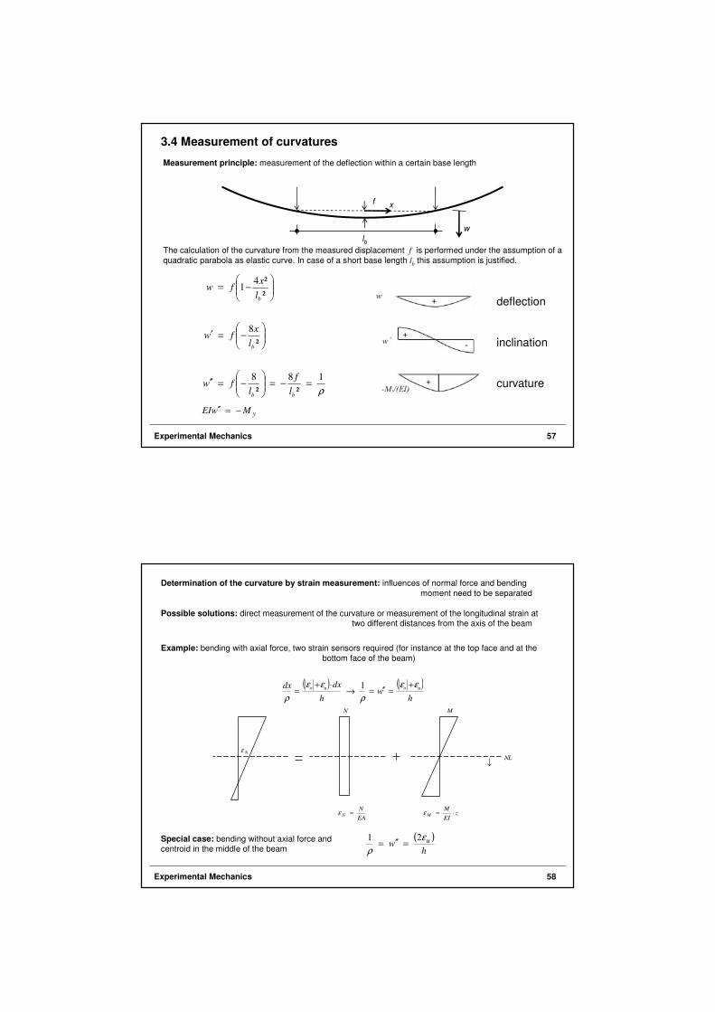
The calculation of the curvature from the measured displacement f is performed under the assumption of a
quadratic parabola as elastic curve. In case of a short base length lb
this assumption is justified.
ρ1
²
8
²
8
²
8
²
²41
=−=
−=′′
−=′
−=
bb
b
b
l
f
lfw
l
xfw
l
xfw
yMwEI −=′′
3.4 Measurement of curvatures
Measurement principle: measurement of the deflection within a certain base length
f
lb
x
w
inclination
deflection
curvature
Experimental Mechanics 58
Determination of the curvature by strain measurement: influences of normal force and bending
moment need to be separated
Possible solutions: direct measurement of the curvature or measurement of the longitudinal strain at two different distances from the axis of the beam
Example: bending with axial force, two strain sensors required (for instance at the top face and at the
bottom face of the beam)
↓
zEI
MM ⋅=ε
EA
NN =ε
Nε
M
NL
N
( ) ( )h
wh
dxdx uouo εε
ρ
εε
ρ
+=′′=→
⋅+=
1
Special case: bending without axial force and centroid in the middle of the beam
( )h
w uερ
21=′′=

Experimental Mechanics 59
Curvature-strain sensor by Quade: simultaneous measurement of the strain due to normal
force and of the curvature due to bending
object of measurement
object of
measurement
neutral axis
Experimental Mechanics 60
Curvature-strain sensor at the lower flange of a steel girder embedded in concrete

Experimental Mechanics 61
3.5. Measurement of strains
State of the art: electrical resistive strain gage
Measurement principle: measurement of the change in electric resistance of a conductor due to mechanical
strain; measurement of the resistance usually by a Wheatstone bridge circuit
Derivation:
²r
l
A
lR
⋅
⋅=
⋅=
πρρ
R ohmic resistance
l length of the conductor
ρ specific electric resistance
A cross-sectional area
rlR
rA
AlR
ln2lnlnlnln
ln2lnln
lnlnlnln
−−+=
+=
−+=
πρ
π
ρ
differentiated with
respect to R:
( )
r
dr
l
dl
R
dR
dR
dr
rdR
dl
l
dRdr
drrd
dRdl
dlld
dR
rd
dR
ld
RdR
Rd
2
12
1
ln2ln
ln2ln1ln
−=
−=
⋅
⋅−
⋅
⋅=
−==
A. C. Ruge with a specimen which was
instrumented with the first electrical strain gage
Experimental Mechanics 62
The elongation (strain) of the wire is accompanied by a change in diameter (Poisson's law).
l
dlµ
r
dr
l
lµµ
l
llql −=
∆−=−=
∆= εεε
µk
)µ(R
dR
)µ(l
dl
l
dlµ
l
dl
R
dR
21where
21
212
+=
+⋅=
+⋅=+=
ε
ε⋅=kR
dR ε strain
k sensitivity
The sensitivity k (also referred to as k-value) amounts to approximately 2 in case of metallic strain
gages; in case of semiconductor strain gages it amounts to approximately 150.
To be noted: The change of the electric resistance does not necessarily result from mechanical strain.
Temperature changes also cause variations of the resistance.

Experimental Mechanics 63
Carrier: made of non-conductive material, e.g. paper or plastics
Measuring grid: electric conductor, printed circuit or made of wire
Cover: insulating, protection against moisture and mechanical impact, preferably
made of silicone, sometimes additional protection against solar radiation required
(reflective cover)
Connections: used for the connection of wires by solder joints
Adhesive joint: connects the strain gage to the object of measurement, should be as thin as
possible, should not be hygroscopic, preferably epoxy resin
Strain gage applied to a structural member
Experimental Mechanics 64
c)

Experimental Mechanics 65
Wheatstone bridge circuit:
special case: bridge is balanced
unbalanced bridge due to the change
of resistances:
43
4
21
1
RR
R
RR
R
U
U
E
A
+−
+=
03
4
2
1 =→=E
A
U
U
R
R
R
R
4433
44
2211
11
RRRR
RR
RRRR
RR
U
U
E
A
∆++∆+
∆+−
∆++∆+
∆+=
:For 1<<∆
R
R
∆−
∆+
∆−
∆≈
4
4
3
3
2
2
1
1
4
1
R
R
R
R
R
R
R
R
U
U
E
A
( )4321
4εεεε −+−=
k
U
U
E
A
UA output voltage
UE excitation voltage
R1 ... R4 resistances
ε1 ... ε4 strains
k sensitivity
The “diagonal” resistance changes are
added, the “neighboring” resistance
changes are subtracted from each other.
Experimental Mechanics 66
a) half-bridge circuit: resistances of the cables are aligned with those of the strain gages
-> errors do to influences on cables and connectors
compensation of temperature:
application: in-situ measurement
b) full-bridge circuit: cable connections are outside the bridge circuit
-> influences of the cables may be neglected
compensation of temperature :
-> application: long-term measurements
Application types of the Wheatstone bridge circuit:
ε⋅= kU
U
E
A
0and 4321 ==−= εεεε
εεεεε =−==−= 4321
1, 3
2, 4
1
2ε⋅=
2
k
U
U
E
A

Experimental Mechanics 67
c) quarter-bridge circuit:
compensation of temperature is not possible
application: multi-channel measurement
excitation voltage must be constant
amplification of the measured
voltage required -> application of
alternating current (AC) useful
Because of the application of
alternating current (AC), the errors
due to the variation of resistances
at the contact points and due to
thermoelectric effects are smaller.
Carrier frequency amplifier:
14
εk
U
U
E
A =
1
excitation measured phase-dependent outputvoltage voltage demodulated signal signal
balancing
Experimental Mechanics 68
It must be considered:
required length of strain gages depends on the inhomogeneity of the material:
steel: comparatively short gages concrete: longer gages (up to 10 cm), recommended: three times maximum
aggregate size
accuracy of the measurement is higher if angles in a rosette are as different as possible:
isotropy: the directions of principal normal strains and principal normal stresses are identical
aaxyayaxa ϕϕτϕσϕσσ cossin2²sin²cos ⋅⋅+⋅+⋅=
aaxyayaxa ϕϕεϕεϕεε cossin2²sin²cos ⋅⋅+⋅+⋅=
aaxyayaxa ϕϕγϕεϕεε cossin²sin²cos ⋅⋅+⋅+⋅=
⋅
⋅
⋅
=
xy
y
x
cccc
bbbb
aaaa
c
b
a
γ
ε
ε
ϕϕϕϕ
ϕϕϕϕ
ϕϕϕϕ
ε
ε
ε
cossin²sin²cos
cossin²sin²cos
cossin²sin²cos
°⋅°⋅°⋅ 1202/602/452
precondition: angles φa, φb and φc are not identical
aσ
yσ
xσ
xyτyxτ
aτ aϕ

Experimental Mechanics 69
stresses are independent of the material (equilibrium of external and internal forces)
Principal normal stresses:
Principal shear stresses:
Plane state of stress:
yx
xy
σσ
τϕ
−=
22tan
2/1
²4)²(2
12/1 xyyx τσστ +−±=
²4)²(2
1
22/1 xyyx
yx τσσσσ
σ +−±+
=
−−
=
xy
y
x
xy
y
xE
γ
ε
ε
µ
µ
µ
µτ
σ
σ
)1(2
100
01
01
²1
0)90()(
)90(
)(
11
12
11
=°+=
→°+=
→=
ϕτϕτ
ϕσσ
ϕσσ
Minimum
Maximum
Extremum→°± )( 451ϕτ
Experimental Mechanics 70
Advantages of the electrical strain gages:
applicable for multi-channel measurements (multiplexing)
high sensitivity
low space requirements for application
low mass
direct contact to the object of measurement
applicable for static and dynamic measurements
easy compensation of temperature variations
measurements at high (up to 800°C) and low temperatures possible
Drawbacks of the electrical strain gages:
in case of outdoor measurements or when embedding the gages in concrete: protection against moisture is required
strain gage may be damaged by cracking of the object of measurement
Application of electrical strain gages in load cells:
( )43214
1εεεε −+−⋅⋅⋅= kUU EA lql εµεεεεεε ⋅−===== 4231 andwith
( ) ( )µεεµεεµε 224
1
4
1+⋅⋅⋅⋅=⋅++⋅+⋅⋅⋅= lEllllEA kUkUU
( ) ElA UkU ⋅⋅⋅+⋅= εµ12
1

Experimental Mechanics 71
3.6 Measurement of forces
Forces may only be determined by measuring their effects.
Effects of forces:
mechanical effects: deformations
accelerations
hydrostatic pressure
electrical effects: electric charge
Requirements:
- load cells should be incorporated in the mechanical system without influencing it, i.e., they
should be comparatively stiff
- forces should be measurable with: - small hysteresis
- small amount of mechanical work
- small creep effects
- sufficient long-term stability
Experimental Mechanics 72
Mechanical force measurement
a) Spring force meter (spring dynamometer)
Principle: - utilization of the elastic deformation of steel springs having a spring constant K
- measurement of the displacement f caused by the force F
K
Ff =
Tension spring force meter
a) with coil spring small forces up to 1 kN
b) with coil springs in a light metal casing
c) with flat springin a metal casing forforces up to 250 kN
light metal casing
fixed beam
spring
tension spring
guiding rod
toothed rack
movable beam

Experimental Mechanics 73
b) Force measuring ring
Force measuring rings
a) tension and compression force measuring device with dial gauge (ring-shaped)
b) tension and compression measuring device (yoke-shaped)
c) 2,5 kN compression measuring ring (type Wazau)
Measurement principle: utilization of the elastic deformation of a ring- or yoke-shaped spring element
made of steel
measurement of the deflection by using a displacement transducer
(e.g. dial gauge or LVDT)
yoke
Experimental Mechanics 74
Force measurement by using electrical load cells
Principle: deformation of a solid body is measured by using electrical strain gages; load cell must be as rigid as possible; sensitive strain gages required (semiconductors); full-bridge circuit for compensating temperature influence
Electrical load cells
a) compression force load cell
b) tensile force sensor
c) bending membrane sensor
casing
end plate
hollow cylinder

Experimental Mechanics 75
Force measurement by using vibrating wires
Vibrating wire gage for the measurement of forces in reinforcing bars
Hydraulic stress sensor
Principle: increase of the pressure in the outer circuit by using a pump until the pressure is equal to the
pressure in the embedded cushion
opening of the membrane valve in the sensor box, liquid starts to flow from the pump to the tank without further pressure increase
pressure at the manometer is equal to the vertical compressive stress in the object of
measurement
Experimental Mechanics 76

Experimental Mechanics 77
Pendulum manometer
used in mechanical testing machines
Principle: the tangent of the inclination angle
corresponds to the hydraulic pressure
back-pressure valve prevents sudden
swing back
Application: limited to the case of low testing velocities
due to the low natural frequency of the
pendulum
oil pressure from the
actuator of the testing
machine
piston
Experimental Mechanics 78
Bourdon gage
Principle: tubular curved spring bends under the
action of increasing internal pressure
and moves a pointer
casing

Experimental Mechanics 79
3.7 Measurement of vibrations
Piezoelectric acceleration sensors
Types of acceleration sensors
prestressing jacket
Experimental Mechanics 80
Piezoelectric acceleration sensors
Since the seismic weight is constant, a force which is proportional to the
acceleration (F = m·a) is acting on the piezoelectric measuring element.
Piezoelectric acceleration sensors consist of a casing, the piezoelectric
measuring element, and seismic weights.
Experimental Mechanics 81
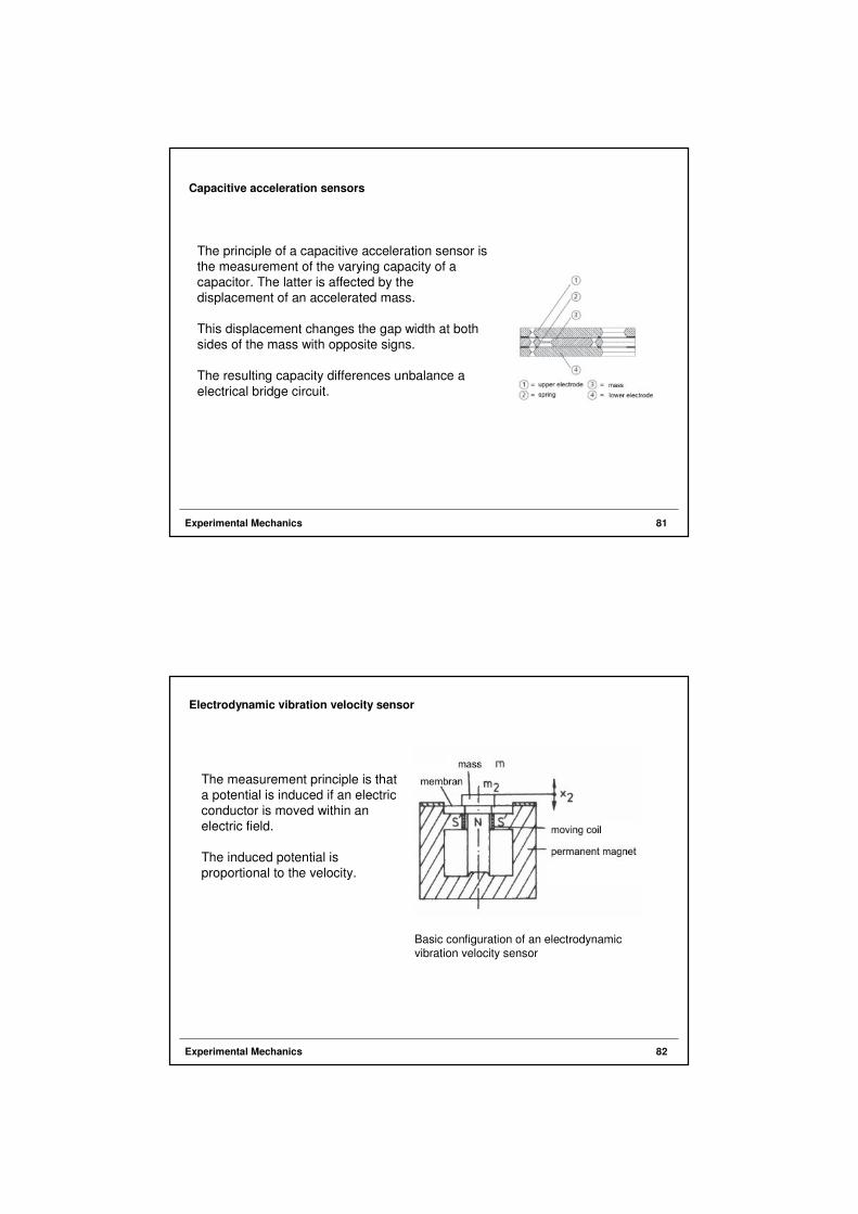
Capacitive acceleration sensors
The principle of a capacitive acceleration sensor is
the measurement of the varying capacity of a
capacitor. The latter is affected by the
displacement of an accelerated mass.
This displacement changes the gap width at both
sides of the mass with opposite signs.
The resulting capacity differences unbalance a
electrical bridge circuit.
Experimental Mechanics 82
Basic configuration of an electrodynamicvibration velocity sensor
The measurement principle is that
a potential is induced if an electric
conductor is moved within an
electric field.
The induced potential is
proportional to the velocity.
Electrodynamic vibration velocity sensor

Experimental Mechanics 83
4. Model tests
4.1 Introduction
Model: scaled copy of the original; in mechanics used for gaining information on the mechanical behavior of the original structure
Applications of models:
• for the conception of structural systems in case reliable analytical modeling can not be guaranteed
• for studying details of structures, especially where static of geometric discontinuities occur (not easy to simulate with analytical models)
• for investigating the origins of structural faults
• for demonstrations in engineering education
Principle: linking the model test and the theoretical analysis (calculation); comparison of the results obtained in the calculation to those of the test
Experimental Mechanics 84
Advantages:
laboratory experiments require less effort than load tests at the original structure and may be performed under suitable conditions (no environmental influences)
some effects concerning the mechanical behavior of structures will occur in a more pronounced way
idealizing assumptions like in the analytical model are not required
Fields of application:
model tests in case of elastic material behavior: application to complex geometrical structures; for stability problems, for dynamic processes, and for teaching
model tests with real materials characterized non-linear deformations and damage processes including cracking, plasticization, bond failure
Hybrid technique:
experimental and analytical techniques are combined

Experimental Mechanics 85
4.2 Introduction to similarity mechanics
4.2.1 The principle of physical similarity
Physical processes will proceed similarly under similar influences and in similar geometric systems.
Application in the mechanics:
Mechanical processes in the original (H) and in the model (M) proceed similarly if they may be described by the same physical model.
4.2.2 Scales
Scale GV : ratio of a quantity GM measurable at the model and the equally named quantity GH
at the original
Equally named quantities:
quantities with the same name, the same physical meaning and same dimension in the original and in the model (e.g. lengths, displacements, etc.)
H
MV
G
GG =
Experimental Mechanics 86
a) Reference scales (basic quantities of the SI-System)
reference scales for mechanical model tests:
Length:
Force:
Time:
Temperature:
-> in case the reference scales constant, we have rigorous mechanical similarity
rigorous geometric similarity in all three directions:
rigorous force similarity:
rigorous time similarity:
rigorous kinematic similarity:
rigorous static similarity:
rigorous dynamic similarity:
H
MV
H
MV
H
MV
H
MV
T
TT
t
tt
F
FF
l
ll
=
=
=
=
.lV const=
const.=VF
const.=Vt
const.andconst == VV t.l
.Fl VV constandconst. ==
const.andconst.andconst. === VVV tFl

Experimental Mechanics 87
b) Derived scales
Precondition: rigorous similarity
Velocity:
Moment:
Stress:
Weight density:
Strain:
c) Scales of material properties
Young's modulus:
Poisson's ratio:
Density:
1/
/
²/
/
/
/
=∆
=∆
∆==
⋅=⋅
⋅==
====
⋅=⋅
⋅==
===
V
V
HH
MM
H
MV
VV
HH
MM
H
MV
V
V
V
V
HH
MM
H
MV
VV
HH
MM
H
MV
V
V
HH
MM
H
MV
l
l
ll
ll
gg
g
l
F
A
F
AF
AF
lFlF
lF
M
MM
t
l
tl
tl
v
vv
εε
ε
ρρρ
γγ
γ
σσ
σ
H
MV
H
MV
H
MV
E
EE
ρρ
ρ
µµ
µ
=
=
=
Experimental Mechanics 88
4.2.3 Model laws
• describe the relations between quantities in M and H
• allow to design models with respect to size, material, loads, measurement method and range of expected measurement results
Example 1: Bending of a beam due to a distributed load
Elastic curve (deflections) and resulting internal forces are to be determined.
l
p
b … width
12
3bh
I =

Experimental Mechanics 89
The differential equation of the elastic curve is presented for both M and H. Then, the quotient is
formed in order to obtain a dimensionless equations.
4
4
4
44
4
4
4
4
4
V
v
H
H
HV
M
H
H
M
M
l
w
dx
wd
dxl
wd
dx
wd
dx
wd
=⋅
=
H
M
H
HHH
M
M
MM
p
p
dx
wdIE
dx
wdIE
′
′=
⋅
⋅
4
4
4
4
bppdx
wdIE ⋅=′=⋅
4
4
and in case of rigorous geometric similarity in all three directions (bV=h
V=l
V)
³3
3
VV
HH
MMV
H
MV hb
hb
hbI
E
EE ⋅=
⋅
⋅== andwith
and the relation of the differential quotients
( )
V
H
H
H
HV
H
H
H
HV
H
H
H
M
w
dx
wd
dx
wdw
dx
wd
dx
wwd
dx
wd
dx
wd
=
⋅
=
⋅
=
4
4
4
4
4
4
4
4
4
4
4
4
todue
H
MVVV
x
xllI == andwith 4
Experimental Mechanics 90
yields:
In case of rigorous geometric similarity: wV
= lV
, i.e., the ratio of the deflections in M and H
is equal to the length scale.
Then,
In case a single load is adopted instead of the distributed load p, yields
The internal forces may be obtained by:
Transformation of the results to the original H:
VVVV
HH
MM
H
MV lppb
pb
pb
p
pp ⋅=⋅=
⋅
⋅=
′
′=′
VVVV
V
VVV wElp
l
wlE ⋅=⋅=⋅
4
4
1und1 =
==
=
VV
V
VV
V
p
E
p
E
l
w
l
w
VVVVV FQlFM =⋅=u n d
V
MH
VV
MH
V
MH
F
lF
MM
l
ww =
⋅==
u n du n d
dxbpF ∫ ⋅=
Hooke's model law
2
VVV lpF ⋅=
and
and
1²
=⋅
VV
V
lE
F
and
and and

Experimental Mechanics 91
The differential equation for the deflection w(x,y) of an isotropic thin plate is:
The flexural rigidity of a plate is rigorously similar only in case:
For the internal moments:
For the shear forces:
Example 2: Bending of a plate
py
w
yx
w
x
wKwK =
∂
∂+
∂∂
∂+
∂
∂=∆∆⋅
4
44
4
4
²²2
²)1(12
³
µ−
⋅=
hEK
1=Vµ Poisson's model law
VxyVVyVVxV FmFmFm ===u n du n d
V
VyV
V
VxV
l
Fq
l
Fq == und
differential equation of the thin plate
Experimental Mechanics 92
4.3 Model materials
4.3.1 Characteristics
The selection of a material for a model test depends on the objective of the investigation:
The model should represent the behavior of the original as realistic as possible.
The model has to be producible with the required accuracy concerning size and shape.
The model material must exhibit sufficient deformability in order to allow for measureable deformations under comparatively small loads.
Precondition: The properties of the model material (e.g. Young's modulus, stress-strain-
curve, Poisson's ratio, creep and temperature behavior) must be known.
Examples for model materials:
metals
mineral materials
plastics

Experimental Mechanics 93
4.3.2 Metals
Characteristics: - distinctive elastic behavior up to the yield limit
- small creep deformations
Advantage of aluminum: for measurable deformations, smaller stresses are required when
compared to steel (Ealu
= 1/3 Esteel
)
4.3.3 Mineral materialsGlass: - ideal-elastic and no creep
- mirror effect: utilization for optical measurement methods
- high risk of brittle fracture
Gypsum: - hygroscopic and brittle with low fracture strain
- moldable (almost arbitrary shapes may be obtained)
- reinforcement of gypsum by using thin wires -> simulation of reinforced concrete
- short hardening period
Fine-grain concrete: - simulation of the load-carrying behavior of (un-)reinforced concrete members
- maximum aggregate size approximately 7 mm
Polymeric concrete: - faster hardening when compared to cement-based concrete
- high tensile strength
- strength and deformations strongly depend on temperature
Experimental Mechanics 94
4.3.4 Plastics
For instance polyvinyl chloride, polycarbonate, polyester resin, epoxy resin
Characteristics: - low Young's module -> even low stresses result into measurable deformations
- Young's module depends on temperature
- higher Poisson's ratio when compared to metals- good workability
- low thermal conductivity (unintentional occurrence of temperature gradients)
- photoelastic effect: optically isotropic when unloaded; optically anisotropic due to
- mechanical stresses
time-dependent deformation
in case of cyclic loading
σ is constant

Experimental Mechanics 95
4.4 Optical measurement methods in model tests
4.4.1 Photoelasticity
Physical effect: some transparent materials such as epoxy resin are birefringent (double refracting) under mechanical load:
- in each direction of refraction different velocities of light propagation - the directions of principal normal stress and refraction are identical
a) Stress-optical bench
Setup: light source, pair of filters (polarizer and analyzer), model located between the filters
Effect: The light emitted from the source „oscillates“ in all directions.
The first filter (polarizer) allows just one oscillation direction to pass.
The polarized light A0 is refracted in the model in a way that the new oscillation directions
correspond to the directions of the principal normal stresses.
The resulting components A1 and A2 pass the model with different velocity. Hence, an
optical path difference s occurs.
The elliptically polarized light reaches the analyzer which is rotated by 90° with respect to the
polarizer. It allows only the corresponding components A‘1 and A‘2 to pass. These two
components have always the same absolute value.
∆
Experimental Mechanics 96
principal normal stresses σ1 and σ2

Experimental Mechanics 97
Generation of isoclines
Isochromates: - lines of the same color or of the same brightness in case of monochromatic light
- correspond to lines of the same difference between the principal normal stresses
- according to the optical path difference, the horizontal components interfere:
● s is equal to zero or equal to an integer multiple of the wave length -> cancellation
● accordingly: s is equal to one half of the wave length -> maximum brightening
- isoclines may be eliminated by additional filters
Isoclines: - lines of the same orientation of the principal normal stresses
- result from the coincidence of the directions of polarization and principal normal stress
- allow the determination of the principal stress trajectories
∆∆
cancellation
Experimental Mechanics 98
( ) dtvvs ⋅−=∆ 21td = runtime of the light through the unloaded model
d = thickness of the model
v1, v2 = velocity of the components A1 and A2 , respectively
v0 = velocity of the light in the unloaded model
( ) ( )
( )
0
2112
2112
121212
2211122112
0
1212
12212
22111
v
d)()kk(s
)()kk(
)(k)(k
kkkkvv
v
dvvtvvs
kkv
kkv
d
⋅−⋅−=∆
−⋅−=
−⋅+−⋅=
⋅−⋅−⋅+⋅=−
⋅−=⋅−=∆
⋅+⋅=
⋅+⋅=
σσ
σσ
σσσσ
σσσσ
σσ
σσ
(Brewster's law)
0v
dtd =

Experimental Mechanics 99
)kk(
vS
dS
)kk(d
v)(
v
d)()kk(
s
12
0
12
0
21
0
2112
−
⋅=⋅=
−⋅
⋅⋅=−
⋅−⋅−=⋅
⋅=∆
λδλδσσ
σσλδ
λδ
with
S = stress-optical constant
= order of the isochromate
cancellation at (δ = 0; 1 ; 2 …) and amplification at (δ = 1/2; 3/2; 5/2 …)
δ
Experimental Mechanics 100
Result of a measurement at the stress-optical bench: Investigation of the plane state of stress, stress
concentrations at the points of geometric discontinuity may be studied.
Principal stress trajectories in a notched beam

Experimental Mechanics 101
b) Surface photoelasticity
Application: investigation of non-transparent M or H objects of measurement, e.g. of objects made
of concrete or metal
Principle: application of a double-refracting layer on the surface of the test object, for instance by gluing a
film to the surface (underneath the film will be a reflective layer)
measurement of the principal normal stress difference und of the principal normal stress
directions by using a reflection polariscope
L light source
P polarizer
A analyzer
V quarter-wave plate
F film
SP,K mirror with
adhesive layer
HSP semipermeable
mirror
Different lighting techniques
Experimental Mechanics 102
4.4.2 Moiré technique
Principle: Moiré effects arise from the superposition of a deformed grid with an undeformed reference grid
a) Moiré of rotated patterns b) Moiré of parallel patterns
Applications: determination of strains or in-plane inclinations in plane surfaces
determination of deflections and out-of-plane inclinations of curved surfaces
Experimental Mechanics 103
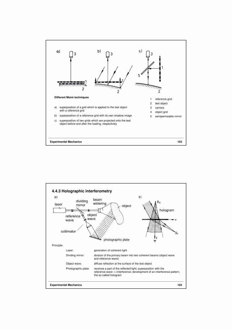
1 reference grid
2 test object
3 camera
4 object grid
5 semipermeable mirror
Different Moiré techniques
a) superposition of a grid which is applied to the test object
with a reference grid
b) superposition of a reference grid with its own shadow image
c) superposition of two grids which are projected onto the test object before and after the loading, respectively
Experimental Mechanics 104
4.4.3 Holographic interferometry
Principle:
Laser: generation of coherent light
Dividing mirror: division of the primary beam into two coherent beams (object wave
and reference wave)
Object wave: diffuse reflection at the surface of the test object
Photographic plate: receives a part of the reflected light; superposition with the
reference wave -> interference; development of an interference pattern,
the so-called hologram
photographic plate

Experimental Mechanics 105
5. Non-destructive testing in civil engineering
Content:
5.1 Rebar locator (electromagnetic)
5.2 Pulsed radar
5.3 Radiography
5.4 Corrosion monitoring / Potential field measurement
5.5 Ultrasonic testing
5.6 Impact-echo method
5.7 Acoustic emission analysis
5.8 Infrared thermography
Significance of the concrete covering:
A sufficiently dense and thick concrete cover is one of the most important preconditions for the durability of reinforced concrete structures.
The requirements are specified in DIN 1045 under consideration of the environmental conditions.
The analysis of damage patterns at concrete members reveals that inadequate concrete cover along with incorrect curing is the predominant reason for these damages.
Guidelines for the planning and implementation of the reinforcement as well as for the quality assurance are given in the recommendation Betondeckung und
Bewehrung (“Concrete cover and reinforcement”) of the DBV (Deutscher
Beton- und Bautechnik-Verein e.V.), a German association for structural engineering.
Furthermore, the measurement of the concrete cover and the statistical evaluation of the results is regulated.
Experimental Mechanics 106
5.1 Rebar locator (electromagnetic)

Experimental Mechanics 107
Measurement principles of magnetic methods
Unidirectional magnetic field
• The simplest instrument is a permanent magnet, which is
moved over the concrete surface. The detection depth can
be estimated by using a reference specimen with known
concrete cover. This depth is usually below 20 mm.
• It is also possible to measure the attracting force between
the permanent magnet and the reinforcing steel.
• The calibration has to be conducted for the each
reinforcement diameter separately.
Experimental Mechanics 108
Alternating magnetic field
• The measurement concept is based on the principle of a
transformer: an alternating (AC) current in a primary coil
induces a voltage in a secondary coil.
• The magnitude of the induced voltage depends on the
amount and on the proximity of magnetizable material. After
calibration in an nonferrous environment, the change of the
induced voltage may be measured accurately by using a
bridge circuit and the distance to a reinforcement bar with
known diameter may be determined.

Experimental Mechanics 109
Concept of the concrete cover measurement by using an alternating
magnetic field which is influenced by the steel reinforcement
AC
Experimental Mechanics 110
Eddy current
• Techniques based on eddy current differ from methods
based on alternating fields only by the strength of the
generated magnetic field.
• In case of non-magnetic reinforcement (e.g. stainless steel),
only the eddy current technique allows to detect the
reinforcement and to measure the concrete cover. The
measurement effect results from the formation and damping
of an alternating current in an electrically conducting
material.
• In principle, it is possible to determine reinforcement
diameter and concrete cover by detecting the real and the
imaginary part of the complex impedance Z. However,
currently no such instrument is offered on the market.

Commercial rebar locators are based on the application of alternating
magnetic fields or on the eddy current method with pulse induction. Only
the eddy current method allows to detect stainless steel.
Modern devices are coupled with a path measurement and allow linear
or planar presentation of the results similar to radar methods. Their
major field of application is the measurement of the concrete cover.
Statistical evaluation, e.g. according to the aforementioned DBV
recommendation, is usually implemented in the software. The accuracy
strongly depends on the diameter of the reinforcement.
The devices are calibrated for the detection of reinforcement and can not
distinguish between steel bars and other metallic inclusions.
Experimental Mechanics 111
Rebar locators based on inductive techniques
Experimental Mechanics 112
• maximum detection depth ranges from 10 cm to 18 cm
• precise determination of the reinforcement position; localization problems may occur in case of close meshes (spacing < 10 cm)
• concrete cover up to 50 mm ± 1 mm for single rebars in case of known rebar diameter; reduced accuracy for close and multilayered reinforcement as well as for large concrete cover
• identification of individual rebars possible if spacing is larger than diameter
• determination of diameters nearly impossible or only with high uncertainty
• inclined rebars detectable in case of a planar presentation
• interpretation of the results difficult at overlapping reinforcement meshes
Rebar locators based on inductive techniques
Summary of performance parameters

Experimental Mechanics 113
Commercially available instruments
Imaging rebar locator (path measurement)
Experimental Mechanics 114

Measurement range
and accuracy
as specified by the
manufacturer
Experimental Mechanics 115
Measurement range and accuracy
(comparative study)
Experimental Mechanics 116

Representation of results as line scan with preset target
concrete cover
Experimental Mechanics 117
Area scan
Experimental Mechanics 118

Area scan
Ceiling at the support
with bent-up bars
Experimental Mechanics 119
Line scan of a concrete wall with irregular concrete cover
Experimental Mechanics 120

Experimental Mechanics 121
Example: Measurement of the concrete cover at a bridge
Experimental Mechanics 122
Example: Measurement of the concrete cover at a bridge

Experimental Mechanics 123
5.2 Pulsed radar
Applications:
• Localization of inclusions in concrete (e.g. reinforcement,
tendon ducts, anchors, dowels)
• Investigation of layers (thickness, inhomogeneities)
• Detection of imperfections and damages (e.g. detachments,
hollow spaces)
• Detection of objects in soils (foundations, tanks, pipelines)
• Screening of material properties (moisture content, salt
content, homogeneity)
Basics
• Radar is a general term for electromagnetic waves in the
frequency range between 106 Hz and 1010 Hz.
• In the case of pulsed radar, short electromagnetic pulses are
emitted. The mean frequencies are ranging from 20 MHz to
approximately 2 GHz.
• The measurement principle is based on the propagation law for
electromagnetic waves. Relevant material properties are the
electrical conductivity б and the relative dielectric constant εr .
• For the detection of steel reinforcement, antennas with a
frequency range from 1 GHz to 2 GHz are commonly used. With
these antennas, an inspection depth of approximately 0,5 m is
achieved in concrete.
Experimental Mechanics 124

oz
o
r
ezc
tEtz ÊEαε −
−= 0),(
Experimental Mechanics 125
With the radar method, the time-dependent electric field is measured
and evaluated.
The propagation of electromagnetic waves is described by the
Maxwell equation. In the case of structural materials, a number of
simplifications may be made. The relative magnetic permeability
may be set to µ r ≈ 1. The conductivity б is rather small, hence the
loss angle is also small.
In that case, the electric field may be described as plane
wave impulse for a linear polarization.),( tzE
2
0 tcs
r
⋅=ε
with: co velocity of light in the vacuumεr relative dielectric constant of the material
α absorption factor
Then, the propagation velocity v is
and the depth s of a reflector:
When the wave hits an interface between two materials, a reflected and a transmitted wave are formed. The reflection coefficient r depends on the angle and on the polarization of the incoming wave. In case of perpendicular
approach:
ε r
cv 0=
εεεε
21
21
rr
rrr+
−=
Experimental Mechanics 126

Experimental Mechanics 127
The depth d of a reflector may be determined approximately on the basis of the
runtime t and of the mean propagation velocity v.
Experimental Mechanics 128
Formation of
reflection hyperbolas

Experimental Mechanics 129
Transmission method
Experimental Mechanics 130
Reflection characteristics, formation of radar images
Simplifying, real impedances may be assumed for dry non-conducting
materials. The reflection factor depends on the difference between the
relative dielectricity constants and the conductivities.

Experimental Mechanics 131
Reinforcement detection
Positioning of a linearly polarized send-receive dipole (SE) lateral to the direction of movement (arrow)
- objects that are aligned parallel to the dipole (black) are easy to detect
- objects that are perpendicular to the dipole (gray) are hardly detectable
Reinforcement bars are detectable with maximum intensity if their orientation is perpendicular to the direction of the antenna's movement.
Detection of different materials
on the basis of the
phase shift
Experimental Mechanics 132

Detection of reinforcement layers and determination of wall thicknesses
Experimental Mechanics 133
Area scans by combining x- and y-traces
Experimental Mechanics 134
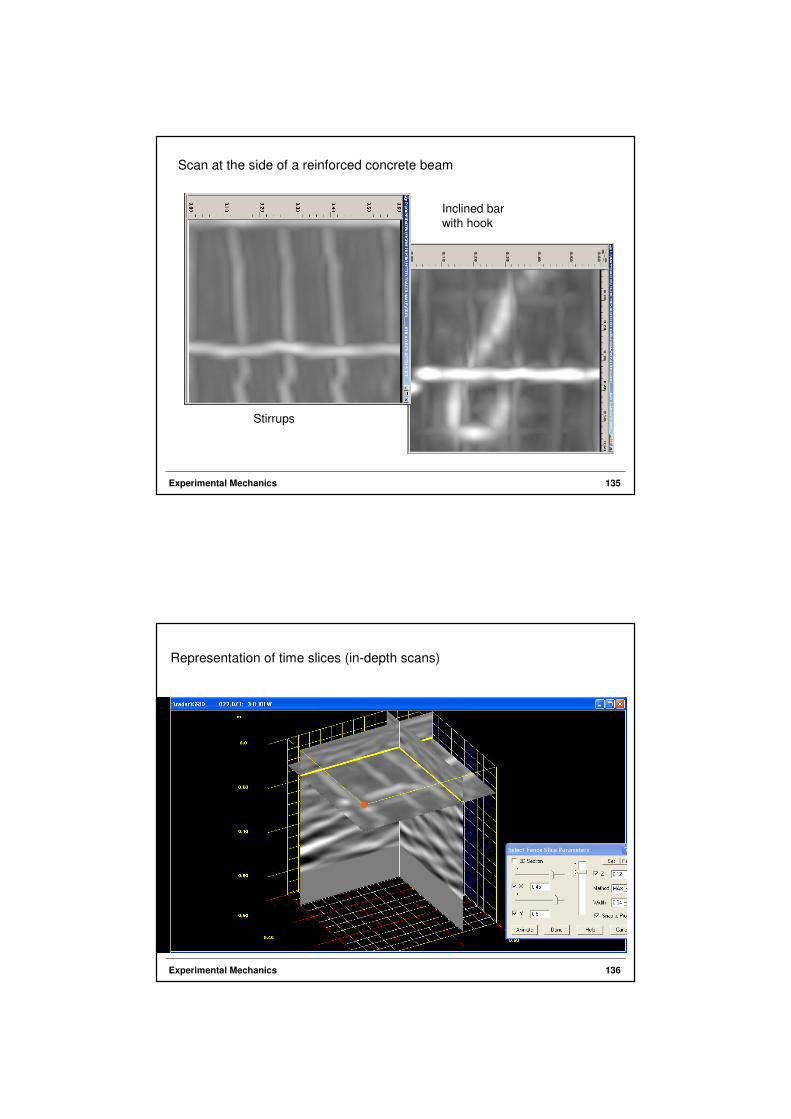
Scan at the side of a reinforced concrete beam
Stirrups
Inclined bar
with hook
Experimental Mechanics 135
Representation of time slices (in-depth scans)
Experimental Mechanics 136

Experimental Mechanics 137
Advantages of pulsed radar:
– larger depth range
– reliable detection of stainless
steel
– non-metallic reflectors are
detectable as well
– quick and comprehensive
scans with large information
content
Advantages of pulsed radar:
– larger depth range
– reliable detection of stainless
steel
– non-metallic reflectors are
detectable as well
– quick and comprehensive
scans with large information
content
Advantages of rebar locators:
– concrete cover measurement
more accurate
– low price
– simple handling
Advantages of rebar locators:
– concrete cover measurement
more accurate
– low price
– simple handling
Disadvantages of both techniques:
• determination of bar diameters inaccurate or impossible
• errors in case of close rebar spacing
Disadvantages of both techniques:Disadvantages of both techniques:
• determination of bar diameters inaccurate or impossible
• errors in case of close rebar spacing
Comparison of pulsed radar and rebar locator
Experimental Mechanics 138
Application
• detection of reinforcement steel• detection of imbedded objects• measurement of layer thicknesses

Detection of the upper reinforcement of a reinforced concrete beam
Experimental Mechanics 139
Beam
Beam
Column
Column
Experimental Mechanics 140
Identification of the structure of a slab
Steel beam
Masonry
Concrete

Detection of stirrups and inclined bars
Experimental Mechanics 141
Column
Column
Detection of stirrups
Experimental Mechanics 142

Radar scan of a floor wall, comparison of different sampling rates
Experimental Mechanics 143
Comparison of radar and electromagnetic rebar locators
at the example of a floor wall
Experimental Mechanics 144

Floor wall, Ferroscan analysis with software
Experimental Mechanics 145
Floor wall, radar line scan, determination of thickness
Experimental Mechanics 146

Experimental Mechanics 147
For comparison: ultrasonic measurement of wall thickness
Experimental Mechanics 148
Example: road construction
Determination of the layer thicknesses by using a horn antenna

Possible results
Experimental Mechanics 149
Experimental Mechanics 150
Screening of railway ballast
mobile measuring device
for the screening of
rail track gravel

Tendencies for the
development
of measurement
instruments
Experimental Mechanics 151
Experimental Mechanics 152
5.3 Radiography using x-ray and gamma radiation
Scope of application:
• Testing of welded joints
• Determination of position, number, and diameter of the
reinforcement, even in case of complex geometry
• Localization of installation parts
• Diagnosis of damages
• Determination of grouting defects
• Detection of voids and compaction defects

Experimental Mechanics 153
Experimental Mechanics 154
Principle of a transport and operation container for isotopic sources
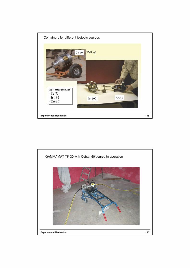
Containers for different isotopic sources
Experimental Mechanics 155
GAMMAMAT TK 30 with Cobalt-60 source in operation
Experimental Mechanics 156

Detection of the reinforcement of a concrete beam
Experimental Mechanics 157
Generation of x-radiation
x-ray tube
Experimental Mechanics 158

Energy spectrum of
x-radiation
Experimental Mechanics 159
X-ray tube
Experimental Mechanics 160

Betatron (accelerator)
Experimental Mechanics 161
Applications
Experimental Mechanics 162

Experimental Mechanics 163
Applications
Experimental Mechanics 164
Applications

Experimental Mechanics 165
testing device and
radiation energy
maximumconcrete thickness
[cm]
exposure timein case of 30 cm concrete and
1 m distance, D8 film
x-ray tube 200 keV 25-30 ca. 30 min
Cobalt-60 1,2 MeV 45-50 ca. 5 min
MegascanTM 7,5 MeV [1] 150 ca. 0,3 min
Comparison of various radiation sources
Experimental Mechanics 166
Application to reinforced concrete structures
Q Q Q'
radiographic inspection double exposure
concept of the radiography
Q - sourced - reinforcement diameter
b - concrete cover (up to rebar center)d' - rebar width on the filmV - displacement
a - distance between source and film
d
bd
x-ray filmd = (a-b) d' / ab =
a V
q+ V
Principle of the detection of reinforcement using radiographic tests

Application principle of radiography to detect reinforcement
Experimental Mechanics 167
Gammaquelle
image on x-ray film
Drill hole radiography
gamma source
Lateral transmission
image on x-ray film
Significant areas for the reinforcement detection in a beam
Experimental Mechanics 168

Example: Beam
Experimental Mechanics 169
Example: Bridge
Experimental Mechanics 170

Example: Beam
Experimental Mechanics 171
Example: Beam
Experimental Mechanics 172

Radiogram of a tendon duct
Experimental Mechanics 173
Radiogram of a concrete slab
Experimental Mechanics 174

Formation of concrete cracks in a slender prestressed beam
Experimental Mechanics 175
Defective reinforcement in a suspender beam
Experimental Mechanics 176

Defective reinforcement (stirrups)
Experimental Mechanics 177
Experimental Mechanics 178
5.4 Corrosion monitoring / Potential field measurement
For the purpose of concrete maintenance, usually the following inspections are required:
- determination of the carbonation depth
- determination of the chloride content (depth profile)
- determination of the concrete cover
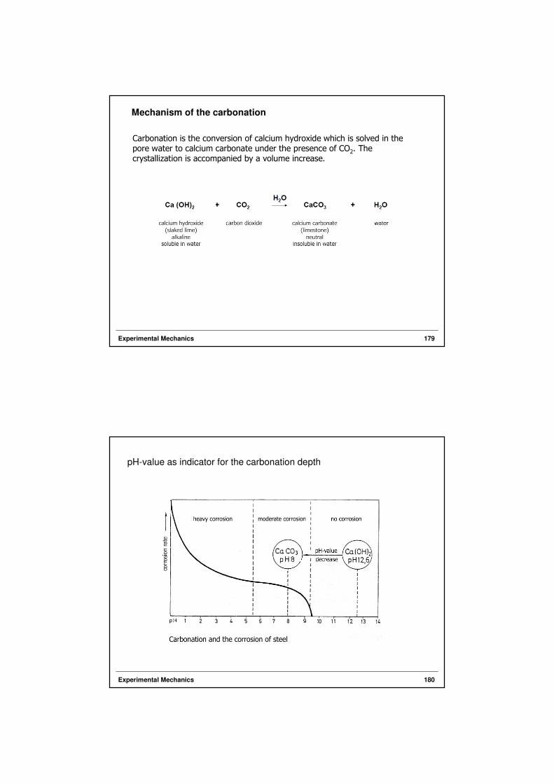
Mechanism of the carbonation
Carbonation is the conversion of calcium hydroxide which is solved in the pore water to calcium carbonate under the presence of CO2. The crystallization is accompanied by a volume increase.
Experimental Mechanics 179
Experimental Mechanics 180
pH-value as indicator for the carbonation depth

Experimental Mechanics 181
a) beginning carbonation without steel corrosion (not detectable by visual
inspection or tapping the concrete surface)
b) advanced carbonation with steel corrosion (visible or detectable by tapping the concrete surface)
Progression of carbonation and subsequent corrosion of reinforcement
• The severest carbonation occurs in rooms which are continually
dry. However, the corrosion protection is given by the lack of
moisture.
• Concrete which is always stored in water is not affected by
carbonation. Corrosion protection is given due to the lack of
oxygen.
Experimental Mechanics 182
K … carbonationR … corrosion

Carbonation rate
Experimental Mechanics 183
Experimental Mechanics 184
Determination of the chloride content
- direct addition of chlorine (hardening accelerator) has been prohibited in Germany for about 30 years
- only free ions induce corrosion; but the total chloride content is determined
• allowable limit values: (chloride content by mass in relation to the cement)
plain concrete 1,0 %
reinforced concrete 0,4 %prestressed concrete 0,2 %
- distinction between the critical chloride content, which causes a depassivation of the steel surface, and
- the chloride content, which leads to corrosion phenomena classified as damage
• best evaluation criterion is the Cl-/OH- ratio, but there is no in-situ
measurement method
• the total chloride content is determined quantitatively by the acid digestation of concrete flour and the subsequent potentiometric titration using a silver nitrate solution (DAfStb Heft 401)

Experimental Mechanics 185
Principle of the chloride corrosion
Experimental Mechanics 186
Corrosion in cracks
rust
Experimental Mechanics 187
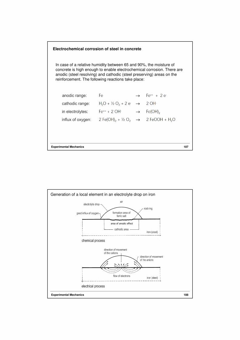
Electrochemical corrosion of steel in concrete
In case of a relative humidity between 65 and 90%, the moisture of
concrete is high enough to enable electrochemical corrosion. There are
anodic (steel resolving) and cathodic (steel preserving) areas on the
reinforcement. The following reactions take place:
Generation of a local element in an electrolyte drop on iron
Experimental Mechanics 188
area of anodic effect

Experimental Mechanics 189
Electrochemical corrosion
of steel in concrete
Experimental Mechanics 190
Basics of potential field measurement
• The electrochemical potential field measurement is a method to
evaluate the corrosion state of the reinforcement.
• The potential difference is measured between the reinforcement
steel and a reference electrode on the concrete's surface.
• Various reference electrodes are common, for instance:
- copper electrode in a solution of copper sulphate
- silver / silver chloride electrode in a solution of potassium
chloride 0,5 mol/l
• The corrosion potential depends on the electrode.
• The inspection of the structures is non-destructive and may be
performed comprehensively.
Experimental Mechanics 191
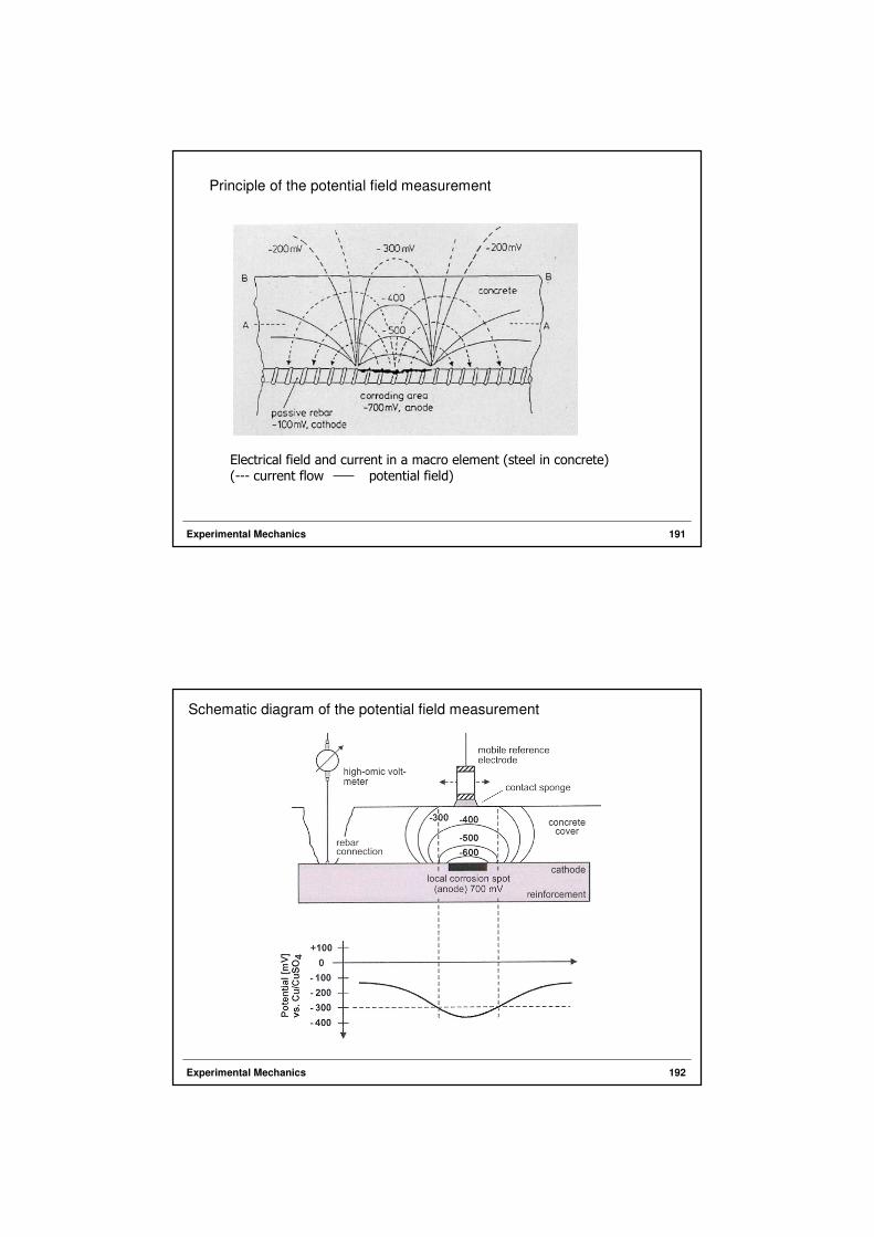
Principle of the potential field measurement
Electrical field and current in a macro element (steel in concrete)
(--- current flow potential field)
Experimental Mechanics 192
Schematic diagram of the potential field measurement

Layout of a measuring electrode
Cu/CuSO4 – half cell with
typical potential range
Experimental Mechanics 193
Local corrosion spots, in particular in case of chloride induced corrosion, may cause the formation of distinctive potential peaks.
Experimental Mechanics 194
Experimental Mechanics 195
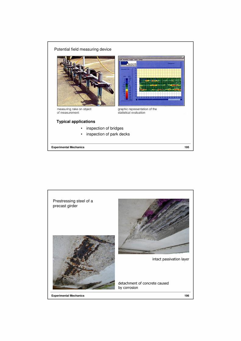
Potential field measuring device
Typical applications
• inspection of bridges
• inspection of park decks
Prestressing steel of a
precast girder
detachment of concrete caused by corrosion
Experimental Mechanics 196
intact passivation layer

Corrosion due to cracks and construction defects
Experimental Mechanics 197
Experimental Mechanics 198
Damages of a bridge resulting from construction defects

Potential distribution on
the surface
of a runway
Experimental Mechanics 199
Corrosion detected
at the reinforcement after
removing
the concrete cover
Example: parking deck
Experimental Mechanics 200

Mapping of the potential
Experimental Mechanics 201
Experimental Mechanics 202
5.5 Ultrasonic testing
• Physical background
– Wave types
– Behavior at interfaces
– Generation of ultrasonic waves
• Transmission
• Ultrasonic echo techniques
• Ultrasonic wave propagation

Wave types in solid
bodies
Experimental Mechanics 203
Experimental Mechanics 204
Behavior at boundary layers
Assumption: perpendicular incidence Example: air-filled hollow in concrete
ZB = 9,2 ⋅106 Ns/m3
ZL = 4,3 ⋅102 Ns/m3 (ρL = 1,3 kg/m3, cL = 333 m/s) The reflection coefficient results in: R = -0,999 In case of a water-filled hollow it comes to: R = -0,72
Reflection: 100% at the boundary concrete / air 50% at the boundary concrete / water 70% at the boundary concrete / steel

Experimental Mechanics 205
Influencing factors for the wave velocity in concrete
• size and type of aggregate
• amount of hollow spaces
• temperature
• water/cement ratio
• density
• cement class, concrete additives
• reinforcement
Imaging method
used with the impulse-
echo technique
Experimental Mechanics 206
Fig. 3a: Ultrasonic intensity versus time or depth (A-Scan)
Fig. 3b: Succession of A-scans by shifting the test probe (B-Scan)

Generation of ultrasonic wavesImportance of the coupling for the transmission of energy
Experimental Mechanics 207
Measurement principle
in transmission
Experimental Mechanics 208

Simulation of the wave propagation in concrete
considering different air entrainments
Experimental Mechanics 209
Concrete modelwith crack
Experimental Mechanics 210
air content: 2% air content: 4%

Calculated A-scan with
air content 0%
Calculated A-scan with
air content 2%
Experimental Mechanics 211
Calculated A-scan with
air content 4%
Experimental Mechanics 212

Wave propagation in concrete without air voids
Experimental Mechanics 213
Experimental Mechanics 214
Sound propagation in concrete having 2% air voids

Experimental Mechanics 215
Sound propagation in concrete having 4% air voids
Experimental Mechanics 216
Applications
• testing of welded joints
• thickness measurement of walls made of steel or concrete
• determination of concrete compressive strength;
evaluation of homogeneity
• evaluation of hardening behavior – prediction of strength development
• flaw detection
• pile integrity test

Thickness measurement of walls made of steel
Experimental Mechanics 217
Experimental Mechanics 218
Transverse wave probes in array arrangement for concrete

Experimental Mechanics 219
Measurement of the wall thickness of a corridor wall
Experimental Mechanics 220
0
100
200
300
400
500
100
200
300
0
10
0
20
0
30
0
40
0
50
0
10 20 30 40 50 60
50
100
150
200
250
300
vL= 3959 m/s
vT= 2415 ...
2533 m/s
Measurement of the wall thickness of a corridor wall

Experimental Mechanics 221
Corridor wall, approximate position of the reinforcement
0
100
200
300
400
500
100
200
300
0
10
0
20
0
30
0
40
0
50
0
10 20 30 40 50 60
50
100
150
200
250
300
vL= 3959 m/s
vT= 2415 ...
2533 m/s
Experimental Mechanics 222
Determination of vL in case of one-sided access
Linear regression for:
Y = A + B * X
parameter value error
--------------------------------------------------------
A 8,28 1,59018
B 2,52629 0,04083
10 20 30 40 50 60
20
40
60
80
100
120
140
160
180
runtim
e in µ
s
distance in cm
Determination of the wave velocity from the slope
vL = s/t
vL = 1 / 2,5263 = 3959 m/s
determination of the US-speed ν of one sideL

Experimental Mechanics 223
Correlation between longitudinal and transverse wave velocity
in case of concrete
)21(
)1(2
)1(2
1
)21)(1(
)1(
2
2
2
2
µ
µ
µρ
µµρ
µ
−
−=
+⋅=
−+
−=
T
L
T
L
v
v
Ev
Ev
LTTL
LTTL
vvvv
vvvv
61,063,120,0
64,0,57,116,0
,==⇒=
==⇒=
µ
µ
The relation vL/vT depends only on µ.
In case of concrete:
vT = 0,61….0,64 vL
Experimental Mechanics 224
Examination of the homogeneity of a pillar using the transmission method

2nd floor; pillar B03 2nd floor; pillar B04
measurement grid 10 x 20cm measurement grid 10 x 20cm
starting from 10 cm over ground starting 10 cm over ground
direction A direction C direction A direction C
75 72 83 65 61 66
73 78 81 68 67 69
77 75 80 64 58 65
69 77 75 65 63 67
71 73 73 65 66 67
73 71 74 67 68 81
75 85 86 73 81 73
81 98 81 69 70 78
77 79 76 67 70 69
72 83 77 65 67 66
2nd floor; pillar B08 2nd floor; pillar B18
measurement grid 10 x 20cm measurement grid 10 x 20cm
starting 10 cm over ground starting 10 cm over ground
direction A direction C direction A direction C
86 68 93 79 85 /
96 78 83 82 79 83
87 81 83 75 103 90
76 82 76 84 79 81
80 73 75 83 71 76
78 82 91 78 79 75
98 99 71 70 86 79
77 72 71 70 67 73
68 65 67 91 70 75
58 63 59 72 69 98
2nd floor; pillar B10
measurement grid 10 x 20cm
starting 10 cm over ground
direction A direction C
73 74 70 color runtime sonic speed
70 71 68 ≥ 90µs ≤ 2222 m/s
71 71 71 ≥ 80µs ≤ 2500 m/s
72 79 74 ≥ 70µs ≤ 2850 m/s
76 71 75 ≥ 60µs ≤ 3333 m/s
73 79 75
85 81 82
83 79 72
73 79 68
88 78 67
Homogeneity check of a pillar
using the transmission method
Experimental Mechanics 225
Correlation of wave velocity and cube compressive strength
for concrete with different compositions
Experimental Mechanics 226

Experimental Mechanics 227
5.6 Impact-echo method
Fields of application:
- thickness measurement of concrete slabs (even
including top layers)
- detection of flaws, detachments, and compaction
deficiencies in slabs
- (detection of cracks normal to surfaces)
- detection of tendons
- (examination of groutings)
- inspection of masonry
Basics of the impact-echo method
Fast Fourier Transformation (FFT)
The evaluation of the measuring signals is conducted at the frequency sprectrum
Experimental Mechanics 228

dd = thickness resp. flaw depth
f = frequency
cP = sonic speed
f
cd
2=
f
cd
2=
Experimental Mechanics 229
Principle of the impact-echo method
Demonstration of the wave propagation
impact by falling steel bullet
Wave propagation during impact-echo examinations
Signals without and with large flaw
Experimental Mechanics 230

Experimental Mechanics 231
Wave propagation during impact-echo examinations
Signals without and with small flaw
Characteristic results as dependent on the
lateral extension of a flaw
Experimental Mechanics 232

Frequency spectrum of the „sending signal“
The energy and the frequency spectrum depend on the diameter of the bullet and on the contact time tc.
Experimental Mechanics 233
Measurement of the velocity of the
longitudinal wave using two sensors.
Experimental Mechanics 234

Experimental Mechanics 235
Measuring devises
� test probes
� coupling
� measuring instruments
Commercial measuring devices
Experimental Mechanics 236

Impact-echo measuring probe
with
integrated impactor
Experimental Mechanics 237
Measuring probes with separate
impactor
Coupling with lead foil
Experimental Mechanics 238

new sensor
developments
Experimental Mechanics 239
Commercial
measuring devices
Experimental Mechanics 240

Movable test probe
Experimental Mechanics 241
Experimental Mechanics 242

The problem:
Tunnels are often constructed with shotcrete. In the construction process, an outer shell
is built first as a temporary protection. Then, an inner shell - usually made of reinforced concrete - is cast.
This two-layer design offers the opportunity to install a plastic sealing sheet between the outer and the inner shell in order to ensure the resistance against a hydrostatic water
pressure on the structure.
During the construction of the inner shell, flaws and reduced thicknesses may occur, in particular in the area of the ridge. In some cases, the outer reinforcement is exposed.
Example of application:
Quality inspection of the inner shell of tunnels; non-destructive verification of a sufficient shell thickness
Experimental Mechanics 243
Experimental Mechanics 244

Experimental Mechanics 245
Approach to a solution: thickness measurement using the echo method
Experimental Mechanics 246

Restoration monitoring possible?
Experimental Mechanics 247
The monitoring is only possible under the condition of a bond between concrete substrate and repair mortar.
In case of segregation, a film of cement paste may be formed, which
leads to the formation of an gap.
Experimental Mechanics 248

Guideline for the conduction of non-destructive inspections
of the inner shells of tunnels (RI-ZFP-TU)
Experimental Mechanics 249
Experimental Mechanics 250
5.7 Acoustic emission analysis
• Basics:
– origins of acoustic emission, propagation
– measurement principle
– characteristics of acoustic emission (AE),
terminology, sensors
– localization and accuracy of localization
• Specifics of reinforced concrete
• Application in load tests
• Further technical applications

Experimental Mechanics 251
Origin of acoustic emission
• Acoustic emissions occur when materials are strained beyond
the elastic limit.
• Microcracks develop at points of material flaws or
inhomogeneities. This process is accompanied by a sudden
release of an elastic wave - an acoustic emission event.
• This released impulse is very broadband. It is used for technical
purposes within a frequency range of 20 – 300 kHz, i.e. within
the ultrasonic range.
• Breaking of glass is an example of acoustic emission within the
audible range, but microcracks in steel and other solid bodies
emit also intensive ultrasonic impulses.
• By acoustic emission analysis, such signals are detected and
interpreted. Hence, it offers the opportunity to detect and study
damage processes.
• The acoustic emission analysis is a passive technique, i.e. the
ultrasonic impulses are recorded in the moment of their formation.
It is not possible to detect flaws that are not active during the
mechanical loading.
• Due to the KAISER effect, the material must be stressed beyond
the previously reached maximum stress in order to allow a
detection of the flaws.
• Leakages or delaminations (in composite materials) may also
cause acoustic emissions.
• Discrete and continuous emissions are distinguished.
Experimental Mechanics 252

Experimental Mechanics 253
Discrete and continuous acoustic emissions
Discrete signal of AE
Continuous signal of AE
Experimental Mechanics 254
Acoustic emission measurement

Signal interpretation
Detection of the wave onset when a threshold value is exceeded
Experimental Mechanics 255
Signal interpretation
Analysis of characteristics of classical signal parameters
Experimental Mechanics 256
• onset time (time of the first threshold exceedance)
• maximum amplitude
• rise time (from first threshold exceedance to the time of max. amplitude)
• signal duration
• amount of exceeding oscillations (counts) (of the threshold in one polarity)
• energy
• RMS (effective value) of the continuous background noise (before the respective hit)

Layout of a AE sensor
Experimental Mechanics 257
Experimental Mechanics 258
Influences on the precision of localization
• Signal attenuation
• Anisotropy of the wave velocity
• Different attenuation of different wave types
• Disturbing signals (threshold exceedance)
• material inhomogeneities

Experimental Mechanics 259
0 mm
545 mm
1010 mm
1535 mm
Options for the presentation of results
Experimental Mechanics 260

Experimental Mechanics 261
Mechanism of the formation of micro cracks in normal concrete
Experimental Mechanics 262

Experimental Mechanics 263
Cracking process in concrete under compressive loading
Applications
• laboratory tests
• experimental safety evaluation of existing structures
• further technical applications
Experimental Mechanics 264

Example for the detection of AE signals during a Brasilian test
Experimental Mechanics 265
Experimental Mechanics 266
Formation of cracks during a during a Brasilian test
fracture surface

Applications for the experimental safety evaluation of existing
structures
• mainly used in areas which are inaccessible for other
methods
• in case of a risk of brittle failure, especially shear failure
• for prestressed concrete structures
Experimental Mechanics 267
Experimental Mechanics 268
The acoustic emission analysis as accompanying method in load tests
• integral method � qualitative information about active cracking processes
• qualitative evaluation of active cracks
� improved determination of the cracking load (transition to cracked mode)
• detection of active areas (multichannel system)
� prevention of crack formation (prestressedconcrete)
� monitoring of damaged areas
� prevention of shear failure
• KAISER effect � information on the loading history

Acoustic emission
analysis in the field of
structural engineering
Investigation of crack
formation in beams
Experimental Mechanics 269
Monitoring of cantilevers and
areas vulnerable to brittle
failure during load tests
Experimental Mechanics 270
Acoustic emission
analysis in the field of
architectural engineering

Load tests of pillars
Experimental Mechanics 271
Neues Museum in Berlin
Historic structure
Experimental Mechanics 272

Loading vehicle BELFA
Reinforced concrete Bridge across the Werra having nine spans,
partially destroyed during world war II
AEA applied to shotcreted beams
Experimental Mechanics 273
Experimental Mechanics 274
Loading vehicle BELFA
Niederbrücke damaged by a flood in Döbeln
AEA applied to an unreinforced concrete arch bridge

Experimental Mechanics 275
AEA applied to reinforced concrete beams
Loading vehicle BELFA - Kaiserin-Augusta-bridge in Berlin
Experimental Mechanics 276
Loading vehicle BELFA
Ferry dock Blexen
AEA used for the pre-
vention of crack formation
in prestressed concrete
beams

Experimental Mechanics 277
Prototype BELFA-DB
Viaduct in Rhena
Railroad viaduct in Rhena
Experimental Mechanics 278
AEA applied to the concrete arches and
to the damaged sandstone pillars

Experimental Mechanics 279
Prototype BELFA-DB
AEA applied to a masonry arch
Experimental Mechanics 280
Further technical applications
• Inspection of containers for liquid and compressed gas – crack
detection
• Monitoring of technological processes
• Analysis of corrosion
• Monitoring of transformators (partial discharge, gas formation)
• Tribology (investigations into friction and wearing)
• Geology
• detection of leakages

Experimental Mechanics 281
5.8 Infrared thermography
• Physical background
– Planck's law
– Wien's law of displacements
– Stefan-Boltzman law
– Influence of the atmosphere
• Applications
– Examination of hidden details of structures
– Application in the field of building physics
Physical background
Experimental Mechanics 282

Planck's radiation law
The law explains the correlation between the spectral distribution of
the thermal radiation and the temperature T for the black body (emits
a spectrum which depends only on the temperature).
From this, two phenomena with practical relevance arise:
• Wien's law of displacements
The location of the radiation's maximum λmax is displaced to smaller wave lengths with increasing temperature.
• Stefan-Boltzmann law
The emitted total radiation increases proportionally with T4.
Experimental Mechanics 283
Atmospheric influences
• Radiation attenuation by absorption and dispersion
some components of the atmosphere such as CO2 and H2O
have strong absorption bands in the range to 14 µm
• Characteristic radiation of the atmosphere
interferes with the radiation of the object
Experimental Mechanics 284

Applications
• Examination of hidden construction details
• Detection of thermal bridges and flaws in the field of
building physics
• Combination with Blower-Door method
• Detection of overheating of technical instruments
Experimental Mechanics 285
Experimental Mechanics 286

Experimental Mechanics 287
Experimental Mechanics 288

Heated exit of an underground garage
Experimental Mechanics 289

Experimental Mechanics 290
6. Experimental safety evaluation of existing structures
6.1 General remarks
Normal case: prove of structural safety by calculations
Special case: sufficient safety can not be proved
by calculations
option 1: - completion of the analysis assumptions (inquiry of
documents, survey of the structure, testing of the building
materials, non-destructive testing)
- improvement of the computational model (static system,
mechanical boundary conditions, spatial load-carrying behavior, non-linear material behavior)
- repeated (improved) calculation of the structural safety
- if still no sufficient safety level is provable:
option 2: - experimental evaluation of structural safety
- by load tests
Experimental Mechanics 291
Principle of the experimental safety evaluation by loading tests
Structure
Application of test loads
Measurement of the Reactions (Deformations, Acoustic emission, Reaction forces)

Experimental Mechanics 292
Experimental Mechanics 293
Load test in 1890
On the history of load tests (in German):
G. Bolle, G. Schacht, S. Marx, Geschichtliche Entwicklung und aktuelle Praxis der Probebelastung, Teil 1: GeschichtlicheEntwicklung im 19. und Anfang des 20. Jahrhunderts, Bautechnik 87(2010)11, 700-707, Teil 2: Entwicklung von Normen und heutige Anwendung, Bautechnik 87(2010)12, 784-789.

Experimental Mechanics 294
Guideline of the DAfStb (Deutscher Ausschuss für Stahlbeton,
German Committee for reinforced concrete) for the application of
load tests at reinforced concrete buildings:
„… make provision against sudden (without warning) failure“
This requirement is met by:
> self-securing loading devices
> on-line measurement and evaluation of the structural behaviour
Experimental Mechanics 295
Safety concept
1
G
anal
ysis
exp
eri
men
t
ultimate load
Lo
ad
Reaction
Load-Reaction
(idealized)
Loading test
service load
Gd
,j
+ Q
d
exp. target load
design load (analysis)
∆∆ ∆∆Q
d
experimental limit load
permanent load
ext Ftarg ≤ ext Flim
ext
Fta
rg
ext
Flim

Experimental Mechanics 296
concrete compressive strain 600 µm/m800 µm/m for ≥ B25
crack opening ∆w = 0,3 mm
from that max. 20% remaining
remaining deflection 10% of the maximum value
Criteria for the experimental limit load
Experimental Mechanics 297
Procedure of the planning of load tests
Formulation of the task
• identification of the load test's objective
• examination of the chance of success under consideration of the actual structure and the experimental capabilities
Pre-examinations
• determination of material parameters, of the building's geometry, and of the static system
• review of existing documents
• pre-calculations and determination of critical load positions and combinations
Planning of the load test
• determination of the target load for the different load cases
• planning of the loading technique including reaction forces (anchoring)
Planning of the measurements
• identification of the required measurements and of the sensor positions
• discussion of the test concept with the client

Experimental Mechanics 298
Loading technique: self-securing loading principle
• self-securing loading by hydraulic actuators
• mobile, adaptable loading frame system
Experimental Mechanics 299
Loading technique: anchoring against dead loads

Experimental Mechanics 300
Measurement methods used for the experimental safety evaluation of structures
Essential components of in situ measurements are:
• computer-aided real-time data acquisition system
• load cells
• inductive displacement sensors (LVDTs) and special sensors designed on the basis of them
• strain gauges
• inclination sensors
• acoustic emission analysis system
The immediate availability of all measured values on a display and the possibility to influence the test procedure at any time are required.
Experimental Mechanics 301
Acoustic emission sensor

Experimental Mechanics 302
Central market hall in Leipzig
Loading with dead loads (left) and
with mobile loading frame (right)
6.3 Case studies
Experimental Mechanics 303
Loading frame on a reinforced concrete ceiling

Experimental Mechanics 304
Loading frame in a historic department store
Experimental Mechanics 305305305
Loading frame in the ground floor
Load distribution „moves“upward from floor to floor
Loading frame in a historic department store

Experimental Mechanics 306
Load distribution on three spans of the ceiling
Experimental Mechanics 307
Measurement of deflections in the historic department store

Experimental Mechanics 308
Example of anchored reaction frame
309309
Example of anchored reaction frame

Experimental Mechanics 310
Example of anchored reaction frame
Experimental Mechanics 311
Example of the examination of balconies

Experimental Mechanics 312312312
Example of the examination of balconies
Experimental Mechanics 313
Example of the examination of balconies

Experimental Mechanics 314314314
Load test of a prestressedconcrete girder which wasdamaged by fire
Anchoring against dead loads
Deflection measurement using a suspension technique
Experimental Mechanics 315
Load test of a prestressed
concrete girder which wasdamaged by fire

Experimental Mechanics 316
Loading frame on a concrete bridge
Experimental Mechanics 317

Experimental Mechanics 318
Development of the principle anchoring against dead loads
BELFA specifications:
• street-legal heavy-duty vehicle which moves to the examination objects autonomously (i.e. driving weight < 80 t, axle weights < 10,5 t and turning circle 22 m)
• loading capability according to DIN 1072 for bridge classes 12 to 60 in the main lane (up to bridge classes 30 without anchoring)
• bridge spans up to 18m (therefore applicable for more than 70% of all existing road bridges in Germany)
Loading vehicle BELFA
Experimental Mechanics 319
319319
BELFA in operation

Experimental Mechanics 320
BELFA - options for ballast
Experimental Mechanics 321
BELFA on a reinforced concrete bridge

Experimental Mechanics 322
Measuring base underneath the bridge
Experimental Mechanics 323
BELFA on an arch bridge

Experimental Mechanics 324
BELFA on a bridge with brickwork vaults
Experimental Mechanics 325
Profile of the bridge with masonry vaults

Experimental Mechanics 326
BELFA on a bridge with masonry vaults
Experimental Mechanics 327
BELFA on a bridge with masonry vaults

Experimental Mechanics 328
Measurement base underneath the bridge
Experimental Mechanics 329
Sensors underneath the bridge
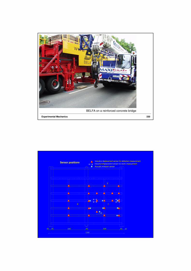
Experimental Mechanics 330
BELFA on a reinforced concrete bridge
Experimental Mechanics 331
Inductive displacement sensor for deflection measurementSensor positions
Inductive displacement sensor for strain measurement
Acoustic emission sensor
12
3
40 50 645
1.38
60 645 50 40
1530

Experimental Mechanics 332
Measurement base
Experimental Mechanics 333
Displacement sensor in the shear area

Experimental Mechanics 334
Loading vehicle BELFA-DB (prototype)
Experimental Mechanics 335
Load test of a railway bridge

Experimental Mechanics 336
Measurement base and sensors
Experimental Mechanics 337
Hydraulic loading system
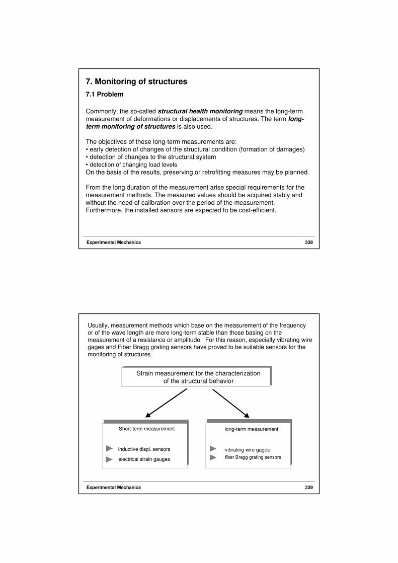
Experimental Mechanics 338
7. Monitoring of structures
7.1 Problem
Commonly, the so-called structural health monitoring means the long-term
measurement of deformations or displacements of structures. The term long-
term monitoring of structures is also used.
The objectives of these long-term measurements are:
• early detection of changes of the structural condition (formation of damages)
• detection of changes to the structural system
• detection of changing load levels
On the basis of the results, preserving or retrofitting measures may be planned.
From the long duration of the measurement arise special requirements for the
measurement methods. The measured values should be acquired stably and
without the need of calibration over the period of the measurement. Furthermore, the installed sensors are expected to be cost-efficient.
Experimental Mechanics 339
Short-term measurement long-term measurement
inductive displ. sensors
electrical strain gauges
vibrating wire gages
fiber Bragg grating sensors
Strain measurement for the characterization
of the structural behavior
Usually, measurement methods which base on the measurement of the frequency or of the wave length are more long-term stable than those basing on the measurement of a resistance or amplitude. For this reason, especially vibrating wire gages and Fiber Bragg grating sensors have proved to be suitable sensors for the monitoring of structures.

Experimental Mechanics 340
7.2 Measuring concepts
7.2.1 Vibrating wire gages
wiretheofdensity
wiretheinstress
wireoflength
wireoffrequency
21
=
=
=
=
=
ρ
σ
L
f
/)L/(f ρσ
The characteristic frequency of a vibrating wire changes with the stress.
image: Geokon company
Experimental Mechanics 341
22
22
)4(
)4/(
fE
L
E
Lf
⋅⋅
=
⋅=
⋅=
ρε
εσ
ρσ
:lawsHooke'using
strain = constant · frequency²
For long-term measurements: constancy of - length- density
- Young's modulus
• Length: influence of temperature is compensated by calculation
• Density: wire within a protective glass
• Young's modulus: elastic loading of the wire

Experimental Mechanics 342
Sensor for the external application on steel or concrete
• measuring range 3000 µm/m
• reusable
• temperature sensor included
image: Geokon company
Experimental Mechanics 343
Sensor for the embedded application during the placement of concrete
• measuring range 3000 µm/m
• not reusable
• temperature sensor included
image: Geokon company

Experimental Mechanics 344
Sensor for the measurement of displacements
e.g. measurement of crack widths or displacement of bearings
• measuring range is independent of wire length (commenly 25 - 50 mm)
• reusable
• temperature sensor included
• anchor embedded in concrete or welded to steel
image: Geokon company
Experimental Mechanics 345
Load cells
• measurement of bearing or prestressing forces
• various force ranges
image: Geokon company

Experimental Mechanics 346
Components of a monitoringsystem
in case of discontinuous readings:handheld measuring device for all sensor types image: Geokon company
Experimental Mechanics 347
reflection and transmission at the grid
segments
constructive interference:
• intensification of light intensity upon reflection
• reduction of light intensity upon transmission
• only in case of a certain wave length which satisfies Bragg's conditions of
reflection→ Bragg's wave length
When changing the distance between the grid segments (strain, temperature), Bragg's wave length
changes proportionally.length wavesBragg'
sensor theoflength period
grid theofindex refractivemean
2
2
0
0
0
=
=Λ
=
Λ⋅=
=
=Λ⋅
λ
λ
λλ
λ
m
m
m
n
n
n
7.2.2 Fiber Bragg grating sensors

Experimental Mechanics 348
• very good long-term stability; no need for calibration
• very good resistance to corrosion
• exposition to temperatures > 700°C possible (custom-built)
• very suitable for the measurement of strains in composite materials; immediate
integration possible (airplanes, wind power stations)
• measurement of large strains, >1% possible
• sensors are small and lightweight
• insensitive to electromagnetic fields
• sensors operate passively (no electric power source needed); application in explosion-prone areas possible
• transmission of signals over large distances (> 50 km) possible
• up to 100 Fiber Bragg gratings may be written into a single fiber
Disadvantages of fiber Bragg grating sensors:
Advantages of fiber Bragg grating sensors:
• considerable temperature dependence; 1°C corresponds to 8 µm/m mechanical strain
Experimental Mechanics 349
opticalspectrum analyzer
(OSA)
Measurement using an optical spectrum analyzer in transmission
light source fiber Bragg sensor
opticalspectrum analyzer
(OSA)
coupler
Measurement using an optical spectrum analyzer in reflection
fiber Bragg sensorlight source

Experimental Mechanics 350
Analysis of the light spectrum
Bragg's wave length
local minimum
(reflection: maximum)
limiting value
Experimental Mechanics 351
Comparison of fiber Bragg grating sensors (FBG) and vibrating wire gages
FBG Vibrating wire
long-term stability very good very good
price in € 200 € for grating only 150 € including temperature sensor
application
• on steel
• in hardened concrete
• in fresh concrete
• for displacements
• on steel
• in hardened concrete
• in fresh concrete
• for displacements
smallest dimension 100 µm 40 mm
installation still expensive simple
electromagnetic compatibility very good usually without any problems
measurement instruments
and data loggerunder development well-engineered

Experimental Mechanics 352
Monitoring of a bridge made of high performance concrete (HPC) in the Weißeritztal
• single-span bridge with a span of 32 m
• first application of HPC for a bridge in Saxony
• built without sealing and without pavement in order to allow the monitoring directly at the structural member
7.3 Practical examples
Experimental Mechanics 353
• 4 displacement sensors Geokon4420-1-1: measurement of the
relative movement between bearing and superstructure; temperature measurement
• 2 strain sensors Geokon VSM 4000: measurement of the strain at midspan on the upper side of the bridge; temperature measurement
• 1 strain sensor Geokon VSM 4000: measurement of the strain at midspan on the lower side of the bridge; temperature measurement
• In parallel to the application of the
vibrating wire gages, fiber Bragg grating sensors were installed.
The following sensors were applied:

Experimental Mechanics 354
downside of the bridge data logger
strain sensors (FBG + SSA)
displacement sensor at the bearing
Experimental Mechanics 355
-10
-5
0
5
10
15
20
19
. J
an
24
. J
an
29
. J
an
03
. F
eb
08
. F
eb
13
. F
eb
18
. F
eb
23
. F
eb
28
. F
eb
05
. M
rz
10
. M
rz
Datum/Zeit
Te
mp
era
tur
in °
C
-0,35-0,3
-0,25
-0,2-0,15
-0,1-0,05
00,05
19
. J
an
24
. J
an
29
. J
an
03
. F
eb
08
. F
eb
13
. F
eb
18
. F
eb
23
. F
eb
28
. F
eb
05
. M
rz
10
. M
rz
Datum/Zeit
Ve
rsc
hie
bu
ng
in
cm Auflager Mst. 4
Auflager Mst. 5
Auflager Mst. 6
Auflager Mst. 7
Measurement results
date / time
date / time

Experimental Mechanics 356
-400
-350
-300
-250
-200
-150
-100
-50
0
19. Jan 24. Jan 29. Jan 03. Feb 08. Feb 13. Feb 18. Feb 23. Feb 28. Feb 05. Mrz 10. Mrz
Datum/Zeit
De
hn
un
g in
µm
/m
Dresden-oben Mitte-unten
Freital-oben
-10
-5
0
5
10
15
20
19
. J
an
24
. J
an
29
. J
an
03
. F
eb
08
. F
eb
13
. F
eb
18
. F
eb
23
. F
eb
28
. F
eb
05
. M
rz
10
. M
rz
Datum/Zeit
Te
mp
era
tur
in °
C
date / time
date / time
Measurement results
Experimental Mechanics 357
-0,1
-0,05
0
0,05
0,1
0
100
200
300
400
500
600
700
800
Datum/Zeit
Vers
ch
ieb
un
g i
n m
m
Auflager Mst. 4
Auflager Mst. 5
Auflager Mst. 6
Auflager Mst. 7
-140
-120-100
-80-60
-40
-200
20
0 100 200 300 400 500 600 700 800
Deh
nu
ng
in
µm
/m
Dresden-oben
Freital-oben
Mitte-unten
Measurement results for the crossing of a 26.6 t vehicle
date / time
displacement at the bearings

Experimental Mechanics 358
Monitoring of a bridge made of high performance concrete (HPC)
across the Mulde near Glauchau
Experimental Mechanics 359
Measurement program
1. Temperature measurement
• hydration heat during construction
• under service conditions
2. Strain measurement within cross-sections
• during load tests
• long-term measurements
3. Deflection measurements
• during load tests

Experimental Mechanics 360
Measuring program
4. Displacements at the bearings
5. Dynamic measurements
• during construction due to hydration heat
• under service conditions
• during load tests
Experimental Mechanics 361
Vibrating wire gage

Experimental Mechanics 362
Cable connections to the sensors
Experimental Mechanics 363
Data logger