MECHANICS MAP

Jacob Moore et al.Pennsylvania State University Mont Alto

Mechanics Map

This text is disseminated via the Open Education Resource (OER) LibreTexts Project (https://LibreTexts.org) and like thehundreds of other texts available within this powerful platform, it is freely available for reading, printing and"consuming." Most, but not all, pages in the library have licenses that may allow individuals to make changes, save, andprint this book. Carefully consult the applicable license(s) before pursuing such effects.

Instructors can adopt existing LibreTexts texts or Remix them to quickly build course-specific resources to meet the needsof their students. Unlike traditional textbooks, LibreTexts’ web based origins allow powerful integration of advancedfeatures and new technologies to support learning.

The LibreTexts mission is to unite students, faculty and scholars in a cooperative effort to develop an easy-to-use onlineplatform for the construction, customization, and dissemination of OER content to reduce the burdens of unreasonabletextbook costs to our students and society. The LibreTexts project is a multi-institutional collaborative venture to developthe next generation of open-access texts to improve postsecondary education at all levels of higher learning by developingan Open Access Resource environment. The project currently consists of 14 independently operating and interconnectedlibraries that are constantly being optimized by students, faculty, and outside experts to supplant conventional paper-basedbooks. These free textbook alternatives are organized within a central environment that is both vertically (from advance tobasic level) and horizontally (across different fields) integrated.

The LibreTexts libraries are Powered by MindTouch and are supported by the Department of Education Open TextbookPilot Project, the UC Davis Office of the Provost, the UC Davis Library, the California State University AffordableLearning Solutions Program, and Merlot. This material is based upon work supported by the National Science Foundationunder Grant No. 1246120, 1525057, and 1413739. Unless otherwise noted, LibreTexts content is licensed by CC BY-NC-SA 3.0.

Any opinions, findings, and conclusions or recommendations expressed in this material are those of the author(s) and donot necessarily reflect the views of the National Science Foundation nor the US Department of Education.

Have questions or comments? For information about adoptions or adaptions contact info@LibreTexts.org. Moreinformation on our activities can be found via Facebook (https://facebook.com/Libretexts), Twitter(https://twitter.com/libretexts), or our blog (http://Blog.Libretexts.org).

This text was compiled on 01/30/2022

®

1 1/30/2022

TABLE OF CONTENTSThe Mechanics Map is an open textbook for engineering statics and dynamics containing written explanations, video lectures, workedexamples, and homework problems. All content is licensed under a creative commons share-alike license, so feel free to use, share, orremix the content. The table of contents below links to all available topics, while the about, instructor resources, and contributing tabsprovide information to those looking to learn more about the project in general.

ABOUT THE AUTHORS

ABOUT THE BOOK

1: BASICS OF NEWTONIAN MECHANICSDefinition of forces, moments, and bodies in the context of engineering mechanics. The impact of forces and moments on bodies.

1.0: VIDEO INTRODUCTION TO CHAPTER 11.1: BODIES1.2: FORCES1.3: MOMENTS1.4: FREE BODY DIAGRAMS1.5: NEWTON'S FIRST LAW1.6: NEWTON'S SECOND LAW1.7: NEWTON'S THIRD LAW1.8: CHAPTER 1 HOMEWORK PROBLEMS

2: STATIC EQUILIBRIUM IN CONCURRENT FORCE SYSTEMSThe definition of static equilibrium and concurrent force systems. Analysis of concurrent force systems at static equilibrium to identifyunknown forces.

2.0: CHAPTER 2 VIDEO INTRODUCTION2.1: STATIC EQUILIBRIUM2.2: POINT FORCES AS VECTORS2.3: PRINCIPLE OF TRANSMISSIBILITY2.4: CONCURRENT FORCES2.5: EQUILIBRIUM ANALYSIS FOR CONCURRENT FORCE SYSTEMS2.6: CHAPTER 2 HOMEWORK PROBLEMS

3: STATIC EQUILIBRIUM IN RIGID BODY SYSTEMSEquilibrium analysis of rigid body systems as opposed to particle systems, which involves analysis of both forces and moments.

3.0: VIDEO INTRODUCTION TO CHAPTER 33.1: MOMENT OF A FORCE ABOUT A POINT (SCALAR CALCULATION)3.2: VARIGNON'S THEOREM3.3: COUPLES3.4: MOMENT ABOUT A POINT (VECTOR)3.5: MOMENT OF A FORCE ABOUT AN AXIS3.6: EQUILIBRIUM ANALYSIS FOR A RIGID BODY3.7: CHAPTER 3 HOMEWORK PROBLEMS

4: STATICALLY EQUIVALENT SYSTEMSStatically equivalent systems that experience different sets of forces and moments. The process for converting between differentstatically equivalent systems.

4.0: VIDEO INTRODUCTION TO CHAPTER 44.1: STATICALLY EQUIVALENT SYSTEMS4.2: RESOLUTION OF A FORCE INTO A FORCE AND A COUPLE4.3: EQUIVALENT FORCE COUPLE SYSTEM4.4: DISTRIBUTED FORCES

2 1/30/2022

4.5: EQUIVALENT POINT LOAD4.6: CHAPTER 4 HOMEWORK PROBLEMS

5: ENGINEERING STRUCTURESClassification of engineering structures into members, trusses, and frames and machines. Methods for equilibrium analysis of thesestructures.

5.0: VIDEO INTRODUCTION TO CHAPTER 55.1: STRUCTURES5.2: TWO-FORCE MEMBERS5.3: TRUSSES5.4: METHOD OF JOINTS5.5: METHOD OF SECTIONS5.6: FRAMES AND MACHINES5.7: ANALYSIS OF FRAMES AND MACHINES5.8: CHAPTER 5 HOMEWORK PROBLEMS

6: FRICTION AND FRICTION APPLICATIONSDefinition of dry friction; the application of dry friction in mechanical processes (wedges, power screws, bearings, disc-shapedmechanisms, belt-and-pulley systems).

6.0: VIDEO INTRODUCTION TO CHAPTER 66.1: DRY FRICTION6.2: SLIPPING VS TIPPING6.3: WEDGES6.4: POWER SCREWS6.5: BEARING FRICTION6.6: DISC FRICTION6.7: BELT FRICTION6.8: CHAPTER 6 HOMEWORK PROBLEMS

7: PARTICLE KINEMATICSParticle kinematics: describing the motion of a particle in one dimension, both continuous and non-continuous; in two dimensions inrectangular, polar, and normal-tangential coordinates; in systems of dependent or relative motion.

7.0: VIDEO INTRODUCTION TO CHAPTER 77.1: ONE-DIMENSIONAL CONTINUOUS MOTION7.2: ONE-DIMENSIONAL NONCONTINUOUS MOTION7.3: TWO-DIMENSIONAL KINEMATICS WITH RECTANGULAR COORDINATES7.4: TWO-DIMENSIONAL KINEMATICS WITH NORMAL-TANGENTIAL COORDINATES7.5: TWO-DIMENSIONAL MOTION WITH POLAR COORDINATES7.6: DEPENDENT MOTION SYSTEMS7.7: RELATIVE MOTION SYSTEMS7.8: CHAPTER 7 HOMEWORK PROBLEMS

8: NEWTON'S SECOND LAW FOR PARTICLESUsing Newton's Second Law to describe forces and their effect on the motion of particles, in one and two dimensions (using rectangular,polar, and normal-tangential coordinate systems).

8.0: VIDEO INTRODUCTION TO CHAPTER 88.1: ONE-DIMENSIONAL EQUATIONS OF MOTION8.2: EQUATIONS OF MOTION IN RECTANGULAR COORDINATES8.3: EQUATIONS OF MOTION IN NORMAL-TANGENTIAL COORDINATES8.4: EQUATIONS OF MOTION IN POLAR COORDINATES8.5: CHAPTER 8 HOMEWORK PROBLEMS

9: WORK AND ENERGY IN PARTICLESWork, energy, power, and the relationship between these quantities. Analyzing the behavior of single particles and of systems ofparticles based on conservation of energy.

3 1/30/2022

9.0: VIDEO INTRODUCTION TO CHAPTER 99.1: CONSERVATION OF ENERGY FOR PARTICLES9.2: POWER AND EFFICIENCY FOR PARTICLES9.3: CONSERVATION OF ENERGY FOR SYSTEMS OF PARTICLES9.4: CHAPTER 9 HOMEWORK PROBLEMS

10: IMPULSE AND MOMENTUM IN PARTICLESThe relationship between impulse and momentum in a particle. Analysis of steady-flow devices and of collisions between particles(one-dimensional, two-dimensional, and surface collisions).

10.0: VIDEO INTRODUCTION TO CHAPTER 1010.1: IMPULSE-MOMENTUM EQUATIONS FOR A PARTICLE10.2: SURFACE COLLISIONS AND THE COEFFICIENT OF RESTITUTION10.3: ONE-DIMENSIONAL PARTICLE COLLISIONS10.4: TWO-DIMENSIONAL PARTICLE COLLISIONS10.5: STEADY-FLOW DEVICES10.6: CHAPTER 10 HOMEWORK PROBLEMS

11: RIGID BODY KINEMATICSRotational kinematics involving extended rigid bodies, as opposed to particles: fixed-axis rotation, gear- and belt-driven systems,relative and absolute motion analysis, and analysis using rotating and translating frames.

11.1: FIXED-AXIS ROTATION IN RIGID BODIES11.2: BELT- AND GEAR-DRIVEN SYSTEMS11.3: ABSOLUTE MOTION ANALYSIS11.4: RELATIVE MOTION ANALYSIS11.5: ROTATING FRAME ANALYSIS11.6: CHAPTER 11 HOMEWORK PROBLEMS

12: NEWTON'S SECOND LAW FOR RIGID BODIESAnalysis of rigid bodies, as opposed to particles, undergoing translation, rotation, and general planar motion.

12.1: RIGID BODY TRANSLATION12.2: FIXED-AXIS ROTATION12.3: RIGID-BODY GENERAL PLANAR MOTION12.4: MULTI-BODY GENERAL PLANAR MOTION12.5: CHAPTER 12 HOMEWORK PROBLEMS

13: WORK AND ENERGY IN RIGID BODIESDiscussion of work and energy in rigid bodies as opposed to particles, including rotational work and kinetic energy. Analysis of rigidbody systems through the method of conservation of energy.

13.1: CONSERVATION OF ENERGY FOR RIGID BODIES13.2: POWER AND EFFICIENCY IN RIGID BODIES13.3: CHAPTER 13 HOMEWORK PROBLEMS

14: IMPULSE AND MOMENTUM IN RIGID BODIESAnalysis of impulse and momentum for rigid bodies, and analysis of rigid body surface collisions. Solution videos for exampleproblems not yet available.

14.1: IMPULSE-MOMENTUM EQUATIONS FOR A RIGID BODY14.2: RIGID BODY SURFACE COLLISIONS14.3: CHAPTER 14 HOMEWORK PROBLEMS

15: VIBRATIONS WITH ONE DEGREE OF FREEDOMAnalysis of vibrations in one dimension: free and forced vibrations; undamped, viscous damped, and friction-damped.

15.1: UNDAMPED FREE VIBRATIONS

4 1/30/2022

15.2: VISCOUS DAMPED FREE VIBRATIONS15.3: FRICTION (COULOMB) DAMPED FREE VIBRATIONS15.4: UNDAMPED HARMONIC FORCED VIBRATIONS15.5: VISCOUS DAMPED HARMONIC FORCED VIBRATIONS

16: APPENDIX 1 - VECTOR AND MATRIX MATH16.1: VECTORS16.2: VECTOR ADDITION16.3: DOT PRODUCT16.4: CROSS PRODUCT16.5: SOLVING SYSTEMS OF EQUATIONS WITH MATRICES16.6: APPENDIX 1 HOMEWORK PROBLEMS

17: APPENDIX 2 - MOMENT INTEGRALSTypes of moment integrals and the methods for calculating them. Overview of some engineering applications of moment integrals.

17.1: MOMENT INTEGRALS17.2: CENTROIDS OF AREAS VIA INTEGRATION17.3: CENTROIDS IN VOLUMES AND CENTER OF MASS VIA INTEGRATION17.4: CENTROIDS AND CENTERS OF MASS VIA METHOD OF COMPOSITE PARTS17.5: AREA MOMENTS OF INERTIA VIA INTEGRATION17.6: MASS MOMENTS OF INERTIA VIA INTEGRATION17.7: MOMENTS OF INERTIA VIA COMPOSITE PARTS AND PARALLEL AXIS THEOREM17.8: APPENDIX 2 HOMEWORK PROBLEMS

BACK MATTERINDEXGLOSSARYCENTER OF MASS AND MASS MOMENTS OF INERTIA FOR HOMOGENEOUS 3D BODIESCENTROIDS AND AREA MOMENTS OF INERTIA FOR 2D SHAPES

Jacob Moore & Contributors 1 1/23/2022 https://eng.libretexts.org/@go/page/51678

About the Authors

Project Lead: Dr. Jacob Moore

Dr. Moore is an Associate Professor of Engineering at Penn State Mont Alto. His research interests include openeducational resources in engineering, concept maps in education, student assessment, and additive manufacturingtechnologies. As the project lead, Dr. Moore oversees all development and evaluation activities and is currently theprimary content developer.

Current Content DevelopersDr. Moore has been assisted by Dr. Majid Chatsaz at Penn State Scranton, Dr. Agnes D'entremont at The University ofBritish Colombia, Joan Kowalski at Penn State New Kensington, and Dr. Douglas Miller at Penn State Dubois.

Past ContributorsWe would also like to acknowledge past software developers, Nathanael Bice, Lauren Gibboney, Joseph Luke, JamesMcIntyre, John Nein, Tucker Noia, Michel Pascale, Joshua Rush, Shawn Shroyer, and Menelik Young as well as thecontent experts we have consulted with, Dr. Robert Scott Pierce and Christopher Venters.

Jacob Moore & Contributors 1 12/21/2021 https://eng.libretexts.org/@go/page/51677

About the Book

About the Mechanics Map Tool

The Mechanics Map Digital Textbook Project is an open digital textbook founded on the idea that expert generated conceptmaps can serve as a powerful advance organizer for textbook content. The overview at the beginning of each chapterconsists of a video showing how all the topics in the chapter are linked together by the author. By providing this overview,the author is seeking to help users organize the knowledge they are developing in a way that matches the expert'sorganization of knowledge.

Theoretical Basis

Advance organizers are high level overviews of more detailed information presented to a learner before detailed instructionin language a novice can understand. This overview will ideally link the new ideas to the learner's prior knowledge. Whenused with instruction, advance organizers have been shown to have a small but significant positive impact on theunderstanding and retention of the content.

Concept maps are node-link diagrams that show the major concepts in a content area and how those concepts are linked.Concept maps were originally developed as a way to chart what children did and did not understand, but they were quicklyfound to be effective as a learning aid. Expert-generated concept maps can serve as particularly powerful advanceorganizers because of their explicit highlighting of the relationships between concepts.

Project History

Work on the Mechanics Map project began in 2011 with NSF funding to explore the feasibility and usefulness of a contentnavigation system based on expert generated concept maps. This interactive navigation system replaced a traditional tableof contents, and allowed users to navigate the material in a non-linear way, all the while absorbing the expert generatedconcept map as an advance organizer.

Videos of the original navigation system can be seen below.

The tool was tested in the classroom and was shown to be more effective than a traditional paper textbook in two respects.First, as predicted with the design, the tool encourages users to spend more time attending to an overview of theinformation, helping students build a skeleton they can fit details into later. Second, the tool encouraged users to step backand review topics from previous sections that were relevant to the topics they were learning. This combination ofbehaviors in the users leads to greater measures of conceptual understanding, with little to no extra effort on the part of thelearner.

Unfortunately the original navigation system, built as a Java Applet, is now inoperable in all major browsers due to thesecurity concerns with Applets. Despite this setback with the software, the content has been significantly expanded to allof engineering statics and engineering dynamics with video lectures, worked examples, and homework problems.Additionally, the video introduction at the beginning of each chapter highlights an expert generated concept map to use asan advance organizer for that chapter's concepts.

About the Adaptive Map ToolAbout the Adaptive Map Tool

Jacob Moore & Contributors 2 12/21/2021 https://eng.libretexts.org/@go/page/51677

Research PublicationsMoore, J., Williams, C., North C., Johri, A., Paretti, M. (2015). "Effectiveness of Adaptive Concept Maps for PromotingConceptual Understanding: Findings from a Design-Based Case Study of a Learner-Centered Tool" Advances inEngineering Education ASEE 4 (4)

Moore, J. Pascale, M., Williams, C. North, C. (2013) Translating Educational Theory Into Educational Software: A CaseStudy of the Adaptive Map Project Proceedings of the 2013 ASEE Annual Conference Atlanta, GA, ASEE.

Moore, J. Pierce, R. S., Williams, C. (2012) Towards an "Adaptive Concept Map": Creating an Expert-Generated ConceptMap of an Engineering Statics Curriculum Proceedings of the 2012 ASEE Annual Conference San Antonio, TX, ASEE.

1 1/30/2022

CHAPTER OVERVIEW1: BASICS OF NEWTONIAN MECHANICSDefinition of forces, moments, and bodies in the context of engineering mechanics. The impact of forces and moments on bodies.

1.0: VIDEO INTRODUCTION TO CHAPTER 1Video introduction to the main focus of this chapter: the impact of forces and moments on bodies.

1.1: BODIESDefines a body in the context of engineering mechanics. Discusses the differences between rigid and deformable bodies, and betweenparticles and extended bodies.

1.2: FORCESDefinition of a force. Quantities of interest of a force: magnitude, direction, points of application.

1.3: MOMENTSDefinition and vector representation of moments. Brief overview of how to calculate moments. Lecture video covering topics fromthis section can be found at bottom of this page.

1.4: FREE BODY DIAGRAMSThe process for drawing free body diagrams, and an overview of the types of forces commonly encountered in problems involvingthese diagrams. Contains multiple worked examples.

1.5: NEWTON'S FIRST LAWExplanation of Newton's First Law, relating force and velocity. Includes the role of net force and the law's application to rotationalmotion.

1.6: NEWTON'S SECOND LAWNewton's Second Law and its application to both translational and rotational motion.

1.7: NEWTON'S THIRD LAWExplanation of Newton's Third Law and Third Law force pairs, using real-world several examples.

1.8: CHAPTER 1 HOMEWORK PROBLEMS

Jacob Moore & Contributors 1.0.1 12/21/2021 https://eng.libretexts.org/@go/page/50567

1.0: Video Introduction to Chapter 1

Video introduction to Chapter 1, delivered by Dr. Jacob Moore. Discusses focus of the chapter: the impact of forces andmoments on physical bodies. YouTube source: https://www.youtube.com/watch?v=ljkTOjZ6jt8&t=3s.

Chapter 1 IntroductionChapter 1 Introduction

Jacob Moore & Contributors 1.1.1 12/21/2021 https://eng.libretexts.org/@go/page/50568

1.1: Bodies

Bodies in Engineering Mechanics

A body, for the purposes of engineering mechanics, is a collection of matter that is analyzed as a single object. This can besomething simple like a rubber ball, or it can be something made of many parts such as a car. What can count as a bodyand what cannot count as a body is dependent on the circumstances of the analysis. In some circumstances in engineeringmechanics, it is useful to make certain assumptions about the bodies being analyzed. We will usually need to assume thebody is either rigid or deformable, and we will also need to assume that the body is either a particle or an extended body.

Rigid versus Deformable Bodies

Rigid bodies do not deform (stretch, compress, or bend) when subjected to loads, while deformable bodies do deform. Inactuality, no physical body is completely rigid, but most bodies deform so little that this deformation has a minimal impacton the analysis. For this reason, we usually assume in the statics and dynamics courses that the bodies discussed are rigid.In the strength of materials course we specifically remove this assumption and examine how bodies deform and eventuallyfail under loading.

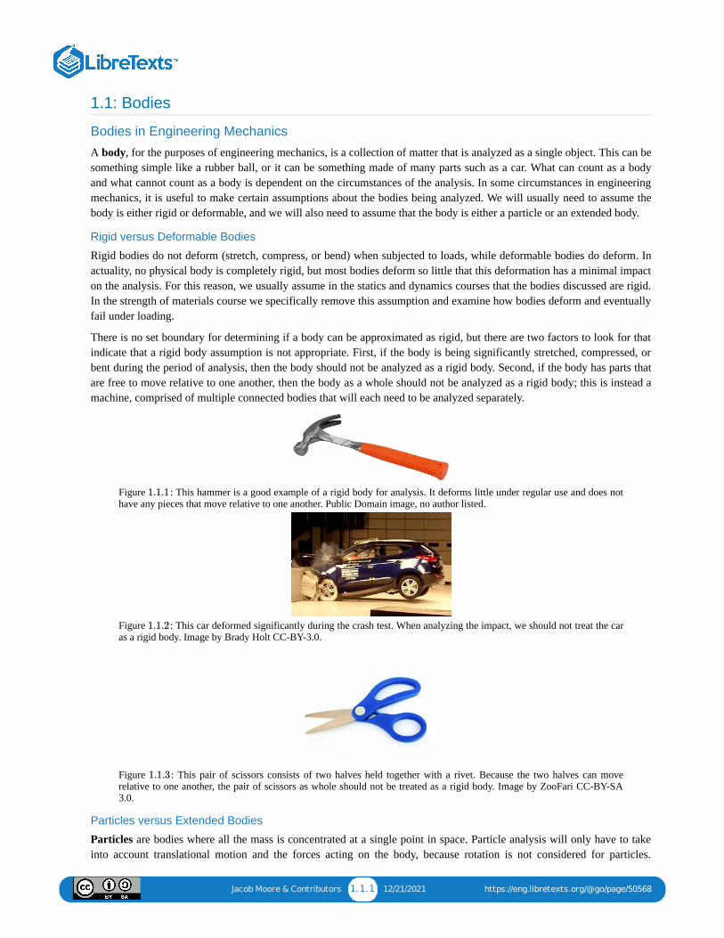
There is no set boundary for determining if a body can be approximated as rigid, but there are two factors to look for thatindicate that a rigid body assumption is not appropriate. First, if the body is being significantly stretched, compressed, orbent during the period of analysis, then the body should not be analyzed as a rigid body. Second, if the body has parts thatare free to move relative to one another, then the body as a whole should not be analyzed as a rigid body; this is instead amachine, comprised of multiple connected bodies that will each need to be analyzed separately.

Figure : This hammer is a good example of a rigid body for analysis. It deforms little under regular use and does nothave any pieces that move relative to one another. Public Domain image, no author listed.

Figure : This car deformed significantly during the crash test. When analyzing the impact, we should not treat the caras a rigid body. Image by Brady Holt CC-BY-3.0.

Figure : This pair of scissors consists of two halves held together with a rivet. Because the two halves can moverelative to one another, the pair of scissors as whole should not be treated as a rigid body. Image by ZooFari CC-BY-SA3.0.

Particles versus Extended Bodies

Particles are bodies where all the mass is concentrated at a single point in space. Particle analysis will only have to takeinto account translational motion and the forces acting on the body, because rotation is not considered for particles.

1.1.1

1.1.2

1.1.3

Jacob Moore & Contributors 1.1.2 12/21/2021 https://eng.libretexts.org/@go/page/50568

Extended bodies, on the other hand, have mass that is distributed throughout a finite volume. Often in engineering statics,we will take a shortcut and say rigid bodies to describe extended bodies that also happen to be rigid. This is becauseparticles, as a single point, cannot deform. Extended body analysis is more complex and also has to take into accountmoments and rotational motions. In actuality, no bodies are truly particles, but some bodies can be approximated asparticles to simplify analysis. Bodies are often assumed to be particles if the rotational motions are negligible whencompared to the translational motions, or in systems where there is no moment exerted on the body, such as a concurrentforce system.

Figure : The rotation of this comet and the moments exerted on the comet are unimportant in modeling its trajectorythrough space, therefore we would treat it as a particle. Public Domain image by Buddy Nath.

Figure : The gravitational forces and the tension forces on the skycam all act through a single point, making this aconcurrent force system that can be analyzed as a particle. Image by Despeaux CC-BY-SA 3.0.

Figure : Rotation and moments will be key to the analysis of the crowbar in this system, therefore the crowbar needsto be analyzed as an extended body. Public Domain image by Pearson Scott Foresman.

Video : Lecture video covering this section, delivered by Dr. Jacob Moore. YouTube source: https://youtu.be/-ETzKW31aZI.

1.1.4

1.1.5

1.1.6

1.1 Bodies - Video Lecture - JPM1.1 Bodies - Video Lecture - JPM

1.1.1

Jacob Moore & Contributors 1.2.1 1/30/2022 https://eng.libretexts.org/@go/page/50569

1.2: ForcesA force is any influence that causes a body to accelerate. Forces on a body can also cause stress in that body, which canresult in the body deforming or breaking. Though forces can come from a variety of sources, there are three distinguishingfeatures to every force. These features are the magnitude of the force, the direction of the force, and the point ofapplication of the force. Forces are often represented as vectors (as in the diagram to the right) and each of these featurescan be determined from a vector representation of the forces on the body.

Figure : A basic point force acting on a body.

Magnitude:The magnitude of a force is the degree to which the force will accelerate the body it is acting on; it is represented by ascalar (a single number). The magnitude can also be thought of as the strength of the force. When forces are represented asvectors, the magnitude of the force is usually explicitly labeled. The length of the vector also often corresponds to therelative magnitude of the vector, with longer vectors indicating larger magnitudes.

The magnitude of force is measured in units of mass times length over time squared. In metric units the most common unitis the Newton (N), where one Newton is one kilogram times one meter over one second squared. This means that a forceof one Newton would cause a one-kilogram object to accelerate at a rate of one meter per second squared. In English units,the most common unit is the pound (lb), where one pound is equal to one slug times a foot over a second squared. Thismeans that a one-pound force would cause an object with a mass of one slug to accelerate at a rate of one foot per secondsquared.

Direction:

In addition to having magnitudes, forces also have directions. As we said before, a force is any influence that causes abody to accelerate. Since acceleration has a specific direction, force also has a specific direction that matches thisacceleration. The direction of the force is indicated in diagrams by the direction of the vector representing the force.

Direction has no units, but it is usually given by reporting angles between the vector representing the force and coordinateaxes, or by reporting the X, Y, and Z components of the vector. Often times vectors that have the same direction as one ofthe coordinate axes will not have any angles or components listed. If this is true, it is usually safe to assume that thedirection does match the direction of one of the coordinate axes.

1.2.1

Force =(mass)(distance)

(time)2(1.2.1)

1 Newton (N) =(kg)(m)

s2(1.2.2)

1 pound (lb) =(slug)(ft)

s2(1.2.3)

Jacob Moore & Contributors 1.2.2 1/30/2022 https://eng.libretexts.org/@go/page/50569

Figure : The magnitude and direction of a vector can be given as a magnitude and an angle of the vector, or by givingmagnitude of the vector components in each of the coordinate axes.

Point of Application:

The point, or points, at which a force is applied to a body is important for understanding how the body will react. Forparticles, there is only a single point for the forces to act on, but for rigid bodies there are an infinite number of possiblepoints of application. Some points of application will lead to the body undergoing simple linear acceleration; some willexert a moment on the body which will cause the body to undergo rotational acceleration as well as linear acceleration.

Depending on the nature of the point of application of a force, there are three general types of forces. These are pointforces, surface forces, and body forces. Below is a diagram of a box being pulled by a rope across a frictionless surface.The box has three forces acting on it. The first is the force from the rope. This is a force applied to a single point on thebox, and is therefore modeled as point force. Point forces are represented by a single vector. Second is the normal forcefrom the ground that is supporting the box. Because this force is applied evenly to the bottom surface of the box, it is bestmodeled as a surface force. Surface forces are indicated by a number of vectors drawn side by side with a profile line toindicate the magnitude of the force at any point. The last force is the gravitational force pulling the box downward.Because this force is applied evenly to the entire volume of the box, it is best modeled as a body force. Body forces aresometimes shown as a field of vectors as shown, though they are often not drawn out at all because they end up clutteringthe free body diagram.

Figure : The box being pulled along a frictionless surface as shown above has three types of forces acting on it. Thetension in the cable is best represented by a point force, the normal force supporting the box is best represented by asurface force, and the gravitational force on the box is best represented as a body force.

We will also sometimes talk about distributed forces. A distributed force is simply another name for either a surface or abody force.

The exact point or surface that the force is acting on can be drawn as either the head or the tail of the force vector in thefree body diagram. Because of the principle of transmissibility, both options are known to represent the same physicalsystem.

1.2.2

1.2.3

Jacob Moore & Contributors 1.2.3 1/30/2022 https://eng.libretexts.org/@go/page/50569

Figure : The diagrams on the left represent two equivalent free body diagrams for the same physical system with asingle point force. The diagrams on the right represent two equivalent free body diagrams for the same physical systemwith a single surface force.

Video : Lecture video covering this section, delivered by Dr. Jacob Moore. YouTube source:https://youtu.be/8MR_w3ZOOiM.

1.2.4

1.2 Forces - Video Lecture - JPM1.2 Forces - Video Lecture - JPM

1.2.1

Jacob Moore & Contributors 1.3.1 1/30/2022 https://eng.libretexts.org/@go/page/50570

1.3: MomentsA moment (also sometimes called a torque) is defined as the "tendency of a force to rotate a body". Where forces causelinear accelerations, moments cause angular accelerations. In this way moments, can be thought of as twisting forces.

Figure : Imagine two boxes on an icy surface. The force on box A would simply cause the box to begin accelerating,but the force on box B would cause the box to both accelerate and to begin to rotate. The force on box B is exerting amoment, where the force on box A is not.

The Vector Representation of a Moment:

Moments, like forces, can be represented as vectors and have a magnitude, a direction, and a "point of application". Formoments however a better name for the point of application is the axis of rotation. This will be the point or axis aboutwhich we will determine all the moments.

Magnitude:

The magnitude of a moment is the degree to which the moment will cause angular acceleration in the body it is acting on.It is represented by a scalar (a single number). The magnitude of the moment can be thought of as the strength of thetwisting force exerted on the body. When a moment is represented as a vector, the magnitude of the moment is usuallyexplicitly labeled. though the length of the moment vector also often corresponds to the relative magnitude of the moment.

The magnitude of the moment is measured in units of force times distance. The standard metric units for the magnitude ofmoments are Newton-meters, and the standard English units for a moment are foot-pounds.

Direction:

In a two-dimensional problem, the direction can be thought of as a scalar quantity corresponding to the direction ofrotation the moment would cause. A moment that would cause a counterclockwise rotation is a positive moment, and amoment that would cause a clockwise rotation is a negative moment.

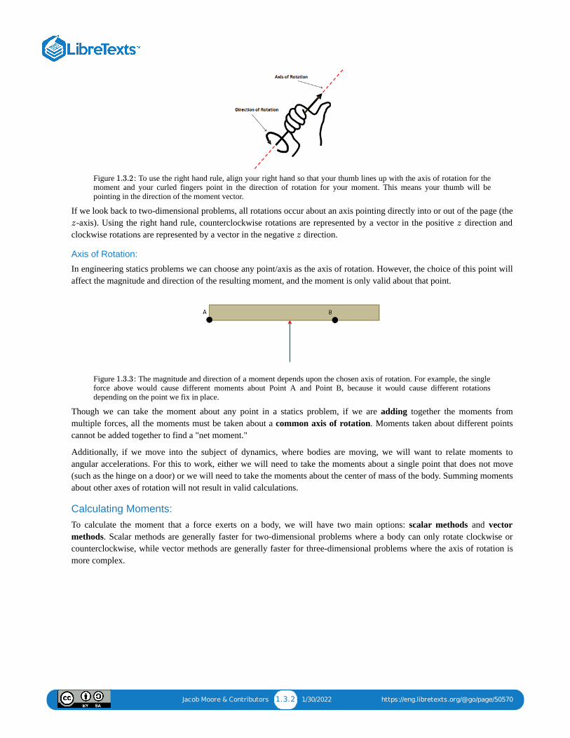
In a three-dimensional problem, however, a body can rotate about an axis in any direction. If this is the case, we need avector to represent the direction of the moment. The direction of the moment vector will line up with the axis of rotationthat moment would cause, but to determine which of the two directions we can use along that axis we have available weuse the right hand rule. To use the right hand rule, align your right hand as shown in Figure so that your thumb linesup with the axis of rotation for the moment and your curled fingers point in the direction of rotation for your moment. Ifyou do this, your thumb will be pointing in the direction of the moment vector.

1.3.1

M = F ∗ d (1.3.1)

Metric: N ∗m (1.3.2)

English: lb ∗ ft (1.3.3)

1.3.2

Jacob Moore & Contributors 1.3.2 1/30/2022 https://eng.libretexts.org/@go/page/50570

Figure : To use the right hand rule, align your right hand so that your thumb lines up with the axis of rotation for themoment and your curled fingers point in the direction of rotation for your moment. This means your thumb will bepointing in the direction of the moment vector.

If we look back to two-dimensional problems, all rotations occur about an axis pointing directly into or out of the page (the-axis). Using the right hand rule, counterclockwise rotations are represented by a vector in the positive direction and

clockwise rotations are represented by a vector in the negative direction.

Axis of Rotation:

In engineering statics problems we can choose any point/axis as the axis of rotation. However, the choice of this point willaffect the magnitude and direction of the resulting moment, and the moment is only valid about that point.

Figure : The magnitude and direction of a moment depends upon the chosen axis of rotation. For example, the singleforce above would cause different moments about Point A and Point B, because it would cause different rotationsdepending on the point we fix in place.

Though we can take the moment about any point in a statics problem, if we are adding together the moments frommultiple forces, all the moments must be taken about a common axis of rotation. Moments taken about different pointscannot be added together to find a "net moment."

Additionally, if we move into the subject of dynamics, where bodies are moving, we will want to relate moments toangular accelerations. For this to work, either we will need to take the moments about a single point that does not move(such as the hinge on a door) or we will need to take the moments about the center of mass of the body. Summing momentsabout other axes of rotation will not result in valid calculations.

Calculating Moments:To calculate the moment that a force exerts on a body, we will have two main options: scalar methods and vectormethods. Scalar methods are generally faster for two-dimensional problems where a body can only rotate clockwise orcounterclockwise, while vector methods are generally faster for three-dimensional problems where the axis of rotation ismore complex.

1.3.2

z z

z

1.3.3

Jacob Moore & Contributors 1.3.3 1/30/2022 https://eng.libretexts.org/@go/page/50570

Video : Lecture video covering this section, delivered by Dr. Jacob Moore. YouTube source:https://youtu.be/RyOwVvYEFHU.

1.3 Moments - Video Lecture - JPM1.3 Moments - Video Lecture - JPM

1.3.1

Jacob Moore & Contributors 1.4.1 1/23/2022 https://eng.libretexts.org/@go/page/51301

1.4: Free Body DiagramsA free body diagram is a tool used to solve engineering mechanics problems. As the name suggests, the purpose of thediagram is to "free" the body from all other objects and surfaces around it so that it can be studied in isolation. We will alsodraw in any forces or moments acting on the body, including those forces and moments exerted by the surrounding bodiesand surfaces that we removed.

The diagram below shows a ladder supporting a person and the free body diagram of that ladder. As you can see, theladder is separated from all other objects and all forces acting on the ladder are drawn in with the key dimensions andangles shown.

Figure : A ladder with a man standing on it is shown on the left. Assuming friction only at the base, a free bodydiagram of the ladder is shown on the right.

Constructing the Free Body Diagram:The first step in solving most mechanics problems will be to construct a free body diagram. This simplified diagram willallow us to more easily write out the equilibrium equations for statics or strengths of materials problems, or the equationsof motion for dynamics problems.

To construct the diagram we will use the following process:

1. First draw the body being analyzed, separated from all other surrounding bodies and surfaces. Pay close attention to theboundary, identifying what is part of the body, and what is part of the surroundings.

2. Second, draw in all external forces and moments acting directly on the body. Do not include any forces or momentsthat do not directly act on the body being analyzed. Do not include any forces that are internal to the body beinganalyzed.

3. Once the forces are identified and added to the free body diagram, the last step is to label any key dimensions andangles on the diagram.

Some common types of forces seen in mechanics problems are:

Gravitational Forces: Unless otherwise noted, the mass of an object will result in a gravitational weight force appliedto that body. This weight is usually given in pounds in the English system, and is modeled as 9.81 ( ) times the mass ofthe body in kilograms for the metric system (resulting in a weight in Newtons). This force will always point downtowards the center of the earth and act on the center of mass of the body.

1.4.1

g

Jacob Moore & Contributors 1.4.2 1/23/2022 https://eng.libretexts.org/@go/page/51301

Figure : Gravitational forces always act downward on the center of mass.

Normal Forces (or Reaction Forces): Every object in direct contact with the body will exert a normal force on thatbody which prevents the two objects from occupying the same space at the same time. Note that only objects in directcontact can exert normal forces on the body.

An object in contact with another object or surface will experience a normal force that is perpendicular (normal) tothe surfaces in contact.Joints or connections between bodies can also cause reaction forces or moments, and we will have one force ormoment for each type of motion or rotation the connection prevents.

Figure : Normal forces always act perpendicular to the surfaces in contact. The barrel in the hand truck shown on theleft has a normal force at each contact point.

Figure : The roller on the left allows for rotation and movement along the surface, but a normal force in the ydirection prevents motion vertically. The pin joint in the center allows for rotation, but normal forces in the x and ydirections prevent motion in all directions. The fixed connection on the right has a normal forces preventing motion in alldirections and a reaction moment preventing rotation.

Friction Forces: Objects in direct contact with the body can also exert friction forces, which will resist the two bodiessliding against one another, on the body. These forces will always be perpendicular to the surfaces in contact. Frictionis the subject of an entire chapter in this book, but for simple scenarios we usually assume rough or smooth surfaces.

For smooth surfaces we assume that there is no friction force.For rough surfaces we assume that the bodies will not slide relative to one another, no matter what. In this case, thefriction force is always just large enough to prevent this sliding.

1.4.2

1.4.3

1.4.4

Jacob Moore & Contributors 1.4.3 1/23/2022 https://eng.libretexts.org/@go/page/51301

Figure : For a smooth surface we assume only a normal force perpendicular to the surface. For a rough surface weassume normal and friction forces are present.

Tension in Cables: Cables, wires or ropes attached to the body will exert a tension force on the body in the direction ofthe cable. These forces will always pull on the body, as ropes, cables and other flexible tethers cannot be used forpushing.

Figure : The tension force in cables always acts along the direction of the cable and will always be a pulling force.

The above forces are the most common, but other forces such as pressure from fluids, spring forces and magnetic forcesexist and may act on the body.

Video : Lecture video covering this section, delivered by Dr. Jacob Moore. YouTube source:https://youtu.be/Kr7obGR68-Y.

Worked Problems:

The drawing below shows two boxes sitting on a table. Draw a free body diagram of box A and box B.

1.4.5

1.4.6

1.4 Free Body Diagrams - Video Lect1.4 Free Body Diagrams - Video Lect……

1.4.1

Example 1.4.1

Jacob Moore & Contributors 1.4.4 1/23/2022 https://eng.libretexts.org/@go/page/51301

Figure : problem diagram for Example ; two boxes are stacked on a flat surface, with one weighing 3 lbs ontop of another weighing 5 lbs.

Solution

Video : Worked solution to example problem , provided by Dr. Jacob Moore. YouTube source:https://youtu.be/RMVa9kioALs.

Two equally sized barrels are being transported in a handtruck as shown below. Draw a free body diagram of each ofthe two barrels.

Figure : problem diagram for Example ; two barrels are stacked horizontally, on a handcart tilted so thebottom is 30° above the horizontal.

Solution

1.4.7 1.4.1

Free Body Diagrams - Adaptive MFree Body Diagrams - Adaptive M……

1.4.2 1.4.1

Example 1.4.2

1.4.8 1.4.2

Jacob Moore & Contributors 1.4.5 1/23/2022 https://eng.libretexts.org/@go/page/51301

Video : Worked solution to example problem , provided by Dr. Jacob Moore. YouTube source:https://youtu.be/1a9gjFOIpK8.

The car shown below is moving and then slams on the brakes locking up all four wheels. The distance between the twowheels is 8 feet and the center of mass is 3 feet behind and 2.5 feet above the point of contact between the front wheeland the ground. Draw a free body diagram of the car as it comes to a stop.

Figure : Car traveling on a level surface, facing left. Public domain image, no author listed.

Solution

Video : Worked solution to example problem , provided by Dr. Jacob Moore. YouTube source:https://youtu.be/GiB3_fSlJBA.

A 600-pound load is supported by a 5 meter long, 100-pound cantilever beam. Assume the beam is firmly anchored tothe wall. Draw a free body diagram of the beam.

Free Body Diagrams - Adaptive MFree Body Diagrams - Adaptive M……

1.4.3 1.4.2

Example 1.4.3

1.4.9

Free Body Diagrams - Adaptive MFree Body Diagrams - Adaptive M……

1.4.4 1.4.3

Example 1.4.4

Jacob Moore & Contributors 1.4.6 1/23/2022 https://eng.libretexts.org/@go/page/51301

Figure : problem diagram for Example ; a 600-lb load hangs from the free end of a horizontal beam whoseother end is attached to a wall.

Solution

The main arm of a crane has a mass of 400 kg (assume the center of mass is at the midpoint of the arm), and supports a200 kg load and a 600 kg counterweight. The arm is connected to the vertical support via a pin joint and two flexiblecables. Draw a free body diagram of the arm.

Figure : problem diagram for Example ; a crane's arm, currently in the horizontal position, holds a load anda counterweight on opposite ends.

Solution

1.4.10 1.4.4

Free Body Diagrams - Adaptive MFree Body Diagrams - Adaptive M……

Example 1.4.5

1.4.11 1.4.5

Jacob Moore & Contributors 1.4.7 1/23/2022 https://eng.libretexts.org/@go/page/51301

Video : Worked solution to example problem , provided by Dr. Jacob Moore. YouTube source:https://youtu.be/0V7ULRnnhmA.

Free Body Diagrams - Adaptive MFree Body Diagrams - Adaptive M……

1.4.6 1.4.5

Jacob Moore & Contributors 1.5.1 12/21/2021 https://eng.libretexts.org/@go/page/51375

1.5: Newton's First LawNewton's first law states that: "A body at rest will remain at rest unless acted on by an unbalanced force. A body inmotion continues in motion with the same speed and in the same direction unless acted upon by an unbalancedforce."

This law, also sometimes called the "law of inertia", means that bodies maintain their current velocity unless a force isapplied to change that velocity. If an object is at rest with zero velocity it will remain at rest until some force begins tochange that velocity, and if an object is moving at a set speed and in a set direction it will remain at that same velocity untilsome force acts on it to change its velocity.

Figure : In the absence of friction in space, this space capsule will maintain its current velocity until some outsideforce causes that velocity to change. Public Domain image by NASA.

Figure : This rock is at rest with zero velocity and will remain at rest until a net force causes the rock to move. Thenet force on the rock is the sum of any force pushing the rock and the friction force of the ground on the rock opposing thatforce. Image by Liz Gray CC-BY-SA 2.0.

Net Forces:It is important to note that the net force is what will cause a change in velocity. The net force is the sum of all forces actingon the body. For example, we can imagine gently pushing on the rock in the figure above and observing that the rock doesnot move. This is because we will have a friction force equal in magnitude and opposite in direction opposing our gentlepushing force. The sum of these two forces will be equal to zero, therefore the net force is zero and the change in velocityis zero.

Rotational Motion:

Newton's first law also applies to moments and rotational velocities. A body will maintain it's current rotational velocityuntil a net moment is exerted to change that rotational velocity. This can be seen in things like toy tops, flywheels,stationary bikes, and other objects that will continue spinning once started until brakes or friction stop them.

Figure : In the absence of friction, this spinning top would continue to spin forever, but the small frictional momentexerted at the point of contact between the top and the ground will slow the tops spinning over time. Image byCarrotmadman6 CC-BY-2.0.

1.5.1

1.5.2

1.5.3

Jacob Moore & Contributors 1.5.2 12/21/2021 https://eng.libretexts.org/@go/page/51375

Video lecture covering this section, delivered by Dr. Jacob Moore. YouTube source: https://youtu.be/MeY-Cj93Tm4.

1.5 Newton's First Law - Video Lectu1.5 Newton's First Law - Video Lectu……

Jacob Moore & Contributors 1.6.1 12/21/2021 https://eng.libretexts.org/@go/page/51376

1.6: Newton's Second Law

Translational Motion:

Newton's second law states that: "When a net force acts on any body with mass, it produces an acceleration of thatbody. The net force will be equal to the mass of the body times the acceleration of the body."

You will notice that the force and the acceleration in the equation above have an arrow above them. This means that theyare vector quantities, having both a magnitude and a direction. Mass, on the other hand, is a scalar quantity having only amagnitude. Based on the above equation, you can infer that the magnitude of the net force acting on the body will be equalto the mass of the body times the magnitude of the acceleration, and that the direction of the net force on the body will beequal to the direction of the acceleration of the body.

Rotational Motion:

Newton's second law also applies to moments and rotational velocities. The revised version of the second law equationstates that the net moment acting on the object will be equal to the mass moment of inertia of the body about the axis ofrotation ( ) times the angular acceleration of the body.

You should again notice that the moment and the angular acceleration of the body have arrows above them, indicating thatthey are vector quantities with both a magnitude and direction. The mass moment of inertia, on the other hand, is a scalarquantity having only a magnitude. The magnitude of the net moment will be equal to the mass moment of inertia times themagnitude of the angular acceleration, and the direction of the net moment will be equal to the direction of the angularacceleration.

Video lecture covering this section, delivered by Dr. Jacob Moore. YouTube source: https://youtu.be/3PF2uNGW7Dw.

= mF   a  (1.6.1)

I

= I ∗M  α  (1.6.2)

1.6 Newton's Second Law - Video Le1.6 Newton's Second Law - Video Le……

Jacob Moore & Contributors 1.7.1 12/21/2021 https://eng.libretexts.org/@go/page/51378

1.7: Newton's Third LawNewton's Third Law states "For any action, there is an equal and opposite reaction." By "action" Newton meant aforce, so for every force one body exerts on another body, that second body exerts a force of equal magnitude but oppositedirection back on the first body. Since all forces are exerted by bodies (either directly or indirectly), all forces come inpairs, one acting on each of the bodies interacting.

Figure : The gravitational pull of the Earth and Moon represent a Newton's Third Law pair. The Earth exerts agravitational pull on the Moon, and the Moon exerts an equal and opposite pull on the Earth. Image adapted from PublicDomain images, no authors listed.

Though there may be two equal and opposite forces acting on a single body, it is important to remember that for each ofthe forces a Third Law pair acts on a separate body. This can sometimes be confusing when there are multiple Third Lawpairs at work. Below are some examples of situations where multiple Third Law pairs occur.

Figure : This volleyball resting on a surface has two pairs of Third Law forces. The first consists of the gravitationalforces (one force on the ball and one force on the ground). The second consists of the normal forces at the point of contact(one force on the ball and one force on the ground). Image adapted from Public Domain image, no author listed.

Figure : If we ignore the weight of the two objects, this clamp will also have two pairs of Third Law forces. The firstwill be a set of normal forces at the top point of contact (one force on the wood and one force on the clamp) and the secondwill be another set of normal forces at the bottom point of contact (one force on the wood and one force on the clamp)Image adapted from Public Domain image, no author listed.

1.7.1

1.7.2

1.7.3

Jacob Moore & Contributors 1.7.2 12/21/2021 https://eng.libretexts.org/@go/page/51378

Video lecture covering this section, delivered by Dr. Jacob Moore. YouTube source: https://youtu.be/zB5l95jwKr4.

1.7 Newton's Third Law - Video Lect1.7 Newton's Third Law - Video Lect……

Jacob Moore & Contributors 1.8.1 12/21/2021 https://eng.libretexts.org/@go/page/51487

1.8: Chapter 1 Homework Problems

A pulley system is being used to hoist a 50 kg engine block as shown below. If distance is currently 1 meter and weassume the pulleys are all frictionless, draw a free body diagram of the engine block with the attached pulley. Includeall forces and important angles.

Figure : problem diagram for Exercise ; an engine block is suspended by a cable with one end attached to ananchor point and the other end passing over a pulley.

The car shown below has a weight of 4500 lbs and a center of mass at point G. Assuming the car is not moving and issitting on a level surface, draw a free body diagram of the car. Include all forces and important distances.

Figure : problem diagram for Exercise ; a car sitting on a level surface is marked with a point G indicatingthe location of its center of mass.

A telephone pole sits on a rough surface. A cable attached to an excavator is then used to pull the pole along thesurface as shown below. Assume the telephone pole has a mass of 350 kg and a length of 12 meters. Draw a free bodydiagram of the telephone pole. Include all forces, important distances, and important angles.

Exercise 1.8.1

d

1.8.1 1.8.1

Exercise 1.8.2

1.8.2 1.8.2

Exercise 1.8.3

Jacob Moore & Contributors 1.8.2 12/21/2021 https://eng.libretexts.org/@go/page/51487

Figure : problem diagram for Exercise ; an excavator pulls a telephone pole across the ground at an angle,through the use of a cable.

1.8.3 1.8.3

1 1/30/2022

CHAPTER OVERVIEW2: STATIC EQUILIBRIUM IN CONCURRENT FORCE SYSTEMSThe definition of static equilibrium and concurrent force systems. Analysis of concurrent force systems at static equilibrium to identifyunknown forces.

2.0: CHAPTER 2 VIDEO INTRODUCTIONVideo introduction to the topics to be covered in this chapter: static equilibrium, equilibrium analysis of concurrent force systems,finding and calculating forces.

2.1: STATIC EQUILIBRIUMDefinition of static equilibrium, and its relation to force and acceleration, in terms of both linear and angular acceleration.

2.2: POINT FORCES AS VECTORSApproximating surface forces as point forces. The line of action of forces. Representation of forces as vectors, magnitude-angle andcomponent notations of vectors. Includes several worked example problems.

2.3: PRINCIPLE OF TRANSMISSIBILITYThe principle of transmissibility, and the situations where it can be applied to analysis of a rigid body vs. those where it cannot.

2.4: CONCURRENT FORCESThe connection between lines of action and the concurrence of a set of point forces. Particle behavior of a body experiencing onlyconcurrent forces.

2.5: EQUILIBRIUM ANALYSIS FOR CONCURRENT FORCE SYSTEMSHow to solve problems involving analysis of concurrent forces on a body at static equilibrium. Includes several worked exampleproblems.

2.6: CHAPTER 2 HOMEWORK PROBLEMS

Jacob Moore & Contributors 2.0.1 1/23/2022 https://eng.libretexts.org/@go/page/51659

2.0: Chapter 2 Video Introduction

Video introduction to Chapter 2, delivered by Dr. Jacob Moore. YouTube source: https://youtu.be/VXhvhP8VBMY.

Chapter 2 IntroductionChapter 2 Introduction

Jacob Moore & Contributors 2.1.1 12/21/2021 https://eng.libretexts.org/@go/page/50572

2.1: Static EquilibriumObjects in static equilibrium are objects that are not accelerating (either linear acceleration or angular acceleration). Theseobjects may be stationary, such as a building or a bridge, or they may have a constant velocity, such as a car or truckmoving at a constant speed on a straight patch of road.

Figure : (left) Because this high rise building is stationary with no acceleration, themembers and overall structure are in equilibrium. Image by Jakembradford CC-BY-SA 4.0.(right): Assuming that this truck is maintaining a constant speed and direction, this truckis in equilibrium because its velocity is not changing over time. Public Domain imageby Klever.

Newton's Second Law states that the force exerted on an object is equal to the mass of the object times the acceleration itexperiences. Therefore, if we know that the acceleration of an object is equal to zero, then we can assume that the sum ofall forces acting on the object is zero. Individual forces acting on the object, represented by force vectors, may not havezero magnitude but the sum of all the force vectors will always be equal to zero for objects in equilibrium. Engineeringstatics is the study of objects in static equilibrium, and the simple assumption of all forces adding up to zero is the basis forthe subject area of engineering statics.

Equilibrium follows a similar pattern for angular accelerations. The rotational equivalent of Newton's Second Law statesthat the moment exerted on an object is equal to the moment of inertia of that object times the angular acceleration of theobject. If we know the angular acceleration of an object is equal to zero, then we know the sum of all moments acting onthe object is equal to zero.

Video lecture covering this section, delivered by Dr. Jacob Moore. YouTube source: https://youtu.be/2Ekp8MkgUYI.

2.1.1

∑ = mF   a  (2.1.1)

a = 0 ; ∑ = 0F   (2.1.2)

∑ = IM  α  (2.1.3)

= 0 ; ∑ = 0α  M  (2.1.4)

2.1 Static Equilibrium - Video Lecture2.1 Static Equilibrium - Video Lecture……

Jacob Moore & Contributors 2.2.1 12/21/2021 https://eng.libretexts.org/@go/page/50573

2.2: Point Forces as VectorsA point force is any force where the point of application is considered to be a single point. In reality, most forces aretechnically surface forces, where the force is applied over an area, but when the area is small enough (in comparison to thebodies being analyzed) it can often be approximated as a point force. Because point forces can be represented as a singlevector (rather than a field of vectors for distributed forces), they are much easier to work with in engineering analysis. Forthis reason, point forces are used in place of distributed forces in engineering analysis whenever possible. Below are someexamples of where it is appropriate to use point forces.

Figure : The tensions in the cables supporting this container can be treated as point forces pulling in the direction ofthe cables. Adapted from Image by maxronnersjo CC-BY-SA 3.0.

Figure : The friction force between the bow and string on this cello can be treated as a point force. Adapted fromPublic Domain image by Levi.

Figure : Though gravitational forces are technically body forces, they are often approximated as a single point forceacting on the center of gravity of the object. Adapted from Public Domain image, no author listed.

Figure : The gravitational force and the normal forces acting on each leg of this table can all be approximated as pointforces. Adapted from Public Domain image by Seahen.

In addition to the magnitude, direction, and point of application of the point force, another important term to understand isthe line of action of the force. The line of action of a force is the line along which the force acts. Given the direction andpoint of application, one can find the line of action, but this term will be important in discussing concurrent forces and inthe principle of transmissibility.

2.2.1

2.2.2

2.2.3

2.2.4

Jacob Moore & Contributors 2.2.2 12/21/2021 https://eng.libretexts.org/@go/page/50573

Figure : The line of action of a point force is the line along which the force acts.

Force Vector Representation:When vectors are drawn to form free body diagrams, the magnitude and direction are usually given in one of two formats:

Overall magnitude and angle(s) to indicate direction (often called magnitude and direction form).Magnitudes in each of the coordinate directions (often called component form).

In either format we will need two values to fully define a force vector in a 2D system (either a magnitude and a singleangle or a magnitude in each of the two coordinate axes), and three values to fully define a force vector in a 3D system(either a magnitude and two angles or a magnitude in each of the three coordinate axes). Below are some examples offorce vectors in both representations.

Figure : The same force can be represented with a magnitude and an angle, as shown in the left, or with magnitudesin relation to each of the coordinate axes as shown on the right.

Figure : In three dimensions forces are represented with either a magnitude and two directions, as shown on the left,or with magnitudes in relation to each of the three coordinate axes as shown on the right.

Changing Force Vector Forms:Because the two different forms of the vector are equivalent, we can switch between representations without changing theproblem. Often in engineering problems, it will initially be easier to write the force in magnitude and angle form, but later,analysis will be easier if forces are written in component form. To switch from magnitude and direction form to componentform you will use right triangles and trigonometry to determine the component of the overall magnitude in each direction.This is a simple vector decomposition, and more information on this process can be seen on the vector decompositionpage. To switch back from component form into magnitude and direction form you simply use the reverse of this initialprocess.

2.2.5

2.2.6

2.2.7

Jacob Moore & Contributors 2.2.3 12/21/2021 https://eng.libretexts.org/@go/page/50573

Video lecture covering this section, delivered by Dr. Jacob Moore. YouTube source: https://youtu.be/kq8vqOKhKeA.

The tension force on the box below is given in magnitude and direction form. Redraw the diagram with the tensionforce given in component form.

Solution

Video : Worked solution to example problem , provided by Dr. Jacob Moore. YouTube source:https://youtu.be/ZERURXWnlDg.

The force acting on the cantilever beam shown below is given in component form. Redraw the diagram with the forcegiven in magnitude and direction form.

2.2 Point Forces - Video Lecture - JPM2.2 Point Forces - Video Lecture - JPM

Example 2.2.1

Point Forces - Adaptive Map WorkPoint Forces - Adaptive Map Work……

2.2.2 2.2.1

Example 2.2.2

Jacob Moore & Contributors 2.2.4 12/21/2021 https://eng.libretexts.org/@go/page/50573

Solution

Video : Worked solution to example problem , provided by Dr. Jacob Moore. YouTube source:https://youtu.be/M3UjDfZzRHY.

The force shown below is given in magnitude and direction form. Redraw the diagram with the force vector given incomponent form.

Solution

Point Forces - Adaptive Map WorkPoint Forces - Adaptive Map Work……

2.2.3 2.2.2

Example 2.2.3

Jacob Moore & Contributors 2.2.5 12/21/2021 https://eng.libretexts.org/@go/page/50573

Video : Worked solution to example problem , delivered by Dr. Jacob Moore. YouTube source:https://youtu.be/DroNv0TxnyA.

Point Forces - Adaptive Map WorkPoint Forces - Adaptive Map Work……

2.2.4 2.2.3

Jacob Moore & Contributors 2.3.1 1/30/2022 https://eng.libretexts.org/@go/page/50574

2.3: Principle of TransmissibilityThe principle of transmissibility states that the point of application of a force can be moved anywhere along its line ofaction without changing the external reaction forces on a rigid body. Any force that has the same magnitude anddirection, and which has a point of application somewhere along the same line of action will cause the same accelerationand will result in the same moment. Therefore, the points of application of forces may be moved along the line of action tosimplify the analysis of rigid bodies.

Figure : Because of the principle of transmissibility, each of the above pairs is equivalent.

When analyzing the internal forces (stress) in a rigid body, the exact point of application does matter. This difference instresses may also result in changes in geometry which will in turn affect reaction forces. For this reason, the principle oftransmissibility should only be used when examining external forces on bodies that are assumed to be rigid.

Figure : The exact point of application of a force will impact how internal forces (stresses) are distributed, so theprinciple of transmissibility cannot be applied when examining internal forces.

Video lecture covering this section, delivered by Dr. Jacob Moore. YouTube source: https://youtu.be/sx__xzA7eqM.

2.3.1

2.3.2

2.3 Principle of Transmissiblity - Vide2.3 Principle of Transmissiblity - Vide……

Jacob Moore & Contributors 2.4.1 1/2/2022 https://eng.libretexts.org/@go/page/50575

2.4: Concurrent ForcesA set of point forces is considered concurrent if all the lines of action of those forces all come together at a single point.

Figure : Because the lines of action for the gravitational force and the two tension forces line up at a single point,these forces are considered concurrent.

Figure : Because the lines of action of the gravitational force and the two normal forces do not intersect at a singlepoint, these forces are not considered concurrent. Adapted from Public Domain image by Seahen.

Because the forces all act through a single point, there are no moments about this point. Because no moments exist, we cantreat this body as a particle. In fact, because real particles only exist in theory, most particle analysis is actually applied toextended bodies with concurrent forces acting on them.

Video lecture covering this section, delivered by Dr. Jacob Moore. YouTube source: https://youtu.be/puLnyApKfuc.

2.4.1

2.4.2

2.4 Concurrent Force Systems - Vide2.4 Concurrent Force Systems - Vide……

Jacob Moore & Contributors 2.5.1 1/30/2022 https://eng.libretexts.org/@go/page/50576

2.5: Equilibrium Analysis for Concurrent Force SystemsIf a body is in static equilibrium, then by definition that body is not accelerating. If we know that the body is notaccelerating then we know that the sum of the forces acting on that body must be equal to zero. This is the basis forequilibrium analysis for a particle.

In order to solve for any unknowns in our sum of forces equation, we actually need to turn the one vector equation into aset of scalar equations. For two dimensional problems, we will split our one vector equation down into two scalarequations. We do this by summing up all the components of the force vectors and setting them equal to zero in our firstequation, and summing up all the components of the force vectors and setting them equal to zero in our second equation.

We do something similar in three dimensional problems except we will break all our force vectors down into , , and components, setting the sum of components equal to zero for our first equation, the sum of all the components equal tozero for our second equation, and the sum of all our components equal to zero for our third equation.

Once we have written out the equilibrium equations, we can solve the equations for any unknown forces.

Finding the Equilibrium Equations:The first step in finding the equilibrium equations is to draw a free body diagram of the body being analyzed. Thisdiagram should show all the known and unknown force vectors acting on the body. In the free body diagram, providevalues for any of the know magnitudes or directions for the force vectors and provide variable names for any unknowns(either magnitudes or directions).

Figure : The first step in equilibrium analysis is drawing a free body diagram. This is done by removing everythingbut the body and drawing in all forces acting on the body. It is also useful to label all forces, key dimensions, and angles.

Next you will need to chose the , , and axes. These axes do need to be perpendicular to one another, but they do notnecessarily have to be horizontal or vertical. If you choose coordinate axes that line up with some of your force vectorsyou will simplify later analysis.

Once you have chosen axes, you need to break down all of the force vectors into components along the , and directions (see the vectors page in Appendix 1 if you need more guidance on this). Your first equation will be the sum ofthe magnitudes of the components in the direction being equal to zero, the second equation will be the sum of themagnitudes of the components in the direction being equal to zero, and the third (if you have a 3D problem) will be thesum of the magnitudes in the direction being equal to zero. Collectively these are known as the equilibrium equations.

Once you have your equilibrium equations, you can solve them for unknowns using algebra. The number of unknowns thatyou will be able to solve for will be the number of equilibrium equations that you have. In instances where you have more

x

y

∑ = 0F   (2.5.1)

∑ = 0 ; ∑ = 0Fx Fy (2.5.2)

x y z

x y

z

∑ = 0F   (2.5.3)

∑ = 0 ; ∑ = 0 ; ∑ = 0Fx Fy Fz (2.5.4)

2.5.1

x y z

x y z

x

y

z

Jacob Moore & Contributors 2.5.2 1/30/2022 https://eng.libretexts.org/@go/page/50576

unknowns than equations, the problem is known as a statically indeterminate problem and you will need additionalinformation to solve for the given unknowns.

Video lecture covering this section, delivered by Dr. Jacob Moore. YouTube source: https://youtu.be/Dbd9SvdfoN8.

The diagram below shows a 3-lb box (Box A) sitting on top of a 5-lb box (box B). Determine the magnitude anddirection of all the forces acting on box B.

Figure \(\PageIndex

{2}\): problem diagram for Example \(\PageIndex

{1}\); two stacked boxes sitting on a flat surface.

Solution

2.5 Equilibrium Analysis in Concurre2.5 Equilibrium Analysis in Concurre……

Example 2.5.1

Jacob Moore & Contributors 2.5.3 1/30/2022 https://eng.libretexts.org/@go/page/50576

Video : Worked solution to example problem , provided by Dr. Jacob Moore. YouTube source:https://youtu.be/J54OZSitzzM.

A 600-lb barrel rests in a trough as shown below. The barrel is supported by two normal forces ( and ).Determine the magnitude of both of these normal forces.

Figure : problem diagram for Example ; a barrel resting in a trough with straight, angled sides.

Solution

Video : Worked solution to example problem , provided by Dr. Jacob Moore. YouTube source:https://youtu.be/qKhZvf55Bc0.

Equilibrium Analysis for ConcurreEquilibrium Analysis for Concurre……

2.5.2 2.5.1

Example 2.5.2

F2 F3

2.5.3 2.5.2

Equilibrium Analysis for ConcurreEquilibrium Analysis for Concurre……

2.5.3 2.5.2

Jacob Moore & Contributors 2.5.4 1/30/2022 https://eng.libretexts.org/@go/page/50576

A 6-kg traffic light is supported by two cables as shown below. Find the tension in each of the cables supporting thetraffic light.

Figure : problem diagram for Example ; a traffic light is held in midair by two cables, one horizontal andone angled..

Solution

Video : Worked solution to example problem , provided by Dr. Jacob Moore. YouTube source:https://youtu.be/Oi2yDg1SmrI.

A 400-kg wrecking ball rests against a surface as shown below. Assuming the wrecking ball is currently inequilibrium, determine the tension force in the cable supporting the wrecking ball and the normal force that existsbetween the wrecking ball and the surface.

Figure : problem diagram for Example ; a wrecking ball on a cable is resting against an angled surface.

Example 2.5.3

2.5.4 2.5.3

Equilibrium Analysis for ConcurreEquilibrium Analysis for Concurre……

2.5.4 2.5.3

Example 2.5.4

2.5.5 2.5.4

Jacob Moore & Contributors 2.5.5 1/30/2022 https://eng.libretexts.org/@go/page/50576

Solution

Video : Worked solution to example problem , provided by Dr. Jacob Moore. YouTube source:https://youtu.be/gETMTfy5Sew.

Barrels A and B are supported in a foot truck as seen below. Assuming the barrels are in equilibrium, determine allforces acting on barrel B.

Figure : problem diagram for Example ; two barrels stacked on their sides are on a handcart, whose bottomis tilted upwards.

Solution

Video : Worked solution to example problem , provided by Dr. Jacob Moore. YouTube source:https://youtu.be/8DgrClhT4AM.

Equilibrium Analysis for ConcurreEquilibrium Analysis for Concurre……

2.5.5 2.5.4

Example 2.5.5

2.5.6 2.5.5

Equilibrium Analysis for ConcurreEquilibrium Analysis for Concurre……

2.5.6 2.5.5

Jacob Moore & Contributors 2.5.6 1/30/2022 https://eng.libretexts.org/@go/page/50576

Three soda cans, each weighing 0.75 lbs and having a diameter of 4 inches, are stacked in a formation as shown below.Assuming no friction forces, determine the normal forces acting on can B.

Figure : problem diagram for Example ; three soda cans are stacked lying on their sides, in a flat areabounded on two sides by walls.

Solution

Video : Worked solution to example problem , provided by Dr. Jacob Moore. YouTube source:https://youtu.be/lAUahV7Mml4.

The skycam shown below is supported by three cables. Assuming the skycam has a mass of 20 kg and that it iscurrently in a state of equilibrium, find the tension in each of the three cables supporting the skycam.

Example 2.5.6

2.5.7 2.5.6

Equilibrium Analysis for ConcurreEquilibrium Analysis for Concurre……

2.5.7 2.5.6

Example 2.5.7

Jacob Moore & Contributors 2.5.7 1/30/2022 https://eng.libretexts.org/@go/page/50576

Figure : problem diagram for Example ; a skycam is held in midair by 3 cables, whose angles in relation toa three-dimensional coordinate plane are shown. Image by Jrienstra CC-BY-SA 3.0.

Solution

Video : Worked solution to example problem , provided by Dr. Jacob Moore. YouTube source:https://youtu.be/FD3yKyfXkGU.

A hot air balloon is tethered to the ground with three cables as shown below. If the balloon is pulling upwards with aforce of 900 lbs, what is the tension in each of the three cables?

2.5.8 2.5.7

Equilibrium Analysis for ConcurreEquilibrium Analysis for Concurre……

2.5.8 2.5.7

Example 2.5.8

Jacob Moore & Contributors 2.5.8 1/30/2022 https://eng.libretexts.org/@go/page/50576

Figure : problem diagram for Example ; a hot-air balloon is tethered to the ground by 3 cables, whose pointsof contact with the ground are given in relation to a three-dimensional coordinate plane. Adapted from image by L.Aragon CC-BY-SA 3.0.

Solution

Video : Worked solution to example problem , provided by Dr. Jacob Moore. YouTube source:https://youtu.be/HQqNGJR3ybQ.

2.5.9 2.5.8

Equilibrium Analysis for ConcurreEquilibrium Analysis for Concurre……

2.5.9 2.5.8

Jacob Moore & Contributors 2.6.1 1/9/2022 https://eng.libretexts.org/@go/page/51513

2.6: Chapter 2 Homework Problems

A 30 kg barrel is sitting on a handcart as shown below. Determine the normal forces at A and B.

Figure : problem diagram for Exercise ; a barrel sitting in a tilted handcart.

Answer

.

A 0.25kg ball rolls into a corner as shown below. Assuming the surfaces are smooth (no friction), determine thenormal forces at A and B.

Figure : problem diagram for Exercise ; a ball wedged into a narrow corner.

Answer

A traffic light is supported by two cables as shown below. The tension in cable one is measured to be 294.8 N. What isthe tension in cable two? What is the mass of the traffic light?

Exercise 2.6.1

2.6.1 2.6.1

= 147.15N ; = 254.87NFA FB

Exercise 2.6.2

2.6.2 2.6.2

= 1.09N ; = 3.01NFA FB

Exercise 2.6.3

Jacob Moore & Contributors 2.6.2 1/9/2022 https://eng.libretexts.org/@go/page/51513

Figure : problem diagram for Exercise ; a traffic light suspended by two angled cables.

Answer

A 50 kg truck engine is lifted using the setup shown below. Assuming that the pulleys shown in the diagram arefrictionless, what force must be applied to the cable to hold the engine in the position shown below with = 1meter? (Hint: Draw a free body diagram of the pulley supporting the engine block)

Figure : problem diagram for Exercise ; an engine block suspended by a cable running through one anchorpoint and one pulley.

Answer

Two weights are supported via cables as shown below. If body B has a weight of 60 pounds, what is the expectedweight of body A based on the angles of the cables?

2.6.3 2.6.3

= 276.6N ; m = 20 kgT2

Exercise 2.6.4

P d

2.6.4 2.6.4

P = 442.1N

Exercise 2.6.5

Jacob Moore & Contributors 2.6.3 1/9/2022 https://eng.libretexts.org/@go/page/51513

Figure : problem diagram for Exercise ; two weights hanging from a single cable with fixed ends.

Answer

Three equally sized cylinders, each with mass 100 kg, are stacked in a groove as shown below. Determine all forcesacting on cylinder C and show them in a diagram.

Figure : problem diagram for Exercise ; three balls wedged in a groove with angled sides.

Answer

You are hanging a pterodactyl model from the ceiling of a museum with three cables as shown below. Assuming thepterodactyl model has a mass of 260 kg, what is the tension we would expect in each of the three cables?

2.6.5 2.6.5

= 24.89 lbsFgA

Exercise 2.6.6

2.6.6 2.6.6

= 490.5N ; = 693.7N ; = 1304.6N ; = 829.7N ; = 981NFAC FBC FC1 FC2 Fg

Exercise 2.6.7

Jacob Moore & Contributors 2.6.4 1/9/2022 https://eng.libretexts.org/@go/page/51513

Figure : problem diagram for Exercise ; a pterodactyl model hanging from the intersection of threeunequally angled cables attached to the ceiling.

Answer

A hot air balloon is tethered as shown below. Assuming that the balloon is pulling upward with a force of 900 lbs,determine the tension in each of the cables.

Figure : problem diagram for Exercise ; a hot air balloon tethered to the ground by three unequally spacedcables.

Answer

2.6.7 2.6.7

= 2306.94N ; = 1393.86N ; = 2569.19NTA TB TC

Exercise 2.6.8

2.6.8 2.6.8

= 545.5 lbs; = 430.7 lbs; = 320.7 lbsTA TB TC

1 1/30/2022

CHAPTER OVERVIEW3: STATIC EQUILIBRIUM IN RIGID BODY SYSTEMSEquilibrium analysis of rigid body systems as opposed to particle systems, which involves analysis of both forces and moments.

3.0: VIDEO INTRODUCTION TO CHAPTER 3Video introduction to the topics to be covered in this chapter: equilibrium analysis for extended rigid body systems, involving thecalculation of moments.

3.1: MOMENT OF A FORCE ABOUT A POINT (SCALAR CALCULATION)Further explanation of the moment of a force, and the equation for calculating a moment. How to calculate the moment using onlyscalar quantities, for two- and three-dimensional systems. Includes several worked examples.

3.2: VARIGNON'S THEOREMUsing Varignon's Theorem as an alternative to finding perpendicular distances, in scalar moment calculations. Includes severalworked examples.

3.3: COUPLESDefinition of a force couple, and calculation of the moment produced by a couple.

3.4: MOMENT ABOUT A POINT (VECTOR)Calculating the moment about a point by taking a vector cross product, with discussion of how to apply this method in both two- andthree-dimensional problems. Includes several worked examples.

3.5: MOMENT OF A FORCE ABOUT AN AXISCalculating the moment a force exerts about an axis.

3.6: EQUILIBRIUM ANALYSIS FOR A RIGID BODYUsing the definition of static equilibrium to set up equations that allow for the analysis of rigid body systems. Includes several workedexamples.

3.7: CHAPTER 3 HOMEWORK PROBLEMS

Jacob Moore & Contributors 3.0.1 12/21/2021 https://eng.libretexts.org/@go/page/50578

3.0: Video Introduction to Chapter 3

Video introduction to the topics covered in Chapter 3, delivered by Dr. Jacob Moore. YouTube source:https://youtu.be/x_L6S6ohu-k.

Chapter 3 IntroductionChapter 3 Introduction

Jacob Moore & Contributors 3.1.1 1/16/2022 https://eng.libretexts.org/@go/page/50579

3.1: Moment of a Force about a Point (Scalar Calculation)The moment of a force is the tendency of some forces to cause rotation. Any easy way to visualize the concept is set a boxon smooth surface. If you were to apply a force to the center of the box, it would simply slide across the surface withoutrotating. If you were instead to push on one side of the box, it will start rotating as it moves. Even though the forces havethe same magnitude and the same direction, they cause different reactions. This is because the off-center force has adifferent point of application, and exerts a moment about the center of the box, whereas the force on the center of the boxdoes not exert a moment about the box's center point.

Figure : If we push a box in the center, it will simply begin sliding. If we push a box off-center, we will exert amoment and the box will rotate in addition to sliding.

Just like forces, moments have a magnitude (the degree of rotation it would cause) and a direction (the axis the body wouldrotate about). Determining the magnitude and direction of these moments about a given point is an important step in theanalysis of rigid body systems (bodies that are both rigid and not experiencing concurrent forces). The scalar methodbelow is the easiest way to do this in simple two-dimensional problems, while the alternative vector methods, which willbe covered later, work best for more complex three-dimensional systems.

The Scalar Method in 2 DimensionsIn discussing how to calculate the moment of a force about a point via scalar quantities, we will begin with the example ofa force on a simple lever as shown below. In this simple lever there is a force on the end of the lever, distance away fromthe center of rotation for the lever (point A) where the force has a magnitude .

Figure : The magnitude of the moment that force exerts about point A on this lever will be equal to the magnitudeof the force times distance .

When using scalar quantities, the magnitude of the moment will be equal to the perpendicular distance between the line ofaction of the force and the point we are taking the moment about.

To determine the sign of the moment, we determine what type of rotation the force would cause. In this case, we can seethat the force would cause the lever to rotate counterclockwise about point A. Counterclockwise rotations are caused bypositive moments while clockwise rotations are caused by negative moments.

Another important factor to remember is that the value is the perpendicular distance from the force to the point we aretaking the moment about. We could measure the distance from point A to the head of the force vector, or the tail of theforce vector, or really any point along the line of action of force . The distance we need to use for the scalar momentcalculation, however, is the shortest distance between the point and the line of action of the force. This will always be aline perpendicular to the line of action of the force, going to the point about which we are taking the moment.

3.1.1

d

F

3.1.2 F

d

M = F ∗ d (3.1.1)

d

F

Jacob Moore & Contributors 3.1.2 1/16/2022 https://eng.libretexts.org/@go/page/50579

Figure : Distance always needs to be the shortest length between the line of action of the force and the point we aretaking the moment about. This distance will be perpendicular to the line of action of the force.

The Scalar Model in 3 DimensionsFor three-dimensional scalar calculations, we will still find the magnitude of the moment in the same way, multiplying themagnitude of the force by the perpendicular distance between the point and the line of action of the force. Thisperpendicular distance again is the minimum distance between the point and the line of action of the force. In some cases,finding this distance may be very difficult.

Figure : For moments in three dimensions, the moment vector will always be perpendicular to both the force vector and the distance vector .

Another difficult factor in three dimensional scalar problems is finding the axis of rotation, as this is now more complexthat just "clockwise or counterclockwise". The axis of rotation will be a line traveling though the point about which we aretaking the moment, and perpendicular to both the force vector and the perpendicular displacement vector (the vector goingfrom the point about which the moment was taken to the point of application of the force). While this is possible in anysituation, it becomes very difficult if the force or displacement vectors do not lie in one of the three coordinate directions.

To further find the direction of the moment vector (which will act along the established line for axis of rotation), we willuse the right-hand rule in a modified form. Wrap the fingers of your right hand around the axis of rotation line with yourfingertips curling in the direction the body would rotate. If you do this, your thumb should point out along the line in thedirection of the moment vector. This is an important last step, because we can rotate clockwise or counterclockwise inabout any given axis of rotation. With the final moment vector, we known not only the axis of rotation, but which way thebody would rotate about that axis.

3.1.3 d

3.1.4

F   d  

Jacob Moore & Contributors 3.1.3 1/16/2022 https://eng.libretexts.org/@go/page/50579

Figure : To use the right-hand rule, align your right hand as shown so that your thumb lines up with the axis ofrotation for the moment and your curled fingers point in the direction of rotation for your moment. If you do this, yourthumb will be pointing in the direction of the moment vector. Adapted from Public Domain image by Schorschi2.

Video lecture covering this section, delivered by Dr. Jacob Moore. YouTube source: https://youtu.be/15h8bIQDjGE.

What is the moment that Force A exerts about point A? What is the moment that Force B exerts about Point A?

Figure : problem diagram for Example ; a lever is attached to a wall with two forces exerted upon the lever'sfree end.

Solution

Video : Worked solution to example problem , provided by Dr. Jacob Moore. YouTube source:https://youtu.be/E9Xq1fXdcyE.

3.1.5

3.1 Moment of a Force About a Point3.1 Moment of a Force About a Point……

Example 3.1.1

3.1.6 3.1.1

Moments (Scalar Calculations) - Moments (Scalar Calculations) - ……

3.1.7 3.1.1

Jacob Moore & Contributors 3.1.4 1/16/2022 https://eng.libretexts.org/@go/page/50579

What is the moment that this force exerts about point A? What is the moment this force exerts about point B?

Figure : problem diagram for Example ; a force is exerted upon one corner of a right triangle.

Solution

Video : Worked solution to example problem , provided by Dr. Jacob Moore. YouTube source:https://youtu.be/9nb2q3EN5gs.

What are the moments that each of the three tension forces exert about point A (the point where the beams cometogether)?

Figure : problem diagram for Example ; three tension forces are exerted on the free ends of two beams thatlie perpendicular to each other.

Example 3.1.2

3.1.2 3.1.2

Moments (Scalar Calculations) - Moments (Scalar Calculations) - ……

3.1.3 3.1.2

Example 3.1.3

3.1.8 3.1.3

Jacob Moore & Contributors 3.1.5 1/16/2022 https://eng.libretexts.org/@go/page/50579

Solution

Video : Worked solution to example problem , provided by Dr. Jacob Moore. YouTube source:https://youtu.be/2W9-K2KsTMU.

Moments (Scalar Calculations) - Moments (Scalar Calculations) - ……

3.1.4 3.1.3

Jacob Moore & Contributors 3.2.1 1/16/2022 https://eng.libretexts.org/@go/page/50580

3.2: Varignon's TheoremVarignon's Theorem, also often called the principle of moments, is a very useful tool in scalar moment calculations. Incases where the perpendicular distance is hard to determine, Varignon's Theorem offers an alternative to finding thatdistance.

In its basic form, Varignon's Theorem states that if we have two or more concurrent forces, the sum of the moments thateach force creates about a single point will be equal to the moment created by the sum of those forces about the samepoint.

Figure : If the sum of and is , then we can assume that the sum of the moments about point A exerted by and will be equal to the moment exerted about point A by .

On its surface this doesn't seem that useful, but in practice we will often use this theorem in reverse by breaking down aforce into components (the components being a set of concurrent forces). We can solve for the moment exerted by eachcomponent (where perpendicular distance is easier to find) and then simply add together the moments from eachcomponent to find the moment from the original force.

Figure : When finding the moment of force about the center point, it will be easier to break down the force intocomponents and find the moments of each component rather than trying to find the perpendicular distance directly usingcomplex geometric relationships.

Video lecture covering this section, delivered by Dr. Jacob Moore. YouTube source: https://youtu.be/XcxXyPv7Wp4.

3.2.1 F  1 F  

2 F  total

F  1 F  

2 F  total

d

3.2.2 F  

3.2 Varignon's Theorem - Video Lect3.2 Varignon's Theorem - Video Lect……

Jacob Moore & Contributors 3.2.2 1/16/2022 https://eng.libretexts.org/@go/page/50580

Use Varignon's Theorem to find the moment that the forces in the diagram below exert about point A.

Figure : problem diagram for Example . A lever is attached to a wall at one end, and 3 different forces areapplied to the lever's free end, 0.5 m from the base's point of contact with the wall (point A).

Solution

Video : Worked solution to example problem , provided by Dr. Jacob Moore. YouTube source:https://youtu.be/JIpgZGxJWu4.

Use Varignon's Theorem to find the moment that the force in the diagram below exerts about point B.

Figure : problem diagram for Example . A rectangular box, which can be considered a two-dimensionalshape, sits on a flat surface and experiences a force applied to its upper right corner.

Solution

Example 3.2.1

3.2.3 3.2.1

Varignon's Theorem - Adaptive MVarignon's Theorem - Adaptive M……

3.2.2 3.2.1

Example 3.2.2

3.2.4 3.2.2

Jacob Moore & Contributors 3.2.3 1/16/2022 https://eng.libretexts.org/@go/page/50580

Video : Worked solution to example problem , provided by Dr. Jacob Moore. YouTube source:https://youtu.be/jpaLEprFndA.

Varignon's Theorem - Adaptive MVarignon's Theorem - Adaptive M……

3.2.3 3.2.2

Jacob Moore & Contributors 3.3.1 1/16/2022 https://eng.libretexts.org/@go/page/50581

3.3: CouplesA couple is a set of equal and opposite forces that exerts a net moment on an object but no net force. Because the coupleexerts a net moment without exerting a net force, couples are also sometimes called pure moments.

Figure : The two equal and opposite forces exerted on this lug wrench are a couple. They exert a moment on the lugnut on this wheel without exerting any net force on the wheel. Adapted from image by Steffen Heinz Caronna CC-BY-SA3.0.

The moment exerted by a couple also differs from the moment exerted by a single force in that it is independent of thelocation you are taking the moment about. In the example below we have a couple acting on a beam. Each force has amagnitude and the distance between the two forces is .

Figure : The moment exerted by this couple is independent of the of the distance .

Now we have some point A, which is distance from the first of the two forces. If we take the moment of each force aboutpoint A, and then add these moments together for the net moment about A we are left with the following formula.

If we rearrange and simplify the formula above, we can see that the variable actually disappears from the equation,leaving the net moment equal to the magnitude of the forces ( ) times the distance between the two forces ( ).

This means that no matter what value of we have, the magnitude of the moment exerted by the couple will be the same.The magnitude of the moment due to the couple is independent of the location we are taking the moment about. This willwork in two or three dimensions as well. The magnitude of the moment due to a couple will always be equal to themagnitude of the forces times the perpendicular distance between the two forces.

3.3.1

F d

3.3.2 x

x

M = −(F ∗ x) +(F ∗ (x+d)) (3.3.1)

x

F d

M = −(F ∗ x) +(F ∗ x) +(F ∗ d) (3.3.2)

M = (F ∗ d) (3.3.3)

x

Jacob Moore & Contributors 3.3.2 1/16/2022 https://eng.libretexts.org/@go/page/50581

Video lecture covering this section, delivered by Dr. Jacob Moore. YouTube source: https://youtu.be/2U4APUz__Gk.

What is the moment that the couple below exerts about point A?

Figure : problem diagram for Example . A couple is applied to a rod, with each force being equidistant frompoint A on the rod.

Solution

Video : Worked solution to example problem , provided by Dr. Jacob Moore. YouTube source:https://youtu.be/rfD-b6V5qNY.

What is the moment that the couple below exerts about point A?

3.3 Couples - Video Lecture - JPM3.3 Couples - Video Lecture - JPM

Example 3.3.1

3.3.3 3.3.1

Couples - Adaptive Map Worked ECouples - Adaptive Map Worked E……

3.3.2 3.3.1

Example 3.3.2

Jacob Moore & Contributors 3.3.3 1/16/2022 https://eng.libretexts.org/@go/page/50581

Figure : problem diagram for Example . A couple is applied to a rod, with one force applied directly at pointA and the other being applied 1.5 meters to the right of A.

Solution

Video : Worked solution to example problem , provided by Dr. Jacob Moore. YouTube source:https://youtu.be/s3-RJwKkH3Y.

3.3.4 3.3.2

Couples - Adaptive Map Worked ECouples - Adaptive Map Worked E……

3.3.3 3.3.2

Jacob Moore & Contributors 3.4.1 1/16/2022 https://eng.libretexts.org/@go/page/50582

3.4: Moment about a Point (Vector)Given any point on an extended body, if there is a force acting on the body that does not travel through that point, then thatforce will cause a moment about that point. As discussed on the moments page, a moment is a force's tendency to causerotation.

The Vector Method in 2 and 3 DimensionsAn alternative to calculating the moment via scalar quantities is to use the vector method or cross product method. Forsimple two-dimensional problems, using scalar quantities is usually sufficient, but for more complex problems the crossproduct method tends to be easier. The cross product method for calculating moments says that the moment vector of aforce about a point will be equal to the cross product of a position vector , from the point to anywhere on the line ofaction of the force, and the force vector itself.

A big advantage of this method is that does not have to be the shortest distance between the point and the line of action;it goes from the point to any part of the line of action. For any problem, there are many possible vectors, but because ofthe way the cross product works, they should all result in the same moment vector in the end.

Figure : The moment vector of the force about point A will be equal to the cross products of the vector and theforce vector. is a vector from point A to any point along the line of action of the force.

It is important to note here that all quantities involved are vectors: , and . Before you can solve for the crossproduct, you will need to write out and in vector component form. You will need to write out all three components ofthese vectors: for two-dimensional problems their components will simply be zero, but those values are necessary for thecalculations.

The moment vector you get will line up with the axis of rotation for the moment, where you can use the right-hand rule todetermine if the moment is going clockwise or counterclockwise about that axis.

r  

= ×M  r   F   (3.4.1)

r  

r  

3.4.1 F r

r  

,r   F   M 

r   F  

z

Jacob Moore & Contributors 3.4.2 1/16/2022 https://eng.libretexts.org/@go/page/50582

Figure : The result of will give us the moment vector. For this two-dimensional problem, the moment vector ispointing in the positive direction. We can use the right-hand rule to determine the direction of rotation from the moment:line our right thumb up with the moment vector and our curled fingers will point in the direction of rotation from themoment.

Finally, it is also important to note that taking the cross product, unlike multiplication, is not communicative. This meansthat the order of the vectors matters, and will not be the same as . It is important to always use whencalculating moments.

Video lecture covering this section, delivered by Dr. Jacob Moore. YouTube source: https://youtu.be/Jt2AE2yZFEQ.

What is the moment that this force exerts about point A? What is the moment this force exerts about point B?

3.4.2 ×r   F  

z

×r   F   ×F   r   ×r   F  

3.4 Moment of a Force About a Point3.4 Moment of a Force About a Point……

Example 3.4.1

Jacob Moore & Contributors 3.4.3 1/16/2022 https://eng.libretexts.org/@go/page/50582

Figure : problem diagram for Example . A force is applied to one corner of a right triangle, producingmoments about the triangle's other corners.

Solution

Video : Worked solution to example problem , provided by Dr. Jacob Moore. YouTube source:https://youtu.be/wn1xJZMpDY4.

Determine the moment that the tension in the cable exerts about the base of the pole (leave the moment in vectorform). What is the magnitude of the moment the tension exerts about this point?

Figure : problem diagram for Example ; a three-dimensional arrangement of an upright pole and a cable thatconnects the pole to the ground.

3.4.3 3.4.1

Moments (Vector Calculations) - Moments (Vector Calculations) - ……

3.4.2 3.4.1

Example 3.4.2

3.4.4 3.4.2

Jacob Moore & Contributors 3.4.4 1/16/2022 https://eng.libretexts.org/@go/page/50582

Solution

Video : Worked solution to example problem , provided by Dr. Jacob Moore. YouTube source:https://youtu.be/ioqy98jZ0Vg.

Moments (Vector Calculations) - Moments (Vector Calculations) - ……

3.4.3 3.4.2

Jacob Moore & Contributors 3.5.1 1/16/2022 https://eng.libretexts.org/@go/page/51708

3.5: Moment of a Force About an AxisIt is sometimes useful to be able to calculate the moment a force exerts about a certain axis that is relevant to the problem.An example would be a force on the vault door in the image below. If we took the moment about a point (such as one ofthe hinges on the door), we may find that the moment vector does not line up with the axis of this hinge. In that case, thecomponent of the moment vector that lines up with the axis of the hinge will cause a rotation, while the component of themoment vector that does not line up with the axis of the hinge will cause reaction moments in the hinge. If we are onlyinterested in the rotation of the door, we will want to find the moment that the force exerts specifically about the axis of thehinges.

Figure : The hinge on a door such as the one shown above will only allow for rotation along the axis of the hinge.Since this corresponds to moments along the axis of the hinge, it may be useful to specifically calculate the moment aforce exerts about the axis of the hinge. Public Domain image, no author listed.

Calculating the Moment About an Axis via the Dot Product

To find the moment of a force about a specific axis, we find the moment that the force exerts about some point on that axisand then we find the component of the moment vector that lines up with the axis we are interested in.

To do this mathematically, we use the cross product to calculate the moment of the force about any point along the axis,and then we take the dot product of a unit vector along the axis and the moment vector we just calculated.

Figure : The moment of a force about an axis is the dot product of and the cross product of and .

The unit vector has a magnitude of one and will be pointing in the direction of the axis we are interested in. Your finalanswer from this operation will be a scalar value (having a magnitude but no direction). This is the magnitude of themoment about the given axis, with the direction being specified by the unit vector .

3.5.1

u 

M = ⋅ ( × )u  r   F   (3.5.1)

3.5.2 u  r   F  

u 

u 

Jacob Moore & Contributors 3.5.2 1/16/2022 https://eng.libretexts.org/@go/page/51708

Video lecture covering this section, delivered by Dr. Jacob Moore. YouTube source: https://youtu.be/FMu8XpvBAMo.

A flat L-shaped plate is attached via two hinges as shown in the diagram below. If force acts on the plate as shownin the diagram, what is the moment that force exerts about the axis of the hinges?

Figure : problem diagram for Example ; a two-dimensional piece of metal experiences a force withcomponents in all three dimensions that causes the metal piece to rotate on hinges.

Solution

Video : Worked solution to example problem , delivered by Dr. Jacob Moore. YouTube source:https://youtu.be/bP9iKRCCrAc.

3.5 Moment of a Force About an Axi3.5 Moment of a Force About an Axi……

Example 3.5.1

F

F

3.5.3 3.5.1

Moment of a Forces About an AxiMoment of a Forces About an Axi……

3.5.2 3.5.1

Jacob Moore & Contributors 3.6.1 1/16/2022 https://eng.libretexts.org/@go/page/51709

3.6: Equilibrium Analysis for a Rigid BodyFor an rigid body in static equilibrium—that is, a non-deformable body where forces are not concurrent—the sum of boththe forces and the moments acting on the body must be equal to zero. The addition of moments (as opposed to particles,where we only looked at the forces) adds another set of possible equilibrium equations, allowing us to solve for moreunknowns as compared to particle problems.

Moments, like forces, are vectors. This means that our vector equation needs to be broken down into scalar componentsbefore we can solve the equilibrium equations. In a two-dimensional problem, the body can only have clockwise orcounterclockwise rotation (corresponding to rotations about the axis). This means that a rigid body in a two-dimensionalproblem has three possible equilibrium equations; that is, the sum of force components in the and directions, and themoments about the axis. The sum of each of these will be equal to zero.

For a two-dimensional problem, we break our one vector force equation into two scalar component equations.

The one moment vector equation becomes a single moment scalar equation.

If we look at a three-dimensional problem we will increase the number of possible equilibrium equations to six. There arethree equilibrium equations for force, where the sum of the components in the , , and directions must be equal to zero.The body may also have moments about each of the three axes. The second set of three equilibrium equations states thatthe sum of the moment components about the , , and axes must also be equal to zero.

We break the forces into three component equations.

Then we also break the moments into three component equations.

Finding the Equilibrium Equations

As with particles, the first step in finding the equilibrium equations is to draw a free body diagram of the body beinganalyzed. This diagram should show all the force vectors acting on the body. In the free body diagram, provide values forany of the known magnitudes, directions, and points of application for the force vectors and provide variable names forany unknowns (either magnitudes, directions, or distances).

Next you will need to choose the , , and axes. These axes do need to be perpendicular to one another, but they do notnecessarily have to be horizontal or vertical. If you choose coordinate axes that line up with some of your force vectorsyou will simplify later analysis.

Once you have chosen axes, you need to break down all of the force vectors into components along the , and directions (see the vectors page in Appendix 1 page for more details on this process). Your first equation will be the sum ofthe magnitudes of the components in the direction being equal to zero, the second equation will be the sum of themagnitudes of the components in the direction being equal to zero, and the third (if you have a 3D problem) will be thesum of the magnitudes in the direction being equal to zero.

z

x y

z

∑ = 0F   (3.6.1)

∑ = 0 ; ∑ = 0Fx Fy (3.6.2)

∑ = 0M  (3.6.3)

∑ = 0Mz (3.6.4)

x y z

x y z

∑ = 0F   (3.6.5)

∑ = 0 ; ∑ = 0 ; ∑ = 0Fx Fy Fz (3.6.6)

∑ = 0M  (3.6.7)

∑ = 0 ; ∑ = 0 ; ∑ = 0Mx My Mz (3.6.8)

x y z

x y z

x

y

z

Jacob Moore & Contributors 3.6.2 1/16/2022 https://eng.libretexts.org/@go/page/51709

Next you will need to come up with the the moment equations. To do this you will need to choose a point to take themoments about. Any point should work, but it is usually advantageous to choose a point that will decrease the number ofunknowns in the equation. Remember that any force vector that travels through a given point will exert no moment aboutthat point. To write out the moment equations, simply sum the moments exerted by each force (adding in pure momentsshown in the diagram) about the given point and the given axis, and set that sum equal to zero. All moments will be aboutthe axis for two-dimensional problems, though moments can be about the , and axes for three-dimensionalproblems.

Once you have your equilibrium equations, you can solve these formulas for unknowns. The number of unknowns that youwill be able to solve for will again be the number of equations that you have.

Video lecture covering this section, delivered by Dr. Jacob Moore. YouTube source: https://youtu.be/OiJ2xbMIixY.

The car below has a weight of 1500 lbs with the center of mass 4 ft behind the front wheels of the car. What are thenormal forces on the front and the back wheels of the car?

Figure : problem diagram for Example . Adapted from the public domain image by Ebaychatter0.

Solution

Video : Worked solution to example problem , provided by Dr. Jacob Moore. YouTube source:https://youtu.be/1LD5QW-70PA.

z x y z

3.6 Rigid Body Equilibrium Analysis - 3.6 Rigid Body Equilibrium Analysis - ……

Example 3.6.1

3.6.1 3.6.1

Equilibrium Equations for an ExteEquilibrium Equations for an Exte……

3.6.2 3.6.1

Jacob Moore & Contributors 3.6.3 1/16/2022 https://eng.libretexts.org/@go/page/51709

A 5-meter-long beam has a fixed connection to a wall at point A and a force acting as shown at point B. What are thereaction forces acting on the beam at point A?

Figure : problem diagram for Example . A horizontal beam attached to the wall at one end experiences aforce applied at its free end.

Solution

Video : Worked solution to example problem , provided by Dr. Jacob Moore. YouTube source:https://youtu.be/JrVV7k1aQEk.

A ladder with negligible mass is supporting a 120-lb person as shown below. If the contact point at A is frictionless,and the contact point at B is a rough connection, determine the forces acting at contact points A and B.

Example 3.6.2

3.6.2 3.6.2

Equilibrium Equations for an ExteEquilibrium Equations for an Exte……

3.6.3 3.6.2

Example 3.6.3

Jacob Moore & Contributors 3.6.4 1/16/2022 https://eng.libretexts.org/@go/page/51709

Figure : problem diagram for Example . A ladder with its base on a rough floor leans against a frictionlesswall, with a person standing on the ladder partway up.

Solution

Video : Worked solution to example problem , provided by Dr. Jacob Moore. YouTube source:https://youtu.be/WzkAnPdhao4.

Member ABC is 6 meters long, with point B being at its midpoint. Determine all forces acting on member ABC.

3.6.3 3.6.3

Equilibrium Equations for an ExteEquilibrium Equations for an Exte……

3.6.4 3.6.3

Example 3.6.4

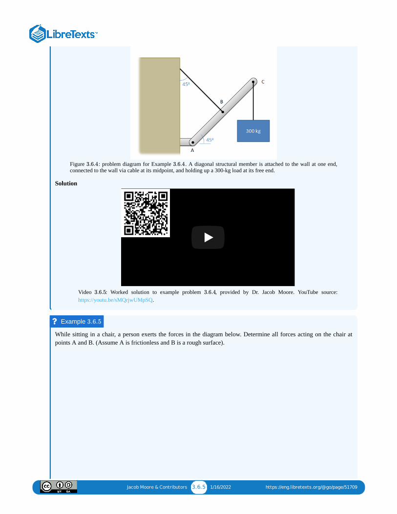
Jacob Moore & Contributors 3.6.5 1/16/2022 https://eng.libretexts.org/@go/page/51709

Figure : problem diagram for Example . A diagonal structural member is attached to the wall at one end,connected to the wall via cable at its midpoint, and holding up a 300-kg load at its free end.

Solution

Video : Worked solution to example problem , provided by Dr. Jacob Moore. YouTube source:https://youtu.be/sMQrjwUMpSQ.

While sitting in a chair, a person exerts the forces in the diagram below. Determine all forces acting on the chair atpoints A and B. (Assume A is frictionless and B is a rough surface).

3.6.4 3.6.4

Extended Body Equilibrium -AdaptExtended Body Equilibrium -Adapt……

3.6.5 3.6.4

Example 3.6.5

Jacob Moore & Contributors 3.6.6 1/16/2022 https://eng.libretexts.org/@go/page/51709

Figure : problem diagram for Example . A chair is placed on a flat surface, with that surface assumed to befrictionless where it contacts the chair's front leg (point A) and exerting friction where it contacts the back leg (pointB).

Solution

Video : Worked solution to example problem , provided by Dr. Jacob Moore. YouTube source:https://youtu.be/nSOxK1ZMggA.

The trailer shown below consists of a deck with a weight of 250 lbs on an axle with wheels with a weight of 350 lbs.Assume the weight forces act in the center of each component. If we wish the tongue weight ( ) of the unloadedtrailer to be 50 lbs, what is the distance from the front where we must place the axle?

Figure : problem diagram for Example . A trailer consists of a flat rectangular deck on top of two wheels onan axle.

Solution

3.6.5 3.6.5

Extended Body Equilibrium -AdaptExtended Body Equilibrium -Adapt……

3.6.6 3.6.5

Example 3.6.6

FT

d

3.6.6 3.6.6

Jacob Moore & Contributors 3.6.7 1/16/2022 https://eng.libretexts.org/@go/page/51709

Video : Worked solution to example problem , provided by Dr. Jacob Moore. YouTube source:https://youtu.be/wpEBuitLD5s.

A 12-inch-by-24-inch flat steel sign is supported by two cables, each 6 inches from the edge of the sign. The sign has aweight of 10 lbs, and the wind is causing the sign to sit at an angle of 10 degrees from vertical (the axis). If we treatthe wind as a point force acting in the negative direction on the center of the sign, how strong must the wind force beto cause this ten-degree angle?

Figure : problem diagram for Example . A hanging sign experiences a wind whose direction points into thescreen, causing the sign to make a 10° angle with the plane of the screen.

Solution

Extended Body Equilibrium -AdaptExtended Body Equilibrium -Adapt……

3.6.7 3.6.6

Example 3.6.7

y

z

3.6.7 3.6.7

Jacob Moore & Contributors 3.6.8 1/16/2022 https://eng.libretexts.org/@go/page/51709

Video : Worked solution to example problem , provided by Dr. Jacob Moore. YouTube source:https://youtu.be/pR-0xbj8wF0.

A sixty-kilogram acoustic panel is suspended by three cables as shown below. Assuming the panel has a uniformlydistributed weight, what is the tension in each of the cables?

Figure : problem diagram for Example . A uniform rectangular panel is suspended from above by 3 cableslocated at different points along its edges.

Solution

Video : Worked solution to example problem , provided by Dr. Jacob Moore. YouTube source:https://youtu.be/Kbsc1m0f9pQ.

Equilibrium Equations for an ExteEquilibrium Equations for an Exte……

3.6.8 3.6.7

Example 3.6.8

3.6.8 3.6.8

Extended Body Equilibrium - AdapExtended Body Equilibrium - Adap……

3.6.9 3.6.8

Jacob Moore & Contributors 3.7.1 1/16/2022 https://eng.libretexts.org/@go/page/52384

3.7: Chapter 3 Homework Problems

An 18-inch shelf is supported by a pin joint at point A, and a cable at point B. The shelf itself has a weight of 60 lbs. Ifwe want the net moment about point A to be zero, what should the tension in the cable be?

Figure : problem diagram for Exercise ; a horizontal shelf is attached to a wall with a pin joint at one endand a cable at the other end.

Solution

What is the moment the force shown below exerts about Point A? About Point B?

Hint: use Varginon's Theorem.

Figure : problem diagram for Exercies ; a rectangular slab is bolted to a wall at two points, A and B, with aforce is exerted on one of the rectangle's unattached corners.

Solution

Exercise 3.7.1

3.7.1 3.7.1

T = 52.30 lbs

Exercise 3.7.2

3.7.2 3.7.2

= 10.88 kNmMA

= 21.02 kNmMB

Jacob Moore & Contributors 3.7.2 1/16/2022 https://eng.libretexts.org/@go/page/52384

You are attempting to rotate a heavy table about the base of one leg at point O and are going to exert a 100-lb force atthe opposite end. Person A recommends pulling straight up, while person B recommends pulling up at 30° fromvertical. What would be the moment about point O, in inch-pounds, in either case?

Figure : problem diagram for Exercise ; a table is rotated about the base of one leg, with one of the twoproposed forces applied at the tabletop at the opposite end.

Solution

Determine the moment vectors that each of the three tension forces in the diagram below exerts about the origin pointO. Provide the answers in vector form with units.

Figure : problem diagram for Exercise ; two straight beams lying in the -plane, joined perpendicularly toeach other, experience 3 upward tension forces (in the + direction).

Solution

Exercise 3.7.3

3.7.3 3.7.3

= 6000 in-lbsMAO

= 6996.15 in-lbsMBO

Exercise 3.7.4

3.7.4 3.7.4 xyz

= [0, −400, 0] NmMAO

= [−300, 0, 0] NmMBO

Jacob Moore & Contributors 3.7.3 1/16/2022 https://eng.libretexts.org/@go/page/52384

You exert a 50-lb force on the side of a fridge as shown below. Assuming the fridge is sitting on a rough surface andnot moving, what is the magnitude of the moment exerted by the couple consisting of the pushing force and thefriction force?

Figure : problem diagram for Exercise ; a force is exerted on a refrigerator that sits on a flat surface, withoutcausing it to move.

Solution

A space station consists of a large ring that spins in order to provide an artificial gravity for the astronauts in thestation. To start the station spinning, a pair of thrusters is attached to the outside of the ring, each pointing in oppositedirections as shown below.

a) If we want to exert a 10 kN-m moment with the thrusters, and the ring has a diameter of 45 meters, whatthrust force should each thruster produce?

b) If we were to use the same thrusters on a 60-meter diameter ring, what moment would they exert?

Figure : problem diagram for Exercise . An example of the spinning ring-shaped space station as describedin the problem (left); a diagram of the locations and directions of the thruster forces on the ring (right).

Solution

a)

b)

= [300, 0, 0]NmMCO

Exercise 3.7.5

3.7.5 3.7.5

M = −100ft-lbs

Exercise 3.7.6

3.7.6 3.7.6

= 222.22 NFthruster

= 13.33 kNmMthruster

Jacob Moore & Contributors 3.7.4 1/16/2022 https://eng.libretexts.org/@go/page/52384

A 60-N force is applied in the plane, 40° from the direction, on an L-shaped bar as shown below.

a) What is the moment vector this force exerts about point O?

b) What is the overall magnitude of the moment about point O?

Figure : problem diagram for Exercise ; an L-shaped bar lies in the plane with one end located at theorigin, point O, and the other experiencing a force in the direction.

Solution

What is the moment that the force shown in the diagram exerts about point O? About the axis of the cylindrical shaft(the -axis)?

Figure : problem diagram for Exercise ; an L-shaped part that extends in the and directions, with oneend located at the origin O, experiences a force in the direction applied at the opposite end.

Solution

Exercise 3.7.7

yz y

3.7.7 3.7.7 xzyz

= [−11.49, −11.57, 13.79] NmMO

|M | = 21.36 Nm

Exercise 3.7.8

y

3.7.8 3.7.8 y zxz

= [16484, 17046, −20979] in − lbsMO

= 17046 in − lbsMy

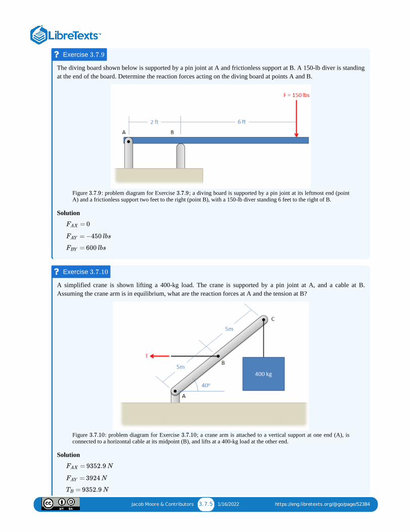
Jacob Moore & Contributors 3.7.5 1/16/2022 https://eng.libretexts.org/@go/page/52384

The diving board shown below is supported by a pin joint at A and frictionless support at B. A 150-lb diver is standingat the end of the board. Determine the reaction forces acting on the diving board at points A and B.

Figure : problem diagram for Exercise ; a diving board is supported by a pin joint at its leftmost end (pointA) and a frictionless support two feet to the right (point B), with a 150-lb diver standing 6 feet to the right of B.

Solution

A simplified crane is shown lifting a 400-kg load. The crane is supported by a pin joint at A, and a cable at B.Assuming the crane arm is in equilibrium, what are the reaction forces at A and the tension at B?

Figure : problem diagram for Exercise ; a crane arm is attached to a vertical support at one end (A), isconnected to a horizontal cable at its midpoint (B), and lifts at a 400-kg load at the other end.

Solution

Exercise 3.7.9

3.7.9 3.7.9

= 0FAX

= −450 lbsFAY

= 600 lbsFBY

Exercise 3.7.10

3.7.10 3.7.10

= 9352.9 NFAX

= 3924 NFAY

= 9352.9 NTB

Jacob Moore & Contributors 3.7.6 1/16/2022 https://eng.libretexts.org/@go/page/52384

An 8-foot ladder sits propped up against a wall at a 60-degree angle as shown below. It has a weight of 50 lbs acting atits center point and supports a 120-lb woman 6 feet from the bottom. Assume that friction acts at the bottom of theladder, but not the top. What are the normal forces acting at the bottom and top of the ladder, and what is the frictionforce acting at the bottom of the ladder?

Figure : problem diagram for Exercise ; an 8-ft ladder weighing 50 lbs and supporting a 120-lb womanwho has climbed 75% of the way up leans, at 60° above the horizontal, against a wall.

Solution

An SUV with a weight of 4200 lbs and a center of mass located as shown below is parked pointed downhill on a 10-degree incline. The parking is engaged, locking up the back wheels but not the front wheels. What is the expectednormal force at the front wheels, the expected normal force at the back wheels, and the expected friction force at theback wheels assuming the SUV does not slip?

Figure : problem diagram for Exercise ; an SUV with front and rear wheels 6 feet apart, and a center ofmass 2 feet above the ground and 2 feet behind the front wheel, is parked pointing downhill on a 10° incline.

Exercise 3.7.11

3.7.11 3.7.11

= 66.4 lbsFN T op

= 170 lbsFN Bottom

= 66.4lbsFf

Exercise 3.7.12

3.7.12 3.7.12

Jacob Moore & Contributors 3.7.7 1/16/2022 https://eng.libretexts.org/@go/page/52384

Solution

A cart with a mass of 3500 kg sits on an inclined surface as shown below. Determine the reaction forces acting on eachwheel of the cart as well as the tension in the cable supporting the cart.

Figure : a two-wheeled cart is parked facing uphill on a 30° slope. A cable stretches from the front of the cart toa support on the incline, making a 38° angle with the plane of the incline.

Solution

The lighting rig above a stage consists of two 100-lb, uniform beams joined together in a T as shown below (assumethe weight acts in the center of each beam). The rig is supported by three cables at A, B, and C. Determine the tensionin each of the three cables.

Figure : problem diagram for Exercise ; two beams attached perpendicularly to each other lie in the plane in a T shape experience upward tension forces from 3 cables, one attached to each free end of the T.

= 729.3 lbsFf

= 3000.6 lbsFN front

= 1135.6 lbsFN back

Exercise 3.7.13

3.7.13

T = 21786 N

= 7222 N ; = 35925 NFA FB

Exercise 3.7.14

3.7.14 3.7.14 xy

Jacob Moore & Contributors 3.7.8 1/16/2022 https://eng.libretexts.org/@go/page/52384

Solution

A 9-meter-long pole with a mass of 100 kg is suspended horizontally, 4 meters from the ceiling with three cables asshown below. Assuming the center of mass of the pole is at the center point of the pole, what is the expected tension ineach of the three cables?

Figure : problem diagram for Exercise ; a pole hangs 4 meters below the ceiling, suspended by 3 cablesattached to the pole at different locations and angles.

Solution

= 50 lbs; = 66.7 lbs; = 83.3 lbsTA TB TC

Exercise 3.7.15

3.7.15 3.7.15

= 357.66 N ; = 357.66 N ; = 408.75 NTA TB TC

1 1/30/2022

CHAPTER OVERVIEW4: STATICALLY EQUIVALENT SYSTEMSStatically equivalent systems that experience different sets of forces and moments. The process for converting between differentstatically equivalent systems.

4.0: VIDEO INTRODUCTION TO CHAPTER 4Video introduction to the topics to be covered in this chapter: statically equivalent systems, and the relation between forces, momentsand couples in such a system.

4.1: STATICALLY EQUIVALENT SYSTEMSDefinition of statically equivalent systems. Outline of how to determine if sets of forces are statically equivalent, and how to convertmultiple forces into a single statically equivalent force.

4.2: RESOLUTION OF A FORCE INTO A FORCE AND A COUPLEThe process for resolving a force applied at one point on a body into a force and a moment acting on another point, using the conceptof couples. Includes several worked examples.

4.3: EQUIVALENT FORCE COUPLE SYSTEMDefinition of an equivalent force couple system, and how to find it for a given set of forces and moments.

4.4: DISTRIBUTED FORCESDefinition of distributed forces, and their classification as surface or body forces. Conventions for representing and analyzingdistributed forces.

4.5: EQUIVALENT POINT LOADDefinition of the equivalent point force and methods of calculating it in two and three dimensions: integration; using the centroid orcenter of volume. Includes several worked samples.

4.6: CHAPTER 4 HOMEWORK PROBLEMS

Jacob Moore & Contributors 4.0.1 12/21/2021 https://eng.libretexts.org/@go/page/50584

4.0: Video Introduction to Chapter 4

Video introduction to the topics covered in Chapter 4, delivered by Dr. Jacob Moore. YouTube source:https://youtu.be/jXY48L2sRR0.

Chapter 4 IntroductionChapter 4 Introduction

Jacob Moore & Contributors 4.1.1 1/9/2022 https://eng.libretexts.org/@go/page/50585

4.1: Statically Equivalent SystemsTwo sets of forces are considered statically equivalent if they cause the same set of reaction forces on a body. Becausethis is true, the two statically equivalent sets of forces are interchangeable in statics analysis.

Figure : A single 200-lb man standing at the center of a beam causes the same reaction forces as two 100-lb childrenstanding evenly along the beam as shown above. The weight force of the man is therefore statically equivalent to theweight forces of the two children.

Determining if Forces are Statically Equivalent:

To determine if two sets of forces are statically equivalent, you must solve for the reaction forces in both cases. If thereaction forces are the same then the two sets of forces must be statically equivalent. For any one set of forces, there are aninfinite number of sets of forces that are statically equivalent to original set of forces.

Finding a Single Equivalent Point Force:In statics analysis, we are usually looking to simplify a problem by turning multiple forces into a single, staticallyequivalent force. To find a single point force that is equivalent to multiple point forces you can use the followingprocedure.

1. Solve for the reaction forces in the original scenario.2. Draw a new free body diagram with these reaction forces. You will also add one force with an unknown magnitude,

direction, and point of application to your diagram. This is the single point load that will be equivalent to your originalset of forces.

3. Write out the equations of equilibrium for this scenario, including the known values for the reaction forces.4. First, solve the force equations to find the and components of this unknown force (or , and components for a

3D problem). This can be used to find the magnitude and direction of the statically equivalent point force.5. Next, use the moment equation (or equations, for 3D problems) to determine the location of the statically equivalent

point force.

4.1.1

x y x y z

Jacob Moore & Contributors 4.1.2 1/9/2022 https://eng.libretexts.org/@go/page/50585

Video : Lecture video covering this section, delivered by Dr. Jacob Moore. YouTube source:https://youtu.be/r0pwzQ_Ge00.

Determine if the two sets of forces shown below are statically equivalent.

Figure : problem diagram for Example ; two identical bars experience the same total magnitude anddirection of external force, applied in different locations and distributions.

Solution

Video : worked solution to example problem , provided by Dr. Jacob Moore. YouTube source:https://youtu.be/Xv5DyvQD29E.

4.1 Statically Equivalent Systems - Vi4.1 Statically Equivalent Systems - Vi……

4.1.1

Example 4.1.1

4.1.2 4.1.1

Statically Equivalent - Adaptive MStatically Equivalent - Adaptive M……

4.1.2 4.1.1

Jacob Moore & Contributors 4.2.1 12/21/2021 https://eng.libretexts.org/@go/page/50586

4.2: Resolution of a Force into a Force and a CoupleAs discussed on the sections on moments, a force can have a tendency to cause both a linear and angular acceleration. Forexample, below is diagram of a force acting on an extended body. If we were to think about everything relative to thecenter of mass of this body, there would be some force acting on the center of mass that would cause the same linearacceleration and some pure moment (couple) that would cause the same angular acceleration. This would be a force andcouple that is statically equivalent to the original force, though the point of application of the force changes.

Figure : The original force acting at A would cause both linear and angular acceleration. The force at B would causethe same linear acceleration and the moment at B would cause the same angular acceleration. The force and the moment atB are statically equivalent to the original force at A.

The process of transforming one force applied at one point, into a force and a couple at some other point is known asresolving a force into a force and a couple. There are a few reasons that we may want to do this, but one primary reasonis to find the equivalent force couple system for a complex set of forces and moments. The equivalent force couplesystem is used to simplify more complex analysis, and consists of a single force and a single pure moment (couple) that arestatically equivalent to some more complex combination of forces and moments. An important first step in finding theequivalent force couple system is to resolve all the forces so that everything is acting at the same point.

In order to visualize the process of resolving a force into a force and a couple, you can use the process outlined in thediagram below. Imagine we have a body with a force acting at some point A. We want to resolve the force into a force anda couple about some other point B. To do this we will first add two forces to the diagram at point B. One will have thesame magnitude and direction as the original force and the other will be equal and opposite to the original force. Becausethese two forces are equal, opposite, and collinear, this will not change the situation (it's the equivalent to adding zero to anequation). Now, with these three forces acting on the diagram, we can break it down into two sets. The first is a forceacting at point B with the same magnitude and direction as the original force. The other two forces act as a couple, exertinga pure moment about point B. Finally, we can redraw the system as a force acting at point B and the pure moment actingabout point B.

4.2.1

Jacob Moore & Contributors 4.2.2 12/21/2021 https://eng.libretexts.org/@go/page/50586

Figure : The process of resolving a force about some point A into a force and a couple about some point B.

As a shortcut to the process described above, we can also see that the force in the equivalent force couple system willalways have a magnitude and direction equal to the original force and the couple will be equal to the moment exerted bythe original force about the new point of application.

Video lecture covering this section, delivered by Dr. Jacob Moore. YouTube source: https://youtu.be/sLixBOWBCuY.

Resolve the force shown below to a force and a couple acting at point A.

Figure : problem diagram for Example ; a rod experiences a single, upwards force applied 6 feet from theleft end of the rod (point A).

Solution

4.2.2

4.2 Resolution of a Force into a Forc4.2 Resolution of a Force into a Forc……

Example 4.2.1

4.2.3 4.2.1

Jacob Moore & Contributors 4.2.3 12/21/2021 https://eng.libretexts.org/@go/page/50586

Video : Worked solution to example problem , provided by Dr. Jacob Moore. YouTube source:https://youtu.be/Wfl3S_5FD0Q.

Resolve the force shown below to a force and a couple acting at point A.

Figure : problem diagram for Example ; a rod experiences a single force, pointing downwards and to theright, applied 0.6 meters from the left end of the rod (point A).

Solution

Video : Worked solution to example problem , provided by Dr. Jacob Moore. YouTube source:https://youtu.be/1hRrKhWzf98.

Resolution of a Force into a Force Resolution of a Force into a Force ……

4.2.2 4.2.1

Example 4.2.2

4.2.4 4.2.2

Resolution of a Force into a Force Resolution of a Force into a Force ……

4.2.3 4.2.2

Jacob Moore & Contributors 4.3.1 1/23/2022 https://eng.libretexts.org/@go/page/50587

4.3: Equivalent Force Couple SystemEvery set of forces and moments has an equivalent force couple system. This is a single force and pure moment (couple)acting at a single point that is statically equivalent to the original set of forces and moments.

Figure : Any set of forces on a body can be replaced by a single force and a single couple acting that is staticallyequivalent to the original set of forces and moments. This set of an equivalent force and a couple is known as theequivalent force couple system.

To find the equivalent force couple system, you simply need to follow the steps below.

1. First, choose a point to take the equivalent force couple system about. Any point will work, but the point you choosewill affect the final values you find for the equivalent force couple system. Traditionally, this point will either be thecenter of mass of the body or some connection point for the body.

2. Next, resolve all the forces not acting though that point to a force and a couple acting at the point you chose.3. To find the "force" part of the equivalent force couple system, add together all the force vectors. This will give you the

magnitude and the direction of the force in the equivalent force couple system.4. To find the "couple" part of the equivalent force couple system, add together any moment vectors (this could be

moments originally acting on the body, or moments from the resolution of the forces into forces and couples). This willgive you the magnitude and direction of the pure moment (couple) in the equivalent force couple system.

Video lecture covering this section, delivered by Dr. Jacob Moore. YouTube source: https://youtu.be/bs6Tnlje3IU.

Find the equivalent force couple system for the forces shown below about point A.

4.3.1

4.3 Equivalent Force Couple System 4.3 Equivalent Force Couple System ……

Example 4.3.1

Jacob Moore & Contributors 4.3.2 1/23/2022 https://eng.libretexts.org/@go/page/50587

Figure : problem diagram for Example . An L-shaped part whose two arms connect at point A experiences arightwards force and a counterclockwise moment about the end of its vertical arm, as well as two downwards forcesalong its horizontal arm.

Solution

Video : Worked solution to example problem , provided by Dr. Jacob Moore. YouTube source:https://youtu.be/cw-rwBZef5w.

4.3.2 4.3.1

Equivalent Force Couple System -Equivalent Force Couple System -……

4.3.2 4.3.1

Jacob Moore & Contributors 4.4.1 1/23/2022 https://eng.libretexts.org/@go/page/52455

4.4: Distributed ForcesA distributed force is any force where the point of application of the force is an area or a volume. This means that the"point of application" is not really a point at all. Though distributed forces are more difficult to analyze than point forces,distributed forces are quite common in real world systems so it is important to understand how to model them.

Distributed forces can be broken down into surface forces and body forces. Surface forces are distributed forces wherethe point of application is an area (a surface on the body). Body forces are forces where the point of application is avolume (the force is exerted on all molecules throughout the body). Below are some examples of surface and body forces.

Figure : The water pressure pushing on the surface of this dam is an example of a surface force. Image by CurimediaCC-BY-SA 2.0.

Figure : The gravitational force on this apple is distributed over the entire volume of the fruit. Gravitational forces arean example of body forces. Image by Zátonyi Sándor CC-BY 3.0.

Representing Distributed Forces:Distributed forces are represented as a field of vectors. This is drawn as a number of discrete vectors along a line, over asurface, or over a volume, that are connected with a line or a surface as shown below.

Figure : This is a representation of a surface force in a 2D problem (a force distributed over a line). The magnitude isgiven in units of force per unit distance.

Figure : This is a representation of a surface force in a 3D problem (a force distributed over an area). The magnitudeis given in units of force per unit area (also called a pressure).

4.4.1

4.4.2

4.4.3

4.4.4

Jacob Moore & Contributors 4.4.2 1/23/2022 https://eng.libretexts.org/@go/page/52455

Though these representations show a discrete number of individual vectors, there is actually a magnitude and direction atall points along the line, surface, or body. The individual vectors represent a sampling of these magnitudes and directions.

It is also important to realize that the magnitudes of distributed forces are given in force per unit distance, area, or volume.We must integrate the distributed force over its entire range to convert the force into the usual units of force.

Analyzing Distributed Forces:

For analysis purposes in statics and dynamics, we will usually substitute in a single point force that is statically equivalentto the distributed force in the problem. This single point force is called the equivalent point load, and it will cause thesame accelerations or reaction forces as the distributed force while simplifying the math. However, in analysis that focuseson the strength of materials where the bodies are not rigid, this substitution will not work as the distributed forces will notcause the same deformations and stresses as the point force.

Video lecture covering this section, delivered by Dr. Jacob Moore. YouTube source: https://youtu.be/VSIopUTg9kA.

4.4 Distributed Forces - Video Lectur4.4 Distributed Forces - Video Lectur……

Jacob Moore & Contributors 4.5.1 12/21/2021 https://eng.libretexts.org/@go/page/52471

4.5: Equivalent Point LoadAn equivalent point load is a single point force that will have the same effect on a body as the original loading condition,which is usually a distributed force. The equivalent point load should always cause the same linear acceleration andangular acceleration as the original force it is equivalent to (or cause the same reaction forces if the body is constrained).Finding the equivalent point load for a distributed force often helps simplify the analysis of a system by removing theintegrals from the equations of equilibrium or equations of motion in later analysis.

Figure : If the body is unconstrained as shown on the left, the equivalent point load (shown as a solid vector) willcause the same linear and angular acceleration as the original distributed load (shown with dashed vectors). If the body isconstrained as on shown on the right, the equivalent point load (shown as a solid vector) will cause the same reactionforces as the original distributed force (shown with dashed vectors).

Finding the Equivalent Point LoadWhen finding the equivalent point load, we need to find the magnitude, direction, and point of application of a single forcethat is equivalent to the distributed force we are given. In this course we will only deal with distributed forces with auniform direction, in which case the direction of the equivalent point load will match the uniform direction of thedistributed force. This leaves the magnitude and the point of application to be found. There are two options available tofind these values:

1. We can find the magnitude and the point of application of the equivalent point load via integration of the forcefunctions.

2. We can use the area/volume and the centroid/center of volume of the area or volume under the force function.

The first method is more flexible, allowing us to find the equivalent point load for any force function that we can make amathematical formula for (assuming we have the skill in calculus to integrate that function). The second method is usuallyfaster, assuming that we can look up the values for the area or volume under the force curve and the values for the centroidor center of volume for the area under the curve.

Using Integration in 2D Surface Force Problems:

Figure : The block shown above has a distributed force acting on it. The force function relates the magnitude of theforce to the position along the top of the box.

Finding the equivalent point load via integration always begins by determining the mathematical formula that is the forcefunction. The force function mathematically relates the magnitude of the force to the position . In this case theforce is acting along a single line, so the position can be entirely determined by knowing the coordinate, but in laterproblems we may also need to relate the magnitude of the force to the and coordinates. In our example above, we canrelate magnitude of the force to the position by stating that the magnitude of the force at any point in Newtons per meter isequal to the position in meters plus one.

4.5.1

4.5.2x

(F ) (x)

x

y z

x

Jacob Moore & Contributors 4.5.2 12/21/2021 https://eng.libretexts.org/@go/page/52471

The magnitude of the equivalent point load will be equal to the area under the force function. This will be the integral ofthe force function over its entire length (in this case, from to ).

Now that we have the magnitude of the equivalent point load such that it matches the magnitude of the original force, weneed to adjust the position such that it would cause the same moment as the original distributed force. The momentof the distributed force will be the integral of the force function times the moment arm about the origin . Themoment of the equivalent point load will be equal to the magnitude of the equivalent point load that we just found timesthe moment arm for the equivalent point load . If we set these two things equal to one another and then solve for theposition of the equivalent point load we are left with the following equation.

Now that we have the magnitude, direction, and position of the equivalent point load, we can draw the point load in ouroriginal diagram. This point force can be used in place of the distributed force in further analysis.

Figure : The values for and that we have solved for are the magnitude and position of the equivalent pointload.

Using the Area and Centroid in 2D Surface Force Problems:As an alternative to using integration, we can use the area under the force curve and the centroid of the area under the forcecurve to find the equivalent point load's magnitude and point of application respectively.

Figure : The magnitude of the equivalent point load is equal to the area under the force function. Also, the equivalentpoint load will travel through the centroid of the area under the force function.

The magnitude of the equivalent point load will be equal to the area under the force function. We can find thisarea using calculus, but there are often easier geometry-based ways of finding the area under the force function.

x = 0 x = 2

= F (x)dxFeq ∫

xmin

xmax

(4.5.1)

( )xeq(F (x)) (x)

( )xeq( )xeq

=xeq

(F (x) ∗ x)dx∫xmin

xmax

Feq

(4.5.2)

4.5.3 Feq xeq

4.5.4

( )Feq

Jacob Moore & Contributors 4.5.3 12/21/2021 https://eng.libretexts.org/@go/page/52471

The equivalent point load will also travel through centroid of the area under the force function. This allows us to findthe value for . The centroid for many common shapes can be looked up in tables, and the parallel axis theorem can beused to determine the centroid of more complex shapes (see the Appendix page on centroids for more details).

Using Integration in 3D Surface Force Problems:

Figure : The magnitude of the surface force in this example varies with both and .

With surface force in a 3D problem, the force is distributed over a surface, rather than along a single line. To find themagnitude of the equivalent point load we will again start by finding the mathematical equation for the force function.Because the force is distributed over an area rather than just a line, the magnitude of the force may be related to both the and the coordinate, rather than just the coordinate as before.

The magnitude of the equivalent point load will be equal to the volume under the force curve. To calculate this valuewe will integrate the force function over the area that the force is applied to. To integrate this function in terms ofthe area, we will need to break the integral down further, integrating over and then integrating over .

Once we solve for the magnitude of the equivalent point load, we can then solve for the position of the equivalent pointload. Since the force is spread over a surface, we will need to calculate both the and the coordinates for theposition. The process for solving for these values is similar to what was done with only an value, except we change themoment arm value to match the equivalent point load coordinate we are looking for.

In each of the equations above, we will need to expand out the area integral into and integrals (as we did for ) inorder to be able to solve them.

Using Volume and Center of Volume in 3D Surface Force Problems:Just as in the 2D problems, there are some available shortcuts to finding the equivalent point load in 3D surface forceproblems. For a force spread over an area, the magnitude of the equivalent point load will be equal to the volumeunder the force function. The equivalent point load will also travel through the center of volume of the volume underthe force function. This should allow you to determine both and .

The center of volume for a shape will be the same as the center of mass for a shape if the shape is assumed to have uniformdensity. It should be possible to look these values up for common shapes in a table. Again, the parallel axis theorem can beused to find the center of volume for more complex shapes (See the Center of Mass page in Appendix 2 for more details).

Using Integration in Body Force Problems:When we jump to body forces, the magnitude of our force will vary with , , and coordinates. This means that our forcefunction can include all of these variables . To find the magnitude of the equivalent point load we integrate

xeq

4.5.5 x y

x

y x

( )Feq

F (x, y)

x y

= ∫ F (x, y)dA = F (x, y)dx dyFeq ∫

y min

y max⎛

⎝⎜ ∫

xmin

xmax⎞

⎠⎟ (4.5.3)

x ( )xeq y ( )yeqx

=xeq∫(F (x, y) ∗ x)dA

Feq

(4.5.4)

=yeq∫(F (x, y) ∗ x)dA

Feq

(4.5.5)

x y Feq

( )Feq

xeq yeq

x y z

(F (x, y, z))

Jacob Moore & Contributors 4.5.4 12/21/2021 https://eng.libretexts.org/@go/page/52471

over the volume, breaking the volume integral down into , , and then integrals.

To find the point of application of the equivalent point load, we will need to find all three coordinate positions. To do this,we will expand out the equations we used with two coordinates to include the third coordinate .

Video lecture covering this section, delivered by Dr. Jacob Moore. YouTube source: https://youtu.be/eikERyUNIOo.

Determine the magnitude and the point of application for the equivalent point load of the distributed force shownbelow.

Figure : problem diagram for Example ; a bar attached to a wall experiences a distributed force whosemagnitude varies linearly over part of its length.

Solution

x y z

Feq = ∫ F (x, y, z)dV

= F (x, y, z)dx dy dz∫

zmin

zmax⎛

⎝⎜ ∫

y min

y max⎛

⎝⎜ ∫

xmin

xmax⎞

⎠⎟

⎞

⎠⎟

(4.5.6)

(4.5.7)

( )zeq

=xeq∫(F (x, y, z) ∗ x)dV

Feq

(4.5.8)

=yeq∫(F (x, y, z) ∗ y)dV

Feq

(4.5.9)

=zeq∫(F (x, y, z) ∗ z)dV

Feq

(4.5.10)

4.5 Equivalent Point Load - Video Le4.5 Equivalent Point Load - Video Le……

Example 4.5.1

4.5.6 4.5.1

Jacob Moore & Contributors 4.5.5 12/21/2021 https://eng.libretexts.org/@go/page/52471

Video : Worked solution to example problem , provided by Dr. Jacob Moore. YouTube source:https://youtu.be/h_E0XjIJaiI.

Determine the magnitude and the point of application for the equivalent point load of the distributed force shownbelow.

Figure : problem diagram for Example ; a bar attached to a wall experiences a distributed force whosemagnitude varies quadratically over its length.

Solution

Video : Worked solution to example problem , provided by Dr. Jacob Moore. YouTube source:https://youtu.be/D4JoQpOyI38.

Equivalent Point Load - Adaptive Equivalent Point Load - Adaptive ……

4.5.2 4.5.1

Example 4.5.2

4.5.7 4.5.2

Equivalent Point Load - Adaptive Equivalent Point Load - Adaptive ……

4.5.3 4.5.2

Jacob Moore & Contributors 4.5.6 12/21/2021 https://eng.libretexts.org/@go/page/52471

Determine the magnitude and the point of application for the equivalent point load of the distributed force shownbelow.

Figure : problem diagram for Example ; a bar attached to a wall experiences a distributed force whosemagnitude varies linearly over part of its length and remains constant for the remainder.

Solution

Video : Worked solution to example problem , provided by Dr. Jacob Moore. YouTube source:https://youtu.be/UbnfNAQctyg.

The wind has piled up sand into a corner on a building. The building supervisor is worried about the weight of the sandpushing against the roof of the basement below. The function describing force of the sand pushing down on the surfaceis given below. Find the magnitude, direction and point of application of the equivalent point load for the distributedforce of the sand. Draw the equivalent point load in a diagram.

Figure : problem diagram for Example ; sand accumulated in the corner of a building is assigned to a three-dimensional coordinate system and the distributed force it exerts on the floor beneath it is described with a forceequation.

Solution

Example 4.5.3

4.5.8 4.5.3

Equivalent Point Load - Adaptive Equivalent Point Load - Adaptive ……

4.5.4 4.5.3

Example 4.5.4

4.5.9 4.5.4

Jacob Moore & Contributors 4.5.7 12/21/2021 https://eng.libretexts.org/@go/page/52471

Video : Worked solution to example problem , provided by Dr. Jacob Moore. YouTube source:https://youtu.be/IaSe_g3_Mgk.

Equivalent Point Load - Adaptive Equivalent Point Load - Adaptive ……

4.5.5 4.5.4

Jacob Moore & Contributors 4.6.1 12/21/2021 https://eng.libretexts.org/@go/page/52472

4.6: Chapter 4 Homework Problems

Determine if the two systems below are statically equivalent.

Figure : part 1 of the problem diagram for Exercise . A horizontal bar held off the ground by two supportsexperiences two point forces at different points along its length.

Figure : part 2 of the problem diagram for Exercise . A horizontal bar held off the ground by two supportsexperiences a single point force partway along its length.

Solution

No, they are not equivalent.

Determine if the set of forces in A is statically equivalent to the set of forces and moments in B.

Figure : problem diagram for Exercise . Two uniform crosses of equal dimensions experience a set of forces(system A, left) and a set of forces and moments (system B, right).

Solution

No, they are not equivalent.

Resolve the force shown below into a force and a couple acting at point A. Draw this force and couple on a diagram ofthe L-shaped beam.

Exercise 4.6.1

4.6.1 4.6.1

4.6.2 4.6.1

Exercise 4.6.2

4.6.3 4.6.2

Exercise 4.6.3

Jacob Moore & Contributors 4.6.2 12/21/2021 https://eng.libretexts.org/@go/page/52472

Figure : problem diagram for Exercise . An L-shaped beam is held parallel to the ground by a pin jointattached at one end (point A), with a force applied to the other free end of the L shape.

Solution

to the left

Find the equivalent force couple system acting at point A for the setup shown below. Draw this force and couple on adiagram of the L-shaped beam.

Figure : problem diagram for Exercise . An L-shaped beam, whose arms intersect at the point A,experiences several forces acting at different points along the arms.

Solution

° below the negative -axis

A helicopter is hovering with the wind force, the force from the tail rotor, and the moment due to drag shown below.Determine the equivalent force couple system at point C. Draw the final force and moment on a new diagram of thehelicopter.

4.6.4 4.6.3

= 150 NFA

= 450 NmMA

Exercise 4.6.4

4.6.5 4.6.4

= 155.2 lbs, 69.5FA x

= −556.9 ft lbsMA

Exercise 4.6.5

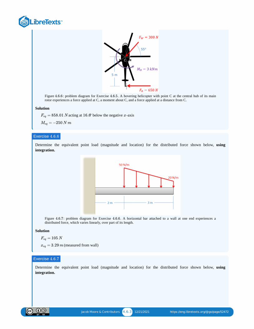
Jacob Moore & Contributors 4.6.3 12/21/2021 https://eng.libretexts.org/@go/page/52472

Figure : problem diagram for Exercise . A hovering helicopter with point C at the central hub of its mainrotor experiences a force applied at C, a moment about C, and a force applied at a distance from C.

Solution

acting at ° below the negative -axis

Determine the equivalent point load (magnitude and location) for the distributed force shown below, usingintegration.

Figure : problem diagram for Exercise . A horizontal bar attached to a wall at one end experiences adistributed force, which varies linearly, over part of its length.

Solution

(measured from wall)

Determine the equivalent point load (magnitude and location) for the distributed force shown below, usingintegration.

4.6.6 4.6.5

= 858.01 NFeq 16.6 x

= −250 N mMeq

Exercise 4.6.6

4.6.7 4.6.6

= 105 NFeq

= 3.29 mxeq

Exercise 4.6.7

Jacob Moore & Contributors 4.6.4 12/21/2021 https://eng.libretexts.org/@go/page/52472

Figure : problem diagram for Exercise . A horizontal bar attached to a wall experiences a distributed forceover its length, with magnitude varying linearly according to a piecewise force function.

Solution

(measured from wall)

Use the method of composite parts to determine the magnitude and location of the equivalent point load for thedistributed force shown below.

Figure : problem diagram for Exercise . A horizontal bar attached to a wall experiences a distributed forceover its length, with magnitude varying linearly according to a piecewise force function.

Solution

(measured from wall)

4.6.8 4.6.7

= 5400 lbsFeq

= 8 ftxeq

Exercise 4.6.8

4.6.9 4.6.8

= 12 kNFeq

= 2.79 mxeq

1 1/30/2022

CHAPTER OVERVIEW5: ENGINEERING STRUCTURESClassification of engineering structures into members, trusses, and frames and machines. Methods for equilibrium analysis of thesestructures.

5.0: VIDEO INTRODUCTION TO CHAPTER 5Introduction to the topics to be covered in Chapter 5: structures as trusses vs frames and machines; two-force members; methods ofanalysis for trusses and for frames and machines.

5.1: STRUCTURESDefinition of an engineering structure. The classification of structures into trusses and frames or machines.

5.2: TWO-FORCE MEMBERSDefinition of two-force members, and how to identify them. The importance of two-force members in truss analysis problems.

5.3: TRUSSESDefinition of trusses, and their classification into plane and space trusses. Overview of the methods for analyzing trusses: the methodof joints and method of sections.

5.4: METHOD OF JOINTSUsing the method of joints, a process centering on the joints or connection points between the members, to solve for the unknownforces acting on members of a truss. Includes several worked examples.

5.5: METHOD OF SECTIONSUsing the method of sections, a process that involves breaking the truss down into sections to each be analyzed as a separate rigidbody, to solve for unknown forces acting on members of a truss. Includes several worked examples.

5.6: FRAMES AND MACHINESDefinition of a frame or machine as a structure with at least one non-two-force member. Distinguishing between frames and machinesby structure rigidity.

5.7: ANALYSIS OF FRAMES AND MACHINESSteps of the process for analyzing frames and machines and determining the forces experienced by each component. Includes severalworked examples.

5.8: CHAPTER 5 HOMEWORK PROBLEMS

Jacob Moore & Contributors 5.0.1 12/21/2021 https://eng.libretexts.org/@go/page/50589

5.0: Video Introduction to Chapter 5

Video introduction to the topics to be covered in Chapter 5, delivered by Dr. Jacob Moore. YouTube source:https://youtu.be/BJ8SdEUnt2U.

Chapter 5 IntroductionChapter 5 Introduction

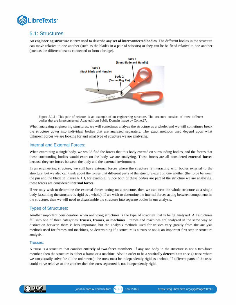
Jacob Moore & Contributors 5.1.1 12/21/2021 https://eng.libretexts.org/@go/page/50590

5.1: StructuresAn engineering structure is term used to describe any set of interconnected bodies. The different bodies in the structurecan move relative to one another (such as the blades in a pair of scissors) or they can be be fixed relative to one another(such as the different beams connected to form a bridge).

Figure : This pair of scissors is an example of an engineering structure. The structure consists of three differentbodies that are interconnected. Adapted from Public Domain image by Comet27.

When analyzing engineering structures, we will sometimes analyze the structure as a whole, and we will sometimes breakthe structure down into individual bodies that are analyzed separately. The exact methods used depend upon whatunknown forces we are looking for and what type of structure we are analyzing.

Internal and External Forces:

When examining a single body, we would find the forces that this body exerted on surrounding bodies, and the forces thatthese surrounding bodies would exert on the body we are analyzing. These forces are all considered external forcesbecause they are forces between the body and the external environment.

In an engineering structure, we still have external forces where the structure is interacting with bodies external to thestructure, but we also can think about the forces that different parts of the structure exert on one another (the force betweenthe pin and the blade in Figure , for example). Since both of these bodies are part of the structure we are analyzing,these forces are considered internal forces.

If we only wish to determine the external forces acting on a structure, then we can treat the whole structure as a singlebody (assuming the structure is rigid as a whole). If we wish to determine the internal forces acting between components inthe structure, then we will need to disassemble the structure into separate bodies in our analysis.

Types of Structures:

Another important consideration when analyzing structures is the type of structure that is being analyzed. All structuresfall into one of three categories: trusses, frames, or machines. Frames and machines are analyzed in the same way sodistinction between them is less important, but the analysis methods used for trusses vary greatly from the analysismethods used for frames and machines, so determining if a structure is a truss or not is an important first step in structureanalysis.

Trusses:

A truss is a structure that consists entirely of two-force members. If any one body in the structure is not a two-forcemember, then the structure is either a frame or a machine. Also,in order to be a statically determinate truss (a truss wherewe can actually solve for all the unknowns), the truss must be independently rigid as a whole. If different parts of the trusscould move relative to one another then the truss separated is not independently rigid.

5.1.1

5.1.1

Jacob Moore & Contributors 5.1.2 12/21/2021 https://eng.libretexts.org/@go/page/50590

Figure : This bridge is an example of a truss. It consists of a number of members connected at only two points (theends of the beams). Public domain image by Leonard G.

A two-force member is a body where forces are applied at only two locations. If forces are applied at more than twolocations, or if any moments are applied, then the body is not a two-force member (see the two-force member page formore details). Because of the unique assumptions we can make with two-force members, we can apply two uniquemethods to the analysis of trusses (the method of joints and the method of sections) that we cannot apply to frames andmachines (where we cannot assume we have two-force members).

Frames and Machines:

A frame or a machine is structure where at least one component of the structure is not a two-force member. Thiscomponent will be a body in the structure that has forces acting at three or more points on it. The difference between aframe and a machine is that a frame is rigid as a whole, while a machine is not rigid as a whole.

Figure : The legs of this stool have forces applied to them in three locations (the top, the cross beams, and the floor).The stool is also independently rigid, so this is a frame. Image by Besceh31 CC-BY-SA 2.5

Figure : Many pieces within this pair of locking pliers have forces applied to them at more than two locations. Thepieces can also move relative to one another, so this is an example of a machine. Image by Duk CC-BY-SA 3.0

Because frames and machines do not consist entirely of two-force members, we cannot make the assumptions that allow usto use the method of joints and the method of sections. For this reason, we need to use a different analysis method (simplycalled the analysis of frames and machines here).

5.1.2

5.1.3

5.1.4

Jacob Moore & Contributors 5.1.3 12/21/2021 https://eng.libretexts.org/@go/page/50590

Video lecture covering this section, delivered by Dr. Jacob Moore. YouTube source: https://youtu.be/5Hz8h7qEVEM.

5.1 Structures - Video Lecture - JPM5.1 Structures - Video Lecture - JPM

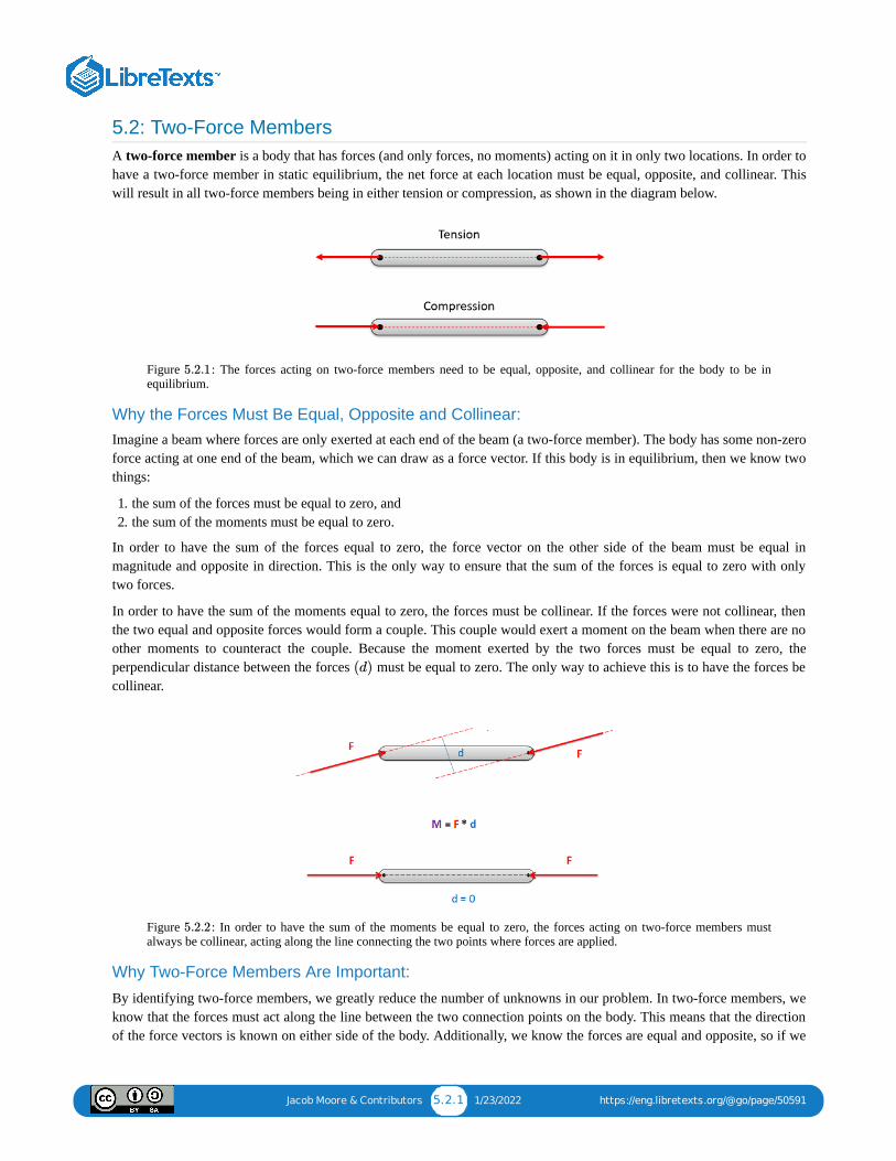
Jacob Moore & Contributors 5.2.1 1/23/2022 https://eng.libretexts.org/@go/page/50591

5.2: Two-Force MembersA two-force member is a body that has forces (and only forces, no moments) acting on it in only two locations. In order tohave a two-force member in static equilibrium, the net force at each location must be equal, opposite, and collinear. Thiswill result in all two-force members being in either tension or compression, as shown in the diagram below.

Figure : The forces acting on two-force members need to be equal, opposite, and collinear for the body to be inequilibrium.

Why the Forces Must Be Equal, Opposite and Collinear:Imagine a beam where forces are only exerted at each end of the beam (a two-force member). The body has some non-zeroforce acting at one end of the beam, which we can draw as a force vector. If this body is in equilibrium, then we know twothings:

1. the sum of the forces must be equal to zero, and2. the sum of the moments must be equal to zero.

In order to have the sum of the forces equal to zero, the force vector on the other side of the beam must be equal inmagnitude and opposite in direction. This is the only way to ensure that the sum of the forces is equal to zero with onlytwo forces.

In order to have the sum of the moments equal to zero, the forces must be collinear. If the forces were not collinear, thenthe two equal and opposite forces would form a couple. This couple would exert a moment on the beam when there are noother moments to counteract the couple. Because the moment exerted by the two forces must be equal to zero, theperpendicular distance between the forces must be equal to zero. The only way to achieve this is to have the forces becollinear.

Figure : In order to have the sum of the moments be equal to zero, the forces acting on two-force members mustalways be collinear, acting along the line connecting the two points where forces are applied.

Why Two-Force Members Are Important:

By identifying two-force members, we greatly reduce the number of unknowns in our problem. In two-force members, weknow that the forces must act along the line between the two connection points on the body. This means that the directionof the force vectors is known on either side of the body. Additionally, we know the forces are equal and opposite, so if we

5.2.1

(d)

5.2.2

Jacob Moore & Contributors 5.2.2 1/23/2022 https://eng.libretexts.org/@go/page/50591

determine the magnitude and direction of the force acting on one side of the body, we automatically know the magnitudeand direction of the force acting on the other side of the body.

Figure : The forces in two-force members will always act along the line connecting the two points where forces areapplied.

Two-force members are also important in distinguishing between trusses, and frames and machines. When we analyzetrusses using either the method of joints or the method of sections, we will assume everything is a two-force member. Ifthis assumption is incorrect, this will cause serious problems in the analysis. By making this assumption, though, we canuse some shortcuts that will make truss analysis easier and faster than the analysis of frames and machines.

Video lecture covering this section, delivered by Dr. Jacob Moore. YouTube source: https://youtu.be/m3GhMaZwHJw.

5.2.3

5.2 Two Force Members - Video Lect5.2 Two Force Members - Video Lect……

Jacob Moore & Contributors 5.3.1 12/21/2021 https://eng.libretexts.org/@go/page/52779

5.3: TrussesA truss is an engineering structure that is made entirely of two-force members. In addition, statically determinate trusses(trusses that can be analyzed completely using the equilibrium equations) must be independently rigid. This means that ifthe truss was separated from its connection points, no one part would be able to move independently with respect to therest of the truss.

Figure : Trusses are made entirely of two-force members. This means that each member will either be in tension orcompression, as shown here.

Trusses can be broken down further into plane trusses and space trusses. A plane truss is a truss where all members lie ina single plane. This means that plane trusses can essentially be treated as two-dimensional systems. Space trusses, on theother hand, have members that are not limited to a single plane. This means that space trusses need to be analyzed as athree-dimensional system.

Figure : The members of these trusses all lie in a single plane. These roof trusses are an example of a plane truss.Image by Riisipuuro CC-BY-SA 3.0.

Figure : This bridge consists of two plane trusses connected by members called stringers. Adapted from image byToddC4176 CC-BY-SA 3.0.

Figure : This roof supporting truss does not lie in a single plane. This is an example of a space truss. Image byIM3847 CC-BY-SA 4.0.

5.3.1

5.3.2

5.3.3

5.3.4

Jacob Moore & Contributors 5.3.2 12/21/2021 https://eng.libretexts.org/@go/page/52779

Figure : The power line tower also does not lie in a single plane and is therefore a space truss. Image by AndersLagerås CC-BY-SA 2.5.

Analyzing Trusses:When we talk about analyzing a truss, we are usually looking to identify not only the external forces acting on the trussstructure, but also the forces acting on each member internally in the truss. Because each member of the truss is a twoforce member, we simply need to identify the magnitude of the force on each member, and determine if each member is intension or compression.

To determine these unknowns, we have two methods available: the method of joints, and the method of sections. Bothwill give the same results, but each through a different process.

The method of joints focuses on the joints, or the connection points where the members come together. We assume wehave a pin at each of these points that we model as a particle, we draw out the free body diagram for each pin, and then wewrite out the equilibrium equations for each pin. This will result in a large number of equilibrium equations that we can useto solve for a large number of unknown forces.

The method of sections involves pretending to split the truss into two or more different sections and then analyzing eachsection as a separate rigid body in equilibrium. In this method we determine the appropriate sections, draw free bodydiagrams for each section, and then write out the equilibrium equations for each section.

The method of joints is usually the easiest and fastest method for solving for all the unknown forces in a truss. The methodof sections, on the other hand, is better suited to targeting and solving for the forces in just a few members without havingto solve for all the unknowns. In addition, these methods can be combined if needed to best suit the goals of the problemsolver.

Video lecture covering this section, delivered by Dr. Jacob Moore. YouTube source: https://youtu.be/jn8sR-lS4tw.

5.3.5

5.3 Trusses - Video Lecture - JPM5.3 Trusses - Video Lecture - JPM

Jacob Moore & Contributors 5.4.1 12/21/2021 https://eng.libretexts.org/@go/page/52780

5.4: Method of JointsThe method of joints is a process used to solve for the unknown forces acting on members of a truss. The method centerson the joints or connection points between the members, and it is usually the fastest and easiest way to solve for all theunknown forces in a truss structure.

Using the Method of Joints:The process used in the method of joints is outlined below.

In the beginning, it is usually useful to label the members and the joints in your truss. This will help you keep everythingorganized and consistent in later analysis. In this book, the members will be labeled with letters and the joints will belabeled with numbers.

Figure : The first step in the method of joints is to label each joint and each member.

Treating the entire truss structure as a rigid body, draw a free body diagram, write out the equilibrium equations, and solvefor the external reacting forces acting on the truss structure. This analysis should not differ from the analysis of a singlerigid body.

Figure : Treat the entire truss as a rigid body and solve for the reaction forces supporting the truss structure.

Assume there is a pin or some other small amount of material at each of the connection points between the members. Nextyou will draw a free body diagram for each connection point. Remember to include:

Any external reaction or load forces that may be acting at that joint.A normal force for each two force member connected to that joint. Remember that for a two force member, the forcewill be acting along the line between the two connection points on the member. We will also need to guess if it will be atensile or a compressive force. An incorrect guess now though will simply lead to a negative solution later on. Acommon strategy then is to assume all forces are tensile, then later in the solution any positive forces will be tensileforces and any negative forces will be compressive forces.Label each force in the diagram. Include any known magnitudes and directions and provide variable names for eachunknown.

5.4.1

5.4.2

Jacob Moore & Contributors 5.4.2 12/21/2021 https://eng.libretexts.org/@go/page/52780

Figure : Drawing a free body diagram of each joint, we draw in the known forces as well as tensile forces from eachtwo-force member.

Write out the equilibrium equations for each of the joints. You should treat the joints as particles, so there will be forceequations but no moment equations. With either two (for 2D problems) or three (for 3D problems) equations for eachjoint; this should give you a large number of equations.

In planar trusses, the sum of the forces in the direction will be zero and the sum of the forces in the directionwill be zero for each of the joints.

In space trusses, the sum of the forces in the direction will be zero, the sum of the forces in the direction will bezero, and the sum of forces in the direction will be zero for each of the joints.

Finally, solve the equilibrium equations for the unknowns. You can do this algebraically, solving for one variable at atime, or you can use matrix equations to solve for everything at once. If you assumed that all forces were tensile earlier,remember that negative answers indicate compressive forces in the members.

Video lecture covering this section, delivered by Dr. Jacob Moore. YouTube source: https://youtu.be/B8SEG7xPI-o.

Find the force acting in each of the members in the truss bridge shown below. Remember to specify if each member isin tension or compression.

5.4.3

x y

∑ = 0F   (5.4.1)

∑ = 0 ; ∑ = 0Fx Fy (5.4.2)

x y

z

∑ = 0F   (5.4.3)

∑ = 0 ; ∑ = 0 ; ∑ = 0Fx Fy Fz (5.4.4)

5.4 The Method of Joints - Video Lec5.4 The Method of Joints - Video Lec……

Example 5.4.1

Jacob Moore & Contributors 5.4.3 12/21/2021 https://eng.libretexts.org/@go/page/52780

Figure : problem diagram for Example . A truss bridge represented as a 2D plane truss, with a standard-orientation -coordinate system.

Solution

Video : Worked solution to example problem , provided by Dr. Jacob Moore. YouTube source:https://youtu.be/vowewkEdTzw.

Find the force acting in each of the members of the truss shown below. Remember to specify if each member is intension or compression.

Figure : problem diagram for Example . A plane truss mounted on a wall, with a standard-orientation -coordinate system.

Solution

5.4.4 5.4.1xy

Method of Joints - Adaptive Map Method of Joints - Adaptive Map ……

5.4.2 5.4.1

Example 5.4.2

5.4.5 5.4.2 xy

Jacob Moore & Contributors 5.4.4 12/21/2021 https://eng.libretexts.org/@go/page/52780

Video : Worked solution to example problem , provided by Dr. Jacob Moore. YouTube source:https://youtu.be/IxnClZ-ppjM.

Find the force acting in each of the members of the truss shown below. Remember to specify if each member is intension or compression.

Figure : problem diagram for Example . A space truss supported by a single ball-and-socket joint, orientedon a 3D coordinate system with the -plane in the plane of the screen and the -axis pointing out of the screen.

Solution

Video : Worked solution to example problem , provided by Dr. Jacob Moore. YouTube source:https://youtu.be/sDKESSbufEk.

Method of Joints - Adaptive Map Method of Joints - Adaptive Map ……

5.4.3 5.4.2

Example 5.4.3

5.4.6 5.4.3yz x

Method Of Joints - Adaptive Map Method Of Joints - Adaptive Map ……

5.4.4 5.4.3

Jacob Moore & Contributors 5.5.1 1/23/2022 https://eng.libretexts.org/@go/page/52781

5.5: Method of SectionsThe method of sections is a process used to solve for the unknown forces acting on members of a truss. The methodinvolves breaking the truss down into individual sections and analyzing each section as a separate rigid body. The methodof sections is usually the fastest and easiest way to determine the unknown forces acting in a specific member of the truss.

Using the Method of Sections:The process used in the method of sections is outlined below.

1. In the beginning, it is usually useful to label the members in your truss. This will help you keep everything organizedand consistent in later analysis. In this book, the members will be labeled with letters.

Figure : The first step in the method of sections is to label each member.

2. Treating the entire truss structure as a rigid body, draw a free body diagram, write out the equilibrium equations, andsolve for the external reacting forces acting on the truss structure. This analysis should not differ from the analysis of asingle rigid body.

Figure : Treat the entire truss as a rigid body and solve for the reaction forces supporting the truss structure.

3. Next, you will imagine cutting your truss into two separate sections. The cut should travel through the member that youare trying to solve for the forces in, and should cut through as few members as possible. The cut does not need to be astraight line.

Figure : Next you will imagine cutting the truss into twoparts. If you want to find the forces in a specific member, be sure to cut through that member. It also makes thingseasier if you cut through as few members as possible.

4. Next, you will draw a free body diagram for either one or both sections that you created. Be sure to include all theforces acting on each section.

Any external reaction or load forces that may be acting at the section.An internal force in each member that was cut when splitting the truss into sections. Remember that for a two-forcemember, the force will be acting along the line between the two connection points on the member. We will also

5.5.1

5.5.2

5.5.3

Jacob Moore & Contributors 5.5.2 1/23/2022 https://eng.libretexts.org/@go/page/52781

need to guess if it will be a tensile or a compressive force. An incorrect guess now, though, will simply lead to anegative solution later on. A common strategy then is to assume all forces are tensile; then later in the solution anypositive forces will be tensile forces and any negative forces will be compressive forces.Label each force in the diagram. Include any known magnitudes and directions and provide variable names for eachunknown.

Figure : Next, draw a free body diagram of one or both halves of the truss. Add the known forces, as well asunknown tensile forces for each member that you cut.

5. Write out the equilibrium equations for each section you drew a free body diagram of. These will be extended bodies,so you will need to write out the force and the moment equations.

For 2D problems you will have three possible equations for each section: two force equations and one momentequation.

For 3D problems you will have six possible equations for each section: three force equations and three momentequations.

6. Finally, solve the equilibrium equations for the unknowns. You can do this algebraically, solving for one variable at atime, or you can use matrix equations to solve for everything at once. If you assumed that all forces were tensile earlier,remember that negative answers indicate compressive forces in the members.

5.5.4

∑ = 0 ∑ = 0F   M  (5.5.1)

∑ = 0 ; ∑ = 0 ; ∑ = 0Fx Fy Mz (5.5.2)

∑ = 0F   (5.5.3)

∑ = 0 ; ∑ = 0 ; ∑ = 0Fx Fy Fz (5.5.4)

∑ = 0M  (5.5.5)

∑ = 0 ; ∑ = 0 ; ∑ = 0Mx My Mz (5.5.6)

Jacob Moore & Contributors 5.5.3 1/23/2022 https://eng.libretexts.org/@go/page/52781

Video lecture covering this section, delivered by Dr. Jacob Moore. YouTube source: https://youtu.be/XcRn776w22Q.

Find the forces acting on members BD and CE. Be sure to indicate if the forces are tensile or compressive.

Figure : problem diagram for Example . A two-dimensional representation of a truss bridge, with astandard-orientation -coordinate system.

Solution

Video : Worked solution to example problem , provided by Dr. Jacob Moore. YouTube source:https://youtu.be/9xxmHpLB1uU.

Find the forces acting on members AC, BC, and BD of the truss. Be sure to indicate if the forces are tensile orcompressive.

5.5 The Method of Sections - Video L5.5 The Method of Sections - Video L……

Example 5.5.1

5.5.5 5.5.1xy

Method of Sections - Adaptive MMethod of Sections - Adaptive M……

5.5.2 5.5.1

Example 5.5.2

Jacob Moore & Contributors 5.5.4 1/23/2022 https://eng.libretexts.org/@go/page/52781

Figure : Problem diagram for Example . A two-dimensional representation of a tower composed of trusses,arranged in a tall rectangle made of rectangular subunits with a trapezoidal top.

Solution

Video : Worked solution to example problem , provided by Dr. Jacob Moore. YouTube source:https://youtu.be/Kp9U4d2qbvE.

5.5.6 5.5.2

Method of Sections - Adaptive MMethod of Sections - Adaptive M……

5.5.3 5.5.2

Jacob Moore & Contributors 5.6.1 1/23/2022 https://eng.libretexts.org/@go/page/53661

5.6: Frames and MachinesA frame or a machine is an engineering structure that that contains at least one member that is not a two-force member.

Figure : This horizontal beam is connected to other members (where normal forces would exist) at more than twolocations. This beam is therefore not a two-force member.

Figure : This beam has two connection points, but a force is acting on a third point. Therefore the beam has forcesacting on it at more than two locations and it is not a two-force member.

A frame is a rigid structure, while a machine is not rigid. This means that no part can move relative to the other parts in aframe, while parts can move relative to one another in a machine. Though there is a difference in vocabulary in describingframes and machines, they are grouped together here because we use the same process to analyze both of these structures.

Figure : This stool contains non-two-force members (the legs) and no part can move relative to the other parts (it isrigid). Therefore it is a frame. Image by Besceh31 CC-BY-SA 2.5.

Figure : This pair of locking pliers contains non-two-force members and has parts that can move relative to oneanother (it is not rigid). Therefore it is a machine. Image by Duk CC-BY-SA 3.0.

Analyzing Frames and Machines:When we talk about analyzing frames or machines, we are usually looking to identify both the external forces acting on thestructure and the internal forces acting between members within the structure.

The method we use to analyze frames and machines (no special name here) centers around the process of breaking thestructure down into individual components and analyzing each component as a rigid body. Where the components areconnected, Newton's Third Law states that each body will exert an equal and opposite force on the other body. Each

5.6.1

5.6.2

5.6.3

5.6.4

Jacob Moore & Contributors 5.6.2 1/23/2022 https://eng.libretexts.org/@go/page/53661

component will be analyzed as an independent rigid body leading to equilibrium equations for each component, butbecause of Newton's Third Law, some unknowns may show up acting on two bodies.

Video lecture covering this section, delivered by Dr. Jacob Moore. YouTube source: https://youtu.be/QY-zWXzL7aI.

5.6 Frames and Machines - Video Le5.6 Frames and Machines - Video Le……

Jacob Moore & Contributors 5.7.1 1/23/2022 https://eng.libretexts.org/@go/page/53662

5.7: Analysis of Frames and MachinesThe process used to analyze frames and machines involves breaking the structure down into individual components inorder to solve for the forces acting on each component. Sometimes the structure as a whole can be analyzed as a rigidbody, and each component can always be analyzed as a rigid body.

The Process for Analyzing Frames and Machines:1. In the beginning it is usually useful to label the members in your structure. This will help you keep everything

organized and consistent in later analysis. In this book, we will label everything by assigning letters to each of thejoints.

Figure : The first step in the analysis of frames and machinesis to label the members.

2. Next you will need to determine if we can analyze the entire structure as a rigid body. In order to do this, the structureneeds to be independently rigid. This means that it would be rigid even if we separated it from its supports. If thestructure is independently rigid (no machines, and only some frames, will be independently rigid), then analyze thestructure as a single rigid body to determine the reaction forces acting on the structure. If the structure is notindependently rigid, skip this step.

Figure : If, and only if, the structure is independently rigid, you should analyze the whole structure as a singlerigid body to solve for the reaction forces.

3. Next you will draw a free body diagram for each of the components in the structure. You will need to include all forcesacting on each member:

First, add any external reaction or load forces that may be acting on the components.Second, identify any two-force members in the structure. At their connection points, they will cause a force withan unknown magnitude but a known direction (the forces will act along the line between the two connection pointson the member).Next, add in the reaction forces (and possibly moments) at the connection points between non-two-force members.For forces with an unknown magnitude and direction (such as in pin joints), the forces are often drawn in as havingunknown and components ( , and for 3D truss problems).Remember that the forces at each of the connection points will be a Newton's Third Law pair. This means that ifone member exerts some force on some other member, then the second member will exert an equal and oppositeforce back on the first. When we draw out our unknown forces at the connection points, we must make sure that theforces acting on each member are opposite in direction.

5.7.1

5.7.2

x y x y z

Jacob Moore & Contributors 5.7.2 1/23/2022 https://eng.libretexts.org/@go/page/53662

Figure \(\PageIndex

{3}\):Separate the structure into individual components and draw a free body diagram of each component. It is importantto remember that the forces at each connection point are a Newton's Third Law pair.

4. Write out the equilibrium equations for each component you drew a free body diagram of. These will be extendedbodies, so you will need to write out the force and the moment equations.

For 2D problems you will have three possible equations for each section: two force equations and one momentequation.

For 3D problems you will have six possible equations for each section: three force equations and three momentequations.

5. Finally, solve the equilibrium equations for the unknowns. You can do this algebraically, solving for one variable at atime, or you can use matrix equations to solve for everything at once. If any force turns out to be negative, thatindicates that the force actually travels in the opposite direction from what is indicated in your initial free bodydiagram.

Video lecture covering this section, delivered by Dr. Jacob Moore. YouTube source: https://youtu.be/6DK6IOU_TmU.

∑ = 0 ∑ = 0F   M  (5.7.1)

∑ = 0 ; ∑ = 0 ; ∑ = 0Fx Fy Mz (5.7.2)

∑ = 0F   (5.7.3)

∑ = 0 ; ∑ = 0 ; ∑ = 0Fx Fy Fz (5.7.4)

∑ = 0M  (5.7.5)

∑ = 0 ; ∑ = 0 ; ∑ = 0Mx My Mz (5.7.6)

5.7 Analysis of Frames and Machine5.7 Analysis of Frames and Machine……

Jacob Moore & Contributors 5.7.3 1/23/2022 https://eng.libretexts.org/@go/page/53662

Find all the forces acting on each of the members in the structure below.

Figure : problem diagram for Example . A symmetrical A-shaped structure experiences an external forceapplied at one point.

Solution

Video : Worked solution to example problem , provided by Dr. Jacob Moore. YouTube source:https://youtu.be/ix2BuRGMGBs.

Find all the forces acting on each of the members in the structure below.

Example 5.7.1

5.7.4 5.7.1

Analysis of Frames and MachinesAnalysis of Frames and Machines……

5.7.2 5.7.1

Example 5.7.2

Jacob Moore & Contributors 5.7.4 1/23/2022 https://eng.libretexts.org/@go/page/53662

Figure : problem diagram for Example . A two-member structure is attached to a wall with pin joints andexperiences an external force applied at one point.

Solution

Video : Worked solution to example problem , provided by Dr. Jacob Moore. YouTube source:https://youtu.be/TJjsz5Yt3Y0.

If two 150-Newton forces are exerted on the handles of the bolt cutter shown below, determine the reaction forces and exerted on the blades of the bolt cutter (this will be equal to the cutting forces exerted by the bolt

cutters).

Figure : problem diagram for Example . Top-down view of a bolt cutter lying on a table facing left, dividedinto members by labeled points.

Solution

5.7.5 5.7.2

Analysis of Frames and MachinesAnalysis of Frames and Machines……

5.7.3 5.7.2

Example 5.7.3

(FR1 ( )FR2

5.7.6 5.7.3

Jacob Moore & Contributors 5.7.5 1/23/2022 https://eng.libretexts.org/@go/page/53662

Video : Worked solution to example problem , provided by Dr. Jacob Moore. YouTube source:https://youtu.be/uLsfSMzc5eQ.

A 100-lb force is exerted on one side of a TV tray as shown below. Assuming there are no friction forces at the base,determine all forces acting on each of the three parts of the TV tray.

Figure : problem diagram for Example . Side view of a rectangular TV tray on two legs arranged in an X-shape, with a downwards force applied on the tray.

Solution

Video : Worked solution to example problem , provided by Dr. Jacob Moore. YouTube source:https://youtu.be/qi7WNDSb43k.

Analysis of Frames and MachinesAnalysis of Frames and Machines……

5.7.4 5.7.3

Example 5.7.4

5.7.7 5.7.4

5.7 WP 004 - Analysis of Frames 5.7 WP 004 - Analysis of Frames ……

5.7.5 5.7.4

Jacob Moore & Contributors 5.8.1 1/30/2022 https://eng.libretexts.org/@go/page/53663

5.8: Chapter 5 Homework Problems

Use the method of joints to solve for the forces in each member of the lifting gantry truss shown below.

Figure : problem diagram for Exercise . A two-dimensional representation of a lifting gantry truss, whichexperiences a downwards force of 40 kN at one end.

Solution

kN T, kN C, kN C

kN T, kN C

The truss shown below is supported by two cables at A and E, and supports two lighting rigs at D and F, as shown bythe loads. Use the method of joints to determine the forces in each of the members.

Figure : problem diagram for Exercise . A two-dimensional representation of a lighting support truss, whichexperiences the weights of lighting rigs hung at two points.

Solution

lbs T, , lbs C

lbs T, lbs T,

lbs C, lbs T, lbs T

The truss shown below is supported by a pin joint at A, a cable at D, and is supporting a 600 N load at point C. Use themethod of joints to determine the forces in each of the members. Assume the mass of the beams are negligible.

Exercise 5.8.1

5.8.1 5.8.1

= 113.14FAB = 80FAC = 120FBC

= 89.44FBD = 80FCD

Exercise 5.8.2

5.8.2 5.8.2

= 60FAB = 0FAC = 305.94FBC

= 300FBD = 120FCD = 0FCE

= 305.94FCF = 300FDF = 120FEF

Exercise 5.8.3

Jacob Moore & Contributors 5.8.2 1/30/2022 https://eng.libretexts.org/@go/page/53663

Figure : problem diagram for Exercise . A two-dimensional representation of a truss connected to the wall atone end, supported by a cable at the other, and experiencing a downwards force at one point.

Solution

N C, N T,

N C, N T

The space truss shown below is being used to lift a 250 lb box. The truss is anchored by a ball-and-socket joint at C(which can exert reaction forces in the , , and directions) and supports at A and B that only exert reaction forces inthe y direction. Use the method of joints to determine the forces acting all members of the truss.

Figure : problem diagram for Exercise . A space truss attached to a wall at three points and supporting aload its free end.

Solution

, lbs T, lbs C

lbs T, lbs C, lbs T

Use the method of sections to solve for the forces acting on members CE, CF, and DF of the gantry truss shown below.

5.8.3 5.8.3

= 1162.97FAB = 709.86FAC = 0FBC

= 1162.97FBD = 709.86FCD

Exercise 5.8.4

x y z

5.8.4 5.8.4

= 0FAB = 144.33FAC = 204.09FAD

= 144.33FBC = 204.09FBD = 288.68FCD

Exercise 5.8.5

Jacob Moore & Contributors 5.8.3 1/30/2022 https://eng.libretexts.org/@go/page/53663

Figure : problem diagram for Exercise . A two-dimensional representation of a gantry truss, whichexperiences downwards forces applied at two points.

Solution

, lbs C, lbs T

You are asked to compare two crane truss designs as shown below. Find the forces in members AB, BC, and CD forDesign 1 and find forces AB, AD, and CD for Design 2. What member is subjected to the highest loads in either case?

Figure : problem diagram for Exercise . Two versions of a crane truss design that differ only in theorientation of their support beams.

Solution

Design 1: lbs T, lbs T, lbs C

Design 2: lbs T, lbs C, lbs C

The largest forces are in member CD for both designs.

The K truss shown below supports three loads. Assume only vertical reaction forces at the supports. Use the method ofsections to determine the forces in members AB and FG. (Hint: you will need to cut through more than three members,but you can use your moment equations strategically to solve for exactly what you need).

5.8.5 5.8.5

= 0FCE = 306.2FCF = 300.2FDF

Exercise 5.8.6

5.8.6 5.8.6

= 11, 276FAB = 2902FBC = 18, 967FCD

= 13, 322FAB = 2902FAD = 16, 914FCD

Exercise 5.8.7

Jacob Moore & Contributors 5.8.4 1/30/2022 https://eng.libretexts.org/@go/page/53663

Figure : problem diagram for Exercise . A two-dimensional representation of a K-truss which experiencesdownwards forces applied at three points.

Solution

lbs C, lbs T

The truss shown below is supported by a pin support at A and a roller support at B. Use the hybrid method of sectionsand joints to determine the forces in members CE, CF, and CD.

Figure : problem diagram for Exercise . A two-dimensional representation of a truss attached to a wall,experiencing a downwards force at one point.

Solution

kN T, kN T, kN C

The shelf shown below is used to support a 50-lb weight. Determine the forces on members ACD and BC in thestructure. Draw those forces on diagrams of each member.

5.8.7 5.8.7

= 1066.67FAB = 1066.67FFG

Exercise 5.8.8

5.8.8 5.8.9

= 21FCE = 8.41FCF = 4.67FCD

Exercise 5.8.9

Jacob Moore & Contributors 5.8.5 1/30/2022 https://eng.libretexts.org/@go/page/53663

Figure : problem diagram for Example . Side view of a wall-mounted horizontal shelf supporting a weightat its free end.

Solution

lbs (Compression), lbs, lbs

A 20 N force is applied to a can-crushing mechanism as shown below. If the distance between points C and D is 0.1meters, what are the forces being applied to the can at points B and D? (Hint: treat the can as a two-force member)

Figure : problem diagram for Exercise . Side view of a wall-mounted can-crushing mechanism that holdsa soda can and experiences an applied force at its handle end.

Solution

N (Compression)

The suspension system on a car is shown below. Assuming the wheel is supporting a load of 3300 N and assuming thesystem is in equilibrium, what is the force we would expect in the shock absorber (member AE)? You can assume allconnections are pin joints.

5.8.9 5.8.9

= 223.6FBC = −200FAX= −50FAY

Exercise 5.8.10

5.8.10 5.8.10

= 148.9Fcan

Exercise 5.8.11

Jacob Moore & Contributors 5.8.6 1/30/2022 https://eng.libretexts.org/@go/page/53663

Figure : problem diagram for Exercise . Side view of the suspension system of one wheel of a car,experiencing an upwards force on the wheel.

Solution

N (Compression)

The chair shown below is subjected to forces at A and B by a person sitting in the chair. Assuming that normal forcesexist at F and G, and that friction forces only act at point G (not at F), determine all the forces acting on each of thethree members in the chair. Draw these forces acting on each part of the chair on a diagram.

Figure : problem diagram for Exercise . Side view of a folding chair with a square seat, facing to the left,that experiences forces at two points from a person sitting in the chair.

Solution

lbs, lbs, lbs

lbs, lbs

lbs, lbs

lbs, lbs

5.8.11 5.8.11

= 4611.9FAE

Exercise 5.8.12

5.8.12 5.8.12

= 108.3FF = −3.95FGX= 39.5FGY

= ± 16.89FCX = ± 295.4FCY

= ± 142.9FDX= ± 147.7FDY

= ± 112.9FEX= ± 256.0FEY

1 1/30/2022

CHAPTER OVERVIEW6: FRICTION AND FRICTION APPLICATIONSDefinition of dry friction; the application of dry friction in mechanical processes (wedges, power screws, bearings, disc-shapedmechanisms, belt-and-pulley systems).

6.0: VIDEO INTRODUCTION TO CHAPTER 6Video introduction to the topics to be covered in this chapter: dry friction and its applications in various mechanical parts.

6.1: DRY FRICTIONIntroduction to dry friction. Modeling dry friction with coulomb friction: the differences between static and kinetic friction, theirrelationship to movement of an object, and how to calculate them.

6.2: SLIPPING VS TIPPINGDetermining whether an object will first undergo translational motion (slipping) or rotational motion (tipping) as a force is applied toit.

6.3: WEDGESWedges as a method of using friction to accomplish tasks. Using the coulomb friction model to calculating the force to be applied to awedge in a given situation.

6.4: POWER SCREWSThe general structure of power screws. Application of friction to analyze the forces involved in a power screw and to determinewhether or not a given power screw is self-locking.

6.5: BEARING FRICTIONThe general structure of plain/journal bearings. Application of friction to analyze the forces and moments involved in the movementof a (plain) bearing.

6.6: DISC FRICTIONFriction in common disc-shaped mechanisms. Calculating moment based on friction for such discs.

6.7: BELT FRICTIONDetermining friction in flat-belt and V-belt pulley systems. Calculating torque and power transmission in belt-driven systems throughapplication of belt friction.

6.8: CHAPTER 6 HOMEWORK PROBLEMS

Jacob Moore & Contributors 6.0.1 12/21/2021 https://eng.libretexts.org/@go/page/50593

6.0: Video Introduction to Chapter 6

Video introduction to the topics covered in Chapter 6, delivered by Dr. Jacob Moore. YouTube source:https://youtu.be/ltBEDVYnFbE.

Chapter 6 IntroductionChapter 6 Introduction

Jacob Moore & Contributors 6.1.1 12/21/2021 https://eng.libretexts.org/@go/page/50594

6.1: Dry FrictionDry friction is the force that opposes one solid surface sliding across another solid surface. Dry friction always opposesthe surfaces sliding relative to one another, and it can have the effect of either opposing motion or causing motion inbodies.

Figure : Dry friction occurs between the bottom of this training sled and the grassy field. The dry friction wouldoppose the motion of the sled along the field in this case. Image by Avenue CC-BY-SA 3.0

Figure : Dry friction occurs between the tires and the road for this motorcycle. The dry friction force for thismotorcycle is what allows it to accelerate, decelerate, and turn. Public Domain image by Takisha Rappold.

The most commonly used model for dry friction is coulomb friction. This type of friction can further be broken down intostatic friction and kinetic friction. These two types of friction are illustrated in the diagram below. First, imagine a boxsitting on a surface. A pushing force is applied parallel to the surface and is constantly being increased. A gravitationalforce, a normal force, and a frictional force are also acting on the box.

Figure : As the pushing force increases, the static friction force will be equal in magnitude and opposite in directionuntil the point of impending motion. Beyond this point, the box will begin to slip as the pushing force is greater inmagnitude than the kinetic friction force opposing it.

Static friction occurs prior to the box slipping and moving. In this region, the friction force will be equal in magnitude andopposite in direction to the pushing force itself. As the magnitude of the pushing force increases, so does the magnitude ofthe friction force.

If the magnitude of the pushing force continues to rise, eventually the box will begin to slip. As the box begins to slip, thetype of friction opposing the motion of the box changes from static friction to what is called kinetic friction. The point justbefore the box slips is known as impending motion. This can also be thought of as the maximum possible static frictionforce before slipping. The magnitude of the maximum static friction force is equal to the static coefficient of friction timesthe normal force existing between the box and the surface. This coefficient of friction is a property that depends on bothmaterials and can usually be looked up in tables.

6.1.1

6.1.2

6.1.3

Jacob Moore & Contributors 6.1.2 12/21/2021 https://eng.libretexts.org/@go/page/50594

Kinetic friction occurs beyond the point of impending motion, when the box is sliding. With kinetic friction, themagnitude of the friction force opposing motion will be equal to the kinetic coefficient of friction times the normal forcebetween the box and the surface. The kinetic coefficient of friction also depends upon the two materials in contact, but willalmost always be less than the static coefficient of friction.

Video lecture covering this section, delivered by Dr. Jacob Moore. YouTube source: https://youtu.be/OPRc38nDpKo.

A 500 lb box is sitting on concrete floor. If the static coefficient of friction is 0.7 and the kinetic coefficient of frictionis 0.6:

What is the friction force if the pulling force is 150 lbs?What pulling force would be required to get the box moving?What is the minimum force required to keep the box moving once it has started moving?

Figure : problem diagram for Example . A box experiences a pulling force towards the right.

Solution

6.1 Dry Friction - Video Lecture - JPM6.1 Dry Friction - Video Lecture - JPM

Example 6.1.1

6.1.4 6.1.1

Jacob Moore & Contributors 6.1.3 12/21/2021 https://eng.libretexts.org/@go/page/50594

Video : Worked solution to example problem , provided by Dr. Jacob Moore. YouTube source:https://youtu.be/7R7kvKBxUjw.

A 30 lb sled is being pulled up an icy incline of 25 degrees. If the static coefficient of friction between the ice and thesled is 0.4 and the kinetic coefficient of friction is 0.3, what is the required pulling force needed to keep the sledmoving at a constant rate?

Figure : problem diagram for Example . A sled with a pulling force applied to move it up a 25° incline.

Solution

Dry Friction - Adaptive Map WorkDry Friction - Adaptive Map Work……

6.1.2 6.1.1

Example 6.1.2

6.1.5 6.1.2

Jacob Moore & Contributors 6.1.4 12/21/2021 https://eng.libretexts.org/@go/page/50594

Video : Worked solution to example problem , provided by Dr. Jacob Moore. YouTube source:https://youtu.be/oPMx-SZyiy4.

A plastic box is sitting on a steel beam. One end of the steel beam is slowly raised, increasing the angle of the surfaceuntil the box begins to slip. If the box begins to slip when the beam is at an angle of 41 degrees, what is the staticcoefficient of friction between the steel beam and the plastic box?

Figure : problem diagram for Example . A box on a steel beam whose left end has been raised until it is at41° above the horizontal.

Solution

Dry Friction - Adaptive Map WorkDry Friction - Adaptive Map Work……

6.1.3 6.1.2

Example 6.1.3

6.1.6 6.1.3

Jacob Moore & Contributors 6.1.5 12/21/2021 https://eng.libretexts.org/@go/page/50594

Video : Worked solution to example problem , provided by Dr. Jacob Moore. YouTube source:https://youtu.be/ShGP5rzIHN4.

Dry Friction - Adaptive Map WorkDry Friction - Adaptive Map Work……

6.1.4 6.1.3

Jacob Moore & Contributors 6.2.1 1/23/2022 https://eng.libretexts.org/@go/page/50595

6.2: Slipping vs TippingImagine a box sitting on a rough surface as shown in the figure below. Now imagine that we start pushing on the side ofthe box. Initially the friction force will resist the pushing force and the box will sit still. However, as we increase the forcepushing the box one of two things will occur.

1. The pushing force will exceed the maximum static friction force and the box will begin to slide across the surface(slipping).

2. Or, the pushing force and the friction force will create a strong enough couple that the box will rotate and fall on itsside (tipping).

Figure : As the pushing force increases on the box, it will either begin to slide along surface (slipping) or it will beginto rotate (tipping).

When we look at cases where either slipping or tipping may occur, we are usually interested in finding which of the twooptions will occur first. To determine this, we usually determine both the pushing force necessary to make the body slideand the pushing force necessary to make the body tip over. Whichever option requires less force is the option that willoccur first.

Determining the Force Required to Make an Object "Slip":A body will slide across a surface if the pushing force exceeds the maximum static friction force that can exist between thetwo surfaces in contact. As in all dry friction problems, this limit to the friction force is equal to the static coefficient offriction times the normal force between the body. If the pushing force exceeds this value then the body will slip.

Figure : If the pushing force exceeds the maximum static friction force then the body will begin to slide.

Determining the Force Required to Make an Object "Tip":The normal forces that support bodies are distributed forces. These forces will not only prevent the body from acceleratinginto the ground due to gravitational forces, but they can also redistribute themselves to prevent a body from rotating whenforces cause a moment to act on the body. This redistribution will result in the equivalent point load for the normal force

6.2.1

6.2.2 ( ∗ )μs FN

Jacob Moore & Contributors 6.2.2 1/23/2022 https://eng.libretexts.org/@go/page/50595

shifting to one side or the other. A body will tip over when the normal force can no longer redistribute itself any further toresist the moment exerted by other forces (such as the pushing force and the friction force).

Figure : At rest (A) the normal force is a uniformly distributed force on the bottom of the body. As a pushing force isapplied (B) the distributed normal force is redistributed, moving the equivalent point load to the right. This creates acouple between the gravity force and the normal force that will counter the couple exerted by the pushing force and thefriction force. If the pushing force becomes large enough (C), the couple exerted by the gravitational force and the normalforce will be unable to counter the couple exerted by the pushing force and the friction force.

The easiest way to think about the shifting normal force and tipping is to imagine the equivalent point load of thedistributed normal force. As we push or pull on the body, the normal force will shift to the left or right. This normal forceand the gravitational force create a couple that exerts a moment. This moment will be countering the moment exerted bythe couple formed by the pushing force and the friction force.

Because the normal force is the direct result of physical contact, we cannot shift the normal force beyond the surfaces incontact (i.e., the edge of the box). If countering the moment exerted by the pushing force and the friction force requiresshifting the normal force beyond the edge of the box, then the normal force and the gravity force will not be able tocounter the moment and as a result the box will begin to rotate (i.e., tip over).

Figure : The body will tip when the moment exerted by the pushing and friction forces exceeds the moment exertedby the gravity and normal forces. For impending motion, the normal force will be acting at the very edge of the body.

Video lecture covering this section, delivered by Dr. Jacob Moore. YouTube source: https://youtu.be/M2OZOkgVRBQ.

6.2.2

6.2.3

6.2 Slipping vs. Tipping - Video Lectu6.2 Slipping vs. Tipping - Video Lectu……

Jacob Moore & Contributors 6.2.3 1/23/2022 https://eng.libretexts.org/@go/page/50595

The box shown below is pushed as shown. If we keep increasing the pushing force, will the box first begin to slide orwill it tip over?

Figure : problem diagram for Example . A box on a flat surface, with a coefficient of static friction of 0.62between the two surfaces, experiences a pushing force at a point on its left side.

Solution

Video : Worked solution to example problem , provided by Dr. Jacob Moore. YouTube source:https://youtu.be/TeYgkfd4rTA.

What is the maximum value of that will allow the box to slide along the surface before tipping?

Figure : problem diagram for Example . A box on a flat surface, with a coefficient of static fricton of 0.62between the two surfaces, experiences a pushing force at a point of unknown height ( on its left side.

Solution

Example 6.2.1

6.2.4 6.2.1

Slipping vs. Tipping - Adaptive MaSlipping vs. Tipping - Adaptive Ma……

6.2.2 6.2.1

Example 6.2.2

d

6.2.5 6.2.2d

Jacob Moore & Contributors 6.2.4 1/23/2022 https://eng.libretexts.org/@go/page/50595

Video : Worked solution to example problem , provided by Dr. Jacob Moore. YouTube source:https://youtu.be/STDWwJsng6k.

Slipping vs. Tipping - Adaptive MaSlipping vs. Tipping - Adaptive Ma……

6.2.3 6.2.2

Jacob Moore & Contributors 6.3.1 1/23/2022 https://eng.libretexts.org/@go/page/53829

6.3: WedgesA wedge is a thin, inclined-plane-shaped object that is used to force two objects apart or to force one object away from anearby surface. Wedges have the effect of allowing users to create very large normal forces to move objects with relativelysmall input forces. The friction forces in wedge systems also tend to be very large, though, and can reduce theeffectiveness of wedges.

Figure : A hammer is used to push this wedge into the crack in this log. The normal forces are pushing the two halvesof the log apart while the friction forces are opposing the pushing force. Adapted from image by Luigi Chiesa. CC-BY-SA-3.0.

To analyze a wedge system, we will need to draw free body diagrams of each of the bodies in the system (the wedge itselfand any bodies the wedge will be moving). We need to be sure that we include the pushing force on the wedge, normalforces along any surfaces in contact, and friction forces along any surfaces in contact.

Figure : The top diagram shows a wedge being used to push a safe away from a wall. The first step in analyzing thesystem is to draw free body diagrams of the wedge and the safe. Remember that all normal forces will be perpendicular tothe surfaces in contact and that all friction forces will be parallel to the surfaces in contact.

6.3.1

6.3.2

Jacob Moore & Contributors 6.3.2 1/23/2022 https://eng.libretexts.org/@go/page/53829

After we draw the free body diagram, we can work to simplify the problem. It is usually assumed that the wedge and thebodies will be sliding against one another, so each friction force will be equal to the kinetic coefficient of friction betweenthe two surfaces times the associated normal force between the two forces. This reduces the number of unknowns and willusually allow us to solve for any unknown values.

Figure : By replacing each of the friction forces with the kinetic coefficient of friction times the normal force, we canreduce the number of unknowns in our analysis.

With our simplified diagram, we will assume that the bodies are all in equilibrium and write out equilibrium equations forthe two bodies. By solving the equilibrium equations, we can solve for any unknowns we have.

Video lecture covering this section, delivered by Dr. Jacob Moore. YouTube source: https://youtu.be/5R3S5bYBULY.

A heavy safe is being pushed away from a wall with a wedge as shown below. Assume the wedge has an angle of 5degrees, the coefficient of friction (static and kinetic) between the wedge and the safe is 0.16, and the coefficients offriction (static and kinetic) between the wedge and the wall and the safe and the floor are both 0.35. What is thepushing force required to move the safe out from the wall?

6.3.3

6.3 Wedges - Video Lecture - JPM6.3 Wedges - Video Lecture - JPM

Example 6.3.1

Jacob Moore & Contributors 6.3.3 1/23/2022 https://eng.libretexts.org/@go/page/53829

Figure : problem diagram for Example . A point-down wedge, with a pushing force applied at its base, isused to pry a safe away from a wall.

Solution

Video : Worked solution to example problem , provided by Dr. Jacob Moore. YouTube source:https://youtu.be/r7Ut0GI8q00.

A wedge as shown below is being used to lift the corner of the foundation of a house. How large must the pushingforce be to exert a lifting force of one ton (2000 lbs)?

Figure : problem diagram for Example . A wedge is used to lift a block on a 10° incline with a force of 2000lbs; coefficients of friction are given as 0.15 between the block and wedge, and 0.05 between the incline and thewedge.

6.3.4 6.3.1

Wedges - Adaptive Map Worked EWedges - Adaptive Map Worked E……

6.3.2 6.3.1

Example 6.3.2

6.3.5 6.3.2

Jacob Moore & Contributors 6.3.4 1/23/2022 https://eng.libretexts.org/@go/page/53829

Solution

Video : Worked solution to example problem , provided by Dr. Jacob Moore. YouTube source:https://youtu.be/kgfh4Mna63M.

Wedges - Adaptive Map Worked EWedges - Adaptive Map Worked E……

6.3.3 6.3.2

Jacob Moore & Contributors 6.4.1 1/23/2022 https://eng.libretexts.org/@go/page/53830

6.4: Power ScrewsA power screw (also sometimes called a lead screw) is another simple machine that can be used to create very large forces.The screw can be thought of as a wedge or a ramp that has been wound around a shaft. By holding a nut stationary androtating the shaft, we can have the nut sliding either up or down the wedge in the shaft. In this way, a relatively smallmoment on the shaft can cause very large forces on the nut.

Figure : The screw in this cider press is rotated with the handle on the top. The stationary nut on the frame of thepress forces the shaft downward as it is turned. Public Domain image by Daderot.

Figure : By rotating the screw in this scissor jack, the user can move the nut (on the left end) closer or further fromthe anchor on the right end, which will raise or lower the car. Public Domain image by nrjfalcon1.

Static Analysis of Power Screws:

The easiest way to analyze a power screw system is to turn the problem into a 2D problem by "unwrapping" the ramp fromaround the shaft. To do this we will need two numbers. First we will need the diameter of the shaft, and second we willneed either the threads-per-inch/centimeter or the pitch of the screw. The threads-per-inch tells you how many threadsyou have per inch/centimeter of screw. With a single thread design (most screws) this will also be the number of times thethread wraps around the screw in one inch/centimeter. The pitch, on the other hand, gives you the distance between twoadjacent threads. Either of these numbers can be used to find the other.

Once we have these numbers, we can imagine unwrapping the ramp from around the screw and ending up with a ramp inone of the two situations below. In either case, we can use the inverse tangent function to find the lead angle, which can bethought of as the angle of the thread that the nut is climbing up. Finding the lead angle is the first step in analyzing a powerscrew system.

Figure : The lead angle of a screw is the angle of the thread that the nut will be climbing up as the shaft rotates.

6.4.1

6.4.2

6.4.3

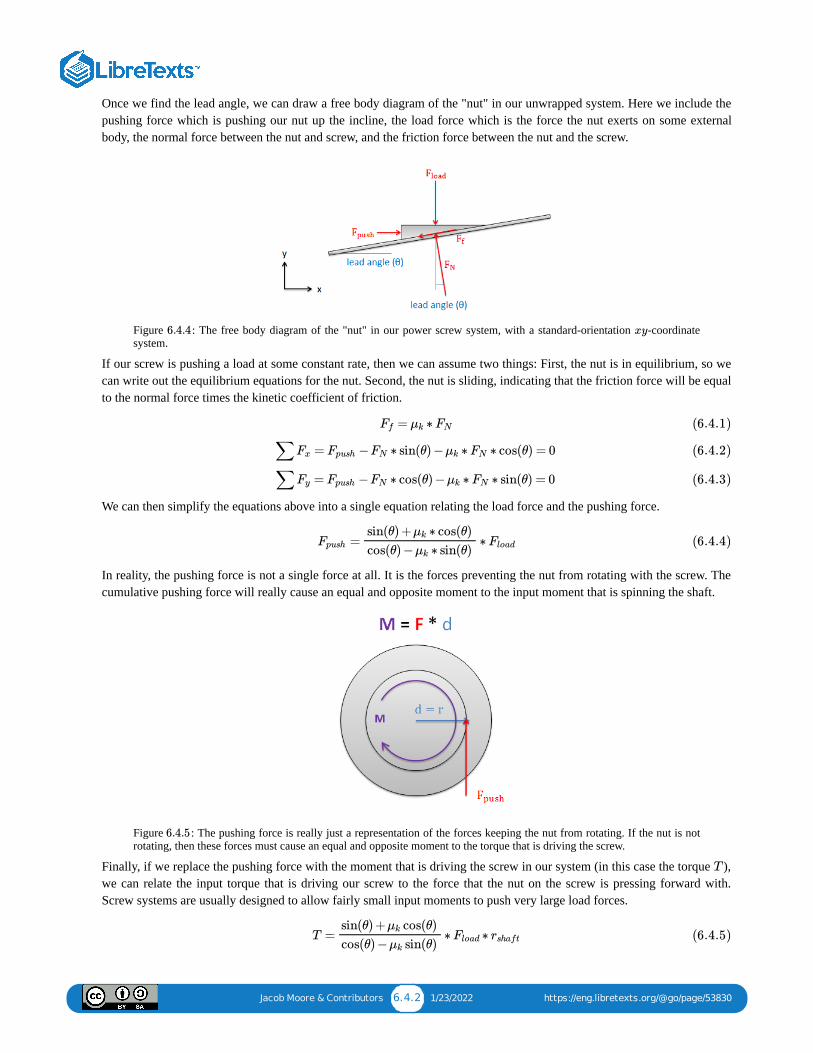
Jacob Moore & Contributors 6.4.2 1/23/2022 https://eng.libretexts.org/@go/page/53830

Once we find the lead angle, we can draw a free body diagram of the "nut" in our unwrapped system. Here we include thepushing force which is pushing our nut up the incline, the load force which is the force the nut exerts on some externalbody, the normal force between the nut and screw, and the friction force between the nut and the screw.

Figure : The free body diagram of the "nut" in our power screw system, with a standard-orientation -coordinatesystem.

If our screw is pushing a load at some constant rate, then we can assume two things: First, the nut is in equilibrium, so wecan write out the equilibrium equations for the nut. Second, the nut is sliding, indicating that the friction force will be equalto the normal force times the kinetic coefficient of friction.

We can then simplify the equations above into a single equation relating the load force and the pushing force.

In reality, the pushing force is not a single force at all. It is the forces preventing the nut from rotating with the screw. Thecumulative pushing force will really cause an equal and opposite moment to the input moment that is spinning the shaft.

Figure : The pushing force is really just a representation of the forces keeping the nut from rotating. If the nut is notrotating, then these forces must cause an equal and opposite moment to the torque that is driving the screw.

Finally, if we replace the pushing force with the moment that is driving the screw in our system (in this case the torque ),we can relate the input torque that is driving our screw to the force that the nut on the screw is pressing forward with.Screw systems are usually designed to allow fairly small input moments to push very large load forces.

6.4.4 xy

= ∗Ff μk FN (6.4.1)

∑ = − ∗ sin(θ) − ∗ ∗ cos(θ) = 0Fx Fpush FN μk FN (6.4.2)

∑ = − ∗ cos(θ) − ∗ ∗ sin(θ) = 0Fy Fpush FN μk FN (6.4.3)

= ∗Fpush

sin(θ) + ∗ cos(θ)μk

cos(θ) − ∗ sin(θ)μk

Fload (6.4.4)

6.4.5

T

T = ∗ ∗sin(θ) + cos(θ)μk

cos(θ) − sin(θ)μk

Fload rshaft (6.4.5)

Jacob Moore & Contributors 6.4.3 1/23/2022 https://eng.libretexts.org/@go/page/53830

Self-Locking ScrewsImagine that we apply a torque to a power screw to lift a body; then when we get the load to the desired height we stopapplying that torque to let the body sit where it is. If we were to redraw our free body diagram from earlier for the newsituation, we would find two things.

1. The pushing force is missing (since a torque is no longer applied to the shaft).2. The friction is now fighting against the nut sliding back down the ramp.

Figure : Without the pushing force from an applied torque, the friction force acts to prevent the nut from sliding downthe ramp.

With this new free body diagram, there are two possible scenarios that could occur:

1. The friction force is large enough to keep the nut from sliding down the ramp, meaning everything will remain in staticequilibrium if released.

2. The friction force will not be sufficient to keep the nut from sliding down the ramp, meaning that the load would beginto fall as soon as the torque is removed from the shaft.

With power screw applications such as a car jack, the second option could be very dangerous. It is therefore important toknow if a power screw system is self-locking (scenario 1 above) or not self-locking (scenario 2 above).

To define the boundary between self-locking systems and non-self-locking systems, we use something called the self-locking angle. As intuition would tell us, slipping does not occur on very gentle slopes (small lead angles) while it doesoccur on very steep slopes (large lead angles). The angle at which the nut would begin to slip is known as the self-lockingangle.

To find the self-locking angle, we will assume impending motion (relating the friction force to the normal force) and leavethe lead angle as an unknown. This lets us create the free body diagram as shown below and gives us the equilibriumequations below.

Figure : To find the self-locking angle we will assume impending motion. We then draw our free body diagram(above) and write out our equilibrium equations (below) accordingly.

6.4.6

6.4.7

∑ = − ∗ sin(θ) + ∗ ∗ cos(θ) = 0Fx FN μs FN (6.4.6)

∑ = − + ∗ cos(θ) + ∗ ∗ sin(θ) = 0Fy Fload FN μs FN (6.4.7)

Jacob Moore & Contributors 6.4.4 1/23/2022 https://eng.libretexts.org/@go/page/53830

Using the equilibrium equation as a starting point, we can solve for the angle (eliminating the normal force all togetherin the process). This new equation shown below gives us the self-locking angle.

Systems with lead angles smaller than this will be self-locking, while systems with lead angles larger than this will not beself-locking.

Video lecture covering this section, delivered by Dr. Jacob Moore. YouTube source: https://youtu.be/mci-kH14JGw.

The power screw below is being used to lift a platform with a weight of 12 pounds. Based on the information below...

What is the required torque on the shaft to lift the load?Would the load fall if the toque was removed from the shaft?

Figure : problem diagram for Example . A power screw with a 0.375-inch screw diameter, 12 threads perinch, is used to lift a platform, with a coefficient of static and kinetic friction of 0.16.

Solution

Video : Worked solution to example problem , provided by Dr. Jacob Moore. YouTube source:https://youtu.be/uB2r3AtxCRs.

x θ

= ( )θlocking tan−1 μs (6.4.8)

6.4 Power Screws - Video Lecture - J6.4 Power Screws - Video Lecture - J……

Example 6.4.1

6.4.8 6.4.1

Power Screws - Adaptive Map WoPower Screws - Adaptive Map Wo……

6.4.2 6.4.1

Jacob Moore & Contributors 6.5.1 12/21/2021 https://eng.libretexts.org/@go/page/53831

6.5: Bearing FrictionA bearing is the machine element used to support a rotating shaft. Bearing friction is the friction that exists between therotating shaft and bearing that is supporting that shaft. Though many types of bearings exist (plain, ball, roller,hydrodynamic), in this course we will only be looking at plain bearings, also sometimes called journal bearings.

Figure : Some friction will exist in the bearings on this train car. Public Domain image by ds_30.

A plain bearing consists of a circular shaft fitted into a slightly larger circular hole as shown below. The shaft will usuallybe rotating and will be exerting some sort of load onto the bearing. The bearing will then be supporting the shaftwith some normal force, and a friction force will exist between the bearing surface and the surface of the shaft. Sometimesthe rotation of the bearing will cause the shaft to climb up the side of the side of the bearing, causing the angle of thenormal and friction forces to change, but this climbing is usually small enough that it is neglected.

Figure : In a plain bearing like the one shown here, a friction force will oppose the rotation of the spinning shaft inthe stationary bearing. This force will cause a small moment opposing the rotation of the shaft.

If we assume that the climbing in the bearing is negligible, the normal of the bearing on the shaft will be equal andopposite to loading force of the shaft on the bearing. Furthermore, if the shaft is rotating relative to the bearing, then thefriction force will be equal to kinetic coefficient of friction times the normal force of the bearing on the shaft.

If the climb angle is assumed to be small, then...

The friction force will then be exerting a moment about the center of the shaft that opposes the rotation of the shaft. Unlesssome other moment is keeping the shaft spinning, this moment will eventually slow down and stop the rotation in the shaft.The magnitude of this moment will be equal to the magnitude of the friction force times the radius of the shaft.

Another important factor to keep in mind is that most bearings are lubricated. This can significantly lower the coefficientsof friction (this is actually the main reason for using lubrication in machinery). When performing calculations, it isimportant to know if the bearing is lubricated and, if so, to use the appropriate friction coefficients.

6.5.1

( )Fload

6.5.2

=Fload FN (6.5.1)

= ∗Ff μk FN (6.5.2)

= ∗ ( ∗ )Mf rshaft μk FN (6.5.3)

Jacob Moore & Contributors 6.5.2 12/21/2021 https://eng.libretexts.org/@go/page/53831

Video lecture covering this section, delivered by Dr. Jacob Moore. YouTube source: https://youtu.be/v8q6xnJN9zE.

A cart and its load weigh a total of 200 lbs. There are two wheels on the cart, each with a diameter of 2 feet and eachsupporting half of the 200-lb load. The bearing attaching each wheel to the cart is a lubricated steel-on-steel (kineticcoefficient of friction = 0.05) journal bearing, with a shaft one inch in diameter. What is the moment due to frictionfrom each bearing? Assuming there are no other sources of friction, what magnitude must the pulling force have inorder to keep the cart moving at a constant speed?

Figure : problem diagram for Example ; a two-wheeled cart assembled with bearings is pulled by someforce to the right.

Solution

Video : Worked solution to example problem , provided by Dr. Jacob Moore. YouTube source:https://youtu.be/1R3BZIBQsXE.

6.5 Bearing Friction - Video Lecture - 6.5 Bearing Friction - Video Lecture - ……

Example 6.5.1

6.5.3 6.5.1

Bearing Friction - Adaptive Map WBearing Friction - Adaptive Map W……

6.5.2 6.5.1

Jacob Moore & Contributors 6.6.1 12/21/2021 https://eng.libretexts.org/@go/page/53832

6.6: Disc FrictionDisc friction is the friction that exists between a stationary surface and the end of a rotating shaft, or other rotating body.Disc friction will tend to exert a moment on the bodies involved, resisting the relative rotation of the bodies. Disc frictionis applicable to a wide variety of designs including end bearings, collar bearings, disc brakes, and clutches.

Figure : This orbital sander rotates a circular sanding disc against a stationary surface. The disc friction between thesanding disc and the surface will exert a moment on both the surface and the sander. Image by Hedwig Storch CC-BY-SA3.0.

Hollow Circular Contact AreaTo start our analysis of disc friction we will use the example of a collar bearing. In this type of bearing, we have a rotatingshaft traveling through a hole in a surface. The shaft is supporting some load force as shown, and a collar is used to supportthe shaft itself. In this case we will have a hollow circular contact area between the rotating collar and the stationarysurface.

Figure : In a collar bearing we will have a hollow circular contact area between the rotating collar and the stationarysurface.

The friction force at any point in the contact area will be equal to the normal force at that point times the kinetic coefficientof friction at that point. If we assume a uniform pressure between the collar and the surface and a uniform coefficient offriction, then we will have the same friction force exerted at all points. However, this does not translate into an equalmoment exerted by each point. Points further from the center of rotation will exert a larger moment than points closer tothe center of rotation because they will have a larger moment arm.

6.6.1

6.6.2

=  Ff μk FN (6.6.1)

=Fi Fo (6.6.2)

≠Mi Mo (6.6.3)

Jacob Moore & Contributors 6.6.2 12/21/2021 https://eng.libretexts.org/@go/page/53832

Figure : Though the friction forces at any point will be the same, points along the outside surface of the contact areawill exert a larger moment than points along the inside surface of the contact area.

To determine the net moment exerted by the friction forces, we will need to use calculus to sum up the individual momentsover the entire contact area. The moment at each individual point will be equal to the kinetic coefficient of friction, timesthe normal force pressure at that point , times the distance from that point to the center of rotation .

To simplify things, we can move the constant coefficient of friction and the constant normal force pressure term outside theintegral. We can also replace the pressure term with the load force on the bearing over the contact area. Finally, so that wecan integrate over the range of values, we can recognize that the rate of change in the area for the hollow circularareas is simply the rate of change of the term times the circumference of the circle at . These changes lead to theequation below.

Finally, we can evaluate the integral from the inner radius to the outer radius. If we evaluate the integral and simplify, wewill end up with the final equation below.

Solid Circular Contact Area

In cases where we have a solid circular contact area, such as a solid circular shaft in an end bearing or the orbital sandershown at the top of the page, we simply set the inner radius to zero and we can simplify the formula. If we do so, theoriginal formula is reduced to the equation below.

Figure : An end bearing has a solid circular contact area between the rotating shaft and the stationary bearing.

6.6.3

(p) (r)

M = dM = ( )(p)(r)dA∫

A

∫

A

μk (6.6.4)

R (dA)

r (dr) r

M = ( ) r(2πr)drμk

Fload

π( − )R2o R2

i

∫

Ri

Ro

(6.6.5)

M =   ( )2

3μk Fload

−R3o R3

i

−R2o R2

i

(6.6.6)

M =    2

3μk Fload Ro (6.6.7)

6.6.4

Jacob Moore & Contributors 6.6.3 12/21/2021 https://eng.libretexts.org/@go/page/53832

Circular Arcs (Disc Brakes)In some cases, such as in disc brakes, we may have a contact area that looks like a section of the hollow circular contactarea we had earlier. For this scenario we have less area on which the friction force can be exerted to cause a moment, butthe smaller area also causes higher pressures in that contact area for the same load force. The end result is that these termscancel each other out and we end up with the same formula we had for the hollow circular contact area when examining asingle brake pad. Most disc brakes, however, have a pair of pads, one on each side of the rotating disc, so we will need todouble the moment in our equation for the usual pair of pads.

Figure : The contact area in disc brakes is often approximated as a circular arc with a given contact angle (theta).

The calculations above show that the contact angle is irrelevant to the stopping power of the brakes in theory. Inpractice, however, larger brake pads can slightly increase the stopping power of the brakes and provide other benefits suchas better heat dissipation.

Video lecture covering this section, delivered by Dr. Jacob Moore. YouTube source: https://youtu.be/jEtTe2cyumc.

A disc sander is pressed against a wooden surface with a force of 50 N. Assuming the kinetic coefficient between thesanding pad and the wood is 0.6 and the diameter of the sanding disc is 0.2 meters, what is the torque the motor mustexert to keep the disc spinning at a constant rate?

6.6.5 θ

Single Brake Pad:

Brake Pad on Each Side:

M =   ( )2

3μk Fload

−R3o R3

i

−R2o R2

i

M =   ( )4

3μk Fload

−R3o R3

i

−R2o R2

i

(6.6.8)

(6.6.9)

theta

6.6 Disc Friction - Video Lecture - JPM6.6 Disc Friction - Video Lecture - JPM

Example 6.6.1

Jacob Moore & Contributors 6.6.4 12/21/2021 https://eng.libretexts.org/@go/page/53832

Figure : problem diagram for Example . Orbital sander being used to sand wood. Image by Hedwig StorchCC-BY-SA 3.0.

Solution

Video : Worked solution to example problem , provided by Dr. Jacob Moore. YouTube source:https://youtu.be/0cBfIfDYDic.

In the disc brake setup shown below, a pair of brake pads is pressed into the rotor with a force of 300 lbs. If the kineticcoefficient of friction between the brake pads and the rotor is 0.4, find the stopping torque exerted by the brake pads.

Figure : problem diagram for Example . Image of a disc brake and diagram of its contact area.

Solution

6.6.6 6.6.1

Disc Friction - Adaptive Map WorkDisc Friction - Adaptive Map Work……

6.6.2 6.6.1

Example 6.6.2

6.6.7 6.6.2

Jacob Moore & Contributors 6.6.5 12/21/2021 https://eng.libretexts.org/@go/page/53832

Video : Worked solution to example problem , provided by Dr. Jacob Moore. YouTube source:https://youtu.be/lYrN0zr6kF8.

Disc Friction - Adaptive Map WorkDisc Friction - Adaptive Map Work……

6.6.3 6.6.2

Jacob Moore & Contributors 6.7.1 1/23/2022 https://eng.libretexts.org/@go/page/53833

6.7: Belt FrictionIn any system where a belt or a cable is wrapped around a pulley or some other cylindrical surface, we have the potentialfor friction between the belt or cable and the surface it is in contact with. In some cases, such as a rope over a tree branchbeing used to lift an object, the friction forces represent a loss. In other cases such as a belt-driven system, these frictionforces are put to use transferring power from one pulley to another pulley.

Figure : In many belt-driven systems, the belt friction keeps the pulley from slipping relative to the belt. This allowsus to use belts to transfer forces from one pulley to another pulley. Image by Kiilahihnakone, CC-BY-SA 3.0.

Figure : If we were to pass a rope over a tree branch to help lift an object such as this bear bag, the rope wouldexperience belt friction resisting the sliding of the rope relative to the surface of the tree branch. Image by Virginia StatePark Staff, CC-BY 2.0.

For analysis, we will start a flat, massless belt passing over a cylindrical surface. If we have an equal tension in each belt,the belt will experience a non-uniform normal force from the cylinder that is supporting it.

In a frictionless scenario, if we were to increase the tension on one side of the rope it would begin to slide across thecylinder. If friction exists between the rope and the surface though, the friction force will oppose with sliding motion, andprevent it up to a point.

Figure : With equal tensions on each side of the belt, only a non-uniform normal force exists between the belt and thesurface.

6.7.1

6.7.2

6.7.3

Jacob Moore & Contributors 6.7.2 1/23/2022 https://eng.libretexts.org/@go/page/53833

Figure : With unequal tensions, a friction force will also be present opposing the relative sliding of the belt to thesurface.

Friction in Flat BeltsA flat belt is any system where the pulley or surface only interacts with the bottom surface of the belt or cable. If the beltor cable instead fits into a groove, then it is considered a V belt.

Figure : For a flat belt, the belt or cable will interact with the bottom surface. For a V belt, the belt or cable willinteract with the sides of a groove.

When analyzing systems with belts, we are usually interested in the range of values for the tension forces where the beltwill not slip relative to the surface. Starting with the smaller tension force on one side , we can increase the secondtension force to some maximum value before slipping. For a flat belt, the maximum value for will depend on thevalue of , the static coefficient of friction between the belt and the surface, and the contact angle between the belt andthe surface given in radians, as described in the equation below.

Figure : The method for determining the maximum value of before the belt starts slipping.

6.7.4

6.7.5

( )T1

( )T2 T2

T1

(β)

=T2maxT1 e βμs (6.7.1)

6.7.6 T2

Jacob Moore & Contributors 6.7.3 1/23/2022 https://eng.libretexts.org/@go/page/53833

Friction in V BeltsA V belt is any belt that fits into a groove on a pulley or surface. For the V belt to be effective, the belt or cable will needto be in contact with the sides of the groove, but not the base of the groove as shown in the diagram below. With thenormal forces on each side, the vertical components must add up the the same as what the flat belt would have, but theadded horizontal components of the normal forces, which cancel each other out, increase the potential for friction forces.

The equation for the maximum difference in tensions in V belt systems is similar to the equation in flat belt systems,except we use an "enhanced" coefficient of friction that takes into account the increased normal and friction forces possiblebecause of the groove.

Figure : In a V belt, the "enhanced" coefficient of friction takes into account the coefficient of friction between thetwo materials as well as the groove angle.

As we can see from the equation above, steeper sides to the groove (which would result in a smaller angle ) result in anincreased potential difference in the tension forces. The tradeoff with steeper sides, however, is that the belt becomeswedged in the groove and will require force to unwedge itself from the groove as it leaves the pulley. This will cause lossesthat decrease the efficiency of the belt driven system. If very high tension differences are required, chain-driven systemsoffer an alternative that is usually more efficient.

Torque and Power Transmission in Belt-Driven SystemsIn belt-driven systems there is usually an input pulley and one or more output pulleys. To determine the maximum torqueor power that can be transmitted by the belt, we will need to consider each of the pulleys independently, understanding thatslipping occurring at either the input or the output will result in a failure of the power transmission.

Figure : A belt-driven system with a single input and a single output.

The first step in determining the maximum torque or power that can be transmitted in the belt drive is to determine themaximum possible value for before slipping occurs at either the input or output pulley (again, slipping at either locationcannot occur). To start we will often be given the "resting tension". This is the tension in the belt when everything isstationary and before power is transferred. Sometimes machines will have adjustments to increase or decrease the restingtension by slightly increasing or decreasing the distance between the pulleys. If we turn on the machine and increase theload torque at the output, the tension on one side of the pulleys will remain constant as the resting tension while the tension

=   ,  whereT2max T1 e βμs (enh) (6.7.2)

=μs (enh)

μs

sin( )α

2

(6.7.3)

6.7.7

α

6.7.8

T2

Jacob Moore & Contributors 6.7.4 1/23/2022 https://eng.libretexts.org/@go/page/53833

on the other side will increase. Since the resting tension is constant and is always the lower of the two tensions, it will bethe tension in equations and .

Though it is often wise to check, assuming the pulleys are made of the same material (and therefore have the samecoefficients of friction), it is often assumed that the belt will first slip at the smaller of the two pulleys in a single-input-single-output belt system. This is because the smaller pulley will have the smaller contact angle , while all other valuesremain the same.

Once we have the maximum value for , we can use that to find the torque at the input pulley and the torque at the outputpulley. Note that these two values will not be the same unless the pulleys are the same size. To find the torque, we willsimply need to find the net moment exerted by the two tension forces, where the radius of the pulley is the moment arm.

Maximum input torque before slipping:

Maximum output torque before slipping:

To find the maximum power we can transfer with the belt drive system, we will use the rotational definition of power,where the power is equal to the torque times the angular velocity in radians per second. Unlike the torque, the power at theinput and the output will be the same, assuming no inefficiencies.

Video lecture covering this section, delivered by Dr. Jacob Moore. YouTube source: https://youtu.be/nVYc7sBk9UQ.

A steel cable supporting a 60-kg mass is run a quarter of the way around a steel cylinder and supported by a pullingforce as shown in the diagram below. The static coefficient of friction between the cable and the steel cylinder is 0.3.

What is the minimum pulling force required to lift the mass?What is the minimum pulling force required to keep the mass from falling?

T1 6.7.1 6.7.2

(β)

T2

= ( − )( )Mmax T2max T1 rinput (6.7.4)

= ( − )( )Mmax T2maxT1 routput (6.7.5)

= ( )( ) = ( )( )Pmax Minput max ωinput Moutput max ωoutput (6.7.6)

6.7 Belt Friction - Video Lecture - JPM6.7 Belt Friction - Video Lecture - JPM

Example 6.7.1

Jacob Moore & Contributors 6.7.5 1/23/2022 https://eng.libretexts.org/@go/page/53833

Figure : problem diagram for Example . Belt passing over a flat pulley supports a mass at one end and issupported by a pulling force at the other.

Solution

Video : Worked solution to example problem , provided by Dr. Jacob Moore. YouTube source:https://youtu.be/SXtKkoF4xtc.

A V-belt pulley as shown below is used to transmit a torque. If the diameter of the pulley below is 5 inches, the restingtension in the belt is 20 lbs, and the coefficient of friction between the belt material and the pulley is 0.4, what is themaximum torque the pulley can exert before slipping?

Figure : problem diagram for Example . A V-belt pulley of given dimensions is used to transmit a torque.

Solution

6.7.9 6.7.1

Belt Friction - Adaptive Map WorkBelt Friction - Adaptive Map Work……

6.7.2 6.7.2

Example 6.7.2

6.7.10 6.7.2

Jacob Moore & Contributors 6.7.6 1/23/2022 https://eng.libretexts.org/@go/page/53833

Video : Worked solution to example problem , provided by Dr. Jacob Moore. YouTube source:https://youtu.be/RLZxKEJVLeo.

A flat belt is being used to transfer power from a motor to an alternator as shown in the diagram below. The coefficientof friction between the belt material and the pulley is 0.5. If we require a power of 100 Watts (Nm/s) while the input isrotating at a rate of 1000 rpm and the output is rotating at a rate of 1428.6 rpm, what is the required resting tension inthe belt? (Assume contact angles of approximately 180 degrees)

Figure : problem diagram for Example . Belt-driven system of with a single input, single output, and flatbelt.

Solution

Video : Worked solution to example problem , provided by Dr. Jacob Moore. YouTube source:https://youtu.be/K7PhVhXgqUQ.

Belt Friction - Adaptive Map WorkBelt Friction - Adaptive Map Work……

6.7.3 6.7.2

Example 6.7.3

6.7.11 6.7.3

Belt Friction Adaptive Map WorkeBelt Friction Adaptive Map Worke……

6.7.4 6.7.3

Jacob Moore & Contributors 6.8.1 1/16/2022 https://eng.libretexts.org/@go/page/53849

6.8: Chapter 6 Homework Problems

A boy is pulling a sled full of snowballs weighing 30 lbs across a snowy flat surface ( = 0.1). Find theforce needed to keep the sled moving at a constant speed.

Figure : problem diagram for Exercise . A sled is pulled across a flat surface with a force applied at anangle.

Solution

lbs

A wooden box sits on a concrete slope ( = 0.55). How much force would be needed to start pulling thisbox up the ramp? If we let go of the box, would it slide down the ramp?

Figure : problem diagram for Exercise . A box is pulled up on a 25° incline by a force applied parallel to theramp.

Solution

N

Box will not slip if released.

A wheelbarrow with a weight of 60 lbs and the dimensions shown below sits on a ten-degree incline. Assume frictionexists at the rear support (A) but no friction exists at the wheel (B). What is the minimum coefficient of friction neededbetween the support and the ground to keep the wheelbarrow from sliding down the hill?

Exercise 6.8.1

= 0.3,μs μk

F

6.8.1 6.8.1

= 3.28Fpull

Exercise 6.8.2

= 0.62,μs μk

6.8.2 6.8.2

= 578.9Fpull

Exercise 6.8.3

Jacob Moore & Contributors 6.8.2 1/16/2022 https://eng.libretexts.org/@go/page/53849

Figure : problem diagram for Exercise . A 60-lb wheelbarrow faces uphill on a 10° incline and experiencesfriction between the ground and its rear support.

Solution

The car below weighs a total of 1500 lbs, has a center of mass at the location shown, and is rear-wheel drive (only therear wheels will create a friction force). Assuming that the tires are rubber and the surface is concrete = 0.9), whatis the maximum angle of the hill that the car will be able to climb at a constant rate before the wheels start to slip?What is the maximum angle if the car is front-wheel drive?

Figure : problem diagram for Exercise . A 1500-lb car climbs uphill at a constant rate on an incline of angle .

Solution

° for rear-wheel drive

° for front-wheel drive

The fridge shown below has a total weight of 120 lbs and a center of mass as shown below. The fridge is pushed asshown until it either starts to slide or tips over. What is the minimum coefficient of friction needed for the fridge to tipbefore it starts sliding?

6.8.3 6.8.3

= 0.418μs

Exercise 6.8.4

(μs

(θ)

6.8.4 6.8.4θ

= 22.0θmax

= 25.7θmax

Exercise 6.8.5

Jacob Moore & Contributors 6.8.3 1/16/2022 https://eng.libretexts.org/@go/page/53849

Figure : problem diagram for Exercise . A 120-lb fridge on a level surface experiences a pushing forcetowards the right.

Solution

at a minimum

You have a bookcase with the dimensions and weight shown below. You are examining the safety of your design.

If a toddler were to pull on the bookcase as shown, what is the pulling force that would tip it over? (assume thecenter of gravity is the center of the bookcase and there is no slipping)What would the static coefficient of friction need to be to have the case slide before it tips over?

Figure : problem diagram for Exercise . A 120-lb bookcase on a level surface experiences a downwardspulling force applied at an angle on its left side.

Solution

lbs

at a maximum

The wedge shown below is pressed by a log splitter into a log with a force of 200 lbs. Assuming the coefficient offriction (both static and kinetic) between the steel wedge and the wood of the log is 0.3, what is the magnitude of thenormal force exerted on either side of the log?

6.8.5 6.8.5

= 0.75μs

Exercise 6.8.6

6.8.6 6.8.6

= 34.64Fpull

= 0.218μs

Exercise 6.8.7

Jacob Moore & Contributors 6.8.4 1/16/2022 https://eng.libretexts.org/@go/page/53849

Figure : problem diagram for Exercise . A wedge with a point angle of 8° is pressed point-down into a log.

Solution

lbs

The power screw in the screw jack shown below has an outside diameter of one and a half inches and a total of threethreads per inch. Assume the coefficients of friction are both 0.16.

What is the moment required to create a two-ton (4000 lb) lifting force?Is this power screw setup self-locking?

Figure : problem diagram for Exercise . A screw jack experiences a downwards force of 4000 lbs from theload placed on it.

Solution

ft-lbs

Screw is self-locking.

The end bearing as shown below is used to support a rotating shaft with a load of 300 N on it. If the shaft and thebearing surface are both lubricated steel (assume the coefficients of friction are both 0.06), what is the moment exertedby the friction forces for…

A solid shaft with a diameter of 2 cm?A hollow shaft with an outside diameter of 2 cm and an inside diameter of 1.5 cm?

6.8.7 6.8.7

= = 271.0FN1 FN2

Exercise 6.8.8

6.8.8 6.8.8

= 58.3Mlift

Exercise 6.8.9

Jacob Moore & Contributors 6.8.5 1/16/2022 https://eng.libretexts.org/@go/page/53849

Figure : problem diagram for Exercise . An end bearing supports a rotating shaft that experiences a 300 Nload.

Solution

N-m (solid shaft)

N-m (hollow shaft)

A 120-lb person is being lifted by a rope thrown over a tree branch as shown below. If the static coefficient of frictionbetween the rope and the tree branch is 0.61, what is the pulling force required to start lifting the person? What is thepulling force required to keep them from falling?

Figure : problem diagram for Exercise . A rope thrown over a branch is pulled downwards at an angle atone end, to lift and hold a 120-lb person on the other end.

Solution

lbs

lbs

6.8.9 6.8.9

= 0.12Mfriction

= 0.159Mfriction

Exercise 6.8.10

6.8.10 6.8.10

= 505.1Flift

= 28.5Fhold

1 1/30/2022

CHAPTER OVERVIEW7: PARTICLE KINEMATICSParticle kinematics: describing the motion of a particle in one dimension, both continuous and non-continuous; in two dimensions inrectangular, polar, and normal-tangential coordinates; in systems of dependent or relative motion.

7.0: VIDEO INTRODUCTION TO CHAPTER 7Video introduction to the topics to be covered in this chapter: continuous motion in one and two dimensions (discussing multiplecoordinate systems), one-dimensional non-continuous motion, dependent and relative motion.

7.1: ONE-DIMENSIONAL CONTINUOUS MOTIONQuantifying one-dimensional continuous motion of a particle in terms of its position, velocity and acceleration as functions of time.Includes worked examples.

7.2: ONE-DIMENSIONAL NONCONTINUOUS MOTIONDescribing one-dimensional noncontinuous motion of an object in terms of its position, velocity, and acceleration as functions oftime. Includes worked examples.

7.3: TWO-DIMENSIONAL KINEMATICS WITH RECTANGULAR COORDINATESAnalyzing two-dimensional kinematics problems in the Cartesian plane; separating position, velocity, and acceleration into xxx andyyy components. Includes worked examples.

7.4: TWO-DIMENSIONAL KINEMATICS WITH NORMAL-TANGENTIAL COORDINATESOverview of the normal-tangential coordinate system. Calculating velocity and acceleration of an object in motion, in terms of thenormal and tangential directions. Includes worked examples.

7.5: TWO-DIMENSIONAL MOTION WITH POLAR COORDINATESOverview of the polar coordinate system. Calculating the velocity and acceleration of a object in motion in a polar coordinate systemas functions of time, in terms of angle to the xxx-axis and distance from the origin. Includes worked examples.

7.6: DEPENDENT MOTION SYSTEMSAnalyzing dependent motion systems and determining their constraints. Includes worked example.

7.7: RELATIVE MOTION SYSTEMSAnalysis of relative motion in multi-object systems, in one and two dimensions. Includes worked examples.

7.8: CHAPTER 7 HOMEWORK PROBLEMS

Jacob Moore & Contributors 7.0.1 12/21/2021 https://eng.libretexts.org/@go/page/50597

7.0: Video Introduction to Chapter 7

Video introduction to the topics covered in this chapter, delivered by Dr. Jacob Moore. YouTube source:https://youtu.be/d2TXkfGc-yI.

7 Particle Kinematics - Video Introdu7 Particle Kinematics - Video Introdu……

Jacob Moore & Contributors 7.1.1 1/16/2022 https://eng.libretexts.org/@go/page/50598

7.1: One-Dimensional Continuous MotionImagine we have a particle that is moving along a single axis. At any given point in time, this particle will have a position,which we can quantify with a single number which we will call . This value will measure the distance from some setorigin point to the position of the particle. If the particle is moving over time, we will need a function to describe theposition over time . This is an equation where if we plug a value for , it will give us the position at that time.

Figure : The position of a particle in one dimension can be described with a single number. If the position is changingover time, we will use the function to describe the position at any given point in time.

The velocity of the particle is then the rate of change of the position over time. If the particle is not moving, then positionis not changing over time and the velocity is zero. If the particle is moving, we will first need to find the equation forposition , and then take the derivative of the position equation to find the velocity equation . Velocity differs fromspeed in that the velocity has a direction (either positive or negative for now) while the speed is simply the magnitude ofthe velocity (always a positive number).

Next up is the acceleration, which is the rate of change of the velocity over time. If the velocity is not changing, theacceleration will be zero. If the velocity does change over time, then we will need to take the derivative of the velocityequation to find the acceleration equation . The acceleration is then also the double derivative of the positionequation over time. Like the velocity, the acceleration has both a magnitude and a direction.

To simplify the notation, we often use a dot on top of the variable to indicate a time derivative. This makes the velocity(the derivative of ) and the acceleration (the derivative of the derivative of ) . These relationships and theirshorthand notations are all shown below.

If we instead start with the equation for acceleration, we can take the integral of that equation to find the equation forvelocity, . But unlike the derivatives, we will have an extra step in this process because whenever we integrate wewind up with a constant of integration (which we will usually call ). When we integrate the acceleration equation to findthe velocity equation, this constant will be the initial velocity (the velocity at time = 0).

Next we can take the integral of the velocity equation to find the position equation . With this integration we willagain wind up with a constant of integration, which in this case will be the initial position (the position at time = 0). Theserelationships are shown below.

Constant Acceleration Systems:

In cases where we have a constant acceleration (often due to a constant force), we can start with a constant value for , and work out the integrals from there. Along the way we will add the initial velocity and the initial position as

the constants of integration to wind up with the formulas below.

x

x(t) t

7.1.1x(t)

x(t) v(t)

v(t) a(t)

x x x x

Position:

Velocity:

Acceleration:

x(t)

v(t) = =dx

dtx

a(t) = = =dv

dt

xd2

dt2x

(7.1.1)

(7.1.2)

(7.1.3)

a(t)

v(t)

C

v(t) x(t)

Acceleration:

Velocity:

Position:

a(t)

v(t) = ∫ a(t)

x(t) = ∫ v(t) =∬ a(t)

(7.1.4)

(7.1.5)

(7.1.6)

a(t) = a

Jacob Moore & Contributors 7.1.2 1/16/2022 https://eng.libretexts.org/@go/page/50598

If we take the equations for the position and the velocity from above, then solve both of them for and set those equationsequal to one another, we can actually wind up with another equation that directly relates position, velocity, and accelerationwithout needing to know the time.

It is important to remember that these equations are only valid when the acceleration is constant. When that is not the case,you will need to use calculus to find the derivatives or integrals based on the equations for position, velocity, andacceleration that you do know.

Video lecture covering this section, delivered by Dr. Jacob Moore. YouTube source: https://youtu.be/uemxYyLN3-U.

You are in a van that steadily accelerates from 20 m/s to 35 m/s over the course of 10 seconds. What is your rate ofacceleration?

Figure : A black van accelerating at a constant rate.

Solution

Acceleration:

Velocity:

Position:

a(t) = a

v(t) = at+v0

x(t) = a + t+1

2t

2v0 x0

(7.1.7)

(7.1.8)

(7.1.9)

t

− = 2a(x− )v2

v20 x0 (7.1.10)

7.1 One Dimensional Continuous Mo7.1 One Dimensional Continuous Mo……

Example 7.1.1

7.1.2

Jacob Moore & Contributors 7.1.3 1/16/2022 https://eng.libretexts.org/@go/page/50598

Video : Worked solution to example problem , provided by Dr. Majid Chatsaz. YouTube source:https://youtu.be/19qGXfNkWcQ.

You are in a van that steadily accelerates from 20 m/s to 35 m/s over the course of 10 seconds. How many meters didyou travel in those ten seconds?

Figure : A black van accelerating at a constant rate.

Solution

WP7.1.1-MRCWP7.1.1-MRC

7.1.2 7.1.1

Example 7.1.2

7.1.3

Jacob Moore & Contributors 7.1.4 1/16/2022 https://eng.libretexts.org/@go/page/50598

Video : Worked solution to Example , provided by Dr. Majid Chatsaz. YouTube source:https://youtu.be/hjyUHnw8FSI.

In a rocket sled deceleration experiment, a manned sled is decelerated from a speed of 200 mph (89.4 m/s) to a stop ata constant rate of 18 G's (176.6 m/s ). How long does it take for the sled to stop? How far does the sled travel whiledecelerating?

Figure : A rocket sled decelerating at a constant rate.

Solution

WP7.1.2-MRCWP7.1.2-MRC

7.1.3 7.1.2

Example 7.1.3

2

7.1.4

Jacob Moore & Contributors 7.1.5 1/16/2022 https://eng.libretexts.org/@go/page/50598

Video : Worked solution to Example , provided by Dr. Majid Chatsaz. YouTube source:https://youtu.be/bXzcdpaxB_c.

A metallic particle is accelerated in a magnetic field such that its velocity over time is defined by the function , where time is in seconds and velocity is in meters per second. If we assume that the particle has an

initial position of zero , what are the equations that describe the acceleration and position over time?

Figure : A particle accelerator.

Solution

WP7.1.3-MRCWP7.1.3-MRC

7.1.4 7.1.3

Example 7.1.4

v(t) = 4 −12t2

( = 0)x0

7.1.5

Jacob Moore & Contributors 7.1.6 1/16/2022 https://eng.libretexts.org/@go/page/50598

Video : Worked solution to Example , provided by Dr. Majid Chatsaz. YouTube source:https://youtu.be/AWhLmMhKygg.

WP7.1.4-MRCWP7.1.4-MRC

7.1.5 7.1.4

Jacob Moore & Contributors 7.2.1 1/16/2022 https://eng.libretexts.org/@go/page/50599

7.2: One-Dimensional Noncontinuous MotionIn continuous motion, we used a single mathematical function each to describe the position, velocity, or acceleration overtime. If we cannot describe the motion with a single mathematical function over the entire time period, that motion isconsidered noncontinuous motion. In cases such as this, we will use different equations for different sections of theoverall time period.

For an example of noncontinuous motion, imagine a car that accelerates for a few seconds, then holds a steady speed for afew seconds, then puts on the brakes and comes to a stop over the final few seconds. There is no one mathematicalfunction we can use to describe the motion for the full time period, but if we break the motion into three pieces, then wecan come up with an equation for each section of the motion.

Figure : As this car accelerates, its velocity steadily goes up for a few seconds, then it holds constant for a fewseconds, then it steadily goes down for a few seconds. Since we would need a separate equation for each section of thismotion, this is considered noncontinuous motion.

Analyzing the first time period will be exactly the same as analyzing a continuous function. We will initially need toidentify the mathematical function to describe position, or velocity, or acceleration for that first time period. Next we takederivatives to move from position to velocity to acceleration or take integrals to move from acceleration to velocity toposition. Whenever we take an integral, we need to remember to include the constant of integration which will representthe initial velocity or the initial position (in the velocity and position equations, respectively).

For the second, third, and any other following sections, we will do much the same process. We will start by identifying anequation for the position, or velocity, or acceleration for that time period. From there we again take derivatives or integralsas appropriate, but now the constants of integration will be a little more complicated. Those constants still represent initialvelocities and and positions in a sense, but they will be the velocity and position when , not the velocity and positionat the start of that section.

To find the constants of integration, we are instead going to have to use the transition point, which is the point in timewhere we are moving from one set of equations to the next. Even though the equations are changing, we cannot have aninstantaneous jump in either the position or velocity. An instantaneous jump in either position or velocity would requireinfinite acceleration, which is physically impossible.

7.2.1

t = 0

Jacob Moore & Contributors 7.2.2 1/16/2022 https://eng.libretexts.org/@go/page/50599

Figure . Though there are noticeable jumps in the acceleration moving from one section to the next, there are nojumps in the velocity or position as we move from one section to the next. This is because jumps in those plots wouldrequire infinite accelerations.

To find the velocity equations for the second time frame (or third, fourth, etc.), we start by integrating the accelerationequation for that same time period. This will lead to an equation with an unknown constant of integration. To solve for thatconstant, we look back to the velocity equation for the previous time frame and solve for the velocity at the very end ofthis prior time period. Since it can't jump instantaneously, this is also the velocity at the start of the current time period.Using this velocity, along with the time at the transition point, we can solve for the last unknown in the current velocityequation (the constant of integration).

To find the position equation for the second time frame (or third, fourth, etc.), we start by integrating the velocity equationfor the same time period (you will need to solve for the unknowns in the velocity equation first, as discussed above). Afterintegration, we should have one new constant of integration in the position equation. Just as we did with the velocityequations, we will use the position equation from the prior time frame to solve for the position at the transition point, thenuse that value along with the known time to solve for the unknown constant in the current position equation.

Video lecture covering this section, delivered by Dr. Jacob Moore. YouTube source: https://youtu.be/yNBenQRalhU.

A car accelerates from rest at a rate of 10 m/s for 10 seconds. The car then immediately begins decelerating at a rateof 4 m/s for another 25 seconds before coming to a stop. Find the equations for the acceleration, velocity, and positionfunctions over the full 35-second time period, and plot these functions.

7.2.1

t

t

7.2 One Dimensional Non-Continuou7.2 One Dimensional Non-Continuou……

Example 7.2.1

2

2

Jacob Moore & Contributors 7.2.3 1/16/2022 https://eng.libretexts.org/@go/page/50599

Figure : A red racecar moving along a track.

Solution

Video : Worked solution to example problem , provided by Dr. Majid Chatsaz. YouTube source:https://youtu.be/tPBlDQsiX_c.

A plane with an initial speed of 95 m/s touches down on a runway. For the first second the plane rolls withoutdecelerating. For the next 5 seconds reverse thrust is applied, decelerating the plane at a rate of 4 m/s . Finally, thebrakes are applied with reverse thrust increasing the rate of deceleration to 8 m/s . How long does it take for the planeto come to a complete stop? How far does the plane travel before coming to a complete stop?

7.2.3

WP7.2.1-MRCWP7.2.1-MRC

7.2.2 7.2.1

Example 7.2.2

2

2

Jacob Moore & Contributors 7.2.4 1/16/2022 https://eng.libretexts.org/@go/page/50599

Figure : A plane is moving down an airport runway.

Solution

Video : Worked solution to example problem , provided by Dr. Majid Chatsaz. YouTube source:https://youtu.be/Of-ipYWblrQ.

A satellite's motion is described by the velocity function shown below over a sixty-second time period. For that sametime period, determine the satellite's acceleration and position functions and draw these functions on a plot.

Figure : problem diagram for Example . Graph of a satellite's velocity in m/s for a period of 60 seconds,with the functions describing the velocity given.

Solution

7.2.4

WP7.2.2-MRCWP7.2.2-MRC

7.2.3 7.2.2

Example 7.2.3

7.2.5 7.2.3

Jacob Moore & Contributors 7.2.5 1/16/2022 https://eng.libretexts.org/@go/page/50599

Video : Worked solution to example problem , provided by Dr. Majid Chatsaz. YouTube source:https://youtu.be/ngI6_I8VFPs.

WP7.2.3-MRCWP7.2.3-MRC

7.2.4 7.2.3

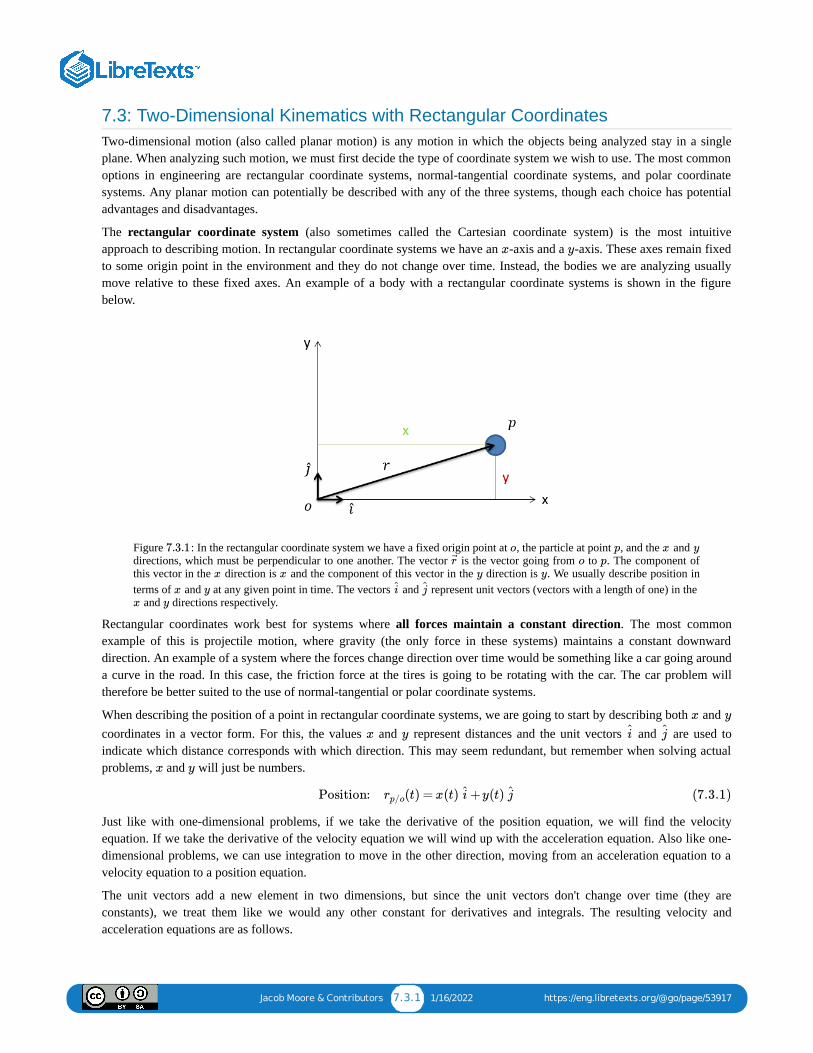
Jacob Moore & Contributors 7.3.1 1/16/2022 https://eng.libretexts.org/@go/page/53917

7.3: Two-Dimensional Kinematics with Rectangular CoordinatesTwo-dimensional motion (also called planar motion) is any motion in which the objects being analyzed stay in a singleplane. When analyzing such motion, we must first decide the type of coordinate system we wish to use. The most commonoptions in engineering are rectangular coordinate systems, normal-tangential coordinate systems, and polar coordinatesystems. Any planar motion can potentially be described with any of the three systems, though each choice has potentialadvantages and disadvantages.

The rectangular coordinate system (also sometimes called the Cartesian coordinate system) is the most intuitiveapproach to describing motion. In rectangular coordinate systems we have an -axis and a -axis. These axes remain fixedto some origin point in the environment and they do not change over time. Instead, the bodies we are analyzing usuallymove relative to these fixed axes. An example of a body with a rectangular coordinate systems is shown in the figurebelow.

Figure : In the rectangular coordinate system we have a fixed origin point at , the particle at point , and the and directions, which must be perpendicular to one another. The vector is the vector going from to . The component ofthis vector in the direction is and the component of this vector in the direction is . We usually describe position interms of and at any given point in time. The vectors and represent unit vectors (vectors with a length of one) in the

and directions respectively.

Rectangular coordinates work best for systems where all forces maintain a constant direction. The most commonexample of this is projectile motion, where gravity (the only force in these systems) maintains a constant downwarddirection. An example of a system where the forces change direction over time would be something like a car going arounda curve in the road. In this case, the friction force at the tires is going to be rotating with the car. The car problem willtherefore be better suited to the use of normal-tangential or polar coordinate systems.

When describing the position of a point in rectangular coordinate systems, we are going to start by describing both and coordinates in a vector form. For this, the values and represent distances and the unit vectors and are used toindicate which distance corresponds with which direction. This may seem redundant, but remember when solving actualproblems, and will just be numbers.

Just like with one-dimensional problems, if we take the derivative of the position equation, we will find the velocityequation. If we take the derivative of the velocity equation we will wind up with the acceleration equation. Also like one-dimensional problems, we can use integration to move in the other direction, moving from an acceleration equation to avelocity equation to a position equation.

The unit vectors add a new element in two dimensions, but since the unit vectors don't change over time (they areconstants), we treat them like we would any other constant for derivatives and integrals. The resulting velocity andacceleration equations are as follows.

x y

7.3.1 o p x y

r   o p

x x y y

x y i j

x y

x y

x y i j

x y

Position: (t) = x(t)  +y(t) rp/o i j (7.3.1)

Jacob Moore & Contributors 7.3.2 1/16/2022 https://eng.libretexts.org/@go/page/53917

The above equations are vector equations with velocities and accelerations broken down into and components. Sincethe and directions are perpendicular, they are also independent (movement in the direction doesn't impact movementin the direction, and vice versa). This essentially means we can split our vector equation into a set of two scalarequations. To do this we just put everything in front of the unit vectors in the equations and everything in front of the unit vectors in the equations.

Once we have everything split into - and -direction equations, we can just use the same processes we used for onedimensional motion to move from to to , and from to to . The variable linking the two equations is time .

Video lecture covering this section, delivered by Dr. Jacob Moore. YouTube source: https://youtu.be/qKqUNuSPWT4.

A motorcycle drives off a one-meter-tall ramp at an angle of 30 degrees as shown below. Determine the equations forthe acceleration, velocity, and position over time. How far does the motorcycle travel in the direction before hittingthe ground?

Figure : problem diagram for Example . A motorcycle drives off the edge of a ramp with an initial velocityof 22 m/s at 30° above the -axis.

Solution

Velocity:

Acceleration:

v(t) = (t)  + (t) x i y j

a(t) = (t)  + (t) x i y j

(7.3.2)

(7.3.3)

x y

x y x

y

i x j

y

Position:

Velocity:

Acceleration:

x(t) = … y(t) = …

(t) = … (t) = …x y

(t) = … (t) = …x y

(7.3.4)

(7.3.5)

(7.3.6)

x y

x x x y y y (t)

7.3 Two Dimensional Motion with Re7.3 Two Dimensional Motion with Re……

Example 7.3.1

x

7.3.2 7.3.1x

Jacob Moore & Contributors 7.3.3 1/16/2022 https://eng.libretexts.org/@go/page/53917

Video : Worked solution to example problem , provided by Dr. Majid Chatsaz. YouTube source:https://youtu.be/ujM4LIQlG1Q.

A basketball is thrown towards a hoop that is three feet higher in the direction and 25 feet away in the direction. Ifthe ball is thrown at an initial angle of 50 degrees, what must the initial velocity be for the ball to make it into thehoop?

Figure : problem diagram for Example . A ball is thrown at some initial velocity, at an angle of 50° abovethe horizontal.

Solution

WP7.3.1-MRCWP7.3.1-MRC

7.3.2 7.3.1

Example 7.3.2

y x

7.3.3 7.3.2

Jacob Moore & Contributors 7.3.4 1/16/2022 https://eng.libretexts.org/@go/page/53917

Video : Worked solution to example problem , provided by Dr. Majid Chatsaz. YouTube source:https://youtu.be/IGBB1YXRNr0.

WP7.3.2-MRCWP7.3.2-MRC

7.3.3 7.3.2

Jacob Moore & Contributors 7.4.1 1/16/2022 https://eng.libretexts.org/@go/page/53918

7.4: Two-Dimensional Kinematics with Normal-Tangential CoordinatesTwo-dimensional motion (also called planar motion) is any motion in which the objects being analyzed stay in a singleplane. When analyzing such motion, we must first decide the type of coordinate system we wish to use. The most commonoptions in engineering are rectangular coordinate systems, normal-tangential coordinate systems, and polar coordinatesystems. Any planar motion can potentially be described with any of the three systems, though each choice has potentialadvantages and disadvantages.

The normal-tangential coordinate system centers on the body in motion. The origin point will be the body itself,meaning that the position of the particle in the normal-tangential coordinate system is always "zero". The tangentialdirection ( -direction) is defined as the direction of travel at that moment in time (the direction of the current velocityvector), with the normal direction ( -direction) being 90 degrees counterclockwise from the -direction. The diagrambelow shows a particle following a curved path with the current normal and tangential directions.

Figure : In the normal-tangential coordinate system, the particle itself serves as the origin point. The -direction is thecurrent direction of travel and the -direction is always 90° counterclockwise from the -direction. The and vectorsrepresent unit vectors in the and directions respectively.

Normal-tangential coordinate systems work best when we are observing motion from the perspective of the body inmotion, such as being a passenger in a car or plane. In such cases, we would define ourself as the origin point and"forward" would be the tangential direction. An important distinction between the rectangular coordinate system and thenormal-tangential coordinate system is that the axes are not fixed in the normal-tangential coordinate system. If we goback to the car example, the "forward" or tangential direction will turn with the car, but the "east" direction or the -direction will remain constant no matter which way the car is pointed.

The way the coordinate system is defined, the position of the particle is always set to be at the origin point. The velocity isalso always set to be in the tangential direction, and thus there is no velocity in the -direction. The variable is the body'scurrent speed.

To find the acceleration, we need to take the derivative of the velocity function. This may seem simple, but there is a newthing to consider in that the unit vector is not constant. This means a change in speed can cause an acceleration, and achange in direction (which would change the direction) can also cause an acceleration. Going back to our car example,this makes some intuitive sense. We can feel accelerations, and we would be able to feel acceleration if we suddenlystepped on the gas and increased our speed, but we would also be able to feel the acceleration if we took a tight turn at aconstant speed.

Going back to the derivative, we will use the product rule, taking the derivative of one piece at a time.

is the rate of change of speed of the body, which is called the tangential acceleration. Going back to our car analogy, thisis the acceleration we would experience from pressing the gas or brake pedals.

t

n t

7.4.1 tn t ut un

t n

x

n v

Position:

Velocity:

(t) = 0  +0 rp/o ut un

v(t) = v ut

(7.4.1)

(7.4.2)

utut

Acceleration: a(t) = +vvut ut (7.4.3)

v

Jacob Moore & Contributors 7.4.2 1/16/2022 https://eng.libretexts.org/@go/page/53918

The other piece of our derivative is the speed times the derivative of a unit vector, which we will need to analyze further.When thinking about the derivative of a rotating unit vector, we think about rotating the coordinate system by a smallamount .

Figure : The derivative of a rotating unit vector can be thought of as the change in position of the head of that vectoras it rotates about a small angle .

The derivative of the vector is then the change in position of the head of the vector. Using some geometry, we can seethat the distance the head of the vector moves is the length of the vector (which is always 1 for a unit vector) times theangle of rotation in radians. The direction the head of the vector travels is roughly the direction. In fact, as approaches zero, it becomes exactly the direction. Putting this back into our derivative, we wind up with the followingequation for acceleration.

Before we arrive at our final set of equations, we have one last potential substitution. If a particle is moving along a curvedpath, the rate at which it is turning will be equal to the velocity of the particle divided by the radius of the path at thatpoint ( divided by rho, ). Putting this last substitution in, we have our final set of equations with two equivalent optionsfor calculating the accelerations.

When using these equations, it is important to remember that they are acceleration equations. If we want to know theoverall acceleration we would need to add the two acceleration components as vectors. Also, if we are given anacceleration that is not in the normal or tangential direction, we will first need to break that acceleration vector down intonormal and tangential components before using the above equations. Finally, if we want the velocity or acceleration indirections other than the normal and tangential directions, we will need to use a coordinate transformation.

Video lecture covering this section, delivered by Dr. Jacob Moore. YouTube source: https://youtu.be/TIjJLcmtaq8.

dθ

7.4.2dθ

ut

ut un dθ

un

a(t) = +v = +vvut ut vut θ un (7.4.4)

( )θ

v ρ

a(t) = +v = +vut θ un vutv2

ρun (7.4.5)

7.4 Two Dimensional Motion with No7.4 Two Dimensional Motion with No……

Jacob Moore & Contributors 7.4.3 1/16/2022 https://eng.libretexts.org/@go/page/53918

A commercial jetliner is traveling at a constant 250 m/s when it executes an emergency 180-degree turn. If the turntakes 20 seconds, what is the acceleration experienced by the passengers? What is the radius of the curve taken by theplane?

Solution

Video : Worked solution to example problem , provided by Dr. Majid Chatsaz. YouTube source:https://youtu.be/1cQ-LQC8Ahg.

Assuming a cloverleaf interchange has a radius of curvature of 80 meters at the tightest part of the turn, what is thefastest a car could travel around this curve without experiencing more than half a in acceleration? Assume the car istraveling at a constant speed. If the car was instead increasing speed at a rate of 2 m/s , what would be the new overallmagnitude of the acceleration experienced by the passengers?

Figure : A cloverleaf interchange on a highway.

Solution

Example 7.4.1

WP7.4.1-MRCWP7.4.1-MRC

7.4.2 7.4.1

Example 7.4.2

g2

7.4.3

Jacob Moore & Contributors 7.4.4 1/16/2022 https://eng.libretexts.org/@go/page/53918

Video : Worked solution to example problem , provided by Dr. Majid Chatsaz. YouTube source:https://youtu.be/_Df_HZU0yHk.

WP7.4.2-MRCWP7.4.2-MRC

7.4.3 7.4.2

Jacob Moore & Contributors 7.5.1 1/16/2022 https://eng.libretexts.org/@go/page/53926

7.5: Two-Dimensional Motion with Polar CoordinatesTwo-dimensional motion (also called planar motion) is any motion in which the objects being analyzed stay in a singleplane. When analyzing such motion, we must first decide the type of coordinate system we wish to use. The most commonoptions in engineering are rectangular coordinate systems, normal-tangential coordinate systems, and polar coordinatesystems. Any planar motion can potentially be described with any of the three systems, though each choice has potentialadvantages and disadvantages.

The polar coordinate system uses a distance and an angle to locate a particle in space. The origin point will be afixed point in space, but the -axis of the coordinate system will rotate so that it is always pointed towards the body in thesystem. The variable is also used to indicate the distance from the origin point to the particle. The theta-axis will then be90 degrees counterclockwise from the -axis with the variable being used to show the angle between the -axis and somefixed axis that does not rotate. The diagram below shows a particle with a polar coordinate system.

Figure : In the polar coordinate system, the direction always points from the origin point to the body. The variable is also used to indicate the distance between the two points. The theta direction will always be 90° counterclockwise fromthe direction. Theta is also used to indicate the angle between the direction and some fixed axis used for reference. The

and vectors represent unit vectors in the and directions, respectively.

Polar coordinate systems work best in systems where a body is being tracked via a distance and an angle, such as a radarsystem tracking a plane. In cases such as this, the raw data from this in the form of an angle and a distance would be directmeasures of and respectively. Polar coordinate systems will also serve as the base for extended body motion, wheremotors and actuators can directly control things like and .

The way the coordinate system is defined, the -axis will always point from the origin point to the body. The distance fromthe origin to the point is defined as with no component of the position being in the direction.

To find the velocity, we need to take the derivative of the position function over time. Since the distance can change overtime as well as the direction changing over time to track the body, we need to worry about the derivative of as well asthe derivative of the unit vector. Like we did with the normal-tangential systems, we will use the product rule and thensubstitute in a value for the derivative of the unit vector.

To find the acceleration, we need to take the derivative of the velocity function. As all of these terms, including the unitvectors, change over time, we will need to use the product rule extensively. The term will split into two terms, and the

term will split into three terms.

Again we will need to substitute in values for the derivatives of the unit vectors similar to before, but it is worthmentioning that the derivative of the vector as it rotates counterclockwise is in the negative direction.

(r) (θ)

r

r

r θ r

7.5.1 r r

r rur uθ r θ

θ r

r θ

r

r θ

Position: (t) = r +0 rp/o ur uθ (7.5.1)

r

ur r

Velocity: v(t) = +r = +rrur ur r ur θ uθ (7.5.2)

ur

uθ

Acceleration: a(t) = + + +r +rrur r ur r θ uθ θ uθ θ uθ (7.5.3)

uθ ur

Jacob Moore & Contributors 7.5.2 1/16/2022 https://eng.libretexts.org/@go/page/53926

Figure : The derivatives of the and unit vectors. Notice that the derivative of the vector is in the negative direction.

After substituting in the derivatives of the unit vectors and simplifying the function, we arrive at our final equation for theacceleration.

Though this final equation has a number of terms, it is still just two components in vector form. Just as with the normal-tangential coordinate system, we will need to remember that we will need to split the single vector equation into twoseparate scalar equations. In this case we will have the equation for the terms in the direction and the equation for theterms in the direction.

Video lecture covering this section, delivered by Dr. Jacob Moore. YouTube source: https://youtu.be/F4i0Kz660aE.

A radar tracking station gives the following raw data to a user at a given point in time. Based on this data, what is thecurrent velocity and acceleration in the and directions? What is the current velocity and acceleration in the and directions?

7.5.2 ur uθ uθ ur

Acceleration: a(t) = + + +r −rrur r θ uθ r θ uθ θ uθ θ2ur

= ( −r ) +(2 +r )r θ2

ur r θ θ uθ

(7.5.4)

(7.5.5)

r

θ

7.5 Two Dimensional Motion with Po7.5 Two Dimensional Motion with Po……

Example 7.5.1

r θ x y

Jacob Moore & Contributors 7.5.3 1/16/2022 https://eng.libretexts.org/@go/page/53926

Figure : Problem diagram for Example . The instantaneous polar-coordinate position values of an airplaneare given as tracked by a radar station, as well as the first and second derivatives of these quantities.

Solution

Video : Worked solution to example problem , provided by Dr. Majid Chatsaz. YouTube source:https://youtu.be/HP4WiIa3Nc0.

A spotlight is tracking an actor as he moves across the stage. If the actor is moving with a constant velocity as shownbelow, what values do we need for the spotlight angular velocity and spotlight angular acceleration so that thespotlight remains fixed on the actor?

7.5.3 7.5.1

WP7.5.1-MRCWP7.5.1-MRC

7.5.2 7.5.1

Example 7.5.2

( )θ ( )θ

Jacob Moore & Contributors 7.5.4 1/16/2022 https://eng.libretexts.org/@go/page/53926

Figure : problem diagram for Example . A spotlight rotates to follow an actor moving across stage at aknown velocity and starting from a known position in relation to the spotlight.

Solution

Video : Worked solution to example problem , provided by Dr. Majid Chatsaz. YouTube source:https://youtu.be/jyD1seNQI14.

7.5.4 7.5.2

WP7.5.2-MRCWP7.5.2-MRC

7.5.3 7.5.2

Jacob Moore & Contributors 7.6.1 1/16/2022 https://eng.libretexts.org/@go/page/53932

7.6: Dependent Motion SystemsDependent motion analysis is used when two or more particles have motions that are in some way connected to oneanother. The way in which the motion of these particles is connected is known as the constraint. A simple example of aconstrained system is shown in the figure below. Imagine that someone's pickup truck gets stuck in the sand, and a frienduses a rope to help pull it out. This friend ties one end of the rope to the rear bumper of her car, loops the rope around a baron the front of the pickup truck, then ties the other end to a stationary tree. In this case the two vehicles will not have thesame velocity or acceleration, but their motions are related because they are tied together by the rope. In this case, the ropeis acting as the constraint, allowing us to know the velocity or acceleration of one vehicle based on the velocity oracceleration of the other vehicle.

Figure : This represents a constrained system. The motion of the car and the pickup truck will be related to oneanother via rope that is connecting them.

The first thing we will need to do when analyzing these systems is to come up with what is known as the constraintequation. A constraint equation will be some geometric relationship that will remain true over the course of the motion. Inthe above example, imagine the rope is 50 feet long. Using the tree as a stationary point, we can also say that the length ofthe rope is the distance from the green car to the tree, plus two times the distance from the pickup truck to the tree (since itmust go out to the pickup truck and then back). If we put this into an equation (the constraint equation) we would have thefollowing.

Once we have a constraint equation that works for positions, we can take the derivative of this equation to find anotherconstraint equation that relates velocities. In this case, the length of the rope is constant, and therefore the derivative of thelength will be zero. If we take the derivative of the constraint equation again, we wind up with a third constraint equationthat relates accelerations.

In these equations, it is important to remember that the values represent the changes in length, rather than direct measuresof velocities. Though both vehicles would have positive velocities in the example above (velocities to the right), one value will be positive and one will be negative. This is because the truck is getting closer to the tree while the car is gettingfurther away. A similar situation will occur for the accelerations, where both vehicles would have positive accelerationseven if the values are a mix of positive and negative values.

7.6.1

Constraint Equation: Positions L = 50 ft = 2 +LA LB (7.6.1)

Constraint Equation: Velocities

Constraint Equation: Accelerations

= 0 = 2 +L LA LB

= 0 = 2 +L LA LB

(7.6.2)

(7.6.3)

L

L

Jacob Moore & Contributors 7.6.2 1/16/2022 https://eng.libretexts.org/@go/page/53932

Video lecture covering this section, delivered by Dr. Jacob Moore. YouTube source: https://youtu.be/J1aPSrdDzdk.

A truck becomes stuck in the sand at a local beach. To help, a friend takes a rope 50 feet in length, ties one end to hercar, loops the rope around a bar at the front of the truck, and then ties the other end to a stationary tree as shown below.If the car accelerates at a rate of 0.2 ft/s², what will the velocity of the truck be by the time it gets to the tree?

Figure : problem diagram for Example . A rope looped around the front of a truck, tied at one end to a treetrunk and at the other to a car's rear bumper, allows the car to pull the truck free of the sand it is stuck in.

Solution

Video : Worked solution to example problem , provided by Dr. Majid Chatsaz. YouTube source:https://youtu.be/IxO_Nrs7Kj0.

7.6 Dependent Motion - Video Lectur7.6 Dependent Motion - Video Lectur……

Example 7.6.1

7.6.2 7.6.1

WP7.6.1-MRCWP7.6.1-MRC

7.6.2 7.6.1

Jacob Moore & Contributors 7.6.3 1/16/2022 https://eng.libretexts.org/@go/page/53932

A man has hooked up a pulley, a rope, and a platform as shown below to lift loads up onto a nearby rooftop. If iscurrently 15 meters, is currently 5 meters, and the man is walking away from the building at a rate of 0.5 meters persecond, what is the current velocity of the platform?

Figure : problem diagram for Example . A man walks away from a 20-meter-high building, holding one endof a rope that passes over a pulley on the rooftop and raises a load on its other end.

Solution

Video : Worked solution to example problem , provided by Dr. Majid Chatsaz. YouTube source:https://youtu.be/z3D_2jHLCik.

Example 7.6.2

x

y

7.6.3 7.6.2

WP7.6.2-MRCWP7.6.2-MRC

7.6.3 7.6.2

Jacob Moore & Contributors 7.7.1 1/16/2022 https://eng.libretexts.org/@go/page/53933

7.7: Relative Motion SystemsRelative motion analysis is the analysis of bodies where more than one body is in motion and we are in some wayexamining the motion of one moving particle relative to another moving particle. An example would be cars on a highway.If you are in one of many cars moving down one side of the highway, you and the other cars will all have velocities in asingle direction. From your perspective inside the car, though, fast cars in front of you will appear to be moving away fromyou and slow cars in front of you will appear to be moving towards you. By knowing your speed, and by observing howfast the cars are moving away from you or towards you, you could determine or at least estimate how fast these cars aregoing. The process of using your speed in conjunction with the relative velocities of the other cars to find the other cars'speed is relative motion analysis.

Relative Motion in One Dimension:In a single dimension, we will usually have at least two moving particles as well as some fixed reference point. We usuallycall the fixed reference point , and then label the other points , , and so on. In the diagram, below we can see anexample of this, with a fixed reference point at , a police car at , and a speeding car at .

Figure : In a single dimension we have a fixed reference point , as well as at least two moving bodies (labeled as and in this case). The vectors represent the distances between bodies, with the subscript indicating the point we areobserving and the point we are observing from. The subscripts should always have the following format: point beingobserved / point we are observing from.

As we can see from the diagram above, the sum of the distance from to and the distance from to will be equal to the distance from to . This gives us our position equation below.

One thing we should notice about the subscripts is that if we keep to our standard naming convention (point beingobserved / point we are observing from) then we should be able to see which points cancel out and which remain. In thiscase, the 's on the top and bottom on the right cancel out, leaving just a on the top and an on the bottom. Thismatches the subscript on the left of the equation.

Furthermore, we can take the derivative of this equation to relate velocities, or a double derivative to relate accelerations.This means that if we know any two of the terms in the equations below, we can solve for the third.

Relative Motion in Two Dimension:Just as with one dimension, we can start by examining a set of relative positions. In this case we will use the example oftwo planes moving through the sky. We may wish to deduce the position of plane B on a map, based on our observationsfrom plane A. By using the information we have on our position relative to some set location, along with the relativeposition read in from on board instrumentation, we should be able to determine the absolute position (including an and coordinate) for plane B.

O A B

O A B

7.7.1 O AB r

O A ( )rA/O A B ( )rB/A

O B ( )rB/O

Position: = +rB/O rA/O rB/A (7.7.1)

A B O

Velocity:

Acceleration:

= +vB/O vA/O vB/A

= +aB/O aA/O aB/A

(7.7.2)

(7.7.3)

x y

Jacob Moore & Contributors 7.7.2 1/16/2022 https://eng.libretexts.org/@go/page/53933

Figure : In two dimensions we have a fixed reference point , as well as at least two moving bodies (labeled as and in this case). The vectors represent the distance vectors between bodies, with the subscript indicating the startingand ending point. The subscripts should always be formatted end point / starting point.

In two dimensions, we will use the same equations as before, except this time we will be using vectors rather than scalarvalues in our equations.

To solve these equations, we will almost always break the vector equations down into a set of component equations. Thiswill let us solve these equations with simple algebra. Because we have more than one particle, we usually use rectangularcoordinate systems for this with a universal set of and coordinates.

Video lecture covering this section, delivered by Dr. Jacob Moore. YouTube source: https://youtu.be/A5aJ2VYvwkw.

A police officer notices a car speeding by. If the police car is traveling 30 m/s and the radar gun measures the relativevelocity to be 15 m/s, how fast is the speeding car actually going? If the police car immediately begins accelerating ata constant rate and catches up to the speeding car after 15 seconds, what is the rate of acceleration of the police car?

Figure : problem diagram for Example . A police car and a speeding car it is chasing after travel in the samedirection on a straight road.

Solution

7.7.2 O AB r  

Position:

Velocity:

Acceleration:

= +r  B/O r  A/O r  B/A

= +v  B/O v  A/O v  B/A

= +a B/O a A/O a B/A

(7.7.4)

(7.7.5)

(7.7.6)

x y

7.7 Relative Motion Particle - Video L7.7 Relative Motion Particle - Video L……

Example 7.7.1

7.7.3 7.7.1

Jacob Moore & Contributors 7.7.3 1/16/2022 https://eng.libretexts.org/@go/page/53933

Video : Worked solution to example problem , provided by Dr. Majid Chatsaz. YouTube source:https://youtu.be/YndovN5yWfc.

A plane has an airspeed of 250 kilometers per hour (airspeed is the velocity of the plane relative to the air) and isflying though an easterly crosswind with a speed of 20 kilometers per hour. If the plane wants to maintain a directnortherly course, what is the angle the plane must point into the wind ?

Figure : problem diagram for Example . A plane aiming to fly directly northwards experiences easterlycrosswinds.

Solution

WP7.7.1-MRCWP7.7.1-MRC

7.7.2 7.7.1

Example 7.7.2

(θ)

7.7.4 7.7.2

Jacob Moore & Contributors 7.7.4 1/16/2022 https://eng.libretexts.org/@go/page/53933

Video : Worked solution to example problem , provided by Dr. Majid Chatsaz. YouTube source:https://youtu.be/ga1qcV38zYA.

You are in a boat that is traveling through the water in an area of swift currents. One instrument measures your speedwith respect to the water to be 20 ft/s with your boat pointed at a 45-degree angle. GPS, however, measures yourabsolute speed and direction to be 25 ft/s at a 55-degree angle. Based on this information, what is the speed anddirection of the water current in this area?

Figure : problem diagram for Example . Instruments on a boat return different readings for its absolutevelocity vs. its velocity relative to the surrounding water.

Solution

WP7.7.2-MRCWP7.7.2-MRC

7.7.3 7.7.2

Example 7.7.3

7.7.5 7.7.3

Jacob Moore & Contributors 7.7.5 1/16/2022 https://eng.libretexts.org/@go/page/53933

Video : Worked solution to example problem , provided by Dr. Majid Chatsaz. YouTube source:https://youtu.be/j8vnM_hrnQg.

WP7.7.3-MRCWP7.7.3-MRC

7.7.4 7.7.3

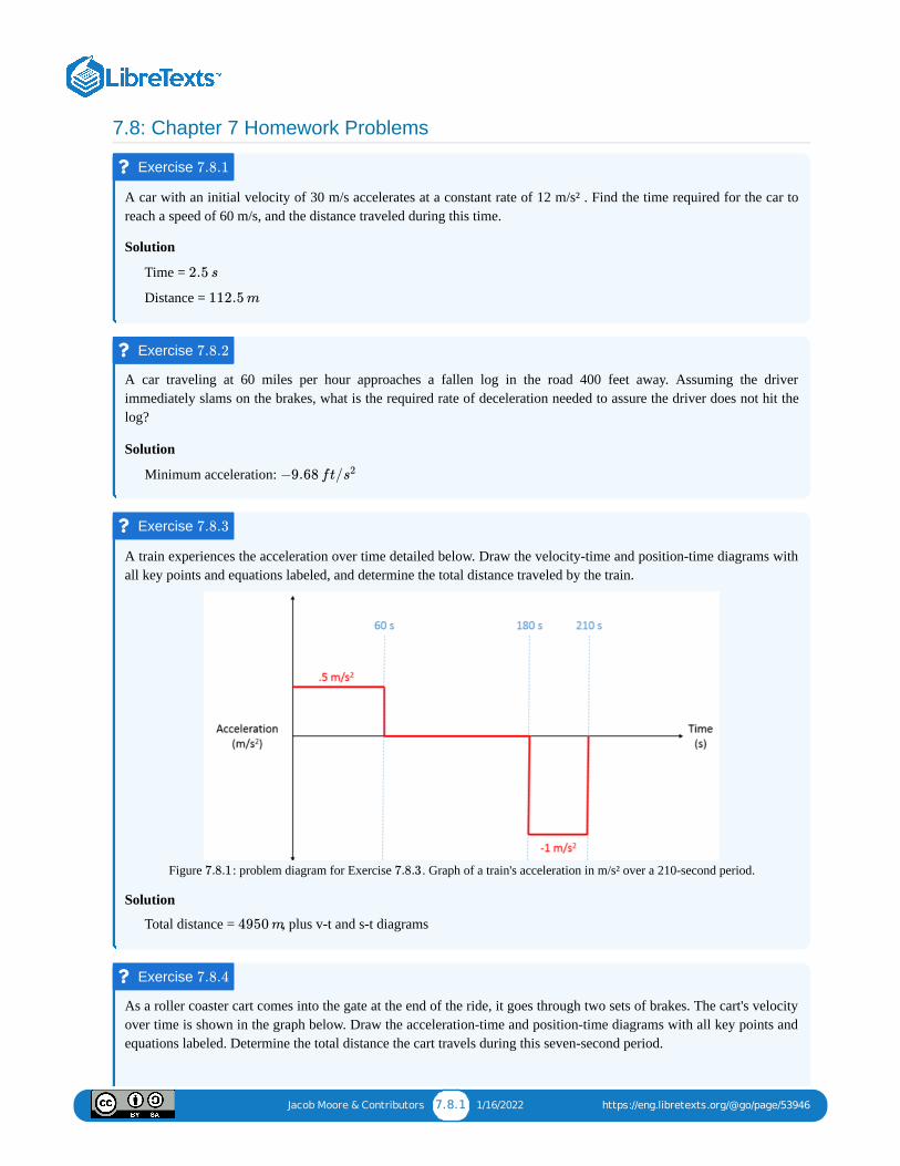
Jacob Moore & Contributors 7.8.1 1/16/2022 https://eng.libretexts.org/@go/page/53946

7.8: Chapter 7 Homework Problems

A car with an initial velocity of 30 m/s accelerates at a constant rate of 12 m/s² . Find the time required for the car toreach a speed of 60 m/s, and the distance traveled during this time.

Solution

Time =

Distance =

A car traveling at 60 miles per hour approaches a fallen log in the road 400 feet away. Assuming the driverimmediately slams on the brakes, what is the required rate of deceleration needed to assure the driver does not hit thelog?

Solution

Minimum acceleration:

A train experiences the acceleration over time detailed below. Draw the velocity-time and position-time diagrams withall key points and equations labeled, and determine the total distance traveled by the train.

Figure : problem diagram for Exercise . Graph of a train's acceleration in m/s² over a 210-second period.

Solution

Total distance = , plus v-t and s-t diagrams

As a roller coaster cart comes into the gate at the end of the ride, it goes through two sets of brakes. The cart's velocityover time is shown in the graph below. Draw the acceleration-time and position-time diagrams with all key points andequations labeled. Determine the total distance the cart travels during this seven-second period.

Exercise 7.8.1

2.5 s

112.5 m

Exercise 7.8.2

−9.68 ft/s2

Exercise 7.8.3

7.8.1 7.8.3

4950 m

Exercise 7.8.4

Jacob Moore & Contributors 7.8.2 1/16/2022 https://eng.libretexts.org/@go/page/53946

Figure : problem diagram for Exercise . Graph of a roller coaster cart's velocity in ft/s over a 7-secondperiod.

Solution

Total distance = , plus a-t and s-t diagrams.

A tank fires a round at a 30-degree angle with a muzzle velocity of 600 m/s. The round is expected to hit amountainside one kilometer away. The mountainside also has an average angle of 30 degrees. How far up themountainside will the round be expected to travel before hitting the ground if we ignore air resistance?

Figure : problem diagram for Exercise . A tank fires a round at an angle, aiming towards a mountainside 1kilometer away.

Solution

A plane with a current speed of 600 ft/s is increasing in speed while also making a turn. The acceleration is measuredat 40 ft/s² at an angle 35° from its current heading. Based on this information, determine the rate at which the plane isincreasing its speed (tangential acceleration) and the radius of the turn for the plane.

7.8.2 7.8.4

25.5 ft

Exercise 7.8.5

(d)

7.8.3 7.8.5

d = 5.37 km

Exercise 7.8.6

Jacob Moore & Contributors 7.8.3 1/16/2022 https://eng.libretexts.org/@go/page/53946

Figure : problem diagram for Exercise . A plane depicted in a normal-tangential coordinate systemundergoes an acceleration that changes both its speed and its direction.

Solution

A radar station is tracking a rocket with a speed of 400 m/s and an acceleration of 3 m/s² in the direction shown below.The rocket is 3.6 km away ( = 3600 m) at an angle of 25°. What would you expect , , , and to be?

Figure : problem diagram for Exercise . A radar station tracks the instantaneous velocity and acceleration ofa rocket located a known distance and angle away.

Solution

The pulley system below is being used to lift a heavy load. Assuming the end of the cable is being pulled at a velocityof 2 ft/s, what is the expected upwards velocity of the load?

7.8.4 7.8.6

= 32.77 ft/at s2

r = 15, 690 ft

Exercise 7.8.7

r r r θ θ

7.8.5 7.8.7

= 282.8 m/s, = 24.34 m/r r s2

= 0.0786 rad/s, −0.01176 rad/θ θ s2

Exercise 7.8.8

Jacob Moore & Contributors 7.8.4 1/16/2022 https://eng.libretexts.org/@go/page/53946

Figure : problem diagram for Exercise . A rope's right end is fastened to the ceiling, and it runs alternatelythrough two pulleys mounted on a load and two pulleys mounted on the ceiling. The left end of the rope is pulleddown to raise the load.

Solution

A cable is anchored at A, goes around a pulley on a movable collar at B, and finally goes around a pulley at C asshown below. If the end of the rope is pulled with a velocity of 0.5 m/s, what is the expected velocity of the collar atthis instant?

Figure : problem diagram for Exercise . A rope attached to the ceiling at one end runs through a pulleymounted on a sliding collar mounted on a post extending from the ceiling, and then through a pulley mounted on theceiling. The free rope's free end is pulled downward, moving the collar.

Solution

You are driving at a velocity of 90 ft/s in the rain while you notice that the rain is hitting your car at an angle 35° fromthe vertical, from your perspective. Assuming the rain is actually coming straight down (when observed by a stationaryperson), what is the velocity of the rain with respect to the ground?

7.8.6 7.8.8

= 0.5 ft/svL

Exercise 7.8.9

7.8.7 7.8.9

= 0.3 m/svB

Exercise 7.8.10

Jacob Moore & Contributors 7.8.5 1/16/2022 https://eng.libretexts.org/@go/page/53946

Figure : problem diagram for Exercise . Illustration of the rain's motion as seen from the perspective of aperson in the car.

Solution

7.8.8 7.8.10

= 128.5 ft/svr

1 1/30/2022

CHAPTER OVERVIEW8: NEWTON'S SECOND LAW FOR PARTICLESUsing Newton's Second Law to describe forces and their effect on the motion of particles, in one and two dimensions (using rectangular,polar, and normal-tangential coordinate systems).

8.0: VIDEO INTRODUCTION TO CHAPTER 8Video introduction to the topics to be covered in this chapter: Newton's Second Law in one and two dimensions (as described withCartesian, polar, and normal-tangential coordinate systems).

8.1: ONE-DIMENSIONAL EQUATIONS OF MOTIONDetermining force in a one-dimensional system through Newton's Second Law. Includes worked examples.

8.2: EQUATIONS OF MOTION IN RECTANGULAR COORDINATESAnalyzing motion in two dimensions by splitting the vector form of Newton's Second Law into xxx and yyy components. Includesworked examples.

8.3: EQUATIONS OF MOTION IN NORMAL-TANGENTIAL COORDINATESAnalyzing motion in two dimensions by splitting the vector form of Newton's Second Law into normal and tangential components.Includes worked examples.

8.4: EQUATIONS OF MOTION IN POLAR COORDINATESAnalyzing motion in two dimensions by splitting the vector form of Newton's Second Law into polar components, rrr and θθ\theta.Includes worked examples.

8.5: CHAPTER 8 HOMEWORK PROBLEMS

Jacob Moore & Contributors 8.0.1 1/23/2022 https://eng.libretexts.org/@go/page/50601

8.0: Video Introduction to Chapter 8

Video introduction to the topics covered in this chapter, delivered by Dr. Jacob Moore. YouTube source:https://youtu.be/HLy8efQ45qQ.

8 Newton's Second Law Particles - Vi8 Newton's Second Law Particles - Vi……

Jacob Moore & Contributors 8.1.1 1/16/2022 https://eng.libretexts.org/@go/page/50602

8.1: One-Dimensional Equations of MotionKinetics is the branch of dynamics that deals with the relationship between motion and the forces that cause that motion.The basis for all of kinetics is Newton's Second Law, which relates forces and accelerations for a given body. In its basicform, Newton's Second Law states that the sum of the forces on a body will be equal to the mass of that body times therate of acceleration. For bodies in motion, we can write this relationship out as the equation of motion.

In cases where accelerations only exist in a single dimension, we can reduce the above vector equation into a single scalarequation. Calling that single direction the direction, we arrive at the single equation of motion shown below. By enteringknown forces or accelerations, we can use this equation to solve for a single unknown force or acceleration term.

Figure : This box being pushed along a frictionless surface can be examined as a one dimensional kinetics problem.Acceleration exists only in the direction, related by the equation of motion to the single unbalanced force in the direction. Because the forces in the direction are balanced, the acceleration in that direction will be zero.

Kinetics and the equation(s) of motion relate forces and accelerations, and are often used in conjunction with thekinematics equations, which relate positions, velocities and accelerations as discussed in the previous chapter. Dependingon the problem being examined, the kinematics equations may need to be examined either before or after the kineticsequations.

Video lecture covering this section, delivered by Dr. Jacob Moore. YouTube source: https://youtu.be/CEL2cpvdQmQ.

A block with a weight of 90 pounds sits on a frictionless surface and a 50-pound force is applied in the direction, asshown below.

∑ = m ∗F   a  (8.1.1)

x

8.1.1x x

y

∑ = m ∗ = m ∗Fx ax x (8.1.2)

8.1 One Dimensional Equations of M8.1 One Dimensional Equations of M……

Example 8.1.1

x

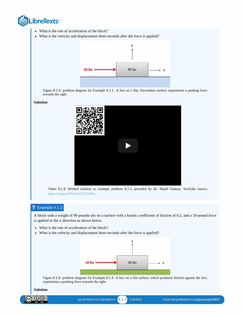
Jacob Moore & Contributors 8.1.2 1/16/2022 https://eng.libretexts.org/@go/page/50602

What is the rate of acceleration of the block?What is the velocity and displacement three seconds after the force is applied?

Figure : problem diagram for Example . A box on a flat, frictionless surface experiences a pushing forcetowards the right.

Solution

Video : Worked solution to example problem , provided by Dr. Majid Chatsaz. YouTube source:https://youtu.be/NwmVFrTGd0A.

A block with a weight of 90 pounds sits on a surface with a kinetic coefficient of friction of 0.2, and a 50-pound forceis applied in the direction as shown below.

What is the rate of acceleration of the block?What is the velocity and displacement three seconds after the force is applied?

Figure : problem diagram for Example . A box on a flat surface, which produces friction against the box,experiences a pushing force towards the right.

Solution

8.1.2 8.1.1

WP8.1.1-MRCWP8.1.1-MRC

8.1.2 8.1.1

Example 8.1.2

x

8.1.3 8.1.2

Jacob Moore & Contributors 8.1.3 1/16/2022 https://eng.libretexts.org/@go/page/50602

Video : Worked solution to example problem , provided by Dr. Majid Chatsaz. YouTube source:https://youtu.be/9BgdnzTUO9I.

A 2000-lb elevator decelerates downward, going from a speed of 25 ft/s to a stop in a distance of 50 ft.

What is the average rate of deceleration?What is the tension in the cable supporting the elevator during this period?

Figure : A descending glass-sided elevator.

Solution

WP8.1.2-MRCWP8.1.2-MRC

8.1.3 8.1.2

Example 8.1.3

8.1.4

Jacob Moore & Contributors 8.1.4 1/16/2022 https://eng.libretexts.org/@go/page/50602

Video : Worked solution to example problem , provided by Dr. Majid Chatsaz. YouTube source:https://youtu.be/I2j0peOLzro.

A rocket test sled is being used to test a solid rocket booster (mass = 1000 kg). It’s known that generally a solid rocketbooster’s force will fit the equation . If the rocket has an initial thrust of 10 kN, and achieves aspeed of 150 m/s and travels 700 meters during a 10-second test run, determine the constants , and for therocket.

Figure : A rocket sled holding a solid booster, moving rightwards on a straight track.

Solution

Video : Worked solution to example problem , provided by Dr. Majid Chatsaz. YouTube source:https://youtu.be/tmUOZXuAzNE.

WP8.1.3-MRCWP8.1.3-MRC

8.1.4 8.1.3

Example 8.1.4

F = A +Bt– Ct2

A B C

8.1.5

WP8.1.4-MRCWP8.1.4-MRC

8.1.5 8.1.4

Jacob Moore & Contributors 8.2.1 1/16/2022 https://eng.libretexts.org/@go/page/50603

8.2: Equations of Motion in Rectangular CoordinatesTo start our discussion of kinetics in two dimensions, we will examine Newton's Second Law as applied to a fixedcoordinate system. In its basic form, Newton's Second Law states that the sum of the forces on a body will be equal to themass of that body times its rate of acceleration. For bodies in motion, we can write this relationship out as the equation ofmotion.

With rectangular coordinates in two dimensions, we will break this single vector equation into two separate scalarequations. To solve the equations, we simply break any given forces and accelerations down into and componentsusing sines and cosines and plug those known values in. With two equations, we should be able to solve for up to twounknown force or acceleration terms.

Just as with a single dimension, the equations of motion are often used in conjunction with the kinematics equations thatrelate positions, velocities and accelerations as discussed in the previous chapter. Depending on the problem beingexamined, the kinematics equations may need to be examined either before or after the kinetics equations.

Rectangular coordinates can be used in any kinetics problem; however, they work best with problems where the forces donot change direction over time. Projectile motion is a good example of this, because the gravity force will maintain aconstant direction, as opposed to the thrust force on a turning plane, where the thrust force changes direction with theplane.

Video lecture covering this section, delivered by Dr. Jacob Moore. YouTube source: https://youtu.be/2D15kYAYUYg.

You are controlling a satellite with a mass of 300 kg. The main and lateral thrusters can exert the forces shown. Howlong do you need to run each of the thrusters to achieve the final velocity as shown in the diagram? Assume thesatellite has zero initial velocity.

∑ = m ∗F   a  (8.2.1)

x y

∑Fx

∑Fy

= m ∗ = m ∗ax x

= m ∗ = m ∗ay y

(8.2.2)

(8.2.3)

8.2 The Equations of Motion in Recta8.2 The Equations of Motion in Recta……

Example 8.2.1

Jacob Moore & Contributors 8.2.2 1/16/2022 https://eng.libretexts.org/@go/page/50603

Figure : problem diagram for Example . A satellite facing the right experiences a rightwards force form itsmain thrusters and an upwards force from its lateral thrusters, changing both its speed and direction.

Solution

Video : Worked solution to example problem , provided by Dr. Majid Chatsaz. YouTube source:https://youtu.be/YawjRTV89Lo.

A man in a flatbed truck that starts at rest moves up a hill at an angle of 10 degrees. If he is carrying a 600-kg crate inthe back and the static coefficient of friction is 0.3, what is the maximum rate of acceleration before the crate slides offof the back of the truck? How long will it take the truck to reach a speed of 25 m/s?

Figure : problem diagram for Example . A truck with a 600-kg load on its bed begins to move up a 10°incline.

8.2.1 8.2.1

WP8.2.1WP8.2.1

8.2.2 8.2.1

Example 8.2.2

8.2.2 8.2.2

Jacob Moore & Contributors 8.2.3 1/16/2022 https://eng.libretexts.org/@go/page/50603

Solution

Video : Worked solution to example problem , provided by Dr. Majid Chatsaz. YouTube source:https://youtu.be/A4ZnX9vWfMA.

WP8.2.2-MRCWP8.2.2-MRC

8.2.3 8.2.2

Jacob Moore & Contributors 8.3.1 1/16/2022 https://eng.libretexts.org/@go/page/53984

8.3: Equations of Motion in Normal-Tangential CoordinatesContinuing our discussion of kinetics in two dimensions, we can examine Newton's Second Law as applied to the normal-tangential coordinate system. In its basic form, Newton's Second Law states that the sum of the forces on a body will beequal to the mass of that body times the rate of acceleration. For bodies in motion, we can write this relationship out as theequation of motion.

Just as we did with with rectangular coordinates, we will break this single vector equation into two separate scalarequations. This involves identifying the normal and tangential directions and then using sines and cosines to break thegiven forces and accelerations down into components in those directions.

Figure : When working in the normal-tangential coordinate system, any given forces or accelerations can be brokendown using sines and cosines as long as the angle of the force or acceleration is known relative to the normal andtangential directions.

Just as with rectangular coordinates, these equations of motion are often used in conjunction with the kinematics equations,which relate positions, velocities and accelerations as discussed in the previous chapter. In particular, we will oftensubstitute the known values below for the normal and tangential components for acceleration.

Normal-tangential coordinates can be used in any kinetics problem; however, they work best with problems where forcesmaintain a consistent direction relative to some body in motion. Vehicles in motion are a good example of this: thedirection of the forces applied are largely dependent on the current direction of the vehicle, and these forces will rotatewith the vehicle as it turns.

∑ = m ∗F   a 

8.3.1

∑Fn

∑Ft

= m ∗ an

= m ∗ at

(8.3.1)

(8.3.2)

= v∗ =an θv2

ρ(8.3.3)

=at v (8.3.4)

Jacob Moore & Contributors 8.3.2 1/16/2022 https://eng.libretexts.org/@go/page/53984

Video lecture covering this section, delivered by Dr. Jacob Moore. YouTube source: https://youtu.be/PK2swJu37sg.

A 1000-kg car travels over a hill at a constant speed of 100 kilometers per hour. The top of the hill can beapproximated as a circle with a 90-meter radius.

What is the normal force the road exerts on the car as it crests the hill?How fast would the car have to be going to get airborne?

Figure : problem diagram for Example . A car is at the top of a hill, moving towards the right at a constantspeed of 100 km/hr.

Solution

Video : Worked solution to example problem , provided by Dr. Majid Chatsaz. YouTube source:https://youtu.be/KOLdXpQ5M1Q.

8.3 The Equations of Motion in Norm8.3 The Equations of Motion in Norm……

Example 8.3.1

8.3.2 8.3.1

WP8.3.1-MRCWP8.3.1-MRC

8.3.2 8.3.1

Jacob Moore & Contributors 8.3.3 1/16/2022 https://eng.libretexts.org/@go/page/53984

A 2500-pound car is traveling 40 feet per second. The coefficient of friction between the car’s tires and the road is 0.9.

If the car is maintaining a constant speed, what is the minimum radius of curvature before slipping?Assuming the car is speeding up at a rate of 10 ft/s², what is the minimum radius of curvature before slipping?

Figure : problem diagram for Example . A car travels around a circular path in a counterclockwise direction.

Solution

Video : Worked solution to example problem , provided by Dr. Majid Chatsaz. YouTube source:https://youtu.be/Gw0_H0wdqm8.

15-kg boxes are being transported around a curve via a conveyor belt, as shown below. Assuming the curve has aradius of 3 meters and the boxes are traveling at a constant speed of 1 meter per second, what is the minimumcoefficient of friction needed to ensure the boxes don’t slip as they travel around the curve?

Example 8.3.2

8.3.3 8.3.2

WP8.3.2-MRCWP8.3.2-MRC

8.3.3 8.3.2

Example 8.3.3

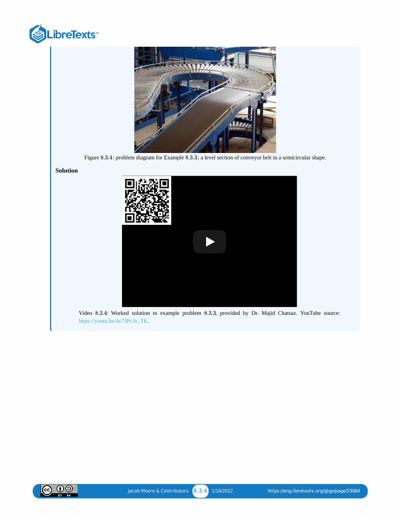
Jacob Moore & Contributors 8.3.4 1/16/2022 https://eng.libretexts.org/@go/page/53984

Figure : problem diagram for Example ; a level section of conveyor belt in a semicircular shape.

Solution

Video : Worked solution to example problem , provided by Dr. Majid Chatsaz. YouTube source:https://youtu.be/4z73Pc3s_TE.

8.3.4 8.3.3

WP8.3.3-MRCWP8.3.3-MRC

8.3.4 8.3.3

Jacob Moore & Contributors 8.4.1 1/16/2022 https://eng.libretexts.org/@go/page/54139

8.4: Equations of Motion in Polar CoordinatesTo finish our discussion of the equations of motion in two dimensions, we will examine Newton's Second law as it isapplied to the polar coordinate system. In its basic form, Newton's Second Law states that the sum of the forces on a bodywill be equal to mass of that body times the rate of acceleration. For bodies in motion, we can write this relationship out asthe equation of motion.

Just as we did with with rectangular and normal-tangential coordinates, we will break this single vector equation into twoseparate scalar equations. This involves identifying the and directions and then using sines and cosines to break thegiven forces and accelerations down into components in those directions.

Figure : When working in the polar coordinate system, any given forces or accelerations can be broken down usingsines and cosines as long as the angle of the force or acceleration is known relative to the and directions.

Just as with our other coordinate systems, the equations of motion are often used in conjunction with the kinematicsequations, which relate positions, velocities and accelerations as discussed in the previous chapter. In particular, we willoften substitute the known values below for the and components for acceleration.

Polar coordinates can be used in any kinetics problem; however, they work best with problems where there is a stationarybody tracking some moving body (such as a radar dish) or there is a particle rotating around some fixed point. Theseequations will also come back into play when we start examining rigid body kinematics.

∑ = m ∗F   a 

r θ

8.4.1r θ

∑Fr

∑Fθ

= m ∗ ar

= m ∗ aθ

(8.4.1)

(8.4.2)

r θ

= −rar r θ2 (8.4.3)

= 2 +raθ r θ θ (8.4.4)

Jacob Moore & Contributors 8.4.2 1/16/2022 https://eng.libretexts.org/@go/page/54139

Video lecture covering this section, delivered by Dr. Jacob Moore. YouTube source: https://youtu.be/XiuQSSVdRKk.

A device consists of two masses, each 0.5 kg in mass, tethered to a central shaft. The tethers are each 0.75 meters longand each tether currently makes a 25-degree angle with the central shaft. Assume the central shaft is spinning at aconstant rate. What is the rate at which the shaft is spinning? If we want it to spin at exactly 100 rpm, what should theangle of the tethers be?

Figure : problem diagram for Example . A spinning shaft supports two identical tethers at its top end, witheach tether holding a mass and splayed out symmetrically from the shaft.

Solution

8.4 The Equations of Motion in Polar 8.4 The Equations of Motion in Polar ……

Example 8.4.1

8.4.2 8.4.1

Jacob Moore & Contributors 8.4.3 1/16/2022 https://eng.libretexts.org/@go/page/54139

Video : Worked solution to example problem , provided by Dr. Majid Chatsaz. YouTube source:https://youtu.be/fGsoMdR1H9I.

A catapult design consists of a steel weight on a frictionless rod. The rod spins at a constant rate of 4 radians persecond and when is 45 degrees from the horizontal, the 30-lb weight is released from its position 2 feet from thecenter of rotation of the shaft. What is the force the shaft exerts on the weight at the instant before and the instant afterit is released? What is the acceleration of the weight along the shaft the instant after it is released?

Figure : problem diagram for Example . A central vertical shaft that rotates supports a horizontal rodbearing a releasable weight.

Solution

WP8.4.1-MRCWP8.4.1-MRC

8.4.2 8.4.1

Example 8.4.2

θ

8.4.3 8.4.2

Jacob Moore & Contributors 8.4.4 1/16/2022 https://eng.libretexts.org/@go/page/54139

Video : Worked solution to example problem , provided by Dr. Majid Chatsaz. YouTube source:https://youtu.be/bKsi80wzLUY.

WP8.4.2-MRCWP8.4.2-MRC

8.4.3 8.4.2

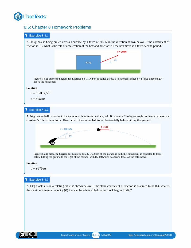
Jacob Moore & Contributors 8.5.1 1/16/2022 https://eng.libretexts.org/@go/page/54180

8.5: Chapter 8 Homework Problems

A 50-kg box is being pulled across a surface by a force of 200 N in the direction shown below. If the coefficient offriction is 0.3, what is the rate of acceleration of the box and how far will the box move in a three-second period?

Figure : problem diagram for Exercise . A box is pulled across a horizontal surface by a force directed 20°above the horizontal.

Solution

A 3-kg cannonball is shot out of a cannon with an initial velocity of 300 m/s at a 25-degree angle. A headwind exerts aconstant 5 N horizontal force. How far will the cannonball travel horizontally before hitting the ground?

Figure : problem diagram for Exercise . Diagram of the parabolic path the cannonball is expected to travelbefore hitting the ground to the right of the cannon, with the leftwards headwind force on the ball shown.

Solution

A 1-kg block sits on a rotating table as shown below. If the static coefficient of friction is assumed to be 0.4, what isthe maximum angular velocity that can be achieved before the block begins to slip?

Exercise 8.5.1

8.5.1 8.5.1

a = 1.23 m/s2

s = 5.52 m

Exercise 8.5.2

8.5.2 8.5.2

d = 6470 m

Exercise 8.5.3

( )θ

Jacob Moore & Contributors 8.5.2 1/16/2022 https://eng.libretexts.org/@go/page/54180

Figure : problem diagram for Exercise . A small block sits 2 meters from the center of a level, rotatingcircular table.

Solution

A 5-kg instrument is held via a cable to a space station. The instrument and space station are both rotating at a rate of0.5 rad/s when the space station begins retracting the cable at a constant rate of 0.25 m/s.

What is the tension in the cable at this instant?What will the angular acceleration of the cable be? Hint: there are no forces in the direction.

Figure : problem diagram for Exercise . A space station and a cable-connected instrument, rotating as asystem, draw closer together as the station pulls in the cable at a constant rate.

Solution

8.5.3 8.5.3

= 1.4θrad

s

Exercise 8.5.4

( )θ θ

8.5.4 8.5.4

T = 15 N

= 0.0208θrad

s2

1 1/30/2022

CHAPTER OVERVIEW9: WORK AND ENERGY IN PARTICLESWork, energy, power, and the relationship between these quantities. Analyzing the behavior of single particles and of systems ofparticles based on conservation of energy.

9.0: VIDEO INTRODUCTION TO CHAPTER 9Video introduction to the topics to be covered in this chapter: work, energy, and the relationship between them; energy conservationanalysis of single bodies and for systems of objects.

9.1: CONSERVATION OF ENERGY FOR PARTICLESIntroduction to conservation of energy as a method of solving analysis problems. Calculating work, kinetic energy, and gravitationaland elastic potential energies. Includes worked examples.

9.2: POWER AND EFFICIENCY FOR PARTICLESDefinition of power and efficiency, and their relationship to work and energy. The application of power and efficiency in anengineering context. Includes worked examples.

9.3: CONSERVATION OF ENERGY FOR SYSTEMS OF PARTICLESUsing the energy conservation method to analyze systems of multiple objects/particles in motion. Includes worked examples.

9.4: CHAPTER 9 HOMEWORK PROBLEMS

Jacob Moore & Contributors 9.0.1 12/21/2021 https://eng.libretexts.org/@go/page/50605

9.0: Video Introduction to Chapter 9

Video introduction to topics covered in this chapter, provided by Dr. Jacob Moore. YouTube source:https://youtu.be/2uuVtzA_SFs.

9 Work and Energy Particles - Video I9 Work and Energy Particles - Video I……

Jacob Moore & Contributors 9.1.1 1/30/2022 https://eng.libretexts.org/@go/page/50606

9.1: Conservation of Energy for ParticlesThe concepts of work and energy provide the basis for solving a variety of kinetics problems. Generally, this method iscalled the Energy Method or the Conservation of Energy, and it can be boiled down to the idea that the work done to abody will be equal to the change in energy of that body. Dividing energy into kinetic and potential energy pieces as weoften do in dynamics problems, we arrive at the following base equation for the conservation of energy.

It is important to notice that unlike Newton's Second Law, the above equation is not a vector equation. It does not need tobe broken down into components which can simplify the process. However, we only have a single equation and thereforecan only solve for a single unknown, which can limit the method.

Work:

To understand how to use the energy method we first need to understand the concepts of work and energy. Work ingeneral is a force exerted over a distance. If we imagine a single, constant force pushing a body in a single direction oversome distance, the work done by that force would be equal to the magnitude of that force times the distance the bodytraveled. If we have a force that is opposing the travel (such as friction), it would be negative work.

Figure : In instances with a constant force and a constant direction, the work done to a body will be equal to themagnitude of that force times the distance the body travels. For forces opposing the motion, the work will be negative.

For instances where forces and the direction of travel do not match, the component of the force in the direction of travel isthe only piece of the force that will do work. Following through with this logic, forces that are perpendicular to thedirection of travel for a body will exert no work on a body because there is no component of the force in the direction oftravel.

Figure : Only the components of a force in the direction of travel exert work on a body. Forces perpendicular to thedirection of travel will exert no work on the body.

W = ΔKE+ΔPE (9.1.1)

9.1.1

= ∗ dWpush Fpush (9.1.2)

= − ∗ dWfriction Ffriction (9.1.3)

9.1.2

= cos(θ) ∗ dWpush Fpush (9.1.4)

= 0Wnormal (9.1.5)

Jacob Moore & Contributors 9.1.2 1/30/2022 https://eng.libretexts.org/@go/page/50606

In the case of a force that does not remain constant, we will need to account for the changing force. To do this we willsimply integrate the force function over the distance traveled by the body. Just as before, only the component of the forcein the direction of travel will count towards the work done, and forces opposing travel will be negative work.

Energy:When discussing energy in engineering dynamics, we will usually break energy down into kinetic energy and potentialenergy. Kinetic energy is the the energy mass in motion, while potential energy represents the energy that is stored up dueto the position or stresses in a body.

In its equation form, the kinetic energy of a particle is represented by one half of the mass of the body times its velocitysquared. If we wish to determine the change in kinetic energy, we would simply take the final kinetic energy minus theinitial kinetic energy.

As a note, a body that is rotating will also have rotational kinetic energy, but we will save that for our discussion of workand energy with rigid bodies.

Potential energy, unlike kinetic energy, is not really energy at all. Instead, it represents the work that a given force willpotentially do between two instants in time. Potential energy can come in many forms, but the two we will discuss here aregravitational potential energy and elastic potential energy. These represent the work that the gravitational force and aspring force will do, respectively. We often use these potential energy terms in place of the work done by gravity orsprings. When including these potential energy terms, it's important to not additionally include the work done by gravity orspring forces.

The change in gravitational potential energy for any system is represented by the product of the mass of the body, the value (9.81 m/s or 32.2 ft/s on the earth's surface), and the vertical change in height between the start position and the end

position. In equation form, this is as follows.

Figure : When finding the change in gravitational potential energy, we multiply the mass by (giving us the weightof the object) and then multiply that by the change in the height of the object, regardless of the path taken.

To find the change in elastic potential energy, we will need to know the stiffness of the spring (represented by , in units offorce per distance) as well as the distance the spring has been stretched or compressed from its natural resting length

W = F (x)dx∫

x1

x2

(9.1.6)

KE = m1

2v2 (9.1.7)

ΔKE = m − m1

2v2f

1

2v2i (9.1.8)

g 2 2

ΔP = m ∗ g∗ ΔhEgravity (9.1.9)

9.1.3 g

k

Jacob Moore & Contributors 9.1.3 1/30/2022 https://eng.libretexts.org/@go/page/50606

(represented by , in units of distance). Once we have those values, the elastic potential energy can be calculated bymultiplying one half of the stiffness by the square of the distance . To find the change in elastic potential energy, wesimply take the final elastic potential energy and subtract the initial elastic potential energy.

Going back to our original conservation of energy equation, we simply plug the appropriate terms on each side (work onthe left and energies on the right) and balance the two sides to solve for any unknowns. Terms that do not exist or do notchange, such as elastic potential energy in a problem with no springs or in a problem where there is no change inthe speed of the body, can be set to zero.

Video lecture covering this section, delivered by Dr. Jacob Moore. YouTube source: https://youtu.be/FMkHrOjKlXs.

A 16-pound crate slides down a ramp as shown below. The crate is released from a height of 10 feet above the ground.

What is the work done by gravity?What is the change in gravitational potential energy?

Figure : problem diagram for Example . A 16-lb crate initially 10 feet above the ground slides down a rampof incline 60°.

Solution

x

x

ΔP = k − kEspring

1

2x2f

1

2x2i (9.1.10)

ΔKE

9.1 Conservation of Energy Particle - 9.1 Conservation of Energy Particle - ……

Example 9.1.1

9.1.4 9.1.1

Jacob Moore & Contributors 9.1.4 1/30/2022 https://eng.libretexts.org/@go/page/50606

Video : Worked solution to example problem . YouTube source: https://youtu.be/ZkopO1aTj54.

A spring with an unstretched length of 40 cm and a value of 120 N/cm is used to lift a 5-kg box from a height of 20cm to a height of 30 cm. If the box starts at rest, what would you expect the final velocity to be?

Figure : problem diagram for Example . A vertically oriented spring supporting a box on its upper end isstretched to lift the load.

Solution

Work Energy - WP001 - DJMWork Energy - WP001 - DJM

9.1.2 9.1.1

Example 9.1.2

k

9.1.5 9.1.2

Jacob Moore & Contributors 9.1.5 1/30/2022 https://eng.libretexts.org/@go/page/50606

Video : Worked solution to example problem . YouTube source: https://youtu.be/T_5JT4XFQN8.

A 2,000-pound wrecking ball hangs from the end of a 40-foot cable. If the wrecking ball is released from an angle of40 degrees from vertical, what would the expected maximum velocity at the bottom point of the travel path be?

Figure : problem diagram for Example . A wrecking ball on a cable is raised slightly above its restingposition, with the cable kept taut, then released.

Solution

Work Energy - WP002 - DJMWork Energy - WP002 - DJM

9.1.3 9.1.2

Example 9.1.3

9.1.6 9.1.3

Jacob Moore & Contributors 9.1.6 1/30/2022 https://eng.libretexts.org/@go/page/50606

Video : Worked solution to example problem . YouTube source: https://youtu.be/UkcpT1lfIDY.

A 24,000-kilogram aircraft is launched from an aircraft carrier using a hydraulic catapult. If the force the catapultexerts over the 90-meter runway is shown in the graph below:

What is the work done by the catapult?What is the speed of the plane at the end of the runway?

Figure : problem diagram for Example . Graph of the force exerted by the catapult vs distance traveled overthe runway, showing a linear relationship between these quantities.

Solution

Video : Worked solution to example problem . YouTube source: https://youtu.be/DfSMeUm1SG8.

Work Energy Work Energy WP003 WP003 DJMDJM

9.1.4 9.1.3

Example 9.1.4

9.1.7 9.1.4

Work Energy Work Energy WP004 WP004 DJMDJM

9.1.5 9.1.4

Jacob Moore & Contributors 9.2.1 12/21/2021 https://eng.libretexts.org/@go/page/50607

9.2: Power and Efficiency for ParticlesRelated to the concepts of work and energy are the concepts of power and efficiency. At its core, power is the rate atwhich work is being done, and efficiency is the percentage of useful work or power that is transferred from the input to theoutput of some system.

PowerPower at any instant is defined as the derivative of work with respect to time. If we look at the average power over a setperiod, we can simply measure the work done and divide that by the time. Work is defined as the force times the distancetraveled, and distance over time is the velocity of a object, giving us many possible options for relating power, work, force,distance, time, and velocity.

The common units of power are watts for the metric system, where one watt is defined as one joule per second, or oneNewton-meter per second, and horsepower in the English system, where one horsepower is defined as 550 foot-poundsper second. Maximum power ratings are often a primary specification for motors and engines, as gear trains can easilychange the torque provided by a motor but the overall power will not be altered by gearing.

Figure : Assuming the two cars above have the same mass, it would take the same amount of work to get them up to aset speed (such as 60 miles per hour). However, the more powerful car would be able to get to this speed in a much shortertime period.

EfficiencyAny devices with work/power inputs and outputs will have some loss of work or power between that input and output, dueto things like friction. While energy is always conserved, some energies such as heat may not be considered useful. Ameasure of the useful work or power that makes it from the input of a device to the output is the efficiency. Specifically,efficiency is defined as the work out of a device divided by the work put into the device. With power being the work overtime, efficiency can also be described as power out divided by the power in to a device (the time term would cancel out,leaving us with our original definition).

It is impossible to have efficiencies greater than one (or 100%) because that would be a violation of the conservation ofenergy; however, for most devices we wish to get the efficiencies as close to one as possible. This is not only becausegreater efficiencies waste less work/power, but also because any work or power that is "lost" in the device will be turnedinto heat that may build up.

P =dW

dt(9.2.1)

= = = F ∗ vPave

W

t

F ∗ d

t(9.2.2)

9.2.1

η = =Wout

Win

Pout

Pin

(9.2.3)

Jacob Moore & Contributors 9.2.2 12/21/2021 https://eng.libretexts.org/@go/page/50607

Video lecture covering this section, delivered by Dr. Jacob Moore. YouTube source: https://youtu.be/BxK5D1DnD1Q.

If a car delivers an average 100 horsepower to the road and weighs a total of 1.2 tons, how long will it take to go from0 to 60 mph?

Figure : A car driving quickly down a straight, tree-lined road.

Solution

Video : Worked solution to example problem . YouTube source: https://youtu.be/ju7TOLHWEZg.

Your car broke down and now needs to be repaired. How much power is required for a lift to raise your 1.2 ton car 6feet off the ground in 15 seconds?

Example 9.2.1

9.2.2

Power WP001 DJMPower WP001 DJM

9.2.2 9.2.1

Example 9.2.2

Jacob Moore & Contributors 9.2.3 12/21/2021 https://eng.libretexts.org/@go/page/50607

Figure : A car in a mechanic's shop is raised off the ground by a lift.

Solution

Video : Worked solution to example problem . YouTube source: https://youtu.be/BCVOzDwPR7c.

The drag force of air on a car is equal to

where is the is the density of the air, is the velocity, is the drag coefficient, and is the frontal area. If a MazdaRX7 has a drag coefficient of 0.29, a frontal area of 5.95 square feet, and a max power output of 146 hp, and thedensity of air is 0.002326 slug/ft³, what is the theoretical top speed of the Mazda assuming it only has to fight windresistance?

Figure : A red Mazda RX7.

Solution

9.2.3

Power WP002 DJMPower WP002 DJM

9.2.3 9.2.2

Example 9.2.3

= ρ AFd

1

2v2cd

ρ v cd A

9.2.4

Jacob Moore & Contributors 9.2.4 12/21/2021 https://eng.libretexts.org/@go/page/50607

Video : Worked solution to example problem . YouTube source: https://youtu.be/DaJIXMjRfZo.

Power WP003 DJMPower WP003 DJM

9.2.4 9.2.3

Jacob Moore & Contributors 9.3.1 12/21/2021 https://eng.libretexts.org/@go/page/54728

9.3: Conservation of Energy for Systems of ParticlesJust as we used the energy method for a single particle, we can also use the energy method for a system of particles. As areminder, the conservation of energy equation states that the change in energy of a body (including kinetic and potentialenergies) will be equal to the work done to a body between during that time.

For a system of particles, the sum of the work done to all particles will be equal to the change in energy of all particlescollectively, essentially combining multiple conservation of energy equations into one.

This would seem to make one complex equation out of multiple simple conservation of energy equations (applying theconservation of energy separately to each body), but there is an advantage in that internal forces in the system will cancelout. In the diagram below, we can see a system of two particles connected via a cable. Examining the bodies separately, wewould have two tension forces and a friction force all doing work to one box or the other. In the single equation for thesystem of boxes, however, the work done by the two tension forces (one positive and one negative) will sum up to zero.This will be true for any forces that are exerted between the bodies in the system, and forces like these are known asinternal forces. The friction force, on the other hand, is an example of an external force, in that it exists between the topbox and the surface (which is not part of our system).

Figure : If we count the two boxes in this diagram as our system, then the tension forces would count as internalforces and can be ignored in our energy conservation equation. Only external forces such as the friction force need to beincluded as part of the work done on the system.

In the end, the sum of the work done by external forces will be equal to the change in total energy for the system ofparticles. Since we only have a single equation, we can only solve for a single unknown. We will often have to go back toour kinematics equations to relate the velocities and displacements of the various bodies to one another. Since thesesystems often consist of bodies connected to one another via cables, dependent motion analysis in particular will oftencome into play.

W = ΔK PEEΔ (9.3.1)

∑W =∑ΔKE+∑ΔPE (9.3.2)

9.3.1

Jacob Moore & Contributors 9.3.2 12/21/2021 https://eng.libretexts.org/@go/page/54728

Video lecture covering this section, delivered by Dr. Jacob Moore. YouTube source: https://youtu.be/r1RBsxURcbY.

Two blocks are connected by a massless rope and a frictionless pulley as shown below. If the coefficient of frictionbetween block A and the surface is 0.4, what is the speed of the blocks after block A has moved 6 ft?

Figure : problem diagram for Example . The 5-lb box B hangs from a cable that runs over a pulley andconnects to the 10-lb box A sitting on a flat surface.

Solution

Video : Worked solution to example problem . YouTube source: https://youtu.be/UW4HXJNId0A.

The elevator shown below has a mass of 1500 kg and the counterweight has a mass of 500 kg. At some point the cableattached to the motor snaps, causing the elevator to begin falling. After falling 3 meters with no outside forces, what isthe speed of the elevator? If the emergency brake is then applied at this point (3 m below the original position),exerting a constant force of 15,000 N, how much farther will the elevator fall before coming to a stop?

9.4 The Conservation of Energy for S9.4 The Conservation of Energy for S……

Example 9.3.1

9.3.2 9.3.1

Conservation Energy System PartConservation Energy System Part……

9.3.2 9.3.1

Example 9.3.2

Jacob Moore & Contributors 9.3.3 12/21/2021 https://eng.libretexts.org/@go/page/54728

Figure : problem diagram for Example . An elevator is attached to the roof of a building only by a singlecable, which is connected by pulleys to a counterweight at its free end.

Solution

Video : Worked solution to example problem . YouTube source: https://youtu.be/QWvh5wZt7jM.

9.3.3 9.3.2

Conservation Energy System PartConservation Energy System Part……

9.3.3 9.3.2

Jacob Moore & Contributors 9.4.1 12/21/2021 https://eng.libretexts.org/@go/page/54729

9.4: Chapter 9 Homework Problems

A car with a mass of 1100 kg locks up its brakes when it is traveling at 50 km/hr, stopping over a distance of 18meters. If the same car were to lock up its brakes when traveling 80 km/hr, how far would you expect the car to slidebefore coming to a stop? (Hint: assume the same friction force in both cases).

Figure : A car with locked-up brakes, visibly skidding.

Solution

A 2500-lb car traveling 60 mph (88 ft/s) impacts a highway crash barrier as shown below. If the barrier were designedto exert the following force over the 40-ft distance of the barrier, how far would you expect the car to travel afterimpacting the barrier?

Figure : problem diagram for Exercise . A highway crash barrier and the graph of the force it exerts on animpacting car over the barrier's length.

Solution

(assuming no holes in the barrier)

The Duquesne Incline transports passengers up a 30.5 degree slope. If a fully loaded car has a mass of 5500 kg, whatpower is required to maintain an uphill speed of 10 km/hr?

Exercise 9.4.1

9.4.1

d = 46.06m

Exercise 9.4.2

9.4.2 9.4.2

d = 25.03 ft

Exercise 9.4.3

Jacob Moore & Contributors 9.4.2 12/21/2021 https://eng.libretexts.org/@go/page/54729

Figure : The Duquesne Incline, a cable car that transports passengers up a steep hillside.

Solution

A bungee jumper with a weight of 150 lbs uses a bungee cord with an unstretched length of 60 feet.

Assuming no air resistance, what will the jumper’s velocity be just before the bungee cord starts to stretch?If the bungee jumper falls a maximum distance of 150 feet, what is the spring constant of the bungee cord?

Figure : A man bungee-jumping above a lake.

Solution

An 1100-kg truck is being used to raise a 100-kg box using the setup shown below. When the box is at a height of 3meters, the box has a velocity of 1 m/s.

How far did the truck travel to lift the box this high? (Hint: this is a dependent motion problem)What is the velocity of the truck at this time?What is the work that the truck has done over this time?

9.4.3

P = 76.13 kW

Exercise 9.4.4

9.4.4

v= 62.16 ft

k= 5.55 lb/ft

Exercise 9.4.5

Jacob Moore & Contributors 9.4.3 12/21/2021 https://eng.libretexts.org/@go/page/54729

Figure : problem diagram for Exercise . A cable attached at one end to a beam 4 feet above the groundpasses through a pulley on a box on the ground and through another pulley on the beam, before being attached to therear of a truck 5 feet away from the box. The truck drives away from the box to raise it from the ground.

Solution

9.4.5 9.4.5

d = 6.7m

v= 2.12m/s

W = 5464.92 J

1 1/30/2022

CHAPTER OVERVIEW10: IMPULSE AND MOMENTUM IN PARTICLESThe relationship between impulse and momentum in a particle. Analysis of steady-flow devices and of collisions between particles(one-dimensional, two-dimensional, and surface collisions).

10.0: VIDEO INTRODUCTION TO CHAPTER 10Video introduction to the topics to be covered in this chapter: impulse, momentum, and their relationship; kinetics analysis ofcollisions and steady-flow devices.

10.1: IMPULSE-MOMENTUM EQUATIONS FOR A PARTICLEIntroduction to the impulse-momentum method of solving kinetic analysis problems. Includes discussion of impulse, momentum, andthe conservation of momentum. Includes worked examples.

10.2: SURFACE COLLISIONS AND THE COEFFICIENT OF RESTITUTIONAnalysis of collisions where one object bounces off a much larger, unmoving surface. Includes worked examples.

10.3: ONE-DIMENSIONAL PARTICLE COLLISIONSAnalyzing one-dimensional particle collisions through momentum conservation; the types of collisions (elastic, semi-elastic, andinelastic) and the constraints they provide. Includes worked examples.

10.4: TWO-DIMENSIONAL PARTICLE COLLISIONSAnalyzing two-dimensional particle collisions through momentum conservation for individual vector components. Types of collisions(elastic, semi-elastic, and inelastic) and the constraints they provide. Includes worked examples.

10.5: STEADY-FLOW DEVICESIntroduction to steady-flow devices; adapting the impulse-momentum equation for analysis of these devices. Includes workedexamples.

10.6: CHAPTER 10 HOMEWORK PROBLEMS

Jacob Moore & Contributors 10.0.1 12/21/2021 https://eng.libretexts.org/@go/page/54731

10.0: Video Introduction to Chapter 10

Video introduction to the topics covered in Chapter 10, delivered by Dr. Jacob Moore. YouTube source:https://youtu.be/Xq39c7jZWPo.

10 Impulse Momentum Particles - Vi10 Impulse Momentum Particles - Vi……

Jacob Moore & Contributors 10.1.1 1/9/2022 https://eng.libretexts.org/@go/page/54732

10.1: Impulse-Momentum Equations for a ParticleThe concepts of impulse and momentum provide a third method of solving kinetics problems in dynamics. Generally thismethod is called the Impulse-Momentum Method, and it can be boiled down to the idea that the impulse exerted on abody over a given time will be equal to the change in that body's momentum. The impulse is usually denoted by thevariable (not to be confused with the polar moment of inertia, which is also J) and the momentum is a body's mass timesits velocity. Impulses and velocities are both vector quantities, giving us the basic equation below.

For two-dimensional problems, we can break the single vector equation down into two scalar components to solve. In thiscase, we simply need to break all forces and velocities into and components.

Impulse:

The concept of an impulse in its most basic form is a force integrated over a time. For a force with a constant magnitude,we can find the magnitude of the impulse by multiplying the magnitude of the force by the time that force is exerted. If theforce is not constant, we simply integrate the force function over the set time period. The direction of the impulse vectorwill be the direction of the force vector and the units will be a force times a time (Newton-seconds or pound-seconds, forexample).

In many cases, we will discuss impulsive forces. This is an instance where we have very large forces acting over a veryshort time frame. In instances of impulsive forces, it is often difficult to measure the exact magnitude of the force or thetime. In these cases we may only be able to deduce the magnitude of the impulse as a whole via the observed change inmomentum of the body.

J

= m −mJ   v  f v  i (10.1.1)

x y

= m −mJx vfx vix (10.1.2)

= m −mJy vfy viy (10.1.3)

Constant Magnitude Force:

Non-Constant Magnitude Force:

= ∗ tJ   F  

= ∫ (t)dtJ   F  

(10.1.4)

(10.1.5)

Jacob Moore & Contributors 10.1.2 1/9/2022 https://eng.libretexts.org/@go/page/54732

Figure : The force the tennis racket exerts on the ball will be very large, but it will be exerted over a very shortperiod of time. Because of this, the force is considered an "impulsive" force. It would be difficult to determine the exactmagnitude of the force or time frame of the impact, but by examining the velocity of the ball before and after the impactwe could deduce the overall magnitude of the impulse as a whole. Photo by David Iliff. License: CC BY-SA 3.0.

Momentum:

The momentum of a body will be equal to the mass of the body times its current velocity. Since velocity is a vector, themomentum will also be a vector, having both magnitude and a direction. Unlike the impulse, which happens over some settime, the momentum is captured as a snapshot of a specific instant in time (usually right before and after some impulse isexerted). The units for momentum will be mass times unit distance per unit time. This is usually kilogram-meters persecond in metric, or slug feet per second in English units.

Conservation of Momentum:

In instances where there is no impulse exerted on a body, we can use the original equation to deduce that there will be nochange in momentum of the body. In this instance, momentum is conserved. This will also hold for systems of bodies,where if no external impulses are exerted on the bodies in a system, the momentum will be conserved as a whole. This isthe basis of analysis for many collisions, as is discussed in the following sections.

Video lecture covering this section, delivered by Dr. Jacob Moore. YouTube source: https://youtu.be/yC9wt53ho9k.

10.1.1

10.1 The Impulse-Momentum Equati10.1 The Impulse-Momentum Equati……

Jacob Moore & Contributors 10.1.3 1/9/2022 https://eng.libretexts.org/@go/page/54732

A tennis ball (0.06 kg) is served to a tennis player at a speed of 10 m/s. The player then returns the ball at a speed of 36m/s.

What is the impulse exerted on the ball?If a high-speed camera reveals the impact lasted 0.02 seconds, what is the average force exerted on the ball duringthe collision?

Figure : A player in a tennis match serves a ball.

Solution

Video : Worked solution to example problem , provided by Dr. Majid Chatsaz. YouTube source:https://youtu.be/WzD-ZyJy-T4.

A plane with a mass of 80,000 kg is traveling at a velocity of 200 meters per second when the engines cut out. Twentyseconds later, it’s noticed that the velocity has dropped to 190 m/s. Assuming the plane is not gaining or losingaltitude, what is the average drag force on the plane?

Example 10.1.1

10.1.2

WP10 1 1 MRCWP10 1 1 MRC

10.1.2 10.1.1

Example 10.1.2

Jacob Moore & Contributors 10.1.4 1/9/2022 https://eng.libretexts.org/@go/page/54732

Figure : An airliner in flight.

Solution

Video : Worked solution to example problem , provided by Dr. Majid Chatsaz. YouTube source:https://youtu.be/dzhIT3r3u3k.

The plot below shows the thrust generated by the engine on a jet fighter (mass of 2500 kg) over ten seconds. If theplane is starting from rest on a runway, and friction and drag are negligible, determine the speed of the plane at the endof these ten seconds.

Figure : problem diagram for Example . Graph of the thrust force generated by a jet engine for the first 10seconds of its motion starting from rest.

Solution

10.1.3

WP10 1 2 MRCWP10 1 2 MRC

10.1.3 10.1.2

Example 10.1.3

10.1.3 10.1.3

Jacob Moore & Contributors 10.1.5 1/9/2022 https://eng.libretexts.org/@go/page/54732

Video : Worked solution to example problem , provided by Dr. Majid Chatsaz. YouTube source:https://youtu.be/XGxVjLa6wqQ.

WP10 1 3 MRCWP10 1 3 MRC

10.1.4 10.1.3

Jacob Moore & Contributors 10.2.1 1/16/2022 https://eng.libretexts.org/@go/page/54733

10.2: Surface Collisions and the Coefficient of RestitutionHere we will use the term surface collision to describe any instance where a body impacts and rebounds off a solid andunmoving surface. A clear example of a surface collision is a basketball bouncing off a hard floor. The basketball will havesome velocity before the collision and some second velocity after the collision, with the floor exerting an impulsive forceduring the collision that causes this change in velocity.

To analyze this collision, we will first need to set up a normal direction (perpendicular to the surface) and a tangentialdirection (parallel to the surface) for our problem, and break our velocities down into components in these directions.Assuming minimal friction during the impact, we will have an impulsive impact force acting entirely in the normaldirection. This fact will form the basis for our analysis.

Figure : In a surface collision, the impulsive collision force will act in the normal direction. Because there is noforce in the tangential direction, the velocity in the tangential direction will not change.

Because the impact force acts entirely in the normal direction, there will be no other significant force to change themomentum of the body in the tangential direction. Assuming the mass remains constant for the body, this means that thevelocity must remain constant in the tangential direction because of the conservation of momentum.

To relate the velocities in the normal direction before and after the collision, we will use something called the coefficientof restitution. The coefficient of restitution is a number between 0 and 1 that measures the "bounciness" of the body andthe surface in the collision. Specifically, for a single body being bounced perpendicularly off a surface, the coefficient ofrestitution is defined as the speed of the body immediately after bouncing off the surface divided by the speed immediatelybefore bouncing off the surface. If we use velocities in place of speed, we will put a negative sign in our equation becausethe bounce causes a change in direction for the body.

In instances where the body is being bounced off the surface at an angle, the impact force is entirely in the normaldirection and the coefficient of restitution relationship specifically applies to the components of the velocities in the normaldirection.

This relationship can be applied to elastic collisions (where would be equal to 1), semi-elastic collisions (where wouldbe some number between 0 and 1) and inelastic collisions (where would be equal to 0).

10.2.1

=vi,t vf,t (10.2.1)

ϵ = −vf

vi

(10.2.2)

ϵ = −vf,n

vi,n(10.2.3)

ϵ ϵ

ϵ

Jacob Moore & Contributors 10.2.2 1/16/2022 https://eng.libretexts.org/@go/page/54733

Video lecture covering this section, delivered by Dr. Jacob Moore. YouTube source: https://youtu.be/MaY6YEWhwJc.

A basketball with an initial speed of 3 meters per second impacts a hard floor at the sixty degree angle as shownbelow. If the collision has a coefficient of restitution of 0.8, what is the expected speed and angle of the basketball afterthe impact?

Figure : problem diagram for Example . A basketball with a known initial velocity bounces off a floorwith a known coefficient of restitution.

Solution

Video : Worked solution to example problem , provided by Dr. Majid Chatsaz. YouTube source:https://youtu.be/A8hl3JPUkB4.

10.2 Surface Collisions and the Coe10.2 Surface Collisions and the Coe……

Example 10.2.1

10.2.2 10.2.1

WP10 3 1 MRCWP10 3 1 MRC

10.2.2 10.2.1

Jacob Moore & Contributors 10.2.3 1/16/2022 https://eng.libretexts.org/@go/page/54733

A bounce test is used to sort ripe cranberries from unripe cranberries. In this test, cranberries are dropped verticallyonto a steel plate sitting at a 45-degree angle. After the impact, a cranberry is observed to bounce off at an angle of 20degrees below the horizontal. Based on this information, what is the coefficient of restitution for the cranberry?

Figure : problem diagram for Example . A cranberry falls straight down onto a tilted plate and bouncesoff at a known angle.

Solution

Video : Worked solution to example problem , provided by Dr. Majid Chatsaz. YouTube source:https://youtu.be/wpPYTx52CD8.

Example 10.2.2

10.2.3 10.2.2

WP10 3 2 MRCWP10 3 2 MRC

10.2.3 10.2.2

Jacob Moore & Contributors 10.3.1 1/7/2022 https://eng.libretexts.org/@go/page/54734

10.3: One-Dimensional Particle CollisionsThe Impulse-Momentum Method is particularly useful when examining collisions between bodies. When examining thebodies colliding as a system of particles, such as the two bodies colliding below, the impulses exerted by internal forces,or the forces exerted between two bodies within the system, will be equal and opposite and hence cancel out in ourimpulse-momentum equation.

Figure : When two bodies collide, Newton's Third Law ensures that the normal forces from the collision will alwaysbe equal and opposite. This means that the impulses will be equal and opposite and will cancel out in our impulse-momentum equation when examining the system of equations.

Because the impulsive forces of the collision are so large over the very short period of the collision, other external forcesare typically regarded as insignificant. This means that for our collision, there is no external impulse and therefore there isno change to the sum of the momentums of the bodies. This is known as the conservation of momentum, and it will holdtrue for all types of collisions.

In the case of the collision of two bodies, body A and body B in this case, we can break apart the sums as follows. Thesubscripts in this case are being used to denote both the body (A or B) and the initial versus final states (before or after thecollision).

In addition to the conservation of momentum equation, we will also usually generate a second equation we can usealongside the conservation of momentum. This second equation will depend on the type of collision, though, with the threepossible collision types being elastic, inelastic, and semi-elastic.

Elastic Collisions

An elastic collision is a collision in which all energy is assumed to be conserved as kinetic energy. In reality, true elasticcollisions do not exist as some energy will always be converted to heat or sound, but in practice two very rigid bodies thatcollide without much deformation can get very close to the ideal of an elastic collision. An example of a collision that isclose to elastic is a set of billiard balls colliding, as in Figure .

An elastic collision conserves energy in addition to momentum, so the conservation of energy equation will be our secondequation that we use to supplement the conservation of momentum.

Inelastic Collisions

An inelastic collision is the opposite of an elastic collision, in that much of the energy of the system is lost in thedeformation of the bodies. In fact, in an inelastic collision the bodies must deform in such as way that they stick together

10.3.1

∑ = 0 =∑m −∑mJ   v  f v  i (10.3.1)

∑m −∑mv  f v  i (10.3.2)

  +   =   +  mA v  A,f mB v  B,f mA v  A,i mB v  B,i (10.3.3)

10.3.1

  +   =   +  1

2mA v  2A,f

1

2mB v  2B,f

1

2mA v  2A,i

1

2mB v  2B,i (10.3.4)

Jacob Moore & Contributors 10.3.2 1/7/2022 https://eng.libretexts.org/@go/page/54734

after the collision. With the two bodies stuck together, they will have matching final velocities.

Semi-Elastic CollisionFinally, anything between an elastic collision and an inelastic collision is considered a semi-elastic collision. This is acollision where less than one hundred percent of the kinetic energy is conserved, but the objects do not stick togetherfollowing the collision. In cases of semi-elastic collisions, we will use something called the coefficient of restitution(usually denoted by the Greek letter epsilon, ), to supplement our conservation of momentum equation.

The coefficient of restitution is a number between 0 and 1 that measures the "bounciness" of the two bodies in thecollision. Specifically, for a single body bouncing off a rigid surface, the coefficient of restitution is defined as the negativeof the velocity after bouncing off the surface divided by the velocity before bouncing off the surface.

A perfectly elastic collision would have a coefficient of restitution of one (no velocity would be lost), while a totallyinelastic collision would have a coefficient of restitution of zero. All other collisions will have a coefficient of restitutionthat lies somewhere in between.

For cases where two bodies are bouncing off of one another, we would simply use relative velocities rather than thevelocity of a single body. Using the velocity of body A relative to the velocity of body B, we come up with the equationbelow.

Video lecture covering this section, delivered by Dr. Jacob Moore. YouTube source: https://youtu.be/lFZ8Mr4Vcow.

A cue ball weighing 0.17 kg, traveling at 1 m/s, impacts a stationary billiard ball with a mass of 0.15kg as shownbelow. If the balls collide directly and the collision is elastic, what will the velocities be after the collision (ignorerotational energies)?

=v  A,f v  B,f (10.3.5)

ϵ

ϵ = −vf

vi

(10.3.6)

ϵ = − = −v  f,A/B

v  i,A/B

−v  f,A v  f,B

−v  i,A v  i,B(10.3.7)

10.3 Particle Collisions in 1D - Video 10.3 Particle Collisions in 1D - Video ……

Example 10.3.1

Jacob Moore & Contributors 10.3.3 1/7/2022 https://eng.libretexts.org/@go/page/54734

Figure : problem diagram for Example . A cue ball traveling at 1 m/s directly impacts a stationary billiardball.

Solution

Video : Worked solution to example problem , provided by Dr. Majid Chatsaz. YouTube source:https://youtu.be/n1g5RwuFYJI.

A 4.2 g bullet traveling at 965 m/s becomes lodged in a stationary log with a mass of 1.5 kg.

What is the the velocity of the log and the bullet immediately after the collision?What percentage of the kinetic energy was lost in the collision?

Figure : problem diagram for Example . A bullet traveling at 965 m/s is flying directly towards a largelog, where it will become lodged.

Solution

10.3.2 10.3.1

WP10 2 1 MRCWP10 2 1 MRC

10.3.2 10.3.1

Example 10.3.2

10.3.3 10.3.2

Jacob Moore & Contributors 10.3.4 1/7/2022 https://eng.libretexts.org/@go/page/54734

Video : Worked solution to example problem , provided by Dr. Majid Chatsaz. YouTube source:https://youtu.be/FyyziesH9LI.

Two masses on a frictionless rod as shown below are set to impact with each other. If the coefficient of restitutionbetween the objects is 0.6, what is the velocity of each body after the collision?

Figure : problem diagram for Example . Two different masses strung on a frictionless rod travel towardseach other at different speeds.

Solution

WP10 2 2 MRCWP10 2 2 MRC

10.3.3 10.3.2

Example 10.3.3

10.3.4 10.3.3

Jacob Moore & Contributors 10.3.5 1/7/2022 https://eng.libretexts.org/@go/page/54734

Video : Worked solution to example problem , provided by Dr. Majid Chatsaz. YouTube source:https://youtu.be/MOUG_7BqcLY.

WP10 2 3 MRCWP10 2 3 MRC

10.3.4 10.3.3

Jacob Moore & Contributors 10.4.1 12/21/2021 https://eng.libretexts.org/@go/page/54745

10.4: Two-Dimensional Particle CollisionsTo analyze collisions in two dimensions, we will need to adapt the methods we used for a single dimension. To start, theconservation of momentum equation will still apply to any type of collision.

This is, of course, a vector equation, so we can break all those velocities into components to make our one vector equationinto two scalar equations. In the equations below, we break the conservation of momentum equation into and components.

In the subscripts for the velocities, we label the particle ( or ), the pre or post collision state ( or ), and thecomponent ( or ). This triple subscript can make things a bit crowded, but as long as you are methodical about labelingand reading these subscripts it is fairly straightforward. To help ease interpretation, it's recommended that you follow aconsistent ordering in the subscripts, labeling body, then pre/post collision, then direction.

To supplement the conservation of momentum equations, we will again need to determine the type of collision, classifyingthe collision as inelastic (where the two particles stick together after impact) or elastic or semi-elastic (where the particlesbounce off of one another).

Inelastic Collisions:In the case of inelastic collisions, the bodies will have the same final velocity as a consequence of sticking together.Rolling this relationship into the above conservation of momentum equations, we wind up with the following equations.These modified equations are usually enough to solve for the unknowns in the equations.

Elastic and Semi-Elastic Collisions:Unlike the inelastic collisions, elastic and semi-elastic collisions will have separate velocities for each of the bodies post-collision. With each body having separate and components, this represents four unknown variables. Assuming weknow all starting conditions, we will need four separate equations to solve for all unknowns.

Unlike the conservation of momentum equation, the conservation of energy equation we would use for elastic collisions isnot a vector equation and cannot be broken down into components. Instead we will need to look to the coefficient ofrestitution, and set it equal to 1 for elastic collisions.

To solve these problems, we will first need to set up a specific set of coordinate axes. These axes will be the tangentialdirection (along the plane of the collision) and the normal direction (perpendicular to the plane of the collision). Anexample of these directions is shown in the figure below.

  +   =   +  mA v  A,f mB v  B,f mA v  A,i mB v  B,i (10.4.1)

x y

  +   =   +  mA vA,f,x mB vB,f,x mA vA,i,x mB vB,i,x (10.4.2)

  +   =   +  mA vA,f,y mB vB,f,y mA vA,i,y mB vB,i,y (10.4.3)

A B i f

x y

  =   +  m(A+B) vf,x mA vA,i,x mB vB,i,x (10.4.4)

  =   +  m(A+B) vf,y mA vA,i,y mB vB,i,y (10.4.5)

x y

Jacob Moore & Contributors 10.4.2 12/21/2021 https://eng.libretexts.org/@go/page/54745

Figure : In a 2-D collision, it is important to identify the normal and tangential directions. The tangential directionwill always be along the plane of impact while the normal direction will be perpendicular to the plane of contact.

In examining the figure above, we can see something special about the tangential direction in that there are no forces oneither body in this direction. With no forces, there is no impulse, and with no impulse there is no change in momentum foreither particle individually in the tangential direction. This means that velocity is conserved for each body in the tangentialdirection on its own. Adding to that, momentum as a whole is conserved in the normal direction and the coefficient ofrestitution equation can be applied to the normal direction and we have the four equations we need to solve most problems.

To use the above equations, we will need to break all known velocities down into and components, then simply plugthose values in and solve the above equations. In the end we may also need to convert the found and velocitycomponents into and components or magnitudes and directions.

Video lecture covering this section, delivered by Dr. Jacob Moore. YouTube source: https://youtu.be/iugmHb5fLMA.

10.4.1

=vA,f,t vA,i,t (10.4.6)

=vB,f,t vB,i,t (10.4.7)

  +   =   +  mA vA,f,n mB vB,f,n mA vA,i,n mB vB,i,n (10.4.8)

ϵ = −−vA,f,n vB,f,n

+vA,i,n vB,i,n(10.4.9)

n t

n t

x y

10.4 Particle Collisions in 2D - Video 10.4 Particle Collisions in 2D - Video ……

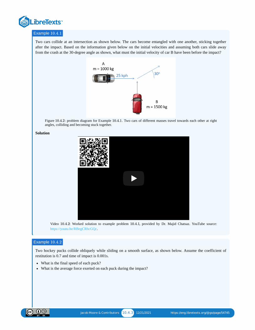
Jacob Moore & Contributors 10.4.3 12/21/2021 https://eng.libretexts.org/@go/page/54745

Two cars collide at an intersection as shown below. The cars become entangled with one another, sticking togetherafter the impact. Based on the information given below on the initial velocities and assuming both cars slide awayfrom the crash at the 30-degree angle as shown, what must the initial velocity of car B have been before the impact?

Figure : problem diagram for Example . Two cars of different masses travel towards each other at rightangles, colliding and becoming stuck together.

Solution

Video : Worked solution to example problem , provided by Dr. Majid Chatsaz. YouTube source:https://youtu.be/RBegCRhcGQc.

Two hockey pucks collide obliquely while sliding on a smooth surface, as shown below. Assume the coefficient ofrestitution is 0.7 and time of impact is 0.001s.

What is the final speed of each puck?What is the average force exerted on each puck during the impact?

Example 10.4.1

10.4.2 10.4.1

WP10 4 1 MRCWP10 4 1 MRC

10.4.2 10.4.1

Example 10.4.2

Jacob Moore & Contributors 10.4.4 12/21/2021 https://eng.libretexts.org/@go/page/54745

Figure : problem diagram for Example . Two hockey pucks of different masses but the same radius movetowards each other, their centers of mass offset by a distance equal to the radius.

Solution

Video : Worked solution to example problem , provided by Dr. Majid Chatsaz. YouTube source:https://youtu.be/mRPjLk8RxQw.

10.4.3 10.4.2

WP10 4 2 MRCWP10 4 2 MRC

10.4.3 10.4.2

Jacob Moore & Contributors 10.5.1 1/30/2022 https://eng.libretexts.org/@go/page/54746

10.5: Steady-Flow DevicesA steady-flow device is any device that will have a continuous flow of material through it. Some examples of steady-flowdevices include pipes, nozzles, diffusers, and pumps. Generally, the material flowing through the device is a gas or liquid,and if the device in any way changes the velocity of the fluid then that fluid will exert a force on the steady flow device inreturn.

Figure : The nozzle on the fire hose is an example of a steady-flow device. Because the nozzle changes the velocityof the water as it exits the hose, it will take a force to hold the nozzle in place.

In order to determine the forces at play on a steady-flow device, we will start with our impulse-momentum equation.

Because this is a continuous process, it doesn't really make sense to have initial and final velocities. Instead, we will haveinlet and outlet velocities. Also, the mass will need to be changed to the mass flow rate (the mass entering or leaving thedevice per unit time) to deal with the continuous-flow nature of the system.

Figure : The mass flow rate is a more appropriate measure for steady-flow devices than standard mass.

Dividing our initial impulse-momentum equation by time on both sides will give us the desired mass flow rate on the right,while the time on the left will cancel out the time component of the impulse.

Simplifying this equation, we will arrive at our final equation, which relates the force our steady-flow device exerts on thefluid to the mass flow rates and velocities at the inlet and outlet. The force the fluid exerts on the device would simply beequal and opposite to the force below.

One final note is that these equations are vector equations. If the device is changing the direction of the flow of a fluid youwill need to break the force and velocities into and components and split the above equation into and components.

Finding Mass Flow Rate:If the mass flow rate in or out of your device is not given directly, you may need to find those values. First we can use asimple identity: we know the mass flow rate will be equal to the density of the fluid times the volumetric flow rate.

10.5.1

= m −mJ   v  f v  i (10.5.1)

10.5.2

= −∗ tF  

t

mout

tv  out

min

tv  in (10.5.2)

= −F   moutv  out minv  in (10.5.3)

x y x y

(ρ)

Jacob Moore & Contributors 10.5.2 1/30/2022 https://eng.libretexts.org/@go/page/54746

Furthermore, the volumetric flow rate can be related to the geometry of the device, in that it will be equal to the averagevelocity of the fluid at the inlet or outlet times the cross-sectional area at the inlet or outlet. Putting this all together, wearrive at the following formula.

Video lecture covering this section, delivered by Dr. Jacob Moore. YouTube source: https://youtu.be/R8A35UeoNyE.

A firefighter supports a hose as shown below. The hose has a volumetric flow rate of 60 gal/min and the nozzlereduces in diameter from 4 cm to 2 cm. What force will the firefighter have to exert, in Newtons, to keep the hose inplace?

Figure : A firefighter supporting the nozzle of a hose. Photo by Macomb Paynes, CC BY-NC-SA 2.0.

Solution

= ρ = ρ Am V v   (10.5.4)

10.5 Steady Flow Devices - Video Le10.5 Steady Flow Devices - Video Le……

Example 10.5.1

10.5.3

Jacob Moore & Contributors 10.5.3 1/30/2022 https://eng.libretexts.org/@go/page/54746

Video : Worked solution to example problem , provided by Dr. Majid Chatsaz. YouTube source:https://youtu.be/rl4A1N_BNGA.

A 90-degree elbow joint redirects the flow along a pipe of diameter 3 cm. If water (density=1000 kg/m ) is travelingthrough the pipe with an average speed of 5 m/s, what is the magnitude and direction of the force the water exerts onthe elbow joint?

Figure : problem diagram for Example . An inverted-L-shaped assembly of two pipe segments connectedby an elbow joint has water entering through the bottom left opening and leaving through the upper right opening.

Solution

WP10 5 1 MRCWP10 5 1 MRC

10.5.2 10.5.1

Example 10.5.2

3

10.5.4 10.5.2

Jacob Moore & Contributors 10.5.4 1/30/2022 https://eng.libretexts.org/@go/page/54746

Video : Worked solution to example problem , provided by Dr. Majid Chatsaz. YouTube source:https://youtu.be/znKq2quYMWk.

WP10 5 2 MRCWP10 5 2 MRC

10.5.3 10.5.2

Jacob Moore & Contributors 10.6.1 1/23/2022 https://eng.libretexts.org/@go/page/54748

10.6: Chapter 10 Homework Problems

A jackhammer exerts the impulse shown below on the 1.5-kilogram bit to drive it towards the ground. If the bit startsat rest, what will the expected velocity of the bit be at the end of the impulse?

Figure : problem diagram for Exercise . Graph of the force exerted by the jackhammer on its bit as afunction of time.

Solution

A 0.05-lb arrow traveling at 350 ft/s impacts a 0.4-lb apple on the top of a post that is 3 feet tall. If the arrow becomeslodged in the apple, how far would we expect the apple to travel before hitting the ground?

Figure : problem diagram for Exercise . An arrow is about to hit an apple; the two will fall together offthe pole where the apple is balanced.

Solution

A basketball impacts a metal surface as shown below. If the initial velocity of the basketball was 3 ft/s straight downand the coefficient of restitution is 0.85, what is the expected speed and direction of the ball after the impact?

Exercise 10.6.1

10.6.1 10.6.1

v= 90 m/s

Exercise 10.6.2

(d)

10.6.2 10.6.2

d = 16.8 ft

Exercise 10.6.3

(θ)

Jacob Moore & Contributors 10.6.2 1/23/2022 https://eng.libretexts.org/@go/page/54748

Figure : problem diagram for Exercise . A basketball falls onto a metal surface tilted at 25° from thehorizontal, bouncing off at some speed at an angle of from the horizontal.

Solution

Puck A, traveling with an initial velocity of 5 m/s, strikes the stationary Puck B. Assuming the collision is elastic, whatwill the velocity of each puck be immediately after the collision?

Figure : problem diagram for Exercise . Puck A moves towards the left, striking the upper right corner ofPuck B and creating a plane of contact that translates to a tangential axis 45° from the horizontal.

Solution

A jet engine with a mass of 700 kg and an air mass flow rate of 50 kg/s is mounted to a stand as shown below (a set oflegs on each side, only one half shown). Based on the input and output velocities shown below, determine the thrustforce of the engine and the forces in stand members , , and . Be sure to indicate if each member is intension or compression.

10.6.3 10.6.3θ

v= 2.64 ft, θ = 36.25°

Exercise 10.6.4

10.6.4 10.6.4

= [−3.34, 1.67]m/sv  A,f

= [−3.34, −3.34]m/sv  B,f

Exercise 10.6.5

AB AD CD

Jacob Moore & Contributors 10.6.3 1/23/2022 https://eng.libretexts.org/@go/page/54748

Figure : problem diagram for Exercise . A jet engine facing towards the left is mounted on a standconsisting of 4 legs, two on the side of the engine facing the viewer and two on the opposite side, with a singlediagonal member connecting the legs within each set.

Solution

10.6.5 10.6.5

= 26 kNFthrust

= 6.04 kN TFAB

= 15.01 kN CFAD

= 1.96 kN CFCD

1 1/30/2022

CHAPTER OVERVIEW11: RIGID BODY KINEMATICSRotational kinematics involving extended rigid bodies, as opposed to particles: fixed-axis rotation, gear- and belt-driven systems,relative and absolute motion analysis, and analysis using rotating and translating frames.

11.1: FIXED-AXIS ROTATION IN RIGID BODIESIntroduction to rotational kinematics: angular position, velocity and acceleration equations; determining angular velocity andacceleration of a point on a body rotating about a fixed axis. Includes worked examples.

11.2: BELT- AND GEAR-DRIVEN SYSTEMSRotational kinematics of belt-driven pulley systems, simple gear systems, and compound gear trains. Includes worked examples.

11.3: ABSOLUTE MOTION ANALYSISAbsolute motion analysis of extended bodies undergoing general planar motion. Includes worked examples.

11.4: RELATIVE MOTION ANALYSISRelative motion analysis of extended bodies undergoing general planar motion. Includes worked examples.

11.5: ROTATING FRAME ANALYSISDiscussion of reference frames that translate and/or rotate with the motion of an object; derivation of kinematics equations for rotatingframe analysis (analysis of multiple moving objects that are not pinned together). Includes worked examples. **Video lecture not yetavailable.**

11.6: CHAPTER 11 HOMEWORK PROBLEMS

Jacob Moore & Contributors 11.1.1 1/30/2022 https://eng.libretexts.org/@go/page/54749

11.1: Fixed-Axis Rotation in Rigid BodiesWhen moving from particle kinematics to rigid body kinematics, we add the rotation of a body into the motion analysisprocess. Some bodies will translate and rotate at the same time, but many engineered systems have components that simplyrotate about some fixed axis. We will start our examination of rigid body kinematics by examining these fixed-axis rotationproblems, where rotation is the only motion we need to worry about.

Figure : The flywheel on this antique motor is a good example of fixed axis rotation.

Figure : The rotating x-ray tube within the gantry of this CT machine is another example of fixed axis rotation.Image by Thirteen of Clubs, CC-BY-SA 2.0.

Angular Position, Velocity, and Acceleration:Just as with translational motion, we will have angular positions which we can take the derivative of to find angularvelocities, which we can again take the derivative of to find angular accelerations. Since we can only have a single axis ofrotation in two-dimensional problems (rotating about the -axis, with counterclockwise rotations being positive, andclockwise rotations being negative) the equations will mirror the one-dimensional equations used in particle kinematics.

Also as with one-dimensional translational motion, we can use integration to move in the opposite direction (justremember your constants of integration).

If we have constant angular accelerations, we can also use the following formulas adapted from one-dimensional motion.

11.1.1

11.1.2

z

Angular Position:

Angular Velocity:

Angular Acceleration:

θ(t)

ω(t) = =dθ

dtθ

α(t) = = =dω

dt

θd2

dt2θ

(11.1.1)

(11.1.2)

(11.1.3)

Acceleration:

Velocity:

Position:

α(t)

ω(t) = ∫ α(t)dt

θ(t) = ∫ ω(t)dt = ∫ ∫ α(t)dt dt

(11.1.4)

(11.1.5)

(11.1.6)

Jacob Moore & Contributors 11.1.2 1/30/2022 https://eng.libretexts.org/@go/page/54749

Velocity and Acceleration of a Point on a Rotating Body:With fixed-axis rotation, there is a single point on a body that does not move; however, all other points on this body willhave some velocity and some acceleration due to the rotation of the body itself.

Figure : The diagram above shows a point P on a body rotating about fixed axis O. Point P is a constant distance away from the fixed point O. We will adapt the polar kinematics equations to find the velocity and acceleration of point Pat any given instant.

To determine the velocities and accelerations of these points, we will adapt the equations we used for polar coordinates. Asa reminder, these equations were as follows:

To simplify the above equations, we can note that for a rigid body, the point P never gets any closer or further away fromthe fixed center point O. This means that the distance never changes, and the and terms in the above equations arezero. Putting this to work, we can simplify the above equations into the equations below.

These equations allow us to find the velocity and acceleration of any point on a body rotating about a fixed axis, given thatwe know the angular velocity of the body \((\dot{\theta)\), the angular acceleration of the body , and the distance fromthe point to the axis of rotation .

Acceleration:

Velocity:

Position:

Without time:

α(t) = α

ω(t) = αt+ω0

θ(t) = α + t+1

2t

2ω0 θ0

− = 2α(θ− )ω2

ω20 θ0

(11.1.7)

(11.1.8)

(11.1.9)

(11.1.10)

11.1.3 r

Velocity:

Acceleration:

v= +rrur θ uθ

a = ( −r ) +(2 +r )r θ2ur r θ θ uθ

(11.1.11)

(11.1.12)

r r r

Velocity:

Acceleration:

v= rθ uθ

a = (−r ) +(r )θ2ur θ uθ

(11.1.13)

(11.1.14)

( )θ

(r)

Jacob Moore & Contributors 11.1.3 1/30/2022 https://eng.libretexts.org/@go/page/54749

Video lecture covering this section, delivered by Dr. Jacob Moore. YouTube source: https://youtu.be/X02-jN5cwF4.

A flywheel rotates on a fixed axle in a steam engine. The flywheel is rotating at a rate of 600 rpm before a brakebegins decelerating the flywheel at a constant rate of 30 rad/s . What is the time required to bring the flywheel to acomplete stop? How many rotations does the flywheel go through while decelerating?

Figure : A steam engine's flywheel rotates on a fixed axle.

Solution

Video : Worked solution to example problem , provided by Dr. Majid Chatsaz. YouTube source:https://youtu.be/z1S9O0XFkDE.

11.1 Fixed Axis Rotation 11.1 Fixed Axis Rotation - Video Lect- Video Lect……

Example 11.1.1

2

11.1.4

WP11 WP11 1 1 MRC1 1 MRC

11.1.2 11.1.1

Jacob Moore & Contributors 11.1.4 1/30/2022 https://eng.libretexts.org/@go/page/54749

A hard drive platter 8 cm in diameter is rotating at a constant rate of 3600 rpm. What is the velocity of a point on theouter edge of the platter? What is the acceleration experienced by a point on the edge of the platter?

Figure : A hard drive platter rotates with its center fixed in place.

Solution

Video : Worked solution to example problem , provided by Dr. Majid Chatsaz. YouTube source:https://youtu.be/n4OixdyqqoU.

Example 11.1.2

11.1.5

WP11 1 2 MRCWP11 1 2 MRC

11.1.3 11.1.2

Jacob Moore & Contributors 11.2.1 12/21/2021 https://eng.libretexts.org/@go/page/54752

11.2: Belt- and Gear-Driven SystemsBelt-and-pulley systems, along with gear-driven systems, represent the common ways that engineers transfer rotationalmotion and torque from one shaft to another shaft. Belts offer flexibility in that the shafts do not need to be right next toone another, and gears are more commonly used in high-load applications.

Figure : Belts and pulleys are often used to transmit motion and torque from one shaft to another.

Figure : Gears are another common way of transmitting motion and torque from one shaft to another shaft.

Position, Velocity, and Acceleration in Belt-Driven SystemsThe diagram below shows a simple belt-driven system. Pulley A and Pulley B each have their own radius, and areconnected via a belt that we will assume is not slipping relative to the pulleys. Each pulley is undergoing fixed axisrotation and will therefore follow those kinematic rules separately; however, the motion of the belt can be used to relate themotion of the two pulleys.

Figure : The diagram above shows a simple belt driven system connecting pulley A and pulley B.

As a constraint, we can assume the speed of the pulley will be uniform throughout the whole loop at any one time. If thiswas not true, the belt would be bunching up in some locations and stretching out in other areas. If the belt isn't slipping, thespeed of the belt will be the same as the speed of the edge of each of the two pulleys. Setting these two speeds equal to oneanother and working backwards to relate them to angular velocities, we wind up with the middle equation below. Takingthe integral or derivative allows us to also relate angular displacements or angular accelerations with similar equations.

If we have a more complex series of belts and pulleys, we will analyze the system one step at at time. This will includepulleys connected via belts as we had above, as well as pulleys connected via a shaft as shown with pulleys B and C in thediagram below.

11.2.1

11.2.2

11.2.3

Angular Displacements:

Angular Velocities:

Angular Accelerations:

(Δ ) = (Δ )rA θA rB θB

=rAωA rBωB

=rAαA rBαB

(11.2.1)

(11.2.2)

(11.2.3)

Jacob Moore & Contributors 11.2.2 12/21/2021 https://eng.libretexts.org/@go/page/54752

Figure : The diagram above shows a multi-stage belt driven system connecting pulley A and pulley D. Pulleys Aand B are connected via a belt, then B and C are on the same shaft, then C and D are connected via a belt.

With pulleys on the same shaft, the angular displacements, the angular velocities, and the angular accelerations will all bethe same.

If we know the angular displacement, angular velocity, or angular acceleration of pulley A, we could find the angulardisplacement, angular velocity, or angular acceleration of pulley D by moving one interaction at a time (finding the motionof pulley B, then C, then D).

Position, Velocity, and Acceleration in Gear Systems:

The diagram below shows a simple gear system. Gear A and Gear B each have their own radius, and are interacting at theirpoint of contact. Each gear is undergoing fixed-axis rotation and will therefore follow those kinematic rules separately;however, the motion of the teeth at the point of contact can be used to relate the motion of one gear to the next.

Figure : The diagram shows a simple gear system with gears A and B interacting.

As a constraint, we can assume that the speed of the teeth at the point of contact will be the same. If this were not true, theteeth of one gear would be passing through the teeth of the other gear. Setting these these two speeds equal to one anotherand working backwards to relate the angular velocities, we find the second equation below. Taking the integral orderivative allows us to also relate the angular displacements or angular accelerations with similar equations.

You will notice that the equations above match the equations we had for belt-driven systems, except for the minus sign onthe right side of each equation. This is because meshed gears rotate in opposite directions (if one gear rotates clockwise,the other will rotate counterclockwise), while pulleys in belt-driven systems always rotate in the same direction.

Also similar to belt driven systems, we can have compound gear trains with three or more gears similar to the figure below.In these scenarios, we will also likely have gears that are connected via a shaft like the blue and yellow gears shown below.

11.2.4

Δ = Δ  ; =  ; =θB θC ωB ωB αB αC (11.2.4)

11.2.5

Angular Displacements:

Angular Velocities:

Angular Accelerations:

(Δ ) = − (Δ )rA θA rB θB

= −rAωA rBωB

= −rAαA rBαB

(11.2.5)

(11.2.6)

(11.2.7)

Jacob Moore & Contributors 11.2.3 12/21/2021 https://eng.libretexts.org/@go/page/54752

In such situations, the gears on the same shaft will have matching angular displacements, angular velocities, and angularaccelerations. As with belt driven systems, you simply need to take the gear train one step at a time, applying the right setof equations to match each step in the interaction.

Figure : The animated diagram above shows a compound gear train. The red and blue gears interact via meshingteeth, then the blue and yellow gears are on the same shaft, then finally the yellow and green gears interact via meshingteeth.

A concept that is commonly used in gear trains that is not commonly used in belt driven systems is the concept of the gearratio. For any gear train, the gear ratio is defined as the angular speed of the input divided by the angular speed of theoutput. Based on the equations above, we can also prove that the ratio of angular displacements or angular accelerationswill similarly be equal to the gear ratio. However, the gear ratio is always defined as a positive number, so you will stillneed to use intuition to determine the direction of output.

In a simple two-gear system, the gear ratio will be equal to the radius of the output gear divided by the radius of the inputgear, or the number of teeth on the output gear divided by the number of teeth on the input gear (since the number of teethwill be directly proportional to the radius). In compound gear trains this simple calculation given below will not work, butif you are given the gear ratio for a compound gear train, you can still apply the equations above.

Video lecture covering this section, delivered by Dr. Jacob Moore. YouTube source: https://youtu.be/6AoVrO5s7ME.

If the input pulley A as shown below is rotating at a rate of 10 rad/s, what is the speed of the output pulley at D? Howmany rotations does D go through in the time it takes for A to make one full rotation?

11.2.6

Gear Ratio = = =ωinput

ωoutput

Δθinput

Δθoutput

αinput

αoutput

(11.2.8)

Gear Ratio = = =ωinput

ωoutput

routput

rinput

Noutput

Ninput

(11.2.9)

11.2 Belt and Gear Driven Systems - 11.2 Belt and Gear Driven Systems - ……

Example 11.2.1

Jacob Moore & Contributors 11.2.4 12/21/2021 https://eng.libretexts.org/@go/page/54752

Figure : problem diagram for Example . Pulleys A and B are connected by one belt; pulley C, which is onthe same shaft as B, is connected to pulley D by a second belt.

Solution

Video : Worked solution to example problem , provided by Dr. Majid Chatsaz. YouTube source:https://youtu.be/IxhXp7eBx3k.

A car is moving at 40 ft/s on 18-inch-diameter wheels. What is the angular velocity of the wheels on the car? If the caris in third gear with a gear ratio of 4.89:1, what is the angular velocity of the engine in rotations per minute? (Hint: theengine is the input to the gear train and the wheels are the output of the gear train.)

Figure : A police car driving on a highway.

Solution

11.2.7 11.2.1

WP11 2 1 MRCWP11 2 1 MRC

11.2.2 11.2.1

Example 11.2.2

11.2.8

Jacob Moore & Contributors 11.2.5 12/21/2021 https://eng.libretexts.org/@go/page/54752

Video : Worked solution to example problem , provided by Dr. Majid Chatsaz. YouTube source:https://youtu.be/-2Gta-grqoI.

WP11 2 2 MRCWP11 2 2 MRC

11.2.3 11.2.2

Jacob Moore & Contributors 11.3.1 1/9/2022 https://eng.libretexts.org/@go/page/54753

11.3: Absolute Motion AnalysisAbsolute motion analysis is one method used to analyze bodies undergoing general planar motion. General planarmotion is motion where bodies can both translate and rotate at the same time. Besides absolute motion analysis, thealternative is relative motion analysis. Either method can be used for any general planar motion problem, but one methodmay be significantly easier to apply for a given situation.

Absolute motion analysis will require calculus, and is generally faster for simple problems and problems where only thevelocities (and not accelerations) are required. Relative motion analysis will not require calculus, but does necessitateusing multiple coordinate systems; it is generally easier to use for more complex problems and problems where velocitiesand accelerations are being analyzed.

Utilizing Absolute Motion Analysis:To start our discussion on absolute motion analysis, we are going to imagine a simple robotic arm such as the one below. Inthis arm, we have two arm sections of fixed length with motors causing rotations at joint A and joint B.

Figure : This robotic arm has a fixed base at A, and two fixed length arm sections (AB and BC) that are controlledvia motors at joints A and B. The end effector of the robotic arm is at C.

The first step in absolute motion analysis is come up with a set of equations describing the position of some point ofinterest. In this case we will be looking at the position of the end effector of the arm at point C, and we will write anequation for the position and the position of this point with respect to the fixed origin point at A. In these equations,anything that is a constant (such as the length of the arm pieces) can be put in as a number, but anything that will change,such as angles and , will need to remain as variables in these equations even if they are known at the moment. Usingthe values in the diagram, we would wind up with the following two position equations.

To find the velocity of point C in the and directions, we simply need to take the derivatives of the position equations.The velocity equations for our robotic arm are below.

To find the acceleration of point C in the and directions, we simply need to take the derivatives of the velocityequations. The acceleration equations for our robotic arm in the and directions are shown below.

11.3.1

x y

θ ϕ

x-position:

y-position:

= 2 cos(θ) +1.5 cos(ϕ)xC

= 2 sin(θ) +1.5 sin(ϕ)yC

(11.3.1)

(11.3.2)

x y

x-velocity:

y-velocity:

= −2 sin(θ)  −1.5 sin(ϕ) vx C θ ϕ

= 2 cos(θ)  +1.5 cos(ϕ) vy C θ ϕ

(11.3.3)

(11.3.4)

x y

x y

x acceleration:

y acceleration:

= −2 cos(θ)  −2 sin(θ)  −1.5 cos(ϕ)  −1.5 sin(ϕ) ax C θ2

θ ϕ2

ϕ

= −2 sin(θ)  +2 cos(θ)  −1.5 sin(ϕ)  +1.5 cos(ϕ) ay C θ2

θ ϕ2

ϕ

(11.3.5)

(11.3.6)

Jacob Moore & Contributors 11.3.2 1/9/2022 https://eng.libretexts.org/@go/page/54753

Once we have the velocity and acceleration equations, we can start solving for any unknowns. If we have known angularvelocities and accelerations ( , , , and ) we can plug those in to find the velocity and acceleration vectors for the endeffector. In other instances, we may known the desired motion of the end effector ( , , , and ) and will haveto plug those values into the equations to solve for unknowns such as and so on.

Video lecture covering this section, delivered by Dr. Jacob Moore. YouTube source: https://youtu.be/y1Pq2VP3qas.

The robotic arm shown below has a fixed orange base at A and fixed-length members AB and BC. Motors at A and Ballow for rotational motion at the joints. Based on the angular velocities and accelerations shown at each joint,determine the velocity and the acceleration of the end effector at C.

Figure : problem diagram for Example . A robotic arm with two segments has motors at its joints,rotating at known velocities and accelerations.

Solution

θ θ ϕ ϕ

vxC vyC axC ayC

θ

11.3 Absolute Motion Analysis - Vide11.3 Absolute Motion Analysis - Vide……

Example 11.3.1

11.3.2 11.3.1

Jacob Moore & Contributors 11.3.3 1/9/2022 https://eng.libretexts.org/@go/page/54753

Video : Worked solution to example problem , provided by Dr. Majid Chatsaz. YouTube source:https://youtu.be/ZBj17t8mhZc.

The robotic arm from the previous problem is in the configuration shown below. Assume that is currently 30 degreesand that point C currently lies along the axis. If we want the end effector at C to travel 1 ft/s in the negative -direction, what should the angular velocities be at joints A and B?

Figure : problem diagram for Example . A two-segmented robotic arm has an effector on its free endmoving at a known speed, as a result of the rotation of the motors at the two joints.

Solution

WP11 3 1 MRCWP11 3 1 MRC

11.3.2 11.3.1

Example 11.3.2

θ

x x

11.3.3 11.3.2

Jacob Moore & Contributors 11.3.4 1/9/2022 https://eng.libretexts.org/@go/page/54753

Video : Worked solution to example problem , provided by Dr. Majid Chatsaz. YouTube source:https://youtu.be/O5mtTTpK1RQ.

A ladder is propped up against a wall as shown below. If the base of the ladder is sliding out at a speed of 2 m/s, whatis the speed of the top of the ladder?

Figure : problem diagram for Example . A ladder propped against a wall is falling, as its foot slides awayfrom the wall.

Solution

WP11 3 2 MRCWP11 3 2 MRC

11.3.3 11.3.2

Example 11.3.3

11.3.4 11.3.3

Jacob Moore & Contributors 11.3.5 1/9/2022 https://eng.libretexts.org/@go/page/54753

Video : Worked solution to example problem , provided by Dr. Majid Chatsaz. YouTube source:https://youtu.be/fOfEaFUiDZI.

The crank-rocker mechanism as shown below consists of a crank with a radius of 0.5 meters rotating about its fixedcenter at C, at a constant rate of 2 rad/s clockwise. Rocker AB is fixed at its base at A and connects to point B alongthe edge of the crank. The pin at point B can slide along a frictionless slot in AB. In the current state, what is theangular velocity of rocker AB?

Figure : problem diagram for Example . A circular side view of a rotating crank with a pin in one edge.The pin moves through a slot at one end of a rocker bar, whose other end is fixed in place.

Solution

WP11 3 3 MRCWP11 3 3 MRC

11.3.4 11.3.3

Example 11.3.4

11.3.5 11.3.4

Jacob Moore & Contributors 11.3.6 1/9/2022 https://eng.libretexts.org/@go/page/54753

Video : Worked solution to example problem , provided by Dr. Majid Chatsaz. YouTube source:https://youtu.be/DydbOzigdpU.

WP11 3 4 MRCWP11 3 4 MRC

11.3.5 11.3.4

Jacob Moore & Contributors 11.4.1 1/30/2022 https://eng.libretexts.org/@go/page/54756

11.4: Relative Motion AnalysisRelative motion analysis is one method used to analyze bodies undergoing general planar motion. General planar motion is motion wherebodies can both translate and rotate at the same time. Besides relative motion analysis, the alternative is absolute motion analysis. Eithermethod can be used for any general planar motion problem, however one method may be significantly easier to apply in certain situations.

Absolute motion analysis will require calculus and is generally faster for simple problems and problems where only the velocities (and notaccelerations) are required. Relative motion analysis will not require calculus, but does necessitate using multiple coordinate systems and isgenerally easier to use for more complex problems and problems where velocities and accelerations are being analyzed.

Utilizing Relative Motion AnalysisTo start our discussion on relative motion analysis, we are going to imagine a simple robotic arm such as the one below. In this arm, we havetwo arm sections of fixed length, with motors causing rotations at joint A and joint B.

Figure : This robotic arm has a fixed base at A, and two fixed length arm sections (AB and BC) that are controlled via motors at jointsA and B. The end effector of the robotic arm is at C.

The first step in relative motion analysis is to break the motion down into simple steps and assign a coordinate system (with and directions) to each step in the chain of motion. We will always start at a fixed point and move step by step from there. In the case of ourrobotic arm, Joint A is the only point that will not be moving so we start there; then we have two cases of rotation without extension as wemove from A to B, then B to C.

Since there are two steps to the motion, there will be two coordinate systems. The first coordinate system will be attached to member AB,with the direction going from point A to point B. The direction will then be ninety degrees counterclockwise from the direction. Thesecond coordinate system will be attached to member BC, with the direction going from point B to point C. Again, the direction isninety degrees counterclockwise from the direction. At this point it is usually good to identify the angles of each of the and directionswith respect to ground. Below is a picture of the robotic arm with both coordinate systems drawn in.

Figure : Two coordinate systems are used in the relative motion analysis of this robotic arm. The first coordinate system is attached tomember AB while the second is attached to member BC. The direction will always line up with the two endpoints of the member, whilethe direction will always be 90° counterclockwise from the corresponding direction.

For relative motion analysis, we can identify the velocity or acceleration of the end point of the arm (C) with respect to the ground (A) byfinding the velocity acceleration of B with respect to A and adding the velocity or acceleration of C with respect to B, just as we did withparticles.

11.4.1

r θ

r θ r

r θ

r r θ

11.4.2r

θ r

Velocity:

Acceleration:

= +v  C/A v  B/A v  C/B

= +a C/A a B/A a B/C

(11.4.1)

(11.4.2)

Jacob Moore & Contributors 11.4.2 1/30/2022 https://eng.libretexts.org/@go/page/54756

The relative motion analysis equations above are for a two-part motion (as there are two sections to the arm in our example), but we caneasily expand the above equation into three, four, or even more pieces for more complex mechanisms by adding more steps to the left side ofour equation.

To use the above equations, we will need to plug in the information we know. Plugging in velocities or accelerations that are given as part ofthe problem for any particular points is a good place to start. If the velocity of points B or C were given, for example, we would plug that infor or respectively. Do remember that point A is our fixed ground point, so is the velocity of point C relative to the groundwhile is the velocity of point C with respect to point B. If any point is fixed (other than our original ground point, which will always befixed), we can also plug in zeros for both velocity and acceleration of that point. Remember that this equation is a vector equation, so thesevelocities have both a magnitude and a direction.

To take into account rotation or extension of any individual pieces, we will need to look back to our kinematics equations for polarcoordinator systems. Below are the equations we had for velocity and acceleration.

In the above equations, represents the length of the respective arm piece (the length of member AB or BC), represents the rate at whichthat length is increasing, and represents the rate at which that rate is increasing. The term represents current angle of the arm piece, isthe angular velocity of that arm piece, and is the angular acceleration of that arm piece. The and directions are the and directions that are attached to that particular section of the arm (in our earlier drawing, and were attached to member AB and and

were attached to member BC).

Though it's certainly possible to have a mechanism that is rotating and extending at the same time, we will often have either just simplerotation, or just simple extension along a fixed direction. With simple rotation, the and terms are zero, and our equations reduce downto the following.

If we have simple extension, where the length of the piece is changing but there is no rotation, the and terms would be zero and ouroriginal equations would reduce down to the following.

If we use the appropriate set of equations for the type of motion in each step and plug in known quantities for angular velocities, angularaccelerations, and rates or extension for each piece, we can add these pieces to our relative motion analysis equation from earlier. Again,these are vectors so be sure to indicate both the magnitudes and directions when we put them into the equation.

Once we have everything in our vector equation, we will break the vector equation into and components in order to solve for anyunknowns. Simply find the angles or each of the and directions using your diagram and then use sines and cosines to break theindividual vectors down into and components. Once you have everything in component form, you should be able to solve for anyunknowns in your equations. As a note, it is often necessary to start with the velocity equations and solve for some unknowns there beforemoving on to the acceleration equations.

Alternate Notation for Rigid Body Relative MotionIn some cases, we want to analyze multiple points on the same or several rigid bodies. Another notation used for this is:

In this notation, A and B are two points on the same rigid body. When we use only one subscript, that indicates theposition/velocity/acceleration of that point with respect to the fixed coordinate system. Because the body is rigid, the two points will notchange the distance between them, but the position vector between them can change orientation (which is where the relative velocitybetween the two points comes from). is the angular velocity of that rigid body (analogous to ), and is the angular acceleration of thatrigid body (analogous to ).

For planar motion, where the angular velocity vector (out of plane) is always perpendicular to the position vector (in the plane), theacceleration can be simplified to:

v  B/A v  C/A v  C/A

v  C/B

Velocity:

Acceleration:

v = +rrur θ uθ

a = ( −r ) +(2 +r )r θ2

ur r θ θ uθ

(11.4.3)

(11.4.4)

r r

r θ θ

θ ur uθ r θ

ur1 uθ1 ur2

uθ2

r r

Velocity:

Acceleration:

v = rθ uθ

a = −r +rθ2ur θ uθ

(11.4.5)

(11.4.6)

θ θ

Velocity:

Acceleration:

v = r ur

a = r ur

(11.4.7)

(11.4.8)

x y

r θ

x y

Position:

Velocity:

Acceleration:

= +r  B r  A r  B/A

= + = + ×v  B v  A v  B/A v  A ω  r  B/A

= + = + × + ×( × )a B a A a B/A a A α  r  B/A ω  ω  r  B/A

(11.4.9)

(11.4.10)

(11.4.11)

ω  θ α 

θ

Acceleration: = + × −a B a A α  r  B/A ω2r  B/A (11.4.12)

Jacob Moore & Contributors 11.4.3 1/30/2022 https://eng.libretexts.org/@go/page/54756

Figure , this robotic arm has a fixed base at A, and two fixed length arm sections (AB and BC) that are controlled via motors at jointsA and B. The end effector of the robotic arm is at C.

If we consider the same robotic arm, we can translate our previous notation to the new rigid body notation:

All vectors will be defined with respect to the and coordinates in the coordinate system shown, rather than the radial and theta directionsas above.

If we want to find the velocity and acceleration of the end point, C, knowing the angular velocities and accelerations, we will find thefollowing relationships:

Video lecture covering this chapter, delivered by Dr. Jacob Moore. YouTube source: https://youtu.be/6qAY9iB9xi0.

The robotic arm shown below has a fixed orange base at A and fixed length members AB and BC. Motors at A and B allow forrotational motion at the joints. Based on the angular velocities and accelerations shown at each joint, determine the velocity and theacceleration of the end effector at C.

11.4.1

θ k

ϕk

θ k

ϕk

= ω AB

= ω BC

= α AB

= α BC

(11.4.13)

(11.4.14)

(11.4.15)

(11.4.16)

x y

Velocity at point B:

Velocity at point C:

Acceleration at point B:

Acceleration at point C:

= + ×v  B v  A ω  r  B/A

= + × = + × + ×v  C v  B ω  r  C/B v  A ω  r  B/A ω  r  C/B

= + × −a B a A α  r  B/A ω2r  B/A

= + × − = + × − + × −a C a B α  r  C/B ω2r  C/B a A α  r  B/A ω2r  B/A α  r  C/B ω2r  C/B

(11.4.17)

(11.4.18)

(11.4.19)

(11.4.20)

11.4 Relative Motion Analysis - Video Lectu11.4 Relative Motion Analysis - Video Lectu……

Example 11.4.1

Jacob Moore & Contributors 11.4.4 1/30/2022 https://eng.libretexts.org/@go/page/54756

Figure : problem diagram for Example . A robotic arm with two segments has motors at its joints, rotating at knownvelocities and accelerations.

Solution

Video : Worked solution to example problem , provided by Dr. Jacob Moore. YouTube source:https://youtu.be/fOjS1O2-3LQ.

The robotic arm from the previous problem is in the configuration shown below. Assume that is currently 30 degrees and that point Ccurrently lies along the axis. If we want the end effector at C to travel 1 ft/s in the negative -direction, what should the angularvelocities be at joints A and B?

Figure : problem diagram for Example . A two-segmented robotic arm has an effector on its free end moving at a knownspeed, as a result of the rotation of the motors at the two joints.

Solution

11.4.4 11.4.1

WP 11.4.1-JPMWP 11.4.1-JPM

11.4.2 11.4.1

Example 11.4.2

θ

x x

11.4.5 11.4.2

Jacob Moore & Contributors 11.4.5 1/30/2022 https://eng.libretexts.org/@go/page/54756

Video : Worked solution to example problem , provided by Dr. Jacob Moore. YouTube source:https://youtu.be/esp_gz8VKRs.

A ladder is propped up against a wall as shown below. If the base of the ladder is sliding out at a speed of 2 m/s, what is the speed of thetop of the ladder?

Figure : problem diagram for Example . A ladder propped against a wall is falling, as its foot slides away from the wall.

Solution

Video : Worked solution to example problem , provided by Dr. Jacob Moore. YouTube source:https://youtu.be/SzAq3HD7qJY.

WP 11.4.2-JPMWP 11.4.2-JPM

11.4.3 11.4.2

Example 11.4.3

11.4.6 11.4.3

WP 11.4.3-JPMWP 11.4.3-JPM

11.4.4 11.4.3

Jacob Moore & Contributors 11.4.6 1/30/2022 https://eng.libretexts.org/@go/page/54756

The crank-rocker mechanism as shown below consists of a crank with a radius of 0.5 meters rotating about its fixed center at C, at aconstant rate of 2 rad/s clockwise. Rocker AB is fixed at its base at A and connects to point B along the edge of the crank. The pin atpoint B can slide along a frictionless slot in AB. In its current state, what is the angular velocity of rocker AB?

Figure : problem diagram for Example . A circular side view of a rotating crank with a pin in one edge. The pin movesthrough a slot at one end of a rocker bar, whose other end is fixed in place.

Solution

Video : Worked solution to example problem , provided by Dr. Jacob Moore. YouTube source:https://youtu.be/Exys74nj02I.

Example 11.4.4

11.4.7 11.4.4

WP 11.4.4-JPMWP 11.4.4-JPM

11.4.5 11.4.4

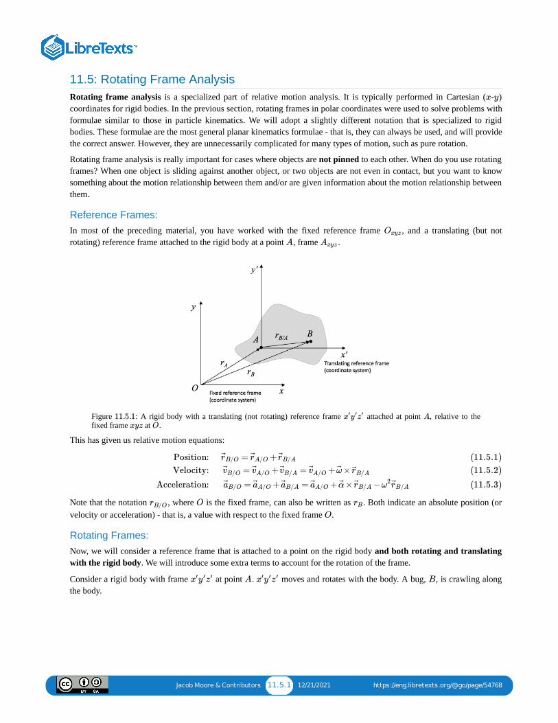
Jacob Moore & Contributors 11.5.1 12/21/2021 https://eng.libretexts.org/@go/page/54768

11.5: Rotating Frame AnalysisRotating frame analysis is a specialized part of relative motion analysis. It is typically performed in Cartesian ( - )coordinates for rigid bodies. In the previous section, rotating frames in polar coordinates were used to solve problems withformulae similar to those in particle kinematics. We will adopt a slightly different notation that is specialized to rigidbodies. These formulae are the most general planar kinematics formulae - that is, they can always be used, and will providethe correct answer. However, they are unnecessarily complicated for many types of motion, such as pure rotation.

Rotating frame analysis is really important for cases where objects are not pinned to each other. When do you use rotatingframes? When one object is sliding against another object, or two objects are not even in contact, but you want to knowsomething about the motion relationship between them and/or are given information about the motion relationship betweenthem.

Reference Frames:In most of the preceding material, you have worked with the fixed reference frame , and a translating (but notrotating) reference frame attached to the rigid body at a point , frame .

Figure : A rigid body with a translating (not rotating) reference frame attached at point , relative to thefixed frame at .

This has given us relative motion equations:

Note that the notation , where is the fixed frame, can also be written as . Both indicate an absolute position (orvelocity or acceleration) - that is, a value with respect to the fixed frame .

Rotating Frames:Now, we will consider a reference frame that is attached to a point on the rigid body and both rotating and translatingwith the rigid body. We will introduce some extra terms to account for the rotation of the frame.

Consider a rigid body with frame at point . moves and rotates with the body. A bug, , is crawling alongthe body.

x y

Oxyz

A Axyz

11.5.1 x′y′z′ Axyz O

Position:

Velocity:

Acceleration:

= +r  B/O r  A/O r  B/A

= + = + ×v  B/O v  A/O v  B/A v  A/O ω  r  B/A

= + = + × −a B/O a A/O a B/A a A/O α  r  B/A ω2r  B/A

(11.5.1)

(11.5.2)

(11.5.3)

rB/O O rB

O

x′y′z′ A x′y′z′ B

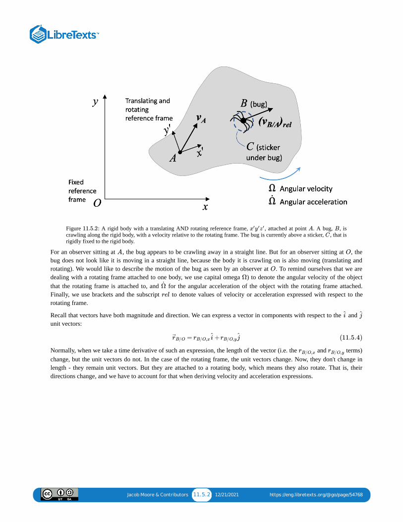
Jacob Moore & Contributors 11.5.2 12/21/2021 https://eng.libretexts.org/@go/page/54768

Figure : A rigid body with a translating AND rotating reference frame, , attached at point . A bug, , iscrawling along the rigid body, with a velocity relative to the rotating frame. The bug is currently above a sticker, , that isrigidly fixed to the rigid body.

For an observer sitting at , the bug appears to be crawling away in a straight line. But for an observer sitting at , thebug does not look like it is moving in a straight line, because the body it is crawling on is also moving (translating androtating). We would like to describe the motion of the bug as seen by an observer at . To remind ourselves that we aredealing with a rotating frame attached to one body, we use capital omega ) to denote the angular velocity of the objectthat the rotating frame is attached to, and for the angular acceleration of the object with the rotating frame attached.Finally, we use brackets and the subscript to denote values of velocity or acceleration expressed with respect to therotating frame.

Recall that vectors have both magnitude and direction. We can express a vector in components with respect to the and unit vectors:

Normally, when we take a time derivative of such an expression, the length of the vector (i.e. the and terms)change, but the unit vectors do not. In the case of the rotating frame, the unit vectors change. Now, they don't change inlength - they remain unit vectors. But they are attached to a rotating body, which means they also rotate. That is, theirdirections change, and we have to account for that when deriving velocity and acceleration expressions.

11.5.2 x′y′z′ A BC

A O

O

Ω

Ω

rel

i j

= +r  B/O rB/O,x i rB/O,y j (11.5.4)

rB/O,x rB/O,y

Jacob Moore & Contributors 11.5.3 12/21/2021 https://eng.libretexts.org/@go/page/54768

Figure : When the reference frame rotates with the rotating rigid body, the unit vectors change with time.

You can see we get small vectors and that describe the change in direction of the unit vectors, and the magnitude ofthat change is directly related to , the angular velocity of the rigid body and the rotating frame.

When we differentiate the relative position of the bug, , with respect to the rotating frame, , we have:

The new term above describes the motion of the bug due to the rotation of the rigid body (and the frame), while thefamiliar term above describes the motion of the bug as seen by an observer fixed to . Our final expression for thevelocity of the bug with respect to the fixed frame is:

This final expression has the new term, , which describes the motion of the bug as viewed from the rotatingframe. You can note that if the bug is not moving, , and we get the familiar expression from the translating,non-rotating frames. Thus, this expression is the most general relative velocity expression.

We can similarly derive an acceleration equation by differentiating the above velocity equation. The final expression is:

11.5.3

di′ dj′

Ω

= Ω × = Ωdi′

dtk i′ j′ (11.5.5)

= Ω × = −Ωdj′

dtk j′ i′ (11.5.6)

B A

= (   +   )+ ×(   +  )dr  B/A

dtrB/A, x′ i′ rB/A, y ′ j′ Ω  rB/A, x′ i′ rB/A, y ′j′ (11.5.7)

New term:

Same as before:

(   +   ) =rB/A, x′ i′ rB/A, y ′ j′ ( )v  B/A rel

×(   +   ) = ×Ω  rB/A, x′ i′ rB/A, y ′ j′ Ω  r  B/A

(11.5.8)

(11.5.9)

x′y′z′

x′y′z′

= + × +(v  B/O v  A/O Ω  r  B/A v  B/A)rel (11.5.10)

(v  B/A)rel( = 0v  B/A)rel

= + × + ×( × ) +2 ×( +(a B/O a A/O Ω ˙r  B/A Ω  Ω  r  B/A Ω  v  B/A)rel a B/A)rel (11.5.11)

Jacob Moore & Contributors 11.5.4 12/21/2021 https://eng.libretexts.org/@go/page/54768

Table : Physical correspondences of Equation components

Motion of rotating frame attached to rigid body:

Coriolis acceleration - interaction of object motion with respect torotating frame and motion of rotating frame:

Motion of object with respect to rotating frame:

Note that, for planar (2D) motion:

Again, if the bug is sitting still, both terms become zero (it is not moving with respect to the rigid body), and we areleft with the same relative motion expression used with translating frames. So, Equation is the most general formof the relative acceleration equation and can always be used.

When tackling these problems, there are several important things to remember:

1. You need to pick the correct body to attach the rotating frame to. The correct body will have another body slidingagainst it. If the object of interest is pinned to the body you chose, it might not be correct.

2. It is often helpful to align your rotating frame such that you end up with a simplified " " term or terms. For example,line up the axis with the direction of movement of the bug, so that is in the -direction.

3. The components of all terms of any one equation must be computed along the same and directions. If the framesare not aligned, you must pick ONE FRAME and express all terms along that the directions of the ONE FRAME. (Youmay be able to switch between frames in different equations, but make sure you are careful with notation!)

4. When you are given information in a problem, pay careful attention to what frame is being referred to.5. Make sure you include all the terms in the acceleration equation! It's easy to miss one. You should have five terms.

These are some of the most complex problems in planar kinematics, so take your time!

A camera drone, , flies over a car race in a curved trajectory (center ) with a constant ground-speed velocity of . At the moment shown, car is traveling with velocity of and an acceleration of as shown. Assume = \ 3 m\).

Find the velocity of the car as observed by the camera on drone D at this instant.Find the acceleration of the car as observed by the camera on drone D at this instant.

11.5.1 11.5.11

+ × + × ( × )a A/O Ω ˙r  B/A Ω  Ω  r  B/A

2 × (Ω  v  B/A)rel

(a B/A)rel

×( × ) = −Ω  Ω  r  B/A Ω2r  B/A (11.5.12)

rel

11.5.11

rel

x′ (v  B/A)rel x′

i j

Exercise 11.5.1

D O

= 9 m/svD C = 12 m/svc= 2 m/ac s2 = 7.5 m,  d1 d2

Jacob Moore & Contributors 11.5.5 12/21/2021 https://eng.libretexts.org/@go/page/54768

Figure : problem diagram for Example . A drone tracing a circular path around point is currentlystraight to the right of a car, with the velocity and acceleration vectors of the two vehicles pointing in the samedirection.

Solution

Video : Worked solution to example problem , provided by Dr. Jacob Moore. YouTube source:https://youtu.be/nqs7bLBVm3g.

A breathing exercise video graphic (somewhat similar to this one) shows a small circle moving in a constrainedcircular path (constant radius 80 cm) at a constant angular velocity of 0.4 rad/s around an expanding and contractinginner circle. The inner circle expands and contracts sinusoidally, from a minimum radius of 30 cm to a maximumradius of 60 cm. The distance from the center of the inner circle to a point on the edge of the inner circle can bedescribed by the equation , where is in meters and is the position of the small circle (zero atthe -axis).

Find the velocity and acceleration of point B on the edge of the inner circle as viewed by an observer on the smallcircle at point (see part C of the figure below). °, °

11.5.4 11.5.1 O

Rot Frame WP002Rot Frame WP002

11.5.1 11.5.1

Example 11.5.2

r = 0.45 −0.15 sin(θ) r θ

x

A θ = 45 α = 45

Jacob Moore & Contributors 11.5.6 12/21/2021 https://eng.libretexts.org/@go/page/54768

Figure : problem diagram for Example . A large circular outline rotates at a constant rate, changing thelocation of a small circle attached to it, while an inner circle concentric with the outline expands and contracts inradius.

Solution

Video : Worked solution to example problem , provided by Dr. Jacob Moore. YouTube source:https://youtu.be/mL0PVJNnOBE.

11.5.5 11.5.2

Rot Frame WP003Rot Frame WP003

11.5.2 11.5.2

Jacob Moore & Contributors 11.6.1 12/21/2021 https://eng.libretexts.org/@go/page/54779

11.6: Chapter 11 Homework Problems

You are designing a bench grinder with an operating speed of 3600 rpm.

If you want the grinder to reach its full operating speed in 4 seconds, what must the rate of angular acceleration bein radians per second squared?If the grinding wheel has a diameter of 8 inches, what will the speed of the surface of the wheel be?

Figure : A bench grinder.

Solution

A belt-driven system has an input at pulley A, which drives pulley B, which is attached with a solid shaft to pulley C,which drives pulley D. If the input is rotating at 60 rad/s counterclockwise, determine the angular velocity anddirection of rotation for the output at D.

Figure : problem diagram for Exercise . A four-pulley system in which A and B are attached by a belt, Cand D are attached by another belt, and B and C are mounted on the same shaft.

Solution

counterclockwise

The piston in a piston and crank mechanism has the velocity and acceleration shown below. Using absolute motionanalysis, determine the current angular velocity and angular acceleration for the crank.

Exercise 11.6.1

11.6.1

α = 94.25  rads

v= 125.67 ft/s

Exercise 11.6.2

11.6.2 11.6.2

= 300 ωDrads

Exercise 11.6.3

Jacob Moore & Contributors 11.6.2 12/21/2021 https://eng.libretexts.org/@go/page/54779

Figure : problem diagram for Exercise . A piston descends, causing the crank mounted on a fixed axlebelow it to rotate due to the bar that connects the piston and the crank.

Solution

clockwise

clockwise

A trapdoor is being opened with a hydraulic cylinder extending at constant rate of 0.7 m/s. If the door is currently at atwenty-degree angle as shown below, what is the current angular velocity and angular acceleration for the door?

Figure : problem diagram for Exercise . Side view of a trapdoor being raised by the extension of ahydraulic cylinder that has one end attached to the door and the other fixed to a point on the ground.

Solution

A robotic arm experiences the angular velocities and accelerations shown below. Based on this information, determinethe velocity and the acceleration of the end of the arm in the and directions.

11.6.3 11.6.3

ω = 13.33  rads

α = 100.16  rads2

Exercise 11.6.4

11.6.4 11.6.4

= 0.896  , = −1.246 θ rad

sθ rad

s2

Exercise 11.6.5

x y

Jacob Moore & Contributors 11.6.3 12/21/2021 https://eng.libretexts.org/@go/page/54779

Figure : problem diagram for Exercise . A two-member robotic arm attached to a fixed base experiencesrotation from two motors located at the joints.

Solution

11.6.5 11.6.5

= 9.44 ft/s, = 4.39 ft/svx vy

= −33.78 ft/ , = 3.39 ft/ax s2 ay s2

1 1/30/2022

CHAPTER OVERVIEW12: NEWTON'S SECOND LAW FOR RIGID BODIESAnalysis of rigid bodies, as opposed to particles, undergoing translation, rotation, and general planar motion.

12.1: RIGID BODY TRANSLATIONIntroduction to analysis of rigid body motion; the difference between dynamics analysis and the static analysis covered in previouschapters. Analysis of translational motion for rigid bodies. Includes a worked example.

12.2: FIXED-AXIS ROTATIONAnalysis of fixed-axis rotation, both balanced and unbalanced, for rigid bodies. Includes worked examples.

12.3: RIGID-BODY GENERAL PLANAR MOTIONAnalysis of a rigid body undergoing general planar motion, incorporating both translation and rotation. Includes worked examples.

12.4: MULTI-BODY GENERAL PLANAR MOTIONAnalysis of general planar motion for systems of multiple rigid bodies. Includes a worked example.

12.5: CHAPTER 12 HOMEWORK PROBLEMS

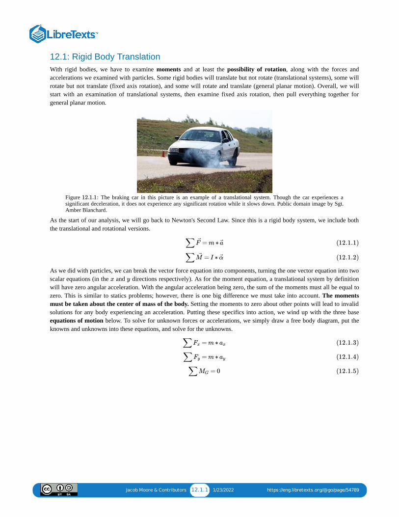
Jacob Moore & Contributors 12.1.1 1/23/2022 https://eng.libretexts.org/@go/page/54789

12.1: Rigid Body TranslationWith rigid bodies, we have to examine moments and at least the possibility of rotation, along with the forces andaccelerations we examined with particles. Some rigid bodies will translate but not rotate (translational systems), some willrotate but not translate (fixed axis rotation), and some will rotate and translate (general planar motion). Overall, we willstart with an examination of translational systems, then examine fixed axis rotation, then pull everything together forgeneral planar motion.

Figure : The braking car in this picture is an example of a translational system. Though the car experiences asignificant deceleration, it does not experience any significant rotation while it slows down. Public domain image by Sgt.Amber Blanchard.

As the start of our analysis, we will go back to Newton's Second Law. Since this is a rigid body system, we include boththe translational and rotational versions.

As we did with particles, we can break the vector force equation into components, turning the one vector equation into twoscalar equations (in the and directions respectively). As for the moment equation, a translational system by definitionwill have zero angular acceleration. With the angular acceleration being zero, the sum of the moments must all be equal tozero. This is similar to statics problems; however, there is one big difference we must take into account. The momentsmust be taken about the center of mass of the body. Setting the moments to zero about other points will lead to invalidsolutions for any body experiencing an acceleration. Putting these specifics into action, we wind up with the three baseequations of motion below. To solve for unknown forces or accelerations, we simply draw a free body diagram, put theknowns and unknowns into these equations, and solve for the unknowns.

12.1.1

∑ = m ∗F   a  (12.1.1)

∑ = I ∗M  α  (12.1.2)

x y

∑ = m ∗Fx ax (12.1.3)

∑ = m ∗Fy ay (12.1.4)

∑ = 0MG (12.1.5)

Jacob Moore & Contributors 12.1.2 1/23/2022 https://eng.libretexts.org/@go/page/54789

Video lecture covering this section, delivered by Dr. Jacob Moore. YouTube source: https://youtu.be/V4Gy-tyHupE.

A refrigerator is 2.5 feet wide and 6 feet tall, and weighs 80 lbs. The center of mass is 1.25 feet from either side and 2feet up from the base. If the refrigerator is on a conveyor belt that is accelerating the fridge at a rate of 1 ft/s , what arethe normal forces at each of the feet?

Figure : problem diagram for Example . A refridgerator of the dimensions described above is on aconveyor belt that accelerates the fridge to the right at a rate of 1 ft/s .

Solution

Video : Worked solution to example problem , provided by Dr. Majid Chatsaz. YouTube source:https://youtu.be/59GRMn_ZvJk.

12.1 Translational System Kinetics - 12.1 Translational System Kinetics - ……

Example 12.1.1

2

12.1.2 12.1.12

WP12 1 1 MRCWP12 1 1 MRC

12.1.2 12.1.1

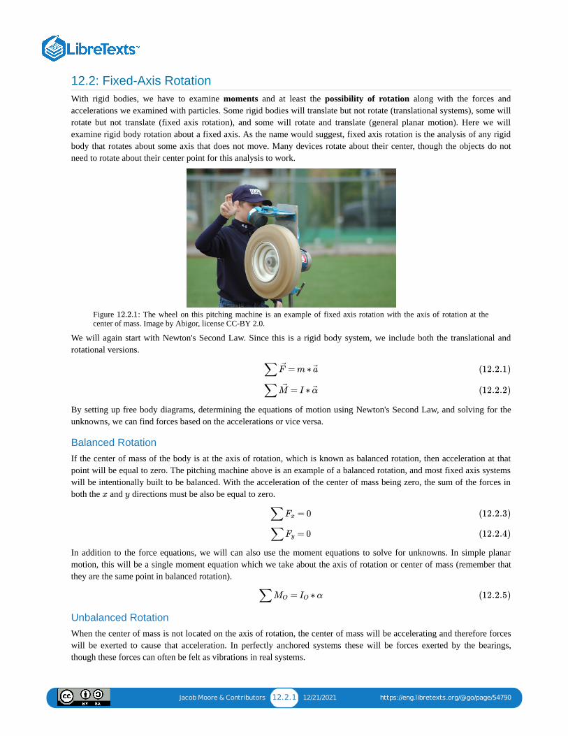
Jacob Moore & Contributors 12.2.1 12/21/2021 https://eng.libretexts.org/@go/page/54790

12.2: Fixed-Axis RotationWith rigid bodies, we have to examine moments and at least the possibility of rotation along with the forces andaccelerations we examined with particles. Some rigid bodies will translate but not rotate (translational systems), some willrotate but not translate (fixed axis rotation), and some will rotate and translate (general planar motion). Here we willexamine rigid body rotation about a fixed axis. As the name would suggest, fixed axis rotation is the analysis of any rigidbody that rotates about some axis that does not move. Many devices rotate about their center, though the objects do notneed to rotate about their center point for this analysis to work.

Figure : The wheel on this pitching machine is an example of fixed axis rotation with the axis of rotation at thecenter of mass. Image by Abigor, license CC-BY 2.0.

We will again start with Newton's Second Law. Since this is a rigid body system, we include both the translational androtational versions.

By setting up free body diagrams, determining the equations of motion using Newton's Second Law, and solving for theunknowns, we can find forces based on the accelerations or vice versa.

Balanced RotationIf the center of mass of the body is at the axis of rotation, which is known as balanced rotation, then acceleration at thatpoint will be equal to zero. The pitching machine above is an example of a balanced rotation, and most fixed axis systemswill be intentionally built to be balanced. With the acceleration of the center of mass being zero, the sum of the forces inboth the and directions must be also be equal to zero.

In addition to the force equations, we will can also use the moment equations to solve for unknowns. In simple planarmotion, this will be a single moment equation which we take about the axis of rotation or center of mass (remember thatthey are the same point in balanced rotation).

Unbalanced RotationWhen the center of mass is not located on the axis of rotation, the center of mass will be accelerating and therefore forceswill be exerted to cause that acceleration. In perfectly anchored systems these will be forces exerted by the bearings,though these forces can often be felt as vibrations in real systems.

12.2.1

∑ = m ∗F   a  (12.2.1)

∑ = I ∗M  α  (12.2.2)

x y

∑ = 0Fx (12.2.3)

∑ = 0Fy (12.2.4)

∑ = ∗ αMO IO (12.2.5)

Jacob Moore & Contributors 12.2.2 12/21/2021 https://eng.libretexts.org/@go/page/54790

Figure : Many video game controllers use motors to rotate the small masses where the center of mass is not at theaxis of rotation. This unbalanced rotation results in forces (felt as vibrations) needed to accelerate the center of mass of thespinning masses. Image by unknown author under a CC0 license.

The kinematics equations discussed in the previous chapter can be used to determine the acceleration of a point on arotating body, that point being the center of mass in this case. After determining those accelerations, they can be put intoforce equations, most likely using the and directions.

Note that as the body rotates, the direction of the acceleration and the direction of the forces change. Also note that thefurther the center of mass is from the axis of rotation, the larger the mass. The larger the angular velocity, the larger theseforces will be.

To supplement the force equations, we can use a moment equation about either the axis of rotation or the center of mass, asthese are no longer the same point. Whichever is chosen, just be sure to be consistent in taking the moments and the massmoment of inertia about the same point.

More information on how to calculate the mass moment of inertia for a body can be found in Appendix 2.

Video lecture covering this section, delivered by Dr. Jacob Moore. YouTube source: https://youtu.be/EGmfwhYbRew.

A hard drive platter 8 cm in diameter accelerates at a constant rate of 150 rad/s . If the hard drive weighs a uniformlydistributed 0.05 kg and we approximate the hard drive as a flat circular disc, what moment does the motor need toexert to accelerate the drive at this rate?

12.2.2

r θ

∑ = mFr ar (12.2.6)

∑ = mFθ aθ (12.2.7)

∑ = ∗ α or ∑ = ∗ αMO IO MG IG (12.2.8)

12.2 Fixed Axis Rotation Kinetics - Vi12.2 Fixed Axis Rotation Kinetics - Vi……

Example 12.2.1

2

Jacob Moore & Contributors 12.2.3 12/21/2021 https://eng.libretexts.org/@go/page/54790

Figure : A picture of a hard drive that emphasizes the flat circular platter.

Solution

Video : Worked solution to example problem , provided by Dr. Majid Chatsaz. YouTube source:https://youtu.be/grJ8WYsGitw.

The drum in a washing machine can be approximated as a cylinder 0.4 meters in diameter and 0.3 meters in heightwith a uniformly distributed mass of 35 kilograms when full. If we wish to achieve an acceleration of 15 rad/s , whattorque must the motor exert at the center of the drum?

Figure : problem diagram for Example . A front-loading washing machine, and an approximation of themachine's drum as a cylinder rotated about its axis by the motor.

Solution

12.2.3

WP12 2 1 MRCWP12 2 1 MRC

12.2.2 12.2.1

Example 12.2.2

2

12.2.4 12.2.2

Jacob Moore & Contributors 12.2.4 12/21/2021 https://eng.libretexts.org/@go/page/54790

Video : Worked solution to example problem , provided by Dr. Majid Chatsaz. YouTube source:https://youtu.be/7G7HnwsyLXk.

WP12 2 2 MRCWP12 2 2 MRC

12.2.3 12.2.2

Jacob Moore & Contributors 12.3.1 1/26/2022 https://eng.libretexts.org/@go/page/54795

12.3: Rigid-Body General Planar MotionIn general planar motion, bodies are both rotating and translating at the same time. As a result, we will need to relate theforces to the acceleration of the center of mass of the body as well as relating the moments to the angular accelerations.

Figure : This tire being rolled along the ground is an example of general planar motion. The tire is both translatingand rotating as it is pushed along. Image by Joy Agyepong, CC-BY-SA 4.0.

To analyze a body undergoing general planar motion, we will start by drawing a free body diagram of the body in motion.Be sure to identify the center of mass, as well as identifying all known and unknown forces, and known and unknownmoments acting on the body. It is also sometimes helpful to label any key dimensions as well as using dashed lines toidentify any known accelerations or angular accelerations.

Next, we move on to identifying the equations of motion. At its core, this means going back to Newton's Second Law.Since this is a rigid body system, we include both the translational and rotational versions.

As we did with the previous translational systems, we will break the force equation into components, turning the onevector equation into two scalar equations. Additionally, it's important to always use the center of mass for the accelerationsin our force equations and take the moments and moment of inertia about the center of mass for our moment equation.

Plugging the known forces, moments, and accelerations into the above equations, we can solve for up to three unknowns.If more than three unknowns exist in the equations, we will sometimes have to go back to kinematics to relate quantitiessuch as acceleration and angular acceleration.

12.3.1

∑ = m ∗F   a  (12.3.1)

∑ = I ∗M  α  (12.3.2)

∑ = m ∗Fx ax (12.3.3)

∑ = m ∗Fy ay (12.3.4)

∑ = I ∗ αMCOM (12.3.5)

Jacob Moore & Contributors 12.3.2 1/26/2022 https://eng.libretexts.org/@go/page/54795

Video lecture covering this section, delivered by Dr. Jacob Moore. YouTube source: https://youtu.be/jhVDM7Zw_LM.

A cylinder with a radius of 0.15 m and a mass of 10 kg is placed on a ramp at a 20-degree angle. If the cylinder isreleased from rest and rolls without slipping, what is the initial angular acceleration of the cylinder and the timerequired for the cylinder to roll 5 meters?

Figure : problem diagram for Example . A uniform cylinder rolls down a ramp that has a 20° incline.

Solution

Video : Worked solution to example problem , provided by Dr. Majid Chatsaz. YouTube source:https://youtu.be/oQFVVC3SzZ0.

12.3 General Planar Motion - Video L12.3 General Planar Motion - Video L……

Example 12.3.1

12.3.2 12.3.1

WP12 3 1 MRCWP12 3 1 MRC

12.3.2 12.3.1

Jacob Moore & Contributors 12.3.3 1/26/2022 https://eng.libretexts.org/@go/page/54795

The cable spool shown below has a weight of 50 lbs and has a moment of inertia of 0.28 slug-ft . Assume the spoolrolls without slipping when we apply a 50-lb tension in the cable.

What is the friction force between the spool and the ground?What is the acceleration of the center of mass of the spool?

Figure : problem diagram for Example . A cable spool, consisting of a central cylinder the cable wrapsaround sandwiched between two larger disks at its bases, is pulled to the right by a tension force on the free end of thecable. Spool image by Seeweb, CC-BY-SA 2.0.

Solution

Video : Worked solution to example problem , provided by Dr. Majid Chatsaz. YouTube source:https://youtu.be/RAhLP-kMYaQ.

You are designing a Frisbee launcher to launch a 40-cm-diameter, 0.6 kg Frisbee that can be modeled as flat circulardisc. If you want the Frisbee to have a linear acceleration of 20 m/s and an angular acceleration of 50 rad/s as shownbelow, what should and be?

Example 12.3.2

2

12.3.3 12.3.2

WP12 3 2 MRCWP12 3 2 MRC

12.3.3 12.3.2

Example 12.3.3

2 2

F1 F2

Jacob Moore & Contributors 12.3.4 1/26/2022 https://eng.libretexts.org/@go/page/54795

Figure : problem diagram for Example . A Frisbee, represented as a circle, accelerates both linearly andangularly as a result of experiencing two forces applied in the same direction at locations on opposite sides of adiameter.

Solution

Video : Worked solution to example problem , provided by Dr. Majid Chatsaz. YouTube source:https://youtu.be/DY9B7oU0j7k.

A pickup truck is carrying a 30-kg, 6-meter-long ladder at a 35-degree angle as shown below. The ladder is wedgedagainst the tailgate at A and makes contact with the roof of the truck at B. The distance from A to B is 2 meters. Atwhat rate of acceleration would we expect the ladder to start to rotate upwards?

12.3.4 12.3.3

WP12 3 3 MRCWP12 3 3 MRC

12.3.4 12.3.3

Example 12.3.4

Jacob Moore & Contributors 12.3.5 1/26/2022 https://eng.libretexts.org/@go/page/54795

Figure : problem diagram for Example . A moving pickup truck carries a ladder that leans forward, withits lower end propped against the tailgate.

Solution

Video : Worked solution to example problem , provided by Dr. Majid Chatsaz. YouTube source:https://youtu.be/UO5XsDFxQoY.

12.3.5 12.3.4

WP12 3 4 MRCWP12 3 4 MRC

12.3.5 12.3.4

Jacob Moore & Contributors 12.4.1 1/23/2022 https://eng.libretexts.org/@go/page/54796

12.4: Multi-Body General Planar MotionIn cases where multiple connected rigid bodies are undergoing some sort of motion, we can extend our analysis of generalplanar motion to this multi-body situation. In these cases, which we will call multi-body kinetics problems, we will analyzeeach body independently as we did for general planar motion, but we will also need to pay attention to the Newton's ThirdLaw pairs. Each body will have forces exerted on it by the surrounding bodies, and it will exert equal and opposite forcesback through those same connections.

Figure : These robotic arms are a good example of a multi-body kinetics problem. As one section of the armaccelerates, it will exert forces on the other arm sections it is connected to. Image by Chris Chesher, CC-BY-NC-SA 2.0.

To analyze a multi-body system, we will start by drawing a free body diagram of each body in motion. Be sure to identifythe center of mass, as well as identifying all known and unknown forces, and known and unknown moments acting on thebody. When drawing forces at connection points, be sure to make the forces equal and opposite on the connected body tosatisfy Newton's Third Law. It is also sometimes helpful to label any key dimensions as well as using dashed lines toidentify any known accelerations or angular accelerations. Often, you will need to solve a kinematics problem usingabsolute motion analysis or relative motion analysis in order to determine the accelerations of the centers of mass and theangular accelerations for each body. Make sure all these accelerations are with respect to ground.

Next we move onto identifying the equations of motion for each body in the system. In two dimensions, we will use thesame three equations we used for general planar motion. Be sure to find the the accelerations of all the centers of masses,find all moments about the center of mass, and take the mass moments of inertia about the center of mass of each body.

Plugging the known forces, moments, and accelerations into the above equations we can solve for up to three unknownsper body. If more than three unknowns exist in any one set of equations, you will need to start with an adjacent body. Onceunknown forces are determined on one body, they can become knowns on the connected body, reducing the number ofunknowns to solve for.

12.4.1

∑ = m ∗Fx ax (12.4.1)

∑ = m ∗Fy ay (12.4.2)

∑ = ∗ αMG IG (12.4.3)

Jacob Moore & Contributors 12.4.2 1/23/2022 https://eng.libretexts.org/@go/page/54796

Video lecture covering this section, delivered by Dr. Jacob Moore. YouTube source: https://youtu.be/-tAP08srNrU.

A robotic arm has two sections (OA and AB), with section OA having a mass of 10 kg and section AB having a massof 7 kg. Treat each section as a slender rod. If we wish to accelerate member AB from a standstill at a rate of 3 rad/s²and keep the left section stationary, what moments must we exert at joints O and A?

Figure : problem diagram for Example . A robotic arm consists of two segments that are currentlyhorizontal, with the left end of the left segment being attached to a base and the right segment undergoing angularacceleration.

Solution

Video : Worked solution to example problem , provided by Dr. Majid Chatsaz. YouTube source:https://youtu.be/zR_uhVM1uH0.

12.4 Multi-Body Kinetics - Video Lect12.4 Multi-Body Kinetics - Video Lect……

Example 12.4.1

12.4.2 12.4.1

WP12 4 1 MRCWP12 4 1 MRC

12.4.2 12.4.1

Jacob Moore & Contributors 12.5.1 1/30/2022 https://eng.libretexts.org/@go/page/54797

12.5: Chapter 12 Homework Problems

The SUV shown below has an initial velocity of 90 ft/s. It slams on its brakes, coming to a stop over a distance of 300feet. If the car has a weight of 3500 lbs and a center of mass as shown below, what are the normal forces at the frontwheels? What are the normal forces at the back wheels?

Figure : problem diagram for Exercise . A car traveling in a straight line applies its brakes, coming to agradual stop.

Solution

A ring-shaped space station can be approximated as a thin ring 60 meters in diameter with a mass of 500,000 kg. Thespace station has a set of thrusters able to exert equal and opposite forces as shown below. If we want to cause anangular acceleration of 0.1 rad/s² in the space station, what is the force required from each thruster?

Figure : problem diagram for Exercise . A ring-shaped space station is given the specified angularacceleration through the firing of two thrusters located on either side of a diameter, pointing in opposite directions.

Solution

Exercise 12.5.1

12.5.1 12.5.1

= 1291.4 lbsFNrear

= 2208.6 lbsFNfront

Exercise 12.5.2

12.5.2 12.5.2

= 750 kNFthruster

Jacob Moore & Contributors 12.5.2 1/30/2022 https://eng.libretexts.org/@go/page/54797

A 50-kg barrel with a diameter of 0.75 meters is placed on a 20-degree slope. Assuming the barrel rolls withoutslipping, what will the acceleration of the barrel's center of mass be?

Figure : problem diagram for Exercise . A 50-kg barrel with a 0.75-meter diameter rolls down a 20°incline without slipping.

Solution

A 3-meter-long, 25-kg beam is supported by two cables as shown below. You can treat the beam as a slender rod.Assume that we want the left end of the beam at point A to remain at a constant height while the right end of the beamat point B accelerates upwards at a rate of 1 m/s².

What is the rate of acceleration of the center of the beam and the rate of angular acceleration for the beam?What will and need to be to achieve these accelerations?

Figure : problem diagram for Exercise . A horizontal beam is held in the air by the tension forces fromtwo vertical cables attached near the beam's ends.

Solution

You are modeling the robotic arm shown below. Treat each section of the arm as a slender rod. Section OA weighs 30lbs and section AB weighs 18 lbs. If we want the relative angular accelerations and velocities shown below, whatshould the motor torques be at O and A? (This is a top-down view of the robot arm.)

Exercise 12.5.3

12.5.3 12.5.3

= 2.24 m/ax s2

Exercise 12.5.4

T1 T2

12.5.4 12.5.4

= 0.5 m/ , α = 0.333 aC\y s2 rads

= 81.75 N , = 176 NT1 T2

Exercise 12.5.5

Jacob Moore & Contributors 12.5.3 1/30/2022 https://eng.libretexts.org/@go/page/54797

Figure : problem diagram for Exercise . Top-down view of a two-segment robotic arm with one endattached to a fixed base, with motors at the two joints providing rotation.

Solution

-

-

12.5.5 12.5.5

= −3.9 ftMO lbs

= −19.3 ftMA lbs

1 1/30/2022

CHAPTER OVERVIEW13: WORK AND ENERGY IN RIGID BODIESDiscussion of work and energy in rigid bodies as opposed to particles, including rotational work and kinetic energy. Analysis of rigidbody systems through the method of conservation of energy.

13.1: CONSERVATION OF ENERGY FOR RIGID BODIESUsing the energy conservation method to analyze kinetics problems involving rigid bodies. In addition to material previously coveredin energy conservation for particles, includes discussion of rotational work, rotational kinetic energy, and torsional springs. Includesworked examples.

13.2: POWER AND EFFICIENCY IN RIGID BODIESRelation of the concepts of work and energy to the concepts of power and efficiency for rigid bodies. Includes a worked example.

13.3: CHAPTER 13 HOMEWORK PROBLEMS

Jacob Moore & Contributors 13.1.1 12/21/2021 https://eng.libretexts.org/@go/page/54803

13.1: Conservation of Energy for Rigid BodiesThe concepts of Work and Energy provide the basis for solving a variety of kinetics problems. Generally, this method iscalled the Energy Method or the Conservation of Energy, and it can be boiled down to the idea that the work done to abody will be equal to the change in energy of that body. Dividing energy into kinetic and potential energy pieces as weoften do in dynamics problems, we arrive at the following base equation for the conservation of energy.

It is important to notice that unlike Newton's Second Law, the above equation is not a vector equation. It does not need tobe broken down into components which can simplify the process. However, we only have a single equation and thereforecan only solve for a single unknown, which can limit this method.

Work in Rigid Body Problems:

For work done to a rigid body, we must consider any force applied over a distance as we did for particles, as well as anymoment exerted over some angle of rotation. If these are constant forces and constant moments, we simply multiple theforce times the distance and the moment times the angle of rotation to find the overall work done in the problem. As withparticles, these are the components of forces in the direction of travel, with forces opposing the motion counting asnegative work. Similarly, these are moments in the direction of rotation, with moments opposing the rotation counting asnegative work. Both types of work are additive, with all work being lumped together for analysis.

In instances of non-constant forces and non-constant moments, we will need to integrate the forces and moments overthe distance traveled and the angle of rotation, respectively.

Energy:In rigid bodies, as with particles, we will break energy into kinetic energy and potential energy. Kinetic energy is the theenergy mass in motion, while potential energy represents the energy that is stored up due to the position or stresses in abody.

In its equation form, the kinetic energy of a rigid body is represented by one-half of the mass of the body times its velocitysquared, plus one-half of the mass moment of inertia times the angular velocity squared. If we wish to determine thechange in kinetic energy, we would simply take the final kinetic energy minus the initial kinetic energy.

Potential energy, unlike kinetic energy, is not really energy at all. Instead, it represents the work that a given force willpotentially do between two instants in time. Potential energy can come in many forms, but the two we will discuss here aregravitational potential energy and elastic potential energy. These represent the work that the gravitational force and aspring force will do, respectively. We often use these potential energy terms in place of the work done by gravity or springsrespectively. When including these potential energy terms, it's important to not also include the work done by gravity orspring forces.

The change in gravitational potential energy for any system is represented by the mass of the body, times the value (9.81m/s or 32.2 ft/s on the earth's surface), times the vertical change in height between the start position and the end position.In equation form, this is as follows.

W = ΔKE+ΔPE (13.1.1)

W = F ∗ d+M ∗ Δθ (13.1.2)

W = F (x)dx+ M(θ)dθ∫

x1

x2

∫

θ1

θ2

(13.1.3)

KE = m + I1

2v2 1

2ω2 (13.1.4)

ΔKE =( m − m )+( I − I )1

2v2f

1

2v2i

1

2ω2f

1

2ω2i (13.1.5)

g2 2

ΔPE = m ∗ g∗ Δh (13.1.6)

Jacob Moore & Contributors 13.1.2 12/21/2021 https://eng.libretexts.org/@go/page/54803

Figure : When finding the change in gravitational potential energy, we multiply the object's mass by (giving us theweight of the object) and then multiply that by the change in the height of the object, regardless of the path taken.

Unlike work and kinetic energy, there is no rotational version of gravitational potential energy, so this is exactly the sameas we had for particles.

To determine the change in elastic potential energy, we will have to identify any linear springs (as we had for particles), aswell as any torsional springs and the spring constants for each of these springs.

Figure : The torsional spring in this mousetrap releases its elastic potential energy to slam the trap shut. Publicdomain image by Evan-Amos.

To find the change in elastic potential energy, we will need to know the stiffness of any spring in the problem (representedby , in units of force per distance for linear springs or moment per angle of twist for torsional springs) as well as thedistance or angle the spring has been stretched above or below its natural resting position. This difference from restingposition is represented by distance for linear springs, or angle for torsional springs. Once we have those values, theelastic potential energy can be calculated by multiplying one-half of the stiffness by the distance squared or the angle squared. To find the change in elastic potential energy, we simply take the final elastic potential energy minus the initialelastic potential energy.

Going back to our original conservation of energy equation, we simply plug the appropriate terms on each side (work onthe left and energies on the right) and balance the two sides to solve for any unknowns. Terms that do not exist or do notchange (such as elastic potential energy in a problem with no springs, or in a problem where there is no change inthe speed of the body) can be set to zero. Again, there is only one equation, so we can only solve for a single unknownunless we supplement the conservation of energy equation with other relationship equations.

13.1.1 g

13.1.2

k

x θ

x θ

ΔP = k  − k Elinear spring1

2x2f

1

2x2i (13.1.7)

ΔP = k  − k Etorsional spring1

2θ2f

1

2θ2i (13.1.8)

ΔKE

Jacob Moore & Contributors 13.1.3 12/21/2021 https://eng.libretexts.org/@go/page/54803

Video lecture covering this section, delivered by Dr. Jacob Moore. YouTube source: https://youtu.be/YVkzjzHSW-g.

The turntable on a record player consists of a disk 12 inches in diameter with a weight of 5 lbs. The motor acceleratesthe turntable from rest to its operating speed of 33.33 rpm in one rotation. What is the work done by the motor? Whatis the average torque the motor exerted?

Figure : A turntable on a record player. Image by Ron Clausen, CC-BY-SA 4.0.

Solution

Video : Worked solution to example problem , provided by Dr. Majid Chatsaz. YouTube source:https://youtu.be/UPHgU-o80Q0.

A system as shown below is used to passively slow the lowering of a gate. The gate can be approximated as a flat plateon its edge with a mass of 25 kilograms and a height of 2 meters. Assume the spring is unstretched as shown in thediagram.

What would the angular velocity of the gate be without the spring?

13.1 Work and Energy in Rigid Body 13.1 Work and Energy in Rigid Body ……

Example 13.1.1

13.1.3

13.1.2 13.1.1

Example 13.1.2

Jacob Moore & Contributors 13.1.4 12/21/2021 https://eng.libretexts.org/@go/page/54803

If we want to reduce the angular velocity at the bottom to 25% of its original value, what should the spring constantbe?

Figure : problem diagram for Example . Top-down view of a hinged gate in a currently open position,attached by a spring to a wall running parallel to it that will slow the gate's motion as it swings shut.

Solution

Video : Worked solution to example problem , provided by Dr. Majid Chatsaz. YouTube source:https://youtu.be/HCAC0tNR18w.

A 5-kilogram spherical ball with a radius of 0.05 meters is placed on a ramp as shown below. If the ball rolls withoutslipping, what is the velocity of the ball at the bottom of the ramp?

Figure : problem diagram for Example . A spherical ball is placed at the top of a ramp, 0.1 meters abovethe ground, and rolls without slipping.

Solution

13.1.4 13.1.2

WP13 1 2 MRCWP13 1 2 MRC

13.1.3 13.1.2

Example 13.1.3

13.1.5 13.1.3

Jacob Moore & Contributors 13.1.5 12/21/2021 https://eng.libretexts.org/@go/page/54803

Video : Worked solution to example problem , provided by Dr. Majid Chatsaz. YouTube source:https://youtu.be/p2pvQ0kCWIU.

A 16-kilogram half-cylinder is placed on a hard, flat surface as shown below and released from rest. What will themaximum angular velocity be as it rocks back and forth?

Figure : problem diagram for Example . A cylinder 50 cm in diameter is sliced in half lengthwise, thenbalanced on a flat, hard surface so that only one of its long, straight edges is in contact with said surface.

Solution

Video : Worked solution to example problem , provided by Dr. Majid Chatsaz. YouTube source:https://youtu.be/HpRtDQjoEBA.

WP13 1 3 MRCWP13 1 3 MRC

13.1.4 13.1.3

Example 13.1.4

13.1.6 13.1.4

WP13 1 4 MRCWP13 1 4 MRC

13.1.5 13.1.4

Jacob Moore & Contributors 13.1.6 12/21/2021 https://eng.libretexts.org/@go/page/54803

A mechanism consists of two 3-kilogram wheels connected to a 2-kilogram bar as shown below. Based on thedimensions in the diagram, what is the minimum required initial velocity for the wheels to ensure the mechanismmakes it all the way through one rotation without rocking backwards?

Figure : problem diagram for Example . A pair of wheels is connected by a bar of fixed length,constraining them to roll together.

Solution

Video : Worked solution to example problem , provided by Dr. Majid Chatsaz. YouTube source:https://youtu.be/8cjQ1S6yOTc.

Example 13.1.5

13.1.7 13.1.5

WP13 1 5 MRCWP13 1 5 MRC

13.1.6 13.1.5

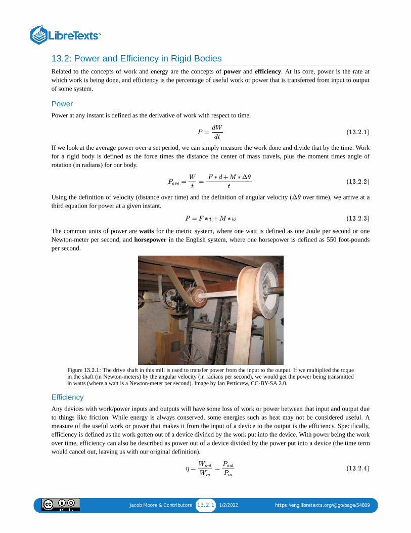
Jacob Moore & Contributors 13.2.1 1/2/2022 https://eng.libretexts.org/@go/page/54809

13.2: Power and Efficiency in Rigid BodiesRelated to the concepts of work and energy are the concepts of power and efficiency. At its core, power is the rate atwhich work is being done, and efficiency is the percentage of useful work or power that is transferred from input to outputof some system.

PowerPower at any instant is defined as the derivative of work with respect to time.

If we look at the average power over a set period, we can simply measure the work done and divide that by the time. Workfor a rigid body is defined as the force times the distance the center of mass travels, plus the moment times angle ofrotation (in radians) for our body.

Using the definition of velocity (distance over time) and the definition of angular velocity ( over time), we arrive at athird equation for power at a given instant.

The common units of power are watts for the metric system, where one watt is defined as one Joule per second or oneNewton-meter per second, and horsepower in the English system, where one horsepower is defined as 550 foot-poundsper second.

Figure : The drive shaft in this mill is used to transfer power from the input to the output. If we multiplied the toquein the shaft (in Newton-meters) by the angular velocity (in radians per second), we would get the power being transmittedin watts (where a watt is a Newton-meter per second). Image by Ian Petticrew, CC-BY-SA 2.0.

EfficiencyAny devices with work/power inputs and outputs will have some loss of work or power between that input and output dueto things like friction. While energy is always conserved, some energies such as heat may not be considered useful. Ameasure of the useful work or power that makes it from the input of a device to the output is the efficiency. Specifically,efficiency is defined as the work gotten out of a device divided by the work put into the device. With power being the workover time, efficiency can also be described as power out of a device divided by the power put into a device (the time termwould cancel out, leaving us with our original definition).

P =dW

dt(13.2.1)

= =Pave

W

t

F ∗ d+M ∗ Δθ

t(13.2.2)

Δθ

P = F ∗ v+M ∗ω (13.2.3)

13.2.1

η = =Wout

Win

Pout

Pin

(13.2.4)

Jacob Moore & Contributors 13.2.2 1/2/2022 https://eng.libretexts.org/@go/page/54809

It is impossible to have efficiencies greater than one (or 100%) because that would be a violation of the conservation ofenergy; however, for most devices we wish to get the efficiencies as close to one as possible. This is not only because itdoes not waste work/power, but also because any work or power that is "lost" in the device will be turned into heat thatmay build up.

Video lecture covering this section, delivered by Dr. Jacob Moore. YouTube source: https://youtu.be/krZ1w5RNdwg.

The input to a gearbox has a measured 32 foot-pounds of torque at 700 rpm. The output has 207 foot-pounds of torqueat 100 rpm.

What is the power at the input?What is the power at the output?What is the efficiency of the gearbox?

Figure : A model of a gearbox.

Solution

13.2 Power in Rigid Body Systems - 13.2 Power in Rigid Body Systems - ……

Example 13.2.1

13.2.2

Jacob Moore & Contributors 13.2.3 1/2/2022 https://eng.libretexts.org/@go/page/54809

Video : Worked solution to example problem , provided by Dr. Majid Chatsaz. YouTube source:https://youtu.be/Zauv-wZN_CE.

WP13 2 1 MRCWP13 2 1 MRC

13.2.2 13.2.1

Jacob Moore & Contributors 13.3.1 12/21/2021 https://eng.libretexts.org/@go/page/54810

13.3: Chapter 13 Homework Problems

An impact-testing device consists of a 20-kilogram box supported by two slender 5-kilogram rods. The two rods areset up in parallel so that the box remains level as it swings. If the whole system is released from the horizontal positionshown below, what is the velocity of the box after it has traveled 90°?

Figure : problem diagram for Exercise . An impact-testing device composed of a pair of rods swivel-mounted on a heavy box and attached to the ceiling, allowing for the box to be raised close to the ceiling and to swingdownwards when released, remaining parallel throughout.

Solution

A 40-lb door with a width of 36 inches is attached to a spring with an unstretched length of 4 inches, designed to closethe door when left open. The spring is anchored as shown below when closed (solid outline is closed, dotted outline isopen 90°). If we want the door to have an angular velocity of 0.2 rad/s upon closing when released from rest at the 90°open position, what should the spring constant of the spring be? (This is the top view of the door below)

Figure : problem diagram for Exercise . Top-down view of the closed and open positions a door designedto close when left open, due to the action of a spring. The unstretched spring is shown attached to the door and the wallbeside the hinge, in the closed position.

Solution

Exercise 13.3.1

13.3.1 13.3.1

v = 3.97 m/s

Example 13.3.2

13.3.2 13.3.2

k = 2.68 lb/ft = 0.224 lb/in.

1 1/30/2022

CHAPTER OVERVIEW14: IMPULSE AND MOMENTUM IN RIGID BODIESAnalysis of impulse and momentum for rigid bodies, and analysis of rigid body surface collisions. Solution videos for exampleproblems not yet available.

14.1: IMPULSE-MOMENTUM EQUATIONS FOR A RIGID BODYCalculating impulse and momentum for rigid bodies, as opposed to particles. Includes example problems, with solutions not yetavailable.

14.2: RIGID BODY SURFACE COLLISIONSAnalyzing the motion of rigid bodies when they collide with larger, unmoving surfaces. Solutions not yet available for exampleproblems.

14.3: CHAPTER 14 HOMEWORK PROBLEMS

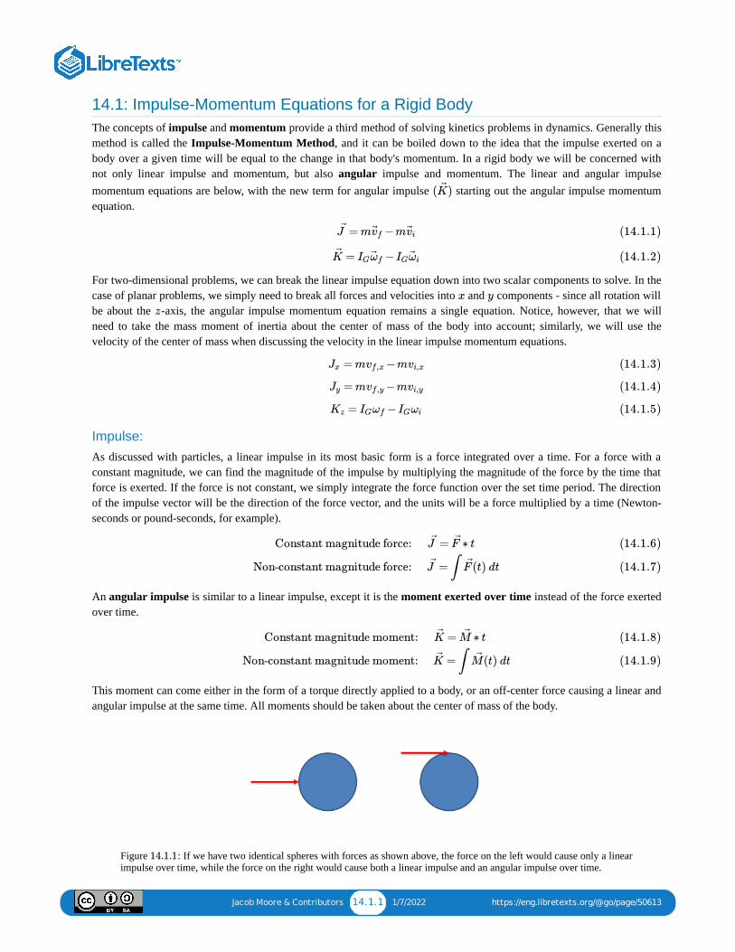
Jacob Moore & Contributors 14.1.1 1/7/2022 https://eng.libretexts.org/@go/page/50613

14.1: Impulse-Momentum Equations for a Rigid BodyThe concepts of impulse and momentum provide a third method of solving kinetics problems in dynamics. Generally thismethod is called the Impulse-Momentum Method, and it can be boiled down to the idea that the impulse exerted on abody over a given time will be equal to the change in that body's momentum. In a rigid body we will be concerned withnot only linear impulse and momentum, but also angular impulse and momentum. The linear and angular impulsemomentum equations are below, with the new term for angular impulse starting out the angular impulse momentumequation.

For two-dimensional problems, we can break the linear impulse equation down into two scalar components to solve. In thecase of planar problems, we simply need to break all forces and velocities into and components - since all rotation willbe about the -axis, the angular impulse momentum equation remains a single equation. Notice, however, that we willneed to take the mass moment of inertia about the center of mass of the body into account; similarly, we will use thevelocity of the center of mass when discussing the velocity in the linear impulse momentum equations.

Impulse:As discussed with particles, a linear impulse in its most basic form is a force integrated over a time. For a force with aconstant magnitude, we can find the magnitude of the impulse by multiplying the magnitude of the force by the time thatforce is exerted. If the force is not constant, we simply integrate the force function over the set time period. The directionof the impulse vector will be the direction of the force vector, and the units will be a force multiplied by a time (Newton-seconds or pound-seconds, for example).

An angular impulse is similar to a linear impulse, except it is the moment exerted over time instead of the force exertedover time.

This moment can come either in the form of a torque directly applied to a body, or an off-center force causing a linear andangular impulse at the same time. All moments should be taken about the center of mass of the body.

Figure : If we have two identical spheres with forces as shown above, the force on the left would cause only a linearimpulse over time, while the force on the right would cause both a linear impulse and an angular impulse over time.

( )K 

= m −mJ   v  f v  i (14.1.1)

= −K  IGω f IGω i (14.1.2)

x y

z

= m −mJx vf,x vi,x (14.1.3)

= m −mJy vf,y vi,y (14.1.4)

= −Kz IGωf IGωi (14.1.5)

Constant magnitude force:

Non-constant magnitude force:

= ∗ tJ   F  

= ∫ (t) dtJ   F  

(14.1.6)

(14.1.7)

Constant magnitude moment:

Non-constant magnitude moment:

= ∗ tK  M 

= ∫ (t) dtK  M 

(14.1.8)

(14.1.9)

14.1.1

Jacob Moore & Contributors 14.1.2 1/7/2022 https://eng.libretexts.org/@go/page/50613

Momentum:As discussed with particles, the linear momentum of a body will be equal to the mass of the body times its current velocity.Since velocity is a vector, the momentum will also be a vector, having both magnitude and a direction. Unlike the impulse,which happens over some set time, the momentum is captured as a snapshot of a specific instant in time (usually rightbefore and after some impulse is exerted). The units for linear momentum will be mass times unit distance per unit time.This is usually kilogram-meters per second in metric, or slug-feet per second in English units.

Angular momentum, on the other hand, will be equal to the body's mass moment of inertia (about its center of mass) timesits current angular velocity. It's important to note that while the mass moment of inertia remains constant if the body doesnot change shape, a shape that does change shape will likely have changes in mass moments of inertia along with changesin angular velocity.

Figure : During a spin, figure skaters will often draw their arms and legs in towards their bodies to reduce their massmoment of inertia. With minimal impulses to change the angular momentum, the angular velocity will increase so thatangular momentum is conserved. Public Domain image by deerstop.

Video lecture covering this section, delivered by Dr. Jacob Moore. YouTube source: https://youtu.be/vPxE2AFXADE.

A miter saw has an operating speed of 1500 rpm. The blade and motor armature have a combined weight of 3 lbs and aradius of gyration of 1 inch.

What is the time required for the bearing friction alone (torque=0.015 inch-lbs) to stop the blade?What is the torque a braking system would need to apply to stop the blade in just 0.25 seconds?

14.1.2

14.1 Rigid Body Impulse Momentum14.1 Rigid Body Impulse Momentum……

Practice 14.1.1

Jacob Moore & Contributors 14.1.3 1/7/2022 https://eng.libretexts.org/@go/page/50613

Figure : A man cuts wood with a miter saw. Public domain image by John F. Looney

Solution (not yet available):

Not yet available.

A bowling ball is modeled as a 7-kilogram uniform sphere, 300 mm in diameter. The ball is released with an initialvelocity of 6 m/s on a horizontal wooden floor ( = 0.1) with zero angular velocity.

How long does it take before the ball begins to roll without slipping?What is the linear velocity of the ball at this time?

Figure : A bowling ball is released down a lane. Public domain image by Jerry Saslav.

Solution (not yet available):

Not yet available.

14.1.3

Practice 14.1.2

μk

14.1.4

Jacob Moore & Contributors 14.2.1 12/21/2021 https://eng.libretexts.org/@go/page/50614

14.2: Rigid Body Surface CollisionsIn instances where a moving rigid body impacts a solid and immovable surface, the resulting impact can seem chaotic.However, we can still use the ideas of impulse and momentum to predict this impact behavior.

Just as with particles, an important first step in solving problems where a rigid body impacts a surface is to identify thenormal and tangential directions. The normal direction will be perpendicular to the surface being impacted, while thetangential direction will be parallel to the surface being impacted. Also important for rigid body impact is identifying boththe center of mass for the body and the point of impact between the body and the surface.

Figure : Dropping a wrench on a concrete floor is a good example of rigid body impact with a solid surface. Thefirst step in solving these problems is to identify the normal and tangential directions, which will be perpendicular andparallel to the surface, respectively. Also important is identifying the center of mass (C) and point of impact (A).

To predict the linear velocities after impact in the and directions, as well as the angular velocity after the impact (a totalof three unknowns), we will need three equations. These equations will come in the form of the conservation ofmomentum in the direction, as well as two equations based on the coefficient of restitution for the velocity in the direction and the angular velocity after the impact.

For momentum, we will notice that the normal forces during impact will always be in the normal direction. Assumingnegligible friction forces (which would be in the tangential direction), we will have no change in momentum in thetangential direction and therefore no change in velocity in the tangential direction for the center of mass of the body.This gives us the first equation we can use.

Next, examining the coefficient of restitution will give us another equation. Specifically, the coefficient of restitutionrelates the velocities before an after the collision in the normal direction at the point of impact.

If the collision is elastic we would also conserve the kinetic energy of the body, giving us our third equation. Moregenerally, however, the coefficient of restitution can be used to quantify the amount of energy lost on the collision, withmore elastic collisions conserving a higher percentage of kinetic energy and more inelastic equations conserving lesskinetic energy. The equation below can be used for any elastic or semi elastic collision with a surface. Using the thirdequation below, we simply set equal to one for elastic collisions or equal to the coefficient of restitution for semi-elasticcollisions.

Between the three equations above and whatever relevant kinematics relationships are necessary, we should be able tosolve for up to three unknowns. This allows us to completely predict the velocities after an impact, assuming we know thepre-impact velocities and the coefficient of restitution for the impact itself.

14.2.1

n t

t n

=vt,C,f vt,C,i (14.2.1)

ϵ = −vn,A,f

vn,A,f

(14.2.2)

ϵ

=ϵ2KEf

KEi

(14.2.3)

Jacob Moore & Contributors 14.2.2 12/21/2021 https://eng.libretexts.org/@go/page/50614

Video lecture covering this section, delivered by Dr. Jacob Moore. YouTube source: https://youtu.be/LQKk2WLMe4A.

An 80-centimeter-long metal bar with a mass of 1 kilogram, falling at 2 meters per second, strikes the edge of a tableas shown below. Assuming a coefficient of restitution of 0.9, what is the expected velocity and angular velocity of thebar after impact?

Figure : problem diagram for Example Problem . A horizontal bar falls straight down, until its leftmostend strikes the top of a flat table.

Solution (not yet available)

Not yet available.

14.2 Rigid Body Surface Collisions - 14.2 Rigid Body Surface Collisions - ……

Practice 14.2.1

14.2.2 14.2.2

Jacob Moore & Contributors 14.3.1 1/30/2022 https://eng.libretexts.org/@go/page/50615

14.3: Chapter 14 Homework Problems

A flywheel with a diameter of 2 ft and a weight of 60 lbs is rotating at a rate of 600 rpm. A brake applies a frictionforce to the outer rim of the flywheel, bringing it to a stop in 1.5 seconds. Based on this information, what was theaverage friction force applied by the brake over this time?

Figure : problem diagram for Example . A brake that is fixed in place applies a tangent frictional force tothe outer rim of a rotating flywheel wheel.

Solution

A ring-shaped space station can be approximated as a thin ring 60 meters in diameter with a mass of 500,000 kg.Centrifugal acceleration of the spinning station will be used to simulate gravity.

To simulate the acceleration of Earth (9.81 m/s²), how fast will the station need to be spinning?If two thrusters each capable of exerting 10 kN of force will be used to get the station up to this speed, how longwill we need to run the thrusters?

Figure : problem diagram for Exercise . A ring-shaped space station is rotating counterclockwise, due tothrust forces in opposite directions provided by two thrusters on opposite sides of the ring.

Solution

Exercise 14.3.1

14.3.1 14.3.1

= 39.01 lbsFbrake

Exercise 14.3.2

14.3.2 14.3.2

= 0.571 ωfrads

= 428.25 stthrust

1 1/30/2022

CHAPTER OVERVIEW15: VIBRATIONS WITH ONE DEGREE OF FREEDOMAnalysis of vibrations in one dimension: free and forced vibrations; undamped, viscous damped, and friction-damped.

15.1: UNDAMPED FREE VIBRATIONSBehavior of undamped free vibrations in one dimension, as modeled by a mass on a spring. Includes worked examples. **Videolecture not yet available.**

15.2: VISCOUS DAMPED FREE VIBRATIONSDefinition of viscous damping of a vibrational system. Determining an equation of motion for a system experiencing viscousdamping. ** Video lecture not yet available. **

15.3: FRICTION (COULOMB) DAMPED FREE VIBRATIONSDefinition of friction damping of a vibrational system. Determining the equation of motion for a system experiencing frictiondamping. ** Video lecture not yet available. **

15.4: UNDAMPED HARMONIC FORCED VIBRATIONSAnalysis of the harmonic vibrations of an object caused by an applied force, in an undamped case. Includes worked examples. **Video lecture not yet available. **

15.5: VISCOUS DAMPED HARMONIC FORCED VIBRATIONSAnalysis of the motion of systems undergoing forced harmonic vibration where viscous damping is present. ** Video lecture not yetavailable. **

Jacob Moore & Contributors 15.1.1 1/16/2022 https://eng.libretexts.org/@go/page/50618

15.1: Undamped Free VibrationsVibrations occur in systems that attempt to return to their resting or equilibrium state when perturbed, or pushed awayfrom their equilibrium state. The simplest vibrations to analyze are undamped, free vibrations with one degree of freedom.

"Undamped" means that there are no energy losses with movement (whether the losses are intentional, from addingdampers, or unintentional, through drag or friction). An undamped system will vibrate forever without any additionalapplied forces. A simple pendulum has very low damping, and will swing for a long time before stopping. "Damped"means that there are resistive forces and energy losses with movement that cause the system to stop moving eventually.

"Free" means that, after the initial perturbation, the only forces acting on the system are internal to the system (springs,dampers) and/or gravity. A tuning fork continues to vibrate after the one initial perturbation of being struck. In contrast,"forced" means there is an external, typically periodic, force acting on the system. A jackhammer vibrates due to having asupply of compressed air continually forcing the bit up and down, and it stops vibrating very quickly without that externalperiodic forcing.

"One degree of freedom" means that we will only consider systems with one mass vibrating along one direction (e.g. usevariable ) or about one axis (e.g. use variable ). Systems having more than one mass or vibrating along or about two ormore axes have more than one degree of freedom.

We can derive the equation of the system by setting up a free body diagram. Consider a mass sitting on a frictionlesssurface, attached to a wall via a spring.

Figure : This is a system consisting of a mass attached to the wall via a spring, sitting on a frictionless surface. Thesystem is currently in equilibrium, and the spring is not stretched or compressed.

The system above is in equilibrium. It is at rest, and will stay at rest unless some other force acts on it.

Figure : Free body diagram of the system in equilibrium position. Since the spring is at its unstretched length, it doesnot produce a force.

To start the system vibrating, we need to perturb it. Perturbation is moving the system away from equilibrium by a smallamount.

x θ

15.1.1

15.1.2

Jacob Moore & Contributors 15.1.2 1/16/2022 https://eng.libretexts.org/@go/page/50618

Figure : Mass-spring system perturbed by an amount from equilibrium. This stretches the spring, causing aspring force which tends to pull the mass back toward equilibrium.

When we perturb this system, we either stretch or compress the spring. This generates a spring force, and the spring forceis always in a direction that tends to pull the system back toward equilibrium.

Figure : Free body diagram of the mass-spring system perturbed by an amount from equilibrium. This stretchesthe spring, causing a spring force which tends to pull the mass back toward equilibrium.

Figure : Mass-spring system vibration. After an initial perturbation, the system oscillates between two extremepositions ( and ). The extreme positions are turnaround points where the velocity is zero, but the spring forceis at a maximum (maximum stretch/compression) and therefore the acceleration is maximum. As the system passesthrough the equilibrium position, the spring is no longer stretched (zero force, zero acceleration), but the velocity is at itsmaximum (this can be determined using conservation of energy) and the inertia of the system carries the mass past theequilibrium position. In the absence of damping or the application of another force, the system will oscillate forever.

We can generate the equation of motion of the system, and determine the specifics of how it will vibrate, by analyzing thisperturbed state. Recall that the spring force or moment is:

Note that the spring constants in the above equations have different units, depending on whether the spring is linear(Newton/meter) or torsional (Newton-meter/radian), and that must be given in radians. The magnitude of the spring force

15.1.3 +x

15.1.4 +x

15.1.5−xmax xmax

= kF  k x  (15.1.1)

= kM k ω  (15.1.2)

θ

Jacob Moore & Contributors 15.1.3 1/16/2022 https://eng.libretexts.org/@go/page/50618

depends on , the distance perturbed from the spring's unstretched length (not necessarily the equilibrium position ofthe system), and the same is true for the moment of a torsional spring. The spring force or moment is in thedirection/orientation opposite that of the displacement. That is, if you pull the mass to the right, the spring force points tothe left.

The process for finding the equation of motion of the system is as follows:

1. Sketch the system with a small positive perturbation ( or ).2. Draw the free body diagram of the perturbed system. Ensure that the spring force has a direction opposing the

perturbation.3. Find the one equation of motion for the system in the perturbed coordinate using Newton's Second Law. Keep the same

positive direction for position, and assign positive acceleration in the same direction.4. Move all terms of the equation to one side, and check that all terms are positive. If all terms are not positive, there is an

error in the direction of displacement, acceleration, and/or spring force.

For the example system above, with mass and spring constant , we derive the following:

This gives us a differential equation that describes the motion of the system. We can rewrite it in normal form:

The term is called the angular natural frequency of the system, and has units of radians/second.

Assuming that the initial perturbation of the system can be described by the position and velocity of the mass at ,then:

The solution to the differential equation, that provides the position of the system at time , is:

The amplitude describes the maximum displacement during the oscillations (i.e. ), and the phase describes howthe sine function is shifted in time.

x

x θ

m k

∑ = m = mFx ax x (15.1.3)

− = mFk x (15.1.4)

−kx = mx (15.1.5)

m +kx = 0x (15.1.6)

m +kx = 0x (15.1.7)

⇒ + x = 0xk

m(15.1.8)

⇒ + x = 0x ω2n (15.1.9)

ωn

=ω2n

k

m(15.1.10)

=ωn

k

m

−−−√ (15.1.11)

t = 0

x(0) = x0 (15.1.12)

v(0) = (0) = .x v0 (15.1.13)

x(t) t

x(t) = C sin( t +ϕ),ωn (15.1.14)

where: = , C = , ϕ = ( ).ωn

k

m

−−−√ +( )

v0

ωn

2

x20

− −−−−−−−−−

√ tan−1 x0ωn

v0(15.1.15)

C xmax ϕ

Jacob Moore & Contributors 15.1.4 1/16/2022 https://eng.libretexts.org/@go/page/50618

Figure : Displacement response of the mass spring system (solution to the differential equation).

For a system where there is torsional vibration (that is, the oscillation involves a rotation), the equations are similarly:

Assuming that the initial perturbation of the system can be described by the position and velocity of the mass at ,

The solution to the differential equation, that provides the position of the system at time , is:

Find an expression for the angular natural frequency of the following system, and find the maximum amplitude ofvibration of the system with mass = 10 kg and spring constant = 200 N/m when given an initial displacement of

= 0.1 m and an initial velocity of = 0.3 m/s.

Figure : problem diagram for Example . A rectangular mass on a flat surface has its left edge attached totwo identical springs, whose other ends are attached to a wall.

Solution

15.1.6

I +kθ = 0θ (15.1.16)

⇒ + θ = 0θk

I(15.1.17)

⇒ + θ = 0,θ ω2n (15.1.18)

where = .ωn

k

I

−−√ (15.1.19)

t = 0

x(0) = x0 (15.1.20)

v(0) = (0) = .x v0 (15.1.21)

x(t) t

x(t) = C sin( t +ϕ)ωn (15.1.22)

where: = , C = , ϕ = ( ).ωn

k

I

−−√ +( )

ω0

ωn

2

θ20

− −−−−−−−−−

√ tan−1 θ0ωn

ω0(15.1.23)

Example 15.1.1

m k

x0 v0

15.1.7 15.1.1

Jacob Moore & Contributors 15.1.5 1/16/2022 https://eng.libretexts.org/@go/page/50618

Video : Worked solution to example problem . YouTube source: https://youtu.be/J1TVxxVjV_c.

Determine the equation of motion of the system from Newton's Second Law. Assume mass = 5 kg and springconstant = 500 N/m. Find the initial displacement, , such that the mass oscillates over a total range of 4 meters.Assume the initial perturbation velocity, , is 10 m/s.

Figure : problem diagram for Example . A mass hangs from a spring attached to a ceiling.

Solution

Video : Worked solution to example problem . YouTube source: https://youtu.be/TAy412iVvwE.

15-1 WP001 AD15-1 WP001 AD

15.1.1 15.1.1

Example 15.1.2

m

k x0

v0

15.1.8 15.1.2

15-1 WP002 AD15-1 WP002 AD

15.1.2 15.1.2

Jacob Moore & Contributors 15.2.1 1/23/2022 https://eng.libretexts.org/@go/page/50619

15.2: Viscous Damped Free VibrationsViscous damping is damping that is proportional to the velocity of the system. That is, the faster the mass is moving, themore damping force is resisting that motion. Fluids like air or water generate viscous drag forces.

Figure : A diagram showing the basic mechanism in a viscous damper. As the system (mass) attached to the loop atthe top vibrates up and down, the damper will resist motion in both directions due to the piston passing through the fluid.Image by Egmason, CC-BY SA.

We will only consider linear viscous dampers, that is where the damping force is linearly proportional to velocity. Theequation for the force or moment produced by the damper, in either or , is:

where is the damping constant. This is a physical property of the damper based on the type of fluid, size of the piston,etc. Note that the units of change depending on whether it is damping linear motion (N-s/m) or rotational motion (N-ms/rad).

Figure : Diagram of a hanging mass-spring system, with a linear viscous damper, in equilibrium position. The springis stretched from its natural length.

When the system is at rest in the equilibrium position, the damper produced no force on the system (no velocity), while thespring can produce force on the system, such as in the hanging mass shown above. Recall that this is the equilibriumposition, but the spring is NOT at its unstretched length, as the static mass produces an extention of the spring.

15.2.1

x θ

= c ,F  c x  (15.2.1)

= c ,M c θ

 (15.2.2)

c

c

15.2.2

Jacob Moore & Contributors 15.2.2 1/23/2022 https://eng.libretexts.org/@go/page/50619

Figure : Free body diagram of the system in equilibrium position. The spring is at its equilibrium position, but it isstretched and does produce a force.

If we perturb the system (applying an initial displacement, an initial velocity, or both), the system will tend to move backto its equilibrium position. What that movement looks like will depend on the system parameters ( , , and ).

Figure : The system in a perturbed position. The spring is stretched further and the damper is extended, compared totheir equilibrium positions.

To determine the equation of motion of the system, we draw a free body diagram of the system with perturbation and applyNewton's Second Law.

Figure : Free body diagram of the system with perturbation.

The process for finding the equation of motion of the system is again:

1. Sketch the system with a small positive perturbation ( or ).2. Draw the free body diagram of the perturbed system. Ensure that the spring force and the damper force have directions

opposing the perturbation.3. Find the one equation of motion for the system in the perturbed coordinate using Newton's Second Law. Keep the same

positive direction for position, and assign positive acceleration in the same direction.4. Move all terms of the equation to one side, and check that all terms are positive. If all terms are not positive, there is an

error in the direction of displacement, acceleration, and/or spring or damper force.

15.2.3

m c k

15.2.4

15.2.5

x θ

Jacob Moore & Contributors 15.2.3 1/23/2022 https://eng.libretexts.org/@go/page/50619

For the example system above, with mass , spring constant and damping constant , we derive the following:

This gives us a differential equation that describes the motion of the system. We can rewrite it in normal form:

As before, the term is called the angular natural frequency of the system, and has units of rad/s.

(zeta) is called the damping ratio. It is a dimensionless term that indicates the level of damping, and therefore the type ofmotion of the damped system.

The expression for critical damping comes from the solution of the differential equation. The solution to the systemdifferential equation is of the form

where is constant and the value(s) of can be can be obtained by differentiating this general form of the solution andsubstituting into the equation of motion.

Because the exponential term is never zero, we can divide both sides by that term and get:

Using the quadratic formula, we can find the roots of the equation:

Critical damping occurs when the term under the square root sign equals zero:

Four Viscous Damping Cases:There are four basic cases for the damping ratio. For the solutions that follow in each case, we will assume that the initialperturbation displacement of the system is and the initial perturbation velocity of the system is .

1. : Undamped

m k c

∑ = m = mFx ax x (15.2.3)

− − = mFk Fc x (15.2.4)

−kx− = mc(x)˙ x (15.2.5)

m + +kx = 0x c(x)˙ (15.2.6)

m +c +kx = 0x x (15.2.7)

⇒ + + x = 0xc

mx

k

m(15.2.8)

⇒ +2ζ + x = 0x ωnx ω2n (15.2.9)

ωn

= ; =ω2n

k

mωn

k

m

−−−√ (15.2.10)

ζ

ζ = =c

cc

actual damping

critical damping(15.2.11)

x(t) = a ,ert (15.2.12)

a r

m +cr +k = 0r2ert ert ert (15.2.13)

⇒ (m +cr+k) = 0r2 ert (15.2.14)

m +cr+k = 0.r2 (15.2.15)

=r1,2−c± −4mkc2

− −−−−−−−√

2m(15.2.16)

= 4mkc2c (15.2.17)

= 2 = 2mcc mk−−−

√ ωn (15.2.18)

x0 v0

ζ =0

c = 0 (15.2.19)

Jacob Moore & Contributors 15.2.4 1/23/2022 https://eng.libretexts.org/@go/page/50619

This is the case covered in the previous section. Undamped systems oscillate about the equilibrium position continuously,unless some other force is applied.

Figure : Response of an undamped system.

2. : Overdamped

Roots are both real and negative, but not equal to each other. Overdamped systems move slowly toward equilibriumwithout oscillating.

Figure : Response of an overdamped system.

The response for an overdamped system is:

3. : Critically damped

Roots are real and both equal to . Critically-damped systems will allow the fastest return to equilibrium withoutoscillation.

15.2.6

ζ >1

> 4mkc2 (15.2.20)

15.2.7

x(t) = + ,a1e( )t

−c+ −4mkc2√

2m

a2e( )t

−c− −4mkc2√

2m

(15.2.21)

where = and = .a1− +v0 r2x0

−r2 r1a2

+v0 r1x0

−r2 r1(15.2.22)

ζ =1

= 4mk(= )c2 c2c (15.2.23)

−ωn

Jacob Moore & Contributors 15.2.5 1/23/2022 https://eng.libretexts.org/@go/page/50619

Figure : Response of an critically-damped system.

The solution for a critically-damped system is:

4. : Underdamped

The roots are complex numbers. Underdamped systems do oscillate around the equilibrium point; unlike undampedsystems, the amplitude of the oscillations diminishes until the system eventually stops moving at the equilibrium position.

Figure : Response of an underdamped system.

The solution for an underdamped system is:

is called the damped natural frequency of the system. It is always less than :

The period of the underdamped response differs from the undamped response as well.

15.2.8

x(t) = (A+Bt) ,e− tωn (15.2.24)

where A = and B = + .x0 v0 x0ωn (15.2.25)

ζ <1

< 4mkc2 (15.2.26)

15.2.9

x(t) = [ sin( t) + cos( t)] ,C1 ωd C2 ωd e− ζtωn (15.2.27)

where = , = , and ζ = .C1+ ζv0 ωn x0

ωd

C2 x0c

2mωn

(15.2.28)

ωd ωn

= .ωd ωn 1 −ζ2− −−−−

√ (15.2.29)

Undamped: =τn2π

ωn

(15.2.30)

Underdamped: =τd2π

ωd

(15.2.31)

Jacob Moore & Contributors 15.2.6 1/23/2022 https://eng.libretexts.org/@go/page/50619

Comparison of Viscous Damping Cases:

Figure : Responses for all four types of system (or values of damping ratio) in viscous damping. All four systemshave the same mass and spring values, and have been given the same initial perturbations (initial position and initialvelocity); this is apparent because they start at the same -intercept and have the same slope at .

In the figure above, we can see that the critically-damped response results in the system returning to equilibrium thefastest. Also, we can see that the underdamped system amplitude is quite attenuated compared to the undamped case.

15.2.10

y x = 0

Jacob Moore & Contributors 15.3.1 1/16/2022 https://eng.libretexts.org/@go/page/50620

15.3: Friction (Coulomb) Damped Free VibrationsFriction can also provide vibration damping. In this case, however, the damping is not proportional to the magnitude ofvelocity. It only depends on the direction of velocity.

We remember from the section on dry friction that the force of friction in sliding depends only on the coefficient of kineticfriction, , and the normal force, .

The above equation does not include velocity. We know that kinetic friction acts to oppose motion, however, so a morecomplete expression would be:

where is the "sign" function, a function that captures the sign (direction) of velocity. The above equation thenindicates that the direction of friction is always opposite the direction of velocity, but the magnitude of velocity does notmake a difference in the magnitude of friction.

The equation of motion of the system becomes:

and the solution to this equation of motion is:

If we plot the response, we can see that there are several differences from a system with viscous damping.

Figure : Response of the system in friction damping.

Some differences when compared to viscous damping include:

1. The system oscillates at the natural frequency of the system, not a damped natural frequency.2. The bounding curves are linear, not exponential.3. The system does not return to zero. This is because the magnitude of the friction force does not diminish as the system

amplitude reduces, and at some point the spring force is no longer able to overcome the static friction that the systemexperiences when it changes direction ( ).

Comparison to Viscous Underdamped SystemIf we consider our simple linear mass-spring system, the magnitude of does not change with velocity, unlike withviscous damping. If we plotted both types of damping for the same system, we would get the following:

μk FN

=Ff μkFN (15.3.1)

= −sgn( ) ,Ff x μkFN (15.3.2)

sgn

m +μmg sgn( ) +kx = 0,x x (15.3.3)

x(t) =( − ) cos( t) + (−1 .x0(2n −1)μmg

kωn

μmg

k)n+1 (15.3.4)

15.3.1

v = 0

Ff

Jacob Moore & Contributors 15.3.2 1/16/2022 https://eng.libretexts.org/@go/page/50620

Figure : Response of the system in friction damping and in viscous damping, for the same initial conditions (), spring constants and masses.

Note that the viscous damping has more reduction in amplitude earlier (despite relatively light damping), but continuesoscillating past the point when the friction-damped system has stopped (specific relative values are dependent on thevalues of damping constant and coefficients of friction). Also note that since the viscous damping is relatively light, thedifference in period between the two plots is quite small in this example.

15.3.2,x0 v0

Jacob Moore & Contributors 15.4.1 1/16/2022 https://eng.libretexts.org/@go/page/50621

15.4: Undamped Harmonic Forced VibrationsOften, mechanical systems are not undergoing free vibration, but are subject to some applied force that causes the systemto vibrate. In this section, we will consider only harmonic (that is, sine and cosine) forces, but any changing force canproduce vibration.

When we consider the free body diagram of the system, we now have an additional force to add: namely, the externalharmonic excitation.

Figure : A mass-spring system with an external force, , applying a harmonic excitation.

The equation of motion of the system above will be:

where is a force of the form:

This equation of motion for the system can be re-written in standard form:

The solution to this system consists of the superposition of two solutions: a particular solution, (related to the forcingfunction), and a complementary solution, (which is the solution to the system without forcing).

As we saw previously, the complementary solution is the solution to the undamped free system:

We can obtain the particular solution by assuming a solution of the form:

where is the frequency of the harmonic forcing function. We differentiate this form of the solution, and then sub intothe above equation of motion:

After solving for , we can then use it to find the particular solution, :

15.4.1 F

m +kx = F ,x (15.4.1)

F

F = sin( t).F0 ω0 (15.4.2)

+ x = sin( t).xk

m

F0

mω0 (15.4.3)

xp

xc

= C sin( t +ϕ).xc ωn (15.4.4)

= D sin( t),xp ω0 (15.4.5)

ω0

= − D sin( t)xp ω20 ω0 (15.4.6)

−m D sin( t) +kD sin( t) = sin( t)ω20 ω0 ω0 F0 ω0 (15.4.7)

D xp

D =

F0

k

1 −( )ω0

ωn

2(15.4.8)

Jacob Moore & Contributors 15.4.2 1/16/2022 https://eng.libretexts.org/@go/page/50621

Thus, the general solution for a forced, undamped system is:

Figure : The complementary solution of the equation of motion. This represents the natural response of the system,and oscillates at the angular natural frequency. This is the transient response.

Figure : The particular solution of the equation of motion. This represents the forced response of the system, andoscillates at the angular forced frequency. This is the steady-state response.

Figure : The general solution of the equation of motion. This represents the combined response of the system, andthe sum of the complementary (or natural) and particular (or forced) responses.

The above figures show the two responses at different frequencies. Recall that the value of comes from the physicalcharacteristics of the system ( ) and comes from the force being applied to the system. These responses are

=   sin( t).xp

F0

k

1 −( )ω0

ωn

2ω0 (15.4.9)

(t) =   sin( t) +C sin( t +ϕ)xG

F0

k

1 −( )ω0

ωn

2ω0 ωn (15.4.10)

15.4.2

15.4.3

15.4.4

ωn

m, k ω0

Jacob Moore & Contributors 15.4.3 1/16/2022 https://eng.libretexts.org/@go/page/50621

summed, to achieve the blue response (general solution) in Figure above.

Steady-State Response:In reality, this superimposed response does not last long. Every real system has some damping, and the natural response ofthe system will be damped out. As long as the external harmonic force is applied, however, the response to it will remain.When evaluating the response of the system to a harmonic forcing function, we will typically consider the steady-stateresponse, when the natural response has been damped out and the response to the forcing function remains.

Amplitude of Forced Vibration

The amplitude of the steady-state forced vibration depends on the ratio of the forced frequency to the natural frequency. As approaches (the ratio approaches 1), the magnitude becomes very large. We can define a magnification factor:

Figure : The magnification factor, , is defined as the ratio of the amplitude of the steady-state vibration to thedisplacement that would be achieved by static deflection.

From the figure above, we can discuss various cases:

: Resonance occurs. This results in very large-amplitude vibrations, and is associated with high stress andfailure to the system.

: The forcing function is nearly static, leaving essentially the static deflection and limited naturalvibration.

: Magnification is positive and greater than 1, meaning the vibrations are in phase (when the force acts to theleft, the system displaces to the left) and the amplitude of vibration is larger than the static deflection.

: Magnification is negative and the absolute value is typically smaller than 1, meaning the vibration is out ofphase with the motion of the forcing function (when the force acts to the left, the system displaces to the right) and theamplitude of vibration is smaller than the static deflection.

: The force is changing direction too fast for the block's motion to respond.

15.4.4

ω0 ωn D

MF = =

F0

k

1 −( )ω0

ωn

2

F0

k

1

1 −( )ω0

ωn

2(15.4.11)

15.4.5 MF

=ω0 ωn

∼ 0, MF ∼ 1ω0

<ω0 ωn

>ω0 ωn

>>ω0 ωn

Jacob Moore & Contributors 15.4.4 1/16/2022 https://eng.libretexts.org/@go/page/50621

Rotating Unbalance:One common cause of harmonic forced vibration in mechanical systems is rotating unbalance. This occurs when the axisof rotation does not pass through the center of mass, meaning that the center of mass experiences some acceleration insteadof remaining stationary. This causes a force on the axle that changes direction as the center of mass rotates. We canrepresent this as a small mass, , rotating about the axis of rotation at some distance, called an eccentricity, . The forcedangular frequency, , in this case is the angular frequency of the rotating system.

A 10-kg fan is fixed to a lightweight beam. The static weight of the fan deflects the beam by 20 mm. If the blade isdesigned to spin at = 15 rad/s, and the blade is mounted off-center (equivalent to a 1.5 kg mass at 50 mm from theaxis of rotation), determine the steady-state amplitude of vibration.

Figure : problem diagram for Example . A horizontal beam not touching the ground is attached to a wallat its left end and holding up a three-bladed rotary fan on its right end.

Solution:

Video : Worked solution to example problem . YouTube source: https://youtu.be/k0vJLxaAjtw.

You are designing a stylish fan that uses only one blade. Approximate that blade as a narrow plate with a density perunit length of 20 g/cm. The base weight of the rest of the device (except for the blade) is 4 kg, and the whole thing ismounted on a lightweight beam. If the spring constant of the beam is = 1000 N/m, find the length of blade than willcause resonance if the fan is designed to spin at = 15 rad/s.

m e

ω0

Example 15.4.1

ω

15.4.6 15.4.1

15-4 WP00115-4 WP001

15.4.1 15.4.1

Example 15.4.2

k

ω

Jacob Moore & Contributors 15.4.5 1/16/2022 https://eng.libretexts.org/@go/page/50621

Figure : problem diagram for Example . A horizontal beam not touching the ground is attached to a wallat its left end and holding up a single-bladed rotary fan on its right.

Solution:

Video : Worked solution to example problem . YouTube source: https://youtu.be/tV4ETwwOyX0.

15.4.7 15.4.2

15-4 WP00215-4 WP002

15.4.2 15.4.2

Jacob Moore & Contributors 15.5.1 1/16/2022 https://eng.libretexts.org/@go/page/55503

15.5: Viscous Damped Harmonic Forced VibrationsAs described in the previous section, many vibrations are caused by an external harmonic forcing function (such asrotating unbalance). While we assumed that the natural vibrations of the system eventually damped out somehow, leavingthe forced vibrations at steady-state, by explicitly including viscous damping in our model we can evaluate the systemthrough the transient stage when the natural vibrations are present.

Figure : A mass-spring-damper system with an external force, , applying a harmonic excitation.

Consider the system above. The equation of the system becomes:

Because the natural vibrations will damp out with friction (as mentioned in undamped harmonic vibrations), we will onlyconsider the particular solution. This particular solution will have the form:

After solving, we determine that the expressions for and are:

The magnification factor now becomes:

15.5.1 F

m +c +kx = sin( t)x x F0 ω0 (15.5.1)

⇒ + + x =   sin( t).xc

mx

k

m

F0

mω0 (15.5.2)

(t) = sin( t − ).xp X ′ ω0 ϕ′ (15.5.3)

X ′ ϕ′

=X′

F0

k

+[1 − ]( )ω0

ωn

2 2

[2 ]c

cc

ω0

ωn

2− −−−−−−−−−−−−−−−−−−−−−−

⎷

(15.5.4)

= .ϕ′ tan−1

⎡

⎣

⎢⎢⎢⎢

2c

cc

ω0

ωn

1 −( )ω0

ωn

2

⎤

⎦

⎥⎥⎥⎥(15.5.5)

MF = =X ′

F0

k

1

+[1 − ]( )ω0

ωn

2 2

[2 ]c

cc

ω0

ωn

2− −−−−−−−−−−−−−−−−−−−−−−

⎷

(15.5.6)

Jacob Moore & Contributors 15.5.2 1/16/2022 https://eng.libretexts.org/@go/page/55503

Figure : This figure shows the various magnification factors associated with different levels of (under)damping.

From the figure above, we can see that the extreme amplitudes at resonance only occur when the damping ratio = 0 and theratio of frequencies is 1. Otherwise, damping inhibits the out-of-control vibrations that would otherwise be seen atresonance.

15.5.2

1 1/30/2022

CHAPTER OVERVIEW16: APPENDIX 1 - VECTOR AND MATRIX MATH

16.1: VECTORSVector representation in two and three dimensions. Covers magnitude-and-direction form, component form, and conversion betweenthe two forms. Includes several worked examples.

16.2: VECTOR ADDITIONAdding vectors in two and three dimensions, through the geometric addition and component addition methods.

16.3: DOT PRODUCTThe dot product (also sometimes called the scalar product) is a mathematical operation that can be performed on any two vectors withthe same number of elements. The result is a scalar number equal to the magnitude of the first vector, times the magnitude of thesecond vector, times the cosine of the angle between the two vectors.

16.4: CROSS PRODUCTThe cross product is a mathematical operation that can be performed on any two three-dimensional vectors. The result of the crossproduct operation will be a third vector that is perpendicular to both of the original vectors and has a magnitude of the first vectortimes the magnitude of the second vector times the sine of the angle between the vectors.

16.5: SOLVING SYSTEMS OF EQUATIONS WITH MATRICESConverting a system of linear equations into a matrix, to be solved by computer. Includes worked example.

16.6: APPENDIX 1 HOMEWORK PROBLEMS

Jacob Moore & Contributors 16.1.1 12/21/2021 https://eng.libretexts.org/@go/page/55331

16.1: VectorsVectors are used in engineering mechanics to represent quantities that have both a magnitude and a direction. Manyengineering quantities, such as forces, displacements, velocities, and accelerations, will need to be represented as vectorsfor analysis. Vector quantities contrast with scalar values (such as mass, area, or speed), which have a magnitude but nodirection.

Figure : The force below is represented as a vector. It has both a magnitude and a direction.

When dealing with vectors in equations, engineers commonly denote something as a vector by putting an arrow over thevariable. Variables without an arrow over top of them represent a scalar quantity, or simply the magnitude of that vectorquantity.

In contrast with scalar quantities, we cannot add, subtract, multiply or divide them by simply adding, subtracting,multiplying or dividing the magnitudes. The directions will also play a critical role in solving equations that contain vectorquantities.

Vector Representation:To represent a vector quantity, we will generally have two options. These two options are:

Magnitude and Direction Form: Where the magnitude is given as a single quantity and the direction is given via anangle or combination of angles.Component Form: Where the magnitude and direction are given through component magnitudes in each coordinatedirection.

Figure : The drawing above shows a force as vector. On the left the vector is represented as a magnitude and adirection. On the right the same force is represented in terms of its - and -components.

The magnitude and direction form of vector quantities are often used at the start and end of a problem. This is because it isoften easier to measure things likes forces and velocities as a magnitude and direction at the start of a problem, and it isoften easier to visualize the final result as a magnitude and direction at the end. Vectors represented as a magnitude anddirection need to be shown visually through the use of an arrow, where the magnitude is the length of the arrow, and thedirection is shown through the arrow head and an angle or angles relative to some known axes or other direction.

The component form of a vector is often used in middle of the problem because it is far easier to do math with vectorquantities in component form. Vectors can be represented in component form in one of two ways. First we can use squarebrackets to indicate a vector, with the , , and possibly components separated by commas. Alternatively, we can writeout a vector in component form using the magnitudes in front of unit vectors to indicate directions (generally the , , and

unit vectors for the , , and directions respectively). Neither of these component forms relies on a visual depiction ofthe vector as with the magnitude and direction form, though it is important to clearly identify the coordinate system inearlier diagrams.

16.1.1

Vector Quantity:

Scalar Quantity:

F  

F

(16.1.1)

(16.1.2)

16.1.2x y

x y z

i j

k x y z

Jacob Moore & Contributors 16.1.2 12/21/2021 https://eng.libretexts.org/@go/page/55331

Converting Between Vector Representations in 2DFor our analysis, we will often find it advantageous to have the vectors in one form or the other, and will therefore need toconvert the vector from a magnitude and direction to component form or vice versa. To do this we will use right trianglesand trigonometry.

Going from a Magnitude and Direction to Component Form

To go from a magnitude and direction to component form, we will first draw a right triangle with the hypotenuse being theoriginal vector. The horizontal arm of the triangle will then be the -component of the vector while the vertical arm is the

component of the vector. If we know the angle of the vector with respect to either the horizontal or the vertical, we canuse the sine and cosine relationship to find the and components.

Figure : Using sine and cosine relationships, we can find the and components of a vector.

It is important to remember that how we measure the angle will affect the sine and cosine relationships. Multiplying themagnitude by the sine will always give us the opposite leg and multiplying the magnitude by the cosine will always give usthe adjacent leg.

Figure : Depending upon how we measure the angle, the sine/cosine may be either the or the component.Remember that the sine will always give you the opposite leg, while the cosine will give you the adjacent leg.

Going from Component Form to Magnitude and Direction

To find the magnitude and the direction of a vector using components, we will use the same process in reverse. We willdraw the components as the legs of a right triangle, where the hypotenuse of the triangle shows the magnitude anddirection of the vector.

To find the magnitude of the vector we will use the Pythagorean Theorem, taking the square root of the sum of the squaresof each component. To find the angle, we can easily use the inverse tangent function, relating the opposite and adjacentlegs of our right triangle.

With Brackets:

With Unit Vectors:

= [3, 4, 5]F  

= 3 +4 +5F   i j k

(16.1.3)

(16.1.4)

x

y

x y

16.1.3 x y

16.1.4 x y

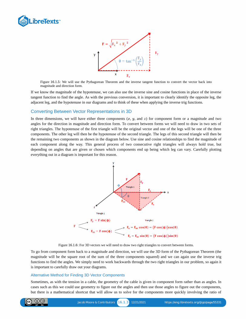
Jacob Moore & Contributors 16.1.3 12/21/2021 https://eng.libretexts.org/@go/page/55331

Figure : We will use the Pythagorean Theorem and the inverse tangent function to convert the vector back intomagnitude and direction form.

If we know the magnitude of the hypotenuse, we can also use the inverse sine and cosine functions in place of the inversetangent function to find the angle. As with the previous conversion, it is important to clearly identify the opposite leg, theadjacent leg, and the hypotenuse in our diagrams and to think of these when applying the inverse trig functions.

Converting Between Vector Representations in 3D

In three dimensions, we will have either three components ( , , and ) for component form or a magnitude and twoangles for the direction in magnitude and direction form. To convert between forms we will need to draw in two sets ofright triangles. The hypotenuse of the first triangle will be the original vector and one of the legs will be one of the threecomponents. The other leg will then be the hypotenuse of the second triangle. The legs of this second triangle will then bethe remaining two components as shown in the diagram below. Use sine and cosine relationships to find the magnitude ofeach component along the way. This general process of two consecutive right triangles will always hold true, butdepending on angles that are given or chosen which components end up being which leg can vary. Carefully plottingeverything out in a diagram is important for this reason.

Figure : For 3D vectors we will need to draw two right triangles to convert between forms.

To go from component form back to a magnitude and direction, we will use the 3D form of the Pythagorean Theorem (themagnitude will be the square root of the sum of the three components squared) and we can again use the inverse trigfunctions to find the angles. We simply need to work backwards through the two right triangles in our problem, so again itis important to carefully draw out your diagrams.

Alternative Method for Finding 3D Vector Components

Sometimes, as with the tension in a cable, the geometry of the cable is given in component form rather than as angles. Incases such as this we could use geometry to figure out the angles and then use those angles to figure out the components,but there is a mathematical shortcut that will allow us to solve for the components more quickly involving the ratio of

16.1.5

x y z

16.1.6

Jacob Moore & Contributors 16.1.4 12/21/2021 https://eng.libretexts.org/@go/page/55331

lengths. Specifically, the ratios of the components of the cable length to the overall length of the cable will be the same asthe ratio of the corresponding force components to the overall magnitude of the force.

To use this method we will first need to find the overall length of the cable (or other physical geometric feature) using thePythagorean Theorem. Once we have that overall length, we find a ratio by taking the x component of the length dividedby the overall length. To find the -component of the force, we simply multiply the overall magnitude of the force by thisratio of lengths ( ). The process for the and components follows a similar path, except the ratios would include the

and component lengths instead of the component.

Figure : The alternative method of breaking a vector down into component form relies on the ratios of the cablecomponents to the overall length of the cable.

Video lecture covering this section, delivered by Dr. Jacob Moore. YouTube source: https://youtu.be/2RO7VZ_u0Iw.

Determine the and components of the vector shown below.

x

/LLx y z

y z x

16.1.7

A 1.1 Vectors - Video Lecture - JPMA 1.1 Vectors - Video Lecture - JPM

Example 16.1.1

x y

Jacob Moore & Contributors 16.1.5 12/21/2021 https://eng.libretexts.org/@go/page/55331

Figure : problem diagram for Example . A force of magnitude 300 N is directed upwards and to the right,at 40° above the horizontal.

Solution:

Video : Worked solution to example problem , provided by Dr. Jacob Moore. YouTube source:https://youtu.be/TRS6jiih96o.

Determine the and components of the vector shown below.

Figure : problem diagram for Example . A tension force of magnitude 60 lbs is exerted along a cable,directed upwards and to the right at a 75° angle from the vertical.

Solution:

16.1.8 16.1.1

Vectors - Adaptive Map Worked EVectors - Adaptive Map Worked E……

16.1.2 16.1.1

Example 16.1.2

x y

16.1.9 16.1.2

Jacob Moore & Contributors 16.1.6 12/21/2021 https://eng.libretexts.org/@go/page/55331

Video : Worked solution to example problem , provided by Dr. Jacob Moore. YouTube source:https://youtu.be/hUrlI6eLGvE.

The velocity vector of the hockey puck shown below is given in component form. Determine the magnitude anddirection of the velocity with respect to the axes given.

Figure : problem diagram for Example . A hockey puck located at the origin of a Cartesian coordinateplane experiences a velocity of components m/s.

Solution:

Video : Worked solution to example problem , provided by Dr. Jacob Moore. YouTube source:https://youtu.be/3GeIU3Fc_qA.

Vectors - Adaptive Map Worked EVectors - Adaptive Map Worked E……

16.1.3 16.1.2

Example 16.1.3

16.1.10 16.1.3[5, −2.5]

Vectors - Adaptive Map Worked EVectors - Adaptive Map Worked E……

16.1.4 16.1.3

Jacob Moore & Contributors 16.1.7 12/21/2021 https://eng.libretexts.org/@go/page/55331

Determine the , , and components of the force vector shown below.

Figure : problem diagram for Example . A 45-Newton force vector with its tail at the origin of aCartesian coordinate system points 20° out of the screen towards the viewer and 30° below the plane of the horizontal.

Solution:

Video : Worked solution to example problem , provided by Dr. Jacob Moore. YouTube source:https://youtu.be/ZG31PoIfIEc.

A cable as shown below is used to tether the top of a pole to a point on the ground. The cable has a tension force of 3kN that acts along the direction of the cable as shown below. What are the , , and components of the tension forceacting on the top of the pole?

Example 16.1.4

x y z

16.1.11 16.1.4

Vectors - Adaptive Map Worked EVectors - Adaptive Map Worked E……

16.1.5 16.1.4

Example 16.1.5

x y z

Jacob Moore & Contributors 16.1.8 12/21/2021 https://eng.libretexts.org/@go/page/55331

Figure : problem diagram for Example . A cable connects the origin of a Cartesian coordinate system tothe top of a 6-meter-long vertical pole with its base at the point (2, 0, 3) meters.

Solution:

Video : Worked solution to example problem , provided by Dr. Jacob Moore. YouTube source:https://youtu.be/dUJwBohfCTU.

16.1.12 16.1.5

Vectors - Adaptive Map Worked EVectors - Adaptive Map Worked E……

16.1.6 16.1.5

Jacob Moore & Contributors 16.2.1 12/21/2021 https://eng.libretexts.org/@go/page/55332

16.2: Vector AdditionThe most common thing we will need to do with many vector quantities is to add them up. The sum of these vectorquantities is the net vector quantity. For example, if we have a number of forces acting on a body, the sum of those forcesis known as the net force.

The sum of any number of vectors can be determined geometrically using the following strategy. Starting with one of thevectors as the base, we redraw the second vector so that the tail of the second vector begins at the tip of the first vector. Wecan repeat this with a third vector, a forth vector and so on, putting the tail of each vector at the tip of the last vector untilwe have added taken all vectors into account. Once the vectors are all drawn tip to tail, the sum of all the vectors will bethe vector connecting the tail of the first vector to the tip of the last vector.

Figure : The geometric addition of vectors involves putting the vectors tip to tail as shown above.

In practice, the easiest way to determine the magnitude and direction of the sum of the vectors is to add the vectors incomponent form. This starts by separating each vector into , , and possibly components. As we can see in thediagram below, the component of the sum of all the vectors will be the sum of all the components of the individualvectors. Similarly, the and components of the sum of the vectors will be the sum of all the components and the sumof all the components respectively.

Figure : By summing all the components in a given direction, we can find the component of the sum of the vectorsin that direction.

Once we find the sum of the components in each direction, we can either leave the net vector in component form, or wecan use the Pythagorean theorem and inverse tangent functions to convert the vector back into a magnitude and directionas detailed on the previous page on vectors.

16.2.1

x y z

x x

y z y

z

16.2.2

Jacob Moore & Contributors 16.2.2 12/21/2021 https://eng.libretexts.org/@go/page/55332

Figure : Vide lecture covering this section, delivered by Dr. Jacob Moore. YouTube source:https://youtu.be/0tv92MX2_ro.

Determine the sum of the force vectors in the diagram below. Leave the sum in component form.

Figure : problem diagram for Example . Three two-dimensional vectors radiate out from a single point.

Solution:

Video : Worked solution to example problem , provided by Dr. Jacob Moore. YouTube source:https://youtu.be/FwC8ntactEQ.

A 1.2 Vector Addition - Video LectureA 1.2 Vector Addition - Video Lecture……

PageIndex1

Example 16.2.1

16.2.3 16.2.1

Vector Addition - Adaptive Map WVector Addition - Adaptive Map W……

16.2.2 16.2.1

Jacob Moore & Contributors 16.2.3 12/21/2021 https://eng.libretexts.org/@go/page/55332

Determine the sum of the force vectors in the diagram below. Give the sum in terms of a magnitude and a direction.

Figure : problem diagram for Example . Three two-dimensional vectors radiate out from a single point.

Solution:

Video : Worked solution to example problem , provided by Dr. Jacob Moore. YouTube source:https://youtu.be/Jj8mCV7rdas.

Determine the sum of the force vectors in the diagram below. Leave the sum in component form.

Example 16.2.2

16.2.4 16.2.2

Vector Addition - Adaptive Map WVector Addition - Adaptive Map W……

16.2.3 16.2.2

Example 16.2.3

Jacob Moore & Contributors 16.2.4 12/21/2021 https://eng.libretexts.org/@go/page/55332

Figure : problem diagram for Example . Two vectors radiate out from the origin of a three-dimensionalCartesian coordinate system.

Solution:

Video : Worked solution to example problem , provided by Dr. Jacob Moore. YouTube source:https://youtu.be/PZzx3eQp6iQ.

16.2.5 16.2.3

Vector Addition - Adaptive Map WVector Addition - Adaptive Map W……

16.2.4 16.2.3

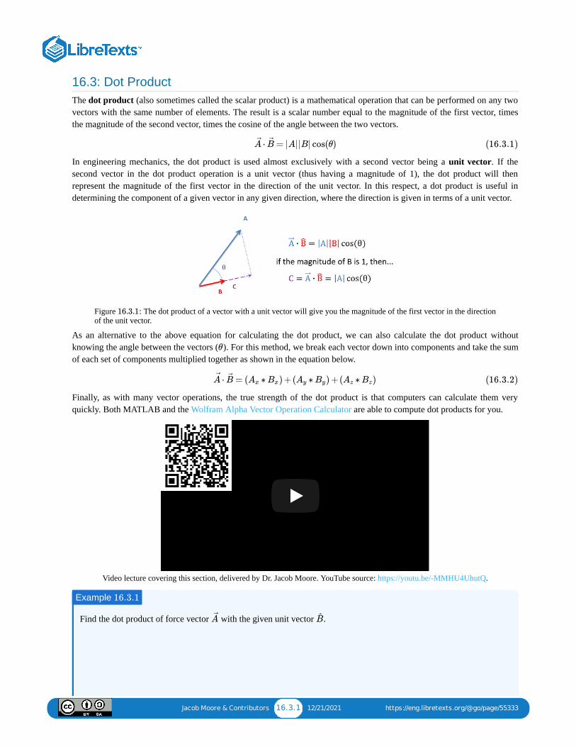
Jacob Moore & Contributors 16.3.1 12/21/2021 https://eng.libretexts.org/@go/page/55333

16.3: Dot ProductThe dot product (also sometimes called the scalar product) is a mathematical operation that can be performed on any twovectors with the same number of elements. The result is a scalar number equal to the magnitude of the first vector, timesthe magnitude of the second vector, times the cosine of the angle between the two vectors.

In engineering mechanics, the dot product is used almost exclusively with a second vector being a unit vector. If thesecond vector in the dot product operation is a unit vector (thus having a magnitude of 1), the dot product will thenrepresent the magnitude of the first vector in the direction of the unit vector. In this respect, a dot product is useful indetermining the component of a given vector in any given direction, where the direction is given in terms of a unit vector.

Figure : The dot product of a vector with a unit vector will give you the magnitude of the first vector in the directionof the unit vector.

As an alternative to the above equation for calculating the dot product, we can also calculate the dot product withoutknowing the angle between the vectors ( ). For this method, we break each vector down into components and take the sumof each set of components multiplied together as shown in the equation below.

Finally, as with many vector operations, the true strength of the dot product is that computers can calculate them veryquickly. Both MATLAB and the Wolfram Alpha Vector Operation Calculator are able to compute dot products for you.

Video lecture covering this section, delivered by Dr. Jacob Moore. YouTube source: https://youtu.be/-MMHU4UhutQ.

Find the dot product of force vector with the given unit vector .

⋅ = |A||B| cos(θ)A   B  (16.3.1)

16.3.1

θ

⋅ = ( ∗ ) +( ∗ ) +( ∗ )A   B  Ax Bx Ay By Az Bz (16.3.2)

A 1.3 The Dot Product - Video LecturA 1.3 The Dot Product - Video Lectur……

Example 16.3.1

A   B

Jacob Moore & Contributors 16.3.2 12/21/2021 https://eng.libretexts.org/@go/page/55333

Figure : problem diagram for Example . A force vector and a unit vector radiate out from the origin of atwo-dimensional Cartesian coordinate system.

Solution:

Video : Worked solution to example problem , provided by Dr. Jacob Moore. YouTube source:https://youtu.be/JJ3aXtIZwZ0.

Calculate the dot product of with by hand.

Figure : problem diagram for Example .

Solution:

16.3.2 16.3.1

Dot Product - Adaptive Map WorkDot Product - Adaptive Map Work……

16.3.2 16.3.1

Example 16.3.2

A   B 

16.3.3 16.3.2

Jacob Moore & Contributors 16.3.3 12/21/2021 https://eng.libretexts.org/@go/page/55333

Video : Worked solution to example problem , provided by Dr. Jacob Moore. YouTube source:https://youtu.be/NuuYcDNeja4.

Calculate the dot product of with using MATLAB.

Figure : problem diagram for Example .

Solution:

Video : Worked solution to example problem , provided by Dr. Jacob Moore. YouTube source:https://youtu.be/B8PKJtL63C0.

Calculate the dot product of with using the Wolfram Vector Operation Calculator.

Figure : problem diagram for Example .

Dot Product - Adaptive Map WorkDot Product - Adaptive Map Work……

16.3.3 16.3.2

Example 16.3.3

A   B 

16.3.4 16.3.3

Dot Product - Adaptive Map WorkDot Product - Adaptive Map Work……

16.3.4 16.3.3

Example 16.3.4

A   B 

16.3.5 16.3.4

Jacob Moore & Contributors 16.3.4 12/21/2021 https://eng.libretexts.org/@go/page/55333

Solution:

Video : Worked solution to example problem , provided by Dr. Jacob Moore. YouTube source:https://youtu.be/2FZSXFASFiQ.

Dot Product - Adaptive Map WorkDot Product - Adaptive Map Work……

16.3.5 16.3.4

Jacob Moore & Contributors 16.4.1 1/30/2022 https://eng.libretexts.org/@go/page/55334

16.4: Cross ProductThe cross product is a mathematical operation that can be performed on any two three-dimensional vectors. The result ofthe cross product operation will be a third vector that is perpendicular to both of the original vectors and has a magnitudeof the first vector times the magnitude of the second vector times the sine of the angle between the vectors.

Figure : The cross product of two vectors will be a vector that is perpendicular to both original vectors with amagnitude of times times the sine of the angle between and .

When finding a cross product, you may notice that there are actually two directions that are perpendicular to both of youroriginal vectors. These two directions will be in exact opposite directions. To find which of these two directions the crossproduct uses, we will use the right-hand rule.

To use the right-hand rule, hold out you right hand, point your index finger in the direction of the first vector, turn yourmiddle finger in towards the direction of the second vector, and hold your thumb up. Your thumb should now point in thedirection of the cross product vector.

Figure : We can use the right-hand rule to determine the direction of the cross product. Image adapted from work byAcdx, license CC-BY-SA 3.0.

One additional thing you can note with the right-hand rule is that switching the order of the two input vectors (switching and ) would result in the cross product pointing in exactly the opposite direction. This is because the cross productoperation is not commutative, meaning that order does matter. Specifically, switching the order of the inputs gives you aresult that is exactly the opposite of what your original calculation.

Calculating the Cross Product

To find the cross product by hand, the easiest method is as follows.

1. Write out the letters in a row as shown in the diagram below.

16.4.1

| |A   | |B  A   B 

16.4.2

A  

B 

x y z x y

Jacob Moore & Contributors 16.4.2 1/30/2022 https://eng.libretexts.org/@go/page/55334

2. Write out the , , and components of the first vector underneath the corresponding letters of the row of letters fromStep 1. Repeat this for the second vector, writing out the second vector's components in a row under the first vector.

3. Draw in diagonals as shown in the diagram. The diagonals that travel to the right as they move down represent positivequantities, while the diagonals that travel to the left as they move down represent negative quantities.

4. Using the letters the diagonals travel through in the top row as a guide for which component of the result each quantityis part of, take the sum of the positive and negative diagonal products for each of the three components in the result.This should give you the final formula shown in the diagram.

Figure : We can use the visual aid above to help remember the formula for the cross product.

In addition to calculating the cross product by hand, we can also use computer tools such as the "cross" command inMATLAB or web-based tools such as the Wolfram Alpha Vector Operation calculator. Access to these tools allows you tovery easily and quickly calculate the cross product and is a major advantage to using vectors operations to analyzeproblems.

Video lecture covering this section, delivered by Dr. Jacob Moore. YouTube source: https://youtu.be/S0eav05be_U.

Calculate the cross product of force vectors and in the diagram below by hand.

x y z

16.4.3

A 1.4 The Cross Product - Video LectA 1.4 The Cross Product - Video Lect……

Example 16.4.1

A   B 

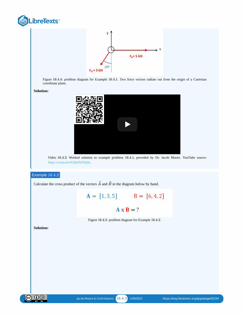
Jacob Moore & Contributors 16.4.3 1/30/2022 https://eng.libretexts.org/@go/page/55334

Figure : problem diagram for Example . Two force vectors radiate out from the origin of a Cartesiancoordinate plane.

Solution:

Video : Worked solution to example problem , provided by Dr. Jacob Moore. YouTube source:https://youtu.be/KQhOkEflq9s.

Calculate the cross product of the vectors and in the diagram below by hand.

Figure : problem diagram for Example .

Solution:

16.4.4 16.4.1

Cross Product - Adaptive Map WoCross Product - Adaptive Map Wo……

16.4.2 16.4.1

Example 16.4.2

A   B 

16.4.5 16.4.2

Jacob Moore & Contributors 16.4.4 1/30/2022 https://eng.libretexts.org/@go/page/55334

Video : Worked solution to example problem , provided by Dr. Jacob Moore. YouTube source:https://youtu.be/oHLU_q3kVKc.

Calculate the cross product of the vectors and in the diagram below using MATLAB.

Figure : problem diagram for Example .

Solution:

Video : Worked solution to example problem , provided by Dr. Jacob Moore. YouTube source:https://youtu.be/a9w6GWQJ96A.

Calculate the cross product of vectors and in the diagram below, using the Wolfram Vector Operation Calculator.

Cross Product - Adaptive Map WoCross Product - Adaptive Map Wo……

16.4.3 16.4.2

Example 16.4.3

A   B 

16.4.6 16.4.3

Cross Product - Adaptive Map WoCross Product - Adaptive Map Wo……

16.4.4 16.4.3

Example 16.4.4

A   B 

Jacob Moore & Contributors 16.4.5 1/30/2022 https://eng.libretexts.org/@go/page/55334

Figure : problem diagram for Example .

Solution:

Video : Worked solution to example problem , provided by Dr. Jacob Moore. YouTube source:https://youtu.be/24JCFHWWGG4.

16.4.7 16.4.4

Cross Product - Adaptive Map WoCross Product - Adaptive Map Wo……

16.4.5 16.4.4

Jacob Moore & Contributors 16.5.1 1/23/2022 https://eng.libretexts.org/@go/page/55335

16.5: Solving Systems of Equations with MatricesA system of equations is any set of equations that share some variables. A linear equation is an equation that consistsentirely of constants and simple variables. These variables can only be multiplied by a constant, and cannot be multipliedtogether, raised to an exponent, used on logs or square roots, or put through other, more complex mathematical functions.An example of a system of linear equations is provided below.

In courses such as statics and dynamics, we will often wind up with a system of linear equations and be asked to solve forthe unknowns in those equations. When we have just a few equations in our system, we will generally solve the equationsby hand using algebraic methods such as substitution or elimination though addition or subtraction. For larger and morecomplex problems, we can wind up with larger systems of equations and at some point the math may become difficult tohandle by hand. For these large systems of linear equations, the easiest way to solve for the unknowns is to convert thesystem of equations into a single matrix equation, and then use computer tools to solve the matrix equation for unknowns.Some computer tools will let you enter the system of equations manually, but in the background the computer is probablyjust converting it to a matrix equation in the background. For this reason it can be useful to understand this process.

In terms of assumptions, it is important to mention that this method will only work with systems of linear equations, andto have a solvable matrix equation we will need to have the same number of equations as unknown variables. Forexample, above we have a system of equations with three equations and three unknown variables. If these numbers do notmatch we will not be able to solve the matrix equation using the method described below.

Converting a System of Equations to a Matrix Equation:The first step in converting a system of equations into a matrix equation is to rearrange the equations into a consistentformat. Generally we will put all the variables with their coefficients on one side of the equation and the constants on theother side of the equation. Additionally, it is best to list the variables in the same order in each equation. This process ofrearranging the equations will make conversion later on easier.

Figure : To convert a system of equations into a single matrix equation, we will first rearrange the equations for aconsistent order. Then we will write out the coefficient ( ), variable ( ), and constant ( matrices.

Next we will begin the process of writing out the three matrices that make up the matrix equation. These three matrices arethe coefficient matrix (often referred to as the matrix), the variable matrix (often referred to as the matrix), and theconstant matrix (often referred to as the matrix).

The coefficient matrix (or matrix) is a matrix (where is the number of equations / number of unknownvariables) that contains all the coefficients for the variables. Each row of the matrix represents a single equation whileeach column represents a single variable (it is sometimes helpful to write the variable at the top of each column). Forinstances where a variable does not show up in an equation, we assume a coefficient of 0.The variable matrix (or matrix) is a matrix that contains all the unknown variables. It is important that theorder of the variables in the coefficient matrix match the order of the variables in the variable matrix.Finally, on the other side of the equal sign we have the constant matrix (or matrix). This is a matrixcontaining all the constants from the right side of the equations. It is important that the order of the constants matches

+ = 0FAX FBX (16.5.1)

−8 = 0FAY (16.5.2)

−16 +4 +8 = 0FAY FAX (16.5.3)

16.5.1A X B)

A X

B

A N ×N N

X N ×1

B N ×1

Jacob Moore & Contributors 16.5.2 1/23/2022 https://eng.libretexts.org/@go/page/55335

the order of equations in the coefficient matrix.

Once we have the three matrices set up, we are ready to solve for the unknowns in the variable matrix.

Solving the Matrix Equation:

Starting with our , , and matrices in the matrix equation below, we are looking to solve for for values of theunknown variables that are contained in our matrix.

For a scalar equation, we would simply do this by dividing both sides by , where the value for would be . With amatrix equation, we will instead need to multiple both sides of the equation by the inverse of the matrix. This willcancel out the matrix on the left side, leaving only the matrix that you are looking for. On the left we will have theinverse of the matrix times the matrix. The result of this operation will be a matrix containing the solution forall the variables. The value in each row of the solution will correspond to the variable listed in the same row of the matrix.

It is possible to find the inverse of the matrix by hand and then multiply this with the matrix, but this process wouldtake longer than just solving the equations using algebra. The true strength of the method is that computer tools such asMATLAB or Wolfram Alpha can perform the matrix inversion and multiplication for you.

Video lecture covering this section, delivered by Dr. Jacob Moore. YouTube source: https://youtu.be/ZLaeFbqR9QU.

The equilibrium equations for the body shown below are listed on the right. Convert the system of equations into asingle matrix equation and solve for the unknowns.

Figure : problem diagram for Example . A system of equations to solve for the forces experienced by avertical pole attached to the ground.

A X B

X

[A][X] = [B] (16.5.4)

A X B/A

A

A X

A B N ×1

X

[X] = [A [B]]−1 (16.5.5)

A B

A 1.5 Solving Systems of Equations A 1.5 Solving Systems of Equations ……

Example 16.5.1

16.5.2 16.5.1

Jacob Moore & Contributors 16.5.3 1/23/2022 https://eng.libretexts.org/@go/page/55335

Solution:

Video : Worked solution to example problem , provided by Dr. Jacob Moore. YouTube source:https://youtu.be/QX-hJhXTEe0.

Matrix Equations - Adaptive Map Matrix Equations - Adaptive Map ……

16.5.2 16.5.1

Jacob Moore & Contributors 16.6.1 12/21/2021 https://eng.libretexts.org/@go/page/55330

16.6: Appendix 1 Homework Problems

Determine the and components of the force vector shown below.

Figure : problem diagram for Exercise . A vector in the first quadrant of a Cartesian coordinate plane,with its tail at the origin.

Solution:

Determine the , , and components of the vector shown below.

Figure : problem diagram for Exercise . A vector originates from the origin of a Cartesian coordinatesystem, pointing into the plane of the screen.

Solution:

Exercise 16.6.1

x y

16.6.1 16.6.1

= 692.8 NFx

= 400NFy

Exercise 16.6.2

x y z

16.6.2 16.6.2

= 4.17 kNFx

= 2.54 kNFy

= −3.50 kNFz

Jacob Moore & Contributors 16.6.2 12/21/2021 https://eng.libretexts.org/@go/page/55330

An 80-lb tension acts along a cable stretching from point O to point A. Based on the dimensions given, break thetension force shown into , , and components.

Figure : problem diagram for Exercise . A cable with a force acting along it connects the origin of aCartesian coordinate system to a given point A.

Solution:

Determine the and components of the sum of the two vectors shown below.

Figure : problem diagram for Exercise . Two force vectors radiate out from the origin of a Cartesiancoordinate plane.

Solution:

Exercise 16.6.3

x y z

16.6.3 16.6.3

= 56.47 lbsFx

= −37.64 lbsFy

= 42.35 lbsFz

Exercise 16.6.4

x y

16.6.4 16.6.4

= [58.2, 41.7] lbsFtotal

Jacob Moore & Contributors 16.6.3 12/21/2021 https://eng.libretexts.org/@go/page/55330

There are two forces acting on a barge as shown below ( and ). The magnitude and direction of is known, butthe magnitude and direction of is not. If the sum of the two forces is 600 N along the -axis, what must themagnitude and direction of be?

Figure : problem diagram for Exercise . Two forces are applied to the same point on a barge, with themagnitude and direction of one of the force vectors as well as the vector sum being known.

Solution:

, at 41.2° below the x-axis

Exercise 16.6.5

F  1 F  

2 F  1

F  2 x

F  2

16.6.5 16.6.5

= 390.3 NF  2

1 1/30/2022

CHAPTER OVERVIEW17: APPENDIX 2 - MOMENT INTEGRALSTypes of moment integrals and the methods for calculating them. Overview of some engineering applications of moment integrals.

17.1: MOMENT INTEGRALSOverview of moment integrals: the general concept of using integration to determine the net moment of a force that is spread over anarea or volume.

17.2: CENTROIDS OF AREAS VIA INTEGRATIONProcedure for finding the location of the centroid of a two-dimensional shape, by taking the first moment integral.

17.3: CENTROIDS IN VOLUMES AND CENTER OF MASS VIA INTEGRATIONProcedure to find the location of the centroid of a three-dimensional volume and to find the center of mass of a volume of non-uniform density, by taking the first moment integral.

17.4: CENTROIDS AND CENTERS OF MASS VIA METHOD OF COMPOSITE PARTSProcedure to find the location of the centroid/center of mass of a shape by the Method of Composite Parts: breaking the shape downinto simpler components for individual analysis.

17.5: AREA MOMENTS OF INERTIA VIA INTEGRATIONProcedure for finding a body's area moments of inertia through integration, used to determine the body's resistance to bending (secondarea moments) or resistance to torsion (polar moment of inertia).

17.6: MASS MOMENTS OF INERTIA VIA INTEGRATIONProcedure for finding an object's mass moment of inertia, or resistance to rotation about an axis, through integration.

17.7: MOMENTS OF INERTIA VIA COMPOSITE PARTS AND PARALLEL AXIS THEOREMCalculating moments of inertia via the Method of Composite Parts, as an alternative to integration.

17.8: APPENDIX 2 HOMEWORK PROBLEMS

Jacob Moore & Contributors 17.1.1 1/7/2022 https://eng.libretexts.org/@go/page/55338

17.1: Moment IntegralsA moment integral, as the name implies, is the general concept of using integration to determine the net moment of aforce that is spread over an area or volume. Because moments are generally a force times a distance, and becausedistributed forces are spread out over a range of distances, we will need to use calculus to to determine the net momentexerted by a distributed force.

Beyond the most literal definition of a moment integral, the term "moment integral" is also general applied the process ofintegrating distributed areas or masses that will be resisting some moment about a set axis.

Some of the applications of moment integrals include:

1. Finding point loads that are equivalent to distributed loads (the equivalent point load).2. Finding the centroid (geometric center) or center of mass for 2D and 3D shapes.3. Finding the area moment of inertia for a beam cross-section, which will be one factor in that beam's resistance to

bending.4. Finding the polar area moment of inertia for a shaft cross-section, which will be one factor in that shaft's resistance to

torsion.5. Finding the mass moment of inertia, indicating a body's resistance to angular accelerations.

When looking at moment integrals, there are number of different types of moment integrals. These will include momentintegrals in one dimension, two dimensions, and three dimensions; moment integrals of force functions, of areas/volumes,or of mass distributions; first order or second order moment integrals; and rectangular or polar moment integrals.

Any combination of these different types is possible (for example, a first-order rectangular 2D area moment integral, or asecond-order polar 3D mass moment integral). However, only some of these combinations will have practical applicationsand will be discussed in detail on future pages.

1D, 2D, and 3D Moment IntegralsTechnically we can take the moment integral in any number of dimensions, but for practical purposes we will never dealwith moment integrals beyond three dimensions. The number of dimensions will affect the complexity of the calculations(with three-dimensional moment integrals being more involved than one- or two-dimensional moment integrals), but thenature of the problem will dictate the dimensions needed. Often this is not listed in the type of moment integral, requiringyou to assume the type based on the context of the problem.

Force, Area/Volume, and Mass Moment Integrals

The next distinction in moment integrals is made with regard what we are integrating. Generally, we can integrate forcefunctions over some distance, area, or volume, we can integrate the area or volume function itself, or we can integrate themass distribution over the area or volume. Each of these types of moment integrals has a different purpose and will startwith a different mathematical function to integrate, but the integration process beyond that will be very similar.

First vs Second Moment IntegralsFor moment integrals we will always be multiplying the force function, area or volume function, or mass distributionfunction by either a distance or a distance squared. First moment integrals just multiply the initial function by the distance,while second moment integrals multiply the function by the distance squared. Again, the type of moment integral we willuse depends upon our application, with things like equivalent point load, centroids, and center of mass relying on firstmoment integrals, and area moments of inertia, polar moments of inertia, and mass moments of inertia relying on secondmoment integrals. As you can probably deduce from this list, second moment integrals, are often labeled as a moment ofinertia.

∫ M = ∫ F (d) ∗ d (17.1.1)

Jacob Moore & Contributors 17.1.2 1/7/2022 https://eng.libretexts.org/@go/page/55338

Rectangular vs Polar Moment IntegralsFinally we will talk about rectangular moment integrals versus polar moment integrals. This is a difference in how wedefine the distance in our moment integral. Let's start with the distinction in 2D. If our distance is measured from someaxis (for example the -axis, or the -axis) then it is a rectangular moment integral. On the other hand, if the distance ismeasured from some point (such as the origin), then it is a polar moment integral.

Figure : In two dimensions, if we locate a point by measuring its distance from some axis (similar to what and do here) then we have a rectangular moment integral. If we locate it by measuring the distance from some point (as with here), then we have a polar moment integral.

This distinction is important for how we will take the integral. For rectangular moment integrals we will move left to rightor bottom to top. For polar moment integrals we will instead take the integral by radiating out from the center point.

In three-dimensional problems, the definitions change slightly. For rectangular moment integrals, the distance will bemeasured from some plane (such as the -plane, -plane, or -plane). Again we will integrate left to right, bottom totop, or now back to front with distances corresponding to the , or coordinates of that point. For a polar momentintegral, the distance will be measured from some axis (such as the the , , or axis), and we will integrate by radiatingoutward from that axis.

Video lecture covering this section, delivered by Dr. Jacob Moore. YouTube source: https://youtu.be/kdCCYkWyF40.

x y

17.1.1 x yr

xy xz yz

x y z

x y z

A 2.1 Moment Integrals - Video LectA 2.1 Moment Integrals - Video Lect……

Jacob Moore & Contributors 17.2.1 1/23/2022 https://eng.libretexts.org/@go/page/55339

17.2: Centroids of Areas via IntegrationThe centroid of an area can be thought of as the geometric center of that area. The location of the centroid is often denotedwith a with the coordinates being , , denoting that they are the average and coordinate for the area. If an areawas represented as a thin, uniform plate, then the centroid would be the same as the center of mass for this thin plate.

Figure : The centroid (marked ) for a few common shapes.

Centroids of areas are useful for a number of situations in the mechanics course sequence, including in the analysis ofdistributed forces, the bending in beams, and torsion in shafts, and as an intermediate step in determining moments ofinertia.

The location of centroids for a variety of common shapes can simply be looked up in tables, such as this table for 2Dcentroids and this table for 3D centroids. However, we will often need to determine the centroid of other shapes; to do this,we will generally use one of two methods.

1. We can use the first moment integral to determine the centroid location.2. We can use the method of composite parts along with centroid tables to determine the centroid location.

On this page we will only discuss the first method, as the method of composite parts is discussed in a later section. Thetables used in the method of composite parts, however, are derived via the first moment integral, so both methodsultimately rely on first moment integrals.

Finding the Centroid via the First Moment IntegralWhen we find the centroid of a two-dimensional shape, we will be looking for both an and a coordinate, represented as

and respectively. Collectively, this coordinate is the centroid of the shape.

To find the average -coordinate of a shape ( ), we will essentially break the shape into a large number of very small andequally sized areas, and find the average -coordinate of these areas. To do this sum of an infinite number of very smallthings, we will use integration. Specifically, we will take the first rectangular area moment integral along the -axis,and then divide that integral by the total area to find the average coordinate. We can do something similar along the -axisto find our value. Writing all of this out, we have the equations below.

Next let's discuss what the variable represents and how we integrate it over the area. The variable is the rate ofchange in area as we move in a particular direction. For we will be moving along the -axis, and for we will bemoving along the -axis in these integrals.

C (x )y x y

17.2.1 C

x y

x y ( ,x y

x x

x

x

y

y

C = ( , )x y (17.2.1)

x

y

=

(dA ∗ x)∫A

A

=

(dA ∗ y)∫A

A

(17.2.2)

(17.2.3)

dA dA

x x y

y

Jacob Moore & Contributors 17.2.2 1/23/2022 https://eng.libretexts.org/@go/page/55339

As we move along the -axis of a shape from its leftmost point to its rightmost point, the rate of change of the area at anyinstant in time will be equal to the height of the shape that point times the rate at which we are moving along the axis ( ).Because the height of the shape will change with position, we do not use any one value, but instead must come up with anequation that describes the height at any given value of x. We will then multiply this equation by the variable (tomake it a moment integral), and integrate that equation from the leftmost position of the shape ( ) to the rightmost position of the shape ( ).

Figure : The procedure for calculating the coordinate of the centroid.

To find the coordinate of the of the centroid, we have a similar process, but because we are moving along the -axis, thevalue is the equation describing the width of the shape times the rate at which we are moving along the axis ( ). Wethen take this equation and multiply it by to make it a moment integral. We will integrate this equation from the position of the bottommost point on the shape ( ) to the position of the topmost point on the shape ( ).

Figure : The procedure for calculating the coordinate of the centroid.

Using the first moment integral and the equations shown above, we can theoretically find the centroid of any shape as longas we can write out equations to describe the height and width at any or value respectively. For more complex shapes,however, determining these equations and then integrating these equations can become very time-consuming. That is whymost of the time, engineers will instead use the method of composite parts or computer tools.

Using Symmetry as a ShortcutShape symmetry can provide a shortcut in many centroid calculations. Remember that the centroid is located at the average

and coordinate for all the points in the shape. If the shape has a line of symmetry, that means each point on one side ofthe line must have an equivalent point on the other side of the line. This means that the average value (AKA the centroid)

x

dx

dA x

x xmin x

xmax

17.2.2 x

y y

dA y dy

dA y y

ymin y ymax

17.2.3 y

x y

x y

Jacob Moore & Contributors 17.2.3 1/23/2022 https://eng.libretexts.org/@go/page/55339

must lie along any axis of symmetry. If the shape has more than one axis of symmetry, then the centroid must exist at theintersection of the two axes of symmetry.

Figure : If a shape has a line of symmetry, the centroid must lie somewhere along that line. If a shape has more thanone line of symmetry, the centroid must exist at the intersection of these lines.

Video lecture covering this section, delivered by Dr. Jacob Moore. YouTube source: https://youtu.be/ilgYN8c1HUk.

Find the and coordinates of the centroid of the shape shown below.

Figure : problem diagram for Example . A right triangle with one leg lying along the -axis in the firstquadrant of a Cartesian plane.

Solution:

17.2.4

A 2.2 Centroid of an Area via IntegraA 2.2 Centroid of an Area via Integra……

Example 17.2.1

x y

17.2.5 17.2.1 x

Jacob Moore & Contributors 17.2.4 1/23/2022 https://eng.libretexts.org/@go/page/55339

Video : Worked solution to example problem , provided by Dr. Jacob Moore. YouTube source:https://youtu.be/dZ2O3zwvuP0.

Find the and coordinates of the centroid of the shape shown below.

Figure : problem diagram for Example . A triangle with its longest side lying along the -axis in the firstquadrant of a Cartesian plane.

Solution:

Video : Worked solution to example problem , provided by Dr. Jacob Moore. YouTube source:https://youtu.be/hmGiCFwgIo8.

Centroids via Integration - AdaptiCentroids via Integration - Adapti……

17.2.2 17.2.1

Example 17.2.2

x y

17.2.6 17.2.2 x

Centroids via Integration - AdaptiCentroids via Integration - Adapti……

17.2.3 17.2.2

Jacob Moore & Contributors 17.2.5 1/23/2022 https://eng.libretexts.org/@go/page/55339

Find the and coordinates of the centroid of the shape shown below.

Figure : problem diagram for Example . An L-shaped region lies along the - and -axes in the firstquadrant of a Cartesian plane.

Solution:

Video : Worked solution to example problem , provided by Dr. Jacob Moore. YouTube source:https://youtu.be/4MHflda4FBw.

Example 17.2.3

x y

17.2.7 17.2.3 x y

Centroids via Integration - AdaptiCentroids via Integration - Adapti……

17.2.4 17.2.3

Jacob Moore & Contributors 17.3.1 1/7/2022 https://eng.libretexts.org/@go/page/55340

17.3: Centroids in Volumes and Center of Mass via IntegrationThe centroid of a volume can be thought of as the geometric center of that shape. It is often denoted as , being beinglocated at the coordinates . If this volume represents a part with a uniform density (like most single material parts)then the centroid will also be the center of mass, a point usually labeled as .

Figure : The centroid point ( ) or the center of mass ( ) for some common shapes. (The centroid and center ofmass are the same point for bodies with a uniform density)

Just as with the centroids of an area, centroids of volumes and the center of mass are useful for a number of situations inthe mechanics course sequence, including the analysis of distributed forces, simplifying the analysis of gravity (which isitself a distributed force), and as an intermediate step in determining mass moments of inertia.

Just as with areas, the location of the centroid (or center of mass) for a variety of common shapes can simply be looked upin tables, such as this one. However, we will often need to determine the centroid or center of mass for other shapes, and todo this we will generally use one of two methods.

1. We can use the first moment integral to determine the centroid or center of mass location.2. We can use the method of composite parts along with centroid tables to determine the centroid or center of mass

location.

On this page we will only discuss the first method, as the method of composite parts is discussed in a later section.However, the tables used in the method of composite parts are derived via the first moment integral, so both methodsultimately rely on first moment integrals.

Finding the Centroid of a Volume via the First Moment Integral

When we find the centroid of a three-dimensional shape, we will be looking for the , , and coordinates ( , , and )of the point that is the centroid of the shape.

Much like the centroid calculations we did with two-dimensional shapes, we are looking to find the shape's averagecoordinate in each dimension. We do this by summing up all the little bits of volume times the , , or coordinate of thatbit of volume and then dividing that sum by the total volume of the shape. Again we will use calculus to sum up an infinitenumber of infinitely small volumes. Specifically this sum will be the first rectangular volume moment integral for theshape.

Working in each of the three coordinate directions we wind up with the following three equations.

C

( , , )x y z

G

17.3.1 C G

x y z x y z

x y z

C = G= ( , , ) for constant-density shapesx y z

Jacob Moore & Contributors 17.3.2 1/7/2022 https://eng.libretexts.org/@go/page/55340

With these new equations we have the variable rather than , because we are integrating over a volume rather thanan area. This represents the rate of change of the volume as we move along an axis from one end to another. The rate ofchange of the volume at any point on the shape will be the cross-sectional area that is perpendicular to that axis times therate at which we are moving along that axis. Since cross-sectional area may vary as we move along the axis, we will needto determine a formula for the cross sectional area at any point along that axis.

Figure : The -coordinate of the centroid/center of mass.

Using the first moment integral and the equations shown above, we can theoretically find the centroid of any volume aslong as we can write an equation to describe the cross section area for each direction. For more complex shapes, however,determining these equations and then integrating these equations may become very time-consuming. For these complexshapes, the method of composite parts or computer tools will most likely be much faster.

Using Symmetry as a Shortcut

Just as with 2D areas, shape symmetry can provide a shortcut in many centroid calculations. Remember that the centroidcoordinate is the average , , and coordinate for all the points in the shape. If the volume has a plane of symmetry, thatmeans each point on one side of the line must have an equivalent point on the other side of the line. This means that theaverage value (AKA the centroid) must lie within that plane. If the volume has more than one plane of symmetry, then thecentroid must exist at the intersection of those planes.

x

y

z

=

(dV ∗ x)∫V

V

=

(dV ∗ y)∫V

V

=

(dV ∗ z)∫V

V

dV dA

17.3.2 z

x y z

Jacob Moore & Contributors 17.3.3 1/7/2022 https://eng.libretexts.org/@go/page/55340

Figure : If a volume has a plane of symmetry, then the centroid must lie somewhere in that plane. If the volume hasmore than one plane of symmetry, the centroid must exist at the intersection of those planes.

Finding the Center of Mass for Non-Uniform Density ShapesIf a body has a non-uniform density, then the centroid of the volume and the center of mass will no longer be the samepoint. In these cases, we will be integrating with respect to mass, rather than integrating the volume. To do this, we will usesomething called a density function, which will provide the density (the mass per unit volume) in terms of the , , and/or

location. In the end, we will also be dividing by total mass, rather than dividing by total volume. The generalizedequations for the center of mass are shown in the equations below.

In instances of uniform density (where the density function did not vary with location and was therefore just a constant),the density constant could be moved outside of the integral. On the bottom, we could also write mass as density timesvolume, and the density terms on the top and bottom of the fraction would cancel out. That is why for uniform-densityparts, the centroid and center of mass will be the same point.

When we have a density function that is not a constant, we will have to come up with a mathematical function for thedensity in terms of and/or and/or locations. If density varies along more than one axis, determining the function andthen integrating it may become quite difficult, and computer modeling may be advisable in these situations.

17.3.3

x y

z

C ≠ G (17.3.1)

G= ( , , )xG yG zG (17.3.2)

xG

yG

zG

= =(dm ∗ x)∫

m

m

(ρ(x, y, z) ∗ dV ∗ x)∫V

m

= =(dm ∗ y)∫mm

(ρ(x, y, z) ∗ dV ∗ y)∫Vm

= =(dm ∗ z)∫

m

m

(ρ(x, y, z) ∗ dV ∗ z)∫V

m

(17.3.3)

(17.3.4)

(17.3.5)

x y z

Jacob Moore & Contributors 17.3.4 1/7/2022 https://eng.libretexts.org/@go/page/55340

Figure : To find the center of mass of a body with a continuously varying density, we must have an equation todescribe the density based on position.

Once you have the density function, you will multiply that by the relevant function as discussed earlier on the page andmultiply it by the variable for the relevant axis. This entire function is integrated from left to right, bottom to top, or backto front, and then that quantity is divided by mass to find the location of the center of mass.

Video lecture covering this section, delivered by Dr. Jacob Moore. YouTube source: https://youtu.be/cBiWKfBLEhk.

The cone shown below is four inches tall and has a four-inch-diameter base. Find the , , and coordinates of thecentroid.

17.3.4

dV

A 2.3 Centroids of Volumes and CenA 2.3 Centroids of Volumes and Cen……

Example 17.3.1

x y z

Jacob Moore & Contributors 17.3.5 1/7/2022 https://eng.libretexts.org/@go/page/55340

Figure : problem diagram for Example . A cone has a circular base centered on the -plane of aCartesian coordinate system, and a central axis that stretches along the positive -axis.

Solution:

Video : Worked solution to example problem , provided by Dr. Jacob Moore. YouTube source:https://youtu.be/IJHwNaOG4-s.

Find the y coordinate of the centroid for the tetrahedron shown in the image below. (The fourth vertex is at the origin)

17.3.5 17.3.1 xy

z

Centroids (3D) via Integration - AdCentroids (3D) via Integration - Ad……

17.3.2 17.3.1

Example 17.3.2

Jacob Moore & Contributors 17.3.6 1/7/2022 https://eng.libretexts.org/@go/page/55340

Figure : problem diagram for Example . A tetrahedron lies in the first octant of a Cartesian coordinatesystem, with three of its edges formed by the coordinate axes.

Solution:

Video : Worked solution to example problem , provided by Dr. Jacob Moore. YouTube source:https://youtu.be/itu_P4ysw9g.

A water and ceramic slurry with a uniform density of 1100 kilograms per meter cubed enters a settling tank with aheight of 1 meter and a diameter of 1 meter. After one hour in the tank, the density of the slurry at the top of the tank ismeasured to be 1000 kilograms per meter cubed and the density at the bottom of the tank is measured to be 1200kilograms per meter cubed. Assume the density of the slurry varies linearly between the top and the bottom. How farhas the center of mass of the slurry dropped between the initial conditions and the current state?

17.3.6 17.3.2

Centroids (3D) via Integration - AdCentroids (3D) via Integration - Ad……

17.3.3 17.3.2

Example 17.3.3

Jacob Moore & Contributors 17.3.7 1/7/2022 https://eng.libretexts.org/@go/page/55340

Figure : problem diagram for Example . As particles in a tank settle, a solution of originally uniformdensity becomes one with linearly decreasing density from bottom to top.

Solution:

Video : Worked solution to example problem , provided by Dr. Jacob Moore. YouTube source:https://youtu.be/BTyO2HolIHY.

17.3.7 17.3.3

Center of Mass via Integration - ACenter of Mass via Integration - A……

17.3.4 17.3.3

Jacob Moore & Contributors 17.4.1 12/21/2021 https://eng.libretexts.org/@go/page/55341

17.4: Centroids and Centers of Mass via Method of Composite PartsAs an alternative to the use of moment integrals, we can use the Method of Composite Parts to find the centroid of anarea or volume or the center of mass of a body. This method is is often easier and faster that the integration method;however, it will be limited by the table of centroids you have available. The method works by breaking the shape orvolume down into a number of more basic shapes, identifying the centroids or centers of masses of each part via a table ofvalues, and then combing the results to find the overall centroid or center of mass.

A key aspect of the method is the use of these centroid tables. This is a set of tables that lists the centroids (and usuallyalso moments of inertia) for a number of common areas and/or volumes. Some centroid tables can be found here for 2Dshapes, and here for 3D shapes. The method of composite parts is limited in that we will need to be able to break ourcomplex shape down entirely into shapes found in the centroid table we have available; otherwise, the method will notwork without us also doing some moment integrals.

Finding the Centroid via the Method of Composite PartsStart the process by labeling an origin point and axes on your shape. It will be important to measure all locations from thesame point. Next, we must break our complex shape down into several simpler shapes. This may include areas or volumes(which we will count as positive areas or volumes) or holes (which we will count as negative areas or volumes). Each ofthese shapes will have a centroid ( ) or center of mass ( ) listed on the diagram.

Figure : For the shape shown at the top, we can break it down into a rectangle (1), a right triangle (2), and a circularhole (3). Each of these simple shapes is something we have listed in the centroid table to the right.

Once we have identified the different parts, we will create a table listing the area or volume of each piece, and the and centroid coordinates (or , , and coordinates in 3D). It is important to remember that each coordinate you list should berelative to the same base origin point that you drew in earlier. You may need to mentally adjust diagrams in the centroidtables so that the shape is oriented in the right direction, and account for the placement of the shape relative to the axes inyour diagram.

C G

17.4.1

x y

x y z

Jacob Moore & Contributors 17.4.2 12/21/2021 https://eng.libretexts.org/@go/page/55341

Figure : For each of the shapes, we need to find the area and the and coordinates of the centroid. Remember tofind the centroid coordinates relative to a single set of axes that is the same for all the shapes.

Once you have the areas and centroid coordinates for each shape relative to your origin point, you can find the and coordinate of the centroid for the overall shape with the following formulas. Remember that areas or volumes for anyshape that is a hole or cutout in the design will be a negative area in your formula.

This generalized formula to find the centroid's -location is simply Area 1 times , plus Area 2 times , plus Area 3times , adding up as many shapes as you have in this fashion and then dividing by the overall area of your combinedshape. The equations are the same for the -location of the overall centroid, except you will instead be using values inyour equations.

For centroids in three dimensions we will simply use volumes in place of areas, and we will have a coordinate for ourcentroid as well as the and coordinates.

Finding the Center of Mass via the Method of Composite Parts

To use the method of composite parts to find the center of mass, we simply need to adjust the process slightly. First, centerof mass calculations will always be in three dimensions. Draw an origin point and some axes on your diagram we did forthe centroid. We will measure all locations relative to this origin point. We will then need to break the complex shape downinto simple volumes, with each simple volume being something in the centroid table we have available. Remember thatwhen we have a part with a uniform material, the centroid and center of mass are the same point, so we will often talkabout these interchangeably.

Figure : When finding the center of mass via composite parts, we will break the shape up into several simplershapes. The figure on the left can be thought of as a hemisphere (1), on top of a cylinder (2) with another smaller cylindercut out of it (3). Each of these simple volumes are listed in our centroid table.

Once we have identified the different parts, we will create a table indicating the mass of each part, and the x, y, and zcoordinate of the center of mass for each individual part. It is important to remember that each coordinate you list should

17.4.2 x y

x y

= =xtotal

∑Aixi

Atotal

y total

∑Ai y i

Atotal

(17.4.1)

x x1 x2

x3

y y

z

x y

17.4.3

Jacob Moore & Contributors 17.4.3 12/21/2021 https://eng.libretexts.org/@go/page/55341

be relative to the same base origin point, so you will need to mentally rotate and position the parts in the table on youraxes.

Figure : Create a table with the mass of each piece of the total shape, as well as the center of mass location ( , ,and coordinates) for each piece.

One complicating factor with mass can be measuring the mass of the pieces separately. If we have a scale, we may simplyknow the overall mass without knowing the mass of the individual pieces. In these cases, you may need work backwards tocalculate the density of the material (by dividing the overall mass by overall volume), and then use density times piecevolume to find the mass of each piece individually. When doing this, remember to count cutouts as negative mass in yourcalculations. For example, for the hollow cylinder in the shape above, you would find the mass of a solid cylinder forShape 2, then have a negative mass for the cylindrical cutout for Shape 3.

Finally, once you have the mass the and center of mass coordinates for each shape, you can find the coordinates of thecenter of mass for the overall volume with the following formulas.

Similar to the centroid equations, the -equation is simply the mass of Shape 1 times , plus the mass of Shape 2 times , and so on for each part. After you have summed up these products for all the shapes, just divide by the total mass.

Video lecture covering this section, delivered by Dr. Jacob Moore. YouTube source: https://youtu.be/wfjLNSfPXAI.

17.4.4 x y

z

= = =xG

∑mixi

mtotal

yG

∑mi y i

mtotal

zG

∑mi z i

mtotal

(17.4.2)

x x1

x2

A 2.4 Centroids and Center of Mass A 2.4 Centroids and Center of Mass ……

Jacob Moore & Contributors 17.4.4 12/21/2021 https://eng.libretexts.org/@go/page/55341

Find the and coordinates of the centroid of the shape shown below.

Figure : problem diagram for Example . A trapezoid with two perpendicular sides and a hole through itsmiddle lies along the axes of the first quadrant of a Cartesian coordinate plane.

Solution:

Video : Worked solution to example problem , provided by Dr. Jacob Moore. YouTube source:https://youtu.be/QIe6Hk4Bofs.

Find the and coordinates of the centroid of the shape shown below.

Example 17.4.1

x y

17.4.5 17.4.1

Centroids via the Method of ComCentroids via the Method of Com……

17.4.2 17.4.2

Example 17.4.2

x y

Jacob Moore & Contributors 17.4.5 12/21/2021 https://eng.libretexts.org/@go/page/55341

Figure : problem diagram for Example . A pentagon with two perpendicular sides lies along the axes ofthe first quadrant of a Cartesian coordinate plane.

Solution:

Video : Worked solution to example problem , provided by Dr. Jacob Moore. YouTube source:https://youtu.be/F1rlzboPlZM.

Find the and coordinates of the centroid of the shape shown below.

17.4.6 17.4.2

Centroids via the Method of ComCentroids via the Method of Com……

17.4.3 17.4.2

Example 17.4.3

x y

Jacob Moore & Contributors 17.4.6 12/21/2021 https://eng.libretexts.org/@go/page/55341

Figure : problem diagram for Example . A rectangle with a hole through one side (shaped like a rectangletopped with a semicircle) lies along the axes of the first quadrant of a Cartesian coordinate plane.

Solution:

Video : Worked solution to example problem , provided by Dr. Jacob Moore. YouTube source:https://youtu.be/tLybTEX8S_I.

The shape shown below consists of a solid semicircular hemisphere on top of a hollow cylinder. Based on thedimensions below, determine the location of the centroid.

17.4.7 17.4.3

Centroids via the Method of ComCentroids via the Method of Com……

17.4.4 17.4.3

Example 17.4.4

Jacob Moore & Contributors 17.4.7 12/21/2021 https://eng.libretexts.org/@go/page/55341

Figure : problem diagram for Example . A hollowed-out cylinder topped with a hemisphere lies along the-axis of a Cartesian coordinate system, with its base being centered in the -plane.

Solution:

Video : Worked solution to example problem , provided by Dr. Jacob Moore. YouTube source:https://youtu.be/vQk4OqTcDpQ.

A spherical steel tank (density = 8050 kg/m ) is filled halfway with water (density = 1000 kg/m ) as shown below.Find the overall mass of the tank and the current location of the center of mass of the tank (measured from the base ofthe tank).

17.4.8 17.4.4z xy

Centroids (3D) via Method of CoCentroids (3D) via Method of Co……

17.4.5 17.4.4

Example 17.4.5

3 3

Jacob Moore & Contributors 17.4.8 12/21/2021 https://eng.libretexts.org/@go/page/55341

Figure : problem diagram for Example . A spherical steel tank of diameter 2 meters and metal thickness0.01 meters is half-filled with water.

Solution:

Video : Worked solution to example problem , provided by Dr. Jacob Moore. YouTube source:https://youtu.be/5zbYD4Wogck.

17.4.9 17.4.5

Center of Mass via Composite PaCenter of Mass via Composite Pa……

17.4.6 17.4.5

Jacob Moore & Contributors 17.5.1 12/21/2021 https://eng.libretexts.org/@go/page/55342

17.5: Area Moments of Inertia via IntegrationArea moments of inertia are used in engineering mechanics courses to determine a body's resistance to bending loads ortorsional loads. Specifically, the area moment of inertia refers to the second area moment integral of a shape, with representing the moment of inertia about the -axis, representing the moment of inertia about the -axis, and (alsocalled the polar moment of inertia) representing the moment of inertia about the -axis. The moment of inertia about eachaxis represents the shapes resistance to a moment applied about that respective axis. Moments about the - and -axeswould tend to bend an object, while moments about the -axis would tend to twist the body.

Figure : The moments of inertia for the cross section of a shape about each axis represents the shape's resistance tomoments about that axis. Moments applied about the -axis and -axis represent bending moments, while moments aboutthe - axis represent torsional moments.

Just as with centroids, each of these moments of inertia can be calculated via integration or by using the method ofcomposite parts and the parallel axis theorem. On this page we are going to focus on calculating the area moments ofinertia via moment integrals.

Bending Stresses and the Second Area MomentWhen an object is subjected to a bending moment, that body will experience both internal tensile stresses and compressivestresses as shown in the diagram below. These stresses exert a net moment to counteract the loading moment, but exert nonet force so that the body remains in equilibrium.

Figure : A bending moment and the resulting internal tensile and compressive stresses needed to ensure the beam isin equilibrium.

As we can see in the diagram, there is some central plane along which there are no tensile or compressive stresses. This isknown as the neutral surface, and if there are no other forces present it will run through the centroid of the cross section.As we move up or down from the neutral surface, the stresses increase linearly. The moment exerted by this stress at anypoint will be the stress times the moment arm, which also linearly increases as we move away from the neutral surface.This means that the resistance to bending provided by any point in the cross section is directly proportional to the distancefrom the neutral axis squared. We can sum up the resistances to bending then by using the second rectangular area momentof inertia, where our distances are measured from the neutral axis.

Ixxx Iyy y Jzz

z

x y

z

17.5.1x y

z

17.5.2

Jacob Moore & Contributors 17.5.2 12/21/2021 https://eng.libretexts.org/@go/page/55342

Assuming we put the origin point at the centroid and that the -axis is the neutral surface, the distance from the neutralsurface to any point is simply the coordinate of that point. Similarly, if we apply a moment about the -axis, and had aneutral surface that ran along the -axis, the distance from the neutral axis would simply be the coordinate of the point.For this reason, includes as the distance, while includes as the distance.

Calculating the Rectangular Area Moment of Inertia via Integration

To determine the area moment of inertia, start by drawing out the area under analysis, and include the axes you are takingthe moment of inertia about. This is important, since the moment of inertia will vary depending on the axis chosen. Incases on bending stresses you will want to put the origin on the neutral surface, which will be at the centroid of the area. Ifthe centroid is not given to you, you will need to determine the centroid as discussed in prior sections.

To take the moment of inertia about the -axis through this point ( ) we will use the general formula discussed earlier.We will be moving from bottom to top, integrating the rate of change of the area as we go, and multiplying that by the -value squared. The rate of change of area ( ) as we move upwards will be the width of the object at any given -valuetimes the rate at which we are moving. Unless the width remains constant, the width will need to be represented as amathematical function in terms of .

Figure : The rectangular moment of inertia about the -axis.

To find the moment of inertia about the -axis through a given point ( ) we will move left to right, using the distancesfrom the -axis in our moment integral (in this case the coordinates of each point). Moving from left to right, the rate ofchange of the area will be the height of the shape at any given -value times the rate at which we are moving left to right.Again, we will need to describe this with an mathematical function if the height is not constant. We will multiply thisfunction by the -value squared for the second moment integral, and this will give us the moment of inertia about the -axis.

I = (dA ∗ )∫A

d2 (17.5.1)

x

y y

y x

Ixx y Iyy x

= (dA ∗ ) = (dA ∗ )Ixx ∫ymax

ymin

y2 Iyy ∫xmax

xmin

x2 (17.5.2)

x Ixxy

dA y

y

17.5.3 x

y Iyyy x

x

x y

Jacob Moore & Contributors 17.5.3 12/21/2021 https://eng.libretexts.org/@go/page/55342

Figure : The rectangular moment of inertia about the -axis.

Torsional Stresses and the Polar Moment of Inertia

When an object is subjected to a torsional moment, that object will experience internal shearing forces as shown in thediagram below. These stresses are oriented in such a way that they will counteract the torsional moment, but do not exertany net force on the shaft so that shaft stays in equilibrium.

Figure : Torsion causes internal shearing stresses that counteract the moment but exert no net force.As we can see in the diagram, there is a central axis along which there are no shearing stresses. This is known as theneutral axis, and if there are no other forces present, then this will travel through the centroid of the shaft's cross section.As we move away from the neutral axis in any direction, the stresses will increase linearly. The moment exerted by thestress at any point will be the stress times the moment arm, which also increases linearly as we move away from theneutral axis. This means that the resistance to torsional loading provided by any one point on the cross section is directlyproportional the square of the distance between the point and neutral axis. We can sum up the resistances to torsionalloading then using the second polar area moment of inertia, where our distances are measured from the neutral axis ( ), asingle point in the shaft's cross-section.

Calculating the Polar Area Moment of Inertia via IntegrationThe first step in determining the polar moment of inertia is to draw the area and identify the point about which we aretaking the moment of inertia. In the case of torsional loading, we will usually want to pick the point at which the neutralaxis travels through the shaft's cross section, which in the absence of other types of loading will be the centroid of the crosssection. If the centroid is not clearly identified, you will need to determine the centroid as discussed in previous sections.

17.5.4 y

17.5.5

r

= (dA ∗ )Jzz ∫rmax

rmin

r2 (17.5.3)

Jacob Moore & Contributors 17.5.4 12/21/2021 https://eng.libretexts.org/@go/page/55342

To take the moment of inertia about this central point, we will be measuring all distances outward from this point. Ratherthan moving left to right or top to bottom, we will instead be integrating from the center radiating outward in all directions.We will be going from the minimum distance from the center for our shape (zero unless there is a central hole in our area)to the maximum distance to the center. We will again be integrating the rate of change of area, which in this case will be afunction for the circumference at a given radius times the rate as which we are moving outwards times the given radiussquared.

Figure : The polar moment of inertia about the neutral axis.

Video lecture covering this section, delivered by Dr. Jacob Moore. YouTube source: https://youtu.be/gCM6Wd8sa6M.

Find the rectangular moments of inertia for this shape about both the -axis and -axis though the centroid. Leave theanswer in terms of the generic width ( ) and height ( ) of the rectangle.

17.5.6

A 2.5 Area Moments of Inertia via IntA 2.5 Area Moments of Inertia via Int……

Example 17.5.1

x y

b h

Jacob Moore & Contributors 17.5.5 12/21/2021 https://eng.libretexts.org/@go/page/55342

Figure : problem diagram for Example . A solid rectangle is centered at the origin of a Cartesiancoordinate plane.

Solution:

Video : Worked solution to example problem , provided by Dr. Jacob Moore. YouTube source:https://youtu.be/PL6QIBL_rPw.

Find the polar moments of inertia for this circular area about its centroid. Leave the answer in terms of the genericradius .

17.5.7 17.5.1

Rectangular Area Moment of InerRectangular Area Moment of Iner……

17.5.2 17.5.1

Example 17.5.2

R

Jacob Moore & Contributors 17.5.6 12/21/2021 https://eng.libretexts.org/@go/page/55342

Figure : problem diagram for Example . A solid circle is centered at the origin of a Cartesian coordinateplane.

Solution:

Video : Worked solution to example problem , provided by Dr. Jacob Moore. YouTube source:https://youtu.be/peqSVmDjThA.

Find the polar moment of inertia of this hollow circular shape about its centroid.

Figure : problem diagram for Example . A disk of diameter 6 inches contains a centered circular cutout ofdiameter 5 inches.

Solution:

17.5.8 17.5.2

Polar Area Moment of Inertia - AdPolar Area Moment of Inertia - Ad……

17.5.3 17.5.2

Exercise 17.5.3

17.5.9 17.5.3

Jacob Moore & Contributors 17.5.7 12/21/2021 https://eng.libretexts.org/@go/page/55342

Video : Worked solution to example problem , provided by Dr. Jacob Moore. YouTube source:https://youtu.be/Jw696gGSDM8.

Polar Area Moment of Inertia - AdPolar Area Moment of Inertia - Ad……

17.5.4 17.5.3

Jacob Moore & Contributors 17.6.1 12/21/2021 https://eng.libretexts.org/@go/page/55343

17.6: Mass Moments of Inertia via IntegrationThe mass moment of inertia represents a body's resistance to angular accelerations about an axis, just as mass representsa body's resistance to linear accelerations. This is represented in an equation with the rotational version of Newton'sSecond Law.

Just as with area moments of inertia, the mass moment of inertia can be calculated via moment integrals or via the methodof composite parts and the parallel axis theorem. This page will only discuss the integration method, as the method ofcomposite parts is discussed on a separate page.

The Mass Moment of Inertia and Angular Accelerations

The mass moment of inertia is a moment integral, specifically the second polar mass moment integral. To see why thisrelates moments and angular accelerations, we start by examining a point mass on the end of a massless stick as shownbelow. Imagine we want to rotate the stick about the left end by applying a moment there. We want to relate the momentexerted to the angular acceleration of the stick about this point.

Figure : A point mass on the end of a massless stick. We are attempting to rotate the mass about the stick's left endby exerting a moment there.

To relate the moment and the angular acceleration, we need to start with the traditional form of Newton's Second Law,stating that the force exerted on the point mass by the stick will be equal to the mass times the acceleration of the pointmass ( ). In this case the moment will be related to the force in that the force exerted on the mass times thelength of the stick ( ) is equal to the moment. We can also relate the linear acceleration of the mass to its rotationalcounterpart in that the linear acceleration is the angular acceleration times the length of the rod ( ). If we take these twosubstitutions and put them into the original equation, we can wind up with an equation that relates the momentand the angular acceleration for our scenario. A simplified version of this new relationship states that the moment will beequal to the mass times the distance squared times the angular acceleration. This mass-times-distance-squared term(relating the moment and angular acceleration) forms the basis for the mass moment of inertia.

Taking our situation one step further, if we were to have multiple masses all connected to a central point, the moment andangular acceleration would be related by the sum of all the mass times distance squared terms.

F = ma (17.6.1)

M = Iα (17.6.2)

17.6.1

F = m ∗ a

d

d

F = m ∗ a

F = m ∗ a (17.6.3)

M = F ∗ d a = d ∗α (17.6.4)

M = (m ∗ ) ∗αd2 (17.6.5)

M =∑(m ∗ ) ∗αd2 (17.6.6)

Jacob Moore & Contributors 17.6.2 12/21/2021 https://eng.libretexts.org/@go/page/55343

Figure : For systems with multiple masses, we would simply sum up all the mass-times-distance-squared terms torelate moments and angular accelerations.

Taking the final step, rigid bodies with mass distributed over a volume are like an infinite number of small masses about anaxis of rotation. Rather than the massless sticks holding everything in place, the mass is simply held in place by thematerial around it. To relate the moment and angular acceleration in this case, we use integration to add up the infinitenumber of small mass-times-distance-squared terms.

Figure : Approximating a rigid body as an infinite number of infinitely small masses all connected to the axis ofrotation, we can sum all the mass-times-distance-squared terms with integration.

This moment integral which can be calculated for any given shape, called the mass moment of inertia, relates the momentand the angular acceleration for the body about a set axis of rotation.

Calculating the Mass Moment of Inertia via Integration

The first step in calculating the mass moment of inertia is to determine the axis of rotation you will be using. Unlike mass,the mass moment of inertia is dependent upon the point and axis that we are rotating about. We can easily demonstrate thiswith something like a broomstick, where depending on the position and the direction of the axis we are rotating about, thebroomstick can be more or less difficult to rotate.

Figure : The mass moment of inertia will vary depending upon the point and direction of the axis of rotation.

17.6.2

17.6.3

M = (dm ∗ ) ∗α∫m

d2 (17.6.7)

I = (dm ∗ )∫m

d2 (17.6.8)

17.6.4

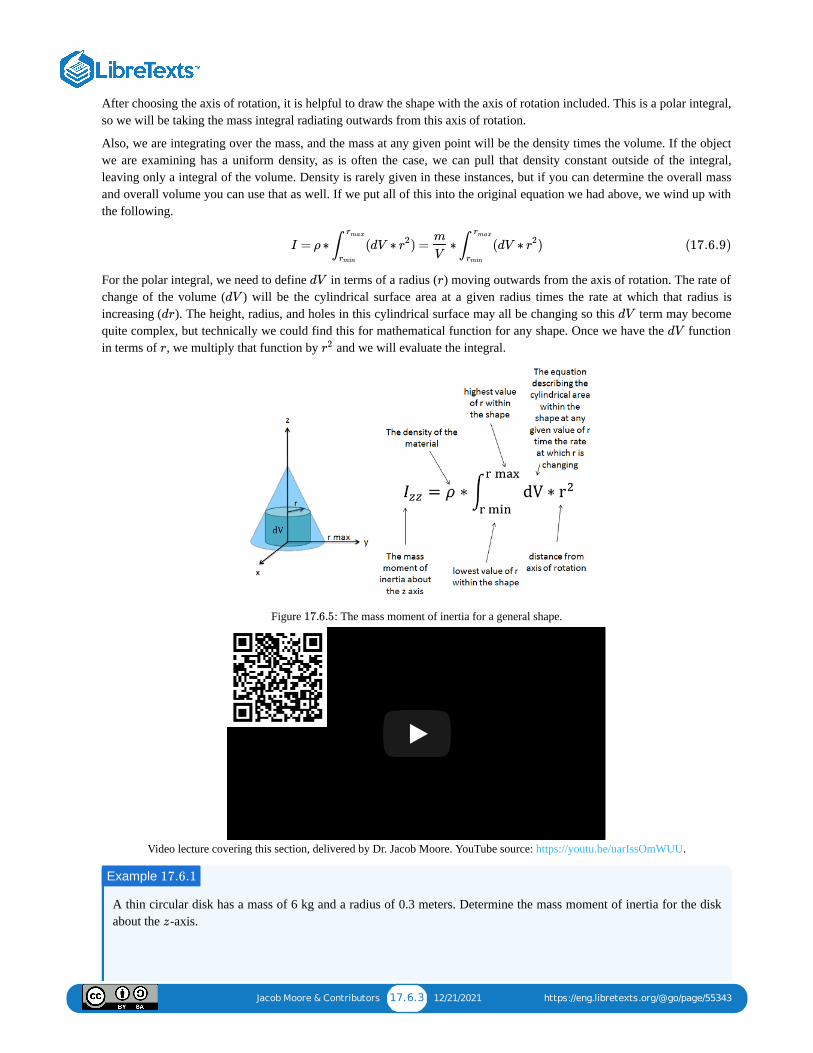
Jacob Moore & Contributors 17.6.3 12/21/2021 https://eng.libretexts.org/@go/page/55343

After choosing the axis of rotation, it is helpful to draw the shape with the axis of rotation included. This is a polar integral,so we will be taking the mass integral radiating outwards from this axis of rotation.

Also, we are integrating over the mass, and the mass at any given point will be the density times the volume. If the objectwe are examining has a uniform density, as is often the case, we can pull that density constant outside of the integral,leaving only a integral of the volume. Density is rarely given in these instances, but if you can determine the overall massand overall volume you can use that as well. If we put all of this into the original equation we had above, we wind up withthe following.

For the polar integral, we need to define in terms of a radius ( ) moving outwards from the axis of rotation. The rate ofchange of the volume ( ) will be the cylindrical surface area at a given radius times the rate at which that radius isincreasing ( ). The height, radius, and holes in this cylindrical surface may all be changing so this term may becomequite complex, but technically we could find this for mathematical function for any shape. Once we have the functionin terms of , we multiply that function by and we will evaluate the integral.

Figure : The mass moment of inertia for a general shape.

Video lecture covering this section, delivered by Dr. Jacob Moore. YouTube source: https://youtu.be/uarIssOmWUU.

A thin circular disk has a mass of 6 kg and a radius of 0.3 meters. Determine the mass moment of inertia for the diskabout the -axis.

I = ρ ∗ (dV ∗ ) = ∗ (dV ∗ )∫rmax

rmin

r2 m

V∫

rmax

rmin

r2 (17.6.9)

dV r

dV

dr dV

dV

r r2

17.6.5

A 2.6 Mass Moments of Inertia via InA 2.6 Mass Moments of Inertia via In……

Example 17.6.1

z

Jacob Moore & Contributors 17.6.4 12/21/2021 https://eng.libretexts.org/@go/page/55343

Figure : problem diagram for Example . A thin cylindrical disk lies along the -axis with its base on the -plane, centered at the origin.

Solution:

Video : Worked solution to example problem , provided by Dr. Jacob Moore. YouTube source:https://youtu.be/e1ZDv6xDUV8.

Determine the mass moment of inertia about the -axis for this general cone with base radius , height , and mass .

Figure : problem diagram for Example . A cone lies along the positive -axis, with the base centered atthe origin in the -plane.

Solution:

17.6.6 17.6.1 zxy

Mass Moment of Inertia - AdaptivMass Moment of Inertia - Adaptiv……

17.6.2 17.6.1

Example 17.6.2

z R h

m

17.6.7 17.6.2 zxy

Jacob Moore & Contributors 17.6.5 12/21/2021 https://eng.libretexts.org/@go/page/55343

Video : Worked solution to example problem , provided by Dr. Jacob Moore. YouTube source:https://youtu.be/rL7xWl9FfWc.

Mass Moment of Inertia - AdaptivMass Moment of Inertia - Adaptiv……

17.6.3 17.6.2

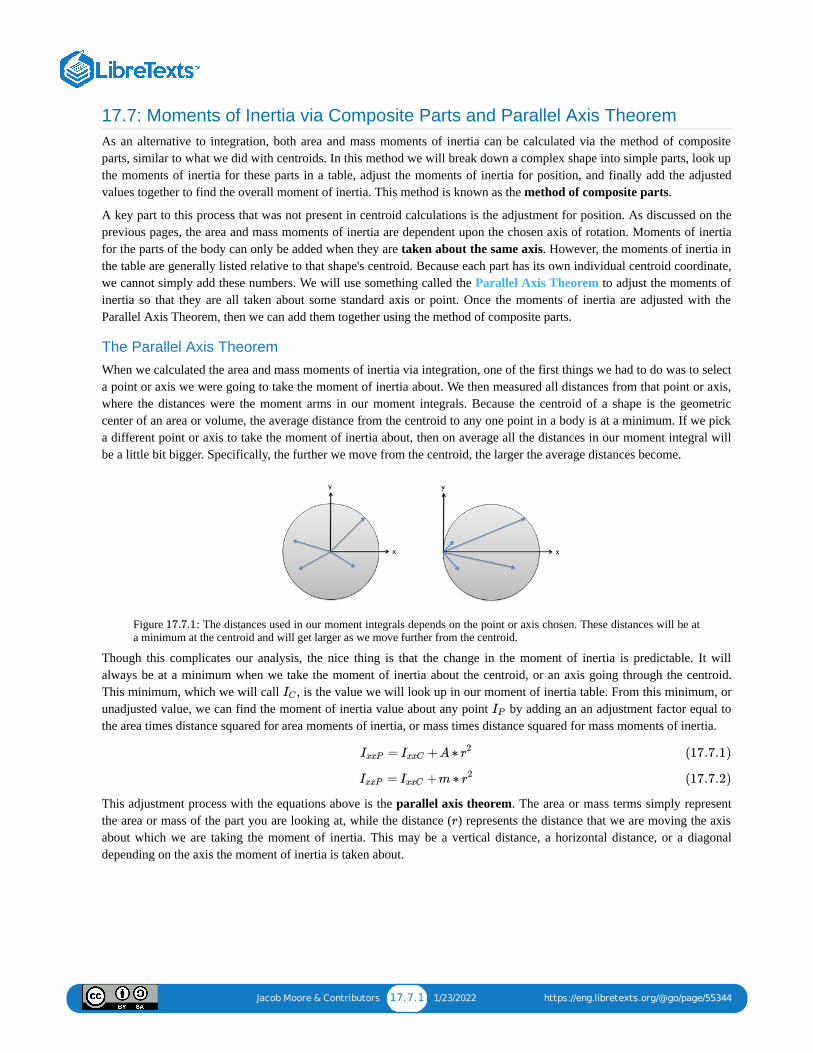
Jacob Moore & Contributors 17.7.1 1/23/2022 https://eng.libretexts.org/@go/page/55344

17.7: Moments of Inertia via Composite Parts and Parallel Axis TheoremAs an alternative to integration, both area and mass moments of inertia can be calculated via the method of compositeparts, similar to what we did with centroids. In this method we will break down a complex shape into simple parts, look upthe moments of inertia for these parts in a table, adjust the moments of inertia for position, and finally add the adjustedvalues together to find the overall moment of inertia. This method is known as the method of composite parts.

A key part to this process that was not present in centroid calculations is the adjustment for position. As discussed on theprevious pages, the area and mass moments of inertia are dependent upon the chosen axis of rotation. Moments of inertiafor the parts of the body can only be added when they are taken about the same axis. However, the moments of inertia inthe table are generally listed relative to that shape's centroid. Because each part has its own individual centroid coordinate,we cannot simply add these numbers. We will use something called the Parallel Axis Theorem to adjust the moments ofinertia so that they are all taken about some standard axis or point. Once the moments of inertia are adjusted with theParallel Axis Theorem, then we can add them together using the method of composite parts.

The Parallel Axis TheoremWhen we calculated the area and mass moments of inertia via integration, one of the first things we had to do was to selecta point or axis we were going to take the moment of inertia about. We then measured all distances from that point or axis,where the distances were the moment arms in our moment integrals. Because the centroid of a shape is the geometriccenter of an area or volume, the average distance from the centroid to any one point in a body is at a minimum. If we picka different point or axis to take the moment of inertia about, then on average all the distances in our moment integral willbe a little bit bigger. Specifically, the further we move from the centroid, the larger the average distances become.

Figure : The distances used in our moment integrals depends on the point or axis chosen. These distances will be ata minimum at the centroid and will get larger as we move further from the centroid.

Though this complicates our analysis, the nice thing is that the change in the moment of inertia is predictable. It willalways be at a minimum when we take the moment of inertia about the centroid, or an axis going through the centroid.This minimum, which we will call , is the value we will look up in our moment of inertia table. From this minimum, orunadjusted value, we can find the moment of inertia value about any point by adding an an adjustment factor equal tothe area times distance squared for area moments of inertia, or mass times distance squared for mass moments of inertia.

This adjustment process with the equations above is the parallel axis theorem. The area or mass terms simply representthe area or mass of the part you are looking at, while the distance ( ) represents the distance that we are moving the axisabout which we are taking the moment of inertia. This may be a vertical distance, a horizontal distance, or a diagonaldepending on the axis the moment of inertia is taken about.

17.7.1

IC

IP

= +A ∗IxxP IxxC r2 (17.7.1)

= +m ∗IxxP IxxC r2 (17.7.2)

r

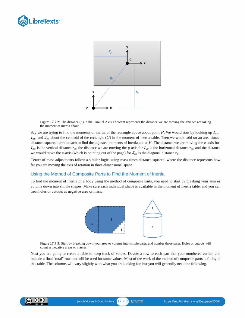
Jacob Moore & Contributors 17.7.2 1/23/2022 https://eng.libretexts.org/@go/page/55344

Figure : The distance ( ) in the Parallel Axis Theorem represents the distance we are moving the axis we are takingthe moment of inertia about.

Say we are trying to find the moments of inertia of the rectangle above about point . We would start by looking up , , and about the centroid of the rectangle ( ) in the moment of inertia table. Then we would add on an area-times-

distance-squared term to each to find the adjusted moments of inertia about . The distance we are moving the axis for is the vertical distance , the distance we are moving the -axis for is the horizontal distance , and the distance

we would move the -axis (which is pointing out of the page) for is the diagonal distance .

Center of mass adjustments follow a similar logic, using mass times distance squared, where the distance represents howfar you are moving the axis of rotation in three-dimensional space.

Using the Method of Composite Parts to Find the Moment of Inertia

To find the moment of inertia of a body using the method of composite parts, you need to start by breaking your area orvolume down into simple shapes. Make sure each individual shape is available in the moment of inertia table, and you cantreat holes or cutouts as negative area or mass.

Figure : Start by breaking down your area or volume into simple parts, and number those parts. Holes or cutouts willcount as negative areas or masses.

Next you are going to create a table to keep track of values. Devote a row to each part that your numbered earlier, andinclude a final "total" row that will be used for some values. Most of the work of the method of composite parts is filling inthis table. The columns will vary slightly with what you are looking for, but you will generally need the following.

17.7.2 r

P Ixx

Iyy Jzz C

P x

Ixx rx y Iyy ry

z Jzz rz

17.7.3

Jacob Moore & Contributors 17.7.3 1/23/2022 https://eng.libretexts.org/@go/page/55344

Figure : Most work in the method of composite parts will revolve around filling out a table such as this one. Thistable contains the rows and columns necessary to find the rectangular area moments of inertia ( and ) for thiscomposite body.

The area or mass for each piece (area for area moments of inertia or mass for mass moments of inertia). Remember thatcutouts should be listed as negative areas or masses.The centroid or center of mass locations ( , and possibly coordinates). Most of the time, we will be finding themoment of inertia about centroid of the composite shape, and if that is not explicitly given to you, you will need to findthat before going further. For more details on this, see the page Centroids and Centers of Mass via Method ofComposite Parts.The moment of inertia values about each shape's centroid. To find these values you will plug numbers for height,radius, mass, etc. into formulas on the moment of inertia table. Do not use these formulas blindly though, as you mayneed to mentally rotate the body, and thus switch equations, if the orientation of the shape in the table does not matchthe orientation of the shape in your diagram.The adjustment distances ( ) for each shape. For this value you will want to determine how far the -axis, -axis, or -axis moves to go from the centroid of the piece to the overall centroid or point you are taking the moment of inertiaabout. To calculate these values, generally you will be finding the horizontal, vertical, or diagonal distances betweenpiece centroids and the overall centroids that you have listed earlier in the table. See the parallel axis theorem section ofthis page earlier for more details.Finally, you will have a column of the adjusted moments of inertia. Take the original moment of inertia about thecentroid, then simply add your area times term or mass times term for this adjusted value.

The overall moment of inertia of your composite body is simply the sum of all of the adjusted moments of inertia for thepieces, which will be the sum of the values in the last column (or columns, if you are finding the moments of inertia aboutmore than one axis).

Video : Video lecture covering this section, delivered by Dr. Jacob Moore. YouTube source:https://youtu.be/zulGTSWF6xs.

17.7.4Ixx Iyy

x y z

r x y z

r2 r2

A 2.7 Moments of Inertia via CompoA 2.7 Moments of Inertia via Compo……

17.7.1

Jacob Moore & Contributors 17.7.4 1/23/2022 https://eng.libretexts.org/@go/page/55344

Use the parallel axis theorem to find the mass moment of inertia of this slender rod with mass and length aboutthe -axis at its endpoint.

Figure : problem diagram for Example . A rod lies along the positive -axis of a Cartesian coordinatesystem, with its left endpoint located at the origin.

Solution:

Video : Worked solution to example problem , provided by Dr. Jacob Moore. YouTube source:https://youtu.be/4oN0kgDO3Yw.

A beam is made by connecting two 2" x 4" beams in a T-pattern with the cross section as shown below. Determine thelocation of the centroid of this combined cross section and then find the rectangular area moment of inertia about the

-axis through the centroid point.

Example 17.7.1

m L

z

17.7.5 17.7.1 x

Moment of Inertia via Composite Moment of Inertia via Composite ……

17.7.2 17.7.1

Example 17.7.2

x

Jacob Moore & Contributors 17.7.5 1/23/2022 https://eng.libretexts.org/@go/page/55344

Figure : problem diagram for Example . The top edge of a vertical 2" x 4" beam is centered on andconnected to the lower edge of a horizontal 2" x 4" beam, creating a T-shaped assembly.

Solution:

Video : Worked solution to example problem , provided by Dr. Jacob Moore. YouTube source:https://youtu.be/lgXlp2lRaiA.

A dumbbell consists of two spheres of diameter 0.2 meter, each with a mass of 40 kg, attached to the ends of a 0.6-meter-long slender rod of mass 20 kg. Determine the mass moment of inertia of the dumbbell about the -axis shownin the diagram.

Figure : problem diagram for Example . A dumbbell consists of a slender rod with a sphere attached toeach end lying along the -axis of a Cartesian coordinate system, with its midpoint at the origin.

17.7.6 17.7.2

Moment of Inertia via Composite Moment of Inertia via Composite ……

17.7.3 17.7.2

Example 17.7.3

y

17.7.7 17.7.3x

Jacob Moore & Contributors 17.7.6 1/23/2022 https://eng.libretexts.org/@go/page/55344

Solution:

Video : Worked solution to example problem , provided by Dr. Jacob Moore. YouTube source:https://youtu.be/ufewJ7CmvIs.

Moment of Inertia via Composite Moment of Inertia via Composite ……

17.7.4 17.7.3

17.8.1 12/21/2021 https://eng.libretexts.org/@go/page/58427

17.8: Appendix 2 Homework Problems

A shape is bounded on the left by the -axis, on the bottom by the -axis, and along its remaining side by the function

. Determine the and coordinates of the centroid of this shape via integration. (Hint: for , work

from the top down to make the math easier.)

Figure : problem diagram for Exercise . A shape in the first quadrant of a Cartesian coordinate plane is

bounded by the intersection of the function with the - and -axes.

Solution:

Determine the and coordinates of the centroid of the shape shown below via integration.

Figure : problem diagram for Exercise . A trapezoid lies in the first quadrant of the Cartesian coordinateplane, with two sides lying along the axes.

Solution:

Exercise 17.8.1

y x

y = − +81

2x2 x y y

17.8.1 17.8.1

y = − + 81

2x2 x y

= 1.5 cm, = 3.2 cmx y

Exercise 17.8.2

x y

17.8.2 17.8.2

= 2.94 in, = 4.24 in.x y

17.8.2 12/21/2021 https://eng.libretexts.org/@go/page/58427

A water tank as shown below takes the form of an inverted, truncated cone. The diameter of the base is 4 ft, thediameter of the top is 8 ft, and the height of the tank is 4 ft. Using integration, determine the height of the center ofmass of the filled tank. (Assume the tank is filled with water and the walls have negligible mass.)

Figure : problem diagram for Exercise . A water tank in the shape of an inverted truncated circular cone,with a wide top and a narrower base.

Solution:

Use the method of composite parts to determine the centroid of the shape shown below.

Figure : problem diagram for Exercise . A composite shape in the first quadrant of a Cartesian coordinateplane, with two sides lying along the axes, consists of two trapezoids, or two rectangles and two right triangles.

Solution:

Exercise 17.8.3

17.8.3 17.8.3

= 2.43 ftzc

Exercise 17.8.4

17.8.4 17.8.4

= 1.14 in, = 1.39 inxc yc

17.8.3 12/21/2021 https://eng.libretexts.org/@go/page/58427

A floating platform consists of a square piece of plywood weighing 50 lbs with a negligible thickness on top of arectangular prism of a foam material weighing 100 lbs as shown below. Based on this information, what is the locationof the center of mass for the floating platform?

Figure : problem diagram for Exercise . A foam rectangular prism with one half of its top face covered bya plywood square lies in the first octant of a Cartesian coordinate system.

Solution:

Use the integration method to find the moments of inertia for the shape shown below…

About the -axis through the centroid.About the -axis through the centroid.

Figure : problem diagram for Exercise . An downwards-facing isosceles triangle has a horizontal base anda center of mass on its line of symmetry.

Solution:

Exercise 17.8.5

17.8.5 17.8.5

= 3.33 ft, = 1.33 ft, = 2 ftxc yc zc

Exercise 17.8.6

x

y

17.8.6 17.8.6

= 6.075 ∗  Ixx 10−7 m4

= 5.0625 ∗  Iyy 10−8 m4

17.8.4 12/21/2021 https://eng.libretexts.org/@go/page/58427

Use the integration method to find the polar moment of inertia for the semicircle shown below about point O.

Figure : problem diagram for Exercise . A semicircle lies with its straight edge centered on the -axis of aCartesian coordinate plane, with origin O.

Solution:

A plastic beam has a square cross-section with semicircular cutouts on the top and bottom as shown below. What is thearea moment of inertia of the beam’s cross section about the and axes through the center point?

Figure : problem diagram for Exercise . A beam cross-section consists of a square with semicircularcutouts centered on the top and bottom sides.

Solution:

A piece of angled steel has a cross section that is 1 cm thick and has a length of 6 cm on each side as shown below.What are the and area moments of inertia through the centroid of the cross section?

Exercise 17.8.7

17.8.7 17.8.7 x

= 1017.9 iJzz n4

Exercise 17.8.8

x y

17.8.8 17.8.8

= 7.08 i , = 17.36 iIxx n4 Iyy n4

Exercise 17.8.9

x y

17.8.5 12/21/2021 https://eng.libretexts.org/@go/page/58427

Figure : problem diagram for Exercise . A part cross-section consists of an L shape composed of twoidentically sized rectangles.

Solution:

The pendulum in an antique clock consists of a brass disc with a mass of 0.25 kg and diameter of 6 cm at the end of aslender wooden rod with a mass of 0.1 kg. Determine the mass moment of inertia of the pendulum about the top of therod.

Figure : problem diagram for Exercise . A clock pendulum is represented as a vertical wooden rod witha brass disc attached to its bottom edge.

Solution:

A space telescope can be approximated as a 600-kg cylinder with a 4-meter diameter and 4-meter height attached totwo 100-kg solar panels as shown below. What is the approximate mass moment of inertia for the space telescopeabout the -axis shown?

17.8.9 17.8.9

= = 35.462 c = 3.546 ∗  Ixx Iyy m4 10−7 m4

Exercise 17.8.10

17.8.10 17.8.10

= 0.02026 kg Izz m2

Exercise 17.8.11

y

17.8.6 12/21/2021 https://eng.libretexts.org/@go/page/58427

Figure : problem diagram for Exercise . A space telescope is represented as a vertical cylinder with twohorizontal rods extending from midway along the cylinder's height, each supporting a solar panel.

Solution:

A flywheel has an original weight of 15 pounds and a diameter of 6 inches. To reduce the weight, four two-inchdiameter holes are drilled into the flywheel, each leaving half an inch to the outside edge as shown below. What wasthe original polar mass moment of about the center point? Assuming a uniform thickness, what is the new massmoment of inertia after drilling in the holes? (Hint: holes count as negative mass in the mass moment calculations.)

Figure : problem diagram for Exercise . A flywheel consists of a circular disk with four circular holesdrilled in a radially symmetric pattern about its center point.

Solution:

17.8.11 17.8.11

= 10, 216.7 kg Iyy m2

Exercise 17.8.12

17.8.12 17.8.12

= 0.01456 slug fJwithoutholes t2

= 0.01060 slug fJwithholes t2

Index

Aabsolute motion analysis

11.3: Absolute Motion Analysis angular acceleration

1.3: Moments 17.6: Mass Moments of Inertia via Integration

axis of rotation1.3: Moments

Bbalanced rotation

12.2: Fixed-Axis Rotation bearing friction

6.5: Bearing Friction body force

4.4: Distributed Forces

CCartesian coordinate system

7.3: Two-Dimensional Kinematics withRectangular Coordinates centroid

17.2: Centroids of Areas via Integration 17.3: Centroids in Volumes and Center of Mass

via Integration concurrent forces

2.4: Concurrent Forces conservation of momentum

10.3: One-Dimensional Particle Collisions constraint equation

7.6: Dependent Motion Systems cross product

16.4: Cross Product

Ddependent motion analysis

7.6: Dependent Motion Systems disc brakes

6.6: Disc Friction disc friction

6.6: Disc Friction dot product

16.3: Dot Product dry friction

6.1: Dry Friction

Eefficiency

9.2: Power and Efficiency for Particles 13.2: Power and Efficiency in Rigid Bodies

elastic collision10.3: One-Dimensional Particle Collisions 10.4: Two-Dimensional Particle Collisions

energy method13.1: Conservation of Energy for Rigid Bodies

equivalent force couple system4.3: Equivalent Force Couple System

equivalent point load4.5: Equivalent Point Load

Ffirst moment integral

17.2: Centroids of Areas via Integration

free body diagram2.5: Equilibrium Analysis for Concurrent Force

Systems friction

15.3: Friction (Coulomb) Damped FreeVibrations

Ggeneral planar motion

11.3: Absolute Motion Analysis 11.4: Relative Motion Analysis 12.3: Rigid-Body General Planar Motion

Iimpending motion

6.1: Dry Friction impulse

10.1: Impulse-Momentum Equations for aParticle

14.1: Impulse-Momentum Equations for a RigidBody inelastic collision

10.3: One-Dimensional Particle Collisions 10.4: Two-Dimensional Particle Collisions

internal forces9.3: Conservation of Energy for Systems of

Particles

Jjournal bearings

6.5: Bearing Friction

Kkinetic friction

6.1: Dry Friction

Mmass moment of inertia

17.6: Mass Moments of Inertia via Integration method of composite parts

17.7: Moments of Inertia via Composite Partsand Parallel Axis Theorem method of joints

5.4: Method of Joints method of sections

5.5: Method of Sections moment

1.3: Moments moment integral

17.1: Moment Integrals momentum

10.1: Impulse-Momentum Equations for aParticle

14.1: Impulse-Momentum Equations for a RigidBody

NNewton's second law

8.3: Equations of Motion in Normal-TangentialCoordinates

Pparallel axis theorem

17.7: Moments of Inertia via Composite Partsand Parallel Axis Theorem plain bearings

6.5: Bearing Friction

point of application2.2: Point Forces as Vectors

polar coordinate system7.5: Two-Dimensional Motion with Polar

Coordinates power

9.2: Power and Efficiency for Particles 13.2: Power and Efficiency in Rigid Bodies

Rrectangular coordinate system

7.3: Two-Dimensional Kinematics withRectangular Coordinates relative motion analysis

11.4: Relative Motion Analysis

Ssign function

15.3: Friction (Coulomb) Damped FreeVibrations single point force

4.5: Equivalent Point Load slip

6.2: Slipping vs Tipping space trusses

5.4: Method of Joints static equilibrium

2.1: Static Equilibrium static friction

6.1: Dry Friction stiction

6.1: Dry Friction surface collision

10.2: Surface Collisions and the Coefficient ofRestitution surface force

4.4: Distributed Forces

Ttip

6.2: Slipping vs Tipping torque

1.3: Moments transmissibility

2.3: Principle of Transmissibility trusses

5.3: Trusses

Uunit vectors

16.3: Dot Product

VVarignon's theorem

3.2: Varignon's Theorem viscous damping

15.2: Viscous Damped Free Vibrations viscous damping constant

15.2: Viscous Damped Free Vibrations

Wwork

9.1: Conservation of Energy for Particles

Glossary

Sample Word 1 | Sample Definition 1

1 1/7/2022 https://eng.libretexts.org/@go/page/58319

Center of Mass and Mass Moments of Inertia for Homogeneous 3D BodiesShape with Volume and Center of Mass Location Shown Mass Moments of Inertia

Slender Rod

Flat Rectangular Plate

Flat Circular Plate

= = mIxx Izz1

12l2

= 0Iyy

= = mIxx′ Izz ′1

3l2

= mIxx1

12h2

= m( + )Iyy1

12h2 b2

= mIzz1

12b2

= = mIxx Izz1

4r2

= mIyy1

2r2

2 1/7/2022 https://eng.libretexts.org/@go/page/58319

Shape with Volume and Center of Mass Location Shown Mass Moments of Inertia

Thin Circular Ring

Rectangular Prism

Cylinder

= = mIxx Izz1

2r2

= mIyy r2

V olume = dwh

Ixx

Iyy

Izz

= m( + )1

12h2 d2

= m( + )1

12d2 w2

= m( + )1

12h2 w2

V olume = π hr2

= = m(3 + )Ixx Izz1

12r2 h2

= mIyy1

2r2

3 1/7/2022 https://eng.libretexts.org/@go/page/58319

Shape with Volume and Center of Mass Location Shown Mass Moments of Inertia

Thin Cylindrical Shell

Half Cylinder

Sphere

= = m(3 + )Ixx Izz1

6r2 h2

= mIyy r2

V olume = π h1

2r2

= = ( − )m + mIxx Izz1

4

16

9π2r2 1

12h2

= ( − )mIyy1

2

16

9π2r2

= = m(3 + )Ixx′ Izz ′1

12r2 h2

= mIyy ′1

2r2

V olume = π4

3r3

= = = mIxx Iyy Izz2

5r2

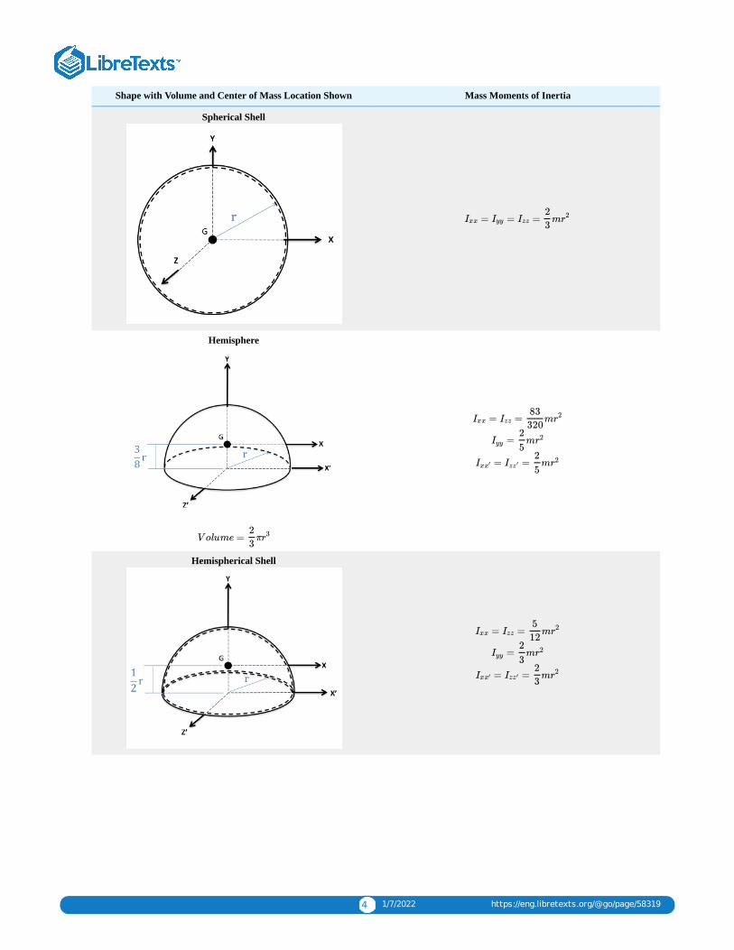
4 1/7/2022 https://eng.libretexts.org/@go/page/58319

Shape with Volume and Center of Mass Location Shown Mass Moments of Inertia

Spherical Shell

Hemisphere

Hemispherical Shell

= = = mIxx Iyy Izz2

3r2

V olume = π2

3r3

= = mIxx Izz83

320r2

= mIyy2

5r2

= = mIxx′ Izz ′2

5r2

= = mIxx Izz5

12r2

= mIyy2

3r2

= = mIxx′ Izz ′2

3r2

5 1/7/2022 https://eng.libretexts.org/@go/page/58319

Shape with Volume and Center of Mass Location Shown Mass Moments of Inertia

Right Circular Cone

V olume = π h1

3r2

= = m(4 + )Ixx Izz3

80r2 h2

= mIyy3

10r2

= = m(3 + 2 )Ixx′ Izz ′1

20r2 h2

1 1/30/2022 https://eng.libretexts.org/@go/page/58050

Centroids and Area Moments of Inertia for 2D ShapesShape with Area and Centroid Location

ShownRectangular Area Moments of Inertia Polar Area Moments of Inertia

Rectangle

Right Triangle

Triangle

Area = bh

Ix

Iy

= b1

12h3

= h1

12b3

= bh( + )Jz1

12b2 h2

Area = bh1

2

Ix

Iy

= b1

36h3

= h1

36b3

Ix′

Iy ′

= b1

12h3

= h1

12b3

Area = bh1

2

= bIx1

36h3

= bIx′

1

12h3

2 1/30/2022 https://eng.libretexts.org/@go/page/58050

Shape with Area and Centroid LocationShown

Rectangular Area Moments of Inertia Polar Area Moments of Inertia

Circle

Circular Annulus

Semicircle

Area = πr2

Ix

Iy

=π

4r4

=π

4r4

=Jz

π

2r4

Area = π( − )r2o r2

i

Ix

Iy

= ( − )π

4r4

o r4i

= ( − )π

4r4

o r4i

= ( − )Jz

π

2r4

o r4i

Area =π

2r2

= ( − )Ixπ

8

8

9πr4

=Iyπ

8r4

=Ix′π

8r4

= ( − )Jzπ

4

8

9πr4

3 1/30/2022 https://eng.libretexts.org/@go/page/58050

Shape with Area and Centroid LocationShown

Rectangular Area Moments of Inertia Polar Area Moments of Inertia

Quarter Circle

Ellipse

Area =π

4r2

Ix

Iy

= ( − )π

16

4

9πr4

= ( − )π

16

4

9πr4

Ix′

Iy ′

=π

16r4

=π

16r4

= ( − )Jzπ

8

8

9πr4

Area = πab

Ix

Iy

= aπ

4b3

= bπ

4a3