MATH 142: COURSE MATERIAL

Math 142 course material OpenStax

This text is disseminated via the Open Education Resource (OER) LibreTexts Project (https://LibreTexts.org) and like the hundredsof other texts available within this powerful platform, it is freely available for reading, printing and "consuming." Most, but not all,pages in the library have licenses that may allow individuals to make changes, save, and print this book. Carefullyconsult the applicable license(s) before pursuing such effects.

Instructors can adopt existing LibreTexts texts or Remix them to quickly build course-specific resources to meet the needs of theirstudents. Unlike traditional textbooks, LibreTexts’ web based origins allow powerful integration of advanced features and newtechnologies to support learning.

The LibreTexts mission is to unite students, faculty and scholars in a cooperative effort to develop an easy-to-use online platformfor the construction, customization, and dissemination of OER content to reduce the burdens of unreasonable textbook costs to ourstudents and society. The LibreTexts project is a multi-institutional collaborative venture to develop the next generation of open-access texts to improve postsecondary education at all levels of higher learning by developing an Open Access Resourceenvironment. The project currently consists of 14 independently operating and interconnected libraries that are constantly beingoptimized by students, faculty, and outside experts to supplant conventional paper-based books. These free textbook alternatives areorganized within a central environment that is both vertically (from advance to basic level) and horizontally (across different fields)integrated.

The LibreTexts libraries are Powered by MindTouch and are supported by the Department of Education Open Textbook PilotProject, the UC Davis Office of the Provost, the UC Davis Library, the California State University Affordable Learning SolutionsProgram, and Merlot. This material is based upon work supported by the National Science Foundation under Grant No. 1246120,1525057, and 1413739. Unless otherwise noted, LibreTexts content is licensed by CC BY-NC-SA 3.0.

Any opinions, findings, and conclusions or recommendations expressed in this material are those of the author(s) and do notnecessarily reflect the views of the National Science Foundation nor the US Department of Education.

Have questions or comments? For information about adoptions or adaptions contact info@LibreTexts.org. More information on ouractivities can be found via Facebook (https://facebook.com/Libretexts), Twitter (https://twitter.com/libretexts), or our blog(http://Blog.Libretexts.org).

This text was compiled on 08/25/2022

®

1

TABLE OF CONTENTS

The material in this book maps the material used in Openstax textbook for teaching Math 142 at DVC.

Technology choices are: Libretexts calculators and other free online calculators.

Link to libretext statistics calculators.

Math 142: Course Sequence Map with OpenStax Text

Math 142 Course Map

Video Playlists

Video List

Chapter 1 Lecture Notes

Ch 1.1 Key Terms and IntroductionCh 1.2 Part 2 Sampling MethodCh 1.2 part 1 Types of Data, Summarize Categorical data, Percent ReviewCh 1.3 Frequency Distribution (GFDT)Ch 1.4 Experimental Design and Ethics

Chapter 2 Lecture Notes

Ch 2.1 Stemplots and DotplotsCh 2.2 HistogramCh 2.3 and 2.4 Percentile, Boxplot and OutliersCh 2.5 and 2.6 Measure of Center and SkewnessCh 2.7 Measure of Spread and Variation

Chapter 3 Lecture Notes

Ch 3.1 Definitions and TermsCh 3.2 Independent and Mutually Exclusive EventsCh 3.3 Addition and Multiplication RuleCh 3.4 Sampling With/Without Replacement

Chapter 4 Lecture Notes

Ch 4.1 Discrete Random VariableCh 4.2 Application of Probability DistributionCh 4.3 Binomial Distribution

Ch 5 and 6 Lecture Notes

Ch 5.1 Continuous Random Variable and Density CurveCh 6.1 Standard Normal DistributionCh 6.2 Application of Normal Distribution

Chapter 7 Lecture Notes

Ch 7.1 Central Limit Theorem for Sample MeansCh 7.2 Central Limit Theorem for Sample Total

2

Chapter 8 Lecture Notes

Ch 8.1 Confidence Interval for Population MeanCh 8.2 Confidence Interval for Mean One Sample No SigmaCh 8.3 Confidence Interval for Population Proportion

Chapter 9 Lectures Notes

Ch 9.1, 9.3 and 9.4 Hypothesis Test BasicCh 9.2 Hypothesis ErrorsCh 9.5 part 1 Hypothesis Test for Population ProportionCh 9.5 part 2 Hypothesis Test for Population Mean

Chapter 10 Lecture Notes

Ch 10.1 and 10.4 Hypothesis Test for 2 Population MeansCh 10.3 Hypothesis Test for 2 Proportions

Chapter 11 Lecture Notes

Ch 11.1 Chi-square DistributionCh 11.3 Test of Independence

Chapter 12 Lecture Notes

Ch 12.2 and 12.4 Scatter Plot and CorrelationCh 12.3 and Ch 12.1 Linear regressionCh 12.5 Prediction

Index

Glossary

Glossary

Math 142: Course Material is shared under a not declared license and was authored, remixed, and/or curated by LibreTexts.

Math 142.1 https://stats.libretexts.org/@go/page/15853

CHAPTER OVERVIEW

Math 142: Course Sequence Map with OpenStax TextThe course sequence is designed to cover all topics in DVC's Math 142 Student Learning Outcomes using materials from Statisticstext from Openstax.

Math 142 Course Map

Math 142: Course Sequence Map with OpenStax Text is shared under a not declared license and was authored, remixed, and/or curated byLibreTexts.

1 https://stats.libretexts.org/@go/page/15854

Math 142 Course MapCourse sequence using OpenStax Statistics Text:

Week1: 1.1, 1.2 : Terms, Data classification, sampling method, Summarize categorical data.

Week 2: 1.3, 1.4 : Frequency distribution, Experiment design.

Week 3: 2.1 to 2.4: Graphical summary of quantitative data, histogram, stemplot, dotplot, boxplot.

Week 4: 2.5 to 2.7: Numerical summary of quantiative data, mean, median, standard deviation.

Week 5: Review

Week 6: 3.1 to 3.4: Probability, "OR", "And", "conditional probability", contingency table, addition and multiplication rule,sampling and independence events.

Week 7: 4.1 to 4.3: Discrete random variable, probability distribution, binomial distribution.

Week 8: 5.1 to 6.2: Density curve, standard normal distribution, application of normal distribution.

Week 9: 7.1 to 7.2: Central limit Theorem

Week 10: 8.1 to 8.3: Confidence Interval for Mean and proportion. t-distribution

Week 11: 9.1, 9.3 and 9.4: Hypothesis basic.

Week 12: 9.5 and 9.2: Hypothesis test for proportion and mean.

Week 13: 10.3: Hypothesis test for two proportions.

Week 14: 10.1 and 10.2: Hypothesis test for two means.

Week 15: 12.1 to 12.4: scatter plot, correlation and prediction.

Week 16: 11.1 and 11.3: Chi-square distribution, test of independence.

Math 142 Course Map is shared under a not declared license and was authored, remixed, and/or curated by LibreTexts.

1 https://stats.libretexts.org/@go/page/15855

CHAPTER OVERVIEW

Video PlaylistsYoutube videos are made to cover topics selected in "Course map".

Video List

Video Playlists is shared under a not declared license and was authored, remixed, and/or curated by LibreTexts.

1 https://stats.libretexts.org/@go/page/15856

Video List

Chapter Playlist links blank notes

Chapter 1 and 2 https://www.youtube.com/watch?v=iZc_...AatH1IIAtxOnlm

Chapter 1 notesChapter 2 notes

Chapter 3 and 4 https://www.youtube.com/playlist?list=PLU8S-meRB9h4P0Vz2HqhqMbaDwRolTlKW

Chapter 3 notesChapter 4 notes

Chapter 5 and 6https://www.youtube.com/playlist?list=PLU8S-meRB9h5KAUG7MjgNDj8QrdRChn4k

Chapter 5 and 6 notes

Chapter 7 and 8https://www.youtube.com/playlist?list=PLU8S-meRB9h4VPeYwSMgYdCa1_6LJ6t7F

Chapter 7 notesChapter 8 notes

Chapter 9 https://www.youtube.com/playlist?list=PLU8S-meRB9h54S0t44Z8SnZ-hbv47fj1g

Chapter 9 notes

Chapter 10 to 12https://www.youtube.com/playlist?list=PLU8S-meRB9h5-U3GFhSVTMO8xmdop9_VT

Chapter 10 notesChapter 11 notesChapter 12 notes

Video List is shared under a not declared license and was authored, remixed, and/or curated by LibreTexts.

1

CHAPTER OVERVIEW

Chapter 1 Lecture NotesIn this chapter, we will learn key terms of Statistics and Probability. We will classify data and introduce different samplingmethods. We will also discuss the two main types of statistical studies and understand the main features of a good statistical study.

By the end of Chapter 1, students should be able to:

Recognize and differentiate between key terms.Apply various types of sampling methods to data collection.Create and interpret frequency tables for categorical and quantitative data.

Ch 1.1 Key Terms and IntroductionCh 1.2 Part 2 Sampling MethodCh 1.2 part 1 Types of Data, Summarize Categorical data, Percent ReviewCh 1.3 Frequency Distribution (GFDT)Ch 1.4 Experimental Design and Ethics

Chapter 1 Lecture Notes is shared under a not declared license and was authored, remixed, and/or curated by LibreTexts.

1 https://stats.libretexts.org/@go/page/15871

Ch 1.1 Key Terms and Introduction

Ch 1.1 Definitions of statistics and probability key terms.Statistics is the science of collecting, analyzing, interpreting and presenting data.

Two main branches of statistics:

· descriptive statistics: organizing and summarizing data.

· Inferential statistics: Draw conclusion from data.

Why should we study statistics?

· To be able to read and understand various statistical studies performed in their fields—requires a knowledge of thevocabulary, symbols, concepts, and statistical procedures

· To conduct research in their fields—requires ability to design experiments which involves collection, analysis, and summaryof data.

· To become better consumers and citizens.

Probability: A tool to study randomness, it deals with the chance of an event occurring. Rare event rule is used to draw conclusionfrom data. An event is “significant” if it has 5% or lower chance of occurring.

Terms: Population vs sample

Population: the target group of person, things, or objects under study. It takes times and money to study the entire population.

Sample: A subset of the larger population to gain information about the population. (A census is a collection of data from everymember of the population.)

Terms: Parameter vs Statistic

Parameter: A numerical characteristic of the population. Statistic: A numerical characteristic of a sample. The value varies from sample to sample.

Sample is collected so we can use the statistic to estimate the corresponding parameter of the population. Sample must berepresentative to give an accurate estimation of the parameter.

Ex. Use sample mean (average) to predict population mean. Use sample proportion to predict population proportion.

Terms: Variable and Data

Variable: a characteristic or measurement for each member of the population.

Data: the actual values of the variables.

Ex 1.

a) 37 students are randomly selected to find the proportion of students who prefer asynchronous mode of teaching.

What is the population? all students.

What is the sample? The 37 students selected.

2 https://stats.libretexts.org/@go/page/15871

b) Of the 37 students surveyed, 14% prefer asynchronous teaching. The number 37% is a parameter or statistic?

c) The average annual income for all residents in a city is $34,000.

The number $34,000 is a parameter or statistic? parameter.

d) A sample of 45 college graduates are surveyed and their average annual income is $34,000.

The number $34,000 is a parameter or statistic? statistics.

Ex 2. Determine what the key terms refer to in the following study.

A study was conducted at a local college to analyze the average cumulative GPA’s of students who graduated last year by surveyinga randomly selected group of students who graduated last year.

a) Cumulative GPA of a student who graduated last year. ______ variable

b) Cumulative GPA of a sample of students graduated last years are: 3.65, 2.80. 1.5, 3.9. _____ data

c) The group of students being surveyed. _______ sample

d) College Registrar published that average cumulative GPA of all students who graduated from the college last year is 3.1.________parameter

e) All students graduated last year in the local college. ______ population

f) Average cumulative GPA from the sample of students is 3.32 ________ statistics

Ex 3. A study on car safeties are performed. A sample of 75 cars with dummies in the front seats were crashed into a wall at aspeed of 35 miles per hour. We want to know the proportion of dummies in the driver’s seat that would have had head injuries, ifthey had been actual drivers. For each car crash, the head injury condition (yes or no) of the dummy is recorded.

a) Population is _____ all cars

b) sample is ______ 75 cars

c) Parameter is ______ head injuries percent from all cars.

d) Statistics is _____ head injuries percent from the sample of 75 cars.

e) Variable is _____ Injury conditions for the dummies.

f) Data is _____ yes, no of head injuries

Ch 1.1 Key Terms and Introduction is shared under a not declared license and was authored, remixed, and/or curated by LibreTexts.

1 https://stats.libretexts.org/@go/page/15876

Ch 1.2 Part 2 Sampling Method

Types of sample:1) Simple Random sample. Any group of n individuals is equally likely to be chosen as any other group of n individuals if the simple random samplingtechnique is used.

2) Random sample:

Any subject has equal chance of being selected.

3) Non-random sample:

Not all subjects have an equal chance of being selected.

Note: A good sample should have the same characteristic as the population it is representing. Random sample or Simple Randomsample can achieve this goal.

Sampling methods:1) Simple Random sampling:

Sample are selected one by one using random procedures such as selecting names from a hat or generated by random numbergenerator.

2) Stratified sampling:

divide the population into groups called strata and then take a proportionate number from each stratum.

3) Cluster sampling:

divide the population area into groups or clusters. The randomly select some of those clusters and choose all members from thoseselected clusters.

4) Systematic sampling: Select some starting point and then select very kth (such as 50 ) element in the population.

5) multistage sampling – use some combination of the preceding sampling methods.

6) Convenience sampling:. Use data that are very easy to get. This will produce a non-random sample Voluntary response sample(self-selected sample) is a convenience sample.

Sampling without replacement: You do not replace the subject you select before selecting the next subject.

Sampling with replacement: Once a member is picked, that member goes back into the population and thus may be chosen morethan once. This guarantee that all subjects has the same chance of being selected.

In practice, simple random sampling is done without replacement and survey are typically done without replacement. If thepopulation is small, sampling without replacement becomes an issue.

Ex. Classify the following method of sampling:

a) Select 4 students by selecting first 4 who arrive first. ____ convenience sampling

b) Select 100 customers by selecting every 50 in a customer database. _____ systematic sampling

c) Select 10 students randomly from each grade in a high school.______stratified sampling

d) Select a sample of restaurants by randomly 10 streets and select all restaurants in the 10 streets. _____cluster sampling

e) Select 100 voters’ response by posting a survey online.____convenience sampling and voluntary sampling

th

th

2 https://stats.libretexts.org/@go/page/15876

Sampling error, non-sampling error, sampling bias.Due to randomness of sampling, sample variation will occur, and the difference are known as sampling error. When sample sizeincrease, sampling error will decrease. Sampling error can be analyzed.

Non sampling error occurs when the process of sampling is not random. Non sampling error cannot be analyzed.

Sampling bias occurs when some subjects in the population are not likely to be selected as others. There can be incorrectconclusion drawn from these sample.

Guideline for evaluating a statistical study:1) Problems with samples: Bias sample is not representative of the population.

2) Self-selected sample (voluntary response sample): response only by subject who choose to participate. This usually only includesubjects with strong opinion of the matter. Internet survey and call-in survey are examples of voluntary response sample.

3) Sample size issues: Small samples are unreliable but are unavoidable such as car test and medical test.

4) undue influence: Questions in survey are worded to influence response.

5) Non-response: high non-response rate make it a voluntary response sample.

6) Self-funded or self-interest study: A study performed by a person or organization in order to support their claim.

7) Causality: Correlation does not imply causation. It may be due to a confounding variable.

8) Misleading use of data: exaggerate difference by using non-zero axis.

Ch 1.2 Part 2 Sampling Method is shared under a not declared license and was authored, remixed, and/or curated by LibreTexts.

1 https://stats.libretexts.org/@go/page/15874

Ch 1.2 part 1 Types of Data, Summarize Categorical data, Percent Review

Chapter 1.2 Data, sampling and VariationTypes of Variable:

Categorical: name, label or a result of categorizing attributes. Also known as qualitative variable.

Quantitative: counts or numerical measurement with units.

Types of Quantitative data:

Discrete: counts or numbers that takes on finite values.

Continuous: measurement data that can have infinitely many possible values between two values not limited by measurementdevice.

Level of measurement:

· Nominal scale level: categorical data with no natural ordering

· Ordinal scale level: categorical data with a natural ordering, difference and mean are not meaningful.

· Interval scale level: quantitative data with no natural zero. Zero value is a mark only. Difference is meaningful but ratio is notmeaningful.

· Ratio scale level: quantitative data with natural zero. Difference and ratio is meaningful.

Note: Nominal and Ordinal data are usually summarized by proportion of the categories. There is no meaning to the mean.

Ex1 classify the data as quantitative or categorical, discrete or continuous if it is quantitative. Classify by level of measurementalso.

a) The number of students in a zoom meeting. ____ quantitative discrete, ratio

b) The major of study of a student._____ categorical, nominal

c) The student id of a student._____categorical, ordinal

d) Jersey number of a basketball player.______ categorical, ordinal

e) The duration (in minutes) it takes to finish a homework.______quantitative continuous, ratio

f) Grade of an exam._____categorical, ordinal

g) Daily high temperature of a city. _____quantitative continuous, interval.

Percent and Decimal:

Decimal → Percentage:

Move decimal point to the right by 2 places.

Example: 0.75 = 75% 0.0178 = 1.78%

Percentage → decimal.

move decimal point to the left by 2 places.

Example: 25% = 0.25, 4% = 0.04 0.1% = 0.001

Find Percent:

→ decimal → percent

Find Percent of an amount: To find percent of an amount, replace the % with decimal notation, interpret “of” to be multiplication.

Example:

part

whole

2 https://stats.libretexts.org/@go/page/15874

6% of 1200 = 0.06 × 1200 = 72

12% of 2418 = 0.12× 2418 =290.16

Exact value of 12% of 2418 adults = 290.16 (no rounding)

Actual value of 12% of 2418 adults = 290 adults

Summarizing Categorical data.

Proportions (relative frequencies) are used to summarize Categorical data. A proportion will be calculated for each category andpresented as a table

Ex 1.

Graphs for categorical data.

1) Bar Graph: Use bars of equal width to show frequencies of categories. May or may not be separated by spaces.

2) Pareto graph: A Bar graph where bars are arranged in descending order of frequencies, so it is easier tocompare difference categories

3) Pie Chart – show categorical data as slices of a circle. each slice is proportional to the frequency count for thecategory. Show composition of the whole.

How to draw a bar graph, pie chart from frequency table:

Use Excel, select the category and frequency or relative frequency column, insert chart.

Note: When Categories proportion does not add up to 100%, a bar graph is appropriate, but a pie chart is not.

A total percentage more than 100% indicates subjects are in more than one category.

A total percentage less than 100% indicates a missing category such as the “other “category.

Ex1: Is it appropriate the graph the following table by bar graph, pie chart?

The total percent for the first frequency table is more than 100%, it is collecting percent of more than one typeof variable.

It should not be graphed in bar graph or pie chart.

The total percent is less than 100%, a pie chart is not appropriate.

Ch 1.2 part 1 Types of Data, Summarize Categorical data, Percent Review is shared under a not declared license and was authored, remixed,and/or curated by LibreTexts.

1 https://stats.libretexts.org/@go/page/15875

Ch 1.3 Frequency Distribution (GFDT)

Ch 1.3 Grouped Frequency Distribution Table (GFDT)Quantitative data can be summarized into a frequency table by classifying data into classes. Class can have a range of non-overlapping value with equal class width (difference between class lower class limits)

Terms related to GFDT:

lower limits: lower bound of each class .

upper limits: upper bound of each class.

class midpoints:

class width: difference between 2 consecutive lower limits.

class boundaries: values between 2 classes.

Ex.Given GFDT below: find lower limits, classwidth, class midpoints.

Because each class has one value, lower limits and upper limits are the same: 0, 1, 2, 3, 4, 5.

classwidth = 1

class midpoints: 0, 1, 2, 3, 4, 5

lower class limits: 60, 70, 80, 90

upper class limits: 69, 79, 89, 99

classwidth = 10

class midpoints: 64.5, 74.5, 84.5, 94.5

Relative and Cumulative frequency Distribution Table

Relative frequency and cumulative frequency can be evaluated for the classes. Because of rounding the relative frequency may notbe sum to 1 but should be close to one.

Rounding review:

If the number place you are rounding is followed by 5, 6, 7, 8, or 9, round the number up.

If the number place you are rounding is followed by 0, 1, 2, 3, or 4, round the number down.

Ex1. Round to three decimal places:

a) 0.1278, b) 0.1283, c) 0.1239, d) 0.1298 e) 5/6

Ans: 0.1278 round to 0.128, 0.1283 round to 0.128, 0.1239 round to 0.124, 5/6 round to 0.833

Ex2. Round to 1 decimal place of a percent.

a) 0.1184 b) 45.677% c) 52/89

0.1184 is 11.84% round to 11.8%, 45.677% round to 45.7%, 52/89 round to 58.4%

Ex3. Round to the nearest whole number.

a) 12% of 781 b) 15.2% of 2344

a) 0.12 (781) =93.72 round to 94 b) 0.152(2344) =356.288 round to 356

(lower +upper)

2

2 https://stats.libretexts.org/@go/page/15875

Relative frequency for a class =

cumulative frequency =sum of the frequencies for that class and all previous classes

Ex1. Find relative and cumulative frequency for service time for a fast food restaurant given in the following GFDT.

total frequency = 50,

Relative frequencies: 11/50 = 0.22, 24/50 = 0.48, 10/50 = 0.2, 3/50 = 0.06, 2/50 = 0.02

class: less than 125, less than 175, less than 225, less than 275, less than 325

Cumulative frequencies: 11, 35, 45, 48, 50

Classes with overlapping class limits:

When frequency table has classes with overlapping limits at the end points, the common convention is

lower limit ≤ data < upper limit. or the classes are assigned so all data values fall between the limits.

Ex2. Find the percent of town with rainfall less than 9.01 in.

Total frequencies = 6 + 7+ 15 + 8 + 9 + 5 = 50

The first three classes has rainfall less than 9.01: (6 + 7 + 15)/50 = 0.56 = 56%

Frequency table where the class is time such as years.

Ex3. Find percent of crashes occurs after 2015.

Total frequencies = 30203 + 32744 + 35485 + 37809 + 37473 + 36560 = 210271

number of crashes after 2015 are at year 2016 to 2018 : 37806+37473+36560 = 111839

Percent = 111839/210271 = 53.2%

Graph a GFDT from data using online "socialscience calculator":

https://www.socscistatistics.com/descriptive/frequencydistribution/default.aspx

1. -Find the minimum data value.2. - Enter data in a column in the input frame.3. - Click Generate. 4. - select number of classes and the lowest class limits that should include the minimum data value and a nice value.5. - Click Edit frequency table for the new table.

Ex1. Construct a GFDT from the data below: use 7 classes and start with a “nice” good lowest limit.

Use socialscience calculator,

Input data to input frame. Click generate, then change class size to 7 and lowest class value to 20. Then click Editfrequency table.

frequency for the class

sum of all frequency

3 https://stats.libretexts.org/@go/page/15875

Ch 1.3 Frequency Distribution (GFDT) is shared under a not declared license and was authored, remixed, and/or curated by LibreTexts.

1 https://stats.libretexts.org/@go/page/15858

Ch 1.4 Experimental Design and Ethics

Ch 1.4 Experimental Design and Ethics.Types of statistical study:

1) Observational study: we observe and measure specific characteristic of the subjects. A survey study is an observational study.We don’t attempt to modify the individuals being studied.

Types of observational study:

a) Cross-sectional study – data are collected at one point in time, not over a period of time.

b) retrospective study – data are collected from a past time by going back in examination of records.

c) prospective study – data are collected in the future from cohort groups.

2) Experimental study: we apply treatments and proceed to observe its effect on individuals.

The purpose of an experiment is to investigate the relationship between two variables. When one variable causes change in another,we call the first variable the explanatory variable. The affected variable is called the response variable.

Observational study can demonstrate an association but no causal relationship. Controlled experiment can demonstrate a causalrelationship.

Feature of good of experimental design:

Control: Use a control group with placebo, blinding or double blinding to reduce placebo effect (also known as power ofsuggestion).

Randomization: subjects are randomly assigned to control and treatment groups. (Completely Randomized Design). Control andTreatment groups should be as similar as possible. Matched-pair design can be used.

Replication: use large sample size in both control and treatment group.

Blinding: subjects are unaware if they are in a control or treatment group.

Double-blinding: one in which both the subjects and the researchers involved with the subjects are blinded.

Ex1. Researchers want to investigate whether taking aspirin regularly reduces the risk of heart attack. Four hundred men betweenthe ages of 50 and 84 are recruited as participants. The men are divided randomly into two groups: one group will take aspirin, andthe other group will take a placebo. Each man takes one pill each day for three years, but he does not know whether he is takingaspirin or the placebo. At the end of the study, researchers count the number of men in each group who have had heart attacks.

Identify the following values for this study: population, sample, experimental units, explanatory variable, response variable,treatments.

population:____ all men between the age of 50 and 84

sample: ____ the 400 men recruited

experimental units:_____each of the 400 men

explanatory variable: ______ take or do no take aspirin

response variable: ________ have or not have heart attacks

treatments: ______aspirin

2 https://stats.libretexts.org/@go/page/15858

Ex 2. A survey shows that students who eat breakfast have higher average GPA. The researcher conclude that breakfast can causean increase in academic performance. Discuss if the conclusion is valid or not and explain.

Answer:

Since the study is a "survey" which is an observational study. The correlation between eating breakfast and higher average GPA are"association" only.

The conclusion of "cause" is not valid.

Ex 3. Classify if the study is an experiment or observational study:

https://www.sciencedaily.com/releases/2008/07/080707081834.htm

Make comment about the headline of the article:

“PTSD Causes Early Death From Heart Disease, Study Suggests.”

Answer: The study is an observation study. Causation conclusion is not valid until experiments are conducted.

Ethics of statistic researcher

Risks to participants must be minimized and reasonable with respect to projected benefits.Participants must give informed consent. This means that the risks of participation must be clearly explained to the subjects ofthe study. Subjects must consent in writing, and researchers are required to keep documentation of their consent.Data collected from individuals must be guarded carefully to protect their privacy

Ch 1.4 Experimental Design and Ethics is shared under a not declared license and was authored, remixed, and/or curated by LibreTexts.

1

CHAPTER OVERVIEW

Chapter 2 Lecture NotesIn this Chapter, we will learn to summarize quantitative data graphically and numerically.

At the end of the chapter, students should be able to:

Display data graphically and interpret graphs: stemplots, histograms, and box plots.Recognize, describe, and calculate the measures of location of data: quartiles and percentiles.Recognize, describe, and calculate the measures of the center of data: mean, median, and mode.Recognize, describe, and calculate the measures of the spread of data: variance, standard deviation, and range.

Ch 2.1 Stemplots and DotplotsCh 2.2 HistogramCh 2.3 and 2.4 Percentile, Boxplot and OutliersCh 2.5 and 2.6 Measure of Center and SkewnessCh 2.7 Measure of Spread and Variation

Chapter 2 Lecture Notes is shared under a not declared license and was authored, remixed, and/or curated by LibreTexts.

1 https://stats.libretexts.org/@go/page/15880

Ch 2.1 Stemplots and Dotplots

Ch 2.1 Stemplots and Dotplots To summarize quantitative data: we look at five areas:

CVDOT: center, variation, distribution, outlier, trend.

Summarize quantitative data by graph:

1. Stemplot2. Dotplot3. Histogram (main one)4. Boxplot.

A) Stemplot

Stemplot is a quick way to graph relatively small quantitative data. It can show the overall pattern and outliers. The main problemis data value must be in a relatively small range. But data values can be recovered from a stemplot. Also, stemplot can easily becreated without use of technology.

Each data value is separated into stem and leaf (the last digit). Data are arranged in order with the same stem in a row. Back-to-back stem plot can be used to compare two datasets. It can be used to show distribution of data (look side way).

Note: do not skip a stem with no leave to show distribution and outliers correctly.

Online stemplot maker:

http://digitalfirst.bfwpub.com/stats_applet/stats_applet_8_ovc.html

If data consists of decimal, use this online stemplot maker: https://www.geogebra.org/m/zPA7QFe

Ex1. A stemplot is given below: legend 6|3 means 63

a) How many data are there? ____ 2 + 2 + 5 + 2 = 11

b) What is the lowest and highest data?_______ lowest value is 63, highest is 99

c) What is the list of data? _____The whole list of data can be recovered as 63, 65, 78, 79, 81, 82, 82, 85, 89, 91, 99.

Ex2. Graph stemplots for the two different samples of grades. Describe shape of distribution.

Sample 1: 63, 65, 68, 69, 81, 82, 82, 85, 89, 91, 99

Sample 2: 63, 65, 68, 69, 81, 82, 82, 85, 89, 91, 99, 123

Use online stemplot calculator

Sample 1

The shape is not very clear because there is only 3 bars.

There is a gap between two peaks.

sample 2

2 https://stats.libretexts.org/@go/page/15880

The shape is not very clear because there are only 4 bars.

There is a gap between 60 and 80. There is an outlier at 123.

B) DotplotDoplots are used for graphing small discrete dataset with small range. It is possible to recreate the original list of data values. Also,Dotplots can be easily created without the use of technology.

Online dotplot maker:

https://www.geogebra.org/m/BxqJ4Vag

(enter data to column A only)

Ex1.

Sketch a dotplot for : 3, 4, 5, 7, 8, 9, 5, 6, 7, 7, 7, 7.

Describe shape of distribution and outliers.

Answer:

Use Geogebra dotplot calculator:

The shape is left-skewed. There are no outliers.

Ch 2.1 Stemplots and Dotplots is shared under a not declared license and was authored, remixed, and/or curated by LibreTexts.

1 https://stats.libretexts.org/@go/page/15881

Ch 2.2 Histogram

2.2 HistogramHistogram can be used to show distribution of medium to large quantitative data. Data are summarized into frequency classes.

- consists of contiguous (adjoining) bars. A Typical histogram should have about 5 to 15 bars or classes. Each bar represents oneclass of data.

- The horizontal axis is labeled with what the data represents in each class.

- The vertical axis is labeled either frequency or relative frequency.

- Histogram can show shape of distribution of the data, the center, and the spread of the data, but data cannot be recovered.

- Histogram can also show outliers that has a frequency of 1 or 2 but with large gap from the rest of data.

Ex1. The histogram below shows distribution of weights of players in a football team.

a) How many players are on the team?

sum of frequencies: 2 + 10 + 9 + 7 + 4 + 2 = 34

b) How many players weight 240 lb. or more?

sum of the last three frequencies: 7 + 4 + 2 = 13

c) Can we tell the actual weights of the players from the histogram?

no because we only have frequency for each class.

d) Are there any outliers?

No outliers.

Graph histogram from dataMethod 1: Use Statdisk (statdisk.org) Histogram

- Input or copy and paste (ctrl-V) data to Sample Editor in a column.

- Select Data/Histogram.

- Select column where data is located.

- Enter Histogram Title, x and y-axis label.

-Use Statdisk default classes (Auto-fit) or select “user-defined”, enter “class-width” and “class start”. “Class start” must be loweror equal to the minimum value in the data.

- Select frequency or relative frequency.

- Click plot. screen shot to save the histogram.

- Find the class range by hovering over each bar.

Ex1. Sketch a histogram for the following commute time. Use class width of 10 and lowest value of 20.

Method 2: Use Statdisk, Explore data.

2 https://stats.libretexts.org/@go/page/15881

- Enter data to one column,

- Select data, select Explore data-descriptive statistics.

- Select column, click evaluate.

- Summary statistics will be on the left and three graphs: Histogram (using auto-fit classes), boxplot and Normal quantile plot willbe on the right.

Ex2. Sketch a Histogram of number of customers in a sample of stores.

12, 34, 45, 67, 43, 55, 57, 89, 77, 72, 56, 37, 45, 49, 51

a) Use default class of statdisk. Copy Histogram below. Describe shape of distribution.

The shape of the distribution is symmetrical normal, bell shape.

b) Regraph histogram with classwidth of 12 and lowest class limit 10.

use statdisk/data/select column 1/ click User-defined,

enter class width = 12

class start = 10

B) Other graphs for quantitative data:

Frequency polygon/relative frequency polygon – Use for large datasets from frequency distribution. Use a line to showfrequency distribution instead of bars. Line starts and ends at the horizontal axis.

Multiple frequency polygons can be graphed on the same graph for comparing two or more datasets.

C) Shape of distribution and skewness

Histogram and frequency polygon can be used to show shape of distribution and skewness of data values.

Normal distribution means data are in a symmetrical bell shape.

Skewed to the right – most data are in the low values.

Skewed to the left – most data are in the high values.

Uniform – data are evenly distributed.

3 https://stats.libretexts.org/@go/page/15881

D) Time Series Graph:

Show trend of data collected over times. Data are not summarized. Time series graph shows increasing and decreasing data valuesover time.

Data are represented by points connected with lines.

Graph time-series graph by Excel

- Input data with time in one column and data in another column.

- Select the data values, insert chart, line graph.

- Select the x-axis label, right click, select data, select

- Edit horizontal axis label by selecting the year column. Select Ok and Ok.

- Input Chart Title, x and y-axis label and marker

Ch 2.2 Histogram is shared under a not declared license and was authored, remixed, and/or curated by LibreTexts.

1 https://stats.libretexts.org/@go/page/15882

Ch 2.3 and 2.4 Percentile, Boxplot and Outliers

Percentile and QuartilesPercentile: are measures of location. Denoted by P P , … P which divide a set of data into 100 groups with about 1% of thevalues in each group.

If x is at 90 percentile, means 90% of all data are less than x. Note, percentile is not the same as percentage.

Quartiles: (Q , Q , Q )

Quartiles are measures of location, which divide a set of data into four groups with about 25% of the values in each group.

Q – First quartile or P . It separates the bottom 25% of value from the top 75%.

Q - Second quartile or P or median. It separates the bottom 50% of values from the top 50%.

Q – Third quartile or P . It separates the bottom 75% of values from the top 25%.

Five-number-summary, IQR and Boxplot:Five-number-summary are:

Mininum, Q Median, Q and Maximum divides the data into four groups of 25% each.

IQR = Q – Q (Inter-quantile Range)

The interquartile range (IQR) is a number that indicates the spread of the middle half or the middle 50% of the data. It is thedifference between the third quartile (Q ) and the first quartile (Q ).

A boxplot shows graphical image of concentration of data. A boxplot is constructed using 5-number summary with Q1, medianand Q3 in a box containing 50% of all data. It gives good distribution of data in 25%, 50% and 75%.

- Maximum and Minimum values are extended as whiskers at the two ends of the box.

Find 5-number-summary and boxplot by Statdisk

- Enter data in a column in Statdisk.

- Select Data, Explore data, descriptive statistic, select column and Click evaluate.

Ex1. The time(in min.) a sample of 15 student spent on exercising daily is given:

0, 40, 60, 30, 60, 10, 46, 30, 300, 90, 30, 120, 60, 0, 20

a) Find the 5-number summary and sketch a boxplot.

Use statdisk, data/explore data/select column data/evaluate, five number summary and boxplot will show.

b) What percent of student exercise from 0 to 60 min?

Because 60 is Q3, so 75% of all student exercise from 0 to 60 min.

c) What percent of student exercise between 20 to 60 min?

Because 20 is Q1, 60 is Q3, so 50% of all students exercise from 20 to 60 min.

Answer: Use Statdisk:

a) Min = 0, Q1=20, Med=40, Q3=60, Max = 300

1, 2 99

th

1 2 3

1 25

2

50

3 75

1, 3

3 1

3 1

2 https://stats.libretexts.org/@go/page/15882

b) Since Q3 = 60, hence 75% of students exercise from 0 to 60 min.

c) Since Q1 = 20 and Q3=60, Hence 50% of students exercise from 20 to 60 min.

Outliers and IQR

IQR is used to determine potential outliers.

Ex1. If Q1 = 34, Q3 = 70, find the lower fence and upper fence for an outlier.

IQR = 70 - 34 = 36

lower fence is 34 - 1.5(36) = -20, upper fence = 70 + 1.5(36) = 124

Value between -20 and 124 are not outliers, values outside the range are outliers.

A potential outlier is a data point that is significantly different from the other data points. These special data points may be errors orsome kind of abnormality or they may be a key to understanding the data.

C) Modified boxplot and outliers:

A modified boxplot can be graphed to show outliers without calculating IQR and applying the Q1-1.5IQR, Q3+1.5IQR. Outliersare shown as markers in the boxplot.

- use Statdisk, click data , Boxplot,

- Select the column of data, click modified boxplot. The outlier will be shown as marker at the lowest or highest end of theboxplot.

- If there are no markers, there is no outliers in the dataset.

- To find the values of the outlier, sort the data. The outliers will be at the top and end of the sorted data.

Ex2. Determine if outliers exist in the exercise time from 15 students.

0, 40, 60, 30, 60, 10, 46, 30, 300, 90, 30, 120, 60, 0, 20

By calculation:

Since Q1 = 20, Q3 = 60, So IQR = 60 – 20 = 40

Lower fence = Q1 – 1.5(IQR) = 20 – 1.5(40) = -40

upper fence = Q3 + 1.5(IQR) = 60 + 1.5(40) = 120

Values lower than -40 and higher than 120 is an outlier. So the value 300 is an outlier.

Graph a modified boxplot to identify outliers.

Use Statdisk, Data/Boxplot/select Modified boxplot.

There is one outlier in the high end of the data. To find the outlier, sort the data and locate the highest value.

3 https://stats.libretexts.org/@go/page/15882

Use Statdisk, Sort, one column, select the column containing the data. The last data (300) is the outlier.

Ch 2.3 and 2.4 Percentile, Boxplot and Outliers is shared under a not declared license and was authored, remixed, and/or curated by LibreTexts.

1 https://stats.libretexts.org/@go/page/15884

Ch 2.5 and 2.6 Measure of Center and Skewness

Ch 2.5 and 2.6 Measure of Center and skewnessCenter: A measure of center is a value at the center or middle of a data set. It is used to provide a representative value that“summarize” the data.

Measure of center: (mean, median, mode, midrange)

1) Mean: the average of the data.

sample mean ; n = sample size, is read as x-bar,

population mean ; N = population size, is read as mu, a greek letter.

*the term “average” is not used by statistician.

Important properties of mean:

a) Use every data value (in a sample or population)

b) Extreme value can change the value of mean substantially. Mean is not resistance.

c) can be used to estimate μ if sample is representative and not bias.

If the sample is voluntary response or biased will not be a good estimate of μ.

Ex1: Mean of 78, 89, 75, 92, 66, 82 is 80.3

Mean of 78, 89, 75, 92, 66, 82, 5 is 69.6 (not middle)

Ex2: Mean of top 5 scores: 90, 95, 92, 98, 89;

is 92.8 but is not a good estimate for the whole class mean because the sample is bias, not from random selection.

2) Median: the middle value when the data are arranged in order of increasing or decreasing magnitude.

How to calculate the median:

a) Sort the values

b) Odd number of values: Median is the middle one

Even number of values: Median is the mean of the middle two values.

Properties of Median:

a) The median does not change when we add a few extreme values. It is resistance.

b) Median does not use every value.

Ex1: Median of 78, 89, 75, 92, 66, 82 is 80

Median of 78, 89, 75, 92, 66, 82, 5 is 78 (middle)

3) Mode: the value (s) that occur(s) with the greatest frequency. Can be calculated for qualitative data. Not common forquantitative continuous data.

Properties of mode:

a) Data can have one, two, multiple or no modes.

b) Bimodal – two data values occur with same greatest frequency.

c) Multimodal – more than two data values occur with the same greatest frequency.

d) No mode – no data value is repeated.

=x∑ x

nx

μ =∑ x

Nμ

x

x

x

2 https://stats.libretexts.org/@go/page/15884

4) Midrange: the value that is midway between the maximum and minimum values in the dataset.

Properties of Midrange:

a) Not resistance to extreme values.

b) Easy to compute but rarely used.

c) Midrange does not use all data. It is not the median and it is not half of range.

Find Mean, median, and midrange by technology:

Use Libretexts online calculator. Link to one variable statistics calculator

Input data separated by commas , check population standard deviation or sample standard deviation, and click calculate.

Find mode by technology

Use online calculator: (for multiple mode)

https://www.calculatorsoup.com/calculators/statistics/mean-median-mode.php

Input data to the window, click Calculate.

Round off rules:

a) Mean, median and Midrange: carry one more decimal place than original data.

b) Mode: leave the value as is without rounding.

Ex1. Find the mean, median, midrange, mode of the length of boats (in ft) parked in a marina.

16, 17, 19, 20, 20, 21, 23, 24, 25, 25, 25, 26, 26, 27, 27,27, 28, 29, 30, 32, 33, 33, 34, 35, 37, 39, 40

a) Find the mean, median, mode and midrange.

Which of the above is the best measure of center?

b) Can this mean be used to estimate mean length of all boats in all marina? Explain.

a) Use Libretexts Online Statistics calculator. and online mode calculator.

Mean = 27.3, Median = 27, min = 16, max = 40

Midrange = (16 + 40)/2 = 28, Mode = 25 and 27.

Mean is a better choice because data is symmetrical and there are no outliers in the data.

b) This mean is not representative because the sample is from one marina only.

Ex. 2 Which is the greatest, mean, median or mode?

11, 11, 12, 12, 12, 12, 13, 15,17, 22, 22, 22

Use Libretexts Online Statistics calculator. and online mode calculator.

Mean = 15.1

Median =12.5

Mode = 12

Midrange = 16.5

midrange =maximum + minimum

2

3 https://stats.libretexts.org/@go/page/15884

Mean, median and skewness:

Choose the best measure of center:

a) Use mode for nominal data as center.

b) Use mean if there is no extreme data.

c) Use median if extreme data exist.

d) Use median if data is skewed.

Find mean from a frequency distribution:

grouped mean ; is the mean from GFDT where

x is the class midpoint of each class.

f is the frequency of each class

Find grouped-mean for GFDT by technology: Libretexts Online Calculator

1. - Enter lower limit to lower bounds, upper limit to upper bounds, enter frequencies for each row in the GFDT.2. - Scroll to the bottom and click calculate.

Ex1. Find grouped mean from GFDT:

Enter the table to Libretexts Online calculator , calculate.

Ans: mean = 84.5

Ex2. Find the mean, median from the data in the histogram.

Write the frequency table by reading the classes and frequencies from the histogram as below:

Enter the table to Libretexts Online calculator , calculate.

Ans: mean = 4.06, median = 4

Note: when data is extremely skewed in a particular way, the mean and median can be the same.

Ch 2.5 and 2.6 Measure of Center and Skewness is shared under a not declared license and was authored, remixed, and/or curated by LibreTexts.

=x∑ f∗x

∑ f

1 https://stats.libretexts.org/@go/page/15885

Ch 2.7 Measure of Spread and Variation

Ch 2.7 Measure of Spread and VariationA measure of variation is used to describe the degree of spread of data.: Range, standard deviation, Interquartile Range.

1) Range: Difference between max and min.

= (maximum value – minimum value)

Properties:

a) Not resistance. Affected by extreme value.

b) Does not take every value into account.

2) Standard Deviation of a sample: Measure of how much data values deviate away from the mean.

Notation: s = sample standard deviation

, where n = sample size. (n -1 ) = degree of freedom.

Properties:

a) s is never negative. It is zero when all data values are the same. Large value of s indicates greater amount of variation.

b) s increases dramatically with one or more outliers. Not resistance to extreme values.

c) s has the same unit as the original data values.

d) s is a biased estimator of population standard deviation. It does not center around the value of σ.

e) Compare standard deviation for data with similar mean only.

f) s increases when data are more spread out.

Ex1:

Find standard deviation of 15, 15,17, 21 by manual calculation : ;

Ex2. Find range, standard deviation of the following data : 5, 6, 3, 2, 6, 8, 10, 12, 17

Use Statdisk, enter data in column 1, Data/Explore Data/Descriptive Statistics, Select column 1,

Sample standard deviation = 4.72 (rounded)

Range = 15

Ex 3. Find standard deviation of Grouped data.

Use the same procedure as finding Grouped mean. Use Statdisk – Frequency Table Generator and DescriptiveStatistics.

s = 12.06

3) Inter-quartile-Range

IQR: Q3 – Q1 = middle 50% range of data. IQR is resistance to extreme values.

s =∑ (x−x)

2

n−1

− −−−−−−√

= 17x

s = = = 2.84+4+0+16

3

− −−−−−−√ 8

–√

2 https://stats.libretexts.org/@go/page/15885

Ex1. Find Range, Standard Deviation and IQR for

dataset A: 5, 6, 3, 2, 6, 8, 10, 12, 17

dataset B: 5, 6, 3, 2, 6, 8, 10, 12, 17, 60

Range SD IQR

Dataset A: 15 4.7 5

Dataset B: 58 17.1 7

IQR is not influenced by one extreme data.

Other measures related to measure of variation.

1) Population Standard deviation ( σ)

, where N = population size and x are data from population

Find Population standard deviation online:

https://www.socscistatistics.com/descriptive/variance/default.aspx

2) Variances:

Population variance:

Sample variance:

Variances are used in statistical analysis.

Relative standing and Z-score.

Standard deviation is used to describe how far away a value is from the mean.

Sample data = mean + (# of stdev) * stdev.

When comparing values from different dataset, it is best to compare how each value is from their respective mean. The number ofstandard deviation is a measure of relative standing.

z-score is the number of standard deviations a data value is from the mean.

for population data.

for sample data.

Round-off rule: round to 2 decimal places.

Properties of z-score:

a) z-score tells how many standard deviations a value is from the mean. Negative means below the mean. Positive means above themean.0

b) z-score has no units.

Ex1:

A student’s English score is 83 when mean = 80 with sd = 10. The student’s History score is 75 when class mean is 72 with sd= 7.

Is the score better in English or History?

English z-score =

σ =∑ (x−μ)

2

N

− −−−−−−√

=σ2 ∑ (x−μ)2

N

s2

z =x−μ

σ

z = x−xs

= 0.383−8010

3 https://stats.libretexts.org/@go/page/15885

History z-score =

The student score less than 1 standard deviation from the mean but since 0.43 > 0.30, hence the student scores better in History.

Ex2.

Ages of 20 fifth graders are given below:

9; 9.5; 9.5; 10; 10; 10; 10; 10.5; 10.5; 10.5; 10.5; 11; 11; 11; 11; 11; 11; 11.5; 11.5; 11.5;

a) Find the mean and standard deviation of ages.

Use statdisk/data/Explore Data/Select data column/Evaluate

mean = 10.5, sd = 0.7

b) What age is one standard deviation above the mean?

10.5 + 1(0.7) = 11.2

c) What age is two standard deviation below the mean?

10.5 - 2(0.7) = 9.1

d) How many data are two standard deviation below the mean or two standard deviation above the mean?

below 2 SD: 10.5 - 2(0.7) = 9.1 or above ; above 2 SD: 10.5 + 2(0.7) = 11.9

one data 9 is below 9.1 and no data are above 11.9.

Ex3.

Measurements of diameter of a bottle cap manufactured in a factory are collected, what situation is best? Explain.

a) High standard deviation.

b) Low standard deviation.

Low standard deviation is better because values will be more consistent and close to the one needed to use for bottle cap.

Ex4. The following histogram show distribution of measurement of diameters of bottle cap from two production line.

Which histogram left or right one represents sample with low standard deviation? Explain.

The one at the left represent low standard deviation because data are not spread out.

Ch 2.7 Measure of Spread and Variation is shared under a not declared license and was authored, remixed, and/or curated by LibreTexts.

= 0.4375−727

1

CHAPTER OVERVIEW

Chapter 3 Lecture NotesIn these chapters, we will learn the basic concepts of Probability and its application to statistic sampling. We will learn the additionrule, multiplication rule and conditional probability rule to calculate probability of complex events.

By the end of Chapter 3, students should be able to:

Understand probability terms such as Sample Space, Events, Probability notation.Understand mutually exclusive events, independent and dependent events.Understand the use of Addition, Multiplication Rule and Conditional probability.Use Contingency table to determine if two categorical data are independent.

Ch 3.1 Definitions and TermsCh 3.2 Independent and Mutually Exclusive EventsCh 3.3 Addition and Multiplication RuleCh 3.4 Sampling With/Without Replacement

Chapter 3 Lecture Notes is shared under a not declared license and was authored, remixed, and/or curated by LibreTexts.

1 https://stats.libretexts.org/@go/page/15891

Ch 3.1 Definitions and Terms

Ch 3.1 and 3.2 Definitions and Terms:Sample space (S): Total possible outcomes of a procedure. The outcomes are by chance and equally possible.

Event: outcome or result of a procedure. A, B, C ..

P(A) : probability of event A occurring.

Possible values for Probabilities

0 ≤ P(A) ≤ 1 (between 0 and 1, inclusive)

P(A) ≤ 0.05 , A is unlikely.

P(A) = 1, A is certain, P(A) = 0, A is impossible

P(A) = 0.5 : A has a 50-50 chance.

Three Approaches to find probability of an event A.

Approach 1: Theoretical probability

All outcomes in the sample space are equally likely.

Example:

Ex1.: Select one card from a standard deck.

P(Heart) = 13/52 = ¼ = 0.25 = 25%

Ex 2: In a batch of 6500 light bulbs, 80 are defective.

Select one light bulb from the batch

P(defective) = 80/6500 = 0.0123

P(good) =(6500-80)/6500 = 0.988

Ex3: Find P(2 boys in three children family)

because sample space= {bbb, bbg, bgb, bgg, gbb, gbg, ggb, ggg}

P(2 boys) = 3/8

Approach 2: Relative frequency approximation

The probability is an estimate of chance.

Ex1: In year 2020, 86% of people use social media at least once per day. If one person is randomly selected, find the probabilitythat the person uses social media at least once per day.

P( uses social media) = 0.86 (the relative frequency)

Ex2: A sample of 568 students shows 320 students are full-time student.

One student is selected from the whole population, find the probability of selecting a full time student.

a) P(full-time) = 320/568=0.563

Ex3: A batch of seed results in 78 white flowers and 65 pink flowers. Find probability of getting a white flower from planting thesame type of seed.

P(white flower) = 78/(78+65) = 0.545

P (A) =number of ways A occurs

number of ways in sample space

P (A) = number of times A occursnumber of times procedures were repeated

2 https://stats.libretexts.org/@go/page/15891

Ex4. Play Monty Hall game, what strategy gives a higher chance of winning?

http://www.shodor.org/interactivate/...mpleMontyHall/

Law of Large number: As the procedures are repeated more and more, the long term relative frequency approximation will getclose to the theoretical probability.

Approach 3: Subjective approach

Use knowledge of the relevant circumstance to estimate the probability. May not be accurate.

Example: P(stuck in an elevator) = ??

This will probably be unlikely to occur, so Probability will likely be lower than 0.05.

Rounding and probability format:

Round to 3 significant digits unless fraction is a simple fraction of a/b where a, b are less than 10.

Use percentage only when communicating result to be the general public. Most software and professional journal use decimalnotation.

Complement of Event A:

: Event A does not occur, complement of A.

Ex: There is 20% chance of rain today. What is the probability of not rain today?

P(not rain) = 1 – P(rain) = 1 – 0.2 = 0.8

“OR” of two simple events.

An outcome is in A or B if the outcome is in A or in B or both.

P(A or B) = Probability that A occurs, B occurs or both A and B occurs =

“AND” of two simple events.

An outcome is in A and B if the outcome is in both A and B.

P(A and B) = Probability that both A and B occurs at the same time =

Conditional probability

An event written as A given B is a conditional probability that A will occur given that B has already occurred.

P( A|B) = Probability that A occurs given that B has already occured =

P(A Given B) = P(A|B) = P( A and B)/ P(B)

Ex1. Toss a 6-face die once, find the probability that the outcome is

a) a “four”

b) a “four” or “five”

c) a “four” and “five”

A

P ( ) = 1 −P (A)A

number of ways for A, B and both A and B

 total number of ways

number of ways for both A and B

 total number of ways

number of ways for both A and B

 total number of ways for B

3 https://stats.libretexts.org/@go/page/15891

d) a “four” given that the outcome is an “even” number.

e) a “prime number”

Answer: a) 1/6, b) 2/6, c) 0, d) 1/3, e) ½

Ex2. A marble jar has 5 red, 3 blue and 7 white marbles. If one marble is randomly selected, find

a) P(red)

b) P(not red)

c) P(red or blue)

d) P(red and blue)

e) P(red given blue)

Answer: a) 5/15 = 1/3 = 0.333 b) 10/15 = 0.667 c) 8/15 = 0.533 d) 0 e) 0

Ex3. One card is drawn from a standard deck, find the following probability:

a) P(black) = 26/52 = 0.5

b) P(black and A) = 2/52 = 0.0385

c) P( four) = 4/52 = 0.0769

d) P( black or A) = (26+2)/52 = 0.5385

e) P( king given black card) = 2/26 = 0.0769

f) P( A | diamond) = 1/13 = 0.0769

g) P( not face card) = 40/52 = 0.7692

Contingency table: (two-way table)

A table used to summarize two categorical variables of a set of data.

P( A) =

P( A and B) =

P(A or B) = (do not double count)

P(A given B) =

Ex1. Given the data, summarize into a contingency table

grand total = 10

If one student is selected at random, use the contingency table to find the following probability

P(F) = (1+2)/10 = 0.3

P(No) = (2+4)/10 = 0.6

Total counts in row A or column A

 Grand Total

sum of all counts in column A and row B

 Grand Total

sum of all counts in colmnn A and row B

 Grand Total

count that is intersection of A and B

 Sum of counts of column B or row B

4 https://stats.libretexts.org/@go/page/15891

P(M and No) = 4/10 = 0.6

P(F and Y) = 1/10 =0.1

P(F or Y) = (1+2+3)/10 = 6/10 = 0.6

p(M or Y) = (3+4+1)/10 = 8/10 = 0.8

P(Yes GIVEN subject is male) = P(Y|M) = 3/7

Drug or clinical Diagnostic Test

False positive: subject does not use drug but get a positive result.

False negative: subject uses drug but test does not detect it.

False positive: subject is not sick but get a positive result.

False negative: subject is sick but test does not detect it.

Ex1. Use the contingency table below, select one.

Find P(positive) = (10+4)/422 = 0.033

Find P(positive given that subject uses drugs)

= 10/(10+8) = 0.556

note: If the subject uses drug, there is a higher chance of getting positive result.

Ch 3.1 Definitions and Terms is shared under a not declared license and was authored, remixed, and/or curated by LibreTexts.

1 https://stats.libretexts.org/@go/page/15892

Ch 3.2 Independent and Mutually Exclusive Events

Mutually exclusive events:Two events are mutually exclusive (disjoint) if they will not occur at the same time. P(A and B) = 0

Ex1: Toss a 6-face die once, determine if the following are mutually exclusive:

a) Getting a “four” and “even”

No, four and even can occur at the same time, four and one are not mutually exclusive.

b) Getting a “four” and “five”

Yes, four and five cannot occur at the same time so four and five are mutually exclusive.

Ex2:

P(F and no opinion) = 0

F and no opinion are mutually exclusive so they cannot occur at the same time.

Independent Events:Two events are independent when any of the following is true: P(A and B) = P(A) ·P(B)

P(A) = P( A | B)

P(B) = P( B | A)

Ex1. Given a 2-way table below:

GT = 51

Is iPhone uses independent on gender?

Check if P(iPhone | female) = P( iPhone)

a) Find P(iPhone) = (18+24)/51 = 0.824

b) Find P(iPhone | female) = 24/30 = 0.8

P(iPhone) and P(iPhone Given female) are not exactly equal, so iPhone use is not independent of gender.

We can conclude that iPhone use is not independent on gender. Gender affect the choice of iPhone.

Ex2. Given a 2-way table below

Grand total = 100

Is Right-handedness independent on gender?

Check if P(M and R) = P(M) · P (R )

P( M) = 52/100 = 0.52

P ( R ) = (43+44)/100 = 87/100 = 0.87

2 https://stats.libretexts.org/@go/page/15892

P(M and R) = 43/100 = 0.43

But P(M) · P( R) = 0.52 (0.87) = 0.45

So they are not exactly equal.

We can conclude they are not independent.

Note: we will visit this again in Ch 11 to take into consideration of sampling variation.

Note: mutually exclusive events are not necessarily independent events. They are two different concepts.

Ch 3.2 Independent and Mutually Exclusive Events is shared under a not declared license and was authored, remixed, and/or curated byLibreTexts.

1 https://stats.libretexts.org/@go/page/15894

Ch 3.3 Addition and Multiplication Rule

Addition Rule:Addition Rule are used to find “OR” in a procedure.

P(A or B) = P(A) + P(B) – P(A and B)

If A and B are mutually exclusive: P(A and B) = 0

P(A or B) = P(A)+ P (B) when A, B are mutually exclusive.

Ex1. Toss a 6-face die once, use addition rule method to find P(one or odd).

P(one or odd) = P(one) + P(odd) – P(one and odd)

= 1/6 + 3/6 – 1/6 = 3/6 =0.5

Ex2. Toss a 6-face die once, use addition rule method to find P( one or even)

Because one and even or mutully exclusive, so P (one or even) = P(one) + P(even) = 1/6 + 3/6 = 0.667

Ex3. Use the contingency table below:

GT = 51

Use addition rule to find P(male or iPhone).

P(male or iPhone) = P(male) + P(iPhone) – P(male and iPhone) = 21/51 + 42/51 – 18/51 = (21+41-18)/51 =45/51 = 0.8823

Multiplication Rule:Multiplication Rule is used to find probability of two events: A and B.

If A and B are independent, P(B|A) = P(B) so

when A, B are independent.

A result of the multiplication rule gives the formula for conditional probability as:

Ex1: Given the two-way table below:

Find P( male |iPhone) = P( male and iPhone)/P(iPhone) =

Ch 3.3 Addition and Multiplication Rule is shared under a not declared license and was authored, remixed, and/or curated by LibreTexts.

P(A and B) = P (A) ∗ P (B|A)

P(A and B) = P (A) ∗ P (B)

textP (AgivenB) = P(A | B) = A and B

P(B)

= = 0.428618/51

42/51

1842

1 https://stats.libretexts.org/@go/page/15893

Ch 3.4 Sampling With/Without Replacement

Ch 3.4 Sampling w/wo replacement

Sampling with replacement – selected subjects are put back into the population before another subject are sampled. Subject canpossibly be selected more than once.

Sampling without replacement – Selected subjects will not be in the “pool” for selection. All selected subjects are unique. This isthe default assumption for statistical sampling.

Compound events involving multiple trials/steps

When events involve multiple steps, they are called compound events A, and then B, the compound event is also called A and B.

But P(A and then B) is not P( A and B) where A and B outcome of one step with 2 categories.

Multiplication rule for two events in two steps:

A and B : Event A occurs in one trial and Event B occurs in another trial.

P(A and B) = P(A) × P(B after A has occurred)

P(A and B) = P(A) × P(B |A)

Independent/Dependent events

1) Dependent: occurrence of one event affect the next event.

P(A and B) = P(A) × P(B| A)

2) Independent: occurrence of one event does not affect the other.

P(A and B) = P(A) x P(B)

In general : P(A and B and C …) = P( A) x P(B) x P(C) … if A, B , C are independent.

Ex1. A fair coin is tossed 5 times. Find P(first 3 tosses are heads) . F( first 4 are heads), P(at least one head in 4 tosses).

Coin tosses are independent events.

a) P(First 3 tosses are heads) =

Since tosses are independent, P( 3 heads) = 0.5 = 0.125

b) P( First 4 tosses are heads) =

Since tosses are independent, P( 4 heads) = 0.5 = 0.0625

P(at least one head in 4 tosses) = 1 – P(all 4 heads are tails) = 1 - 0.5 = 0.9375

Ex2. In a group of 300 all adults, 272 are right-handed, 3 adults are selected with replacement.

Find P( all 3 are right- handed ) and P(all 3 left-handed).

Ans:

P(one right-handed) = 272/300 =0.907

P(one left-handed) = (300-272)/300 = 28/300 = 0.093

P(3 right-handed) = (272/300) (272/300)(272/300) = (272/300) = 0.745

P( 3 left-handed) = (28/300)(28/300)(28/300) = (28/300) = 0.0008

P(At least one right-handed) = 1 – P(All 3 left-handed) = 1 - 0.0008 = 0.9992

3

4

4

3

3

2 https://stats.libretexts.org/@go/page/15893

Ex3. In a jar with 5 red, 6 blue and 2 white marbles. Two marbles are selected, find the probability that both are red if:

a) If two marbles are selected with replacement.

b) If two marbles are selected without replacement.

Ans:

a) If marbles are replaced, the events are independent.

P( both are red) = 5/13 * 5/13 = 0.1479

b) If two marbles are selected without replacement, the events are dependent,

P(both are red) = 5/13 * 4/12 = 1282

Sampling and independent event

Sampling with replacement – independent events

Sampling without replacement – dependent events

Treating Sampling without replacement as independent if one of the following are satisfied:

a) Assume a very big population when population size is not given. Only P(A) is given.

b) Use 5% guideline for cumbersome calculations:

When sampling without replacement and the sample size is no more than 5% of the size of population, treat sampling asindependent. (Even though they are actually dependent.)

Ex1. Assume that 10% of adults in the United states are left handed. Find the probability that three selected adults all are lefthanded.

Since the population size is not given only P(L) = 0.1 is given, we can treat sampling without replacement as independent.

P(L and L and L) = P(L) × P(L) × P(L) = 0.1 × 0.1 × 0.1

= 0.001

Ex2. In batch of 6400 light bulbs, 80 are defective.

If 12 light bulbs are selected from the batch without replacements, find probability that all are good.

Ans:

sample size = 12, population size = 6400

Since sampling proportion = 12/6400 = 0.00188 < 0.05

we can treat the sampling as independent by apply 5% guideline for cumbersome calculation.

P (one good) = (6400-80)/6400 = 0.9875

P (one defective) = 80/6400 = 0.0125

P( all 12 are good) = 0.9875 = 0.860

P (at least one defective) = 1 – P(all 12 are good) = 0.14

12

3 https://stats.libretexts.org/@go/page/15893

Rare Event RuleIf, under a given assumption, the probability of a particular observed event is very small and the observed event occurssignificantly less than or greater than what we typically expect with that assumption, we conclude the assumption is not correct.

P( A ) ≤ 0.05, then A is unlikely to occur by chance.

Use Probability to form Conclusion:

If P(A) > 0.05, A can occurs by chance, so there is not sufficient evidence to conclude that “the change” is effective.

If P(A) ≤ 0.05, A cannot have occurred by chance, so there is sufficient evidence to conclude that “the change” is effective.

Ex1. A study is done to test if vitamin C intake will reduce common cold. 6 out of 56 subject taking vitamin C catch the commoncold compare to 8 out of 56 subjects not taking vitamin C. If vitamin C has no effect, there is a 0.32 chance of getting such sampleresult. What can we conclude?

Ans: Since probability 0.32 is not unlikely, the result could have occurred by chance rather than due to vitamin C treatment. Thereis not sufficient evidence to conclude vitamin C is effective.

Ch 3.4 Sampling With/Without Replacement is shared under a not declared license and was authored, remixed, and/or curated by LibreTexts.

1

CHAPTER OVERVIEW

Chapter 4 Lecture NotesIn Chapter 4, we will learn to use probability distribution to analyze discrete Random Variable. We will also use technology to findprobability of binomial distribution to solve applications.

At the end of the chapter, students should be able to:

Use Discrete Probability Distribution to find Expected Value. Understand the requirement for binomial distribution and use technology to find probability of binomial distribution.Use Binomial Distribution to find probability of events that are of binary nature.

Ch 4.1 Discrete Random VariableCh 4.2 Application of Probability DistributionCh 4.3 Binomial Distribution

Chapter 4 Lecture Notes is shared under a not declared license and was authored, remixed, and/or curated by LibreTexts.

1 https://stats.libretexts.org/@go/page/15873

Ch 4.1 Discrete Random Variable

Ch 4.1 Discrete Random Variable

Random VariableRandom Variable: is a variable (X) that has a single numerical value, determined by chance, for each outcome of a procedure.

Probability distribution: is a table, formula or graph that gives the probability of each value of the random variable.

A Discrete Random Variable has a collection of values that is finite or countable similar to discrete data.

A Continuous Random Variable as infinitely many values and the collection of values is not countable.

Ex : X = the number of times “four” shows up after tossing a die 10 times is a discrete random variable.

X = weight of a student randomly selected from a class. X is a continuous random variable

X = the method a friend contacts you online. X is not a random variable. ( X is not numerical)

A Probability Distribution (PDF) for a Discrete Random Variable is a table, graph or formula that gives Probability of each value ofX.

A Probability Distribution Function (PDF or PD) satisfies the following requirements:

1. The value X is numerical, not categorical and each P(x) is associated with the corresponding probability.

2 ΣP(X) = 1 . A ΣP(X) = 0.999 or 1.01 is acceptable as a result of rounding.

3. 0 ≤P(x) ≤ 1 for all P(x) in the PDF.

Ex1: PDF for number of heads in a two-coin toss are given as a table and a graph.

Table graph

Both are valid PDF because Σ P(X) = 1

and each value of P(X) is between 0 and 1.

Ex2: The number of medical tests a patient receives after entering a hospital is given by the PDF below

a) Is the table a valid PDF?

The table is not a probability distribution because Σ P(x) = 0.02+0.18+0.3+0.4 = 0.9 is not 1

b) Define the random variable x.

x = no. of medical tests a patient receives after entering a hospital.

c) Explain why the x = 0 is not in the PDF?

A patient always receives at least one medical test in the hospital.

2 https://stats.libretexts.org/@go/page/15873

Parameters of a Probability distribution:Mean μ for a probability distribution:

Variance σ for a probability distribution:

Standard deviation for a probability distribution:

To calculate Mean, variance and standard deviation of a probability distribution by technology:

Use Libretext statistics calculator:

https://stats.libretexts.org/Bookshelves/Ancillary_Materials/02%3A_Interactive_Statistics/10%3A_Expected_Value_and_Standard_Deviation_Calculator?adaptView

Enter Number of outcomes, each X and P(X), calculate.

round off rule: one more decimal place than for E(x)

Two decimal places for σ and σ .

Expected value = the long-term outcome of average of x when the procedure is repeated infinitely many times. Round to onedecimal place.

Non-significant values of X.

1. The range of X from are non-significant. (Range of rule of Thumb)

2. X that are outside of are significant that is unlikely to occur.

Ex1: X = no. of year a new hire will stay with the company. P(x) = Prob. that a new hire with stay for x year.

a) Find mean, variance, st. deviation and determine the Expected number of years a new hire will stay.

Use easycalculation.com statistics discrete random variable calculator,

Enter number of outcomes = 7. Mean = 2.4, σ = 2.73, σ =1.65

The Expected no. of year a new hire will stay is 2.4 years.

b) Find probability that a new hire will stay for 4 years or more.

Add P(4), P(5) and P(6) = P( 4 or more) = 0.1 + 0.1 + 0.05 = 0.25

c) Find probability that a new hire will stay for between 3 or 5 years inclusive.

P( 3 to 5 inclusive) = 0.15 + 0.1+0.1 = 0.35

d) Find the probability that a new hire will stay for 2 years or fewer.

P(2 or fewer) = 0.12 + 0.18 + 0.30 = 0.6

e) Find the range of non-significant year of stay.

2.4 -2(1.65) to 2.4 + 2(1.65) is -0.9 to 5.7

E(x) = μ =∑x ⋅ P (x)

2

=∑ (x −μ ⋅ P (x)σ2 )2

σ = ∑ (x −μ ⋅ P (x))2− −−−−−−−−−−−−−√

2

μ −2 ⋅ σ to μ +2 ⋅ σ

μ −2 ⋅ σ to μ +2 ⋅ σ

2

3 https://stats.libretexts.org/@go/page/15873

Ex2: Given x = of number of textbooks a student buy per semester. What is the expected number of textbooks?

a) Find mean, variance and standard deviation.

Use easycalculation.com statistics discrete random variable calculator, Enter number of outcomes = 6

E(x) = μ = 3.5, σ = 0.61, σ = 0.78

Expected number of textbook is 3.5 books.

b) Find Probability that a student buys at least 5 textbook.

P( at least 5) = P(5 or more) = 0.03 + 0.02 = 0.05,

c) Find probability that x is at most 2.

P(at most 2 ) = P( 2 or fewer) = 0.02 + 0.03 = 0.05

c) Find the range non-significant.

Range of non-significant is 3.5 – 2(0.78) to 2.5 + 2(0.78) is 1.94 to 5.06.

Ch 4.1 Discrete Random Variable is shared under a not declared license and was authored, remixed, and/or curated by LibreTexts.

2

1 https://stats.libretexts.org/@go/page/15896

Ch 4.2 Application of Probability Distribution

Ch 4.2 Application of Probability Distribution

Application of expected value.

The expected average gain or profit for a game or business in the long run.

X = Long term average net gain after a bet or Profit for a business, E(x) is expected gain for a game or a business after constructinga probability distribution.

Ex1. Suppose you play lottery where the chance of winning is 0.0001. You need to pay $3 to play. If you win, you will collect$10,000. What is the expected value of the game?

P(lose) = 1- P(win) = 1-0.0001 = 0.9999

Net win = 10,000 – 3 = 9997

Build a PD as below:

E(X) = (negative means loss)

In the long run, the expected loss per game is $2.

Ex1. Bet $5 on number 7 in roulette can be summarized below:

EV = E(X) = = -0.26 or 26 cents loss.

For every $5 bet, you can expect to lose an average of 26 cents.

Ex 3. The probability a 25- year- old male passes away within the year is .0.0005. He pays $275 for a one year $160000 lifeinsurance policy. What is the expected value of the policy for the insurance company? Round your answer to the nearest cent.

From the insurance company’s point of view,

P(live) = 1 – P(die) = 1 – 0.0005 = 0.9995

If policy holder die, net loss = 275 - 160000 = -159725

Use the information to build the PD as follow

E(X) = 275(0.9995) + (-159725)(0.0005) = $195

In the long run, the company will gain $195 per policy.

Ch 4.2 Application of Probability Distribution is shared under a not declared license and was authored, remixed, and/or curated by LibreTexts.

∑xP (X) = 9997(0.0001) +(−3)(0.9999) = −2

∑xP (X)

1 https://stats.libretexts.org/@go/page/15897

Ch 4.3 Binomial Distribution

Requirements for Binomial Distribution:X can be modeled by binomial distribution if it satisfies four requirements:

1. The procedure has a fixed number of trials. (n)

2. The trials must be independent.

3. Each trial has exactly two outcomes, success and failure, where x = number of success in n trials.

4. The probability of a success remains the same in all trials. P(success in one trial ) = p.

P(failure in one trial ) = 1 – p = q

P(X) = x number of success in n trials.

Note: for sampling, use 5% guideline for independent.

Ex1: Determine if the following X is binomial or not

a. X = number of adults out of 5 who use iPhone.

b. X = number of times a student raises his/her hand in a class.

c. X = number of one after tossing a die 7 times.

d. X = number of tosses until the “one” shows up.

e. X = the way student commute to school.

a and c are binomial. a = B(5, p), c = B(7, 1/6)

b,d does not have a fixed number of trials.

e : X is not a count of success.

Find P(X) or P(range of X) when X is binomial:

n = number of trials, p= P(success in one trial)

q = P(failure in one trial) = 1 - p, X = number of success.

Method 1: use formula:

Method 2: Use Statdisk /Analysis/ Probability Distribution/Binomial distribution

Enter n, p, x.. output in sample editor under P(x), P(x or fewer) or P(x or greater).

Optional: use OnlineStatbook binomial calculator:

http://onlinestatbook.com/2/calculators/binomial_dist.html

input n and p (to N and ∏), select above, below or between.

Parameters of binomial distribution:

mean μ = np

variance: \( σ = npq \)

standard deviation

P (x) = n!x!(n−x)!

pxqn−x

2

σ = npq−−−√

2 https://stats.libretexts.org/@go/page/15897

Range rule of thumb:

Values not significant: Between (μ - 2σ ) and (μ + 2σ )

Find parameters of binomial distribution

Use Statdisk /Analysis/ Probability Distribution/ Binomial distribution, enter n, p, x, evaluate.

Mean, standard deviation and variances are under the sample editor.

Ex1. In a college, 35% of all students are full-time students. If 11 students are randomly chosen.

a) Can probability of X = number of full time students out of 11 be modeled by binomial distribution?

Ans: yes, since 11 students is less than 5% of all students, P(one student is full time) = 0.35 = constant, 11 is a constant numberof trials.

there are two outcomes for each student, full-time or not full-time.

b) What is the probability that there are 4 full-time students out of 11?

Use statdisk/analysis/probability distribution/ binomial distribution n = 11, p = 0.35, x = 4, evaluate. Use P(x)

P(x) = 0.2428, P(4 out of 11 are full-time) = 0.2428.

c) What is the probability that there are less than 5 full-time students?

Use statdisk/analysis/probability distribution/ binomial distribution n = 11, p = 0.35, x = 4. use P(x or fewer)

P( x or fewer) = 0.6683. The chance of less than 5 full-time students out of 11 is 0.6683.

d) What is the probability of there are more than 3 full-time students?

P( more than 3) = P( 4 or more)

Use Statdisk/analysis/probability distribution/ binomial distribution n= 11, p = 0.35, x = 4 use P( x or greater)

P( x or greater) = 0.5744

Ex2: A bookstore manager estimates that 9.5% of all customers coming in the store will buy a book or magazine. If 24 customersvisit the store on a certain business hour,

a) Can x = number of customers out of 24 who buy a book or magazine be modeled by binomial distribution?

Yes X can be modeled by binomial distribution because there are 2 outcomes, buy book or magazine or not "buy book ormagazine". 24 customers should be less than 5% of the population of all customers, so sample are independent. P(one customerbuy) = 0.095 is constant.

So we can use binomial distribution n = 24, p =0.095,

b) Find the probability that exactly 3 customers will buy a book or magazine.

Use Statdisk/analysis/probability distribution/ binomial distribution n = 24, p =0.095, x = 3, evaluate, use P( x)

P(x) = 0.2133

c) Find the probability that at least 5 customers will buy a book or magazine.

P( at least 5) = P( 5 or more)

Use Statdisk/analysis/probability distribution/ binomial distribution n = 24, p =0.095, x = 5, evaluate, use P(x or greater)

3 https://stats.libretexts.org/@go/page/15897

P(x or greater) = 0.0714

d) Find the probability that at most 2 customers will buy a book or magazine.

P( at most 2) = (2 or fewer)

Use Statdisk/analysis/probability distribution/ binomial distribution n = 24, p =0.095, x = 2, evaluate, use P(x or fewer)

P( x or fewer) = 0.5977

e) Find the non-significant range of customer who will buy a book or magazine out of 24 customers.

Find mean and standard deviation from statdisk/analysis/probability distribution/ binomial distribution, n = 24, p = 0.095, x = 0,evaluate

Evaluate, look at the bottom of the table.

Mean = 2.28, sd = 1.44,

Non-significant range = 2.28 – 2(1.44) = -0.60 to 2.28 + 2(1.44) = 5.16.

X values from -0.6 to 5.2 are non-significance.

Ex3. A small airline has a policy of booking as many as 60 persons on an airplane that can seat only 53. (Past studies have revealedthat only 78% of the booked passengers actually arrive for the flight.) a) Find the probability that if the airline books 60 persons, not enough seats will be available.

Use binomial distribution n= 60, p= 0.78, P(not enough seats) = P( 54 or more)

Use Statdisk/analysis/probability distribution/ binomial distribution n = 60, p =0.78, x = 54, evaluate, use P(x or more)

P( x or more) = 0.013.

b) Find the non-significant range of passengers who will arrive out of 60 passengers.

Look at the bottom of the statdisk table, mean = 46.80, sd =3.21

non-significant range is from 46.8 - 2(3.21) to 46.8 + 2(3.21). From 40.38 to 53.22 or 40.4 to 53.2

Ch 4.3 Binomial Distribution is shared under a not declared license and was authored, remixed, and/or curated by LibreTexts.

1

CHAPTER OVERVIEW

Ch 5 and 6 Lecture NotesIn these chapters, we will learn the basic concept of Continuous Random Variable. We will also learn the Normal Distribution indetail which include how to find probability of Normal distributed random variable and its applications.

By the end of Chapter 5 and 6, you should be able to:

Understand the approach to find probability of Continuous Random Variable.Know the properties of Standard Normal Distribution and the meaning of z-score. Know how to find probability of Z and cut-off value given a percent or percentile.Use Online Normal Calculator to find probability of X that can be modelled by Normal DistributionUse Online Inverse Normal Calculator to find cut-off values of X.Solve applications related to Normal Distribution.Understand the concept of significant level and how to determine a critical value z that corresponds to a given significant level.

Ch 5.1 Continuous Random Variable and Density CurveCh 6.1 Standard Normal DistributionCh 6.2 Application of Normal Distribution

Ch 5 and 6 Lecture Notes is shared under a not declared license and was authored, remixed, and/or curated by LibreTexts.

1 https://stats.libretexts.org/@go/page/15899

Ch 5.1 Continuous Random Variable and Density Curve

Ch 5.1 Continuous random variable

A) Density CurveProbability of a Continuous Random Variable X is defined by its Probability Density Function(pdf) or density curve: so that

- Area under the density curve corresponds to probability or relative frequency (percent).

- Total area under the density curve is equal to 1

- the graph is always above x-axis.

Probability = Area = Percent

Two important continuous Probability Distributions

1) Uniform Distribution – The probability of X is equally likely to occur. Histogram of sample data usually bars of similar heights. There is lowest and highest value of X.

Ex1. X is modeled by Uniform Distribution for

lowest 2 and highest 8.8.

Probability that X is between 3 and 6 is the shaded area under the density curve.

b) Normal Distribution

Probability that X is between a and b =

the area under the bell curve for x = a and x = b.

Shaded left area =

probability that x is less than a.

Shaded right area =

probability that x is greater than a.

f(x)

2 https://stats.libretexts.org/@go/page/15899

Notation and property of probability of Continuous random variable X.

Probability that X = a: P(X = a) = 0

Probability that X is between a and b:

P( a < X < b) or P(a ≤ X ≤ b)

Probability that X is less than a: P( X < a) = P( X ≤ a)

Probability that X is greater than a: P(X > a) = P(x ≥ a)

Ch 5.1 Continuous Random Variable and Density Curve is shared under a not declared license and was authored, remixed, and/or curated byLibreTexts.

1 https://stats.libretexts.org/@go/page/15900

Ch 6.1 Standard Normal Distribution

Ch 6.1 Standard Normal distributionNormal Density Curve

A random variable X has a distribution with a graph that is symmetric and bell-shaped, and it can be described by the equationgiven by

, then it has a “Normal distribution”

Normal Density Curve:

Note: the distribution is determined by μ and σ.

Z-score

Z-score of x = is the standardized value of x.

z-score tells the number of standard deviation X is above or below the mean. Positive z implies X is above the mean, negative zimplies X is below the mean.

A) Standard Normal

(also known as z distribution) is a normal distribution with parameters:

Mean μ = 0 and standard deviation σ = 1.

The total area under its density curve is equal to 1.

Properties of standard normal (z-normal):

- area left of z of 0 = 0.5

- area right of z of 0 = 0.5

- area left of z = area right of - z

- area right of z = 1 – area left of z

B) Empirical Rule (68-95-99.7)

If X is normally distributed, 68% are within 1 sd from the mean. 95% are within 2 sd from the mean, 99.7% are within 3 sd fromthe mean.

P( Z-score between -1 and 1 ) = 68%

P( Z-score between -2 and 2 ) = 95%

P( Z-score between -3 and 3 ) = 99.7%

Ex1. Weight of a certain type of dog is normally distributed with mean = 18 lb. and standard deviation of 2 lb.

write the marking of mean, mean - 1sd, mean - 2sd, mean + sd, mean + 2d on a number line.

y = e⋅

−1

2( )

x−μ

σ

2

σ 2π√

x−μ

σ

2 https://stats.libretexts.org/@go/page/15900

a) What is the z-score of 14lb and 22 lb? What is the probability that a dog weighs between 14 lb and 22lb?

14 and 22 are 2 sd from the mean, so according to the Empirical rule, the probability is 95%.

b) What is the z-score of 20lb and 16lb? What is the probability that a dog weighs between16lb and 20 lb?

16 and 20 are 1 sd from the mean, so according to the Empirical rule, the probability is 68%.

c) What is the z-score of 24 lb and 12 lb? What is the probability that a dog weigh between 12lb and 24lb?

24 is 3 sd above the mean, so z-score of 24 lb is 3.

12 is 3 sd below the mean, so z-score of 12 lb is -3.

C) Probability of z-score in standard normal

Use online Normal distribution calculator

http://onlinestatbook.com/2/calculators/normal_dist.html

Specify mean μ =0 standard deviation &sigma&

-For left area or P(x < a) click below

-For right area or P(x > a) click above

-For area between two values a and b P( a < x < b), click between

-For area outside of a and b, P(x < a or x > b), click outside

-Click “Recalculate”

Ex1: Find probability that z is between -1.8 and 1.8. Sketch the area.

Use online Normal calculator Mean = 0, SD = 1

Click between, enter -1.8, 1.8

Recalculate: P( -1.8 < z < 1.8 ) = 0.9281

Ex2. Find the probability that z is less than 0.44. Sketch the area.

Use online Normal calculator μ =0 , SD=1

Click below , enter 0.44

Recalculate: P( z < 0.44 ) = 0.67

Ex3. Find the probability that z is greater than 1.8. Sketch the area.

Use online Normal calculator μ =0 , SD=1

Click above , enter 1.8

Recalculate: P( z >1.8) = 0.0359

Ex 4. Find the probability that z is less than – 1.2. Sketch the area.

3 https://stats.libretexts.org/@go/page/15900

Use online Normal calculator μ =0 , SD=1

Click below , enter -1.2

Recalculate: P( z < -1.2) = 0.1151

D) Find percentile of a z-score

k Percentile corresponds to a value that is higher thank% of all values. Or k% of data are less than the kpercentile value. This corresponds to left area of k%.

Ex5. What percentile is the z-score 2.2?

Use online Normal calculator Mean =0 , SD=1

Percentile is referring to 2.2 or less. Click below , enter 2.2

Recalculate: P( z < 2.2) = 0.9861 = 98.6%

Round to whole percent = 99th percentile

Ex 6. What percentile is the z-score -1.35

Use online Normal calculator μ =0 , σ=1

Click below , enter -1.35

Recalculate: P( z < -1.35) = 0.0885 = 8.9%

Round to whole percent. 9th percentile

E) Find z-score given area or percentile. Online Inverse Normal calculator is use to find the z-score that is the cut-off for the left area, right area or percentile.

http://onlinestatbook.com/2/calculators/inverse_normal_dist.html

Specify area, mean= 0 and SD= 1

Select if area is below, above, between or outside.

Click “Recalculate”

Ex1. Find the z-score that corresponds to bottom 10% of all values.

Use Inverse Normal Calculator. Convert 10% to 0.1.

Specify area = 0.1, Mean = 0, sd =1,

Click below.

Recalculate. P( z < __-1.28_____ ) = 0.1, cut-off z = -1.28

4 https://stats.libretexts.org/@go/page/15900

Ex2. Find the cutoff for top 20%.

Use Inverse Normal Calculator. Convert 20% to 0.2.

Specify area = 0.2

Mean = 0, sd =1,

Click above ( for top percent). Recalculate.

P( z > __0.842______) = 0.2 z-cutoff = 0.84

Ex3. Find P , 91th percentile of all z.

Use Inverse Normal calculator.

Specify area = 0.91

Mean = 0, sd =1,

Click below. Recalculate.

P( z < __1.341______) = 0.91 91th percentile of all z = 1.34.

Ex4. Find P 15 percentile of all z.

Convert 15% = 0.15. Use Inverse Normal calculator.

Specify area = 0.15, Mean = 0, sd =1,

Click below. Recalculate

P( z < _-1.036_______) = 0.15 15th percentile = -1.04

F) Find Critical value Z

α = significant level. The probability of unlikely, default is 0.05 if not specify.

Critical value z : the positive z-value that separates significantly high values of z with non-significant z.

Note: Significantly low critical value = - z

To find z : Use Inverse Normal calculator

Specify area = α, Mean = 0, sd =1,

Click above. Recalculate.

Ex1. Given α = 0.02, Find the critical value Z

91

15, th

α

α

α

α

0.02.

5 https://stats.libretexts.org/@go/page/15900

Use Inverse Normal calculator

Specify area = 0.02, Mean = 0, sd =1,

Click above. Recalculate.

Z = 2.054

Ex2. Given α = 0.06, find the critical value Z

Use Inverse Normal calculator

Specify area = 0.06, Mean = 0, sd =1,

Click above. Recalculate.

Z = 1.555

Ch 6.1 Standard Normal Distribution is shared under a not declared license and was authored, remixed, and/or curated by LibreTexts.

0.02

0.06

0.06

1 https://stats.libretexts.org/@go/page/15902

Ch 6.2 Application of Normal Distribution

Ch 6.2 Using the Normal distributionWhen X is normally distributed with mean μ and standard deviation σ, N( μ,σ) probability of range of X can be represented by the

area under normal density curve (no need to memorize.)

The same properties of bell shape density curve apply:

Probability = area = relative frequency (percentage)

a) P( X > μ ) = 0.5, P(X < μ) = 0.5

b) P( a < X < b) = area between a and b under the density bell curve.

A) Find Probability of X in Normal distributionUse online Normal distribution calculator to find prob.

http://onlinestatbook.com/2/calculators/normal_dist.html

Specify mean = μ, SD= σ

-For left area or P(x < a) click below

-For right area or P(x > a) click above

-For area between two values a and b P( a < x < b), click between

-For area outside of a and b, P(x <a or x > b), click outside

-Click “Recalculate”

B) Find X given probability in Normal DistributionUse Inverse Normal Calculator to find the cut-off given a left area, right area, between area or outside area of two tails.

http://onlinestatbook.com/2/calculators/inverse_normal_dist.html

Specify area, mean= μ, SD= σ

select if area is below, above, between or outside.

Click “Recalculate”

Note: left area = bottom percentage = percentile. Right area = top percent

a) Find cutoff X for Top k percentage:

Use Inverse online calculator, above

b) Find cutoff X for Bottom k percentage or k percentile: Use Inverse online calculator, below

Ex1. Final exam of a standardized test is normally distributed with mean 63 and standard deviation 5.

a) Find the probability that a randomly selected student scored more than 65 on the exam.

Use Online Normal calculator.

y = e⋅

−1

2( )

x−μ

σ

2

σ 2π√

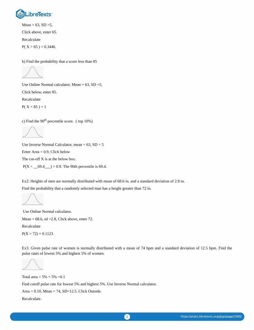
2 https://stats.libretexts.org/@go/page/15902

Mean = 63, SD =5,

Click above, enter 65.

Recalculate

P( X > 65 ) = 0.3446.

b) Find the probability that a score less than 85

Use Online Normal calculator. Mean = 63, SD =5,

Click below, enter 85.

Recalculate

P( X < 85 ) = 1

c) Find the 90 percentile score. ( top 10%)

Use Inverse Normal Calculator, mean = 63, SD = 5

Enter Area = 0.9, Click below

The cut-off X is at the below box.

P(X < __69.4___) = 0.9. The 90th percentile is 69.4.

Ex2: Heights of men are normally distributed with mean of 68.6 in. and a standard deviation of 2.8 in.

Find the probability that a randomly selected man has a height greater than 72 in.

Use Online Normal calculator.

Mean = 68.6, sd =2.8, Click above, enter 72.

Recalculate

P(X > 72) = 0.1123

Ex3. Given pulse rate of women is normally distributed with a mean of 74 bpm and a standard deviation of 12.5 bpm. Find thepulse rates of lowest 5% and highest 5% of women.

Total area = 5% + 5% =0.1

Find cutoff pulse rate for lowest 5% and highest 5%. Use Inverse Normal calculator.

Area = 0.10, Mean = 74, SD=12.5. Click Outside.

Recalculate.

th

3 https://stats.libretexts.org/@go/page/15902

lowest 5% cutoff = 53.4 bpm highest 5%=94.6 bpm

Ex4. A circus farmer grows mandarin oranges finds that the diameters of mandarin oranges harvested on his farm follow a normaldistribution with a mean diameter of 5.85 cm and standard deviation of 0.24cm.

a) Find the probability that a normally selected mandarin orange from his farm has a diameter larger than 6 cm.

Use Online Normal calculator.

Mean = 5.85, sd =0.24,

Click above, enter 6.

Recalculate

P( X > 6 ) = 0.266

b) Find the middle 20% diameter of mandarin oranges from his farm.

Use Inverse Normal Calculator

Area = 0.2, Mean = 5.85, sd=0.24

Click Between.

P( _5.79____< X < __5.91____) = 0.2

Ex5. A TV has a life that is normally distributed with a mean of 6.5 years and a standard deviation of 2.3 years. If the companyoffers a warranty to replace any TV within 3 years. What percent of TV will need to be replaced?

To find percent, use Normal online calculator.

Mean = 6.5 , sd =2.3,

Click below, enter 3.

Recalculate

P (X < 3) = 0.064 = 6.4%

Ch 6.2 Application of Normal Distribution is shared under a not declared license and was authored, remixed, and/or curated by LibreTexts.

1

CHAPTER OVERVIEW

Chapter 7 Lecture NotesIn chapter 7, we will learn the sampling distribution of sample mean. Central Limit will be introduced to understand the distributionof sample mean. Application of Central limit for sample mean and for sum will be used to solve applications of mean and sum ofContinuous Random Variable.

By the end of Chapter 7, students should be able to:

Understand Central Limit Theorem and how it can be used to model sampling distribution of sample mean and sample sum.Apply Central Limit Theorem to solve application problems.

Ch 7.1 Central Limit Theorem for Sample MeansCh 7.2 Central Limit Theorem for Sample Total

Chapter 7 Lecture Notes is shared under a not declared license and was authored, remixed, and/or curated by LibreTexts.

1 https://stats.libretexts.org/@go/page/15911

Ch 7.1 Central Limit Theorem for Sample Means

Ch 7.1 Central Limit Theorem for Sample Means

Sample distribution of sample mean:

When sample means of same size n taken from the same population, the Sample means have the following behavior:

1) If the population distribution of X is normal, the distribution of is always normal for all sample size n.

Sampling distribution of x-bar

2) When population distribution of X is not normal, The sampling distribution x-bar tends to be a normal distribution. Thedistribution become closer to normal when sample size increase.

Activity to discover the Central Limit Theorem:

https://stats.libretexts.org/Bookshelves/Ancillary_Materials/02%3A_Interactive_Statistics/15%3A_Discover_the_Central_Limit_Theorem_Activity

Central Limit Theorem for Sample Mean:

For all sample of the same size n with n > 30, the sampling distribution of can be approximated by a normal distribution withmean μ and standard deviation

Note: -This applies to all distribution of x. If X is normally distributed, n > 30 is not needed. Any n will work.

-The sample should be a Simple Random Sample.

Central Limit Theorem: ,

\( \sigma _{\bar{x}} = \frac{\sigma}{\sqrt{n} \)} Ex1 A standardized test with scores that are normally distributed with mean μ = 150 and standard deviation σ = 18. A class of 20students take the test. The mean score of the 20 students are calculated.

a) Is the distribution of mean score of 20 students Normally distributed?

Ans: Yes because the original score is Normal.

a) What is the mean and standard deviation of ?

Use Central Limit Theorem: mean = 150, SD = ≈ 4.0249

b) Find the probability that a student’s score is greater than 160.

Use Online Normal Calculator, Mean = 150, SD = 4.0249

c) Find the probability that the mean score of 20 students is greater than 160.

Click above, enter 160. Recalculate. P( > 160) = 0.0065

x

x

x

=σxσ

n√

= μμx

x

x

18

20√

x

x

2 https://stats.libretexts.org/@go/page/15911

Ex2: Coke cans are filled so that the actual amounts have a mean of 12 oz and a standard deviation of 0.11 oz. The distribution ofamount of coke is unknown.

a) Is the distribution of mean amount of coke in 36 cans normally distributed?

Yes, because n > 30, according to CLT, will be normally distributed.

b) What is the mean and standard deviation of ?

Ans: according to CLT: = 12, = 0.11/√36 ≈ 0.01833

c) Find the percent of individual coke with amount between 11.9 to 12.1 oz.

Use online Normal Calculator: Mean = 12, SD = 0.11

Click between, enter 11.9 and 12.1, Recalculate. P( 11.9 < x < 12.1 ) = 0.6367

63.67% of coke have amount between 11.9 oz to 12.1 oz.

d) Find the percent of mean amount of 36 coke with between 11.9 and 12.1 oz.

Use online Normal Calculator: Mean = 12, SD = 0.01833,

Click between, enter 11.9 and 12.1, Recalculate. P( 11.9 < < 12.1 ) = 1

100% of mean amount of 36 coke is between 11.9 and 12.1 oz.

Ex3. Annual incomes are known to have a distribution that is skewed to the right. Assume that 20

workers’ mean incomes are collected.

a) Will the distribution of mean income be normally distributed?

Ans: No, since X is not normal and n < 30, CLT does not apply, may not be normally distributed.

Ch 7.1 Central Limit Theorem for Sample Means is shared under a not declared license and was authored, remixed, and/or curated by LibreTexts.

x

x

μx σx

x

x

x

x

1 https://stats.libretexts.org/@go/page/15913

Ch 7.2 Central Limit Theorem for Sample Total

Ch 7.2 Central Limit Theorem for Sample sumFor all sample of the same size n with n > 30, the sampling distribution of can be approximated by a normal distribution

with mean = and standard deviation =

Central Limit Theorem for Sample Sum:

-This applies to all distribution of x. If X is normally distributed, n > 30 is not needed. Any n will work.

-The sample should be a Simple Random Sample.

Ex1. An unknown distribution has a mean of 45 and a standard deviation of 8. A sample size of 50 is drawn randomly from thepopulation. .

a) Can Central Limit for Sum be used to model the distribution of the sum of 50 sample? Explain.

Yes, because sample size 50 > 30.

b) Find the probability that the sum of the 50 values is more than 2400.

Use Central limit for sum:

Use Onlline Normal Calculator: mean = 2250, SD = 56.5685, Select above, enter 2400, recalculate

P( > 2400) = 0.004

Ex2: An elevator has a maximum weight limit of 5000 lb or 27 passengers. Assume adult males have weights that are normallydistributed with a mean of 189 lb. and a standard deviation of 39 lb.

a) Can the sum of 27 passengers’ weight be modeled by Normal distribution? If yes, what is the mean and standard deviation ofsum of weight of 27 passengers?

Yes, because the population distribution of adult male are given as normally distributed.

According to CLT, mean = 189* 27 = 5103, SD = = 202.6499

b) Does this elevator appear to be safe? Find the probability that the total weight of 27 passengers exceed the maximum weightlimit.

Use online Normal Calculator, mean = 5103, SD = 202.6499, Click above, enter 5000, recalculate

P (sum of 27 > 5000) = 0.6944 > 0.05

The sum of 27 male adults has a 69.44% chance of over the weight limit of 5000lb. This event is not unlikely, so the elevator is notsafe.

Ex3. The passenger load for a water-taxi is 3500 lb. Assume weights of passenger are normally distributed with mean 174 lb. witha standard deviation of 21 lb. Is it safe have a passenger limit of up to 20?

a) Can the sum weight of 20 passengers be modeled by Central limit Theorem of sum? If yes, what is the mean and standarddeviation of the weights?

Yes, because the population distribution of adult male are given as normally distributed.

According to CLT, mean = 174* 20 =3480, SD = = 93.9149

∑x

(n)μ σ ∗ n−−

√

= nμ; = σ ∗μsum σsum n−−

√

= 45 ∗ 50 = 2250; = 8 ∗ = 56.5685μsum σsum 50−−

√

\sum{x}}

39 ∗ 27−−

√

21 ∗ 20−−

√

2 https://stats.libretexts.org/@go/page/15913

b) Determine the probability that 20 passenger’s total weight will exceed the passenger load of 3500 lb. Is the 20-passenger limitsafe?

Use online Normal Calculator, mean = 3480, SD = 93.9149, Click above, enter 3500. Recalculate

P (sum of 20 > 3500) = 0.4157 > 0.05

The sum of 20 passengers has a 41.57% chance of exceeding 3500 lb. This event is not unlikely, so the passenger limit is not safe.

Normality assessment:The following procedure can be used to determine if sample data are from a population having a Normal distribution.

1) Histogram: If the histogram departs dramatically from a bell shape, conclude data do not come from a normal distribution.

If Histogram from the sample does not departs from a bell shape distribution, conclude the Population may beNormal.

2) Outliers: If there is more than one outlier, conclude data do not come from a normal distribution.

3) Normal Quantile plot: If patterns of the points is reasonably close to a straight line and the points does not showsome systematic pattern that is not a straight line pattern, conclude Normal distribution

Normal quantile plot (or Normal probability plot) is a plot of (x, y) where x is the original data and y is the corresponding z-score that is expected from a normal distribution.

Steps:

1) input data to Sample editor in Statdisk.

2) Data/Normality Assessment/

3) Check that number of outliers are at most 1. Check that Histogram has a approximately bell shape distribution. Check thatpoints on Normal Quantile plot are reasonably close to a straight line.

Ex1. Sample question: Do the following values come from a population with normal distribution?

7.19, 6.31, 5.89, 4.5, 3.77, 4.25, 5.19, 5.79, 6.79.

Input data to statdisk, data/Noramality Assessment/

-number of outliers is 0

Histogram shows relatively symmetrical

-Normal quantile plot shows plot along a linear pattern.

3 https://stats.libretexts.org/@go/page/15913

Final conclusion: the sample are from a population that is Normal.

Ch 7.2 Central Limit Theorem for Sample Total is shared under a not declared license and was authored, remixed, and/or curated by LibreTexts.

1

CHAPTER OVERVIEW

Chapter 8 Lecture NotesCh 8.1 Confidence Interval for Population MeanCh 8.2 Confidence Interval for Mean One Sample No SigmaCh 8.3 Confidence Interval for Population Proportion

Chapter 8 Lecture Notes is shared under a not declared license and was authored, remixed, and/or curated by LibreTexts.

1 https://stats.libretexts.org/@go/page/15914

Ch 8.1 Confidence Interval for Population Mean

Ch 8.1 Confidence Interval for mean with one sample when σ is knownTerms: Population mean: μ, sample mean:

sample standard deviation: s, sample size: n

Population standard deviation: σ

Confidence Level: Clevel,

Significant Level α: 1 – Clevel (unlikely)

A) Estimate μ (when σ is given)Use one sample with size n, , s or raw data:

When when σ is given.

Use Online calculator statdisk to find confidence interval of mean when σ is given.

use https://www.statdisk.com/#

Analysis/Confidence Intervals/Mean one sample/. If summary statistics ( , s, n) are given.

Select “use Summary Statistics” tab otherwise use “use data” tab.

Enter C-level, , s or select with data

Must enter that is given

Output: E is the margin of error or Error bound for mean.

Confidence interval estimate is lower limit < upper limit

Note: the requirement for the confidence interval is CLT applies. (n > 30 or X is Normal), sample is SRS.

is the critical value with C-level in the middle

To find

use Inverse Normal Calculator, Area = α/2, mean = 0, sd = 1, click above, recalculate.

Explanation:

According to Central Limit Theorem, if n > 30 or X is normal, has a sampling distribution that is Normal with mean = μ and SD=

Given a C-level, the maximum sampling error of from μ is E with a right tail of area = α/2.

Since standard error is , so the range of values

from should include the real population mean at a confidence level of

C-level.

Ex1. Suppose scores on a standardized exam are normally distributed with standard deviation of 35.

x

x

 1) point estimate of μ:   x

 2) Interval estimate of μ:  −E < μ < +E x x

E(EBM) = zα/2σ

n√

x

x

σ

μ

zα/2

zα/2

xσ

n√

x

σ

n√

- E  to  +Ex x μ

2 https://stats.libretexts.org/@go/page/15914

A sample of 14 scores are collected with sample mean 137.3 and sample standard deviation 37.2.

a) Use the sample to estimate the population mean score of the standardized test at a 98% confidence level.

Identify: C-level = 0.98 n = 14, = 137.3, s = 37.2, σ = 35

Statdisk/Analysis/Confidence intervals/Mean one sample/

b) At a confidence level of 98%, what is the significant level and the critical value?

If Clevel = 0.98, α=0.02, use Inverse-Normal calculator with right tail = 0.01, critical value = = 2.326

c) A previous study shows that the mean scores was 144.2. Is the population mean score below 144.2?

No, Since the mean scores can be between 115.5 to 159.06, it cannot be below 144.2.

d) Explain what will happen to margin of error E if sample size increase.

When sample size increase, margin of error should decrease because the formula

e) Explain what will happen to margin of error E if confidence level increase to 99%.

When Clevel increase, the critical value will increase so Margin of error will increase.

Ex2. The specific Absorption Rate (SAR) for a cell phone measures the amount of radio frequency energy absorbed by the user’sbody when using the handset. The legal SAR level is no more than 1.6 watts per kilogram. The following SAR data are collectedfrom 30 phones.

1.11, 1.48, 1.43, 1.3, 1.09, 0.455, 1.41, 0.82, 0.78, 1.25, 1.36, 1.34, 1.18, 1.3, 1.26, 1.29, 0.36, 0.52, 1.6, 1.39, 0.74, 0.5, 0.4, 0.867,0.68, 0.51, 1.13, 0.3, 1.48, 1.38.

a) Use the sample to find the 95% confidence interval of the mean SAR level for all phones given that population standarddeviation is σ = 0.337.

Ans: Use Statdisk/Analysis/Confidence Interval/One sample mean/ with data tab

output:

b) Write the confidence interval in the form of interval notation and +/- notation.

The interval is \pm E. = (lower limit + upper limit)/2 = 1.02

The +/- notation is 1.02 0.12

c) Can we conclude that the mean SAR level is below the legal allowable value of 1.6?

Yes, since interval of mean is between 0.90 to 1.14, all these values are below 1.6.

d) Find the critical value .

Since Clevel = 0.95, = 0.05, so = 0.025.

Use Inverse normal calculator, set area = 0.025, mean = 0, sd = 1, click above, recalculate.

x

zα/2

x x

±

zα/2

α α/2

3 https://stats.libretexts.org/@go/page/15914

= 1.96

e) If we want to decrease the margin of error, what can be done?

We can increase the margin of error, or decrease Clevel.

B) Find sample size n for a given Margin of error (EBM)

From central limit Theorem, we have the equation between E and n is . Algebra can be used to show that for

a given C-level, E and σ,

Find sample size by online calculator:

Statdisk.com / Analysis/sample size Determination/ Estimate mean/

Enter Clevel, E, population standard deviation.

Note: when sample size increase, E decrease.

when E increase, sample size decrease.

Ex3. The population standard deviation of student’s age in a community college is 15 years. If we want to be 95% confidence thatthe error in confidence interval estimate for mean student's age is within 2 years from the real mean age of all students, how manystudents must be surveyed?

Use Statdisk/ Analysis / Sample size Determination/

Estimate Mean Clevel = 0.95, E = 2, pop. sd = 15

Required sample size = 217.

Ch 8.1 Confidence Interval for Population Mean is shared under a not declared license and was authored, remixed, and/or curated by LibreTexts.

zα/2

E(EBM) = zα/2σ

n√

n = ( )⋅σzα/2

E

2

1 https://stats.libretexts.org/@go/page/15922

Ch 8.2 Confidence Interval for Mean One Sample No Sigma

Ch 8.2 Confidence Interval for mean with one sample when sigma is not known.Use one sample with size n, , s

When when σ is not given or unknown.

Use Online calculator to find confidence interval of mean when is not given.

- use online statdisk: https://www.statdisk.com/#

Analysis/Confidence Intervals/Mean one sample/.

If summary statistics ( , s, n) are given, select “use Summary Statistics” tab otherwise use “use data” tab.

Enter Clevel, n, , s, or select with data tab.

Do not enter population standard deviation.

Output: E is the margin of error or Error bound for Mean.

Confidence interval estimate is

Note: the requirement for this confidence interval is CTL applies (n > 30 or X is normal). Sample is SRS.

B) T-distribution is the critical value with C-level in the middle.

To find

Use Online Stat book Inverse-t Calculator: http://onlinestatbook.com/2/calculators/inverse_t_dist.html

the degree of freedom = n – 1, Select confidence interval from 90%, 95% or 99%. “Calculate”

The “t for confidence interval” is the critical value t .

Properties of t-distributions:

1) = no. of times of is from mean μ when has a normal distribution.

2) Each t-distribution is different for different sample size according to the degree of freedom df = n – 1.

3) Each t-distribution has the same general symmetric bell shape as standard normal, but with more variability.

4) As sample size increase, the student t- distribution approaches the standard normal distribution.

Ex1: Patients with insomnia are treated with zopiclone. After the treatment, the 16 subjects had a mean wake time of 98.9 min. anda sample standard deviation of 42.3 min. Assume that wake times are normally distributed.

a) Construct a 98% confidence interval estimate of mean wake time for all patients treated by zopiclone.

- since X is normal, x-bar is normal, σ is not known, so use t-distribution.

- Identify C-level = 0.98, n= 16, = 98.9, s = 42.3,

- Use statdisk/ Analysis/Confidence interval/ Mean one sample/

x

 1) point estimate of μ :  x

 2) Interval estimate of μ:  −E < μ < +E x x

E(EBM) = tα/2s

n√

x

x

−E < μ < +Ex x

tα/2

tα/2

α/2

t =x−μ

s/ n√s/ n

−−√ x x

x

2 https://stats.libretexts.org/@go/page/15922

- output: E = 27.521, Confidence interval is 71.379 < μ < 126.421

interval format (71.379, 126.421), +/- format: x-bar E, 89.9 ± 27.521

b) Can we conclude the mean wake time is less than 100 min.?

No, since the interval is from 71.4 to 126.4, not all values are less than 100 min.

c) If confidence level is decreased to 95%, what will happen to the margin of error?

When confidence level decrease, will decrease, so Margin of error will decrease.

C) Interpret the Confidence interval of mean:

i) We estimate with ________ confidence that the true population mean for ______________is between ___ and ___ .

ii) 90% of confidence interval constructed in this way contains the true ______________population mean.

Make conclusion from a confidence Interval:

1) Any value in the confidence Interval can be μ.

2) If the whole interval > a, we can conclude μ > a

3) If the whole interval < a, we can conclude μ < a.

4) When two confidence interval overlap, we can conclude that the two μ may be the same. We cannot conclude one of the μ ishigher.

5) Never make conclusion about population mean based solely on value of .

Ex2. Listed below are amounts of arsenic (in ug, per serving) in samples of brown rice from California.

5.4, 5.6, 7.3, 4.5, 7.5, 1.5, 5.5, 9.1, 8.7, 8.4

a) Can we assume that amount of arsenic in brown rice is from a normal distribution?

Use Normal Quantile plot to access Normality.

Copy data to statdisk. Data/Normal Assessment

The points are reasonably close to a straight line. So we can assume population X is normal.

b) Construct 90% confidence interval of mean arsenic in all brown rice from California. What distribution is sued?

-Since X is normal, so is normal, σ is not known, so use t distribution.

-identify Clevel = 0.9, column in statdisk.

- Statdisk Analysis/Confidence intervals/Mean One sample /use data tab.

output: E = 1.348 , 5.002 < mean < 7.698

-Interval estimate: 5.0 ug < μ < 7.7 ug

c) Find the critical value.

Since t-distribution is used when σ is not known, use online calculator inverse t-calculator.

degree of freedom = 9, C-level = 90% , critical value t = 1.833

±

tα/2

x

x

0.05

3 https://stats.libretexts.org/@go/page/15922

d) Interpret the meaning of the confidence Interval:

“We estimate with 90% confidence that the mean amount of arsenic is between 5.0 ug and 7.7 ug.”

“90% of all confidence interval collected from sample of size 10 will contain the true mean arsenic.”

d) Can we conclude the mean amount is less than 8 ug?

Yes, because all values in the interval are less than 8 ug. We can conclude that the mean amount of arsenic in all brown rice are lessthan 9 ug. at 90% confidence.

Ch 8.2 Confidence Interval for Mean One Sample No Sigma is shared under a not declared license and was authored, remixed, and/or curated byLibreTexts.

1 https://stats.libretexts.org/@go/page/15923

Ch 8.3 Confidence Interval for Population Proportion

Ch 8.3 Confidence Interval for population proportion:Terms: Population proportion: p

Sample proportion: = (x/n)

Number of success: x; sample size: n

Confidence Level: C-level

Significant Level: α = 1 – C-level (probability of unlikely)

EBP: Error Bound for proportion, margin of error

A) To Estimate p:

Note: E is the approximated value of sampling error of sampling distribution of , which has a normal distribution when x and n-x ≥ 5.

Use Statdisk online calculator to find the confidence interval.

- identify C-level, sample size n and success = x.

- https://www.statdisk.com/# , Analysis/ Confidence Intervals/Proportion one sample/

output: E (EBP) and lower < p < upper

is the critical value with C-level in the middle.

To find

Use online Inverse Normal calculator, set area = , mean = 0, sd =1,

click above, recalculate.

Explanation:

X = number of success is a binomial distribution with mean = np and sd = .

When np and nq ≥ 5, distribution of X is normal with mean = np and sd = .

So distribution of is normal with mean = p and SD = .

At a given C-level, the maximum error of and p is E where

Note: the requirement for this confidence interval is not n > 30 but np and nq ≥ 5.

Interpret a 95% Confidence Interval:

We are 95% confidence that the interval from ____ to ____ actual contain the true value of the population proportion of thecategory of interest.

The Confidence interval also shows that 95% of all confidence Intervals contain the true value of p.

Make conclusion from confidence interval:

1) Any value in the confidence Interval can be p.

p

1) point estimate:  = x/n p

 2) Interval estimate:  −E to  +E p p

E(EBP ) = zα/2p q

n

−−−√

p

zα/2

zα/2

α/2

npq−−−√

npq−−−√

=pxn

p q

n

−−−√

p E(EBP ) = zα/2p q

n

−−−√

2 https://stats.libretexts.org/@go/page/15923

2) If the whole interval > a, we can conclude p > a

3) If the whole interval < a, we can conclude p < a.

4) When two confidence interval overlap, we can conclude that the two p may be the same. We cannot conclude one of the p ishigher.

Ex1. A research is conducted to determine how many household use Netflix to stream videos. A random sample of 500 householdsshow that 442 households use Netflix.

a) Use a 90% confidence level to compute a confidence interval estimate of true proportion of households using Netflix.

use Statdisk Analysis/Confidence Intervals/Proportion one sample : Clevel = 0.9, n = 500, x = 442,

b) Find the critical value.

Use Inverse Normal calculator, since clevel = 90%, , set area = 0.05, mean = 0, sd = 1,

click above, recalculate.

= 1.645

c) Interpret the confidence interval in non-technical term.

We estimate with 90% confidence that the true proportion of all households that use Netflix is between 86.0% to 90.8%

d) Can we conclude with 90% confidence that more than 80% of households use Netflix?

Since the interval contains 86.0% to 90.8%, all values are more than 80%, so we can conclude that.

Ex2: A Gallup poll of 1487 adults showed that 43% of the respondents have Facebook pages.

a) Find the number in the sample who have Facebook pages. = 1487 (0.43) = 639

c) Find the interval estimate of p at 95% confidence level and margin of error E.

Use statdisk with Clevel = 0.95, n = 1487, x = 639

Interval estimate is 0.405 < p < 0.455, E = 0.025

d) Write a non-technical interpretation of the above

We are 95% confidence that the true percent of adults who have Facebook pages are between 40.5% to 45.5%.

e) Can we claim that less than 60% of all adults have Facebook pages?

Since the whole interval is less than 0.6, yes, we can conclude less than 60% of all adults have Facebook pages.

B) Determine sample size for a desired E

Since

when an estimate is known.

when no estimate is known.

Use statdisk / Analysis/Sample size Determination/ Estimate proportion to find sample size for a given error E.

α = 0.1, α/2 = 0.05

zα/2

x = n( )p

E(EBP ) = zα/2p q

n

−−−√

n =(zα/2 )

2p q

E2 p

n =( ⋅0.25zα/2 )

2

E2 p

3 https://stats.libretexts.org/@go/page/15923

Input C-Level, Desired E, Estimate of p = , evaluate.

Ex3. What sample size should be used if we want the keep the margin of error within 2.1% when estimating a proportion at a 90%confidence interval. use as an old estimation of p.

C-level = 0.9, E = 0.021, estimate of p = 0.43, Evaluate

Sample size p = 1504.

b) If no previous study has been done , what sample size will be needed. (do not use p-hat = 0.43)

Use statdisk / Analysis/Sample size Determination/ Estimate proportion

C-level = 0.9, E = 0.021, estimate of p = blank, evaluate

sample size p = 1534

Ch 8.3 Confidence Interval for Population Proportion is shared under a not declared license and was authored, remixed, and/or curated byLibreTexts.

=px

n

= 0.43p

1

CHAPTER OVERVIEW

Chapter 9 Lectures Notes

Ch 9.1, 9.3 and 9.4 Hypothesis Test BasicCh 9.2 Hypothesis ErrorsCh 9.5 part 1 Hypothesis Test for Population ProportionCh 9.5 part 2 Hypothesis Test for Population Mean

Chapter 9 Lectures Notes is shared under a not declared license and was authored, remixed, and/or curated by LibreTexts.

1 https://stats.libretexts.org/@go/page/15916

Ch 9.1, 9.3 and 9.4 Hypothesis Test Basic

Ch 9.1, 9.3 and 9.4 Hypothesis Test basicHypothesis test: (or test of significance) is a procedure based on sample evidence and probability, used to test claim regarding acharacteristic of one or more populations. Characteristic of population proportion (p) and mean (μ) will be covered in this course.

To test a hypothesis, you should state a pair of hypotheses, one that represents the claim and the other, its complement. When oneof these hypotheses is false, the other must be true. The null hypothesis represents currently acceptable truth.

The alternative hypothesis contains opposing viewpoint.

Basic process of a Hypothesis test (p-value method)1) Identify the claim.

2) Translate the claim in algebraic symbolic form.

3) Identify the null and alternative hypothesis test and write in symbolic form. H0 and Ha (or H1) are the symbols for the twohypotheses.

4) Select a significant level α. (based on seriousness of making a type I error.)

5) Collect a sample and identify the “Type” of hypothesis test in Ha. Determine the sampling distribution (normal or t).

6) Use calculator to find test statistic and p-value.

7) Make conclusion on H0 based on p-value.

8) Rewrite the conclusion in simple non-technical term and address the original claim.

Part A: Step 1, 2, 3The claim is about value of a population parameter, we can claim that the parameter is greater, less than, equal to or not equal to avalue. (Note: claim of at most, at least is equivalent to claiming equal.)

a) Since the claim is about population parameter, the symbolic form can be: (p or μ) ( ) a claim value.

b) The null hypothesis is the first assumption we use to calculate probability of the sample we obtained,

so the null hypothesis must be of equality form.

c) The alternative hypothesis is the second assumption that must not overlap (or opposite) with the null hypothesis.

H0: (p or μ ) = (a value) ; Ha: (p or μ ) is ( ) (a value); (a value ) is value that shows up in the claim.

Ex1: Claim that mean body temperature is less than 98.6 F:

claim: μ < 98.6 H0: μ = 98.6 Ha: μ < 98.6

Ex2. Claim that proportion of red M&M is greater than 10%.

claim: p > 0.1; H0: p = 0.1 Ha: p > 0.1

Ex3. Claim that mean IQ scores of college professor is different from 100.

claim: μ = 100; H0: μ = 100 Ha: μ ≠ 100

Ex4. Claim that mean IQ scores of college student is 105.

claim: μ = 105; H0: μ = 105 Ha: μ ≠ 105

Part B: Step 4, 5 and 6: Common significant level α is 0.05, but if Type 1 error is very undesirable, a lower significant level is better.

If the claim is about p, the sampling distribution is z normal because is normally distributed.

<, >, ≤, ≥, ≠, =

<, >, ≠

o

2 https://stats.libretexts.org/@go/page/15916

If the claim is about μ, the sampling distribution is t or z normal depending on if σ is known. According to CLT, is normallydistributed if n > 30 or population is Normal.

Obtain a sample and use calculator to find the a “test statistic” and a “p-value”

Test statistic tells the number of SD the sample is from the assumed parameter value assumed in H0.

P-value tells the probability of getting the sample or worse if the assumption of H0 is true.

P-value are calculated based the “Type” of test:

Types of Hypothesis Test: (determined by looking at Ha)

Left-tail test: when Ha has the form of p < value. p-value is left area of test statistic.

right-tail test: when Ha has the form of p > value. P-value is right area of the test statistic.

Two-tail test: when Ha has the form of p ≠ value

p-value is twice of area in left or right area from the test statistic.

The online calculator will calculate test statistic and p-value. https://www.statdisk.com/ #/Analysis/Hypothesis Testing

More detail will be covered in Ch 9.5.

Part C: Step 7 and 8:The conclusion of a hypothesis test is based on the

Rare Event Rule:

“Based on an assumption, if the observed event is very rare (lower than significant level α), we conclude the assumption is properlynot true.”

In a Hypothesis Test, the assumption is H0, the null hypothesis. We determine if the sample is rare based on the assumed claimpopulation characteristic in H0.

Step 7: If p-value ≤ α, reject null hypothesis. Result is Significant!

If p-value > α, fail to reject the null hypothesis.

[ If p-value is low, the null must go.

If p-value is high, the null will fly.]

Step 8: Make conclusion about the claim.

If the p-value ≤ α: use “there is sufficient evidence…”

If the p-value > α, use “there is not sufficient evidence…”

If the claim is H0: Reject H0 implies reject the claim.

If the claim is Ha: Reject H0 implies support the claim. Or

Conclusion about the claim

x

3 https://stats.libretexts.org/@go/page/15916

Conditions ConclusionConditions Conclusion

Original claim does not include equality and H0 is rejected. "There is sufficient evidence to support the claim that .... "

Original claim does not include equality and H0 is failed to be rejected. "There is not sufficient evidence to support the claim that...."

Original claim include equality and H0 is rejected. "There is sufficient evidence to reject the claim that ... "

Original claim include equality and H0 is failed to be rejected. "There is not sufficient evidence to reject the claim that ..."

Note:

“Not sufficient evidence to reject the claim” implies it is plausible that the claim is true.

“Not sufficient evidence to support the claim” implies the claim may not be true.

Ex1. If significant level = 0.05 and p-value = 0.04, what is the conclusion on H0?

Since 0.04 < 0.05, sample is significant, so reject H0.

Ex2. If significant level = 0.05 and p-value = 0.006, what is the conclusion on H0?

Since 0.006 < 0.05, the sample is significant, so reject H0.

Ex3. If significant level = 0.01 and p-value = 0.03, what is the conclusion on H0

Since 0.03 > 0.01, the sample is not significant, so fail to reject H0.

Ex4. If the claim is Ha and you fail to reject H0, what is the claim conclusion?

There is not enough evidence to support the claim.

Ex5. If the claim is H0 and you reject H0, what is the claim conclusion?

There is sufficient evidence to reject the claim.

All steps practice:

Ex1. Test a claim that body temperature of adult is less than 98.6 F. Use α = 0.05. A random sample of 38 body temperatures (withgives a test statistic of t = –2.56 and p-value of 0.0072.

a) Write the claim and hypothesis,

b) Determine the type of distribution used and “type of hypothesis test.” and significant level.

c) Interpret the meaning of test statistic and p-value.

d) Use p-value to make conclusion about H0 and about the claim.

Answer:

a) Claim: μ < 98.6 H0: μ = 98.6 Ha: μ < 98.6

b) Since μ is the parameter, σ is not known, so use t distribution. Since Ha is “<”, Type of test is left tail.

α = 0.05.

c) Test statistic of t = -2.56 means the sample data is 2.56 standard deviation below μ = 98.6.

p-value of 0.0071 means the probability of having the sample or worse is 0.71% if the real mean is 98.6.

d) Conclusion about H0:

Since p-value < 0.05, reject H0, sample is significant

p-value ≤ α -> use “ there is sufficient evidence”..

Slaim is Ha -> use “ support the claim.”

“There is sufficient evidence to support the claim that mean body temperature is less than 98.6 F.

o

o

4 https://stats.libretexts.org/@go/page/15916

Ex2: Claim that proportion of red M&M is greater than 10%. Use α = 0.05. A sample (15 red out of 102 M&M candies) gives atest statistic of z = 1.91, p-value = 0.0566.

a) Write the claim and hypothesis,

b) Determine the type of distribution used and “type of hypothesis test” and significant level.

c) Interpret the meaning of test statistic and p-value.

d) Use p-value to make conclusion about H0 and about the claim.

Answer:

a) claim: p > 0.1; H0: p = 0.1; Ha: p > 0.1

b) α = 0.01. Since p is the claim parameter, sampling distribution is normal, z distribution is used.

Since Ha use p > 0.1, Type of test is right tail test.

α = 0.05.

c) A test statistic of z = 1.91 means the sample proportion is 1.91 times of SD above the mean of p = 0.1.

P-value of 0.0566 means there is 5.66% probability to obtain such as sample if p = 0.1 is true.

d) p-value of 0.0566 > 0.05: fail to reject H0 (sample is not significant because the sample is not a rare event.)

Since p-value > α so use “there is not sufficient evidence” statement.

claim is Ha, use “ support the claim”

Final conclusion: there is not sufficient evidence to support the claim that proportion of red M&M is greater than 10%.

Ex3. Claim that IQ scores of college student has a mean equal to 104. Given that σ for IQ score is 15. A sample of IQ scores from40 college students ( = 106, s = 16) give a test statistic z = 0.84 and a

p-value = 0.1995. Use α = 0.05 to test the claim.

a) Write the claim and hypothesis.

b) Determine the type of distribution used and type of hypothesis test and significant level.

c) Interpret the meaning of test statistic and p-value.

d) Use p-value to make conclusion about H0 and about the claim.

Ans:

a) claim: μ = 104; H0: σ = 104; Ha: μ ≠ 104

b) Since claim parameter is μ but σ is known, so use z-Normal distribution. Since Ha has the form of ≠, the Hypothesis test is a“Two-tail Test”. α = 0.05.

c) Test statistic z = 0.8432 means the sample is 0.84 times of standard deviation from μ = 104.

p-value of 0.1995 means there is 19.95% chance of getting such sample if μ = 104 is true.

d) p-value 0.1995 > 0.05, the sample is not a rare event, fail to reject H0, sample is not significant.

P-value > α so, “Use the wording there is not sufficient evidence.”

Claim is in H0, Use “reject the claim” statement.

Conclusion: There is not sufficient evidence to reject the claim that the college student’s mean IQ is equal to 104. (Conclude thatmean IQ for college student could be 104.)

5 https://stats.libretexts.org/@go/page/15916

Ch 9.1, 9.3 and 9.4 Hypothesis Test Basic is shared under a not declared license and was authored, remixed, and/or curated by LibreTexts.

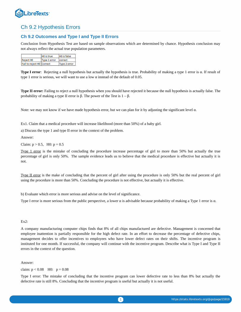
1 https://stats.libretexts.org/@go/page/15919

Ch 9.2 Hypothesis Errors

Ch 9.2 Outcomes and Type I and Type II ErrorsConclusion from Hypothesis Test are based on sample observations which are determined by chance. Hypothesis conclusion maynot always reflect the actual true population parameters.

Type I error: Rejecting a null hypothesis but actually the hypothesis is true. Probability of making a type 1 error is α. If result oftype 1 error is serious, we will want to use a low α instead of the default of 0.05.

Type II error: Failing to reject a null hypothesis when you should have rejected it because the null hypothesis is actually false. Theprobability of making a type II error is β. The power of the Test is 1 – β.

Note: we may not know if we have made hypothesis error, but we can plan for it by adjusting the significant level α.

Ex1. Claim that a medical procedure will increase likelihood (more than 50%) of a baby girl.

a) Discuss the type 1 and type II error in the context of the problem.

Answer:

Claim: p > 0.5, H0: p = 0.5

Type 1 error is the mistake of concluding the procedure increase percentage of girl to more than 50% but actually the truepercentage of girl is only 50%. The sample evidence leads us to believe that the medical procedure is effective but actually it isnot.

Type II error is the make of concluding that the percent of girl after using the procedure is only 50% but the real percent of girlusing the procedure is more than 50%. Concluding the procedure is not effective, but actually it is effective.

b) Evaluate which error is more serious and advise on the level of significance.

Type I error is more serious from the public perspective, a lower α is advisable because probability of making a Type 1 error is α.

Ex2:

A company manufacturing computer chips finds that 8% of all chips manufactured are defective. Management is concerned thatemployee inattention is partially responsible for the high defect rate. In an effort to decrease the percentage of defective chips,management decides to offer incentives to employees who have lower defect rates on their shifts. The incentive program isinstituted for one month. If successful, the company will continue with the incentive program. Describe what is Type I and Type IIerrors in the context of the question.

Answer:

claim: p < 0.08 H0: p = 0.08

Type I error: The mistake of concluding that the incentive program can lower defective rate to less than 8% but actually thedefective rate is still 8%. Concluding that the incentive program is useful but actually it is not useful.

2 https://stats.libretexts.org/@go/page/15919

Type II error: The mistake of concluding that the defective rate is 8% but actually the defective rate after the incentive program isless than 8%. Conclude that the incentive program is not useful but actually it is useful.

b) Discuss if type I or type II error is more serious.

Should management use a high or low significant level?

Ans:

Type I error means company will spend money on something that is not useful. So to avoid unnecessary expense, Type I errorshould be avoided.

Hence a low significant level may be better.

If cost is a priority, Type I error should be avoided so a lower α is better.

Type II error means you bypass a good program that can decrease defective rate or increase profit. Type II error should be avoidedif profit is a priority, hence a lower α is unnecessary.

Ch 9.2 Hypothesis Errors is shared under a not declared license and was authored, remixed, and/or curated by LibreTexts.

1 https://stats.libretexts.org/@go/page/15917

Ch 9.5 part 1 Hypothesis Test for Population Proportion

Ch 9.5- part 1 Full Hypothesis Test for population proportionNotations:

x = number of success

n = sample size (number of observations)

= sample proportion

p = claim proportion mentioned in claim, use in H0

q = 1 – p

α = significant level. (probability of unlikely)

STEPS:

1) Write claim, H0 and Ha in symbolic form.

Identify n, x.

2) Determine significant level α, type of test (left-tail, right-tail or two-tail test based on Ha and sampling distribution. Samplingdistribution of is Normal.

3) Use Statdisk.com to find test-statistic and p-value:

Analysis/Hypothesis testing/Proportion One sample.

Select Population proportion “not equal” or “ >” or

“< “claimed proportion according to Ha.

Input Significance α; claimed proportion (in H0); sample size n; number of successes x. Evaluate.

Output: test stat z and p-value p.

4) Make conclusion about H0.

If p-value ≤ α, reject H0. Sample is significant.

If p-value > α, fail to reject H0

5) Conclusion about the claim:

There is (sufficient or not sufficient ) evidence to

(support / reject) the claim that ……

Use table or flowchart for wordings.

6) Make additional inference from the conclusion.

The three conditions for using the hypothesis test are:

a) Number of success and failures are at least 5.

np ≥ 5, nq ≥ 5.

b) Fixed number of samples with two outcomes and independent sample. (binomial requirement)

c) Sample are randomly collected.

Ex1: A Pitney Bowers survey of 1009 customers shows that 545 of customers are uncomfortable with Drone deliveries. Test theclaim that majority of customers are uncomfortable with Drone deliveries. Use α=0.05.

p

2 https://stats.libretexts.org/@go/page/15917

(Majority means greater than 50%.)

Answer:

1) Claim: p > 0.50 H0: p = 0.50 Ha: p > 0.5

n = 1009 , x = 545,

2) α = 0.05, right- tail test, use z distribution

3) Use Statdisk/Analysis/Hypothesis Test/proportion one sample. Select ">" for Alternative hypothesis. Enter significance = 0.05,chaim proportion 0.5.

n = 1009, x = 545 , calculate.

Output: z-stat = 2.55 and p-value =0.0054

This means the sample is 2.55 sd from the mean of p = 0.5 and the probability of getting the sample or worse is 0.0054 when H0is true.

4) Since 0.0054 < 0.05 Reject H0, significant sample.

5) Use “sufficient evidence” because p-value < α,

Use “support the claim” because claim is Ha.

“There is sufficient evidence to support the claim that majority of customers are uncomfortable with drone deliveries.”

b) Should a company start to invest in drone deliveries now?

No, because majority of customers are uncomfortable with drone deliveries.

Ex2: Test the claim that less than 30% of adults have sleep-walked. Use significant level α = 0.05. A random sample shows 29.7%of 1913 adults have sleep-walked.

Answer:

1) claim: p < 0.30 H0: p = 0.30 Ha: p < 0.30

n = 1913, x = 1913(0.297 ) = 568

2) α=0.05, left-tail test, use z distribution

3) Use Statdisk/Analysis/Hyp Test/proportion one sample. Select “<” for Alternative Hypothesis. Enter Significance = 0.05,claimed proportion 0.3,

n = 1913, x = 568 , calculate.

Output: Z = – 0.29, p-value = 0.384

This means the sample is – 0.29 of s.d. below the assumed true H0 value. The probability of getting the sample is 0.384 whenH0 is true.

4) 0.384 > 0.05 , fail to reject H0. (not significant)

5) Fail to reject H0: use “not sufficient evidence..”

claim is in Ha: use “…support the claim.”

There is not sufficient evidence to support the claim that less than 30% of adults have sleep-walked.

b) Is the claim true?

No, not sufficient evidence to support the claim so the claim is not true.

Ex3: In a USA today survey of 510 people, 53% said that we should replace passwords with biometric security such as fingerprints.

3 https://stats.libretexts.org/@go/page/15917

a) Use a significant level of 0.1 to test the claim that exactly 50% of all adults like the idea of replacing passwords with biometricsecurity.

Answer:

1) Claim: p = 0.5, H0: p = 0.5, Ha: p ≠ 0.5

n = 510 , x = 510(0.53) =270,

2) α = 0.1, two-tail test, use z- distribution.

3) Use Statdisk/Analysis/Hypothesis Test/proportion one sample. Select “not =” for Alternative hypothesis.

Enter Significance = 0.1, claimed proportion 0.5,

n = 510, x = 270, calculate.

output: Test statistic z = 1.33, p-value = 0.184

4) 0.184 > 0.1, fail to reject H0.

Since we fail to reject H0: use “ not sufficient evidence…”

The claim is in H0, use “… reject the claim.” statement.

There is not sufficient evidence to reject the claim that half of all adults like the idea of replacing password with biometrics.

b) Is the claim true?

yes, not sufficient evidence to reject the 50% proportion, conclude the only 50% of the population like the idea.

c) Discuss if the conditions for hypothesis test of proportion is satisfied?

The success-failure condition: np = 510(0.5) > 5

nq = 510(1-0.5) ≥ 5. Assuming the sample is a simple random sample, so conditions are satisfied.

Ch 9.5 part 1 Hypothesis Test for Population Proportion is shared under a not declared license and was authored, remixed, and/or curated byLibreTexts.

1 https://stats.libretexts.org/@go/page/15918

Ch 9.5 part 2 Hypothesis Test for Population Mean

Ch 9.5-part 2 Full Hypothesis Test for MeanTerms: Population mean: μ

Sample mean:

sample standard deviation: s

sample size: n

Population standard deviation: σ (given or unknown)

significant Level: α (probability of unlikely)

1) Write claim, H0 and Ha in symbolic form.

Identify σ, n, , s or input sample data in one column of statdisk sample editor.

2) Determine significant level and type of test (left-ail, right tail or two-tail test based on Ha), the sampling distribution for mean isz if σ is known, the sampling distribution for mean is t if σ is not given.

3) Use Statdisk/Analysis/Hypothesis Testing/ Mean one sample:

- If n, , s is available, use summary statistic tab,

- If sample data is available, use “Data” tab.

- Select Alternative Hypothesis: “not equal” for two-tail test, “<” for left tail test, “>” for right tail test.

- Enter significance, claimed mean, population SD if known. Select data column or enter n, , s. Evaluate.

- Output: Test stat z or t, p-value.

4) Make conclusion about H0.

If p-value ≤ α, reject H0. Sample is significant.

If p-value > α, fail to reject H0

5) Conclusion about the claim:

There is (sufficient or not sufficient ) evidence to

(support /reject ) the claim that ……

Use table or flow chart to make conclusion.

6) Make inference from the conclusion.

Conditions for Hypothesis Testing of mean:

1) Sample is SRS.

2) The population is normally distributed or n >30.

Use Normal quantile plot to check for normality if data is given.

Ex1: Test the claim that mean amount of adult sleep is less than 7 hours. A sample 12 adults gives = 6.82 hr., s = 1.99 hr. Use asignificant level of 0.05. Given that hours of sleep are normally distributed.

Answer:

1) Claim: μ < 7, H0: μ = 7 , Ha: μ < 7

x

x

x

x

x

2 https://stats.libretexts.org/@go/page/15918

n = 12, = 6.82, s = 1.99

2) α = 0.05, Left-tail test and use t-distribution

3) Use Statdisk/Analysis/Hypothesis Test/ Mean one sample/ Use summary statistics tab.

Select Alternative Hypothesis Test: select “<”

Enter significance = 0.05, n, , s. calculate.

Output: Test statistic t = - 0.31, p-value = 0.3799.

4) Since p-value > 0.05, Fail to reject H0. Sample is not significant.

5) There is no sufficient evidence to support the claim that mean sleep hour is less than 7 hours.

b) Public Health guideline for hours of sleep per night is 7 hours or more. Does the public follow the guideline from Public Health?

Yes, the result concludes that the mean is not less than 7 hours so it is plausible to be 7 hours or more.

Ex2: Given below are the measured radiation emissions (in W/kg) corresponding to a sample of 11 most popular brand of cellphones. Use a 0.05 significant level to test the claim that cell phones have a mean radiation level that is greater than 0.7 W/kg.

0.38 0.55 1.54 1.55 0.50 0.60 0.92 0.96 1.00 0.86 1.46

Answer:

1) Claim: μ > 0.7, H0: μ = 0.7 , Ha: μ > 0.7

Input data to a column in statdisk.

2) α = 0.05, Right-tail test and use t-distribution.

3) Use Statdisk/Analysis/Hypothesis Test/ Mean one sample/ Use data tab.

Select Alternative Hypothesis Test for “>”

Enter significance = 0.05, select data column, Evaluate.

Output: Test statistic = 1.868, p-value = 0.0456.

4) Since p-value = 0.0456 < 0.05 Reject H0

5) Because we reject H0, use sufficient evidence statement. The claim is in Ha, use “support the claim” statement.

There is sufficient evidence to support the claim that the mean radiation for cell phones is greater than 0.7 W/kg.

b) Is this result useful for all cell phones in use?

- No, the sample is not a random sample. The sample are from each of the top selling cell phone so it is not useful for all cellphones in use.

c) Discuss if the condition for hypothesis test for mean is satisfied or not.

- A normal quantile plot and boxplot shows the points are close to a straight line and there is no outliers. So the requirement forNormal distribution is satisfied.

Ex3: Output from a Minitab software shows the following after inputting a sample that have = 9.81 km , s = 5.01km and n=50.

Use the output to test the claim that mean depth of all earthquakes is equal to 10 km at α = 0.05.

x

x

x

3 https://stats.libretexts.org/@go/page/15918

Answer:

1) Claim: μ = 10, H0: μ = 10, Ha: μ ≠ 10.

2) test statistic = t = -0.27, p value = 0.790 from above.

3) Since p-value 0.790 > 0.05, fail to reject H0

4) Use “not sufficient evidence” statement and

Use “reject the claim” statement (because claim is in H0)

Not sufficient evidence to reject the claim that mean depth is 10 km, so claim is true the mean depth of all earthquakes are 10km.

Flowchart: Claim is H0, fail to reject H0, Box 2

Claim is true.

Ch 9.5 part 2 Hypothesis Test for Population Mean is shared under a not declared license and was authored, remixed, and/or curated byLibreTexts.

1

CHAPTER OVERVIEW

Chapter 10 Lecture NotesMain objectives in chapter 10

- Compare the same population parameter (p or μ) from two different populations by using sample from each of the twopopulations.

- Use the samples to tell if the population parameters are significantly different, are the same, or one is higher (or lower) than theother.

- Use the samples to estimate the difference in the two population parameters if there is significant difference.

Ch 10.1 and 10.4 Hypothesis Test for 2 Population MeansCh 10.3 Hypothesis Test for 2 Proportions

Chapter 10 Lecture Notes is shared under a not declared license and was authored, remixed, and/or curated by LibreTexts.

1 https://stats.libretexts.org/@go/page/15926

Ch 10.1 and 10.4 Hypothesis Test for 2 Population Means

Ch 10.1 and 10.4 Hypothesis Test for 2 population means

Independent and Dependent samplesIndependent samples: - sample values from one population are not related to or naturally paired or matched with the samplevalues from the other. Sample size can be same or different.

Summary statistics or data can be given.

Dependent samples: - sample values are some how matched, where the matching is based on some inherent relationship. (This canbe measurement from the same subject before/after, or each pair consists of matched pairs such as husband/wife, twin of siblings.)Note: “match paired” does not mean cause/effect.

Sample size must be the same. Paired sample data will be given.

Note: Experiment result from dependent samples are more favorable than result from independent sample.

Ex1. sample 1: heights of 14 men.

sample 2: heights of 16 women.

The above samples are independent.

Ex2: sample 1: Heights of husband of a couple.

sample 2: Height of the wife of each couple.

Since each paired value are from the same couple. The samples are dependent.

Use independent samples to compare population means

To compare population mean(μ1 and μ2) from two populations, sample means ( ) are collected. If and arenormally distributed, then the difference will be also be normally distributed.

The standard deviation of will have a value that is square root of the sum of variances.

The most common case is both σ1 and σ2 are unknown and unequal.

Hence variances are not pooled, and sample variances are used to standardize the distribution of

with

Note: by default, when σ1 and σ2 are not given, we assume σ1 and σ2 are unknown and unequal, resulting in not pooling thevariances.

Use paired difference (d) to compare population means.When samples are dependent, we define a new variable d = x1 – x2 for each paired data.

andx1 x2 x1 x1

−x1 x2

−x1 x2

−x1 x2 t =( − )−( − )x1 x2 μ1 μ2

+(s1)2

n1

(s2)2

n2√

2 https://stats.libretexts.org/@go/page/15926

The distribution of will be normal if X1 and X2 are normal or sample size n1 = n2 = n > 30. The sample mean of d is withstandard deviation .

The distribution of will have a standard deviation . Hence t distribution is used to describe the standard error with

Note: We are not comparing but analyzing a new variable d = (x1 – x2) from each paired sample.

Note: statdisk does not give a new column of d in the output but provide a mean of d and sd of d.

Inference about means from two populations.a) Test a claim about μ1 and μ2 where μ1 and μ2 are population mean (of the same type of measurement) from population one andtwo.

b) Estimate the confidence interval of the difference of μ1 – μ2 or mean differences .

Note: The procedure works only if n1, n2 > 30 or X1 , X2 are normal. Assume σ1 and σ2 are unknown and unequal so no poolingof variances is used.

Steps:

1) Determine if the two samples are independent or dependent.

If samples are independent,

Define population 1, record n1, , s1.

Define population 2, record n2, , s2

If data are given, enter data to columns in Statdisk.

If samples are dependent, define the difference d = (x1 – x2).

Enter data to 2 columns.

2) Set up Claim, H0 and H1 according to claim statement.

For independent samples:

Claim: μ1 ( =, > , <, ≠) μ2, H0: μ1 = μ2, Ha: μ1 (<, > or ≠) μ2

For dependent samples:

Claim: μ (=, < , > or ≠) 0, H0: μ = 0, Ha: μ (<, > or ≠) 0

3) Identify significant level and type of test. distribution is t and not pooling variances.

4) For independent sample – use statdisk/Analysis/Hypothesis/ Mean 2 independent samples. Select alternative Hypothesis andsignificant level.

If statistic summaries are given, enter n1, , s1 , and n2, , s2. If data are given, click “use data tab”, select columnscontaining sample 1 and 2.

Use the default “unequal variances, no pooled”. Evaluate

Output: test statistic (t) and p-value (p), confidence interval of μ1 – μ2 at appropriate level of 1-α or 1-2α

For dependent sample – use statdisk/Analysis/Hypothesis/ Mean Matched pairs. Select alternative Hypothesis and significantlevel. Select the column where matched-pair samples are inputted.

Evaluate.

d d

sd

dsd

n√

t =−d μd

/sd n√

−x1 x2

( )μd

x1

x2

d d d

x1 x2

3 https://stats.libretexts.org/@go/page/15926

Output: test statistic (t ) and p-value (p), confidence interval of

5) If P-value ≤ α, reject H0, conclude there is significant difference between μ1 and μ2.

If p-value > α, fail to reject H0, conclude there is no significant difference between μ1 and μ2.

6) Write conclusion about the claim. Use table or flowchart.

7) If there is significant difference, use the confidence interval for the difference μ1 - μ2 or μ

where C_level is 1 – α (2-tail test) or 1 - 2α (1-tail test)

8 Optional)

Use Confidence Interval With any C-level to test a claim or estimate mean differences μ1 – μ2 or mean differences ( ).

For independent samples: Use Statdisk/Analysis /Confidence intervals/Mean two independent samples/

For dependent samples: use Statdisk/Analysis/ Confidence intervals/Mean Match pairs

Enter all inputs or data columns:

Output: Confidence interval: L. limit < μ1 - μ2 < U. limit, or

L. limit < μ < U. limit and p-value:

9) Make conclusion using C-level:

i) If the interval contains zero, conclude μ1 and μ2 have no significant difference. (L limit is negative U limit is positive.)

ii) If the interval is all positive, conclude μ1 > μ2

(L. Limit and U. Limits are both positive.)

iii) If the interval is all negative, conclude μ1 < μ2.

(L. limit and U. Limits are both negative.)

Note: When H0 is rejected, there is sufficient evidence to conclude that there is significant difference between μ1 and μ2.

Note: Conclusion from hypothesis test is exactly the same as the conclusion from Confidence Interval for testing of the meanbecause the standard errors are the same.

Ex1. A study claims that mean enrollment at two-year college is lower than at four-year colleges in the United States. Two samplesare collected, from the 35 two-year colleges surveyed, the mean enrollment was 5,068 with a standard deviation of 4,777. Of the 35four-year colleges surveyed, the mean enrollment was 5,466 with a standard deviation of 8,191. Test at sign. level of 0.05.

The samples are independent.

i) Define population 1 = two-year colleges, n1 = 35 = 5068, s1=4777, σ1 = not given,

Define population 2 = four-year colleges, n2=35, = 5466, s2 = 8191, σ2 = not given.

ii) Claim: μ1 < μ2; H0 : μ1 = μ2; Ha= μ1 < μ2

iii) Sign level = 0.05, left-tail test, use t-distribution.

iv) Use Statdisk/Analysis/Mean 2 independent samples

Select Alt. hypothesis : Pop Mean 1 < Pop Mean 2

Enter 0.05 to significance, enter n1 = 35, = 5068, s1=4777, σ1 = not given,

n2=35, = 5466 s2 = 8191, σ2 = not given. Use “Unequal variance, no Pool”. Evaluate.

μd

d

μd

d

x1

x2

x1

x2

4 https://stats.libretexts.org/@go/page/15926

Output test stat t = -0.248, p-value = 0.4024

90% confidence interval = -3079.7 < μ1 – μ2 < 2283.7

v) since p-value (0.4024) > 0.05, fail to reject H0

vi) Since sample is not significant and the claim is Ha, the following statement is used for conclusion:

There is not sufficient evidence to support the claim the mean enrollment in two-year college is less than those at four-yearcollege.

Ex2. Use confidence interval at 95% confidence to estimate the difference in mean life of Duracell and Eveready battery. Sampleresults are as follow:

Duracell: n1 = 8, =41 hr, s1= 18 hr

Eveready: n2 = 10, = 45 hr, s2 = 20 hr

i) Samples are independent.

Define population 1 – Duracell

Define population 2 – Eveready

ii) Use Statdisk/Analysis/Confidence Intervals/

Mean 2 independent samples

Enter C-level = 0.95,

Enter sample 1 : n1 = 8, =41, s1= 18 hr

Enter sample 2: n2 = 10, = 45 hr, s2 = 20 hr

Use ‘Unequal variances, no Pool”. Evaluate

Output: p-value = 0.6618, 95% confidence interval

-23.05 < µ1-µ2 < 15.05 hr

iii) Since zero contains in the interval, there is no sufficient evidence conclude there is significant difference.

Conclude that the mean life for the two batteries has no significant difference.

Ex3: A study of seat belt use involved children who were hospitalized after car accidents. For 123 children who were wearing seatbelts, the number of days in ICU has a mean of 0.83 days and a standard deviation of 1.77 days. For the sample of 290 childrenwho were not wearing seat belts, the number of days in ICU has a mean of 1.39 days and a standard deviation of 3.06 days. Test theclaim at α = 0.05 by hypothesis and Confidence interval that seat belt use for children is effective in lowering the degree ofinjuries.

i) The two samples are independent. Values are summarized.

Define population 1: children who wear seat belts ,n1 = 123, =0.83, s1=1.77

Define population 2: children who do not wear seat belts, n2 = 290, =1.39, s1=3.06

ii) Claim: μ1 < μ2, H0: μ1 = μ2, Ha: μ1 < μ2

iii) Use α = 0.05, left-tail test, use t distribution.

iv) Use Statdisk/Analysis/Hypothesis Testing /Mean 2 independent samples/

Select alternative hypothesis Mean 1 < Mean 2

Enter significance = 0.05,

Enter n1, , s1, n2, , s2.

x1

x2

x1

x2

x1

x1

x1 x2

5 https://stats.libretexts.org/@go/page/15926

Select options Unequal variances, no pool.

Output: t = -2.33 p-value = 0.0102.

90% confidence interval is -0.9563< μ1 – μ2 < -0.1637

v) P-value (0.0102) < 0.05 Reject H0. There is significant difference between mean ICU times.

vi) There is sufficient evidence to support the claim that seat belt use for children is effective in lowering the degree of injuries.

Confidence interval is -0.96 < μ1 - μ2 < -0.16 days

Since interval contains negative number, conclude there is sufficient evidence to show that μ1 < μ2, so conclude degree of injuriesfor children wearing seat belts are lower.

Conclusion from hypothesis test and confidence interval are the same.

Ex4: Listed below are course evaluation scores for courses taught by female professors and male professors.

a) Use = 0.05 to test the claim that there is a difference in mean evaluation scores of course taught by female professors and maleprofessors.

i) The samples are independent because pairs of value are not matched or related.

Define population 1 – female professor scores

population 2 – male professor scores

Enter data to Statdisk.

ii) Claim: μ1 ≠ μ2, H0: μ1 = μ2, Ha: μ1 ≠ μ2.

iii) Use α = 0.05, Two-tail test, use t distribution.

iv) Use Statdisk/Hypothesis Testing/Mean 2 independent samples / Click “use data” tab

Select “Population mean 1 not = pop mean 2” as alternative hypothesis, select columns for data, sample 1 is female professors’scores,

sample 2 is male professors’ scores.

Use Unequal variances, No Pooled. Evaluate.

Output: t = -0.66, p-value(p) = 0.5172, df=19.06

Confidence interval (95%) -0.53 < μ1 - μ2 < 0.27.

v) p-value (0.5172 ) > 0.05, fail to reject H0. Conclude no significant difference.

vi) Since the claim is in H1: Conclusion about the claim: There is not sufficient evidence to support the claim that there is adifference in evaluation scores between course taught by female and male professor. Conclude plausibly no difference in scores.

vii) The confidence interval -0.53 < μ1 - μ2 < 0.27, contains zero, conclude there could be no significant difference between thetwo means. (Not sufficient evidence to support the claim of difference.

Ex5: Assume Freshmen year for college student is from September to April of the following year. Use the sample data given belowwith a 0.05 significance level to test the claim that there is no difference(ie the same) in mean weight change from September toApril for students in their Freshman year. Samples are SRS and weights are normally distributed.

i) The samples are dependent because pairs of value are from the same student.

α

6 https://stats.libretexts.org/@go/page/15926

define d = September weight – April weight

Enter data to Statdisk.

ii) Claim: μ = 0, H0: μ = 0, H1: μ ≠0 (claim is H0)

iii) α= 0.05, two-tail test, use t -distribution.

iv) Use Statdisk/Analysis/Hypothesis Testings/Mean match pairs.

Select alt. hypothesis: mean of difference not = 0

Enter significance = 0.05,

Select sample 1 for September weights. Select Sample 2 for April's weights. Evaluate.

Output t = -0.19, p-value(p) = 0.8605

95% confidence interval is -3.16 < < 2.76 kg

v) P-value(0.8605) > 0.05, fail to reject H0.

vi) There is not sufficient evidence to reject the claim that there is no mean weight change from September to April for students intheir freshmen year.

Conclude the claim is plausibly true that there is no weights difference.

vii) Since Confidence interval is -3.16 kg < < 2.76 kg. Interval contains zero. We are 95% confidence that the mean change inweight from September to April can be between an increase of 3.16 kg to a decrease of 2.76 kg.

Since the difference contains zero, conclude there is no mean difference at September and April’s weights.

Note: Conclusion from Hypothesis test and Confidence Interval are the same.

Ex 6: A study was conducted to investigate the effectiveness of hypnotism in reducing pain. Randomly selected subjects are givenhypnotic treatment and their pain level before and after measured and recorded below. Higher level corresponds to greater level ofpain.

a) Conduct a hypothesis test to test the claim that hypnotism treatment can reduce pain. Use α= 0.05.

b) Construct an appropriate confidence interval for the mean difference of pain before and after hypnotism treatment.

i) The samples are dependent because each pair of values are from the same patient.

define d = before – after pain level.

( d > 0 if hypnotic treatment reduce pain)

Enter before and after data to Statdisk.

ii) Claim: μ > 0, H0: μ = 0, H1: μ > 0

iii) α= 0.05, two-tail test, use t -distribution

iv) Use Statdisk/Analysis/Hypothesis Testing/Mean match pair.

Select alt. hypothesis : Mean of differences > 0

Enter significance 0.05, select "before data" for sample 1, select after data for sample 2. Evaluate.

Output: = 3.125, sd= 2.91, Output t = 3.04 and p-value = 0.0095

90% confidence interval is 1.1748 < μ < 5.0752

v) P-value (0.0095) < 0.05 reject H0.

vi) There is sufficient evidence to support the claim that hypnotism treatment can reduce pain level.

d d d

μd

μd

d d d

d

d

7 https://stats.libretexts.org/@go/page/15926

vii ) 90% Confidence interval is 1.17 < μ < 5.08

Since the interval does not contain zero, there is a significant difference. The interval contains only positive values. So pain levelbefore > pain level after.

Conclude hypnotism treatment can reduce pain.

Note: Conclusion from Hypothesis test and Confidence interval are the same.

Ch 10.1 and 10.4 Hypothesis Test for 2 Population Means is shared under a not declared license and was authored, remixed, and/or curated byLibreTexts.

d

1 https://stats.libretexts.org/@go/page/15924

Ch 10.3 Hypothesis Test for 2 Proportions

Ch 10.3 Hypothesis Test for 2 proportions.Terms:

Significant different – means the parameters are not the same statistically, taking into considering of sampling error.

Independent vs dependent samples: Samples are independent if values are not naturally paired.

Inference about proportions from two populations.

1) Test a claim about p1 and p2 where p1 and p2 are population proportion (of the same category) from population one and two.

2) Estimate the confidence interval of the difference of p1 – p2.

Notations:

, These are sample proportions from the two populations.

( )

Pooled sample: (variances are pooled)

Assume p1 and p2 are the same, we can combine the two samples to create a pooled sample ;

The difference of two sample proportions will be normally distributed with

mean = p1 – p2 , sd = . where

are at least 5.

Steps for Testing claim of 2 population proportions:

1) Define populations, record n1, x1, n2, x2,

Requirement is x1, n1-x1, x2, n2-x2 are at least 5.

2) Record the claim in symbolic form:

p1 ( =, < , > or ≠) p2.

Write H0 (p1 = p2) and Ha (p1 <, > or ≠ p2) in symbolic form.

Note: p1 must be on the left, p2 on the right.

3) Identify significant level, type of test (left-tail, right-tail or two-tail test) and the sampling distribution.

For proportion, distribution is z-normal.

4) Use Statdisk/Hypothesis Testing/proportion two samples find test statistic and p-value.

· Select Ha: p1 not = 2 or p1 >p2 or p1<p2.

· Enter significant level: α

· Enter x1, n1, x2, n2. Evaluate.

Output:

= , =p1x1

n1p2

x2

n2

= ⋅ , = ⋅x1 n1 p1 x2 n2 p2

=p+x1 x2

+n1 n2

= 1 −q p

−p1 p2

+p q

n1

p q

n2

− −−−−−−√

, , − , −x1 x2 n1 x1 n2 x2

2 https://stats.libretexts.org/@go/page/15924

· test statistic, z – describe how many SD the sample difference is from the H0 assumption of p1 = p2, (p1 – p2 = 0)in a normal distribution.

· P-value: probability of getting the sample difference or worse if p1 = p2 is true.

· Confidence interval at appropriate C-level lower bound < p1 – p2 < upper bound

5) If P-value ≤ α, reject H0, conclude there is significant difference between p1 and p2.

If p-value > α, fail to reject H0, conclude there is no significant difference between p1 and p2. The difference are dueto sample variation.

6) Write conclusion about the claim:

There is (sufficient / not sufficient) evidence to (reject / support) the claim.

Use “sufficient evidence” if sample is significant.

Use “reject” if claim is H0, use “support” if claim is Ha.

7) Make conclusion using Confidence Interval:

a) Confidence interval is included in an hypothesis test output. OR

b) Use Statdisk/Confidence Interval/Proportion 2 sample to find confidence interval.

Input appropriate C-level:

two-tail test: C-level = 1 – α.

Left-tail or right-tail test: C-level = 1 - 2α

input n1,x1, n2, x2.

Output: lower limit < p1 – p2 < upper limit.

Make conclusion below:

i) If the interval contains zero or both positive and negative values, conclude p1 and p2 has no significant difference. Sample is notsignificant.

(L limit is negative U limit is positive.)

ii) If the interval is all positive, conclude p1 > p2

(L. Limit and U. Limits are both positive.)

iii) If the interval is all negative, conclude p1 < p2

(L. limit and U. Limits are both negative.)

Note: appropriate C-level: Two tail test: Clevel = 1 - α

Left-tail or right-tail test: C-level = 1 - 2α

Summary:

p1 – p2 > 0 implies p1 > p2 p1 – p2 < 0 implies p1 < p2 p1 – p2 = 0 implies p1 = p2

Note: Conclusion from hypothesis test is more accurate than conclusion from Confidence Interval for Proportion test. Check p-value to confirm if sample difference is significant.

−p1 p2

−p1 p2

−p1 p2

3 https://stats.libretexts.org/@go/page/15924

p-value ≤ α , there is significant difference.

p-value > α , there is no significant difference.

Ex1: Given the table below about number of cars with Rare and Front License plates at two states.

Connecticut New York

Cars with rare license plates only 239 9

cars with both front and rarelicense plates

1810 541

Total 2049 550

The sample proportion for Connecticut is 239/2049 (11.7%) The sample proportion for New York = 9/550 (1.6%). The samplesare different, but are they statistically different?

a) Test with a significant level of 0.05 that the proportions of car with only rare license plate in Connecticut and New York are thesame.

1) Define population 1 = Connecticut, , n1= 2049, x1= 239, population 2 = New York, n2 = 550, x2= 9,.

2) Claim: p1 = p2, H0: p1 = p2 , Ha: p1 ≠ p2

3) Significant level = 0.05, Ha use ≠, so two-tail test,

distribution is z.

4) Use Statdisk/Hypothesis/proportion 2 samples, Select Ha: p1 not = p2. significance = 0.05,

input n1=2049, x1=239,n2=550,x2=9,. Evaluate.

Test statistic z = 7.11, p-value = 0.0000

5) Since p-value (0.0000) < α(0.05), reject H0

6) Since H0 is the claim and we rejected H0,

There is sufficience evidence to reject the claim that the proportion of cars with rare only License plate are the same with that ofNew York.

b) The 95% confidence Interval of the difference is

0.083 < p1 – p2 < 0.118

Conclude the difference is between 8.3% to 11.8% at a confidence level of 95%.

Since the interval contains all positive values, the two proportions are significantly different and not the same as stated in theclaim.

Note: when x is not given: x = p n

when n is not given: n = successs + failure.

Ex2: An experiment is set up to test the effectiveness of Aspirin in preventing heart disease. 11,037 adults were treated with aspirinand another 11,034 adults were given placebo. Among the subjects in the treatment group, 1.26% experienced heart attacks.

4 https://stats.libretexts.org/@go/page/15924

Among the subjects given placebos, 2.17% experienced heart attacks.

a) Use a 0.05 significant level to test the claim that aspirin is effective in lowering heart attacks.

i) Def population 1 – treatment group,

n1= 11037, x1=0.0126(11037) =139 .

population 2 – placebo group,

n2 = 11034, x2=0.0217(11034) = 239.

ii) Claim p1< p2, H0: p1 = p2, Ha: p1< p2

iii) α= 0.05, Ha is “<”, so left-tail test, use z-distribution

iv) Use Statdisk/hypothesis/Proportion 2 samples, select ha: p1< p2, significance = 0.05,

enter n1, x1, n2, x2, evaluate.

Output: test statistic z = -5.19, p-value = 0.0000

-0.012 < p1 – p2 < -0.006

v) p-value (0.0000) < 0.05 Reject H0, there is significant difference between p1 and p2.

vi) Since claim is H1, we use support statement,

Since we reject H0, we use “sufficient evidence”.

Flow chart will be at box 3.

There is sufficient evidence that to support the claim that aspirin is effective in lowering heart attacks.

b) The 90% confidence interval is calculated because the test is a left-tail test. C-level = 1 – 2(0.05) =0.90

-0.012 < p1 – p2 < -0.006

Since confidence interval does not contain zero, conclude there is significant difference.

Since the whole interval is negative, conclude p1 < p2.

implying aspirin can lower heart attack.

c) Based on the result, would aspirin be recommended for adults to avoid heart attacks?

Yes, the result conclude that aspirin is effective.

d) Would the result be useful if the treatment group are selected from males only and the placebo group are selected from femalesonly.

The result may not apply to general population because the two groups are not only different on the treatment. The result may bedue to other confounding factors between male and female.

Ex3. In a randomly picked year from 1985 to present, there were 1840 Hispanic students at Cabrillo College out of a total of 12328students. At Lake Tahoe College, there were 321 Hispanic students out of a total of 2441 students. Test the claim at a significantlevel of 1% that the percent of Hispanic student is higher in Cabrillo College.

Ans:

1) Define population 1 – Cabrillo College n1 = 12328, x1 = 1840, population 2 – Lake Tahoe College, n2 = 2441, x2 = 321.

5 https://stats.libretexts.org/@go/page/15924

Ex4. In a random sample of 100 forests in the United States, 56 were coniferous or contained conifers. In a random sample of 80forests in Mexico, 40 were coniferous. Is the Is the proportion of conifers in the United States statistically more than the proportionof confiers in Mexico? At a significant level of 1%, construct an appropriate confidence interval to test the claim and estimate thedifference.

Ans:

Define population1 -United States forests, n1 = 100, x1= 56.

Population 2 – Mexico’s forests, n2 = 80, x2 = 40

Claim: p1 > p2. H0: p1 = p2, Ha: p1> p2 (right tail test)

We can do a confidence interval to determine if p1 > p2.

Appropriate C-level = 1 – 2 α (right-tail test) = 0.98

statdisk/Confidence Interval/proportion 2 samples/

input Clevel = 0.98 (1 – 2(0.01)), n1 = 100, x1 = 56, x2= 80, n2 = 40, evaluate

Output: - 0.114 < p1 – p2 < 0.234

Since 0 is in the interval, conclude there is no statistical difference between p1 and p2. p1 = p2,

Sample is not significant. ( use “not sufficient evidence” statement). Ha is claim. (use “support”)

Conclusion: There is not sufficient evidence to support the claim that the proportion of conifers in the United States statisticallymore than the proportion of conifers in Mexico. The difference in percentage can be between -11.4% to 23.4% at 98% confidence

Ch 10.3 Hypothesis Test for 2 Proportions is shared under a not declared license and was authored, remixed, and/or curated by LibreTexts.

1

CHAPTER OVERVIEW

Chapter 11 Lecture NotesWe will study Chi-square distribution that can be used to explore association between two categorical variables.

By the end of Chapter 11, students should be able to:

Use Chi-square test to test independence of two categorical variables summarized in a contingency table.

Ch 11.1 Chi-square DistributionCh 11.3 Test of Independence

Chapter 11 Lecture Notes is shared under a not declared license and was authored, remixed, and/or curated by LibreTexts.

1 https://stats.libretexts.org/@go/page/15930

Ch 11.1 Chi-square Distribution

Ch 11.1 Facts about Chi-square distributionNotation for chi-square distribution is χ . It is a distribution with degree of freedom (df = n -1).

Characteristic of chi-square distribution.

i) Shape of the distribution is right skew,

non-symmetrical. There is a different chi-square curve for each df. When df > 90, the chi-square curve approximates the normaldistribution.

ii) mean μ = df (n-1), σ = . The mean is located just right of the peak.

iii) = sum of (n-1) independent, standard normal variable. χ is always positive.

Chi-square distribution calculator:

http://onlinestatbook.com/2/calculators/chi_square_prob.html

The calculator can be used to find area to the right of a chi-square value P( χ > a)

Ex. Find probability that χ is greater than 31 when

df = 10.

Enter chi-square = 31, df = 10, calculate.

Ch 11.1 Chi-square Distribution is shared under a not declared license and was authored, remixed, and/or curated by LibreTexts.

2

2 df−−

√

2

2

2

1 https://stats.libretexts.org/@go/page/15864

Ch 11.3 Test of IndependenceContingency table

A contingency table is a table consisting of frequency counts of categorical data corresponding to two different variables. (Onevariable is used to categorize rows, the second is used to categorize columns.)

- It is used to calculate conditional probability.

- It is also used to study if row and column variables are independent or independent (associations.)

Test of independenceApproach: Compare expected counts with observed counts in a contingency table to determine association or dependency.

Example:

Given the survey summary of a group of students. Can we conclude choice of favorite snack is dependent on gender?

Use the total in each row and column to analysis the expected counts in each cell.

Expected count tables.

calculate where O = observed counts, E = expected counts.

Large value implies big discrepancy from expected count so conclude row and columns are dependent. There is associationbetween the variables.

Chi-square distribution is used with df = (r-1)(c-1) where r = number of rows, c = number columns.

Requirements:

-Expected counts in each cell is at least 5.

-Sample is simple random sample (SRS).

-The summaries are contingency table of counts.

Null hypothesis(H0) is always no association or independent.

Notes:

A small chi-square value means independence, because the observed counts agree with the expected counts.

The test of independence is always a right tail test.

because large χ value corresponds to Ha value.

Steps to conduct test of independence:

1) Write H0 and Ha and identify if claim is in H0 or Ha.

H0: the row and column variables are independent events. (no associations)

E =(row total)(column total)

column total

=∑χ2 (O−E)2

E

χ2

2

2 https://stats.libretexts.org/@go/page/15864

Ha: the row and column variables are dependent events. (has associations)

2) Input the contingency table in columns to Statdisk.

Analysis/Contingency table/Enter significance. Select the columns that contain the contingency table.

Evaluate. Output: degree of freedom , Test statistics and p-value.

3) If p-value ≤ α, Reject H0, conclude dependent. (the row and column variable are associated.)

If p-value > α, fail to reject H0, conclude independent.

4) Conclusion about the claim. If H0 is rejected, there is sufficient evidence, if H0 is failed to be rejected, there is not sufficientevidence.

5) Check that all expected count are at least 5. Use https://www.mathsisfun.com/data//chi-square-calculator.html

Ex1: Results of using nicotine patch and nicotine gum are summarized below. Test the claim results are independent of the methodof treatment. Use α = 0.05

1) Write the null hypothesis:

H0: success and failure are independent of treatment.

Ha: success and failure are dependent of treatment.

Note: claim is H0.

2) Input the table to Statdisk. Analysis/Contingency Table/, input significance = 0.05, check column 1 , 2

Evaluate. Output: df = 1, Test stat = 2.9, p-value =0.0886.

3) Since 0.0886 > 0.05, fail to reject H0, conclude no association, the result and treatments are independent.

4) There is not sufficient evidence to reject the claim that success and failure are independent of the method of treatment. Concludethey are independent.

5) Check expected count from Mathisfun chi-square calculator.

all expected counts are at least 5, conclude requirement for Chi-square test of independence are satisified.

Ex2.

Echinacea experiment was by randomly assign patients to three treatment groups, a placebo group, a 20%-extract group and a 60%-extract group. Counts of infected and not infected for each group is summarized below. Test the claim that infected outcomes aredependent on type of treatments? Use α = 0.05.

1) H0: infected outcome is independent of treatment.

Ha: infected outcome is dependent of treatment.

Note: Claim is Ha.

Input data to statdisk, use Analysis/Contingency Table/, input significance = 0.05, Select column 1, 2, 3, evaluate.

Output: df = 2, test statistics = = 23.19., p-value = 0.

3) Since p-value < 0.05, Reject H0,

4) There is sufficient evidence to support the claim that infected rate is dependent of the type of treatment.

5) Use mathisfun chi-square calculator to find expected counts.

χ2

χ2

χ2

3 https://stats.libretexts.org/@go/page/15864

Requirement for Chi-square test is satisfied.

Test of homogeneity:When sample data are summarized in a contingency table from different populations, and we can use chi-square test to determinewhether those populations have the same proportion of some characteristic being considered, the hypothesis test is known as

“test of homogeneity”. The method is the same as that of “test of independence.”

A chi-square test of homogeneity is a test of the claim that different populations have the same proportions of some characteristics.

Example:

Sample are collected from three populations of workers. Use test of homogeneity to test the claim that choice of transportation aredifferent among the three profession of workers.

A test of homogeneity should be used instead of test of independence

The only difference is how samples are collected, the name of the test and how H0 and Ha are written. Everything else are the sameas Test of independence.

Ex1. Test the claim that choices of transportation are different among the three profession of workers. Use a significant level of0.05.

1) H0: proportion of the transportation choices are the same among the three professions.

Ha: At least one of the choices are different.

2) Input data to statdisk (do not enter the total columns). Analysis/Contingency Table/ Select column 1, 2, 3, 4, evaluate.

Output: df = 6 test stat = ., p-value = 0.0026

3) Since p-value < 0.05, Reject H0, conclude different proportions of choices between 3 populations.

4) There is sufficient evidence to support the claim that choices of transportation is different among the three populations ofprofession.

5) Calculate the expected counts by Mathisfun Chi-square calculator.

a few expected counts are below 5, so requirement for chi-square test is not satisfied. The result may not be reliable. More sampleshould be collected.

Ex2. The Contingency table below summarized a Civil Exam results collected from white candidates and minority candidates. Isthere evidence to support the claim that results are different, so the exam is discriminatory? Test the claim that white and miniority

1) H0: White and minority candidates have same chance of passing the exam

Ha: White and minority candidate do not have the same chance of passing the exam

Note: claim is Ha

2) Input the table to Statdisk. Analysis/Contingency Table. Enter significance, select column 1, 2 evaluate.

= 20.13χ2

4 https://stats.libretexts.org/@go/page/15864

Output: df = 1 test stat = = 6.28, p-value = 0.0122,

3) Since 0.0122 < 0.05, Reject H0. Conclude the two population has different chance of passing.

4) There is sufficient evidence to support the claim that white and minority candidates do not have the same chance of passing theexam.

5) Check requirement by calculating expected counts.

All expected counts are at least 5, hence chi-square test requirement is satisfied.

Ch 11.3 Test of Independence is shared under a not declared license and was authored, remixed, and/or curated by LibreTexts.

χ2

1

CHAPTER OVERVIEW

Chapter 12 Lecture NotesObjectives for Chapter 12:

1) Analyze matched pair data to determine if there is “correlation” between the matched pair (x, y).

2) Determine if the correlation is linear.

3) Use the linear correlation result to predict y value give a x value.

Ch 12.2 and 12.4 Scatter Plot and CorrelationCh 12.3 and Ch 12.1 Linear regressionCh 12.5 Prediction

Chapter 12 Lecture Notes is shared under a not declared license and was authored, remixed, and/or curated by LibreTexts.

1 https://stats.libretexts.org/@go/page/15927

Ch 12.2 and 12.4 Scatter Plot and Correlation

Ch 12.2 and 12.4 Scatter plot and correlationCorrelation

Ex1. Given the matched pair sample data below. Can we conclude correlation between height and shoe size?

Ex2. Given the matched pair sample below, can we conclude correlation between shoe size and math scores?

Terms:Correlation: Correlation between matched pair data (x, y) exists when values of y are associated with the values of x. Note:correlation does not imply causation.

Tools to study correlation:

1) Graphical: scatter plot. Each pair of (x, y) is plotted as one point on a graph. If a systematic pattern exists, there is correlationbetween x and y. Note: the pattern can be linear or non-linear.

2) Mathematical: use (x, y) sample data to calculate a correlation coefficient (r) . Value of r is used to determine if linearcorrelation exists and the strength and type of linear correlation.

Scatter plot examples

no correlation weak positive strong positive prefect positive strong negative weak negative non-linear correlations

Scatter plot

Construct scatter plot: Enter x and y data to statdisk in two different columns. Data/scatter plot/

Select x and y columns. Uncheck show regression line.

copy the scatter plot by labeling the axis and axis title.

Correlation coefficient (r )

The value shows how strongly the matched pair data x, y related to each other linearly.

Use Statdisk, enter data to 2 different columns.

Analysis/Correlation and Regression. Enter significance, select x and y columns, Evaluate.

output under “correlation result”

r = is the correlation coefficient, critical r is the critical threshold for evidence of linear correlation.

p-value is the probability of getting the sample under the H0 assumption of no linear correlation.

Properties of r:

1) between -1 and 1. r = 0 means no linear correlation. r =1 means perfect linear correlation.

2) If |r| is close to 1, there is strong linear correlation. If |r| is close to 0, there is weak linear correlation.

3) r > 0, correlation is positive, x increase, y increase.

r < 0, correlation is negative, x increase, y decrease.

2 https://stats.libretexts.org/@go/page/15927

Relationship between scatter plot and correlation coefficient r.

Use Guess correlation game to understand relationship between r and scatter plot. https://istics.net/Correlations/

To determine if matched pair (x, y) has linear correlation:

Step 1: Check scatter plot, If non -linear pattern exists, conclude no linear correlation.

Step 2:

Method 1: Use Hypothesis test method with a given α.

ρ = correlation coefficient for population.

r = correlation coefficient for sample.

H0: ρ = 0 (no linear correlation) Ha: : ρ ≠ 0

Use statdisk/Analysis/Correlation and Regression/ to find p-value.

P-value ≤ α Reject H0, conclude linear correlation

p-value > α Fail to reject H0, conclude no linear correlation.

Method2: Compare r and critical value.

Use Analysis/Correlation and Regression to find r and critical r.

If – critical r ≤ r ≤ +critical r , conclude no linear correlation.

If r < - critical r or r > + critical value of n and α, conclude linear correlation.

Note: Check scatter plot for non-linear correlation before deciding linear correlation. Do not depend on r only or p-value only.

Ex1. Determine if linear correlation exists between the following pairs of r and p-value given n and α. Assume scatter plots do notshow any non-linear patterns.

a) r = – 0.823, critical r = ±754

Since r is < - 754, conclude there is linear correlation.

b) α = 0.05, p-value = 0.012

Since only p-value is given, use hypothesis testing method

0.012 < 0.05, Reject H0, conclude there is linear correlation.

Ex2. Determine if linear correlation exists between height and shoe size in the given matched pair data. Use α= 0.05

Enter data Statdisk data columns. Statdisk/data/scatter plot/uncheck regression line.

Graph does not show non-linear pattern.

Analysis/Correlation and Regression/

3 https://stats.libretexts.org/@go/page/15927

Select height and shoe size columns.

Output: r = 0.8485, critical r = ±0.8783, p-value = 0.0692

Method 1: (p-value method)

0.0691 > 0.05, fail to reject H0, conclude no linear correlation.

Method 2: (critical value method)

0.8485 < 0.878, conclude no linear correlation.

Ex3. Determine if linear correlation exists between shoe size and math scores for 6 children. use α = 0.05

Enter to statdisk data columns.

Data/scatter plot/ select data columns, uncheck show regression line.

Scatter plot does not show non-linear pattern.

Analysis/Correlation and Regression/enter significance.

Select data columns. Evaluate

Output: r = 0.8758, critical r =±0.8114, p-value = 0.0222

Method 1: (p-value method)

p-value 0.0222 < 0.05 Reject H0, conclude linear correlation.

Method 2: (critical value method)

0.876 > 0.811, conclude linear correlation

Other properties of r:

1) r does not change if x and y switches.

2) r does not change when different units are used in x and/or y.

Ch 12.2 and 12.4 Scatter Plot and Correlation is shared under a not declared license and was authored, remixed, and/or curated by LibreTexts.

1 https://stats.libretexts.org/@go/page/15928

Ch 12.3 and Ch 12.1 Linear regression

Ch 12.1 Linear EquationsA linear equation has the form of where the graph is in the form of a line.

y is the dependent variable or explanatory variable.

x is the independent variable or predictor or response variable.

The goal is to use x to predict y.

when b > 0, the line has a positive slope, graph (a ).

when b < 0, the line has a negative slope, graph (c).

when b = 0, the line is a horizontal line, graph (b).

The value of a is called y-intercept, it is the value of y when x = 0.

Ex1. The cost of ordering x items includes a fix shipping cost of $4.99 and $3.20 per item. Write the cost y and number of item x. Interpret the slope and y intercept of the equation.

Ans: equation is

slope is 3.2 that is a cost of $3.2 per item.

y-intercept is 4.99 which is the cost when 0 item are ordered. 4.99 is not meaningful in real life.

Ch 12.3 The regression equationMatch pairs sample can be used to find the equation of the “best fit line” also known as “linear regression line” or “least-squaresline”.

The line of best fit is used to predict y given a known value of x. (note: the prediction is a point estimate.)

Terms: Given a matched pair data (x, y)

x – explanatory variable, independent variable

y – response variable, predictor variable, dependent variable.

Line of best fit is

where is the predicted value of y. (y is the observed value in the data.)

where b is the y-intercept (predicted y value when x = 0)

b is the slope (rate of change of y per change of x)

Coefficient of determination (r )

r shows the proportion of variation of y that can be predicted by change of x. It tells how good linear prediction is.

How to determine the line of best fit?

The criterion to determin the line that is better than all others is based on the vertical distances between the original data points andthe regression line. The distance is also known as residuals.

Residual (ε)= observed y – predicted y is .

y = a +bx

y = 4.99 +3.2x

= + xy b0 b1

y

0

1

2

2

y − y

2 https://stats.libretexts.org/@go/page/15928

The best fit line is the line that satisfy the “least-squares proprety” if the sum of squares of the residuals (SSE)is the smallest sum possible. (Calculus are used to build this.)

This also results in always on the line.

Find equation of line of best fit:

Method 1: (use Statdisk)

- Enter match data to two columns of Statdisk, use Analysis/Correlation and Regression/

Enter significance, select data columns, evaluate

output: b0 and b1 for equation is

x is dependent variable, = predicted value of y.

Method 2: use formula

Note: slope has the same sign as r.

use x to predict or estimate y.

the line of best fit is different if x and y switch.

Ex1. Given following matched pair data:

a) Find the best fit-line. Interpret slope.

Enter shoe size and scores to Statdisk. Cick Analysis/Correlation and Regression/

Enter significance, select data columns, evaluate.

output: b = 3.861, b =8.474 (round to 3 dec. places), r = 0,767 or 76.7%, is the linear regression line.

The score will increase 8.574 points for every increase in shoe size of the child.

b) Find correlation of determination. Interpret in the context of this problem.

Ans:

r = 76.7% means 76.7% of variation in math scores can be predicted by the variation in shoe size.

Ch 12.3 and Ch 12.1 Linear regression is shared under a not declared license and was authored, remixed, and/or curated by LibreTexts.

( , )x y

  = + x y b0 b1

y

= r , = −b1sy

sxb0 y b1x

0 12 = 3.861 +8.474xy

2

1 https://stats.libretexts.org/@go/page/15929

Ch 12.5 Prediction

Ch 12.5 Prediction

Criteria for using the line of best fit to predict y:1) Scatte plot indicates a linear pattern with no other non-linear patterns or outliers.

2) (x, y) are matched-pair and linearly correlated. Scatter plot does not show non-linear patterns.

3) x is within the prediction domain for intrapolation. The range of x values in the sample is the appropriate domain.

4) For each fixed value of x, the corresponding values of y have a normal distribution. (loose requirement)

Find best prediction for y.Step1: Find the Linear regression equation, p-value and r and the scatter plot.

Enter matched pair data to statdisk columns. Use Analysis/Correlation and Regression/ Enter significance, select data columns.

Output: r, critical r, p-value, b0 and b1, r and scatter plot. is the regression line. Step 2: check scatter plot linear pattern and inspect if there is any non-linear pattern or outliers.

Step 3: Determine if (x, y) are linear related.

If p-value ≤ α , reject H0, conclude x, y are linear correlated

If p-value > α, conclude x, y are not linear correlated. OR

If r outside the range of -critical r and +critical r, conclude x, y are linear correlated.

Step 4: Find the best predicted y.

If x,y are linear correlated, use the linear regression equation to find the best predicted y, .

If x, y are not linear correlated, use (mean of y) as best predicted y.

To find , use Statdisk/ Explore Data/ to find mean of y.

How good is the predictionThe correlation of determination, r descibes how good the linear regression is in predicating the variation of y. The higher thecorrelation of determination, the better is the prediction.

Ex 1: Given the following matched pair data:

Use the information to find the best predicted value of sleep time if the screen time is 3 hours. Use α=0.05

1) Find regression line equation, p-value,r, scatter plot.

Enter data to 2 columns of statdisk. Use Analysis/Correlation and Regression/ Enter significance, select data columns.

Output: r = -0.579, critical r = ±0.878, p-value=0.3061, b0= 9.774, b1=-1.099, scatter plot in other tab.

Linear regression equation is

2) Check Scatter plot

There is no systematic non-linear pattern. There seems to be a negative weak correlation.

2 = + xy b0 b1

= + xy b0 b1

y

y

2

= 9.774 +1.099xy

2 https://stats.libretexts.org/@go/page/15929

3) Determine if x, y are linear correlated.

since r = -0.579 is between -0.878 and +0.878, conclude no linear correlation.

OR : since p-value (0.306) > 0.05, conclude no linear correlation.

4) Since x, y are not linearly correlated, the best predicted value is mean of y.

Statdisk/Data/Explore data/select sleep time column, mean = 7.4. So best predicted y when x = 3 hour is 7.4 hours

Ex 3. Given matched pair data for 7 students’ study hour and final exam scores.

Use α= 0.05 to predict a student’s final score based on study hour of 6 hours.

Step 1) Find linear regression equation, p-value ,r and scatter plot.

Enter study hour and final scores to statdisk.

Analysis/Correlation and Regression/enter significance = 0.05, select data columns.

Output: r = 0.789, critical r = ±0.754, p-value = 0.0351, b0 =64.017, b1 = 3.217.

So is the linear regression line.

Step 2) Check scatter plot:

Check scatter plot tab.

There is no non-linear patterns or outliers. The correlation is not very strong.

Step 3) Determine if x and y are linearly correlated.

Since p-value < 0.05 reject H0, conclude x and y are linearly correlated. OR r = 0.789 is outside the range of -0.754 and +0.754, sothere is linear correlation.

4) Since x, y are linearly correlated, use linear regression line to find best prediction of score when x = 6 hours.

. Best predicted scores = 83.3

b) Can the line of best fit equation be used to find predicted scores when study hour is 0. Explain.

Since 0 is not within the prediction domain, the regression line should not be used for prediction.

Ex4:

Given x, y are matched pair data with no non-linear pattern in scatter plot with =3.3 and

The line of best fit is .

Correlation r = 0.82, and critical r= 0.754, find the best predicted y when x is 2.5 at α= 0.05.

Since r = 0.82 > 0.754 so x, y are linear correlated.

The best predicted y is from the linear regression line = 2.1+ 0.32(2.5) =2.9.

Ex5:

Given x, y are matched pair data with no non-linear pattern in scatter plot with and .

y

= 64.017 +3.217xy

= 64.017 +3.217 ∗ 6y

= 2.1 +0.32xy

= 6.5x = 1.9y

3 https://stats.libretexts.org/@go/page/15929

The line of best fit is .

Given correlation p-value = 0.11, find the best predicted y when x is 5 at α= 0.05.

Since p-value 0.11 > 0.05 so x, y are not linear correlated.

The best predicted y is the mean of y = 1.9 instead of using the linear regression line.

Ch 12.5 Prediction is shared under a not declared license and was authored, remixed, and/or curated by LibreTexts.

= 2.1 +0.32xy

1 https://stats.libretexts.org/@go/page/15868

Index

1 https://stats.libretexts.org/@go/page/15869

GlossarySample Word 1 | Sample Definition 1

1 https://stats.libretexts.org/@go/page/15959

GlossarySample Word 1 | Sample Definition 1