MAT 142 - Analysis II - Stony Brook Mathematics

Home Info Instructors Schedule & Homework Exams

Welcome to Mat 142! The aim of the course is to further develop the rigorous theory ofsingle variable calculus after the Analysis I course.

Click on the top for more information:

The Info section contains times and locations of the lectures and recitations, informationabout the textbook, etc.

You will find information about office hours and ways to contact your instructors in theInstructors section.

The week-by-week progress of the lectures and the weekly homework assignments areposted in the Schedule & Homework section.

Information about the exams is contained in the Exams section.

MAT 142 - Analysis II


Times and places:

Lectures MW 5.30-6.50pm Physics P112 Lorenzo Foscolo

Recitations M 4-4.53pm Physics P128 Jordan Rainone

Important dates are on the university Spring 2017 academic calendar.

Textbook:

Notes for each lecture will be made available on the Schedule & Homework page.

The basic textbook for the course is:

[A] Calculus. Vol. 1: One-variable calculus with an introduction to linear algebra, by T.Apostol,

This has already been used in Analysis I and will serve as a reference for the basicdefinitions and results. However, most of the topics we will discuss during the courseare not included in this book. Specific references will be given during the course.

Besides Apostol’s book, two classic books on one-variable calculus that is worthconsulting from time to time are:

[R] Principles of Mathematical Analysis by W. Rudin, Mc Graw-Hill

[S] Calculus by M. Spivak, Publish or Perish

Note: in the homework and notes for the lectures I will use [A], [R], [S] to refer to thesebooks.

Prerequisites:

Info

http://www.stonybrook.edu/commcms/registrar/calendars/acalcontent/ay1617/Ugrd%20Spring%202017%20101316.pdf

C or higher in MAT 141 or permission of the Advanced Track Committee.

Main topics covered:

The main topics we will cover in the course are: applications of integrals to geometry(length of parametrised plane curves, the Isoperimetric Problem); convergence,approximation and compactness results for sequences of functions; existence anduniqueness of solutions to first-order differential equations; Fourier Series andapplications to mathematical physics.

Lectures and office hours:

You are expected to attend lectures and recitations every week. Lectures give somebasic understanding of the topics covered in the course. Recitations build yourproblem-solving skills. They are very important because one learns mathematics onlyby doing it. The time and location of the lectures and recitations are given above.

The lecturer and the recitation instructors hold office hours every week. The timesand locations are on the Instructors page, as well as contact details of all theinstructors. You are encouraged to see your lecturer or recitation instructor to discusshomework and other questions.

Homework:

Homework is assigned weekly. It is due at the recitation meeting the following weekand must be handed in to the recitation instructor. No late homework will be accepted.Every week 10/15 problems will be assigned and 4 of these will be graded.

Grading policy:

There will be two midterm exams worth 20% of the final grade each, a final exam(40%) and weekly homework (20%). Check the Exams page for the dates of theexams and make sure to be available at those times.

If you need math help:

We are happy to help! Come to our office hours with questions on homework andlectures. Additional help is also available at the Math Learning Center.

http://www.math.sunysb.edu/%7Elfoscolo/mat118-spr14/mat118-spr14/Instructors.html

http://mat211-spring17/Exams.html

http://www.math.sunysb.edu/MLC/

DSS advisory:

If you have a physical, psychiatric, medical, or learning disability that could adverselyaffect your ability to carry out assigned course work, we urge you to contact theDisabled Student Services office (DSS), Educational Communications Center (ECC)Building, room 128, (631) 632-6748. DSS will review your situation and determine,with you, what accommodations are necessary and appropriate. All information anddocumentation regarding disabilities will be treated as strictly confidential.Students for whom special evacuation procedures might be necessary in the event ofan emergency are encouraged to discuss their needs with both the instructor and withDSS. Important information regarding these issues can also be found at the followingweb site: http://ws.cc.stonybrook.edu/ehs/fire/disabilities.shtml

Academic Integrity:

Each student must pursue his or her academic goals honestly and be personallyaccountable for all submitted work. Representing another person’s work as your ownis always wrong. Faculty are required to report any suspected instances of academicdishonesty to the Academic Judiciary. Faculty in the Health Sciences Center (Schoolof Health Technology and Management, Nursing, Social Welfare, Dental Medicine)and School of Medicine are required to follow their school-specific procedures. Formore comprehensive information on academic integrity, including categories ofacademic dishonesty, please refer to the academic judiciary website at:http://www.stonybrook.edu/uaa/academicjudiciary

http://ws.cc.stonybrook.edu/ehs/fire/disabilities.shtml

http://www.stonybrook.edu/uaa/academicjudiciary


Lorenzo Foscolo

Room 2-121, Math TowerE-mail: [email protected]

Office hours:

M 4-5pm in Math Tower 2-121Tue 1.30-2.30pm in the MLCTue 2.30-3.30pm in Math Tower 2-121

Jordan Rainone

Room S-240A, Math TowerE-mail: [email protected]

Office hours:

M 1.30-3.30pm in MLCF 12-1pm in MLC

Instructors

mailto:[email protected]

mailto:[email protected]?subject=


Week 1, Jan 23-29

Problem sheet 1.

(This homework will not be graded. Solutions will be discussed during the lecture ofWednesday Jan 25.)

Week 2, Jan 30 - Feb 5

Review: definition of integrals §§ 1.9, 1.12, 1.16, 1.17 in [A]

the Fundamental Theorem of Calculus §§ 5.1-5.3 in [A]

complex numbers §§ 9.1-9.7 in [A]

Notes: Notes1

Reading: vectors, dot product, norm: §§ 12.1-12.9 in [A]

polar coordinates: §§ 2.9-2.10 in [A]

parametrized curves: Appendix to Chapter 12 in [S]

Homework: HW1 (due on Feb 6 at the recitation meeting)

Week 3, Feb 6 - Feb 12

Reading: uniform continuity and integrability: §§ 3.17-3.18 in [A]

parametrized curves and their length: pp. 135-137 in [R]

curvature: §§ 2.1-2.3 in [P]

For a reference to the topics on curves (length, curvature and the IsoperimetricInequality) we are studying you can have a look at sections 1.1, 1.2, 1.3, 2.1, 2.2, 3.1 and3.2 of

[P] Elementary Differential Geometry, by A. Pressley, Springer UndergraduateMathematics Series.

Notes: Notes1 and Notes2


Schedule & Homework

Week 4, Feb 13 - Feb 19

Reading: the Isoperimetric Inequality: §§ 3.1-3.2 in [P]

sequences: §§ 10.2-10.3 in [A] and Chapter 3 in [R]



Week 5, Feb 20 - 26

Review and First Midterm Exam

Week 6, Feb 27 - Mar 5

Reading: Newton’s Method: exercises 16-17-18 on p. 81 in [R]

Uniform convergence: §§11.1-11.4 in [A] and pp. 143-154 in [R]


Homework: HW4 (due on Mar 6 at the recitation meeting)

Week 7, Mar 6-12

Reading: Uniform convergence: Chapter 7, pp. 143-160 in [R]

Notes: Notes4


Week 8, Mar 20-26

Reading: Weierstrass Approximation Theorem: Chapter 7, pp. 159-160 in [R]

Taylor polynomials: Chapter 7, §§ 7.1-7.8 in [A]

Series of functions: Chapter 11, §§ 11.6-11.16 in [A]

Notes: Notes4


Week 9, Mar 27 - Apr 2

Reading: Power series, Taylor series: Chapter 11, §§ 11.6-11.13 in [A]

Homework: HW7 (due on Apr 3 at the recitation meeting)

Week 10, Apr 3-9

Second Midterm Exam

Reading: First-order differential equations. Notes5 provides a guide to readings andexercises and contains detailed references to sections in Chapter 8 of [A].

Homework: problems 1, 2.(a), 2.(b).iv, 2.(c) in Notes5

(due on Apr 9 at the recitation meeting)

Week 11, Apr 10-16

Reading: First-order differential equations. Notes5 provides a guide to readings andexercises and contains detailed references to sections in Chapter 8 of [A].

Homework: problems 10-11 in §8.5 in [A], 2 and 10 in §8.24 in [A], 4.(d) and 5 in Notes5


Week 12, Apr 17-23

Reading: First and second-order differential equations. Notes5 provides a guide toreadings and exercises and contains detailed references to sections in Chapter 8 of [A].

Homework: problems 6.(e), 7.(a) and (c) for exercises 3 and 5 in §8.22 of [A], 7.(b) forexercise 6 in §8.26 of [A], 8 in Notes5


Week 13, Apr 24-30

Reading: Second-order differential equations. Notes5 provides a guide to readings andexercises and contains detailed references to sections in Chapter 8 of [A].

Homework: exercises 15, 17, 19, 20 in §8.14 of [A]

exercises 6, 7, 12, 22 in §8.17 of [A]

problems 14.(b) and 14.(c) in Notes5

(due on May 1 at the recitation meeting)

Week 14, May 1-7

Reading: §14.20 in [A].

Review.


Midterm I: Wednesday Feb 22, 5.30-6.50pm, Physics P112

The Review Sheet 1 contains pointers to all the topics we have covered so far andthat you should expect to find on the exam. The exam will contain 3 problems, two oncurves and one on sequences.

Midterm II: Monday April 3, 5.30-6.50pm, Physics P112

The exam will cover:1) Newton’s Method and existence of fixed points2) Uniform convergence of sequences of functions (uniform convergence and

continuity/integration/differentiation, Dini’s Theorem)3) Arzelà-Ascoli Theorem4) Weierstrass Approximation Theorem5) Taylor polynomials and integral formula for the remainder6) Uniform convergence of series of functions7) Power series and radius of convergence8) Taylor series

Final exam: Thursday May 11, 8.30-11pm, Physics P112

The exam will cover everything we have seen during the semester, with an emphasison differential equations. You can expect- a bunch of questions of the form “solve this differential equation/initial value

problem”- a more “theoretical” question about differential equations (such as problems 8, 9

and 10 in Notes 5 about existence and uniqueness of solutions)- a couple of questions about uniform convergence and/or Taylor series- a couple of questions about curves (length, curvature) and polar coordinates

In order to prepare for the exam, review past homework assignments, online notes,your personal notes, textbooks and do plenty of exercises (including reproving someof the results we studied).

I will hold office hours as follows:

Exams

Monday May 8, 4-5pm, Math Tower 2-121

Tuesday May 9, 11am-1pm, Math Tower 2-121 1.30-2.30pm in MLC

If you need help outside of these times, write me an email and we will arrange a time tomeet.


Welcome to Mat 142! The aim of the course is to further develop the rigorous theory ofsingle variable calculus after the Analysis I course.

Click on the top for more information:

The Info section contains times and locations of the lectures and recitations, informationabout the textbook, etc.

You will find information about office hours and ways to contact your instructors in theInstructors section.

The week-by-week progress of the lectures and the weekly homework assignments areposted in the Schedule & Homework section.

Information about the exams is contained in the Exams section.

MAT 142 - Analysis II

MAT (1^2 - A t H A L Y S i S H ' - N o T E S ' i (werK z - vs/EtK 3 )

X. THf FLA HE

^ 1 , Vectors

T U vector sâce of n-tu.pies |R" ,s tbt Sf i te of a i l n~tu.pies y = ( v , , - . . , s c , )

of rea l h i tmk rs wittv fke following ^peiatons of a d d l f o n ^ ^.nd staXar

mal-tCÛcatCon:

^Y = C^v. , . . . , kvn) € r

TKeofm (Froi>erfies of vecbr a ^ U l k n a*\ s ca la r muXtvplltation^

^g2_^^^^|gg2^^£j^ ¥ u^Y, w e R " end c L > t l l l we k i v e :

u) u f W X V t U

I'ii) U 4 ( i i + w ) ^ (!i+Y)-t-w

{i,;) U e vecbr 0 * (0, ..-ô) an "addcfive i dcn fL l j i ' : £ f Y = Y + e « Y

Ov) d. ( b u ) = (eb) u

U ) a ( u + w ) ; «,u + a w

(vi.) (a4-b) u = a u 4- bu.

tvkj 0 l l = 0 and I a 3 a

(V iu j - U s - I u IS fKe addtfCve ifwerse of M ( ! i + - Y ) - ! i = Y

Remark ( Cjômetrie witzTpretddiorv of vexdor addlfi'ovj and. sca la r m ie l f ip t i ca f ion)

, i (4Y

c -

• 4

©

5 l.t I k e ilcd produ-ct

IVe U pd»xct of -Uo v e c b r s u = K . . , t c ^ ) and Y - ( ^ . , " . ^ n ) in iS

TkeoRm (fo^eft tes <tf f k i o t pffldecfc)

¥ Y, W € R " and. k€ R we kei/e;

o) U ' Y = Y * u icomtnuiidivi, ta.w)

tu) u , ( Y f w ) = u . v + y . u f (A'sdrlbudCve (a^^)

(iu) k U * ^ ) = ( k u } . v ^ U^f fe-Y) (IvomojeneCf^)

C'w) u . Y ; > o and u # u = o t t f u ^ o Cpont tvL^)

^kmark. ( ^x>|yl,edric in ter f ret idwn of 4 k hi ^cadud)

u«u

T k e o r e m ( Caxick«|-Sc/kwari X n e c j e a U ^ )

V u ^ Y C l R . " we U v e ( u * Y ) ^ ^ ( Y ' t t ) ( Y ^ Y )

Koreover e^ jvcai t^ U d s i f f 3 k€ R s t u ^ k v ^ = ^ i i -

Wio^ we can assetne fka-t « t 5 A Y (oHmv ise fke fesu.tt is: d n v i a l )

fdS^JHo^J^d^khfSe^ USIA^ property we tan ^§22iS^ -F i t r fker assntme

Indeed, we can f e p k c e u wikk Y ,

Consider f k e vector ^ - Y - ( Y ' Y ) U . pfoperdj l i ' f ) we kave

Y ' W ^ 0 wctk ei | i tel i : f^ I f f 52 = £ , f ka t is Y = k u wifk k s u»Y

Now, w . w - v * y ~ 2 ( u . Y ) ^ 4- ( Y * Y ) ^ s ince

Here we u.sed proper f iep ( i ) , ( i t ) and (uC)^

R i L a r r a n g i n ^ ^ W ' . W : > o ^ Y * v ^ ( U * U ) ( Y ' Y )

Def jn ' t i iQn

T U norm Hull 3.- vector u e IR" is II Y i| - J u . u ^

Tkeorem ( P o p er ties of tke nvrm'j

Vw^Vc and ke R we kave:

u) i l i i ^ 0 and i | u ( j - ^ I-ff u = £

til) H u l i - (k| i l u l l ikowio^muli^)

t nO 2 ( ) i i l | V 2 | | Y I | ^ = : ( l u t Y f t I l i - Y l l ' ' CfudUlo^rdM (aw)

(Iv) /^u.v 3 H u r x i r - | |u -vH^ (paUrlzatCon identi ty)

(V) l U 4 - Y l l ^ l i Y i i t l l Y l ) (in^^lc Inc^^Uihj)

I l u 4 - X l l ^ = ( « + Y ) . ( Y t v ) l l « l l ' ' t | j Y l l ^ t 2 Y * Y

(full 4- (1X11)''= flili%«Y(|^+ 2//a/j|/Y//

Ca.iLokvj-ScKwar2 Ine<juaU-b|: UAV < ( u * v | ^ (/U // l i Y I I

Remark (geometric Interpretation)

l i i i+Yl l

lY i l

•pa^ralUU^ram taw i rk f t ( | /e t n e ^ ^ a l t t y

Exe rc i se Viken Jioes a<|aattt^ keUs m tke i r i a n j i e ' m e ( | i c a t l t ^ 2

Definition

I K e d i s t a n c e b e t w e e n two po in ts i J i , t i n I R " i s

®

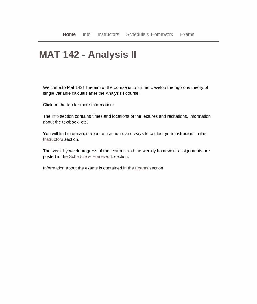
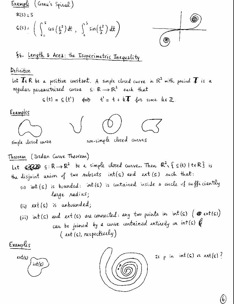
Tkegfevn (Pfoper-Kes of fke distance)

¥ u, Y, w t R'* we Kave :

CO d U > Y ) = ol (Y> l i )

C i ) d ( ! i , Y ) = : 0 I f f u = Y

(iU) J l ( u , w ) ^ d [ u , v ) . f d ( Y , W )

Da-flnltvorigr

l%i2j^fiigîe_j^Ml2i(feje TKe set of conv.p(eK nicmbers C is R^ endowed,

Wb+k vector sem ( e, t>)"f- ( c , d ) = ( d + c , b+d.) and -Hve prodicct

(< , b) C c , c | ) . ( o - c - b d , e d + b c ) .

To connect "Hds ip -(ke stu^d^d complex txoiaAion Z = a - l - b l we nêd

-tkiree observatCohS :

(i) ever vector (O-jb) In (R can be wr'tên as

3 e ( k o ) 4- b ( o . l )

Ct) Iko) is tke mttifipUeative identlfvj in C- 0>o) ( i t .b)^ (e^b)

V C e j b j ^ C . atixse of notat ion we tkevx w r l t ^ UC,o}

( i i i ) t o , l ) ( ( ? ; i ) - - U 0^*1 we Set 1 = ( ® / 0

T k t o r e m

C is an a l ^ e b f a over

of vec to r a d d c t i o o , t^^Sf^^ S c a l a r m e - t - t i p t i c a t l o h b a r e a l n u m b e r a n d

product i ^ e t ^ ^ f i ^ s a t t s t ^

(i) ( u + X ) w = Y w 4- V w

Ci) U CY+ W ) = U Y -k Y W

OiO k ( w Y ) 3 ( k u ) Y ^ = « f k v )

¥ YAJ ^W C J C end k € R

^ 3 . Volar coordinates

\9 Hfccall•• ^dar -form of a (implex hw^mber "2 = t e 5 •

ToUf coofdinates : (' X = IC0S ^ L ^ = !isln9

^3.1 Area In potar coordinates

U t f 1 (>,bj > R k a fitnctLon SVLCL iki-i

. 0 < b- CL Y a r

Tke polar e^o.atu>n = ^ ) , H c fe^ b

plane in polar cocjfoliinates • 6».b

describes a carve in. t k

Examples

t i l) fLx

(UL) (spiral of Arckimedes) ft- ^

^iven a poUr

rad ia l set

education rc= | ( f ) j V c k j consider tke

R of -f over C^yb].

Tkeontm

m m ^ ^ ^ H Y 4 . 3 r 4 ( e f . > J rte^ R „ « . a . ^ r 4 ( e

Ltt s> i ie two stiif -fanctions Sttcl t ka t

oY m < | ( f) ^ i ( ^ ) ^

u t S and T k t k r a d i a l sets of s i , respecti ve(y, ever | » J .

Siftce I ^ t we kave 5 c R c T and tke^'efore b m<?notone

propectij^ of area <tCSj^ £L(R) ^ a.tt).

Now abserve t U t t U area cf a clrcttUr sector

J-^. is I fio (4--^,)

(acos0, nSmd)^liCl o^H^ 7

y p

We a;r)cUde tbat *(S) = I [ s ' l f j d^ a.d a ( l - ) = i r i Y ^ ^ d ^ (wk^?) 2. 2. e

W e e : / b .V ^ n

Since f is i n f e ^ r a t f e j n i * « . i r b l - t r a r ^ step C n d x o n s w i th

©

H . m TUHl CVfLVtS

1 1 . Vumdr'iZtA ciervcs

A paramekdzed (plane) otrve is a vector-valued kittnckvon

Lat 0 4 3 - 4 . 1 R U 0, âncdon s i . {(•t)ô and b - ^ ^

TKen cL-b)- (-{(4)costy | ( t ) s m t ) is a pun.«.md:dza4ton 4 tke curve 7 e s o r i U d

kj i k e ôUftp icîia^Hcif) t = - | ( ^ ) . Bc[<7jk].

Remark : Tke i cs t i nc t i on between -3. paraMetrized cu.rve and i ts "UaceJ' s.kou.i<L be

e d a i ' i c(t}= (cos (ei), s in (It)) , t r [ ^ . ^ J kus ike s<t^<^ trance is

d l i ) . (cosg:), s i n ® ) ) , t c C ^ l t r ] and

e t t ) r [cosHlsinLb)) , t ^ O ' . b ^ ]

(^jven two p a r a m e W d curve? C 0 4 ] R Y d : f l i ] - ^ / R " " and a A n c t i o n

c : O i ] — ^ IR we d e R n e

C + d : 0>- l ^ -l? ' ^3 ( c + d ) i ) = Cji)^ d ( t ) vect(n. oddcton) ^ ^ • 0 4 ] >|R^ k;j O c ) (i)^ d ( i ) c ( i ) (u44n^ 4<îW >iui!tL(^l^^

Let c = ( u , v ) ^ 4 g £ i ^ , 4 ^ ^ U a p a w a M ^ t n s e ^ CurviZ.. T t e n i k e r y m k l ?

i i m c ( t ) and c i t ) m e a n

I t m C ( t ) 3 i i m ic4j f i m vl-Dî

£ Y - t ) = ( u i t ) , v i t ) )

"^«ure is a di-UjiXad iûiM^vd dtkncixQn of t t m i ^ ?ee ^(12^ ÎA/1

(?ne could also d e W : ^ cjt.k) - c ( i ) , , , , 4 ^ to L . )

A ôn e^tdvuCeî d£|tKci(i>i. y

<l) ( Y + i ) Y ^'î'

(ii) (dc)*3 i ' c +

iiii) S^V.înt a Wcklon c - d : [ I j b ] — > R b^ (e*i)Ck). £ (+)* i ( - f )

T W ( c # d ) ' 0 ) = c\b)0dii) 4- £ 0 ) * d Y k ) . prove to kr/nicta^

D4irvi4ion

A parametrUed curve c : 0 4 ] —? IR is re^tdar a ! io^fa-jb] i ^ c ^ i ) r x i s t f

a J c4 ' fco )?b0 .

c is Uvular at 4 we deflrvc kKe tangent (ine ef c a-t £ (ib) a.S'

to set of palnfs of -Hve, f k m c Ct,)-l- S cî , )

tlemark

r ^ i v | ( ^ '= i>^ i '" - P ^ . . n ^ 6 - : W h - r - - « - t ^ ^ * - < '

Note kow one cannot define d k t o j e n t Lne U to oryin 0 .

Definition

U i £: 0 4 J — k a para Metn zed curve^ .Jnd p: O ^ f J — ^ 0 . > ^ J ^

fuflcioKi. Tke parawetrized curve Cop : 0>?J—> defined, kj

( c o p ) ( t ) - £ ( f l f ) ) called ^ repara<Yietrlza,tion of c .

Lemma (ckaln Rule)

fe4)Vt) iOo e x i s t s a.nd ( c o p ) Y t ) = fVf) £ f f f t } )

c W = ( a ( i ) , v ( t j ) C£op)4U l^Lftp)^ v(i

(c.p)4t)= (Ctclfyw, Oop)Yt)) . ( .Y f i i ) )p to , ^Vfi iV®) 8,

^ 2 . L e n j t h

U t 0 4 ] > U a /Uî4ua ÂJVOMJiiAJLlAJt CUA.Vt,

U t ? = f t * , — ^ t n } U e puvtit ioa o| O ' U .

n

Lemm3

10 I | c pwtojwetnXus 3- straLgft segment t W i (Ê,f )= ||cCk)_£(Oll

for m r ^ par-tition ?.

(li) I | c (Lcs not prametrize a strdgkf segment t k m t U r e exist? a paHxUon

P . { ( i 4 . 4 i ^^t. i ( c , ? ) > ||c(b). c(e) l l

Ci) c t t ) 3 c(a)4- t i Y (£Cb)-£Ce))

1=3 U ( i ) _ c II I t i - t i - I I U O U k i I

^ l ( c l t c ) - c t U J l l ^ I t i t y ^ i M . i . fc-i,..) = |U4 ) -C le ) | | 1 = 1

Cii) S 4 c e to trace c is not contained m a (iney 3 fi^ 1 , 4

c O j _ c ( e ) is hot paraCtel U £ ( t ) _ c O). Tkevv to Triangle IneguaUtg

is s t r i c t : ( I c t b ) . cca)|| < l l c ( t . ) - cce)(| 4 ( i c a ) - c ( - t . ) l | ^

Rtmark. P t o (ii) s'oys tkot a Atiai^kt 4lne <t <^ is to sLodtMt cxiAVt Utw£tA

two po'ufits.

I t tt£s^ so^s t k o t t ( e , p j is Ucaeatog i | we ae^^ne to ^M£,ixo»i.

Tke togtlv of to curve C is i 4 ) - aw-f ^ [ c ^ ô\f'\.djl<i tixtS huMloxx. .exUt?, In tos case we 4 a l £ is adxVMt.

We to {lU Jim a. {oi^Jiou lox. A(c)^d Aad ÛM. <V Cijrvtiauous.

Tkeomm (TheoreiM 3.1^ In j A ] )

IS

U t 0 4 ] - 4 R U u Contthuous - T u n c t o n . Tken | is k t e g r a U e on 0 4 J .

^Lven u poA t i t on ? ^ { t , = a . , t , y - - t n = b ] o| O y b ] Consl t to to step ^ u n c l i m S

S tutd S d e f W us | o | ^

S U ) = ft.,,til Sm^K « ft-., t i l

t e | U ^ i S b l i l ? ) ^ f S t t ) c { i , i : W i ( t i - t i - , )

r U f t ) = jU(t)4£-- t M i f t j - t . , )

R i -co f i -Hvot e v M e ^ coniLHuû.5 Wvidiovi on fuyfc] is aneôrmtg o?n,tinw.oti5

(TUoremi 3.13 Im CA ] ) ; V £ > 0 3 S>c; s.t. t ^ ^ ^ ^ ^ ^ ^ j a ^ ^

f i x 4>o imd oUose to- partlfwrv P so t k o t k - t t - , < S V t = i,„^n

T U n H i - m , < e and tKe^'eforx

I (1ft) - I (1ft) < £ t ( t . - t i . . i = c -*-) -How, 'v| X ( | ) and 1 ( 1 ) uru t U Uwer a l ^ i upper i r v teg ra l s o f ^ we f u v e

I Uft) ^ Id)* Id) ^Ttlfft) ^"^" '^ 1 ( 1 ) - T ( 4 ) ^ I ( l , P ) - I ( i ; ? ) < ( L . t ) £ .

Sintt £ (J a- r l l t ra - r^ w* csncWe t t i - t 1 ( ^ ) ^ 1 ( 1 ) ,

Ut c : O t , k ] ^ R ^ U «. ^ ^ a ^ p m i m e - t a z e d curve wttiv U : 043—7»/R^

conHnaoics. Tkun £ is nec+v^CuWe and

4 ( 4 ) = P l l c ' W l l o t t

Wrvile c ( i ) = (ttW, v(t)) -ia ^ |uivc£mS ^ V r O i ^ — A R w4iu cotout fuS dertV4liv/-eC,

Mote -HLCI: ||c4-t)|| - I [u'C+)J% [ V ® ) ] ^ ' < '3i>h.wx>i>L£ OncfvoK on 0 4 J .

Uef\e|oTe (lc7-t)dt(l exists. Houova, |w>vu to ptoc ^ to ptvUuC toerm

r 1" 3 54,,

^ X ( «c^«f t ) - I ( « ^ ^ « T ) < 6. (*)

Now conslJi/v | | c ( C ) _ c ( t i . , ) ( ) . Me«A Va.(..ii!. T U o r ^ M a f f C e i i W

f — — • ^ — — I

£ ( t i ) - c ( Z ) i = J [ i t ( C ) - u f t . , ) j 4 [ v t t i ) - v f t - , ) r

C l w r n : V £ > 0 , 3 S j > 0 s t . l l | t i - - t ; . | l < S i "fkiJa

(«*)

c t e 1 - c { t u ) I Cftt)|| ft-t;.,)

•V ^ 0 , 3 >o s . t

ft-rW<i. V x , j 4 ftaftj w l l L ( x - j I c S p

0

3 Wyo 4 I t i - t , , / < g ton

y O ) ] Y [d(g) ]^ < ld(x)+a7^) | l uVx i -uY^ )

< l\^ iu|x),ttYy)

^ 2M . j £ L = 1 V x, je

g -for Vl

Hence ' em\' - [ * "« ) ]y [ v r n j

a n d we conclodiZ "fk<et

[ U ' ( ^ ; ) O K J ] ' " - / [¥(P)]Y Cv i t ) ] '

Usin ^ 3^ oUUus eslLmrfle t i - t z , <: L (t 3k CUm ft (vto\4ed

U^2^2J^i@^2)!^^ Now ^ iX E > If OJid u poAdllio^c P wttiv

< x . v i 4 S „ S i l 'So ft4

'TWv ( 4 4 4 ) toplce? tooct

1 ( 4 ? ) - t ^ i ( c , ? ) « ( C ^ 1 ( ' f f t ) + e

Hence _ pk —

\ and torefcre K c ) ixUds and syks^tQ

Since £>o iS arklxajTtj to T k i o r ^ is ^fQ[jzJi,

(0

^'i'^^ OT.Ueorm A sd^M^ Ji-ffjueA proof

fx ample

c(t)= ( {it) cost, > t c 0 4 l wt4iv contou-ouf.

U t C:Ca-U] _ ^ r be u / u g u , ^ ponoUnetuW Cunue Witk continuous c\

Tx t e O f ] . Tke arc UngtR ^ c W t is

k * i w t Let i , be ôlds in 0 , b ] . Demote bg £j^.^^^ to QCAVZ

' to

Definition

Wi Sug fkJt C: O f ] iS puront eWed kg one A n g l L l |

s l t ) = t - to |ox £ome t ^ C^>b3.

C : [ ( i4 ]—ÎR^ '.s pxra-vnedncsed^ kg are togto \ l!cYt)|| H i .

Bg to Fundamental Tkeorem ct CatcultcS,

s ( t ) . t - i ^^soMtUM ^ sYtU I Ilc4-t)|( = i V l z f e f ] V ieO;y (

Everg fugular jaraiinatrris'ed outve w/to a?n-tu\uoui' <kx'i\i3Jlx\jiL£t c<^ ke

ÛjxoJiAjdAisiA dy a a J&jm^tk.

(0

Problem sheet 1 MAT 142, Spring 2017

1. Prove the parallelogram law and the polarization identity: for every pair of vectorsu,v ∈ R2 we have

∥u+ v∥2 + ∥u− v∥2 = 2∥u∥2 + 2∥v2, ∥u+ v∥2 − ∥u− v∥2 = 4u · v,

2. For a vector u = (u1, u2) ∈ R2 define

∥u∥1 = |u1|+ |u2|, ∥u∥∞ = maxi=1,2

|ui|.

Determine whether ∥ · ∥1 and ∥ · ∥∞ satisfy each of the following properties:

(a). Positivity: ∥u∥ ≥ 0 for all u ∈ R2 and ∥u∥ = 0 if and only if u = 0;

(b). Homogeneity: ∥cu∥ = |c| ∥u∥.

(c). Triangle Inequality: ∥u+ v∥ ≤ ∥u∥+ ∥v∥ for all u,v ∈ R2.

Draw the sets of points in the plane with ∥u∥1 ≤ 1 and ∥u∥∞ ≤ 1 respectively.

3. (Exercises 1 and 3 in Chapter 4, Appendix 1 of [S])Given a point v in R2 let Rθ(v) be the point obtained by rotating v through an angle θ

in anticlockwise direction around the origin.

(a). Show thatRθ(1, 0) = (cos θ, sin θ), Rθ(0, 1) = (− sin θ, cos θ).

(b). It should be clear that

Rθ(u+ v) = Rθ(u) +Rθ(v), Rθ(cv) = cRθ(v)

for every u,v ∈ R2 and c ∈ R. Deduce the formula

Rθ(x, y) = (x cos θ − y sin θ, x sin θ + y cos θ).

(c). Show thatRθ(u) ·Rθ(v) = u · v

for every u,v ∈ R2.

(d). Let e be the vector e = (1, 0) and w = Rθ(e) = (cos θ, sin θ). Observe that ∥e∥ = 1,∥w∥ = 1 and e ·w = cos θ. Deduce that for every u,v ∈ R2 we have

u · v = ∥u∥ ∥v∥ cos θ,

where θ is the angle between u and v.

4. Let u = (u1, u2) and v = (v1, v2) be two vectors and define

u× v = u1v2 − u2v1.

(a). How does × behaves with respect to the operations of addition and scalar multiplica-tion? What happens if one interchanges the order of u and v?

(b). Show that Rθ(u)×Rθ(v) = u× v.

(c). Argue in a similar way as in Problem 2 to show that

u× v = ∥u∥ ∥v∥ sin θ,

where θ is the angle between u and v.

(d). Deduce that |u× v| is the area of the parallelogram with vertices 0,u,v and u+ v.

5. Let (r1, θ1) and (r2, θ2) be the polar coordinates of two points in the plane. Show thatthe distance d between the two points is given by

d2 = r21 + r22 − 2r1r2 cos (θ1 − θ2).

6. The cardiod is the curve with polar equation r = 1− sin θ, θ ∈ [0, 2π).

(a). Sketch the graph of the cardiod.

(b). Show that it can be described by the equation

(x2 + y2 + y)2 = x2 + y2.

(Take some care in motivating your choice of sign when taking square roots!)

(c). Calculate the area of the region enclosed by the cardiod.

7. Find a parametrized curve that runs clockwise twice around the unit circle centered atthe origin.

8. (Parametrization of an interval; exercise 2 in Chapter 4 of [S])There is a very useful way of describing the points of the closed interval [a, b] (where we

assume, as usual, that a < b).

(a). First consider the interval [0, b], for b > 0. Prove that if x ∈ [0, b], then x = tb for somet with 0 ≤ t ≤ 1. What is the significance of the number t? What is the mid-point ofthe interval [0, b]?

(b). Now prove that if x ∈ [a, b], then x = (1 − t)a + tb for some t with 0 ≤ t ≤ 1. (Hint:

This expression can also be written as a+ t(b− a).) What is the midpoint of the interval[a, b]? What is the point 1/3 of the way from a to b?

2

(c). Prove, conversely, that if 0 ≤ t ≤ 1, then (1− t)a+ tb is in [a, b].

(d). Prove that the points of the open interval (a, b) are those of the form (1− t)a+ tb for0 < t < 1.

9. Let f(t) be the function

f(t) =

{t2 if t ≥ 0−t2 if t ≤ 0.

Let c(t) be the parametrised curve c(t) = (f(t), t2).

(a). Show that f is differentiable.

(b). Calculate c′(t).

(c). Show that the trace of c is the same of the trace of the parametrized curve s 7→ (s, |s|).

(This problem shows why it makes sense to insist that c′(t) = 0 in the definition of a regular

parametrized curve.)

10. We say that a parametrized curve c : [a, b] → R2 has a weak tangent at t if the unit

vector c(t+h)−c(t)∥c(t+h)−c(t)∥ has a limit when h → 0. Prove that the cuspidal cubic c(t) = (t3, t2),

t ∈ R, has a weak tangent at the origin but it is not regular there. Make a sketch.

11. Consider a curve given by the polar equation r = f(θ), θ ∈ [a, b]. We can parametrizethe curve by

c(t) = (f(t) cos t, f(t) sin t) , t ∈ [a, b].

(a). Find a formula for the slope of the tangent line of the curve at the point with polarcoordinates (f(t), t).

(b). Calculate the slope of the tangent lines to the spiral of Archimedes r = θ, θ ≥ 0, atthe point with θ = π

4. Make a sketch of the spiral and the tangent line.

12. There are two natural ways of defining limits of vector-valued functions. Let c0 =(x0, y0) be a point in R2 and c(t) = (x(t), y(t)) be a vector-valued function c : [a, b] → R2.

• Definition 1.

We say that limt→t0 c(t) = c0 if limt→t0 x(t) = x0 and limt→t0 y(t) = y0.

• Definition 2.

We say that limt→t0 c(t) = c0 if for every ε > 0 there exists δ > 0 such that

∥c(t)− c0∥ < ε

whenever |t− t0| < δ.

Prove that the two definitions are equivalent.

3

H . ?LANE CuflUCS

Curvatutrc

"to c is k a*af vado-L r (i) c'[i] ^ V - t x ( » ] .

lleUi)ll

W l i ^ -Hvd c : f a ^ ] ( R ' IS f o n ^ t k W ^ c - f k ^ 3 L s e R H .

T W (icMt)lUl anl -IWf-i^ r(§J= d ( s ) .

kSSmm iked: ^Li) xxisfs. TUvv

Pa-fi"al4ion ^ un' fMj?-

(") il(3)» r d ) = 0

(ni) Id) X iid) > 0

] W k : I | C:RbJ_^(R^ k j imd ruxinai n oni flS t] —^ C^dJ ,= s k ^ ^ ^

1? = (thh-i J ikiL f k uiuf noa-U'ud ej' Ci>p "(S -n .

im-&Myik and assu-me t M : t' exists. Bj L m m i l s X ) ^ ri(

^ e. (5

Id c .— (R k A. ALj JlaA. ^^iltoMxt'\^^t(l uuxyVt^ not nuiA^OsvUty

o| £ AdJtw[dLA:

i X £" I

^5 iicMi db

ilcjll ^ ^ - -tied 06 ii c\v 1 WCW

How, J_.((|cMl ) c L\[X?\\x c • c

li ci W

a? ii c> I-

5cS il £Mi

i\

H'fWcXD'sm'O

3 3c - ^ - 1k(ULk to cu;-L oL,c£ of ofoudiovL k .

5iii££^ «k {u U[^d]

s^M M urn RbM k t k xak .s o| tU o a c l ^^.l.^ iCjk ^ f.as ,(3)^ c ( tR )^ c ( t d ) . T U . 4 k osckoivK. W k . o4 e

R(i)= itm R(3d).

Sv i osc t u t R(t) b' ti dix(d. I R m R(4) = - 1 — .

<L tUtUvJj^ -

W . wse t k s | o x m u ^ - io cJicJlai^ R ( f ^ ) : 3 k 4Axa> y ^ o a ^

c ( t d ) - 2(4 ii i 2(4- e ( 3 d ) j M U ( t + M - 2(4-3) fj

2 "e(t+3)-£(4r X ' e(3+3)t c (44)- 2e(4]]

©

SltNl+ert-hl g^^ Hani nsd -fk |a-cf -Hruxf fk o/tiaL

a| -fk i/aA>ojA wi'-k ve ivcM 2 c (k3f c (3-3)

eitf3)-ca) % 2(4-3)>cdJ

iS 1 X 2

e (43) - c Ci) c Ml c(i) 4- c (4-/,j - c ( 4

Now,

t<-?0 1 ^ e ( i l - c a d ) ^ c ^ i )

c ( k k ) - c ( i - H ^ ^ c d 4 j i M i l ^ ^ i l l ^ i i i ^ = 2 7 4 }

(|oi. jixounpfii, vUL can uSu 4'-HoSpiM fJljL .ciciu Co^nfciioic ^ d l o M ;

Pt|imbon

to 3k ihaj/utodiok\g Vr(<i>.)^R^ (V

TH) 4 k tvotcdii n o| 0- c IR 11

|o2 Some 0 2 C H b ) ^ R ^

rjdi

tbU %cM) c74 ) c R , d d )

p* fd f=> - V 11 d) il k . y Ii Re 2 (4 li k = ( (i c\a) lUi^ . 5

•tc

5^[ik 244x c'U) ^ Re eft) X cdi) ^ cMi)xcd4) _ ^^^j

112'(4 IP |lRee4i)f l(eU4)lP

Since ReU. ReV: = u«.v oxf ^%tixRpV/= Uxv;.

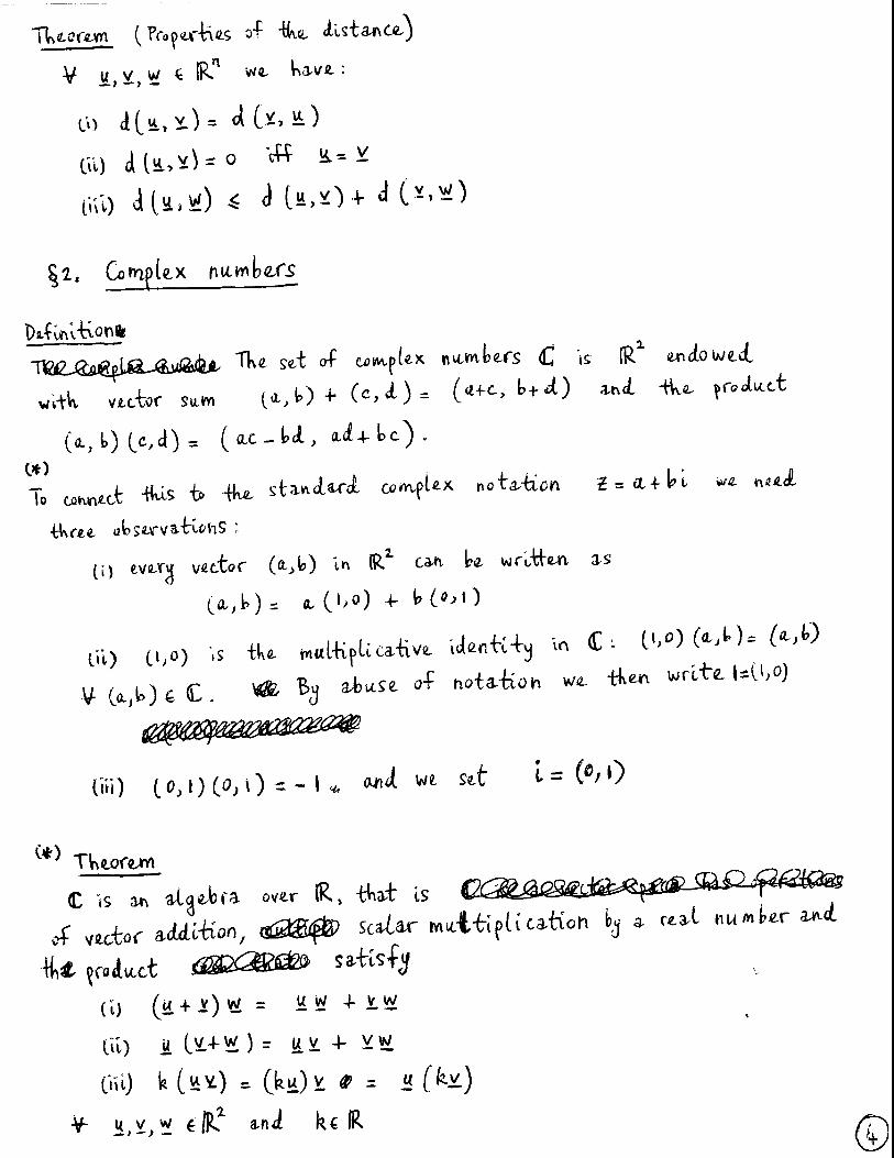
Tkeofa M ( "miaMimtal "Ueore n of -fk bed Tkeorg of Plm^ Corves)

CMAvt c : [itd] —^(R^ podXTUAdkied bj ttdic-ian fk 5«.civ 3 W f dc(fj is ds

cuAVoiuAjL. Ko-utovM/, t| c -atotku^ Auck. cuAve 3 k n 2 j - X f e{s)) -VrejAdl

ox Some /tt i/ Jaoflovi T!

c (s) r ( COS 0(s), Sin (s)) K Some ^oncfiox 0: M —> R

0\s)= 4c(s)

' f Go E Ct) ft 4- , J %m€tt) Ak 4 k ) V W * ( v . , k k ^ ^ 2CS) =

ft|{xAjLtAt ctto'lces s|

fit iug i i /iM.o'Hon,

2(s). ' [d.(pit, fH'pX V V 0 0 /

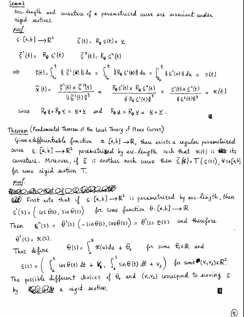
Ut Xc R U poSitivL ajAstant. A Si»npit dosd corvt iv petLocL iS at ft doTV patua^aik^id oive C; (R— {pd ^^cR -Hvd

Clt) = ciX) ^ 4 = i+ b T 4ox some

?(*«pk clcSti UAAVt

Tkmrgm [loXiiajn Cortve Tke-oPem)

Ut ^303^ c:(R—4lR^ 4 simp4 ciosef Oanve.. Tke+v IR \ 2 (4) | tc IR] is

4k flsjomt oKxoa o| two AJOSXS cAt(c) oni Tuct (c) .jacL -Htoi::

lU -udCc) IS kuAaeol: '^f^) 13 conta uief mslje a. cncft salfvo-ent^y

Ciii) lKt(2) eivi xx4(c) atveaa/aefei: oaj Uo oiiM 4v ktCc) [ 0 ixtU)) COMy be jolnef bj A otAl/e tonfatin^ JUtftAiiy i-a mf (c) ^

( xxt (c), .atspecilvdy)

Is p In "mt(c) n xxt(c] ?

Pe|ia(.4loA

Lt £:(R-9lR' U a. Simple cfiosei cunve witic pentoi T ojuL adinitcats T k Anitk i C O =i 2 is

ir2]= rit^^(t)iui

Li c: R-^l^' U e s anpic ciosei onve wc-k ôJi J W omitntcottr d If c \ pa/\a>ce.tbW b<| odic Anj-Ht i k n T - JE^C)

i(2)= U2U)iUs - ^ Js T

ut c:jR_ IR^ U 0, s.npA ciosxo/ OAAVIL . We Saty t U i c (S pistilvjtiy

(njuiaijif i| 4viL U>ui >uJuacuL rl (4) poi>kuU udo itvtCs) \t t(.k.

• GempOAt X(c) wv-Bv ik OJiXO. 4 Ut(c) Isopmimdric Problem: wbtcR msSi2iS$> simpU dosei Otnve AnîL -6 bauid-f

4Ujt ô-oi onto.?

Uoait U t c: (R- -lR" k A. AXAJ^ JooSid OOAML. A/Kuui.a-fUi -f(c) anf

(Jlfiatfc)) j id. iod T:tRU_^(R^ be x /Ll d >I^>UJYL. aid oyvtSiiet t k

Ctuvve c'C-fc]-T(caO. " k n 2 IS OL iMpA chseA CMAMIL

<U ICDziW), a.(.at(c)) , c3.(^miCc)).

Work. TUs sjLy/J tUti w^ a m xw ove onves oiUJiad bj Myî jmyjions i? in 3U -iiuosi Goiivvmimi position, f i exittxpit we a m ai2wou)5 dSStonL l U i •

ir) 0 3'iat(c): "'1 v= C'l' b) 3 mtCO ccaSt<feo "Ik otAVe

til) £= C(a) ; OrakleA/ i k OxAJ/t 2 - 2 (4

Ut c U A Akcp4 do^l o^ve w C k CevcWcoits c\n

d ( Inter)) ^ J_ iCc)""

Houovjet XjUAiit-b| Utots ;|fl c is it O/tdji.

De|iaitioi>i

A simjA c^sef coju/e c ij convex i| t k xtAoc^kt icAt At^mjurd: d"^^

!>Mxj two ôink in "(nt(c) - 4. WX/uA/ umfokuct m iHCc)

coavtx

Remark •l^^Jî|_^|i2iQjaî(SuSi^^ kf.-u(re%, U o w m ^ t U l s o p e W t w c iKnôcollty fn cmvxx C U A V X ^ J

•k XSopeAX^miUu: rv>JLo|u.aiAkj cuAvr:

kfincKon Ud C:1R ->(R' U 1 c « H M X s . « . | 4 cdcsid cuAVi. Fox «.vxtjj paA*ltv.,->u

W e t U m sd tL(irat2]c ^ ( i d c ^ ? ) m J Sey -fkd mtc is

kmuk: TUs Is s-Agivit^ ckoiinj, we rkoiAiol i>(t|dct o/iut Mxkc| I A S U C W . a,

©

Z\imm [(^/mi's VcnMvdd ^ Aam)

Ut c(t). ix(t),g(4)) lot d fo5itudy-oxcmW siitap4 Jlx)Std ottve dtt ^ o l T

OKA cmtumoits d. HvMt intCr) is in£/ts uyut-Pe a>d

m.

Fiasi fvoU Ikot > k U j U E d J - ^ R a \ ocdUutouj? 4u^Lhcy^ ml "kie crui •

- |xM3)-xMs)(<e

, lijl4)-aMs)| <£

In pjdlOuJbOud d 4Mx)VJh AUot X j U j X ^ is ccpxfuKtLOicr <fvt E,Tj m f -kixJL^ru

iS^'^k'g^^ JUt jX.sk. Koie-ovM., Ityo^SSyo /tk. i|

po-i!y JOaciil CAjovve wdk vutiGeS c [t,), c [t,), . -., 2 [U)c 2 (t.)

,( .) U t a(i^,P) ^ ^ t e iki ojx^d 4 ^

aegiow koitnaei % 3ks p^^aofi cuA.i/e.

Tkea £L(*htc)= sof (L(id2,4)

U k . l

>tL|>

Obs iAVSL Uoct 0. (mt c R) _ U_

3 ^ ( a d 7 7 ^ ) x > (cid4u.)T > 3 - ( a x ^ / ^ ) i

' ^rw '^^'i ^ ± '[''s''s]^r^ >r''4-'T) ' 4'"' d "^MUT^ ^ ^^''^'^ '^'^

wx-fmxl W + |r^].x)|C4}U(?#|+j(4xuf^).Rl KDxit (r4x^|c4)x-P4]^

> /[Wd'04vxJ(4)^ - C^Xx [(flUft}Bj - [(9X^(^^)dJ(4}x (d)v^ [(4]X-(T}x'

: W d - W,K(4)x] - [(7) X (Ml U(^-^s^ ('4)x

T 3 L i*.* Kir ^/O '•

'^"^ T-L GJ M^ yU^.^'x 1 /i^niiyMri^ '>rio|inw j\rv s^upT^-vmoy -35-n

^9. ^ 3 > [(4}d(>}R - W7d)xJ - [(-5)^ (M)U(^4iU4)x

> ^ ^^'8 E u><3 A

d u

T k w m (WlrKa^er's IhejualiPj)

Lilt F: Ed ]—yR U <L uj-vcikv wttL coJtinM,C{ji^ dib^vdJbivJL ikat

0 TV O HouoveL, egwajU-bj irverfis a>d od^ i| F(4) = A s m ^ ^ ^ j A ^ R .

Aow, F ' z &1in(s-t) + I G W c c i ( x d ) .

f (_F.)'«tt r(G ' ) C , C r i + ) - 2jr G G ' s m ( x F j a . s k F ) t2? G b = ( i

Now,

21 P GG^ si«( t) c.s(ii)di . X Gli«(iFj».(iF) T 0

jt f t

TUit|trce.-

ii^ ^•^cMsd4F)-^^'44i]^

r ( T M ^

JUt

>y Jl , T -2 • .

G sin j d F'it Vd' -4 cA-,0

TUoreufi (isopKU-imeirnc rne niCt-iy Ur bnvex Gu'vei) id C : | R - ^ r be 0. sifVLp4 c2csei ccwvjix O L A V X witk peaxol T a^d

03duuiOu.s c\a

^(mtc) i- £C2)^

a>ii jiuxii-tij Itveds i|| c is d dxcMjL.

I -tf-

W£oj we ctUL a.ssiti«Ae -Hud c is paAa-WtetdsXol bj dAcJUv^ik^ p^lix^tlj cbcMXiiJ.

(Ud SoilS^XS £ ( o ) c £ .2 C (T ) . ( k a i L H U i i ( : c ) ^-^CT. C is piutiuvu.

by JULC jUlvg k .

We aSe paUu cooxctattixs XcttcosB , J B as inO, ^

Notofion • ]) _ il y

We co lcutd ie :

2 ' -2 * ' 2 A y - l L + a t f Xy-.XJ/= fl X7

Wt aaJiX U vise a. "UXcb-:

-r r:r H f il£) - (tl'dfe)) ^ d

TT^ -rr 0 it

^ 0 bj W u t i w j W s Taeg^ci lc4/.

poiaovi/u 1 = 0 u

r

^ c

(D


1. Let c(t) = (e−t cos t, e−t sin t), t ∈ [0,∞).

(a). Prove that limt→∞ c(t) = 0. Draw a sketch of the trace of c.

(b). Prove that limt→∞∫ t

0‖c′(τ)‖ dτ exists and justify the claim that c has finite length

over [0,∞).

In the following problems 2–5, c = (u, v) : [a, b] → R2 is a regular parametrized curvewith continuous derivative c′.

2. For every [t1, t2] ⊂ [a, b] define∫ t2

t1

c(t) dt =

(∫ t2

t1

u(t) dt,

∫ t2

t1

v(t) dt

)∈ R2.

Prove the Fundamental Theorem of Calculus for this notion of integral, i.e. prove that

c(t2)− c(t1) =

∫ t2

t1

c′(t) dt.

3. You are going to prove that the straight line between c(a) and c(b) is shorter than c.

(a). Prove that for every x ∈ R2 we have

(c(b)− c(a)

)· x ≤ ‖x‖

∫ b

a

‖c′(t)‖ dt.

(b). Take x = c(b)− c(a) and deduce that ‖c(b)− c(a)‖ ≤ `(c). When does equality hold?

4. Define a vector x = (x1, x2) ∈ R2 by

x1 =

∫ t2

t1

u(t) dt, x2 =

∫ t2

t1

v(t) dt.

Note that we can write

‖x‖2 = x1

∫ t2

t1

u(t) dt+ x2

∫ t2

t1

v(t) dt =

∫ t2

t1

(x1u(t) + x2v(t)

)dt.

Prove that ‖x‖2 ≤ ‖x‖∫ t2t1‖c(t)‖ dt. Deduce that∥∥∥∥∫ t2

t1

c(t) dt

∥∥∥∥ ≤ ∫ t2

t1

‖c(t)‖ dt.

5. Prove the Mean Value Inequality: there exists t ∈ [t1, t2] such that

‖c(t2)− c(t1)‖ ≤ ‖c′(t)‖(t2 − t1).

6. This is an example of a non-rectifiable curve. Define c : [0, 1]→ R2 by

c(t) =(

1, t sin(πt

))if t > 0 and c(0) = 0.

(a). Show that c is continuous.

(b). Consider the arc cn of c over the interval 1n+1≤ t ≤ 1

n. Since c is regular with

continuous derivative away from t = 0, cn is rectifiable for every n ≥ 1. Use Problem5 to show that

`(cn) ≥ 4

2n+ 1.

(c). Consider the length of c over the interval 1N+1

≤ t ≤ 1 and deduce that c is notrectifiable.

7. The hyperbolic cosine and sine are the functions R→ R defined by

cosh t =et + e−t

2, sinh t =

et − e−t

2.

(a). Show that cosh2 t− sinh2 t = 1. Observe that cosh t > 0 for all t ∈ R.

(b). Show that the derivative of cosh t is sinh t and the derivative of sinh t is cosh t.

(c). The catenary is the curve c : R→ R2 defined by

c(t) = (t, cosh t).

Show that the curvature of the catenary is

κ(t) =1

cosh2 t.

2

MAT Wpi - AwALYsis IT : N/c-res 3 (WEEK p-G)

12. ^€6IUEKCES

L4 Aeoi fituniim")

"D4"ud-Kt?n A s^îoj'vc^'^s a. {u^cdion. (N >IR.

TKto few

(0.) [a^^] (iMU.o^JU to d i{ V t>o L L '\J4M.VA (<L-£,<Llt) (joirdouUAA M hd MAAJ^

y{afiUuj VOJIMJA- tin.

d) Tkt Mii 4 -Hl^Xi^Ct i4 ^ U p a x J a^z OL I Xitvi a,, r d ikjUt (L-oJ

(c) I | \ân] cotiviwx^ "Hvm [ t i n ] W ttôkikd-. 3 H;'o 4T. | a n l < h l / n c / H .

A MXjUJUice fa^^ IA

( i ) oQg? (AaCAXJUdvg 4 <:iu '^^ M

lu) kjjaJ3Jt^<^ '4 ^ tin+, V n-^/N

E v z p touMxdjLcl îtuivvxinyvuc .4pf(/x4/Lce. ccvtvxp.6i.

ASSUMJL fil-nl mMXxidp md 0t diX €L \et dn- Âz. LM d zx.\AtA

% J^v<4^W 4 ^ > ^ 3 N£l>l .JX. a,^> a-£.

0

D4dxlu3Vl C^vXM. cL .ûpJlÛL a . U d .puuaxcL { M ^ 4 r^^di^x m t ^ g M A

-xdm

Ev(Lxg boUAuClot .4tx|wXi4(X Ccvttadx^ d

rdd l<d i j ® I x ^ ] ^ U X b i W i i , 4piXXivcx. "TIonx -(Ux'tt xxixt id, < /jd.

\>AMXAJ^ ÔUp X ; iUid M I ^ r T,'(

•d(

di £ Xn^ « .

A , ^ a , $ ^ Xn, $ k ^ - - ^ k ^ k , & o^k'Ctk = A x

B i j piAJL covtvep-t>Aa 4 ALtoKo-kirdc AU|ixe>i.UA vx kotv^, Aifwlkk

iL^n dw 3 6L lim \?^z \ ) ,

A

,d X - oi = k

kqo«

I a n - am < ^ V H,vn>. M.

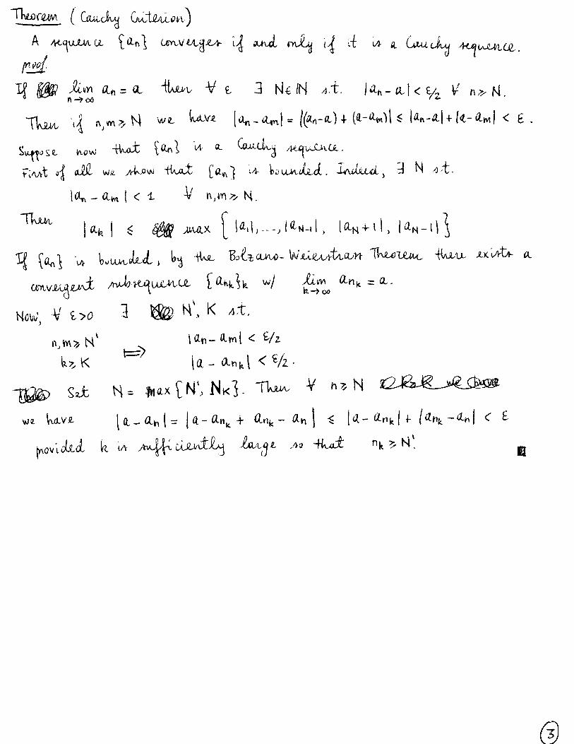
A AtguiAia [M u w v ^ l g ^ 4 m i ^ 4 3 iA it U u c i u ^ A p u m ^ e .

I W 4 Uvi? (a^,ci^l= ((dn-d)4 {a-a^)U |An-^| + [<t-a.m| < E .

flAAt 4 AXOW -ikdt [dn] 'A U a^LofjLd. Xruduij 3 N >)-t.

TkjuA . r

How, V i>0) ^ ^ H \ ^ t .

j d n - Ami < B/2

^ la - 0,^4 <

a - a n | = a-O-n^ + a o j , - a n I ^ | a - a n j 4 - a ^ l <r E

^X4kg4 [Ht-^toh, I64i)

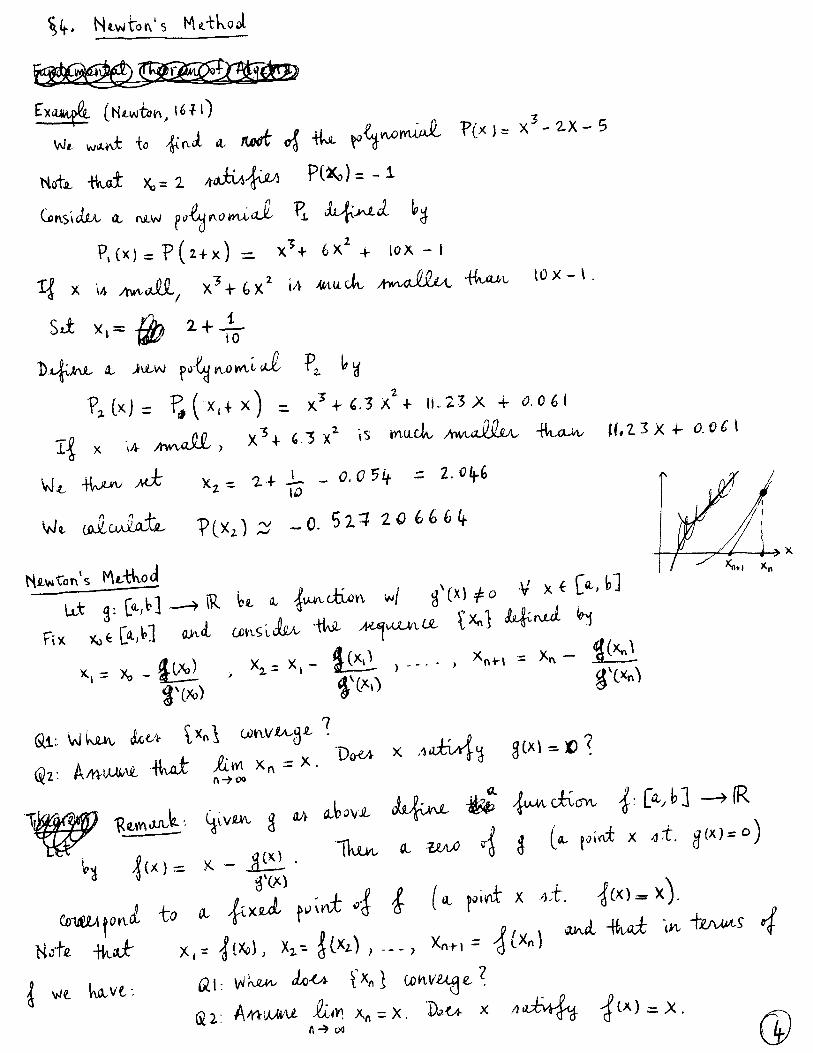
W*. w* E to XiU d rud 4 tU ^^^rniJi ?(;xj=r X ^ - 2 X - 5

Hoii tkat x,=:2 AdkUîJ^ P(i<o)=-l

P.(x)= ? ( 2 + x ) - 6X^ + iox - i

10

D4EV>JL OL pjYgru>^JoL£ P ^ kg

K k j = ^ i ( x , 4 x ) = X^46.3X^-(- |£23A + a 0 6 l

I | X lA Awodd ,

X, = 24 J - - a C? r 2.

Wt uAaJlAid ViX^) 2^ _ 0 . 5 l T 2 0 6 66(^.

HiiVNton's l^t-tkog}

X^4 6.3 1 ^dcL AmôMju. -LoLM. ti.lZ X 4- 0.0 6 \

Ut ^: k T

f i x X j t C ' ^ M O0^x<;[M HviL AÛJU/lUL f X n ] i ^ C r u i bg

x,= x , . i ( ^ . k - > - - • > - ^

gdx,) f(.M g'M

X)»i x„

1>M

0>mApU to a {ixU p{vd4 i ^ T ' ^ ^ i^^^-^)-

H o t . X . x f X o ) . X,. | t X 2 ) , . . . , Xn,,= 4(Xn) ^ ^ ^ ^ ^

koLVe-. 6il: VvWv dotA fx^} {jO^VU^d'^.

6^2. A A W U U icivi Xrt = x D^<A X AodvAu 4^y) :^x

\-- {\-M , M- Xn^., =: |(Xn).

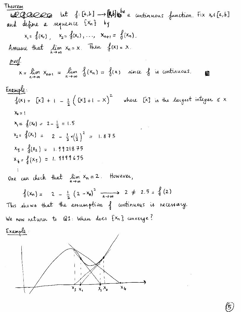
iJCX) z [x] f i - i (^Cx3 + I - X)""

Xo= I

M l^M ^ 2 - l ^ i ] ' :r ( . 8 7 5

^3- llM = I. 11216 t3

j(X5) = '• l^'^l'^^^

OK. con dkci 4 U t itm Xn = X . HoWfiyyix.,

ft->t<0

TklS AkoWA - H u x t tivJL O A V U A i A j d l o a I CokdClYAOtcS U hJLCJLMdd^.

W . n o w njbtuA^v to ( S i : Wk jAu dotA { ^ n l c o n v e p . ?

c<>0. aix )= x ' - o ( ^ > J j t x ) ^ X - l l ! l l ^

T x JO( CjOYxSldtd - L L IK^pyAJUAUL ^Xn] dL|Lyvj6ct k^

0) ?Y)v. tkflufc { x n ] u AJLOU^CMYK^ c<;Rd2tc(4i Y k a i

X 4

t i l ) S e t E n = Xn - 3 7 9X\A ALOVI 4^^JJct

< MK drL ^ M 2 X „ 2 i ?

-¥ n:*. f

(iiO ^ 3 X- XJ =1 2 -Heat J± < ± oML iMoL^

E^ < 4 iO''^ ^5< t-iO-^^

1 4 C X ) - 4 U l | ^ I X - j i V x , g 4 G t > ] .

U t ' I ' [ H ' W X [ H / C I d, ( ^ ^ f l t t d c i x d W .

OrMxcfjU.' 4kjL MMUA.UL {x^

n -»-oo

We Jjpjt'i Aov} -Huxt CXn} U (L GxAxzk^ AdoM^Ci. I a < W - j

h o t . t k o i - t

rvi-l

Km-^4-- d_ - X „ , J ^ I | C M - K J I Z - C 1 - C

i - C

Suet c < ( , JlX^c^o ojdl -MAJO^M- " ^ E X O

3 N 4.4 4 M - x J J - < £ V n . . M .

B.J HvjL Couu-ciuj Ouiritu.isn, ^ f X n j is conv /eAgJzAt . S i t X * =: ^JpL

How c k s M . V . t k o t lA O o a t t ^ L c o u X - :

Ve>o 4 i x p l < I wt U v . I | w - | c ^ ) | <M-3\ ^ . c = E

A M V , = A - t ^ l = ^ ( f 4 l ' < " ) = t ' ^ O n_^oo 0 - - ' = d I

I .e . X,t 15 d ^cxjt(L

H U t x ; IS m o ^ U t ^ X ^ f ^ i n t .

3 0 . ( 0,0 4 . 4 l 4 w U < c V x . U O .

I | ^ I? a. coWtdtctioiu t /OL iv 3 ce C ^ i ) / i t .

i ( x 4 K ) - ' | ( x ) ^ < i lk l wiA - i W l ^ n x

CojvVMAeig , i | U Y ^ ) N c -V ^ € ( a - A ) U v . V x,gACct,k]

4 x ) P ( ^ ) = ( x - j ) Y A o m . C s k ) . ^ 3CoL Pl.iUt W U .


1. Consider the ellipse x2

a2+ y2

b2= 1 and its parametrization

c(t) = (a cos t, b sin t), t ∈ [0, 2π].

(a). Calculate the curvature of the ellipse.

(b). Calculate the area of the region enclosed by the ellipse using Green’s Formula.

(c). Show that ∫ 2π

0

√a2 sin2 t+ b2 cos2 t dt ≥ 2π

√ab

and that equality holds if and only if a = b.

2. Let c be the parametrized curve

c(t) = ((1 + 2 cos t) cos t, (1 + cos t) sin t) .

Show that c(t+ 2π) = c(t) but c is not a simple closed curve. Draw a sketch.

3. Does there exist a simple closed curve 4 ft long and bounding an area of 2 ft2?

4. Consider the sequence {an} defined by

1

2,1

3,2

3,1

4,2

4,3

4,1

5,2

5,3

5,4

5, . . .

Find all numbers a ∈ R such that there exists a subsequence of {an} converging to a.

5. The Euler number γ is defined as

γ = limn→∞

(1 +

1

2+ · · ·+ 1

n− log n

).

Show that γ is well-defined. (Hint: show that the sequence an = 1 + 12 + · · · + 1

n − log n is

decreasing.)

6. Let {an} a bounded sequence. Define two new sequences {xn} and {yn} by

xn = inf{an, an+1, an+2, . . . }, yn = sup{an, an+1, an+2, . . . }.

(a). Prove that {xn} is decreasing and {yn} is increasing and deduce that both sequenceshave a limit. Set

limn→∞an = limn→∞

xn, limn→∞an = limn→∞

yn.

(b). Calculate limn→∞an when an = 1n.

(c). Prove thatlimn→∞an ≤ limn→∞an.

(d). Prove that {an} is convergent if and only if limn→∞an = limn→∞an and that in thiscase limn→∞ an = limn→∞an = limn→∞an.

7. Prove that every continuous function f : [a, b] → R is uniformly continuous using theBolzano–Weierstrass Theorem.

2

INAT 1^2 _ H O T E S

.fu(k(3:: i,^^C(GiA.Ij,=o | 3 4 C ( : m ) , W W (4|)^x)= 4tx)^(x) V x ^ M '' ^"^^^

tJ^J^dm foU SOJVU^ |4(!(Kkj) MX U\\:=

ID llk|ll= Ikliilll V K4lR, I ^ C f e W )

(ii) iiif^li^ Mil¥1^11 ¥4.§^ca-A.i)

tiv) U ^ d ^ MlllUll

i i w u ^ U t « f ) i = y i ) ( 5 w f ^ ' ^ i ^ ^ ^ j ' i M / ^ i i

§2. Um-Poftn Gouv.v-gJ>' e<nce

(^xuJ2^ to I 4 ¥ £ 7 . , 3HfelN ' i t .

t w |4Ct& '>3) .

fix X4 ftjb]. Wi Y^vt ikod 4 A otyJtiMAJiouA- at X. fix €.70.

ivMSL 4« um^Vi^Y^ UMipujJi^ b 3N4{H At. U«l)|)-|ti(;| < 1 ^ n:?^N,K«f4[4A]

3 S>o 4 . t . < I Y x Q i ^ ('^-^\.

||(X)-|[- )(= M0()-^iX)f tX)-|,t )4 |nl l-fo)l

« l l e x ) . | c x ) ¥ x f r * / ^ :

^iiiit^^ -1. & n 1 — » I R ,

" T V o v 1 u m , \ / i x ^ X 4 - jHiUdvA /ue t o 4 ^ x ) =

0 'I o ^ x < l

C^rSMMyOiXA.

_ 1 in

X n41 n-7oo 2.

H ^ " - r 4„(x) Ix y, ^ I m Icx) atx

T k t a f j ^ u . (UjA¥|o-i^t (ag j^Sgd®!^ c o > t v ^ 4 . ^ c e , UCte-^^ixiLovt)

D 4 4 ^ a f u t c t t a v u v F i ; c x ) = J ' ^ ^ |a¥)i4t

Nott -fUt F 4 «Aa s/jiM-JkypMJiA, AU/^UL ^ ^ OAJL unJtcMxxoiiA lUfJi - d o u l ^

xdXl'i^ydJlsL.

"B VJM^nAM, (jsnMJlA,^lM,iJL ^ ' K to ^ Vf?^ 3 f/-4 W AX.

b - a ,

- R x > | = i W - # ) i t ^ f ll„t+)-i(+)(<tt

f x a i a | ) 4 lUaXydst

06VIV ;eA,|X4- u^vl nxus^M to 1X1^1x7

Hot«. tLoir 4*v ¥ ii i4(*ûuvtvUtL IvutA ttiovu bat ^ "t^'t.

o U -fkxLt 4" ¥1- c<s>ctt.vvae iM-. A^vuuwi. -fUi: 4vv OTA-vxAgx - ^wLutwU^ to it ÛMxtisK

^ tcnv^^^ ui'U/.'lirtittt to ou (o>iittuxjtUA) . u>utli>>t ^.

lUut 1 (.«>W.e4 aj- iutLlrvM%£, ^ I ^ ^\

-HAt ikoTiiM, <My UMMf-ui^ u>vv x.j,« ct JP iattôiiavu

l t X ) - | ^ a ) = 4 ^ ^ ) ^ cmVXC^S lAMiÛMiZ^ ta ^ ^Li) Jit

Oiv tla o t W kcmxt 4 U puJ:o,iM IcJAAkb^ Icxj-îfa) 4cx)_^t«t).

V e>o , 3 Ht IH 41 . - 4 ^ 11 < £ V N.

, Cc»VVttgAt\t" 1=7 Gutiivg -

ccvtvuÂA uM^nMJ4 t> 4 . T U v V£>o 3 N4/N 4.t. I//.. M ( <t,

e Gutclc !==> Oer»tV2t ,e>vt:

^ Wt Uow t u t ¥e>o, 3 ^ t N 4t. l lU)- |mix)|<t V x 4 feb]. 4^ ) --= fyj^ 4.CX).

m Fix 170. I W 3 N4IH At. (l(x)-4^(x)| < I V x t [ a , 4 n,rv,^N.

Fix A ^ H oKcl amA{<t£A. licx)-l(x)

Sina itm 1,1X1= |(xj, 3 Nx4(N At.

|n(X)-|cX)|= ( i (X) - i , , (X) i -4aX)- | (X)

lx)-|mex)(< I ¥ m>.U,.

2 2

->1R ^ < 3 F

lot Mn 1 bt <t 4ti|tuUtCL 4 to t.Ka*3u4- 4 ^ ^ * ^ I'l-* - —^ ^'FF

ôivdwUt t t U t 4" &''l' "~ ll - A i-isUwa -Hutt 4- *^ umtx>ûu?u^ gtmi

(InCX)i ^2M^ '[KCAJLOJInM,^ (skcAjL^l^) ¥ x ^ f ^ , b ] ,

3 U L CcrvVOtgXA tUVt4oXU/l-£^ -to |.

t| lex) 4^,(x) itlcta ^cx)= 4Cx)^ l(x)

14 1 ( X ) > . 1 H ( X ) ^ > I ^ f.lX)_- 1 ( X ) - 4CX7

« U ttntUuupum

o gn(X) > Jrvf, ( X ) V Xfc

• ^« (x )=o I t J v ^w Ixjwt x-i [llîo3

4 not, 3 n.fH * X. M 4.1 gnCXXO. But t t ^ V r.>.A

SmlX) g y x X O

oJL 4vjwa|rijt 0 = -G^m g , (.X3 ^ gn(X) < ^ , w l a c k IA it uyJyuuULctiiTK,

Now, W £ woul -b f>x)ve-. ¥ e > o , 3 /H /j.t o t ? g , ( X ) < £ 3/ n>.N, X€ f«.,¥.

A/ftoMt 4u4- (4 M.ot 4UJL C W : 3 So>o At. V n4 (N 3 XnÔ^jb] WitU

Tkt yveguma fx"! ^ ^^^dxj£ AYo^wuAUb 1^ R . tivt îiiiinA-WiiexMkaAA

"TlaOTjUtt 3 * C(PA,veA.ge>nt 4T4?i 4;|u£*t6e X-Xn^l Y tt*vi X „ ^ = x .

P.x A7/N. SiAtii gn ¥ (jcnAinujouA, 3 So>o ^.t. U«>ex)- gn(37 (< if

How oLoost k K 4.t. Hj n [4ku t/1- >mtk4 ixw\^

3 M v ) - a M x ) + gntx) ^nMV] ^ 3n(V) = 3MXn,1-^Cx)-b g^X)

T < if 3 k E,

a -2

\fiyCyl4-Q.PAL ÂyiMX-kuiAAAOAX -VmUM, Ata±<A iUt njAA^ l o ^ ^ AiMt^^MUL ^ i , ^ . ^

UA <L (xnyu^t AJOA^^LL . > f m x t W ^ MA^ZJ^ W MMUJLMULA f^ {tU axU

\PMX^V ( i/eA>|£,(A. a

PJÛAXICI^ UJE W oL ui.6xa^4 ^cloMA. Wc 4Ut

CO o(ttwt4C Uu>uU. ,| ^X ' 'a n,>0 A t. U n ( X ) U ¥ A ^ ( N

1^)-- I— X€

M h V i ^ WUsL^ruU^ U,A.^<4Jl: Un(x)Ul VHÎN.XM^B]

' ' L ( x l = o ooulvw'ioe

i[x)=m.a(Ax] , xxQpn-]

?±fc%i Ut fin] U 2 M,îAMJL 4 u vdcGWA 4,,,

Wi yWMj ikot M M U e<|iUurAtvvat a.l- Cf ¥ £>£j, 3 /jt.

Ut M A } W 0. .4 vAJuva at E:(C«-,bJ) -Htot cr^vaujM iutt4ruu,.U t? 4- 1 ^ Ww."

In-î uW.4«T>tUj . 3 He (IS .^t. ||.(K)_4(K)| < ¥ N, x^C^bl

i i ] ^ uavl|ruU^ uwteivzLCu '. 3 g>o M(x)-la)|<

flvLX)-iilS)| < E w U a v t A ix- l <

How li lX-gl< ;uun f Si,..,l,H.,M] wz Uve-.

ll;lx)-l(^)ke ^ i = (,-yN'i

|{«ix)-1( )1= lilxl- I^CXH I x ) . 4{ )f 4(^)-l(y)

(Itx)- |ix) U I icx). 1^)1 ^ 11^)-1 tol < | 4 i + 1 = £

¥ n>..M

^ jljîMÛSyJtuWLoUiA, T W M M ^ Uatl4«T^^% WtUrJU.

Bj Bo£ zahX)-Wja.eA4t¥itn fx„} oc u>tv.eA. A>vt AidriÂJiAYCt x fiy]

Mow cUost K4 (K 'i t. Iî^^t\^x- { ^ k:^ K]

Smci M M A ÛuMtinicoinyf, 3 S > f o t . |X-J/<S f=) (lW-l^^)/<i. -Vn /M

5 I t b O U llttM- k ( V l > Mmui | . ^ ft)

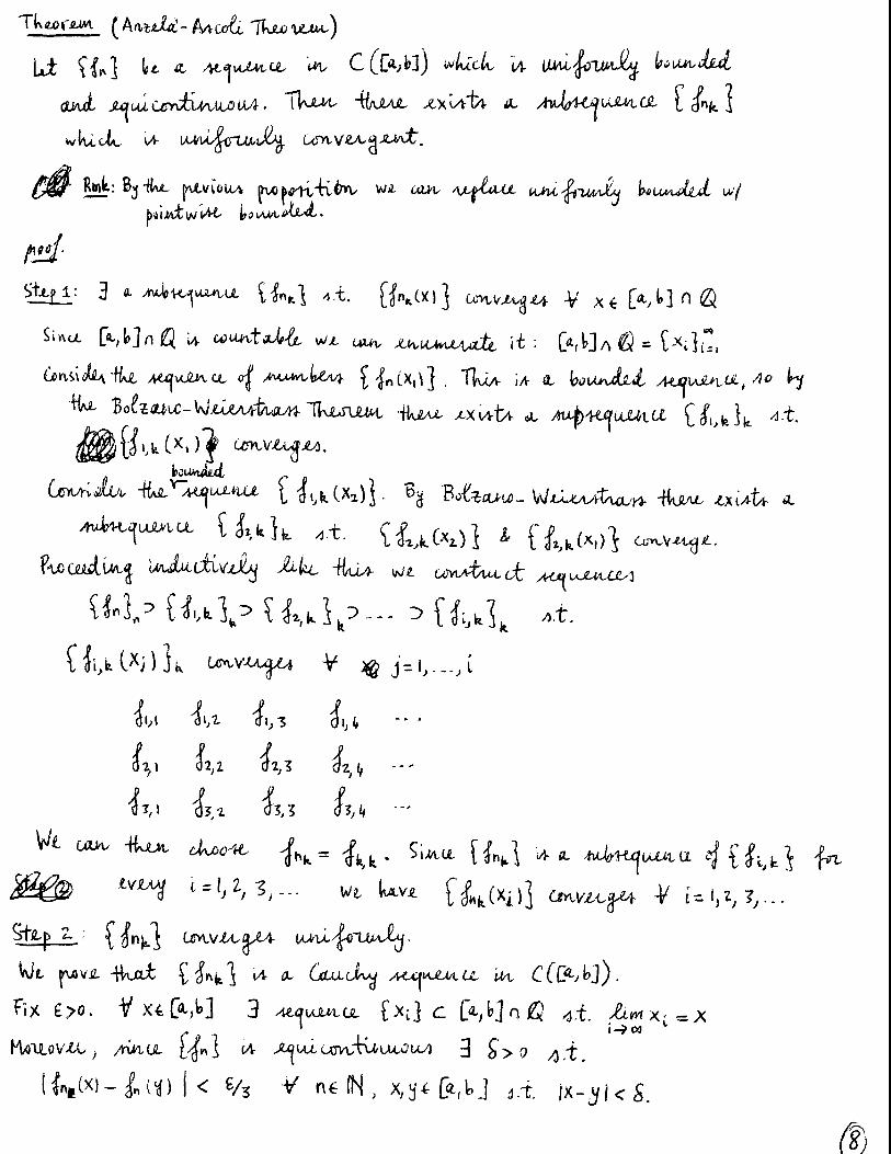
OLKcl JUÛiCcydxYMÔOA. T W t ¥UMJL XxUtv it AvtMpJUAO, [lie]

^y5^ Rwk: Bj-fUi- jatvvoUA ^^tfoi/'U^ Aa|>t<UX uAiipiMdij UUMAJLA W/

f)aizitlA/l4t WiUnl.t-

1: 3 <X Mkyy^KJi (lit] ^t. [K^Xl] CovtvXtgX4 V X t b M n ^

Ci>rvS\i£u "HvX yVtguj2ztCL /MAAfny\aÂA \

Ha BoMiWUJ-WxUA^Wxi-llxjWTj^ ikiAJL XX'\AtA a AUÂUÛMIU d feJk 4.t.

^î:lue>^«)1' arvv.agxo.

(js/uridiji, ikspMxp7,iiiUL (l tCXa)!. BoE iUic-WtltnAWhi- 3 W xxUth »t

^ 1 ^ ^ ^ t l > k AX. (4MXZ )1 ^ fl.fxM a.V.H^X.

F-tCOaUtg uatctlV'iixj ii-kc "HLU- WX LCnAtuJcdC MJpUULCJLy'^

9 Z X f dz,) ai,z dz,

'J i iz,Z ••'

Vt w>u 3U>u ££u>(?4e 4 h k = -Ikk^ Si.ua ( 1 ^ 1 Ait iUngcoita ^^tî.k]

l = IM; l - Wt U V X fl,(X|)] Or.VM^ ¥ ©-kFF...

StiLp 2. : USAS/JUL ipiA- UMiX-XiXixxlAj.

WL ^ V X fkai; d k l '4- a Giaciv^ Accjuxxttt Un G(G^ybJ).

fix iyo. VxeC^-iM 3 /oaujutciL Cxi] c C- -ykln© of. icnix;=;<

l W x ) - l i ^ ) i < V3 V n e l N , x,y4[ayj ,.t. (x-^l<S.

^^QJX&ASULAS^,XS^J^ S m w - ^m x; = )c, wc c«v p U ; |x-xu<S.

XldiM, 4 b Wit koLVX ;

t^M'^©i^he^)| l l M ^ ) - I' a ') ¥ |Aktxc)--|n,(xc)4 4êA7)- -l^yx)

3 3 3

b ' Approxm^ttAO coixtlvvuaws: 4undxc)ii\ w t ik po(yiiotntalc, I

"'n? /»t,(yk -tUot (Pn ] COKViU. U^VUIXUAX^ to g*.

3(x)= 4(*'* ' ' ( U e ) ) _ Ice) ,_ X [4(b)

"lion, I'.O'ill >R w/ gCa)=0=g(0

KflUovee, i| (?„] U e yK.gui>v(x pî\s>v\,\idU Hudt c<r*vvitta uou^nuziX^ to +¥o -

Fn ( |u j ^ 4(e) 3- hzd [ F M - ^ e ) " prôu-WoXi -fkoCt UVKMSU^^

jijUJ^jîj to I.

ccw¥auupu/) 4tu^c¥Cqv. y xKitUvj 4o<).f 4 "

Note 4 U t (i-X^)'' I- ffx"- 4 # ¥xt[o, l ] m l - fW4>ra.

2 alrt '\lh

Now iellirx

Pntx). I i U ^ Y ^ ^ V d ^ .[^ iun)<liWd^ - iii) aA^-X) di

So F lA 4t p<j^ AiTWv-iuit ov X .

Now /»vKa I

1(^+3)-|CX) < i 2

« mini C^ C-s')" t i < e


1. Let f : [0, 1] → [0, 1] be an increasing continuous function. Show that there existsx0 ∈ [0, 1] such that f(x0) = x0.(Hint: start with any point x0 ∈ [0, 1]; if f(x0) = x0 then you’re done; assume then that f(x0) 6= x0and consider the sequence x1 = f(x0), x2 = f(x1), . . . , xn = f(xn−1) when f(x0) > x0 and when

f(x0) < x0.)

2. Fix c ∈ [0.5, 1] and consider the function

fc(x) = c

(x+

1

x

).

(a). Prove that fc : [1,∞)→ [1,∞).

(b). Prove that if c < 1 then fc is a contraction. The theorem proved in class then guaran-tees that fc has a unique fixed point in [1,∞). Can you find it?

(c). Suppose now that c = 1. Prove that f1 satisfies

|f1(x)− f1(y)| < |x− y|, for all x, y ∈ [1,∞) with x 6= y.

(d). Using part (c) show that f1 has at most one fixed point in the interval [1,∞).

(e). Show that f1 has no fixed point in [1,∞).

3. (Exercise 17 in Chapter 3 of [R]) Fix α > 1 and x0 >√α. Define a sequence {xn} by

x1 =α + x01 + x0

, xn+1 =α + xn1 + xn

= xn +α− x2n1 + xn

.

(a). Prove that x1 > x3 > x5 > . . . and x0 < x2 < x4 < . . . .

(b). Prove that {xn} converges and that limn→∞ xn =√α.

4. Let α be any number with α > 5 and consider the function f(x) = x3+x2+1α

.

(a). Show that f : [−1, 1]→ [−1, 1].

(b). Show that f : [−1, 1]→ [−1, 1] is a contraction.

(c). Show that the equation x3 + x2 + 1 = αx has a unique solution in [−1, 1].

5. Use Newton’s Method to approximate a zero of the function f(x) = cosx − x2 near0. Find the best approximation within the accuracy of your calculator (that is, stop theiteration whenever you start getting the same result over and over again).

6. For the following sequences of functions determine the pointwise limit on the intervalindicated and whether the convergence is uniform.

(a). fn(x) = e−nx2, x ∈ [−1, 1]

(b). fn(x) = e−x2

n2 , x ∈ R

(c). fn(x) = xn − x2n, x ∈ [0, 1]

(d). fn(x) =√x+ 1

n, x ∈ [0,∞)

(e). fn(x) = n(√

x+ 1n−√x)

, x ∈ [a,∞) for some a > 0

2


1. Let {fn} be a sequence of continuous functions on a closed bounded interval [a, b] andassume that fn converges uniformly to f .

(a). Let {xn} be a sequence of points in [a, b] such that limn→∞ xn = x. Prove thatlimn→∞ fn(xn) = f(x).

(b). Prove the converse to part (a): Let f be a continuous functions defined on [a, b] and letfn be a sequence of functions such that limn→∞ fn(xn) = f(x) whenever limn→∞ xn = x.Then fn converges to f uniformly.

2. Suppose that fn, g : [0,∞) → R are continuous functions such that∫∞0

g(x) dx exists,|fn(x)| ≤ g(x) for all x ∈ [0,∞) and fn converges uniformly to a function f on [0, T ] forevery T > 0. Prove that

limn→∞

∫ ∞

0

fn(x) dx =

∫ ∞

0

f(x) dx.

3. For every function g : [0, 1]→ R with continuous derivative let `(g) denote the length of

the parametrized curve c(t) =(t, g(t)

), t ∈ [0, 1] (this is the most obvious parametrization

of the graph of g). Find a sequence of functions fn : [0, 1] → R that converge uniformly toa function f with `(f) 6= limn→∞ `(fn).

4. Dini’s Theorem states that if {fn} is a sequence of functions fn : I → R (where I is aninterval in R) such that:

(i) fn is continuous for all n;

(ii) I = [a, b] is a closed bounded interval;

(iii) fn(x) ≤ fn+1(x) for all x ∈ I (or fn(x) ≥ fn+1(x) for all x ∈ I);

(iv) fn converges pointwise to a continuous function f ;

then fn converges uniformly to f .

(a). Assume hypotheses (i), (ii), (iii) are satisfied. Show that the pointwise limit f(x) =limn→∞ fn(x) exists for all x ∈ I. The content of the hypothesis (iv) is to assume thatthis pointwise limit is a continuous function.

(b). Consider the functions

fn : [0, 1]→ R, gn : [0,∞)→ R, hn : [0, 1]→ R, kn : [0, 1]→ R

defined by:

fn(x) = xn gn(x) =

0 if 0 ≤ x ≤ nx− n if n ≤ x ≤ n + 11 if x > n + 1

hn(x) =

1 if 0 ≤ x ≤ 1− 1

n

0 if 1− 1n< x < 1

1 if x = 1

and kn is the function whose graph is:

– the straight line segment from (0, 0) to ( 12n, 1),

– the straight line segment from ( 12n, 1) to ( 1

n, 0),

– the straight line segment from ( 1n, 0) to (1, 0).

Use these functions to show that all hypotheses in Dini’s Theorem are necessary. Inother words, for each of these sequences of functions decide whether hypotheses (i)–(iv)hold, calculate the pointwise limit and decide whether the convergence is uniform.

5. Let {fn} be a sequence of continuous functions on the closed bounded interval [a, b].Assume that {fn} is equicontinuous and that fn converges pointwise to f .

(a). Show that f is continuous.

(b). Show that fn converges uniformly to f .

6. Let {fn} be a sequence of continuous functions on the closed bounded interval [a, b].Assume that fn converges pointwise to f and let {fnk

} be a subsequence.

(a). Prove that if fnkconverges pointwise to g then f = g.

(b). Prove that if fnkconverges uniformly to f then fn converges uniformly to f .

(c). Use part (b) and the Arzela–Ascoli Theorem to give a different proof of part (b) inProblem 5.

2


1. Suppose that f : R → R is a continuous function. Let fn(x) = f(nx) for x ∈ [0, 1].Assume that {fn} is equicontinuous. Prove that f is constant.

2. You are going to prove that the function f : [−1, 1] → R defined by f(x) = |x| can beapproximated uniformly by polynomials without using Weierstrass Approximation Theorem.

(a). Given x ∈ [0, 1], show that the sequence

y1 = 1, yn+1 =1

2

(x + 2yn − y2n

)defines a decreasing sequence in [0, 1] converging to

√x.

(b). Deduce from part (a) that there exists polynomials Pn : [−1, 1] → R such that thesequence {Pn} converges pointwise to f(x) = |x|. (Hint: define P1(x) = 1 and Pn+1(x) =12

(x2 + 2Pn(x)− Pn(x)2

)for all n ≥ 1.)

(c). Use Dini’s Theorem to show that {Pn} converges uniformly to f(x) = |x| in [−1, 1].(Hint: deduce from part (a) that Pn(x) ≥ Pn+1(x) ≥ 0 for all x ∈ [−1, 1].)

3. Prove that every continuous function on a closed bounded interval [a, b] can be approxi-mated uniformly by piece-wise linear functions, that is, functions whose graph is a polygonalcurve.

4. Suppose that f : [0, 1]→ R is a continuous function such that∫ 1

0

f(x)xn dx = 0

for every n ∈ N. Prove that f(x) = 0 for all x ∈ [0, 1]. (Hint: use the Weierstrass Approximation

Theorem to show that∫ 10 f2 dx = 0.)

5. Exercise 10 in §7.4 of [A].

6. Exercise 9 in §7.8 of [A].

Note: [A] indicates Apostol, Calculus I.


1. Let {an} be a sequence of real numbers and suppose that there exists x0 6= 0 such that∑∞n=0 anx

n0 converges. Fix 0 < r < |x0|. Prove that

∑∞n=0 anx

n converges uniformly to acontinuous function f on [−r, r].

2. Let f be the function obtained in Problem 1. Show that f is integrable on [−r, r] and∫ x

0

f(t) dt =∞∑n=0

ann + 1

xn+1.

3. Let f be the function obtained in Problem 1. Show that f is differentiable on [−r, r]and ∫ x

0

f(t) dt =∞∑n=1

nanxn−1.

4. Let {an} be a sequence such that∑∞

n=1 an converges. By Problem 1,∑∞

n=0 anxn is

uniformly convergent on [−a, a] for every 0 < a < 1.

(i). Prove Abel’s Theorem:∑∞

n=0 anxn is uniformly convergent in [0, 1]. (Hint: You can use

the following fact without proof:

|am + am+1 + · · ·+ am+k| < ε =⇒ |amxm + am+1xm+1 + · · ·+ am+kx

m+k| < ε

for every x ∈ [0, 1].)

(ii). Find a sequence {an} such that∑∞

n=0 an converges but∑∞

n=0 anxn does not converge

for x = −1.

5. You are going to prove Bernstein’s Theorem: Assume that f is a function f : [0, r]→ Rsuch that f (n)(x) ≥ 0 for all n ≥ 0 and x ∈ [0, r]; then the Taylor series

∑∞k=0

f (k)(0)k!

xk

converges to f(x) for every x ∈ [0, r).

(i). Set En = f − Tn(f), where Tn(f) is the Taylor polynomial of f of degree n centeredat 0. Show that 0 ≤ En(x) ≤ f(x) for all x ∈ [0, r].

(ii). Show thatEn(x)

xn+1=

1

n!

∫ 1

0

(1− s)nf (n+1)(sx) ds.

(iii). Deduce from the formula in part (ii) that

En(x)

xn+1

is a decreasing function of x ∈ (0, r]. In particular, deduce that

En(x) ≤(xr

)n+1

En(r).

(iv). Use part (i) and (iv) to deduce that

En(x) ≤ f(r)(xr

)n+1

.

(v). Deduce from part (iv) that limn→∞En(x) = 0 for all x ∈ [0, r).

(vi). Is the convergence of∑∞

k=0f (k)(0)

k!xk to f uniform on [0, a] for any a < r?

2

Notes 5: Differential Equations MAT 142, Spring 2017

1. [Warm-up] Assume that there exists a function f : R → R which is not always zeroand satisfies f ′′ + f = 0.

(a). Prove that f 2 + (f ′)2 is constant and deduce that either f(0) 6= 0 or f ′(0) 6= 0.

(b). Prove that there exists a function s such that s′′ + s = 0, s(0) = 0 and s′(0) = 1. (Wewill show later in the course that s is the unique such function.) (Hint: look for s of the

form s = af + bf ′ fo constants a, b ∈ R.)

We can now define the trigonometric functions sine and cosine by sinx = s(x) andcosx = s′(x). Many of the properties of the trigonometric functions follow easily from thedifferential equation satisfied by s.

(c). Prove that (cosx)′ = − sinx.

(d). Prove that sin (x+ a) = sin x cos a+sin a cosx and cos (x+ a) = cos x cos a−sinx sin a.(Hint: show that f(x) = sin (x+ a) and g(x) = sinx cos a+ sin a cosx both satisfy the IVP

y′′ + y = 0y(0) = sin ay′(0) = cos a

Assume that this IVP has a unique solution and deduce that f = g. Taking derivatives now

derive the identity involving cos (x+ a).)

More work is required to define π and show that sin and cos are periodic functions ofperiod 2π, that is, sin (x+ 2π) = sin (x) and cos (x+ 2π) = cos (x) for all x ∈ R.

(e). Show that cos x cannot be positive for all x > 0. (Hint: you can use the following

Theorem, that you proved in the quiz at the very beginning of the course: Let f be a twice-

differentiable function f : [0,∞) → R such that f(x) > 0 for all x ≥ 0, f is decreasing and

f ′(0) = 0. Then there exists x∗ > 0 such that f ′′(x∗) = 0.)

By part (e) there exists a positive number π such that π2

is the smallest positive numbersuch that cos x = 0.

(f). Show that sin π2

= 1.

(g). Show that sin x and cosx are periodic functions of period 2π. (Hint: Use repeatedly part

(d), first to calculate sin 2π and cos 2π and then to calculate sin (x+ 2π) and cos (x+ 2π).)

PART I: FIRST-ORDER EQUATIONS

Reading: §§8.1–8.7 and 8.20–8.27 in [A].

2. [Exponential growth] Fix k ∈ R. You are going to solve the differential equationy′ = ky and study some physical phenomena modelled by this equation.

(a). Prove that y(x) = y0 ekx for some constant y0 ∈ R. (Hint: Consider the quantity

y(x)e−kx.)

(b). The decay of a radioactive substance is modelled by the differential equation A′ = kAwhere A(t) is the amount of substance at time t and k is a constant that depends onthe radioactive substance.

i. Assuming k given, find a formula for A(t) in terms of A0 = A(0).

ii. Exercise 1 in §8.7 on [A].

iii. Show that there exists τ > 0 (called the half-life of the substance) such thatA(t+ τ) = 1

2A(τ) for all t ∈ R.

iv. Exercise 3 in §8.7 of [A].

(c). Newton’s Law of Cooling states that the temperature of an object decreases at a rateproportional to the difference of its temperature and the ambient temperature.

i. Find a formula for the temperature T (t) of the object at time t in terms of thetemperature T0 at time t = 0 assuming that the ambient temperature Ta is keptat a fixed constant. (Hint: Note that since Ta is a constant T ′ = (T − Ta)′.)

ii. Exercise 7 in §8.7 of [A].

3. [Linear first-order equations] A linear first-order differential equation is a differentialequation of the form

y′ + p(x) y = q(x)

where p, q are given functions. We usually try to solve the IVP

y′ + p(x) y = q(x), y(x0) = y0. (1)

(a). Consider first the case q = 0. Assume that p is a continuous function on an openinterval I such that x0 ∈ I and fix a constant y0 ∈ R. Prove that the solution y of theIVP (1) is y(x) = y0 e

−P (x), where P (x) =∫ xx0p(t) dt is the (unique) antiderivative of p

that vanishes at x0. (Hint: Consider the quantity y(x) eP (x).)

(b). More in general, assume that p, q are continuous functions on an open interval I thatcontains x0. Show that the unique solution of the IVP (1) is

y(x) = e−P (x)

(y0 +

∫ x

x0

e−P (t)q(t) dt

),

where P is defined in part (a). (Hint: Consider the quantity y(x) eP (x).)

2

(c). Exercises 1–12 in §8.5 of [A].

4. [Separation of variables and other tricks] There is no general formula to solvenon-linear first-order equations. However, in some special cases there exists tricks to reducethe solution of the equation to the Fundamental Theorem of Calculus or to a linear equation.

(a). (Separation of variables, see §8.23 of [A].) Let a be a continuous function defined onan open interval containing y0 and q a continuous function defined on an open intervalcontaining the point x0. Assume that the IVP

a(y)y′ = q(x), y(x0) = y0

has a unique solution y. Show that y is defined implicitly by∫ y(x)

y0

a(s) ds =

∫ x

x0

q(t) dt.

(b). Exercises 1–11 in §8.24 of [A]. Write the solution with arbitrary initial condition y(x0) =y0, for constants x0, y0 such that the hypotheses of part (a) are satisfied.

(c). The Bernoulli Equation: exercises 13–18 in §8.5 of [A].

(d). The Riccati Equation: exercises 19-20 in §8.5 of [A].

5. [Application: population growth] Exercises 13–18 in §8.7 of [A].

6. [Existence and Uniqueness of solutions to first-order differential equations]

(a). Consider the IVPy′ = y2, y(0) = 1.

Find a solution y by separation of variables and show that limx→1 y(x) =∞.

(b). Consider the IVP

y′ = y23 , y(0) = 0.

Show that y(x) = 0 and y(x) = x3

27are two distinct solutions of this IVP.

(c). Uniqueness: exercises 26 and 27 in Chapter 5 of [R] (see Review Sheet 2).

(d). Existence: exercise 25 in Chapter 7 of [R] (see Review Sheet 2).

(e). Here’s an alternative proof of Existence and Uniqueness of solutions to first-orderdifferential equations. The procedure of proof is called Picard Iteration. Let φ : R→ Rbe a function defined on a rectangle R = [a, b] × [α, β] ⊂ R2. Assume that φ iscontinuous on R and moreover there exists A > 0 such that

|φ(x, y2)− φ(x, y1)| ≤ A|y2 − y1|

3

for all (x, y1), (x, y2) ∈ R. Fix x0 ∈ (a, b) and y0 ∈ (α, β) consider the IVP

y′ = φ(x, y), y(x0) = y0. (2)

We are going to prove that this IVP has a unique solution provided b−a is sufficientlysmall using ideas related to the Contraction Mapping Theorem, which was our maintool to prove the convergence of Newton’s Method.

i. Show that y is a solution of the IVP if and only if y = y0 +∫ xx0φ(t, y(t)

)dt.

Let C([a, b]) be the space of continuous real-valued functions on the interval [a, b].Recall that we can define a norm on C([a, b]) by

‖f‖ = supx∈[a,b]

|f(x)|.

Define a “function” T : C([a, b])→ C([a, b]) by

T (f) = y0 +

∫ x

x0

φ(t, f(t)

)dt.

By part i we have to show that T has a unique fixed point.

ii. Prove that that‖T (f)− T (g)‖ ≤ A(b− a)‖f − g‖

for every f, g ∈ C([a, b]). In particular, by considering a smaller interval we canassume that b−a is small enough so that T is a contraction: there exists 0 < c < 1such that

‖T (f)− T (g)‖ ≤ c‖f − g‖for every f, g ∈ C([a, b]).

iii. Deduce that the IVP (2) has at most one solution.

iv. Consider the sequence of functions yn ∈ C([a, b]) defined by

y1 = 0, yn+1 = T (yn).

Prove that {yn} is a Cauchy sequence and that yn converges uniformly to a solutionof the IVP (2).

7. [Integral curves] Let y : [a, b] → R be a solution of the differential equation y′ =φ(x, y). We can consider the graph of y as a curve in R2. In fact we can think of thedifferential equation as describing a family of curves, called integral curves of the differentialequation, by prescribing their slopes. If φ satisfies the conditions in our Existence andUniqueness Theorems, then for every point in R2 there exists a unique integral curve of thedifferential equation passing through that point.

(a). Exercises 1–12 in §8.22 of [A].

(b). Exercises 1–11 in §8.26 of [A].

(c). For the examples of part (a) try to study the orthogonal trajectories to the given familyof curves.

4

PART II: SECOND-ORDER EQUATIONS

Reading: §§8.8–8.19 in [A].

8. [Uniqueness of solutions to y′′ + b y = 0] Fix b ∈ R and consider the IVPy′′ + b y = 0y(x0) = y0y′(x0) = z0

(3)

You are going to prove that this IVP has a unique solution, in two different ways.

(a). Show that the IVP (3) has a unique solution if the IVPy′′ + b y = 0y(0) = 0y′(0) = 0

(4)

has the unique solution y = 0.

(b). The first way of proving uniqueness uses Taylor polynomials.

i. Let y be a solution to the IVP (4). Prove that

y(2n)(x) = (−1)nbny(x), y(2n+1)(x) = (−1)nbny′(x).

ii. Deduce from i. that the Taylor polynomial of y at 0 of degree 2n − 1 is 0 andtherefore y(x) = E2n−1(x).

iii. Show that for every c > 0 there exists a constant M ≥ 0 such that

|y(2n)(x)| ≤M |b|n

for all x ∈ [−c, c]. (Hint: set M = max[−c,c] |y(x)|, which exists since y is continuous.)

iv. By choosing n sufficiently large, show that |y(x)| < ε on [−c, c] for every ε > 0and deduce that y = 0.

(c). This proof is more elementary but more “clever”.

i. Prove that b y2 + (y′)2 = 0.

ii. If b ≥ 0 deduce immediately from part i. that y = 0.

iii. Assume now that b = −k2 < 0. Suppose that y(x) 6= 0 for all x ∈ [α, β]. Use parti. to prove that there exists C ∈ R such that either y(x) = Cekx or y(x) = Ce−kx

for all x ∈ [α, β].

iv. Assume that y(x∗) 6= 0 for some x∗ 6= 0. Use the continuity of y to show thatthere exists a point a with 0 ≤ |a| < |x∗| such that y(a) = 0 but y(x) 6= 0 on thewhole open interval joining a and x∗. Use this fact and part iii. to prove thaty = 0.

5

9. [Homogeneous linear second-order equations with constant coefficients] Wecan now study existence of solutions to homogeneous linear second-order constant-coefficientsequations, that is, differential equations of the form

y′′ + a y′ + b y = 0

for constants a, b ∈ R.

(a). Fix b ∈ R. Find all solutions to the equation

y′′ + b y = 0

(Hint: Treat separately the case b = 0, b = k2 > 0 and b = −k2 < 0.)

(b). Fix a, b ∈ R and consider the equation

y′′ + a y′ + b y = 0

i. Show that y satisfies y′′ + a y′ + b y = 0 if and only if u(x) = ea2xy(x) satisfies

u′′ +4b− a2

4u = 0

ii. Combine parts i. and (a) to find all solutions to y′′ + a y′ + b y = 0.

iii. Deduce that the IVP y′′ + a y′ + b y = 0y(x0) = y0y′(x0) = z0

has a unique solution.

(c). Exercises 1–16, 18, 20 in §8.14 of [A].

10. [Inhomogeneous linear second-order constant-coefficients equations] Fixa, b ∈ R. For a twice-differentiable function y write L(y) = y′′ + a y′ + b y. L is calleda differential operator.

(a). Show that L(c1y1 + c2y2) = c1L(y1) + c2L(y2) for every pair of twice-differentiablefunctions y1, y2 and constants c1, c2. This is why we say that L is a linear differentialoperator.

(b). Let R : R→ R be a continuous function. Suppose that y∗ is a solution of the differentialequation L(y∗) = R. Show that all solutions of the differential equation L(y) = R areof the form y = y∗+yh, where yh is a solution of the homogeneous equation L(yh) = 0.

(c). By Problem 9, yh = c1y1+c2y2, where c1, c2 ∈ R and y1, y2 are two solutions of L(y) = 0such that y1/y2 is not constant. The Wronskian of y1 and y2 is the function

W (x) = y1(x) y′2(x)− y′1(x) y2(x).

Exercises 21–23 in §8.14 of [A] establish properties of W .

6

(d). Fix x0 ∈ R and define

c1(x) = −∫ x

x0

y2(t)R(t)

W (t)dt, c2(x) =

∫ x

x0

y1(t)R(t)

W (t)dt.

Set y∗(x) = c1(x) y1(x) + c2(x) y2(x) and show that L(y∗) = R. (This method to obtain

a particular solution of the equation L(y) = R is called variation of parameters.)

(e). Exercises 1–25 in §8.17 of [A]. (Hints: 1. If b = 0 then the solution is found more quickly by

applying the Fundamental Theorem of Calculus twice since y′′ + a y′ = (y′ + a y)′. 2. When

R(x) is a polynomial of degree d and b 6= 0 then one can quickly find a particular solution

y∗ of the equation L(y) = R guessing that y∗ must be another polynomial of degree d. 3. If

e−mxR(x) is a polynomial of degree d the we can look for a particular solution of the form

y∗ = emx× a polynomial of degree d.)

11. [Application: simple harmonic motion (Example 1 in §8.18 of [A])] Exercises1–7 in §8.19 of [A].

12. [BVP vs. IVP] We saw above that the IVP problem for second-order linear con-stant coefficient equations always has a unique solution. One is also interested in studyingboundary value problems (BVP) instead of IVPs: fix an interval [x1, x2] ⊂ R, constantsa, b, α1, α2, β1, β2 ∈ R and try to find all twice-differentiable functions y such that

y′′ + a y′ + b y = 0α1y(x1) + β1y

′(x1) = 0α2y(x2) + β2y

′(x2) = 0

In contrast to the IVP, in general a solution to the BVP does not exists. Do exercises 17and 19 in §8.14 of [A] for some examples of this.

13. [Linear constant-coefficients homogeneous equations] Fix constants a0, . . . , an−1and consider a degree–n linear constant-coefficients equation

y(n) + an−1 y(n−1) + · · ·+ a1 y

′ + a0 y = 0. (5)

In this problem you will get a glimpse of how the theory we have developed for second-orderequations generalises to higher-order equations.

(a). Suppose that α ∈ C is a root of the polynomial

xn + an−1 xn−1 + · · ·+ a1 x+ a0 = 0. (6)

Show that y(x) = eαx is a (complex-valued) solution of the differential equation (5).

(b). Write α = a + ib and deduce that y(x) = eax cos (bx) and y(x) = eax sin (bx) are two(real-valued) solutions of (5).

(c). Suppose that α is a double root of the polynomial (6). Show that y(x) = xeαx is asecond (complex-valued) solution of (5).

7

(d). Suppose that α is a root of the polynomial (6) of order r. Show that y(x) = xkeαx isa (complex-valued) solution of (5) for all 0 ≤ k ≤ r.

(In this way one can always find n (real-valued) solutions y1, . . . , yn of (5) (why?) and in fact every

solution of the differential equation can be written as y = c1 y1 + · · ·+ cn yn.)

14. [Linear second-order equations] A homogeneous linear second-order equation is anequation of the form

y′′ + a(x) y′(x) + b(x) y = R(x),

where a, b, R are given continuous functions. One can prove existence and uniqueness forthe IVP (see Exercises 28–29 in Chapter 5 and 26 in Chapter 7 of [R]), but there exists nogeneral formula for writing the solution.

(a). In this problem we show that we can always reduce to the case

y′′ + g(x) y = f(x).

Unfortunately there is no general formula for the solution to such an equation.

i. Show that every linear second-order equation can be re-written in the form

(p(x) y′)′+ q(x) y = r(x)

for continuous functions p, q, r with p(x) > 0 for all x. (Hint: calculate the derivative

of eA(x)y and then choose the function A appropriately; this is similar to how we dealt

with linear first-order equations.)

ii. By making a change of variable s = s(x) such that s′(x) = 1p(x)

, reduce theprevious equation further to an equation of the form

u′′ + g(s)u = f(s)

where y(x) = u(s(x)

).

(b). You are going to prove a version of the Sturm Comparison Theorem: suppose that y1and y2 are solutions to

y′′1 + g1(x) y1 = 0, y′′2 + g2(x) y2 = 0,

for continuous functions g1, g2 such that g2(x) > g1(x) . If a and b are consecutivezeroes of y1 then y2 must have a zero in the interval (a, b).

i. Show that y′′1 y2 − y′′2 y1 = (g2 − g1) y1 y2.ii. Assume that y1(x), y2(x) > 0 for all x ∈ (a, b) and show that∫ b

a

y′′1(x) y2(x)− y′′2(x) y1(x) dx > 0.

8

iii. Deduce that(y′1(b) y2(b)− y′1(a) y2(a)

)−(y1(b) y

′2(b)− y1(a) y′2(a)

)> 0.

iv. Deduce that it is impossible that y1(a) = 0 = y1(b). (Hint: consider the sign of

y′1(a) and y′1(b).)

v. Similarly, prove that we cannot have y1(a) = 0 = y1(b) if we assume that y1(x) > 0and y2(x) < 0 for all x ∈ (a, b), or y1(x) < 0 and y2(x) > 0 for all x ∈ (a, b), ory1(x) < 0 and y2(x) < 0 for all x ∈ (a, b).

(c). Let y be a solution of the equation

y′′ + (x2 + k2) y = 0.

Use part (b) to show that y has infinitely many zeroes which are within πk

of eachother.

9

Review Sheet 1 MAT 142, Spring 2017

1. For vectors x = (x1, x2) and y = (y1, y2) in R2 we have defined:

• The dot product: x · y = x1y1 + x2y2

• The cross product or determinant: x× y = x1y2 − x2y1

• The norm: ‖x‖ =√x · x =

√x21 + x22

• The distance: d(x,y) = ‖x− y‖

We showed that

• x · y = ‖x‖ ‖y‖ cos θ

• x× y = ‖x‖ ‖y‖ sin θ

where θ is the angle between the two vectors.

2. We defined polar coordinates

x = r cos θ, y = r sin θ

• We studied polar equations r = f(θ), θ ∈ [a, b]

• We showed that if f 2 is integrable then the area of the polar region R bounded by thepolar equation r = f(θ), θ ∈ [a, b] is

area(R) =1

2

∫ b

a

f 2(θ) dθ

3. We have studied regular parametrized curves c : [a, b]→ R2.

• We have defined the tangent vector c′(t) and the unit normal vector n(t) to c

• We have defined the length `(c) of c and proved that if c′ is continuous then

`(c) =

∫ b

a

‖c′(t)‖ dt

• We have defined the arc length of c:

s(t) =

∫ t

t0

‖c′(u)‖ du,

where t0 ∈ [a, b]. We said that c is parametrized by arc length if ‖c′(t)‖ = 1 for allt ∈ [a, b]

• We have defined the curvature κ of c: if c is parametrized by arc length then

c′′(t) = κ(t)n(t)

If c is not necessarily parametrized by arc length, we found the formula

κ(t) =c′(t)× c′′(t)

‖c′(t)‖3

• We have proved that for every differentiable function κ : [a, b] → R there exists aunique curve up to rigid motions with curvature κ

• We have defined simple closed curves and stated the Jordan Closed Theorem: everysuch curve encloses a bounded connected region int(c) of the plane

• We have shown the Green’s Formula for area for convex simple closed curves withperiod T and with continuous derivative:

area(int(c)

)=

1

2

∫ T

0

c(t)× c′(t) dt

• We have proved the Isoperimetric Inequality: for every simple closed curve with con-tinuous c′ we have

area(int(c)

)≤ 1

4π2`(c)2

Moreover, equality holds if and only if c is a circle.

4. We have studied sequences of real numbers.

• We proved that every monotonic sequence is convergent

• We defined the notion of a subsequence and proved the Bolzano–Weiestrass Theorem:every bounded sequence has a convergent subsequence

• We proved the Cauchy Criterion: a sequence converges if and only if it is a Cauchysequence

2

MAT 142 - Analysis II - Stony Brook Mathematics

Documents

Transcript of MAT 142 - Analysis II - Stony Brook Mathematics