MAT 303 - Calculus IV - Stony Brook Mathematics

MAT 303: Calculus IV with ApplicationsFall 2016

Schedule & Homework

Home Course Information Schedule & Homework

Schedule

This is our tentative weekly schedule and it will be updated as we advance in the semester, please check regularly. Studentsare expected to attend class regularly and to keep up with the material presented in the lecture and the assigned reading.As a general rule, the written homework assignment is due Fridays (for example, HW1 is due Friday, Sept 9, Week 2), unlessotherwise stated.

Week Lectures (Assigned Reading) Assignments

Week 1 8/29 - 9/4

1.1: Differential equations and math models 1.2: Integrals as general and particular solutions 1.4: Separable differential equations

1.1: 26, 48 1.2: 8, 10, 44 1.4: 18, 28, 32, 36, 37, 39

Week 2 9/5 - 9/11

No class on Sept 5 (Labor Day) 1.5: Linear first order differential equations 1.3: Slope fields and solutions curves

1.3: 11, 14, 18, 27, 29, 30 1.5: 1, 6, 16, 19, 27, 38

Week 3 9/12 - 9/18

1.3: Local Existence and Uniqueness of Solutions Intro: Diff Eq and Phase Portraits in Mathematica (.nb)1.6: Substitution Methods and Exact Equations

1.6: 8, 11, 21, 27, 29, 441.6: 47, 57, 58, Mathematica

Week 4 9/19 - 9/25

1.6: Substitution Methods and Exact Equations (exact.pdf) due Monday, Oct 3

1.6: 33, 37, 38 2.1: 13, 23, 33 2.2: 8, 9

2.6: 25, 27 from exact.pdf

Week 5 9/26 - 10/2

2.1: Population models 2.2: Equilibrium solutions and stability 2.3: Acceleration-Velocity models

Midterm 1 – Wednesday, October 5, 12 - 12:53pm, in class; Midterm I Solutions covers Chapter 1 and Sections 2.1 and 2.2 Practice Problems (Spring 2013) with Solutions

Week 6 10/3 - 10/9

2.4: Numerical approximation: Euler's Method 3.1: Second order eq. with constant coeff. (see also 3.3)

2.2: 19, 22 2.4: 1, 27 3.1: 39, 51, 52, 56 3.3: 9, 21, 23

Week 7 10/10 - 10/16

3.1: Second order linear equations

3.2: Nth-order linear equations

3.3: Nth-order equations with constant coefficients

3.1: 19, 29, 30, 32, 3.2: 28, 35, 36, 38, 433.3: 12, 15, 20

Week 8 10/17 - 10/23

3.4: Mechanical vibrations3.5: Nonhomogeneous eq. and undetermined coefficients

3.4: 3, 14, 15 3.5: 5, 19, 21, 22, 34Additional Exercises

Week 9 10/24 - 10/30

3.6: Forced Oscillations and Resonance3.8: Endpoint Problems and Eigenvalues

3.6: 1, 8, 11, 26, 27 3.8: 3, 6, 7, 13, 16

http://www.math.stonybrook.edu/~rtanase/index.html

http://www.math.stonybrook.edu/~rtanase/calc303/ODE303.nb

http://www.math.stonybrook.edu/~rtanase/calc303/HW3-Mathematica.nb

Last updated December 7, 2016

Week 10 10/31 - 11/6

4.1: First Order Systems & The Elimination Method in 4.25.1: Matrices and Linear Systems 5.2: The Eigenvalue Method for Homogeneous Systems

4.1: 19 5.1: 3, 23 4.2: 2 5.2: 1, 6, 17, 19

Week 11 11/7 - 11/13

4.1: Fundamental Set of Solutions5.5: The Eigenvalue Method: Repeated Eigenvalues

Midterm 2 – Wednesday, November 16, 12 - 12:55pm, in class Midterm II Solutions covers Sections 2.2, 2.4, Chapter 3, and Sections 4.1, 4.2, 5.1, 5.2 Practice Problems I with Solutions Practice Problems II with Solutions

Week 12 11/14 - 11/20

Review on Monday5.5: Repeated Eigenvalues

TBA, due Friday, Dec 2

5.5: 13, 16, 20, 33 5.6: 23, 25, 34, 35 Additional

ExercisesWeek 13

11/21 - 11/275.6: Matrix Exponentials and Linear Systems Thanksgiving Break!

Week 14 11/28 - 12/4

5.6: Matrix Exponentials and Linear Systems 5.7: Nonhomogeneous Systems; Variation of Parameters Jordan canonical forms Lecture Notes! Mathematica Tutorial!

Read the Lecture Notes attached

and the Mathematica Tutorial!

5.7: 24, 31 Instructions6.2: 1, 3, 10, 13, 15, 29, 33

Week 15 12/5 - 12/11

6.1: Stability and the Phase Plane 6.2: Linear and Almost Linear Systems

Final exam – Thursday, December 15, 5:30 - 8pm, in Harriman Hall 137the final covers everything! Practice Final (2013) with Solutions

Review Session on Monday, December 12, 11am - 1pm, in Javits 111

http://www.math.stonybrook.edu/~rtanase/calc303/Tutorial2.nb

http://www.math.stonybrook.edu/~rtanase/calc303/Tutorial2.nb

http://ericmalm.net/ac/teaching/mat303-spr13/exams/final.pdf

http://ericmalm.net/ac/teaching/mat303-spr13/exams/final-solutions.pdf


Course Information

Home Course Information Schedule & Homework

Course Description

This course is an introduction to differential equations, with particular emphasis on scientific applications. Topics we willcover include homogeneous and non homogeneous linear differential equations, systems of linear differential equations,non-linear systems, Laplace transforms, series solutions to equations. We study standard techniques for solving ordinarydifferential equations, including numerical methods, and their applications to engineering, physics, biology, chemistry,economics, social sciences.

Click here to download a copy of the course syllabus. Please visit also the course website on Blackboard.

Textbook

The course textbook is Differential Equations with Boundary Value Problems: Computing and Modelling (5th edition), byEdwards & Penney.

Office Hours

Instructor: Raluca Tanase Office hours: Mondays 1-2pm in MLC, Thursdays 1:30-2:30pm in Math Tower 4-120 Wednesdays 1-2:30pm in Math Tower 4-120, or by appointment.

Recitations

LEC 01 MWF 12 - 12:53pm Harriman Hall 137 Raluca Tanase

R 01 W 10:00am-10:53am Library W4535 Dyi-Shing Ou

R 02 F 1:00pm - 1:53pm Library E4330 Timothy Ryan

R 03 Tu 5:30pm - 6:23pm Library W4525 Timothy Ryan

R 04 W 7:00pm - 7:53pm Library W4525 Alexandra Viktorova

R 05 M 5:30pm - 6:23pm Lgt Engr Lab 152 Jiasheng Teh

Blackboard

Almost all course administration will take place on Blackboard. Your exam and homework grades will also be reported onBlackboard. On this webpage, under Schedule & Homework you will find the most up-to-date version of the weeklycourse schedule and the written homework assigments.

http://www.math.stonybrook.edu/~rtanase/index.html

http://www.math.stonybrook.edu/~rtanase/calc303/m303-Syllabus.pdf

https://blackboard.stonybrook.edu/

http://www.math.stonybrook.edu/~rtanase/calc303/m126-Sp16-schedule.html

Last updated September 28, 2016

Grading Policy

Grades will be computed using the following scheme:

Recitation & Homework – 20%Each Midterm – 20%Final Exam – 40%

Students are expected to attend the lectures and recitations regularly and to keep up with the material presented in thelecture and the assigned reading.

Homework

You cannot learn differential equations without working problems. Each week, you will be given a set of problems, due thenext Friday, in class. Do all of the assigned problems, as well as additional ones to study. Most of the homework problemswill be analytic exercises, whose solutions will require only pen and paper. A few of them (clearly marked) will require theuse of a computer program like Mathematica . Your solutions for the homework should be written neatly and legibly ingrammatically correct mathematical English, and all steps should be clearly outlined. For the ones that require computersoftware, the generating code should also be turned in.

Software

We will use Mathematica, which is a computational software program developed by Wolfram Research and used in manyscientific, engineering, mathematical and computing fields, based on symbolic mathematics. Mathematica has acomprehensive documentation.

Stony Brook students can download the Windows/Mac/Linux version of Mathematica 10.3 from Softweb. You need yourStony Brook netID and netID password to log in to Softweb. To obtain an Activation Key for Mathematica you must visit theWolfram User Portal. If it's your first time visiting the Wolfram User Portal, you must create a Wolfram ID and follow thesteps in there to request an Activation Key.

In addition, you can use any of the campus SINC sites, or you can access the Virtual SINC site.

http://reference.wolfram.com/language/

http://softweb.cc.stonybrook.edu/

https://user.wolfram.com/portal/login.html

http://it.stonybrook.edu/services/virtual-sinc-site

August 7, 2012 21:03 c02 Sheet number 65 Page number 95 cyan black

2.6 Exact Equations and Integrating Factors 95

(b) If the substances P and Q are the same, then p = q and Eq. (i) is replaced by

dx/dt = α(p − x)2. (ii)

If x(0) = 0, determine the limiting value of x(t) as t → ∞ without solving the differentialequation. Then solve the initial value problem and determine x(t) for any t.

2.6 Exact Equations and Integrating FactorsFor first order equations there are a number of integration methods that are applica-ble to various classes of problems. The most important of these are linear equationsand separable equations, which we have discussed previously. Here, we consider aclass of equations known as exact equations for which there is also a well-definedmethod of solution. Keep in mind, however, that those first order equations thatcan be solved by elementary integration methods are rather special; most first orderequations cannot be solved in this way.

E X A M P L E

1

Solve the differential equation2x + y2 + 2xyy′ = 0. (1)

The equation is neither linear nor separable, so the methods suitable for those types ofequations are not applicable here. However, observe that the function ψ(x, y) = x2 + xy2 hasthe property that

2x + y2 = ∂ψ

∂x, 2xy = ∂ψ

∂y. (2)

Therefore, the differential equation can be written as

∂ψ

∂x+ ∂ψ

∂ydydx

= 0. (3)

Assuming that y is a function of x, we can use the chain rule to write the left side of Eq. (3) asdψ(x, y)/dx. Then Eq. (3) has the form

dψ

dx(x, y) = d

dx(x2 + xy2) = 0. (4)

By integrating Eq. (4) we obtain

ψ(x, y) = x2 + xy2 = c, (5)

where c is an arbitrary constant. The level curves of ψ(x, y) are the integral curves of Eq. (1).Solutions of Eq. (1) are defined implicitly by Eq. (5).

In solving Eq. (1) the key step was the recognition that there is a function ψ thatsatisfies Eqs. (2). More generally, let the differential equation

M(x, y) + N(x, y)y′ = 0 (6)


96 Chapter 2. First Order Differential Equations

be given. Suppose that we can identify a function ψ(x, y) such that

∂ψ

∂x(x, y) = M(x, y),

∂ψ

∂y(x, y) = N(x, y), (7)

and such that ψ(x, y) = c defines y = φ(x) implicitly as a differentiable functionof x. Then

M(x, y) + N(x, y)y′ = ∂ψ

∂x+ ∂ψ

∂ydydx

= ddx

ψ[x, φ(x)]

and the differential equation (6) becomes

ddx

ψ[x, φ(x)] = 0. (8)

In this case Eq. (6) is said to be an exact differential equation. Solutions of Eq. (6),or the equivalent Eq. (8), are given implicitly by

ψ(x, y) = c, (9)

where c is an arbitrary constant.In Example 1 it was relatively easy to see that the differential equation was exact

and, in fact, easy to find its solution, at least implicitly, by recognizing the requiredfunction ψ. For more complicated equations it may not be possible to do this soeasily. How can we tell whether a given equation is exact, and if it is, how can we findthe function ψ(x, y)? The following theorem answers the first question, and its proofprovides a way of answering the second.

Theorem 2.6.1 Let the functions M, N , My, and Nx, where subscripts denote partial derivatives,be continuous in the rectangular17 region R: α < x < β, γ < y < δ. Then Eq. (6)

M(x, y) + N(x, y)y′ = 0

is an exact differential equation in R if and only if

My(x, y) = Nx(x, y) (10)

at each point of R. That is, there exists a function ψ satisfying Eqs. (7),

ψx(x, y) = M(x, y), ψy(x, y) = N(x, y),

if and only if M and N satisfy Eq. (10).

17It is not essential that the region be rectangular, only that it be simply connected. In two dimensionsthis means that the region has no holes in its interior. Thus, for example, rectangular or circular regionsare simply connected, but an annular region is not. More details can be found in most books on advancedcalculus.



The proof of this theorem has two parts. First, we show that if there is a functionψ such that Eqs. (7) are true, then it follows that Eq. (10) is satisfied. ComputingMy and Nx from Eqs. (7), we obtain

My(x, y) = ψxy(x, y), Nx(x, y) = ψyx(x, y). (11)

Since My and Nx are continuous, it follows that ψxy and ψyx are also continuous. Thisguarantees their equality, and Eq. (10) is valid.

We now show that if M and N satisfy Eq. (10), then Eq. (6) is exact. The proofinvolves the construction of a function ψ satisfying Eqs. (7)

ψx(x, y) = M(x, y), ψy(x, y) = N(x, y).

We begin by integrating the first of Eqs. (7) with respect to x, holding y constant. Weobtain

ψ(x, y) = Q(x, y) + h(y), (12)

where Q(x, y) is any differentiable function such that ∂Q(x, y)/∂x = M(x, y). Forexample, we might choose

Q(x, y) =! x

x0

M(s, y) ds, (13)

where x0 is some specified constant in α < x0 < β. The function h in Eq. (12) is anarbitrary differentiable function of y, playing the role of the arbitrary constant. Nowwe must show that it is always possible to choose h(y) so that the second of Eqs. (7)is satisfied—that is, ψy = N . By differentiating Eq. (12) with respect to y and settingthe result equal to N(x, y), we obtain

ψy(x, y) = ∂Q∂y

(x, y) + h′(y) = N(x, y).

Then, solving for h′(y), we have

h′(y) = N(x, y) − ∂Q∂y

(x, y). (14)

In order for us to determine h(y) from Eq. (14), the right side of Eq. (14), despiteits appearance, must be a function of y only. One way to show that this is true is toshow that its derivative with respect to x is zero. Thus we differentiate the right sideof Eq. (14) with respect to x, obtaining

∂N∂x

(x, y) − ∂

∂x∂Q∂y

(x, y). (15)

By interchanging the order of differentiation in the second term of Eq. (15), we have

∂N∂x

(x, y) − ∂

∂y∂Q∂x

(x, y),

or, since ∂Q/∂x = M,∂N∂x

(x, y) − ∂M∂y

(x, y),

which is zero on account of Eq. (10). Hence,despite its apparent form,the right side ofEq. (14) does not, in fact, depend on x. Then we find h(y) by integrating Eq. (14), and



upon substituting this function in Eq. (12), we obtain the required function ψ(x, y).This completes the proof of Theorem 2.6.1.

It is possible to obtain an explicit expression for ψ(x, y) in terms of integrals (seeProblem 17),but in solving specific exact equations, it is usually simpler and easier justto repeat the procedure used in the preceding proof. That is, integrate ψx = M withrespect to x, including an arbitrary function of h(y) instead of an arbitrary constant,and then differentiate the result with respect to y and set it equal to N . Finally, usethis last equation to solve for h(y). The next example illustrates this procedure.

E X A M P L E

2

Solve the differential equation

(y cos x + 2xey) + (sin x + x2ey − 1)y′ = 0. (16)

By calculating My and Nx, we find that

My(x, y) = cos x + 2xey = Nx(x, y),

so the given equation is exact. Thus there is a ψ(x, y) such that

ψx(x, y) = y cos x + 2xey,

ψy(x, y) = sin x + x2ey − 1.

Integrating the first of these equations, we obtain

ψ(x, y) = y sin x + x2ey + h(y). (17)

Setting ψy = N gives

ψy(x, y) = sin x + x2ey + h′(y) = sin x + x2ey − 1.

Thus h′(y) = −1 and h(y) = −y. The constant of integration can be omitted since any solutionof the preceding differential equation is satisfactory; we do not require the most general one.Substituting for h(y) in Eq. (17) gives

ψ(x, y) = y sin x + x2ey − y.

Hence solutions of Eq. (16) are given implicitly by

y sin x + x2ey − y = c. (18)

E X A M P L E

3

Solve the differential equation

(3xy + y2) + (x2 + xy)y′ = 0. (19)

We haveMy(x, y) = 3x + 2y, Nx(x, y) = 2x + y;

since My = Nx, the given equation is not exact.To see that it cannot be solved by the proceduredescribed above, let us seek a function ψ such that

ψx(x, y) = 3xy + y2, ψy(x, y) = x2 + xy. (20)

Integrating the first of Eqs. (20) gives

ψ(x, y) = 32 x2y + xy2 + h(y), (21)



where h is an arbitrary function of y only. To try to satisfy the second of Eqs. (20), we computeψy from Eq. (21) and set it equal to N , obtaining

32 x2 + 2xy + h′(y) = x2 + xy

orh′(y) = − 1

2 x2 − xy. (22)

Since the right side of Eq. (22) depends on x as well as y, it is impossible to solve Eq. (22) forh(y). Thus there is no ψ(x, y) satisfying both of Eqs. (20).

Integrating Factors. It is sometimes possible to convert a differential equation that isnot exact into an exact equation by multiplying the equation by a suitable integratingfactor. Recall that this is the procedure that we used in solving linear equations inSection 2.1. To investigate the possibility of implementing this idea more generally,let us multiply the equation

M(x, y) + N(x, y)y′ = 0 (23)

by a function µ and then try to choose µ so that the resulting equation

µ(x, y)M(x, y) + µ(x, y)N(x, y)y′ = 0 (24)

is exact. By Theorem 2.6.1, Eq. (24) is exact if and only if

(µM)y = (µN)x. (25)

Since M and N are given functions, Eq. (25) states that the integrating factor µ mustsatisfy the first order partial differential equation

Mµy − Nµx + (My − Nx)µ = 0. (26)

If a function µ satisfying Eq. (26) can be found, then Eq. (24) will be exact. Thesolution of Eq. (24) can then be obtained by the method described in the first part ofthis section.The solution found in this way also satisfies Eq. (23), since the integratingfactor µ can be canceled out of Eq. (24).

A partial differential equation of the form (26) may have more than one solution;if this is the case, any such solution may be used as an integrating factor of Eq. (23).This possible nonuniqueness of the integrating factor is illustrated in Example 4.

Unfortunately, Eq. (26), which determines the integrating factor µ, is ordinarilyat least as hard to solve as the original equation (23). Therefore, although in princi-ple integrating factors are powerful tools for solving differential equations, in practicethey can be found only in special cases.The most important situations in which simpleintegrating factors can be found occur when µ is a function of only one of the variablesx or y, instead of both.

Let us determine conditions on M and N so that Eq. (23) has an integrating factorµ that depends on x only. If we assume that µ is a function of x only, then the partialderivative µx reduces to the ordinary derivative dµ/dx and µy = 0. Making thesesubstitutions in Eq. (26), we find that

dµ

dx= My − Nx

Nµ. (27)



If (My − Nx)/N is a function of x only, then there is an integrating factor µ that alsodepends only on x; further,µ(x) can be found by solving Eq. (27), which is both linearand separable.

A similar procedure can be used to determine a condition under which Eq. (23)has an integrating factor depending only on y; see Problem 23.

E X A M P L E

4

Find an integrating factor for the equation

(3xy + y2) + (x2 + xy)y′ = 0 (19)

and then solve the equation.In Example 3 we showed that this equation is not exact. Let us determine whether it has an

integrating factor that depends on x only. On computing the quantity (My − Nx)/N , we findthat

My(x, y) − Nx(x, y)

N(x, y)= 3x + 2y − (2x + y)

x2 + xy= 1

x. (28)

Thus there is an integrating factor µ that is a function of x only, and it satisfies the differentialequation

dµ

dx= µ

x. (29)

Henceµ(x) = x. (30)

Multiplying Eq. (19) by this integrating factor, we obtain

(3x2y + xy2) + (x3 + x2y)y′ = 0. (31)

Equation (31) is exact, since

∂

∂y(3x2y + xy2) = 3x2 + 2xy = ∂

∂x(x3 + x2y).

Thus there is a function ψ such that

ψx(x, y) = 3x2y + xy2, ψy(x, y) = x3 + x2y. (32)

Integrating the first of Eqs. (32), we obtain

ψ(x, y) = x3y + 12 x2y2 + h(y).

Substituting this expression for ψ(x, y) in the second of Eqs. (32), we find that

x3 + x2y + h′(y) = x3 + x2y,

so h′(y) = 0 and h(y) is a constant. Thus the solutions of Eq. (31), and hence of Eq. (19), aregiven implicitly by

x3y + 12 x2y2 = c. (33)

Solutions may also be found in explicit form since Eq. (33) is quadratic in y.You may also verify that a second integrating factor for Eq. (19) is

µ(x, y) = 1xy(2x + y)

and that the same solution is obtained, though with much greater difficulty, if this integratingfactor is used (see Problem 32).



PROBLEMS Determine whether each of the equations in Problems 1 through 12 is exact. If it is exact, findthe solution.

1. (2x + 3) + (2y − 2)y′ = 0 2. (2x + 4y) + (2x − 2y)y′ = 0

3. (3x2 − 2xy + 2) + (6y2 − x2 + 3)y′ = 0 4. (2xy2 + 2y) + (2x2y + 2x)y′ = 0

5.dydx

= −ax + bybx + cy

6.dydx

= −ax − bybx − cy

7. (ex sin y − 2y sin x) + (ex cos y + 2 cos x)y′ = 08. (ex sin y + 3y) − (3x − ex sin y)y′ = 09. (yexy cos 2x − 2exy sin 2x + 2x) + (xexy cos 2x − 3)y′ = 0

10. (y/x + 6x) + (ln x − 2)y′ = 0, x > 011. (x ln y + xy) + (y ln x + xy)y′ = 0; x > 0, y > 0

12.x

(x2 + y2)3/2+ y

(x2 + y2)3/2

dydx

= 0

In each of Problems 13 and 14, solve the given initial value problem and determine at leastapproximately where the solution is valid.13. (2x − y) + (2y − x)y′ = 0, y(1) = 314. (9x2 + y − 1) − (4y − x)y′ = 0, y(1) = 0

In each of Problems 15 and 16, find the value of b for which the given equation is exact, andthen solve it using that value of b.15. (xy2 + bx2y) + (x + y)x2y′ = 0 16. (ye2xy + x) + bxe2xyy′ = 017. Assume that Eq. (6) meets the requirements of Theorem 2.6.1 in a rectangle R and is

therefore exact. Show that a possible function ψ(x, y) is

ψ(x, y) =! x

x0

M(s, y0) ds +! y

y0

N(x, t) dt,

where (x0, y0) is a point in R.18. Show that any separable equation

M(x) + N(y)y′ = 0

is also exact.

In each of Problems 19 through 22, show that the given equation is not exact but becomesexact when multiplied by the given integrating factor. Then solve the equation.19. x2y3 + x(1 + y2)y′ = 0, µ(x, y) = 1/xy3

20."

sin yy

− 2e−x sin x#

+"

cos y + 2e−x cos xy

#y′ = 0, µ(x, y) = yex

21. y + (2x − yey)y′ = 0, µ(x, y) = y22. (x + 2) sin y + (x cos y)y′ = 0, µ(x, y) = xex

23. Show that if (Nx − My)/M = Q, where Q is a function of y only, then the differentialequation

M + Ny′ = 0

has an integrating factor of the form

µ(y) = exp!

Q(y) dy.



24. Show that if (Nx − My)/(xM − yN) = R, where R depends on the quantity xy only, thenthe differential equation

M + Ny′ = 0

has an integrating factor of the form µ(xy). Find a general formula for this integratingfactor.

In each of Problems 25 through 31, find an integrating factor and solve the given equation.25. (3x2y + 2xy + y3) + (x2 + y2)y′ = 0 26. y′ = e2x + y − 127. 1 + (x/y − sin y)y′ = 0 28. y + (2xy − e−2y)y′ = 029. ex + (ex cot y + 2y csc y)y′ = 030. [4(x3/y2) + (3/y)] + [3(x/y2) + 4y]y′ = 0

31."

3x + 6y

#+

"x2

y+ 3

yx

#dydx

= 0

Hint: See Problem 24.32. Solve the differential equation

(3xy + y2) + (x2 + xy)y′ = 0

using the integrating factor µ(x, y) = [xy(2x + y)]−1. Verify that the solution is the sameas that obtained in Example 4 with a different integrating factor.

2.7 Numerical Approximations: Euler’s MethodRecall two important facts about the first order initial value problem

dydt

= f (t, y), y(t0) = y0. (1)

First, if f and ∂f /∂y are continuous, then the initial value problem (1) has a uniquesolution y = φ(t) in some interval surrounding the initial point t = t0. Second, it isusually not possible to find the solution φ by symbolic manipulations of the differ-ential equation. Up to now we have considered the main exceptions to the latterstatement: differential equations that are linear, separable, or exact, or that can betransformed into one of these types. Nevertheless, it remains true that solutions ofthe vast majority of first order initial value problems cannot be found by analyticalmeans, such as those considered in the first part of this chapter.

Therefore, it is important to be able to approach the problem in other ways. As wehave already seen, one of these ways is to draw a direction field for the differentialequation (which does not involve solving the equation) and then to visualize thebehavior of solutions from the direction field. This has the advantage of being arelatively simple process, even for complicated differential equations. However, itdoes not lend itself to quantitative computations or comparisons, and this is often acritical shortcoming.

For example, Figure 2.7.1 shows a direction field for the differential equation

dydt

= 3 − 2t − 0.5y. (2)

MAT 303 Spring 2013 Calculus IV with Applications

Midterm #1 Practice Problems1. Solve the following initial value problems:(a) xy′ = y + x2, y(1) = 0

(b) y′ = 6e2x−y, y(0) = 0

(c) y′ = − 2x y + 1

x2 , y(1) = 2

(d) (1 + x)y′ = 4y, y(0) = 1

(e) v′ − 1x v = xv6, v(1) = 1

(f) 2xyy′ = x2 + 2y2, y(1) = 2

2. Find the (complete) general solution to each of the following differential equations:(a) y′ + 2xy + 6x = 0

(b) (3x2 + 2y2) dx + (4xy + 6y2) dy = 0

(c) xy′′ + y′ = 12x2

(d) 9y′ = xy2 + 5xy− 14x

(e) y′ + 23x y + 3y−2 = 0

(f) y′ + y cot x = cos x

(g) x2y′ + 1x y3 = 2y2

(h) (xy + y2) dx + x2 dy = 0

(i) y′ = ( 4x + 1)y

(j) (2x− ln yx2 ) dx + 1

xy dy = 0

3. Consider the differential equationdydx

=4y

x2 − 4.

(a) Find all values a and b such that this equation with the initial condition y(a) = b isguaranteed to have a unique solution.

(b) Find the general solution to the differential equation.

(c) Sketch a slope field for this equation, along with several representative solutions. Arethere any points where solutions exist but are not unique?

4. A cold drink at 36°F is placed in a sweltering conference room at 90°F. After 15 minutes,its temperature is 54°F.(a) Find the temperature T(t) of the drink after t minutes, assuming it obeys Newton’s

law of cooling.

(b) How long does it take for the drink to reach 74°F?

1


5. A tank with capacity 500 liters originally contains 200 l of water with 100 kg of saltin solution. Water containing 1 kg salt per liter is entering at a rate of 3 l/min, and themixture is allowed to flow out of the tank at a rate of 2 l/min.(a) Find the amount of salt in the tank at any time t before it starts to overflow.

(b) Find the concentration (in kg/l) of salt in the tank at the time when the tank overflows.

(c) If the tank has infinite volume, what is the limiting concentration in the tank?

6. Suppose that at time t = 0, half of a “logistic” population of 100,000 persons haveheard a certain rumor, and that the number of those who have heard it is then increasingat the rate of 1000 persons per day. How long will it take for this rumor to spread to 80%of the population?

7. Consider the differential equation y′ + tan y = 0.(a) Find all equilibrium solutions to this equation, and characterize their stability, with

justification.

(b) Find the general solution to the differential equation, and sketch a few representativesolutions.

8. Consider the differential equation y′ = y2 − 4y− 4k2 + 8k with parameter k.(a) Given k = 2, find the critical points of the differential equation, draw a phase diagram,

and determine the stability of the critical points.

(b) Draw the bifurcation diagram for this differential equation, and label the stability ofthe equilibria.

9. A boat moving at 27 m/s suddenly loses power and starts to coast. The water re-sistance slows the boat down with force proportional to the 4/3-power of its velocity.Suppose the boat takes 20 seconds to slow down to 8 m/s. What is the total distance theboat travels as it slows down to a stop?

2


Solutions to Midterm #1 Practice Problems1. Solve the following initial value problems:(a) xy′ = y + x2, y(1) = 0

Solution: Writing the DE as xy′ − y = x2, we recognize it as linear. Normalizing,we have y′ − 1

x y = x, so the integrating factor is µ(x) = e∫− 1

x dx = e− ln |x| = 1x .

Multiplying the normalized DE by this factor, we obtain(1x

y)′

=1x

y′ − 1x2 y = 1.

Integrating, 1x y = x + C, so y = x2 + Cx is the general solution. We apply the initial

condition: y(1) = 1 + C = 0, so C = −1, and the particular solution is y = x2 − x.

(b) y′ = 6e2x−y, y(0) = 0Solution: Rewriting the exponential, the DE becomes y′ = 6e2xe−y, which is separable.Separating, eyy′ = 6e2x, which we integrate to obtain ey = 3e2x + C. Applying theinitial condition, e0 = 3e0 + C, so 1 = 3 + C, and C = −2. Hence, ey = 3e2x − 2, soy = ln(3e2x − 2).

(c) y′ = − 2x y + 1

x2 , y(1) = 2

Solution: We observe that this equation is already linear and normalized: y′ + 2x y =

1x2 . The integrating factor is then µ(x) = e

∫ 2x dx = x2, so (x2y)′ = x2y′ + 2xy = 1.

Integrating, x2y = x + C, so y = 1x + C

x2 . Applying the initial condition, y(1) =

1 + C = 2, so C = 1. Then y = 1x + 1

x2 .

(d) (1 + x)y′ = 4y, y(0) = 1Solution: This DE is separable, and we can rewrite it as 1

y y′ = 41+x . Integrating,

ln |y| = 4 ln |1 + x|+ C = ln(1 + x)4 + C

and, redefining C, y = C(1 + x)4. Applying the initial condition, 1 = C(1)4, so C = 1,and y = (1 + x)4.

(e) v′ − 1x v = xv6, v(1) = 1

Solution: Since this equation is linear except for the xv6 term, we recognize it as aBernoulli equation, with n = 6. We therefore make the substitution u = v1−n = v−5.Then v = u−1/5, so v′ = −1

5 u−6/5u′, and the DE becomes

−15

u−6/5u′ − 1x

u−1/5 = xu−6/5.

1


Multiplying by −5u6/5, this equation normalizes to u′ + 5x u = −5x, with is linear

in u(x). The integrating factor is x5, so we have (x5u)′ = −5x6, which integrates tox5u = −5

7 x7 + C. Dividing by x5,

v−5 = u =Cx5 −

5x2

7.

We apply the initial condition, so 1 = C − 57 , and C = 12

7 . Then v−5 = 127x5 − 5x2

7 =12−5x7

7x5 , so

v =5

√7x5

12− 5x7 .

(f) 2xyy′ = x2 + 2y2, y(1) = 2Solution: We try normalizing this DE, dividing by 2xy to obtain y′ = x

2y + yx . We

observe that y′ is expressed entirely in terms of y/x, so we let v = y/x. Then y = xvand y′ = xv′ + v, so this DE becomes

xv′ + v =1

2v+ v.

Hence, xv′ = 12v , which is separated, so 2vv′ = 1

x . Integrating, v2 = ln |x| + C, sov = ±

√ln |x|+ C, and y = ±x

√ln |x|+ C.

Applying the initial condition, 2 = ±1√

C, so we must take the positive branch of thesquare root, and C = 22 = 4. Then the solution to the IVP is

y = x√

ln x + 4,

and is valid for x > 0.

2. Find the (complete) general solution to each of the following differential equations:(a) y′ + 2xy + 6x = 0

Solution: We observe that this DE is linear, with integrating factor µ(x) = e∫

2x dx =

ex2. Then the DE becomes(

ex2y)′

= −6xex2∫−→ ex2

y = −3ex2+ C ⇒ y = Ce−x2 − 3.

(b) (3x2 + 2y2) dx + (4xy + 6y2) dy = 0Solution: Given the format of the DE, we check whether the coefficient functionsM(x, y) = 3x2 + 2y2 and N(x, y) = 4xy + 6y2 make it exact. Since My = 4y and

2


Nx = 4y, it is. We can then integrate M with respect to x to find a function F(x, y)such that this DE is dF = 0, up to pure y-indeterminacy in F:

F(x, y) =∫

3x2 + 2y2 dx = x3 + 2xy2 + g(y).

Then Fy = 4xy + g′(y), but this is also N = 4xy + 6y2, so g′(y) = 6y2. Then g(y) =

2y3 + C, so one value for F is x3 + 2xy2 + 2y3. Finally, solutions to the DE are the levelsets

x3 + 2xy2 + 2y3 = C,

which cannot easily be solved explicitly for y.

(c) xy′′ + y′ = 12x2

Solution: Since y is not present in this DE, we recognize it as being a reducible second-order equation. We take p(x) = y′, so y′′ = p′. Thus, we obtain the linear DE xp′ +p = 12x2. Since the left-hand side is already (xp)′, we integrate to get xp = 4x3 + C,so y′ = p = 4x2 + C

x . Integrating again, y = 43 x3 + C ln x + D.

(d) 9y′ = xy2 + 5xy− 14xSolution: Factoring an x out of the terms on the right-hand side, 9y′ = x(y2 + 5y− 14),which reveals that the DE is separable. Hence, we separate this to

9y2 + 5y− 14

y′ = x,

which excludes the constant solutions y = 2 and y = −7. We use partial fractions todecompose the fraction on the left-hand side. Since y2 + 5y− 14 = (y + 7)(y− 2), wehave

Ay− 2

+B

y + 7=

9y2 + 5y− 14

⇒ A(y + 7) + B(y− 2) = 9.

Plugging in y = −7 and y = 2, we see that A = 1 and B = −1. Then integrating,∫ 1y− 2

− 1y + 7

dy =∫

x dx ⇒ ln |y− 2| − ln |y + 7| = 12

x2 + C

Combining the difference of the logs and exponentiating, y−2y+7 = Cex2/2. Solving for y,

y =9

1− Cex2/2− 7.

Setting C = 0 recovers the solution y = 2, but no value of C gives y = −7, so werecord this as a singular solution not incorporated into the general solution.

3


(e) y′ + 23x y + 3y−2 = 0

Solution: We recognize this as a Bernoulli equation with n = −2, so we make thesubstitution v = y1−n = y3. Then y = v1/3, so y′ = 1

3 v−2/3v′. Thus, the DE becomes

13

v−2/3v′ +2

3xv1/3 + 3v−2/3 = 0 ⇒ v′ +

2x

v = −9.

This DE is linear in v with integrating factor µ(x) = x2, so (x2v)′ = −9x2. Integrating,x2v = −3x3 + C, so v = −3x + C/x2. Since y = v1/3,

y =3

√Cx2 − 3x.

(f) y′ + y cot x = cos xSolution: We see that this equation is already linear, with p(x) = cot x = cos x

sin x , soits integrating factor is µ(x) = e

∫cot x dx = eln | sin x| = sin x. Multiplying by this

integrating factor, we get(y sin x)′ = sin x cos x,

so integrating gives y sin x = 12 sin2 x + C, and y = 1

2 sin x + Csin x .

(g) x2y′ + 1x y3 = 2y2

Solution: We start by normalizing the DE: y′ + y3

x3 = 2 y2

x2 . Then the entire DE can bewritten in terms of y′ and y/x, so it is homogeneous. Making the standard substitu-tion v = y/x, y′ = xv′ + v, we have

xv′ + v + v3 = 2v2,

so xv′ = −v3 + 2v2 − v = −v(v− 1)2. Separating variables, we have − 1v(v−1)2 v′ = 1

x .By partial fraction theory, we expect to be able to decompose this fraction as

− 1v(v− 1)2 =

Av+

Bv− 1

+C

(v− 1)2 .

Then −1 = A(v − 1)2 + Bv(v − 1) + Cv, so we set v = 0 and v = 1 to determineA = −1 and C = −1. Then −1 = −(v − 1)2 − v + Bv(v − 1), so expanding andcancelling terms we have that B = 1. Thus, we integrate:∫ 1

v− 1− 1

v− 1

(v− 1)2 dv =∫ 1

xdx ⇒ ln |v− 1| − ln |v|+ 1

v− 1= ln |x|+ C.

Exponentiating and using v = y/x, we obtain the implicit solution(1− x

y

)e

xy−x = Cx.

4


(h) (xy + y2) dx + x2 dy = 0Solution: We check whether this DE is exact: letting M(x, y) = xy + y2 and N(x, y) =x2, we compute My = x + 2y and Nx = 2x. Since these are not equal, the DE is notexact!

We instead divide by x2 dx to obtain yx + y2

x2 +dydx = 0, which is homogeneous. Then

letting v = y/x, we have v + v2 + xv′ + v = 0, so xv′ = −2v − v2 = −v(v + 2).Separating variables, − 1

v(v+2)v′ =1x , and by partial fractions, 1

v(v+2) = 12(

1v −

1v+2).

Therefore, ( 1v+2 −

1v )v′ = 2

x , so integrating gives

ln |v + 2| − ln |v| = C + 2 ln |x|.

Exponentiating, v+2v = Cx2, so 2

v = Cx2 − 1, and v = 2Cx2−1 . We also potentially

omitted the solutions v = 0 and v = −2 when we divided above, but the case C = 0recovers v = −2. Finally, we recover y, as

y = xv =2x

Cx2 − 1,

or y = 0.

(i) y′ = ( 4x + 1)y

Solution: This equation is separable, so we separate variables to get 1y y′ = 4

x + 1.Integrating, ln |y| = ln x4 + x + C, so y = Cx4ex. Dividing by y above excludes thesolution y = 0, but we recover it when C = 0.

(j) (2x− ln yx2 ) dx + 1

xy dy = 0

Solution: We check for exactness: M(x, y) = 2x− ln yx2 and N(x, y) = 1

xy , so My = − 1x2y

and Nx = − 1x2y . Hence, the DE is exact.

We integrate M with respect to x:

F(x, y) =∫

2x− ln yx2 dy = x2 +

ln yx

+ g(y).

Then Fy = 1xy + g′(y) = N = 1

xy , so g′(y) = 0, and g(y) is constant. Hence, one choice

for F(x, y) is x2 + ln yx , and the solutions are level sets

x2 +ln y

x= C.

Solving for y, ln y = Cx− x3, so y = eCx−x3.

5


3. Consider the differential equationdydx

=4y

x2 − 4.

(a) Find all values a and b such that this equation with the initial condition y(a) = b isguaranteed to have a unique solution.

Solution: We let f (x, y) = 4yx2−4 , so that this DE is y′ = f (x, y). Then both f and its

derivative fy(x, y) = 4x2−4 are continuous for x 6= 2 and x 6= −2. Hence, for all a not

equal to 2 or −2 and all b, the DE with the initial condition y(a) = b has a uniquesolution.

(b) Find the general solution to the differential equation.Solution: We note that this equation is separable, so we separate it into

1y

y′ =4

x2 − 4=

1x− 2

− 1x + 2

,

which excludes y = 0 as a solution. Integrating, ln |y| = ln |x − 2| − ln |x + 2| + C.Exponentiating,

y = Cx− 2x + 2

= C(

1− 4x + 2

),

with the case C = 0 corresponding to the solution y = 0 that we would otherwisehave missed. These are hyperbolas along the axes x = −2 and y = C.

(c) Sketch a slope field for this equation, along with several representative solutions. Arethere any points where solutions exist but are not unique?Solution: Below is a slope field with several solutions:

-4 -2 0 2 4

-4

-2

0

2

4

6


We see that all of the parabolas to the right of x = −2 intersect at the point (2, 0), sothis is a point where uniqueness fails but existence does not.

4. A cold drink at 36°F is placed in a sweltering conference room at 90°F. After 15 minutes,its temperature is 54°F.(a) Find the temperature T(t) of the drink after t minutes, assuming it obeys Newton’s

law of cooling.Solution: The DE governing the temperature T(t) is T′ = −k(T − A), where A =90. Writing this as a normalized linear DE, then, it becomes T′ + kT = 90k, so theintegrating factor is ekt. Hence, (ektT)′ = 90kekt, so integrating yields ektT = 90ekt +C,or T = 90 + Ce−kt. Finally, applying the initial condition T(0) = 36 gives that C =36− 90 = −54. Hence, the temperature is given by

T(t) = 90− 54e−kt.

We now determine k: T(15) = 90− 54e−15k = 54, so e−15k = −36−54 = 2

3 , and k = 115 ln 3

2 .Therefore,

T(t) = 90− 54e−t

15 ln 32 = 90− 54

(23

) t15

.

(b) How long does it take for the drink to reach 74°F?

Solution: We set T = 74 and solve for t: 90− 54(2

3

) t15 = 74, so

(23

) t15 = −16

−54 = 827 =

(23)

3. Then t/15 = 3, so t = 45 min.

5. A tank with capacity 500 liters originally contains 200 l of water with 100 kg of saltin solution. Water containing 1 kg salt per liter is entering at a rate of 3 l/min, and themixture is allowed to flow out of the tank at a rate of 2 l/min.(a) Find the amount of salt in the tank at any time t before it starts to overflow.

Solution: We set up a differential equation for the amount x(t) of salt in the tank attime t. The volume of solution in the tank is V(t) = 200 + (3− 2)t = 200 + t, so dx

dt isgiven by

dxdt

= rincin − routcout = (3)(1)− 2x(t)

200 + t= 3− 2

200 + tx.

Then x′ + 2200+t x = 3, which is linear, with integrating factor µ(t) = e

∫ 2200+t dt =

e2 ln |200+t| = (200 + t)2. Then ((200 + t)2x)′ = 3(200 + t)2, so integrating gives

(200 + t)2x = (200 + t)3 + C ⇒ x(t) = 200 + t +C

(200 + t)2 .

7


At time t = 0, x(t) = 100, so 100 = 200 + C2002 , and C = −100(200)2 = −4× 106.

Thus,

x(t) = 200 + t− 4,000,000(200 + t)2 .

(b) Find the concentration (in kg/l) of salt in the tank at the time when the tank overflows.Solution: The concentration in the tank is given by

c(t) =x(t)V(t)

= 1− 4,000,000(200 + t)3 .

The tank overflows when V(t) = 500, so at this time

c = 1− 4,000,0005003 = 1− 4

125= 1− 0.032 = 0.968 kg/l.

(c) If the tank has infinite volume, what is the limiting concentration in the tank?Solution: We have that

limt→∞

c(t) = limt→∞

1− 4,000,000(200 + t)3 = 1 kg/l.

6. Suppose that at time t = 0, half of a “logistic” population of 100,000 persons haveheard a certain rumor, and that the number of those who have heard it is then increasingat the rate of 1000 persons per day. How long will it take for this rumor to spread to 80%of the population?

Solution: Let P(t) be the number of persons in the population who have heard the rumor.Then P(0) = P0 = 50,000, and P′ = kP(M − P), with M = 100,000. Furthermore,P′(0) = 1000, so

1000 = k(50,000)(100,000− 50,000) = k(50,000)2 = (2.5× 109)k,

and k = 12.5×106 = 4× 10−7. Thus, kM = (4× 10−7)(100,000) = 4× 10−2 = 1/25.

Recalling that P(t) is given by

P(t) =MP0

P0 + (M− P0)e−kMt ,

we solve P(t) = 80,000 for t. Then

80,000 =(100,000)(50,000)

50,000 + (50,000)e−t/25 ⇒ 45=

11 + e−t/25 ⇒ e−t/25 =

54− 1 =

14

.

Then −t/25 = ln 14 = −2 ln 2, so t = 50 ln 2 ≈ 34.7 days.

8


7. Consider the differential equation y′ + tan y = 0.(a) Find all equilibrium solutions to this equation, and characterize their stability, with

justification.Solution: Since the DE is y′ = f (y), with f (y) = − tan y, we look for solutions to− tan y = 0. This occurs when sin y = 0, or when y = nπ for any integer n. Hence,we expect equilibria at these y values. Furthermore, for nπ − π

2 < y < nπ, − tan y ispositive, and for nπ < y < nπ + π

2 , − tan y is negative, so each equilibrium y = nπis stable.

Alternately, since f (y) = − tan y is differentiable at each nπ, we examine f ′(y) =− sec2 y = − 1

cos2 y there: cos nπ = ±1, so f (nπ) = −11 = −1. Thus, the derivative is

negative, so f (y) is decreasing across this equilibrium, and it is therefore stable.

(b) Find the general solution to the differential equation, and sketch a few representativesolutions.Solution: We note that this DE is separable, since it is autonomous, and we separate itinto − 1

tan y y′ = − cos ysin y y′ = 1. Integrating, and using u-substitution with u = sin y,

− ln | sin y| = x + C.

Then sin y = Ce−x, redefining C, and y = sin−1(Ce−x). We note that there is someambiguity in sin−1: canonically, it takes values between −π/2 and π/2, but it maybe translated by 2nπ, or translated by (2n + 1)π with a sign reversal. In any case,we obtain the following representative graphs for y for different choices of C and thearcsine branch:

0.0 0.5 1.0 1.5 2.0-10

-5

0

5

10

9


8. Consider the differential equation y′ = y2 − 4y− 4k2 + 8k with parameter k.(a) Given k = 2, find the critical points of the differential equation, draw a phase diagram,

and determine the stability of the critical points.Solution: When k = 2, the DE is y′ = y2 − 4y− 16 + 16 = y2 − 4y = y(y− 4). Thus,the equilibria are y = 0 and y = 4. Since y2 − 4y is a parabola opening upwards,its values are negative between 0 and 4 and positive otherwise. Hence, we have thefollowing stability diagram:

yy′ sign0 0 +−+

0 4

Thus, the equilibrium y = 0 is stable, and the equilibrium y = 4 is unstable.

(b) Draw the bifurcation diagram for this differential equation, and label the stability ofthe equilibria.Solution: We solve y2− 4y− 4k2 + 8k = 0 to find the equilibria for general k: using thequadratic formula,

y =4±√

16 + 16k2 − 32k2

=4± 4

√k2 − 2k + 1

2= 2± 2(k + 1).

Thus, the equilibria are y = 2+ 2k− 2 = 2k and 2− 2k+ 2 = 4− 2k, which are straightlines in the yk-plane. By the stability analysis above, the upper branch is unstable, andthe lower branch is stable. Finally, when the branches meet at k = 1 and y = 2, thatequilibrium is semistable. We illustrate this below (red is unstable, green is stable):

-2 -1 1 2 3 4

-4

-2

2

4

6

8

10


9. A boat moving at 27 m/s suddenly loses power and starts to coast. The water re-sistance slows the boat down with force proportional to the 4/3-power of its velocity.Suppose the boat takes 20 seconds to slow down to 8 m/s. What is the total distance theboat travels as it slows down to a stop?

Solution: The DE governing the velocity of the boat is v′ = −kv4/3, which is separable.Then v−4/3v′ = −k, so integrating gives −3v−1/3 = C − kt. Hence, v−1/3 = 1

v1/3 =

C + 13 kt. Applying the initial condition v(0) = v0 = 27 = 33, 1

3 = C + 0, so C = 13 .

Therefore, v1/3 = 1C+ 1

3 kt= 1

13+

13 kt

= 31+kt , and

v(t) =27

(1 + kt)3 .

We now determine k. At t = 20, v(t) = 8, so 8 = 27(1+20k)3 . Then (1 + 20k)3 = 27

8 = (32)

3,

so 1 + 20k = 32 , and k = 1

2 ·120 = 1

40 .

We determine x(t), the distance that the boat travels over time. Integrating v(t) =27(1 + kt)−3 from 0 to t,

x(t)− x0 =∫ t

027(1 + kt)−3 =

[27

1−2

1k(1 + kt)−2

]t

0=

272k

(1− 1

(1 + kt)2

).

Then limt→∞ x(t) = limt→∞ = 272k

(1− 1

(1+kt)2

)= 27

2k . With k = 1/40, this is 27(20) =

540 m.

11

MAT 303 - HW7 - Additional Problems

Exercise 1. [Reduction of Order] Show that if y1 is a solution of the differential equation

y ′′′ + p1(t)y′′ + p2(t)y

′ + p3(t)y = 0

then y2 = y1v is a new solution of the differential equation above, provided that v satisfies thefollowing second order equation in v ′:

y1v′′′ + (3y ′

1 + p1y1)v′′ + (3y ′′

1 + 2p1y′1 + p2y1)v

′ = 0

Exercise 2. Consider the differential equation

t2(t+ 3)y ′′′ − 3t(t+ 2)y ′′ + 6(1+ t)y ′ − 6y = 0, t > 0

Assume that a solution of this equation is already known, y1(t) = t2.

a) Use the method of reduction of order to find a fundamental set of solutions for the differen-tial equations (that is, three linearly independent solutions).

b) Check that the solutions obtained at part a) are linearly independent in two ways: by usingthe definition of linear independence, and by using the Wronskian test.

c) Find the general solution of the differential equation.

Exercise 3. Consider the differential equation

y ′′′ − 3y ′′ + 3y ′ − y = 0

which has characteristic polynomial p(r) = (r − 1)3. By the general theory of equations withconstant coefficients, we know that y1(t) = et is a solution of this differential equation. Use themethod of reduction of order to find a fundamental set of solutions for this differential equation.

If you need help with 3x3 determinants, you can browse through the following lecture notes:http://ksuweb.kennesaw.edu/˜plaval//math3260/det1.pdfhttp://ksuweb.kennesaw.edu/˜plaval//math3260/det2.pdf

http://ksuweb.kennesaw.edu/~plaval//math3260/det1.pdf

http://ksuweb.kennesaw.edu/~plaval//math3260/det2.pdf


Practice problems for Midterm 2

Problem 1:

a) Find the general solution of the ODE y′′ + 4y = 4 cos(2t).

b) Make a sketch of yp vs. t, where yp(t) denotes the particular solution found in part a).What is the pseudo-period of the oscillation and the time varying amplitude?

Problem 2: Consider the 4th order ODE y(4) + 4y′′ = f(x).

a) Obtain the homogeneous solution.

b) For each case given below, give the general form of the particular solution using themethod of undetermined coefficients. Do not evaluate the coefficients.

1. f(x) = 5 + 8x3 2. f(x) = x sin(5x)

3. f(x) = cos(2x) 4. f(x) = 2 sin2(x)

Problem 3: Consider the boundary value problem (BVP):

t2d2y

dt2+ t

dy

dt+ λy = 0, 1 < t < e, y(1) =

dy

dt(e) = 0.

a) Find all positive values of λ ∈ (0,∞) such that the BVP has a nontrivial solution.

b) Determine a nontrivial solution corresponding to each of the values of λ found in parta).

c) For what values of λ ∈ (0,∞) does the BVP admit a unique solution? What is thatsolution.

Problem 4: Consider the ODE

t2y′′ + ty′ + λy = 0, t > 0. (1)

a) For λ = 4, find two solutions of (1), calculate their Wronskian and thus deduce thatthey form a fundamental set of solutions.

b) Verify your answer for the Wronskian using Abel’s Theorem and a convenient initialcondition from part a).

1

c) Solve the eigenvalue problem (1) on 1 < t < e, subject to y(1) = y′(e) = 0, that is findall values of λ such that the boundary value problem has a nontrivial solution and inthat case determine the latter.

Problem 5: Find the general solution of the system

x′1 = 4x1 + x2 + x3

x′2 = x1 + 4x2 + x3

x′3 = x1 + x2 + 4x3.

Problem 6: Consider the differential equation

x2y′′ + xy′ − 9y = 0, x > 0.

We know that y1(x) = x3 is a solution to this ODE. Use the method of reduction of orderto find a second solution y2. Show that y1 and y2 form a fundamental set of solutions of thedifferential equation (that is, show that they are linearly independent).

Problem 7: Find the critical value of λ in which bifurcations occur in the system

x = 1 + λx+ x2.

Sketch the phase portrait for various values of λ and the bifurcation diagram. Classify thebifurcation.

2


Practice problems for Midterm 2Solutions

Problem 1:

a) Find the general solution of the ODE y′′ + 4y = 4 cos(2t).

b) Make a sketch of yp vs. t, where yp(t) denotes the particular solution found in part a).What is the pseudo-period of the oscillation and the time varying amplitude?

Solution. The characteristic equation for the homogeneous ODE is r2 + 4 = 0, which hassolutions r = ±2i. The homogeneous solution is yh(t) = C1 cos(2t) +C2 sin(2t). We look forparticular solutions yp(t) = t(A cos(2t) +B sin(2t)). We compute

y′p(t) = A cos(2t) +B sin(2t) + 2t(−A sin(2t) +B cos(2t))

y′′p(t) = −4A sin(2t) + 4B cos(2t)− 4t(A cos(2t) +B sin(2t)).

Plugging these in the initial ODE we find

y′′p + 4yp = −4A sin(2t) + 4B cos(2t) = 4 cos(2t),

which gives A = 0 and B = 1. Hence a particular solution is yp(t) = t sin(2t). The amplitude

is A(t) = t, the frequency is ω = 2, so the period is T =2π

ω= π. The general solution is

y = yh + yp = C1 cos(2t) + (C2 + t) sin(2t).

π

2π 3 π

22 π 5 π

23 π

t1

3

5

8

yp

�

1

Problem 2: Consider the 4th order ODE y(4) + 4y′′ = f(x).

a) Obtain the homogeneous solution.

b) For each case given below, give the general form of the particular solution using themethod of undetermined coefficients. Do not evaluate the coefficients.

1. f(x) = 5 + 8x3 2. f(x) = x sin(5x)

3. f(x) = cos(2x) 4. f(x) = 2 sin2(x)

Solution.

a) The characteristic equation is r4 + 4r2 = 0, which has roots r = 0 (repeated root oforder 2) and r = ±2i. The homogeneous solution is

yh(x) = C1 + C2x+ C3 cos(2x) + C4 sin(2x).

b) 1. yp = x2(a0 + a1x+ a2x2 + a3x

3)

2. yp = (a0 + a1x) cos(5x) + (b0 + b1x) sin(5x)

3. yp = x(A cos(2x) +B sin(2x))

4. Note that 2 sin2(x) = 1− cos(2x), hence yp = a0x2 + x(A cos(2x) +B sin(2x)).

�

Problem 3: Consider the boundary value problem (BVP):

t2d2y

dt2+ t

dy

dt+ λy = 0, 1 < t < e, y(1) =

dy

dt(e) = 0.

a) Find all positive values of λ ∈ (0,∞) such that the BVP has a nontrivial solution.

b) Determine a nontrivial solution corresponding to each of the values of λ found in parta).

c) For what values of λ ∈ (0,∞) does the BVP admit a unique solution? What is thatsolution.

Solution. We make the change of variables x = ln(t). Note that ln(1) = 0 and ln(e) = 1.The equivalent BVP is

d2y

dx2+ λy = 0, 0 < x < 1, y(0) = y′(1) = 0.

a) Let λ > 0. The general solution is y = c1 cos(√λx) + c2 sin(

√λx). We have y(0) =

c1 = 0 and y′(1) = −c2√λ cos(

√λ) = 0. This gives

√λ =

(2n− 1)π

2, n = 1, 2, . . ..

2

b) y = c2 sin

((2n− 1)πx

2

)= c2 sin

((2n− 1)π

2ln(t)

), n = 1, 2, . . ..

c) For λ 6= (2n− 1)π

2, n = 1, 2, . . ., the unique solution is y = 0.

�

Problem 4: Consider the ODE

t2y′′ + ty′ + λy = 0, t > 0. (1)

a) For λ = 4, find two solutions of (1), calculate their Wronskian and thus deduce thatthey form a fundamental set of solutions.

b) Verify your answer for the Wronskian using Abel’s Theorem and a convenient initialcondition from part a).

c) Solve the eigenvalue problem (1) on 1 < t < e, subject to y(1) = y′(e) = 0, that is findall values of λ such that the boundary value problem has a nontrivial solution and inthat case determine the latter.

Solution.

a) For λ = 4, the equation becomes t2y′′ + ty′ + λy = 0, t > 0. We make a change ofvariables x = ln(t) and obtain the ODE y′′ + 4y = 0. The fundamental solutions arey1 = cos(2x) and y2 = sin(2x) or y1(t) = cos(2 ln(t)) and y2(t) = sin(2 ln(t)). By differ-

entiating with respect to t, we find y′1(t) = −2

tsin(2 ln(t)) and y′2(t) =

2

tcos(2 ln(t)).

For t > 0, the Wronskian is

W (y1, y2) =2

tcos2(2 ln(t)) +

2

tsin2(2 ln(t)) =

2

t.

Clearly W 6= 0 so y1, and y2 are linearly independent and form a fundamental set ofsolutions.

b) We put the original ODE in the form

y′′ +1

ty′ +

4

t2y = 0, t > 0.

By Abel’s theorem we get W = C exp

(−∫

1

tdt

)= C exp(− ln(t)) =

C

t. From part

a), W (1) = 2, which gives C = 2.

c) By making a change of variables x = ln(t), we have to solve the eigenvalue problem

y′′ + 4y = 0, y(0) = 0, y′(1) = 0.

We find eigenvalues λn =

((2n− 1)π

2

)2

, for n = 1, 2, . . . and corresponding eigenfunc-

tions yn(x) = sin

((2n− 1)πx

2

), n = 1, 2, . . .. �

3

Problem 5: Find the general solution of the system

x′1 = 4x1 + x2 + x3

x′2 = x1 + 4x2 + x3

x′3 = x1 + x2 + 4x3.

Solution. The system can be written as X ′ = AX, where

X =

x1x2x3

and A =

4 1 11 4 11 1 4

.

The characteristic polynomial of A is∣∣∣∣∣∣4− λ 1 1

1 4− λ 11 1 4− λ

∣∣∣∣∣∣ =

∣∣∣∣∣∣6− λ 6− λ 6− λ

1 4− λ 11 1 4− λ

∣∣∣∣∣∣ = (6− λ)

∣∣∣∣∣∣1 1 11 4− λ 11 1 4− λ

∣∣∣∣∣∣= (6− λ)

∣∣∣∣∣∣1 1 10 3− λ 00 0 3− λ

∣∣∣∣∣∣ = (6− λ)(3− λ)2.

The eigenvalues are λ1 = 6 (of algebraic multiplicity 1) and λ2 = 3 (of algebraic multiplicity2). The eigenvectors for the eigenvalue λ2 = 3 are given by the equation (A− 3I3)v = 0. Wewrite 1 1 1

1 1 11 1 1

v1v2v3

=

000

and obtain v1 + v2 + v3 = 0, hence v3 = −v1 − v2. Thus v1

v2v3

=

v1v2

−v1 − v2

= v1

10−1

+ v2

01−1

.

The geometric multiplicity is 2. Two linearly independent eigenvectors of λ2 = 3 are

w1 =

10−1

and w2 =

01−1

.

The eigenvectors for λ1 = 6 are solutions of −2 1 11 −2 11 1 −2

v1v2v3

=

000

.

4

We find the following system of equations:

−2v1 + v2 + v3 = 0

v1 − 2v2 + v3 = 0

v1 + v2 − 2v3 = 0

The third equation is redundant. Subtracting the second equation from the first we get−3v1 + 3v2 = 0, so v1 = v2. Substituting this in the first equation yields v3 = v1. It followsthat

w3 =

111

is an eigenvector for λ1 = 6. The general solution for the given system of equations is

x(t) = c1e3tw1 + c2e

3tw2 + c3w3e6t.

�

Problem 6: Consider the differential equation

x2y′′ + xy′ − 9y = 0, x > 0.

We know that y1(x) = x3 is a solution to this ODE. Use the method of reduction of orderto find a second solution y2. Show that y1 and y2 are linearly independent.

Solution. Substitute y = vx3 in the given equation and simplify. We get the differential

equation xv′′ + 7v′ = 0, which is separable. We writev′′

v′= −7

xand integrate. This gives

ln v′ = −7 lnx+ lnA, which yields v′ =A

x7and finally v(x) = − A

6x6+B. With A = −6 and

B = 0 we get v(x) =1

x6, so y2(x) =

1

x3.

To show linear independence, assume that ax3 + b1

x3= 0 for all x > 0. This is equivalent

to ax6 + b = 0. When x = 1 we get a+ b = 0. When x = 2 we get 64a+ b = 0, so the onlyvalues of a and b for which both conditions are satisfied is a = b = 0. In conclusion, y1 andy2 are two linearly independent solutions. �

Problem 7: Find the critical value of λ in which bifurcations occur in the system

x = 1 + λx+ x2.

Sketch the phase portrait for various values of λ and the bifurcation diagram. Classify thebifurcation.

Solution. The critical points c1 and c2 of the system verify 1 + λx+ x2 = 0, so

c1,2 =−λ±

√λ2 − 4

2.

5

-4 -2 2 4

5

10

Figure 1: The graph of λ2 − 4.

We have three cases to consider. First, suppose λ2 = 4. Then λ = ±2. For λ = 2, the

system has one critical point c = −λ2

= −1, which is semi-stable, since f(x) = 1 + 2x+x2 =

(1 + x)2 ≥ 0 for all x. Similarly, for λ = −2, the system has one critical point c = −λ2

= 1,

which is semi-stable, since f(x) = 1− 2x+ x2 = (1− x)2 ≥ 0 for all x.If λ2 < 4, then −2 < λ < 2 and there are no critical points.If λ2 > 4, then λ > 2 or λ < −2. The system has two distinct critical points:

c1 =−λ−

√λ2 − 4

2(stable)

c2 =−λ+

√λ2 − 4

2(unstable)

The function f(x) = 1 + λx + x2 is positive when x < c1 or x > c2, and negative whenc1 < x < c2.

-4 -2 2 4Parameter λ

-4

-2

2

4

Critical Points c1,2

Figure 2: The bifurcation diagram.

The system undergoes a saddle-node bifurcation. �

6


Midterm #2 — April 12, 2013, 10:00 to 10:53 AM

Name:

Circle your recitation:

R01 (Claudio · Fri) R02 (Xuan ·Wed) R03 (Claudio ·Mon)

• You have a maximum of 53 minutes. This is a closed-book, closed-notes exam. Nocalculators or other electronic aids are allowed.

• Read each question carefully. Show your work and justify your answers for fullcredit. You do not need to simplify your answers unless instructed to do so.

• If you need extra room, use the back sides of each page. If you must use extra paper,make sure to write your name on it and attach it to this exam. Do not unstaple ordetach pages from this exam.

Grading

1 /30

2 /15

3 /20

4 /15

5 /20

Total /100


1. (30 points) Find the general solution to each of the following differential equations:(a) (10 points) y′′ − 4y′ + 3y = 0

(b) (10 points) y′′ − 4y′ + 4y = 0

(c) (10 points) y′′ − 4y′ + 5y = 0

1


2. (15 points) Two solutions to the DE y′′ − 3y′ − 10y = 0 are y1 = e5x and y2 = e−2x.Find a solution to this DE satisfying the initial conditions y(0) = 7 and y′(0) = 7.

2


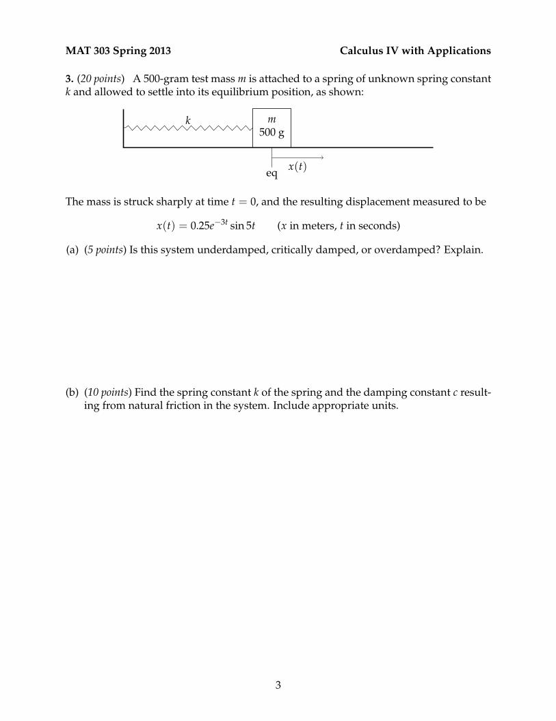
3. (20 points) A 500-gram test mass m is attached to a spring of unknown spring constantk and allowed to settle into its equilibrium position, as shown:

m500 g

k

eq x(t)

The mass is struck sharply at time t = 0, and the resulting displacement measured to be

x(t) = 0.25e−3t sin 5t (x in meters, t in seconds)

(a) (5 points) Is this system underdamped, critically damped, or overdamped? Explain.

(b) (10 points) Find the spring constant k of the spring and the damping constant c result-ing from natural friction in the system. Include appropriate units.

3


(c) (5 points) Suppose we then apply a periodic force f (t) = 10 cos ωt (in newtons) to thespring-mass system, where we may vary the forcing frequency ω. Find the value ofω at which the system exhibits practical resonance, or explain why it does not occur.

4


4. (15 points) Find a particular solution to the nonhomogeneous DE

y(3) − 6y′′ + 12y′ = 40e2x − 24.

5


5. (20 points) Let y1(x) = x and y2(x) = x4.(a) (10 points) Show that y1 and y2 are both solutions to the DE x2y′′ − 4xy′ + 4y = 0.

(b) (5 points) Show that y1 and y2 are linearly independent functions on the entire realline.

6


(c) (5 points) Find the general solution to the nonhomogeneous DE

x2y′′ − 4xy′ + 4y = 6x4 − 9x.

7


Midterm #2 — April 12, 2013, 10:00 to 10:53 AM

Name: Solution Key

Circle your recitation:

R01 (Claudio · Fri) R02 (Xuan ·Wed) R03 (Claudio ·Mon)

• You have a maximum of 53 minutes. This is a closed-book, closed-notes exam. Nocalculators or other electronic aids are allowed.

• Read each question carefully. Show your work and justify your answers for fullcredit. You do not need to simplify your answers unless instructed to do so.

• If you need extra room, use the back sides of each page. If you must use extra paper,make sure to write your name on it and attach it to this exam. Do not unstaple ordetach pages from this exam.

Grading

1 /30

2 /15

3 /20

4 /15

5 /20

Total /100


1. (30 points) Find the general solution to each of the following differential equations:(a) (10 points) y′′ − 4y′ + 3y = 0

Solution: The characteristic equation of this homogeneous, constant-coefficient DE isr2− 4r + 3 = 0, which factors as (r− 1)(r− 3) = 0. Therefore, the roots are r = 1 andr = 3, so the general solution is y = c1ex + c2e3x.

(b) (10 points) y′′ − 4y′ + 4y = 0Solution: The characteristic equation of this DE is r2 − 4r + 4 = 0, which factors as(r− 2)2 = 0. Therefore, the only root is a double root r = 2, so the general solution isy = c1e2x + c2xe2x.

(c) (10 points) y′′ − 4y′ + 5y = 0Solution: The characteristic equation of this DE is r2 − 4r + 5 = 0, which has dis-criminant 42 − 4(1)(5) = −4, and therefore has complex roots. By the quadraticformula, these roots are r = 1

2(4 ±√−4) = 2 ± i, so the general solution is y =

c1e2x cos x + c2e2x sin x.

1


2. (15 points) Two solutions to the DE y′′ − 3y′ − 10y = 0 are y1 = e5x and y2 = e−2x.Find a solution to this DE satisfying the initial conditions y(0) = 7 and y′(0) = 7.

Solution: Since this DE is second-order, homogeneous, and linear, and since y1 and y2 areclearly linearly independent, y(x) = c1e5x + c2e−2x is the general solution to this DE. Wethen match it and its derivative y′(x) = 5c1e5x − 2c2e−2x to the initial conditions at x = 0.We obtain the linear system

c1 + c2 = 7, 5c1 − 2c2 = 7.

Then c2 = 7− c1, so 5c1 − 14 + 2c1 = 7, and c1 = 21/7 = 3. Hence, c2 = 7− 3 = 4, soy(x) = 3e5x + 4e−2x solves this IVP.

2


3. (20 points) A 500-gram test mass m is attached to a spring of unknown spring constantk and allowed to settle into its equilibrium position, as shown:

m500 g

k

eq x(t)

The mass is struck sharply at time t = 0, and the resulting displacement measured to be

x(t) = 0.25e−3t sin 5t (x in meters, t in seconds)

(a) (5 points) Is this system underdamped, critically damped, or overdamped? Explain.Solution: Since the displacement of the mass in this free system takes the form of afunction e−at sin bt, which contains a sinusoidal factor, the system is underdamped.

(b) (10 points) Find the spring constant k of the spring and the damping constant c result-ing from natural friction in the system. Include appropriate units.Solution: We reconstruct the differential equation mx′′ + cx′ + kx = 0 governing themotion. First, since the motion is a multiple of e−3t sin 5t, this DE has complex rootsr = −3± 5i. Therefore, its characteristic equation is a multiple of (r + 3− 5i)(r + 3 +5i) = (r + 3)2 + 52 = r2 + 6r + 34 = 0. The coefficient on the r2-term must be m = 1/2(in mks units), though, so we multiply through by this to obtain 1

2r2 + 3r + 17. Hence,c = 3 N-s/m, and k = 17 N/m.

Many students tried to use the relation ω0 =√

k/m to determine k, but since damp-ing is present in the system, ω0 does not come directly from the frequency of thesine factor in the displacement, and therefore is not 5 rad/s. The frequency in thedisplacement is instead ω1, and ω2

0 = ω21 + p2, where p = 3 is the exponent in the

displacement’s exponential factor e−pt.

3


(c) (5 points) Suppose we then apply a periodic force f (t) = 10 cos ωt (in newtons) to thespring-mass system, where we may vary the forcing frequency ω. Find the value ofω at which the system exhibits practical resonance, or explain why it does not occur.Solution: We recall that, as a function of ω and the parameters m, c, k, and F0, theamplitude of the steady-state solution is

C(ω) =F0√

(k−mω2)2 + (cω)2.

(We can arrive at this solution by assuming a steady periodic displacement of the formA cos ωt + B sin ωt; see pp. 219–220 for details.) By minimizing the denominator,

we can show that, if c2 < 2km, C(ω) has a maximum at ωm =

√2km− c2

2m2 . Since

c2 = 32 = 9 and 2km = 2(17)(12) = 17, c is small enough for practical resonance to

occur at

ωm =

√2km− c2

2m2 =

√17− 9

2(1/2)2 =√

16 = 4rad

s.

4


4. (15 points) Find a particular solution to the nonhomogeneous DE

y(3) − 6y′′ + 12y′ = 40e2x − 24.

Solution: From the form of the forcing term 40e2x − 24, we expect the particular solutionto contain terms corresponding to the roots r = 2 (from the e2x) and r = 0 (from theconstant term). Before we construct our guess, though, we must also check whether theseroots also contribute to the complementary solution. The characteristic equation for theassociated homogeneous DE is

r3 − 6r2 + 12r = r(r2 − 6r + 12) = 0,

which then has r = 0 as a single root. We check for overlap with r = 2: since (2)2− 6(2) +12 = 4− 12 + 12 = 4 6= 0, 2 is not a root. Hence, to avoid overlaps on r = 0, we guess aparticular solution of the form

y = Ae2x + Bx.

(Notice we have shifted only the constant term by a power of x, and not the non-overlappinge2x term.) Then y′ = 2Ae2x + B, y′′ = 4Ae2x, and y′′′ = 8Ae2x, which we plug into thenonhomogeneous DE:

8Ae2x − 6(4Ae2x) + 12(2Ae2x + B) = 40e2x − 24.

Simplifying, 8Ae2x + 12B = 40e2x − 24, so 8A = 40 and 12B = −24. Then A = 5 andB = −2, so a particular solution is

y = 5e2x − 2x.

5


5. (20 points) Let y1(x) = x and y2(x) = x4.(a) (10 points) Show that y1 and y2 are both solutions to the DE x2y′′ − 4xy′ + 4y = 0.

Solution: We compute the first and second derivatives of these functions:

y′1 = 1, y′′1 = 0, y′2 = 4x3, y′′2 = 12x2.

Plugging these into the homogeneous DE,

x2y′′1 − 4xy′1 + 4y1 = x2(0)− 4x(1) + 4(x) = −4x + 4x = 0,

x2y′′2 − 4xy′2 + 4y2 = x2(12x2)− 4x(4x2) + 4(x4) = (12− 16 + 4)x4 = 0.

(b) (5 points) Show that y1 and y2 are linearly independent functions on the entire realline.Solution: We compute the Wronskian W(x) of y1 and y2:

W(y1, y2)(x) =∣∣∣∣y1 y2y′1 y′2

∣∣∣∣ = ∣∣∣∣x x4

1 4x3

∣∣∣∣ = 4x4 − x4 = 3x4.

Since this function is nonzero on the real line (in fact, everywhere but x = 0), thesefunctions are linearly independent.

6


(c) (5 points) Find the general solution to the nonhomogeneous DE

x2y′′ − 4xy′ + 4y = 6x4 − 9x.

Solution: We use variation of parameters to solve this nonhomogeneous DE. First, wewrite the normalized version of the DE, dividing by x2 to obtain

y′′ − 4x

y′ +4x2 y = 6x2 − 9x−1.

Then f (x) = 6x2− 9x−1, which we include in the formula for variation of parameters:

y = −y1

∫ y2(x) f (x)W(x)

dx + y2

∫ y1(x) f (x)W(x)

dx

= −x∫ x4(6x2 − 9x−1)

3x4 dx + x4∫ x(6x2 − 9x−1)

3x4 dx

= −x∫

2x2 − 3x

dx + x4∫ 2

x− 3

x4 dx

= −x(

23

x3 − 3 ln x)+ x4(2 ln x + x−3)

= 3x ln x− 23

x4 + 2x4 ln x + x.

The general solution to the homogeneous equation is yc = c1y1 + c2y2 = c1x + c2x4,so adding this to the particular solution above produces the general solution to thenonhomogeneous equation:

y = c1x + c2x4 + 3x ln x− 23

x4 + 2x4 ln x + x = C1x + C2x4 + 3x ln x + 2x4 ln x,

where C1 = c1 + 1 and C2 = c2− 23 are new arbitrary constants that absorb the y1 and

y2 terms coming from the integration. (We also observe that if we had included theconstants of integration, we would have obtained the general solution directly fromthe variation of parameters formula.)

7

MAT 303 - HW10 - Additional Problemsdue Friday, December 2All homework problems are mandatory!

Exercise 1. Consider the system of differential equations x ′ = Ax, where A =

λ 0 0

0 λ 1

0 0 λ

and

λ is an arbitrary real number.

a) Compute A2 and A3. Use an inductive argument to show that An =

λn 0 0

0 λn nλn−1

0 0 λn

.

b) Determine the exponential eAt using the computations in part a).

c) Find the exponential eAt by first writing A as a sum of a diagonal matrix and a nilpotentmatrix A = λI3 + C, then computing eAt as a product of two exponential matrices eλI3teCt.

d) Find the general solution of the system x ′ = Ax using the exponential eAt.

e) Find the eigenvalues and eigenvectors of the matrix A.

f) Find the general solution of the system x ′ = Ax using part e), then compare it to the answeryou got for part d).

Exercise 2. Consider the system of differential equations x ′ = Bx, where B =

λ 1 0

0 λ 1

0 0 λ

and λ

is an arbitrary real number.

a) ComputeB2, B3. Use an inductive argument to show thatBn =

λn nλn−1n(n−1)2 λn−2

0 λn nλn−1

0 0 λn

.

b) Determine the exponential eBt using part a).

c) Find the exponential eBt, using a different approach: write B as a sum of a scalar multiple ofthe identity matrix and a nilpotent matrix B = λI3 + C. Then use the fact that eBt = eλI3teCt.

d) Find the general solution of the system x ′ = Bx using the exponential matrix eBt.

e) Find the eigenvalues and eigenvectors of the matrix B.

f) Find the general solution of the system x ′ = Bx using part e), then compare it to the answeryou got for part d).


Lecture Notes - Friday, December 2

Let A be an n× n matrix. Let λ1 be an eigenvalue of A. Let’s recall first some definitions:

Algebraic Multiplicity: The algebraic multiplicity of λ1 is the number of times the factorλ− λ1 appears in the characteristic polynomial p(λ) = det(A− λIn).

Geometric Multiplicity: The geometric multiplicity of λ1 is the maximum number oflinearly independent eigenvectors corresponding to the eigenvalue λ1.

Defect: The defect of the eigenvalue λ1 is equal to the Algebraic Multiplicity of λ1 minusits Geometric Multiplicity.

Invertible: An n × n square matrix S is called invertible if there exists an n × n matrixS−1, called the inverse of S, such that S−1S = SS−1 = In.

It can be shown that S is invertible if and only if the determinant of S is different from0. It can also be shown that if S is invertible, then its inverse S−1 is unique.

The inverse of a 2× 2 matrix: If S =

(a bc d

)and det(S) = ad− bc 6= 0, then

S−1 =1

det(S)

(d −b−c a

).

DiagonalizationTheorem : Let A be an n×n matrix. Let λ1, λ2, . . . , λn be the eigenvaluesof A (not necessarily distinct). Assume that all eigenvalues of A have algebraic multiplic-ity equal to their geometric multiplicity. Then A has n linearly independent eigenvectorsv1, . . . , vn. If we denote by S the matrix whose columns are the eigenvectors v1, . . . , vn, thenS is an invertible matrix, and

S−1AS = D,

where D =

λ1 0 . . . 00 λ2 . . . 0. . . . . . . . . . . .0 0 0 λn

is a diagonal matrix whose diagonal entries are precisely

the eigenvalues of A. We say that A is a diagonalizable matrix.

Remark: It can be shown that if A has repeated eigenvalues with geometric multiplicitydifferent from the algebraic multiplicity (so A has fewer than n eigenvectors!), then A cannotbe diagonalized. It is still possible however to transform A into a nearly diagonal matrixcalled the Jordan canonical form.Remark: Matrix multiplication is not commutative in general! Hence S−1AS is not the

same as AS−1S = AIn = A!

1

Jordan Block: Let λ be an eigenvalue of some matrix A. An m×m matrix B is called aJordan block of size m corresponding to λ if

B =

λ 1 0 0 . . . 00 λ 1 0 . . . 0. . . . . . . . . . . . . . . . . .0 0 . . . λ 1 00 0 . . . 0 λ 10 0 . . . 0 0 λ

, (1)

that is, the entries on the main diagonal of B are all equal to λ, and the entries right abovethe main diagonal are equal to 1. All the other entries are equal to 0.

The exponential matrix of a Jordan Block: If B has the form from Equation (1), then

eBt = eλt

1 tt2

2

t3

3!. . .

tm−1

(m− 1)!

0 1 tt2

2. . .

...

. . . . . . . . . . . . . . ....

0 0 . . . 1 tt2

20 0 . . . 0 1 t0 0 . . . 0 0 1

Proof. To make the computations easier, let’s give the proof for m = 4. The Jordan block

can be written as B = λI4 + C, where C =

0 1 0 00 0 1 00 0 0 10 0 0 0

is a nilpotent matrix. The

matrix C has the property that C2 =

0 0 1 00 0 0 10 0 0 00 0 0 0

, C3 =

0 0 0 10 0 0 00 0 0 00 0 0 0

, C4 = 04.

The matrix exponential eCt can be computed as

eCt = I4 +∞∑n=1

Cntn

n!= I4 + Ct+ C2 t

2

2+ C3 t

3

3!=

1 t t2/2 t3/3!0 1 t t2/20 0 1 t0 0 0 1

The matrix D = λI4 has the property that Dn = I4λ

n for every n > 0. Therefore

eDt = I4 +∞∑n=1

Dntn

n!= I4 +

∞∑n=1

I4λntn

n!= I4(1 +

∞∑n=1

λntn

n!) = I4e

λt

2

In conclusion eBt = eλI4t+Ct = eDteCt = eDtI4eλt = eDteλt = eλt

1 t t2/2 t3/3!0 1 t t2/20 0 1 t0 0 0 1

.

�

Examples:

a) If B = (λ) is a Jordan block of size 1, then eBt = eλt (1) =(eλt).

a) If B =

(λ 10 λ

), then eBt = eλt

(1 t0 1

).

c) B =

5 1 0 00 5 1 00 0 5 10 0 0 5

, eBt = e5t

1 t

t2

2

t3

3!

0 1 tt2

20 0 1 t0 0 0 1

=

e5t te5t t2e5t/2 t3e5t/60 e5t te5t t2e5t/20 0 e5t te5t

0 0 0 e5t

.

Jordan Canonical Form Theorem :Let A be any n× n matrix. There exists an invertible matrix S such that

S−1AS = J, where J =

J1 0

J2. . .

0 Js

(2)

J is a block diagonal matrix, where J1, J2, . . . , Js are Jordan blocks corresponding to theeigenvalues of A, as in Equation (1). The columns of the matrix S are chosen as follows: Eachcolumn of S that corresponds to the first column of each Jordan block Jk is an eigenvectorvk of A. The rest of the columns are generalized eigenvectors.

Remarks: An eigenvalue can produce several Jordan blocks (the number of Jordan blocksfor one eigenvalue is equal to the geometric multiplicity of the eigenvalue). The size of oneJordan block is equal to the length of a chain of generalized eigenvectors.

Examples: Let A be a 2× 2 matrix.

a) If A has a repeated eigenvalue λ1 with algebraic and geometric multiplicity 2, then its

Jordan canonical form is the diagonal matrix J =

(λ1 00 λ1

). In this case, J has two

Jordan blocks, each of size 1.

b) If A has a repeated eigenvalue λ1 with algebraic multiplicity 2, and geometric multi-

plicity 1 then its Jordan canonical form is the block diagonal matrix J =

(λ1 10 λ1

).

The Jordan matrix has a single Jordan block, of size 2.

3

Examples: Let A be a 7× 7 matrix. Assume that A has eigenvalues λ (with algebraic mul-tiplicity 2 and geometric multiplicity 1) and µ (with algebraic multiplicity 5 and geometricmultiplicity 2). Matrix A has 3 linearly independent eigenvectors v1, w1, u1: one correspond-ing to the eigenvalue λ, and two corresponding to the eigenvalue µ. Assume that after doingsome computations, we found 3 chains of generalized eigenvectors

{v1, v2}, where (A− λI7)v1 = 0, (A− λI7)v2 = v1

{w1, w2}, where (A− µI7)w1 = 0, (A− µI7)w2 = w1

{u1, u2, u3}, where (A− µI7)u1 = 0, (A− µI7)u2 = u1, (A− µI7)u3 = u2

If we let S be the 7× 7 matrix with columns S = [v1, v2, w1, w2, u1, u2, u3], then

S−1AS =

λ 1 0 0 0 0 00 λ 0 0 0 0 00 0 µ 1 0 0 00 0 0 µ 0 0 00 0 0 0 µ 1 00 0 0 0 0 µ 10 0 0 0 0 0 µ

(3)

This is the Jordan canonical form of A. It has 3 Jordan blocks, one corresponding to theeigenvalue λ, and two corresponding to the eigenvalue µ. The canonical form is unique upto permutations of the Jordan blocks. If we write the columns of S is a different order, forexample S = [v1, v2, u1, u2, u3, w1, w2], we get

S−1AS =

λ 1 0 0 0 0 00 λ 0 0 0 0 00 0 µ 1 0 0 00 0 0 µ 1 0 00 0 0 0 µ 0 00 0 0 0 0 µ 10 0 0 0 0 0 µ

(4)

Applications of the Jordan canonical form: Assume that S−1AS = J , where J is theJordan canonical form.

1. Exponential of a Jordan matrix: If J1, . . . Js are the Jordan blocks of J , then

eJt =

eJ1t 0

eJ2t

. . .0 eJst

.

The exponential matrix of each block can then be computed as in Equation (1).

2. Computing powers of the matrix A: It can be easily seen that A = SJS−1 and soAn = S−1JnS for every n > 0.

4

3. Finding the exponential matrix of A: eAt = SeJtS−1. Indeed,

eAt =∞∑n=0

Antn

n!=∞∑n=0

(SJnS−1)tn

n!= S(

∞∑n=0

Jntn

n!)S−1 = SeJtS−1.

4. Solving the system of differential equations x′ = Ax: The general solution of thesystem x′ = Ax is given by x(t) = eAtc, where c is a vector of coefficients. If J is the Jordancanonical form of A, then the solution can also be written as:

x(t) = SeJtS−1c = SeJtc,

where c = S−1c is a new vector of random constants. The matrix Φ(t) = SeJt is thereforea fundamental matrix of the system x′ = Ax. When solving the system x′ = Ax we preferto work with the fundamental matrix Φ(t) because it does not require finding the inverse ofthe matrix S, unlike eAt.

5. Reducing a system of differential equations Consider the system of differentialequations

x′ = Ax. (5)

We do the variable substitution x = Sy, which gives x′ = Sy′ and obtain the equivalentsystem

Sy′ = ASy

After multiplication by S−1, we end up with

y′ = S−1ASy = Jy (6)

A fundamental matrix of the system y′ = Jy is eJt. The general solution is then y(t) = eJtc.Since the relation between Systems (5) and (6) is given by the substitution x = Sy, it followsthat the general solution of System (5) is x(t) = Sy(t) = SeJtc. Therefore Φ(t) = SeJt is afundamental matrix for System (5).

Solving a nonhomogeneous system x′ = Ax+f(t) : As proven in class, using integratingfactors, the general solution is given by the Variation of Parameters formula:

x(t) = eAt∫e−Atf(t)dt = Φ(t)

∫Φ−1(t)f(t)dt,

where Φ(t) is any fundamental matrix of x′ = Ax.

Example 1: Based on Exercise 5.5.26 from the textbook. We will solve the system x′ = Ax,

where A =

5 −1 11 3 0−3 2 1

using two different methods.

5

Solution. The eigenvalues of A are the roots of the characteristic polynomial

p(λ) =

∣∣∣∣∣∣5− λ −1 1

1 3− λ 0−3 2 1− λ

∣∣∣∣∣∣ =

∣∣∣∣∣∣5− λ −1 1− 1

1 3− λ 0 + (3− λ)−3 2 (1− λ) + 2

∣∣∣∣∣∣ =

∣∣∣∣∣∣5− λ −1 0

1 3− λ 3− λ−3 2 3− λ

∣∣∣∣∣∣=

∣∣∣∣∣∣5− λ −1 0

1− (−3) (3− λ)− 2 (3− λ)− (3− λ)−3 2 3− λ

∣∣∣∣∣∣ =

∣∣∣∣∣∣5− λ −1 0

4 1− λ 0−3 2 3− λ

∣∣∣∣∣∣= (3− λ)

∣∣∣∣ 5− λ −14 1− λ

∣∣∣∣ = (3− λ) ((5− λ)(1− λ) + 4) = (3− λ)(9− 6λ+ λ2) = (3− λ)3.

Therefore λ = 3 is the only eigenvalue of A, and it has algebraic multiplicity 3. To find itsgeometric multiplicity, we solve the equation

(A− 3I3)v = 0, where v =

abc

.

This gives 2 −1 11 0 0−3 2 −2

abc

=

000

,

which gives the system of equations:

2a− b+ c = 0

a = 0

−3a+ 2b− 2c = 0

The third equation is redundant. The first equation gives c = b. Therefore, all eigenvectorscorresponding to the eigenvalue λ = 3 are of the form

v =

0bb

= b

011

All eigenvectors are therefore scalar multiples of the eigenvector v1 =

011

and they

belong to the line spanned by v1 in R3. Since we can find at most one linearly independenteigenvector, it follows that the geometric multiplicity of λ = 3 is 1.

We need to find two generalized eigenvectors v2 and v3, starting from v1,by successivelysolving the equations

(A− 3I3)v2 = v1 (7)

(A− 3I3)v3 = v2. (8)

6

{v1, v2, v3} will then be a chain of length 3 for the eigenvalue λ. For Equation (7), we solve 2 −1 11 0 0−3 2 −2

abc

=

011

,

and get the system

2a− b+ c = 0

a = 1

−3a+ 2b− 2c = 1

which reduces to a = 1 and c = b − 2. Therefore, v2 =

1b

b− 2

= b

011

+

10−2

.

The first term of the sum can be ignored, because it is an eigenvector of A, and we can

choose v2 =

10−2

.

We now solve Equation (8). 2 −1 11 0 0−3 2 −2

abc

=

10−2

,

which gives the system

2a− b+ c = 1

a = 0

−3a+ 2b− 2c = −2

which is equivalent to a = 0 and c = b+1. Hence v2 =

0b

b+ 1

= b

011

+

001

. The

first term can be ignored since it is an eigenvector of A, so we choose the second generalized

eigenvector to be v3 =

001

.

We have obtained three linearly independent vectors, forming a chain of length 3:

{v1, v2, v3} =

0

11

,

10−2

,

001

Now we go back to solving the system x′ = Ax.

7

Method 1: Three linearly independent solutions can be found by setting

x1(t) = e3tv1 = e3t

011

x2(t) = e3t(v2 + tv1) = e3t

1t

−2 + t

x3(t) = e3t(v3 + tv2 +

t2

2v1) = e3t

tt2/2

1− 2t+ t2/2

The general solution is x(t) = c1x1(t) + c2x2(t) + c3x3(t), where c1, c2, c3 are realnumbers. In expanded form this gives:

x(t) = e3t

c2 + c3t

c1 + c2t+ c3t2

2

c1 + c2(t− 2) + c3(t2

2− 2t+ 1)

.

Method 2: Consider the matrix S = [v1, v2, v3] =

0 1 01 0 01 −2 1

.

Since A has a repeated eigenvalue λ = 3, with algebraic multiplicity 3, and geometricmultiplicity 1, the Jordan canonical form J of A will contain a single Jordan block:

J =

3 1 00 3 10 0 3

Then eJt = eλt

1 tt2

20 1 t0 0 1

, so a fundamental matrix for x′ = Ax is given by

Φ(t) = SeJt =

0 1 01 0 01 −2 1

eλt

1 tt2

20 1 t0 0 1

= eλt

0 1 t

1 tt2

2

1 t− 2t2

2− 2t+ 1

.

The general solution of x′ = Ax is given by

x′ = Φ(t)c = Φ(t)

c1c2c3

= eλt

c2 + c3t

c1 + c2t+ c3t2

2

c1 + c2(t− 2) + c3(t2

2− 2t+ 1)

8

Example 2: Based on Exercise 5.5.16 in the textbook. Solve the system x′ = Ax, where

A =

1 0 0−2 −2 −32 3 4

, in two different ways.

Solution. The characteristic polynomial of A is

p(λ) =

∣∣∣∣∣∣1− λ 0 0−2 −2− λ −32 3 4− λ

∣∣∣∣∣∣ = (1−λ)

∣∣∣∣ −2− λ −33 4− λ

∣∣∣∣ = (1−λ)((−2−λ)(4−λ)+9) = (1−λ)3.

The matrix A has a single eigenvalue λ = 1, with algebraic multiplicity 3. To find theeigenvectors corresponding to the eigenvalue λ = 1 we solve the system (A− I3)v = 0: 0 0 0

−2 −3 −32 3 3

abc

=

000

=⇒ 2a+ 3b+ 3c = 0 =⇒ c = −2

3a− b

=⇒ v =

ab

−2

3a− b

= a

10

−2

3

+ b

01−1

,

where a and b are random constants. Because it’s more convenient to work with integernumbers, we can also write

v = a

30−2

+ b

01−1

,

where a := a/3 and b are any random constants. All eigenvectors belong to a plane in R3,spanned by the linearly independent eigenvectors

v =

30−2

and w =

01−1

,

hence the eigenvalue λ = 1 has geometric multiplicity 2.We need to find one more generalized eigenvector u, starting from either v or w.

Starting from v: Find u such that (A− I3)u = v. This condition implies 0 0 0−2 −3 −32 3 3

abc

=

30−2

=⇒ 0a+ 0b+ 0c = 3 =⇒ 0 = 3,

which is a contradiction, hence there does not exist any generalized eigenvector u that solves(A− I3)u = v. It means that {v} is a chain of length 1.Starting from w: Find u such that (A− I3)u = w. This condition implies 0 0 0

−2 −3 −32 3 3

abc

=

01−1

=⇒ 2a+ 3b+ 3c = −1 =⇒ c = −1

3− 2

3a− b

9

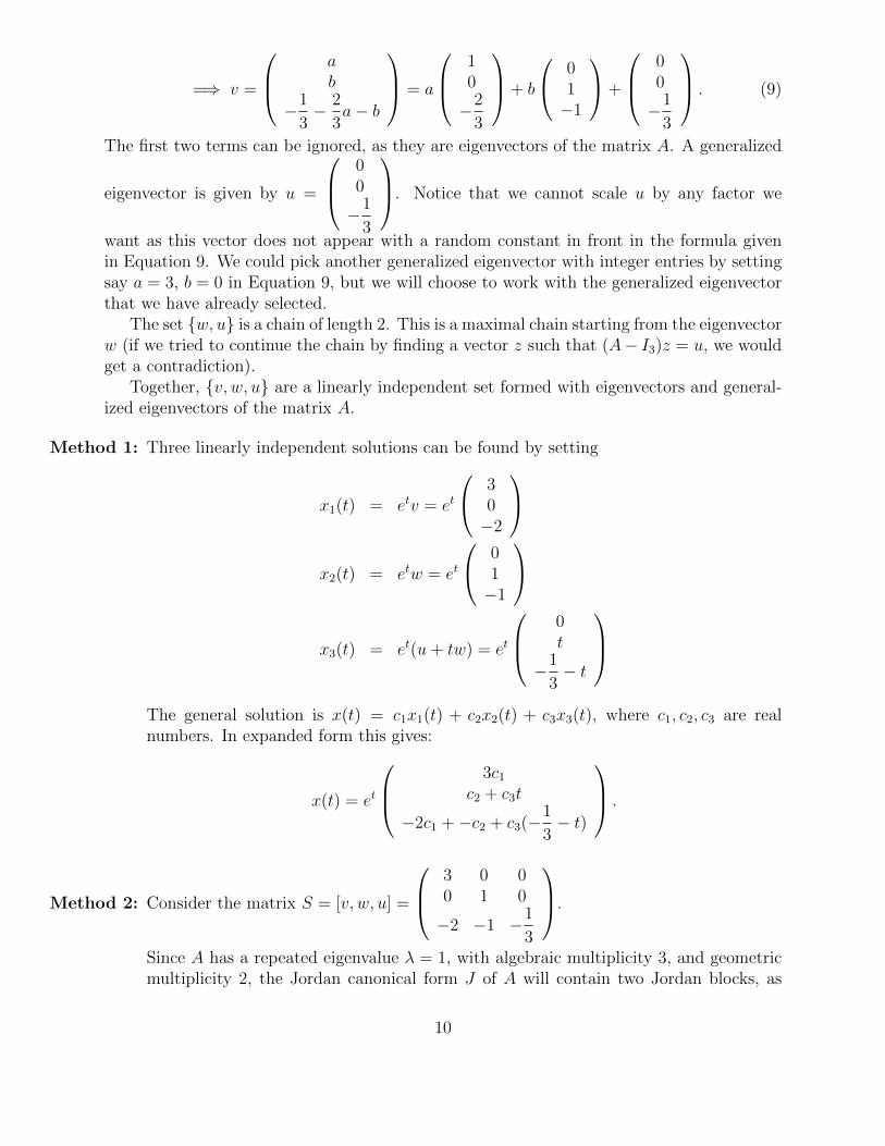
=⇒ v =

ab

−1

3− 2

3a− b

= a

10

−2

3

+ b

01−1

+

00

−1

3

. (9)

The first two terms can be ignored, as they are eigenvectors of the matrix A. A generalized

eigenvector is given by u =

00

−1

3

. Notice that we cannot scale u by any factor we

want as this vector does not appear with a random constant in front in the formula givenin Equation 9. We could pick another generalized eigenvector with integer entries by settingsay a = 3, b = 0 in Equation 9, but we will choose to work with the generalized eigenvectorthat we have already selected.

The set {w, u} is a chain of length 2. This is a maximal chain starting from the eigenvectorw (if we tried to continue the chain by finding a vector z such that (A− I3)z = u, we wouldget a contradiction).

Together, {v, w, u} are a linearly independent set formed with eigenvectors and general-ized eigenvectors of the matrix A.

Method 1: Three linearly independent solutions can be found by setting

x1(t) = etv = et

30−2

x2(t) = etw = et

01−1

x3(t) = et(u+ tw) = et

0t

−1

3− t

The general solution is x(t) = c1x1(t) + c2x2(t) + c3x3(t), where c1, c2, c3 are realnumbers. In expanded form this gives:

x(t) = et

3c1c2 + c3t

−2c1 +−c2 + c3(−1

3− t)

.

Method 2: Consider the matrix S = [v, w, u] =

3 0 00 1 0

−2 −1 −1

3

.

Since A has a repeated eigenvalue λ = 1, with algebraic multiplicity 3, and geometricmultiplicity 2, the Jordan canonical form J of A will contain two Jordan blocks, as

10

follows: the first Jordan block is of size 1, corresponding to the chain formed by {v},whereas the second Jordan block corresponds to the chain {w, u} and has size 2. TheJordan canonical form of the matrix A is therefore

J =

1 0 00 1 10 0 1

Then eJt = eλt

1 0 00 1 t0 0 1

, so a fundamental matrix for x′ = Ax is given by

Φ(t) = SeJt =

3 0 00 1 0

−2 −1 −1

3

eλt

1 0 00 1 t0 0 1

= eλt

3 0 00 1 t

−2 −1 −t− 1

3

.

The general solution of x′ = Ax is given by

x′ = Φ(t)c = Φ(t)

c1c2c3

= eλt

3c1c2 + c3t

−2c1 − c2 + c3(−t−1

3)

.

11

MAT 303: Calculus IV with Applications

Homework 11 - Instructions

HW 11 contains only two exercises from Section 5.7 and several exercises from Section 6.2 of thetextbook. Please read the lecture notes and browse the Mathematica tutorial before getting started.Please solve Exercises 5.7.24 and 5.7.31 completely, as follows:

1) Please compute the exponential of matrix A, given in the problem, both analytically and byusing Mathematica. Analytically, this can be done as in the examples from the lecture notes:

a) find the eigenvalues of the matrix, and their geometric and algebraic multiplicities. Writethe Jordan canonical form J of A.

b) Use the formula for the exponential of a Jordan block to compute eJt.

c) Find a complete set of eigenvectors and generalized eigenvectors for A, and write themcolumnwise (in the proper order) in a matrix S, as in the Lecture Notes. At this moment,you know that S−1AS = J .

d) Compute Φ(t) = SeJt and eAt = SeJtS−1. Both Φ(t) and eAt are fundamental matricesof the homogeneous system x′ = Ax.

2) Find the solution of the nonhomogeneous system by using the method of Variation of Param-eters. Two equivalent (but not identical ways) of writing the solution are:

x(t) = eAt

∫e−Atf(t)dt

x(t) = Φ(t)

∫Φ(t)−1f(t)dt.

Here we take the most general antiderivative of the integrand,

∫g(t)dt = G(t) + c. If we

keep the constant of integration c, then x(t) is the general solution of the nonhomogeneoussystem. If we ignore the constant of integration c, then we get a particular solution of thenonhomogeneous system. If we have an initial condition in the problem, like x(t0) = x0, thenwe can obtain the unique solution as

x(t) = eAt

(x0 +

∫ t

t0

e−Asf(s)ds

)= Φ(t)

(Φ−1(t0)x0 +

∫ t

t0

Φ(s)−1f(s)ds

).

Use Mathematica to check the computations. You will need the functions MatrixExp[..] andIntegrate[..], as in the tutorial. Matrix Multiplication in Mathematica is a dot ”.”

For the problems from Section 6.2, use Mathematica as instructed in the textbook.

1

MAT 303 - Calculus IV - Stony Brook Mathematics

Documents

Transcript of MAT 303 - Calculus IV - Stony Brook Mathematics