Variants of Turing Machines - Stony Brook Computer Science

Variants of Turing Machines

Variants of Turing Machines – p.1/49

Robustness

� Robustness of a mathematical object (suchas proof, definition, algorithm, method, etc.) ismeasured by its invariance to certain changes

� To prove that a mathematical object is robustone needs to show that it is equivalent with itsvariants

Question: is the definition of a Turing machine ro-

bust?


TM definition is robust

� Variants of TM with multiple tapes or withnondeterminism abound

� Original model of a TM and its variants allhave the same computation power, i.e., theyrecognize the same class of languages.

Hence, robustness of TM definition is measured

by the invariance of its computation power to cer-

tain changes


Example of robustness

Note: transition function of a TM in our definitionforces the head to move to the left or right aftereach step. Let us vary the type of transitionfunction permitted.

� Suppose that we allow the head to stay put,i.e.;

��

�

� Does this feature allow TM to recognizeadditional languages? Answer: NOSketch of proof:

1. An

transition can be represented by two transitions: one thatmove to the left followed by one that moves to the right.

2. Since we can convert a TM which stay put into one that hasno this facility the answer is No.


Equivalence of TMs

To show that two models of TM are equivalent we

need to show that we can simulate one by an-

other.


Multitape Turing Machines

A multitape TM is like an ordinary TM withseveral tapes

� Each tape has its own head forreading/writing

� Initially the input is on tape 1 and other areblank

� Transition function allow for reading, writing,and moving the heads on all tapessimultaneously, i.e.,

��

� � �

� � ��

�

where

�

is the number of tapes.Variants of Turing Machines – p.6/49

Formal expression

� � ��

��

� ��

��

� � � � � �

� �

��

� �

means that:

if the machine is in state � � and heads 1 through k are

reading symbols � � through � � the machine goes to

state � , writes

� through

� on tapes 1 through k re-

spectively and moves each head to the left or right as

specified by�


Theorem (3.8) 3.13

Every multitape Turing machine has anequivalent single tape Turing machine.

Proof: we show how to convert a multitape TM

into a single tape TM

�

. The key idea is to show

how to simulate with�


Simulating with

Assume that has

�

tapes

�

�

simulates the effect of

�

tapes by storingtheir information on its single tape

�

�

uses a new symbol as a delimiter toseparate the contents of different tapes

�

�

keeps track of the location of the heads bymarking with a � the symbols where theheads would be.


Example simulation

Figure 1 shows how to represent a machinewith 3 tapes by a machine

�

with one tape.

S�

000�� 0 1 0

�

b

��

� �� a

�

� � �

M

b a

� � �

b a

� � �

0 1 0 1 0

� � �

Figure 1: Multitape machine simulation


General construction

�

= "On input � � � � ��

��

1. Put

��

in the format that represents ��

:

� �� 2. Scan the tape from the first

�

(which represent the left-hand end)to the

� ��

-st

�

(which represent the right-hand end) todetermine the symbols under the virtual heads. Then

makesthe second pass over the tape to update it according to the way

’s transition function dictates.

3. If at any time

moves one of the virtual heads to the right of

�

itmeans that

has moved on the corresponding tape onto the

unread blank portion of that tape. So,

shifts the tape contentsfrom this cell until the rightmost

�

, one unit to the right, and thenwrites a

�on the free tape cell thus obtained. Then it continues to

simulates as before".Variants of Turing Machines – p.11/49

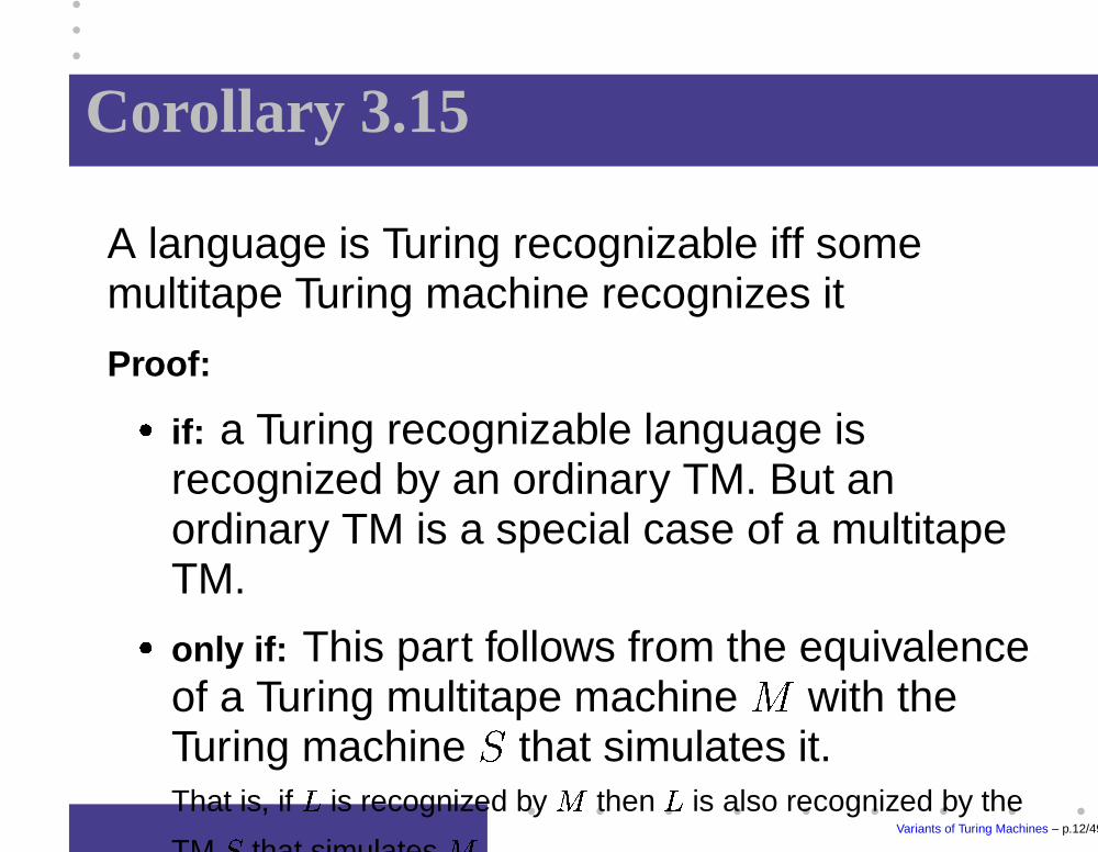
Corollary 3.15

A language is Turing recognizable iff somemultitape Turing machine recognizes it

Proof:

� if: a Turing recognizable language isrecognized by an ordinary TM. But anordinary TM is a special case of a multitapeTM.

� only if: This part follows from the equivalenceof a Turing multitape machine with theTuring machine

�

that simulates it.That is, if

�

is recognized by

then

�

is also recognized by the

TM

that simulates


Nondeterministic TM

� A NTM is defined in the expected way: at anypoint in a computation the machine mayproceed according to several possibilities

� Formally,

��

�

� Computation performed by a NTM is a treewhose branches correspond to differentpossibilities for the machine

� If some branch of the computation tree leadsto the accept state, the machine accepts theinput


Theorem 3.16

Every nondeterministic Turing machine, , hasan equivalent deterministic Turing machine, .

Proof idea: show that a NTM can be simulatedwith a DTM .

Note: in this simulation tries all possible

branches of ’s computation. If ever finds the

accept state on one of these branches then it ac-

cepts. Otherwise simulation will not terminate


More on NTM simulation

� ’s computation on an input � is a tree,

� � �

.

� Each branch of

� � �

represents one of thebranches of the nondeterminism

� Each node of

� � �

is a configuration of .

� The root of

� � �

is the start configuration

Note: searches

� � �

for an accepting configu-

ration


A tempting bad idea

Design to explore

� � �

by a depth-first searchNote:

�

A depth-first search goes all the way down on one branch beforebacking up to explore next branch.

�

Hence,

�

could go forever down on an infinite branch and miss anaccepting configuration on an other branch


A better idea

Design to explore the tree by using abreadth-first searchNote:

�

This strategy explores all branches at the same depth beforegoing to explore any branch at the next depth.

�

Hence, this method guarantees that

�

will visit every node of

� � � � until it encounters an accepting configuration


Formal proof

has three tapes, Figure 2:

1. Tape 1 always contains the input and is neveraltered

2. Tape 2 (called the simulation tape) maintains a copyof ’s tape on some branch of itsnondeterministic computation

3. Tape 3 (called address tape) keeps track of ’slocation in ’s nondeterministic computationtree


Deterministic simulation of

D

1 2 3 3 2 3 1 2 1 1 3

� � �

address tape

x x

�

1 x

� � �

simulation tape

0 0 1 0

� � �

input tape

�

�

Figure 2: Deterministic TM D simulating N


Address tape

� Every node in

� � �

can have at most

children, where

is the size of the largest setof possible choices given by ’s transitionfunction

� Hence, to every node we assign an addressthat is a string in the alphabet

� ��

�

��

.

� Example: we assign the address 231 to the node reached by

starting at the root, going to its second child and then going to that

node’s third child and then going to that node’s first child


Note

�

Each symbol in a node address tells us which choice to make nextwhen simulating a step in one branch in

�

’s nondeterministiccomputation

�

Sometimes a symbol may not correspond to any choice if too fewchoices are available for a configuration. In that case the addressis invalid and doesn’t correspond to any node

�

Tape 3 contains a string over�� which represents a branch of

�

’scomputation from the root to the node addressed by that string,unless the address is invalid.

�

The empty string � is the address of the root.


The description of

1. Initially tape 1 contains � and tape 2 and 3 are empty

2. Copy tape 1 over tape 2

3. Use tape 2 to simulate

�

with input � on one branch of itsnondeterministic computation.

�

Before each step of

�

, consult the next symbol on tape 3 todetermine which choice to make among those allowed by

�

’stransition function

�

If no more symbols remain on tape 3 or if this nondeterministicchoice is invalid, abort this branch by going to stage 4.

�

If a rejecting configuration is reached go to stage 4; if anaccepting configuration is encountered, accept the input

4. Replace the string on tape 3 with the lexicographically next stringand simulate the next branch of

�

’s computation by going tostage 2.


Corollary 3.17

A language is Turing-recognizable iff somenondeterministic TM recognizes it

Proof:

� if: If a language is Turing-recognizable it is recognized by a DTM.Any deterministic TM is automatically anondeterministic TM.

� only if: If language is recognized by a NTM then it is

Turing-recognizable.This follow from the fact that any NTM can besimulated by a DTM.


Corollary 3.19

A language is decidable iff some NTM decides itSketch of a proof:

�

if: If a language

�

is decidable, it can be decided by a DTM. Sincea DTM is automatically a NTM, it follows that if L is decidable it isdecidable by a NTM.

�

only if: If a language

�

is decided by a NTM

�

it is decidable. Thismeans that

� � � � �

that decides

�

.

� �

runs the same algorithmas in the proof of theorem 3.16 with an addition stage:reject if all branches of nondeterminism of

�

are exhausted.


The description of

�

1. Initially tape 1 contains � and tape 2 and 3 are empty

2. Copy tape 1 over tape 2

3. Use tape 2 to simulate

�

with input � on one branch of itsnondeterministic computation.

�

Before each step of

�

, consult the next symbol on tape 3 todetermine which choice to make among those allowed by

�

’s

�

.

�

If no more symbols remain on tape 3 or if this nondeterministicchoice is invalid, abort this branch by going to stage 4.

�

If a rejecting configuration is reached go to stage 4; if anaccepting configuration is encountered, accept the input

4. Replace the string on tape 3 with the lexicographically next stringand simulate the next branch of

�

’s computation by going tostage 2.

5. Reject if all branches of are exhausted.


�

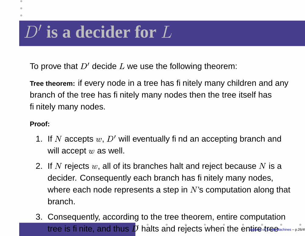
is a decider for

To prove that

� �

decide

�

we use the following theorem:

Tree theorem: if every node in a tree has finitely many children and anybranch of the tree has finitely many nodes then the tree itself hasfinitely many nodes.

Proof:

1. If

�

accepts �, � �

will eventually find an accepting branch andwill accept � as well.

2. If

�

rejects �, all of its branches halt and reject because

�

is adecider. Consequently each branch has finitely many nodes,where each node represents a step in

�

’s computation along thatbranch.

3. Consequently, according to the tree theorem, entire computationtree is finite, and thus

� �

halts and rejects when the entire treehas been explored


Enumerators

� An enumerator is a variant of a TM with anattached printer

� The enumerator uses the printer as an outputdevice to print strings

� Every time the TM wants to add a string tothe list of recognized strings it sends it to theprinter

Note: some people use the term recursively enumerable language for

languages recognized by enumerators


Computation of an enumerator

� An enumerator starts with a blank input tape

� If the enumerator does not halt it may print aninfinite list of strings

� The language recognized by the enumeratoris the collection of strings that it eventuallyprints out.

Note: an enumerator may generate the strings of

the language it recognizes in any order, possibly

with repetitions.Variants of Turing Machines – p.28/49

Theorem 3.21

A language is Turing-recognizable iff someenumerator enumerates itProof:

�

if: If

�

is recognizable in means that there is a TM

thatrecognizes

�

. Then we can construct an enumerator

�

for

�

. Forthat consider� �� the list of all possible strings in

� �

, where

�

is the alphabet of

.

�

= "Ignore the input.

1. Repeat for

� � ��

��

��

2. Run

for�

steps on each input� ��

3. If any computation accepts, prints out the corresponding� "


Note

If accepts �, eventually it will appear on the listgenerated by .

In fact� will appear infinitely many times because

runs from the

beginning on each string for each repetition of step 1. I.e., it appears

that

runs in parallel on all possible input strings


Proof, continuation

� only if: If we have an enumerator thatenumerates a language then a TMrecognizes . works as follows:

= "On input �:1. Run

�

. Every time

�

outputs a string, compare it with �.2. If � ever appears in the output of

�

accept."

Clearly accepts those strings that appearon ’s list.


Problems

Now we solve two problems from the textbook:

� Problem 3.11 asking to show that a Turingmachine with double infinite tape is equivalentto an ordinary Turing machine

� Problem 3.14 asking to show that a queueautomaton is equivalent to an ordinary Turingmachine.


TM with double infinite tape

A Turing machine with double infinite tape is likean ordinary Turing machine but its tape is infinitein both directions, to the left and to the right.

Assumption: the tape is initially filled with blanks

except for the portion that contains the input.

Computation is defined as usual except that the

head never encounters an end to the tape as it

moves leftward.


Problem

Show that a TM with double infinite tape can

simulate an ordinary TM and an ordinary TM

can simulate a TM with double infinite tape.


Simulating by

A TM with double infinite tape can simulate anordinary TM by marking the left-hand side ofthe input to detect and prevent the head frommoving off of that end.This is done by:

1. Mark the left-hand end of the input. Let this mark be

� �� .

2. Each transition

��

� �

performs as follows:

� � � ��


Simulating by

We show first how to simulate with a 2-tapeTM which was already shown to be equivalentto an ordinary TM.

�

The first tape of the 2-tape TM

is written with the input stringand the second tape is blank.

�

Then cut the tape of the doubly infinite tape TM into two parts, atthe starting cell of the input string.

�

The portion with the input string and all the blank spaces to itsright appears on the first tape of the 2-tape TM. The portion to theleft of the input string appears on the second tape, in reverseorder, Figure 3


Replacing -tape by 2 -tapes

� � � � � �

M-tape,

��1 2

�

��

M-tape,

��

� � � � � � ��

-tape

�

2 1

Figure 3: Representing

�

tape by 2

-tapes


Deterministic Queue Automata

A DQA is like a push-down automaton exceptthat the stack is replaced by a queue.

�

A queue is a tape allowing symbols to be written only on theleft-hand end and read only at the right hand-end.

�

Each write operation (called a � � �) adds a symbol to the

left-hand end of the queue

�

Each read operation (called a � � �

) reads and removes a symbolat the right-hand end.

Note: As with a PDA, the input of a DQA is placed

on a separate read-only input tape, and the head

on the input tape can move only from left to right.Variants of Turing Machines – p.38/49

More on the DQA

� Initial condition: the input tape of a DQAcontains a cell with a blank symbol followingthe input, so that the end of the input can bedetected.

� Computation: A queue automaton accepts itsinput by entering a special accept state at anytime.

� Problem: Show that a language can berecognized by a deterministic queueautomaton, DQA, iff the language isTuring-recognizable.


Solution sketch

� Show that any DQA can be simulated witha 2-tape TM

� Show that any single-tape deterministic TMcan be simulated by a DQA .


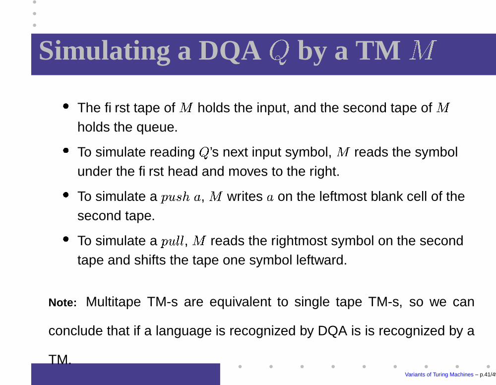
Simulating a DQA by a TM

�

The first tape of

holds the input, and the second tape of

holds the queue.

�

To simulate reading

�

’s next input symbol,

reads the symbolunder the first head and moves to the right.

�

To simulate a � � �� ,

writes� on the leftmost blank cell of thesecond tape.

�

To simulate a � � �

,

reads the rightmost symbol on the secondtape and shifts the tape one symbol leftward.

Note: Multitape TM-s are equivalent to single tape TM-s, so we can

conclude that if a language is recognized by DQA is is recognized by a

TM.Variants of Turing Machines – p.41/49

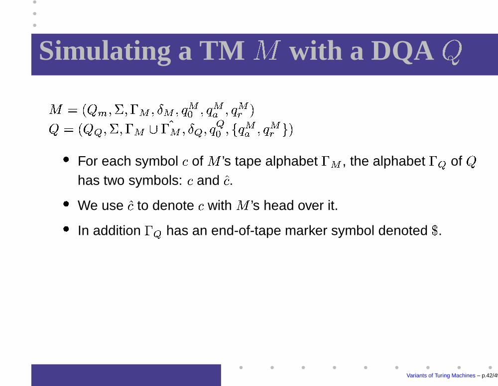
Simulating a TM with a DQA

� � ��

��

� ��

��

� � � ��

� � ��

�

For each symbol of

’s tape alphabet� � , the alphabet

�� of

�

has two symbols: and

.

�

We use

to denote with

’s head over it.

�

In addition

�� has an end-of-tape marker symbol denoted

�

.


The simulation

� simulates by maintaining a copy of the’s tape in the queue.

� can effectively scan the tape from right toleft by pulling symbols from the right-handend of the queue and pushing them back onthe left-hand end side, until

�

is seen.

� When a

�� symbol is encountered, can

determine ’s next move, because canrecord ’s current state in its control.


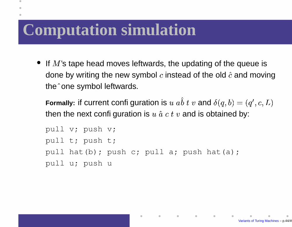
Computation simulation

�

If

’s tape head moves leftwards, the updating of the queue isdone by writing the new symbol instead of the old

and movingthe

one symbol leftwards.

Formally: if current configuration is � � � � and

� ��

� �

then the next configuration is � � � and is obtained by:

pull v; push v;

pull t; push t;

pull hat(b); push c; pull a; push hat(a);

pull u; push u


Computation simulation

�

If

’s tape head moves rightward, the updating is harder becausethe

must go to the right.

�

By the time

is pulled from the queue, the symbol which receivesthe

has already been pushed onto the queue.


Solution

The solution is to hold tape symbols in the control for an extra move,before pushing them onto the queue. This gives

�

enough time tomove the

rightward if necessary.

Formally: if current configuration is � � � � and

� ��

� �

thenthe next configuration is � � � and is obtained by:

pull v; push v;

pull t; hold (t);

pull hat(b); push hat(t); push(c);

pull u; push u;


Equivalence with other models

� There are many other models of generalpurpose computation.Example: recursive functions, normal algorithms, semi-thue

systems,

�

-calculus, etc.

� Some of these models are very much likeTuring machines; other are quite different

� All share the essential feature of a TM:unrestricted access to unlimited memory

� All these models turn out to be equivalent incomputation power with TM


Analogy

� There are hundreds of programminglanguages

� However, if an algorithm can be programmedusing one language it might be programmedin any other language

� If one language�

� can be mapped intoanother language

� � it means that

�� and

� �

describe exactly the same class of algorithms


Philosophy

� Even though there are many differentcomputational models, the class of algorithmsthat they describe is unique

� Whereas each individual computationalmodel has certain arbitrariness to itsdefinition, the underlying class of algorithms itdescribes is natural because it is the same forother models

This has profound implications in mathematics


Variants of Turing Machines - Stony Brook Computer Science

Documents

Transcript of Variants of Turing Machines - Stony Brook Computer Science