SPACE COMPEXITYShahid Mahmood

Domez Colony Kundian, Pakistanms140400344 @vu.edu.pk

Abstract—Space complexity is the class ofComputational complexity which deals whichdeals with the required space by the Turingmachines while working on the input receivedthrough the input tap. Actual space complexityis combination of two spaces, input tap spaceand working tap space. We want to minimize thetotal space required by the Turing machine asmuch as possible. In the paper we are dealingwith the two classes of the space complexity,deterministic and non deterministic spaceoccupied by the Turing machines. The aim ofthis paper is to provide Basic knowledge aboutthe space complexity.

Keywords— DSPACE; NSPACE; NL; L;

I. INTRODUCTION An algorithm (Turing Machine) means a mathematical procedure used to compute or construct a mathematical solution to a given problem,and which is carried out mechanically without thinking. A program in the Pascal programming language is a good example of an algorithm specification. Since the “mechanical “nature of an algorithm is its most important feature, instead of the notion of algorithm, in the paper we will discuss the space occupied during the execution of the algorithm and various aspects of a mathematical machine or a Turing machine.

Turing machines are very much like thereal computers, as most of us are familiar with the real computers: we willomit some inessential features of Turing machine, and add some essential features to the paper.

Turing machine is a finite automata equipped with an unbounded memory. For the purpose of memory we use some tapes, which are infinite in both directions (theoretically). We divide the tape into multiple (infinite cells). Each tape has specific cell. On every cell of every tape, a symbol from a finite alphabet canbe written. We treat the empty cell as

the special symbol written on the tape. To access the information on the tapes, we supply each tape by a read-write head.At a particular moment tape head have a particular position on the tape cell. However we can have more then one tape head at a single moment. But all head have their specific position also. The read-write heads are connected to a control unit, which is a finite automation. Its possible states form a finite set (ta). There is a distinguished starting state “START “and a halting state “STOP”. Initially, the control unit is in the “START” state, andthe heads sit on the starting cells of the tapes. During each step, each head reads the character\symbol in the given cell of the tape, and sends it to the control unit. Using these symbols and onits own state, the control unit carries out following things.

It sends a symbol to Turing machine heads to write the symbol on the tape.

Control unit sends the command to each head to move it “RIGHT” ,”LEFT” or “NO MOVE”.

Transition function is translated by the control unit to apply the specific control onthe Turing machine.

Turing machine heads carry out these commands, which complete one step of the computation at one moment. The machine halts when the control unit reaches the “STOP” or “HALT” state. We can translate the input information, and transition function into purely mathematical terms.

Space Complexity of an algorithm is space occupied (memory) during the execution of a Turing machine (algorithm)with respect to the input tape size and working tape. Space complexity has both the auxiliary space and space used by theinput. Where the Auxiliary space is the

temporary space used by the Turing machine during its execution.

Let suppose that we want to compare standard sorting algorithms on the basis of space, and then auxiliary space would be a better criteria than space complexity. Merge sort takes O (n) auxiliary space, Insertion sort and Heap Sort takes O (1) auxiliary space. Howeverspace complexity of all these sorting algorisms is O (n).

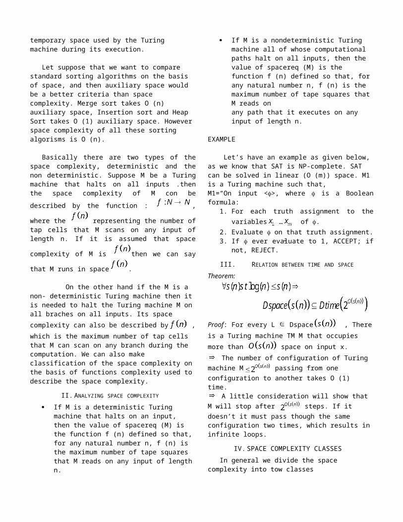
Basically there are two types of thespace complexity, deterministic and thenon deterministic. Suppose M be a Turingmachine that halts on all inputs .thenthe space complexity of M con bedescribed by the function : ,

where the representing the number oftap cells that M scans on any input oflength n. If it is assumed that space

complexity of M is then we can say

that M runs in space .

On the other hand if the M is a non- deterministic Turing machine then itis needed to halt the Turing machine M onall braches on all inputs. Its space complexity can also be described by ,which is the maximum number of tap cells that M can scan on any branch during the computation. We can also make classification of the space complexity onthe basis of functions complexity used todescribe the space complexity.

II.ANALYZING SPACE COMPLEXITY If M is a deterministic Turing

machine that halts on an input, then the value of spacereq (M) is the function f (n) defined so that,for any natural number n, f (n) is the maximum number of tape squares that M reads on any input of lengthn.

If M is a nondeterministic Turing machine all of whose computational paths halt on all inputs, then the value of spacereq (M) is the function f (n) defined so that, forany natural number n, f (n) is the maximum number of tape squares thatM reads onany path that it executes on any input of length n.

EXAMPLE

Let’s have an example as given below,as we know that SAT is NP-complete. SAT can be solved in linear (O (m)) space. M1is a Turing machine such that,M1=“On input <f>, where f is a Booleanformula:

1. For each truth assignment to thevariables … of f.

2. Evaluate f on that truth assignment.3. If f ever evaluate to 1, ACCEPT; if

not, REJECT.”

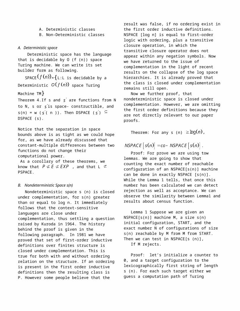
III. RELATION BETWEEN TIME AND SPACE Theorem:

Proof: For every L Dspace , Thereis a Turing machine TM M that occupies more than space on input x.

The number of configuration of Turing machine M passing from one configuration to another takes O (1) time.

A little consideration will show that M will stop after steps. If it doesn’t it must pass though the same configuration two times, which results ininfinite loops.

IV.SPACE COMPLEXITY CLASSESIn general we divide the space

complexity into tow classes

A. Deterministic classesB. Non-Deterministic classes

A. Deterministic space Deterministic space has the language

that is decidable by O (f (n)) space Turing machine. We can write its set builder form as following.

SPACE ={L:L is decidable by a Deterministic space Turing

Machine TM}Theorem 4.If s and are functions from Nto N, s or is space- constructible, and s(n) = w ( ( n )). Then DSPACE ( ) DSPACE (s).

Notice that the separation in space bounds above is as tight as we could hopefor, as we have already discussed that constant-multiple differences between twofunctions do not change their computational power. As a corollary of these theorems, we know that , and that L PSPACE.

B. Nondeterministic Space s(n)Nondeterministic space s (n) is closed

under complementation, for s(n) greater than or equal to log n. It immediately follows that the context-sensitive languages are close under complementation, thus settling a questionraised by Kuroda in 1964. The history behind the proof is given in the following paragraph. In 1981 we have proved that set of first-order inductive definitions over finites structure is closed under complementation. This is true for both with and without ordering relation on the structure. If an orderingis present in the first order inductive definitions then the resulting class is P. However some people believe that the

result was false, if no ordering exist inthe first order inductive definitions. NSPACE [log n] is equal to first-order logic with ordering, plus a transitive closure operation, in which the transitive closure operator does not appear within any negation symbols. Now we have returned to the issue of complementation in the light of recent results on the collapse of the log space hierarchies. It is already proved that the class is closed under complementationremains still open.

Now we further proof, that nondeterministic space is closed under complementation. However, we are omittingthe first order definitions because they are not directly relevant to our paper proofs.

Theorem: For any s (n)

Proof: For prove we are using tow

lemmas. We are going to show that counting the exact number of reachable configuration of an NSPACE[s(n)] machine can be done in exactly NSPACE [s(n)]. While the Lemma 1 tells, that once this number has been calculated we can detect rejection as well as acceptance. We can observe the similarity between Lemma1 andresults about census function.

Lemma 1 Suppose we are given an NSPACE[s(n)] machine M, a size s(n) initial configuration, START, and the exact number N of configurations of size s(n) reachable by M from M from START. Then we can test in NSPACE[s (n)],

If M rejects.

Proof: let’s initialize a counter to 0, and a target configuration to the lexicographically first string of length s (n). For each such target either we guess a computation path of Turing

machine TM M from START to target, and increment both counter and target; or we simply increment target. For each final state, we have found a path, if it is an accept configuration of Turing machine M then we reject. Finally, if when we are done with the last target the counter is equal to N, we accept; otherwise we reject. Note that we accept if and only if we have found N reachable configurations. None of which is accepting. (Let’s suppose that M accepts.In this case there can be at most N-1 reachable configurations that are not accepting, and our machine will reject. In contrast if Turing machine TM M rejects then there are N non- accepting reachable configurations. Thus our nondeterministic machine can guess paths to each of them in turn and accept. ) . Hence we accept if and only if Turing machine M rejects.

Lemma 2: Given START, as in Lemma 1, we can calculate N- the total number of configurations of size s (n) reachable byM from START in NSPACE [s (N)].

Proof: Let’s suppose that the number of configurations is reachable from START in at most d steps. Computations proceed in where d= 0, 1…n. Using the mathematical induction on d we can prove that each may be calculated in NSPACE[s (n)]. The base case d=0 is obvious.

In the inductive step, Given we arepresenting that is also holds. Remind it from the lemma 1 that there are

Reachable configurations, and we cycle though all of them only the target configurations in lexicographical order. For each of these we do the following: Cycle through all configurations reachable in at most d steps, again we find a path of length at most d for each

reach able one, and if we don’t find allof then we will reject . For each of

these configurations, check if it is equal to target, or if target is reachable from it in one step. If so thenincrement the counter, and start on target+1. On Each iteration, we will increment by 1 the start configuration. In the end we will have reachable configurations from the start configuration. Since N is bounded above

for some constant c, the space needed is O[s (n)].

To compute the proof of the lemma and the theorem note that N is equal to the first such that .

Corollary 1: The class of context sensitive languages is closed under complementation.

Proof: In the proof we can present the proof of Kuroda, he showed in 1964 that CSL =NSPACE [N].

Corollary 2: The Log Space Alternating Hierarchy and the Log Space Oracle Hierarchy both collapse to NSPACE [log n].

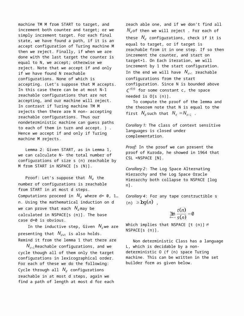
Corollary 4: For any tape constructible s (n) ,

Which implies that NSPACE [t (n)] NSPACE[s (n)].

Non deterministic Class has a language L, which is decidable by a non- deterministic O (f (n) space Turing machine. This can be written in the set builder form as given below.

NSPACE = {L: L is decidable by non-deterministic space Turing

Machine}We will come to this discussion in

short while , let’s discuss the low spaceclasses first

V. LOW SPACE CLASSESThere are some classes of the space

complexity which are defined as the low space classes such that.

A.B. It is interesting to be noted that

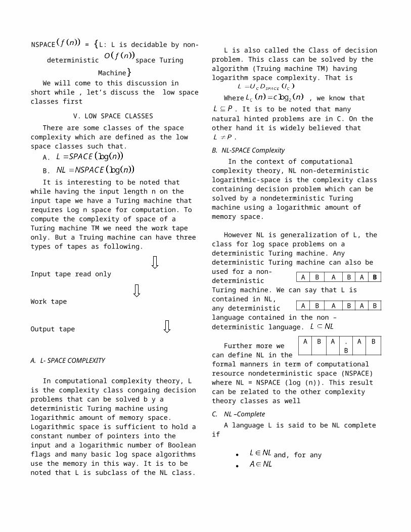
while having the input length n on the input tape we have a Turing machine that requires Log n space for computation. To compute the complexity of space of a Turing machine TM we need the work tape only. But a Truing machine can have threetypes of tapes as following.

Input tape read only

Work tape

Output tape

A. L- SPACE COMPLEXITY

In computational complexity theory, L is the complexity class congaing decisionproblems that can be solved b y a deterministic Turing machine using logarithmic amount of memory space. Logarithmic space is sufficient to hold aconstant number of pointers into the input and a logarithmic number of Booleanflags and many basic log space algorithmsuse the memory in this way. It is to be noted that L is subclass of the NL class.

L is also called the Class of decisionproblem. This class can be solved by the algorithm (Truing machine TM) having logarithm space complexity. That is

Where , we know that

. It is to be noted that many natural hinted problems are in C. On the other hand it is widely believed that

. B. NL-SPACE Complexity

In the context of computational complexity theory, NL non-deterministic logarithmic-space is the complexity classcontaining decision problem which can be solved by a nondeterministic Turing machine using a logarithmic amount of memory space.

However NL is generalization of L, theclass for log space problems on a deterministic Turing machine. Any deterministic Turing machine can also be used for a non-deterministicTuring machine. We can say that L is contained in NL,any deterministiclanguage contained in the non –deterministic language.

Further more wecan define NL in theformal manners in term of computational resource nondeterministic space (NSPACE) where NL = NSPACE (log (n)). This result can be related to the other complexity theory classes as wellC. NL –Complete

A language L is said to be NL complete if

and, for any

A B A B A B

A B A B A B

A B A .B

A B

If the second condition holds then the problem is in NL-hard. There are several NL-complete problems which close under thelog-space reduction, such as ST-connectivity and 2-satisability.In ST connectivity we use a directed graph whichhas such two nodes s and t, that there is a path from the s to node t.

VI.REDUCTIONSProblem reducibility is central to the study of complexity. Reductions allow us to determine the relative complexity of problems without knowing the absolute complexity of those problems. If A and B are two problems, then A <B denotes thatA reduces to B. This implies that the complexity of A is no greater than the complexity of B (modulo the complexity of the reduction itself), so the notation A<Bis sensible in this context. We consider two types of reductions, mapping reductions and oracle reductions. Mapping reductions are more restrictive

VII. COMPLEXITY OF CIRCUIT EVALUATION:Let CEVL denote the set of pairs (C,

) such that C is a Boolean circuit and C ( ) =1. Then CEVL is in P and every problem in P is log-space karp-reducible to CEVL

Let’s suppose that there is a polynomial time algorithm, then we have acircuit C such that which takes a n-bit long input string x and returns the C (n). For bounded circuit fan-in, space complexity of such algorithm can be made linear in the depthof the circuit. This is done by using theDFS type algorithm.

VIII. SIMULATION TIME COMPLEXITY

Time complexity for at least logarithmic space complex Turing machine

is always upper bound of exponential function in that space.

However this exponential time complexity function goes beyond the limits of exponentially for the given ploy-logarithm space complexity. This leads us to define a class of algorithms that are solvable in polynomial time and a poly-logarithm space complexity. This class SC is indeed a sub-class of P and contains a Class L.

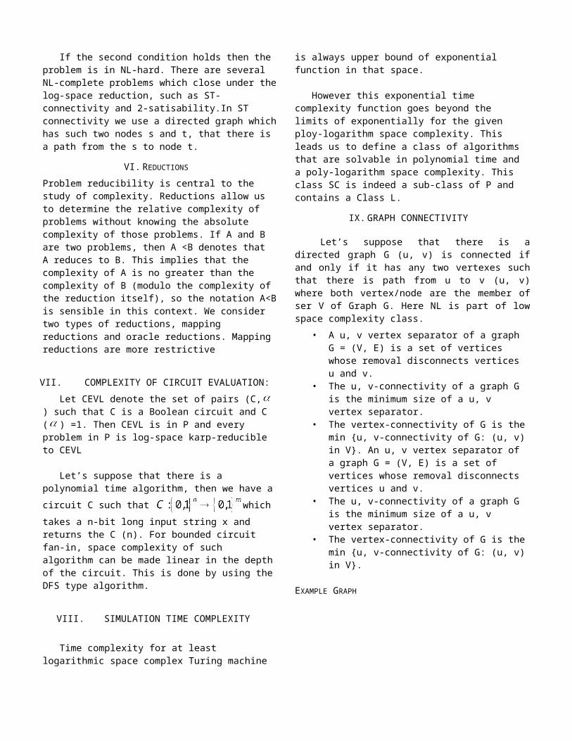
IX.GRAPH CONNECTIVITY

Let’s suppose that there is adirected graph G (u, v) is connected ifand only if it has any two vertexes suchthat there is path from u to v (u, v)where both vertex/node are the member ofser V of Graph G. Here NL is part of lowspace complexity class.

• A u, v vertex separator of a graph G = (V, E) is a set of vertices whose removal disconnects vertices u and v.

• The u, v-connectivity of a graph G is the minimum size of a u, v vertex separator.

• The vertex-connectivity of G is themin {u, v-connectivity of G: (u, v)in V}. An u, v vertex separator of a graph G = (V, E) is a set of vertices whose removal disconnects vertices u and v.

• The u, v-connectivity of a graph G is the minimum size of a u, v vertex separator.

• The vertex-connectivity of G is themin {u, v-connectivity of G: (u, v)in V}.

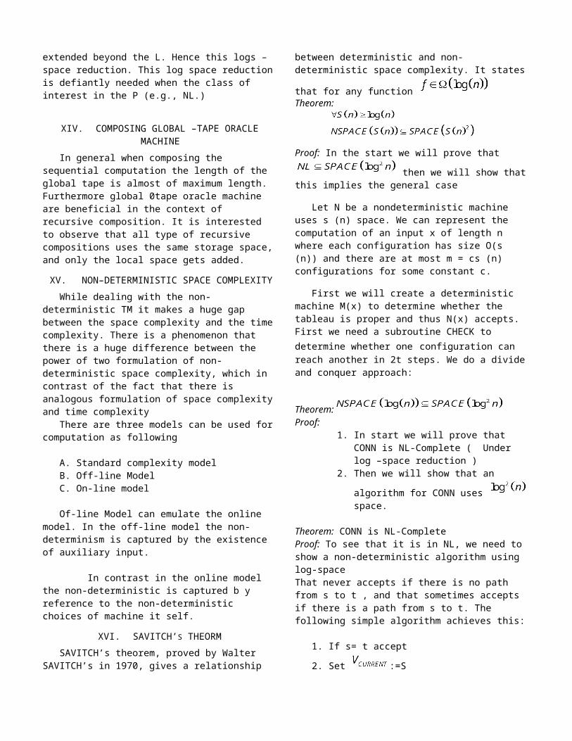
EXAMPLE GRAPH

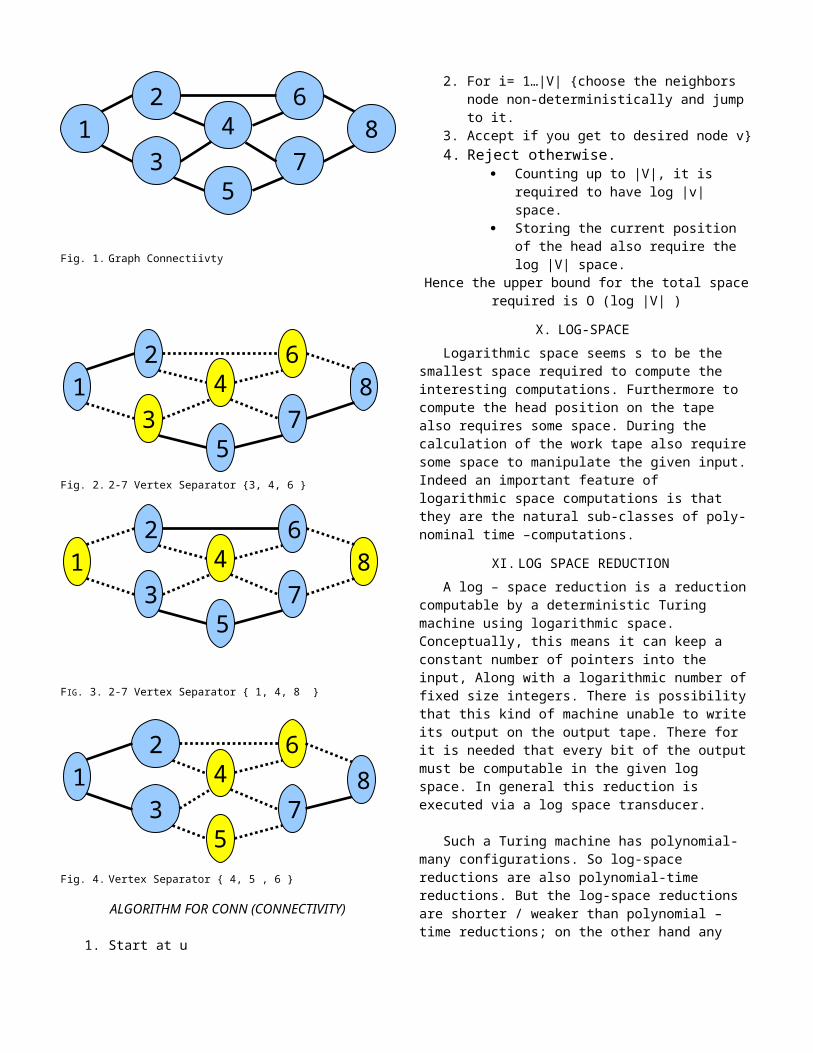
Fig. 1. Graph Connectiivty

Fig. 2. 2-7 Vertex Separator {3, 4, 6 }

FIG. 3. 2-7 Vertex Separator { 1, 4, 8 }

Fig. 4. Vertex Separator { 4, 5 , 6 }

ALGORITHM FOR CONN (CONNECTIVITY)

1. Start at u

2. For i= 1…|V| {choose the neighbors node non-deterministically and jump to it.

3. Accept if you get to desired node v}4. Reject otherwise.

Counting up to |V|, it is required to have log |v| space.

Storing the current position of the head also require the log |V| space.

Hence the upper bound for the total spacerequired is O (log |V| )

X. LOG-SPACE Logarithmic space seems s to be the

smallest space required to compute the interesting computations. Furthermore to compute the head position on the tape also requires some space. During the calculation of the work tape also requiresome space to manipulate the given input.Indeed an important feature of logarithmic space computations is that they are the natural sub-classes of poly-nominal time –computations.

XI.LOG SPACE REDUCTIONA log – space reduction is a reduction

computable by a deterministic Turing machine using logarithmic space. Conceptually, this means it can keep a constant number of pointers into the input, Along with a logarithmic number offixed size integers. There is possibilitythat this kind of machine unable to writeits output on the output tape. There for it is needed that every bit of the outputmust be computable in the given log space. In general this reduction is executed via a log space transducer.

Such a Turing machine has polynomial-

many configurations. So log-space reductions are also polynomial-time reductions. But the log-space reductions are shorter / weaker than polynomial – time reductions; on the other hand any

12

34

5

6

78

12

34

5

6

78

12

34

5

6

78

12

34

5

6

78

non-empty , non full language in p is polynomial-time reducible to any non-empty non full language in P, a log spacereduction between a language in NL and a language in L, both subsets of p, would imply the unlikely L=NL . It is an open question if the NP – complete problems are different with respect to log –space and polynomial reductions.

Log-space reductions are normally usedon languages in P, in which case it usually does not matter whether many-one reductions or Turing reductions are used,since it has been verified that L, NL, and P are all closed under Turing reductions, meaning that Turing reductions can be used to show a problem is in any of these classes. However, other sub-classes. However, other subclasses of P such as NC may not be closed under Turing reductions, and so many-reductions must be used.

Just as polynomial-time reductions areuseless within p and its subclasses, log-spaces reductions are useless to distinguish problems in L and its sub-classes, in particular, almost every problem in L is trivially L-complete under log-space reductions, while even weaker reductions exist, they are not often used in practice, because complexity classes smaller than L (that is, strictly contained or thought to be strictly contained in L (receive relatively little attention).

XII. KARP –REDUCTION

is a log space many to on e reduction of S(space) to S’ if is a function that computes in the log-space variant of Levin reduction. It is to be noted that both type of reductions are transitive. Furthermore these reductions run in polynomial time. Hence the notion of reduction from many to one is a special case of karp reduction.

As we observed that all KARP reductions demonstrate that NP-completeness results are actually log-space reduction.

We say that f is a log space many to

on e reduction of S to S’ if is log space computable and, for every x, it holds that . Clearly if s is so reducible to then A L

Here under given a theorem is sufficed to show that any problem in p isreducible to the problem of evaluating a circuit on a give input. Note that circuit problem is in P hence we can say that it is in NP-complete under the log space reductions.

Claim: if is the log space reduction

M is a log space machine forB

Then A is in L

Proof: On input in or not in ASimulate M and whenever TM M reads the

symbol of its input tape. Run on x

and wait for the bit to be an output on the output tape.

XIII. USES OF LOG SPACE REDUCTION Log space reduction is used to define

the completeness usually with respect to the other classes that are assumed to be

extended beyond the L. Hence this logs – space reduction. This log space reductionis defiantly needed when the class of interest in the P (e.g., NL.)

XIV. COMPOSING GLOBAL –TAPE ORACLEMACHINE

In general when composing the sequential computation the length of the global tape is almost of maximum length. Furthermore global 0tape oracle machine are beneficial in the context of recursive composition. It is interested to observe that all type of recursive compositions uses the same storage space,and only the local space gets added.

XV. NON–DETERMINISTIC SPACE COMPLEXITY While dealing with the non-

deterministic TM it makes a huge gap between the space complexity and the timecomplexity. There is a phenomenon that there is a huge difference between the power of two formulation of non-deterministic space complexity, which in contrast of the fact that there is analogous formulation of space complexityand time complexity

There are three models can be used forcomputation as following

A. Standard complexity modelB. Off-line ModelC. On-line model

Of-line Model can emulate the online model. In the off-line model the non-determinism is captured by the existence of auxiliary input.

In contrast in the online model the non-deterministic is captured b y reference to the non-deterministic choices of machine it self.

XVI. SAVITCH’S THEORMSAVITCH’s theorem, proved by Walter

SAVITCH’s in 1970, gives a relationship

between deterministic and non-deterministic space complexity. It states

that for any function Theorem:

Proof: In the start we will prove that

then we will show thatthis implies the general case

Let N be a nondeterministic machine uses s (n) space. We can represent the computation of an input x of length n where each configuration has size O(s (n)) and there are at most m = cs (n) configurations for some constant c.

First we will create a deterministic machine M(x) to determine whether the tableau is proper and thus N(x) accepts. First we need a subroutine CHECK to determine whether one configuration can reach another in 2t steps. We do a divideand conquer approach:

Theorem:Proof:

1. In start we will prove that CONN is NL-Complete ( Under log –space reduction )

2. Then we will show that an

algorithm for CONN uses space.

Theorem: CONN is NL-CompleteProof: To see that it is in NL, we need to show a non-deterministic algorithm using log-spaceThat never accepts if there is no path from s to t , and that sometimes accepts if there is a path from s to t. The following simple algorithm achieves this:

1. If s= t accept

2. Set :=S

3. For i=1 to n:

4. Guess a vertex

5. If there is no edge from to

reject

6. If = t, accept7. if i= n and no decision has yet

been made , reject

This algorithm also requires some storage such as I (using log n bits) and at most the labels of two vertices.

and (using O(log n ) bits). To see that CONN is NL-complete, assume

that and let be a non-deterministic log-space machine deciding L. Our log-space reduction from L to CONN

takes input and outputs a graph in which the vertices represent configurations of (x) and edges represent allowed transitions. (It also outputs s = start and t = accept, where these are the starting and accepting configurations of (x), respectively.) Each configuration can be represented using O (log n) bits.

A Fact: Without loosing the generality we can assume that all the NTM accept the exactly one accepting configuration.

XVII. CONFIGURATION GRAPHIf there is a non- deterministic

Turing machine M which is given the inputX. this machine has the start configuration as S and final /accepting configuration as t. there is a vertex configuration for each vertex. This machine can move from u to v while

, where (u, v) is an edge and E is the set of all edges in the graph.

CORRECTNESS:Claim: If there is a non- deterministicTuring machine M and it takes input x.

Then machine M will accept input x if andonly if there is a path from s to t in

the graph, where s and t are themember of the set of vertex in the Graph

XVIII. CONN IS NL-COMPLETECorollary: CONN is NL –complete Proof: We have shown CONN is in NL. It is recalled that we have also presented a reduction from non deterministic languageNL to CONN where this CONN is complete ina given log-space.

XIX. NL NL is subset of polynomial Proof: Any NL language can be reduced to CONN in logarithm space.

Thus any NL language is ploy-time reducible to CONN

Hence CONN is in P Thus any NL language is in P

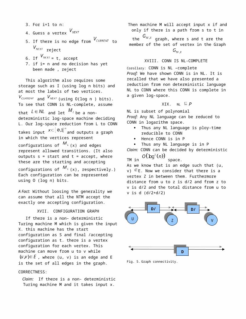
Claim: CONN can be decided by deterministic

TM in space. As we know that is an edge such that (u, v) E. Now we consider that there is a vertex Z in between them. Furthermore distance from u to z is d/2 and from z tov is d/2 and the total distance from u tov is d (d/2+d/2)

Fig. 5. Graph connectivity.

U Z V

D/

D

D/

XX. O SPACE DTM

Claim: There is a deterministic TM which

decides CONN in Proof: To solve CONN, we consider the Path (s, t, |V|) Where S is the start node while t is the destination vertex or nodethen the space complexity can be determined by using the following equation

That is upper bound for Theorm: Claim: let there are two space constructible functions

Where log n is the overhead of simulation

Furthermore,

XXI. RELATION BETWEEN NSPACE AND DSPACE

We can convert a non-deterministic space into deterministic Space by using the polynomial complexity,while conversion of non- deterministic time complexity to deterministic time complexity requires the exponential time complexity.

THEORM: (Non-Deterministic VS Deterministic Space)For any space s such that

That is at least logarithmic, it holds that Furthermore it is to be noted that non-deterministic polynomial space is contained in the deterministic polynomialspace, and any non-deterministic polynomial space can be contained within the deterministic polynomial space.

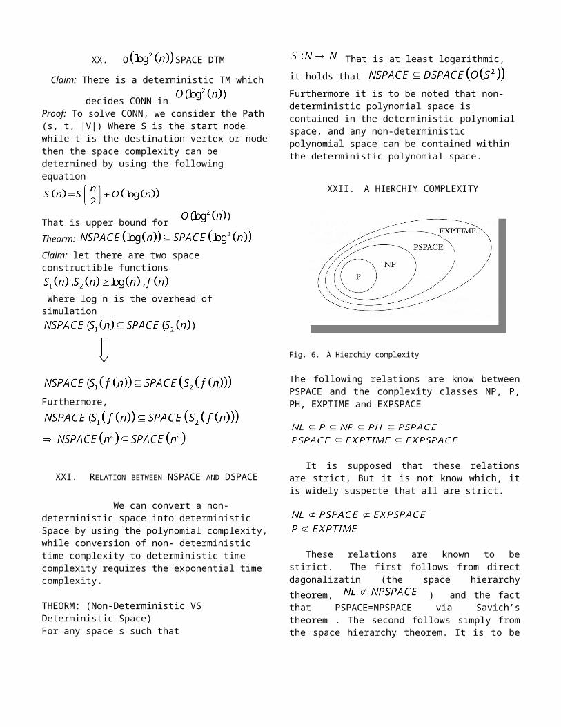
XXII. A HIERCHIY COMPLEXITY

Fig. 6. A Hierchiy complexity

The following relations are know betweenPSPACE and the conplexity classes NP, P,PH, EXPTIME and EXPSPACE

It is supposed that these relationsare strict, But it is not know which, itis widely suspecte that all are strict.

These relations are known to bestirict. The first follows from directdagonalizatin (the space hierarchytheorem, ) and the factthat PSPACE=NPSPACE via Savich’stheorem . The second follows simply fromthe space hierarchy theorem. It is to be

noted that the hardest problem in PSPACEare the PSPACE-Complete problems.

XXIII. TQBFThe language TQBF is a formal language

consisting of the true quantified Booleanformulas. A fully quantified Boolean formula is a formula in quantified propositional logic where every variable is quantified, using either existential or universal quantifier, at the beginningof the sentence. Such a formula is equivalent to either true or false (Sincethere are no free variables). If such a formula evaluated to true, then that formula is in the language TQBF. It is also known as QSAT (Quantified SAT)Instance: A fully quantified Boolean formulaProblem: it is needed to decide if is true or false.Example: A fully quantified Boolean formula Where the variable range is {0, 1}

XXIV. TQBM IS IN PSPACE

Theorem: Proof: Let, prove that a poly-space algorithm A for evaluating a Boolean formula.

If a Boolean formula does not have quantifiers then we can evaluate it as

If for A use the and

If both are true then accept Reject otherwise On the other hand if

then for A use the and Accept if any of both is true Reject otherwise

XXV. TQBF IS PSPACE COMPLETE

Proof: To show that TQBFÎPSPACE, we give an algorithm that assigns values to the variables and recursively evaluates the

truth of the formula for those values. To show that A£pTQBF for every AÎPSPACE, we begin with a polynomial-space machine M for A. Then we give a polynomial time reduction that maps a string w to a formula f that encodes a simulation of M on input w. f Is true if and only if M accepts w (and hence if and only if wÎA).At first, naive, attempt to do so could be trying to precisely imitate the proof of the Cook-Levin theorem. We can indeed construct a f , that simulates M on inputw by expressing the requirements for an accepting tableau. As in the proof of theCook-Levin theorem, such a tableau has polynomial width O (n, k), the space usedby M. But the problem is that the height of the tableau would be exponential! Instead, we use a technique related to the proof of SAVITCH’s theorem to construct the formula. The formula divides the tableau into halves and employs the universal quantifier to represent each half with the same part ofthe formula. The result is a much shorterformula.

REFERENCES[1] G. Eason, B. Noble, and I. N. Sneddon, “On

certain integrals of Lipschitz-Hankel typeinvolving products of Bessel functions,” Phil.Trans. Roy. Soc. London, vol. A247, pp. 529–551,April 1955.

[2] Papadimitriou, Christos H. (1994). ComputationalComplexity, Reading, Massachusetts: Addison-Wesley. ISBN 0-201-53082-1.

[3] A. Borodin. S.A. Cook, P.W. Dymond, W.L. Ruzzo,and M. Tompa,”Two Applications of Complementatinvia Inductive Counting, “ this volume.

[4] S.A Cook, “A Taxonomy of Problems with FastParallel Algorithms,” Information and Control64(1985), 2-22.

[5] http://en.wikipedia.org/wiki [6] Manuel Blum and Silvio Micali, How to generate

cryptographically strong sequences ofpseudorandom bits, SIAM Journal on Computing ,13(4) ( 1984).

[7] Sanjeev Arora and Boaz Barak. ComputationalComplexity - A Modern Approach . CambridgeUniversity Press, 2009.

[8] Omer Reingold. Undirected st-connectivity inlog-space

[9] Oded Goldreich , Modern Cryptography,Probabilistic Proodfs and Pseudorandom ness,Springer-Verlag, 1999.

[10] Michael E. Saks and Shiyu Zhou. Bph space(s)subseteq dspace(s 3/2 ). J. Comput. Syst. Sci. ,58(2):376{ 403, 1999.

[11] Walter J. Savitch. Relationships betweennondeterministic and deterministic tape

complexities. Journal of Computer and SystemSciences , 4(2):177 { 192, 1970.

[12] Ben Green and Terence Tao, The primescontain arbitratily lon g arithmeticprogressions, Annals of Mathematics, 167 (2008),481-547.

[13] L. J. Stockmeyer and A. R. Meyer. Wordproblems requiring exponential time(preliminaryreport). In Proceedings of the Noga Alon , Eldar Fischer, Michael

Krivelevich and Mario Szegedy, Efficienttesting of large graphs,Combinatiorica,

20(4) (2000), 451- 476).