CSci 311, Models of Computation Chapter 9 Turing Machines
24
CSci 311, Models of Computation Chapter 9 Turing Machines H. Conrad Cunningham 29 December 2015 Contents Introduction ................................. 1 9.1 The Standard Turing Machine ................... 2 9.1.1 What is a Turing Machine? ................. 2 9.1.1.1 Schematic Drawing of Turing Machine ...... 2 9.1.1.2 Definition of Turing Machine ........... 3 9.1.1.3 Linz Example 9.1 ................. 4 9.1.1.4 A Simple Computer ................ 4 9.1.1.5 Linz Example 9.2 ................. 5 9.1.1.6 Transition Graph for Turing Machine ...... 6 9.1.1.7 Linz Example 9.3 (Infinite Loop) ......... 6 9.1.1.8 Standard Turing Machine ............. 7 9.1.1.9 Instantaneous Description of Turing Machine . . 7 9.1.1.10 Computation of Turing Machine ......... 8 9.1.2 Turing Machines as Language Acceptors .......... 9 9.1.2.1 Linz Example 9.6 ................. 10 9.1.2.2 Linz Example 9.7 ................. 11 9.1.3 Turing Machines as Transducers .............. 13 9.1.3.1 Linz Example 9.9 ................. 14 1
-
Upload
khangminh22 -
Category
Documents
-
view
0 -
download
0
Transcript of CSci 311, Models of Computation Chapter 9 Turing Machines

CSci 311, Models of ComputationChapter 9
Turing Machines
H. Conrad Cunningham
29 December 2015
Contents
Introduction . . . . . . . . . . . . . . . . . . . . . . . . . . . . . . . . . 1
9.1 The Standard Turing Machine . . . . . . . . . . . . . . . . . . . 2
9.1.1 What is a Turing Machine? . . . . . . . . . . . . . . . . . 2
9.1.1.1 Schematic Drawing of Turing Machine . . . . . . 2
9.1.1.2 Definition of Turing Machine . . . . . . . . . . . 3
9.1.1.3 Linz Example 9.1 . . . . . . . . . . . . . . . . . 4
9.1.1.4 A Simple Computer . . . . . . . . . . . . . . . . 4
9.1.1.5 Linz Example 9.2 . . . . . . . . . . . . . . . . . 5
9.1.1.6 Transition Graph for Turing Machine . . . . . . 6
9.1.1.7 Linz Example 9.3 (Infinite Loop) . . . . . . . . . 6
9.1.1.8 Standard Turing Machine . . . . . . . . . . . . . 7
9.1.1.9 Instantaneous Description of Turing Machine . . 7
9.1.1.10 Computation of Turing Machine . . . . . . . . . 8
9.1.2 Turing Machines as Language Acceptors . . . . . . . . . . 9
9.1.2.1 Linz Example 9.6 . . . . . . . . . . . . . . . . . 10
9.1.2.2 Linz Example 9.7 . . . . . . . . . . . . . . . . . 11
9.1.3 Turing Machines as Transducers . . . . . . . . . . . . . . 13
9.1.3.1 Linz Example 9.9 . . . . . . . . . . . . . . . . . 14
1
9.1.3.2 Linz Example 9.10 . . . . . . . . . . . . . . . . . 14
9.1.3.3 Linz Example 9.11 . . . . . . . . . . . . . . . . . 16
9.2 Combining Turing Machines for Complicated Tasks . . . . . . . . 16
9.2.1 Introduction . . . . . . . . . . . . . . . . . . . . . . . . . 16
9.2.2 Using Block Diagrams . . . . . . . . . . . . . . . . . . . . 18
9.2.2.1 Linz Example 9.12 . . . . . . . . . . . . . . . . . 18
9.2.3 Using Pseudocode . . . . . . . . . . . . . . . . . . . . . . 19
9.2.3.1 Macroinstructions . . . . . . . . . . . . . . . . . 19
9.2.3.2 Linz Example 9.13 . . . . . . . . . . . . . . . . . 20
9.2.3.3 Subprograms . . . . . . . . . . . . . . . . . . . . 20
9.2.3.4 Linz Example 9.14 . . . . . . . . . . . . . . . . . 21
9.3 Turing’s Thesis . . . . . . . . . . . . . . . . . . . . . . . . . . . . 22
Copyright (C) 2015, H. Conrad Cunningham
Acknowledgements: MS student Clay McLeod assisted in preparation of thesenotes. These lecture notes are for use with Chapter 9 of the textbook: PeterLinz. Introduction to Formal Languages and Automata, Fifth Edition, Jones andBartlett Learning, 2012. The terminology and notation used in these notes aresimilar to those used in the Linz textbook. This document uses several figuresfrom the Linz textbook.
Advisory: The HTML version of this document requires use of a browser thatsupports the display of MathML. A good choice as of December 2015 seems tobe a recent version of Firefox from Mozilla.
Introduction
A finite accepter (nfa, dfa)
• has no local storage• accepts a regular language
A pushdown accepter (npda, dpda)
• has a stack for local storage
• accepts a language from a larger family
– an npda accepts a context-free language– a dpda accepts a deterministic context-free language
2

The family of regular languages is a subset of the deterministic context-freelanguages, which is a subset of the context-free languages.
But, as we saw in Chapter 8, not all languages of interest are context-free. Toaccept languages like {anbncn : n ≥ 0} and {ww : w ∈ {a, b}∗}, we need anautomaton with a more flexible internal storage mechanism.
What kind of internal storage is needed to allow the machine to accept languagessuch as these? multiple stacks? a queue? some other mechanism?
More ambitiously, what is the most powerful automaton we can define? Whatare the limits of mechanical computation?
This chapter introduces the Turing machine to explore these theoretical ques-tions. The Turing machine is a fundamental concept in the theoretical study ofcomputation.
The Turing machine
• has a tape, a one-dimensional array of readable and writable cells that isunbounded in both directions
• accepts a language from the family of recursively enumerable languages, alarger family of languages than context-free
Although Turing machines are simple mechanisms, the Turing thesis (also knownas the Church-Turing thesis) maintains that any computation that can be carriedout on present-day computers an be done on a Turing machine.
Note: Much of the work on computability was published in the 1930’s, beforethe advent of electronic computers a decade later. It included work by Austrian(and later American) logician Kurt Goedel on primitive recursive function theory,American mathematician Alonso Church on lambda calculus (a foundation offunctional programming), British mathematician Alan Turing (also later a PhDstudent of Church’s) on Turing machines, and American mathematician EmilPost on Post machines.
9.1 The Standard Turing Machine
9.1.1 What is a Turing Machine?
9.1.1.1 Schematic Drawing of Turing Machine
Linz Figure 9.1 shows a schematic drawing of a standard Turing machine.
This deviates from the general scheme given in Chapter 1 in that the inputfile, internal storage, and output mechanism are all represented by a singlemechanism, the tape. The input is on the tape at initiation and the output ison that tape at termination.
3

On each move, the tape’s read-write head reads a symbol from the current tapecell, writes a symbol back to that cell, and moves one cell to the left or right.
Linz Fig. 9.1: Standard Turing Machine
9.1.1.2 Definition of Turing Machine
Turing machines were first defined by British mathematician Alan Turing in1937, while he was a graduate student at Cambridge University.
Linz Definition 9.1 (Turing Machine): A Turing machine M is defined by
M = (Q,Σ,Γ, δ, q0,�, F )
where
1. Q is the set of internal states2. Σ is the input alphabet3. Γ is a finite set of symbols called the tape alphabet4. δ is the transition function5. � ∈ Γ is a special symbol called the blank6. q0 ∈ Q is the initial state7. F ⊆ Q is the set of final states
We also require
8. Σ ⊆ Γ− {�}
and define
9. δ : Q× Γ→ Q× Γ× {L,R}.
Requirement 8 means that the blank symbol � cannot be either an input or anoutput of a Turing machine. It is the default content for any cell that has nomeaningful content.
From requirement 9, we see that the arguments of the transition function δ are:
4
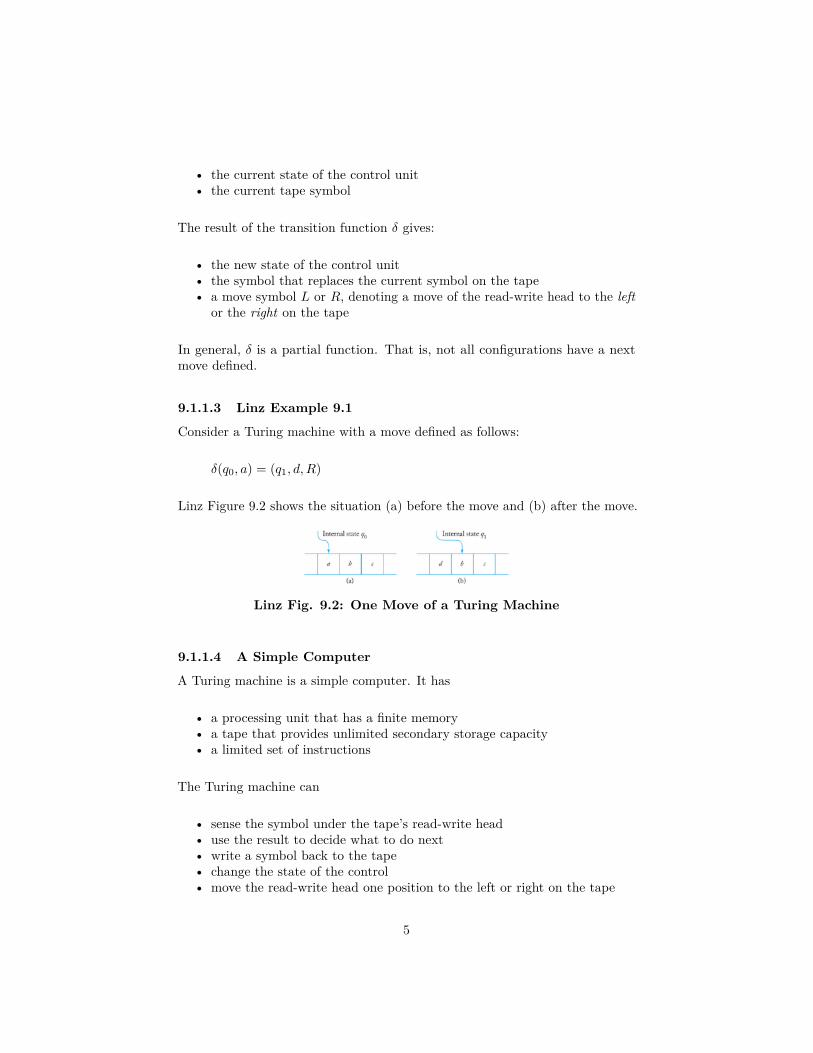
• the current state of the control unit• the current tape symbol
The result of the transition function δ gives:
• the new state of the control unit• the symbol that replaces the current symbol on the tape• a move symbol L or R, denoting a move of the read-write head to the left
or the right on the tape
In general, δ is a partial function. That is, not all configurations have a nextmove defined.
9.1.1.3 Linz Example 9.1
Consider a Turing machine with a move defined as follows:
δ(q0, a) = (q1, d, R)
Linz Figure 9.2 shows the situation (a) before the move and (b) after the move.
Linz Fig. 9.2: One Move of a Turing Machine
9.1.1.4 A Simple Computer
A Turing machine is a simple computer. It has
• a processing unit that has a finite memory• a tape that provides unlimited secondary storage capacity• a limited set of instructions
The Turing machine can
• sense the symbol under the tape’s read-write head• use the result to decide what to do next• write a symbol back to the tape• change the state of the control• move the read-write head one position to the left or right on the tape
5

The transition function δ determines the behavior of the machine, i.e., it is themachine’s program.
The Turing macine starts in initial state q0 and then goes through a sequence ofmoves defined by δ. A cell on the tape may be read and written many times.
Eventually the Turing machine may enter a configuration for which δ is undefined.When it enters such a state, the machine halts. Hence, this state is called a haltstate.
Typically, no transitions are defined on any final state.
9.1.1.5 Linz Example 9.2
Consider the Turing machine defined by
Q = {q0, q1},Σ = {a, b},Γ = {a, b,�},F = {q1}
where δ is defined as follows:
1. δ(q0, a) = (q0, b, R),
2. δ(q0, b) = (q0, b, R),
3. δ(q0,�) = (q1,�, L).
Linz Figure 9 .3 shows a sequence of moves for this Turing machine:
• It begins in state q0 with the input positioned over an a.• When an a is read, transition rule 1 fires, replaces a by b on the tape,
moves right, and stays in state q0.• When a b is read, transition rule 2 fires, leaves b on the tape, moves right,
and stays in state q0.• It continues moving right, replacing each a by a b and leaving each b
unchanged.• When a blank (�) is read, transition rule 3 fires, leaves the blank on the
tape, moves left, and enters final state q1.
6

Linz Fig. 9.3: A Sequence of Moves of a Turing Machine
9.1.1.6 Transition Graph for Turing Machine
As with finite and pushdown automata, we can use transition graphs to representTuring machines. We label the edges of the graph with a triple giving (1) thecurrent tape symbol, (2) the symbol that replaces it, and (3) the direction inwhich the read-write head moves.
Linz Figure 9.4 shows a transition graph for the Turing machine given in LinzExample 9.2.
Linz Fig. 9.4: Transition Graph for Example 9.2
9.1.1.7 Linz Example 9.3 (Infinite Loop)
Consider the Turing machine defined in Linz Figure 9.5.
Linz Fig. 9.5: Infinite Loop
Suppose the tape initially contains ab . . . with the read-write head positionedover the a and in state q0. Then the Turing machine executes the followingsequence of moves:
7

1. The machine reads symbol a, leaves it unchanged, moves right (now oversymbol b), and enters state q1.
2. The machine reads b, leaves it unchanged, moves back left (now over aagain), and enters state q0 again.
3. The machine then repeats steps 1-3.
Clearly, regardless of the tape configuration, this machine does not halt. It goesinto an infinite loop.
9.1.1.8 Standard Turing Machine
Because we can define a Turing machine in several different ways, it is useful tosummarize the main features of our model.
A standard Turing machine:
1. has a tape that is unbounded in both directions, allowing any number ofleft and right moves
2. is deterministic in that δ defines at most one move for each configuration
3. has no special input or output files. At the initial time, the tape hassome specified content, some of which is considered input. Whenever themachine halts, some or all of the contents of the tape is considered output.
These definitions are chosen for convenience in this chapter. Chapter 10 (whichwe do not cover in this course) examines alternative versions of the Turingmachine concept.
9.1.1.9 Instantaneous Description of Turing Machine
As with pushdown automata, we use instantaneous descriptions to examine theconfigurations in a sequence of moves. The notation (using strings)
x1qx2
or (using individual symbols)
a1a2 · · · ak−1qakak+1 · · · an
gives the instantaneous description of a Turing machine in state q with the tapeas shown in Linz Figure 9.5.
8
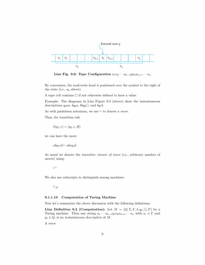
Linz Fig. 9.6: Tape Configuration a1a2 · · · ak−1qakak+1 · · · an
By convention, the read-write head is positioned over the symbol to the right ofthe state (i.e., ak above).
A tape cell contains � if not otherwise defined to have a value.
Example: The diagrams in Linz Figure 9.3 (above) show the instantaneousdescriptions q0aa, bq0a, bbq0�, and bq1b.
As with pushdown automata, we use ` to denote a move.
Thus, for transition rule
δ(q1, c) = (q2, e, R)
we can have the move
abq1cd ` abeq2d.
As usual we denote the transitive closure of move (i.e., arbitrary number ofmoves) using:
`∗
We also use subscripts to distinguish among machines:
`M
9.1.1.10 Computation of Turing Machine
Now let’s summarize the above discussion with the following definitions.
Linz Definition 9.2 (Computation): Let M = (Q,Σ,Γ, δ, q0,�, F ) be aTuring machine. Then any string a1 · · · ak−1q1akak+1 · · · an with ai ∈ Γ andq1 ∈ Q, is an instantaneous description of M .
A move
9

a1 · · · ak−1q1akak+1 · · · an ` a1 · · · ak−1bq2ak+1 · · · an
is possible if and only if
δ(q1, ak) = (q2, b, R).
A move
a1 · · · ak−1q1akak+1 · · · an ` a1 · · · q2ak−1bak+1 · · · an
is possible if and only if
δ(q1, ak) = (q2, b, L).
M halts starting from some initial configuration x1qix2 if
x1qix2 `∗ y1qjay2
for any qj and a, for which δ(qj , a) is undefined.
The sequence of configurations leading to a halt state is a computation.
If a Turing machine does not halt, we use the following special notation todescribe its computation:
x1qx2 `∗ ∞
9.1.2 Turing Machines as Language Acceptors
Can a Turing machine accept a string w?
Yes, using the following setup:
• Write w on the tape initially.• Fill all the unused cells on the tape with blanks �.• Start the Turing machine with read-write head over leftmost symbol of w.• If the machine halts in a final state, then it accepts string w.
Linz Definition 9.3 (Language Accepted by Turing Machine): LetM =(Q,Σ,Γ, δ, q0,�, F ) be a Turing machine. Then the language accepted by M is
L(M) = {w ∈ Σ+ : q0w `∗ x1qfx2, qf ∈ F, x1, x2 ∈ Γ∗}.
10

Note: The finite string w must be written to the tape with blanks on both sides.No blanks can are embedded within the input string w itself.
Question: What if w 6∈ L(M)?
The Turing machine might:
1. halt in nonfinal state2. never halt
Any string for which the machine does not halt is, by definition, not in L(M).
9.1.2.1 Linz Example 9.6
For Σ = {0, 1}, design a Turing machine that accepts the language denoted bythe regular expression 00∗.
We use two internal states Q = {q0, q1}, one final state F = {q1}, and transitionfunction:
δ(q0, 0) = (q0, 0, R),δ(q0,�) = (q1,�, R)
The transition graph shown below implements this machine.
• While a 0 appears under the read-write head, the head moves to the right.• If a blank is read, the machine halts in final state q1.• If a 1 is read, the machine halts in the nonfinal state q0 because δ(q0, 1) is
undefined.
The Turing machine also halts in a final state if started in state q0 on a blank.We could interpret this as acceptance of λ, but for technical reasons the emptystring is not included in Linz Definition 9.3.
11
9.1.2.2 Linz Example 9.7
For Σ = {a, b}, design a Turing machine that accepts
L = {anbn : n ≥ 1}.
We can design a machine that incorporates the following algorithm:
While both a’s and b’s remainreplace leftmost a by xreplace leftmost b by y
If no a’s or b’s remainaccept
elsereject
Filling in the details, we get the following Turing machine for which:
Q = {q0, q1, q2, q3, q4}F = {q4}Σ = {a, b}Γ = {a, b, x, y,�}
The transitions can be broken into several sets.
The first set
1. δ(q0, a) = (q1, x,R)
2. δ(q1, a) = (q1, a, R)
3. δ(q1, y) = (q1, y, R)
4. δ(q1, b) = (q2, y, L)
replaces the leftmost a with an x, then causes the read-write head to travelright to the first b, replacing it with a y. The machine then enters a state q2,indicating that an a has been successfully paired with a b.
The second set
5. δ(q2, y) = (q2, y, L)
6. δ(q2, a) = (q2, a, L)
7. δ(q2, x) = (q0, x,R)
12
reverses the direction of movement until an x is encountered, repositions theread-write head over the leftmost a, and returns control to the initial state.
The machine is now back in the initial state q0, ready to process the next a-bpair.
After one pass through this part of the computation, the machine has executedthe partial computation:
q0aa · · · abb · · · b `∗ xq0a · · · ayb · · · b
So, it has matched a single a with a single b.
The machine continues this process until no a is found on leftward movement.
If all a’s have been replaced, then state q0 detects a y instead of an a and changesto state q3. This state must verify that all b’s have been processed as well.
8. δ(q0, y) = (q3, y, R)
9. δ(q3, y) = (q3, y, R)
10. δ(q3,�) = (q4,�, R)
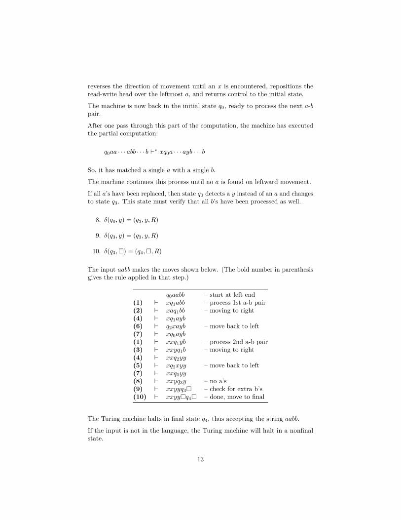
The input aabb makes the moves shown below. (The bold number in parenthesisgives the rule applied in that step.)
q0aabb – start at left end(1) ` xq1abb – process 1st a-b pair(2) ` xaq1bb – moving to right(4) ` xq1ayb(6) ` q2xayb – move back to left(7) ` xq0ayb(1) ` xxq1yb – process 2nd a-b pair(3) ` xxyq1b – moving to right(4) ` xxq2yy(5) ` xq2xyy – move back to left(7) ` xxq0yy(8) ` xxyq3y – no a’s(9) ` xxyyq3� – check for extra b’s(10) ` xxyy�q4� – done, move to final
The Turing machine halts in final state q4, thus accepting the string aabb.
If the input is not in the language, the Turing machine will halt in a nonfinalstate.
13
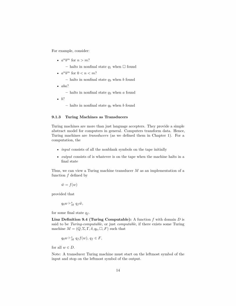
For example, consider:
• anbm for n > m?– halts in nonfinal state q1 when � found
• anbm for 0 < n < m?– halts in nonfinal state q3 when b found
• aba?– halts in nonfinal state q3 when a found
• b?– halts in nonfinal state q0 when b found
9.1.3 Turing Machines as Transducers
Turing machines are more than just language accepters. They provide a simpleabstract model for computers in general. Computers transform data. Hence,Turing machines are transducers (as we defined them in Chapter 1). For acomputation, the
• input consists of all the nonblank symbols on the tape initially
• output consists of is whatever is on the tape when the machine halts in afinal state
Thus, we can view a Turing machine transducer M as an implementation of afunction f defined by
w = f(w)
provided that
q0w `∗M qf w,
for some final state qf .
Linz Definition 9.4 (Turing Computable): A function f with domain D issaid to be Turing-computable, or just computable, if there exists some Turingmachine M = (Q,Σ,Γ, δ, q0,�, F ) such that
q0w `∗M qff(w), qf ∈ F ,
for all w ∈ D.
Note: A transducer Turing machine must start on the leftmost symbol of theinput and stop on the leftmost symbol of the output.
14
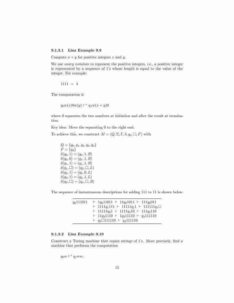
9.1.3.1 Linz Example 9.9
Compute x+ y for positive integers x and y.
We use unary notation to represent the positive integers, i.e., a positive integeris represented by a sequence of 1’s whose length is equal to the value of theinteger. For example:
1111 = 4
The computation is
q0w(x)0w(y) `∗ qfw(x+ y)0
where 0 separates the two numbers at initiation and after the result at termina-tion.
Key idea: Move the separating 0 to the right end.
To achieve this, we construct M = (Q,Σ,Γ, δ, q0,�, F ) with
Q = {q0, q1, q2, q3, q4}F = {q4}δ(q0, 1) = (q0, 1, R)δ(q0, 0) = (q1, 1, R)δ(q1, 1) = (q1, 1, R)δ(q1,�) = (q2,�, L)δ(q2, 1) = (q3, 0, L)δ(q3, 1) = (q3, 1, L)δ(q3,�) = (q4,�, R)
The sequence of instantaneous descriptions for adding 111 to 11 is shown below.
q0111011 ` 1q011011 ` 11q01011 ` 111q0011` 1111q1111 ` 11111q11 ` 111111q1�` 11111q21 ` 1111q310 ` 111q3110` 11q31110 ` 1q311110 ` q3111110` q3�111110 ` q4111110
9.1.3.2 Linz Example 9.10
Construct a Turing machine that copies strings of 1’s. More precisely, find amachine that performs the computation
q0w `∗ qfww,
15

for any w ∈ {1}+.
To solve the problem, we implement the following procedure:
1. Replace every 1 by an x.2. Find the rightmost x and replace it with 1.3. Travel to the right end of the current nonblank region and create a 1 there.4. Repeat steps 2 and 3 until there are no more x’s.
A Turing machine transition function for this procedure is as follows:
δ(q0, 1) = (q0, x,R)δ(q0,�) = (q1�, L)δ(q1, x) = (q2, 1, R)δ(q2, 1) = (q2, 1, Rδ(q2,�) = (q1, 1, L)δ(q1, 1) = (q1, 1, L)δ(q1,�) = (q3,�, R)
where q3 is the only final state.
Linz Figure 9.7 shows a transition graph for this Turing machine.
Linz Fig. 9.7: Transition Graph for Example 9.10
This is not easy to follow, so let us trace the program with the string 11. Thecomputation performed is as shown below.
q011 ` xq01 ` xxq0� ` xq1x` x1q2� ` xq111 ` q1x11` 1q211 ` 11q21 ` 111q2�` 11q111 ` 1q1111` q11111 ` q1�1111 ` q31111
16
9.1.3.3 Linz Example 9.11
Suppose x and y are positive integers represented in unary notation.
Construct a Turing machine that halts in a final state qy if x ≥ y and in anonfinal state qn if x < y.
That is, the machine must perform the computation:
q0w(x)0w(y) `∗ qyw(x)0w(y), if x ≥ yq0w(x)0w(y) `∗ qnw(x)0w(y), if x < y
We can adapt the approach from Linz Example 9.7. Instead of matching a’s andb’s, we match each 1 on the left of the dividing 0 with the 1 on the right. At theend of the matching, we will have on the tape either
xx · · · 110xx · · ·x�
or
xx · · ·xx0xx · · ·x11�,
depending on whether x > y or y > x.
A transition graph for machine is shown below.
9.2 Combining Turing Machines for Complicated Tasks
9.2.1 Introduction
How can we compose simpler operations on Turing machines to form morecomplex operations?
Techniques discussed in this section include use of:
• Top-down stepwise refinement, i.e., starting with a high-level descriptionand refining it incrementally until we obtain a description in the actuallanguage
• Block diagrams or pseudocode to state high-level descriptions
17

18
9.2.2 Using Block Diagrams
In the block diagram technique, we define high-level computations in boxeswithout internal details on how computation is done. The details are filled in ona subsequent refinement.
To explore the use of block diagrams in the design of complex computations,consider Linz Example 9.12, which builds on Linz Examples 9.9 and 9.11 (above).
9.2.2.1 Linz Example 9.12
Design a Turing machine that computes the following function:
f(x, y) = x+ y, if x ≥ y,f(x, y) = 0, if x < y.
For simplicity, we assume x and y are positive integers in unary representationand the value zero is represented by 0, with the rest of the tape blank.
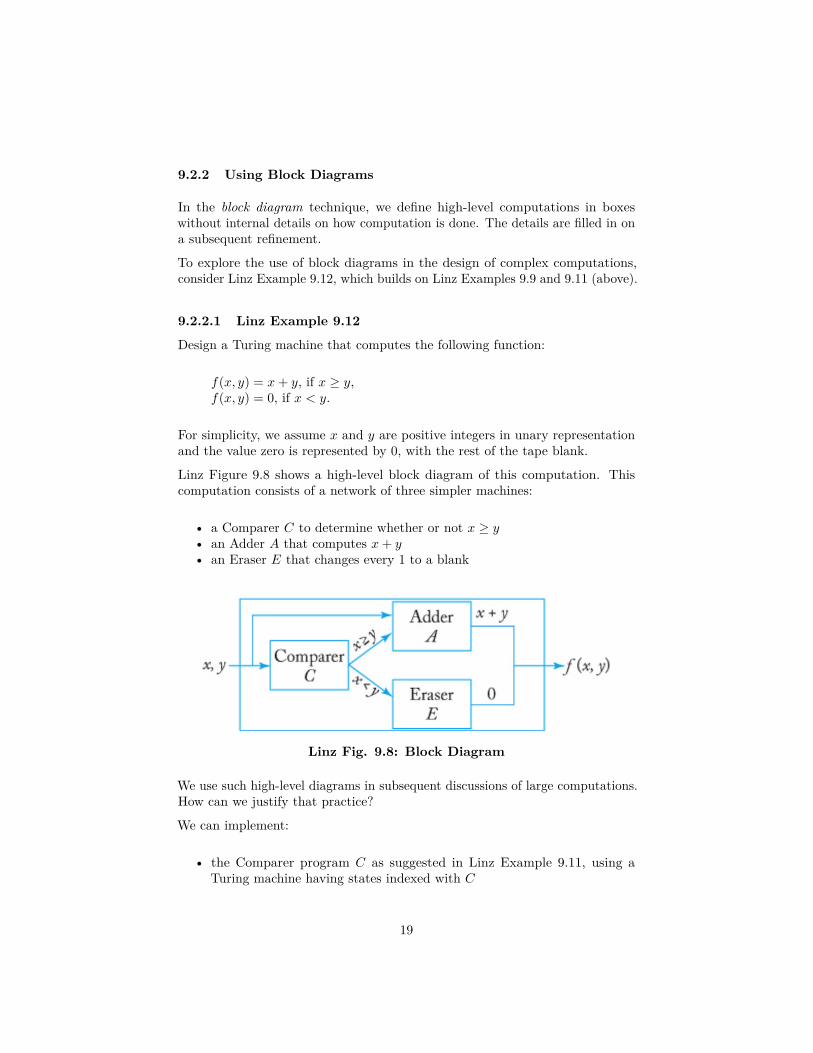
Linz Figure 9.8 shows a high-level block diagram of this computation. Thiscomputation consists of a network of three simpler machines:
• a Comparer C to determine whether or not x ≥ y• an Adder A that computes x+ y• an Eraser E that changes every 1 to a blank
Linz Fig. 9.8: Block Diagram
We use such high-level diagrams in subsequent discussions of large computations.How can we justify that practice?
We can implement:
• the Comparer program C as suggested in Linz Example 9.11, using aTuring machine having states indexed with C
19
• the Adder program A as suggested in Linz Example 9.9, with states indexedwith A
• the Eraser program E by constructing a Turing machine having statesindexed with E
Comparer C carries out the computations
qC,0w(x)0w(y) `∗ qA,0w(x)0w(y), if x ≥ y,
and
qC,0w(x)0w(y) `∗ qE,0w(x)0w(y), if x < y.
If qA,0 and qE,0 are the initial states of computations A and E, respectively,then C starts either A or E.
Adder A carries out the computation
qA,0w(x)0w(y) `∗ qA,fw(x+ y)0.
And, Eraser E carries out the computation
qE,0w(x)0w(y) `∗ qE,f 0.
The outer diagram in Linz Figure 9.8 thus represents a single Turing machinethat combines the actions of machines C, A, and E as shown.
9.2.3 Using Pseudocode
In the pseudocode technique, we outline a computation using high-level descriptivephrases understandable to people. We refine and translate it to lower-levelimplementations later.
9.2.3.1 Macroinstructions
A simple kind of pseudocode is the macroinstruction. A macroinstruction is asingle statement shorthand for a sequence of lower-level statements.
We first define the macroinstructions in terms of the lower-level language. Thenwe compose macroinstructions into a larger program, assuming the relevantsubstitutions will be done.
20
9.2.3.2 Linz Example 9.13
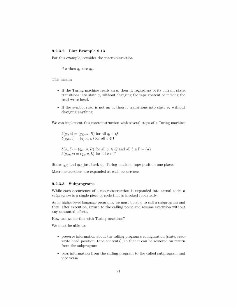
For this example, consider the macroinstruction
if a then qj else qk.
This means:
• If the Turing machine reads an a, then it, regardless of its current state,transitions into state qj without changing the tape content or moving theread-write head.
• If the symbol read is not an a, then it transitions into state qk withoutchanging anything.
We can implement this macroinstruction with several steps of a Turing machine:
δ(qi, a) = (qj0, a, R) for all qi ∈ Qδ(qj0, c) = (qj , c, L) for all c ∈ Γ
δ(qi, b) = (qk0, b, R) for all qi ∈ Q and all b ∈ Γ− {a}δ(qk0, c) = (qk, c, L) for all c ∈ Γ
States qj0 and qk0 just back up Turing machine tape position one place.
Macroinstructions are expanded at each occurrence.
9.2.3.3 Subprograms
While each occurrence of a macroinstruction is expanded into actual code, asubprogram is a single piece of code that is invoked repeatedly.
As in higher-level language programs, we must be able to call a subprogram andthen, after execution, return to the calling point and resume execution withoutany unwanted effects.
How can we do this with Turing machines?
We must be able to:
• preserve information about the calling program’s configuration (state, read-write head position, tape contents), so that it can be restored on returnfrom the subprogram
• pass information from the calling program to the called subprogram andvice versa
21

We can do this by partitioning the tape into several regions. Linz Figure 9.9illustrates this technique for a program A (a Turing machine) that calls asubprogram B (another Turing machine).
1. A executes in its own workspace.2. Before transferring control to B, A writes information about its configura-
tion and inputs for B into some separate region T .3. After transfer, B finds its input in T .4. B executes in its own separate workspace.5. When B completes, it writes relevant results into T .6. B transfers control back to A, which resumes and gets the needed results
from T .
Linz Fig. 9.9: Tape Regions for Subprograms
Note: This is similar to what happens in an actual computer for a subprogram(function, procedure) call. The region T is normally a segment pushed onto theprogram’s runtime stack or dynamically allocated from the heap memory.
9.2.3.4 Linz Example 9.14
Design a Turing machine that multiplies x and y, positive integers representedin unary notation.
Assume the initial and final tape configurations are as shown in Linz Figure 9.10.
We can multiply x by y by adding y to itself x times as described in the algorithmbelow.
Repeat until x contains no more 1’sFind a 1 in x and replace it with another symbol aReplace the leftmost 0 by 0y
Replace all a’s with 1’s
Linz Fig. 9.10: Multiplication
22
Although the above description of the pseudocode approach is imprecise, theidea is sufficiently simple that it is clear we can implement it.
We have not proved that the block diagram, macroinstruction, or subprogramapproaches will work in all cases. But the discussion in this section shows thatit is plausible to use Turing machines to express complex computations.
9.3 Turing’s Thesis
The Turing thesis is an hypothesis that any computation that can be carried outby mechanical means can be performed by some Turing machine.
This is a broad assertion. It is not something we can prove!
The Turing thesis is actually a definition of mechanical computation: a compu-tation is mechanical if and only if it can be performed by some Turing machine.
Some arguments for accepting the Turing thesis as the definition of mechanicalcomputation include:
1. Anything that can be computed by any existing digital computer can alsobe computed by a Turing machine.
2. There are no known problems that are solvable by what we intuitivelyconsider an algorithm for which a Turing machine program cannot bewritten.
3. No alternative model for mechanical computation is more powerful thanthe Turing machine model.
The Turing thesis is to computing science as, for example, classical Newtonianmechanics is to physics. Newton’s “laws” of motion cannot be proved, but theycould possibly be invalidated by observation. The “laws” are plausible modelsthat have enabled humans to explain much of the physical world for severalcenturies.
Similarly, we accept the Turing thesis as a basic “law” of computing science. Theconclusions we draw from it agree with what we know about real computers.
The Turing thesis enables us to formalize the concept of algorithm.
Linz Definition 9.5 (Algorithm): An algorithm for a function f : D → R isa Turing machine M , which given as input any d ∈ D on its tape, eventuallyhalts with the correct answer f(d) ∈ R on its tape. Specifically, we can requirethat
q0d `∗M qff(d), qf ∈ F ,
23

for all d ∈ D.
To prove that “there exists an algorithm”, we can construct a Turing machinethat computes the result.
However, this is difficult in practice for such a low-level machine.
An alternative is, first, to appeal to the Turing thesis, arguing that anything thatwe can compute with a digital computer we can compute with a Turing machine.Thus a program in suitable high-level language or precise pseudocode can computethe result. If unsure, then we can validate this by actually implementing thecomputation on a computer.
Note: A higher-level language is Turing-complete if it can express any algorithmthat can be expressed with a Turing machine. If we can write a Turing machinesimulator in that language, we consider the language Turing complete.
24